Planning and Conception of Next-Generation Optical

Access Networks

António Miguel Barata da Eira

Dissertação para obtenção do Grau de Mestre em

Engenharia Electrotécnica e de Computadores

Júri

Presidente: Prof. Dr. José Manuel Bioucas Dias

Orientador: Prof. Dr. João José de Oliveira Pires

Co-Orientador: Eng. João Manuel Ferreira Pedro

Vogal: Prof. Dr. Amaro Fernandes de Sousa

Outubro 2010

ii

iii

Acknowledgements

Upon completion of this Thesis, I would first like to thank Prof. João Pires for his valuable guidance

throughout the whole process, particularly for allowing me the liberty to pursue my own objectives in this

work within the framework he defined.

To João Pedro, of Nokia-Siemens Networks, for his availability and invaluable help in getting me

started on linear programming basics, and also to João Santos, also of Nokia-Siemens Networks, for

taking the time to meet with me and review the formulation.

To Engs. João Horta and Eduardo Almeida, of Sonaecom, for their willingness to receive us and take

us through the process of PON planning from an operator’s viewpoint, as well as providing extremely

valuable information on PON costs.

To my good friends at IST, Pedro Frade, Tiago Rodrigues, Rui Marmé and all the others too many to

mention. It certainly would not have been the same without them.

To my grandparents, mother, brother and specially my father for not having ever given less than

everything he possibly could for me.

To Inês, for more than I can put into words.

iv

Abstract

The generalized deployment of Passive Optical Networks (PONs) as the new-generation solution for

fixed Access Networks has brought with it the need for increasingly more efficient and automated

planning methods in such networks. This work presents an approach based on Integer Linear

Programming (ILP) models to determine the optimal number of splitters and the allocation of Optical

Network Terminations (ONTs) to them.

This Thesis extends previous work in the area by considering Operational Expenditures (OPEX) in

the planning process and being formulated towards realistic PON configurations. Another model was

created for planning multi-stage PONs with various levels of cascading splitters. In both cases, heuristic

methods were developed to quickly obtain results in the larger scenarios that the ILP models cannot

handle.

Based on the ILP models, two studies are presented: one on the physical aspects of the migration

from Gigabit-PON (GPON) to XG-PON, and another concerning a cost comparison of PON and Point-to-

Point (P2P) solutions.

Results of the single-stage model show that it is possible to optimally allocate scenarios with up to

8 000 ONTs in 1 minute. Beyond that number, the heuristics provide good approximations in short times.

The multi-stage model is still too complex for networks spanning more than 50 ONTs. The heuristic

method developed for the multi-stage problem shows reasonable results for scenarios where the ILP

benchmarking was available.

The studies presented also conclude that current XG-PON specifications only allow a seamless

migration from GPON in short-range PONs, and that PONs are cheaper to deploy than P2P but more

expensive factoring in available bandwidth.

Keywords: PON Planning, Integer Linear Programming, multi-stage PON, XG-PON, P2P.

v

Resumo

A adopção generalizada de Redes Ópticas Passivas (PONs) como a solução para a nova geração

de Redes de Acesso fixas trouxe consigo a necessidade de métodos de planeamento mais eficientes e

automatizados. Este trabalho apresenta uma abordagem baseada em modelos de Programação Linear

Inteira (ILP) para determinar o número óptimo de splitters e a alocação de terminais ópticos a estes.

Esta Tese aprofunda o trabalho prévio na área ao considerar despesas operacionais no processo de

planeamento e ao ser formulada tendo em atenção configurações reais de PONs. Outro modelo foi

criado para o planeamento de PONs multi-andar, com vários níveis de splitters em cascata. Em ambos

os casos, métodos heurísticos foram desenvolvidos para obter resultados rápidos nos cenários mais

exigentes que os modelos ILP não resolveram em tempo útil.

Baseado nos modelos ILP, dois estudos são apresentados: um sobre os aspectos físicos da

migração da GPON para XG-PON, e outro sobre uma comparação em termos de custo entre soluções

PON e ponto-a-ponto.

Os resultados do modelo de andar único mostram que é possível alocar de forma óptima cenários

com até 8 000 terminais num minuto. Para lá desse número, as heurísticas proporcionam boas

aproximações em pouco tempo. O modelo multi-nível é ainda demasiado complexo para redes com mais

de 50 terminais. A heurística desenvolvida para multi-nível mostra resultados razoáveis para os cenários

onde a comparação com o ILP foi possível.

Os estudos apresentados também concluem que as especificações actuais da XG-PON apenas

permitem uma migração suave para PONs de curto alcance, e que PONs custam menos a instalar que

soluções ponto-a-ponto, mas são mais caras quando se entra em conta com a largura de banda

oferecida.

Palavras Chave: Planeamento de PONs, Programação Linear Inteira, PONs multi-nível, XG-PON,

P2P.

vi

Table of Contents

1. Introduction .............................................................................................................................. 1

1.1 Evolution of Access Networks ............................................................................................... 2

1.2 State of the Art ...................................................................................................................... 8

1.3 Motivation, Objectives and Structure ................................................................................... 10

1.4 Original Contributions ......................................................................................................... 11

2. PON Planning ......................................................................................................................... 12

2.1 Network Planning ................................................................................................................ 13

2.2 ILP Model 1 – Original Formulation ..................................................................................... 15

2.2.1 Costs and Scenarios ................................................................................................... 16

2.2.2 Performance and Scalability ........................................................................................ 18

2.3 ILP Model 2 – Updated Formulation .................................................................................... 20

2.3.1 Splitter Co-Location ..................................................................................................... 24

2.3.2 ONT Co-Location ........................................................................................................ 25

2.3.3 Additional Variables .................................................................................................... 26

2.4 Heuristic Methods ............................................................................................................... 28

2.4.1 ADD Heuristic ............................................................................................................. 29

2.4.2 LP Relaxation ............................................................................................................. 31

2.5 Results and Discussion ....................................................................................................... 32

2.5.1 ILP Model 1 – Comparative Performance ................................................................... 32

2.5.2 ILP Model 2 – Comparative Performance .................................................................... 35

2.5.3 Cost Distribution .......................................................................................................... 38

2.5.4 Costs by configuration ................................................................................................. 40

2.6 Summary ............................................................................................................................ 41

3. Multi-Stage PON Planning ...................................................................................................... 42

3.1 Hierarchical Network Algorithms Review ............................................................................. 43

3.2 Multi-Stage PON ILP Model ................................................................................................ 45

3.3 Heuristics............................................................................................................................ 50

3.3.1 LP and MILP Relaxation .............................................................................................. 50

3.3.2 Two-Stage Multi-Level Heuristic .................................................................................. 50

3.3.3 Heuristic Bound ........................................................................................................... 55

3.4 Results ............................................................................................................................... 56

3.5 Summary ............................................................................................................................ 57

4. Physical, Technological and Topology Aspects ....................................................................... 59

4.1 Physical Level Constraints .................................................................................................. 60

4.1.1 Power Budget and Dispersion ..................................................................................... 60

vii

4.1.2 Maximum Differential Distance .................................................................................... 63

4.2 Evolution to XG-PON .......................................................................................................... 64

4.2.1 Evolution Analysis ....................................................................................................... 65

4.3 P2P vs. PON ...................................................................................................................... 68

4.3.1 Architectural Differences ............................................................................................. 69

4.3.2 ILP P2P Model ............................................................................................................ 69

4.3.3 Results........................................................................................................................ 71

4.4 Summary ............................................................................................................................ 73

5. Conclusions and Future Work ................................................................................................. 74

5.1 General Conclusions........................................................................................................... 75

5.2 Future Work ........................................................................................................................ 75

References ...................................................................................................................................... 77

A. Efficiency of Fixed Access Networks ....................................................................................... 81

A.1 Overview ............................................................................................................................ 81

A.1.1 GPON ......................................................................................................................... 82

A.1.2 EPON ......................................................................................................................... 84

A.1.3 DOCSIS ...................................................................................................................... 86

A.2 Comparative Results ........................................................................................................... 88

B. Software Implementation ........................................................................................................ 91

B.1 Describing the Model .......................................................................................................... 91

B.2 Setting the Scenarios .......................................................................................................... 92

C. Physical Parameters ............................................................................................................... 95

C.1 Power Budget ..................................................................................................................... 95

C.2 Dispersion Effects ............................................................................................................... 97

viii

List of Figures

Figure 1.1 - Various types of FTTx (Source: Wikipedia). ..................................................................... 3

Figure 1.2 - Downstream bitrate for xDSL technologies as a function of distance. (Source: Wikipedia)

................................................................................................................................................................ 3

Figure 1.3 - HFC network (Source: Wikipedia). .................................................................................. 4

Figure 1.4 - a) Historical and projected bandwidth demand. b) Evolution of penetration of Broadband

home devices. (Source: Verizon). ............................................................................................................ 4

Figure 1.5 - a) P2P Topology. b) P2MP Topology. (Source: Alcatel-Lucent) ....................................... 5

Figure 1.6 - Downstream average throughput for EPON, GPON and DOCSIS 3.0 ............................. 7

Figure 1.7 - Upstream average throughput for EPON, GPON and DOCSIS 3.0. ................................. 7

Figure 2.1 – Double-Star Topology .................................................................................................. 13

Figure 2.2 - Savings in conduit sharing. ........................................................................................... 16

Figure 2.3 - Connections in Manhattan Distance. ............................................................................. 17

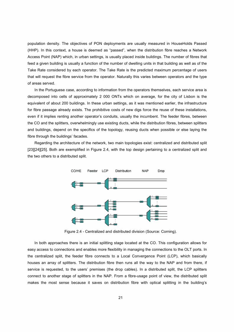
Figure 2.4 - Centralized and distributed division (Source: Corning). .................................................. 21

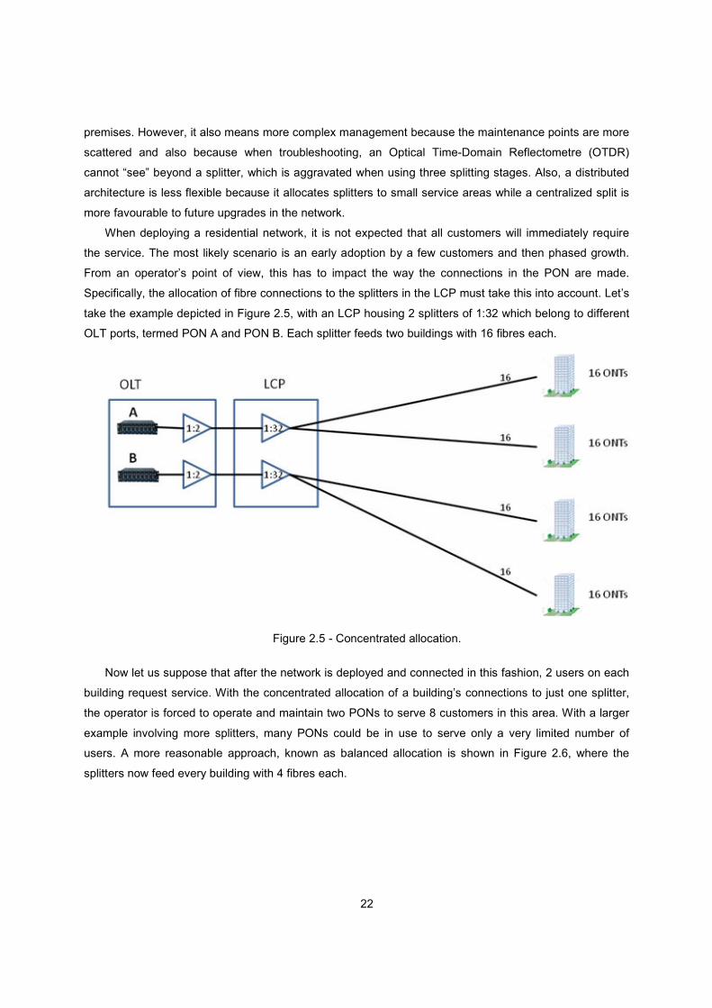
Figure 2.5 - Concentrated allocation. ............................................................................................... 22

Figure 2.6 - Balanced allocation. ...................................................................................................... 23

Figure 2.7 - Fusion splice (left) and Optical Connectors (right). (Source: Mike Geiger). ..................... 23

Figure 2.8 - Implicit splitting stage at the CO. ................................................................................... 26

Figure 2.9 - ADD heuristic flowchart. ................................................................................................ 29

Figure 2.10 - Drawback of ADD. ...................................................................................................... 30

Figure 2.11 - Flowchart of LP Relaxation. ........................................................................................ 32

Figure 2.12 - Network costs per method for original formulation. ...................................................... 34

Figure 2.13 - Network costs per method for updated formulation. ..................................................... 36

Figure 2.14 - Network costs by number of ONTs. ............................................................................. 38

Figure 2.15 - Average cost breakdown for urban scenarios. ............................................................. 39

Figure 2.16 - Average cost breakdown for rural scenarios. ............................................................... 39

Figure 2.17 - Network costs by configuration. ................................................................................... 41

Figure 3.1 - Single and Multi-Level concentrator networks. Source: [34]. .......................................... 43

Figure 3.2 - Multi-staged PON.......................................................................................................... 44

Figure 3.3 - Examples of splitter capacity variables. ......................................................................... 46

Figure 3.4 - Multi-Level PON obtained from ILP. .............................................................................. 49

Figure 3.5 - Flowchart of two-stage PON heuristic. ........................................................................... 51

Figure 3.6 - Example of two-stage heuristic first layout. .................................................................... 53

Figure 3.7 - Reallocation of ONTs and branch discarding. ................................................................ 54

Figure 3.8 - Comparative costs for Single Stage ILP and Two-Stage heuristic. ................................. 57

Figure 4.1 - Power budget in PON link. Source: [38]......................................................................... 60

Figure 4.2 - Standard link model. ..................................................................................................... 61

ix

Figure 4.3 - Operating wavelengths for GPON/XG-PON co-existence. Source: [25]. ........................ 64

Figure 4.4 - WDM filtering at the OLT. .............................................................................................. 64

Figure 4.5 - Downstream optical path penalties for GPON. ............................................................... 66

Figure 4.6 - Upstream optical path penalties for GPON. ................................................................... 67

Figure 4.7 - Downstream optical path penalties for XG-PON. ........................................................... 67

Figure 4.8 - Upstream optical path penalties for XG-PON. ................................................................ 68

Figure 4.9 - Junction derivation in fibre cable. .................................................................................. 69

Figure 4.10 - Total network costs for PON and P2P. ........................................................................ 72

Figure 4.11 - Network cost per Mbps offered for PON and P2P. ....................................................... 72

Figure A.1 - GPON downstream frame. ............................................................................................ 82

Figure A.2 - Upstream user burst. .................................................................................................... 83

Figure A.3 - Downstream Average throughput. ................................................................................. 89

Figure A.4 - Upstream Average throughput. ..................................................................................... 89

Figure B.1 - Network element placement: Rural (left) and Urban (right). ........................................... 92

Figure B.2 - Network representation for rural scenario. ..................................................................... 93

Figure B.3 - Network representation for urban scenario. ................................................................... 94

x

List of Tables

Table 2.1 - Costs for preliminary analysis. ........................................................................................ 18

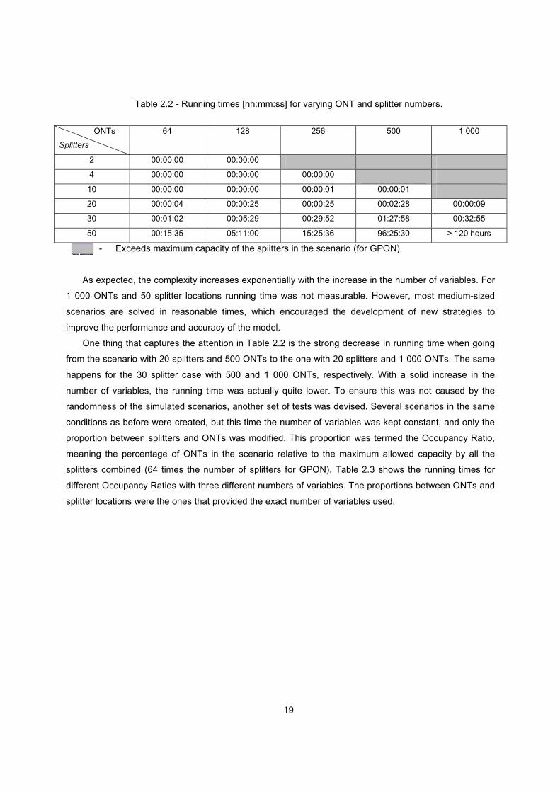
Table 2.2 - Running times [hh:mm:ss] for varying ONT and splitter numbers. ................................... 19

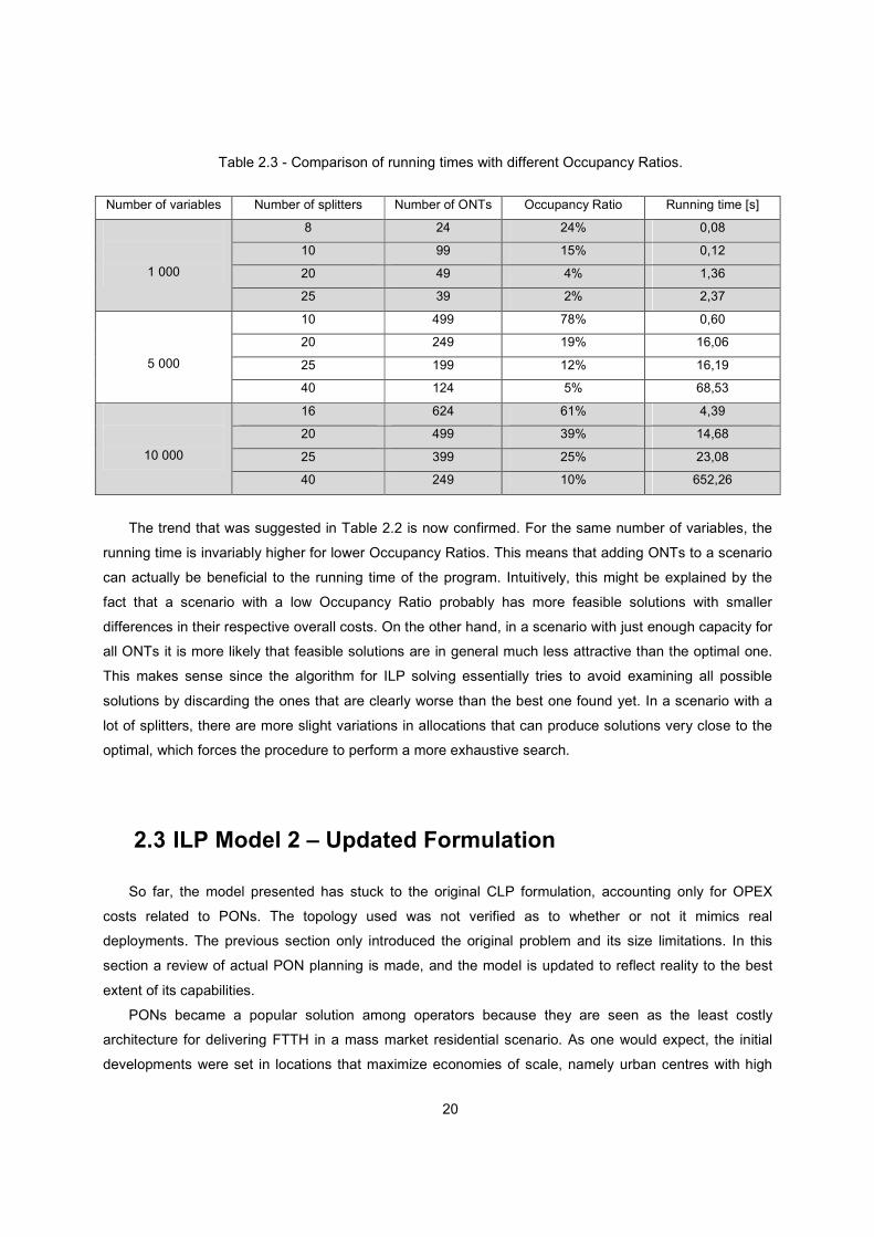
Table 2.3 - Comparison of running times with different Occupancy Ratios. ....................................... 20

Table 2.4 - Results for model with splitter co-location. ...................................................................... 25

Table 2.5 - List of costs considered. Source: [29] and Sonaecom. .................................................... 33

Table 2.6 - Test maps' dimensions. .................................................................................................. 33

Table 2.7 - Total network costs for original formulation. .................................................................... 34

Table 2.8 - Running times per method for original formulation. ......................................................... 35

Table 2.9 – Model 2 test scenarios' dimensions. .............................................................................. 36

Table 2.10 - Total network costs for updated formulation. ................................................................. 36

Table 2.11 - Running times per method for updated formulation. ...................................................... 37

Table 3.1 - Running times for multi-stage ILP model. ....................................................................... 49

Table 3.2 - Costs for exemplified scenario. ....................................................................................... 54

Table 3.3 - Multi-stage test scenarios' size. ...................................................................................... 56

Table 3.4 - Costs and running times for single and multi-stage PONs. .............................................. 56

Table 4.1 - Average system margins. ............................................................................................... 65

Table 4.2 - Costs for P2P. Source: [29]. ........................................................................................... 71

Table A.1 - Average GPON efficiency per number of users. ............................................................. 84

Table A.2 - Average liquid throughput per user for GPON. ............................................................... 84

Table A.3 - Average efficiency for EPON by number of users. .......................................................... 86

Table A.4 - Average throughput per user in EPON. .......................................................................... 86

Table A.5 - Average throughput in HFC by cell size. ........................................................................ 88

Table C.1 - GPON optical power levels for 2,488 Gbps downstream and 1,244 Gbps upstream.

Source: [39] ........................................................................................................................................... 95

Table C.2 - XG-PON1 optical power levels for 9,9533 Gbps downstream and 2,488 Gbps upstream

(class Nominal1). Source: [50]. .............................................................................................................. 96

Table C.3 - Attenuations for link elements. ....................................................................................... 97

Table C.4 - Attenuation coefficients and chromatic dispersion values for selected wavelenths. ......... 97

xi

List of Acronyms

ADSL Asymmetric Digital Subscriber Line

APON ATM Passive Optical Network

ATM Asynchronous Transfer Mode

BER Bit Error Ratio

BPON Broadband Passive Optical Network

CAPEX Capital Expenditure

CATV Cable Television

CLP Concentrator Location Problem

CMTS Cable Modem Termination System

DFB Distributed Feed-Back

DML Directly Modulated Laser

DOCSIS Data Over Cable Service Interface Specification

DSL Digital Subscriber Line

DSLAM Digital Subscriber Line Access Multiplexer

EFM Ethernet First Mile

EML Externally Modulated Laser

EPON Ethernet Passive Optical Network

FEC Forward Error Correction

FP Fabry-Perot

FSAN Full Service Access Networks

FTTB Fibre To The Building

FTTC Fibre To The Curb

FTTH Fibre To The Home

FTTN Fibre To The Node

FTTx Fibre To The x

GEM Generic Encapsulation Method

GPON Gigabit Passive Optical Network

HDTV High Definition Television

xii

HFC Hybrid Fibre-Coaxial

HHP Households Passed

ILP Integer Linear Program

IPTV Internet Protocol Television

LCC Local Convergence Cabinet

LCP Local Convergence Point

LP Linear Program

MILP Mixed Integer Linear Program

NAP Network Access Point

OPEX Operational Expenditure

OTDR Optical Time-Domain Reflectometre

P2MP Point To Multipoint

P2P Point to Point

PON Passive Optical Network

POTS Plain Old Telephone Service

QoS Quality of Service

RARA Recursive Association and Relocation Algorithm

RF Radio Frequency

TAP Terminal Assignment Problem

TDM Time Division Multiplexing

VDSL Very High Speed Digital Subscriber Line

WDM Wavelength Division Multiplexing

1

1. Introduction

This chapter presents an historical overview of Access Networks and how fibre-optics were

introduced in them. The motivation for this Thesis, its objectives and structure are also presented. A

review of the state of the art in the field of PON planning is conducted and the Thesis’ original

contributions are outlined.

2

1.1 Evolution of Access Networks

The evolution of fixed telecommunication networks denotes a clear unifying principle across

operators from all quadrants: integration of services. Traditionally telecommunication networks were

planned with the purpose of delivering a specific service, such as telephone in the now called Plain Old

Telephony Service (POTS) or television services in the Cable Television (CATV) networks. Nowadays the

trend lies in the concentration of a variety of services in the same network infrastructure. This tendency

can be traced back to telephone companies offering data and phone services simultaneously over their

existing copper lines. The growth of the Internet spurred an enormous increase in data traffic

consumption throughout the 1990’s [1], forcing operators to continuously update their networks with the

development of the various flavours of Digital Subscriber Line (DSL or xDSL to denote its various

versions). Increased bandwidths favoured the emergence of Internet Protocol Television (IPTV), which

also allowed these operators to provide television services through DSL. At the same time, CATV

operators sought the opportunity to reuse their own infrastructure, in order to provide internet access to

their customers. The Data Over Cable Service Interface Specification (DOCSIS) standard was launched

in 1997 with this purpose, and was revised throughout the years to improve transmission speeds and

overall efficiency, with the current version named DOCSIS 3.0, being released in 2006.

Today, it is customary for legacy phone and cable operators to provide the termed Triple-Play

service, consisting of High-Speed Internet Access, Television and Voice services on a single broadband

connection. Naturally, the accommodation of these services implies that much more bandwidth must be

available in the Access Network, which is responsible for connecting the subscriber to its service provider.

Because of its inherently more scattered nature, the Access Network has historically been known as the

last mile bottleneck, meaning that the capacity of the Access Network is usually what constraints the

available bit-rate of a subscriber.

While the use of fibre optics in core and metro networks has been commonplace since the late

1970s [2], until very recently the bulk of the fixed Access Networks was based on copper wires, be it

twisted pair or coaxial cable. The advantages of fibre over the copper lines lie mainly in its much lower

attenuation and immunity to electromagnetic interference, resulting in more bandwidth available at greater

distances. However, while the cost of fibre itself is relatively low, optical components like lasers and

photodetectors still pose a significant investment for operators. To keep costs down, such investments

must then be shared to serve as many subscribers as possible. While this is the case in long haul

networks, the introduction of fibre in the Access Network has been phased in time according to bandwidth

demand and the cost decrease of optical transceivers [3]. This introduction is conducted bringing the fibre

progressively closer to the subscriber’s premises. This is the case for both DSL lines and CATV networks,

where introducing fibre allows reducing the length of the copper wires, enabling the use of the latter in

higher frequency bands and/or using more aggressive modulation techniques to increase throughput

while maintaining adequate signal levels. This is usually known as the various flavours of Fibre In The

3

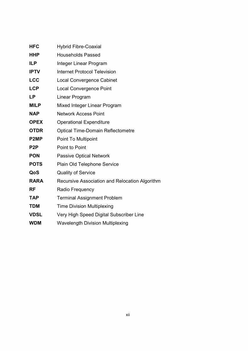
Loop or FTTx. There are various types of configurations for FTTx, present in Figure 1.1, like fibre laid to a

remote node (FTTN), street cabinet or curb (FTTC) or a building (FTTB) in the hybrid fibre-copper

configurations or replacing copper entirely in the case of Fibre To The Home (FTTH).

Figure 1.1 - Various types of FTTx (Source: Wikipedia).

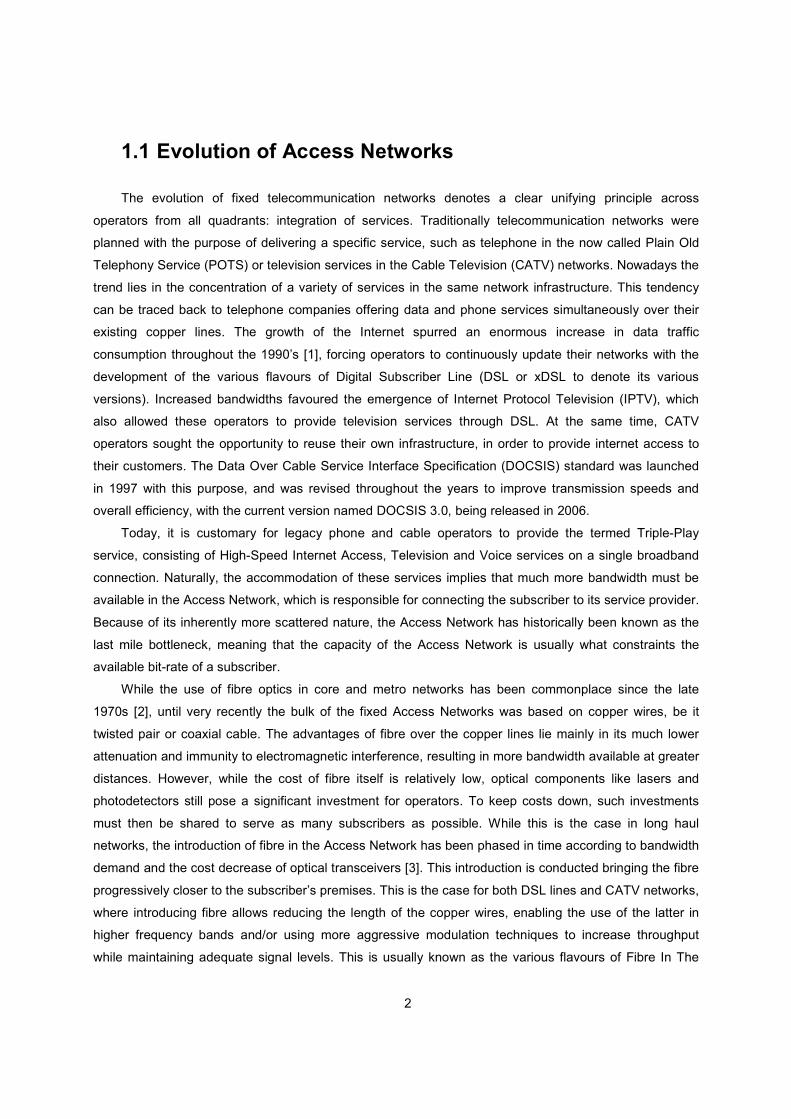
In the case of xDSL lines, the extension of copper wires in the loop dictates the type of technology

that can be deployed. It can range from common Asymmetric Digital Subscriber Line (ADSL) to Very-High

Bitrate DSL (VDSL). Figure 1.2 shows the attainable bitrates for each technology as a function of the

distance covered by the twisted pair.

Figure 1.2 - Downstream bitrate for xDSL technologies as a function of distance. (Source: Wikipedia)

In 2006, ITU-T presented Recommendation G.993.2 which standardized VDSL 2, an upgrade to

VDSL which enabled 100 Mbps in the downstream with loop distances reaching 500 m, and maintaining

ADSL2-like performances beyond that [4].

4

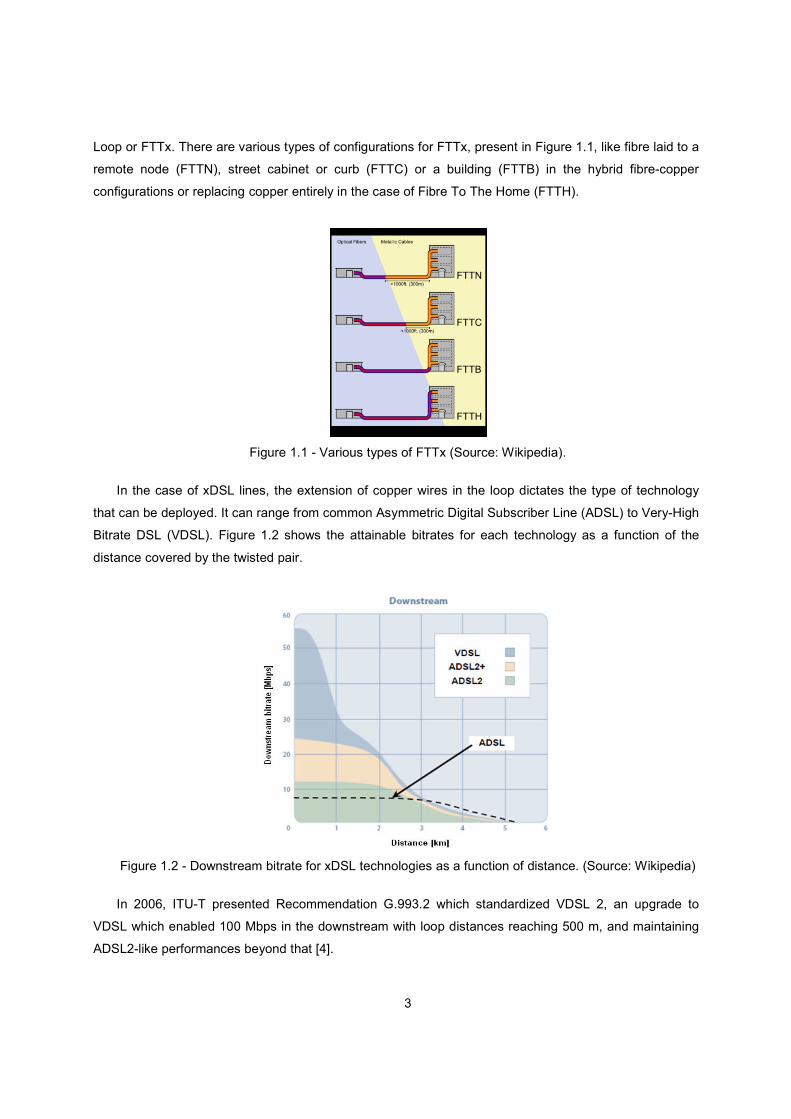
Hybrid Fibre-Coaxial (HFC) networks don’t use the star topology seen in DSL lines, but instead a tree

topology, like the one seen in Figure 1.3. Basically, a fibre-based transport structure interconnects an

Headend which circulates the video channels through Distribution Hubs, that in turn feed Optical Nodes.

The electrical interface of this node is the Cable Modem Termination System (CMTS) that connects cells

of subscribers through a shared coaxial cable. Radio-Frequency (RF) Amplifiers are used to boost the

signal level in the coaxial cable to ensure adequate reception by TV sets. To increase capacity in these

networks, the key is also extending fibre further towards the users, reducing the number of users served

by each CMTS.

Figure 1.3 - HFC network (Source: Wikipedia).

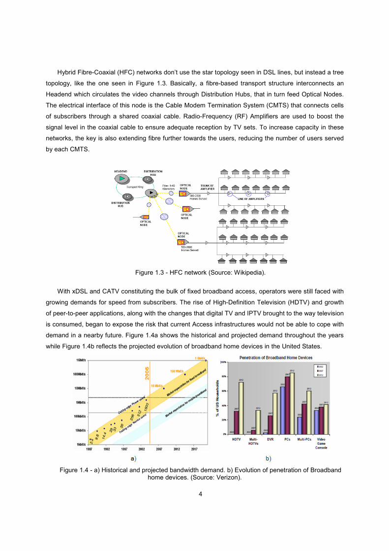
With xDSL and CATV constituting the bulk of fixed broadband access, operators were still faced with

growing demands for speed from subscribers. The rise of High-Definition Television (HDTV) and growth

of peer-to-peer applications, along with the changes that digital TV and IPTV brought to the way television

is consumed, began to expose the risk that current Access infrastructures would not be able to cope with

demand in a nearby future. Figure 1.4a shows the historical and projected demand throughout the years

while Figure 1.4b reflects the projected evolution of broadband home devices in the United States.

Figure 1.4 - a) Historical and projected bandwidth demand. b) Evolution of penetration of Broadband home devices. (Source: Verizon).

5

Figure 1.4a paints a clear picture of the challenges operators face concerning the update of Access

Networks. While some have opted to upgrade to more advanced xDSL solutions like ADSL2+, VDSL or

VDSL2 [5], most see this as a temporary “fix”, that will only delay the inevitable road to FTTH. While

VDSL2 does provide near 100 Mbps per user in the downstream, it does so with a local loop consisting

almost entirely of fibre. Therefore, it made sense for a lot of operators to skip that step and go for an all-

fibre solution, allowing them to future-proof their networks. As for cable companies, since HFC networks

offer a wider margin to accommodate demand, the penetration of fibre is taking place at a slower pace,

using mostly strategies of node splitting. For more on the capacity of HFC and DOCSIS, refer to

APPENDIX A.

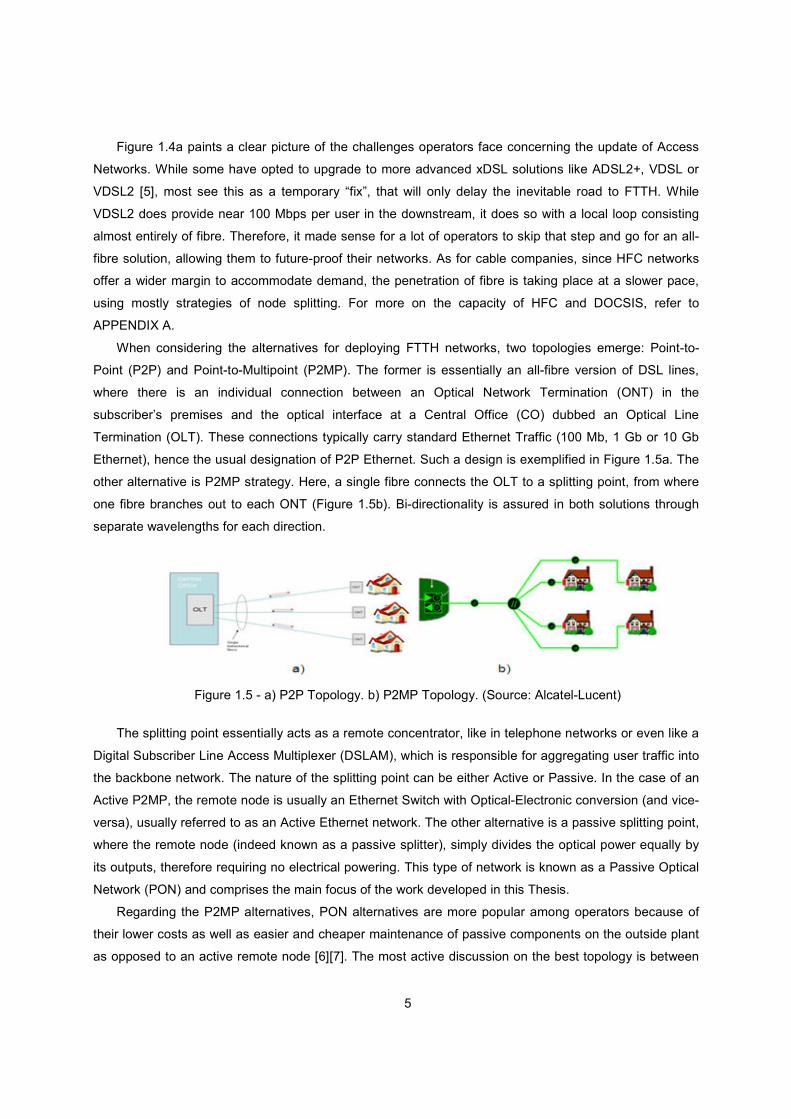
When considering the alternatives for deploying FTTH networks, two topologies emerge: Point-to-

Point (P2P) and Point-to-Multipoint (P2MP). The former is essentially an all-fibre version of DSL lines,

where there is an individual connection between an Optical Network Termination (ONT) in the

subscriber’s premises and the optical interface at a Central Office (CO) dubbed an Optical Line

Termination (OLT). These connections typically carry standard Ethernet Traffic (100 Mb, 1 Gb or 10 Gb

Ethernet), hence the usual designation of P2P Ethernet. Such a design is exemplified in Figure 1.5a. The

other alternative is P2MP strategy. Here, a single fibre connects the OLT to a splitting point, from where

one fibre branches out to each ONT (Figure 1.5b). Bi-directionality is assured in both solutions through

separate wavelengths for each direction.

Figure 1.5 - a) P2P Topology. b) P2MP Topology. (Source: Alcatel-Lucent)

The splitting point essentially acts as a remote concentrator, like in telephone networks or even like a

Digital Subscriber Line Access Multiplexer (DSLAM), which is responsible for aggregating user traffic into

the backbone network. The nature of the splitting point can be either Active or Passive. In the case of an

Active P2MP, the remote node is usually an Ethernet Switch with Optical-Electronic conversion (and vice-

versa), usually referred to as an Active Ethernet network. The other alternative is a passive splitting point,

where the remote node (indeed known as a passive splitter), simply divides the optical power equally by

its outputs, therefore requiring no electrical powering. This type of network is known as a Passive Optical

Network (PON) and comprises the main focus of the work developed in this Thesis.

Regarding the P2MP alternatives, PON alternatives are more popular among operators because of

their lower costs as well as easier and cheaper maintenance of passive components on the outside plant

as opposed to an active remote node [6][7]. The most active discussion on the best topology is between

6

PON and P2P networks. The comparison here is much harder since the topologies themselves are

different, and specific scenarios might favour one approach over the other. In short, P2P solutions are

seen as having better overall capacity and security, since they offer dedicated connections to each

subscriber, while PONs must share the capacity of a single fibre over all the users covered and require

the use of encryption mechanisms to prevent eavesdropping since the entire bit stream is available to

every ONT in the PON. On the other hand, a PON offers less fibre expenditure and reduced operational

costs since it only needs one interface at the OLT per PON, while a P2P architecture requires one per

subscriber, driving up running costs on power and space taken at the CO [8] [9].

Several technologies make use of a PON architecture. They differ amongst themselves essentially on

the protocols they use and the classes of equipments defined. The first technology to be standardized

was a PON carrying the then popular Asynchronous Transfer Mode (ATM) traffic, called ATM-PON

(APON). Standardized as ITU-T Rec. G.983.1 in 1998, it envisioned bitrates of 622 and 155,52 Mbps in

the downstream and upstream directions respectively [10]. It was a Time-Division Multiplexing (TDM)

PON, meaning the information pertaining and belonging to each user is transmitted in different instants,

and conveniently marked so the intended receiver knows which packets belong to him. TDM-PONs are

still the prevalent PON technology today. In 2001, APON was encapsulated in a broader

Recommendation (ITU-T G.983) which detailed the aspects of Broadband PON (BPON). BPON had

updated rates of 1,244 Gbps in the downstream and 622 Mbps in the upstream and also introduced Video

Overlay, a Wavelength Division Multiplexing (WDM) strategy that involves a dedicated wavelength at

1550 nm to transmit a RF video signal.

The popularity of Ethernet in local networks and its growth in metro networks (through Carrier

Ethernet) made an Ethernet-based Access Network very attractive in terms of interoperability.

Furthermore, the rise in IP traffic meant that the fixed 53 byte ATM cells used in APON/BPON burdened

much larger IP Packets with unnecessary overhead (the cell tax), making the process very inefficient. In

this context, among the solutions presented in 2004 for Ethernet in the Access by the Ethernet First Mile

(EFM) group one can find Ethernet PON (EPON), as standard IEEE 802.3ah. EPON follows the Ethernet

philosophy of low cost and simple operation which made it popular for early deployments in Asian

countries [11]. EPON carries symmetrical 1 Gbps Ethernet traffic (with a 1,25 Gbps line rate using 8B/10B

encoding) and originally allowed splitting ratios up to 1:32.

The low efficiency of BPON for IP traffic and the shortcomings of Ethernet when it comes to

applications with strict time demands like voice or IPTV, led the Full Service Access Network (FSAN)

group to develop a more versatile PON, capable of efficiently carrying all kinds of traffic. Thus the ITU-T

G.984 standard was born, introducing the Gigabit-PON (GPON). Unlike EPON, GPON was designed from

an operator and service point of view. This is reflected in its embedded Quality of Service (QoS)

requirements, which are not inherent in EPON. Also, it uses a General Encapsulation Method (GEM)

which aims to efficiently carry all types of traffic (including Ethernet). It presents bitrates of up to 2,488

Gbps in both directions (although 1,244 Gbps is the most common in the upstream) and has a maximum

7

split ratio of 1:64 with a maximum range of 20 km. It is however more complex and expensive than

EPON. Its service-oriented philosophy garnered it popularity among operators in Europe and North

America [11]. Despite the fact that the work performed in this Thesis tries to maintain an approach

applicable to any TDM-PON technology, the technological aspects like bitrates and maximum splitting

ratios and the costs considered in the PON deployment and operation pertain to GPON, since it is the

only technology deployed in the region where the work was performed and as such where practical

information was readily available.

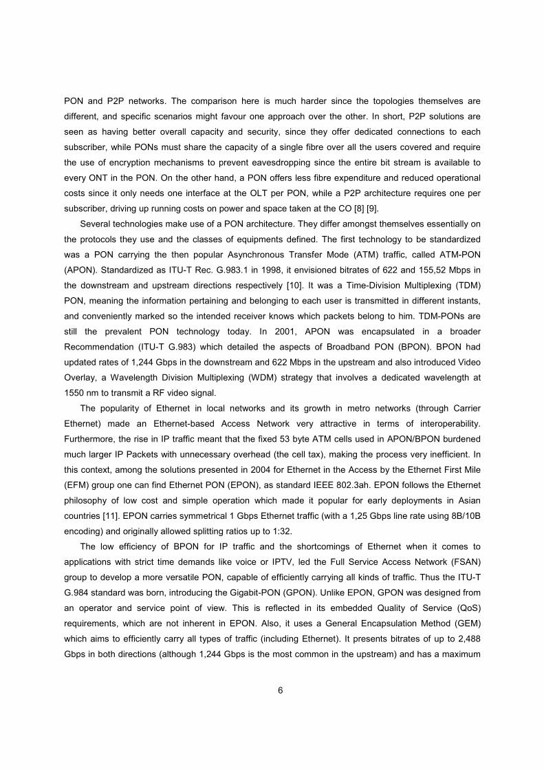
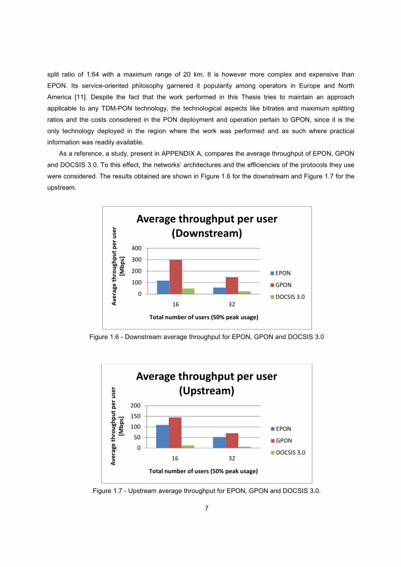
As a reference, a study, present in APPENDIX A, compares the average throughput of EPON, GPON

and DOCSIS 3.0. To this effect, the networks’ architectures and the efficiencies of the protocols they use

were considered. The results obtained are shown in Figure 1.6 for the downstream and Figure 1.7 for the

upstream.

Figure 1.6 - Downstream average throughput for EPON, GPON and DOCSIS 3.0

Figure 1.7 - Upstream average throughput for EPON, GPON and DOCSIS 3.0.

0

100

200

300

400

16 32Av

era

ge

th

rou

gh

pu

t p

er

use

r

[Mb

ps]

Total number of users (50% peak usage)

Average throughput per user

(Downstream)

EPON

GPON

DOCSIS 3.0

0

50

100

150

200

16 32

Av

era

ge

th

rou

gh

pu

t p

er

use

r

[Mb

ps]

Total number of users (50% peak usage)

Average throughput per user

(Upstream)

EPON

GPON

DOCSIS 3.0

8

The main conclusion that arises from these results is that indeed fibre offers a new degree of

potential for offering bandwidth in the Access Network.

1.2 State of the Art

Given how the PON market has grown exponentially in the last decade and is expected to keep

growing in the near future [11], the issue of PON planning is of key importance. Deploying a PON implies

massive investments in labour and equipment. It is therefore crucial to understand all the stages in

planning a PON and identify in which of them more efficient strategies can be elaborated in order to allow

for cost savings.

The field of network planning in general has been the focus of extensive research. Because it is such

a broad area, it is important to specify the scope of the planning/optimization intended. In the case of

PONs, the interest lies in Access Networks. Furthermore, because of the PON general architecture,

Access Networks with concentrator nodes are of particular interest. On this topic, [12] offers a

comprehensive review of the work completed in the optimization of hub locations in tributary/backbone

networks. This includes a very wide range of networks and several aspects to optimize: cost, reliability,

traffic engineering, and others. In the framework of this Thesis, demand patterns are considered constant

throughout all users, so routing issues are discarded. The focus of the optimization process is cost. The

main building block of most of the models developed in this work is the Concentrator Location Problem

(CLP), which is described in [13] and detailed in Chapter 2.

Regarding the area of PON planning, the work presented in [14] applies genetic algorithms for the

design of greenfield PONs, meaning a PON designed in a scenario without any existing infrastructure

(cable-ducts for instance). The scenario considered in [14] has three layers: the connection of users to

hosts, the allocation of service boxes to hosts and the design of the PON itself, with the hosts acting as

ONTs, who connect to splitters who in turn connect to the OLT. Obviously, this is not an FTTH

architecture, since the fibre only runs to the hosts, who in turn connect users with service boxes, which

are interfaces for several types of traffic. The third layer is therefore the one which has common ground

with the work in this Thesis. However, since a lot of the effort lies in optimizing host capacity to service

demand and connect the users, the scenario considered for just the PON involves two possible OLT

locations, ten possible splitter locations and 100 hosts (or ONTs). This is relatively small for the kind of

residential mass-market PONs that are currently being deployed. Furthermore, the design of the optical

network is admittedly simplified by the authors, since it does not account for specific PON details,

reducing the problem to a more classic hierarchical computer network case.

A tool termed PON Builder is presented in [15] and partially summarized in [16]. The author takes a

very complete approach to the issue of automating the physical layout of a PON, given the location of the

OLT and all the ONTs. The work is mainly focused on using a graph-theory approach to finding the least

9

costly set of ducts and fibres that interconnect the ONTs, the splitter and the OLT. This includes

accounting for obstacles in the map (roads, buildings…) and already existing ducts to extract the best

possible layout for the fibre cables. The splitter location is either defined a priori as the arithmetic mean of

the ONT and OLT locations, or placed after the layout is set in the first derivation of the cable starting

from the OLT. When the scenario includes more ONTs than a single PON can accommodate, some

clustering techniques are applied to geographically separate the ONTs into logical PONs and then the

program is executed for each PON. While the duct-layout part of the program is very thorough and seems

to provide good results on realistic scenarios, other aspects receive less attention. The program runs on

the (truthful) assumption that the costs of digging ducts and laying fibre are much greater than the ones of

the fibre itself. Therefore the fibre connections of the PON are largely ignored. This implies that the

splitter location is essentially not a variable because it doesn’t have much impact on the duct layout, but it

has a considerable one on the fibres that run through the ducts. Also, power budget constraints are not

considered. Finally, there is a separation between the procedure of assigning users to a PON (done

through clustering) and the network layout procedure itself. It could be advantageous to address both

problems together since the clustering procedure is done based on an intuitive geographical notion, which

does not necessarily ensure the cheapest network considering the scenarios’ obstacles and existing

ducts. It should be noted that the work developed in this Thesis is more complementary than juxtaposing

relative to [15]. The models developed here assume the costs of connecting the different (possible)

network elements are already known or estimated. PON Builder does a comprehensive work in such

calculations. Therefore it could be combined with this approach which is more concerned with optimal

allocation of users to terminals and placement of splitters, by feeding it with the connection costs it

calculated.

A more recent approach is presented in [17], which proposes an algorithm aimed at producing least-

cost deployments for greenfield PONs with scenarios ranging in the hundreds of ONTs. The authors

present a heuristic procedure that they call Recursive Association and Relocation Algorithm (RARA). The

algorithm receives the OLT and ONT locations as input. It starts with a randomly assigned set of splitters

and then recursively allocates ONTs to splitters and updates the splitters’ locations until convergence of

the solution costs is obtained. The authors also present an Integer Linear Programming (ILP) model for

PON assignment which is part of the overall algorithm. This model shares some features with the one

developed in this Thesis, and takes great care to ensure the PON constraints like power budget or

differential distance are met. However the authors state that the model is too complex for the bigger

scenarios and so it is only used for the medium-sized ones (with a few hundred ONTs). Results show that

the heuristic algorithm produces results for a scenario with 600 ONTs in between 20 and 40 hours.

Another strategy was developed which essentially acts as a clustering procedure. The ONTs are divided

in two scenarios according to their distance to the OLT and the algorithm is executed for both scenarios

separately. This allows improvement in the computation time while the authors assure the performance of

the algorithm isn’t significantly affected. It seems that this work finds more usefulness in PONs serving

10

less densely populated areas. This is because in the most common deployment scenarios, in very

crowded areas, the planning procedures usually involve cells that cover up to a few thousand users,

which by the results shown goes beyond the practical capacity of the algorithm. Also, in more urban

scenarios, splitters are deployed in so called Junction Boxes, which house arrays of several splitters, to

concentrate the installation costs and network points of access in case of repairs or updates.

Furthermore, as it will be explained later on, geographical criteria are not necessarily the best ones to

separate ONTs into specific PONs. There is no mention of Operational Expenditures (OPEX) affecting the

model in any way. Finally, the designs considered are only of single-staged splitting, without mention of

other configurations.

1.3 Motivation, Objectives and Structure

The academic approaches detailed in the previous section deal with various aspects of automating

and optimizing PON planning, like best-path calculations for fibre connections, splitter placement and

ONT clustering. The core of the work, however, lies in either the geographic layout of the connections or

the clustering of sets of ONTs into logical PONs. As it will be made clearer later, these problems, while

worth addressing, do not account for all the issues that operators face when deploying PONs, namely

OPEX and the subscriber take-rate. Furthermore, no approach was found which enabled more flexible

PON designs, specifically multi-stage PONs with cascaded splitters. Classical network planning software

packages already offer support for PONs, by updating the existing tools to reflect PON constraints

[18][19], but the underlying methods to do so are naturally undisclosed.

The work performed in this Thesis comprises three main objectives. Firstly, to develop an ILP model

that partially describes the problem of PON planning, while assessing practicality of such approach and

suggesting other sub-optimal algorithms.

The second main objective is to develop another ILP model that allows for multi-staged PON

structures, and again assess its practicality and experiment alternative approaches. This should allow the

analysis of potential benefits or lack thereof in using such configurations as opposed to the more standard

ones used in the industry.

Finally, this Thesis also aims to draw a comparison between PON and P2P solutions in terms of costs

and bitrates provided, as well as evaluate the challenges of evolving current PONs into the next

generation at 10 Gbps.

This work is structured as follows: Chapter 1 presents an historical introduction to the evolution of

Access Networks and the emergence of FTTH solutions and how they compare to HFC networks. Then, it

presents the state of the art on the subject of PON planning, outlines the motivation, objectives and

structure of the document and presents the original contributions of the Thesis. Chapter 2 elaborates on

the issues of PON planning, and then proceeds to present the ILP model for the problem and the sub-

11

optimal algorithms also proposed. Their comparative results are shown and discussed. Chapter 3 shows

the ILP model for multi-stage PONs compared with another algorithm developed with the same purpose.

Chapter 4 tackles more technological issues, such as the preparedness of the networks calculated in

Chapter 2 to cope with an evolution to the next standard in PONs and the comparison of PON topologies

with P2P. Finally, Chapter 5 contains a general reflection on the work performed and its results and

outlines the directions for future work in this area.

1.4 Original Contributions

The work presented in this Thesis differs or deepens the approaches described in the previous

section in the following ways: an ILP model was developed and assessed for single-stage PON planning,

in realistic scenarios with up to thousands of ONTs using actual field-deployed PON configurations and

accounting for factors like OPEX which are largely ignored in the literature reviewed. Several heuristics

were also proposed in this context. Another ILP model was developed to plan multi-stage PONs. To the

best knowledge of the author, no work in the area of multi-stage PONs is available, meaning the work

performed here is an entirely new approach. A two-stage PON heuristic was also developed for

comparison purposes.

The developed models were also reused and altered to evaluate the issues concerning the evolution

to the next generation of PONs and the potential benefits and drawbacks of PON and P2P.

12

2. PON Planning

This chapter includes a review of the classical concepts for network planning and optimization and

how they can be applied to the case of PONs. The original ILP model for that purpose is then presented.

The faithfulness of the model is then evaluated against real PON deployments and the resulting additions

to the ILP are introduced. In the following section some heuristic methods are proposed to try and

achieve lower computational times with similar results. Finally, the results of the model are evaluated in

terms of computational complexity and its performance compared against the heuristics.

13

2.1 Network Planning

As mentioned in Chapter 1, we are interested in algorithms for the planning of networks with

concentrator nodes, or hubs. In all the literature reviewed by [12], the concept of a hub is very broad. In

the context of PONs, the hub is naturally the splitter which acts as a concentrator, since it connects

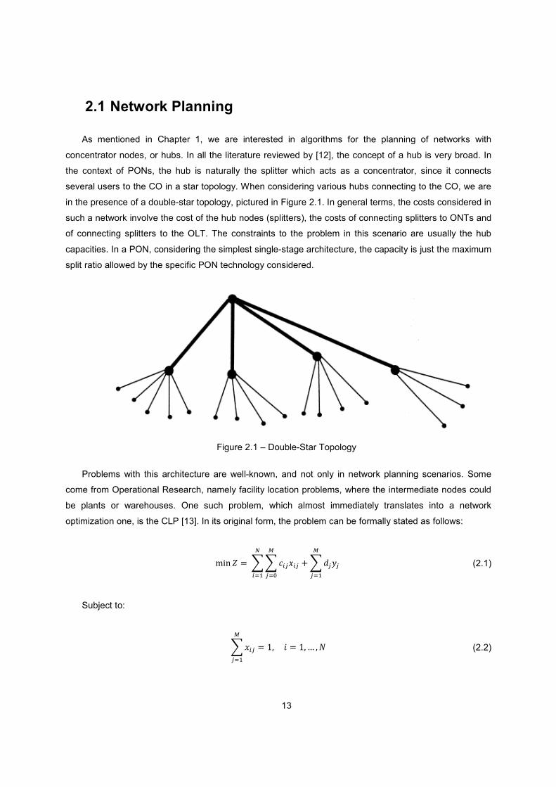
several users to the CO in a star topology. When considering various hubs connecting to the CO, we are

in the presence of a double-star topology, pictured in Figure 2.1. In general terms, the costs considered in

such a network involve the cost of the hub nodes (splitters), the costs of connecting splitters to ONTs and

of connecting splitters to the OLT. The constraints to the problem in this scenario are usually the hub

capacities. In a PON, considering the simplest single-stage architecture, the capacity is just the maximum

split ratio allowed by the specific PON technology considered.

Figure 2.1 – Double-Star Topology

Problems with this architecture are well-known, and not only in network planning scenarios. Some

come from Operational Research, namely facility location problems, where the intermediate nodes could

be plants or warehouses. One such problem, which almost immediately translates into a network

optimization one, is the CLP [13]. In its original form, the problem can be formally stated as follows:

��� � � ����� �� ��

��

�

��

�

��� (2.1)

Subject to:

�� � �������� � ��� � ��

�� (2.2)

14

�� � ���

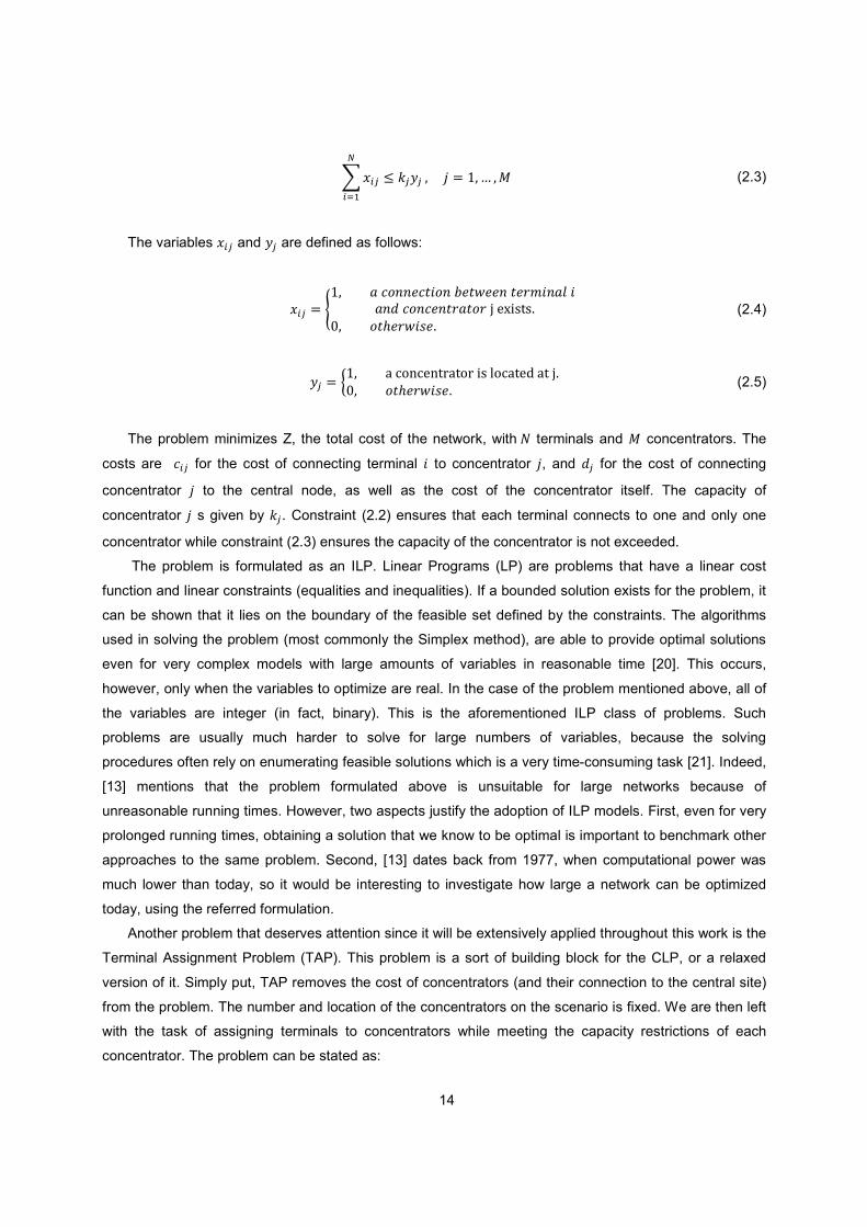
��������� � ��� ������� (2.3)

The variables � and � are defined as follows:

� � ��� ���� !�"�� �#!"$!! �"!%&� �'���� ��� �! "%�"�%�(�)*�+,+-.� �"/!%$�0!-1 (2.4)

� � 2�� 3�45�4)�,63,56��+�7543,)8�3,�(-.� �"/!%$�0!- 1 (2.5)

The problem minimizes Z, the total cost of the network, with�� terminals and � concentrators. The

costs are � for the cost of connecting terminal � to concentrator �, and for the cost of connecting

concentrator � to the central node, as well as the cost of the concentrator itself. The capacity of

concentrator � s given by �. Constraint (2.2) ensures that each terminal connects to one and only one

concentrator while constraint (2.3) ensures the capacity of the concentrator is not exceeded.

The problem is formulated as an ILP. Linear Programs (LP) are problems that have a linear cost

function and linear constraints (equalities and inequalities). If a bounded solution exists for the problem, it

can be shown that it lies on the boundary of the feasible set defined by the constraints. The algorithms

used in solving the problem (most commonly the Simplex method), are able to provide optimal solutions

even for very complex models with large amounts of variables in reasonable time [20]. This occurs,

however, only when the variables to optimize are real. In the case of the problem mentioned above, all of

the variables are integer (in fact, binary). This is the aforementioned ILP class of problems. Such

problems are usually much harder to solve for large numbers of variables, because the solving

procedures often rely on enumerating feasible solutions which is a very time-consuming task [21]. Indeed,

[13] mentions that the problem formulated above is unsuitable for large networks because of

unreasonable running times. However, two aspects justify the adoption of ILP models. First, even for very

prolonged running times, obtaining a solution that we know to be optimal is important to benchmark other

approaches to the same problem. Second, [13] dates back from 1977, when computational power was

much lower than today, so it would be interesting to investigate how large a network can be optimized

today, using the referred formulation.

Another problem that deserves attention since it will be extensively applied throughout this work is the

Terminal Assignment Problem (TAP). This problem is a sort of building block for the CLP, or a relaxed

version of it. Simply put, TAP removes the cost of concentrators (and their connection to the central site)

from the problem. The number and location of the concentrators on the scenario is fixed. We are then left

with the task of assigning terminals to concentrators while meeting the capacity restrictions of each

concentrator. The problem can be stated as:

15

���� ������

��

�

�� (2.6)

Subject to:

�� � �������� � ��� � ��

�� (2.7)

�� � ��

��������� � ��� �� (2.8)

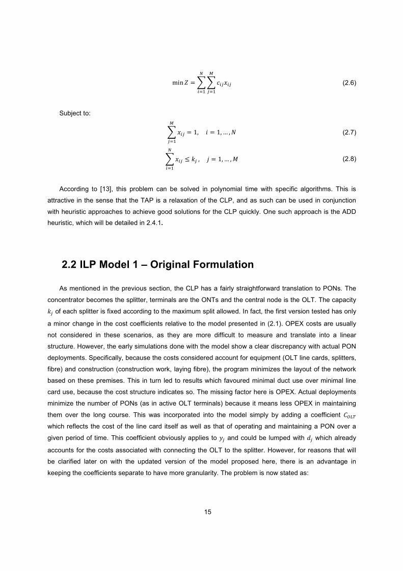
According to [13], this problem can be solved in polynomial time with specific algorithms. This is

attractive in the sense that the TAP is a relaxation of the CLP, and as such can be used in conjunction

with heuristic approaches to achieve good solutions for the CLP quickly. One such approach is the ADD

heuristic, which will be detailed in 2.4.1.

2.2 ILP Model 1 – Original Formulation

As mentioned in the previous section, the CLP has a fairly straightforward translation to PONs. The

concentrator becomes the splitter, terminals are the ONTs and the central node is the OLT. The capacity

� of each splitter is fixed according to the maximum split allowed. In fact, the first version tested has only

a minor change in the cost coefficients relative to the model presented in (2.1). OPEX costs are usually

not considered in these scenarios, as they are more difficult to measure and translate into a linear

structure. However, the early simulations done with the model show a clear discrepancy with actual PON

deployments. Specifically, because the costs considered account for equipment (OLT line cards, splitters,

fibre) and construction (construction work, laying fibre), the program minimizes the layout of the network

based on these premises. This in turn led to results which favoured minimal duct use over minimal line

card use, because the cost structure indicates so. The missing factor here is OPEX. Actual deployments

minimize the number of PONs (as in active OLT terminals) because it means less OPEX in maintaining

them over the long course. This was incorporated into the model simply by adding a coefficient 9:;<

which reflects the cost of the line card itself as well as that of operating and maintaining a PON over a

given period of time. This coefficient obviously applies to � and could be lumped with which already

accounts for the costs associated with connecting the OLT to the splitter. However, for reasons that will

be clarified later on with the updated version of the model proposed here, there is an advantage in

keeping the coefficients separate to have more granularity. The problem is now stated as:

16

��� � � ����� ��= � 9:;<> ? ��

��

�

��

�

�� (2.9)

And is still subject to restrictions (2.2) and (2.3). The ILP was implemented using the free-licensed

solver lpsolve [22], which was interfaced with MATLAB® where the scenarios were created and the costs

calculated. For more details on the software implementation refer to APPENDIX B.

2.2.1 Costs and Scenarios

The inputs for the ILP model are the costs of equipment, the costs of connecting the network

elements and the operational costs of running a PON. The equipment costs are the most simple among

these. Operational costs are difficult to estimate but do not affect the validity of the model’s structure. The

connection costs, however, are more problematic. The model assumes the costs of interconnecting

elements (ONTs to splitters and these to the OLT) are known in advance. This assumption is by default

erroneous. The problem here is the sharing of resources, namely ducts. In [15] this problem is called the

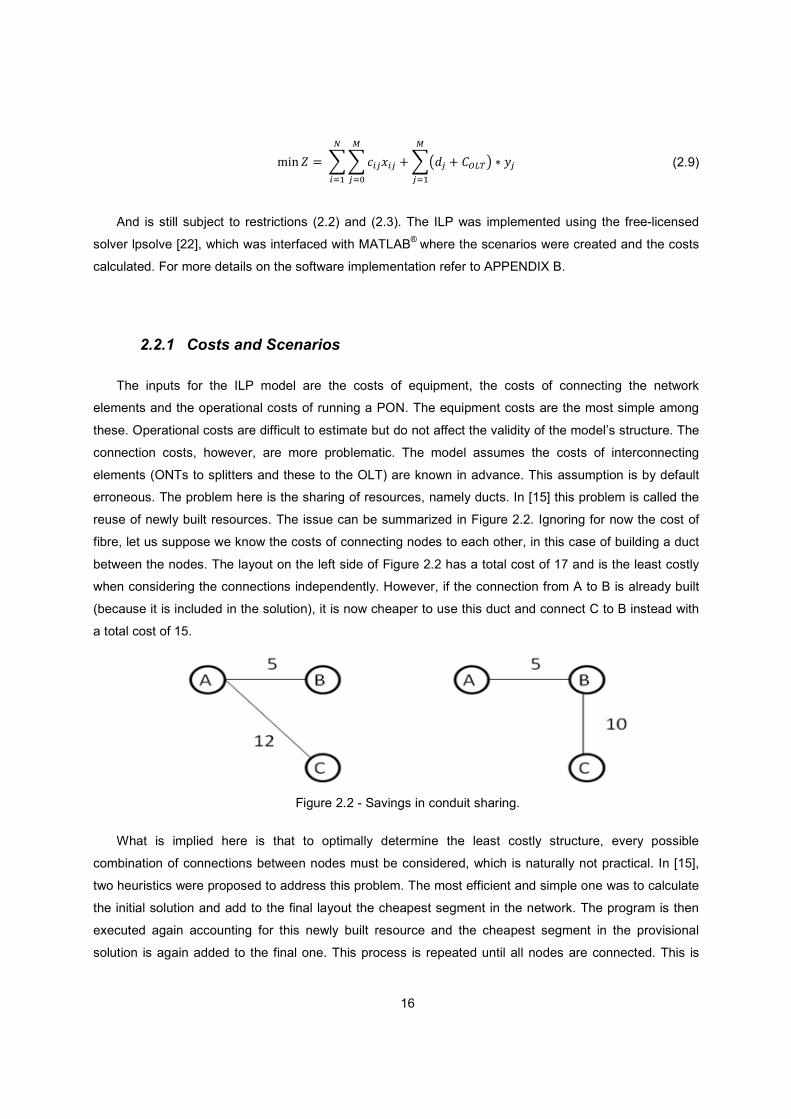
reuse of newly built resources. The issue can be summarized in Figure 2.2. Ignoring for now the cost of

fibre, let us suppose we know the costs of connecting nodes to each other, in this case of building a duct

between the nodes. The layout on the left side of Figure 2.2 has a total cost of 17 and is the least costly

when considering the connections independently. However, if the connection from A to B is already built

(because it is included in the solution), it is now cheaper to use this duct and connect C to B instead with

a total cost of 15.

Figure 2.2 - Savings in conduit sharing.

What is implied here is that to optimally determine the least costly structure, every possible

combination of connections between nodes must be considered, which is naturally not practical. In [15],

two heuristics were proposed to address this problem. The most efficient and simple one was to calculate

the initial solution and add to the final layout the cheapest segment in the network. The program is then

executed again accounting for this newly built resource and the cheapest segment in the provisional

solution is again added to the final one. This process is repeated until all nodes are connected. This is

17

adequate to the graph theory approach of [15]. For the ILP model, however, the costs must be known a

priori which has been shown not to be possible. Essentially, the connections costs are non-linear (i.e.

they depend on other connections), and as such cannot be formulated into an ILP without enumerating

every possible connection layout. The solutions provided by the program are therefore not optimal since

they do not account for conduit sharing. However, some practical reasons mitigate this effect. In urban

areas, PON deployments overwhelmingly use already existing ducts. This means that there are usually

well-defined duct paths to interconnect terminals to a CO. In this sense, the costs of connections are for

the most part known in advance. The error now lies in the fact that two connections that share a common

segment will also share a fibre cable. Since the cost of cables is dependent on the number of fibres they

carry it is impossible to account for this directly since it cannot be known in advance how many fibres will

use a given segment. When looking at the cost structure of the problem though, it can be noticed that this

is less likely to impact the overall layout of the network because the difference between the costs of

various cable types weighs much less on the overall cost of the network than that of deciding whether or

not to build a new duct. When considering greenfield areas or scenarios with insufficient infrastructure for

laying fibre, a tool like [15] can be used to obtain the layout of the infrastructure and the costs of laying

fibre can be derived from that information and fed to the ILP.

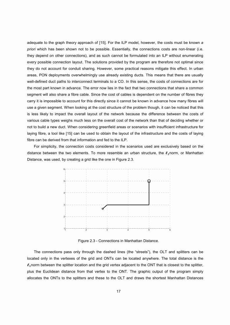
For simplicity, the connection costs considered in the scenarios used are exclusively based on the

distance between the two elements. To more resemble an urban structure, the @Anorm, or Manhattan

Distance, was used, by creating a grid like the one in Figure 2.3.

Figure 2.3 - Connections in Manhattan Distance.

The connections pass only through the dashed lines (the “streets”), the OLT and splitters can be

located only in the vertexes of the grid and ONTs can be located anywhere. The total distance is the

@Anorm between the splitter location and the grid vertex adjacent to the ONT that is closest to the splitter,

plus the Euclidean distance from that vertex to the ONT. The graphic output of the program simply

allocates the ONTs to the splitters and these to the OLT and draws the shortest Manhattan Distances

1 2 3 4 5 61

2

3

4

5

6

18

between them. Examples of the visual output of the program for both Manhattan and Euclidean distances

can be found in APPENDIX B.

2.2.2 Performance and Scalability

One of the most important aspects when evaluating an ILP model is to ascertain the scalability of the

problem. In cases such as this, where variables denote the existence or not of a connection between

every hierarchical combination of network elements, the complexity is expected to grow exponentially as

the scenarios get larger. This reflects not only on the running time of the problem, but also on the memory

occupation when scenarios become very large. Looking closely at (2.9) it becomes clear that the number

of variables in the program is (� ? � ��B. The number of restrictions on the other hand is � ��. This

means that for a given scenario, to allocate the restriction matrix, a total of C ? D� ? � � �B ? D� � �B bytes of contiguous free memory are required. For a scenario with 2 000 ONTs and 50 possible splitter

locations, more than 1,6 GB of memory is needed.

In order to evaluate, in an earlier stage, if the ILP approach was worth pursuing, several scenarios

ranging in size were simulated with the model. For this analysis the cost structure was simplified, not

reflecting the costs as accurately as the simulations in following sections. Table 2.1 shows the costs

considered in this stage of the simulation.

Table 2.1 - Costs for preliminary analysis.

Parameter Equipment cost [cost units] Connection cost [cost units per km]

9:;< 100

� 5

5 5

The created scenarios were squares with a 10 km side. The OLT was placed at the centre of the

square, while the splitters were randomly placed with a uniform distribution within 3 km of the OLT. The

ONTs were randomly placed with a uniform distribution throughout the square. Table 2.2 registers the

obtained running times for the program with various numbers of ONTs and OLTs. Results were obtained

using an Intel® Core2E Duo 2,33 GHz processor with 2 GB of memory.

19

Table 2.2 - Running times [hh:mm:ss] for varying ONT and splitter numbers.

ONTs

Splitters

64 128 256 500 1 000

2 00:00:00 00:00:00

4 00:00:00 00:00:00 00:00:00

10 00:00:00 00:00:00 00:00:01 00:00:01

20 00:00:04 00:00:25 00:00:25 00:02:28 00:00:09

30 00:01:02 00:05:29 00:29:52 01:27:58 00:32:55

50 00:15:35 05:11:00 15:25:36 96:25:30 > 120 hours

- Exceeds maximum capacity of the splitters in the scenario (for GPON).

As expected, the complexity increases exponentially with the increase in the number of variables. For

1 000 ONTs and 50 splitter locations running time was not measurable. However, most medium-sized

scenarios are solved in reasonable times, which encouraged the development of new strategies to

improve the performance and accuracy of the model.

One thing that captures the attention in Table 2.2 is the strong decrease in running time when going

from the scenario with 20 splitters and 500 ONTs to the one with 20 splitters and 1 000 ONTs. The same

happens for the 30 splitter case with 500 and 1 000 ONTs, respectively. With a solid increase in the

number of variables, the running time was actually quite lower. To ensure this was not caused by the

randomness of the simulated scenarios, another set of tests was devised. Several scenarios in the same

conditions as before were created, but this time the number of variables was kept constant, and only the

proportion between splitters and ONTs was modified. This proportion was termed the Occupancy Ratio,

meaning the percentage of ONTs in the scenario relative to the maximum allowed capacity by all the

splitters combined (64 times the number of splitters for GPON). Table 2.3 shows the running times for

different Occupancy Ratios with three different numbers of variables. The proportions between ONTs and

splitter locations were the ones that provided the exact number of variables used.

20

Table 2.3 - Comparison of running times with different Occupancy Ratios.

Number of variables Number of splitters Number of ONTs Occupancy Ratio Running time [s]

1 000

8 24 24% 0,08

10 99 15% 0,12

20 49 4% 1,36

25 39 2% 2,37

5 000

10 499 78% 0,60

20 249 19% 16,06

25 199 12% 16,19

40 124 5% 68,53

10 000

16 624 61% 4,39

20 499 39% 14,68

25 399 25% 23,08

40 249 10% 652,26

The trend that was suggested in Table 2.2 is now confirmed. For the same number of variables, the

running time is invariably higher for lower Occupancy Ratios. This means that adding ONTs to a scenario

can actually be beneficial to the running time of the program. Intuitively, this might be explained by the

fact that a scenario with a low Occupancy Ratio probably has more feasible solutions with smaller

differences in their respective overall costs. On the other hand, in a scenario with just enough capacity for

all ONTs it is more likely that feasible solutions are in general much less attractive than the optimal one.

This makes sense since the algorithm for ILP solving essentially tries to avoid examining all possible

solutions by discarding the ones that are clearly worse than the best one found yet. In a scenario with a

lot of splitters, there are more slight variations in allocations that can produce solutions very close to the

optimal, which forces the procedure to perform a more exhaustive search.

2.3 ILP Model 2 – Updated Formulation

So far, the model presented has stuck to the original CLP formulation, accounting only for OPEX

costs related to PONs. The topology used was not verified as to whether or not it mimics real

deployments. The previous section only introduced the original problem and its size limitations. In this

section a review of actual PON planning is made, and the model is updated to reflect reality to the best

extent of its capabilities.

PONs became a popular solution among operators because they are seen as the least costly

architecture for delivering FTTH in a mass market residential scenario. As one would expect, the initial

developments were set in locations that maximize economies of scale, namely urban centres with high

21

population density. The objectives of PON deployments are usually measured in HouseHolds Passed

(HHP). In this context, a house is deemed as “passed”, when the distribution fibre reaches a Network

Access Point (NAP) which, in urban settings, is usually placed inside buildings. The number of fibres that

feed a given building is usually a function of the number of dwelling units in that building as well as of the

Take Rate considered by each operator. The Take Rate is the predicted maximum percentage of users

that will request the fibre service from the operator. Naturally this varies between operators and the type

of areas served.

In the Portuguese case, according to information from the operators themselves, each service area is

decomposed into cells of approximately 2 000 ONTs which on average, for the city of Lisbon is the

equivalent of about 200 buildings. In these urban settings, as it was mentioned earlier, the infrastructure

for fibre passage already exists. The prohibitive costs of new digs force the reuse of these installations,

even if it implies renting another operator’s conduits, usually the incumbent. The feeder fibres, between

the CO and the splitters, overwhelmingly use existing ducts, while the distribution fibres, between splitters

and buildings, depend on the specifics of the topology, reusing ducts when possible or else laying the

fibre through the buildings’ facades.

Regarding the architecture of the network, two main topologies exist: centralized and distributed split

[23][24][25]. Both are exemplified in Figure 2.4, with the top design pertaining to a centralized split and

the two others to a distributed split.

Figure 2.4 - Centralized and distributed division (Source: Corning).

In both approaches there is an initial splitting stage located at the CO. This configuration allows for

easy access to connections and enables more flexibility in managing the connections to the OLT ports. In

the centralized split, the feeder fibre connects to a Local Convergence Point (LCP), which basically

houses an array of splitters. The distribution fibre then runs all the way to the NAP and from there, if

service is requested, to the users’ premises (the drop cables). In a distributed split, the LCP splitters

connect to another stage of splitters in the NAP. From a fibre-usage point of view, the distributed split

makes the most sense because it saves on distribution fibre with optical splitting in the building’s

22

premises. However, it also means more complex management because the maintenance points are more

scattered and also because when troubleshooting, an Optical Time-Domain Reflectometre (OTDR)

cannot “see” beyond a splitter, which is aggravated when using three splitting stages. Also, a distributed

architecture is less flexible because it allocates splitters to small service areas while a centralized split is

more favourable to future upgrades in the network.

When deploying a residential network, it is not expected that all customers will immediately require

the service. The most likely scenario is an early adoption by a few customers and then phased growth.

From an operator’s point of view, this has to impact the way the connections in the PON are made.

Specifically, the allocation of fibre connections to the splitters in the LCP must take this into account. Let’s

take the example depicted in Figure 2.5, with an LCP housing 2 splitters of 1:32 which belong to different

OLT ports, termed PON A and PON B. Each splitter feeds two buildings with 16 fibres each.

Figure 2.5 - Concentrated allocation.

Now let us suppose that after the network is deployed and connected in this fashion, 2 users on each

building request service. With the concentrated allocation of a building’s connections to just one splitter,

the operator is forced to operate and maintain two PONs to serve 8 customers in this area. With a larger

example involving more splitters, many PONs could be in use to serve only a very limited number of

users. A more reasonable approach, known as balanced allocation is shown in Figure 2.6, where the

splitters now feed every building with 4 fibres each.

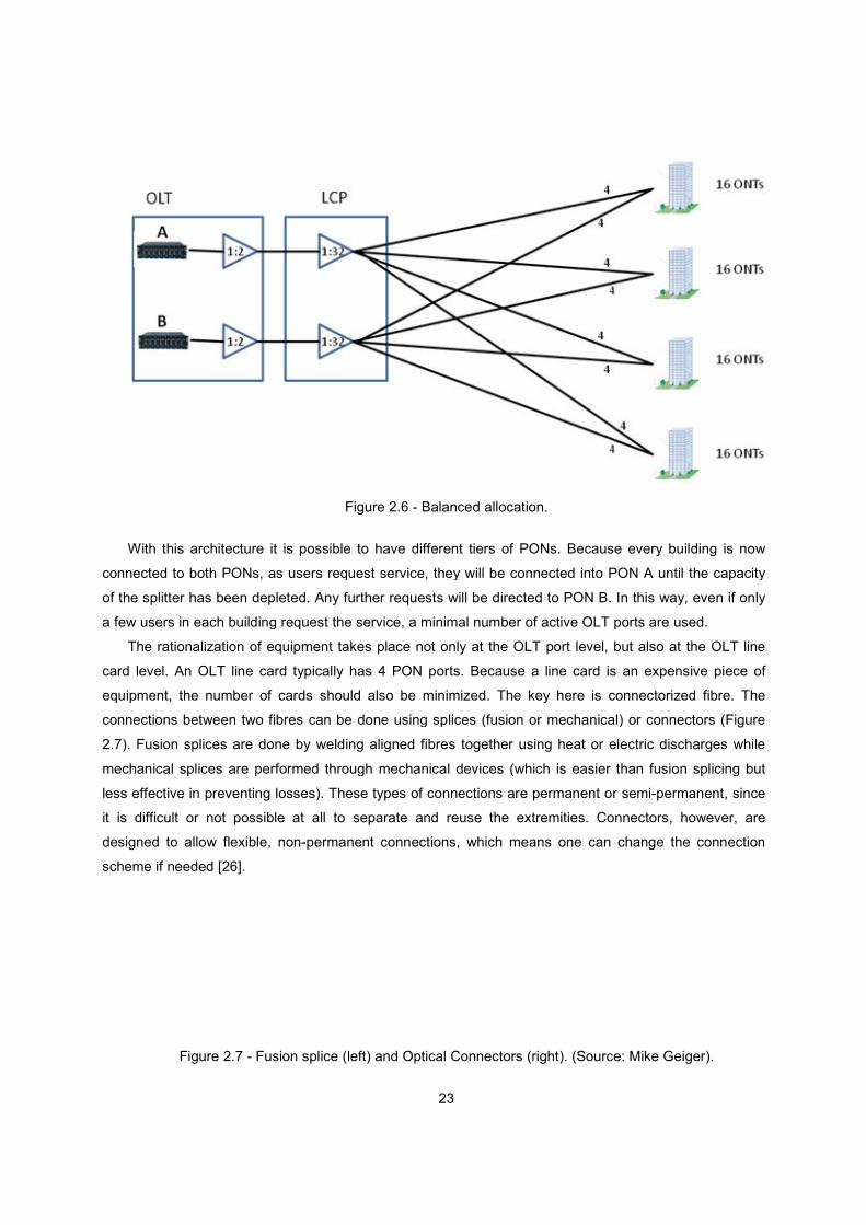
With this architecture it is possible to

connected to both PONs, as users request service, they will be connected into PON A until the capacity

of the splitter has been depleted. Any further requests will be directed to PON B.

a few users in each building request the service, a minima

The rationalization of equipment takes place not only at the OLT port level, but also at the OLT line

card level. An OLT line card typically h

equipment, the number of cards should also be minimized. The key here is connectorized fibre. The

connections between two fibres can be done using splices (fusion or mechanical) or connectors (

2.7). Fusion splices are done by welding aligned fibres together using heat or electric discharges while

mechanical splices are performed through mechanical devi

less effective in preventing losses). These types of connections are permanent or semi

it is difficult or not possible at all to separate and reuse the extremities. Connectors, however, are

designed to allow flexible, non-permanent connections, which means one can change the connection

scheme if needed [26].

Figure 2.7 - Fusion splice (left) and Optical Connectors (right). (Source: Mike Geiger).

23

Figure 2.6 - Balanced allocation.

With this architecture it is possible to have different tiers of PONs. Because every building is now

connected to both PONs, as users request service, they will be connected into PON A until the capacity

of the splitter has been depleted. Any further requests will be directed to PON B.

a few users in each building request the service, a minimal number of active OLT ports are

The rationalization of equipment takes place not only at the OLT port level, but also at the OLT line

card level. An OLT line card typically has 4 PON ports. Because a line card is an expensive piece of

equipment, the number of cards should also be minimized. The key here is connectorized fibre. The

connections between two fibres can be done using splices (fusion or mechanical) or connectors (

). Fusion splices are done by welding aligned fibres together using heat or electric discharges while

mechanical splices are performed through mechanical devices (which is easier than fusion splicing but

less effective in preventing losses). These types of connections are permanent or semi

it is difficult or not possible at all to separate and reuse the extremities. Connectors, however, are

permanent connections, which means one can change the connection

Fusion splice (left) and Optical Connectors (right). (Source: Mike Geiger).

have different tiers of PONs. Because every building is now

connected to both PONs, as users request service, they will be connected into PON A until the capacity

of the splitter has been depleted. Any further requests will be directed to PON B. In this way, even if only

l number of active OLT ports are used.

The rationalization of equipment takes place not only at the OLT port level, but also at the OLT line

as 4 PON ports. Because a line card is an expensive piece of

equipment, the number of cards should also be minimized. The key here is connectorized fibre. The

connections between two fibres can be done using splices (fusion or mechanical) or connectors (Figure

). Fusion splices are done by welding aligned fibres together using heat or electric discharges while

ces (which is easier than fusion splicing but

less effective in preventing losses). These types of connections are permanent or semi-permanent, since

it is difficult or not possible at all to separate and reuse the extremities. Connectors, however, are

permanent connections, which means one can change the connection

Fusion splice (left) and Optical Connectors (right). (Source: Mike Geiger).

24

This is especially useful for the mentioned purpose of line card optimization. The connections from

the OLT to the first stage of splitters located at the CO are connectorized. In this way, the connections

from first stage splitters that serve used PONs can be directed to the same line cards, allowing operators

to use the least possible amount of cards. If applied to the entire network, connectorized solutions would

allow total flexibility, since the connections could always be rearranged as to minimize the total number of

active PONs. However some practical factors negate the advantages of this solution. Aside from the fact

that connectors are more expensive than splicing, the attenuation of a connector is much higher than that

of a fusion splice (0.3 dB vs. 0.05 dB was considered in this work). Furthermore, when the LCP is located

in the ducts (in which case it is usually called a Junction Box), there might not exist enough space for

connectorized links nor is the access to these Boxes easy enough to perform rearrangements on a

regular basis. Furthermore, access to the ducts is often conditioned, especially for operators renting

them, so connectorization in the outside plant is not so popular.

Finally, the nature of the LCP should be mentioned. The most popular solution in Portugal is the use

of Junction Boxes, which are basically derivations in the main feeder fibre cables that house arrays of

splitters to serve more specific areas. Another alternative are Local Convergence Cabinets (LCC), which

are outdoor cabinets that are naturally more expensive, but allow for easy access and extended capacity

for splitters and connectorized links. However, aside from the costs of the cabinets themselves, operators

are subjected to municipal licenses to install them which further increases costs and makes this solution

less viable.

2.3.1 Splitter Co-Location

Based on the previous discussion, it is clear the model presented in 2.2 does not accurately reflect

some aspects of actual PON configurations. One such example is the fact that it allows only one splitter

per location which is rarely the case. This also causes the scenarios to become too large and consume

too much memory just to be able to have enough splitters to accommodate all the ONTs. One option for

introducing this aspect would be to set the capacities � as multiples of 64 according to the capacity of the

Cabinet or Junction Box. This approach is mentioned in [13]. However, it would violate the spirit of this

formulation, since this wouldn’t account for the fact that these new splitters mean new PONs with extra

OPEX. The solution to this problem was to have the variables � reflect the number of splitters that the

locations house. This can be accomplished by setting � to integer instead of just binary, this is

accomplished. The model remains unchanged except for adding the following constraint:

� � F (2.10)

which basically sets the maximum amount of splitters that location � can accommodate to F.

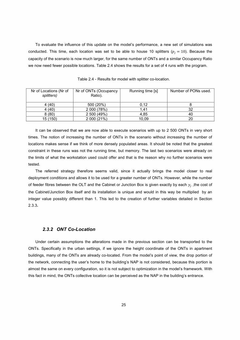
25

To evaluate the influence of this update on the model’s performance, a new set of simulations was

conducted. This time, each location was set to be able to house 10 splitters (F � �.). Because the

capacity of the scenario is now much larger, for the same number of ONTs and a similar Occupancy Ratio

we now need fewer possible locations. Table 2.4 shows the results for a set of 4 runs with the program.

Table 2.4 - Results for model with splitter co-location.

Nr of Locations (Nr of splitters)

Nr of ONTs (Occupancy Ratio).

Running time [s] Number of PONs used.

4 (40) 500 (20%) 0,12 8 4 (40) 2 000 (78%) 1,41 32 8 (80) 2 500 (49%) 4,85 40

15 (150) 2 000 (21%) 10,09 20

It can be observed that we are now able to execute scenarios with up to 2 500 ONTs in very short

times. The notion of increasing the number of ONTs in the scenario without increasing the number of

locations makes sense if we think of more densely populated areas. It should be noted that the greatest

constraint in these runs was not the running time, but memory. The last two scenarios were already on

the limits of what the workstation used could offer and that is the reason why no further scenarios were

tested.

The referred strategy therefore seems valid, since it actually brings the model closer to real

deployment conditions and allows it to be used for a greater number of ONTs. However, while the number

of feeder fibres between the OLT and the Cabinet or Junction Box is given exactly by each � ,the cost of

the Cabinet/Junction Box itself and its installation is unique and would in this way be multiplied by an

integer value possibly different than 1. This led to the creation of further variables detailed in Section

2.3.3.

2.3.2 ONT Co-Location

Under certain assumptions the alterations made in the previous section can be transported to the

ONTs. Specifically in the urban settings, if we ignore the height coordinate of the ONTs in apartment

buildings, many of the ONTs are already co-located. From the model’s point of view, the drop portion of

the network, connecting the user’s home to the building’s NAP is not considered, because this portion is

almost the same on every configuration, so it is not subject to optimization in the model’s framework. With

this fact in mind, the ONTs collective location can be perceived as the NAP in the building’s entrance.

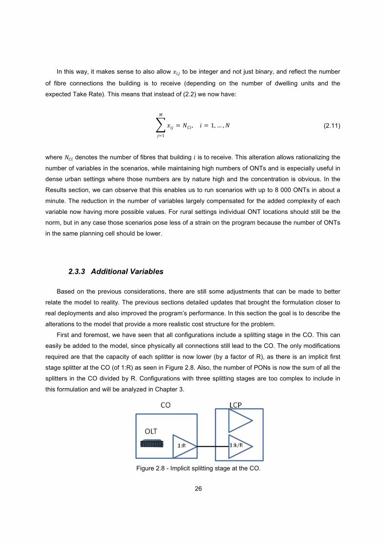
26

In this way, it makes sense to also allow � to be integer and not just binary, and reflect the number

of fibre connections the building is to receive (depending on the number of dwelling units and the

expected Take Rate). This means that instead of (2.2) we now have:

� ��� � �9� ������� � �� � � ��

��� (2.11)

where �G denotes the number of fibres that building � is to receive. This alteration allows rationalizing the

number of variables in the scenarios, while maintaining high numbers of ONTs and is especially useful in

dense urban settings where those numbers are by nature high and the concentration is obvious. In the

Results section, we can observe that this enables us to run scenarios with up to 8 000 ONTs in about a

minute. The reduction in the number of variables largely compensated for the added complexity of each

variable now having more possible values. For rural settings individual ONT locations should still be the

norm, but in any case those scenarios pose less of a strain on the program because the number of ONTs

in the same planning cell should be lower.

2.3.3 Additional Variables

Based on the previous considerations, there are still some adjustments that can be made to better

relate the model to reality. The previous sections detailed updates that brought the formulation closer to

real deployments and also improved the program’s performance. In this section the goal is to describe the

alterations to the model that provide a more realistic cost structure for the problem.

First and foremost, we have seen that all configurations include a splitting stage in the CO. This can

easily be added to the model, since physically all connections still lead to the CO. The only modifications

required are that the capacity of each splitter is now lower (by a factor of R), as there is an implicit first

stage splitter at the CO (of 1:R) as seen in Figure 2.8. Also, the number of PONs is now the sum of all the

splitters in the CO divided by R. Configurations with three splitting stages are too complex to include in

this formulation and will be analyzed in Chapter 3.

Figure 2.8 - Implicit splitting stage at the CO.

27

As it was mentioned in section 2.3.1, the modification of the variables that signal a connection

between the OLT and the splitters no longer accurately reflects the costs involved. It now accounts for the

number of fibre connections between the OLT and the splitter array. But there is only one Cabinet or

Junction Box, and its cost is now multiplied by an integer probably larger than one. While some

approximation could be employed here, it is clear the problem needs more granularity in this respect.

Furthermore, the OPEX optimization takes place on the OLT port level. It has been mentioned that line

card optimization is also important. With this in mind, some variables were added to the model to reflect

these issues. They are described as follows:

• A variable to address the number of line cards at the OLT, �:;<, which is basically the

rounding up of the quotient between the number of PONs, �H:� and the number of PONs per

card, �HG (usually 4).

• Variables that reflect the cost of the Cabinets or Junction Boxes, I. These are binary

variables, since they only indicate the existence of the concentration points..

The revised formulation, termed ILP Model 2, is now formally stated as:

����JKL��MJN�O�P�Q�:;< ? 9:;< ��H:� ? 9H:� ����� �� �� ��

��

�

��

�

����!I

�

�� (2.12)

Subject to:

�� � �G ������� � ��� � ��

������ (2.13)

�� � �R ��

��������� � ��� ������ (2.14)

� � F (2.15)

�H:� S T ����R (2.16)

�:;< S �H:�R (2.17)

I � � ������� � ��� ��� (2.18)

I S �F ������� � ��� ��� (2.19)

9:;< is now the cost of a line card and the OPEX associated with it. 9H:� is the cost associated with

operating a single PON port within a line card and the cost of the first splitter in the CO. The variables ! denote the costs of the Cabinets or Junction Boxes and of installing fibre between the OLT and splitter

location �.

28

Constraint (2.13) was already introduced in (2.11). Constraint (2.14) ensures the connections to � do

not exceed the capacity of the array of splitters placed there, and that capacity is set by (2.15) where F is

the maximum number of splitters supported at location �. Constraint (2.16) sets the correct number of line

cards, while constraint (2.17) says that the number of PONs is the total sum of second-stage splitters in

the network divided by the ratio of those splitters (since the variable is integer the inequality ensures the

result from the division is rounded up). Constraint (2.18) forces I to zero if � is zero (i.e. there are no

splitters at �). Finally, constraint (2.19) acts as a way to make sure I is above zero if � also is, but

divided by 9P so I � � in any circunstance. Otherwise, the problem would not be feasible.

The concentration of ONTs was described in the same way as the concentration of splitters was.

However, while in the splitter case we added an extra set of binary variables that reflect the existence of a

single Cabinet/Junction Box between the OLT and the splitters, this was not the case for the ONTs. A

similar strategy could be employed, by creating another set of binary variables that were equal to 1

whenever the corresponding � U .. However this would imply creating an additional � ? � variables

which burdened the problem with too much complexity, rendering it unable to solve even medium sized

scenarios. Under our assumptions, though, the cost of laying fibre is proportional to the number of fibres

themselves, since most of the time spent in labour is splicing, conditioning and testing fibres. The element

we are discarding here is the cost of the NAP, which is usually a small box inside the building where all

the fibre connections are available to make the drop connections when required. Since there is only one

per building in any case, it did not seem logical to needlessly add complexity to the program just to reflect

the cost differences in installing bigger or smaller NAPs.

The results for this model show that, for scenarios with concentrated ONTs (dense urban), networks

below 10 000 ONTs and 40 possible Junction Boxes are optimized in less than 4 hours.

2.4 Heuristic Methods

Heuristics can be described as the use of available information through intuitive empirical rules to

quickly achieve solutions as close as possible to the optimum [27]. For the problem in question, where the

running times to attain optimal solutions can exceed dozens of hours for large scenarios, these methods

are of great importance. They should provide solutions relatively close to the optimal one given by the

ILP, bypassing its inherent complexity.

The methods used here preserve the core of the problem’s original formulation. This means they are

based on partitions or relaxations of the original problem with heuristic decision processes in between

iterations. This option has two main drivers: to maximize the reuse of the work performed with the ILP

formulation and to allow modifications to the model such as the ones described above more easily

translate into the heuristics. The following sections present the two methods proposed.

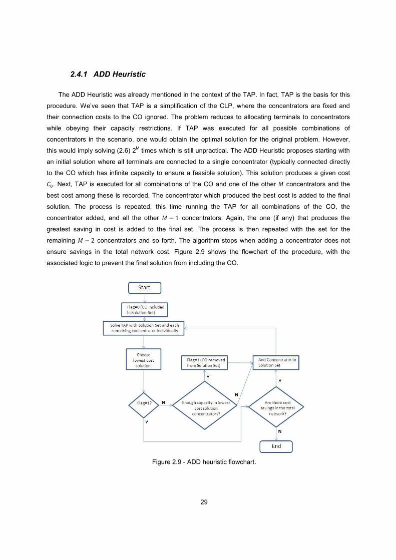
29

2.4.1 ADD Heuristic

The ADD Heuristic was already mentioned in the context of the TAP. In fact, TAP is the basis for this

procedure. We’ve seen that TAP is a simplification of the CLP, where the concentrators are fixed and

their connection costs to the CO ignored. The problem reduces to allocating terminals to concentrators

while obeying their capacity restrictions. If TAP was executed for all possible combinations of

concentrators in the scenario, one would obtain the optimal solution for the original problem. However,

this would imply solving (2.6) 2M times which is still unpractical. The ADD Heuristic proposes starting with

an initial solution where all terminals are connected to a single concentrator (typically connected directly

to the CO which has infinite capacity to ensure a feasible solution). This solution produces a given cost

9�. Next, TAP is executed for all combinations of the CO and one of the other � concentrators and the

best cost among these is recorded. The concentrator which produced the best cost is added to the final

solution. The process is repeated, this time running the TAP for all combinations of the CO, the

concentrator added, and all the other � V � concentrators. Again, the one (if any) that produces the

greatest saving in cost is added to the final set. The process is then repeated with the set for the

remaining � V W concentrators and so forth. The algorithm stops when adding a concentrator does not

ensure savings in the total network cost. Figure 2.9 shows the flowchart of the procedure, with the

associated logic to prevent the final solution from including the CO.

Figure 2.9 - ADD heuristic flowchart.

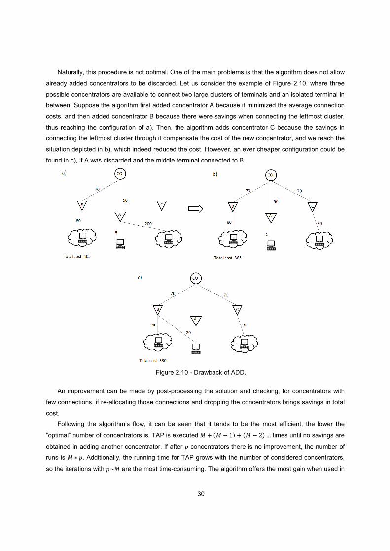
30

Naturally, this procedure is not optimal. One of the main problems is that the algorithm does not allow

already added concentrators to be discarded. Let us consider the example of Figure 2.10, where three

possible concentrators are available to connect two large clusters of terminals and an isolated terminal in

between. Suppose the algorithm first added concentrator A because it minimized the average connection

costs, and then added concentrator B because there were savings when connecting the leftmost cluster,

thus reaching the configuration of a). Then, the algorithm adds concentrator C because the savings in

connecting the leftmost cluster through it compensate the cost of the new concentrator, and we reach the

situation depicted in b), which indeed reduced the cost. However, an ever cheaper configuration could be

found in c), if A was discarded and the middle terminal connected to B.

Figure 2.10 - Drawback of ADD.

An improvement can be made by post-processing the solution and checking, for concentrators with

few connections, if re-allocating those connections and dropping the concentrators brings savings in total

cost.

Following the algorithm’s flow, it can be seen that it tends to be the most efficient, the lower the

“optimal” number of concentrators is. TAP is executed � � D� V �B � D� V WB� times until no savings are

obtained in adding another concentrator. If after F concentrators there is no improvement, the number of

runs is � ? F. Additionally, the running time for TAP grows with the number of considered concentrators,

so the iterations with FX� are the most time-consuming. The algorithm offers the most gain when used in

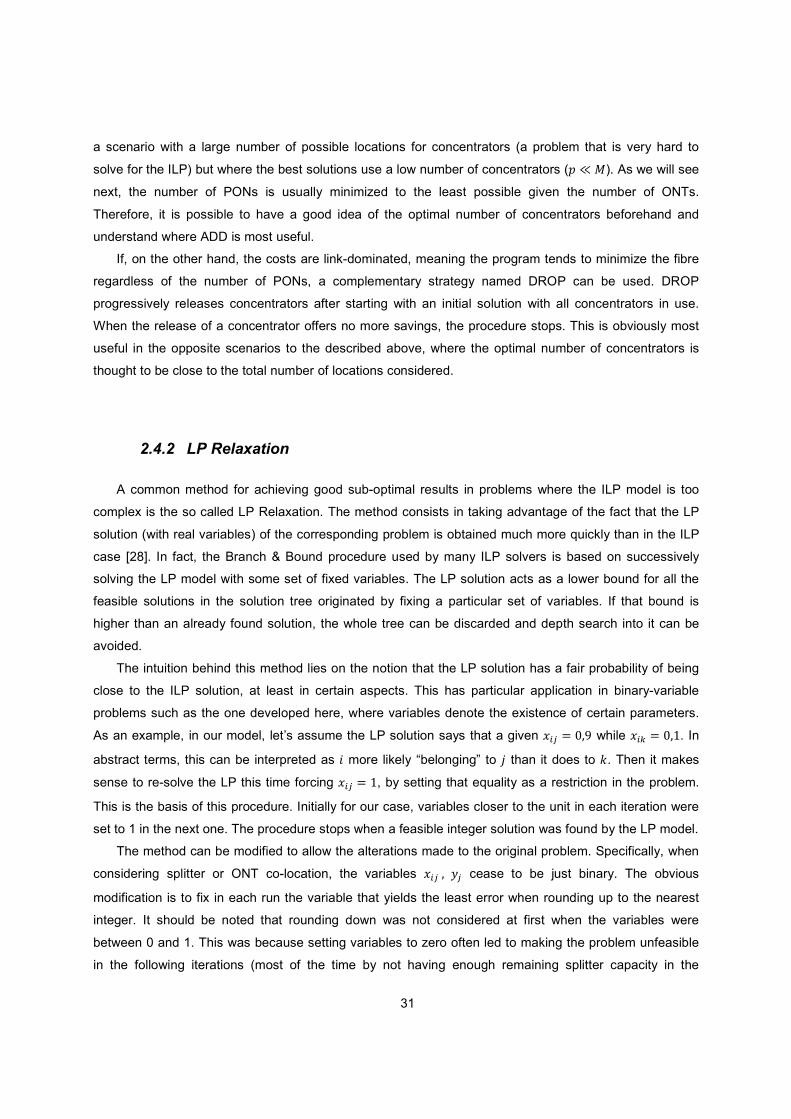
31

a scenario with a large number of possible locations for concentrators (a problem that is very hard to

solve for the ILP) but where the best solutions use a low number of concentrators (F Y �). As we will see

next, the number of PONs is usually minimized to the least possible given the number of ONTs.

Therefore, it is possible to have a good idea of the optimal number of concentrators beforehand and

understand where ADD is most useful.

If, on the other hand, the costs are link-dominated, meaning the program tends to minimize the fibre

regardless of the number of PONs, a complementary strategy named DROP can be used. DROP

progressively releases concentrators after starting with an initial solution with all concentrators in use.

When the release of a concentrator offers no more savings, the procedure stops. This is obviously most

useful in the opposite scenarios to the described above, where the optimal number of concentrators is

thought to be close to the total number of locations considered.

2.4.2 LP Relaxation

A common method for achieving good sub-optimal results in problems where the ILP model is too

complex is the so called LP Relaxation. The method consists in taking advantage of the fact that the LP

solution (with real variables) of the corresponding problem is obtained much more quickly than in the ILP

case [28]. In fact, the Branch & Bound procedure used by many ILP solvers is based on successively

solving the LP model with some set of fixed variables. The LP solution acts as a lower bound for all the

feasible solutions in the solution tree originated by fixing a particular set of variables. If that bound is

higher than an already found solution, the whole tree can be discarded and depth search into it can be

avoided.

The intuition behind this method lies on the notion that the LP solution has a fair probability of being

close to the ILP solution, at least in certain aspects. This has particular application in binary-variable

problems such as the one developed here, where variables denote the existence of certain parameters.

As an example, in our model, let’s assume the LP solution says that a given � � .�Z while �[ � .��. In

abstract terms, this can be interpreted as � more likely “belonging” to � than it does to �. Then it makes

sense to re-solve the LP this time forcing � � �, by setting that equality as a restriction in the problem.

This is the basis of this procedure. Initially for our case, variables closer to the unit in each iteration were

set to 1 in the next one. The procedure stops when a feasible integer solution was found by the LP model.

The method can be modified to allow the alterations made to the original problem. Specifically, when

considering splitter or ONT co-location, the variables � �� � cease to be just binary. The obvious

modification is to fix in each run the variable that yields the least error when rounding up to the nearest

integer. It should be noted that rounding down was not considered at first when the variables were

between 0 and 1. This was because setting variables to zero often led to making the problem unfeasible

in the following iterations (most of the time by not having enough remaining splitter capacity in the

32

scenario). Later, the lowest rounding error (up or down) was considered for all variables greater than 1,

but this was empirically determined to present worse results than only rounding up, so the final version

only rounds variables up. Figure 2.11 shows the flowchart of the process.

Figure 2.11 - Flowchart of LP Relaxation.

2.5 Results and Discussion

This section presents the results obtained with the ILP model developed. The performance of ILP

Model 1 is compared with the heuristics. Then, Model 2 and the updated heuristics are analyzed.

Following that, the cost breakdown of the scenarios is presented regarding the density of the scenario

and the configuration used in the PON.

2.5.1 ILP Model 1 – Comparative Performance

The two most important parameters that must be observed when comparing the ILP model and the

heuristics are the cost of the solutions provided and the time it took them to be generated. Obviously the

cost reference is the one provided by the ILP, since it is optimal.

The costs considered were based on [17] and [29], and merged with inquiries made at Sonaecom, a

Portuguese FTTH operator. The yearly residential user OPEX cost in a PON from [29] was used (around

200 $ per year), and then scaled up to reflect operating a full GPON (64 users) throughout a period of 10

years. The cost of fibre cables has a non-linear variation because the cost per fibre goes down as the

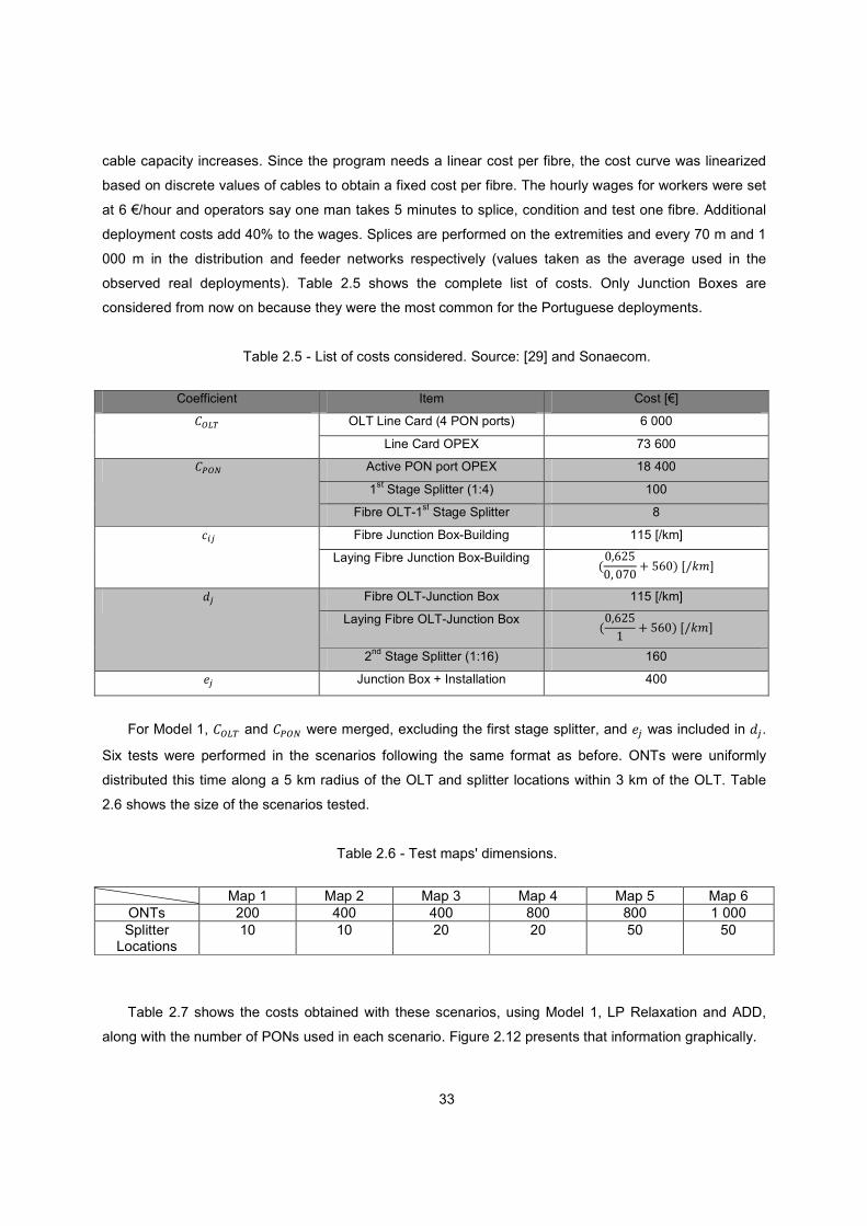
33

cable capacity increases. Since the program needs a linear cost per fibre, the cost curve was linearized

based on discrete values of cables to obtain a fixed cost per fibre. The hourly wages for workers were set

at 6 €/hour and operators say one man takes 5 minutes to splice, condition and test one fibre. Additional

deployment costs add 40% to the wages. Splices are performed on the extremities and every 70 m and 1

000 m in the distribution and feeder networks respectively (values taken as the average used in the

observed real deployments). Table 2.5 shows the complete list of costs. Only Junction Boxes are

considered from now on because they were the most common for the Portuguese deployments.

Table 2.5 - List of costs considered. Source: [29] and Sonaecom.

Coefficient Item Cost [€]

9:;< OLT Line Card (4 PON ports) 6 000

Line Card OPEX 73 600

�9H:� Active PON port OPEX 18 400

1st Stage Splitter (1:4) 100

Fibre OLT-1st Stage Splitter 8

� Fibre Junction Box-Building 115 [/km]

Laying Fibre Junction Box-Building D.�\W].� .^. � ]\.B�_`�&a Fibre OLT-Junction Box 115 [/km]

Laying Fibre OLT-Junction Box D.�\W]� � ]\.B�_`�&a 2nd Stage Splitter (1:16) 160

! Junction Box + Installation 400

For Model 1, 9:;< and 9H:� were merged, excluding the first stage splitter, and ! was included in . Six tests were performed in the scenarios following the same format as before. ONTs were uniformly

distributed this time along a 5 km radius of the OLT and splitter locations within 3 km of the OLT. Table

2.6 shows the size of the scenarios tested.

Table 2.6 - Test maps' dimensions.

Map 1 Map 2 Map 3 Map 4 Map 5 Map 6 ONTs 200 400 400 800 800 1 000 Splitter

Locations 10 10 20 20 50 50

Table 2.7 shows the costs obtained with these scenarios, using Model 1, LP Relaxation and ADD,

along with the number of PONs used in each scenario. Figure 2.12 presents that information graphically.

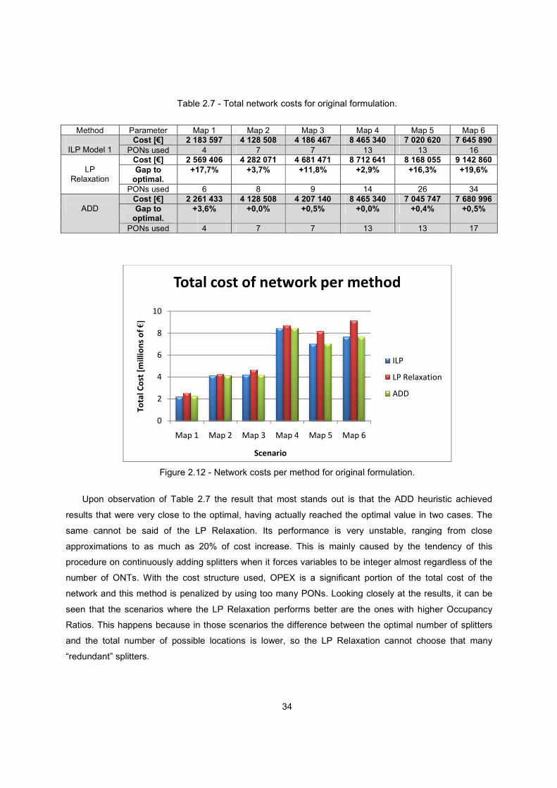
Table

Method Parameter Map 1

ILP Model 1 Cost [€] 2 183 597

PONs used

LP Relaxation

Cost [€] 2 569 406

Gap to optimal.

+17,7%

PONs used

ADD Cost [€] 2 261 433

Gap to optimal.

+3,6%

PONs used

Figure 2.12

Upon observation of Table

results that were very close to the optimal, having actually reached the optimal value in two cases. The

same cannot be said of the LP Relaxation. Its performance is very unstable, ranging from close

approximations to as much as 20% of cost increase. This is mainly caused

procedure on continuously adding splitters when it forces variables to be integer almost regardless of the

number of ONTs. With the cost structure used, OPEX is a significant portion of the total cost of the

network and this method is penalized by using too many PONs. Looking closely at the results, it can be

seen that the scenarios where the LP Relaxation

Ratios. This happens because in those scenarios the difference between the op

and the total number of possible locations is l

“redundant” splitters.

0

2

4

6

8

10

Map 1

To

tal

Co

st [

mil

lio

ns

of €]

Total cost of network per method

34

Table 2.7 - Total network costs for original formulation.

Map 1 Map 2 Map 3 Map 4 2 183 597 4 128 508 4 186 467 8 465 340

4 7 7 13 2 569 406 4 282 071 4 681 471 8 712 641

17,7% +3,7% +11,8% +2,9%

6 8 9 14 2 261 433 4 128 508 4 207 140 8 465 340

3,6% +0,0% +0,5% +0,0%

4 7 7 13

12 - Network costs per method for original formulation.

Table 2.7 the result that most stands out is that the ADD heuristic achieved

e very close to the optimal, having actually reached the optimal value in two cases. The

same cannot be said of the LP Relaxation. Its performance is very unstable, ranging from close

approximations to as much as 20% of cost increase. This is mainly caused by the tendency of this

procedure on continuously adding splitters when it forces variables to be integer almost regardless of the

number of ONTs. With the cost structure used, OPEX is a significant portion of the total cost of the

is penalized by using too many PONs. Looking closely at the results, it can be

seen that the scenarios where the LP Relaxation performs better are the ones with higher Occupancy

Ratios. This happens because in those scenarios the difference between the optimal number of splitters

and the total number of possible locations is lower, so the LP Relaxation cannot

Map 1 Map 2 Map 3 Map 4 Map 5 Map 6

Scenario

Total cost of network per method

ILP

LP Relaxation

ADD

Total network costs for original formulation.

Map 5 Map 6 7 020 620 7 645 890

13 16 8 168 055 9 142 860

+16,3% +19,6%

26 34 7 045 747 7 680 996

+0,4% +0,5%

13 17

Network costs per method for original formulation.

the result that most stands out is that the ADD heuristic achieved

e very close to the optimal, having actually reached the optimal value in two cases. The

same cannot be said of the LP Relaxation. Its performance is very unstable, ranging from close

by the tendency of this

procedure on continuously adding splitters when it forces variables to be integer almost regardless of the

number of ONTs. With the cost structure used, OPEX is a significant portion of the total cost of the

is penalized by using too many PONs. Looking closely at the results, it can be

better are the ones with higher Occupancy

timal number of splitters

ower, so the LP Relaxation cannot choose that many

Total cost of network per method

ILP

LP Relaxation

ADD

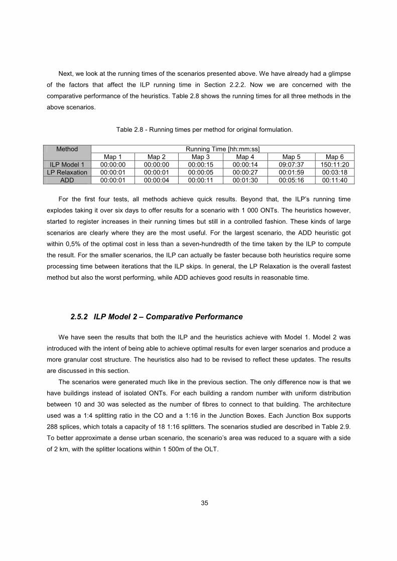
35

Next, we look at the running times of the scenarios presented above. We have already had a glimpse

of the factors that affect the ILP running time in Section 2.2.2. Now we are concerned with the

comparative performance of the heuristics. Table 2.8 shows the running times for all three methods in the

above scenarios.

Table 2.8 - Running times per method for original formulation.

Method Running Time [hh:mm:ss] Map 1 Map 2 Map 3 Map 4 Map 5 Map 6

ILP Model 1 00:00:00 00:00:00 00:00:15 00:00:14 09:07:37 150:11:20 LP Relaxation 00:00:01 00:00:01 00:00:05 00:00:27 00:01:59 00:03:18

ADD 00:00:01 00:00:04 00:00:11 00:01:30 00:05:16 00:11:40

For the first four tests, all methods achieve quick results. Beyond that, the ILP’s running time

explodes taking it over six days to offer results for a scenario with 1 000 ONTs. The heuristics however,

started to register increases in their running times but still in a controlled fashion. These kinds of large

scenarios are clearly where they are the most useful. For the largest scenario, the ADD heuristic got

within 0,5% of the optimal cost in less than a seven-hundredth of the time taken by the ILP to compute

the result. For the smaller scenarios, the ILP can actually be faster because both heuristics require some

processing time between iterations that the ILP skips. In general, the LP Relaxation is the overall fastest

method but also the worst performing, while ADD achieves good results in reasonable time.

2.5.2 ILP Model 2 – Comparative Performance

We have seen the results that both the ILP and the heuristics achieve with Model 1. Model 2 was

introduced with the intent of being able to achieve optimal results for even larger scenarios and produce a

more granular cost structure. The heuristics also had to be revised to reflect these updates. The results

are discussed in this section.

The scenarios were generated much like in the previous section. The only difference now is that we

have buildings instead of isolated ONTs. For each building a random number with uniform distribution

between 10 and 30 was selected as the number of fibres to connect to that building. The architecture

used was a 1:4 splitting ratio in the CO and a 1:16 in the Junction Boxes. Each Junction Box supports

288 splices, which totals a capacity of 18 1:16 splitters. The scenarios studied are described in Table 2.9.

To better approximate a dense urban scenario, the scenario’s area was reduced to a square with a side

of 2 km, with the splitter locations within 1 500m of the OLT.

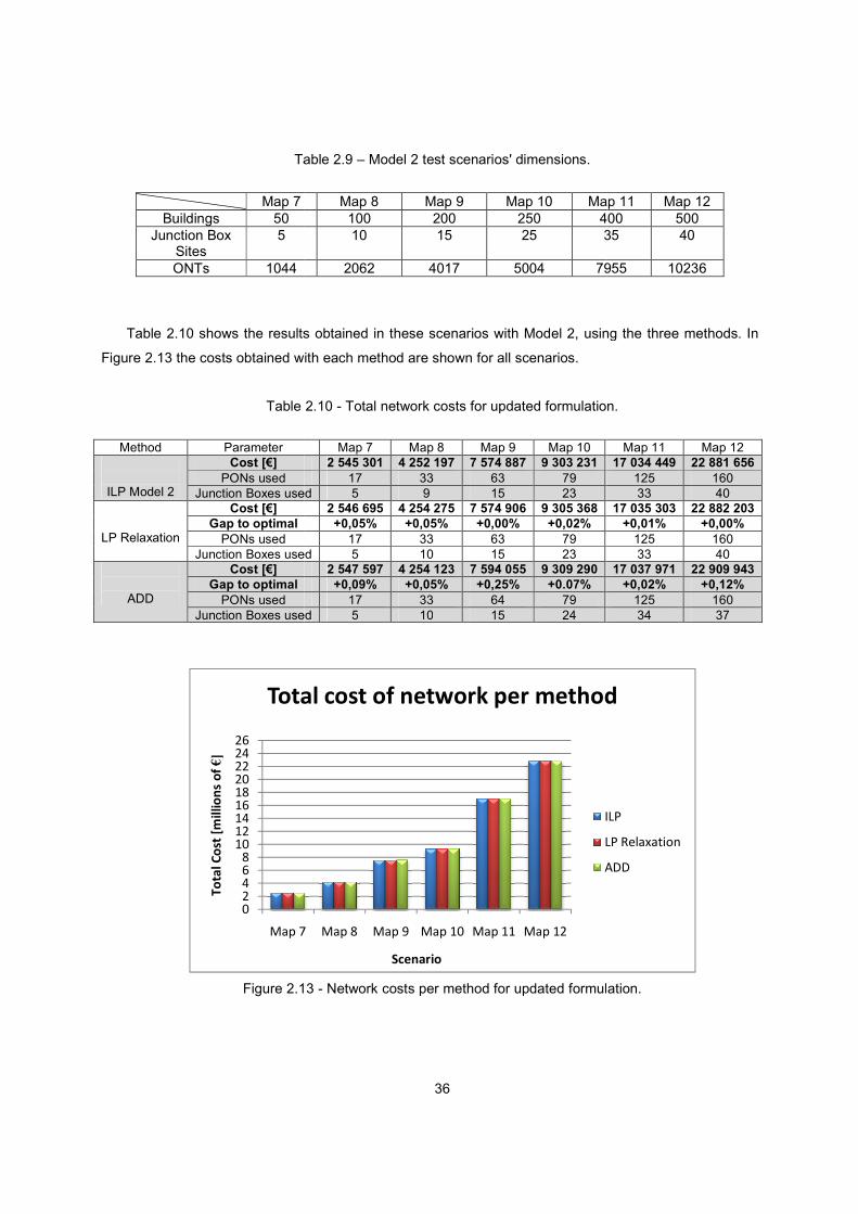
Table

Map 7 Buildings 50

Junction Box Sites

5

ONTs 1044

Table 2.10 shows the results obtained in these scenarios with Model 2, using the three methods. In

Figure 2.13 the costs obtained with each method are shown for all scenarios.

Table

Method Parameter

ILP Model 2

Cost [€]

PONs used Junction Boxes used

LP Relaxation

Cost [€]

Gap to optimal

PONs used Junction Boxes used

ADD

Cost [€]

Gap to optimal

PONs used Junction Boxes used

Figure 2.13

02468

101214161820222426

Map 7

To

tal

Co

st [

mil

lio

ns

of €]

Total cost of network per method

36

Table 2.9 – Model 2 test scenarios' dimensions.

Map 8 Map 9 Map 10 Map 11100 200 250 40010 15 25 35

2062 4017 5004 7955

shows the results obtained in these scenarios with Model 2, using the three methods. In

he costs obtained with each method are shown for all scenarios.

Table 2.10 - Total network costs for updated formulation.

Map 7 Map 8 Map 9 Map 10 2 545 301 4 252 197 7 574 887 9 303 231

17 33 63 79 Junction Boxes used 5 9 15 23

2 546 695 4 254 275 7 574 906 9 305 368

+0,05% +0,05% +0,00% +0,02%

17 33 63 79 Junction Boxes used 5 10 15 23

2 547 597 4 254 123 7 594 055 9 309 290

+0,09% +0,05% +0,25% +0.07%

17 33 64 79 Junction Boxes used 5 10 15 24

13 - Network costs per method for updated formulation.

Map 7 Map 8 Map 9 Map 10 Map 11 Map 12

Scenario

Total cost of network per method

ILP

LP Relaxation

ADD

Map 11 Map 12 400 500 35 40

7955 10236

shows the results obtained in these scenarios with Model 2, using the three methods. In

Total network costs for updated formulation.

Map 11 Map 12 17 034 449 22 881 656

125 160 33 40

17 035 303 22 882 203

+0,01% +0,00%

125 160 33 40

17 037 971 22 909 943

+0,02% +0,12%

125 160 34 37

Network costs per method for updated formulation.

Total cost of network per method

ILP

LP Relaxation

ADD

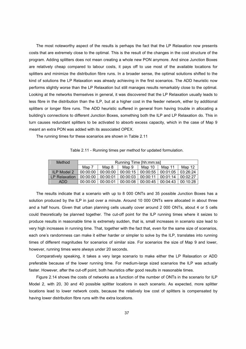
37

The most noteworthy aspect of the results is perhaps the fact that the LP Relaxation now presents

costs that are extremely close to the optimal. This is the result of the changes in the cost structure of the

program. Adding splitters does not mean creating a whole new PON anymore. And since Junction Boxes

are relatively cheap compared to labour costs, it pays off to use most of the available locations for

splitters and minimize the distribution fibre runs. In a broader sense, the optimal solutions shifted to the

kind of solutions the LP Relaxation was already achieving in the first scenarios. The ADD heuristic now

performs slightly worse than the LP Relaxation but still manages results remarkably close to the optimal.

Looking at the networks themselves in general, it was discovered that the LP Relaxation usually leads to

less fibre in the distribution than the ILP, but at a higher cost in the feeder network, either by additional

splitters or longer fibre runs. The ADD heuristic suffered in general from having trouble in allocating a

building’s connections to different Junction Boxes, something both the ILP and LP Relaxation do. This in

turn causes redundant splitters to be activated to absorb excess capacity, which in the case of Map 9

meant an extra PON was added with its associated OPEX.

The running times for these scenarios are shown in Table 2.11

Table 2.11 - Running times per method for updated formulation.

Method Running Time [hh:mm:ss] Map 7 Map 8 Map 9 Map 10 Map 11 Map 12

ILP Model 2 00:00:00 00:00:00 00:00:15 00:00:55 00:01:05 03:26:24 LP Relaxation 00:00:00 00:00:01 00:00:03 00:00:11 00:01:14 00:02:27

ADD 00:00:00 00:00:01 00:00:08 00:00:45 00:04:43 00:10:28

The results indicate that a scenario with up to 8 000 ONTs and 35 possible Junction Boxes has a

solution produced by the ILP in just over a minute. Around 10 000 ONTs were allocated in about three

and a half hours. Given that urban planning cells usually cover around 2 000 ONTs, about 4 or 5 cells

could theoretically be planned together. The cut-off point for the ILP running times where it seizes to

produce results in reasonable time is extremely sudden, that is, small increases in scenario size lead to

very high increases in running time. That, together with the fact that, even for the same size of scenarios,

each one’s randomness can make it either harder or simpler to solve by the ILP, translates into running

times of different magnitudes for scenarios of similar size. For scenarios the size of Map 9 and lower,

however, running times were always under 20 seconds.

Comparatively speaking, it takes a very large scenario to make either the LP Relaxation or ADD

preferable because of the lower running time. For medium-large sized scenarios the ILP was actually

faster. However, after the cut-off point, both heuristics offer good results in reasonable times.

Figure 2.14 shows the costs of networks as a function of the number of ONTs in the scenario for ILP

Model 2, with 20, 30 and 40 possible splitter locations in each scenario. As expected, more splitter

locations lead to lower network costs, because the relatively low cost of splitters is compensated by

having lower distribution fibre runs with the extra locations.

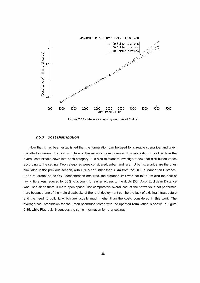
38

Figure 2.14 - Network costs by number of ONTs.

2.5.3 Cost Distribution

Now that it has been established that the formulation can be used for sizeable scenarios, and given

the effort in making the cost structure of the network more granular, it is interesting to look at how the

overall cost breaks down into each category. It is also relevant to investigate how that distribution varies

according to the setting. Two categories were considered: urban and rural. Urban scenarios are the ones

simulated in the previous section, with ONTs no further than 4 km from the OLT in Manhattan Distance.

For rural areas, as no ONT concentration occurred, the distance limit was set to 14 km and the cost of

laying fibre was reduced by 30% to account for easier access to the ducts [30]. Also, Euclidean Distance

was used since there is more open space. The comparative overall cost of the networks is not performed

here because one of the main drawbacks of the rural deployment can be the lack of existing infrastructure

and the need to build it, which are usually much higher than the costs considered in this work. The

average cost breakdown for the urban scenarios tested with the updated formulation is shown in Figure

2.15, while Figure 2.16 conveys the same information for rural settings.

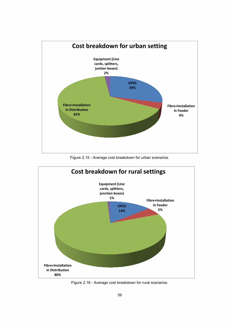
Figure 2

Figure

Fibre+Installation

in Distribution

65%

Cost breakdown for urban setting

Fibre+Installation

in Distribution

80%

Cost breakdown for rural settings

39

2.15 - Average cost breakdown for urban scenarios.

Figure 2.16 - Average cost breakdown for rural scenarios.

OPEX

29%

Fibre+Installation

in Distribution

Equipment (Line

cards, splitters,

juntion boxes)

2%

Cost breakdown for urban setting

OPEX

14%

Fibre+Installation

in Feeder

5%

Equipment (Line

cards, splitters,

junction boxes)

1%

Cost breakdown for rural settings

Average cost breakdown for urban scenarios.

Average cost breakdown for rural scenarios.

Fibre+Installation

in Feeder

4%

Cost breakdown for urban setting

Fibre+Installation

in Feeder

Cost breakdown for rural settings

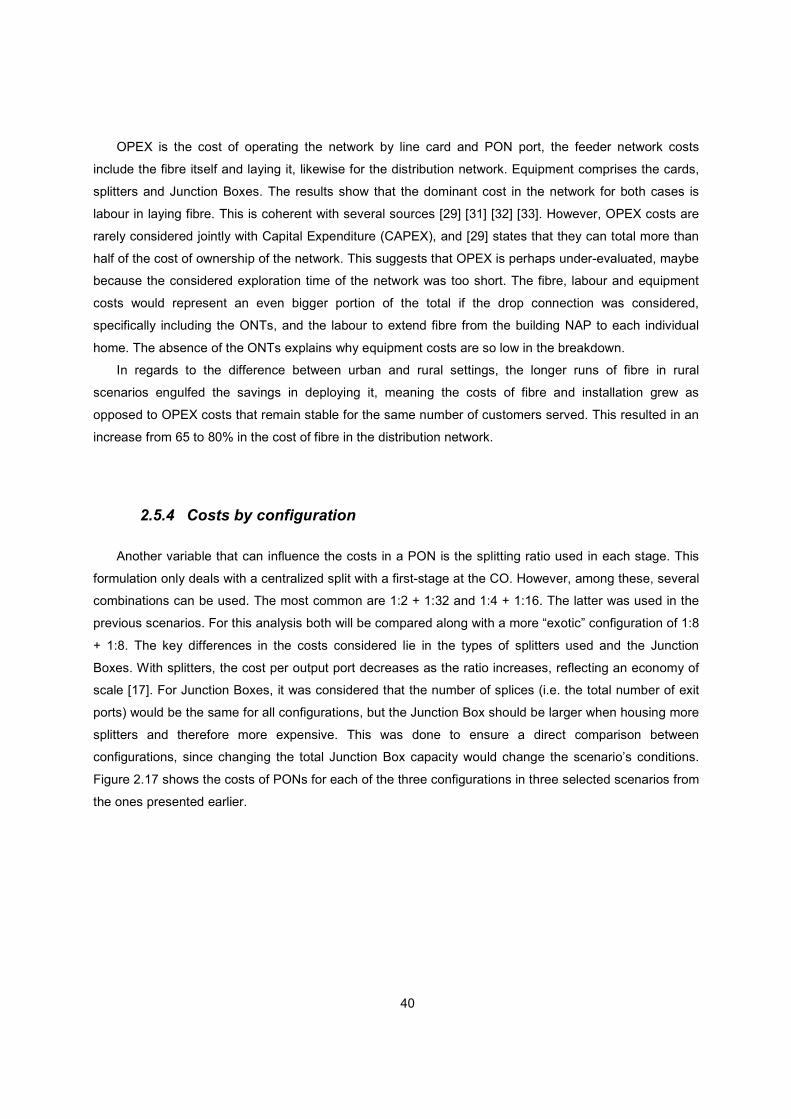
40

OPEX is the cost of operating the network by line card and PON port, the feeder network costs

include the fibre itself and laying it, likewise for the distribution network. Equipment comprises the cards,

splitters and Junction Boxes. The results show that the dominant cost in the network for both cases is

labour in laying fibre. This is coherent with several sources [29] [31] [32] [33]. However, OPEX costs are

rarely considered jointly with Capital Expenditure (CAPEX), and [29] states that they can total more than

half of the cost of ownership of the network. This suggests that OPEX is perhaps under-evaluated, maybe

because the considered exploration time of the network was too short. The fibre, labour and equipment

costs would represent an even bigger portion of the total if the drop connection was considered,

specifically including the ONTs, and the labour to extend fibre from the building NAP to each individual

home. The absence of the ONTs explains why equipment costs are so low in the breakdown.

In regards to the difference between urban and rural settings, the longer runs of fibre in rural

scenarios engulfed the savings in deploying it, meaning the costs of fibre and installation grew as

opposed to OPEX costs that remain stable for the same number of customers served. This resulted in an

increase from 65 to 80% in the cost of fibre in the distribution network.

2.5.4 Costs by configuration

Another variable that can influence the costs in a PON is the splitting ratio used in each stage. This

formulation only deals with a centralized split with a first-stage at the CO. However, among these, several

combinations can be used. The most common are 1:2 + 1:32 and 1:4 + 1:16. The latter was used in the

previous scenarios. For this analysis both will be compared along with a more “exotic” configuration of 1:8

+ 1:8. The key differences in the costs considered lie in the types of splitters used and the Junction

Boxes. With splitters, the cost per output port decreases as the ratio increases, reflecting an economy of

scale [17]. For Junction Boxes, it was considered that the number of splices (i.e. the total number of exit

ports) would be the same for all configurations, but the Junction Box should be larger when housing more

splitters and therefore more expensive. This was done to ensure a direct comparison between

configurations, since changing the total Junction Box capacity would change the scenario’s conditions.

Figure 2.17 shows the costs of PONs for each of the three configurations in three selected scenarios from

the ones presented earlier.

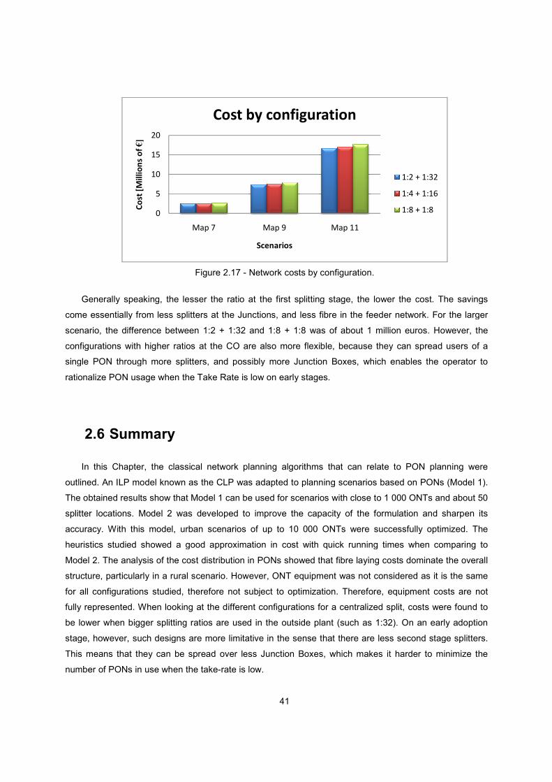
Figure

Generally speaking, the lesser the ratio at the first splitting stage, the lower the cost. The savings

come essentially from less splitters

scenario, the difference between 1:2 + 1:32 and 1:8 + 1:8 was of about 1 million euros. However, the

configurations with higher ratios at the CO are also more flexible, because they ca

single PON through more splitters, and possibly more Junction Boxes, which enables the operator to

rationalize PON usage when the Take Rate is low on early stages.

2.6 Summary

In this Chapter, the classical

outlined. An ILP model known as the CLP was adapted to planning scenarios based on

The obtained results show that Model 1 can be used for scenarios with close to 1 000 ONTs and about 50

splitter locations. Model 2 was developed

accuracy. With this model, urban scenarios of up to 10 000 ONTs were successfully optimized. The

heuristics studied showed a good approximation in

Model 2. The analysis of the cost distribution in PONs showed that fibre laying costs dominate the overall

structure, particularly in a rural scenario. However, ONT equipment was not considered as it is the same

for all configurations studied, therefore not subject to optimization. Therefore,

fully represented. When looking at the different configurations for a centralized split, costs were found to

be lower when bigger splitting ratios are used in the outside plan

stage, however, such designs are more limitative in the sense that there are less second stage splitters.

This means that they can be spread over less Junction Boxes, which makes it harder to minimize the

number of PONs in use when the take

0

5

10

15

20

Map 7

Co

st [

Mil

lio

ns

of €]

41

Figure 2.17 - Network costs by configuration.

Generally speaking, the lesser the ratio at the first splitting stage, the lower the cost. The savings

come essentially from less splitters at the Junctions, and less fibre in the feeder network. For the larger

scenario, the difference between 1:2 + 1:32 and 1:8 + 1:8 was of about 1 million euros. However, the

configurations with higher ratios at the CO are also more flexible, because they ca

single PON through more splitters, and possibly more Junction Boxes, which enables the operator to

rationalize PON usage when the Take Rate is low on early stages.

In this Chapter, the classical network planning algorithms that can relate to PON planning were

outlined. An ILP model known as the CLP was adapted to planning scenarios based on

Model 1 can be used for scenarios with close to 1 000 ONTs and about 50

was developed to improve the capacity of the formulation and sharpen its

accuracy. With this model, urban scenarios of up to 10 000 ONTs were successfully optimized. The

heuristics studied showed a good approximation in cost with quick running times

Model 2. The analysis of the cost distribution in PONs showed that fibre laying costs dominate the overall

particularly in a rural scenario. However, ONT equipment was not considered as it is the same

udied, therefore not subject to optimization. Therefore, equipment costs are not

When looking at the different configurations for a centralized split, costs were found to

be lower when bigger splitting ratios are used in the outside plant (such as 1:32).

stage, however, such designs are more limitative in the sense that there are less second stage splitters.

This means that they can be spread over less Junction Boxes, which makes it harder to minimize the

Ns in use when the take-rate is low.

Map 7 Map 9 Map 11

Scenarios

Cost by configuration

Generally speaking, the lesser the ratio at the first splitting stage, the lower the cost. The savings

at the Junctions, and less fibre in the feeder network. For the larger

scenario, the difference between 1:2 + 1:32 and 1:8 + 1:8 was of about 1 million euros. However, the

configurations with higher ratios at the CO are also more flexible, because they can spread users of a

single PON through more splitters, and possibly more Junction Boxes, which enables the operator to

can relate to PON planning were

outlined. An ILP model known as the CLP was adapted to planning scenarios based on PONs (Model 1).

Model 1 can be used for scenarios with close to 1 000 ONTs and about 50

to improve the capacity of the formulation and sharpen its

accuracy. With this model, urban scenarios of up to 10 000 ONTs were successfully optimized. The

cost with quick running times when comparing to

Model 2. The analysis of the cost distribution in PONs showed that fibre laying costs dominate the overall

particularly in a rural scenario. However, ONT equipment was not considered as it is the same

equipment costs are not

When looking at the different configurations for a centralized split, costs were found to

(such as 1:32). On an early adoption

stage, however, such designs are more limitative in the sense that there are less second stage splitters.

This means that they can be spread over less Junction Boxes, which makes it harder to minimize the

1:2 + 1:32

1:4 + 1:16

1:8 + 1:8

42

3. Multi-Stage PON Planning

In this Chapter, a new formulation is devised to allow the automated planning of a PON with more

than one explicit splitting stage. A review of the work in similar fields is made, and the ILP formulation

developed is presented. The work performed in the attempt to develop less complex heuristic procedures

for this problem is also shown. Finally, the results obtained with both approaches are demonstrated.

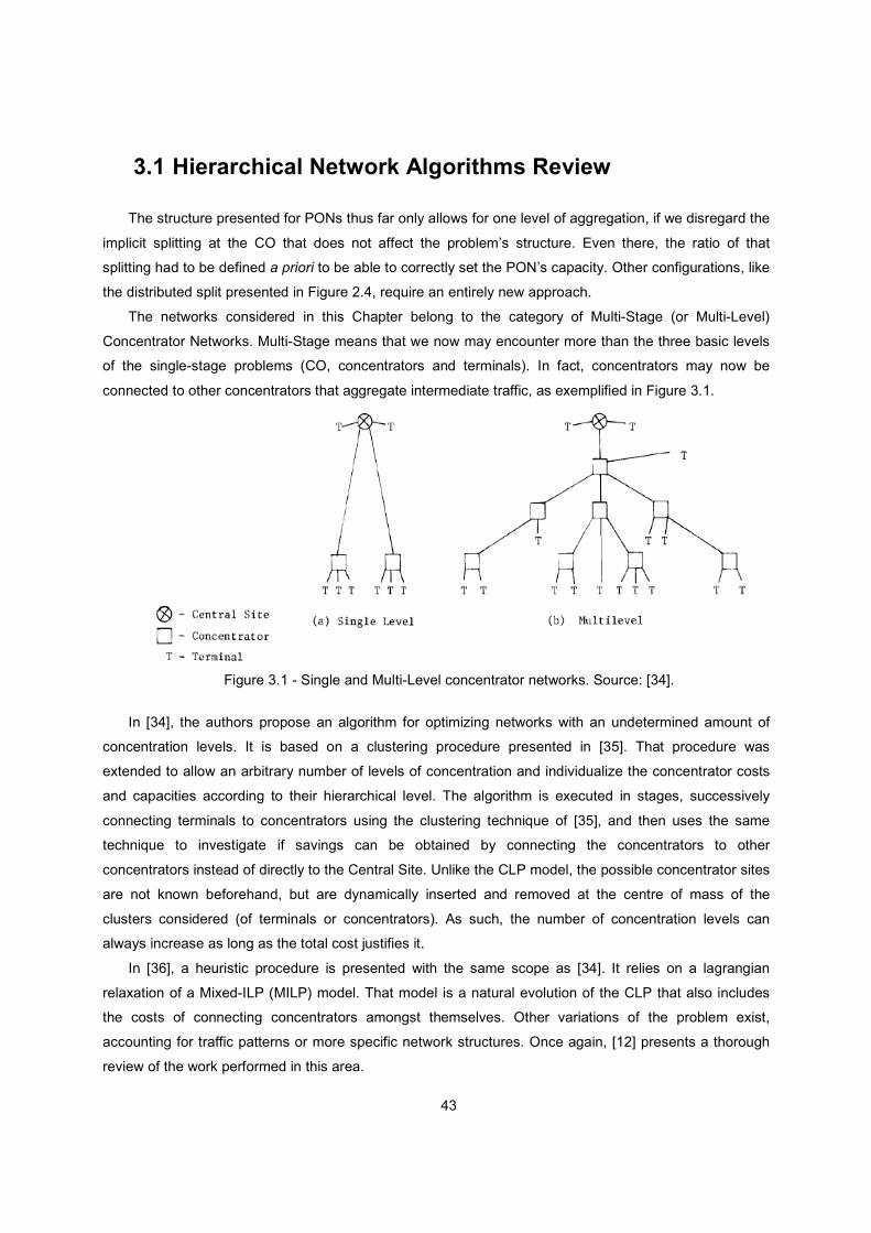
43

3.1 Hierarchical Network Algorithms Review

The structure presented for PONs thus far only allows for one level of aggregation, if we disregard the

implicit splitting at the CO that does not affect the problem’s structure. Even there, the ratio of that

splitting had to be defined a priori to be able to correctly set the PON’s capacity. Other configurations, like

the distributed split presented in Figure 2.4, require an entirely new approach.

The networks considered in this Chapter belong to the category of Multi-Stage (or Multi-Level)

Concentrator Networks. Multi-Stage means that we now may encounter more than the three basic levels

of the single-stage problems (CO, concentrators and terminals). In fact, concentrators may now be

connected to other concentrators that aggregate intermediate traffic, as exemplified in Figure 3.1.

Figure 3.1 - Single and Multi-Level concentrator networks. Source: [34].

In [34], the authors propose an algorithm for optimizing networks with an undetermined amount of

concentration levels. It is based on a clustering procedure presented in [35]. That procedure was

extended to allow an arbitrary number of levels of concentration and individualize the concentrator costs

and capacities according to their hierarchical level. The algorithm is executed in stages, successively

connecting terminals to concentrators using the clustering technique of [35], and then uses the same

technique to investigate if savings can be obtained by connecting the concentrators to other

concentrators instead of directly to the Central Site. Unlike the CLP model, the possible concentrator sites

are not known beforehand, but are dynamically inserted and removed at the centre of mass of the

clusters considered (of terminals or concentrators). As such, the number of concentration levels can

always increase as long as the total cost justifies it.

In [36], a heuristic procedure is presented with the same scope as [34]. It relies on a lagrangian

relaxation of a Mixed-ILP (MILP) model. That model is a natural evolution of the CLP that also includes

the costs of connecting concentrators amongst themselves. Other variations of the problem exist,

accounting for traffic patterns or more specific network structures. Once again, [12] presents a thorough

review of the work performed in this area.

44

When considering PONs, however, the algorithms mentioned have one essential problem. Their

framework considered the paradigm of computer or telephone networks, where concentrators are usually

switches that have a pre-determined capacity. In that framework, the capacity of a concentrator is just the

number of connections it supports from lower level network elements (terminals or other concentrators).

For simplicity, it can be thought of as the number of output ports in a concentrator. This enables [34] to

initialize the capacity of concentrators in a given level before the algorithm is started. For a PON, this is

not possible. The reason for this is that the nature of a concentrator in a PON is different. The capacity of

concentrators in different levels is not independent. This becomes obvious when we see that the shared

resource in a PON is essentially optical power. The OLT supplies a reference power level to a splitter that

shares it equally through its output ports to all network elements it supports. If one of those elements is

another splitter (in which case we have a multi-stage PON), the optical power it receives already depends

on the type of splitter used in the first-stage. If yet another splitting level exists, its power depends on the

ratios of the two splitters that precede it and so forth. Therefore, the number of ONTs (or splitters) a given

splitter can service cannot be known without looking at the complete PON layout. The thought process

described above is a top-bottom approach, setting the higher levels of concentrators before moving on to

lower levels. A heuristic procedure (like [34]) usually does the opposite, first connecting terminals to

concentrators at the lowest level and inserting additional concentrator levels if the cost savings justify it.

To exemplify this issue, we can look at Figure 3.2. If the maximum ratio is 1:64, splitter 5 has a

maximum ratio of 1:4 defined by the ratios of the splitters preceding it, while splitter 4 has a maximum

ratio of 1:8 for the same reasons.

Figure 3.2 - Multi-staged PON.

This occurs for any splitter in the network in both directions, that is, the capacity of a splitter depends

on the capacities of the splitters above and below it. The PON system constraints like the inability to pre-

determine splitter capacities make the problem more complex than the hierarchical network models

described above. To the best knowledge of the author, no optimal algorithm within the multi-level PON

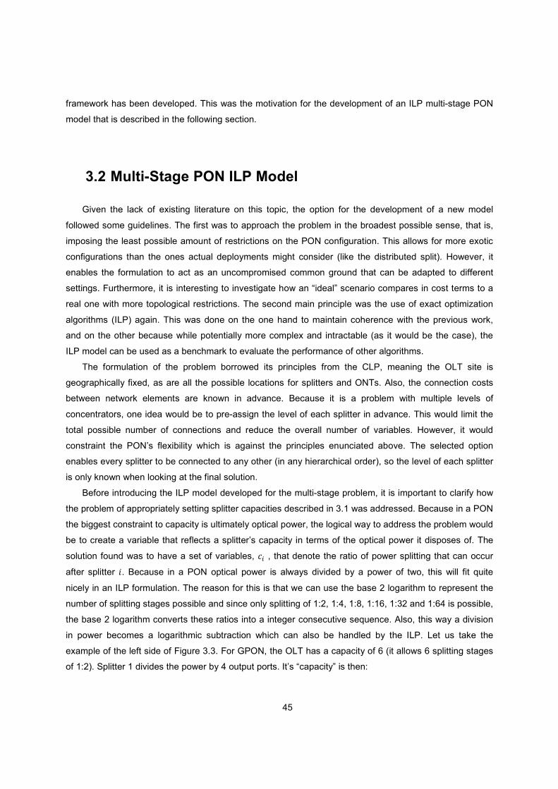
45

framework has been developed. This was the motivation for the development of an ILP multi-stage PON

model that is described in the following section.

3.2 Multi-Stage PON ILP Model

Given the lack of existing literature on this topic, the option for the development of a new model

followed some guidelines. The first was to approach the problem in the broadest possible sense, that is,

imposing the least possible amount of restrictions on the PON configuration. This allows for more exotic

configurations than the ones actual deployments might consider (like the distributed split). However, it

enables the formulation to act as an uncompromised common ground that can be adapted to different

settings. Furthermore, it is interesting to investigate how an “ideal” scenario compares in cost terms to a

real one with more topological restrictions. The second main principle was the use of exact optimization

algorithms (ILP) again. This was done on the one hand to maintain coherence with the previous work,

and on the other because while potentially more complex and intractable (as it would be the case), the

ILP model can be used as a benchmark to evaluate the performance of other algorithms.

The formulation of the problem borrowed its principles from the CLP, meaning the OLT site is

geographically fixed, as are all the possible locations for splitters and ONTs. Also, the connection costs

between network elements are known in advance. Because it is a problem with multiple levels of

concentrators, one idea would be to pre-assign the level of each splitter in advance. This would limit the

total possible number of connections and reduce the overall number of variables. However, it would

constraint the PON’s flexibility which is against the principles enunciated above. The selected option

enables every splitter to be connected to any other (in any hierarchical order), so the level of each splitter

is only known when looking at the final solution.

Before introducing the ILP model developed for the multi-stage problem, it is important to clarify how

the problem of appropriately setting splitter capacities described in 3.1 was addressed. Because in a PON

the biggest constraint to capacity is ultimately optical power, the logical way to address the problem would

be to create a variable that reflects a splitter’s capacity in terms of the optical power it disposes of. The

solution found was to have a set of variables, � , that denote the ratio of power splitting that can occur

after splitter �. Because in a PON optical power is always divided by a power of two, this will fit quite

nicely in an ILP formulation. The reason for this is that we can use the base 2 logarithm to represent the

number of splitting stages possible and since only splitting of 1:2, 1:4, 1:8, 1:16, 1:32 and 1:64 is possible,

the base 2 logarithm converts these ratios into a integer consecutive sequence. Also, this way a division

in power becomes a logarithmic subtraction which can also be handled by the ILP. Let us take the

example of the left side of Figure 3.3. For GPON, the OLT has a capacity of 6 (it allows 6 splitting stages

of 1:2). Splitter 1 divides the power by 4 output ports. It’s “capacity” is then:

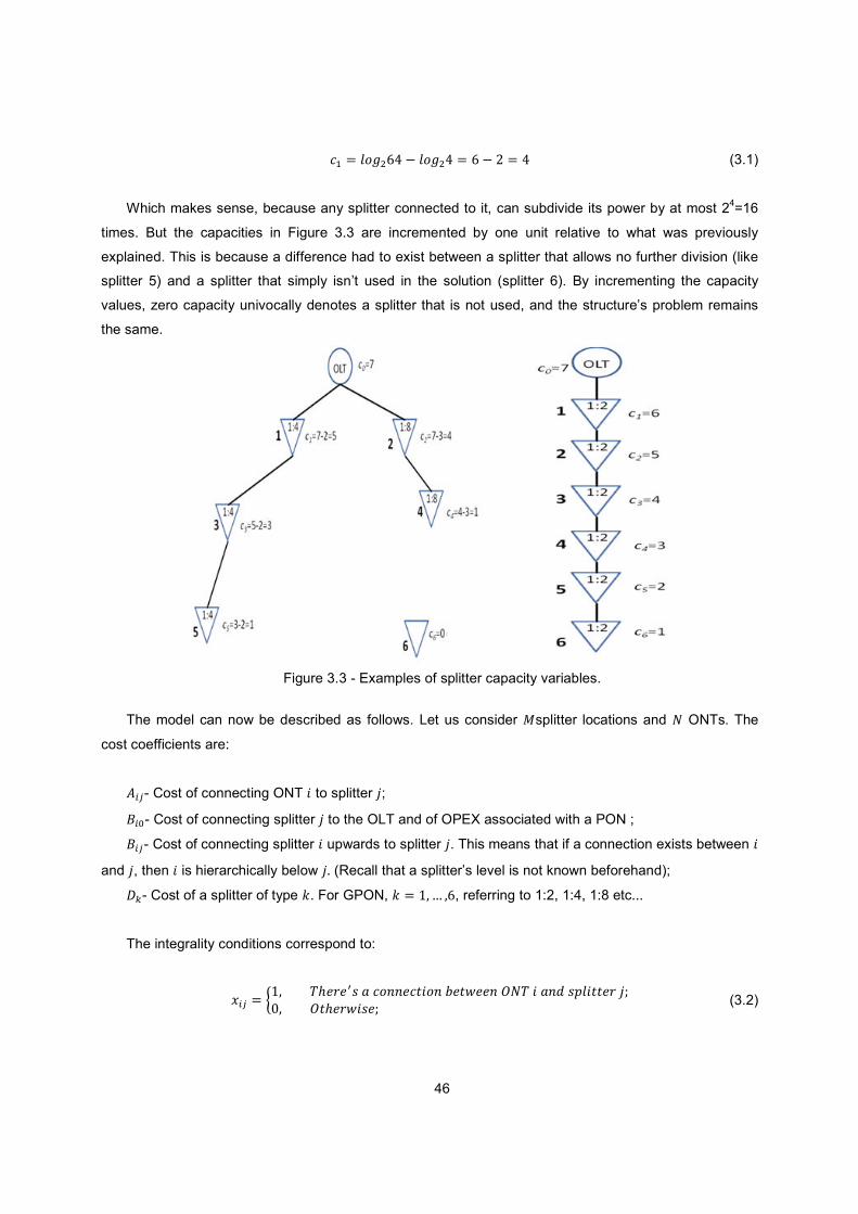
46

�� � '�bc\d V '�bcd � \ V W � d (3.1)

Which makes sense, because any splitter connected to it, can subdivide its power by at most 24=16

times. But the capacities in Figure 3.3 are incremented by one unit relative to what was previously

explained. This is because a difference had to exist between a splitter that allows no further division (like

splitter 5) and a splitter that simply isn’t used in the solution (splitter 6). By incrementing the capacity

values, zero capacity univocally denotes a splitter that is not used, and the structure’s problem remains

the same.

Figure 3.3 - Examples of splitter capacity variables.

The model can now be described as follows. Let us consider �splitter locations and � ONTs. The

cost coefficients are:

e- Cost of connecting ONT � to splitter �; f�- Cost of connecting splitter � to the OLT and of OPEX associated with a PON ;

f- Cost of connecting splitter � upwards to splitter �. This means that if a connection exists between � and �, then � is hierarchically below �- (Recall that a splitter’s level is not known beforehand);

g[- Cost of a splitter of type �. For GPON, � � ��� �\, referring to 1:2, 1:4, 1:8 etc...

The integrality conditions correspond to:

� � 2�� h/!%!i0����� !�"�� �#!"$!! �j�h���� �0F'�""!%��k.� j"/!%$�0!k 1 (3.2)

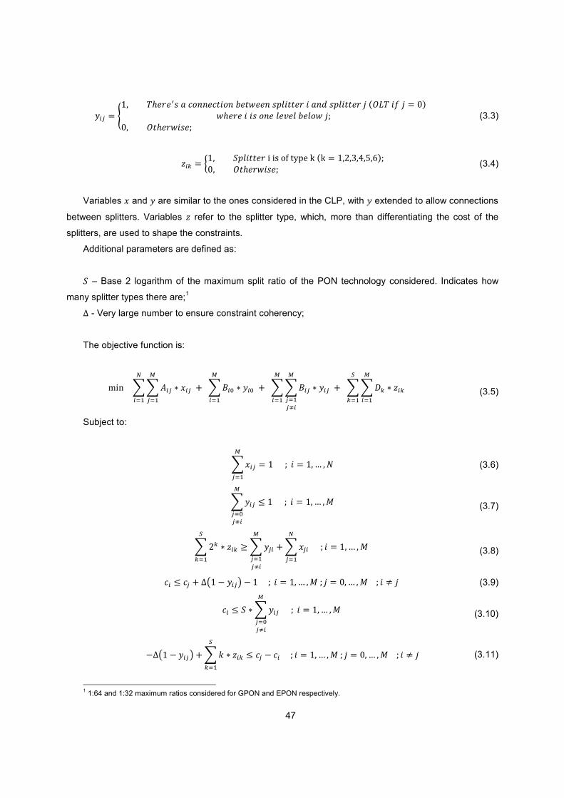
47

� � ��� h/!%!i0����� !�"�� �#!"$!! �0F'�""!%���� �0F'�""!%���Djlh��m�� � .B$/!%!����0�� !�'!n!'�#!'�$��k.� j"/!%$�0!k1 (3.3)

I[ � 2�� oF'�""!%����+�5p�,qr)�s�Ds � ��W�t�d�]�\Bk.� j"/!%$�0!k 1 (3.4)

Variables � and � are similar to the ones considered in the CLP, with � extended to allow connections

between splitters. Variables I refer to the splitter type, which, more than differentiating the cost of the

splitters, are used to shape the constraints.

Additional parameters are defined as:

o – Base 2 logarithm of the maximum split ratio of the PON technology considered. Indicates how

many splitter types there are;1

u - Very large number to ensure constraint coherency;

The objective function is:

��� �����e ? ��

���� ���f� ? ��

�

���� ����f ? �

�

��v�� ����g[ ? I[

�

��

w

[��

�

��

�

������ (3.5)

Subject to:

�� � ��

������� k �� � �� � � � (3.6)

�� � ��

��v����� k �� � �� � �� (3.7)

�W[ ? I[w

[��S��

�

��v���

�

������� k � � ��� ��� (3.8)

� � � � u=� V �> V ������k �� � �� � ���k � � .�� ������k � x �� (3.9)

� � o ?���

��v����� k �� � ��� ��� (3.10)

Vu=� V �> ��� ? I[w

[��� � V � �����k � � �� � ���k � � .� � ������k � x � (3.11)

1 1:64 and 1:32 maximum ratios considered for GPON and EPON respectively.

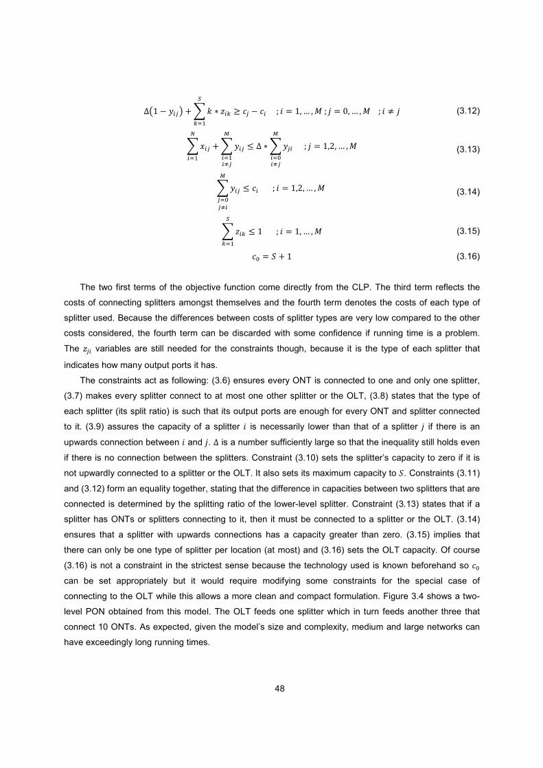
48

u=� V �> ��� ? I[w

[��S � V � �����k � � ��� ���k � � .�� ������k � x � (3.12)

���

�����

�

��v� u ?��

�

��v����� k � � ��W� � �� (3.13)

���

��v� � �������k � � ��W� � ��� (3.14)

�I[w

[��� ��������k � � �� � �� (3.15)

�� � o � � (3.16)

The two first terms of the objective function come directly from the CLP. The third term reflects the

costs of connecting splitters amongst themselves and the fourth term denotes the costs of each type of

splitter used. Because the differences between costs of splitter types are very low compared to the other

costs considered, the fourth term can be discarded with some confidence if running time is a problem.

The I variables are still needed for the constraints though, because it is the type of each splitter that

indicates how many output ports it has.

The constraints act as following: (3.6) ensures every ONT is connected to one and only one splitter,

(3.7) makes every splitter connect to at most one other splitter or the OLT, (3.8) states that the type of

each splitter (its split ratio) is such that its output ports are enough for every ONT and splitter connected

to it. (3.9) assures the capacity of a splitter � is necessarily lower than that of a splitter � if there is an

upwards connection between � and �. u is a number sufficiently large so that the inequality still holds even

if there is no connection between the splitters. Constraint (3.10) sets the splitter’s capacity to zero if it is

not upwardly connected to a splitter or the OLT. It also sets its maximum capacity to o. Constraints (3.11)

and (3.12) form an equality together, stating that the difference in capacities between two splitters that are

connected is determined by the splitting ratio of the lower-level splitter. Constraint (3.13) states that if a

splitter has ONTs or splitters connecting to it, then it must be connected to a splitter or the OLT. (3.14)

ensures that a splitter with upwards connections has a capacity greater than zero. (3.15) implies that

there can only be one type of splitter per location (at most) and (3.16) sets the OLT capacity. Of course

(3.16) is not a constraint in the strictest sense because the technology used is known beforehand so ��

can be set appropriately but it would require modifying some constraints for the special case of

connecting to the OLT while this allows a more clean and compact formulation. Figure 3.4 shows a two-

level PON obtained from this model. The OLT feeds one splitter which in turn feeds another three that

connect 10 ONTs. As expected, given the model’s size and complexity, medium and large networks can

have exceedingly long running times.

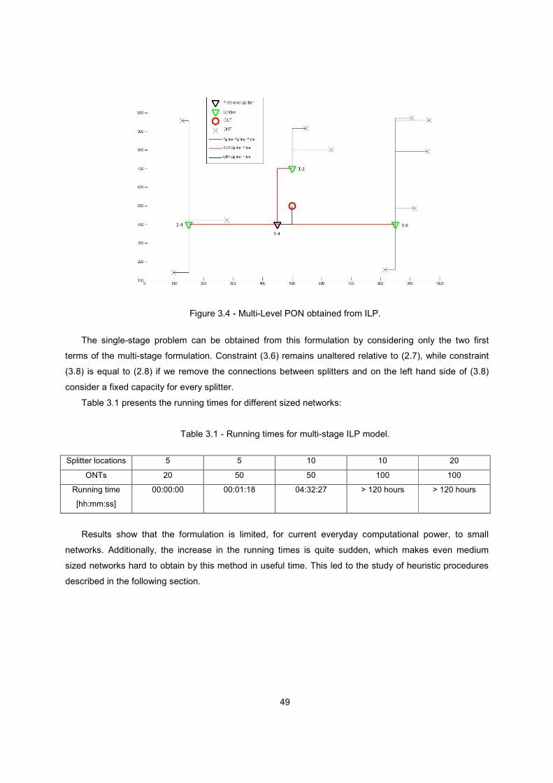
49

Figure 3.4 - Multi-Level PON obtained from ILP.

The single-stage problem can be obtained from this formulation by considering only the two first

terms of the multi-stage formulation. Constraint (3.6) remains unaltered relative to (2.7), while constraint

(3.8) is equal to (2.8) if we remove the connections between splitters and on the left hand side of (3.8)

consider a fixed capacity for every splitter.

Table 3.1 presents the running times for different sized networks:

Table 3.1 - Running times for multi-stage ILP model.

Splitter locations 5 5 10 10 20

ONTs 20 50 50 100 100

Running time

[hh:mm:ss]

00:00:00 00:01:18 04:32:27 > 120 hours > 120 hours

Results show that the formulation is limited, for current everyday computational power, to small

networks. Additionally, the increase in the running times is quite sudden, which makes even medium

sized networks hard to obtain by this method in useful time. This led to the study of heuristic procedures

described in the following section.

50

3.3 Heuristics

Because the range of scenarios that the ILP can solve in useful time is so limited, it was natural that

some heuristic procedures were developed to decrease complexity. They are presented in this section.

The LP Relaxation is tried again for this purpose, together with a newly developed algorithm for two-stage

PONs. It is also discussed how the heuristics can be combined with the ILP itself.

3.3.1 LP and MILP Relaxation

Since it presented very acceptable results in the revised single-stage problem and is relatively easy to

implement when the ILP model has been developed, the LP Relaxation was the first heuristic tested.

Unfortunately, the results were very disappointing. In the single-stage formulation there is a simple

structure and defined hierarchy, which favours the setting of variables to integers. The multi-stage model

is much more complex because of the number of possible solutions it allows, but also because it features

a reasonably complicated set of restrictions to implement PON specifications. This did not go well with the

LP Relaxation, because forcing variables to integer often led to making the problem unfeasible. The most

common occurrence was on one iteration the program connecting one splitter to another, and in the next

connecting the latter to the former, forming a cycle. When a verification phase was added to prevent this,

the Relaxation fixed the splitters’ capacities to values that again made the problem unfeasible.

The next strategy was turning the problem into a MILP, by only allowing certain variables to be real

while others remain integer. The obvious consequence of this procedure is that the running time in each

iteration would be much higher, but hopefully still lower than the full integer program. All combinations of

the sets of variables were relaxed, but the only method that actually produced feasible results was

relaxing the � and �� variables. One might notice that this is essentially relaxing the single-stage part of

the program (the ONT-splitter and OLT-splitter connections). What happened was that the MILP model

itself was too heavy in each iteration and executing it several times resulted in running times higher than

that of the ILP itself.

Faced with these results, another heuristic had to be created for the problem, and it will be discussed

in the following section.

3.3.2 Two-Stage Multi-Level Heuristic

Failing to get results with the LP Relaxation, a heuristic was developed from scratch for this problem.

For simplicity, this heuristic was limited to two stages of splitters. A third stage can be implicit at the CO

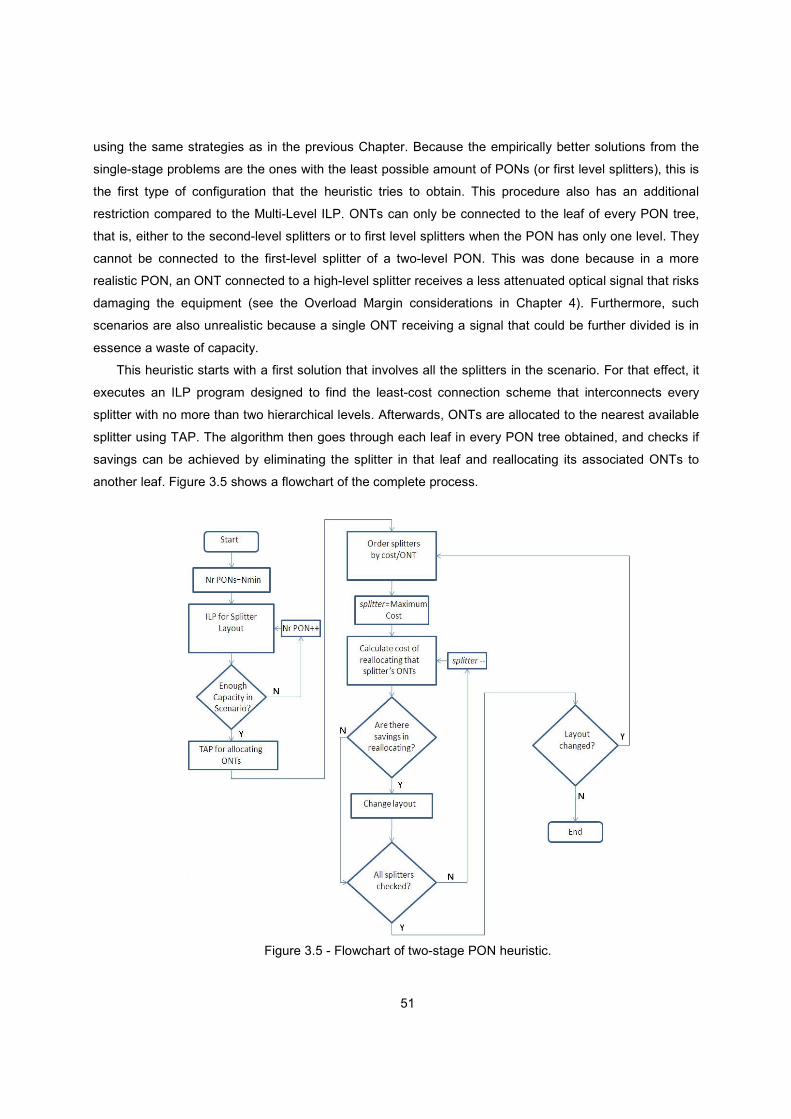
51

using the same strategies as in the previous Chapter. Because the empirically better solutions from the

single-stage problems are the ones with the least possible amount of PONs (or first level splitters), this is

the first type of configuration that the heuristic tries to obtain. This procedure also has an additional

restriction compared to the Multi-Level ILP. ONTs can only be connected to the leaf of every PON tree,

that is, either to the second-level splitters or to first level splitters when the PON has only one level. They

cannot be connected to the first-level splitter of a two-level PON. This was done because in a more

realistic PON, an ONT connected to a high-level splitter receives a less attenuated optical signal that risks

damaging the equipment (see the Overload Margin considerations in Chapter 4). Furthermore, such

scenarios are also unrealistic because a single ONT receiving a signal that could be further divided is in

essence a waste of capacity.

This heuristic starts with a first solution that involves all the splitters in the scenario. For that effect, it

executes an ILP program designed to find the least-cost connection scheme that interconnects every

splitter with no more than two hierarchical levels. Afterwards, ONTs are allocated to the nearest available

splitter using TAP. The algorithm then goes through each leaf in every PON tree obtained, and checks if

savings can be achieved by eliminating the splitter in that leaf and reallocating its associated ONTs to

another leaf. Figure 3.5 shows a flowchart of the complete process.

Figure 3.5 - Flowchart of two-stage PON heuristic.

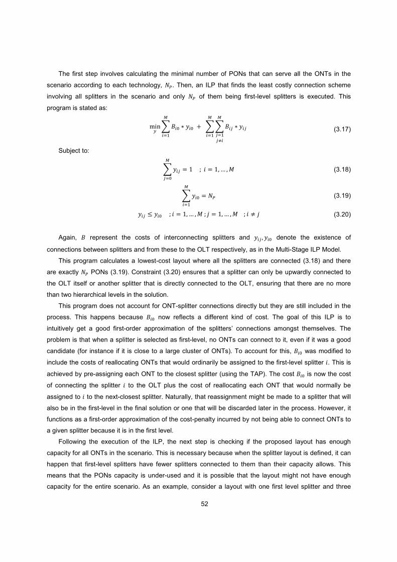
52

The first step involves calculating the minimal number of PONs that can serve all the ONTs in the

scenario according to each technology, �H. Then, an ILP that finds the least costly connection scheme

involving all splitters in the scenario and only �H of them being first-level splitters is executed. This

program is stated as:

���P �f� ? ���

���� ����f ? �

�

��v�

�

�� (3.17)

Subject to:

�� � ��

������ k �� � ��� �� (3.18)

��� � �H�

�� (3.19)

� � �������k � � ��� ���k � � �� � ������k � x � (3.20)

Again, f represent the costs of interconnecting splitters and � � �� denote the existence of

connections between splitters and from these to the OLT respectively, as in the Multi-Stage ILP Model.

This program calculates a lowest-cost layout where all the splitters are connected (3.18) and there

are exactly �H PONs (3.19). Constraint (3.20) ensures that a splitter can only be upwardly connected to

the OLT itself or another splitter that is directly connected to the OLT, ensuring that there are no more

than two hierarchical levels in the solution.

This program does not account for ONT-splitter connections directly but they are still included in the

process. This happens because f� now reflects a different kind of cost. The goal of this ILP is to

intuitively get a good first-order approximation of the splitters’ connections amongst themselves. The

problem is that when a splitter is selected as first-level, no ONTs can connect to it, even if it was a good

candidate (for instance if it is close to a large cluster of ONTs). To account for this, f� was modified to

include the costs of reallocating ONTs that would ordinarily be assigned to the first-level splitter �. This is

achieved by pre-assigning each ONT to the closest splitter (using the TAP). The cost f� is now the cost

of connecting the splitter � to the OLT plus the cost of reallocating each ONT that would normally be

assigned to � to the next-closest splitter. Naturally, that reassignment might be made to a splitter that will

also be in the first-level in the final solution or one that will be discarded later in the process. However, it

functions as a first-order approximation of the cost-penalty incurred by not being able to connect ONTs to

a given splitter because it is in the first level.

Following the execution of the ILP, the next step is checking if the proposed layout has enough

capacity for all ONTs in the scenario. This is necessary because when the splitter layout is defined, it can

happen that first-level splitters have fewer splitters connected to them than their capacity allows. This

means that the PONs capacity is under-used and it is possible that the layout might not have enough

capacity for the entire scenario. As an example, consider a layout with one first level splitter and three

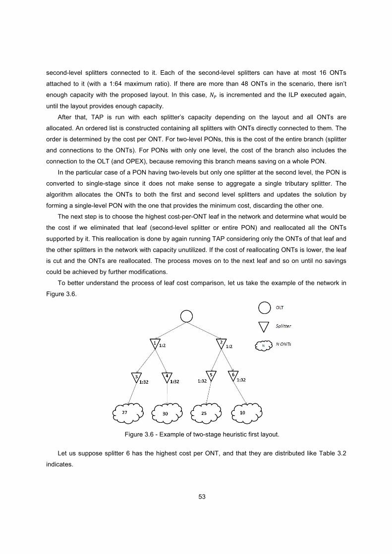
53

second-level splitters connected to it. Each of the second-level splitters can have at most 16 ONTs

attached to it (with a 1:64 maximum ratio). If there are more than 48 ONTs in the scenario, there isn’t

enough capacity with the proposed layout. In this case, �H is incremented and the ILP executed again,

until the layout provides enough capacity.

After that, TAP is run with each splitter’s capacity depending on the layout and all ONTs are

allocated. An ordered list is constructed containing all splitters with ONTs directly connected to them. The

order is determined by the cost per ONT. For two-level PONs, this is the cost of the entire branch (splitter

and connections to the ONTs). For PONs with only one level, the cost of the branch also includes the

connection to the OLT (and OPEX), because removing this branch means saving on a whole PON.

In the particular case of a PON having two-levels but only one splitter at the second level, the PON is

converted to single-stage since it does not make sense to aggregate a single tributary splitter. The

algorithm allocates the ONTs to both the first and second level splitters and updates the solution by

forming a single-level PON with the one that provides the minimum cost, discarding the other one.

The next step is to choose the highest cost-per-ONT leaf in the network and determine what would be

the cost if we eliminated that leaf (second-level splitter or entire PON) and reallocated all the ONTs

supported by it. This reallocation is done by again running TAP considering only the ONTs of that leaf and

the other splitters in the network with capacity unutilized. If the cost of reallocating ONTs is lower, the leaf

is cut and the ONTs are reallocated. The process moves on to the next leaf and so on until no savings

could be achieved by further modifications.

To better understand the process of leaf cost comparison, let us take the example of the network in

Figure 3.6.

Figure 3.6 - Example of two-stage heuristic first layout.

Let us suppose splitter 6 has the highest cost per ONT, and that they are distributed like Table 3.2

indicates.

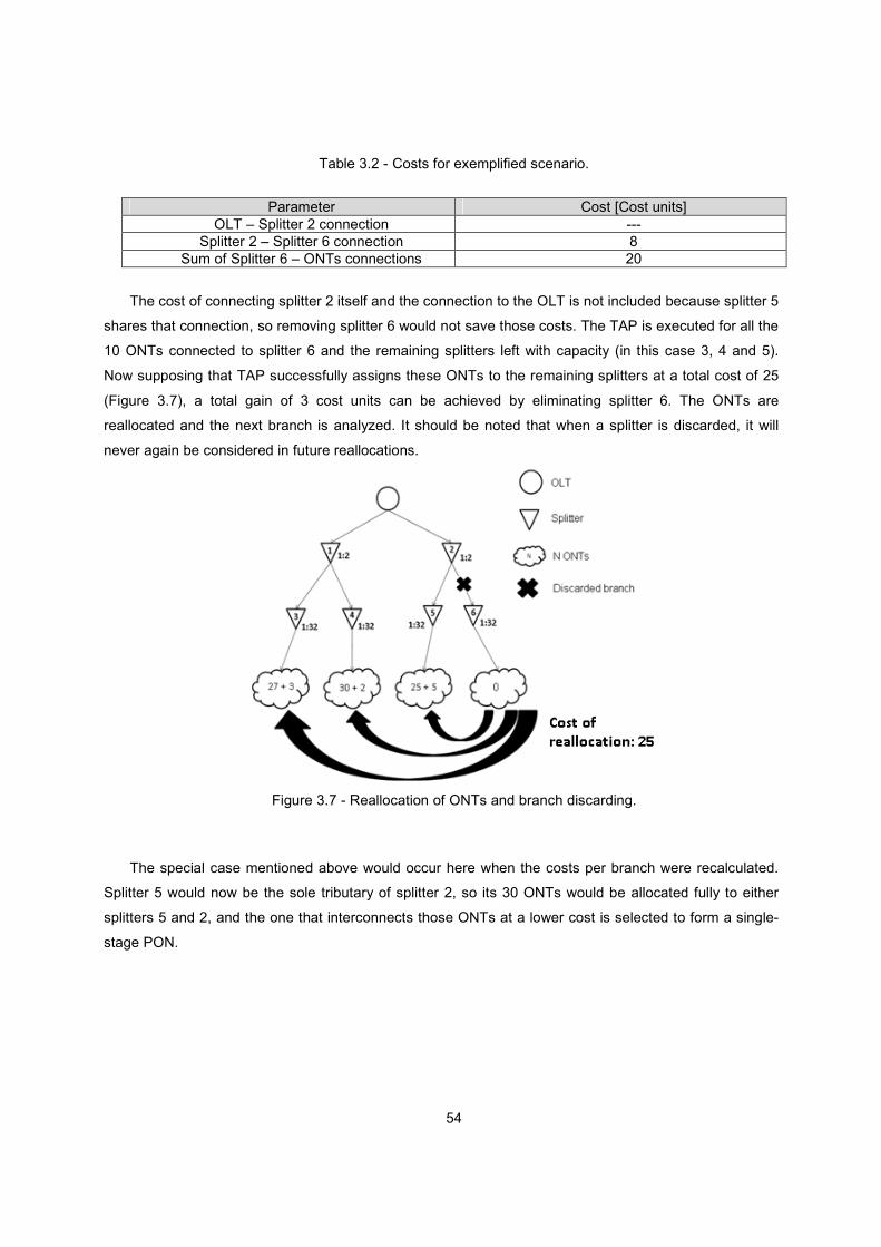
54

Table 3.2 - Costs for exemplified scenario.

Parameter Cost [Cost units] OLT – Splitter 2 connection ---

Splitter 2 – Splitter 6 connection 8 Sum of Splitter 6 – ONTs connections 20

The cost of connecting splitter 2 itself and the connection to the OLT is not included because splitter 5

shares that connection, so removing splitter 6 would not save those costs. The TAP is executed for all the

10 ONTs connected to splitter 6 and the remaining splitters left with capacity (in this case 3, 4 and 5).

Now supposing that TAP successfully assigns these ONTs to the remaining splitters at a total cost of 25

(Figure 3.7), a total gain of 3 cost units can be achieved by eliminating splitter 6. The ONTs are

reallocated and the next branch is analyzed. It should be noted that when a splitter is discarded, it will

never again be considered in future reallocations.

Figure 3.7 - Reallocation of ONTs and branch discarding.

The special case mentioned above would occur here when the costs per branch were recalculated.

Splitter 5 would now be the sole tributary of splitter 2, so its 30 ONTs would be allocated fully to either

splitters 5 and 2, and the one that interconnects those ONTs at a lower cost is selected to form a single-

stage PON.

55

3.3.3 Heuristic Bound

Because the previous heuristic seemed to provide apparently reasonable results for multi-stage

networks, it seemed appropriate to use that result to try to improve the ILP model. The underlying concept

for this strategy is based on the solving method the Branch & Bound algorithm uses to solve the ILP

problem. Branch & Bound starts by, for a given integer variable, fixing it in one of its possible values.

Then it proceeds to solve the corresponding LP problem which will be much faster than the LP. The

optimal cost obtained from solving the LP model is a lower bound of the ILP problem, since the solution

space of the LP problem encompasses that of the ILP [37]. We now know, that for a given fixed value for

some variable (or various), the cost will always be equal or greater than the one obtained with the LP.

Supposing a feasible solution for the ILP has already been found earlier by the algorithm, the whole

branch of solutions given by the variables already fixed can be discarded if that feasible solution is lower

than the lower bound given by the LP solution for that branch.

Because the heuristic operates on the same principles and costs that the ILP does, the solution

provided by the heuristic is necessarily a feasible solution of the ILP problem. That solution can then be

fed to the ILP as a lower bound at the start of the program, and any branches whose LP solution exceeds

the cost of the heuristic can be ignored by the algorithm, potentially saving time. The closer the cost is to

the optimal, the better the bound is and the more solutions can be discarded.

This approach proved correct in theory, since some scenarios were successfully simulated in less

time than without any initial bound. In the best case registered, a scenario dropped from a running time of

12 minutes to under 7 minutes. However, in general, the bounding procedure offered little practical

results, since significant savings in time were obtained for only a reduced number of scenarios, with no

discernible pattern for the type of networks where the bounding was most effective. In the majority of

cases, the difference was negligible. One might argue that this might be related with the bounds given by

the heuristic not being close enough to the optimum to allow discarding a lot of solutions. To assert this,

scenarios in which the optimum value was given by the ILP in reasonable time were again executed but

this time fed with a bound very close to the optimum. No significant improvements were achieved. It was

observed that when solving LP relaxations of the model, the costs obtained were much lower than those

of the heuristic. Because the model has such an intertwined set of restrictions, when relaxing the

variables, they tend to assume “strange” values which allow the solution to save on costs that the ILP

cannot avoid (such as OPEX when connecting to the OLT). This way, the bounds given by the LP solving

are usually much lower than the heuristic bound, and the solution branches still need to be checked

exhaustively.

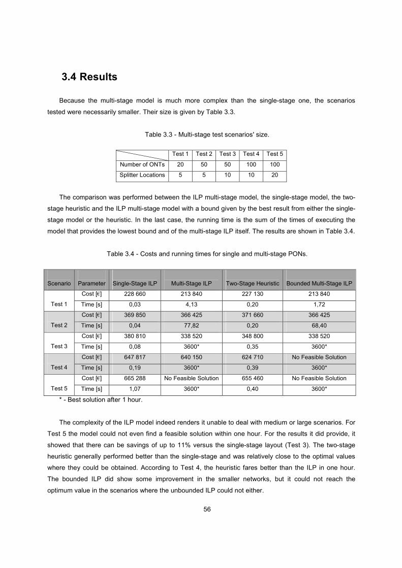
56

3.4 Results

Because the multi-stage model is much more complex than the single-stage one, the scenarios

tested were necessarily smaller. Their size is given by Table 3.3.

Table 3.3 - Multi-stage test scenarios' size.

Test 1 Test 2 Test 3 Test 4 Test 5

Number of ONTs 20 50 50 100 100

Splitter Locations 5 5 10 10 20

The comparison was performed between the ILP multi-stage model, the single-stage model, the two-

stage heuristic and the ILP multi-stage model with a bound given by the best result from either the single-

stage model or the heuristic. In the last case, the running time is the sum of the times of executing the

model that provides the lowest bound and of the multi-stage ILP itself. The results are shown in Table 3.4.

Table 3.4 - Costs and running times for single and multi-stage PONs.

Scenario

Parameter

Single-Stage ILP

Multi-Stage ILP

Two-Stage Heuristic

Bounded Multi-Stage ILP

Test 1

Cost [€] 228 660 213 840 227 130 213 840

Time [s] 0,03 4,13 0,20 1,72

Test 2

Cost [€] 369 850 366 425 371 660 366 425

Time [s] 0,04 77,82 0,20 68,40

Test 3

Cost [€] 380 810 338 520 348 800 338 520

Time [s] 0,08 3600* 0,35 3600*

Test 4

Cost [€] 647 817 640 150 624 710 No Feasible Solution

Time [s] 0,19 3600* 0,39 3600*

Test 5

Cost [€] 665 288 No Feasible Solution 655 460 No Feasible Solution

Time [s] 1,07 3600* 0,40 3600*

* - Best solution after 1 hour.

The complexity of the ILP model indeed renders it unable to deal with medium or large scenarios. For

Test 5 the model could not even find a feasible solution within one hour. For the results it did provide, it

showed that there can be savings of up to 11% versus the single-stage layout (Test 3). The two-stage

heuristic generally performed better than the single-stage and was relatively close to the optimal values

where they could be obtained. According to Test 4, the heuristic fares better than the ILP in one hour.

The bounded ILP did show some improvement in the smaller networks, but it could not reach the

optimum value in the scenarios where the unbounded ILP could not either.

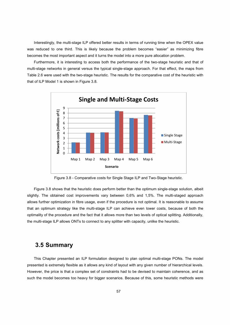
57

Interestingly, the multi-stage ILP offered better results in terms of running time when the OPEX value

was reduced to one third. This is likely because the problem becomes “easier” as minimizing fibre

becomes the most important aspect and it turns the model into a more pure allocation problem.

Furthermore, it is interesting to access both the performance of the two-stage heuristic and that of

multi-stage networks in general versus the typical single-stage approach. For that effect, the maps from

Table 2.6 were used with the two-stage heuristic. The results for the comparative cost of the heuristic with

that of ILP Model 1 is shown in Figure 3.8.

Figure 3.8 - Comparative costs for Single Stage ILP and Two-Stage heuristic.

Figure 3.8 shows that the heuristic does perform better than the optimum single-stage solution, albeit

slightly. The obtained cost improvements vary between 0,6% and 1,5%. The multi-staged approach

allows further optimization in fibre usage, even if the procedure is not optimal. It is reasonable to assume

that an optimum strategy like the multi-stage ILP can achieve even lower costs, because of both the

optimality of the procedure and the fact that it allows more than two levels of optical splitting. Additionally,

the multi-stage ILP allows ONTs to connect to any splitter with capacity, unlike the heuristic.

3.5 Summary

This Chapter presented an ILP formulation designed to plan optimal multi-stage PONs. The model

presented is extremely flexible as it allows any kind of layout with any given number of hierarchical levels.

However, the price is that a complex set of constraints had to be devised to maintain coherence, and as

such the model becomes too heavy for bigger scenarios. Because of this, some heuristic methods were

0

1

2

3

4

5

6

7

8

9

Map 1 Map 2 Map 3 Map 4 Map 5 Map 6

Ne

two

rk c

ost

s [m

illi

on

s o

f €]

Scenario

Single and Multi-Stage Costs

Single Stage

Multi-Stage

58

attempted. The LP relaxation of the model proved unfeasible. A heuristic was developed with the TAP as

its building block, for PONs with up to two stages of splitting. The algorithm produces quick results that

tend to improve when the scenarios grow larger. Its gap to the optimum is hard to assess because

optimum results could not be achieved for large networks, and the bound given by the LP relaxation is

unrealistically low. However, when compared to the single-stage ILP Model 1, it shows a slight cost

improvement for the same scenarios because of less fibre usage.

The last method studied was to use the results of the heuristic or the single-stage model to feed the

multi-stage ILP with an upper bound to start with. This approach proved correct in theory, as some

improvement was verified, but still not enough to make the ILP applicable to larger networks.

59

4. Physical, Technological and

Topology Aspects

This Chapter addresses the more technological aspects of PONs. First, the physical layer

specifications of PONs, like the optical power budget, dispersion effects and differential distance are

introduced into the planning procedures. Then, according to those specifications, the single-stage models

are adapted to study how the physical requirements might affect the current deployments’ evolution to the

next generation of PONs at 10 Gbps. Finally, a comparison is performed between PON and P2P

architectures, in terms of cost and bandwidth available.

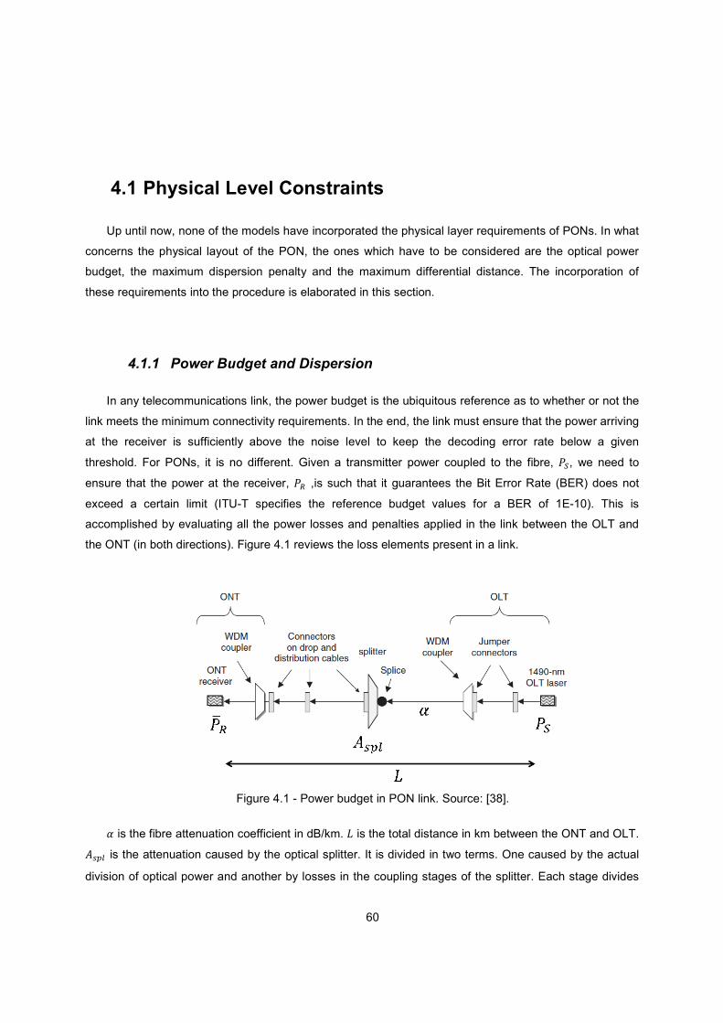
60

4.1 Physical Level Constraints

Up until now, none of the models have incorporated the physical layer requirements of PONs. In what

concerns the physical layout of the PON, the ones which have to be considered are the optical power

budget, the maximum dispersion penalty and the maximum differential distance. The incorporation of

these requirements into the procedure is elaborated in this section.

4.1.1 Power Budget and Dispersion

In any telecommunications link, the power budget is the ubiquitous reference as to whether or not the

link meets the minimum connectivity requirements. In the end, the link must ensure that the power arriving

at the receiver is sufficiently above the noise level to keep the decoding error rate below a given

threshold. For PONs, it is no different. Given a transmitter power coupled to the fibre, yw, we need to

ensure that the power at the receiver, yz ,is such that it guarantees the Bit Error Rate (BER) does not

exceed a certain limit (ITU-T specifies the reference budget values for a BER of 1E-10). This is

accomplished by evaluating all the power losses and penalties applied in the link between the OLT and

the ONT (in both directions). Figure 4.1 reviews the loss elements present in a link.

Figure 4.1 - Power budget in PON link. Source: [38].

{ is the fibre attenuation coefficient in dB/km. l is the total distance in km between the ONT and OLT.

e|}~ is the attenuation caused by the optical splitter. It is divided in two terms. One caused by the actual

division of optical power and another by losses in the coupling stages of the splitter. Each stage divides

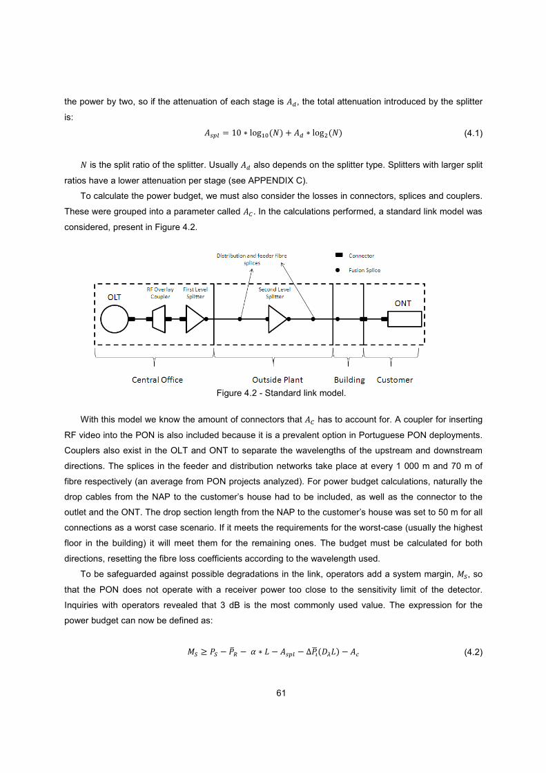
61

the power by two, so if the attenuation of each stage is e�, the total attenuation introduced by the splitter

is:

e|}~ � �. ? 75���D�B � e� ? 75�cD�B (4.1)

� is the split ratio of the splitter. Usually e� also depends on the splitter type. Splitters with larger split

ratios have a lower attenuation per stage (see APPENDIX C).

To calculate the power budget, we must also consider the losses in connectors, splices and couplers.

These were grouped into a parameter called eG . In the calculations performed, a standard link model was

considered, present in Figure 4.2.

Figure 4.2 - Standard link model.

With this model we know the amount of connectors that eG has to account for. A coupler for inserting

RF video into the PON is also included because it is a prevalent option in Portuguese PON deployments.

Couplers also exist in the OLT and ONT to separate the wavelengths of the upstream and downstream

directions. The splices in the feeder and distribution networks take place at every 1 000 m and 70 m of

fibre respectively (an average from PON projects analyzed). For power budget calculations, naturally the

drop cables from the NAP to the customer’s house had to be included, as well as the connector to the

outlet and the ONT. The drop section length from the NAP to the customer’s house was set to 50 m for all

connections as a worst case scenario. If it meets the requirements for the worst-case (usually the highest

floor in the building) it will meet them for the remaining ones. The budget must be calculated for both

directions, resetting the fibre loss coefficients according to the wavelength used.

To be safeguarded against possible degradations in the link, operators add a system margin, �w, so

that the PON does not operate with a receiver power too close to the sensitivity limit of the detector.

Inquiries with operators revealed that 3 dB is the most commonly used value. The expression for the

power budget can now be defined as:

�w S yw V y�z V �{ ? l V e|}~ V uy��Dg�lB V e� (4.2)

62

uy��Dg�lB is the power penalty associated with dispersion related effects.

In the simulations performed, the values used were based on an industry best practise for GPON

found in [39], which relates to Class B+ GPON systems. For further details on the specifications, please

refer to APPENDIX C.

The model developed by [17] directly accounts for power budget constraints in the ILP model (and

also differential distance). In ILP Model 2, with a fixed architecture, (the one in the standard model), the

only real variable in expression (4.2) is distance, so if we define a maximum distance for the feeder and

distribution fibre runs, the constraint is easily added to the model. But to limit the overall OLT-ONT

distance, one would need additional variables to relate the ONT-splitter and splitter-OLT runs. As such,

[17] requires additional constraints to check the budget feasibility of every possible feeder and distribution

connection (like the multi-stage formulation did for the capacity restrictions). In this work, a simpler

approach was adopted. Because we know beforehand the lengths of all the connection paths, the power

budget can be computed for every feeder+distribution combination before the ILP is executed. With the

standard link model presented, this is very fast even for large networks. In this way, we find out which

ONTs cannot be connected to which splitter locations. If the power budget is not met for a given

connection, we simply set the appropriate � � . in the ILP. This avoids adding complexity to the model

and still achieves the same goals.

Another budget related issue that needs to be addressed is the Overload Margin, �:. The power

reaching the ONT or the OLT cannot exceed a given threshold, otherwise it risks damaging the

equipment. Similar calculations to the power budget must be made, only this time assuming “best-case”

scenarios, that is, the ones where the most power reaches the terminals. This means not considering

power penalties or the system margin. The power reaching a detector must be below its Overload Power.

y:, by at least the value of the Overload Margin. This condition is expressed by:

y: � yw V �{ ? l V e|}~ V e� ��: (4.3)

If the maximum receiver power criteria are not met, there is an option of using optical attenuators.

However that was not considered in this framework.

The power penalties play an important role in the link budget. They account for degradation in the

Signal-to-Noise Ratio (SNR) caused by physical effects like chromatic dispersion, non-ideal extinction

ratios, frequency chirping, etc... In PONs, the optical links are relatively short as are the bit rates when

compared to transport links, so these effects are much more negligible [38]. However, because we will

look at PONs operating at 10 Gbps in Section 4.2, it is important to make sure these effects do not

become more noticeable. There were two penalties considered here. One is the burst-mode penalty. In a

TDM-PON, the OLT receives information in bursts, as each ONT transmits in different time periods.

Because each ONT is at a different distance from the OLT, the phase and amplitude of each signal will be

different, which forces the receiver to quickly adjust. For this purpose power levelling is used to smooth

63

the differences in the receiving amplitudes. Because the ITU-T parameters used already factor in a 3 dB

penalty to the OLT receiver sensitivity because of burst-mode operation, this penalty is already implied in

the model. The other factor is chromatic dispersion. This arises from the fact that the several wavelengths

in the optical signal travel at different speeds, which causes the signal to become increasingly distorted in

time leading to inter-symbol interference. This is accounted for by setting a power penalty associated with

the parameters that influence dispersion that cannot be exceeded. For details, again refer to APPENDIX

C. The dispersion effects are mentioned here because they were dealt with in the same way as the power

budget. The only changing variable between the various links is distance, so a pre-processing routine

was made that checks all ONT-splitter-OLT path combinations and sets the ONT-splitter connections that

do not meet the requirements to zero.

4.1.2 Maximum Differential Distance

The maximum differential distance is a constraint on the range of distances that ONTs can have to

the OLT. This is important because the further apart two ONTs are relative to the OLT, the harder it is for

the latter to perform ranging, power levelling and synchronization procedures. Recommendation G.984.2

defines the maximum differential logical reach at 20 km and the maximum differential optical path loss at

15 dB. Again, [17] included this information (for the logical reach) in the ILP itself. Here, because we

included a splitting stage at the CO, the “members” of the same PON are not clearly defined. That was in

fact the purpose, because an operator wants to have that kind of flexibility. For this purpose however,

each specific ONT is only allocated to a Junction Box, not to any PON. This means we cannot know the

differential distances before service is requested. A somewhat naive solution was implemented in this

case, by post-processing the solution. When the ILP is executed and the solution obtained, the PONs are

defined in the following way: each PON will successively spread its second level splitters by as many

Junction Boxes as possible. Since we cannot know when customers will require service and therefore

which splitter they will be connected to, the calculations are made for all the PONs that the ONTs have

access to, meaning the ones that have splitters in Junction Boxes where the ONTs are connected.

Basically we create virtual super-PONs that include every ONT that can possibly be connected to it and

check the differential distance and path loss. The final conclusion however was that the maximum

differential distance is too large to impact the scenarios studied (without any reach extension) and the

optical path loss is never an issue because the loss of a 1:64 splitting ratio (18 dB) alone is only 10 dB

short of the total 28 dB maximum path loss, so there cannot be a 15 dB difference when PONs use 1:64

ratios.

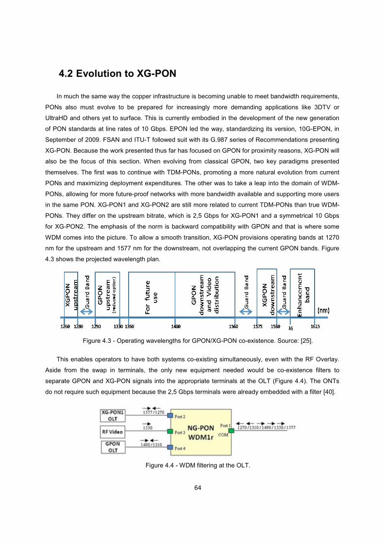
64

4.2 Evolution to XG-PON

In much the same way the copper infrastructure is becoming unable to meet bandwidth requirements,

PONs also must evolve to be prepared for increasingly more demanding applications like 3DTV or

UltraHD and others yet to surface. This is currently embodied in the development of the new generation

of PON standards at line rates of 10 Gbps. EPON led the way, standardizing its version, 10G-EPON, in

September of 2009. FSAN and ITU-T followed suit with its G.987 series of Recommendations presenting

XG-PON. Because the work presented thus far has focused on GPON for proximity reasons, XG-PON will

also be the focus of this section. When evolving from classical GPON, two key paradigms presented

themselves. The first was to continue with TDM-PONs, promoting a more natural evolution from current

PONs and maximizing deployment expenditures. The other was to take a leap into the domain of WDM-

PONs, allowing for more future-proof networks with more bandwidth available and supporting more users

in the same PON. XG-PON1 and XG-PON2 are still more related to current TDM-PONs than true WDM-

PONs. They differ on the upstream bitrate, which is 2,5 Gbps for XG-PON1 and a symmetrical 10 Gbps

for XG-PON2. The emphasis of the norm is backward compatibility with GPON and that is where some

WDM comes into the picture. To allow a smooth transition, XG-PON provisions operating bands at 1270

nm for the upstream and 1577 nm for the downstream, not overlapping the current GPON bands. Figure

4.3 shows the projected wavelength plan.

Figure 4.3 - Operating wavelengths for GPON/XG-PON co-existence. Source: [25].

This enables operators to have both systems co-existing simultaneously, even with the RF Overlay.

Aside from the swap in terminals, the only new equipment needed would be co-existence filters to

separate GPON and XG-PON signals into the appropriate terminals at the OLT (Figure 4.4). The ONTs

do not require such equipment because the 2,5 Gbps terminals were already embedded with a filter [40].

Figure 4.4 - WDM filtering at the OLT.

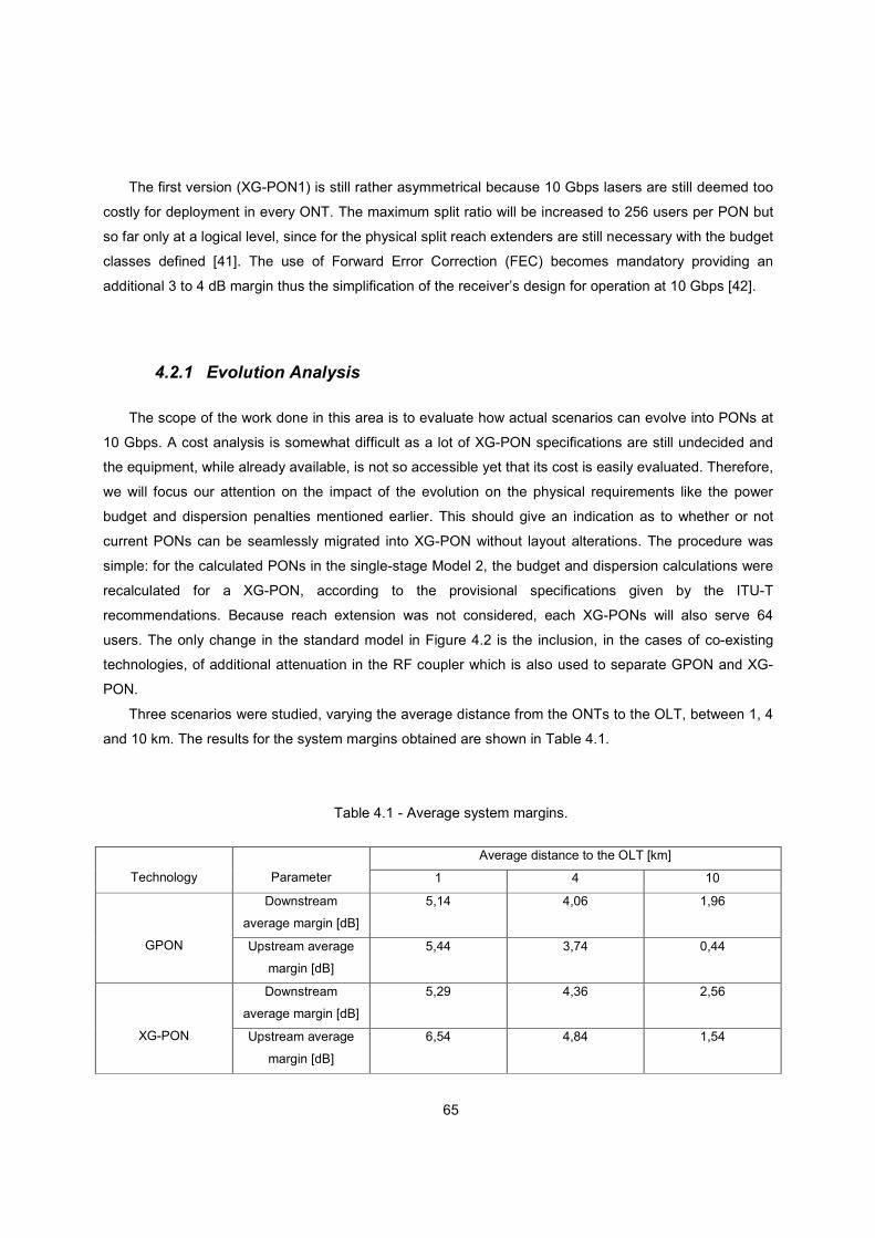
65

The first version (XG-PON1) is still rather asymmetrical because 10 Gbps lasers are still deemed too

costly for deployment in every ONT. The maximum split ratio will be increased to 256 users per PON but

so far only at a logical level, since for the physical split reach extenders are still necessary with the budget

classes defined [41]. The use of Forward Error Correction (FEC) becomes mandatory providing an

additional 3 to 4 dB margin thus the simplification of the receiver’s design for operation at 10 Gbps [42].

4.2.1 Evolution Analysis

The scope of the work done in this area is to evaluate how actual scenarios can evolve into PONs at

10 Gbps. A cost analysis is somewhat difficult as a lot of XG-PON specifications are still undecided and

the equipment, while already available, is not so accessible yet that its cost is easily evaluated. Therefore,

we will focus our attention on the impact of the evolution on the physical requirements like the power

budget and dispersion penalties mentioned earlier. This should give an indication as to whether or not

current PONs can be seamlessly migrated into XG-PON without layout alterations. The procedure was

simple: for the calculated PONs in the single-stage Model 2, the budget and dispersion calculations were

recalculated for a XG-PON, according to the provisional specifications given by the ITU-T

recommendations. Because reach extension was not considered, each XG-PONs will also serve 64

users. The only change in the standard model in Figure 4.2 is the inclusion, in the cases of co-existing

technologies, of additional attenuation in the RF coupler which is also used to separate GPON and XG-

PON.

Three scenarios were studied, varying the average distance from the ONTs to the OLT, between 1, 4

and 10 km. The results for the system margins obtained are shown in Table 4.1.

Table 4.1 - Average system margins.

Technology

Parameter

Average distance to the OLT [km]

1 4 10

GPON

Downstream

average margin [dB]

5,14 4,06 1,96

Upstream average

margin [dB]

5,44 3,74 0,44

XG-PON

Downstream

average margin [dB]

5,29 4,36 2,56

Upstream average

margin [dB]

6,54 4,84 1,54

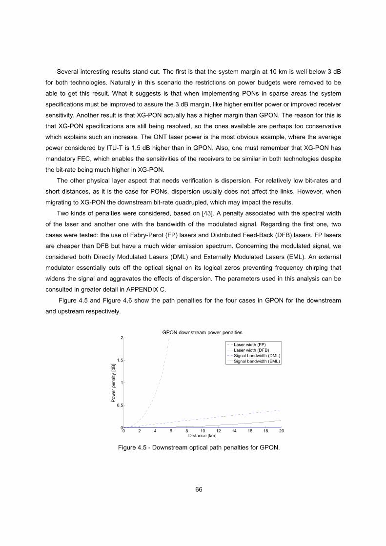
66

Several interesting results stand out. The first is that the system margin at 10 km is well below 3 dB

for both technologies. Naturally in this scenario the restrictions on power budgets were removed to be

able to get this result. What it suggests is that when implementing PONs in sparse areas the system

specifications must be improved to assure the 3 dB margin, like higher emitter power or improved receiver

sensitivity. Another result is that XG-PON actually has a higher margin than GPON. The reason for this is

that XG-PON specifications are still being resolved, so the ones available are perhaps too conservative

which explains such an increase. The ONT laser power is the most obvious example, where the average

power considered by ITU-T is 1,5 dB higher than in GPON. Also, one must remember that XG-PON has

mandatory FEC, which enables the sensitivities of the receivers to be similar in both technologies despite

the bit-rate being much higher in XG-PON.

The other physical layer aspect that needs verification is dispersion. For relatively low bit-rates and

short distances, as it is the case for PONs, dispersion usually does not affect the links. However, when

migrating to XG-PON the downstream bit-rate quadrupled, which may impact the results.

Two kinds of penalties were considered, based on [43]. A penalty associated with the spectral width

of the laser and another one with the bandwidth of the modulated signal. Regarding the first one, two

cases were tested: the use of Fabry-Perot (FP) lasers and Distributed Feed-Back (DFB) lasers. FP lasers

are cheaper than DFB but have a much wider emission spectrum. Concerning the modulated signal, we

considered both Directly Modulated Lasers (DML) and Externally Modulated Lasers (EML). An external

modulator essentially cuts off the optical signal on its logical zeros preventing frequency chirping that

widens the signal and aggravates the effects of dispersion. The parameters used in this analysis can be

consulted in greater detail in APPENDIX C.

Figure 4.5 and Figure 4.6 show the path penalties for the four cases in GPON for the downstream

and upstream respectively.

Figure 4.5 - Downstream optical path penalties for GPON.

0 2 4 6 8 10 12 14 16 18 200

0.5

1

1.5

2GPON downstream power penalties

Distance [km]

Po

wer

pe

nalty

[d

B]

Laser width (FP)Laser width (DFB)Signal bandwidth (DML)Signal bandwidth (EML)

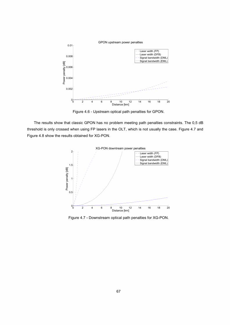
67

Figure 4.6 - Upstream optical path penalties for GPON.

The results show that classic GPON has no problem meeting path penalties constraints. The 0,5 dB

threshold is only crossed when using FP lasers in the OLT, which is not usually the case. Figure 4.7 and

Figure 4.8 show the results obtained for XG-PON.

Figure 4.7 - Downstream optical path penalties for XG-PON.

0 2 4 6 8 10 12 14 16 18 200

0.002

0.004

0.006

0.008

0.01GPON upstream power penalties

Distance [km]

Pow

er p

ena

lty [d

B]

Laser width (FP)Laser width (DFB)Signal bandwidth (DML)Signal bandwidth (EML)

0 2 4 6 8 10 12 14 16 18 200

0.5

1

1.5

2XG-PON downtream power penalties

Distance [km]

Pow

er p

ena

lty [d

B]

Laser width (FP)Laser width (DFB)Signal bandwidth (DML)Signal bandwidth (EML)

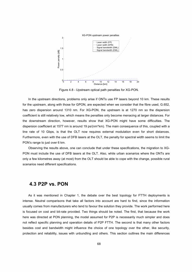
68

Figure 4.8 - Upstream optical path penalties for XG-PON.

In the upstream directions, problems only arise if ONTs use FP lasers beyond 10 km. These results

for the upstream, along with those for GPON, are expected when we consider that the fibre used, G.652,

has zero dispersion around 1310 nm. For XG-PON, the upstream is at 1270 nm so the dispersion

coefficient is still relatively low, which means the penalties only become menacing at larger distances. For

the downstream direction, however, results show that XG-PON might have some difficulties. The

dispersion coefficient at 1577 nm is around 19 ps/(nm*km). The main consequence of this, coupled with a

line rate of 10 Gbps, is that the OLT now requires external modulation even for short distances.

Furthermore, even with the use of DFB lasers at the OLT, the penalty for spectral width seems to limit the

PON’s range to just over 6 km.

Observing the results above, one can conclude that under these specifications, the migration to XG-

PON must include the use of DFB lasers at the OLT. Also, while urban scenarios where the ONTs are

only a few kilometres away (at most) from the OLT should be able to cope with the change, possible rural

scenarios need different specifications.

4.3 P2P vs. PON

As it was mentioned in Chapter 1, the debate over the best topology for FTTH deployments is

intense. Neutral comparisons that take all factors into account are hard to find, since the information

usually comes from manufacturers who tend to favour the solution they provide. The work performed here

is focused on cost and bit-rate provided. Two things should be noted. The first, that because the work

here was directed at PON planning, the model assumed for P2P is necessarily much simpler and does

not reflect specific planning and operation details of P2P FTTH. The second is that many other factors

besides cost and bandwidth might influence the choice of one topology over the other, like security,

protection and reliability, issues with unbundling and others. This section outlines the main differences

0 2 4 6 8 10 12 14 16 18 200

0.5

1

1.5

2XG-PON upstream power penalties

Distance [km]

Pow

er p

enal

ty [d

B]

Laser width (FP)Laser width (DFB)Signal bandwidth (DML)Signal bandwidth (EML)

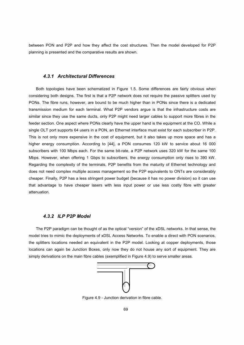
69

between PON and P2P and how they affect the cost structures. Then the model developed for P2P

planning is presented and the comparative results are shown.

4.3.1 Architectural Differences

Both topologies have been schematized in Figure 1.5. Some differences are fairly obvious when

considering both designs. The first is that a P2P network does not require the passive splitters used by

PONs. The fibre runs, however, are bound to be much higher than in PONs since there is a dedicated

transmission medium for each terminal. What P2P vendors argue is that the infrastructure costs are

similar since they use the same ducts, only P2P might need larger cables to support more fibres in the

feeder section. One aspect where PONs clearly have the upper hand is the equipment at the CO. While a

single OLT port supports 64 users in a PON, an Ethernet interface must exist for each subscriber in P2P.

This is not only more expensive in the cost of equipment, but it also takes up more space and has a

higher energy consumption. According to [44], a PON consumes 120 kW to service about 16 000

subscribers with 100 Mbps each. For the same bit-rate, a P2P network uses 320 kW for the same 100

Mbps. However, when offering 1 Gbps to subscribers, the energy consumption only rises to 390 kW.

Regarding the complexity of the terminals, P2P benefits from the maturity of Ethernet technology and

does not need complex multiple access management so the P2P equivalents to ONTs are considerably

cheaper. Finally, P2P has a less stringent power budget (because it has no power division) so it can use

that advantage to have cheaper lasers with less input power or use less costly fibre with greater

attenuation.

4.3.2 ILP P2P Model

The P2P paradigm can be thought of as the optical “version” of the xDSL networks. In that sense, the

model tries to mimic the deployments of xDSL Access Networks. To enable a direct with PON scenarios,

the splitters locations needed an equivalent in the P2P model. Looking at copper deployments, those

locations can again be Junction Boxes, only now they do not house any sort of equipment. They are

simply derivations on the main fibre cables (exemplified in Figure 4.9) to serve smaller areas.

Figure 4.9 - Junction derivation in fibre cable.

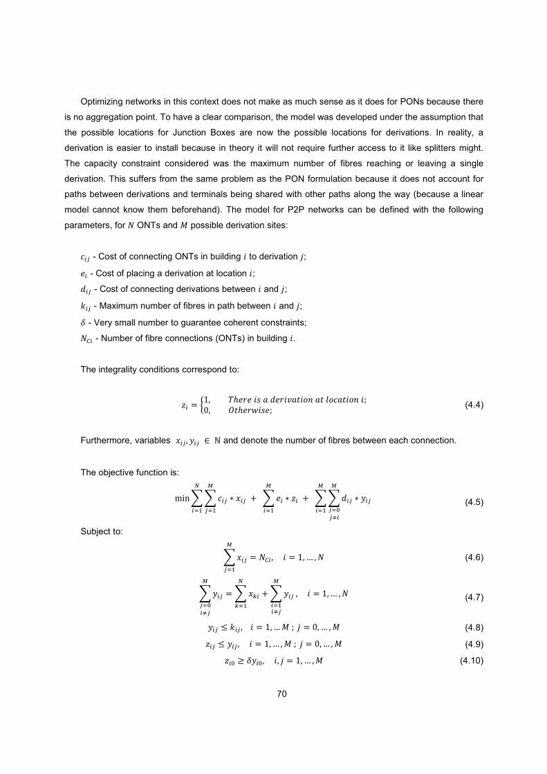
70

Optimizing networks in this context does not make as much sense as it does for PONs because there

is no aggregation point. To have a clear comparison, the model was developed under the assumption that

the possible locations for Junction Boxes are now the possible locations for derivations. In reality, a

derivation is easier to install because in theory it will not require further access to it like splitters might.

The capacity constraint considered was the maximum number of fibres reaching or leaving a single

derivation. This suffers from the same problem as the PON formulation because it does not account for

paths between derivations and terminals being shared with other paths along the way (because a linear

model cannot know them beforehand). The model for P2P networks can be defined with the following

parameters, for � ONTs and � possible derivation sites:

� - Cost of connecting ONTs in building � to derivation �; ! - Cost of placing a derivation at location �; - Cost of connecting derivations between � and �; � - Maximum number of fibres in path between � and �; � - Very small number to guarantee coherent constraints;

�G - Number of fibre connections (ONTs) in building �.

The integrality conditions correspond to:

I � 2�� h/!%!��0��� !%�n�"�� ��"�'���"�� ��k.� j"/!%$�0!k 1 (4.4)

Furthermore, variables �� � � � �� and denote the number of fibres between each connection.

The objective function is:

������ ? ��

���� ���! ? I

�

���� ���� ? �

�

��v�

�

��

�

�� (4.5)

Subject to:

�� � �G ������� � ��� � ��

�� (4.6)

�� � ��[ ����

��v

�

[��

�

��v������� � ��� � � (4.7)

� � � ������ � �����k �� � .� � �� (4.8)

I � � ������� � �� � ���k �� � .�� �� (4.9)

I� S ����������� � � ��� �� (4.10)

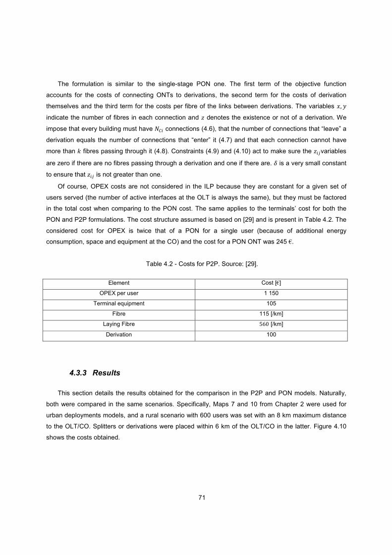
71

The formulation is similar to the single-stage PON one. The first term of the objective function

accounts for the costs of connecting ONTs to derivations, the second term for the costs of derivation

themselves and the third term for the costs per fibre of the links between derivations. The variables �� �

indicate the number of fibres in each connection and I denotes the existence or not of a derivation. We

impose that every building must have �G connections (4.6), that the number of connections that “leave” a

derivation equals the number of connections that “enter” it (4.7) and that each connection cannot have

more than � fibres passing through it (4.8). Constraints (4.9) and (4.10) act to make sure the Ivariables

are zero if there are no fibres passing through a derivation and one if there are. � is a very small constant

to ensure that I is not greater than one.

Of course, OPEX costs are not considered in the ILP because they are constant for a given set of

users served (the number of active interfaces at the OLT is always the same), but they must be factored

in the total cost when comparing to the PON cost. The same applies to the terminals’ cost for both the

PON and P2P formulations. The cost structure assumed is based on [29] and is present in Table 4.2. The

considered cost for OPEX is twice that of a PON for a single user (because of additional energy

consumption, space and equipment at the CO) and the cost for a PON ONT was 245 €.

Table 4.2 - Costs for P2P. Source: [29].

Element Cost [€]

OPEX per user 1 150

Terminal equipment 105

Fibre 115 [/km]

Laying Fibre ]\. [/km]

Derivation 100

4.3.3 Results

This section details the results obtained for the comparison in the P2P and PON models. Naturally,

both were compared in the same scenarios. Specifically, Maps 7 and 10 from Chapter 2 were used for

urban deployments models, and a rural scenario with 600 users was set with an 8 km maximum distance

to the OLT/CO. Splitters or derivations were placed within 6 km of the OLT/CO in the latter. Figure 4.10

shows the costs obtained.

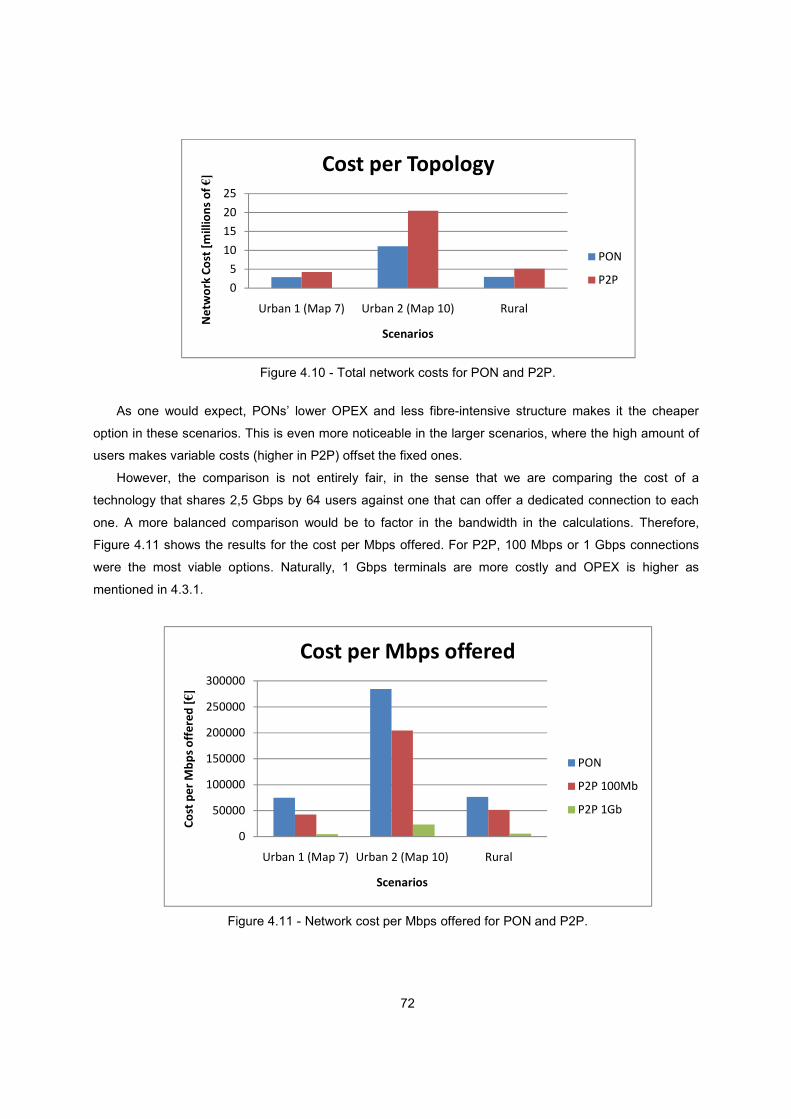
72

Figure 4.10 - Total network costs for PON and P2P.

As one would expect, PONs’ lower OPEX and less fibre-intensive structure makes it the cheaper

option in these scenarios. This is even more noticeable in the larger scenarios, where the high amount of

users makes variable costs (higher in P2P) offset the fixed ones.

However, the comparison is not entirely fair, in the sense that we are comparing the cost of a

technology that shares 2,5 Gbps by 64 users against one that can offer a dedicated connection to each

one. A more balanced comparison would be to factor in the bandwidth in the calculations. Therefore,

Figure 4.11 shows the results for the cost per Mbps offered. For P2P, 100 Mbps or 1 Gbps connections

were the most viable options. Naturally, 1 Gbps terminals are more costly and OPEX is higher as

mentioned in 4.3.1.

Figure 4.11 - Network cost per Mbps offered for PON and P2P.

0

5

10

15

20

25

Urban 1 (Map 7) Urban 2 (Map 10) Rural

Ne

two

rk C

ost

[m

illi

on

s o

f €]

Scenarios

Cost per Topology

PON

P2P

0

50000

100000

150000

200000

250000

300000

Urban 1 (Map 7) Urban 2 (Map 10) Rural

Co

st p

er

Mb

ps

off

ere

d [€]

Scenarios

Cost per Mbps offered

PON

P2P 100Mb

P2P 1Gb

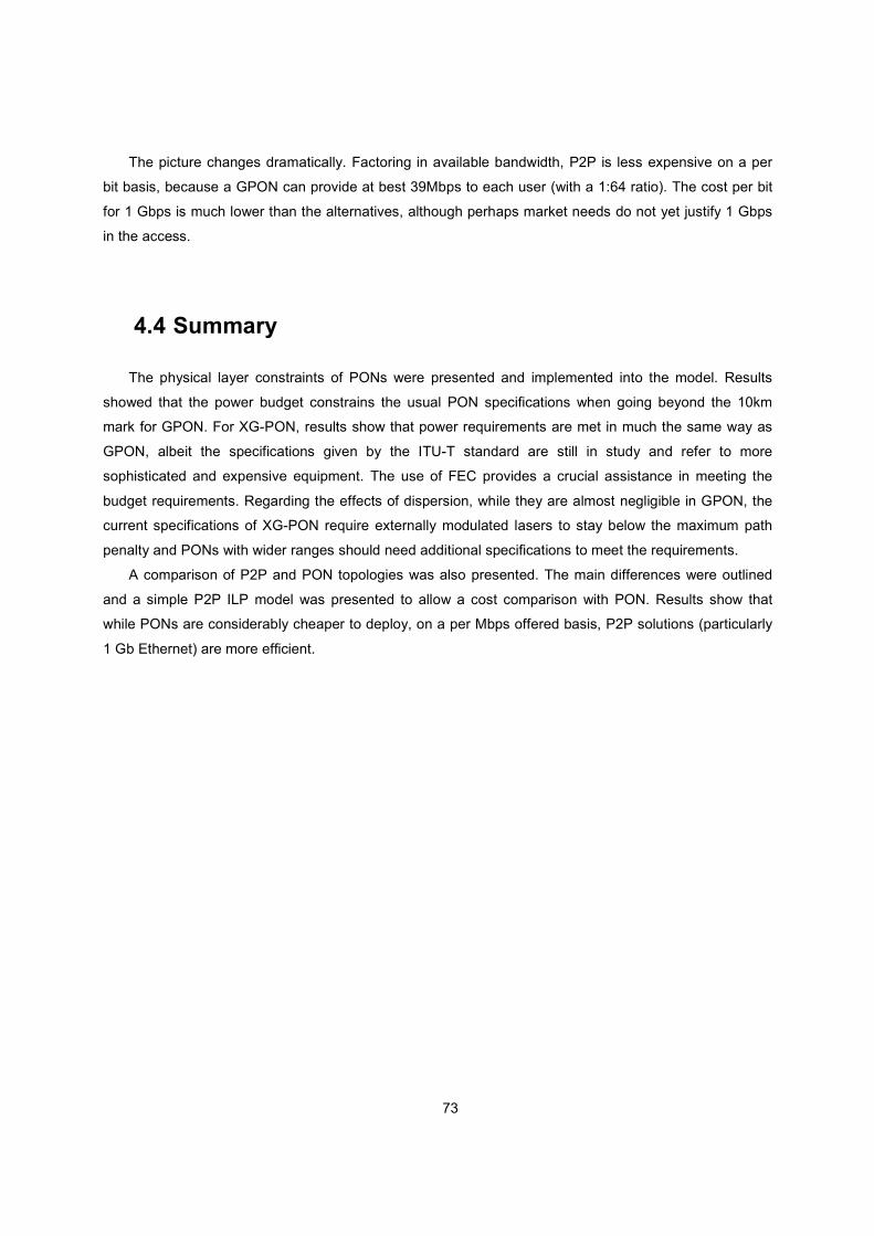
73

The picture changes dramatically. Factoring in available bandwidth, P2P is less expensive on a per

bit basis, because a GPON can provide at best 39Mbps to each user (with a 1:64 ratio). The cost per bit

for 1 Gbps is much lower than the alternatives, although perhaps market needs do not yet justify 1 Gbps

in the access.

4.4 Summary

The physical layer constraints of PONs were presented and implemented into the model. Results

showed that the power budget constrains the usual PON specifications when going beyond the 10km

mark for GPON. For XG-PON, results show that power requirements are met in much the same way as

GPON, albeit the specifications given by the ITU-T standard are still in study and refer to more

sophisticated and expensive equipment. The use of FEC provides a crucial assistance in meeting the

budget requirements. Regarding the effects of dispersion, while they are almost negligible in GPON, the

current specifications of XG-PON require externally modulated lasers to stay below the maximum path

penalty and PONs with wider ranges should need additional specifications to meet the requirements.

A comparison of P2P and PON topologies was also presented. The main differences were outlined

and a simple P2P ILP model was presented to allow a cost comparison with PON. Results show that

while PONs are considerably cheaper to deploy, on a per Mbps offered basis, P2P solutions (particularly

1 Gb Ethernet) are more efficient.

74

5. Conclusions and Future Work

This Chapter reflects on the work conducted in the framework of this Thesis, and the way it can

contribute for further development of the relevant areas it addresses. It also discusses possible paths in

which the work presented here can be continued, either by continuously improving the methodologies

presented or by extending their application range to adjacent areas.

75

5.1 General Conclusions

The objectives of this Thesis were summarized in Chapter 1 as comprising three main objectives. The

first was to develop an ILP model for PON planning and assess its practicality. It was shown in Chapter 2

that the CLP can, with today’s computational power, be used to solve problems with several hundred

terminals and a few dozen concentrators. This problem was then applied to PON planning with coherent

results. The alterations made to the model allowed not only to better relate it to the challenges facing an

operator deploying a PON (like OPEX and the take-rate) but also to extend the model’s range to several

thousand users per scenario, when considering concentrated urban deployments. The model deviates

from the usual approaches in the area in the sense that it does not perform best path calculations for the

PON elements, rather it optimizes the allocation and placement of splitters in PONs. For the scenarios

where the formulation takes too much time to respond, the heuristics tested achieve good results quickly.

The second objective was to develop an ILP model for multi-staged PONs. This was probably the

most original contribution of this Thesis, as no comparable approach could be found in the literature. The

proposed model enables a great degree of flexibility as it allows any kind of connections between splitters

(while complying with PON requirements) and any desired number of splitting stages. However, as often

is the case with ILP models, it is still too complex for regular computational power, allowing only optimal

scenarios for relatively small networks. It did however show the potential benefits of using such an

architecture against a single-stage design. The proposed heuristic achieved coherent results although its

overall performance needs some benchmarking.

The third objective related to analyzing the evolution of current GPON to XG-PON and comparing

PON topologies with P2P ones. The results show that with current specifications for XG-PON, the

migration is possible for PONs spanning less than 6 km if external modulation is applied at the OLT laser.

Regarding the topological analysis, results suggest that current PONs are cheaper to deploy but cost

more on a per bit offered basis.

5.2 Future Work

The work presented here, being either the application of classical algorithms to a new reality (PONs)

or the development of a brand new model (for multi-stage PONs), was relatively new and over a

considerable array of issues. Therefore, it is only natural that many of the methods and models used can

be perfected to achieve improvements in both the output results and the performance of the algorithms.

In the case of the single-stage formulation, a more interesting end-to-end solution could be achieved

by interfacing the model with path-calculation programs (such as the one described in [15]) to better

account for conduit sharing for instance. Also, it should be investigated whether the single-stage

76

formulation can be modified to allow different first-stage splitting ratios in the same network without

making it too complex. Modifications could also attempt to mimic the distributed-split architecture, possibly

by co-locating splitter locations with building locations.

For the multi-stage model, the work presented was a first approach to the problem, which opens

many possibilities for further developing it. First of all, more advanced techniques should be studied in

order to attempt to lower the running times of the model and get results for larger networks. A more

complex relaxation procedure could be employed, or the settings of the Branch & Bound procedure could

be optimized (like a heuristic procedure to select which solution branches to check first and with which

values). Also, simplifications of the model could be tested, like limiting the configurations (in the number

of levels allowed for instance). The heuristic developed for two-stage PONs has room for improvement,

starting by expanding it to allow more than two levels. More complex verification stages in the reallocation

procedures were tried without success, but it is still an open problem.

Regarding the work in Chapter 4, it is more of a closed analysis rather than an evolving model or

algorithm. However, the underlying methodology can be used with more accurate data. This is most

evident in the case of XG-PON, where the costs of the equipment would allow a cost estimate of evolving

the networks. Also for the case of XG-PON, when the final specifications are ratified a more conclusive

analysis can be conducted on the feasibility of seamless migration scenarios.

In a more general note, the models presented should allow the simulation of future optical access

networks, like WDM-PONs, with minimal adaptations to their structure. Other aspects could also be

introduced, such as protection schemes in PONs, by changing the constraints to allow more than one

connection per ONT and force those connections to go through geographically separate Junction Boxes.

77

References

[1] K. G. Coffman and A. M. Odlyzko. (1998) The Size and Growth Rate of the Internet. [Online].

http://www.dtc.umn.edu/~odlyzko/doc/internet_size.pdf

[2] G. Agrawal, Fiber-Optic Communication Systems, 3rd ed.: Wiley & Sons Inc., 2002.

[3] P. Green, Fiber to the Home: The New Empowerment.: Wiley & Sons Inc., 2005.

[4] ITU-T Recommendation G.993.2, Very High Speed Digital Subscriber Line Transceivers 2

(VDSL2), 2006.

[5] O. Hammer. (2008, January) How Big is the VDSL Market? [Online].

http://seekingalpha.com/article/59668-jkanos-communications-how-big-is-the-vdsl-market-part-iii

[6] (2008) AON Vs. PON - A comparison of two access network technologies and the different

impact on operations. [Online].

http://www.eurocomms.com/asset/583/AON%20vs.%20PON%20%28White%20Paper%29.pdf

[7] L., Chen, J. Wosinska, "How much to pay for protection in fiber access networks: Cost and

reliability tradeoff," in IEEE 3rd International Symposium on Advanced Networks and

Telecommunication Systems, 2009, pp. 1-3.

[8] J. Weingart. (2007) Metro Ethernet Forum. [Online].

http://www.metroethernetforum.org/PPT_Documents/FTTxMEF070620.ppt

[9] J. Pires, "Redes de Acesso Ópticas," ISCTE, Seminário sobre Redes Ópticas de Nova

Geração. 2009.

[10] ITU-T Recommendation G.983.1, Broadband optical access systems based on Passive Optical

Networks (PON), 2005.

[11] (2010, September) PON market to reach $7.62bn in five years. [Online].

http://www.ciol.com/Technology/Networking/News-Reports/PON-market-to-reach-$762bn-in-

five-years/8210131129/0/

[12] J. G. Klincewicz, "Hub location in backbone/tributary network design: a review," Location

Science, vol. 6, pp. 307-335, 1998.

[13] R. R. Boorstyn and H. Frank, "Large-Scale Network Topological Optimization," IEEE

Transactions on Communications, vol. 25, no. 1, pp. 29-47, January 1977.

[14] E. Bonsma, N. Karunatillake, R. Shipman, M. Shackleton, and D. Mortimore, "Evolving

Greenfield Passive Optical Networks," BT Technology Journal, vol. 21, no. 4, 2003.

[15] B. Lakic, "PON Builder: Automated Planning of a Passive Optical Network," University of

Coimbra, Faculty of Sciences and Technology, Master's Thesis in Electrical and Computer

Engineering. 2008.

78

[16] B. Lakic and M. Hajduczenia, "On optimized Passive Optical Network (PON) deployment," in

Second International Conference on Access Networks, 2007, pp. 1-8.

[17] J. Li and G. Shen, "Cost Minimization Planning for Greenfield Passive Optical Networks,"

Journal of Optical Communications and Networking, vol. 1, no. 1, pp. 17-29, 2009.

[18] Telcordia Technologies, Inc. Telcordia Network Engineer. [Online].

http://www.telcordia.com/collateral/brochures/net_engineer.pdf

[19] Nokia Corporation. Nokia Netact Planner. [Online].

http://sysdoc.doors.ch/NOKIA/nokia_netact_planner.pdf

[20] D. Luenberger and Y. Ye, Linear and Nonlinear Programming, 3rd ed.: Springer, 2008.

[21] M. Trick. (1998) A Tutorial on Integer Programming. [Online].

http://mat.gsia.cmu.edu/orclass/integer/integer.html

[22] M. Berkelaar, K. Eikland, and P. Notebaert. (2004, May) lpsolve: Open source (Mixed-Integer)

Linear Programming system. [Online]. http://lpsolve.sourceforge.net/5.5/

[23] B. Perkins, "Optimal Splitter Placement in PONs," Bechtel Telecommunications Technical

Journal, September 2004.

[24] G. Schnick. (2007, April) Corning Cable Systems. [Online].

catalog2.corning.com/CorningCableSystems/./EVO-745-EN.pdf

[25] J. Salgado, P. Mão-Cheia, C. Rodrigues, M. Bernardo, and J. Figueiredo, "Evolution of Access

Networks from GPON to XGPON to WDM-PON from operator point of view," in 15th European

Conference on Networks and Optical Communications, 2010.

[26] A. Costa, Juntas e Conectores Ópticos, Faculdade de Engenharia da Universidade do Porto.

[27] J. Pearl, Heuristics: Intelligent Search Strategies for Computer Problem Solving.: Addison-

Wesley, 1983.

[28] J. Matousek and B. Gartner, "Integer Programming and LP Relaxation," in Understanding and

using Linear Programming.: Springer, 2007, ch. 3, pp. 29-40.

[29] J. Chen, L. Wosinska, C. Machuca, and M. Jaeger, "Cost vs. reliability performance study of

fiber access network architectures," IEEE Communications Magazine, vol. 48, no. 2, pp. 56-65,

2010.

[30] J. L. Riding, J. C. Ellershaw, A. V. Tran, L. J. Guan, and T. Smith, "Economics of broadband

access technologies for rural areas," in Conference on Optical Fiber Communication, 2009, pp.

1-3.

[31] N. J. Frigo, "A View of Fiber to the Home Economics," IEEE Communications Magazine, vol. 42,

no. 8, pp. 16-23, 2004.

79

[32] I.B. Heard, "Availability and cost estimation of secured FTTH architectures," in International

Conference on Optical Network Design and Modeling, 2008.

[33] L. Wosinska, "Impact of Protection Mechanisms on Cost in PONs," in 11th International

Conference on Transparent Optical Networks, 2009.

[34] G. Schneider and M. Zastrow, "An algorithm for the design of multilevel concentrator networks,"

Computer Science (1976), vol. 6, no. 1, pp. 1-11, February 1982.

[35] P. McGregor and D. Shen, "Network design: an algorithm for the access facility location

problem," IEEE Transactions on Communications, vol. 25, no. 1, pp. 61-73, 1977.

[36] S. Narasimhan and H. Pirkul, "Hierarchical concentrator location problem," Computer

Communications, vol. 15, pp. 185-191, 1992.

[37] J. Chinneck. (2010) Practical Optimization: A Gentle Introduction - Chapter 12: Integer/Discrete

Programming via Branch and Bound. [Online].

http://www.sce.carleton.ca/faculty/chinneck/po/Chapter12.pdf

[38] G. Keiser, FTTx Concepts and Applications.: Wiley & Sons, 2006.

[39] ITU-T Recommendation G.984.2 (Ammendment I), Industry best practice for 2.488 Gbit/s

downstream, 1.244 Gbit/s upstream G-PON , 2006.

[40] F. Bougart, "Optical Access Transmission: XG-PON system aspects," in FTTH Conference,

Lisbon, 2010.

[41] G.987.1 ITU-T Recommendation, 10-Gigabit-capable passive optical networks (XG-PON):

General requirements , 2010.

[42] G.987.2 ITU-T Recommendation, Ten gigabit-capable passive optical networks: Physical

dependent layer specifications, 2010.

[43] A. Cartaxo, "Transmissão por fibra óptica," 2005.

[44] C. Lange and A. Gladisch, "On the Energy Consumption of FTTH Access Networks," in

Conference on Optical Fiber Communication, 2009, pp. 1-3.

[45] D. Sala. (2001) Broadcom. [Online]. http://wwwcsif.cs.ucdavis.edu/~kramer/code/pcktsize.html

[46] M. Hajduczenia, H. Silva, and P. Monteiro, "On efficiency of Ethernet Passive Optical Networks

(EPONs)," in 11th IEEE Symposium on Computers and Communications, 2006, pp. 566-571.

[47] G. Kramer, "Ethernet PON (EPON): Design and Analysis of an Optical Access Network," 2000.

[48] Cisco Systems Inc. (2008) Understanding Data Throughput in a DOCSIS World.

[49] G.987.2 ITU-T Recommendation, Ten gigabit-capable passive optical networks: Physical

dependent layer specifications, 2010.

[50] G.652 ITU-T Recommendation, Characteristics of a single-mode fibre and cable, 2009.

[51] Corning Incorporated. (2010) Corning ClearCurve ZBL Optical Fiber. [Online].

80

http://www.corning.com/WorkArea/showcontent.aspx?id=34163

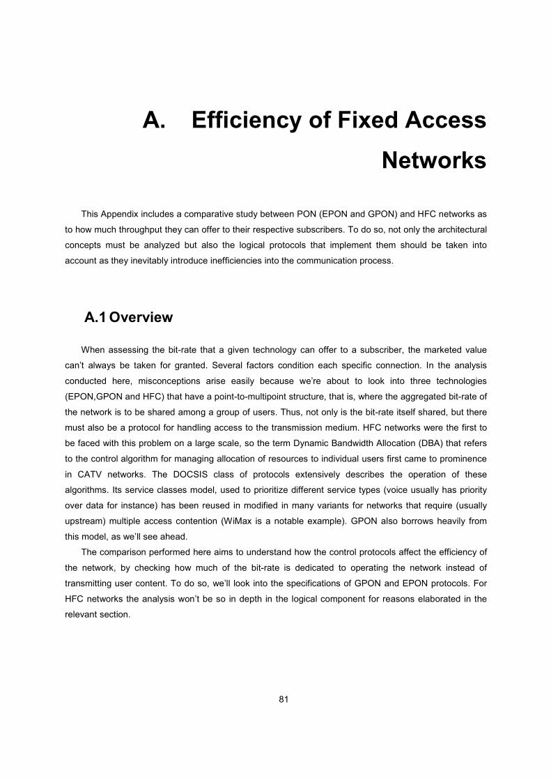
81

A. Efficiency of Fixed Access

Networks

This Appendix includes a comparative study between PON (EPON and GPON) and HFC networks as

to how much throughput they can offer to their respective subscribers. To do so, not only the architectural

concepts must be analyzed but also the logical protocols that implement them should be taken into

account as they inevitably introduce inefficiencies into the communication process.

A.1 Overview

When assessing the bit-rate that a given technology can offer to a subscriber, the marketed value

can’t always be taken for granted. Several factors condition each specific connection. In the analysis

conducted here, misconceptions arise easily because we’re about to look into three technologies

(EPON,GPON and HFC) that have a point-to-multipoint structure, that is, where the aggregated bit-rate of

the network is to be shared among a group of users. Thus, not only is the bit-rate itself shared, but there

must also be a protocol for handling access to the transmission medium. HFC networks were the first to

be faced with this problem on a large scale, so the term Dynamic Bandwidth Allocation (DBA) that refers

to the control algorithm for managing allocation of resources to individual users first came to prominence

in CATV networks. The DOCSIS class of protocols extensively describes the operation of these

algorithms. Its service classes model, used to prioritize different service types (voice usually has priority

over data for instance) has been reused in modified in many variants for networks that require (usually

upstream) multiple access contention (WiMax is a notable example). GPON also borrows heavily from

this model, as we’ll see ahead.

The comparison performed here aims to understand how the control protocols affect the efficiency of

the network, by checking how much of the bit-rate is dedicated to operating the network instead of

transmitting user content. To do so, we’ll look into the specifications of GPON and EPON protocols. For

HFC networks the analysis won’t be so in depth in the logical component for reasons elaborated in the

relevant section.

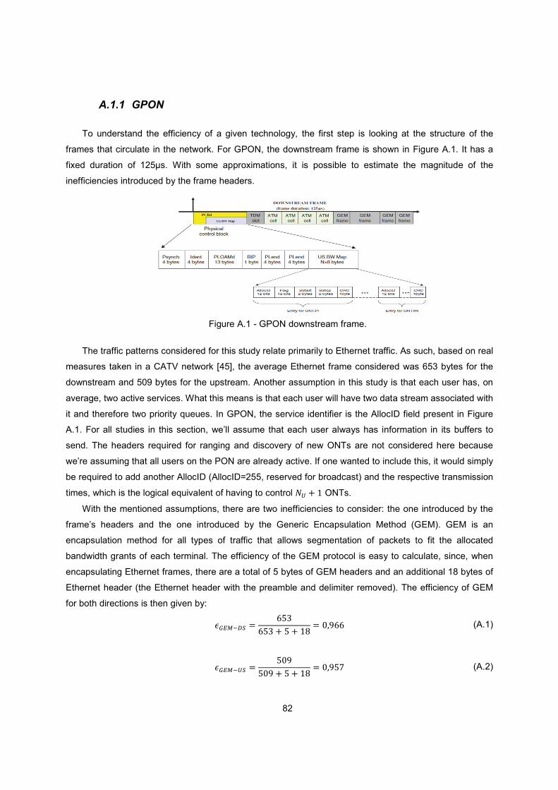
82

A.1.1 GPON

To understand the efficiency of a given technology, the first step is looking at the structure of the

frames that circulate in the network. For GPON, the downstream frame is shown in Figure A.1. It has a

fixed duration of 125µs. With some approximations, it is possible to estimate the magnitude of the

inefficiencies introduced by the frame headers.

Figure A.1 - GPON downstream frame.

The traffic patterns considered for this study relate primarily to Ethernet traffic. As such, based on real

measures taken in a CATV network [45], the average Ethernet frame considered was 653 bytes for the

downstream and 509 bytes for the upstream. Another assumption in this study is that each user has, on

average, two active services. What this means is that each user will have two data stream associated with

it and therefore two priority queues. In GPON, the service identifier is the AllocID field present in Figure

A.1. For all studies in this section, we’ll assume that each user always has information in its buffers to

send. The headers required for ranging and discovery of new ONTs are not considered here because

we’re assuming that all users on the PON are already active. If one wanted to include this, it would simply

be required to add another AllocID (AllocID=255, reserved for broadcast) and the respective transmission

times, which is the logical equivalent of having to control �� � � ONTs.

With the mentioned assumptions, there are two inefficiencies to consider: the one introduced by the

frame’s headers and the one introduced by the Generic Encapsulation Method (GEM). GEM is an

encapsulation method for all types of traffic that allows segmentation of packets to fit the allocated

bandwidth grants of each terminal. The efficiency of the GEM protocol is easy to calculate, since, when

encapsulating Ethernet frames, there are a total of 5 bytes of GEM headers and an additional 18 bytes of

Ethernet header (the Ethernet header with the preamble and delimiter removed). The efficiency of GEM

for both directions is then given by:

������w � \]t\]t � ] � �C � .�Z\\ (A.1)

������w � ].Z].Z � ] � �C � .�Z]^ (A.2)

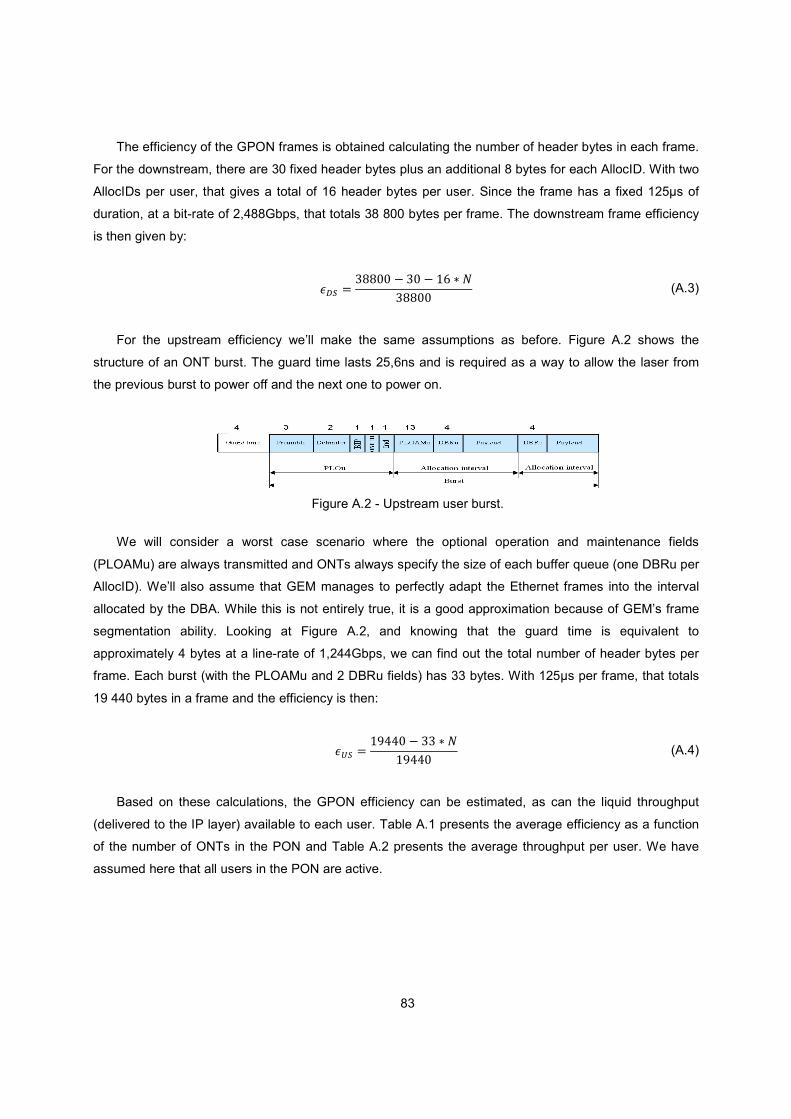
83

The efficiency of the GPON frames is obtained calculating the number of header bytes in each frame.

For the downstream, there are 30 fixed header bytes plus an additional 8 bytes for each AllocID. With two

AllocIDs per user, that gives a total of 16 header bytes per user. Since the frame has a fixed 125µs of

duration, at a bit-rate of 2,488Gbps, that totals 38 800 bytes per frame. The downstream frame efficiency

is then given by:

��w � tCC.. V t. V �\ ? �tCC.. (A.3)

For the upstream efficiency we’ll make the same assumptions as before. Figure A.2 shows the

structure of an ONT burst. The guard time lasts 25,6ns and is required as a way to allow the laser from

the previous burst to power off and the next one to power on.

Figure A.2 - Upstream user burst.

We will consider a worst case scenario where the optional operation and maintenance fields

(PLOAMu) are always transmitted and ONTs always specify the size of each buffer queue (one DBRu per

AllocID). We’ll also assume that GEM manages to perfectly adapt the Ethernet frames into the interval

allocated by the DBA. While this is not entirely true, it is a good approximation because of GEM’s frame

segmentation ability. Looking at Figure A.2, and knowing that the guard time is equivalent to

approximately 4 bytes at a line-rate of 1,244Gbps, we can find out the total number of header bytes per

frame. Each burst (with the PLOAMu and 2 DBRu fields) has 33 bytes. With 125µs per frame, that totals

19 440 bytes in a frame and the efficiency is then:

��w � �Zdd. V tt ? ��Zdd. (A.4)

Based on these calculations, the GPON efficiency can be estimated, as can the liquid throughput

(delivered to the IP layer) available to each user. Table A.1 presents the average efficiency as a function

of the number of ONTs in the PON and Table A.2 presents the average throughput per user. We have

assumed here that all users in the PON are active.

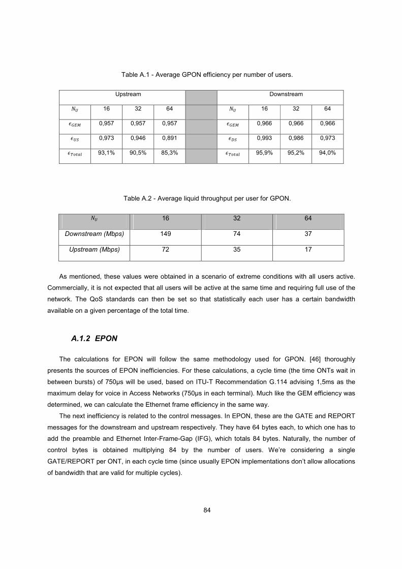
84

Table A.1 - Average GPON efficiency per number of users.

Upstream Downstream

�� 16 32 64 �� 16 32 64

���� 0,957 0,957 0,957 ���� 0,966 0,966 0,966

��w 0,973 0,946 0,891 ��w 0,993 0,986 0,973

�<���~ 93,1% 90,5% 85,3% �<���~ 95,9% 95,2% 94,0%

Table A.2 - Average liquid throughput per user for GPON.

�� 16 32 64

Downstream (Mbps) 149 74 37

Upstream (Mbps) 72 35 17

As mentioned, these values were obtained in a scenario of extreme conditions with all users active.

Commercially, it is not expected that all users will be active at the same time and requiring full use of the

network. The QoS standards can then be set so that statistically each user has a certain bandwidth

available on a given percentage of the total time.

A.1.2 EPON

The calculations for EPON will follow the same methodology used for GPON. [46] thoroughly

presents the sources of EPON inefficiencies. For these calculations, a cycle time (the time ONTs wait in

between bursts) of 750µs will be used, based on ITU-T Recommendation G.114 advising 1,5ms as the

maximum delay for voice in Access Networks (750µs in each terminal). Much like the GEM efficiency was

determined, we can calculate the Ethernet frame efficiency in the same way.

The next inefficiency is related to the control messages. In EPON, these are the GATE and REPORT

messages for the downstream and upstream respectively. They have 64 bytes each, to which one has to

add the preamble and Ethernet Inter-Frame-Gap (IFG), which totals 84 bytes. Naturally, the number of

control bytes is obtained multiplying 84 by the number of users. We’re considering a single

GATE/REPORT per ONT, in each cycle time (since usually EPON implementations don’t allow allocations

of bandwidth that are valid for multiple cycles).

85

Next we need to consider the guard times. These only take place in the upstream, to allow on-off

laser times, clock recovery and gain control. A typical EPON value is 400ns for gain control and clock

recovery, 512 ns for on-off laser time, and 32ns for code alignment. Adding all that up, we get 1856ns that

means 232 bytes per ONT in each cycle. The ranging and ONT discovery process also consumes bytes,

but to keep a balanced comparison with GPON, they weren’t considered here either.

Finally, we need to consider the so called Unused Slot Remainder (USR). This relates to the bytes

that are allocated by the OLT to a given ONT, but aren’t used because the Ethernet frame that a user

needs to transmit doesn’t fit the allocated window. Because unlike GEM, Ethernet frames cannot be

segmented, the frame must be transmitted in the next window. The average USR is obtained in [47] and

is given by:

�oR � T % ? D� V ����D%BB;��������T 0 ? Dm���D0BB;���|�;��� (A.5)

l��O � l�� are the maximum and minimum size of Ethernet frames, % is the number of bytes left in a

slot, ���� is the cumulative distribution function of Ethernet frame size, m��� is the probability density

function for the same variable and 0 is the size of the Ethernet frame. The calculations yielded an average

USR of 596 bytes.

The average EPON efficiency can now be calculated factoring in all these inefficiencies. In a 750µs

cycle there are 93 750 bytes being transmitted (calculations are performed at 1Gbps, not the line rate of

1.25Gbps because of the line coding). In the downstream, we simply have to subtract from this the bytes

reserved for control messages:

��w � Zt^]. V � ? CdZt^]. (A.6)

The upstream efficiency also has to account for the guard times and USR:

��w � Zt^]. V � ? Cd V � ? WtW V ]Z\Zt^]. (A.7)

Aggregating all the expressions, plus the Ethernet frame efficiency we get the results shown in Table

A.3.

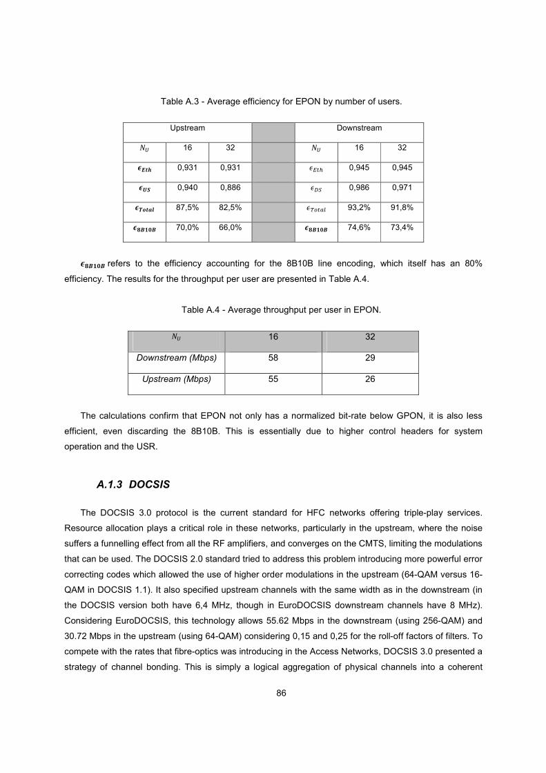
86

Table A.3 - Average efficiency for EPON by number of users.

Upstream Downstream

�� 16 32 �� 16 32

���� 0,931 0,931 ���� 0,945 0,945

� ¡ 0,940 0,886 ��w 0,986 0,971

�¢£�¤¥ 87,5% 82,5% �<���~ 93,2% 91,8%

�¦§A¨§ 70,0% 66,0% �¦§A¨§ 74,6% 73,4%

�¦§A¨§�refers to the efficiency accounting for the 8B10B line encoding, which itself has an 80%

efficiency. The results for the throughput per user are presented in Table A.4.

Table A.4 - Average throughput per user in EPON.

�� 16 32

Downstream (Mbps) 58 29

Upstream (Mbps) 55 26

The calculations confirm that EPON not only has a normalized bit-rate below GPON, it is also less

efficient, even discarding the 8B10B. This is essentially due to higher control headers for system

operation and the USR.

A.1.3 DOCSIS

The DOCSIS 3.0 protocol is the current standard for HFC networks offering triple-play services.

Resource allocation plays a critical role in these networks, particularly in the upstream, where the noise

suffers a funnelling effect from all the RF amplifiers, and converges on the CMTS, limiting the modulations

that can be used. The DOCSIS 2.0 standard tried to address this problem introducing more powerful error

correcting codes which allowed the use of higher order modulations in the upstream (64-QAM versus 16-

QAM in DOCSIS 1.1). It also specified upstream channels with the same width as in the downstream (in

the DOCSIS version both have 6,4 MHz, though in EuroDOCSIS downstream channels have 8 MHz).

Considering EuroDOCSIS, this technology allows 55.62 Mbps in the downstream (using 256-QAM) and

30.72 Mbps in the upstream (using 64-QAM) considering 0,15 and 0,25 for the roll-off factors of filters. To

compete with the rates that fibre-optics was introducing in the Access Networks, DOCSIS 3.0 presented a

strategy of channel bonding. This is simply a logical aggregation of physical channels into a coherent

87

stream. The capacity of the network itself wasn’t increased, only the maximum throughput that one single

user can have. In a typical example, 4 bonded channels in the downstream allow an ideal rate of 222,68

Mbps. For the upstream, 122,88 Mbps can be achieved in the same conditions.

HFC networks were originally conceived for delivering TV service. So naturally the data channels

referred above are shared in the coaxial cable spectrum with TV channels. This is where a study of HFC

efficiency becomes difficult. Each operator has a different allocation of the spectrum between data and

TV. Sometimes the same operator has different allocations in different regions. The tendency for HFC

operators is to progressively leave analog TV channels that occupy the full 8 MHz of each channel. Digital

TV channels on the other hand are more bandwidth efficient, so one can place around 10 Standard

Definition (SD) channels or 5 High Definition (HD) channels in a single 8 MHz carrier. This allows an

operator to release channels for the data service increasing capacity. The problem is that many legacy

subscribers don’t have the equipment required for digital decoding and cannot simply be shut down.

CATV operators are then faced with, in the future, having to provide the digital boxes at a lower cost to

encourage adoption in order to benefit from the bandwidth left available from the analog carriers.

A critical factor in the capacity of the network is the number of users per cell. Unlike PONs, where the

number is set by the maximum split ratio, for HFC networks this was originally set to guarantee a

threshold of TV quality for all the users in a cell. When the data service began being provided, cell sizes

had to be reduced because the total capacity had to be shared among all users subscribing to data. This

is why cell sizes ranging in the 1 500 users per cell were cut to about 200. With the increased competition

from PONs, this is expected to go even lower, to about 50 users per cell in high density areas. There are

two ways to increase capacity: a logical node split and a physical one. The logical node split consists in

multiplexing wavelengths between distribution hubs and optical nodes (that serves various cells).

Originally these were serviced by a single wavelength. By adding additional wavelengths (adding lasers

at the hub and the node) an operator can prevent that higher activity in one cell means another cell

connected in the same node has less bandwidth available. The physical node split is the process of

pushing the optical node further into the cell by laying fibre until the next derivation in the coaxial cable.

This way, the old cell is effectively split in two, and each new cell has the same capacity has the old one

but fewer users to share the resources.

The focus of this Thesis was on PONs rather than HFC. For this reason, the analysis presented here

is not as deep as the one provided for PONs. Another reason is that as was shown HFC networks are

less “standard” than PONs, since the number of users varies, as does the number of channels.

Additionally, DOCSIS is backward compatible, meaning that a DOCSIS 2.0 cable modem can be

connected to a DOCSIS 3.0 CMTS and be serviced, but this also means more overhead in controlling

different types of users. Besides that, DOCSIS can operate on both Time Division Multiple Access

(TDMA) and Synchronous Code Division Multiple Access (S-CDMA) modes, which also means additional

overhead if both modes are present. Because of this, the overhead calculations for DOCSIS 3.0 were

based on common values presented in [48]. In the downstream we have 4,7% of inefficiency due to the

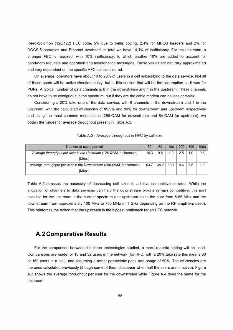
88

Reed-Solomon (128/122) FEC code, 5% due to trellis coding, 2.4% for MPEG headers and 2% for

DOCSIS operation and Ethernet overhead. In total we have 14,1% of inefficiency. For the upstream, a

stronger FEC is required, with 10% inefficiency, to which another 10% are added to account for

bandwidth requests and operation and maintenance messages. These values are naturally approximated

and very dependent on the specific HFC cell considered.

On average, operators have about 10 to 20% of users in a cell subscribing to the data service. Not all

of those users will be active simultaneously, but in this section that will be the assumption as it was for

PONs. A typical number of data channels is 8 in the downstream and 4 in the upstream. These channels

do not have to be contiguous in the spectrum, but if they are the cable modem can be less complex.

Considering a 20% take rate of the data service, with 8 channels in the downstream and 4 in the

upstream, with the calculated efficiencies of 85,9% and 80% for downstream and upstream respectively

and using the most common modulations (256-QAM for downstream and 64-QAM for upstream), we

obtain the values for average throughput present in Table A.5.

Table A.5 - Average throughput in HFC by cell size.

Number of users per cell 30 50 100 200 500 1000

Average throughput per user in the Upstream (128-QAM, 4 channels)

[Mbps].

16,3 9,8 4,9 2,5 1,0 0,5

Average throughput per user in the Downstream (256-QAM, 8 channels)

[Mbps].

63,7 38,2 19,1 9.6 3,8 1,9

Table A.5 stresses the necessity of decreasing cell sizes to achieve competitive bit-rates. While the

allocation of channels to data services can help the downstream bit-rate remain competitive, this isn’t

possible for the upstream in the current spectrum (the upstream takes the slice from 5-65 MHz and the

downstream from approximately 100 MHz to 750 MHz or 1 GHz depending on the RF amplifiers used).

This reinforces the notion that the upstream is the biggest bottleneck for an HFC network.

A.2 Comparative Results

For the comparison between the three technologies studied, a more realistic setting will be used.

Comparisons are made for 16 and 32 users in the network (for HFC, with a 20% take rate this means 80

or 160 users in a cell), and assuming a rather pessimistic peak rate usage of 50%. The efficiencies are

the ones calculated previously (though some of them disappear when half the users aren’t active). Figure

A.3 shows the average throughput per user for the downstream while Figure A.4 does the same for the

upstream.

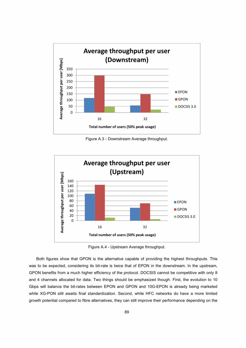
89

Figure A.3 - Downstream Average throughput.

Figure A.4 - Upstream Average throughput.

Both figures show that GPON is the alternative capable of providing the highest throughputs. This

was to be expected, considering its bit-rate is twice that of EPON in the downstream. In the upstream,

GPON benefits from a much higher efficiency of the protocol. DOCSIS cannot be competitive with only 8

and 4 channels allocated for data. Two things should be emphasized though. First, the evolution to 10

Gbps will balance the bit-rates between EPON and GPON and 10G-EPON is already being marketed

while XG-PON still awaits final standardization. Second, while HFC networks do have a more limited

growth potential compared to fibre alternatives, they can still improve their performance depending on the

0

50

100

150

200

250

300

350

16 32Av

era

ge

th

rou

gh

pu

t p

er

use

r [M

bp

s]

Total number of users (50% peak usage)

Average throughput per user

(Downstream)

EPON

GPON

DOCSIS 3.0

0

20

40

60

80

100

120

140

160

16 32

Av

era

ge

th

rou

gh

pu

t p

er

use

r [M

bp

s]

Total number of users (50% peak usage)

Average throughput per user

(Upstream)

EPON

GPON

DOCSIS 3.0

90

operators’ ability to reuse the analog channels in the spectrum for data services, and perhaps extend the

upstream band towards a less asymmetrical network.

91

B. Software Implementation

This Appendix offers some insight on the implementation of the ILP models in the software used,

namely lpsolve and MATLAB®.

B.1 Describing the Model

The solver used for implementing the ILP models was lpsolve, a free licensed package. As with most

solvers, to describe the model one only has to feed the usual parameters, in the canonical form:

��� m (B.1)

Subject to:

e� � # (B.2)

Normally, this would have to be inserted manually. However, in this case lpsolve’s Application

Programming Interface (API) was used in conjunction with MATLAB®. This enabled the use of MATLAB’s

matrix oriented interface to quickly formulate different models.

The vectors m and # and the matrix e are easily inserted with MATLAB. As for the sign of the

inequalities, lpsolve accepts an inequality vector where -1 means “lower than or equal”, 0 means “equal”

and 1 means “greater than or equal”. The software does not accept strict inequalities because of rounding

errors. For LP models the practical result is the same since the solution can be as close to the bound as

desired without reaching it. For ILP or MILP models, an equivalent strict inequality is achieved by setting

the bound to the next or previous integer according to the inequality sign, so for instance if one has � © W

it is the same as having � � � when � is integer.

The definition of the variables’ bounds is also provided in vector form with an entry for each variable.

By default, the variables in lpsolve have a lower bound of zero. In all the models described in this work,

no variable could be negative so this was not changed. That is the reason (along with compactness of the

model) why the formulations do not include the explicit constraints setting the variables to be greater than

or equal to zero. The lower bound vector is therefore filled with zeros. The upper bound vector can either

be set accordingly to the model (for instance in ILP Model 2, the � variables had an upper bound

corresponding to the maximum number of splitters per Junction Box) or it can be set to plus infinity and let

specific constraints limit the variable’s range. Setting bounds through the bound vectors usually helps

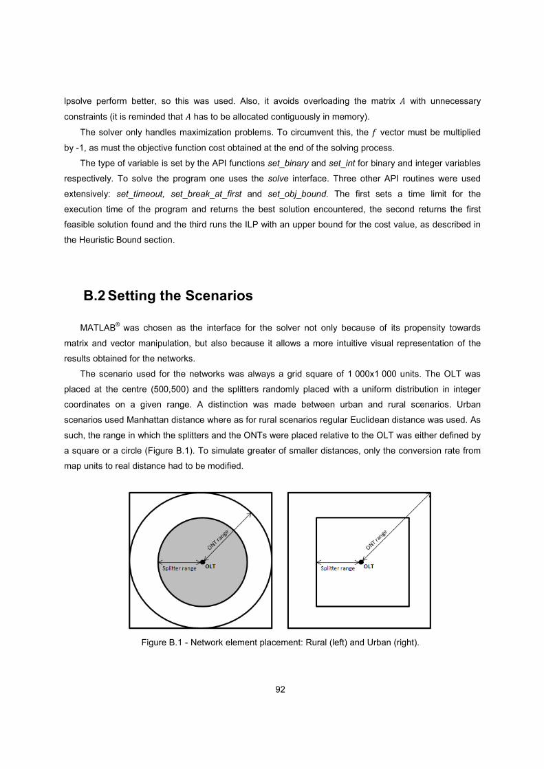
92

lpsolve perform better, so this was used. Also, it avoids overloading the matrix e with unnecessary

constraints (it is reminded that e has to be allocated contiguously in memory).

The solver only handles maximization problems. To circumvent this, the m vector must be multiplied

by -1, as must the objective function cost obtained at the end of the solving process.

The type of variable is set by the API functions set_binary and set_int for binary and integer variables

respectively. To solve the program one uses the solve interface. Three other API routines were used

extensively: set_timeout, set_break_at_first and set_obj_bound. The first sets a time limit for the

execution time of the program and returns the best solution encountered, the second returns the first

feasible solution found and the third runs the ILP with an upper bound for the cost value, as described in

the Heuristic Bound section.

B.2 Setting the Scenarios

MATLAB® was chosen as the interface for the solver not only because of its propensity towards

matrix and vector manipulation, but also because it allows a more intuitive visual representation of the

results obtained for the networks.

The scenario used for the networks was always a grid square of 1 000x1 000 units. The OLT was

placed at the centre (500,500) and the splitters randomly placed with a uniform distribution in integer

coordinates on a given range. A distinction was made between urban and rural scenarios. Urban

scenarios used Manhattan distance where as for rural scenarios regular Euclidean distance was used. As

such, the range in which the splitters and the ONTs were placed relative to the OLT was either defined by

a square or a circle (Figure B.1). To simulate greater of smaller distances, only the conversion rate from

map units to real distance had to be modified.

Figure B.1 - Network element placement: Rural (left) and Urban (right).

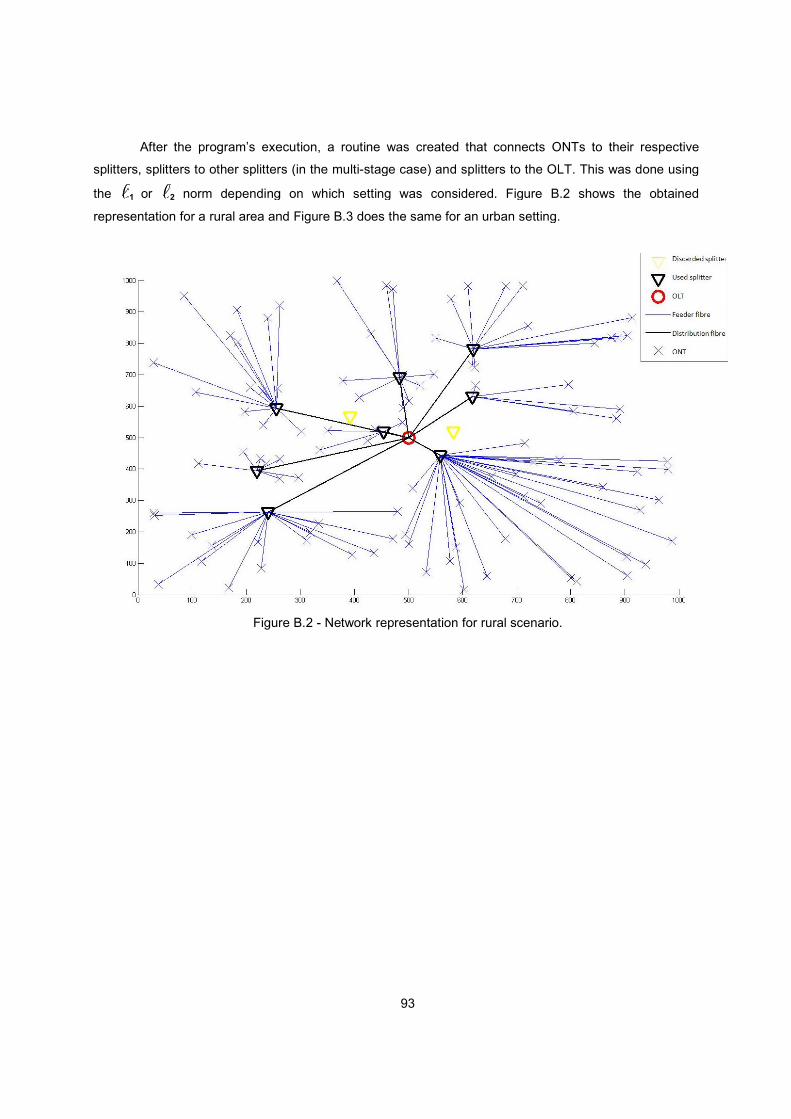
After the program’s execution, a routine was created that connects ONTs to their respective

splitters, splitters to other splitters (in the multi

the 1 or 2 norm depending on which setting was con

representation for a rural area and

Figure B.

93

After the program’s execution, a routine was created that connects ONTs to their respective

splitters, splitters to other splitters (in the multi-stage case) and splitters to the OLT. This was done using

norm depending on which setting was considered. Figure B.

representation for a rural area and Figure B.3 does the same for an urban setting.

Figure B.2 - Network representation for rural scenario.

After the program’s execution, a routine was created that connects ONTs to their respective

stage case) and splitters to the OLT. This was done using

Figure B.2 shows the obtained

does the same for an urban setting.

Network representation for rural scenario.

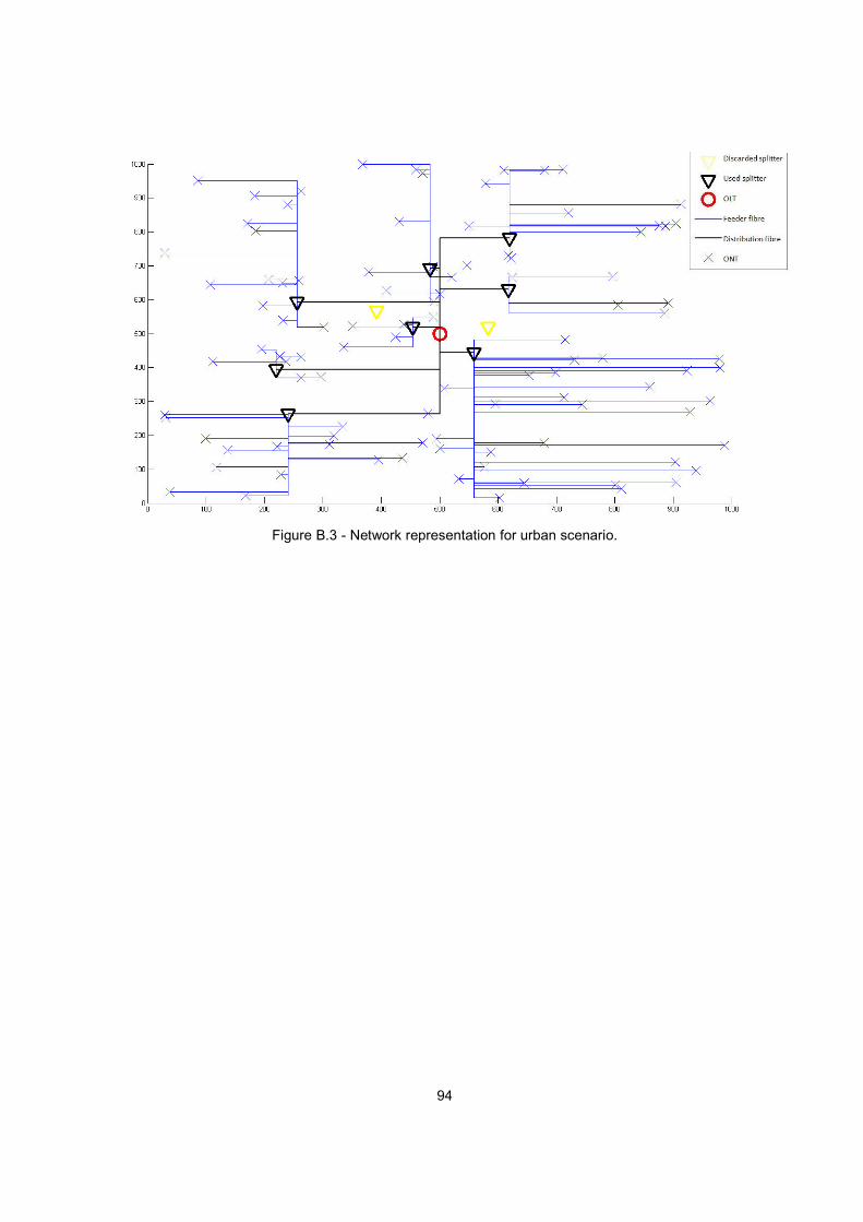
94

Figure B.3 - Network representation for urban scenario.

95

C. Physical Parameters

This Appendix covers the details regarding the physical layer properties considered in the model,

describing the values used, based on ITU-T Recommendations, for power budget calculations. The

optical penalties’ expressions are also presented.

C.1 Power Budget

The values used for the calculation of the optical power budget were extracted from ITU-T

Recommendation G.984.2 for GPON and Recommendation G.987.2 for XG-PON. For GPON, a industry-

best-practise amendment was used, detailing most common values for operation of GPON with 2,488

Gbps in the downstream and 1,244 Gbps in the upstream. The most relevant aspects of this

consideration are the use of class B+ optics, a more restrictive maximum optical path penalty of 0,5 dB

and the mandatory use of FEC in the downstream. The relevant values are shown in Table C.1

Table C.1 - GPON optical power levels for 2,488 Gbps downstream and 1,244 Gbps upstream. Source:[39]

Item Unit Value

OLT

Minimum mean launched power dBm 1,5

Maximum mean launched power dBm 5

Minimum sensitivity dBm -28

Minimum overload dBm -8

Downstream optical path penalty dB 0,5

ONT

Minimum mean launched power dBm 0,5

Maximum mean launched power dBm 5

Minimum sensitivity dBm -27

Minimum overload dBm -8

Upstream optical path penalty dB 0,5

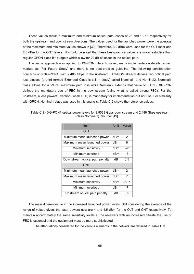
96

These values result in maximum and minimum optical path losses of 28 and 13 dB respectively for

both the upstream and downstream directions. The values used for the launched power were the average

of the maximum and minimum values shown in [39]. Therefore, 3,2 dBm were used for the OLT laser and

2,8 dBm for the ONT lasers. It should be noted that these best-practise values are more restrictive than

regular GPON class B+ budgets which allow for 29 dB of losses in the optical path.

The same approach was applied to XG-PON. Here however, many implementation details remain

marked as “For Future Study” and there is no best-practise guideline. The following consideration

concerns only XG-PON1 (with 2,488 Gbps in the upstream). XG-PON already defines two optical path

loss classes (a third termed Extended Class is still in study) called Nominal1 and Nominal2. Nominal1

class allows for a 29 dB maximum path loss while Nominal2 extends that value to 31 dB. XG-PON

defines the mandatory use of FEC in the downstream (using what is called strong FEC). For the

upstream, a less powerful version (weak FEC) is mandatory for implementation but not use. For similarity

with GPON, Nominal1 class was used in this analysis. Table C.2 shows the reference values.

Table C.2 - XG-PON1 optical power levels for 9,9533 Gbps downstream and 2,488 Gbps upstream (class Nominal1). Source: [49].

Item Unit Value

OLT

Minimum mean launched power dBm 2

Maximum mean launched power dBm 6

Minimum sensitivity dBm -28

Minimum overload dBm -8

Downstream optical path penalty dB 0,5

ONT

Minimum mean launched power dBm 2

Maximum mean launched power dBm 7

Minimum sensitivity dBm -27,5

Minimum overload dBm -7

Upstream optical path penalty dB 0,5

The main differences lie in the increased launched power levels. Still considering the average of the

range of values given, the laser powers now are 4 and 4,5 dBm for the OLT and ONT respectively. To

maintain approximately the same sensitivity levels at the receivers with an increased bit-rate the use of

FEC is essential and the equipment must be more sophisticated.

The attenuations considered for the various elements in the network are detailed in Table C.3.

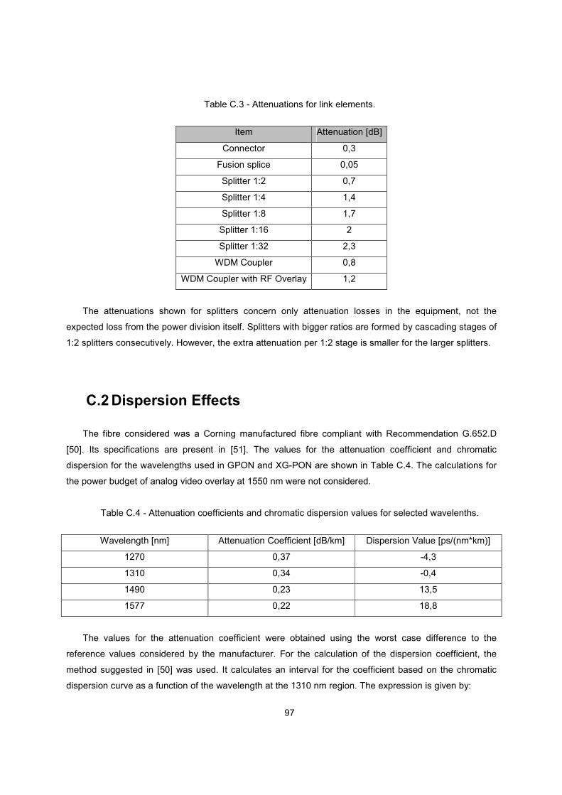
97

Table C.3 - Attenuations for link elements.

Item Attenuation [dB]

Connector 0,3

Fusion splice 0,05

Splitter 1:2 0,7

Splitter 1:4 1,4

Splitter 1:8 1,7

Splitter 1:16 2

Splitter 1:32 2,3

WDM Coupler 0,8

WDM Coupler with RF Overlay 1,2

The attenuations shown for splitters concern only attenuation losses in the equipment, not the

expected loss from the power division itself. Splitters with bigger ratios are formed by cascading stages of

1:2 splitters consecutively. However, the extra attenuation per 1:2 stage is smaller for the larger splitters.

C.2 Dispersion Effects

The fibre considered was a Corning manufactured fibre compliant with Recommendation G.652.D

[50]. Its specifications are present in [51]. The values for the attenuation coefficient and chromatic

dispersion for the wavelengths used in GPON and XG-PON are shown in Table C.4. The calculations for

the power budget of analog video overlay at 1550 nm were not considered.

Table C.4 - Attenuation coefficients and chromatic dispersion values for selected wavelenths.

Wavelength [nm] Attenuation Coefficient [dB/km] Dispersion Value [ps/(nm*km)]

1270 0,37 -4,3

1310 0,34 -0,4

1490 0,23 13,5

1577 0,22 18,8

The values for the attenuation coefficient were obtained using the worst case difference to the

reference values considered by the manufacturer. For the calculation of the dispersion coefficient, the

method suggested in [50] was used. It calculates an interval for the coefficient based on the chromatic

dispersion curve as a function of the wavelength at the 1310 nm region. The expression is given by:

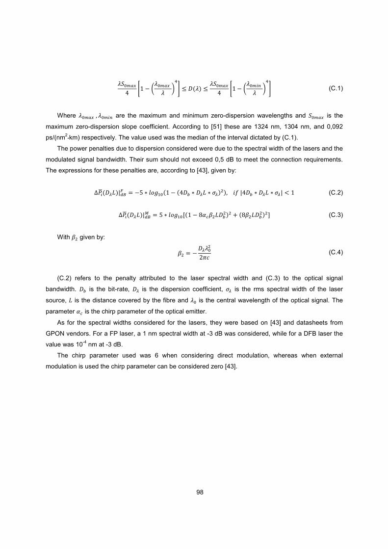
98

ªo�«�Od ¬� V ­ª�«�O �ª ®¯° � gDªB � ªo�«�Od ¬� V ­ª�«� �ª ®¯° (C.1)

Where ª�«�O �� ª�«� are the maximum and minimum zero-dispersion wavelengths and o�«�O is the

maximum zero-dispersion slope coefficient. According to [51] these are 1324 nm, 1304 nm, and 0,092

ps/(nm2*km) respectively. The value used was the median of the interval dictated by (C.1).

The power penalties due to dispersion considered were due to the spectral width of the lasers and the

modulated signal bandwidth. Their sum should not exceed 0,5 dB to meet the connection requirements.

The expressions for these penalties are, according to [43], given by:

uy��Dg�lB±�²³ � V] ? '�b��D� V Ddg´ ? g�l ? µ�BcB������m�±dg´ ? g�l ? µ�± © � (C.2)

uy��Dg�lB±�²� � ] ? '�b��_D� V C{�¶clgcBc � DC¶clgcBca (C.3)

With ¶c given by:

¶c � Vg�ª�cW·� (C.4)

(C.2) refers to the penalty attributed to the laser spectral width and (C.3) to the optical signal

bandwidth. g´ is the bit-rate, g� is the dispersion coefficient, µ� is the rms spectral width of the laser

source, l is the distance covered by the fibre and ª� is the central wavelength of the optical signal. The

parameter {� is the chirp parameter of the optical emitter.

As for the spectral widths considered for the lasers, they were based on [43] and datasheets from

GPON vendors. For a FP laser, a 1 nm spectral width at -3 dB was considered, while for a DFB laser the

value was 10-4 nm at -3 dB.

The chirp parameter used was 6 when considering direct modulation, whereas when external

modulation is used the chirp parameter can be considered zero [43].

99