Embed Size (px)
Citation preview

R. GRIBONVAL - CSA 2015 - Berlin
Contributors & Collaborators
2
Anthony Bourrier Nicolas Keriven Yann Traonmilin
Tomer Peleg
Gilles Puy
Mike Davies Patrick PerezGilles Blanchard

R. GRIBONVAL - CSA 2015 - Berlin
Agenda
From Compressive Sensing to Compressive Learning ? Information-preserving projections & sketches Compressive Clustering / Compressive GMM Conclusion
3

R. GRIBONVAL - CSA 2015 - Berlin
Machine Learning
Available data training collection of feature vectors = point cloud
Goals infer parameters to achieve a certain task generalization to future samples with the same probability distribution
Examples
4
Compressive Gaussian Mixture Estimation
Anthony Bourrier
12, R
´
emi Gribonval
2, Patrick P
´
erez
11 Technicolor, 975 Avenue des Champs Blancs, 35576 Cesson Sevigne, France
2 INRIA Rennes - Bretagne Atlantique, Campus de Beaulieu, 35042 Rennes, [email protected]
Motivation
Goal: Infer parameters ✓ from n-dimensional data X = {x1
, . . . ,xN}. Thistypically requires extensive access to the data. Proposed method: Inferfrom a sketch of the data ) memory and privacy savings.
n x
1
. . .xN
Learning set(size Nn)
ˆ
A
=) mˆ
z
Database sketch(size m)
L=) K ✓
Learned parameters(size K)
Figure 1: Illustration of the proposed sketching framework. A is a sketch-
ing operator, L is a learning method from the sketch.
Model and problem statement
Application to mixture of isotropic Gaussians in Rn:
fµ / exp
��kx� µk2
2
/(2�2
)
�. (1)
Data X = {xj}Nj=1 ⇠i.i.d.
p =
Pks=1↵sfµs
with:
•weights ↵1
, . . . ,↵k (positive, sum to one)•means µ
1
, . . . ,µk 2 Rn.
Sketch = Fourier samplings at different frequencies: (Af )l = ˆf (!l).Empirical version: ( ˆA(X ))l =
1
N
PNj=1 exp(�ih!l,xji) ⇡ (Ap)l.
We want to infer the mixture parameters from ˆ
z =
ˆ
A(X ).Problem casted as:
p = argminq2⌃k
kˆz�Aqk22
, (2)
where ⌃k = mixtures of k isotropic Gaussians with positive weights.Standard CS Our problem
Signal x 2 Rn f 2 L1
(Rn)
Dimension n InfiniteSparsity k k
Dictionary {e1
, . . . , en} F = {fµ,µ 2 Rn}Measurements x 7! ha,xi f 7!
RRn f (x)e�ih!,xidx
Algorithm
Current estimate p with weights {↵s}ks=1 and support ˆ� = {ˆµs}ks=1.Residual ˆr = ˆ
z�Ap.1. Searching new support functions:
Search for ”good components to add” to the support) Local minima of µ 7! �hAfµ, ˆri, added to the support ˆ�.New support ˆ�0.
2. k-term thresholding:Projection of ˆz onto ˆ
�
0 with positivity constraints on coefficients:
argmin�2RK
+
||ˆz�U�||22
, (3)
with U = [
ˆµ1
, . . . , ˆµK].k highest coefficients and corresponding support are kept! new support ˆ� and coefficients ↵
1
, . . . , ↵k.3. Final ”shift”:
Gradient descent algorithm on the objective function, with initialization atthe current support and coefficients.
First step Second step Third step
Figure 2: Algorithm illustration in dimension n = 1 for k = 3 Gaus-
sians. Top: Iteration 1. Bottom: Iteration 2. Blue curve=true mixture,
Red curve=reconstructed mixture, Green curve=gradient function. Green
Dots=Candidate Centroids, Red Dots=Reconstructed Centroids.
Experimental results
Data setup: � = 1, (↵1
, . . . ,↵k) drawn uniformly on the simplex.Entries of µ
1
, . . . ,µk ⇠i.i.d.
N (0, 1).
Algorithm heuristics:•Frequencies drawn i.i.d. from N (0, Id).
•New support function search (step 1) initialized as ru, where r uniformly
drawn in0,max
x2X||x||
2
�and u uniformly drawn on B
2
(0, 1).
Comparison between:•Our method: Sketch is computed on-the-fly and data is discarded.
•EM: Data is stored to allow the standard optimization steps to be per-formed.
Quality measures: KL Divergence and Hellinger distance.
NCompressed EM
KL div. Hell. Mem. KL div. Hell. Mem.10
3
0.68± 0.28 0.06± 0.01 0.6 0.68± 0.44 0.07± 0.03 0.2410
4
0.24± 0.31 0.02± 0.02 0.6 0.19± 0.21 0.01± 0.02 2.410
5
0.13± 0.15 0.01± 0.02 0.6 0.13± 0.21 0.01± 0.02 24
Table 1: Comparison between our method and an EM algorithm. n =
20, k = 10,m = 1000.
−4 −2 0 2 4 6 8
−4
−2
0
2
4
6
ˆ
A
=)
−0.5 0 0.5 10
10
20
30
40
50
60 n=10, Hell. for 80%
sketch size m
k*n/
m
200 400 600 800 1000 1200 1400 1600 1800 2000
1
0.9
0.8
0.7
0.6
0.5
0.4
0.3
0.2
0.1
0
0.02
0.04
0.06
0.08
0.1
0.12
0.14
0.16
Figure 3: Left: Example of data and sketch for n = 2. Right: Reconstruc-
tion quality for n = 10.
-6 -4 -2 0 2 4 6-4
-3
-2
-1
0
1
2
3
PCA principal subspace
Dictionary learning dictionary
Clustering centroids
Classification classifier parameters
(e.g. support vectors)
X

R. GRIBONVAL - CSA 2015 - Berlin
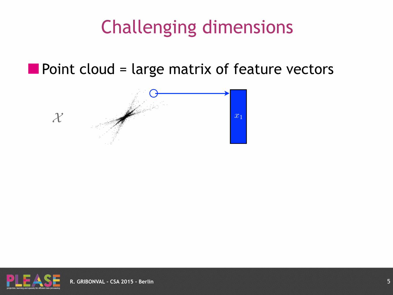
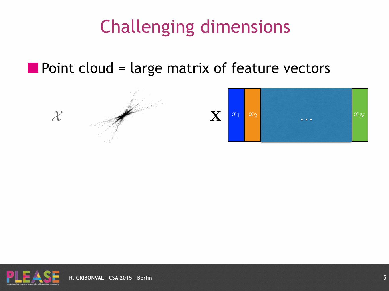
Point cloud = large matrix of feature vectors
Challenging dimensions
5
X
R. GRIBONVAL - CSA 2015 - Berlin
Point cloud = large matrix of feature vectors
Challenging dimensions
5
x1X
R. GRIBONVAL - CSA 2015 - Berlin
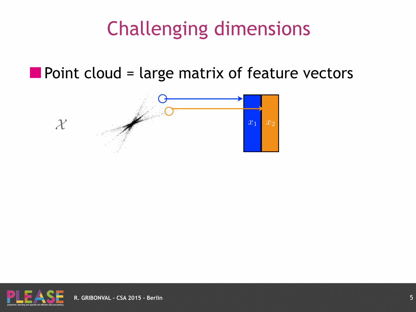
Point cloud = large matrix of feature vectors
Challenging dimensions
5
x1 x2X
R. GRIBONVAL - CSA 2015 - Berlin
Point cloud = large matrix of feature vectors
Challenging dimensions
5
x1 x2 xN…X X
R. GRIBONVAL - CSA 2015 - Berlin
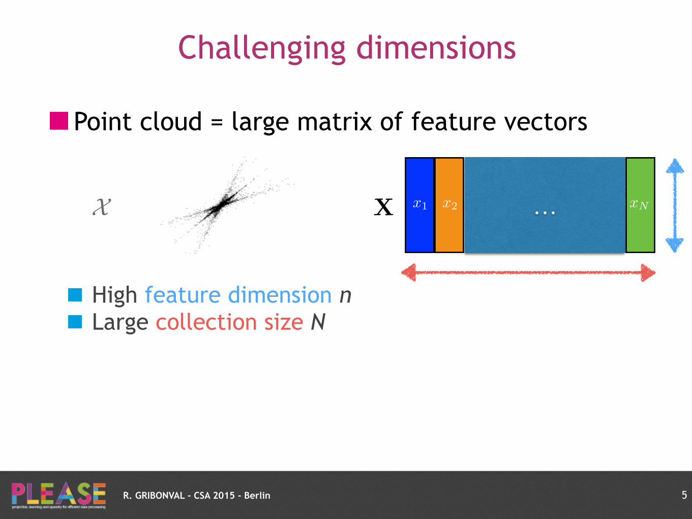
Point cloud = large matrix of feature vectors
High feature dimension n Large collection size N
Challenging dimensions
5
x1 x2 xN…X X
R. GRIBONVAL - CSA 2015 - Berlin
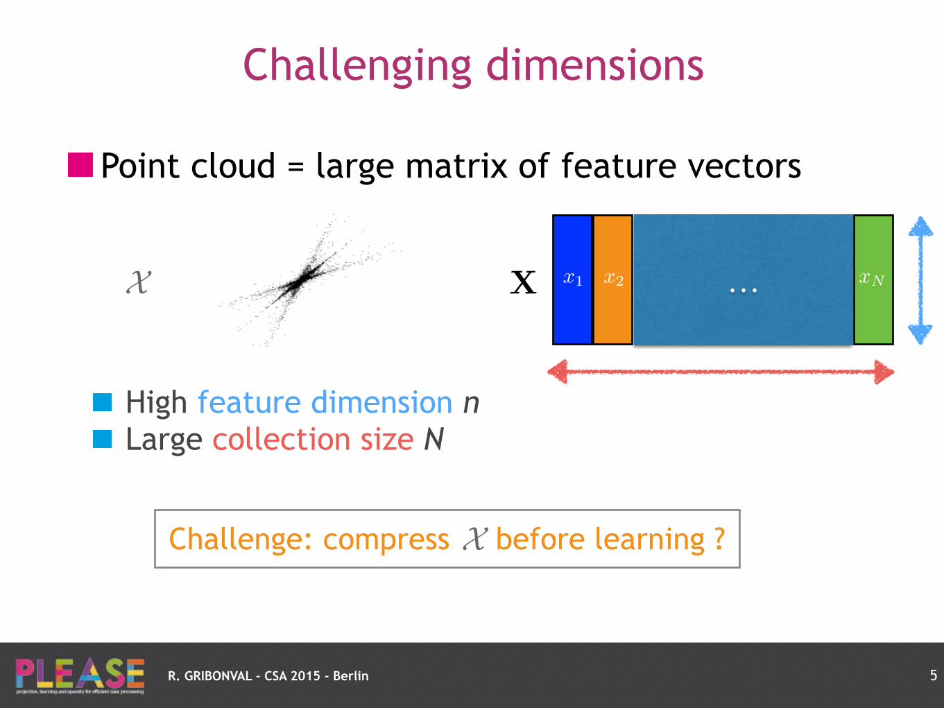
Point cloud = large matrix of feature vectors
High feature dimension n Large collection size N
Challenging dimensions
5
x1 x2 xN…X X
Challenge: compress before learning ?X
R. GRIBONVAL - CSA 2015 - Berlin
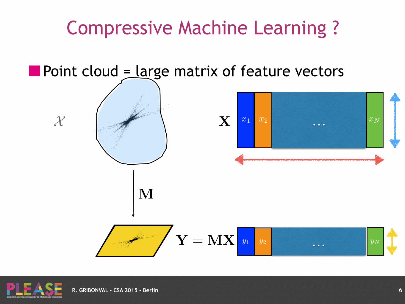
Compressive Machine Learning ?
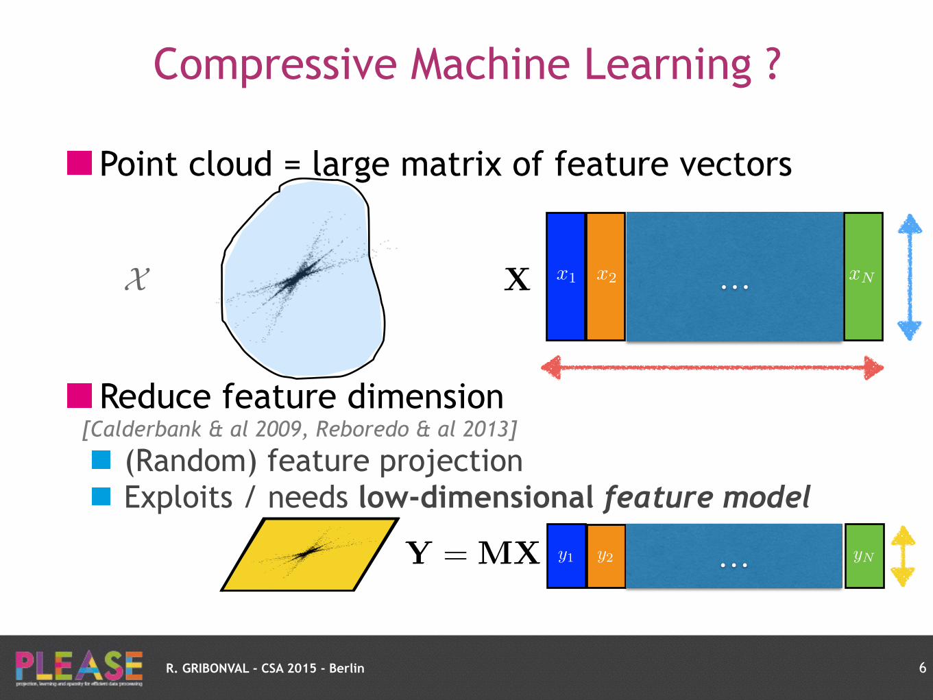
Point cloud = large matrix of feature vectors
6
x1 x2 xN…X X
yNy2 …y1Y = MX
M
R. GRIBONVAL - CSA 2015 - Berlin
Compressive Machine Learning ?
Point cloud = large matrix of feature vectors
Reduce feature dimension [Calderbank & al 2009, Reboredo & al 2013]
(Random) feature projection Exploits / needs low-dimensional feature model
6
x1 x2 xN…X X
yNy2 …y1Y = MX

R. GRIBONVAL - CSA 2015 - Berlin
Challenges of large collections
Feature projection: limited impact
7
X
Y = MX

R. GRIBONVAL - CSA 2015 - Berlin
Challenges of large collections
Feature projection: limited impact
7
X
Y = MX
“Big Data” Challenge: compress collection size

R. GRIBONVAL - CSA 2015 - Berlin
Compressive Machine Learning ?
Point cloud = … empirical probability distribution
8
X
R. GRIBONVAL - CSA 2015 - Berlin
Compressive Machine Learning ?
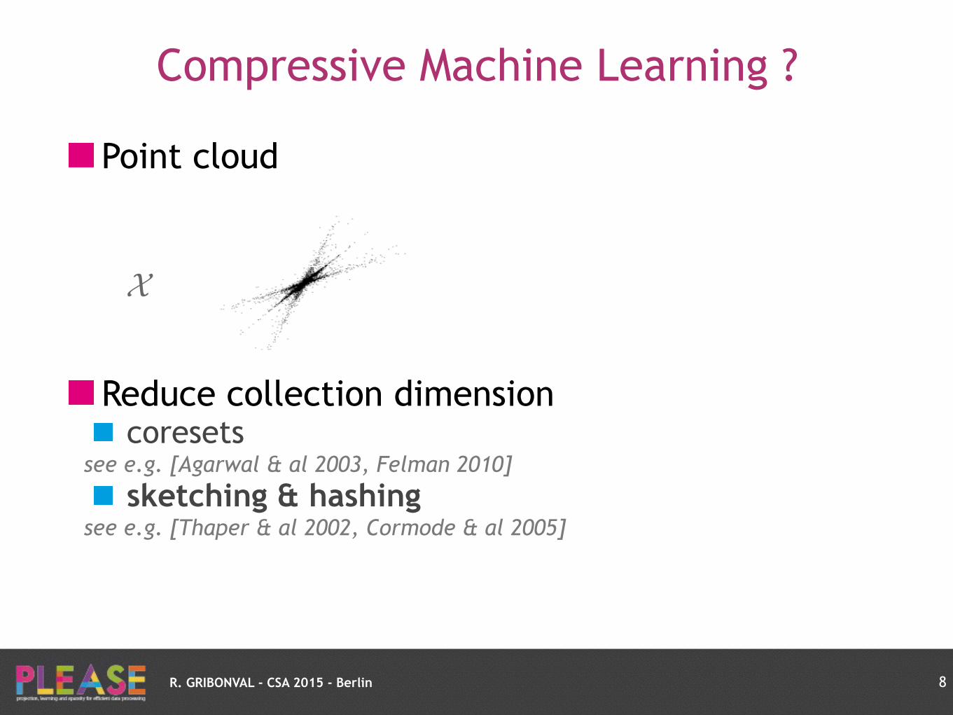
Point cloud = … empirical probability distribution
Reduce collection dimension coresets
see e.g. [Agarwal & al 2003, Felman 2010]
sketching & hashing see e.g. [Thaper & al 2002, Cormode & al 2005]
8
X
R. GRIBONVAL - CSA 2015 - Berlin
Compressive Machine Learning ?
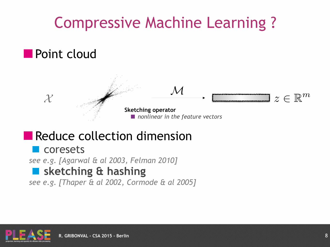
Point cloud = … empirical probability distribution
Reduce collection dimension coresets
see e.g. [Agarwal & al 2003, Felman 2010]
sketching & hashing see e.g. [Thaper & al 2002, Cormode & al 2005]
8
XM
z 2 Rm
Sketching operator nonlinear in the feature vectors
linear in their probability distribution
R. GRIBONVAL - CSA 2015 - Berlin
Compressive Machine Learning ?
Point cloud = … empirical probability distribution
Reduce collection dimension coresets
see e.g. [Agarwal & al 2003, Felman 2010]
sketching & hashing see e.g. [Thaper & al 2002, Cormode & al 2005]
8
XM
z 2 Rm
Sketching operator nonlinear in the feature vectors
linear in their probability distribution
R. GRIBONVAL - CSA 2015 - Berlin
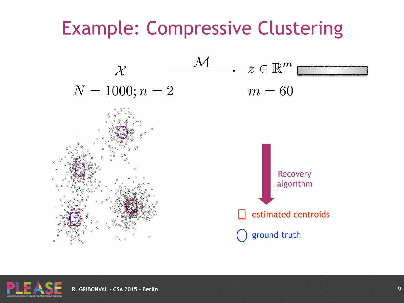
Example: Compressive Clustering
9
X
Compressive Gaussian Mixture Estimation
Anthony Bourrier
12, R
´
emi Gribonval
2, Patrick P
´
erez
11 Technicolor, 975 Avenue des Champs Blancs, 35576 Cesson Sevigne, France
2 INRIA Rennes - Bretagne Atlantique, Campus de Beaulieu, 35042 Rennes, [email protected]
Motivation
Goal: Infer parameters ✓ from n-dimensional data X = {x1
, . . . ,xN}. Thistypically requires extensive access to the data. Proposed method: Inferfrom a sketch of the data ) memory and privacy savings.
n x
1
. . .xN
Learning set(size Nn)
ˆ
A
=) mˆ
z
Database sketch(size m)
L=) K ✓
Learned parameters(size K)
Figure 1: Illustration of the proposed sketching framework. A is a sketch-
ing operator, L is a learning method from the sketch.
Model and problem statement
Application to mixture of isotropic Gaussians in Rn:
fµ / exp
��kx� µk2
2
/(2�2
)
�. (1)
Data X = {xj}Nj=1 ⇠i.i.d.
p =
Pks=1↵sfµs
with:
•weights ↵1
, . . . ,↵k (positive, sum to one)•means µ
1
, . . . ,µk 2 Rn.
Sketch = Fourier samplings at different frequencies: (Af )l = ˆf (!l).Empirical version: ( ˆA(X ))l =
1
N
PNj=1 exp(�ih!l,xji) ⇡ (Ap)l.
We want to infer the mixture parameters from ˆ
z =
ˆ
A(X ).Problem casted as:
p = argminq2⌃k
kˆz�Aqk22
, (2)
where ⌃k = mixtures of k isotropic Gaussians with positive weights.Standard CS Our problem
Signal x 2 Rn f 2 L1
(Rn)
Dimension n InfiniteSparsity k k
Dictionary {e1
, . . . , en} F = {fµ,µ 2 Rn}Measurements x 7! ha,xi f 7!
RRn f (x)e�ih!,xidx
Algorithm
Current estimate p with weights {↵s}ks=1 and support ˆ� = {ˆµs}ks=1.Residual ˆr = ˆ
z�Ap.1. Searching new support functions:
Search for ”good components to add” to the support) Local minima of µ 7! �hAfµ, ˆri, added to the support ˆ�.New support ˆ�0.
2. k-term thresholding:Projection of ˆz onto ˆ
�
0 with positivity constraints on coefficients:
argmin�2RK
+
||ˆz�U�||22
, (3)
with U = [
ˆµ1
, . . . , ˆµK].k highest coefficients and corresponding support are kept! new support ˆ� and coefficients ↵
1
, . . . , ↵k.3. Final ”shift”:
Gradient descent algorithm on the objective function, with initialization atthe current support and coefficients.
First step Second step Third step
Figure 2: Algorithm illustration in dimension n = 1 for k = 3 Gaus-
sians. Top: Iteration 1. Bottom: Iteration 2. Blue curve=true mixture,
Red curve=reconstructed mixture, Green curve=gradient function. Green
Dots=Candidate Centroids, Red Dots=Reconstructed Centroids.
Experimental results
Data setup: � = 1, (↵1
, . . . ,↵k) drawn uniformly on the simplex.Entries of µ
1
, . . . ,µk ⇠i.i.d.
N (0, 1).
Algorithm heuristics:•Frequencies drawn i.i.d. from N (0, Id).
•New support function search (step 1) initialized as ru, where r uniformly
drawn in0,max
x2X||x||
2
�and u uniformly drawn on B
2
(0, 1).
Comparison between:•Our method: Sketch is computed on-the-fly and data is discarded.
•EM: Data is stored to allow the standard optimization steps to be per-formed.
Quality measures: KL Divergence and Hellinger distance.
NCompressed EM
KL div. Hell. Mem. KL div. Hell. Mem.10
3
0.68± 0.28 0.06± 0.01 0.6 0.68± 0.44 0.07± 0.03 0.2410
4
0.24± 0.31 0.02± 0.02 0.6 0.19± 0.21 0.01± 0.02 2.410
5
0.13± 0.15 0.01± 0.02 0.6 0.13± 0.21 0.01± 0.02 24
Table 1: Comparison between our method and an EM algorithm. n =
20, k = 10,m = 1000.
−4 −2 0 2 4 6 8
−4
−2
0
2
4
6
ˆ
A
=)
−0.5 0 0.5 10
10
20
30
40
50
60 n=10, Hell. for 80%
sketch size m
k*n/
m
200 400 600 800 1000 1200 1400 1600 1800 2000
1
0.9
0.8
0.7
0.6
0.5
0.4
0.3
0.2
0.1
0
0.02
0.04
0.06
0.08
0.1
0.12
0.14
0.16
Figure 3: Left: Example of data and sketch for n = 2. Right: Reconstruc-
tion quality for n = 10.
M z 2 Rm
Recovery algorithm
estimated centroids
ground truth
N = 1000;n = 2 m = 60
R. GRIBONVAL - CSA 2015 - Berlin
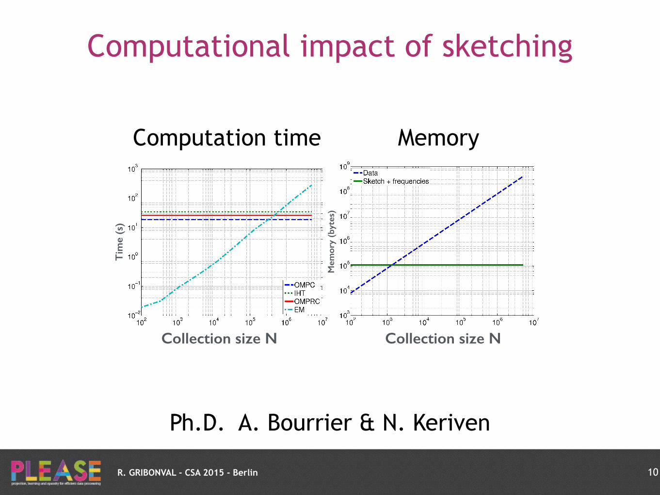
Computational impact of sketching
10
Ph.D. A. Bourrier & N. Keriven
Computation time Memory
Collection size N Collection size N
Tim
e (s
)
Mem
ory
(byt
es)

R. GRIBONVAL - CSA 2015 - Berlin
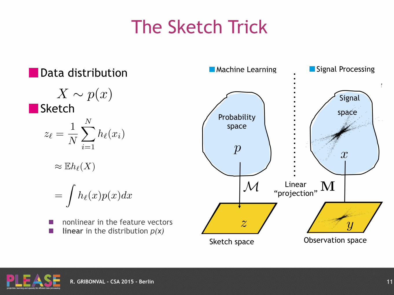
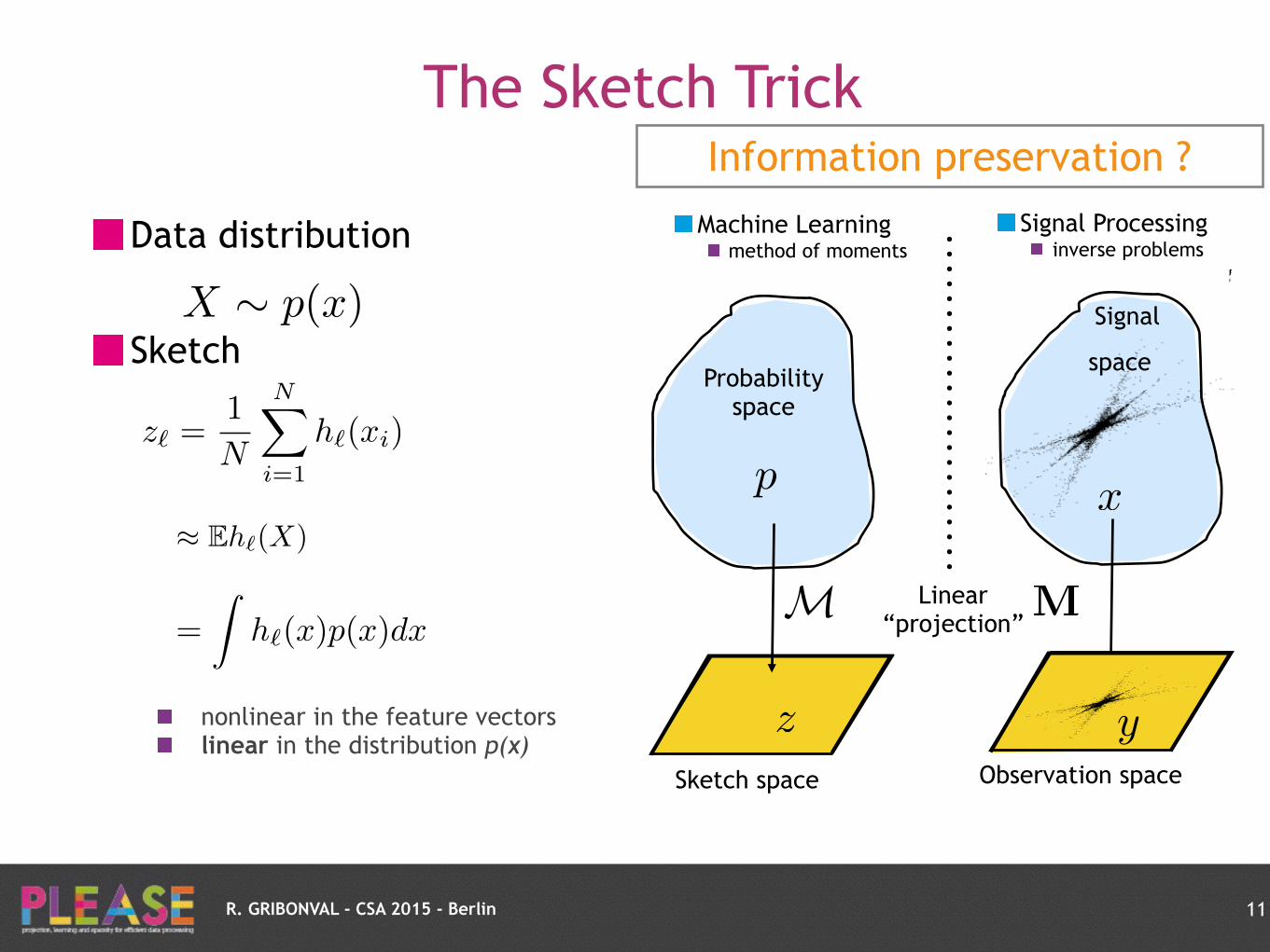
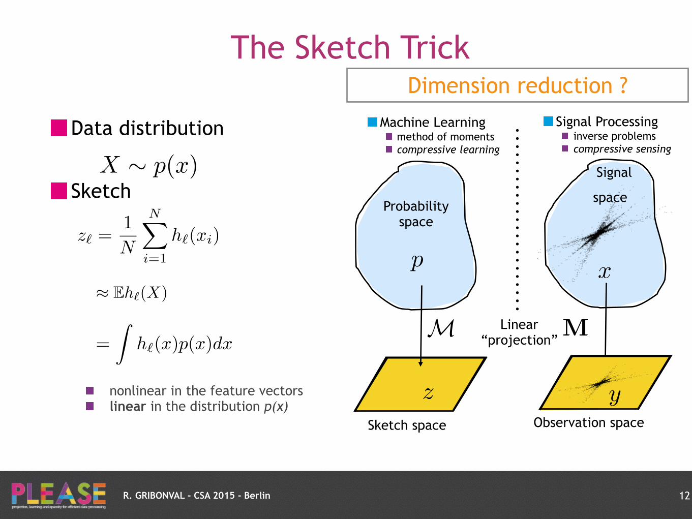
Data distribution
Sketch
The Sketch Trick
11
X ⇠ p(x)
z` =1
N
NX
i=1
h`(xi)

R. GRIBONVAL - CSA 2015 - Berlin
Data distribution
Sketch
The Sketch Trick
11
X ⇠ p(x)
z` =1
N
NX
i=1
h`(xi)
⇡ Eh`(X)

R. GRIBONVAL - CSA 2015 - Berlin
Data distribution
Sketch
The Sketch Trick
11
X ⇠ p(x)
z` =1
N
NX
i=1
h`(xi)
⇡ Eh`(X)
=
Zh`(x)p(x)dx

R. GRIBONVAL - CSA 2015 - Berlin
Data distribution
Sketch
The Sketch Trick
11
X ⇠ p(x)
z` =1
N
NX
i=1
h`(xi)
⇡ Eh`(X)
=
Zh`(x)p(x)dx
nonlinear in the feature vectors linear in the distribution p(x)
R. GRIBONVAL - CSA 2015 - Berlin
Data distribution
Sketch
The Sketch Trick
11
X ⇠ p(x)
z` =1
N
NX
i=1
h`(xi)
⇡ Eh`(X)
=
Zh`(x)p(x)dx
y
Signal
space
x
Observation space
Signal Processing inverse problems compressive sensing
MM
Probability space
Sketch space
Machine Learning method of moments compressive learning
z
p
Linear “projection”
nonlinear in the feature vectors linear in the distribution p(x)
R. GRIBONVAL - CSA 2015 - Berlin
Information preservation ?
Data distribution
Sketch
The Sketch Trick
11
X ⇠ p(x)
z` =1
N
NX
i=1
h`(xi)
⇡ Eh`(X)
=
Zh`(x)p(x)dx
y
Signal
space
x
Observation space
Signal Processing inverse problems compressive sensing
MM
Probability space
Sketch space
Machine Learning method of moments compressive learning
z
p
Linear “projection”
nonlinear in the feature vectors linear in the distribution p(x)
R. GRIBONVAL - CSA 2015 - Berlin
The Sketch Trick
Data distribution
Sketch
Dimension reduction ?
12
X ⇠ p(x)
z` =1
N
NX
i=1
h`(xi)
⇡ Eh`(X)
=
Zh`(x)p(x)dx
y
Signal
space
x
Observation space
Signal Processing inverse problems compressive sensing
MM
Probability space
Sketch space
Machine Learning method of moments compressive learning
z
p
Linear “projection”
nonlinear in the feature vectors linear in the distribution p(x)

Information preserving projections
R. GRIBONVAL - CSA 2015 - Berlin
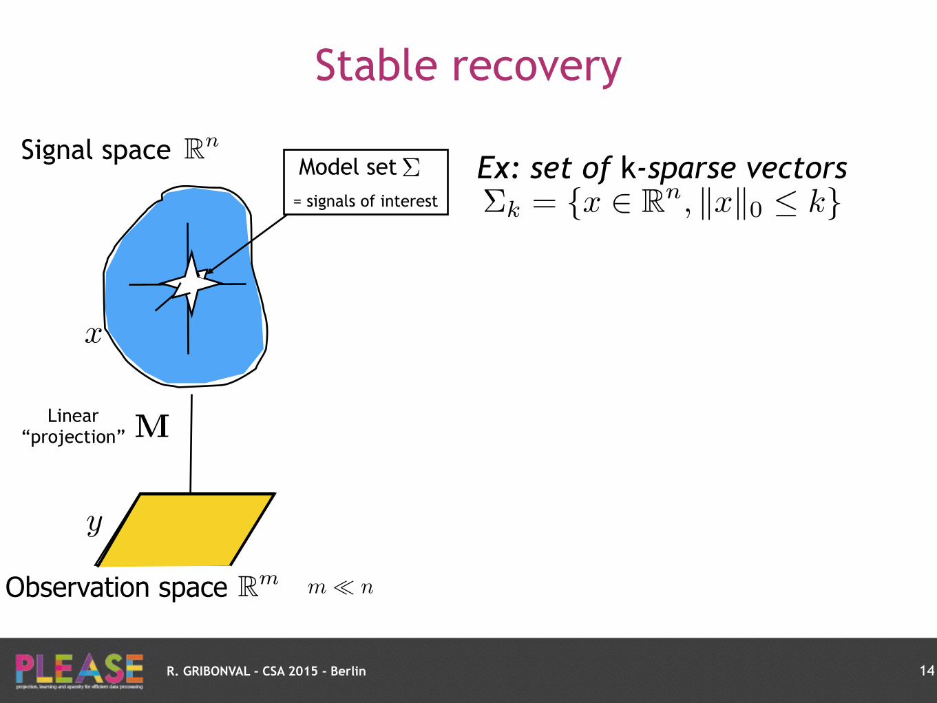
Stable recovery
Signal space
Observation space
Linear “projection”
x
Ex: set of k-sparse vectors
14
M
y
m ⌧ nRm
Rn
Model set = signals of interest
⌃
⌃k = {x 2 Rn, kxk0 k}
R. GRIBONVAL - CSA 2015 - Berlin
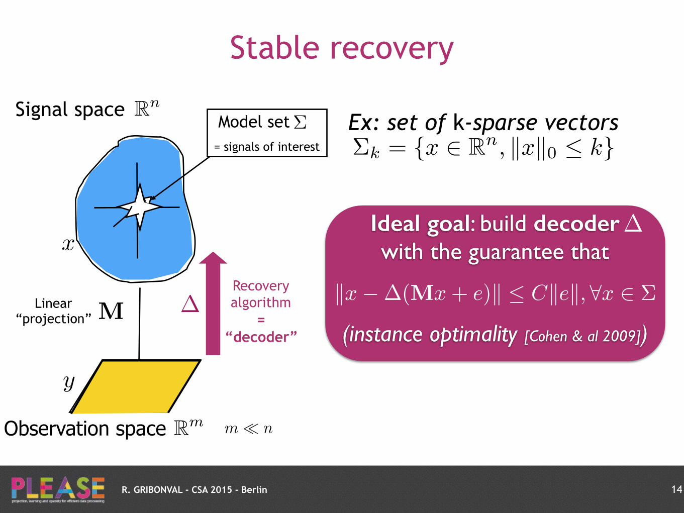
Stable recovery
Signal space
Observation space
Linear “projection”
x
Ex: set of k-sparse vectors
14
M
y
m ⌧ nRm
Rn
Model set = signals of interest
⌃
⌃k = {x 2 Rn, kxk0 k}
Recovery algorithm
= “decoder”
�
Ideal goal: build decoder with the guarantee that
(instance optimality [Cohen & al 2009])
�
kx��(Mx+ e)k Ckek, 8x 2 ⌃
R. GRIBONVAL - CSA 2015 - Berlin
Stable recovery
Signal space
Observation space
Linear “projection”
x
Ex: set of k-sparse vectors
14
M
y
m ⌧ nRm
Rn
Model set = signals of interest
⌃
⌃k = {x 2 Rn, kxk0 k}
Recovery algorithm
= “decoder”
�
Ideal goal: build decoder with the guarantee that
(instance optimality [Cohen & al 2009])
�
kx��(Mx+ e)k Ckek, 8x 2 ⌃
Are there such decoders?
R. GRIBONVAL - CSA 2015 - Berlin
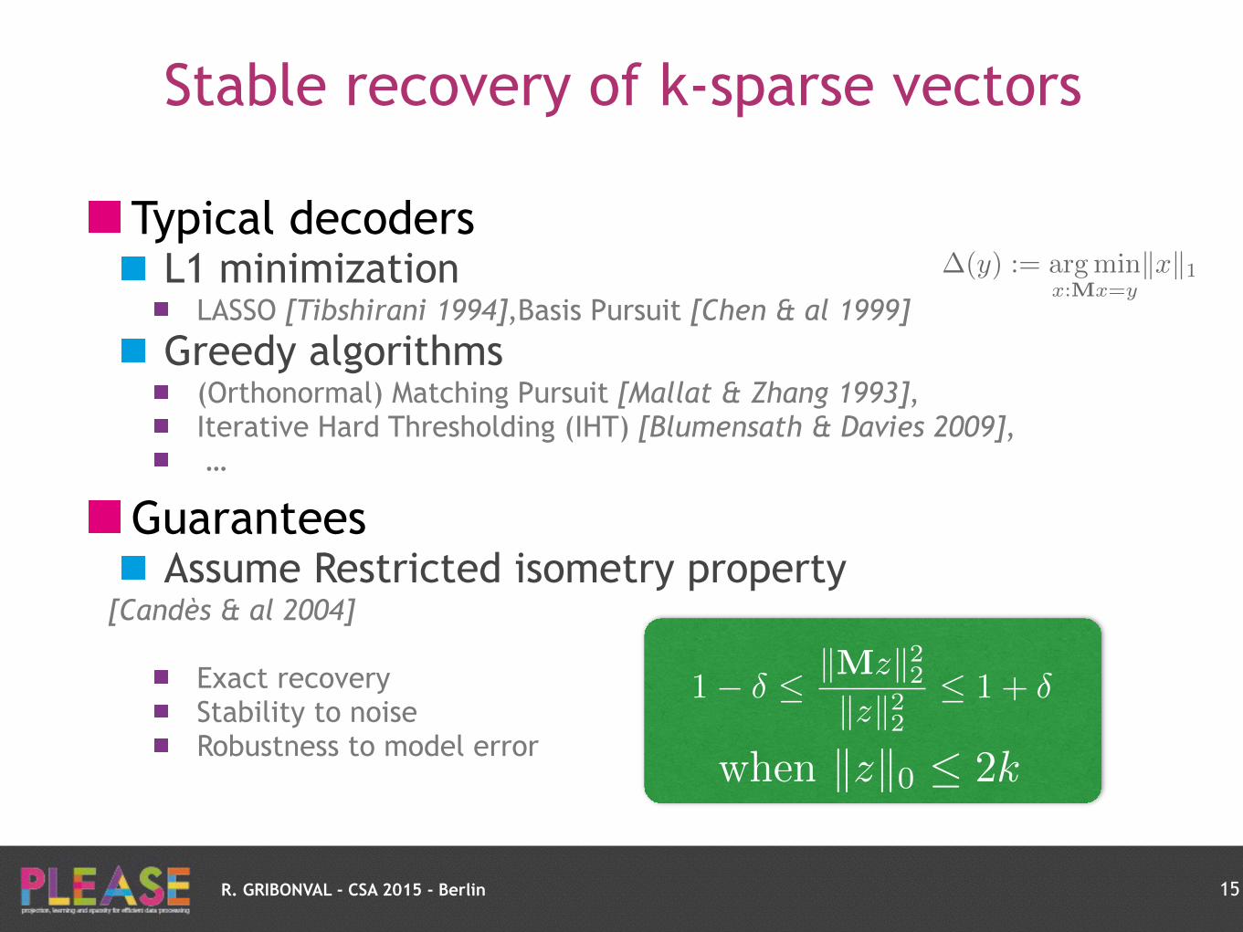
Stable recovery of k-sparse vectors
Typical decoders L1 minimization
LASSO [Tibshirani 1994],Basis Pursuit [Chen & al 1999]
Greedy algorithms (Orthonormal) Matching Pursuit [Mallat & Zhang 1993], Iterative Hard Thresholding (IHT) [Blumensath & Davies 2009], …
Guarantees Assume Restricted isometry property
[Candès & al 2004]
Exact recovery Stability to noise Robustness to model error
15
�(y) := argminx:Mx=y
kxk1
1� � kMzk22kzk22
1 + �
when kzk0 2k
R. GRIBONVAL - CSA 2015 - Berlin
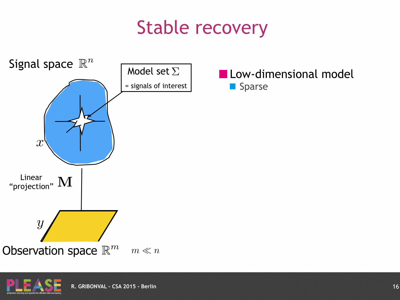
Stable recovery
Low-dimensional model Sparse
16
Signal space
Observation space
Linear “projection”
x
M
y
m ⌧ nRm
Rn
Model set = signals of interest
⌃

R. GRIBONVAL - CSA 2015 - Berlin
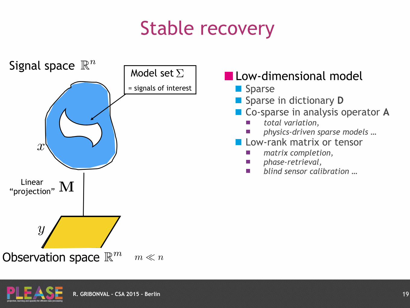
Stable recovery
Low-dimensional model Sparse Sparse in dictionary D
Signal space
Observation space
Linear “projection”
x
M
y
m ⌧ nRm
Rn
Model set = signals of interest
⌃
17

R. GRIBONVAL - CSA 2015 - Berlin
Stable recovery
Low-dimensional model Sparse Sparse in dictionary D Co-sparse in analysis operator A
total variation,
physics-driven sparse models ..
18
Signal space
Observation space
Linear “projection”
x
M
y
m ⌧ nRm
Rn
Model set = signals of interest
⌃
R. GRIBONVAL - CSA 2015 - Berlin
Stable recovery
Low-dimensional model Sparse Sparse in dictionary D Co-sparse in analysis operator A
total variation,
physics-driven sparse models …
Low-rank matrix or tensor matrix completion,
phase-retrieval,
blind sensor calibration …
19
Signal space
Observation space
Linear “projection”
x
M
y
m ⌧ nRm
Rn
Model set = signals of interest
⌃
R. GRIBONVAL - CSA 2015 - Berlin
Low-dimensional model Sparse Sparse in dictionary D Co-sparse in analysis operator A
total variation,
physics-driven sparse models …
Low-rank matrix or tensor matrix completion,
phase-retrieval,
blind sensor calibration …
Manifold / Union of manifolds detection, estimation,
localization, mapping …
Matrix with sparse inverse Gaussian graphical models
Given point cloud database indexing
Stable recovery
20
Signal space
Observation space
Linear “projection”
x
M
y
m ⌧ nRm
Rn
Model set = signals of interest
⌃
R. GRIBONVAL - CSA 2015 - Berlin
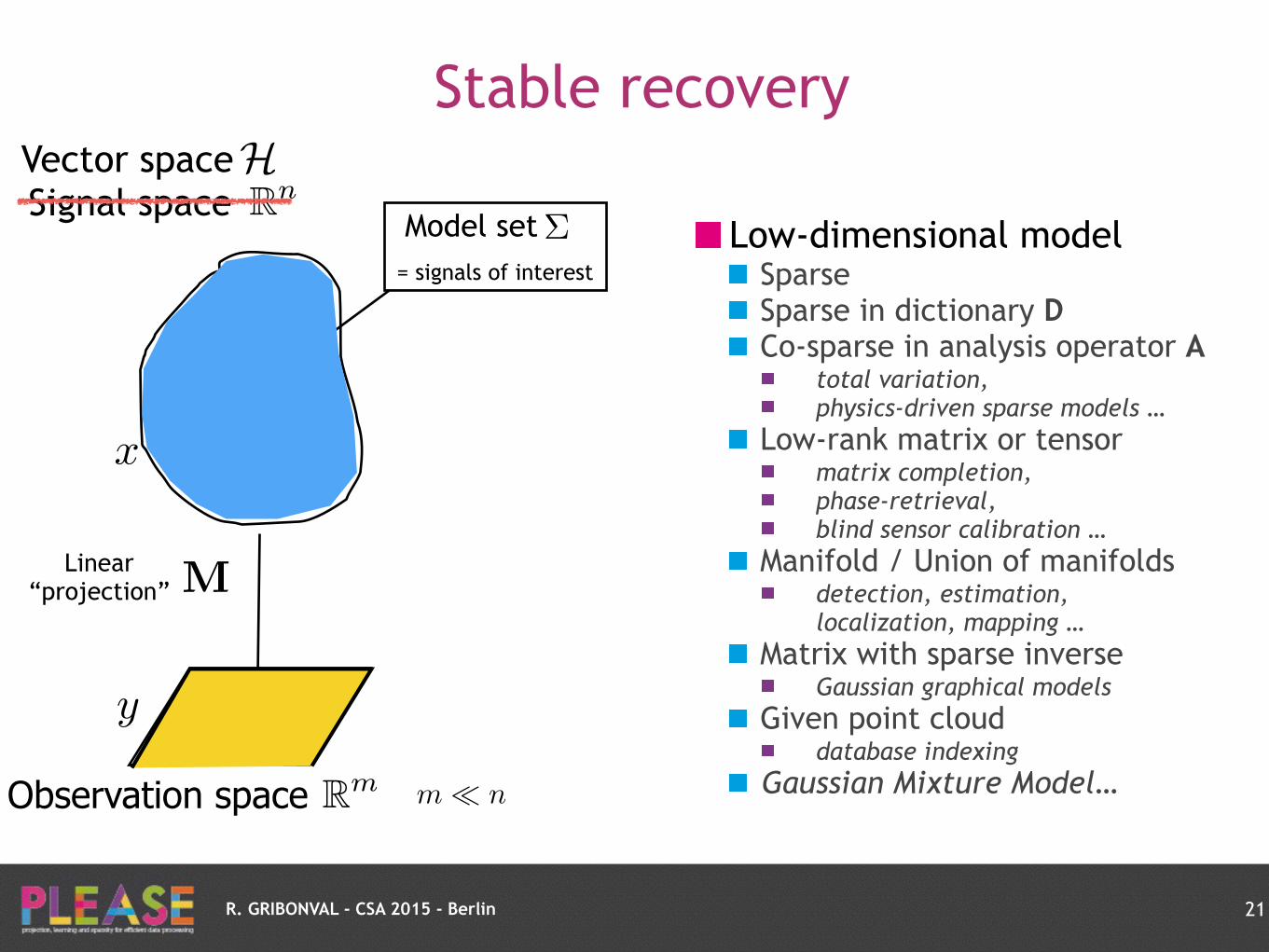
Low-dimensional model Sparse Sparse in dictionary D Co-sparse in analysis operator A
total variation,
physics-driven sparse models …
Low-rank matrix or tensor matrix completion,
phase-retrieval,
blind sensor calibration …
Manifold / Union of manifolds detection, estimation,
localization, mapping …
Matrix with sparse inverse Gaussian graphical models
Given point cloud database indexing
Gaussian Mixture Model…
Stable recovery
21
Signal space
Observation space
Linear “projection”
x
M
y
m ⌧ nRm
Rn
Model set = signals of interest
⌃
Vector spaceH
R. GRIBONVAL - CSA 2015 - Berlin
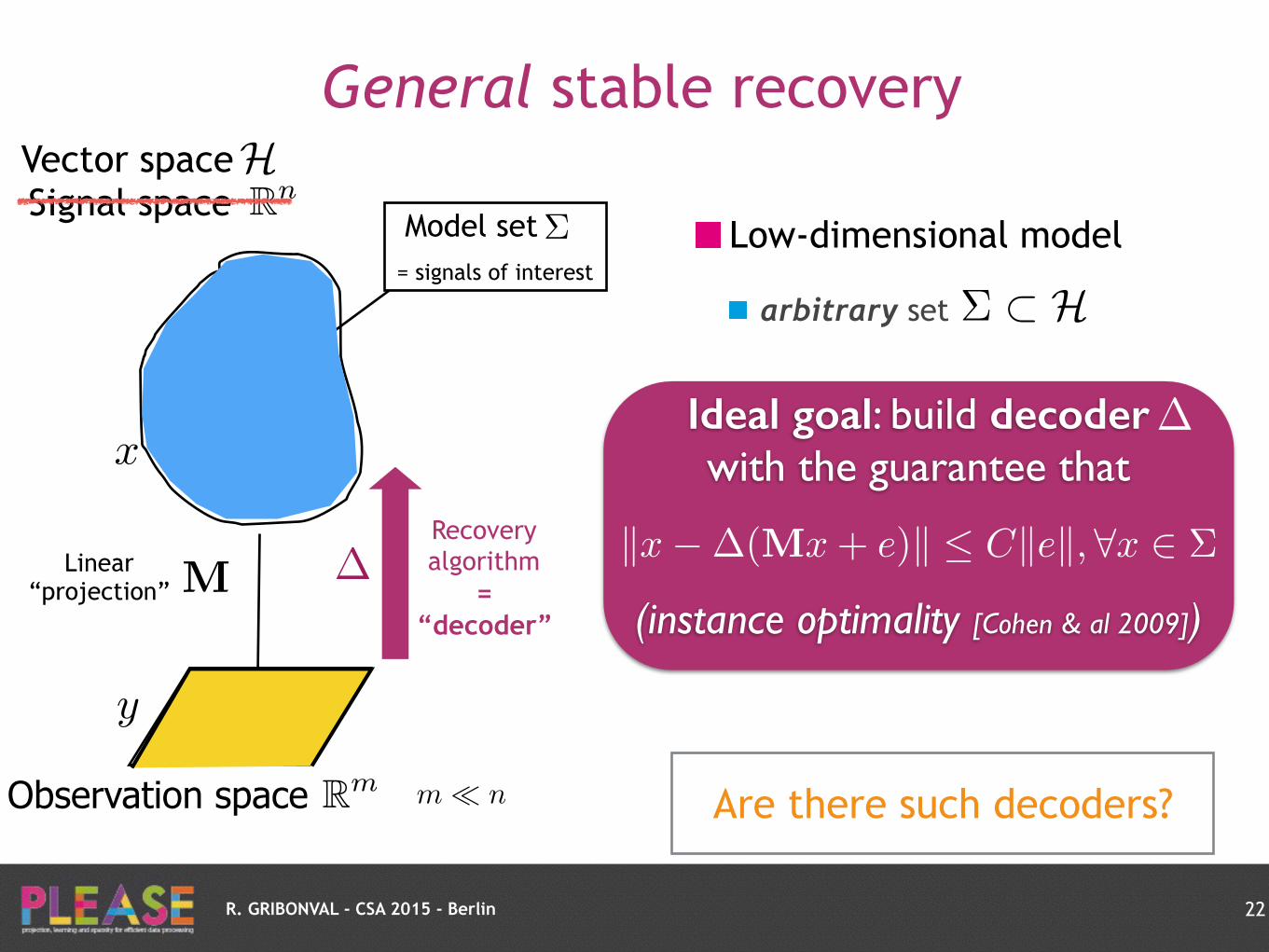
Low-dimensional model
arbitrary set
General stable recovery
22
Observation space
Linear “projection”
x
M
y
m ⌧ nRm
Model set = signals of interest
⌃
⌃ ⇢ H
Signal space RnVector spaceH
Recovery algorithm
= “decoder”
�
Ideal goal: build decoder with the guarantee that
(instance optimality [Cohen & al 2009])
�
kx��(Mx+ e)k Ckek, 8x 2 ⌃
Are there such decoders?

R. GRIBONVAL - CSA 2015 - Berlin
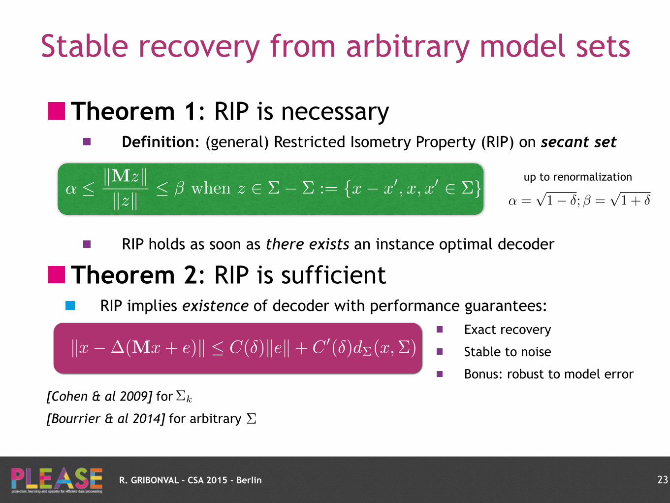
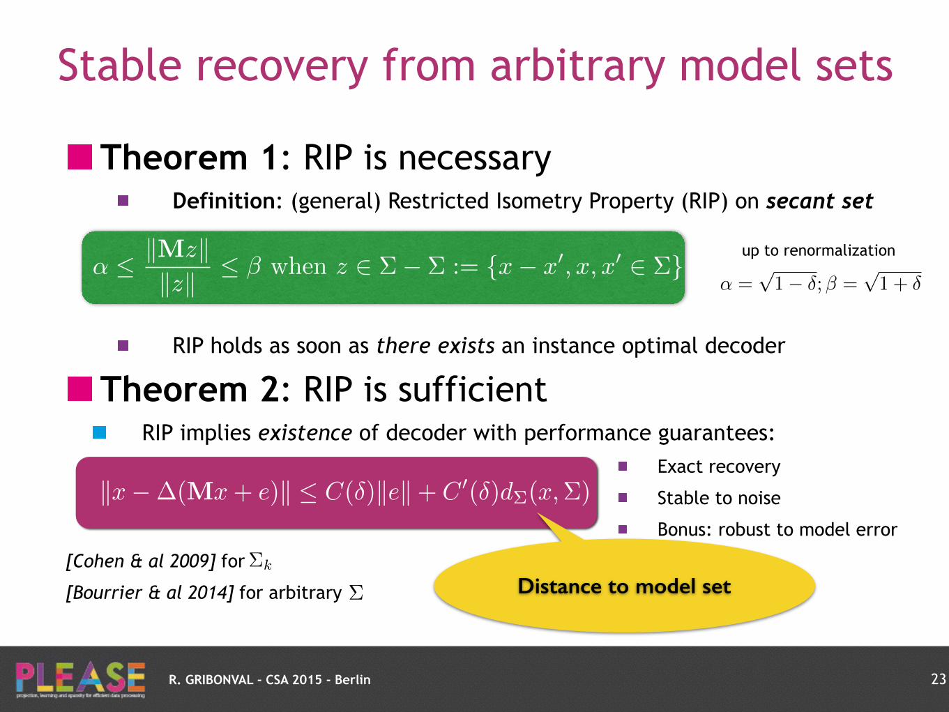
Theorem 1: RIP is necessary Definition: (general) Restricted Isometry Property (RIP) on secant set
RIP holds as soon as there exists an instance optimal decoder
Stable recovery from arbitrary model sets
23
↵ kMzkkzk � when z 2 ⌃� ⌃ := {x� x
0, x, x
0 2 ⌃}up to renormalization
↵ =p1� �;� =
p1 + �

R. GRIBONVAL - CSA 2015 - Berlin
Theorem 1: RIP is necessary Definition: (general) Restricted Isometry Property (RIP) on secant set
RIP holds as soon as there exists an instance optimal decoder
Theorem 2: RIP is sufficient RIP implies existence of decoder with performance guarantees:
Exact recovery
Stable to noise
Bonus: robust to model error
[Cohen & al 2009] for
[Bourrier & al 2014] for arbitrary
kx��(Mx+ e)k C(�)kek+ C
0(�)d⌃(x,⌃)
Stable recovery from arbitrary model sets
23
↵ kMzkkzk � when z 2 ⌃� ⌃ := {x� x
0, x, x
0 2 ⌃}up to renormalization
↵ =p1� �;� =
p1 + �
⌃k
⌃
R. GRIBONVAL - CSA 2015 - Berlin
Theorem 1: RIP is necessary Definition: (general) Restricted Isometry Property (RIP) on secant set
RIP holds as soon as there exists an instance optimal decoder
Theorem 2: RIP is sufficient RIP implies existence of decoder with performance guarantees:
Exact recovery
Stable to noise
Bonus: robust to model error
[Cohen & al 2009] for
[Bourrier & al 2014] for arbitrary
kx��(Mx+ e)k C(�)kek+ C
0(�)d⌃(x,⌃)
Stable recovery from arbitrary model sets
23
↵ kMzkkzk � when z 2 ⌃� ⌃ := {x� x
0, x, x
0 2 ⌃}up to renormalization
↵ =p1� �;� =
p1 + �
⌃k
⌃ Distance to model set

Compressive Learning Examples
R. GRIBONVAL - CSA 2015 - Berlin
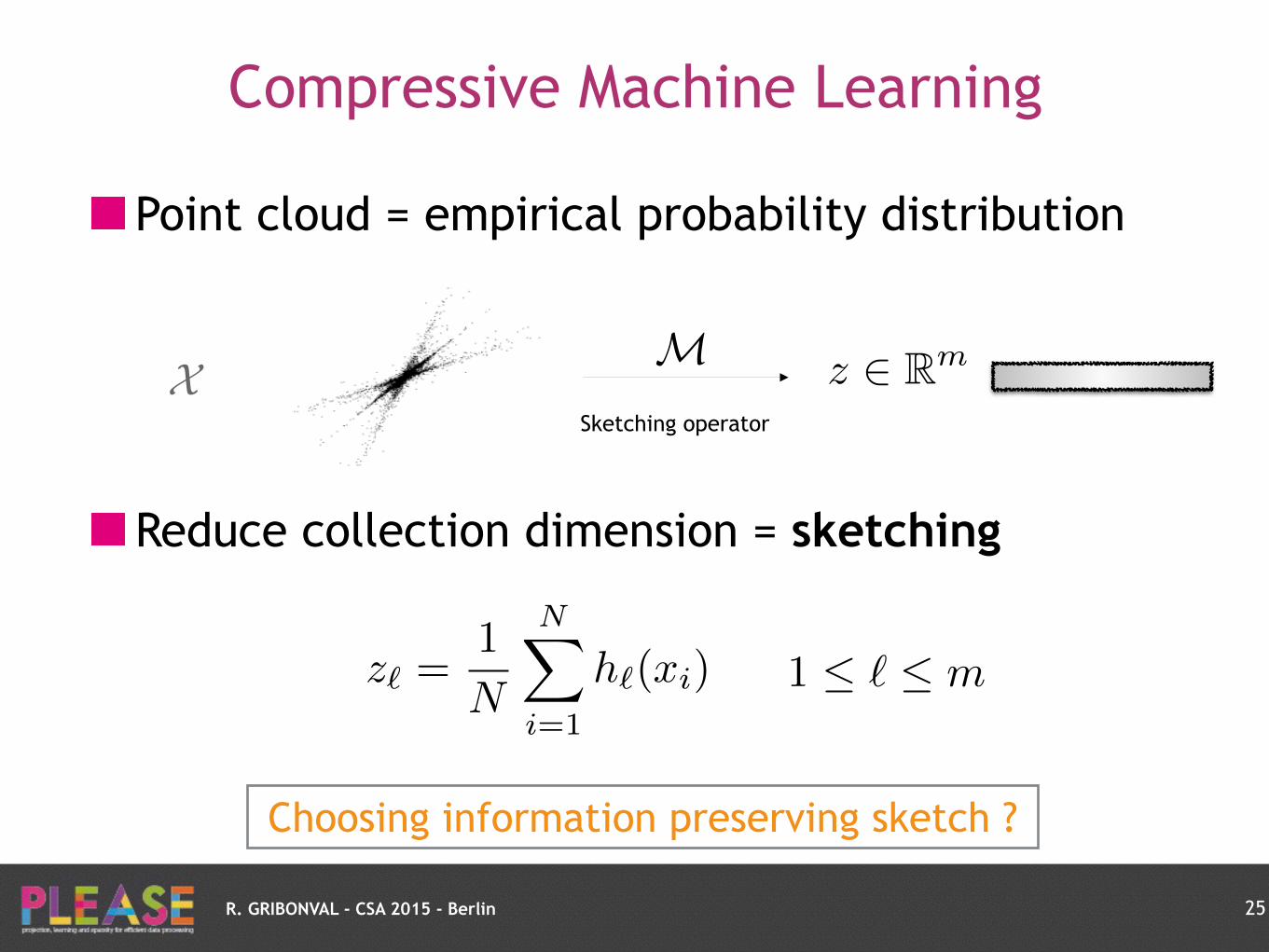
Compressive Machine Learning
Point cloud = empirical probability distribution
Reduce collection dimension = sketching
25
X
z` =1
N
NX
i=1
h`(xi) 1 ` m
M z 2 Rm
Sketching operator
Choosing information preserving sketch ?
R. GRIBONVAL - CSA 2015 - Berlin
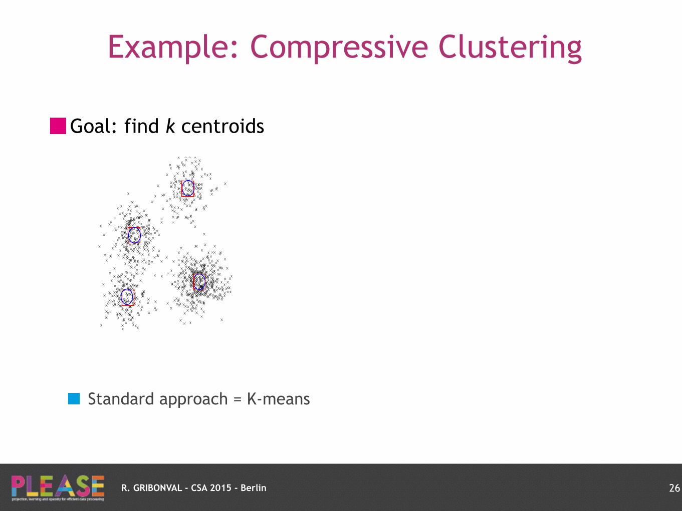
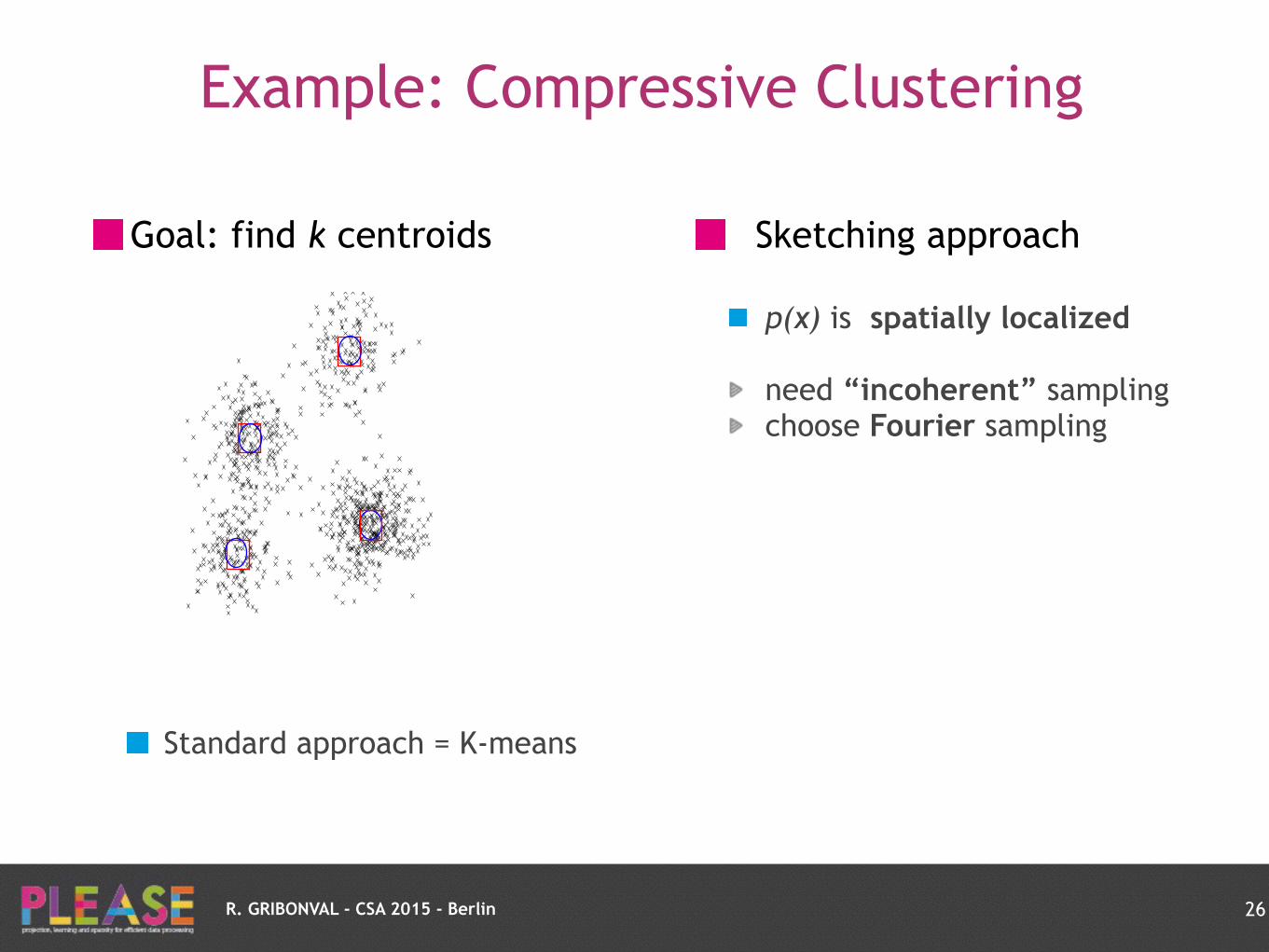
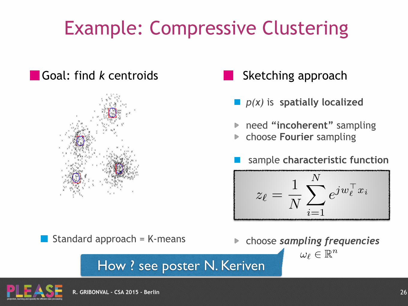
Goal: find k centroids
Standard approach = K-means
Sketching approach
p(x) is spatially localized
need “incoherent” sampling choose Fourier sampling
sample characteristic function
choose sampling frequencies
Example: Compressive Clustering
26
Compressive Gaussian Mixture Estimation
Anthony Bourrier
12, R
´
emi Gribonval
2, Patrick P
´
erez
11 Technicolor, 975 Avenue des Champs Blancs, 35576 Cesson Sevigne, France
2 INRIA Rennes - Bretagne Atlantique, Campus de Beaulieu, 35042 Rennes, [email protected]
Motivation
Goal: Infer parameters ✓ from n-dimensional data X = {x1
, . . . ,xN}. Thistypically requires extensive access to the data. Proposed method: Inferfrom a sketch of the data ) memory and privacy savings.
n x
1
. . .xN
Learning set(size Nn)
ˆ
A
=) mˆ
z
Database sketch(size m)
L=) K ✓
Learned parameters(size K)
Figure 1: Illustration of the proposed sketching framework. A is a sketch-
ing operator, L is a learning method from the sketch.
Model and problem statement
Application to mixture of isotropic Gaussians in Rn:
fµ / exp
��kx� µk2
2
/(2�2
)
�. (1)
Data X = {xj}Nj=1 ⇠i.i.d.
p =
Pks=1↵sfµs
with:
•weights ↵1
, . . . ,↵k (positive, sum to one)•means µ
1
, . . . ,µk 2 Rn.
Sketch = Fourier samplings at different frequencies: (Af )l = ˆf (!l).Empirical version: ( ˆA(X ))l =
1
N
PNj=1 exp(�ih!l,xji) ⇡ (Ap)l.
We want to infer the mixture parameters from ˆ
z =
ˆ
A(X ).Problem casted as:
p = argminq2⌃k
kˆz�Aqk22
, (2)
where ⌃k = mixtures of k isotropic Gaussians with positive weights.Standard CS Our problem
Signal x 2 Rn f 2 L1
(Rn)
Dimension n InfiniteSparsity k k
Dictionary {e1
, . . . , en} F = {fµ,µ 2 Rn}Measurements x 7! ha,xi f 7!
RRn f (x)e�ih!,xidx
Algorithm
Current estimate p with weights {↵s}ks=1 and support ˆ� = {ˆµs}ks=1.Residual ˆr = ˆ
z�Ap.1. Searching new support functions:
Search for ”good components to add” to the support) Local minima of µ 7! �hAfµ, ˆri, added to the support ˆ�.New support ˆ�0.
2. k-term thresholding:Projection of ˆz onto ˆ
�
0 with positivity constraints on coefficients:
argmin�2RK
+
||ˆz�U�||22
, (3)
with U = [
ˆµ1
, . . . , ˆµK].k highest coefficients and corresponding support are kept! new support ˆ� and coefficients ↵
1
, . . . , ↵k.3. Final ”shift”:
Gradient descent algorithm on the objective function, with initialization atthe current support and coefficients.
First step Second step Third step
Figure 2: Algorithm illustration in dimension n = 1 for k = 3 Gaus-
sians. Top: Iteration 1. Bottom: Iteration 2. Blue curve=true mixture,
Red curve=reconstructed mixture, Green curve=gradient function. Green
Dots=Candidate Centroids, Red Dots=Reconstructed Centroids.
Experimental results
Data setup: � = 1, (↵1
, . . . ,↵k) drawn uniformly on the simplex.Entries of µ
1
, . . . ,µk ⇠i.i.d.
N (0, 1).
Algorithm heuristics:•Frequencies drawn i.i.d. from N (0, Id).
•New support function search (step 1) initialized as ru, where r uniformly
drawn in0,max
x2X||x||
2
�and u uniformly drawn on B
2
(0, 1).
Comparison between:•Our method: Sketch is computed on-the-fly and data is discarded.
•EM: Data is stored to allow the standard optimization steps to be per-formed.
Quality measures: KL Divergence and Hellinger distance.
NCompressed EM
KL div. Hell. Mem. KL div. Hell. Mem.10
3
0.68± 0.28 0.06± 0.01 0.6 0.68± 0.44 0.07± 0.03 0.2410
4
0.24± 0.31 0.02± 0.02 0.6 0.19± 0.21 0.01± 0.02 2.410
5
0.13± 0.15 0.01± 0.02 0.6 0.13± 0.21 0.01± 0.02 24
Table 1: Comparison between our method and an EM algorithm. n =
20, k = 10,m = 1000.
−4 −2 0 2 4 6 8
−4
−2
0
2
4
6
ˆ
A
=)
−0.5 0 0.5 10
10
20
30
40
50
60 n=10, Hell. for 80%
sketch size mk*
n/m
200 400 600 800 1000 1200 1400 1600 1800 2000
1
0.9
0.8
0.7
0.6
0.5
0.4
0.3
0.2
0.1
0
0.02
0.04
0.06
0.08
0.1
0.12
0.14
0.16
Figure 3: Left: Example of data and sketch for n = 2. Right: Reconstruc-
tion quality for n = 10.
z`
=1
N
NX
i=1
ejw>` xi
!` 2 Rn
R. GRIBONVAL - CSA 2015 - Berlin
Goal: find k centroids
Standard approach = K-means
Sketching approach
p(x) is spatially localized
need “incoherent” sampling choose Fourier sampling
sample characteristic function
choose sampling frequencies
Example: Compressive Clustering
26
Compressive Gaussian Mixture Estimation
Anthony Bourrier
12, R
´
emi Gribonval
2, Patrick P
´
erez
11 Technicolor, 975 Avenue des Champs Blancs, 35576 Cesson Sevigne, France
2 INRIA Rennes - Bretagne Atlantique, Campus de Beaulieu, 35042 Rennes, [email protected]
Motivation
Goal: Infer parameters ✓ from n-dimensional data X = {x1
, . . . ,xN}. Thistypically requires extensive access to the data. Proposed method: Inferfrom a sketch of the data ) memory and privacy savings.
n x
1
. . .xN
Learning set(size Nn)
ˆ
A
=) mˆ
z
Database sketch(size m)
L=) K ✓
Learned parameters(size K)
Figure 1: Illustration of the proposed sketching framework. A is a sketch-
ing operator, L is a learning method from the sketch.
Model and problem statement
Application to mixture of isotropic Gaussians in Rn:
fµ / exp
��kx� µk2
2
/(2�2
)
�. (1)
Data X = {xj}Nj=1 ⇠i.i.d.
p =
Pks=1↵sfµs
with:
•weights ↵1
, . . . ,↵k (positive, sum to one)•means µ
1
, . . . ,µk 2 Rn.
Sketch = Fourier samplings at different frequencies: (Af )l = ˆf (!l).Empirical version: ( ˆA(X ))l =
1
N
PNj=1 exp(�ih!l,xji) ⇡ (Ap)l.
We want to infer the mixture parameters from ˆ
z =
ˆ
A(X ).Problem casted as:
p = argminq2⌃k
kˆz�Aqk22
, (2)
where ⌃k = mixtures of k isotropic Gaussians with positive weights.Standard CS Our problem
Signal x 2 Rn f 2 L1
(Rn)
Dimension n InfiniteSparsity k k
Dictionary {e1
, . . . , en} F = {fµ,µ 2 Rn}Measurements x 7! ha,xi f 7!
RRn f (x)e�ih!,xidx
Algorithm
Current estimate p with weights {↵s}ks=1 and support ˆ� = {ˆµs}ks=1.Residual ˆr = ˆ
z�Ap.1. Searching new support functions:
Search for ”good components to add” to the support) Local minima of µ 7! �hAfµ, ˆri, added to the support ˆ�.New support ˆ�0.
2. k-term thresholding:Projection of ˆz onto ˆ
�
0 with positivity constraints on coefficients:
argmin�2RK
+
||ˆz�U�||22
, (3)
with U = [
ˆµ1
, . . . , ˆµK].k highest coefficients and corresponding support are kept! new support ˆ� and coefficients ↵
1
, . . . , ↵k.3. Final ”shift”:
Gradient descent algorithm on the objective function, with initialization atthe current support and coefficients.
First step Second step Third step
Figure 2: Algorithm illustration in dimension n = 1 for k = 3 Gaus-
sians. Top: Iteration 1. Bottom: Iteration 2. Blue curve=true mixture,
Red curve=reconstructed mixture, Green curve=gradient function. Green
Dots=Candidate Centroids, Red Dots=Reconstructed Centroids.
Experimental results
Data setup: � = 1, (↵1
, . . . ,↵k) drawn uniformly on the simplex.Entries of µ
1
, . . . ,µk ⇠i.i.d.
N (0, 1).
Algorithm heuristics:•Frequencies drawn i.i.d. from N (0, Id).
•New support function search (step 1) initialized as ru, where r uniformly
drawn in0,max
x2X||x||
2
�and u uniformly drawn on B
2
(0, 1).
Comparison between:•Our method: Sketch is computed on-the-fly and data is discarded.
•EM: Data is stored to allow the standard optimization steps to be per-formed.
Quality measures: KL Divergence and Hellinger distance.
NCompressed EM
KL div. Hell. Mem. KL div. Hell. Mem.10
3
0.68± 0.28 0.06± 0.01 0.6 0.68± 0.44 0.07± 0.03 0.2410
4
0.24± 0.31 0.02± 0.02 0.6 0.19± 0.21 0.01± 0.02 2.410
5
0.13± 0.15 0.01± 0.02 0.6 0.13± 0.21 0.01± 0.02 24
Table 1: Comparison between our method and an EM algorithm. n =
20, k = 10,m = 1000.
−4 −2 0 2 4 6 8
−4
−2
0
2
4
6
ˆ
A
=)
−0.5 0 0.5 10
10
20
30
40
50
60 n=10, Hell. for 80%
sketch size mk*
n/m
200 400 600 800 1000 1200 1400 1600 1800 2000
1
0.9
0.8
0.7
0.6
0.5
0.4
0.3
0.2
0.1
0
0.02
0.04
0.06
0.08
0.1
0.12
0.14
0.16
Figure 3: Left: Example of data and sketch for n = 2. Right: Reconstruc-
tion quality for n = 10.
z`
=1
N
NX
i=1
ejw>` xi
!` 2 Rn
How ? see poster N. Keriven
R. GRIBONVAL - CSA 2015 - Berlin
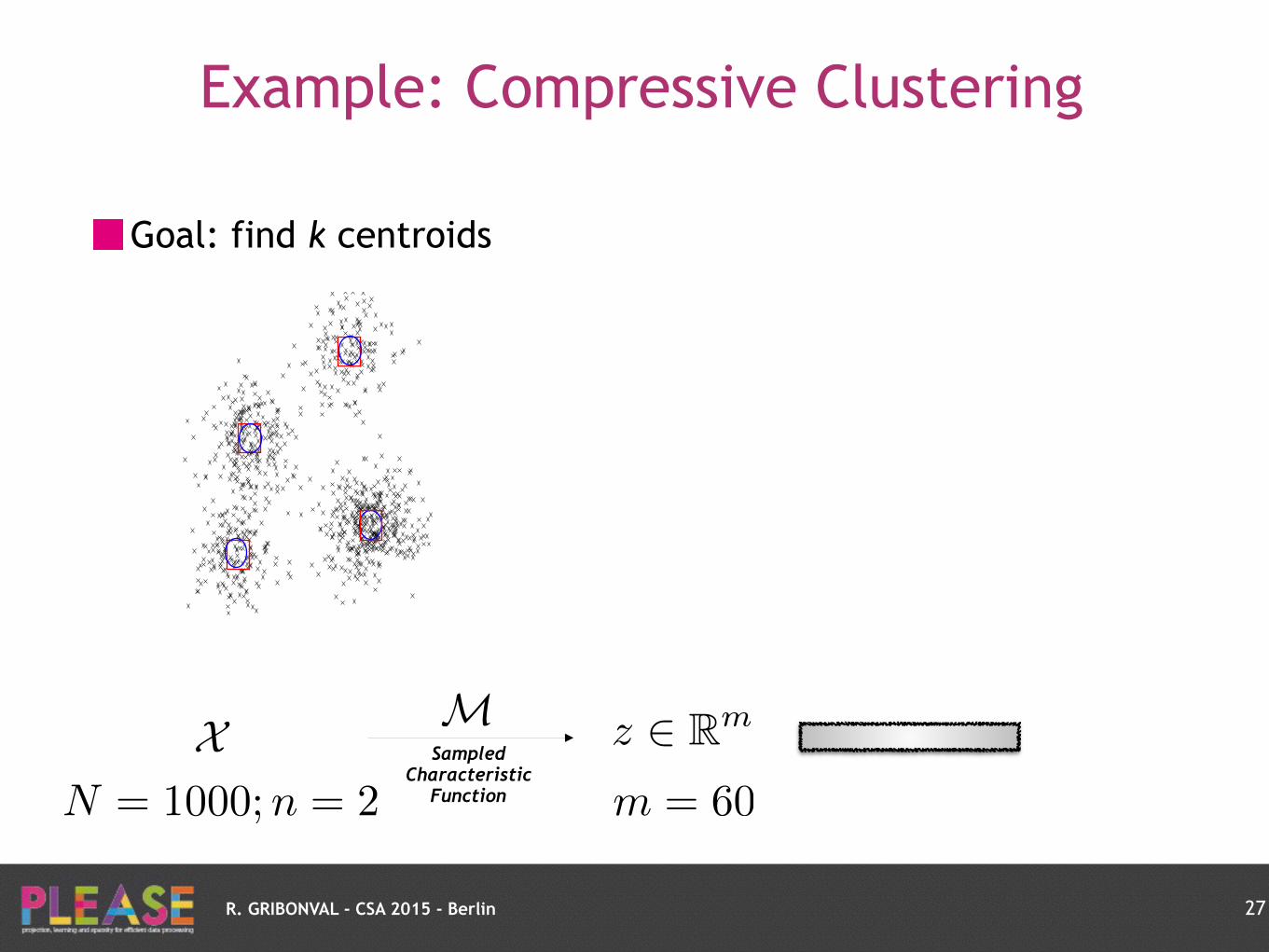
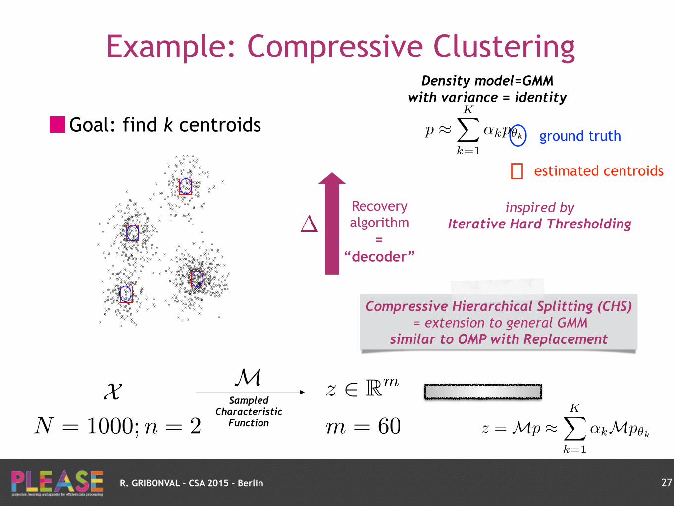
Goal: find k centroids
27
X M z 2 Rm
N = 1000;n = 2Sampled
Characteristic Function m = 60
Compressive Gaussian Mixture Estimation
Anthony Bourrier
12, R
´
emi Gribonval
2, Patrick P
´
erez
11 Technicolor, 975 Avenue des Champs Blancs, 35576 Cesson Sevigne, France
2 INRIA Rennes - Bretagne Atlantique, Campus de Beaulieu, 35042 Rennes, [email protected]
Motivation
Goal: Infer parameters ✓ from n-dimensional data X = {x1
, . . . ,xN}. Thistypically requires extensive access to the data. Proposed method: Inferfrom a sketch of the data ) memory and privacy savings.
n x
1
. . .xN
Learning set(size Nn)
ˆ
A
=) mˆ
z
Database sketch(size m)
L=) K ✓
Learned parameters(size K)
Figure 1: Illustration of the proposed sketching framework. A is a sketch-
ing operator, L is a learning method from the sketch.
Model and problem statement
Application to mixture of isotropic Gaussians in Rn:
fµ / exp
��kx� µk2
2
/(2�2
)
�. (1)
Data X = {xj}Nj=1 ⇠i.i.d.
p =
Pks=1↵sfµs
with:
•weights ↵1
, . . . ,↵k (positive, sum to one)•means µ
1
, . . . ,µk 2 Rn.
Sketch = Fourier samplings at different frequencies: (Af )l = ˆf (!l).Empirical version: ( ˆA(X ))l =
1
N
PNj=1 exp(�ih!l,xji) ⇡ (Ap)l.
We want to infer the mixture parameters from ˆ
z =
ˆ
A(X ).Problem casted as:
p = argminq2⌃k
kˆz�Aqk22
, (2)
where ⌃k = mixtures of k isotropic Gaussians with positive weights.Standard CS Our problem
Signal x 2 Rn f 2 L1
(Rn)
Dimension n InfiniteSparsity k k
Dictionary {e1
, . . . , en} F = {fµ,µ 2 Rn}Measurements x 7! ha,xi f 7!
RRn f (x)e�ih!,xidx
Algorithm
Current estimate p with weights {↵s}ks=1 and support ˆ� = {ˆµs}ks=1.Residual ˆr = ˆ
z�Ap.1. Searching new support functions:
Search for ”good components to add” to the support) Local minima of µ 7! �hAfµ, ˆri, added to the support ˆ�.New support ˆ�0.
2. k-term thresholding:Projection of ˆz onto ˆ
�
0 with positivity constraints on coefficients:
argmin�2RK
+
||ˆz�U�||22
, (3)
with U = [
ˆµ1
, . . . , ˆµK].k highest coefficients and corresponding support are kept! new support ˆ� and coefficients ↵
1
, . . . , ↵k.3. Final ”shift”:
Gradient descent algorithm on the objective function, with initialization atthe current support and coefficients.
First step Second step Third step
Figure 2: Algorithm illustration in dimension n = 1 for k = 3 Gaus-
sians. Top: Iteration 1. Bottom: Iteration 2. Blue curve=true mixture,
Red curve=reconstructed mixture, Green curve=gradient function. Green
Dots=Candidate Centroids, Red Dots=Reconstructed Centroids.
Experimental results
Data setup: � = 1, (↵1
, . . . ,↵k) drawn uniformly on the simplex.Entries of µ
1
, . . . ,µk ⇠i.i.d.
N (0, 1).
Algorithm heuristics:•Frequencies drawn i.i.d. from N (0, Id).
•New support function search (step 1) initialized as ru, where r uniformly
drawn in0,max
x2X||x||
2
�and u uniformly drawn on B
2
(0, 1).
Comparison between:•Our method: Sketch is computed on-the-fly and data is discarded.
•EM: Data is stored to allow the standard optimization steps to be per-formed.
Quality measures: KL Divergence and Hellinger distance.
NCompressed EM
KL div. Hell. Mem. KL div. Hell. Mem.10
3
0.68± 0.28 0.06± 0.01 0.6 0.68± 0.44 0.07± 0.03 0.2410
4
0.24± 0.31 0.02± 0.02 0.6 0.19± 0.21 0.01± 0.02 2.410
5
0.13± 0.15 0.01± 0.02 0.6 0.13± 0.21 0.01± 0.02 24
Table 1: Comparison between our method and an EM algorithm. n =
20, k = 10,m = 1000.
−4 −2 0 2 4 6 8
−4
−2
0
2
4
6
ˆ
A
=)
−0.5 0 0.5 10
10
20
30
40
50
60 n=10, Hell. for 80%
sketch size mk*
n/m
200 400 600 800 1000 1200 1400 1600 1800 2000
1
0.9
0.8
0.7
0.6
0.5
0.4
0.3
0.2
0.1
0
0.02
0.04
0.06
0.08
0.1
0.12
0.14
0.16
Figure 3: Left: Example of data and sketch for n = 2. Right: Reconstruc-
tion quality for n = 10.
Example: Compressive Clustering
R. GRIBONVAL - CSA 2015 - Berlin
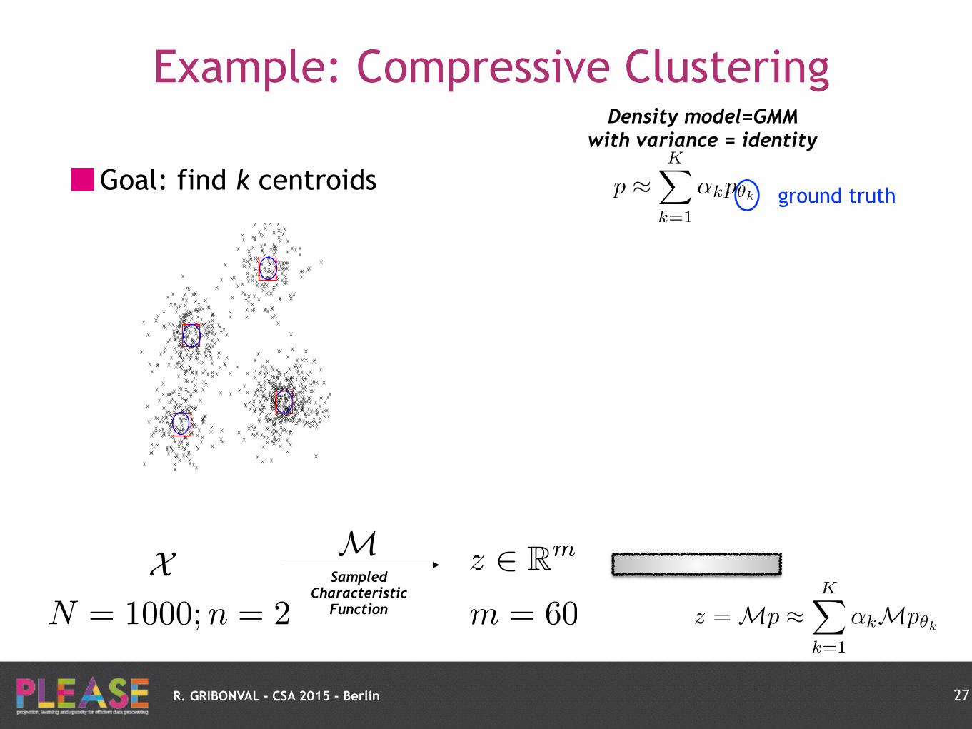
Goal: find k centroids
27
ground truth
X M z 2 Rm
N = 1000;n = 2Sampled
Characteristic Function m = 60 z = Mp ⇡
KX
k=1
↵kMp✓k
p ⇡KX
k=1
↵kp✓k
Density model=GMM with variance = identity
Compressive Gaussian Mixture Estimation
Anthony Bourrier
12, R
´
emi Gribonval
2, Patrick P
´
erez
11 Technicolor, 975 Avenue des Champs Blancs, 35576 Cesson Sevigne, France
2 INRIA Rennes - Bretagne Atlantique, Campus de Beaulieu, 35042 Rennes, [email protected]
Motivation
Goal: Infer parameters ✓ from n-dimensional data X = {x1
, . . . ,xN}. Thistypically requires extensive access to the data. Proposed method: Inferfrom a sketch of the data ) memory and privacy savings.
n x
1
. . .xN
Learning set(size Nn)
ˆ
A
=) mˆ
z
Database sketch(size m)
L=) K ✓
Learned parameters(size K)
Figure 1: Illustration of the proposed sketching framework. A is a sketch-
ing operator, L is a learning method from the sketch.
Model and problem statement
Application to mixture of isotropic Gaussians in Rn:
fµ / exp
��kx� µk2
2
/(2�2
)
�. (1)
Data X = {xj}Nj=1 ⇠i.i.d.
p =
Pks=1↵sfµs
with:
•weights ↵1
, . . . ,↵k (positive, sum to one)•means µ
1
, . . . ,µk 2 Rn.
Sketch = Fourier samplings at different frequencies: (Af )l = ˆf (!l).Empirical version: ( ˆA(X ))l =
1
N
PNj=1 exp(�ih!l,xji) ⇡ (Ap)l.
We want to infer the mixture parameters from ˆ
z =
ˆ
A(X ).Problem casted as:
p = argminq2⌃k
kˆz�Aqk22
, (2)
where ⌃k = mixtures of k isotropic Gaussians with positive weights.Standard CS Our problem
Signal x 2 Rn f 2 L1
(Rn)
Dimension n InfiniteSparsity k k
Dictionary {e1
, . . . , en} F = {fµ,µ 2 Rn}Measurements x 7! ha,xi f 7!
RRn f (x)e�ih!,xidx
Algorithm
Current estimate p with weights {↵s}ks=1 and support ˆ� = {ˆµs}ks=1.Residual ˆr = ˆ
z�Ap.1. Searching new support functions:
Search for ”good components to add” to the support) Local minima of µ 7! �hAfµ, ˆri, added to the support ˆ�.New support ˆ�0.
2. k-term thresholding:Projection of ˆz onto ˆ
�
0 with positivity constraints on coefficients:
argmin�2RK
+
||ˆz�U�||22
, (3)
with U = [
ˆµ1
, . . . , ˆµK].k highest coefficients and corresponding support are kept! new support ˆ� and coefficients ↵
1
, . . . , ↵k.3. Final ”shift”:
Gradient descent algorithm on the objective function, with initialization atthe current support and coefficients.
First step Second step Third step
Figure 2: Algorithm illustration in dimension n = 1 for k = 3 Gaus-
sians. Top: Iteration 1. Bottom: Iteration 2. Blue curve=true mixture,
Red curve=reconstructed mixture, Green curve=gradient function. Green
Dots=Candidate Centroids, Red Dots=Reconstructed Centroids.
Experimental results
Data setup: � = 1, (↵1
, . . . ,↵k) drawn uniformly on the simplex.Entries of µ
1
, . . . ,µk ⇠i.i.d.
N (0, 1).
Algorithm heuristics:•Frequencies drawn i.i.d. from N (0, Id).
•New support function search (step 1) initialized as ru, where r uniformly
drawn in0,max
x2X||x||
2
�and u uniformly drawn on B
2
(0, 1).
Comparison between:•Our method: Sketch is computed on-the-fly and data is discarded.
•EM: Data is stored to allow the standard optimization steps to be per-formed.
Quality measures: KL Divergence and Hellinger distance.
NCompressed EM
KL div. Hell. Mem. KL div. Hell. Mem.10
3
0.68± 0.28 0.06± 0.01 0.6 0.68± 0.44 0.07± 0.03 0.2410
4
0.24± 0.31 0.02± 0.02 0.6 0.19± 0.21 0.01± 0.02 2.410
5
0.13± 0.15 0.01± 0.02 0.6 0.13± 0.21 0.01± 0.02 24
Table 1: Comparison between our method and an EM algorithm. n =
20, k = 10,m = 1000.
−4 −2 0 2 4 6 8
−4
−2
0
2
4
6
ˆ
A
=)
−0.5 0 0.5 10
10
20
30
40
50
60 n=10, Hell. for 80%
sketch size mk*
n/m
200 400 600 800 1000 1200 1400 1600 1800 2000
1
0.9
0.8
0.7
0.6
0.5
0.4
0.3
0.2
0.1
0
0.02
0.04
0.06
0.08
0.1
0.12
0.14
0.16
Figure 3: Left: Example of data and sketch for n = 2. Right: Reconstruc-
tion quality for n = 10.
Example: Compressive Clustering
R. GRIBONVAL - CSA 2015 - Berlin
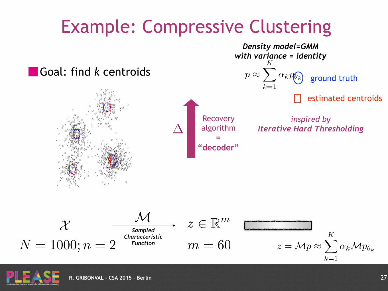
Goal: find k centroids
27
estimated centroids
ground truth
X M z 2 Rm
N = 1000;n = 2Sampled
Characteristic Function m = 60 z = Mp ⇡
KX
k=1
↵kMp✓k
p ⇡KX
k=1
↵kp✓k
Density model=GMM with variance = identity
Compressive Gaussian Mixture Estimation
Anthony Bourrier
12, R
´
emi Gribonval
2, Patrick P
´
erez
11 Technicolor, 975 Avenue des Champs Blancs, 35576 Cesson Sevigne, France
2 INRIA Rennes - Bretagne Atlantique, Campus de Beaulieu, 35042 Rennes, [email protected]
Motivation
Goal: Infer parameters ✓ from n-dimensional data X = {x1
, . . . ,xN}. Thistypically requires extensive access to the data. Proposed method: Inferfrom a sketch of the data ) memory and privacy savings.
n x
1
. . .xN
Learning set(size Nn)
ˆ
A
=) mˆ
z
Database sketch(size m)
L=) K ✓
Learned parameters(size K)
Figure 1: Illustration of the proposed sketching framework. A is a sketch-
ing operator, L is a learning method from the sketch.
Model and problem statement
Application to mixture of isotropic Gaussians in Rn:
fµ / exp
��kx� µk2
2
/(2�2
)
�. (1)
Data X = {xj}Nj=1 ⇠i.i.d.
p =
Pks=1↵sfµs
with:
•weights ↵1
, . . . ,↵k (positive, sum to one)•means µ
1
, . . . ,µk 2 Rn.
Sketch = Fourier samplings at different frequencies: (Af )l = ˆf (!l).Empirical version: ( ˆA(X ))l =
1
N
PNj=1 exp(�ih!l,xji) ⇡ (Ap)l.
We want to infer the mixture parameters from ˆ
z =
ˆ
A(X ).Problem casted as:
p = argminq2⌃k
kˆz�Aqk22
, (2)
where ⌃k = mixtures of k isotropic Gaussians with positive weights.Standard CS Our problem
Signal x 2 Rn f 2 L1
(Rn)
Dimension n InfiniteSparsity k k
Dictionary {e1
, . . . , en} F = {fµ,µ 2 Rn}Measurements x 7! ha,xi f 7!
RRn f (x)e�ih!,xidx
Algorithm
Current estimate p with weights {↵s}ks=1 and support ˆ� = {ˆµs}ks=1.Residual ˆr = ˆ
z�Ap.1. Searching new support functions:
Search for ”good components to add” to the support) Local minima of µ 7! �hAfµ, ˆri, added to the support ˆ�.New support ˆ�0.
2. k-term thresholding:Projection of ˆz onto ˆ
�
0 with positivity constraints on coefficients:
argmin�2RK
+
||ˆz�U�||22
, (3)
with U = [
ˆµ1
, . . . , ˆµK].k highest coefficients and corresponding support are kept! new support ˆ� and coefficients ↵
1
, . . . , ↵k.3. Final ”shift”:
Gradient descent algorithm on the objective function, with initialization atthe current support and coefficients.
First step Second step Third step
Figure 2: Algorithm illustration in dimension n = 1 for k = 3 Gaus-
sians. Top: Iteration 1. Bottom: Iteration 2. Blue curve=true mixture,
Red curve=reconstructed mixture, Green curve=gradient function. Green
Dots=Candidate Centroids, Red Dots=Reconstructed Centroids.
Experimental results
Data setup: � = 1, (↵1
, . . . ,↵k) drawn uniformly on the simplex.Entries of µ
1
, . . . ,µk ⇠i.i.d.
N (0, 1).
Algorithm heuristics:•Frequencies drawn i.i.d. from N (0, Id).
•New support function search (step 1) initialized as ru, where r uniformly
drawn in0,max
x2X||x||
2
�and u uniformly drawn on B
2
(0, 1).
Comparison between:•Our method: Sketch is computed on-the-fly and data is discarded.
•EM: Data is stored to allow the standard optimization steps to be per-formed.
Quality measures: KL Divergence and Hellinger distance.
NCompressed EM
KL div. Hell. Mem. KL div. Hell. Mem.10
3
0.68± 0.28 0.06± 0.01 0.6 0.68± 0.44 0.07± 0.03 0.2410
4
0.24± 0.31 0.02± 0.02 0.6 0.19± 0.21 0.01± 0.02 2.410
5
0.13± 0.15 0.01± 0.02 0.6 0.13± 0.21 0.01± 0.02 24
Table 1: Comparison between our method and an EM algorithm. n =
20, k = 10,m = 1000.
−4 −2 0 2 4 6 8
−4
−2
0
2
4
6
ˆ
A
=)
−0.5 0 0.5 10
10
20
30
40
50
60 n=10, Hell. for 80%
sketch size mk*
n/m
200 400 600 800 1000 1200 1400 1600 1800 2000
1
0.9
0.8
0.7
0.6
0.5
0.4
0.3
0.2
0.1
0
0.02
0.04
0.06
0.08
0.1
0.12
0.14
0.16
Figure 3: Left: Example of data and sketch for n = 2. Right: Reconstruc-
tion quality for n = 10.
inspired by
Iterative Hard Thresholding Recovery algorithm
= “decoder”
�
Example: Compressive Clustering
R. GRIBONVAL - CSA 2015 - Berlin
Goal: find k centroids
27
estimated centroids
ground truth
X M z 2 Rm
N = 1000;n = 2Sampled
Characteristic Function m = 60 z = Mp ⇡
KX
k=1
↵kMp✓k
p ⇡KX
k=1
↵kp✓k
Density model=GMM with variance = identity
Compressive Gaussian Mixture Estimation
Anthony Bourrier
12, R
´
emi Gribonval
2, Patrick P
´
erez
11 Technicolor, 975 Avenue des Champs Blancs, 35576 Cesson Sevigne, France
2 INRIA Rennes - Bretagne Atlantique, Campus de Beaulieu, 35042 Rennes, [email protected]
Motivation
Goal: Infer parameters ✓ from n-dimensional data X = {x1
, . . . ,xN}. Thistypically requires extensive access to the data. Proposed method: Inferfrom a sketch of the data ) memory and privacy savings.
n x
1
. . .xN
Learning set(size Nn)
ˆ
A
=) mˆ
z
Database sketch(size m)
L=) K ✓
Learned parameters(size K)
Figure 1: Illustration of the proposed sketching framework. A is a sketch-
ing operator, L is a learning method from the sketch.
Model and problem statement
Application to mixture of isotropic Gaussians in Rn:
fµ / exp
��kx� µk2
2
/(2�2
)
�. (1)
Data X = {xj}Nj=1 ⇠i.i.d.
p =
Pks=1↵sfµs
with:
•weights ↵1
, . . . ,↵k (positive, sum to one)•means µ
1
, . . . ,µk 2 Rn.
Sketch = Fourier samplings at different frequencies: (Af )l = ˆf (!l).Empirical version: ( ˆA(X ))l =
1
N
PNj=1 exp(�ih!l,xji) ⇡ (Ap)l.
We want to infer the mixture parameters from ˆ
z =
ˆ
A(X ).Problem casted as:
p = argminq2⌃k
kˆz�Aqk22
, (2)
where ⌃k = mixtures of k isotropic Gaussians with positive weights.Standard CS Our problem
Signal x 2 Rn f 2 L1
(Rn)
Dimension n InfiniteSparsity k k
Dictionary {e1
, . . . , en} F = {fµ,µ 2 Rn}Measurements x 7! ha,xi f 7!
RRn f (x)e�ih!,xidx
Algorithm
Current estimate p with weights {↵s}ks=1 and support ˆ� = {ˆµs}ks=1.Residual ˆr = ˆ
z�Ap.1. Searching new support functions:
Search for ”good components to add” to the support) Local minima of µ 7! �hAfµ, ˆri, added to the support ˆ�.New support ˆ�0.
2. k-term thresholding:Projection of ˆz onto ˆ
�
0 with positivity constraints on coefficients:
argmin�2RK
+
||ˆz�U�||22
, (3)
with U = [
ˆµ1
, . . . , ˆµK].k highest coefficients and corresponding support are kept! new support ˆ� and coefficients ↵
1
, . . . , ↵k.3. Final ”shift”:
Gradient descent algorithm on the objective function, with initialization atthe current support and coefficients.
First step Second step Third step
Figure 2: Algorithm illustration in dimension n = 1 for k = 3 Gaus-
sians. Top: Iteration 1. Bottom: Iteration 2. Blue curve=true mixture,
Red curve=reconstructed mixture, Green curve=gradient function. Green
Dots=Candidate Centroids, Red Dots=Reconstructed Centroids.
Experimental results
Data setup: � = 1, (↵1
, . . . ,↵k) drawn uniformly on the simplex.Entries of µ
1
, . . . ,µk ⇠i.i.d.
N (0, 1).
Algorithm heuristics:•Frequencies drawn i.i.d. from N (0, Id).
•New support function search (step 1) initialized as ru, where r uniformly
drawn in0,max
x2X||x||
2
�and u uniformly drawn on B
2
(0, 1).
Comparison between:•Our method: Sketch is computed on-the-fly and data is discarded.
•EM: Data is stored to allow the standard optimization steps to be per-formed.
Quality measures: KL Divergence and Hellinger distance.
NCompressed EM
KL div. Hell. Mem. KL div. Hell. Mem.10
3
0.68± 0.28 0.06± 0.01 0.6 0.68± 0.44 0.07± 0.03 0.2410
4
0.24± 0.31 0.02± 0.02 0.6 0.19± 0.21 0.01± 0.02 2.410
5
0.13± 0.15 0.01± 0.02 0.6 0.13± 0.21 0.01± 0.02 24
Table 1: Comparison between our method and an EM algorithm. n =
20, k = 10,m = 1000.
−4 −2 0 2 4 6 8
−4
−2
0
2
4
6
ˆ
A
=)
−0.5 0 0.5 10
10
20
30
40
50
60 n=10, Hell. for 80%
sketch size mk*
n/m
200 400 600 800 1000 1200 1400 1600 1800 2000
1
0.9
0.8
0.7
0.6
0.5
0.4
0.3
0.2
0.1
0
0.02
0.04
0.06
0.08
0.1
0.12
0.14
0.16
Figure 3: Left: Example of data and sketch for n = 2. Right: Reconstruc-
tion quality for n = 10.
inspired by
Iterative Hard Thresholding Recovery algorithm
= “decoder”
�
Example: Compressive Clustering
Compressive Hierarchical Splitting (CHS) = extension to general GMM
similar to OMP with Replacement

R. GRIBONVAL - CSA 2015 - Berlin
Application: Speaker Verification Results (DET-curves)
28
MFCC coefficients xi 2 R12
N = 300 000 000
~ 50 Gbytes ~ 1000 hours of speech

R. GRIBONVAL - CSA 2015 - Berlin
Application: Speaker Verification Results (DET-curves)
28
MFCC coefficients xi 2 R12
After silence detection
N = 60 000 000
N = 300 000 000
~ 50 Gbytes ~ 1000 hours of speech

R. GRIBONVAL - CSA 2015 - Berlin
Application: Speaker Verification Results (DET-curves)
28
MFCC coefficients xi 2 R12
After silence detection
N = 60 000 000
Maximum size manageable by EM
N = 300 000
N = 300 000 000
~ 50 Gbytes ~ 1000 hours of speech
R. GRIBONVAL - CSA 2015 - Berlin
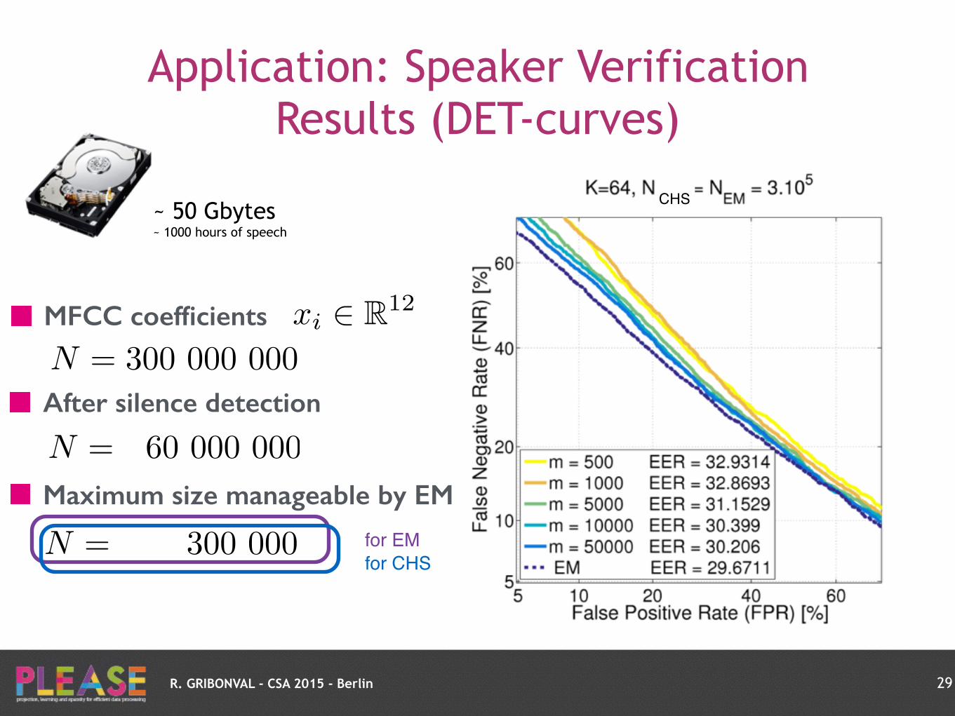
Application: Speaker Verification Results (DET-curves)
29
MFCC coefficients xi 2 R12
After silence detection
N = 60 000 000
Maximum size manageable by EM
N = 300 000
N = 300 000 000
~ 50 Gbytes ~ 1000 hours of speech
CHS
for EMfor CHS
R. GRIBONVAL - CSA 2015 - Berlin
CHS
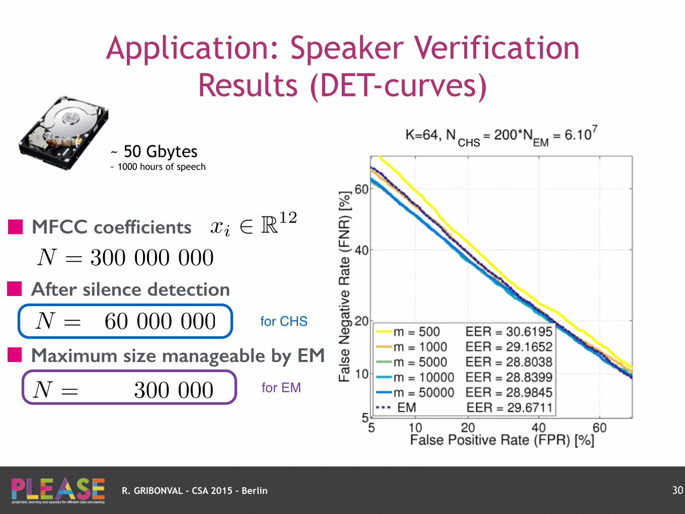
Application: Speaker Verification Results (DET-curves)
30
MFCC coefficients xi 2 R12
After silence detection
N = 60 000 000
Maximum size manageable by EM
N = 300 000
N = 300 000 000
~ 50 Gbytes ~ 1000 hours of speech
for EM
for CHS
R. GRIBONVAL - CSA 2015 - Berlin
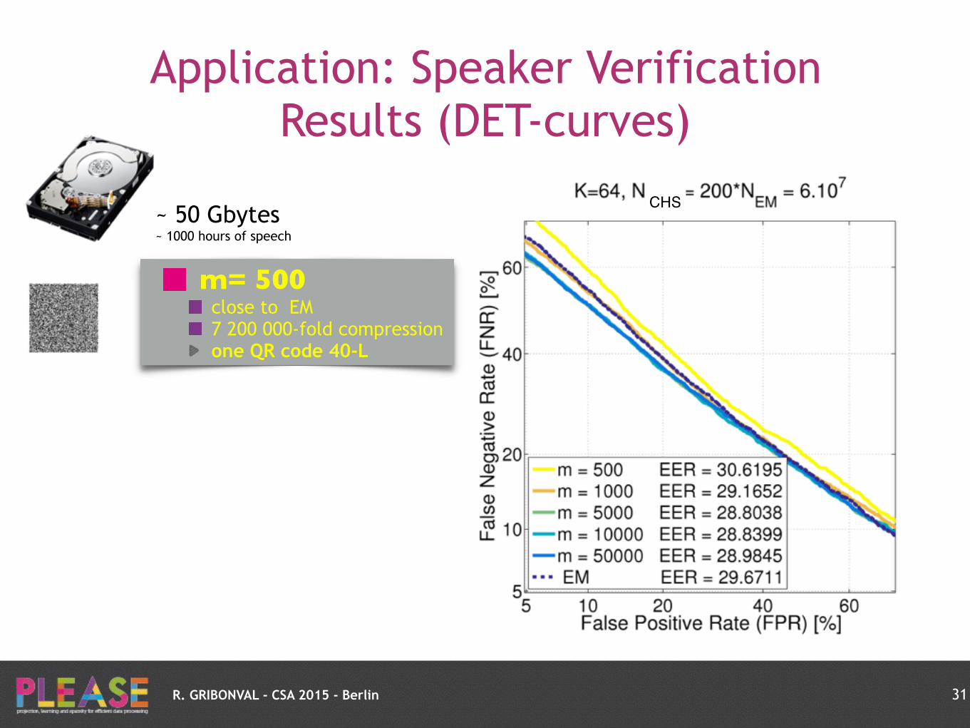
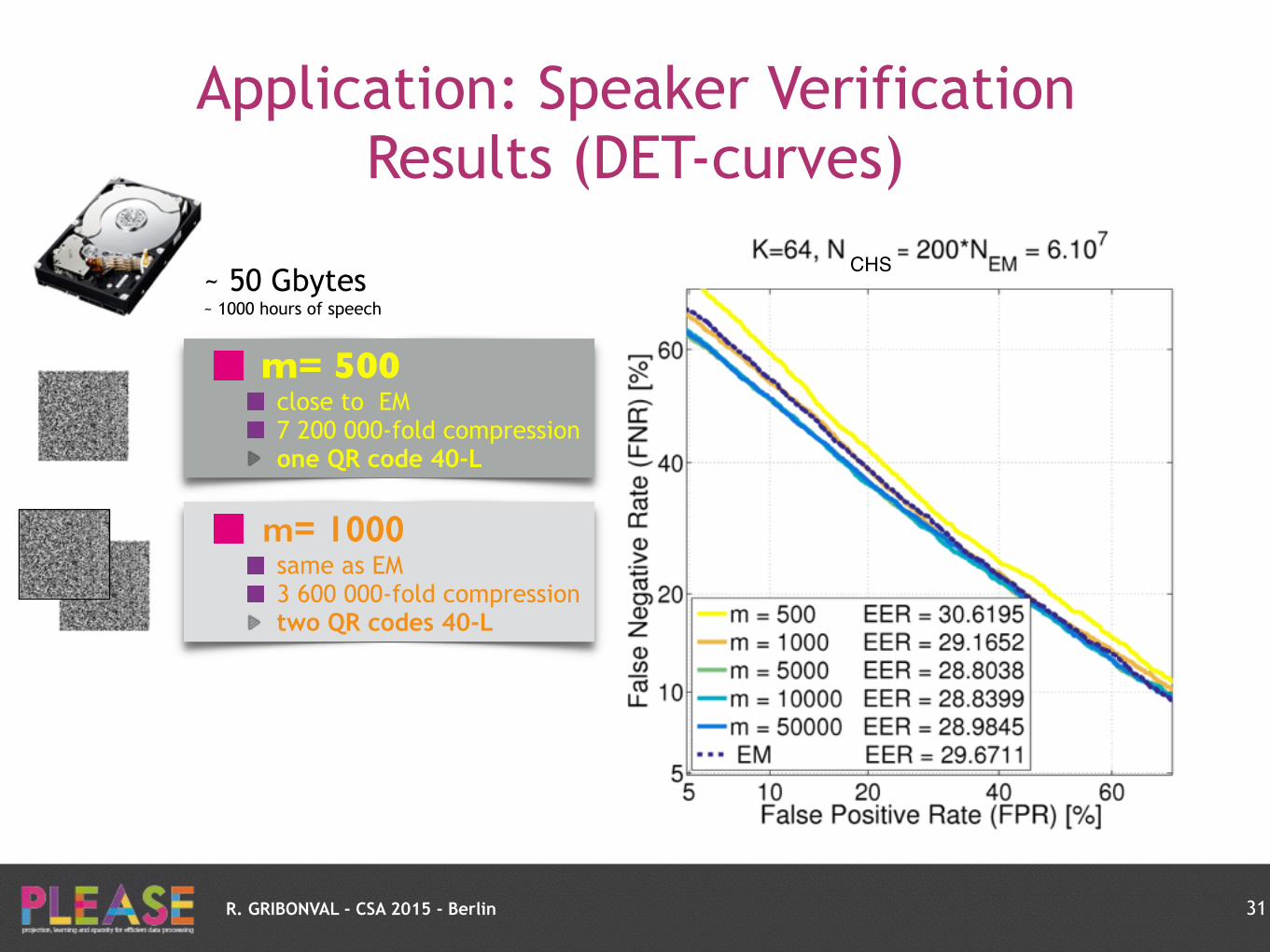
Application: Speaker Verification Results (DET-curves)
31
~ 50 Gbytes ~ 1000 hours of speech
m= 500close to EM 7 200 000-fold compression one QR code 40-L
CHS
R. GRIBONVAL - CSA 2015 - Berlin
Application: Speaker Verification Results (DET-curves)
31
~ 50 Gbytes ~ 1000 hours of speech
m= 1000same as EM 3 600 000-fold compression two QR codes 40-L
m= 500close to EM 7 200 000-fold compression one QR code 40-L
CHS
R. GRIBONVAL - CSA 2015 - Berlin
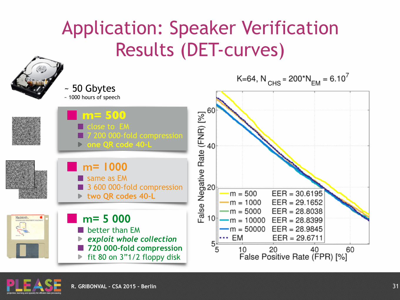
m= 5 000better than EM exploit whole collection 720 000-fold compression fit 80 on 3”1/2 floppy disk
Application: Speaker Verification Results (DET-curves)
31
~ 50 Gbytes ~ 1000 hours of speech
m= 1000same as EM 3 600 000-fold compression two QR codes 40-L
m= 500close to EM 7 200 000-fold compression one QR code 40-L
CHS

Computational Efficiency

R. GRIBONVAL - CSA 2015 - Berlin
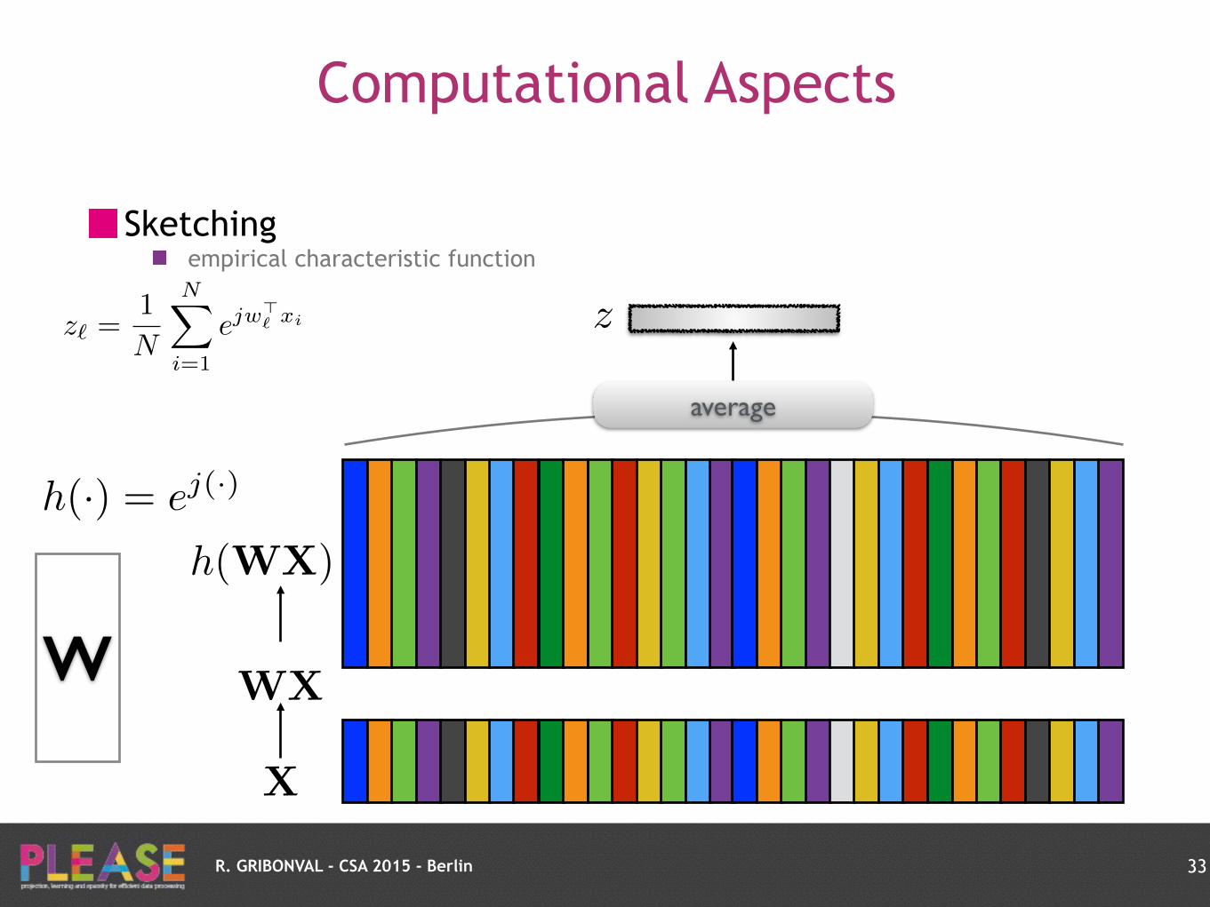
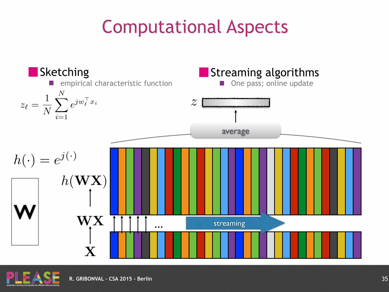
Computational Aspects
Sketching empirical characteristic function
33
z`
=1
N
NX
i=1
ejw>` xi
R. GRIBONVAL - CSA 2015 - Berlin
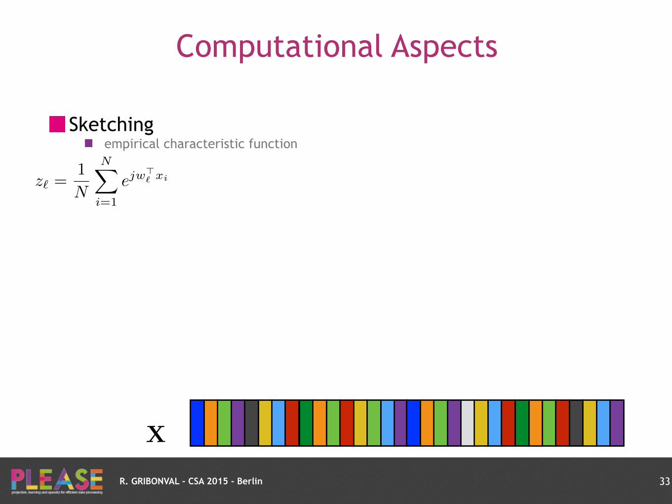
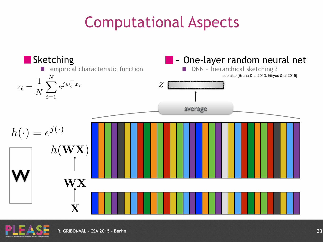
Computational Aspects
Sketching empirical characteristic function
33
z`
=1
N
NX
i=1
ejw>` xi
X
R. GRIBONVAL - CSA 2015 - Berlin
Computational Aspects
Sketching empirical characteristic function
33
z`
=1
N
NX
i=1
ejw>` xi
X
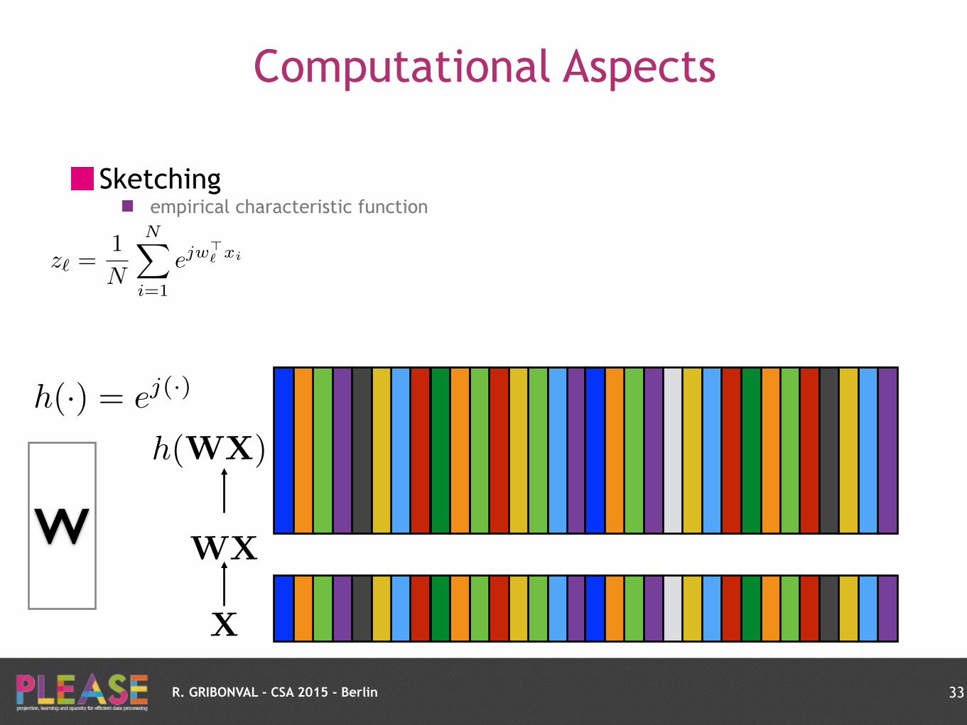
W WX
h(WX)
h(·) = ej(·)
R. GRIBONVAL - CSA 2015 - Berlin
Computational Aspects
Sketching empirical characteristic function
33
z`
=1
N
NX
i=1
ejw>` xi
X
W WX
h(WX)
h(·) = ej(·)
z
average
R. GRIBONVAL - CSA 2015 - Berlin
Computational Aspects
Sketching empirical characteristic function
33
z`
=1
N
NX
i=1
ejw>` xi
X
W WX
h(WX)
h(·) = ej(·)
z
average
~ One-layer random neural net DNN ~ hierarchical sketching ?
see also [Bruna & al 2013, Giryes & al 2015]
R. GRIBONVAL - CSA 2015 - Berlin
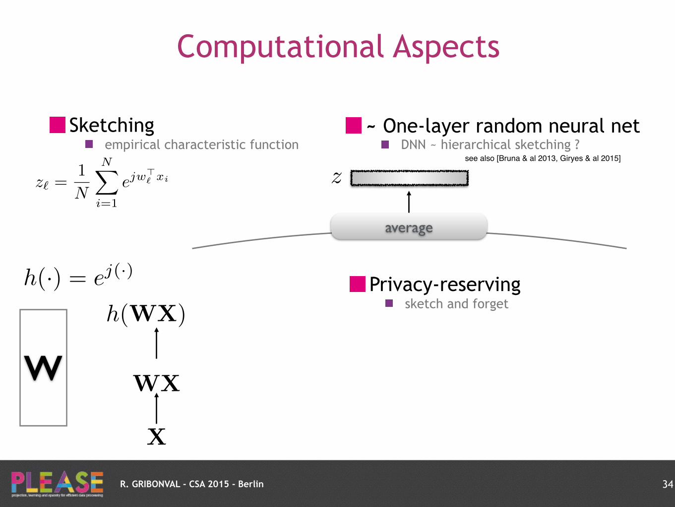
Computational Aspects
Sketching empirical characteristic function
34
z`
=1
N
NX
i=1
ejw>` xi
X
W WX
h(WX)
h(·) = ej(·)
z
average
Privacy-reserving sketch and forget
~ One-layer random neural net DNN ~ hierarchical sketching ?
see also [Bruna & al 2013, Giryes & al 2015]
R. GRIBONVAL - CSA 2015 - Berlin
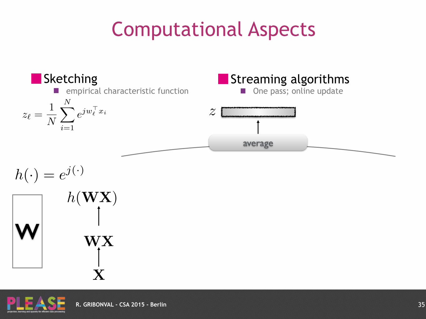
Computational Aspects
Sketching empirical characteristic function
35
z`
=1
N
NX
i=1
ejw>` xi
X
W WX
h(WX)
h(·) = ej(·)
z
average
Streaming algorithms One pass; online update
R. GRIBONVAL - CSA 2015 - Berlin
Computational Aspects
Sketching empirical characteristic function
35
z`
=1
N
NX
i=1
ejw>` xi
X
W WX
h(WX)
h(·) = ej(·)
z
average
streaming…
Streaming algorithms One pass; online update
R. GRIBONVAL - CSA 2015 - Berlin
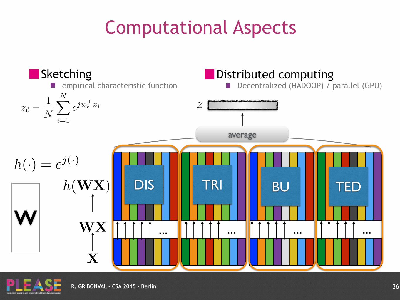
Computational Aspects
Sketching empirical characteristic function
36
z`
=1
N
NX
i=1
ejw>` xi
X
W WX
h(WX)
h(·) = ej(·)
z
average
… … … …
DIS TRI BU TED
Distributed computing Decentralized (HADOOP) / parallel (GPU)

Conclusion
R. GRIBONVAL - CSA 2015 - Berlin
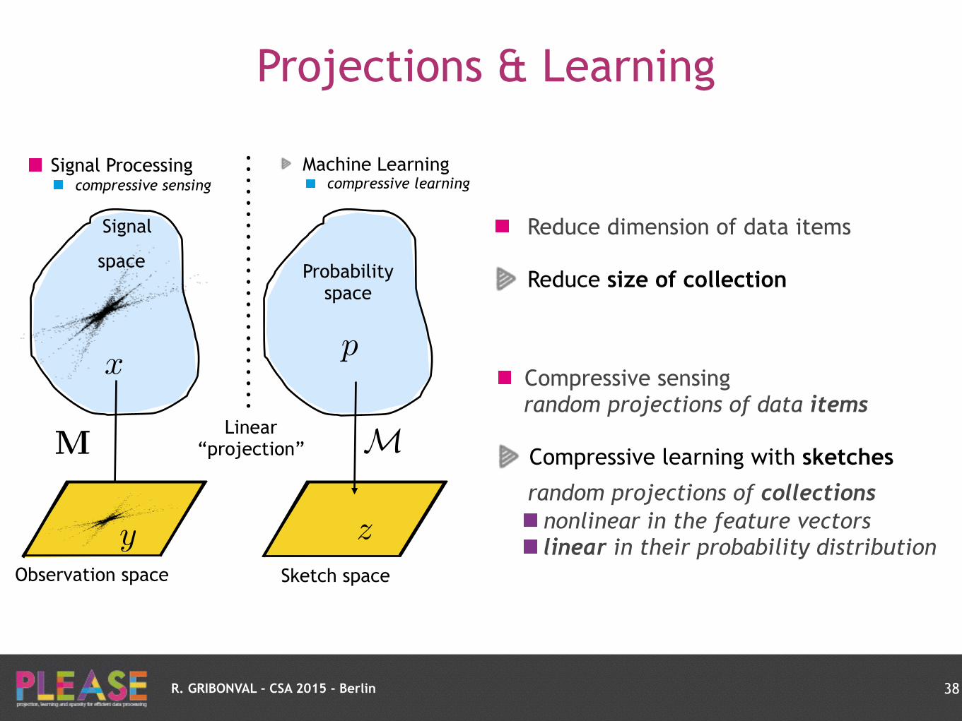
Projections & Learning
38
y
Signal
space
x
Observation space
Signal Processing compressive sensing
M M
Probability space
Sketch space
Machine Learning compressive learning
z
p
Linear “projection”
Compressive sensing random projections of data items
Compressive learning with sketches
random projections of collections
nonlinear in the feature vectors
linear in their probability distribution
Reduce dimension of data items
Reduce size of collection

R. GRIBONVAL - CSA 2015 - Berlin
Summary
Compressive clustering & Compressive GMM Bourrier, G., Perez, Compressive Gaussian Mixture Estimation. ICASSP 2013 Keriven & G.. Compressive Gaussian Mixture Estimation by Orthogonal Matching Pursuit with Replacement. SPARS 2015, Cambridge, United Kingdom Keriven & al, Sketching for Large-Scale Learning of Mixture Models (draft)
Unified framework covering projections & sketches Instance Optimal Decoders Restricted Isometry Property
Bourrier & al, Fundamental performance limits for ideal decoders in high-dimensional linear inverse problems. IEEE Transactions on Information Theory, 2014
39
Challenge: compress before learning ?X
Information preservation ?
Details: poster N. Keriven

R. GRIBONVAL - CSA 2015 - Berlin
Recent / ongoing work / challenges
Sufficient dimension for RIP
Puy, Davies & G., Recipes for stable linear embeddings from Hilbert spaces to ℝ^m, hal-01203614, see also EUSIPCO 2015 and [Dirksen 2014]
RIP for sketches in RKHS applied to compressive GMM upcoming, Keriven, Bourrier, Perez & G.
Compressive statistical learning: intrinsic dimension of PCA and other related learning tasks
work in progress, Blanchard & G.
RIP-based guarantees for general (convex & nonconvex) regularizers
Traonmilin & G, Stable recovery of low-dimensional cones in Hilbert spaces - One RIP to rule them all, arXiv:1510.00504
extends sharp RIP 1/sqrt(2) [Cai & Zhang 2014] beyond sparsity (low-rank; block/structured …)
40
m = O(dB(⌃� ⌃))
Dimension reduction ?
Decoders?
Details: poster G. Puy

R. GRIBONVAL - CSA 2015 - Berlin
•Postdoc / R&D engineer positions @ IRISA ✓ theoretical and algorithmic foundations of large-scale
machine learning & signal processing ✓ funded by ERC project PLEASE
TH###NKS#
Interested ? Joint the team
41

TH###NKS#


![Homology of gaussian groups - Centre Mersenne · 493 1.1. Gaussian and locally Gaussian monoids. Our notations follow those of [42] on the one hand, and those of [25] and [23] on](https://img.pdfslide.fr/doc/110x75/5fd4001a720ab320977220ad/homology-of-gaussian-groups-centre-mersenne-493-11-gaussian-and-locally-gaussian.jpg)