Simulation of phase contrast MRI of turbulent

flow

Sven Petersson, Petter Dyverfeldt, Roland Gårdhagen, Matts Karlsson and Tino Ebbers

Linköping University Post Print

N.B.: When citing this work, cite the original article.

This is the pre-reviewed version of the following article:

Sven Petersson, Petter Dyverfeldt, Roland Gårdhagen, Matts Karlsson and Tino Ebbers,

Simulation of phase contrast MRI of turbulent flow, 2010, Magnetic Resonance in Medicine,

(64), 4, 1039-1046.

which has been published in final form at:

http://dx.doi.org/10.1002/mrm.22494

Copyright: Wiley-Blackwell

http://eu.wiley.com/WileyCDA/Brand/id-35.html

Postprint available at: Linköping University Electronic Press

http://urn.kb.se/resolve?urn=urn:nbn:se:liu:diva-60696

Simulation of Phase-Contrast MRI of Turbulent Flow

Sven Petersson 1,2, Petter Dyverfeldt 1-3, Roland Gårdhagen 2,3, Matts Karlsson 2,3, Tino

Ebbers 1-3.

1 Division of Cardiovascular Medicine, Department of Medical and Health Sciences,

Linköping University, Linköping, Sweden.

2 Center for Medical Image Science and Visualization (CMIV), Linköping University,

Linköping, Sweden.

3 Division of Applied Thermodynamics and Fluid Mechanics, Department of Management

and Engineering, Linköping University, Linköping, Sweden.

Short running head: Simulation of Phase-Contrast MRI of Turbulent Flow

Word Count: 3942

Correspondence: Sven Petersson, Division of Cardiovascular Medicine, Department of

Medical and Health Sciences, Linköping University,

SE-58185 Linköping, Sweden.

E-mail: sven.petersson@liu.se

Grant sponsors: Swedish Research Council; Swedish Heart-Lung Foundation; Center for

Industrial Information Technology (CENIIT).

Abstract Phase-contrast MRI is a powerful tool for the assessment of blood flow. However, especially

in the highly complex and turbulent flow that accompanies many cardiovascular diseases,

phase-contrast MRI may suffer from artifacts. Simulation of phase-contrast MRI of turbulent

flow could increase our understanding of phase-contrast MRI artifacts in turbulent flows and

facilitate the development of phase-contrast MRI methods for the assessment of turbulent

blood flow. We present a method for the simulation of phase-contrast MRI measurements of

turbulent flow. The method uses an Eulerian-Lagrangian approach, where spin particle

trajectories are computed from time-resolved large eddy simulations. The Bloch equations are

solved for each spin for a frame of reference moving along the spins trajectory. The method

was validated by comparison with phase-contrast MRI measurements of velocity and

intravoxel velocity standard deviation on a flow phantom consisting of a straight rigid pipe

with a stenosis. Turbulence related artifacts, such as signal drop and ghosting, could be

recognized in the measurements as well as in the simulations. The velocity and the intravoxel

velocity standard deviation obtained from the magnitude of the phase-contrast MRI

simulations agreed well with the measurements.

Keywords: Phase contrast magnetic resonance imaging, computer simulation, turbulent flow,

constriction, turbulence intensity.

Introduction Phase-contrast magnetic resonance imaging (PC-MRI) is a powerful tool for the

quantification of blood flow velocity. Clinically, PC-MRI velocity mapping is used primarily

for volume flow measurements (1-2). Three-dimensional three-directional time-resolved PC-

MRI velocity mapping (3) has been used to study blood flow, for example, in the heart (4-5)

and the aorta (6-7). The assessment of flow in cardiovascular diseases, such as valvular and

vascular stenosis, has the potential to become an important diagnostic tool. PC-MRI has been

used to assess aortic coarctations (8), and mitral regurgitation and stenoses (9). However,

many PC-MRI artifacts are more prominent in the different types of flow that accompany

cardiovascular diseases. In the vicinity of a stenosis, for example, the blood flow is

accelerating and contains fluctuating velocities. The presence of fluctuating velocities is an

indicator of disturbed or turbulent flow; turbulence intensity is a measure of the magnitude of

the velocity fluctuations in relation to the mean flow velocity. Accelerating and fluctuating

flow can cause spatial misregistration errors (displacement) due to phase shifts from higher

order motion, flow related signal loss due to intravoxel phase-dispersion (10), and ghosting,

due to view-to-view variations. Because of the importance of characterizing and quantifying

flow in cardiovascular diseases, PC-MRI assessment of these types of flows has been an

important research topic (11-12). Recent investigations in this area have led to the

development of PC-MRI with an ultrashort echo time (TE) (13), in order to reduce artifacts,

such as signal loss. Another approach is to exploit the effects of velocity fluctuations on the

MRI signal magnitude, as is done in generalized PC-MRI, to map the intravoxel velocity

standard deviation (IVSD) (14), which can be used to estimate the turbulence intensity.

Nevertheless, due to the complexity of the flow and its effect on the PC-MRI measurements,

PC-MRI assessment of flow in many cardiovascular diseases remains challenging. Therefore,

tools for optimization, quality control and validation of PC-MRI methods are needed.

The true flow in the subject measured is unknown, therefore it is difficult to determine the

extent of errors in both in-vivo and in-vitro PC-MRI measurements. Simulations of PC-MRI

measurements on numerical flow data, obtained from for example computational fluid

dynamics (CFD) simulations, permit investigations of the outcome of a measurement on a

known flow field. In this way, in-depth studies of artifacts as well as the quality control and

validation of PC-MRI methods can be made.

Different approaches for performing numerical simulations of PC-MRI measurements for

laminar flow exist. For example, Doorly and Ljungdahl (15) and Lee et al. (16) used an

Eulerian-Lagrangian approach to simulate two-dimensional through-plane PC-MRI

measurements from CFD data of flow with a low Reynolds number. In those studies, the CFD

data was computed on a fixed numerical mesh (Eulerian procedure) and the magnetization

was evaluated by solving the Bloch equations for virtual spins as they traveled along their

trajectories (Lagrangian procedure). Another possibility is an Eulerian approach, such as that

used by Jou and Saloner (17) and Lorthois et al. (18), to simulate time-of-flight MR images

from CFD data. The Eulerian approach does not comprise computations of particle

trajectories, and is therefore less computationally expensive than the Eulerian-Lagrangian

approach. In the Eulerian-Lagrangian approach, spatial misregistration artifacts are

automatically accounted for, whereas in the Eulerian approach a transformation of the mesh is

necessary. Turbulent flow can be described as “an irregular condition of flow in which the

various quantities show a random variation with time and space coordinates, so that

statistically distinct average values can be discerned” (19). These velocity fluctuations affect

PC-MRI measurements and have to be taken into account when simulating PC-MRI

measurements of turbulent flow. Previously, numerical simulations of 2D time-of-flight

measurements have been carried out in order to study the mechanisms of signal loss in

stenotic flow (20). In that study, a k-ε method was used to model the turbulent velocity

fluctuations. Instead of solving the Bloch equations, the phase shifts of virtual spin packets

were estimated by integration over the slice-encoding gradient, which was placed in the

principal flow direction. To keep their simulation simple, the phase and frequency-encoding

gradients were not included in the simulation. Simulation of PC-MRI using time-resolved

CFD data that describes turbulent flow has not been performed.

The aim of this work was to develop an approach for the simulation of PC-MRI

measurements of turbulent flow. This was achieved by solving the Bloch equations using an

Eulerian-Lagrangian approach in which the particle trajectories of virtual spin packets were

computed from time-resolved numerical velocity data, obtained by large eddy simulations

(LES). The method was validated by comparing the PC-MRI simulations of velocity and

IVSD measurements with in-vitro PC-MRI measurements on a flow phantom that consisted

of a straight rigid pipe with a cosine shaped stenosis.

Methods

PC-MRI Simulation

The proposed PC-MRI simulation approach utilizes time-resolved numerical velocity data

that resolves turbulent velocity fluctuations, such as obtained by direct numerical simulation

or LES. In direct numerical simulation, the whole range of spatial and temporal scales is

resolved, whereas in LES, the larger turbulent scales are resolved and the smaller ones are

modeled.

The trajectories of virtual spins were computed from the simulated velocity data. This was

achieved by integrating the velocity field over time using a fourth-order Runge Kutta

algorithm with a time-varying integration step (EnSight 8.0, CEI, Apex, NC, USA).

Data describing the gradients and radiofrequency-pulse were imported to the PC-MRI

simulation directly from the MRI-scanner software (Philips Healthcare, Best, the Netherlands)

to obtain realistic pulse sequences and facilitate comparison with measurements. The initial

transverse magnetization before every excitation was assumed to be zero and no saturation

effects were simulated.

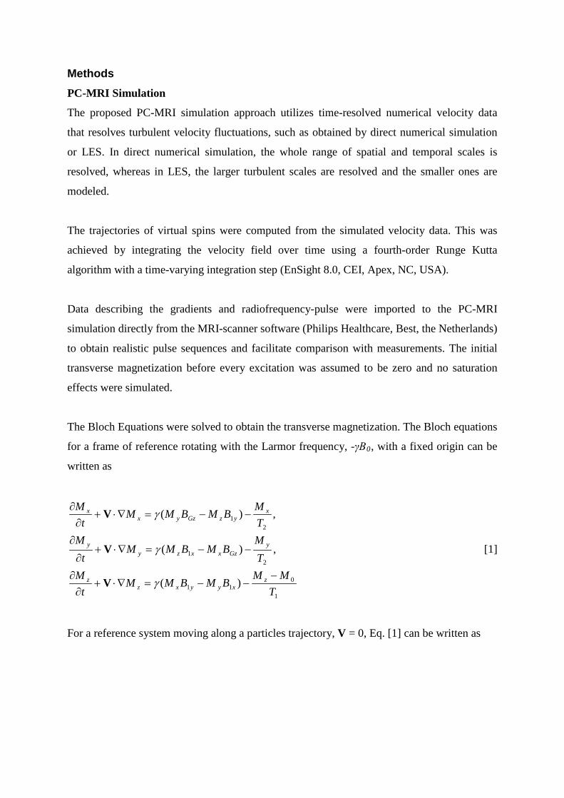
The Bloch Equations were solved to obtain the transverse magnetization. The Bloch equations

for a frame of reference rotating with the Larmor frequency, -γB0, with a fixed origin can be

written as

1

011

21

21

)(

,)(

,)(

TMM

BMBMMt

MTM

BMBMMt

MTM

BMBMMt

M

zxyyxz

z

yGzxxzy

y

xyzGzyx

x

−−−=∇⋅+

∂∂

−−=∇⋅+∂

∂

−−=∇⋅+∂∂

γ

γ

γ

V

V

V

[1]

For a reference system moving along a particles trajectory, V = 0, Eq. [1] can be written as

1

011

21

21

)(

,)(

,)(

TMM

BMBMdt

dMTM

BMBMdt

dMTM

BMBMdt

dM

zxyyx

z

yGzxxz

y

xyzGzy

x

−−−=

−−=

−−=

γ

γ

γ

[2]

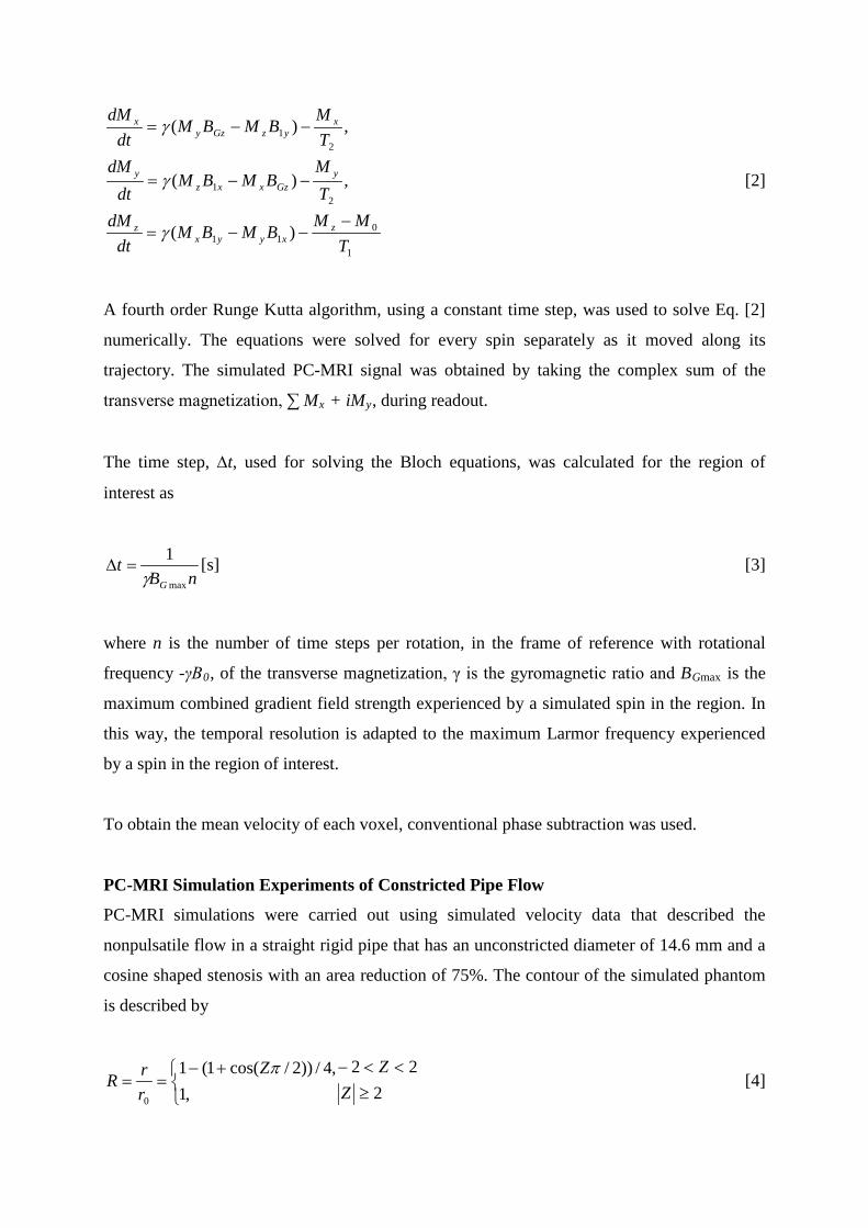
A fourth order Runge Kutta algorithm, using a constant time step, was used to solve Eq. [2]

numerically. The equations were solved for every spin separately as it moved along its

trajectory. The simulated PC-MRI signal was obtained by taking the complex sum of the

transverse magnetization, ∑ Mx + iMy, during readout.

The time step, ∆t, used for solving the Bloch equations, was calculated for the region of

interest as

nBt

G max

1γ

=∆ [s] [3]

where n is the number of time steps per rotation, in the frame of reference with rotational

frequency -γB0, of the transverse magnetization, γ is the gyromagnetic ratio and BGmax is the

maximum combined gradient field strength experienced by a simulated spin in the region. In

this way, the temporal resolution is adapted to the maximum Larmor frequency experienced

by a spin in the region of interest.

To obtain the mean velocity of each voxel, conventional phase subtraction was used.

PC-MRI Simulation Experiments of Constricted Pipe Flow

PC-MRI simulations were carried out using simulated velocity data that described the

nonpulsatile flow in a straight rigid pipe that has an unconstricted diameter of 14.6 mm and a

cosine shaped stenosis with an area reduction of 75%. The contour of the simulated phantom

is described by

222

,1,4/))2/cos(1(1

0 ≥<<−

+−

==Z

ZZrrR

π [4]

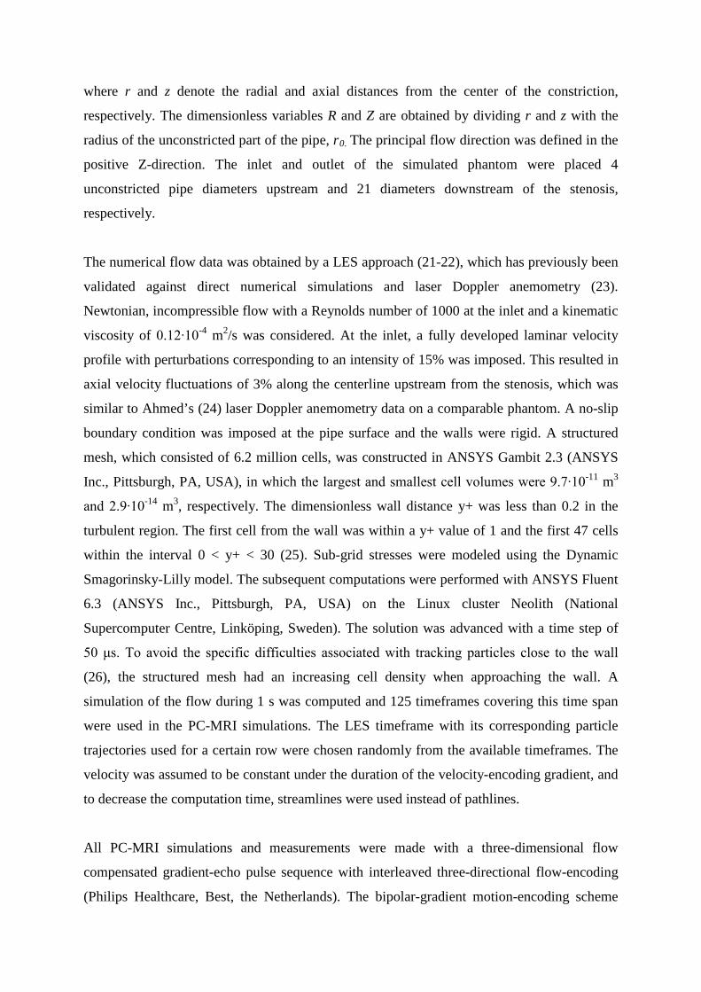
where r and z denote the radial and axial distances from the center of the constriction,

respectively. The dimensionless variables R and Z are obtained by dividing r and z with the

radius of the unconstricted part of the pipe, r0. The principal flow direction was defined in the

positive Z-direction. The inlet and outlet of the simulated phantom were placed 4

unconstricted pipe diameters upstream and 21 diameters downstream of the stenosis,

respectively.

The numerical flow data was obtained by a LES approach (21-22), which has previously been

validated against direct numerical simulations and laser Doppler anemometry (23).

Newtonian, incompressible flow with a Reynolds number of 1000 at the inlet and a kinematic

viscosity of 0.12∙10-4 m2/s was considered. At the inlet, a fully developed laminar velocity

profile with perturbations corresponding to an intensity of 15% was imposed. This resulted in

axial velocity fluctuations of 3% along the centerline upstream from the stenosis, which was

similar to Ahmed’s (24) laser Doppler anemometry data on a comparable phantom. A no-slip

boundary condition was imposed at the pipe surface and the walls were rigid. A structured

mesh, which consisted of 6.2 million cells, was constructed in ANSYS Gambit 2.3 (ANSYS

Inc., Pittsburgh, PA, USA), in which the largest and smallest cell volumes were 9.7∙10-11 m3

and 2.9∙10-14 m3, respectively. The dimensionless wall distance y+ was less than 0.2 in the

turbulent region. The first cell from the wall was within a y+ value of 1 and the first 47 cells

within the interval 0 < y+ < 30 (25). Sub-grid stresses were modeled using the Dynamic

Smagorinsky-Lilly model. The subsequent computations were performed with ANSYS Fluent

6.3 (ANSYS Inc., Pittsburgh, PA, USA) on the Linux cluster Neolith (National

Supercomputer Centre, Linköping, Sweden). The solution was advanced with a time step of

50 μs. To avoid the specific difficulties associated with tracking particles close to the wall

(26), the structured mesh had an increasing cell density when approaching the wall. A

simulation of the flow during 1 s was computed and 125 timeframes covering this time span

were used in the PC-MRI simulations. The LES timeframe with its corresponding particle

trajectories used for a certain row were chosen randomly from the available timeframes. The

velocity was assumed to be constant under the duration of the velocity-encoding gradient, and

to decrease the computation time, streamlines were used instead of pathlines.

All PC-MRI simulations and measurements were made with a three-dimensional flow

compensated gradient-echo pulse sequence with interleaved three-directional flow-encoding

(Philips Healthcare, Best, the Netherlands). The bipolar-gradient motion-encoding scheme

included a reference segment with a first gradient moment of zero and one differentially

motion-encoded segment in each direction (simple four-point method (27)).

For an overview, a PC-MRI simulation using the time-averaged LES data was made using a

relatively low intravoxel spin density of 10 spins/voxel, slice-encoding in the principal flow

direction and with a FOV that covered the stenosis and the whole jet (Sim_MeanVel: TE/TR:

2.4/4.3 ms, flip angle: 8°, VENC: 4 m/s, voxel size: 1.5x1.5x1.5 mm3). The temporal

resolution used when solving the Bloch equations in Sim_MeanVel was chosen to allow a

minimum of 30 time steps per revolution (15).

Two simulations were carried out using the time-resolved LES data, one with frequency-

encoding in the principal flow direction (Sim_FreqEncZ) and one with the slice-encoding in

the principal flow direction (Sim_SliceEncZ). In these two simulations, 500 spins/voxel were

emitted to fully account for the intravoxel spin velocity effects on the PC-MRI signal. In order

to reduce the computational requirements, the simulations focused on three limited regions. A

region of size 4 x 4 x 140 mm3 was defined along the centerline after the stenosis, including

the turbulent regime where the flow jet breaks down. To obtain cross-sectional images from

Sim_SliceEncZ, spins were also emitted from two 12 mm long cylinders that covered the

entire cross section of the pipe; they were placed at the turbulence peak (Z = 4.3) and at the

reattachment zone (Z = 3.1), respectively. The temporal resolution used when solving the

Bloch equations in these simulations was chosen to allow a minimum of 60 time steps per

revolution (15). The scan parameters in these PC-MRI simulations were: TE/TR: 2.3/4.2 ms,

flip angle: 8°, VENC: 1.5 m/s, voxel size: 2x2x2 mm3. The velocity data was corrected for

phase wraps.

To evaluate the effects of incorporating the velocity fluctuations in PC-MRI simulations of

turbulent flow, a simulation using the time-averaged LES data (Sim_TimeAvLES) was

carried out using the same parameters and number of spins as in Sim_SliceEncZ.

In-vitro PC-MRI Experiments of Constricted Pipe Flow

For comparison with the PC-MRI simulations, PC-MRI measurements were made on an in-

vitro flow phantom designed to mimic the simulated flow phantom. The flow in the in-vitro

phantom had the same kinematic viscosity (0.12∙10-4 m2/s) and Reynolds number (1000) as in

the numerical phantom. The in-vitro phantom, which has been described previously (14), has

an entrance length of about 100 diameters and a downstream stenosis length of about 30

diameters. The phantom was connected to a gear pump (Gearchem G6, Pulsafeeder,

Rochester, NY, USA) via plastic hoses. The pump was fed by a computer-controlled AC-

servo motor (JVL Industri Elektronik A/S, Blokken, Denmark). A honeycomb flow

straightener, constructed from plastic straws, was placed at the inlet of the phantom to reduce

the effects of flow structures that may be present in the hoses.

Three PC-MRI measurements were carried out using a clinical 1.5 T MRI scanner (Philips

Achieva; Philips Healthcare, Best, the Netherlands) and the same type of pulse sequence as in

the PC-MRI simulations.

For comparison with the PC-MRI simulation using the time-averaged LES data and a low

intravoxel spin density (Sim_MeanVel), a corresponding measurement (Meas_MeanVel) was

carried out with the following parameters: TE/TR = 2.7/5.9 ms, flip angle = 25°, VENC = 4

m/s, voxel size = 1.5 mm3, FOV = 160 x 69 x 150 mm3, number of signal averages (NSA) =

8.

For comparison with the PC-MRI simulations using time-resolved (Sim_FreqEncZ,

Sim_SliceEncZ) and time-averaged LES data (Sim_TimeAvLES), respectively, two

measurements were carried out; one with frequency-encoding in the principal flow direction

(Meas_FreqEncZ) and one with slice-encoding in the principal flow direction

(Meas_SliceEncZ). In these measurements the following parameters were used: TE/TR =

3.2/5.7, flip angle = 15°, VENC = 1.5 m/s, voxel size = 2 mm3. The measurement that used

frequency-encoding in the principal flow direction had a FOV of 60 mm x 158 mm x 220 mm

and NSA 8. The measurement with slice-encoding in the principal flow direction had a FOV

of 220 mm x 150 mm x 130 mm and NSA 5.

To permit a quantitative comparison between the signal magnitude from PC-MRI simulations

and PC-MRI measurements, the IVSD was calculated. The IVSD is a measure of the standard

deviation of the velocity fluctuations (28), which can also be measured by other experimental

techniques such as laser Doppler anemometry and particle image velocimetry, and is used to

estimate the turbulence intensity. The IVSD, σIVSD, was obtained from the signal magnitude

relationship

2

)()0(

ln2

v

vIVSD k

kSS

σ

= [ms-1], [5]

where kv=π/VENC describes the amount of applied motion sensitivity (14), S(0) is the MRI

signal from a reference segment with a first gradient moment of zero, and S(kv) is the signal

from a motion-encoded segment. The IVSD was compared with the root mean square (RMS)

of the fluctuating velocity as computed directly from the LES data.

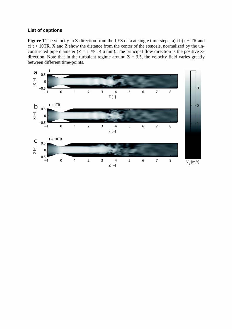
Results The LES simulations of the stenotic flow were carried out successfully. At the break down of

the jet (around Z = 3.5), the velocity field varied greatly between different time-points

separated by one TR (Figure 1).

A comparison between the mean velocity in the principal flow direction from the PC-MRI

simulation using the time-averaged LES data and a low intravoxel spin density

(Sim_MeanVel), and the corresponding PC-MRI measurement (Meas_MeanVel), is shown in

Figure 2. The length of the jet in the measurement and the PC-MRI simulation agree well, and

partial volume effects can be seen along the jet’s periphery in both the measurement and the

PC-MRI simulation. However, there is very poor agreement between the IVSD as obtained

from the PC-MRI simulation using only the time-averaged velocity LES data

(Sim_TimeAvLES) and the IVSD from the PC-MRI measurements (Meas_SliceEncZ)

(Figure 3). This poor agreement was expected, as this simulation did not take the velocity

fluctuations into account.

The velocity and IVSD along the centerline of the phantom from the PC-MRI simulation that

used time-resolved LES data and slice-encoding in the principal flow direction

(Sim_SliceEncZ) are compared to the corresponding measurement (Meas_SliceEncZ) and

LES data in Figure 4. Figure 5 and Figure 6 show cross sectional views and radial plots of the

IVSD (Sim_SliceEncZ, Meas_SliceEncZ) and RMS of the LES data at the reattachment zone

and the turbulence peak, respectively. Plots of the velocity and IVSD from the simulation that

used frequency-encoding in the principal flow direction (Sim_FreqEncZ) and the

corresponding measurement are shown in Figure 7. As seen in Figure 4-Figure 7, there is an

overall good agreement between the PC-MRI simulations using time-resolved LES data and

the corresponding PC-MRI measurements.

The view-to-view variations that occur in PC-MRI measurements of fluctuating flow cause

ghosting artifacts; this implies that the signal from one voxel is dispersed to other voxels in

the phase-encoding direction resulting in an increased uncertainty. In three-dimensional PC-

MRI, slice-encoding is almost identical to phase-encoding; accordingly, this effect can be

seen in the plot of IVSD along the centerline of the phantom when slice-encoding was in the

principal flow direction (Sim_SliceEncZ, Figure 4). These ghosting artifacts along the

centerline diminished when frequency-encoding was done in the principal flow direction

(Figure 7), and instead, displacement was present in the principal flow direction. In this case,

the time difference between velocity-encoding and readout, which caused the displacement

artifact, was around 1.5 ms. During this time, a spin on the centerline that is velocity encoded

at Z = 4.0 will travel around 3.7 mm or 0.26 unconstricted diameters, Z, in the Z-direction.

The corresponding velocity measurement point in the PC-MRI simulation is displaced around

3.2 mm or 0.22 unconstricted diameters (Figure 7 a). When slice-encoding was done in the

principal flow direction, readout occurred almost simultaneously with the velocity-encoding

in this direction and no notable displacement was observed (Figure 4). In the in-vitro PC-MRI

measurements, an unexpected artifact was present in the magnitude data immediately

downstream from the stenosis, upstream from the turbulence peak (Figure 4, Figure 7). The

origin of this artifact is unknown; several parameters, including fat-shift-direction, phase-

encoding direction and echo time were changed without removing the artifact. The artifact

may have resulted from a real flow effect, originating in disturbances of the inflow. These

disturbances could for example been induced by vibrations in the MRI scanner or from the

pump.

Discussion An approach for the simulation of PC-MRI measurements of turbulent flow has been

presented and validated.

The results obtained by the proposed approach for simulating PC-MRI velocity and IVSD

measurements in turbulent flow consistently show a good overall agreement to the PC-MRI

measurements. Slight differences between the measurements and the PC-MRI simulations

seem to have their origin in discrepancies between the measurements and the LES simulation.

Computational fluid dynamics simulation of turbulent flow is still extremely difficult, and

phantom measurements of turbulent flow are also sensitive to many environmental factors,

such as temperature and vibrations, which are difficult to control in an MRI system. Some

differences can therefore be expected. However, the quality of LES data of turbulent flow

proved to be more than sufficient for studying PC-MRI artifacts and their behavior for

different pulse sequences in a controlled environment; the primary use of PC-MRI

simulations.

The usability of the PC-MRI simulation approach was tested and demonstrated by comparing

simulations with frequency and slice-encoding in the principle flow direction, which as

expected, resulted in different ghosting and displacement artifacts. As expected, ghosting

artifacts were present in the slice-encoding direction (Figure 4). When frequency-encoding

was done in the principal flow direction, the data was displaced along the centerline and no

ghosting artifacts were present in the frequency-encoding direction, which resulted in

smoother velocity and IVSD curves (Figure 7). The displacement in the PC-MRI simulations

agreed well with numerical predictions based on the LES data. Choosing the optimal

directions for phase or frequency-encoding is a trade off between ghosting, displacement

artifacts and scan time. The results from the PC-MRI measurements seem to suffer less from

ghosting than the results from the PC-MRI simulations (Figure 4). A possible explanation

could be the relatively short time span of LES data used. The duration of the simulated scan is

16 s, resulting in the fact that the same set of timeframes will be used 16 times. But this effect

can also be a result of the number of signal averages used in the PC-MRI measurement.

The proposed simulation approach resemble a PC-MRI measurement to a high degree, thus

the approach includes many known and unknown artifacts, at the cost of computational time.

For some applications, a less computationally intensive approach may be sufficient.

Simulation of PC-MRI using LES data not including velocity fluctuations, such as the mean

velocity field in stationary flow, has shown to be sufficient for stationary laminar or non-

fluctuating flow (20). As can be observed in Figure 2, this less computationally intensive

approach may also be sufficient for turbulent flow for applications in which only the PC-MRI

velocity is studied. However, this approach does not correctly simulate the complete complex-

valued PC-MRI signal, as can be seen from the IVSD values in Figure 3. Consequently, in

order to study artifacts related to the signal, such as ghosting or signal loss in turbulent flow, a

full PC-MRI simulation, including the effect of velocity fluctuations, is necessary. Also for

the simulation of IVSD measurements using generalized PC-MRI, velocity fluctuations have

to be included. These results are in agreement with a previous study on simulations of 2D

time-of-flight MRI measurements (20), which indicated that the intravoxel phase dispersion

due to velocity fluctuations is the major cause of signal drop in the vicinity of a stenosis, and

ghosting and mean flow intravoxel phase dispersion act as secondary effects. Furthermore, by

computing the particle trajectories of virtual spins, it is possible to separate the signal

originating from different spins in the PC-MRI simulations, something which could be useful

when studying different artifacts, including displacement, ghosting and signal loss due to

turbulence. The use of an Eulerian approach, such as that presented by Siegel et al. (29), may

allow for a reduction in the computation time. However, whether the explicit assumptions

incorporated in the Eulerian approach can be extended to correctly account for the effects of

turbulence on PC-MRI has to be investigated. The Eulerian-Lagrangian approach presented

here may be improved by using an adaptive differential equation solver for solving the Bloch

equations.

Here, we have focused on the simulation of fluctuating flow, but the method presented can

also be extended to study partial volume artifacts by the wall; an important factor when

developing methods for the assessment of wall shear stress. These artifacts can be included by

simulating the signal from the wall of e.g. blood vessels. The approach presented does not

include the effects of noise on the PC-MRI measurement, but this can be included by adding

Gaussian noise to both transverse magnetic components, assuming that the noise in each

channel of the quadrature detector is Gaussian with zero mean. The method could also be

improved by implementing more artifacts e.g. nonlinear gradients.

In conclusion, we have presented a method for the simulation of PC-MRI measurements of

mean velocity and IVSD in turbulent flow. The results demonstrate the validity and feasibility

of simulating PC-MRI of turbulent flow conditions using the method proposed. The

simulation of PC-MRI of turbulent flow can be a powerful tool for studying artifacts that

appear in the presence of turbulent flow. It can prove very useful when developing, evaluating

and optimizing new methods for e.g. quantifying turbulence and assessing wall shear stress.

Although the simulated flow was by definition not an exact representation of the true flow in

the manufactured phantom, the overall appearance of the PC-MRI simulations and the

measurement show strong similarities. The fact that those artifacts that appear in the

measurements, such as signal drop, velocity aliasing, intravoxel phase dispersion, ghosting

and displacement, also appear in the PC-MRI simulation, further demonstrates the validity of

the proposed simulation approach.

Acknowledgements

This work was funded by the Swedish Research Council, the Swedish Heart-Lung Foundation

and the Center for Industrial Information Technology (CENIIT).

References

1. Pennell D, Sechtem U, Higgins C, Manning W, Pohost G, Rademakers F, van Rossum A, Shaw L, Yucel E. Clinical indications for cardiovascular magnetic resonance (CMR): Consensus Panel report. European Heart Journal. Volume 25: Eur Soc Cardiology; 2004. p 1940-1965.

2. Hendel R, Patel M, Kramer C, Poon M, Carr J, Gerstad N, Gillam L, Hodgson J, Kim R. ACCF/ACR/SCCT/SCMR/ASNC/NASCI/SCAI/SIR 2006 Appropriateness Criteria for Cardiac Computed Tomography and Cardiac Magnetic Resonance Imaging: A Report of the American College of Cardiology Foundation Quality Strategic Directions Committee Appropriateness Criteria Working Group, American College of Radiology, Society of Cardiovascular Computed Tomography, Society for Cardiovascular Magnetic Resonance, American Society of Nuclear Cardiology, North American Society for Cardiac Imaging, Society for Cardiovascular Angiography and Interventions, and Society of Interventional Radiology. Journal of the American College of Cardiology 2006;48(7):1475–1497.

3. Wigström L, Sjöqvist L, Wranne B. Temporally resolved 3D phase-contrast imaging. Magnetic Resonance in Medicine 1996;36(5):800 - 803.

4. Bolger A, Heiberg E, Karlsson M, Wigstrom L, Engvall J, Sigfridsson A, Ebbers T, Kvitting J, Carlhall C, Wranne B. Transit of Blood Flow Through the Human Left Ventricle Mapped by Cardiovascular Magnetic Resonance. Journal of Cardiovascular Magnetic Resonance 2007;9(5):741-747.

5. Kilner P, Yang G, Wilkes A, Mohiaddin R, Firmin D, Yacoub M. Asymmetric redirection of flow through the heart. Nature 2000;404:759-761.

6. Kvitting J, Ebbers T, Wigström L, Engvall J, Olin C, Bolger A. Flow patterns in the aortic root and the aorta studied with time-resolved, 3-dimensional, phase-contrast magnetic resonance imaging: implications for aortic valve–sparing surgery. The Journal of Thoracic and Cardiovascular Surgery 2004;127(6):1602-1607.

7. Markl M, Draney M, Hope M, Levin J, Chan F, Alley M, Pelc N, Herfkens R. Time-resolved 3-dimensional velocity mapping in the thoracic aorta: visualization of 3-directional blood flow patterns in healthy volunteers and patients. Journal of computer assisted tomography 2004;28(4):459.

8. Frydrychowicz A, Schlensak C, Stalder A, Russe M, Siepe M, Beyersdorf F, Langer M, Hennig J, Markl M. Ascending–descending aortic bypass surgery in aortic arch coarctation: Four-dimensional magnetic resonance flow analysis. The Journal of Thoracic and Cardiovascular Surgery 2007;133(1):260-262.

9. Gatenby J, McCauley T, Gore J. Mechanisms of signal loss in magnetic resonance imaging of stenoses. Medical physics 1993;20:1049.

10. O'Brien K, Cowan B, Jain M, Stewart R, Kerr A, Young A. MRI phase contrast velocity and flow errors in turbulent stenotic jets. Journal of Magnetic Resonance Imaging 2008;28(1).

11. Ståhlberg F, Thomsen C, Søndergaard L, Henriksen O. Pulse sequence design for MR velocity mapping of complex flow: notes on the necessity of low echo times. Magnetic resonance imaging 1994;12(8):1255-1262.

12. Oshinski J, Ku D, Pettigrew R. Turbulent fluctuation velocity: the most significant determinant of signal loss in stenotic vessels. Magnetic Resonance in Medicine 1995;33(2):193-199.

13. O'Brien K, Myerson S, Cowan B, Young A, Robson M, Freemasons N, Trust W, Fellowship S. Phase contrast ultrashort TE: A more reliable technique for measurement of high-velocity turbulent stenotic jets. Magnetic Resonance in Medicine 2009;62(3):626-636.

14. Dyverfeldt P, Sigfridsson A, Kvitting J, Ebbers T. Quantification of intravoxel velocity standard deviation and turbulence intensity by generalizing phase-contrast MRI. Magnetic Resonance in Medicine 2006;56(4):850-858.

15. Doorly DJ, Ljungdahl M. Computational simulation of magnetic resonance imaging techniques for velocity field measurements. Proceedings of ASME Fluids Engineering Division Summer Meeting 1997.

16. Lee KL, Doorly DJ, Firmin DN. Numerical simulations of phase contrast velocity mapping of complex flows in an anatomically realistic bypass graft geometry. Medical Physics 2006;33(7):2621-2631.

17. Jou LD, Saloner D. A numerical study of magnetic resonance images of pulsatile flow in a two dimensional carotid bifurcation - A numerical study of MR images. Medical Engineering & Physics 1998;20(9):643-652.

18. Lorthois S, Stroud-Rossman J, Berger S, Jou LD, Saloner D. Numerical simulation of magnetic resonance angiographies of an anatomically realistic stenotic carotid bifurcation. Annals of Biomedical Engineering 2005;33(3):270-283.

19. Hinze JO. Turbulence: McGraw-Hill Inc. New York.; 1975. 20. Siegel Jr. J, Oshinski J, Pettigrew R, Ku D. Computational simulation of turbulent

signal loss in 2D time-of-flight magnetic resonance angiograms. Magnetic Resonance in Medicine 1997;37(4):609-614.

21. Mathieu J, Scott J. An Introduction to Turbulent Flow: Cambridge University Press; 2000.

22. Gårdhagen R, Lantz J, Carlsson F, Karlsson M. Quantifying Turbulent Wall Shear Stress in a Stenosed Pipe using Large Eddy Simulation. Journal of Biomechanical Engineering 2010;In press.

23. Gårdhagen R, Lantz J, Carlsson F, Karlsson M. Large Eddy Simulation of Flow Through a Stenosed Pipe. American Society of Mechanical Engineers Summer Bioengineering Conference, Marco Island, Florida, USA 2008.

24. Ahmed S. An experimental investigation of pulsatile flow through a smooth constriction. Experimental Thermal and Fluid Science 1998;17(4):309-318.

25. Oefelein J, Schefer R, Barlow R. Toward Validation of Large Eddy Simulation for Turbulent Combustion. AIAA Journal 2006;44(3):418-433.

26. Jou LD, vanTyen R, Berger SA, Saloner D. Calculation of the magnetization distribution for fluid flow in curved vessels. Magnetic Resonance in Medicine 1996;35(4):577-584.

27. Pelc N, Bernstein M, Shimakawa A, Glover G. Encoding strategies for three-direction phase-contrast MR imaging of flow. Journal of Magnetic Resonance Imaging 1991;1(4):405-413.

28. Dyverfeldt P, Gårdhagen R, Sigfridsson A, Karlsson M, Ebbers T. On MRI Turbulence Quantification. Magnetic resonance imaging 2009;27(7):913-922.

29. Gudbjartsson H, Patz S. The Rician distribution of noisy MRI data. Magnetic resonance in medicine 1995;34(6):910.

List of captions

Figure 1 The velocity in Z-direction from the LES data at single time-steps; a) t b) t + TR and c) t + 10TR. X and Z show the distance from the center of the stenosis, normalized by the un-constricted pipe diameter (Z = 1 14.6 mm). The principal flow direction is the positive Z-direction. Note that in the turbulent regime around Z = 3.5, the velocity field varies greatly between different time-points.

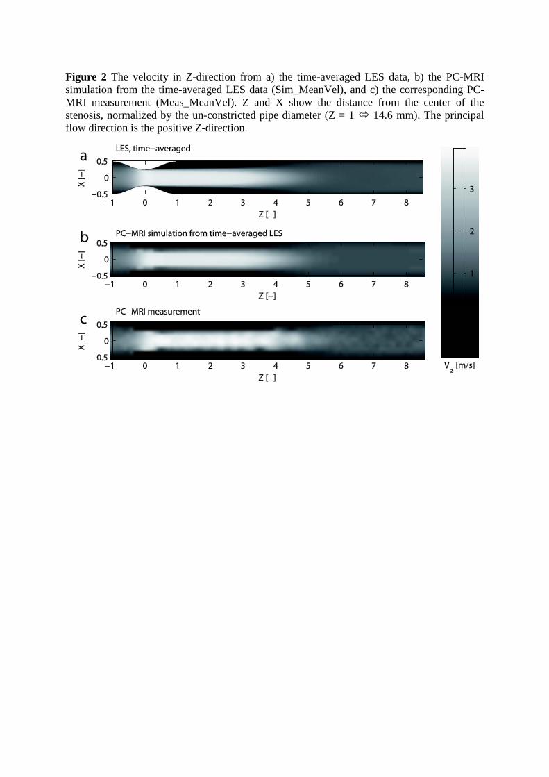
Figure 2 The velocity in Z-direction from a) the time-averaged LES data, b) the PC-MRI simulation from the time-averaged LES data (Sim_MeanVel), and c) the corresponding PC-MRI measurement (Meas_MeanVel). Z and X show the distance from the center of the stenosis, normalized by the un-constricted pipe diameter (Z = 1 14.6 mm). The principal flow direction is the positive Z-direction.

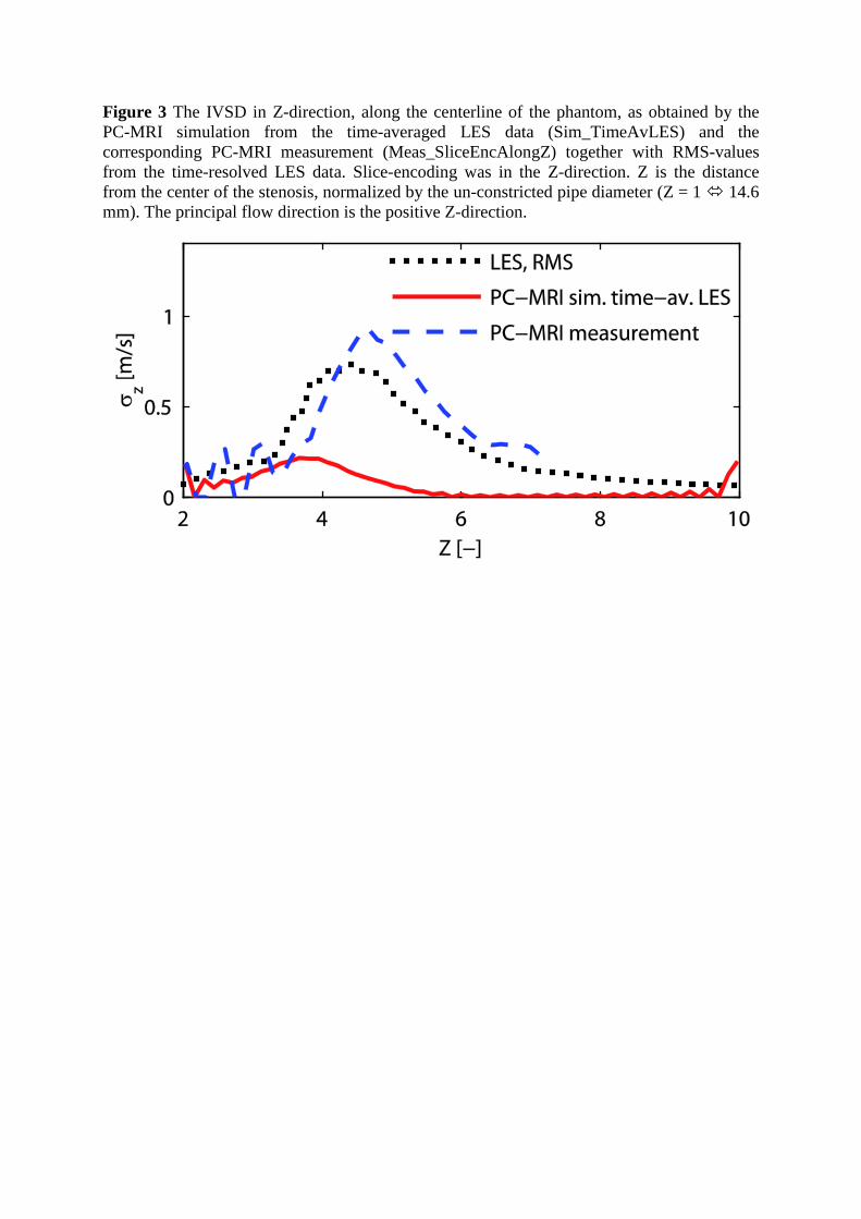
Figure 3 The IVSD in Z-direction, along the centerline of the phantom, as obtained by the PC-MRI simulation from the time-averaged LES data (Sim_TimeAvLES) and the corresponding PC-MRI measurement (Meas_SliceEncAlongZ) together with RMS-values from the time-resolved LES data. Slice-encoding was in the Z-direction. Z is the distance from the center of the stenosis, normalized by the un-constricted pipe diameter (Z = 1 14.6 mm). The principal flow direction is the positive Z-direction.

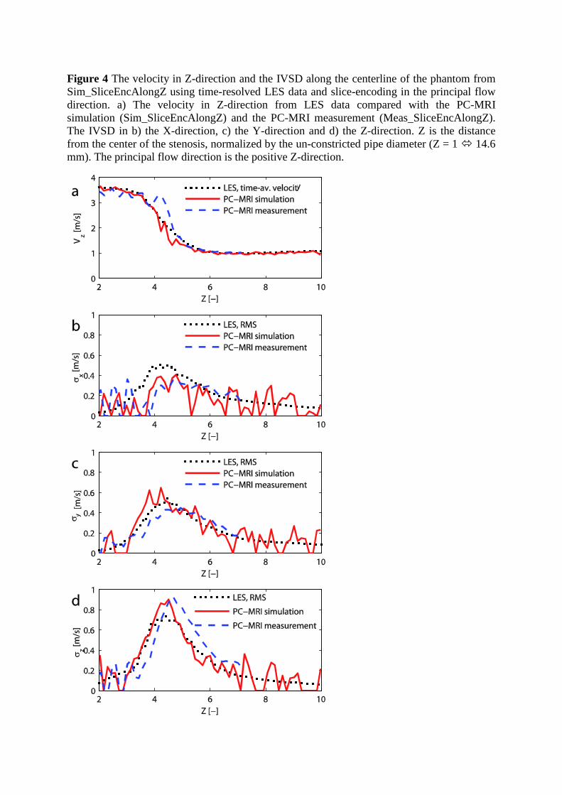
Figure 4 The velocity in Z-direction and the IVSD along the centerline of the phantom from Sim_SliceEncAlongZ using time-resolved LES data and slice-encoding in the principal flow direction. a) The velocity in Z-direction from LES data compared with the PC-MRI simulation (Sim_SliceEncAlongZ) and the PC-MRI measurement (Meas_SliceEncAlongZ). The IVSD in b) the X-direction, c) the Y-direction and d) the Z-direction. Z is the distance from the center of the stenosis, normalized by the un-constricted pipe diameter (Z = 1 14.6 mm). The principal flow direction is the positive Z-direction.

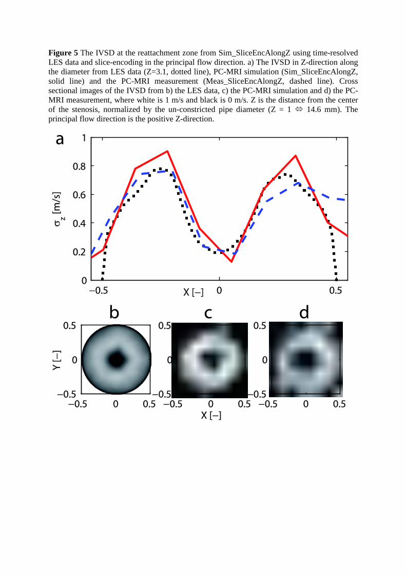
Figure 5 The IVSD at the reattachment zone from Sim_SliceEncAlongZ using time-resolved LES data and slice-encoding in the principal flow direction. a) The IVSD in Z-direction along the diameter from LES data (Z=3.1, dotted line), PC-MRI simulation (Sim_SliceEncAlongZ, solid line) and the PC-MRI measurement (Meas_SliceEncAlongZ, dashed line). Cross sectional images of the IVSD from b) the LES data, c) the PC-MRI simulation and d) the PC-MRI measurement, where white is 1 m/s and black is 0 m/s. Z is the distance from the center of the stenosis, normalized by the un-constricted pipe diameter (Z = 1 14.6 mm). The principal flow direction is the positive Z-direction.

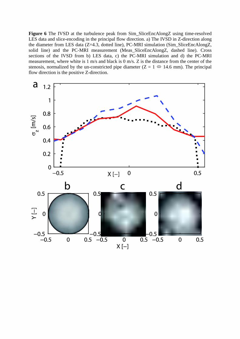
Figure 6 The IVSD at the turbulence peak from Sim_SliceEncAlongZ using time-resolved LES data and slice-encoding in the principal flow direction. a) The IVSD in Z-direction along the diameter from LES data (Z=4.3, dotted line), PC-MRI simulation (Sim_SliceEncAlongZ, solid line) and the PC-MRI measurement (Meas_SliceEncAlongZ, dashed line). Cross sections of the IVSD from b) LES data, c) the PC-MRI simulation and d) the PC-MRI measurement, where white is 1 m/s and black is 0 m/s. Z is the distance from the center of the stenosis, normalized by the un-constricted pipe diameter (Z = 1 14.6 mm). The principal flow direction is the positive Z-direction.

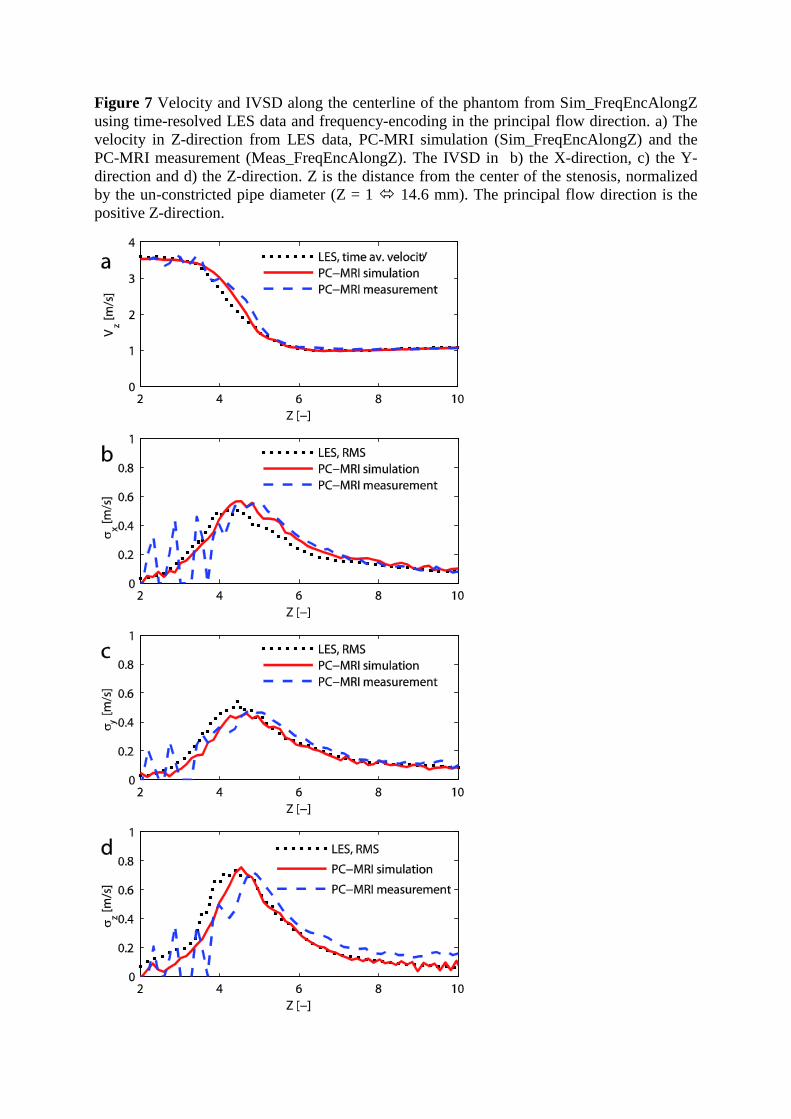
Figure 7 Velocity and IVSD along the centerline of the phantom from Sim_FreqEncAlongZ using time-resolved LES data and frequency-encoding in the principal flow direction. a) The velocity in Z-direction from LES data, PC-MRI simulation (Sim_FreqEncAlongZ) and the PC-MRI measurement (Meas_FreqEncAlongZ). The IVSD in b) the X-direction, c) the Y-direction and d) the Z-direction. Z is the distance from the center of the stenosis, normalized by the un-constricted pipe diameter (Z = 1 14.6 mm). The principal flow direction is the positive Z-direction.