Embed Size (px)
Citation preview
Visualization
Statistical Analysis of Microarray Data
Jacques van Helden
[email protected] Aix-Marseille Université, France
Technological Advances for Genomics and Clinics (TAGC, INSERM Unit U1090)
http://jacques.van-helden.perso.luminy.univ-amu.fr/
FORMER ADDRESS (1999-2011) Université Libre de Bruxelles, Belgique
Bioinformatique des Génomes et des Réseaux (BiGRe lab) http://www.bigre.ulb.ac.be/
Heat maps
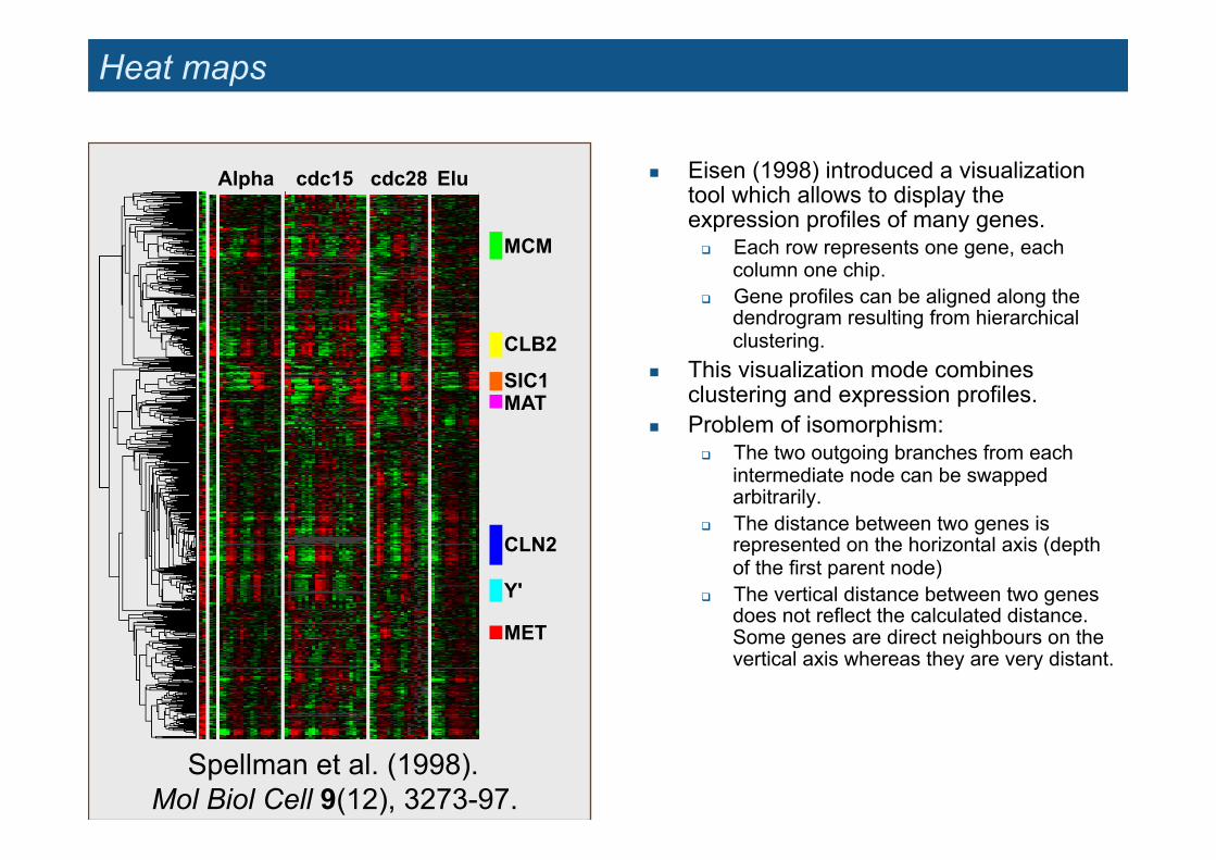
! Eisen (1998) introduced a visualization tool which allows to display the expression profiles of many genes.
" Each row represents one gene, each column one chip.
" Gene profiles can be aligned along the dendrogram resulting from hierarchical clustering.
! This visualization mode combines clustering and expression profiles.
! Problem of isomorphism: " The two outgoing branches from each
intermediate node can be swapped arbitrarily.
" The distance between two genes is represented on the horizontal axis (depth of the first parent node)
" The vertical distance between two genes does not reflect the calculated distance. Some genes are direct neighbours on the vertical axis whereas they are very distant.
MCM
CLB2
SIC1 MAT
CLN2
Y'
MET
Alpha cdc15 cdc28 Elu
Spellman et al. (1998). Mol Biol Cell 9(12), 3273-97.
Reduction in data dimension
Statistical Analysis of Microarray Data
Jacques van Helden
[email protected] Aix-Marseille Université (AMU), France
Technological Advances for Genomics and Clinics (TAGC, INSERM Unit U1090)
http://jacques.van-helden.perso.luminy.univmed.fr/
Why to reduce dimensionality ?
! A series of microarrays can be represented as a N x p matrix, where " each one of the p columns contains information about an experiment (different conditions,
treatments, tissues) " each one of the N rows contains information about a spot (gene)
! Object dimensions " Each gene can be considered as a p-dimensional object (one dimension per experiment). " Each experiment can be considered as a N-dimensional object (one dimension per gene).
! Visualization " Visualization devices are restricted to 2 (printer) or at best 3 (space explorer) dimensions. " One would thus like to display objects in 2D or 3D, whilst retaining the maximum of information. " After reduction of dimensions, some clusters may already appear in the data set.
! Analysis " Some analysis methods loose their accuracy when there are too many vriables (over-fitting). " Reducing the data to a subset of dimensions will allow a trade-of between the loss of information
and the gain in accuracy. In this case, the appropriate number of dimensions may be higher than 3, its choice depends on the data itself (e.g. number of objects per training group).
How to reduce dimensionality ?
! Several methods are available for reducing the number of dimensions of a data set " Principal Component Analysis " Singular Value Decomposition " Spring embedding
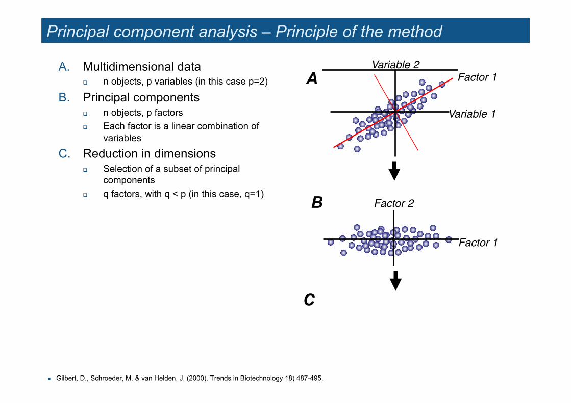
Principal component analysis – Principle of the method
! Gilbert, D., Schroeder, M. & van Helden, J. (2000). Trends in Biotechnology 18) 487-495.
A. Multidimensional data " n objects, p variables (in this case p=2)
B. Principal components " n objects, p factors " Each factor is a linear combination of
variables
C. Reduction in dimensions " Selection of a subset of principal
components " q factors, with q < p (in this case, q=1)
Factor 2!
Factor 1!
Variable 2!
Variable 1!
Factor 1!A
B
C
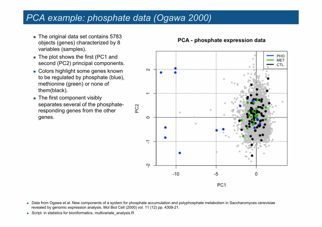
PCA example: phosphate data (Ogawa 2000)
! Data from Ogawa et al. New components of a system for phosphate accumulation and polyphosphate metabolism in Saccharomyces cerevisiae revealed by genomic expression analysis. Mol Biol Cell (2000) vol. 11 (12) pp. 4309-21.
! Script: in statistics for bioniformatics, multivariate_analysis.R
! The original data set contains 5783 objects (genes) characterized by 8 variables (samples).
! The plot shows the first (PC1 and second (PC2) principal components.
! Colors highlight some genes known to be regulated by phosphate (blue), methionine (green) or none of them(black).
! The first component visibly separates several of the phosphate-responding genes from the other genes.
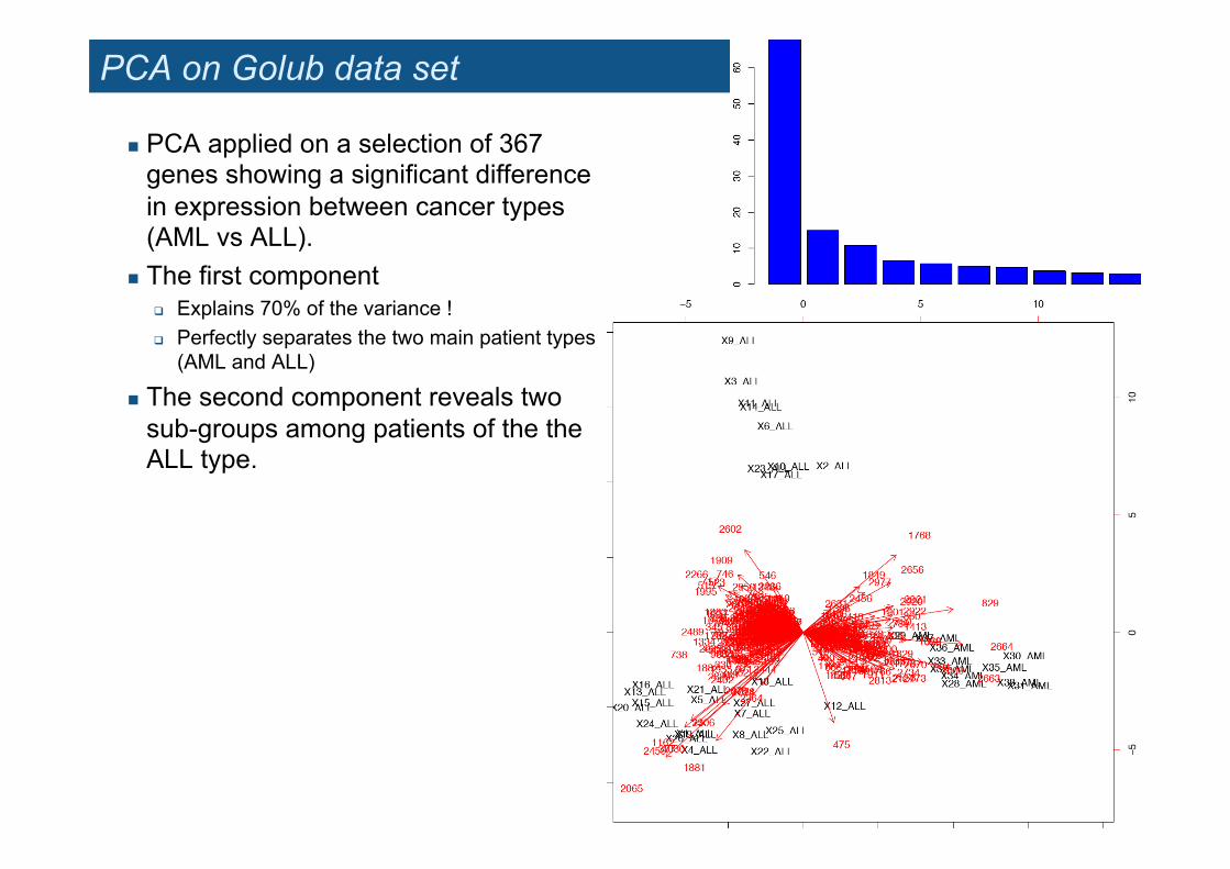
PCA on Golub data set
! PCA applied on a selection of 367 genes showing a significant difference in expression between cancer types (AML vs ALL).
! The first component " Explains 70% of the variance ! " Perfectly separates the two main patient types
(AML and ALL)
! The second component reveals two sub-groups among patients of the the ALL type.
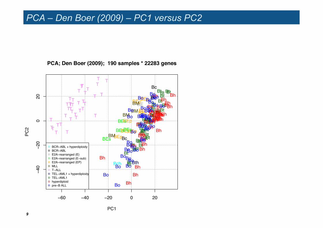
PCA – Den Boer (2009) – PC1 versus PC2
9
−60 −40 −20 0 20
−40
−20
020
PCA; Den Boer (2009); 190 samples * 22283 genes
PC1
PC2
T
TTT T
T
T
TT
TT
T
T
T
T
T
T
T
T
TT
TT
T T
T
T
TT
T
TTT
T
T
T
BtBt
Bt
Bt
Bt
BtBt
BtBt
BtBt
BtBt
Bt
BtBt
Bt
Bt
BtBt
Bt
Bt
Bt
Bt
Bt
Bt
Bt
BtBt
BtBt
Bt
Bt
Bt
Bt
Bt
Bt
Bt
Bt
Bt
Bt
BtBt
Bth
Bh
BhBh
Bh
Bh
BhBh
BhBhBhBh
Bh
BhBh
Bh
Bh
Bh
BhBh
Bh
Bh
Bh
Bh
Bh
Bh
Bh
Bh
BhBh
BhBh
Bh
BhBh
BhBh
Bh
Bh
Bh
BhBh
Bh
BhBh
BEBEp
BEpBEp
BEpBEp
BEp
BEp
BEp
BEs
BEs
BEs
BEs
Bc
Bc
Bc
Bc
Bch
BM
BM
BMBM
BoBo
Bo
Bo
Bo
Bo
BoBo
Bo
BoBo
BoBo
Bo
Bo
Bo
Bo
BoBo
BoBo
Bo
BoBo
Bo
Bo
Bo
Bo
Bo
Bo BoBo
Bo
BoBo
Bo
Bo
Bo
BoBo
Bo
Bo
Bo
Bo
●
●
●
●
●
●
●
●
●
●
●
BCR−ABL + hyperdiploidyBCR−ABLE2A−rearranged (E)E2A−rearranged (E−sub)E2A−rearranged (EP)MLLT−ALLTEL−AML1 + hyperdiploidyTEL−AML1hyperdiploidpre−B ALL
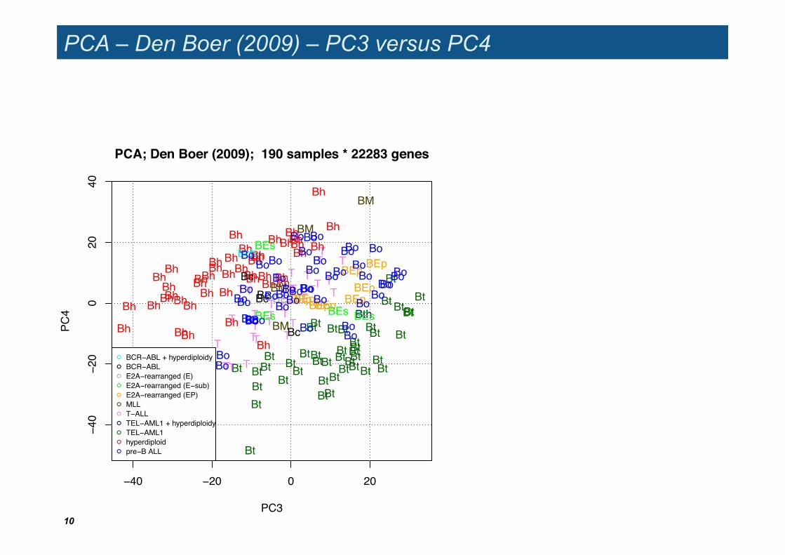
PCA – Den Boer (2009) – PC3 versus PC4
10
−40 −20 0 20
−40
−20
020
40
PCA; Den Boer (2009); 190 samples * 22283 genes
PC3
PC4
TT
T
T
TT
T
T
T
T
TT
TT
T
T
T
T
T
T
T
T
T T
T
T
T
T T
TT
T TT
T
T Bt
Bt
BtBtBt
Bt
Bt Bt
BtBt
Bt
Bt
Bt
Bt
BtBt
Bt
Bt
Bt
Bt
Bt
BtBtBt
Bt
BtBt
BtBt BtBt
BtBt
Bt
Bt
Bt
Bt
Bt
Bt Bt
BtBt
Bt
BthBh
BhBh
Bh
Bh
BhBh
Bh
Bh
Bh
BhBh Bh
Bh
Bh
Bh
Bh
Bh
Bh
BhBh
Bh
Bh
BhBh
BhBh
BhBh
BhBhBh
Bh
Bh
BhBh
Bh
BhBh
Bh
Bh
Bh
Bh
Bh
BE
BEp
BEpBEp
BEp BEpBEp
BEp
BEpBEsBEs BEs
BEs
Bc
Bc
BcBc
Bch
BM
BM
BM
BM
BoBo
Bo
Bo Bo
Bo
Bo
BoBo
Bo
Bo
Bo
Bo
BoBo
Bo
Bo
Bo
BoBo
Bo
BoBo Bo
Bo
Bo
Bo
BoBo
BoBoBo
Bo
Bo
Bo
Bo
Bo Bo
Bo
BoBo Bo
Bo
Bo
●
●
●
●
●
●
●
●
●
●
●
BCR−ABL + hyperdiploidyBCR−ABLE2A−rearranged (E)E2A−rearranged (E−sub)E2A−rearranged (EP)MLLT−ALLTEL−AML1 + hyperdiploidyTEL−AML1hyperdiploidpre−B ALL
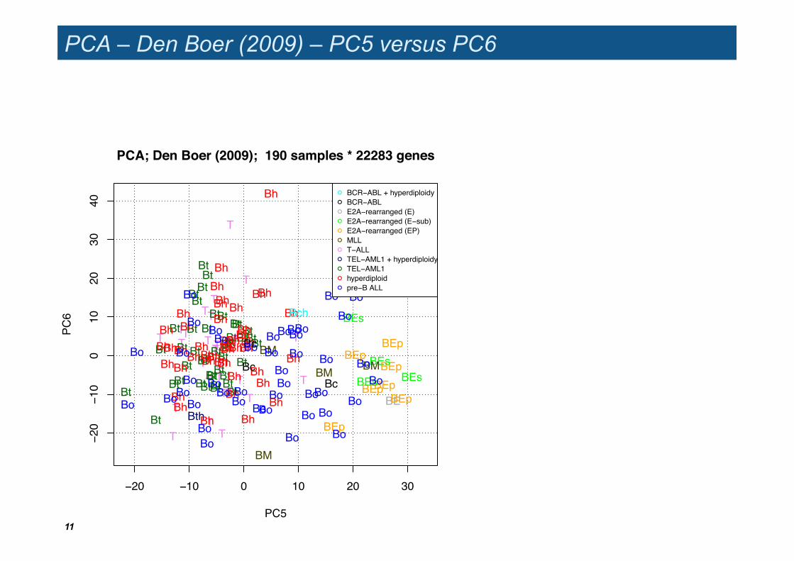
PCA – Den Boer (2009) – PC5 versus PC6
11
−20 −10 0 10 20 30
−20
−10
010
2030
40
PCA; Den Boer (2009); 190 samples * 22283 genes
PC5
PC6 T
T
T
T
T
TT
T
T
TT
T TT
T
T
T
T
T
T
T T TT
T
TT
TT
T
T
T
TTT
T
Bt
BtBt
Bt
Bt
Bt BtBtBt
BtBt
Bt
Bt
Bt
Bt Bt
Bt
BtBt
Bt
Bt
Bt
Bt
Bt
Bt
Bt
BtBt
BtBt Bt
Bt
Bt
Bt
BtBtBt
Bt
Bt
Bt
Bt
Bt
Bt
BthBh
Bh
Bh
Bh
BhBhBh
BhBh BhBh Bh
BhBh
Bh
Bh
Bh
Bh
BhBh
Bh
Bh
Bh
Bh
Bh
Bh
BhBhBhBh
BhBhBhBh
BhBhBh Bh
Bh
Bh
BhBh Bh
Bh
BE
BEp
BEp
BEp
BEp
BEp
BEp
BEp
BEp
BEsBEsBEs
BEs
Bc
Bc
Bc
Bc
Bch
BM
BMBMBM
Bo
Bo
BoBo
Bo
Bo
BoBo
BoBo
Bo
Bo
Bo
Bo
Bo
Bo
Bo
Bo
Bo
BoBo
Bo
Bo
Bo
Bo
BoBo
Bo Bo
Bo
Bo
Bo
Bo
Bo
BoBo
Bo
BoBoBo
Bo
Bo
Bo
Bo
●
●
●
●
●
●
●
●
●
●
●
BCR−ABL + hyperdiploidyBCR−ABLE2A−rearranged (E)E2A−rearranged (E−sub)E2A−rearranged (EP)MLLT−ALLTEL−AML1 + hyperdiploidyTEL−AML1hyperdiploidpre−B ALL
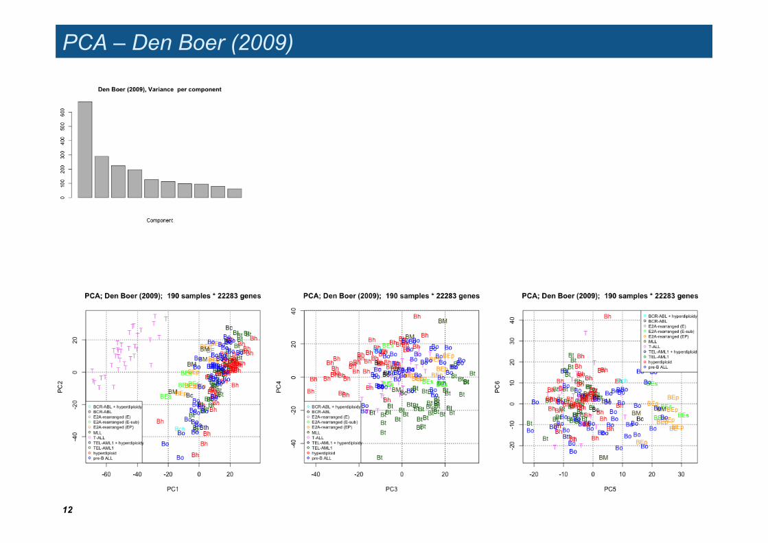
PCA – Den Boer (2009)
12
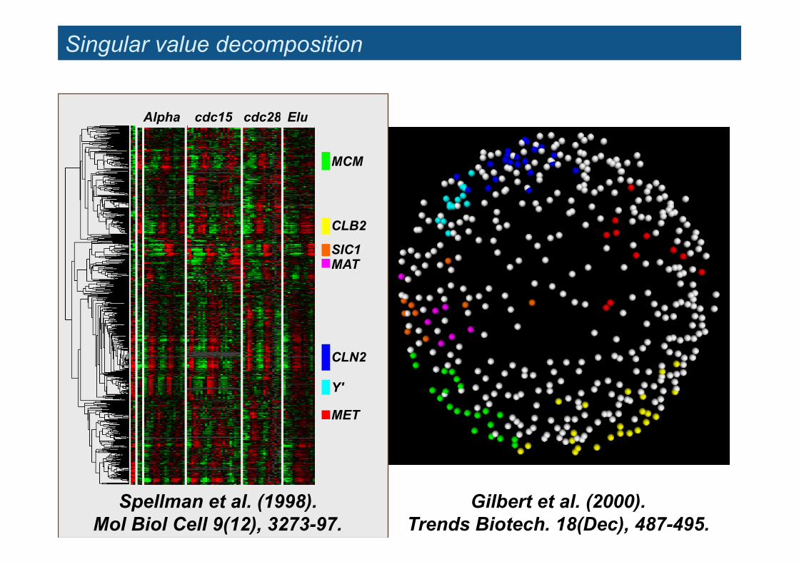
Singular value decomposition
Gilbert et al. (2000). Trends Biotech. 18(Dec), 487-495.
MCM
CLB2
SIC1 MAT
CLN2
Y'
MET
Alpha cdc15 cdc28 Elu
Spellman et al. (1998). Mol Biol Cell 9(12), 3273-97.
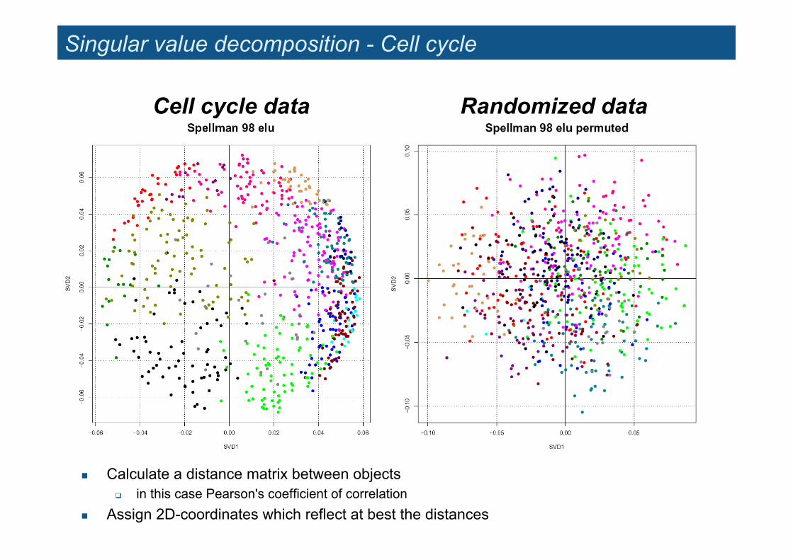
Singular value decomposition - Cell cycle
! Calculate a distance matrix between objects " in this case Pearson's coefficient of correlation
! Assign 2D-coordinates which reflect at best the distances
Cell cycle data Randomized data
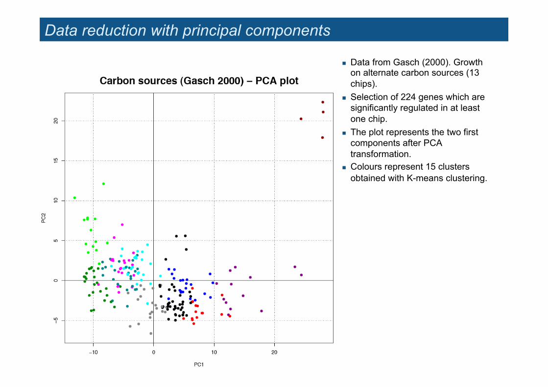
Data reduction with principal components
! Data from Gasch (2000). Growth on alternate carbon sources (13 chips).
! Selection of 224 genes which are significantly regulated in at least one chip.
! The plot represents the two first components after PCA transformation.
! Colours represent 15 clusters obtained with K-means clustering.
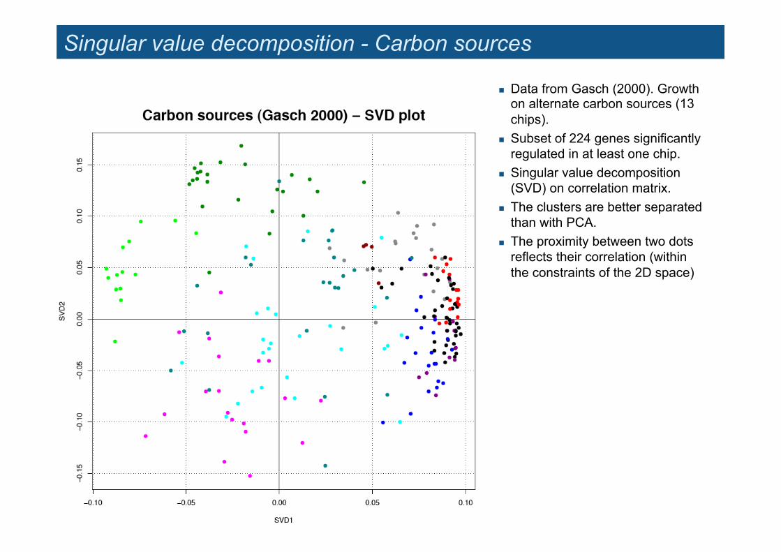
Singular value decomposition - Carbon sources
! Data from Gasch (2000). Growth on alternate carbon sources (13 chips).
! Subset of 224 genes significantly regulated in at least one chip.
! Singular value decomposition (SVD) on correlation matrix.
! The clusters are better separated than with PCA.
! The proximity between two dots reflects their correlation (within the constraints of the 2D space)

Singular value decomposition
Gilbert et al. (2000). Trends Biotech. 18(Dec), 487-495.
MCM
CLB2
SIC1 MAT
CLN2
Y'
MET
Alpha cdc15 cdc28 Elu
Spellman et al. (1998). Mol Biol Cell 9(12), 3273-97.

Singular value decomposition - Cell cycle
! Calculate a distance matrix between objects " in this case Pearson's coefficient of correlation
! Assign 2D-coordinates which reflect at best the distances
Cell cycle data Randomized data
Principal component analysis!
Raw data!
Multivariate data matrix!• n objects"• p variables"
Distance matrix!• n x n distances"• symmetrical"
Pairwise distance measurement!
Normalization!• mean!• variance!• covariance!
Coordinates"• n elements"• d dimensions"
Multidimensional scaling!• PCoA!• spring embedding!
Clustering!
Normalized table"• n elements"• p dimensions"
Reduction!to significant!dimensions!
Process!Data" display!
Visualization!
Tree drawing!
Space explorer!(VRML)!
Dendrogram!• rooted"• unrooted"• n leaves!
Euclidian space!• 1D to 3D"• n dots"• coloring"• dot volume"• interactive"
Matrix!• n rows"• p columns"• coloring"
Matrix viewer!
Processing!
Clusters,Tree"
Ordering (optional)!• row swapping!• column swapping!
Coloring!(optional)!
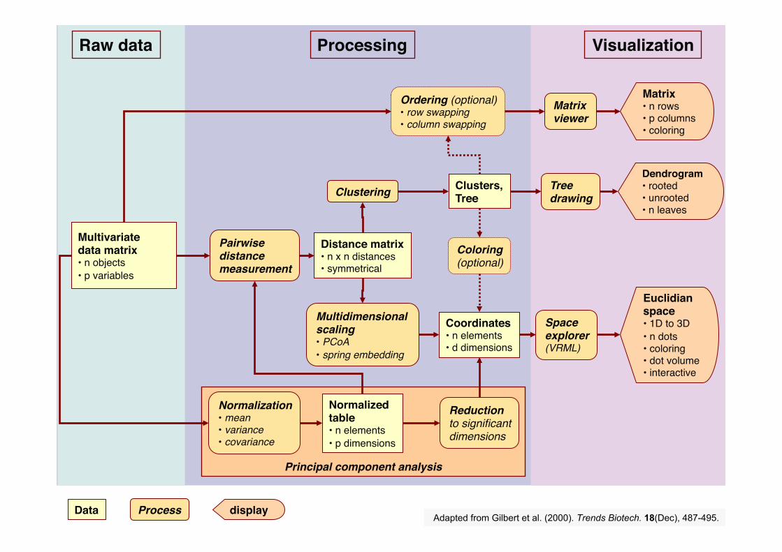
Adapted from Gilbert et al. (2000). Trends Biotech. 18(Dec), 487-495.


![Rinnai News a] 15a 2081 1—5.5Ê RR-055MST (BK) (42-3161) ¥ ... · (42-3128) ¥100, 800 OOMST ¥ 80,600 (#58) http//ogawa I pg. com . Created Date: 5/13/2013 12:08:39 PM](https://img.pdfslide.fr/doc/110x75/6047706187cb8619734988fa/rinnai-news-a-15a-2081-1a55-rr-055mst-bk-42-3161-42-3128-100.jpg)