TESTING QUANTUM-LIKE MODELS OF JUDGMENT FOR QUESTION ORDER EFFECTS

Documents de travail GREDEG GREDEG Working Papers Series

Thomas Boyer-KassemSébastien DuchêneEric Guerci

GREDEG WP No. 2015-06http://www.gredeg.cnrs.fr/working-papers.html

Les opinions exprimées dans la série des Documents de travail GREDEG sont celles des auteurs et ne reflèlent pas nécessairement celles de l’institution. Les documents n’ont pas été soumis à un rapport formel et sont donc inclus dans cette série pour obtenir des commentaires et encourager la discussion. Les droits sur les documents appartiennent aux auteurs.

The views expressed in the GREDEG Working Paper Series are those of the author(s) and do not necessarily reflect those of the institution. The Working Papers have not undergone formal review and approval. Such papers are included in this series to elicit feedback and to encourage debate. Copyright belongs to the author(s).

Testing quantum-like models of judgment for

question order effect

Thomas Boyer-Kassem∗, Sebastien Duchene†, Eric Guerci†

GREDEG Working Paper No. 2015–06

Abstract

Lately, so-called “quantum” models, based on parts of the mathematics of quantummechanics, have been developed in decision theory and cognitive sciences to accountfor seemingly irrational or paradoxical human judgments. We consider here some suchquantum-like models that address question order effects, i.e. cases in which givenanswers depend on the order of presentation of the questions. Models of variousdimensionalities could be used; can the simplest ones be empirically adequate? Fromthe quantum law of reciprocity, we derive new empirical predictions that we call theGrand Reciprocity equations, that must be satisfied by several existing quantum-likemodels, in their non-degenerate versions. Using substantial existing data sets, we showthat these non-degenerate versions fail the GR test in most cases, which means that,if quantum-like models of the kind considered here are to work, it can only be in theirdegenerate versions. However, we suggest that the route of degenerate models is notnecessarily an easy one, and we argue for more research on the empirical adequacy ofdegenerate quantum-like models in general.

“Research is needed which designs tests of quantum propertiessuch as the law of reciprocity and the law of double stochasticity”

(Busemeyer and Bruza 2012, 342)

1 Introduction

In decision theory and in cognitive sciences, classical cognitive models of judgmentrely on Bayesian probabilities and suppose that agents’ decisions or choices are guided bypreferences or attitudes that are determined at any time. Yet, various empirical resultshave threatened the predictive and explanatory power of these classical models: humanjudgments display order effects — the answers given to two questions depend on the orderof presentation of these questions (Schuman and Presser 1981, Tourangeau, Ribs andRasinski 2000, Moore 2002) —, conjunction fallacies — someone is judged less likely tohave characteristic C than characteristics C and D (Tversky and Kahneman 1982 and1983, Gavanski and Roskos-Ewoldsen 1991, Stolarz-Fantino et al. 2003) —, violate thesure-thing principle — stating that preferring X to Y given any possible state of the world

∗Tilburg Center for Logic and Philosophy of Science, Tilburg University, PO Box 90153, 5000 LETilburg, The Netherlands, and Archives H. Poincare (UMR 7117: CNRS, Universite de Lorraine), 91avenue de la Liberation, 54000 Nancy, France. E-mail: thomas.boyer@univ-lorraine.fr†GREDEG (UMR 7321: CNRS, Universite de Nice Sophia Antipolis), 250 rue Albert Einstein, 06560

Valbonne, France. E-mail: sebastien.duchene@gredeg.cnrs.fr, eric.guerci@gredeg.cnrs.fr

1

should imply preferring X to Y when the exact state of the world is not known (Allais1953, Ellsberg 1961, Shafir and Tversky 1992) —, or asymmetries in similarity — X isjudged more similar to Y than Y to X (Tversky 1977, Krumhansl 1978, Ashby and Perrin1988). In the classical cognitive framework, these behaviors have often been dubbed asirrational or paradoxical.

Recently, a research field that rely on so-called “quantum” or “quantum-like” modelshas developed to account for such behaviors. The qualifier “quantum” is used to indicatethat the models exploit the mathematics of a contemporary physical theory, quantummechanics. Note that only some mathematical tools of quantum mechanics are employed,and that the claim is not that these models are justified by an application of quantumphysics to the brain. For that reason, we shall prefer to call them “quantum-like” models.Such models put into question two classical characteristics recalled above: they abandonBayesian probabilities for others which are similar to probabilities in quantum mechanics,and they allow for preferences or attitudes to be undetermined. Quantum-like modelshave received much interest from psychologists, physicists, economists, cognitive scientistsand philosophers. For example, new theoretical frameworks have been proposed in decisiontheory and bounded rationality (Danilov and Lambert-Mogiliansky 2008 and 2010, Yukalovand Sornette 2011).

Various quantum-like models have been proposed to account for any of the seeminglyparadoxical behaviors recalled above (for reviews, see Pothos and Busemeyer 2013, Ash-tiani and Azgomi 2015). First, as the mathematics involved in quantum mechanics arewell-known for their non-commutative features, one of their natural application is the ac-count of question order effects. For instance, Wang and Busemeyer (2013) and Wang etal. (2014) offer a general quantum-like model for attitude questions that are asked inpolls. Conte et al. (2009) present a model for mental states of visual perception, andAtmanspacher and Romer (2012) discuss non-commutativity. Quantum-like models havealso been offered to explain the conjunction fallacy. For instance, Franco (2009) arguesthat it can be recovered from interference effects, which are central features in quantummechanics and at the origin of the violation of classical probabilities. Busemeyer et al.(2011) present a quantum-like model that could explain conjunction fallacy from some or-der effects. The violation of the sure thing principle has also been investigated by means ofquantum-like models. Busemeyer, Wang and Townsend (2006), and Busemeyer and Wang(2007) use quantum formalism to explain this violation by introducing probabilistic inter-ference and superposition of states. Khrennikov and Haven (2009) also explain Ellsberg’sparadox, and Aerts et al. (2011) model the Hawaii problem. Lambert-Mogiliansky et al.(2009) offer a model for the indeterminacy of preferences. Dynamical models, that rely ona time evolution of the mental state, have also been introduced (Pothos and Busemeyer2009, Busemeyer et al. 2009, and Trueblood and Busemeyer 2011). Several other empiricalfeatures, such as asymmetry judgments in similarity have also been offered a quantum-likemodel (Pothos and Busemeyer, 2011).

We shall concentrate in this paper on one kind of quantum-like models, those whichclaim to account for question order effect — that answers depend on the order in whichquestions are asked. We choose these models because (i) order effect is a straightforwardapplication of the non-commutative mathematics from quantum mechanics, (ii) order effectmodels are perhaps the simplest ones and (iii) some of them are at the roots of other models.All quantum-like models for order effect are not identical. Yet, several of them are builtalong the same lines, as in Conte et al. (2009), Busemeyer et al. (2009), Busemeyer etal. (2011), Atmanspacher and Romer (2012), Pothos and Busemeyer (2013), Wang andBusemeyer (2013) and Wang et al. (2014). We choose to focus here on this kind of models

2

for order effect (to be characterized, at least partly, in Section 2). So, we do not considerfor instance the model in Aerts, Gabora and Sozzo (2013) that rely on different hypotheses,or a quantum-like model for order effect in inference that can be found in Trueblood andBusemeyer (2011) or in Busemeyer et al. (2011). Our analyses only bear on the previouslymentioned kind of models.

When such quantum-like models for order effects were proposed, empirical adequacywas cared about: it was argued that the models were able to account either for existingempirical data (e.g. Wang and Busemeyer 2013 for the data from Moore 2002, Wang etal. 2014 for data from around 70 national surveys) or for data from new experiments (e.g.Conte et al. 2009, Wang and Busemeyer 2013). This is not all: a supplementary a prioriconstraint (the “QQ equality”) has been derived and it has been successfully verified onthe above-mentioned data (Wang and Busemeyer 2013, Wang et al. 2014). So, it seemsthat quantum-like models for question order effects are well verified and can be consideredas adequate, at least for a vast set of experiments.

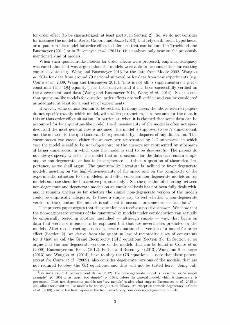
However, some details remain to be settled. In many cases, the above-referred papersdo not specify exactly which model, with which parameters, is to account for the data inthis or thus order effect situation. In particular, when it is claimed that some data can beaccounted for by a quantum-like model, the dimensionality of the model is often not spec-ified, and the most general case is assumed: the model is supposed to be N dimensional,and the answers to the questions can be represented by subspaces of any dimension. Thisencompasses two cases: either the answers are represented by 1-D subspaces, in whichcase the model is said to be non-degenerate, or the answers are represented by subspacesof larger dimensions, in which case the model is said to be degenerate. The papers donot always specify whether the model that is to account for the data can remain simpleand be non-degenerate, or has to be degenerate — this is a question of theoretical im-portance, as we shall argue. The quantum-like literature is inclined to favor degeneratemodels, insisting on the high-dimensionality of the space and on the complexity of theexperimental situation to be modeled, and often considers non-degenerate models as toymodels and use them for illustrative purposes only1. So, the question of choosing betweennon-degenerate and degenerate models on an empirical basis has not been fully dealt with,and it remains unclear so far whether the simple non-degenerate version of the modelscould be empirically adequate. Is there a simple way to test whether a non-degenerateversion of the quantum-like models is sufficient to account for some order effect data?

The present paper argues that this question can receive a positive answer. We show thatthe non-degenerate versions of the quantum-like models under consideration can actuallybe empirically tested in another unstudied — although simple — way, that bears ondata that were not intended to be explained but that are nevertheless predicted by themodels. After reconstructing a non-degenerate quantum-like version of a model for ordereffect (Section 2), we derive from the quantum law of reciprocity a set of constraintsfor it that we call the Grand Reciprocity (GR) equations (Section 3). In Section 4, weargue that the non-degenerate versions of the models that can be found in Conte et al.(2009), Busemeyer and Bruza (2012), Pothos and Busemeyer (2013), Wang and Busemeyer(2013) and Wang et al. (2014), have to obey the GR equations — note that these papers,except for Conte et al. (2009), also consider degenerate versions of the models, that arenot required to obey the GR equations, and thus will not be tested here. Using only

1For instance, in Busemeyer and Bruza (2012), the non-degenerate model is presented as “a simpleexample” (p. 100) or as “much too simple” (p. 108), before the general model, which is degenerate, ispresented. That non-degenerate models are “toy models” is also what suggest Busemeyer et al. 2015 p.240, albeit for quantum-like models for the conjunction fallacy. An exception towards degeneracy is Conteet al. (2009), one of the first papers in the field, which only considers non-degenerate models.

3

available data and without carrying out any new experiment, we are able to put the GRequations to the test (Section 5). We show that a vast majority of empirical cases failto satisfy the GR equations, which means that the non-degenerate versions of the above-mentioned models cannot account for these cases. In other words, if the quantum-likemodels that have been proposed are indeed to work, it cannot be in the special case oftheir non-degenerate versions, as the authors themselves had rightly anticipated, and thedata should be accounted for with degenerate models. In Section 6, we suggest howeverthat the route of degenerate models is not necessarily an easy one, and we argue for moreresearch on the empirical adequacy of models in general. Overall, the positive conclusion ofour results, we suggest, is that research on quantum-like models for question order effectshould be directed towards degenerate models, both as a consequence of the failure ofnon-degenerate ones and in order to find generalizations of the GR equations that shouldenable to empirically test them. This paper is the first one to challenge non-degeneratemodels for order effect and to show that they cannot be used as such in many cases. Ourwork puts warnings about the future use of these specific models, and provides a criticaland constructive look at quantum models of cognition.

2 A general non-degenerate quantum-like model for ques-tion order effect

As indicated in the introduction, we are concerned here with the following quantum-like models for order effect: Conte et al. (2009), Busemeyer et al. (2009), Busemeyer etal. (2011), Atmanspacher and Romer (2012), Pothos and Busemeyer (2013), Wang andBusemeyer (2013) and Wang et al. (2014). As they are more or less built along the samelines, we choose for simplicity to present in this section one simple and general model,which sets the notations and on which all the discussions will be made. A crucial point isthis: these models, except for Conte et al. (2009), are quite general and can be degenerateor non-degenerate, as already noted. As we shall be concerned here with testing theirnon-degenerate versions only, as a special case, the model we present in this section isnon-degenerate. In Section 4, we shall discuss in detail how this model is included in themodels from the above list.

The model is about the beliefs of a person, about which dichotomous yes-no questionscan be asked, for instance “is Clinton honest?”. A vector space on the complex numbersis introduced to represent the beliefs of the agent, and the answers to the questions. Inthe model, two dichotomous questions A and B are posed successively to an agent, inthe order A-then-B or B-then-A. Answer “yes” (respectively “no”) to A is representedby the vector |a0〉 (respectively |a1〉), and similarly for B, with vectors |b0〉 (respectively)|b1〉. It is important to note that an answer is supposed to be represented by a vector (ormore exactly, see below, by the ray defined by this vector), and not by a plane or by anysubspace of dimension greater than 1. Since there are no other possible answers to questionA (respectively B) than 0 and 1, the set (|a0〉, |a1〉) (respectively (|b0〉, |b1〉)) forms a basisof the vector space of possible answers, and the vector space is thus of dimension 2. Notethat it is the same vector space that is used to represents answers to questions A and B;this space just has two different bases.2

The vector space is supposed to be equipped with a scalar product, thus becoming aHilbert space: for two vectors |x〉 and |y〉, the scalar product 〈x|y〉 is a complex number;

2In the literature, questions that can be represented in this way are known as “incompatible”. “Com-patible” questions have a common basis, but the model is then equivalent to a classical one, and there isnothing quantum about it. Cf. for instance Busemeyer and Bruza (2012, 32–34).

4

- |a0〉

6

|a1〉

����

����

��1 |b0〉

BBBBBBBBBBM

|b1〉

O δ

9δ

〈a0|b0〉

〈a1|b1〉

〈a1|b0〉

〈a0|b1〉- |a0〉

6

|a1〉

����

����

��1 |b0〉

BBBBBBBBBBM

|b1〉

��������>

|ψ〉

α0

α1

β0β1

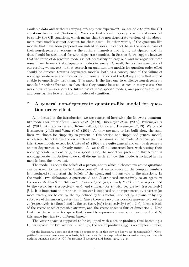
Figure 1: [Left:] The basis vectors |b0〉 and |b1〉 can be decomposed on the other basisvectors |a0〉 and |a1〉, so as to be expressed as in eq. 1 and 2. The scalar products areeither equal to cos δ or to sin δ. [Right:] The state vector |ψ〉 can be expressed in the twoorthonormal bases (|a0〉, |a1〉) and (|b0〉, |b1〉). These figures assume the special case of aHilbert space on real numbers.

its complex conjugate, 〈x|y〉∗, is just 〈y|x〉. The Hilbert space is on the complex numbers,and vectors can be multiplied by any complex number.3 The basis (|a0〉, |a1〉) is supposedto be orthonormal, i.e. 〈a0|a1〉 = 0 and 〈a0|a0〉 = 〈a1|a1〉 = 1; similarly for B. Note thatthere exists a correspondence between the two bases (cf. figure 1 left):

|b0〉 = 〈a0|b0〉|a0〉+ 〈a1|b0〉|a1〉, (1)

|b1〉 = 〈a0|b1〉|a0〉+ 〈a1|b1〉|a1〉, (2)

and similarly for |a0〉 and |a1〉 expressed as a function of |b0〉 and |b1〉.An agent’s beliefs about the subject matter of the questions A and B are represented

by a normalized belief state |ψ〉 from this vector space (|〈ψ|ψ〉|2 = 1). It is supposedto gather all the relevant information to predict her behaviour in the situation (like inorthodox quantum mechanics). |ψ〉 can be expressed in the basis (|a0〉, |a1〉) as

|ψ〉 = α0|a0〉+ α1|a1〉, (3)

with (α0, α1) ∈ C2 (cf. fig. 1 right). It can also be expressed in the basis (|b0〉, |b1〉) as

|ψ〉 = β0|b0〉+ β1|b1〉, (4)

with (β0, β1) ∈ C2, and with an appropriate correspondence between the coefficients.The belief state |ψ〉 determines the answer in a probabilistic way, and changes only

when a question is answered, according to the following rules:

• Born’s rule: the probability for the agent to answer xi (i = 0, 1) to question X(X = A,B) is given by the squared modulus of the scalar product between |ψ〉 and|xi〉:

Pr(xi) = |〈xi|ψ〉|2 (5)

3We consider here this general case. In the literature, some quantum-like models consider a real Hilbertspace, in which scalar products are real numbers, and vectors can be multiplied by real numbers only.

5

• projection postulate: the agent’s belief state just after the answer xi is the normalizedprojection of her belief state prior to the question onto the vector |xi〉 correspondingto her answer:

|ψ〉 7−→ 〈xi|ψ〉|〈xi|ψ〉|

|xi〉. (6)

For instance, if an agent is described by the state vector |ψ〉 = α0|a0〉 + α1|a1〉, theprobability that she answers i to question A is given by |αi|2, in which case the state afterthe answer is αi

|αi| |ai〉. On fig. 1, this probability can be obtained by first orthogonally

projecting |ψ〉 on the basis vector corresponding to the answer, and then taking the squareof this length. A consequence of the projection postulate in this model is that, just afteran answer i to question X has been given, the state is of the form λ|xi〉 with λ ∈ C and|λ| = 1. The fact that the state after the answer is equal to |xi〉 “up to a phase factor”,as one says, is true whatever the state prior to the question. On fig. 1, in the case of areal Hilbert space, the projection postulates can be interpreted as follow: project |ψ〉 onthe basis vector corresponding to the answer, then normalize it (i.e. expand it so that itgets a length 1); the result is ±|xi〉, according to the relative orientation of |ψ〉 and |xi〉.In the general case, answering a question modifies the agent’s state of belief, but there areexceptions: if an agent’s state of belief is λ|xi〉 (with |λ| = 1), Born’s rule states that shewill answer i (“yes” or “no”) with probability 1, and her state of belief is thus unchanged.Such vectors from which an answer can be given with certainty are called “eigenvectors”,and their set is the “eigenspace”, for the “eigenvalue” i. In this model, all eigenspaces areof dimension 1, and are called “rays” (equivalently, one can say that the eigenvalue is notdegenerate), since it has been supposed that an answer is represented by a vector, andnot by several independent vectors; this will be of decisive importance in the next section.Another consequence of the projection postulate is that, once an agent has answered i toquestion A, she will answer i with probability 1 to the same question A if it is posed againjust afterwards.4

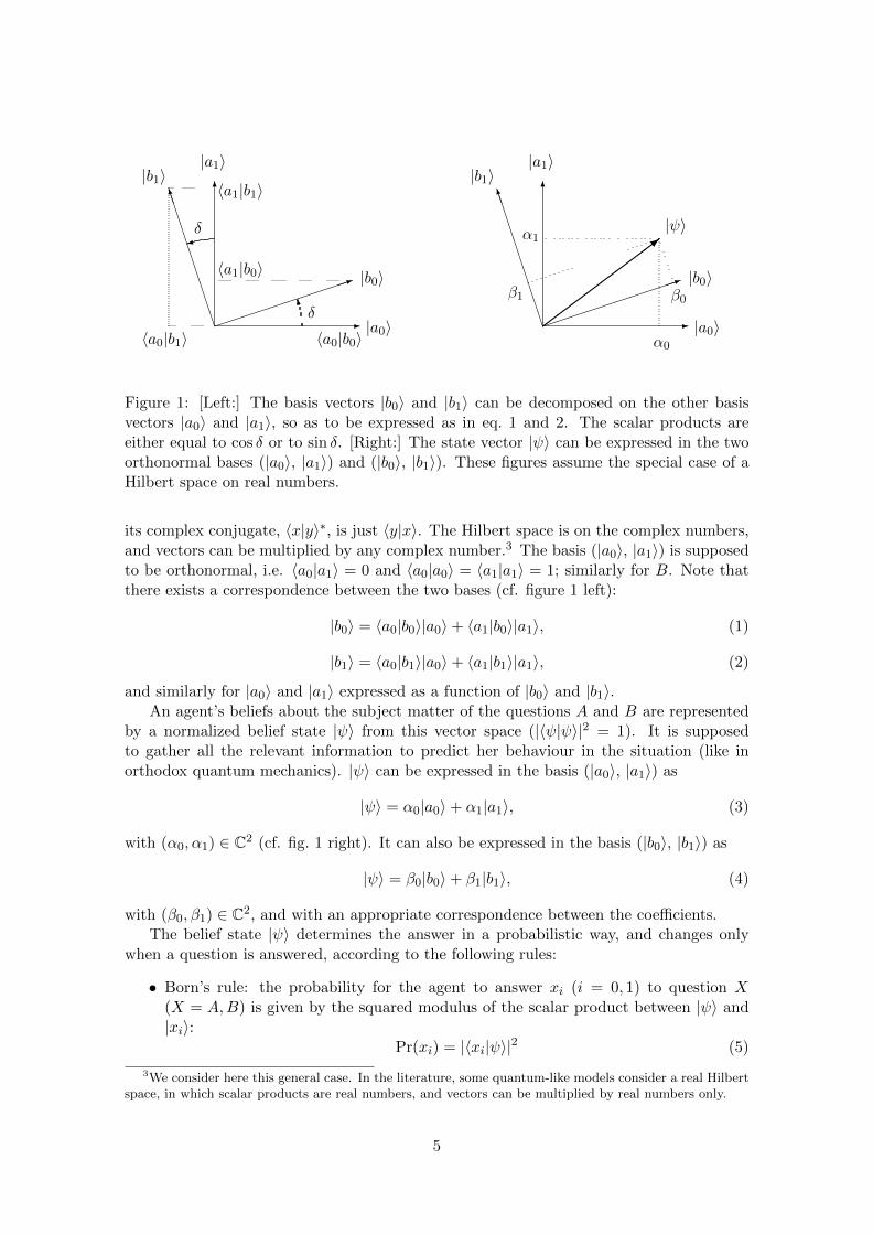
Such a quantum-like model displays order features. Compare for instance p(a0, b0),the probability to answer 0 to question A and then 0 to question B, and p(b0, a0), theprobability to give the same answers but in the reverse order. To compute p(a0, b0), onecan project the initial state on |a0〉 without normalizing the result, then project the resulton |b0〉, still without normalizing, and take the squared modulus of the final result.5 Inother words, to compare the two probabilities, one can just compare the length of successiveprojections of |ψ〉, first on |a0〉 and then |b0〉, or in the reverse order. Figure 2 shows thatthey are not necessary equal. Because quantum-like models display these order features, ithas been naturally suggested that they can account for experimentally documented ordereffects; Section 4 discusses several such models.

3 Constraints: the Grand Reciprocity equations

Some general empirical predictions can be derived from the non-degenerate modelpresented in the previous section.

4Of course, this is not true if another question, say B, is posed in-between.5Proof. Note p(yj |xi) the probability to answer j to question Y given that question X has been

answered with i. After the answer xi, the state is λ|xi〉 with |λ| = 1, so p(yj |xi) = |〈yj |xi〉|2. Note p(xi)the probability to answer i to question X when this question is asked first. p(a0, b0) = p(a0) · p(b0|a0) =|〈a0|ψ〉|2 ·|〈b0|a0〉|2 = |〈a0|ψ〉·〈b0|a0〉|2 = |〈b0|a′0〉|2, where |a′0〉 = 〈a0|ψ〉|a0〉. Since |a′0〉 is |ψ〉 projected onto|a0〉 and not normalized, computing |〈b0|a′0〉|2 means that |a′0〉 is projected onto |b0〉 and not normalized,before the squared modulus is computed. QED.

6

- |a0〉

6

|a1〉

����

����

��1 |b0〉

BBBBBBBBBBM

|b1〉

��������>

|ψ〉

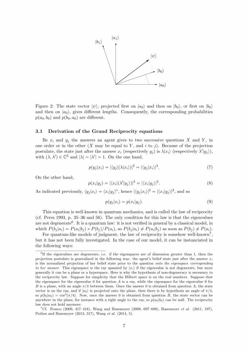
Figure 2: The state vector |ψ〉, projected first on |a0〉 and then on |b0〉, or first on |b0〉and then on |a0〉, gives different lengths. Consequently, the corresponding probabilitiesp(a0, b0) and p(b0, a0) are different.

3.1 Derivation of the Grand Reciprocity equations

Be xi and yj the answers an agent gives to two successive questions X and Y , inone order or in the other (X may be equal to Y , and i to j). Because of the projectionpostulate, the state just after the answer xi (respectively yj) is λ|xi〉 (respectively λ′|yj〉),with (λ, λ′) ∈ C2 and |λ| = |λ′| = 1. On the one hand,

p(yj |xi) = |〈yj |(λ|xi〉)|2 = |〈yj |xi〉|2. (7)

On the other hand,p(xi|yj) = |〈xi|(λ′|yj〉)|2 = |〈xi|yj〉|2. (8)

As indicated previously, 〈yj |xi〉 = 〈xi|yj〉∗, hence |〈yj |xi〉|2 = |〈xi|yj〉|2, and so

p(yj |xi) = p(xi|yj). (9)

This equation is well-known in quantum mechanics, and is called the law of reciprocity(cf. Peres 1993, p. 35–36 and 56). The only condition for this law is that the eigenvaluesare not degenerate6. It is a quantum law: it is not verified in general by a classical model, inwhich P (bj |ai) = P (ai|bj)×P (bj)/P (ai), so P (bj |ai) 6= P (ai|bj) as soon as P (bj) 6= P (ai).

For quantum-like models of judgment, the law of reciprocity is somehow well-known7,but it has not been fully investigated. In the case of our model, it can be instanciated inthe following ways:

6If the eigenvalues are degenerate, i.e. if the eigenspaces are of dimension greater than 1, then theprojection postulate is generalized in the following way: the agent’s belief state just after the answer xiis the normalized projection of her belief state prior to the question onto the eigenspace correspondingto her answer. This eigenspace is the ray spanned by |xi〉 if the eigenvalue is not degenerate, but moregenerally it can be a plane or a hyperspace. Here is why the hypothesis of non-degeneracy is necessary tothe reciprocity law. Suppose for simplicity that the Hilbert space is on the real numbers. Suppose thatthe eigenspace for the eigenvalue 0 for question A is a ray, while the eigenspace for the eigenvalue 0 forB is a plane, with an angle π/4 between them. Once the answer 0 is obtained from question A, the statevector is on the ray, and if |a0〉 is projected onto the plane, then there is by hypothesis an angle of π/4,so p(b0|a0) = cos2(π/4). Now, once the answer 0 is obtained from question B, the state vector can beanywhere in the plane, for instance with a right angle to the ray, so p(a0|b0) can be null. The reciprocitylaw does not hold anymore.

7Cf. Franco (2009, 417–418), Wang and Busemeyer (2009, 697–698), Busemeyer et al. (2011, 197),Pothos and Busemeyer (2013, 317), Wang et al. (2014, 5).

7

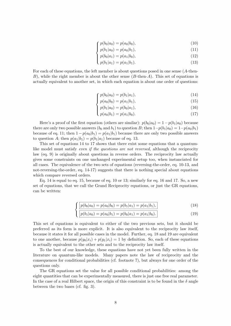
p(b0|a0) = p(a0|b0), (10)

p(b1|a0) = p(a0|b1), (11)

p(b0|a1) = p(a1|b0), (12)

p(b1|a1) = p(a1|b1). (13)

For each of these equations, the left member is about questions posed in one sense (A-then-B), while the right member is about the other sense (B-then-A). This set of equations isactually equivalent to another set, in which each equation is about one order of questions:

p(b0|a0) = p(b1|a1), (14)

p(a0|b0) = p(a1|b1), (15)

p(b1|a0) = p(b0|a1), (16)

p(a0|b1) = p(a1|b0). (17)

Here’s a proof of the first equation (others are similar): p(b0|a0) = 1−p(b1|a0) becausethere are only two possible answers (b0 and b1) to questionB; then 1−p(b1|a0) = 1−p(a0|b1)because of eq. 11; then 1− p(a0|b1) = p(a1|b1) because there are only two possible answersto question A; then p(a1|b1) = p(b1|a1) because of eq. 13.

This set of equations 14 to 17 shows that there exist some equations that a quantum-like model must satisfy even if the questions are not reversed, although the reciprocitylaw (eq. 9) is originally about questions in reverse orders. The reciprocity law actuallygives some constraints on one unchanged experimental setup too, when instanciated forall cases. The equivalence of the two sets of equations (reversing-the-order, eq. 10-13, andnot-reversing-the-order, eq. 14-17) suggests that there is nothing special about equationswhich compare reversed orders.

Eq. 14 is equal to eq. 15, because of eq. 10 or 13; similarly for eq. 16 and 17. So, a newset of equations, that we call the Grand Reciprocity equations, or just the GR equations,can be written:

p(b0|a0) = p(a0|b0) = p(b1|a1) = p(a1|b1), (18)

p(b1|a0) = p(a0|b1) = p(b0|a1) = p(a1|b0). (19)

This set of equations is equivalent to either of the two previous sets, but it should bepreferred as its form is more explicit. It is also equivalent to the reciprocity law itself,because it states it for all possible cases in the model. Further, eq. 18 and 19 are equivalentto one another, because p(y0|xi) + p(y1|xi) = 1 by definition. So, each of these equationsis actually equivalent to the other sets and to the reciprocity law itself.

To the best of our knowledge, these equations have not yet been fully written in theliterature on quantum-like models. Many papers note the law of reciprocity and theconsequences for conditional probabilities (cf. footnote 7), but always for one order of thequestions only.

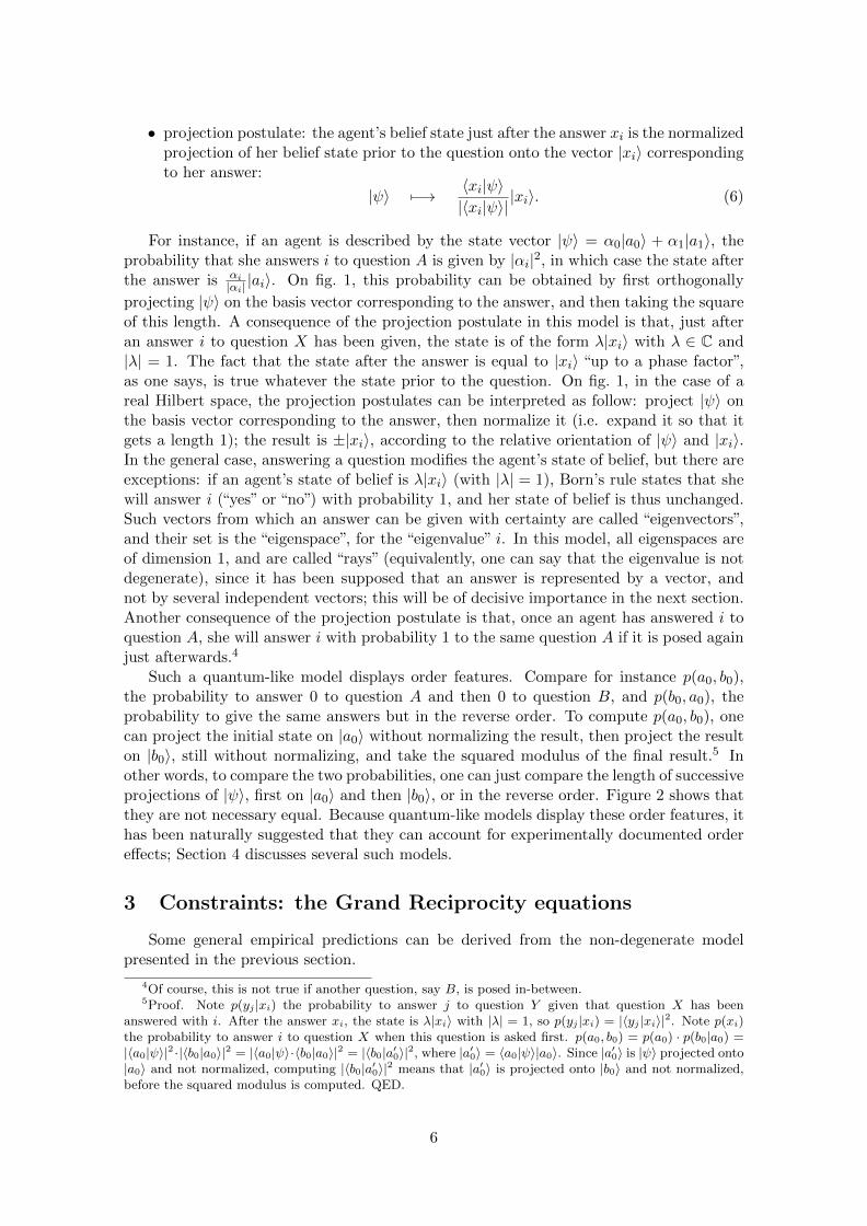
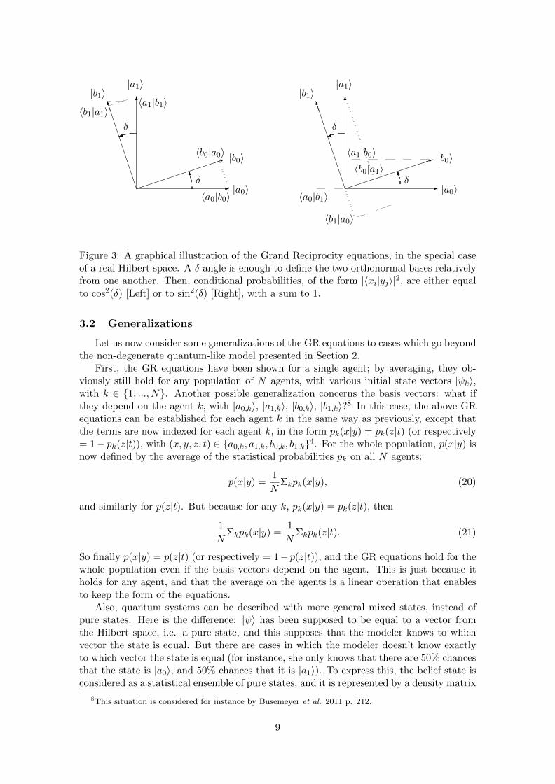
The GR equations set the value for all possible conditional probabilities: among theeight quantities that can be experimentally measured, there is just one free real parameter.In the case of a real Hilbert space, the origin of this constraint is to be found in the δ anglebetween the two bases (cf. fig. 3).

8

- |a0〉

6

|a1〉

����

����

��1 |b0〉

BBBBBBBBBBM

|b1〉

O δ

9δ

〈a0|b0〉

〈b0|a0〉

〈a1|b1〉〈b1|a1〉

- |a0〉

6

|a1〉

����

����

��1 |b0〉

BBBBBBBBBBM

|b1〉

O δ

9δ

〈a1|b0〉〈b0|a1〉

〈a0|b1〉

〈b1|a0〉

Figure 3: A graphical illustration of the Grand Reciprocity equations, in the special caseof a real Hilbert space. A δ angle is enough to define the two orthonormal bases relativelyfrom one another. Then, conditional probabilities, of the form |〈xi|yj〉|2, are either equalto cos2(δ) [Left] or to sin2(δ) [Right], with a sum to 1.

3.2 Generalizations

Let us now consider some generalizations of the GR equations to cases which go beyondthe non-degenerate quantum-like model presented in Section 2.

First, the GR equations have been shown for a single agent; by averaging, they ob-viously still hold for any population of N agents, with various initial state vectors |ψk〉,with k ∈ {1, ..., N}. Another possible generalization concerns the basis vectors: what ifthey depend on the agent k, with |a0,k〉, |a1,k〉, |b0,k〉, |b1,k〉?8 In this case, the above GRequations can be established for each agent k in the same way as previously, except thatthe terms are now indexed for each agent k, in the form pk(x|y) = pk(z|t) (or respectively= 1− pk(z|t)), with (x, y, z, t) ∈ {a0,k, a1,k, b0,k, b1,k}4. For the whole population, p(x|y) isnow defined by the average of the statistical probabilities pk on all N agents:

p(x|y) =1

NΣkpk(x|y), (20)

and similarly for p(z|t). But because for any k, pk(x|y) = pk(z|t), then

1

NΣkpk(x|y) =

1

NΣkpk(z|t). (21)

So finally p(x|y) = p(z|t) (or respectively = 1− p(z|t)), and the GR equations hold for thewhole population even if the basis vectors depend on the agent. This is just because itholds for any agent, and that the average on the agents is a linear operation that enablesto keep the form of the equations.

Also, quantum systems can be described with more general mixed states, instead ofpure states. Here is the difference: |ψ〉 has been supposed to be equal to a vector fromthe Hilbert space, i.e. a pure state, and this supposes that the modeler knows to whichvector the state is equal. But there are cases in which the modeler doesn’t know exactlyto which vector the state is equal (for instance, she only knows that there are 50% chancesthat the state is |a0〉, and 50% chances that it is |a1〉). To express this, the belief state isconsidered as a statistical ensemble of pure states, and it is represented by a density matrix

8This situation is considered for instance by Busemeyer et al. 2011 p. 212.

9

(for instance, we write ρ = 0.5|a0〉〈a0| + 0.5|a1〉〈a1| for the above case). The question isthen: are the GR equations valid for pure states only, or also for mixed states? For both,because no particular hypothesis has been made on the state before the first question isasked. What matters for the demonstration is the state after the first question, and itis doomed to be the corresponding eigenvector (up to a phase factor), whether the beliefstate was described as a statistical mixture or not before the question was asked. So, theGR equations hold even if mixed states are assumed, which can prove very powerful.

The GR equations apply to a model with 2 questions with 2 possible answers each, butone could also consider a larger set of questions. Consider a model with q questions A,B, C, . . . that are asked in a row, in various orders, each with 2 possible non-degenerateanswers, in a Hilbert space of dimension 2. For the questions considered 2 by 2, thereciprocity law (eq. 9) holds, since what matters is that answers are represented by 1Dsubspaces, and so the GR equations hold too. This gives a set of q · (q−1)/2 GR equationsthat this model must satisfy. Consider now a model with 2 questions, each with r possibleanswers, with non-degenerate eigenvalues, in a complex Hilbert space of dimension r. Thereciprocity law still holds in this case, and the GR equations hold for each couple of indexes(i, j) ∈ {1, ..., r}2. Overall, the GR equations can be generalized to apply for models withq questions and r possible non-degenerate answers.

The hypothesis that eigenvalues are non-degenerate, i.e. that eigenspaces are of dimen-sion 1, can be relaxed in some cases. Suppose a model M with eigenspaces of dimensionsgreater than 1 is empirically equivalent to a model M ′ with eigenspaces of dimension 1.So to speak, the supplementary dimensions of M are theoretically useless, and empiricallymeaningless. As the GR equations hold for M ′, they will also hold for M , to which it isequivalent. So, more generally, the GR equations hold for models which have eigenspacesof dimension 1, or which are reducible (i.e. equivalent) to it.

These results may have a larger impact still. Suppose that there exists a set of elemen-tary questions, the answers of which would be represented by non-degenerate eigenspaces,i. e. rays. These elementary rays would define the fundamental basis belief states, onwhich any belief could be decomposed. The number of such elementary rays would definethe dimensionality of the Hilbert space representing human beliefs. Such an assumptionis widespread in the quantum-like literature. For instance, a similar idea is expressed byPothos and Busemeyer about emotions:

“one-dimensional sub-spaces (called rays) in the vector space would correspond to the

most elementary emotions possible. The number of unique elementary emotions and

their relation to each other determine the overall dimensionality of the vector space.

Also, more general emotions, such as happiness, would be represented by subspaces of

higher dimensionality.” (Pothos and Busemeyer 2013, 258).

Generalized GR equations would hold for such elementary questions. Then, all modelswith degenerate eigenspaces would just be coarse-grained models, which could be refinedwith more elementary questions and rays. For instance, a degenerate answer representedby a plane combines two elementary dimensions because it fails to distinguish betweenthem. As a consequence, the meaning of a degenerate answer could be specified throughmore specific elementary answers. More importantly, the degenerate model could actuallybe tested on these fundamental questions, with our GR equations or their generalizedversions with q questions and r answers. In other words, if elementary questions existed— and it seems to be a usual assumption in the quantum-like literature — any model ofthe kind presented in Section 2, but with non-degenerate answers or not, could be testedwith GR equations. This is of fantastic interest, as it enables to test any model, and ithas never been noted before. We shall come back on this point in Section 6.

10

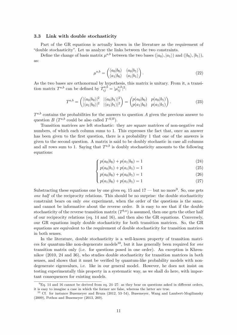
3.3 Link with double stochasticity

Part of the GR equations is actually known in the literature as the requirement of“double stochasticity”. Let us analyze the links between the two constraints.

Define the change of basis matrix µa,b between the two bases (|a0〉, |a1〉) and (|b0〉, |b1〉),as:

µa,b =

(〈a0|b0〉 〈a0|b1〉〈a1|b0〉 〈a1|b1〉

). (22)

As the two bases are orthonormal by hypothesis, this matrix is unitary. From it, a transi-tion matrix T a,b can be defined by T a,bij = |µa,bij |2:

T a,b =

(|〈a0|b0〉|2 |〈a0|b1〉|2|〈a1|b0〉|2 |〈a1|b1〉|2

)=

(p(a0|b0) p(a0|b1)p(a1|b0) p(a1|b1)

). (23)

T a,b contains the probabilities for the answers to question A given the previous answer toquestion B (T a,b could be also called TA|B).

Transition matrices are left stochastic: they are square matrices of non-negative realnumbers, of which each column sums to 1. This expresses the fact that, once an answerhas been given to the first question, there is a probability 1 that one of the answers isgiven to the second question. A matrix is said to be doubly stochastic in case all columnsand all rows sum to 1. Saying that T a,b is doubly stochasticity amounts to the followingequations:

p(a0|b0) + p(a1|b0) = 1 (24)

p(a0|b1) + p(a1|b1) = 1 (25)

p(a0|b0) + p(a0|b1) = 1 (26)

p(a1|b0) + p(a1|b1) = 1 (27)

Substracting these equations one by one gives eq. 15 and 17 — but no more9. So, one getsone half of the reciprocity relations. This should be no surprise: the double stochasticityconstraint bears on only one experiment, when the order of the questions is the same,and cannot be informative about the reverse order. It is easy to see that if the doublestochasticity of the reverse transition matrix (T b,a) is assumed, then one gets the other halfof our reciprocity relations (eq. 14 and 16), and then also the GR equations. Conversely,our GR equations imply double stochasticity for both transition matrices. So, the GRequations are equivalent to the requirement of double stochasticity for transition matricesin both senses.

In the literature, double stochasticity is a well-known property of transition matri-ces for quantum-like non-degenerate models10, but it has generally been required for onetransition matrix only (i.e. for questions posed in one order). An exception is Khren-nikov (2010, 24 and 36), who studies double stochasticity for transition matrices in bothsenses, and shows that it must be verified by quantum-like probability models with non-degenerate eigenvalues, i.e. like in our general model. However, he does not insist ontesting experimentally this property in a systematic way, as we shall do here, with impor-tant consequences for existing models.

9Eq. 14 and 16 cannot be derived from eq. 24–27: as they bear on questions asked in different orders,it is easy to imagine a case in which the former are false, whereas the latter are true.

10 Cf. for instance Busemeyer and Bruza (2012, 53–54), Busemeyer, Wang and Lambert-Mogiliansky(2009), Pothos and Busemeyer (2013, 269).

11

Although the GR equations are equivalent to double stochasticity in both orders fortransition matrices, there are several reasons why the former formulation should be pre-ferred, both pragmatically and theoretically. To test double stochasticity, one first needsto write equations like eq. 24–27. But such equations are not independent, so it compli-cates the statistical tests of significance. Or in order not to test useless equations, somework needs to be done beforehand to find the independent equations. Actually, untanglingthe equations would just lead to the GR equations, which are directly usable. Overall,the GR equations can be considered as the pragmatic form one should use to test doublestochasticity in both orders. They also clearly show that two set of equations (18 and19) are equivalent, and that one needs to pick only the corresponding data. Also, the GRequations show at first sight that there is only one free parameter among all the possi-ble conditional probabilities, while this is not transparent from the double stochasticityrequirement. More theoretically, the GR equations are directly linked with a central math-ematical property of the scalar product in the model, making it clear why it holds. Onthe other hand, the reason why double stochasticity should hold in this model is more ob-scure. Finally, the GR equations connect with a fundamental law of quantum mechanics,namely the law of reciprocity, which helps to understand why it holds only in the case ofnon-degenerate eigenvalues, like in quantum mechanics.

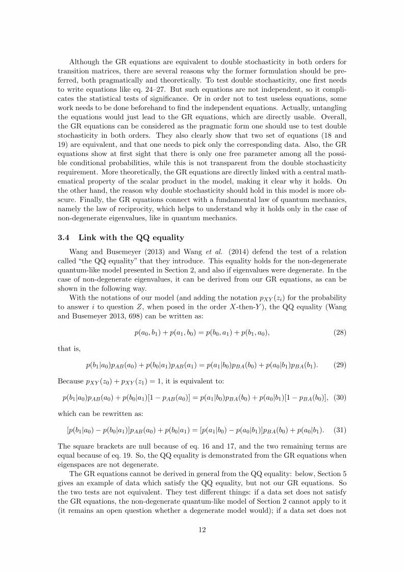
3.4 Link with the QQ equality

Wang and Busemeyer (2013) and Wang et al. (2014) defend the test of a relationcalled “the QQ equality” that they introduce. This equality holds for the non-degeneratequantum-like model presented in Section 2, and also if eigenvalues were degenerate. In thecase of non-degenerate eigenvalues, it can be derived from our GR equations, as can beshown in the following way.

With the notations of our model (and adding the notation pXY (zi) for the probabilityto answer i to question Z, when posed in the order X-then-Y ), the QQ equality (Wangand Busemeyer 2013, 698) can be written as:

p(a0, b1) + p(a1, b0) = p(b0, a1) + p(b1, a0), (28)

that is,

p(b1|a0)pAB(a0) + p(b0|a1)pAB(a1) = p(a1|b0)pBA(b0) + p(a0|b1)pBA(b1). (29)

Because pXY (z0) + pXY (z1) = 1, it is equivalent to:

p(b1|a0)pAB(a0) + p(b0|a1)[1− pAB(a0)] = p(a1|b0)pBA(b0) + p(a0|b1)[1− pBA(b0)], (30)

which can be rewritten as:

[p(b1|a0)− p(b0|a1)]pAB(a0) + p(b0|a1) = [p(a1|b0)− p(a0|b1)]pBA(b0) + p(a0|b1). (31)

The square brackets are null because of eq. 16 and 17, and the two remaining terms areequal because of eq. 19. So, the QQ equality is demonstrated from the GR equations wheneigenspaces are not degenerate.

The GR equations cannot be derived in general from the QQ equality: below, Section 5gives an example of data which satisfy the QQ equality, but not our GR equations. Sothe two tests are not equivalent. They test different things: if a data set does not satisfythe GR equations, the non-degenerate quantum-like model of Section 2 cannot apply to it(it remains an open question whether a degenerate model would); if a data set does not

12

satisfy the QQ equality, the non-degenerate quantum-like model of Section 2 cannot applyto it, and a degenerate version of it could not either. In other words, a non-degeneratequantum-like model must satisfy both the GR equations and the QQ equality, and adegenerate quantum-like model must satisfy the QQ equality.

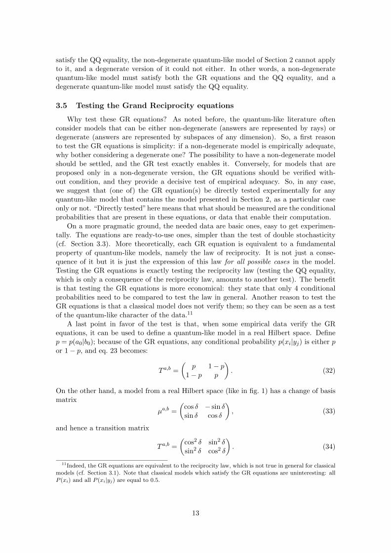
3.5 Testing the Grand Reciprocity equations

Why test these GR equations? As noted before, the quantum-like literature oftenconsider models that can be either non-degenerate (answers are represented by rays) ordegenerate (answers are represented by subspaces of any dimension). So, a first reasonto test the GR equations is simplicity: if a non-degenerate model is empirically adequate,why bother considering a degenerate one? The possibility to have a non-degenerate modelshould be settled, and the GR test exactly enables it. Conversely, for models that areproposed only in a non-degenerate version, the GR equations should be verified with-out condition, and they provide a decisive test of empirical adequacy. So, in any case,we suggest that (one of) the GR equation(s) be directly tested experimentally for anyquantum-like model that contains the model presented in Section 2, as a particular caseonly or not. “Directly tested”here means that what should be measured are the conditionalprobabilities that are present in these equations, or data that enable their computation.

On a more pragmatic ground, the needed data are basic ones, easy to get experimen-tally. The equations are ready-to-use ones, simpler than the test of double stochasticity(cf. Section 3.3). More theoretically, each GR equation is equivalent to a fundamentalproperty of quantum-like models, namely the law of reciprocity. It is not just a conse-quence of it but it is just the expression of this law for all possible cases in the model.Testing the GR equations is exactly testing the reciprocity law (testing the QQ equality,which is only a consequence of the reciprocity law, amounts to another test). The benefitis that testing the GR equations is more economical: they state that only 4 conditionalprobabilities need to be compared to test the law in general. Another reason to test theGR equations is that a classical model does not verify them; so they can be seen as a testof the quantum-like character of the data.11

A last point in favor of the test is that, when some empirical data verify the GRequations, it can be used to define a quantum-like model in a real Hilbert space. Definep = p(a0|b0); because of the GR equations, any conditional probability p(xi|yj) is either por 1− p, and eq. 23 becomes:

T a,b =

(p 1− p

1− p p

). (32)

On the other hand, a model from a real Hilbert space (like in fig. 1) has a change of basismatrix

µa,b =

(cos δ − sin δsin δ cos δ

), (33)

and hence a transition matrix

T a,b =

(cos2 δ sin2 δsin2 δ cos2 δ

). (34)

11Indeed, the GR equations are equivalent to the reciprocity law, which is not true in general for classicalmodels (cf. Section 3.1). Note that classical models which satisfy the GR equations are uninteresting: allP (xi) and all P (xi|yj) are equal to 0.5.

13

Taking δ = arccos(√p) enables the real model to account for the data of conditional

probabilities. To put it another way, checking the empirically validity of the GR equationsenables at the same time to define the two bases relatively from one another.

Note that testing the GR equations require that the experiment be conducted in bothquestion orders (A-then-B and B-then-A). If only one question order is studied, a testcan still be performed, but only on half of the equations. So, whenever a quantum-likemodel of the kind depicted here is proposed to account for the results of a succession oftwo questions in one order only, then the model should also be tested for the reverse order.

4 Applying the GR equations to non-degenerate (versionsof) existing models

The non-degenerate quantum-like model that we introduced in Section 2 was intendedto serve as a concise presentation for several models from the literature. In this section,we discuss in detail the relation between our model and existing ones, in order to clarifywhether the latter should verify the GR equations. Recall that satisfying the GR equationsis required in general for non-degenerate models only. So, if an existing model is proposedin the most general case either as non-degenerate or degenerate, then the GR equationsapply only to the non-degenerate version of the model, not to its degenerate version.

Consider first Conte et al. (2009), who propose a quantum-like model to account fororder effects in mental states during visual perception of ambiguous figures. Their modelcan be cast into the lines of our general model: the two dichotomous questions or tests arealso called A and B, and the probabilities of the answers are noted p(A = +), p(A = −),p(B = +) and p(B = +), corresponding to our p(a0), p(a1), p(b0) and p(b1). The questionsconcern visual perception of ambiguous figures, and a vector state, noted here φ (insteadof our ψ) represents the state of consciousness about the perception. It belongs to acomplex Hilbert space, and an answer is represented by a one-dimensional subspace (thisis implicit in their formula (3)). The usual Born rule makes the link with probabilities.The model also involves a projection postulate: during perception, the “potential” state ofconsciousness is collapsed onto “an actual or manifest state of consciousness” (p. 6 and 7).Note however a slight difference: for Conte et al., the projection of the state arises duringperception of the figure, not during answering a question. But as the latter quickly followsthe former, and as an agent answers a question only once her perception has stabilized,this does not make any difference in practice. Overall, Conte et al. (2009)’s model matchesour general model in all respects, as it supposes that eigenspaces are of dimension 1. So,it has to obey the GR equations.

Consider now the model proposed by Wang and Busemeyer (2013), called the QQmodel, which is to account for several types of order effects about judgments on varioustopics (politics, sports, society, etc.). The clear presentation of the model in their Section 2,together with their geometric approach which provides figures similar to ours (in the caseof a real Hilbert space), easily enables to see that it encompasses the non-degenerate modelof Section 2. However, Wang and Busemeyer’s model is more general and allows for ananswer to be represented either with a subspace of dimension 1 (non-degenerate version),or with a subspace of dimension larger than 1 (degenerate version). The GR equationsapply only to the former version, as a special case. For instance, they apply to figures 1and 2 (p. 4 and 5), which represent “a two-dimensional example of the quantum-like modelof question order effects”. Hence, the GR test will exactly fit here the aim we set it inthe introduction: within this general model, specify whether non-degenerate model can be

14

sufficient, or degenerate model are required.Wang and Busemeyer’s general model is also at the basis of two other presentations:

in Busemeyer and Bruza’s 2012 book (p. 99–116), and in the review article of Pothos andBusemeyer (2013). Here too, the model can be non-degenerate or degenerate, and the GRequations apply with the same conditions: only to the special case of the non-degenerateversion.

Atmanspacher and Romer (2012, p. 277) make the suggestion that Wang and Buse-meyer’s model could be extended to mixed states, instead of just pure states. Althoughthis is an interesting theoretical possibility, it is clear that it cannot be used to avoid theGR equations, as they are valid for pure as for mixed states (cf. Section 3.2).

Building on the paper of Wang and Busemeyer (2013), Wang et al. (2014) take upthe same quantum-like model for order effect, in order to apply it to a much larger setof experiments. Here again, answers are supposed to be represented with subspaces ofany dimension. So, the GR equations apply only to the special case of the model in itsnon-degenerate version, i. e. when answers are represented with rays as in the model ofSection 2.

5 An empirical glimpse: the GR tests

The previous section has listed several cases in which the GR equations can be tested.For all cases but Conte et al. (2009), the models have been proposed for any N dimen-sions, i. e. as either non-degenerate or degenerate. Then, the GR equations can test thespecial case of the non-degenerate version of these models, in order to determine whetherthis simplest case is sufficient, or if the more general degenerate models are required. Thissection is concerned with performing these empirical GR tests. They are done using theempirical data that are provided in the papers, and which come from either laboratory orfield experiments. To study these empirical data, we divide them into two sets, accordingto the topic and the authors: first, in Sections 5.1 to 5.3, we consider the data on exper-iments about judgment on social or political questions, which enable to test the modelfirst proposed by Wang and Busemeyer (2013) and considered by Busemeyer and Bruza(2012), Pothos and Busemeyer (2013), and Wang et al. (2014); second, in Section 5.4, thedata concern an experiment about visual perception, and we test the model proposed byConte et al. (2009).

5.1 First data set

Our first data set gathers 72 experiments on order effects, with 70 national surveysmade in the USA plus 2 laboratory experiments:

– 66 national surveys from the Pew Research Center run between 2001 and 2011 aboutpolitics, religion, economic policy and so on, considered in Wang et al. (2014) (notedin Table 1 as experiments 1 to 66);

– 3 surveys from Moore (2002) concerning Gallup public opinion polls (noted as ex-periments 67 to 69), which are considered in Wang and Busemeyer (2013) and inWang et al. (2014) ;

– 2 laboratory experiments conducted by Wang and Busemeyer (2013). In the firstexperiment, the authors replicate in a laboratory setting the experiment proposedby Moore (2002) about racial hostility, whereas, in the second one, they replicatethe survey of Wilson et al. (2008) (experiments 70 and 71) ;

15

Table 1: Questions of the experiments included in the first data set.1-26 (26 experiments).

A. Do you approve or disapprove of the way Bush/Obama is handlingthe job as President?

B. All in all, are you satisfied or dissatisfied with the way things are goingin this country today?

27-41 (15 experiments).

A. Do you approve or disapprove of the job the Republican leadersin Congress are doing?

B. Do you approve or disapprove of the job the Democratic leadersin Congress are doing?

42-66 (25 experiments).

These experiments include diverse questions covering topics, from religiousbeliefs to support to economic policy.

67.

A. Do you generally think Bill Clinton is honest and trustworthy?B. Do you generally think Al Gore is honest and trustworthy?

68.

A. Do you think Newt Gingrich is honest and trustworthy?B. Do you think Bob Dole is honest and trustworthy?

69 and 70.

A. Do you think that only a few or many white people dislike black people?B. Do you think that only a few or many black people dislike white people?

71.

A. Do you generally favor or oppose affirmative action (AA) programs forracial minorities?

B. Do you generally favor or oppose affirmative action (AA) programs forwomen?

72.

A. Do you think it should be possible for a pregnant woman to obtaina legal abortion if she is married and does not want any more children?

B. Do you think it should be possible for a pregnant woman to obtaina legal abortion if there is a strong chance of serious defect in the baby?

– one further Gallup survey reported by Schuman et al. (1981), also considered inWang et al. (2014) (experiment 72).

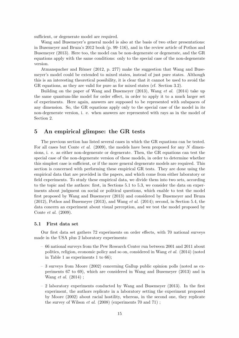
Figure 4 reports the box plot of the distribution of the total number of subjects perexperiment. The median experiment (741 subjects) is thus supposed to involve half of thesamples (about 370 subjects) in the A-then-B treatment and the remaining half in theB-then-A treatment. The circle on the left part of the box-plot, outside the left whisker,pinpoints the two laboratory experiments 70 and 71, which involve the smallest sample,that is, 228 subjects.

Each experiment can be described according to the following common model and no-tations: two response categorical variables,

– the bernoulli random variable A ∈ {a0, a1} that represents the possible replies (re-spectively “yes” or “no”) to the dichotomous question A,

16

0 500 1000 1500 2000

Figure 4: Distribution of number of subjects per experiment.

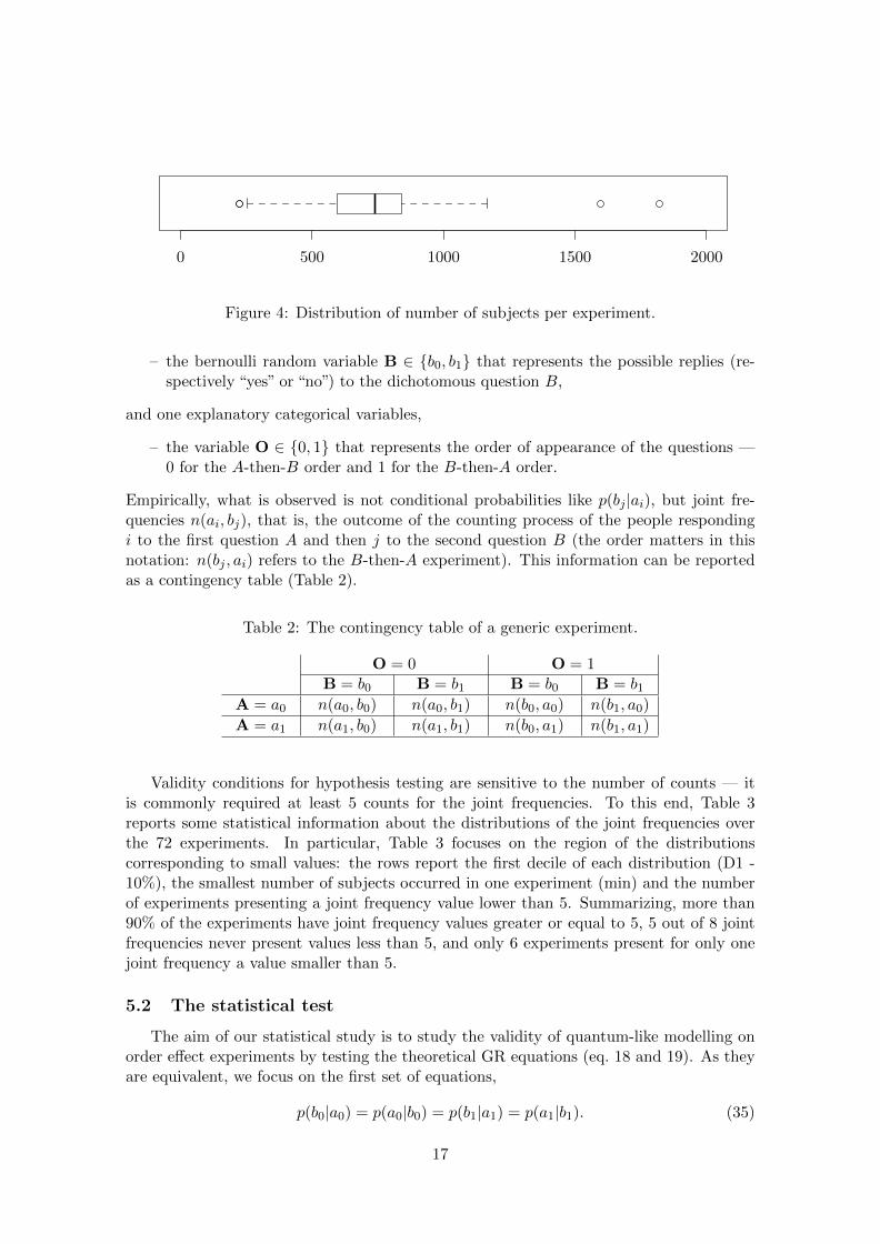
– the bernoulli random variable B ∈ {b0, b1} that represents the possible replies (re-spectively “yes” or “no”) to the dichotomous question B,

and one explanatory categorical variables,

– the variable O ∈ {0, 1} that represents the order of appearance of the questions —0 for the A-then-B order and 1 for the B-then-A order.

Empirically, what is observed is not conditional probabilities like p(bj |ai), but joint fre-quencies n(ai, bj), that is, the outcome of the counting process of the people respondingi to the first question A and then j to the second question B (the order matters in thisnotation: n(bj , ai) refers to the B-then-A experiment). This information can be reportedas a contingency table (Table 2).

Table 2: The contingency table of a generic experiment.

O = 0 O = 1B = b0 B = b1 B = b0 B = b1

A = a0 n(a0, b0) n(a0, b1) n(b0, a0) n(b1, a0)

A = a1 n(a1, b0) n(a1, b1) n(b0, a1) n(b1, a1)

Validity conditions for hypothesis testing are sensitive to the number of counts — itis commonly required at least 5 counts for the joint frequencies. To this end, Table 3reports some statistical information about the distributions of the joint frequencies overthe 72 experiments. In particular, Table 3 focuses on the region of the distributionscorresponding to small values: the rows report the first decile of each distribution (D1 -10%), the smallest number of subjects occurred in one experiment (min) and the numberof experiments presenting a joint frequency value lower than 5. Summarizing, more than90% of the experiments have joint frequency values greater or equal to 5, 5 out of 8 jointfrequencies never present values less than 5, and only 6 experiments present for only onejoint frequency a value smaller than 5.

5.2 The statistical test

The aim of our statistical study is to study the validity of quantum-like modelling onorder effect experiments by testing the theoretical GR equations (eq. 18 and 19). As theyare equivalent, we focus on the first set of equations,

p(b0|a0) = p(a0|b0) = p(b1|a1) = p(a1|b1). (35)

17

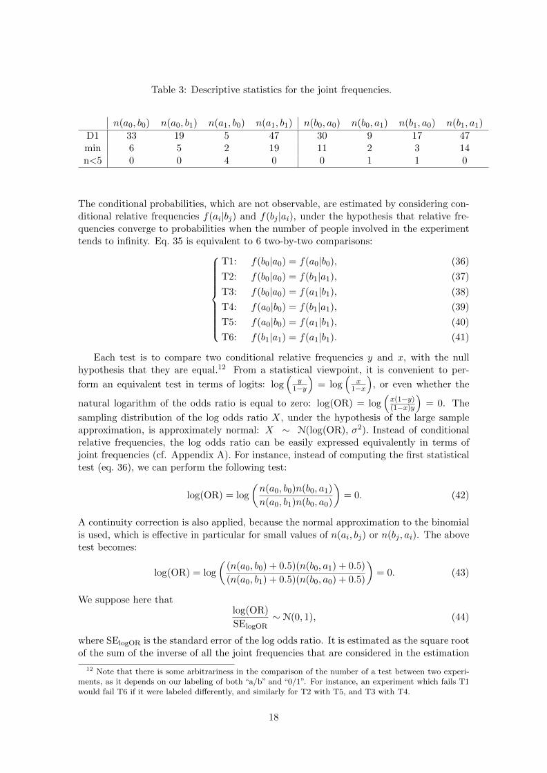
Table 3: Descriptive statistics for the joint frequencies.

n(a0, b0) n(a0, b1) n(a1, b0) n(a1, b1) n(b0, a0) n(b0, a1) n(b1, a0) n(b1, a1)

D1 33 19 5 47 30 9 17 47min 6 5 2 19 11 2 3 14n<5 0 0 4 0 0 1 1 0

The conditional probabilities, which are not observable, are estimated by considering con-ditional relative frequencies f(ai|bj) and f(bj |ai), under the hypothesis that relative fre-quencies converge to probabilities when the number of people involved in the experimenttends to infinity. Eq. 35 is equivalent to 6 two-by-two comparisons:

T1: f(b0|a0) = f(a0|b0), (36)

T2: f(b0|a0) = f(b1|a1), (37)

T3: f(b0|a0) = f(a1|b1), (38)

T4: f(a0|b0) = f(b1|a1), (39)

T5: f(a0|b0) = f(a1|b1), (40)

T6: f(b1|a1) = f(a1|b1). (41)

Each test is to compare two conditional relative frequencies y and x, with the nullhypothesis that they are equal.12 From a statistical viewpoint, it is convenient to per-

form an equivalent test in terms of logits: log(

y1−y

)= log

(x

1−x

), or even whether the

natural logarithm of the odds ratio is equal to zero: log(OR) = log(x(1−y)(1−x)y

)= 0. The

sampling distribution of the log odds ratio X, under the hypothesis of the large sampleapproximation, is approximately normal: X ∼ N(log(OR), σ2). Instead of conditionalrelative frequencies, the log odds ratio can be easily expressed equivalently in terms ofjoint frequencies (cf. Appendix A). For instance, instead of computing the first statisticaltest (eq. 36), we can perform the following test:

log(OR) = log

(n(a0, b0)n(b0, a1)

n(a0, b1)n(b0, a0)

)= 0. (42)

A continuity correction is also applied, because the normal approximation to the binomialis used, which is effective in particular for small values of n(ai, bj) or n(bj , ai). The abovetest becomes:

log(OR) = log

((n(a0, b0) + 0.5)(n(b0, a1) + 0.5)

(n(a0, b1) + 0.5)(n(b0, a0) + 0.5)

)= 0. (43)

We suppose here thatlog(OR)

SElogOR∼ N(0, 1), (44)

where SElogOR is the standard error of the log odds ratio. It is estimated as the square rootof the sum of the inverse of all the joint frequencies that are considered in the estimation

12 Note that there is some arbitrariness in the comparison of the number of a test between two experi-ments, as it depends on our labeling of both “a/b” and “0/1”. For instance, an experiment which fails T1would fail T6 if it were labeled differently, and similarly for T2 with T5, and T3 with T4.

18

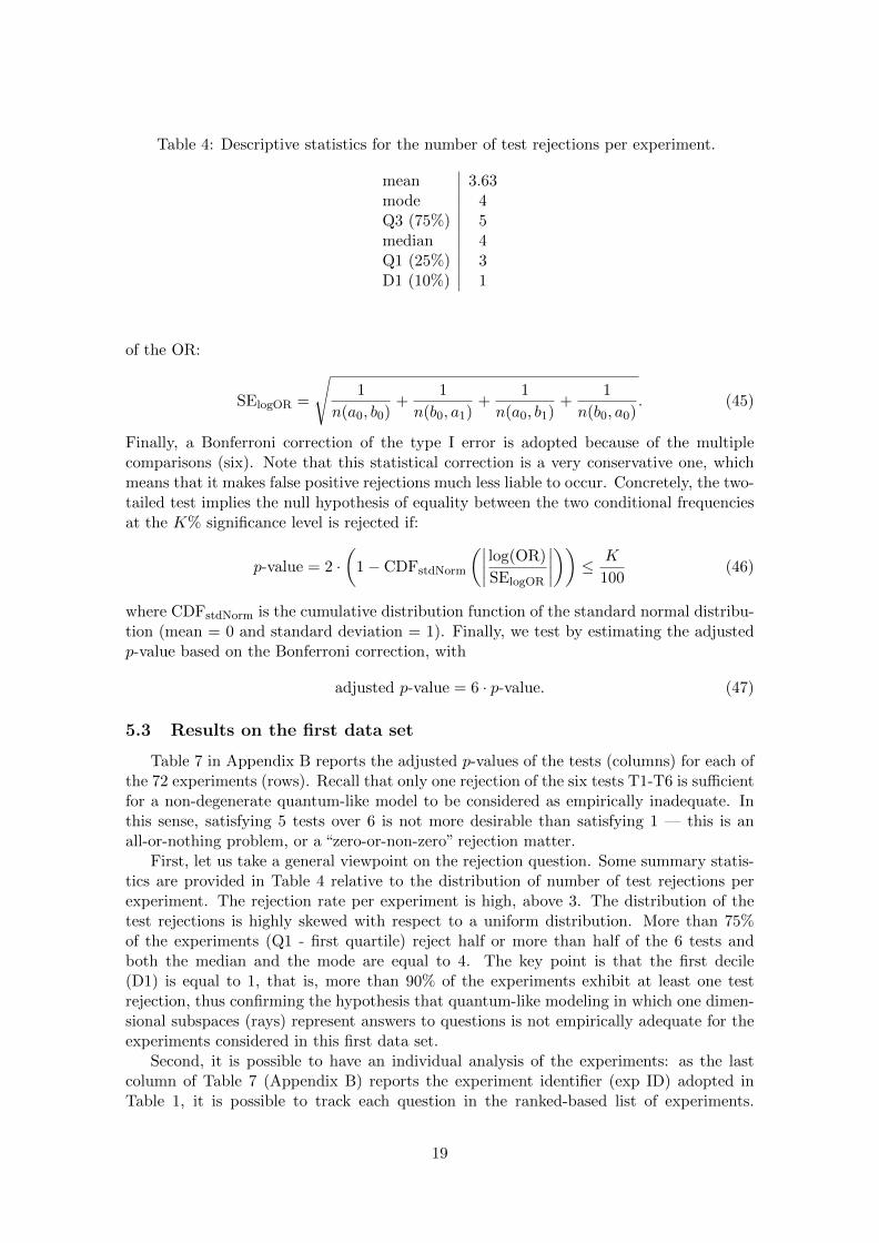
Table 4: Descriptive statistics for the number of test rejections per experiment.

mean 3.63mode 4Q3 (75%) 5median 4Q1 (25%) 3D1 (10%) 1

of the OR:

SElogOR =

√1

n(a0, b0)+

1

n(b0, a1)+

1

n(a0, b1)+

1

n(b0, a0). (45)

Finally, a Bonferroni correction of the type I error is adopted because of the multiplecomparisons (six). Note that this statistical correction is a very conservative one, whichmeans that it makes false positive rejections much less liable to occur. Concretely, the two-tailed test implies the null hypothesis of equality between the two conditional frequenciesat the K% significance level is rejected if:

p-value = 2 ·(

1− CDFstdNorm

(∣∣∣∣ log(OR)

SElogOR

∣∣∣∣)) ≤ K

100(46)

where CDFstdNorm is the cumulative distribution function of the standard normal distribu-tion (mean = 0 and standard deviation = 1). Finally, we test by estimating the adjustedp-value based on the Bonferroni correction, with

adjusted p-value = 6 · p-value. (47)

5.3 Results on the first data set

Table 7 in Appendix B reports the adjusted p-values of the tests (columns) for each ofthe 72 experiments (rows). Recall that only one rejection of the six tests T1-T6 is sufficientfor a non-degenerate quantum-like model to be considered as empirically inadequate. Inthis sense, satisfying 5 tests over 6 is not more desirable than satisfying 1 — this is anall-or-nothing problem, or a “zero-or-non-zero” rejection matter.

First, let us take a general viewpoint on the rejection question. Some summary statis-tics are provided in Table 4 relative to the distribution of number of test rejections perexperiment. The rejection rate per experiment is high, above 3. The distribution of thetest rejections is highly skewed with respect to a uniform distribution. More than 75%of the experiments (Q1 - first quartile) reject half or more than half of the 6 tests andboth the median and the mode are equal to 4. The key point is that the first decile(D1) is equal to 1, that is, more than 90% of the experiments exhibit at least one testrejection, thus confirming the hypothesis that quantum-like modeling in which one dimen-sional subspaces (rays) represent answers to questions is not empirically adequate for theexperiments considered in this first data set.

Second, it is possible to have an individual analysis of the experiments: as the lastcolumn of Table 7 (Appendix B) reports the experiment identifier (exp ID) adopted inTable 1, it is possible to track each question in the ranked-based list of experiments.

19

500 1000 1500

01

23

45

6

sample size

# te

st r

ejec

tions

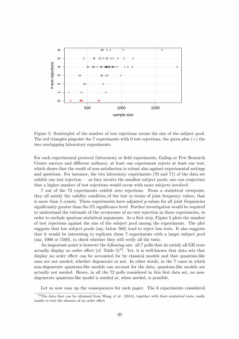
Figure 5: Scatterplot of the number of test rejections versus the size of the subject pool.The red triangles pinpoint the 7 experiments with 0 test rejections, the green plus (+) thetwo overlapping laboratory experiments.

For each experimental protocol (laboratory or field experiments, Gallup or Pew ResearchCenter surveys and different authors), at least one experiment rejects at least one test,which shows that the result of non-satisfaction is robust also against experimental settingsand questions. For instance, the two laboratory experiments (70 and 71) of the data setexhibit one test rejection — as they involve the smallest subject pools, one can conjecturethat a higher number of test rejections would occur with more subjects involved.

7 out of the 72 experiments exhibit zero rejections. From a statistical viewpoint,they all satisfy the validity condition of the test in terms of joint frequency values, thatis more than 5 counts. These experiments have adjusted p-values for all joint frequenciessignificantly greater than the 5% significance level. Further investigation would be requiredto understand the rationale of the occurrence of no test rejection in these experiments, inorder to exclude spurious statistical arguments. As a first step, Figure 5 plots the numberof test rejections against the size of the subject pool among the experiments. The plotsuggests that low subject pools (say, below 500) tend to reject less tests. It also suggeststhat it would be interesting to replicate these 7 experiments with a larger subject pool(say, 1000 or 1500), to check whether they still verify all the tests.

An important point is however the following one: all 7 polls that do satisfy all GR testsactually display no order effect (cf. Table 5)13. Yet, it is well-known that data sets thatdisplay no order effect can be accounted for by classical models and that quantum-likeones are not needed, whether degenerate or not. In other words, in the 7 cases in whichnon-degenerate quantum-like models can account for the data, quantum-like models areactually not needed. Hence, in all the 72 polls considered in this first data set, no non-degenerate quantum-like model is needed or, when needed, is possible.

Let us now sum up the consequences for each paper. The 6 experiments considered

13The data that can be obtained from Wang et al. (2014), together with their statistical tests, easilyenable to test the absence of an order effect.

20

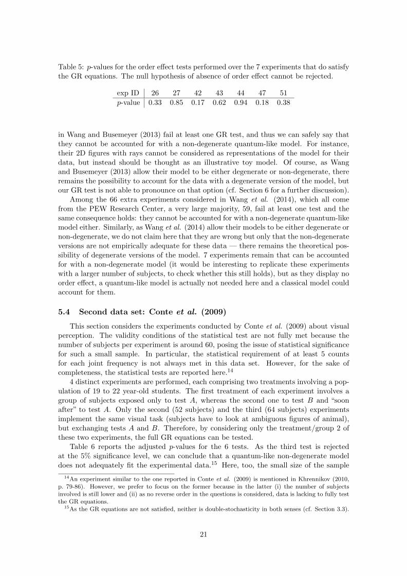
Table 5: p-values for the order effect tests performed over the 7 experiments that do satisfythe GR equations. The null hypothesis of absence of order effect cannot be rejected.

exp ID 26 27 42 43 44 47 51

p-value 0.33 0.85 0.17 0.62 0.94 0.18 0.38

in Wang and Busemeyer (2013) fail at least one GR test, and thus we can safely say thatthey cannot be accounted for with a non-degenerate quantum-like model. For instance,their 2D figures with rays cannot be considered as representations of the model for theirdata, but instead should be thought as an illustrative toy model. Of course, as Wangand Busemeyer (2013) allow their model to be either degenerate or non-degenerate, thereremains the possibility to account for the data with a degenerate version of the model, butour GR test is not able to pronounce on that option (cf. Section 6 for a further discussion).

Among the 66 extra experiments considered in Wang et al. (2014), which all comefrom the PEW Research Center, a very large majority, 59, fail at least one test and thesame consequence holds: they cannot be accounted for with a non-degenerate quantum-likemodel either. Similarly, as Wang et al. (2014) allow their models to be either degenerate ornon-degenerate, we do not claim here that they are wrong but only that the non-degenerateversions are not empirically adequate for these data — there remains the theoretical pos-sibility of degenerate versions of the model. 7 experiments remain that can be accountedfor with a non-degenerate model (it would be interesting to replicate these experimentswith a larger number of subjects, to check whether this still holds), but as they display noorder effect, a quantum-like model is actually not needed here and a classical model couldaccount for them.

5.4 Second data set: Conte et al. (2009)

This section considers the experiments conducted by Conte et al. (2009) about visualperception. The validity conditions of the statistical test are not fully met because thenumber of subjects per experiment is around 60, posing the issue of statistical significancefor such a small sample. In particular, the statistical requirement of at least 5 countsfor each joint frequency is not always met in this data set. However, for the sake ofcompleteness, the statistical tests are reported here.14

4 distinct experiments are performed, each comprising two treatments involving a pop-ulation of 19 to 22 year-old students. The first treatment of each experiment involves agroup of subjects exposed only to test A, whereas the second one to test B and “soonafter” to test A. Only the second (52 subjects) and the third (64 subjects) experimentsimplement the same visual task (subjects have to look at ambiguous figures of animal),but exchanging tests A and B. Therefore, by considering only the treatment/group 2 ofthese two experiments, the full GR equations can be tested.

Table 6 reports the adjusted p-values for the 6 tests. As the third test is rejectedat the 5% significance level, we can conclude that a quantum-like non-degenerate modeldoes not adequately fit the experimental data.15 Here, too, the small size of the sample

14An experiment similar to the one reported in Conte et al. (2009) is mentioned in Khrennikov (2010,p. 79-86). However, we prefer to focus on the former because in the latter (i) the number of subjectsinvolved is still lower and (ii) as no reverse order in the questions is considered, data is lacking to fully testthe GR equations.

15As the GR equations are not satisfied, neither is double-stochasticity in both senses (cf. Section 3.3).

21

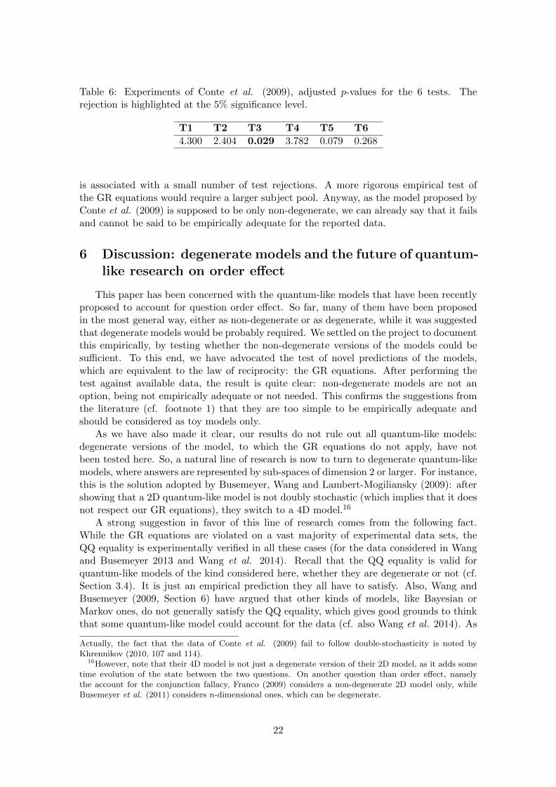
Table 6: Experiments of Conte et al. (2009), adjusted p-values for the 6 tests. Therejection is highlighted at the 5% significance level.

T1 T2 T3 T4 T5 T6

4.300 2.404 0.029 3.782 0.079 0.268

is associated with a small number of test rejections. A more rigorous empirical test ofthe GR equations would require a larger subject pool. Anyway, as the model proposed byConte et al. (2009) is supposed to be only non-degenerate, we can already say that it failsand cannot be said to be empirically adequate for the reported data.

6 Discussion: degenerate models and the future of quantum-like research on order effect

This paper has been concerned with the quantum-like models that have been recentlyproposed to account for question order effect. So far, many of them have been proposedin the most general way, either as non-degenerate or as degenerate, while it was suggestedthat degenerate models would be probably required. We settled on the project to documentthis empirically, by testing whether the non-degenerate versions of the models could besufficient. To this end, we have advocated the test of novel predictions of the models,which are equivalent to the law of reciprocity: the GR equations. After performing thetest against available data, the result is quite clear: non-degenerate models are not anoption, being not empirically adequate or not needed. This confirms the suggestions fromthe literature (cf. footnote 1) that they are too simple to be empirically adequate andshould be considered as toy models only.

As we have also made it clear, our results do not rule out all quantum-like models:degenerate versions of the model, to which the GR equations do not apply, have notbeen tested here. So, a natural line of research is now to turn to degenerate quantum-likemodels, where answers are represented by sub-spaces of dimension 2 or larger. For instance,this is the solution adopted by Busemeyer, Wang and Lambert-Mogiliansky (2009): aftershowing that a 2D quantum-like model is not doubly stochastic (which implies that it doesnot respect our GR equations), they switch to a 4D model.16

A strong suggestion in favor of this line of research comes from the following fact.While the GR equations are violated on a vast majority of experimental data sets, theQQ equality is experimentally verified in all these cases (for the data considered in Wangand Busemeyer 2013 and Wang et al. 2014). Recall that the QQ equality is valid forquantum-like models of the kind considered here, whether they are degenerate or not (cf.Section 3.4). It is just an empirical prediction they all have to satisfy. Also, Wang andBusemeyer (2009, Section 6) have argued that other kinds of models, like Bayesian orMarkov ones, do not generally satisfy the QQ equality, which gives good grounds to thinkthat some quantum-like model could account for the data (cf. also Wang et al. 2014). As

Actually, the fact that the data of Conte et al. (2009) fail to follow double-stochasticity is noted byKhrennikov (2010, 107 and 114).

16However, note that their 4D model is not just a degenerate version of their 2D model, as it adds sometime evolution of the state between the two questions. On another question than order effect, namelythe account for the conjunction fallacy, Franco (2009) considers a non-degenerate 2D model only, whileBusemeyer et al. (2011) considers n-dimensional ones, which can be degenerate.

22

our present results exclude non-degenerate models, the hopes are now on the degenerateones. Overall, the following tests might be made on a data set of question order effect:1) test the QQ equality; if it is violated, no quantum-like model (of the sort consideredin this paper) can account for it; if it is not violated, it gives good grounds to think (butdoes not prove) that a degenerate or non-degenerate quantum-like model can account forit; 2) test the GR equations; if they are violated, no non-degenerate quantum-like modelcan account for the data; if they are not, one can.

However, in our view, the route of degenerate models is not necessarily an easy one, andwe would like to recommend that some research be done about their empirical adequacy.First, degenerate models are not a priori freed from any constraint, and this is the pointon which we would like to insist very much. One should not consider that, when a dataset satisfies the QQ equality and violates the GR equations, the solution safely lies ina degenerate model. The moral of our paper should be taken as insisting on the needto empirically test all quantum-like models. Note that we do not just call for runningmore experiments; all the tests we have done here have been made on available data, andcould have been made beforehand. Importantly, empirical adequacy does not only meanapplying to a vast number of empirical cases, but also, for one experimental case, makingcorrect predictions in all respects, and for that it is crucial to pull the threads of all possiblepredictions. Here, we have found simple and ready-to-use tests for non-degenerate models,and we suspect that some other constraints apply to degenerate models. Research isurgently needed here to find general tests. At least, when a degenerate model is proposedto account for some features of a data set, we suggest that all parameters be specifiedand that serious efforts be directed towards empirically testing this model by unveilingexperimental predictions that lie outside the feature one intends to explain, so as to preventlater “bad surprises”.

A promising way to test degenerate models has already been indicated in the end ofSection 3.2: degenerate eigenspaces may actually encompass non-degenerate and morefundamental eigenspaces, that correspond to fundamental elementary questions — to beidentified. If such elementary questions exist, and the quantum-like literature seems notto have doubts on that, all degenerate models can actually be tested against generalizedGR equations for these more fundamental questions. In other words, our GR test for non-degenerate models can possibly apply at a fundamental level for all degenerate models,provided elementary questions are identified.17 We are ready to admit, however, that thefundamental dimensions and the corresponding tests can be hard to uncover.

The need to specify the elementary dimensions of the Hilbert space for degeneratemodels is also required by other arguments. Introducing dimensions of degeneracy shouldbe justified, so as not to be accused of being just ad hoc. As Pothos and Busemeyer (2013,p. 215) write, “Dimensionality is not a free parameter”. In quantum physics for instance,degeneration is usually theoretically justified with a symmetry in the Hamiltonian, andthe degeneration can be experimentally removed by introducing some factor that wasnot present (e.g., the spin degeneration is removed by introducing a magnetic field). Forquantum-like judgment models as well, one should provide a similar theoretical justificationand an experimental way of removing the degeneration. In this respect, the idea that thereexists fundamental questions and rays will certainly be helpful; the work is then to findout which fundamental dimensions are hidden behind the degenerate eigenspace.

Overall, all this argues against the view that switching to degenerate models when

17These generalized GR equations for elementary questions might help to establish the constraints thatdegenerate models must satisfy in general, but for non-elementary questions, that have been discussed inthe above paragraph.

23

GR equations are violated would be a natural or unquestioned move to have and that itwould solve all problems. Instead, supplementary dimensions should be justified, probablywith elementary questions, and other predictions of the model than those one intends toaccount for should be investigated and tested, possibly with generalized GR equations.

Beyond degenerate quantum-like models in the flavor of the model presented in Sec-tion 2, there are also other possible lines of research around quantum ideas. For instance,Khrennikov has proposed to consider hyperbolic Hilbert space models, instead of complexones like in this paper. Hyperbolic models enable probabilities that are not constrained inthe same way, and can account for some data that are out of reach for complex quantum-like models (see Khrennikov 2010 for a synthesis). Also, other tools than projectors, likePOVMs, could be considered; or other axioms of standard quantum-like models, like theprojection postulate or the Born rule, could be abandoned or modified.

To conclude, quantum-like models have brought to discussion many provoking andseminal ideas, such as the hypotheses that judgments or preferences might be undeterminedinstead of only unknown, or that non-classical probabilities could be considered. We haveinsisted on the need to empirically test existing models for question order effect, and ourresults suggest that non-degenerate quantum-like models should be considered more astoy models than as empirically adequate models, in accordance with suggestions from theliterature, and that future investigations should focus on degenerate models. In spite ofthe potential difficulties that such models face, there is plenty of room for future researchin the area, and besides our results can be taken as posing a challenge liable to trigger arevival of the discussion on quantum-like models of various sorts.

Acknowledgments

Many thanks to Camille Aron, Jerome R. Busemeyer, Sophie Dubois, Dorian Jullien,Corrado Lagazio, Ariane Lambert-Mogiliansky, Gabriel Lemarie, Zheng J. Wang, andto the audience from conferences at the MSHS du Sud-Est (Nice, France) and at theToronto Fields Institute (Canada) for valuable comments or suggestions. Of course, weare solely responsible for our analysis and conclusions. We further thank Zheng J. Wang,Tyler Solloway, Richard M. Shiffrin, and Jerome R. Busemeyer who kindly gave us theopportunity to use their data set to perform our tests.

References

Aerts, Diederik (2009), “Quantum Structure in Cognition”, Journal of Mathematical Psy-chology 53: 314–348.

Aerts, Diederik, Liane Gabora and Sandro Sozzo (2013), “Concepts and Their Dy-namics: A Quantum-Theoretic Modeling of Human Thought”, Topics in CognitiveSciences 5: 737–772.

Allais, Maurice (1953), “Le comportement de l’homme rationnel devant le risque : cri-tique des postulats et axiomes de l’ecole Americaine”, Econometrica 21:503–546.

Ashby, F. Gregory and Nancy A. Perrin (1988), “Towards a unified theory of similarityand recognition”, Psychological Review, 95:124–50.

Ashtiani, Mehrdad and Mohammad A. Azgomi (2015), “A survey of quantum-like ap-proaches to decision making and cognition”, Mathematical Social Sciences 75: 49–80.

Busemeyer, Jerome R. and Peter D. Bruza (2012), Quantum models of Cognition andDecision, Cambridge: Cambridge University Press.

24

Busemeyer, Jerome R., Emmanuel M. Pothos, Riccardo Franco and Jennifer S. True-blood (2011), “A Quantum Theoretical Explanation for Probability Judgment Er-rors”, Psychological Review 118 (2): 193–218.

Busemeyer, Jerome R., Zheng J. Wang, and Ariane Lambert-Mogiliansky (2009),“Empirical comparison of Markov and quantum models of decision making”, Journalof Mathematical Psychology 53: 423–433.

Busemeyer, Jerome R., Zheng J. Wang, Emmanuel M. Pothos and Jennifer S. True-blood (2015), “The Conjunction Fallacy, Confirmation, and Quantum Theory: Com-ment on Tentori, Crupi, and Russo (2013)”, Journal of Experimental Psychology:General 144(1): 236-243.

Conte, Elio, Andrei Yuri Khrennikov, Orlando Todarello, Antonio Federici, LeonardoMendolicchio, and Joseph P. Zbilut (2009), “Mental States Follow Quantum Me-chanics During Perception and Cognition of Ambiguous Figures”, Open Systems &Information Dynamics 16(1) 1–17.

Danilov, Vladimir I. and Ariane Lambert-Mogiliansky (2008), “Measurable systemsand behavioral sciences”, Mathematical Social Sciences 55(3): 315–340.

Danilov, Vladimir I. and Ariane Lambert-Mogiliansky (2010), “Expected utility the-ory under non-classical uncertainty”, Theory and Decision 68(1): 25–47.

Ellsberg, Daniel (1961), “Risk, ambiguity, and the Savage axioms”, Quarterly Journalof Economics 75(4): 643–669.

Franco, Riccardo (2009), “The conjunction fallacy and interference effects”, Journal ofMathematical Psychology 53: 415–422.

Gavanski, Igor and David R. Roskos-Ewoldsen (1991), “Representativeness and con-joint probability”, Journal of Personality and Social Psychology 61:181–94.

Haven, Emmanuel and Andrei Khrennikov (2013), Quantum Social Science, Cambridge:Cambridge University Press.

Khrennikov, Andrei (2010), Ubiquitous Quantum Structure. From Psychology to Fi-nance, Heildelberg: Springer.

Krumhansl, Carol L. (1978),“Concerning the applicability of geometric models to similar-ity data: The interrelationship between similarity and spatial density”, PsychologicalReview 85:445–63.

Lambert-Mogiliansky, Ariane, Shmuel Zamir and Herve Zwirn (2009), “Type inde-terminacy: A model of the KT(Kahneman–Tversky)-man”, Journal of MathematicalPsychology 53:349–361.

Moore, David W. (2002), “Measuring new types of question-order effects”, Public OpinionQuarterly, 66: 80–91.

Peres, Asher (1993), Quantum Theory: Concepts and Methods, Kluwer.Pothos, Emmanuel M. and Jerome R. Busemeyer (2013), “Can quantum probability

provide a new direction for cognitive modeling?”, Behavioral and Brain Sciences 36:255–327.

Schuman, Howard and Stanley Presser (1981), Questions and answers in attitude sur-veys: Experiments on question form, wording, and context, Academic Press.

Shafir, Eldar and Amos Tversky (1992), “Thinking through uncertainty: nonconse-quential reasoning and choice”, Cognitive Psychology 24:449–74.

Stolarz-Fantino, Stepanie, Edmund Fantino, Daniel J. Zizzo, and Julie Wen (2003),“The conjunction effect: New evidence for robustness”, American Journal of Psychol-ogy 116(1):15–34.

Tourangeau, Roger, Lance J. Rips and Kenneth A. Rasinski (2000), The psychologyof survey response, Cambridge University Press.

25

Trueblood Jennifer S. and Jerome R. Busemeyer (2011), “A Quantum ProbabilityAccount of Order Effects in Inference”, Cognitive Science 35: 1518–1552.

Tversky, Amos (1977), “Features of similarity”, Psychological Review 84(4): 327–52.Tversky, Amos and Daniel Kahneman (1982), “Judgments of and by representative-

ness”, in: Judgment under uncertainty: Heuristics and biases, ed. by D. Kahneman,P. Slovic & A. Tversky, p. 84–98, Cambridge University Press.

— (1983), “Extensional versus intuitive reasoning: The conjunction fallacy in probabilityjudgment”, Psychological Review 90(4): 293–315.

Wang, Zheng J. and Jerome R. Busemeyer (2013), “A quantum question order modelsupported by empirical tests of an a priori and precise prediction”, Topics in CognitiveScience 5(4): 689–710.

Wang, Zheng J., Tyler Solloway, Richard M. Shiffrin and Jerome R. Busemeyer(2014), “Context effects produced by question orders reveal quantum nature of humanjudgments”, PNAS, www.pnas.org/cgi/doi/10.1073/pnas.1407756111.

Yukalov, Vyacheslav I. and Didier Sornette (2011), “Decision theory with prospectinterference and entanglement”, Theory and Decision, 70: 283–328.

26

A Testing the equality of two conditional relative frequen-cies

The statistical test is to compare two conditional relative frequencies y and x, with thenull hypothesis that they are equal. The test is therefore

y = x, (48)

where both y and x are observed conditional relative frequencies.Testing equation 48 is equivalent to test

log

(y

1− y

)= log

(x

1− x

),

given that y and x are not equal to zero.Alternatively, we can formulate the test in terms of the log odds ratio (OR)

log(OR) = log

(y

1−yx

1−x

)= 0.

Now let’s suppose that we want to test

f(a0|b0) = f(b0|a0). (49)

We can thus test the following condition:

log

(f(a0|b0)

1− f(a0|b0)

)= log

(f(b0|a0)

1− f(b0|a0)

),

or

log

(f(a0|b0)f(a1|b0)

)= log

(f(b0|a0)f(b1|a0)

).

By expressing the conditional relative frequencies in terms of joint frequencies, that is,

f(a0|b0) =n(b0, a0)

n(b0, ·), f(b0|a0) =

n(a0, b0)

n(a0, ·), . . .

being n(b0, ·) and n(a0, ·) the marginal frequencies of B and A, respectively, we obtain

log

(n(b0, a0)

n(b0, ·)n(b0, ·)n(b0, a1)

)= log

(n(a0, b0)

n(a0, ·)n(a0, ·)n(a0, b1)

),

or simplifying

log

(n(b0, a0)n(a0, b1)

n(b0, a1)n(a0, b0)

)= 0. (50)

We can thus test indifferently eq. 49 or 50.

27

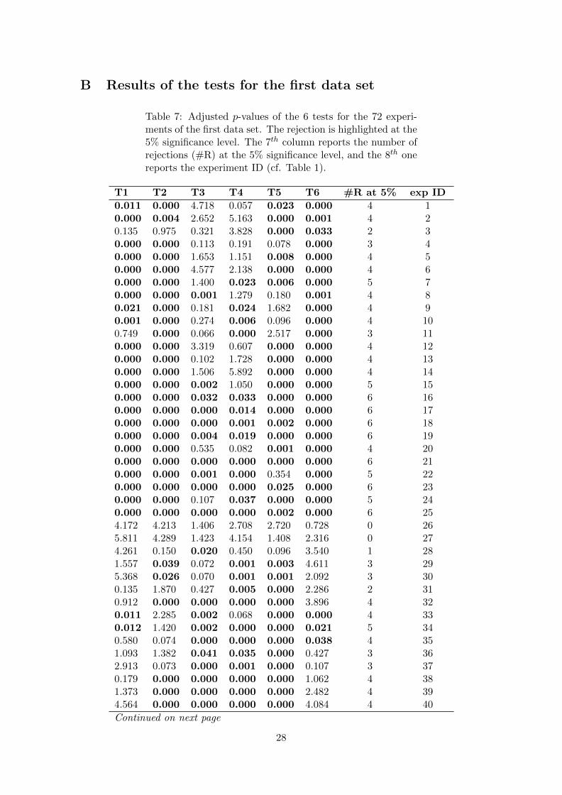
B Results of the tests for the first data set

Table 7: Adjusted p-values of the 6 tests for the 72 experi-ments of the first data set. The rejection is highlighted at the5% significance level. The 7th column reports the number ofrejections (#R) at the 5% significance level, and the 8th onereports the experiment ID (cf. Table 1).

T1 T2 T3 T4 T5 T6 #R at 5% exp ID

0.011 0.000 4.718 0.057 0.023 0.000 4 10.000 0.004 2.652 5.163 0.000 0.001 4 20.135 0.975 0.321 3.828 0.000 0.033 2 30.000 0.000 0.113 0.191 0.078 0.000 3 40.000 0.000 1.653 1.151 0.008 0.000 4 50.000 0.000 4.577 2.138 0.000 0.000 4 60.000 0.000 1.400 0.023 0.006 0.000 5 70.000 0.000 0.001 1.279 0.180 0.001 4 80.021 0.000 0.181 0.024 1.682 0.000 4 90.001 0.000 0.274 0.006 0.096 0.000 4 100.749 0.000 0.066 0.000 2.517 0.000 3 110.000 0.000 3.319 0.607 0.000 0.000 4 120.000 0.000 0.102 1.728 0.000 0.000 4 130.000 0.000 1.506 5.892 0.000 0.000 4 140.000 0.000 0.002 1.050 0.000 0.000 5 150.000 0.000 0.032 0.033 0.000 0.000 6 160.000 0.000 0.000 0.014 0.000 0.000 6 170.000 0.000 0.000 0.001 0.002 0.000 6 180.000 0.000 0.004 0.019 0.000 0.000 6 190.000 0.000 0.535 0.082 0.001 0.000 4 200.000 0.000 0.000 0.000 0.000 0.000 6 210.000 0.000 0.001 0.000 0.354 0.000 5 220.000 0.000 0.000 0.000 0.025 0.000 6 230.000 0.000 0.107 0.037 0.000 0.000 5 240.000 0.000 0.000 0.000 0.002 0.000 6 254.172 4.213 1.406 2.708 2.720 0.728 0 265.811 4.289 1.423 4.154 1.408 2.316 0 274.261 0.150 0.020 0.450 0.096 3.540 1 281.557 0.039 0.072 0.001 0.003 4.611 3 295.368 0.026 0.070 0.001 0.001 2.092 3 300.135 1.870 0.427 0.005 0.000 2.286 2 310.912 0.000 0.000 0.000 0.000 3.896 4 320.011 2.285 0.002 0.068 0.000 0.000 4 330.012 1.420 0.002 0.000 0.000 0.021 5 340.580 0.074 0.000 0.000 0.000 0.038 4 351.093 1.382 0.041 0.035 0.000 0.427 3 362.913 0.073 0.000 0.001 0.000 0.107 3 370.179 0.000 0.000 0.000 0.000 1.062 4 381.373 0.000 0.000 0.000 0.000 2.482 4 394.564 0.000 0.000 0.000 0.000 4.084 4 40

Continued on next page

28

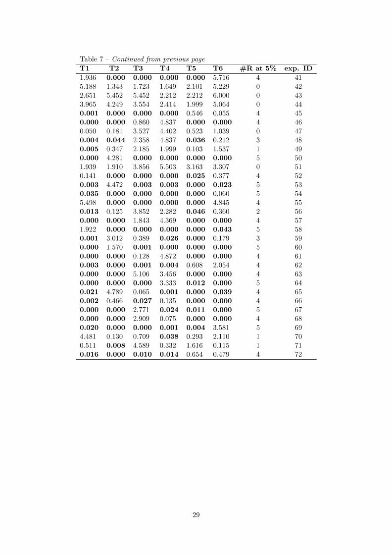
Table 7 – Continued from previous page

T1 T2 T3 T4 T5 T6 #R at 5% exp. ID

1.936 0.000 0.000 0.000 0.000 5.716 4 415.188 1.343 1.723 1.649 2.101 5.229 0 422.651 5.452 5.452 2.212 2.212 6.000 0 433.965 4.249 3.554 2.414 1.999 5.064 0 440.001 0.000 0.000 0.000 0.546 0.055 4 450.000 0.000 0.860 4.837 0.000 0.000 4 460.050 0.181 3.527 4.402 0.523 1.039 0 470.004 0.044 2.358 4.837 0.036 0.212 3 480.005 0.347 2.185 1.999 0.103 1.537 1 490.000 4.281 0.000 0.000 0.000 0.000 5 501.939 1.910 3.856 5.503 3.163 3.307 0 510.141 0.000 0.000 0.000 0.025 0.377 4 520.003 4.472 0.003 0.003 0.000 0.023 5 530.035 0.000 0.000 0.000 0.000 0.060 5 545.498 0.000 0.000 0.000 0.000 4.845 4 550.013 0.125 3.852 2.282 0.046 0.360 2 560.000 0.000 1.843 4.369 0.000 0.000 4 571.922 0.000 0.000 0.000 0.000 0.043 5 580.001 3.012 0.389 0.026 0.000 0.179 3 590.000 1.570 0.001 0.000 0.000 0.000 5 600.000 0.000 0.128 4.872 0.000 0.000 4 610.003 0.000 0.001 0.004 0.608 2.054 4 620.000 0.000 5.106 3.456 0.000 0.000 4 630.000 0.000 0.000 3.333 0.012 0.000 5 640.021 4.789 0.065 0.001 0.000 0.039 4 650.002 0.466 0.027 0.135 0.000 0.000 4 660.000 0.000 2.771 0.024 0.011 0.000 5 670.000 0.000 2.909 0.075 0.000 0.000 4 680.020 0.000 0.000 0.001 0.004 3.581 5 694.481 0.130 0.709 0.038 0.293 2.110 1 700.511 0.008 4.589 0.332 1.616 0.115 1 710.016 0.000 0.010 0.014 0.654 0.479 4 72

29

DOCUMENTS DE TRAVAIL GREDEG PARUS EN 2015GREDEG Working Papers Released in 2015

2015-01 Laetitia Chaix & Dominique Torre The Dual Role of Mobile Payment in Developing Countries2015-02 Michaël Assous, Olivier Bruno & Muriel Dal-Pont Legrand The Law of Diminishing Elasticity of Demand in Harrod’s Trade Cycle (1936)2015-03 Mohamed Arouri, Adel Ben Youssef & Cuong Nguyen Natural Disasters, Household Welfare and Resilience: Evidence from Rural Vietnam2015-04 Sarah Guillou & Lionel Nesta Markup Heterogeneity, Export Status and the Establishment of the Euro2015-05 Stefano Bianchini, Jackie Krafft, Francesco Quatraro & Jacques Ravix Corporate Governance, Innovation and Firm Age: Insights and New Evidence2015-06 Thomas Boyer-Kassem, Sébastien Duchêne & Eric Guerci Testing Quantum-like Models of Judgment for Question Order Effects