Embed Size (px)
Citation preview
1
The regionalization of national input-
output tables: a study of South
Korean regions
Anthony T. Flegg
Department of Accounting, Economics and Finance,
University of the West of England, Bristol, UK
and
Timo Tohmo School of Business and Economics,
University of Jyväskylä, Jyväskylä, Finland
Economics Working Paper Series
1705
2
The regionalization of national inputoutput tables: a study of
South Korean regions
Anthony T. Flegg Department of Accounting, Economics and Finance, University of the West of England, Coldharbour
Lane, Bristol BS16 1QY, UK
E-mail: [email protected]
Timo Tohmo School of Business and Economics, University of Jyväskylä, Jyväskylä, Finland
Email: [email protected]
Abstract. This paper uses survey-based data for 16 South Korean regions to refine the application of
Flegg’s location quotient (FLQ) and its variant, the sector-specific FLQ (SFLQ). These regions vary
markedly in terms of size. Especial attention is paid to the problem of choosing appropriate values for
the unknown parameter δ in these formulae. Alternative approaches to this problem are evaluated and
tested. Our paper adds to earlier research that aims to find a cost-effective way of adapting national
coefficients, so as to produce a satisfactory initial set of regional input coefficients for regions where
survey-based data are unavailable.
JEL classification: C67, O18, R15
Key words: Location quotients, FLQ, SFLQ, inputoutput, South Korea
1 Introduction
Regional inputoutput tables contain much useful information to guide regional planners, yet regional
tables based largely on survey data are rare. This rarity reflects the expense and difficulty of
constructing such tables. Consequently, analysts typically rely on indirect methods of constructing
regional tables, by adapting national data using formulae based on location quotients (LQs).
However, the paucity of survey-based regional tables makes it very challenging to perform reliable
tests of the available non-survey methods. Indeed, most empirical studies of LQ-based methods have
examined data for single regions; recent examples include a study of the German state of Baden-
Wuerttemberg by Kowalewski (2015) and one of the Argentinian province of Córdoba by Flegg et al.
(2016). A potential weakness of such studies is, of course, that they may reflect the idiosyncrasies of
particular regions and thus lack generality.
An innovative way of obtaining more general results was proposed by Bonfiglio and Chelli (2008),
who employed Monte Carlo methods to generate, for each of 20 regions, 1000 multiregional tables
with 20 sectors, which were aggregated to produce corresponding national tables. They were then
able to assess the relative accuracy of several alternative non-survey methods in terms of their ability
to estimate the values of 400,000 regional output multipliers. The results demonstrated that Flegg’s
LQ (FLQ) and its variant, the augmented FLQ (AFLQ), gave by far the best estimates of these
multipliers.
Nevertheless, Flegg and Tohmo (2016, p. 33) remark that ‘the simplifying assumptions underlying
a Monte Carlo simulation mean that it cannot replicate the detailed economic structure and sectoral
interrelationships of regional economies.’ This feature may well explain why the results exhibit
unusually large mean relative absolute errors (Bonfiglio and Chelli 2008, table 1).
Here we pursue an alternative approach, in an effort to circumvent the limitations of both Monte
Carlo methods and single-region studies. To attain greater generality, we examine survey-based
tables for 16 South Korean regions of differing size. The reliability of our study is enhanced by the
fact that the detailed regional and national tables for the year 2005 were constructed on a consistent
3
basis by the Bank of Korea. Our main aim is to make full use of this valuable data set to refine the
application of the FLQ formula for estimating regional input coefficients and hence sectoral output
multipliers. We pay especial attention to the choice of a value for the unknown parameter δ in this
formula. Along with regional size, this value determines the size of the adjustment for regional
imports in the FLQ formula.
Earlier work on this topic using data for two Korean regions was carried out by Zhao and Choi
(2015). However, we argue that there are several key shortcomings in this pioneering study, so an
effort is made to address these limitations. In the next section, we discuss the FLQ formula and some
related formulae based on location quotients (LQs). Relevant empirical evidence is also considered.
In Section 3, we examine some of Zhao and Choi’s key findings but find that they cannot be
replicated. We also raise some fundamental methodological issues concerning their approach. In
Section 4, we examine the proposed sector-specific FLQ (SFLQ) approach of Kowalewski (2015) and
consider how it might be used in a practical context. The penultimate section extends our analysis
from 2 to 16 regions, while the final section concludes.
2 The FLQ and related formulae
LQs offer a simple and cheap way of regionalizing a national inputoutput table.1 Earlier analysts
have often used the simple LQ (SLQ) or the cross-industry LQ (CILQ), yet both are known to
underestimate regional trade. This effect occurs largely because they either rule out (as with the SLQ)
or greatly understate (as with the CILQ) the extent of cross-hauling (the simultaneous importing and
exporting of a given commodity).2 The SLQ is defined here as
SLQi rii
nii
ni
ri
nii
ni
rii
ri
Q
Q
Q
Q
/
/, (1)
where riQ is regional output in sector i and
niQ is the corresponding national figure.
riiQ and
niiQ are the respective regional and national totals. Likewise, the CILQ is defined as
CILQij nj
rj
ni
ri
j
i
SLQ
SLQ
/
/ , (2)
where the subscripts i and j refer to the supplying and purchasing sectors, respectively.
It should be noted that the SLQ and CILQ are defined in terms of output rather than the more usual
employment. Using output is preferable to using a proxy such as employment because output figures
are not distorted by differences in productivity across regions. Fortunately, regional sectoral output
data were readily available in this instance.
The first step in the application of LQs is to transform the national transactions matrix into a
matrix of input coefficients. This matrix can then be ‘regionalized’ via the formula
rij = βij × aij, (3)
where rij is the regional input coefficient, βij is an adjustment coefficient and aij is the national input
coefficient (Flegg and Tohmo 2016, p. 311). rij measures the amount of regional input i required to
produce one unit of regional gross output j; it thus excludes any supplies of i obtained from other
regions or from abroad. Similarly, aij excludes any foreign inputs. The role of βij is to take account of
a region’s purchases of input i from other regions.
We can estimate the rij by replacing βij in equation (3) with an LQ. Thus, for instance:
4
ijr = CILQij × aij. (4)
No scaling is applied to aij where CILQij ≥ 1 and likewise for SLQi.
The CILQ has the merit that a different scaling can be applied to each cell in a given row of the
national coefficient matrix. Unlike the SLQ, the CILQ does not presume that a purchasing sector is
either an exporter or an importer of a given commodity but never both. Even so, empirical evidence
indicates that the CILQ still substantially understates regional trade. Flegg et al. (1995) attempted to
address this demerit of the CILQ via their FLQ formula, which was later refined by Flegg and Webber
(1997). The FLQ is defined here as
FLQij ≡ CILQij × λ*, for i ≠ j, (5)
FLQij ≡ SLQi × λ*, for i = j, (6)
where3
λ* ≡ [log2(1 + nii
rii QQ / )]
δ. (7)
It is assumed that 0 ≤ δ < 1; the higher the value of δ, the bigger the allowance for
interregional imports. δ = 0 represents a special case whereby FLQij = CILQij for i ≠ j and
FLQij = SLQi for i = j. As with other LQ-based formulae, the constraint FLQij ≤ 1 is
imposed.
It is worth emphasizing two aspects of the FLQ formula: its cross-industry foundations and the
explicit role given to regional size. With the FLQ, the relative size of the regional purchasing and
supplying sectors is considered when making an adjustment for interregional trade. Furthermore, by
taking explicit account of a region’s relative size, Flegg and Tohmo (2016, p. 312) argue that the FLQ
should help to address the problem of cross-hauling, which is likely to be more acute in smaller
regions than in larger ones. Smaller regions are apt to be more open to interregional trade.
It is now well established that the FLQ can give more precise results than the SLQ and CILQ.
This evidence includes, for instance, case studies of Scotland (Flegg and Webber 2000), Finland
(Tohmo 2004; Flegg and Tohmo 2013a, 2016), Germany (Kowalewski 2015), Argentina (Flegg et al.
2016) and Ireland (Morrissey 2016). This evidence from case studies is bolstered by the Monte Carlo
simulation results of Bonfiglio and Chelli (2008) mentioned earlier. Nonetheless, some evidence to
the contrary is presented by Lamonica and Chelli (2017), who find initially that the SLQ gives
slightly better results than the FLQ.
Lamonica and Chelli’s study is unusual since it is based on the World InputOutput Database.
The sample comprised 27 European countries, 13 other major countries plus the rest of the world as a
composite ‘country’. Data for 35 industries (economic sectors) in the period 19952011 were
examined. However, when the authors disaggregated their sample into small and large countries,
rather different findings emerged. For the smaller economies, characterized by a high percentage of
input coefficients close to zero, the FLQ (with δ = 0.2) was the best method, whereas the SLQ
performed the best in the larger economies.
The FLQ’s focus is on the output and employment generated within a specific region. As Flegg
and Tohmo (2013b) point out, it should only be used in conjunction with national inputoutput tables
where the inter-industry transactions exclude imports (type B tables). By contrast, where the focus is
on the overall supply of goods, Kronenberg’s Cross-Hauling Adjusted Regionalization Method
(CHARM) can be employed (Flegg et al. 2015; Többen and Kronenberg 2015). CHARM requires
type A tables, those where imports have been incorporated into the national transactions table
(Kronenberg 2009, 2012).
A variant of the FLQ is the augmented FLQ (AFLQ) formula devised by Flegg and Webber
(2000), which aims to capture the impact of regional specialization on the size of regional input
coefficients. This effect is measured via SLQj. The AFLQ is defined as
5
AFLQij ≡ FLQij × log2(1 + SLQj). (8)
The specialization term, log2(1 + SLQj), only applies where SLQj > 1 (Flegg and Webber 2000, p.
566). The AFLQ has the novel property that it can encompass cases where rij > aij in equation (3). As
with the FLQ, the constraint AFLQij ≤ 1 is imposed.
Although the AFLQ has some theoretical merits relative to the FLQ, its empirical performance is
typically very similar. For instance, in the Monte Carlo study by Bonfiglio and Chelli (2008), the
AFLQ gave only slightly more accurate results than the FLQ.4 This outcome was confirmed by Flegg
et al. (2016). Kowalewski (2015) also tested both formulae but again obtained comparable results.
For this reason, along with limitations of space, only the FLQ will be examined here.
Another variant of the FLQ is proposed by Kowalewski (2015). Her innovative approach involves
relaxing the assumption that δ is invariant across sectors. Kowalewski’s industry-specific FLQ, the
SFLQ, is defined as
SFLQij ≡ CILQij × [log2(1 + Er/E
n)]
δj, (9)
where Er/E
n is regional size measured in terms of employment. For i = j, CILQij is replaced by SLQi.
In order to estimate the values of δj, Kowalewski specifies a regression model of the following form
δj = α + β1 CLj + β2 SLQj + β3 IMj + β4 VAj + εj, (10)
where CLj is the coefficient of localization, which measures the degree of concentration of national
industry j, IMj is the share of foreign imports in total national intermediate inputs, VAj is the share of
value added in total national output and εj is an error term. Regional data are needed for SLQj,
whereas CLj, IMj and VAj require national data. CLj is calculated as
n
r
nj
rj
rjE
E
E
ECL 5.0 . (11)
3 Zhao and Choi’s study
Zhao and Choi (2005) based their analysis on a 28 × 28 national technological coefficient matrix for
2005 produced by the Bank of Korea. It should be noted that this was a type A matrix, which
incorporated imports from abroad. Nevertheless, the authors regionalized this matrix by applying
various LQ-based formulae calculated using employment data. The Bank divided the country into 16
regions and computed type I output multipliers for each region. Zhao and Choi chose to study two
regions in detail, namely Daegu and Gyeongbuk, and used the Bank’s regional multipliers as a
benchmark for assessing the accuracy of their simulations. As criteria, they used the mean absolute
distance and the mean absolute percentage error (MAPE). However, the results from these two
measures hardly differed, so only MAPE will be considered here. It was calculated via the formula
MAPE = (100/n) Σj | jj mm ˆ | / mj, (12)
where mj is the type I output multiplier for sector j and n = 28 is the number of sectors.
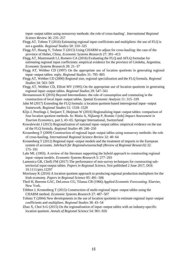
Table 1
A selection of Zhao and Choi’s results is presented in Table 1. As expected, the FLQ outperforms
the SLQ and CILQ but the extent of this superior performance is striking. It echoes the clear-cut
findings in the Monte Carlo study of Bonfiglio and Chelli (2008), yet other authors such as Flegg and
6
Tohmo (2013a, 2016), Flegg et al. (2016) and Kowalewski (2015) have found more modest
differences in performance. An interesting facet of the results is that MAPE is minimized at a
relatively high value of δ in both regions. However, most other studies, including those mentioned
above, have found much lower optimal values.
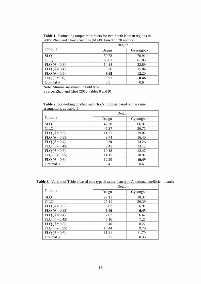
Table 2
At the outset, we attempted to replicate Zhao and Choi’s results using identical assumptions. To
attain greater precision, we used steps of 0.05 for δ. Our findings, which are displayed in Table 2, are
clearly somewhat different from theirs. Having checked our own calculations carefully, it is evident
that errors of an unknown nature must have occurred in Zhao and Choi’s simulations.5 In the case of
Daegu, there is a cut in the optimal δ from 0.5 to 0.4, along with a rise in the corresponding value of
MAPE from 8.7% to 9.2%. By contrast, for Gyeongbuk, the optimal δ is still 0.6, yet MAPE has
risen sharply from 8.5% to 10.5%. The performance of the SLQ and CILQ is somewhat better in both
regions, albeit more so in Daegu than in Gyeongbuk.
A demerit of Zhao and Choi’s approach is their use of a type A national coefficient matrix, which
would tend to overstate the optimal values of δ. The explanation is straightforward: instead of using
the equation ijr = FLQij × aij to estimate the input coefficients, one would be using the equation ijr =
FLQij × (aij + fij), where fij is the national propensity to import from abroad. Minimizing MAPE
would then require a higher δ.
Table 3
Table 3 illustrates the consequences of using a type A rather than type B national coefficient
matrix. The most striking changes compared with Table 2 occur in Gyeongbuk: there is a big fall in
the optimal δ from 0.6 to 0.35, while the corresponding value of MAPE is cut from 10.5% to 6.5%.
For Daegu, the optimal δ also falls, albeit less dramatically, from 0.4 to 0.35, while MAPE is lowered
from 9.2% to 6.5%. It is remarkable how similar the results now are for the two regions. There is a
further improvement in the performance of the SLQ and CILQ, although they are still far less accurate
than the FLQ.
It is evident that Zhao and Choi (2015) have substantially overstated the required values of δ and
understated the FLQ’s accuracy. Also, even though the FLQ is still demonstrably more accurate than
the SLQ and CILQ, the extent of this superiority is less marked than their results initially suggested.
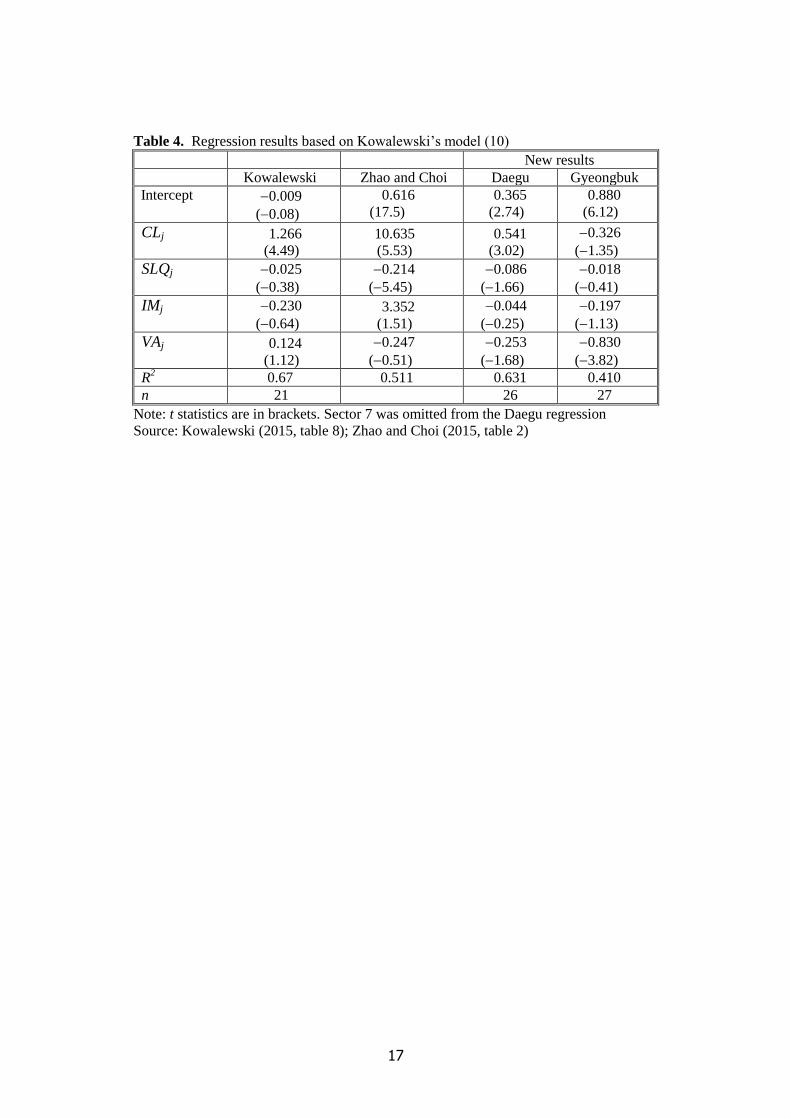
4 The sector-specific approach using the SFLQ
A key part of Zhao and Choi’s study is a test of a new sector-specific FLQ formula, the SFLQ,
devised by Kowalewski (2015). As explained earlier, this method involves using the regression
model (10) to generate sector-specific values of δ for each region. Kowalewski’s results for a German
region are reproduced in Table 4, along with Zhao and Choi’s Korean findings and our own estimates.
For consistency, we computed the SLQj using sectoral employment data.
Table 4
Looking first at Kowalewski’s results, it is striking how one of the regressors, CLj, is highly
statistically significant, whereas the remaining three have low t statistics. The positive estimated
coefficient of CLj is consistent with Kowalewski’s argument that ‘the more an industry is
concentrated in space, the higher the regional propensity to import goods or services of this industry’
(Kowalewski 2015, p. 248). Such industries would require a higher value of δ to adjust for this higher
propensity. As expected, SLQj has a negative estimated coefficient. Kowalewski’s rationale here is
that ‘regional specialization would lead to an increase in intra-regional trade and a decrease in
7
imports’, so that ‘one would expect a higher SLQj to be accompanied by a lower value of δj, which
would additionally (to the FLQ formula) dampen regional imports’ (Kowalewski 2015, p. 248).
However, the t statistic for SLQj is very low, which suggests that this variable may not be relevant.
Likewise, the results for both IMj and VAj cast doubt on their relevance.
Zhao and Choi’s results are puzzling. Kowalewski’s method requires a separate regression for
each region since the values of SLQj would vary across regions. However, the authors report results
for only one regression and offer no explanation as to how it was estimated or to which region it
relates. Moreover, the estimated coefficient of CLj is implausibly large and is markedly out of line
with both Kowalewski’s estimate and our own figures for Daegu and Gyeongbuk. The credibility of
Zhao and Choi’s results is also undermined by the fact that they were derived from a type A national
coefficient matrix.
Turning now to our own regressions, the results for Daegu look sensible on the whole. The R2 is
only a little below that reported by Kowalewski. Moreover, CLj is statistically significant at the 1%
level and its estimated coefficient has the anticipated sign. Although SLQj and VAj are still not
significant at conventional levels, their t ratios are much better than in Kowalewski’s regression. IMj
has a negligible t ratio in both regressions.
Our regression for Gyeongbuk leaves much to be desired in terms of both goodness of fit and the
outcomes for CLj and SLQj. However, a redeeming feature is the highly statistically significant result
for VAj. Kowalewski does not offer a rationale for including this variable but one might argue that a
higher share of value added in total national output would mean a lower share of intermediate inputs
and hence lower imports. If this effect were transmitted to regions, it is possible that a lower δj would
be needed, i.e. β4 < 0 in equation (10).
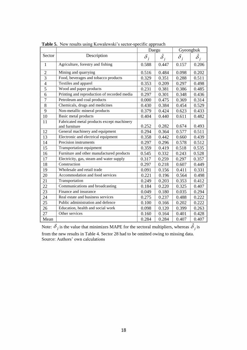
Table 5
Table 5 displays estimates of δj derived from our regressions, along with the ‘optimal’ values that
would minimize MAPE for the type I output multipliers. To compute the optimal δj, we performed
the calculations on a sectoral basis, using steps of 0.025 for δ, and then applied linear interpolation.
To evaluate our estimates, we correlated j with j . The simple correlation coefficient, r, was
0.739 (p = 0.000) for Daegu and 0.640 (p = 0.000) for Gyeongbuk. The fact that both correlations are
highly statistically significant lends support to Kowalewski’s approach, although there is clearly still
much scope for enhanced accuracy. The difference in the size of r reflects the fact that Table 4 shows
a higher R2 for Daegu than for Gyeongbuk.
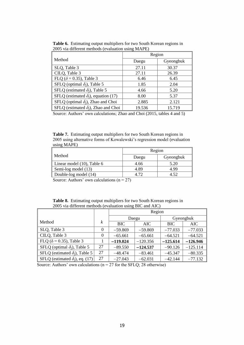
Table 6
The relative performance of the SFLQ in terms of MAPE is examined in Table 6. The table
distinguishes between optimal values and regression-based estimates. Based on the optimal values, a
residual error of about 2% would remain in each region. However, analysts using non-survey
methods would not know the optimal values, so the results illustrate the best outcomes that could be
attained with the SFLQ in a perfect world. More realistically, Table 6 records a MAPE of 4.7% in
Daegu and 5.2% in Gyeongbuk. With δ = 0.35, the potential gains from using the SFLQ rather than
the FLQ would be 1.8 percentage points in Daegu and 1.25 in Gyeongbuk.
In discussing their findings, Zhao and Choi (2015, p. 913) comment that it is ‘undeniable that
SFLQ presents an extraordinary ability to minimize errors produced by regionalization’. However,
this statement is based on a comparison with results derived using optimal values. We would argue
that the only relevant comparison is with regression-based estimates, which would be the only
information potentially available to an analyst using non-survey data. Clearly, with a MAPE of
19.5% for Daegu and 15.7% for Gyeongbuk, Zhao and Choi’s results would not be helpful in that
respect.
The results so far indicate that the SFLQ approach could yield a useful, albeit modest,
enhancement of accuracy relative to the FLQ if used in conjunction with a well-specified regression
8
model. Zhao and Choi (2015, p. 915) suggest that possible ways of refining these regressions could
include (i) introducing new explanatory variables and (ii) using non-linear formulations.
Unfortunately, it is hard to think of new variables for which data would be readily available. As
regards refinement (ii), we considered the following alternative non-linear models:
ln δj = a + b1 CLj + b2 SLQj + b3 IMj + b4 VAj + ej, (13)
ln δj = c + d1 ln CLj + d2 ln SLQj + d3 ln IMj + d4 ln VAj + fj. (14)
Table 7
Table 7 reports a mixed outcome: the linear model (10) is best for Daegu, whereas the double-log
model (14) is best for Gyeongbuk. However, the differences in performance of the three models are
not substantial.
Nevertheless, there is a fundamental problem inherent in using the SFLQ: as noted earlier, analysts
employing non-survey methods would not know the optimal values, so would be unable to fit a
region-specific regression like those shown in Table 4. Furthermore, when we fitted Kowalewski’s
regression model to data for the other South Korean regions, we found that the results were unstable
in terms of goodness of fit, the values of regression coefficients, and which variables were statistically
significant. This instability suggests that it would be inadvisable to attempt to transfer results from
one region to another.
It is evident that the need to use some region-specific data is an obstacle to the application of
Kowalewski’s approach. For this reason, we modified her regression model (10) by imposing the
restriction β2 = 0 and re-expressing the dependent variable as the mean value of δj across all regions.
SLQj was excluded on the basis that it is a region-specific variable.
Fitting the revised model to data for 27 sectors and 16 regions gave the following result:
δj = 0.669 + 0.269 CLj 0.403 IMj 0.628 VAj + ej, (17)
where ej is a residual. IMj is highly statistically significant (t = 3.54; p = 0.002) and so too is VAj (t =
4.57; p = 0.000), whereas CLj is only marginally significant (t = 1.77; p = 0.090). CLj has a positive
coefficient, as anticipated, yet its modest t ratio is rather surprising. Since the role of this variable is
to capture any regional imbalances in employment in sector j, we expected it to be more significant.
The R2 = 0.589 reflects both the omission of relevant explanatory variables and random variation in
the values of δj.
We now need to assess the performance of equation (17). Table 6 shows an evaluation in terms of
MAPE. The results for Daegu are not encouraging: MAPE is 6.5% for the FLQ (with δ = 0.35), yet
8.0% for the SFLQ. By contrast, for Gyeongbuk, MAPE is 6.5% for the FLQ but 5.4% for the SFLQ.
However, when assessing the relative accuracy of the SFLQ and FLQ, we should also consider the
number of parameters, k, to be estimated in each case. For the SFLQ, 27 sector-specific values of δ
are required, so k = 27. By contrast, k = 1 for the FLQ. This aspect can be incorporated into the
analysis via criteria such as the Bayesian information criterion (BIC) or Akaike’s information
criterion (AIC), whereby the number of parameters is penalized to avoid the ‘overfitting’ of models
(Burnham and Anderson 2004).
The BIC is defined here as:
, (15)
where is the number of observations, is the number of parameters and is the variance of the
estimated sectoral multipliers, namely = (1/n) Σj 2)ˆ( jj mm . AIC and BIC differ in one key
respect: for n > 2, AIC imposes a smaller penalty for extra parameters. It is defined here as:
9
(16)
As k rises, with given n, BIC and AIC increasingly diverge, as BIC imposes a rising penalty for extra
parameters. Consequently, using BIC or AIC rather than MAPE or to compare regionalization
methods will generally indicate one involving fewer parameters. In this instance, given , the
optimal value typically will be negative, so we will be looking for the most negative AIC or BIC.
Table 8
Table 8 reveals that, once we consider the number of parameters, and focus on the regression-
based results, the FLQ convincingly outperforms the SFLQ. This outcome suggests that the enhanced
precision gained by capturing the intersectoral dispersion in the values of δ is outweighed by the
statistical uncertainty entailed by having to estimate 27 parameters rather than only one. As expected,
BIC yields more pronounced differences in performance than does AIC.
An interesting question now arises: would it be possible to refine the regression model to the
extent that the SFLQ gave more accurate estimates than the FLQ? For the BIC results in Table 8, the
answer is definitely no. Even with R2 = 1, the best attainable result for Daegu would be BIC =
89.550, which is clearly inferior to the 119.024 for the FLQ with δ = 0.35. The same outcome
would occur in Gyeongbuk. In terms of AIC, we can see that the SFLQ with an ideal regression
would outperform the FLQ in Daegu, albeit not very convincingly, but slightly underperform in
Gyeongbuk. However, building such a regression is obviously unrealistic. In the light of these
results, therefore, we would not recommend using the SFLQ.
5 Extension to all regions
5.1 Results for 16 regions
In this section, we expand our analysis to encompass all 16 South Korean regions, which should help
to identify results that are more generally valid, particularly in terms of finding appropriate values for
δ. Before considering our findings, it may be helpful to examine the key regional characteristics
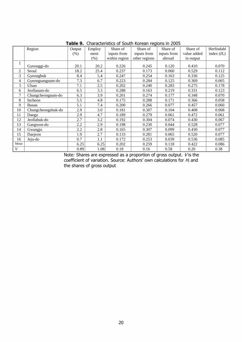
presented in Table 9.
Table 9
Table 9 examines two alternative ways of measuring regional size. Although one can see at a
glance that the output and employment shares are not perfectly matched, there is agreement that
Gyeonggi-do and Seoul are the two biggest regions and that Jeju-do is the smallest. Even so, the
strong correlation (r = 0.921) between the output and employment shares may mask much variability
in productivity at the sectoral level. Consequently, we opted to use the regional share of gross output,
So, as our preferred measure of regional size.
Correlation analysis offers a convenient way of exploring the relationship between So and the other
variables in Table 9. As anticipated by the FLQ approach, there is a positive association between So
and the intraregional share of inputs (r = 0.557; p = 0.025) and a negative one between So and the
share of inputs from other regions (r = 0.508; p = 0.045).
Nevertheless, what is most striking about the data in Table 9 is the marked interregional variation
in the share of foreign inputs in gross output, Sf, which poses some challenges for the FLQ approach.
Ulsan stands out as having an especially high share of inputs from abroad. It is interesting that Sf is
strongly negatively correlated (r = 0.932; p = 0.000) with the share of value added, Sv, yet it is not
significantly correlated (at the 5% level) with any other variable. Sv, in turn, is not significantly
correlated with any other variable.
10
Herfindahl’s index, Hr = 2)/( r
iirii QQ , where
riQ is the output of sector i in region r,
measures the extent to which each region’s output is concentrated in one or more sectors. Ulsan again
stands out as having an unusually high value for Hr. However, apart from Seoul, Gyeongbuk and
Jeollanam-do, the values of Hr are fairly close to the mean. It is worth noting that Hr is significantly
correlated with both the share of inputs from abroad (r = 0.638; p = 0.008) and the share from other
regions (r = 0.567; p = 0.022).
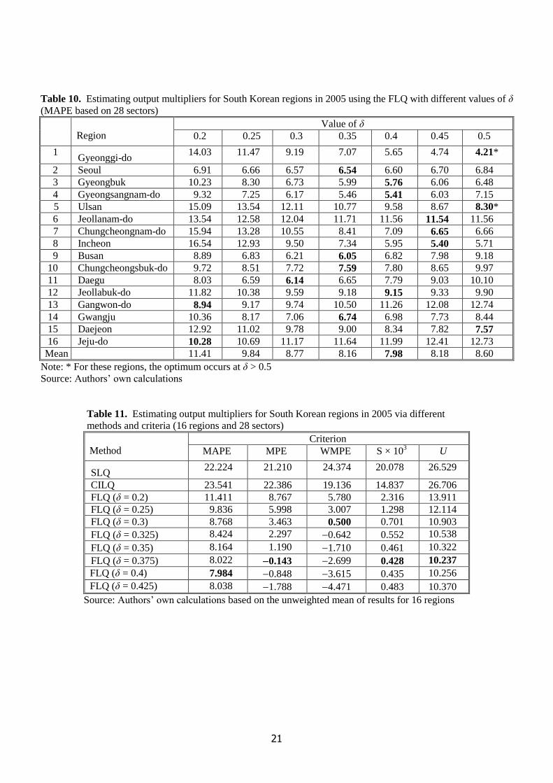
Table 10
The minimum MAPE in each region is identified in bold in Table 10, along with the corresponding
optimal δ.6 It should be noted that these calculations do not take into account possible intersectoral
variation in the values of δ in each region. There is much interregional variation in these optimal
values, yet it is also true that ten of them lie in the range 0.4 ± 0.05, where MAPE is about 8%.
Gangwon-do and Jeju-do are atypical in requiring δ = 0.2, whereas three regions need at least δ = 0.5.7
Looking at the overall pattern of results, there does seem to be some tendency for the optimal δ to rise
with regional size.
5.2 Sensitivity analysis using different criteria
The simulations thus far have been evaluated primarily in terms of MAPE, thereby facilitating
comparisons with the work of Zhao and Choi (2015). Although MAPE has some desirable properties
as a criterion, it does not capture all aspects relevant to the choice of method. It is desirable,
therefore, to employ a range of criteria with different properties. In line with previous research (Flegg
and Tohmo 2013a, 2016; Flegg et al. 2016), the following additional statistics will be employed to
evaluate the estimated multipliers:
MPE = (100/28) Σj jjj m mm /)ˆ( , (18)
WMPE = 100 Σj wj jjj m mm /)ˆ( , (19)
S = 2)}sd( )ˆ{sd( jj mm , (20)
U = 100
j j
j jj
m
mm
2
2)ˆ(. (21)
MPE is the mean percentage error. This statistic has been included since it offers a
convenient way of measuring the amount of bias in a relative sense. It has also been used in
many previous studies. WMAE is the weighted mean percentage error, which takes into
account the relative importance of each sector. wj is the proportion of total regional output
produced in sector j. The role of the squared difference in standard deviations (S) is to assess
how far each method is able to replicate the dispersion of the benchmark distribution of
multipliers. Finally, U is Theil’s well-known inequality index, which has the merit that it
encompasses both bias and variance (Theil et al. 1966, pp. 1543). A demerit of U is,
however, that the use of squared differences has the effect of emphasizing any large positive
or negative errors and thereby skewing the results.
Table 11
Table 11 reveals a high degree of consistency in the results across different criteria. Regardless of
which criterion is used, the SLQ and CILQ yield comparable outcomes and both perform very poorly
11
indeed relative to the FLQ. MPE shows, for example, that the SLQ overstates the sectoral multipliers
by 21.2% on average across the 16 regions, whereas the FLQ with δ = 0.375 exhibits negligible bias.
Furthermore, δ = 0.375 gives MAPE = 8.0%, which is well below the outcomes for the SLQ and
CILQ.
Since MPE, S and U all indicate δ ≈ 0.375, this suggests that there is no conflict between
minimizing bias and variance in this data set. Furthermore, the FLQ with δ = 0.375 gives MAPE =
8.0%, which is well below the figures for the SLQ and CILQ. However, one should note that WMPE
indicates an optimum of δ = 0.3, so δ < 0.375 may be needed for the relatively larger sectors.
The discussion so far has been conducted solely in terms of multipliers, so it is worth considering
briefly whether different findings would emerge from an analysis of input coefficients.8 A selection
of results is presented in Table 12.
Table 12
Tables 11 and 12 reveal a very similar pattern in terms of the approximate optimal values of δ; this
feature is especially noticeable for the WMPE and U criteria. Even so, for a given δ, the estimated
coefficients are clearly much more prone to error than are the corresponding estimated multipliers.
For instance, for δ = 0.375, MAPE is 8.0% for multipliers but 44.9% for coefficients. This well-
known phenomenon arises because the elements in the difference matrix, D = ]ˆ[ ijij rr , are bound to
exhibit far more dispersion than is true for the errors in the column sums of the Leontief inverse
matrix, d´ = ]ˆ[ jj mm ; much offsetting of errors occurs when computing multipliers (Flegg and
Tohmo 2013a, pp. 716717). It is also worth noting that the results in Table 12 confirm the previous
finding for multipliers that the FLQ’s performance far surpasses that of the SLQ and CILQ.
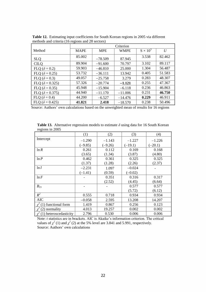
5.3 Choosing values for δ
Although the results presented earlier offer some guidance regarding appropriate values of δ, it would
be helpful if a suitable estimating equation could be developed. With this aim in mind, Flegg and
Tohmo (2013a, p. 713) fitted the following model to survey-based data for twenty Finnish regions in
1995:
ln δ = 1.8379 + 0.33195 ln R + 1.5834 ln P 2.8812 ln I + e, (22)
where R is regional size measured in terms of output and expressed as a percentage; P is the
proportion of each region’s gross output imported from other regions, averaged over all sectors and
divided by the mean for all regions; I is each region’s average use of intermediate inputs (including
inputs from other regions), divided by the corresponding national average; e is a residual.
Observations on ln δ were derived by finding the value of δ that minimized MPE for each Finnish
region. R2 = 0.915 and all three regressors were highly statistically significant. The model
comfortably passed all χ2 diagnostic tests.
Table 13
Table 13 records the results of our re-estimation of Flegg and Tohmo’s model using data for all 16
South Korean regions.9 Observations on ln δ were derived by finding the value of δ that minimized
MAPE for each region.10
Regression (1) has the same specification as equation (22) and the
corresponding estimated elasticities have identical signs. However, in terms of the usual statistical
criteria, this new model is less satisfactory than the Finnish one. We therefore attempted to refine it
by adding a new regressor, ln F, where F is the average proportion of each region’s gross output
imported from abroad, divided by the mean for all regions. As illustrated in Table 9, the share of
foreign imports in gross output varies greatly across regions, so this variable should be relevant.
12
It is evident that ln F adds greatly to the model’s explanatory power and its estimated coefficient
has the anticipated sign. However, the χ2 statistic reveals that the residuals are not normally
distributed. Daejeon was identified as the main source of this problem: its residual is more than two
standard errors from zero. To address this problem, and to prevent this outlier from distorting the
results, a binary variable, B15, was added to the model.11
Regression (3) records the outcome.
The χ2 statistic now shows no discernible skewness and kurtosis in the residuals. The big rise in R
2
reflects the fact that B15 is highly statistically significant. There is also a marked rise in the t ratios for
ln R, ln P and ln F. However, the results strongly suggest that ln I is redundant, so it has been omitted
from regression (4). This regression now has the highest AIC, hence the best fit.12
It also has the best
t ratios and comfortably passes all χ2 diagnostic tests. Although regression (4) differs in several
respects from the Finnish equation (22), these dissimilarities can largely be explained by the
differences between Finland and South Korea in the amount of interregional variation in each
variable.13
Before assessing how well regression (4) can estimate δ for individual regions, it is worth
examining an alternative approach proposed by Bonfiglio (2009), who used simulated data from a
Monte Carlo study to derive the following regression equation:
= 0.994 PROP 2.819 RSRP, (23)
where PROP is the propensity to interregional trade (the proportion of a region’s total intermediate
inputs bought from other regions) and RSRP is the relative size of regional purchases (the ratio of
total regional to total national intermediate inputs). The principal advantage of a Monte Carlo
approach, according to Flegg and Tohmo (2016, p. 33), lies in the generality of the findings, whereas
‘the results derived from a single region may reflect the peculiarities of that region and thus not be
valid in general.’ However, with data for 16 regions, concerns about a lack of generality are less
compelling here, although there remains the possibility that South Korea is a unique case.
Table 14
The first column in Table 14 displays the optimal values of δ, those that minimize MAPE for the
sectoral multipliers, while the second column records the predicted values from regression (4) in
Table 13. There is a very close correspondence between the two sets of values, with r = 0.957 (p =
0.000). This outcome reflects the high R2 of regression (4). By contrast, Bonfiglio’s method gives
very poor estimates of δ and there is a negative, rather than positive, correlation between and δ,
with r = 0.485 (p = 0.057).14
Moreover, 0ˆ for the two largest regions, which contradicts the
theoretical restriction δ ≥ 0. Flegg and Tohmo (2016, p. 33) note that 0ˆ can occur where regions
are relatively large or exhibit below-average propensities to import from other regions or have both
characteristics. Given these problems, we would not recommend the use of Bonfiglio’s method.15
Regarding Flegg and Tohmo’s method, the way in which regression (4) in Table 13 is specified
should make it easier for an analyst to estimate δ. The regression, with B15 = 0, is reproduced below.
ln δ = 1.2263 + 0.1680 ln R + 0.3254 ln P + 0.3170 ln F + e, (24)
An analyst would need to make an informed assumption about how far a region’s propensity to import
from other regions diverged from the mean for all regions in a country, which should be easier than
having to measure this propensity directly. Likewise, an allowance could be made for any assumed
divergence between the regional and national shares of foreign inputs. It would also be easy to carry
out a sensitivity analysis. However, in some cases, it might be more convenient to employ the
following variant of equation (24):
ln δ = 3.0665 + 0.1680 ln R + 0.3254 ln p + 0.3170 ln f + e, (25)
13
where p is each region’s propensity to import from other regions and f is each region’s average use of
foreign intermediate inputs, both measured as a proportion of gross output.
To evaluate regression (4) in terms of sectoral multipliers, again consider Table 14, where the
estimated δ for each region was used to compute sectoral multipliers and hence MAPE. The results
were then averaged over all regions to get MAPE ≈ 7.3%. By contrast, Table 11 reveals that using δ
= 0.375 for all regions would give MAPE ≈ 8.0%, which represents a potential gain of about 0.7
percentage points, on average, from using the region-specific estimates.
6 Conclusion
This paper has employed survey-based data for 16 South Korean regions to refine the application of
the FLQ formula for estimating regional input coefficients. The focus was on the choice of values for
the key unknown parameter δ in this formula.
Several important findings emerged from our statistical analysis. For instance, on average across
the 16 regions, the FLQ with δ = 0.375 gave a mean absolute percentage error (MAPE) of 8.0% for
the type I sectoral output multipliers, compared with 23.5% for the CILQ and 22.2% for the SLQ.
The corresponding mean percentage error was 0.1% for the FLQ, yet 22.4% for the CILQ and 21.2%
for the SLQ. Although it is unsurprising that the CILQ and SLQ should yield overstated multipliers,
the size of this bias is striking. The credibility of these findings is bolstered by the fact that they were
confirmed by Theil’s inequality index, which takes both bias and dispersion into account.
We considered in detail the proposed sector-specific approach of Kowalewski (2015), which aims
to enhance the accuracy of the FLQ by permitting δ to vary across sectors. Her SFLQ approach
employs a regression model to estimate a δ for each sector j in a region. We first fitted this model to
data for two South Korean regions, using as regressors a region-specific variable, SLQj, and three
other variables based on national data. The model worked fairly well in one region but less so in the
other. We then excluded SLQj and reran the regression using data for all 16 regions simultaneously.
The aim here was to produce a more useful general model based on readily available national data.
The general model produced mixed results: for example, relative to the FLQ with δ = 0.35, MAPE
was cut by 1.1 percentage points in one region but raised by 1.5 percentage points in the other. As the
accuracy of the SFLQ depends crucially on the regression model used to estimate the δj, more
research is clearly needed to improve its specification.
However, an even more fundamental concern was raised regarding the SFLQ approach: whereas
the FLQ requires the estimation (or assumption) of a single value of δ, the SFLQ calls for the
estimation of a δ for every sector. This requirement introduces a new element of statistical
uncertainty. Using the AIC and BIC criteria, we found that the extra accuracy gained by permitting δ
to vary across sectors was outweighed by the need to estimate numerous extra parameters.
Consequently, we would argue that a more refined regression model needs to be developed before the
SFLQ can be used in a practical context.
Unlike the SFLQ, Flegg and Tohmo’s regression model for estimating δ uses region-specific data
exclusively. In our reformulation of this model using South Korean data, we included regressors to
capture regional size and the propensities to import from other regions and from abroad. Interregional
variation in the propensity to import from abroad played a key role in determining the size of δ. The
model satisfied a range of statistical criteria and gave relatively accurate estimates of δ. Using this
model to derive region-specific estimates of δ lowered MAPE by some 0.7 percentage points on
average.
It seems fair to conclude that the findings in this paper offer support for the FLQ’s use as a
regionalization technique. Nonetheless, as with all such pure non-survey methods, it can only be
relied upon to give a satisfactory initial set of regional input coefficients. Analysts should always
seek to refine these estimates via informed judgement, using any available superior data, carrying out
surveys of key sectors and so on. Indeed, we would argue that the FLQ is very well suited to building
the non-survey foundations of a hybrid model (Lahr 1993). It is worth noting, finally, that interesting

14
recent work by Hermannsson (2016) and Jahn (2017) has extended the use of the FLQ from an
analysis of single regions to a multi-regional context.
Notes 1. See Klijs et al. (2016) for a comparison of LQ-based methods and Morrissey (2016) for an
interesting application.
2. See Flegg and Tohmo (2013b, p. 239 and note 3).
3. Cf. Flegg and Webber (1997, p. 798), who define λ* in terms of employment. This reflects the
fact that, in most cases, employment has to be used as a proxy for output.
4. See Bonfiglio and Chelli (2008, table 1).
5. We are grateful to Professors Zhao and Choi for letting us examine their data. This enabled us to
verify that we were using the same sectoral classifications, national transactions matrix,
employment data and LQs, yet we were still unable to replicate their findings.
6. The results for Daegu and Gyeongbuk in Tables 3 and 10 differ because we used sectoral output
data for Table 10 but employment data for Table 3. We also used our own calculations of
benchmark multipliers for Table 10 but the Bank of Korea’s figures for Table 3.
7. The optimal δ is approximately 0.534 for Gyeonggi-do, 0.542 for Ulsan and 0.497 for Daejeon.
8. Typically, the ranking of methods is not materially affected by whether one examines multipliers
or input coefficients. See, for example, Flegg and Tohmo (2016).
9. Zhao and Choi (2015, table 2) report the results of estimating, using South Korean data, what
they refer to as ‘Flegg’s model’. However, this regression has an R2 = 0.003 and regional size, R,
is the sole explanatory variable. How this result was obtained is not explained. By contrast,
when we regressed ln δ on ln R alone, R2 = 0.394.
10. To estimate a value yielding the minimum MAPE in each region, we varied δ in steps of 0.0001.
11. B15 = 1 for Daejeon and zero otherwise. As the second smallest region, Daejeon is atypical in the
sense that it requires an unusually high value of δ ≈ 0.5. Without B15, = 0.306 for this region.
12. AIC = ln L (k + 1), where ln L is the maximized log-likelihood of the regression and k is the
number of regressors. Compared with the more conventional 2R , AIC takes more account of k.
13. Although we tried to refine the regressions by adding ln H, where H is Herfindahl’s index of
concentration, ln H always had a negligible t ratio. The likely explanation is that H varies little
across regions (see Table 9). Flegg and Tohmo (2013a, note 26) report a similar outcome for
Finland.
14. We used output shares (see Table 9) to proxy RSRP. For PROP, we used the ratio A/B, where A
represents imports from other South Korean regions, and B = A + intraregional intermediate
inputs + imports from abroad.
15. For a more detailed evaluation of Bonfiglio’s method, see Flegg and Tohmo (2016, pp. 3334).
Acknowledgements Helpful suggestions were received from Malte Jahn and Jeroen Klijs.
References Bonfiglio A (2009) On the parameterization of techniques for representing regional economic
structures. Economic Systems Research 21: 115127
Bonfiglio A, Chelli F (2008) Assessing the behaviour of non-survey methods for constructing
regional inputoutput tables through a Monte Carlo simulation. Economic Systems Research 20:
243258
Burnham KP, Anderson DR (2004) Multimodel inference: understanding AIC and BIC in model
selection. Sociological Methods and Research 33: 261304
Flegg AT, Tohmo T (2013a) Regional inputoutput tables and the FLQ formula: a case study of
Finland. Regional Studies 47: 703721
Flegg AT, Tohmo T (2013b) A comment on Tobias Kronenberg’s ‘Construction of regional
15
inputoutput tables using nonsurvey methods: the role of cross-hauling’. International Regional
Science Review 36: 235257
Flegg AT, Tohmo T (2016) Estimating regional input coefficients and multipliers: the use of FLQ is
not a gamble. Regional Studies 50: 310325
Flegg AT, Huang Y, Tohmo T (2015) Using CHARM to adjust for cross-hauling: the case of the
province of Hubei, China. Economic Systems Research 27: 391413
Flegg AT, Mastronardi LJ, Romero CA (2016) Evaluating the FLQ and AFLQ formulae for
estimating regional input coefficients: empirical evidence for the province of Córdoba, Argentina.
Economic Systems Research 28: 2137
Flegg AT, Webber CD (1997) On the appropriate use of location quotients in generating regional
inputoutput tables: reply. Regional Studies 31: 795805
Flegg AT, Webber CD (2000) Regional size, regional specialization and the FLQ formula. Regional
Studies 34: 563569
Flegg AT, Webber CD, Elliott MV (1995) On the appropriate use of location quotients in generating
regional inputoutput tables. Regional Studies 29: 547561
Hermannsson K (2016) Beyond Intermediates: the role of consumption and commuting in the
construction of local inputoutput tables. Spatial Economic Analysis 11: 315339
Jahn M (2017) Extending the FLQ formula: a location quotient-based interregional inputoutput
framework. Regional Studies 51: 15181529
Klijs J, Peerlings J, Steijaert T, Heijman W (2016) Regionalising inputoutput tables: comparison of
four location quotient methods. In: Matia A, Nijkamp P, Romão J (eds) Impact Assessment in
Tourism Economics, part I, 4365. Springer International, Switzerland
Kowalewski J (2015) Regionalization of national inputoutput tables: empirical evidence on the use
of the FLQ formula. Regional Studies 49: 240250
Kronenberg T (2009) Construction of regional inputoutput tables using nonsurvey methods: the role
of cross-hauling. International Regional Science Review 32: 4064
Kronenberg T (2012) Regional inputoutput models and the treatment of imports in the European
system of accounts. Jahrbuch für Regionalwissenschaft (Review of Regional Research) 32:
175191
Lahr ML (1993). A review of the literature supporting the hybrid approach to constructing regional
inputoutput models. Economic Systems Research 5: 277293
Lamonica GR, Chelli FM (2017) The performance of non-survey techniques for constructing sub-
territorial input-output tables. Papers in Regional Science, first published 2 June 2017, DOI:
10.1111/pirs.12297
Morrissey K (2016) A location quotient approach to producing regional production multipliers for the
Irish economy. Papers in Regional Science 95: 491506
Theil H, Beerens GAC, DeLeeuw CG, Tilanus CB (1966) Applied Economic Forecasting. Elsevier,
New York.
Többen J, Kronenberg T (2015) Construction of multi-regional inputoutput tables using the
CHARM method. Economic Systems Research 27: 487507
Tohmo T (2004) New developments in the use of location quotients to estimate regional inputoutput
coefficients and multipliers. Regional Studies 38: 4354
Zhao X, Choi S-G (2015) On the regionalization of inputoutput tables with an industry-specific
location quotient. Annals of Regional Science 54: 901926
16
Table 1. Estimating output multipliers for two South Korean regions in
2005: Zhao and Choi’s findings (MAPE based on 28 sectors)
Formula
Region
Daegu Gyeongbuk
SLQ 50.78 70.91
CILQ 63.01 61.85
FLQ (δ = 0.3) 14.14 22.89
FLQ (δ = 0.4) 9.36 15.84
FLQ (δ = 0.5) 8.65 12.20
FLQ (δ = 0.6) 9.91 8.48
Optimal δ 0.5 0.6
Note: Minima are shown in bold type
Source: Zhao and Choi (2015, tables 8 and 9)
Table 2. Reworking of Zhao and Choi’s findings based on the same
assumptions as Table 1
Formula
Region
Daegu Gyeongbuk
SLQ 42.70 66.97
CILQ 45.37 56.71
FLQ (δ = 0.3) 11.71 19.07
FLQ (δ = 0.35) 9.74 16.40
FLQ (δ = 0.4) 9.20 14.26
FLQ (δ = 0.45) 9.45 13.12
FLQ (δ = 0.5) 10.18 12.47
FLQ (δ = 0.55) 11.15 10.91
FLQ (δ = 0.6) 12.20 10.49
Optimal δ 0.4 0.6
Table 3. Variant of Table 2 based on a type B rather than type A national coefficient matrix
Formula
Region
Daegu Gyeongbuk
SLQ 27.11 30.37
CILQ 27.11 26.39
FLQ (δ = 0.3) 6.82 6.91
FLQ (δ = 0.35) 6.46 6.45
FLQ (δ = 0.4) 7.07 6.62
FLQ (δ = 0.45) 8.16 7.21
FLQ (δ = 0.5) 9.40 8.22
FLQ (δ = 0.55) 10.44 9.79
FLQ (δ = 0.6) 11.41 11.79
Optimal δ 0.35 0.35
17
Table 4. Regression results based on Kowalewski’s model (10)
New results
Kowalewski Zhao and Choi Daegu Gyeongbuk
Intercept 0.009
(0.08)
0.616
(17.5)
0.365
(2.74)
0.880
(6.12)
CLj 1.266
(4.49)
10.635
(5.53)
0.541
(3.02)
0.326
(1.35)
SLQj 0.025
(0.38)
0.214
(5.45)
0.086
(1.66)
0.018
(0.41)
IMj 0.230
(0.64)
3.352
(1.51)
0.044
(0.25)
0.197
(1.13)
VAj 0.124
(1.12)
0.247
(0.51)
0.253
(1.68)
0.830
(3.82)
R2
0.67 0.511 0.631 0.410
n 21 26 27
Note: t statistics are in brackets. Sector 7 was omitted from the Daegu regression
Source: Kowalewski (2015, table 8); Zhao and Choi (2015, table 2)
18
Table 5. New results using Kowalewski’s sector-specific approach
Daegu Gyeongbuk
Sector Description j j j j
1 Agriculture, forestry and fishing 0.588 0.447 0.157 0.206
2 Mining and quarrying 0.516 0.484 0.098 0.202
3 Food, beverages and tobacco products 0.329 0.351 0.288 0.511
4 Textiles and apparel 0.353 0.209 0.297 0.498
5 Wood and paper products 0.231 0.381 0.386 0.485
6 Printing and reproduction of recorded media 0.297 0.301 0.348 0.436
7 Petroleum and coal products 0.000 0.475 0.369 0.314
8 Chemicals, drugs and medicines 0.430 0.384 0.454 0.529
9 Non-metallic mineral products 0.379 0.424 0.623 0.433
10 Basic metal products 0.404 0.440 0.611 0.482
11 Fabricated metal products except machinery
and furniture 0.252 0.282 0.674 0.493
12 General machinery and equipment 0.294 0.364 0.577 0.511
13 Electronic and electrical equipment 0.358 0.442 0.660 0.439
14 Precision instruments 0.297 0.296 0.578 0.512
15 Transportation equipment 0.359 0.419 0.518 0.535
16 Furniture and other manufactured products 0.545 0.332 0.243 0.528
17 Electricity, gas, steam and water supply 0.317 0.259 0.297 0.357
18 Construction 0.297 0.218 0.607 0.449
19 Wholesale and retail trade 0.091 0.156 0.411 0.331
20 Accommodation and food services 0.221 0.196 0.564 0.498
21 Transportation 0.249 0.203 0.353 0.412
22 Communications and broadcasting 0.184 0.220 0.325 0.407
23 Finance and insurance 0.049 0.180 0.035 0.294
24 Real estate and business services 0.275 0.237 0.488 0.222
25 Public administration and defence 0.100 0.166 0.202 0.222
26 Education, health and social work 0.098 0.120 0.399 0.263
27 Other services 0.160 0.164 0.401 0.428
Mean 0.284 0.284 0.407 0.407
Note: j is the value that minimizes MAPE for the sectoral multipliers, whereas j is
from the new results in Table 4. Sector 28 had to be omitted owing to missing data.
Source: Authors’ own calculations
19
Table 6. Estimating output multipliers for two South Korean regions in
2005 via different methods (evaluation using MAPE)
Method
Region
Daegu Gyeongbuk
SLQ, Table 3 27.11 30.37
CILQ, Table 3 27.11 26.39
FLQ (δ = 0.35), Table 3 6.46 6.45
SFLQ (optimal δj), Table 5 1.85 2.04
SFLQ (estimated δj), Table 5 4.66 5.20
SFLQ (estimated δj), equation (17) 8.00 5.37
SFLQ (optimal δj), Zhao and Choi 2.885 2.121
SFLQ (estimated δj), Zhao and Choi 19.536 15.719
Source: Authors’ own calculations; Zhao and Choi (2015, tables 4 and 5)
Table 7. Estimating output multipliers for two South Korean regions in
2005 using alternative forms of Kowalewski’s regression model (evaluation
using MAPE)
Method
Region
Daegu Gyeongbuk
Linear model (10), Table 6 4.66 5.20
Semi-log model (13) 4.89 4.99
Double-log model (14) 4.72 4.52
Source: Authors’ own calculations (n = 27)
Table 8. Estimating output multipliers for two South Korean regions in
2005 via different methods (evaluation using BIC and AIC)
Method
k
Region
Daegu Gyeongbuk
BIC AIC BIC AIC
SLQ, Table 3 0 59.869 59.869 77.033 77.033
CILQ, Table 3 0 65.661 65.661 64.521 64.521
FLQ (δ = 0.35), Table 3 1 119.024 120.356 125.614 126.946
SFLQ (optimal δj), Table 5 27 89.550 124.537 90.126 125.114
SFLQ (estimated δj), Table 5 27 48.474 83.461 45.347 80.335
SFLQ (estimated δj), eq. (17) 27 27.043 62.031 42.144 77.132
Source: Authors’ own calculations (n = 27 for the SFLQ; 28 otherwise)
20
Table 9. Characteristics of South Korean regions in 2005 Region Output
(%)
Employ
ment
(%)
Share of
inputs from
within region
Share of
inputs from
other regions
Share of
inputs from
abroad
Share of
value added
in output
Herfindahl
index (Hr)
1 Gyeonggi-do 20.1 20.2 0.226 0.245 0.120 0.410 0.070
2 Seoul 18.2 25.4 0.237 0.173 0.060 0.529 0.112
3 Gyeongbuk 8.4 5.4 0.247 0.254 0.163 0.336 0.125
4 Gyeongsangnam-do 7.3 6.7 0.223 0.284 0.125 0.369 0.065
5 Ulsan 7.1 2.5 0.202 0.240 0.283 0.275 0.178
6 Jeollanam-do 6.5 3.3 0.288 0.163 0.219 0.331 0.123
7 Chungcheongnam-do 6.3 3.9 0.201 0.274 0.177 0.348 0.070
8 Incheon 5.5 4.8 0.175 0.288 0.171 0.366 0.058
9 Busan 5.1 7.4 0.200 0.266 0.077 0.457 0.060
10 Chungcheongsbuk-do 2.9 3.0 0.181 0.307 0.104 0.408 0.068
11 Daegu 2.9 4.7 0.189 0.279 0.061 0.472 0.061
12 Jeollabuk-do 2.7 3.2 0.192 0.304 0.074 0.430 0.067
13 Gangwon-do 2.2 2.9 0.198 0.230 0.044 0.528 0.077
14 Gwangju 2.2 2.8 0.165 0.307 0.099 0.430 0.077
15 Daejeon 1.9 2.7 0.133 0.281 0.065 0.520 0.077
16 Jeju-do 0.7 1.1 0.172 0.253 0.039 0.536 0.085 Mean 6.25 6.25 0.202 0.259 0.118 0.422 0.086
V 0.89 1.08 0.18 0.16 0.58 0.20 0.38
Note: Shares are expressed as a proportion of gross output. V is the coefficient of variation. Source: Authors’ own calculations for Hr and the shares of gross output
21
Table 10. Estimating output multipliers for South Korean regions in 2005 using the FLQ with different values of δ
(MAPE based on 28 sectors)
Region
Value of δ
0.2 0.25 0.3 0.35 0.4 0.45 0.5
1 Gyeonggi-do
14.03 11.47 9.19 7.07 5.65 4.74 4.21*
2 Seoul 6.91 6.66 6.57 6.54 6.60 6.70 6.84
3 Gyeongbuk 10.23 8.30 6.73 5.99 5.76 6.06 6.48
4 Gyeongsangnam-do 9.32 7.25 6.17 5.46 5.41 6.03 7.15
5 Ulsan 15.09 13.54 12.11 10.77 9.58 8.67 8.30*
6 Jeollanam-do 13.54 12.58 12.04 11.71 11.56 11.54 11.56
7 Chungcheongnam-do 15.94 13.28 10.55 8.41 7.09 6.65 6.66
8 Incheon 16.54 12.93 9.50 7.34 5.95 5.40 5.71
9 Busan 8.89 6.83 6.21 6.05 6.82 7.98 9.18
10 Chungcheongsbuk-do 9.72 8.51 7.72 7.59 7.80 8.65 9.97
11 Daegu 8.03 6.59 6.14 6.65 7.79 9.03 10.10
12 Jeollabuk-do 11.82 10.38 9.59 9.18 9.15 9.33 9.90
13 Gangwon-do 8.94 9.17 9.74 10.50 11.26 12.08 12.74
14 Gwangju 10.36 8.17 7.06 6.74 6.98 7.73 8.44
15 Daejeon 12.92 11.02 9.78 9.00 8.34 7.82 7.57
16 Jeju-do 10.28 10.69 11.17 11.64 11.99 12.41 12.73
Mean 11.41 9.84 8.77 8.16 7.98 8.18 8.60
Note: * For these regions, the optimum occurs at δ > 0.5
Source: Authors’ own calculations
Table 11. Estimating output multipliers for South Korean regions in 2005 via different
methods and criteria (16 regions and 28 sectors)
Method
Criterion
MAPE MPE WMPE S × 103
U
SLQ 22.224 21.210 24.374 20.078 26.529
CILQ 23.541 22.386 19.136 14.837 26.706
FLQ (δ = 0.2) 11.411 8.767 5.780 2.316 13.911
FLQ (δ = 0.25) 9.836 5.998 3.007 1.298 12.114
FLQ (δ = 0.3) 8.768 3.463 0.500 0.701 10.903
FLQ (δ = 0.325) 8.424 2.297 0.642 0.552 10.538
FLQ (δ = 0.35) 8.164 1.190 1.710 0.461 10.322
FLQ (δ = 0.375) 8.022 0.143 2.699 0.428 10.237
FLQ (δ = 0.4) 7.984 0.848 3.615 0.435 10.256
FLQ (δ = 0.425) 8.038 1.788 4.471 0.483 10.370
Source: Authors’ own calculations based on the unweighted mean of results for 16 regions
22
Table 12. Estimating input coefficients for South Korean regions in 2005 via different
methods and criteria (16 regions and 28 sectors)
Method
Criterion
MAPE MPE WMPE S × 103
U
SLQ 85.002
78.509 87.945 3.538 82.462
CILQ 89.904 91.600 70.797 3.102 89.117
FLQ (δ = 0.2) 59.903 46.810 25.000 1.304 56.487
FLQ (δ = 0.25) 53.732 36.111 13.942 0.405 51.583
FLQ (δ = 0.3) 49.057 25.758 3.279 0.283 48.307
FLQ (δ = 0.325) 57.326 20.774 1.121 0.255 47.367
FLQ (δ = 0.35) 45.948 15.904 6.118 0.236 46.863
FLQ (δ = 0.375) 44.940 11.170 11.006 0.231 46.750
FLQ (δ = 0.4) 44.200 6.527 14.476 0.229 46.911
FLQ (δ = 0.425) 41.821 2.418 18.570 0.238 50.496
Source: Authors’ own calculations based on the unweighted mean of results for 16 regions
Table 13. Alternative regression models to estimate δ using data for 16 South Korean
regions in 2005
(1) (2) (3) (4)
Intercept 1.290
(9.85)
1.143
(9.26)
1.227
(19.1)
1.226
(20.1)
ln R 0.261
(3.65)
0.112
(1.34)
0.169
(3.87)
0.168
(4.80)
ln P 0.462
(1.37)
0.361
(1.28)
0.325
(2.26)
0.325
(2.37)
ln I 2.231
(1.41)
1.097
(0.59)
0.024
(0.02)
-
ln F -
0.351
(2.52)
0.316
(4.45)
0.317
(6.64)
B15 -
-
0.577
(5.72)
0.577
(6.12)
R2
0.555 0.718 0.934 0.934
AIC 0.058 2.595 13.208 14.207
χ2 (1) functional form 1.419 0.867 0.256 0.123
χ2 (2) normality 4.013 19.257 0.002 0.002
χ2 (1) heteroscedasticity 2.796 0.530 0.006 0.006
Note: t statistics are in brackets. AIC is Akaike’s information criterion. The critical
values of χ2 (1) and χ
2 (2) at the 5% level are 3.841 and 5.991, respectively.
Source: Authors’ own calculations
23
Table 14. Alternative ways of estimating δ for 16 South Korean regions in
2005
Minimum
MAPE
Table 13,
regression (4)
Bonfiglio’s
method
Gyeonggi-do 0.534 0.481 0.156
Seoul 0.337 0.336 0.147
Gyeongbuk 0.401 0.469 0.142
Gyeongsangnam-do 0.389 0.433 0.239
Ulsan 0.542 0.543 0.129
Jeollanam-do 0.441 0.434 0.059
Chungcheongnam-do 0.470 0.472 0.240
Incheon 0.438 0.463 0.297
Busan 0.344 0.339 0.344
Chungcheongsbuk-do 0.347 0.360 0.434
Daegu 0.297 0.289 0.444
Jeollabuk-do 0.370 0.316 0.454
Gangwon-do 0.212 0.234 0.423
Gwangju 0.340 0.336 0.474
Daejeon 0.497 0.497 0.528
Jeju-do 0.196 0.191 0.522
Mean 0.385 0.387 0.277
MAPE (multipliers) 7.226 7.334
Source: Authors’ own calculations
24
Recent UWE Economics Papers See http://www1.uwe.ac.uk/bl/research/bristoleconomicanalysis for a full list.
2017
1705 The regionalization of national inputoutput tables: a study of South Korean regions
Anthony T. Flegg and Timo Tohmo
1704 The impact of quantitative easing on aggregate mutual fund flows in the UK
Iris Biefang-Frisancho Mariscal
1703 Where are the female CFOs?
Gail Webber, Don J Webber, Dominic Page and Tim Hinks
1702 Mental health and employment transitions: a slippery slope Don J Webber, Dominic Page and Michail Veliziotis
1701 SMEs access to formal finance in post-communist economies: do institutional structure and
political connectedness matter?
Kobil Ruziev and Don J Webber
2016
1611 Curriculum reform in UK economics: a critique
Andrew Mearman, Sebastian Berger and Danielle Guizzo
1610 Can indeterminacy and self-fulfilling expectations help explain international business cycles?
Stephen McKnight and Laura Povoledo
1609 Pricing behaviour and the role of trade openness in the transmission of monetary shocks
Laura Povoledo
1608 Measuring compliance with minimum wages
Felix Ritchie, Michail Veliziotis, Hilary Drew and Damian Whittard
1607 Can a change in attitudes improve effective access to administrative data for research?
Felix Ritchie
1606 Application of ethical concerns for the natural environment into business design: a novel
business model framework Peter Bradley, Glenn Parry and Nicholas O’Regan
1605 Refining the application of the FLQ Formula for estimating regional input coefficients:
an empirical study for South Korean regions
Anthony T. Flegg and Timo Tohmo
1604 Higher education in Uzbekistan: reforms and the changing landscape since independence
Kobil Ruziev and Davron Rustamov
1603 Circular econmoy
Peter Bradley
1602 Do shadow banks create money? ‘Financialisation’ and the monetary circuit
Jo Michell
1601 Five Safes: designing data access for research
Tanvi Desai, Felix Ritchie and Richard Welpton
25
2015
1509 Debt cycles, instability and fiscal rules: a Godley-Minsky model
Yannis Dafermos
1508 Evaluating the FLQ and AFLQ formulae for estimating regional input coefficients: empirical
evidence for the province of Córdoba, Argentina
Anthony T. Flegg, Leonardo J. Mastronardi and Carlos A. Romero
1507 Effects of preferential trade agreements in the presence of zero trade flows: the cases of China
and India Rahul Sen, Sadhana Srivastava and Don J Webber
1506 Using CHARM to adjust for cross-hauling: the case of the Province of Hubei, China
Anthony T. Flegg, Yongming Huang and Timo Tohmo
1505 University entrepreneurship education experiences: enhancing the entrepreneurial ecosystems in
a UK city-region Fumi Kitagawa, Don J. Webber, Anthony Plumridge
and Susan Robertson
1504 Can indeterminacy and self-fulfilling expectations help explain international business cycles?
Stephen McKnight and Laura Povoledo
1503 User-focused threat identification for anonymised microdata
Hans-Peter Hafner, Felix Ritchie and Rainer Lenz
1502 Reflections on the one-minute paper
Damian Whittard
1501 Principles- versus rules-based output statistical disclosure control in remote access
environments
Felix Ritchie and Mark Elliot
2014
1413 Addressing the human factor in data access: incentive compatibility, legitimacy and cost-
effectiveness in public data resources
Felix Ritchie and Richard Welpton
1412 Resistance to change in government: risk, inertia and incentives
Felix Ritchie
1411 Emigration, remittances and corruption experience of those staying behind
Artjoms Ivlevs and Roswitha M. King
1410 Operationalising ‘safe statistics’: the case of linear regression
Felix Ritchie
1409 Is temporary employment a cause or consequence of poor mental health?
Chris Dawson, Michail Veliziotis, Gail Pacheco and Don J Webber
1408 Regional productivity in a multi-speed Europe
Don J. Webber, Min Hua Jen and Eoin O’Leary
1407 Assimilation of the migrant work ethic
Chris Dawson, Michail Veliziotis, Benjamin Hopkins