Embed Size (px)
Citation preview
UNIVERSITÉ CHARLES DE GAULLE - LILLE III
T H È S Eprésentée en vue de l’obtention du grade de
Docteur Ès-Sciences
Discipline : Mathématiques Appliquées aux Sciences
Économiques
présentée par
Yacouba BOUBACAR MAINASSARA
sous le titre
Estimation, validation et identificationdes modèles ARMA faibles multivariés
Composition du Jury
Directeurs de thèse M. Christian FRANCQ Professeur Université Lille 3M. Jean-Michel ZAKOÏAN Professeur Université Lille 3.
Rapporteurs M. Sébastien LAURENT Professeur Université de MaastrichtMme Anne PHILIPPE Professeure Université de Nantes.
Présidente Mme Laurence BROZE Professeure Université Lille 3.Examinateurs M. Michel CARBON Professeur Université Rennes 2.
M. Cristian PREDA Professeur Polytech’Lille.
Remerciements
Tout d’abord je tiens à remercier chaleureusement Messieurs les Professeurs Chris-tian Francq et Jean-Michel Zakoïan d’avoir accepté d’encadrer mon travail de re-cherche avec compétence et enthousiasme. Leurs qualités scientifiques et humaines,leurs suivis attentifs à tous les stades d’élaboration de cette thèse, leurs disponibilitésà chaque fois que j’en avais eu recours, leurs soutiens et surtout leurs conseils très pré-cieux qu’ils ont eu à me prodiguer m’ont permis de mener à bien cette thèse. Je tiensaussi à leurs exprimer ma profonde gratitude.
Je tiens à remercier Monsieur le Professeur Sébastien Laurent et Madame la Pro-fesseure Anne Philippe de l’honneur qu’ils me font d’avoir accepté d’être les rappor-teurs de cette thèse et pour l’intérêt qu’ils ont porté à mon travail. Je remercie égalementMessieurs les Professeurs Michel Carbon et Cristian Preda d’avoir accepté de siégerà ce jury.
Je tiens tout particulièrement à remercier chaleureusement Madame la ProfesseureLaurence Broze d’avoir accepté d’être la présidente du jury de soutenance et pour toutle soutien qu’elle nous (mon épouse et moi) a apporté depuis mon master 2.
Un grand merci également à tous les membres du laboratoire EQUIPPE-GREMARSqui m’ont permis d’effectuer cette thèse dans une ambiance vraiment sereine et pourleur accueil très chaleureux. Je remercie vivement Madame Christiane Francq pour salecture très attentive de la partie en français de cette thèse. Je voudrais aussi adresserun grand merci à mes parents, à toute ma famille et à mes amis qui m’ont toujourssoutenu moralement et matériellement pour poursuivre mes études jusqu’à ce niveau.
Je dédie ce travail à mon père décédé en juillet 2008, ma mère, mon fils et toute mafamille.
Enfin, je voudrais dire merci à tous ceux, famille ou amis , qui m’entourent et àl’ensemble des personnes présentes à cette soutenance.
Résumé
Dans cette thèse nous élargissons le champ d’application des modèles ARMA (Auto-Regressive Moving-Average) vectoriels en considérant des termes d’erreur non corrélésmais qui peuvent contenir des dépendances non linéaires. Ces modèles sont appelés desARMA faibles vectoriels et permettent de traiter des processus qui peuvent avoir desdynamiques non linéaires très générales. Par opposition, nous appelons ARMA fortsles modèles utilisés habituellement dans la littérature dans lesquels le terme d’erreurest supposé être un bruit iid. Les modèles ARMA faibles étant en particulier densesdans l’ensemble des processus stationnaires réguliers, ils sont bien plus généraux queles modèles ARMA forts. Le problème qui nous préoccupera sera l’analyse statistiquedes modèles ARMA faibles vectoriels. Plus précisément, nous étudions les problèmesd’estimation et de validation. Dans un premier temps, nous étudions les propriétésasymptotiques de l’estimateur du quasi-maximum de vraisemblance et de l’estimateurdes moindres carrés. La matrice de variance asymptotique de ces estimateurs est dela forme "sandwich" Ω := J−1IJ−1, et peut être très différente de la variance asymp-totique Ω := 2J−1 obtenue dans le cas fort. Ensuite, nous accordons une attentionparticulière aux problèmes de validation. Dans un premier temps, en proposant desversions modifiées des tests de Wald, du multiplicateur de Lagrange et du rapport devraisemblance pour tester des restrictions linéaires sur les paramètres de modèles ARMAfaibles vectoriels. En second, nous nous intéressons aux tests fondés sur les résidus, quiont pour objet de vérifier que les résidus des modèles estimés sont bien des estimationsde bruits blancs. Plus particulièrement, nous nous intéressons aux tests portmanteau,aussi appelés tests d’autocorrélation. Nous montrons que la distribution asymptotiquedes autocorrelations résiduelles est normalement distribuée avec une matrice de cova-riance différente du cas fort (c’est-à-dire sous les hypothèses iid sur le bruit). Nous endéduisons le comportement asymptotique des statistiques portmanteau. Dans le cadrestandard d’un ARMA fort, il est connu que la distribution asymptotique des testsportmanteau est correctement approximée par un chi-deux. Dans le cas général, nousmontrons que cette distribution asymptotique est celle d’une somme pondérée de chi-deux. Cette distribution peut être très différente de l’approximation chi-deux usuelle ducas fort. Nous proposons donc des tests portmanteau modifiés pour tester l’adéquationde modèles ARMA faibles vectoriels. Enfin, nous nous sommes intéressés aux choix desmodèles ARMA faibles vectoriels fondé sur la minimisation d’un critère d’information,
iii
notamment celui introduit par Akaike (AIC). Avec ce critère, on tente de donner uneapproximation de la distance (souvent appelée information de Kullback-Leibler) entrela vraie loi des observations (inconnue) et la loi du modèle estimé. Nous verrons que lecritère corrigé (AICc) dans le cadre des modèles ARMA faibles vectoriels peut, là aussi,être très différent du cas fort.
Mots-clés : AIC, autocorrelations résiduelles, estimateur HAC, estimateur spectral, infor-
mation de Kullback-Leibler, modèles VARMA faibles, forme échelon, processus non linéaire,
QMLE/LSE, représentation structurelle des modèles VARMA, test du Multiplicateur de La-
grange, tests portmanteau de Ljung-Box et Box-Pierce, test du rapport de vraisemblance, test
de Wald.
Abstract
The goal of this thesis is to study the vector autoregressive moving-average(V)ARMA models with uncorrelated but non-independent error terms. These modelsare called weak VARMA by opposition to the standard VARMA models, also calledstrong VARMA models, in which the error terms are supposed to be iid. We relax thestandard independence assumption, and even the martingale difference assumption, onthe error term in order to be able to cover VARMA representations of general nonli-near models. The problems that are considered here concern the statistical analysis.More precisely, we concentrate on the estimation and validation steps. We study theasymptotic properties of the quasi-maximum likelihood (QMLE) and/or least squaresestimators (LSE) of weak VARMA models. Conditions are given for the consistencyand asymptotic normality of the QMLE/LSE. A particular attention is given to theestimation of the asymptotic variance matrix, which may be very different from thatobtained in the standard framework. After identification and estimation of the vec-tor autoregressive moving-average processes, the next important step in the VARMAmodeling is the validation stage. The validity of the different steps of the traditionalmethodology of Box and Jenkins, identification, estimation and validation, depends onthe noise properties. Several validation methods are studied. This validation stage is notonly based on portmanteau tests, but also on the examination of the autocorrelationfunction of the residuals and on tests of linear restrictions on the parameters. Modifiedversions of the Wald, Lagrange Multiplier and Likelihood Ratio tests are proposed fortesting linear restrictions on the parameters. We studied the joint distribution of theQMLE/LSE and of the noise empirical autocovariances. We then derive the asympto-tic distribution of residual empirical autocovariances and autocorrelations under weakassumptions on the noise. We deduce the asymptotic distribution of the Ljung-Box (orBox-Pierce) portmanteau statistics for VARMA models with nonindependent innova-tions. In the standard framework (i.e. under the assumption of an iid noise), it is shownthat the asymptotic distribution of the portmanteau tests is that of a weighted sum ofindependent chi-squared random variables. The asymptotic distribution can be quitedifferent when the independence assumption is relaxed. Consequently, the usual chi-squared distribution does not provide an adequate approximation to the distributionof the Box-Pierce goodness-of fit portmanteau test. Hence we propose a method to ad-just the critical values of the portmanteau tests. Finally, we considered the problem of
v
orders selection of weak VARMA models by means of information criteria. We proposea modified Akaike information criterion (AIC).
Keywords : AIC, Box-Pierce and Ljung-Box portmanteau tests, Discrepancy, Echelon form,
Goodness-of-fit test, Kullback-Leibler information, Lagrange Multiplier test, Likelihood Ratio
test, Nonlinear processes, Order selection, QMLE/LSE, Residual autocorrelation, Structural
representation, Weak VARMA models, Wald test.
Table des matières
Résumé ii
Abstract iv
Table des matières viii
Liste des tableaux x
Table des figures xi
1 Introduction 1
1.0.1 Concepts de base et contexte bibliographique . . . . . . . . . . 11.0.2 Représentations VARMA faibles de processus non linéaires . . . 4
1.1 Résultats du chapitre 2 . . . . . . . . . . . . . . . . . . . . . . . . . . . 101.1.1 Estimation des paramètres . . . . . . . . . . . . . . . . . . . . . 111.1.2 Estimation de la matrice de variance asymptotique . . . . . . . 151.1.3 Tests sur les coefficients du modèle . . . . . . . . . . . . . . . . 17
1.2 Résultats du chapitre 3 . . . . . . . . . . . . . . . . . . . . . . . . . . . 211.2.1 Notations et paramétrisation des coefficients du modèle VARMA 221.2.2 Expression des dérivées des résidus du modèle VARMA . . . . . 231.2.3 Expressions explicites des matrices J et I . . . . . . . . . . . . . 241.2.4 Estimation de la matrice de variance asymptotique Ω := J−1IJ−1 26
1.3 Résultats du chapitre 4 . . . . . . . . . . . . . . . . . . . . . . . . . . . 281.3.1 Modèle et paramétrisation des coefficients . . . . . . . . . . . . 291.3.2 Distribution asymptotique jointe de θn et des autocovariances em-
piriques du bruit . . . . . . . . . . . . . . . . . . . . . . . . . . 301.3.3 Comportement asymptotique des autocovariances et autocorréla-
tions résiduelles . . . . . . . . . . . . . . . . . . . . . . . . . . . 311.3.4 Comportement asymptotique des statistiques portmanteau . . . 321.3.5 Mise en oeuvre des tests portmanteau . . . . . . . . . . . . . . . 35
1.4 Résultats du chapitre 5 . . . . . . . . . . . . . . . . . . . . . . . . . . . 371.4.1 Modèle et paramétrisation des coefficients . . . . . . . . . . . . 371.4.2 Définition du critère d’information . . . . . . . . . . . . . . . . 38
vii
1.4.3 Contraste de Kullback-Leibler . . . . . . . . . . . . . . . . . . . 391.4.4 Critère de sélection des ordres d’un modèle VARMA . . . . . . 40
1.5 Annexe . . . . . . . . . . . . . . . . . . . . . . . . . . . . . . . . . . . . 461.5.1 Stationnarité . . . . . . . . . . . . . . . . . . . . . . . . . . . . 461.5.2 Ergodicité . . . . . . . . . . . . . . . . . . . . . . . . . . . . . . 471.5.3 Accroissement de martingale . . . . . . . . . . . . . . . . . . . . 481.5.4 Mélange . . . . . . . . . . . . . . . . . . . . . . . . . . . . . . . 49
Références bibliographiques 51
2 Estimating weak structural VARMA models 55
2.1 Introduction . . . . . . . . . . . . . . . . . . . . . . . . . . . . . . . . . 552.2 Model and assumptions . . . . . . . . . . . . . . . . . . . . . . . . . . . 582.3 Quasi-maximum likelihood estimation . . . . . . . . . . . . . . . . . . 592.4 Estimating the asymptotic variance matrix . . . . . . . . . . . . . . . . 622.5 Testing linear restrictions on the parameter . . . . . . . . . . . . . . . . 632.6 Numerical illustrations . . . . . . . . . . . . . . . . . . . . . . . . . . . 652.7 Appendix of technical proofs . . . . . . . . . . . . . . . . . . . . . . . . 712.8 Bibliography . . . . . . . . . . . . . . . . . . . . . . . . . . . . . . . . . 762.9 Appendix of additional example . . . . . . . . . . . . . . . . . . . . . . 78
2.9.1 Verification of Assumption A8 on Example 2.1 . . . . . . . . . 782.9.2 Details on the proof of Theorem 2.1 . . . . . . . . . . . . . . . . 792.9.3 Details on the proof of Theorem 2.2 . . . . . . . . . . . . . . . . 82
3 Estimating the asymptotic variance of LSE of weak VARMA models 88
3.1 Introduction . . . . . . . . . . . . . . . . . . . . . . . . . . . . . . . . . 883.2 Model and assumptions . . . . . . . . . . . . . . . . . . . . . . . . . . . 903.3 Expression for the derivatives of the VARMA residuals . . . . . . . . . 923.4 Explicit expressions for I and J . . . . . . . . . . . . . . . . . . . . . . 943.5 Estimating the asymptotic variance matrix . . . . . . . . . . . . . . . . 963.6 Technical proofs . . . . . . . . . . . . . . . . . . . . . . . . . . . . . . . 973.7 References . . . . . . . . . . . . . . . . . . . . . . . . . . . . . . . . . . 1103.8 Verification of expression of I and J on Examples . . . . . . . . . . . . 111
4 Multivariate portmanteau test for weak structural VARMA models 118
4.1 Introduction . . . . . . . . . . . . . . . . . . . . . . . . . . . . . . . . . 1194.2 Model and assumptions . . . . . . . . . . . . . . . . . . . . . . . . . . . 1204.3 Least Squares Estimation under non-iid innovations . . . . . . . . . . . 1214.4 Joint distribution of θn and the noise empirical autocovariances . . . . 1244.5 Asymptotic distribution of residual empirical autocovariances and auto-
correlations . . . . . . . . . . . . . . . . . . . . . . . . . . . . . . . . . 125
viii
4.6 Limiting distribution of the portmanteau statistics . . . . . . . . . . . . 1254.7 Examples . . . . . . . . . . . . . . . . . . . . . . . . . . . . . . . . . . 1274.8 Implementation of the goodness-of-fit portmanteau tests . . . . . . . . 1324.9 Numerical illustrations . . . . . . . . . . . . . . . . . . . . . . . . . . . 133
4.9.1 Empirical size . . . . . . . . . . . . . . . . . . . . . . . . . . . . 1344.9.2 Empirical power . . . . . . . . . . . . . . . . . . . . . . . . . . . 138
4.10 Appendix . . . . . . . . . . . . . . . . . . . . . . . . . . . . . . . . . . 1394.11 References . . . . . . . . . . . . . . . . . . . . . . . . . . . . . . . . . . 144
5 Model selection of weak VARMA models 152
5.1 Introduction . . . . . . . . . . . . . . . . . . . . . . . . . . . . . . . . . 1525.2 Model and assumptions . . . . . . . . . . . . . . . . . . . . . . . . . . . 1545.3 General multivariate linear regression model . . . . . . . . . . . . . . . 1575.4 Kullback-Leibler discrepancy . . . . . . . . . . . . . . . . . . . . . . . . 1575.5 Criteria for VARMA order selection . . . . . . . . . . . . . . . . . . . . 158
5.5.1 Estimating the discrepancy . . . . . . . . . . . . . . . . . . . . 1605.5.2 Other decomposition of the discrepancy . . . . . . . . . . . . . . 163
5.6 References . . . . . . . . . . . . . . . . . . . . . . . . . . . . . . . . . . 166
Conclusion générale 168
Perspectives 170
Liste des tableaux
2.1 Empirical size of standard and modified tests : relative frequencies (in %) of
rejection of H0 : b1(2, 2) = 0. The number of replications is N = 1000. . . . 672.2 Empirical power of standard and modified tests : relative frequencies (in %) of
rejection of H0 : b1(2, 2) = 0. The number of replications is N = 1000. . . . 68
4.1 Empirical size (in %) of the standard and modified versions of the LB
test in the case of the strong VARMA(1, 1) model (4.13)-(4.14), with θ0 =
(0.225,−0.313, 0.750). . . . . . . . . . . . . . . . . . . . . . . . . . . . . 1354.2 Empirical size (in %) of the standard and modified versions of the LB test in
the case of the strong VARMA(1, 1) model (4.13)-(4.14), with θ0 = (0, 0, 0). 1354.3 Empirical size (in %) of the standard and modified versions of the LB
test in the case of the weak VARMA(1, 1) model (4.13)-(4.15), with θ0 =
(0.225,−0.313, 0.750). . . . . . . . . . . . . . . . . . . . . . . . . . . . . 1364.4 Empirical size (in %) of the standard and modified versions of the LB test in
the case of the weak VARMA(1, 1) model (4.13)-(4.15), with θ0 = (0, 0, 0). . 1364.5 Empirical size (in %) of the standard and modified versions of the LB
test in the case of the weak VARMA(1, 1) model (4.13)-(4.16), with θ0 =
(0.225,−0.313, 0.750). . . . . . . . . . . . . . . . . . . . . . . . . . . . . 1374.6 Empirical size (in %) of the standard and modified versions of the LB
test in the case of the weak VARMA(1, 1) model (4.13)-(4.17), with θ0 =
(0.225,−0.313, 0.750). . . . . . . . . . . . . . . . . . . . . . . . . . . . . 1374.7 Empirical size (in %) of the standard and modified versions of the LB test in
the case of the weak VARMA(2, 2) model (4.18)-(4.15). . . . . . . . . . . . 1384.8 Empirical size (in %) of the standard and modified versions of the LB test in
the case of the strong VARMA(2, 2) model (4.18)-(4.14). . . . . . . . . . . 1394.9 Empirical size (in %) of the standard and modified versions of the LB test in
the case of the strong VARMA(1, 1) model (4.13)-(4.14). . . . . . . . . . . 1444.10 Empirical size (in %) of the standard and modified versions of the LB test in
the case of the strong VARMA(1, 1) model (4.13)-(4.14). . . . . . . . . . . 1454.11 Empirical size (in %) of the standard and modified versions of the LB test in
the case of the weak VARMA(1, 1) model (4.13)-(4.15). . . . . . . . . . . . 146
x
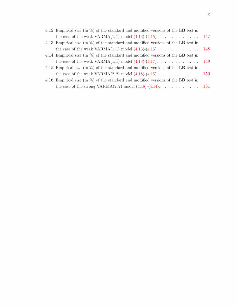
4.12 Empirical size (in %) of the standard and modified versions of the LB test in
the case of the weak VARMA(1, 1) model (4.13)-(4.15). . . . . . . . . . . . 1474.13 Empirical size (in %) of the standard and modified versions of the LB test in
the case of the weak VARMA(1, 1) model (4.13)-(4.16). . . . . . . . . . . . 1484.14 Empirical size (in %) of the standard and modified versions of the LB test in
the case of the weak VARMA(1, 1) model (4.13)-(4.17). . . . . . . . . . . . 1494.15 Empirical size (in %) of the standard and modified versions of the LB test in
the case of the weak VARMA(2, 2) model (4.18)-(4.15). . . . . . . . . . . . 1504.16 Empirical size (in %) of the standard and modified versions of the LB test in
the case of the strong VARMA(2, 2) model (4.18)-(4.14). . . . . . . . . . . 151
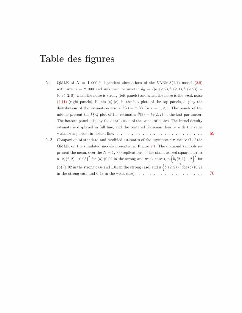
Table des figures
2.1 QMLE of N = 1, 000 independent simulations of the VARMA(1,1) model (2.9)
with size n = 2, 000 and unknown parameter ϑ0 = ((a1(2, 2), b1(2, 1), b1(2, 2)) =
(0.95, 2, 0), when the noise is strong (left panels) and when the noise is the weak noise
(2.11) (right panels). Points (a)-(c), in the box-plots of the top panels, display the
distribution of the estimation errors ϑ(i) − ϑ0(i) for i = 1, 2, 3. The panels of the
middle present the Q-Q plot of the estimates ϑ(3) = b1(2, 2) of the last parameter.
The bottom panels display the distribution of the same estimates. The kernel density
estimate is displayed in full line, and the centered Gaussian density with the same
variance is plotted in dotted line. . . . . . . . . . . . . . . . . . . . . . . . . 692.2 Comparison of standard and modified estimates of the asymptotic variance Ω of the
QMLE, on the simulated models presented in Figure 2.1. The diamond symbols re-
present the mean, over the N = 1, 000 replications, of the standardized squared errors
n a1(2, 2)− 0.952 for (a) (0.02 in the strong and weak cases), n
b1(2, 1)− 22
for
(b) (1.02 in the strong case and 1.01 in the strong case) and n
b1(2, 2)2
for (c) (0.94
in the strong case and 0.43 in the weak case). . . . . . . . . . . . . . . . . . . 70
Chapitre 1
Introduction
Lorsque l’on dispose de plusieurs séries présentant des dépendances temporelles ouinstantanées, il est utile de les étudier conjointement en les considérant comme lescomposantes d’un processus vectoriel (multivarié).
1.0.1 Concepts de base et contexte bibliographique
Dans la littérature économétrique et dans l’analyse des séries temporelles (chrono-logiques), la classe des modèles autorégressifs moyennes mobiles vectoriels (VARMApour Vector AutoRegressive Moving Average) (voir Reinsel, 1997, Lütkepohl, 2005) etla sous-classe des modèles VAR (voir Lütkepohl, 1993) sont utilisées non seulementpour étudier les propriétés de chacune de ces séries, mais aussi pour décrire de possiblesrelations croisées entre les différentes séries chronologiques. Ces modèles VARMA oc-cupent une place centrale pour la modélisation 1 des séries temporelles multivariées. Ilssont une extension naturelle des modèles ARMA qui constituent la classe la plus utili-sée de modèles de séries temporelles univariées (voir Brockwell et Davis, 1991). Cetteextension pose néanmoins des problèmes ardus, comme par exemple, l’identification etl’estimation des paramètres du modèle et suscite des axes de recherches spécifiques,comme la cointégration (voir Lütkepohl, 2005). Ces modèles sont généralement utilisésavec des hypothèses fortes sur le bruit qui en limitent la généralité. Ainsi, nous appe-lons VARMA forts les modèles standard dans lesquels le terme d’erreur est supposé
1. Opération par laquelle on établit un modèle d’un phénomène, afin d’en proposer une représenta-
tion qu’on peut interpréter, reproduire et simuler. Par ailleurs, modèle est synonyme de théorie, mais
avec une connotation pratique : un modèle, c’est une théorie orientée vers l’action à laquelle elle doit
servir. En clair, elle permet d’avoir un aperçu théorique d’une idée en vue d’un objectif concret.
Chapitre 1. Introduction 2
être une suite indépendante et identiquement distribuée (i.e. iid), et nous parlons demodèles VARMA faibles quand les hypothèses sur le bruit sont moins restrictives. Nousparlons également de modèle semi-fort quand le bruit est supposé être une différence demartingale. Plusieurs formulations VARMA ont été introduites pour décrire différentstypes de séries temporelles multivariées. L’une des formulations les plus générales et lesplus simples est le modèle VARMA structurel sans tendance suivant
A00Xt −p0∑
i=1
A0iXt−i = B00ǫt −q0∑
j=1
B0iǫt−j , ∀t ∈ Z (1.1)
où Xt = (X1 t, . . . , Xd t)′ (on notera par la suite X = (Xt)) est un processus vectoriel
stationnaire au second ordre de dimension d, à valeurs réelles. Les paramètres A0i,i ∈ 1, . . . , p0 et B0j , j ∈ 1, . . . , q0 sont des matrices d × d, et p0 et q0 sont desentiers appelés ordres. Le terme d’erreur ǫt = (ǫ1 t, . . . , ǫd t)
′ est un bruit blanc, c’est-à-dire une suite de variables aléatoires centrées (Eǫt = 0), non corrélées, avec une matricede covariance non singulière Σ0.
La représentation (1.1) est dite réduite lorsque l’on suppose A00 = B00 = Id, etstructurelle dans le cas contraire. Les modèles structurels permettent d’étudier desrelations économiques instantanées. Les formes réduites sont plus pratiques d’un pointde vue statistique, car elles donnent les prévisions de chaque composante en fonctiondes valeurs passées de l’ensemble des composantes.
Afin de donner une définition précise d’un modèle linéaire et non linéaire d’un pro-cessus, commençons par rappeler la décomposition de Wold (1938) qui affirme que si(Zt) est un processus stationnaire, purement non déterministe, il peut être représentécomme une moyenne mobile infinie (i.e. MA(∞)) (voir Brockwell et Davis, 1991, pourle cas univarié). Les arguments utilisés s’étendent directement au cas multivarié (voirReinsel, 1997). Ainsi tout processus X = (Xt) de dimension d vérifiant les conditionsci-dessus admet une représentation MA(∞) vectorielle
Xt =∞∑
ℓ=0
Ψℓǫt−ℓ, (1.2)
où∑∞
ℓ=0 ‖Ψℓ‖2 < ∞. Le processus (ǫt) est l’innovation linéaire du processus X. Nousparlons de modèles linéaires lorsque le processus d’innovation (ǫt) est iid et de modèlesnon linéaires dans le cas contraire. Dans le cadre univarié Francq, Roy et Zakoïan (2005),Francq et Zakoïan (1998) ont montré qu’il existe des processus très variés admettant,à la fois, des représentations non linéaires et linéaires de type ARMA, pourvu que leshypothèses sur le bruit du modèle ARMA soient suffisamment peu restrictives. Relâchercette hypothèse permet aux modèles VARMA faibles de couvrir une large classe deprocessus non linéaires.
Chapitre 1. Introduction 3
Pour les applications économétriques, le cadre univarié est très restrictif. Les sérieséconomiques présentent des interdépendances fortes rendant nécessaire l’étude simulta-née de plusieurs séries. Le développement de la littérature sur la cointégration (fondéesur les travaux du prix Nobel d’économie Granger) atteste de l’importance de cetteproblématique. Parmi les modèles pouvant être ajustés au processus d’innovation li-néaire, dont les autocorrélations sont nulles mais qui peut néanmoins présenter desdépendances temporelles, nous pouvons citer les modèles autorégressifs conditionnelle-ment hétéroscédastiques (ARCH) introduits par Engle (1982) et leur extension GARCH(ARCH généralisés) due à Bollerslev (1986). Contrairement aux modèles ARMA, lesextensions des modèles GARCH au cadre multivarié ne sont pas directes. Il existe dansla littérature différents types de modèles GARCH multivariés (voir Bauwens, Laurent etRombouts, 2006), comme le modèle à corrélation conditionnelle constante proposé parBollerslev (1988) et étendu par Jeantheau (1998). Les séries générées par ces modèlessont des différences de martingales et sont utilisés pour décrire des séries financières.Pour la modélisation de ces séries financières, d’autres modèles peuvent être utilisés,comme par exemple les modèles all-pass (Davis et Breidt, 2006) qui gênèrent aussi desséries non corrélées mais qui ne sont pas en général des différences de martingales.
De nombreux outils statistiques ont été développés pour l’analyse, l’estimation etl’interprétation des modèles VARMA forts (voir e.g. Chitturi (1974), Dunsmuir et Han-nan (1976), Hannan (1976), Hannan, Dunsmuir, et Deistler (1980), Hosking (1980,1981a, 1981b), Kascha (2007), Li et McLeod (1981) et Reinsel, Basu et Yap (1992)). Leproblème, qui nous préoccupera, sera l’analyse statistique des modèles VARMA faibles.Le principal but de cette thèse est d’étudier l’estimation et la validité d’outils statis-tiques dans le cadre des modèles VARMA faibles et d’en proposer des extensions. Lestravaux consacrés à l’analyse statistique des modèles VARMA faibles sont pour l’heureessentiellement limités au cas univarié. Sous certaines hypothèses d’ergodicité et de mé-lange, la consistance et la normalité asymptotique de l’estimateur des moindres carrésordinaires ont été montrés par Francq et Zakoïan (1998). Il se trouve que la précisionde cet estimateur dépend de manière cruciale des hypothèses faites sur le bruit. Il estdonc nécessaire d’adapter la méthodologie usuelle d’estimation de la matrice de varianceasymptotique comme dans Francq et Zakoïan (2000). Parmi les autres résultats statis-tiques disponibles, signalons des travaux importants sur le comportement asymptotiquedes autocorrélations empiriques établis par Romano et Thombs (1996). Ces auteurs ontégalement introduits des processus non corrélés mais dépendants et qui peuvent êtreétendus au cas multivarié. Signalons aussi les travaux importants sur les gains d’ef-ficacité des estimateurs de type GMM obtenus par Broze, Francq et Zakoïan (2001),sur l’utilisation des tests portmanteau par Francq, Roy et Zakoïan (2005), sur les testsde linéarité et l’estimation HAC de modèles ARMA faibles par Francq, et Zakoïan(2007) et sur l’utilisation d’une méthode d’estimation basée sur la régression proposée
Chapitre 1. Introduction 4
par Hannan et Rissanen (1982) dans un cadre semi-fort. En analyse multivariée, desprogrès importants ont été réalisés par Dufour et Pelletier (2005) qui ont proposé unegénéralisation de la méthode d’estimation basée sur la régression introduite par Han-nan et Rissanen (1982) et étudié les propriétés asymptotiques de cet estimateur. Ils ontégalement proposé un critère d’information modifié convergent pour la sélection desmodèles VARMA faibles
log det Σ + dim(γ)(log n)1+δ
n, δ > 0,
qui est aussi une extension de celui Hannan et Rissanen (1982). Par ailleurs, Francq etRaïssi (2007) ont étudié des tests portmanteau d’adéquation de modèles VAR faibles.
1.0.2 Représentations VARMA faibles de processus non li-
néaires
Cette thèse se situe dans la continuité des travaux de recherche cités précédemment.Parmi la grande diversité des modèles stochastiques de séries temporelles à temps dis-cret, on distingue, et on oppose parfois, les modèles linéaires et les modèles non linéaires.En réalité ces deux classes de modèles ne sont pas incompatibles et peuvent même êtrecomplémentaires. Les fervents partisans des modèles non linéaires, ou de la prévision nonparamétrique, reprochent souvent aux modèles linéaires ARMA (AutoRegressive Mo-ving Average) d’être trop restrictifs, de ne convenir qu’à un petit nombre de séries. Ceciest surtout vrai si on suppose, comme on le fait habituellement, des hypothèses fortessur le bruit qui intervient dans l’écriture ARMA. Des processus très variés admettent,à la fois, des représentations non linéaires et linéaires de type ARMA, pourvu que leshypothèses sur le bruit du modèle ARMA soient suffisamment peu restrictives. On parlealors de modèles ARMA faibles. L’étude des modèles ARMA faibles a des conséquencesimportantes pour l’analyse des séries économiques, pour lesquelles de nombreux travauxont montrés que les modèles ARMA standard sont mal adaptés.
Interprétations des représentations linéaires faibles
Si dans (1.1), ǫ = (ǫt) est un bruit blanc fort, 2 à savoir une suite de variables iid,alors on dit que X = (Xt) est un modèle VARMA(p0, q0) structurel fort. Si l’on supposeque ǫ est une différence de martingale, 3 alors on dit que X admet une représentation
2. Voir Remarque 1.13 de l’annexe pour la définition.3. Voir Définition 1.11 de l’annexe.
Chapitre 1. Introduction 5
VARMA(p0, q0) structurelle semi-forte. Et si on suppose simplement que ǫ est un bruitblanc faible, 4 mais qu’il n’est pas forcément iid, ni même une différence de martingale,on dit que X admet une représentation VARMA(p0, q0) structurelle faible. Ainsi ladistinction entre modèle VARMA(p0, q0) structurel fort, semi-fort ou faible n’est doncqu’une question d’hypothèse sur le bruit. En plus, du fait que la contrainte sur ǫ estmoins forte pour un modèle structurel faible que pour un modèle structurel semi-fortou fort, il est clair que la classe des modèles VARMA(p0, q0) structurels faibles est laplus large. Nous en déduisons la relation suivante
VARMA forts ⊂ VARMA semi-forts ⊂ VARMA faibles .Soit HX(t− 1) l’espace de Hilbert engendré par les variables aléatoires Xt−1, Xt−2, . . . .Cet espace contient les combinaisons linéaires de la forme
∑mi=1CiXt−i et leurs limites
en moyenne quadratique. Notons FX(t−1) la tribu engendrée par Xt−1, Xt−2, . . . . Nousappellerons HX(t− 1) le passé linéaire de Xt et FX(t− 1) sera appelé le passé de Xt.Il est parfois pratique d’écrire l’équation (1.1) sous la forme compacte
A(L)Xt = B(L)ǫt
où L est l’opérateur retard (i.e. Xt−1 = LXt, ǫt−k = Lkǫt pour tout t, k ∈ Z), A(z) =
A0 −∑p0
i=1Aizi est le polynôme VAR et B(z) = B0 −
∑q0j=1Bjz
j est le polynôme MAvectoriel. Notons par det(·), le déterminant d’une matrice carrée. Pour l’étude des sérieschronologiques, la notion de stationnarité faible 5 conduit à imposer des contraintessur les racines des polynômes VAR et MA vectoriel. Si les racines de detA(z) = 0
sont à l’extérieur du disque unité, alors Xt est une combinaison linéaire de ǫt, ǫt−1, . . .
(cette combinaison est une solution non anticipative ou causale de (1.1)). Si les racinesde detB(z) = 0 sont à l’extérieur du disque unité, alors ǫt peut s’écrire comme unecombinaison linéaire de Xt, Xt−1, . . . (l’équation (1.1) est dite inversible). Les deuxhypothèses précédentes sur les polynômes VAR et MA vectoriel seront regroupées dansl’hypothèse suivante
H1 : detA(z) detB(z) = 0 ⇒ |z| > 1.Sous l’hypothèse H1, le passé (linéaire) de X coïncide donc avec le passé (linéaire) deǫ :
FX(t− 1) = Fǫ(t− 1), HX(t− 1) = Hǫ(t− 1).
Si en plus, ǫ est un bruit blanc faible, on en déduit que la meilleure prévision de Xt estune fonction linéaire du passé
A00E Xt|HX(t− 1) = B00E ǫt|Hǫ(t− 1)+p∑
i=1
A0iXt−i −q∑
j=1
B0iǫt−j ,
=
p∑
i=1
A0iXt−i −q∑
j=1
B0iǫt−j .
4. Voir Définition 1.8 de l’annexe.5. Voir Définition 1.7 de l’annexe.
Chapitre 1. Introduction 6
Le bruit ǫ s’interprète donc comme une normalisation du processus des innovationslinéaires de X :
ǫt = B−100 A00 (Xt − E Xt|HX(t− 1)) .
Lorsque la forme VARMA est réduite, c’est-à-dire quand A00 = B00 = Id, alors ǫtcoïncide précisément avec l’innovation linéaire Xt − E Xt|HX(t− 1). Ainsi dans unmodèle VARMA faible on suppose simplement que le terme d’erreur est l’innovationlinéaire. Par contre, dans un modèle VARMA (semi-)fort on suppose que le termed’erreur est l’innovation forte :
ǫt = B−100 A00 (Xt − E Xt|FX(t− 1)) . (1.3)
Ceci revient donc à dire que le meilleur prédicteur de Xt est une combinaison linéairedes valeurs passées, que l’on obtient en déroulant (1.1). C’est évidemment une hypo-thèse extrêmement restrictive car, au sens des moindres carrés, la meilleure prévisionde Xt est souvent une fonction non linéaire du passé de X. L’hypothèse (1.3) est cepen-dant d’usage courant pour le traitement statistique des modèles VARMA. Ceci permetd’utiliser la théorie asymptotique des martingales (Hall et Heyde, 1980) : lois des grandsnombres, théorème de la limite centrale, . . . . Ceci met néanmoins l’accent sur un défautmajeur du modèle VARMA (semi-)fort : il est peu plausible pour un certain nombrede séries temporelles car il est souvent peu réaliste de supposer a priori que le meilleurprédicteur est linéaire.
Approximation de la décomposition de Wold
Au moins comme approximation, sous certaines hypothèses de régularité, les mo-dèles VARMA faibles sont assez généraux car, comme nous allons le voir dans cettepartie, l’ensemble des processus VARMA faibles est dense dans l’ensemble des proces-sus stationnaires au second ordre. Rappelons que, sous les hypothèses de (1.2), nousavons
Xt =∞∑
ℓ=0
Ψℓǫt−ℓ,
où (ǫt) est le processus des innovations linéaires du processus (Xt). Ainsi pour approxi-mer le processus (Xt), considérons le processus suivant
Xt(q0) = Ψ0ǫt +
q0∑
ℓ=1
Ψℓǫt−ℓ.
Il est important de remarquer que (ǫt) est aussi le processus des innovations linéaires de(Xt(q0)) si det Ψ(z) a ses racines à l’extérieur du disque unité, où Ψ(z) = Ψ0+
∑q0i=1Ψiz
i.Si ce n’est pas le cas, il faut changer le bruit et les coefficients des matrices pour
Chapitre 1. Introduction 7
obtenir la représentation explicite. Le processus (Xt(q0)) est une MA(q0) vectoriellefaible car Xt(q0) et Xt−h(q0) sont non corrélés pour h > q0. Notons ‖·‖2 la norme
définie par ‖Z‖2 =√
E ‖Z‖2, où Z est un vecteur aléatoire de dimension d. Comme∑∞
ℓ=0 ‖Ψℓ‖2 <∞, nous avons
‖Xt(q0)−Xt‖22 = E ‖ǫt‖2∑
i>q0
‖Ψi‖2 → 0 quand q0 → ∞.
Par conséquent l’ensemble des moyennes mobiles finies faibles est dense dans l’ensembledes processus stationnaires au second ordre et réguliers. La même propriété est évidem-ment vraie pour l’ensemble des modèles VARMA faibles. Trivialement, en suivant leprincipe de parcimonie qui nous fait préférer un modèle avec moins de paramètres, onutilise plutôt les modèles VARMA qui permettent parfois d’obtenir la même précisionen utilisant moins de paramètres. Ainsi le modèle linéaire (1.2), qui regroupe les mo-dèles VARMA et leurs limites, est très général si le terme d’erreur ǫt correspond à cequi n’est pas prévu linéairement, il est par contre peu réaliste si le terme d’erreur estce que l’on ne peut prévoir par aucune fonction du passé.
Agrégation temporelle des modèles VARMA faibles
La plupart des séries économiques, et plus particulièrement les séries financières,sont analysées à différentes fréquences (jour, semaine, mois,. . . ). Le choix de la fréquenced’observation a souvent une importance cruciale quant aux propriétés de la série étudiéeet, par suite au type de modèle adapté. Dans le cas des modèles GARCH, les travauxempiriques font généralement apparaître une persistance plus forte lorsque la fréquenceaugmente.
Du point de vue théorique, le problème de l’agrégation temporelle peut être poséde la manière suivante : étant donnés un processus (Xt) et un entier m, quelles sontles propriétés du processus échantillonné (Xmt) (i.e. construit à partir de (Xt) en neretenant que les dates multiples de m) ? Lorsque, pour tout entierm et pour tout modèled’une classe donnée, admettant (Xt) comme solution, il existe un modèle de la mêmeclasse dont (Xmt) soit solution, cette classe est dite stable par agrégation temporelle.
Un exemple très simple de modèle stable par agrégation temporelle est évidemmentle bruit blanc (fort ou faible) : la propriété d’indépendance (ou de non corrélation) sub-siste lorsque l’on passe d’une fréquence donnée à une fréquence plus faible. Par contre,les modèles ARMA au sens fort ne sont généralement pas stables par agrégation tem-porelle. Ce n’est qu’en relâchant l’hypothèse d’indépendance du bruit (ARMA faibles)
Chapitre 1. Introduction 8
qu’on obtient l’agrégation temporelle (voir Drost et Nijman (1993) pour le cas univariéde processus GARCH, Nijman et Enrique (1994) pour une extension au cas multivarié).
Exemples de processus ARMA forts vectoriels admettant une représentation
faible
Certaines transformations de processus VARMA forts, comme par exemple des agré-gations temporelles, des échantillonnages ou encore des transformations linéaires plusgénérales, admettent des représentations VARMA faibles. Les exemples suivants illus-trent le cas où l’on considère des sous vecteurs du processus observé.
Exemple 1.1. Soit un processus (Xt) de dimension d = d1+d2 qui satisfait un modèleVARMA(1, 1) fort de la forme
(
X1 t
X2 t
)
=
(
0d1×d1 A12
A21 A22
)(
X1 t−1
X2 t−1
)
+
(
ǫ1 t
ǫ2 t
)
−(
0d1×d1 0d1×d2
B21 0d2×d2
)(
ǫ1 t−1
ǫ2 t−1
)
,
où X1 t, ǫ1 t (resp. X2 t, ǫ2 t) sont des vecteurs de dimension d1 (resp. d2) et les matricesA12, A21, A22 et B21 sont de tailles appropriées. Si l’on suppose que ǫt = (ǫ′1 t, ǫ
′2 t)
′ estun bruit blanc fort de matrice variance-covariance
Ωǫ =
(
Ω11 0d1×d2
0d2×d1 Ω22
)
,
alors X2 t satisfait le modèle VAR(2) suivant
X2 t = A22X2 t−1 + A21A12X2 t−2 + νt,
où νt = ǫ2 t + (A21 − B21)ǫ1 t−1 est non corrélé. Cependant dès que l’on suppose qu’ilexiste une dépendance entre ǫ2 t et ǫ1 t, et que A21 6= B21, le processus (νt) n’est plus unbruit blanc fort.
Contribution de la thèse
L’objectif principal de la thèse est d’étudier dans quelle mesure les travaux citésprécédemment sur l’analyse statistique des modèles ARMA peuvent s’étendre au casmultivarié faible. En particulier, nous étudions de quelle manière il convient d’adapter
Chapitre 1. Introduction 9
les outils statistiques standard pour l’estimation et l’inférence des modèles VARMAfaibles.
Le deuxième chapitre est consacré à établir les propriétés asymptotiques des estima-teurs du quasi-maximum de vraisemblance (en anglais QMLE) et des moindres carrés(noté LSE pour Least Squares Estimator), afin de les comparer à celles du cas stan-dard. Ensuite, nous accordons une attention particulière à l’estimation de la matricede variance asymptotique de ces estimateurs. Cette matrice est de la forme "sandwich"Ω := J−1IJ−1, et peut être très différente de la variance asymptotique standard, dont laforme est Ω := 2J−1. Enfin des versions modifiées des tests de Wald, du multiplicateurde Lagrange et du rapport de vraisemblance sont proposées pour tester des restrictionslinéaires sur les paramètres libres du modèle.
Dans le troisième chapitre, nous considérons de façon plus détaillée le problème del’estimation de la matrice de variance asymptotique Ω des estimateurs QML/LS d’unmodèle VARMA sans faire l’hypothèse d’indépendance habituelle sur le bruit. Dans unpremier temps, nous proposons une expression des dérivées des résidus en fonction desparamètres du modèle VARMA. Ceci nous permettra ensuite de donner une expressionexplicite des matrices I et J impliquées dans la variance asymptotique Ω, en fonctiondes paramètres des polynômes VAR et MA, et des moments d’ordre deux et quatre dubruit. Enfin nous en déduisons un estimateur de Ω, dont nous établissons la convergence.
Dans le quatrième chapitre, nous nous intéressons au problème de la validation desmodèles VARMA faibles. Dans un premier temps, nous étudions la distribution asymp-totique jointe de l’estimateur du QML et des autocovariances empiriques du bruit. Cecinous permet d’obtenir les distributions asymptotiques des autocovariances et autocor-rélations résiduelles. Ces autocorrélations résiduelles sont normalement distribuées avecune matrice de covariance différente du cas iid. Enfin, nous déduisons le comporte-ment asymptotique des statistiques portmanteau. Dans le cadre standard (c’est-à-diresous les hypothèses iid sur le bruit), il est connu que la distribution asymptotique destests portmanteau est approximée par un chi-deux. Dans le cas général, nous montronsque cette distribution asymptotique est celle d’une somme pondérée de chi-deux. Cettedistribution peut être très différente de l’approximation chi-deux usuelle du cas fort.Nous en déduisons des tests portmanteau modifiés pour tester l’adéquation de modèlesVARMA faibles.
Le cinquième chapitre est consacré au problème très important de sélection de mo-dèles en séries chronologiques. Depuis des années, ce champ de recherche suscite unintérêt croissant au sein de la communauté des économètres et des statisticiens. Enattestent les nombreuses publications scientifiques dans ce domaine et les différents
Chapitre 1. Introduction 10
champs d’application ouverts. Les praticiens se sont toujours trouvés confrontés auproblème du choix d’un modèle adéquat leur permettant de décrire le mécanisme ayantgénéré les observations et de faire des prévisions. Ces questions concernent les différentsdomaines d’application des séries temporelles, tels que la communication, la clima-tologie, l’épidémiologie, les systèmes de contrôle, l’économétrie et la finance. Afin derésoudre ce problème de choix de modèles, nous proposons une modification du critèred’information de Akaike (AIC pour Akaike’s Information Criterion). Ce AIC modifiéest fondé sur une généralisation du critère AIC corrigé introduit par Tsai et Hurvich(1989).
Nous illustrons enfin nos résultats sur des études empiriques basées sur des ex-périences de Monte Carlo. Les logiciels de prévision qui utilisent la méthodologie deBox et Jenkins (identification, estimation et validation de modèles ARMA forts) neconviennent pas aux ARMA faibles. Il nous faudra donc déterminer comment adapterles sorties de ces logiciels.
Le dernier chapitre propose des perspectives pour des développement futurs.
Nous présentons maintenant nos résultats de façon plus détaillée.
1.1 Résultats du chapitre 2
L’objectif de ce chapitre est d’étudier, dans un premier temps, les propriétés asymp-totiques du QMLE et du LSE des paramètres d’un modèle VARMA sans faire l’hy-pothèse d’indépendance sur le bruit, contrairement à ce qui est fait habituellementpour l’inférence de ces modèles. Relâcher cette hypothèse permet aux modèles VARMAfaibles de couvrir une large classe de processus non linéaires. Ensuite, nous accordonsune attention particulière à l’estimation de la matrice de variance asymptotique deforme "sandwich" Ω := J−1IJ−1. Nous établissons la convergence d’un estimateur deΩ. Enfin, des versions modifiées des tests de Wald, du multiplicateur de Lagrange etdu rapport de vraisemblance sont proposées pour tester des restrictions linéaires sur lesparamètres libres du modèle.
Chapitre 1. Introduction 11
1.1.1 Estimation des paramètres
Pour l’estimation des paramètres, nous utiliserons la méthode du quasi-maximumde vraisemblance, qui est la méthode du maximum de vraisemblance gaussien lorsquel’hypothèse de bruit blanc gaussien est relâchée. Nous présentons l’estimation du modèleARMA(p0, q0) structurel d-multivarié (1.1) dans lequel Xt = (X1 t, . . . , Xd t)
′ est unprocessus vectoriel stationnaire au second ordre, à valeurs réelles. Le terme d’erreurǫt = (ǫ1 t, · · · , ǫd t)
′ est une suite de variables aléatoires centrées, non corrélées, avecune matrice de covariance non singulière Σ. Les paramètres sont les coefficients desmatrices carrées d’ordre d suivantes : Ai, i ∈ 1, . . . , p0, Bj , j ∈ 1, . . . , q0 et Σ.Avant de détailler la procédure d’estimation et ses propriétés, nous étudions quellesconditions imposer aux matrices Ai, Bj et Σ afin d’assurer l’identifibialité du modèle,c’est-à-dire l’unicité des (p0 + q0 +3)d2 paramètres du modèle. Nous supposons que cesmatrices sont paramétrées suivant le vecteur des vraies valeurs des paramètres noté ϑ0.Nous notons A0i = Ai(ϑ0), i ∈ 1, . . . , p0, Bj = Bj(ϑ0), j ∈ 1, . . . , q0 et Σ0 = Σ(ϑ0),où ϑ0 appartient à l’espace compact des paramètres Θ ⊂ Rk0 , et k0 est le nombre deparamètres inconnus qui est inférieur à (p0+q0+3)d2. Pour tout ϑ ∈ Θ, nous supposonsaussi que les applications ϑ 7→ Ai(ϑ) i = 0, . . . , p0, ϑ 7→ Bj(ϑ) j = 0, . . . , q0 et ϑ 7→ Σ(ϑ)
admettent des dérivées continues d’ordre 3.
Conditions d’identifiabilité
Pour la suite, nous notons Ai(ϑ), Bj(ϑ) et Σ(ϑ) par Ai, Bj et Σ. Soit les poly-nômes Aϑ(z) = A0 −
∑p0i=1Aiz
i et Bϑ(z) = B0 −∑q0
i=1Bizi. Dans le cadre de modèles
VARMA(p0, q0) structurels, l’hypothèse H1 qui assure que les polynômes Aϑ0(z) etBϑ0(z) n’ont pas de racine commune, ne suffit pas à garantir l’identifiabilité du para-mètre, c’est-à-dire à garantir que seule la valeur ϑ = ϑ0 satisfasse Aϑ(L)Xt = Bϑ(L)ǫt.
On suppose donc queH2 : pour tout ϑ ∈ Θ tel que ϑ 6= ϑ0, soit les fonctions de transfert
A−10 B0B
−1ϑ (z)Aϑ(z) 6= A−1
00 B00B−1ϑ0
(z)Aϑ0(z) pour un z ∈ C
ouA−1
0 B0ΣB′0A
−1′0 6= A−1
00 B00Σ0B′00A
−1′00 .
Cette condition équivaut à l’existence d’un opérateur U(L) tel que
Aϑ(L) = U(L)Aϑ0(L), A0 = U(1)A00, Bϑ(L) = U(L)Bϑ0(L) et B0 = U(1)B00.
On dit que U(L) est unimodulaire si detU(L) est une constante non nulle. Lorsque lesseuls facteurs communs à deux polynômes P (L) et Q(L) sont unimodulaires, c’est-à-dire
Chapitre 1. Introduction 12
siP (L) = U(L)P1(L), Q(L) = U(L)Q1(L) =⇒ detU(L) = cste 6= 0,
on dit que P (L) et Q(L) sont coprimes à gauche (en anglais left-coprime). Divers typesde conditions peuvent être imposées pour assurer l’identifiabilité (voir Reinsel, 1997,p. 37-40, ou Hannan (1971, 1976), Hannan et Deistler, 1988, section 2.7). Pour avoiridentifiabilité, il est parfois nécessaire d’introduire des formes plus contraintes, commepar exemple la forme échelon. Pour des renseignements complémentaires sur les formesidentifiables, et en particulier la forme échelon, on peut par exemple se référer à Hannan(1976), Hannan et Deistler (1976), Dufour J-M. et Pelletier D. (2005), Lütkepohl (1991,p. 246-247 et 289-297, 2005, p. 452-453 et 498-507) et Reinsel (1997).
Définition de l’estimateur du QML
Pour des raisons pratiques, nous écrivons le modèle sous sa forme réduite
Xt −p0∑
i=1
A−100 A0iXt−i = et −
q0∑
j=1
A−100 B0jB
−100 A00et−j , et = A−1
00 B00ǫt.
On dispose d’une observation de longueur n,X1, . . . , Xn. Pour 0 < t ≤ n et pour toutϑ ∈ Θ, les variables aléatoires et(ϑ) sont définies récursivement par
et(ϑ) = Xt −p0∑
i=1
A−10 AiXt−i +
q0∑
j=1
A−10 BjB
−10 A0et−j(ϑ),
où les valeurs initiales inconnues sont remplacées par zéro : e0(ϑ) = · · · = e1−q0(ϑ) =
X0 = · · · = X1−p0 = 0. Nous montrons que, comme dans le cas univarié, ces valeursinitiales sont asymptotiquement négligeables et, en particulier, que et(ϑ0) − et → 0
presque sûrement quand t → ∞. Ainsi, le choix des valeurs initiales est sans effet surles propriétés asymptotiques de l’estimateur. La quasi-vraisemblance gaussienne s’écrit
Ln(ϑ) =
n∏
t=1
1
(2π)d/2√det Σe
exp
−1
2e′t(ϑ)Σ
−1e et(ϑ)
,
où Σe = Σe(ϑ) = A−10 B0ΣB
′0A
−1′0 . Un estimateur du QML de ϑ0 est défini comme toute
solution mesurable ϑn de
ϑn = argmaxϑ∈Θ
Ln(ϑ) = argminϑ∈Θ
ℓn(ϑ), ℓn(ϑ) =−2
nlog Ln(ϑ).
Chapitre 1. Introduction 13
Propriétés asymptotiques de l’estimateur du QML/LS
Afin d’établir la convergence forte de l’estimateur du QML, il est utile d’approxi-mer la suite (et(ϑ)) par une suite stationnaire ergodique. C’est ainsi que nous faisonsl’hypothèse d’ergodicité suivante
H3 : Le processus (ǫt) est stationnaire et ergodique.Nous pouvons maintenant énoncer le théorème de convergence forte suivant.
Théorème 1.1. (Convergence forte) Sous les hypothèses H1, H2 et H3, soit (Xt)
une solution causale ou non anticipative de l’équation (1.1) et soit (ϑn) une suite d’es-timateurs du QML. Alors, nous avons presque sûrement ϑn → ϑ0 quand n→ ∞.
Ainsi comme dans le cas où le processus des innovations est un bruit blanc fort,nous obtenons la consistance forte de l’estimateur ϑn dans le cas faible.
Nous montrons ce théorème en appliquant le théorème 1.12 6, les conditionsd’identifiabilité et l’inégalité élémentaire Tr(A−1B) − log det(A−1B) ≥ Tr(A−1A) −log det(A−1A) = d pour toute matrice symétrique semi-définie positive de taille d× d.
L’ergodicité ne suffit pas pour obtenir un théorème central limite (noté TCL dansla suite). Pour la normalité asymptotique du QMLE, nous avons donc besoin des hypo-thèses supplémentaires. Il est d’abord nécessaire de supposer que le paramètre ϑ0 n’estpas situé sur le bord de l’espace compact des paramètres Θ.
H4 : Nous avons ϑ0 ∈
Θ, où
Θ est l’intérieur de Θ.Nous introduisons les coefficients de mélange fort d’un processus vectoriel X = (Xt)
définis par
αX (h) = supA∈σ(Xu,≤t),B∈σ(Xu,≥t+h)
|P (A ∩ B)− P (A)P (B)| .
On dit que X est fortement mélangeant si αX (h) → 0 quand h→ ∞. Nous considéronsl’hypothèse suivante qui nous permet de contrôler la dépendance dans le temps duprocessus (ǫt).
H5 : Il existe un réel ν > 0 tel que E‖ǫt‖4+2ν < ∞ et les coefficients demélange du processus (ǫt) vérifient
∑∞k=0 αǫ(k)
ν2+ν <∞.
Notons que d’après l’hypothèse H1 et l’équation (1.1), le processus (Xt) peut s’écrirecomme une combinaison linéaire de ǫt, ǫt−1, . . . , ce qui implique, d’après H5 que le pro-cessus (Xt) est mélangeant. Cette hypothèse H5 est donc plus faible que l’hypothèse debruit blanc fort de point de vue de la dépendance. D’autre part, nous faisons l’hypothèsed’existence de moments d’ordre 4+ (supérieur à quatre), c’est-à-dire E‖ǫt‖4+2ν < ∞
6. Théorème ergodique, voir annexe.
Chapitre 1. Introduction 14
pour un réel ν > 0, qui est légèrement plus forte que l’hypothèse d’existence de mo-ments d’ordre 4 qui est faite dans le cas standard. Étant donné l’hypothèse H1 sur lesracines des polynômes, il est clair que les hypothèses de moment E‖ǫt‖4+2ν < ∞ etE‖Xt‖4+2ν < ∞ sont équivalentes. Par contre, les hypothèses de mélanges ne sont paséquivalentes.
Nous définissons la matrice des coefficients de la forme réduite du modèle par
Mϑ0 = [A−100 A01 : · · · : A−1
00 A0p : A−100 B01B
−100 A00 : · · · : A−1
00 B0qB−100 A00 : Σe0].
Ainsi nous avons besoin d’une hypothèse qui spécifie comment cette matrice dépend du
paramètre ϑ0. Soit
Mϑ0 la matrice ∂vec(Mϑ)/∂ϑ′ appliquée en ϑ0.
H6 : La matrice
Mϑ0 est de plein rang k0.Nous pouvons maintenant énoncer le théorème suivant qui nous donne le comportementasymptotique de l’estimateur du QML.
Théorème 1.2. (Normalité asymptotique) Sous les hypothèses du Théorème 1.1,H4, H5 et H6, nous avons
√n(
ϑn − ϑ0
)L→ N (0,Ω := J−1IJ−1),
où J = J(ϑ0) et I = I(ϑ0), avec
J(ϑ) = limn→∞
∂2
∂ϑ∂ϑ′ℓn(ϑ) p.s., I(ϑ) = lim
n→∞Var
∂
∂ϑℓn(ϑ).
La démonstration de ce théorème repose sur le théorème 1.13 7 de Herrndorf (1984),le théorème 1.1 et l’inégalité 8 de Markov (1968) pour les processus mélangeants.
Remarque 1.1. Dans le cas standard de modèles VARMA forts, i.e. quand l’hypothèse
H3 est remplacée par celle que les termes d’erreur (ǫt) sont iid, nous avons I = 2J ,
ainsi Ω = 2J−1. Par contre dans le cas général, nous avons I 6= 2J . Comme consé-
quence, les logiciels utilisés pour ajuster les modèles VARMA forts ne fournissent pas
une estimation correcte de la matrice Ω pour le cas de processus VARMA faibles. C’est
aussi le même problème dans le cas univarié (voir Francq et Zakoïan (2007), et d’autres
références ).
Notons que, pour les modèles VARMA sous la forme réduite, il n’est pas restrictifde supposer que les coefficients A0, . . . , Ap0, B0, . . . , Bq0 sont fonctionnellement indépen-dants du coefficient Σe. Ceci nous permet de faire l’hypothèse suivante
7. Voir TCL pour processus α-mélangeant en annexe8. Voir inégalité de covariance en annexe
Chapitre 1. Introduction 15
H7 : Posons ϑ = (ϑ(1)′, ϑ(2)
′)′, où ϑ(1) ∈ Rk1 dépend des coefficients
A0, . . . , Ap0 et B0, . . . , Bq0, et où ϑ(2) = D vec Σe ∈ Rk2 dépend uniquement deΣe, pour une matrice D de taille k2 × d2, avec k1 + k2 = k0.
Par abus de notation, nous écrivons et(ϑ) = et(ϑ(1)). Le produit de Kronecker de deux
matrices A et B est noté par A⊗B (noté dans la suite A⊗2 quand A = B). Le théorèmesuivant montre que pour des modèles VARMA sous la forme réduite, les estimateursdu QML et du LS coincident.
Théorème 1.3. Sous les hypothèses du Théorème 1.2 et H7, le QMLE ϑn =
(ϑ(1)′n , ϑ
(2)′n )′ peut être obtenu par
ϑ(2)n = D vec Σe, Σe =1
n
n∑
t=1
et(ϑ(1)n )e′t(ϑ
(1)n ),
et
ϑ(1)n = argminϑ(1)
det
n∑
t=1
et(ϑ(1))e′t(ϑ
(1)).
De plus, nous avons
J =
(
J11 0
0 J22
)
, avec J11 = 2E
∂
∂ϑ(1)e′t(ϑ
(1)0 )
Σ−1e0
∂
∂ϑ(1)′et(ϑ
(1)0 )
et J22 = D(Σ−1e0 ⊗ Σ−1
e0 )D′.
Remarque 1.2. Notons que la matrice J a la même expression dans les cas de modèles
ARMA fort et faible (voir Lütkepohl (2005) page 480). Contrairement, à la matrice I
qui est en général plus compliquée dans le cas faible que dans le cas fort.
1.1.2 Estimation de la matrice de variance asymptotique
Afin d’obtenir des intervalles de confiance ou de tester la significativité des coeffi-cients VARMA faibles, il sera nécessaire de disposer d’un estimateur au moins faible-ment consistant de la matrice de variance asymptotique Ω.
Estimation de la matrice J
La matrice J peut facilement être estimée par
J =
(
J11 0
0 J22
)
, J22 = D(Σ−1e0 ⊗ Σ−1
e0 )D′ et
Chapitre 1. Introduction 16
J11 =2
n
n∑
t=1
∂
∂ϑ(1)e′t(ϑ
(1)n )
Σ−1e0
∂
∂ϑ(1)′et(ϑ
(1)n )
.
Dans le cas standard des VARMA forts Ω = 2J−1 est un estimateur fortementconvergent de Ω. Dans le cas général des VARMA faibles, cet estimateur n’est pasconvergent quand I 6= 2J .
Estimation de la matrice I
Nous avons besoin d’un estimateur convergent de la matrice I. Notons que
I = varas1√n
n∑
t=1
Υt =
+∞∑
h=−∞
cov(Υt,Υt−h), (1.4)
où
Υt =∂
∂ϑ
log det Σe + e′t(ϑ
(1))Σ−1e et(ϑ
(1))
ϑ=ϑ0.
L’existence de la somme des covariances dans (1.4) est une conséquence de l’hypothèseH5 et de l’inégalité de covariance de Davydov (1968). Cette matrice I est plus délicateà estimer. Néanmoins nous nous reposons sur deux méthodes suivantes pour l’estimer
– la méthode d’estimation non paramètrique du noyau aussi appelée HAC (Hete-roscedasticity and Autocorrelation Consistent),
– la méthode d’estimation paramètrique de la densité spectrale (notée SP).
Définition de l’estimateur HAC de la matrice I
Dans la littérature économique, l’estimateur non paramètrique du noyau (aussi ap-pelé HAC) est largement utilisé pour estimer une matrice de covariance de la forme de I.La technique que nous utilisons consiste à pondérer convenablement certains momentsempiriques. Cette pondération se fait au moyen d’une suite de poids (ou fenêtre). Cetteapproche est semblable à celle de Andrews (1991), Newey et West (1994). Soit Υt levecteur obtenu en remplaçant ϑ0 par ϑn dans Υt. La matrice Ω est donc estimée par unestimateur "sandwich" de la forme
ΩHAC = J−1IHACJ−1, IHAC =1
n
n∑
t,s=1
ω|t−s|ΥtΥs,
où ω0, . . . , ωn−1 est une suite de poids (ou fenêtre).
Chapitre 1. Introduction 17
Définition de l’estimateur SP de la matrice I
Une méthode alternative consiste à utiliser un modèle VAR paramètrique estimé dela densité spectrale du processus (Υt). Cette approche a été étudiée par Berk (1974)(voir aussi den Haan et Levin, 1997). Ceci revient à interpréter (2π)−1I comme étant ladensité spectrale évaluée à la fréquence 0 du processus stationnaire (Υt) (voir Brockwellet Davis, 1991, p. 459). Nous nous basons sur l’expression
I = Φ−1(1)ΣuΦ
−1(1)
quand (Υt) satisfait une représentation VAR(∞) de la forme
Φ(L)Υt := Υt +∞∑
i=1
ΦiΥt−i = ut,
où ut est un bruit blanc faible de matrice covariance Σu. Notons Φr,1, . . . , Φr,r lescoefficients de la régression des moindres carrés de Υt sur Υt−1, . . . , Υt−r et posonsΦr(z) = Ik0−s +
∑ri=1 Φr,iz
i. Soit ur,t les résidus de cette regression et Σurla variance
empirique de ur,1, . . . , ur,n. Nous énonçons maintenant le théorème suivant qui est uneextension de celui de Francq, Roy et Zakoïan (2005).
Théorème 1.4. (Convergence faible de I) Sous les hypothèses du Théorème 1.3,nous supposons que le processus (Υt) admet une représentation VAR(∞) pour laquelleles racines de detΦ(z) = 0 sont à l’extérieur du disque unité, ‖Φi‖ = o(i−2), et que lamatrice Σu = Var(ut) est non singulière. Nous supposons également que ‖ǫt‖8+4ν < ∞et∑∞
k=0αX,ǫ(k)ν/(2+ν) < ∞ pour un réel ν > 0, où αX,ǫ(k)k≥0 désigne la suite descoefficients de mélange fort du processus (X ′
t, ǫ′t)
′. Alors, l’estimateur
ISP := Φ−1r (1)Σur
Φ′−1r (1) → I
en probabilité quand r = r(n) → ∞ et r3/n→ 0 quand n→ ∞.
La démonstration s’inspire de celle de Francq, Roy et Zakoïan (2005) et repose surune série de lemmes.
1.1.3 Tests sur les coefficients du modèle
En dehors des contraintes imposées pour assurer l’identifiabilité du modèleVARMA(p0, q0), d’autres contraintes linéaires peuvent être testées sur les paramètres
Chapitre 1. Introduction 18
ϑ0 du modèle (en particulier A0p = 0 ou B0q = 0). Afin de tester s0 contraintes linéairessur les coefficients, nous définissons notre hypothèse nulle
H0 : R0ϑ0 = r0,
où R0 est une matrice s0 × k0 connue de rang s0 et r0 est aussi un vecteur connude dimension s0. Pour effectuer ce test H0 : R0ϑ0 = r0, il existe diverses approchesasymptotiques dont les plus classiques sont la procédure de Wald (notée W), celle dumultiplicateur de Lagrange (en anglais LM) encore appelée du score ou de Rao-score etla méthode du rapport de vraisemblance (notée LR pour likelihood ratio). Pour calculernos différentes statistiques de test, nous considérons la matrice Ω = J−1I J−1, où J etI sont des estimateurs consistants de J et I définis dans la section 1.1.2.
Statistique de Wald
Le principe est d’accepter l’hypothèse nulle, si l’estimateur non contraint ϑn de ϑ0est suffisamment proche de zéro. Ainsi de la normalité asymptotique de ϑ0, nous endéduisons que
√n(
R0ϑn − r0
)L→ N
(0, R0ΩR
′0 := R0
(J−1IJ−1
)R′
0
),
quand n→ ∞. Sous les hypothèses du théorème 1.3 et l’hypothèse que I est inversible,la statistique de Wald modifiée est
Wn = n(R0ϑn − r0)′(R0ΩR
′0)
−1(R0ϑn − r0).
Sous H0, cette statistique suit une distribution de χ2s0
. Ainsi nous retrouvons la mêmeformulation que dans le cas fort standard. Nous rejetons H0 quand Wn > χ2
s0(1 − α)
pour un niveau de risque asymptotique α.
Remarque 1.3. Notons que le test de Wald nécessite la maximisation de la quasi-
vraisemblance non contrainte, mais pas la maximisation de la quasi-vraisemblance
contrainte.
Statistique du LM
L’idée de ce test consiste à accepter l’hypothèse nulle, si le score contraint est prochede zéro. Soit ϑcn le QMLE contraint sous H0. Définissons le Lagrangien
L(ϑ, λ) = ℓn(ϑ)− λ′(R0ϑ− r0),
Chapitre 1. Introduction 19
où λ est le vecteur multiplicateur de Lagrange de dimension s0. Les conditions depremier ordre s’écrivent
∂ℓn∂ϑ
(ϑcn) = R′0λ, R0ϑ
cn = r0.
Notons a c= b pour signifier que a = b + c. En effectuant le développement limité de
Taylor sous H0, nous avons
0 =√n∂ℓn(ϑn)
∂ϑ
oP (1)=
√n∂ℓn(ϑ
cn)
∂ϑ− J
√n(
ϑn − ϑcn
)
.
Nous déduisons que
√n(R0ϑn − r0) = R0
√n(ϑn − ϑcn)
oP (1)= R0J
−1√n∂ℓn(ϑ
cn)
∂ϑ= R0J
−1R′0
√nλ.
Il en résulte, que sous l’hypothèse H0 et les hypothèses précédentes la normalité asymp-totique du vecteur multiplicateur de Lagrange,
√nλ
L→ N0, (R0J
−1R′0)
−1R0ΩR′0(R0J
−1R′0)
−1, (1.5)
ainsi que la statistique du LM modifiée définie par
LMn = nλ′
(R0J−1R′
0)−1R0ΩR
′0(R0J
−1R′0)
−1−1
λ
= n∂ℓn∂ϑ′
(ϑcn)J−1R′
0
(
R0ΩR′0
)−1
R0J−1∂ℓn∂ϑ
(ϑcn).
Rappelons que dans le cas de modèles VARMA forts Ω = 2J−1. Ce qui donne à lastatistique du LM une forme plus conventionnelle LM
∗n = (n/2)λ′R0J
−1R′0λ. De la
convergence (1.5) du vecteur multiplicateur de Lagrange, nous avons la distributionasymptotique de la statistique LMn qui suit une distribution χ2
s0sous H0. Pour un
niveau de risque asymptotique α, l’hypothèse nulle est rejetée quand LMn > χ2s0(1−α).
Ceci reste valide dans le cas des modèles VARMA forts.
Remarque 1.4. Notons que pour calculer la statistique du LM, nous remplaçons ϑ0 par
son estimation ϑcn (i.e. ϑn sous H0) dans l’expression de la variance asymptotique de√nλ. Par conséquent, le test du LM nécessite uniquement la maximisation de la quasi-
vraisemblance contrainte (i.e. la maximisation de la quasi-vraisemblance non contrainte
sous H0).
Statistique du LR
Ce test est fondé sur la comparaison des valeurs maximales de la log-quasi-vraisemblance contrainte et non contrainte. L’hypothèse nulle est acceptée, si l’écart
Chapitre 1. Introduction 20
entre les maxima contraint et non contraint de la log-quasi-vraisemblance est assezpetit. Un développement limité de Taylor montre que
√n(
ϑn − ϑcn
)op(1)= −√
nJ−1R′0λ,
et que la statistique du LR satisfait
LRn := 2
log Ln(ϑn)− log Ln(ϑcn)
oP (1)=
n
2(ϑn − ϑcn)
′J(ϑn − ϑcn)oP (1)= LM
∗n.
En utilisant ces précédents calculs et des résultats standard sur les formes quadratiquesde vecteurs (voir e.g. le lemme 17.1 de van der Vaart, 1998), nous trouvons que lastatistique du LR (i.e. LRn) suit asymptotiquement une distribution
∑s0i=1 λiZ
2i où les
Zi sont iid N (0, 1) et les λ1, . . . , λs0 sont les valeurs propres de la matrice
ΣLR = J−1/2SLRJ−1/2, SLR =
1
2R′
0(R0J−1R′
0)−1R0ΩR
′0(R0J
−1R′0)
−1R0.
Notons que dans le cas de modèles VARMA forts, i.e. quand Ω = 2J−1, la matriceΣLR = J−1/2R′
0(R0J−1R′
0)−1R0J
−1/2 est une matrice de projection. Les valeurs propresde cette matrice sont donc, soit égales à 0 ou 1, et le nombre de valeurs propres égales à1 est Tr J−1/2R′
0(R0J−1R′
0)−1R0J
−1/2 = Tr Is0 = s0. Ainsi, nous retrouvons le résultatbien connu que LRn ∼ χ2
s0 sous H0 dans le cas des modèles VARMA forts. Pour lesmodèles VARMA faibles la distribution asymptotique est celle d’une forme quadratiquede vecteurs gaussiens, qui peut être évaluée avec l’algorithme de Imhof (1961), qui acependant l’inconvénient de nécessiter beaucoup de temps de calcul. Une alternativeest d’utiliser une statistique transformée
n
2(ϑn − ϑcn)
′J S−LRJ(ϑn − ϑcn),
où S−LR
est l’inverse généralisée de SLR. Cette statistique suit une distribution χ2s0
sous H0, quand J et SLR sont des estimateurs faiblement convergents de J et SLR.L’estimateur S−
LRpeut être obtenu à partir d’une décomposition des valeurs singulières
d’un estimateur faiblement convergent SLR de SLR. Plus précisément, nous définissons
la matrice diagonale Λ = diag(
λ1, . . . , λk0
)
où λ1 ≥ λ2 ≥ · · · ≥ λk0 sont les valeurs
propres de la matrice symétrique SLR, et notons P la matrice orthogonale telle queSLR = P ΛP ′, nous posons
S−LR
= P Λ−P ′, Λ− = diag(
λ−11 , . . . , λ−1
s0, 0, . . . , 0
)
.
Alors, la matrice S−LR
converge faiblement vers la matrice S−LR
, laquelle satisfaitSLRS
−LRSLR = SLR, puisque SLR est de plein rang s0.
Remarque 1.5. Notons que le test du LR nécessite à la fois la maximisation de la
quasi-vraisemblance contrainte et non contrainte, et en plus l’estimation de l’inverse
généralisée de la matrice SLR ou l’utilisation de l’algorithme de Imhof (1961).
Chapitre 1. Introduction 21
Remarque 1.6. (Comparaison des tests) Notons que le choix parmi ces trois prin-
cipes peut être fondé sur les propriétés de ces tests qui sont difficiles à expliciter. Une
alternative est de se reposer sur la simplicité de calcul de la statistique. Ainsi au vue
des remarques 1.3, 1.4 et 1.5, les procédures de Wald et du multiplicateur de Lagrange
se révèlent les plus simples. En général, la procédure du multiplicateur de Lagrange qui
nécessite le calcul de l’estimateur contraint se révèle la plus simple.
Enfin, nous illustrons nos résultats de ce chapitre 2 par une étude empirique baséesur des expériences de Monte Carlo réalisée sur de modèles VARMA(1, 1) bi-variésfort et faible sous la forme échelon dont le vecteur de paramètres à estimer ϑ =
(a1(2, 2), b1(2, 1), b1(2, 2))′. L’innovation dans le cas du modèle fort est ǫt ∼ IIDN (0, I2)
et dans le cas du modèle faible, l’innovation est
ǫi,t = ηi,t(|ηi,t−1|+ 1)−1, i = 1, 2 avec ηt ∼ IIDN (0, I2).
Ce bruit blanc faible est une extension directe de celui défini par Romano et Thombs(1996) dans le cas univarié. Ces expériences montrent que les distributions de a1(2, 2)et b1(2, 1) sont similaires dans les cas fort et faible. Par contre le QMLE de b1(2, 2)est plus précis dans le cas faible que dans le cas fort. Dans des simulations similairesavec comme bruit blanc faible ǫi,t = ηi,tηi,t−1 i = 1, 2, le QMLE de b1(2, 2) est plusprécis dans le cas fort que dans le cas faible. Ceci est en concordance avec les résultatsde Romano et Thombs (1996) qui ont montré que, avec ce genre de bruit blanc faiblela variance asymptotique des autocorrélations de l’échantillon peut être supérieure ouégale à 1 alors que dans le cas fort, cette variance asymptotique est 1. Ces expériencesde Monte Carlo réalisées montrent aussi que les tests standard de Wald, du LM et duLR ne sont plus valides quand les innovations présentent des dépendances temporelles.
1.2 Résultats du chapitre 3
Dans ce chapitre, nous considérons le problème de l’estimation de la matrice devariance asymptotique des estimateurs QML/LS d’un modèle VARMA sans faire l’hy-pothèse d’indépendance habituelle sur le bruit. L’objectif est de proposer une méthoded’estimation qui est différente de celles utilisées dans le chapitre précédent (i.e. dif-férente des méthodes du HAC et de la densité spectrale) de la matrice de varianceasymptotique Ω := J−1IJ−1. La méthode que nous proposons consiste à trouver desestimateurs des matrices J et I dans lesquels, les estimateurs des coefficients du modèleVARMA sont isolés de ceux dépendants de la distribution de l’innovation. Dans unpremier temps, nous proposons une expression des dérivées des résidus en fonction des
Chapitre 1. Introduction 22
résidus passés et des paramètres du modèle VARMA. Ceci nous permettra ensuite dedonner une expression explicite des matrices I et J impliquées dans la variance asymp-totique des estimateurs QML/LS, en fonction des paramètres des polynômes VAR etMA, et des moments d’ordre deux et quatre du bruit. Enfin nous en déduisons unestimateur de la matrice Ω. Nous établissons la convergence de cet estimateur.
1.2.1 Notations et paramétrisation des coefficients du modèle
VARMA
Nous utilisons la méthode du quasi-maximum de vraisemblance déjà définie dans lechapitre précédent pour l’estimation des paramètres du modèle ARMA(p0, q0) structureld-multivarié (1.1) dont le terme d’erreur ǫt = (ǫ1 t, · · · , ǫd t)
′ est une suite de variablesaléatoires centrées, non corrélées, avec une matrice de covariance non singulière Σ.Les paramètres sont les coefficients des matrices carrées d’ordre d suivantes : Ai, i ∈1, . . . , p0, Bj, j ∈ 1, . . . , q0. Dans ce chapitre nous considérons la matrice Σ commeun paramètre de nuisance. Nous supposons que ces matrices sont paramétrées suivantle vecteur des vraies valeurs des paramètres noté θ0. Nous notons A0i = Ai(θ0), i ∈1, . . . , p0, Bj = Bj(θ0), j ∈ 1, . . . , q0 et Σ0 = Σ(θ0), où θ0 appartient à l’espacecompact des paramètres Θ ⊂ R
k0 , et k0 est le nombre de paramètres inconnus quiest inférieur à (p0 + q0 + 2)d2 (i.e. le nombre de paramètres sans aucune contrainte).Pour tout θ ∈ Θ, nous supposons aussi que les applications θ 7→ Ai(θ) i = 0, . . . , p0,θ 7→ Bj(θ) j = 0, . . . , q0 et θ 7→ Σ(θ) admettent des dérivées continues d’ordre 3. Nousdéfinissons vec(·) l’opérateur qui consiste à empiler en un vecteur les colonnes d’unematrice en partant de la première colonne jusqu’à la dernière. Sous l’hypothèse H1, lesmatrices A00 et B00 sont inversibles. Ceci nous permet d’écrire le modèle réduit sous saforme compacte
Aθ(L)Xt = Bθ(L)et(θ),
où Aθ(L) = Id − ∑p0i=1AiL
i est le polynôme VAR et Bθ(L) = Id −∑q0i=1BiL
i estle polynôme MA, avec Ai = A−1
0 Ai et Bi = A−10 BiB
−10 A0. Pour ℓ = 1, . . . , p0 et
ℓ′ = 1, . . . , q0, posons Aℓ = (aij,ℓ), Bℓ′ = (bij,ℓ′), aℓ = vec[Aℓ] et bℓ′ = vec[Bℓ′ ].Notons respectivement par
a := (a′1, . . . , a
′p0)′ et b := (b′
1, . . . ,b′q0)′,
les coefficients des polynômes VAR et MA. Ainsi il n’est pas restrictif de réécrireθ = (a′,b′)′, où a ∈ Rk1 dépend des matrices A0, . . . , Ap0 et où b ∈ Rk2 dépend deB0, . . . , Bq0, avec k1 + k2 = k0. Pour i, j = 1, · · · , d, définissons les (d × d) opérateursmatriciels Mij(L) et Nij(L) par
Mij(L) = B−1θ (L)EijA
−1θ (L)Bθ(L) and Nij(L) = B
−1θ (L)Eij ,
Chapitre 1. Introduction 23
où Eij est une matrice carrée d’ordre d prenant la valeur 1 à la position (i, j) et 0
ailleurs. Notons A∗ij,h et B
∗ij,h les matrices carrées d’ordre d définies par
Mij(z) =∞∑
h=0
A∗ij,hz
h, Nij(z) =∞∑
h=0
B∗ij,hz
h, |z| ≤ 1
pour h ≥ 0. Par convention A∗ij,h = B
∗ij,h = 0 quand h < 0. Soit A
∗h =
[A
∗11,h : A∗
21,h : · · · : A∗dd,h
]et B
∗h =
[B
∗11,h : B∗
21,h : · · · : B∗dd,h
]les matrices de tailles
d× d3. Posons
λh(θ) =[−A
∗h−1 : · · · : −A
∗h−p0 : B
∗h−1 : · · · : B∗
h−q0
], (1.6)
la matrice de taille d×d3(p0 + q0) constituée uniquement des paramètres des polynômesVAR et MA. Cette matrice est bien définie car les coefficients A
−1θ et B
−1θ décroissent
exponentiellement vers zéro.
1.2.2 Expression des dérivées des résidus du modèle VARMA
Dans le cas de modèles ARMA univariés, McLeod (1978) avait défini des dérivéesrésiduelles par
∂et∂φi
= υt−i, i = 1, . . . , p0 et∂et∂βj
= ut−j, j = 1, . . . , q0,
où φi et βj sont respectivement les paramètres AR et MA. Définissons les polynômesφθ(L) = 1−∑p0
i=1 φiLi et ϕθ(L) = 1−∑q0
i=1 ϕiLi. Notons φ∗
h et ϕ∗h les coefficients définis
par
φ−1θ (z) =
∞∑
h=0
φ∗hz
h, ϕ−1θ (z) =
∞∑
h=0
ϕ∗hz
h, |z| ≤ 1
pour h ≥ 0. Posons θ = (θ1, . . . , θp0 , θp0+1, . . . , θp0+q0)′, pour p0 et q0 différents de 0.
Alors, on peut facilement représenter les dérivées résiduelles univariées par
∂et(θ)
∂θ= (υt−1(θ), . . . , υt−p0(θ), ut−1(θ), . . . , ut−q0(θ))
′,
où
υt(θ) = −φ−1θ (L)et(θ) = −
∞∑
h=0
φ∗het−h(θ), ut(θ) = ϕ−1
θ (L)et(θ) =
∞∑
h=0
ϕ∗het−h(θ)
avec l’innovationet(θ) = ϕ−1
θ (L)φθ(L)Xt.
Nous énonçons la proposition suivante qui donne une extension au cas multivarié desexpressions de ces dérivées résiduelles.
Chapitre 1. Introduction 24
Proposition 1.1. Sous les hypothèses H1–H6, nous avons
∂et(θ)
∂θ′= [Vt−1(θ) : · · · : Vt−p0(θ) : Ut−1(θ) : · · · : Ut−q0(θ)] ,
où
Vt(θ) = −∞∑
h=0
A∗h (Id2 ⊗ et−h(θ)) et Ut(θ) =
∞∑
h=0
B∗h (Id2 ⊗ et−h(θ))
avec A∗h =
[A
∗11,h : A∗
21,h : · · · : A∗dd,h
]et B
∗h =
[B
∗11,h : B∗
21,h : · · · : B∗dd,h
]les matrices
de taille d× d3 définies immédiatement avant (1.6). De plus, pour θ = θ0 nous avons
∂et∂θ′
=∑
i≥1
λi(Id2(p0+q0) ⊗ et−i
),
où les matrices λi sont définies par (1.6).
La démonstration de cette proposition repose sur deux lemmes qui donnent lesexpressions des dérivées résiduelles par rapport aux paramètres VAR et MA.
1.2.3 Expressions explicites des matrices J et I
Nous donnons des expressions explicites des matrices I et J impliquées dans lavariance asymptotique Ω du QMLE. Dans ces expressions, nous isolons tout ce qui estfonction du paramètre θ0 du modèle VARMA, de ce qui est fonction de la distributiondu bruit blanc faible et. Nous notons par
M := E(Id2(p0+q0) ⊗ e′t
)⊗2
la matrice impliquant les moments d’ordre deux de l’innovation (et). Maintenant nousdonnons l’expression de J = J(θ0,Σe0), dans laquelle les termes dépendants de θ0 (via lesmatrices λi) sont distingués de ceux dépendants des moments d’ordre deux du processus(et) (via la matrice M) et des termes dépendants de la variance de l’innovation (via lamatrice Σe0).
Proposition 1.2. Sous les hypothèses de la proposition 1.1, nous avons
vec J = 2∑
i≥1
Mλ′i ⊗ λ′i vec Σ−1e0 ,
où les matrices λi sont définies par (1.6).
Chapitre 1. Introduction 25
La démonstration de cette proposition repose sur le théorème ergodique 1.12 et laproposition 1.1.
Rappelons que
I = Varas1√n
n∑
t=1
Υt =+∞∑
h=−∞
Cov(Υt,Υt−h), (1.7)
où
Υt =∂
∂θ
log det Σe + e′t(θ)Σ
−1e et(θ)
θ=θ0. (1.8)
Comme pour la matrice J , nous décomposons I en termes impliquant le paramètreθ0 du modèle VARMA et ceux impliquant la distribution des innovations et. Soit lesmatrices
Mij,h := E(e′t−h ⊗
(Id2(p0+q0) ⊗ e′t−j−h
)⊗e′t ⊗
(Id2(p0+q0) ⊗ e′t−i
)).
Les termes dépendants des paramètres du modèle VARMA sont les matrices λi définiespar (1.6). Les matrices
Γ(i, j) :=
+∞∑
h=−∞
Mij,h
mettent en jeux les moments d’ordre quatre du bruit blanc faible et. Les termes dépen-dants de la variance de l’innovation sont dans la matrice Σe0. Nous énonçons maintenantla proposition suivante pour la matrice I = I(θ0,Σe0) qui est similaire à la proposition1.2.
Proposition 1.3. Sous les hypothèses de la proposition 1.2, nous avons
vec I = 4
+∞∑
i,j=1
Γ(i, j)(Id ⊗ λ′j
⊗ Id ⊗ λ′i
)vec(
vec Σ−1e0
vec Σ−1
e0
′)
,
où les matrices λi sont définies par (1.6).
La démonstration de cette proposition repose sur la proposition 1.1, ainsi que surquelques formules de calculs sur le produit de Kronecker et l’opérateur vec.
Remarque 1.7. En considérant le cas univarié, i.e. quand d = 1, nous avons
vec J = 2∑
i≥1
λi ⊗ λi′ et vec I =4
σ4
+∞∑
i,j=1
γ(i, j) λj ⊗ λi′ ,
où γ(i, j) =∑+∞
h=−∞E (etet−iet−het−j−h) et les vecteurs λ′i ∈ Rp0+q0 sont définis par
(1.6).
Chapitre 1. Introduction 26
Remarque 1.8. Toujours pour le cas univarié (d = 1), Francq, Roy and Zakoïan
(2005) ont utilisé l’estimateur des moindres carrés et ont obtenu
E∂2
∂θ∂θ′e2t (θ0) = 2
∑
i≥1
σ2λiλ′i et Var
2et(θ0)∂et(θ0)
∂θ
= 4∑
i,j≥1
γ(i, j)λiλ′j
où σ2 est la variance du processus univarié et et les vecteurs λi =(−φ∗
i−1, . . . ,−φ∗i−p0, ϕ
∗i−1, . . . , ϕ
∗i−q0
)′ ∈ Rp0+q0, avec la convention φ∗
i = ϕ∗i = 0 quand
i < 0. En utilisant l’opérateur vec et la relation élémentaire vec(aa′) = a ⊗ a′, leur
résultat donne
vec J = vecE∂2
∂θ∂θ′ℓn(θ0) =
1
σ2vecE
∂2
∂θ∂θ′e2t (θ0) = 2
∑
i≥1
λi ⊗ λi et
vec I = vecVar
∂ℓn(θ0)
∂θ
=1
σ4vecVar
2et∂et(θ0)
∂θ
=4
σ4
∑
i,j≥1
γ(i, j)λi ⊗ λj ,
lesquelles sont les expressions données dans la remarque 1.7.
1.2.4 Estimation de la matrice de variance asymptotique Ω :=
J−1IJ−1
Étant donné que nous disposons des expressions explicites de I et J , nous nousintéressons à l’estimation de ces matrices. Soit et = et(θn) les résidus du QMLE quandp0 > 0 et q0 > 0, et soit et = et = Xt quand p0 = q0 = 0. Quand p0+ q0 6= 0, nous avonset = 0 pour t ≤ 0 et t > n, et posons
et = Xt −p0∑
i=1
A−10 (θn)Ai(θn)Xt−i +
q0∑
i=1
A−10 (θn)Bi(θn)B
−10 (θn)A0(θn)et−i,
pour t = 1, . . . , n, avec Xt = 0 pour t ≤ 0 et Xt = Xt pour t ≥ 1. Soit Σe0 =
n−1∑n
t=1 ete′t un estimateur de Σe0. La matrice M impliquée dans l’expression de J
peut facilement être estimée empiriquement par
Mn :=1
n
n∑
t=1
(Id2(p+q) ⊗ e′t
)⊗2
.
En vue de la proposition 1.2, nous définissons un estimateur Jn de J par
vec Jn =∑
i≥1
Mn
λ′i ⊗ λ′i
vec Σ−1e0 .
Nous énonçons maintenant le théorème suivant qui montre la consistance forte de Jn.
Chapitre 1. Introduction 27
Théorème 1.5. (Convergence forte de Jn) Sous les hypothèses de la proposition1.3, nous avons
Jn → J p.s quand n→ ∞.
La démonstration de ce théorème repose sur une série de trois lemmes, dans lesquelsnous montrons les convergences presque sûres de λi, de Mn et de Σ−1
e0 .
Dans le cas de modèles VARMA forts standard Ω = 2J−1 est un estimateur forte-ment consistant de Ω. Dans le cadre général de modèles VARMA faibles, cet estimateurn’est pas consistant dès que I 6= 2J . Dans ce cas, nous avons besoin d’un estimateur deI. Cette matrice est délicate à estimer car son expression explicite fait intervenir uneinfinité de moments d’ordre quatre
Γ(i, j) =+∞∑
h=−∞
Mij,h.
Afin d’estimer cette matrice, nous utilisons une technique qui consiste à pondérer conve-nablement certains moments empiriques (voir Andrews 1991, voir aussi Newey et West1987). Cette pondération se fait au moyen d’une fonction de poids (ou fenêtre) et d’unparamètre de troncature. Soit
Mn ij,h :=1
n
n−|h|∑
t=1
(e′t−h ⊗
(Id2(p0+q0) ⊗ e′t−j−h
)⊗e′t ⊗
(Id2(p0+q0) ⊗ e′t−i
)).
Pour estimer Γ(i, j), nous considérons une suite de réels (bn)n∈N∗ telle que
bn → 0 et nb10+4ν
νn → ∞ quand n→ ∞, (1.9)
et une fonction de poids f : R → R bornée, à support compact [−a, a] et continue àl’origine avec f(0) = 1. Notons que sous les hypothèses précédentes, nous avons
bn∑
|h|<n
|f(hbn)| = O(1). (1.10)
Soit
Mn ij,h :=1
n
n−|h|∑
t=1
(e′t−h ⊗
(Id2(p0+q0) ⊗ e′t−j−h
)⊗e′t ⊗
(Id2(p0+q0) ⊗ e′t−i
)).
Nous considérons la matrice
Γn(i, j) :=
+Tn∑
h=−Tn
f(hbn)Mn ij,h et Tn =
[a
bn
]
,
Chapitre 1. Introduction 28
où [x] désigne la partie entière de x.
En vue de la proposition 1.3, nous définissons un estimateur In de I par
vec In = 4+∞∑
i,j=1
Γn(i, j)(
Id ⊗ λ′i
⊗
Id ⊗ λ′j
)
vec
(
vec Σ−1e0
vec Σ−1e0
′)
.
Maintenant nous énonçons le théorème suivant qui montre la consistance faible del’estimateur empirique In.
Théorème 1.6. (Consistance faible de In) Sous les hypothèses du théorème 1.5,nous avons
In → I en probabilité, quand n→ ∞.
La démonstration de ce théorème repose sur une série de trois lemmes, dans lesquelsnous montrons les convergences de λi et de Σ−1
e0 . Dans le dernier lemme, nous montronsla convergence de Γn(i, j) uniformément en i et j.
Les théorèmes 1.5 et 1.6 montrent alors que
Ωn := J−1n InJ
−1n
est un estimateur faiblement consistant de la matrice de covariance asymptotique Ω :=
J−1IJ−1.
1.3 Résultats du chapitre 4
Dans la modélisation des séries temporelles, la validité des différentes étapes de laméthodologie traditionnelle de Box et Jenkins, à savoir les étapes d’identification, d’es-timation et de validation, dépend des propriétés du bruit blanc. Après l’identificationet l’estimation du processus vectoriel autorégressif moyenne mobile, la prochaine étapeimportante dans la modélisation de modèles VARMA consiste à vérifier si le modèleestimé est compatible avec les données. Cette étape d’adéquation permet de valider oud’invalider le choix des ordres du modèle. Ce choix est important pour la précision desprévisions linéaires et pour une bonne interprétation du modèle.
Pour les modèles VARMA(p0, q0), le choix de p0 et q0 est particulièrement importantparce que le nombre (p0 + q0 + 2)d2 de paramètres augmente rapidement avec p0 et q0.
Chapitre 1. Introduction 29
La sélection d’ordres trop grands a pour effet d’introduire des termes qui ne sontpas forcément pertinents dans le modèle et aussi d’engendrer des difficultés statistiquescomme par exemple un trop grand nombre de paramètres à estimer, ce qui est suscep-tible d’engendrer une perte de précision de l’estimation des paramètres. Le praticienpeut aussi choisir des ordres trop petits qui entraînent la perte d’une information quipeut être détectée par une corrélation des résidus ou encore une estimation non conver-gente des paramètres.
L’objectif de ce chapitre est d’étudier le comportement asymptotique du test port-manteau dans le cadre de modèles VARMA dont les termes d’erreur sont non corrélésmais peuvent contenir des dépendances non linéaires. Nous avons choisi d’étudier cetest car c’est l’outil le plus utilisé pour tester les ordres p0 et q0. Ainsi pour des ordresp0 et q0 donnés, nous testons l’hypothèse nulle
H0 : (Xt) satisfait une représentation V ARMA(p0, q0)
contre l’alternative
H1 : (Xt) n’admet pas une représentation V ARMA,
ou admet une représentation V ARMA(p, q) avec p > p0 ou q > q0.
Dans un premier temps, nous étudions la distribution asymptotique jointe duQMLE/LSE et des autocovariances empiriques du bruit. Ceci nous permet ensuite d’ob-tenir les distributions asymptotiques des autocovariances et autocorrélations résiduelles.Ces autocorrélations résiduelles sont normalement distribuées avec une matrice de co-variance différente du cas iid. Enfin, nous déduisons le comportement asymptotique desstatistiques portmanteau. Dans le cadre standard (c’est-à-dire sous les hypothèses iidsur le bruit), il est connu que la distribution asymptotique des tests portmanteau estapproximée par un chi-deux. Dans le cas général, nous montrons que cette distributionasymptotique est celle d’une somme pondérée de chi-deux. Cette distribution peut êtretrès différente de l’approximation chi-deux usuelle du cas fort. Nous en déduisons destests portmanteau modifiés pour tester l’adéquation de modèles VARMA faibles.
1.3.1 Modèle et paramétrisation des coefficients
Pour une lecture indépendante de cette section, rappelons brièvement le cadredes chapitres précédents. Comme estimateur des paramètres du modèle ARMA(p0, q0)
structurel d-multivarié (1.1), nous utilisons l’estimateur des moindres carrés défini dansle théorème 1.3. Le terme d’erreur ǫt = (ǫ1 t, . . . , ǫd t)
′ est une suite de variables aléatoirescentrées, non corrélées, avec une matrice de covariance non singulière Σ. Les paramètres
Chapitre 1. Introduction 30
sont les coefficients des matrices carrées d’ordre d suivantes : Ai, i ∈ 1, . . . , p0, Bj ,j ∈ 1, . . . , q0. Dans ce chapitre aussi, nous considérons la matrice Σ comme un para-mètre de nuisance. Nous supposons que ces matrices sont paramétrées suivant le vecteurdes vraies valeurs des paramètres noté θ0. Nous notons A0i = Ai(θ0), i ∈ 1, . . . , p0,Bj = Bj(θ0), j ∈ 1, . . . , q0 et Σ0 = Σ(θ0), où θ0 appartient à l’espace compact desparamètres Θ ⊂ R
k0, et k0 est le nombre de paramètres inconnus qui est inférieur à(p0 + q0 + 2)d2 (i.e. le nombre de paramètres sans aucune contrainte).
1.3.2 Distribution asymptotique jointe de θn et des autocova-
riances empiriques du bruit
Définissons les autocovariances empiriques du bruit
γ(h) =1
n
n∑
t=h+1
ete′t−h pour 0 ≤ h < n.
Notons que les γ(h) ne sont pas des statistiques (sauf si p0 = q0 = 0) puisqu’ellesdépendent des innovations théoriques et = et(θ0). Nous considérons des vecteurs des m(pour m ≥ 1) premières autocovariances empiriques du bruit
γm =(vecγ(1)′ , . . . , vecγ(m)′
)′
et soit
Γ(ℓ, ℓ′) =∞∑
h=−∞
E(et−ℓ ⊗ et et−h−ℓ′ ⊗ et−h′
),
pour (ℓ, ℓ′) 6= (0, 0). Afin d’assurer l’existence de ces matrices dans le cas de modèlesARMA univariés, Francq, Roy et Zakoïan (2004) ont montré dans leur lemme A.1 que|Γ(ℓ, ℓ′)| ≤ Kmax(ℓ, ℓ′) pour une constante K. Ce résultat peut être directement étenduau cas de processus ARMA multivariés. Ansi nous obtenons ‖Γ(ℓ, ℓ′)‖ ≤ Kmax(ℓ, ℓ′)
pour une constante K. La démonstration est similaire au cas univarié. Nous allonsmaintenant énoncer le théorème suivant qui est une extension directe du résultat donnédans Francq, Roy et Zakoïan (2004).
Théorème 1.7. Supposons p0 > 0 ou q0 > 0. Sous les hypothèses H1–H6, quandn→ ∞, nous avons
√n(γm, θn − θ0)
′ d⇒ N (0,Ξ) où Ξ =
(
Σγm Σγm,θn
Σ′γm,θn
Σθn
)
,
avec Σγm = Γ(ℓ, ℓ′)1≤ℓ,ℓ′≤m , Σ′γm,θn
= Cov(√nJ−1Yn,
√nγm) et Σθn
=
Varas(√nJ−1Yn) = J−1IJ−1.
Chapitre 1. Introduction 31
La démonstration de ce théorème résulte des formules de dérivations matriciellesstandard, de l’inégalité de covariance obtenue par Davydov (1968), du théorème de laconvergence de θn et du théorème 1.13 (TCL).
1.3.3 Comportement asymptotique des autocovariances et au-
tocorrélations résiduelles
Soit et = et(θn) les résidus du LSE quand p0 > 0 et q0 > 0, et soit et = et = Xt
quand p0 = q0 = 0. Quand p0+ q0 6= 0, nous avons et = 0 pour t ≤ 0 et t > n, et posons
et = Xt −p0∑
i=1
A−10 (θn)Ai(θn)Xt−i +
q0∑
i=1
A−10 (θn)Bi(θn)B
−10 (θn)A0(θn)et−i,
pour t = 1, . . . , n, avec Xt = 0 pour t ≤ 0 et Xt = Xt pour t ≥ 1. Définissons lesautocovariances résiduelles
Γe(h) =1
n
n∑
t=h+1
ete′t−h pour 0 ≤ h < n.
Soit Σe0 = Γe(0) = n−1∑n
t=1 ete′t. Nous considérons des vecteurs des m (pour m ≥ 1)
premières autocovariances résiduelles
Γm =
(
vecΓe(1)′
, . . . ,
vecΓe(m)′)′
.
Soit les matrices diagonales
Se = Diag (σe(1), . . . , σe(d)) et Se = Diag (σe(1), . . . , σe(d)) ,
où σ2e(i) est la variance de la i-ème coordonnée de l’innovation et et σ2
e(i) est son estima-teur, avec σe(i) =
√
Ee2it et σe(i) =√
n−1∑n
t=1 e2it. Nous définissons les autocorrélations
théoriques et résiduelles de retard ℓ
Re(ℓ) = S−1e Γe(ℓ)S
−1e et Re(ℓ) = S−1
e Γe(ℓ)S−1e ,
avec Γe(ℓ) := Eete′t−ℓ = 0, ∀ℓ 6= 0. Nous définissons aussi la matrice
Φm = E
et−1
...et−m
⊗ ∂et(θ0)
∂θ′
. (1.11)
Nous considérons des vecteurs des m (pour m ≥ 1) premières autocorrélations rési-duelles
ρm =
(
vecRe(1)′
, . . . ,
vecRe(m)′)′
.
Chapitre 1. Introduction 32
Nous énonçons le résultat suivant qui donne le comportement asymptotique des auto-covariances et autocorrélations résiduelles.
Théorème 1.8. Sous les hypothèses du théorème 1.7, nous avons
√nΓm ⇒ N
(0,ΣΓm
)et
√nρm ⇒ N (0,Σρm) où,
ΣΓm= Σγm + ΦmΣθn
Φ′m + ΦmΣθn,γm
+ Σ′θn,γm
Φ′m (1.12)
Σρm =Im ⊗ (Se ⊗ Se)
−1ΣΓm
Im ⊗ (Se ⊗ Se)
−1
(1.13)
et Φm est donné par (1.11).
Dans la démonstration de ce théorème, nous utilisons les autocovariances empiriquesdu bruit précédemment définies et le théorème 1.7. Le résultat (1.12) découle de larelation
Γm :=
(
vecΓe(1)′
, . . . ,
vecΓe(m)′)′
= γm + Φm(θn − θ0) +OP (1/n),
que nous montrons en utilisant un développement limité de Taylor. Finalement nousobtenons le résultat (1.13) en calculant la variance asymptotique Var(
√nρm) de
ρm =Im ⊗ (Se ⊗ Se)
−1Γm +OP (n
−1).
1.3.4 Comportement asymptotique des statistiques portman-
teau
Le test portmanteau a été introduit par Box et Pierce (1970) (noté BP dans la suite)afin de mesurer la qualité d’ajustement d’un modèle ARMA fort univarié. Ce test a étéétendu au cas de modèles ARMA multivariés par Chitturi (1974). Comme dans le casunivarié, ce test est basé sur les résidus ǫt résultants de l’estimation des paramètres dumodèle (1.1). Hosking (1981a) a proposé plusieurs formes équivalentes à la statistique
Chapitre 1. Introduction 33
de BP dont les plus basiques sont les suivantes
Pm = nm∑
h=1
Tr(
Γ′e(h)Γ
−1e (0)Γe(h)Γ
−1e (0)
)
= nm∑
h=1
vec(
Γe(h))′ (
Γ−1e (0)⊗ Id
)
vec(
Γ−1e (0)Γe(h)
)
= n
m∑
h=1
vec(
Γe(h))′ (
Γ−1e (0)⊗ Id
)(
Id ⊗ Γ−1e (0)
)
vec(
Γe(h))
= n
m∑
h=1
vec(
Γe(h))′ (
Γ−1e (0)⊗ Γ−1
e (0))
vec(
Γe(h))
= nΓ′m
(
Im ⊗
Γ−1e (0)⊗ Γ−1
e (0))
Γm
= nρ′m
(
Im ⊗
Γe(0)Γ−1e (0)Γe(0)
⊗
Γe(0)Γ−1e (0)Γe(0)
)
ρm
= nρ′m
(
Im ⊗
R−1e (0)⊗ R−1
e (0))
ρm.
Ces égalités sont obtenues à partir des relations élémentaires vec(AB) = (I ⊗A) vecB,(A⊗ B)(C ⊗D) = AC ⊗ BD et Tr(ABC) = vec(A′)′(C ′ ⊗ I) vecB.
Ljung et Box (1978) (LB dans la suite) ont proposé une version modifiée du testportmanteau univarié de BP qui est à nos jours l’un des outils de diagnostic le pluspopulaire dans la modélisation ARMA de séries chronologiques. D’une façon similaireà la statistique du test LB en univarié, Hosking (1980) a défini une version multivariéede cette statistique du test portmanteau
Pm = n2
m∑
h=1
(n− h)−1Tr(
Γ′e(h)Γ
−1e (0)Γe(h)Γ
−1e (0)
)
,
qui a de meilleurs résultats pour des échantillons de petites tailles que la statistique deBP quand les erreurs sont gaussiennes. Sous les hypothèses que le DGP (pour datagenerating process) suit un modèle VARMA(p0, q0) fort et que les racines des polynômesVAR et MA ne sont pas trop proches de la racine unité, la distribution asymptotiquedes statistiques Pm et Pm est généralement bien approximée par la distribution χ2
d2m−k0
(d2m > k0). Lorsque les innovations sont gaussiennes, Hosking (1980) a constaté que ladistribution des échantillons finis de Pm est plus proche d’une distribution χ2
d2(m−(p0+q0))
que celle de Pm. En vue du théorème 1.8 nous déduisons le résultat suivant, qui donne laloi asymptotique exacte de la statistique standard Pm. Nous verrons que cette distribu-tion peut être très différente de celle d’une distribution χ2
d2m−k0dans le cas de modèles
VARMA(p0, q0).
Théorème 1.9. Sous les hypothèses du théorème 1.8, les statistiques Pm et Pm
Chapitre 1. Introduction 34
convergent en loi, quand n→ ∞, vers
Zm(ξm) =
d2m∑
i=1
ξi,d2mZ2i
où ξm = (ξ1,d2m, . . . , ξd2m,d2m)′ est le vecteur des valeurs propres de la matrice
Ωm =(Im ⊗ Σ−1/2
e ⊗ Σ−1/2e
)ΣΓm
(Im ⊗ Σ−1/2
e ⊗ Σ−1/2e
),
et les Z1, . . . , Zm sont des variables indépendantes, centrées et réduites normalementdistribuées.
Ainsi quand le processus d’erreurs est un bruit blanc faible, la distribution asymp-totique des statistiques Pm et Pm est une somme pondérée de chi-deux.
En vue du théorème 1.9, la distribution asymptotique des statistiques du test port-manteau de BP et de LB dépend du paramètre de nuisance Σe, de la matrice Φm etdes éléments de la matrice Ξ. Nous avons donc besoin d’estimateurs consistants de cesmatrices inconnues. La matrice Σe peut être estimée à partir des résidus d’estimationpar Σe = Γe(0). La matrice Φm peut être estimée empiriquement par
Φm =1
n
n∑
t=1
(e′t−1, . . . , e
′t−m
)′ ⊗ ∂et(θ0)
∂θ′
θ0=θn
.
Afin d’estimer la matrice Ξ, nous utilisons la méthode d’estimation de la densité spec-trale (déjà définie les chapitres précédents) du processus stationnaire Υt = (Υ′
1 t,Υ′2 t)
′,où Υ1 t =
(e′t−1, . . . , e
′t−m
)′⊗ et et Υ2 t = −2J−1 (∂e′t(θ0)/∂θ) Σ−1e0 et(θ0). En interprétant
(2π)−1Ξ comme étant la densité spectrale évaluée en zéro du processus stationnaire(Υt), nous avons
Ξ = Φ−1(1)ΣuΦ
−1(1)
quand (Υt) satisfait une représentation VAR(∞) de la forme
Φ(L)Υt := Υt +
∞∑
i=1
ΦiΥt−i = ut, (1.14)
où ut est un bruit blanc faible de matrice de variance Σu. Puisque Υt est inconnu,nous posons Υt le vecteur obtenu en remplaçant θ0 par θn dans l’expression de Υt.Nous définissons le polynôme Φr(z) = Ik0+d2m +
∑ri=1 Φr,iz
i, où Φr,1, · · · , Φr,r sont lescoefficients de la régression des moindres carrés de Υt sur Υt−1, · · · , Υt−r. Notons ur,tles résidus de cette régression et Σur
la variance empirique des résidus ur,1, . . . , ur,n.Nous établissons le théorème suivant qui est une extension du résultat de Francq, Royet Zakoïan (2004).
Chapitre 1. Introduction 35
Théorème 1.10. Sous les hypothèses du théorème 1.9, nous supposons que le processus(Υt) admet une représentation VAR(∞) (1.14) dont les racines de detΦ(z) = 0 sontà l’extérieur du disque unité, ‖Φi‖ = o(i−2), et que la matrice Σu = Var(ut) est nonsingulière. De plus, nous supposons que ‖ǫt‖8+4ν < ∞ et
∑∞k=0αX,ǫ(k)ν/(2+ν) < ∞
pour un réel ν > 0, où αX,ǫ(k)k≥0 est une suite de coefficients de mélange fort duprocessus (X ′
t, ǫ′t)
′. Alors l’estimateur spectral de Ξ
ΞSP := Φ−1r (1)Σur
Φ′−1r (1) → Ξ
en probabilité quand r = r(n) → ∞ et r3/n→ 0 quand n→ ∞.
Soit Ωm la matrice obtenu en remplaçant Ξ par son estimateur Ξ et Σe par Σe
dans la matrice Ωm. Nous définissons ξm = (ξ1,d2m, . . . , ξd2m,d2m)′ le vecteur des valeurs
propres de Ωm.
Pour un niveau asymptotique de risque α, le test de LB (resp. celui de BP)que nous proposons consiste à rejeter l’hypothèse H0 (i.e. l’adéquation de modèlesVARMA(p0, q0) faibles) quand
Pm > Sm(1− α) (resp. Pm > Sm(1− α))
où Sm(1− α) est tel que P
Zm(ξm) > Sm(1− α)
= α.
1.3.5 Mise en oeuvre des tests portmanteau
Les observations dont nous disposons sont des vecteurs X1, . . . , Xn de dimension d.Pour tester l’adéquation de modèles VARMA(p0, q0) faibles à ces données, nous propo-sons la méthode suivante pour implémenter les versions modifiées des tests portmanteau(LB et BP).
1. Calculer les estimateurs A1, . . . , Ap0, B1, . . . , Bq0 par QML.
2. Calculer les résidus de ce QMLE et = et(θn) quand p0 > 0 où q0 > 0, et soitet = et = Xt quand p0 = q0 = 0. Quand p0+ q0 6= 0, nous avons et = 0 pour t ≤ 0
et t > n, et posons
et = Xt −p0∑
i=1
A−10 (θn)Ai(θn)Xt−i +
q0∑
i=1
A−10 (θn)Bi(θn)B
−10 (θn)A0(θn)et−i,
pour t = 1, . . . , n, avec Xt = 0 pour t ≤ 0 et Xt = Xt pour t ≥ 1.
Chapitre 1. Introduction 36
3. Calculer les autocovariances résiduelles Γe(0) = Σe0 et Γe(h) pour h = 1, . . . , m
et Γm =
(
Γe(1)′
, . . . ,
Γe(m)′)′
.
4. Calculer la matrice J = 2n−1∑n
t=1 (∂e′t/∂θ) Σ
−1e0 (∂et/∂θ
′) .
5. Calculer le processus Υt =(
Υ′1 t, Υ
′2 t
)′
, où Υ1 t =(e′t−1, . . . , e
′t−m
)′ ⊗ et et Υ2 t =
−2J−1 (∂e′t/∂θ) Σ−1e0 et.
6. Ajuster le modèle V AR(r)
Φr(L)Υt :=
(
Id2m+k0 +r∑
i=1
Φr,i(L)
)
Υt = ur,t.
Notons que l’ordre r du modèle VAR peut être fixé ou sélectionné par un critèred’information comme celui de Akaike, le AIC.
7. Définir l’estimateur
ΞSP := Φ−1r (1)Σur
Φ′−1r (1) =
(
Σγm Σγm,θn
Σ′γm,θn
Σθn
)
, Σur=
1
n
n∑
t=1
ur,tu′r,t.
8. Définir l’estimateur
Φm =1
n
n∑
t=1
(e′t−1, . . . , e
′t−m
)′ ⊗ ∂et(θ0)
∂θ′
θ0=θn
.
9. Définir les estimateurs
ΣΓm= Σγm + ΦmΣθn
Φ′m + ΦmΣθn,γm
+ Σ′θn,γm
Φ′m
Σρm =
Im ⊗ (Se ⊗ Se)−1
ΣΓm
Im ⊗ (Se ⊗ Se)−1
10. Calculer les valeurs propres ξm = (ξ1,d2m, . . . , ξd2m,d2m)′ de la matrice
Ωm =(
Im ⊗ Σ−1/2e0 ⊗ Σ
−1/2e0
)
ΣΓm
(
Im ⊗ Σ−1/2e0 ⊗ Σ
−1/2e0
)
.
11. Calculer les statistiques des tests portmanteau de BP et de LB
Pm = nρ′m
(
Im ⊗
R−1e (0)⊗ R−1
e (0))
ρm et
Pm = n2
m∑
h=1
1
(n− h)Tr(
Γ′e(h)Γ
−1e (0)Γe(h)Γ
−1e (0)
)
.
12. Évaluer les p-valeurs
P
Zm(ξm) > Pm
et P
Zm(ξm) > Pm
, Zm(ξm) =
d2m∑
i=1
ξi,d2mZ2i ,
en utilisant l’algorithme de Imhof (1961). Le test de BP (resp. celui de LB)rejette l’adéquation de modèles VARMA(p0, q0) faibles quand la première (resp.la seconde) p-valeur est inférieure au niveau asymptotique α.
Chapitre 1. Introduction 37
Les expériences de Monte Carlo réalisées dans ce chapitre sur des modèles VARMA bi-variés montrent que les résultats des tests modifiés de LB et de BP sont meilleurs queceux des tests standard de LB et de BP, en particulier quand les innovations présententdes dépendances et quand le nombre d’autocorrélations m = 1, 2 (i.e. m ≤ p0 + q0).Il est donc préférable d’utiliser la distribution que nous proposons dans le théorème1.9 plutôt que l’approximation chi-deux usuelle. Nous constatons aussi que, commedans le cas où les erreurs sont gaussiennes (Hosking, 1980), la statistique de LB a demeilleurs résultats pour des échantillons de petites tailles que celle de BP pour deserreurs dépendantes.
1.4 Résultats du chapitre 5
Dans l’étape d’identification de la traditionnelle méthodologie de Box et Jenkins,un des problèmes les plus délicats est celui de la sélection d’un petit nombre de valeursplausibles pour les ordres p0 et q0 du modèle VARMA.
Parmi les méthodes d’identification, les plus populaires sont celles basées sur l’opti-misation d’un critère d’information. Le critère d’information de Akaike (noté AIC pourAkaike’s information criterion) est le plus utilisé. L’objectif de ce chapitre est d’étudierle problème de sélection des ordres p0 et q0 de modèles VARMA dont les termes d’erreursont non corrélés mais non nécessairement indépendants. Les fondements théoriques ducritère AIC ne sont plus établis lorsque l’hypothèse de bruit iid est relâchée. Afin deremédier à ce problème, nous proposons un critère d’information de Akaike modifié(noté AICM).
1.4.1 Modèle et paramétrisation des coefficients
Nous utilisons la méthode du quasi-maximum de vraisemblance déjà définie dansle chapitre 2 pour l’estimation des paramètres du modèle ARMA(p0, q0) structurel d-multivarié (1.1) dont le terme d’erreur ǫt = (ǫ1 t, . . . , ǫd t)
′ est une suite de variablesaléatoires centrées, non corrélées, avec une matrice de covariance non singulière Σ.Les paramètres sont les coefficients des matrices carrées d’ordre d suivantes : Ai, i ∈1, . . . , p0, Bj , j ∈ 1, . . . , q0 et Σ. Nous supposons que ces matrices sont paramétréessuivant le vecteur des vraies valeurs des paramètres noté θ0. Nous notons A0i = Ai(θ0),i ∈ 1, . . . , p0, Bj = Bj(θ0), j ∈ 1, . . . , q0 et Σ0 = Σ(θ0), où θ0 appartient à l’espacecompact des paramètres Θp0,q0 ⊂ Rk0 , et k0 est le nombre de paramètres inconnus qui

Chapitre 1. Introduction 38
est inférieur à (p0+q0+3)d2 (i.e. le nombre de paramètres sans aucune contrainte). Sousles hypothèses H1–H6, nous avons établi dans le chapitre 2 la consistance (θn → θ0 p.s
quand n→ ∞) et la normalité asymptotique du QMLE :
√n(
θn − θ0
)L→ N (0,Ω := J−1IJ−1), (1.15)
où J = J(θ0) et I = I(θ0), avec
J(θ) = limn→∞
2
n
∂2
∂θ∂θ′log Ln(θ) p.s
et
I(θ) = limn→∞
Var2√n
∂
∂θlog Ln(θ).
Dans le chapitre 3, sous les hypothèses H1–H7, nous avons obtenu des expressionsexplicites des matrices I11 et J11, données par
vec J11 = 2∑
i≥1
Mλ′i ⊗ λ′i vec Σ−1e0 et
vec I11 = 4+∞∑
i,j=1
Γ(i, j)(Id ⊗ λ′j
⊗ Id ⊗ λ′i
)vec(
vec Σ−1e0
vec Σ−1
e0
′)
,
où la matriceM := E
(Id2(p0+q0) ⊗ e′t
)⊗2
,
les matrices λi dépendent du paramètre θ0 et les matrices
Γ(i, j) =+∞∑
h=−∞
E(e′t−h ⊗
(Id2(p0+q0) ⊗ e′t−j−h
)⊗e′t ⊗
(Id2(p0+q0) ⊗ e′t−i
))
ont déjà été définies.
1.4.2 Définition du critère d’information
En statistique on est souvent confronté au problème de l’identification d’un modèleparmi m modèles, où les modèles candidats ont des paramètres θm de dimensions km.Le choix peut s’effectuer en estimant chaque modèle et en minimisant un critère de laforme
mesure de l’erreur d’ajustement + terme de pénalisation.
On mesure souvent cette erreur d’ajustement par la somme des carrés des résidus, ouencore par −2 fois la log-quasi-vraisemblance i.e. −2 log Ln(θm). Le terme de pénali-sation est une fonction croissante de la dimension km du paramètre θm. Ce terme est
Chapitre 1. Introduction 39
indispensable car la mesure de l’erreur d’ajustement est systématiquement minimalepour le modèle qui possède le plus grand nombre de paramètres, lorsque θm minimisecette erreur d’ajustement et quand les modèles sont emboîtés. Le critère le plus connuest sans doute le AIC introduit par Akaike (1973) et défini de manière suivante
AIC(modèle m estimé) = −2 log Ln(θm) + dim(θm).
Le critère AIC est fondé sur un estimateur de la divergence de Kullback-Leibler dontnous en parlerons ultérieurement. Tsai et Hurvich (1989, 1993) ont proposé une correc-tion de biais du critère AIC pour des modèles de séries temporelles autorégressifs dansles cas univarié et multivarié sous les hypothèses que les innovations ǫt sont indépen-dantes et identiquement distribuées.
1.4.3 Contraste de Kullback-Leibler
Soit les observations X = (X1, . . . , Xn) de loi à densité f0 inconnue par rapport àune mesure σ-finie µ. Considérons un modèle candidat m avec lequel les observationsseraient à densité fm(·, θm), avec un paramètre θm de dimension km. L’écart entre lemodèle candidat et le vrai modèle peut être mesuré par la divergence (ou information,ou entropie) de Kullback-Leibler
∆ fm(·, θm)|f0 = Ef0 logf0(X)
fm(X, θm)= Ef0 log f0(X) +
1
2d fm(·, θm)|f0 ,
où
d fm(·, θm)|f0 = −2Ef0 log fm(X, θm) = −2
∫
log fm(x, θm) f0(x)µ(dx)
est souvent appelé le contraste de Kullback-Leibler (ou l’écart entre le modèle ajustéet le vrai modèle). Notons que ∆(f |f0) n’est pas symétrique en f et f0, et s’interprètecomme la capacité moyenne d’une observation de loi f0 à se distinguer d’une observationde loi f . On peut aussi interpréter ∆(f |f0) comme étant une perte d’information liée àl’utilisation du modèle f quand le vrai modèle est f0. En utilisant l’inégalité de Jensen,nous montrons que ∆ fm(·, θm)|f0 existe toujours dans [0,∞] :
∆ fm(·, θm)|f0 = −∫
logfm(x, θm)
f0(x)f0(x)µ(dx)
≥ − log
∫fm(x, θm)
f0(x)f0(x)µ(dx) = 0,
avec égalité si et seulement si les lois de fm(·, θm) et f0 sont les mêmes i.e. fm(·, θm) =f0. Telle est la propriété principale de la divergence de Kullback-Leibler. Minimiser
Chapitre 1. Introduction 40
∆ fm(·, θm)|f0 revient à minimiser le contraste de Kullback-Leibler d fm(·, θm)|f0.Soit
θ0,m = arg infθmd fm(·, θm)|f0 = arg inf
θm−2E log fm(X, θm)
le paramètre optimal du modèle m (nous supposons qu’un tel paramètre θ0,m existe).Nous estimons ce paramètre par le QMLE θn,m.
1.4.4 Critère de sélection des ordres d’un modèle VARMA
Soit
ℓn(θ) = −2
nlog Ln(θ)
=1
n
n∑
t=1
d log(2π) + log det Σe + e′t(θ)Σ
−1e et(θ)
.
Dans le lemme 7 de l’annexe du chapitre 2, nous avons montré que ℓn(θ) = ℓn(θ)+ o(1)
p.s, où
ℓn(θ) = −2
nlog Ln(θ)
=1
n
n∑
t=1
d log(2π) + log det Σe + e′t(θ)Σ
−1e et(θ)
,
et oùet(θ) = A−1
0 B0B−1θ (L)Aθ(L)Xt.
Nous avons aussi montré uniformément en θ ∈ Θ que
∂ℓn(θ)
∂θ=∂ℓn(θ)
∂θ+ o(1) p.s,
dans le lemme 9 de l’annexe du même chapitre. Notons que les mêmes égalités sontaussi vérifiées pour les dérivées secondes de ℓn. Pour tout θ ∈ Θ, nous avons
−2 log Ln(θ) = nd log(2π) + n log det Σe +n∑
t=1
e′t(θ)Σ−1e et(θ).
Dans la partie précédente consacrée au contraste de Kullback-Leibler, nous avons vu queminimiser l’information de Kullback-Leibler pour tout modèle candidat caractérisé parle paramètre θ, revient à minimiser le contraste ∆(θ) = E −2 log Ln(θ). En omettantla constante nd log(2π), nous trouvons que
∆(θ) = n log det Σe + nTr(Σ−1
e S(θ)),
où S(θ) = Ee1(θ)e′1(θ). Nous énonçons le lemme suivant.
Chapitre 1. Introduction 41
Lemme 1.4. Pour tout θ ∈ ⋃p,q∈NΘp,q, nous avons
∆(θ) ≥ ∆(θ0).
Nous montrons ce lemme en utilisant le théorème 1.12 ergodique et l’inégalité élé-mentaire Tr(A−1B) − log det(A−1B) ≥ Tr(A−1A) − log det(A−1A) = d pour toutematrice symétrique semi-définie positive de taille d× d.
En vue de ce lemme, l’application θ 7→ ∆(θ) est minimale en θ = θ0.
Estimation de la divergence moyenne
Soit X = (X1, . . . , Xn) les observations satisfaisant la représentation VARMA (1.1).Posons θn le QMLE du paramètre θ du modèle VARMA candidat. Soit et = et(θn) lesrésidus du QMLE/LSE quand p0 > 0 et q0 > 0, et soit et = et = Xt quand p0 = q0 = 0.Quand p + q 6= 0, nous avons et = 0 pour t ≤ 0 et t > n, et posons
et = Xt −p0∑
i=1
A−10 (θn)Ai(θn)Xt−i +
q0∑
i=1
A−10 (θn)Bi(θn)B
−10 (θn)A0(θn)et−i,
pour t = 1, . . . , n, avec Xt = 0 pour t ≤ 0 et Xt = Xt pour t ≥ 1. En vue du Lemme1.4, il est naturel de minimiser le contraste moyen E∆(θn). L’écart ∆(θn) − ∆(θ0)s’interprète comme une perte de précision globale moyenne quand on utilise le modèleestimé à la place du vrai modèle. Nous allons par la suite adapter le critère d’informationde Akaike corrigé (noté AICc) introduit par Hurvich et Tsai (1989) pour obtenir unestimateur approximativement sans biais de E∆(θn). En utilisant un développementlimité de Taylor de ∂ log Ln(θn)/∂θ
(1) au voisinage de θ(1)0 , il s’en suit que
(
θ(1)n − θ(1)0
) op(
1√n
)
= −2
nJ−111
∂ log Ln(θ0)
∂θ(1)= −2
n
n∑
t=1
J−111
∂e′t(θ0)
∂θ(1)Σ−1
e0 et(θ0), (1.16)
où J11 = J11(θ0) avec
J11(θ) = limn→∞
2
n
∂2 log Ln(θ)
∂θ(1)∂θ(1)′p.s.
Nous avonsE∆(θn) = En log det Σe + nETr
(
Σ−1e S(θn)
)
, (1.17)
où Σe = Σe(θn) est un estimateur de la matrice de variance des erreurs, avec Σe(θ) =
n−1∑n
t=1 et(θ)e′t(θ). Ensuite, le premier terme du second membre de l’équation (1.17)
peut être estimée sans biais par n log det
n−1∑n
t=1 et(θn)e′t(θn)
. Par conséquent, nous
Chapitre 1. Introduction 42
prenons uniquement en considération l’estimation du deuxième terme. En outre, en vuede (1.15), un développement de Taylor de et(θ) au voisinage de θ(1)0 vérifie
et(θ) = et(θ0) +∂et(θ0)
∂θ(1)′(θ(1) − θ
(1)0 ) +Rt, (1.18)
où
Rt =1
2(θ(1) − θ
(1)0 )′
∂2et(θ∗)
∂θ(1)∂θ(1)′(θ(1) − θ
(1)0 ) = OP
(π2),
avec π =∥∥∥θ(1) − θ
(1)0
∥∥∥ et θ∗ est entre θ(1)0 et θ(1). Nous obtenons alors
S(θ) = S(θ0) + E
∂et(θ0)
∂θ(1)′(θ(1) − θ
(1)0 )e′t(θ0)
+ ERte′t(θ0)
+E
et(θ0)(θ(1) − θ
(1)0 )′
∂e′t(θ0)
∂θ(1)
+D(θ(1))
+ERt
(θ(1) − θ(1)0 )′
∂e′t(θ0)
∂θ(1)
+ Eet(θ0)Rt
+E
∂et(θ0)
∂θ(1)′(θ(1) − θ
(1)0 )
Rt + ER2t ,
où
D(θ(1))= E
∂et(θ0)
∂θ(1)′(θ(1) − θ
(1)0 )(θ(1) − θ
(1)0 )′
∂e′t(θ0)
∂θ(1)
.
En utilisant les propriétés d’orthogonalité entre et(θ0) et toute combinaison linéaire desvaleurs passées de et(θ0) (en particulier ∂et(θ0)/∂θ′ et ∂2et(θ0)/∂θ∂θ′), et le fait que lesinnovations sont centrées i.e. Eet(θ0) = 0, nous avons
S(θ) = S(θ0) +D(θ(1)) +O(π4)= Σe0 +D(θ(1)) +O
(π4),
où Σe0 = Σe(θ0). Nous pouvons donc écrire l’écart moyen (1.17) comme
E∆(θn) = En log det Σe + nETr(
Σ−1e Σe0
)
+ nETr(
Σ−1e D(θ(1)n )
)
+nETr(
Σ−1e
)
OP
(1
n2
)
. (1.19)
Comme dans une régression multivariée classique, nous avons la relation
Σe0 ≈n
n− d(p+ q)E
Σe
=dn
dn− k1E
Σe
.
De cette précédente approximation et de la consistence de Σe, nous déduisons
E
Σ−1e
≈
EΣe
−1
≈ nd(nd− k1)−1Σ−1
e0 . (1.20)
Chapitre 1. Introduction 43
En utilisant des propriétés élémentaires sur la trace d’une matrice, nous avons
TrΣ−1
e (θ)D(θ(1)n
)= Tr
(
Σ−1e (θ)E
∂et(θ0)
∂θ(1)′(θ(1) − θ
(1)0 )(θ(1) − θ
(1)0 )′
∂e′t(θ0)
∂θ(1)
)
= E
(
Tr
∂e′t(θ0)
∂θ(1)Σ−1
e (θ)∂et(θ0)
∂θ(1)′(θ(1) − θ
(1)0 )′(θ(1) − θ
(1)0 )
)
= Tr
(
E
∂e′t(θ0)
∂θ(1)Σ−1
e (θ)∂et(θ0)
∂θ(1)′
(θ(1) − θ(1)0 )′(θ(1) − θ
(1)0 )
)
.
Maintenant, en utilisant (1.15), (1.20) et cette dernière égalité en θn, nous avons
ETr
Σ−1e D
(
θ(1)n
)
=1
nTr
(
E
∂e′t(θ0)
∂θ(1)Σ−1
e
∂et(θ0)
∂θ(1)′
En(θ(1)n − θ(1)0 )′(θ(1)n − θ
(1)0 ))
=d
nd− k1Tr
(
E
∂e′t(θ0)
∂θ(1)Σ−1
e0
∂et(θ0)
∂θ(1)′
J−111 I11J
−111
)
=d
2(nd− k1)Tr(I11J
−111
),
où J11 = 2E∂e′t(θ0)/∂θ
(1)Σ−1e0 ∂et(θ0)/∂θ
(1)′
(Voir le Théorème 3 dans Boubacar Mai-nassara et Francq, 2009). Par conséquent, en utilisant (1.20), nous avons
ETr(
Σ−1e S(θn)
)
= ETr(
Σ−1e Σe0
)
+ ETr
Σ−1e D
(
θ(1)n
)
+E
Tr(
Σ−1e
)
OP
(1
n2
)
=nd
nd− k1Tr(Σ−1
e0 Σe0
)+
d
2(nd− k1)Tr(I11J
−111
)+O
(1
n2
)
=nd2
nd− k1+
d
2(nd− k1)Tr(I11J
−111
)+O
(1
n2
)
.
Ainsi, en utilisant cette dernière égalité dans E∆(θn), sous les hypothèses H1–H7 nousobtenons un estimateur approximativement sans biais de E∆(θn) (noté AICM pour AIC"modifié") donné par
AICM = n log det Σe +n2d2
nd− k1+
nd
2(nd− k1)Tr(
I11,nJ−111,n
)
,
où les vecteurs vec I11,n et vec J11,n sont des estimateurs des vecteurs vec I11 et vec J11définis à la sous-section 1.4.1. En utilisant la relation Tr (AB) = vec (A′)′ vec (B), nousavons
AICM = n log det Σe +n2d2
nd− k1+
nd
2(nd− k1)
(
vec I ′11,n
)′ (
vec J−111,n
)
. (1.21)
Nous obtenons des estimateurs p et q des ordres p0 et q0 en minimisant le critère modifié(1.21).
Chapitre 1. Introduction 44
Autre décomposition du contraste (écart)
Dans la section précédente le contraste (écart) minimal a été approximé par−2E log Ln(θn) (l’espérance est prise avec l’observation du vrai modèle X). Notonsque l’étude de cette moyenne de l’écart est trop difficile en raison de la dépendanceentre l’estimateur θn et l’observation X. Une méthode alternative (légèrement diffé-rente de celle de la section précédente mais équivalente en interprétation) pour arriverà la quantité E∆(θn) (écart moyen) consiste à considérer θn comme étant le QMLE deθ fondé sur l’observation X et soit Y = (Y1, . . . , Yn) l’observation indépendante de Xet générée par le même modèle (1.1). Ensuite, nous approximons la distribution de (Yt)
par Ln(Y, θn). Nous considérons donc l’écart moyen du modèle ajusté (modèle candidatY ) en θn. Ainsi, il est généralement plus facile de chercher un modèle qui minimise
C(θn) = −2EY log Ln(θn), (1.22)
où EY est l’espérance de l’observation Y du modèle candidat. Puisque θn et Y sont indé-pendants, C(θn) est la même quantité que l’écart moyen E∆(θn). Le modèle minimisant(1.22) peut être interprété comme le modèle qui aura une meilleure approximation glo-bale sur une copie indépendante d’observations de X, mais ce modèle peut ne pas êtrele meilleur pour les données à portée de main. Cette moyenne du contraste peut êtredécomposée comme
C(θn) = −2EX log Ln(θn) + a1 + a2,
oùa1 = −2EX log Ln(θ0) + 2EX log Ln(θn)
eta2 = −2EY log Ln(θn) + 2EX log Ln(θ0).
Le QMLE satisfait log Ln(θn) ≥ log Ln(θ0) presque sûrement (c’est-à-dire un ajustementanormal des données au modèle quand ce sont ces mêmes données qui ont ajusté lemodèle), donc le terme a1 s’interprète comme le sur-ajustement de ce QMLE. Notonsque EX log Ln(θ0) = EY log Ln(θ0), donc le terme a2 s’interprète comme le coût moyend’utilisation (sur replications indépendantes de l’observation X) du modèle estimé àla place du vrai modèle. Nous discutons maintenant dans la proposition suivante desconditions de régularité dont nous aurons besoin afin que les termes a1 et a2 soientéquivalents au nombre Tr
(I11J
−111
).
Proposition 1.5. Sous les hypothèses H1–H7, quand n → ∞, nous avons a1 (sur-ajustement moyen) et a2 (perte de précision sur replications indépendantes) sont tousdeux égaux à Tr
(I11J
−111
).
Remarque 1.9. Dans le cas de modèles VARMA forts c’est-à-dire quand l’hypothèse
d’ergodicité H3 est remplacée par celle dont les termes d’erreurs sont iid, nous avons
Chapitre 1. Introduction 45
I11 = 2J11 et Tr(I11J
−111
)= k1. Par conséquent, en vue de la proposition 1.5, nous obte-
nons que les termes a1 (sur-ajustement moyen) et a2 (perte de précision sur replications
indépendantes) sont tous deux égaux à fois k1 = dim(θ(1)0 ) (nombre de paramètres). Dans
ce cas, un estimateur approximativement sans biais de E∆(θn) prend la forme suivante
AICM = n log det Σe +n2d2
nd− k1+
nd
2(nd− k1)2k1
= n log det Σe +nd
nd− k1(nd+ k1)
= n log det Σe + nd+nd
nd − k12k1, (1.23)
qui illustre que les critères AIC standard et AICM ne diffèrent que de l’inclusion d’un
terme de pénalité nd/(nd − k1). Ce facteur peut jouer un rôle important dans perfor-
mance du AICM si k1 est non négligeable par rapport à la taille de l’échantillon n. En
particulier, ce facteur contribue à réduire le biais du AIC, lequel peut être important
quand n n’est pas grand. Par conséquent, l’utilisation de cet estimateur amélioré de
l’écart moyen devrait conduire à une amélioration des performances du AICM plus que
le AIC en termes de choix du modèle.
Remarque 1.10. Sous certaines hypothèses de régularité, il est montré dans Findley
(1993) que, les termes a1 et a2 sont tous les deux équivalents à k1. Dans ce cas, le
critère AIC
AIC = −2 log Ln(θn) + 2k1 (1.24)
est un estimateur approximativement sans biais du contraste C(θn). La sélection des
ordres du modèle est obtenue en minimisant (1.24) pour les modèles candidats.
Remarque 1.11. Pour une famille donnée de modèles candidats, nous préférons celui
qui minimise E∆(θn). Ainsi les ordres p et q du modèle sélectionné sont choisis dans
l’ensemble des ordres qui minimise le critère d’information (1.21).
Remarque 1.12. En considérant le cas univarié d = 1, nous obtenons
AICM = nσ2e +
n
n− (p0 + q0)
(
n+1
σ4
+∞∑
i,j,i′=1
γ(i, j)
λjλ−1′i′ ⊗ λiλ
−1′i′
)
,
où σ2e est la variance estimée du processus univarié (et) et où γ(i, j) sont des estimateurs
des γ(i, j) =∑+∞
h=−∞E (etet−iet−het−j−h). Les vecteurs λ′i ∈ Rp0+q0 sont les estimateurs
des vecteurs définis par (1.6).
Chapitre 1. Introduction 46
1.5 Annexe
Pour une lecture indépendante de l’ouvrage, cette annexe regroupe des résultatsélémentaires de stationnarité, ergodicité et mélange. Nous reprenons pour cela l’annexedu livre de Francq et Zakoïan (2009), en énonçant certains résultats dans un cadremultivarié.
1.5.1 Stationnarité
La stationnarité joue un rôle majeur en séries temporelles car elle remplace de ma-nière naturelle l’hypothèse d’observations iid en statistique standard. Garantissant quel’accroissement de la taille de l’échantillon s’accompagne d’une augmentation du mêmeordre de l’information, la stationnarité est à la base d’une théorie asymptotique géné-rale. On considère la notion de stationnarité forte ou stricte et celle de la stationnaritéfaible ou au second ordre. Nous considérons un processus vectoriel (Xt)t∈Z de dimensiond, Xt = (X1 t, . . . , Xd t)
′.
Définition 1.6. Le processus vectoriel (Xt) est dit strictement stationnaire si les vec-teurs (X ′
1, . . . , X′t)
′ et(X ′
1+h, . . . , X′t+h
)′ont la même loi jointe pour tout h ∈ Z et tout
t ∈ Z.
La définition de la stationnarité stricte s’énonce donc de la même manière en univariéet en multivarié. La stationnarité au second ordre se définit comme suit.
Définition 1.7. Le processus vectoriel (Xt) à valeurs réelles est dit stationnaire ausecond ordre si
(i) EX2i t <∞ ∀ t ∈ Z, i ∈ 1, . . . , d ,
(ii) EXt = m ∀ t ∈ Z,
(iii) Cov (Xt, Xt+h) = E[(Xt −m) (Xt+h −m)′
]= Γ(h) ∀ h, t ∈ Z.
La fonction Γ(·), à valeur dans l’espace des matrices d× d est appelée fonction d’auto-covariance de (Xt).
Il est évident que ΓX(h) = Γ′X(−h). En particulier ΓX(0) = Var (Xt) est une ma-
trice symétrique. Cette définition de la stationnarité faible est moins exigeante quela précédente car elle n’impose de contraintes qu’aux deux premiers moments des va-riables (Xt), mais contrairement à la stationnarité stricte, elle requiert l’existence de
Chapitre 1. Introduction 47
ceux-ci. L’exemple le plus simple de processus stationnaire multivarié est le bruit blanc,défini comme une suite de variables centrées et non corrélées, de matrice de varianceindépendante du temps.
Définition 1.8. Le processus vectoriel (ǫt) est appelé bruit blanc faible s’il vérifie
(i) Eǫt = 0 ∀ t ∈ Z,
(ii) Eǫtǫ′t = Σ ∀ t ∈ Z,
(iii) Cov (ǫt, ǫt+h) = 0 ∀ h, t ∈ Z, h 6= 0,
où Σ, est une matrice d× d de variance-covariance non singulière.
Remarque 1.13. Il est important de noter qu’aucune hypothèse d’indépendance n’est
faite dans la définition du bruit blanc faible . Les variables aux différentes dates sont
seulement non corrélées. Il est parfois nécessaire de remplacer l’hypothèse (iii) par l’hy-
pothèse plus forte
– (iii’) les variables ǫt sont des différences de martingale.
On parle alors de bruit blanc semi-fort.
Il est parfois nécessaire de remplacer l’hypothèse (iii) par une hypothèse encore plus
forte
– (iii") les variables ǫt et ǫt−h sont indépendantes.
On parle alors de bruit blanc fort.
1.5.2 Ergodicité
On dit qu’une suite vectoriel stationnaire est ergodique si elle satisfait la loi fortedes grands nombres.
Définition 1.9. Un processus vectoriel strictement stationnaire (Xt)t∈Z, à valeurs dansR
d, est dit ergodique si et seulement si, pour tout borélien B de Rd(h−1) et tout entier
h,1
n
n∑
t=1
IB(X ′
t, X′t+1 . . . , X
′t+h
)′ → P[(X ′
1, . . . , X′1+h
)′ ∈ B]
avec probabilité 1.
Certaines transformations de suites ergodiques restent ergodiques.
Théorème 1.11. Si (Xt)t∈Z est un processus vectoriel strictement stationnaire ergo-dique de dimension d et si (Yt)t∈Z est défini par
Yt = f(. . . , X ′
t−1, X′t, X
′t+1, . . .
),
Chapitre 1. Introduction 48
où f est une fonction mesurable de R∞ dans Rd, alors (Yt)t∈Z est également un processusvectoriel strictement stationnaire ergodique.
Théorème 1.12. Si (Xt)t∈Z est un processus vectoriel strictement stationnaire etergodique de dimension d, si f est une fonction mesurable de R
∞ dans Rd et si
E∥∥f(. . . , X ′
t−1, X′t, X
′t+1, . . .
)∥∥ <∞, alors
1
n
n∑
t=1
f(. . . , X ′
t−1, X′t, X
′t+1, . . .
) p.s→ Ef(. . . , X ′
t−1, X′t, X
′t+1, . . .
).
1.5.3 Accroissement de martingale
Dans un jeu équitable de hasard pur (par exemple F et G jouent à pile ou face, Fdonne un euro à G quand la pièce fait pile, G donne un euro à F quand la pièce faitface), la fortune d’un joueur est une martingale.
Définition 1.10. Soit (Xt)t∈N est un processus vectoriel de variables aléatoires réelles(v.a.r) et (Ft)t∈N une suite de tribus. La suite (Xt,Ft)t∈N est une martingale si etseulement si
1. Ft ⊂ Ft+1,
2. Xt est Ft-mesurable,
3. E ‖Xt‖ <∞,
4. E (Xt+1|Ft) = Xt.
Quand on dit que (Xt)t∈N est une martingale, on prend implicitement Ft =
σ (Xu, u ≤ t), c’est-à-dire la tribu engendrée par les valeurs passées et présentes.
Définition 1.11. Soit (ηt)t∈N un processus vectoriel de v.a.r et (Ft)t∈N une suite detribus. La suite (ηt,Ft)t∈N est une différence de martingale (ou une suite d’accroissementde martingale) si et seulement si
1. Ft ⊂ Ft+1,
2. ηt est Ft-mesurable,
3. E ‖ηt‖ <∞,
4. E (ηt+1|Ft) = 0.
Remarque 1.14. Si la suite (Xt,Ft)t∈N est une martingale et si on pose η0 = X0,ηt = Xt−Xt−1, alors la suite (ηt,Ft)t∈N est une différence de martingale : E (ηt+1|Ft) =
E (Xt+1|Ft)− E (Xt|Ft) = 0.
Chapitre 1. Introduction 49
Remarque 1.15. Si la suite (ηt,Ft)t∈N est une différence de martingale et si onpose Xt =
∑tn=0 ηn, alors la suite (Xt,Ft)t∈N est une martingale : E (Xt+1|Ft) =
E (Xt + ηt+1 |Ft) = Xt.
1.5.4 Mélange
Définition de l’α-mélange
Dans un espace probabilisé (Ω,A0, P ), considérons A et B deux sous-tribus de A0.Nous définissons le coefficient de α-mélange (ou de mélange fort) entre ces deux tribuspar
α (A,B) = supA∈A,B∈B
|P (A ∩ B)− P (A)P (B)| .
Il est évident que si A et B sont indépendantes alors α (A,B) = 0. Si par contreA = B = A,Ac,∅,Ω avec P (A) = 1/2 alors α (A,B) = 1/4. Les coefficients demélange fort d’un processus vectoriel X = (Xt) sont définis par
αX (h) = suptα [σ (Xu,≤ t) , σ (Xu,≥ t+ h)] .
Si X est stationnaire, on peut enlever le terme supt. On dit que X est fortement mé-langeant si αX (h) → 0 quand h→ ∞.
Inégalité de covariance
Soient p, q et r trois nombres positifs tels que p−1 + q−1 + r−1 = 1. Davydov (1968)a montré l’inégalité de covariance suivante
|Cov(X, Y )| ≤ K0‖X‖p‖Y ‖q [α σ(X), σ(Y )]1/r , (1.25)
où ‖X‖pp = EXp et K0 est une constante universelle. Dans le cas univarié, Davydovavait proposé K0 = 12. Rio (1993) a obtenu une inégalité plus fine, faisant intervenir lesfonctions quantiles de X et Y . Cette inégalité montre également que l’on peut prendreK0 = 4 dans (1.25). Notons que (1.25) entraîne que la fonction d’autocovariance d’unprocessus stationnaire α-mélangeant ( et possédant des moments suffisants) tend verszéro. Ces résultats peuvent être directement étendus à un processus vectoriel.

Chapitre 1. Introduction 50
Théorème central limite (TCL)
Herrndorf (1984) a montré le TCL suivant pour un processus α-mélangeant
Théorème 1.13. Soit X = (Xt) un processus centré tel que
supt
‖Xt‖2+ν <∞ et∞∑
k=0
αX(k)ν
2+ν <∞ pour un ν > 0.
Si σ2 = limn→∞ Var(n−1/2
∑nt=1Xt
)existe et est non nulle, alors
n−1/2
n∑
t=1
Xtd→ N
(0, σ2
).
Ce résultat aussi peut être directement étendu à un processus vectoriel.
Références bibliographiquesAhn, S. K. (1988) Distribution for residual autocovariances in multivariate autore-
gressive models with structured parameterization. Biometrika 75, 590–93.
Akaike, H. (1973) Information theory and an extension of the maximum likelihoodprinciple. In 2nd International Symposium on Information Theory, Eds. B. N.Petrov and F. Csáki, pp. 267–281. Budapest : Akadémia Kiado.
Andrews, D.W.K. (1991) Heteroskedasticity and autocorrélation consistent cova-riance matrix estimation. Econometrica 59, 817–858.
Andrews, B., Davis, R. A. et Breidt, F.J. (2006) Maximum likelihood estima-tion for all-pass time series models. Journal of Multivariate Analysis 97, 1638–59.
Bauwens, L., Laurent, S. et Rombouts, J.V.K. (2006) Multivariate GARCHmodels : a survey. Journal of Applied Econometrics 21, 79–109.
Berk, K.N. (1974) Consistent Autoregressive Spectral Estimates. Annals of Statistics2, 489–502.
Bollerslev, T. (1986) Generalized autoregressive conditional heteroskedasticity.Journal of Econometrics 31, 307–327.
Bollerslev, T. (1988) On the correlation structure for the generalized autoregressiveconditional heteroskedastic process. Journal of Time Series Analysis 9, 121–131.
Box, G. E. P. et Pierce, D. A. (1970) Distribution of residual autocorrélations inautoregressive integrated moving average time series models. Journal of the Ame-rican Statistical Association 65, 1509–26.
Brockwell, P.J. et Davis, R.A. (1991) Time series : theory and methods. SpringerVerlag, New York.
Broze, L., Francq, C. et Zakoïan, J-M. (2001) Non redundancy of high ordermoment conditions for efficient GMM estimation of weak AR processes. Eco-nomics Letters 71, 317–322.
Chitturi, R. V. (1974) Distribution of residual autocorrélations in multiple autore-gressive schemes. Journal of the American Statistical Association 69, 928–934.
Davydov, Y. A. (1968) Convergence of Distributions Generated by Stationary Sto-chastic Processes. Theory of Probability and Applications 13, 691–696.
den Hann, W.J. et Levin, A. (1997) A Practitioner’s Guide to Robust CovarianceMatrix Estimation. In Handbook of Statistics 15, 291–341.
Drost, F. C. et Nijman T. E. (1993) Temporal Aggregation of GARCH Processes.Econometrica, 61, 4 909–927.
Chapitre 1. Introduction 52
Duchesne, P. et Roy, R. (2004) On consistent testing for serial correlation of unk-nown form in vector time series models. Journal of Multivariate Analysis 89,148–180.
Dufour, J-M. et Pelletier, D. (2005) Practical methods for modelling weakVARMA processes : identification, estimation and specification with a macroe-conomic application. Technical report, Département de sciences économiques andCIREQ, Université de Montréal, Montréal, Canada.
Dunsmuir, W.T.M. et Hannan, E.J. (1976) Vector linear time series models, Ad-vances in Applied Probability 8, 339–364.
Engle, R. F. (1982) Autoregressive conditional heteroskedasticity with estimates ofthe variance of the United Kingdom inflation. Econometrica 50, 987–1007.
Fan, J. et Yao, Q. (2003) Nonlinear time series : Nonparametric and parametricmethods. Springer Verlag, New York.
Findley, D.F. (1993) The overfitting principles supporting AIC, Statistical ResearchDivision Report RR 93/04, Bureau of the Census.
Francq, C. and Raïssi, H. (2006) Multivariate Portmanteau Test for Autoregres-sive Models with Uncorrelated but Nonindependent Errors, Journal of Time Se-ries Analysis 28, 454–470.
Francq, C., Roy, R. et Zakoïan, J-M. (2005) Diagnostic checking in ARMA Mo-dels with Uncorrelated Errors, Journal of the American Statistical Association100, 532–544.
Francq, C. et Zakoïan, J-M. (1998) Estimating linear representations of nonlinearprocesses, Journal of Statistical Planning and Inference 68, 145–165.
Francq, C. et Zakoïan, J-M. (2000) Covariance matrix estimation of mixing weakARMA models, Journal of Statistical Planning and Inference 83, 369–394.
Francq, C. et Zakoïan, J-M. (2005) Recent results for linear time series modelswith non independent innovations. In Statistical Modeling and Analysis for Com-plex Data Problems, Chap. 12 (eds P. Duchesne and B. Rémillard). New York :Springer Verlag, 137–161.
Francq, C. et Zakoïan, J-M. (2007) HAC estimation and strong linearity testingin weak ARMA models, Journal of Multivariate Analysis 98, 114–144.
Francq,C. et Zakoïan, J-M. (2009) Modèles GARCH : structure, inférence statis-tique et applications financières. Collection Economie et Statistiques Avancées,Economica.
Hall, P. et Heyde, C. C. (1980)Martingale limit theory and its application Acade-mic press, New York.
Hannan, E.J. (1976) The identification and parametrization of ARMAX and statespace forms, Econometrica 44, 713–723.
Hannan, E.J. et Deistler, M. (1988) The Statistical Theory of Linear SystemsJohn Wiley, New York.
Chapitre 1. Introduction 53
Hannan, E.J., Dunsmuir, W.T.M. et Deistler, M. (1980) Estimation of vectorARMAX models, Journal of Multivariate Analysis 10, 275–295.
Hannan, E.J. et Rissanen (1982) Recursive estimation of mixed of AutoregressiveMoving Average order, Biometrika 69, 81–94.
Herrndorf, N. (1984) A Functional Central Limit Theorem for Weakly DependentSequences of Random Variables. The Annals of Probability 12, 141–153.
Hosking, J.R.M. (1980) The multivariate portmanteau statistic, Journal of theAmerican Statistical Association 75, 602–608.
Hosking, J.R.M. (1981a) Equivalent forms of the multivariate portmanteau statis-tic, Journal of the Royal Statistical Society B 43, 261–262.
Hosking, J.R.M. (1981b) Lagrange-tests of multivariate time series models, Journalof the Royal Statistical Society B 43, 219–230.
Hurvich, C. M. et Tsai, C-L. (1989) Regression and time series model selection insmall samples. Biometrika 76, 297–307.
Hurvich, C. M. et Tsai, C-L. (1993) A corrected Akaïke information criterion forvector autoregressive model selection. Journal of Time Series Analysis 14, 271–279.
Imhof, J.P. (1961) Computing the distribution of quadratic forms in normal va-riables. Biometrika 48, 419–426.
Jeantheau, T. (1998) Strong consistency of estimators for multivariate ARCH mo-dels, Econometric Theory 14, 70–86.
Kascha, C. (2007) A Comparison of Estimation Methods for Vector Autore-gressive Moving-Average Models. ECO Working Papers, EUI ECO 2007/12,http ://hdl.handle.net/1814/6921.
Li, W. K. et McLeod, A. I. (1981) Distribution of the residual autocorrélations inmultivariate ARMA time series models, Journal of the Royal Statistical Society B43, 231–239.
Lütkepohl, H. (1993) Introduction to multiple time series analysis. Springer Verlag,Berlin.
Lütkepohl, H. (2005) New introduction to multiple time series analysis. SpringerVerlag, Berlin.
Lütkepohl, H. et Claessen, H. (1997) Analysis of cointegrated VARMA processes.Journal of Econometrics 80, 223–239.
Magnus, J.R. et H. Neudecker (1988) Matrix Differential Calculus with Applica-tion in Statistics and Econometrics. New-York, Wiley.
McLeod, A.I. (1978) On the distribution of residual autocorrélations in Box-Jenkinsmodels, Journal of the Royal Statistical Society B 40, 296–302.
Newey, W.K., et West, K.D. (1987) A simple, positive semi-definite, heteroske-dasticity and autocorrélation consistent covariance matrix. Econometrica 55, 703–708.
Chapitre 1. Introduction 54
Nijman, T. E. et Sentana, E. (1994) Marginalization and Contemporaneous Ag-gregation in Multivariate GARCH Processes. Journal of Econometrics, 71,71-87.
Nsiri, S., et Roy, R. (1996) Identification of refined ARMA echelon form models formultivariate time series, Journal of Multivariate Analysis 56, 207–231
Raissi, H. (2009) Autocorrelation based tests for vector error correction models withuncorrelated but nonindependent errors. A paraître dans Test.
Reinsel, G.C. (1993) Elements of multivariate time series. Springer Verlag, NewYork.
Reinsel, G.C. (1997) Elements of multivariate time series Analysis. Second edition.Springer Verlag, New York.
Reinsel, G.C., Basu S. et Yap, S.F. (1992) Maximum likelihood estimators in themultivariate Autoregressive Moving Average Model from a generalized lest squaresviewpoint, Journal of Time Series Analysis 13, 133–145.
Rissanen, J. et Caines, P.E. (1979) The strong consistency of maximum likelihoodestimators for ARMA processes. Annals of Statistics 7, 297–315.
Romano, J.L. et Thombs, L.A. (1996) Inference for autocorrélations under weakassumptions, Journal of the American Statistical Association 91, 590–600.
Schwarz, G. (1978) Estimating the dimension of a model. Annals of Statistics 6,461–464.
Tong, H. (1990) Non-linear time series : A Dynamical System Approach, ClarendonPress Oxford.
van der Vaart, A.W. (1998) Asymptotic statistics, Cambridge University Press,Cambridge.
Wald, A. (1949) Note on the consistency of the maximum likelihood estimate. Annalsof Mathematical Statistics 20, 595–601.
Wold, H. (1938) A study in the analysis of stationary time series, Uppsala, Almqvistand Wiksell.
Chapitre 2
Estimating structural VARMA modelswith uncorrelated butnon-independent error terms
Abstract The asymptotic properties of the quasi-maximum likelihood estimator(QMLE) of vector autoregressive moving-average (VARMA) models are derived underthe assumption that the errors are uncorrelated but not necessarily independent. Re-laxing the independence assumption considerably extends the range of application ofthe VARMA models, and allows to cover linear representations of general nonlinearprocesses. Conditions are given for the consistency and asymptotic normality of theQMLE. A particular attention is given to the estimation of the asymptotic variancematrix, which may be very different from that obtained in the standard framework.Modified versions of the Wald, Lagrange Multiplier and Likelihood Ratio tests are pro-posed for testing linear restrictions on the parameters.
Keywords : Echelon form, Lagrange Multiplier test, Likelihood Ratio test, Nonlinear pro-
cesses, QMLE, Structural representation, VARMA models, Wald test.
2.1 Introduction
This paper is devoted to the problem of estimating VARMA representations ofmultivariate (nonlinear) processes.
In order to give a precise definition of a linear model and of a nonlinear process,first recall that by the Wold decomposition (see e.g. Brockwell and Davis, 1991, for
Chapitre 2. Estimating weak structural VARMA models 56
the univariate case, and Reinsel, 1997, in the multivariate framework) any zero-meanpurely non deterministic d-dimensional stationary process (Xt) can be written in theform
Xt =
∞∑
ℓ=0
Ψℓǫt−ℓ, (ǫt) ∼ WN(0,Σ) (2.1)
where∑
ℓ ‖Ψℓ‖2 < ∞. The process (ǫt) is called the linear innovation process of theprocess X = (Xt), and the notation (ǫt) ∼ WN(0,Σ) signifies that (ǫt) is a weakwhite noise. A weak white noise is a stationary sequence of centered and uncorrelatedrandom variables with common variance matrix Σ. By contrast, a strong white noise,denoted by IID(0,Σ), is an independent and identically distributed (iid) sequence ofrandom variables with mean 0 and variance Σ. A strong white noise is obviously aweak white noise, because independence entails uncorrelatedness, but the reverse is nottrue. Between weak and strong white noises, one can define a semi-strong white noiseas a stationary martingale difference. An example of semi-strong white noise is thegeneralized autoregressive conditional heteroscedastic (GARCH) model. In the presentpaper, a process X is said to be linear when (ǫt) ∼ IID(0,Σ) in (2.1), and is saidto be nonlinear in the opposite case. With this definition, GARCH-type processes areconsidered as nonlinear. Leading examples of linear processes are the VARMA and thesub-class of the vector autoregressive (VAR) models with iid noise. Nonlinear models arebecoming more and more employed because numerous real time series exhibit nonlineardynamics, for instance conditional heteroscedasticity, which can not be generated byautoregressive moving-average (ARMA) models with iid noises. 1
The main issue with nonlinear models is that they are generally hard to identifyand implement. This is why it is interesting to consider weak (V)ARMA models, thatis ARMA models with weak white noises, such linear representations being universal ap-proximations of the Wold decomposition (2.1). Linear and nonlinear processes also haveexact weak ARMA representations because a same process may satisfy several models,and many important classes of nonlinear processes admit weak ARMA representations(see Francq, Roy and Zakoïan, 2005, and the references therein).
The estimation of autoregressive moving-average (ARMA) models is however muchmore difficult in the multivariate than in univariate case. A first difficulty is that nontrivial constraints on the parameters must be imposed for identifiability of the para-meters (see Reinsel, 1997, Lütkepohl, 2005). Secondly, the implementation of standardestimation methods (for instance the Gaussian quasi-maximum likelihood estimation)is not obvious because this requires a constrained high-dimensional optimization (seeLütkepohl, 2005, for a general reference and Kascha, 2007, for a numerical comparison
1. To cite few examples of nonlinear processes, let us mention the self-exciting threshold autore-gressive (SETAR), the smooth transition autoregressive (STAR), the exponential autoregressive (EX-PAR), the bilinear, the random coefficient autoregressive (RCA), the functional autoregressive (FAR)(see Tong, 1990, and Fan and Yao, 2003, for references on these nonlinear time series models). Allthese nonlinear models have been initially proposed for univariate time series, but have multivariateextensions.
Chapitre 2. Estimating weak structural VARMA models 57
of alternative estimation methods of VARMA models). These technical difficulties cer-tainly explain why VAR models are much more used than VARMA in applied works.This is also the reason why the asymptotic theory of weak ARMA model estimation ismainly limited to the univariate framework (see Francq and Zakoïan, 2005, for a reviewon weak ARMA models). Notable exceptions are Dufour and Pelletier (2005) who studythe asymptotic properties of a generalization of the regression-based estimation methodproposed by Hannan and Rissanen (1982) under weak assumptions on the innovationprocess, and Francq and Raïssi (2007) who study portmanteau tests for weak VARmodels.
For the estimation of ARMA and VARMA models, the commonly used estimationmethod is the QMLE, which can also be viewed as a nonlinear least squares estimation(LSE). The asymptotic properties of the QMLE of VARMA models are well-known un-der the restrictive assumption that the errors ǫt are independent (see Lütkepohl, 2005).The asymptotic behavior of the QMLE has been studied in a much wider context byDunsmuir and Hannan (1976) and Hannan and Deistler (1988) who proved consis-tency, under weak assumptions on the noise process and based on a spectral analysis.These authors also obtained asymptotic normality under a conditionally homoscedasticmartingale difference assumption on the linear innovations. However, this assumptionprecludes most of the nonlinear models. Little is thus known when the martingale dif-ference assumption is relaxed. Our aim in this paper is to consider a flexible VARMAspecification covering the structural forms encountered in econometrics, and to relaxthe independence assumption, and even the martingale difference assumption, in orderto be able to cover weak VARMA representations of general nonlinear models.
The paper is organized as follows. Section 2.2 presents the structural weak VARMAmodels that we consider here. Structural forms are employed in econometrics in orderto introduce instantaneous relationships between economic variables. The identifiabilityissues are discussed. It is shown in Section 2.3 that the QMLE is strongly consistentwhen the weak white noise (ǫt) is ergodic, and that the QMLE is asymptotically nor-mally distributed when (ǫt) satisfies mild mixing assumptions. The asymptotic varianceof the QMLE may be very different in the weak and strong cases. Section 2.4 is devotedto the estimation of this covariance matrix. In Section 2.5 it is shown how the standardWald, LM (Lagrange multiplier) and LR (likelihood ratio) tests must be adapted in theweak VARMA case in order to test for general linearity constraints. This section is alsoof interest in the univariate framework because, to our knowledge, these tests have notbeen studied for weak ARMA models. Numerical experiments are presented in Section2.6. The proofs of the main results are collected in the appendix.
Chapitre 2. Estimating weak structural VARMA models 58
2.2 Model and assumptions
Consider a d-dimensional stationary process (Xt) satisfying a structuralVARMA(p, q) representation of the form
A00Xt −p∑
i=1
A0iXt−i = B00ǫt −q∑
i=1
B0iǫt−i, (ǫt) ∼ WN(0,Σ0), (2.2)
where Σ0 is non singular and t ∈ Z = 0,±1, . . .. The standard VARMA(p, q) form,which is sometimes called the reduced form, is obtained for A00 = B00 = Id. The struc-tural forms are mainly used in econometrics to identify structural economic shocks andto allow instantaneous relationships between economic variables. Of course, constraintsare necessary for the identifiability of the (p+q+3)d2 elements of the matrices involvedin the VARMA equation (2.2). We thus assume that these matrices are parameterizedby a vector ϑ0 of lower dimension. We then write A0i = Ai(ϑ0) and B0j = Bj(ϑ0) fori = 0, . . . , p and j = 0, . . . , q, and Σ0 = Σ(ϑ0), where ϑ0 belongs to the parameter spaceΘ ⊂ Rk0 , and k0 is the number of unknown parameters, which is typically much smallerthat (p + q + 3)d2. The parametrization is often linear (see Example 2.1 below), andthus satisfies the following smoothness conditions.
A1 : The applications ϑ 7→ Ai(ϑ) i = 0, . . . , p, ϑ 7→ Bj(ϑ) j = 0, . . . , q andϑ 7→ Σ(ϑ) admit continuous third order derivatives for all ϑ ∈ Θ.
For simplicity we now write Ai, Bj and Σ instead of Ai(ϑ), Bj(ϑ) and Σ(ϑ). LetAϑ(z) = A0 −
∑pi=1Aiz
i and Bϑ(z) = B0 −∑q
i=1Bizi. We assume that Θ corresponds
to stable and invertible representations, namelyA2 : for all ϑ ∈ Θ, we have detAϑ(z) detBϑ(z) 6= 0 for all |z| ≤ 1.
To show the strong consistency of the QMLE, we will use the following assumptions.A3 : We have ϑ0 ∈ Θ, where Θ is compact.
A4 : The process (ǫt) is stationary and ergodic.
A5 : For all ϑ ∈ Θ such that ϑ 6= ϑ0, either the transfer functions
A−10 B0B
−1ϑ (z)Aϑ(z) 6= A−1
00 B00B−1ϑ0
(z)Aϑ0(z)
for some z ∈ C, or
A−10 B0ΣB
′0A
−1′0 6= A−1
00 B00Σ0B′00A
−1′00 .
Remark 2.1. The previous identifiability assumption is satisfied when the parameterspace Θ is sufficiently constrained. Note that the last condition in A5 can be droppedfor the standard reduced forms in which A0 = B0 = Id, but may be important for struc-tural VARMA forms (see Example 2.1 below). The identifiability of VARMA processeshas been studied in particular by Hannan (1976) who gave several procedures ensuringidentifiability. In particular A5 is satisfied when we impose A0 = B0 = Id, A2, thecommon left divisors of Aϑ(L) and Bϑ(L) are unimodular (i.e. with nonzero constantdeterminant), and the matrix [Ap : Bq] is of full rank.
Chapitre 2. Estimating weak structural VARMA models 59
The structural form (2.2) allows to handle seasonal models, instantaneous economicrelationships, VARMA in the so-called echelon form representation, and many otherconstrained VARMA representations.
Example 2.1. Assume that income (Inc) and consumption (Cons) variables are re-lated by the equations Inct = c1 + α01 Inct−1 + α02 Const−1 + ǫ1t and Const =c2 + α03 Inct + α04 Inct−1 + α05 Const−1 + ǫ2t. In the stationary case the processXt = Inct − E(Inct),Const − E(Const)′ satisfies a structural VAR(1) equation
(1 0
−α03 1
)
Xt =
(α01 α02
α04 α05
)
Xt−1 + ǫt.
We also assume that the two components of ǫt correspond to uncorrelated structuraleconomic shocks, with respective variances σ2
01 and σ202. We thus have
ϑ′0 = (α01, α02, α03, α04, α05, σ201, σ
202).
Note that the identifiability condition A5 is satisfied because for all ϑ =(α1, α2, α3, α4, α5, σ
21, σ
22)
′ 6= ϑ0 we have
I2 −(
α1 α2
α1α3 + α4 α2α3 + α5
)
z 6= I2 −(
α01 α02
α01α03 + α04 α02α03 + α05
)
z
for some z ∈ C, or
(σ21 σ2
1α3
σ21α3 σ2
1α23 + σ2
2
)
6=(
σ201 σ2
01α03
σ201α03 σ2
01α203 + σ2
02
)
.
2.3 Quasi-maximum likelihood estimation
Let X1, . . . , Xn be observations of a process satisfying the VARMA representation(2.2). Note that from A2 the matrices A00 and B00 are invertible. Introducing theinnovation process
et = A−100 B00ǫt,
the structural representation Aϑ0(L)Xt = Bϑ0(L)ǫt can be rewritten as the reducedVARMA representation
Xt −p∑
i=1
A−100 A0iXt−i = et −
q∑
i=1
A−100 B0iB
−100 A00et−i. (2.3)
For all ϑ ∈ Θ, we recursively define et(ϑ) for t = 1, . . . , n by
et(ϑ) = Xt −p∑
i=1
A−10 AiXt−i +
q∑
i=1
A−10 BiB
−10 A0et−i(ϑ),
Chapitre 2. Estimating weak structural VARMA models 60
with initial values e0(ϑ) = · · · = e1−q(ϑ) = X0 = · · · = X1−p = 0. It will be shown thatthese initial values are asymptotically negligible and, in particular, that et(ϑ0)− et → 0almost surely as t→ ∞. The Gaussian quasi-likelihood is given by
Ln(ϑ) =n∏
t=1
1
(2π)d/2√det Σe
exp
−1
2e′t(ϑ)Σ
−1e et(ϑ)
,
whereΣe = Σe(ϑ) = A−1
0 B0ΣB′0A
−1′0 .
Note that the variance of et is Σe0 = Σe(ϑ0) = A−100 B00Σ0B
′00A
−1′00 . A quasi-maximum
likelihood estimator (QMLE) is a measurable solution ϑn of
ϑn = argmaxϑ∈Θ
Ln(ϑ) = argminϑ∈Θ
ℓn(ϑ), ℓn(ϑ) =−2
nlog Ln(ϑ).
The following theorem shows that, for the consistency of the QMLE, the conven-tional assumption that the noise (ǫt) is an iid sequence can be replaced by the lessrestrictive ergodicity assumption A4. Dunsmuir and Hannan (1976) for VARMA inreduced form, and Hannan and Deistler (1988) for VARMAX models, obtained anequivalent result, using spectral analysis. For the proof, we do not use the spectral ana-lysis techniques employed by the above-mentioned authors, but we follow the classicaltechnique of Wald (1949), as was done by Rissanen and Caines (1979) to show thestrong consistency of the Gaussian maximum likelihood estimator of VARMA models.
Theorem 2.1. Let (Xt) be the causal solution of the VARMA equation (2.2) satisfyingA1–A5 and let ϑn be a QMLE. Then ϑn → ϑ0 a.s. as n→ ∞.
For the asymptotic normality of the QMLE, it is necessary to assume that ϑ0 is noton the boundary of the parameter space Θ.
A6 : We have ϑ0 ∈
Θ, where
Θ denotes the interior of Θ.We now introduce mixing assumptions similar to those made by Francq and Zakoïan
(1998), hereafter FZ. We denote by αǫ(k), k = 0, 1, . . . , the strong mixing coefficientsof the process (ǫt).
A7 : We have E‖ǫt‖4+2ν <∞ and∑∞
k=0 αǫ(k)ν
2+ν <∞ for some ν > 0.We define the matrix of the coefficients of the reduced form (2.3) by
Mϑ0 = [A−100 A01 : · · · : A−1
00 A0p : A−100 B01B
−100 A00 : · · · : A−1
00 B0qB−100 A00 : Σe0].
Now we need an assumption which specifies how this matrix depends on the parameter
ϑ0. Let
Mϑ0 be the matrix ∂vec(Mϑ)/∂ϑ′ evaluated at ϑ0.
A8 : The matrix
Mϑ0 is of full rank k0.One can easily verify that A8 is satisfied in Example 2.1.
Chapitre 2. Estimating weak structural VARMA models 61
Theorem 2.2. Under the assumptions of Theorem 2.1, and A6-A8, we have
√n(
ϑn − ϑ0
)L→ N (0,Ω := J−1IJ−1),
where J = J(ϑ0) and I = I(ϑ0), with
J(ϑ) = limn→∞
∂2
∂ϑ∂ϑ′ℓn(ϑ) a.s., I(ϑ) = lim
n→∞Var
∂
∂ϑℓn(ϑ).
For VARMA models in reduced form, it is not very restrictive to assume that thecoefficients A0, . . . , Ap, B0, . . . , Bq are functionally independent of the coefficient Σe.Thus we can write ϑ = (ϑ(1)
′, ϑ(2)
′)′, where ϑ(1) ∈ Rk1 depends on A0, . . . , Ap and
B0, . . . , Bq, and where ϑ(2) ∈ Rk2 depends on Σe, with k1 + k2 = k0. With some abuse
of notation, we will then write et(ϑ) = et(ϑ(1)).
A9 : With the previous notation ϑ = (ϑ(1)′, ϑ(2)
′)′, where ϑ(2) = D vec Σe for
some matrix D of size k2 × d2.The following theorem shows that for VARMA in reduced form, the QMLE and LSEcoincide. We denote by A⊗B the Kronecker product of two matrices A and B.
Theorem 2.3. Under the assumptions of Theorem 2.2 and A9 the QMLE ϑn =
(ϑ(1)′n , ϑ
(2)′n )′ can be obtained from
ϑ(2)n = D vec Σe, Σe =1
n
n∑
t=1
et(ϑ(1)n )e′t(ϑ
(1)n ),
and
ϑ(1)n = argminϑ(1)
det
n∑
t=1
et(ϑ(1))e′t(ϑ
(1)).
Moreover
J =
(J11 00 J22
)
, with J11 = 2E
∂
∂ϑ(1)e′t(ϑ
(1)0 )
Σ−1e0
∂
∂ϑ(1)′et(ϑ
(1)0 )
and J22 = D(Σ−1e0 ⊗ Σ−1
e0 )D′.
Remark 2.2. One can see that J has the same expression in the strong and weakARMA cases (see Lütkepohl (2005) page 480). On the contrary, the matrix I is ingeneral much more complicated in the weak case than in the strong case.
Remark 2.3. In the standard strong VARMA case, i.e. when A4 is replaced by theassumption that (ǫt) is iid, we have I = 2J , so that Ω = 2J−1. In the general case wehave I 6= 2J . As a consequence the ready-made software used to fit VARMA do notprovide a correct estimation of Ω for weak VARMA processes. The problem also holdsin the univariate case (see Francq and Zakoïan, 2007, and the references therein).
Chapitre 2. Estimating weak structural VARMA models 62
2.4 Estimating the asymptotic variance matrix
Theorem 2.2 can be used to obtain confidence intervals and significance tests for theparameters. The asymptotic variance Ω must however be estimated. The matrix J caneasily be estimated by its empirical counterpart. For instance, under A9, one can take
J =
(J11 0
0 J22
)
, J11 =2
n
n∑
t=1
∂
∂ϑ(1)e′t(ϑ
(1)n )
Σ−1e
∂
∂ϑ(1)′et(ϑ
(1)n )
,
and J22 = D(Σ−1e ⊗ Σ−1
e )D′. In the standard strong VARMA case Ω = 2J−1 is astrongly consistent estimator of Ω. In the general weak VARMA case this estimator isnot consistent when I 6= 2J (see Remark 2.3). So we need a consistent estimator of I.Note that
I = Varas1√n
n∑
t=1
Υt =
+∞∑
h=−∞
Cov(Υt,Υt−h), (2.4)
where
Υt =∂
∂ϑ
log det Σe + e′t(ϑ
(1))Σ−1e et(ϑ
(1))
ϑ=ϑ0. (2.5)
In the econometric literature the nonparametric kernel estimator, also called heteros-cedastic autocorrelation consistent (HAC) estimator (see Newey and West, 1987, orAndrews, 1991), is widely used to estimate covariance matrices of the form I. Let Υt
be the vector obtained by replacing ϑ0 by ϑn in Υt. The matrix Ω is then estimated bya "sandwich" estimator of the form
ΩHAC = J−1IHACJ−1, IHAC =1
n
n∑
t,s=1
ω|t−s|ΥtΥs,
where ω0, . . . , ωn−1 is a sequence of weights (see Andrews, 1991, and Newey and West,1987, for the problem of the choice of weights).
Interpreting (2π)−1I as the spectral density of the stationary process (Υt) evaluatedat frequency 0 (see Brockwell and Davis, 1991, p. 459), an alternative method consists inusing a parametric AR estimate of the spectral density of (Υt). This approach, whichhas been studied by Berk (1974) (see also den Haan and Levin, 1997), rests on theexpression
I = Φ−1(1)ΣuΦ
−1(1)
when (Υt) satisfies an AR(∞) representation of the form
Φ(L)Υt := Υt +∞∑
i=1
ΦiΥt−i = ut, (2.6)
where ut is a weak white noise with variance matrix Σu. Let Φr(z) = Ik0 +∑r
i=1 Φr,izi,
where Φr,1, · · · , Φr,r denote the coefficients of the LS regression of Υt on Υt−1, · · · , Υt−r.
Chapitre 2. Estimating weak structural VARMA models 63
Let ur,t be the residuals of this regression, and let Σurbe the empirical variance of
ur,1, . . . , ur,n.
We are now able to state the following theorem, which is an extension of a resultgiven in Francq, Roy and Zakoïan (2005).
Theorem 2.4. In addition to the assumptions of Theorem 2.2, assume that the pro-cess (Υt) defined in (2.5) admits an AR(∞) representation (2.6) in which the rootsof detΦ(z) = 0 are outside the unit disk, ‖Φi‖ = o(i−2), and Σu = Var(ut) is non-singular. Moreover we assume that ‖ǫt‖8+4ν < ∞ and
∑∞k=0αX,ǫ(k)ν/(2+ν) < ∞ for
some ν > 0, where αX,ǫ(k)k≥0 denotes the sequence of the strong mixing coefficientsof the process (X ′
t, ǫ′t)
′. Then the spectral estimator of I
ISP := Φ−1r (1)Σur
Φ′−1r (1) → I
in probability when r = r(n) → ∞ and r3/n→ 0 as n→ ∞.
2.5 Testing linear restrictions on the parameter
It may be of interest to test s0 linear constraints on the elements of ϑ0 (in particularA0p = 0 or B0q = 0). We thus consider a null hypothesis of the form
H0 : R0ϑ0 = r0
where R0 is a known s0× k0 matrix of rank s0 and r0 is a known s0-dimensional vector.The Wald, LM and LR principles are employed frequently for testing H0. The LM testis also called the score or Rao-score test. We now examine if these principles remainvalid in the non standard framework of weak VARMA models.
Let Ω = J−1I J−1, where J and I are consistent estimator of J and I, as defined inSection 2.4. Under the assumptions of Theorems 2.2 and 2.4, and the assumption thatI is invertible, the Wald statistic
Wn = n(R0ϑn − r0)′(R0ΩR
′0)
−1(R0ϑn − r0)
asymptotically follows a χ2s0 distribution under H0. Therefore, the standard formulation
of the Wald test remains valid. More precisely, at the asymptotic level α, the Wald testconsists in rejecting H0 when Wn > χ2
s0(1 − α). It is however important to note that
a consistent estimator of the form Ω = J−1I J−1 is required. The estimator Ω = 2J−1,which is routinely used in the time series softwares, is only valid in the strong VARMAcase.
We now turn to the LM test. Let ϑcn be the restricted QMLE of the parameter underH0. Define the Lagrangean
L(ϑ, λ) = ℓn(ϑ)− λ′(R0ϑ− r0),
Chapitre 2. Estimating weak structural VARMA models 64
where λ denotes a s0-dimensional vector of Lagrange multipliers. The first-order condi-tions yield
∂ℓn∂ϑ
(ϑcn) = R′0λ, R0ϑ
cn = r0.
It will be convenient to write ac= b to signify a = b+ c. A Taylor expansion gives under
H0
0 =√n∂ℓn(ϑn)
∂ϑ
oP (1)=
√n∂ℓn(ϑ
cn)
∂ϑ− J
√n(
ϑn − ϑcn
)
.
We deduce that
√n(R0ϑn − r0) = R0
√n(ϑn − ϑcn)
oP (1)= R0J
−1√n∂ℓn(ϑ
cn)
∂ϑ= R0J
−1R′0
√nλ.
Thus under H0 and the previous assumptions,
√nλ
L→ N0, (R0J
−1R′0)
−1R0ΩR′0(R0J
−1R′0)
−1, (2.7)
so that the LM statistic is defined by
LMn = nλ′
(R0J−1R′
0)−1R0ΩR
′0(R0J
−1R′0)
−1−1
λ
= n∂ℓn∂ϑ′
(ϑcn)J−1R′
0
(
R0ΩR′0
)−1
R0J−1∂ℓn∂ϑ
(ϑcn).
Note that in the strong VARMA case, Ω = 2J−1 and the LM statistic takes the moreconventional form LM
∗n = (n/2)λ′R0J
−1R′0λ. In the general case, strong and weak as
well, the convergence (2.7) implies that the asymptotic distribution of the LMn statisticis χ2
s0 under H0. The null is therefore rejected when LMn > χ2s0(1 − α). Of course the
conventional LM test with rejection region LM∗n > χ2
s0(1 − α) is not asymptotically
valid for general weak VARMA models.
Standard Taylor expansions show that
√n(ϑn − ϑcn)
oP (1)= −√
nJ−1R′0λ,
and that the LR statistic satisfies
LRn := 2
log Ln(ϑn)− log Ln(ϑcn)
oP (1)=
n
2(ϑn − ϑcn)
′J(ϑn − ϑcn)oP (1)= LM
∗n.
Using the previous computations and standard results on quadratic forms of normalvectors (see e.g. Lemma 17.1 in van der Vaart, 1998), we find that the LRn statistic isasymptotically distributed as
∑s0i=1 λiZ
2i where the Zi’s are iid N (0, 1) and λ1, . . . , λs0
are the eigenvalues of
ΣLR = J−1/2SLRJ−1/2, SLR =
1
2R′
0(R0J−1R′
0)−1R0ΩR
′0(R0J
−1R′0)
−1R0.
Chapitre 2. Estimating weak structural VARMA models 65
Note that when Ω = 2J−1, the matrix ΣLR = J−1/2R′0(R0J
−1R′0)
−1R0J−1/2 is a projec-
tion matrix. Its eigenvalues are therefore equal to 0 and 1, and the number of eigenvaluesequal to 1 is Tr J−1/2R′
0(R0J−1R′
0)−1R0J
−1/2 = Tr Is0 = s0. Therefore we retrieve thewell-known result that LRn ∼ χ2
s0under H0 in the strong VARMA case. In the weak
VARMA case, the asymptotic null distribution of LRn is complicated. It is possibleto evaluate the distribution of a quadratic form of a Gaussian vector by means of theImhof algorithm (Imhof, 1961), but the algorithm is time consuming. An alternative isto use the transformed statistic
n
2(ϑn − ϑcn)
′J S−LRJ(ϑn − ϑcn) (2.8)
which follows a χ2s0
under H0, when J and S−LR
are weakly consistent estimators of J andof a generalized inverse of SLR. The estimator S−
LRcan be obtained from the singular
value decomposition of any weakly consistent estimator SLR of SLR. More precisely,defining the diagonal matrix Λ = diag(λ1, . . . , λk0) where λ1 ≥ λ2 ≥ · · · ≥ λk0 denotethe eigenvalues of the symmetric matrix SLR, and denoting by P an orthonormal matrixsuch that SLR = P ΛP ′, one can set
S−LR
= P Λ−P ′, Λ− = diag(
λ−11 , . . . , λ−1
s0 , 0, . . . , 0)
.
The matrix S−LR
then converges weakly to a matrix S−LR
satisfying SLRS−LRSLR = SLR,
because SLR has full rank s0.
2.6 Numerical illustrations
We first study numerically the behaviour of the QMLE for strong and weak VARMAmodels of the form(X1t
X2t
)
=
(0 00 a1(2, 2)
)(X1,t−1
X2,t−1
)
+
(ǫ1,tǫ2,t
)
−(
0 0b1(2, 1) b1(2, 2)
)(ǫ1,t−1
ǫ2,t−1
)
,
(2.9)where (
ǫ1,tǫ2,t
)
∼ IIDN (0, I2), (2.10)
in the strong case, and(ǫ1,tǫ2,t
)
=
(η1,t(|η1,t−1|+ 1)−1
η2,t(|η2,t−1|+ 1)−1
)
, with
(η1,tη2,t
)
∼ IIDN (0, I2), (2.11)
in the weak case. Model (2.9) is a VARMA(1,1) model in echelon form. The noise definedby (2.11) is a direct extension of a weak noise defined by Romano and Thombs (1996)in the univariate case. The numerical illustrations of this section are made with thefree statistical software R (see http ://cran.r-project.org/). We simulated N = 1, 000
Chapitre 2. Estimating weak structural VARMA models 66
independent trajectories of size n = 2, 000 of Model (2.9), first with the strong Gaussiannoise (2.10), second with the weak noise (2.11). Figure 2.1 compares the distribution ofthe QMLE in the strong and weak noise cases. The distributions of a1(2, 2) and b1(2, 1)are similar in the two cases, whereas the QMLE of b1(2, 2) is more accurate in the weakcase than in the strong one. Similar simulation experiments, not reported here, revealthat the situation is opposite, that is the QMLE is more accurate in the strong casethan in the weak case, when the weak noise is defined by ǫi,t = ηi,tηi,t−1 for i = 1, 2. Thisis in accordance with the results of Romano and Thombs (1996) who showed that, withsimilar noises, the asymptotic variance of the sample autocorrelations can be greater orless than 1 as well (1 is the asymptotic variance for strong white noises).
Figure 2.2 compares the standard estimator Ω = 2J−1 and the sandwich estimatorΩ = J−1I J−1 of the QMLE asymptotic variance Ω. We used the spectral estimatorI = ISP defined in Theorem 2.4, and the AR order r is automatically selected byAIC, using the function VARselect() of the vars R package. In the strong VARMAcase we know that the two estimators are consistent. In view of the two top panels ofFigure 2.2, it seems that the sandwich estimator is less accurate in the strong case.This is not surprising because the sandwich estimator is more robust, in the sense thatthis estimator continues to be consistent in the weak VARMA case, contrary to the
standard estimator. It is clear that in the weak case nVar
b1(2, 2)− b1(2, 2)2
is better
estimated by ΩSP(3, 3) (see the box-plot (c) of the right-bottom panel of Figure 2.2)than by 2J−1(3, 3) (box-plot (c) of the left-bottom panel). The failure of the standardestimator of Ω in the weak VARMA framework may have important consequences interms of identification or hypothesis testing.
Table 2.1 displays the empirical sizes of the standard Wald, LM and LR tests, andthat of the modified versions proposed in Section 2.5. For the nominal level α = 5%,the empirical size over the N = 1, 000 independent replications should vary between thesignificant limits 3.6% and 6.4% with probability 95%. For the nominal level α = 1%,the significant limits are 0.3% and 1.7%, and for the nominal level α = 10%, theyare 8.1% and 11.9%. When the relative rejection frequencies are outside the significantlimits, they are displayed in bold type in Table 2.1. For the strong VARMA model I, allthe relative rejection frequencies are inside the significant limits. For the weak VARMAmodel II, the relative rejection frequencies of the standard tests are definitely outsidethe significant limits. Thus the error of first kind is well controlled by all the tests inthe strong case, but only by modified versions of the tests in the weak case. Table 2.2shows that the powers of all the tests are very similar in the Model III case. The sameis also true for the two modified tests in the Model IV case. The empirical powers ofthe standard tests are hardly interpretable for Model IV, because we have already seenin Table 2.1 that the standard versions of the tests do not well control the error of firstkind in the weak VARMA framework.
From these simulation experiments and from the asymptotic theory, we draw theconclusion that the standard methodology, based on the QMLE, allows to fit VARMA
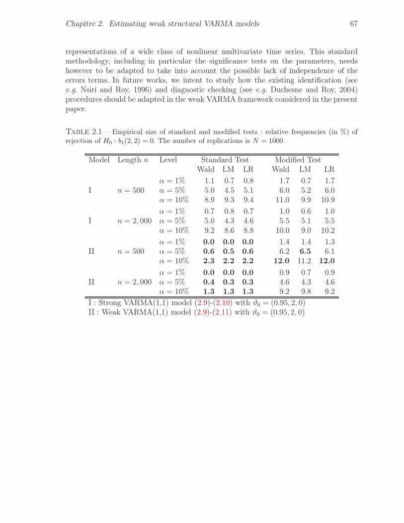
Chapitre 2. Estimating weak structural VARMA models 67
representations of a wide class of nonlinear multivariate time series. This standardmethodology, including in particular the significance tests on the parameters, needshowever to be adapted to take into account the possible lack of independence of theerrors terms. In future works, we intent to study how the existing identification (seee.g. Nsiri and Roy, 1996) and diagnostic checking (see e.g. Duchesne and Roy, 2004)procedures should be adapted in the weak VARMA framework considered in the presentpaper.
Table 2.1 – Empirical size of standard and modified tests : relative frequencies (in %) ofrejection of H0 : b1(2, 2) = 0. The number of replications is N = 1000.
Model Length n Level Standard Test Modified TestWald LM LR Wald LM LR
α = 1% 1.1 0.7 0.8 1.7 0.7 1.7I n = 500 α = 5% 5.0 4.5 5.1 6.0 5.2 6.0
α = 10% 8.9 9.3 9.4 11.0 9.9 10.9
α = 1% 0.7 0.8 0.7 1.0 0.6 1.0I n = 2, 000 α = 5% 5.0 4.3 4.6 5.5 5.1 5.5
α = 10% 9.2 8.6 8.8 10.0 9.0 10.2
α = 1% 0.0 0.0 0.0 1.4 1.4 1.3II n = 500 α = 5% 0.6 0.5 0.6 6.2 6.5 6.1
α = 10% 2.3 2.2 2.2 12.0 11.2 12.0
α = 1% 0.0 0.0 0.0 0.9 0.7 0.9II n = 2, 000 α = 5% 0.4 0.3 0.3 4.6 4.3 4.6
α = 10% 1.3 1.3 1.3 9.2 9.8 9.2
I : Strong VARMA(1,1) model (2.9)-(2.10) with ϑ0 = (0.95, 2, 0)II : Weak VARMA(1,1) model (2.9)-(2.11) with ϑ0 = (0.95, 2, 0)
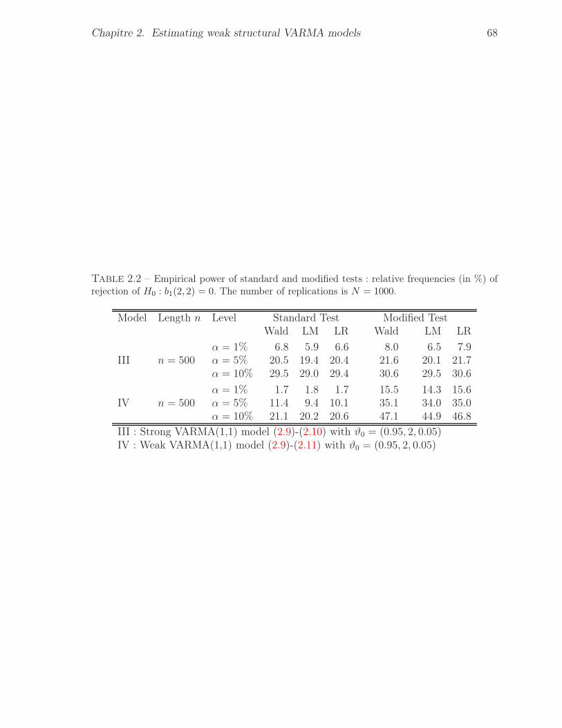
Chapitre 2. Estimating weak structural VARMA models 68
Table 2.2 – Empirical power of standard and modified tests : relative frequencies (in %) ofrejection of H0 : b1(2, 2) = 0. The number of replications is N = 1000.
Model Length n Level Standard Test Modified TestWald LM LR Wald LM LR
α = 1% 6.8 5.9 6.6 8.0 6.5 7.9III n = 500 α = 5% 20.5 19.4 20.4 21.6 20.1 21.7
α = 10% 29.5 29.0 29.4 30.6 29.5 30.6
α = 1% 1.7 1.8 1.7 15.5 14.3 15.6IV n = 500 α = 5% 11.4 9.4 10.1 35.1 34.0 35.0
α = 10% 21.1 20.2 20.6 47.1 44.9 46.8
III : Strong VARMA(1,1) model (2.9)-(2.10) with ϑ0 = (0.95, 2, 0.05)IV : Weak VARMA(1,1) model (2.9)-(2.11) with ϑ0 = (0.95, 2, 0.05)
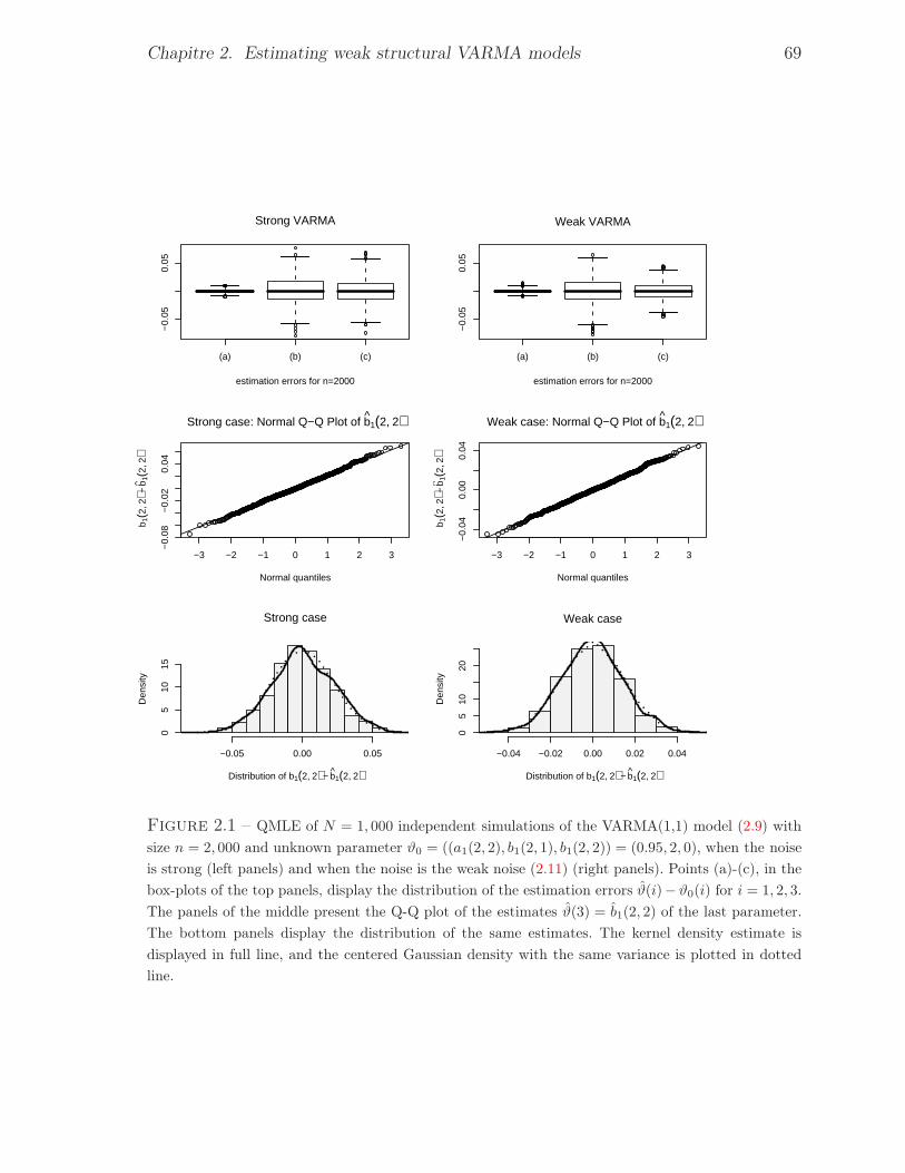
Chapitre 2. Estimating weak structural VARMA models 69
(a) (b) (c)
−0.
050.
05
estimation errors for n=2000
Strong VARMA
(a) (b) (c)
−0.
050.
05
estimation errors for n=2000
Weak VARMA
−3 −2 −1 0 1 2 3
−0.
08−
0.02
0.04
Normal quantiles
b 1(2
, 2)−
b 1(2
, 2)
Strong case: Normal Q−Q Plot of b1(2, 2)
−3 −2 −1 0 1 2 3
−0.
040.
000.
04
Normal quantiles
b 1(2
, 2)−
b 1(2
, 2)
Weak case: Normal Q−Q Plot of b1(2, 2)
Strong case
Distribution of b1(2, 2) − b1(2, 2)
Den
sity
−0.05 0.00 0.05
05
1015
Weak case
Distribution of b1(2, 2) − b1(2, 2)
Den
sity
−0.04 −0.02 0.00 0.02 0.04
05
1020
Figure 2.1 – QMLE of N = 1, 000 independent simulations of the VARMA(1,1) model (2.9) with
size n = 2, 000 and unknown parameter ϑ0 = ((a1(2, 2), b1(2, 1), b1(2, 2)) = (0.95, 2, 0), when the noise
is strong (left panels) and when the noise is the weak noise (2.11) (right panels). Points (a)-(c), in the
box-plots of the top panels, display the distribution of the estimation errors ϑ(i)−ϑ0(i) for i = 1, 2, 3.
The panels of the middle present the Q-Q plot of the estimates ϑ(3) = b1(2, 2) of the last parameter.
The bottom panels display the distribution of the same estimates. The kernel density estimate is
displayed in full line, and the centered Gaussian density with the same variance is plotted in dotted
line.
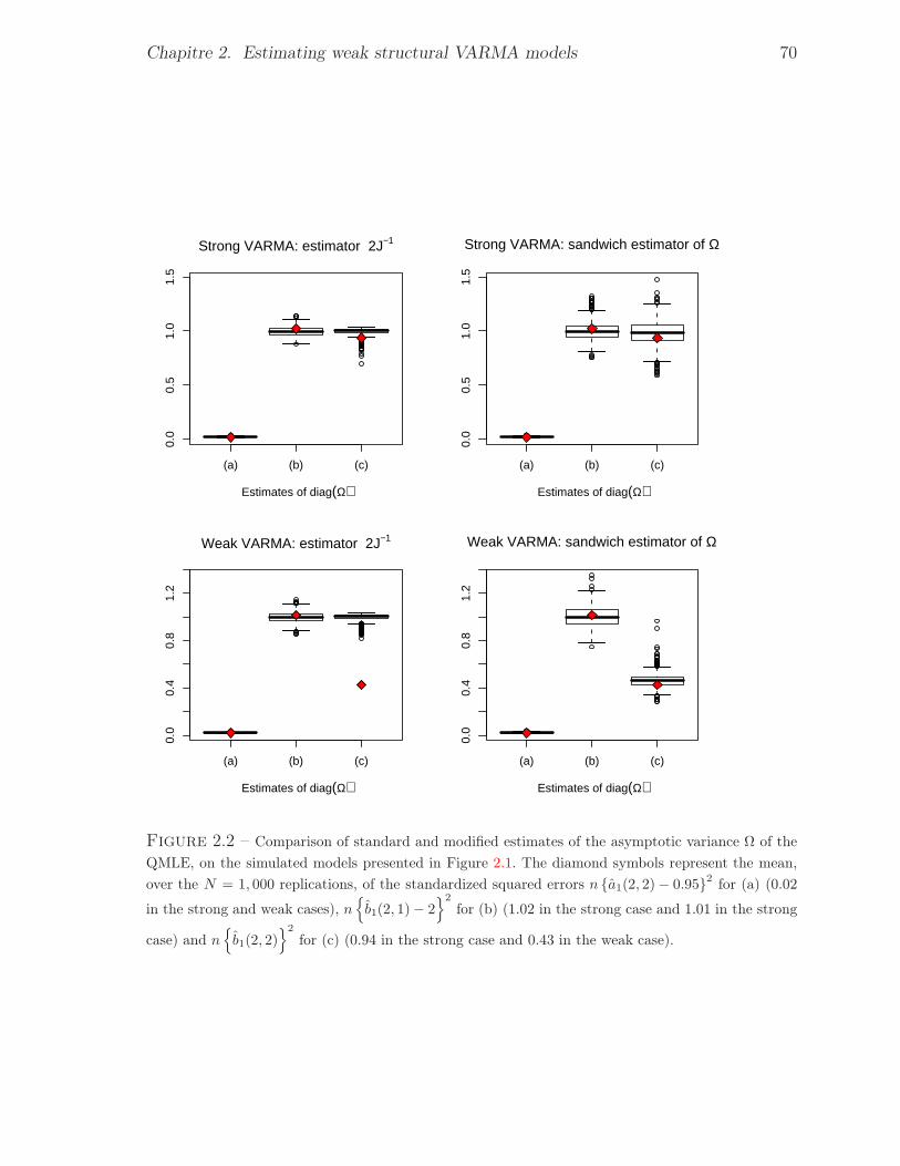
Chapitre 2. Estimating weak structural VARMA models 70
(a) (b) (c)
0.0
0.5
1.0
1.5
Estimates of diag(Ω)
Strong VARMA: estimator 2J−1
(a) (b) (c)0.
00.
51.
01.
5
Estimates of diag(Ω)
Strong VARMA: sandwich estimator of Ω
(a) (b) (c)
0.0
0.4
0.8
1.2
Estimates of diag(Ω)
Weak VARMA: estimator 2J−1
(a) (b) (c)
0.0
0.4
0.8
1.2
Estimates of diag(Ω)
Weak VARMA: sandwich estimator of Ω
Figure 2.2 – Comparison of standard and modified estimates of the asymptotic variance Ω of the
QMLE, on the simulated models presented in Figure 2.1. The diamond symbols represent the mean,
over the N = 1, 000 replications, of the standardized squared errors n a1(2, 2)− 0.952 for (a) (0.02
in the strong and weak cases), n
b1(2, 1)− 22
for (b) (1.02 in the strong case and 1.01 in the strong
case) and n
b1(2, 2)2
for (c) (0.94 in the strong case and 0.43 in the weak case).
Chapitre 2. Estimating weak structural VARMA models 71
2.7 Appendix of technical proofs
We begin with a lemma useful to show the identifiability of ϑ0.
Lemma 1. Assume that Σ0 is non singular and that A5 holds true. IfA−1
0 B0B−1ϑ (L)Aϑ(L)Xt = A−1
00 B00ǫt with probability one and A−10 B0ΣB
′0A
−1′0 =
A−100 B00Σ0B
′00A
−1′00 , then ϑ = ϑ0.
Proof : Let ϑ 6= ϑ0. Assumption A5 implies that either A−10 B0ΣB
′0A
−1′0 6=
A−100 B00Σ0B
′00A
−1′00 or there exist matrices Ci such that Ci0 6= 0 for some i0 > 0 and
A−10 B0B
−1ϑ (z)Aϑ(z)− A−1
00 B00B−1ϑ0
(z)Aϑ0(z) =
∞∑
i=i0
Cizi.
By contradiction, assume that A−10 B0B
−1ϑ (L)Aϑ(L)Xt = A−1
00 B00ǫt =A−1
00 B00B−1ϑ0
(L)Aϑ0(L)Xt with probability one. This implies that there exists λ 6= 0 suchthat λ′Xt−i0 is almost surely a linear combination of the components of Xt−i, i > i0.By stationarity, it follows that λ′Xt is almost surely a linear combination of thecomponents of Xt−i, i > 0. Thus λ′ǫt = 0 almost surely, which is impossible when thevariance Σ0 of ǫt is positive definite. 2
Proof of Theorem 2.1 : Note that, due to the initial conditions, et(ϑ) is notstationary, but can be approximated by the stationary ergodic process
et(ϑ) = A−10 B0B
−1ϑ (L)Aϑ(L)Xt. (2.12)
From an extension of Lemma 1 in FZ, it is easy to show that supϑ∈Θ ‖et(ϑ)− et(ϑ)‖ → 0almost surely at an exponential rate, as t→ ∞. We thus have
ℓn(ϑ)oP (1)= ℓn(ϑ) :=
1
n
n∑
t=1
lt(ϑ) as n→ ∞,
wherelt(ϑ) = d log(2π) + log det Σe + e′t(ϑ)Σ
−1e et(ϑ).
Now the ergodic theorem shows that almost surely
ℓn(ϑ) → d log(2π) +Q(ϑ),
where Q(ϑ) = log det Σe + Ee′1(ϑ)Σ−1e e1(ϑ). We have
Q(ϑ) = E e1(ϑ0)′ Σ−1e e1(ϑ0)+ log det Σe
+E e1(ϑ)− e1(ϑ0)′ Σ−1e e1(ϑ)− e1(ϑ0)
+2E e1(ϑ)− e1(ϑ0)′ Σ−1e e1(ϑ0).
Chapitre 2. Estimating weak structural VARMA models 72
The last expectation is null because the linear innovation et = et(ϑ0) is orthogonal tothe linear past (i.e. to the Hilbert space Ht−1 generated by linear combinations of theXu for u < t), and because et(ϑ)− et(ϑ0) belongs to this linear past Ht−1. Moreover
Q(ϑ0) = log det Σe0 + Ee′1(ϑ0)Σ−1e0 e1(ϑ0)
= log det Σe0 + TrΣ−1e0 Ee1(ϑ0)e
′1(ϑ0) = log det Σe0 + d.
ThusQ(ϑ)−Q(ϑ0) ≥ TrΣ−1
e Σe0 − log det Σ−1e Σe0 − d ≥ 0 (2.13)
using the elementary inequality Tr(A−1B) − log det(A−1B) ≥ Tr(A−1A) −log det(A−1A) = d for all symmetric positive semi-definite matrices of orderd × d. At least one of the two inequalities in (2.13) is strict, unless if e1(ϑ) = e1(ϑ0)with probability 1 and Σe = Σe0, which is equivalent to ϑ = ϑ0 by Lemma 1. Therest of the proof relies on standard compactness arguments, as in Theorem 1 of FZ. 2
Proof of Theorem 2.2 : In view of Theorem 2.1 and A6, we have almost surely
ϑn → ϑ0 ∈
Θ. Thus ∂ℓn(ϑn)/∂ϑ = 0 for sufficiently large n, and a Taylor expansiongives
0oP (1)=
√n∂ℓn(ϑ0)
∂ϑ+∂2ℓn(ϑ0)
∂ϑ∂ϑ′√n(
ϑn − ϑ0
)
, (2.14)
using arguments given in FZ (proof of Theorem 2). The proof then directly follows fromLemma 3 and Lemma 5 below. 2
We first state elementary derivative rules, which can be found in Appendix A.13 ofLütkepohl (1993).
Lemma 2. If f(A) is a scalar function of a matrix A whose elements aij are functionof a variable x, then
∂f(A)
∂x=∑
i,j
∂f(A)
∂aij
∂aij∂x
= Tr
∂f(A)
∂A′
∂A
∂x
. (2.15)
When A is invertible, we also have
∂ log |det(A)|∂A′
= A−1 (2.16)
∂Tr(CA−1B)
∂A′= −A−1BCA−1 (2.17)
∂Tr(CAB)
∂A′= BC (2.18)
Lemma 3. Under the assumptions of Theorem 2.2, almost surely
∂2ℓn(ϑ0)
∂ϑ∂ϑ′→ J,
where J is invertible.
Chapitre 2. Estimating weak structural VARMA models 73
Proof of Lemma 3 : Let ϑ = (ϑ1, . . . , ϑk0)′. In view of (2.15), (2.16) and (2.17),
for all i ∈ 1, . . . , k0, we have
∂lt(ϑ)
∂ϑi= Tr
Σ−1e
∂Σe
∂ϑi− Σ−1
e et(ϑ)e′t(ϑ)Σ
−1e
∂Σe
∂ϑi
+ 2∂e′t(ϑ)
∂ϑiΣ−1
e et(ϑ). (2.19)
Using the previous relations and (2.18), for all i, j ∈ 1, . . . , k0, we have
∂2lt(ϑ)
∂ϑi∂ϑj= Tr
Σ−1e
∂2Σe
∂ϑi∂ϑj− Σ−1
e
∂Σe
∂ϑiΣ−1
e
∂Σe
∂ϑj− Σ−1
e et(ϑ)e′t(ϑ)Σ
−1e
∂2Σe
∂ϑi∂ϑj
+Σ−1e
∂Σe
∂ϑiΣ−1
e et(ϑ)e′t(ϑ)Σ
−1e
∂Σe
∂ϑj+ Σ−1
e et(ϑ)e′t(ϑ)Σ
−1e
∂Σe
∂ϑiΣ−1
e
∂Σe
∂ϑj
−Σ−1e
∂Σe
∂ϑiΣ−1
e
∂et(ϑ)e′t(ϑ)
∂ϑj
+ 2∂2e′t(ϑ)
∂ϑi∂ϑjΣ−1
e et(ϑ)
+2∂e′t(ϑ)
∂ϑiΣ−1
e
∂et(ϑ)
∂ϑj− 2Tr
Σ−1e et(ϑ)
∂e′t(ϑ)
∂ϑiΣ−1
e
∂Σe
∂ϑj
. (2.20)
Using Eete′t = Σe, Eet = 0, the uncorrelatedness between et and the linear past Ht−1,∂et(ϑ0)/∂ϑi ∈ Ht−1, and ∂2et(ϑ0)/∂ϑi∂ϑj ∈ Ht−1, we have
E∂2lt(ϑ0)
∂ϑi∂ϑj= Tr
Σ−1e0
∂Σe(ϑ0)
∂ϑiΣ−1
e0
∂Σe(ϑ0)
∂ϑj
+ 2E∂e′t(ϑ0)
∂ϑiΣ−1
e0
∂et(ϑ0)
∂ϑj= J(i, j). (2.21)
The ergodic theorem and the next lemma conclude. 2
Lemma 4. Under the assumptions of Theorem 2.2, the matrix
J = E∂2lt(ϑ0)
∂ϑ∂ϑ′
is invertible.
Proof of Lemma 4 : In view of (2.21), we have J = J1 + J2, where
J2 = 2E∂e′t(ϑ0)
∂ϑΣ−1
e0
∂et(ϑ0)
∂ϑ′
and
J1(i, j) = Tr
Σ−1/2e0
∂Σe(ϑ0)
∂ϑiΣ
−1/2e0 Σ
−1/2e0
∂Σe(ϑ0)
∂ϑjΣ
−1/2e0
= h′ihj,
with
hi = (Σ−1/2e0 ⊗ Σ
−1/2e0 )di, di = vec
∂Σe(ϑ0)
∂ϑi.
In the previous derivations, we used the well-known relations Tr(A′B) = (vecA)′vecBand vec(ABC) = (C ′ ⊗ A)vecB. Note that the matrices J , J1 and J2 are semi-definite
Chapitre 2. Estimating weak structural VARMA models 74
positive. If J is singular, then there exists a vector c = (c1, . . . , ck0)′ 6= 0 such that
c′J1c = c
′J2c = 0. Since Σ−1/2e0 ⊗Σ
−1/2e0 and Σ−1
e0 are definite positive, we have c′J1c = 0
if and only ifk0∑
k=1
ckdk =
k0∑
k=1
ckvec∂Σe(ϑ0)
∂ϑk= 0 (2.22)
and c′J2c = 0 if and only if
∑k0k=1 ck
∂et(ϑ0)∂ϑk
= 0 a.s. Differentiating the two sides of thereduced form representation (2.3), the latter equation yields the VARMA(p− 1, q − 1)equation
∑pi=1A
∗iXt−i =
∑pj=1B
∗j et−j . The identifiability assumption A5 excludes the
existence of such a representation. Thus
A∗i =
k0∑
k=1
ck∂A−1
0 Ai
∂ϑk(ϑ0) = 0, B∗
j =
k0∑
k=1
ck∂A−1
0 BjB−10 A0
∂ϑk(ϑ0) = 0. (2.23)
It can be seen that (2.22) and (2.23), for i = 1, . . . , p and j = 1, . . . , q, are equivalent
to
Mϑ0 c = 0. We conclude from A8. 2
Lemma 5. Under the assumptions of Theorem 2.2,
√n∂ℓn(ϑ0)
∂ϑL→ N (0, I).
Proof of Lemma 5 : In view of (2.12), we have
∂et(ϑ0)
∂ϑi=
∞∑
ℓ=1
d′ℓet−ℓ, (2.24)
where the sequence of matrices dℓ = dℓ(i) is such that ‖dℓ‖ → 0 at a geometric rate asℓ→ ∞. By (2.19), we have for all m
∂lt(ϑ0)
∂ϑi= Tr
[
Σ−1e0
Id − ete
′tΣ
−1e0
∂Σe(ϑ0)
∂ϑi
]
+ 2∂e′t(ϑ0)
∂ϑiΣ−1
e0 et
= Yt,m,i + Zt,m,i
where
Yt,m,i = Tr
[
Σ−1e0
Id − ete
′tΣ
−1e0
∂Σe(ϑ0)
∂ϑi
]
+ 2m∑
ℓ=1
e′t−ℓd′ℓΣ
−1e0 et
Zt,m,i = 2∞∑
ℓ=m+1
e′t−ℓd′ℓΣ
−1e0 et.
Let Yt,m = (Yt,m,1, . . . , Yt,m,k0)′ and Zt,m = (Zt,m,1, . . . , Yt,m,k0)
′. The processes (Yt,m)tand (Zt,m)t are stationary and centered. Moreover, under Assumption A7 and m
Chapitre 2. Estimating weak structural VARMA models 75
fixed, the process Y = (Yt,m)t is strongly mixing, with mixing coefficients αY (h) ≤αǫ (max0, h−m). Applying the central limit theorem (CLT) for mixing processes(see Herrndorf, 1984) we directly obtain
1√n
n∑
t=1
Yt,mL→ N (0, Im), Im =
∞∑
h=−∞
Cov (Yt,m, Yt−h,m) .
As in FZ Lemma 3, one can show that I = limm→∞ Im exists. Since ‖Zt,m‖2 → 0 at anexponential rate when m → ∞, using the arguments given in FZ Lemma 4, one canshow that
limm→∞
lim supn→∞
P
∥∥∥∥∥n−1/2
n∑
t=1
Zt,m
∥∥∥∥∥> ε
= 0 (2.25)
for every ε > 0. From a standard result (see e.g. Brockwell and Davis, 1991, Proposition6.3.9), we deduce that
1√n
n∑
t=1
∂lt(ϑ0)
∂ϑ=
1√n
n∑
t=1
Yt,m +1√n
n∑
t=1
Zt,mL→ N (0, I),
which completes the proof. 2
Proof of Theorem 2.3 : Note that
ℓn(ϑ) =1
n
n∑
t=1
lt(ϑ), lt(ϑ) = d log(2π) + log det Σe + e′t(ϑ)Σ−1e et(ϑ).
Under the assumption of the theorem, ∂e′t(ϑ)/∂ϑ(2) = 0, and (2.19) yields
∂lt(ϑn)
∂ϑi= Tr
[
Σ−1e
Id − et(ϑ(1)n )e′t(ϑ
(1)n )Σ−1
e
∂Σe(ϑn)
∂ϑi
]
for i = k1 + 1, . . . k0, with Σe such that ϑ(2)n = D vec Σe. Assumption A6 entails thatthe first order condition ∂ℓn(ϑn)/∂ϑ(2) = 0 is satisfied for n large enough. We then have
Σe = n−1n∑
t=1
et(ϑ(1)n )e′t(ϑ
(1)n )
andℓn(ϑn) = d log(2π) + log det Σe + d,
because1
n
n∑
t=1
e′t(ϑ(1)n )Σ−1
e et(ϑ(1)n ) = Tr
[
1
n
n∑
t=1
et(ϑ(1)n )e′t(ϑ
(1)n )Σ−1
e
]
= d.
The conclusion follows. 2
Chapitre 2. Estimating weak structural VARMA models 76
2.8 Bibliography
Andrews, D.W.K. (1991) Heteroskedasticity and autocorrelation consistent cova-riance matrix estimation. Econometrica 59, 817–858.
Berk, K.N. (1974) Consistent Autoregressive Spectral Estimates. Annals of Statis-tics, 2, 489–502.
Brockwell, P.J. and Davis, R.A. (1991) Time series : theory and methods. Sprin-ger Verlag, New York.
den Hann, W.J. and Levin, A. (1997) A Practitioner’s Guide to Robust Cova-riance Matrix Estimation. In Handbook of Statistics 15, Rao, C.R. and G.S. Mad-dala (eds), 291–341.
Duchesne, P. and Roy, R. (2004) On consistent testing for serial correlation ofunknown form in vector time series models. Journal of Multivariate Analysis 89,148–180.
Dufour, J-M., and Pelletier, D. (2005) Practical methods for modelling weakVARMA processes : identification, estimation and specification with a macroe-conomic application. Technical report, Département de sciences économiques andCIREQ, Université de Montréal, Montréal, Canada.
Dunsmuir, W.T.M. and Hannan, E.J. (1976) Vector linear time series models,Advances in Applied Probability 8, 339–364.
Fan, J. and Yao, Q. (2003) Nonlinear time series : Nonparametric and parametricmethods. Springer Verlag, New York.
Francq, C. and Raïssi, H. (2007) Multivariate Portmanteau Test for Autoregres-sive Models with Uncorrelated but Nonindependent Errors, Journal of Time Se-ries Analysis 28, 454–470.
Francq, C., Roy, R. and Zakoïan, J-M. (2005) Diagnostic checking in ARMAModels with Uncorrelated Errors, Journal of the American Statistical Associa-tion 100, 532–544.
Francq, C. and Zakoïan, J-M. (1998) Estimating linear representations of nonli-near processes, Journal of Statistical Planning and Inference 68, 145–165.
Francq, and Zakoïan, J-M. (2005) Recent results for linear time series models withnon independent innovations. In Statistical Modeling and Analysis for ComplexData Problems, Chap. 12 (eds P. Duchesne and B. Rémillard). New York :Springer Verlag, 137–161.
Francq, and Zakoïan, J-M. (2007) HAC estimation and strong linearity testing inweak ARMA models, Journal of Multivariate Analysis 98, 114–144.
Hannan, E.J. (1976) The identification and parametrization of ARMAX and statespace forms, Econometrica 44, 713–723.
Hannan, E.J. and Deistler, M. (1988) The Statistical Theory of Linear SystemsJohn Wiley, New York.
Chapitre 2. Estimating weak structural VARMA models 77
Hannan, E.J., Dunsmuir, W.T.M. and Deistler, M. (1980) Estimation of vec-tor ARMAX models, Journal of Multivariate Analysis 10, 275–295.
Hannan, E.J. and Rissanen (1982) Recursive estimation of mixed of Autoregres-sive Moving Average order, Biometrika 69, 81–94.
Herrndorf, N. (1984) A Functional Central Limit Theorem for Weakly DependentSequences of Random Variables. The Annals of Probability 12, 141–153.
Imhof, J.P. (1961) Computing the distribution of quadratic forms in normal va-riables. Biometrika 48, 419–426.
Kascha, C. (2007) A Comparison of Estimation Methods for Vector Autore-gressive Moving-Average Models. ECO Working Papers, EUI ECO 2007/12,http ://hdl.handle.net/1814/6921.
Lütkepohl, H. (1993) Introduction to multiple time series analysis. Springer Verlag,Berlin.
Lütkepohl, H. (2005) New introduction to multiple time series analysis. SpringerVerlag, Berlin.
Newey, W.K., and West, K.D. (1987) A simple, positive semi-definite, heteros-kedasticity and autocorrelation consistent covariance matrix. Econometrica 55,703–708.
Nsiri, S., and Roy, R. (1996) Identification of refined ARMA echelon form modelsfor multivariate time series. Journal of Multivariate Analysis 56, 207–231.
Reinsel, G.C. (1997) Elements of multivariate time series Analysis. Second edition.Springer Verlag, New York.
Rissanen, J. and Caines, P.E. (1979) The strong consistency of maximum likeli-hood estimators for ARMA processes. Annals of Statistics 7, 297–315.
Romano, J.L. and Thombs, L.A. (1996) Inference for autocorrelations underweak assumptions, Journal of the American Statistical Association 91, 590–600.
Tong, H. (1990) Non-linear time series : A Dynamical System Approach, ClarendonPress Oxford.
van der Vaart, A.W. (1998) Asymptotic statistics, Cambridge University Press,Cambridge.
Wald, A. (1949) Note on the consistency of the maximum likelihood estimate. Annalsof Mathematical Statistics 20, 595–601.
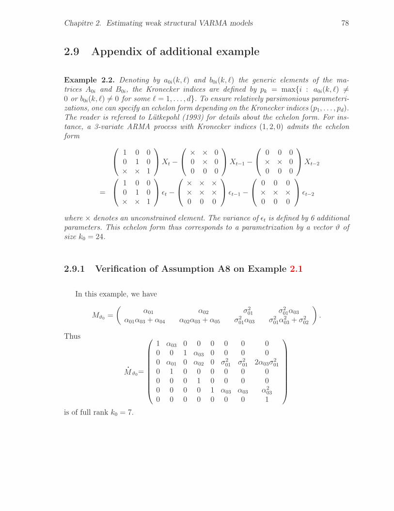
Chapitre 2. Estimating weak structural VARMA models 78
2.9 Appendix of additional example
Example 2.2. Denoting by a0i(k, ℓ) and b0i(k, ℓ) the generic elements of the ma-trices A0i and B0i, the Kronecker indices are defined by pk = maxi : a0i(k, ℓ) 6=0 or b0i(k, ℓ) 6= 0 for some ℓ = 1, . . . , d. To ensure relatively parsimonious parameteri-zations, one can specify an echelon form depending on the Kronecker indices (p1, . . . , pd).The reader is refereed to Lütkepohl (1993) for details about the echelon form. For ins-tance, a 3-variate ARMA process with Kronecker indices (1, 2, 0) admits the echelonform
1 0 00 1 0× × 1
Xt −
× × 00 × 00 0 0
Xt−1 −
0 0 0× × 00 0 0
Xt−2
=
1 0 00 1 0× × 1
ǫt −
× × ×× × ×0 0 0
ǫt−1 −
0 0 0× × ×0 0 0
ǫt−2
where × denotes an unconstrained element. The variance of ǫt is defined by 6 additionalparameters. This echelon form thus corresponds to a parametrization by a vector ϑ ofsize k0 = 24.
2.9.1 Verification of Assumption A8 on Example 2.1
In this example, we have
Mϑ0 =
(α01 α02 σ2
01 σ201α03
α01α03 + α04 α02α03 + α05 σ201α03 σ2
01α203 + σ2
02
)
.
Thus
Mϑ0=
1 α03 0 0 0 0 0 00 0 1 α03 0 0 0 00 α01 0 α02 0 σ2
01 σ201 2α03σ
201
0 1 0 0 0 0 0 00 0 0 1 0 0 0 00 0 0 0 1 α03 α03 α2
03
0 0 0 0 0 0 0 1
is of full rank k0 = 7.
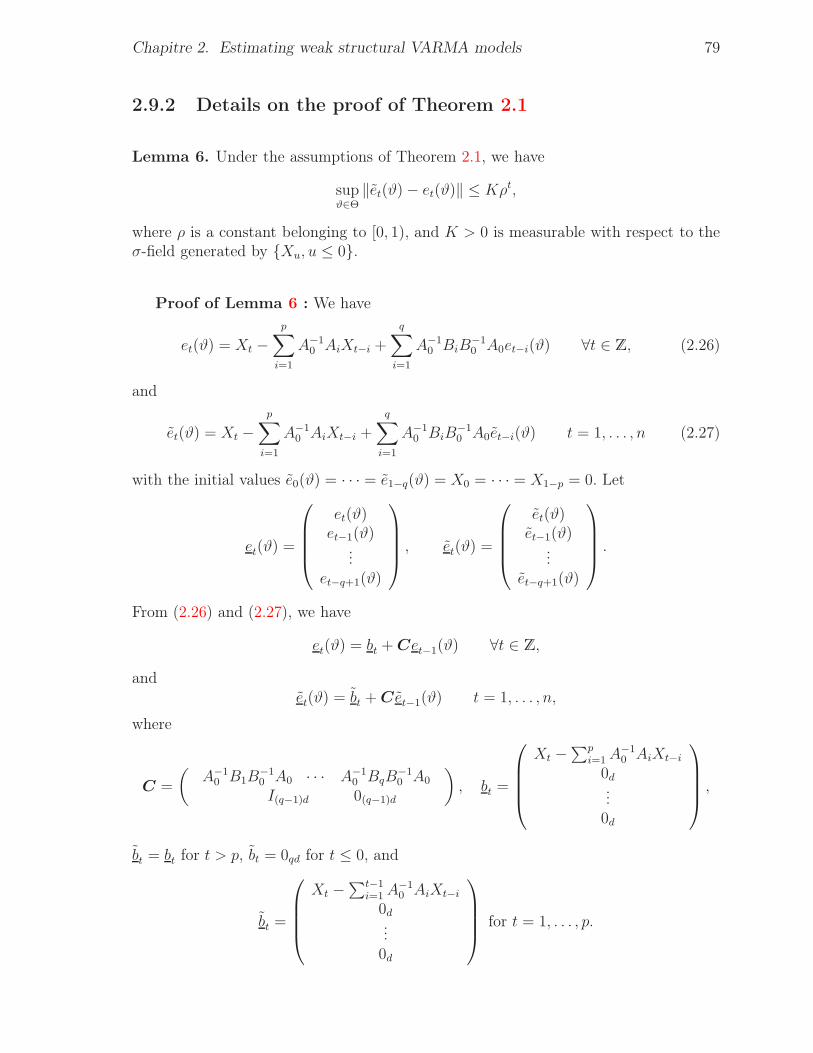
Chapitre 2. Estimating weak structural VARMA models 79
2.9.2 Details on the proof of Theorem 2.1
Lemma 6. Under the assumptions of Theorem 2.1, we have
supϑ∈Θ
‖et(ϑ)− et(ϑ)‖ ≤ Kρt,
where ρ is a constant belonging to [0, 1), and K > 0 is measurable with respect to theσ-field generated by Xu, u ≤ 0.
Proof of Lemma 6 : We have
et(ϑ) = Xt −p∑
i=1
A−10 AiXt−i +
q∑
i=1
A−10 BiB
−10 A0et−i(ϑ) ∀t ∈ Z, (2.26)
and
et(ϑ) = Xt −p∑
i=1
A−10 AiXt−i +
q∑
i=1
A−10 BiB
−10 A0et−i(ϑ) t = 1, . . . , n (2.27)
with the initial values e0(ϑ) = · · · = e1−q(ϑ) = X0 = · · · = X1−p = 0. Let
et(ϑ) =
et(ϑ)et−1(ϑ)
...et−q+1(ϑ)
, et(ϑ) =
et(ϑ)et−1(ϑ)
...et−q+1(ϑ)
.
From (2.26) and (2.27), we have
et(ϑ) = bt +Cet−1(ϑ) ∀t ∈ Z,
andet(ϑ) = bt +C et−1(ϑ) t = 1, . . . , n,
where
C =
(A−1
0 B1B−10 A0 · · · A−1
0 BqB−10 A0
I(q−1)d 0(q−1)d
)
, bt =
Xt −∑p
i=1A−10 AiXt−i
0d...0d
,
bt = bt for t > p, bt = 0qd for t ≤ 0, and
bt =
Xt −∑t−1
i=1A−10 AiXt−i
0d...0d
for t = 1, . . . , p.
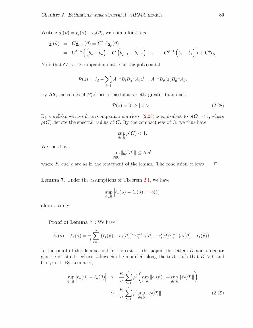
Chapitre 2. Estimating weak structural VARMA models 80
Writing dt(ϑ) = et(ϑ)− et(ϑ), we obtain for t > p,
dt(ϑ) = Cdt−1(ϑ) = Ct−pdp(ϑ)
= Ct−p(
bp − bp
)
+C
(
bp−1 − bp−1
)
+ · · ·+Cp−1(
b1 − b1
)
+Cpb0.
Note that C is the companion matrix of the polynomial
P(z) = Id −q∑
i=1
A−10 BiB
−10 A0z
i = A−10 Bϑ(z)B
−10 A0.
By A2, the zeroes of P(z) are of modulus strictly greater than one :
P(z) = 0 ⇒ |z| > 1 (2.28)
By a well-known result on companion matrices, (2.28) is equivalent to ρ(C) < 1, whereρ(C) denote the spectral radius of C. By the compactness of Θ, we thus have
supϑ∈Θ
ρ(C) < 1.
We thus havesupϑ∈Θ
‖dt(ϑ)‖ ≤ Kρt,
where K and ρ are as in the statement of the lemma. The conclusion follows. 2
Lemma 7. Under the assumptions of Theorem 2.1, we have
supϑ∈Θ
∣∣∣ℓn(ϑ)− ℓn(ϑ)
∣∣∣ = o(1)
almost surely.
Proof of Lemma 7 : We have
ℓn(ϑ)− ℓn(ϑ) =1
n
n∑
t=1
et(ϑ)− et(ϑ)′Σ−1e et(ϑ) + e′t(ϑ)Σ
−1e et(ϑ)− et(ϑ) .
In the proof of this lemma and in the rest on the paper, the letters K and ρ denotegeneric constants, whose values can be modified along the text, such that K > 0 and0 < ρ < 1. By Lemma 6,
supϑ∈Θ
∣∣∣ℓn(ϑ)− ℓn(ϑ)
∣∣∣ ≤ K
n
n∑
t=1
ρt(
supϑ∈Θ
‖et(ϑ)‖+ supϑ∈Θ
‖et(ϑ)‖)
≤ K
n
n∑
t=1
ρt supϑ∈Θ
‖et(ϑ)‖ (2.29)
Chapitre 2. Estimating weak structural VARMA models 81
In view of (2.26), and using A1 and the compactness of Θ, we have
et(ϑ) = Xt +
∞∑
i=1
Ci(ϑ)Xt−i, supϑ∈Θ
‖Ci(ϑ)‖ ≤ Kρi. (2.30)
We thus have E supϑ∈Θ ‖et(ϑ)‖ <∞, and the Markov inequality entails
∞∑
t=1
P
(
ρt supϑ∈Θ
‖et(ϑ)‖ > ε
)
≤ E supϑ∈Θ
‖et(ϑ)‖∞∑
t=1
ρt
ε<∞.
By the Borel-Cantelli theorem, ρt supϑ∈Θ ‖et(ϑ)‖ → 0 almost surely as t → ∞. TheCesàro theorem implies that the right-hand side of (2.29) converges to zero almostsurely. 2
Lemma 8. Under the assumptions of Theorem 2.1, any ϑ 6= ϑ0 has a neighborhoodV (ϑ) such that
lim infn→∞
infϑ∗∈V (ϑ)
ℓn(ϑ∗) > El1(ϑ0), a.s. (2.31)
Moreover for any neighborhood V (ϑ0) of ϑ0 we have
lim supn→∞
infϑ∗∈V (ϑ0)
ℓn(ϑ∗) ≤ El1(ϑ0), a.s. (2.32)
Proof of Lemma 8 : For any ϑ ∈ Θ and any positive integer k, let Vk(ϑ) be theopen ball with center ϑ and radius 1/k. Using Lemma 7, we have
lim infn→∞
infϑ∗∈Vk(ϑ)∩Θ
ℓn(ϑ∗) ≥ lim inf
n→∞inf
ϑ∗∈Vk(ϑ)∩Θℓn(ϑ
∗)− lim supn→∞
supϑ∈Θ
|ℓn(ϑ)− ℓn(ϑ)|
≥ lim infn→∞
n−1n∑
t=1
infϑ∗∈Vk(ϑ)∩Θ
lt(ϑ∗)
= E infϑ∗∈Vk(ϑ)∩Θ
l1(ϑ∗)
For the last equality we applied the ergodic theorem to the ergodic stationary pro-cess
infϑ∗∈Vk(ϑ)∩Θ ℓt(ϑ
∗)
t. By the Beppo-Levi theorem, when k increases to ∞,
E infϑ∗∈Vk(ϑ)∩Θ l1(ϑ∗) increases to El1(ϑ). Because El1(ϑ) = d log(2π) + Q(ϑ), the dis-
cussion which follows (2.13) entails El1(ϑ) > El1(ϑ0), and (2.31) follows.
To show (2.32), it suffices to remark that Lemma 7 and the ergodic theorem entail
lim supn→∞
infϑ∗∈V (ϑ)∩Θ
ℓn(ϑ∗) ≤ lim sup
n→∞inf
ϑ∗∈V (ϑ)∩Θℓn(ϑ
∗) + lim supn→∞
supϑ∈Θ
|ℓn(ϑ)− ℓn(ϑ)|
≤ lim supn→∞
n−1n∑
t=1
lt(ϑ0)
= El1(ϑ0).
Chapitre 2. Estimating weak structural VARMA models 82
2
The proof of Theorem 2.1 is completed by the arguments of Wald (1949). Moreprecisely, the compact set Θ is covered by a neighborhood V (ϑ0) of ϑ0 and a finitenumber of neighborhoods V (ϑ1), . . . , V (ϑk) satisfying (2.31) with ϑ replaced by ϑi,i = 1, . . . , k. In view of (2.31) and (2.32), we have almost surely
infϑ∈Θ
ℓn(ϑ) = mini=0,1,...,k
infϑ∈V (ϑi)∩Θ
ℓn(ϑ) = infϑ∈V (ϑ0)∩Θ
ℓn(ϑ)
for n large enough. Since the neighborhood V (ϑ0) can be chosen arbitrarily small, theconclusion follows.
2.9.3 Details on the proof of Theorem 2.2
Lemma 9. Under the assumptions of Theorem 2.2, we have
√n sup
ϑ∈Θ
∥∥∥∥∥
∂ℓn(ϑ)
∂ϑ− ∂ℓn(ϑ)
∂ϑ
∥∥∥∥∥= oP (1).
Proof of Lemma 9 : Similar to (2.30), Assumption A1 entails that, for k =1, . . . , k0,
∂et(ϑ)
∂ϑk=
∞∑
i=1
C(k)i (ϑ)Xt−i,
∂et(ϑ)
∂ϑk=
t−1∑
i=1
C(k)i (ϑ)Xt−i, (2.33)
C(k)i (ϑ) =
∂Ci(ϑ)
∂ϑk, sup
ϑ∈Θ
∥∥∥C
(k)i (ϑ)
∥∥∥ ≤ Kρi. (2.34)
Similar to Lemma 6, we then have
supϑ∈Θ
∥∥∥∥
∂et(ϑ)
∂ϑ′− ∂et(ϑ)
∂ϑ′
∥∥∥∥≤ Kρt. (2.35)
Using (2.19), we have
√n
∂ℓn(ϑ)
∂ϑk− ∂ℓn(ϑ)
∂ϑk
= a1 + a2,
with
a1 =2√n
n∑
t=1
(∂e′t(ϑ)
∂ϑk− ∂e′t(ϑ)
∂ϑk
)
Σ−1e et(ϑ) +
∂e′t(ϑ)
∂ϑkΣ−1
e (et(ϑ)− et(ϑ))
a2 = Tr
(
Σ−1e
[et(ϑ)− et(ϑ) e′t(ϑ) + et(ϑ) et(ϑ)− et(ϑ)′
]Σ−1
e
∂Σe
∂ϑk
)
.
Chapitre 2. Estimating weak structural VARMA models 83
From Lemma 6 and (2.35), it follows that
|a1|+ |a2| ≤K√n
n∑
t=1
bt, bt = ρt
supϑ∈Θ
∥∥∥∥
∂et(ϑ)
∂ϑk
∥∥∥∥+ sup
ϑ∈Θ‖et(ϑ)‖ +Kρt
.
In view of (2.30) and (2.33)-(2.34), we have
E supϑ∈Θ
∥∥∥∥
∂et(ϑ)
∂ϑk
∥∥∥∥<∞, E sup
ϑ∈Θ‖et(ϑ)‖ <∞.
By the Markov inequality, for all ε > 0 we thus have
P
(
K√n
n∑
t=1
bt > ε
)
≤ K
ε√n
n∑
t=1
ρt → 0,
and the conclusion follows. 2
Lemma 10. Under the assumptions of Theorem 2.2, (2.14) holds, that is
0oP (1)=
√n∂ℓn(ϑ0)
∂ϑ+∂2ℓn(ϑ0)
∂ϑ∂ϑ′√n(
ϑn − ϑ0
)
.
Proof of Lemma 10 : By Lemma 9 and already given arguments, we have
0 =√nℓn(ϑn)
∂ϑ=
√nℓn(ϑn)
∂ϑ+√nℓn(ϑn)
∂ϑ−√
nℓn(ϑn)
∂ϑ
oP (1)=
√nℓn(ϑn)
∂ϑ.
Taylor expansions of the functions ∂ℓn(·)/∂ϑi around ϑ0 give
√nℓn(ϑn)
∂ϑ=
√n∂ℓn(ϑ0)
∂ϑ+
[∂2ℓn(ϑ
∗i )
∂ϑi∂ϑj
]√n(
ϑn − ϑ0
)
,
for some ϑ∗i between ϑn and ϑ0.
From (2.20) and Lemma 2, one can see that the random terms involved in
∂3lt(ϑ)
∂ϑk1∂ϑk2∂ϑk3
are linear combinations of the elements of the following matrices
et(ϑ)e′t(ϑ), et(ϑ)
∂e′t(ϑ)
∂ϑki, et(ϑ)
∂2e′t(ϑ)
∂ϑki∂ϑkj,
∂et(ϑ)
∂ϑki
∂e′t(ϑ)
∂ϑkj,
∂et(ϑ)
∂ϑki
∂2e′t(ϑ)
∂ϑkj∂ϑkℓ, et(ϑ)
∂3e′t(ϑ)
∂ϑki∂ϑkj∂ϑkℓ.
Chapitre 2. Estimating weak structural VARMA models 84
Since all these matrices have finite expectations uniformly in ϑ ∈ Θ, we have
E supϑ∈Θ
∣∣∣∣
∂3lt(ϑ)
∂ϑk1∂ϑk2∂ϑk3
∣∣∣∣<∞ (2.36)
for all k1, k2, k3 ∈ 1, . . . , k0. Now a second Taylor expansion yields
∂2ℓn(ϑ∗i )
∂ϑi∂ϑj=
∂2ℓn(ϑ0)
∂ϑi∂ϑj+
∂
∂ϑ′
∂2ℓn(ϑ
∗)
∂ϑi∂ϑj
(ϑ∗i − ϑ0)
=∂2ℓn(ϑ0)
∂ϑi∂ϑj+ o(1) a.s.
using the ergodic theorem, (2.36) and the almost sure convergence of ϑ∗i to ϑ0. Theproof is complete. 2
Now we need the following covariance inequality obtained by Davydov (1968). 2
Lemma 11 (Davydov (1968)). Let p, q and r three positive numbers such that p−1 +q−1 + r−1 = 1. Davydov (1968) showed that
|Cov(X, Y )| ≤ K0‖X‖p‖Y ‖q [α σ(X), σ(Y )]1/r , (2.37)
where ‖X‖pp = EXp, K0 is an universal constant, and α σ(X), σ(Y ) denotes thestrong mixing coefficient between the σ-fields σ(X) and σ(Y ) generated by the randomvariables X and Y , respectively.
Lemma 12. Under the assumptions of Theorem 2.2, (2.25) holds, that is
limm→∞
lim supn→∞
P
∥∥∥∥∥n−1/2
n∑
t=1
Zt,m
∥∥∥∥∥> ε
= 0.
Proof of Lemma 12 : For i = 1, . . . , k0, by stationarity we have
var
(
1√n
n∑
t=1
Zt,m,i
)
=1
n
n∑
t,s=1
Cov(Zt,m,i, Zs,m,i)
=1
n
∑
|h|<n
(n− |h|)Cov(Zt,m,i, Zt−h,m,i)
≤∞∑
h=−∞
|Cov(Zt,m,i, Zt−h,m,i)| .
Because ‖dℓ‖ ≤ Kρℓ, we have
|Zt,m,i| ≤ K
∞∑
ℓ=m+1
ρℓ‖et‖‖et−ℓ‖.
2. Davydov, Y. A. (1968) Convergence of Distributions Generated by Stationary StochasticProcesses. Theory of Probability and Applications 13, 691–696.
Chapitre 2. Estimating weak structural VARMA models 85
Using also E‖et‖4 <∞, it follows from the Hölder inequality that
suph
|Cov(Zt,m,i, Zt−h,m,i)| = suph
|EZt,m,iZt−h,m,i| ≤ Kρm. (2.38)
Let h > 0 such that [h/2] > m. Write
Zt,m,i = Zh−t,m,i + Zh+
t,m,i,
where
Zh−t,m,i = 2
[h/2]∑
ℓ=m+1
e′t−ℓd′ℓΣ
−1e0 et, Zh+
t,m,i = 2
∞∑
ℓ=[h/2]+1
e′t−ℓd′ℓΣ
−1e0 et.
Note that Zh−t,m,i belongs to the σ-field generated by et, et−1, . . . , et−[h/2] and that
Zt−h,m,i belongs to the σ-field generated by et−h, et−h−1, . . .. Note also that αe(·) =αǫ(·) and that, by A7, E|Zh−
t,m,i|2+ν < ∞ and E|Zt−h,m,i|2+ν < ∞. Lemma 11 thenentails that ∣
∣∣Cov(Zh−
t,m,i, Zt−h,m,i)∣∣∣ ≤ Kαν/(2+ν)
ǫ ([h/2]). (2.39)
By the argument used to show (2.38), we also have∣∣∣Cov(Zh+
t,m,i, Zt−h,m,i)∣∣∣ ≤ Kρhρm. (2.40)
In view of (2.38), (2.39) and (2.40),∞∑
h=0
|Cov(Zt,m,i, Zt−h,m,i)| ≤ Kρm +K∞∑
h=m
αν/(2+ν)ǫ (h) → 0
as m → ∞ by A7. We have the same bound for h < 0. The conclusion follows fromthe Markov inequality. 2
Lemma 13. Let the assumptions of Theorem 2.2 be satisfied. For ϑ ∈ Θ, the matrix
I(ϑ) = limn→∞
Var∂
∂ϑℓn(ϑ),
exists.
Proof of Lemma 13 : Let
lt =∂
∂ϑlt(ϑ) =
(∂
∂ϑ1lt(ϑ), . . . ,
∂
∂ϑk0lt(ϑ)
)′
. (2.41)
By stationarity of(
lt
)
t, we have
var
(∂
∂ϑℓn(ϑ)
)
= var
(
1√n
n∑
t=1
lt
)
=1
n
n∑
t,s=1
Cov(
lt, ls
)
=1
n
n−1∑
h=−n+1
(n− |h|)Cov(
lt, lt−h
)
.
Chapitre 2. Estimating weak structural VARMA models 86
By the dominated convergence theorem, it follows that I(ϑ) exists and is given by
I(ϑ) =
∞∑
h=−∞
Cov(
lt, lt−h
)
whenever∞∑
h=−∞
∥∥∥Cov
(
lt, lt−h
)∥∥∥ <∞. (2.42)
Recall that, for all i ∈ 1, . . . , k0 we have
∂lt(ϑ)
∂ϑi= Tr
[
Σ−1e
Id − et(ϑ)e
′t(ϑ)Σ
−1e
∂Σe(ϑ)
∂ϑi
]
+ 2∂e′t(ϑ)
∂ϑiΣ−1
e et(ϑ)
= Tr
[
Σ−1e
Id − et(ϑ)e
′t(ϑ)Σ
−1e
∂Σe(ϑ)
∂ϑi
]
+ 2∞∑
ℓ=1
e′t−ℓ(ϑ)d′ℓΣ
−1e et(ϑ).
In view of the last equality, the i-th component of lt is of the form
li t =
∞∑
ℓ=0
d∑
k1,k2=1
αℓ(i, k1, k2)ek1 t(ϑ)ek2 t−ℓ(ϑ) (2.43)
where|αℓ(i, k1, k2)| ≤ Kρℓ, (2.44)
uniformly in (i, k1, k2) ∈ 1, . . . , k0 × 1, . . . , d2. In order to obtain (2.42), it sufficesto show that
∞∑
h=−∞
∣∣∣Cov
(
li t, lj t−h
)∣∣∣ <∞ (2.45)
for all (i, j) ∈ 1, . . . , k02. In view of (2.43) and (2.44), we have for h ≥ 0
∣∣∣Cov
(
li t, lj t−h
)∣∣∣ ≤ c1 + c2,
where
c1 = K
∞∑
ℓ=[h/2]+1
∞∑
ℓ′=0
d∑
k1,...,k4=1
ρℓ+ℓ′ |Cov (ek1t(ϑ)ek2t−ℓ(ϑ), ek3t−h(ϑ)ek4t−ℓ′−h(ϑ))|
and
c2 = K
[h/2]∑
ℓ=0
∞∑
ℓ′=0
d∑
k1,...,k4=1
ρℓ+ℓ′ |Cov (ek1 t(ϑ)ek2 t−ℓ(ϑ), ek3 t−h(ϑ)ek4 t−ℓ′−h(ϑ))| .
Because
|Cov (ek1 t(ϑ)ek2 t−ℓ(ϑ), ek3 t−h(ϑ)ek4 t−ℓ′−h(ϑ))| ≤ E ‖et(ϑ)‖4 <∞
Chapitre 2. Estimating weak structural VARMA models 87
by Assumption A7, we havec1 ≤ Kρh.
Lemma 11 entails that
c2 ≤ K
[h/2]∑
ℓ=0
∞∑
ℓ′=0
ρℓ+ℓ′αν/(2+ν)ǫ ([h/2]) ≤ Kαν/(2+ν)
ǫ ([h/2]) .
It follows that
∞∑
h=0
∣∣∣Cov
(
li t, lj t−h
)∣∣∣ ≤ K
∞∑
h=0
ρh +K
∞∑
h=0
αν/(2+ν)ǫ ([h/2]) <∞
by Assumption A7. The same bounds clearly holds for
0∑
h=−∞
∣∣∣Cov
(
li t, lj t−h
)∣∣∣ ,
which shows (2.45) and completes the proof. 2
Chapitre 3
Estimating the asymptotic variance ofLS estimator of VARMA models withuncorrelated but non-independenterror terms
Abstract We consider the problems of estimating the asymptotic variance of theleast squares (LS) and/ or quasi-maximum likelihood (QML) estimators of vector auto-regressive moving-average (VARMA) models under the assumption that the errors areuncorrelated but not necessarily independent. We relax the standard independence as-sumption to extend the range of application of the VARMA models, and allow to coverlinear representations of general nonlinear processes. We first give expressions for thederivatives of the VARMA residuals in terms of the parameters of the models. Secondlywe give an explicit expression of the asymptotic variance of the QML/LS estimator, interms of the VAR and MA polynomials, and of the second and fourth-order structure ofthe noise. We deduce a consistent estimator of the asymptotic variance of the QML/LSestimator.
Keywords : QMLE/LSE, residuals derivatives, Structural representation, weak VARMA
models.
3.1 Introduction
The class of vector autoregressive moving-average (VARMA) models and the sub-class of vector autoregressive (VAR) models are used in time series analysis and eco-nometrics to describe not only the properties of the individual time series but also the
Chapitre 3. Estimating the asymptotic variance of LSE of weak VARMA models 89
possible cross-relationships between the time series (see Reinsel, 1997, Lütkepohl, 2005,1993). This paper is devoted to the problems of estimating the asymptotic variance ofthe least squares (LS) and/ or quasi-maximum likelihood (QML) estimators of VARMAmodels under the assumption that the errors are uncorrelated but not necessarily inde-pendent (i.e. weak VARMA models). A process X = (Xt) is said to be nonlinear whenthe innovation process in the Wold decomposition (see e.g. Brockwell and Davis, 1991,for the univariate case, and Reinsel, 1997, in the multivariate framework) is uncorrela-ted but not necessarily independent, and is said to be linear in the opposite case (i.e.when the innovation process in the Wold decomposition is iid). We relax the standardindependence assumption to extend the range of application of the VARMA models,and allow to cover linear representations of general nonlinear processes.
The estimation of weak VARMA models has been studied in Boubacar Mainassaraand Francq (2009). They showed that the asymptotic variance of the usual estimatorshas the "sandwich" form Ω = J−1IJ−1, which reduces to the standard form Ω = J−1 inthe linear case. They used an empirical estimator of the matrix J . To obtain a consistentestimator of the matrix I, they used a nonparametric kernel estimator, also calledheteroscedastic autocorrelation consistent (HAC) estimator (see Newey and West, 1987,or Andrews, 1991) and they also used an alternative method based on a parametric ARestimate of a spectral density at frequency 0 (see Brockwell and Davis, 1991, p. 459). Theasymptotic theory of weak ARMA model is mainly limited to the univariate framework(see Francq and Zakoïan, 2005, for a review of this topic). In the multivariate analysis,notable exceptions are Dufour and Pelletier (2005) who study the asymptotic propertiesof a generalization of the regression-based estimation method proposed by Hannan andRissanen (1982) under weak assumptions on the innovation process, Francq and Raïssi(2007) who study portmanteau tests for weak VAR models and Boubacar Mainassara(in a working paper, 2009) who studies portmanteau tests for weak VARMA models.The main goal of the present article is to complete the available results concerningthe statistical analysis of weak VARMA models, by proposing another estimator of Ω,which allows to separate the effects due to the VARMA parameters from those dueto the nonlinear structure of the noise. This topic has not been studied in the above-mentioned papers.
The paper is organized as follows. Section 3.2 presents the models that we considerhere, and presents the results on the QMLE/LSE asymptotic distribution obtained byBoubacar Mainassara and Francq (2009). In Section 3.3 we give expressions for thederivatives of the VARMA residuals in terms of parameters of the models. Section 3.4is devoted to find an explicit expression of the asymptotic variance of the QML/LSestimator, in terms of the VAR and MA polynomials, and of the second and fourth-order structure of the noise. In Section 3.5 we deduce a consistent estimator of thisasymptotic variance. The proofs of the main results are collected in the appendix. Wedenote by A ⊗ B the Kronecker product of two matrices A and B (and by A⊗2 whenthe matrix A = B), and by vecA the vector obtained by stacking the columns of A. Thereader is refereed to Magnus and Neudecker (1988) for the properties of these operators.
Chapitre 3. Estimating the asymptotic variance of LSE of weak VARMA models 90
Let 0r be the null vector of Rr, and let Ir be the r × r identity matrix.
3.2 Model and assumptions
Consider a d-dimensional stationary process (Xt) satisfying a structuralVARMA(p, q) representation of the form
A00Xt −p∑
i=1
A0iXt−i = B00ǫt −q∑
i=1
B0iǫt−i, ∀t ∈ Z = 0,±1, . . ., (3.1)
where ǫt is a white noise, namely a stationary sequence of centered and uncorrelatedrandom variables with a non singular variance Σ0. The structural forms are mainly usedin econometrics to introduce instantaneous relationships between economic variables.Of course, constraints are necessary for the identifiability of these representations. Let[A00 . . . A0pB00 . . . B0q] be the d × (p + q + 2)d matrix of all the coefficients, withoutany constraint. The matrix Σ0 is considered as a nuisance parameter. The parameter ofinterest is denoted θ0, where θ0 belongs to the parameter space Θ ⊂ R
k0 , and k0 is thenumber of unknown parameters, which is typically much smaller that (p+q+2)d2. Thematrices A00, . . . , A0p, B00, . . . , B0q involved in (3.1) are specified by θ0. More precisely,we write A0i = Ai(θ0) and B0j = Bj(θ0) for i = 0, . . . , p and j = 0, . . . , q, and Σ0 =Σ(θ0). We need the following assumptions used by Boubacar Mainassara and Francq(2009) to ensure the consistence and the asymptotic normality of the quasi-maximumlikelihood estimator (QMLE).
A1 : The applications θ 7→ Ai(θ) i = 0, . . . , p, θ 7→ Bj(θ) j = 0, . . . , q andθ 7→ Σ(θ) admit continuous third order derivatives for all θ ∈ Θ.
For simplicity we now write Ai, Bj and Σ instead of Ai(θ), Bj(θ) and Σ(θ). Let Aθ(z) =A0 −
∑pi=1Aiz
i and Bθ(z) = B0 −∑q
i=1Bizi.
A2 : For all θ ∈ Θ, we have detAθ(z) detBθ(z) 6= 0 for all |z| ≤ 1.
A3 : We have θ0 ∈ Θ, where Θ is compact.
A4 : The process (ǫt) is stationary and ergodic.
A5 : For all θ ∈ Θ such that θ 6= θ0, either the transfer functions
A−10 B0B
−1θ (z)Aθ(z) 6= A−1
00 B00B−1θ0
(z)Aθ0(z)
for some z ∈ C, or
A−10 B0ΣB
′0A
−1′0 6= A−1
00 B00Σ0B′00A
−1′00 .
A6 : We have θ0 ∈
Θ, where
Θ denotes the interior of Θ.
Chapitre 3. Estimating the asymptotic variance of LSE of weak VARMA models 91
A7 : We have E‖ǫt‖4+2ν <∞ and∑∞
k=0 αǫ(k)ν
2+ν <∞ for some ν > 0.
The reader is referred to Boubacar Mainassara and Francq (2009) for a discus-sion of these assumptions. Note that (ǫt) can be replaced by (Xt) in A4, becauseXt = A−1
θ0(L)Bθ0(L)ǫt and ǫt = B−1
θ0(L)Aθ0(L)Xt, where L stands for the backward
operator. Note that from A1 the matrices A0 and B0 are invertible. Introducing theinnovation process et = A−1
00 B00ǫt, the structural representation Aθ0(L)Xt = Bθ0(L)ǫtcan be rewritten as the reduced VARMA representation
Xt −p∑
i=1
A−100 A0iXt−i = et −
q∑
i=1
A−100 B0iB
−100 A00et−i.
We thus recursively define et(θ) for t = 1, . . . , n by
et(θ) = Xt −p∑
i=1
A−10 AiXt−i +
q∑
i=1
A−10 BiB
−10 A0et−i(θ),
with initial values e0(θ) = · · · = e1−q(θ) = X0 = · · · = X1−p = 0. The gaussianquasi-likelihood is given by
Ln (θ,Σe) =n∏
t=1
1
(2π)d/2√det Σe
exp
−1
2e′t(θ)Σ
−1e et(θ)
, Σe = A−10 B0ΣB
′0A
−1′0 .
A quasi-maximum likelihood estimator (QMLE) of θ and Σe is a measurable solution(θn, Σe) of
(θn, Σe) = arg maxθ∈Θ,Σe
Ln(θ,Σe).
We now use the matrix Mθ0 of the coefficients of the reduced form to that made byBoubacar Mainassara and Francq (2009), where
Mθ0 = [A−100 A01 : . . . : A
−100 A0p : A
−100 B01B
−100 A00 : . . . : A
−100 B0qB
−100 A00].
Now we need an assumption which specifies how this matrix depends on the parameter
θ0. Let
M θ0 be the matrix ∂vec(Mθ)/∂θ′ evaluated at θ0.
A8 : The matrix
M θ0 is of full rank k0.Under Assumptions A1–A8, Boubacar Mainassara and Francq (2009) have showed theconsistency (θn → θ0 a.s. as n→ ∞) and the asymptotic normality of the QMLE :
√n(
ϑn − ϑ0
)L→ N (0,Ω := J−1IJ−1), (3.2)
where J = J(θ0,Σe0) and I = I(θ0,Σe0), with
J(θ,Σe) = limn→∞
2
n
∂2
∂θ∂θ′log Ln(θ,Σe) a.s.
and
I(θ,Σe) = limn→∞
Var2√n
∂
∂θlog Ln(θ,Σe). (3.3)
Chapitre 3. Estimating the asymptotic variance of LSE of weak VARMA models 92
3.3 Expression for the derivatives of the VARMA re-
siduals
The reduced VARMA representation can be rewritten under the compact form
Aθ(L)Xt = Bθ(L)et(θ),
where Aθ(L) = Id−∑p
i=1AiLi and Bθ(L) = Id−
∑qi=1BiL
i, with Ai = A−10 Ai and Bi =
A−10 BiB
−10 A0. For ℓ = 1, . . . , p and ℓ′ = 1, . . . , q, let Aℓ = (aij,ℓ), Bℓ′ = (bij,ℓ′), aℓ =
vec[Aℓ] and bℓ′ = vec[Bℓ′]. We denote respectively by
a := (a′1, . . . , a
′p)
′ and b := (b′1, . . . ,b
′q)
′,
the coefficients of the multivariate AR and MA parts. Thus we can rewrite θ = (a′,b′)′,where a ∈ Rk1 depends on A0, . . . , Ap, and where b ∈ Rk2 depends on B0, . . . , Bq, withk1 + k2 = k0. For i, j = 1, . . . , d, let Mij(L) and Nij(L) the (d × d)−matrix operatorsdefined by
Mij(L) = B−1θ (L)EijA
−1θ (L)Bθ(L) and Nij(L) = B
−1θ (L)Eij ,
where Eij is the d × d matrix with 1 at position (i, j) and 0 elsewhere. We denote byA
∗ij,h and B
∗ij,h the (d× d) matrices defined by
Mij(z) =∞∑
h=0
A∗ij,hz
h, Nij(z) =∞∑
h=0
B∗ij,hz
h, |z| ≤ 1
for h ≥ 0. Take A∗ij,h = B
∗ij,h = 0 when h < 0. Let respectively A
∗h =
[A
∗11,h : A∗
21,h : . . . : A∗dd,h
]and B
∗h =
[B
∗11,h : B∗
21,h : . . . : B∗dd,h
]the d × d3 matrices.
We consider the white noise "empirical" autocovariances
Γe(h) =1
n
n∑
t=h+1
ete′t−h, for 0 ≤ h < n.
For k, k′, m,m′ = 1, . . . ,∞, let
Γ(k, k′) =
∞∑
h=−∞
E(et−k ⊗ et et−h−k′ ⊗ et−h′
),
and
Γm,m′ = (Γ(k, k′))1≤k≤m,1≤k′≤m′ =
∞∑
h=−∞
Cov(Υt,Υt−h)
where Υt = (e′t−1, . . . , e′t−m)
′ ⊗ et. Let the d× d3(p+ q) matrix
λh(θ) =[−A
∗h−1 : . . . : −A
∗h−p : B
∗h−1 : . . . : B
∗h−q
]. (3.4)
Chapitre 3. Estimating the asymptotic variance of LSE of weak VARMA models 93
This matrix is well defined because the coefficients of the series expansions of A−1θ
and B−1θ decrease exponentially fast to zero. For the univariate ARMA model, Francq,
Roy and Zakoïan (2004) have showed in Lemma A.1 that |Γ(k, k′)| ≤ Kmax(k, k′)for some constant K. We can generalize this result for the multivariate ARMA model.Then we obtain ‖Γ(k, k′)‖ ≤ Kmax(k, k′) for some constant K. The proof is similarto the univariate case. For univariate ARMA models, McLeod (1978) defined the noisederivatives by writing
∂et∂φi
= υt−i, i = 1, . . . , p and∂et∂βj
= ut−j, j = 1, . . . , q,
where φi and βj are respectively the univariate AR and MA parameters. Let φθ(L) =1 −∑p
i=1 φiLi and ϕθ(L) = 1 −∑q
i=1 ϕiLi. We denote by φ∗
h and ϕ∗h the coefficients
defined by
φ−1θ (z) =
∞∑
h=0
φ∗hz
h, ϕ−1θ (z) =
∞∑
h=0
ϕ∗hz
h, |z| ≤ 1
for h ≥ 0. When p and q are not both equal to 0, let θ = (θ1, . . . , θp, θp+1, . . . , θp+q)′.
Then, McLeod (1978) showed that the univariate noise derivatives can be representedas
∂et(θ)
∂θ= (υt−1(θ), . . . , υt−p(θ), ut−1(θ), . . . , ut−q(θ))
′,
where
υt(θ) = −φ−1θ (L)et(θ) = −
∞∑
h=0
φ∗het−h(θ), ut(θ) = ϕ−1
θ (L)et(θ) =∞∑
h=0
ϕ∗het−h(θ)
andet(θ) = ϕ−1
θ (L)φθ(L)Xt.
We can generalize these expansions for the multivariate case in the following propo-sition.
PropositionA 1. Under the assumptions A1–A8, we have
∂et(θ)
∂θ′= [Vt−1(θ) : . . . : Vt−p(θ) : Ut−1(θ) : . . . : Ut−q(θ)] ,
where
Vt(θ) = −∞∑
h=0
A∗h (Id2 ⊗ et−h(θ)) and Ut(θ) =
∞∑
h=0
B∗h (Id2 ⊗ et−h(θ))
with the d × d3 matrices A∗h =
[A
∗11,h : A∗
21,h : . . . : A∗dd,h
]and B
∗h =
[B
∗11,h : B∗
21,h : . . . : B∗dd,h
]. Moreover, at θ = θ0 we have
∂et(θ0)
∂θ′=∑
i≥1
λi(Id2(p+q) ⊗ et−i(θ0)
),
with the λi’s are defined in (3.4).
Chapitre 3. Estimating the asymptotic variance of LSE of weak VARMA models 94
3.4 Explicit expressions for I and J
We now give expressions for the matrices I and J involved in the asymptotic varianceΩ of the QMLE. In these expressions, we separate terms depending from the parameterθ0 from terms depending on the weak noise second-order structure. Let the matrix
M := E(Id2(p+q) ⊗ e′t
)⊗2
involving the second-order moments of (et). For (i1, i2) ∈ 1, . . . , d2(p+ q) ×1, . . . , d3(p+ q), let Mi1i2 the (i1, i2)-th block of M of size d2(p + q) × d3(p + q).Note that the block matrix M is not block diagonal. For j1 ∈ 1, . . . , d, we haveMi1i2 6= 0d2(p+q)×d3(p+q) if i2 = d(i1 − 1) + j1 and Mi1i2 = 0d2(p+q)×d3(p+q) otherwise.For (k, k′) ∈ 1, . . . , d2(p+ q) × 1, . . . , d3(p+ q) and j2 ∈ 1, . . . , d, the (k, k′)-thelement of Mi1i2 as of the form σ2
j1j2if k′ = d(k− 1)+ j2 and zero otherwise and where
σ2j1j2
= Eej1tej2t = Σ(j1, j2). We are now able to state the following proposition, whichprovides a form for J = J(θ0,Σe0), in which the terms depending on θ0 (through thematrices λi) are distinguished from the terms depending on the second-order momentsof (et) (through the matrix M) and the terms of the noise variance of the multivariateinnovation process (through the matrix Σe0).
PropositionA 2. Under Assumptions A1–A8, we have
vec J = 2∑
i≥1
Mλ′i ⊗ λ′i vec Σ−1e0 ,
where the λi’s are defined by (3.4).
In view of (3.3), we have
I = Varas1√n
n∑
t=1
Υt =
+∞∑
h=−∞
Cov(Υt,Υt−h), (3.5)
where
Υt =∂
∂θ
log det Σe + e′t(θ)Σ
−1e et(θ)
θ=θ0. (3.6)
The existence of the sum of the right-hand side of (3.5) is a consequence of A7 and ofDavyvov’s inequality (1968) (see e.g. Lemma 11 in Boubacar Mainassara and Francq,2009). As the matrix J , we will decompose I in terms involving the VARMA parameterθ0 and terms involving the distribution of the innovations et. Let the matrices
Mij,h := E(e′t−h ⊗
(Id2(p+q) ⊗ e′t−j−h
)⊗e′t ⊗
(Id2(p+q) ⊗ e′t−i
)).
The terms depending on the VARMA parameter are the matrices λi defined in (3.4)and let the matrices
Γ(i, j) =+∞∑
h=−∞
Mij,h
Chapitre 3. Estimating the asymptotic variance of LSE of weak VARMA models 95
involving the fourth-order moments of et. The terms depending on the noise varianceof the multivariate innovation process are in Σe0. For (i1, i2) ∈ 1, . . . , d2(p+ q) ×1, . . . , d4(p+ q), let Mi1i2,ij,h be the (i1, i2)-th block of Mij,h of size d2(p+q)×d4(p+q).Note that the block matrices Mij,h are not block diagonal. For j1 ∈ 1, . . . , d, we haveMi1i2,ij,h 6= 0d2(p+q)×d4(p+q) if i2 = d2(i1 − 1) − d(i1 − 1) + j1 and i2 = d3(p + q) +d2(i1 − 1) − d(i1 − 1) + j1, and Mi1i2,ij,h = 0d2(p+q)×d4(p+q) otherwise. For (k, k′) ∈1, . . . , d2(p+ q) × 1, . . . , d4(p+ q) and j2 ∈ 1, . . . , d, the (k, k′)-th element ofMi1i2,ij,h is of the form Eej1t−hej1t−j−hej1tej2t−i when k′ = d2(k− 1)− d(k− 1)+ j2 andof the form Eej2t−hej1t−j−hej1tej2t−i when k′ = d3(p+ q)+ d2(k− 1)− d(k− 1)+ j2, andzero otherwise. We now state an analog of Proposition 2 for I = I(θ0,Σe0).
PropositionA 3. Under Assumptions A1–A8, we have
vec I = 4
+∞∑
i,j=1
Γ(i, j)(Id ⊗ λ′j
⊗ Id ⊗ λ′i
)vec(
vec Σ−1e0
vec Σ−1
e0
′)
,
where the λi’s are defined by (3.4).
Remark 3.1. Consider the univariate case d = 1. We obtain
vec J = 2∑
i≥1
λi ⊗ λi′ and vec I =4
σ4
+∞∑
i,j=1
γ(i, j) λj ⊗ λi′ ,
where γ(i, j) =∑+∞
h=−∞E (etet−iet−het−j−h) and λ′i ∈ Rp+q are defined by (3.4).
Remark 3.2. Francq, Roy and Zakoïan (2005) considered the univariate case d = 1.In their paper, they used the least squares estimator and they obtained
E∂2
∂θ∂θ′e2t (θ0) = 2
∑
i≥1
σ2λiλ′i and Var
2et(θ0)∂et(θ0)
∂θ
= 4∑
i,j≥1
γ(i, j)λiλ′j
where σ2 is the variance of the univariate process et and the vectors λi =(−φ∗
i−1, . . . ,−φ∗i−p, ϕ
∗i−1, . . . , ϕ
∗i−q
)′ ∈ Rp+q, with the convention φ∗i = ϕ∗
i = 0 wheni < 0. Using the vec operator and the elementary relation vec(aa′) = a⊗ a′, their resultwrites
vec J = vecE∂2
∂θ∂θ′ℓn(θ0) =
1
σ2vecE
∂2
∂θ∂θ′e2t (θ0) = 2
∑
i≥1
λi ⊗ λi and
vec I = vecVar
∂ℓn(θ0)
∂θ
=1
σ4vecVar
2et∂et(θ0)
∂θ
=4
σ4
∑
i,j≥1
γ(i, j)λi ⊗ λj ,
which are the expressions given in Remark 3.1.
Chapitre 3. Estimating the asymptotic variance of LSE of weak VARMA models 96
3.5 Estimating the asymptotic variance matrix
In Section 3.4, we obtained explicit expressions for I and J . We now turn to theestimation of these matrices. Let et = et(θn) be the QMLE residuals when p > 0 orq > 0, and let et = et = Xt when p = q = 0. When p + q 6= 0, we have et = 0 for t ≤ 0and t > n and
et = Xt −p∑
i=1
A−10 (θn)Ai(θn)Xt−i +
q∑
i=1
A−10 (θn)Bi(θn)B
−10 (θn)A0(θn)et−i,
for t = 1, . . . , n, with Xt = 0 for t ≤ 0 and Xt = Xt for t ≥ 1. Let Σe0 = n−1∑n
t=1 ete′t
be an estimator of Σe0. The matrix M involved in the expression of J can easily beestimated by its empirical counterpart
Mn :=1
n
n∑
t=1
(Id2(p+q) ⊗ e′t
)⊗2
.
In view of Proposition 2, we define an estimator Jn of J by
vec Jn =∑
i≥1
Mn
λ′i ⊗ λ′i
vec Σ−1e0 .
We are now able to state the following theorem, which shows the strong consistency ofJn.
Theorem 3.1. Under Assumptions A1–A8, we have
Jn → J a.s as n→ ∞.
In the standard strong VARMA case Ω = 2J−1 is a strongly consistent estimator ofΩ. In the general weak VARMA case this estimator is not consistent when I 6= 2J . Sowe need a consistent estimator of I. Let
Mn ij,h :=1
n
n−|h|∑
t=1
(e′t−h ⊗
(Id2(p+q) ⊗ e′t−j−h
)⊗e′t ⊗
(Id2(p+q) ⊗ e′t−i
)).
To estimate Γ(i, j) consider a sequence of real numbers (bn)n∈N∗ such that
bn → 0 and nb10+4ν
νn → ∞ as n→ ∞, (3.7)
and a weight function f : R → R which is bounded, with compact support [−a, a] andcontinuous at the origin with f(0) = 1. Note that under the above assumptions, wehave
bn∑
|h|<n
|f(hbn)| = O(1). (3.8)
Chapitre 3. Estimating the asymptotic variance of LSE of weak VARMA models 97
Let
Mn ij,h :=1
n
n−|h|∑
t=1
(e′t−h ⊗
(Id2(p+q) ⊗ e′t−j−h
)⊗e′t ⊗
(Id2(p+q) ⊗ e′t−i
)).
Consider the matrix
Γn(i, j) :=
+Tn∑
h=−Tn
f(hbn)Mn ij,h and Tn =
[a
bn
]
,
where [x] denotes the integer part of x. In view of Proposition 3, we define an estimatorIn of I by
vec In = 4
+∞∑
i,j=1
Γn(i, j)(
Id ⊗ λ′i
⊗
Id ⊗ λ′j
)
vec
(
vec Σ−1e0
vec Σ−1e0
′)
.
We are now able to state the following theorem, which shows the weak consistency ofIn.
Theorem 3.2. Under Assumptions A1–A8, we have
In → I in probability as n→ ∞.
Therefore Theorems 3.1 and 3.2 show that
Ωn := J−1n InJ
−1n
is a weakly estimator of the asymptotic covariance matrix Ω := J−1IJ−1.
3.6 Technical proofs
Proof of Proposition 1 : Because θ′ = (a′,b′), Lemmas 3.3 and 3.4 below showthat
∂et(θ)
∂θ′= [Vt−1(θ) : . . . : Vt−p(θ) : Ut−1(θ) : . . . : Ut−q(θ)]
=∞∑
h=0
[−A
∗h−1 (Id2 ⊗ et−h(θ)) : . . . : −A
∗h−p (Id2 ⊗ et−h(θ)) :
B∗h−1 (Id2 ⊗ et−h(θ)) : . . . : B
∗h−q (Id2 ⊗ et−h(θ))
]
=
∞∑
h=0
[−A
∗h−1 : . . . : −A
∗h−p : B
∗h−1 : . . . : B
∗h−q
][Id2p ⊗ et−h(θ)Id2q ⊗ et−h(θ)
]
=∞∑
h=1
λh(θ)(Id2(p+q) ⊗ et−h(θ)
).
Chapitre 3. Estimating the asymptotic variance of LSE of weak VARMA models 98
Hence, at θ = θ0 we have
∂et∂θ′
=∑
i≥1
λi(Id2(p+q) ⊗ et−i
).
It thus remains to prove the following two Lemmas. 2
Lemma 3.3. We have
∂et(θ)
∂a′= −
∞∑
h=0
A∗θ,h (Id2p ⊗ et−h(θ)) ,
where A∗θ,h =
[A
∗h−1 : A
∗h−2 : . . . : A
∗h−p
]is a d× d3p matrix.
Proof of Lemma 3.3. Differentiating the two terms of the following equality
Aθ(L)Xt = Bθ(L)et(θ),
with respect to the AR coefficients, we obtain
∂et(θ)
∂aij,ℓ= −B
−1θ (L)EijXt−ℓ = −B
−1θ (L)EijA
−1θ (L)Bθ(L)et−ℓ(θ)
= −Mij(L)et−ℓ(θ), ℓ = 1, . . . , p,
where Eij = ∂Aℓ/∂aij,ℓ is the d×d matrix with 1 at position (i, j) and 0 elsewhere and
et(θ) = B−1θ (L)Aθ(L)Xt.
Then we have
∂et(θ)
∂aij,ℓ
= −∞∑
h=0
A∗ij,het−ℓ−h(θ). (3.9)
Hence, for any aℓ writing the multivariate noise derivatives
∂et(θ)
∂a′ℓ
= − [M11(L)et−ℓ(θ) :M21(L)et−ℓ(θ) : . . . :Mdd(L)et−ℓ(θ)]︸ ︷︷ ︸
d×d2
= − [M11(L) :M21(L) : . . . :Mdd(L)]︸ ︷︷ ︸
d×d3
et−ℓ(θ) 0 0 00 et−ℓ(θ) 0 0... 0
. . ....
......
. . ....
0 0 . . . et−ℓ(θ)
︸ ︷︷ ︸
d3×d2
= − [M11(L) :M21(L) : . . . :Mdd(L)] (Id2 ⊗ et−ℓ(θ))
= −M(L) (Id2 ⊗ et−ℓ(θ)) = −M(L)et−ℓ(θ) = Vt−ℓ(θ),
Chapitre 3. Estimating the asymptotic variance of LSE of weak VARMA models 99
where M(L) = [M11(L) :M21(L) : . . . :Mdd(L)] , et−ℓ(θ) = Id2 ⊗ et−ℓ(θ) and Vt−ℓ(θ)are respectively the d× d3, d3 × d2 and d× d2 matrices. Hence, we have
∂et(θ)
∂a′ℓ
= −∞∑
h=0
A∗het−ℓ−h(θ) = −
∞∑
k−ℓ=0
A∗k−ℓet−k(θ) = −
∞∑
k=ℓ
A∗k−ℓet−k(θ)
= −∞∑
k=0
A∗k−ℓet−k(θ) = Vt−ℓ(θ),
with A∗k−ℓ = 0 when k < ℓ. With these notations, we obtain
∂et(θ)
∂a′= −
∞∑
k=0
[A
∗k−1et−k(θ) : A
∗k−2et−k(θ) : . . . : A
∗k−pet−k(θ)
]
︸ ︷︷ ︸
d×d2p
= −∞∑
k=0
[A
∗k−1 : A
∗k−2 : . . . : A
∗k−p
]
︸ ︷︷ ︸
d×d3p
et−k(θ) 0 0 00 et−k(θ) 0 0... 0
. . ....
......
. . ....
0 0 . . . et−k(θ)
︸ ︷︷ ︸
d3p×d2p
= −∞∑
k=0
[A
∗k−1 : A
∗k−2 : . . . : A
∗k−p
](Ip ⊗ et−k(θ))
= −∞∑
k=0
A∗θ,k (Id2p ⊗ et−k(θ)) ,
where A∗θ,k =
[A
∗k−1 : A
∗k−2 : . . . : A
∗k−p
]is the d × d3q matrix. The conclusion fol-
lows. 2
Lemma 3.4. We have
∂et(θ)
∂b′=
∞∑
h=0
B∗θ,h (Id2q ⊗ et−h(θ)) ,
where B∗θ,h =
[B
∗h−1 : B
∗h−2 : . . . : B
∗h−q
]is a d× d3q matrix.
Proof of Lemma 3.4. The proof is similar to that given in Lemma 3.3. Differen-tiating the two terms of the following equality
Aθ(L)Xt = Bθ(L)et(θ),
with respect to the MA coefficients, we obtain
∂et(θ)
∂bij,ℓ′= B
−1θ (L)EijB
−1θ (L)Aθ(L)Xt−ℓ′ = B
−1θ (L)Eijet−ℓ′(θ)
= Nij(L)et−ℓ′(θ), ℓ′ = 1, . . . , q,
Chapitre 3. Estimating the asymptotic variance of LSE of weak VARMA models 100
where Eij = ∂Bℓ′/∂bij,ℓ′ is the d × d matrix with 1 at position (i, j) and 0 elsewhere.We then have
∂et(θ)
∂bij,ℓ′=
∞∑
h=0
B∗ij,het−ℓ′−h(θ). (3.10)
Similarly to Lemma 3.4, we have
∂et(θ)
∂b′ℓ′
= [N11(L)et−ℓ′(θ) : N21(L)et−ℓ′(θ) : . . . : Ndd(L)et−ℓ′(θ)]︸ ︷︷ ︸
d×d2
= N(L) (Id2 ⊗ et−ℓ′(θ)) = N(L)et−ℓ′(θ) = Ut−ℓ′(θ),
where N(L) = [N11(L) : N21(L) : . . . : Ndd(L)] and Ut−ℓ′ are respectively the d× d3 andd× d2 matrices. Then, we have
∂et(θ)
∂b′ℓ′
=
∞∑
h=0
B∗het−ℓ′−h(θ) =
∞∑
k=0
B∗k−ℓ′et−k(θ) = Ut−ℓ′(θ),
where B∗k−ℓ′ = 0 when k < ℓ′. With these notations, we obtain
∂et(θ)
∂b′=
∞∑
k=0
[B
∗k−1et−k(θ) : B
∗k−2et−k(θ) : . . . : B
∗k−qet−k(θ)
]
︸ ︷︷ ︸
d×d2q
=∞∑
k=0
B∗θ,k (Id2q ⊗ et−k(θ)) ,
where B∗θ,k =
[B
∗k−1 : B
∗k−2 : . . . : B
∗k−q
]is the d×d3q matrix. The conclusion follows. 2
Proof of Proposition 2 : Let
∂
∂θ′et(θ0) =
(∂
∂θ1et(θ0), . . . ,
∂
∂θk0et(θ0)
)
.
Let
ℓn(θ) = −2
nlog Ln(θ)
=1
n
n∑
t=1
d log(2π) + log det Σe + e′t(θ)Σ
−1e et(θ)
.
In Boubacar Mainassara and Francq (2009), it is shown that ℓn(θ) = ℓn(θ) + o(1) a.s.,where
ℓn(θ) =1
n
n∑
t=1
d log(2π) + log det Σe + e′t(θ)Σ
−1e et(θ)
.
Chapitre 3. Estimating the asymptotic variance of LSE of weak VARMA models 101
It is also shown uniformly in θ ∈ Θ that
∂ℓn(θ)
∂θ=∂ℓn(θ)
∂θ+ o(1) a.s.
The same equality holds for the second-order derivatives of ℓn. We thus have
J = limn→∞
Jn a.s, where Jn =∂2ℓn(θ0)
∂θ∂θ′.
Using well-known results on matrix derivatives, we have
∂ℓn(θ0)
∂θ=
2
n
n∑
t=1
∂
∂θe′t(θ0)
Σ−1e0 et(θ0). (3.11)
In view of (3.11), we have
Jn =2
n
n∑
t=1
(∂e′t(θ0)
∂θΣ−1
e0
∂et(θ0)
∂θ′+∂2e′t(θ0)
∂θ∂θ′Σ−1
e0 et(θ0)
)
→ 2E
∂2e′t(θ0)
∂θ∂θ′
Σ−1e0 et + 2E
∂
∂θe′t(θ0)
Σ−1e0
∂
∂θ′et(θ0)
, a.s
by the ergodic theorem. Using the orthogonality between et and any linear combinationof the past values of et, we have 2E ∂2e′t(θ0)/∂θ∂θ′Σ−1
e0 et = 0. Thus we have
J = 2E
∂
∂θe′t(θ0)Σ
−1e0
∂
∂θ′et(θ0)
.
Using vec (ABC) = (C ′ ⊗ A) vec (B) with C = Id2(p+q) and in view of Proposition 1,we obtain
vec J = 2E
∂e′t(θ0)
∂θ⊗ ∂e′t(θ0)
∂θ
vec Σ−1e0
= 2∑
i≥1
E(Id2(p+q) ⊗ e′t−i
)λ′i⊗(Id2(p+q) ⊗ e′t−i
)λ′ivec Σ−1
e0 .
Using also AC ⊗BD = (A⊗B) (C ⊗D), we have
vec J = 2∑
i≥1
E(Id2(p+q) ⊗ e′t
)⊗(Id2(p+q) ⊗ e′t
)λ′i ⊗ λ′i vec Σ−1
e0
= 2∑
i≥1
E(Id2(p+q) ⊗ e′t
)⊗2
λ′⊗2i vec Σ−1
e0 = 2∑
i≥1
Mλ′⊗2i vec Σ−1
e0 .
The proof is complete. 2
Proof of Proposition 3 : In view of (3.6), let
Υt =∂
∂θLt(θ0) =
(∂
∂θ1Lt(θ), . . . ,
∂
∂θk0Lt(θ)
)′
θ=θ0
Chapitre 3. Estimating the asymptotic variance of LSE of weak VARMA models 102
whereLt(θ) = log det Σe + e′t(θ)Σ
−1e et(θ).
We have
Υt = 2∂e′t(θ0)
∂θΣ−1
e0 et(θ0) = 2
e′t(θ0)⊗∂e′t(θ0)
∂θ
vec Σ−1e0 .
In view of (3.5), we have
I =+∞∑
h=−∞
Cov
(
2
∂
∂θe′t(θ0)
Σ−1e0 et, 2
∂
∂θe′t−h(θ0)
Σ−1e0 et−h
)
=
+∞∑
h=−∞
Cov
(
2
e′t ⊗∂e′t∂θ
vec Σ−1e0 , 2
e′t−h ⊗∂e′t−h
∂θ
vec Σ−1e0
)
= 4
+∞∑
h=−∞
E
(
e′t ⊗∂e′t∂θ
vec Σ−1e0
vec Σ−1
e0
′
e′t−h ⊗∂e′t−h
∂θ
′)
.
Using the elementary relation vec (ABC) = (C ′ ⊗A) vecB, we have
vec I = 4+∞∑
h=−∞
E
(
e′t−h ⊗∂e′t−h
∂θ
⊗
e′t ⊗∂e′t∂θ
)
vec(
vec Σ−1e0
vec Σ−1
e0
′)
.
By Proposition 1, we obtain
vec I = 4+∞∑
h=−∞
+∞∑
i,j=1
E(e′t−h ⊗
(Id2(p+q) ⊗ e′t−j−h
)λ′j
⊗e′t ⊗
(Id2(p+q) ⊗ e′t−i
)λ′i)
vec(
vec Σ−1e0
vec Σ−1
e0
′)
.
Using AC ⊗ BD = (A⊗ B) (C ⊗D), we have
vec I = 4
+∞∑
h=−∞
+∞∑
i,j=1
E(e′t−h ⊗
(Id2(p+q) ⊗ e′t−j−h
) Id ⊗ λ′j
⊗e′t ⊗
(Id2(p+q) ⊗ e′t−i
)Id ⊗ λ′i
)vec(
vec Σ−1e0
vec Σ−1
e0
′)
.
Using also AC ⊗BD = (A⊗B) (C ⊗D), we have
vec I = 4
+∞∑
h=−∞
+∞∑
i,j=1
E(e′t−h ⊗
(Id2(p+q) ⊗ e′t−j−h
)⊗e′t ⊗
(Id2(p+q) ⊗ e′t−i
))
(Id ⊗ λ′j
⊗ Id ⊗ λ′i
)vec(
vec Σ−1e0
vec Σ−1
e0
′)
= 4+∞∑
i,j=1
Γ(i, j)(Id ⊗ λ′j
⊗ Id ⊗ λ′i
)vec(
vec Σ−1e0
vec Σ−1
e0
′)
,
Chapitre 3. Estimating the asymptotic variance of LSE of weak VARMA models 103
where
Γ(i, j) =
+∞∑
h=−∞
E(e′t−h ⊗
(Id2(p+q) ⊗ e′t−j−h
)⊗e′t ⊗
(Id2(p+q) ⊗ e′t−i
)).
The proof is complete. 2
Proof of Remark 3.1. For d = 1, we have
M := E(I(p+q) × et
)⊗2
= σ2I(p+q)2 ,
where σ2 is the variance of the univariate process. We also have
Γ(i, j) =
+∞∑
h=−∞
E(et−het−j−hI(p+q)
⊗etet−iI(p+q)
)
=
+∞∑
h=−∞
E (etet−iet−het−j−h) I(p+q)2 = γ(i, j)I(p+q)2. (3.12)
In view of Proposition 2, we have
vec J = 2∑
i≥1
Mλ′i ⊗ λ′iσ−2.
Replacing M by σ2I(p+q)2 in vec J , we have
vec J = 2∑
i≥1
λi ⊗ λi′ .
Using (3.12) and in view of Proposition 3, we have
vec I =4
σ4
+∞∑
i,j=1
Γ(i, j)λ′j ⊗ λ′i
=
4
σ4
+∞∑
i,j=1
γ(i, j) λj ⊗ λi′ .
The proof is complete. 2
Proof of Theorem 3.1. For any multiplicative norm, we have∥∥∥vec J − vec Jn
∥∥∥ ≤ 2
∑
i≥1
∥∥∥M−Mn
∥∥∥
∥∥∥λ
′⊗2i
∥∥∥
∥∥vec
(Σ−1
e0
)∥∥
+∥∥∥Mn
∥∥∥
∥∥∥λ
′⊗2i − λ
′⊗2i
∥∥∥
∥∥vec Σ−1
e0
∥∥
+∥∥∥Mn
∥∥∥
∥∥∥λ
′⊗2i
∥∥∥
∥∥∥vec
(
Σ−1e0 − Σ−1
e0
)∥∥∥
.
The proof will thus follow from Lemmas 3.5, 3.6 and 3.8 below. 2
Chapitre 3. Estimating the asymptotic variance of LSE of weak VARMA models 104
Lemma 3.5. Under Assumptions A1–A8, we have∥∥∥vec(λi − λi(θ0))
∥∥∥ ≤ Kρi × oa.s(1) a.s as n→ ∞,
where ρ is a constant belonging to [0, 1[, and K > 0.
Proof of Lemma 3.5. Boubacar Mainassara and Francq (2009) showed the strongconsistency of θn (θn → θ0 a.s. as n→ ∞), which entails
∥∥∥θn − θ0
∥∥∥ = oa.s(1). (3.13)
We have A∗ij,h = O(ρh) and B
∗ij,h = O(ρh) uniformly in θ ∈ Θ for some ρ ∈ [0, 1[. In
view of (3.4), we thus have supθ∈Θ ‖λh(θ)‖ ≤ Kρh. Similarly for any m ∈ 1, . . . , k0,we have
supθ∈Θ
∥∥∥∥
∂λh(θ)
∂θm
∥∥∥∥≤ Kρh. (3.14)
Using a Taylor expansion of vec λi about θ0, we obtain
vec λi = vec λi +∂ vec λi(θ
∗n)
∂θ′(θn − θ0),
where θ∗n is between θn and θ0. For any multiplicative norm, we have
∥∥∥vec(λi − λi)
∥∥∥ ≤
∥∥∥∥
∂ vec λi(θ∗n)
∂θ′
∥∥∥∥
∥∥∥θn − θ0
∥∥∥ .
In view of (3.13) and (3.14), the proof is complete. 2
Lemma 3.6. Under Assumptions A1–A8, we have
Mn → M a.s as n→ ∞.
Proof of Lemma 3.6. We have
et(θ) = Xt −p∑
i=1
A−10 AiXt−i +
q∑
i=1
A−10 BiB
−10 A0et−i(θ) ∀t ∈ Z. (3.15)
For any θ ∈ Θ, let
Mn(θ) :=1
n
n∑
t=1
(Id2(p+q) ⊗ e′t(θ)
)⊗2
and M(θ) := E(Id2(p+q) ⊗ e′t(θ)
)⊗2
.
Now the ergodic theorem shows that almost surely
Mn(θ) → M(θ).
Chapitre 3. Estimating the asymptotic variance of LSE of weak VARMA models 105
In view of (3.15), and using A2 and the compactness of Θ, we have
et(θ) = Xt +
∞∑
i=1
Ci(θ)Xt−i, supθ∈Θ
‖Ci(θ)‖ ≤ Kρi.
We thus haveE sup
θ∈Θ‖et(θ)‖2 <∞, (3.16)
by Assumption A7. Now, we will consider the norm defined by : ‖Z‖2 =√
E ‖Z‖2,where Z is a d1 random vector. In view of Proposition 1, (3.16) and supθ∈Θ ‖λh(θ)‖ ≤Kρh, we have
∥∥∥∥supθ∈Θ
∂et(θ)
∂θ′
∥∥∥∥2
≤∑
i≥1
supθ∈Θ
‖λi(θ)‖ ×∥∥∥∥supθ∈Θ
Id2(p+q) ⊗ et(θ)
∥∥∥∥2
<∞. (3.17)
Let et = (e1t, . . . , edt)′. The non zero components of the vector vecMn(θ) are of the
form n−1∑n
t=1 eit(θ)ejt(θ), for (i, j) ∈ 1, . . . , d2. We deduce that the elements of thematrix ∂ vecMn(θ)/∂θ
′ are linear combinations of
2
n
n∑
t=1
eit(θ)∂ejt(θ)
∂θ.
By the Cauchy-Schwartz inequality we have
∥∥∥∥∥
2
n
n∑
t=1
supθ∈Θ
eit(θ)∂ejt(θ)
∂θ
∥∥∥∥∥
≤
√√√√
2
n
n∑
t=1
supθ∈Θ
e2it(θ) ×2
n
n∑
t=1
∥∥∥∥supθ∈Θ
∂ejt(θ)
∂θ
∥∥∥∥
2
≤ 2
√√√√
1
n
n∑
t=1
supθ∈Θ
‖et(θ)‖2 ×1
n
n∑
t=1
∥∥∥∥supθ∈Θ
∂et(θ)
∂θ′
∥∥∥∥
2
.
The ergodic theorem shows that almost surely
limn→∞
2
n
n∑
t=1
∥∥∥∥supθ∈Θ
eit(θ)∂ejt(θ)
∂θ
∥∥∥∥≤ 2
√
E supθ∈Θ
‖et(θ)‖2 ×E
∥∥∥∥supθ∈Θ
∂et(θ)
∂θ′
∥∥∥∥
2
.
Now using (3.16) and (3.17), the right-hand side of the inequality is bounded. We thendeduce that
supθ∈Θ
∥∥∥∥
∂ vecMn(θ)
∂θ′
∥∥∥∥= Oa.s(1). (3.18)
A Taylor expansion of vecMn about θ0 gives
vecMn = vecMn +∂ vecMn(θ
∗n)
∂θ′(θn − θ0),
Chapitre 3. Estimating the asymptotic variance of LSE of weak VARMA models 106
where θ∗n is between θn and θ0. Using the strong consistency of θn and (3.18), it is easilyseen that
vecMn = vecMn(θn) → vecM(θ0) = vecM, a.s.
The proof is complete. 2
Lemma 3.7. Under Assumptions A1–A8, we have
Σe0 → Σe0 a.s, as n→ ∞.
Proof of Lemma 3.7 : We have Σe0 = Σn(θn) with Σn(θ) = n−1∑n
t=1 et(θ)e′t(θ). By
the ergodic theoremΣn(θ) → Σe(θ) := Eet(θ)e
′t(θ), a.s.
Using the elementary relation vec(aa′) = a ⊗ a, where a is a vector, we havevec Σe0 = n−1
∑nt=1 et(θn) ⊗ et(θn) and vec Σn(θ0) = n−1
∑nt=1 et(θ0) ⊗ et(θ0). Using
a Taylor expansion of vec Σe0 around θ0 and (3.2), we obtain
vec Σe0 = vecΣn(θ0) +1
n
n∑
t=1
et ⊗∂et∂θ′
+∂et∂θ′
⊗ et
(θn − θ0) +OP
(1
n
)
.
Using the strong consistency of θn,
E supθ∈Θ
‖et(θ)‖2 <∞ and
∥∥∥∥supθ∈Θ
∂et(θ)
∂θ′
∥∥∥∥2
<∞,
it is easily seen that
vec Σe0 → vec Σe(θ0) = vec Σe0, a.s.
The proof is complete. 2
Lemma 3.8. Under Assumptions A1–A8, we have
Σ−1e0 → Σ−1
e0 a.s as n→ ∞.
Proof of Lemma 3.8 : For any multiplicative norm, we have∥∥∥Σ−1
e0 − Σ−1e0
∥∥∥ =
∥∥∥−Σ−1
e0
(
Σe0 − Σe0
)
Σ−1e0
∥∥∥ ≤
∥∥∥Σ−1
e0
∥∥∥
∥∥∥Σe0 − Σe0
∥∥∥
∥∥Σ−1
e0
∥∥ .
In view of Lemma 3.7 and∥∥Σ−1
e0
∥∥ < ∞ (because the matrix Σe0 is nonsingular), we
have∥∥∥Σ−1
e0 − Σ−1e0
∥∥∥→ 0 a.s.
Chapitre 3. Estimating the asymptotic variance of LSE of weak VARMA models 107
The proof is complete. 2
Proof of Theorem 3.2. Let the matrices
Λij =(
Id ⊗ λ′i
⊗
Id ⊗ λ′j
)
, Λij =(Id ⊗ λ′i ⊗
Id ⊗ λ′j
),
∆e0 =
(
vec Σ−1e0
vec Σ−1e0
′)
and ∆e0 =(
vec Σ−1e0
vec Σ−1
e0
′)
.
For any multiplicative norm, we have∥∥∥vec I − vec In
∥∥∥ ≤ 4
∑
i,j≥1
∥∥∥Γ(i, j)− Γn(i, j)
∥∥∥ ‖Λij‖ ‖vec∆e0‖
+∥∥∥Γn(i, j)
∥∥∥
∥∥∥Λij − Λij
∥∥∥ ‖vec∆e0‖
+∥∥∥Γn(i, j)
∥∥∥
∥∥∥Λij
∥∥∥
∥∥∥vec
(
∆e0 − ∆e0
)∥∥∥
.
Lemma 3.5 and ‖λi‖ = O(ρi) entail∥∥∥vec Λij − vec Λij
∥∥∥ ≤
∥∥∥vec
Id ⊗ (λi − λi)⊗ (Id ⊗ λj)∥∥∥
+∥∥∥vec
(Id ⊗ λi)⊗(
Id ⊗ (λj − λj))∥∥∥
≤ Kρi+j × oa.s(1).
We also have ‖Λij‖ = O(ρi+j). In view of Lemma 3.8 and∥∥Σ−1
e0
∥∥ <∞, we have
∥∥∥∆e0 −∆e0
∥∥∥ ≤
∥∥∥vec
(
Σ−1e0 − Σ−1
e0
)∥∥∥
∥∥∥∥
vec Σ−1e0
′∥∥∥∥
+∥∥vec Σ−1
e0
∥∥
∥∥∥∥
vec(
Σ−1e0 − Σ−1
e0
)′∥∥∥∥→ 0 a.s.
In the univariate case Francq, Roy and Zakoïan (2005) showed (see the proofs of theirLemmas A.1 and A.3) that supℓ,ℓ′>0 |Γ(ℓ, ℓ′)| <∞. This can be directly extended in themultivariate case. The non zero elements of Γ(i, j) are of the form
∞∑
h=−∞
E (ei1 tei2 t−iei3 t−hei4 t−h−j) , for (i1, i2, i3, i4) ∈ 1, . . . , d4.
We thus have
supi,j≥1
∣∣∣∣∣
∞∑
h=−∞
E (ei1 tei2 t−iei3 t−hei4 t−h−j)
∣∣∣∣∣≤ sup
i,j≥1‖Γ(i, j)‖ <∞. (3.19)
We then deduce that supi,j≥1 ‖Γ(i, j)‖ = O(1). The proof will thus follow from Lemma
3.9 below, in which we show the consistency of Γn(i, j) uniformly in i and j. 2
Chapitre 3. Estimating the asymptotic variance of LSE of weak VARMA models 108
Lemma 3.9. Under Assumptions A1–A8, we have
supi,j
∥∥∥Γn(i, j)− Γ(i, j)
∥∥∥→ 0 in probability as n→ ∞.
Proof of Lemma 3.9. For any θ ∈ Θ, let
Mn ij,h(θ) :=1
n
n−|h|∑
t=1
(e′t−h(θ)⊗
(Id2(p+q) ⊗ e′t−j−h(θ)
)
⊗e′t(θ)⊗
(Id2(p+q) ⊗ e′t−i(θ)
)).
By the ergodic theorem, we have
Mn ij,h(θ) → Mij,h(θ) := E(e′t−h(θ)⊗
(Id2(p+q) ⊗ e′t−j−h(θ)
)
⊗e′t(θ)⊗
(Id2(p+q) ⊗ e′t−i(θ)
))a.s.
A Taylor expansion of vecMn ij,h around θ0 and (3.2) give
vecMn ij,h = vecMn ij,h +
∂ vecMn ij,h
∂θ′
θ0
(θn − θ0) +OP
(1
n
)
.
In view of (3.19), we then deduce that
limn→∞
supi,j≥1
sup|h|<n
∥∥∥∥
∂vecMn ij,h
∂θ′
∥∥∥∥<∞, a.s. (3.20)
By the ergodic theorem, (3.2) and (3.20), for any multiplicative norm, we have
supi,j≥1
sup|h|<n
∥∥∥vec
(
Mn ij,h −Mij,h
)∥∥∥ ≤ lim
n→∞supi,j≥1
sup|h|<n
∥∥∥∥
∂ vecMn ij,h
∂θ′
∥∥∥∥
∥∥∥θn − θ0
∥∥∥
+OP
(1
n
)
= OP
(1√n
)
. (3.21)
We have
Γn(i, j)− Γ(i, j) =+Tn∑
h=−Tn
f(hbn)(
Mn ij,h −Mij,h
)
++Tn∑
h=−Tn
f(hbn)− 1Mij,h −∑
|h|>Tn
Mij,h.
By the triangular inequality, for any multiplicative norm, we have
supi,j≥1
∥∥∥Γn(i, j)− Γ(i, j)
∥∥∥ ≤ g1 + g2 + g3,
Chapitre 3. Estimating the asymptotic variance of LSE of weak VARMA models 109
where
g1 = supi,j≥1
sup|h|<n
∥∥∥Mn ij,h −Mij,h
∥∥∥
∑
|h|≤Tn
|f(hbn)| ,
g2 =∑
|h|≤Tn
|f(hbn)− 1| ‖Mij,h‖ and g3 =∑
|h|>Tn
‖Mij,h‖ .
The non zero elements of Mij,h are of the form E (ei1 tei2 t−iei3 t−hei4 t−h−j), with(i1, i2, i3, i4) ∈ 1, . . . , d4. Now, using the covariance inequality obtained by Davydov(1968), it is easy to show that
|E (ei1 tei2 t−iei3 t−hei4 t−h−j)| = |Cov (ei1 tei2 t−i, ei3 t−hei4 t−h−j)|≤ Kαν/(2+ν)
ǫ (h) .
We then deduce that‖Mij,h‖ ≤ Kαν/(2+ν)
ǫ (h) . (3.22)
In view of A7, we thus have g3 → 0 as n → ∞. Let m be a fixed integer and writeg2 ≤ s1 + s2, where
s1 =∑
|h|≤m
|f(hbn)− 1| ‖Mij,h‖ and s2 =∑
m<|h|≤Tn
|f(hbn)− 1| ‖Mij,h‖ .
For |h| ≤ m, we have hbn → 0 as n → ∞ and f(hbn) → 1, it follows that s1 → 0. Ifwe choose m sufficiently large, s2 becomes small, using (3.22) and the fact that f(·) isbounded. It follows that g2 → 0. In view of (3.8) and (3.21), we have
g1 ≤1
bnsupi,j≥1
sup|h|<n
∥∥∥Mn ij,h −Mij,h
∥∥∥O(1) = OP
(1
bn√n
)
= op(1),
since nb2n → ∞, in view of (3.7). The conclusion is complete. 2
Chapitre 3. Estimating the asymptotic variance of LSE of weak VARMA models 110
3.7 References
Andrews, D.W.K. (1991) Heteroskedasticity and autocorrelation consistent cova-riance matrix estimation. Econometrica 59, 817–858.
Boubacar Mainassara, Y. and Francq, C. (2009) Estimating structural VARMAmodels with uncorrelated but non-independent error terms. Working Papers,http ://perso.univ-lille3.fr/ cfrancq/pub.html.
Brockwell, P. J. and Davis, R. A. (1991) Time series : theory and methods.Springer Verlag, New York.
Davydov, Y. A. (1968) Convergence of Distributions Generated by Stationary Sto-chastic Processes. Theory of Probability and Applications 13, 691–696.
Dufour, J-M., and Pelletier, D. (2005) Practical methods for modelling weakVARMA processes : identification, estimation and specification with a macroe-conomic application. Technical report, Département de sciences économiques andCIREQ, Université de Montréal, Montréal, Canada.
Francq, C. and Raïssi, H. (2006) Multivariate Portmanteau Test for Autoregres-sive Models with Uncorrelated but Nonindependent Errors, Journal of Time Se-ries Analysis 28, 454–470.
Francq, C., Roy, R. and Zakoïan, J-M. (2005) Diagnostic checking in ARMAModels with Uncorrelated Errors, Journal of the American Statistical Associa-tion 100, 532–544.
Francq, and Zakoïan, J-M. (2005) Recent results for linear time series models withnon independent innovations. In Statistical Modeling and Analysis for ComplexData Problems, Chap. 12 (eds P. Duchesne and B. Rémillard). New York :Springer Verlag, 137–161.
Hannan, E. J. and Rissanen (1982) Recursive estimation of mixed of Autoregres-sive Moving Average order, Biometrika 69, 81–94.
Lütkepohl, H. (1993) Introduction to multiple time series analysis. Springer Verlag,Berlin.
Lütkepohl, H. (2005) New introduction to multiple time series analysis. SpringerVerlag, Berlin.
Magnus, J.R. and H. Neudecker (1988) Matrix Differential Calculus with Appli-cation in Statistics and Econometrics. New-York, Wiley.
Newey, W.K., and West, K.D. (1987) A simple, positive semi-definite, heteros-kedasticity and autocorrelation consistent covariance matrix. Econometrica 55,703–708.
Reinsel, G. C. (1997) Elements of multivariate time series Analysis. Second edition.Springer Verlag, New York.
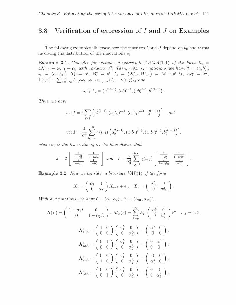
Chapitre 3. Estimating the asymptotic variance of LSE of weak VARMA models 111
3.8 Verification of expression of I and J on Examples
The following examples illustrate how the matrices I and J depend on θ0 and termsinvolving the distribution of the innovations et.
Example 3.1. Consider for instance a univariate ARMA(1, 1) of the form Xt =aXt−1 − bǫt−1 + ǫt, with variance σ2. Then, with our notations we have θ = (a, b)′,θ0 = (a0, b0)
′, A∗i = ai, B
∗i = bi, λi =
(A
∗i−1,B
∗i−1
)= (ai−1, bi−1) , Eǫ2t = σ2,
Γ(i, j) =∑+∞
h=−∞E (ǫtǫt−iǫt−hǫt−j−h) I4 = γ(i, j)I4 and
λi ⊗ λi =(a2(i−1), (ab)i−1, (ab)i−1, b2(i−1)
).
Thus, we have
vec J = 2∑
i≥1
(
a2(i−1)0 , (a0b0)
i−1, (a0b0)i−1, b
2(i−1)0
)′
and
vec I =4
σ40
+∞∑
i,j=1
γ(i, j)(
a2(i−1)0 , (a0b0)
i−1, (a0b0)i−1, b
2(i−1)0
)′
,
where σ0 is the true value of σ. We then deduce that
J = 2
[1
1−a20
11−a0b0
11−a0b0
11−b20
]
and I =4
σ40
+∞∑
i,j=1
γ(i, j)
[1
1−a20
11−a0b0
11−a0b0
11−b20
]
.
Example 3.2. Now we consider a bivariate VAR(1) of the form
Xt =
(α1 00 α2
)
Xt−1 + et, Σe =
(σ211 00 σ2
22
)
.
With our notations, we have θ = (α1, α2)′, θ0 = (α01, α02)
′,
A(L) =
(1− α1L 0
0 1− α2L
)
, Mij(z) =∞∑
h=0
Eij
(αh1 00 αh
2
)
zh i, j = 1, 2,
A∗11,h =
(1 00 0
)(αh1 00 αh
2
)
=
(αh1 00 0
)
,
A∗12,h =
(0 10 0
)(αh1 00 αh
2
)
=
(0 αh
2
0 0
)
,
A∗21,h =
(0 01 0
)(αh1 00 αh
2
)
=
(0 0αh1 0
)
,
A∗22,h =
(0 00 1
)(αh1 00 αh
2
)
=
(0 00 αh
2
)
.
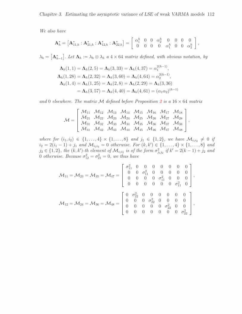
Chapitre 3. Estimating the asymptotic variance of LSE of weak VARMA models 112
We also have
A∗h =
[A
∗11,h : A∗
21,h : A∗12,h : A∗
22,h
]=
[αh1 0 0 αh
2 0 0 0 00 0 0 0 αh
1 0 0 αh2
]
,
λh =[A
∗h−1
]. Let Λh := λh ⊗ λh a 4× 64 matrix defined, with obvious notation, by
Λh(1, 1) = Λh(2, 5) = Λh(3, 33) = Λh(4, 37) = α2(h−1)1 ,
Λh(1, 28) = Λh(2, 32) = Λh(3, 60) = Λh(4, 64) = α2(h−1)2 ,
Λh(1, 4) = Λh(1, 25) = Λh(2, 8) = Λh(2, 29) = Λh(3, 36)
= Λh(3, 57) = Λh(4, 40) = Λh(4, 61) = (α1α2)(h−1)
and 0 elsewhere. The matrix M defined before Proposition 2 is a 16× 64 matrix
M =
M11 M12 M13 M14 M15 M16 M17 M18
M21 M22 M23 M24 M25 M26 M27 M28
M31 M32 M33 M34 M35 M36 M37 M38
M41 M42 M43 M44 M45 M46 M47 M48
,
where for (i1, i2) ∈ 1, . . . , 4 × 1, . . . , 8 and j1 ∈ 1, 2, we have Mi1i2 6= 0 ifi2 = 2(i1 − 1) + j1 and Mi1i2 = 0 otherwise. For (k, k′) ∈ 1, . . . , 4 × 1, . . . , 8 andj2 ∈ 1, 2, the (k, k′)-th element of Mi1i2 is of the form σ2
j1j2if k′ = 2(k − 1) + j2 and
0 otherwise. Because σ212 = σ2
21 = 0, we thus have
M11 = M23 = M35 = M47 =
σ211 0 0 0 0 0 0 00 0 σ2
11 0 0 0 0 00 0 0 0 σ2
11 0 0 00 0 0 0 0 0 σ2
11 0
,
M12 = M24 = M36 = M48 =
0 σ222 0 0 0 0 0 0
0 0 0 σ222 0 0 0 0
0 0 0 0 0 σ222 0 0
0 0 0 0 0 0 0 σ222
,
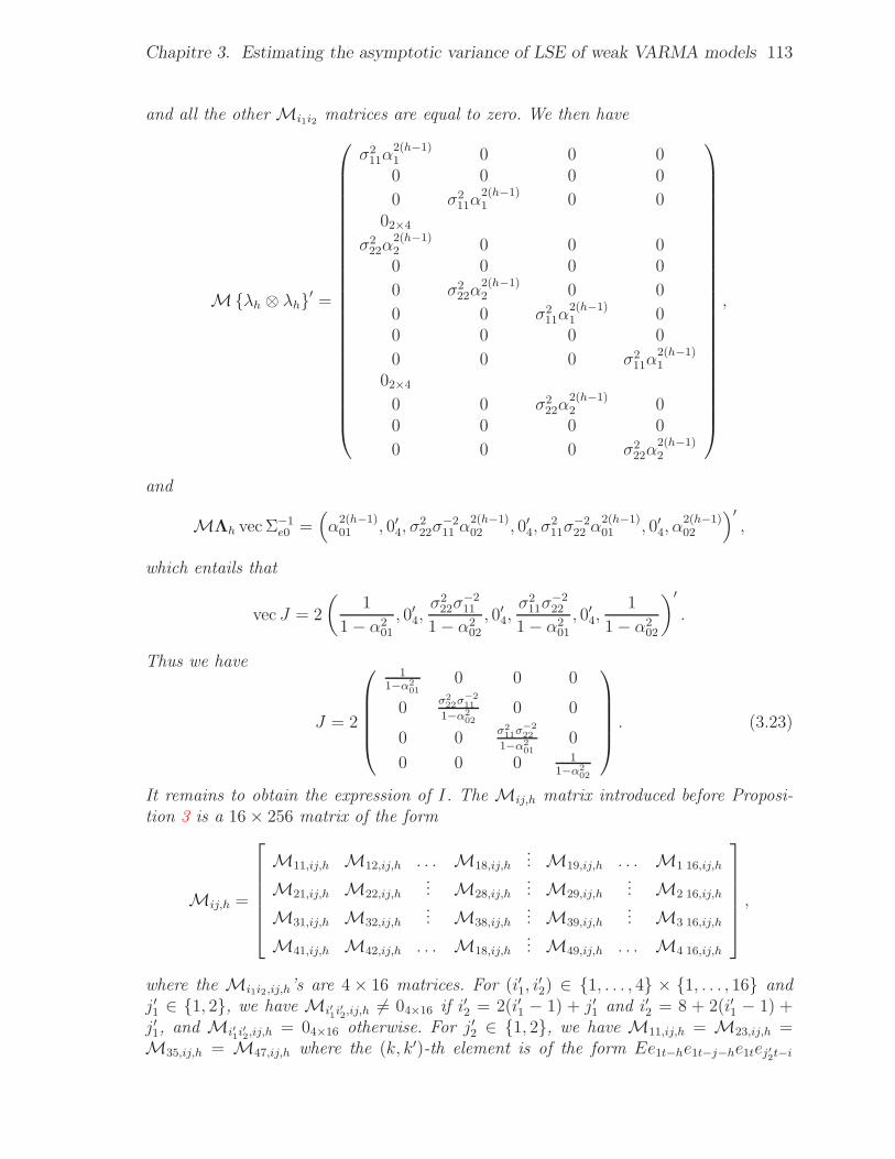
Chapitre 3. Estimating the asymptotic variance of LSE of weak VARMA models 113
and all the other Mi1i2 matrices are equal to zero. We then have
Mλh ⊗ λh′ =
σ211α
2(h−1)1 0 0 00 0 0 0
0 σ211α
2(h−1)1 0 0
02×4
σ222α
2(h−1)2 0 0 00 0 0 0
0 σ222α
2(h−1)2 0 0
0 0 σ211α
2(h−1)1 0
0 0 0 0
0 0 0 σ211α
2(h−1)1
02×4
0 0 σ222α
2(h−1)2 0
0 0 0 0
0 0 0 σ222α
2(h−1)2
,
and
MΛh vec Σ−1e0 =
(
α2(h−1)01 , 0′4, σ
222σ
−211 α
2(h−1)02 , 0′4, σ
211σ
−222 α
2(h−1)01 , 0′4, α
2(h−1)02
)′
,
which entails that
vec J = 2
(1
1− α201
, 0′4,σ222σ
−211
1− α202
, 0′4,σ211σ
−222
1− α201
, 0′4,1
1− α202
)′
.
Thus we have
J = 2
11−α2
010 0 0
0σ222σ
−211
1−α202
0 0
0 0σ211σ
−222
1−α201
0
0 0 0 11−α2
02
. (3.23)
It remains to obtain the expression of I. The Mij,h matrix introduced before Proposi-tion 3 is a 16× 256 matrix of the form
Mij,h =
M11,ij,h M12,ij,h . . . M18,ij,h... M19,ij,h . . . M1 16,ij,h
M21,ij,h M22,ij,h... M28,ij,h
... M29,ij,h... M2 16,ij,h
M31,ij,h M32,ij,h... M38,ij,h
... M39,ij,h... M3 16,ij,h
M41,ij,h M42,ij,h . . . M18,ij,h... M49,ij,h . . . M4 16,ij,h
,
where the Mi1i2,ij,h’s are 4× 16 matrices. For (i′1, i′2) ∈ 1, . . . , 4 × 1, . . . , 16 and
j′1 ∈ 1, 2, we have Mi′1i′2,ij,h
6= 04×16 if i′2 = 2(i′1 − 1) + j′1 and i′2 = 8 + 2(i′1 − 1) +j′1, and Mi′1i
′2,ij,h
= 04×16 otherwise. For j′2 ∈ 1, 2, we have M11,ij,h = M23,ij,h =M35,ij,h = M47,ij,h where the (k, k′)-th element is of the form Ee1t−he1t−j−he1tej′2t−i
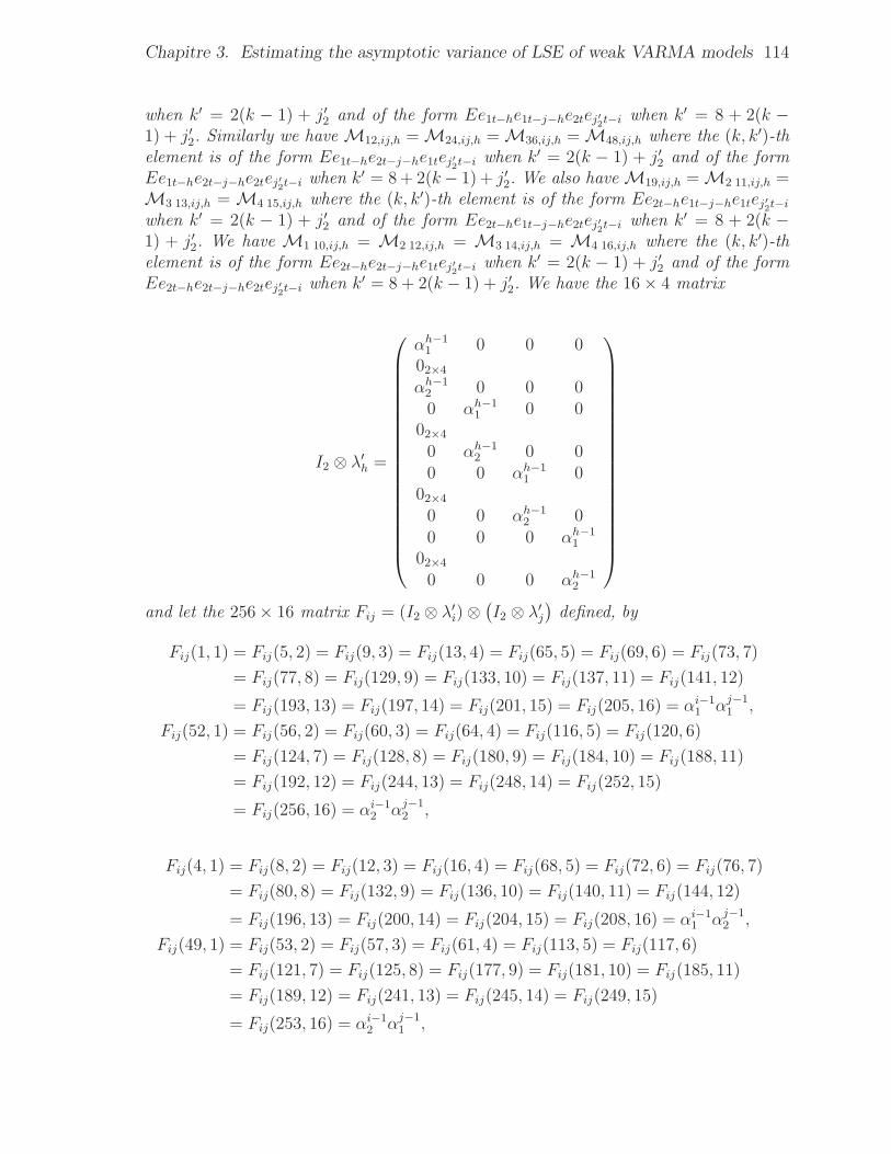
Chapitre 3. Estimating the asymptotic variance of LSE of weak VARMA models 114
when k′ = 2(k − 1) + j′2 and of the form Ee1t−he1t−j−he2tej′2t−i when k′ = 8 + 2(k −1) + j′2. Similarly we have M12,ij,h = M24,ij,h = M36,ij,h = M48,ij,h where the (k, k′)-thelement is of the form Ee1t−he2t−j−he1tej′2t−i when k′ = 2(k − 1) + j′2 and of the formEe1t−he2t−j−he2tej′2t−i when k′ = 8+ 2(k− 1) + j′2. We also have M19,ij,h = M2 11,ij,h =M3 13,ij,h = M4 15,ij,h where the (k, k′)-th element is of the form Ee2t−he1t−j−he1tej′2t−i
when k′ = 2(k − 1) + j′2 and of the form Ee2t−he1t−j−he2tej′2t−i when k′ = 8 + 2(k −1) + j′2. We have M1 10,ij,h = M2 12,ij,h = M3 14,ij,h = M4 16,ij,h where the (k, k′)-thelement is of the form Ee2t−he2t−j−he1tej′2t−i when k′ = 2(k − 1) + j′2 and of the formEe2t−he2t−j−he2tej′2t−i when k′ = 8 + 2(k − 1) + j′2. We have the 16× 4 matrix
I2 ⊗ λ′h =
αh−11 0 0 0
02×4
αh−12 0 0 00 αh−1
1 0 002×4
0 αh−12 0 0
0 0 αh−11 0
02×4
0 0 αh−12 0
0 0 0 αh−11
02×4
0 0 0 αh−12
and let the 256× 16 matrix Fij = (I2 ⊗ λ′i)⊗(I2 ⊗ λ′j
)defined, by
Fij(1, 1) = Fij(5, 2) = Fij(9, 3) = Fij(13, 4) = Fij(65, 5) = Fij(69, 6) = Fij(73, 7)
= Fij(77, 8) = Fij(129, 9) = Fij(133, 10) = Fij(137, 11) = Fij(141, 12)
= Fij(193, 13) = Fij(197, 14) = Fij(201, 15) = Fij(205, 16) = αi−11 αj−1
1 ,
Fij(52, 1) = Fij(56, 2) = Fij(60, 3) = Fij(64, 4) = Fij(116, 5) = Fij(120, 6)
= Fij(124, 7) = Fij(128, 8) = Fij(180, 9) = Fij(184, 10) = Fij(188, 11)
= Fij(192, 12) = Fij(244, 13) = Fij(248, 14) = Fij(252, 15)
= Fij(256, 16) = αi−12 αj−1
2 ,
Fij(4, 1) = Fij(8, 2) = Fij(12, 3) = Fij(16, 4) = Fij(68, 5) = Fij(72, 6) = Fij(76, 7)
= Fij(80, 8) = Fij(132, 9) = Fij(136, 10) = Fij(140, 11) = Fij(144, 12)
= Fij(196, 13) = Fij(200, 14) = Fij(204, 15) = Fij(208, 16) = αi−11 αj−1
2 ,
Fij(49, 1) = Fij(53, 2) = Fij(57, 3) = Fij(61, 4) = Fij(113, 5) = Fij(117, 6)
= Fij(121, 7) = Fij(125, 8) = Fij(177, 9) = Fij(181, 10) = Fij(185, 11)
= Fij(189, 12) = Fij(241, 13) = Fij(245, 14) = Fij(249, 15)
= Fij(253, 16) = αi−12 αj−1
1 ,
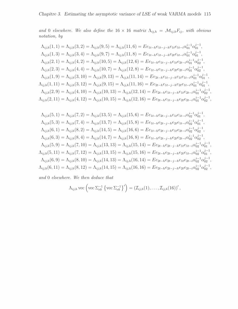
Chapitre 3. Estimating the asymptotic variance of LSE of weak VARMA models 115
and 0 elsewhere. We also define the 16 × 16 matrix Λij,h = Mij,hFij, with obviousnotation, by
Λij,h(1, 1) = Λij,h(3, 2) = Λij,h(9, 5) = Λij,h(11, 6) = Ee1t−he1t−j−he1te1t−iαi−101 α
j−101 ,
Λij,h(1, 3) = Λij,h(3, 4) = Λij,h(9, 7) = Λij,h(11, 8) = Ee1t−he1t−j−he2te1t−iαi−101 α
j−101 ,
Λij,h(2, 1) = Λij,h(4, 2) = Λij,h(10, 5) = Λij,h(12, 6) = Ee1t−he1t−j−he1te2t−iαi−101 α
j−102 ,
Λij,h(2, 3) = Λij,h(4, 4) = Λij,h(10, 7) = Λij,h(12, 8) = Ee1t−he1t−j−he2te2t−iαi−101 α
j−102 ,
Λij,h(1, 9) = Λij,h(3, 10) = Λij,h(9, 13) = Λij,h(11, 14) = Ee2t−he1t−j−he1te1t−iαi−101 α
j−101 ,
Λij,h(1, 11) = Λij,h(3, 12) = Λij,h(9, 15) = Λij,h(11, 16) = Ee2t−he1t−j−he2te1t−iαi−101 α
j−101 ,
Λij,h(2, 9) = Λij,h(4, 10) = Λij,h(10, 13) = Λij,h(12, 14) = Ee2t−he1t−j−he1te2t−iαi−101 α
j−102 ,
Λij,h(2, 11) = Λij,h(4, 12) = Λij,h(10, 15) = Λij,h(12, 16) = Ee2t−he1t−j−he2te2t−iαi−101 α
j−102 ,
Λij,h(5, 1) = Λij,h(7, 2) = Λij,h(13, 5) = Λij,h(15, 6) = Ee1t−he2t−j−he1te1t−iαi−102 α
j−101 ,
Λij,h(5, 3) = Λij,h(7, 4) = Λij,h(13, 7) = Λij,h(15, 8) = Ee1t−he2t−j−he2te1t−iαi−102 α
j−101 ,
Λij,h(6, 1) = Λij,h(8, 2) = Λij,h(14, 5) = Λij,h(16, 6) = Ee1t−he2t−j−he1te2t−iαi−102 α
j−102 ,
Λij,h(6, 3) = Λij,h(8, 4) = Λij,h(14, 7) = Λij,h(16, 8) = Ee1t−he2t−j−he2te2t−iαi−102 α
j−102 ,
Λij,h(5, 9) = Λij,h(7, 10) = Λij,h(13, 13) = Λij,h(15, 14) = Ee2t−he2t−j−he1te1t−iαi−102 α
j−101 ,
Λij,h(5, 11) = Λij,h(7, 12) = Λij,h(13, 15) = Λij,h(15, 16) = Ee2t−he2t−j−he2te1t−iαi−102 α
j−101 ,
Λij,h(6, 9) = Λij,h(8, 10) = Λij,h(14, 13) = Λij,h(16, 14) = Ee2t−he2t−j−he1te2t−iαi−102 α
j−102 ,
Λij,h(6, 11) = Λij,h(8, 12) = Λij,h(14, 15) = Λij,h(16, 16) = Ee2t−he2t−j−he2te2t−iαi−102 α
j−102 ,
and 0 elsewhere. We then deduce that
Λij,h vec(
vec Σ−1e0
vec Σ−1
e0
′)
= (Iij,h(1), . . . , Iij,h(16))′ ,
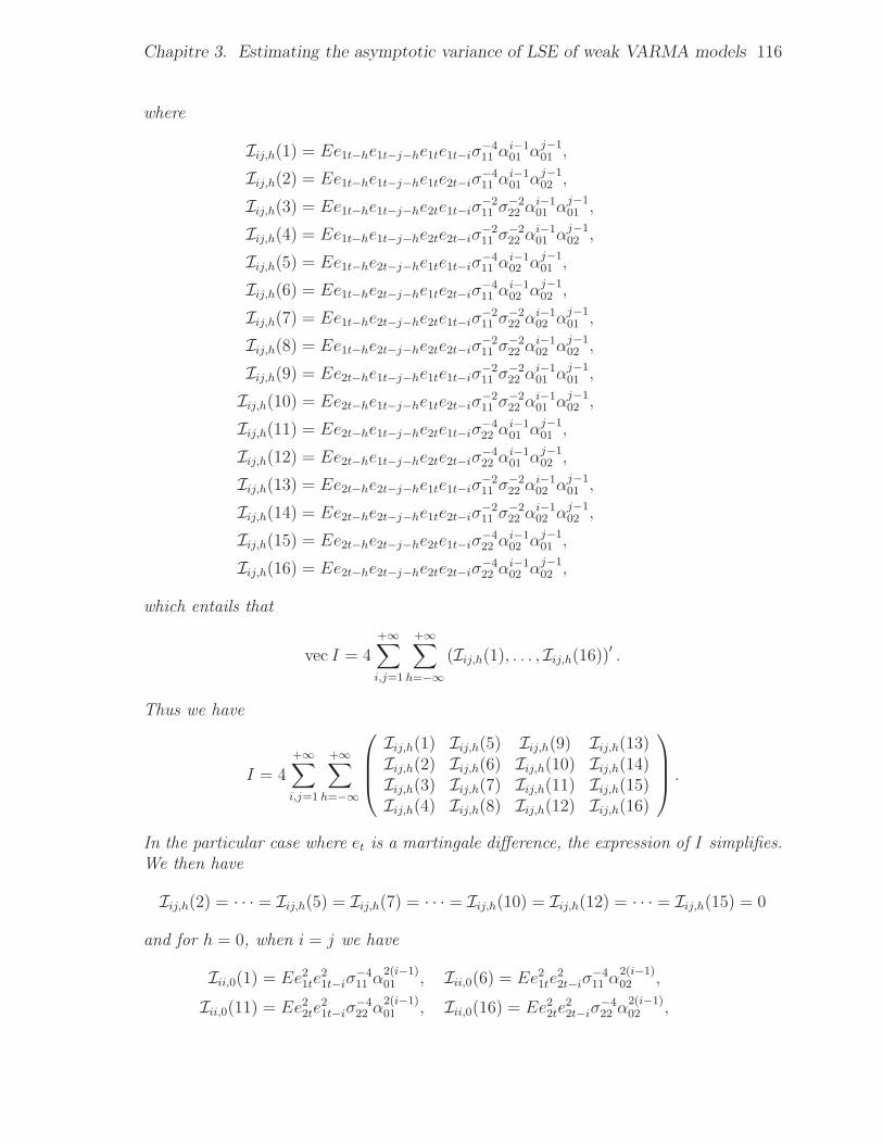
Chapitre 3. Estimating the asymptotic variance of LSE of weak VARMA models 116
where
Iij,h(1) = Ee1t−he1t−j−he1te1t−iσ−411 α
i−101 α
j−101 ,
Iij,h(2) = Ee1t−he1t−j−he1te2t−iσ−411 α
i−101 α
j−102 ,
Iij,h(3) = Ee1t−he1t−j−he2te1t−iσ−211 σ
−222 α
i−101 α
j−101 ,
Iij,h(4) = Ee1t−he1t−j−he2te2t−iσ−211 σ
−222 α
i−101 α
j−102 ,
Iij,h(5) = Ee1t−he2t−j−he1te1t−iσ−411 α
i−102 α
j−101 ,
Iij,h(6) = Ee1t−he2t−j−he1te2t−iσ−411 α
i−102 α
j−102 ,
Iij,h(7) = Ee1t−he2t−j−he2te1t−iσ−211 σ
−222 α
i−102 α
j−101 ,
Iij,h(8) = Ee1t−he2t−j−he2te2t−iσ−211 σ
−222 α
i−102 α
j−102 ,
Iij,h(9) = Ee2t−he1t−j−he1te1t−iσ−211 σ
−222 α
i−101 α
j−101 ,
Iij,h(10) = Ee2t−he1t−j−he1te2t−iσ−211 σ
−222 α
i−101 α
j−102 ,
Iij,h(11) = Ee2t−he1t−j−he2te1t−iσ−422 α
i−101 α
j−101 ,
Iij,h(12) = Ee2t−he1t−j−he2te2t−iσ−422 α
i−101 α
j−102 ,
Iij,h(13) = Ee2t−he2t−j−he1te1t−iσ−211 σ
−222 α
i−102 α
j−101 ,
Iij,h(14) = Ee2t−he2t−j−he1te2t−iσ−211 σ
−222 α
i−102 α
j−102 ,
Iij,h(15) = Ee2t−he2t−j−he2te1t−iσ−422 α
i−102 α
j−101 ,
Iij,h(16) = Ee2t−he2t−j−he2te2t−iσ−422 α
i−102 α
j−102 ,
which entails that
vec I = 4+∞∑
i,j=1
+∞∑
h=−∞
(Iij,h(1), . . . , Iij,h(16))′ .
Thus we have
I = 4
+∞∑
i,j=1
+∞∑
h=−∞
Iij,h(1) Iij,h(5) Iij,h(9) Iij,h(13)Iij,h(2) Iij,h(6) Iij,h(10) Iij,h(14)Iij,h(3) Iij,h(7) Iij,h(11) Iij,h(15)Iij,h(4) Iij,h(8) Iij,h(12) Iij,h(16)
.
In the particular case where et is a martingale difference, the expression of I simplifies.We then have
Iij,h(2) = · · · = Iij,h(5) = Iij,h(7) = · · · = Iij,h(10) = Iij,h(12) = · · · = Iij,h(15) = 0
and for h = 0, when i = j we have
Iii,0(1) = Ee21te21t−iσ
−411 α
2(i−1)01 , Iii,0(6) = Ee21te
22t−iσ
−411 α
2(i−1)02 ,
Iii,0(11) = Ee22te21t−iσ
−422 α
2(i−1)01 , Iii,0(16) = Ee22te
22t−iσ
−422 α
2(i−1)02 ,
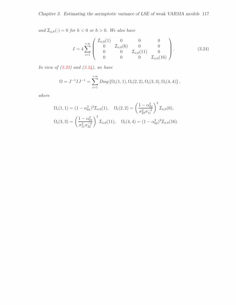
Chapitre 3. Estimating the asymptotic variance of LSE of weak VARMA models 117
and Iij,h(·) = 0 for h < 0 or h > 0. We also have
I = 4+∞∑
i=1
Iii,0(1) 0 0 00 Iii,0(6) 0 00 0 Iii,0(11) 00 0 0 Iii,0(16)
. (3.24)
In view of (3.23) and (3.24), we have
Ω = J−1IJ−1 =+∞∑
i=1
Diag Ωi(1, 1),Ωi(2, 2),Ωi(3, 3),Ωi(4, 4) ,
where
Ωi(1, 1) = (1− α201)
2Iii,0(1), Ωi(2, 2) =
(1− α2
02
σ222σ
−211
)2
Iii,0(6),
Ωi(3, 3) =
(1− α2
01
σ211σ
−222
)2
Iii,0(11), Ωi(4, 4) = (1− α202)
2Iii,0(16).
Chapitre 4
Multivariate portmanteau test forstructural VARMA models withuncorrelated but non-independenterror terms
Abstract We consider portmanteau tests for testing the adequacy of vector au-toregressive moving-average (VARMA) models under the assumption that the errorsare uncorrelated but not necessarily independent. We relax the standard independenceassumption to extend the range of application of the VARMA models, and allow tocover linear representations of general nonlinear processes. We first study the jointdistribution of the quasi-maximum likelihood estimator (QMLE) or the least squaredestimator (LSE) and the noise empirical autocovariances. We then derive the asympto-tic distribution of residual empirical autocovariances and autocorrelations under weakassumptions on the noise. We deduce the asymptotic distribution of the Ljung-Box (orBox-Pierce) portmanteau statistics for VARMA models with nonindependent innova-tions. In the standard framework (i.e. under iid assumptions on the noise), it is knownthat the asymptotic distribution of the portmanteau tests is that of a weighted sum ofindependent chi-squared random variables. The asymptotic distribution can be quitedifferent when the independence assumption is relaxed. Consequently, the usual chi-squared distribution does not provide an adequate approximation to the distribution ofthe Box-Pierce goodness-of fit portmanteau test. Hence we propose a method to adjustthe critical values of the portmanteau tests. Monte carlo experiments illustrate the finitesample performance of the modified portmanteau test.
Keywords : Goodness-of-fit test, QMLE/LSE, Box-Pierce and Ljung-Box portmanteau tests,
residual autocorrelation, Structural representation, weak VARMA models.
Chapitre 4. Multivariate portmanteau test for weak structural VARMA models 119
4.1 Introduction
The vector autoregressive moving-average (VARMA) models are used in time seriesanalysis and econometrics to represent multivariate time series (see Reinsel, 1997, Lüt-kepohl, 2005). These VARMA models are a natural extension of the univariate ARMAmodels, which constitute the most widely used class of univariate time series models (seee.g. Brockwell and Davis, 1991). The sub-class of vector autoregressive (VAR) modelshas been studied in the econometric literature (see also Lütkepohl, 1993). The validityof the different steps of the traditional methodology of Box and Jenkins, identification,estimation and validation, depends on the noises properties. After identification andestimation of the vector autoregressive moving-average processes, the next importantstep in the VARMA modeling consists in checking if the estimated model fits satisfac-tory the data. This adequacy checking step allows to validate or invalidate the choiceof the orders p and q. In VARMA(p, q) models, the choice of p and q is particularlyimportant because the number of parameters, (p + q + 2)d2, quickly increases with pand q, which entails statistical difficulties. Thus it is important to check the validityof a VARMA(p, q) model, for a given order p and q. This paper is devoted to the pro-blem of the validation step of VARMA representations of multivariate processes. Thisvalidation stage is not only based on portmanteau tests, but also on the examinationof the autocorrelation function of the residuals. Based on the residual empirical auto-correlations, Box and Pierce (1970) (BP hereafter) derived a goodness-of-fit test, theportmanteau test, for univariate strong ARMA models. Ljung and Box (1978) (LBhereafter) proposed a modified portmanteau test which is nowadays one of the mostpopular diagnostic checking tool in ARMA modeling of time series. The multivariateversion of the BP portmanteau statistic was introduced by Chitturi (1974). We use thisso-called portmanteau tests considered by Chitturi (1974) and Hosking (1980) for che-cking the overall significance of the residual autocorrelations of a VARMA(p, q) model(see also Hosking, 1981a,b ; Li and McLeod, 1981 ; Ahn, 1988). Hosking (1981a) gaveseveral equivalent forms of this statistic. The papers on the multivariate version of theportmanteau statistic are generally under the assumption that the errors ǫt are inde-pendent. This independence assumption is restrictive because it precludes conditionalheteroscedasticity and/ or other forms of nonlinearity (see Francq and Zakoïan, 2005,for a review on weak univariate ARMA models). Relaxing this independence assump-tion allows to cover linear representations of general nonlinear processes and to extendthe range of application of the VARMA models. VARMA models with nonindependentinnovations (i.e. weak VARMA models) have been less studied than VARMA modelswith iid errors (i.e. strong VARMA models). The asymptotic theory of weak ARMAmodel validation is mainly limited to the univariate framework (see Francq and Zakoïan,2005). In the multivariate analysis, notable exceptions are Dufour and Pelletier (2005)who study the choice of the order p and q of VARMA models under weak assumptionson the innovation process, Francq and Raïssi (2007) who study portmanteau tests forweak VAR models and Boubacar Mainassara and Francq (2009) who study the consis-tency and the asymptotic normality of the QMLE for weak VARMA model. The main
Chapitre 4. Multivariate portmanteau test for weak structural VARMA models 120
goal of the present article is to complete the available results concerning the statisticalanalysis of weak VARMA models by considering the adequacy problem, which havenot been studied in the above-mentioned papers. We proceed to study the behaviourof the goodness-of fit portmanteau tests when the ǫt are not independent. We will seethat the standard portmanteau tests can be quite misleading in the framework of nonindependent errors. A modified version of these tests is thus proposed.
The paper is organized as follows. Section 4.2 presents the structural weak VARMAmodels that we consider here. Structural forms are employed in econometrics in or-der to introduce instantaneous relationships between economic variables. Section 4.3presents the results on the QMLE/LSE asymptotic distribution obtained by BoubacarMainassara and Francq (2009) when (ǫt) satisfies mild mixing assumptions. Section 4.4is devoted to the joint distribution of the QMLE/LSE and the noise empirical auto-covariances. In Section 4.5 we derive the asymptotic distribution of residual empiricalautocovariances and autocorrelations under weak assumptions on the noise. In Section4.6 it is shown how the standard Ljung-Box (or Box-Pierce) portmanteau tests mustbe adapted in the case of VARMA models with nonindependent innovations. In Sec-tion 4.7 we give examples of multivariate weak white noises. Numerical experiments arepresented in Section 4.9. The proofs of the main results are collected in the appendix.
We denote by A⊗B the Kronecker product of two matrices A and B, and by vecAthe vector obtained by stacking the columns of A. The reader is refereed to Magnusand Neudecker (1988) for the properties of these operators. Let 0r be the null vector ofRr, and let Ir be the r × r identity matrix.
4.2 Model and assumptions
Consider a d-dimensional stationary process (Xt) satisfying a structuralVARMA(p, q) representation of the form
A00Xt −p∑
i=1
A0iXt−i = B00ǫt −q∑
i=1
B0iǫt−i, ∀t ∈ Z = 0,±1, . . ., (4.1)
where ǫt is a white noise, namely a stationary sequence of centered and uncorrelatedrandom variables with a non singular variance Σ0. It is customary to say that (Xt) is astrong VARMA(p, q) model if (ǫt) is a strong white noise, that is, if it satisfies
A1 : (ǫt) is a sequence of independent and identically distributed (iid) randomvectors, Eǫt = 0 and Var (ǫt) = Σ0.
We say that (4.1) is a weak VARMA(p, q) model if (ǫt) is a weak white noise, that is,if it satisfies
A1’ : Eǫt = 0, Var (ǫt) = Σ0, and Cov (ǫt, ǫt−h) = 0 for all t ∈ Z and allh 6= 0.
Chapitre 4. Multivariate portmanteau test for weak structural VARMA models 121
Assumption A1 is clearly stronger than A1’. The class of strong VARMA modelsis often considered too restrictive by practitioners. The standard VARMA(p, q) form,which is sometimes called the reduced form, is obtained for A00 = B00 = Id. Let[A00 . . . A0pB00 . . . B0q] be the d× (p+ q+2)d matrix of VAR and MA coefficients. Theparameter θ0 = vec [A00 . . . A0pB00 . . . B0q] belongs to the compact parameter spaceΘ ⊂ Rk0, where k0 = (p+ q + 2)d2 is the number of unknown parameters in VAR andMA parts.
It is important to note that, we cannot work with the structural representation (4.1)because it is not identified. The following assumption ensure the identification of thestructural VARMA models.
A2 : For all θ ∈ Θ, θ 6= θ0, we have A−10 B0B
−1θ (L)Aθ(L)Xt 6= A−1
00 B00ǫt withnon zero probability, or A−1
0 B0ΣB′0A
−1′0 6= A−1
00 B00Σ0B′00A
−1′00 .
The previous identifiability assumption is satisfied when the parameter space Θ is suf-ficiently constrained.
For θ ∈ Θ, such that θ = vec [A0 . . . ApB0 . . . Bq], write Aθ(z) = A0 −∑p
i=1Aizi
and Bθ(z) = B0 −∑q
i=1Bizi. We assume that Θ corresponds to stable and invertible
representations, namelyA3 : for all θ ∈ Θ, we have detAθ(z) detBθ(z) 6= 0 for all |z| ≤ 1.
Under the assumption A3, it is well known that the process (Xt) can be written as aMA(∞) of the form
Xt =
∞∑
i=0
ψ0iǫt−i, ψ00 = A−100 B00,
∞∑
i=0
‖ψ0i‖ <∞. (4.2)
A4 : Matrix Σ0 is positive definite.
To show the strong consistency, we will use the following assumptions.A5 : The process (ǫt) is stationary and ergodic.
Note that A5 is entailed by A1, but not by A1′. Note that (ǫt) can be replaced by
(Xt) in A5, because Xt = A−1θ0(L)Bθ0(L)ǫt and ǫt = B−1
θ0(L)Aθ0(L)Xt, where L stands
for the backward operator.
4.3 Least Squares Estimation under non-iid innova-
tions
Let X1, . . . , Xn be observations of a process satisfying the VARMA representation(4.1). Let θ ∈ Θ and A0 = A0(θ), . . . , Ap = Ap(θ), B0 = B0(θ), . . . , Bq = Bq(θ),Σ =Σ(θ) such that θ = vec [A0 . . . Ap B0 . . . Bq]. Note that from A3 the matrices A0 and B0
are invertible. Introducing the innovation process et = A−100 B00ǫt, the structural repre-
Chapitre 4. Multivariate portmanteau test for weak structural VARMA models 122
sentation Aθ0(L)Xt = Bθ0(L)ǫt can be rewritten as the reduced VARMA representation
Xt −p∑
i=1
A−100 A0iXt−i = et −
q∑
i=1
A−100 B0iB
−100 A00et−i. (4.3)
Note that et(θ0) = et. For simplicity, we will omit the notation θ in all quantitiestaken at the true value, θ0. For all θ ∈ Θ, the assumption on the MA polynomial(from A3) implies that there exists a sequence of constants matrices (Ci(θ)) such that∑∞
i=1 ‖Ci(θ)‖ <∞ and
et(θ) = Xt −∞∑
i=1
Ci(θ)Xt−i. (4.4)
Given a realization X1, X2, . . . , Xn, the variable et(θ) can be approximated, for 0 < t ≤n, by et(θ) defined recursively by
et(θ) = Xt −p∑
i=1
A−10 AiXt−i +
q∑
i=1
A−10 BiB
−10 A0et−i(θ),
where the unknown initial values are set to zero : e0(θ) = · · · = e1−q(θ) = X0 = · · · =X1−p = 0. The gaussian quasi-likelihood is given by
Ln(θ,Σe) =n∏
t=1
1
(2π)d/2√det Σe
exp
−1
2e′t(θ)Σ
−1e et(θ)
, Σe = A−10 B0ΣB
′0A
−1′0 .
A quasi-maximum likelihood (QML) of θ and Σe are a measurable solution (θn, Σe) of
(θn, Σe) = argminθ,Σe
log(det Σe) +1
n
n∑
t=1
et(θ)Σ−1e e′t(θ)
.
Under the following additional assumptions, Boubacar Mainassara and Francq (2009)showed respectively in Theorem 1 and Theorem 2 the consistency and the asymptoticnormality of the QML estimator of weak multivariate ARMA model.
Assume that θ0 is not on the boundary of the parameter space Θ.
A6 : We have θ0 ∈
Θ, where
Θ denotes the interior of Θ.We denote by αǫ(k), k = 0, 1, . . . , the strong mixing coefficients of the process (ǫt). Themixing coefficients of a stationary process ǫ = (ǫt) are denoted by
αǫ(k) = supA∈σ(ǫu,u≤t),B∈σ(ǫu,u≥t+h)
|P (A ∩B)− P (A)P (B)| .
The reader is referred to Davidson (1994) for details about mixing assumptions.A7 : We have E‖ǫt‖4+2ν <∞ and
∑∞k=0 αǫ(k)
ν2+ν <∞ for some ν > 0.
One of the most popular estimation procedure is that of the least squares estimator(LSE) minimizing
log det Σe = log det
1
n
n∑
t=1
et(θ)e′t(θ)
,
Chapitre 4. Multivariate portmanteau test for weak structural VARMA models 123
or equivalently
det Σe = det
1
n
n∑
t=1
et(θ)e′t(θ)
.
For the processes of the form (4.3), under A1’, A2-A7, it can be shown (see e.g.Boubacar Mainassara and Francq 2009), that the LS estimator of θ coincides withthe gaussian quasi-maximum likelihood estimator (QMLE). More precisely, θn satisfies,almost surely,
Qn(θn) = minθ∈Θ
Qn(θ),
where
Qn(θ) = log det
1
n
n∑
t=1
et(θ)e′t(θ)
or Qn(θ) = det
1
n
n∑
t=1
et(θ)e′t(θ)
.
To obtain the consistency and asymptotic normality of the QMLE/LSE, it will beconvenient to consider the functions
On(θ) = log det Σn or On(θ) = det Σn,
where Σn = Σn(θ) = n−1∑n
t=1 et(θ)e′t(θ) and (et(θ)) is given by (4.4). Under A1’,
A2-A7 or A1-A4 and A6, let θn be the LS estimate of θ0 by maximizing
On(θ) = log det
1
n
n∑
t=1
et(θ)e′t(θ)
.
In the univariate case, Francq and Zakoïan (1998) showed the asymptotic normality ofthe LS estimator under mixing assumptions. This remains valid of the multivariate LS
estimator. Then under the assumptions A1’, A2-A7,√n(
θn − θ0
)
is asymptotically
normal with mean 0 and covariance matrix Σθn:= J−1IJ−1, where J = J(θ0) and
I = I(θ0), with
J(θ) = limn→∞
1
n
∂2
∂θ∂θ′Qn(θ) a.s.
and
I(θ) = limn→∞
Var1√n
∂
∂θQn(θ).
In the standard strong VARMA case, i.e. when A5 is replaced by the assumptionA1 that (ǫt) is iid, we have I = J , so that Σθn
= J−1.
Chapitre 4. Multivariate portmanteau test for weak structural VARMA models 124
4.4 Joint distribution of θn and the noise empirical
autocovariances
Let et = et(θn) be the LS residuals when p > 0 or q > 0, and let et = et = Xt whenp = q = 0. When p+ q 6= 0, we have et = 0 for t ≤ 0 and t > n and
et = Xt −p∑
i=1
A−10 (θn)Ai(θn)Xt−i +
q∑
i=1
A−10 (θn)Bi(θn)B
−10 (θn)A0(θn)et−i,
for t = 1, . . . , n, with Xt = 0 for t ≤ 0 and Xt = Xt for t ≥ 1. Let, Σe0 = Γe(0) =n−1
∑nt=1 ete
′t. We denote by
γ(h) =1
n
n∑
t=h+1
ete′t−h and Γe(h) =
1
n
n∑
t=h+1
ete′t−h
the white noise "empirical" autocovariances and residual autocovariances. It should benoted that γ(h) is not a statistic (unless if p = q = 0) because it depends on theunobserved innovations et = et(θ0). For a fixed integer m ≥ 1, let
γm =(vecγ(1)′ , . . . , vecγ(m)′
)′
and
Γm =
(
vecΓe(1)′
, . . . ,
vecΓe(m)′)′
,
and let
Γ(ℓ, ℓ′) =
∞∑
h=−∞
E(et−ℓ ⊗ et et−h−ℓ′ ⊗ et−h′
),
for (ℓ, ℓ′) 6= (0, 0). For the univariate ARMA model, Francq, Roy and Zakoïan (2005)have showed in Lemma A.1 that |Γ(ℓ, ℓ′)| ≤ Kmax(ℓ, ℓ′) for some constant K, which issufficient to ensure the existence of these matrices. We can generalize this result for themultivariate ARMA model. Then we obtain ‖Γ(ℓ, ℓ′)‖ ≤ Kmax(ℓ, ℓ′) for some constantK. The proof is similar to the univariate case.
We are now able to state the following theorem, which is an extension of a resultgiven in Francq, Roy and Zakoïan (2005).
Theorem 4.1. Assume p > 0 or q > 0. Under Assumptions A1’-A2-A7 or A1-A4,
and A6, as n→ ∞,√n(γm, θn − θ0)
′ d⇒ N (0,Ξ) where
Ξ =
(
Σγm Σγm,θn
Σ′γm,θn
Σθn
)
,
with Σγm = Γ(ℓ, ℓ′)1≤ℓ,ℓ′≤m , Σ′γm,θn
= Cov(√nJ−1Yn,
√nγm) and Σθn
=
Varas(√nJ−1Yn) = J−1IJ−1.
Chapitre 4. Multivariate portmanteau test for weak structural VARMA models 125
4.5 Asymptotic distribution of residual empirical au-
tocovariances and autocorrelations
Let the diagonal matrices
Se = Diag (σe(1), . . . , σe(d)) and Se = Diag (σe(1), . . . , σe(d)) ,
where σ2e(i) is the variance of the i-th coordinate of et and σ2
e(i) is its sample estimate,i.e. σe(i) =
√
Ee2it and σe(i) =√
n−1∑n
t=1 e2it. The theoretical and sample autocorrela-
tions at lag ℓ are respectively defined by Re(ℓ) = S−1e Γe(ℓ)S
−1e and Re(ℓ) = S−1
e Γe(ℓ)S−1e ,
with Γe(ℓ) := Eete′t−ℓ = 0 for all ℓ 6= 0. Consider the vector of the first m sample auto-
correlations
ρm =
(
vecRe(1)′
, . . . ,
vecRe(m)′)′
.
Theorem 4.2. Under Assumptions A1-A4 and A6 or A1’, A2-A7,
√nΓm ⇒ N
(0,ΣΓm
)and
√nρm ⇒ N (0,Σρm) where,
ΣΓm= Σγm + ΦmΣθn
Φ′m + ΦmΣθn,γm
+ Σ′θn,γm
Φ′m (4.5)
Σρm =Im ⊗ (Se ⊗ Se)
−1ΣΓm
Im ⊗ (Se ⊗ Se)
−1
(4.6)
and Φm is given by (4.26) in the proof of this Theorem.
4.6 Limiting distribution of the portmanteau statis-
tics
Box and Pierce (1970) (BP hereafter) derived a goodness-of-fit test, the portman-teau test, for univariate strong ARMA models. Ljung and Box (1978) (LB hereafter)proposed a modified portmanteau test which is nowadays one of the most popular diag-nostic checking tool in ARMA modeling of time series. The multivariate version of theBP portmanteau statistic was introduced by Chitturi (1974). Hosking (1981a) gaveseveral equivalent forms of this statistic. Basic forms are
Chapitre 4. Multivariate portmanteau test for weak structural VARMA models 126
Pm = nm∑
h=1
Tr(
Γ′e(h)Γ
−1e (0)Γe(h)Γ
−1e (0)
)
= n
m∑
h=1
vec(
Γe(h))′ (
Γ−1e (0)⊗ Id
)
vec(
Γ−1e (0)Γe(h)
)
= n
m∑
h=1
vec(
Γe(h))′ (
Γ−1e (0)⊗ Id
)(
Id ⊗ Γ−1e (0)
)
vec(
Γe(h))
= n
m∑
h=1
vec(
Γe(h))′ (
Γ−1e (0)⊗ Γ−1
e (0))
vec(
Γe(h))
= nΓ′m
(
Im ⊗
Γ−1e (0)⊗ Γ−1
e (0))
Γm
= nρ′m
(
Im ⊗
Γe(0)Γ−1e (0)Γe(0)
⊗
Γe(0)Γ−1e (0)Γe(0)
)
ρm
= nρ′m
(
Im ⊗
R−1e (0)⊗ R−1
e (0))
ρm.
Where the equalities is obtained from the elementary relations vec(AB) = (I⊗A) vecB,(A⊗B)(C ⊗D) = AC ⊗ BD and Tr(ABC) = vec(A′)′(C ′ ⊗ I) vecB. Similarly to theunivariate LB portmanteau statistic, Hosking (1980) defined the modified portmanteaustatistic
Pm = n2m∑
h=1
(n− h)−1Tr(
Γ′e(h)Γ
−1e (0)Γe(h)Γ
−1e (0)
)
.
These portmanteau statistics are generally used to test the null hypothesis
H0 : (Xt) satisfies a VARMA(p, q) represntation
against the alternative
H1 : (Xt) does not admit a VARMA represntation or admits a
VARMA(p′, q′) represntation with p′ > p or q′ > q.
These portmanteau tests are very useful tools for checking the overall significance ofthe residual autocorrelations. Under the assumption that the data generating process(DGP) follows a strong VARMA(p, q) model, the asymptotic distribution of the statis-tics Pm and Pm is generally approximated by the χ2
d2m−k0distribution (d2m > k0) (the
degrees of freedom are obtained by subtracting the number of freely estimated VARMAcoefficients from d2m). When the innovations are gaussian, Hosking (1980) found thatthe finite-sample distribution of Pm is more nearly χ2
d2(m−(p+q)) than that of Pm. FromTheorem 4.2 we deduce the following result, which gives the exact asymptotic distribu-tion of the standard portmanteau statistics Pm. We will see that the distribution maybe very different from the χ2
d2m−k0in the case of VARMA(p, q) models.
Chapitre 4. Multivariate portmanteau test for weak structural VARMA models 127
Theorem 4.3. Under Assumptions A1-A4 and A6 or A1’, A2-A7, the statistics Pm
and Pm converge in distribution, as n→ ∞, to
Zm(ξm) =
d2m∑
i=1
ξi,d2mZ2i
where ξm = (ξ1,d2m, . . . , ξd2m,d2m)′ is the vector of the eigenvalues of the matrix
Ωm =(Im ⊗ Σ−1/2
e ⊗ Σ−1/2e
)ΣΓm
(Im ⊗ Σ−1/2
e ⊗ Σ−1/2e
),
and Z1, . . . , Zm are independent N (0, 1) variables.
4.7 Examples
We now present examples of sequences of the uncorrelated but non independentrandom variables.
Example 4.1. In the univariate case, Romano and Thombs (1996) built weak whitenoises (ǫt) by setting ǫt = ηtηt−1 . . . ηt−k where (ηt) is a strong white noise and k ≥ 1.This approach has been extended by Francq and Raïssi (2006) to the d-multivariateby setting ǫt = B(ηt) . . .B(ηt−k+1)ηt−k, where ηt = (η1 t, . . . , ηd t)
′t is a d-dimensionalstrong white noise, and B(ηt) = Bij(ηt) is a d × d random matrix whose elementsare linear combinations of the components of ηt. It is obvious to see that Eǫt = 0 andCov(ǫt, ǫt−h) = 0 for all h 6= 0. Therefore ǫt is a white noise, but in general this noiseis not a strong one. Indeed, assuming for simplicity that k = 1 and B11(ηt) = η1 t andB1j(ηt) = 0 for all j > 1, we have
Cov(ǫ21 t, ǫ
21 t−1
)=
Eη21 t
2Var
η21 t
6= 0,
which shows that the ǫt’s are not independent.
Example 4.2. For i = 1, . . . , d let ǫi t =∏2k
m=0 ηi t−m be the i-th coordinate of the vectorǫt = (ǫ1 t, . . . , ǫd t)
′ where (ηt) = (η1 t, . . . , ηd t)′ is a strong white noise and k ≥ 1. This
d-multivariate noise ǫt is the direct extension of the weak white noise defined by Romanoand Thombs (1996) in the univariate case. To show the ǫt’s are not independent, wecalculate Cov
(ǫ2i t, ǫ
2i t−2k
)and Cov
(ǫ2i t, ǫ
2j t−2k
), for j = 1, . . . , d. For simplicity assume
that the d-multivariate (ηt) is gaussian with Var(ηi t) = 1 and Cov(ηi t, ηj t) = ρ|i−j| ∈(−1, 1). More generally take,
Cov(ǫ2i t, ǫ
2j t
)= Eǫ2i tǫ
2j t −
Eǫ2i t
2 Eǫ2j t
2
= E
2k∏
m=0
η2i t−mη2j t−m − 1.
Chapitre 4. Multivariate portmanteau test for weak structural VARMA models 128
Let, Σij =
(1 ρ|i−j|
ρ|i−j| 1
)
the covariance matrix of the vector (ηi t, ηj t)′. A joint
probability density function of the bivariate random vector (ηi t, ηj t)′ with mean vector
zero is of the form
f(x) = (2π)−1|Σij |−1/2 exp[(−1/2)x′Σ−1ij x],
with |Σij | = 1− ρ2|i−j|. If |ρ| < 1 the matrix Σij is invertible and
Σ−1ij =
1
1− ρ2|i−j|×(
1 −ρ|i−j|
−ρ|i−j| 1
)
.
Then we have
f(x1, x2) =1
2π√
1− ρ2|i−j|exp
−1
2 (1− ρ2|i−j|)
(x21 + x22 − 2ρ|i−j|x1x2
)
.
Letting β = 1/2π√
1− ρ2|i−j| and α =√
1− ρ2|i−j|, we calculate the integral
Ex21x22 = β
∫ ∫
R2
x21x22e
−12
(
x1−ρ|i−j|x2α
)2
+x22
dx1dx2.
Setting u =(x1 − ρ|i−j|x2
)/α and s = x2, the Jacobian of this transformation is |J| =
α. Then we have
Ex21x22 = βα
∫ ∫
R2
(αu+ ρ|i−j|s
)2s2e
−12 (u
2+s2)duds,
= βα
∫
R
s2e−12s2∫
R
(α2u2 + 2αρ|i−j|us+ ρ2|i−j|s2
)e
−12u2
du
ds.
Integrating by parts and passing to polar coordinates, we have
Ex21x22 = βα
∫
R
(
α2√2π + ρ2|i−j|
√2πs2
)
s2e−12s2ds,
= βα(2πα2 + 6πρ2|i−j|
)
= 1 + 2ρ2|i−j|.
Thus, we have
Cov(ǫ2i t, ǫ
2j t
)= Eǫ2i tǫ
2j t −
Eǫ2i t
2 Eǫ2j t
2
= E
2k∏
m=0
η2i t−mη2j t−m − 1
=(1 + 2ρ2|i−j|
)2k+1 − 1,
then, we have
Cov(ǫ2i t, ǫ
2j t−h
)=(1 + 2ρ2|i−j|
)2k−h+1 − 1.
Chapitre 4. Multivariate portmanteau test for weak structural VARMA models 129
Thus
Cov(ǫ2i t, ǫ
2j t−h
)=
2ρ2|i−j| if h = 2k
0 if h ≥ 2k + 1(4.7)
If i = j, we have
Cov(ǫ2i t, ǫ
2i t
)= 32k+1 − 1
then, we have
Cov(ǫ2i t, ǫ
2i t−h
)= 32k−h+1 − 1.
Thus
Cov(ǫ2i t, ǫ
2i t−h
)=
3− 1 if h = 2k0 if h ≥ 2k + 1
(4.8)
From (4.7) and (4.8), the conclusion follows that the ǫt’s are not independent.
Example 4.3. The example 4.2 may be complicated by switching successively the com-ponents at the i-th coordinate which are not pair lag with those at the (i+1)-th coordinateof the vector ǫt = (ǫ1 t, . . . , ǫd t)
′ where (ηt) = (η1 t, . . . , ηd t)′ is a strong white noise. For
a d fixed, i = 1, . . . , d − 1 and k ≥ 1 let ǫi t = ηi t∏k
m=1 ηi+1 t−2m+1ηi t−2m be the i-th
coordinate of the vector ǫt and ǫd t = ηd t
∏km=1 η1 t−2m+1ηd t−2m be the last coordinate.
This d-multivariate noise ǫt is also an extension of the weak white noise defined byRomano and Thombs (1996) in the univariate case. For simplicity assume that the d-multivariate (ηt) is gaussian with Var(ηi t) = 1, Cov(ηi t, ηj t) = ρ|i−j| ∈ (−1, 1) andEη2i tη
2j t = 1 + 2ρ2|i−j|, for j = 1, . . . , d. Then for j = i, we obtain
Cov(ǫ2i t, ǫ
2i t−1
)= Eǫ2i tǫ
2i t−1 −
Eǫ2i t
2 Eǫ2i t−1
2
= Eη2i t
k∏
m=1
η2i t−1η2i+1 t−2m+1η
2i+1 t−2mη
2i t−2mη
2i t−2m−1 − 1
= ρ2k − 1
where ρ = 1 + 2ρ2 and
Cov(ǫ2d t, ǫ
2d t−1
)= Eǫ2d tǫ
2d t−1 −
Eǫ2d t
2 Eǫ2d t−1
2
= Eη2d t
k∏
m=1
η2d t−1η21 t−2m+1η
2d t−2mη
21 t−2mη
2d t−2m−1 − 1
=(1 + 2ρ2|d−1|
)2k − 1.
Chapitre 4. Multivariate portmanteau test for weak structural VARMA models 130
By induction, we have
Cov(ǫ2i t, ǫ
2i t−h
)= ρ2k−h+1 − 1 =
2ρ2 if h = 2k0 if h ≥ 2k + 1
(4.9)
and
Cov(ǫ2d t, ǫ
2d t−h
)=
(1 + 2ρ2|d−1|
)2k−h+1 − 1
=
2ρ2|d−1| if h = 2k
0 if h ≥ 2k + 1. (4.10)
Similarly, for i 6= j we have
Cov(ǫ2i t, ǫ
2j t−1
)= Eη2i t
k∏
m=1
η2j t−1η2i+1 t−2m+1η
2j+1 t−2mη
2i t−2mη
2j t−2m−1 − 1
=(1 + 2ρ2|i−j−1|
)2k − 1.
By induction, we have
Cov(ǫ2i t, ǫ
2j t−h
)=
(1 + 2ρ2|i−j−1|
)2k−h+1 − 1
=
2ρ2|i−j−1| if h = 2k
0 if h ≥ 2k + 1. (4.11)
From (4.9), (4.10) and (4.11) the ǫt’s are not independent.
Example 4.4. The GARCH models constitute important examples of weak whitenoises in the univariate case. These models have numerous extensions to the multiva-riate framework (see Bauwens, Laurent and Rombouts (2006) for a review). Jeantheau(1998) has proposed the simplest extension of the multivariate GARCH with conditio-nal constant correlation. In this model, the process (ǫt) verifies the following relationǫt = Htηt where ηt = (η1 t, . . . , ηd t)
′t is an iid centered process with Var ηi t = 1 andHt is a diagonal matrix whose elements hii t verify
h211 t...
h2dd t
=
c1...cd
+
q∑
i=1
Ai
ǫ21 t−i...
ǫ2d t−i
+
p∑
j=1
Bj
h211 t−j...
h2dd t−j
.
The elements of the matrices Ai and Bj, as well as the vector ci, are supposed tobe positive. In addition suppose that the stationarity conditions hold. For simplicity,consider the ARCH(1) case with A1 such that add 6= 0 and a11 = · · · = a1 d−1 = 0.Then it is easy to see that
Cov(ǫ2d t, ǫ
2d t−1
)= Cov
(cd + addǫ
2d t−1
)η2d t, ǫ
2d t−1
= addVar
ǫ2d t
6= 0,
which shows that the ǫt’s are not independent. Thus, the solution of the GARCH equa-tion satisfies the assumption A1’, but does not satisfy A1 in general.
Chapitre 4. Multivariate portmanteau test for weak structural VARMA models 131
It is seen in Theorem 4.3, that the asymptotic distribution of the BP and LBportmanteau tests depends of the nuisance parameters involving Σe, the matrix Φm andthe elements of the matrix Ξ. We need an consistent estimator of the above unknownmatrices. The matrix Σe can be consistently estimate by its sample estimate Σe = Γe(0).The matrix Φm can be easily estimated by its empirical counterpart
Φm =1
n
n∑
t=1
(e′t−1, . . . , e
′t−m
)′ ⊗ ∂et(θ0)
∂θ′
θ0=θn
.
In the econometric literature the nonparametric kernel estimator, also called heteros-kedastic autocorrelation consistent (HAC) estimator (see Newey and West, 1987, orAndrews, 1991), is widely used to estimate covariance matrices of the form Ξ. An alter-native method consists in using a parametric AR estimate of the spectral density of Υt =(Υ′
1 t,Υ′2 t)
′, where Υ1 t =(e′t−1, . . . , e
′t−m
)′⊗et and Υ2 t = −2J−1 (∂e′t(θ0)/∂θ) Σ−1e0 et(θ0).
Interpreting (2π)−1Ξ as the spectral density of the stationary process (Υt) evaluatedat frequency 0 (see Brockwell and Davis, 1991, p. 459). This approach, which has beenstudied by Berk (1974) (see also den Hann and Levin, 1997). So we have
Ξ = Φ−1(1)ΣuΦ
−1(1)
when (Υt) satisfies an AR(∞) representation of the form
Φ(L)Υt := Υt +
∞∑
i=1
ΦiΥt−i = ut, (4.12)
where ut is a weak white noise with variance matrix Σu. Since Υt is not observable, letΥt be the vector obtained by replacing θ0 by θn in Υt. Let Φr(z) = Ik0+d2m+
∑ri=1 Φr,iz
i,where Φr,1, . . . , Φr,r denote the coefficients of the LS regression of Υt on Υt−1, . . . , Υt−r.Let ur,t be the residuals of this regression, and let Σur
be the empirical variance ofur,1, . . . , ur,n.
We are now able to state the following theorem, which is an extension of a resultgiven in Francq, Roy and Zakoïan (2005).
Theorem 4.4. In addition to the assumptions of Theorem 4.1, assume that the pro-cess (Υt) admits an AR(∞) representation (4.12) in which the roots of detΦ(z) = 0are outside the unit disk, ‖Φi‖ = o(i−2), and Σu = Var(ut) is non-singular. Moreo-ver we assume that ‖ǫt‖8+4ν < ∞ and
∑∞k=0αX,ǫ(k)ν/(2+ν) < ∞ for some ν > 0,
where αX,ǫ(k)k≥0 denotes the sequence of the strong mixing coefficients of the process(X ′
t, ǫ′t)
′. Then the spectral estimator of Ξ
ΞSP := Φ−1r (1)Σur
Φ′−1r (1) → Ξ
in probability when r = r(n) → ∞ and r3/n→ 0 as n→ ∞.
Let Ωm be the matrix obtained by replacing Ξ by Ξ and Σe by Σe in Ωm. Denoteby ξm = (ξ1,d2m, . . . , ξd2m,d2m)
′ the vector of the eigenvalues of Ωm. At the asymptotic
Chapitre 4. Multivariate portmanteau test for weak structural VARMA models 132
level α, the LB test (resp. the BP test) consists in rejecting the adequacy of the weakVARMA(p, q) model when
Pm > Sm(1− α) (resp. Pm > Sm(1− α))
where Sm(1− α) is such that P
Zm(ξm) > Sm(1− α)
= α.
4.8 Implementation of the goodness-of-fit portman-
teau tests
Let X1, . . . , Xn, be observations of a d-multivariate process. For testing the adequacyof weak VARMA(p, q) model, we use the following steps to implement the modifiedversion of the portmanteau test.
1. Compute the estimates A1, . . . , Ap, B1, . . . , Bq by QMLE.
2. Compute the QMLE residuals et = et(θn) when p > 0 or q > 0, and let et = et =Xt when p = q = 0. When p + q 6= 0, we have et = 0 for t ≤ 0 and t > n and
et = Xt −p∑
i=1
A−10 (θn)Ai(θn)Xt−i +
q∑
i=1
A−10 (θn)Bi(θn)B
−10 (θn)A0(θn)et−i,
for t = 1, . . . , n, with Xt = 0 for t ≤ 0 and Xt = Xt for t ≥ 1.
3. Compute the residual autocovariances Γe(0) = Σe0 and Γe(h) for h = 1, . . . , m
and Γm =
(
Γe(1)′
, . . . ,
Γe(m)′)′
.
4. Compute the matrix J = 2n−1∑n
t=1 (∂e′t/∂θ) Σ
−1e0 (∂et/∂θ
′) .
5. Compute Υt =(
Υ′1 t, Υ
′2 t
)′
, where Υ1 t =(e′t−1, . . . , e
′t−m
)′ ⊗ et and Υ2 t =
−2J−1 (∂e′t/∂θ) Σ−1e0 et.
6. Fit the VAR(r) model
Φr(L)Υt :=
(
Id2m+k0 +r∑
i=1
Φr,i(L)
)
Υt = ur,t.
The VAR order r can be fixed or selected by AIC information criteria.
7. Define the estimator
ΞSP := Φ−1r (1)Σur
Φ′−1r (1) =
(
Σγm Σγm,θn
Σ′γm,θn
Σθn
)
, Σur=
1
n
n∑
t=1
ur,tu′r,t.
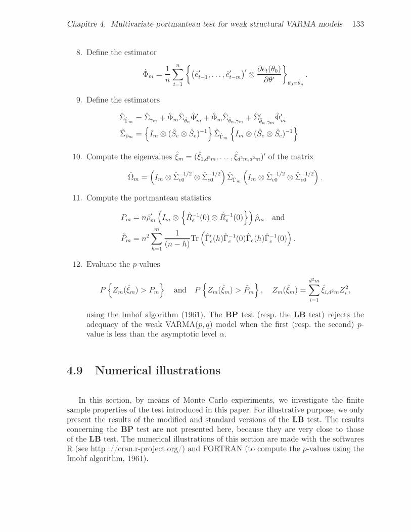
Chapitre 4. Multivariate portmanteau test for weak structural VARMA models 133
8. Define the estimator
Φm =1
n
n∑
t=1
(e′t−1, . . . , e
′t−m
)′ ⊗ ∂et(θ0)
∂θ′
θ0=θn
.
9. Define the estimators
ΣΓm= Σγm + ΦmΣθn
Φ′m + ΦmΣθn,γm
+ Σ′θn,γm
Φ′m
Σρm =
Im ⊗ (Se ⊗ Se)−1
ΣΓm
Im ⊗ (Se ⊗ Se)−1
10. Compute the eigenvalues ξm = (ξ1,d2m, . . . , ξd2m,d2m)′ of the matrix
Ωm =(
Im ⊗ Σ−1/2e0 ⊗ Σ
−1/2e0
)
ΣΓm
(
Im ⊗ Σ−1/2e0 ⊗ Σ
−1/2e0
)
.
11. Compute the portmanteau statistics
Pm = nρ′m
(
Im ⊗
R−1e (0)⊗ R−1
e (0))
ρm and
Pm = n2
m∑
h=1
1
(n− h)Tr(
Γ′e(h)Γ
−1e (0)Γe(h)Γ
−1e (0)
)
.
12. Evaluate the p-values
P
Zm(ξm) > Pm
and P
Zm(ξm) > Pm
, Zm(ξm) =
d2m∑
i=1
ξi,d2mZ2i ,
using the Imhof algorithm (1961). The BP test (resp. the LB test) rejects theadequacy of the weak VARMA(p, q) model when the first (resp. the second) p-value is less than the asymptotic level α.
4.9 Numerical illustrations
In this section, by means of Monte Carlo experiments, we investigate the finitesample properties of the test introduced in this paper. For illustrative purpose, we onlypresent the results of the modified and standard versions of the LB test. The resultsconcerning the BP test are not presented here, because they are very close to thoseof the LB test. The numerical illustrations of this section are made with the softwaresR (see http ://cran.r-project.org/) and FORTRAN (to compute the p-values using theImohf algorithm, 1961).
Chapitre 4. Multivariate portmanteau test for weak structural VARMA models 134
4.9.1 Empirical size
To generate the strong and weak VARMA models, we consider the bivariate modelof the form
(X1t
X2t
)
=
(0 00 a1(2, 2)
)(X1t−1
X2t−1
)
+
(ǫ1tǫ2t
)
−(
0 0b1(2, 1) b1(2, 2)
)(ǫ1t−1
ǫ2t−1
)
, (4.13)
where (a1(2, 2), b1(2, 1), b1(2, 2)) = (0.225,−0.313, 0.750). This model is a VARMA(1,1)model in echelon form.
Strong VARMA case
We first consider the strong VARMA case. To generate this model, we assume thatin (4.13) the innovation process (ǫt) is defined by
(ǫ1,tǫ2,t
)
∼ IIDN (0, I2). (4.14)
We simulated N = 1, 000 independent trajectories of size n = 500, n = 1, 000 andn = 2, 000 of Model (4.13) with the strong Gaussian noise (4.14). For each of theseN replications we estimated the coefficients (a1(2, 2), b1(2, 1), b1(2, 2)) and we appliedportmanteau tests to the residuals for different values of m.
For the standard LB test, the VARMA(1,1) model is rejected when the statistic Pm
is greater than χ2(4m−3)(0.95), where m is the number of residual autocorrelations used in
the LB statistic. This corresponds to a nominal asymptotic level α = 5% in the standardcase. We know that the asymptotic level of the standard LB test is indeed α = 5% when(a1(2, 2), b1(2, 1), b1(2, 2)) = (0, 0, 0). Note however that, even when the noise is strong,the asymmptotic level is not exactly α = 5% when (a1(2, 2), b1(2, 1), b1(2, 2)) 6= (0, 0, 0)).
For the modified LB test, the model is rejected when the statistic Pm is greater than
Sm(0.95) i.e. when the p-value(
P
Zm(ξm) > Pm
)
is less than the asymptotic level
α = 0.05. Let A and B be the (2× 2)-matrices with non zero elements a1(2, 2), b1(2, 1)and b1(2, 2). When the roots of det(I2 − Az) det(I2 − Bz) = 0 are near the unit disk,the asymptotic distribution of Pm is likely to be far from its χ2
(4m−3) approximation.Table 4.1 displays the relative rejection frequencies of the null hypothesis H0 that theDGP follows an VARMA(1, 1) model, over the N = 1, 000 independent replications.As expected the observed relative rejection frequency of the standard LB test is veryfar from the nominal α = 5% when the number of autocorrelations used in the LBstatistic is m ≤ p + q. This is in accordance with the results in the literature on the
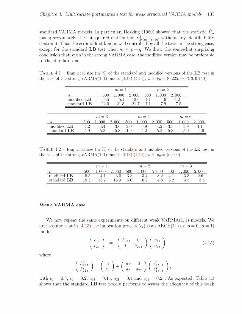
Chapitre 4. Multivariate portmanteau test for weak structural VARMA models 135
standard VARMA models. In particular, Hosking (1980) showed that the statistic Pm
has approximately the chi-squared distribution χ2d2(m−(p+q)) without any identifiability
contraint. Thus the error of first kind is well controlled by all the tests in the strong case,except for the standard LB test when m ≤ p + q. We draw the somewhat surprisingconclusion that, even in the strong VARMA case, the modified version may be preferableto the standard one.
Table 4.1 – Empirical size (in %) of the standard and modified versions of the LB test inthe case of the strong VARMA(1, 1) model (4.13)-(4.14), with θ0 = (0.225,−0.313, 0.750).
m = 1 m = 2n 500 1, 000 2, 000 500 1, 000 2, 000modified LB 5.5 5.1 3.6 4.1 4.6 4.2standard LB 22.0 21.3 21.7 7.1 7.9 7.5
m = 3 m = 4 m = 6n 500 1, 000 2, 000 500 1, 000 2, 000 500 1, 000 2, 000modified LB 4.2 4.4 3.6 3.0 3.9 4.2 3.3 3.9 4.1standard LB 5.9 5.8 5.3 4.9 5.2 5.2 5.3 5.0 4.6
Table 4.2 – Empirical size (in %) of the standard and modified versions of the LB test inthe case of the strong VARMA(1, 1) model (4.13)-(4.14), with θ0 = (0, 0, 0).
m = 1 m = 2 m = 3n 500 1, 000 2, 000 500 1, 000 2, 000 500 1, 000 2, 000modified LB 5.5 4.1 3.0 3.8 3.4 3.2 4.1 3.3 2.6standard LB 18.3 18.7 16.9 6.0 6.2 4.8 5.2 4.5 3.5
Weak VARMA case
We now repeat the same experiments on different weak VARMA(1, 1) models. Wefirst assume that in (4.13) the innovation process (ǫt) is an ARCH(1) (i.e. p = 0, q = 1)model
(ǫ1 t
ǫ2 t
)
=
(h11 t 00 h22 t
)(η1 t
η2 t
)
(4.15)
where(h211 t
h222 t
)
=
(c1c2
)
+
(a11 0a21 a22
)(ǫ21 t−1
ǫ22 t−1
)
,
with c1 = 0.3, c2 = 0.2, a11 = 0.45, a21 = 0.4 and a22 = 0.25. As expected, Table 4.3shows that the standard LB test poorly performs to assess the adequacy of this weak
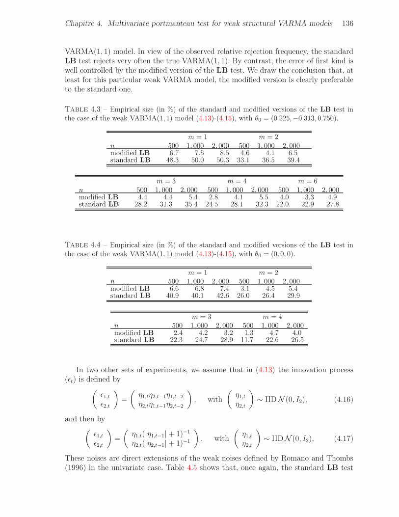
Chapitre 4. Multivariate portmanteau test for weak structural VARMA models 136
VARMA(1, 1) model. In view of the observed relative rejection frequency, the standardLB test rejects very often the true VARMA(1, 1). By contrast, the error of first kind iswell controlled by the modified version of the LB test. We draw the conclusion that, atleast for this particular weak VARMA model, the modified version is clearly preferableto the standard one.
Table 4.3 – Empirical size (in %) of the standard and modified versions of the LB test inthe case of the weak VARMA(1, 1) model (4.13)-(4.15), with θ0 = (0.225,−0.313, 0.750).
m = 1 m = 2n 500 1, 000 2, 000 500 1, 000 2, 000modified LB 6.7 7.5 8.5 4.6 4.1 6.5standard LB 48.3 50.0 50.3 33.1 36.5 39.4
m = 3 m = 4 m = 6n 500 1, 000 2, 000 500 1, 000 2, 000 500 1, 000 2, 000modified LB 4.4 4.4 5.4 2.8 4.1 5.5 4.0 3.3 4.9standard LB 28.2 31.3 35.4 24.5 28.1 32.3 22.0 22.9 27.8
Table 4.4 – Empirical size (in %) of the standard and modified versions of the LB test inthe case of the weak VARMA(1, 1) model (4.13)-(4.15), with θ0 = (0, 0, 0).
m = 1 m = 2n 500 1, 000 2, 000 500 1, 000 2, 000modified LB 6.6 6.8 7.4 3.1 4.5 5.4standard LB 40.9 40.1 42.6 26.0 26.4 29.9
m = 3 m = 4n 500 1, 000 2, 000 500 1, 000 2, 000modified LB 2.4 4.2 3.2 1.3 4.7 4.0standard LB 22.3 24.7 28.9 11.7 22.6 26.5
In two other sets of experiments, we assume that in (4.13) the innovation process(ǫt) is defined by
(ǫ1,tǫ2,t
)
=
(η1,tη2,t−1η1,t−2
η2,tη1,t−1η2,t−2
)
, with
(η1,tη2,t
)
∼ IIDN (0, I2), (4.16)
and then by(ǫ1,tǫ2,t
)
=
(η1,t(|η1,t−1|+ 1)−1
η2,t(|η2,t−1|+ 1)−1
)
, with
(η1,tη2,t
)
∼ IIDN (0, I2), (4.17)
These noises are direct extensions of the weak noises defined by Romano and Thombs(1996) in the univariate case. Table 4.5 shows that, once again, the standard LB test
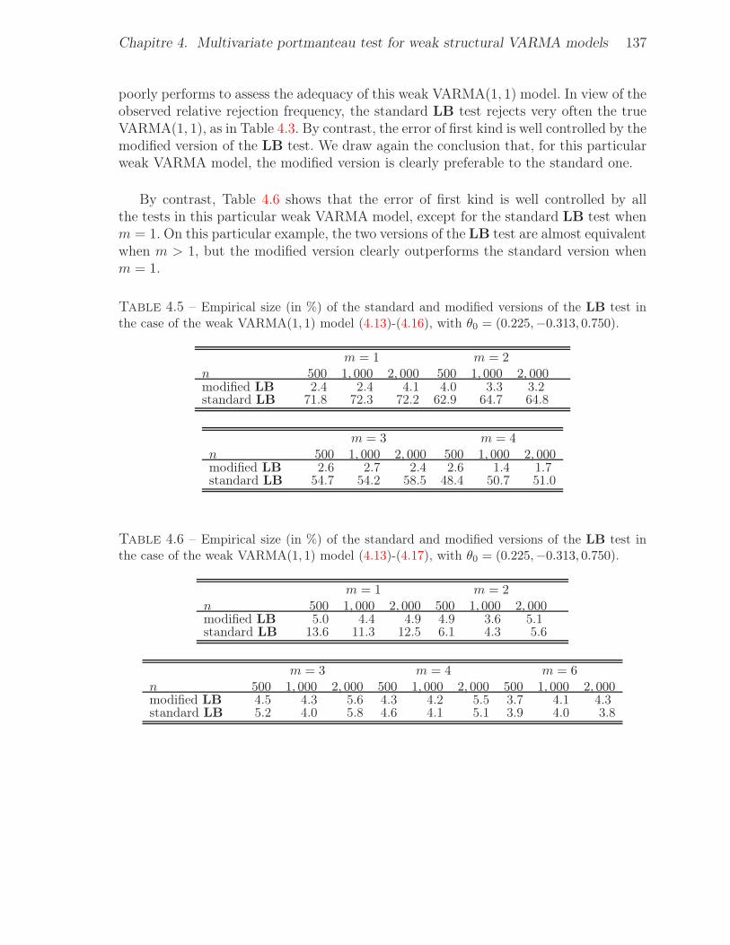
Chapitre 4. Multivariate portmanteau test for weak structural VARMA models 137
poorly performs to assess the adequacy of this weak VARMA(1, 1) model. In view of theobserved relative rejection frequency, the standard LB test rejects very often the trueVARMA(1, 1), as in Table 4.3. By contrast, the error of first kind is well controlled by themodified version of the LB test. We draw again the conclusion that, for this particularweak VARMA model, the modified version is clearly preferable to the standard one.
By contrast, Table 4.6 shows that the error of first kind is well controlled by allthe tests in this particular weak VARMA model, except for the standard LB test whenm = 1. On this particular example, the two versions of the LB test are almost equivalentwhen m > 1, but the modified version clearly outperforms the standard version whenm = 1.
Table 4.5 – Empirical size (in %) of the standard and modified versions of the LB test inthe case of the weak VARMA(1, 1) model (4.13)-(4.16), with θ0 = (0.225,−0.313, 0.750).
m = 1 m = 2n 500 1, 000 2, 000 500 1, 000 2, 000modified LB 2.4 2.4 4.1 4.0 3.3 3.2standard LB 71.8 72.3 72.2 62.9 64.7 64.8
m = 3 m = 4n 500 1, 000 2, 000 500 1, 000 2, 000modified LB 2.6 2.7 2.4 2.6 1.4 1.7standard LB 54.7 54.2 58.5 48.4 50.7 51.0
Table 4.6 – Empirical size (in %) of the standard and modified versions of the LB test inthe case of the weak VARMA(1, 1) model (4.13)-(4.17), with θ0 = (0.225,−0.313, 0.750).
m = 1 m = 2n 500 1, 000 2, 000 500 1, 000 2, 000modified LB 5.0 4.4 4.9 4.9 3.6 5.1standard LB 13.6 11.3 12.5 6.1 4.3 5.6
m = 3 m = 4 m = 6n 500 1, 000 2, 000 500 1, 000 2, 000 500 1, 000 2, 000modified LB 4.5 4.3 5.6 4.3 4.2 5.5 3.7 4.1 4.3standard LB 5.2 4.0 5.8 4.6 4.1 5.1 3.9 4.0 3.8
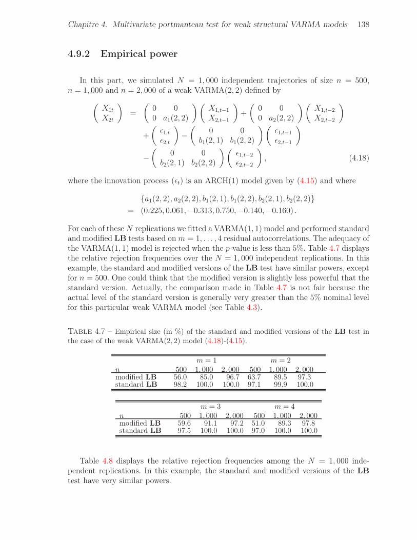
Chapitre 4. Multivariate portmanteau test for weak structural VARMA models 138
4.9.2 Empirical power
In this part, we simulated N = 1, 000 independent trajectories of size n = 500,n = 1, 000 and n = 2, 000 of a weak VARMA(2, 2) defined by
(X1t
X2t
)
=
(0 00 a1(2, 2)
)(X1,t−1
X2,t−1
)
+
(0 00 a2(2, 2)
)(X1,t−2
X2,t−2
)
+
(ǫ1,tǫ2,t
)
−(
0 0b1(2, 1) b1(2, 2)
)(ǫ1,t−1
ǫ2,t−1
)
−(
0 0b2(2, 1) b2(2, 2)
)(ǫ1,t−2
ǫ2,t−2
)
, (4.18)
where the innovation process (ǫt) is an ARCH(1) model given by (4.15) and where
a1(2, 2), a2(2, 2), b1(2, 1), b1(2, 2), b2(2, 1), b2(2, 2)= (0.225, 0.061,−0.313, 0.750,−0.140,−0.160) .
For each of theseN replications we fitted a VARMA(1, 1) model and performed standardand modified LB tests based onm = 1, . . . , 4 residual autocorrelations. The adequacy ofthe VARMA(1, 1) model is rejected when the p-value is less than 5%. Table 4.7 displaysthe relative rejection frequencies over the N = 1, 000 independent replications. In thisexample, the standard and modified versions of the LB test have similar powers, exceptfor n = 500. One could think that the modified version is slightly less powerful that thestandard version. Actually, the comparison made in Table 4.7 is not fair because theactual level of the standard version is generally very greater than the 5% nominal levelfor this particular weak VARMA model (see Table 4.3).
Table 4.7 – Empirical size (in %) of the standard and modified versions of the LB test inthe case of the weak VARMA(2, 2) model (4.18)-(4.15).
m = 1 m = 2n 500 1, 000 2, 000 500 1, 000 2, 000modified LB 56.0 85.0 96.7 63.7 89.5 97.3standard LB 98.2 100.0 100.0 97.1 99.9 100.0
m = 3 m = 4n 500 1, 000 2, 000 500 1, 000 2, 000modified LB 59.6 91.1 97.2 51.0 89.3 97.8standard LB 97.5 100.0 100.0 97.0 100.0 100.0
Table 4.8 displays the relative rejection frequencies among the N = 1, 000 inde-pendent replications. In this example, the standard and modified versions of the LBtest have very similar powers.
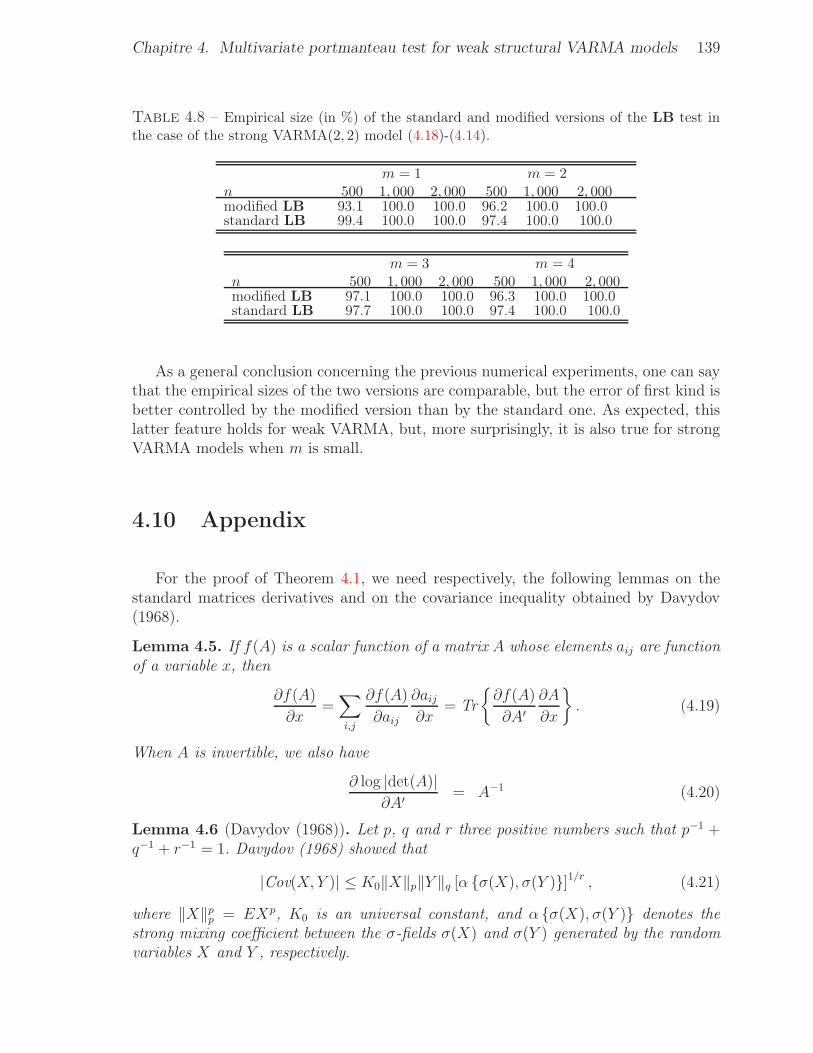
Chapitre 4. Multivariate portmanteau test for weak structural VARMA models 139
Table 4.8 – Empirical size (in %) of the standard and modified versions of the LB test inthe case of the strong VARMA(2, 2) model (4.18)-(4.14).
m = 1 m = 2n 500 1, 000 2, 000 500 1, 000 2, 000modified LB 93.1 100.0 100.0 96.2 100.0 100.0standard LB 99.4 100.0 100.0 97.4 100.0 100.0
m = 3 m = 4n 500 1, 000 2, 000 500 1, 000 2, 000modified LB 97.1 100.0 100.0 96.3 100.0 100.0standard LB 97.7 100.0 100.0 97.4 100.0 100.0
As a general conclusion concerning the previous numerical experiments, one can saythat the empirical sizes of the two versions are comparable, but the error of first kind isbetter controlled by the modified version than by the standard one. As expected, thislatter feature holds for weak VARMA, but, more surprisingly, it is also true for strongVARMA models when m is small.
4.10 Appendix
For the proof of Theorem 4.1, we need respectively, the following lemmas on thestandard matrices derivatives and on the covariance inequality obtained by Davydov(1968).
Lemma 4.5. If f(A) is a scalar function of a matrix A whose elements aij are functionof a variable x, then
∂f(A)
∂x=∑
i,j
∂f(A)
∂aij
∂aij∂x
= Tr
∂f(A)
∂A′
∂A
∂x
. (4.19)
When A is invertible, we also have
∂ log |det(A)|∂A′
= A−1 (4.20)
Lemma 4.6 (Davydov (1968)). Let p, q and r three positive numbers such that p−1 +q−1 + r−1 = 1. Davydov (1968) showed that
|Cov(X, Y )| ≤ K0‖X‖p‖Y ‖q [α σ(X), σ(Y )]1/r , (4.21)
where ‖X‖pp = EXp, K0 is an universal constant, and α σ(X), σ(Y ) denotes thestrong mixing coefficient between the σ-fields σ(X) and σ(Y ) generated by the randomvariables X and Y , respectively.
Chapitre 4. Multivariate portmanteau test for weak structural VARMA models 140
Proof of Theorem 4.1. Recall that
Qn(θ) = log det
1
n
n∑
t=1
et(θ)e′t(θ)
and On(θ) = log det
1
n
n∑
t=1
et(θ)e′t(θ)
.
In view of Theorem 1 in Boubacar Mainassara and Francq (2009) and A6, we have
almost surely θn → θ0 ∈
Θ. Thus ∂Qn(θn)/∂θ = 0 for sufficiently large n, and a standardTaylor expansion of the derivative of Qn about θ0, taken at θn, yields
0 =√n∂Qn(θn)
∂θ=
√n∂Qn(θ0)
∂θ+∂2Qn(θ
∗)
∂θ∂θ′√n(
θn − θ0
)
=√n∂On(θ0)
∂θ+∂2On(θ0)
∂θ∂θ′√n(
θn − θ0
)
+ oP (1), (4.22)
using arguments given in FZ (proof of Theorem 2), where θ∗ is between θ0 and θn. Thus,by standard arguments, we have from (4.22) :
√n(
θn − θ0
)
= −J−1√n∂On(θ0)
∂θ+ oP (1)
= J−1√nYn + oP (1)
where
Yn = −∂On(θ0)
∂θ= − ∂
∂θlog det
1
n
n∑
t=1
et(θ0)e′t(θ0)
.
Showing that the initial values are asymptotically negligible, and using (4.19) and(4.20), we have
∂On(θ)
∂θi= Tr
∂ log |Σn|∂Σn
∂Σn
∂θi
= Tr
Σ−1n
∂Σn
∂θi
, (4.23)
with∂Σn
∂θi=
2
n
n∑
t=1
et(θ)∂e′t(θ)
∂θi.
Then, for 1 ≤ i ≤ k0 = (p + q + 2)d2, the i-th coordinate of the vector Yn is of theform
Y (i)n = −Tr
2
n
n∑
t=1
Σ−1e0 et(θ0)
∂e′t(θ0)
∂θi
, Σe0 = Σn(θ0).
It is easily shown that for ℓ, ℓ′ ≥ 1,
Cov(√n vec γ(ℓ),
√n vec γ(ℓ′)) =
1
n
n∑
t=ℓ+1
n∑
t′=ℓ′+1
E(et−ℓ ⊗ et et′−ℓ′ ⊗ et′′
)
→ Γ(ℓ, ℓ′) as n→ ∞,
Chapitre 4. Multivariate portmanteau test for weak structural VARMA models 141
Then, we have
Σγm = Γ(ℓ, ℓ′)1≤ℓ,ℓ′≤m
Cov(√nJ−1Yn,
√n vec γ(ℓ)) = −
n∑
t=ℓ+1
J−1E
(∂On
∂θet−ℓ ⊗ et′
)
→ −+∞∑
h=−∞
2J−1E(Et et−h−ℓ ⊗ et−h′
),
where Et =((
Tr
Σ−1e0 et(θ0)
∂e′t(θ0)∂θ1
)′
, . . . ,(
Tr
Σ−1e0 et(θ0)
∂e′t(θ0)∂θk0
)′)′
. Then, we have
Cov(√nJ−1Yn,
√nγm) → −
+∞∑
h=−∞
2J−1E
Et
et−h−1...
et−h−m
⊗ et−h
′
= Σ′γm,θn
Applying the central limit theorem (CLT) for mixing processes (see Herrndorf, 1984)we directly obtain
Varas(√nJ−1Yn) = J−1IJ−1
= Σθn
which shows the asymptotic covariance matrix of Theorem 4.1. It is clear that theexistence of these matrices is ensured by the Davydov (1968) inequality (4.21) inLemma 4.6. The proof is complete. 2
Proof of Theorem 4.2. Recall that
et(θ) = Xt −∞∑
i=1
Ci(θ)Xt−i = B−1θ (L)Aθ(L)Xt
where Aθ(L) = Id − ∑pi=1AiL
i and Bθ(L) = Id − ∑qi=1BiL
i with Ai =A−1
0 Ai and Bi = A−10 BiB
−10 A0. For ℓ = 1, . . . , p and ℓ′ = 1, . . . , q, let Aℓ =
(aij,ℓ) and Bℓ′ = (bij,ℓ′).
We define the matrices A∗ij,h and B
∗ij,h by
B−1θ (z)Eij =
∞∑
h=0
A∗ij,hz
h, B−1θ (z)EijB
−1θ (z)Aθ(z) =
∞∑
h=0
B∗ij,hz
h, |z| ≤ 1
Chapitre 4. Multivariate portmanteau test for weak structural VARMA models 142
for h ≥ 0, where Eij = ∂Aℓ/∂aij,ℓ = ∂Bℓ′/∂bij,ℓ′ is the d× d matrix with 1 at position(i, j) and 0 elsewhere. Take A
∗ij,h = B
∗ij,h = 0 when h < 0. For any aij,ℓ and bij,ℓ′ writing
respectively the multivariate noise derivatives
∂et∂aij,ℓ
= −B−1θ (L)EijXt−ℓ = −
∞∑
h=0
A∗ij,hXt−h−ℓ (4.24)
and∂et∂bij,ℓ′
= B−1θ (L)EijB
−1θ (L)Aθ(L)Xt−ℓ′ =
∞∑
h=0
B∗ij,hXt−h−ℓ′. (4.25)
On the other hand, considering Γ(h) and γ(h) as values of the same function at thepoints θn and θ0, a Taylor expansion about θ0 gives
vec Γe(h) = vec γ(h) +1
n
n∑
t=h+1
et−h(θ)⊗∂et(θ)
∂θ′
+∂et−h(θ)
∂θ′⊗ et(θ)
θ=θ∗n
(θn − θ0) +OP (1/n)
= vec γ(h) + E
(
et−h(θ0)⊗∂et(θ0)
∂θ′
)
(θn − θ0) +OP (1/n),
where θ∗n is between θn and θ0. The last equality follows from the consistency of θnand the fact that (∂et−h/∂θ
′) (θ0) is not correlated with et when h ≥ 0. Then forh = 1, . . . , m,
Γm :=
(
vecΓe(1)′
, . . . ,
vecΓe(m)′)′
= γm + Φm(θn − θ0) +OP (1/n),
where
Φm = E
et−1...
et−m
⊗ ∂et(θ0)
∂θ′
. (4.26)
In Φm, one can express (∂et/∂θ′) (θ0) in terms of the multivariate derivatives (4.24) and(4.25). From Theorem 4.1, we have obtained the asymptotic joint distribution of γmand θn − θ0, which shows that the asymptotic distribution of
√nΓm, is normal, with
mean zero and covariance matrix
Varas(√nΓm) = Varas(
√nγm) + ΦmVaras(
√n(θn − θ0))Φ
′m
+ΦmCovas(√n(θn − θ0),
√nγm)
+Covas(√nγm,
√n(θn − θ0))Φ
′m
= Σγm + ΦmΣθnΦ′
m + ΦmΣθn,γm+ Σ′
θn,γmΦ′
m.
From a Taylor expansion about θ0 of vec Γe(0) we have, vec Γe(0) = vec γ(0)+OP (n−1/2).
Moreover,√n(vec γ(0) − E vec γ(0)) = OP (1) by the CLT for mixing processes. Thus
Chapitre 4. Multivariate portmanteau test for weak structural VARMA models 143
√n(Se ⊗ Se − Se ⊗ Se) = OP (1) and, using (4.5) and the ergodic theorem, we obtain
n
vec(S−1e Γe(h)S
−1e )− vec(S−1
e Γe(h)S−1e )
= n
(S−1e ⊗ S−1
e ) vec Γe(h)− (S−1e ⊗ S−1
e ) vec Γe(h)
= n
(Se ⊗ Se)−1 vec Γe(h)− (Se ⊗ Se)
−1 vec Γe(h)
= (Se ⊗ Se)−1√n(Se ⊗ Se − Se ⊗ Se)(Se ⊗ Se)
−1√n vec Γe(h)
= OP (1).
In the previous equalities we also use vec(ABC) = (C ′⊗A) vec(B) and (A⊗B)−1 =A−1 ⊗ B−1 when A and B are invertible. It follows that
ρm =
(
vecRe(1)′
, . . . ,
vecRe(m)′)′
=
(
(Se ⊗ Se)−1vecΓe(1)
′
, . . . ,
(Se ⊗ Se)−1vecΓe(m)
′)′
=
Im ⊗ (Se ⊗ Se)−1
Γm =Im ⊗ (Se ⊗ Se)
−1Γm +OP (n
−1).
We now obtain (4.6) from (4.5). Hence, we have
Var(√nρm) =
Im ⊗ (Se ⊗ Se)
−1ΣΓm
Im ⊗ (Se ⊗ Se)
−1.
The proof is complete. 2
Proof of Theorem 4.4. The proof is similar to that given by Francq, Roy andZakoïan (2005) for Theorem 5.1. 2
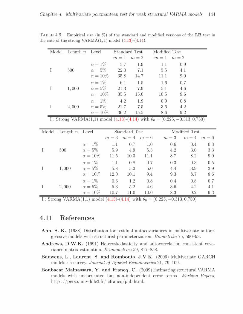
Chapitre 4. Multivariate portmanteau test for weak structural VARMA models 144
Table 4.9 – Empirical size (in %) of the standard and modified versions of the LB test inthe case of the strong VARMA(1, 1) model (4.13)-(4.14).
Model Length n Level Standard Test Modified Testm = 1 m = 2 m = 1 m = 2
α = 1% 5.7 1.9 1.1 0.9I 500 α = 5% 22.0 7.1 5.5 4.1
α = 10% 35.8 14.7 11.1 9.0
α = 1% 6.1 1.5 1.6 0.7I 1, 000 α = 5% 21.3 7.9 5.1 4.6
α = 10% 35.5 15.0 10.5 9.6
α = 1% 4.2 1.9 0.9 0.8I 2, 000 α = 5% 21.7 7.5 3.6 4.2
α = 10% 36.2 15.5 8.6 9.2
I : Strong VARMA(1,1) model (4.13)-(4.14) with θ0 = (0.225,−0.313, 0.750)
Model Length n Level Standard Test Modified Testm = 3 m = 4 m = 6 m = 3 m = 4 m = 6
α = 1% 1.1 0.7 1.0 0.6 0.4 0.3I 500 α = 5% 5.9 4.9 5.3 4.2 3.0 3.3
α = 10% 11.5 10.3 11.1 8.7 8.2 9.0
α = 1% 1.1 0.8 0.7 0.3 0.3 0.5I 1, 000 α = 5% 5.8 5.2 5.0 4.4 3.9 3.9
α = 10% 12.0 10.1 9.4 9.3 8.7 8.6
α = 1% 0.6 1.2 0.8 0.4 0.8 0.7I 2, 000 α = 5% 5.3 5.2 4.6 3.6 4.2 4.1
α = 10% 10.7 11.0 10.0 8.3 9.2 9.3
I : Strong VARMA(1,1) model (4.13)-(4.14) with θ0 = (0.225,−0.313, 0.750)
4.11 References
Ahn, S. K. (1988) Distribution for residual autocovariances in multivariate autore-gressive models with structured parameterization. Biometrika 75, 590–93.
Andrews, D.W.K. (1991) Heteroskedasticity and autocorrelation consistent cova-riance matrix estimation. Econometrica 59, 817–858.
Bauwens, L., Laurent, S. and Rombouts, J.V.K. (2006) Multivariate GARCHmodels : a survey. Journal of Applied Econometrics 21, 79–109.
Boubacar Mainassara, Y. and Francq, C. (2009) Estimating structural VARMAmodels with uncorrelated but non-independent error terms. Working Papers,http ://perso.univ-lille3.fr/ cfrancq/pub.html.
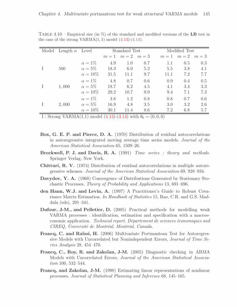
Chapitre 4. Multivariate portmanteau test for weak structural VARMA models 145
Table 4.10 – Empirical size (in %) of the standard and modified versions of the LB test inthe case of the strong VARMA(1, 1) model (4.13)-(4.14).
Model Length n Level Standard Test Modified Testm = 1 m = 2 m = 3 m = 1 m = 2 m = 3
α = 1% 4.9 1.0 0.7 1.1 0.5 0.3I 500 α = 5% 18.3 6.0 5.2 5.5 3.8 4.1
α = 10% 31.5 11.1 9.7 11.1 7.2 7.7
α = 1% 4.8 0.7 0.6 0.9 0.4 0.5I 1, 000 α = 5% 18.7 6.2 4.5 4.1 3.4 3.3
α = 10% 29.2 10.7 9.9 9.4 7.1 7.3
α = 1% 3.8 1.2 0.8 0.8 0.7 0.6I 2, 000 α = 5% 16.9 4.8 3.5 3.0 3.2 2.6
α = 10% 30.1 11.4 8.6 7.2 6.8 5.7
I : Strong VARMA(1,1) model (4.13)-(4.14) with θ0 = (0, 0, 0)
Box, G. E. P. and Pierce, D. A. (1970) Distribution of residual autocorrelationsin autoregressive integrated moving average time series models. Journal of theAmerican Statistical Association 65, 1509–26.
Brockwell, P. J. and Davis, R. A. (1991) Time series : theory and methods.Springer Verlag, New York.
Chitturi, R. V. (1974) Distribution of residual autocorrelations in multiple autore-gressive schemes. Journal of the American Statistical Association 69, 928–934.
Davydov, Y. A. (1968) Convergence of Distributions Generated by Stationary Sto-chastic Processes. Theory of Probability and Applications 13, 691–696.
den Hann, W.J. and Levin, A. (1997) A Practitioner’s Guide to Robust Cova-riance Matrix Estimation. In Handbook of Statistics 15, Rao, C.R. and G.S. Mad-dala (eds), 291–341.
Dufour, J-M., and Pelletier, D. (2005) Practical methods for modelling weakVARMA processes : identification, estimation and specification with a macroe-conomic application. Technical report, Département de sciences économiques andCIREQ, Université de Montréal, Montréal, Canada.
Francq, C. and Raïssi, H. (2006) Multivariate Portmanteau Test for Autoregres-sive Models with Uncorrelated but Nonindependent Errors, Journal of Time Se-ries Analysis 28, 454–470.
Francq, C., Roy, R. and Zakoïan, J-M. (2005) Diagnostic checking in ARMAModels with Uncorrelated Errors, Journal of the American Statistical Associa-tion 100, 532–544.
Francq, and Zakoïan, J-M. (1998) Estimating linear representations of nonlinearprocesses, Journal of Statistical Planning and Inference 68, 145–165.
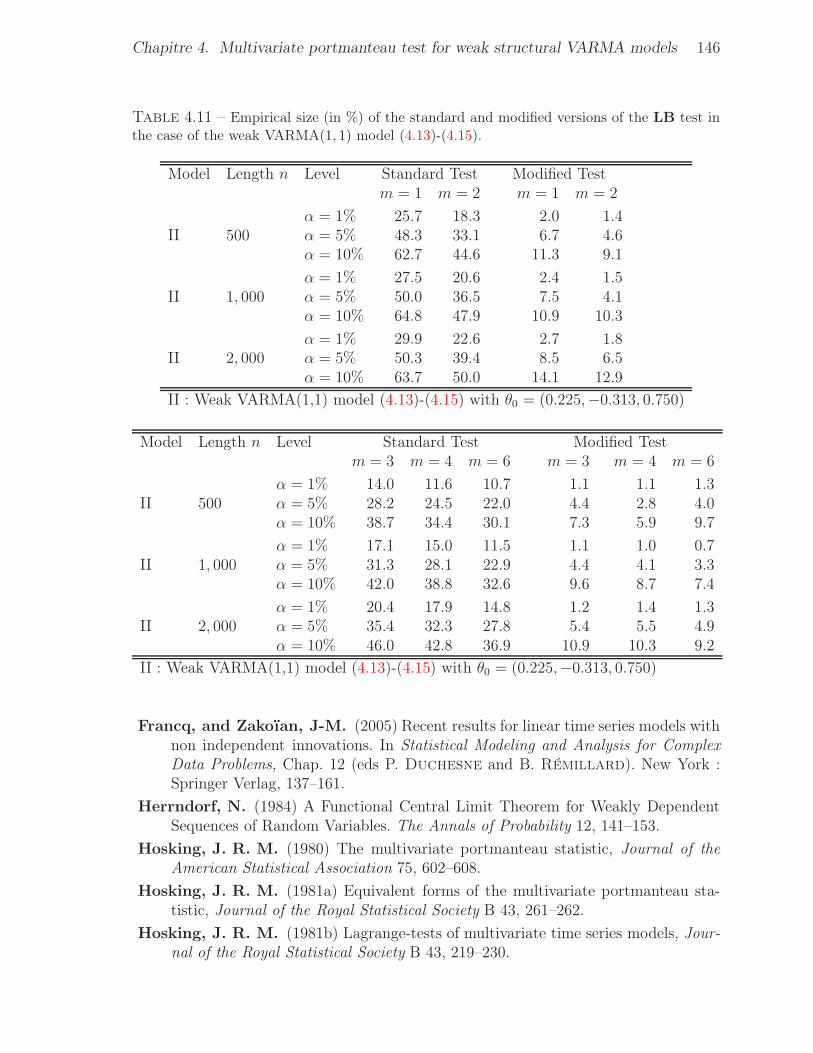
Chapitre 4. Multivariate portmanteau test for weak structural VARMA models 146
Table 4.11 – Empirical size (in %) of the standard and modified versions of the LB test inthe case of the weak VARMA(1, 1) model (4.13)-(4.15).
Model Length n Level Standard Test Modified Testm = 1 m = 2 m = 1 m = 2
α = 1% 25.7 18.3 2.0 1.4II 500 α = 5% 48.3 33.1 6.7 4.6
α = 10% 62.7 44.6 11.3 9.1
α = 1% 27.5 20.6 2.4 1.5II 1, 000 α = 5% 50.0 36.5 7.5 4.1
α = 10% 64.8 47.9 10.9 10.3
α = 1% 29.9 22.6 2.7 1.8II 2, 000 α = 5% 50.3 39.4 8.5 6.5
α = 10% 63.7 50.0 14.1 12.9
II : Weak VARMA(1,1) model (4.13)-(4.15) with θ0 = (0.225,−0.313, 0.750)
Model Length n Level Standard Test Modified Testm = 3 m = 4 m = 6 m = 3 m = 4 m = 6
α = 1% 14.0 11.6 10.7 1.1 1.1 1.3II 500 α = 5% 28.2 24.5 22.0 4.4 2.8 4.0
α = 10% 38.7 34.4 30.1 7.3 5.9 9.7
α = 1% 17.1 15.0 11.5 1.1 1.0 0.7II 1, 000 α = 5% 31.3 28.1 22.9 4.4 4.1 3.3
α = 10% 42.0 38.8 32.6 9.6 8.7 7.4
α = 1% 20.4 17.9 14.8 1.2 1.4 1.3II 2, 000 α = 5% 35.4 32.3 27.8 5.4 5.5 4.9
α = 10% 46.0 42.8 36.9 10.9 10.3 9.2
II : Weak VARMA(1,1) model (4.13)-(4.15) with θ0 = (0.225,−0.313, 0.750)
Francq, and Zakoïan, J-M. (2005) Recent results for linear time series models withnon independent innovations. In Statistical Modeling and Analysis for ComplexData Problems, Chap. 12 (eds P. Duchesne and B. Rémillard). New York :Springer Verlag, 137–161.
Herrndorf, N. (1984) A Functional Central Limit Theorem for Weakly DependentSequences of Random Variables. The Annals of Probability 12, 141–153.
Hosking, J. R. M. (1980) The multivariate portmanteau statistic, Journal of theAmerican Statistical Association 75, 602–608.
Hosking, J. R. M. (1981a) Equivalent forms of the multivariate portmanteau sta-tistic, Journal of the Royal Statistical Society B 43, 261–262.
Hosking, J. R. M. (1981b) Lagrange-tests of multivariate time series models, Jour-nal of the Royal Statistical Society B 43, 219–230.
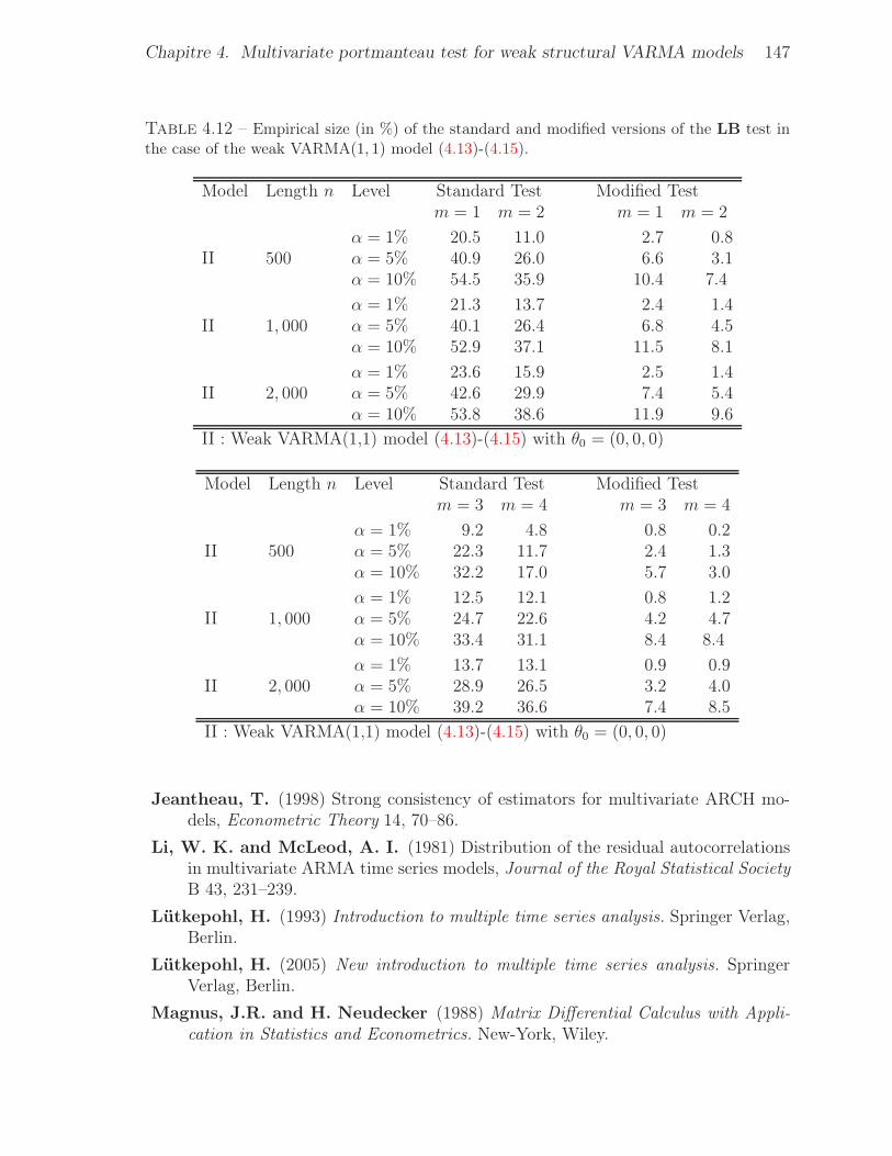
Chapitre 4. Multivariate portmanteau test for weak structural VARMA models 147
Table 4.12 – Empirical size (in %) of the standard and modified versions of the LB test inthe case of the weak VARMA(1, 1) model (4.13)-(4.15).
Model Length n Level Standard Test Modified Testm = 1 m = 2 m = 1 m = 2
α = 1% 20.5 11.0 2.7 0.8II 500 α = 5% 40.9 26.0 6.6 3.1
α = 10% 54.5 35.9 10.4 7.4
α = 1% 21.3 13.7 2.4 1.4II 1, 000 α = 5% 40.1 26.4 6.8 4.5
α = 10% 52.9 37.1 11.5 8.1
α = 1% 23.6 15.9 2.5 1.4II 2, 000 α = 5% 42.6 29.9 7.4 5.4
α = 10% 53.8 38.6 11.9 9.6
II : Weak VARMA(1,1) model (4.13)-(4.15) with θ0 = (0, 0, 0)
Model Length n Level Standard Test Modified Testm = 3 m = 4 m = 3 m = 4
α = 1% 9.2 4.8 0.8 0.2II 500 α = 5% 22.3 11.7 2.4 1.3
α = 10% 32.2 17.0 5.7 3.0
α = 1% 12.5 12.1 0.8 1.2II 1, 000 α = 5% 24.7 22.6 4.2 4.7
α = 10% 33.4 31.1 8.4 8.4
α = 1% 13.7 13.1 0.9 0.9II 2, 000 α = 5% 28.9 26.5 3.2 4.0
α = 10% 39.2 36.6 7.4 8.5
II : Weak VARMA(1,1) model (4.13)-(4.15) with θ0 = (0, 0, 0)
Jeantheau, T. (1998) Strong consistency of estimators for multivariate ARCH mo-dels, Econometric Theory 14, 70–86.
Li, W. K. and McLeod, A. I. (1981) Distribution of the residual autocorrelationsin multivariate ARMA time series models, Journal of the Royal Statistical SocietyB 43, 231–239.
Lütkepohl, H. (1993) Introduction to multiple time series analysis. Springer Verlag,Berlin.
Lütkepohl, H. (2005) New introduction to multiple time series analysis. SpringerVerlag, Berlin.
Magnus, J.R. and H. Neudecker (1988) Matrix Differential Calculus with Appli-cation in Statistics and Econometrics. New-York, Wiley.
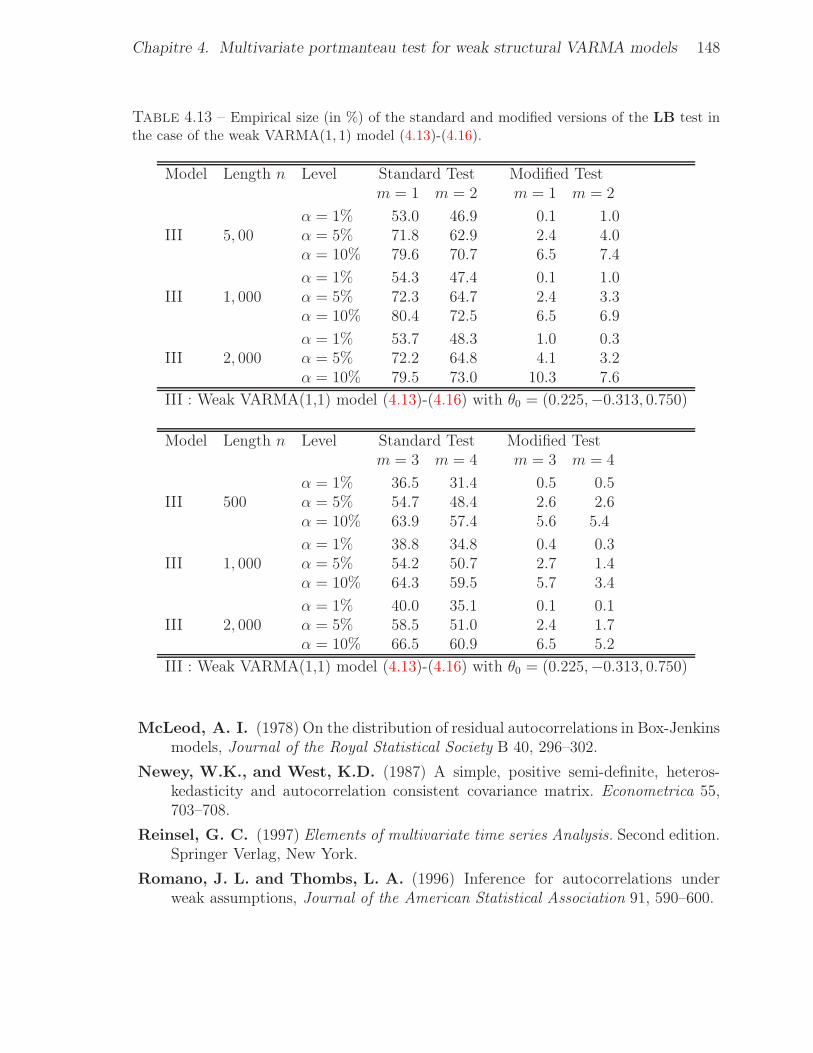
Chapitre 4. Multivariate portmanteau test for weak structural VARMA models 148
Table 4.13 – Empirical size (in %) of the standard and modified versions of the LB test inthe case of the weak VARMA(1, 1) model (4.13)-(4.16).
Model Length n Level Standard Test Modified Testm = 1 m = 2 m = 1 m = 2
α = 1% 53.0 46.9 0.1 1.0III 5, 00 α = 5% 71.8 62.9 2.4 4.0
α = 10% 79.6 70.7 6.5 7.4
α = 1% 54.3 47.4 0.1 1.0III 1, 000 α = 5% 72.3 64.7 2.4 3.3
α = 10% 80.4 72.5 6.5 6.9
α = 1% 53.7 48.3 1.0 0.3III 2, 000 α = 5% 72.2 64.8 4.1 3.2
α = 10% 79.5 73.0 10.3 7.6
III : Weak VARMA(1,1) model (4.13)-(4.16) with θ0 = (0.225,−0.313, 0.750)
Model Length n Level Standard Test Modified Testm = 3 m = 4 m = 3 m = 4
α = 1% 36.5 31.4 0.5 0.5III 500 α = 5% 54.7 48.4 2.6 2.6
α = 10% 63.9 57.4 5.6 5.4
α = 1% 38.8 34.8 0.4 0.3III 1, 000 α = 5% 54.2 50.7 2.7 1.4
α = 10% 64.3 59.5 5.7 3.4
α = 1% 40.0 35.1 0.1 0.1III 2, 000 α = 5% 58.5 51.0 2.4 1.7
α = 10% 66.5 60.9 6.5 5.2
III : Weak VARMA(1,1) model (4.13)-(4.16) with θ0 = (0.225,−0.313, 0.750)
McLeod, A. I. (1978) On the distribution of residual autocorrelations in Box-Jenkinsmodels, Journal of the Royal Statistical Society B 40, 296–302.
Newey, W.K., and West, K.D. (1987) A simple, positive semi-definite, heteros-kedasticity and autocorrelation consistent covariance matrix. Econometrica 55,703–708.
Reinsel, G. C. (1997) Elements of multivariate time series Analysis. Second edition.Springer Verlag, New York.
Romano, J. L. and Thombs, L. A. (1996) Inference for autocorrelations underweak assumptions, Journal of the American Statistical Association 91, 590–600.
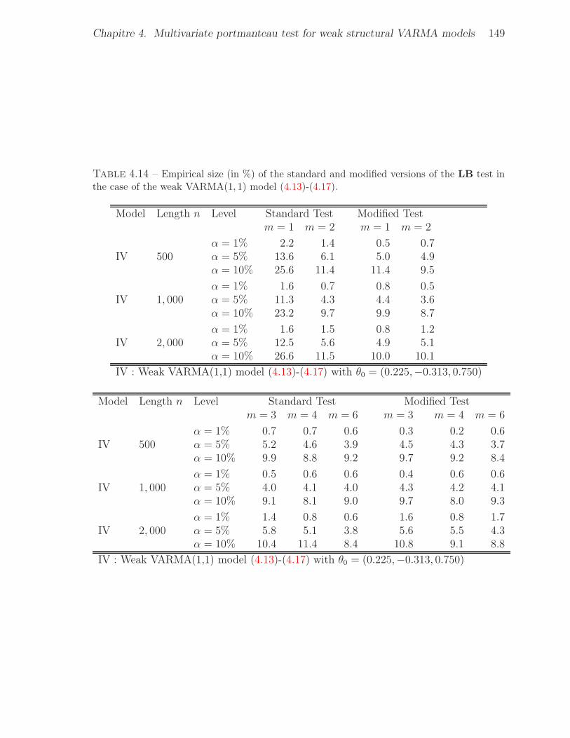
Chapitre 4. Multivariate portmanteau test for weak structural VARMA models 149
Table 4.14 – Empirical size (in %) of the standard and modified versions of the LB test inthe case of the weak VARMA(1, 1) model (4.13)-(4.17).
Model Length n Level Standard Test Modified Testm = 1 m = 2 m = 1 m = 2
α = 1% 2.2 1.4 0.5 0.7IV 500 α = 5% 13.6 6.1 5.0 4.9
α = 10% 25.6 11.4 11.4 9.5
α = 1% 1.6 0.7 0.8 0.5IV 1, 000 α = 5% 11.3 4.3 4.4 3.6
α = 10% 23.2 9.7 9.9 8.7
α = 1% 1.6 1.5 0.8 1.2IV 2, 000 α = 5% 12.5 5.6 4.9 5.1
α = 10% 26.6 11.5 10.0 10.1
IV : Weak VARMA(1,1) model (4.13)-(4.17) with θ0 = (0.225,−0.313, 0.750)
Model Length n Level Standard Test Modified Testm = 3 m = 4 m = 6 m = 3 m = 4 m = 6
α = 1% 0.7 0.7 0.6 0.3 0.2 0.6IV 500 α = 5% 5.2 4.6 3.9 4.5 4.3 3.7
α = 10% 9.9 8.8 9.2 9.7 9.2 8.4
α = 1% 0.5 0.6 0.6 0.4 0.6 0.6IV 1, 000 α = 5% 4.0 4.1 4.0 4.3 4.2 4.1
α = 10% 9.1 8.1 9.0 9.7 8.0 9.3
α = 1% 1.4 0.8 0.6 1.6 0.8 1.7IV 2, 000 α = 5% 5.8 5.1 3.8 5.6 5.5 4.3
α = 10% 10.4 11.4 8.4 10.8 9.1 8.8
IV : Weak VARMA(1,1) model (4.13)-(4.17) with θ0 = (0.225,−0.313, 0.750)
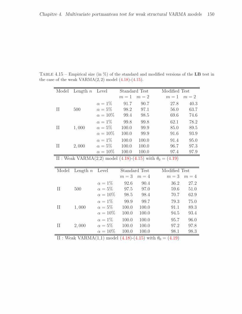
Chapitre 4. Multivariate portmanteau test for weak structural VARMA models 150
Table 4.15 – Empirical size (in %) of the standard and modified versions of the LB test inthe case of the weak VARMA(2, 2) model (4.18)-(4.15).
Model Length n Level Standard Test Modified Testm = 1 m = 2 m = 1 m = 2
α = 1% 91.7 90.7 27.8 40.3II 500 α = 5% 98.2 97.1 56.0 63.7
α = 10% 99.4 98.5 69.6 74.6
α = 1% 99.8 99.8 62.1 78.2II 1, 000 α = 5% 100.0 99.9 85.0 89.5
α = 10% 100.0 99.9 91.6 93.9
α = 1% 100.0 100.0 91.4 95.0II 2, 000 α = 5% 100.0 100.0 96.7 97.3
α = 10% 100.0 100.0 97.4 97.9
II : Weak VARMA(2,2) model (4.18)-(4.15) with θ0 = (4.19)
Model Length n Level Standard Test Modified Testm = 3 m = 4 m = 3 m = 4
α = 1% 92.6 90.4 36.2 27.2II 500 α = 5% 97.5 97.0 59.6 51.0
α = 10% 98.5 98.4 70.7 62.9
α = 1% 99.9 99.7 79.3 75.0II 1, 000 α = 5% 100.0 100.0 91.1 89.3
α = 10% 100.0 100.0 94.5 93.4
α = 1% 100.0 100.0 95.7 96.0II 2, 000 α = 5% 100.0 100.0 97.2 97.8
α = 10% 100.0 100.0 98.1 98.3
II : Weak VARMA(1,1) model (4.18)-(4.15) with θ0 = (4.19)
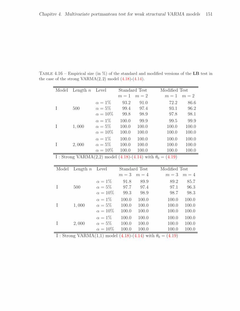
Chapitre 4. Multivariate portmanteau test for weak structural VARMA models 151
Table 4.16 – Empirical size (in %) of the standard and modified versions of the LB test inthe case of the strong VARMA(2, 2) model (4.18)-(4.14).
Model Length n Level Standard Test Modified Testm = 1 m = 2 m = 1 m = 2
α = 1% 93.2 91.0 72.2 86.6I 500 α = 5% 99.4 97.4 93.1 96.2
α = 10% 99.8 98.9 97.8 98.1
α = 1% 100.0 99.9 99.5 99.9I 1, 000 α = 5% 100.0 100.0 100.0 100.0
α = 10% 100.0 100.0 100.0 100.0
α = 1% 100.0 100.0 100.0 100.0I 2, 000 α = 5% 100.0 100.0 100.0 100.0
α = 10% 100.0 100.0 100.0 100.0
I : Strong VARMA(2,2) model (4.18)-(4.14) with θ0 = (4.19)
Model Length n Level Standard Test Modified Testm = 3 m = 4 m = 3 m = 4
α = 1% 91.8 89.9 89.2 85.7I 500 α = 5% 97.7 97.4 97.1 96.3
α = 10% 99.3 98.9 98.7 98.3
α = 1% 100.0 100.0 100.0 100.0I 1, 000 α = 5% 100.0 100.0 100.0 100.0
α = 10% 100.0 100.0 100.0 100.0
α = 1% 100.0 100.0 100.0 100.0I 2, 000 α = 5% 100.0 100.0 100.0 100.0
α = 10% 100.0 100.0 100.0 100.0
I : Strong VARMA(1,1) model (4.18)-(4.14) with θ0 = (4.19)
Chapitre 5
Model selection of weak VARMAmodels
Abstract We consider the problem of orders selections of vector autoregressivemoving-average (VARMA) models under the assumption that the errors are uncorrela-ted but not necessarily independent. We relax the standard independence assumptionto extend the range of application of the VARMA models, and allow to cover linear re-presentations of general nonlinear processes. We propose a modified Akaike informationcriterion (AIC).
Keywords : AIC, discrepancy, Kullback-Leibler information, QMLE/LSE, order selection,
structural representation, weak VARMA models.
5.1 Introduction
The class of vector autoregressive moving-average (VARMA) models and the sub-class of vector autoregressive (VAR) models are used in time series analysis and eco-nometrics to describe not only the properties of the individual time series but alsothe possible cross-relationships between the time series (see Reinsel, 1997, Lütkepohl,2005, 1993). In a VARMA(p, q) models, the choice of p and q is particularly impor-tant because the number of parameters, (p + q + 3)d2 where d is the number of theseries, quickly increases with p and q, which entails statistical difficulties. If orders lo-wer than the true orders of the VARMA(p, q) models are selected, the estimate of theparameters will not be consistent and if too high orders are selected, the accuracy ofthe estimation parameters is likely to be low. This paper is devoted to the problem ofthe choice (by minimizing an information criterion) of the orders of VARMA modelsunder the assumption that the errors are uncorrelated but not necessarily independent.
Chapitre 5. Model selection of weak VARMA models 153
Such models are called weak VARMA, by contrast to the strong VARMA models, thatare the standard VARMA usually considered in the time series literature and in whichthe noise is assumed to be iid. Relaxing the independence assumption allows to extendthe range of application of the VARMA models, and allows to cover linear representa-tions of general nonlinear processes. The statistical inference of weak ARMA modelsis mainly limited to the univariate framework (see Francq and Zakoïan, 2005, for areview on weak ARMA models). In the multivariate analysis, important advances havebeen obtained by Dufour and Pelletier (2005) who study the asymptotic properties ofa generalization of the regression-based estimation method proposed by Hannan andRissanen (1982) under weak assumptions on the innovation process, Francq and Raïssi(2007) who study portmanteau tests for weak VAR models, Boubacar Mainassara andFrancq (2009) who study the consistency and the asymptotic normality of the QMLEfor weak VARMA models and Boubacar Mainassara (2009a, 2009b) who studies port-manteau tests for weak VARMA models and studies the estimation of the asymptoticvariance of QML/LS estimator of weak VARMA models. Dufour and Pelletier (2005)have proposed a modified information criterion
log det Σ + dim(γ)(log n)1+δ
n, δ > 0,
which gives a consistent estimates of the orders p and q of a weak VARMA models.Their criterion is a generalization of the information criterion proposed by Hannan andRissanen (1982).
The choice amongst the models is often made by minimizing an information crite-rion. The most popular criterion for model selection is the Akaike information criterion(AIC) proposed by Akaike (1973). The AIC was designed to be an approximately unbia-sed estimator of the expected Kullback-Leibler information of a fitted model. Tsai andHurvich (1989, 1993) derived a bias correction to the AIC for univariate and multiva-riate autoregressive time series under the assumption that the errors ǫt are independentidentically distributed (i.e. strong models). The main goal of our paper is to completethe above-mentioned results concerning the statistical analysis of weak VARMA models,by proposing a modified version of the AIC criterion.
The paper is organized as follows. Section 5.2 presents the models that we considerhere and summarizes the results on the QMLE/LSE asymptotic distribution obtained byBoubacar Mainassara and Francq (2009). For selft-containedness purposes, Section 5.3recalls useful the results concerning the general multivariate linear regression model,and Section 5.4 presents the definition and mains properties of the Kullback-Leiblerdivergence. In Section 5.5, we present the AICM criterion which we minimize to choosethe orders for a weak VARMA(p, q) models. This section is also of interest in theunivariate framework because, to our knowledge, this model selection criterion has notbeen studied for weak ARMA models. We denote by A ⊗ B the Kronecker product oftwo matrices A and B (and by A⊗2 when the matrix A = B), and by vecA the vectorobtained by stacking the columns of A. The reader is refereed to Magnus and Neudecker(1988) for the properties of these operators. Let 0r be the null vector of Rr, and let Ir
Chapitre 5. Model selection of weak VARMA models 154
be the r × r identity matrix.
5.2 Model and assumptions
Consider a d-dimensional stationary process (Xt) satisfying a structuralVARMA(p0, q0) representation of the form
A00Xt −p0∑
i=1
A0iXt−i = B00ǫt −q0∑
i=1
B0iǫt−i, ∀t ∈ Z = 0,±1, . . ., (5.1)
where ǫt is a white noise, namely a stationary sequence of centered and uncorrelatedrandom variables with a non singular variance Σ0. The structural forms are mainly usedin econometrics to introduce instantaneous relationships between economic variables.Of course, constraints are necessary for the identifiability of these representations. Let[A00 . . . A0p0B00 . . . B0q0Σ0] be the d × (p0 + q0 + 3)d matrix of all the coefficients, wi-thout any constraint. The parameter of interest is denoted θ0, where θ0 belongs to theparameter space Θp0,q0 ⊂ Rk0, and k0 is the number of unknown parameters, whichis typically much smaller that (p0 + q0 + 3)d2. The matrices A00, . . . A0p0 , B00, . . . B0q0
involved in (5.1) and Σ0 are specified by θ0. More precisely, we write A0i = Ai(θ0) andB0j = Bj(θ0) for i = 0, . . . , p0 and j = 0, . . . , q0, and Σ0 = Σ(θ0). We need the followingassumptions used by Boubacar Mainassara and Francq (2009) to ensure the consistenceand the asymptotic normality of the quasi-maximum likelihood estimator (QMLE).
A1 : The functions θ 7→ Ai(θ) i = 0, . . . , p, θ 7→ Bj(θ) j = 0, . . . , q andθ 7→ Σ(θ) admit continuous third order derivatives for all θ ∈ Θp,q.
For simplicity we now write Ai, Bj and Σ instead of Ai(θ), Bj(θ) and Σ(θ). Let Aθ(z) =A0 −
∑pi=1Aiz
i and Bθ(z) = B0 −∑q
i=1Bizi.
A2 : For all θ ∈ Θp,q, we have detAθ(z) detBθ(z) 6= 0 for all |z| ≤ 1.
A3 : We have θ0 ∈ Θp0,q0, where Θp0,q0 is compact.
A4 : The process (ǫt) is stationary and ergodic.
A5 : For all θ ∈ Θp,q such that θ 6= θ0, either the transfer functions
A−10 B0B
−1θ (z)Aθ(z) 6= A−1
00 B00B−1θ0
(z)Aθ0(z)
for some z ∈ C, or
A−10 B0ΣB
′0A
−1′0 6= A−1
00 B00Σ0B′00A
−1′00 .
A6 : We have θ0 ∈
Θp0,q0, where
Θp0,q0 denotes the interior of Θp0,q0.
A7 : We have E‖ǫt‖4+2ν <∞ and∑∞
k=0 αǫ(k)ν
2+ν <∞ for some ν > 0.
Chapitre 5. Model selection of weak VARMA models 155
The reader is referred to Boubacar Mainassara and Francq (2009) for a discus-sion of these assumptions. Note that (ǫt) can be replaced by (Xt) in A4, becauseXt = A−1
θ0(L)Bθ0(L)ǫt and ǫt = B−1
θ0(L)Aθ0(L)Xt, where L stands for the backward
operator. Note that from A1 the matrices A0 and B0 are invertible. Introducing theinnovation process et = A−1
00 B00ǫt, the structural representation Aθ0(L)Xt = Bθ0(L)ǫtcan be rewritten as the reduced VARMA representation
Xt −p∑
i=1
A−100 A0iXt−i = et −
q∑
i=1
A−100 B0iB
−100 A00et−i.
We thus recursively define et(θ) for t = 1, . . . , n by
et(θ) = Xt −p∑
i=1
A−10 AiXt−i +
q∑
i=1
A−10 BiB
−10 A0et−i(θ),
with initial values e0(θ) = · · · = e1−q(θ) = X0 = · · · = X1−p = 0. The gaussianquasi-likelihood is given by
Ln (θ) =
n∏
t=1
1
(2π)d/2√det Σe
exp
−1
2e′t(θ)Σ
−1e et(θ)
, Σe = A−10 B0ΣB
′0A
−1′0 .
A quasi-maximum likelihood estimator (QMLE) of θ is a measurable solution θn of
θn = argmaxθ∈Θ
Ln(θ).
We now use the matrix Mθ0 of the coefficients of the reduced form to that made byBoubacar Mainassara and Francq (2009), where
Mθ0 = [A−100 A01 : . . . : A
−100 A0p : A
−100 B01B
−100 A00 : . . . : A
−100 B0qB
−100 A00 : Σe0].
Now we need an assumption which specifies how this matrix depends on the parameter
θ0. Let
M θ0 be the matrix ∂vec(Mθ)/∂θ′ evaluated at θ0.
A8 : The matrix
M θ0 is of full rank k0.Under Assumptions A1–A8, Boubacar Mainassara and Francq (2009) showed theconsistency (θn → θ0 a.s as n → ∞) and the asymptotic normality of the QMLE :
√n(
θn − θ0
)L→ N (0,Ω := J−1IJ−1), (5.2)
where J = J(θ0) and I = I(θ0), with
J(θ) = limn→∞
2
n
∂2
∂θ∂θ′log Ln(θ) a.s
and
I(θ) = limn→∞
Var2√n
∂
∂θlog Ln(θ).
Chapitre 5. Model selection of weak VARMA models 156
Note that, for VARMA models in reduced form, it is not very restrictive to assume thatthe coefficients A0, . . . , Ap, B0, . . . , Bq are functionally independent of the coefficientΣe. Thus we can write θ = (θ(1)
′, θ(2)
′)′, where θ(1) ∈ R
k1 depends on A0, . . . , Ap andB0, . . . , Bq, and where θ(2) ∈ Rk2 depends on Σe, with k1 + k2 = k0. With some abuseof notation, we will then write et(θ) = et(θ
(1)).A9 : With the previous notation θ = (θ(1)
′, θ(2)
′)′, where θ(2) = D vec Σe for
some matrix D of size k2 × d2.Let J11 and I11 be respectively the upper-left block of the matrices J and I, withappropriate size. Under Assumptions A1–A9, in a working paper, Boubacar Mainassara(2009) obtained explicit expressions of I11 and J11, given by
vec J11 = 2∑
i≥1
Mλ′i ⊗ λ′i vec Σ−1e0 and
vec I11 = 4+∞∑
i,j=1
Γ(i, j)(Id ⊗ λ′j
⊗ Id ⊗ λ′i
)vec(
vec Σ−1e0
vec Σ−1
e0
′)
,
whereM := E
(Id2(p+q) ⊗ e′t
)⊗2
,
the matrices λi depend on θ0 (see Boubacar Mainassara (2009) for the precise definitionof these matrices) and
Γ(i, j) =+∞∑
h=−∞
E(e′t−h ⊗
(Id2(p+q) ⊗ e′t−j−h
)⊗e′t ⊗
(Id2(p+q) ⊗ e′t−i
)).
We first define an estimator Jn of J by
vec Jn =∑
i≥1
Mn
λ′i ⊗ λ′i
vec Σ−1e0 , where Mn :=
1
n
n∑
t=1
(Id2(p+q) ⊗ e′t
)⊗2
.
To estimate I consider a sequence of real numbers (bn)n∈N∗ such that
bn → 0 and nb10+4ν
νn → ∞ as n→ ∞,
and a weight function f : R → R which is bounded, with compact support [−a, a] andcontinuous at the origin with f(0) = 1. Let In an estimator of I defined by
vec In = 4
+∞∑
i,j=1
Γn(i, j)(
Id ⊗ λ′i
⊗
Id ⊗ λ′j
)
vec
(
vec Σ−1e0
vec Σ−1e0
′)
,
where
Γn(i, j) :=
+Tn∑
h=−Tn
f(hbn)Mn ij,h and Tn =
[a
bn
]
,
where [x] denotes the integer part of x, and where
Mn ij,h :=1
n
n−|h|∑
t=1
(e′t−h ⊗
(Id2(p+q) ⊗ e′t−j−h
)⊗e′t ⊗
(Id2(p+q) ⊗ e′t−i
)).
Chapitre 5. Model selection of weak VARMA models 157
5.3 General multivariate linear regression model
Let Zt = (Z1t, . . . , Zdt)′ be a d-dimensional random vector of response variables,
Xt = (X1t, . . . , Xkt)′ be a k-dimensional input variables and B = (β1, . . . , βd) be a
k × d matrix. We consider a multivariate linear model of the form Zit = X ′tβi + ǫit,
i = 1, . . . , d, or Z ′t = X ′
tB+ǫ′t, t = 1, . . . , n, where the ǫt = (ǫ1t, . . . , ǫdt)′ are uncorrelated
and identically distributed random vectors with variance Σ = Eǫtǫ′t. The i-th column
of B (i.e. βi) is the vector of regression coefficients for the i-th response variable.Now, given the n observations Z1, . . . , Zn and X1, . . . , Xn, we define the n × d datamatrix Z = (Z1, . . . , Zn)
′, the n × k matrix X = (X1, . . . , Xn)′ and the n × d matrix
ε = (ǫ1, . . . , ǫn)′. Then, we have the multivariate linear model Z = XB + ε. Now, it is
well known that the QMLE of B is the same as the LSE and, hence, is given by
B = (X′X)−1
X′Z, that is, βi = (X′
X)−1X
′Zi, i = 1, . . . , d,
where Zi = (Zi 1, . . . , Zi n)′ is the i-th column of Z. We also have
ε := Z−XB =MXZ = ε−X(X′X)−1
X′ε =MXε,
where MX = In −X(X′X)−1
X′ is a projection matrix. The usual unbiased estimator
of the error covariance matrix Σ is
Σ∗ =1
n− kε′ε =
1
n− k(Z−XB)′(Z−XB)
=1
n− k
n∑
t=1
(Zt − B′Xt)(Zt − B′Xt)′
or Σ∗ = (n − k)−1∑n
t=1 ǫtǫ′t, where the ǫt = Zt − B′Xt are the residual vectors. Note
that the gaussian quasi-likelihood is given by
Ln (B,Σ;Z) =1
(2π)d/2√det Σe
exp
−1
2
n∑
t=1
(Zt − B′Xt)′Σ−1 (Zt − B′Xt)
,
whose maximization shows that the QML estimators of B is equal to B and that of Σ isΣ := n−1
∑nt=1 ǫtǫ
′t = (n− k)n−1Σ∗. Because Σ∗ is an unbiased estimator of the matrix
Σ, by definition we have E Σ∗ = Σ, we then deduce that
n
n− kE
Σ
=1
n− kEε′ε =
1
n− kEε′MXε = Σ. (5.3)
5.4 Kullback-Leibler discrepancy
Assume that, with respect to a σ-finite measure µ, the true density of the observa-tionsX = (X1, . . . , Xn) is f0, and that some candidate modelm gives a density fm(·, θm)
Chapitre 5. Model selection of weak VARMA models 158
to the observations, where θm is a km-dimensional parameter. The discrepancy betweenthe candidate and the true models can be measured by the Kullback-Leibler divergence(or information)
∆ fm(·, θm)|f0 = Ef0 logf0(X)
fm(X, θm)= Ef0 log f0(X) +
1
2d fm(·, θm)|f0 ,
where
d fm(·, θm)|f0 = −2Ef0 log fm(X, θm) = −2
∫
log fm(x, θm) f0(x)µ(dx)
is sometimes called the Kullback-Leibler contrast (or the discrepancy between the ap-proximating and the true models). Using the Jensen inequality, we have
∆ fm(·, θm)|f0 = −∫
logfm(x, θm)
f0(x)f0(x)µ(dx)
≥ − log
∫fm(x, θm)
f0(x)f0(x)µ(dx) = 0,
with equality if and only if fm(·, θm) = f0. This is the main property of the Kullback-Leibler divergence. Minimizing ∆ fm(·, θm)|f0 with respect to fm(·, θm) is equivalentto minimizing the contrast d fm(·, θm)|f0. Let
θ0,m = arg infθmd fm(·, θm)|f0 = arg inf
θm−2E log fm(X, θm)
be an optimal parameter for the model m corresponding to the density fm(·, θm) (as-suming that such a parameter exists). We estimate this optimal parameter by QMLEθn,m.
5.5 Criteria for VARMA order selection
Let
ℓn(θ) = −2
nlog Ln(θ)
=1
n
n∑
t=1
d log(2π) + log det Σe + e′t(θ)Σ
−1e et(θ)
.
In Boubacar Mainassara and Francq (2009), it is shown that ℓn(θ) = ℓn(θ) + o(1) a.s,where
ℓn(θ) = −2
nlog Ln(θ)
=1
n
n∑
t=1
d log(2π) + log det Σe + e′t(θ)Σ
−1e et(θ)
,
Chapitre 5. Model selection of weak VARMA models 159
whereet(θ) = A−1
0 B0B−1θ (L)Aθ(L)Xt.
It is also shown uniformly in θ ∈ Θp,q that
∂ℓn(θ)
∂θ=∂ℓn(θ)
∂θ+ o(1) a.s.
The same equality holds for the second-order derivatives of ℓn. For all θ ∈ Θp,q, we have
−2 log Ln(θ) = nd log(2π) + n log det Σe +n∑
t=1
e′t(θ)Σ−1e et(θ).
In view of Section 5.4, minimizing the Kullback-Leibler information of any approxima-ting (or candidate) model, characterized by the parameter vector θ, is equivalent tominimizing the contrast ∆(θ) = E −2 log Ln(θ). Omitting the constant nd log(2π),we find that
∆(θ) = n log det Σe + nTr(Σ−1
e S(θ)),
where S(θ) = Ee1(θ)e′1(θ). In view of the following Lemma, the function θ 7→ ∆(θ) is
minimal for θ = θ0.
Lemma 5.1. For all θ ∈ ⋃p,q∈NΘp,q, we have
∆(θ) ≥ ∆(θ0).
Proof of Lemma 5.1 : We have
∆(θ) = n log det Σe + nTr(Σ−1
e
Ee1(θ0)e
′1(θ0) + 2Ee1(θ0) e1(θ)− e1(θ0)′
+ E (e1(θ)− e1(θ0)) (e1(θ)− e1(θ0))′) .
Now, using the fact that the linear innovation et(θ0) is orthogonal to the linear past (i.e.to the Hilbert space Ht−1 generated by the linear combinations of the Xu for u < t),it follows that Ee1(θ0) e1(θ)− e1(θ0)′ = 0, since et(θ)− et(θ0) belongs to the linearpast Ht−1. We thus have
∆(θ) = n log det Σe + nTr(Σ−1
e Σe0
)
+nTrΣ−1
e E (e1(θ)− e1(θ0)) (e1(θ)− e1(θ0))′ .
Moreover
∆(θ0) = n log det Σe0 + nTr(Σ−1
e0 S(θ0))= n log det Σe0 + nTr
(Σ−1
e0 Σe0
)
= n log det Σe0 + nd.
Thus, we obtain
∆(θ)−∆(θ0) = −n log det(Σ−1
e Σe0
)− nd+ nTr
(Σ−1
e Σe0
)
+nTrΣ−1
e E (e1(θ)− e1(θ0)) (e1(θ)− e1(θ0))′
≥ −n log det(Σ−1
e Σe0
)− nd+ nTr
(Σ−1
e Σe0
),

Chapitre 5. Model selection of weak VARMA models 160
with equality if and only if e1(θ) = e1(θ0) a.s. Using the elementary inequalityTr(A−1B)− log det(A−1B) ≥ Tr(A−1A)− log det(A−1A) = d for all symmetric positivesemi-definite matrices of order d× d, it is easy see that ∆(θ)−∆(θ0) ≥ 0. The proof iscomplete. 2
5.5.1 Estimating the discrepancy
Let X = (X1, . . . , Xn) be observation of a process satisfying the VARMA represen-tation (5.1). Let θn be the QMLE of the parameter θ of a candidate VARMA model.Let, et = et(θn) be the QMLE/LSE residuals when p > 0 or q > 0, and let et = et = Xt
when p = q = 0. When p + q 6= 0, we have et = 0 for t ≤ 0 and t > n, and
et = Xt −p∑
i=1
A−10 (θn)Ai(θn)Xt−i +
q∑
i=1
A−10 (θn)Bi(θn)B
−10 (θn)A0(θn)et−i,
for t = 1, . . . , n, with Xt = 0 for t ≤ 0 and Xt = Xt for t ≥ 1.
In view of Lemma 5.1, it is natural to minimize an estimation of the theoreticalcriterion E∆(θn). Note that E∆(θn) can be interpreted as the average discrepancywhen one uses the model of parameter θn. The Akaike information criterion (AIC)is an approximately unbiased estimator of E∆(θn). We will adapt to weak VARMAmodels the corrected AIC version (AICc) introduced by Tsai and Hurvich (1989) for theunivariate strong AR models. Under Assumptions A1–A9, an approximately unbiasedestimator of E∆(θn) is given by
AICM = n log det Σe +n2d2
nd− k1+
nd
2(nd− k1)
(
vec I ′11,n
)′ (
vec J−111,n
)
, (5.4)
with vec J11,n and vec I11,n are defined in Section 5.2. The AICM stands for AIC "mo-dified".
Justification of (5.4). Using a Taylor expansion of the functions ∂ log Ln(θn)/∂θ(1)
around θ(1)0 , it follows that
(
θ(1)n − θ(1)0
) op(
1√n
)
= −2
nJ−111
∂ log Ln(θ0)
∂θ(1)= −2
n
n∑
t=1
J−111
∂e′t(θ0)
∂θ(1)Σ−1
e0 et(θ0), (5.5)
where ac= b signifies a = b+ c and where J11 = J11(θ0) with
J11(θ) = limn→∞
2
n
∂2 log Ln(θ)
∂θ(1)∂θ(1)′a.s.
Chapitre 5. Model selection of weak VARMA models 161
We haveE∆(θn) = En log det Σe + nETr
(
Σ−1e S(θn)
)
, (5.6)
where Σe = Σe(θn) is the estimated error variance matrix under θn, with Σe(θ) =n−1
∑nt=1 et(θ)e
′t(θ). Then the first term on the right-hand side of (5.6) can be estima-
ted without bias by n log det
n−1∑n
t=1 et(θn)e′t(θn)
. Hence, only an estimate for the
second term needs to be considered. Moreover, in view of (5.2), a Taylor expansion ofet(θ) around θ(1)0 yields
et(θ) = et(θ0) +∂et(θ0)
∂θ(1)′(θ(1) − θ
(1)0 ) +Rt, (5.7)
where
Rt =1
2(θ(1) − θ
(1)0 )′
∂2et(θ∗)
∂θ(1)∂θ(1)′(θ(1) − θ
(1)0 ) = OP
(π2),
with π =∥∥∥θ(1) − θ
(1)0
∥∥∥ and θ∗ is between θ
(1)0 and θ(1). We then obtain
S(θ) = S(θ0) + E
∂et(θ0)
∂θ(1)′(θ(1) − θ
(1)0 )e′t(θ0)
+ ERte′t(θ0)
+E
et(θ0)(θ(1) − θ
(1)0 )′
∂e′t(θ0)
∂θ(1)
+D(θ(1))
+ERt
(θ(1) − θ(1)0 )′
∂e′t(θ0)
∂θ(1)
+ Eet(θ0)Rt
+E
∂et(θ0)
∂θ(1)′(θ(1) − θ
(1)0 )
Rt + ER2t ,
where
D(θ(1))= E
∂et(θ0)
∂θ(1)′(θ(1) − θ
(1)0 )(θ(1) − θ
(1)0 )′
∂e′t(θ0)
∂θ(1)
.
Using the orthogonality between et(θ0) and any linear combination of the past valuesof et(θ0) (in particular ∂et(θ0)/∂θ′ and ∂2et(θ0)/∂θ∂θ
′), and the fact that Eet(θ0) = 0,we have
S(θ) = S(θ0) +D(θ(1)) +O(π4)= Σe0 +D(θ(1)) +O
(π4),
where Σe0 = Σe(θ0). Thus, we can write the expected discrepancy quantity in (5.6) as
E∆(θn) = En log det Σe + nETr(
Σ−1e Σe0
)
+ nETr(
Σ−1e D(θ(1)n )
)
+nE
Tr(
Σ−1e
)
OP
(1
n2
)
. (5.8)
As in the classical multivariate regression model, an analog of (5.3) is
Σe0 ≈n
n− d(p+ q)E
Σe
=dn
dn− k1E
Σe
.
Chapitre 5. Model selection of weak VARMA models 162
Thus, using the last approximation and from the consistency of Σe, we obtain
E
Σ−1e
≈
EΣe
−1
≈ nd(nd− k1)−1Σ−1
e0 . (5.9)
Using the elementary property on the trace, we have
TrΣ−1
e (θ)D(θ(1)n
)= Tr
(
Σ−1e (θ)E
∂et(θ0)
∂θ(1)′(θ(1) − θ
(1)0 )(θ(1) − θ
(1)0 )′
∂e′t(θ0)
∂θ(1)
)
= E
(
Tr
∂e′t(θ0)
∂θ(1)Σ−1
e (θ)∂et(θ0)
∂θ(1)′(θ(1) − θ
(1)0 )′(θ(1) − θ
(1)0 )
)
= Tr
(
E
∂e′t(θ0)
∂θ(1)Σ−1
e (θ)∂et(θ0)
∂θ(1)′
(θ(1) − θ(1)0 )′(θ(1) − θ
(1)0 )
)
.
Now, using (5.2), (5.9) and the last equality, we have
ETr
Σ−1e D
(
θ(1)n
)
=1
nTr
(
E
∂e′t(θ0)
∂θ(1)Σ−1
e
∂et(θ0)
∂θ(1)′
En(θ(1)n − θ(1)0 )′(θ(1)n − θ
(1)0 ))
=d
nd− k1Tr
(
E
∂e′t(θ0)
∂θ(1)Σ−1
e0
∂et(θ0)
∂θ(1)′
J−111 I11J
−111
)
=d
2(nd− k1)Tr(I11J
−111
),
where J11 = 2E∂e′t(θ0)/∂θ
(1)Σ−1e0 ∂et(θ0)/∂θ
(1)′
(see Theorem 3 in Boubacar Mainas-sara and Francq, 2009). Thus, using (5.9), we have
ETr(
Σ−1e S(θn)
)
= ETr(
Σ−1e Σe0
)
+ ETr
Σ−1e D
(
θ(1)n
)
+E
Tr(
Σ−1e
)
OP
(1
n2
)
=nd
nd− k1Tr(Σ−1
e0 Σe0
)+
d
2(nd− k1)Tr(I11J
−111
)+O
(1
n2
)
=nd2
nd− k1+
d
2(nd− k1)Tr(I11J
−111
)+O
(1
n2
)
.
Therefore, using the last expression in (5.8), we deduce an approximately unbiasedestimator of E∆(θn) given by
AICM = n log det Σe +n2d2
nd− k1+
nd
2(nd− k1)Tr(
I11,nJ−111,n
)
,
where vec J11,n and vec I11,n are defined in Section 5.2. Using Tr (AB) =vec (A′)′ vec (B), we then obtain
AICM = n log det Σe +n2d2
nd− k1+
nd
2(nd− k1)
(
vec I ′11,n
)′ (
vec J−111,n
)
.
The justification is complete. 2
Chapitre 5. Model selection of weak VARMA models 163
5.5.2 Other decomposition of the discrepancy
In Section 5.5.1, the minimal discrepancy (contrast) has been approximated by−2E log Ln(θn) (the expectation is taken under the true model X). Note that studyingthis average discrepancy is too difficult because of the dependance between θn andX. Analternative slightly different but equivalent interpretation for arriving at the expecteddiscrepancy quantity E∆(θn), as a criterion for judging the quality of an approximatingmodel, is obtained by supposing θn be the QMLE of θ based on the observation X andlet Y = (Y1, . . . , Yn) be independent observation of a process satisfying the VARMArepresentation (5.1) (i.e. X and Y independent observations satisfying the same pro-cess). Then, we may be interested in approximating the distribution of (Yt) by usingLn(Y, θn). So we consider the discrepancy for the approximating model (model Y ) thatuses θn and, thus, it is generally easier to search a model that minimizes
C(θn) = −2EY log Ln(θn), (5.10)
where EY denotes the expectation under the candidate model Y . Since θn and Y areindependent, C(θn) is the same quantity as the expected discrepancy E∆(θn). A modelminimizing (5.10) can be interpreted as a model that will do globally the best job onan independent copy of X, but this model may not be the best for the data at hand.The average discrepancy can be decomposed into
C(θn) = −2EX log Ln(θn) + a1 + a2,
wherea1 = −2EX log Ln(θ0) + 2EX log Ln(θn)
anda2 = −2EY log Ln(θn) + 2EX log Ln(θ0).
The QMLE satisfies log Ln(θn) ≥ log Ln(θ0) almost surely, thus a1 can be inter-preted as the average over-adjustment (over-fitting) of this QMLE. Now, note thatEX log Ln(θ0) = EY log Ln(θ0), thus a2 can be interpreted as an average cost due to theuse of the estimated parameter instead of the optimal parameter, when the model isapplied to an independent replication of X. We now discuss the regularity conditionsneeded for a1 and a2 to be equivalent to Tr
(I11J
−111
)in the following Proposition.
PropositionA 4. Under Assumptions A1–A9, a1 and a2 are both equivalent toTr(I11J
−111
), as n→ ∞.
Proof of Proposition 4 : Using a Taylor expansion of the quasi log-likelihood, weobtain
−2 log Ln(θ0) = −2 log Ln(θn) + n(θ(1)n − θ(1)0 )′J11(θ
(1)n − θ
(1)0 ) + oP (1).
Chapitre 5. Model selection of weak VARMA models 164
Taking the expectation (under the true model) of both sides, and in view of (5.2) weshown that
EXn(θ(1)n − θ
(1)0 )′J11(θ
(1)n − θ
(1)0 ) = Tr
J11EXn(θ(1)n − θ
(1)0 )′(θ(1)n − θ
(1)0 )
→ Tr(I11J
−111
),
we then obtain a1 = Tr(I11J
−111
)+ o(1). Now a Taylor expansion of the discrepancy
yields
∆(θn) = ∆(θ0) + (θ(1)n − θ(1)0 )′
∂∆(θ)
∂θ(1)
∣∣∣∣θ=θ0
+1
2(θ(1)n − θ
(1)0 )′
∂2∆(θ)
∂θ(1)∂θ(1)′
∣∣∣∣θ=θ0
(θ(1)n − θ(1)0 ) + oP (1)
= ∆(θ0) + n(θ(1)n − θ(1)0 )′J11(θ
(1)n − θ
(1)0 ) + oP (1),
assuming that the discrepancy is smooth enough, and that we can take its derivativesunder the expectation sign. We then deduce that
EY − 2 log Ln(θn) = EX∆(θn) = EX∆(θ0) + Tr(I11J
−111
)+ o(1),
which shows that a2 is equivalent to a1. The proof is complete. 2
Remark 5.1. In the standard strong VARMA case, i.e. when A4 is replaced by theassumption that (ǫt) is iid, we have I11 = 2J11, so that Tr
(I11J
−111
)= k1. Therefore, in
view of Proposition 4, a1 and a2 are both equivalent to k1 = dim(θ(1)0 ). In this case, an
approximately unbiased estimator of E∆(θn) takes the following form
AICM = n log det Σe +n2d2
nd− k1+
nd
2(nd− k1)2k1
= n log det Σe +nd
nd− k1(nd+ k1)
= n log det Σe + nd+nd
nd − k12k1, (5.11)
which illustrates that the standard AIC and AICM differ only through the inclusionof the scale factor nd/(nd − k1) in the penalty term of AICM . This factor can playa substantial role in the performance of AICM if k1 is non negligible fraction of thesample size n. In particular, this factor helps to reduce the bias of AIC, which maybe substantial when n is not large. Consequently, use of this improved estimator of thediscrepancy should lead to improved performance of AICM over AIC in terms of modelselection.
Remark 5.2. Under some regularity assumptions given in Section 5.2, it is shown inFindley (1993) that, a1 and a2 are both equivalent to k1. In this case, the AIC formula
AIC = −2 log Ln(θn) + 2k1 (5.12)
is an approximately unbiased estimate of the contrast C(θn). Model selection is thenobtained by minimizing (5.12) over the candidate models.
Chapitre 5. Model selection of weak VARMA models 165
Remark 5.3. Given a collection of competing families of approximating models, theone that minimizes E∆(θn) might be preferred. For model selection, we then choose pand q as the set which minimizes the information criterion (5.4).
Remark 5.4. Consider the univariate case d = 1. We then have
AICM = nσ2e +
n
n− (p+ q)
(
n +1
σ4
+∞∑
i,j,i′=1
γ(i, j)
λjλ−1′i′ ⊗ λiλ
−1′i′
)
,
where σ2e is the variance estimate of the univariate process and where γ(i, j) are the
estimators of γ(i, j) =∑+∞
h=−∞E (etet−iet−het−j−h) and λ′i are the estimators of λ′i ∈R
p+q given in Section 5.2.
Proof of Remark 5.4 : For d = 1, we have
AICM = nσ2e +
n
n− (p+ q)
n +1
2
(
vec I ′11
)′ (
vec J−111
)
.
In view of Section 5.2, we obtained
vec J11 = 2∑
i′≥1
λi′ ⊗ λi′′
and vec I11 =4
σ4
+∞∑
i,j=1
γ(i, j)
λj ⊗ λi
′
,
where γ(i, j) are the estimators of γ(i, j) =∑+∞
h=−∞E (etet−iet−het−j−h) and λ′i are theestimators of λ′i ∈ R
p+q given in Section 5.2. Using the last expressions of vec J11 andvec I11, we then have
AICM = nσ2e +
n
n− (p+ q)
(
n+1
σ4
+∞∑
i,j,i′=1
γ(i, j)
λj ⊗ λi
λi′ ⊗ λi′−1′
)
.
Using (A⊗ B)(C ⊗D) = AC ⊗BD, we have
AICM = nσ2e +
n
n− (p+ q)
(
n+1
σ4
+∞∑
i,j,i′=1
γ(i, j)
λjλ−1′i′ ⊗ λiλ
−1′i′
)
.
The proof is complete. 2
Chapitre 5. Model selection of weak VARMA models 166
5.6 References
Akaike, H. (1973) Information theory and an extension of the maximum likelihoodprinciple. In 2nd International Symposium on Information Theory, Eds. B. N.Petrov and F. Csáki, pp. 267–281. Budapest : Akadémia Kiado.
Boubacar Mainassara, Y. and Francq, C. (2009) Estimating structural VARMAmodels with uncorrelated but non-independent error terms. Working Papers,http ://perso.univ-lille3.fr/ cfrancq/pub.html.
Brockwell, P. J. and Davis, R. A. (1991) Time series : theory and methods.Springer Verlag, New York.
Dufour, J-M., and Pelletier, D. (2005) Practical methods for modelling weakVARMA processes : identification, estimation and specification with a macroe-conomic application. Technical report, Département de sciences économiques andCIREQ, Université de Montréal, Montréal, Canada.
Findley, D.F. (1993) The overfitting principles supporting AIC, Statistical ResearchDivision Report RR 93/04, Bureau of the Census.
Francq, C. and Raïssi, H. (2006) Multivariate Portmanteau Test for Autoregres-sive Models with Uncorrelated but Nonindependent Errors, Journal of Time Se-ries Analysis 28, 454–470.
Francq, C., Roy, R. and Zakoïan, J-M. (2005) Diagnostic checking in ARMAModels with Uncorrelated Errors, Journal of the American Statistical Associa-tion 100, 532–544.
Francq, and Zakoïan, J-M. (1998) Estimating linear representations of nonlinearprocesses, Journal of Statistical Planning and Inference 68, 145–165.
Francq, and Zakoïan, J-M. (2000) Covariance matrix estimation of mixing weakARMA models, Journal of Statistical Planning and Inference 83, 369–394.
Francq, and Zakoïan, J-M. (2005) Recent results for linear time series models withnon independent innovations. In Statistical Modeling and Analysis for ComplexData Problems, Chap. 12 (eds P. Duchesne and B. Rémillard). New York :Springer Verlag, 137–161.
Francq, and Zakoïan, J-M. (2007) HAC estimation and strong linearity testing inweak ARMA models, Journal of Multivariate Analysis 98, 114–144.
Hannan, E. J. and Rissanen (1982) Recursive estimation of mixed of Autoregres-sive Moving Average order, Biometrika 69, 81–94.
Hurvich, C. M. and Tsai, C-L. (1989) Regression and time series model selectionin small samples. Biometrika 76, 297–307.
Hurvich, C. M. and Tsai, C-L. (1993) A corrected Akaïke information criterionfor vector autoregressive model selection. Journal of Time Series Analysis 14,271–279.
Lütkepohl, H. (1993) Introduction to multiple time series analysis. Springer Verlag,Berlin.
Chapitre 5. Model selection of weak VARMA models 167
Lütkepohl, H. (2005) New introduction to multiple time series analysis. SpringerVerlag, Berlin.
Magnus, J.R. and H. Neudecker (1988) Matrix Differential Calculus with Appli-cation in Statistics and Econometrics. New-York, Wiley.
Reinsel, G. C. (1993) Elements of multivariate time series. Springer Verlag, NewYork.
Reinsel, G. C. (1997) Elements of multivariate time series Analysis. Second edition.Springer Verlag, New York.
Romano, J. L. and Thombs, L. A. (1996) Inference for autocorrelations underweak assumptions, Journal of the American Statistical Association 91, 590–600.
Conclusion généraleDans cette thèse nous avons étudié des modèles VARMA faibles dont les termes
d’erreur sont non corrélés mais non nécessairement indépendants. Ceci nous permetd’englober de nombreux processus non linéaires existant dans la littérature pour lesquelsles hypothèses d’innovations iid ne sont plus valides.
Sous des hypothèses plus large (ergodicité et mélange), nous avons établi la conver-gence forte et la normalité asymptotique des estimateurs du QML/LS. Nous avonsaussi estimé la matrice de variance asymptotique de ces estimateurs sous les mêmeshypothèses. Nous avons notamment montré que le comportement asymptotique des es-timateurs peut être très différent du cas iid, si des dépendances existent entre les termesd’erreurs.
Nous avons proposé des versions modifiées des tests de Wald, du multiplicateur deLagrange et du rapport de vraisemblance pour tester des restrictions linéaires sur lesparamètres libres des modèles VARMA faibles. Nous avons également étudié la validitédu test LR dans le cas de modèles VARMA forts standard.
Ensuite, nous avons abordé le problème de la validation des modèles VARMA faiblesen proposant des tests portmanteau modifiés qui tiennent compte des dépendances destermes d’erreur. Dans un premier temps, nous avons étudié la distribution asympto-tique jointe de l’estimateur du QML/LS et des autocovariances empiriques du bruit.Ceci nous permet ensuite d’obtenir les distributions asymptotiques des autocovarianceset autocorrelations résiduelles, et aussi des statistiques portmanteau. Ces autocorrela-tions résiduelles sont normalement distribuées avec une matrice de covariance différentedu cas iid. Dans ce cas il est aussi connu que la distribution asymptotique des testsportmanteau est approximée par un chi-deux. Dans le cas général, nous avons montréque cette distribution asymptotique est celle d’une somme pondérée de chi-deux. Cettedistribution peut être très différente de l’approximation chi-deux usuelle du cas fort.Les tests portmanteau que nous avons proposé sont fondés sur une distribution exactede la statistique de test. Enfin, nous avons adapté aux modèles VARMA des méthodespermettant d’obtenir des valeurs critiques de telle distribution.
Nous avons par ailleurs proposé un critère d’information de Akaike modifié pourfaciliter les sélections des modèles VARMA faibles.
Signalons que les logiciels actuellement disponibles n’évaluent pas correctement la
Chapitre 5. Model selection of weak VARMA models 169
précision des estimations des paramètres des représentations VARMA faibles, ce quipeut entraîner de graves erreurs de spécifications, notamment la sélection des modèlesavec des ordres très grands. D’une manière générale nous avons justifié une pratiquetrès courante, qui consiste à ajuster un modèle VARMA, même si les données dont ondispose présentent des non linéarités évidentes.
Perspectives
Le travail que nous avons développé dans cette thèse comporte de nombreuses ex-tensions possibles. Parmi ces futures extensions nous citons :
Estimation des modèles VARMA faibles avec tendance
déterministe
Une voie de recherche future pour le chapitre 2 est d’étendre l’étude des propriétésasymptotiques du QMLE/LSE, l’estimation de la matrice de variance asymptotique deces estimateurs et les tests asymptotiques de Wald, du multiplicateur de Lagrange etdu rapport de vraisemblance aux modèles VARMA avec une tendance déterministe,dans lesquels on suppose que les erreurs ne sont pas corrélées, mais non nécessairementindépendantes. Cependant, l’une des difficultés est que, en raison de la perte de sta-tionnarité, les distributions asymptotiques du QMLE/LSE ne peuvent pas être calculéesde la même manière que celles des processus stationnaires. La deuxième difficulté estliée au fait que les estimations des paramètres de ces modèles avec tendance détermi-niste ont différentes vitesses de convergence asymptotique. Par conséquent, il faudra desconditions supplémentaires afin d’établir la consistance et la normalité asymptotiquede QMLE/LSE.
Sous l’hypothèse que les innovations linéaires sont une différence de martingaleconditionnellement homoscédastique, Sims, Stock et Watson (1990) ont proposé uneapproche afin d’obtenir la distribution asymptotique de l’estimateur des paramètresdans le cas de modèles linéaires de séries temporelles en présence d’une ou de plusieursracines unitaires.
Le comportement asymptotique de l’estimateur des moindres carrés ordinaires(MCO) d’un modèle de séries temporelles simple avec une tendance déterministe aégalement été étudié par Hamilton (1994) sous l’hypothèse précédente, c’est-à-dire ensupposant que les erreurs sont une différence de martingale conditionnellement homos-cédastique. Toutefois, ce genre d’hypothèse est très proche du cas iid et exclut la plupart
Chapitre 5. Model selection of weak VARMA models 171
des modèles non linéaires (comme les modèles GARCH). C’est pourquoi il semble inté-ressant d’étudier l’effet de l’ajout de tendances déterministes à des VARMA faibles.
On peut aussi envisager d’étendre ce travail aux modèles VARMA saisonniers avectendance déterministe. Le cas de tendances stochastiques est également très intéressantpour les applications, mais requiert des techniques complètement différentes.
Tests portmanteau de modèles VARMA faibles non sta-
tionnaires
Une voie de recherche future pour le chapitre 4 est d’étendre les tests portman-teau modifiés que nous avons proposés pour tester les ordres p0 et q0 des modèlesVARMA(p0, q0) faibles cointégrés.
Sous des hypothèses que les termes d’erreurs sont iid, Lütkepoh et Claessen (1997)ont étudié la distribution asymptotique de l’estimateur du maximum de vraisemblancedes paramètres d’un modèle VARMA sous la forme échelon. Raissi (2009) a récemmentobtenu des résultats semblables dans le cas VAR faible. Nous chercherons a étendre cesrésultats dans le cas des VARMA faibles.
Critère de sélection de modèles VARMA faibles
Le chapitre 5 pourra être complété de diverses manières. Tout d’abord, il convien-drait de développer des modifications de critères de style BIC (Bayesian InformationCriterion, Schwarz 1978) adaptées au cas d’erreurs faibles. Nous savons que le critèreBIC aboutit à une procédure convergente de sélection des ordres p et q d’un ARMA(p, q)univarié fort, et que ce n’est pas le cas avec le critère AIC. Qu’en est-il dans le casVARMA faible ? La question mérite d’être examinée.