Embed Size (px)
Citation preview
@Mn. 2 3
ÉCOLE DES HAUTES ÉTUDES COMMERCIALES Affiliated with the
University of Montréal
Three Essays on Dynamic Asset Pricing
by
Henri Fouda
École des Hautes Études Commerciales
Thesis presented to École des HEC in partial fulfilment for the degree of
Philosophœ Doctor in Business administration
March, 1995
° Henri Fouda, 1995
ÉCOLE DES HAUTES ÉTUDES COMMERCIALES Université de Montréal
Cette thèse est intitulée:
Three Essays on Dynamic Asset Pricing
Présentée par:
Henri Fouda
a été évaluée par un jury composé des personnes suivantes:
Michel Patry, Ph.D.
Minh Chau To, Ph.D.
Lawrence Kryzanowski, Ph.D.
Van Son Lai, Ph.D.
\
président-rapporteur
directeur de Recherche
membre du Jury
examinateur externe

i
ACKNOVVLEDGEMENTS
I would first like ta thank my supervisor, Professor Minh Chau To, for spending countless hours
working on this dissertation. This thesis would flot have been possible without his insights and guidance.
I would also like to acknowledge the assistance of the other (past and present) members of my doctoral
conunittee: Professors Jérôme Detemple, Lawrence Kryzanowski, and Lorne Switzer. They gave me
insights that improved the quality of this research. I am grateful to them.
In addition, I would like to thank the Social Sciences and Humanities Research Council of
Canada, and the École des Hautes Études Commerciales de Montréal for their financial assistance.
I would also like ta thank those who have encouraged me through this project. First, my parents
for their absolute commitment ta the education of their children. Second, my mentor Benoît Atangana
Onana who encouraged me ta start graduate studies. Finally, most of ail, I would like ta thank my wife,
Marguerite and my daughter Priyanka for their support and understanding.
ABSTRACT
The purpose of this thesis is two-fold. The first purpose is to investigate efficiency, risk
preferences, and equilibrium pricing, and thus contributing to the assessment of application of the
dynamic asset pricing theory to derivatives. The second purpose is to propose an equilibrium model of
derivative security prices when economic agents are heterogenous and the underlying asset is flot
marketable. This extends the dynamic asset pricing theory.
Chapter two is comprised of the first essay: "The Price of Risk for Bond Futures." The market
price of risk implied by the futures price of bonds is obtained from market data assuming that the
theoretical model used is correct. Exact formulas of bond futures prices under discrete, and continuous
marking-to-market are derived using Vasicek's framework and Jamshidian's methodology. The market
price of risk of the instantaneous interest rate and parameters of the interest rates process are estimated
using Treasury bill futures prices from the Chicago Mercantile Exchange (CME), and Treasury bond
futures prices from the Chicago Board of Trade (CBOT). The empirical procedure used for the
estimation is the Generalized Method of Moments (GMM) of Hansen (1982). Since the market price of
interest rate risk must reflect risk preferences, an issue raised in this essay is whether the estimated values
of the market price of interest rate risk can be accounted for by assumptions about tastes and beliefs. The
estimated market price of risk provides, along with the GMM tests, information about the reliability of
the models of bond futures prices.
Chapter three is comprised of the second essay: "An Empirical Investigation of the Term
Structure of Implied Volatilities in Currency Options". This chapter examines a fundamental hypothesis
of dynamic asset pricing models; namely the no-arbitrage condition. If intertemporal arbitrage
opportunities exist, expectations about prices are flot formed rationally, and the market is inefficient. The
iii
no-arbitrage condition is tested in this essay using the terrn structure of implied volatilities, and listed
currency options from the Philadelphia Exchange.
The third and final essay entitled: "Futures Market Equilibrium with Heterogeneity," is presented
in chapter four. This essay studies equilibrium in the futures market of a commodity in a single good
economy, which is populated by heterogeneous producers and speculators. The commodity is traded in
a spot market at the harvest lime. The model illustrates the role of heterogeneity and non-tradeness in
a futures market equilibrium.
iv
RÉSUMÉ
L'objectif de cette thèse est de contribuer à l'examen et à l'extension de la théorie d'évaluation
dynamique des actifs appliquée aux produits dérivés. Dans un premier temps, les préférences des
investisseurs, l'éfficience, et les prix d'équilibres dans les marchés de produits sont testés. Ensuite, un
modèle de prix d'équilibre de contrats à terme lorsque les investisseurs sont hétérogènes est dérivé.
Le premier de la série de trois éssais composant la thèse est intitulé: "The price of Risk For Bond
Futures." Cette recherche consiste à estimer les paramètres décrivant l'évolution des taux d'intérêt et la
prime de risque unitaire à partir de modèles d'évaluation de prix à terme d'obligations. Les données
utilisées dans l'étude empirique proviennent du Chicago Mercantile Exchange (CMM) et du Chicago
Board of Trade (CBOT). La prime de risque unitaire implicite pourrait être indicateur consistence des
préférences du modèle avec les données empiriques.
Le deuxième éssai de la thèse est intitulé: "An Empirical Investigation of the Term Structure of
Implied Volatilities in Currency Options." Cette étude consiste à examiner une hypothèse fondamentale
de la théorie d'évaluation dynamique des actifs: l'absence d'arbitrage. Condition nécéssaire à l'éfficience
des marchés, l'absence d'arbitrage (intertemporel) est testée pour diverses options sur devise échangées
à la bourse des valeurs de Philadelphie. L'étude qui exploite des modèles de structure à terme des
volatilités implicites d'options, teste également l'adéquation des processus de taux de change retenus.
Le troisième et dernier éssai de la thèse est intitulé: "Futures Market Equilibrium with
Heterogeneity." Ce travail de recherche consiste à déterminer l'équilibre en temps continu du marché
à terme d'une denrée produite dans une économie à bien unique. Le marché au comptant de la denrée
n'est ouvert qu'à la date de récolte qui coincide avec l'échéance du contrat à terme. L'économie en
question est composée de producteurs et spéculateurs hétérogènes. Le modèle permet de mettre en
évidence le rôle de l'hétérogenité dans les demandes d'équilibre et de déterminer la dynamique des prix
à terme sous des contraintes de transaction.
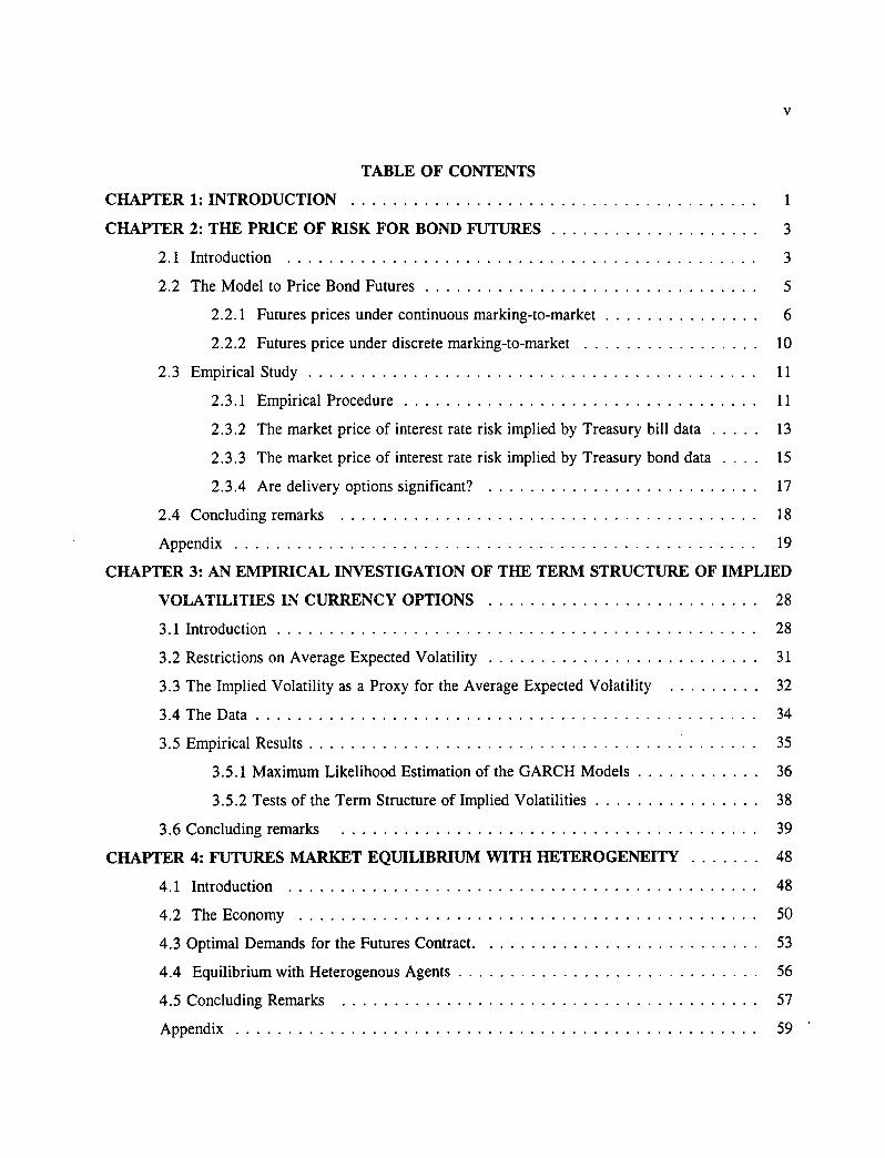
TABLE OF CONTENTS
CHAPTER 1: INTRODUCTION 1
CHAPTER 2: THE PRICE OF RISK FOR BOND FUTURES 3
2.1 Introduction 3
2.2 The Model to Price Bond Futures 5
2.2.1 Futures prices under continuous marking-to-market 6
2.2.2 Futures price under discrete marking-to-market 10
2.3 Empirical Study 11
2.3.1 Empirical Procedure 11
2.3.2 The market price of interest rate risk implied by Treasury bill data 13
2.3.3 The market price of interest rate risk implied by Treasury bond data . 15
2.3.4 Are delivery options significant? 17
2.4 Concluding remarks 18
Appendix 19
CHAPTER 3: AN EMPIRICAL INVESTIGATION OF THE TERM STRUCTURE OF IMPLIED
VOLATILITIES IN CURRENCY OPTIONS 28
3.1 Introduction 28
3.2 Restrictions on Average Expected Volatility 31
3.3 The Implied Volatility as a Proxy for the Average Expected Volatility 32
3.4 The Data 34
3.5 Empirical Results 35
3.5.1 Maximum Likelihood Estimation of the GARCH Models 36
3.5.2 Tests of the Term Structure of Implied Volatilities 38
3.6 Concluding remarks 39
CHAPTER 4: FUTURES MARKET EQUILIBRIUM WITH HETEROGENEITY 48
4.1 Introduction 48
4.2 The Economy 50
4.3 Optimal Demands for the Futures Contract. 53
4.4 Equilibrium with Heterogenous Agents 56
4.5 Concluding Remarks 57
Appendix 59
v i
TABLE OF CONTENTS (CONT'D)
CHAPTER 5: MAJOR FINDINGS, IMPLICATIONS AND DIRECTIONS FOR FUTURE
RESEARCH 65
REFERENCES 67
TABLES
Table 2.1 Summary Statistics 21
Table 2.2 Model Estimates for Treasury Bill Futures... 22
Table 2.3 Model Estimates for Treasury Bill Futures... 23
Table 2.4 Model Estimates for Treasury Bond Futures... 24
Table 2.5 Mode! Estimates for Treasury Bond Futures... 25
Table 2.6 Mode! Estimates for Treasury Bond Futures... 26
Table 2.7 The Market Price of Risk Estimates for other Studies 27
Table 3.1 Sample Statistics 41
Table 3.2 Autocorrelations 42
Table 3.3 Japanese yen 43
Table 3.4 Swiss franc 44
Table 3.5 Deutschmark 45
Table 3.6 Term Structure of Implied Volatility Test Statistics 46
Table 3.7 Parameters of the Term Structure Relationship 46
Table 3.8 Term Structure Tests for... 47
1
CHAPTER 1: INTRODUCTION
During the past two decades, the dynamic asset pricing theory has grown as a distinctive part of
financial economics. The traditional dynamic asset pricing models share a small set of basic assumptions:
absence of arbitrage, single agent optimality, and equilibrium. The results obtained from these models
are usually unified by two key concepts: state prices and martingales. This parsimonious presentation
has contributed to the success of the theory. The conceptual and methodological development of the
dynamic asset pricing theory is rooted in the decade spanning roughly from 1969 to 1979, called "the
golden decade" by Duffie (1992). The advances occurred in both the discrete time and continuous time
framework, with the latter considered as a useful approximation of the former.
Merton (1969) has given the initial impulse to the continuous time modelling with his explicit
dynamic solution for optimal portfolio and consumption policies. These results set the stage for general
equilibrium asset pricing models like those derived by Merton (1973) and later by Cox, Ingersoll and
Ross (1985). In the discrete time framework, equilibrium asset pricing models have been mainly
multiperiod extensions of the CAPM like that of LeRoy (1973), Rubinstein (1976a), and Lucas (1978),
among others. However, the simplest multiperiod version of the CAPM is the continuous-time
consumption-based CAPM derived by Breeden (1979).
The other major development in the dynamic asset pricing theory during that period is the
contingent claims analysis. Contingent claims analysis is a technique for determining the price of
derivative securities like futures contracts, options, ban guaranties, and mortgage backed securities.
Although connected with the continuous-time portfolio models, the contingent daims analysis is primarily
linked to the important breakthrough of Black and Scholes (1973) on the theory of option pricing. An
influential discrete time simplification of the Black and Scholes model, the binomial option pricing model
has been later presented by Cox, Ross and Rubinstein (1979). Building on the ideas of Black and Scholes
(1973), Cox and Ross (1976) and Ross (1978), Harrison and Kreps (1979), and Harrison and Pliska
(1981) have given to contingent daims analysis, and to the other aspects of dynamic asset pricing theory
their current conceptual structure. Major innovations in dynamic asset pricing theory occurred during
its first decade of existence. The present direction of the research in the field is the validation of existing
models through empirical studies, and extension and reassessment of early models using alternative sets
of assumptions.
2
The purpose of this thesis is two-fold. The first purpose is to investigate efficiency, risk
preferences, and equilibrium pricing, and thus contributing to the assessment of application of the
dynamic asset pricing theory to derivatives. The second purpose is to propose an equilibrium model of
derivative security prices when economic agents are heterogenous and the underlying asset is flot
marketable. This extends the dynamic asset pricing theory.
The remainder of this thesis is organized as follows. Chapter two is comprised of the first essay:
"The Price of Risk for Bond Futures." The market price of risk implied by the futures price of bonds
is obtained from market data assuming that the theoretical model used is correct. Exact formulas of bond
futures prices under discrete, and continuous marking-to-market are derived using Vasicek's framework
and Jamshidian's methodology. The market price of risk of the instantaneous interest rate and parameters
of the interest rate process are estimated using Treasury bill futures prices from the Chicago Mercantile
Exchange (CME), and Treasury bond futures prices from the Chicago Board of Trade (CBOT). The
empirical procedure used for the estimation is the Generalized Method of Moments (GMM) of Hansen
(1982). Since the market price of interest rate risk must reflect risk preferences, an issue raised in this
essay is whether the estimated values of the market price of interest rate risk can be accounted for by
assumptions about tastes and beliefs. The estimated market price of risk may provide, along with the
GMM tests, information about the reliability of the models of bond futures prices.
Chapter three is comprised of the second essay: "An Empirical Investigation of the Term
Structure of Implied Volatilities in Currency Options". This chapter examines a fundamental hypothesis
of dynamic asset pricing models; namely the no-arbitrage condition. If intertemporal arbitrage
opportunities exist, expectations about prices are flot formed rationally, and the market is inefficient. The
no-arbitrage condition is tested in this essay using the term structure of implied volatilities, and listed
currency options from the Philadelphia Exchange.
The third and final essay entitled: "Futures Market Equilibrium with Heterogeneity," is presented
in chapter four. This essay studies equilibrium in the futures market of a commodity in a single good
economy, which is populated by heterogeneous producers, and speculators. The conunodity is traded in
a spot market at the harvest time. Each producer is endowed with a non-traded private technology. Both
classes of agents trade in futures contracts written on the conunodity, and in bonds.
3
CHAPTER 2: THE PRICE OF RISK FOR BOND FUTURES
2.1 Introduction
According to standard option theory, the value of a contingent daim depends on the dynamics
of the underlying asset. For traded assets, a hedge portfolio consisting of the derivative asset and the
underlying asset can be constnicted so that the portfolio is without risk. If this portfolio earns other than
the risk-free interest rate, arbitrage opportunities exist. A risk neutral valuation of the components of the
portfolio is possible (i.e, the risk premia can be disregarded). Unfortunately, in the case of an interest
rate derivative valuation, the state variable (interest rate) is flot a traded asset. A hedge portfolio cannot
be constructed so that risk is eliminated, and the valuation is preference free. The valuation of such a
contingent claim requires the knowledge of the market price of interest rate risk.
When an interest rate contingent claim model is derived in a general equilibrium framework [such
as Cox, Ingersoll, and Ross (CIR, 1985)], the market price of interest rate risk which is determined
endogenously, depends on the characteristics of the economy. Alternatively, in partial equilibrium models
of interest rate contingent daims, the underlying variable process and the market price of interest rate
risk are exogenous. Such models usually assume a constant market price of interest rate risk [e.g.,
Vasicek (1977), Brennan and Schwartz (1977, 1979), Richard (1978), and Jamshidian (1989)]. Dothan
(1978) provides a theoretical justification for a constant market price of interest rate risk, based on a
continuous time CAPM with a logaritlunic utility function for the consumer. CIR (1985), however, point
out that partial equilibrium models of interest rate contingent claims can be internally inconsistent. First,
no underlying equilibrium may be consistent with the assumption about the dynamics of the instantaneous
interest rate. Second, arbitrarily selecting a functional form for the market price of interest rate risk may
produce a model that violates the nonarbitrage condition. CIR (1981) show that the only version of the
expectations theory of the term structure of interest rates that is obtained in a continuous time rational
expectations equilibrium is the local expectations hypothesis. Therefore, the only valid equilibrium value
for the market price of interest rate risk is zero.
Campbell (1985) argues that CIR's criticisms apply to versions of the pure expectations theory
of the term structure, which states that the term premia are zero. However, much of the literature is
concerned with a less restrictive theory, the expectations theory, which states that term premia are
4
constant through time.' He provides an example, based on a general equilibrium foundation for the
Vasicek mode!, which shows that two versions of the expectations theory hold simultaneously in
continuous time. Although the term premia are not strictly equal, the differences among them are second-
order effects of bond yield variability. In the mode! of Vasicek, the market price of interest rate risk is
a constant. 2
As shown by Campbell using the Vasicek mode!, the market price of interest rate risk does flot
have to be zero for the partial equilibrium models to be consistent. Another consistency issue is whether
the estimated market prices of interest rate risk yielded by these models can be accounted for by both the
assumptions about tastes and beliefs, and the volatility of relevant economic data. For example, a very
high estimated market price of interest rate risk might imply an unrealistic holding premium for the utility
function assumed in the model, and the variance of interest rates.
The primary objective of this paper is to investigate the market price of interest rate risk for
various models of bond futures prices. The market prices and parameters of the interest rate process are
obtained from market data assuming that the model used is correct. Models of bond futures prices are
derived in the Vasicek framework by using Jamshidian's methodology. The data used are Treasury bill
futures prices from the Chicago Mercantile Exchange (CME), and Treasury bond futures prices from the
Chicago Board of Trade (CBOT). The estimation procedure used is the Generalized Method of Moments
(GMM) of Hansen (1982).
The contribution of this essay can be summarized as follows. First, models of continuous time
bond futures prices under discrete marking-to-market are derived by using the fact that equispaced
sampling of a continuous lime AR-1 (the Ornstein-Uhlenbeck process) results in a discrete time AR-1.
The formulas obtained are tractable and suitable for empirical investigation unlike a formula derived
earlier by Chen (1992b). Second, meaningful estimates of the market price of interest rate risk are
'Campbell defines two term premia as the primary objects of expectations theories. The first is the instantaneous holding premium, which is the expected difference at t between the instantaneous holding return on a bond which matures at T and the spot rate t. The second is the instantaneous forward premium, which is the expected difference at t between the forward rate and spot rate at t.
2 A constant market price of risk need flot imply constant term premia. Longstaff (1990) shows that the expectations hypothesis can imply time-varying term premia if the time frame for which the expectations hypothesis holds differs from the measurement period.
5
obtained and Treasury bond futures data are shown to be a valid alternative to the bond data used in
previous studies to estimate such market prices? Since delivery options held by the short side of a
Treasury bond futures contract do flot appear to have an impact on the market price of interest rate risk,
the very active Treasury bond futures market is a good source of data for empirical estimations.
Estimates of the market price of interest rate risk obtained using models of Treasury bill futures prices
data are far higher than those from other studies. Whether these estimates are too high to account for
both a logarithmic utility function and the volatility of interest rate is an open empirical question. These
results might be explained by market distortions. An alternative interpretation is that the models are
misspecified. Estimations improve for long-lived futures contracts with long-term underlying bonds when
a model with discrete marking-to-market is used.
The remainder of this essay is organized as follows. In section 2.2 the closed form solutions of
futures prices of bonds are derived, and then used in the empirical investigation reported and discussed
in section 2.3. Section 2.4 provides some concluding remarks.
2.2 The Model to Price Bond Futures
The continuous time futures price of a discount bond is derived below under the alternative
assumptions of discrete and continuous marking-to-market. The new formula for a futures price under
discrete marking-to-market is obtained directly from the continuous marking-to-market formula by taking
advantage of the properties of the interest rate process rather than applying recursive methods as in
previous studies. 4 For the remainder of the paper, futures bonds are denoted by U'(t,r,T,T'), or U:,
where the the superscript i =d (D), c (C), for discount bond futures under continuous (discrete) marking-
to-market, and coupon bond futures under continuous (discrete) marking-to-market, respectively. The
distinction between the subscript t used for the futures price at time t, and the partial derivative of the
futures price relative to time will always be clear from the context. The arguments of the futures price
will be defined later.
3 See for example Brennan and Schwartz (1979), Dietrich-Campbell and Schwartz (1986), L,ongstaff (1989), and Duan (1992).
4For discussions of the issues involved with continuous versus discrete timing to market, see Chen (1992b) and Flesaker (1993).
6
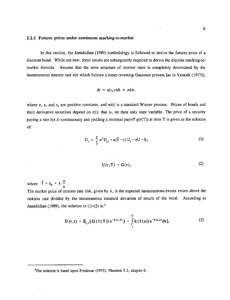
2.2.1 Futures prices under continuous marking-to-market
In this section, the Jamshidian (1989) methodology is followed to derive the futures price of a
discount bond. While flot new, these results are subsequently required to derive the discrete marking-to-
market formula. Assume that the term structure of interest rates is completely determined by the
instantaneous interest rate r(t) which follows a mean-reverting Gaussian process [as in Vasicek (1977)],
dr = a(ro-r)dt + odw,
where u, a, and ro are positive constants, and w(t) is a standard Wiener process. Prices of bonds and
their derivative securities depend on r(t); that is, on their only state variable. The price of a security
paying a rate h(r,t) continuously and yielding a terminal payoff g(r(T)) at time T is given as the solution
of:
U = 1 - 2 U +a(i-r)Ur -rU+ h, 2 "
U(r,T) = G(r),
where = ro + —(7 . a
The market price of interest rate risk, given by X, is the expected instantaneous excess return above the
riskless rate divided by the instantaneous standard deviation of return of the bond. According to
Jamshidian (1989), the solution to (1)-(2) is: 5
U(r,t) = Er,t [G(i(T))e -Y(t ' l) ] + f h(1. (s))e -"mds], (3)
5The solution is based upon Friedman (1975), Theorem 5.3, chapter 6.
(1)
(2)
7
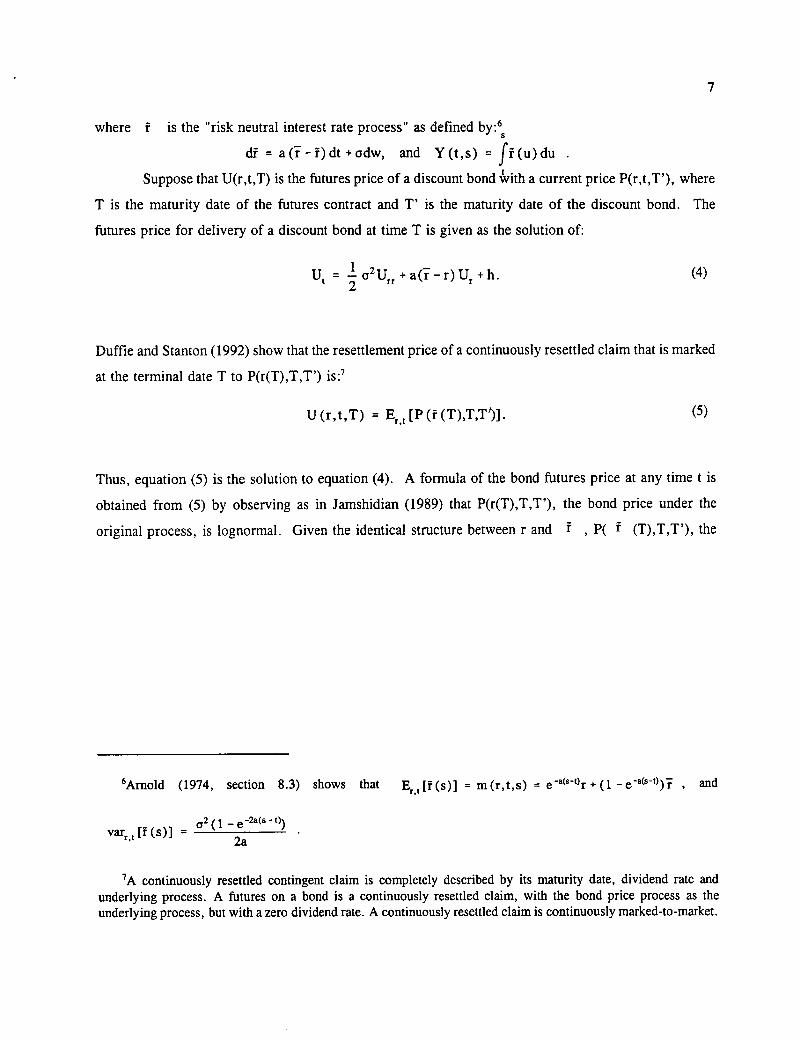
where is the "risk neutral interest rate process" as defined by: 6s
di = a (7 f) dt + odw, and Y (t ,$) = f (u) du .
Suppose that U(r,t,T) is the futures price of a discount bond With a current price P(r,t,T'), where
T is the maturity date of the futures contract and T' is the maturity date of the discount bond. The
futures price for delivery of a discount bond at time T is given as the solution of:
2., U = — a u +ag-r)Ui. +h. t 2 rr (4)
Duffie and Stanton (1992) show that the resettlement price of a continuously resettled daim that is marked
at the terminal date T to P(r(T),T,T') is: 7
U(r,t,T) = Er [P(î:( T ),T,T)] (5)
Thus, equation (5) is the solution to equation (4). A formula of the bond futures price at any time t is
obtained from (5) by observing as in Jamshidian (1989) that P(r(T),T,T'), the bond price under the
original process, is lognormal. Given the identical structure between r and i , P( (T),T,T'), the
6Amold (1974, section 8.3) shows that E 1 (s)] = m (r , t, s) = e -es-t) r + ( 1 - e -es-t) ) , and
a2 (1 - e -2a(s t)) varr,t [(s)] - • 2a
continuously resettled contingent daim is completely described by its maturity date, dividend rate and underlying process. A futures on a bond is a continuously resettled daim, with the bond price process as the underlying process, but with a zero dividend rate. A continuously resettled daim is continuously marked-to-market.
8
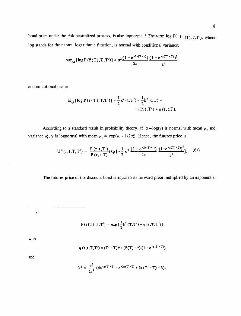
bond price under the risk neutralized process, is also lognorma1. 8 The term log P( f (T),T,T'), where
log stands for the natural logaritlunic function, is normal with conditional variance:
2a(T -t) ) (1 - CaCri-T))2 varr,t [logP (I. (T),T,T i)] - a2 (1 — e- 2a a2
and conditional mean:
Er,t [log P (f (T),T,T i)] =1k2 (t,T i) - 12-k2 (t,T) -
n(r,t,r) + n (r,t,T).
According to a standard result in probability theory, if x=log(y) is normal with mean I.L„ and
variance (..„ y is lognormal with mean ity = exp(K, - 1/2o). Hence, the futures price is:
U d (r,t,T,r) - P (1.t;ri)ex [ _ 1 2 (1 - e-2a(T - t) ) (1 — e -aCrl - T))2 ]. (6a) ' P(r,t,T) P 2 a 2a a2
The futures price of the discount bond is equal to its forward price multiplied by an exponential
8
P (i. (T),T,r) = exp [-1 k2 (T,V) -n (f,T,T i)] 2
with
n (r,t,T,Ti) = (T / - Tri + (f (T) -1) (1 - e -a (Ti-T) )
and
k2 = °2 (4e -8 (T/ - T) — e -2a Cri - Il + 2a (T / - T) - 3). 2a3
9
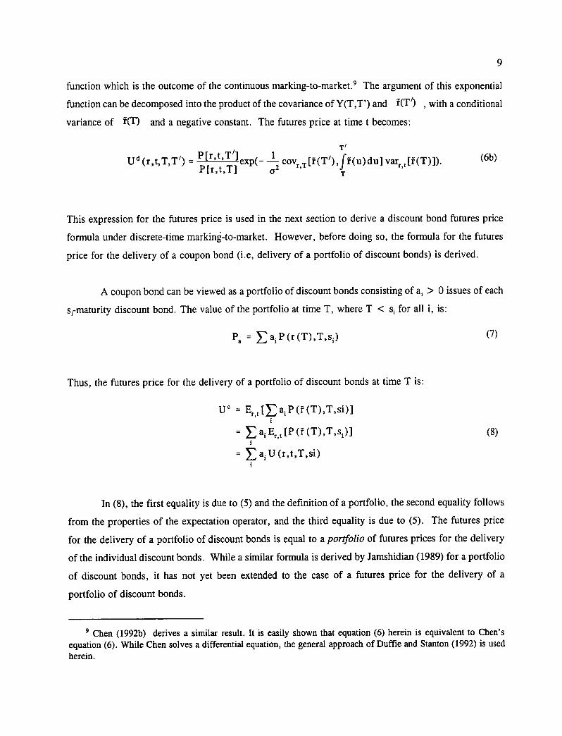
function which is the outcome of the continuous marking-to-market. 9 The argument of this exponential
function can be decomposed into the product of the covariance of Y(T,T') and i(i') , with a conditional
variance of f(T) and a negative constant. The futures price at time t becomes:
1./ P[r t T i] 1 U d (r,t,T,T /) - " exp(- —2 covr,T [f(r),ff(u)du] var[f(T)]). P[r,t,T] a
(6b)
This expression for the futures price is used in the next section to derive a discount bond futures price
formula under discrete-time markini-to-market. However, before doing so, the formula for the futures
price for the delivery of a coupon bond (i.e, delivery of a portfolio of discount bonds) is derived.
A coupon bond can be viewed as a portfolio of discount bonds consisting of a, > 0 issues of each
s,-maturity discount bond. The value of the portfolio at time T, where T < s, for ail i , is:
= ai P (r (T),T,si )
(7)
Thus, the futures price for the delivery of a portfolio of discount bonds at time T is:
1.1c = E t [E ai P (f (T),T,si)]
= ai Ei [P (f (T),T,si )] (8)
= ai U (r,t,T,si)
In (8), the first equality is due to (5) and the definition of a portfolio, the second equality follows
from the properties of the expectation operator, and the third equality is due to (5). The futures price
for the delivery of a portfolio of discount bonds is equal to a portfolio of futures prices for the delivery
of the individual discount bonds. While a similar formula is derived by Jamshidian (1989) for a portfolio
of discount bonds, it has flot yet been extended to the case of a futures price for the delivery of a
portfolio of discount bonds.
9 Chen (1992b) derives a similar result. It is easily shown that equation (6) herein is equivalent to Chen's equation (6). While Chen solves a differential equation, the general approach of Duffie and Stanton (1992) is used herein.
10
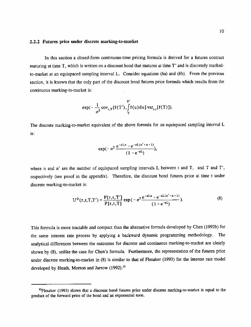
2.2.2 Futures price under discrete marldng-to-market
In this section a closed-form continuous-time pricing formula is derived for a futures contract
maturing at time T, which is written on a discount bond that matures at time T' and is discretely marked-
to-market at an equispaced sampling interval L. Consider equations (6a) and (6b). From the previous
section, it is known that the only part of the discount bond futures price formula which results from the
continuous marking-to-market is:
Ti exp(- —1 cov, T [f(T /),f i(u)du] var, , ,[i(T)]).
02 ,
The discrete marking-to-market equivalent of the above formula for an equispaced sampling interval L
is:
eXp(— 2 C aLn — Ca +1) L(n i +n
0. (1 _Ca)
where n and n' are the number of equispaced sampling intervals L between t and T, and T and T',
respectively (see proof in the appendix). Therefore, the discount bond futures price at time t under
discrete marking-to-market is:
LT D (r,t,T,T i) - P[r ' t,T/ exp( a2 e -a Ln — e -aL(n/ +ri + 1)
). P[r,t,T] (1 - Ce-)
(8)
This formula is more tractable and compact than the alternative formula developed by Chen (1992b) for
the same interest rate process by applying a backward dynamic programming methodology. The
analytical differences between the outcomes for discrete and continuous marking-to-market are clearly
shown by (8), unlike the case for Chen's formula. Furthermore, the representation of the futures price
under discrete marking-to-market in (8) is similar to that of Flesaker (1993) for the interest rate model
developed by Heath, Morton and Jarrow (1992). 10
1°Flesaker (1993) shows that a discount bond futures price under discrete marking-to-market is equal to the product of the forward price of the bond and an exponential term.
11
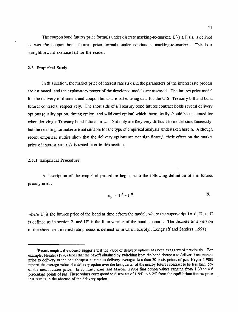
The coupon bond futures price formula under discrete marking-to-market, Uc(r,t,T,si), is derived
as was the coupon bond futures price formula under continuous marking-to-market. This is a
straightforward exercise left for the reader.
2.3 Empirical Study
In this section, the market price of interest rate risk and the parameters of the interest rate process
are estimated, and the explanatory power of the developed models are assessed. The futures price model
for the delivery of discount and coupon bonds are tested using data for the U.S. Treasury bill and bond
futures contracts, respectively. The short side of a Treasury bond futures contract holds several delivery
options (quality option, timing option, and wild card option) which theoretically should be accounted for
when deriving a Treasury bond futures price. Not only are they very difficult to model simultaneously,
but the resulting formulae are flot suitable for the type of empirical analysis undertaken herein. Although
recent empirical studies show that the delivery options are flot significant," their effect on the market
price of interest rate risk is tested later in this section.
2.3.1 Empirical Procedure
A description of the empirical procedure begins with the following definition of the futures
pricing error:
e 1 t = Uti - Utm (9)
where U is the futures price of the bond at time t from the model, where the superscript i= d, D, c, C
is defined as in section 2, and UT is the futures price of the bond at time t. The discrete time version
of the short-term interest rate process is defined as in Chan, Karolyi, Longstaff and Sanders (1991):
11Recent empirical evidence suggests that the value of delivery options has been exaggerated previously. For example, Hemler (1990) finds that the payoff obtained by switching from the bond cheapest to deliver three months prior to delivery to the one cheapest at time to delivery averages less than 30 basis points of par. Hegde (1988) reports the average value of a delivery option over the last quarter of the nearby futures contract to be less than .5% of the mean futures price. In contrast, Kane and Marcus (1986) find option values ranging from 1.39 to 4.6 percentage points of par. These values correspond to discounts of 1.9% to 6.2% from the equilibrium futures price that results in the absence of the delivery option.
12
= rt - rt _ 1 - a (ro - rt _ 1 ) (10) e2t
2 ,2 (11) e3t C 2t
where a, ro , and a are the parameters of the continuous-time interest rate process defined earlier. The
econometric approach adopted herein is to test (9)-(11) as a set of overidentifying restrictions on a system
of moment equations using the Hansen (1982) Generalized Method of Moments (GMM). This technique
is applied to test option pricing models by Rindell and Sandàs (1991). The GMM estimators and their
standard errors are consistent even if the disturbances e u are conditionally heteroscedastic and serially
correlated. The temporal aggregation problem, resulting from the estimation of a continuous-time process
with discrete time data, is likely to affect the distribution of the disturbances in a minor fashion. 12 Thus,
the GMM approach is appropriate for this empirical study.' A family of orthogonality conditions is
constructed under this approach. Consider the vector of errors e, with elements e ll , e2„ and e3„ and define
a vector of parameters 0 with elements a, a, X and ro . The vector of errors is a function of the
parameters and is denoted as e 1(0). A trivial orthogonality condition is that the expected error vector,
evaluated at some 0 =00 , must be zero; that is :
E[e1 (00)] = 0. (12)
According to the unbiasedness hypothesis, the error vector should flot be correlated with variables in the
information set of the investor. Define z, as a g-dimensional vector of variables in the investors'
information set at lime t. The unbiasedness hypothesis implies:
E [E, (90) 0;] = o, (13)
12 Chan et al. (1991) acknowledge that the discretized process is only an approximation of the continuous time specification. The error introduced can be shown to be of second order if changes in the interest rate are measured over a short period of time, which is the case herein.
13 Chan et al. (1991)
13
where 0 denotes the Kronecker operator. The GMM procedure consists of replacing E[e,(0)(g)] with its
sample counterpart, g(0), which for a sample of T observations is:
T
gT(0) =-_c (0)®z. (14)
The parameter estimates that minimize the following quadratic form are chosen:
JT (e) = e(e)w gT (e) (15)
where W is a positive-definite symmetric weighting matrix. When the number of orthogonality conditions
equals the number of parameters, a solution exists and JT = O. When the number of orthogonality
conditions exceeds the number of parameters to be estimated, the model is said to have overidentifying
restrictions, so that no 0 simultaneously solve ail the moment conditions. Hansen (1982) shows that the
minimized value of J T is chi-squared distributed under the null hypothesis that the model is true, with
degrees of freedom equal to the number of overidentifying restrictions (that is, the number of
orthogonality conditions less the number of parameters te be estimated). The chi-square statistic supplies
a goodness-of-fit test for the model. A significance test of individual parameters is provided by the
asymptotic covariance matrix for the GMM estimate of 0.
2.3.2 The market price of interest rate risk implied by Treasury bill data.
In this section, the market price of interest rate risk and the parameters of the short-term interest
rate and discount bond futures price models are estimated. Data used are U. S. Treasury bill futures
prices traded at the Chicago Mercantile Exchange (CME). Treasury bill futures contracts require delivery
of a Treasury bill maturing three months from the first delivery day. The settlements occur for each
delivery month during three successive delivery days. The first delivery day us the first day of the
delivery month on which a three month Treasury bill is issued and an original one-year bill issue has
three months remaining to maturity. The time period considered for the empirical estimations of the
parameters implied by the Treasury bill futures prices runs from January 1983 to December 1989. The
volume of trade of Treasury bill futures contracts depends on the time te maturity of the contract. While
almost no trade occurs in the early period of the contract, the volume of contracts traded increases as the
14
maturity date approaches. The Treasury bill futures data are Wednesday settlement prices for contracts
with various delivery months. The proxy of the short-term interest rate of Treasury bill futures prices
is the one-week Treasury bill yield.
As outlined by Gallant (1987), the GMM estimators depend on the choice of instrumental
variables. Since the optimal choice of instrument is still unresolved, the entire set or subsets of the
following instrumental variables are used herein: a constant term of one; the one-period-lagged interest
rate; the one-period-lagged trade volume; the one-period-lagged futures price; and the time to maturity.
The statistics and autocorrelation structure at lags of 1, 2, 3, 4 and 5 weeks of interest rates, bond
futures price and volume samples are summarized in Table 2.1. The parameter estimates, the standard
deviations of parameters, and the GMM minimized criterion (x 2) values for the system consisting of a
model of a discount bond futures price under discrete marking-to-market and the short-term interest rate
process are presented in Table 2.2. The X2 test for goodness-of-fit suggests that the models cannot be
rejected at the usual 95% confidence level. The parameter estimates, the standard deviations of the
parameters and the GMM minimized criterion values for the model consisting of a discount bond futures
price under continuous marking-to-market and the short-term interest rate process are presented in Table
2.3. The similarity of results obtained under the alternative marking-to-market assumptions in Tables 2.2
and 2.3 implies that the economic significance of marking interest rate futures contracts to the market on
a daily basis is fairly trivial for futures contracts with maturity well below a year [as found earlier by
Flesaker (1993)].
The estimates of the models provide a number of insights about the dynamics of short-term
interest rates and the market price of interest rate risk. Since the parameter a is significant, strong
evidence exists for mean reversion in the short-term interest rate. The market price of interest rate risk
X is inferred by the estimates of Xa and è . 14 X has the expected sign and is significantly different from
zero for ail the studied periods. The absolute values of the implied market price of interest rate risk are
too high if compared with values from other studies reported in Table 2.7. While the lowest absolute
value of the implied market price of interest rate risk herein is 2.27, the highest absolute value reported
in other studies is 0.487. These unusual higher values obtained herein may be due to the pattern of trade
14XΠand aro are estimated as individual parameters because the GMM procedure did flot converge otherwise.
15
in the Treasury bill futures market. Trading in any particular futures contract is very low when first
traded, increases over time, and is again low as the delivery date approaches. Thus, some price
quotations might not be representative of the market value of the bond futures price due to market
inefficiencies." X is the only parameter which can capture specific aspects of the Treasury bill futures
market, since the other variables are constrained by the two empirical equations of the short-term interest
rate process. Thus, the implied market price of interest rate risk appears to be affected by market
imperfections. An alternative interpretation of these results may be that the instantaneous holding
premium implied by the market price of interest rate risk is too high to be consistent with the log utility
function underlying the model, and the estimated volatility of the short-term interest rate.' However,
this daim should be investigated empirically before any reliable conclusion.
2.3.3 The market price of interest rate risk implied by Treasury bond data
In this section, the market price of interest rate risk and the parameters of the short-term interest
rate and coupon bond futures price models are estimated. Data used are U.S. Treasury bond futures
prices traded at the Chicago Board of Trade (CBOT). The Treasury bond futures price is determined
from an instrument with a 8 percent coupon rate and yield, and 20 years time to maturity. A Treasury
bond futures contract calls for the delivery of a Treasury bond at any day of the delivery month that, if
callable, is flot callable for at least 15 years from the first day of the delivery month or, if flot callable,
has a maturity of at least 15 years from the first day of the delivery month. The Treasury bond is treated
as a portfolio of discount bonds, and delivery options are addressed later in this study. The market for
Treasury bond futures is always very active. Weekly futures settlement prices are used from January
1989 to September 1991. The short-term interest rate used herein is the yield on three-month Treasury
bills.
The parameter estùnates, the standard deviations of the parameters and, the GMM minimized
criterion (x2) values for the system consisting of a model of a coupon bond futures price under discrete
lime marking-to-market and the short-term interest rate process are presented in Table 2.4. The x 2 test
I5Treasury bill futures prices may be affected (albeit temporarily) by other events. This is left to a future study.
16 The instantaneous holding premia implied by the values of the market price of interest rate risk reported in Table 2 are 2.1%, 3.48%, and 2.38%, respectively.
16
for goodness-of-fit suggests that the models cannot be rejected at the usual 95% confidence level. The
parameter estimates, the standard deviations of the parameters, and GMM minimized criterion values
for the model of a coupon bond futures price under discrete marking-to-market and the short-terni interest
rate process are presented in Table 2.5. The x2 test for goodness-of-fit suggests that these models cannot
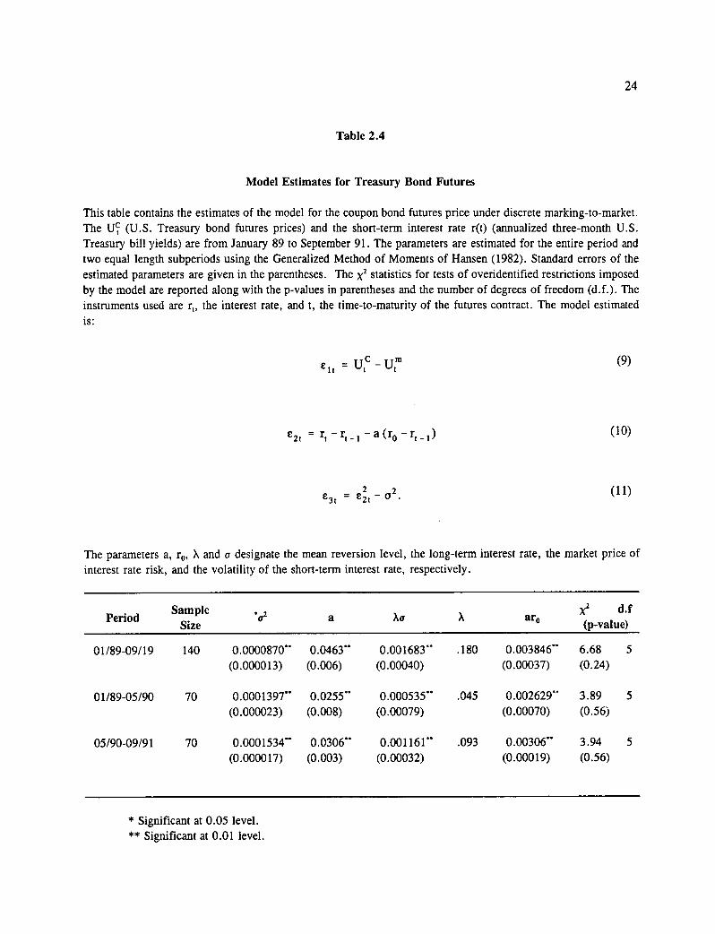
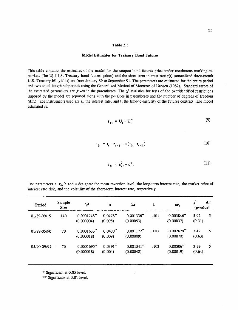
be rejected at the usual 95% confidence level. Unlike the Treasury bill futures, the values of the
parameters for Treasury bond futures prices are different for the continuous marking-to-market mode!
(Table 2.5) and discrete marking-to-market models (Table 2.4). Furthermore, the model with discrete
marking-to-market fits the data better based on the x2 test. This finding confirms the observation of
Flesaker that the economic effects of daily marking-to-market are significant when a futures contract has
a long time-to-maturity, and is written on a long-term bond. Over half of the futures price observations
used herein are for contracts with time-to-maturity above one year, and the underlying instruments of the
futures contracts are long-term bonds.
Ah l of the estimated parameters in Table 2.4 are significant. The coefficients of mean reversion
are low compared to those obtained for the period of 1983-1989. The difference may be explained by
a temporal shift in the interest rate process or by the proxies used. The implied market price of risk is
always low but significantly different from zero for the model under discrete marking-to-market. The
X values are 0.101, 0.087 and 0.103, for the entire period and the two subperiods, respectively. The
signs of the estimated values of X are consistent with the findings from other studies involving coupon
bonds.' Based on these results, the market price of interest rate risk is low but significantly different
from zero. Morever, it does flot change much over time. While these results appear to be more reliable
than those obtained from the Treasury bill futures, the effect of delivery options on the parameters needs
to be checked before any conclusion is drawn. 18
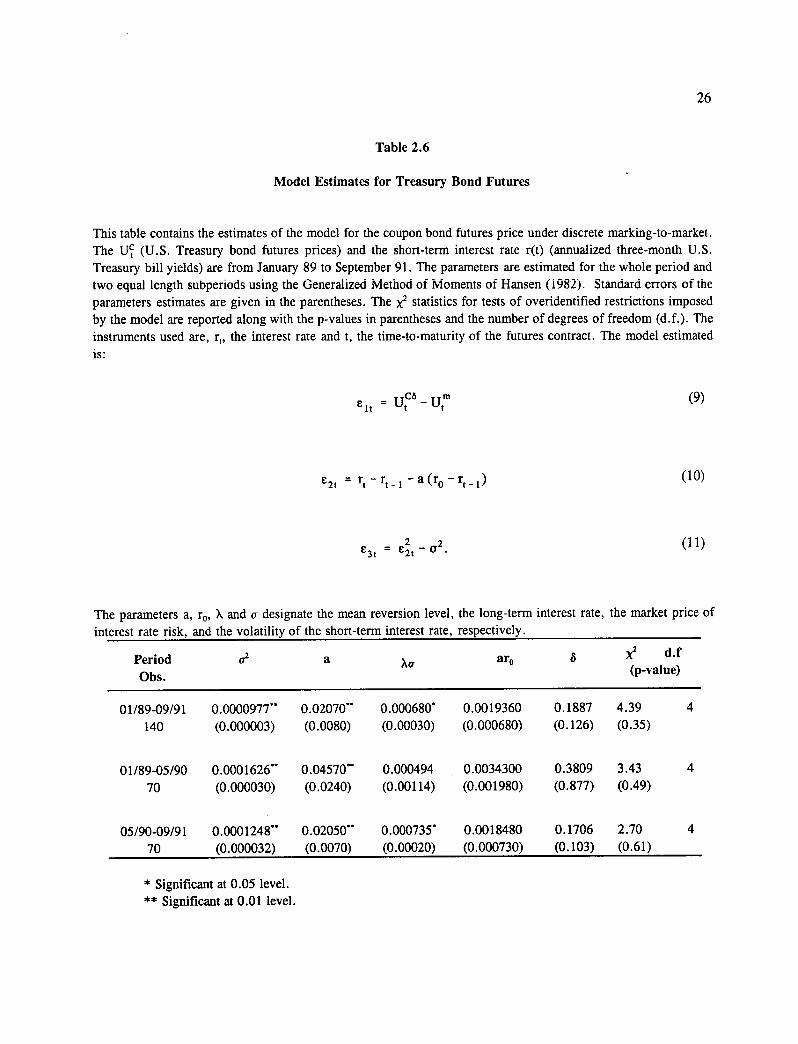
2.3.4 Are delivery options significant?
While some empirical studies of the Treasury bond futures market conclude that delivery options
I7The implied market price of interest risk has values 0.180, 0.093, and 0.045 when the model of futures price under continuous marking-to-market is used. The two first values are significant.
I8The holding premiums implied by the values of the market price of interest rate risk reported in Table 5 are - 0.0013, -0.0010, and -0.0013.
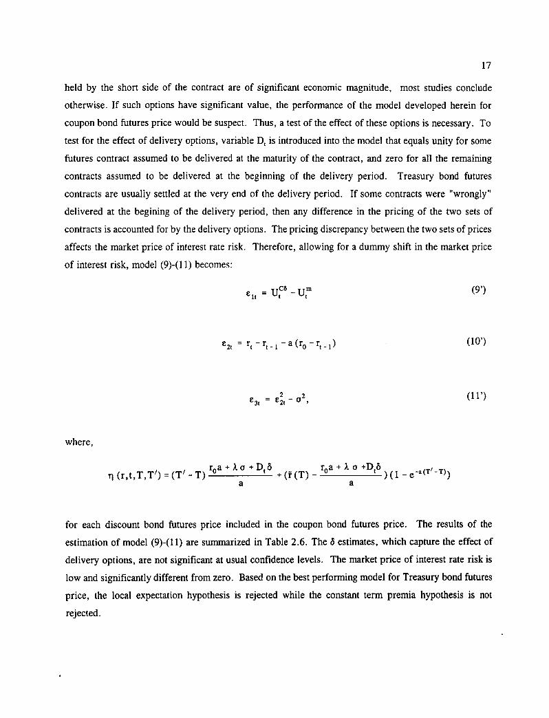
17
held by the short side of the contract are of significant economic magnitude, most studies conclude
otherwise. If such options have significant value, the performance of the model developed herein for
coupon bond futures price would be suspect. Thus, a test of the effect of these options is necessary. To
test for the effect of delivery options, variable D, is introduced into the mode! that equals unity for some
futures contract assumed to be delivered at the maturity of the contract, and zero for ail the remaining
contracts assumed to be delivered at the beginning of the delivery period. Treasury bond futures
contracts are usually settled at the very end of the delivery period. If some contracts were "wrongly"
delivered at the begining of the delivery period, then any difference in the pricing of the two sets of
contracts is accounted for by the delivery options. The pricing discrepancy between the two sets of prices
affects the market price of interest rate risk. Therefore, allowing for a dununy shift in the market price
of interest risk, model (9)-(11) becomes:
= 1-4c6 - (9')
e 2t = rt - -1 - a (r0 - rt 1 )
2 2 3t = C2t - G ,
where,
(r,t,T,r) = (T/ - T) 0 X 0 + D t 8 4. (T) ro a + 0 +Dt8
) ( I - e (Ti - T) )
a a
for each discount bond futures price included in the coupon bond futures price. The results of the
estimation of mode! (9)-(11) are summarized in Table 2.6. The t3 estimates, which capture the effect of
delivery options, are flot significant at usual confidence levels. The market price of interest rate risk is
low and significantly different from zero. Based on the best performing mode! for Treasury bond futures
price, the local expectation hypothesis is rejected while the constant term premia hypothesis is flot
rejected.
(10')
(11')
18
2.4 Concluding remarks
Exact formulae of futures price for the delivery of discount bond and coupon bonds are derived
under the alternative assumptions of discrete marking-to-market and continuous marking-to-market.
Treasury bill futures prices and Treasury bond futures prices are used to assess the formulas, to determine
the parameters of the interest rate process, and to estimate the market price of the short-term interest rate
risk by using the GMM approach. The market price of interest rate risk is different from zero for each
data set. This suggests that the local expectation hypothesis is not adequate for the partial equilibrium
valuation of bonds and bond derivatives. The alternative hypothesis of constant holding and forward
premia, and a constant market price of interest rate risk is flot rejected for the best performing model
applied to Treasury bond futures and three-month Treasury bill yields as interest rates. The market price
of interest rate risk estimated with the Treasury bill futures data and one-week Treasury bill yields seems
to be too high, which suggests the possibility of inefficiencies in the market. An alternative explanation
is that the Vasicek model is flot successful in describing the dynamics of short-term bonds and their
derivative securities (i.e, futures contracts).
Excluding delivery options from the futures price formulas does flot affect the parameters
significantly. The strong effect of discrete marking-to-market on long-lived futures on long-term
underlying bonds is supported herein.
19
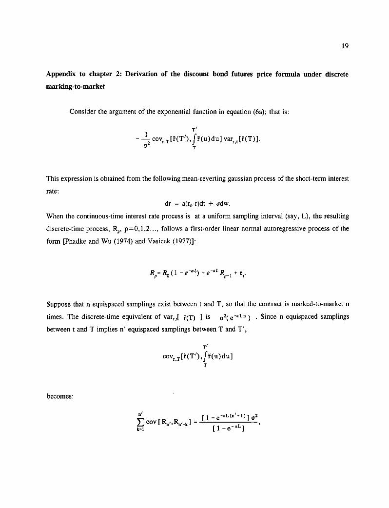
Appendix to chapter 2: Derivation of the discount bond futures price formula under discrete
marking-to-market
Consider the argument of the exponential function in equation (6a); that is:
Ti , - 2- cov...,,[f(T /),f i(u)du] var [f(T)].
aa r,t a' T
This expression is obtained from the following mean-reverting gaussian process of the short-term interest
rate:
dr = a(ro-r)dt + adw.
When the continuous-time interest rate process is at a uniform sampling interval (say, L), the resulting
discrete-time process, Rp, p=0,1,2..., follows a first-order linear normal autoregressive process of the
form [Phadke and Wu (1974) and Vasicek (1977)]:
D . jj,0 (1 _e_0) + e-aL R
p-1 + e
itP it r
Suppose that n equispaced samplings exist between t and T, so that the contract is marked-to-market n
times. The discrete-time equivalent of var[ i(r) ] is 02( e-aLn ) . Since n equispaced samplings
between t and T implies n' equispaced samplings between T and T',
T/ COVr,T [f(T/),f f(u) du]
T
becomes:
ni E cov [R„„R.,_ki -
[1 _ e -aL(ni +1)] a2 ,
k=1 [1_e-al
20
[Nelson 1972, pp. 11 and 12]. By replacing the variance and covariance expressions with their discrete-
time equivalents, the formula for bond futures prices under discrete marking-to-market is obtained.
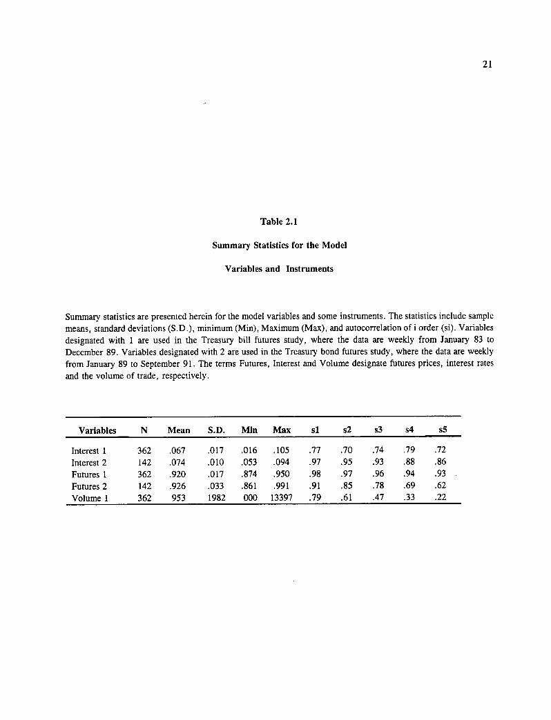
Table 2.1
Summary Statistics for the Mode!
Variables and Instruments
Summary statistics are presented herein for the model variables and some instruments. The statistics include sample means, standard deviations (S.D.), minimum (Min), Maximum (Max), and autocorrelation of i order (si). Variables designated with 1 are used in the Treasury bill futures study, where the data are weekly from January 83 to December 89. Variables designated with 2 are used in the Treasury bond futures study, where the data are weekly from January 89 to September 91. The tenns Futures, Interest and Volume designate futures prices, interest rates and the volume of trade, respectively.
Variables N Mean S.D. Min Max si s2 s3 s4 s5
Interest 1 362 .067 .017 .016 .105 .77 .70 .74 .79 .72 Interest 2 142 .074 .010 .053 .094 .97 .95 .93 .88 .86 Futures 1 362 .920 .017 .874 .950 .98 .97 .96 .94 .93 Futures 2 142 .926 .033 .861 .991 .91 .85 .78 .69 .62 Volume 1 362 953 1982 000 13397 .79 .61 .47 .33 .22
21
22
Table 2.2
Model Estimates for Treasury Bill Futures
This table contains the estimates of the model for the discount bond futures price under discrete marking-to-market. The U? (U. S. Treasury bill futures prices) and short-term interest rates r(t) (annualized one-week U. S. Treasury bill yields) are from January 83 to December 89. The parameters are estimated for the entire period and two equal length subperiods using the Generalized Method of Moments of Hansen (1982). Standard errors of the parameter estimates given in the parentheses. The x2 statistics for tests of the overidentified restrictions imposed by the model are reported along with p-values in parentheses and the number of degrees of freedom (d.f.). The instruments used are r„ the interest rate, and V„ the volume of transactions. The model estimated is:
e = 1413 - Utm (9) it
(10)
2 2 C 3t = e2t - G.
The parameters a, ro , X and u designate the mean reversion level, the long-term interest rate, the market price of interest rate risk, and the volatility of the short-term interest rate, respectively.
Period Sample Size o2 a Xi, X aro
X d.f (p-value)
01/83-12/89 362 0.0001160- 0.4013- -0.0245- -2.27 0.0271 - 6.62 5 (0.000011) (0.101) (0.006) (0.006) (0.25)
01/83-07/86 181 0.0001124- 0.6795- -0.0480- -4.52 0.0530- 2.49 5 (0.000016) (0.170) (0.012) (0.013) (0.78)
07/86-12/89 181 0.0001793- 0.6254- -0.0317- -2.36 0.0349- 3.75 5 (0.000028) (0.168) (0.009) (0.010) (0.58)
* Significant at 0.05 level. ** Significant at 0.01 level.
23
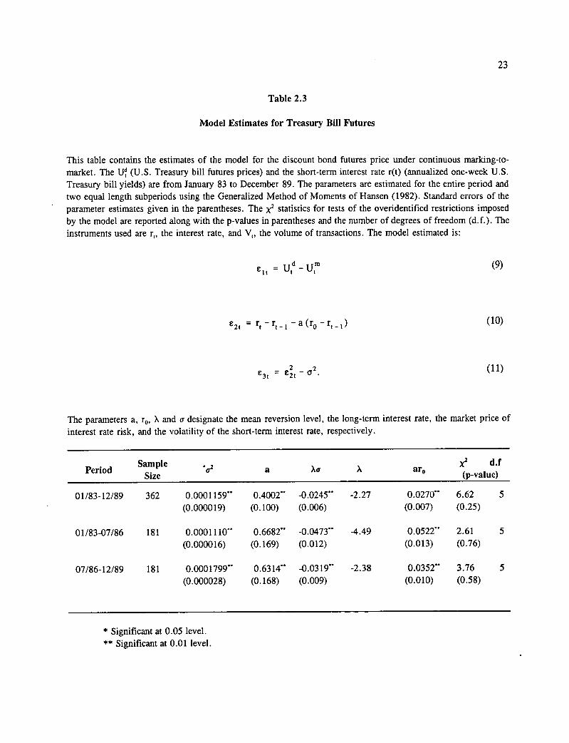
Table 2.3
Mode! Estimates for Treasury Bill Futures
This table contains the estimates of the model for the discount bond futures price under continuous marking-to-market. The Ud, (U. S. Treasury bill futures prices) and the short-term interest rate r(t) (annualized one-week U. S. Treasury bill yields) are from January 83 to December 89. The parameters are estimated for the entire period and two equal length subperiods using the Generalized Method of Moments of Hansen (1982). Standard errors of the parameter estimates given in the parentheses. The x 2 statistics for tests of the overidentified restrictions imposed by the model are reponed along with the p-values in parentheses and the number of degrees of freedom (d.f.). The instruments used are r„ the interest rate, and V„ the volume of transactions. The model estimated is:
c = Utd - Ur (9) it
e 2t = rt - rt -1 - a (r0 - rt -1 ) (10)
2 2 e3t = C 2t - a •
The parameters a, ro , X and u designate the mean reversion level, the long-term interest rate, the market price of interest rate risk, and the volatility of the short-term interest rate, respectively.
Period Sample
Size 'ff2 a Xa X aro x2 d.f
(p-value)
01/83-12/89 362 0.0001159- 0.4002- -0.0245- -2.27 0.0270- 6.62 5 (0.000019) (0.100) (0.006) (0.007) (0.25)
01/83-07/86 181 0.0001110- 0.6682- -0.0473- -4.49 0.0522- 2.61 5 (0.000016) (0.169) (0.012) (0.013) (0.76)
07/86-12/89 181 0.0001799- 0.6314- -0.0319- -2.38 0.0352 3.76 5 (0.000028) (0.168) (0.009) (0.010) (0.58)
* Significant at 0.05 level. ** Significant at 0.01 level.
24
Table 2.4
Model Estimates for Treasury Bond Futures
This table contains the estimates of the model for the coupon bond futures price under discrete marking-to-market. The U (U.S. Treasury bond futures prices) and the short-term interest rate r(t) (annualized three-month U.S. Treasury bill yields) are from January 89 to September 91. The parameters are estimated for the entire period and two equal length subperiods using the Generalized Method of Moments of Hansen (1982). Standard errors of the estimated parameters are given in the parentheses. The x2 statistics for tests of overidentified restrictions imposed by the model are reported along with the p-values in parentheses and the number of degrees of freedom (d.f.). The instruments used are r„ the interest rate, and t, the time-to-maturity of the futures contract. The model estimated is:
£ i = UtC - Utin (9)
E 21 = rt - rt -1 - a (r0 - r1-1 ) (10)
2 C 3t e 21 G
2.
The parameters a, ro, X and u designate the mean reversion level, the long-term interest rate, the market price of interest rate risk, and the volatility of the short-term interest rate, respectively.
Period Sample Size a Xcr X aro )(2 d.f
(p-value)
01/89-09/19 140 0.0000870** 0.0463- 0.001683- .180 0.003846- 6.68 5 (0.000013) (0.006) (0.00040) (0.00037) (0.24)
01/89-05/90 70 0.0001397- 0.0255- 0.000535- .045 0.002629- 3.89 5 (0.000023) (0.008) (0.00079) (0.00070) (0.56)
05/90-09/91 70 0.0001534- 0.0306- 0.001161 - .093 0.00306- 3.94 5 (0.000017) (0.003) (0.00032) (0.00019) (0.56)
* Significant at 0.05 level. ** Significant at 0.01 level.
25
Table 2.5
Model Estimates for Treasury Bond Futures
This table contains the estimates of the model for the coupon bond futures price under continuous marking-to-market. The Uci (U.S. Treasury bond futures prices) and the short-term interest rate r(t) (annualized three-month U. S. Treasury bill yields) are from January 89 to September 91. The parameters are estimated for the entire period and two equal length subperiods using the Generalized Method of Moments of Hansen (1982). Standard errors of the estimated parameters are given in the parentheses. The x2 statistics for tests of the overidentified restrictions imposed by the model are reported along with the p-values in parentheses and the number of degrees of freedom (d.f.). The instruments used are r„ the interest rate, and t, the time-to-maturity of the futures contract. The model estimated is:
e 1 t = Ut - (9)
€ 2t = rt - rt - 1 - a (r0 - rt -1 )
(10)
2 e3t = ezt'12 *
The parameters a, ro , X and o designate the mean reversion level, the long-term interest rate, the market price of interest rate risk, and the volatility of the short-term interest rate, respectively.
Period Sample Size *cr2 a Xcr X aro d.f
(p-value)
01/89-09/19 140 0.0001748- 0.0478- 0.001336- .101 0.003846- 5.92 5 (0.000004) (0.008) (0.00053) (0.00037) (0.31)
01/89-05/90 70 0.0001633- 0.0400- 0.001122- .087 0.002629- 3.42 5 (0.000018) (0.009) (0.00009) (0.00070) (0.63)
05/90-09/91 70 0.0001695- 0.0391 - 0.001341 - .103 0.00306- 3.33 5 (0.000018) (0.004) (0.00048) (0.00019) (0.64)
* Significant at 0.05 level. ** Significant at 0.01 level.
26
Table 2.6
Model Estimates for Treasury Bond Futures
This table contains the estimates of the model for the coupon bond futures price under discrete marking-to-market. The Ig (U. S. Treasury bond futures prices) and the short-term interest rate r(t) (annualized three-month U. S. Treasury bill yields) are from January 89 to September 91. The parameters are estimated for the whole period and two equal length subperiods using the Generalized Method of Moments of Hansen (1982). Standard errors of the parameters estimates are given in the parentheses. The x 2 statistics for tests of overidentified restrictions imposed by the model are reported along with the p-values in parentheses and the number of degrees of freedom (d.f.). The instruments used are, r„ the interest rate and t, the time-to-maturity of the futures contract. The model estimated is:
e it = u -u (9)
e 2t = rt - rt -1 - a (r0 - rt -1 ) (10)
2 2 e3t = e2t - a •
The parameters a, ro , X and cf designate the mean reversion level, the long-term interest rate, the market price of interest rate risk, and the volatility of the short-term interest rate, respectively.
Period Obs.
a2 a Xo aro d.f (p-value)
01/89-09/91 0.0000977- 0.02070- 0.000680 0.0019360 0.1887 4.39 4 140 (0.000003) (0.0080) (0.00030) (0.000680) (0.126) (0.35)
01/89-05/90 0.0001626- 0.04570- 0.000494 0.0034300 0.3809 3.43 4 70 (0.000030) (0.0240) (0.00114) (0.001980) (0.877) (0.49)
05/90-09/91 0.0001248- 0.02050- 0.000735' 0.0018480 0.1706 2.70 4 70 (0.000032) (0.0070) (0.00020) (0.000730) (0.103) (0.61)
* Significant at 0.05 level. ** Significant at 0.01 level.
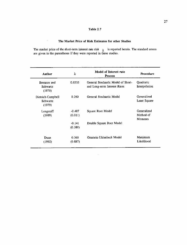
Table 2.7
The Market Price of Risk Estimates for other Studies
The market price of the short-term interest rate risk 1 is reponed herein. The standard errors are given in the parentheses if they were reported in these studies.
Mode! of Interest rate Author X Process
Procedure
Brennan and 0.0335 General Stochastic Mode! of Short- Quadratic Schwartz and Long-tenn Interest Rates Interpolation
(1979)
Dietrich-Campbell 0.260 General Stochastic Mode! Generalized Schwartz Least Square
(1979)
Longstaff -0.487 Square Root Mode! Generalized (1989) (0.011) Method of
Moments -0.141 Double Square Root Mode! (0.380)
Duan 0.360 Omstein-Uhlenbeck Mode! Maximum (1992) (0.887) Likelihood
27
28
CHAPTER 3: AN EMPIRICAL INVESTIGATION OF THE TERNI STRUCTURE
OF IMPLIED VOLATILITIES IN CURRENCY OPTIONS
3.1 Introduction
The valuation of a derivative security depends on the dynamics of its underlying asset. For assets
whose volatility changes over time, a constant volatility model like the Black-Scholes model is not always
appropriate for option pricing. As a result, Hull and White (1987), Johnson and Shanno (1987), Scott
(1987), Wiggins (1987), and Duan (1995) derive alternative models under the assumption of stochastic
volatility. They find that stochastic volatility has a significant impact on option prices. If no risk
premium exists for bearing volatility risk, the value of an at-the-money option is approximately equal to
the Black-Scholes value, where volatility is equal to the average expected volatility of the underlying asset
over the option's Hence, if the stochastic volatility model is well specified, the at-the-money
implied volatility obtained using the market price and the Black-Scholes formula should be approximately
equal to the average expected volatility over the time to maturity. The relationship between the average
and implied volatilities for a given process can be exploited to derive the so-called "term structure" of
implied volatilities. The term structure of implied volatilities is the relationship between the implied
volatilities obtained by applying the inverse of the Black-Scholes formula to the theoretical values of two
options on an asset following a specific process, where the options only differ in their maturities.
The term structure of implied volatilities can be used to construct a test of efficiency of the option
market. As stated in Heynen, Kemna and Vorst (1994), if a specific asset return model describes the data
I9This result follows because the Black-Scholes formula is nearly linear in volatility for at-the-money calls.
29
correctly, and the pricing model used to uncover the implied volatility is assumed to be accurate, then
the term structure test checks whether the restrictions on implied volatilities are consistent with the
hypothesis that investors' expectations about average volatility are formed rationally. Conversely, if the
expectation hypothesis is admitted, then the term structure of implied volatilities can be used to test the
dynamics of the underlying asset, and ultimately the option pricing formula obtained from those
dynamics.
Stein (1989) is the first author to construct a test of efficiency of the option market with the term
structure of implied volatilities. Based on a sample of Standard & Poor 100 options, Stein concludes that
long-term volatilities overreact te changes in short-term volatilities which result in inefficiencies in the
option market studied. Heynen, Kemna and Vorst (1994) perform ex-ante efficiency tests on the
relationship between short-term and long-term implied volatilities. They reject the joint hypothesis of a
correct specification of asset dynamics and ex-ante efficiency in the option market when the stock return
volatility follows a mean reverting GARCH(1,1) process. They are unable te reject this joint hypothesis
for the case of a mean reverting EGARCH(1,1) process. Campa and Chang (1993) test the expectation
hypothesis on the term structure of implied volatilities with over-the-counter options. They detect
overreactions in the long-rate to current changes in the short-rate resulting in option mispricing for many
cases. Lamoureux and Lastrapes (1993) consider market overreactions to recent volatility shocks as an
alternative interpretation of the results of tests conducted on stock options traded on the Chicago Board
Options Exchange (CBOE). Diz and Finucane (1993) question the methodology of Stein. Based on an
alternative set of tests, they find no indication of overreaction in the market for index options. Canina
and Figlewski (1993) find implied volatility to be a poor forecast of subsequent realized volatility for
Index options. Therefore, widespread use of implied volatility in other models as an ex-ante measure of
perceived asset price risk is debatable. They conjecture that the rejection of the implied volatility as a
30
good proxy for the future volatility might be related to the difficulty of arbitrage trade for the index
options studied.' The conjecture is indirectly substantiated in a simulation study by Sheikh and Vora
(1994) discussed later.
Since the evidence concerning overreaction in the market is mixed, more studies are required in
various settings to better understand the reaction of investors to the arrival of new information in the
option market. This study performs a joint test of the expectation hypothesis on the term structure of
implied volatilities, and the dynamics of the exchange rate of the Japanese yen, the Swiss franc and the
Deutschmark against the American Dollar. The implied volatilities of relative changes of exchange rates
are estimated using the formula for currency options derived by Garman and Kohlhagen (1983). 21 The
derivation of the term structure of implied volatilities is based on Heynen, Kemna and Vorst (1994). The
joint hypothesis of a correct model specification and ex-ante efficiency is flot rejected for the Japanese
yen and the Swiss franc, and this hypothesis is rejected for the Deutschmark. The rejection could be
interpreted as evidence that inefficiencies caused by noise exist in the Deutschmark currency-option
market during the studied period. However, other specifications for the Deutschmark exchange rate
process need to be tested before a reliable conclusion on inefficiencies. The results reported herein can
also be considered as an implicit test of the currency options equivalent of the Duan Garch-option model
for stock options.
The conditional variance of the relative changes of the exchange rate is assumed to follow a
GARCH(1,1) process which is specified in the next section. While researchers have recognized that asset
returns exhibit both fat-tailed marginal distributions and volatility clustering since Fama (1965) and
n'Arbitrage involving currency options is relatively easy to do.
2IThis model for currency options is equivalent to the Black and Scholes model for stock options.
31
Mandelbrot (1966), only recently have applied researchers explicitly modelled these features. These
empirical observations are interpreted as evidence that volatilities of financial asset prices are stochastic
and that the innovations in the process are persistent. One tool used to describe such changing variances
is the autoregressive conditional heteroscedasticity (ARCH) class of models. 22
The failure of traditional time series models to capture stylized facts about short-run exchange
rate movements has lead many authors to consider the ARCH class of models as alternatives. Hsieh
(1989), McCurdy and Morgan (1988), Kugler and Lenz (1990), Pappell and Sayer (1990), Heynen and
Kat (1993), and Kodres (1993) show that the simple synunetric linear GARCH(1,1) model may provide
a good model of the second-order dynamics of most exchange rates series.' Theodossiou (1994) uses
an EGARCH model with a generalised error distribution to investigate the properties of five major
Canadian exchange rates.
The remainder of this essay is organized as follows. In section 3.2, the restrictions on average
expected volatilities are derived. In section 3.3, the use of implied volatility as a proxy for average
expected volatilities is discussed. In section 3.4, the data are described. In section 3.5, the empirical
results are reported; and in section 3.6, some concluding remarks are offered.
3.2 Restrictions on Average Expected Volatility
The restrictions on relative option prices that are implied by a GARCH(1,1) model of the
nSee Bollerslev et al. (1992) for an extensive review.
23 Kodres finds that a GARCH(1,1) specification is adequate to describe the exchange rate dynamics of the Deutschmark and the Swiss franc versus the American dollar. In the case of the British pound, the Canadian dollar, and the Japanese yen, a Garch(2,1) model fits the data best.
32
volatility of the underlying asset are developed in this section. These restrictions are derived in Heynen,
Kemna and Vorst (1994) based on the approach developed by Stein (1989) for a continuous time mean-
reverting AR1 process.
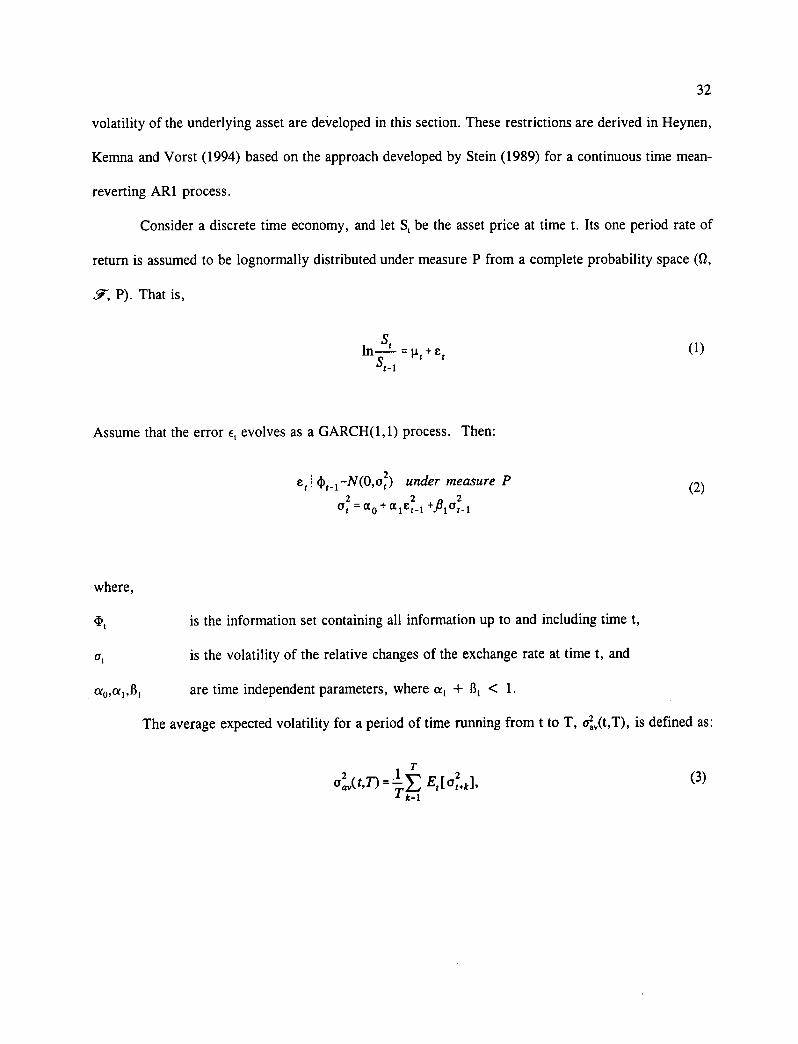
Consider a discrete time economy, and let S t be the asset price at time t. Its one period rate of
return is assumed to be lognormally distributed under measure P from a complete probability space ((,
P). That is,
= + e t St-t
Assume that the error E t evolves as a GARCH(1,1) process. Then:
e 4 1) -N(0 a2) under measure P t-- t
02
= a + Π1 E 2 +.13 2 t 0 t-1 a t-1
where,
(Pt is the information set containing ah l information up to and including time t,
is the volatility of the relative changes of the exchange rate at time t, and
ao,a 1 ,13, are time independent parameters, where a l + B I < 1.
The average expected volatility for a period of time running from t to T, aL(t,T), is defined as:
E Et [0,2,k], (3) k=1
(1)
(2)
33
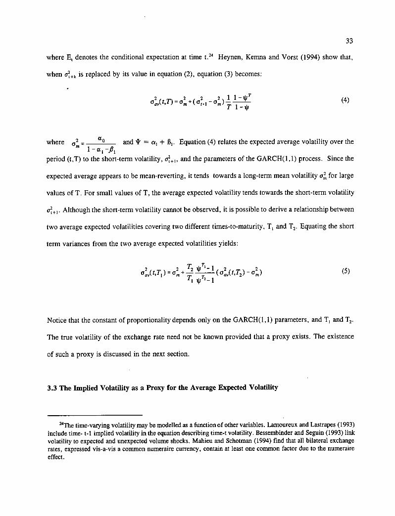
where E denotes the conditional expectation at time t. 24 Heynen, Kemna and Vorst (1994) show that,
when oî +k is replaced by its value in equation (2), equation (3) becomes:
2 2 2 2 1 1 - 11I T 0,nft,n= am + (a t.i - and
T 1-41
ceo where 02 - and NF = al + BI . Equation (4) relates the expected average volatility over the m 1 - a -fi l
period (t,T) to the short-term volatility, cq +1 , and the parameters of the GARCH(1,1) process. Since the
expected average appears to be mean-reverting, it tends towards a long-term mean volatility cr i , for large
values of T. For small values of T, the average expected volatility tends towards the short-term volatility
Although the short-term volatility cannot be observed, it is possible to derive a relationship between
two average expected volatilities covering two different times-to-maturity, T I and T2. Equating the short
term variances from the two average expected volatilities yields:
2 1 2 2 y - A 2 aajt,Ti ) = a+
T (a.2 ,(t,T2 )- a.) m ipT2_1
(5)
Notice that the constant of proportionality depends only on the GARCH(1,1) parameters, and T I and T2.
The true volatility of the exchange rate need flot be known provided that a proxy exists. The existence
of such a proxy is discussed in the next section.
3.3 The Implied Volatility as a Proxy for the Average Expected Volatility
24The time-varying volatility may be modelled as a function of other variables. Lamoureux and Lastrapes (1993) include time- t-1 implied volatility in the equation describing time-t volatility. Bessembinder and Seguin (1993) link volatility to expected and unexpected volume shocks. Mahieu and Schotman (1994) find that ail bilateral exchange rates, expressed vis-a-vis a common numeraire currency, contain at least one common factor due to the numeraire effect.
(4)
34
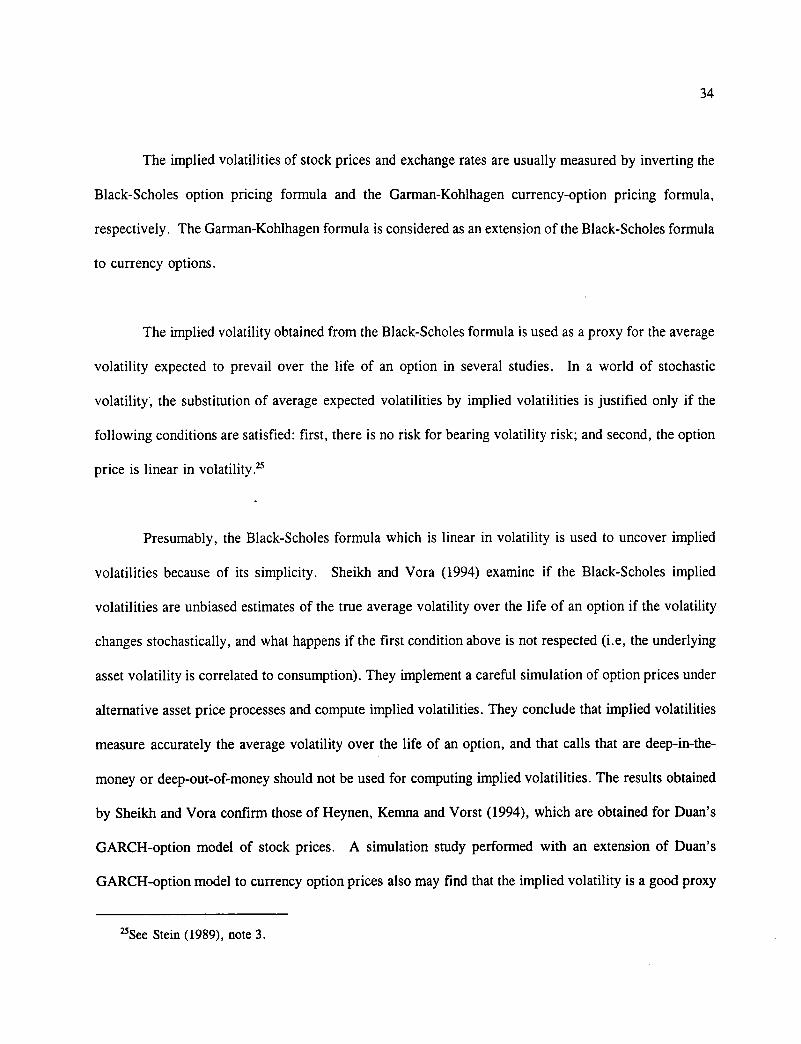
The implied volatilities of stock prices and exchange rates are usually measured by inverting the
Black-Scholes option pricing formula and the Garman-Kohlhagen currency-option pricing formula,
respectively. The Garman-Kohlhagen formula is considered as an extension of the Black-Scholes formula
to currency options.
The implied volatility obtained from the Black-Scholes formula is used as a proxy for the average
volatility expected to prevail over the life of an option in several studies. In a world of stochastic
volatility, the substitution of average expected volatilities by implied volatilities is justified only if the
following conditions are satisfied: first, there is no risk for bearing volatility risk; and second, the option
price is linear in volatility.'
Presumably, the Black-Scholes formula which is linear in volatility is used to uncover implied
volatilities because of its simplicity. Sheikh and Vora (1994) examine if the Black-Scholes implied
volatilities are unbiased estimates of the true average volatility over the life of an option if the volatility
changes stochastically, and what happens if the first condition above is flot respected (j. e, the underlying
asset volatility is correlated to consumption). They implement a careful simulation of option prices under
alternative asset price processes and compute implied volatilities. They conclude that implied volatilities
measure accurately the average volatility over the life of an option, and that calls that are deep-in-the-
money or deep-out-of-money should flot be used for computing implied volatilities. The results obtained
by Sheikh and Vora confirm those of Heynen, Kemna and Vorst (1994), which are obtained for Duan's
GARCH-option model of stock prices. A simulation study performed with an extension of Duan's
GARCH-option model to currency option prices also may find that the implied volatility is a good proxy
2.5See Stein (1989), note 3.
35
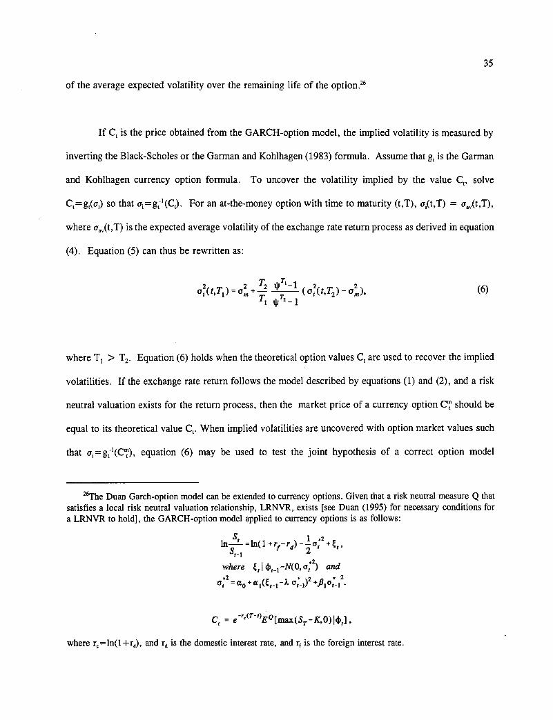
of the average expected volatility over the remaining life of the option.'
If C, is the price obtained from the GARCH-option model, the implied volatility is measured by
inverting the Black-Scholes or the Garman and Kohlhagen (1983) formula. Assume that g, is the Garman
and Kohlhagen currency option formula. To uncover the volatility implied by the value C„ solve
Ci = g,(a,) so that a i = (C,). For an at-the-money option with time to maturity (t,T), a,(t,T) =
where aav(t,T) is the expected average volatility of the exchange rate return process as derived in equation
(4). Equation (5) can thus be rewritten as:
T 2 2 2 lir 1 2 2 a ,(47.1 ) = a „z + (a,(t,T2 )-
Tl III T2 _1 (6)
where T 1 > T2. Equation (6) holds when the theoretical option values C, are used to recover the implied
volatilities. If the exchange rate return follows the model described by equations (1) and (2), and a risk
neutral valuation exists for the return process, then the market price of a currency option CT should be
equal to its theoretical value C,. When implied volatilities are uncovered with option market values such
that a1 =g,-1 (CT), equation (6) may be used to test the joint hypothesis of a correct option model
26The Duan Garch-option model can be extended to currency options. Given that a risk neutral measure Q that satisfies a local risk neutral valuation relationship, LRNVR, exists [see Duan (1995) for necessary conditions for a LRNVR to hold], the GARCH-option model applied to currency options is as follows:
i *2 =ln(1 St_ i 2
where t,1 4:$ 4 _ 1 -N(0, a:2) and *2 2
at = ao + igt-1 -1 cr:- )2 +fila t-1
C, = e -r`(7. t)EQ[max(S K,0)14)t],
where +rd), and rd is the domestic interest rate, and r f is the foreign interest rate.
36
specification and the assumption that expectations are formed rationally.
3.4 The Data
Two sets of data are used in this study. The first set consists of the daily spot prices from the
New York foreign exchange market on the U.S dollar versus the Japanese yen, the Swiss franc and the
Deutsclunark for the period from January 23, 1987 to January 21, 1988. This results in 250 observations
for each exchange rate series.
The second set of data consists of the implied volatilities for call options on three currencies
traded at the Philadelphia Exchange from January to June 1988: Japanese yen, Swiss franc, and
Deutsclunark. The implied volatilities for other major currencies are not used because trading in the
currencies was thin during the period studied.' Two series of prices are selected for each exchange
rate; namely, one for short-term call options, and one for long-term call options. Short-term options have
times-to-maturity of less than 40 days, while long-term options have times-to-maturity of more than 80
days. As in Xu and Taylor (1994), the following exclusion criteria are used to remove the uninformative
, option observations from the studied samples:'
'Only currencies with enough option data are studied. For a call option with less than one year to maturity and domestic interest rates greater than foreign interest rates, the European boundary condition exceeds the American. No early exercise premium exists, and the American feature has no value [Adams and Wyatt (1987)]. Therefore, the Garman and Kohlhagen model for European call options is also suitable for American call options. This allows for more observations for currencies with lower interest rates than the American dollar during the sample period, such as the Japanese yen, the Deutschmark and the Swiss franc. There is flot enough data to perform the tests for other major currencies (the British Pound, the French franc and the Italian lira) because American call options are excluded from the samples because interest rates related to these currencies are higher than the American interest rates during the period of study.
28The notation used herein is standard: S is the spot rate; X is the exercise price; T is the turne to the expiry date as measured in years; rd is the domestic interest rate; and rf is the foreign interest rate.
37
i) Options with time to expiration of less than 15 calendar days;
ii) Options violating the European boundary conditions
C < Se -r, - Xe -rdT. ,
iii) Options violating the American boundary conditions, C < S-X;
iv) Option premia less than or equal to .015 cents; and
y) Options that are 'far' in- or out-of-the money; i.e, X < .975S or X > 1.025S.
Criterion i) eliminates options with very short times to maturity because implied volatilities are
unreliable for such options. Criteria ii) and iii) eliminate options violating the boundary conditions for
European and American options. Criterion iv) excludes options for which the discrete market prices are
likely to distort the calculation of implied volatilities. Criterion v) is used to retain only at-the-money
options, since the implied volatilities computed from such options seem to be the best proxies of expected
average volatilities. Thus, the implied volatilities are obtained by applying the inverse of the Garman and
Kohlhagen option model for currency options to the option prices, using only the closing prices of the
nearest-the-money options.
3.5 Empirical Results
In this section, efficiency of the currency-option and the validity of the GARCH(1,1) market and
the GARCH(1,1) process for the conditional variance of the relative changes of exchange rates are jointly
tested by examining restrictions on implied volatilities. The estimated parameters of the GARCH(1,1)
process are compared to those of alternative ARCH/GARCH models. The estimated parameters of the
process are used to derive the term structure of implied volatilities, and to perform the tests of the joint
38
hypothesis.
3.5.1 Maximum Likelihood Estimation of the GARCH Models
Different model assumptions for the volatility of the relative changes of various exchange rates
are tested now. The spot exchange rates S, are converted to continuously compounded rates of return
using:
S Y' =h1( — ). St _ i
(7)
Some descriptive statistics for y, for the Japanese yen, the Swiss franc and the Deutschmark are reported
in Table 3.1. All the series exhibit leptolcurtic behaviour. The unconditional sample kurtosis of the
Japanese yen of 1.62 (which is the highest among the three series) is below the normal value of three by
more than four standard errors. The Wald statistic for the null hypothesis of normality is rejected for
ail three series.' The autocorrelations and partial autocorrelations of the (squared) exchange rate return
series are presented in Table 3.2. The Ljung-Box (1978) portmanteau test statistic for up to the tenth-
order serial correlation in the residuals yields values that are flot significant at the usual 5% level of
confidence for ail three currencies (see Ljung-Box 1, Table 3.1)." In contrast, the squared residuals
are flot uncorrelated over time. The Ljung-Box test statistic for no serial correlation in the squares is
significant for ail three series (see, Ljung-Box 2, Table 3.1). The absence of dependence in the
29Under the null hypothesis of normality, the Wald statistic is distributed as chi-squared with two degrees of freedom. The five percent critical value from the chi-squared table for two degrees of freedom is 5.99.
30The Ljung-Box statistic for up to the tenth-order serial correlation follows a x Io distribution.
39
conditional first moment and the dependence in the conditional second moment indicates that ARCH
models are adequate choices for the representation of the volatility processes of the series studied.
To describe the volatility processes of the return series, the following three alternative models
are considered: the GARCH(1,1), the GARCH(0,1), and the ARCH(1). The return series are modelled
as
Y, =1-t + e t (8)
2 t-1 -N( 0, at )
2 2 2 a t ' 11 0 + e i e t-1 4- ce2e1-2 +fliat-i
(9)
In (9), the ARCH(1) process is obtained if fi l =0 and a2 = 0; the GARCH(0,1) process is obtained if a l =0
and a2 = 0; the GARCH(1,1) process is obtained if « 2 =0; and the ARCH(2) process is obtained if B I =0.
Standard maximum likelihood techniques are used to estimate and test these ARCH/GARCH models.
Assuming that the process is described by equations (8) and (9), the log-likelihood, Log L, is given, apart
from some initial conditions, by:
T 2 1 2 e t log L = - —T log (27s ) - — E [log a ' + —1,
2 2,= 2 a,
where all the terms are as defined earlier.
Maximum likelihood estimates of the parameters for the alternative models are presented in
(10)
Tables 3.3, 3.4 and 3.6. The estimates are obtained using the Berndt, Hall, Hall and Hausman (1974)
40
algorithm using numerical derivatives. For the Japanese yen, the Ljung-Box test statistic for the
standardized residuals and the standardized squared residuals from the estimated GARCH(1,1) and the
ARCH(1) model do flot indicate any first-order or second-order serial dependence. However, for the
GARCH(0,1) model, some second-order serial dependence still remains. For the Swiss franc, the
GARCH(1,1) and the GARCH(0,1) fit the data well. Both the GARCH(1,1) and the ARCH(1) models
are adequate descriptions of the conditional volatility of the relative change of the Deutsclunark exchange
rate. However, likelihood ratio test results indicate that the optimal choice of model for the three
exchange rates series is the GARCH(1,1) process. 31
The GARCH(1,1) model provides a good description of the second-order dynamics of the
Japanese yen, the Swiss franc and the Deutsclunark return series. However, it should be noted that the
excess kurtosis in the raw data is flot captured by the assumption of conditional normality as shown by
the values of the Wald test statistic. 32
3.5.2 Tests of the Term Structure of Implied Volatilities
The parameters of the GARCH(1,1) process estimated in the previous section are used to specify
the ex-ante relationship between the long- and short-term implied volatilities derived earlier. For each
currency, the joint hypothesis of a correct model specification and the assumption that average volatility
expectations are formed rationally is tested. The equation to be tested is:
31 If La and La are the maximum log likelihood values under the null and alternative hypotheses, respectively, then the test statistic -2[1..„-La] is asymptotically chi-squared distributed with degrees of freedom equal to the difference in the number of parameters under the null and the alternative.
32Estimation of the different models under the assumption of a standardized t-distribution does flot change the parameter estimations, and different tests do flot change the results significantly. For further discussion of this issue, see McCurdy and Morgan (1987), Hsieh (1989), Baillie and Bollerslev (1989), and Bollerslev, Chou and Kroner (1992).
41
2 2 T2 11J - 1 2 2 ]+ e =0, [cr(t,Ti) - a m ] [ crajt,T2)- am 7'1 4T2_1 t
where T I > T2 . The parameter estimates for equation (11) for the different processes are presented in
Table 3.6. The residual in equation (11) should be white noise; that is, E(E,)=0 and E(E tEt_i)=0 for every
j. The test is performed on 103 pairs of implied volatilities for the relative change of the Japanese yen
exchange rate, 103 pairs of the relative change of the Swiss franc exchange rate, and 103 pairs of the
relative change of the Deutschmark exchange rate. The test results for these three currencies are
summarized in Table 3.7. Based on the t-values of the means of the residuals and the Ljung-Box test
statistics, the assumption of white noise cannot be rejected for the Swiss franc and the Japanese yen.
Thus, the joint hypothesis of a correct model specification and ex-ante efficiency of the option market
cannot be rejected for the Swiss franc and the Japanese yen. This result is consistent with recent studies
of the term structure using implied volatilities in the currency and the stock markets. For example,
Heynen, Kemna and Vorst (1994) cannot reject the joint hypothesis of a correct model specification and
ex-ante efficiency in the case of an EGARCH(1,1) conditional variance of stock returns. Similarily,
based on a study of volatility expectations for four currencies, Xu and Taylor (1994) conclude that there
is no evidence that currency option markets overreact.
Based on the t-values and the Ljung-Box statistics, the assumption of white noise is rejected for
the GARCH(1,1) model for the conditional variance of the Deutschmark exchange rate return. The
significant positive mean error suggests that the forecasts of long-term average volatility by investors in
the case of the Deutsclunark are larger than expected from the term structure relation. Such
overreaction might be explained by the arrival of contradictory information into the market. In the first
half of 1988, contrary to the economic fundamentals, the Deutschmark lost value against the American
42
dollar and other currencies.' The contradictory information may be interpreted as a noisy signal about
the long-term exchange rate between the American dollar and the Deutsclunark. Noise may lead to
"excess" long-term exchange rate volatility which is captured by the term structure of implied volatilities.
However, other specifications for the Deutsclunark exchange rate process need to be tested before
reaching any reliable conclusion about inefficiencies during the period under review.
An alternative possibility is that the rejection is due to a mispecification of the exchange rate
volatility dynamics. In practical terms, this suggests that the GARCH(1,1) estimate of the unconditional
variance (i.e, the major detenninant of the term structure relationship) is flot correct. However, based
on a sensitivity analysis summarized in Table 3.8, a change in the conditional volatility does flot change
the initial results (that is, a rejection of the term structure relationship for the Deutschmark).
3.6 Concluding remarks
In this essay, ex-ante tests of the relationship between short- and long-tenn implied volatilities
are performed for the exchange rates of the Japanese yen, the Swiss franc and the Deutschmark versus
the American dollar. The model selected for the conditional volatilities of the exchange rate relative
change series for these currencies is the GARCH(1,1). The joint hypothesis of a correct model
specification and ex-ante efficiency is flot rejected for the Japanese yen and the Swiss franc, but is
rejected for the Deutsclunark. The rejection could be interpreted as evidence that inefficiencies caused
by noise exist in the Deutschmark currency-option market during the studied period. An alternative
possibility is that the rejection is due to a mispecification of the exchange rate volatility dynamics. While
tests of the hypothesis for other major currencies (like the British pound, the French franc, the Italian lira
33Bundesbank Animal Report 1988.
43
and the Canadian dollar) are of interest, the size of the available data samples does flot allow for
meaningful analyses.
The results reported herein contribute to both sides of the ongoing debate about whether option
markets are efficient. Interesting avenues for future research are to extend tests of the term structure of
implied volatilities to other specifications of the exchange rate dynamics and to determine the conditions
under which inefficiencies arise, if any .
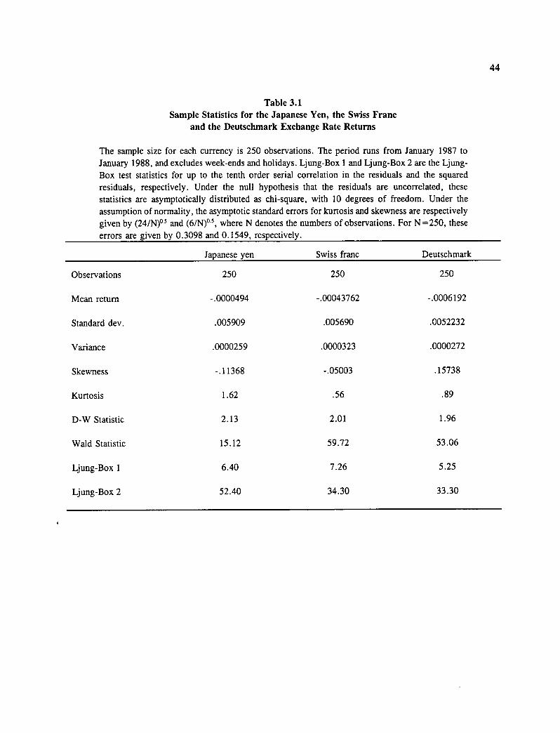
44
Table 3.1 Sample Statistics for the Japanese Yen, the Swiss Franc
and the Deutschmark Exchange Rate Returns
The sample size for each currency is 250 observations. The period runs from January 1987 to January 1988, and excludes week-ends and holidays. Ljung-Box 1 and Ljung-Box 2 are the Ljung-Box test statistics for up to the tenth order serial correlation in the residuals and the squared residuals, respectively. Under the null hypothesis that the residuals are uncorrelated, these statistics are asymptotically distributed as chi-square, with 10 degrees of freedom. Under the assumption of normality, the asymptotic standard errors for kurtosis and skewness are respectively given by (24/N)" and (6/N)°-5 , where N denotes the numbers of observations. For N =250, these errors are given by 0.3098 and 0.1549, respectively.
Japanese yen Swiss franc Deutschmark
Observations 250 250 250
Mean return -.0000494 -.00043762 -.0006192
Standard dey. .005909 .005690 .0052232
Variance .0000259 .0000323 .0000272
Skewness -.11368 -.05003 .15738
Kurtosis 1.62 .56 .89
D-W Statistic 2.13 2.01 1.96
Wald Statistic 15.12 59.72 53.06
Ljung-Box 1 6.40 7.26 5.25
Ljung-Box 2 52.40 34.30 33.30
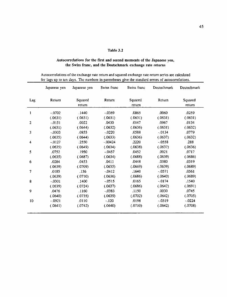
Table 3.2
Autocorrelations for the first and second moments of the Japanese yen, the Swiss franc, and the Deutsclunark exchange rate returns
Autocorrelations of the exchange rate retum and squared exchange rate return series are calculated for lags up to ten days. The numbers in parentheses give the standard errors of autocorrelations.
Lag
Japanese yen
Return
Japanese yen
Squared return
Swiss franc
Return
Swiss franc
Squared return
Deutschmark
Return
Deutschmark
Squared return
1 -.0702 .1440 -.0369 .0865 .0060 .0259 (.0631) (.0631) (.0631) (.0631) (.0631) (.0631)
2 -.0151 .0022 .0430 .0147 .0967 .0134 (.0631) (.0644) (.0632) (.0636) (.0631) (.0632)
3 -.0303 .0855 -.0220 .0588 -.0134 .0779 (.0635) (.0644) (.0633) (.0636) (.0637) (.0632)
4 -.0127 .2550 -.00424 .2220 -.0558 .288 (.0635) (.0649) (.0634) (.0638) (.0637) (.0636)
5 .0752 .1950 -.0457 .0452 .0021 .0717 (.0635) (.0687) (.0634) (.0688) (.0639) (.0686)
6 .0284 .0453 .0411 .0448 .0380 .0319 (.0639) (.0709) (.0635) (.0669) (.0639) (.0689)
7 .0185 .156 -.0412 .1640 -.0571 .0561 (.0639) (.0710) (.0636) (.0686) (.0640) (.0689)
8 -.0301 .1400 -.0515 .0165 -.0174 .1540 (.0639) (.0724) (.0637) (.0686) (.0642) (.0691)
9 .0476 .1160 -.0383 .1150 .0030 .0745 (.0640) (.0735) (.0639) (.0702) (.0642) (.0705)
10 -.0921 .0110 -.120 .0198 -.0519 -.0224 (.0641) (.0742) (.0640) (.0710) (.0642) (.0708)
45
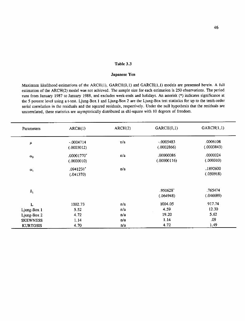
Table 3.3
Japanese Yen
Maximum likelihood estimations of the ARCH(1), GARCH(0,1) and GARCH(1,1) models are presented herein. A full estimation of the ARCH(2) model was flot achieved. The sample size for each estimation is 250 observations. The period runs from January 1987 to January 1988, and excludes week-ends and holidays. An asterisk (*) indicates significance at the 5 percent level using a t-test. Ljung-Box 1 and Ljung-Box 2 are the Ljung-Box test statistics for up to the tenth-order serial correlation in the residuals and the squared residuals, respectively. Under the null hypothesis that the residuals are uncorrelated, these statistics are asymptotically distributed as chi-square with 10 degrees of freedom.
Parameters ARCH(1) ARCH(2) GARCH (0,1) GARCH(1,1)
iL -.0004714 n/a -.0005483 .0006108 (.0003012) (.0002866) (.0003843)
ao .00001770 n/a .00000086 .0000024 (.0000010) (.00000116) (.000010)
ot, .0941231' n/a .1892600 (.041370) (.050918)
B, .950628` .765474 (.064948) (.046689)
L 1002.73 n/a 1004.05 917.74 Ljung-Box 1 5.52 n/a 4.59 12.30 Ljung-Box 2 4.72 n/a 19.20 5.62 SKEWNESS 1.14 n/a 1.14 .09 KURTOSIS 4.70 n/a 4.72 1.49
46
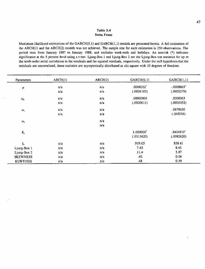
47
Table 3.4 Swiss Franc
Maximum likelihood estimations of the GARCH(0,1) and GARCH(1,1) models are presented herein. A full estimation of the ARCH(1) and the ARCH(2) models was not achieved. The sample size for each estimation is 250 observations. The period runs from January 1987 to January 1988, and excludes week-ends and holidays. An asterisk (*) indicates significance at the 5 percent level using a t-test. Ljung-Box 1 and Ljung-Box 2 are the Ljung-Box test statistics for up to the tenth-order serial correlation in the residuals and the squared residuals, respectively. Under the null hypothesis that the residuals are uncorrelated, these statistics are asymptotically distributed as chi-square with 10 degrees of freedom.
Parameters ARCH(1) ARCH(2) GARCH(0,1) GARCH(1,1)
g n/a nia .0008202' -.0008865' nia n/a (.0004103) (.0005279)
cio n/a n/a .00000005 .0000063 nia n/a (.0000011) (.0000052)
a, n/a n/a .0678630
012
n/a n/a
n/a n/a
(.045036)
13, 1.000000' .8404910' (.0315620) (.0982620)
L n/a n/a 919.05 838.61 Ljung-Box 1 n/a n/a 7.63 8.61 Ljung-Box 2 n/a nia 11.4 3.87 SKEWNESS n/a n/a .40 0.04 KURTOSIS n/a n/a .48 0.59
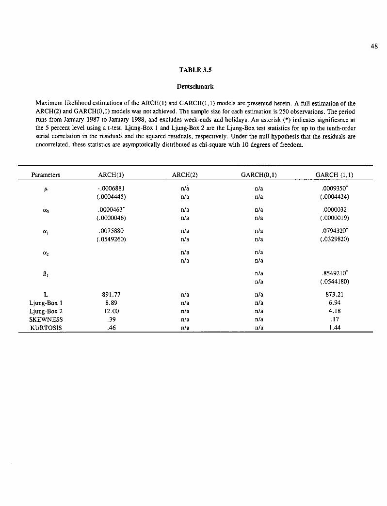
48
TABLE 3.5
Deutschmark
Maximum likelihood estimations of the ARCH(1) and GARCH(1,1) models are presented herein. A full estimation of the ARCH(2) and GARCH(0,1) models was flot achieved. The sample size for each estimation is 250 observations. The period runs from January 1987 to January 1988, and excludes week-ends and holidays. An asterisk (*) indicates significance at the 5 percent level using a t-test. Ljung-Box 1 and Ljung-Box 2 are the Ljung-Box test statistics for up to the tenth-order serial correlation in the residuals and the squared residuals, respectively. Under the null hypothesis that the residuals are uncorrelated, these statistics are asymptotically distributed as chi-square with 10 degrees of freedom.
Parameters ARCH(1) ARCH(2) GARCH(0,1) GARCH (1,1)
g -.0006881 n/à n/a .0009350* (.0004445) n/a n/a (.0004424)
cio .0000463* n/a n/a .0000032 (.0000046) n/a n/a (.0000019)
a, .0075880 n/a n/a .0794320* (.0549260) n/a n/a (.0329820)
(x2 n/a n/a
n/a n/a
n/a .8549210* n/a (.0544180)
L 891.77 n/a n/a 873.21 Ljung-Box 1 8.89 n/a n/a 6.94 Ljung-Box 2 12.00 n/a n/a 4.18 SKEWNESS .39 n/a n/a .17 KURTOSIS .46 n/a n/a 1.44
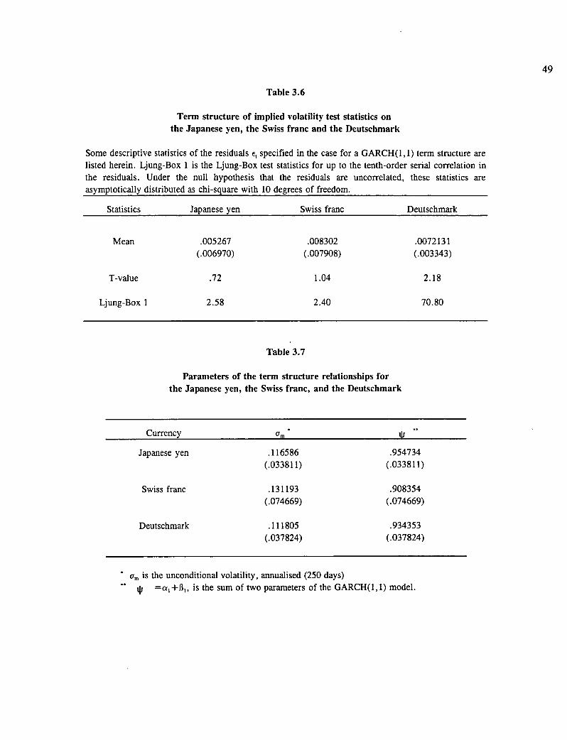
Table 3.6
Term structure of implied volatility test statistics on the Japanese yen, the Swiss franc and the Deutschmark
Some descriptive statistics of the residuals Et specified in the case for a GARCH(1,1) term structure are listed herein. Ljung-Box 1 is the Ljung-Box test statistics for up to the tenth-order serial correlation in the residuals. Under the null hypothesis that the residuals are uncorrelated, these statistics are asymptotically distributed as chi-square with 10 degrees of freedom.
Statistics Japanese yen Swiss franc Deutschmark
Mean .005267 .008302 .0072131 (.006970) (.007908) (.003343)
T-value .72 1.04 2.18
Ljung-Box 1 2.58 2.40 70.80
Table 3.7
Parameters of the term structure relationships for the Japanese yen, the Swiss franc, and the Deutschmark
Currency cr.
Japanese yen
Swiss franc
Deutschmark
.116586 .954734 (.033811) (.033811)
.131193 .908354 (.074669) (.074669)
.111805 .934353 (.037824) (.037824)
• an, is the unconditional volatility, annualised (250 days) .. iii =a,+13,, is the sum of two parameters of the GARCH(1,1) model.
49
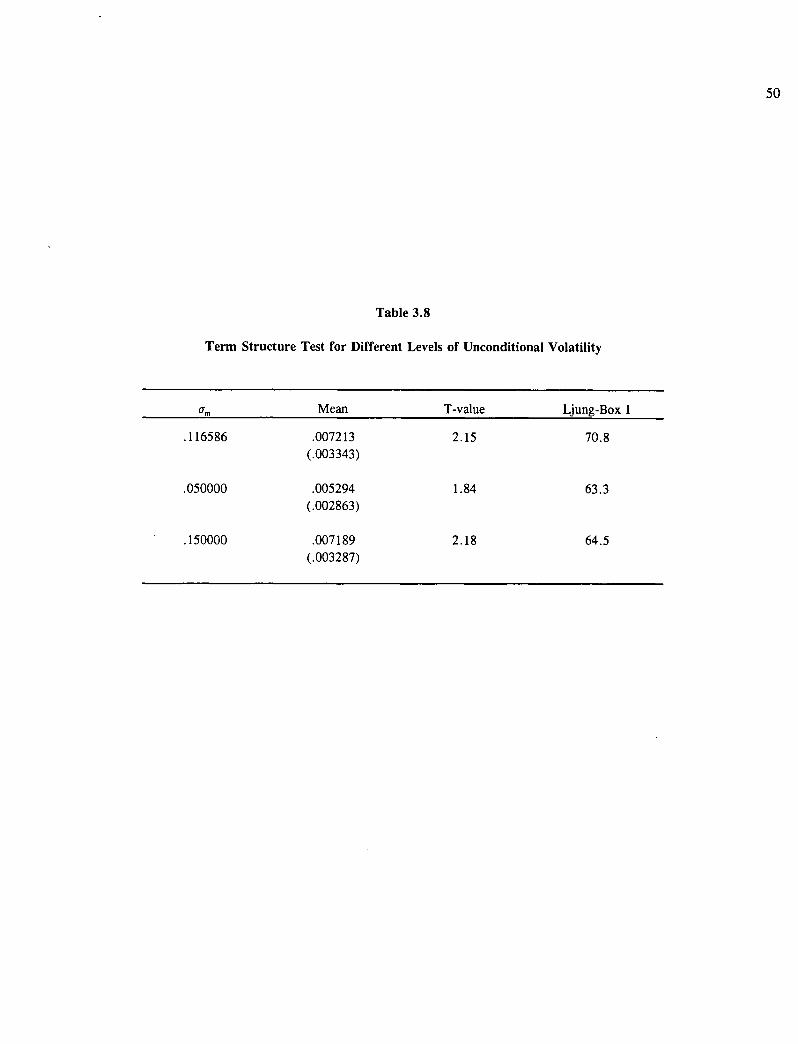
Table 3.8
Term Structure Test for Different Levels of Unconditional Volatility
50
Mean T-value Ljung-Box 1
.116586 .007213 2.15 70.8 (.003343)
.050000 .005294 1.84 63.3 (.002863)
.150000 .007189 2.18 64.5 (.003287)
51
CHAPTER 4: FUTURES MARKET EQUILIBRIUM VVITH HETEROGENEITY
4.1 Introduction
This paper studies hedging and equilibrium in the futures market for a commodity in a single
good economy, which is populated by heterogeneous producers and speculators. The commodity is
traded in a spot market at harvest time. Each producer is endowed with a non-traded private technology
and trades in futures contracts in order to reduce her quantity and price risk. Speculators invest their
initial wealths in bonds and take positions in futures contracts written on the commodity.
The model is motivated by the observation that a spot market is opened only at harvest time for
some commodities.' In such a setting, the producer faces both a price and a quantity risk. However,
most of the optimal hedging literature deals only with price risk. Hirshleifer (1990, 1991) discusses the
effects of both types of risk on the hedging decision but does not model them simultaneously. A simple
way to represent the quantity and price rislcs of each producer is to model them as a private cash flow
risk, where the cash position of a hedger is the present value of her terminal cash flows. The difficulty
in solving the equilibrium under these conditions is that both the futures price and the cash position of
a hedger are endogenous. In more traditional models, the cash position, which is the fixed quantity of
the commodity held by the producer, is independent of the futures price."
34 Fresh strawberries are an example of an agricultural product which hos a spot market at harvest lime, and which can be traded in futures market in the interim period by farmers, agro-industrial firms, consumers, and speculators.
35See, for example, Anderson and Danthine (1980)
52
Although equilibrium futures price and portfolio policies are determined simultaneously, the
determination herein proceeds in two stages for mathematical convenience. First, the demand of each
agent is derived assuming that the parameters of the futures price are known. Then, individual demands
are aggregated to obtain the equilibrium futures price at any point in time.
The optimal demand for a futures contract depends on tastes, on the resolution of uncertainty,
and on the formulation of the hedging problem. Early contributions in the optimal hedging literature
usually assumed that hedgers were monoperiodic expected utility maximizers (see for instance Stein
(1961), Johnson (1960), Anderson and Danthine (1980) and Losq (1982)). A conunon result from most
of these papers is that the optimal hedge ratio consists of a pure hedge component, and a mean variance
component.
More recent models are derived in a continuous-time framework, whereby the hedger maximizes
the expected utility of intertemporal consumption subject to a wealth-budget or cash-budget dynamic
constraint. The cash-budget formulation has been used by Ho (1984) in a model in which a farmer,
subject to both output and price risk during the production period, hedges a non-traded position. The
optimal demand for futures contracts depends on the exogenous cash position (the output), and includes
both a mean-variance efficiency component and a Merton-Breeden dynamic hedging component. The
wealth-budget formulation, initiated by Stulz (1984), is used by Adler and Detemple (1988) to solve a
problem similar to that of Ho. The resulting demand for futures contracts depends on the output, but also
includes a mean-variance efficiency term, a dynamic hedging component, and a minimum-variance
component. However, for myopic investors, both formulations yield tractable optimal demands, similar
to those obtained in single period models. Therefore, investors are assumed to have logaritlunic utility
functions in the model developed herein.
53
The demand for futures contracts depends on the uncertainty structure of the spot and the futures
market. A producer that hedges against price risk to protect a non-traded position has a demand
dependent on the output. Without trade constraints, and in the absence of frictions, the demand for
futures contracts is independent of the output [see Briys, Crouhy and Schlesinger (1990)]. In the model
developed herein, a producer is concerned with both quantity and price risk, and thus hedges against the
risk of individual cash flows.
The optimal demand for futures contracts by each investor is derived by assuming temporarily
that the parameters of the futures price are known, and by applying the equivalent martingale method
developed by Karatzas, Lehoczky and Shreve (1987). Diversity in cash flow risk leads to different
hedging strategies. The demand for futures contracts by a producer depends on her wealth, the present
value of her terminal production and the relative risk process of the futures contract. This structure of
demand is motivated by a desire to diversify, and to insure the actual value of the terminal production.
Producers are long or short in the futures contract if there is heterogeneity in cash flow risks. A similar
result is obtained by Hirshleifer (1991) in a discrete-time model where heterogeneity in the resolution of
uncertainty leads to different hedging strategies. In the model developed herein, the differential in cash
flow risk can also be interpreted as a differential in the resolution of uncertainty.
Once the optimal demand for futures contracts is derived, the aggregation follows easily. A
continuous-time equilibrium exists in the futures market when producers account for both quantity and
price risk by hedging against their individual and terminal cash flow risks. Stochastic cash positions and
equilibrium futures price are endogenous, unlike previous equilibrium models which ignore quantity risk.
The parameters of the futures price depend on wealth and the relative risk process. The volatility of the
futures price is stochastic and increases, on average, as the lime to maturity decreases. This maturity
54
effect in the model is consistent with Samuelson (1965). The stochastic volatility obtained in the model
is also consistent with the recent empirical evidence on the behaviour of daily futures prices. 36 The
positive mean of the instantaneous growth rate of futures prices indicates normal backwardation in the
model. The relative risk process of futures prices is a weighted sum of the present values of ah l the
terminal productions of hedgers.
Aggregation is made easier by assuming a logaritlunic utility function which allows for the
treatment of heterogeneity. The relative risk process of futures prices in the model of heterogeneous
agents developed herein has a weighted-average structure. Detemple and Murthy (1994), who appear to
be the first to deal with heterogeneity in an intertemporal production economy, obtain a similar result for
the equilibrium interest rate.
The remainder of the chapter is organized as follows. In section 4.2, the economy is described.
In section 4.3, optimal demands for futures contracts by each type of investor are derived. In section 4.4,
equilibrium futures price is derived; and in section 4.5, some concluding remarks are offered.
4.2 The Economy
Consider a continuous-time production economy with a Brownian uncertainty structure that is
populated with two classes of agents. The first class consists of producers indexed by i=1,2,...,n, and
the second class consists of speculators indexed by k=1,2...,m.
Consider a complete probability space (9, 5 P) and a finite time horizon [0,T]. On (9, P),
define a Brownian motion z with values in R. Also assume the following:
36See, for example, Milonas (1986) and Anderson (1985).
55
Al) Ail producers grow the same commodity, and each producer is endowed with a specific
production technology with a stochastic constant return to scale." The value of the production
in process Sit satisfies
=S:(Wdt +
where the constant parameter represents the expected instantaneous change in the rate of
production growth, and ai is the constant local variance of the process. is the production at
harvest time, expressed as a cash flow in units of the numeraire (that is, the commodity). The
production in process S', is flot tradeable, and S o > O.
A2) Producers and speculators have free and unlimited access to a financial market where a futures
contract written on the specified commodity is traded. The settlement price of this contract, F„
satisfies
dFi = a(.,t)dt + 45(.,t)dz r .
The production growth rate and the futures contract have the same uncertainty structure, and a
and ô are determined in equilibrium later.
A3) An instantaneously risldess bond is available and is held by both types of agents. The roll-over
value of an investment I in the riskless rate solves
dit = 10 =1,
"The aggregate production at maturity time T is homogenous. However, the differences in the stochastic constant returns to scale lead to differences in the individual quantities of production at maturity time T.
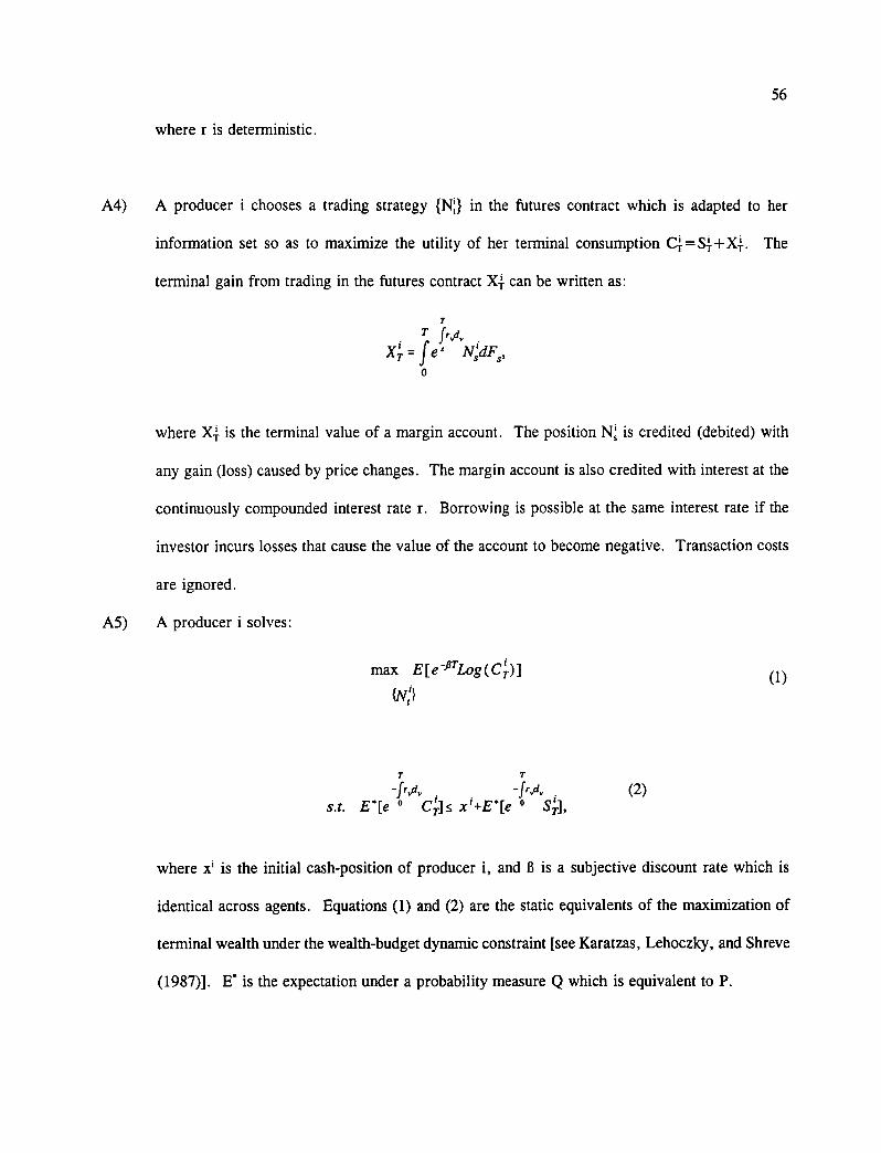
56
where r is deterministic.
A4) A producer i chooses a trading strategy {M} in the futures contract which is adapted to her
information set so as to maximize the utility of her terminal consumption C4=S-t+X-;.. The
terminal gain from trading in the futures contract XI can be written as:
T f rvd,
X; = f es N.:c1Fs,
where X. is the terminal value of a margin account. The position 1•1; is credited (debited) with
any gain (loss) caused by price changes. The margin account is also credited with interest at the
continuously compounded interest rate r. Borrowing is possible at the same interest rate if the
investor incurs losses that cause the value of the account to become negative. Transaction costs
are ignored.
A5) A producer i solves:
max E[e -firLog(CTi )] (1) {N:}
_frd . -frA . (2) s.t. ° Crls x i +E[e ° 4],
where x is the initial cash-position of producer i, and 13 is a subjective discount rate which is
identical across agents. Equations (1) and (2) are the static equivalents of the maximization of
terminal wealth under the wealth-budget dynamic constraint [see Karatzas, Lehoczky, and Shreve
(1987)]. E. is the expectation under a probability measure Q which is equivalent to P.
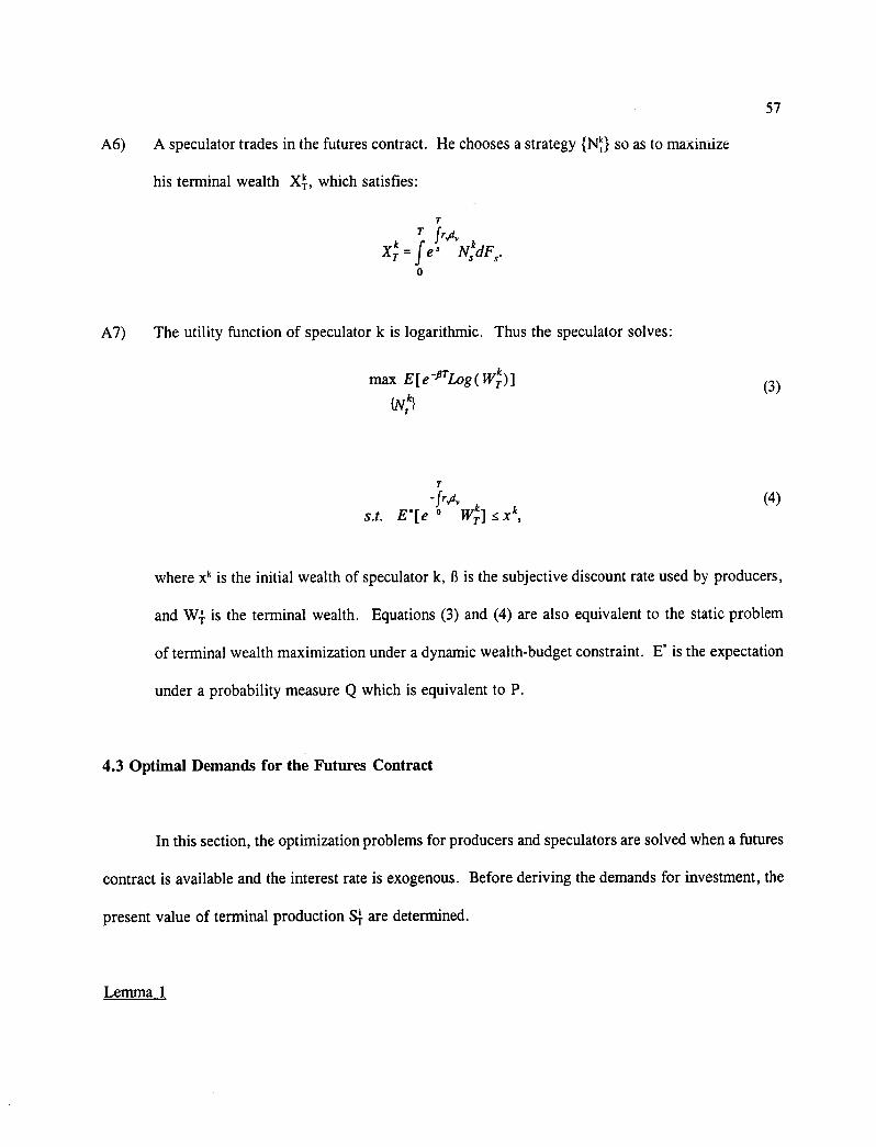
57
A6) A speculator trades in the futures contract. He chooses a strategy {N9 so as to maximize
his terminal wealth X14, which satisfies:
T frvd,, XTk = f e 3 NskdFs .
A7) The utility function of speculator k is logaritlunic. Thus the speculator solves:
max E[e -ieLog(WTk)] {e
-fr,d, s.t. E*[e ° WTic] X k,
where xk is the initial wealth of speculator k, fi is the subjective discount rate used by producers,
and W. is the terminal wealth. Equations (3) and (4) are also equivalent to the static problem
of terminal wealth maximization under a dynamic wealth-budget constraint. E . is the expectation
under a probability measure Q which is equivalent to P.
4.3 Optimal Demands for the Futures Contract
In this section, the optimization problems for producers and speculators are solved when a futures
contract is available and the interest rate is exogenous. Before deriving the demands for investment, the
present value of terminal production S . are determined.
(3)
(4)
Lemrna 1
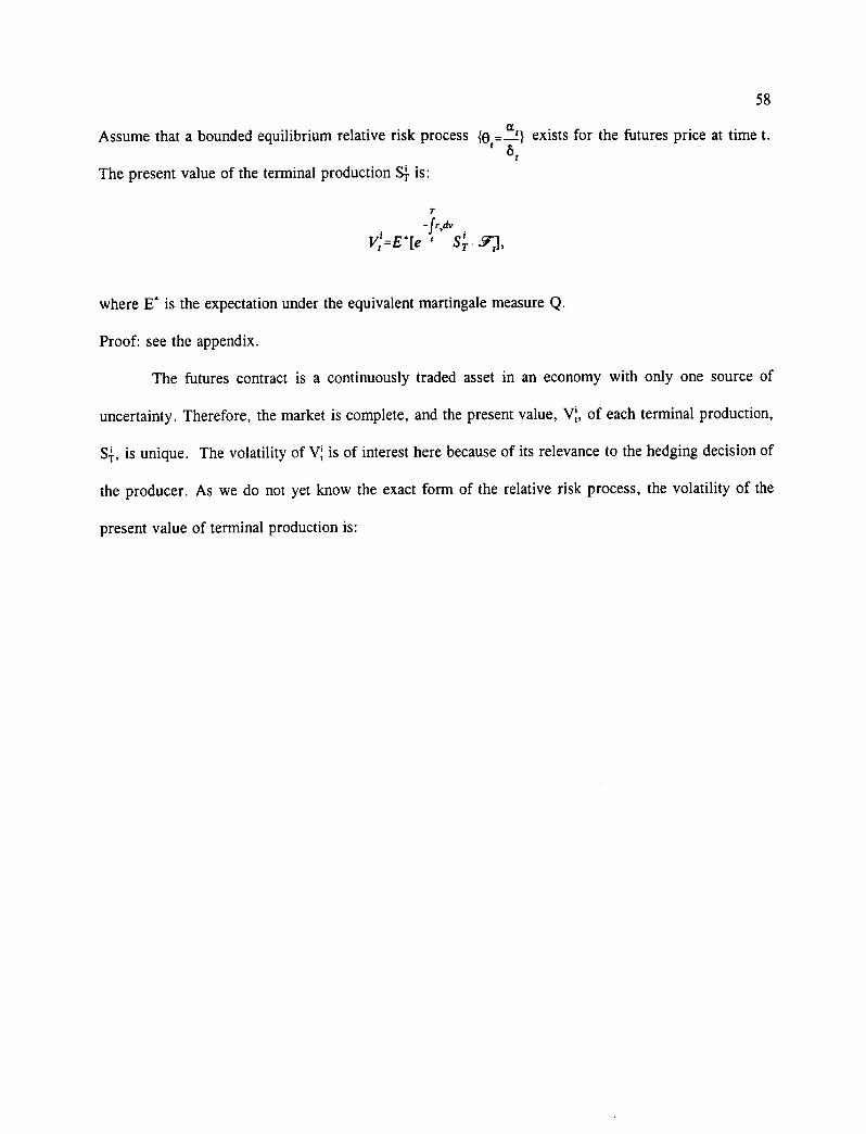
58 a Assume that a bounded equilibrium relative risk process fe —1} exists for the futures price at time t.
t
The present value of the terminal production SI is:
V:=E*[e S I 971,
where E is the expectation under the equivalent martingale measure Q.
Proof: see the appendix.
The futures contract is a continuously traded asset in an economy with only one source of
uncertainty. Therefore, the market is complete, and the present value, Ni;, of each terminal production,
is unique. The volatility of NT is of interest here because of its relevance to the hedging decision of
the producer. As we do flot yet know the exact form of the relative risk process, the volatility of the
present value of terminal production is:
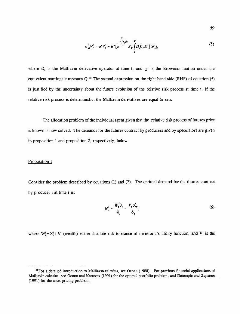
-fv» T = o iVti - ' ST fDAdfs Sil
where D, is the Malliavin derivative operator at time t, and f is the Brownian motion under the
equivalent martingale measure Q. 38 The second expression on the right hand side (RHS) of equation (5)
is justified by the uncertainty about the future evolution of the relative risk process at lime t. If the
relative risk process is deterministic, the Malliavin derivatives are equal to zero.
The allocation problem of the individual agent given that the relative risk process of futures price
is lcnown is now solved. The demands for the futures contract by producers and by speculators are given
in proposition 1 and proposition 2, respectively, below.
Proposition 1
Consider the problem described by equations (1) and (2). The optimal demand for the futures contract
by producer i at time t is:
=
v:avri (6) ô t
where W!=,C+ (wealth) is the absolute risk tolerance of investor i's utility function, and V is the
38For a detailed introduction to Malliavin calculus, see Ocone (1988). For previous financial applications of Malliavin calculus, see Ocone and Karatzas (1991) for the optimal portfolio problem, and Detemple and Zapatero . (1991) for the asset pricing problem.
59
(5)
60
present value of the cash flows generated by the position in the commodity at time T."
For the proof see the appendix.
The first and second terms on the RHS of equation (6) are the demand for mean variance
efficiency and the hedge ratio, respectively- . The present value of the non-traded position in the
commodity is insured. The producer uses futures contracts to offset variations in the present value
of the cash flow S,;- received from her non-traded position at maturity. The diversity in initial
endowments and technologies implies that some producers might be short in the futures contract at any
time t, whereas others are long in the futures contract. The net position of a producer in futures contracts
is determined by the difference between the volatility of her wealth and the volatility of the present value
of her terminal production. Producers with highly (un)certain terminal cash flows smooth their terminal
consumptions by buying (selling) futures contracts. The fact that some producers are long when others
are short in the futures contract is a consequence of heterogeneity. Hirshleifer (1991) obtains a similar
result for a discrete time model in which heterogeneity concerns the resolution of uncertainty for
producers. In contrast, heterogeneity is part of the equilibrium in the present mode!, and the hedging
position of the producer is determined by the relative volatility of her production process. In the
Hirshleifer mode!, arrival of information is independent of the equilibrium futures price, and the
assumption of additively separable preferences, complete markets, and a non-random endowment of the
numeraire are required to obtain a martingale property for the futures price. This martingale property
of the futures price is instrumental in deriving the demand for futures contracts. No restriction on the
futures or the spot price of the commodity are needed to solve for the equilibrium in the next section of
the paper.
39See Detemple and Murthy (1994).
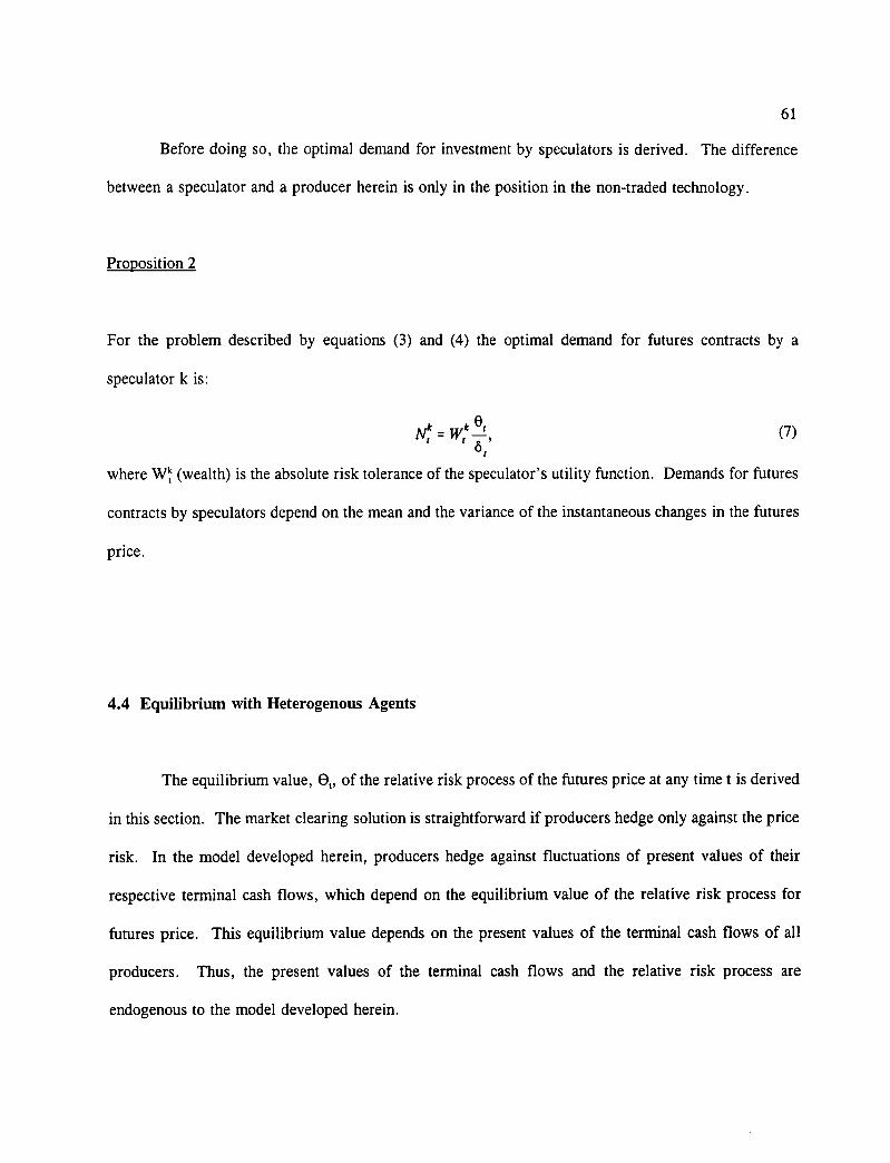
61
Before doing so, the optimal demand for investment by speculators is derived. The difference
between a speculator and a producer herein is only in the position in the non-traded technology.
Proposition 2
For the problem described by equations (3) and (4) the optimal demand for futures contracts by a
speculator k is:
hrk ufk et (7) 4 ' 1
where W (wealth) is the absolute risk tolerance of the speculator's utility function. Demands for futures
contracts by speculators depend on the mean and the variance of the instantaneous changes in the futures
price.
4.4 Equilibrium with Heterogenous Agents
The equilibrium value, 0„ of the relative risk process of the futures price at any time t is derived
in this section. The market clearing solution is straightforward if producers hedge only against the price
risk. In the model developed herein, producers hedge against fluctuations of present values of their
respective terminal cash flows, which depend on the equilibrium value of the relative risk process for
futures price. This equilibrium value depends on the present values of the terminal cash flows of all
producers. Thus, the present values of the terminal cash flows and the relative risk process are
endogenous to the model developed herein.
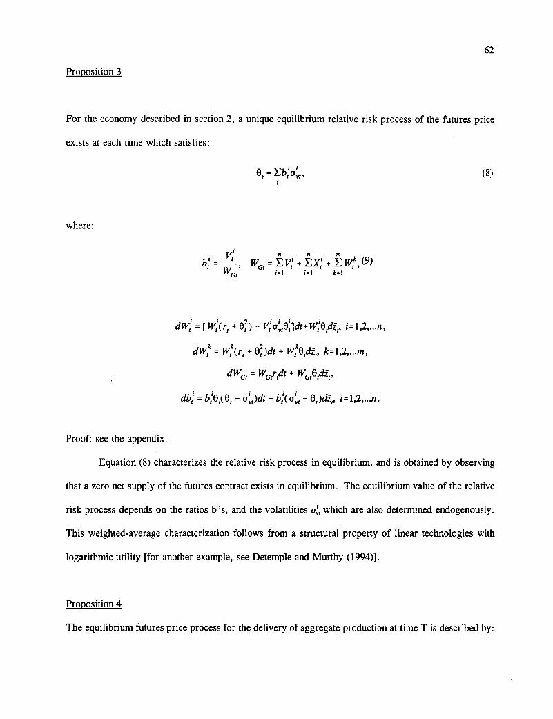
62
Proposition 3
For the economy described in section 2, a unique equilibrium relative risk process of the futures price
exists at each time which satisfies:
13, = Ebo , ( 8)
where:
n n m b= = ,
WGI 1=1 1=1 k=1
dW: = [111(r, + ) - W:Orceet, i =1,2,...n ,
dw,k = wt̀ c(ri + 02 )dt + wtkete„ k=1,2,...m,
dWG, = WGitclt + WGietclit ,
= - )dt + - Ode, i=1,2,...n.
Proof: see the appendix.
Equation (8) characterizes the relative risk process in equilibrium, and is obtained by observing
that a zero net supply of the futures contract exists in equilibrium. The equilibrium value of the relative
risk process depends on the ratios bi 's, and the volatilities cf!, which are also determined endogenously.
This weighted-average characterization follows from a structural property of linear technologies with
logarithmic utility [for another example, see Detemple and Murthy (1994)].
Proposition 4
The equilibrium futures price process for the delivery of aggregate production at time T is described by:
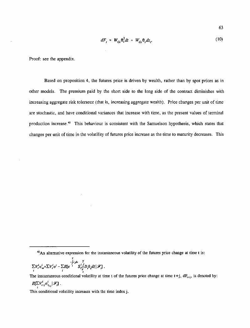
63
dFf = WG,62,dt + WGr etdzr. (10)
Proof: see the appendix.
Based on proposition 4, the futures price is driven by wealth, rather than by spot prices as in
other models. The premium paid by the short side to the long side of the contract diminishes with
increasing aggregate risk tolerance (that is, increasing aggregate wealth). Price changes per unit of time
are stochastic, and have conditional variances that increase with time, as the present values of terminal
production increase.e This behaviour is consistent with the Samuelson hypothesis, which states that
changes per unit of lime in the volatility of futures price increase as the time to maturity decreases. This
40An alternative expression for the instantaneous volatility of the futures price change at time t is:
-frvd, T
EV:G y,' =EV:a i - EE[e STi fDAdil..9;] .
The instantaneous conditional volatility at time t of the futures price change at time t+j, dF t+i , is denoted by:
E[E11:+ja vi .
This conditional volatility increases with the time index j.
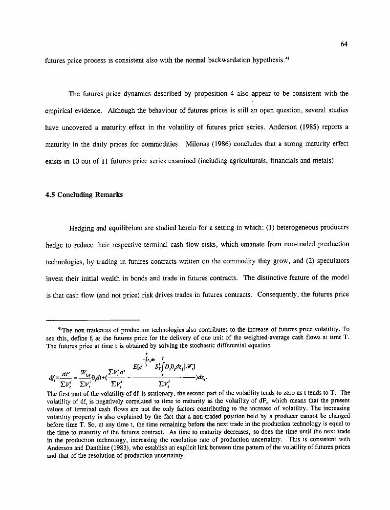
64
futures price process is consistent also with the normal backwardation hypothesis. 41
The futures price dynamics described by proposition 4 also appear to be consistent with the
empirical evidence. Although the behaviour of futures prices is still an open question, several studies
have uncovered a maturity effect in the volatility of futures price series. Anderson (1985) reports a
maturity in the daily prices for commodities. Milonas (1986) concludes that a strong maturity effect
exists in 10 out of 11 futures price series examined (including agriculturals, financials and metals).
4.5 Concluding Remarks
Hedging and equilibrium are studied herein for a setting in which: (1) heterogeneous producers
hedge to reduce their respective terminal cash flow risks, which emanate from non-traded production
technologies, by trading in futures contracts written on the commodity they grow, and (2) speculators
invest their initial wealth in bonds and trade in futures contracts. The distinctive feature of the model
is that cash flow (and not price) risk drives trades in futures contracts. Consequently, the futures price
4I The non-tradeness of production technologies also contributes to the increase of futures price volatility. To see this, define f, as the futures price for the delivery of one unit of the weighted-average cash flows at time T. The futures price at lime t is obtained by solving the stochastic differential equation
E e ' STIDAdze lirj dF WG EV:a'
dfra— - )dz,. E E vti vrt E
The first part of the volatility of df, is stationary, the second part of the volatility tends to zero as t tends to T. The volatility of df, is negatively correlated to time to maturity as the volatility of dF„ which means that the present values of terminal cash flows are not the only factors contributing to the increase of volatility. The increasing volatility property is also explained by the fact that a non-traded position held by a producer cannot be changed before lime T. So, at any lime t, the time remaining before the next trade in the production technology is equal to the time to maturity of the futures contract. As lime to maturity decreases, so does the time until the next trade in the production technology, increasing the resolution rate of production uncertainty. This is consistent with Anderson and Danthine (1983), who establish an explicit link between time pattern of the volatility of futures prices and that of the resolution of production uncertainty.
65
and the cash position are endogenous.
This theoretical framework yields some interesting insights. First, the net position in futures
contracts depends on the relative volatility of the producer cash flows. Producers with cash flow
uncertainty, which are resolved less rapidly than the aggregate, will tend to go short in order to smooth
their terminal consumption, or alternatively, will hold futures contracts. This result differs from that
obtained in traditional models in which producers sell futures contracts to hedge their non-traded positions
against spot price fluctuations. This result is consistent with practice where the distinction between
hedgers and speculators is ambiguous. Second, changes in the equilibrium futures price depend on wealth
and the relative risk process. The futures price dynamics resulting from this model are consistent with
empirical evidence for commodity futures price, where trading is absent. Specifically, the model predicts
an inverse relation between volatility of futures price increments and maturity (the Samuelson hypothesis).
An interesting avenue for future research would be to study a similar model in an incomplete
market setting. This might be able to account better for the ARCH behaviour reported in studies of
futures prices .42
42Yang and Brorsen (1993) report ARCH/GARCH behaviour of commodity futures prices.
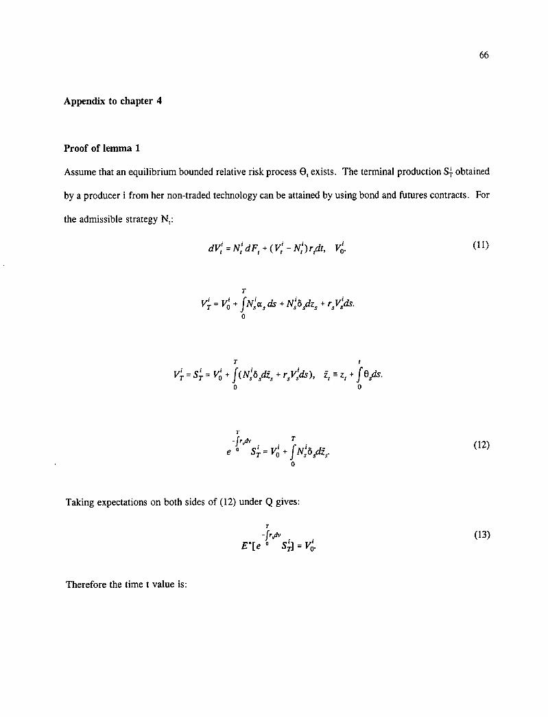
66
Appendix to chapter 4
Proof of lemma 1
Assume that an equilibrium bounded relative risk process A, exists. The terminal production S. obtained
by a producer i from her non-traded technology can be attained by using bond and futures contracts. For
the admissible strategy N t :
= dFt + ( V: - N:)rtdt, V.
= v+ f Nsi a s ds + Nsi 6 sdzs + rysids.
= S = v+ f(1■1:8sdis + rysids), fesds.
-f e ° sss
Taking expectations on both sides of (12) under Q gives:
-fr*,» . . ° = V.
(12)
(13)
Therefore the time t value is:
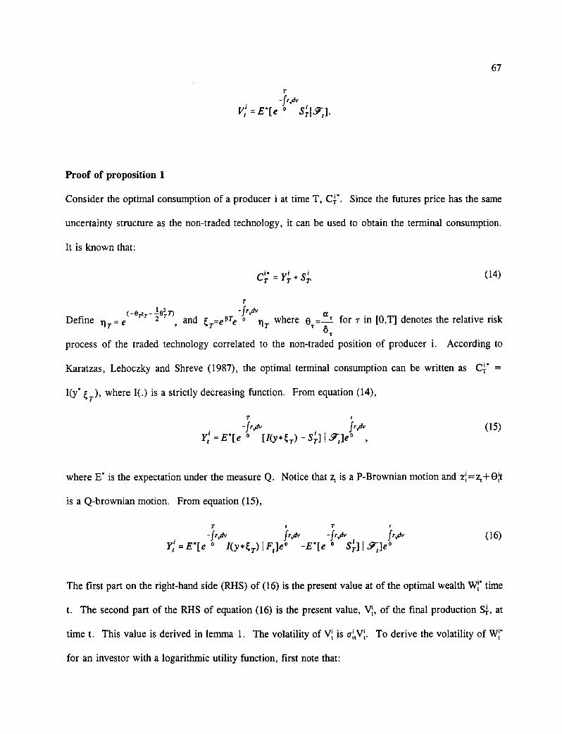
67
-frfr . • =Ele ° 4.19].
Proof of proposition 1
Consider the optimal consumption of a producer i at time T, C. Since the futures price has the same
uncertainty structure as the non-traded technology, it can be used to obtain the terminal consumption.
It is known that:
(14)
T
(-e TeT - 1627.n -f,dv
rIT— a Define - e
2 and z T=efiTe ° li T where 6 ,_r for T in [0,T] denotes the relative risk ,
process of the traded technology correlated to the non-traded position of producer i. According to
Karatzas, Lehoczky and Shreve (1987), the optimal terminal consumption can be written as
I(y* z where I(.) is a strictly decreasing function. From equation (14),
-frbplv • frphe
Y: = E*[e ° [I(y*Z T) - 411 .7;]e° ,
where E. is the expectation under the measure Q. Notice that z, is a P-Brownian motion and 21=z,+0It
is a Q-brownian motion. From equation (15),
• -frve • frfr (16) Y: = ° I(y*Z T) I F je° ° 4.] I
The first part on the right-hand side (RHS) of (16) is the present value at of the optimal wealth Wr time
t. The second part of the RI-IS of equation (16) is the present value, VI, of the final production SI-, at
time t. This value is derived in lemma 1. The volatility of NT; is To derive the volatility of Wr
for an investor with a logarithmic utility fimction, first note that:
Ô T
=
(15)
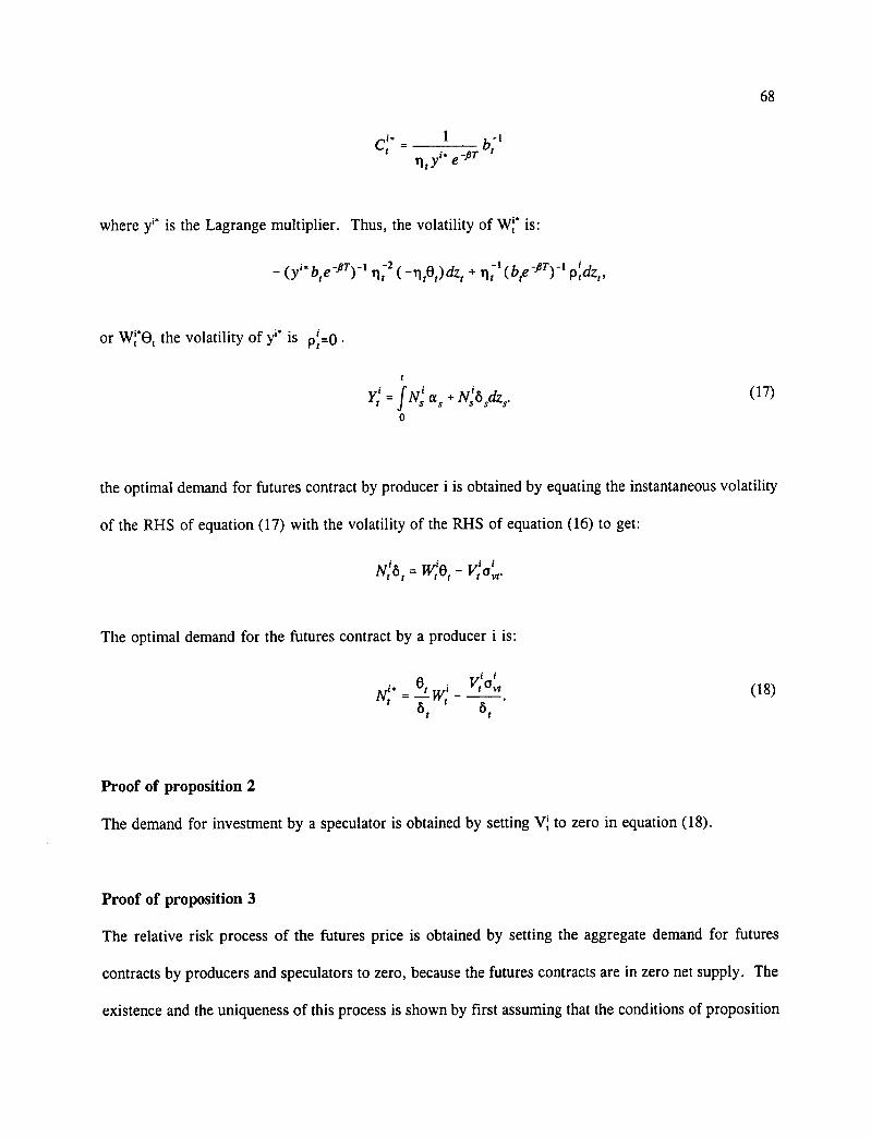
where yl* is the Lagrange multiplier. Thus, the volatility of Wr is:
- (y' b,e -ieT) -1 1 2 ( -ri te)dzr + t(ly -fiT) -1
or WrO, the volatility of y' is p it .0
= f IsIsi + Nsi te sdzs.
the optimal demand for futures contract by producer i is obtained by equating the instantaneous volatility
of the RETS of equation (17) with the volatility of the RETS of equation (16) to get:
NÔ = W:(3, - vw,„
The optimal demand for the futures contract by a producer i is:
e . via' N:* = - vt ei t •
(16)
Proof of proposition 2
The demand for investment by a speculator is obtained by setting V; to zero in equat ion (18).
Proof of proposition 3
The relative risk process of the futures price is obtained by setting the aggregate demand for futures
contracts by producers and speculators to zero, because the futures contracts are in zero net supply. The
existence and the uniqueness of this process is shown by first assuming that the conditions of proposition
68
(17)
69
3 are respected. Then, the aggregate production at time t can be written as a function of the relative risk
process 0, as:
rjIS (19)
API) =EV, = Es [e 49'1
where:
A T =E4.. (20)
The instantaneous variation of aggregate production is:
EV,tr,dt + E V: a ivedit. (21)
Using the equilibrium condition 0, = E and setting Ex i Ewk / the following process is i k t "
obtained for (the value of A, when using equilibrium condition), with:
c/Â, = Ârridt + (À, + 1, )(3,dit, (22)
which is equivalent to:
c/À-, = + 62,) + /,02, + (Â, + 1,)0,dz,. (23)
Remark: Since 1, is independent of 0, and the V't 's, and a zero net supply of the futures contracts exists
in equilibrium, then: dl, = 1,r,dt + E ( a, dt +
di = 1,r,dt, 10 =
70
l, depends only on the interest rate and the initial cash position of agents, both of which are exogenous.
The system of equations (19)-(23) is consistent if and only if:
(24)
Thus, at each point in time t, Ât and 0, should be such that ÂT = Ar The above problem can be viewed
as a design problem in which  , and 0, are chosen at each time t such that the terminal condition is met.
This is the equivalent to solving a backward stochastic differential equation of the type studied by
Pardoux and Peng (1990); namely:
1 1 x(t) + ffts, x(s),y(s))ds + f g (s ,x(s),y(s))dWs =X.
t t (25)
The conditions for the existence of a unique solution to equation (25) are:
a) f(.,0,0) and g(.,0,0) belong to /%42(0,1,R), the set of
integrable and progressively measurable functions relative to the information set.
b) c > 0 exists such that
If(t,x1 ,y 1 ) -f(t,x2,y2 ) I + I g(t ,xpyi ) - g(t,x2,y2 I s c ( lx 1 - x2 I + ly1 -y2 I)
for ail x l , x2 E R, and Yi' y2 E R, (t,w) a.e.
c) An a exists such that:
Ig(t,x,y1 ) - g(t,x,y2 ) 1 2 a ly1 - y21)
for ail x E R, and yl , y2 E R, (t,w) a.e.
In the case of Ât :
fit, x(t),y(t)) =;if (r, + O) + 4 ( 6,2 ), 6, = Eb:a ivr; t
71
g(t,x(t),y(t)) =( À, + l)er
Condition a) obviously holds for the differential equation of Â, . Condition b) is the Lipschitz condition.
Since 0, is bounded, the Lipschitz condition holds for the differential equation of . Condition c) also
holds for the differential equation of  , . This is apparent after setting a = min { I, / t E [0, T] }, and
lcnowing that 1E, is always positive. When these three conditions are respected, a unique couple (À ,e) solving the differential equation (21) with the terminal condition (24) exists at each time t. The solution
to the system (21)-(24) is equivalent to an optimal allocation made by a central planner.
That the solution is compatible with equilibrium in the initial decentralised economy is now
shown. If a unique couple (Â. ,0*,) solution exists to the system of (21)-(24) at each time t, then:
edV Àt * E'[e A T ISri]
= EE's S;13-,-1
The volatility of À. is then:
E v:*(7 1,:
However, from equation (22) the volatility of Â. is:
+
Equating the two volatilities leads to the equilibrium condition of the decentralised economy:
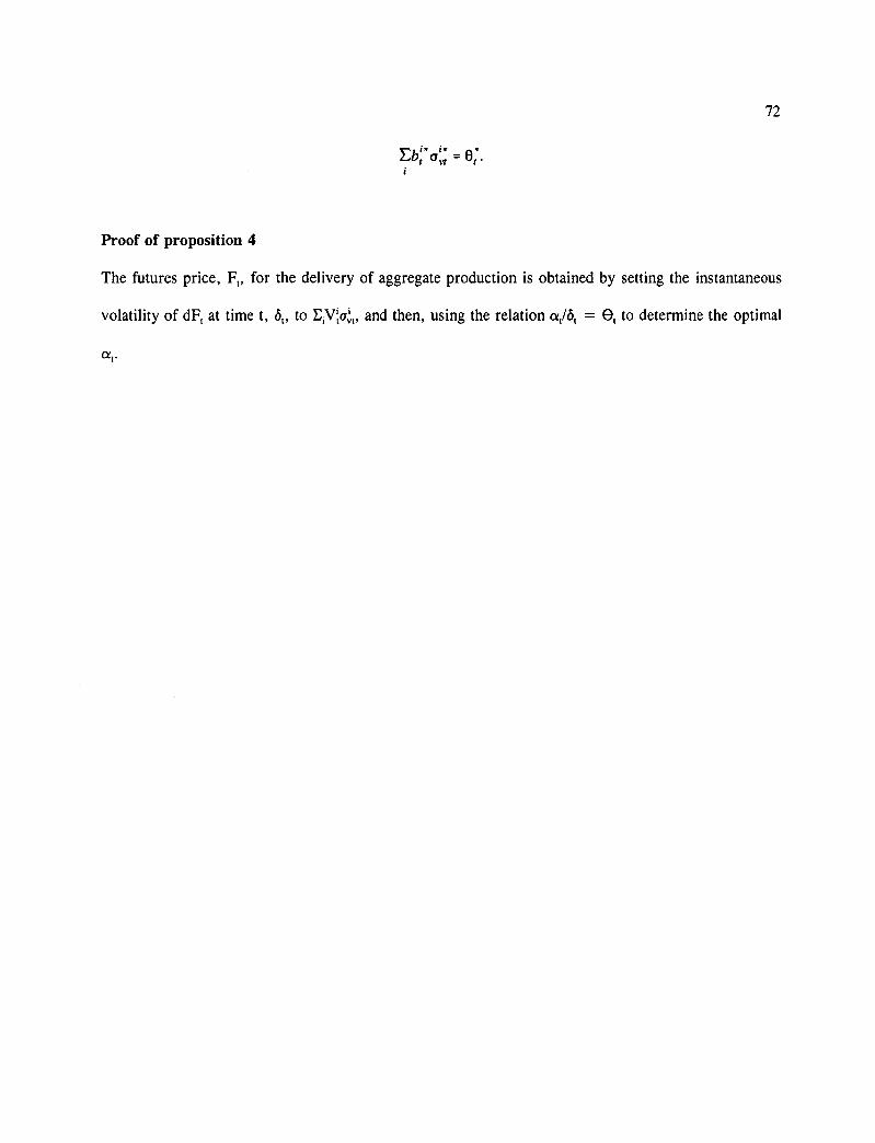
72
Proof of proposition 4
The futures price, F„ for the delivery of aggregate production is obtained by setting the instantaneous
volatility of dF, at time t, ô„ to E,V1a,' and then, using the relation a,/.5, = 0, to determine the optimal
a,.
73
CHAPTER 5: MAJOR FINDINGS, IMPLICATIONS
AND DIRECTIONS FOR FUTURE RESEARCH
This thesis used a dynamic asset pricing framework to investigate the efficiency of currency
option markets, risk preferences of investors implied by a partial equilibrium model of bond futures
prices, and to study equilibrium in futures market with heterogeneity. The major findings of the three
essays are summarized next.
In the first essay, models of continuous time bond futures prices under discrete marking-to-market
are derived by using the fact that equispaced sampling of a continuous time AR-1 (the Ornstein-Uhlenbeck
process) results in a discrete time AR-1. The formulas obtained are tractable and suitable for empirical
investigation unlike a formula derived earlier by Chen (1992b). Second, meaningful estimates of the
market price of interest rate risk are obtained, and Treasury bond futures data are shown to be a valid
alternative to the bond data used in previous studies to estimate such market prices.' Since delivery
options held by the short side of a Treasury bond futures contract do flot appear to have an impact on the
market price of interest rate risk, the very active Treasury bond futures market is a good source of data
for empirical estimations. Since estimates of the market price of interest rate risk obtained using models
of Treasury bill futures prices data are too high to account for both a logarithmic utility ftmction, and the
volatility of interest rates, these models models are rejected. These results might be explained by market
distortions. An alternative interpretation is that the models are misspecified. Estimations improve for
long-lived futures contracts with long-term underlying bonds when a model with discrete marking-to-
43 See for example Brennan and Schwartz (1979), Dietrich-Campbell and Schwartz (1986), Longstaff (1989), and Duan (1992).
74
market is used.
In the second essay, ex-ante tests of the relationship between short- and long-term implied
volatilities are performed for the exchange rates of the Japanese yen, the Swiss franc and the
Deutschmark versus the American dollar. The model selected for the conditional volatilities of the
exchange rate relative return series for these currencies is the GARCH(1,1). The joint hypothesis of a
correct model specification and ex-ante efficiency is flot rejected for the Japanese yen and the Swiss franc,
and is rejected for the Deutsclunark. This rejection is interpreted as evidence that inefficiencies caused
by noise exist in the Deutschmark currency-option market during the studied period. The results reported
herein contribute to both sides of the ongoing debate about whether option markets are efficient.
In the third essay, hedging and equilibrium are studied herein for a setting in which: (1)
heterogeneous producers hedge to reduce their respective terminal cash flow risks, which emanate from
non-traded production technologies, by trading in futures contracts written on the cornmodity they grow,
and (2) speculators invest their initial wealth in bonds and trade in futures contracts. The distinctive
feature of the model is that cash flow (and flot price) risk drives trades in futures contracts.
Cons equently, the futures price and the cash position are endogenous. This theoretical framework yields
some interesting insights. First, the net position in futures contracts depends on the relative volatility of
a producer's cash flows. Producers with cash flows uncertainty which are resolved less rapidly than the
aggregate, will tend to go short in order te smooth their terminal consumption, or alternatively will hold
futures contracts. This result differs from that obtained in traditional models in which producers sell
futures contracts to hedge their non-traded positions against spot price fluctuations. This result is
consistent with what is observed in practice where the distinction between hedgers and speculators is
ambiguous. Second, changes in the equilibrium futures price depend on wealth and the relative risk
75
process. The futures price dynamics resulting from this model are consistent with empirical evidence for
conunodity futures price, where trading is absent. Specifically, the model predicts an inverse relation
between volatility of futures price increments and maturity (the Samuelson hypothesis).
Several directions for future research emerge from this thesis. First, the research methodology
used herein for the Japanese yen, the Swiss franc and the Deutschmark should be applied to other major
currencies, and other periods, or in relation to market events, so that the conditions under which
inefficiencies arise are determined. Second, further investigations of .the market price of interest rate risk
taking into account confounding events, and the possibility of structural breaks might yield richer results.
It would be interesting to test Treasury bill futures price models with data sampled exclusively when the
number of transactions is high, and the risk of inefficiencies low. Third, a model of equilibrium in an
incomplete futures market with heterogeneity might explain the GARCH behaviour of some futures
prices.
76
REFERENCES
Adams, P.D. and S.B. Wyatt, 1987, "Biases in Option Prices, Evidence from the Foreign Currency Option Market," Journal of Banking and Finance 11, 549-562
Adler, M. and Detemple, J., 1988, "On the Optimal Hedge of a Non-Traded Cash Position," Journal of Finance 23, 143-153.
Anderson, R.W., 1985, "Some Determinants of the Volatility of Futures Prices," Journal of Futures Markets 5, 331-348.
Anderson, R.W. and J.-P. Danthine, 1980, "Hedging and Joint Production: Theory and Illustrations," Journal of Finance 35, 487-501
Arnold, L., 1974, Stochastic Differential Equations, New York: John Wiley & Sons.
Baillie, R.T., and T. Bollerslev, 1989, "The Message in Daily Exchange Rates: A Conditional Variance Tale," Journal of Business and Economic Statistics 7, 297-305.
Berndt, E.K., B.H. Hall, R.E. Hall and J.A. Hausman, 1974, "Estimation and Inference in Nonlinear Structural Models," Annals of Economic and Social Measurement 4, 653-665.
Bessembinder, H. and P.J. Seguin, 1993, "Price Volatility, Trading Volume, and Market Depth: Evidence from Futures Markets," Journal of Financial and Quantitative Analysis 28, 21-34.
Black, F., 1986, "Noise," Journal of Finance 61, 529-543.
Bollerslev, T., 1987, "A Conditionally Heteroskedatic Time Series Model for Speculative Prices and Rates of Return," Review of Economics and Statistics 69, 542-547.
Bollerslev, T., R.Y. Chou, and K.F. Kroner, 1992, "ARCH Modelling in Finance: A Review of the Theory and Empirical Evidence," Journal of Econometrics 52, 5-59.
Brennan, M.J. and E.S. Schwartz, 1977, "Savings Bonds, Retractable Bonds and Callable Bonds," Journal of Financial Economics 5, 67-88.
Brennan, M.J . and E. S. Schwartz, 1979, "A Continuous Time Approach to the Pricing of Bonds," Journal of Banking and Finance 3, 133-155.
Briys, E., Crouhy, M. and Schlesinger, H., 1990, "Optimal Hedging under Intertemporally Dependent Preferences," Journal of Finance 45, 1315-1324.
Campa, J. M., and P.H.K. Chang, 1993, "Testing the Expectation Hypothesis on the Term Structure of Implied Volatilities in Foreign Exchange Options," Working Paper, March 1993.
Campbell, J. Y., 1986, "A Defense of Traditional Hypotheses about the Term Structure of Interest Rates," Journal of Finance 41, 183-193.
77
Canina, L., and S. Figlewski, 1993, "The Informational Content of Implied Volatility," Review of Financial Studies 6, 659-681.
Chan, K.C., G.A. Karolyi, F.A. Longstaff and A.B. Sanders, 1992, "An Empirical Comparison of Alternative Models of the Short-Term Interest Rate," Journal of Finance 57, 1209-1227.
Chen, R.R., 1992a, "Exact Solutions for Futures and European Futures Options on Pure Discount Bonds," Journal of Financial and Quantitative Analysis 27, 97-107.
Chen, R.R., 1992b, "A New Look at Interest Rate Futures Contracts," Journal of Futures Markets 12, 539-548
Cox, J.C., J.E. Ingersoll Jr., and S.A. Ross, 1985, "On the Term Structure of Interest Rates," Econometrica 53, 385-407.
Cox, J.C., J.E. Ingersoll Jr., and S.A. Ross, 1981, "A Re-examination of Traditional Hypotheses about the Term Structure of Interest Rates," Journal of Finance, 36, 769-799.
Cox, J.C. and S.A. Ross, 1976, "The Valuation of Options for Alternative Stochastic Processes," Journal of Financial Economics 3, 145-166.
Cox, J.C., S.A. Ross and M. Rubinstein, 1979, "Option Pricing: A Simplified Approach," Journal of Financial Economics 7, 229-263.
Detemple, J. and Murthy, S., 1994, "Intertemporal Asset Pricing with Heterogeneous Beliefs," Journal of Economic Theory 62, 294-320.
Detemple, J. and Zapatero, F., 1991, "Asset Prices in an Exchange Economy with Habit Formation", Econometrica 59, 1633-1657.
Dietrich-Campbell, B. and E.S. Schwartz, 1986, "Valuing Debt Options - Empirical Evidence," Journal of Financial Economics 16, 321-343.
Diz, F., and T. J. Finucane, 1993, "Do the Options Markets Really Overreact?" The Journal of Futures Markets 13, 299-312.
Dothan, L. U., 1978, "On the Term Structure of Interest Rates," Journal of Financial Economics 6, 59- 69.
Duan, J.-C., 1992, "Maximum Likelihood Estimation Using Price Data of the Derivative Contract," Working Paper, Faculty of Management, McGill University.
Duan, J.-C, 1995, The GARCH Option Price Mode!, 1995, Mathemati cal Finance 5, 13-32.
Duffie, D. and Jackson 0.M., 1990, "Optimal Hedging and Equilibrium in a Dynamic Futures Market," Journal of Economic Dynamics and Control 14, 21-33.
Duffie, D. and R. Stanton, 1992, "Pricing Continuously Resettled Contingent Claims," Journal of
78
Economic Dynamics and Control 16, 561-573.
Fama, E., 1965, "The Behavior of Stock Market Prices," Journal of Business 38, 34-105.
Flesaker, B., 1993, "Arbitrage Free Pricing of Interest Rate Futures and Forward Contracts," Journal of Futures Markets, 13, 77-91.
Feinstein, S, 1989, "The Black-Scholes Formula is Nearly Linear in a for at the Money Options," Presentation at the AFA conference, Washington D.C., December 1990.
Friedman, A., 1975, Stochastic Differential Equations and Applications, New York: Academic Press, 1.
Gallant, A.R., 1987, Nonlinear Statistical Models, John Wiley and Sons, New York, 607.
Garman, M.B., and S.W. Kohlhagen, 1983, "Foreign Currency Option Values," Journal of International Money and Finance, 2, 231-237.
Hansen, L.P, 1982, "Large Sample Properties of Generalized Method of Moments Estimators," Econometrica 50, 1029-1054
Harrison, J.M., and D. Kreps, 1979, "Martingales and Arbitrage in Multiperiod Securities Markets," Journal of Economic Theory 20, 381-408.
Harrison, J.M., and S. Pliska, 1981, "Martingales and Stochastic Integrals in the Theory of Continuous Trading," Stochastic Processes and Their Applications 11, 215-260.
Harvey, C.R., and R.E. Whaley, 1992, "Market Volatility Prediction and the Efficiency of the S&P 100 Index Option Market," Journal of Financial Economics 31, 43-73.
Hegde, S.P, 1988, "An Empirical Analysis of Implicit Delivery Options in the Treasury Bond Futures Contract," Journal of Banking and Finance 12, 469-492.
Hemler, M.L., 1990, "The Quality Delivery Option in Treasury Bond Futures Contracts," Journal of Finance 15, 1565-1586.
Heynen, R.C., and H.M. Kat, 1993, "Volatility Prediction: A Comparison of the GARCH(1,1), EGARCH(1,1) and Stochastic Volatility Model," Working Paper, Department of Operation Research, Erasmus University Rotterdam.
Heynen, R., A. Kemna, and T. Vorst, 1994, "Analysis of the Term Structure of Implied Volatilities," Journal of Financial and Quantitative Analysis 29, 31-56.
Hirshleifer, D., 1990, "Hedging Pressure and Futures Price Movements In a General Equilibrium," Econometrica 58, 411-428.
Hirshleifer, D., 1991, "Seasonal Patterns of Futures Hedging and the Resolution of Output Uncertainty," Journal of Economic Theory 53, 304-327.
79
Ho, T., 1984,"Intertemporal Commodities Futures Hedging and the Production Decision," Journal of Finance 39, 351-376.
Hsieh, D.A., 1989, "Modeling Heteroskedasticity in Daily Foreign Exchange Rates," Journal of Business and Economic Statistics 7, 307-317
Hull, J. and A. White, 1987, "The Pricing of Options on Assets with Stochastic Volatilities," The Journal of Finance 3, 281-300.
Jamshidian, F., 1989, "An Exact Bond Option Formula," Journal of Finance 44, 205-209.
Johnson, L., 1960, "The Theory of Hedging and Speculation in Commodity Futures," Review of Economic Studies 27, 139-151.
Johnson, H. and D. Shanno, 1987, "Option Pricing when the Variance is Changing," Journal of Financial and Quantitative Analysis 22, 143-151.
Kane, A. and A. Marcus, 1986, "The Quality Option in the Treasury Bond Futures Market: An Empirical Assessment," Journal of Futures Markets 6, 231-248.
Karatzas, I., J.P. Lehoczky and S.E. Shreve, 1987, "Optimal Portfolio and Consumption Decisions for a 'Small Investor' on a Finite Horizon," SIAM Journal of Control and Optimization 25, 1557-1586.
Karatzas, I. and S.E. Shreve, 1988, Brownian Motion and Stochastic Calculus, Springer Verlag, New York.
Karatzas, I., J.P. Lehoczky, S.E. Shreve and G. Xu, 1991, "Martingale and Duality Methods for Utility Maximization in an Incomplete market," SIAM Journal of Control and Optimization 29, 702-730.
Kodres, L.E., 1993, "Tests of Unbiasedness in the Foreign Exchange Futures Markets: An Examination of Price Limits and Conditional Heteroscedasticity," Journal of Business 66, 463-489
Kugler, P. and C. Lenz, 1990, "Chaos, ARCH and the Foreign Exchange Market: Empirical Results from Weekly Data, Unpublished Manuscript (Volkswirtschaftliches Institut, Zurich).
Lamoureux, C.G., and W.D. Lastrapes, 1993, "Forecasting Stock-Return Variance: Toward an Understanding of Stochastic Implied Volatilities," Review of Financial Studies 6, 293-326.
Leroy, S. F., 1973, "Risk Aversion and the Martingale Property of Stock Prices," International Economic Review 14, 436-446.
Ljung, G. and G.E.P. Box, 1978, "On a Measure of Lack of Fit in Time Series Models," Biometrika 65, 297-303.
Longstaff, F.A., 1989, "A Nonlinear General Equilibrium Model of the Term Structure of Interest Rates," Journal of Financial Economics 23, 195-224.
80
Longstaff, F.A., 1990, "Time Varying Term Premia and Traditional Hypotheses about the Term Structure," Journal of Finance 65, 1307-1314.
Losq, E., 1982, "Hedging with Price and Output Uncertainty," Economics Letters 12, 65-70.
Lucas, R., 1978, "Asset Prices in an Exchange Economy," Econometrica 46, 1429-1445.
Mahieu, R., and P. Schotman, 1994, "Neglected Conunon Factors in Exchange Rate Volatility," Journal of Empirical Finance 1, 279-311.
Mandelbrot, B., 1966, "Forecast of Futures Prices, Unbiased Markets, and Martingale Models," Journal of Business 39, 241-255.
McCurdy, T.H. and I. Morgan, 1987, "Testing the Martingale Hypothesis for Foreign Currency Futures with Time Varying Volatility," International Journal of Forecasting 3, 131-148.
Merton, R., 1969, "Lifetime Portfolio Selection under Uncertainty: The Continuous Time Case," Review of economics and Statistics 51, 247-257.
Merton, R., 1973, An Intertemporal Capital Asset Pricing Mode!," Econometrica 41, 867-888.
Milonas, N.T., 1986, "Price Variability and the Maturity Effect in the Futures Market," Journal of Futures Markets 6, 443-460.
Nelson, C.R., 1972, The Term Structure of Interest Rates, Basic Books, New York.
Newey, W and K. West, 1987, "A Simple, Positive Definite, Heteroscedasticity and Autocorrelation Consistent Covariance Matrix," Econometrica 55, 703-708.
Ocone, D., 1988, "A Guide to the Stochastic Calculus of Variations," Lectures Notes in Mathematics 1316, 1-79
Ocone, D. and Karatzas, I., 1991, "A Generalized Clark Representation Formula, with Application to Optimal Porfolios," Stochastics and Stochastics Reports 34, 187-220.
Papell, D.H. and C.L. Sayers, 1990, "Nonlinear Dynamics and Exchange Rate Frequency," Unpublished Manuscript (University of Houston, Houston, TX).
Pardoux, E. and Peng, S., 1990, "Adapted Solution of a Backward Stochastic Differential Equation," System and Control Letters 14, 55-61.
Phadke, M.S. and S.M. Wu, 1974, "Modelling of Continuous Stochastic Processes from Discrete Observation with Application to Sunspots Data," Journal of the American Statistical Association 69, 325- 329.
Richard, S., 1978, "An Arbitrage Model of the Term Structure of Interest Rates," Journal of Financial Economics 6, 33-58.
81
Richard, S.F. and Sundaresan, M., 1981, "A Continuous Time Equilibrium Mode! of Forward Prices and Futures Prices in a Multigood Economy," Journal of Financial Economics 6, 347-371.
Rindell, K. and P. Sandas, 1991, "An Empirical Examination of the Pricing of European Bond Options," Journal of Banking and Finance, 15, 521-533.
Ross, S.A., 1976, "The Arbitrage Theory of Capital Asset Pricing," Journal of Economic Theory 13, 341-360.
Rubinstein, M., 1976a, "The Valuation of Uncertain Income Streams and the Pricing of Options," Bell Journal of Economics 1, 225-244.
Rubinstein, M., 1976b, "The Strong Case For The Generalized Logarithmic Utility Model as the Premier Model of Financial Markets," Journal of Finance 31, 551-571.
Samuelson, P.A., 1965, "Proof That Properly Anticipated Prices Fluctuate Randomly," Industrial Management Review 6, 41-59.
Scott, L., 1987, "Option Pricing when the Variance Changes Randomly: Theory, Estimation and Application," Journal of Financial and Quantitative Analysis 22, 439-438.
Sheikh, A.M. and G. Vora, 1994, The Robustness of Volatilities Implied by the Black-Scholes Formula," Unpublished Manuscript, School of Business, Indiana University.
Stein, J., 1961, "The Simultaneous Determination of Spot and Futures Prices," American Economic Review 51, 1012-1025.
Stein, J., 1989, "Overreaction in the Options Market," Journal of Finance 44, 1011-1023.
Stulz, R.M,. 1984, "Optimal Hedging Policies," Journal of Financial and Quantitative Analysis 19, 127- 140.
Theodossiou, 1994, "The Stochastic Properties of Major Canadian Exchange Rates," The Financial Review 29, 193-221.
Vasicek, 0.A., 1977, "An Equilibrium Characterization of Term Structure," Journal of Financial Economics 5, 177-188.
Wiggins, J., 1987, "Option Values under Stochastic Volatility," Journal of Financial Economics 19, 351- 372.
Xu, X. and S.J. Taylor, 1994, "The Term Structure of Volatility Implied by Foreign Exchange Options," Journal of Financial and Quantitative Analysisis 29, 57-70.
Yang, S-R. and B.W. Brorsen, 1993, "Nonlinear Dynamics of Daily Futures Prices: Conditional Heteroskedasticity or Chaos?" Journal of Futures Markets 13, 175-1911.

82