trac´e De Courbes Et De Surfaces Avec Matplotlibhebergement.u-psud.fr/naulin/matplotlib_notice_magistere.pdf · L3Mag1Phys. fond. Noticematplotlib 2015-09-2909:00:34 page1 Trac´e

L3 Mag1 Phys. fond. Notice matplotlib 2015-09-29 09:00:34 page 1

Trace de courbes et de surfaces avec Python et matplotlib

Appel de Python depuis le C

Ni le C ni le C++ ne possedent d’instructions graphiques permettant de tracer des courbes et des surfaces.Le but de cette notice est de montrer comment utiliser les possibilites graphiques de Python et de matplotlib a partirdu C ou du C++.

1 Trois facons de tracer une courbe

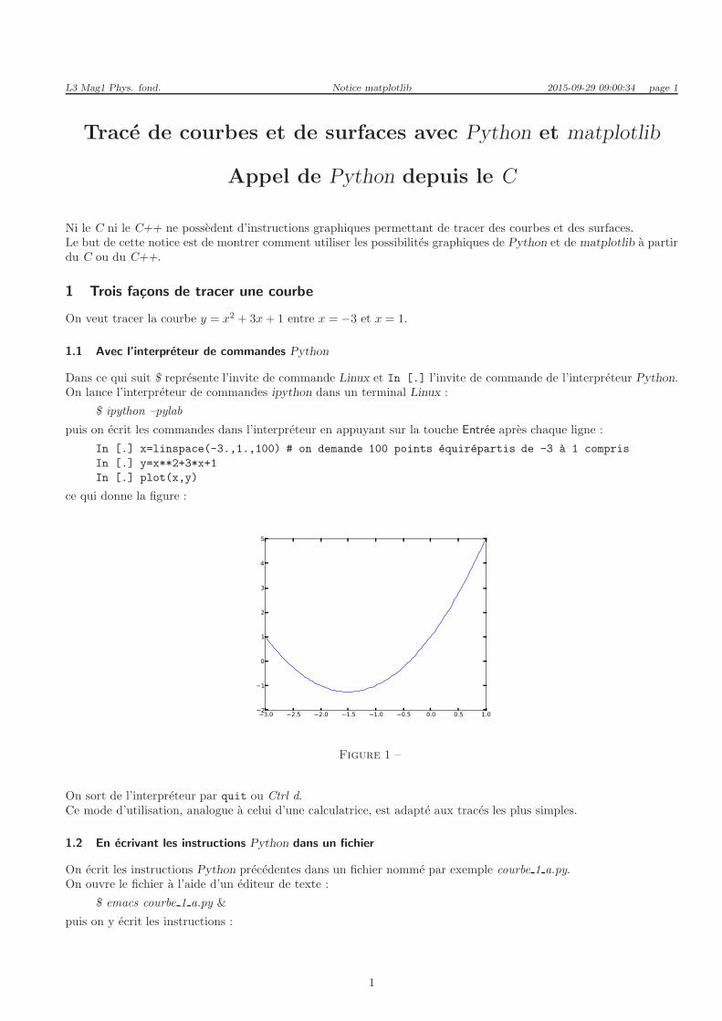
On veut tracer la courbe y = x2 + 3x+ 1 entre x = −3 et x = 1.

1.1 Avec l’interpreteur de commandes Python

Dans ce qui suit $ represente l’invite de commande Linux et In [.] l’invite de commande de l’interpreteur Python.On lance l’interpreteur de commandes ipython dans un terminal Linux :

$ ipython –pylab

puis on ecrit les commandes dans l’interpreteur en appuyant sur la touche Entree apres chaque ligne :

In [.] x=linspace(-3.,1.,100) # on demande 100 points equirepartis de -3 a 1 compris

In [.] y=x**2+3*x+1

In [.] plot(x,y)

ce qui donne la figure :

−3.0 −2.5 −2.0 −1.5 −1.0 −0.5 0.0 0.5 1.0−2

−1

0

1

2

3

4

5

Figure 1 –

On sort de l’interpreteur par quit ou Ctrl d.Ce mode d’utilisation, analogue a celui d’une calculatrice, est adapte aux traces les plus simples.

1.2 En ecrivant les instructions Python dans un fichier

On ecrit les instructions Python precedentes dans un fichier nomme par exemple courbe 1 a.py.On ouvre le fichier a l’aide d’un editeur de texte :

$ emacs courbe 1 a.py &

puis on y ecrit les instructions :

1

L3 Mag1 Phys. fond. Notice matplotlib 2015-09-29 09 :00 :34 page 2

from numpy import *

from matplotlib.pyplot import *

x=linspace(-3.,1.,100)

y=x**2+3*x+1

plot(x,y)

show()

et on fait executer le programme Python ecrit dans le fichier courbe 1 a.py par la commande :

$ ipython courbe 1 a.py

Ce mode d’utilisation est adapte des que le nombre d’instructions et superieur a deux ou trois ou quand on veutconserver ces instructions pour les reutiliser en les modifiant ou completant si necessaire.

Ici il faut appeler explicitement les modules numpy et matplotlib.pyplot et ajouter l’instruction show() alors quece n’etait pas necessaire avec l’interpreteur grace a l’option –pylab. Pour eviter d’avoir a reecrire a chaque fois leslignes :

from numpy import *

from matplotlib.pyplot import *

et :

show()

il existe une commande propre au Magistere nommee ipy qui les introduit automatiquement.Si le fichier courbe 1 b.py ne contient que les lignes :


y=x**2+3*x+1

plot(x,y)

il suffit d’ecrire la commande :

$ ipy courbe 1 b.py

au lieu de :

$ ipython courbe 1 b.py

1.3 En ecrivant les instructions Python a partir d’un programme C

1.3.1 Methode brute

On peut ecrire et executer le programme Python a partir d’un programme C comme celui-ci :

#include<Python.h>

#include<iostream>

#include<sstream>

using namespace std;

int main()

{

ostringstream ostpy;

ostpy

<< "from numpy import *\n"

<< "from matplotlib.pyplot import *\n"

<< "x=linspace(-3.,1.,100)\n"

<< "y=x**2+3*x+1\n"

<< "plot(x,y)\n"

<< "show()"

;

Py_Initialize();

PyRun_SimpleString(ostpy.str().c_str());

Py_Finalize();

return 0;

}

2

L3 Mag1 Phys. fond. Notice matplotlib 2015-09-29 09:00:34 page 3

Les instructions Python sont ecrites dans une chaıne de caracteres 1 nommee ici ostpy puis executees par l’instructionC :

PyRun_SimpleString(ostpy.str().c_str());

Ce mode d’utilisation permet de beneficier des possibilites graphiques de Python dans un programme C.

1.3.2 En utilisant une fonction

On peut transformer en une fonction (nommee ici make plot py) la partie du programme precedent qui est toujoursla meme :

#include<Python.h>

#include<iostream>

#include<sstream>

using namespace std;

void make_plot_py(ostringstream &ss)

{

ostringstream run_py;

run_py

<< "from numpy import *\n"

<< "from matplotlib.pyplot import *\n"

<< "from mpl_toolkits.mplot3d import Axes3D\n"

<< ss.str()

<< "show()"

;

// cout << run_py.str() << endl;

Py_Initialize();

PyRun_SimpleString(run_py.str().c_str());

Py_Finalize();

}

int main()

{

ostringstream pyth;

pyth

<< "x=linspace(-3.,1.,100)\n"

<< "y=x**2+3*x+1\n"

<< "plot(x,y)\n"

;

make_plot_py(pyth);

return 0;

}

1.3.3 En utilisant la fonction mise dans la bibliotheque du Magistere

La fonction make plot py etant incluse dans la bibliotheque du Magistere on aura juste a ecrire :

#include<Python.h>

#include<bibli_fonctions.h>

int main()

{

ostringstream pyth;

pyth

<< "x=linspace(-3.,1.,100)\n"

<< "y=x**2+3*x+1\n"

<< "plot(x,y)\n"

;

1. On utilise ici une chaıne de type ostringstream et non du type courant string pour des raisons qui apparaissent a la section 2.

Le couple de caracteres \n indique un passage a la ligne dans la chaıne.

3


make_plot_py(pyth);

return 0;

}

2 Passage de parametres du C a Python

Supposons qu’on veuille tracer non plus la courbe y = x2 +3x+1 mais y = x

2 + ax+1 ou a est une variable definiedans le programme C.Il suffit d’ajouter, dans le main du programme precedent, les instructions qui declarent et attribuent une valeur a lavariable a :

int main()

{

double a;

...

a=... // calcul quelconque

...

return 0;

}

et de remplacer la ligne :

<< "y=x**2+3*x+1\n"

par :

<< "y=x**2+" << a << "*x+1\n"

A partir d’ici, dans ces notes, on n’ecrit plus que les instructions Python proprement dites,

l’appel a partir du C comme a la sous-section 1.3.3 etant sous-entendu.

Par exemple dans un cas comme celui du programme de la sous-section 1.3.3, on ecrira seulement dans ces notes :


y=x**2+3*x+1

plot(x,y)

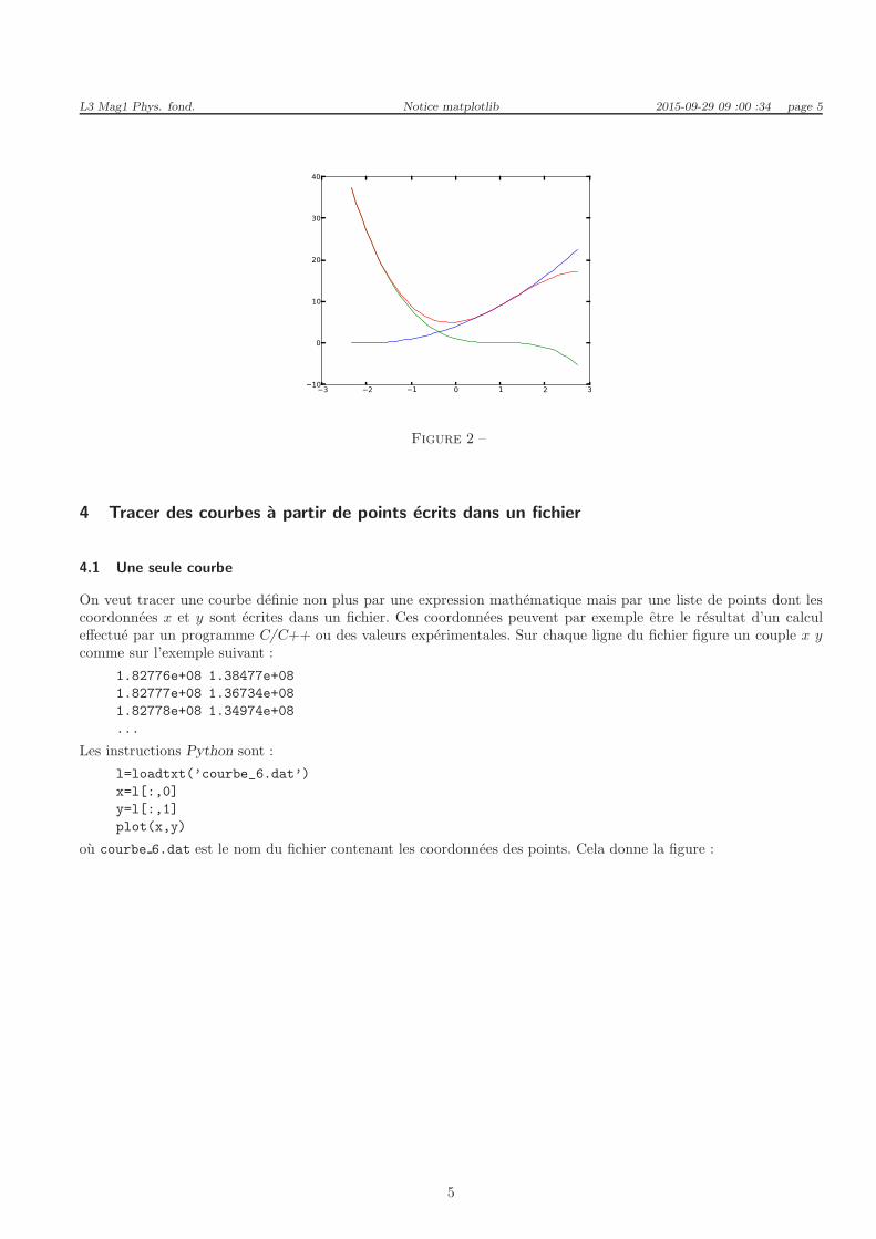
3 Tracer plusieurs courbes sur le meme graphe

x=linspace(-2.34,2.73,47)

y1=(2+x)**2

y2=(1-x)**3

y3=y1+y2

plot(x,y1)

plot(x,y2)

plot(x,y3)

ce qui donne la figure :

4


−3 −2 −1 0 1 2 3−10

0

10

20

30

40

Figure 2 –

4 Tracer des courbes a partir de points ecrits dans un fichier

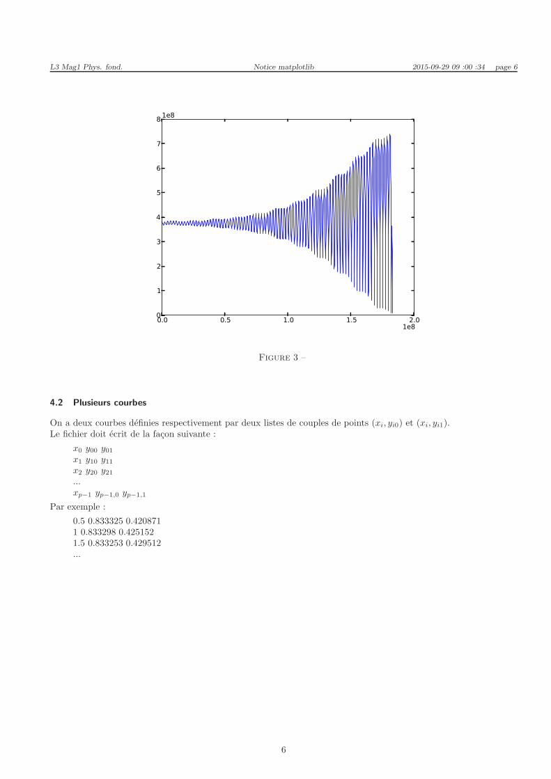
4.1 Une seule courbe

On veut tracer une courbe definie non plus par une expression mathematique mais par une liste de points dont lescoordonnees x et y sont ecrites dans un fichier. Ces coordonnees peuvent par exemple etre le resultat d’un calculeffectue par un programme C/C++ ou des valeurs experimentales. Sur chaque ligne du fichier figure un couple x y

comme sur l’exemple suivant :

1.82776e+08 1.38477e+08

1.82777e+08 1.36734e+08

1.82778e+08 1.34974e+08

...

Les instructions Python sont :

l=loadtxt(’courbe_6.dat’)

x=l[:,0]

y=l[:,1]

plot(x,y)

ou courbe 6.dat est le nom du fichier contenant les coordonnees des points. Cela donne la figure :

5


0.0 0.5 1.0 1.5 2.01e8

0

1

2

3

4

5

6

7

8 1e8

Figure 3 –

4.2 Plusieurs courbes

On a deux courbes definies respectivement par deux listes de couples de points (xi, yi0) et (xi, yi1).Le fichier doit ecrit de la facon suivante :

x0 y00 y01

x1 y10 y11

x2 y20 y21

...xp−1 yp−1,0 yp−1,1

Par exemple :

0.5 0.833325 0.4208711 0.833298 0.4251521.5 0.833253 0.429512...

6


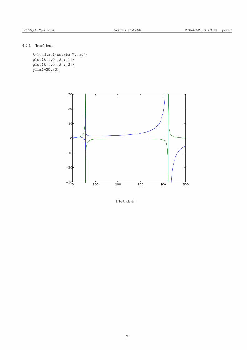
4.2.1 Trace brut

A=loadtxt(’courbe_7.dat’)

plot(A[:,0],A[:,1])

plot(A[:,0],A[:,2])

ylim(-30,30)

0 100 200 300 400 500−30

−20

−10

0

10

20

30

Figure 4 –

7


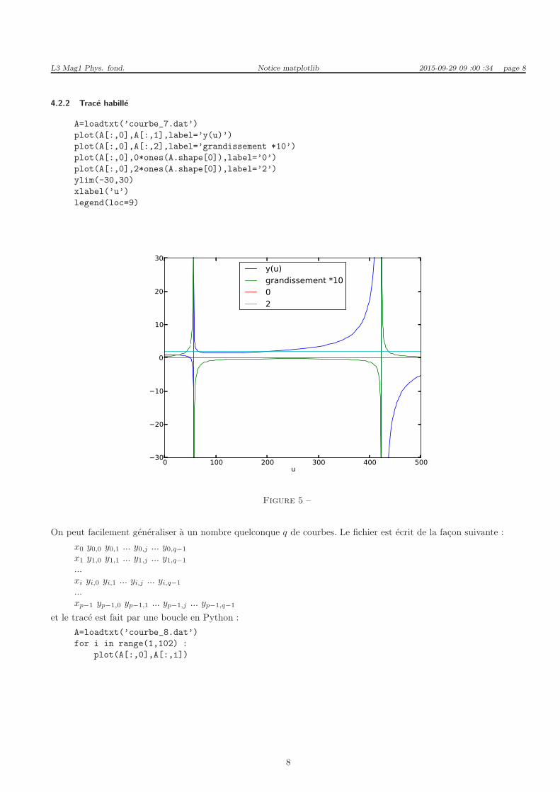
4.2.2 Trace habille


plot(A[:,0],A[:,1],label=’y(u)’)

plot(A[:,0],A[:,2],label=’grandissement *10’)

plot(A[:,0],0*ones(A.shape[0]),label=’0’)

plot(A[:,0],2*ones(A.shape[0]),label=’2’)

ylim(-30,30)

xlabel(’u’)

legend(loc=9)

0 100 200 300 400 500u

−30

−20

−10

0

10

20

30y(u)grandissement *1002

Figure 5 –

On peut facilement generaliser a un nombre quelconque q de courbes. Le fichier est ecrit de la facon suivante :

x0 y0,0 y0,1 ... y0,j ... y0,q−1

x1 y1,0 y1,1 ... y1,j ... y1,q−1

...xi yi,0 yi,1 ... yi,j ... yi,q−1

...xp−1 yp−1,0 yp−1,1 ... yp−1,j ... yp−1,q−1

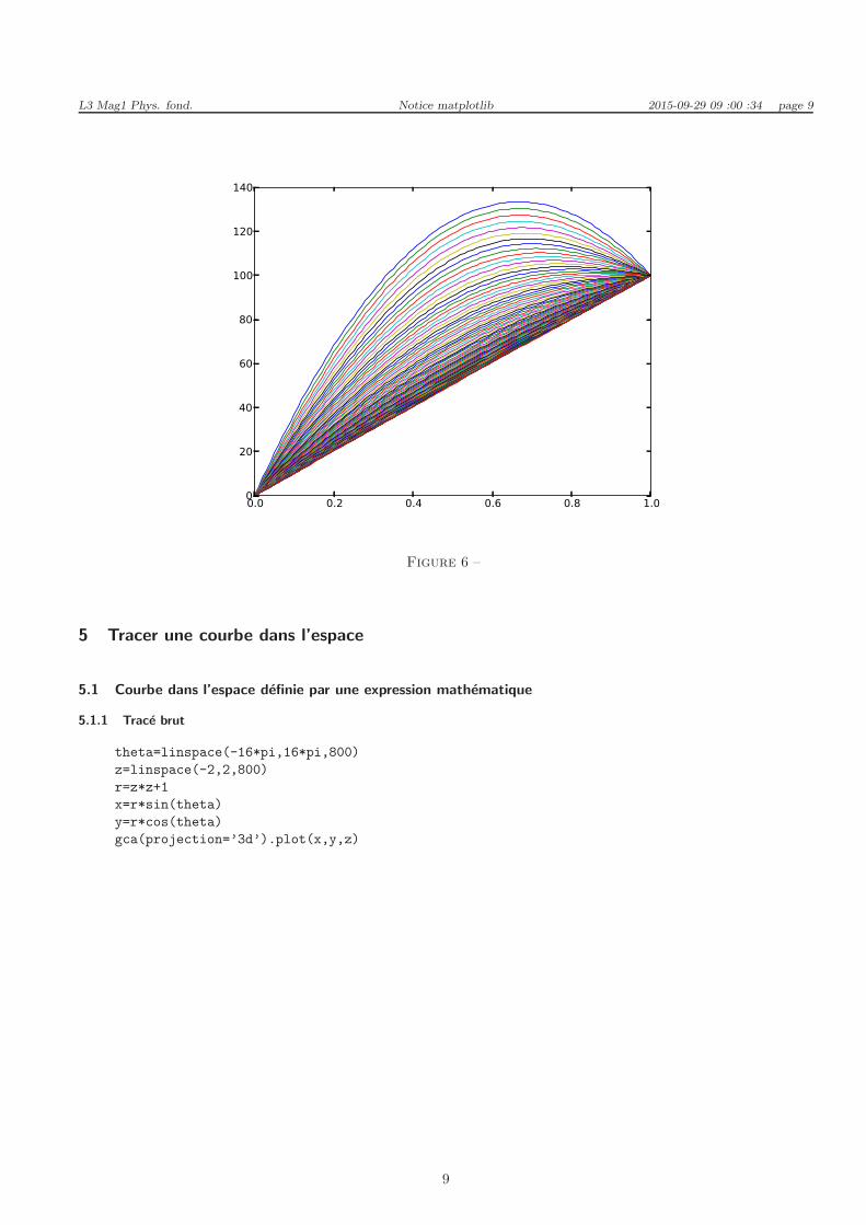
et le trace est fait par une boucle en Python :


for i in range(1,102) :

plot(A[:,0],A[:,i])

8


0.0 0.2 0.4 0.6 0.8 1.00

20

40

60

80

100

120

140

Figure 6 –

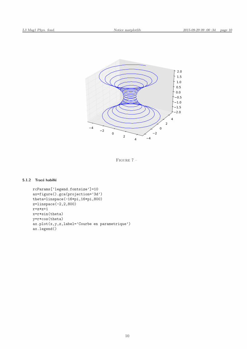
5 Tracer une courbe dans l’espace

5.1 Courbe dans l’espace definie par une expression mathematique

5.1.1 Trace brut

theta=linspace(-16*pi,16*pi,800)

z=linspace(-2,2,800)

r=z*z+1

x=r*sin(theta)

y=r*cos(theta)

gca(projection=’3d’).plot(x,y,z)

9


−4−2

02

4 −4−2

02

4

−2.0−1.5−1.0−0.50.00.51.01.52.0

Figure 7 –

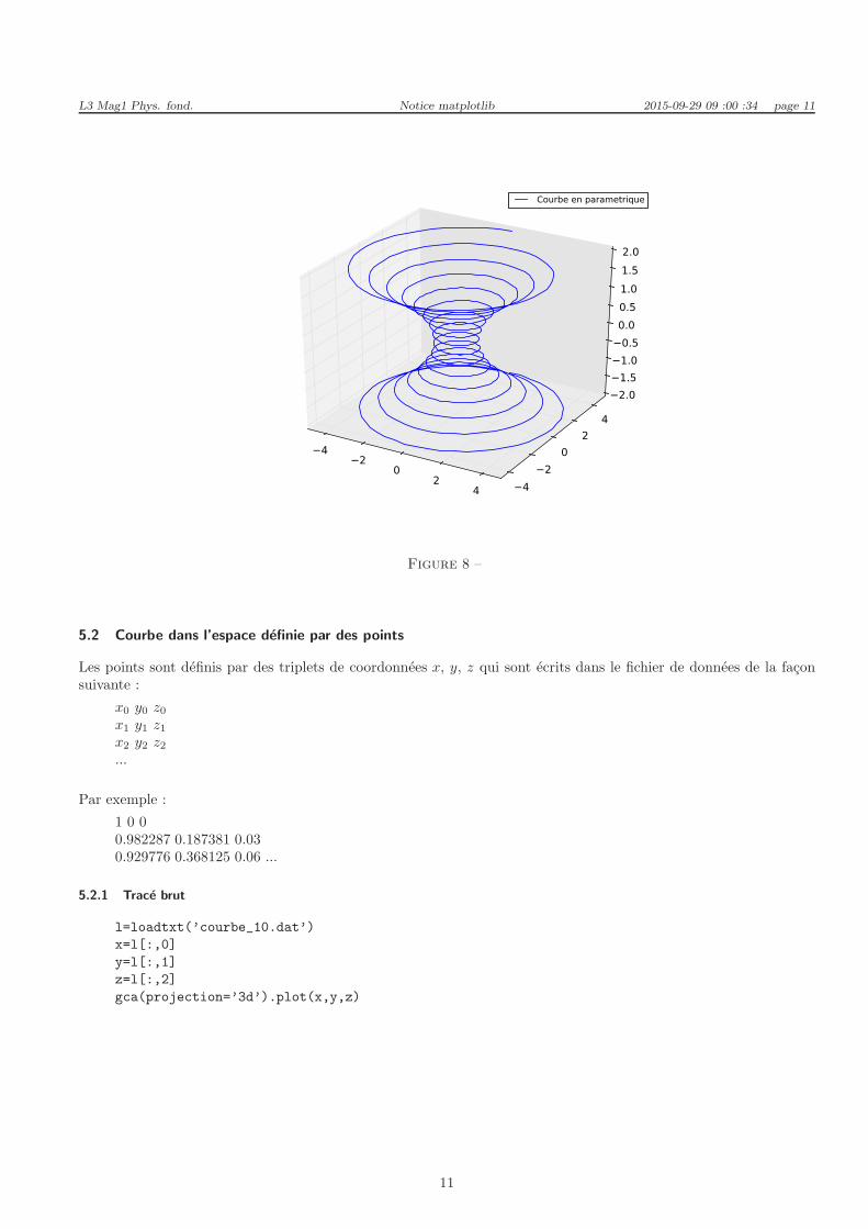
5.1.2 Trace habille

rcParams[’legend.fontsize’]=10

ax=figure().gca(projection=’3d’)

theta=linspace(-16*pi,16*pi,800)

z=linspace(-2,2,800)

r=z*z+1

x=r*sin(theta)

y=r*cos(theta)

ax.plot(x,y,z,label=’Courbe en parametrique’)

ax.legend()

10


−4−2

02

4 −4−2

02

4

−2.0−1.5−1.0−0.50.00.51.01.52.0

Courbe en parametrique

Figure 8 –

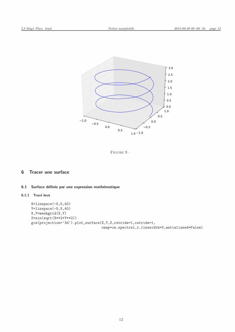
5.2 Courbe dans l’espace definie par des points

Les points sont definis par des triplets de coordonnees x, y, z qui sont ecrits dans le fichier de donnees de la faconsuivante :

x0 y0 z0

x1 y1 z1

x2 y2 z2

...

Par exemple :

1 0 00.982287 0.187381 0.030.929776 0.368125 0.06 ...

5.2.1 Trace brut

l=loadtxt(’courbe_10.dat’)

x=l[:,0]

y=l[:,1]

z=l[:,2]

gca(projection=’3d’).plot(x,y,z)

11


−1.0−0.5

0.00.5

1.0 −1.0

−0.50.0

0.51.00.0

0.5

1.0

1.5

2.0

2.5

3.0

Figure 9 –

6 Tracer une surface

6.1 Surface definie par une expression mathematique

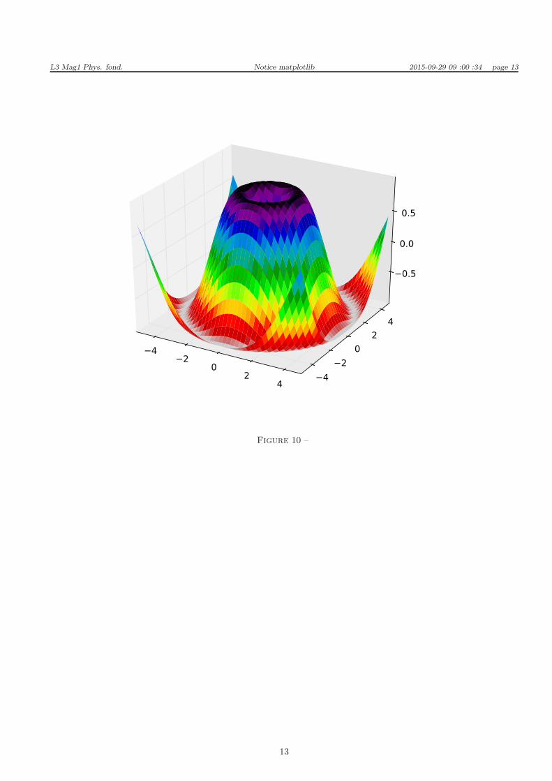
6.1.1 Trace brut

X=linspace(-5,5,40)

Y=linspace(-5,5,40)

X,Y=meshgrid(X,Y)

Z=sin(sqrt(X**2+Y**2))

gca(projection=’3d’).plot_surface(X,Y,Z,rstride=1,cstride=1,

cmap=cm.spectral_r,linewidth=0,antialiased=False)

12


−4−2

02

4 −4−2

02

4

−0.5

0.0

0.5

Figure 10 –

13


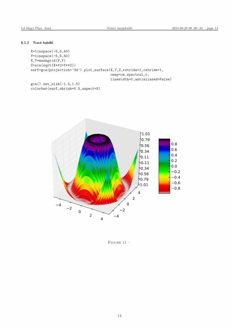
6.1.2 Trace habille

X=linspace(-5,5,40)

Y=linspace(-5,5,40)

X,Y=meshgrid(X,Y)

Z=sin(sqrt(X**2+Y**2))

surf=gca(projection=’3d’).plot_surface(X,Y,Z,rstride=1,cstride=1,

cmap=cm.spectral_r,

linewidth=0,antialiased=False)

gca().set_zlim(-1.5,1.5)

colorbar(surf,shrink=0.5,aspect=5)

−4−2

02

4 −4−2

02

4

-1.01-0.79-0.56-0.34-0.110.110.340.560.791.01

−0.8−0.6−0.4−0.20.00.20.40.60.8

Figure 11 –

14


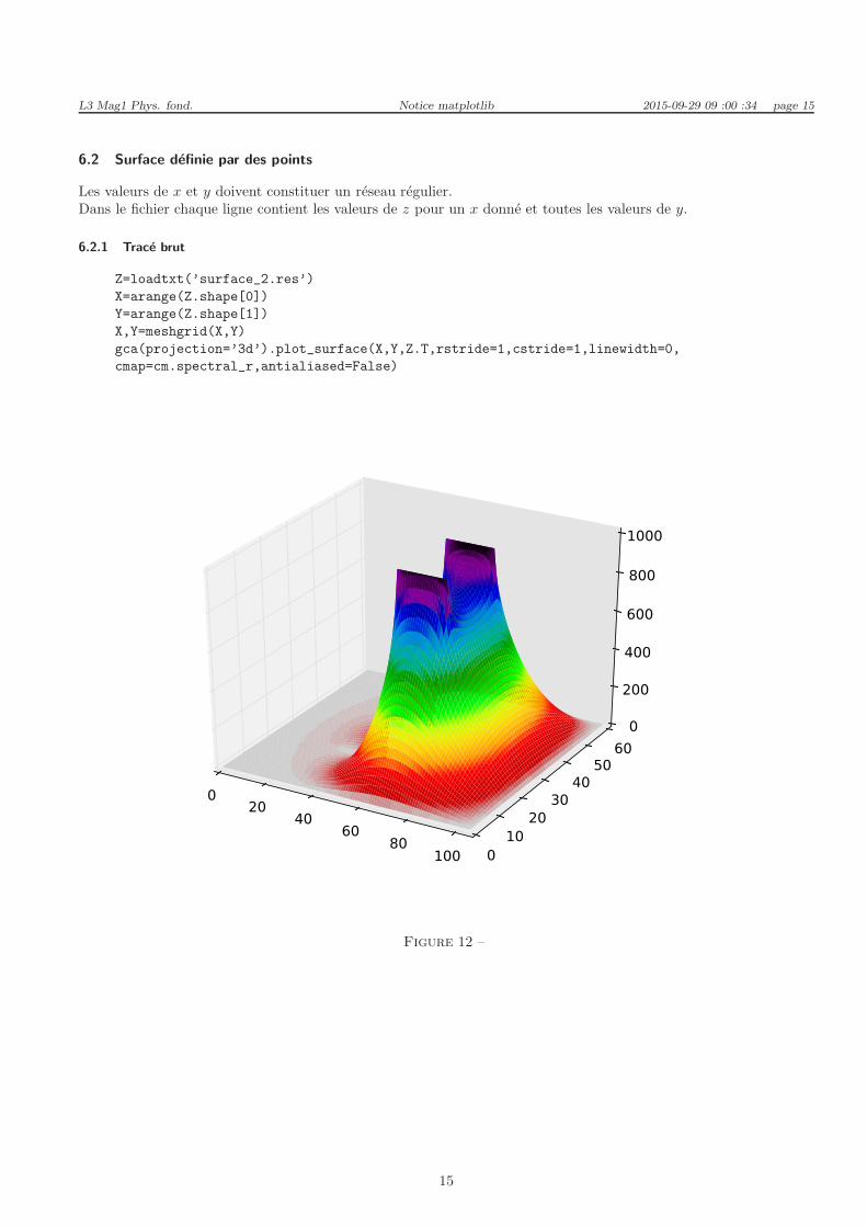
6.2 Surface definie par des points

Les valeurs de x et y doivent constituer un reseau regulier.Dans le fichier chaque ligne contient les valeurs de z pour un x donne et toutes les valeurs de y.

6.2.1 Trace brut

Z=loadtxt(’surface_2.res’)

X=arange(Z.shape[0])

Y=arange(Z.shape[1])

X,Y=meshgrid(X,Y)

gca(projection=’3d’).plot_surface(X,Y,Z.T,rstride=1,cstride=1,linewidth=0,

cmap=cm.spectral_r,antialiased=False)

020

4060

80100 0

1020

3040

50600

200

400

600

800

1000

Figure 12 –

15


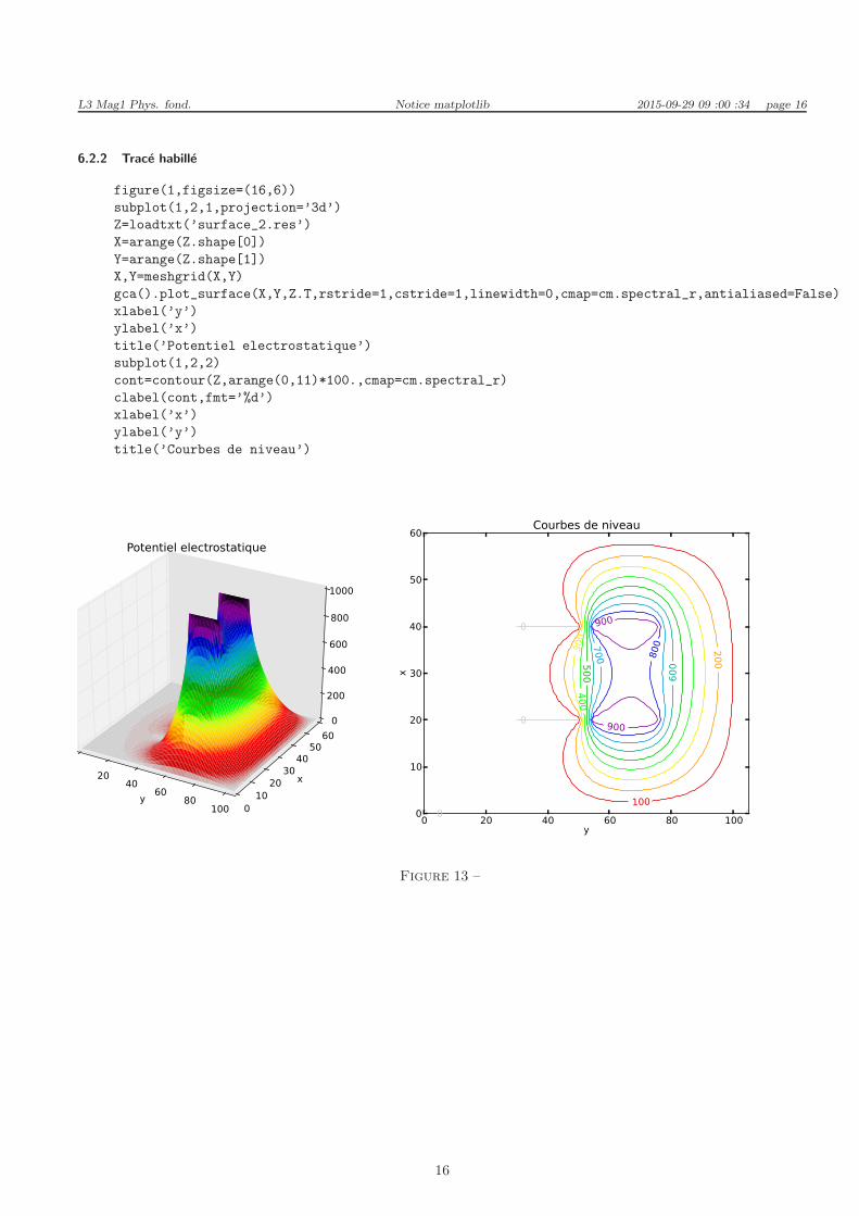
6.2.2 Trace habille

figure(1,figsize=(16,6))

subplot(1,2,1,projection=’3d’)

Z=loadtxt(’surface_2.res’)

X=arange(Z.shape[0])

Y=arange(Z.shape[1])

X,Y=meshgrid(X,Y)

gca().plot_surface(X,Y,Z.T,rstride=1,cstride=1,linewidth=0,cmap=cm.spectral_r,antialiased=False)

xlabel(’y’)

ylabel(’x’)

title(’Potentiel electrostatique’)

subplot(1,2,2)

cont=contour(Z,arange(0,11)*100.,cmap=cm.spectral_r)

clabel(cont,fmt=’%d’)

xlabel(’x’)

ylabel(’y’)

title(’Courbes de niveau’)

y

020

4060

80100

x

010

2030

4050

600

200

400

600

800

1000

Potentiel electrostatique

0 20 40 60 80 100y

0

10

20

30

40

50

60

x

0

0

0

100

200

300

400500 60

0

700 800

900

900

Courbes de niveau

Figure 13 –

16

Documents

trac´e De Courbes Et De Surfaces Avec Matplotlibhebergement.u-psud.fr/naulin/matplotlib_notice_magistere.pdf · L3Mag1Phys. fond. Noticematplotlib 2015-09-2909:00:34 page1 Trac´e