Embed Size (px)
Citation preview
UNIVERSITÉ DU QUÉBEC
MÉMOIRE PRÉSENTÉ À L'UNIVERSITÉ DU QUÉBEC À
TROIS-RIVIÈRES
COMME EXIGENCE PARTIELLE
DE LA MAÎTRISE EN MATHÉMATIQUES ET INFORMATIQUE
APPLIQUÉES
PAR
TARIK BAHRAOUI
FON CTIONS DE C-PUISSANCE ET APPLICATION À
L'INFÉRENCE DE COPULES
NOVEMBRE 2012
Université du Québec à Trois-Rivières
Service de la bibliothèque
Avertissement
L’auteur de ce mémoire ou de cette thèse a autorisé l’Université du Québec à Trois-Rivières à diffuser, à des fins non lucratives, une copie de son mémoire ou de sa thèse.
Cette diffusion n’entraîne pas une renonciation de la part de l’auteur à ses droits de propriété intellectuelle, incluant le droit d’auteur, sur ce mémoire ou cette thèse. Notamment, la reproduction ou la publication de la totalité ou d’une partie importante de ce mémoire ou de cette thèse requiert son autorisation.
REMERCIEMENTS
Au terme de ce t ravail de maîtrise, je t iens à exprimer ma profonde gra
t itude et mes remerciements sincères à M. Jean-François Quessy, qui est
mon directeur de recherche et professeur de statistique au département de
Mathématiques et d 'information de l'Université du Québec à Trois-Rivières
(UQTR). Je lui suis reconnaissant du temps qu'il m'a consacré, de ses direc
t ives précieuses et de la qualité de son encadrement durant ces deux années.
J 'adresse également des remerciements aux professeurs Mhamed Mesfioui et
Fathallah Nouboud, du département de Mathématiques et d 'information de
l'UQTR. Leur appui moral et leurs encouragements durant ces deux années
d 'étude à l'UQTR ont été t rès appréciés. Je veux aussi remercier les membres
du jury, MM. Taoufik Bouezmarni et Mhamed Mesfioui , pour avoir accepté
de lire et évaluer mon mémoire. Leurs judicieux commentaires m'ont permis
d 'améliorer la version finale de ce t ravail.
Mes études de maîtrise ont été financées par des subventions de recherche
octroyées à M. Jean-François Quessy par le Fonds Québécois de Recherche
Nature et Technologies et par le Conseil National de Recherche en Sciences
Naturelles et en Génie du Canada. Je remercie aussi l'Institut des Sciences
Mathématiques du Québec pour les bourses d 'étude qu 'ils m'ont accordées.
Enfin , la vie continue.
A la memoria de mi padre
Table des matières
Remerciements
Liste des tableaux
Liste des figures
Chapitre 1. Introduction
Chapitre 2. Généralités sur les copules
2. 1 Préliminaires ........ .
2.2 Copules & Théorème de Sklar
2.3 Quelques modèles . . . . . .
2.4 Copules à valeurs extrêmes.
2.5 Copules Archimédiennes ..
2.6 Transformation intégrale de probabilité
Chapitre 3. Les fonctions de C-puissance théoriques
3 .1 Définition . . . . . . . . . . . . . .
3.2 Quelques propriétés fondamentales
3.3 Lipschitz ..... . . . .
3.4 Dominance stochastique
3.5 Calculs pour quelques modèles.
11
v
VI
1
6
6
8
II
13
15
18
22
22
23
23
24
25
TABLE DES MATIÈRES
3.5.1 Copule d'indépendance .
3.5.2 Copules Archimédiennes
3.5.3 Transformation d 'un générateur Archimédien .
3.5.4 Copules à valeurs extrêmes.
3.5.5 Copules Archimax ..
3.5.6 Copules de Durante .
3.5.7 Transformation de copules
Chapitre 4. Méthode Delta fonctionnelle
4.1 Version classique .. .... .... .
4.2 Généralisation aux espaces vectoriels
4.3 Fonction de répartition empirique
4.4 Autres applications . . . . . . . .
4.4.1 Fonction de répartition empirique bivariée
4.4.2 Copule empirique . .
4.4 .3 Processus de Kendall
Chapitre 5. Empirical C-power pro cesses and their use for pa-
III
25
26
27
28
31
32
32
33
33
34
37
40
40
42
44
rameter estimation and goodness-of-fit in copula models 46
5.1 Estimation of the C-power functions 46
5.2 A multiplier centrallimit Theorem . 56
5.3 A generalized method-of-moment for the copula parameters . 63
5.4 Goodness-of-fit tests for copulas
5.4.1 Test statistics ..... .
5.4.2 Computation of p-values
5.4.3 Verification of Assumption (3) for some models
5.5 Simulation studies
65
66
69
71
73
TABLE DES MATIÈRES
5.5.1 Efficiency of the parameter estimation ..
5.5.2 Efficiency of the goodness-of-fit procedures
5.6 Illustration on the Uranium exploration data set
Chapitre 6. Conclusion
Références
Annexe A. Estimation du générateur Archimédien
A.1 Un estimateur plug-in ...
A.2 Interpolation linéaire de Kn
IV
73
75
78
88
90
95
95
98
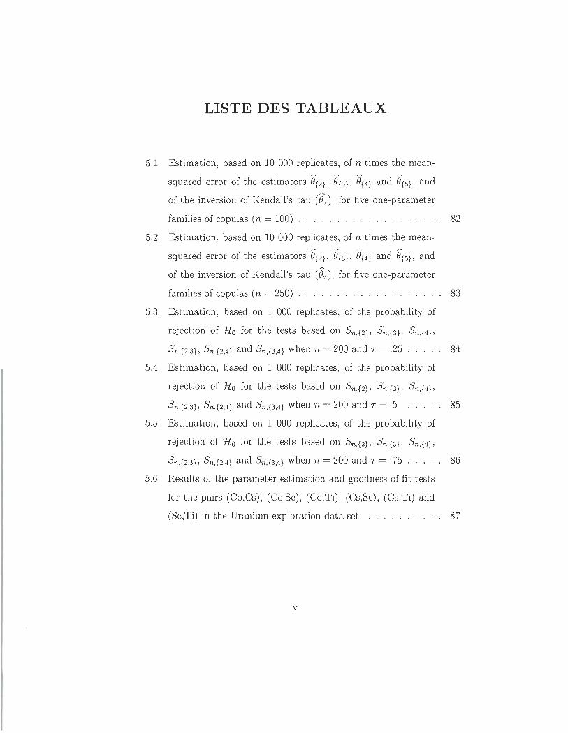
LISTE DES TABLEAUX
5.1 Estimation, based on 10 000 replicates, of n t imes the mean-..-.. --.. .......... ..........
squared error of the estimators 0{2}, 0{3}, O{4} and f.}{5} , and
of the inversion of Kendall 's tau (ilT ) , for five one-parameter
families of copulas (n = 100) . . . . . . . . . . . . . . . . . .. 82
5.2 Estimation, based on 10 000 replicates, of n times the mean-......... ......... -- --
squared error of the estimators 0{2}, 0{3}, O{4} and O{5} , and
of the inversion of Kendall's tau (ilT ) , for five one-parameter
families of copulas (n = 250) . . . . . . . . . . . . . . . . . .. 83
5.3 Estimation, based on 1 000 replicates, of the probability of
rejection of No for the tests based on Sn,{2} ' Sn,{3} , Sn,{4} ,
Sn,{2,3} , Sn,{2,4} and Sn,{3 ,4} when n = 200 and T = .25 . . . .. 84
5.4 Estimation, based on 1 000 replicates, of the probability of
rejection of No for the tests based on Sn,{2} , Sn,{3} , Sn,{4} ,
Sn,{2 ,3} , Sn,{2,4} and Sn,{3 ,4} wh en n = 200 and T =.5 ..... 85
5.5 Estimation, based on 1 000 replicates, of the probability of
rejection of N o for the tests based on Sn,{2} ' Sn,{3} , Sn,{4} ,
Sn,{2,3}, Sn,{2,4} and Sn,{3,4} when n = 200 and T = .75 . . . . . 86
5.6 Results of the parameter estimation and goodness-of-fit tests
for the pairs (Co,Cs) , (Co,Sc), (Co,Ti), (Cs,Sc), (Cs,Ti) and
(Sc,Ti) in the Uranium exploration data set .... . . . . . . 87
v
LISTE DES FIGURES
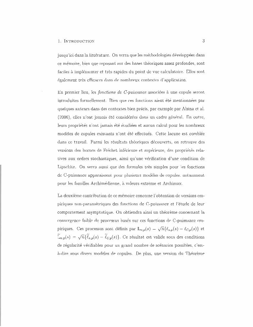
3. 1 Fonctions de C-puissance de la borne de Fréchet supérieure
(-), de la copule d'indépendance (- - -) et de la borne de
Fréchet inférieure (- . -) quand p = 2. . . . . . . . . . . . . .. 26
3.2 Fonctions de C-puissance de la borne de Fréchet supérieure
(-), de la copule d'indépendance (- - -) et de la borne de
Fréchet inférieure (- . - ) quand p = 5. . . . . . . . . . . . . .. 27
5. 1 Empirical C-power function (black) , 95% confidence bands
(red) , and C-power function of the Gumbel- Hougaard copula
when p = 2 (upper panel) and p = 3 (lower panel) . . . . . .. 80
5.2 Empirical C-power function (black), 95% confidence bands
(red), and C-power function of the Clay ton copula wh en p = 2
(upper panel) and p = 3 (lower panel) . . . . . . . . . . . . . . 81
VI
CHAPITRE 1
INTRODUCTION
Soit un couple de variables aléatoires (X, Y) dont la fonction de répartition
conjointe est , pour (x,y) E JR2,
H(x, y) = P (X ~ x, Y ~ y) ,
et les lois marginales sont
F(x) = P (X ~ .1:) et C(y) = P (Y ~ y).
Afin de modéliser le comportement de (X , Y), une approche très populaire ces
dernières années consiste à ajuster des modèles statistiques pour les marges
et la structure de dépendance dans des étapes séparées. Cette approche est
rendue possible grâce à un célèbre théorème dû à Sklar (1959) . Ce résultat ,
qui sera détaillé plus loin dans ce mémoire, stipule que si les lois F et C
sont continues, alors il existe une unique copule C : [0, IF -t [0,1] telle que
pour tout (x,y) E JR2, on a la représentation H(x,y) = C{F(x),C(y)}.
Autrement dit, la loi de (X, Y) peut se décomposer d 'une part , selon les
comportements marginaux représentés par F et C, et d'autre part selon la
structure de dépendance dont l'information est contenue dans la fonction C .
1. INT ROD UCTION 2
À part ir d 'un échant illon (Xl , YI) , ' . . , (Xn , Yn ) de copies aléatoires de (X, Y ),
un problème d 'un grand intérêt est d 'inférer sur la forme inconnue de la co
pule C. Une approche populaire consiste à supposer que C appart ient à une
certaine famille paramétrique F = {Ce; e E 8 } et à estimer le paramètre in
connu e. Cette ét ape d 'estimation peut se faire, par exemple, via le maximum
de la pseudo fonction de vraisemblance proposée par Shih & Louis (1995) et
Genest et al. (1995) ou encore via une approche à distance minimale tel que
proposée par Tsukahara (2005). Parmi les autres possibilités populaires, on
retrouve l'inversion d 'une mesure d 'association, tel que suggéré par Genest
et al. (2006) et Mesfioui et al. (2009).
Une autre étape cruciale dans la modélisation de la dépendance est d 'attester
que la famille de modèles choisie, à savoir F = {Ce; e E 8 }, est adéquate.
Pour s'assurer que F modélise correctement la dépendance d 'un phénomène,
on ut ilise généralement un t est d 'adéquation. Le développement de tels tests
est relativement récent . Parmi les premières cont ribut ions dans ce domaine,
on retrouve les t ravaux de Fermanian (2005), Dobrié & Schmid (2005) et
Genest et al. (2006). Quelques variantes et extensions de ces méthodes ont été
proposées par Genest et al. (2009) et Mesfioui et al. (2009) , entre autres. Plus
récemment, Quessy & Bellerive (2012) ont étudié des méthodes d 'adéquation
pour la famille particulière des copules ellipt iques.
L'objectif principal de ce mémoire est de développer de nouvelles méthodes
d 'estimation de paramètres et d 'adéquation pour les modèles de copules à
deux variables. L'idée maîtresse repose sur la notion de fonctions de C
puissance associées à une copule. Cette approche n 'a jamais été considérée
1. INTRODUCTION 3
jusqu'ici dans la littérature. On verra que les méthodologies développées dans
ce mémoire, bien que reposant sur des bases théoriques assez profondes, sont
faciles à implémenter et t rès rapides du point de vue calculatoire. Elles sont
également très efficaces dans de nombreux contextes d 'application.
En premier lieu, les fon ctions de C-puissance associées à une copule seront
introduites formellement . Bien que ces fonctions aient été mentionnées par
quelques auteurs dans des contextes bien précis, par exemple par Alsina et al.
(2006), elles n 'ont jamais été considérées dans un cadre général. En out re,
leurs propriétés n 'ont jamais été étudiées et aucun calcul pour les nombreux
modèles de copules existants n 'ont été effectués. Cette lacune est comblée
dans ce t ravail. Parmi les résultats théoriques découverts, on retrouve des
versions des bornes de Fréchet inférieure et supérieure, des propriétés rela
tives aux ordres stochastiques , ainsi qu 'une vérification d 'une condition de
Lipschitz. On verra aussi que des formules très simples pour les fonctions
de C-puissance apparaissent pour plusieurs modèles de copules, notamment
pour les familles Archimédienne, à valeurs extrême et Archimax.
La deuxième contribut ion de ce mémoire concerne l'obtent ion de versions em-
piriques non-paramétriques des fonctions de C-puissance et l'étude de leur
comportement asymptotique. On obtiendra ainsi un théorème concernant la
convergence faible de processus basés sur ces fonctions de C-puissance em
piriques. Ces processus sont définis par lLn,p(s) = Vn{€n,p( s) - t'c,p(s )} et
in,p(s) = Vn{ln,p(s) - lc,p(s )} . Ce résultat est valide sous des conditions
de régularité vérifiables pour un grand nombre de scénarios possibles, c'est
à-dire sous divers modèles de copules. De plus, une version du Théorème
1. INTRODUCTION 4
de la limite centrale du multiplicateur est décrite et validée rigoureusement.
Ce résultat est extrêmement important puisqu'il permet d'imiter le com
portement asymptotique des processus de C-puissance, et ainsi de calculer
la p-valeur de tests d 'adéquation. Il s'agit d'une variante de la méthode du
bootstrap classique.
Le troisième et dernier objectif de ce travail consiste à exploiter les pro
priétés théoriques et échantillonnales des fonctions de C-puissance afin de
développer de nouveaux outils d'inférence pour les modèles de copules. Ceci
inclue l'estimation de paramètres pour des familles multi-paramétriques , de
même qu 'une méthodologie formelle et graphique pour l'adéquation à une
famille. Dans de nombreux cas, les formules nécessaires pour estimer le
paramètre d'une famille donnée sont faciles à manipuler, ce qui mène à des
procédures faciles à mettre en œuvre. Ceci est particulièrement attirant
dans des situations où la méthode d 'inversion du tau de Kendall est diffi
cile à appliquer, notamment pour plusieurs modèles à valeurs extrêmes. Une
utilité notable concerne la relative facilité à traiter les modèles à plusieurs
paramètres, ce qui n'est pas possible avec les méthodes d 'inversion. Aussi , en
exploitant la nature récursive des fonctions de C-puissance, les statistiques
d 'adéquation qui sont proposées sont très faciles à implémenter et rapide
à calculer. En outre, leurs versions multiplicateurs s'obtiennent aisément.
Enfin, on verra à l'aide de simulations Monte-Carlo que ces méthodes sont
efficaces dans de nombreuses situations.
Le mémoire est organisé comme suit. Au Chapitre 2, on fait une revue des
principaux résultats théoriques concernant les copules; quelques familles im-
1. INTRODUCTION 5
portantes sont également décrites. Au Chapitre 3, on introduit formellement
la notion de fonctions de C-puissance, on étudie quelques-unes de leurs pro
priétés fondamentales , et on présente des calculs pour un grand nombre de
familles. Le Chapitre 4 est un prélude à la compréhension du Chapitre 5.
Il concerne la méthode Delta fonctionnelle, qui est un outil fondamental en
statistique asymptotique; plusieurs exemples d 'application sont présentés.
Le Chapitre 5 offre, en anglais, les Sections 3-8 d 'un article qui a été soumis
à la revue B ernoulli. L'information des sections amp'utées 1 et 2 se retrou
vent néanmoins dans ce mémoire. En effet, la Section 1 est une introduction
dont l'essentiel se retrouve dans le présent Chapitre 1. Pour ce qui est de
la Section 2, il s'agit principalement du Chapitre 3 du mémoire. Ainsi, la
Section 5.1 définie les fonctions de C-puissance empiriques et un algorithme
simple et rapide pour leur calcul est détaillé; aussi, on énonce un résultat sur
leur convergence faible et on le démontre rigoureusement. À la Section 5.2 ,
on définit des versions multiplicateurs de des processus de C-puissance et
on démontre qu 'elles sont valides asymptotiquement. Les sections 5.3-5.4
concernent le développement de méthodes d'inférence pour les modèles de
copules bivariées, à savoir l'estimation de paramètres et l'adéquation. La Sec
tion 5.5 présente et commente des résultats de simulations Monte-Carlo pour
étudier les propriétés à tailles finies des procédures nouvellement dévelloppées.
Enfin, notre méthodologie est illustrée sur un jeu de données multivariées
classique de Cook & Johnson (1981) concernant des mesures de concentra
tion d'éléments chimiques dans des échantillons d 'eau .
CHAPITRE 2
GÉNÉRALITÉS SUR LES COPULES
2.1 Préliminaires
Avant de commencer , quelques notations seront int roduites. D'abord, soit
lR, la droite réelle ordinaire, c'est-à-dire (- 00, +00), et JR, la droite réelle
achevée, c'est-à-dire lR U {-oo, +oo}. De plus, JR2 représentera le plan eucli
dien JR x JR. Un rectangle B dans JR2 est donc le produit cartésien de deux
intervalles fermés, à savoir B = [X l , X2] X [YI , Y2]. Les sommets des rectangle
B sont les points (Xl, YI), (X1,Y2), (x2,Yd et (X2,Y2). Le carré unité, noté 12 ,
est le produit l x 1, où l = [0, 1].
Soient 51 et 52, deux sous-ensembles non vides de JR2 . Soit aussi H , une
fonction réelle bivariée dont le domaine de définit ion est Dom( H) = 51 X 52
et dont l'image est Im( H) ç R Pour un rectangle B = [X l , X2] X [YI , Y2] dont
les sommets sont dans Dom(H) , le H-volume de B est défini par
2. GÉNÉRALITÉS SUR LES COPULES 7
En définissant les différences d 'ordre un de H sur le rectangle B par
et
L1t~ H(x, y) = H(x, Y2) - H(x, yd,
on peut écrire, de façon équivalente,
D éfinition 2.1. Une fonction H est dite 2-croissante si et seulement si
VH(B) 2': 0 pour tout rectangle B dont les sommets sont dans Dom(H) .
Soit la fonction J-/(x, y) = max(x, y) définie sur I 2 = [0,1]2. Celle-ci n 'est
pas 2-croissante car selon la Définition de H-volume, on a
H(l, 1) - H(l , 0) - H(O , 1) + H(O , 0)
1 - 1 - 1 + 0 = -1 < 0,
ce qui contredit la Définition 2.1.
Proposition 2.1. On dit que la fon ction H de domaine Dom(H) = 51 x 52
sur lR est attachée si est seulement si pour tout (x, y) E Dom( H) , on a
où al et a2 sont les plus petits éléments de 51 et 52, respectivement.
Exemple 2.1. 50it une fonction croissante J : / 2 -+ / telle que f(t , 1) =
f(l , t) = t pour tout t dans J . La fonction f est attachée car f(O , 1) =
f(l , O) = O. Par exemple, la fon ction f( x, y) = x x y est attachée car
f(l , t) = 1 x t = t et f(t , 1) = t x 1 = t.
2. GÉNÉRALITÉS SUR LES COPULES 8
2.2 Copules & Théorème de Sklar
Les copules sont des cas particuliers de fonctions attachées définies sur [2 .
On verra qu 'elles ont une grande importance dans l'analyse de la dépendance
de vecteurs aléatoires. On en donne d 'abord la définition.
D éfinition 2.2. Une copule bivariée est une fonction C : 12 -+ [ telle que
(i) pour tout u E J, C(u,O) = C(O, u) = 0;
(ii) pour tout u E l, C(u , 1) = C(1, u) = u;
Le Théorème suivant, dÎt à Sklar (1959), permet de relier la notion de copule
à celle de fonction de répartition multivariée.
Théorèm e 2.1. Soit H : ]R2 -+ ]R, une fonction de répartition bidimension
nelle dont les fonctions de répartition marginales sont
F(x) = lim H(x , y) et C(y) = lim H(x , y). y-too x-too
Si F et C sont continues, alors il existe une unique copule C : [2 -+ [ telle
que pour tout (x, y) E JR.2, on a la représentation
H(x , y) = C {F(x) , C(y)}. (2.1)
Le Théorème de Sklar (1959) permet de voir que la loi H d'un couple (X, Y)
est composée des comportements marginaux de X et de Y, représentés res
pectivement par F et C, ainsi que de la dépendance entre X et Y , représentée
2. GÉNÉRALITÉS SUR LES COPULES 9
par la copule C. En effectuant le changement de variables u = F(x) et
v = G(y) , on extrait la copule C de H via l'équation (2.1), ce qui donne
(2.2)
Proposition 2.2 . Toute copule C satisfait la condition de Lipschitz, c'est
à-dire que pour tout UI, U2, VI, V2 E 12, on a
Par conséquent, toute copule C est uniformément continue sur son domaine.
On définit les dérivées partielles d 'une copule C par
a a CIO(u,v) = au C(u ,v) et COI(u,v) = av C(u,v). (2.3)
À noter que les fonctions u ri COl(u, v) et v ri CIO(u, v) sont non décrois
santes presque partout .
Théorèm e 2.2. Pour tout v E l , la dérivée partielle CIO existe presque
sûrement pour tout u E 1 et 0 ~ CIO ( u , v) ~ 1. De m ême, pour tout u E
l , la dérivée partielle COI existe presque sûrem ent pour tout v E 1 et 0 ~
COl(u,v) ~ 1.
Il est possible d 'obtenir des bornes valides pour toute copule C. D'abord,
pour toute fonction de répartition H , les bornes de Fréchet-Hoeffding, d 'abord
découvertes par Fréchet (1957) , sont telles que pour tout (.'C, y) E JR2,
max {F(x) + G(y) - 1, O} ~ H( x, y) ~ min {F(x), G(y)}.
2. GÉNÉRALITÉS SUR LES COPULES 10
Par l'équation (2 .2) , on déduit que les copules associées à ces bornes sont
respectivement W(u , v) = max (u + v-l , 0) et M(u, v) = min(u, v). Ainsi,
toute copule C est telle que pour tout u , v E [0 , 1 F, on a
W(u, v) ~ C(u, v) ~ M(u, v).
La copule West la structure de dépendance qui correspond à la dépendance
négative parfaite, alors que M correspond à la dépendance positive parfaite.
Proposition 2.3. Soit une copule C et sa section diagonale définie par
8c(t) = C(t , t) . Alors 8w (t) ~ 8c(t) ~ 8M (t), où 8w (t) = max (2t - 1,0) et
8M (t) = t.
D émonstration. On sait que pour toute copule C et pour tout (u, v) E
(0,1)2 , on a W(u,v) ~ C(u ,v) ~ M(u ,v). Donc, en particulier pour u =
v = t, on a 8w (t) ~ 8c (t) ~ 8M (t), où 8w (t) = W(t, t) = max(2t - 1,0) et
8M (t) = M(t, t) = min(t , t) = t , ce qui complète la preuve. <>
On peut montrer que si 8c( t) = 8 M (t) pour tout tEl, alors C est la copule
de Fréchet- Hoeffding M. Par contre, si 8c(t) = 8w (t) pour tout tEl, cela
n 'implique pas nécessairement que C = W. On peut se référer à Nelsen
(2006) pour la preuve de ces résultats.
2. GÉNÉRALITÉS SUR LES COPULES 11
2.3 Quelques modèles
Exemple 2.2. La distribution de Gumbel (1960) bivariée est de la forme
{
1 - e-x - e-Y + e-(x+y+8xy) si x > O. y > O' Ho(x, y) = ' - , - ,
0, sinon,
où (x , y) E JR2 et e E [0,1]. Les fonctions de répartition marginales sont
F(x) = 1im H( x, y) = 1 - e-x et C(y) = 1im H(x, y) = 1 - e-Y . y-too x-too
Ces fonctions de répartition correspondent à la loi exponentielle d 'espémnce
un. En posant u = F(x) et v = C(y), on retrouve les fonctions inverses
F-1(u) = -1n(1 - u) et C- 1(v) = -1n(1 - v).
Donc, d 'après l'équation (2.2), on obtient après quelques calculs que l 'unique
copule de Ho est
Co(u, v) = u + v - 1 + (1 - u)(1 - v)e-0 1n(1-U)X ln(1-v).
Exemple 2.3. Soit un couple de variables aléatoires (X , Y) dont la fonction
de répartition conjointe est
Cette loi s'appelle la distribution logistique bivariée de Gumbel (1961). Les
fonctions de répartition marginales sont données par
F(x) = 1im H(x, y) = (1 + e-X) -1 et C(y) = 1im H(x, y) = (1 + e-y) -1 .
y-too x-too
2. GÉNÉRALITÉS SUR LES COPULES 12
Comme les fonctions inverses sont
-1 (1) F (u) = - ln ~ - 1
on obtient, de l 'équation (2.2), que la copule associée à H est
uv C(u, v) = .
u + v - uv
Exemple 2.4. Pour al, a2 E [0, 1] tels que al + a2 < 1, les copules de
Fréchet- Mardia sont de la form e
où W et M sont respectivement les bornes inf érieure et supérieure de Fréchet,
et II est la copule d'indépendance.
Exemple 2.5. On dit qu'un vecteur aléatoire X = (Xl, . . . , X d ) suit une loi
elliptique si et seulement si il admet une représentation stochastique de la
form e X = J.L + RAU, où J.L E IRd est le vecteur des moyennes, R est une
variable aléatoire positive, U est uniformément distribuée sur l 'hypersphère
unité {z E IRd 1 z T Z = 1} et A E IRdxd est une matrice telle que ~ = AAT est
non-singulière et définie positive. La fon ction de répartition associée à X n'a
généralement pas de forme explicite. Les copules elliptiques sont simplement
les copules qui sont extraites des lois elliptiques via la représentation de Sklar
inverse présentée à l 'équation (2.2). Par exemple, la loi Normale fait parti
de la famill e elliptique. Sa copule dans le cas à deux variables est
j
<I> - l(U) j <I> _l(V)
Cp(u,v) = - 00 - 00 hp(s,l)dtds,
où <I> est la fonction de répartition de la loi Normale standard et
hp(x,y) = À exp { --21
(X2 + y2 - 2PXY) } 27r 1 - p2
2. GÉNÉRALITÉS SUR LES COPULES 13
est la densité Normale bivariée de moyennes nulles, de variances unitaires,
et de corrélation p E [-1, 1]. La copule de Student, qui est également un
membre des modèles elliptiques, est
où P E [-1, 1] et Tv est la fonction de répartition de la loi de Student à v
degrés de liberté, c'est-à-dire
jx r (~ + 1) ( Z2 ) vt1
Tv(x) = r,-;;;; (~) 1 + - dz. -00 V V7r r 2 v
2.4 Copules à valeurs extrêmes
Soit une suite Xl, ... , X n de variables aléatoire i.i.d. de fonction de répartition
F , et considérons leur maximum, à savoir la statistique
Supposons qu 'il existe deux suites de nombres réels (an) et (bn) telles que
où F* est une fonction de répartition non dégénérée. Tel que démontré
par Fisher & Tippett (1928), il Y a uniquement trois formes possibles pour
F* , à savoir les lois de Gumbel, Fréchet et Wei bull, dont les fonctions de
répartition sont données respectivement par F*(x) = exp (-e- X), x E ]R,
F*(x) = exp (-x - a), X > 0, a> 0, et F*(x) = exp {-( -x)a}, X :=:; 0, a > O.
2. GÉNÉRALITÉS SUR LES COPULES 14
La théorie des valeurs extrêmes a également été développée dans le cas bi
varié. Pour la décrire, soit une suite de vecteurs aléatoires indépendants
(Xl , YI), ... , (Xn , Yn ) dans JR2 de fonction de répartition H. On considère les
statistiques d 'ordre maximum
Leur distribution conjointe est
P (Mn,x ~ x, Mn,y ~ y) P(Xj ~ x,rj ~ y , pour toutj E {l , ... ,n}) n
j=l
{H(x,y )}n .
Pour étudier le comportement asymptotique de (Mn ,x, Mn,y) quand n -t 00,
il faut considérer une normalisation de ces variables aléatoires car
lim P (Mn,x ~ x , Mn,y ~ y) = lim {H(x, y)t = 0 n--too n--too
pour tout (x, y) E JR2. Pour ce faire , soient des suites an,x, bn,x, an,Y, bn,Y,
et posons
M* _ Mn,x - bn,x n ,X - a
et M* _ Mn,y - bn,y n,Y -
On calcule alors
P (M~,x ~ x, M~,y ~ y)
n,X an,Y
P (Mn,x ~ an,x .7: + bn,x, Mn,y ~ an,Y y + bn,y)
{ H (an,x x + bn,x, an,Y y + bn,y )} n .
Si les suites sont choisies de telle sorte que la limite quand n -t 00 de la
probabilité précédente converge vers une loi bivariée non dégénérée, Pickands
2. GÉNÉRALITÉS SUR LES COPULES 15
(1981) a démontré que cette distribution limite est nécessairement de la forme
H* (x , y) = exp { - (x + y) A (.1: ~ y ) } ,
où A : [0,1] -+ [0,1/2] est une fonction convexe qui satisfai t
max (t , 1 - t) :::; A(t) :::; 1 et A(O) = A(1) = 1.
De l'équation (2. 2) , on déduit que les copules à valeurs extrêmes s'écrivent
CA (u, v) = exp { log uv A C~Ogg uUv
) } .
Parmi les copules à valeurs extrêmes, on retrouve la copule de Gumbel
Houggard, dont la fonction de dependance est
Ae(L) = {(1 - 1/ + /,e}l /e, B ~ 1.
La copule de Gumbel type A est générée par Ae(l) = Bi;2 - Bt; + 1, alors que
pour la copule de Galambos, on a
2.5 Copules Archimédiennes
Les copules Archimédiennes sont de la forme générale
(2.4)
où cp : [0, 1] -+ [0,00) est un générateur convexe, continu et décroissant qui
satisfait cp( 1) = O. Ces copules possèdent des propriétés intéressantes et
2. GÉNÉRALITÉS SUR LES COPULES 16
de nombreuses familles paramétriques, représentant une grande variété de
structures de dépendance, sont Archimédiennes. Pour plus de détails sur
leurs propriétés, se référer à l'excellent ouvrage de Nelsen (2006).
Un cas particulier survient lorsque cp (t) = - ln t. On a alors cp - 1 (t)
exp( -t), ce qui fait que
c (u , v) = exp [- {( - ln u) + ( - ln v)}] = uv.
Autrement dit, cp(/;) = - ln L génère la copule d 'indépendance. Parmi les
modèles de copules Archimédiennes, on retrouve la copule de Frank
CF ( ) __ ~ 1 { (e - OU - l)(e-OV
- 1)} o u , v - (J n 1 + 0 ' e- - 1
dont le générateur est
(
-Ot 1) cp~(t) = -ln :-0 ~ 1 ' (J E lR \ {O}.
Lorsque le générateur est cp~jH(t) = IlntI 1/ 1- O, (J E [0, 1], on obtient la copule
de Gumbel- Hougaard, à savoir
Enfin , le modèle de Clayton découle du générateur <p~L(t) = (rO - l)/(J, où
(J 2: -1. La copule est alors
Exemple 2.6. La borne inférieure de Fréchet est Archimédienne. En effet,
soit <p(t) = 1 - t. Comme cp- 1(t) = 1 - t si t E [0,1] et cp- 1(t) = 0 si t > 1,
2. GÉNÉRALITÉS SUR LES COPULES
alors <p-l(t) = max(1 - t, 0) . La copule associée à ce générateur est donc
Ainsi, Cp = W.
<p- l {<p(u) + <p(v)}
<p- l (2 - u - v)
max {1 - (2 - u - v) , O}
max ( u + v - 1, 0) .
17
De Nelsen (2006), une condition nécessaire pour qu 'une copule C soit Ar
chimédienne est que t5c(s) < s pour tout s E (0,1). Cette condition n'est
pas satisfaite par la borne de Fréchet supérieure M (u, v) = min( u, v), car la
diagonale t5 M (s) = sn' est pas strictement inférieure à s. Ainsi, Mn' est pas
une copule Archimédienne.
Parmi les propriétés des copules Archimédiennes, on a que Ccp est symétrique
au sens où Ccp(u, v) = Ccp (v , u) pour tout (u, v) E [0, 1]. En effet,
De plus, Ccp est associative, c'est-à-dire que pour tout u, v, w E [0,1],
Il s'agit de calculer directement
<p- l {<p (Ccp(u, v)) + <p(w )}
<p- l {<p(u) + <p(v) + <p(w)}
<p-l {<p(u) + <p (Ccp (v, w))}
Ccp {u ,Ccp(v,w)} .
2. GÉNÉRALITÉS SUR LES COPULES 18
Enfin, si K est une constante positive, alors rp(t) = K r.p(t) génère aussi la
copule C<p ' Il s'agit d 'abord de noter que rp-1(t) = r.p(tj K ). Ainsi,
Ccp(u,v) rp - 1 {rp(u) + rp(v)}
r.p-1 { :( (Kr.p(u) + Kr.p(v))}
r.p - 1 {r.p(u) + r.p(v)}
C<p(u, v).
Le critère d 'Abel stipule qu'une copule C est Archimédienne si et seulement si
les dérivées partielles, définies à l'équation (2 .3), existent et si on peut trouver
une fonction intégrable ç : (0, 1) --+ (0 ,00) telle que pour tout u , v E [0, 1],
ç(u) C01(u, v) = ç(v) ClO (u, v).
Le cas échéant , le générateur r.p de C<p est donné, à une constante près, par
r.p (t) = Il ç (s ) ds.
2.6 Transformation intégrale de probabilité
En statistique, la notion de transformation intégrale de probabilité est connue
comme la transformation d 'une variable aléatoire continue X de fonction
de répartition F par U = F(X) . On montre alors facilement que U est
uniformément distribuée sur l'intervalle [0, 1]. En effet, pour tout 'U E [0, 1],
P (U ~ u) = P{F(X) ~ u} = P {X ~ F-1(u)} = F{F-1(U)} = U.
Toutefois, la transformation intégrale de probabilité dans le cas bivarié ne
mène pas à la même loi pour tous les modèles. D'abord , pour un couple
2. G ÉNÉRALITÉS SUR LES COPULES 19
aléatoire (X , Y) de fonction de répart it ion H, on la défini t comme la loi de
T = H(X , Y ), c'est-à-dire
KH(l) = P {J-/ (X , Y ) ~ t} .
Si les marges F (x) = limy-too H(x, y) et G(y) = limx-too H(x, y) sont cont i
nues, alors on sait que H(x , y) = C{F(x) , G(y )} . Ainsi, en posant U = F(X)
et V = G(Y ), on peut écrire
KH(t) = P {C {F(X ), G(Y)} ~ t } = P {C(U, V) ~ t } ,
où (U, V) '" C . Par conséquent, la t ransformation intégrale de probabilité
bivariée ne dépend que de la copule, et non des marges d 'une distribut ion.
Ainsi, on notera KG dans la suite. Un lien intéressant peut être fait ent re la
fonction KG et la mesure de dépendance de Kendall. En effet , celle-ci peut
se définir par T( C) = 4E {C(U, V )} - 1. Ainsi,
T(C) = 4E(T ) - 1 = 411
t dKc(t) - 1.
Par une simple intégration par partie, on peut également écrire
T(C) = 3 - 411
Kc(l) dt. (2.5)
Pour plus de dét ails sur KG et sur les mesures de dépendance, consulter
l 'ouvrage de Nelsen (2006).
Un des cas les plus simples pour le calcul de KG est lorsque C est la copule
d 'indépendance, c'est-à-dire C('U, v) = 'Uv . La t ransformation intégrale de
2. GÉNÉRALITÉS SUR LES COPULES 20
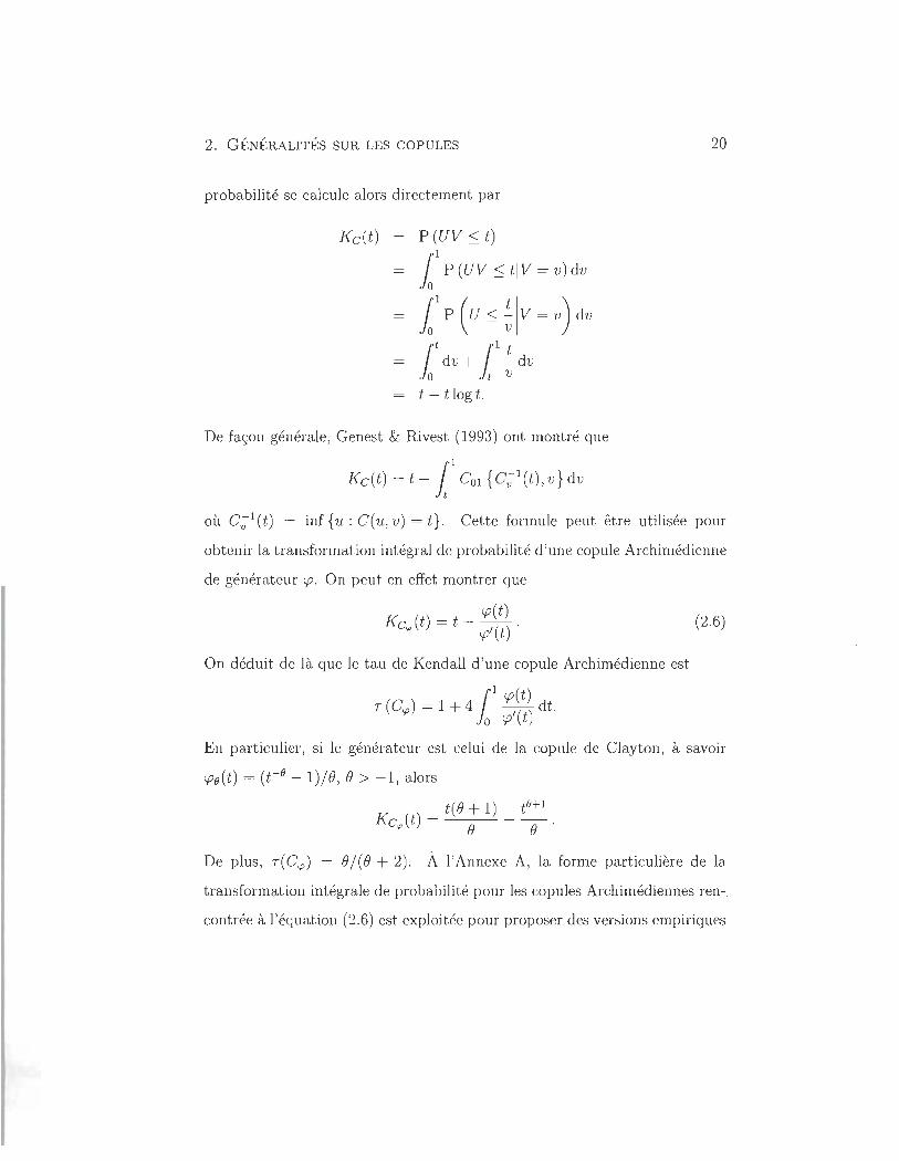
probabilité se calcule alors directement par
I<c(t) P (UV:S t)
11 P (UV :S LIV = v) dv
11 P (u :S ~ 1 V = v) dv
lt 11 l dv + ~ dv
o t v t - t log t.
De façon générale, Genest & Rivest (1993) ont montré que
I<c(t) = t - Il COI { C; l(t), v } dv
où C;;l(t) = inf {u : C(u, v) = t}. Cette formule peut être utilisée pour
obtenir la transformation intégral de probabilité d 'une copule Archimédienne
de générateur <p. On peut en effet montrer que
<p( t) I< c'" ( t) = t - <p' ( t) .
On déduit de là que le tau de Kendall d 'une copule Archimédienne est
t <p(t) T (Cp) = 1 + 4 Jo <p'(t) dt .
(2.6)
En particulier, si le générateur est celui de la copule de Clay ton , à savoir
<Po (t) = (rO - 1) / e, e > -1 , alors
t(e + 1) tH1
I<c", (t) = e - -e-·
De plus, T( Ctp) = e/(e + 2) . À l'Annexe A, la forme particulière de la
transformation intégrale de probabilité pour les copules Archimédiennes ren-.
contrée à l'équation (2.6) est exploitée pour proposer des versions empiriques
2. GÉNÉRALITÉS SUR LES COPULES 21
pour le générateur cp. L'idée consiste d 'abord à représenter cp en fonction de
K c,/" et ensuite à estimer K c,/, avec l'estimateur non-paramétrique introduit
par Genest & Rivest (1993). Deux méthodes sont décrites, l'une qui ut ilise
directement cet estimateur, l'autre qui emploie une version linéarisée.
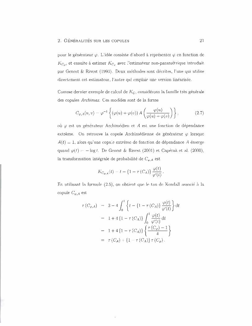
Comme dernier exemple de calcul de K c, considérons la famille très générale
des copules Archimax. Ces modèles sont de la forme
-l{ ( cp(u) )} Ccp,A(U, v) = cp (cp(u) + cp(v)) A cp(u) + cp(v) , (2.7)
où cp est un générateur Archimédien et A est une fonction de dépendance
extrême. On retrouve la copule Archimédienne de générateur cp lorsque
A(t) == 1, alors qu 'une copule extrême de fonction de dépendance A émerge
quand cp(/,) = - log l. De Genest & Rivest (2001) et Capéraà et al. (2000),
la transformation intégrale de probabilité de Ccp,A est
cp(t) K c A(t)=t -{I-T(CA)}-(-). ,/" cp' t
En utilisant la formule (2.5), on obtient que le tau de Kendall associé à la
copule Ccp,A est
t { cp(t) } 3 - 4 Jo t - {1 - T (CA)} cp'(t) dt
1 + 4 {1 - T (CA)} rI cp((t)) dt Jo cp' f;
1 + 4 {1 _ T (CA )} {T (C~ - 1 }
T (CA) + {1 - T (CA)} T (Ccp ) .
CHAPITRE 3
LES FONCTIONS DE C-PUISSANCE THÉORIQUES
Dans ce chapitre, on définit d 'abord formellement les fonctions de C-puissance.
Ensuite, quelques propriétés générales sont énoncées et démontrées. Enfin,
des calculs pour un grand nombre de familles de copules sont présentés. On
verra que des formules très simples émergent pour plusieurs de ces modèles.
3.1 Définition
Soit C, une copule. Les fonctions de C-puissance fc,p : [0, 1] -t [0 , 1] et
lc,p : [0 , 1] -t [0,1] associées à C sont définies récursivement par fC,l(S) =
lC,l(S) = s et pour p 2: 1,
fC,p+l(S) = C {s, fc,p(s)} et lc,p+1(s) = C { lc,p(s), s } . (3.1)
À noter que eC,2(S) = lC,2(S) = C(s, s) est la diagonale de C.
3. L ES FONCTIONS DE C -PUISSANCE T HÉORIQUES 23
3.2 Quelques propriétés fondamentales
Comme première propriété des fonctions de C-puissance, on voit que Pc,p =
lc,p pour tout P E M lorsque C est symétrique, i. e. quand
C(u,v) = C(v ,u) pour tout (u,v) E [0, 1]2 .
Aussi, les propriétés de C sur la front ière de [0, 1 F a pour effet que
PC,p(O) = CC,p(O) = 0 et PC,p( l ) = CC,p( l ) = 1.
De plus, pour chaque p E M, les fonctions Pc,p et Pc,p sont non-décroissantes.
Pour le voir, on procède par induction. On note d 'abord que PC,I(S) = S
est croissante. Ensuite, en supposant que Pc,p est croissante pour un certain
p E M, on a pour tout SI :::; S2 E [0, 1] que
en utilisant le fait que les copules bivariées sont croissantes dans leurs argu
ments et que PC,p(SI) :::; PC,p(S2) , par l'hypothèse d 'induction. Par conséquent ,
Pc,p est non-décroissante pour tout p E M. La preuve est similaire pour Pc,p'
3.3 Lipschitz
Les fonctions de C-puissance sont Lipschit z, c'est-à-dire que pour toute co
pule C, on a pour chaque p E M que
3. LES FONCTIONS DE C -PUISSANCE THÉORIQUES 24
Par conséquent , ec,p et lc,p sont uniformément cont inues sur [0, 1]. Pour le
mont rer , on remarque que le résultat est vrai quand p = 1 car t'C,l (8) = 8.
Ensuite, en supposant que (3 .2) est vraie pour un certain pEN, on a
IC {81, t'C,p(81)} - C {82, t'C,p(82 )} 1
< 181 - 821 + lt'c,p(8d - t'C,p(82) 1
< (p + 1) 181 - 821 ,
où on a ut ilisé le fait que C est elle-même Lipschitz, c'est-à-dire que pour
tout (U 1, V1) , (U2 , V2) E [0, 1]2, on a
3.4 Dominance stochastique
Une copule bivariée Cl est stochastiquement dominée par une aut re copule
C2 si seulement si
On note alors Cl -< C2 . Cette propriété implique l'ordre stochastique de
fonction C-puissallce. Plus précisément, si Cl -< C2 , alors pour tout 8 E [0, 1],
(3 .2)
Pour démontrer ce résultat par induction, on remarque d 'abord qu 'il est vrai
pour p = 2. En effet ,
3. L ES FONCTIONS DE C -PUISSANCE T HÉORIQUES 25
Ensuite, supposons que (3.2) est vraie pour un certain pEN. Comme les
copules bivariées sont croissantes dans leurs arguments, on a
La preuve est similaire pour fc,p.
Une conséquence de (3.2) est que toute fonction de C-puissance est bornée
inférieurement et supérieurement. En effet , on a pour tout S E [0, 1] que
où
fw,p(s) = max (ps + 1 - p, 0) et fM,p(s) = S
sont les fonctions de C-puissance associée aux bornes de Fréchet- Hoeffding
W (u , v) = max(u + v -l , 0) et M(u , v) = min(u, v) ,
respectivement. On rappelle que les copules W et M sont telles que pour
toute copule C ,
W(u, v) :::; C(u, v) :::; M(u, v), pour tout (u , v) E [0, 1]2.
3.5 Calculs pour quelques modèles
3.5.1 Copule d 'indépendance
Soit II (u , v) = 'uv , la copule d 'indépendance. Il est facile de mont rer que
3. LES FONCTIONS DE C -PUISSANCE THÉORIQUES 26
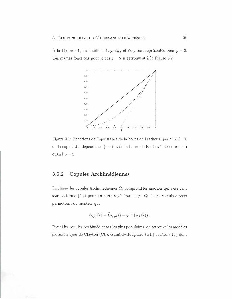
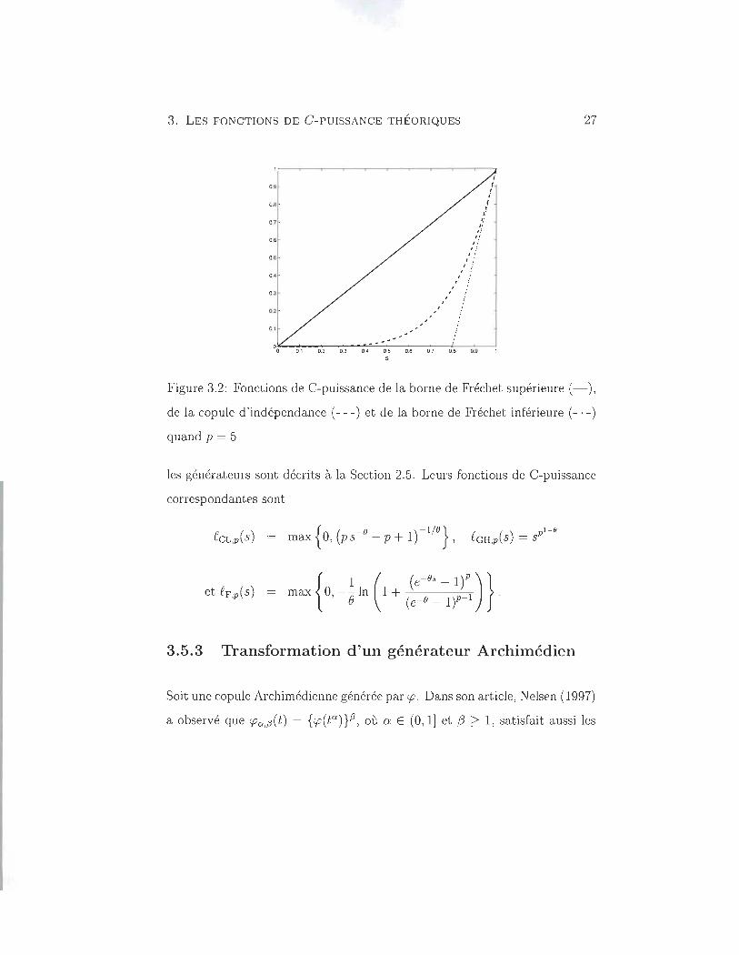
À la Figure 3.1, les fonctions f'w,p, f'n,p et f'M,p sont représentée pour p = 2.
Ces mêmes fonctions pour le cas p = 5 se retrouvent à la Figure 3.2.
0.9
0.9
0.7
0.6
0 5
0.4
0.3 ,
, , , ,
, ,
, ,
" 1: " ,,, , :' , ,,
' .: , . ' . , ..
, ,. , .-
u ~ M M ~ M U 5
, i
Figure 3.1: Fonctions de C-puissance de la borne de Fréchet supérieure (-),
de la copule d'indépendance (- - - ) et de la borne de Fréchet inférieure (- . -)
quand p = 2
3.5.2 Copules Archimédiennes
La classe des copules Archimédiennes Ccp comprend les modèles qui s'écrivent
sous la forme (2.4) pour un certain générateur cp. Quelques calculs directs
permettent de montrer que
Parmi les copules Archimédiennes les plus populaires, on retrouve les modèles
paramétriques de Clay ton (CL), Gumbel-Hougaard (GH) et Frank (F) dont
3 . LES FONCTIONS DE C -PUISSANCE T HÉORIQUES
09
0.8
0.7
06
0.5
o.
, ,
If l '
I.f
,'j
"
I I
" 1 ;
1 :
" ./ , , , ;
" / , ,
;
0.4 0.5 0.6 0.7 0.8 0.9 S
27
Figure 3.2: Fonctions de C-puissance de la borne de Fréchet supérieure (-),
de la copule d 'indépendance (- - - ) et de la borne de Fréchet inférieure (- . - )
quand p = 5
les générateurs sont décrits à la Section 2.5. Leurs fonctions de C-puissance
correspondantes sont
{ 1 ( (e-es_ 1) p)}
max 0, - -0 ln 1 + - 1 ' (e-e - It
3.5.3 Transformation d 'un générateur Archimédien
Soit une copule Archimédienne générée par <p. Dans son art icle, Nelsen (1997)
a observé que <Po:.{3 (t) = {<p(to:)}f3, où a E (0, 1] et f3 ~ 1, satisfait aussi les
3. LES FONCTIONS DE C-PUISSANCE THÉORIQUES 28
propriétés d'un générateur Archimédien. On calcule
cp~,~ {PCPa,{3 (s)}
[cp-l {pl /{3 cp (sa)} ] lia
{ tp
l !f3 (sa) } lia.
Par exemple, si cp(t) = Cl - 1, alors CPa,{3 (t) = (ca - 1){3 . On a donc
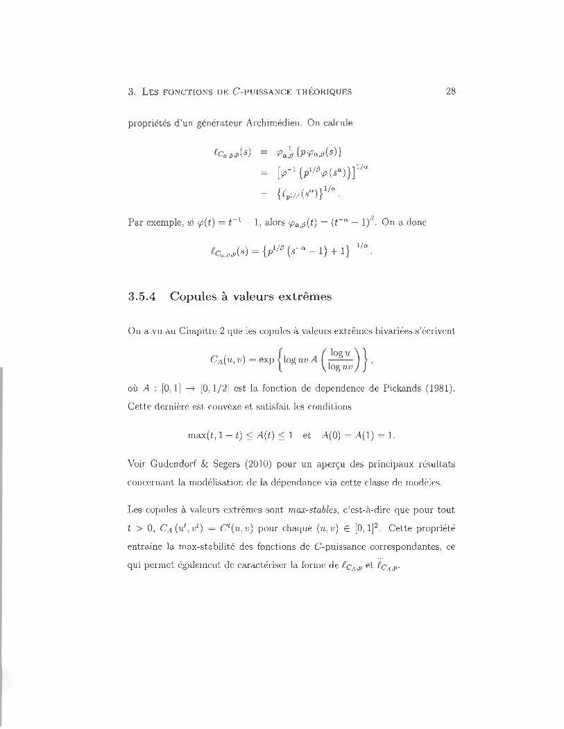
3.5.4 Copules à valeurs extrêmes
On a vu au Chapitre 2 que les copules à valeurs extrêmes bivariées s 'écrivent
CA(u, v) = exp {lOg uv A ( llogu )} , oguv
où A : [0, 1] ---t [0, 1/2] est la fonction de dependence de Pickands (1981).
Cette dernière est convexe et satisfait les conditions
max(t , 1 - t) :::; A(t) :::; 1 et A.(O) = A(I) = 1.
Voir Gudendorf & Segers (2010) pour un aperçu des principaux résultats
concernant la modélisation de la dépendance via cette classe de modèles.
Les copules à valeurs extrêmes sont max-stables, c'est-à-dire que pour tout
t > 0, CA (ut , vt) = Ct( U , v) pour chaque (u , v) E [0,1]2. Cette propriété
entraîne la max-stabilité des fonctions de C-puissance correspondantes, ce
qui permet également de caractériser la forme de fCA ,p et fCA ,p.
3. LES FONCTIONS DE C-PUISSANCE THÉORIQUES 29
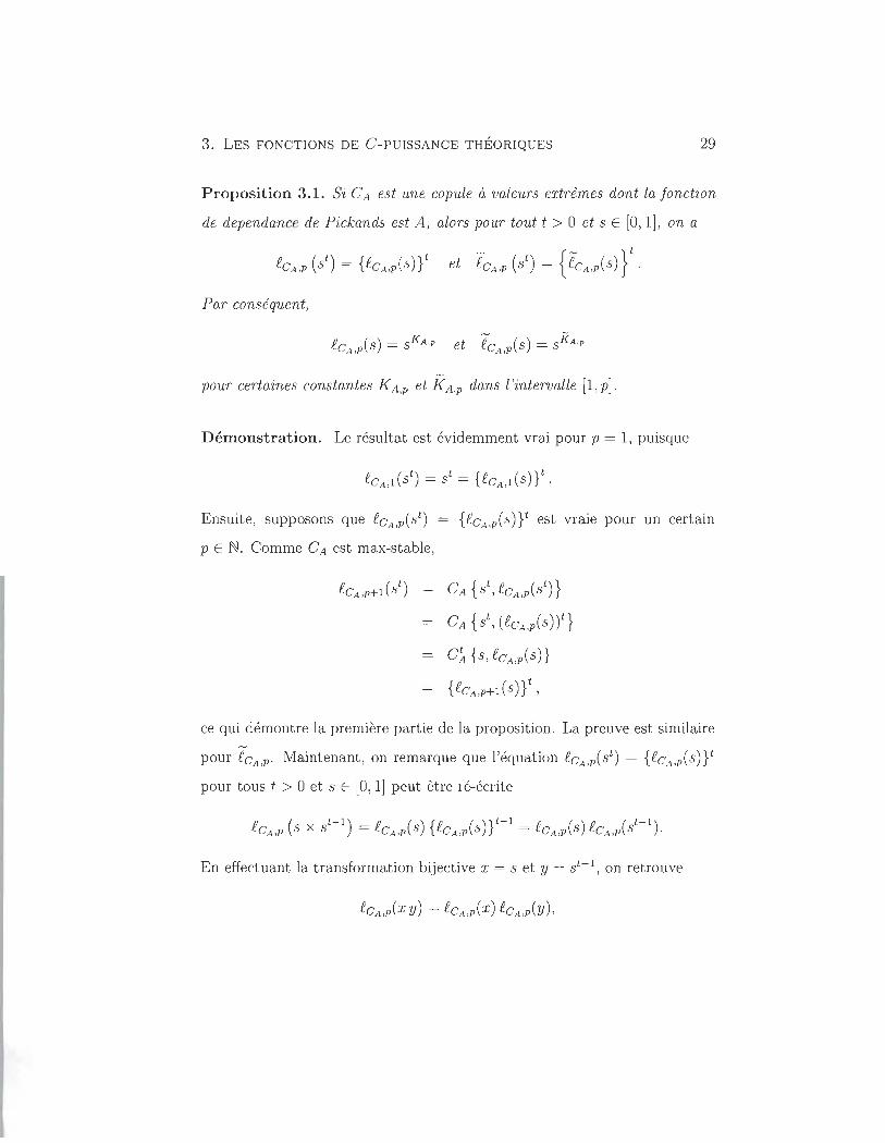
Proposition 3.1. Si CA est une copule à valeurs extrêmes dont la fonction
de dependance de Pickands est A, alors pour tout t > 0 et s E [0, 1], on a
Par conséquent,
pour certaines constantes KA,p et KA ,p dans l'intervalle [1, pl .
D émonstration. Le résultat est évidemment vrai pour p = 1, puisque
Ensuite, supposons que eCA,p(st) = {eCA,P(S)}t est vraie pour un certain
pEN. Comme CA est max-stable,
CA {st, eCA ,p(st)}
CA {st , (eCA,p(s))t}
C~ {s ,eCA ,p(s)}
(eCA ,P+l(S)}t,
ce qui démontre la première partie de la proposition. La preuve est similaire
pour lcA ,p. Maintenant, on remarque que l'équation fcA,p(st) = {fcA,p(s )}t
pour tous t > 0 et s E [0, 1] peut être ré-écrite
En effectuant la transformation bijective x = s et y = st-l, on retrouve
3. LES FONCTIONS DE C-PUISSANCE THÉORIQUES 30
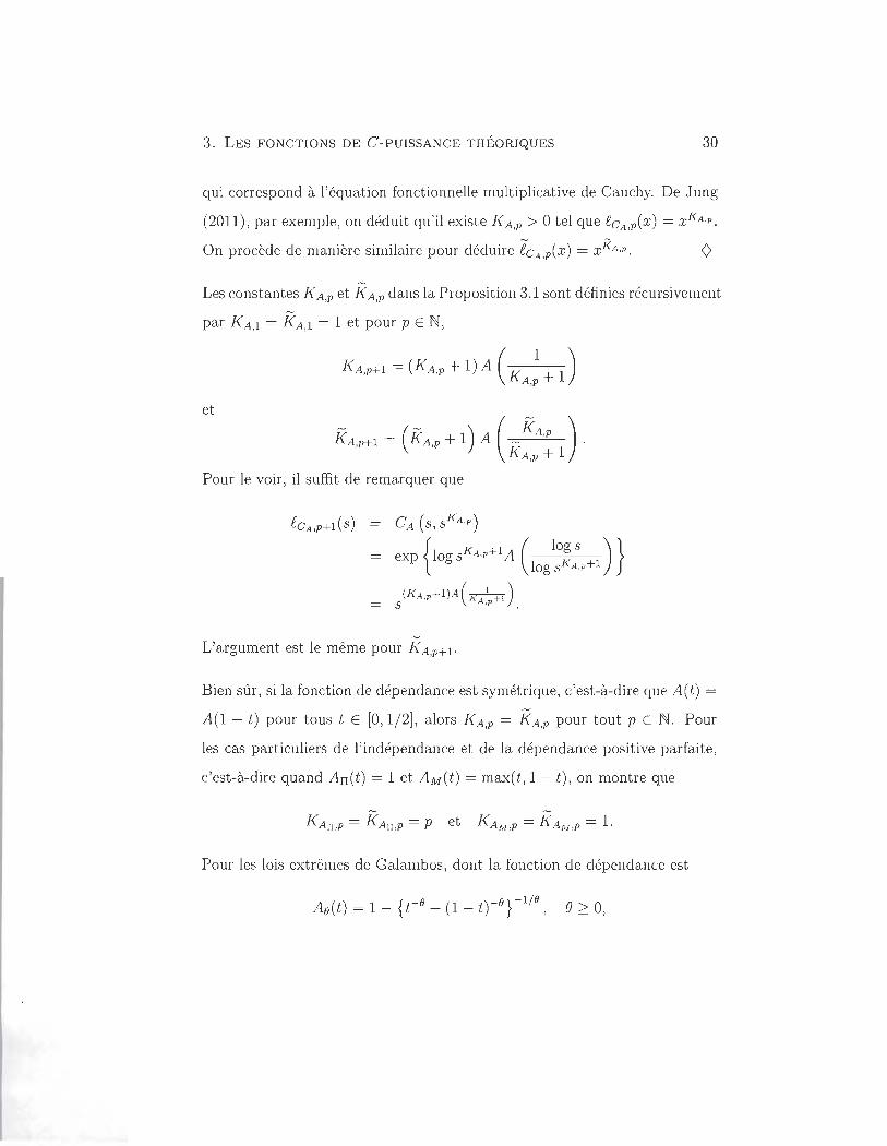
qui correspond à l'équation fonctionnelle multiplicative de Cauchy. De Jung
(2011), par exemple, on déduit qu 'il existe KA ,p > 0 tel que fCA,p(x) = XKA ,p .
On procède de manière similaire pour déduire PcA ,p(x) = XKA,p.
Les constantes KA,p et KA,p dans la Proposition 3.1 sont définies récursivement
par KA,l = KA ,l = 1 et pour pEN,
KA,p+l = (KA,p + 1) A (K 1 + 1) A,p
et
KA ,PH = (KA,p + 1) A ( _ KA,p ) . KA ,p + 1
Pour le voir , il suffit de remarquer que
(KA,p+l)A(K 1 +1) S A,p.
L'argument est le même pour KA,pH'
Bien sûr , si la fonction de dépendance est symétrique, c'est-à-dire que A(t) =
A(1 - t) pour tous l E [0,1/2], alors KA,p = KA ,p pour tout pEN. Pour
les cas particuliers de l'indépendance et de la dépendance positive parfaite,
c'est-à-dire quand Arr(t) = 1 et AM(t) = max(t, 1 - t), on montre que
Pour les lois extrêmes de Galambos, dont la fonction de dépendance est
Ao(t) = 1 - {CO + (1 - ttO} -1 /0, e ~ 0,
3. LES FONCTIONS DE C-PUISSANCE THÉORIQUES 31
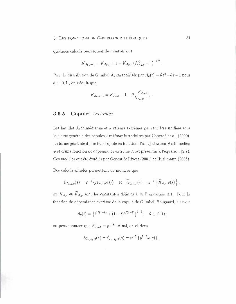
quelques calculs permettent de montrer que
Pour la distribution de Gumbel A, caractérisée par Ao(t) = e t2 - e t + 1 pour
e E [0, 1], on déduit que
3.5.5 Copules Archimax
Les familles Archimédienne et à valeurs extrêmes peuvent être unifiées sous
la classe générale des copules Archimax introduites par Capéraà et al. (2000).
La forme générale d 'une telle copule en fonction d'un générateur Archimédien
cp et d 'une fonction de dépendance extrême A est présentée à l 'équation (2.7).
Ces modèles ont été étudiés par Genest & Rivest (2001) et Hürlimann (2005).
Des calculs simples permettent de montrer que
où KA,p et KA,p sont les constantes définies à la Proposition 3.1. Pour la
fonction de dépendance extrême de la copule de Gumbel-Hougaard , à savoir
Ao(t) = {t1/(1-0) + (1 - t)1 /(1-0)} 1-0 , e E [0 , 1) ,
on peut montrer que KAo ,p = pl - O. Ainsi, on obtient
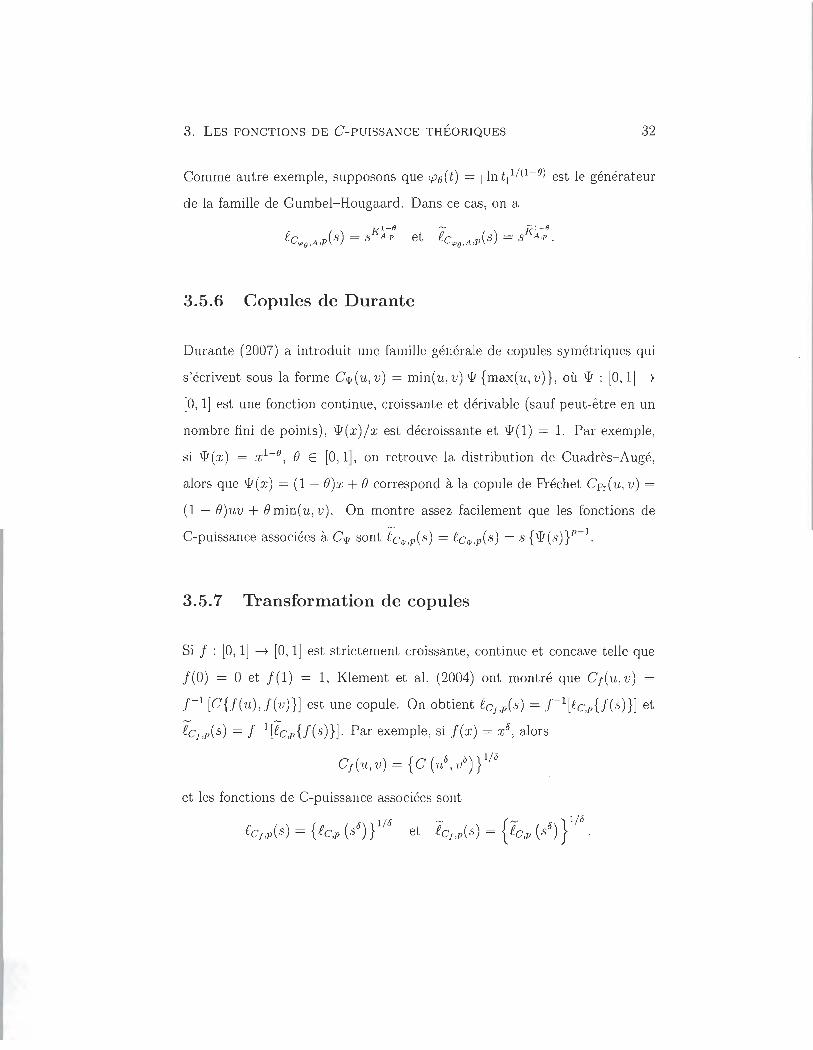
3. LES FONCTIONS DE C-PUISSANCE THÉORIQUES 32
Comme aut re exemple, supposons que c.po(t) = l In W/(l-O) est le générateur
de la famille de Gumbel- Hougaard. Dans ce cas, on a
Kl - 9 - j(1 - 9 fc AP(S) = S A,p et fc AP(S) = S A,p. "'8. 1 t.fJo. ,
3.5.6 Copules de Durante
Durante (2007) a introduit une famille générale de copules symétriques qui
s'écrivent sous la forme Cw(u, v) = min(u , v) W {max(u, v)} , où W : [0,1] -7
[0, 1] est une fonction continue, croissante et dérivable (sauf peut-être en un
nombre fini de points) , w(x)jx est décroissante et W(I ) = 1. Par exemple,
si W (.x) = .X1 - fi, e E [0, 1], on retrouve la distribution de Cuadrès-Augé,
alors que w(x) = (1 - e)x + e correspond à la copule de Fréchet CFr(u, v) =
(1 - e)uv + e min( u, v) . On montre assez facilement que les fonctions de
C-puissance associées à Cw sont ecw ,p(s) = ecw ,p(s) = S {W (S)}p- 1.
3.5.7 Transformation de copules
Si f : [0, 1] -7 [0, 1] est strictement croissante, continue et concave telle que
f(O) = 0 et f(l) = 1, Klement et al. (2004) ont montré que Cf(u , v) =
.r- 1 [C UCu), .r(v)}] est une copule. On obtient eCj ,p(s) = .r- 1[fc,pU(s)}] et
eCj ,p(s) = f -1[ec,p{J(s)}]. Par exemple, si f(x) = x", alors
Cf Cu, v) = {C (u", v" )} 1/"
et les fonctions de C-puissance associées sont
f cj,p(s) = { fc,p (s" )} 1/" et eCj ,p(s) = { ec,p (s") } 1/" .
CHAPITRE 4
MÉTHODE DELTA FONCTIONNELLE
4.1 Version classique
Soit (Xn)nE]\j , une suite de variables aléatoires à valeurs dans lR telle qu'il
existe f-l E lR et a > 0 tel que
Si g : lR ----7 lR est une fonction différentiable dont la dérivée g' est bornée
dans un voisinage de f-l , alors on peut montrer que
où ici et dans la suite, ~ signifie convergence en loi, aussi appelée la con
vergence faible. Cc résultat découle d'un développement en série de Taylor
d'ordre un de g autour de f-l. En effet , on a de façon heuristique que
4. MÉTHODE DELTA FONCTIONNELLE 34
De là,
En fait , de façon plus rigoureuse, on peut mont rer que
où le terme op( l ) représente une quantité aléatoire qui converge en probabilité
vers zéro. Puisque Vn (Xn - J.l ) "-"+ N (O, (J2) , une application du Lemme de
Slutsky (voir Casella & Berger (1990), par exemple, pour plus de dét ails)
permet d 'obtenir le résultat annoncé. Ce résultat se généralise assez facile
ment au cas où (Xn)nEN est une suite de vecteurs aléatoires à valeurs dans
IRd . Dans ce cas, en autant que
où Od = (0, . . . , 0) E IRd , IL E IRd et L: est une matrice de variance-covariance
définie posit ive, on montre que pour toute fonction dérivable 9 : IRd -+ IR,
où
( 0 O )T
g' (x ) = OX I g(x ), . . . , ox/(x )
4.2 Généralisation aux espaces vectoriels
D'un intérêt encore plus considérable que la méthode Delta classique est
sa généralisation à des fonctionnelles définies entre deux espaces vectoriels.
4. MÉT HODE DELTA FONCTIONNELLE 35
Pour la décrire, soient deux espaces vectoriels normés]])) et lE, de même qu 'une
fonctionnelle <I> : ]]))'1> -+ lE, où ]]))~ Ç ]])). On définit d 'abord la dérivabilité au
sens d 'Hadamard.
Définition 4.3. La fo nctionnelle <I> est dérivable au sens d'Hadamard au
point C E ]]))~ s'il existe une fo nctionnelle linéaire continue <I>c : ]])) -+ lE telle
que pour tout Ô E ]])) et pour toute suite Ô n E ]])) et tn -+ 0 tel que Ô n -+ Ô
et C + tn Ô n E ]]))~, on a
Il <I> (C + tn Ô n) - <I> (C) - <I>c(Ô)Il -----r O.
tn E n--+oo
Pour illustrer la définition précédente, soit l'espace des fonctions càdlàg (con
t inue à droite, limite à gauche) sur l'intervalle [0, 1], noté]])) = 0 [0,1], muni
de la norme uniforme, c'est-à-dire
Iif - gll = sup If( x) - g(x )l· XE [O, l )
Soit l'ensemble ]]))~ = {J E D[O, 1] : If l > O} et considérons la fonctionnelle
<I> :]]))~ -+ lE, où lE = D[O , 1], définie par
1 <I> {J (x )} = f (x) .
On remarque que pour tout CE ]]))<1> et n ~ l ,
<I> { C ( x) + tn Ô n ( x )} - <I> { C ( x )} =
tn
1
tn { C ( x) + tn Ô n ( X )}
-ôn(x) C(x ) {C(x) + tn ô n(x )}
ô (x) {C(X )}2'
1
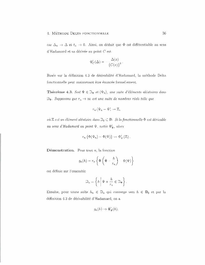
4. MÉTHODE DELTA FONCTIONNELLE 36
car ~n ---+ ~ et t n ---+ O. Ainsi , on déduit que <P est différentiable au sens
d 'Hadamard et sa dérivée au point C est
<P' (~) = _ ~(x) . C {C(x )}2
Basée sur la définition 4.3 de dérivabilité d 'Hadamard , la méthode Delta
fonctionnelle peut maintenant être énoncée formellement.
Théorème 4.3. Soit W E j[))<l> et (W n ), 'une suite d'éléments aléatoires dans
j[))<l> . Supposons que r n ---+ 00 est une suite de nombres réels telle que
où Z est un élément aléatoire dans j[))o C j[)) . Si la fonctionnelle <P est dérivable
au sens d 'Hadamard au point W, notée <P~ , alors
Démonstration. Pour tout n, la fonction
9n (h) = r n { <P ( W + r: ) -<P (w) }
est définie sur l'ensemble
Ensuite, pour toute suite hn E j[))n qui converge vers h E j[))o et par la
définition 4.3 de dérivabilité d 'Hadamard, on a
9n(h) ---+ <P~(h) .
4. MÉTHODE DELTA FONCTIONNELLE 37
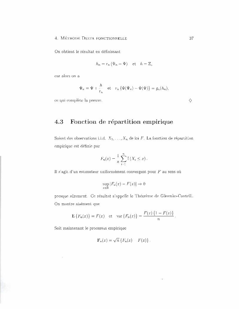
On obtient le résultat en définissant
car alors on a
ce qui complète la preuve.
4.3 Fonction de répartition empirique
Soient des observations i.i .d. Xl , . . . , X n de loi F. La fonction de répartition
empirique est définie par
Il s 'agit d 'un estimateur uniformément convergent pour F au sens où
sup IFn(x) - F(x )1 -t 0 x EIR
presque sûrement. Ce résultat s 'appelle le Théorème de Glivenko-Cantelli.
On montre aisément que
E {Fn(x)} = F(x ) et var {Fn(x )} = F(x){l - F(x )} . n
Soit maintenant le processus empirique
4. MÉTHODE DELTA FONCTIONNELLE 38
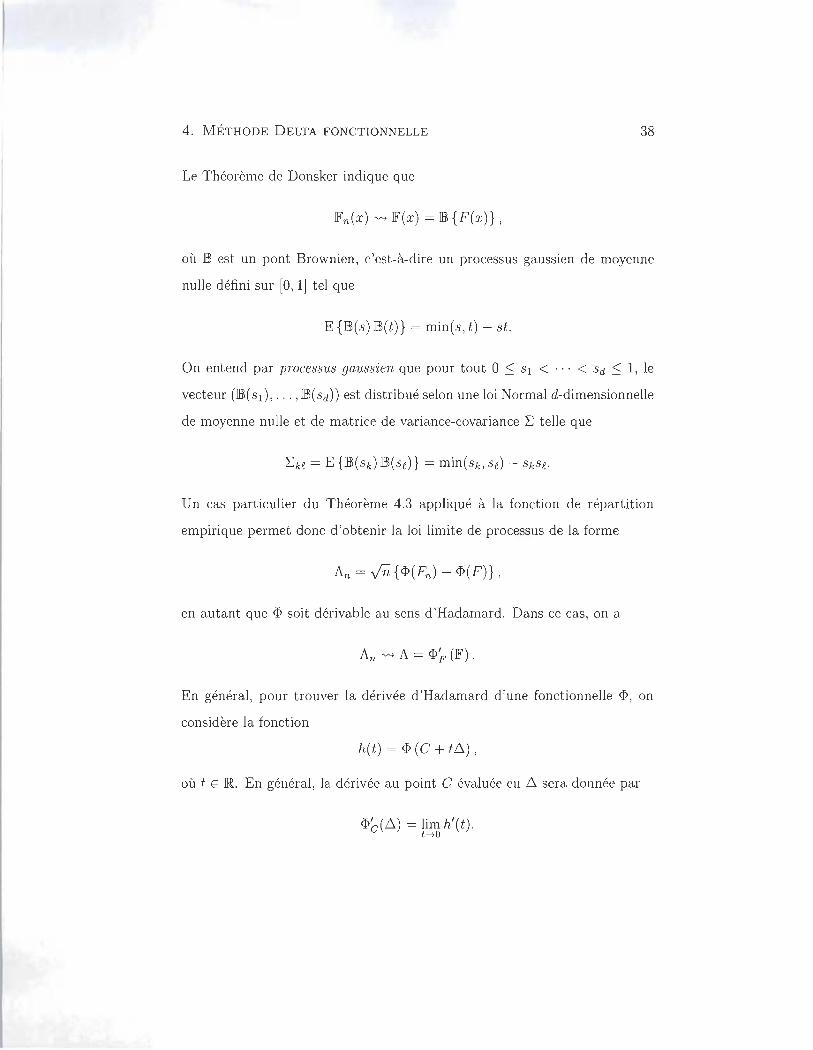
Le Théorème de Donsker indique que
IFn(X) 'V't lF(x) = lB {F(x)} ,
où lB est un pont Brownien, c'est-à-dire un processus gaussien de moyenne
nulle défini sur [0, 1] tel que
E {lB( s) lB(t)} = min(s, t) - st .
On entend par processus gaussien que pour tout 0 :::; SI < .. . < Sd :::; 1, le
vecteur (lB (SI) , .. . , lB(Sd)) est distribué selon une loi Normal d-dimensionnelle
de moyenne nulle et de matrice de variance-covariance L; telle que
Un cas particulier du Théorème 4.3 appliqué à la fonction de répartition
empirique permet donc d 'obtenir la loi limite de processus de la forme
en autant que <I> soit dérivable au sens d 'Hadamard. Dans ce cas, on a
An 'V't A = <I>~ (IF) .
En général, pour trouver la dérivée d 'Hadamard d 'une fonctionnelle <I> , on
considère la fonction
h(t ) = <I> (C + t~),
où t E IR. En général, la dérivée au point C évaluée en ~ sera donnée par
<I>~ (~) = lim h' (t). t--+O
4. MÉTHODE DELTA FONCTIONNELLE 39
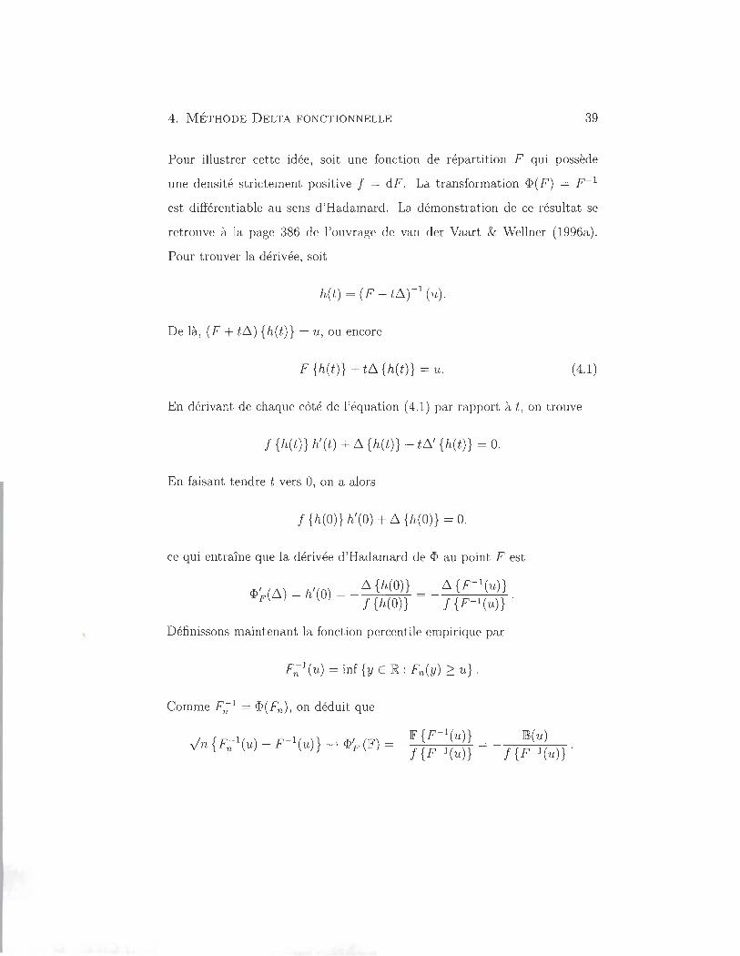
Pour illustrer cette idée, soit une fonction de répartition F qui possède
une densité strictement positive f = dF. La transformation <P(F) = F- 1
est différentiable au sens d'Hadamard. La démonstration de ce résultat se
retrouve à la page 386 de l'ouvrage de van der Vaart & Wellner (1996a).
Pour trouver la dérivée, soit
h(L) = (F + L~)-l Cu).
De là, (F + t~) {h(t)} = u, ou encore
F {h(t)} + t~ {h(t)} = u. (4.1)
En dérivant de chaque côté de l'équation (4.1) par rapport à t , on trouve
f {h(t)} h'(t) + ~ {h(t)} + t~' {h(t)} = O.
En faisant tendre t vers 0, on a alors
f {h(O)} h'(O) + ~ {h(O)} = 0,
ce qui entraîne que la dérivée d'Hadamard de <P au point Fest
<P' (~) = h'(O) = _ ~ {h(O)} = _ ~ {F-1(u)}
F f{h(O)} f{F-l(u)} .
Définissons maintenant la fonction percentile empirique par
F;l(U) = inf {y E lR: Fn(Y) 2 u}.
Comme F;;l = <P(Fn) , on déduit que
r::: { -1() -1()} , ( lF {F- 1(u)} lBl(u)
yn Fn u - F u -v-+ <P F lF) = - f {F- l(U)} = - f {F- l(U)} .
4. MÉTHODE D ELTA FONCTIONNELLE 40
4.4 Autres applications
4.4.1 Fonction de répartition empirique bivariée
Soit un échantillon de paires indépendantes et ident iquement distribuées
(Xl , YI ),' . . , (X n , Yn ) d'une certaine loi H . La fonction de répartit ion em
pirique conjointe de ces observations est définie par
1 n
Hn(x , y) = - L [(Xi::; X, Yi ::; y) . n i=l
(4.2)
La fonction empirique Hn est estimateur sans biais de H. En effet, pour tout
(X,y ) E lR2,
1 n
E{Hn(x , y)} = - L P (X i ::; X , Yi ::; y) = H(x , y). n i=l
Soit maintenant le processus empirique
Son comportement asymptotique est semblable à celui du processus lFn décrit
à la Section 4.3 . Spécifiquement , on peut montrer que 1HIn -vo-+ H , où H est un
processus gaussien centré tel que
Si <I> est une fonctionnelle définie sur un espace de fonctions bivariées et
que <I>~ est sa dérivée d 'Hadamard au point H , alors une application de la
méthode Delta fonctionnelle assure que
(4.3)
· 4. MÉTHODE D ELTA FONCTIONNELLE 41
L'exemple suivant est une application du résultat 4.3 pour obtenir le com
portement limite du tau de Kendall empirique.
Exemple 4.1. Le tau de Kendall est une mesure de dépendance définie
comme la différence entre les probabilités de concordance et de discordance.
Pour un couple (X , Y) dont la loi conjointe est H , une représentation du tau
de Kendall est
T(H) = 4 r H(x, y) dH(x, y) - 1. JR2
Une version empirique habituellement 'utilisée pour estimer T(H) est basée
sur une U-statistique d'ordre deux. Une représentation asymptotiquement
équivalente, et commode ici, est
Afin d'obtenir le comportement asymptotique de
on remarque d'abord que T(H) = <p(H) et Tn = <p(Hn ) , où
<P h ) = 4 r , (x, y) d, (x, y) - 1. JR2
Ainsi, en présupposant que <P admet une dérivée d'Hadamar'd <PH , on aura
'li' n = vn { <P ( H n) - <P ( H )} 'V't <P~ (lHI) .
Pour obtenir la dérivée d'Hadamard de <P , soit
h(t) <P(H+t~)
= 4 r {H(x, y)+t~(x, y)}d{H(x , y) + t~(x, y)}-1. JR2
4. MÉTHODE D ELTA FONCTIONNELLE 42
On montre alors que la dérivée de <I> au point H évaluée en b. est
<I>~ (b.) = lim h' (t) = 4 { r b. (x, y) dH (x , y) + r H (x, y) db. (x, y) } . t-+O j JR2 j JR2
Par conséquent,
'lfn "'" 4 {12 1HI(.'E , y) dH(x, y) + 12 11(.'E , y) dlHI(x , y) } .
4.4.2 Copule empirique
Soit un couple (X , Y) de loi H dont les marges F et C sont continues. Alors
on sait de l'équation (2.2) qu 'il existe une unique copule C telle que
C(u, v) = H {F- 1(u) ,C- 1(v)}.
Un estimateur de C consiste à remplacer H, F et C par les estimateurs Hn,
Fn et Cn , où I1n est défini Ft l'équation (4.2), alors que
et 1 n
Gn(y) = lim Hn(x , y) = - '"""' II (Yi ::; y) x-+oo n ~
i=l
sont les fonctions de répartition empiriques marginales. Ainsi , on peut es
timer C via la copule empirique
4. MÉTHODE DELTA FONCTIONNELLE 43
où 'Yx = 'Y(x,oo) et 'Yy = 'Y(oo,y). Soit maintenant
La dérivée de <P au point H évaluée en 6. est
<p~(6.) = h'(O) = 6. {H;I(u), H;;I(V) }
+ H10 {H; I(U) , H;;I(V) } dd (Hx + t6.x)-1 (U)I t t=O
+ HOl {H;I(U), H;;I(V) } dd (Hy + t6.yr1 (v)1 . t t=O
Après quelques calculs, on obtient
et
i {Hy + t6.y} -1 (v)1 = _ 6.y {(x), H;;I(V) } . dl t=O hy {Hyl(V) }
Une application directe du Théorème (4.3) amène alors
On peut ensuite montrer que <P~ (H) = C(u, v), où
C(u, v) = lI))(u, v) - C01 (u , v) lI))(u, 1) - ClO(u, v) 11))(1, v)
et II)) est la limite du processus empirique
1 n
II))n(u, v) = vin L li {(F(Xi ) ~ U, G(}'i) ~ v) - C(u, v)} . 2=1
4. MÉTHODE DELTA FONCTIONNELLE 44
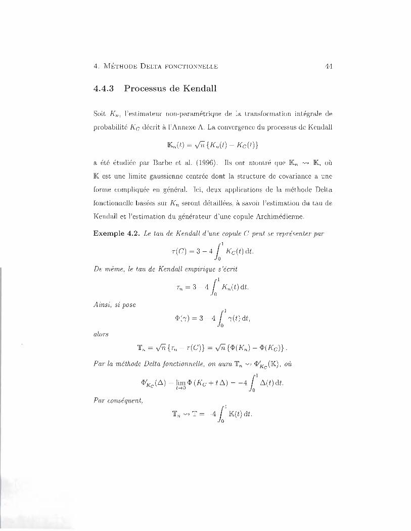
4.4.3 Processus de Kendall
Soit Kn, l'estimateur non-paramétrique de la transformation intégrale de
probabilité Kc décrit à l'Annexe A. La convergence du processus de Kendall
a été étudiée par Barbe et al. (1996). Ils ont montré que IKn """' IK, où
IK est une limite gaussienne centrée dont la structure de covariance a une
forme compliquée en général. Ici, deux applications de la méthode Delta
fonctionnelle basées sur Kn seront détaillées , à savoir l'estimation du tau de
Kendall et l'estimation du générateur d'une copule Archimédienne.
Exemple 4.2. Le tau de Kendall d'une copule C peut se représenter par
T(C) = 3 - 411
Kc(t) dt.
De même, le tau de K endall empirique s'écrit
Tn = 3 - 4 t Kn(t) dt. Jo
Ainsi, si pose
<Ph) = 3 - 411
,(t) dt,
alors
Par la méthode Delta fon ctionnelle, on aura 'TI' n """' <P~c (IK), où
<P~c (~) = lim <P (Kc + t~) = -4 t ~(t) dt. t-tO Jo
Par conséquent,
'TI'n """' 'TI' = -4 1 1IK(t) dt.
4. MÉTHODE DELTA FONCTIONNELLE 45
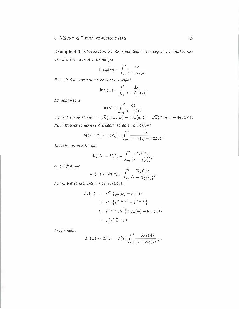
Exemple 4 .3. L 'estimateur rpn du générateur d'une copule A rchimédienne
décrit à l'Annexe A.1 est tel que
j w ds ln rpn ( w) = _ K ( ) .
wo S n S
Il s'agit d'un estimateur de rp qui satisfait
fw ds ln rp( w) = _ K ( ) .
. wo s CS
En définissant
j w ds <I>(r)= ()' wos - ,s
on peut écrire wn(w) = J1ï{lnrpn(w) - In rp(w)} = J1ï{<I>(Kn) - <I>(Kc)} .
Pour trouver la dérivée d'Hadamard de <I>, on définit
jw ds h(t) = <I>(r + tl:::,.) = ( ) /\( ). wos-,s -tus
Ensuite, on montre que
ce qui fait que
<I>~( I:::,.) = h'(O) = j W I:::,.( s) ds 2 '
Wo {s - , (s)}
Wn(w) ~ w(w) = j W lK(s) ds 2.
wo {S - Kc(s)} Enfin, par la méthode Delta classique,
Finalement,
~ e1n cp(w) y'n {ln rpn(w) -lnrp(w)}
rp(W) Wn(W).
jw lK(s) ds
An(w) ~ A(w) = rp(W) 2 . Wo {S - Kc(s)}
CHAPITRE 5
EMPIRICAL C-POWER PROCESSES AND THEIR USE FOR PARAMETER
ESTIMATION AND GOODNESS-OF-FIT IN COPULA MODELS
5.1 Estimation of the C-power functions
Let (Xl, YI) , "" (Xn , Yn ) be independent copies of (X, Y) rv H , where H
has continuo us margins F and G. The aim of this section is to provide
uniformly consistent estimators of the C-power functions and establish their
weak convergence. The first step is to rely on the consistent estimation of
the unique copula C of H via the empirical copula
1 n
Cn(u, v) = - L li (Ui ,n :S u, Vi,n :S v) , n
i=l
1 n
Fn(x ) = - L li (Xi :S X) n
and i=l
5. EMPIRICAL C-POWER PROCESSES 47
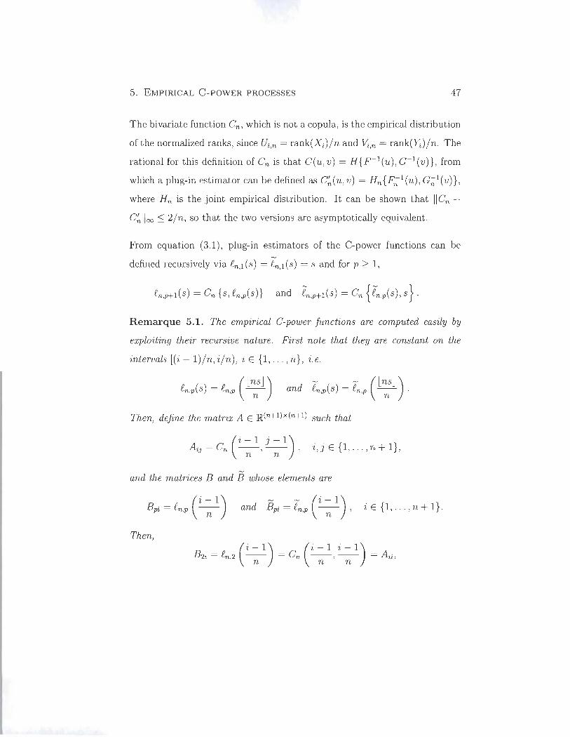
The bivariate function Cn, which is not a copula, is the empirical distribution
of the normalized ranks, since Ui,n = rank(Xi)/n and Vi,n = rank(Y;) /n. The
rational for this definition of Cn is that C (u , v) = H { F-l ( u), G- l ( v)}, from
which a plug-in estimator can be defined as C~(u, v) = Hn{F;:l(U), G;:;-l(V)},
where Hn is the joint empirical distribution. It can be shown that IICn -C~lloo :::; 2/n, so that the two versions are asymptotically equivalent.
From equation (3.1), plug-in estimators of the C-power functions can be
defined recursively via Rn,l (s) = en,l (s) = s and for p 2: 1,
R emarque 5.1. The empirical C-power functions are computed easily by
exploiting their recursive nature. First note that they are constant on the
intervals [(i - 1) /n, i/n), i E {1 , ... , n}, i.e.
- - (lnsJ) and I!n,p (s) = I!n,p -:;;- .
Then, define the matrix A E lR(n+l) x(n+l) such that
(i-l j-l)
Aj = Cn ---:;;:- ' -n- , i,j E {1 , ... ,n+l},
and the matrices Band B whose elements are
(i -1) Bpi = I!n,p -n- - - (i -1) and Bpi = I!n,p ---:;;:- , i E {1 , ... ,n+ 1}.
Then,
(i-l) ( 'i-l 'i-l) B2i = en,2 -n- = Cn ---:;;:- ' -n- = Aii ,
5. EMPIRICAL C-POWER PROCESSES 48
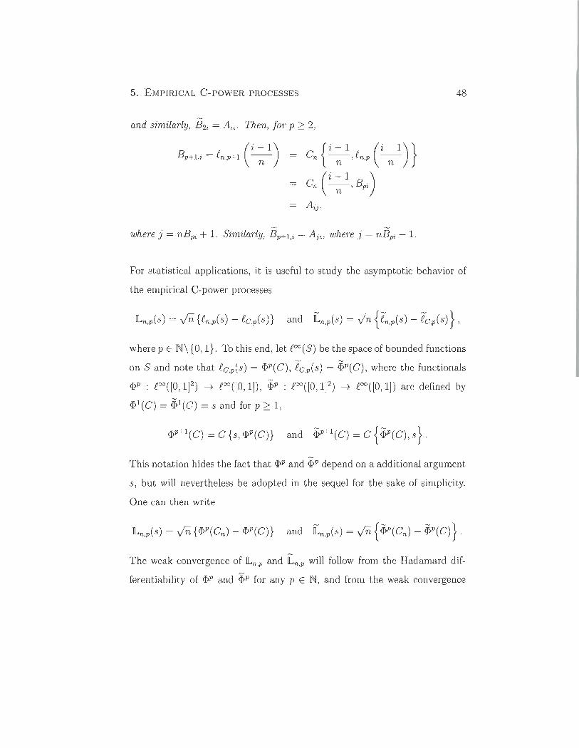
and similarly, B2i = Aii ' Then, for p ~ 2,
(i - 1) Bp+l,i = [n,p+1 ----:;:- = c {~ [ (~)} n n ' n,p n
Cn C ~ 1 , Bpi)
Aij ,
- -where j = nBpi + 1. Similarly, B p+1,i = Aji' where j = nBpi + 1.
For statistical applications, it is useful to study the asymptotic behavior of
the empirical C-power processes
where p E N\ {O, 1}. To this end, let [oo(S) be the space of bounded functions
on S and note that [c,p(s) = <I>P(C) , fc ,p(s) = 1)P(C) , where the functionals
<I>P : [00([0, IF) -+ [00([0, 1]) , 1)P : [00([0, IF) -+ [00([0, 1]) are defined by
<I>l(C) = 1)l(C) = s and for p ~ 1,
<I>P+l(C) = C {s , <I>P(C)} and 1)P+l(C) = C {1)P(C), s}.
This notation hides the fact that <I>P and <I>P depend on a additional argument
s, but will nevertheless be adopted in the sequel for the sake of simplicity.
One can then write
The weak convergence of ILn,p and ILn,p will follow from the Hadamard dif
ferentiability of <I>P and <I>P for any pEN, and from the weak convergence
5. EMPIRICAL C-POWER PRO CESSES 49
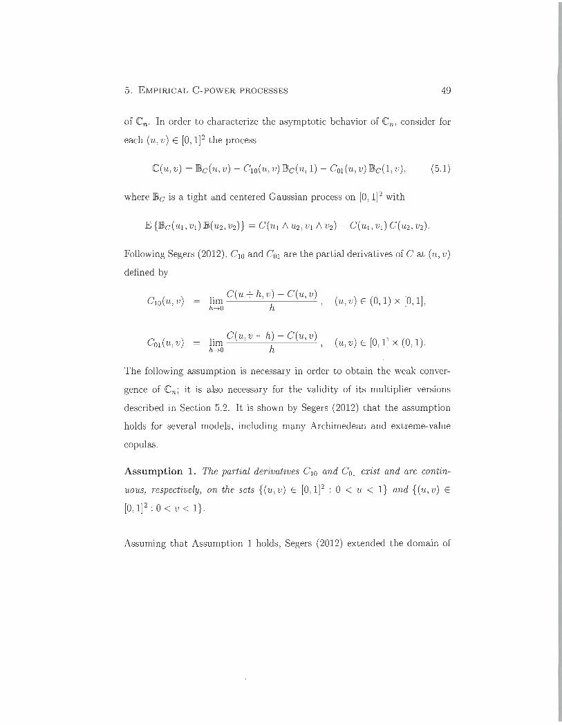
of <Cn . In or der to characterize the asymptotic behavior of <Cn , consider for
each (u, v) E [0,1]2 the process
<C(u, v) = lBc(u, v) - ClO(u, v) lBc(u, 1) - COl Cu, v) lBc(I, v), (5.1)
where lBe is a tight and centered Gaussian process on [0, 1 F with
Following Segers (2012), ClO and COl are the partial derivatives of C at (u, v)
defined by
ClO(u, v) 1. C(u + h, v) - C(u, v) lm h ' h-+O
(u, v) E (0,1) x [0,1],
1. C(u,v+h)-C(u,v)
COl(u,v) = lm h ' h-+O
(u, v) E [0,1] x (0,1).
The following assumption is necessary in order to obtain the weak conver
gence of <Cn ; it is also necessary for the validity of its multiplier versions
described in Section 5.2. It is shown by Segers (2012) that the assumption
holds for several models, including many Archimedean and extreme-value
copulas.
Assumption 1. The partial derivatives ClO and COl exist and are contin
uous, respectively, on the sets {(u , v) E [0, IF : 0 < u < 1} and {(u, v) E
[0, 1 F : 0 < v < 1}.
Assuming that Assumption 1 holds, Segers (2012) extended the domain of
5. EMPIRICAL C-POWER PROCESSES
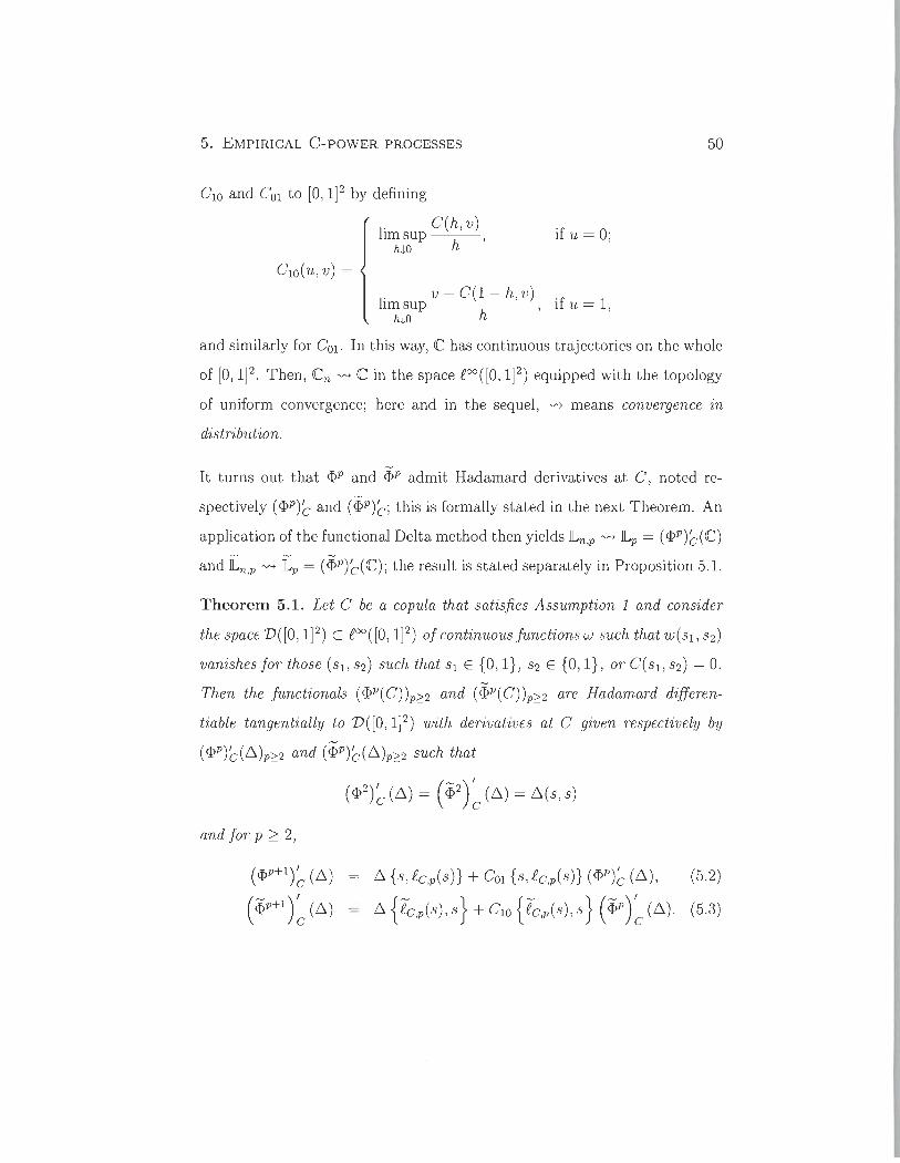
ClO and COI to [0, 1 F by defining
ClO(u , v) =
C(h, v) lim sup --'----'--
h.j.O h' if u = 0;
. v - C(1 - h, v) hm sup , if u = 1,
h.j.O h
50
and similarly for COI' In this way, Chas continuo us trajectories on the whole
of [0, IF. Then, Cn ~ C in the space ROO([O, IF) equipped with the topology
of uniform convergence; here and in the sequel, ~ means convergence in
distribution.
It turns out that <I>P and <I>P admit Hadamard derivatives at C, noted re
spectively (<I>P)~ and (;f;p)~; this is formally stated in the next Theorem. An
application of the functional Delta method then yields lLn,p ~ lLp = (<I>P)~ (q
and in,p ~ i p = (;f;p)~(q; the result is stated separately in Proposition 5.1.
Theorem 5.1. Let C be a copula that satisfies Assumption 1 and consider
the space V([O , IF) C ROO([O, IF) of continuous functions w such that W(Sl' S2)
vanishes for those (SI, S2) su ch that SI E {O, 1}, S2 E {O, 1}, or C(Sl, S2) = O.
Then the functionals (<I>P( C) )p~ 2 and (;f;p( C) )p~2 are Hadamard differen
tiable tangentially to V([O , IF) with derivatives at C given respectively by
(<I>P)~(~)p~ 2 and (;f;P)~(~)P~2 such that
and for p ~ 2,
( <I>p+l ) ~ (~)
( ;f;p+l ) ~ (~)
(<I>2)~(~) = (;f;2)~(~) = ~(s , s)
~ {s , Rc,p(s)} + COI {s , Rc,p(s)} (<I>P)~ (~), (5.2)
~ {lc,p(s) , s} + ClO {lc,p(s), s} (;f;p)~ (~). (5.3)
5. EMPIRICAL C-POWER PROCESSES 51
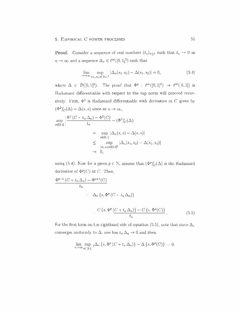
Proof. Consider a sequence of real numbers (tn)n~l such that tn -t 0 as
n -t 00 and a sequence ~n E poo ([0, 1]2) such that
(5.4)
where ~ E D([O , I]2). The pro of that <I>P : eoo ([O,I]2) -t Poo([O,I]) is
Hadamard differentiable with respect to the sup norm will proceed recur
sively. First, <I>2 is Hadamard differentiable with derivative at C given by
(<I>2)C(~) = ~(s, s) since as n -t 00,
sup 1 <I>2 (C + tn ~n) - <I>2(C) _ (<I>2)c(~)1 SE [O,l] tn
sup l.6.n (s,s) - ~(s , s)1 sE [O,l]
< sup l~n(Sl, S2) - ~(Sl , s2)1 (Sl,S2)E[O,1j2
-t 0,
using (5.4) . Now for a given pEN, assume that (<I>P)c(~) is the Hadamard
derivative of <I>P( C) at C. Then,
<I>p+l (C + tn ~n) - <I>p+l (C)
tn
~n { s, <I>P (C + Ln .6.n) }
+ C {s , <I>P (C + tn ~n)} - C {s , <I>P( C)} . (5.5) tn
For the first term on the righthand side of equation (5.5), note that since ~n
converges uniformly to ~ , one has tn ~n -t 0 and then
5. EMPIRICAL C-POWER PROCESSES 52
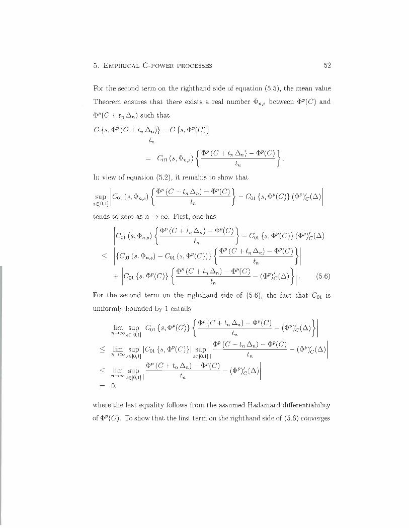
For the second term on the righthand side of equation (5.5), the mean value
Theorem ensures that there exists a real number CPn,s between cpP( C) and
cpP (C + tn ~n) such that
C {s, cpP (C + tn ~n)} - C {s, cpP(C)} tn
= c, ( cp ) {CPP (C + tn ~n) - CPP(C)} 01 s, n,s tn .
In view of equation (5.2), it remains to show that
sup ICOI (s , cpn,s) {CPP (C + tn ~n) - CPP(C)} - COl {s, cpP(C)} (CPP)~(~)I sE[O,l ] tn
tends to zero as n -+ 00 . First, one has
1 COl (s, cpn,s) {CPP (C + tn ~n) - CPP(C)} - COl {s, cpP(C)} (CPP)~(~)I
< 1 {COl (s , cpn,s) - COl (s, cpP( C))} { cpP (C + tn ~n) - cpP( C) } 1
+ ICods , CPP(C)}{CPP(C+ln~n)-CPP(C) -(CPP)~(~)}I. (5.6)
For the second term on the righthand si de of (5.6), the fact that COl is
uniformly bounded by 1 entails .
lim sup ICOl{S , CPP(C)}{CPP(C+ln~n)-CPP(C) -(CPP)~(~) }I n-+oo sE [O,l ] tn
< lim sup 1 COl {s , cpP(C)} 1 sup ICPP(C+tn~n)-CPP(C) -(CPP)~(~)I n-+oo sE [O,l ] SE[O,l] tn
< lim sup ICPP(C+tn~n)-CPP(C) _(CPP)~(~)I n-+oo SE [O,l ] tn 0,
where the last equality follows from the assumed Hadamard differentiability
of cpP( C). To show that the first tcrm on the righthand side of (5.6) converges
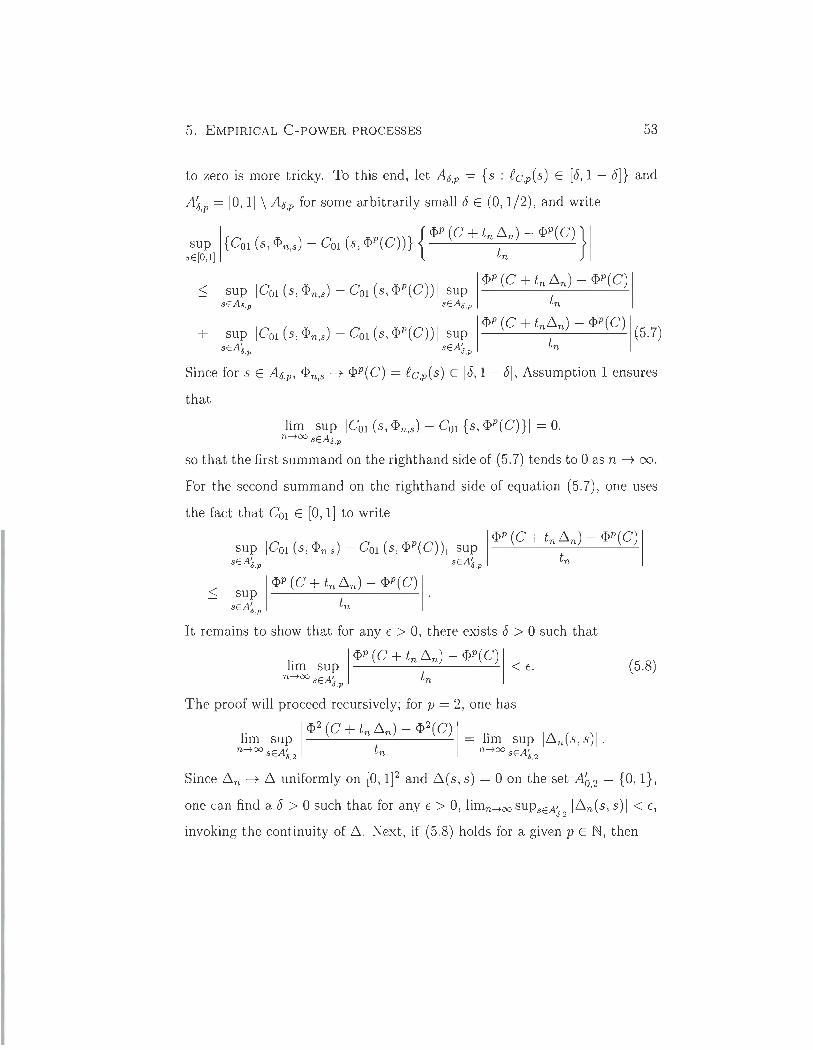
5. EMPIRICAL C-POWER PROCESSES 53
to zero is more tricky. To this end, let A8,p = {s : fc,p (s) E [8, 1 - 8]} and
A~,p = [0,1] \ A8,p for sorne arbitrarily small 8 E (0,1/2), and write
sup 1 {COI (s, <Pn,s) - COl (s, <pp ( C))} { <PP (C + tn ~n) - <PP( C) } 1
sE[O,I) tn
< SUp ICOl(s, <Pn,s) -COl(S,<pP(C)) 1 SUp I<PP(C+tn~n)-<PP(C)1 SEA6 .p sEA6,p ln
+ sup ICOl (s , <Pn,s) - COI (S, <PP(C)) I sup 1 <pp (C + tn~n) - <PP(C) 1 (5.7) sEA' sEA' tn 6.p 6,p
Since for s E A8,p, <Pn,s -t <PP(C) = fc,p(s) E [8,1- 8], Assumption 1 ensures
that
lim sup ICOI (s, <Pn,s) - COl {s , <PP(C)} 1 = o. n-+oo sEA6.p
so that the first summand on the righthand side of (5.7) tends to 0 as n -t 00.
For the second summand on the righthand side of equation (5.7), one uses
the fact that COl E [0, 1] to write
sup ICOI(s,<Pn,s)-COl(s,<pP(C))1 sup I<PP(C+tn~n)-<PP(C)1 sEA' SEA' tn 6,p 6,p
< I<PP(C+tn~n)-<PP(C)1
sup . sEA' tn 6,p
It remains to show that for any 10 > 0, there exists 8 > 0 such that
1. 1 <pp (C + tn ~n) - <PP(C) 1 ~ ~p <10 .
n-+oo sEA' tn 6,p
(5.8)
The proof will proceed recursively; for p = 2, one has
. 1<P2(C+tn~n)-<P2(C)1 1 ( )1 hm sup = lim sup ~n s, S . n-+oo sEA' tn n-+oo sEA'
6,2 6,2
Since ~n -t ~ uniformly on [0,1]2 and ~(s , s) = 0 on the set A~,2 = {O, 1} ,
one can find a 8> 0 such that for any 10 > 0, limn -+oo SUPSEA' I~n(s, s)1 < 10, 6 ,2
invoking the continuity of~. Next, if (5.8) holds for a given pEN, then
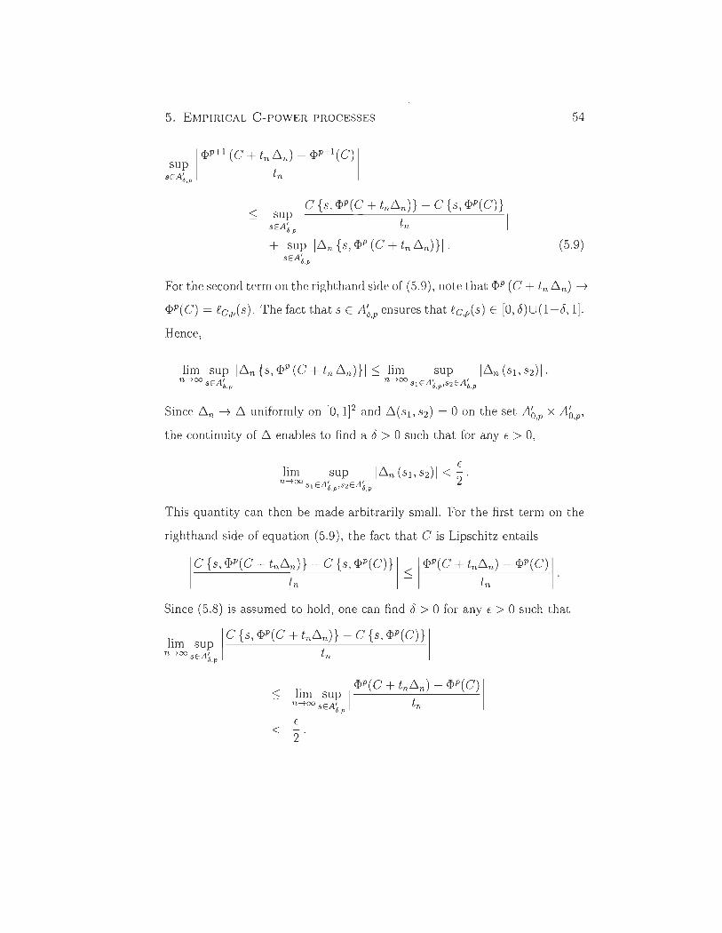
5. EMPIRICAL C-POWER PROCESSES
1
<I>p+l (C + tn ~n) - <I>p+l (C) 1
sup sE A' tn 6,p
< 1
C {s , <I>P(C + tn~n)} - C {s, <I>P(C)} 1 SUp
sEA' tn 6,p
+ SUp I ~n {s , <I>P (C + tn ~n)} l. SEA8,p
54
(5.9)
For the second term on the righthand side of (5.9), note that <I>P (C + ln ~n) ~
<I>P(C) = ec,p(s). The fact that s E A~,p ensures that ec,p(s) E [0, 15)U(I-15, 1] .
Renee,
Since ~n ~ ~ uniformly on [0, IF and ~(S l , S2) = 0 on the set A~,p x A~,p,
the continuity of ~ enables ta find a 8 > 0 such that for any E > 0,
This quantity can then be made arbitrarily small. For the first term on the
righthand side of equation (5.9), the fact that C is Lipschitz entails
1
C {s, <I>P( C + tn~n)} - C {s, <I>P( C )} 1 :S 1 <I>P( C + tn~n) - <I>P( C) 1.
Ln ln
Since (5.8) is assumed ta hold, one can find 8 > 0 for any E > 0 such that
1. 1 C {s , <I>P(C + tn~n)} - C {s, <I>P(C)} 1 lm sup
n-too sEA' tn 6,p
E < -
2
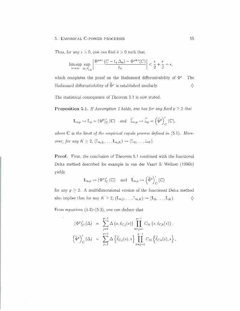
5. EMPIRICAL C-POWER PROCESSES 55
Thus, for any E > 0, one can find 8 > 0 such that
. 1 <pp+! (C + tn ~n) - <pp+! (C) 1 E E hm sup sup < -2 + -2 = E,
n-too sE A' tn J ,p
which completes the pro of on the Hadamard differentiability of <Pp. The
Hadamard differentiability of <pp is established similarly.
The statistical consequence of Theorem 5.1 is now stated.
Proposition 5.1. If Assumption 1 holds, one has for any fixed p 2 2 that
where <C is the limit of the empirical copula process defined in (5 .1 ). More
over, for any K 2 2, (ILn,2,"" ILn,K) "'" (1L2 , . . . , ILK).
Proof. First, the conclusion of Theorem 5.1 combined with the functional
Delta method described for example in van der Vaart & Wellner (1996b)
yields
for any p 2 2. A multidimensional version of the functional Delta method
also implies that for any K 2 2, (ILn,2 ' ... , lLn,K) "'" (1L2 , ... ,ILK). (;
From equations (5.2)- (5.3), one can deduce that
p-1 p-1 L ~ { s, ee,j (s)} II COl {s , ee,k (s)} , j=l k=j+! p-1 p-1
L ~ { ie,j(s), s } II ClO { ie,k(S), s } , j=l k=j+1
5. EMPIRICAL C - POWER PROCESSES 56
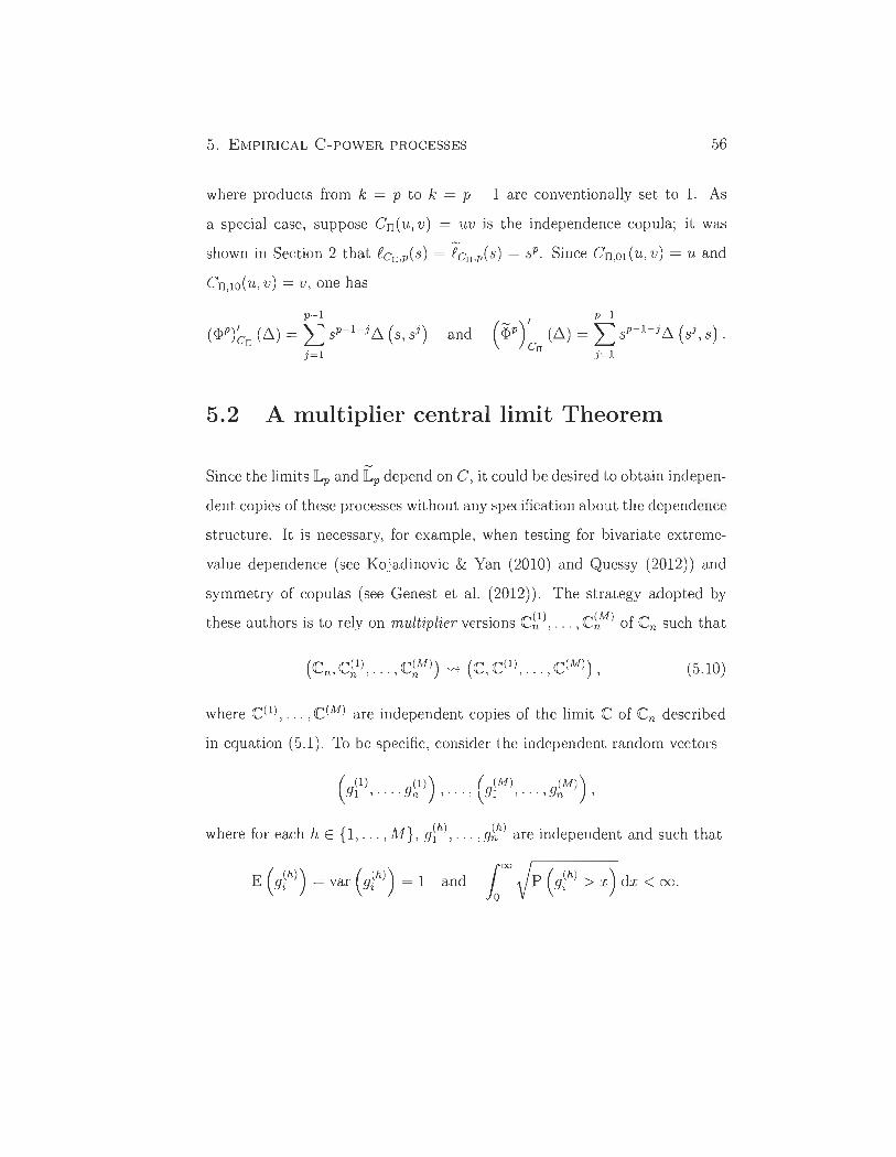
where products from k = p to k = p - 1 are conventionally set to 1. As
a special case, suppose Cn (u , v) = uv is the independence copula; it was
shown in Section 2 that tCn ,p( s) = eCn ,p( s) = sp. Sinee Cn,Ol (u, v) = u and
Cn,lO(U, v) = v, one has
p- 1 (<I>P)~n (~) = L sp-1- j ~ (s, sj) and
j=l
5.2 A multiplier central limit Theorem
Since the limits lLp and lLp depend on C, it could be desired to obtain indepen
dent copies of these proeesses without any specification about the dependence
structure. It is necessary, for example, when testing for bivariate extreme-
value dependenee (see Kojadinovie & Yan (2010) and Quessy (2012)) and
symmetry of copulas (see Genest et al. (2012)). The strategy adopted by
these authors is to rely on multiplier versions C~1) , ... , C~M) of Cn sueh that
(5.10)
where C(1), .. . , C(M) are independent copies of the limit C of Cn deseribed
in equation (5.1). To be specifie, eonsider the independent random veetors
h e { } (h) (h) . W ere 10r eaeh h El, ... , M , 091 , .. . , o9n are mdependent and sueh that
5. EMPIRICAL C-POWER PROCESSES 57
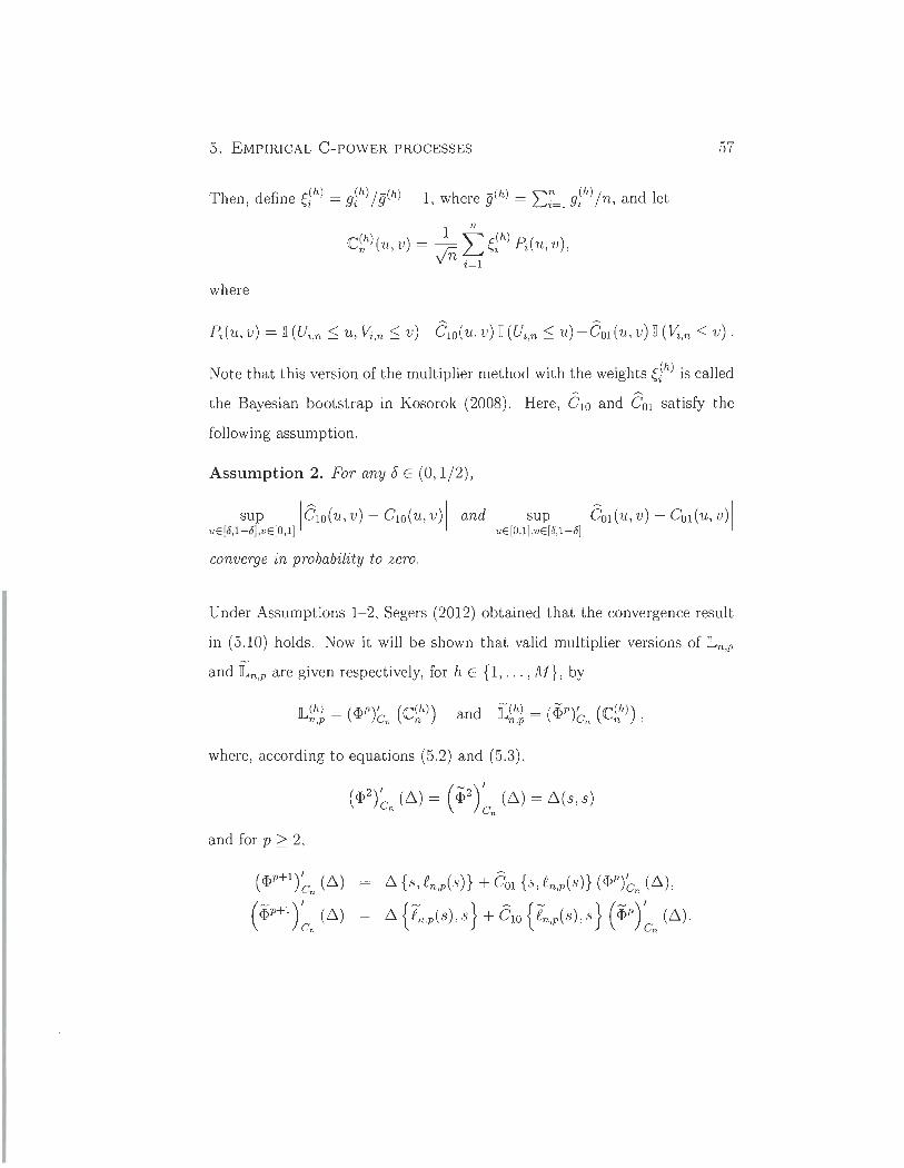
Then define ç(h) = g(h)/g- (h) _ 1 where g-(h) = " n g(h)/n and let , <"t t , L .. .n=l t ,
1 n C(h)( ,U v) = - '" ç(h) P·(n v) n' 'ri ~<"t t, ,
V f. i=l
where
Note that this version of the multiplier method with the weights ç~h) is called
the Bayesian bootstrap in Kosorok (2008). Here, êlO and êOl satisfy the
following assumption.
Assumption 2. For any {) E (0,1/2),
sup !êlO(n,v) - ClO(n,v) ! and sup !êOl(n,v) - COI (n, v)! UE [<5,l-<5},vE[O, l } UE [O,l },vE [<5,l -<5}
converge in probability ta zero.
Under Assumptions 1- 2, Segers (2012) obtained that the convergence result
in (5.10) holds. Now it will be shown that valid multiplier versions of lLn,p
and in,p are given respectively, for h E {l , ... , M}, by
lL(h) = (q,P)' (C(hl ) and Ühl = (<pP)' (C(h) ) n,p Cn n n,p Cn n ,
where, according to equations (5.2) and (5.3),
( q,2) ~n (~ ) = (<p2) ~n (~) = ~ (s, s)
and for p ~ 2,
~ {s, Rn,p(s)} + êOl {s, Rn,p(s)} ( q,P)~n (~),
~ { en,p(S) , S} + êlO { en,p(S), s } (<Pp) ~n (~).
5. EMPIRICAL C - POWER PROCESSES 58
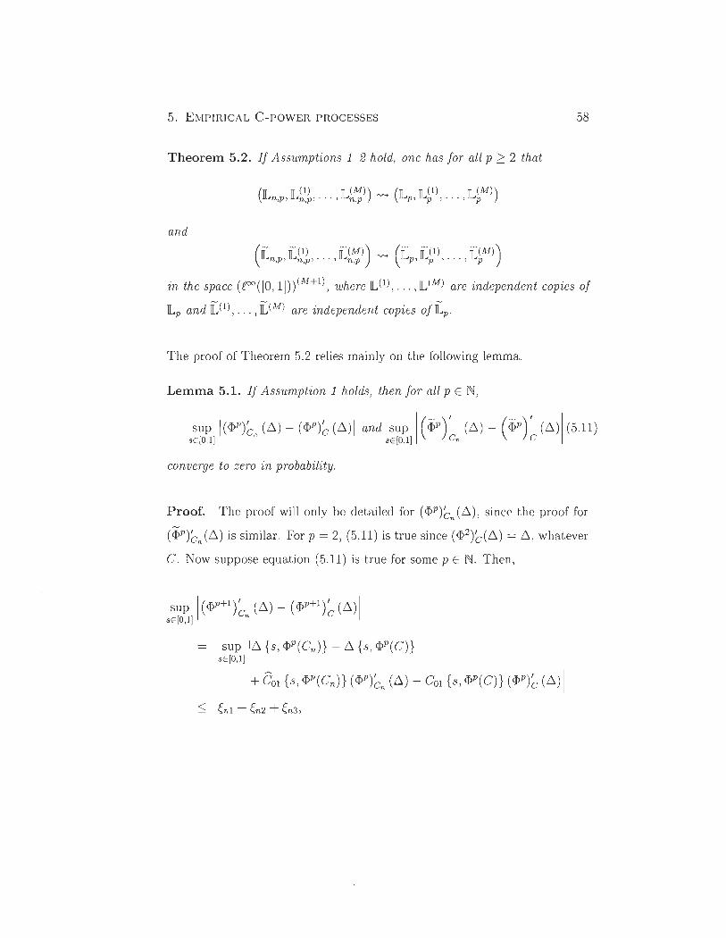
Theorem 5.2. If Assumptions 1- 2 hold, one has for all p 2: 2 that
and
in the space (fOO([O , 1])) (M+1) , where Il)!), ... ,II)M) are independent copies of
lLp and jUI), .. . ,jUM) are independent copies of [p '
The proof of Theorern 5.2 relies rnainly on the following lernrna.
Lemma 5.1. If Assumption 1 holds, then for all pEN,
converge to zero in probability.
Proof. The proof will only be detailed for (<I>P)cJ ~) , since the pro of for
(<PP)cn (~) is sirnilar. For p = 2, (5.11) is true since (<I>2)C(~) = ~ , whatever
C. Now suppose equation (5.11) is true for sorne pEN. Then,
sup 1(<I>p+1)~n (~) - (<I>P+I)~(~)I sE [O,l ]
sup I~ {s , <I>P( Cn)} - ~ {s, <I>P( C)} sE [O,l]
+ êOl {s , <I>P(Cn)} (<I>P)~n (~) - COl {s , <I>P(C)} (<I>P)~ (~)I
< ÇnI + Çn2 + Çn3,
5. EMPIRICAL C-POWER PROCESSES 59
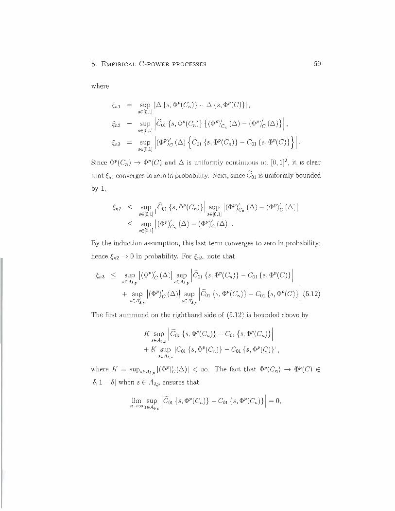
where
Çnl sup 16 {s, <pP (Cn)} - 6 {s , <pP(C)} 1 , sE [O,l]
Çn2 sup lêods,<pP(Cn)}{(<PP)~n(6)-(<PP)~(6)}I, sE [O,l]
Çn3 sup 1(<PP)~(6) { êOl{S , <PP(Cn)}-COl{S , <PP(C)}}I· sE lo,!]
Since <pP( Cn) -+ <pP ( C) and 6 is uniformly continuous on [0,1 F, it is clear
that Çnl converges to zero in probability. Next, sin ce COl is uniformly bounded
by 1,
Çn2 < sup lêOl {s, <pP (Cn)}1 sup 1(<pP)~n (6) - (<pP)~ (6)1 SE [O,l ] sE [O,l ]
< sup 1(<pP)~n (6) - (<pP)~ (6)1· SE[O,l]
By the induction assumption, this last term converges to zero in probability;
hence Çn2 -+ 0 in probability. For Çn3 , note that
Çn3 :::; sup 1(<pP)~ (6)1 sup lêOl {s, <pP(Cn)} - COl {s, <pP(C)} 1
sEAo,p sEAo,p
+ sup 1(<pP)~(6)1 sup lêods ,<pP(Cn)}-COl{S ,<Pp(C)}I(5.12) SEA6,p SEA6,p
The first summand on the righthand side of (5.12) is bounded above by
K sup lêol {s, <pP(Cn)} - COl {s, <pP (Cn)}1 sEAo,p
+ K sup ICOl {s , <pP(Cn)} - COl {s , <pP(C)} 1 ,
SEAo,p
where K = SUPSEAo,p 1(<PP)c(6)1 < 00 . The fact that <pP(Cn) -+ <pP(C) E
[8,1 - 8] when s E A",p ensures that
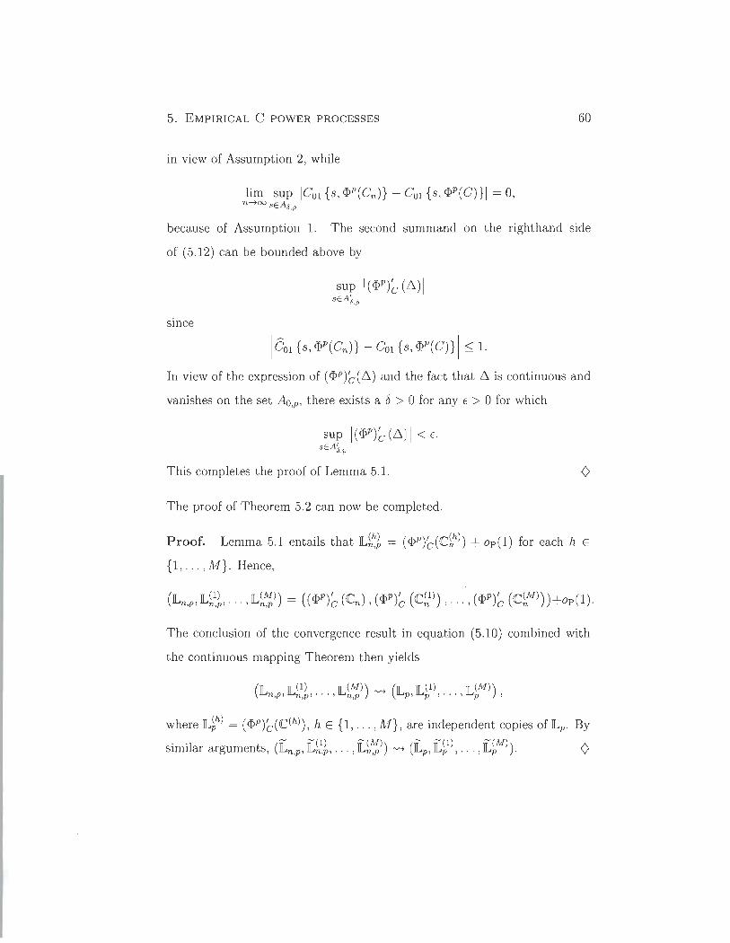
5. EMPIRICAL C-POWER PROCESSES 60
in view of Assumption 2, while
because of Assumption 1. The second summand on the righthand side
of (5.12) can be bounded above by
since
lêol {s, <I>P(Cn )} - COI {s, <I>P(C)} 1 ~ 1.
In view of the expression of (<I>P)c (~) and the fact that ~ is continuous and
vanishes on the set Ao,p, there exists a,5 > 0 for any E > 0 for which
This completes the proof of Lemma 5.1.
The proof of Theorem 5.2 can now be completed.
Proof. Lemma 5.1 entails that L~~~ = (<I>P)C(C~h)) + op(l) for each h E
{l , ... , M}. Rence,
The conclusion of the convergence result in equation (5.10) combined with
the continuous mapping Theorem then yields
where L~h) = (<I>p)C(C(h)), hE {l , ... , M}, are independent copies of Lp. By
5. EMPIRICAL C-POWER PROCESSES 61
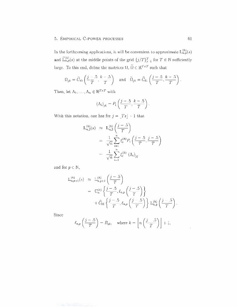
In the forthcoming applications, i t will be convenient to approximate IL~~~ (s )
and i~~~( s) at the middle points of the grid {j jT}J=l for T E N sufficiently
large. To this end, define the matrices 0, n E RT x T such that
- ~ (j -.5 k - .5) and Ojk = Cal ---;y-' ---r- .
Then, let Al , ... , An E RT x T with
With this notation, one has for j = l Ts J + 1 that
lL(h) (j - .5) n,2 T
_1 ~ ç(h) Pc (j -.5 j - .5) r;;: ~<", , T ' T
yn i=l
and for pEN,
(h) () ILn,PH s (h) (j - .5)
~ ILn ,P+1 T
C(h) {~ f (~)} nT' n,p T
~ {j - .5 (j - .5)} (h) (j - .5) + Cal ---;y-' fn ,p ---;y- ILn,p ---;y- .
Since
(j - .5)
fn,p ---;y- = Bpk ' wherek= ln(j;·5)J +1 ,

5. EMPIRICAL C-POWER PROCESSES 62
one has for r = lT Bpk + .5 J that
lL(h) () "-' C(h) (j -.5 r - .5) n,p+l S "-' nT ' T
ê (j -.5 r - .5) lL(h) (j - .5) + 01 T' T n,p T
1 ~ (h) - (h) (j - .5) vin f=t Ç,i (Ai)jr + Ojr lLn,p ---y;- .
-(hl . -(hl (h) -For lLn,p, one obtams lLn,2(S) = lLn,2(S) and for r = lTBpk + .5J ,
-(hl "-' _1_ ~ (h). . -(hl (j - .5) lLn,P+l(S) "-' vin f=tÇ,i (At)rj +OrJlLn,p T .
The above multiplier method can be used to build nonparametric confidence
bands for an unknown C-power functions Cc,p . To this end, let qp,o: be the
real number such that
lim P { sup IlLn,p(s)1 > qp,o: } = a. n-too SE[O,l]
Renee, an approximate 1 - a confidence band for Cc,p is given by
CBp(a) = [Cn,p(S) - fo' Cn,p(s) + fo] . Since qp,o: depends on the unknown value of C, the latter has to be estimated.
A solution consists in using qp,o: as the (1 - a)-th percentile of
sup IlL~~~(s) 1 ~ . max IlL~~~ (j - .5) l, hE {1 , ... , M}, SE[O,l] JE{l , ... T} T ,
yielding
C~) = [Cn,p(S) - ~, Cn,p(s) + ~] as an approximate 1 - a confidence band for Cc,p. To our knowledge, it is the
first time that such model-free confidence bands are considered in a copula --context. The construction of CBp(a) from a real data set is presented in
Section 5.6.
5. EMPIRICAL C-POWER PROCESSES 63
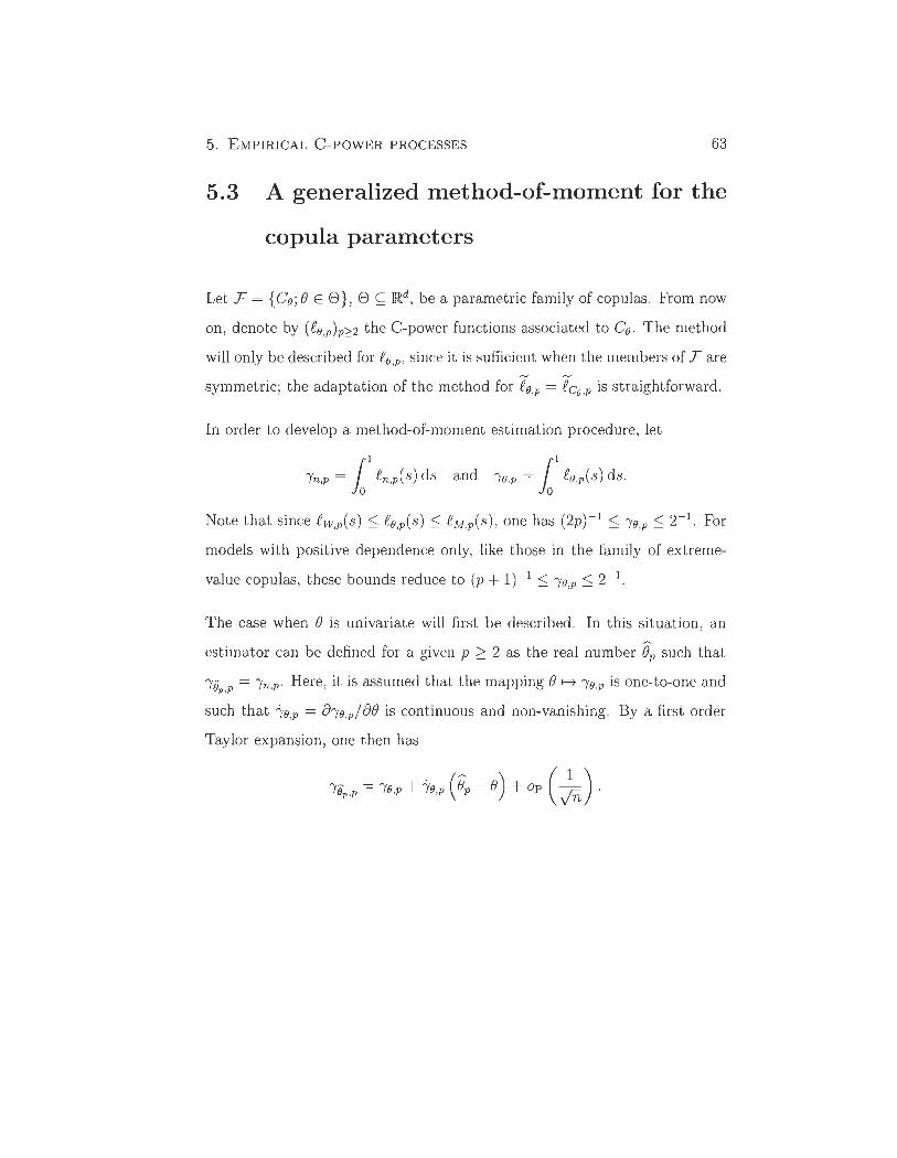
5.3 A generalized method-of-moment for the
copula parameters
Let F = {Ce; e E e}, e ç ]Rd , be a parametric family of copulas. From now
on, denote by (Re ,p)p~ 2 the C-power functions associated to Ce . The method
will only be described for ee,p, since it is sufficient when the members of F are - -
symmetric; the adaptation of the method for ee,p = RC8 ,p is straightforward.
In order to develop a method-of-moment estimation procedure, let
'Yn,p = 11
en,p(S) ds and 'Yo,p = 11
eo,p(S) ds.
Note that since ew,p(s) ::; ee,p(s) ::; eM,p(s) , one has (2 p)- 1 ::; 'Ye ,p ::; 2- 1. For
models with positive dependence only, like those in the family of extreme
value copulas, these bounds reduce to (p + I t 1 ::; 'Yo,p ::; 2- 1.
The case when e is univariate will first be described . In t his sit uation, an
estimator can be defincd for a given p ~ 2 as the real number êp such that
'Yôp ,p = 'Yn,p. Here, it is assumed that the mapping e H 'Ye,p is one-to-one and
such that 'Ye,p = a'Ye,p/ ae is continuous and non-vanishing. By a first order
Taylor expansion, one then has
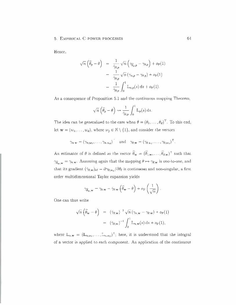
5. EMPIRICAL C-POWER PROCESSES
Henee,
~ vin ( 'YB p - 'Yo,p ) + op(l) 'Yo,p p,
1 -. - vin ("(n,p - 'Yo,p) + op(l) 'Yo,p
= ~ rI ILn,p(S) ds + op(l). 'Yo,p Jo
64
As a consequence of Proposition 5.1 and the continuous mapping Theorem,
The idea can be generalized to the case when () = (()l, ... , ()d) T. To this end,
let W = (Wl,"" Wd), where Wj EN \ {1}, and consider the vectors
'Yn,w = ('Yn,wl' ... , 'Yn,wJ T and 'Yo,w = ('YO,Wl' ... , 'Yo ,wJ T.
An estimator of () is defined as the vector êw = (êl ,w, ... , êd,w) T such that
'YBw,w = 'Yn,w' Assuming again that the mapping () H 'Yo,w is one-to-one, and
that its gradient (i-O,w)kl' = fY"(o,wjf)()1' is continuous and non-singular , a first
order multidimensional Taylor expansion yields
'YBw,w = 'Yo ,w + 'Yo ,w (êw - e) + Op (Jn) . One can thus write
(i-o,wrl vin ("(n,w - 'Yo ,w) + oP(l)
(i-o,wr l 11 ILn,w(S) ds + op(l),
where ILn,w = (ILn,Wll"" ILn,wJ T; here, it is understood that the integral
of a vector is applied to each component. An application of the continuous
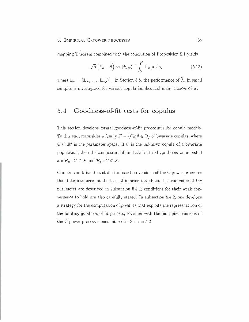
5. EMPIRICAL C-POWER PROCESSES 65
mapping Theorem combined with the conclusion of Proposition 5.1 yields
v'n (êw - e) ~ bO,w)-l 11 lLw(S) ds, (5.13)
where lLw = (lLWll '" , lLWd)T. In Section 5.5, the performance of êw in small
samples is investigated for various copula families and many choices of w.
5.4 Goodness-of-fit tests for copulas
This section develops formaI goodness-of-fit procedures for copula models.
To this end, reconsider a family F = {Co; e E 8} of bivariate copulas, where
8 ç ]Rd is the parameter space. If C is the unknown copula of a bivariate
population, then the composite null and alternative hypotheses to be tested
are No : C E F and N I : C tt. F.
Cramér-von Mises test statistics based on versions of the C-power pro cesses
that take into account the lack of information about the true value of the
parameter are described in subsection 5.4.1; conditions for their weak con
vergence to hold are also carefully stated. In subsection 5.4.2, one develops
a strategy for the computation of p-values that exploits the representation of
the limiting goodness-of-fit process, together with the multiplier versions of
the C-power pro cesses encountered in Section 5.2.
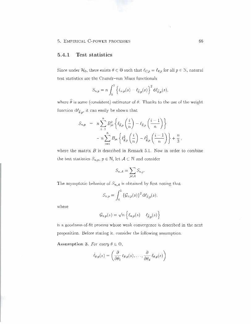
5. EMPIRICAL C-POWER PRO CESSES 66
5.4.1 Test statistics
Since under Ho, there exists e E e such that fc,p = fo ,p for aIl pEN, natural
test statistics are the Cramér-von Mises functionals
Sn,p = n 11 { tn,p(s) - fô,p(s) } 2 dfô,p(S),
where ê is some (consistent) estimator of B. Thanks to the use of the weight
function dfô , it can easily be shown that ,p
n "'" B 2 f - - - f - -n {(i) (i-l)} ~ pt O,p n O,p n i=l
Ln { 2 (i) 2 (i-l)} n - n Bpi f - - - f - -- + - , O,p n O,p n 3 i=l
where the matrix B is described in Remark 5.1. Now in order to combine
the test statistics Sn,p, pEN, let A C N and consider
Sn,A = L Sn,j. jEA
The asymptotic behavior of Sn,A is obtained by first noting that
Sn,p = 11 {9n ,p(S)}2 dfô,p(s) ,
where
is a goodness-of-fit process whose weak convergence is described in the next
proposition. Before stating it, consider the foIlowing assumption.
Assumption 3. For every BEe,
. ( a a ) fo ,p(s) = aBl
f o,p(s), . .. , aBd
fo,p(s)
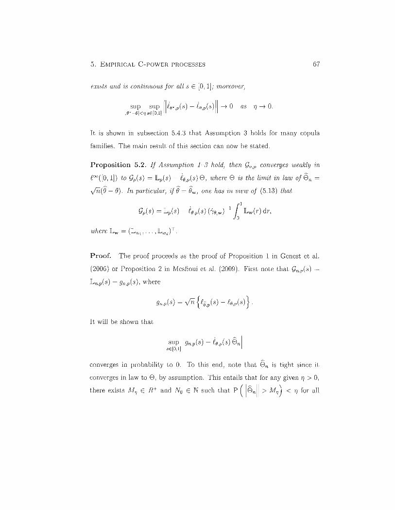
5. EMPIRICAL C-POWER PROCESSES
exists and is continuous for all sE [0,1]; moreover,
sup sup II J?o*,p(s) - [o,p(s)ll-+ 0 as fl-+ O. 10*-01<1) sE [O,l)
67
It is shown in subsection 5.4.3 that Assumption 3 holds for many copula
families. The main result of this section can now be stated.
Proposition 5.2. If Assumption 1-3 hold, then gn,p converges weakly in
[00([0,1]) to gp(s) = lLp(s) - J?o ,p(s) e, where e is the limit in Law of ên =
fo(ê - B). In particular, ifê = êw , one has in view of (5.13) that
gp(s) = lLp(s) - eo,p(s) hO,w)-l 11
lLw(r) dr ,
where lLw = (lLW1 ' ... , lLwJ T .
Proof. The proof proceeds as the pro of of Proposition 1 in Genest et al.
(2006) or Proposition 2 in Mesfioui et al. (2009). First note that gn,p(s) =
lLn,p(s) - 9n,p(S), where
It will be shown that
converges in probability to O. To this end, note that en is tight since it
converges in law to e, by assumption. This entails that for any given fl > 0,
there exists M1) E R+ and No E N such that P (1lênll > M1)) < fl for aIl
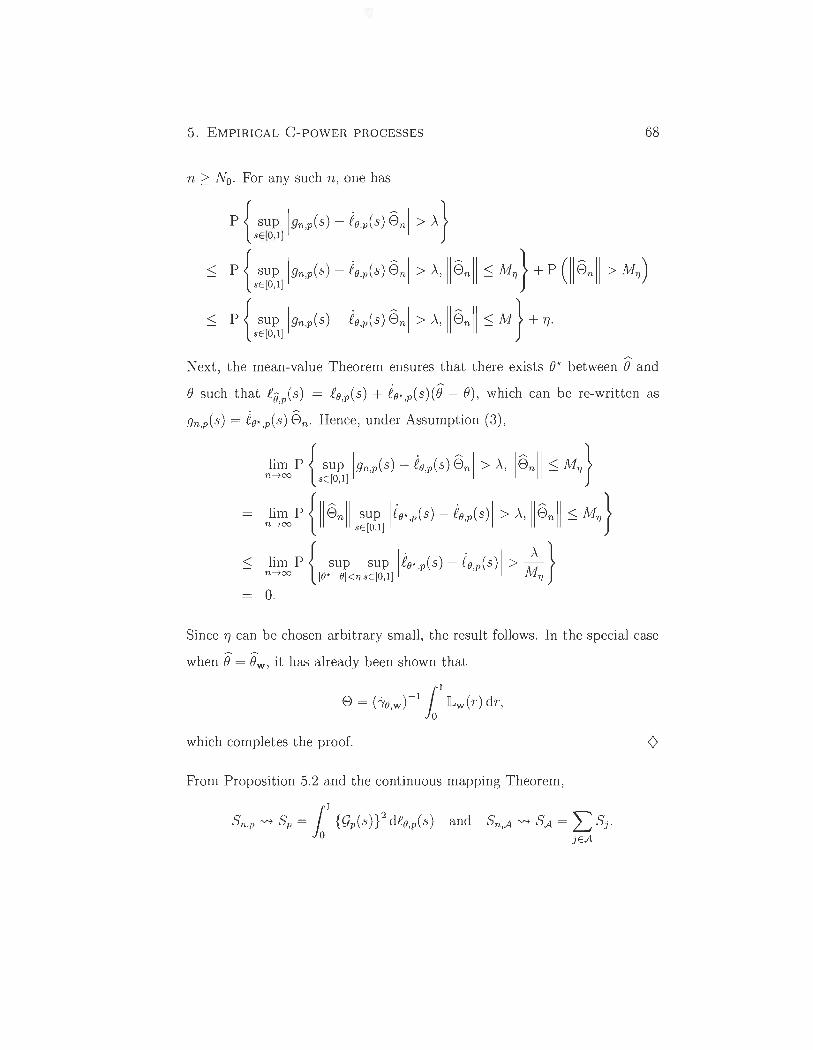
5. E MPIRICAL C-POWER PROCESSES 68
n 2: No. For any such n, one has
P { sup 19n,p(S) - èe,p(s) ênl > À} SE[O,I ]
< P { sup 19n,p(S) - èe,p(s) ênl > À, Ilênll ~ M1) } + P (1lên ll > M1) ) SE[O, I]
< P { sup 19n,p(S) - èe,p(s) ênl > À, Il ên ll ~ M } + 1] . sE [O,I]
Next, the mean-value Theorem ensures that there exists e* between e and
e such that fê,p(s) = fe,p(s) + èe*,p(s )(ê - e), which can be re-written as
9n,p(S) = èe* ,p(s) ên- Hence, under Assumption (3) ,
lim P { sup 19n,p(S) - èe,p(s) ênl > À, Ilênll ~ M1) } n-too sE [O,I ]
!i,~ P {ll ê.11 ,~fl,l l i,.,,(sl -i",(sll > À, Ilê.11 :s M. }
< lim P { sup sup lèe* ,p(s) - ie,p(s) 1 > MÀ
} n-too le*-el<1) SE [O,I ] 1)
o.
Since 1] can be chosen arbitrary small, the result follows. In the special case ~ ~
when e = ew , it has already been shown that
which completes the proof.
From Proposit ion 5.2 and the continuo us mapping Theorem,
Sn,A 'V'-t SA = L Sj. jEA
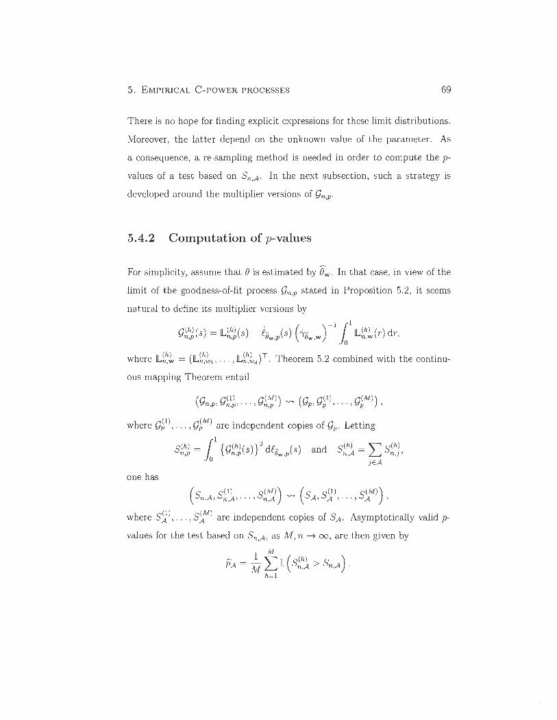
5. EMPIRICAL C-POWER PROCESSES 69
There is no hope for finding explicit expressions for t hese limit distributions.
Moreover , the latter depend on the unknown value of the parameter. As
a consequence, a re-sampling method is needed in order to compute the p
values of a test based on Sn,A. In the next subsection, such a strategy is
developed around the multiplier versions of gn,p .
5.4.2 Computation of p-values
For simplicity, assume that B is estimated by Bw . In that case, in view of the
limit of the goodness-of-fi t process gn,p stated in Proposition 5.2, it seems
natural to define its mult iplier versions by
g (h) (8) = lL(h) (8) - i~ (8) (-v~ ) -111 lL(h) (r ) dr n,p n,p Ow ,p I()w ,w n,w '
o
h lL(h) (lL(h) lL(h) )T Th b d h h w ere n,w = n,Wl ' ... , n,wd. eorem 5.2 corn ine wit t e continu-
ous mapping Theorem entail
(gn,p, g~~~, .. . , g~~) ) "'" (gp, g~l), ... , g~M) ) ,
where g~1) , . . . , g~M) are independent copies of gp. Letting
S(h) = t {g(h)(8) }2 dt'~ (8) and S(h) = " S(h) n,p Jo n,p ()w ,p n,A L.... n,J' o jEA
one has
(S S(l ) (M) ) ( (1) (M) ) n,A, n,A, · ·· ,Sn,A "'" SA, SA , ... , SA '
where S~), . .. , s1M) are independent copies of SA. Asymptotically valid p
values for the test based on Sn,A, as M , n -t 00, are then given by
M
PA = ~ L il ( S~~~ > Sn,A ) . h=l
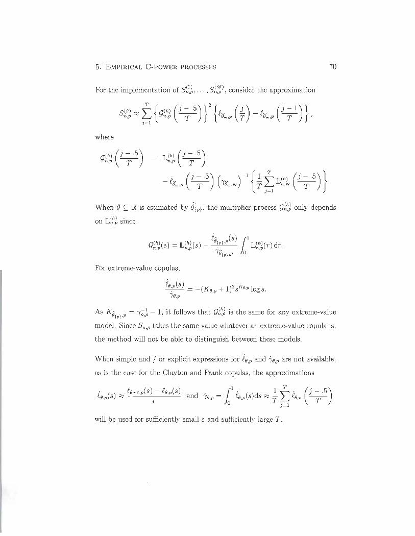
5. EMPIRICAL C-POWER PROCESSES 70
For the implementation of S~:~, ... , S~~:), consider the approximation
(h) ~{ (h) (j-.5 )} 2 { (j) (j - l)} Sn,p ~ ~ gn,p ----;y- eôw ,p T - eôw ,p -y ,
where
g (h) (j - .5) n,p T
[)h) (j - .5) n,p T
_._ (~)( ._ ) -1 {~~ (h) (~)} eow,p T 'Yow,w T ~lLn,w T .
When () ç IR is estimated by ê{p}, the multiplier process g~~ only depends
on lL~~~ since
g (h) (8) = lL(h) (8) - o~p} ,p lL(h) (r) dr. e- (8) 11 n,p n,p 'Y- n,p
o{p} ,P 0
For extreme-value copulas,
As Kr; p = 'Y;;:p1 - 1, it follows that g~hJ is the same for any extreme-value U{p }' , ,
model. Since Sn,p takes the same value whatever an extreme-value copula is,
the method will not be able to distinguish between these models.
When simple and / or explicit expressions for io,p and 'Yo,p are not available,
as is the case for the Clay ton and Frank copulas, the approximations
e· ()",eO+ê ,p(8)-eB,p(8) d' - ( le' ()d "'~ ~ e· (j-.5 ) B,p 8 '" E an 'Yo,p - Jo o,p 8 8 '" T ~ o,p T
o j=l
will be used for sufficiently small é and sufficiently large T.
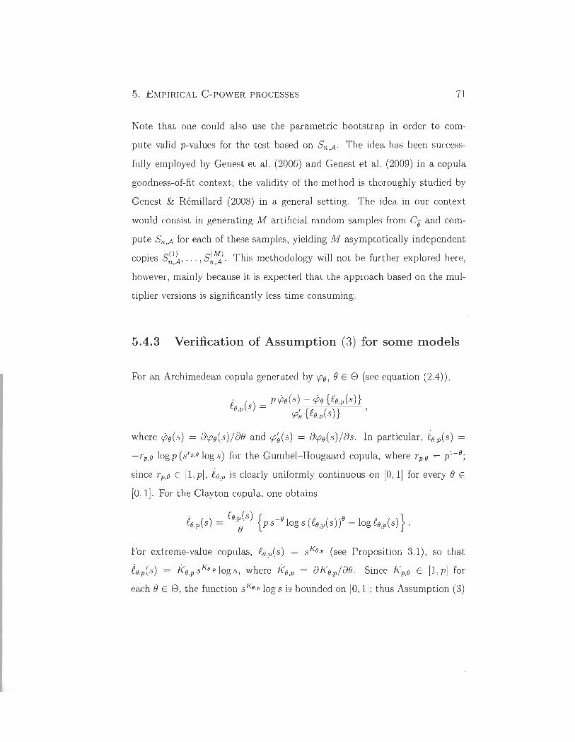
5. EMPIRICAL C-POWER PROCESSES 71
Note that one cou Id also use the parametric bootstrap in order to com
pute valid p-values for the test based on Sn,A. The idea has been success
fully employed by Genest et al. (2006) and Genest et al. (2009) in a copula
goodness-of-fit context; the validity of the method is thoroughly studied by
Genest & Rémillard (2008) in a general setting. The idea in our context
would consist in generating M artificial random samples from Oô and com
pute Sn,A for each of these samples, yielding M asymptotically independent
copies S~~~, . .. , S~'- . This methodology will not be further explored here,
however, mainly because it is expected that the approach based on the mul
tiplier versions is significantly less time consuming.
5.4.3 Verification of Assurnption (3) for sorne rnodels
For an Archimedean copula generated by <p(l, BEe (see equation (2.4)) ,
i () _ PCPo(s) - CPo {fo ,p(s)} O,p S - <p~ {fo ,p(s)} ,
where cpo(s) = 8<po(s)/8B and <p~(s) = 8<po(s)/8s. In particular , io,p(s) =
-r p,O log p (STp ,O log s) for the Gumbel- Hougaard copula, where r p,O = pl-O;
since r p,o E [1, pl, io,p is clearly uniformly continuous on [0, 1] for every B E
[0, 1] . For the Clay ton copula, one obtains
For extreme-value copulas, fo ,p(s) = sKo,p (see Proposition 3.1), so that
io,p(s) = Ko,p sKo.p log s, where Ko ,p = 8Ko,p/8B. Since Kp,o E [1, p] for
each BEe, the function sKo,p log sis bounded on [0,1]; thus Assumption (3)
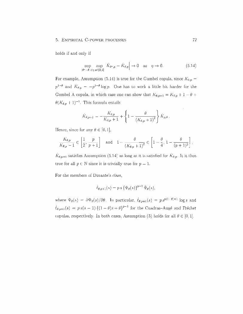
5. EMPIRICAL C-POWER PROCESSES 72
ho Ids if and only if
sup sup Iko* ,p - ko,pl ~ 0 as 'fi ~ O. 10*-01<11 s E[O,l ]
(5.14)
For example, Assumption (5.14) is true for the Gumbel copula, since Ko,p =
p1-0 and ko,p = -p1- 01ogp. One has to work a little bit harder for the
Gumbel A copula, in which case one can show that KO,p+1 = Ko,p + 1 - 0 +
O(Ko,p + 1)- 1. This formula entails
. Ko { o} . K = - ,p + 1- K O,pH K + 1 (K 1)2 p,O . O,p O,p +
Hence, since for any 0 E [0 , 1],
Ko,p [1 p] Ko,p + 1 E 2' p + 1
and 1 - 0 E [1 _ ~ 1 _ -:--_0--:-::-] (Ko ,p+l)2 4 ' (p+l)2 '
kO,pH satisfies Assumption (5 .14) as long as it is satisfied for ko,p. It it thus
true for aH pEN since it is trivially true for p = 1.
For the members of Durante's class,
where wo(s) = 8wo(s)/80. In particular , iO ,pH(S) = psP(1-0)H logs and
iO,pH(S) = ps(s - 1) {(1 - O)s + Oy- 1 for the Cuadras- Augé and Fréchet
copulas, respectively. In both cases, Assumption (3) holds for aH 0 E [0 , 1].
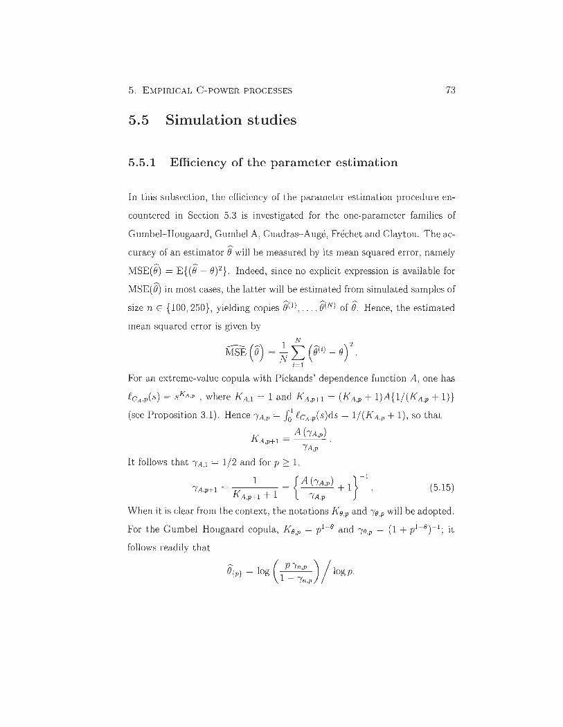
5. EMPIRICAL C-POWER PROCESSES 73
5.5 Simulation studies
5.5.1 Efficiency of the parameter estimation
In this subsection, the efficiency of the parameter estimation procedure en
countered in Section 5.3 is investigated for the one-parameter families of
Gumbel- Rougaard, Gumbel A, Cuadras- Augé, Fréchet and Clay ton. The ac-~
curacy of an estimator e will be measured by its mean squared error, namely
MSE(ê) = E{ (ê - e)2}. Indeed, since no explicit expression is available for
MSE(ê) in most cases, the latter will be estimated from simulated samples of
size n E {100, 250}, yielding copies ê(1) , ... ,ê(N) of ê. Rence, the estimated
mean squared error is given by
For an extreme-value copula with Pickands' dependence function A, one has
eCA ,p(s) = SKA.7' , where KA,l = 1 and KA,p+l = (KA,p + l)A{l/(KA,p + 1)}
(see Proposition 3.1). Rence Î'A ,p = fol fcA,p(s)ds = l/(KA,p + 1), so that
}'/ _ A hA,p) '\.A,p+l - .
Î'A,p
It follows that Î' A,l = 1/2 and for p ~ 1,
1 {A hA,p) }-l Î'Ap+l= = +1
, KA,p+l + 1 Î'A ,p (5.15)
When it is clear from the context, the notations Ke,p and Î'e,p will be adopted.
For the Gumbel- Rougaard copula, Ke,p = pl-e and Î'e,p = (1 + pl-etl ; it
follows readily that
ê{p} = log ( P_Î'n,p ) / log p. 1 Î'n,p
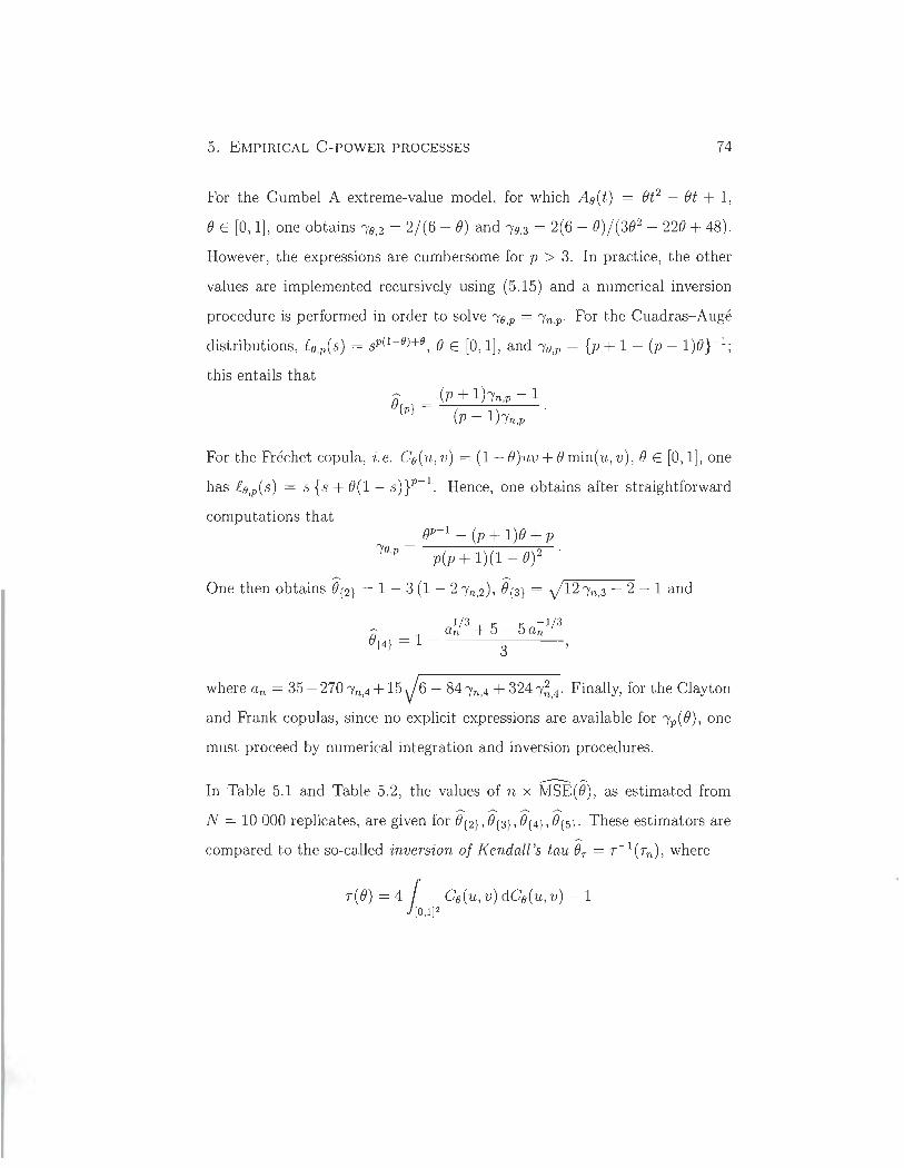
5. EMPIRICAL C-POWER PROCESSES 74
For the Gumbel A extreme-value model, for which Ao(t) = Bt2 - Bt + 1,
B E [0,1], one obtains 10,2 = 2/(6 - B) and 10,3 = 2(6 - B) /( 3B2 - 22B + 48).
However, the expressions are cumbersome for p > 3. In practice, the other
values are implemented recursively using (5.15) and a numerical inversion
procedure is performed in order to solve 10,P = In,p. For the Cuadras-Augé
distributions, Co ,p(s) = sp{l-O) +II , B E [0,1], and 10,P = {p + 1 - (p - 1)B} -1;
this entails that ê = (p + 1 hn,p - 1
{p} (p - 1hn,p .
For the Fréchet copula, i.e. Co(u, v) = (1- B)uv + Bmin(u, v), B E [0,1], one
has Co,p(s) = s {s + B(l - S)}P-1. Hence, one obtains after straightforward
computations that BP+! - (p + l)B + P
10,P = p(p + 1)(1 _ B)2
One then obtains ê{2} = 1 - 3 (1 - 2 In,2) , ê{3} = J12 , n ,3 - 2 - 1 and
~ 1/ 3 + 5 _ 5 -1/ 3 B _l_ an an
{4} - 3'
where an = 35 - 270 In,4 + 15)6 - 84 ,n,4 + 324';,4. Finally, for the Clay ton
and Frank copulas, since no explicit expressions are available for 'P( B) , one
must proceed by numerical integration and inversion procedures.
------ ~ In Table 5.1 and Table 5.2, the values of n x MSE(B) , as estimated from
N = 10000 replicates, are given for ê{2} , ê{3}, ê{4} , ê{5}. These estimators are
compared to the so-called inversion of Kendall's tau êT = T- 1(Tn ) , where
T(B) = 4 r Co(u , v) dCo(u, v) - 1 ) [0,1]2
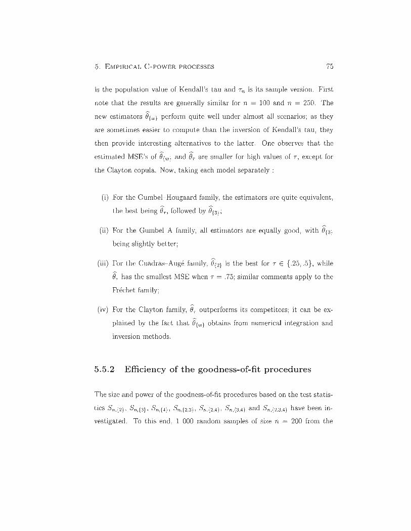
5. EMPIRICAL C-POWER PROCESSES 75
is the population value of Kendall's tau and Tn is its sample version. First
note that the results are generally similar for n = 100 and n = 250. The ~
new estimators e{w} perform quite well under almost aU scenarios; as they
are sometimes easier to compute than the inversion of Kendall's tau, they
then provide interesting alternatives to the latter. One observes that the ~ ~
estimated MSE's of e{w } and eT are sm aller for high values of T, except for
the Clay ton copula. Now, taking each model separately :
(i) For the Gumbel- Hougaard family, the estimators are quite equivalent, ~ ~
the best being en followed by e{3};
(ii) For the Gumbel A family, all estimators are equally good, with e{3}
being slightly better;
(iii) For the Cuadras- Augé family, ê{2} is the best for T E {.25, .5}, while
eT has the smallest MSE when T = .75; similar comments apply to the
Fréchet family ;
(iv) For the Clay ton family, eT outperforms its competitors; it can be ex
plained by the fact that e{w } obtains from numerical integration and
inversion methods.
5.5.2 Efficiency of the goodness-of-fit procedures
The size and power of the goodness-of-fit procedures based on the test statis
tics Sn,{2} , Sn,{3} , Sn,{ 4}, Sn,{2 ,3} , Sn,{2 ,4} , S n, {3 ,4} and Sn,{2 ,3,4} have been in
vestigated. To this end, 1 000 random samples of size n = 200 from the
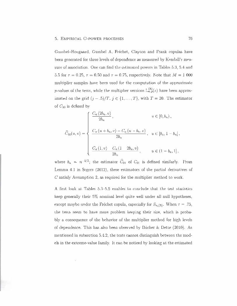
5. EMPIRICAL C-POWER PROCESSES 76
Gumbel-Hougaard , Gumbel A, Fréchet , Clay ton and Frank copulas have
been generated for three levels of dependence as measured by Kendall's mea
sure of association. One can find the estimated powers in Tables 5.3, 5.4 and
5.5 for T = 0.25, T = 0.50 and T = 0.75, respectively. Note that M = 1 000
multiplier samples have been used for the computation of the approximate
p-values of the tests , while the multiplier versions lL~~~( s) have been approx
imated on the grid (j - .5)/T, j E {l, . .. ,T}, with T = 20. The estimator
of C lO is defined by
Cn (2bn, v) u E [0, bn),
2bn
êlO(u, v) = Cn (u + bn, v) - Cn (u - bn, v)
u E [bn, 1 - bnl , 2bn
,
Cn (1 , v) - Cn (1 - 2bn, v) u E (1 - bn, 1],
2bn
where bn = n-I/2; the estimator COI of COl is defined similarly. From
Lemma 4.1 in Segers (2012), these estimators of the partial derivatives of
C satisfy Assumption 2, as required for the multiplier method to work.
A first look at Tables 5.3-5 .5 enables to conclu de that the test statistics
keep generally their 5% nominal level quite well under all null hypotheses,
except maybe under the Fréchet copula, especially for Sn,{3}' When T = .75,
the tests seem to have more problem keeping their size, which is proba
bly a consequence of the behavior of the multiplier method for high levels
of dependence. This has also been observed by Bücher & Dette (2010). As
mentioned in subsection 5.4.2, the tests cannot distinguish between the mod
els in the extreme-value family. It can be noticed by looking at the estimated
5. EMPIRICAL C-POWER PROCESSES 77
probability of rejection of Ho wh en the data come from either the Gumbel
Hougaard or Gumbel A copula. Under Clay ton alternatives, all test statistics
are very powerful, especially when the null hypothesis concerns an extreme
value model; this coincides with the empirical results of Quessy (2012) when
testing for extreme-value dependence. The Frank copula is also well detected
by all the test statistics. One can also note that
(i) wh en the alternatives belong to the extreme-value family, Sn,{3}, Sn,{4}'
Sn,{2,3} , Sn,{2,4} , Sn,{3 ,4} and Sn,{2,3,4} are almost as powerful (Sn,{2 ,4} is
the best) , Sn,{2} being significantly less powerful;
(ii) under Fréchet alternatives , Sn,{2} is significantly most powerful than its
competitors, followed by Sn,{2,3}, while Sn,{4} is the less powerful;
(iii) un der Clay ton alternatives, the null hypothesis of an extreme-value
copula is rejected for almost all test statistics.
It is also worth to note that our tests are very quick to implement, which
is not negligible especially if one wants to analyze large data sets. This is
mainly due to the use of the multiplier method and the recursive nature of
the C-power functions. Considering this and the fact that the power of our
tests seems in general comparable to that of the goodness-of-fit test of Genest
et al. (2006), our method is an interesting alternative to existing methods.
5. EMPIRICAL C-POWER PROCESSES 78
5.6 Illustration on the Uranium exploration
data set
The methods developed in this work will be illustrated on the Uranium ex
ploration data set first considered by Cook & Johnson (1981) and Cook &
Johnson (1986) and later revisited by Genest et al. (2006) in the light of
new goodness-of-fit tests for copulas. The data set consists of 655 chemical
measurements from water samples collected from the Montrose quadrangle of
western Colorado in the United States. The analysis presented here considers
the concentrations in cobalt (Co), caesium (Cs), scandium (Sc) and titanium
(Ti). The models that were tested are the one-parameter copula families
of Gumbel, Fréchet, Clay ton and Frank. The results of the goodness-of-fit
procedures based on Sn,{2,3} , Sn, {2 ,4} and Sn,{3 ,4} are in Table 5.6. The tests
based on Sn,{2}, Sn,{3} and Sn,{4} were also performed, but the results were
very similar; they therefore have been omitted. The p-values were estimated
from M = 1 000 multiplier samples. The conclusions coincide generally with
those of Genest et al. (2006).
Sorne of the conclusions that one can extract from Table 5.6 could also be
deduced by looking at the empirical C-power functions and their associated
95% confidence band computed from the multiplier method. For example,
the Gumbel copula was selected as an appropriate model for the pair (Cs,Ti) ;
aIl other models were clearly rejected. In that case, the C-power functions
of the Gumbel copula can be seen to live inside the confidence band wh en
p = 2 and p = 3 (see Figure 5.1) , contrary to the C-power functions of the
5. EMPIRICAL C-POWER PROCESSES 79
.Clayton copula (see Figure 5.2).
For the pair (Sc,Ti), the Fréchet copula was accepted, but the p-values are
only slightly higher than .05. In such cases, it would be interesting to consider
multi-parameter models. For example, consider an Archimax copula with a
Gumbel Archimedean generator 'l/;f3 (t) = IlogtI 1/ (1- f3 ) and a Cuadras-Augé
extreme part AQ (t) = 1 - a min ( t, 1 - t). In that case, the estimation of
(a , /3) E [0, IF based on the method in Section 6 with w = {2, 3} exploits
the fact that the first two C-power functions are of the fonu
where K2(a) = 2 - a and K3(a) = 3 - 2a. It can be shown that â{2,3} is the
solution of
and then
log Cr~J - 1) log Cr~~ - 1)
log(2 - a) log(3 - 2a) ,
~ log Cr;;:~ - 1) /3{2 ,3} = 1 - ( , ~ ).
log 2 - a{2,3}
Since for the pair (Sc,Ti), "/n,2 = .402 and "/n,3 = .343, one finds â{2,3} = .245
and /3{2,3} = .294. This estimation method for more than one parameter and
the related goodness-of-fit test deserve to be investigated in more details in
future works.
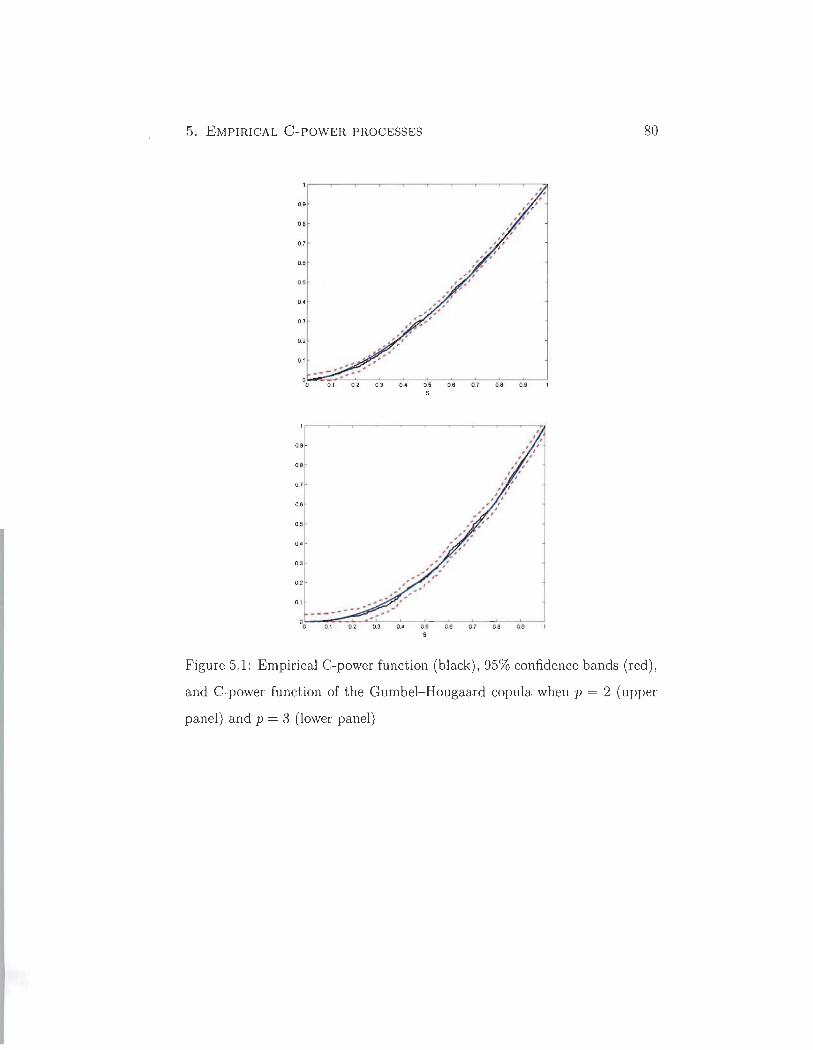
5. EMPIRICAL C-POWER PROCESSES
o .•
0.8
0.7
O .•
0.5
o .•
0.3
0.2
0.1
0 0 0.1
1 1
1 1 1 1
1 1 1 1
1 1 1 1
1 1 1 1
1 1 Il Il
1 1 , 1
, 1
,~' .. " , " , , ,
" , 1 l'
" " , 1 , 1
~ .. -' ,.,' " ,
,,.' ,,'
o.. 0.5 0.6 0.7 0.8 0.9
S
80
Figure 5.1: Empirical C-power function (black), 95% confidence bands (red) ,
and C-power function of the Gumbel- Hougaard copula when p = 2 (upper
panel) and p = 3 (lower panel)
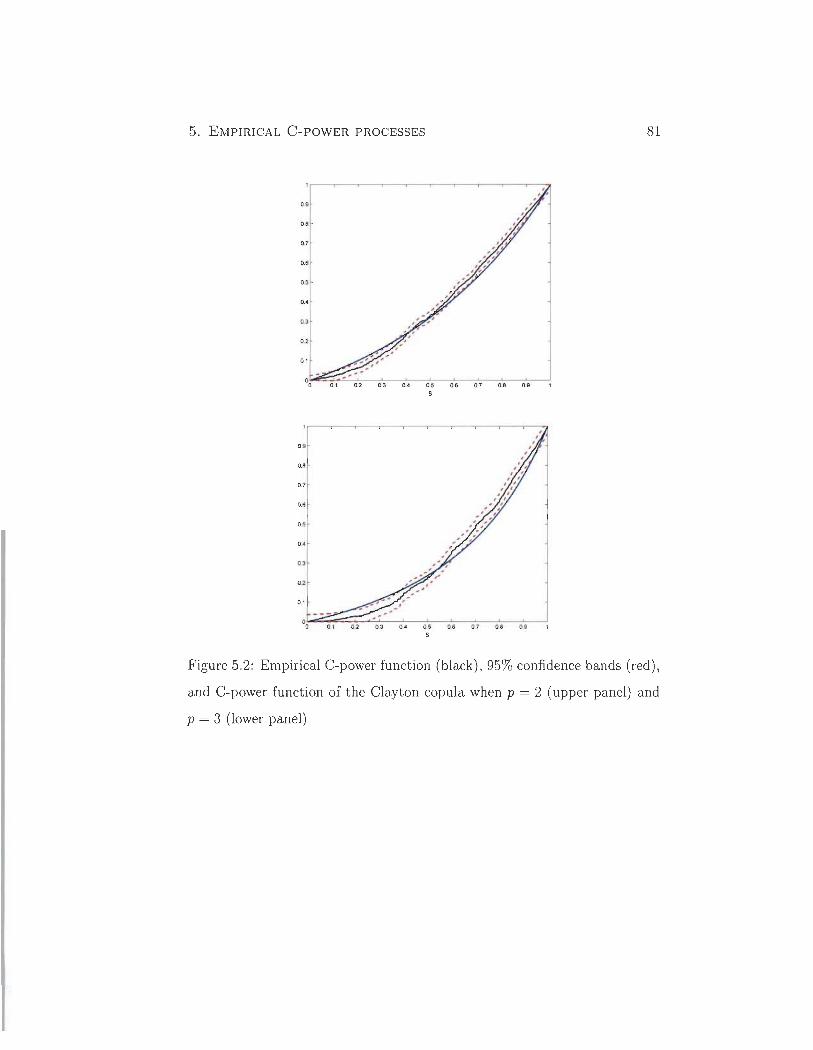
5. EMPIRICAL C-POWER PROCESSES 81
0.9
0.8
0.7
0.6
0.5
o .•
0.3
0.2
0 .1
Figure 5.2: Empirical C-power function (black) , 95% confidence bands (red),
and C-power function of the Clay ton copula when p = 2 (upper panel) and
p = 3 (lower panel)
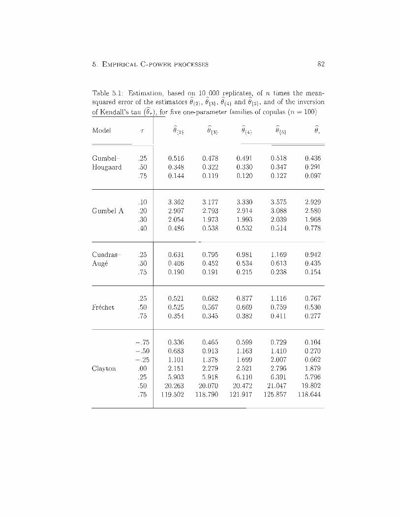
5. EMPIRICAL C-POWER PROCESSES 82
Table 5.1: Estimation, based on 10 000 replicates, of n times the meansquared error of the estimators ê{2} , ê{3 } , ê{ 4} and ê{5}' and of the inversion
:::~drul'S t.uT(o'!' for fi~:)on~PM:::ter fami;:: of copu;:) (n ~ 100:,
GumbelHougaard
Gumbel A
CuadrasAugé
Fréchet
Clay ton
.25
.50
.75
.10
.20
.30
.40
.25
.50
.75
.25
.50
.75
-.75 -.50 -.25 .00 .25 .50 .75
0.516 0.348 0.144
3.362 2.907 2.054 0.486
0.631 0.406 0.190
0.521 0.525 0.354
0.336 0.683 1.101 2.151 5.903
20.263 119.502
0.478 0.322 0.119
3.177 2.793 1.973 0.538
0.795 0.452 0.191
0.682 0.567 0.345
0.465 0.913 1.378 2.279 5.918
20.070 118.790
0.491 0.330 0.120
3.330 2.914 1.993 0.532
0.981 0.534 0.215
0.877 0.669 0.382
0.599 1.163 1.699 2.521 6.110
20.472 121.917
0.518 0.347 0.127
3.575 3.088 2.039 0.514
1.169 0.613 0.238
1.116 0.759 0.411
0.729 1.410 2.007 2.796 6.391
21.047 125.857
0.436 0.291 0.097
2.929 2.580 1.968 0.778
0.942 0.435 0.154
0.767 0.530 0.277
0.104 0.270 0.662 1.879 5.796
19.802 118.644

5. EMPIRICAL C-POWER PROCESSES 83
Table 5.2: Estimation, based o}l 10 ~OOO !eplicate~ of n times the meansquared error of the estimators B{2}, B{3}' B{4} and B{5}, and of the inversion
:o::~dall'S taUT(ôl for fi:(:}on~p~:::ter frun::: of coPu;:} (n ~ 250:,
GumbelHougaard
Gumbel A
CuadrasAugé
Fréchet
Clay ton
.25
.50
.75
.10
.20
.30
.40
.25
.50
.75
.25
.50
.75
-.75 -.50 -.25 .00 .25 .50 .75
0.472 0.303 0.107
3.013 2.889 2.227 0.687
0.653 0.446 0.213
0.559 0.575 0.392
0.701 1.044 1.398 2.363 5.688
19.824 126.997
0.455 0.293 0.098
2.957 2.851 2.144 0.733
0.809 0.469 0.196
0.695 0.586 0.353
1.001 1.424 1.789 2.524 5.616
19.063 114.073
0.468 0.302 0.100
3.138 2.939 2.168 0.725
0.996 0.548 0.217
0.880 0.685 0.389
1.389 1.935 2.325 2.938 5.937
19.620 116.321
0.489 0.316 0.104
3.386 3.073 2.222 0.709
1.183 0.628 0.239
1.079 0.803 0.427
1.788 2.507 2.939 3.440 6.411
20.425 121.520
0.429 0.279 0.089
3.036 2.814 1.937 0.863
0.901 0.432 0.151
0.757 0.525 0.269
0.103 0.264 0.642 1.821 5.456
18.533 114.604
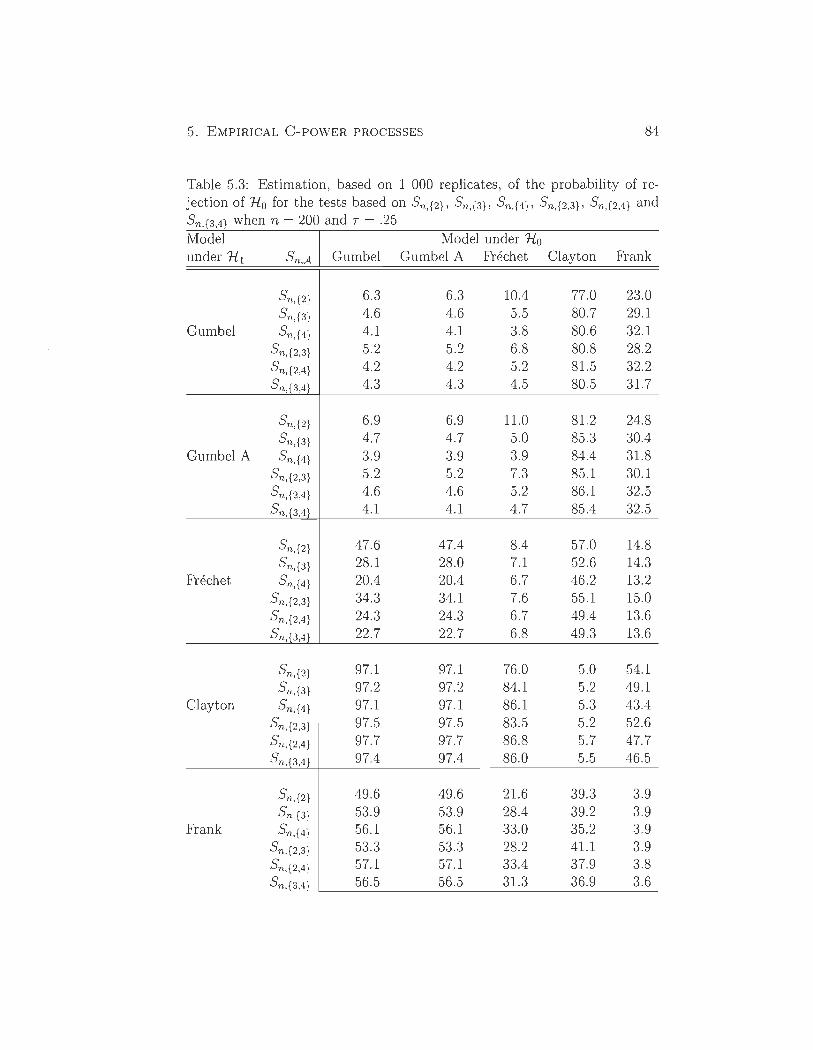
5. EMPIRICAL C-POWER PRO CESSES 84
Table 5.3: Estimation, based on 1 000 replicates, of the probability of rejection of Ho for the tests based on Sn,{2}, Sn,{3} , Sn,{4}, Sn,{2,3}, Sn,{2,4} and Sn,{3 ,4} when n = 200 and 7 = .25 Madel Madel under Ho under Hl Sn,A Gumbel Gumbel A Fréchet Clay ton Frank
Sn,{2} 6.3 6.3 10.4 77.0 23.0
Sn,{3} 4.6 4.6 5.5 80.7 29.1 Gumbel Sn,{4} 4.1 4.1 3.8 80.6 32.1
Sn,{2 ,3} 5.2 5.2 6.8 80.8 28.2
Sn,{2,4} 4.2 4.2 5.2 81.5 32.2
Sn,{3,4} 4.3 4.3 4.5 80.5 31.7
Sn,{2} 6.9 6.9 11.0 81.2 24.8
Sn,{3} 4.7 4.7 5.0 85.3 30.4 Gumbel A Sn,{4} 3.9 3.9 3.9 84.4 31.8
Sn,{2 ,3} 5.2 5.2 7.3 85.1 30.1 Sn,{2,4} 4.6 4.6 5.2 86.1 32.5
Sn,{3,4} 4.1 4.1 4.7 85.4 32.5
Sn,{2} 47.6 47.4 8.4 57.0 14.8 Sn,{3} 28.1 28.0 7.1 52.6 14.3
Fréchet Sn,{4} 20.4 20.4 6.7 46.2 13.2
Sn,{2 ,3} 34.3 34.1 7.6 55.1 15.0
Sn,{2,4} 24.3 24.3 6.7 49.4 13.6 Sn,{3,4} 22.7 22.7 6.8 49.3 13.6
Sn,{2} 97.1 97.1 76.0 5.0 54.1 Sn,{3} 97.2 97.2 84.1 5.2 49.1
Clay ton Sn,{4} 97.1 97.1 86.1 5.3 43.4
Sn,{2 ,3} 97.5 97.5 83.5 5.2 52.6 Sn,{2,4} 97.7 97.7 86.8 5.7 47.7
Sn,{3 ,4} 97.4 97.4 86.0 5.5 46.5
Sn,{2} 49.6 49.6 21.6 39.3 3.9 Sn,{3} 53.9 53.9 28.4 39.2 3.9
Frank Sn,{4} 56.1 56.1 33.0 35.2 3.9
Sn,{2 ,3} 53.3 53.3 28.2 41.1 3.9 Sn,{2 ,4} 57.1 57.1 33.4 37.9 3.8 Sn,{3,4} 56.5 56.5 31.3 36.9 3.6
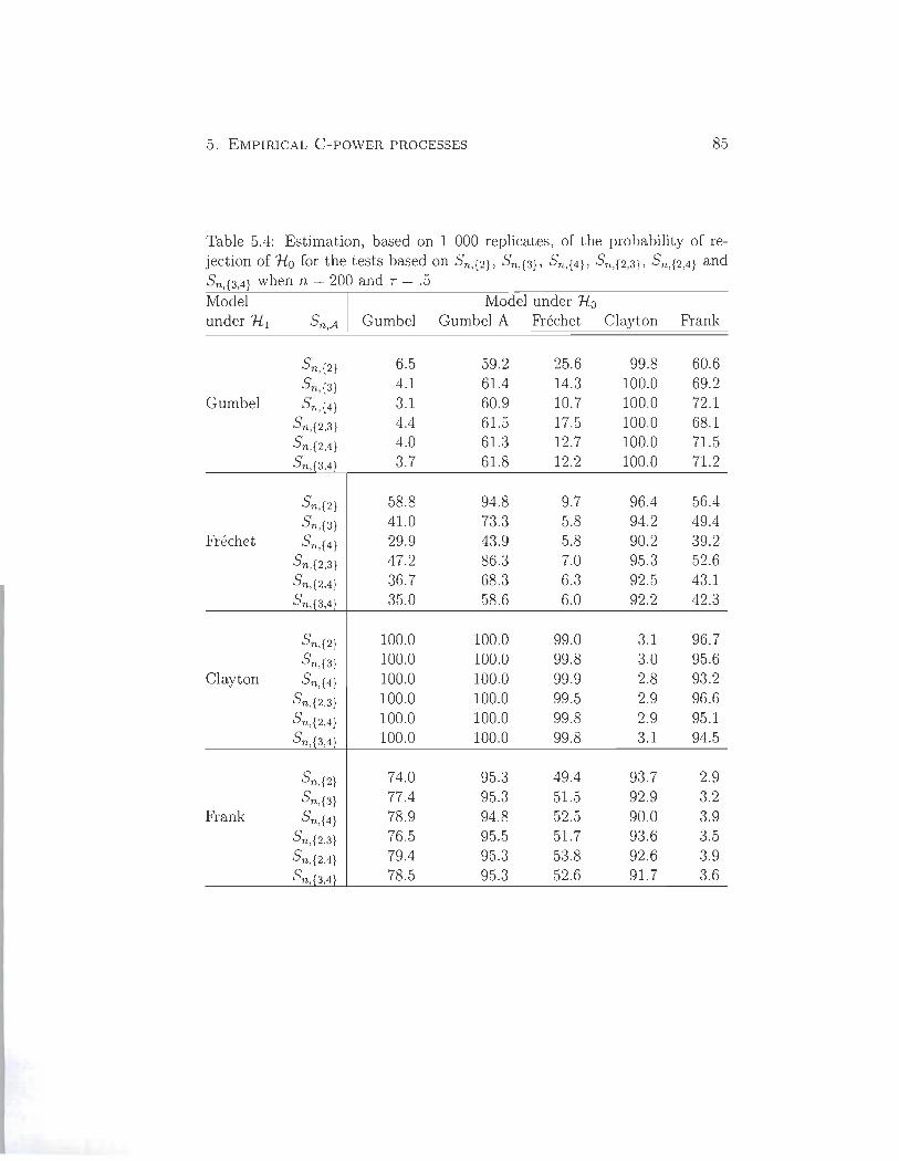
5. EMPIRICAL C-POWER PROCESSES 85
Table 5.4: Estimation, based on 1 000 replicates, of the probability of rejection of Ho for the tests based on Sn,{2}, Sn,{3} , Sn,{4} , Sn,{2 ,3} , Sn,{2 ,4} and Sn{34} wh en n = 200 and T = .5 , ,
Model Model under Ho under Hl Sn,A Gumbel Gumbel A Fréchet Clay ton Frank
Sn,{2} 6.5 59.2 25.6 99.8 60.6 Sn,{3} 4.1 61.4 14.3 100.0 69.2
Gumbel Sn,{4} 3.1 60.9 10.7 100.0 72.1
Sn, {2 ,3} 4.4 61.5 17.5 100.0 68.1
Sn,{2 ,4} 4.0 61.3 12.7 100.0 71.5
Sn,{3 ,4} 3.7 61.8 12.2 100.0 71.2
Sn,{2} 58.8 94.8 9.7 96.4 56.4 Sn,{3} 41.0 73.3 5.8 94.2 49.4
Fréchet Sn,{4} 29.9 43.9 5.8 90.2 39.2 Sn,{2 ,3} 47.2 86.3 7.0 95.3 52.6 Sn,{2 ,4} 36.7 68.3 6.3 92.5 43.1
Sn,{3 ,4} 35.0 58.6 6.0 92.2 42.3
Sn,{2} 100.0 100.0 99.0 3.1 96.7 Sn,{3} 100.0 100.0 99.8 3.0 95.6
Clay ton Sn,{4} 100.0 100.0 99.9 2.8 93.2
Sn,{2 ,3} 100.0 100.0 99.5 2.9 96.6 Sn,{2,4} 100.0 100.0 99.8 2.9 95.1 Sn,{3,4} 100.0 100.0 99.8 3.1 94.5
Sn,{2} 74.0 95.3 49.4 93.7 2.9 Sn,{3} 77.4 95.3 51.5 92.9 3.2
Frank Sn,{4} 78.9 94.8 52.5 90.0 3.9
Sn,{2 ,3} 76.5 95.5 51.7 93.6 3.5 Sn,{2,4} 79.4 95.3 53.8 92.6 3.9
Sn,{3,4} 78.5 95.3 52.6 91.7 3.6
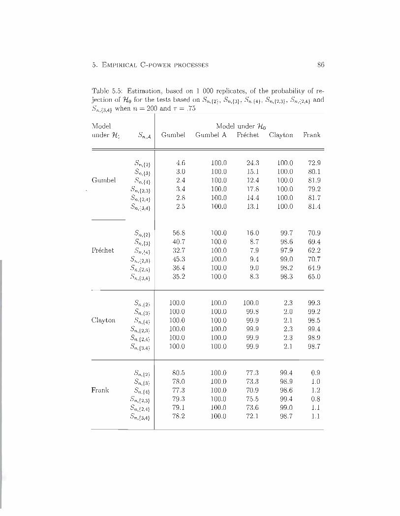
5. EMPIRICAL C-POWER PROCESSES 86
Table 5.5: Estimation, based on 1 000 replicates, of the probability of rejection of Ho for the tests based on Sn,{2}, Sn,{3}, Sn,{4} , Sn,{2,3} , Sn,{2,4} and Sn,{34} wh en n = 200 and T = .75 ,
Model Model under Ho un der Hl Sn,A Gumbel Gumbel A Fréchet Clay ton Frank
Sn,{2} 4.6 100.0 24.3 100.0 72.9 Sn,{3} 3.0 100.0 15.1 100.0 80.1
Gumbel Sn,{4} 2.4 100.0 12.4 100.0 81.9 Sn,{2,3} 3.4 100.0 17.8 100.0 79.2 Sn,{2 ,4} 2.8 100.0 14.4 100.0 81.7 Sn,{3,4} 2.5 100.0 13.1 100.0 81.4
Sn,{2} 56.8 100.0 16.0 99.7 70.9 Sn,{3} 40.7 100.0 8.7 98.6 69.4
Fréchet Sn,{4} 32.7 100.0 7.9 97.9 62.2 Sn,{2,3} 45.3 100.0 9.4 99.0 70.7 Sn,{2,4} 36.4 100.0 9.0 98.2 64.9 Sn,{3,4} 35.2 100.0 8.3 98.3 65.0
Sn,{2} 100.0 100.0 100.0 2.3 99.3 Sn,{3} 100.0 100.0 99.8 2.0 99.2
Clay ton Sn,{4} 100.0 100.0 99.9 2.1 98.5 Sn,{2 ,3} 100.0 100.0 99.9 2.3 99.4 Sn,{2 ,4} 100.0 100.0 99.9 2.3 98.9 Sn,{3,4} 100.0 100.0 99.9 2.1 98.7
Sn,{2} 80.5 100.0 77.3 99.4 0.9 Sn,{3} 78.0 100.0 73.3 98.9 1.0
Frank Sn,{4} 77.3 100.0 70.9 98.6 1.2 Sn,{2,3} 79.3 100.0 75.5 99.4 0.8 Sn,{2,4} 79.1 100.0 73.6 99.0 1.1 Sn,{3 ,4} 78.2 100.0 72.1 98.7 1.1
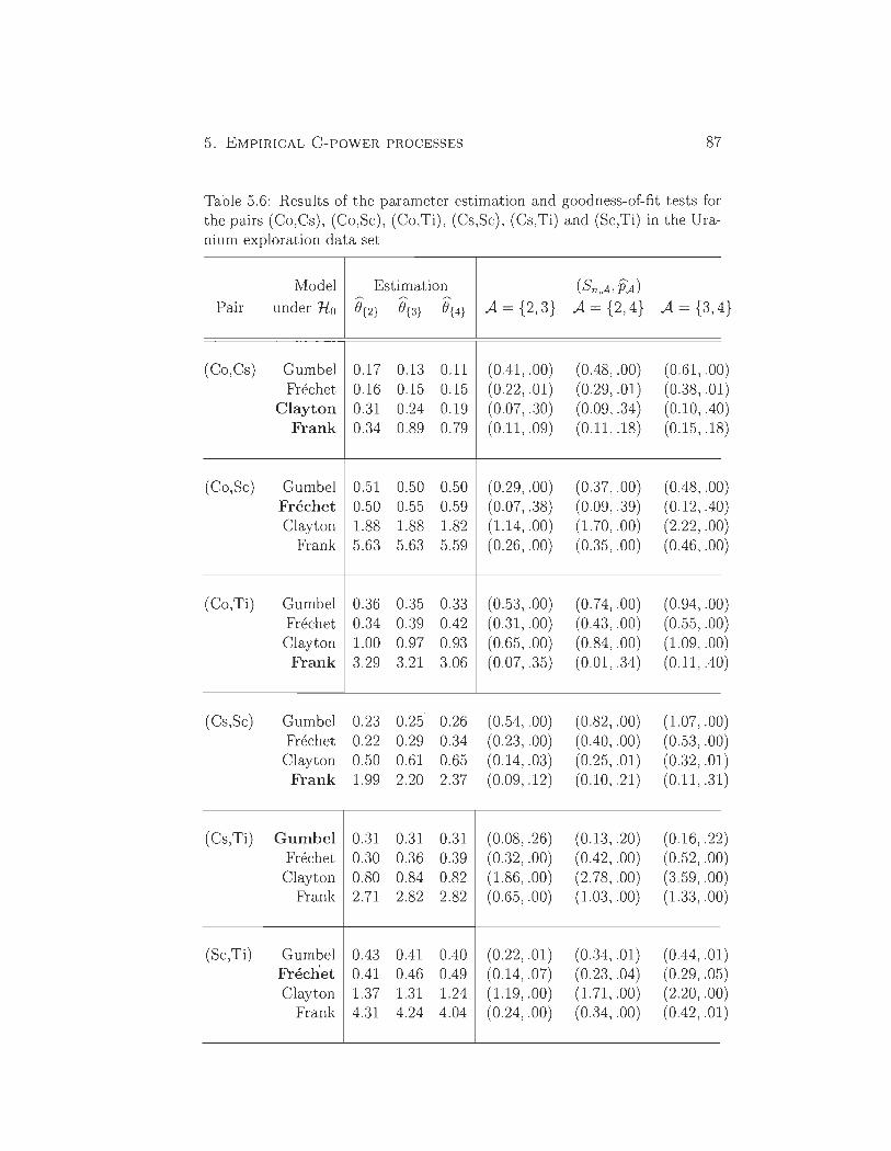
5. EMPIRICAL C-POWER PROCESSES 87
Table 5.6: Results of the parameter estimation and goodness-of-fit tests for the pairs (Co,Cs) , (Co,Sc), (Co,Ti) , (Cs,Sc), (Cs,Ti) and (Sc,Ti) in the Uranium exploration data set
Model Estimation (Sn,A , PA) Pair under Ho B{2} B{3} B{4} A = {2, 3} A={2,4} A= {3, 4}
(Co,Cs) Gumbel 0.17 0.13 0.11 (0.41 , .00) (0.48 , .00) (0.61 , .00 Fréchet 0.16
Clay ton 0.31 Frank 0.34
(Co, Sc) Gumbel 0.51 Fréchet 0.50 Clay ton 1.88
Frank 5.63
(Co,Ti) Gumbel 0.36 Fréchet 0.34 Clay ton 1.00
Frank 3.29
(Cs,Sc) Gumbel 0.23 Fréchet 0.22
Clay ton 0.50 Frank 1.99
(Cs,Ti) Gumbel 0.31 Fréchet 0.30 Clay ton 0.80
Frank 2.71
(Sc,Ti) Gumbel 0.43 Fréchet 0.41 Clay ton 1.37
Frank 4.31
0.15 0.15 0.24 0.19 0.89 0.79
0.50 0.50 0.55 0.59 1.88 1.82 5.63 5.59
0.35 0.33 0.39 0.42 0.97 0.93 3.21 3.06
0.25 0.26 0.29 0.34 0.61 0.65 2.20 2.37
0.31 0.31 0.36 0.39 0.84 0.82 2.82 2.82
0.41 0.40 0.46 0.49 1.31 1.24 4.24 4.04
(0.22, .01) (0.29 , .01) (0.07, .30) (0.09, .34) (0.11, .09) (0.11 , .18)
(0.29 , .00) (0.37, .00) (0.07, .38) (0.09, .39) (1.14, .00) (1.70 , .00) (0.26, .00) (0 .35, .00)
(0.53, .00) (0.74, .00) (0.31 , .00) (0 .43, .00) (0.65 , .00) (0.84, .00) (0.07, .35) (0.01 , .34)
(0.54, .00) (0.82, .00) (0.23, .00) (0.40 , .00) (0.14, .03) (0.25, .01) (0.09, .12) (0.10 , .21)
(0.08, .26) (0 .13, .20) (0.32 , .00) (0.42 , .00) (1.86 , .00) (2.78, .00) (0.65 , .00) (1.03, .00)
(0.22 , .01) (0.34, .01) (0.14, .07) (0.23, .04) (1.19, .00) (1.71 , .00) (0 .24, .00) (0 .34, .00)
(0.38, .01 (0.10 , .40 (0.15 , .18
(0.48, .00 (0 .12, .40 (2 .22 , .00 (0.46 , .00
(0.94, .00 (0.55 , .00 (1.09 , .00 (0.11 , .40
(1.07, .00 (0.53, .00 (0.32, .01 (0.11 , .31
(0 .16, .22 (0.52, .00 (3.59, .00 (1.33, .00
(0.44, .01 (0 .29, .05 (2.20, .00 (0.42 , .01
) ) ) )
CHAPITRE 6
CONCLUSION
Dans ce mémoire, les fonctions de C-puissance associées à une copule ont été
introduites et leurs propriétés ont été étudiées théoriquement. Ensuite, des
versions empiriques ont été proposées, de même que des formules résursives
qui facilitent grandement leur évaluation. Par une application non-triviale
de la méthode Delta fonctionnelle, on a mont ré la convergence faible de
processus basés sur les versions normalisées de ces fonctions empiriques. On
a également démontré rigoureusement la validité asymptotique de versions
multiplicateurs de ces processus.
Comme applications des résultats asymptotiques obtenus, de nouvelles procé
dures d 'inférence pour les modèles de copules ont été développées. Première
ment , on a proposé une méthode d 'estimation de paramètres qui s'avère par
ticulièrement utile pour des modèles à plusieurs paramètres. Deuxièmement,
des statistiques d 'adéquation ont été définies afin de t ester l'hypothèse d 'ap
partenance à une certaine famille de copules. Ces statistiques sont faciles
à calculer et puissantes. Des illustrations sur de vraies données ont montré
l'utilité de ces méthodes.
6. CONCLUS ION 89
Dans le fut ur , il serait intéressant d 'utiliser les fonctions de C-puissance
pour t ester d 'aut res types d 'hypothèses relatives aux copules. Par exem
ple, une adaptation relativement directe des résultats de ce mémoire permet
t rait de tester la symétrie d 'un modèle de copule. On pourrait également
développer des t ests pour les valeurs extrêmes bivariées, ainsi que pour
vérifier l 'hypothèse d'A rchimédianité.
Références
ALSINA, C. , FRANK, M. J. & SCHWEIZER, B. (2006). Associative functions.
World Scientific Publishing Co. Pte . Ltd., Hackensack, NJ. Triangular
norms and copulas.
BARBE, P. , GENEST, C. , GHOUDI , K. & RÉMILLARD, B. (1996). On
Kendall 's process. J. Multivariate Anal. 58, 197- 229.
BÜCHER, A. & DETTE, H. (2010). A note on bootstrap approximations
for the empirical copula process. Statistics and Probability Letters 80,
1925- 1932.
CAPÉRAÀ, P. , FOUGÈRES , A.-L. & GENEST, C. (2000). Bivariate dis
tributions with given extreme value attractor. J. Multivariate Anal. 72 ,
30- 49.
CASELLA , G. & BERGER, R. L. (1990). Statistical inference. The
Wadsworth & Brooks/Cole Statistics/ Probability Series . Pacific Grove,
CA: Wadsworth & Brooks/Cole Advanced Books & Software.
COOK, R. D. & JOHNSON, M. E. (1981). A family of distributions for
90
RÉFÉRENCES 91
modelling nonelliptically symmetric multivariate data. J. Roy. Statist.
Soc. Ser. B 43, 210- 218.
COOK, R. D. & JOHNSON, M. E. (1986). Generalized Burr-Pareto-logistic
distributions with applications to a uranium exploration data set. Tech
nometrics 28, 123- 131.
DOBRIé, J. & SCHMID, F. (2005) . Testing goodness of fit for parametric
families of copulas-application to financial data. Comm. Statist. B
Simul. Comput. 34, 1053- 1068.
DURANTE, F. (2007). A new family of symmetric bivariate copulas. C. R.
Math. Acad. Sei. Paris 344, 195- 198.
FERMANIAN, J.-D. (2005). Goodness-of-fit tests for copulas. J. Multivariate
Anal. 95 , 119- 152.
FISHER, R. A. & TIPPETT, L. H . C. (1928). Limiting forms ofthe frequency
distribution of the largest or smallest member of a sample. Mathematical
Proceedings of the Cambridge Philosophical Society 24, 180.
FRÉCHET, M. (1957). Les tableaux de corrélation dont les marges et des
bornes sont données. Ann. Univ. Lyon. Sect. A (3) 20, 13- 31.
GENEST, C., GHOUDI, K. & RIVEST , L.-P. (1995). A semiparametric
estimation procedure of dependence parameters in multivariate families of
distributions. Biometrika 82, 543- 552.
GENEST, C., NESLEHOVA, J . & QUESSY, J.-F. (2012). Tests of symmetry
for bivariate copulas. Ann. Inst. Statist. Math ..
RÉFÉRENCES 92
GENEST, C. , QUESSY, J.-F. & RÉMILLARD, B. (2006). Goodness-of-fit
procedures for copula models based on the probability integral transfor
mation. Scand. J. Statist. 33, 337- 366.
GENEST, C. & RÉMILLARD, B. (2008). Validity of the parametric bootstrap
for goodness-of-fit testing in semiparametric models. Ann. Inst. Henri
Poincaré Probab. Stat. 44, 1096- 1127.
GENEST, C., RÉMILLARD, B. & BEAUDOIN, D. (2009). Goodness-of-fit
tests for copulas: a review and a power study. Insurance Math. Econom.
44, 199- 213.
GENEST, C. & RIVEST, L.-P. (1993). Statistical inference procedures for
bivariate Archimedean copulas. J. Amer. Statist. Assoc. 88, 1034- 1043.
GENEST, C. & RIVEST, L.-P. (2001). On the multivariate probability in
. tegral transformation. Statist. Probab. Lett. 53, 391- 399.
GUDENDORF, G. & SEGERS, J. (2010). Extreme-value copulas. Copula
Theory and Its Applications , 127- 145.
GUMBEL, E. J. (1960). Bivariate exponential distributions. J. Amer. Statist.
Assoc. 55 , 698- 707.
GUMBEL, E. J. (1961). Bivariate logis tic distributions. J. Amer. Statist.
Assoc. 56, 335- 349.
HÜRLIMANN, W. (2005). Properties and measures of dependence for the
Archimax copula. Adv. Appl. Stat. 5, 125- 143.
RÉFÉRENCES 93
JUNG , S.-M. (2011). Hyers-Ulam-Rassias stability offunctional equations in
nonlinear analysis, vol. 48 of Springer Optimization and Its Applications.
New York: Springer.
KLEMENT, E. P. , MESIAR, R. & PAP , E. (2004) . Transformation of copulas
and quasi-copulas. In Soft methodology and random information systems,
Adv. Soft Comput . Berlin: Springer, pp. 181- 188.
KOJADINOVIC , 1. & YAN, J. (2010). Nonparametric rank-based tests of
bivariate extreme-value dependence. 1. Multivariate Anal. 101 , 2234- 2249.
KOSOROK, M. (2008). Introduction to empirical processes and semiparamet
ric inference. New York: Springer.
MESFIOUI, M., QUESSY, J.-F. & TOUPIN, M.-H. (2009). On a new
goodness-of-fit pro cess for families of copulas. Canad. 1. Statist. 37, 80-
101.
NELSEN, R. B. (1997). Dependence and order in families of Archimedean
copulas. 1. Multivariate Anal. 60, 111- 122.
NELSEN, R. B. (2006). An introduction to copulas. Springer Series in Statis
tics. New York: Springer, 2nd ed.
PICKANDS, III, J. (1981) . Multivariate extreme value distributions. In
Proceedings of the 43rd session of the International Statistical Institute,
Vol. 2 (Buenos Aires, 1981), vol. 49. With a discussion.
QUESSY, J.-F. (2012). Testing for bivariate extreme dependence using
Kendall's process. Scandinavian Journal of Statistics 39 , 398- 417.
RÉFÉRENCES 94
QUESSY, J.-F. & BELLERIVE, R. (2012). Statistical procedures for the
selection of a multidimensional meta-elliptical distribution. Journal de la
Société Française de Statistique - Special issue on copula modelling .
SEGERS, J. (2012). Weak convergence of empirical copula pro cesses under
nonrestrictive smoothness assumptions. B ernoulli 18, 764- 782.
SHIH, J. H. & LOUIS, T. A. (1995). Inferences on the association parameter
in copula models for bivariate survival data. Biometries 51 , 1384- 1399.
SKLAR, M. (1959). Fonctions de répartition à n dimensions et leurs marges.
Publ. Inst. Statist. Univ. Paris 8, 229-23l.
TSUKAHARA, H. (2005). Semiparametric estimation in copula models.
Canad. J. Statist. 33, 357- 375.
VAN DER VAART, A. W. & WELLNER, J. A. (1996a). Weak convergence
and empirical processes. Springer Series in Statistics. New York: Springer
Verlag. With applications to statistics.
VAN DER VAART, A. W. & WELLNER, J. A. (1996b). Weak convergence
and empirical processes. Springer Series in Statistics. New York: Springer
Verlag. With applications to statistics.
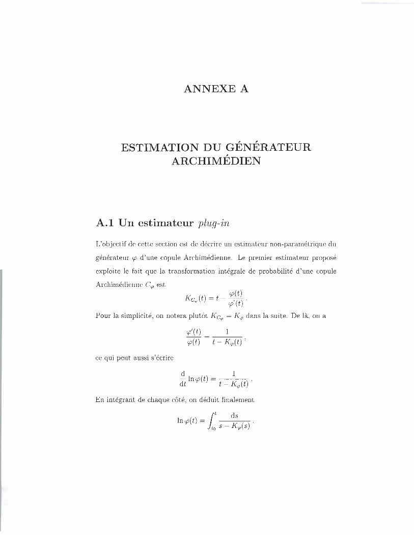
ANNEXE A
ESTIMATION DU GÉNÉRATEUR ARCHIMÉDIEN
A.l Un estimateur plug-in
L'objectif de cette section est de décrire un estimateur non-paramétrique du
générateur <p d'une copule Archimédienne. Le premier estimateur proposé
exploite le fait que la transformation intégrale de probabilité d 'une copule
Archimédienne Ccp est <p(t)
Kc,!,(t) = t - <p'(t) .
Pour la simplicité, on notera plutôt Kc,!, = Kcp dans la suite. De là, on a
<p' (t) 1 <p(t) t - Kcp(t) ,
ce qui peut aussi s'écrire
d 1 dt ln <p(t) = t - Kcp(t) .
En intégrant de chaque côté, on déduit finalement
lt ds
ln <p(t) = _ K ( ) . to S cp S
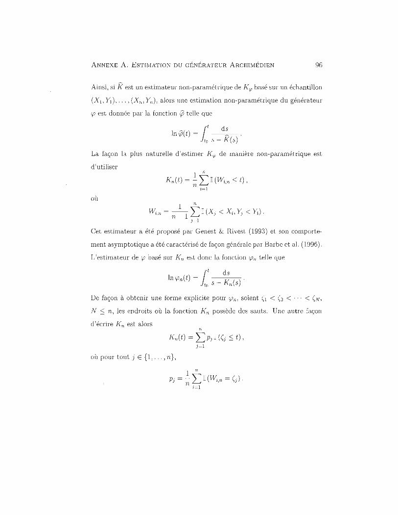
ANNEXE A. ESTIMATION DU GÉNÉRATEUR ARCHIMÉDIEN 96
Ainsi , si R est un estimateur non-paramétrique de Kep basé sur un échantillon
(Xl, YI) , ' .. ,(Xn , Yn ), alors une estimation non-paramétrique du générateur
cp est donnée par la fonction cp telle que
[
t ds ln cp(t) = ~ .
. to S - K(s)
La façon la plus naturelle d 'estimer K ep de manière non-paramétrique est
d 'utiliser 1 n
Kn(t) = - L II (Wi,n ::; t) , n i=l
où 1 n
Wi ,n = n _ 1 L II (Xj < Xi, Yj < Yi) . J=l
Cet estimateur a été proposé par Genest & Rivest (1993) et son comporte
ment asymptotique a été caractérisé de façon générale par Barbe et al. (1996).
L'estimateur de cp basé sur Kn est donc la fonction CPn telle que
it ds
ln CPn (t) = ( ) . to S - Kn s
De façon à obtenir une forme explicite pour CPn, soient (1 < (2 < ... < (N,
N ::; n, les endroits où la fonction Kn possède des sauts. Une autre façon
d 'écrire Kn est alors n
Kn(t) = LPj II ((j ::; t), j=l
où pour tout jE {1 , ... ,n},
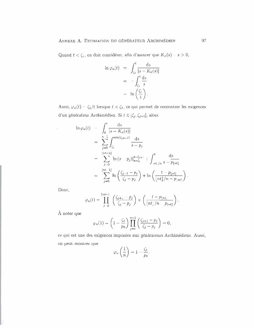
ANNEXE A. ESTIMATION DU GÉNÉRATEUR ARCHIMÉDIEN 97
Quand t < (l , on doit considérer, afin d 'assurer que Kn(8) - 8 > 0,
Ainsi , <Pn(t) = (dt lorsque t < (l, ce qui permet de rencontrer les exigences
d 'un générateur Archimédien. Si t E [(j, (j+l], alors
Donc,
À noter que
t d8
Jo 18 - Kn(8)1 I: I ffiin((J+1,t) ~
j=O (j 8 - Pj
Lnt-lj t " l ( - .) 18=(j+1 1 d8 ~ n 8 PJ 5=(j + j=O Lntj/n 8 - PLntj
Lnt- lj " l ( (Hl-Pj ) + 1 ( t-PLntj ) ko n (j - Pj n lntJ/n - PLntj .
Lnt-lj (t)- Il ( (Hl-Pj ) ( t-PLntj )
<Pn - j=O (j - Pj x lntJ/n - PLntj .
<Pn(1) = (1 - (1 ) fi ( (Hl_- pj ) = 0, Po j=l (J PJ
ce qui est une des exigences imposées aux générateurs Archimédiens. Aussi ,
on peut montrer que
<Pn (~) = 1 _ (1 . n Po
ANNEXE A. ESTIMATION DU GÉNÉRATEUR ARCHIMÉDIEN
A.2 Interpolation linéaire de Kn
L'interpolation linéaire de Kn est définie pour t E [(i-l, (i) par
K~(t) = Kn((i-d + {Kn((i) - Kn((i-d } (~i -=- ~i~lJ ((i - t) Kn((i-l) - ((i-l - t) Kn((i)
(i - (i-l
En notant que
N
LpjIT ((j ~ (i) j=l
i N
L pjIT((j ~ (i) + L pjIT((j ~ (i) j=l Hl
i
L Pj , j=l
on déduit que pour t E [Ci-l, (i),
Soit maintenant
ln<p~(t) = l t
_ ~*( )" to S n S
98
La fonction <p~ est un générateur Archimédien au sens où elle est convexe et
décroissante. Aussi , <p~(1) = 0 en autant que K~(t) > t pour tout t. Il s'agit
de prendre, en général, to = (1 et Po = (0 = O. Dans le cas t < (l, on a
ANNEXE A . ESTIMATION DU GÉNÉRATEUR ARCHIMÉDIEN 99
On a ainsi
ln<p~(t)
ce qui fait que
( t )~ 'P~(t) = - . (1
Si t E [(i- 1, (i), alors
ln<p~(t) f 1(j ds + 1t ds
j=2 (j - 1 S - K~(s) ( i- 1 S - K~(s) i - 1
= LJj + ~(t). j=2
Ici ,
où j-1
K . _ '" + Pj (j-1 J - ~Pk .
k=l (j - (j - 1

ANNEXE A. ESTIMATION DU GÉNÉRATEUR ARCHIMÉDIEN 100
En intégrant, on obtient
- 1 { r. (1 -~) - K'] Pj '>J ( ;-( j 1 J Ij = 1 - ln . ( (; -"J ( - 1 (1 - ----"'----) - K J ( j- ( j - 1 J
Également ,
On montre ainsi que