Embed Size (px)
Citation preview
UNIVERSITÉ DU QUÉBEC
MÉMOIRE PRÉSENTÉ À L'UNIVERSITÉ DU QUÉBEC À TROIS-RIVIÈRES
COMME EXIGENCE PARTIELLE DE LA MAÎTRISE EN GÉNIE ÉLECTRIQUE
PAR YIFEI HOU
ÉTUDE COMPARATIVE DES ESTIMATEURS DE CANAL DANS LES SYSTÈMES MIMO-CDMA
DÉCEMBRE 2009
Université du Québec à Trois-Rivières
Service de la bibliothèque
Avertissement
L’auteur de ce mémoire ou de cette thèse a autorisé l’Université du Québec à Trois-Rivières à diffuser, à des fins non lucratives, une copie de son mémoire ou de sa thèse.
Cette diffusion n’entraîne pas une renonciation de la part de l’auteur à ses droits de propriété intellectuelle, incluant le droit d’auteur, sur ce mémoire ou cette thèse. Notamment, la reproduction ou la publication de la totalité ou d’une partie importante de ce mémoire ou de cette thèse requiert son autorisation.
Résumé substantiel en français
Contexte
De nos jours, la communication sans fil est largement répandue et le nombre
d ' utilisateurs augmente sans cesse. Le coût d ' opération de ces réseaux, leur
consommation d ' énergie et leur taux d ' erreurs (BER) sont cependant des problèmes
cruciaux pour cette nouvelle technologie émergente.
Depuis que le premier système numérique commercial (GSM, 2G) a été lance en
Finlande en 1991 [1][2], des ingénieurs ont développé sans cesse la technologie au
niveau de la performance. Depuis ce temps, les technologies sans fil ont passé de la
deuxième génération à la troisième génération et nous pourrions voir une quatrième
(4G) ainsi qu ' une cinquième génération (5G) prochainement. La technologie sans fil
évolue donc très rapidement. Par exemple, dans un système 2G typique, les données se
transmettent à une vitesse de 56Kbits par secondes alors que dans la technologie GSM,
GPRS la vitesse passait à 114 Kbits par seconde. Avec le développement de la
technologie EDGE, une évolution de la rapidité pour GSM, apparue en 2003 , il était
désormais possible d'atteindre le 236.8 Kbit/s.
Dans le but de satisfaire la forte demande en rapidité de transfert et en bande
passante, une troisième génération (3G) a été développée [4]. Cette technologie a
révolutionné l' Industrie avec un 14.4Mbits par seconde en réception et 5,8Mbits en
envoie. Basé sur un haut débit de donnée, le réseau 3G a permis le développement à
Fr-2
grande échelle de la téléphonie numérique sans fil , des appels vidéo amsl que la
technologie mobile à large bande.
Le terme 4G (quatrième technologie) sert présentement à décrire la prochaine
évolution complète en matière de technologie sans fil. Le système 4G sera en mesure de
fournir une solution IP ou la voix, les données et du streaming multimedia pourraient
être fournis a l' utilisateur sur un «n 'importe où, n 'importe quand». Il n'y a cependant
aucune définition concrète de ce que sera le 4G . Toutefois, on peut déjà dire que le 4G
sera un système ayant complètement intégré la technologie IP. Le 4G permettra
d ' atteindre une vitesse entre 1 OOMbits/sec et 1 Gbits/s tant à l'intérieur qu'à l'extérieur,
et ce, avec une très haute quai ité et sécurité [3].
Problèmes
MIMO-CDMA est une technologie intégrée qui a principalement été conçue
pour le 4G et même le 5G . Nous continuerons d ' utiliser la base «codage-décodage»
mais quand nous ferons un travail de transmission nous utiliserons une antenne
MIMO pour émettre et recevoir les signaux. Comme pour dans la technologie
traditionnelle CDMA, l' estimation des canaux est toujours un élément important
dans l' ensemble du réseau.
Fr-3
La plupart des recherches et des expériences se sont concentrées sur un seul
algorithme ou sur une version améliorée d ' un seul. Dans ces cas, nous pouvons
seulement voir la performance de cet algorithme. De plus, toutes ces recherches ont
été conduites dans des environnements différents au niveau de l' encodage et des
canaux. En d ' autres mots, elles n' utilisent généralement pas la même plateforme.
Dans cette situation, nous ne pouvons pas voir la comparaison des différents
algorithmes clairement. Nous n'avons donc aucune idée si un algorithme est
meilleur qu ' un autre. Il est donc très important de construire une telle plateforme
qui mettra les différentes estimations de canaux dans un même environnement.
Méthodologie
Avant de commencer une recherche dans ce domaine, nous avons consulté plusieurs
références à la bibl iothèque et sur Internet. Nous étudierons les algorithmes
d ' estimation du canal pour les systèmes MIMO. Ensuite, nous appliquerons aux
systèmes MIMO-CDMA. Après, nous avons construit une plateforme de simulation.
Nous assumons la situation multiutilisateur. La plateforme de simulation devra
comprendre une station de base et plusieurs utilisateurs. Pour chaque utilisateur/ station,
il y aura plusieurs antennes. Nous devrons aussi considérer le modèle du signal pour
rendre la situation le plus proche possible de la réalité.
Fr-4
Lorsque la platefonne de simulation sera complétée, nous étudierons plusieurs
algorithmes d'estimation de canaux. Nous tenterons aussi d ' intégrer ces algorithmes
sur la plateforme construite précédemment.
Ensuite, nous ferons la simulation de tous ces algorithmes afin d ' obtenir des résultats et
enfin, nous comparerons les résultats.
Système MIMO-CDMA
CDMA
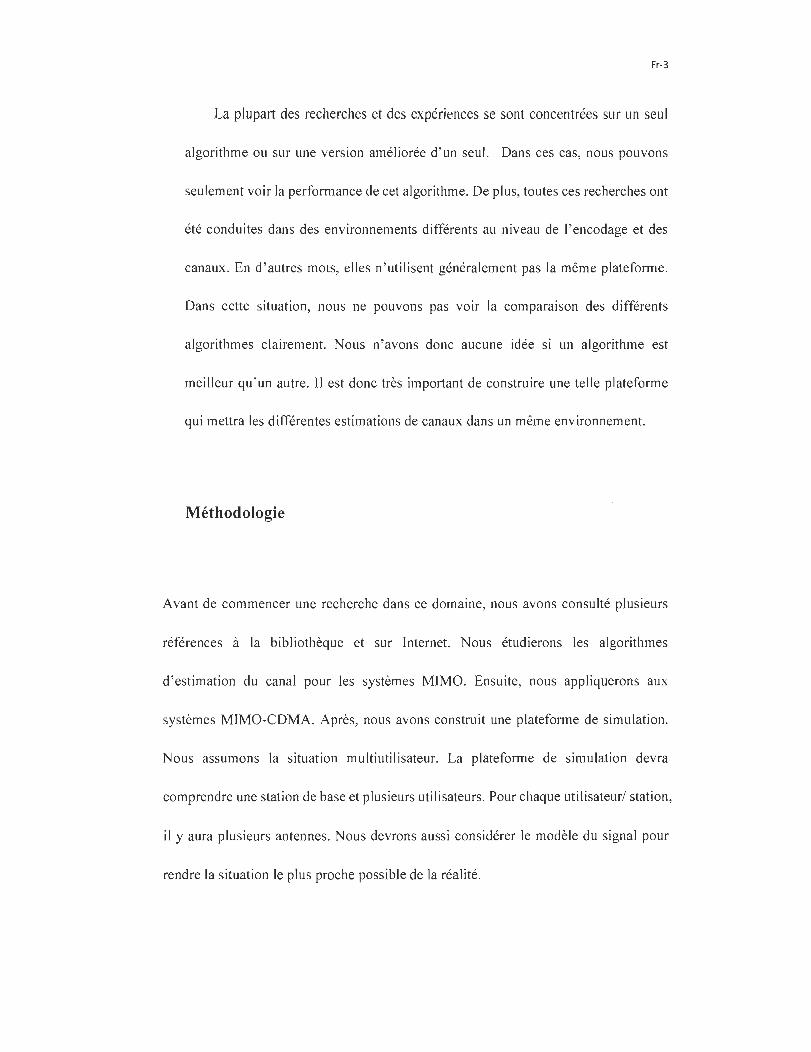
Dans un système radiophonique, il y a deux bases que l' on doit prendre en compte
soit la fréquence et le temps. Le système est divisé et une fréquence du spectre est alors
allouée en tout temps à chaque paire de communicateurs. On appelle cela l'accès
multiple par répartition en fréquence (ou FDMA en anglais). Les systèmes sont divisés
en temps et chaque pair de comm unicateurs alloue tout (ou du moins une grande partie)
du spectre pour la partie du temps appelé multiplexage temporel ou plus couramment
Time division multiple access (TDMA) en anglais. En COMA, tout le spectre sera alloué
aux communicateurs en tout temps.
Fr-5
FOMA TOMA COMA
Figure 2.1 Comparaison de différent accès.
Le CDMA utilise des codes pour identifier les connexIons. C 'est une fonne
d ' étalement de spectre à séquence directe (DSSS) qui est utilisée en communication
militaire depuis longtemps. En réponse à une demande mondiale sans cesse croissante
en communication mobile et sociale, la technologie à large spectre numérique a
accompli une bien meilleure efficacité en utilisation de bande passante par chaque
allocation de spectre et par le même fait, a pu répondre à bien plus d ' utilisateurs qu'en
technologie analogique et même les autres technologies numériques . Comme
auparavant lors de son implantation chez les militaires, les réseaux à large spectre ont
accompli beaucoup en incorporant un grand nombre de fonctions uniques. En plus
d ' augmenter l' efficience du spectre, cela élimine aussi la tâche de planifier différentes
allocations de fréquences pour les utilisateurs avoisinants. Beaucoup d 'options sur les
systèmes à accès multiples sont rendues possibles par cette fréquence universelle
réutilisée par des terminaux employant des ondes du style sonore (noise-like signal
waveforms). L' avantage le plus important est la rapidité et la précision de
l' ajustement de la pui ssance, ce qui assure un haut niveau de transmission de qualité

Fr-6
pendant qu 'on règle le problème de la distance en maintenant un bas IlIveau de
puissance pour chaque terminal et par le même fait, un bas niveau d'interférence aux
autres term inaux.
MIMO
Multiple Input Multiple Output (MIMO) est une technologie d ' antenne dans
laquelle plusieurs antennes sont utilisées pour à la fois les transmetteurs et les
émetteurs. C'est une forme d 'antenne intelligente. Sa plus ancienne mention sur le
terrain remonte à A.R Kaye et D.A George en 1970 et W. van Etten en 1975 et 1976.
Après cela, plusieurs recherches sur le beamforming ont mentionné des applications en
1984 et 1986 publiées par Jack Winters et Jack Salz au laboratoire Bell. Jusqu 'en 1993,
Arogyaswami Paulraj et Thomas Kailath ont proposé le concept du Spatial
Multiplexing utilisant MIMO. C'était la première fois que cette technologie était
utilisée pour une diffusion sans fil. Dans le domaine commercial, Iospan Wireless Inc. a
développé le premier système en 2001 qui utilisait la technologie MIMO-OFDMA. Ce
système supportait un encodage diversifié ainsi que le Spacial Multiplexing. En
utilisant la technologie MIMO, nous pouvons minimiser les erreurs et optimiser la
vitesse des données. En même temps, cela ne nécessitera pas de bandes passantes
additionnelles ou de puissance de transmission.
Fr-7
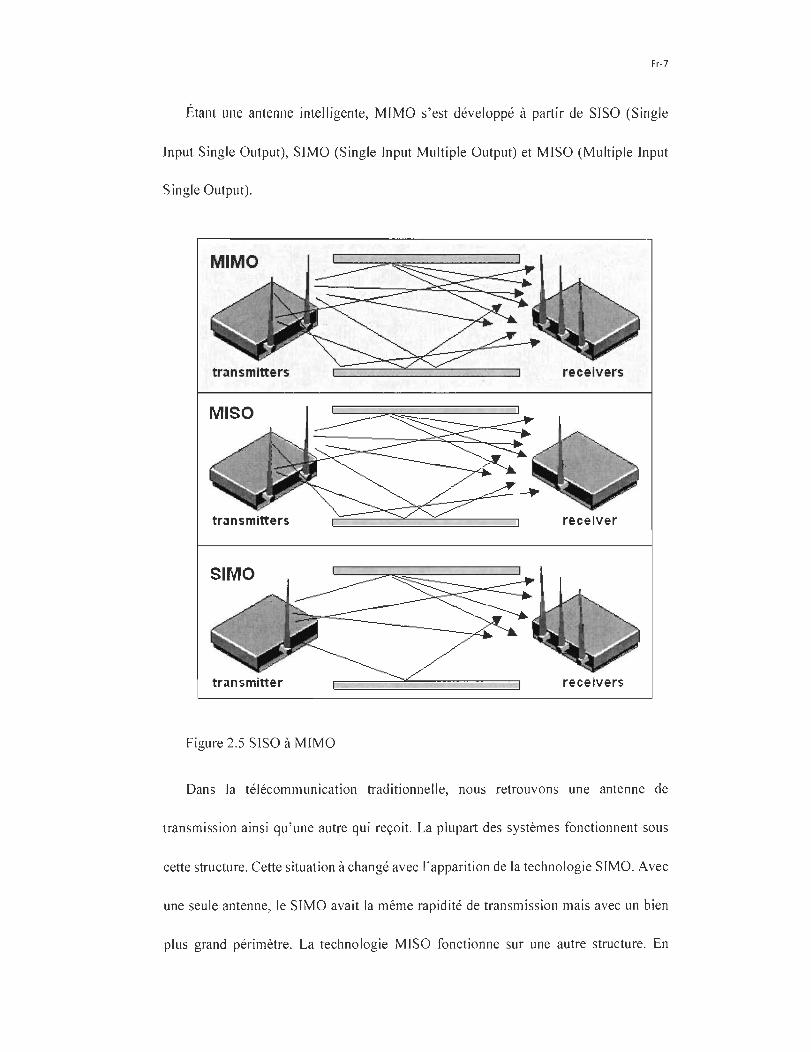
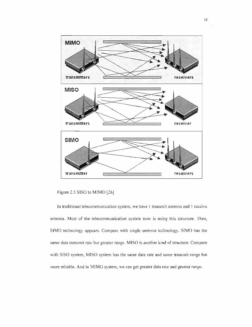
Étant une antenne intelligente, MIMO s 'est développé à partir de SISO (Single
Input Single Output), SIMO (Single Input Multiple Output) et MISO (Multiple Input
Single Output).
MIMO
MISO
SIMO
transmitter receivers
Figure 2.5 SISO à MIMO
Dans la télécommunication traditionnelle, nous retrouvons une antenne de
transmission ainsi qu ' une autre qui reçoit. La plupart des systèmes fonctionnent sous
cette structure. Cette situation à changé avec l' apparition de la technologie SIMO. Avec
une seule antenne, le SIMO avait la même rapidité de transmission mais avec un bien
plus grand périmètre. La technologie MISO fonctionne sur une autre structure. En
Fr-8
comparaison avec le SISO, le système MISO a la même vitesse de transmission et le
même périmètre mais est beaucoup plus fiable. Le système MIMO a quant à lui
améliorer la vitesse et le périmètre.
Algorithme d'estimation de canaux
Les canaux de radio dans les systèmes mobiles ont souvent causé les interférences
inter-symbole (ISI) dans le signal reçu. Pour enlever ces ISI du signal, plusieurs sortes
d ' égaliseurs peuvent être utilisés. Les algorithmes de détection basés sur les recherches
de Trellis ( MLSE et MAP) offrent une bonne perfonnance de réception en plus de ne
pas être trop complexes informatiquement. Ces algorithmes sont donc devenus très
populaires.
Cependant, ces détecteurs demandent une bonne connaissance sur la réponse
impulsionnelle (CIR), ce qui est fourni séparément par un bon estimateur de canaux.
Nonnalement l' estimation des canaux est basée sur une séquence connue de bits, qui
est unique pour certains transmetteurs et qui se répète à chaque rafale de transmission .
L ' estimateur de canaux est donc capable d ' estimer le CIR pour chaque rafale
séparément en exploitant les bits transmis et en les comparant aux échantillons
correspondants.

Fr-9
n
~t~ __ .L~ -1 '+' . .:I ... C:~~ ,:, ,, , f----.. ~ . \ 1 _ . y , _,l r .ll t'E-r
'-----.--'
)'
1
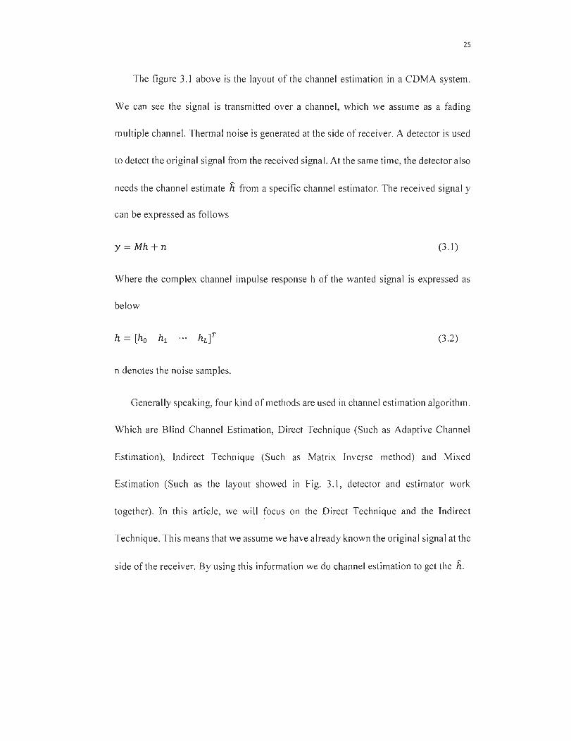
Figure 3.1 Plan d ' un estimateur de canaux,
La figure 3.1 ci-dessus est le plan d ' un estimateur dans un système COMA. Nous
pouvons y voir le signal transmis dans un canal multiple atténuant (fading multiple
channel) . Des bruits thermiques sont générés d ' un côté d ' un récepteur. Un détecteur est
aussi utilisé pour détecter le signal original reçu . Simultanément, le détecteur a aussi
besoin du canal estimé h d' un estimateur de canaux spécifiques. Le signal y reçu peut
être exprimé comme suit:
y = Mh+n (3.1 )
Où la réponse d ' impulsion complexe de canal h du signal voulu est exprimée comme
suit:
(3.2)
n exprime les échantillons de bruit
Généralement, on utilise quatre méthodes en algorithme d'évaluation de canal.
Soit: l'évaluation sans visibilité (Blind Channel Estimation), la technique indirecte
comme celle de la matrice inversée, et l'évaluation mixe (comme démontré dan s la
Fr-ID
figure 4.1, le détecteur et l' estimateur fonctionnent ensemble). Dans cet article, nous
nous concentrerons sur la technique directe et la technique indirecte. Nous assumerons
donc l' hypothèse que nous connaissons déjà le signal original du côté du récepteur. En
utilisant cette information, nous faisons l' estimation pour avoir le fi.
Techniques indirectes
Estimation des LS (Least Square)
L' estimation des moindres carrés peut être interprétée comme une méthode pour
adapter les données. La mei lleure valeur dans les valeurs carrées sont l' instance dans
laquelle le modèle pour lequel la somme des carrés résiduels est la plus petite valeur et
par résiduel, on veut dire la différence entre la valeur observe et la valeur donnée par le
modèle. La méthode a été décrite originalement par Carl Friedrich Gauss autour de
1974.
Selon (3.1) et (3.2), nous pouvons obtenir:
(3.3)
Supposant que nous avons le bruit, nous obtenons:
(3.4)
Où ()H et ()-1 dénote les matrices hermitiennes et inverses respectivement.
1 Estimation de canal LMS (Least-Mean-Squares)
L' algorithme LMS est un important membre de la famille stochastique gradient.
Le terme stochastique gradient algorithme est prévu pour distinguer l' algorithme LMS
Fr-ll
de la méthode de la descente rapide (steepest descent) , qui emploie un gradient
détenniniste dans le calcul récursif de Wierner pour les entrées stochastiques. Un
avantage significatif de l'algorithme LMS est sa simplicité. D' ailleurs, il n'ex ige pas
de mesure de corrélation ni de matrice inversée
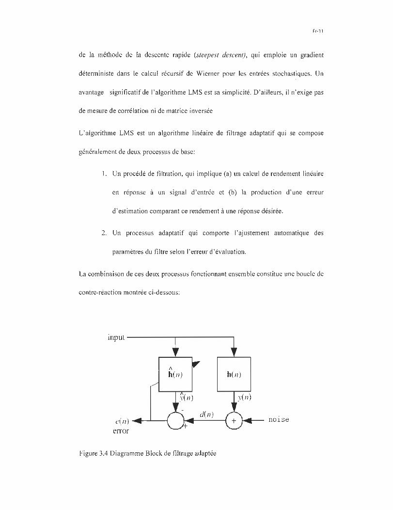
L ' algorithme LMS est un algorithme linéaire de filtrage adaptatif qui se compose
généralement de deux processus de base:
1. Un procédé de filtration, qui implique (a) un calcul de rendement linéaire
en réponse à un signal d' entrée et (b) la production d ' une erreur
d ' estimation comparant ce rendement à une réponse désirée.
2. Un processus adaptatif qui comporte l'aj ustement automatique des
paramètres du filtre selon l'erreur d'évaluation.
La combinaison de ces deux processus fonctionnant ensemble constitue une boucle de
contre-réaction montrée ci-dessous:
input -----"'T'""--------,
1\
h(n) h(n)
e( 11) ~----L--4 nOlse
enor
Figure 3.4 Diagramme Block de filtrage adaptée
Fr-12
Dans cette recherche, nous considérons, la situation par trajets multiples dans le
système de SISO et MIMO. Nous assumons aussi que le délai sera de 6 ce qui signifie
que l' ordre de filtrage de tous les filtres adaptatifs qui sont utilisés sera de 6.
L 'algorithme LMS pour un ordre de pth peut être résumé ainsi:
h(D) = D
x(n) = [x(n), x(n - 1), ... , x(n - p + 1) JI
e(n) = den) - liH (n)x(n)
li(n + 1) = lien) + Ile*(n)x(n)
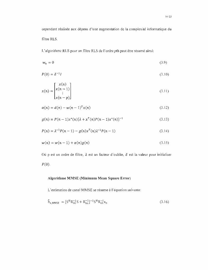
Algorithme de RLS (Recursive Least Squares)
(3.5)
(3.6)
(3.7)
(3.8)
L' algorithme RLS est employé dans des filtres adaptatifs pour trouver les
coefficients de filtrage qui se rapportent à produire périodiquement le moins de carrés
du signal d ' erreur. Cela est contraire aux autres algorithmes qui visent à réduire l' erreur
de moyenne carrée. La différence est que les filtres RLS dépendent des signaux
eux-mêmes, tandis que les filtres MSE dépendent de leurs statistiques. Si ces
statistiques sont connues, un filtre MSE avec des coefficients fixes peut être construit.
Un dispositif important de ce filtre est que son taux de convergence est typiquement un
ordre de grandeur plus rapide que celui du filtre LMS étant donné que le filtre RLS
blanchit les données d'entrée en employant la matrice de corrélation inverse des
données, assumées pour être de zéro. Cette amélioration en performance est
Fr-13
cependant réalisée aux dépens d ' une augmentation de la complexité informatique du
filtre RLS.
L' algorithme RLS pour un filtre RLS de l' ordre pth peut être résumé ainsi:
(3.9)
peO) = o-lI (3.10)
[
x(n) 1 x(n) = x(n:- 1)
x(n - p)
(3.11 )
a(n) = den) - w(n - l)T x(n) (3.12)
g(n) = pen - l)x*(n){À + xT (n)P(n - l)x*(n)}-l (3.13)
(3.14)
w(n) = w(n - 1) + a(n)g(n) (3 . 15)
Où p est un ordre de filtre, À est un facteur d 'oublie, 0 est la valeur pour initialiser
P(O).
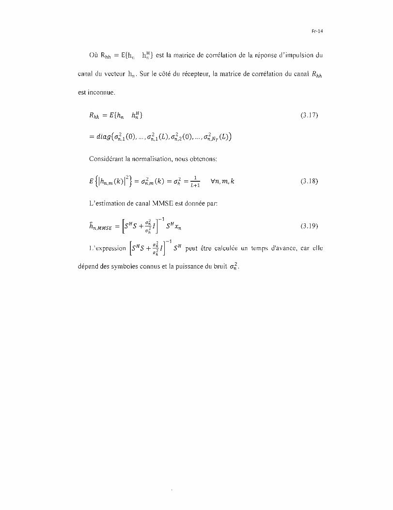
Algorithme MMSE (Minimum Mean Square Error)
L ' estimation de canal MM SE se résume à l' équation suivante:
h~ [SH R-1S + R-1]-lSH R-1 n,MMSE = nn hh nn xn (3.16)
Fr-14
Où Rhh = E{hn h~} est la matrice de corrélation de la réponse d ' impulsion du
canal du vecteur hn . Sur le côté du récepteur, la matrice de corrélation du canal Rhh
est inconnue.
(3.17)
Considérant la nomlalisation, nous obtenons:
(3.18)
L' estimation de canal MMSE est donnée par:
~ [H O"~ ]-1 H hn,MMSE = S S + O"~ 1 S xn (3 .19)
L' expression [SH S + :~ 1 r1
SH peut être calculée un temps d'avance, car elle
dépend des symboles connus et la puissance du bruit O"J.
Fr-15
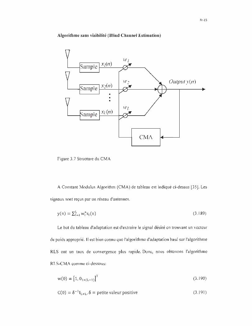
Algorithme sans visibilité (Blind Channel Estimation)
OUIPU! y en)
CMA
Figure 3.7 Structure du CMA
A Constant Modulus Algorithm (CMA) de tableau est indiqué ci-dessus [35]. Les
signaux sont reçus par un réseau d'antennes.
(3.189)
Le but du tableau d'adaptation est d'extraire le signal désiré en trouvant un vecteur
de poids approprié. Il est bien connu que l'algorithme d'adaptation basé sur l'algorithme
RLS ont un taux de convergence plus rapide. Donc, nous obtenons l'algorithme
RLS-CMA comme ci-dessous:
((0) = 8-1 ILx L1 8 = petite valeur positive
(3.190)
(3.191 )
zen) = x(n)x H (n)w(n - 1) /x H (n)w(n - 1) /p-2
h(n) = zH(n)C(n - 1)
g(n) = C(n- l)z(n)/(À+ h(n)z(n))
C(n) = C(n-l)- g(n)h (n)
À
e(n) = wH (n - l)z(n) - 1
w(n) = w(n - 1) + g(n)e*(n)
Simulations
Simulation d'un SISO-CDMA
Fr-16
(3.192)
(3.193)
(3.194)
(3.195)
(3.196)
(3 .197)
Dans la simulation, nous commencerons à partir de la plate-forme SISO-CDM
parce que l' antenne SISO est moins compliquée que le système d ' antenne MIMO. En
attendant, nous pouvons comparer les résultats de la simulation SISO aux résultats de la
simulation MIMO. Nous pouvons voir les différences du même algorithme
d ' évaluation de canal entre deux systèmes différents d ' antenne. Nous pouvons voir
comment les éléments de canal affectent les résultats d ' évaluation.
Fr-17
/
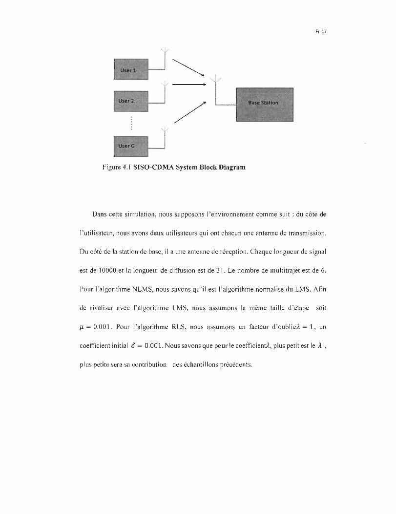
Figure 4.1 SISO-CDMA System B10ck Diagram
Dans cette simulation, nous supposons l' environnement comme suit : du côté de
l' utilisateur, nous avons deux utilisateurs qui ont chacun une antenne de transmission .
Du côté de la station de base, il a une antenne de réception . Chaque longueur de s ignal
est de 10000 et la longueur de diffusion est de 31. Le nombre de multitrajet est de 6.
Pour l'algorithme NLMS, nous savons qu ' il est l'algorithme nonnalise du LMS. Afin
de rivaliser avec l' algorithme LMS, nous assumons la même taille d 'étape soit
Il = 0.001. Pour l'algorithme RLS, nous assumons un facteur d 'oublieÀ = 1 , un
coefficient initial ô = 0.001. Nous savons que pour le coefficientÀ, plus petit est le À ,
plus petite sera sa contribution des échantillons précédents.

ex. w al
Fr-18
sisa 100 ~_~ __ ~ __ ~ __ :: __ ~ __ ~_~~_~_~ __ :: __ ~ __ ~ __ ~_~ __ :: __ ~ __ ~ __ ~-~--~--~~~-~--~-E-~- -~--~--~-~-~--~- -~-
~: - - - - - Î - - - - - - - Î - r - - - - - -,- - - - - - - -,- - - - - - - -.- -.
10-"'
10-4
: : : : : f : : : : : : : f : f ::::: ::: : : : : : : ::: : : : : : : ::: ~ -- P e rfect - - - - - ,. - - - - - - - 1· - - - - - -,- - - - - - - ·1· - - - - - - .,. - ,
- :..:=..-~-------~ -~ ------:--------:--------:- ~ LrvlS - - - - ~--=...=....::.r - - - - - - - r - - - - - - -,- - - - - - - -,- - - - - - - -,- - - - - - - ï - - -
------..; .. , ' 1 1 l' LS -=-:~~-~:----- - -:- ---- ---:--------:-------:--- == RLS
-- NUv1S
-B- MrvlSE
-------' - ---_.: ------_: ------_:_ -______ I _ ':~~ .... . __ . ___ : ___ ____ : _______ : ___ ___ _ : : : : : : :; :: -:::;:: : ::::;:::::: ::: : : : : : : ::: : : - - ,~ -, - - : ~ : : ~: : : : : : : ~: : : : : : : ~: : : : : : : - - - - - - - r"' - - - - -,.. - - - - - - -,.. - - - - - - - , - - - - - - - - , - - - - - - .. . . - - - - .: - - - - - - - , - - - - - - - .., - - - - - - -
~ ~ ~ ~ ~ ~ ~l ~ ~ ~ ~ ~ 1 ~ ~ ~ ~ ~ ~ ~i~ ~ ~ ~ ~ ~ ~ l~ ~ ~ ~ ~ ~~ ~ ~ ~ ~ ~: 1~ ~ ~ ~ ~ ~ ~ l , :\ 1 1 l ,==='\ t 1
_ -_ ~ , -L: -j: ~ ~ ~ ~ ~ ~[\~ L ~: ~ :i-_ -,: J- ~~ ~~: ~ L_ ~~: ~~-J ~ ~ ~ ~ ~ ~ : : : : : : : ~ : : : : : : : ~ : : : : : : : ~ : : : : : \::: : : : : : : ::: : : : : : : ::: : : : : : : ~: : : : : : : ::: : : : : : : ~: : : : : : : : : : : : : : ~ : : : : : : : ~ : : : : : : : ~ : : : : : :~: : : : : : : ::: : : : : : : ::: : : : : : : :: : : : : : : :: : : : : : : :: : : : : : : - - - - - - -:- - - - - - - -:- - - - - - - -:- - - - - - - -:- - - - - - - -:- - - - - - - -:- - - - - - - -:- - - - - - - -:- - - - - - - -:- - - - - --
---- - - - ~ ----- --~ - - - - - - - ~ - - ---- -:- - - - - - - -:- - - - - - - -:- - - - - - - ~ - - - - - - - ~ -------~ - - - - - - -1 1 1 1 l , 1 l ,
- - - - - - -,.. - - - - - - -,.. - - - - - - -,.. - - - - - - -,- - - - - - - -,- - - - - - - -1- - - - - - - ., - - - - - - - ., - - - - - - - ., - - - - - - -, , , , 10-5 I....-._---L.-__ -'--_--'-__ -'--_--'-__ -'--_--'-__ -'--_--'-__
o 2 4 6 8 10 12 14 16 18 20 SNR,dB
Figure 4.2 Résultats des simulations en environnement SISO-CDMA (1)
Nous pouvons voir que dans un environnement SISO-CDMA, lorsqu ' un SNR est
entre OdM et] OdB, les algorithmes adaptatifs ont des perfonnances semblables avec
l'algorithme RLS-CMA. D ' une façon générale, en cet état de SNR, l'algorithme
adaptatif et RLS-CMA est un peu meilleur que l'algorithme LS. Dans la même gamme
de SNR, les algorithmes MMSE et algorithmes adaptatifs n' ont pas beaucoup de
différence. Quand le SNR est entre 15dB et 20 dB, nous pouvons voir que l'algorithme
LS devient bien mieux que tous les autres algorithmes.
Fr-19
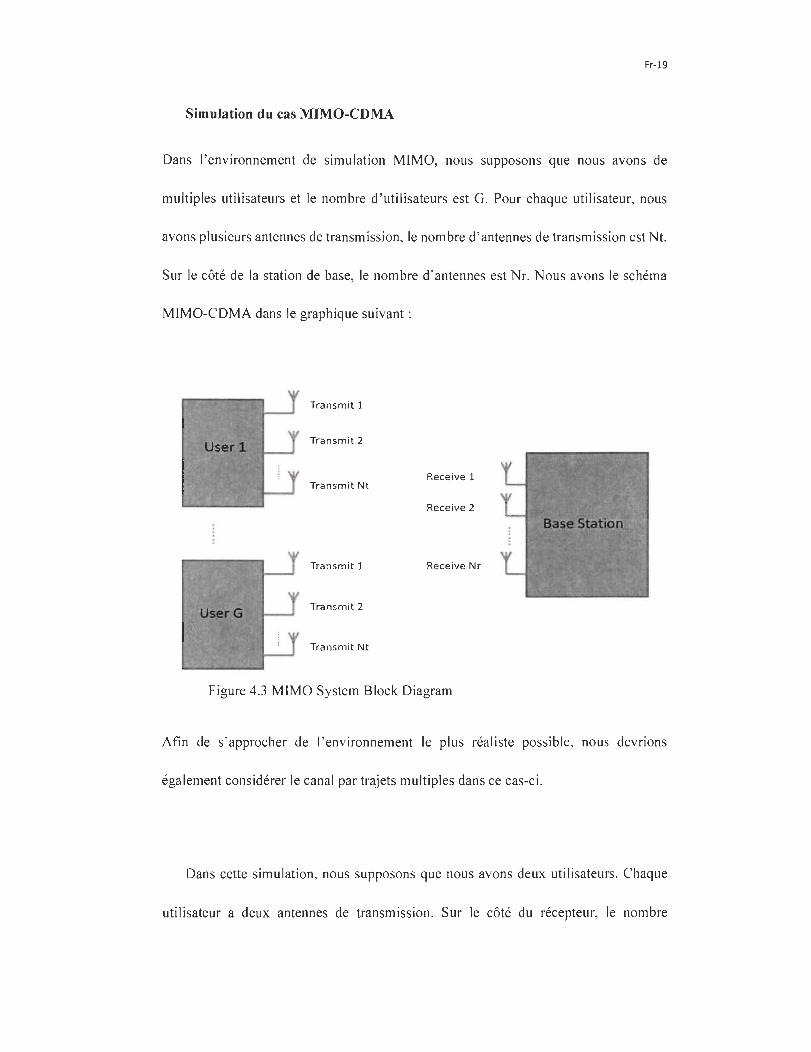
Simulation du cas MIMO-CDMA
Dans l' environnement de simulation MIMO, nous supposons que nous avons de
multiples utilisateurs et le nombre d ' utilisateurs est G. Pour chaque utilisateur, nous
avons plusieurs antennes de transmission, le nombre d'antennes de transmission est Nt.
Sur le côté de la station de base, le nombre d ' antennes est Nr. Nous avons le schéma
MIMO-CDMA dans le graphique suivant:
Transmit 1
Tran smit 2
Receive 1 Tran smit Nt
Receive 2
Tra nsmit 1 Rece ive Nr
Transmit 2
Tra nsm it Nt
Figure 4.3 MIMO System Block Diagram
Afin de s ' approcher de l' environnement le plus réaliste possible, nous devrions
également considérer le canal par trajets multiples dans ce cas-ci.
Dans cette simulation, nous supposons que nous avons deux utilisateurs. Chaque
utilisateur a deux antennes de transmission. Sur le côté du récepteur, le nombre
Fr-20
d'antennes de réception est de quatre. Chaque paire de canaux de signal ( une antenne
de transmission et une antenne de réception) a un canal d'effacement de 6 chemins
(fading channel).
Pour l' algorithme d'évaluation LMS, nous supposons la taille il = 0.1. Nous
savons que plus la valeur de la taille d 'étape est grande, plus la convergence
d'algorithme sera rapide. Vu la complexité du système d'antenne MIMO, nous
espérons que ce sera rapide
Pour l' algorithme NLMS, nous choisissons la même taille que le LMS soit:
il = 0.1.
Pour l'algorithme RLS, nous assumons un facteur d'oublis ,1= 1, un coefficient
initial de 8 = 0.001. Nous savons que pour le coefficient À, plus petit est À is, plus
petit sera la contribution des échantillons précédents. Dans le système d' Antenne
MIMO, l' état des canaux est très compliqué.
Fr-21
MIMO 1 OV r:~:~:~: :~:"!"T~: :~:~:~: :~,~:~: :~:~:~: :!:.:~:~: :~:~: ~:,..~:~:~: :~:~: T~:~:~: :~:~:"!", :~:~:~: :~:~,~: -p-::;:-:;:;--::::-E:;--::::-::;:-:;:;--;:r::::-:;:;- -::::-::;:-~
: : : : : : ~ : : : : : : ~ : : : : : : ::: : : : : : ::: : : : : : : f : : : : : : ~ : : : : : : ~: -- P'e rfect --~- - - - - - , - - - - - - -,- - - - - - - r - - - - - - T - - - - - - , - - - - - - j-
r ~~~~~~.:~~~~::: ::t: ::: ::I::: :::J::::::~: Lr\t1S -1 -----~ ~:------~-.. : : : : -- LS
10 :::::::i::::~;..::_~ -::::?b.; :::::i::::::~::::::~: RLS :::::::: ::::! :::::::: :: :: ~ :: :: :::: ~:..:.._::: c :"'t .. ::: ::::!:: :: :: :::::: ~:: :: :: :: ::::::: --------T------.,-------,---=---_ . ' ---T------.,-------,- __ NLr\t1S.
~ 10' ~;;;;:i;;;:;~I~~~~;;~:~~1~M~: 10~ !!!! '! ! !!!!~!!:! ~ mm "-w-"-!! __ \~~ 0m;i~~ 10~ """ f"""!",,' ":" 'mll""" f",," f"",,!' m~~,,'" m,,,,,
t 1 1 l , 1 1 1 1 ------ T------,-------,-------r-- ---- y----- - ,------,-------r------r------l , . 1 1 1 l , , 1
10-5 ~--~----~ ____ ~ __ ~ ____ ~ ____ ~ __ ~ ____ ~ ____ ~ __ ~ a 2 4 5 8 10
SNR,dB 12 14 16 18
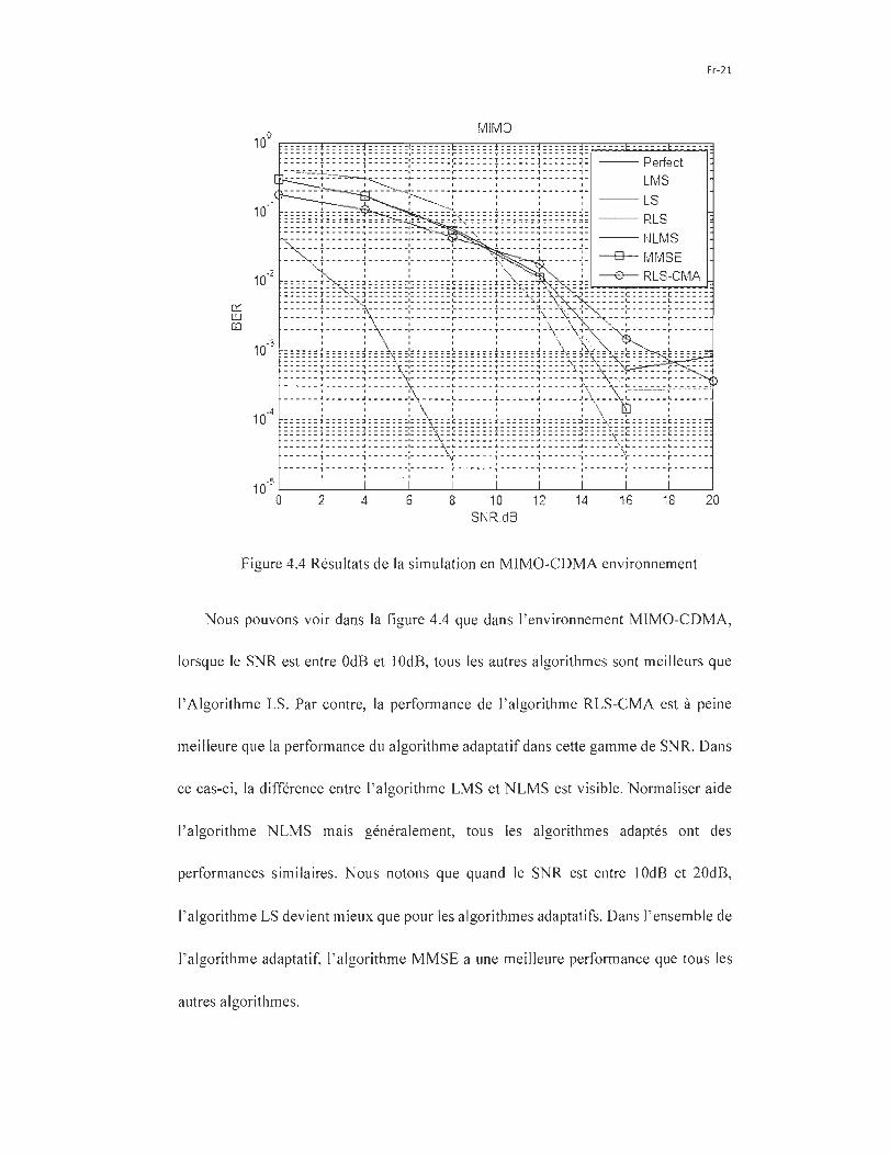
Figure 4.4 Résultats de la simulation en MIMO-CDMA environnement
20
Nous pouvons voir dans la figure 4.4 que dans l' environnement MJMO-CDMA,
lorsque le SNR est entre OdB et IOdB, tous les autres algorithmes sont meilleurs que
l'Algorithme LS. Par contre, la performance de l' algorithme RLS-CMA est à peine
meilleure que la performance du algorithme adaptatif dans cette gamme de SNR. Dans
ce cas-ci, la différence entre l'algorithme LMS et NLMS est visible. Normaliser aide
l' algorithme NLMS mais généralement, tous les algorithmes adaptés ont des
performances similaires. Nous notons que quand le SNR est entre lOdB et 20dB,
l' algorithme LS devient mieux que pour les algorithmes adaptatifs. Dans l' ensemble de
l' algorithme adaptatif, l' algorithme MMSE a une meilleure performance que tous les
autres algorithmes.
CONTENTS
CONTENTS ....... ...... ...... ........ .... ... ...... ...... ........... .... ................ ... .. .. ... ...... ... ...... ..... ....... ........ .... .......... ..... ...... ii
1. Introduction ... ......... .......... ... .................... .. .. ... ...... ... ... ...... ... .... ........ ........ ... ..... .. ...... ...... ..... ...... .. ......... 1
1.1 Background ... ... .... ..... .... .. ...... ......... .... .... ......... .. ..... .......... ... ..... .... ...... ........... .. ... ...... ............... 1
1.1.1 2G Network ... ..... ........ .... ....... ....... .. ........ ... .................. ... ............................ .......... .. ........ .. 1
1.1.2 3G Network ... ... ... .. .. .. .. .. ...... .. .......... ..... .............. .. .. ...... .. .. ... ..... .... ...... .... .... ....... .... .... ....... 2
1.1.3 4G Network .... ........ ......... ..... .... ...... .... .................. ..... ..... ......... ....... ...... ... ... .. .... ... ..... ..... ... 3
1.2 Problems ....... ........ .... ...... .. ....... .... ..... .... ............. .. ....... ....... .. ................... .... ......... ................... 4
1.3 Objective .... ........... ............ ............... ..... ............. .. ... ... ......... .. ........... .. .. .... ... .... .... .. .. .......... ... ... 5
1.3 Methodology ................ .... ............. ... ...... ... ....... ....... .. ....... .............. ............. .......... .......... ........ 5
1.4 Organization of the papers ......... .... .. ........ .. .......... .. .... .. .. .. .. .. .. ..... ....... ..... ....... .. .......... ...... .. ..... 6
2. MIMO-CDMASystem ...... .... ..... ..... ..... ...... .... .... ........ .... ............... ........ ... ... .... ... .......... ...... ............. ....... 7
2.1 CDMA ..................... ...... ......... ... ..... ... .... ... .. .. .... ...... ....... ....... ... ... ... ............. ...... ...... ..... ......... .... 7
2.1.1 Background ............................... ...... .. .. ......... ... .. ............ .. ..... .. ... ......... ... ..... .. ...... ............ .. 7
2.1.2 Principle of Spread Code Communication ................................. .. .......... .... ...................... 9
2.2 MIMO ...... .. ............ .... .... ..... ..... .............. .... ... ....... .... ............ ......... ............ ..... .......... .... .... ... ... 15
2. 2.1 Background ....... ... .. .. .... ... .... ....... .... .... ..... .... ... ...... .... .... ... .... .. ......................... ... .... ......... 15
2.2.2 Benefits of MIMO .. ............. .. ................. .. .................... .. .... ......... .. ................. .. .... ...... .. .. . 17
2.2.3 Capacity of MIMO ...... ......... .. .... .. ........ .. ............ .. .. .. ..... .. .......... ........... .. .... ..................... 19
2.2.4 MIMO Channel ......... ...... ...... ........ ............ ................. .... ..... .................. .......................... 20
2.3 Rake Receiver ... .. ... ...... .... .. .. ..... .. .... ............ ..... .... ... .... .. ..... .. ... ...... .. ................. ............ ...... .. .. 22
3. Channel Estimation Algorithms .... .............. .. ......................... .. ..................... .. ......... .. .... .. ........ .. ........ 24
3.1 introductions ......... ........... .... ................... .. .... ..................... ...... ....... ........ .... ............ .............. 24
3.2 Ind irect Techniques ...... ... ....... .................. .. ..... ... .. .. .... .. ..... ... ...... .......... ... .......... .. ......... ......... 26
3.2.1 Least-squares (LS) channel estimation .. .. .. .. .. .. .. ................. .. .... ...................................... 26
3.2.2 Blind Channel Estimation for MIMO-CDMA using first -order statistics .. .... .... .. .. .... .. .... . 26
3.2.3 Blind Multipath Estimation with Toeplitz displacement for long code DS-CDMA .......... 29
iii
3.2.4 EM Vector Channel Estimation .. ...... ............. ... ... ........ ............. ...... ... .. ....... .... ..... .. .... ... ... 33
3.2.5 Reduced-Rank Space-time Channel Estimation for OS-CDMA ........................... .... ........ 36
3.2.6 Linear MMSE channel estimation .................... ...................... .. .. .. .................................. 40
3.3 Oirect Techniques ....... .. .... ........ ...... ..... ..... ... ... ........ ...... .. .. .. .. .. .. ...... .......... ... .......................... 40
3.3.1 Least-Mean-Squares (LMS) Channel Estimation ............ .. ............ ................................. .40
3.3.2 Recursive Least Squares (RLS) Channel Estimation .................................................... .... 42
3.3.3 Iterative Channel Estimation for Turbo Receivers in OS-COMA ......... .... .... .................... 43
3.3.4 Blind Adaptive MIMa Channel Estimation Algorithm .................................................... 45
3.3.5 Novel Channel Estimation Aigorithm Using Kalman Filter ........... .... .. ........ .. ................. .47
3.3.6 Joint Channel Estimation ..... ........ .. ..... .... .... .... ......... ....... .. .. ..... ........... ..... ..... ... .. .. ... ....... . 52
3.3.7 Modified Leaky LMS Aigorithm ............................ ........ ........ .......................... .......... ...... 55
3.3.8 Recursive Least Square Constant Modulus Aigorithm for Blind Adaptive Array .. .... ...... 57
4. Simulations ... ............... ..... .... ... ............................. .... .... .... .......... ...... ........ .. ............. .... .. ....... ........... .. 59
4.1 Simulation of SISO-COMA .......... ...... ...... ........ ................. .. ...................... ............ .................. 59
4.1.1 SISO-COMA Platform ........................... ............. .... .......... .. .................... .. ........................ 59
4.1.2 Simulations ....... .. .... ...... ... ... .. .. .. ....... .. ... ................. ... ... .. .... ......... .. ................. .... .......... ... 61
4.2 Simulation of MIMa-COMA ............. ...... .................. .... .... ........................ .... .... .... .. ...... .... ..... 63
4.2 .1MIMO-COMA Platform ... .. ..... .... ... .... ... ...... .... .... ...... .... ............ ..... ....... .. ...... ....... ....... ... .. 63
4.2.2 Simulations .. ........... .... ... .. ..... ...... ............. ...... ...... ... ...... .. ... .......... .......... ... ...... .... ..... .... ... 65
5. Conclusion .. ....... ....... ..... .. .. .. ...... ..... ..... ........... .... ... .... .. ... ......................... ........... .... ... ......... .. .............. 67
References .... ..... ... ..... ............ ..... ............... ....... ..... ..... .... ... .... ...... ... ......... ........ ... ............ ..... .... ... ........... .... 69
1. Introduction
1.1 Background
Nowadays, wireless communication develops quickly. The number of users
becomes more and more. Cost of network operation, power consumption, number of
users and low bit error rate (BER) are the main issues of emerging wireless
technologies. Since 1991 , the first GSM (Global System for Mobile communications)
network was launched in Finland [1]. Telecommunication system comes through
several generations' development.
1.1.1 2G Network
In 1991 , Fin land launched the first GSM network. Since then, engineers are always
trying to improve the performance oftelecommunication systems. GSM is considered
as a typical 2G network technology. Tt can provide voice cali service, text messaging
service and so on . Because of the limitation ofbandwidth, a traditional GSM network
cannot support high-speed data transform. Which means it's impossible to use a GSM
cell phone to browser website via GSM network. That's why GPRS (General Packet
Radio Service) comes out. Compare with "pure" GSM network, GPRS network can
provide data rate from 56 up to 114 kbit/s. It's approaching early-age internet dialing
2
access rate on computer. We often describe GPRS as a 2.5G technology, which
between 2G and 3G. In 2003 , a new technology called EDGE (Enhanced Data rates for
GSM Evolution) deployed on GSM network [2]. lt is also a technology which enhanced
traditional GSM network. Jt can carry data rate up to 236.8 kbitls for 4 timeslots. Which
means it's 4 times faster than a standard GPRS network. In fact, EDGE can match part
ofthe requirements of3G telecommunication system. So sometimes we sort it into 3G.
But most frequently we consider it as a 2.75G technology, which exactly indicated its
position. It is based on GSM netv"ork. We don't need to change any core equipments to
upgrade to EDGE. Only sorne modifications are needed in base station. That' s why
EDGE becomes more and more popular in worldwide. It is the easiest and most
economy resolution for ail mobile operators in the world.
1.1.2 3G Network
Although GSM network is the most widely-used network on the earth, meanwhile
we also have new technology such as EDGE to improve the performance of GSM
network, we still need faster data rate and more bandwidth. 3G (Third Generation)
system is exactly designed for this. 3G network enable network operators to offer users
a wider range of more advanced services while achieving greater network capacity
through improved spectral efficiency. Services include wide-area wireless voice
telephony, video calls, and broadband wireless data, ail in a mobile environment.
Additional features also include HSPA data transmission capabilities able to deliver
speeds up to 14.4 Mbit/s on the downlink and 5.8 Mbitls on the uplink. Right now we
3
have 3 mainly standards for 3G network, which are CDMA2000, WCDMA and
TO-SCDMA. These technologies are based on COMA.
1.1.3 4G Network
4G (Fourth Generation) telecommunication system is a term used to describe the
next complete evolution in wireless communications [3]. A 4G system will be able to
provide a comprehensive IP solution where voice, data and streamed multimedia can be
given to users on an "Anytime, Anywhere" basis, and at higher data rates than previous
generations. There is no formaI definition for what 4G is. However, there are certain
objectives that are projected for 4G. These objectives include: that 4G will be a fully
IP-based integrated system. 4G will be capable of providing between 100 Mbit/s and 1
Gbit/s speeds both indoors and outdoors, with premium quality and high security.
In order to achieve this aim , we bring several new concepts in. IPv6 is one of the
most important concepts. Because 4G will be based on packet switching only. This will
require low-Iatency data transmission. By the time that 4G is deployed, the process of
IPv4 address exhaustion is expected to be in its final stages. Therefore, in the context of
4G, IPv6 support is essential in order to support a large number of wireless-enabled
devices. Another important new concept for 4G networks is advanced antenna system.
The perf0n11anCe of radio communications obviously depends on the advances of an
antenna system, refer to smart or intelligent antenna. This increases the data rate into
multiple folds with the number equal to minimum of the number of transmit and receive
antennas, which is called MIMO (as a branch of intelligent antenna). Apart from this,
4
the reliability in transmitting high speed data in the fading channel can be improved by
using more antennas at the transmitter or at the receiver. This paper is exactly focus on
this subject. A MIMO model will be built on COMA basis.
1.2 Problems
Code Oivision Multiple Access (COMA) is a well-known channel access method
technology which is used in commercial telecommunication for a long time. COMA
uses spread-spectrum technology and a special coding scheme to allow multiple users
to be multiplexed over the same physical channel.
Multiple Jnput Multiple Output (MIMO) is actually a kind of smart antenna
technology. Compare with traditional antenna system, such as SISO (Single Input
Single Output), MIMO system uses more than one antenna in both transmits and
receives side which can improve the capacity of the signal channel. So, we can get the
better performance ofthe system. In this work, MIMO-COMA systems are considered
combining multiple access scheme capability of COMA with MIMO performance.
We have lots of papers and researches about channel estimation in traditional
COMA. But for MIMO-COMA, there is not as much research as SISO-COMA. Most
of the research and paper only focus on one kind of algorithm or improve from one kind
of algorithm. In these cases, we can only see the performances of one algorithm.
Besides, ail these researches are in different environment, for example the different

5
channel and the different coding system. In other words, they usually do not use the
same platform. In this situation, we cannot see the comparison of different algorithms'
performances clearly. Tt becomes difficult to compare their perfonnances. So it is very
important to build such a platform which makes ail different channel estimation
algorithms work in the same environment.
1.3 Objective
The main objective of this work is to compare channel estimation techniques for
MIMO-COMA systems within the same simulation environment.
1.3 Methodology
Before doing research in this field, we collect lots of research paper form library and
internet. We know that there are not many papers in MIMO-COMA channel estimation
field. So we try to study the other channel estimation algorithm in SISO OS-CDMA
system also. Then we can try to extend the SISO technology into MIMO filed.
After then, we build a simulation platform. We assume the multi-users situation. The
simulation platform should contain a base-station and several users. For each
user/station, we assume multiple antennas situation. We also should consider the signal
channel model to make it close to real.
6
When simulation platform is done, we study different kind of channel estimation
algorithms. Try to implement these algorithms on the platform we built previously.
Then, we do the simulation of ail these algorithms.
1.4 Organization of the papers
In Chapter 2, we will introduce the MIMO-CDMA system. We study from the
s ingle input single output system to multiple input multiple output system. In Chapter 3,
we study several kinds of channel estimation algorithms, which include indirect
technologies and direct technologies. In Chapter 4, we study the simulation progress.
We do simulation on both SISO and MIMO platform by using different kind of channel
estimation algorithms. In Chapter 5, we make the conclusion.
2. MIMO-CDMA System
2.1 CDMA
2.1.1 Background
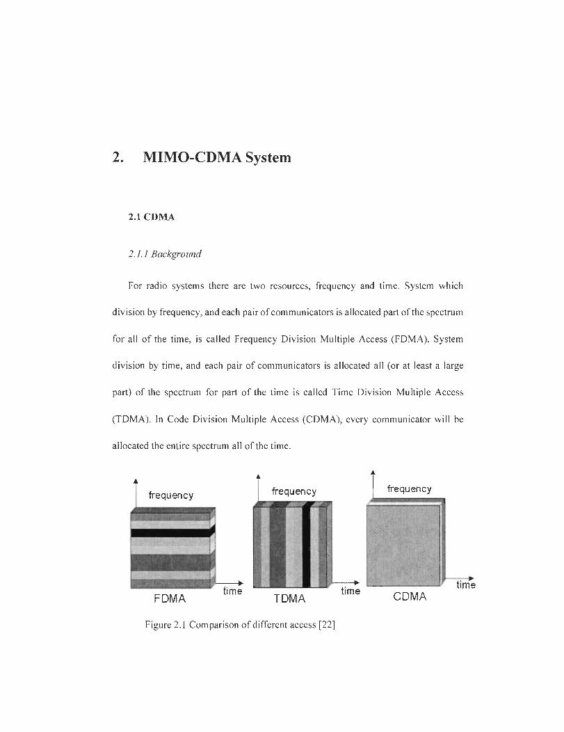
For radio systems there are two resources, frequency and time. System which
division by frequency, and each pair of communicators is allocated part of the spectrum
for ail of the time, is called Frequency Division Multiple Access (FDMA). System
division by time, and each pair of communicators is allocated ail (or at least a large
part) of the spectrum for part of the time is called Time Division Multiple Access
(TDMA). In Code Division Multiple Access (CD MA), every communicator will be
allocated the entire spectrum ail of the time.
frequency
. .. tlme
FOMA TOMA CDMA
Figure 2.1 Comparison of different access [22]
8
CDMA uses codes to identify connections. It is a form of Direct Sequence Spread
Spectrum communication technology, which has been used in military communications
for a long time. In response to an ever-accelerating worldwide demand for mobile and
personal portable communications, spread spectrum digital technology has achieved
much higher bandwidth efficiency for given wireless spectrum allocation, and hence
serves a far large population of multiple access users, than analog or other digital
technologies. Like its implementation in military predecessors, the spread spectrum
wireless network ach ieves efficiency improvements by incorporating a number of
unique features made possible by the benign noise-like characteristics of the signal
waveform. Chief among these is universal frequency reuse. Besides increasing the
efficiency of spectrum usage, this also eliminates the chore of planning for different
frequency allocation for neighboring users or cells. Many other important multiple
access system features are made possible through this universal frequency reuse by
terminaIs employing wideband (spread) noise-like signal waveforms. Most important
one is fast and accurate power control, which ensure a high level of transmission quality
while overcoming the distance problem by maintaining a low transmitted power level
for each terminal , and hence a low level of interference to other user terminais. Another
is mitigation of faded transmission through the use of a Rake receiver, which
constructively combines muItipath components rather than allowing them to
destructively combine as in narrowband transmission. A third major benefit is soft
handoff among multiple cell base station, which provides improved cell-boundary
performance and d prevents dropped calls.
9
2.1.2 Principle ofSpread Code Communication
COMA uses ul1lque spreading codes to spread the baseband data before
transmission. The signal is transmitted in a channel, which is below noise level. The
receiver then uses correlators to dispreads the wanted signal, which is passed through a
narrow band pass filter. Unwanted signaIs will not be despread and will not pass
through the filter. Codes are in the form of a carefully designed binary (onelzero)
sequence produced at a much higher rate than that of the baseband data. The rate of a
spreading code is referred to as chip rate rather than bit rate. Usually, in CDMA a
spread code runs at a much higher rate than the data to be transmitted. Data for
transmission is sim ply logically XOR added with the faster code.
Tb , 1\
/J"------ ~ ... ------_~ l '
----------~. " ---------,
Figure 2.2 Generate spread spectrum signal [23]
Data Signal
Pseudorandom Code
Transmitted Signal: Data Signal XOR with the Pseudo random
The figure 2.2 shows how spread spectrum signal is generated. The data signal with
pulse duration of Tb is XOR added with the code signal with pulse duration of Tc.
Therefore, the bandwidth of the data signal is llTb
and the bandwidth of the spread
spectrum signal is1/r . Since Tc is much smaller thanTb , the bandwidth of the spread c
10
spectrum signal is much larger than the bandwidth of the original signal. Each user in a
COMA system uses a different code to modulate their signal. Choosing the codes used
to modulate the signal is very important in the performance of COMA systems. The
best performance will occur when there is good separation between the signal of a
desired user and the signais of other users. The separation of the signais is made by
correlating the received signal with the locally generated code ofthe desired user. Ifthe
signal matches the des ired user's code then the correlation function will be high and the
system can extractthat signal. If the desired user's code has nothing in common with the
signal the correlation should be as close to zero as possible (thus eliminating the
signal); this is referred to as cross correlation. Ifthe code is correlated with the signal at
any time offset other than zero, the correlation should be as close to zero as possible.
This is referred to as auto-correlation and is used to reject multi-path interference.
In general , COMA belongs to two basic categories: synchronous (orthogonal
codes) and asynchronous (pseudorandom codes). In this paper, we will discuss the
asynchronous COMA.
2.1.2.1 rn-sequence in CD MA
For COMA spreading code, we need a random sequence that passes certain
"quality" criterion for randomness. These criterions are
• The number ofruns ofO ' s and l ' s is equal. We want equal number oftwo
O' s and l ' s, a length of three O' s and l ' s and four O' s and l ' s etc. This
property gives us a perfectly random sequence.
11
• There are equal number of runs of O' s and 1 ' s. This ensures that the
sequence is balanced.
• The periodic autocorrelation function (ACF) is nearly two valued with
peaks at 0 shift and is zero elsewhere. This allows us to encrypt the signal
effectively and using the ACF peak to demodulate quickly.
Maximum length sequence (rn-sequence) meets ail these three requirements
strictly. We can generate this sequence by using a linear feedback registers. Which
structure is shown in Figure 2.3.
3 stage LFSR generating l11-sequellce ofperiod 7. , USillg taps l and 3.
Another 3 stage LFSR gellera ting m-~equence ofperiod ï , using taps :2 and 3
Figure 2.3 The structure of linear feedback registers (LFSR) [24]
Each configuration of N registers produces one sequence of length ZN. If taps are
changed, a new sequence is produced in the same length. There are only a limited
number of rn-sequences of a particular size.
12
The cross correlation between an m-sequences and noise is low which is very useful
in filtering out noise at the receiver. The cross correlation between any two different
m-sequences is also low and is useful in providing both encryption and spreading. The
low amount of cross-correlation is used by the receiver to discriminate among user
signais generated by different m-sequences.
Think of m-sequence as a code applied to each message. Each letter (bit) of the
message is changed by the code sequence. The spreading quality of the sequence is an
added dimensionality and benefit in CDMA systems.
2.1.2.2 Gold Codes in CDMA
In this paper we discuss the asynchronous COMA systems. So we need to learn the
Gold code, which is used in this kind of system.
A Gold Code is a set of random sequences which was discovered in 1967, often
called pseudo-noise (PN) sequences, which are statistically uncorrelated . Gold codes
have three-valued autocorrelation and cross-correlation function with values
{-l, -t(m), t(m) - 2}, where
{
2 (m+l)/2 + 1 for odd m t(m) =
2 (m+2)/2 + 1 for even m (2.1 )
AlI pairs of m-sequences do not yield Gold codes and those which yield Gold codes are
called preferred pairs. Moreover, such preferred pairs can be used to construct a who le
family of codes that have the same period as weIl as the same correlation property.
13
Gold codes are used in non-orthogonal CDMA as chipping sequences that allow
several users to use the same frequency, resulting in less interference and better
utilization of the available bandwidth.
We usually combine two rn-sequence to get the Gold codes.
2 3
EX-OR
3
Figure 2.4 Generating Gold codes by combining two preferred pairs of
rn-sequences [25]
2.1.2.3 Long Code
In JS-95 and IS-2000 system, there is another kind of rn-sequence which called long
code. lts length is 242 - 1 bits. We can create it from a LFSR of 42 registers. It runs at
1.2288 Mb/s. The time it takes to recycle this length of code at this speed is 41.2 days.
Long code is used to both spread the signal and to encrypt it. A cyclically shifted
version of the long code is generated by the cell phone during cali setup. The shift is
called the Long Code Mask and is unique to each phone calI. CDMA networks have a
security protocol called CAVE that requires a 64-bit authentication key, called A-key
and the unique Electronic Seriai Number (ESN). The network uses both of these to
14
create a random number that is then used to create a mask for the long code used to
encrypt and spread each phone calI. This number, the long code mask is not fixed but
changes each time a connection is created.
Here are another two concepts, public long code and private long code. The Public
long code is used by the mobile to communicate with the base during the cali setup
phase. The private long code is one generated for each cali then abandoned after the cali
is completed.
2.1.2.4 Short Code
Short code in CDMA is based on a rn-sequence which length is 215 - 1. These
codes are used for synchronization in the forward and reverse links and for cell/base
station identification in the forward link. The short code repeats every 26.666
milliseconds. The sequences repeat 75 times in every 2 seconds. We want this sequence
to be fairl y short because during cali setup, the mobile is looking for a short code and
needs to be able find it fairly quickly. Two seconds is the maximum time that a mobile
will need to find a base station.
A mobile is assigned a short code PN offset by the base station to which it is
transmitting. The mobile adds the short code at the specified PN offset to its traffic
message, so that the base station in the region knows that the particular message is
meant for it. This is the way the primary base station is identified in a phone calI. The
base station keeps a list of nearby base stations and during handoff the mobile is
notified of the change in the short code.
15
2.2MIMO
2.2.1 Background
Multiple Input Multiple Output (MIMO) is an antenna technology, in which
multiple antennas are used in both transmitter and receiver [5]. It is one of forms of
smart antenna. The earliest idea in this field was mentioned by A.R. Kaye and D.A.
George in 1970 and W. van Etten in 1975 and 1976. After then, several papers on
beamforming related applications in 1984 and 1986 which were published by Jack
Winters and Jack Salz at bell laboratories. Until 1993 , Arogyaswami Paulraj and
Thomas Kailath proposed the concept of Spatial Multiplexing using MIMO. It is the
first time that this technology is used in wireless broadcast. ln commercial arena,
Iospan Wireless Inc. developed the first commercial system in 2001 which used
MIMO-OFDMA technology. It supports both diversity coding and spatial multiplexing.
By using MIMO technology we can minimize the errors and optimize data speed. At
the same time, it does not need additional bandwidth or transmit power.
As a part of smart antenna technology, MIMO develop from SISO (Single Input
Single Output), SIMO (Single Input Multiple Output), MISO (Multiple Input Single
Output).
16
MIMO
MISO
SIMO
transmitter receivers
Figure 2.5 S1S0 to MIMO [26]
In traditional telecommunication system, we have 1 transmit antenna and 1 receive
antenna. Most of the telecommunication system now is using this structure. Then,
SIMO technology appears. Compare with single antenna technology, SIMO has the
same data transmit rate but greater range. MISO is another kind of structure. Compare
with SlS0 system, MISO system has the same data rate and same transmit range but
more reliable. And in MIMO system, we can get greater data rate and greater range.
17
2.2.2 Benefits of MIMO
The benefits ofMIMO technology that help achieve such significant gains as below
[5]
• Array gain
Array gain is the increase in receive SNR that results from a coherent combing
effect of the wireless signais at a receiver. The coherent combing may be realized
through spatial processing at the receive antenna array or spatial pre-processing at the
transmit antenna array. Array gain improves resistance to noise, thereby improving the
coverage and the range of wireless network.
• Spatial diversity gain
Spatial diversity gain mitigates fading and is realized by providing the receiver with
multiple copies of the transmitted signal in space, frequency or time. With an increasing
number of independent copies, assume that at least one of the copies is not experiencing
a deep fade increases, thereby improving the quality and reliability of reception. A
MIMO channel with Nt transmitters and Nr receivers potentially offer NtNr
independently fading links, and hence a spatial diversity order ofNtNr.
• Spatial multiplexing gain
Using spatial multiplexing in MIMO system can increase data rate. For example,
transmitting multiple, independently data streams within the bandwidth of operation.
Under suitable channel conditions, in this kind of environment the receiver can separate
18
the data streams. Furthermore, each data stream ex peri en ces at least the same chanJlel
quality that would be experienced by a SISO system, effectively enhancing the capacity
by a multiplicative factor equal to the number of streams. In general, the number of data
streams that can be reliably supported by a MIMO channel equals the minimum of the
number of transmit antennas and the number of receive antenna. The spatial
multiplexing gain increases the capacity of a wireless network.
• Interference reduction and avoidance
Interference in wireless networks results from multiple users sharing time and
frequency resources. Interference may be mitigated in MIMO systems by exploiting the
spatial dimension to increase the separation between users. For instance, in the
presence of interference, array gain increase the tolerance to noise as weil as the
interference power, hence improving the SINR. Additionally, the spatial dimension
may be leveraged for the purposes of interference avoidance. For example, directing
signal energy forwards the intended used and minimizing interference to other users.
Interference reduction and avoidance improve the coverage and range of wireless
network.
In general, it may not be possible to exploit simultaneously ail the benefits
described above due to conflicting demands on the spatial degrees of freedom .
However, using sorne combination ofthe benefits across a wireless network will result
in improved capacity, coverage and reliability.
19
2.2.3 Capacity of MIMO
As we mentioned before, one of the benefits of MIMO system is the capacity
increases [6]. When the system is SISO status, we could estimate its capacity by using
Shannon 's Capacity Formula:
C = 8 . logz (1 + _P-) NoB
(2.2)
In which 8 is bandwidth, P is transmitted signal power and No is single noise spectrum.
Assumes the channel is White Gaussian. This formula gives an upper limit for the
achieved error-free SISO transmission rate. If the transmission rate is less than C
bits/sec(bps), then an appropriate coding scheme exits that could lead to reliable and
error-free transmission. On the contrary, if the transmission rate is more than C bps,
th en the received signal, regardless of the robustness of employed code, will involve bit
errors.
When we discuss the case in MIMO system, we can extend Shannon ' s Capacity
Formula for MIMO. We consider an antenna array with nt elements at the side of
transmitter and an antenna array with 11r elements at the side of receiver. The impulse
of the channel between the jth transmitter element and the ith receiver element IS
denoted as hi,j (T, t) . The MIMO channel can th en be described as below:
[
hll (T, t)
H(T, t) = hz,l (T, t)
hn l(T,t) r,
h1,z (T, t)
hz z(T, t)
hn z(T,t) r,
h1n(T,t)] , t
hz,neCT, t)
hMR,n:(T, t)
(2.3)
20
The matrix elements are complex numbers that correspond to the attenuation and phase
shift that the wireless channel introduces to the signal reaching the receiver with delay
T . The input-output notation of the MIMO system can now be expressed by the
following equation:
y(t) = H(T, t) ® set) + u(t) (2.4)
Where ® denotes convolution, set) is corresponding to the nt transmitted signaIs, y(t)
is corresponding to the 1tr received signaIs and u(t) is the additive white noise. If the
transmitted signal bandwidth is narrow enough that the channel response can be seen as
flat across frequency, then the discrete time description corresponding to equation (2.3)
IS
(2.5)
Then the capacity of MIMO channel can be estimated by the following equation
(2.6)
Where H is the channel matrix, Rss is the covariance matrix ofthe transmitted vector s,
HH is the transpose conjugate of the H matrix and p is the maximum nonnalized
transmit power. C is the estimation of capacity for MIMO channel.
2.2.4 MIMO Channel
MIMa channels arise in wireless communications environment where multiple
transmit and receive antennas are used. MIMO channels work best in highly scattering
transmission environment, where multiple paths exist between transmitters and
21
receivers. Multipath is the propagation phenomenon which causes by atmospheric
ducting, ionosphere reflection and refraction, and reflection from terrestrial objects,
such as mountains and buildings.
Figure 2.6 MIMO channels [27]
ln engineering, we usually describe MlMO system as follow
Rec -iv - Array - -------:--------,
r---------------· kJ' :r 1 l 1
:n2 ! [>-;---.~~E9n, ------~:~.~ Y2
_':>_~- _~'_", ~<7 ~'---T----<~..;~n l l
h11
1 1
Tnlll;_luit. ~ 1:2
Antenna
Array
'" \... /~
Figure 2.7 Block Diagram ofMIMO channel [28]
~ YI
~ n lVr
[) ! ~ & : L _______________ ~
22
In a MIMO system, the effects of multipath include constructive and destructive
interference, and phase shifting of the signal. It may cause ISI which will affect signal
transmission quality.
2.3 Rake Receiver
At the side of the receiver, we have to use sorne technique to correct the ISI. It is
very important for the whole communication system. Rake receive is one ofthe choices
which uses in CDMA based system. A Rake receiver is a radio receiver designed to
counter the effects of multipath fading. It does this by using several "sub-receivers"
called fingers, that is, several correlators each assigned to a different multipath
component. Each finger independently decodes a single multipath component; at a later
stage the contribution of ail fingers are combined in order to make the most use of the
different transmission characteristics of each transmission path. 1t could weil result in
higher Signal to Noise Ratio (SNR) environment.

Iii 1 path-1 ~
"J1l~ /" PathDelay
'1 ,~h-l ~L
COD EA Path Delay \'\oith timing of 1)<)th-1
CODEA
~ r "JL 'Mth timing of l)<lth-2 Path Delay
Figure 2.8 Rake receiver [29].
23
ffi: path-3
L.. t : ~~! ~ path-2
1 ~ path-1 i :
0_: _ o, _ o' ----il-
The multipath channel through which a signal transmits can be seen as transmitting the
original signal plus a number of multipath components. Multipath components are
delayed copies of the original transmitted signal traveling through a different echo path,
each with a different magnitude and time-of-arrival at the receiver. Since each
component contains the original information, after the process of channel estimation ail
the components can be added coherently to improve the infonnation reliability.
3. Channel Estimation Aigorithms
3.1 introductions
The radio channel in mobile radio systems are usually causing intersymbol interference
(IST) and enhances multiple access interferences (MAI) in the received signal [9]. In
order to remove ISf and MAI from the signal, many kinds of equalizers can be used .
Indirect detection algorithms require knowledge of the channel impulse response (CIR),
which can be provided by a separate channel estimator. Usually the channel estimation
is based on the known sequence of bits, which is unique for a certain transmitter and
which is repeated in every transmission burst. Thus, the channel estimator is able to
estimate CfR for each burst separately by exploiting the known transmitted bits and the
corresponding received samples.
n
H .1 ~Sl_g~_ .. a_l~ L_CH_:~_~:_EL~----+~~~)
Figure 3.1 Layout of the channel estimation [30)
25
The figure 3.1 above is the layout of the channel estimation in a CDMA system.
We can see the signal is transmitted over a channel, which we assume as a fading
multiple channel. Thermal noise is generated at the side of receiver. A detector is used
to detect the original signal from the received signal. At the same time, the detector also
needs the channel estimate h from a specific channel estimator. The received signal y
can be expressed as follows
y = Mh+n (3.1 )
Where the complex channel impulse response h of the wanted signal is expressed as
below
(3.2)
n denotes the noise samples.
Generally speaking, four kind of methods are used in channel estimation algorithm.
Which are Blind Channel Estimation, Direct Technique (Such as Adaptive Channel
Estimation), Indirect Technique (Such as Matrix Inverse method) and Mixed
Estimation (Such as the layout showed in Fig. 3.1, detector and estimator work
together). In this article, we will focus on the Direct Technique and the Indirect
Technique. This means that we assume we have already known the original signal at the
side ofthe receiver. By using this information we do channel estimation to get the h.
26
3.2 Indirect Techniques
3.2.1 Least-squares (LS) channel estimation
Least squares can be interpreted as a method of fitting data. The best fit in the
least-squares sense is that instance of the model for which the sum of squared residuals
has its least value, a residual being the difference between an observed value and the
value given by the mode\. The method was first described by Carl Friedrich Gauss
around 1794.
According to the equation (3.1) and (3.2), we can get that
fi. = arg minh lIy - Mhll 2 (3.3)
Assuming we've got the noise, we get
(3.4)
Where C)H and C )-1 denote the Hermitian and inverse matrices, respectively.
3.2.2 Blind Channel Estimationfor MIMO-CDMA using.first-order statistics
Blind channel estimation algorithm is another important estimation algorithm
which receives considerable interest recently [10]. People believe that this kind of
algorithm has potential to increase the system throughput significantly.
We assume that we have a Nt transmit antenna and NI' receive antenna system. At
the side of transmitter, each symbol is spread by aperiodic code vector ciCk) with
spreading gain P, followed by a chip pulse-shaping filter. Atthe side ofreceiver, signais

27
are passed through a chip-matched filter and sam pied at the chip rate. So we can get
channel model '7i (k) , k = l, ... Lji '
2.,
;---- y Ji (n) ~ 1 1
D -J..- y .. (}'l).!-D 1 1 l' .::...J~ .) 1 .:li 1
Figure 3.2 Channel response [31]
We get the received signal as below,
Ci (nT + 1) Ci (nT + 1)
Ci (nT + P)
(3.5)
From figure 3.2 we can see that 01 and 02 are overlapped zones corrupted by data
from the previous and following symbol. We consider only the part without
intersymbol interference, we get
(3 .6)
So we can write the received signais as following
(3.8)
28
(3.9)
Where matrix ~ is a block diagonal with 0i as the ith block. We can get the signal at
the side of receiver which is
lj = diag(C(n)/" / C(n + m -1)). (lm ® ~)b + w = C!kb+"'i
(3.10)
Where "'i represents the additive Gaussian noise. C is block diagonal matrix with C(n)
as its diagonal block. lm ®~ is the Kronecker product. When we consider about Nr
receive antenna. We get
1 [ ~ 1 b + w = CJfb + w C !!.Nr
Then, we can get output of the matched filter ct as
t = ct y = Jfb + n = [~ lb + v !!.Nr
Where v = ctw is the colored noise vector. C= (lNr®C), so we have
Where
tjn = ~ ben) + Vjn j = 1, ... / Nr. n = 1/ ... / m
t.~n ) = b·(n)· h .. +v·· (n) i = 1··· Nt J! ! "J! J! / /
(3.11 )
(3.12)
(3.13 )
(3 .14)
(3.15)
Because bien) is generated from the finite-alphabet set {-l ,+l} and Vji(n) IS
zero-mean additive noise, the set of tjn can be classified into two sets as below
29
(3.16)
(3.17)
The centers of the two sets can be found by using such as K-means clustering.
(3.18)
C2 = center(S2) (3.19)
Assume that for m synbols there are p points belonging to SI and q points belonging to
S2,
We have
(3.20)
3.2. 3 Blind Multipath Estimation with Toeplitz displacement for long code
DS-CDMA
According to [11] , the baseband representation of the received signal after coherent
reception is given by
(3.21)
Where w(t) is the additive and circularly symmetric Gaussian noise process with
variance O"~ , and Ak is the amplitude of the signal for user k.
(3.22)
Where '!/J(t) is the shape of the chip with a duration Tc

30
We use M matched filters per received symbol to fully exploit the properties of the
DS-CDMA signaIs.
Where the matched filtering matrix Sl (n) is presented by
Sien) =
CI,M (n + N)
CfM(n + N)
o
o
CIM(n + aN)
CfM(n + aN)
The matrix si (n) and Cl (n) are related by
(3.23)
(3.24)
(3.25)
Let us consider the aM x 1 matched filter output vector yen) , the covariance matrix
ofthis observation vector is obtained as
Where (Jf = AiE{bf(n)} , Rw(n) = (JJS1(n)S[(n) is noise autocorrelation matrix,
and the contribution of other user' s interference is
(3.27)
We introduce the Toeplitz displacement method here to remove the effects of the
channel noise and interference. Let us define
31
(3.28)
Where Ns is the number oftransmitted symbols. Then we can get
Rh = Ry (2: aM, 2: aM) - Ry (l: aM - 1,1: aM - 1) = R; - Ry =
(3.29)
sci and SCI are formed by removing the first and the last row of SC 1.
Then we can get
Rh (n) = R;(n) - Ry(n) = Ry (n)(2: aM, 2: aM) - Ry (n)(l: aM - 1,1: aM - 1)
(3.30)
We present the estimation error matrix to be
The estimation error can be defined with squared Frobenius norm of Eh
(3.32)
The cost function can be built as the cumulative error
(3.33)
The channel parameters can be obtained by minimizing this co st function. ln practice,
the average correlation matrix Ry is sampled and formed by
(3.34)
32
The estimated Rh can be formed. We define new unknown by
(3.35)
The error matrix (12) becomes
(3.36)
And
Let
(3.38)
(3 .39)
We have
(3040)
Therefore, our cost function becomes
l N { ~ }H{ ~} ] = Ns Ln~l Qd l - vec(Rh (n)) Qdl - vec(Rh (n)) (3 Al)
The following LMS type recursion can be formulated for dl with step size Il
dCn+l ) - d Cn) _ r7 J() l - l j1.v d~ n (3.42)
(3.43)
So we can get
(3044)
33
3.2.4 EM Vector Channel Estimation
In [12J, the system consists of G users. There are Nt antennas in the transmitters of
wach mobile user and Nr antennas in the receiver of the base station through a
correlated multipath Rayleigh fading channel , so that the total number oftransmitting
antennas from aIl users is K=G*Nt. The considered MIMO-CDMA system is over a
correlated multipath fading channel. At each time interval [IT, (I+1)T], the ith antenna
of gth user generates a symbol bgJ Cl) from the symbol set {+ 1.-1 }th equal probability.
The each symbol is spread by the aperiodic spreading sequence
(3.45)
Where cIN+n,g here is the quadratic-phase random signature sequence for user g, and
l/JCt) is the chip waveform with duration [0, Tcl . The spreading waveform are
normalized. The transmitted signal of the gth user' s the ith antenna is
(3.46)
Where bg,iCl) is the data symbol of the gth user' s the ith antenna at symbol index 1.
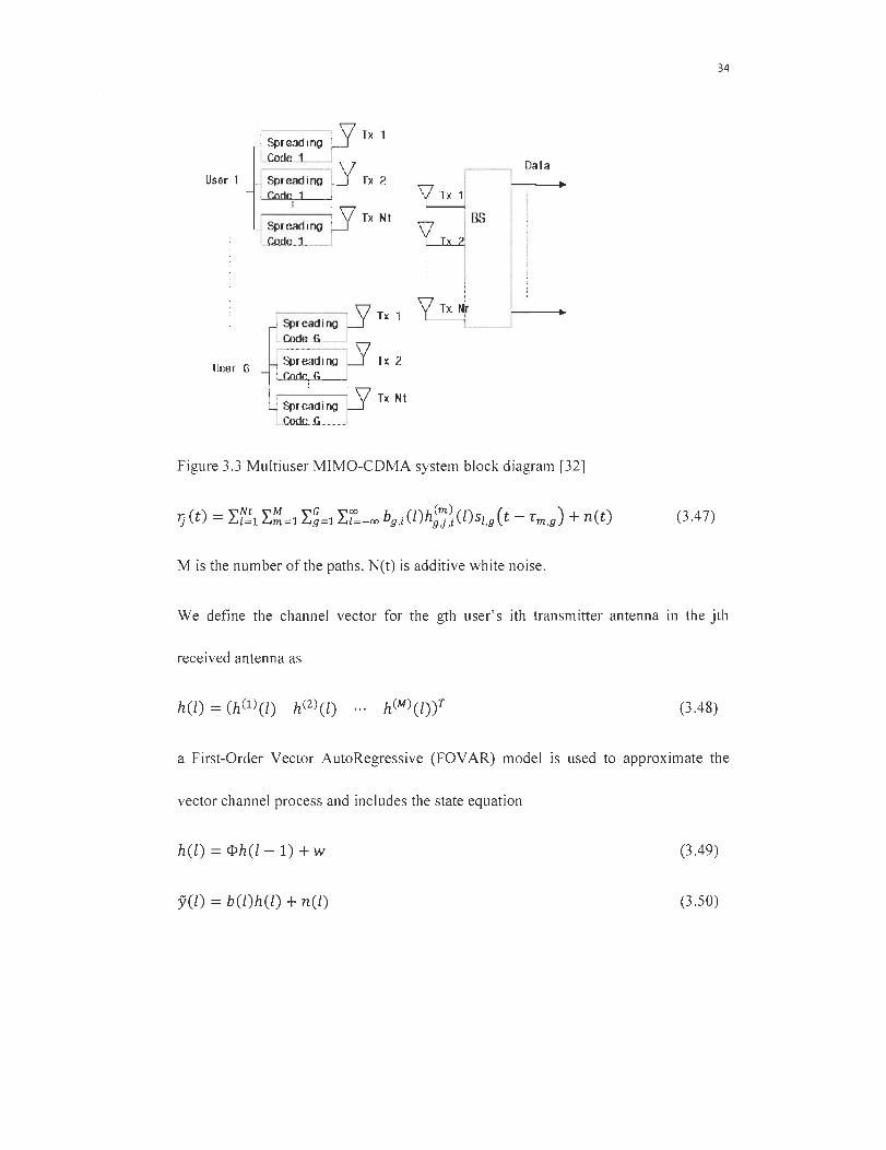
1 . , Vlx1 • Sprcad lng U
User 1 f; ... ~:;:. ~:-i~~g. u.... lx 2 , corte: l ,
, . 'S Tx Nt 1 Sprnad 1 no , ' .... C,ortc ... J ......... .
BS
Figure 3.3 Multiuser MIMO-CDMA system block diagram [32]
Mis the number of the paths. N(t) is additive white noise.
34
(3.4 7)
We define the channel vector for the gth user' s ith transmitter antenna in the jth
received antenna as
(3.48)
a First-Order Vector AutoRegressive (FOVAR) model is used to approximate the
vector channel process and inc\udes the state equation
h(l) = cph(l- 1) + w (3.49)
y(l) = b(l)h(l) + n(Z) (3.50)
35
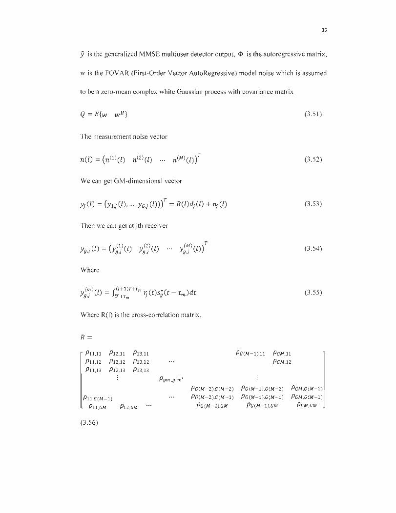
y is the generalized MMSE multiuser detector output, <1> is the autoregressive matrix,
w is the FOY AR (First-Order yector AutoRegressive) model noise which is assumed
to be a zero-mean complex white Gaussian process with covariance matrix
The measurement noise vector
We can get GM-dimensional vector
Then we can get at jth receiver
(M ) )T ... Y . (l) 9d
Where
(m)C) r(l+l )THm C) *C )d Yg,} l = J1TH
m 1] t Sg t - Tm t
Where R(I) is the cross-correlation matrix.
R=
Pll ,ll P12,1l P13,ll
Pll ,12 P1 2,12 P13 ,12
Pll ,13 P12,13 P13,13
Pgm ,g'm'
PG (M-l ), ll PGM,ll
PGM,12
PG (M-2 ),G(M-2 ) PG (M-l ),G (M-2 )
Pll ,G(M-l ) PG (M-2 ),G (M-l ) PG (M-l ),G(M-l )
Pll ,GM P12 ,GM PG (M-2 ),GM PG (M-l ),GM
(3.56)
(3.51 )
(3.52)
(3.53)
(3.54)
(3.55)
PGM,G (M-2 )
PGM ,G(M-l )
PGM,GM
36
Pgm ,g'm' is the cross-correlation of the symbols of the gth user, the mth path and the
g' th user, the m ' th path ,
CT ( ) * 'r ' , Pgm ,g'm' = Jo Sg t - mTm,g Sg ' Ct - m m ,9 )dt (3 .57)
Tm,g is the path delay of gth user, the mth path.
_ [ (1) (2) (M ) (1) (2) (M)]T dj - d1,j,d1,j,···,d1,j , ... ,dG,j,dG,j,· .. ,dG,j (3.58)
Which denote the MG-dimensional column vector.
d~~) = Lf~l h~~~bg , i represents the ail oftransmitter antenna for the gth user by the
mth path at jth receiver.
rit is MG-dimensional A WGN noise vector with variance matrix (J2I.
So we use MMSE for ail users' data and MMSE output are denote by MG-dimensional
column vector
(3.59)
Where SNR is signal to noise ratio.
3.2.5 Reduced-Rank Space-time Channel Estimationfor DS-CDMA
In [13], consider a asynchronous OS-COMA system with K-users. The transmitted
baseband signal model can be written as follow
(3.60)
Where Tc is the chip interval. {CkU)} is the spreading sequence of user k. ({JCt) is
normalized chip wave fonn of duration Tc . Then, the baseband multipath channel
37
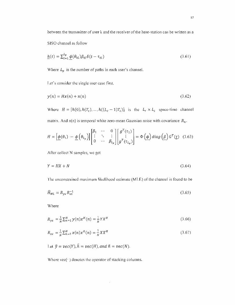
between the transmitter ofuser k and the receiver of the base-station can be written as a
SISO channel as follow
(3.61 )
Where Lp is the number of paths in each user's channel.
Let's consider the single user case first.
yen) = Hx(n) + n(n) (3.62)
Where H = [h(Q), h(Te), ... , h((Le - l)Te)] IS the Lr x Le space-time channel
matrix. And n(n) is temporal white zero-mean Gaussian noise with covariance Rn'
After collect N samples, we get
y = HX +N (3.64)
The unconstrained maximum likelihood estimate (MLE) of the channel is found ta be
(3.65)
Where
(3 .66)
R = ~ ~N_ x(n)xH(n) = ~XXH xx N L-n-l N (3.67)
Let y = vec(Y), li = vec(H), and fi = vec(N).
Where vec(- ) denotes the operator of stacking columns.
38
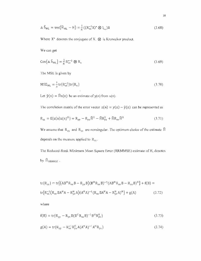
(3.68)
Where X· den otes the conjugate of X. ® is Kronecker product.
We can get
(3.69)
The MSE is given by
(3.70)
Let yen) = Hx(n) be an estimate ofy(n) from x(n).
The correlation matrix of the error vector zen) = yen) - Yen) can be represented as
_ H _ ~H ~ H ~ ~H
Rzz - E{z(n)z(n) } - Ryy - Ryx H - HRyx + HRxx H (3.71 )
We assume that Ryy and Rxx are nonsingular. The optimum choice ofthe estimate H
depends on the measure applied to Rzz .
The Reduced-Rank Minimum Mean Square Error (RRMMSE) estimate ofR, denotes
by HRRMMSE .
(3.72)
where
(3.73)
(3.74)
39
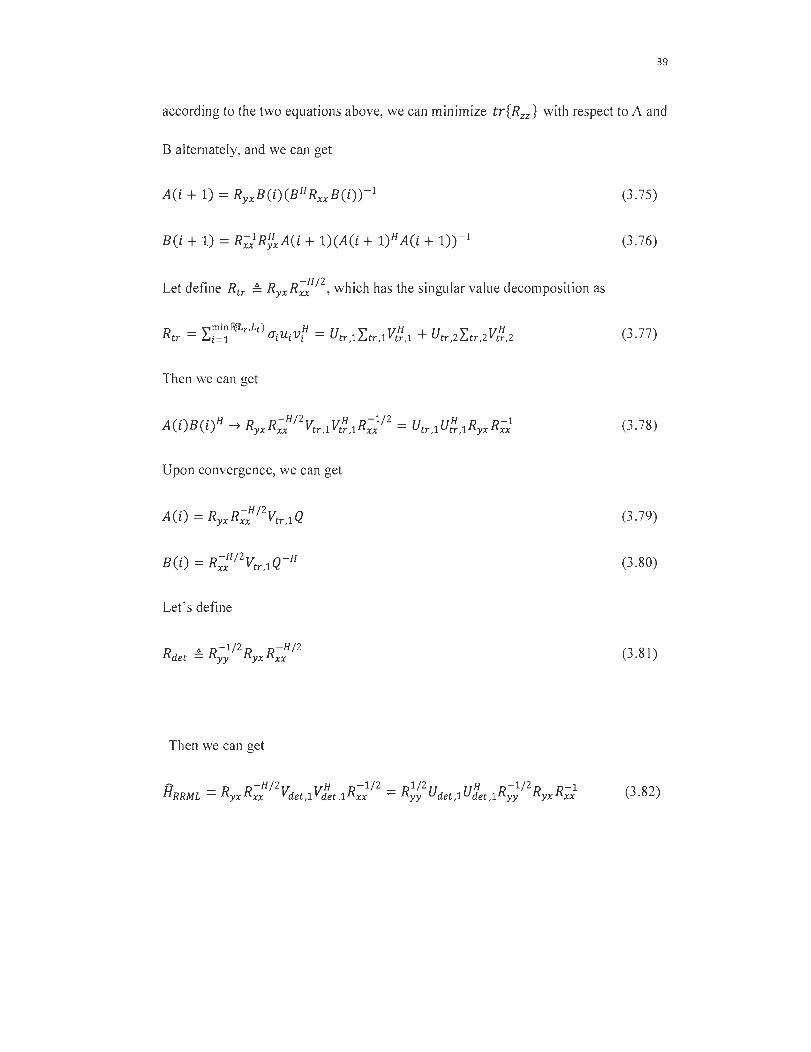
according to the two equations above, we can minimize tr[Rzz} with respect to A and
B alternately, and we can get
(3.75)
(3 .76)
Let define Rtr ~ Ryx R;: / 2, which has the singular value decomposition as
(3.77)
Then we can get
AC ')BC')H R R-H/ 2TT TTH R-1/2 - U UH R R-1 l l -t yx xx Vtr,l Vtr ,l xx - tr,l tr,l yx xx (3.78)
Upon convergence, we can get
(3 .79)
BC') = R-H/2v, Q-H l xx tr,l (3.80)
Let ' s define
,,-1/2 -H/2 Rdet = Ryy Ryx Rxx (3.81 )
Then we can get
(3.82)
40
3.2.6 Linear MMSE channel estimation
The linear MMSE algorithm [14] compute a matrix W, which is chosen to minimize the
mean square error E{IIh - W*rIl 2}.
R = E[rr*] = E[(Ah + n)(Ah + n)*] = APA* + Nol
cp = E[rh*] = E[(Ah + n)h*] = AP
P = E[hh*] = diag(Pl,l, ' .. , Pk,l' ... , PKh )
fiLMMSE = WMMSEr = cp*R- l r = P*Â*(ÂPÂ* + NoI)-l r
3.3 Direct Techniques
3.3.1 Least-Mean-Squares (LMS) Channel Estimation
(3.83)
(3.84)
(3.85)
(3.86)
(3.87)
The LMS algorithm is an important member of the family of stochastic gradient
algorithms [15]. The term stochastic gradient is intended to distinguish the LMS
algorithm from the method of steepest descent, which uses a deterministic gradient in a
recursive computation of the Wiener fiIter for stochastic inputs. A significant feature of
the LMS algorithm is its simplicity. Moreover, it does not require measurements of the
pertinent correlation functions, nor does it require matrix inversion.
LMS algorithm is a linear adaptive filtering algorithm which generally consists oftwo
basic processes:
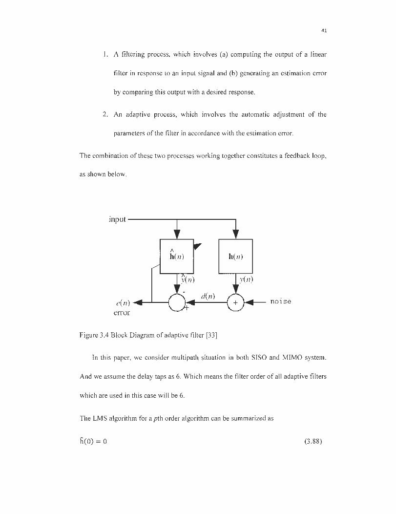
41
J. A filtering process, which involves (a) computing the output of a linear
filter in response to an input signal and (b) generating an estimation error
by comparing this output with a desired response.
2. An adaptive process, which involves the automatic adjustment of the
parameters ofthe filter in accordance with the estimation error.
The combination ofthese two processes working together constitutes a feedback loop,
as shown below.
input -----........ --------,
1\
l1(n) h(n)
yen)
e( n) -4-----L--i d(n)
nOI se
error
Figure 3.4 Block Diagram ofadaptive filter [33]
In this paper, we consider multipath situation in both SISO and MIMO system.
And we assume the delay taps as 6. Which means the filter order of ail adaptive fiIters
which are used in this case will be 6.
The LMS algorithm for a pth order algorithm can be summarized as
heO) = 0 (3.88)
x(n) = [x(n), x(n - 1), ... , x(n - p + l)F
e(n) = den) - flH (n)x(n)
fl(n + 1) = fl(n) + ~e'(n)x(n)
Where fiH (n) denotes the Hermitian transpose of fi(n).
3.3.2 Recursive Least Squares (RLS) Channel Estimation
42
(3.89)
(3.90)
(3.91 )
Recursive least squares (RLS) algorithm is used in adaptive filters to find the filter
coefficients that relate to recursively producing the least squares of the error signal [16].
This is contrast to other algorithms that aim to reduce the mean square error. The
difference is that RLS filters are dependent on the signaIs themselves, whereas MSE
filters are dependent on their statistics. lfthese statistics are known, an MSE filter with
fixed coefficients can be built. An important feature of this filter is that its rate of
convergence is typically an order ofmagnitude faster than that of the simple LMS filter,
due to the fact that the RLS filter whitens the input data by using the inverse correlation
matrix of the data, assumed to be of zero mean. This improvement in performance,
however, is achieved at the expense of an increase in computational complexity of the
RLS fiIter.
The RLS algorithm for a pth order RLS filter can be summarized as
P(O) = 8-1/
(3.92)
(3.93)
43
[
x(n) 1 x(n) = x(n ~ 1)
x(n - p)
(3.94)
a(n) = den) - w(n - if x(n) (3.95)
g(n) = pen - l)x*(n){À + xT (n)P(n - l)x*(n)}-l (3.96)
(3.97)
w(n) = w(n - 1) + a(n)g(n) (3.98)
Where pis filter order, À is forgetting factor, 15 is value to initialize P(Q).
3.3.3 Iterative Channel Estimationfor Turbo Receivers in DS-CDMA
Here we introduce another kind of direct technique of channel estimation [17].
1( 0)
Figure 3.5 Transmission System [34]
We consider a transm ission system (see Fig. 3.5) in which the binary information bits
are first encoded via a turbo or a convolution encoder, interleaved and then modulated
to symbols using a complex constellation. We will denote this set of bits as a coding
block. In the modulation stage, the bits to symbols mapping must be done in such a
form that the in-phase and in-quadrature components of each symbo1 can be treated as
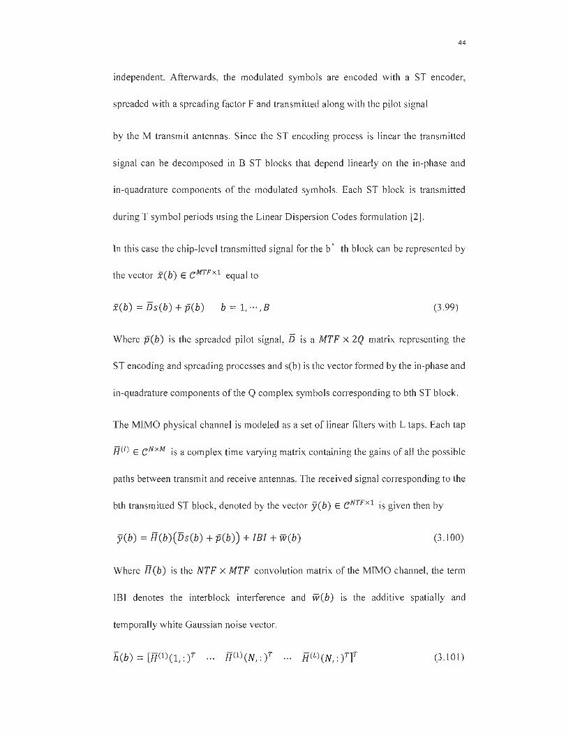
44
independent. Afterwards, the modulated symbols are encoded with a ST encoder,
spreaded with a spreading factor F and transmitted along with the pilot signal
by the M transmit antennas. Since the ST encoding process is linear the transmitted
signal can be decomposed in B ST blocks that depend linearly on the in-phase and
in-quadrature components of the modulated symbols. Each ST block is transmitted
during T symbol periods using the Linear Dispersion Codes formulation [2].
In this case the chip-Ievel transmitted signal for the b' th block can be represented by
the vector i(b) E CMTFXl equal to
i(b) = l5s(b) +p(b) b = 1,···,B (3.99)
Where p(b) is the spreaded pilot signal , l5 is a MTF x 2Q matrix representing the
ST encoding and spreading processes and s(b) is the vector formed by the in-phase and
in-quadrature components of the Q complex symbols corresponding to bth ST block.
The MIMO physical channel is modeled as a set of linear filters with L taps. Each tap
H CI) E C NxM is a complex time varying matrix containing the gains of ail the possible
paths between transmit and receive antennas. The received signal corresponding to the
bth transmitted ST block, denoted by the vector yeb) E CNTF x l is given then by
y(b) = H(b)(l5s(b) + p(b)) + IBI + web) (3.100)
Where H(b) is the NTF x MTF convolution matrix of the MIMO channel, the term
lBI denotes the interblock interference and w(b) is the additive spatially and
temporally white Gaussian noise vector.
(3.101)
Neglecting the lBI for the moment, received signal can be written as below
y(b) = H(b)15s(b) + Gp(b)h(b) + web)
Gp(b)h(b) = H(b)p(b)
y(b) = Gs(b)s(b) + Gp(b)h(b) + web)
45
(3.102)
(3.103)
(3.104)
As the Bayesian estimate of the channel vector h(b) by assum ing it to be Gaussian
distributed with mean 1Jh and covariance matrix Chh . We also consider symbol vector
s(b) as Gaussian with mean 1Js and covariance matrix Css. So we can get
h(b) = c{h(b) Iy(b)} = 1Jh (b - 1) + Chh (b - l)Gp (b? Cyy (b)-l(y
Gs (b)1Js(b) - Gp(b)1Jh(b - 1) (3.105)
Where
1Jh(b) = h(b)
Chh(b) = Chh(b -1)(1 - G{(b)C;/(b)Gp(b)Chh(b -1))
3.3.4 Blind Adaptive MIMO Channel Estimation Algorithm
Here we will study a kind of combine technique [18].
(3.106)
(3.107)
We consider a DS-CDMA system which has K users . The received signal is sampled
once per spreading chip.
(3.1 08)
"!! is noise vector, which can be defined as
Cak ( 0) Cak (1)
cak(M - 1)
Cak = 0
0
T]T !lA
0 cak (0 ) Cak (1)
cak (M - 1)
0
C represents M IMO channel:
[e!l C12 ...
C
l"1 C= :
C! K = [Cl CAl CA2 .. .
0
cak (0) cak ( l )
cak ( M - 1)
C2 ... CK]
The spreading signature code matrix S is defined as fo llow
S = diag{§.l §.z ... §.K }
Data vector is defined as below
46
(3 .109)
(3 .110)
(3.111 )
(3. 11 2)
(3.113)
(3.114)
(3.115)
We know that for multiuser signais detection, the decision is made in every symbol
interva l. The channel information is updated in every chip interval. So we get
(3. 11 6)
Where the channel vector fo r the ath antenna
47
(3 .117)
And the input vector
qJ(n) = ~(n) ~(n) ... ~(n)F (3.118)
Using the Linear Minimum Mean Square Estimation (LMMSE) technique, our
objective is to estimate the MIMO channels by minimizing the Mean Square Error
(MSE) between the received signal and the estimator,
fMMSE en) = L~=lfa (n) = L~=l Elxa (n) - Xa (n) 12
xa(n) = flE(n)
(3.119)
(3.120)
Where E(n) is the respread chip sequence between the (n-M+ 1 )th and the nth chip
intervals. 0t is the estimator of channel vector.
(3.121 )
Where f1ch is the step size for interation.
3.3.5 Novel Channel Estimation Aigorithm Using Kalman Filter
Assume K-user asynchronous DS-CDMA system has J paths [19].
(3.122)
Spreading waveforrn Sk(t) is given by
(3.123)
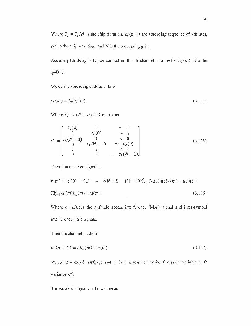
48
Where Tc = TsiN is the chip duration, Cken) is the spreading sequence of kth user,
pet) is the chip waveform and N is the processing gain .
Assume path delay is D, we can set multipath channel as a vector hk (m) pf order
q=D+I .
We define spreading code as follow
(3 .124)
Where Ck is (N + D) x D matrix as
Ck(O) 0 0 Ck(O)
Ck = ck(N - 1) 0
0 ck(N - 1) ... Ck(O) (3.125)
0 0 ... ck(N-1)
Then, the received signal is
(3.126)
Where u includes the multiple access interference (MAI) signal and inter-symbol
interference (lSI) signaIs.
Then the channel model is
(3.127)
Where a = exp[!~i- 2rrfd Ts ) and v IS a zero-mean white Gaussian variable with
variance (JJ.
The received signal can be written as
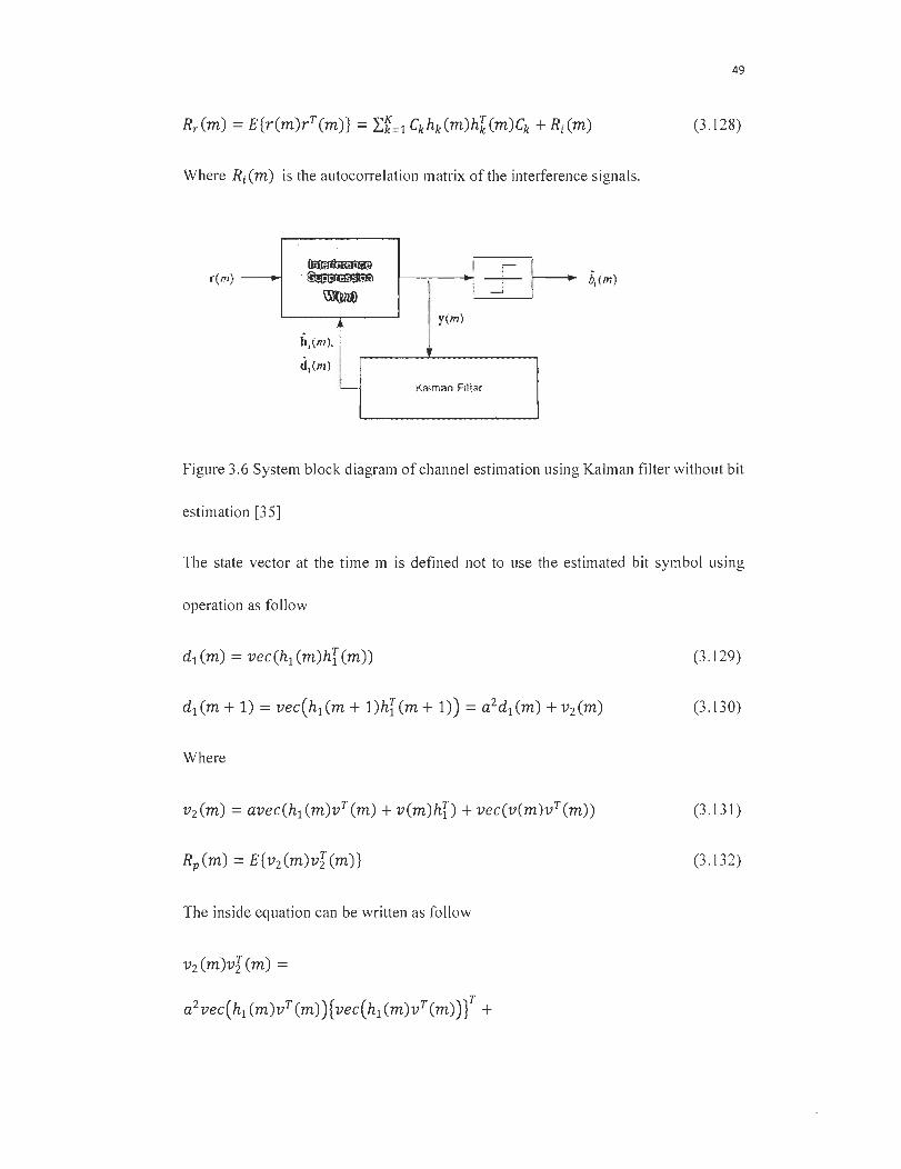
Where Ri(m) is the autocorrelation matrix ofthe interference signaIs.
h,(m). j
d,(m ) 1
~ Kalman Fiher
49
(3.128)
Figure 3.6 System block diagram of channel estimation using Kalman filter without bit
estimation [35]
The state vector at the time m is defined not to use the estimated bit symbol using
operation as follow
dl Cm) = vecChl Cm)hi Cm)) (3.129)
(3 .130)
Where
(3.131 )
(3.132)
The inside equation can be written as follow
Vz Cm)vICm) =
T a2vec( v(m)h[ (m)){vec(v(m)h[ (m))} +
T vec( v(m)vT (m)){ vec( v(m)vT (m))} +
a2vec(h1 (m)vT (m)){vec(v(m)h[ (m))Y +
T avec(hl (m)vT (m) ){vec( v(m)vT (m))} +
T a2vec( v(m)h[ (m) ){vec(hl (m)vT (m))} +
avec( v(m)h[ (m)){ vec( v(m)vT (m)) f +
T avec( v(m)vT (m) ){vec(hl (m)vT (m))} +
avec(v(m)vT(m)){vec(v(m)h[(m))}T
The expectation of each tenn in the right side is solved as
sa
(3.133)
E{a2vec(v(m)h[(m)){vec(v(m)h[(m))Y} = a20'J (hl (m)h[(m)) ® 1] (3.135)
E{vec(v(m)vT(m)){vec(v(m)vT(m))Y} = O'j l] x] (3.136)
E{avec(hl (m)vT (m)){vec(v(m)vT (m))Y} = D, x] (3.138)
(3.139)
E{avec(v(m)h[ (m)){vec(v(m)vT (m))}T} = D] x] (3.140)
E{avec(v(m)vT (m) ){vec(v(m)vT (m))}T} = D] x] (3.141 )
E{avec(v(m)vT (m)){vec(v(m)h[ (m))Y} = D] x] (3.142)
The measurement vector y(m) is defined as follow
51
(3.143)
Where
W(m) =
(3.145)
Where Rin (m) is the estimated autocorrelation matrix of MAI and ISI
(3.l46)
Assume that the decorrelating filter suppress interference signaIs sufficiently, the
measurement equation is constructed using the output ofCMVM filter as follow
Where
WT(m))vec(v(m)h[(m)C[) + (WT(m) ® WT(m))vec(v(m)vT(m))
vec(ABC) = (CT ® A)vec(B) The correlation matrix ofthe measurement noise vector is defined as
E{vw(m)vX(m)} = Wz(m)E{vec(v(m)vT(m)vec(v(m)v(m))}W!(m) =
Wz (m)W! (m)O'~I (N +D)x(N +D)
From the equations above, Ka/man fi/ter can be written as follow
(3.147)
(3.148)
(3.149)
(3.150)
(3 .l51)
52
rem) = aZ A(m, m - l)Q[ (m) . [QIA(m, m - l)Q[ (m) + Rm (m)]-l
(3.152)
a(m) = y(m) - QI (m)a l (m)
(3.153)
al Cm + 1) = aZdl Cm) + rCm)aCm) (3.154)
K(m) = i\(m, m - 1) - aZr(m)QI (m)i\(m, m - 1) (3.155)
i\Cm, m - 1) = a 4 KCm) + Rp Cm) (3.156)
Where rCm) in Kalman filter gain at the time m, aCm) is the innovations vector at
time m, i\Cm) is the correlation matrix of the error in dl Cm + 1), and K(m) is the
correlation matrix of error in al Cm)
Finally, we can get hl Cm) from dl Cm).
3.3.6 Joint Channel Estimation
We assume that we have K users in the channel [20].
(3.157)
The baseband equivalent received signal from K users plus the additive noise can
be written as
(3.158)
Where M is the number of data symbols per user in the data frame of interest, T is
the symbol interval, and L is the number of paths in each user' s channel.
53
At the receiver, when signal passed matched-filter, linear prediction is applied for
each Ith path of the receiver to estimate the column vector subspace of the channel
matrix using only the spreading code ofthe desired user.
The received the signal can be written as
(3.159)
Then we can get the signal vector as follow
( ') - J,iT+Tkj +(n+l )Tc ()P ( -'T - - T )dt Yn l -'T T r t T t l r kZ n c ! +Tkj +n c c
(3.160)
Then, we can get
(3.161 )
Where n(i) = (JIN is the white Gaussian noise vector of the receiver with variance
of (J 2, and i(i) consists ofthe interfering signaIs
We can get
(3.162)
Where
Ul () f Tk1 +(n+l )Tc (' ) ( )d sk' Z n = T Sk' Z t-JT-rk' Z PT t-rkZ-nTc t Tkl+n c c
(3.163)
We construct following linear prediction problem
(3.164)
Where y[Ol (i) is corresponding to sI~l, y[eZse 1 (i) is corresponding to s~l.
54
Assume that the symbols Xk(i) are uncorrelated in time. We define
(3.l65)
Where Xk (i') contains ail symbol components in [xf (0, ... , x~ (i)]H except for
Xk (i). Ho is the column vector of the channel matrix [akl (Okl)gkISk] corresponding
The optimal linear prediction matrix P gives
(3.166)
Let
(3.167)
Then we have
(3.168)
The solution ofP and the linear prediction error can also be represented by the data
correlation. Then we get the prediction equation
. r y[O] (i) ] EI(l) = [I = P] ty[else1(0 (3.169)
And let
R - E {r y[O] (i) ] [ [0] (.) y[else] (i)]} = [Rn RIZ] - ty[else](i) y l R21 R22
(3.170)
(3.171)
(3.172)
55
Where Riz denotes the pseudo inverse of Rzz.
Using above linear prediction algorithm we can estimate the channel response Ho
corresponding to Xk (i) for the receiver.
3.3.7 Madified Leaky LMS A/gari/hm
In DS-CDMA system, after the RAKE receiver, the received signal can be written
as follow [21]
x(k) = h(k) + n(k) (3.173)
Where h(k) is channel parameter and n(k) is zero-mean additive white noise.
Suppose that an estimation ofh(k) is given by
h(k) = WH x(k) (3.174)
Where w is an N-dimensional tap weight vector
x(k) = [x(k), x(k - 1), "', x(k - N + 1)V (3.175)
The optimal tap weight Wo minimizing E [Ih(k) - h(k)n satisfies the
Wiener-Hopf equation
Rwo = Pxh
Where R = E[x(k)xH (k)]
Pxh = E[x(k)h*(k)]
We can write Pxh as follow
Pxh = Pxx - [O"z , 0, ... ,oF
(3.176)
(3.177)
(3.178)
(3.179)

56
Where
Pxx = E[x(k)x*(k)] (3.180)
(J 2 is the variance ofn(k)
Then we can get
(R + A)wo = Pxx (3.181 )
The parameter ao is given by
(3.182)
The steepest descent algorithm for obtaining Wo is given by
w(k + 1) = w(k) - JLE[ -x(k)x*(k) + (x(k)xH (k) + A)w] (3.183)
After removing the expectation E[.], we can get
w(k + 1) = (I - jLA)w(k) + JLx(k){x(k) - WH (k)x(k)}* (3.184)
So
(3.185)
Where wo(k) is the first element ofw(k)
The proposed channel estimation algorithm is summarized as follow:
• Channel estimation
h(k) = WH (k)x(k) (3.186)
• Estimation error
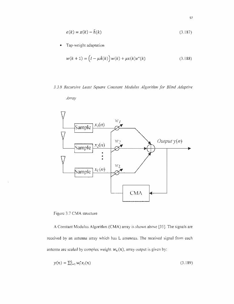
57
e(k) = x(k) - h(k) (3.187)
• Tap-weight adaptation
w(k + 1) = (1 - liÂ(k)) w(k) + lixCk)e*Ck) (3.188)
3.3.8 Recursive Least Square Constant Modu/us A/gorithm for Blind Adaptive
Array
Outputy(n)
eivV\
Figure 3.7 CMA structure
A Constant Modulus Algorithm (CMA) array is shown above [35]. The signais are
received by an antenna array which has L antennas. The received signal from each
antenna are scaled by complex weight wn (n) , array output is given by:
(3.189)
58
Where the superscript * denotes complex conjugate.
The purpose of the adaptive array is to extract the desired signal by finding a suitable
weight vector. It is weil known that adaptation algorithm based on the RLS algorithm
have a faster convergence rate. So we get RLS-CMA algorithm as below:
w(O) = [1, 01 X(L-1 ) f
C(O) = 8-1 h XL, 8 = small positive constant
zen) = x(n)xH (n)w(n - 1) IxH (n)w(n - 1) IP-2
h(n) = ZH (n)C(n - 1)
g(n) = C(n - l)z(n) j(À + h(n)z(n))
C(n) = C(n-1 )-g (n ) h (n )
À
e(n) = WH (n - l)z(n) - 1
w(n) = w(n - 1) + g(n)e*(n)
(3.190)
(3.191 )
(3.192)
(3 .193)
(3.194)
(3.195)
(3.196)
(3.197)

4. Simulations
4.1 Simulation of SISO-CDMA
4.1.1 SISO-CDMA Platform
ln simulation, we will start from the STSO-CDMA platform. Because of the SISO
antenna system is less complicated than the MIMO antenna system. Meanwhile, we can
compare the STSO's simulation results with the MIMO's simulation results. We can see
the differences of the same channel estimation algorithm between two different antenna
systems. We can see how the channel elements affect the estimation results.
/
Figure 4.1 SISO-CDMA System Block Diagram
60
As shown in Figure 5.l , we assume this simulation platform is composed by
multiple users and 1 base station. Between each user and base station, we will consider
the multi-path channels. In realistic environment we have many multipaths. In this
simulation environment, considering the computation complexity, we assume that there
are 6 multipaths. It will cause delay during signal transmission.
The platform we build here is actually a short-code DS-CDMA. At the side of the
transmitter, we use Gold code to spread the original signal. We get
x = B xS (4 .1 )
Where B denotes the original signaIs, S denotes spread code, in this case which is Gold
code.
In order to approaching the real environment, we consider the signal channel as a
multipath channel. So we get the channel as below:
(4.2)
Where L depends on the number oftap we assume in the multipath delay. In this case,
L=6.
At the side of receiver, we describe the received signal as below:
y = Hx +n (4.3)
Where y is received signaIs, H is the signal channel coefficient, x is the spreading code,
n denotes noise sample.
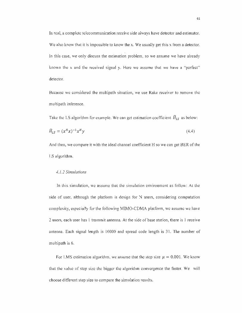
61
In real , a complete telecommunication receive side al ways have detector and estimator.
We also know that it is impossible to know the x. We usually get this x from a detector.
In this case, we only discuss the estimation problem, so we assume we have already
known the x and the received signal y. Here we assume that we have a "perfect"
detector.
Because we considered the multipath situation, we use Rake receiver to remove the
multipath inference.
Take the LS algorithm for example. We can get estimation coefficient fhs as below:
(4.4)
And then, we compare it with the ideal channel coefficient H so we can get BER ofthe
LS algorithm.
4.1.2 Simulations
In this simulation, we assume that the simulation environment as follow: At the
side of user, aIthough the platform is design for N users, considering computation
complexity, especially for the following MIMO-CDMA platform, we assume we have
2 users, each user has 1 transm it antenna. At the side of base station, there is 1 receive
antenna. Each signal length is 10000 and spread code length is 3l. The num ber of
multipath is 6.
For LMS estimation algorithm, we assume that the step size Il- = 0.001. We know
that the value of step size the bigger the algorithm convergence the faster. We will
choose different step size to compare the simulation results.
62
For NLMS algorithm, we know that the NLMS algorithm is normalized LMS
algorithm.ln order to compare with LMS algorithm, we hereby assume the step size the
same as the LMS algorithm, step size J1 = 0.001.
For the RLS algorithm, we assume forgetting factor il. = 1 , initial coefficient
o = 0.001. We know that for the coefficient il. , the sm aller the il. is, the smaller
contribution of previous samples.
0::: W ru
SI SO 10° ------- ----- -- ------- ------------------------------ ------- ---- --- -- -----
-- Pe riect U'J1S
- - - - - - -:---- -- - -:- - - - - - - -:- - - - - - - -:- - - - - - - -:- - - - - - - -:-- - - - - --:-- ---- - -:- - - - - - - -:-- - - - ---------~ -- - --- -~ - - - - -- -~ ----- - -:- - -- -- - -:- - - - - - - -:- - - - - - - ~ - - - - - - - ~ -- - - - - - ~ -------
1 1 1 1 1 l , , 1 - - - - - - -r- - - - - - - -r- - - - - - - - ,.. - - - - - - -,- - - - - - - -,- - - - - - - -,- - - - - - -.,- - - - - - - -,- - - - - - - -, - - - - - --
1 l , , l , , l ,
1 r , , 1 1 1 l ,
1 o-t< '--_-'-_----L __ ..L.-_---L_---l __ --'-----_---L __ L-_---L-__
o 2 4 fi 8 10 SNR,dB
12 14 16 18 20
Figure 4.2 Simulation Results in SISO-CDMA environment
We can see that in SISO-CDMA environment. When SNR is between around OdB
and lOdB, adaptive filter algorithms have the similar performance with the MMSE
algorithm. RLS-CMA (Blind) algorithm has the best performance. Generally speaking,
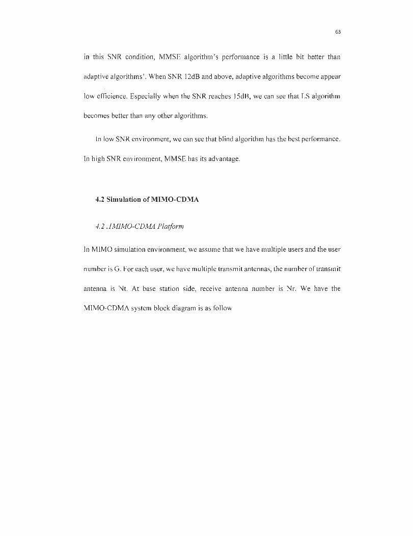
63
in this SNR condition, MMSE algorithm 's performance is a little bit better than
adaptive algorithms'. When SNR 12dB and above, adaptive algorithms become appear
low efficience. Especially when the SNR reaches 15dB, we can see that LS algorithm
becomes better than any other algorithms.
In low SNR environment, we can see that blind algorithm has the best performance.
In high SNR environment, MMSE has its advantage.
4.2 Simulation ofMIMO-CDMA
4.2 .1MIMO-CDMA Platform
In MIMO simulation environment, we assume that we have multiple users and the user
number is G. For each user, we have multiple transmit antennas, the number of transmit
antenna is Nt. At base station side, receive antenna Humber is Nf. We have the
MIMO-CDMA system block diagram is as follow
64
Transm it 1
Tra nsmi t 2
Receive 1 Transmit Nt
Receive 2
Transmit 1 Receive Nr
Transmit 2
Tran smit Nt
Figure 4.3 MIMO System Block Diagram
In order to approach the realistic environment, we should also consider the multipath
channel in this case.
Same as the SISO-CDMA platforrn, we use Gold code as the spread code. ln the
simulation platfonn, the same user use the same spread code on different transmit
antenna. The transmitted signal ofthe gth user's the ith antenna is:
(4.5)
Where b g,i (1) is the data symbol ofthe gth user' s the ith antenna at symbol index 1.
The received signal by the jth antenna is
(4.6)
Where L denotes the number ofmultipath. hg(m) (1) is the ith transmit antenna ofthe gth ,),1
user's fading coefficient of the Lth path at the jth receive antenna at symbol index l, and
65
the delay lm,g is the delay for the Lth multipath of the gth user. net) denotes thermal
nOIse.
We get the channel model as
(4.7)
So, the received signal should be as
y(l) = x(l)H(l) + n(I) (4.8)
4. 2.2 Simulations
ln this simulation, we assume that we have 2 users. Each user has 2 transmit
antennas. At the side of receiver, receiving antenna number is 4. Each pair of signal
channel (1 transmit antenna and 1 receive antenna) has 6-path fading channel.
For LMS estimation algorithm, we assume that the step size J1 = 0.1. We know
that the value of step size the bigger the algorithm convergence the faster. Considering
the complexity ofMIMO antenna system, we hope the convergence time the shorter the
better.
For NLMS algorithm, we choose the step size the same with LMS, which J1 = 0.1.
For the RLS algorithm, we assume forgetting factor il. = 1, initial coefficient
8 = 0.001. We know that for the coefficient il. , the sm aller the il. is, the sm aller
contribution of previous samples. In MIMO antenna system, the channel condition is
very complicated.

c:: w co
MIMO 10
0 f:~:~:~: :~:!T :~:~:~: :~:"!,~: :~:~:~: ~_r:,_ ~~"'§"r~~:~: :~,~: :~~~~~,~-;:;--;:;:-:;:-;:E-;:;:-:;:--;:;-;:;:-:;]-[;-:;:-:;:--;:;:-:;;3-
::::::F:: : ::F::::' := :::F: ~ -- Pelfect -.::...=...=.... - - - - , - - - - - -1- Î - - - T - - i
------+--=-=------...---- ... ... ~ LMS. _-::-.:-:-~ ___ - 1 ~:--:-;-.._=: _______ ~ ______ ! ______ ~ ___ __ _ ~ _ ____ ' . 1" __ -..... , l , 1 -- L.S.
-~ RLS
--NU./lS
l , \ ' , 1 1 \ \ -. '- 1 1
- - - - - - ~ - - - - - - ~ - 'Y\- - - -:- - - - - - - ~ - - - - - - ~ - - - - - - ~ - ... ( - - \1 ., ---"i~- -----~ ------l , l , II \. \. --'. ... ...... 1
mmmmm!mm~!mmmmmm-m1~~ ~ ~ ~ ~ ~ ~ 1 ~ ~ ~ ~ ~ ~ ~ ~ ~ ~ ~ ~ ~ ~i~ ~ ~~H~,~ ~ ~ ~ ~ ~ ~ 1 ~ ~ ~ ~ ~ ~ ~ ~ ~ ~ ~ ~ ~ ~~ ~ ~ rHt~ ~ ~ ~ ~ ~ ~ ~ ~ ~ ~ ~ ~ ~
, l , 1 l , 1 l , - - - - - - T - - - - - - , - - - - - - -.- - - - - - - Î - - - - - - T - - - - - - , - - - - - - ï - - - - - - - ('" - - - - - - r - - - - - -
1 1 1 1 1 1 1 1 1
10-5 ~ __ ~ ____ ~ __ ~~ __ _L ____ ~ __ ~~ __ _L ____ ~ __ ~~ __ _"
o 2 4 6 8 10 SNRdB
12 14 16
Figure 4.4 Simulation Results in MIMO-CDMA environment
18 20
66
From Figure 4.4, we can find that in low SNR condition (between OdB and lOdB),
adaptive estimation algorithms, MMSE and blind algorithm are better than LS
algorithm. Blind algorithm has the best performance in this area. Ali adaptive algorithm
have the similar performance. When in high SNR condition (lOdB and above), blind
algorithm (RLS-CMA) become low efficient. LS algorithm has the best performance in
this condition. The performance of each algorithm can be written as below,
LS>MMSE>RLS>NLMS>LMS>RLS-CMA (Blind).
5. Conclusion
From the simulation results above, because ofthat ail the algorithms are simulated
on the same platforms, we can compare the results directly. We can find out that in both
SISO and MIMO antenna system environment, when SNR is relatively low, which
means in the high noise environment, blind algorithm and adaptive techniques have
better performance. Although in SISO-CDMA system, different technique ' s advantage
in low SNR environment is not distinctly. When SNR is rising, indirect technique such
as LS algorithm becomes much better than others. We can see that generally speaking
blind algorithm is better for low SNR environment, while indirect technique is better
for high SNR environment. Compare with SISO platform, MIMO platform has more
complicated channel environment and noise interference, direct technique ' s
performance in MIMO environment is worse than in SISO environment. For indirect
technique, the performance is more stable than direct technique; the complicated
channel does not affect indirect technique as much as direct technique does.
We should also notice that because of the signal resource we use in this simulation
platform is generated randomly by computer, sometimes the simulation will have some

68
different results. But the nexus of each algorithm ' s performances are comparatively
stable.
When we choose estimation algorithm, we should consider different SNR
environ ment. Like what we see in the simulations above, different estimations III
different SNR environment may have their own advantage. Also, we have to consider
the processing time and computation complexity.

References
[1] GSM (Global System for Mobile communication), Wikipedia
[2] GPRS (General Packet Radio Service), Wikipedia
[3] Madhuri Kulkami, 4G Wireless and Internatinal Mobile Telecommunication
(IMT) Advanced, April 2008
[4] 3G (3 rd Geberation telecommunication System), Wikipedia
[5] MIMO (Multiple Input Multiple Output), Wikipedia
[6] Volker Kühns, « Wireless Communications over MIMO channels», 2006,
pp.73-77
[7] Introduction ofHigh Capacity Digital Communication Lab. University of Alberta.
[8] CDMA Basis, Do\cera Public Wiki
[9] Markku Pukkila, Channel Estimation Modeling, Nokia Research Center, HUT
19.12.2000
[10] Yuanjie Li , Luxi Yang and Zhenya He, Blind Channel Estimation for Long Code MIMO CDMA Using First-order Statistics , pp97- 100, IEEE CNF, 20-22 Oct
2004.
[II] Qian Yu, Gaonan Zhang and Guoan Bi, Improved Blind Channel Estimation Method With TOEPLITZ Displacement For Long Code DS-CDMA, pp224-228,
IEEE CNF, 15-18 June 2003.
[12] Shu-Ming Tseng, Hung-Chieh Yu, Chi-Lung Chang, Yuan-Ching Tseng and
Kuen-Chemg Lin, EM vector channel estimation and V-BLAST/P IC detection for multiuser long-code MIMO CDMA in multipath Rayleigh fading channels, pp565-5,69, Vol. l, IEEE CNF, 28-30 March 2005.
[13] Fu-Hsuan Chiu; Sau-Hsuan Wu; Kuo, c.-c.J. Reduced-rank space-time channel estimation for DS-CDMA in MIMO dispersive channels, pp3782-3786, Vol. 5,
IEEE CNF, 26-29 September 2004
70
[14] Pei Xiao; Strom, E. ; Carrasco, R. ; Estimation oftime-varying multipath Rayleigh fading channels in asynchronous DS-CDMA systems, pp2570-2575 , Vol. 4, IEEE
CNF, 5-8 September 2004
[15] Simon Haykin, « Adaptive Filter Theory», 4th Edition, pp231-312
[16] Simon Haykin, « Adaptive Filter Theory», 4th Edition, pp436-463
[17] Garcia, L.; Pages-Zamora, A.; Fonollosa, J.R. ; Iterative channel estimation for turbo receivers in DS-CDMA, pp989-992, Vol. 4, IEEE CNF, 17-21 May 2004
[18] Zarifi , K. ; Gershman, A.B. ; Subspace-Based Blind Channel Estimation in DS-CDMA Systems with Unknown Wide-Sense Stationary Intelference, pp. 4,
Vol. 4, IEEE CNF, 14-19 May 2006
[19] Kuk-Jin Song; Sug-Ky Hong; Sung-Yoon Jung; Dong-Jo Park; Novel channel estimation algorithm using Kalmanfilter for DS-CDMA Rayleighfading channel, pp.429-432, Vol. 4, IEEE CNF, 6-10 April 2003
[20] Zi-Wei Zheng; Yi-Sheng Zhu; Joint channel estimation and interference cancellation for multipath long-code DS-CDMA, pp211-214, Vol.2, IEEE CNF,
28-31 October 2003
[21] Sungkwon Jo; Jihoon Choi ; Lee, Y.H.; Modified leaky LMS algorithmfor channel estimation in DS-CDMA systems, pp202-204, Vol. 6, IEEE CNF, May 2002
[22] http://dossantos .cbpa.louisvi lle.edll/wwwcraig/pro jects/elec431 /multaccess.html
[23] CDMA (Code division multiple access), Wikipedia
[24] M-sequence, Wikipedia
[25] Gold Code, Wikipedia
[26] http://www.answers.com/topic/mim o-3
[27] http : //www.ece .ua l berta . ca/~HCDC/m imohistorv.html
[28] http : //www.ece.llal berta . ca/~HCDC/mimohistory . h tml
[29] CDMA Basis, www.do lcera.com
[30] Markku Pukkila, Channel Estimation Modeling, Nokia Research Center, HUT
19.12.2000
[31] Yuanjie Li , Luxi Yang and Zhenya He, Blind Channel Estimation for Long Code
MIMO CDMA Using First-order Statistics , pp97-100, IEEE CNF, 20-22 Oct
2004.
71
[32] Shu-Ming Tseng, Hung-Chieh Yu, Chi-Lung Chang, Yuan-Ching Tseng and
Kuen-Chemg Lin, EM vector channel estimation and V-BLAST/P lC detection for multiuser long-code MIMO CDMA in multipath Rayleigh fading channels,
pp565-569, Vol. l, IEEE CNF, 28-30 March 2005.
[33] LMS filter, Wikipedia
[34] Garcia, L.; Pages-Zamora, A.; Fonollosa, J.R.; Iterative channel estimation for turbo receivers in DS-CDMA, pp989-992, Vol. 4, IEEE CNF, 17-21 May 2004
[35] Kuk-Jin Song; Sug-Ky Hong; Sung-Yoon Jung; Dong-Jo Park; Novel channel estimation algorithm using Kalmanfilter for DS-CDMA Rayleighfading channel, pp.429-432, Vol. 4, IEEE CNF, 6-10 April 2003
[35] Yuxin Chen, Tho Le-Ngoc, Benoit Champagne, and Changjiang Xu; Recursive Least Squares Constant Modulus Algorithm for Blind Adaptive Array, Vol. 52,
No. 5, IEEE TRANSACTION, May 2004