Embed Size (px)
Citation preview

Les articles publiés dans la série "Économie et statistiques" n'engagent que leurs auteurs. Ils ne reflètent pas forcément les vues du STATEC et n'engagent en rien sa responsabilité.
87 Economie et Statistiques
Working papers du STATEC juin 2016
Auteur: Christian Glocker
Introducing a financial accelerator in Modux
Abstract
Many structural macroeconometric models used in policy circles fail in properly explaining the observed fluctuations surrounding the global financial crisis episode and its aftermath. In several instances this follows from the fact the macrofinancial interactions are left unexplained. In what follows I introduce a basic financial market structure into Modux - a model characterizing the Luxembourgish economy - with the intention of being able to better explain the aforementioned episode. The macrofinancial extension is limited to the machinery & equipment sector. The results show that the overall model fit improves noticeably once interactions between the financial sector and the real economy are allowed for. Moreover, the corresponding financial accelerator effects contribute significantly to magnifying the effects of structural disturbances.

INTRODUCING A FINANCIAL ACCELERATOR IN MODUX
Abstract. Many structural macroeconometric models used in policy cir-
cles fail in properly explaining the observed fluctuations surrounding the
global financial crisis episode and its aftermath. In several instances this
follows from the fact the macrofinancial interactions are left unexplained.
In what follows I introduce a basic financial market structure into Modux -
a model characterizing the Luxembourgish economy - with the intention of
being able to better explain the aforementioned episode. The macrofinancial
extension is limited to the machinery & equipment sector. The results show
that the overall model fit improves noticeably once interactions between the
financial sector and the real economy are allowed for. Moreover, the corre-
sponding financial accelerator effects contribute significantly to magnifying
the effects of structural disturbances.
1. Motivation
The following is a project report concerning the extension of Modux - a struc-
tural macroeconometric model used at Statec/Luxembourg - with a financial
accelerator block.
The project is motivated by the deficiencies of the current specification of
the equation for capital in Modux in explaining the episode surrounding the
financial crisis and its aftermath. The inability to properly explain the fluctua-
tions in this episode is in fact a drawback in many structural macroeconometric
models. These models perform sufficiently well in explaining the fluctuations
in capital until the outbreak of the global financial crisis; however, from then
onwards the model fit gets noticeably worse. In particular, these models dis-
play large residuals in the years surrounding the global financial crisis and its
aftermath. The failure in explaining the path of the capital stock is replicated
Project Report written by Christian Glocker, March 2016.
Les opinions exprimees dans la presente publication sont celles des auteurs et ne refletent
pas forceement les opinions du STATEC et de l’ANEC.
2 INTRODUCING A FINANCIAL ACCELERATOR IN MODUX
in an inadequate fit of investment. This does not only violate the normality
property of the residuals, it also introduces a high degree of autocorrelation
which all together is insufficient to meet the requirements for any further statis-
tical analysis. Still, the estimation could be improved by introducing dummy
variables in the form of time-dummies in order to get appropriate residuals
also for the financial crisis episode. Though this would support the fit of the
equation to the data, it would nevertheless not improve the fit of the model to
the data as the model continues to fail in explaining this episode.
One commonly used explanation for this is a technical one involving func-
tional forms - the global financial crisis is replicated in the data in the form of
a major irregularity in many macroeconomic time series. It shows up in the
form of a previously unobserved large and abrupt drop in output and many
series alike. It seems as if the volatility pattern is a complete different one over
the crisis years. Many consider this as a form of non-linearity. Since most of
the structural macroeconometric models at use are linear or log-linear in their
basic functional structure, their ability in explaining non-linearities in the data
is hence limited. As a result, these models perform poorly in explaining the
years surrounding the global financial crisis episode and its aftermath.
Another explanation commonly used addresses the pure structure of these
models. Many of these models have a structure too focused on the real econ-
omy involving the production, income and spending accounts, the fiscal sector,
labour markets and the interaction with foreign economies. However, what is
yet ignored in many of these models is the extent to which financial markets
and in particular the interaction of financial markets with the real economy
plays a role for economic fluctuations. As a matter of fact, the omission of the
financial sector and its interaction with the real economy might be an alter-
native explanation why these models fail in properly explaining the observed
economic fluctuations surrounding the global financial crisis episode.

INTRODUCING A FINANCIAL ACCELERATOR IN MODUX 3
Against this background I proceed by elaborating on the latter. So far
Modux does not feature any financial market structure. There are a few fi-
nancial variables in the model, as for instance short and long term government
bond rates and the eurostoxx50 - index, however, most of them are specified as
purely exogenous variables. Hence at this stage, the model does not allow for
any endogenous interaction between financial markets and the real economy -
that is to say, macrofinancial linkages are missing. Hence it does not come as
a big surprise that the model, and in particular the equations for capital and
investment, fail to adequately explain the financial crisis episode.
In what follows I introduce a basic financial market structure with the inten-
tion of being able to better explain the crisis episode. The analysis is restricted
to the sector of machinery & equipment. The model extension presented herein
is based on a version of Modux documented in Adam (2004) and implies an
extended model for the real economy that is furnished with a financial block.
The role of the financial block is to take account of the comovements and
procyclicality of credit, asset prices and real economic activity that typically
characterizes a financial accelerator. The model differs from optimizing rep-
resentative agent models in several respects, the main reason for this being a
wider and less stringent theoretical framework and the fact that data are given
a more central role in shaping the long- and short-run structure of the model.
In what follows I begin with an explanation and a review of the literature
concerning the financial accelerator (section 2). The block of equations com-
prising the financial accelerator is elaborated in sections 3.1 - 3.3 and sections
3.4 - 3.5 finally discuss some differences between the original model and the
extended one by means of impulse response functions, short and medium term
forecasts and root mean squared errors statistics. Appendix A summarizes the
data being used.

4 INTRODUCING A FINANCIAL ACCELERATOR IN MODUX
2. Financial frictions in macroeconomic models
The recent global financial crisis has highlighted that macroeconomic mod-
els need to allocate a higher weight to the financial sector for understanding
the dynamics of the business cycle. In contrast to what has repeatedly been
reported, there is a well-established series of publications in macroeconomics
concerning the incorporation of financial market frictions in standard macroe-
conomic models. Bernanke and Gertler (1989) is an early study in this respect.
Kiyotaki and Moore (1997) provide another approach to adding financial fric-
tions in a general equilibrium model of the macroeconomy. These contributions
are now key references for most of the work done in this area during the last
two decades. Even though these studies had a big influence in the academic
field, macroeconomic models which are used in policy circles have so far ig-
nored this branch of economic research to a large extent. That is why it is
worth to stress at this point that the recent approaches in this field are not
new. Rather they are based on ideas that have been formalized already a long
time ago, starting with the work of Bernanke and Gertler (1989).
There is much to show concerning the extent to which financial frictions
are capable of having an important impact on the transmission mechanism of
shocks. One motivating observation is that the flows of credit and debt in
general are highly procyclical. As shown in the top panel of Figure 15 in the
appendix, credit growth moves closely with the business cycle. In particular,
the growth rate of debt declines significantly during recessions.
The cyclical properties of financial markets can be seen not only by the
aggregate dynamics of credit flows, but also by indicators of tightening credit
standards (see for instance ECB, 2015 and reports alike). More and more
banks tend to tighten their credit standard during economic downturns.
As Quadrini (2011) highlights, if markets were complete, the financial struc-
ture of individual agents, be it financial intermediaries, firms or households
would be indeterminate. We would then be in a Modigliani and Miller (1958)

INTRODUCING A FINANCIAL ACCELERATOR IN MODUX 5
world and there would not be reasons for financial sector flows to be charac-
terized by some cyclical pattern. However, the fact that financial flows are
highly cyclical (for instance credit flows are highly procyclical whereas the in-
dex of credit standard tightening is highly countercyclical) suggests that the
complete-market paradigm has some limitations.
Of course, from contractions in credit one cannot identify whether it is a
recession in the real economy that causes the decline in credit growth or if
the credit fall causes or amplifies the macroeconomic contraction. Against this
background, it is convenient to distinguish three possible transmission channels
linking real activity and financial flows.
(1) Real activity causes movements in financial flows
(2) Amplification
(3) Financial shocks
Most of the literature in dynamic macrofinance has focused on the second
channel, that is, on the amplification mechanism caused by impediments in
the financial sector. In particular, the key hypothesis is that financial frictions
exacerbate a recession, however, they are not considered as the cause of the
recession. In this context, something wrong happens the real sector in the first
place. This could be caused by exogenous shocks to productivity, the terms-of-
trade, monetary aggregates, interest rates, preferences, etc. These structural
innovations would trigger a macroeconomic contraction even in the absence of
financial market frictions. When financial frictions are prevalent, however, the
magnitude of the contraction becomes more pronounced.
The third channel, that is, the analysis of financial shocks as a source of
real economic fluctuations, has received less attention in the academic litera-
ture (with the exception of the work of Hyman Philip Minski), though more
recently, more and more studies started to explore this possibility.
2.1. The financial accelerator in more detail. The role of a financial
sector block in macroeconomic models is to take account of the comovements
of credit, asset prices and real economic activity that typically characterizes a
6 INTRODUCING A FINANCIAL ACCELERATOR IN MODUX
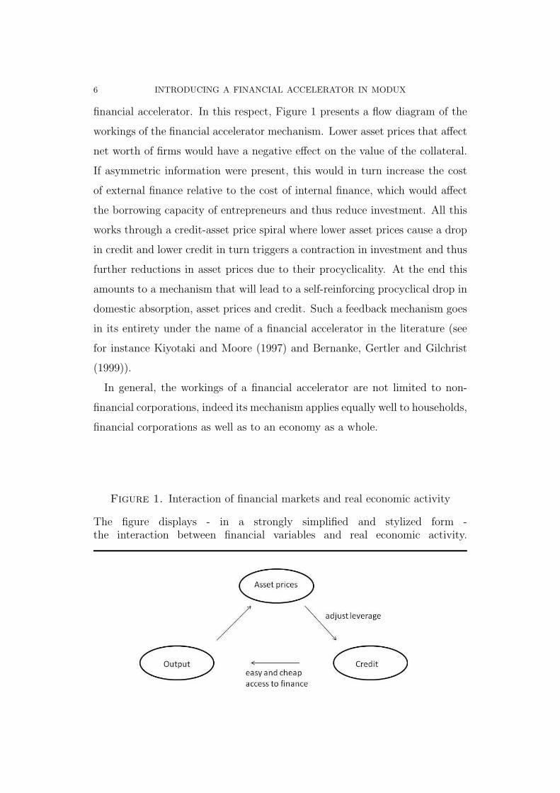
financial accelerator. In this respect, Figure 1 presents a flow diagram of the
workings of the financial accelerator mechanism. Lower asset prices that affect
net worth of firms would have a negative effect on the value of the collateral.
If asymmetric information were present, this would in turn increase the cost
of external finance relative to the cost of internal finance, which would affect
the borrowing capacity of entrepreneurs and thus reduce investment. All this
works through a credit-asset price spiral where lower asset prices cause a drop
in credit and lower credit in turn triggers a contraction in investment and thus
further reductions in asset prices due to their procyclicality. At the end this
amounts to a mechanism that will lead to a self-reinforcing procyclical drop in
domestic absorption, asset prices and credit. Such a feedback mechanism goes
in its entirety under the name of a financial accelerator in the literature (see
for instance Kiyotaki and Moore (1997) and Bernanke, Gertler and Gilchrist
(1999)).
In general, the workings of a financial accelerator are not limited to non-
financial corporations, indeed its mechanism applies equally well to households,
financial corporations as well as to an economy as a whole.
Figure 1. Interaction of financial markets and real economic activity
The figure displays - in a strongly simplified and stylized form -the interaction between financial variables and real economic activity.
INTRODUCING A FINANCIAL ACCELERATOR IN MODUX 7
Standard macroeconomic models usually embed the Modigliani-Miller as-
sumption about perfect capital markets. Hence there is no theoretical role for
modeling the interactions between real and financial factors. However, these
factors are explicitly interconnected in credit channel models where capital
markets are imperfect. An important result from the literature on the credit
channel is that under the presence of information asymmetries, firms are likely
to finance investment projects using internal funds (for instance retained earn-
ings) rather than drawing on external finance. Put differently, external finance
is more costly than internal finance. This difference is called the external fi-
nance premium, which is essentially a markup over the price of internal finance.
This premium arises due to various frictions, as for instance, external lenders
cannot perfectly observe nor control the risks that a project inherits to which
a bank supplies funds for to borrowers. Hence lenders require a compensation
for the expected agency costs. Borrowers using internal funds do not face the
problem of informational asymmetry. Agency costs on the one hand and the
external finance premium on the other are likely to vary with borrowers cred-
itworthiness. For instance, the stake of a borrower in a project - measured by
the degree to which the borrower is able to finance the project using internal
funds - can provide a signal of the unobserved risk of lending (the adverse se-
lection effect), which may affect the borrowers likely incentive to act diligently
(the moral hazard effect) and the incentive to report project outcomes truth-
fully. This relationship between financial health in the corporate sector and
expected agency costs in lending can provide a direct link between the overall
financial conditions and real economic activity.
The key innovation in financial accelerator models is that they embed the
problem of information asymmetries in a standard macroeconomic model. The
key element in these models is the introduction of entrepreneurial net worth,
which basically comes from retained earnings. Shocks to net worth relative to
total finance requirements generate endogenous changes in agency costs and in
the finance premia for external funds which are charged above risk-free rates.

8 INTRODUCING A FINANCIAL ACCELERATOR IN MODUX
In this set-up, any structural shock is likely to be amplified relative to a model
set-up where the financial accelerator extension is omitted. So far the literature
has focused on two key transmission mechanisms:
(1) Corporate cash flow. An unexpected rise in interest rates which reduces
output exerts downward pressure on corporate cash flow and increases the
share of a given investment project that has to be financed using external
funds. This raises expected agency (default) costs and hence also the external
finance premium. This in turns depresses investment and subsequently also
output, revenues and corporate cash flows.
(2) Asset prices and the value of collateral. Consider an unanticipated mon-
etary tightening which reduces the demand for capital and depresses asset
prices. This lowers the value of corporate collateral which is available to back
loans. This in turn raises the external finance premium which reduces current
investment and subsequently output, revenues and corporate cash flows. Any
expectations of future drops in cash flows can amplify the current movement
in (forward-looking) asset prices and hence exacerbate the downturn.
The model developed in Bernanke et al. (1999) incorporates both of these
transmission mechanisms in a standard new Keynesian model. In their set-up,
households work, consume and invest their savings in a financial intermediary.
The financial intermediary pools savings and lends to corporates. These cor-
porates produce goods which are sold in competitive markets using labour and
capital, with the capital stock being financed from internal funds (net worth
which is built up from retained earnings) and/or external funds. Production is
bought by retailers who differentiate goods and sell them in monopolistically
competitive markets which gives rise to price stickiness, as in Calvo (1983).
The monetary authority uses a simple forward-looking interest rate rule to
stabilize inflation.
Given the standard nature of many parts of the Bernanke et al. (1999)
model, I focus here exclusively on the key innovation in the capital/investment
block. In a standard model, without financial accelerator effects, firms would

INTRODUCING A FINANCIAL ACCELERATOR IN MODUX 9
increase their capital stock until the expected return on capital (Rkt+1) was
equal to the opportunity cost of funds (Rt+1). However, in the model with
the financial accelerator extension, the financial health of firms matters for the
cost of finance. In particular, it endogenously reacts to the level of corporate
internal funds (net worth, Nt) relative to total financing requirements (QtKt),
where Q and K are the price and quantity of capital respectively. Firms finance
the value of their capital stock QtKt out of their net worth Nt and with bank
loans Lt, which gives rise to the following balance sheet:
(1) QtKt = Lt + Nt
If a substantial share of corporate investment is funded internally - that is,
borrowing and capital gearing is low - then the external finance premium is
small (in fact, it would tend to zero if the capital stock were to be fully financed
internally or collateralized). However, if corporate investment is primarily
financed through external funds (gearing is high), then the premium is likely
to be high. This relationship is captured by the following equation:
(2) Et
!
Rk
t+1
"
= f
#
QtKt
Nt
$
Rt+1, with f ′(·) > 0
Equation (2) shows that the external finance premium f (QtKt/Nt) increases
with the share of debt in total financing. The intuition behind that is that
the intermediary’s participation constraint in the optimal financial contract
involving lenders and borrowers requires a premium sufficient so as to offset the
greater likelihood that the borrower will declare default. In this case the lender
will incur default costs from the loan. Moreover, the steady state position of the
corporate sector is essential for the responses of net worth, the cost of finance
and investment to structural shocks. For a highly-geared entrepreneur, a shock
to the project return will have a far more marked impact on internal funds and
hence on the external finance premium than for a firm that has low gearing.
This additional element introduces a higher amplitude and persistence of key
10 INTRODUCING A FINANCIAL ACCELERATOR IN MODUX
variables in reaction to structural shocks. The model therefore provides a
theoretical foundation for the observation that more indebted economies tend
to be more vulnerable to adverse shocks.
2.2. Implications of the financial accelerator. A good way of analyzing
the working of the financial accelerator is by means of a monetary policy shock
since this structural disturbance has produced a wide consensus of opinion
about how the macroeconomy is likely to react.
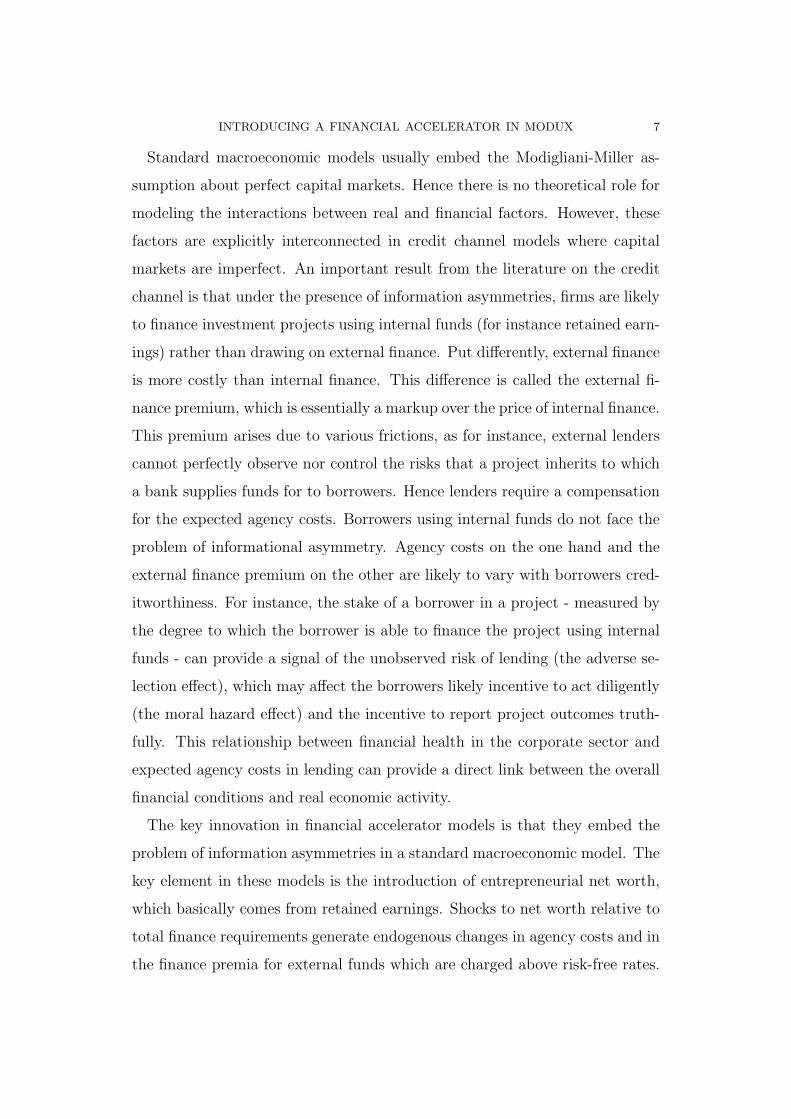
For this, Figure 2 reports the impulse response functions. The time units
in the figure are to be interpreted as quarters. In each picture the solid line
designates the baseline impulse response, generated by a model without the
financial accelerator extension. The dashed line in each picture indicates the
response observed in the model with the financial accelerator included.
The shock considered in Figure 2 is an unanticipated 25 basis point (on
an annual basis) increase in the nominal interest rate. The graphs show the
reaction of output, investment and the external finance premium. The first
thing to note is that although the extension of the basic model with credit-
market frictions does not affect the shape of the impulse response functions,
it does lead to a stronger response of the variables. In particular, with the
financial accelerator included, the initial reaction of output to the monetary
shock is about 50% higher, and the effect on investment is nearly twice as
high. Furthermore, the persistence of the real effects is notably larger in the
presence of the credit-market frictions, that is, output and investment in the
model with financial-market imperfections after four quarters are about where
they are in the base model already after two quarters.
The impact of the financial accelerator can be inspected by considering the
behavior of the external finance premium, which is passive in the baseline
model (by construction), however, it increases sharply in the extended model.
The unanticipated rise in the monetary policy rate dampens the demand for
capital and investment. This depresses investment and the price of capital.
The unanticipated decrease in asset prices lowers net worth and hence increases
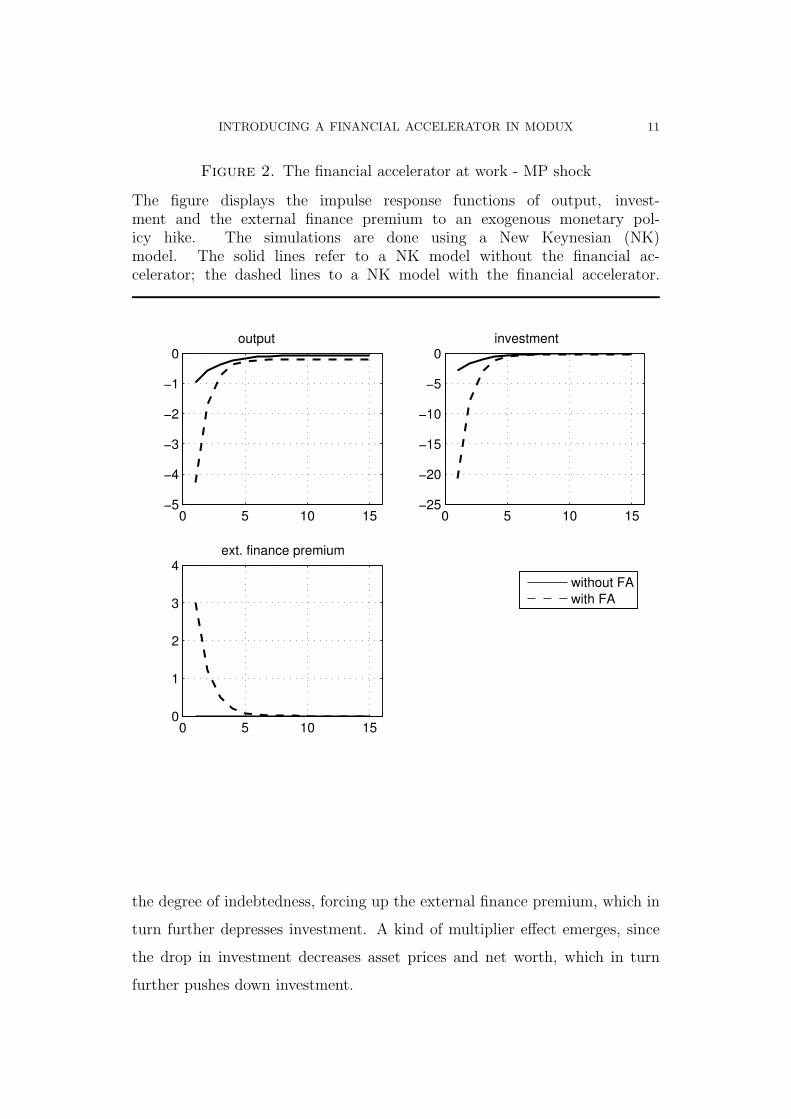
INTRODUCING A FINANCIAL ACCELERATOR IN MODUX 11
Figure 2. The financial accelerator at work - MP shock
The figure displays the impulse response functions of output, invest-ment and the external finance premium to an exogenous monetary pol-icy hike. The simulations are done using a New Keynesian (NK)model. The solid lines refer to a NK model without the financial ac-celerator; the dashed lines to a NK model with the financial accelerator.
0 5 10 15−5
−4
−3
−2
−1
0output
0 5 10 15−25
−20
−15
−10
−5
0investment
0 5 10 150
1
2
3
4ext. finance premium
without FAwith FA
the degree of indebtedness, forcing up the external finance premium, which in
turn further depresses investment. A kind of multiplier effect emerges, since
the drop in investment decreases asset prices and net worth, which in turn
further pushes down investment.

12 INTRODUCING A FINANCIAL ACCELERATOR IN MODUX
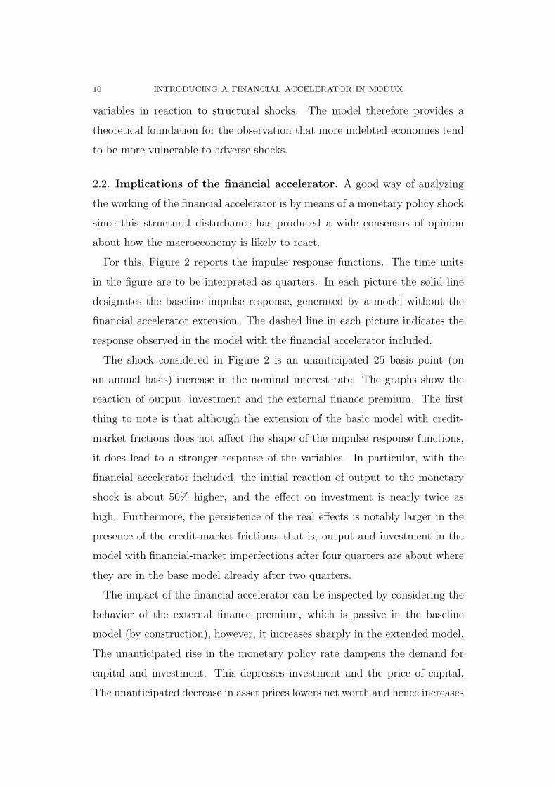
Figure 3. The financial accelerator at work - demand shock
The figure displays the impulse response functions of output, invest-ment and the external finance premium to an expansionary demandshock. The simulations are done using a New Keynesian (NK) model.The solid lines refer to a NK model without the financial accelera-tor; the dashed lines to a NK model with the financial accelerator.
0 5 10 150
0.01
0.02
0.03output
0 5 10 15−0.05
0
0.05
0.1
0.15
0.2investment
0 5 10 15−15
−10
−5
0
5x 10
−3 ext. finance premium
without FAwith FA
Figure 3 shows the working of the financial accelerator to a classical demand
shock in the form of an increase in government spending which is deficit fi-
nanced. Also in this case the model extension is associated with a stronger
reaction of the model’s variables in response to the structural innovation.
The financial accelerator tends to augment economic fluctuations in both
directions - contractionary shock lead to a more pronounced decline in output
whereas expansionary shocks trigger a stronger positive reaction in output

INTRODUCING A FINANCIAL ACCELERATOR IN MODUX 13
compared to a model without the financial accelerator extension. The key
mechanism behind that is the countercyclical nature of the external finance
premium. It increases in downswings which gives an additional impetus to
the contraction as it increases the cost of financing. The external finance
premium decreases instead in response to an expansionary shock, which exerts
downward pressure on the cost of finance. This in turn spurs investment and
hence capital and output.
3. Methodology: equation specification and estimation
As far as the specification of the financial block’s equations is concerned, the
approach followed here closely relates to Hendry (1993), though it clearly is
more restrictive than indicated by a completely a-theoretical modeling strat-
egy. Thus, as a backdrop for model design it was sought to start out with the
most general specification given support by what a priori was perceived to be
reasonably adequate, and then to simplify down to a parsimonious represen-
tation. In an ideal set-up, the process of reduction should take place within
the framework of a simultaneous equation system. However, a general lack of
degrees of freedom due to short time series makes such an approach unfeasible
and limits the modeling strategies.
The model extension discussed here has been designed and estimated by
following a pragmatic view. Thus, I have neither adopted a pure top-down
approach where data is allowed to determine the outcome of the new equation
system all alone, nor a pure bottom-up approach where a structure motivated
by economic theory is imposed on the equations system without taking proper
account of data. Instead I undertake something in between, where the data
and the theory are combined in an attempt of identifying the structure that
best explains the observed fluctuation of the data. In this set-up, theory
contributes by constructing a theoretical possibility set, while the data play a
role in choosing among the alternatives spanned by the theoretically motivated
possibility set.

14 INTRODUCING A FINANCIAL ACCELERATOR IN MODUX
The starting point is the equation for the real capital stock in the sector for
machinery and equipment that has so far been used in Modux. The equation
is replicated here once more for convenience.
The stock of capital - original equation
∆ log(capbmeq rt) = −0.007[−1.67]
+ 0.41[2.57]
· ∆ log(capbmeq rt−1) + 0.06[1.28]
· ∆ log(vabprvo rt)(3)
− 0.05[−3.31]
·
%
log
#
capbmeq rt−1
vabprvo rt−1
$
+ 0.6 · log(pucmeqt−1/p vabprvot−1)
&
− 0.02[−1.96]
· ∆(pucmeqt−1/p vabprvot−1) + ϵcapbmeq rt
OLS, R2 = 0.81, σcapbmeq r = 0.01
T = 1980 : 2014, DW = 2.39
The values in brackets are t-statistics. The fit of this specification can be
judged graphically in Figure 8. The overall capability of the equation in ex-
plaining the variation in the capital stock is good, the adjusted R-squared is
sufficiently high and the independent variables’ coefficients are all statistically
different form zero with high probability. Of course all this has to be taken
with caution as the degrees of freedom are rather small. This critique also
applies to the upcoming regressions. Nevertheless, the equation is incapable of
explaining the change in the capital stock in several episodes sufficiently well.
One of these episodes is the one of the global financial crisis episode. Once
using dummies for the outliers in the year 2011 and onwards, the fit of the
equation can be significantly improved, however, at the cost of loosing degrees
of freedom.
Moreover, the extent to which the fit of the equation for capital can be
improved by adding dummy variables does not imply that the fit of the overall
model improves - the unexplainable episodes have simply been dummied out.
Hence equation (3) will be substituted by a new set-up involving financial
variables. This implies that the model will feature additional equations which
are not yet part of the equation system.
INTRODUCING A FINANCIAL ACCELERATOR IN MODUX 15
3.1. The equations comprising the financial accelerator extension.
The key aspect of the financial accelerator is its characterization of an asset-
credit spiral which mutually reinforce each other. This implies that assets - in
the following specification asset will be measured by the value of the capital
stock - will depend on credit and the stock of credit in turn will be affected
by the capital stock. Ideally this simultaneous equations system consisting of
the capital stock and the corporate credit stock would be estimated within a
simultaneous equations set-up. This would establish a consistent estimation
of the block of equations comprising the financial accelerator. However, the
lack of sufficiently long time-series does not allow for this approach. Instead I
proceed by estimating each equation individually.
The extension of Modux comprises three equations of which two are in fact
new, whereas the one for the real capital stock is only modified. The following
lists the equations in their VECM representation.
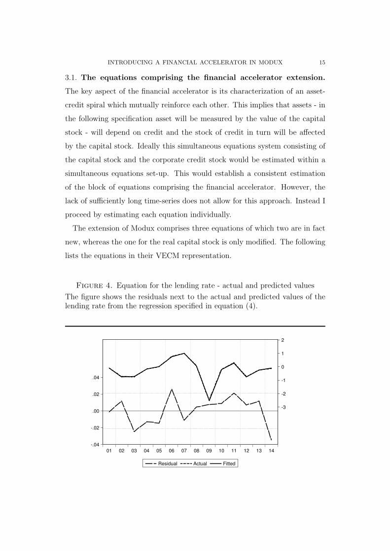
Figure 4. Equation for the lending rate - actual and predicted values
The figure shows the residuals next to the actual and predicted values of thelending rate from the regression specified in equation (4).
-.04
-.02
.00
.02
.04
-3
-2
-1
0
1
2
01 02 03 04 05 06 07 08 09 10 11 12 13 14
Residual Actual Fitted
16 INTRODUCING A FINANCIAL ACCELERATOR IN MODUX
The lending rate
∆credit ratet = 0.73[26.3]
· ∆ticteurt − 0.10[−3.07]
· ∆(credit ratet−1) − 0.14[−2.19]
· cwKt(4)
− 0.12[−2.28]
·!
credit ratet−1 − ticteurt−1 − 1.32 + 0.15 · cwKt−2
"
+ ϵcredit ratet
OLS, R2 = 0.99, σcredit rate = 0.08,
T = 1999 : 2014, DW = 1.98,
The credit rate is modeled as a vector-error-correction equation involving
the short term government bond rate (ticteur) and a measure for the credit-
worthiness in the machinery & equipment sector (cwKt ) given by:
(5) cwK
t :=capbmeq rt · p imeqt
credit nfct/1000
The cointegration relation implies that in the long term, the credit rate
moves one to one with short term rates; however, there is a constant markup
of around 1.3 percentage points which can be considered as an exogenous
lending margin which is supposed to be time-invariant. Moreover, a leverage
being too high also exerts upward pressure on the lending rate in the long
term. An increase in the degree of indebtedness implies a fall in cwKt . While
there is full pass-through of changes in short term-rates on lending rates in the
long run, the short run pass-through is 0.73. Still, the short term dynamics
are driven to a large extent by the short term rate, however at a limited degree
compared to the long-run trade off. Besides that, also the lagged lending rate
as well as the degree of indebtedness play a role in explaining the variation in
the credit rate. Figure 4 shows the fit of the model graphically.
Equation (4) is estimated. In several models (Hammerland et al., 2014;
Bardsen and Nymoen, 2009; Bardasen et al., 2006 and Bardsen et al., 2005)
this equation is calibrated instead. Still the estimated parameters here are
similar to those approaches where they were calibrated instead.

INTRODUCING A FINANCIAL ACCELERATOR IN MODUX 17
The stock of credit for non-financial corporations
∆ log(credit nfct/p imeqt) = 0.63[3.69]
+ 0.01[1.97]
· ogt − 0.32[−4.27]
· ∆(credit ratet − ticteurt)(6)
− 0.36[−3.54]
· [log(credit nfct−1/p imeqt−1) − 2.21 · log(capbmeq rt−1)
+ 0.96 · (credit ratet−1 − ticteurt−1)] + ϵcredit nfct
OLS, R2 = 0.84, σcredit nfc = 0.05
T = 1999 : 2014, DW = 1.67
The stock of credit is modeled using a risk spread involving the credit and the
short term rate (credit rate− ticteur), the capital stock used in the machinery
& equipment sector (capbmeq r) as well as the overall output gap (og). In the
long term an increase in the capital stock of one percent implies a rather
strong increase in (real) credit of around two percent. However, high credit
rates, as well as an overall high level of risk, captured by the spread between
credit and short term rates, dampen the demand for credit. The risk measure
also matters for short term dynamics - high risk exerts downward pressure on
credit demand, though the effect tends to be a bit weaker here than within the
long term relationship. Finally, the output gap also contributes significantly
to explaining the variation in the stock of real credit. A high output gap -
implying that the economy is operating above its potential - triggers upward
pressure on the credit stock.
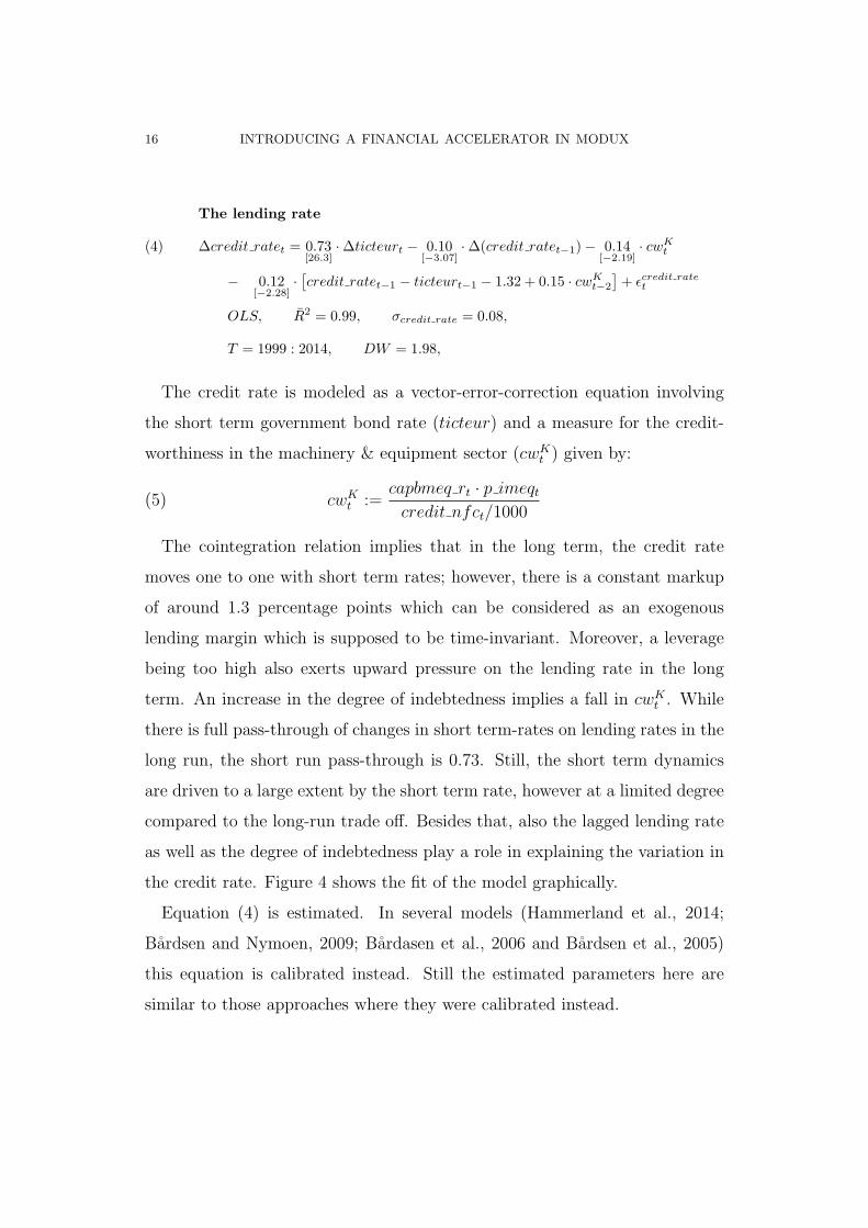
Figure 5 shows the fit of the equation for the credit stock graphically.
The stock of capital
∆ log(capbmeq rt) = 0.05[28.1]
− 0.02[−2.58]
· ∆(credit ratet − ticteurt)(7)
− 0.07[−4.35]
·
%
log
#
capbmeq rt−1
vabprvo rt−1
$
− 0.09 · log(credit nfct−1/p imeqt−1)
&
+ ϵcapbmeq rt
OLS, R2 = 0.62, σcapbmeq r = 0.006
T = 1999 : 2014, DW = 1.44
18 INTRODUCING A FINANCIAL ACCELERATOR IN MODUX
Figure 5. Equation for the credit stock - actual and predicted values
The figure shows the residuals next to the actual and predicted values of thecredit stock from the regression specified in equation (6).
-.12
-.08
-.04
.00
.04
.08
-.2
-.1
.0
.1
.2
.3
.4
00 01 02 03 04 05 06 07 08 09 10 11 12 13 14
Residual Actual Fitted
The equation for the capital stock (capbmeq r) involves the value added from
the private, non financial sector (vabprvo r), the stock of credit measured in
real terms (credit nfc) as well as the spread between the credit rate and the
short term rate (credit rate− ticteur). The cointegration relationship implies
that in the long term, the real capital stock moves one-to-one with the output
produced in this sector. This trade-off has not been estimated but imposed on
the long term interaction. A full estimation of the cointegration relationship
would yield a value of 0.83 rather than unity for the output variable. The
cointegration relationship also involves the real stock of credit. An increase in
credit of one percent implies a rise in the capital stock of 0.09 percent. The
effect seems weak, though, it is reasonable. Considering that the yearly growth
rate of the capital stock is in the range of 2% to 6% and that of the real stock
of credit of -12% to 36%, then the seemingly small parameter estimate for the
credit stock still turns out to be economically important.
INTRODUCING A FINANCIAL ACCELERATOR IN MODUX 19
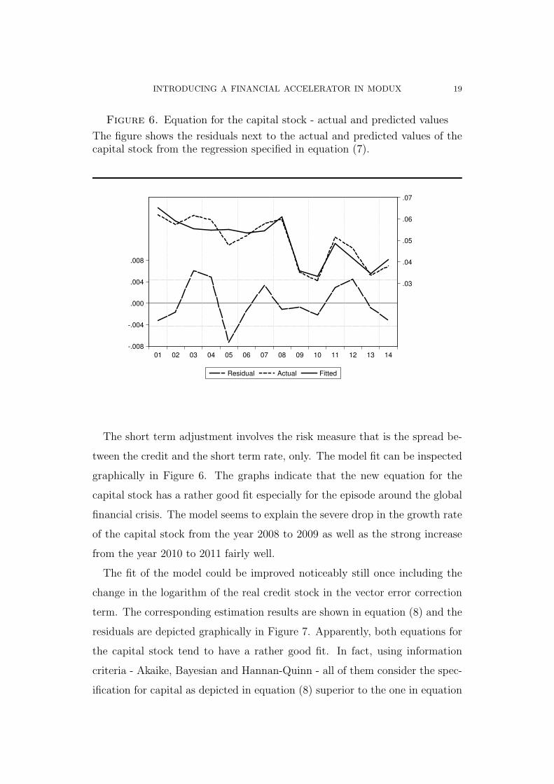
Figure 6. Equation for the capital stock - actual and predicted values
The figure shows the residuals next to the actual and predicted values of thecapital stock from the regression specified in equation (7).
-.008
-.004
.000
.004
.008
.03
.04
.05
.06
.07
01 02 03 04 05 06 07 08 09 10 11 12 13 14
Residual Actual Fitted
The short term adjustment involves the risk measure that is the spread be-
tween the credit and the short term rate, only. The model fit can be inspected
graphically in Figure 6. The graphs indicate that the new equation for the
capital stock has a rather good fit especially for the episode around the global
financial crisis. The model seems to explain the severe drop in the growth rate
of the capital stock from the year 2008 to 2009 as well as the strong increase
from the year 2010 to 2011 fairly well.
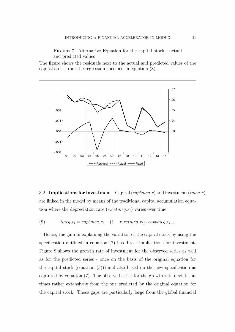
The fit of the model could be improved noticeably still once including the
change in the logarithm of the real credit stock in the vector error correction
term. The corresponding estimation results are shown in equation (8) and the
residuals are depicted graphically in Figure 7. Apparently, both equations for
the capital stock tend to have a rather good fit. In fact, using information
criteria - Akaike, Bayesian and Hannan-Quinn - all of them consider the spec-
ification for capital as depicted in equation (8) superior to the one in equation

20 INTRODUCING A FINANCIAL ACCELERATOR IN MODUX
(7). The better fit can also be motivated by the higher adjusted R-squared
of the specification in equation (8). However, I give preference to equation
(7) since its alternative, equation (8), involves two additional exogenous vari-
ables. Against the background that the sample size is rather small, equation
(7) is hence considered as the new equation for the capital stock involving the
financial accelerator.
The stock of capital - alternative equation
∆ log(capbmeq rt) = 0.05[36.3]
− 0.02[−5.44]
· ∆(credit ratet − ticteurt)(8)
− 0.10[−8.27]
·
%
log
#
capbmeq rt−1
vabprvo rt−1
$
− 0.09 · log(credit nfct−1/p imeqt−1)
&
− 0.01[−2.17]
· ∆(credit ratet−1 − ticteurt−1)
− 0.02[−1.83]
· ∆ log(credit nfct/p imeqt) + ϵcapbmeq rt
OLS, R2 = 0.91, σcapbmeq r = 0.003
T = 1999 : 2014, DW = 2.29
The fit of the different models in terms of their overall fit can also be judged
graphically by means of the corresponding residuals, depicted in Figure 8. The
specifications for capital as outlined in equations (7)-(8) imply rather similar
errors in terms of their time pattern as well as in terms of their standard
deviation. The difference to the residuals to the original specification - outlined
in equation (3) - is particularly large in the years from 2008 and onwards.
Before that episode the path of the residuals of the three specifications is
fairly similar, except maybe for the year 2005. However, from 2008 onwards,
the difference in the residuals of the original equation to the ones of the two
new specifications is remarkable. It highlights the extent to which the overall
fit can be improved by introducing financial variables, even by the specification
as outlined in equation (7) which estimates only three parameters compared
to five as is the case in the original specification.
INTRODUCING A FINANCIAL ACCELERATOR IN MODUX 21
Figure 7. Alternative Equation for the capital stock - actualand predicted values
The figure shows the residuals next to the actual and predicted values of thecapital stock from the regression specified in equation (8).
-.008
-.004
.000
.004
.008
.03
.04
.05
.06
.07
01 02 03 04 05 06 07 08 09 10 11 12 13 14
Residual Actual Fitted
3.2. Implications for investment. Capital (capbmeq r) and investment (imeq r)
are linked in the model by means of the traditional capital accumulation equa-
tion where the depreciation rate (r retmeq rt) varies over time:
(9) imeq rt = capbmeq rt − (1 − r retmeq rt) · capbmeq rt−1
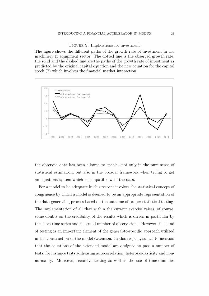
Hence, the gain in explaining the variation of the capital stock by using the
specification outlined in equation (7) has direct implications for investment.
Figure 9 shows the growth rate of investment for the observed series as well
as for the predicted series - once on the basis of the original equation for
the capital stock (equation (3))) and also based on the new specification as
captured by equation (7). The observed series for the growth rate deviates at
times rather extensively from the one predicted by the original equation for
the capital stock. These gaps are particularly large from the global financial

22 INTRODUCING A FINANCIAL ACCELERATOR IN MODUX
Figure 8. Comparing the residuals of the different specifications
The figure shows the residuals of the original specification for capital (equation(3)) as well as the residuals for the specification in (7) as well as equation (8).
2000 2002 2004 2006 2008 2010 2012 2014−0.015
−0.01
−0.005
0
0.005
0.01
0.015
0.02
based on equation (8)based on equation (7)original equation (3)
crisis onwards. Before that episode the gap is moderate. The series of the
growth rate of investment based on the new equation for the capital stock
behaves as good as the old growth series for investment until the global financial
crisis came up. In fact, the difference between the two predicted series is
fairly small until and including the year 2008. However, from the year 2009
onwards, the investment growth rate based on the new equation - using eye-
ball-econometrics at this stage - tends to have a better fit.
To summarize, the model extension developed in this section has been de-
signed and estimated by relying extensively on the general-to-specific approach
of Hendry (1993) and using a classical estimation methodology without impos-
ing a priori restrictions on the parameters of the model. Against this back-
ground the model can thus be considered to be the outcome of a process where
INTRODUCING A FINANCIAL ACCELERATOR IN MODUX 23
Figure 9. Implications for investment
The figure shows the different paths of the growth rate of investment in themachinery & equipment sector. The dotted line is the observed growth rate,the solid and the dashed line are the paths of the growth rate of investment aspredicted by the original capital equation and the new equation for the capitalstock (7) which involves the financial market interaction.
the observed data has been allowed to speak - not only in the pure sense of
statistical estimation, but also in the broader framework when trying to get
an equations system which is compatible with the data.
For a model to be adequate in this respect involves the statistical concept of
congruence by which a model is deemed to be an appropriate representation of
the data generating process based on the outcome of proper statistical testing.
The implementation of all that within the current exercise raises, of course,
some doubts on the credibility of the results which is driven in particular by
the short time series and the small number of observations. However, this kind
of testing is an important element of the general-to-specific approach utilized
in the construction of the model extension. In this respect, suffice to mention
that the equations of the extended model are designed to pass a number of
tests, for instance tests addressing autocorrelation, heteroskedasticity and non-
normality. Moreover, recursive testing as well as the use of time-dummies

24 INTRODUCING A FINANCIAL ACCELERATOR IN MODUX
shows that the sub-system as well as the individual equations of the model
extension are stable and not subject to structural breaks.
3.3. The working of the financial accelerator. The mechanism of the
financial accelerator within the new equations system can best be seen once
the steady state of the three new equations is considered - they are replicated
here once more for convenience:
credit rate = 1.32 + ticteur − 0.15 · cwK(10)
where cwK ∝capbmeq r · p imeq
credit nfc
log
#
credit nfc
p imeq
$
= 2.21 · log(capbmeq r)(11)
−0.96 · (credit rate − ticteur)
log(capbmeq r) = log(vabprvo r) + 0.09 · log
#
credit nfc
p imeq
$
(12)
The essential element of a financial accelerator is a continuous dynamic
interaction between financial variables and those of the real macroeconomy.
This is replicated in the above equations system by means of the capital stock
- the variable of the real economic sector - and the credit stock as the variable
from the financial market sector. An increase in the credit stock implies a
higher capital stock as stated by equation (12) and in turn a higher capital
stock implies a higher credit stock as implied by equation (11). This interaction
implies a direct dynamic feedback effect within the model with the consequence
of an overall increase in the volatility of the predicted series. In more details,
a higher volatility could be achieved by both an increase in the periodicity
as well as in the amplitude of the predicted cycles. As far as the financial
accelerator is concerned, the increase in the overall volatility is caused by an
increase in the amplitude of the cycles, whereas the periodicity is basically left
unchanged.

INTRODUCING A FINANCIAL ACCELERATOR IN MODUX 25
The equations set-up given by equations (4)-(7) and their steady state rep-
resentations given by equations (10)-(12) essentially give rise to two distinct
feedback loops. Consider a hike in capital (capbmeq r) in each case. A higher
capital stock implies an increase in value added in the machinery & equipment
sector and hence in GDP. This in turn implies a higher output gap (og) since
potential output tends to react with a lag to increases in the capital stock.
The higher output gap exerts upward pressure on the credit stock as given by
equation (6) which in turn again increases the capital stock and the loop starts
again from the beginning.
(13) capbmeq r ↑→ (vabprvo r, GDP ) ↑→ og ↑→ credit nfc ↑→ capbmeq r ↑
The second loop operates by means of equations (2) and (4). Again consider
an increase in the capital stock. A higher capital stock implies a higher cred-
itworthiness of borrowers from the point of view of lenders. Hence lenders are
willing to offer new credit at a lower price which is characterized by equation
(4). The lower lending rate exerts upward pressure on credit demand which in
turn pushes up the capital stock and the loop starts from the beginning again.
(14) capbmeq r ↑→ cwK ↑→ credit rate ↓→ credit nfc ↑→ capmeq r ↑
Within the dynamic interaction, the risk measure - as captured by the spread
between the lending and the short government bond rate - plays a key role as
it strongly affects both the credit stock as well as the capital stock. Equation
(11) is an attempt to empirically replicate equation (2) from the theory on
financial frictions. The credit spread hence can be considered as the empirical
pendant to the theoretically motivated concept of the external finance pre-
mium. The external finance premium is generally positive, as is the spread
between lending and short term government bond rates as depicted in Figure
15. Moreover, the theory predicts that the external finance premium that a
borrower must pay should depend inversely on the strength of the borrower’s
26 INTRODUCING A FINANCIAL ACCELERATOR IN MODUX
financial position, measured in terms of factors such as net worth, liquidity, and
current and future expected cash flows. Fundamentally, a financially strong
borrower has more skin in the game, so to speak, and consequently has greater
incentives to make well-informed investment choices and to take the actions
needed to ensure good financial outcomes. Because of the good incentives that
flow from the borrower’s having a significant stake in the enterprise and the
associated reduction in the need for intensive evaluation and monitoring by the
lender, borrowers in good financial condition generally pay a lower premium
for external finance.
The inverse relationship of the external finance premium and the financial
condition of borrowers creates a channel through which otherwise short-lived
economic shocks may have long-lasting effects. The borrowers’ financial con-
dition is empirically modeled by the ratio of the capital stock to the credit
stock; Figure 15 shows its path over time. An increase in capital relative to
the credit stock triggers a fall in the credit spread. This in turn exerts up-
ward pressure on credit and hence on the capital stock, which together will
cause further changes in the credit spread. This dynamic interaction of credit
spreads, the credit stock and the capital stock comprise the essence of the
financial accelerator, replicated in a structural macroeconometric model.
The persistence in the spreads provides an additional source of dynamics.
An increase in the risk premium - triggered either by an increase in the credit
rate or by a fall in the short term rate - implies an immediate negative impact
on the credit stock. This is passed on the capital stock in the form of a
decline therein. To the extent that credit is procyclical, the external finance
premium will be countercyclical, enhancing the swings in borrowing and thus
in investment, spending, and production.
The model’s extension by means of a financial accelerator as motivated by
the previous equations has been done using real variables, e.g. the real value of
the credit stock and the capital stock. This is in accordance with other studies
that use a Bernanke et al. (1999) framework and debt contracts which are
INTRODUCING A FINANCIAL ACCELERATOR IN MODUX 27
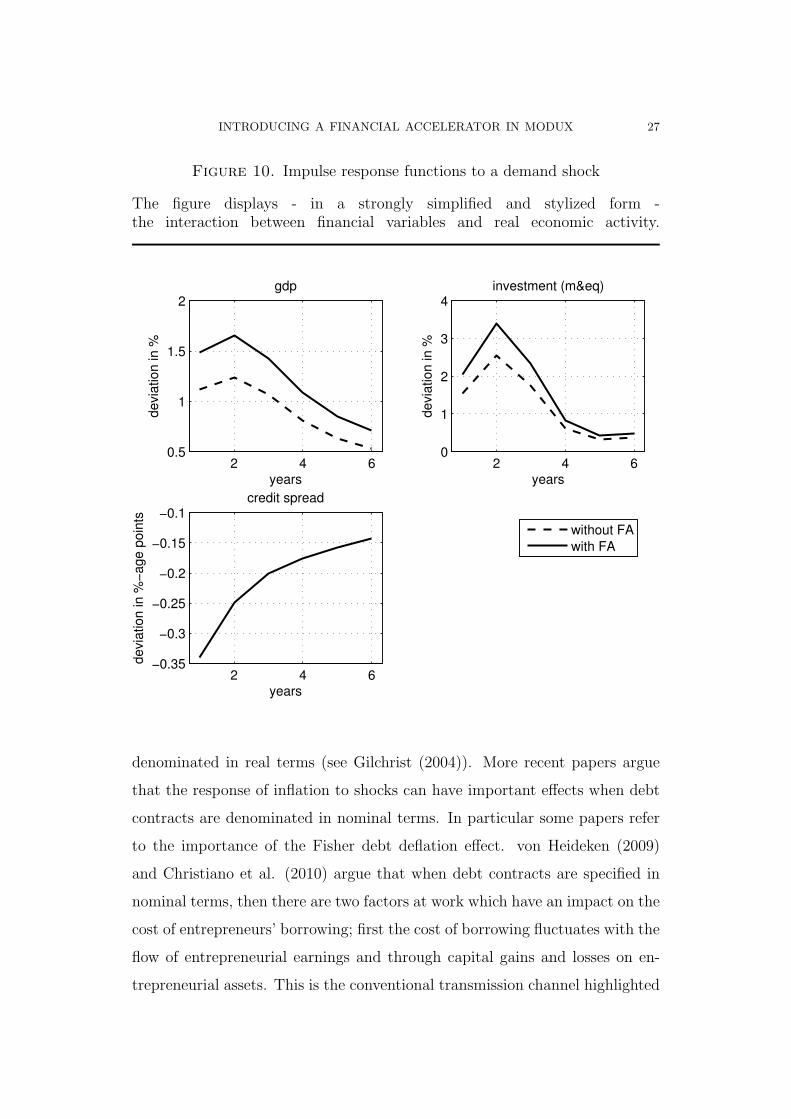
Figure 10. Impulse response functions to a demand shock
The figure displays - in a strongly simplified and stylized form -the interaction between financial variables and real economic activity.
2 4 60.5
1
1.5
2
years
devi
atio
n in
%
gdp
2 4 60
1
2
3
4
years
devi
atio
n in
%
investment (m&eq)
2 4 6−0.35
−0.3
−0.25
−0.2
−0.15
−0.1
years
devi
atio
n in
%−
age p
oin
ts
credit spread
without FAwith FA
denominated in real terms (see Gilchrist (2004)). More recent papers argue
that the response of inflation to shocks can have important effects when debt
contracts are denominated in nominal terms. In particular some papers refer
to the importance of the Fisher debt deflation effect. von Heideken (2009)
and Christiano et al. (2010) argue that when debt contracts are specified in
nominal terms, then there are two factors at work which have an impact on the
cost of entrepreneurs’ borrowing; first the cost of borrowing fluctuates with the
flow of entrepreneurial earnings and through capital gains and losses on en-
trepreneurial assets. This is the conventional transmission channel highlighted

28 INTRODUCING A FINANCIAL ACCELERATOR IN MODUX
in the Bernanke et al. (1999) framework which tends to amplify the economic
impact of a structural disturbance. However, they also point to a further mech-
anism where entrepreneurs’ obligation to pay debt varies because inflation can
ex post change the real debt burden. This second effect is referred to as a
Fisher debt deflation impact. The Fisher debt deflation and accelerator type
mechanisms tend to reinforce each other in the case of shocks that move the
inflation rate and output in the same direction, and they tend to be offsetting
in the presence of shocks which move the inflation rate and output in opposite
directions. The presence of a Fisher debt deflation channel tends to cancel out
the amplification impact of the financial accelerator mechanism1. This implies
that the specification of the debt contract has important consequences for the
size of the amplification effect that results from financial impediments when
the economy is subject to supply shocks. Using an approach where capital and
credit are used in nominal terms instead would imply an amplification effect
that is weaker, moreover the overall model fit would be worse than in the case
of using the real measures for the two variables2. For this reason the equations
involving the capital and credit stock have been denominated in real terms in
each case.
3.4. Impulse response function analysis. This section is to show in how
far the model with the financial accelerator extension compares with the orig-
inal one once impulse response functions are considered. In the vein of the
structural shocks which are shown in Figure 2 and 3 by means of a DSGE
model, I proceed by considering a demand shock within Modux (the shock
1Consider a negative productivity shock which triggers a contraction in aggregate supplyand pushes inflation and output in opposite directions. The fall in output pulls down onasset prices and entrepreneurial earnings which pushes up on the cost of borrowing but this isoffset by the impact of inflation on entrepreneurs’ real debt burden which reduces the cost ofborrowing. If debt contracts are agreed in nominal terms the rise in inflation in response tothe shock reduces the real value of entrepreneurs’ outstanding debt. As a result, the externalfinance premium falls because entrepreneurs’ leverage declines as their real debt levels areeroded because of higher inflation. The fall in the external finance premium pushes downon borrowing costs and dampens the negative impact of the supply shock on investment.Thus, the Fisher deflation effect offsets the amplification effect of the financial accelerator.2The results for the regressions of equation (4) - (7) are not shown here but available uponrequest.

INTRODUCING A FINANCIAL ACCELERATOR IN MODUX 29
considered is a (variance weighted) foreign demand shock (output in the Euro-
area)). Figure 10 shows the impulse response functions of real GDP, real
investment in the machinery & equipment sector as well as the credit spread
in response to a surprise demand innovation. As expected, the shock causes a
rise in output and investment alike. The investment hike triggers an increase
in the capital stock which then exerts upward pressure on the creditworthiness
resulting in a decline in the credit spread. This in turn spurs additional up-
ward pressure on investment and GDP. As a consequence of that, the reaction
of investment and output is stronger in the case the financial accelerator ex-
tension is included relative to the version of Modux where the financial market
interaction is omitted.
The difference in the impulse response functions of the empirical model are
moderate as far as GDP is concerned - the gap is around 0.3 percentage points
in the first two years and declines continuously with the horizon. The difference
in the reaction of (real) investment in the machinery & equipment sector is,
however, more pronounced, in particular in the second year, the gap is around
0.9 percentage points.
Care has to be taken in comparing the impulse response functions of the
DSGE model with those of the empirical model. The DSGE model is calibrated
using standard values. It is not specifically targeted towards the Luxembour-
gish economy. Hence the comparison of the impulse response functions is, if
anything, only valid as far as it concerns their shape. A quantitative judgment
would require estimating at least those parameters of the DGSE model which
address the financial accelerator, as they are usually difficult to calibrate.
The empirical model basically replicates the shape of the theoretical model
fairly well, even though the DSGE model’s impulse response functions do not
have a hump-shaped pattern. This could be introduced theoretically by, for
instance, extensions in the form of investment delays or frictions alike address-
ing the accumulation of capital (see for instance Bernanke et al. (1999) for
further details).
30 INTRODUCING A FINANCIAL ACCELERATOR IN MODUX
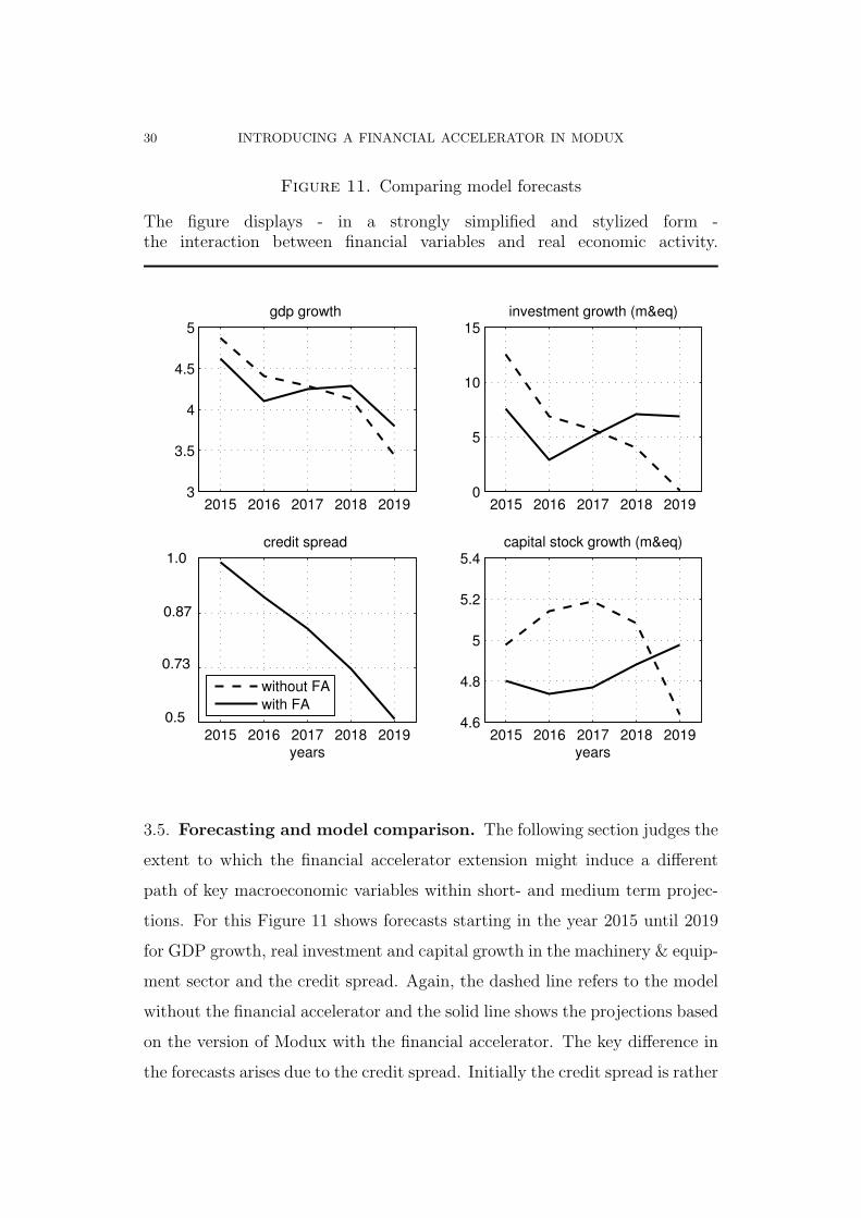
Figure 11. Comparing model forecasts
The figure displays - in a strongly simplified and stylized form -the interaction between financial variables and real economic activity.
2015 2016 2017 2018 20193
3.5
4
4.5
5gdp growth
2015 2016 2017 2018 20190
5
10
15investment growth (m&eq)
2015 2016 2017 2018 20192.5
3
3.5
4
years
credit spread
without FAwith FA
2015 2016 2017 2018 20194.6
4.8
5
5.2
5.4
years
capital stock growth (m&eq)
3.5. Forecasting and model comparison. The following section judges the
extent to which the financial accelerator extension might induce a different
path of key macroeconomic variables within short- and medium term projec-
tions. For this Figure 11 shows forecasts starting in the year 2015 until 2019
for GDP growth, real investment and capital growth in the machinery & equip-
ment sector and the credit spread. Again, the dashed line refers to the model
without the financial accelerator and the solid line shows the projections based
on the version of Modux with the financial accelerator. The key difference in
the forecasts arises due to the credit spread. Initially the credit spread is rather
1.01.0
0.87
0.73
0.5

INTRODUCING A FINANCIAL ACCELERATOR IN MODUX 31
high which causes investment and capital growth to be significantly lower com-
pared to the projections where the financial accelerator has been ignored. The
high credit spread exerts downward pressure on the growth rate of the credit
stock, which in turn implies lower dynamics in capital and investment. This
is replicated also in GDP growth, though the gap between the two models is
low - the growth rates differ by around 0.3 percentage points within the first
three years. However, the continuous decline in the credit spread over time
triggers upward pressure on capital and investment growth. Especially from
2017 onwards the decline in the spread is more pronounced than within the
initial period. As a result this finally triggers a turnaround in the path of the
capital and investment growth rates. After having passed a trough in 2016,
both investment and capital tend to accelerate from 2017 onwards. The gap
in the growth rate comprises a steady increase and tends to be particularly
pronounced in 2019. From then onwards, the gap declines again (not shown
in Figure 11).
The previous discussion compares the dynamic path of the projections with
and without the financial accelerator. However, it does not say anything about
the precision of the forecasts. For this Figures 12 - 14 give some insights in
terms of root-mean-squared-error (rmse) statistics. They show forecast rel-
evant statistics to judge the models in terms of their forecast precision. A
root-mean-squared-error of around 0.8 from the original equation compares to
a value of this statistic of 0.3 for the specification of capital from equation (7)
and a value of 0.1 from the alternative capital equation outlined in equation
(8). In all cases, the extension by means of financial variables tends to im-
prove the forecast precision where the gain is particularly pronounced with the
specification of equation (8).
4. Summary
What has been studied here is an extension to a macroeconometric model
with a block of equations that allows for self-reinforcing comovements between

32 INTRODUCING A FINANCIAL ACCELERATOR IN MODUX
Figure 12. RMSE - original equation for capital
30
40
50
60
70
80
00 01 02 03 04 05 06 07 08 09 10 11 12 13 14
CAPBMEQ_RF – 2 S.E.
Forecast: CAPBMEQ_RF
Actual: CAPBMEQ_R
Forecast sample: 2000 2014
Included observations: 15
Root Mean Squared Error 0.805465
Mean Absolute Error 0.624396
Mean Abs. Percent Error 1.154804
Theil Inequality Coefficient 0.007990
Bias Proportion 0.524076
Variance Proportion 0.282248
Covariance Proportion 0.193675
Figure 13. RMSE - equation (7) for capital
32
36
40
44
48
52
56
60
64
68
72
00 01 02 03 04 05 06 07 08 09 10 11 12 13 14
CAPBMEQ_RF – 2 S.E.
Forecast: CAPBMEQ_RF
Actual: CAPBMEQ_R
Forecast sample: 2000 2014
Included observations: 15
Root Mean Squared Error 0.314124
Mean Absolute Error 0.261552
Mean Abs. Percent Error 0.582673
Theil Inequality Coefficient 0.003098
Bias Proportion 0.005592
Variance Proportion 0.495591
Covariance Proportion 0.498817
Figure 14. RMSE - equation (8) for capital
30
35
40
45
50
55
60
65
70
01 02 03 04 05 06 07 08 09 10 11 12 13 14
CAPBMEQ_RF – 2 S.E.
Forecast: CAPBMEQ_RF
Actual: CAPBMEQ_R
Forecast sample: 2001 2014
Included observations: 14
Root Mean Squared Error 0.102482
Mean Absolute Error 0.084414
Mean Abs. Percent Error 0.180969
Theil Inequality Coefficient 0.000990
Bias Proportion 0.021608
Variance Proportion 0.055842
Covariance Proportion 0.922550
INTRODUCING A FINANCIAL ACCELERATOR IN MODUX 33
the financial sector and real economic activity, often denominated in the liter-
ature as a financial accelerator. The model extension considered here has tried
to integrate a financial accelerator mechanism in a full-fledged macroeconomic
model framework. The working of the financial accelerator has been limited to
the non-financial corporate sector, in particular the machinery & equipment
sector.
Noteworthy, the shape of the impulse response functions of the empirical
model are very much in line with those of DSGE models. This applies both
to the corresponding models with as well as without the financial accelerator
extension. The results for the empirical model show that once the model allows
for macrofinancial interactions, the corresponding financial accelerator effects
contribute to magnify the effects of shocks to the economy. Taken at face
value, this suggests that in the absence of the macrofinancial block, the model
could underestimate the effects of shocks on the macroeconomic level.
As far as economic projection properties are concerned, the extended model
tends to outperform the model without the financial accelerator. In addition
to that the projections of the model with macrofinancial interaction turn out
to be richer in their path. This, of course, at times renders their interpretation
a bit more difficult.
An extension to the work presented here could be the introduction of macro-
financial linkages to sectors other than the one considered here. In particular,
financial accelerator mechanisms could be specified at the household level as
well as for financial corporations.

34 INTRODUCING A FINANCIAL ACCELERATOR IN MODUX
References
[1] Adam, Ferdy, 2004. Modeling a small open economy: What is different? The case of
Luxembourg, available at:
http://www.statistiques.public.lu/en/methodology/definitions/M/Modux/Modux.pdf
[2] Bardsen, G., Ø. Eitrheim, E. S. Jansen and R. Nymoen, 2005. The econometrics of
macroeconomic modelling. Oxford University Press.
[3] Bardsen, G., Lindquist, K. G. and D. P. Tsomocos, 2006. Evaluation of macroeconomic
models for financial stability analysis, Working Paper No. 1, Norges Bank.
[4] Bardsen, G. and R. Nymoen, 2009. Macroeconometric modelling for policy, Ch 17,
Palgrave Handbook of Econometrics Vol. 2, Palgrave Mac-Millan.
[5] Bernanke, Ben and Gertler, Mark, 1989. Agency Costs, Net Worth, and Business
Fluctuations, American Economic Review, American Economic Association, vol. 79(1),
pages 14-31, March.
[6] Bernanke, Ben S., Gertler, Mark and Gilchrist, Simon, 1999. The financial accelerator
in a quantitative business cycle framework, Handbook of Macroeconomics, in: J. B.
Taylor and M. Woodford (ed.), Handbook of Macroeconomics, edition 1, volume 1,
chapter 21, pages 1341-1393 Elsevier.
[7] Calvo, Guillermo A., 1983. Staggered prices in a utility-maximizing framework, Journal
of Monetary Economics, Elsevier, vol. 12(3), pages 383-398, September.
[8] Christiano, Lawrence, Rostagno, Massimo and Motto, Roberto, 2010. Financial factors
in economic fluctuations, Working Paper Series 1192, European Central Bank.
[9] ECB, 2015. The euro area bank lending survey, Third quarter of 2015, available at:
https://www.ecb.europa.eu/stats/pdf/blssurvey 201510.pdf
[10] Gilchrist, S., 2004. Financial Markets and Financial Leverage in a Two-Country World
Economy, Central Banking, Analysis, and Economic Policies Book Series, in: Luis
Antonio Ahumada & J. Rodrigo Fuentes & Norman Loayza (Series Editor) & Klaus
Schmidt-Hebbel (Se (ed.), Banking Market Structure and Monetary Policy, edition 1,
volume 7, chapter 2, pages 027-058 Central Bank of Chile.
[11] Kiyotaki, Nobuhiro and Moore, John, 1997. Credit Cycles, Journal of Political Economy,
University of Chicago Press, vol. 105(2), pages 211-48, April.
[12] Hammersland, Roger and Træe, Cathrine Bolstad, 2014. The financial accelerator and
the real economy: A small macroeconometric model for Norway with financial frictions,
Economic Modelling, Elsevier, vol. 36(C), pages 517-537.
[13] Hammersland, R. and D. H. Jacobsen, 2008. The Financial Accelerator: Evidence using
a procedure of Structural Model Design, Discussion Paper No. 569, Statistics Norway.

INTRODUCING A FINANCIAL ACCELERATOR IN MODUX 35
[14] Hendry, D. F., 1993. Econometrics: Alchemy or Science?, Essays in Econometric
Methodology, Blackwell Publishers, Oxford.
[15] Modigliani, Franco, and Miller, 1958. The Cost of Capital, Corporation Finance and
the Theory of Investment, American Economic Review 48 (3), pages 261-297.
[16] Quadrini, Vincenzo, 2011. Financial frictions in macroeconomic fluctuations, Economic
Quarterly, vol. 97(3), pages 209-254.
[17] von Heideken, V. Q., 2009. How Important are Financial Frictions in the United States
and the Euro Area?, Scandinavian Journal of Economics, Wiley Blackwell, vol. 111(3),
pages 567-596, 09.
36 INTRODUCING A FINANCIAL ACCELERATOR IN MODUX
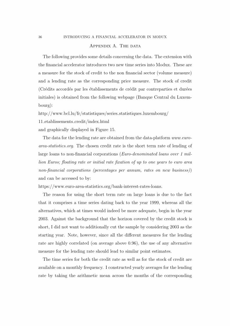
Appendix A. The data
The following provides some details concerning the data. The extension with
the financial accelerator introduces two new time series into Modux. These are
a measure for the stock of credit to the non financial sector (volume measure)
and a lending rate as the corresponding price measure. The stock of credit
(Credits accordes par les etablissements de credit par contreparties et durees
initiales) is obtained from the following webpage (Banque Central du Luxem-
bourg):
http://www.bcl.lu/fr/statistiques/series statistiques luxembourg/
11 etablissements credit/index.html
and graphically displayed in Figure 15.
The data for the lending rate are obtained from the data-platform www.euro-
area-statistics.org. The chosen credit rate is the short term rate of lending of
large loans to non-financial corporations (Euro-denominated loans over 1 mil-
lion Euros; floating rate or initial rate fixation of up to one years to euro area
non-financial corporations (percentages per annum, rates on new business))
and can be accessed to by:
https://www.euro-area-statistics.org/bank-interest-rates-loans.
The reason for using the short term rate on large loans is due to the fact
that it comprises a time series dating back to the year 1999, whereas all the
alternatives, which at times would indeed be more adequate, begin in the year
2003. Against the background that the horizon covered by the credit stock is
short, I did not want to additionally cut the sample by considering 2003 as the
starting year. Note, however, since all the different measures for the lending
rate are highly correlated (on average above 0.96), the use of any alternative
measure for the lending rate should lead to similar point estimates.
The time series for both the credit rate as well as for the stock of credit are
available on a monthly frequency. I constructed yearly averages for the lending
rate by taking the arithmetic mean across the months of the corresponding

INTRODUCING A FINANCIAL ACCELERATOR IN MODUX 37
years. The credit stock is aggregated to the annual frequency by constructing
the sum over the months which comprise a year.
In addition to that the Figure 15 shows the spread between the credit rate
and the short term government bond rate (subplot no. 4). Finally, the last
subplot shows the path of the measure of the creditworthiness as defined in
equation (5).
Figure 15. The data
2000 2005 2010 20158
9
10credit stock (log−level)
2000 2005 2010 2015−20
0
20
40credit stock growth rate (in %)
2000 2005 2010 20150
2
4
6lending rate (percent per annum)
2000 2005 2010 20150
0.5
1
1.5credit spread (percent per annum)
2000 2005 2010 20153
4
5
6creditworthiness