N° d’ordre : 2011-22-TH
THÈSE DE DOCTORAT
SPECIALITE : PHYSIQUE
Ecole Doctorale « Sciences et Technologies de l’Information des Télécommunications et des Systèmes »
Présentée par :
Ayaz AHMAD
Sujet : Optimisation de Ressources et Méthodes Robustes de Renvoi de CQI dans les Réseaux Sans fil
(On Resource Optimization and Robust CQI Reporting for Wireless Communication Systems)
Soutenue le 09 Décembre 2011 devant les membres du jury : M. Mohamad ASSAAD Supélec Encadrant
M. Philippe CIBLAT TELECOM ParisTech Examinateur
M. Pierre DUHAMEL L2S, Supélec Examinateur
M. Christophe LE MARTRET THALES Communications Rapporteur
M. Zeno TOFFANO Supélec Directeur de Thèse
M. Djamal ZEGHLACHE Télécom Sud Paris Rapporteur


i
Acknowledgments
I would like to express my gratitude to my Ph.D. supervisor Dr. Mohamad
Assaad for his continuous guidance, support and cooperation without which this
thesis would not have been completed. I would like also to thank Dr. Hamidou
Tembine for several useful discussions during my final year of thesis.
I am grateful to Prof. Djamal Zeghlache and Dr. Christophe Le Martret for
reviewing my thesis manuscript and providing me with valuable comments on
the earlier version of this manuscript. I am also thankful to Prof. Zeno Toffano,
Prof. Pierre Duhamel and Prof. Philippe Ciblat for being part of the jury members
of my Ph.D. defense.
Warm thanks to my colleagues at Telecommunications department over the
last four years: Amr Ismail, Najett Neji, Jakob Richard HOYDIS, Joffrey Villard,
Naveed Ul Hassan, and Christophe Gaie. They provided a very pleasant research
environment and made my stay at Supélec a really enjoyable one. In particular, I
am highly indebted to Amr and Najett for their generous help in composing the
French extended abstract of my thesis. I also wish to thank my Pakistani friends,
Mohammad Shoaib Saleem, Yasir Faheem, and Mubashir Hussain Rehmani for
the wonderful weekends all over these four years.
Last but not least, I would like to thank my family. My profound respect and
sincere gratitude go to my mother and father whose love, support, and encour-
agement accompanied me all my way. I owe my loving thanks to my fiancée
Nabeela. Her understanding, and loving support was a powerful source of en-
ergy for moving forward through the seemingly random ups and downs of my
last two years in France.

ii

iii
“To my dearest parents, my loving siblings, and my
sweet fiancée, Nabeela”

iv
v
Publications
Journals
1. A. Ahmad, M. Assaad and H. Tembine, “Joint Power Control and Rate
Adaptation for Video Streaming in Multi-node Wireless Networks," in re-
view IEEE Transaction on Communications.
2. A. Ahmad, M. Assaad, H. Tembine and N. Ul Hassan, “Robust CQI Report-
ing in Multi-Carrier and Multi-user Systems," in review IEEE Transaction on
Mobile Computing.
3. A. Ahmad and M. Assaad, “Canonical Dual Method for Resource Alloca-
tion and Adaptive Modulation in Uplink SC-FDMA Systems," in second
round review IEEE Transaction on Signal Processing.
4. A. Ahmad and M. Assaad, “Optimal Resource Allocation in Downlink OFDMA
System with Imperfect Channel Knowledge," Accepted for Publication in
Springer Journal on Optimization and Engineering.
Conferences
1. A. Ahmad, N. Ul Hassan, M. Assaad, H. Tembine, “Stability and Power
Control in an Arbitrary Wireless Network Environment," Submitted to IEEE
ICC 2012.
2. A. Ahmad and M. Assaad, “Polynomial-Complexity Optimal Resource Al-
location Framework for Uplink SC-FDMA Systems," Accepted for publication
in IEEE GLOBECOM 2011.
3. M. Assaad, A. Ahmad and H. Tembine “Risk-Sensitive Resource Control
Approach for Delay Limited Traffic in Wireless Networks," Accepted for pub-
lication in IEEE GLOBECOM 2011.
4. A. Ahmad and M. Assaad, “Power Efficient Resource Allocation in Uplink
SC-FDMA Systems," Accepted for publication in IEEE PIMRC 2011.
vi
5. A. Ahmad and M. Assaad, “Joint Resource Optimization and Relay Se-
lection in Cooperative Cellular Networks with Imperfect Channel Knowl-
edge," in Proc. IEEE SPAWC, Marrakech Morocco, June 2010, pp. 1-5.
6. A. Ahmad and M. Assaad, “Optimal Resource Allocation Framework for
Downlink OFDMA System with Channel Estimation Error," in Proc. IEEE
WCNC, Sydney Australia, April 2010, pp. 1-5.
7. A. Ahmad and M. Assaad, “Margin adaptive Resource Allocation in Down-
link OFDMA System with Outdated Channel State Information," in Proc.
IEEE PIMRC, Tokyo Japan, Sept. 2009, pp. 1868-1872.
vii
Abstract
Adaptive resource allocation in wireless communication systems is crucial in
order to support the diverse QoS requirements of the services and to efficiently
utilize the limited communication resources. However, the design of any adap-
tive resource allocation scheme should consider the service type for which it is in-
tended. Resource allocation schemes for non-real time services are solely aimed
at the efficient utilization of the resources with no stringent delay constraints.
On the other hand, resource allocation techniques for real time services or ap-
plications with stringent delay constraints should also guarantee the delay re-
quirements in addition to efficient resource utilization. Moreover, for efficient re-
source allocation, the transmitter/base station needs information about the chan-
nel conditions. However, due to imperfect channel estimation at the end node
or/and feedback delay, the information about the channel reported to the trans-
mitter may be erroneous or/and outdated, and its use for resource allocation may
severely degrade the system performance. The objective of this thesis is to study
resource allocation for wireless communication systems while taking the afore-
mentioned limiting factors into consideration.
In this thesis, first we consider resource allocation and adaptive modulation
in SC-FDMA systems without considering any specific delay constraint on the
users’ packets transmission and assuming perfect channel knowledge at the trans-
mitter. Unlike OFDMA, in addition to the restriction of allocating a sub-channel
to one user at most, the multiple sub-channels allocated to a user in SC-FDMA
should be consecutive as well. This renders the resource allocation a difficult
combinatorial problem where the computational complexity of finding the opti-
mal solution is exponential. The standard optimization tools (e.g., Lagrange dual
approach widely used for OFDMA, etc.) can not help towards its optimal solu-
tion. We develop a novel optimization framework for the solution of this problem
that is inspired from the recently developed canonical duality theory, and derive
resource allocation algorithms that have polynomial complexities. We provide
viii
conditions under which the derived algorithms are optimal, and explore some
bounds on the sub-optimality of the algorithms if these conditions are not satis-
fied.
Then, we study resource allocation for services with stringent delay constraints,
and consider joint power control and rate adaptation for video streaming in multi-
node wireless networks with interference. This is a challenging problem where
the nodes demand for better video quality with stringent delay constraints while
their channels and interferences have a time-varying nature. In addition, there
should be some fairness criterion among nodes for utilizing the limited network
resources. In this thesis, we develop a cross-layer optimization framework that
performs instantaneous power control at the PHY/MAC layer and average video
rate adaptation at the APPLICATION layer jointly. To this end, we model the
power and the rate variations of the nodes as linear stochastic dynamic equa-
tions, and formulate a risk-sensitive control problem that captures the hard delay
constraints of the video services, and a given fairness criterion for resources uti-
lization.
Finally, in order to deal with the aforementioned channel imperfections, we
adapt a new approach. Unlike the traditional approach of dealing with these im-
perfections at the transmitter, we deal with them at the receiver/user terminal at
the channel quality indicator (CQI) reporting level. Using stochastic control the-
ory, we design a novel best-M CQI reporting scheme for multi-carrier and multi-
user systems that accommodates the impact of the channel imperfections in the
computation of the CQIs. Instead of reporting the erroneous estimation of the
CQIs, each user reports so-called adapted CQIs that accommodate the impact of
estimation error and feedback delay. The adapted CQIs are computed such that
the deviation between the allocated rate by the transmitter and the actual chan-
nel rate is minimized. These adapted CQIs are then directly used for resource
allocation at the transmitter. Moreover, in the traditional best-M CQI reporting
scheme, the number M of reported CQIs is fixed for all users while the wireless
environment is dynamic. Therefore, by using some tools from game theory, we

ix
develop a so-called dynamic best-M scheme which dynamically determines the
efficient number M of CQIs that should be reported by each user to the transmit-
ter. The dynamic scheme improves the system performance without increasing
the system’s overall feedback overhead.

x
xi
Résumé
Au cours de cette thèse, nous nous sommes d’abord intéressés à l’optimisation
des ressources et à la modulation adaptative dans les systèmes utilisant la tech-
nique d’accès multiple SC-FDMA (" Single Carrier Frequency Division Multi-
ple Access "), choisie pour les transmissions en voix montante pour le standard
3GPP-LTE. Cette technique suppose qu’une sous-porteuse ne peut être assignée
qu’à un seul utilisateur, et que les sous-porteuses multiples attribuées à un util-
isateur doivent être consécutives. Suite à ces deux contraintes, l’optimisation
des ressources devient un problème combinatoire à complexité de calcul expo-
nentielle. Afin de pallier à cette difficulté, nous avons proposé une nouvelle ap-
proche d’allocation de ressources et de modulation adaptative basée sur la théorie
de la dualité canonique récemment développée. Grâce à notre méthodologie, la
complexité du problème d’optimisation devient polynômiale et cela en constitue
une remarquable amélioration. A travers des calculs analytiques, nous avons
mis en évidence que sous certaines conditions, l’approche proposée est optimale
mais qu’au cas où ces conditions ne sont pas satisfaites, l’optimalité ne pourrait
pas être assurée. Cependant, nos résultats numériques prouvent que la solution
obtenue par notre développement est très proche de la solution optimale. Dans
cette perspective, nous avons établi quelques bornes pour évaluer la performance
de la solution proposée lorsque les conditions d’optimalité ne sont pas satisfaites.
Nous avons ensuite étudié la problématique complexe de l’allocation de resso-
urces pour le "Streaming Vidéo" dans les réseaux sans fil, où il est nécessaire
d’assurer une transmission vidéo de haute qualité en présence de canaux et de
brouillages variables au cours du temps. Pour ce type d’applications, un critère
d’équité parmi les nœuds du réseau s’impose lors de l’utilisation des ressources
limitées disponibles. Dans ce contexte, nous avons proposé une nouvelle méth-
ode d’allocation de puissance conjointement à l’adaptation du débit vidéo. L’app-
roche proposée exploite la diversité temporelle des canaux, en répondant aux
contraintes strictes de délai associées aux applications vidéo, et en respectant un
xii
critère d’équité spécifique. Selon notre approche, l’allocation des ressources au
niveau de la couche PHY/MAC est effectuée dans le but d’atteindre un SINR ("
Signal to Interference and Noise Ratio ") cible tout en minimisant le délai entre
l’arrivée et le départ des paquets. Cette allocation tient compte des débits vari-
ables attribués à la couche APPLICATION, de manière à assurer la qualité de
vidéo demandée par les nIJuds selon le critère d’équité et l’état de leurs canaux.
Pour ce faire, nous avons adopté une approche de la théorie de contrôle, intitulée
" Risk-Sensitive Control ".
Nous avons dédié la troisième partie de la thèse à la conception d’une nou-
velle stratégie " best-M " pour le renvoi du CQI (" Channel Quality Indicator ")
pour les systèmes multi-utilisateurs et multi-porteuses. Dans les stratégies " best-
M " existantes, l’erreur d’estimation du CQI ainsi que son délai de renvoi sont
gérés au niveau de la station de base. Sachant que toutefois, les utilisateurs ont
une meilleure connaissance des conditions de leurs canaux, l’erreur d’estimation
et le délai de renvoi du CQI seraient mieux traités au niveau des utilisateurs.
Ainsi, notre nouvelle stratégie " best-M " suppose que la gestion de ces prob-
lèmes est confiée aux utilisateurs. Chacun parmi eux renvoie des " CQIs adaptés
", calculés à partir de la résolution d’un problème de contôle stochastique, tel
que l’écart entre le débit alloué par la station de base et le débit réel du canal
soit minimal. D’autre part, en utilisant certains outils de la théorie des jeux, nous
avons développé une stratégie "best-M " dynamique, permettant de déterminer le
nombre efficace de CQIs devant être renvoyés par chaque utilisateur, de manière
dynamique. Cette stratégie se distingue des méthodes actuelles, selon lesquelles
ce nombre est fixé pour tous les utilisateurs. De ce fait, la performance du sys-
tème se trouve améliorée sans que son débit de signalisation ne soit augmenté en
voix montante.
xiii
Contents
1 Résumé long en français (French extended abstract) 1
1.1 Introduction . . . . . . . . . . . . . . . . . . . . . . . . . . . . . . . . 1
1.2 Allocation des ressources et modulation adaptative dans les Sys-
tèmes SC-FDMA . . . . . . . . . . . . . . . . . . . . . . . . . . . . . 4
1.2.1 Formulation des Problèmes . . . . . . . . . . . . . . . . . . . 6
1.2.1.1 Maximisation du somme des utilitiés (SUmax) . . 6
1.2.1.2 Problème BIP équivalant du problème SUmax . . . 7
1.2.1.3 Modulation adaptative conjointe avec minimisa-
tion de la somme des coûts (JAMSCmin) . . . . . 9
1.2.1.4 Forme BIP équivalante du problème JAMSCmin . 9
1.2.2 Approche canonique pour la solution des problèmes BIP . . 11
1.2.2.1 Forme duale canonique du problème SUmax et
conditions d’optimalité . . . . . . . . . . . . . . . . 12
1.2.2.2 Forme duale canonique pour le problème JAM-
SCMin et conditions d’optimalité . . . . . . . . . . 13
1.2.3 Algorithmes d’allocation de ressources et d’adaptation de
modulation . . . . . . . . . . . . . . . . . . . . . . . . . . . . 14
1.2.3.1 Algorithme d’allocation de ressources pour SUmax 14
1.2.3.2 Sous-optimalité de l’algorithme . . . . . . . . . . . 14
1.2.3.3 Résultats de l’algorithme pour N →∞ . . . . . . . 15
1.2.3.4 Stratégie de modulation adaptive pour SUmax . . 15
xiv
1.2.3.5 Algorithme de modulation adaptative conjointe à
l’allocation de resso- urces pour JAMSCmin . . . . 16
1.2.4 Résultats numériques . . . . . . . . . . . . . . . . . . . . . . 16
1.3 Contrôle de puissance conjointe à l’adaptation du débit pour le
streaming vidéo dans les réseaux sans fil . . . . . . . . . . . . . . . . 16
1.3.1 Approche stochastique . . . . . . . . . . . . . . . . . . . . . . 18
1.3.2 Problème de commande " Risk-Sensitive " et sa solution op-
timale . . . . . . . . . . . . . . . . . . . . . . . . . . . . . . . 20
1.3.2.1 Équation d’état . . . . . . . . . . . . . . . . . . . . . 20
1.3.2.2 Formulation de la fonction du coût . . . . . . . . . 21
1.3.2.3 Solution du problème . . . . . . . . . . . . . . . . . 22
1.3.3 Résultats numériques . . . . . . . . . . . . . . . . . . . . . . 23
1.4 Méthodes robustes pour le renvoi du CQI dans les systèmes multi-
porteuses et multi-utilisateurs . . . . . . . . . . . . . . . . . . . . . . 23
1.4.1 Conception de la méthode robuste "best-M" de renvoi du CQI 25
1.4.1.1 Sélection des meilleurs Mk CQIs et leur renvoi . . 28
1.4.2 Méthode robuste dynamique " best-M " de renvoi du CQI . 29
1.4.2.1 Approche pour la détermination de Mk . . . . . . . 29
1.4.2.2 Solution distribuée et algorithme "Efficient Inter-
active Trial and Error Learning" . . . . . . . . . . . 31
1.4.3 Résultats numériques . . . . . . . . . . . . . . . . . . . . . . 32
1.5 Conclusion et perspectives . . . . . . . . . . . . . . . . . . . . . . . . 33
2 Introduction 35
2.1 General Introduction . . . . . . . . . . . . . . . . . . . . . . . . . . . 35
2.1.1 Single Carrier Frequency Division Multiple Access (SC-FDMA) 38
2.1.2 Video Streaming in Wireless Networks . . . . . . . . . . . . 40
2.1.3 Channel Quality Indicator (CQI) Reporting in Multi-carrier
and Multi-user Systems . . . . . . . . . . . . . . . . . . . . . 42
2.2 Problems considered in this thesis . . . . . . . . . . . . . . . . . . . 44
xv
2.2.1 Resource Allocation and Adaptive Modulation in SC-FDMA
Systems . . . . . . . . . . . . . . . . . . . . . . . . . . . . . . 44
2.2.2 Joint Power Control and Rate Adaptation for Video Stream-
ing in Wireless Networks . . . . . . . . . . . . . . . . . . . . 46
2.2.3 CQI Reporting in Multi-carrier and Multi-user Systems with
Imperfect Channel Knowledge . . . . . . . . . . . . . . . . . 49
2.3 State of the art . . . . . . . . . . . . . . . . . . . . . . . . . . . . . . . 51
2.3.1 Resource Allocation in SC-FDMA Systems . . . . . . . . . . 51
2.4 Resource Allocation for Video Streaming in Wireless Networks . . 54
2.4.1 CQI Reporting in Multi-Carrier and Multi-User Systems . . 57
2.5 Thesis Organization and Contributions . . . . . . . . . . . . . . . . 61
2.5.1 Chapter 3 . . . . . . . . . . . . . . . . . . . . . . . . . . . . . 61
2.5.2 Chapter 4 . . . . . . . . . . . . . . . . . . . . . . . . . . . . . 63
2.5.3 Chapter 5 . . . . . . . . . . . . . . . . . . . . . . . . . . . . . 64
2.6 Notations . . . . . . . . . . . . . . . . . . . . . . . . . . . . . . . . . . 66
3 Resource Allocation and Adaptive Modulation in SC-FDMA Systems 69
3.1 Introduction . . . . . . . . . . . . . . . . . . . . . . . . . . . . . . . . 69
3.2 System Model . . . . . . . . . . . . . . . . . . . . . . . . . . . . . . . 70
3.3 Problems Formulation . . . . . . . . . . . . . . . . . . . . . . . . . . 72
3.3.1 Sum-Utility Maximization (SUmax) . . . . . . . . . . . . . . 73
3.3.1.1 SUmax Problem Formulation . . . . . . . . . . . . 73
3.3.1.2 Equivalent BIP Problem for SUmax problem . . . . 74
3.3.2 Joint Adaptive Modulation and Sum-Cost Minimization (JAM-
SCmin) . . . . . . . . . . . . . . . . . . . . . . . . . . . . . . . 76
3.3.2.1 JAMSCmin Problem Formulation . . . . . . . . . . 76
3.3.2.2 Equivalent BIP for JAMSCmin Problem . . . . . . 77
3.4 Canonical Dual Approach for Solving the BIP Problems . . . . . . . 80
3.4.1 Canonical Dual Problem and Optimality Conditions for SUmax
Problem . . . . . . . . . . . . . . . . . . . . . . . . . . . . . . 81
xvi
3.4.2 Canonical Dual Problem and Optimality Conditions for JAM-
SCmin Problem . . . . . . . . . . . . . . . . . . . . . . . . . . 86
3.5 Resource Allocation and Adaptive Modulation Algorithms . . . . . 89
3.5.1 Resource Allocation Algorithm for SUmax . . . . . . . . . . 89
3.5.1.1 Adaptive Modulation Scheme for SUmax . . . . . 90
3.5.2 Joint Adaptive Modulation and Resource Allocation Algo-
rithm for JAMSCmin . . . . . . . . . . . . . . . . . . . . . . . 92
3.5.3 Complexity of the algorithm . . . . . . . . . . . . . . . . . . 92
3.5.3.1 Complexity of the algorithm for SUmax problem . 92
3.5.3.2 Complexity of the algorithm for JAMSCmin prob-
lem . . . . . . . . . . . . . . . . . . . . . . . . . . . 93
3.5.4 On the Optimality of the Algorithm . . . . . . . . . . . . . . 93
3.5.4.1 Analysis of the algorithm’s results for N →∞ . . . 95
3.6 Simulation Results . . . . . . . . . . . . . . . . . . . . . . . . . . . . 95
3.6.1 Sum-utility maximization . . . . . . . . . . . . . . . . . . . . 96
3.6.2 Joint Adaptive Modulation and Resource Allocation . . . . 97
3.7 Conclusion . . . . . . . . . . . . . . . . . . . . . . . . . . . . . . . . . 98
4 Joint Power Control and Rate Adaptation for Video Streaming in Wire-
less Networks 101
4.1 Introduction . . . . . . . . . . . . . . . . . . . . . . . . . . . . . . . . 101
4.2 System Model and Problem Statement . . . . . . . . . . . . . . . . . 102
4.3 Stochastic Framework for Joint Power Control and Rate Adaptation 106
4.3.1 CINR Probability Distribution Function . . . . . . . . . . . . 106
4.3.2 Stochastic Linear Dynamic Model for Power Control . . . . 110
4.3.3 Stochastic Linear Dynamic Model for Rate Adaptation . . . 113
4.4 Risk-sensitive Control Problem and its Optimal Solution . . . . . . 116
4.4.1 State Space Equation . . . . . . . . . . . . . . . . . . . . . . . 116
4.4.2 Cost Function Formulation . . . . . . . . . . . . . . . . . . . 117
4.4.3 Intuitive View of the Risk-Sensitive Criterion . . . . . . . . . 119
xvii
4.4.4 Solution of the Problem . . . . . . . . . . . . . . . . . . . . . 119
4.4.5 Implementation . . . . . . . . . . . . . . . . . . . . . . . . . . 121
4.5 Simulation Results . . . . . . . . . . . . . . . . . . . . . . . . . . . . 122
4.6 Conclusion . . . . . . . . . . . . . . . . . . . . . . . . . . . . . . . . . 127
5 Robust CQI Reporting Schemes for Multi-carrier and Multi-user Sys-
tems 129
5.1 Introduction . . . . . . . . . . . . . . . . . . . . . . . . . . . . . . . . 129
5.2 System Description and Problem Statement . . . . . . . . . . . . . . 131
5.3 Robust best-M CQI Reporting Scheme . . . . . . . . . . . . . . . . . 133
5.3.1 Reporting Scheme Design . . . . . . . . . . . . . . . . . . . . 134
5.3.2 Solution of the above Linear Control Problem . . . . . . . . 138
5.3.2.1 LQG based solution . . . . . . . . . . . . . . . . . . 139
5.3.2.2 H∞ Controller Based Solution . . . . . . . . . . . . 141
5.3.3 Selection and Reporting of the Best Mk CQIs . . . . . . . . . 144
5.3.4 Dealing with Noisy Feedback Channels . . . . . . . . . . . . 144
5.4 Dynamic M-best CQI Reporting Scheme . . . . . . . . . . . . . . . . 146
5.4.1 Mk Determination Framework . . . . . . . . . . . . . . . . . 146
5.4.2 Distributed solution . . . . . . . . . . . . . . . . . . . . . . . 148
5.4.2.1 Efficient Interactive Trial and Error Learning Al-
gorithm . . . . . . . . . . . . . . . . . . . . . . . . . 149
5.5 Simulation Results . . . . . . . . . . . . . . . . . . . . . . . . . . . . 152
5.6 Conclusion . . . . . . . . . . . . . . . . . . . . . . . . . . . . . . . . . 157
6 Conclusion 159
6.1 Contributions . . . . . . . . . . . . . . . . . . . . . . . . . . . . . . . 160
6.2 Future Work . . . . . . . . . . . . . . . . . . . . . . . . . . . . . . . . 164
A Appendix chapter 2 167
A.1 Proof of Theorem 3.4.1 . . . . . . . . . . . . . . . . . . . . . . . . . . 167
A.2 Proof of Theorem 3.4.2 . . . . . . . . . . . . . . . . . . . . . . . . . . 169

xviii
A.3 Proof of Theorem 3.5.1 . . . . . . . . . . . . . . . . . . . . . . . . . . 170
A.4 Proof of Corollary 3.5.1 . . . . . . . . . . . . . . . . . . . . . . . . . . 173
B Appendix Chapter 4 175
B.1 Proof of Theorem 5.4.1 . . . . . . . . . . . . . . . . . . . . . . . . . . 175
Bibliography 179
xix
List of Figures
3.1 Empirical CDF of sum-utility . . . . . . . . . . . . . . . . . . . . . . 96
3.2 Empirical CDF of sum-cost . . . . . . . . . . . . . . . . . . . . . . . 97
4.1 Illustration of Controller Implementation and Signaling between
Nodes . . . . . . . . . . . . . . . . . . . . . . . . . . . . . . . . . . . . 121
4.2 Cost for the proposed Risk-Sensitive (RS) scheme with different
values of risk-sensitive parameter µ, and Cost for LQG solution . . 123
4.3 Difference between target and actual SINR levels for LQG solution 124
4.4 Square of the difference between target and actual SINR levels for
the proposed Risk-Sensitive solution with risk-sensitive parameter,
µ = 0.15 . . . . . . . . . . . . . . . . . . . . . . . . . . . . . . . . . . . 124
4.5 Square of the difference between target and actual SINR levels for
the proposed Risk-Sensitive solution with risk-sensitive parameter,
µ = 0.31 . . . . . . . . . . . . . . . . . . . . . . . . . . . . . . . . . . . 125
4.6 Variance of SINR deviation . . . . . . . . . . . . . . . . . . . . . . . 125
4.7 Probability that the actual delay occurred is greater than the given
target delay . . . . . . . . . . . . . . . . . . . . . . . . . . . . . . . . 126
5.1 Per-user average cost with M=5 (Fixed) and Gaussian noise . . . . 153
5.2 Per-user average cost with M=5 (Fixed) and Rayleigh distributed
noise . . . . . . . . . . . . . . . . . . . . . . . . . . . . . . . . . . . . 153
5.3 Per-user average cost with M=5 (Fixed) and exponentially distributed
noise . . . . . . . . . . . . . . . . . . . . . . . . . . . . . . . . . . . . 154

xx
5.4 Per-user average cost for our proposed scheme with various values
of M . . . . . . . . . . . . . . . . . . . . . . . . . . . . . . . . . . . . . 155
5.5 Empirical CDF of per-user average cost . . . . . . . . . . . . . . . . 155
5.6 Empirical CDF of sum of reported CQIs by all users (value ofKMk)
for our dynamic best-M scheme . . . . . . . . . . . . . . . . . . . . . 156

xxi
List of Tables
3.1 Resource Allocation Algorithm . . . . . . . . . . . . . . . . . . . . . 91
5.1 Iterative Trial and Error Algorithm . . . . . . . . . . . . . . . . . . . 151

xxii

1
Chapter 1
Résumé long en français (French
extended abstract)
1.1 Introduction
Les progrès récents dans les technologies de communication sans fil et leur ca-
pacité de fournir des débits élevés ont révolutionné la façon dont la société mod-
erne fonctionne. En plus de la transmission de la voix, la communication sans
fil moderne permet des services/applications diverses telles que la transmission
de données, messagerie électronique, le streaming vidéo en haute résolution, etc.
Ces services sont associés à des besoins différents en termes de qualité de service
(QoS), exprimée en débits de données, délais de transmission, taux d’erreur, etc.
Les systèmes modernes de communication sans fil sont capables de supporter
ces services diverses et variés, mais ils doivent garantir des besoins différents de
QoS. Ceci est difficile, premièrement à cause de la limitation des ressources de
communication sans fil (fréquences, puissance, etc.), et deuxièmement à cause
de la non-fiabilité de la capacité du canal sans fil, dûe à plusieurs phénomènes
comme les variations temporelles du canal, la propagation par trajets multiples
et les interférences mutuelles parmi plusieurs transmissions simultanées.
Il est nécessaire de développer des stratégies dynamiques/adaptatives d’alloc-
ation de ressources afin de fournir la QoS demandée tout en utilisant les ressources
2
de communication disponibles de manière efficace. Certes, la variabilité (dans
le domaine temporel) des canaux sans fil pose certaines limites, mais elle per-
met d’atteindre un débit de données élevé par l’exploitation de la diversité tem-
porelle pour l’allocation des ressources. L’allocation adaptative des ressources
exploite aussi la diversité des utilisateurs/nœuds et la diversité fréquentielle.
Cependant, la conception de telles stratégies requiert la connaissance de la qual-
ité du canal sans fil. Ainsi, le développement de stratégies renvoyant ce type
d’information (" feedback ") est essentiel pour permettre une allocation efficace
des ressources. Comme son nom l’indique, le but principal de l’allocation adap-
tative des ressources est de répartir les ressources de manière dynamique parmi
plusieurs utilisateurs/nœuds selon la qualité de leurs canaux. Certains nœuds
dans le réseau sont susceptibles de demander des services diverses, qui peu-
vent avoir des besoins différents en termes de QoS. En effet, certains utilisateurs
peuvent demander des services “non-temps réel" ou applications tolérantes aux
délais (transfert de fichiers, contrôle d’e-mails, etc.) tandis que d’autres peu-
vent demander des services “temps réel" ou applications à contraintes de délai
fortes (communication vocale, streaming vidéo, etc.). Les stratégies d’allocation
de ressources pour des applications “temps-réel" ou des services avec contraintes
de délai fortes doivent aussi respecter les exigences de délai en plus de l’allocation
efficace des ressources. La conception de ces stratégies doit alors prendre en
compte les services/applications demandés.
L’information sur la qualité du canal des différents nœuds/utilisateurs du
réseau est un paramètre supplémentaire à considérer dans l’allocation adapta-
tive des ressources. D’une manière générale, chaque nœud/utilisateur estime
son canal et renvoie à la station de base/émetteur un indicateur de qualité de
canal (CQI : " Channel Quality Indicator ") qui sera utilisé par l’unité d’allocation
de ressources. Toutefois, le CQI au niveau de la station de base/émetteur risque
d’être imparfait suite à une erreur dans son estimation par le nœud. L’imperfection
du CQI peut être aussi engendrée par son délai de renvoi et dans ce cas précis,
il ne représente pas le canal actuel. Par conséquent, ce phénomène lié au CQI ne
3
doit pas être négligé dans l’élaboration des stratégies adaptatives d’allocation de
ressources. Selon les méthodes actuelles, ces imperfections sont compensées au
niveau de la station de base/émetteur. Etant donné que l’allocation de ressources
est plus efficace quand la connaissance du CQI au niveau de la station de base/ém-
etteur est plus correcte, et que les utilisateurs ont une connaissance plus complète
des CQIs, une autre approche intéressante serait donc de traiter les imperfec-
tions du canal au niveau des utilisateurs/nœuds. Ceux-ci renvoient alors vers
la station de base/émetteur des CQIs robustes (c’est-à-dire incluant les imperfec-
tions évoquées précédemment) qui seront directement utilisés pour l’allocation
des ressources.
Le problème de l’allocation adaptative des ressources dans les systèmes multi-
utilisateur a été largement étudié jusqu’à présent. Plusieurs techniques d’allocation
pour ce type de systèmes ont été traitées dans de précédents travaux, à l’image de
la technique OFDMA (" Orthogonal Frequency Division Multiple Access ") et de
la technique CDMA (" Code Division Multiple Access "). Toutefois, l’allocation
des ressources dans les systèmes utilisant la technique SC-FDMA (" Single Carrier
Frequency Division Multiple Access") n’a pas été abordée d’une manière appro-
fondie à l’heure actuelle et de ce fait, l’étude de cette problématique requiert des
travaux de recherche considérables.
Dans ce contexte, cette thèse se focalise sur plusieurs aspects concernant l’allo-
cation des ressources dans les systèmes multi-utilisateurs utilisant le SC-FDMA.
Dans un premier temps, on analyse cette allocation ainsi que la modulation adap-
tative sans tenir compte des contraintes sur le délai de transmission et en sup-
posant la connaissance parfaite des informations sur les canaux d’émission au
niveau de la station de base / émetteur. Dans un deuxième temps, on aborde le
problème en considérant dans le réseau des applications / services à contraintes
fortes de délai. Pour ce faire, on développe d’abord une approche d’allocation
de ressources pour le cas particulier de l’application " vidéo streaming " dans un
réseau sans fil quelconque, dans l’objectif de la généraliser pour l’ensemble des
systèmes SC-FDMA. Toutefois, en raison de la durée limitée de la thèse et de
4
la complexité de la problématique de gestion des ressources dans les systèmes
SC-FDMA, l’atteinte de cet objectif s’inscrit dans les perspectives des travaux ac-
complis. Dans un troisième temps, on présente une nouvelle approche pour le
traitement des imperfections de l’information sur le canal disponible à l’émetteur
(expliqué dans les précédents paragraphes). Cette méthode se distingue des ap-
proches classiques puisqu’elle permet de faire face à ces imperfections au niveau
des renvois du CQI au lieu de la station de base / émetteur. Etant donnée la
nature multi-porteuse de la technique SC-FDMA, on propose dans cette thèse
une stratégie de renvoi du CQI adaptée aux systèmes multi-porteuses et multi-
utilisateurs et qui prend en considération l’erreur d’estimation du canal ainsi que
le délai de renvoi du CQI. Les indicateurs sont alors calculés comprenant l’effet
des différentes imperfections et sont ensuite renvoyés à la station de base pour
pouvoir être directement utilisés pour l’allocation des ressources. La stratégie
proposée a un caractère générique et pourrait donc être adaptée à plusieurs types
de systèmes de communication sans fil multi-porteuses et multi-utilisateurs.
Dans les prochains paragraphes, on présentera une à une les trois probléma-
tiques étudiées pendant cette thèse. On y détaille les solutions respectives pro-
posées, ainsi que les résultats obtenus pour mettre en évidence les principales
contributions des travaux réalisés. Dans une dernière partie, on récapitulera les
conclusions de la thèse et on donnera quelques perspectives de recherche qui en
découlent.
1.2 Allocation des ressources et modulation adapta-
tive dans les Systèmes SC-FDMA
Dans cette partie, nous considérons l’allocation des ressources et la modula-
tion adaptative dans les systèmes appelés " Localized SC-FDMA ". Nous traitons
deux aspects: D’une part, le problème de maximisation de la somme des utilités
(“SUmax : Sum-Utility Maximization"), et d’autre part, le problème d’adaptation
de la modulation conjointement à minimisation de la somme des coûts (“JAM-
5
SCmin : Joint Adaptive Modulation and Sum-Cost Minimization"). La SUmax
vise à maximiser la somme des utilités des utilisateurs sous contraintes de puis-
sance maximale d’émission de chaque utilisateur et de valeur crête de la puis-
sance émise sur chaque sous-porteuse. Par ailleurs, la JAMSCmin cherche à min-
imiser la somme des puissances émises par les utilisateurs sous contraintes de
débits de données atteints par les utilisateurs. A l’image de l’OFDMA, une sous-
porteuse dans un système SC-FDMA est attribuée à un seul utilisateur. Dans le
cas des systèmes " Localized SC-FDMA ", les sous-porteuses multiples attribuées
à chaque utilisateur doivent être consécutives en plus de la restriction de l’allocat-
ion de chaque sous porteuse à un utilisateur unique. Par ailleurs, l’expression du
SNR (Signal to Noise Ratio) d’un utilisateur dans un système SC-FDMA est plus
compliquée que celle d’un utilisateur OFDMA (Orthogonal Division Multiple Ac-
cess) en raison de l’égalisation dans le domaine fréquentiel sur toutes ses sous-
porteuses. Par conséquent, l’allocation de puissance pour chaque sous-porteuse
d’un utilisateur dépend de l’ensemble des sous-porteuses attribuées à cet util-
isateur. Cette structure du SNR rend le problème d’allocation des ressources
extrêmement difficile dont la complexité de trouver une solution optimale est
exponentielle. Les stratégies d’allocation des ressources développées pour les
systèmes OFDMA ne sont pas applicables aux systèmes SC-FDMA. En plus, on
ne peut pas se servir des outils classiques d’optimisation (telle que l’approche
Lagrangienne largement utilisée pour OFDMA, etc.) pour trouver une solution
optimale à ce problème.
Ainsi, dans cette partie du manuscrit, nous développons une nouvelle tech-
nique d’optimisation pour résoudre les deux problématiques evoquées précédem-
ment. Cette technique est inspirée par la théorie de la dualité canonique récem-
ment développée. D’abord, nous formulons les deux problèmes d’optimisation
sous forme des problèmes BIP (Binary-Integer Programming). Ensuite, nous ex-
primons les deux problèmes BIP sous forme duale canonique dans R. Les prob-
lèmes duales canoniques sont des problèmes de maximisation concave dans cer-
tains cas et leur solution est donc très simple. Concernant la problématique
6
SUmax, nous proposons un algorithme d’allocation de puissance et de sous-
porteuses basé sur la solution du problème dual canonique correspondante. Une
stratégie de modulation adaptative pour le problème SUmax est aussi dévelop-
pée. Selon la répartition de la puissance et des sous-porteuses effectuée par
l’algorithme proposé, cette stratégie permet de choisir une technique de modula-
tion appropriée pour chaque utilisateur. De manière analogue, nous proposons
également un algorithme d’allocation de puissance et de sous-porteuses conjoin-
tement à la modulation adaptative pour le problème JAMSCmin. La complexité
du calcul des deux algorithmes est polynômiale. Cela représente une améliora-
tion significative par rapport à la complexité exponentielle. Nous avons prouvé
analytiquement que sous certaines conditions, les algorithmes proposés sont op-
timaux. Nous indiquons également quelques bornes de sous-optimalité de nos
algorithmes dans le cas où les conditions d’optimalité ne sont pas satisfaites. A
travers plusieurs simulations, nous évaluons la performance des algorithmes pro-
posés tout en les comparant aux algorithmes existants dans la littérature.
1.2.1 Formulation des Problèmes
Dans cette sous-chapitre, nous formulons les deux problèmes et leurs formes
BIP équivalentes.
1.2.1.1 Maximisation du somme des utilitiés (SUmax)
Nous cherchons à maximiser la somme des utilités sous contrainte de la puis-
sance totale d’émission par chaque utilisateur, désigné par Pmaxk . A cette con-
trainte s’ajoute une contrainte sur la puissance crête appelée P peakk,n . En effet, la
puissance crête émise sur chaque sous-porteuse par un utilisateur quelconque ne
doit pas dépasser P peakk,n , à condition de maintenir le PAPR à une valeur basse [1].
En outre, toutes les sous-porteuses attribuées à un utilisateur doivent avoir la
même puissance (c.f. standard LTE [1]), de manière à conserver un niveau faible
de PAPR [2]. L’utilité de l’utilisateur k, dénotée Uk(γk), est une fonction arbitraire
7
monotone croissante du SNR de l’utilisateur k (désigné par γk). Le problème
global d’allocation des ressources peut être formulé comme suit:
maxK∑k=1
Uk(γk) (1.1)
s.t.∑n∈Nk
Pk,n ≤ Pmaxk , ∀k
Pk,n ≤ P peakk,n , ∀k, n
Pk,n = Pk,l, ∀k, n, l
Nk ∩Nj = ∅,∀k = jn ∩
( K∪j=1,j =k
Nj
)= ∅ | n ∈ n1, n1 + 1, ..., n2 − 1, n2
, ∀k
oùNk de cardinalitéNk est l’ensemble des sous-porteuses attribuées à l’utilisateur
k, N1 = min(Nk) et N2 = max(Nk). La quatrième contrainte signifie que chaque
sous-porteuse ne peut pas être attribuée qu’à un seul utilisateur et la dernière
contrainte assure que les sous-porteuses incluses dans l’ensembleNk sont conséc-
utives. Du fait de ces contraintes, le problème d’optimisation (1.1) est combina-
toire. Par exemple, pourK = 10 utilisateurs etN = 24 sous-porteuses, la solution
optimale nécessite une recherche parmi 5,26×10¹² choix possibles d’allocation des
sous-porteuses [3], ce qui n’est pas réalisable en pratique.
1.2.1.2 Problème BIP équivalant du problème SUmax
Nous formulons le problème sous forme d’un problème BIP où des groupes
de sous-porteuses consécutives sont formés et alloués de manière optimale parmi
les utilisateurs (au lieu d’allouer des sous-porteuses d’une manière individuelle)
tel que les contraintes sur la répartition des sous-porteuses sont satisfaites. Nous
présentons l’idée générale de la formation des groupes des sous-porteuses avec
un exemple simple. Supposons que K = 2 utilisateurs et N = 4 sous-porteuses.
Dans chaque groupe, nous mettons 1 si une sous-porteuse est attribuée à un util-
isateur et mettons 0 dans le cas contraire. Ainsi, compte tenu de la contrainte
de consécutivité des sous-porteuses, l’ensemble réalisable de groupes de sous-
8
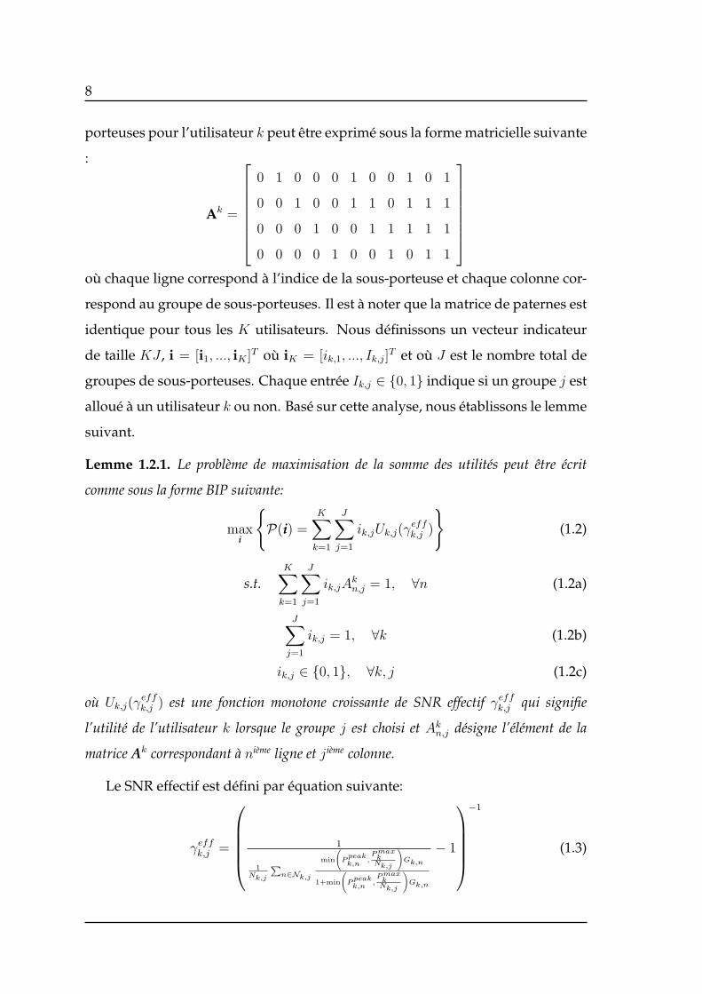
porteuses pour l’utilisateur k peut être exprimé sous la forme matricielle suivante
:
Ak =
0 1 0 0 0 1 0 0 1 0 1
0 0 1 0 0 1 1 0 1 1 1
0 0 0 1 0 0 1 1 1 1 1
0 0 0 0 1 0 0 1 0 1 1
où chaque ligne correspond à l’indice de la sous-porteuse et chaque colonne cor-
respond au groupe de sous-porteuses. Il est à noter que la matrice de paternes est
identique pour tous les K utilisateurs. Nous définissons un vecteur indicateur
de taille KJ , i = [i1, ..., iK ]T où iK = [ik,1, ..., Ik,j]T et où J est le nombre total de
groupes de sous-porteuses. Chaque entrée Ik,j ∈ 0, 1 indique si un groupe j est
alloué à un utilisateur k ou non. Basé sur cette analyse, nous établissons le lemme
suivant.
Lemme 1.2.1. Le problème de maximisation de la somme des utilités peut être écrit
comme sous la forme BIP suivante:
maxi
P(i) =
K∑k=1
J∑j=1
ik,jUk,j(γeffk,j )
(1.2)
s.t.K∑k=1
J∑j=1
ik,jAkn,j = 1, ∀n (1.2a)
J∑j=1
ik,j = 1, ∀k (1.2b)
ik,j ∈ 0, 1, ∀k, j (1.2c)
où Uk,j(γeffk,j ) est une fonction monotone croissante de SNR effectif γeffk,j qui signifie
l’utilité de l’utilisateur k lorsque le groupe j est choisi et Akn,j désigne l’élément de la
matrice Ak correspondant à nième ligne et j ième colonne.
Le SNR effectif est défini par équation suivante:
γeffk,j =
1
1Nk,j
∑n∈Nk,j
min
(Ppeakk,n
,PmaxkNk,j
)Gk,n
1+min
(Ppeakk,n
,PmaxkNk,j
)Gk,n
− 1
−1
(1.3)

9
1.2.1.3 Modulation adaptative conjointe avec minimisation de la somme des
coûts (JAMSCmin)
Ce problème peut être formulé comme suit:
minK∑k=1
Ck(Pmaxk , Pk) (1.4)
s.t. Rk ≥ RTk ,∀k
Pk,n = Pk,l, ∀k, n, l
γk ≥ Γ∗m,∀k,m
|Mk ∩M | = 1,∀k
Nk ∩Nj = ∅,∀k = jn ∩
( K∪j=1,j =k
Nj
)= ∅ | n ∈ n1, n1 + 1, ..., n2 − 1, n2
, ∀k
Dans (1.4), Ck(Pmaxk , Pk) = − exp [Pmax
k − Pk], Rk et RTk représentent le débit de
données atteint et le débit de données cible de l’utilisateur k, respectivement. Par
ailleursMk est un ensemble à cardinalité 1, indiquant la modulation choisie pour
l’utilisateur k etNk, n1 et n2 sont les mêmes que ceux définis pour le problème de
SUmax. La quatrième contrainte signifie qu’une seule technique de modulation
est choisie pour chaque utilisateur de l’ensemble M .
1.2.1.4 Forme BIP équivalante du problème JAMSCmin
Les groupes de sous-porteuses consécutives et la matrice correspondante sont
exactement les mêmes que ceux exprimés pour le problème SUmax. Cepen-
dant, étant donné que le problème JAMSCmin tient compte de phénomène de
l’adaptation de la modulation conjointement à l’allocation des ressources, nous
introduisons le sélection de modulation dans la matrice des groupes de sous-
porteuses. Cette matrice (pour l’exemple susmentionné avec K = 2 et N = 4)
10
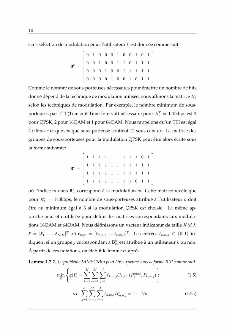
sans sélection de modulation pour l’utilisateur k est donnée comme suit :
Bk =
0 1 0 0 0 1 0 0 1 0 1
0 0 1 0 0 1 1 0 1 1 1
0 0 0 1 0 0 1 1 1 1 1
0 0 0 0 1 0 0 1 0 1 1
Comme le nombre de sous-porteuses nécessaires pour émettre un nombre de bits
donné dépend de la technique de modulation utilisée, nous affinons la matriceBk
selon les techniques de modulation. Par exemple, le nombre minimum de sous-
porteuses par TTI (Transmit Time Interval) nécessaire pour RTk = 140kbps est 3
pour QPSK, 2 pour 16QAM et 1 pour 64QAM. Nous rappelons qu’un TTI est égal
à 0.5msec et que chaque sous-porteuse contient 12 sous-canaux. La matrice des
groupes de sous-porteuses pour la modulation QPSK peut être alors écrite sous
la forme suivante:
Bk1 =
1 1 1 1 1 1 1 1 1 0 1
1 1 1 1 1 1 1 1 1 1 1
1 1 1 1 1 1 1 1 1 1 1
1 1 1 1 1 1 1 1 0 1 1
où l’indice m dans Bk
m correspond à la modulation m. Cette matrice revèle que
pour RTk = 140kbps, le nombre de sous-porteuses attribué à l’utilisateur k doit
être au minimum égal à 3 si la modulation QPSK est choisie. La même ap-
proche peut être utilisée pour définir les matrices correspondants aux modula-
tions 16QAM et 64QAM. Nous définissons un vecteur indicateur de taille KMJ ,
ℓ = [ℓ1,1, ..., ℓK,M ]T où ℓk,m = [ℓk,m,1, ..., ℓk,m,J ]T . Les entrées ℓk,m,j ∈ 0, 1 in-
diquent si un groupe j correspondant à Bkm est attribué à un utilisateur k ou non.
Á partir de ces notations, on établit le lemme ci-aprés.
Lemme 1.2.2. Le problème JAMSCMin peut être exprimé sous la forme BIP comme suit:
minℓ
g(ℓ) =
K∑k=1
M∑m=1
J∑j=1
ℓk,m,jCk,j,m(Pmaxk , Pk,m,j)
(1.5)
s.t.K∑k=1
M∑m=1
J∑j=1
ℓk,m,jBkm,n,j = 1, ∀n (1.5a)

11
M∑m=1
J∑j=1
ℓk,m,j = 1,∀k (1.5b)
ℓk,m,j ∈ 0, 1, ∀k,m, j (1.5c)
où Bkm,n,j désigne l’élément de la matrice Bk
m correspondant à nième ligne et j ième colonne,
Pk,m,j = f(γeffk,m,j, RTk ,Γ
∗m) est la puissance transmise par l’utilisateur k quand le j ième
groupe de sous-porteuses correspondant à Bkm est choisi et Ck,m,j(P
maxk , Pk,m,j) =
− exp [Pmaxk − Pk,m,j].
Les paramètres γeffk,m,j et Pk,m,j indiquent le SNR et la puissance émise par
l’utilisateur k quand le groupe j et la modulation m sont choisis. Ainsi γeffk,m,j
est défini par:
γeffk,m,j =
(1
1Nk,m,j
∑n∈Nk,m,j
Pk,m,nGk,n
1+Pk,m,nGk,n
− 1
)−1
(1.6)
avecNk,m,j de cardinalitéNk,m,j l’ensemble des sous-porteuses attribué à l’utilisateur
k lorsque le groupe j est choisi de Bkm. Les entités Pk,m,j’s sont obtenues avant
l’allocation des ressources en résolvant les équations suivantes:∑n∈Nk,m,j
(Pk,m,jGk,n
Nk,m,j + Pk,m,jGk,n
)− Nk,m,jΓ
∗m
1 + Γ∗m
= 0,∀k,m, j (1.7)
1.2.2 Approche canonique pour la solution des problèmes BIP
Tout d’abord, en utilisant la théorie de la dualité canonique, nous exprimons
chacun des deux problèmes BIP (SUmax et JAMSCmin) sous forme d’un prob-
lème dual canonique dans R. Nous étudions ensuite l’optimalité de notre ap-
proche canonique et nous prouvons que sous certaines conditions, la solution de
chaque problème dual canonique constitue la solution optimale du problème BIP
correspondant.

12
1.2.2.1 Forme duale canonique du problème SUmax et conditions d’optimalité
La fonction objectiveP(i) mentionnée au problème (1.2) est une fonction réelle
linéaire définie sur Ia = i ⊂ RK×J avec le domaine réalisable, et donnée par :
If =
i ∈ Ia ⊂ RK×J |
K∑k=1
J∑j=1
ik,jAkn,j = 1,∀n;
J∑j=1
ik,j = 1,∀k; ik,j ∈ 0, 1∀k, j
(1.8)
Le problème dual canonique associé au problème SUmax est obtenu comme suit
:
maxfd(ϵ∗,λ∗,ρ∗) | (ϵ∗,λ∗,ρ∗) ∈ χ∗
♯
(1.9)
Où χ∗♯ désigne le domaine dual défini par :
χ∗♯ = (ϵ∗,λ∗,ρ∗) ∈ χ∗
a | ϵ∗ > 0,λ∗ > 0,ρ∗ > 0 (1.10)
Et fd(ϵ∗,λ∗,ρ∗) est la fonction duale canonique associée au problème BIP corre-
spondant :
fd(ϵ∗,λ∗,ρ∗) =
−1
4
K∑k=1
J∑j=1
(Uk,j + ρ∗k,j − λ∗k −
∑Nn=1 ϵ
∗nA
kn,j
)2ρ∗k,j
−N∑
n=1
ϵ∗n −K∑k=1
λ∗k (1.11)
fd(ϵ∗,λ∗,ρ∗) est une fonction concave dans le domaine χ∗♯ . Par ailleurs, nous
avons obtenu les résultats suivants concernant la relation entre le problème BIP et
son dual (dualité parfaite: Théorème 1.2.1) et les conditions d’optimalité globale
(Théorème 1.2.2).
Théorème 1.2.1. Si (ϵ∗,λ∗,ρ∗) ∈ χ∗
♯ est le point stationnaire de fd(ϵ∗,λ∗,ρ∗), tel que:
i = [i1,1, ..., iK,J ]T avec ik,j =
1
2ρ∗k,j
(Uk,j + ρ∗k,j − λ
∗k −
N∑n=1
ϵ∗nAkn,j
), ∀k, j (1.12)
est le point KKT du problème BIP et
f(i) = fd(ϵ∗,λ∗,ρ∗). (1.13)
alors les problèmes canonique (1.9) et BIP (1.2) sont duales.

13
Preuve. Annexe A.1.
Théorème 1.2.2. Si (ϵ∗,λ∗,ρ∗) ∈ χ∗
♯ , alors i défini par (1.12) est le minimiseur global
de f(i) sur If et (ϵ∗,λ∗,ρ∗) est le maximiseur global de fd(ϵ∗,λ∗,ρ∗) sur χ∗
♯ , et on a
f(i) = mini∈If
f(i) = max(ϵ∗,λ∗,ρ∗)∈χ∗
♯
fd(ϵ∗,λ∗,ρ∗) = fd(ϵ∗,λ∗,ρ∗). (1.14)
Preuve. Annexe A.2.
1.2.2.2 Forme duale canonique pour le problème JAMSCMin et conditions
d’optimalité
La fonction objective g(ℓ) exprimée au problème (1.5) est une fonction réelle
linéaire définie sur La = ℓ ⊂ RK×M×J avec domaine de faisabilité définie par :
Lf =
ℓ ∈ La|
K∑k=1
M∑m=1
J∑j=1
ℓk,m,jBkm,n,j = 1, ∀n;
M∑m=1
J∑j=1
ℓk,m,j = 1,∀k; ℓk,m,j ∈ 0, 1,∀k,m, j
(1.15)
Le problème canonique dual associé au problème JAMSCMin est obtenu comme
suit :
extgd(ξ∗,µ∗,ϱ∗) | (ξ∗,µ∗,ϱ∗) ∈ Y∗
♯
(1.16)
Où Y∗♯ est le domaine dual défini par :
Y∗♯ =
(ξ∗,µ∗,ϱ∗) ∈ RN × RK × RKMJ | ξ∗ > 0,µ∗ > 0,ϱ∗ > 0
(1.17)
En outre, la fonction duale canonique associée au problème BIP correspondant
gd(ξ∗,µ∗,ϱ∗) : RN × RK × RKMJ → R est défini par:
gd(ξ∗,µ∗,ϱ∗) =
−1
4
K∑k=1
M∑m=1
J∑j=1
(ϱ∗k,m,j − Ck,m,j − µ∗
k −∑N
n=1 ξ∗nB
km,n,j
)2ϱ∗k,m,j
−N∑
n=1
ξ∗n −K∑k=1
µ∗k
(1.18)
14
cette fonction est une fonction concave dans Y∗♯ . Les résultats sur la dualité entre
le problème BIP et son correspondant canonique et les conditions d’optimalité
globale sont obtenues d’une manière similaire à celle adoptée pour le problème
SUmax.
1.2.3 Algorithmes d’allocation de ressources et d’adaptation de
modulation
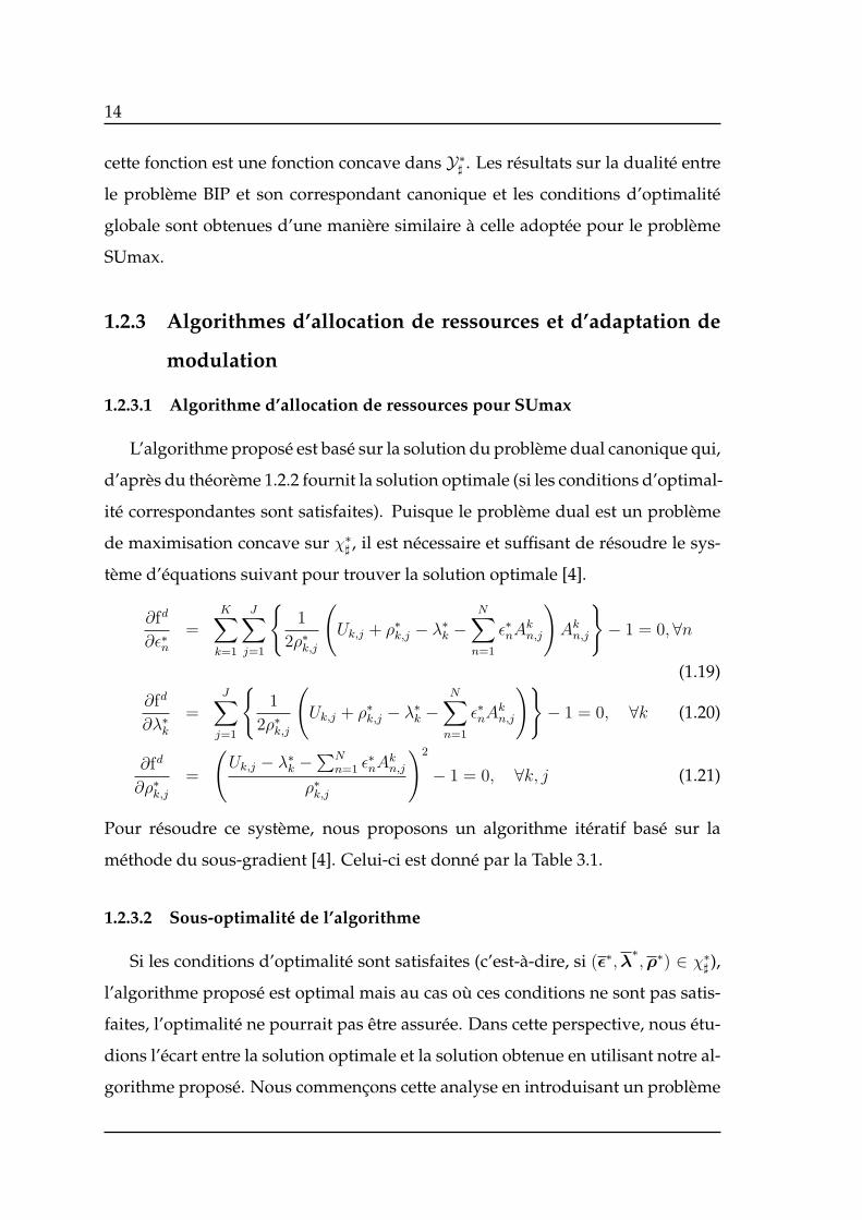
1.2.3.1 Algorithme d’allocation de ressources pour SUmax
L’algorithme proposé est basé sur la solution du problème dual canonique qui,
d’après du théorème 1.2.2 fournit la solution optimale (si les conditions d’optimal-
ité correspondantes sont satisfaites). Puisque le problème dual est un problème
de maximisation concave sur χ∗♯ , il est nécessaire et suffisant de résoudre le sys-
tème d’équations suivant pour trouver la solution optimale [4].
∂fd
∂ϵ∗n=
K∑k=1
J∑j=1
1
2ρ∗k,j
(Uk,j + ρ∗k,j − λ∗k −
N∑n=1
ϵ∗nAkn,j
)Ak
n,j
− 1 = 0,∀n
(1.19)
∂fd
∂λ∗k=
J∑j=1
1
2ρ∗k,j
(Uk,j + ρ∗k,j − λ∗k −
N∑n=1
ϵ∗nAkn,j
)− 1 = 0, ∀k (1.20)
∂fd
∂ρ∗k,j=
(Uk,j − λ∗k −
∑Nn=1 ϵ
∗nA
kn,j
ρ∗k,j
)2
− 1 = 0, ∀k, j (1.21)
Pour résoudre ce système, nous proposons un algorithme itératif basé sur la
méthode du sous-gradient [4]. Celui-ci est donné par la Table 3.1.
1.2.3.2 Sous-optimalité de l’algorithme
Si les conditions d’optimalité sont satisfaites (c’est-à-dire, si (ϵ∗,λ∗,ρ∗) ∈ χ∗
♯ ),
l’algorithme proposé est optimal mais au cas où ces conditions ne sont pas satis-
faites, l’optimalité ne pourrait pas être assurée. Dans cette perspective, nous étu-
dions l’écart entre la solution optimale et la solution obtenue en utilisant notre al-
gorithme proposé. Nous commençons cette analyse en introduisant un problème

15
dual canonique modifié dont la solution optimale n’est pas nécessaire et qui ne
remplacera pas notre problème réel, mais qui est uniquement utilisé pour étudier
l’écart d’optimalité de notre algorithme. Dans notre analyse, d’abord, nous trou-
vons la solution du problème modifié. Ensuite, nous montrons dans le Théorème
1.2.1 que la solution de ce problème modifié est équivalente à la solution opti-
male du problème primal avec des valeurs d’utilités Uk,j légèrement différentes.
Enfin, en Corollaire 1.2.1, nous montrons que sous certaines conditions, la solu-
tion du problème dual canonique obtenue en utilisant notre algorithme fournit
une solution au problème primal qui est très proche de l’optimum.
Théorèm 1.2.1. Pour Uk,j = Uk,j − 2θk,jρ∗k,j avec θk,j ∈ −1, 0, 1, ∀k, j; il existe un
problème primal f(i) avec les utilités Uk,j , et qui peut être résolu de façon optimale en
utilisant l’algorithme donné par la Table 3.1.
Preuve. Annexe A.3.
Corollaire 1.2.1. Si ρ∗k,j << Uk,j,∀k, j; alors, la solution obtenue du problème dual
canonique en utilisant l’algorithme proposé (Table 3.1) fournit une solution au problème
primal qui est très proche de la solution optimale.
Preuve. Annexe A.4.
1.2.3.3 Résultats de l’algorithme pour N →∞
Nous également étudions la performance de l’algorithme proposé lorsque le
nombre de sous-canaux est très élevé. Dans ce cas, on peut montrer que ρ∗k,j <<
Uk,j,∀k, j. Par conséquent, la solution obtenue en utilisant l’algorithme proposé
est très proche de la solution optimale.
1.2.3.4 Stratégie de modulation adaptive pour SUmax
Soit Γ∗m le SNR minimum nécessaire pour garantir un BLER (Block Error Rate)
cible au récepteur si la mième technique de modulation est utilisée. La meilleur

16
modulation pour l’utilisateur k est déterminé en fonction de γeffk , de la manière
suivante:
m∗(k) = arg minm∈M
(γeffk − Γ∗
m)|Γ∗m≤γeff
k
(1.22)
où m est l’indice de modulation et M = QPSK, 4QAM,16QAM.
1.2.3.5 Algorithme de modulation adaptative conjointe à l’allocation de resso-
urces pour JAMSCmin
Un système d’équations non-linéaires et un algorithme itératif pour ce prob-
lème peuvent être obtenus d’une manière similaire à celle adoptée pour le prob-
lème SUMax.
1.2.4 Résultats numériques
Les figures, 3.1 et 3.2 (voir le chapitre 3) représentent la performance de nos
algorithmes proposés pour SUmax et JAMSCmin, respectivement. Á partir des
résultat, on constate que ces algorithmes donnent de meilleurs résultats que les
algorithmes existants et les solutions obtenues sont très proches des solutions
optimales correspondantes.
1.3 Contrôle de puissance conjointe à l’adaptation du
débit pour le streaming vidéo dans les réseaux
sans fil
Nous considérons une approche d’optimisation inter-couches pour le contrôle
de puissance conjointement à l’adaptation du débit pour le streaming vidéo dans
les réseaux sans fil. Dans le scénario que nous supposons d’étudier, il faut assurer
une transmission vidéo à haute qualité pour chaque nœud du réseau sachant que
son canal et l’interférence varient dans le domaine temporel. Comme le stream-
ing vidéo a des exigences fortes de délai, les paquets arrivés dans la file d’attente
17
d’un nœud doivent être transmis pendant une durée fixée au delà de laquelle
ils seront rejetés. Par ailleurs, un critère d’équité entre les nœuds devrait être
établi pour l’utilisation des ressources limitées du réseau. Afin d’exploiter la di-
versité temporelle des canaux, le débit vidéo de chaque nœud doit être adapté
conformément à ses conditions de canal. En outre, la puissance d’émission de
chaque nœud doit être contrôlée pour utiliser l’énergie de manière efficace. Le
contrôle de puissance est efficace pas seulement du point de vue de consomma-
tion d’énergie, mais ainsi du point de vue de gestion d’interférences. En effect,
la réduction de la puissance d’émission d’un nœud engendre la réduction des in-
terférences causées à d’autres nœuds. Cependant, le contrôle de puissance doit
être réalisé instantanément alors que l’adaptation du débit de données en stream-
ing vidéo doit être effectuée par moyennage sur une durée assez longue. Cette
différence dans l’échelle temporelle rend le contrôle de puissance conjointement
à l’adaptation du débit très difficile. Dans cette section, nous proposons une ap-
proche d’optimisation qui permet d’effectuer de contrôle de la puissance instan-
tané à la couche PHY/MAC conjointement avec l’adaptation du débit moyen à la
couche APPLICATION. L’approche évoquée exploite la diversité temporelle des
canaux en satisfaisant les contraintes fortes sur le délai associées aux applications
vidéo, et en respectant un critère d’équité précis pour l’allocation des ressources
parmi les nœuds. L’allocation des ressources au niveau de la couche PHY/MAC
est effectuée dans le but d’atteindre un SINR (Signal to Interference and Noise
Ratio) cible et à condition de minimiser le délai entre l’arrivée et le départ des
paquets. Cette allocation est réalisée en variant le débit attribué à la couche AP-
PLICATION de manière à assurer la qualité de la vidéo demandée par les nœuds
selon l’état de leurs canaux et le critère d’équité. Dans ce contexte, nous mod-
élisons les variations de puissance et celles du débit vidéo des nœuds par des
équations dynamiques linéaires stochastiques. Ensuite, nous les formulons sous
la forme d’un problème de commande optimale. Une approche de la théorie
d’automatique intitulée " Risk-Sensitive Control " est adoptée pour résoudre ce
problème d’allocation de puissance et d’adaptation du débit vidéo. Nous four-
18
nissons, ainsi, la solution optimale de ce problème, et nous évaluons la perfor-
mance de l’approche proposée à travers plusieurs simulations.
1.3.1 Approche stochastique
Soit γk,j(t) = pk,j(t)gk,j(t) le SINR instantané du noeud k qui reçoit des don-
nées multimédia envoyées par noeud j, où gk,j(t) signifie le CINR (Channel to In-
terference plus Noise Ratio) et Pk,j(t) est la puissance émise par le noeud j. Pour
formuler notre problème sous forme d’un problème de commande stochastique,
nous avons prouvé que la densité de probabilité de gk,j(t) peut être approximée
par une densité log-normale sous certaines contraintes. Nous utilisons ensuite ce
résultat intermédiaire pour décrire la variation de puissance et celle de débit des
nœuds par des équations linéaires stochastiques.
Notons que le contrôle de puissance est équivalant au contrôle du SINR (γk,j(t))
puisque γk,n(t) = pk,n(t)gk,n(t) sachant que gk,n(t) dépend du canal et ne peut
pas être contrôlé. Par conséquent, nous effectuerons notre analyse en termes de
valeurs du SINR. Soit x = 10 log x la valeur de la variable x en décibels (dB). En
utilisant la formule de débit suivante rk,j(t) = 12log2[1 + γk,j(t)], pour γk,j(t) >> 1
(c’est le cas en streaming vidéo), le débit de données est proportionnel à γk,j(t).
Soit γ∗k,j(t) le SINR cible (c’est à dire, le SINR correspondant au débit vidéo cible).
Nous avons alors la proposition suivante pour le contrôle de puissance.
Proposition 1.3.1. Le contrôle de puissance peut être écrit sous la forme suivante:
γk,j(t+ 1) = 1− βk,jγk,j(t) + βk,jγ∗k,j(t) + ng(t) (1.23)
où βk,j est un pas donné et ng(t) est un bruit d’espérance nulle.
Dans l’algorithme de contrôle de puissance ci-dessus, nous n’avons pas en-
core introduit de contrainte par rapport à la puissance maximale d’émission.
Comme les canaux et les interférences varient au cours du temps, la valeur corre-
spondante de la puissance maximale faisable d’émission varie aussi pour chaque
nœud. Par conséquent, nous introduisons une nouvelle variable pfk,j(t) appelée

19
la puissance faisable qui dénote la puissance maximale d’un nœud j qui pourrait
émise à l’instant t. Soit γfk,j(t) la valeur du SINR lorsque pfk,j(t) est émise.Nous
avons alors le résultant suivant concernat la variation de puissance faisable.
Proposition 1.3.2. La puissance faisable varie selon le modèle dynamique linéaire stochas-
tique suivant:
γfk,j(t+ 1) = 1− ϵk,jγfk,j(t) + ϵk,j(t)γmax + ng(t) (1.24)
où ϵk,j est un pas fixé .
Afin d’assurer que pk,j(t) ≤ pfk,j(t) à tout instant t, le taux d’arrivée des paquets
r∗k,j(t) doit être adapté de sorte que γ∗k,j(t) ≤ γfk,j(t).
Soit fk,j l’équité instantanée et fTk,j l’équité cible. En intégrant la notion de la
puissance faisable avec l’adaptation de taux d’arrivée, nous obtenons la proposi-
tion suivante :
Proposition 1.3.3. Le débit vidéo/taux d’arrivée peut être adapté en utilisant l’équation
stochastique linéaire suivante:
γ∗k,j(t+ 1) = γ∗k,j(t) + ξk,j(t)γfk,j(t)− γ
∗k,j(t)
+ξk,j(t)
fTk,j − fk,j(t)
γ∗k,j(t) + δtnt(t) (1.25)
où le pas ξk,j(t) est défini comme suit :
ξk,j(t) =
1 if t = mWT
0 elsewhere(1.26)
WT est la durée pendant laquelle le débit vidéo (taux de l’arrivé) doit être fixe, m est un
nombre entier positif, et δt et nt(t) sont des petits nombres positifs.
Selon la définition ci-dessus de ξk,j(t), pour m ∈ N (tout entier naturel), le
taux d’arrivée varie à t = mWT alors que sa variation sera négligeable entre les
instants t1 = mt et t2 = mt+WT − 1.
L’approche du contrôle du taux d’arrivée se base sur l’idée que pour le stream-
ing vidéo, le débit de données est mis à jour après une période de temps suff-
isamment large. Par ailleurs, selon cette approche le taux d’arrivée est adapté en
fonction du canal associé au nœud.

20
L’objectif principal est maintenant de développer une méthode permettant
d’adapter γfk,j(t) et γ∗k,j(t) dans une manière conjointe et dynamique, et en ajustant
la puissance tel que γk,j(t) tend vers γ∗k,j(t).
1.3.2 Problème de commande " Risk-Sensitive " et sa solution
optimale
Dans cette partie, nous exprimons dans un premier temps les trois équations
dynamiques (1.23), (1.24) et (1.25) sous forme d’un problème de commande "
Risk-Sensitive " afin de fournir une solution dynamique au problème du contrôle
de puissance conjointement à l’adaptation de taux d’arrivée au niveau de chaque
nœud.
1.3.2.1 Équation d’état
Afin de formuler notre problème sous forme d’un problème classique d’automatique
stochastique, nous introduisons un vecteur d’état en trois dimensions défini par :
zk,j(t) = [γ∗k,j(t) γk,j(t) γfk,j(t)]T (1.27)
En combinant (1.23), (1.24) et (1.25), nous obtenons le modèle d’état ci-dessous :
zk,j(t+ 1) = Ak,j(t)zk,j(t) + fk,j(t) + nk,j(t) (1.28)
Où fk,j(t) = [0 0 ϵk,jγmax]T , nk,j(t) =
[δtnt(t) ng(t) ng(t)
]Tet
Ak,j(t) =
1− ξk,j(t) + ξk,j(t)
fTk,j − fk,j(t)
0 ξk,j(t)
βk,j 1− βk,j 0
0 0 1− ϵk,j
Par ailleurs, nous introduisons un vecteur du contrôle uk,j(t) = [u∗k,j(t) upk,j(t) 0]T
dans (1.28) afin d’assurer que γk,j(t) tend vers γ∗k,j(t) défini comme suit :
zk,j(t+ 1) = Ak,j(t)zk,j(t) + fk,j(t) + Buk,j(t) + nk,j(t) (1.29)

21
où B est la matrice identité en trois dimensions. Le modèle d’état ci-dessus peut
être écrit sous la forme classique suivante:
xk,j(t+ 1) = Ak,j(t)xk,j(t) +Buk,j(t) + nk,j(t) (1.30)
où xk,j(t) =
zk,j(t)
1
, Ak,j(t) =
Ak,j(t) fk,j(t)
0 1
, B =
B 0
0 0
, uk,j(t) = uk,j(t)
0
, et nk,j(t) =
nk,j(t)
0
.
1.3.2.2 Formulation de la fonction du coût
La fonction du coût quadratique est définir par:
Jk,j =τ∑
t=1
xTk,j(t)Qxk,j(t) + uT
k,j(t)Ruk,j(t)
(1.31)
où R =
R 0
0 1
est une matrice définie positive, Q =
Q 0
0 0
, et où R est la
matrice identité en quatre dimensions et Q est la matrice donnéé par:
Q =
1 −1 0 0
−1 1 0 0
0 0 0 0
0 0 0 0
Le choix ci-dessus de Q engendre le résultat suivant :
xTk,j(t)Qxk,j(t) =
γ∗k,j(t)− γk,j(t)
2 (1.32)
La minimisation de l’entité exprimée en (1.32) est l’objectif principal du problème
d’automatique évoqué ci avant. Puisque nous traitons la transmission vidéo,
nous construisons la fonction du coût exponentielle suivante :
Jk,j = E exp(Jk,j) (1.33)
L’introduction de la fonction de coût exponentiel a pour but d’amplifier l’effet de
l’écart de taux (γ∗k,j(t)− γk,j(t)
2). Dans cette situation, le régulateur visera à
22
garder Jk,j très faible, ce qui minimise l’écart de taux et réduit alors la gigue dans
la transmission vidéo. Nous améliorons la fonction de coût exponentielle par
la définition d’une fonction de coût plus générale appelée " Risk-Sensitive " [5].
Cette fonction a un paramètre appelé " Risk-Sensitive ", dont la variation change
la fonction du coût. En particulier, une valeur élevée de ce paramètre rends la
fonction du coût infinie indépendamment des stratégies de régulation. Dans
notre problème, ce paramètre peut être choisi selon le critère souhaité, ce qui peut
attribuer une pondération plus ou moins importante à l’écart de débit dans la
fonction du coût. Le problème ainsi formulé est appelé problème d’automatique "
Risk-Sensitive ". Nous reformulon dans un deuxième temps notre problème sous
forme d’un problème d’automatique " Risk-Sensitive " où la fonction du coût est
définie par:
Vk,j = EeµJk,j
(1.34)
où µ > 0 est le paramètre " Risk-Sensitive ". Par application d’une transformation
logarithmique, nous obtenons :
Wk,j = infuk,j(0)...,uk,j(T )
1
µlog Vk,j (1.35)
Notre problème devient alors de trouver la séquence de commandes uk,j(0), ...,
uk,j(T )minimisant la fonction du coût ci-dessus.
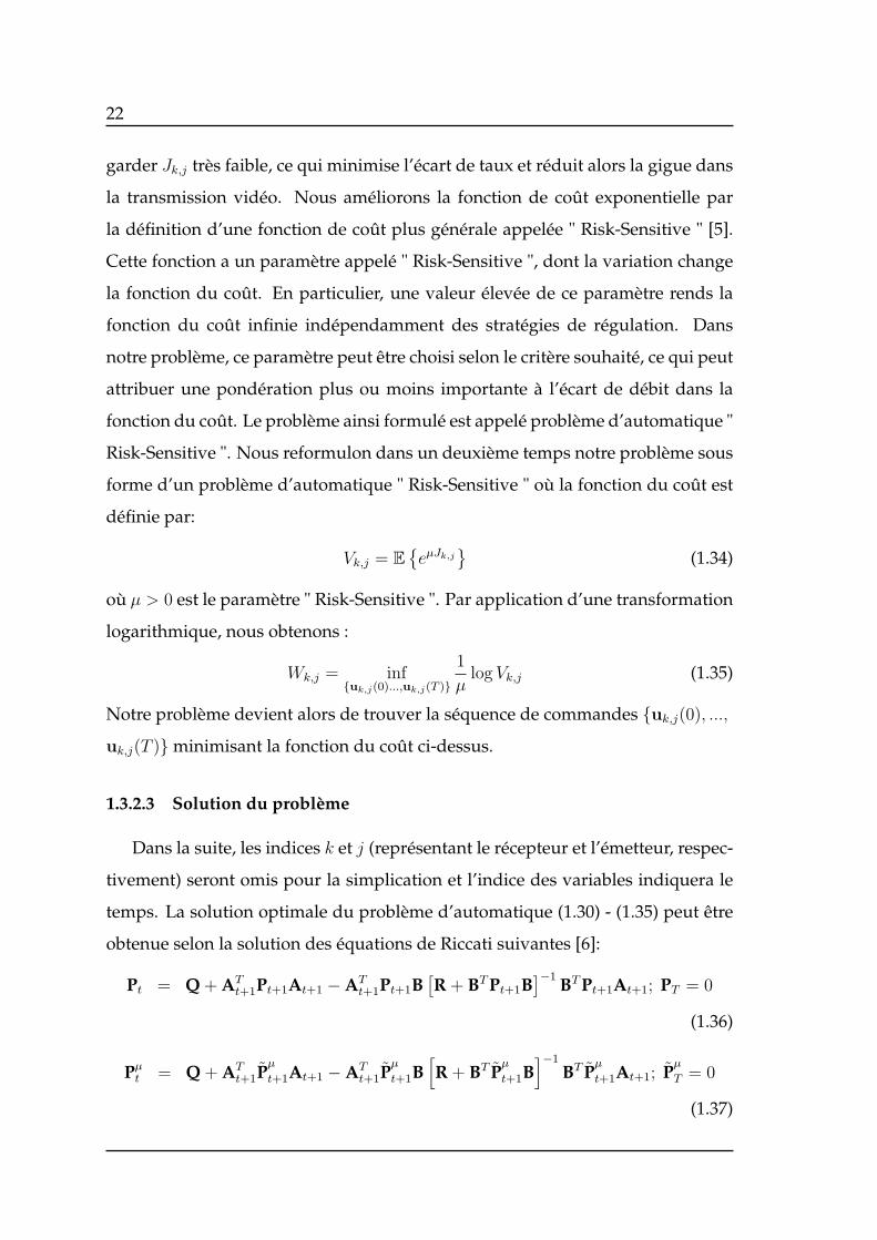
1.3.2.3 Solution du problème
Dans la suite, les indices k et j (représentant le récepteur et l’émetteur, respec-
tivement) seront omis pour la simplication et l’indice des variables indiquera le
temps. La solution optimale du problème d’automatique (1.30) - (1.35) peut être
obtenue selon la solution des équations de Riccati suivantes [6]:
Pt = Q + ATt+1Pt+1At+1 −AT
t+1Pt+1B[R + BTPt+1B
]−1 BTPt+1At+1; PT = 0
(1.36)
Pµt = Q + AT
t+1Pµ
t+1At+1 −ATt+1P
µ
t+1B[R + BT P
µ
t+1B]−1
BT Pµ
t+1At+1; Pµ
T = 0
(1.37)
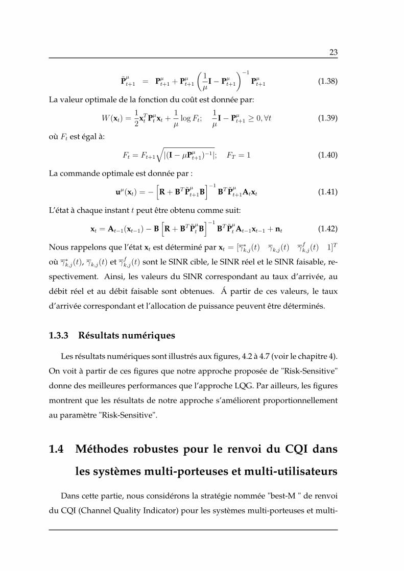
23
Pµ
t+1 = Pµt+1 + Pµ
t+1
(1
µI− Pµ
t+1
)−1
Pµt+1 (1.38)
La valeur optimale de la fonction du coût est donnée par:
W (xt) =1
2xTt Pµ
t xt +1
µlogFt;
1
µI− Pµ
t+1 ≥ 0,∀t (1.39)
où Ft est égal à:
Ft = Ft+1
√|(I− µPµ
t+1)−1|; FT = 1 (1.40)
La commande optimale est donnée par :
uµ(xt) = −[R + BT P
µ
t+1B]−1
BT Pµ
t+1Atxt (1.41)
L’état à chaque instant t peut être obtenu comme suit:
xt = At−1(xt−1)− B[R + BT P
µ
t B]−1
BT Pµ
t At−1xt−1 + nt (1.42)
Nous rappelons que l’état xt est déterminé par xt = [γ∗k,j(t) γk,j(t) γfk,j(t) 1]T
où γ∗k,j(t), γk,j(t) et γfk,j(t) sont le SINR cible, le SINR réel et le SINR faisable, re-
spectivement. Ainsi, les valeurs du SINR correspondant au taux d’arrivée, au
débit réel et au débit faisable sont obtenues. Á partir de ces valeurs, le taux
d’arrivée correspondant et l’allocation de puissance peuvent être déterminés.
1.3.3 Résultats numériques
Les résultats numériques sont illustrés aux figures, 4.2 à 4.7 (voir le chapitre 4).
On voit à partir de ces figures que notre approche proposée de "Risk-Sensitive"
donne des meilleures performances que l’approche LQG. Par ailleurs, les figures
montrent que les résultats de notre approche s’améliorent proportionnellement
au paramètre "Risk-Sensitive".
1.4 Méthodes robustes pour le renvoi du CQI dans
les systèmes multi-porteuses et multi-utilisateurs
Dans cette partie, nous considérons la stratégie nommée "best-M " de renvoi
du CQI (Channel Quality Indicator) pour les systèmes multi-porteuses et multi-
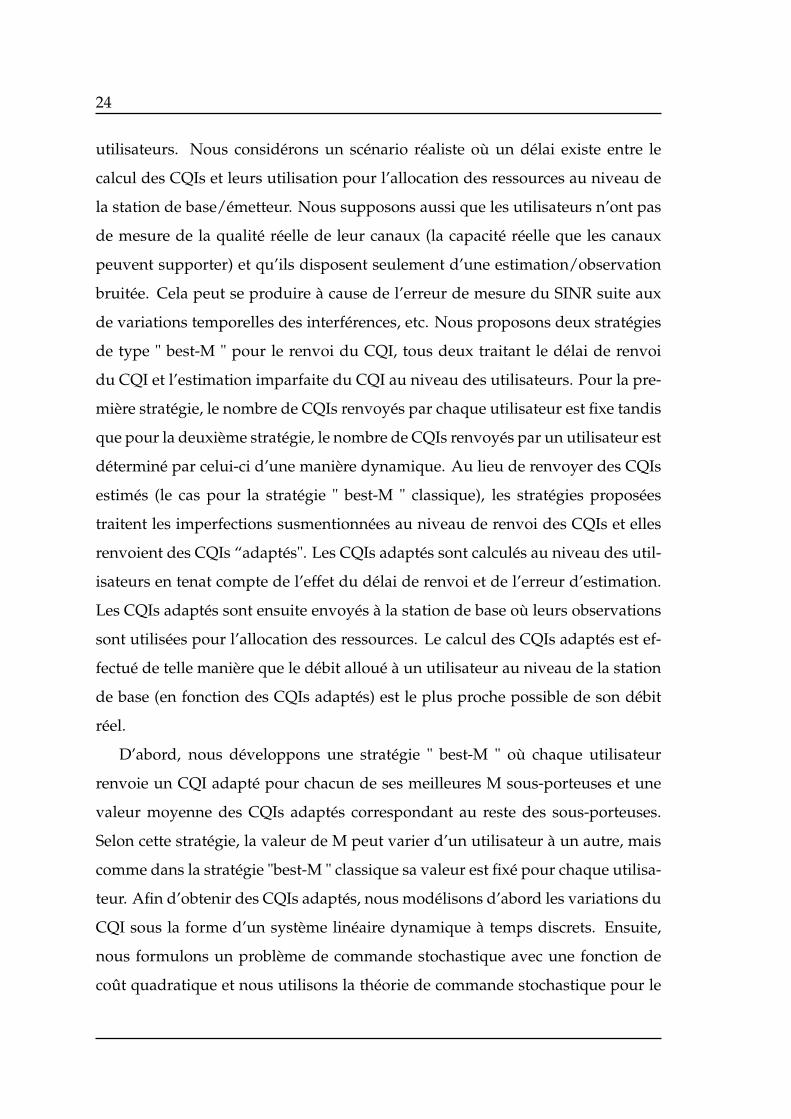
24
utilisateurs. Nous considérons un scénario réaliste où un délai existe entre le
calcul des CQIs et leurs utilisation pour l’allocation des ressources au niveau de
la station de base/émetteur. Nous supposons aussi que les utilisateurs n’ont pas
de mesure de la qualité réelle de leur canaux (la capacité réelle que les canaux
peuvent supporter) et qu’ils disposent seulement d’une estimation/observation
bruitée. Cela peut se produire à cause de l’erreur de mesure du SINR suite aux
de variations temporelles des interférences, etc. Nous proposons deux stratégies
de type " best-M " pour le renvoi du CQI, tous deux traitant le délai de renvoi
du CQI et l’estimation imparfaite du CQI au niveau des utilisateurs. Pour la pre-
mière stratégie, le nombre de CQIs renvoyés par chaque utilisateur est fixe tandis
que pour la deuxième stratégie, le nombre de CQIs renvoyés par un utilisateur est
déterminé par celui-ci d’une manière dynamique. Au lieu de renvoyer des CQIs
estimés (le cas pour la stratégie " best-M " classique), les stratégies proposées
traitent les imperfections susmentionnées au niveau de renvoi des CQIs et elles
renvoient des CQIs “adaptés". Les CQIs adaptés sont calculés au niveau des util-
isateurs en tenat compte de l’effet du délai de renvoi et de l’erreur d’estimation.
Les CQIs adaptés sont ensuite envoyés à la station de base où leurs observations
sont utilisées pour l’allocation des ressources. Le calcul des CQIs adaptés est ef-
fectué de telle manière que le débit alloué à un utilisateur au niveau de la station
de base (en fonction des CQIs adaptés) est le plus proche possible de son débit
réel.
D’abord, nous développons une stratégie " best-M " où chaque utilisateur
renvoie un CQI adapté pour chacun de ses meilleures M sous-porteuses et une
valeur moyenne des CQIs adaptés correspondant au reste des sous-porteuses.
Selon cette stratégie, la valeur de M peut varier d’un utilisateur à un autre, mais
comme dans la stratégie "best-M " classique sa valeur est fixé pour chaque utilisa-
teur. Afin d’obtenir des CQIs adaptés, nous modélisons d’abord les variations du
CQI sous la forme d’un système linéaire dynamique à temps discrets. Ensuite,
nous formulons un problème de commande stochastique avec une fonction de
coût quadratique et nous utilisons la théorie de commande stochastique pour le
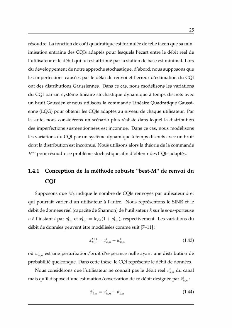
25
résoudre. La fonction de coût quadratique est formulée de telle façon que sa min-
imisation entraîne des CQIs adaptés pour lesquels l’écart entre le débit réel de
l’utilisateur et le débit qui lui est attribué par la station de base est minimal. Lors
du développement de notre approche stochastique, d’abord, nous supposons que
les imperfections causées par le délai de renvoi et l’erreur d’estimation du CQI
ont des distributions Gaussiennes. Dans ce cas, nous modélisons les variations
du CQI par un système linéaire stochastique dynamique à temps discrets avec
un bruit Gaussien et nous utilisons la commande Linéaire Quadratique Gaussi-
enne (LQG) pour obtenir les CQIs adaptés au niveau de chaque utilisateur. Par
la suite, nous considérons un scénario plus réaliste dans lequel la distribution
des imperfections susmentionnées est inconnue. Dans ce cas, nous modélisons
les variations du CQI par un système dynamique à temps discrets avec un bruit
dont la distribution est inconnue. Nous utilisons alors la théorie de la commande
H∞ pour résoudre ce problème stochastique afin d’obtenir des CQIs adaptés.
1.4.1 Conception de la méthode robuste "best-M" de renvoi du
CQI
Supposons que Mk indique le nombre de CQIs renvoyés par utilisateur k et
qui pourrait varier d’un utilisateur à l’autre. Nous représentons le SINR et le
débit de données réel (capacité de Shannon) de l’utilisateur k sur le sous-porteuse
n à l’instant t par gtk,n et xtk,n = log2(1 + gtk,n), respectivement. Les variations du
débit de données peuvent être modélisées comme suit [7–11] :
xt+1k,n = xtk,n + wt
k,n (1.43)
où wtk,n est une perturbation/bruit d’espérance nulle ayant une distribution de
probabilité quelconque. Dans cette thèse, le CQI représente le débit de données.
Nous considérons que l’utilisateur ne connaît pas le débit réel xtk,n du canal
mais qu’il dispose d’une estimation/observation de ce débit designée par xtk,n :
xtk,n = xtk,n + ϑtk,n (1.44)
26
où ϑtk,n est l’erreur d’estimation d’espérance nulle. Par ailleurs, en raison du délai
de renvoi, le débit attribué à l’instant t au niveau de la station de base dépendra
de l’estimation du débit au niveau de l’utilisateur à l’instant t− τ où τ représente
le délai de renvoi. En d’autres termes, le CQI disponible à l’instant t au niveau
de la station de base laquelle suppose que le CQI est calculé en fonction de xtk,n
est en réalité le CQI correspondant à xt−τk,n . Du point de vue de la station de base,
l’effet du délai de renvoi au niveau de l’utilisateur peut être traduit par l’équation
suivante:
xtk,n = xt−τk,n + νtk,n (1.45)
où νtk,n est une erreur d’espérance nulle indiquant l’effet du délai de renvoi, selon
le modèle de variation du débit de données (1.43) dans lequel le débit entre deux
instants varie par un bruit d’espérance nulle. En combinant (1.44) et (1.45) nous
obtenons:
xt−τk,n = xtk,n + vtk,n (1.46)
où vtk,n = ϑtk,n−νtk,n répresente l’effet du délai de renvoi et de l’erreur d’estimation.
En dénotant xt−τk,n par ytk,n, les variations du débit de données peuvent être écrites
sous forme de représentation d’état (pour un système linéaire dynamique à temps
discrets:
xt+1k,n = xtk,n + wt
k,n (1.47)
ytk,n = xtk,n + vtk,n (1.48)
Á cause du délai de renvoi, l’observation du CQI adapté calculé à l’instant t−τ est
utilisée pour l’allocation des ressources au niveau de la station de base à l’instant
t. Compte tenu de son utilisation au temps t pour l’allocation des ressources au
niveau de la station de base et afin d’éviter toute confusion dans la formulation
du problème, nous utilisons l’indice t au lieu de t− τ et le CQI adapté calculé au
temps t− τ sera noté par xtk,n. Similairement à xtk,n, les variations temporelles de
xtk,n peuvent être modélisées comme suit :
xt+1k,n = xtk,n + wt
k,n (1.49)

27
où ωtk,n est un bruit d’espérance nulle. Comme l’observation de xtk,n est utilisée
pour l’allocation des ressources, notre objectif est de minimiser xtk,n − xtk,n (c’est
à dire, l’écart entre le débit alloué et le débit réel). Pour ce faire, nous utilisons la
théorie de commande linéaire avec un coût quadratique.
L’observation du système dynamique (1.47-1.48) est imparfaite tandis que xtk,n
dans (1.49) est parfaitement connu. Ainsi, afin de formuler les deux systèmes dy-
namiques (1.47-1.48) et (1.49) sous forme d’un système standard en temps discret,
nous supposons avoir une observation imparfaite pour xtk,n donnée par :
ytk,n = xtk,n + ϵ0vtk,n (1.50)
où 0 < ϵ0 <<< 1 (c’est à dire, ϵ0 → 0). Avec cette valeur de ϵ0, l’observation ytk,n
est presque égale à xtk,n. Par ailleurs, comme xtk,n est la variable à contrôler pour
tendre vers le débit réel xtk,n, nous introduisons une variable de commande utk,n
dans (1.49) et nous modélisons les variations du CQI adapté par le modèle d’état
dynamique suivant:
xt+1k,n = xtk,n + utk,n + wt
k,n (1.51)
ytk,n = xtk,n + ϵ0vtk,n (1.52)
Pour exprimer notre problème, nous combinons (1.47) avec (1.51) et (1.48) avec
(1.52). Pour ce faire, nous introduisons les vecteurs d’état, d’observation, de com-
mande et de bruit définis comme suit :
xtk,n = [xtk,n xtk,n]
T
ytk,n = [ytk,n ytk,n]
T
utk,n = [0 utk,n]
T
xtk,n = [wt
k,n wtk,n]
T
vtk,n = [vtk,n ϵ0v
tk,n]
T
La représentation finale d’état (combinée pour le débit réel et le CQI adapté) peut
alors être écrite selon les deux équations suivantes:
xt+1k,n = xt
k,n + utk,n + wt
k,n (1.53)
ytk,n = xt
k,n + vtk,n (1.54)

28
L’équation (1.53) représente l’état et l’équation (1.54) l’observation d’un système
dynamique à temps discret perturbé par un bruit de distribution de probabilité
quelconque. Pour chaque utilisateur, N équations d’état sont obtenues. Nous
cherchons alors une séquence de commandes utk,n minimisant la fonction de
coût quadratique pour chaque utilisateur définit comme:
Lk =
T∑t=1
N∑n=1
(∥xt
k,n∥2Q + ∥utk,n∥2R
)(1.55)
où la notation ∥b∥2S désigne la norme pondérée du vecteur b donnée par bHSb, R
est la matrice identité en deux dimensions et Q est la matrice
Q =
1 −1
− 1
Le choix de R et Q ci-dessus implique le résultat suivant :
∥xtk,n∥2Q + ∥ut
k,n∥2R = ∥xtk,n − xtk,n∥2 + ∥utk,n∥2 (1.56)
Minimiser la fonction de coût quadratique est alors équivalent à minimiser la
quantité ∥xtk,n − xtk,n∥, ce qui est notre objectif principal. Les équations (1.53),
(1.54) et (1.55) représentent un problème d’automatique stochastique linéaire à
temps discrets [12].
Nous proposons une solution au problème évoqué ci-dessus à travers deux
approches différentes. Premièrement, nous supposons que le débit de données
xtk,n varie selon une distribution gaussienne et ainsi, le bruit wtk,n est considéré
comme gaussien [7]- [11]. Dans ce cas, la solution est obtenue en utilisant la
commande Linéaire Quadratique Gaussienne (LQG) [13, 14]. Pour la deuxième
approche, nous abordons le problème d’une manière plus réaliste où la distribu-
tion de probabilité du bruit est imprévisible. Dans ce cas, nous proposons une
solution basée sur la méthode d’optimisation H∞ [12].
1.4.1.1 Sélection des meilleurs Mk CQIs et leur renvoi
En utilisant les méthodes ci-dessus (commande LQG et méthode H∞) , chaque
utilisateur calcule des CQIs adaptés pour l’ensemble de ses N sous-porteuses.

29
Chaque utilisateur k, choisit ensuite ses meilleurs Mk sous-porteuses et renvoie
un CQI (xtk,n) correspondant à chacune parmi elles. Un seul CQI pour les sous-
porteuses restantes N −Mk est renvoyé par l’utilisateur, ceci est obtenu en cal-
culant une valeur moyenne des CQIs des N −Mk sous-porteuses restantes (i.e.,
xtk,m = 1N−Mk
∑Nn=Mk+1 x
tk,n).
1.4.2 Méthode robuste dynamique " best-M " de renvoi du CQI
Dans cette partie, nous concevons une méthode robuste de type "best-M" dans
laquelle le nombre des CQIs renvoyés Mk n’est pas fixé pour chaque utilisa-
teur mais il est déterminé de manière efficace et dynamique. Chaque utilisateur
calcule les CQIs adaptés pour toutes ses sous-porteuses en utilisant l’approche
d’automatique stochastique proposée dans la sous-section précédente (commande
LQG/H∞). Ensuite, selon les conditions de ses sous-porteuses, chaque utilisateur
détermine de manière dynamique le nombre efficace de CQIs qu’il doit renvoyer
à la station de base.
1.4.2.1 Approche pour la détermination de Mk
Nous supposons que chaque utilisateur trie ses sous-porteuses par ordre décrois-
sant selon leurs valeurs de CQIs. Nous définissons alors un vecteur indicateur de
taille KN , it = [it1, ..., itK ]
T avec itk = [itk,1, ..., itk,N ]
T . L’élément itk,n indique si le CQI
correspondant à la sous-porteuse n de l’utilisateur k à l’instant t est renvoyé à la
station de base ou non. L’expression de itk,n est alors donnée par:
itk,n =
1 Si le CQI pour la sous-porteuse n de l’utilisateur k est renvoyé
0 Sinon.(1.57)
Par ailleurs, nous introduisons un autre vecteur indicateur jt = [jt1, ..., jtK ]
T avec
jtk = [jtk,1, ..., jtk,N ]
T . L’élément jtk,m indique le nombre total m de sous-porteuses
de l’utilisateur k dont les CQIs individuels ne sont pas renvoyés à la station de

30
base à l’instant t:
jtk,m =
1 Si pour utilisateur k, le nombre de CQIs individuels
non-renvoyés est égal à m
0 Sinon.
(1.58)
Puisque le nombre total de CQIs non-renvoyés de l’utilisateur k est égal àN−Mk
(lorsque Mk =∑n
n=1 itk,n) son ensemble d’indicateurs faisables est défini par la
forme suivante:
χk = itk, jtk ∈ 0, 1N | jtk,m = 1,∀m = N−Mk; jtk,m = 0,∀N−Mk+1 ≤ m < N−Mk
(1.59)
Á partir de ces paramètres, nous définissons l’écart instantané de débit pour
l’utilisateur k comme suit:
Lt
k =N∑
n=1
itk,n∥xtk,n∥2Q +
N∑m=1
jtk,mm∥xtk,m∥2Q (1.60)
où ∥xtk,n∥2Q = ∥xtk,n − xk,n∥2, ∥xt
k,m∥2Q = ∥xtk,m − xk,m∥2; et où xtk,n, xtk,n et xtk,m sont
définis de la même manière qu’au sous-chapitre précédent et xtk,m = 1N−Mk
∑Nn=Mk+1 xk,n.
Nous rappelons que ces derniers sont obtenus grâce à l’approche d’automatique
stochastique proposée précédemment.
Selon cette méthode, les utilisateurs déterminent leurs Mks de manière dy-
namique. Par conséquent, pour ne pas diminuer le débit utile en liaison montante
(utilisateurs vers station de base), nous introduisons la contrainte suivante:
Pr
(K∑k=1
N∑n=1
itk,n ≤MK
)≥ (1− ε) (1.61)
Cette contrainte signifie que la probabilité que le nombre total de CQIs renvoyés
à la station de base soit inférieure ou égal à MK est supérieure ou égale à (1− ε),
avec 0 << (1 − ε) < 1. Nous pouvons ainsi mettre en équation notre problème
d’optimisation comme suit:
min E
K∑k=1
(N∑
n=1
itk,n∥xt
k,n∥2Q∥xtk,n∥
+N∑
m=1
jtk,mm∥xt
k,m∥2Q∥xtm,n∥
)(1.62)
s.t. Pr
(K∑k=1
N∑n=1
itk,n ≤MK
)≥ (1− ε) (1.63)
itk,n, jtk,m ∈ χk, ∀k, n,m (1.64)

31
Il s’agit donc d’un problème binaire stochastique dont la résolution se fait d’une
manière distribuée, c’est à dire séparément par chaque utilisateur.
1.4.2.2 Solution distribuée et algorithme "Efficient Interactive Trial and Error
Learning"
Nous formulons d’abord notre problème initial par un problème relaxé. Soit
S l’ensemble des itk,n’s respectant la contrainte commune∑K
k=1
∑Nn=1 i
tk,n ≤ MK.
Cet ensemble est donnée par:
S =
it ∈ 0, 1KN |
K∑k=1
N∑n=1
itk,n ≤MK
(1.65)
Pour l’utilisateur k soit 1itk∈S l’indicateur égal à 1 si itk = [itk,1, ..., itk,N ]
T ∈ S et 0
sinon. Définissons alors le coût moyen de l’utilisateur k à l’instant t par :
Ltk = E
N∑
n=1
itk,n∥xt
k,n∥2Q∥xtk,n∥
+N∑
m=1
jtk,mm∥xt
k,m∥2Q∥xtm,n∥
(1.66)
Le problème relaxé peut alors être décrit de la maniére suivant: si it ∈ S (i.e. la
contrainte commune∑K
k=1
∑Nn=1 i
tk,n ≤ MK est satisfaite), donc chaque utilisa-
teur minimise l’écart de son débit LtK . Si la contrainte commune n’est pas satis-
faite, alors nous introduisons un coût de pénalité Ψk. La valeur de ce dernier sera
choisie élevée si l’écart du débit de l’utilisateur est faible et s’il est souhaitable de
changer sa configuration au prochain instant, et vice versa. Cette nouvelle fonc-
tion de coût que chaque utilisateur doit minimiser peut être écrite sous la forme
:
Ltk =
(Lt
k
)1itk∈S + (Ψk)1itk∈S
(1.67)
Le coût ci-dessus que chaque utilisateur k minimise séparément dépend de la
contrainte commune. Comme la contrainte commune ne dépend pas seulement
de la valeur de Mk choisie par l’utilisateur k mais aussi des valeurs des Mk des
autres (K−1) utilisateurs, tous les utilisateurs sont interdépendants dans la min-
imisation de leurs coûts individuels. Ainsi, le problème se présente comme un
problème distribué d’automatique dans lequel les utilisateurs sont couplés par la
32
contrainte commune mais n’interagissent pas directement entre eux pour la prise
de décision sur leurs Mk. Dans ce situation, il est donc impossible de satisfaire en
permanence la contrainte commune.
Pour résoudre ce problème de manière efficace, nous proposons un algorithme
de type "Efficient Interactive Trial and Error Learning" utilisant des résultats de la
théorie des jeux. L’algorithme est donné par la Table 5.1. Cet algorithme choisit
la valeur de Mk de manière efficace pour chaque utilisateur k en satisfaisant la
contrainte commune avec une trés grande probabilité. On obtient le théorème
suivant qui concerne l’optimalité de l’algorithme proposé.
Théorème 1.4.1. Si chaque utilisateur emploie l’algorithme proposé, un équilibre pur de
Nash sera visité avec une probabilité supérieure ou égale à 1−δ (0 < δ < 1) et le problème
défini par (1.62-1.64) sera résolu de façon optimale.
Preuve. Annex B.1.
1.4.3 Résultats numériques
Les résultats de simulation sont présentés aux figures, 5.1 à 5.6 (voir le chapitre
5). Afin d’évaluer sa performance, nous comparons notre approche à la méthode
LQG et à l’algorithme existant utilisé dans le standard LTE. Les résultats mon-
trent que la performance de notre approche (avec une valeur fixe de Mk) est dans
tous les cas nettement meilleur (35%-40%) que l’algorithme utilisé dans le stan-
dard LTE. Quand la probabilité de la distribution du bruit est inconnue, la per-
formance de l’approche LQG peut être moins bonne que l’algorithme utilisé dans
le LTE. Par ailleurs, les simulations montrent que les résultats de notre approche
s’améliorent proportionnellement au nombre de CQIs renvoyés. On remarque
aussi que la performance de la stratégie "best-M" dynamique est meilleure que
notre stratégie avec une valuer fixe de Mk. En plus, les résultats montrent que
cette stratégie dynamique ne augmente pas la signalisation total au niveau de la
liaison montante du système.
33
1.5 Conclusion et perspectives
Dans cette thèse nous avons traité trois problématiques différentes d’allocation
de ressources dans les systèmes de communication sans fil:
– Une approche d’allocation de ressources et de modulation adaptative, basée
sur la théorie de la dualité canonique récemment développée, est proposée
pour les systèmes SC-FDMA.
– Une nouvelle approche de contrôle de puissance à la couche PHY/MAC
conjointe à l’adaptation du débit au niveau de la couche APPLICATION
pour le streaming vidéo dans les réseaux sans fil est établie. Pour ce faire,
la théorie de commande " Risk-Sensitive " a été appliquée.
– Á partir de certains outils de la théorie de commande stochastique et de
la théorie des jeux, deux nouvelle stratégies " best-M " de renvoi du CQI
(Channel quality Indicator) pour les systèmes multiporteuses et multiutilis-
ateurs tenant compte du délai de renvoi et de l’erreur d’estimation du canal
sont proposées. Dans le cadre de première stratégie, un nombre M fixe
des meilleures CQIs pour chaque utilisateur est renvoyé. Alors que dans
la deuxième stratégie appelé " best-M " dynamique, le nombre des CQIs
qui doivent être renvoyés par chaque utilisateur est déterminé de manière
distribuée et dynamique par l’utilisateur en question.
Les travaux menés dans cette thèse mettent en évidence plusieurs problématiques
intéressantes qui devraient être explorées à l’avenir. Dans ce qui suit, nous en
évoquons un certain nombre et nous mettrons en évidence quelques perspectives
pour le futur proche.
L’allocation de ressources et la modulation adaptative pour le système SC-
FDMA étudiées dans cette thèse supposent que la station de base connaît par-
faitement les conditions des canaux des utilisateurs servis. Pour étudier l’effet
du délai de renvoi et de l’erreur d’estimation du canal, nous avons développé
des stratégies robustes de renvoi du CQI traitant ces imperfections. L’effet de ces
imperfections pourrait traiter au niveau de la station de base pour les Systèmes
34
SC-FDMA, ce qui n’a pas été considérée dans cette thèse.
Par ailleurs, l’approche d’allocation de ressources proposée pour le système
SC-FDMA est une approche centralisée selon laquelle la répartition de puissance
et de sous-porteuses parmi les utilisateurs ainsi que le choix de modulation sont
décidées au niveau de la station de base et ces décisions sont ensuite commu-
niquées aux utilisateurs. Le paradigme exploré dans cette thèse peut être étendu à
une approche distribuée où les décisions d’allocation de ressources seraient prises
aux niveaux des utilisateurs.
L’approche d’allocation de ressources pour le streaming vidéo proposée dans
cette thèse est fondée sur l’hypothèse que tous les nœuds utilisent la même bande
large pour la transmission. Cette étude peut être étendue aux systèmes sans fil
multi-porteuses et multi-utilisateurs, à l’image des systèmes SC-FDMA et OFDMA.
D’autre part, le critère d’équité pour l’allocation de ressources concernant le
streaming vidéo est basé sur le débit de données vidéo des nœuds. D’autres
critères d’équité comme la valeur moyenne du PSNR (Peak Signal to Noise Ra-
tio) ou le taux de distorsion vidéo des nœuds peuvent aussi être incorporés dans
l’approche proposée. En outre, les SNRs des nœuds sont représentés d’une manière
approximative comme des variables aléatoires de distribution log-normale. Un
scénario plus réaliste où la distribution du SNR est inconnue ou plus réaliste
pourrait également être envisagé.
Les approches proposées dans cette thèse tendent à optimiser les ressources au
niveau de l’émetteur en négligeant l’état des paquets arrivés au niveau du récep-
teur. Puisque les canaux/liens sans fil ne sont pas fiables, certains protocoles de
retransmission des paquets erronés, (e.g. ARQ (Automatic Repeat reQuest), etc.)
doivent être également intégrés dans l’allocation des ressources, afin d’assurer la
réussite de la transmission des paquets.
Les stratégies de renvoi des CQIs proposées dans cette thèse ne considèrent
pas le phénomène compression des CQIs. Toutefois, dans l’objectif de réduire
d’avantage le débit de renvoi des CQIs, des versions compressées des meilleurs
M CQIs pour chaque utilisateur peuvent être renvoyées.
35
Chapter 2
Introduction
2.1 General Introduction
The recent advances in wireless communication technologies and their capa-
bilities of providing high data rates have revolutionized the way the modern
society functions. In addition to voice transmission, the modern day wireless
communication permits diverse services/applications such as data transmission,
electronic email, high resolution video streaming, etc. These services have differ-
ent Quality-of-Service (QoS) requirements that are characterized in terms of data
rates, delays, error rates, etc. However, being capable of supporting these di-
verse services, the modern wireless communication systems face the challenging
problem of ensuring the diverse QoS requirements of the services. The reason
is twofold: the wireless communication resources e.g., bandwidth, power, etc,
are scarce; and the capacity of the wireless channel is unreliable due to the time-
varying nature of the channel, multi-path propagation, and mutual interference
among multiple simultaneous transmissions.
In order to provide the required QoS as well as efficiently utilize the limited
available communication resources, adaptive channel aware resource allocation
strategies are needed. Though the time-varying nature of the wireless channels
poses some limitations, it provides the opportunity to achieve high data rate by
exploiting the time diversity at the resource allocation level. In addition, the
36
multi-nodes/users diversity and the frequency diversity of the wireless fading
channels can be exploited by resource allocation schemes. However, the design
of any adaptive resource allocation scheme is not possible without having the
knowledge of the wireless channel. Thus, there is also a need of developing the
channel quality reporting schemes that help the resource allocation unit in effi-
ciently allocating the resources.
The principle objective of adaptive resource allocation as obvious from its
name is to efficiently allocate the resources among multiple nodes/users in accor-
dance to their channel conditions. However, the multiple nodes sharing the same
network may demand for different services with different QoS requirements. In
the same network, some of the users may be using non-real time services or de-
lay tolerant services e.g., file transfer/email checking while others may demand
for applications with stringent delay requirements like video streaming, etc. Re-
source allocation schemes for real time applications or services with stringent de-
lay constraint should also guarantee the delay requirements of the applications
in addition to efficiently allocating the resources. Thus, the design of any adap-
tive resource allocation schemes for wireless network should also consider the
service/application demanded by the nodes/users.
Another factor which should be considered in adaptive resource allocation is
the information on the wireless channel conditions of the nodes/users. In gen-
eral, each end node/user in the wireless networks estimates its channel, com-
putes an indicator for its channel quality, and reports it to the transmitter/base
station. The resource allocation unit at the transmitter/base station uses this
channel quality indicator (CQI) for resource allocation. However, the CQI ar-
rived at the transmitter may be outdated due to feedback delay and my not be
a perfect indicator/measure of the current channel anymore. In addition, it may
happen that due to time-varying interference, etc., there is an error in the CQI
measurement/estimation at the end node or the feedback channel used for re-
porting the CQI is noisy, and the CQI reported to the transmitter/base station
is an imperfect measure of the actual channel. Thus, it is essential to consider
37
these issues of imperfect knowledge of the channel quality in adaptive resource
allocation. The traditional approach used is to deal with the possible channel
imperfections at the transmitter/base station. However, the more accurate is the
CQI available at the transmitter, the more efficient is the resource allocation per-
formed. Thus, another interesting approach could be dealing with these issues at
the CQI reporting level and providing the transmitter with such robust CQI that
has already accommodated the aforementioned imperfections. The transmitter
will then directly use this robust CQI for resource allocation.
Adaptive resource allocation in multi-user systems has been extensively stud-
ied. A rich literature on resource allocation in multi-user systems like Orthogonal
Frequency Division Multiple Access (OFDMA), and Code Division Multiple Ac-
cess (CDMA) exists. However, resource allocation in Single Carrier Frequency Di-
vision Multiple Access (SC-FDMA) systems has not been well studied and needs
a considerable work.
In this thesis, first we consider resource allocation and adaptive modulation
in SC-FDMA systems without considering any delay constraint on the transmis-
sion of users’ packets and assuming the availability of perfect channel state in-
formation at the transmitter/base station. Then, while aiming to study the re-
source allocation for SC-FDMA with delay constrained application/services, we
develop a general resource allocation framework for video streaming in a wire-
less networks. The main goal was to first develop a framework for wireless video
streaming in a general multi-node network and then extend this framework to the
SC-FDMA systems. However, due to the time limitation and the difficult nature
of resource management in SC-FDMA systems, the extension of this framework
to SC-FDMA systems has been left as a future work. In this thesis, the general
framework is presented. Finally, in order to deal with the imperfections in the
channel information available at the transmitter, we adapt a new approach. Un-
like the traditional approach of dealing with the channel imperfections at the
transmitter, we deal with them at the CQI reporting level. Keeping in view the
multi-carrier nature of SC-FDMA, we develop a CQI reporting scheme in multi-
38
carrier and multi-user systems that takes into account the feedback delay and
the error in the channel quality measurement at the CQI reporting level. In this
scheme, the CQI are computed and reported in such a manner that they accom-
modate the impact of the aforementioned imperfections and when arrived at the
transmitter can directly be used for resource allocation. The proposed scheme is
more general and can be adapted for any multi-carrier and multi-user system.
The rest of this chapter is organized as follows. The remainder of this section
introduces the SC-FDMA, the video streaming in multi-node wireless networks,
and the CQI reporting in multi-carrier and multi-user systems. Section 2.2 pro-
vides a detailed overview of the problems considered in this thesis. The sate of
the art is provided in Section 2.3 and the thesis organization and contributions
are provided in Section 2.5.
2.1.1 Single Carrier Frequency Division Multiple Access (SC-
FDMA)
SC-FDMA is a multiple access scheme for the uplink communication in high
data rate cellular systems such as the Third Generation Partnership Project Long
Term Evolution (3GPP-LTE) standard [1]. Like Orthogonal Frequency Division
Multiple Access (OFDMA) scheme, it is based on orthogonal frequency division
multiplexing (OFDM) technique [15, 16]. In OFDM, the total frequency band is
divided into a number of narrow orthogonal sub-bands called sub-carriers or
sub-channels. The information data in OFDM systems is divided into parallel
streams where these streams are transmitted simultaneously by transmitting a
single stream on each sub-channel, and thus, can achieve very high bit rates. In
addition, it inherits the immunity to inter-symbol-interference (ISI) in frequency
selective fading channel and offers good flexibility and performance for a rea-
sonable complexity. Due to these advantages OFDM is employed in wireless
LANs based on the IEEE 802.11a and IEEE 802.11g standards. These remark-
able advantages of OFDM have also motivated the wireless communication so-

39
ciety to use it as a multiple access scheme called OFDMA where the users of a
same cell are multiplexed in frequency, each user’s data being transmitted on a
subset of the sub-channels of an OFDM symbol. OFDMA has been adopted for
both uplink and downlink air interfaces of WiMAX fixed and mobile standards,
namely IEEE802.16d and IEEE802.16e respectively [17, 18] and more recently for
the downlink air interface of the 3GPP-LTE standard [1].
Although OFDMA has numerous advantages, it suffers from high envelope
fluctuation in the time domain thus leading to high peak-to-average-power ratio
(PAPR). This high PAPR nature of the signals results in non-linear distortion. To
deal with this problem and achieve the linearity, the power amplifiers have to
operate at very high power, and thus, suffer from poor power efficiency. Thus,
given the power limitations at the mobile terminal, OFDMA is not a good candi-
date for the uplink transmission. In addition, the non-linear distortion of signals
also effects the orthogonality of sub-channels, and thereby causing inter- channel
interference.
In order to overcome the aforementioned disadvantages of OFDMA, SC-FDMA
is currently attracting a lot of attention as an alternative to OFDMA in the uplink.
Its low PAPR feature has the potential to benefit the mobile terminals in term of
transmit power efficiency. In fact, SC-FDMA is a single carrier multiple access
technique which utilizes single carrier modulation and frequency domain equal-
ization. Its overall structure and performance are similar to that of OFDMA sys-
tem. Unlike the parallel transmission of the orthogonal sub-channels in OFDMA,
the sub-channels are transmitted sequentially in SC-FDMA. This sequential trans-
mission of sub-channels considerably reduces the envelope fluctuation in trans-
mitted waveform and results in low PAPR [2]. However, very efficient in terms of
PAPR, SC-FDMA signals suffer substantial inter-symbol interference at the base
station due to severe multi-path propagation. This necessitates employing adap-
tive frequency domain equalization at the base station to cancel out this interfer-
ence. Though it costs complex signal processing at the base station, frequency
domain equalization is far more better than using high power linear amplifiers at
40
the mobile terminal.
There are two types of SC-FDMA: localized-FDMA (L-FDMA) in which the
sub-channels assigned to a user are adjacent to each other, and interleaved-FDMA
(I-FDMA) in which users are assigned with sub-channels distributed over the
entire frequency band [2]. Though L-FDMA and I-FDMA both are better than
OFDMA with respect to PAPR, L-FDMA with channel-dependent scheduling can
achieve multi-user diversity, and has the potential for higher capacity in terms of
number of users than I-FDMA [2]. In 3GPP-LTE standard [1], the current working
assumption is to use OFDMA for downlink and localized SC-FDMA for uplink.
In this thesis, we focus on adaptive resource allocation in L-FDMA specific to
3GPP-LTE uplink.
2.1.2 Video Streaming in Wireless Networks
Video streaming is the transmission of video content/multimedia data from
a streaming server to an end node where the end node is capable of playing the
transmitted video content before being completely downloaded. The capabilities
of modern wireless communication technologies to provide the nodes/users with
high data rates (e.g., in 1xEV-DO and HSDPA) have motivated video streaming
over multi-node wireless networks and its application is increasing very rapidly
(e.g., see [19–21]). However, video streaming over multi-node wireless networks
faces the challenge of providing the same video service to multiple nodes/recievers
with different channel characteristics. These multiple nodes demand the same
video while the bit rate they can support and the packet loss they experience
may be different due to their different channel conditions. In addition, the data
rate requirement for transmitting video contents is very high, the end nodes de-
mand for better quality videos, and the wireless communication resources shared
among the nodes are limited. It is thus essential that the data rate of the video
stream is adapted to nodes’ channel conditions as well as the network resources
are efficiently utilized and shared among the nodes.
In wireless video streaming, in order that the video transmission rate is adapted
41
to the individual channel condition of each node, one of the following five prin-
ciple rate adaption methods can be used. In the first method called encoder rate
control, the video encoder at the application layer adapts the frame rate or quan-
tization parameters to achieve a given target rate that depends on the packet loss
estimation and the round trip time (e.g., [22, 23]). The second method consist
in selecting one among several non-scalable bitstreams with different bit rates
(and off course with different quality) associated to the same video [24–26]. This
method is referred to as bitstream switching where the choice of bitstream for
each node is made according to its demanded/promised quality and its bit rate
support capability. The third rate adaptation method uses a single high qual-
ity bitstream which during streaming is converted into another bitstream with a
transcoder to match the node’s requirements [27–29]. The fourth method is called
packet pruning where a single encoded video stream is available and the rate
adaptation is performed by intelligently dropping the pre-encoded video pack-
ets [30,31]. In the fifth method called the scalable video streaming, the video is en-
coded once in a single scalable bitstream that can be adapted to the node’s chan-
nel condition [32]. More specifically, this method use scalable coding technique
wherein a video is encoded into a single bitstream with a base layer and several
enhancement layers. The base layer is non-scalable and is necessary for decoding
the video stream, whereas the enhancement layers that improves its quality are
scalable and can be truncated at any point to meet the quality-of-service (QoS)
requirement and bit rate supporting constraint of each node. This method has
small storage requirements, and provide more simplicity and flexibility in terms
of bitstream truncation/switching [33]. One among the above mentioned meth-
ods which is more suitable according to some given preferences, and limitations,
can be chosen for video streaming in multi-node wireless networks.
In multi-node wireless video streaming, in addition to video rate adaptation,
resource optimization across different protocol layers is very essential so that
the limited available bandwidth and the power is efficiently utilized. Adap-
tive/channel aware resource allocation can overwhelmingly improve the net-
42
work performance. Since the multiple nodes demand for better video quality
while sharing the same communication resources, the resource allocation for multi-
node video streaming should also consider the competition among them for com-
munication resources.
2.1.3 Channel Quality Indicator (CQI) Reporting in Multi-carrier
and Multi-user Systems
Multi-carrier/multi-channel transmission techniques in multi-user wireless
communication system significantly improve the system performance by exploit-
ing the frequency diversity and the multi-user diversity of the system [34–36].
This can be achieved by performing channel-aware modulation and coding scheme
adaptation, and resource allocation (powers, sub-channels and slots) among users
based on the so-called channel quality indicators (CQIs) reported to the transmit-
ter/base station. A CQI is nothing but a parameter that represent the wireless
channel condition e.g., a quantized signal-to-noise ratio (SNR) measurement, etc.
In fact, each user should estimate/measure its channels conditions, and feed the
CQIs back to the transmitter/base station, so that the transmitter can determine
the appropriate modulation and coding schemes, and can perform efficient re-
source allocation. However, reporting CQIs to the transmitter/base station needs
a feedback link as well as transmission resources. In multi-carrier systems, the
total bandwidth is divided into a number of sub-carrier/sub-channels with inde-
pendent physical layer transmission on each sub-carrier/sub-channel. Thus, re-
porting the CQI on each sub-carrier/sub-channel may lead to prohibitively high
feedback overhead that may not be feasible for portable devices. On the other
hand in order to enable the transmitter/base station to adapt the appropriate
modulation and coding schemes, and to efficiently allocate the resources, maxi-
mum information on the sub-channels should be reported. The above two objec-
tives are thus conflicting and there is a risk in achieving one at the expense of the
other. Therefore, a trade-off between the system performance and the feedback

43
overhead should be achieved while designing a CQIs reporting scheme.
There are two major classes of techniques used for feedback overhead re-
duction. The first one that exploits the correlation of the CQI between adjacent
sub-channels and time instants, consists in feeding back a compressed version of
the CQIs of all the sub-channels by each user. This may either be CQI quanti-
zation in which the discrete quantized values of the channel state are reported
(e.g., [37–39]), or a discrete cosine transform (DCT) based feedback in which the
dominant terms of the DCT of the per-subchannel signal to interference plus
noise ratio (SINR) are reported to the transmitter (e.g., [40]). In the second class,
the CQIs of those users or/and sub-channels are reported which have high SNR
compared to the other users/sub-channels or a given threshold. The second class
has two groups: the threshold based CQI reporting, and the best-M based CQI
reporting. In threshold based feedback schemes, a user only reports its CQI if its
SNR is greater than a pre-defined threshold. In the best-M based CQI reporting, a
user reports either the full individual CQIs values or an average CQI value of its
best M sub-channels, and an average CQI value of the remaining sub-channels.
Increasing the feedback interval can also help to reduce the feedback overhead
when the mobility is low [41].
Since a user in multi-carrier and multi-user systems is most likely to be al-
located with the sub-carriers/sub-channels having good channel conditions, the
best M CQIs reporting is quite a good choice. It is shown that the best-M scheme
is an appropriate scheme for multi-user OFDM and multi-carrier CDMA sys-
tems [42–45]. The best M CQIs scheme has been adapted as the reporting scheme
for Third Generation Partnership Project (3GPP) for the Long Term Evolution
(LTE) systems [43].
44
2.2 Problems considered in this thesis
2.2.1 Resource Allocation and Adaptive Modulation in SC-FDMA
Systems
Concerning adaptive resource allocation in multi-user multi-channel systems,
most of the previous work has focused on power and sub-channel allocation in
OFDMA systems, and a quite rich literature exist in this area of research (e.g.,
[36, 46–49]). On the other hand, adaptive resource allocation problem in SC-
FDMA systems has rarely been considered by researcher. This lack of consid-
eration of SC-FDMA resource allocation problem is due to its prohibitively diffi-
cult nature. Like the mutual exclusivity restriction on sub-channel allocation in
OFDMA, a sub-channel in SC-FDMA can be allocated to one user at most. In ad-
dition, the multiple sub-channels allocated to a user in localized SC-FDMA must
be consecutive as well. These constraints render the resource optimization prob-
lem a prohibitively difficult combinatorial problem. Moreover, in OFDMA, the
signal-to-noise-ratio (SNR) on each sub-channel is independent from the other
sub-channels and the allocation of each sub-channel among the users and the al-
location of power to each sub-channel is independent from other sub-channels.
On the other hand in SC-FDMA, the use of frequency domain equalization in
SC-FDMA over all the sub-channels makes the SNR expression much more com-
plicated where the power allocation to any sub-channels of a user is dependent
on all the other allocated sub-channels of that user. This further increases the
difficulty of the resource allocation problem in SC-FDMA. Though the resource
allocation problem in OFDMA systems is also a very difficult combinatorial prob-
lem due to the exclusive allocation of sub-channels among the users, some op-
timal/nearly optimal algorithms have already been discovered. The common
approach used for resource allocation in OFDMA is to formulate the mutual ex-
clusivity restriction on sub-channels allocation as binary-integer constraint, solve
the problem to get an approximated solution in continuous domain, and then
discretize the continuous values into the closest binary values. But in SC-FDMA

45
resource allocation, this approach cannot be employed. The reason is that if the
problem is solved by relaxing the 0-1 constraint, then, during discretization of the
continuous domain solution, the adjacency constraint on sub-channels allocation
cannot be assured.
Though very difficult combinatorial problem, some efforts are still made to-
wards the solution of resource allocation problem in SC-FDMA. However, almost
all the exiting solutions are greedy sub-optimal, and most of them are not com-
plete in all respects. Some of the proposed resource allocation frameworks do
not respect the adjacency constraint on the sub-channel allocation, whereas the
others do not consider any constraint on the transmit power. Being a very dif-
ficult combinatorial problem, the greedy and sub-optimal nature of the existing
proposed solutions is still reasonable but sacrificing the adjacency constraint on
sub-channel allocation which is the important physical layer requirement of the
localized SC-FDMA is not a realistic approach at all. Moreover, all the previ-
ous work is based on rate/capacity maximization and no work to the best of our
knowledge has considered power minimization joint with adaptive modulation
in uplink SC-FDMA systems. Since the mobile terminals have limited energy,
energy-economization is needed and fast power control should be considered
while allocating the resources to the users in the uplink.
In this thesis, we consider resource allocation and adaptive modulation in lo-
calized SC-FDMA systems. We consider two optimization problems: sum-utility
maximization (SUmax), and joint adaptive modulation and sum-cost minimiza-
tion (JAMSCmin). Both these problems are combinatorial in nature whose opti-
mal solutions are exponentially complex in general. The performance metric con-
sidered in the SUmax problem is the total utility of the system. Utility is basically
an economics concept that reflects the user satisfaction in the system. We assume
that each user in the system has an associated utility function, and the objective is
to maximize the sum-utility in the system while respecting all the constraints of
localized SC-FDMA systems specific to the LTE uplink. The user utility function
specific to this thesis is defined as an arbitrary function that is monotonically in-
46
creasing in user’s SNR. The performance of the system can be further enhanced
by choosing an efficient modulation scheme for each user. Therefore, based on
the resource allocation, we also consider adaptive modulation scheme, wherein
an appropriate modulation is chosen for each user depending upon its effective
SNR. The cost associated to each user in the JAMSCmin problem is a function that
is monotonically increasing in the transmit power of that user. The objective of
the JAMSCmin is to propose a low-complexity framework that jointly allocates
the transmit powers, sub-channels and the modulation schemes to the users in
order to minimize the total transmit power while ensuring the individual target
data rates of the users as well as capturing the basic constraints of the localized
SC-FDMA systems. The joint adaptive modulation in the JAMSCmin problem is
important due to the fact that in order to ensure the target data rate of the users,
the powers and sub-channels allocation should take into account the modulation
schemes used by the users.
2.2.2 Joint Power Control and Rate Adaptation for Video Stream-
ing in Wireless Networks
Video streaming over wireless networks is a challenging task. The main rea-
sons are the time varying nature of the wireless channel, the better video quality
(high data rate) demand of the multiple nodes, the hard transmission delay con-
straints of the streaming applications (i.e., the packets in the buffer of the trans-
mitting node should be delivered to the receiving node within a small period
of time), and the limited available communication resources (e.g., bandwidth,
transmission power, etc.). Due to the different characteristics of the time-varying
channels of the multiple nodes, the bit rate they can achieve and the packet loss
they experience is different which in turn does not allow broadcasting a single
video stream with constant bit rate to all receiving nodes. The reason is that if a
video stream with high data rate is chosen, then, the nodes that have bad channel
condition and that can not support this data rates will be unable to decode the
47
video content successfully. On the other hand if the video stream is broadcasted
in accordance to the receiver nodes with bad channel qualities, all the other re-
ceiver nodes are essentially reduced to the performance of the worst nodes. Thus,
in order to support video streaming over multi-node wireless networks, a video
bitstream with appropriate data rate must be adapted for each node in accor-
dance to the bit rate supporting capability of its wireless channel. Moreover, the
transmission of multiple nodes in wireless networks are interdependent. This in-
terdependency occurs due to the competition among the multiple nodes for the
limited available network resources, and the interference caused to the nodes due
to the simultaneous transmissions in the network. Each node in the network tries
to utilize the network resources to the maximum in order to have a good quality
video. The increased use of resources by a node not only deprives the other nodes
from network resources but the increase in its transmit power also results in an in-
creased level of interference to other nodes which in turn reduces their achieved
data rates, and increases the transmission delay of these nodes. Thus, in order
to satisfy the stringent delay constraints of the streaming applications, intelli-
gent resource allocation and scheduling policies must be designed that performs
a fair sharing of the bandwidth among the multiple nodes, and efficiently allocate
the power to them in different time slots. The fair distribution of the bandwidth
can overwhelmingly improve the network performance by making sure that each
node is provided with a promised QoS streaming service/application. Adjusting
the transmit power according to the node’s allocated/demanded bit rate and its
channel quality is not only efficient in term of its power consumption but will also
help in reducing the interference caused to the neighbor nodes. However, unfor-
tunately, the interdependent nature of the multi-node transmissions renders the
design of such resource allocation and scheduling policies extremely difficult. In
addition, the video bitstream/rate adaptation is performed at the APPLICATION
layer whereas the resource allocation/scheduling is performed at the PHY/MAC
and thus a cross-layer design is needed which is a challenging task.
The temporal variations of the wireless fading channels can be exploited by
48
optimally controlling the power in different time slots, and adapting the video
bitstream/rate in different video sessions. However, in order to develop an op-
timal power control and rate adaptation scheme, channel gain values and packet
arrival rates for current and future time slots are required. Unfortunately, the
information about future channel and arrival processes is not available which
makes this problem very challenging. Generally, the existing work on resource
allocation for video streaming in wireless networks does not consider the compe-
tition among multiple nodes for communication resources. In addition, the un-
derlying approach is to simplify the resource allocation problem by assuming no
background interference at all or assume a constant value for interference which
is an unrealistic approach. This is a crucial issue which should be accounted for
in resource allocation.
Furthermore, the power control at the PHY/MAC layer should be performed
instantaneously so that an instantaneous target SINR corresponding to the given
video rate is achieved. On the other hand due to the interdependent nature of
the video frames in video streaming, the video rate at the APPLICATION layer
should be adapted in an average manner after a long enough time. Thus, it is
even difficult to formulate a framework that allows instantaneous power control
at the PHY/MAC layer, and average video rate adaptation at the APPLICATION
layer jointly.
In this thesis, we consider the above challenging problem of joint video bit-
stream/rate adaptation and dynamic power control for video streaming in a multi-
node wireless networks where the multiple nodes cause interference to each other.
The interference is assumed to be time-varying and the nodes compete for net-
work resources where each node opt to have a better quality video. We design
a cross-layer optimization framework that performs instantaneous power con-
trol at the PHY/MAC, and adapts the video rate in an average manner at the
APPLICATION layer jointly. In our optimization framework, we also introduce
a certain fairness/satisfaction criterion among the multiple nodes so that each
node is assured of getting its share of the network resources. The joint cross-layer
49
framework provides all the nodes with good quality video for minimum power
consumption such that the strict delay constraints of the streaming applications
are satisfied and the fairness/satisfaction criterion among the nodes is respected.
2.2.3 CQI Reporting in Multi-carrier and Multi-user Systems with
Imperfect Channel Knowledge
The problem of efficient CQI reporting in multi-carrier and multi-user systems
as expected has been quite well studied. However, the underlying assumption in
the previous work is to report the CQIs to the transmitter/base station without
considering the impact of error in their measurement and the feedback delay on
the CQIs values received at the transmitter/base station. In general, there always
occurs a time delay between the estimation of the CQIs and their utilization for
resource management at the transmitter/base station. It is possible that the char-
acteristics of the channel are significantly changed during this delay/feedback
interval and the corresponding CQI received at the transmitter/base station is
not relevant anymore. In addition, due to time-varying interferences etc., the
CQI estimation/measurement at the user terminal may not be perfect, and con-
sequently, the value of the corresponding CQIs will be erroneous. Performing re-
source allocation on the basis of these delayed and erroneous CQIs may severely
degrade the system performance. Though not being ignored by the wireless com-
munication society, these issues are generally dealt with at the resource allocation
level at the transmitter/base station (e.g., [50–54]). Moreover, these works assume
simple imperfection models e.g., assuming some statistical distribution for chan-
nel imperfections, and that the transmitter knows, at each time, the estimated
CQIs and the distribution of imperfections for all sub-channels. This is an unreal-
istic approach, since due to the different levels of interferences caused to different
sub-channels and due their time-varying nature, the covariances of the noise for
different sub-channels are different as well as time-varying.
Considering the impact of feedback delay and imperfect CQI estimation on
50
resource allocation at the base station makes sense if the CQIs of all the sub-
channels for each user are reported. But reporting the CQIs of all the sub-channels
for each user in a multi-user system is not appropriate due to the resulting pro-
hibitively increased overhead. On the other hand the use of the best-M CQIs
scheme reduces the overhead but it makes difficult to efficiently allocate the re-
sources and to cope with the CQI imperfections at the transmitter. In a realistic
scenario where the best-M reporting scheme is used, the transmitter cannot know
the channel statistics for all the sub-channels since only M (which is a small num-
ber e.g., 4 or 5 for 3GPP-LTE) imperfect and delayed CQIs are available at each
time. Moreover, during resource allocation at the transmitter, it may happen that
the sub-channels corresponding to the individually reported M best CQIs of a
user are not allocated to that user but other sub-channels whose individual CQIs
are not reported are allocated. In multi-carrier systems, different sub-channels
have different channel conditions and have different noise covariances due to
different levels of interferences caused to them. Therefore, it is unrealistic to treat
all the sub-channels in a similar way. Moreover, it is inefficient to let the trans-
mitter solve alone the problem of resource allocation and rate assignment, and
deal with the imperfections in CQIs. Since the users have an estimation of the
CQI for each sub-channel, they can contribute to solve the above problem if a
feedback scheme is developed which takes care of the imperfections in the CQIs
at the reporting level at the user terminals. In this way, the CQIs available at the
transmitter would have already accommodated the impact of imperfections, and
can directly be used for resource allocation.
Furthermore, in wireless standards such as 3GPP-LTE, M is assumed to be
fixed, and the same for all users. In practice if M increases the deviation between
the allocated rate and the actual achieved/experienced rate decreases. However,
this deviation depends also upon the channel conditions of each user e.g., users
near the base station will have lower deviations than users at the cell border. Thus
adapting the value of M for each user according to its channel quality can further
improve the system performance. Though looking very interesting, adapting the
51
value of M dynamically is a challenging task. In addition, there is a risk that the
total system overhead hugely increases compared to the traditional scheme with
fixed value of M.
In this thesis, we consider a more realistic scenario where a multi-carrier and
multi-user system uses the M-best CQI reporting scheme, and a feedback delay
occurs as well as the CQIs estimation at the user terminal are not perfect. In
addition to employing the common approach of assuming some statistical distri-
bution for the imperfections in CQIs we also view the problem realistically and
consider the case when the distribution of the CQI imperfections is completely
unknown. We consider a novel M-best CQI reporting scheme which should deal
with the feedback delay and CQI estimation error at the CQIs reporting level
while retaining the property of feedback overhead reduction. In other words,
the impact of these imperfections on the CQIs values, and consequently on the
possible future allocated rate at the transmitter is considered at the user termi-
nal prior to CQIs reporting. By utilizing the same framework, we also develop a
so-called dynamic M-best CQIs reporting scheme in which the value of M is not
fixed and equal for all users but is adapted for each user individually according
to its current channel quality while respecting the system’s cumulative feedback
overhead.
2.3 State of the art
2.3.1 Resource Allocation in SC-FDMA Systems
The key feature of the multi-channel and multi-user wireless systems is their
inherit frequency, time, and multi-user diversities. Resource allocation techniques
can be used to take advantage of these diversities of the system in order to op-
timize the use of the available resources. These techniques exploit the available
channel state information (CSI) at the transmitter side for accomplishing adaptive
modulation, and sharing the resources (powers, sub-channels, slots, etc.) among
52
the users.
Most of the previous work on resource allocation in multi-channel and multi-
user systems has focused on power and sub-channels allocation in downlink
OFDMA systems (e.g., [36, 46–49, 55, 56]). One of the well known approaches
for solving the OFDMA resource allocation problem is exploiting its time-sharing
property [57]. Based on this property, it is shown in [49], and [57] that for practical
number of sub-channels, the resource allocation problem in OFDMA systems can
be solved by Lagrange multipliers method with zero duality gap. However, none
of above is directly applicable to uplink SC-FDMA. This is due to the fact that in
localized SC-FDMA in addition to the restriction of allocating a sub-channel to
one user at most, the multiple sub-channels allocated to a user should be adja-
cent to each other as well. Furthermore, a frequency domain equalizer is used in
SC-FDMA over all the sub-channels allocated to the user which makes the signal
to noise ratio (SNR) expression much more complicated than in OFDMA where
the SNR on each sub-channel is independent from the other sub-channels. This
further adds to the difficulty of the resource allocation problem.
In most of the previous work on SC-FDMA, the implementation problems in
the physical layer are studied (e.g., [58–62]). In [58], a comparative analysis of the
PAPR characteristics of OFDMA, I-FDMA, and L-FDMA is peformed. In [59], the
authors have proposed maximum likelihood detection for I-FDMA system and
have investigated that in comparison with multi-carrier code-division multiple-
access it has better performance with some additional advantages. In [60], SC-
FDMA is considered as the multiple access scheme for the uplink of broadband
wireless systems that allows users to transmit simultaneously with different data
rates. In [61], the capacity behavior of single carrier modulation with frequency
domain equalization is studied. The effective signal to interference and noise
ratio (SINR) for SC-FDMA with frequency domain equalizers is derived in [62].
The resource allocation problem in uplink SC-FDMA has also been addressed
in a number of publications. In [63], a heuristic opportunistic scheduler for allo-
cating frequency bands to the users in the uplink of 3G LTE systems is proposed.
53
In [64], the authors have proposed a greedy sub-optimal schedular for uplink
SC-FDMA systems that is based on marginal capacity maximization. In [65], the
authors revise the same framework used in [64] for developing a proportional
fair scheduling scheme. However, in addition to being sub-optimal, the proposed
schedulers in both [64] and [65] do not consider the sub-channels adjacency con-
straint which is an important physical layer requirement for localized SC-FDMA.
In [66], a set of greedy sub-optimal proportional fair algorithms for localized SC-
FDMA systems is proposed in the frequency-domain setting. This work respects
the sub-channels adjacency constraint but does not consider any constraint on
the power. The authors, in [67] use the so-called Hungarian algorithm to pro-
pose dynamic sub-carrier allocation algorithm for SC-FDMA but it has very high
computational complexity and does not consider power allocation. In [68], radio
resource management for QoS provisioning in LTE with emphasis on admission
control and handover is studied. Similarly, a case study of LTE for scheduling and
link adaptation for uplink SC-FDMA Systems is performed in [69]. The works in
both [68] and [69] are simulation based works that do not provide any analytical
model for resource management. In [3], a weighted-sum rate maximization in
localized SC-FDMA systems is considered where the problem is formulated as
a pure binary-integer program. Though the proposed binary-integer program-
ming framework captures all the basic constraints of the localized SC-FDMA and
allows to perform resource allocation without resorting to exhaustive search, it
is still not the best solution as the 0-1 requirement turns the problem into combi-
natorial with exponential complexity. Thus, keeping in view the computational
complexity of the binary-integer programming, the authors have also proposed a
greedy sub-optimal algorithm that is similar in spirit to the approach in [64] with
an additional constraint on the adjacency of the allocated sub-channels. In [70],
some greedy sub-optimal resource allocation algorithms are proposed that are
inspired from that work carried out in [3]. A chunk based greedy sub-optimal
resource allocation framework is proposed in [71] where the sub-channels are
divided into chunks with equal number of sub-channels and the total number
54
of chunks equal to the number of users. Each user is then assigned with a sin-
gle chunk such that the sum-rate is maximized. In [72], a Hungarian method
based distributed SC-FDMA resource allocation for multi-cell network is pro-
posed. However, this work could not prove the convergence of the proposed
algorithm, and its proximity to the global optimal solution; and these issues are
left for future work.
All the cited work is limited to simplifying this exponentially complex prob-
lem by taking some assumptions, and proposing some greedy sub-optimal solu-
tions. None of the above works has solved this problem optimally or provided
analytical investigation for the proximity of the proposed solution to the optimal
solution. The only work where the problem is attacked from optimal solution
perspective is formulating the problem as a binary-integer program [3]. How-
ever, due to the exponential complex solution of the binary-integer program, the
authors of [3] are also reverted to proposing a greedy sub-optimal iterative algo-
rithm.
2.4 Resource Allocation for Video Streaming in Wire-
less Networks
Resource allocation for wireless video streaming has attracted a lot of atten-
tion in recent years, and a rich literature exists in this area. Most of the existing
work on rate allocation or power control has been performed from the individ-
ual user point of view. Some of the studies have considered the rate and power
allocation based on the users groups where each group is treated as a single en-
tity. However, resource allocation for video streaming in multi-node wireless
networks that takes into account the inter-dependency of the transmissions of
the multiple nodes and the competition among them for network resources is an
area that still needs considerable work.
An efficient bit allocation algorithm for scalable video transmission is pro-
posed in [73] which distributes the source bites, and the channel bits between
55
the source and channel codecs so that the resulting distortion is minimized. A
low-power multimedia communication system for indoor multimedia applica-
tions specially for image transmission is investigated in [74]. In [75], a scheme
for bit allocation between source and channel coders is proposed that minimize
the total power consumption of a single user or a group of users in the cell. A
general approach for power-optimized joint source-channel coding for scalable
video streaming over wireless channel is proposed in [76]. A joint source cod-
ing and transmit power minimization under distortion and delay constraints for
wireless video communication is considered in [77]. In [78], a channel-aware
distortion/power-minimized bit-allocation scheme for scalable video transmis-
sion over third generation (3G) wireless networks is proposed which optimally
distributes the bits among source coding, forward error correction, and ARQ.
In [79], the authors propose a framework for video streaming in which multiple
mirror sites transmit simultaneously to a single receiver in order to achieve higher
throughput. An aggregate utility maximization based rate control for multi-rate
multi-cast real-time sessions is proposed in [80] where the network is divided
into a number of multi-cast groups with each group containing a set of receivers.
The rate of transmission for each receiver in each multi-cast group is chosen in
such a way that the sum-utility of that multi-cast session is maximized.
In [81], the tradeoff between the network overhead, and the fairness prop-
erty of the rate adaptation schemes in mobile host supporting multimedia net-
works is investigated. In [82], power control and resource management for the
uplink of a single cell CDMA system is investigated. This work first consider
sum-power minimization with constraints on the users’ achieved data rates, and
then considers sum-rate maximization with constraints on the transmit power
of each user. In [83], the end-to-end QoS support for layered multi-cast video
communication over internet is studied where the rate allocation is performed in
such a manner that the expected fairness index for all the receivers in a session
is maximized. In [84], the authors propose bandwidth adaptation algorithms for
multimedia services in cellular networks that are based on the layered coding ap-
56
proach where the bandwidth of a multimedia session can take a set of discrete
values, and the coding is adapted at the base station. According to these algo-
rithms if there is no congestion in the cell, the base station transmits the full mul-
timedia stream i.e., the whole set of layered coding to the mobile terminals. On
the hand when congestion occurs, only a subset of layered coding in accordance
to the level of congestion in the cell is transmitted to the mobile terminals. A
framework for joint adaptation of source coding and packet priority assignment
for maximizing the system performance is presented in [85]. In [86], the authors
consider error control and power allocation for transmitting wireless video over
CDMA networks in which a small number of CDMA channels is dedicated to
video transmission while assuming fixed powers on all the remaining channels
in the network. In [87], a joint link capacities and traffic flows allocation frame-
work for wireless ad-hoc networks is proposed where the multimedia data is
partitioned into various classes for adaptive transmission. A QoS mapping ar-
chitecture that addresses cross-layer QoS issues for video delivery over wireless
networks is presented in [88]. In this work, the time-varying characteristics of the
wireless channel are assumed to follow a discrete-time Markov model where each
state represents the transmission rate under current channel conditions. In [89],
the authors propose some methods for maximizing the number of admitted sta-
tions/users by creating multiple sub-flows from one video and giving them dif-
ferent priorities according to their importance. In [90], a mechanism to perform
rate adaptation based on monitoring changes to the amount of traffic flow in the
network at any time, and exploiting the layered bitstream of H.264/AVC scal-
able video coding scheme is proposed. In [91], a framework for rate allocation
among multiple video streams sharing multiple heterogeneous access networks
is proposed that performs rate allocation on the basis of observed network con-
ditions, and the video distortion rate. A joint capacity, flow and rate allocation
scheme for multi-user video streaming in Ad-hoc wireless networks which aims
to minimize the trad-off between encoded video quality of all users versus over-
all network congestion is proposed in [92]. In [93], an unequal power allocation
57
scheme is proposed for the transmission of scalable video coded packets in a
WiMax system where the base layer packets are allocated more power compared
to enhancement layer packets. A joint source adaptation, and resource allocation
framework for video streaming in CDMA networks is presented in [94]. How-
ever, in this work, for the uplink transmission, the interference and the maxi-
mum received power values are assumed to be not changing frequently which
is not a realistic approach for wireless networks. The authors in [95] propose a
gradient-based scheduling and resource allocation algorithm for multi-user scal-
able video streaming over OFDM downlink system which maximizes the aver-
age peak-signal-to-noise-ratio (PSNR) of all video users under a total downlink
transmission power constraint. However, this work is carried out for a single
cell network with orthogonal users and is based on the assumption that there is
no inter-cell interference which is practically not true. In [8], a Linear Quadratic
Gaussian (LQG) control approach is employed for power and flow-rate control
for wireless networks. In [10], a so-called Kalman-filter method for power con-
trol for broadband packet-switched TDMA wireless networks is proposed. This
method determines the transmit power from the predicted interference and esti-
mated path gain between the transmitter and the receiver, in order to achieve a
target SINR.
2.4.1 CQI Reporting in Multi-Carrier and Multi-User Systems
Multi-carrier and multi-user systems like OFDMA and SC-FDMA are capable
to bring significant performance improvement in terms of throughput, latency,
and resource optimization. However, the performance improvement can be ob-
tained by deploying proper link adaptation, and developing efficient resource
management techniques that exploit the multi-user diversity in both time and
frequency domains. In order to exploit these diversities, the users need to feed-
back the channel quality indicator (CQI) values to the transmitter/base station.
However, this may lead to overwhelmingly high control signaling overhead and
there is a need of designing low overhead CQI reporting schemes. In addition,
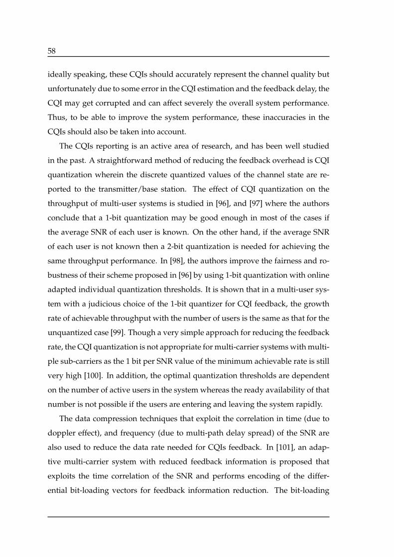
58
ideally speaking, these CQIs should accurately represent the channel quality but
unfortunately due to some error in the CQI estimation and the feedback delay, the
CQI may get corrupted and can affect severely the overall system performance.
Thus, to be able to improve the system performance, these inaccuracies in the
CQIs should also be taken into account.
The CQIs reporting is an active area of research, and has been well studied
in the past. A straightforward method of reducing the feedback overhead is CQI
quantization wherein the discrete quantized values of the channel state are re-
ported to the transmitter/base station. The effect of CQI quantization on the
throughput of multi-user systems is studied in [96], and [97] where the authors
conclude that a 1-bit quantization may be good enough in most of the cases if
the average SNR of each user is known. On the other hand, if the average SNR
of each user is not known then a 2-bit quantization is needed for achieving the
same throughput performance. In [98], the authors improve the fairness and ro-
bustness of their scheme proposed in [96] by using 1-bit quantization with online
adapted individual quantization thresholds. It is shown that in a multi-user sys-
tem with a judicious choice of the 1-bit quantizer for CQI feedback, the growth
rate of achievable throughput with the number of users is the same as that for the
unquantized case [99]. Though a very simple approach for reducing the feedback
rate, the CQI quantization is not appropriate for multi-carrier systems with multi-
ple sub-carriers as the 1 bit per SNR value of the minimum achievable rate is still
very high [100]. In addition, the optimal quantization thresholds are dependent
on the number of active users in the system whereas the ready availability of that
number is not possible if the users are entering and leaving the system rapidly.
The data compression techniques that exploit the correlation in time (due to
doppler effect), and frequency (due to multi-path delay spread) of the SNR are
also used to reduce the data rate needed for CQIs feedback. In [101], an adap-
tive multi-carrier system with reduced feedback information is proposed that
exploits the time correlation of the SNR and performs encoding of the differ-
ential bit-loading vectors for feedback information reduction. The bit-loading
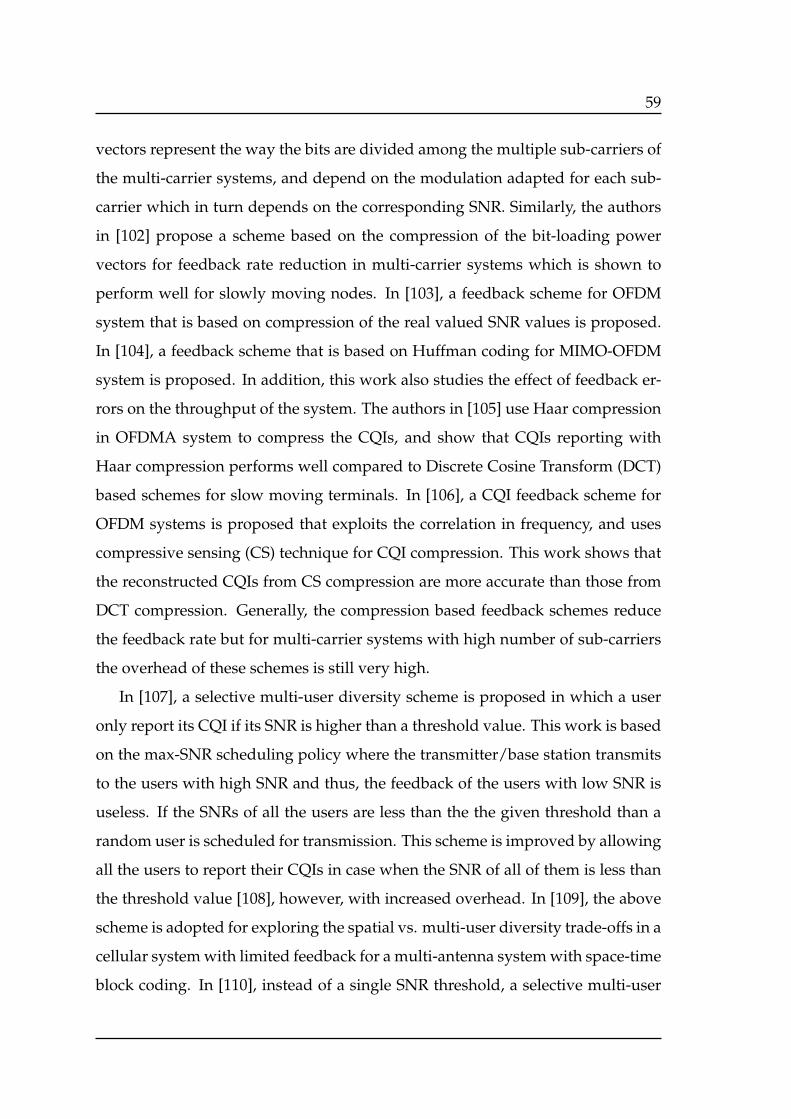
59
vectors represent the way the bits are divided among the multiple sub-carriers of
the multi-carrier systems, and depend on the modulation adapted for each sub-
carrier which in turn depends on the corresponding SNR. Similarly, the authors
in [102] propose a scheme based on the compression of the bit-loading power
vectors for feedback rate reduction in multi-carrier systems which is shown to
perform well for slowly moving nodes. In [103], a feedback scheme for OFDM
system that is based on compression of the real valued SNR values is proposed.
In [104], a feedback scheme that is based on Huffman coding for MIMO-OFDM
system is proposed. In addition, this work also studies the effect of feedback er-
rors on the throughput of the system. The authors in [105] use Haar compression
in OFDMA system to compress the CQIs, and show that CQIs reporting with
Haar compression performs well compared to Discrete Cosine Transform (DCT)
based schemes for slow moving terminals. In [106], a CQI feedback scheme for
OFDM systems is proposed that exploits the correlation in frequency, and uses
compressive sensing (CS) technique for CQI compression. This work shows that
the reconstructed CQIs from CS compression are more accurate than those from
DCT compression. Generally, the compression based feedback schemes reduce
the feedback rate but for multi-carrier systems with high number of sub-carriers
the overhead of these schemes is still very high.
In [107], a selective multi-user diversity scheme is proposed in which a user
only report its CQI if its SNR is higher than a threshold value. This work is based
on the max-SNR scheduling policy where the transmitter/base station transmits
to the users with high SNR and thus, the feedback of the users with low SNR is
useless. If the SNRs of all the users are less than the the given threshold than a
random user is scheduled for transmission. This scheme is improved by allowing
all the users to report their CQIs in case when the SNR of all of them is less than
the threshold value [108], however, with increased overhead. In [109], the above
scheme is adopted for exploring the spatial vs. multi-user diversity trade-offs in a
cellular system with limited feedback for a multi-antenna system with space-time
block coding. In [110], instead of a single SNR threshold, a selective multi-user
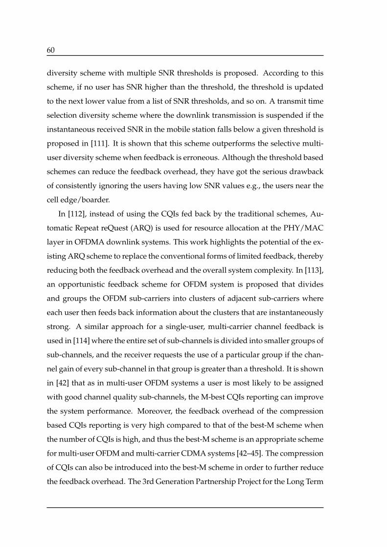
60
diversity scheme with multiple SNR thresholds is proposed. According to this
scheme, if no user has SNR higher than the threshold, the threshold is updated
to the next lower value from a list of SNR thresholds, and so on. A transmit time
selection diversity scheme where the downlink transmission is suspended if the
instantaneous received SNR in the mobile station falls below a given threshold is
proposed in [111]. It is shown that this scheme outperforms the selective multi-
user diversity scheme when feedback is erroneous. Although the threshold based
schemes can reduce the feedback overhead, they have got the serious drawback
of consistently ignoring the users having low SNR values e.g., the users near the
cell edge/boarder.
In [112], instead of using the CQIs fed back by the traditional schemes, Au-
tomatic Repeat reQuest (ARQ) is used for resource allocation at the PHY/MAC
layer in OFDMA downlink systems. This work highlights the potential of the ex-
isting ARQ scheme to replace the conventional forms of limited feedback, thereby
reducing both the feedback overhead and the overall system complexity. In [113],
an opportunistic feedback scheme for OFDM system is proposed that divides
and groups the OFDM sub-carriers into clusters of adjacent sub-carriers where
each user then feeds back information about the clusters that are instantaneously
strong. A similar approach for a single-user, multi-carrier channel feedback is
used in [114] where the entire set of sub-channels is divided into smaller groups of
sub-channels, and the receiver requests the use of a particular group if the chan-
nel gain of every sub-channel in that group is greater than a threshold. It is shown
in [42] that as in multi-user OFDM systems a user is most likely to be assigned
with good channel quality sub-channels, the M-best CQIs reporting can improve
the system performance. Moreover, the feedback overhead of the compression
based CQIs reporting is very high compared to that of the best-M scheme when
the number of CQIs is high, and thus the best-M scheme is an appropriate scheme
for multi-user OFDM and multi-carrier CDMA systems [42–45]. The compression
of CQIs can also be introduced into the best-M scheme in order to further reduce
the feedback overhead. The 3rd Generation Partnership Project for the Long Term
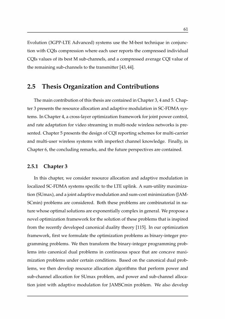
61
Evolution (3GPP-LTE Advanced) systems use the M-best technique in conjunc-
tion with CQIs compression where each user reports the compressed individual
CQIs values of its best M sub-channels, and a compressed average CQI value of
the remaining sub-channels to the transmitter [43, 44].
2.5 Thesis Organization and Contributions
The main contribution of this thesis are contained in Chapter 3, 4 and 5. Chap-
ter 3 presents the resource allocation and adaptive modulation in SC-FDMA sys-
tems. In Chapter 4, a cross-layer optimization framework for joint power control,
and rate adaptation for video streaming in multi-node wireless networks is pre-
sented. Chapter 5 presents the design of CQI reporting schemes for multi-carrier
and multi-user wireless systems with imperfect channel knowledge. Finally, in
Chapter 6, the concluding remarks, and the future perspectives are contained.
2.5.1 Chapter 3
In this chapter, we consider resource allocation and adaptive modulation in
localized SC-FDMA systems specific to the LTE uplink. A sum-utility maximiza-
tion (SUmax), and a joint adaptive modulation and sum-cost minimization (JAM-
SCmin) problems are considered. Both these problems are combinatorial in na-
ture whose optimal solutions are exponentially complex in general. We propose a
novel optimization framework for the solution of these problems that is inspired
from the recently developed canonical duality theory [115]. In our optimization
framework, first we formulate the optimization problems as binary-integer pro-
gramming problems. We then transform the binary-integer programming prob-
lems into canonical dual problems in continuous space that are concave maxi-
mization problems under certain conditions. Based on the canonical dual prob-
lems, we then develop resource allocation algorithms that perform power and
sub-channel allocation for SUmax problem, and power and sub-channel alloca-
tion joint with adaptive modulation for JAMSCmin problem. We also develop
62
an adaptive modulation scheme for SUmax problem. We provide the global op-
timality conditions under which the solution to each dual canonical problem is
identical to the solution of the corresponding primal problem. Our proposed
framework has polynomial complexity. The major contributions of this chapter
are as follows.
– Framework: This chapter presents a novel framework for sum-utility maxi-
mization and a joint adaptive modulation and sum-cost minimization prob-
lems which performs power and sub-channels allocation, and modulation
adaption in localized SC-FDMA systems. The problems are converted into
binary-integer programming problems, and a novel canonical duality based
approach is used to transform these exponential complex problems into
continuous space concave maximization problems whose solution is ex-
tremely easy compared to the corresponding primal binary-integer pro-
grams.
– Algorithm: Resource allocation algorithm that is based on the solution of the
continuous space concave maximization problem is developed. The algo-
rithm solves the problems in continuous domain and provide exact integer
solution to the corresponding binary-integer programs.
– Performance Evaluation: The optimality of the proposed algorithm is thor-
oughly studied and conditions under which the algorithms optimally solve
the corresponding primal problems are provided. Some bounds on the sub-
optimality of the algorithm when the optimality conditions are not satisfied
are also explored. It is shown through simulations that the proposed al-
gorithm outperforms the existing algorithms in the literature and provides
optimal solution to the primal problems most of the times and if not opti-
mal, it is always very close to the optimal solution. In addition, the com-
putational complexity of the solution of the primal problem is exponential
whereas our proposed framework has polynomial complexity which is a
remarkable improvement.
63
2.5.2 Chapter 4
In this chapter, we consider the challenging problem of joint dynamic power
control and video bitstream/rate adaptation for video streaming in multi-node
wireless networks with interference. The main objective is to jointly control the
power at the PHY/MAC layer and the video rate at the APPLICATION layer
such that all the nodes are provided with good quality video while consuming
the minimum possible transmit power, and achieving the stringent delay con-
straints of the video applications. Unlike the underlying approach of assuming
no interference at all or assuming it to be fixed in many of the available solu-
tion for resource allocation in wireless networks, we approach this problem re-
alistically when the wireless channel and the interference gains of the nodes are
both time-varying. Since we consider a network with interference, the increase
of power of a given node will result in an increase of interference exerted by this
node on the other nodes. This will reduce the rates achieved by the other nodes
and increase the delay of these nodes. Consequently, the power allocation should
consider the interference and satisfy the delay constraints of all the nodes. More-
over, the power control at the PHY/MAC layer should be performed instanta-
neously whereas the video rate at the APPLICATION layer should be adapted in
an average manner after a long enough time. Due to these constraints, even the
formulation of a joint dynamic power control, and video rate adaptation frame-
work is a challenging task. In this chapter, we address these issues, and for-
mulate a cross-layer optimization framework that takes care of the time-varying
interferences, exploits the time-varying nature of the channels; and performs in-
stantaneous power control, and average video rate adaptation jointly. In addi-
tion to exploiting the time-varying nature of the channels, we also introduce a
fairness/satisfaction criterion among the nodes so that irrespective of its channel
condition, each node can get a promised share in system total resources/capacity
which is a challenging goal.
In order to solve the above joint power control and rate adaptation problem,
we analyze the Channel to Interference and Noise Ratio (CINR) distribution, and
64
model the power control and rate adaptation for each node as linear stochastic
dynamic equations and write the problem as a dynamic stochastic control prob-
lem. We then formulate a risk-sensitive control problem that jointly performs
power control and rate adaptation for all nodes while satisfying the stringent
delay constraints of the streaming applications, and respecting the nodes’ fair-
ness/satisfaction criterion. We provide the optimal solution of the above control
problem, and provide simulation results to illustrate the performance of the pro-
posed framework. The major contributions of this chapter are highlighted as
follows.
– Framework: A cross-layer optimization framework which considers joint
instantaneous power control at the PHY/MAC layer, and average video
rate adaptation at the APPLICATION layer for multi-node wireless video
streaming (an application with stringent delay constraints) is presented.
– Time-Varying Interference Consideration: In addition to the wireless channel,
the time-varying nature of the interferences is also taken into account.
– Risk-Sensitive Control Approach: The power control and rate adaptation are
modeled as linear stochastic dynamic equations, the optimization problem
is formulated as a control problem, and a risk-sensitive control approach is
used to optimally solve this problem.
2.5.3 Chapter 5
In this chapter, first we consider the best-M CQIs reporting technique in which
each user estimates its channel conditions on all sub-channels, measures/estimates
the CQI values for all its sub-channels, and reports the full CQIs values of the best
M sub-channels, and an average CQI value for the remaining sub-channels. We
approach this problem realistically where a delay between the estimation/observ-
ation of the CQIs at the user terminal and their use at the transmitter/base sta-
tion occurs. Though the main objective here is to deal with the feedback delay,
we also consider the error in the CQI estimation at the user terminal. Moreover,
the imperfections are dealt with at the CQIs reporting level at the user termi-
65
nals. We model the CQI variations from one time slot to another as a stochas-
tic discrete time linear dynamic system with an imperfect (stochastic) measure-
ment/observation. Instead of transmitting directly the estimated CQIs, the users
will compute so-called adapted CQIs taking into account the feedback delay and
the imperfect observation of the CQI, and will feed them back to the transmit-
ter/base station. An adapted CQI represents a rate that implicitly accommodates
the impact of feedback delay and the imperfections in the CQI observation, and
is obtained by using stochastic linear control theory in such a way that the devia-
tion between the actual achieved rate and the allocated rate by the transmitter is
minimum. To obtain/regulate the optimal adapted CQIs in the presence of these
imperfections, we use two different approaches: the Linear Quadratic Gaussian
(LQG) based solution [13, 14], and the H∞ controller based solution [12]. The
LQG approach can optimally solve the above regulating problem when the im-
perfections varies according to Gaussian distribution. The H∞ controller has the
ability to provide a robust solution to the above problem without knowing the
distribution of the CQI imperfections. These adapted CQIs are then reported to
the transmitter where they are directly used in the resource allocation.
We then consider the dynamic value of M that may not be the same for all
users and develop a stochastic framework that optimize the value of M per user
such that the probability that the sum of the CQIs reported by all users does not
exceed a certain value (e.g., the total signalling overhead of the system should
not exceed that of the case where the value of M is fixed and equal for all the
users) is greater then or equal to 1− ϵ where 0 << (1− ϵ) < 1. Since the transmit-
ter does not know the CQIs of all sub-channels, the stochastic framework should
be implemented at the user terminal. Each user separately determines its own
value of M in order to provide enough information to transmitter about its CQIs
while respecting the system’s total signalling overhead constraint. To this end, we
propose an efficient distributed constrained interactive trial and error algorithm
which hugely improves the system performance both in terms of signalling over-
head and rate deviation. We prove that the proposed algorithm converges to an
66
equilibrium. The major contributions of this chapter are highlighted as follows.
– Framework: The main feature of this work is to design a CQIs reporting
schemes that deals with the feedback delay and CQI estimation error at the
CQIs reporting level. The framework is implemented at the user terminals
whereas the transmitter receives the CQIs in which the impact of imper-
fections has already been accommodated, and can be used directly in the
resource management.
– Modeling the Channel Dynamics and the Control Theoretic Solution: The CQI
variations are modeled as a linear discrete state space model, and the CQIs
determination problem is formulated as a control problem. Two cases for
the CQI imperfection are considered: when the statistical distribution of
the imperfection is Gaussian, and when the distribution of the imperfec-
tion is unknown. The problems corresponding to these two cases are then
approached by using a LQG based solution and an H∞ controller based
solution respectively.
– Dynamic best-M CQIs Scheme: In dynamic best-M scheme, in addition to
dealing with the feedback delay and CQI estimation error, a dynamic value
of M that depends on the channel quality of each user is also considered.
This scheme has the potential to improves the system performance without
increasing the feedback overhead.
2.6 Notations
The following notations are used throughout this thesis. Uppercase and low-
ercase boldface letters denote matrices, and vectors respectively. Superscripts
(.)T , and (.)H stand for transpose, and Hermitian of a vector or a matrix respec-
tively. The notation diag(.) represents the diagonal elements of a matrix, and IN
denotes an identity matrix of dimension N . The cardinality of a set is denoted
by | . | whereas O(.) stands for “Big O". The expression x ≥ 0 means that all the
elements of the vector x are non-negative. The notations staf(x), and extf(x)

67
denote the stationary, and extremum point of the function f(x) respectively. The
Euclidean norm of a vector is denoted by ∥ . ∥ whereas ∥ x ∥2Y stands for the
weighted norm of the vector x given as xHYx. The mathematical expectation of
a variable is represented by E., and Pr(.) stands for probability. The spectral
radius of a matrix is denoted by ρ(.).

68

69
Chapter 3
Resource Allocation and Adaptive
Modulation in SC-FDMA Systems
3.1 Introduction
In this chapter, we consider resource allocation and adaptive modulation in
localized SC-FDMA systems. We formulate two problems: A sum-utility maxi-
mization (SUmax) problem, and a joint adaptive modulation and sum-cost min-
imization (JAMSCmin) problem. The SUmax problem aims at maximizing the
sum of the users’ utilities under constraints on the maximum transmit power of
each user and the peak power transmitted on each sub-channel. The objective
of the JAMSCmin problem is to minimize the sum of users’ powers under con-
straints on the achieved data rates of the users. In SC-FDMA, like in OFDMA,
a sub-channel is allowed to be allocated to one user at most. However, in lo-
calized SC-FDMA, in addition to the restriction of allocating a sub-channel to
one user at most, the multiple sub-channels allocated to a user should be con-
secutive as well. Moreover, due to employing the frequency domain equalization
over all sub-channels, the SNR expression for SC-FDMA user is very complicated
than that of OFDMA user, and the power allocation on any sub-channel is depen-
dent on all the sub-channel allocated to that user. This structure renders the SC-
FDMA resource allocation problem prohibitively difficult and the computational
70
complexity of finding its optimal solution is exponential. The resource allocation
schemes developed for OFDMA systems are not applicable to SC-FDMA system.
Moreover, the standard optimization tools (e.g., Lagrange dual approach widely
used for OFDMA, etc.) can not help towards its optimal solution. In this chap-
ter, we develop a novel optimization framework for the solution of these prob-
lems that is inspired from the recently developed canonical duality theory. We
first formulate the optimization problems as binary-integer programming prob-
lems and then transform these binary-integer programming problems into con-
tinuous space canonical dual problems. The canonical dual problems are con-
cave maximization problems and their solution is very easy. Based on the solu-
tion of its corresponding continuous space dual problem, we derive power and
sub-channel allocation algorithm for SUmax problem. An adaptive modulation
scheme for SUmax problem is also developed that based on the power and sub-
channel allocation performed by the proposed algorithm selects an appropriate
modulation scheme for each user. Similarly, based on its corresponding canonical
dual problem, a joint power, sub-channel and adaptive modulation algorithm for
JAMSCmin is also developed. Both the algorithms have polynomial complexi-
ties which is a significant improvement over exponential complexity. We provide
certain optimality conditions under which the proposed algorithms are optimal.
We also provide some bounds on the sub-optimality of our algorithms if the op-
timality conditions are not satisfied. We perform simulations in order to assess
the performance of the proposed algorithms and compare them with the existing
algorithms in the literature.
3.2 System Model
We consider the uplink of a single cell model that utilizes localized SC-FDMA.
The generalization to multi-cell scenario is straightforward by considering the
inter cell interference in the signal-to-interference-plus-noise ratio (SINR) expres-
sion. We make it clear that this work does not study inter-cell interference reduc-
71
tion/mangement but aims to optimize the resources in each cell by an efficient
resource allocation algorithm. In the cell, K users are summed to be simultane-
ously active. The total bandwidth B is divided into N sub-channels each having
12 sub-carriers. The channel is assumed to be slowly fading or in other words as-
sumed to exhibit block fading characteristics. The coherence time of the channel
is greater than the transmission-time-interval (TTI) so that the channel stays rela-
tively constant during the TTI (in 3GPP-LTE, TTI = 0.5msec). The users’ channel
gains are assumed to be perfectly known.
In the following, all signals are represented by their discrete time equivalents
in the complex baseband. Assume that Nk be the number of consecutive sub-
channels allocated to user k (since a sub-channel cannot be allocated to more
than one user simultaneously,∑K
k=1Nk = N ). Let sk = [sk,1, ..., sk,Nk]T be the
modulated symbol vector of the kth user, and FN and FHN denote an N -point DFT
and an N -point Inverse DFT (IDFT) matrices respectively. The assignment of the
data modulated symbols sk to the user specific set of Nk sub-channels can be de-
scribed by a Nk-point DFT precoding matrix FNk, a N ∗ Nk mapping matrix Dk
and an N -point IDFT matrix FHN . The mapping matrix Dk represents the block-
wise sub-channel allocation where the elements Dk(n, q) for n = 0, ..., N − 1 and
q = 0, ..., Nk − 1 are given by
Dk(n, q) =
1 n =∑k−1
j=1 Nj + q
0 elsewhere(3.1)
The transmitted signal is then
xk = FHNDkFNk
sk (3.2)
At the receiver, the received signal is transformed into the frequency domain via
aN -point DFT. The received signal vector for user k assuming perfect sample and
symbol synchronization, is given as
yk = HkFHNDkFNk
sk + zk (3.3)
where Hk = diag(hk,1, ..., hk,N) and zk = [zk,1, ..., zk,N ]T are respectively the diag-
onal channel response matrix and the diagonal Additive White Gaussian Noise
72
(AWGN) vector in the frequency domain. A frequency domain equalizer is then
used in order to mitigate the ISI. The equalized symbols are transformed back to
the time domain via an Nk-point IDFT, and the detection takes place in the time
domain. Let Pk,n, and σ2z denote the transmit power of user k on sub-channel n,
and the ambient noise variance at the receiver for user k respectively. After sev-
eral manipulations, the effective SNR for user k can be obtained as follows [62]:
γZFk =
(1
Nk
Nk∑n=1
1
Pk,nGk,n
)−1
, γMMSEk =
11Nk
∑Nk
n=1Pk,nGk,n
1+Pk,nGk,n
− 1
−1
(3.4)
where γZFk is the SNR when ZF equalizer is used and γMMSE
k is the SNR when
MMSE equalizer is used, and where Gk,n =|hk,n|2σ2z
. The optimization framework
developed in this chapter assumes an MMSE frequency domain equalization at
the receiver. Nevertheless, the proposed framework is equally applicable for ZF
equalization at the receiver.
Unlike OFDMA where a different constellation can be adopted for each sub-
channel, in SC-FDMA a single constellation is chosen for each user depending
upon its channel quality. This is due to the fact that the transmit symbols di-
rectly modulate the sub-channels in OFDMA whereas in SC-FDMA, the transmit
symbols are first fed to the FFT block and the output discrete Fourier terms are
then mapped to the sub-channels. In 3GPP LTE, the constellation for each user is
chosen from the set M = QPSK, 16QAM, 64QAM.
3.3 Problems Formulation
In this section, we formulate the two optimization problems and their equiv-
alent binary-integer programming (BIP) problems respectively. The formulation
of the problems as equivalent binary integer programs is an intermediate step
towards its solution which are then approached by the canonical dual method.
73
3.3.1 Sum-Utility Maximization (SUmax)
3.3.1.1 SUmax Problem Formulation
We want to maximize the sum-utility subject to constraint on the total transmit
power of each individual user Pmaxk . We also have per sub-channel peak power
constraint, P peakk,n i.e., the peak power transmitted on each sub-channel by any
user should not exceed P peakk,n so that the PAPR is kept low [1]. In addition, in
SC-FDMA for LTE uplink, the power on all the sub-channels allocated to a user
should be equal [1], so that the low PAPR benefits could retain [2]. The utility of
user k denoted as Uk(γk) is an arbitrary function that is monotonically increasing
in user’s SNR γk. The overall resource allocation problem can be formulated as
maxK∑k=1
Uk(γk) (3.5)
s.t.∑n∈Nk
Pk,n ≤ Pmaxk , ∀k
Pk,n ≤ P peakk,n , ∀k, n
Pk,n = Pk,l, ∀k, n, l
Nk ∩Nj = ∅,∀k = jn ∩
( K∪j=1,j =k
Nj
)= ∅ | n ∈ n1, n1 + 1, ..., n2 − 1, n2
, ∀k
where Nk with cardinality Nk is the set of sub-channels allocated to users k,
n1 = min(Nk) and n2 = max(Nk). The fourth constraint determines that each
sub-channel is allowed to be allocated to one user at most while the last con-
straint ensures that the sub-channels included in the set Nk are consecutive. The
optimization problem (3.5) is combinatorial in nature. There is a twofold diffi-
culty in solving this problem, that is in addition to the exclusivity restriction on
the sub-channel allocation, the allocated sub-channels to any user should be adja-
cent as well. For example, forK = 10 users andN = 24 sub-channels, the optimal
solution requires a search across 5.26 × 10¹² possible sub-channel allocations [3],
which is not practical.
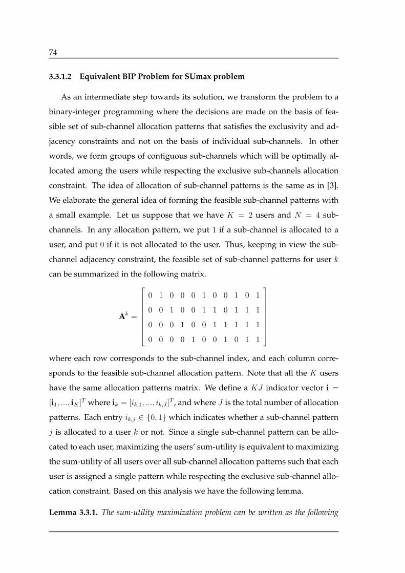
74
3.3.1.2 Equivalent BIP Problem for SUmax problem
As an intermediate step towards its solution, we transform the problem to a
binary-integer programming where the decisions are made on the basis of fea-
sible set of sub-channel allocation patterns that satisfies the exclusivity and ad-
jacency constraints and not on the basis of individual sub-channels. In other
words, we form groups of contiguous sub-channels which will be optimally al-
located among the users while respecting the exclusive sub-channels allocation
constraint. The idea of allocation of sub-channel patterns is the same as in [3].
We elaborate the general idea of forming the feasible sub-channel patterns with
a small example. Let us suppose that we have K = 2 users and N = 4 sub-
channels. In any allocation pattern, we put 1 if a sub-channel is allocated to a
user, and put 0 if it is not allocated to the user. Thus, keeping in view the sub-
channel adjacency constraint, the feasible set of sub-channel patterns for user k
can be summarized in the following matrix.
Ak =
0 1 0 0 0 1 0 0 1 0 1
0 0 1 0 0 1 1 0 1 1 1
0 0 0 1 0 0 1 1 1 1 1
0 0 0 0 1 0 0 1 0 1 1
where each row corresponds to the sub-channel index, and each column corre-
sponds to the feasible sub-channel allocation pattern. Note that all the K users
have the same allocation patterns matrix. We define a KJ indicator vector i =
[i1, ..., iK ]T where ik = [ik,1, ..., ik,J ]T , and where J is the total number of allocation
patterns. Each entry ik,j ∈ 0, 1 which indicates whether a sub-channel pattern
j is allocated to a user k or not. Since a single sub-channel pattern can be allo-
cated to each user, maximizing the users’ sum-utility is equivalent to maximizing
the sum-utility of all users over all sub-channel allocation patterns such that each
user is assigned a single pattern while respecting the exclusive sub-channel allo-
cation constraint. Based on this analysis we have the following lemma.
Lemma 3.3.1. The sum-utility maximization problem can be written as the following
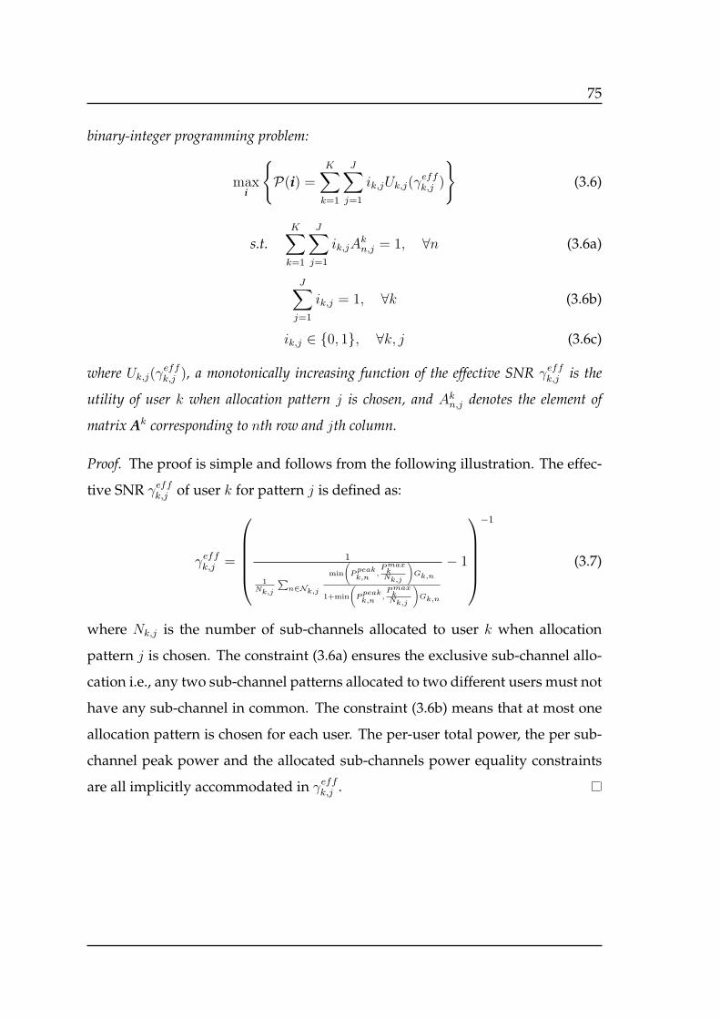
75
binary-integer programming problem:
maxi
P(i) =
K∑k=1
J∑j=1
ik,jUk,j(γeffk,j )
(3.6)
s.t.K∑k=1
J∑j=1
ik,jAkn,j = 1, ∀n (3.6a)
J∑j=1
ik,j = 1, ∀k (3.6b)
ik,j ∈ 0, 1, ∀k, j (3.6c)
where Uk,j(γeffk,j ), a monotonically increasing function of the effective SNR γeffk,j is the
utility of user k when allocation pattern j is chosen, and Akn,j denotes the element of
matrix Ak corresponding to nth row and jth column.
Proof. The proof is simple and follows from the following illustration. The effec-
tive SNR γeffk,j of user k for pattern j is defined as:
γeffk,j =
1
1Nk,j
∑n∈Nk,j
min
(Ppeakk,n
,PmaxkNk,j
)Gk,n
1+min
(Ppeakk,n
,PmaxkNk,j
)Gk,n
− 1
−1
(3.7)
where Nk,j is the number of sub-channels allocated to user k when allocation
pattern j is chosen. The constraint (3.6a) ensures the exclusive sub-channel allo-
cation i.e., any two sub-channel patterns allocated to two different users must not
have any sub-channel in common. The constraint (3.6b) means that at most one
allocation pattern is chosen for each user. The per-user total power, the per sub-
channel peak power and the allocated sub-channels power equality constraints
are all implicitly accommodated in γeffk,j .
76
3.3.2 Joint Adaptive Modulation and Sum-Cost Minimization (JAM-
SCmin)
3.3.2.1 JAMSCmin Problem Formulation
We now formulate the joint resource allocation and adaptive modulation prob-
lem. The objective is to allocate powers and sub-channels, and to choose the mod-
ulation scheme for each user in order to minimize the sum-cost while satisfying
the the target data rate constraint of all the users (i.e., RTk , ∀k). For a modula-
tion m ∈ M to be chosen, the effective SNR of the user should not be less than
a minimum value Γ∗m that guarantees a target Block Error Rate (BLER) at the re-
ceiver. In addition, the power on all the sub-channels allocated to a user should
be equal [1]. In the uplink the users terminals are more sensitive to transmit
power due to their batteries’s power limitations. Therefore, we introduce in the
JAMSCmin formulation a user’s cost which is function of its transmit power and
has to be minimized. We define the following cost function for each user k
Ck(Pmaxk , Pk) = − exp [Pmax
k − Pk] (3.8)
where Pmaxk is the maximum power a user can transmit, and Pk =
∑n∈Nk
Pk,n
is the sum of powers transmitted by user k on its allocated set of sub-channels
Nk. The cost function is monotonically increasing in Pk whereas it is monotoni-
cally decreasing in Pmaxk . With this choice of cost function, the JAMSCmin prob-
lem will not only minimize the sum-power of the users but will also ensure that
each user’s transmit power is minimized in accordance to its Pmaxk level. In other
words, a user with small Pmaxk will transmit small power compared to another
user with high Pmaxk , and vice versa. The joint optimization problem can now be
formulated as follows
minK∑k=1
Ck(Pmaxk , Pk) (3.9)
s.t. Rk ≥ RTk ,∀k
Pk,n = Pk,l,∀k, n, l
γk ≥ Γ∗m,∀k,m
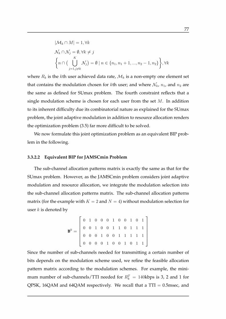
77
|Mk ∩M | = 1, ∀k
Nk ∩Nj = ∅, ∀k = jn ∩
( K∪j=1,j =k
Nj
)= ∅ | n ∈ n1, n1 + 1, ..., n2 − 1, n2
,∀k
where Rk is the kth user achieved data rate,Mk is a non-empty one element set
that contains the modulation chosen for kth user; and where Nk, n1, and n2 are
the same as defined for SUmax problem. The fourth constraint reflects that a
single modulation scheme is chosen for each user from the set M . In addition
to its inherent difficulty due its combinatorial nature as explained for the SUmax
problem, the joint adaptive modulation in addition to resource allocation renders
the optimization problem (3.5) far more difficult to be solved.
We now formulate this joint optimization problem as an equivalent BIP prob-
lem in the following.
3.3.2.2 Equivalent BIP for JAMSCmin Problem
The sub-channel allocation patterns matrix is exactly the same as that for the
SUmax problem. However, as the JAMSCmin problem considers joint adaptive
modulation and resource allocation, we integrate the modulation selection into
the sub-channel allocation patterns matrix. The sub-channel allocation patterns
matrix (for the example with K = 2 and N = 4) without modulation selection for
user k is denoted by
Bk =
0 1 0 0 0 1 0 0 1 0 1
0 0 1 0 0 1 1 0 1 1 1
0 0 0 1 0 0 1 1 1 1 1
0 0 0 0 1 0 0 1 0 1 1
Since the number of sub-channels needed for transmitting a certain number of
bits depends on the modulation scheme used, we refine the feasible allocation
pattern matrix according to the modulation schemes. For example, the mini-
mum number of sub-channels/TTI needed for RTk = 140kbps is 3, 2 and 1 for
QPSK, 16QAM and 64QAM respectively. We recall that a TTI = 0.5msec, and
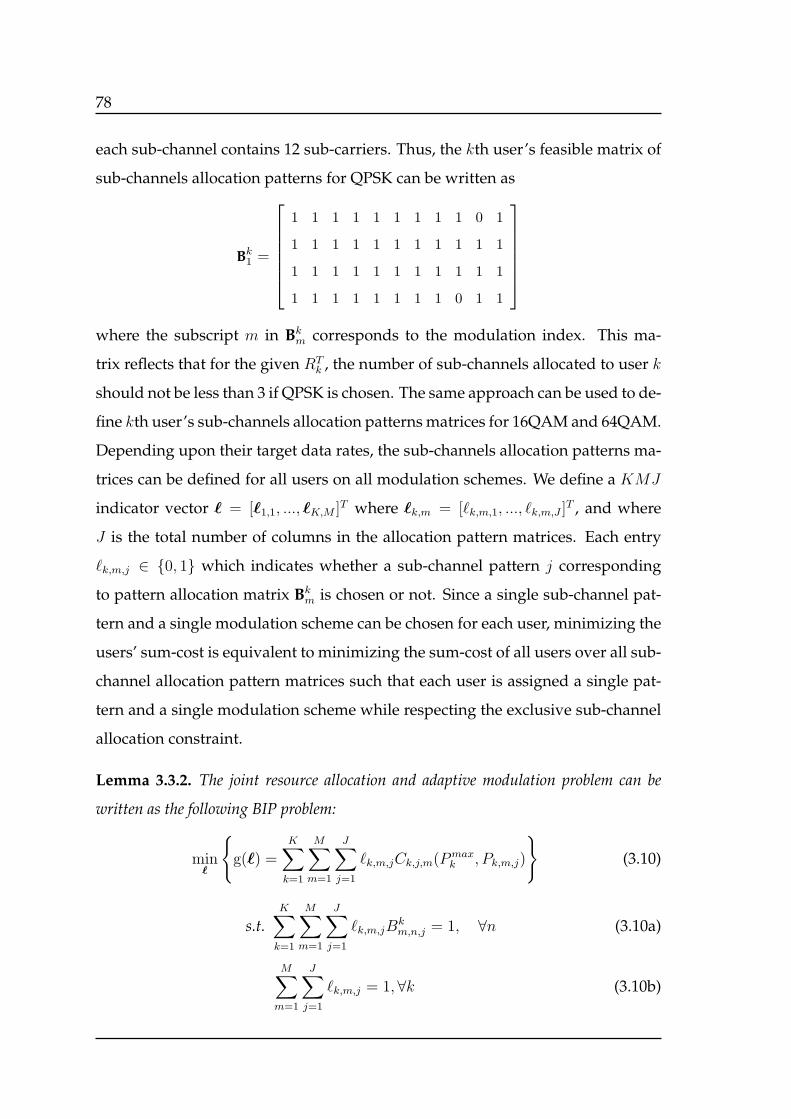
78
each sub-channel contains 12 sub-carriers. Thus, the kth user’s feasible matrix of
sub-channels allocation patterns for QPSK can be written as
Bk1 =
1 1 1 1 1 1 1 1 1 0 1
1 1 1 1 1 1 1 1 1 1 1
1 1 1 1 1 1 1 1 1 1 1
1 1 1 1 1 1 1 1 0 1 1
where the subscript m in Bk
m corresponds to the modulation index. This ma-
trix reflects that for the given RTk , the number of sub-channels allocated to user k
should not be less than 3 if QPSK is chosen. The same approach can be used to de-
fine kth user’s sub-channels allocation patterns matrices for 16QAM and 64QAM.
Depending upon their target data rates, the sub-channels allocation patterns ma-
trices can be defined for all users on all modulation schemes. We define a KMJ
indicator vector ℓ = [ℓ1,1, ..., ℓK,M ]T where ℓk,m = [ℓk,m,1, ..., ℓk,m,J ]T , and where
J is the total number of columns in the allocation pattern matrices. Each entry
ℓk,m,j ∈ 0, 1 which indicates whether a sub-channel pattern j corresponding
to pattern allocation matrix Bkm is chosen or not. Since a single sub-channel pat-
tern and a single modulation scheme can be chosen for each user, minimizing the
users’ sum-cost is equivalent to minimizing the sum-cost of all users over all sub-
channel allocation pattern matrices such that each user is assigned a single pat-
tern and a single modulation scheme while respecting the exclusive sub-channel
allocation constraint.
Lemma 3.3.2. The joint resource allocation and adaptive modulation problem can be
written as the following BIP problem:
minℓ
g(ℓ) =
K∑k=1
M∑m=1
J∑j=1
ℓk,m,jCk,j,m(Pmaxk , Pk,m,j)
(3.10)
s.t.K∑k=1
M∑m=1
J∑j=1
ℓk,m,jBkm,n,j = 1, ∀n (3.10a)
M∑m=1
J∑j=1
ℓk,m,j = 1,∀k (3.10b)
79
ℓk,m,j ∈ 0, 1, ∀k,m, j (3.10c)
where Bkm,n,j denotes the element of matrix Bk
m corresponding to nth row and jth col-
umn, Pk,m,j = f(γeffk,m,j, RTk ,Γ
∗m) is the power transmitted by user k when jth sub-
channels allocation pattern corresponding to Bkm is chosen, and Ck,m,j(P
maxk , Pk,m,j) =
− exp [Pmaxk − Pk,m,j].
Proof. The transmit power Pk,m,j is a function of RTk , Γ∗
m, and the effective SNR
γeffk,m,j of user k for jth pattern of Bkm. Let Pk,m,n be the power for user k on sub-
channel n when modulation m is chosen, then γeffk,m,j is given by
γeffk,m,j =
(1
1Nk,m,j
∑n∈Nk,m,j
Pk,m,nGk,n
1+Pk,m,nGk,n
− 1
)−1
(3.11)
where Nk,m,j with cardinality Nk,m,j is the set of sub-channels allocated to user
k when jth pattern from Bkm is chosen. The power allocation values Pk,m,j’s are
obtained prior to resource allocation by solving the following equations:∑n∈Nk,m,j
(Pk,m,jGk,n
Nk,m,j + Pk,m,jGk,n
)− Nk,m,jΓ
∗m
1 + Γ∗m
= 0,∀k,m, j (3.12)
which are obtained by setting γeffk,m,j = Γ∗m and Pk,m,n =
Pk,m,j
Nk,m,jand hence the per
user minimum SNR and the allocated sub-channels powers equality constraint
are implicitly accommodated in Pk,m,j . The per-user target data rate constraint
is already implicitly accommodated in the definition of allocation patterns and
hence in the calculation of Pk,m,j . The constraint (3.10a) reflects the mutual ex-
clusivity restriction on the sub-channels allocation and constraint (3.10b) means
that at most one allocation pattern and one modulation scheme is chosen for each
user.
We recall that the formulation of the problems as equivalent binary-integer
programs is an intermediate step towards their solution. Although the BIP prob-
lems may look simple compared to the primal problem but unfortunately, their
solutions are exponentially complex due to their combinatorial nature. A sim-
ilar binary-integer programming solution was proposed for weighted-sum rate
80
maximization problem in [3] but as mentioned before it is exponentially com-
plex which is not practical. In the following section, we propose a polynomial-
complexity framework for the solution of both the above problems that is in-
spired from the canonical dual transformation method. The main idea of our
proposed approach is to transform each binary-integer programming problem
into a canonical dual problem in the continuous space whose solution is identical
to the corresponding binary integer program under certain conditions.
3.4 Canonical Dual Approach for Solving the BIP Prob-
lems
Under certain constraints/conditions, the canonical duality theory [115] can
be used to reformulate some non-convex/non-smooth constrained problem into
certain convex/smooth canonical dual problems with perfect primal/dual rela-
tionship. However, this theory does not provide any general strategy for the
solution of non-convex/non-smooth problems. The constraints under which the
canonical dual problem could be perfectly dual to its primal problem is purely de-
pendent on the nature of the primal problem under consideration and should be
studied for each specific problem anew. This theory comprises of canonical dual
transformation, an associated complementary-dual principle, and an associated
duality theory. The canonical dual transformation can be used to convert the non-
smooth problem into a smooth canonical dual problem; the complementary-dual
principle can be used to study the relationship between the primal and its canon-
ical dual problems; and the associated duality theory can help to identify both
local and global extrema. Comprehensive details about this theory, and its ap-
plication to an unconstrained 0-1 quadratic programming problems can be found
in [115], and [116] respectively. Due to the presence of additional constraints, our
problems are far more difficult compared to that described in [116].
By using the aforementioned theory, we transform each of the SUmax and
JAMSCmin primal problems into a continuous space canonical dual problem in
81
the following. We then study the optimality conditions, and prove that under
these conditions, the solution of each canonical dual problem is identical to that
of the corresponding primal problem.
3.4.1 Canonical Dual Problem and Optimality Conditions for SUmax
Problem
The objective function, P(i) in problem (3.6) is a real valued linear function
defined on Ia = i ⊂ RK×J with feasible space defined by
If =
i ∈ Ia ⊂ RK×J |
K∑k=1
J∑j=1
ik,jAkn,j = 1,∀n;
J∑j=1
ik,j = 1,∀k; ik,j ∈ 0, 1∀k, j
(3.13)
We start our development by introducing new constraints ik,j(ik,j−1) = 0,∀k, j
which means that any ik,j can only take an integer value from the set 0, 1.
This approach is used for the solution of a 0-1 quadratic programming problem
in [116]. However, the problem considered in [116] is a simple unconstrained 0-
1 quadratic programming problem while our problem is combinatorial in nature
with additional constraints. In other words, in addition to the binary-integer con-
straint on ik,j’s, we have the mutual exclusivity restriction on the sub-channel pat-
terns allocation (i.e., ik,j × il,j = 0|k = l, ∀k, l ∈ 1, ..., K), and the mutual ex-
clusivity constraint on the sub-channel allocation i.e.,∑K
k=1
∑Jj=1 ik,jA
kn,j = 1, ∀n.
Furthermore, at most one sub-channel pattern can be allocated to a user i.e.,∑Jj=1 ik,j = 1,∀k. Note that the mutual exclusivity restriction on the sub-channel
patterns allocation is accommodated implicitly in the formulation of the primal
problem and does not show up explicitly. We temporarily relax the new con-
straints ik,j(ik,j − 1) = 0, ∀k, j, and the equality constraints (3.6a-3.6b) to inequali-
ties and transform the primal problem with these inequality constraints into con-
tinuous domain canonical dual problem. We will then solve the canonical dual
problem in the continuous space and chose the solution which lies in If as de-
fined by (3.13). Furthermore, for our convenience, we reformulate our primal
82
problem as an equivalent minimization problem. The primal problem with these
inequality constraints can now be written as follows.
mini
f (i) = −
K∑k=1
J∑j=1
ik,jUk,j
(3.14)
s.t.K∑k=1
J∑j=1
ik,jAkn,j ≤ 1, ∀n
J∑j=1
ik,j ≤ 1, ∀k
ik,j (ik,j − 1) ≤ 0, ∀k, j
ik,j ∈ 0, 1, ∀k, j
where Uk,j is used to denote Uk,j(γeffk,j ) and will be used in the remainder of this
chapter.
The temporary relaxation of the constraints to inequalities is needed for de-
veloping the canonical dual framework. We prove later that the solution of the
canonical dual problem achieves the binary-integer constraints i.e., ik,j (ik,j − 1) =
0, ∀k, j and all the other constraints with equality. As a first step towards its trans-
formation into a canonical dual problem, we relax the primal problem ( [115,116]).
To this end, we define the so-called canonical geometrical operator x = Λ(i) for
the above primal problem as follows:
x = Λ(i) = (ϵ,λ,ρ) : RKJ → RN × RK × RKJ (3.15)
which is a vector-valued mapping and where ϵ =[ (∑K
k=1
∑Jj=1 ik,jA
k1,j − 1
), ..
..,(∑K
k=1
∑Jj=1 ik,jA
kN,j − 1
) ]Tis an N-vector, ρ = [iT1 (i1 − 1), ..., iTK(iK − 1)]T is a
KJ-vector with iTk (ik−1) = [ik,1(ik,1−1), ..., ik,J(ik,J−1)]T , andλ =[ (∑J
j=1 i1,j − 1),
...,(∑J
j=1 iK,j − 1) ]T
is a K-vector ρ = [iT1 (i1 − 1), ..., iTK(iK − 1)]T is a KJ-vector
with iTk (ik − 1) = [ik,1(ik,1 − 1), ..., ik,J(ik,J − 1)]T . Let χa be a convex subset of
χ = RN × RK × RKJ defined as follows
χa =
x = (ϵ,λ,ρ) ∈ RN × RK × RKJ | ϵ ≤ 0,λ ≤ 0,ρ ≤ 0
(3.16)

83
We introduce an indicator function V : χ→ R ∪ +∞, defined as
V (x) =
0 if x ∈ χa,
+∞ otherwise.(3.17)
Thus, the inequality constraints in the primal problem (3.14) can now be relaxed
by the indicator function V (x), and the primal problem can be written in the fol-
lowing canonical form [116]:
mini
V (Λ(i))−
K∑k=1
J∑j=1
ik,jUk,j | ik,j ∈ 0, 1∀k, j
(3.18)
We now define the canonical dual variables and the canonical conjugate function
associated to the indicator function in order to proceed with the transformation
of the primal problem into canonical dual. Since V (x) is convex, lower semi-
continuous on χ, the canonical dual variable x∗ ∈ χ∗ = χ = RN × RK × RKJ is
defined as:
x∗ ∈ ∂V (x) =
(ϵ∗,λ∗,ρ∗) if ϵ∗ ≥ 0 ∈ RN ,λ∗ ≥ 0 ∈ RK ,ρ∗ ≥ 0 ∈ RKJ ,
∅ otherwise.(3.19)
By the Legendre-Fenchel transformation, the canonical super-conjugate function
of V (x) is defined by
V ♯(x∗) = supx∈χ
xTx∗ − V (x)
= sup
ϵ≤0supλ≤0
supρ≤0
ϵTϵ∗ + λTλ∗ + ρTρ∗
=
0 if ϵ∗ ≥ 0,λ∗ ≥ 0,ρ∗ ≥ 0,
+∞ otherwise.(3.20)
The effective domain of V ♯(x) is given by
χ∗a =
(ϵ∗,λ∗,ρ∗) ∈ RN × RK × RKJ | ϵ∗ ≥ 0 ∈ RN ,λ∗ ≥ 0 ∈ RK ,ρ∗ ≥ 0 ∈ RKJ
(3.21)
Since both V (x) and V ♯(x) are convex, lower semi-continuous, the Fenchel sup-
duality relations
x∗ ∈ ∂V (x)⇔ x ∈ ∂V ♯(x∗)⇔ V (x) + V ♯(x∗) = xTx∗ (3.22)

84
hold on χ× χ∗. The pair (x, x∗) is called the extended / Legendre canonical dual
pair on χ × χ∗, and the functions V (x) and V ♯(x) are called canonical functions
[115]. The optimal solution of our primal problem can be obtained if and only if
x = If ∈ χa, i.e., along with the satisfaction of the binary-integer constraints, all
the other constraints must be achieved with equality. Thus, we need to study the
conditions under which the canonical dual variables x∗ ∈ χ∗a can ensure that x =
If ∈ χa. By the definition of sub-differential, the canonical sup-duality relations
(3.22) are equivalent to the following:
x ≤ 0, x∗ ≥ 0, xTx∗ = 0 (3.23)
From the complementarity condition xTx∗ = 0, for x∗ > 0, we have x = 0
(i.e., ϵ = 0,λ = 0,ρ = 0) and consequently x = If ∈ χa. This means that for
x∗ > 0, all the constraints of the primal problem (3.14) are achieved by equal-
ity (with ik,j ∈ 0, 1, ∀k, j which comes from ρ = 0). Thus, the dual feasible
space for the primal problem is an open positive cone defined by
χ∗♯ = (ϵ∗,λ∗,ρ∗) ∈ χ∗
a | ϵ∗ > 0,λ∗ > 0,ρ∗ > 0 (3.24)
The so-called total complementarity function (see [115,116] for definition), Ξ(i, x∗) :
χ× χ∗♯ → R associated with the primal problem (3.14) can be defined as follows.
Ξ(i, x∗) = Λ(i)Tx∗ − V ♯(x∗)−K∑k=1
J∑j=1
ik,jUk,j (3.25)
which is obtained by replacing V (Λ(i)) in (3.18) by Λ(i)Tx∗− V ♯(x∗) from Fenchel
sup-duality relations (3.22). From the definition of Λ(i) and V ♯(x∗), the total com-
plementarity function takes the form:
Ξ(i, ϵ∗,λ∗,ρ∗) =K∑k=1
J∑j=1
ρ∗k,ji
2k,j +
(λ∗k − ρ∗k,j − Uk,j +
N∑n=1
ϵ∗nAkn,j
)ik,j
−
N∑n=1
ϵ∗n −K∑k=1
λ∗k
(3.26)
Similar to [116], the canonical dual function fd(ϵ∗,λ∗,ρ∗) associated to our primal
problem for a given (ϵ∗,λ∗,ρ∗) ∈ χ∗♯ can be defined as
fd(ϵ∗,λ∗,ρ∗) = sta Ξ(i, ϵ∗,λ∗,ρ∗) | i ∈ Ia (3.27)

85
where staf(x) stands for finding the stationary points of f(x). The comple-
mentarity function is a quadratic function of i ∈ Ia, and has therefore a unique
stationary point with respect to it for a given (ϵ∗,λ∗,ρ∗) ∈ χ∗a. The stationary
points of Ξ(i, ϵ∗,λ∗,ρ∗) over i ∈ Ia occurs at i(x∗) with
ik,j(x∗) =1
2ρ∗k,j
(Uk,j + ρ∗k,j − λ∗k −
N∑n=1
ϵ∗nAkn,j
), ∀k, j (3.28)
Replacing ik,j by ik,j(x∗) in (3.26), we have
fd(ϵ∗,λ∗,ρ∗) =
−1
4
K∑k=1
J∑j=1
(Uk,j + ρ∗k,j − λ∗k −
∑Nn=1 ϵ
∗nA
kn,j
)2ρ∗k,j
−N∑
n=1
ϵ∗n −K∑k=1
λ∗k (3.29)
which is a concave function in χ∗♯ . The canonical dual problem associated with
the primal problem (3.14) can now be formulated as follows
extfd(ϵ∗,λ∗,ρ∗) | (ϵ∗,λ∗,ρ∗) ∈ χ∗
♯
(3.30)
where the notation ext f(x) stands for finding the extremum values of f(x).
We have the following canonical duality theorem (Complementary-Dual Prin-
ciple) on the dual relationship between the primal and its corresponding canoni-
cal dual problem.
Theorem 3.4.1. If (ϵ∗,λ∗,ρ∗) ∈ χ∗
♯ is the stationary point of fd(ϵ∗,λ∗,ρ∗), such that
i = [i1,1, ..., iK,J ]T with ik,j =
1
2ρ∗k,j
(Uk,j + ρ∗k,j − λ
∗k −
N∑n=1
ϵ∗nAkn,j
),∀k, j
(3.31)
is the KKT point of the primal problem, and
f(i) = fd(ϵ∗,λ∗,ρ∗). (3.32)
then the canonical dual problem (3.30) is dual to the primal problem (3.6).
Proof. See the proof in Appendix A.1.
86
The above theorem shows that the binary-integer programming problem (3.10)
is converted into a dual problem in continuous domain which is perfectly dual
to it. Furthermore, the KKT point of the dual problem provides the KKT point
for the primal problem. However, as the KKT conditions are necessary but not
sufficient for optimality in general, we need some additional information on the
global optimality. Based on the properties of the primal and dual problems, we
have the following theorem on the global optimality conditions.
Theorem 3.4.2. If (ϵ∗,λ∗,ρ∗) ∈ χ∗
♯ , then i defined by (3.31) is a global minimizer of f(i)
over If and (ϵ∗,λ∗,ρ∗) is a global maximizer of fd(ϵ∗,λ∗,ρ∗) over χ∗
♯ , and
f(i) = mini∈If
f(i) = max(ϵ∗,λ∗,ρ∗)∈χ∗
♯
fd(ϵ∗,λ∗,ρ∗) = fd(ϵ∗,λ∗,ρ∗). (3.33)
Proof. See Appendix A.2.
3.4.2 Canonical Dual Problem and Optimality Conditions for JAM-
SCmin Problem
The objective function, g(ℓ) in problem (3.10) is a real valued linear function
defined on La = ℓ ⊂ RK×M×J with feasible space defined by
Lf =
ℓ ∈ La|
K∑k=1
M∑m=1
J∑j=1
ℓk,m,jBkm,n,j = 1, ∀n;
M∑m=1
J∑j=1
ℓk,m,j = 1,∀k; ℓk,m,j ∈ 0, 1,∀k,m, j
(3.34)
By introducing the additional constraint ℓk,m,j (ℓk,m,j − 1) ≤ 0, ∀k,m, j, and tem-
porarily relaxing the equality constraints to inequalities, the primal JAMSCmin
problem (3.10) takes the following form:
minℓ
g (ℓ) =
K∑k=1
M∑m=1
J∑j=1
ℓk,m,jCk,m,j
(3.35)
s.t.K∑k=1
M∑m=1
J∑j=1
ℓk,m,jBkm,n,j ≤ 1, ∀n

87
M∑m=1
J∑j=1
ℓk,m,j ≤ 1, ∀k
ℓk,m,j (ℓk,m,j − 1) ≤ 0, ∀k,m, j
ℓk,m,j ∈ 0, 1, ∀k,m, j
where Ck,m,j is used to denote Ck,m,j(Pmaxk , Pk,m,j), and will be used in the rest
of this chapter. By following the same steps of canonical dual transformation
as followed for the SUmax problem, the total complementarity function can be
derived as
Ω(ℓ, ξ∗,µ∗,ϱ∗) =K∑k=1
M∑m=1
J∑j=1
ϱ∗k,m,jℓ
2k,m,j +
(µ∗k − ϱ∗k,m,j + Ck,m,j +
N∑n=1
ξ∗nBkm,n,j
)ℓk,m,j
−N∑
n=1
ξ∗n −K∑k=1
µ∗k (3.36)
Accordingly, the canonical dual problem associated to the above primal problem
(3.35) can be formulated as follows:
extgd(ξ∗,µ∗,ϱ∗) | (ξ∗,µ∗,ϱ∗) ∈ Y∗
♯
(3.37)
where Y∗♯ is the associated dual feasible space defined as
Y∗♯ =
(ξ∗,µ∗,ϱ∗) ∈ RN × RK × RKMJ | ξ∗ > 0,µ∗ > 0 ∈,ϱ∗ > 0
(3.38)
The canonical dual function gd(ξ∗,µ∗,ϱ∗) : RN × RK × RKMJ → R is defined as
follows:
gd(ξ∗,µ∗,ϱ∗) =
−1
4
K∑k=1
M∑m=1
J∑j=1
(ϱ∗k,m,j − Ck,m,j − µ∗
k −∑N
n=1 ξ∗nB
km,n,j
)2ϱ∗k,m,j
−N∑
n=1
ξ∗n −K∑k=1
µ∗k
(3.39)
which is a concave function on Y∗♯ . Moreover, the following results on the pri-
mal/dual relationship and the global optimality conditions follow.

88
Theorem 3.4.3. If (ξ∗,µ∗,ϱ∗) ∈ Y∗
♯ is the stationary point of gd(ξ∗,µ∗,ϱ∗), such that
ℓ = [ℓ1,1,1, ..., ℓK,J,M ]T with
ℓk,m,j =1
2ϱ∗k,m,j
(ϱ∗k,j − Ck,m,j − µ∗
k −N∑
n=1
ξ∗nB
km,n,j
),∀k,m, j (3.40)
is the KKT point of the primal problem, and
g(ℓ) = gd(ξ∗,µ∗,ϱ∗). (3.41)
then the canonical dual problem (3.37) is dual to the primal problem (3.10).
Proof. This theorem can be proved by a similar procedure used for the proof of
theorem 3.4.1.
This theorem shows that by using the canonical dual transformation the binary-
integer programming problem (3.6) is converted into a dual problem in continu-
ous domain which is perfectly dual to it. Moreover, the KKT point of the primal
problem can be obtained from that of the dual problem. The sufficient conditions
for the global optimality are provided by the following theorem.
Theorem 3.4.4. If (ξ∗,µ∗,ϱ∗) ∈ Y∗
♯ , then ℓ defined by (3.40) is a global minimizer of
g(ℓ) over Lf and (ξ∗,µ∗,ϱ∗) is a global maximizer of gd(ξ∗,µ∗,ϱ∗) over Y∗
♯ , and
g(ℓ) = minℓ∈Lf
g(i) = max(ξ∗,µ∗,ϱ∗)∈Y∗
♯
gd(ξ∗,µ∗,ϱ∗) = gd(ξ∗,µ∗,ϱ∗). (3.42)
Proof. The proof of this theorem parallels to that of theorem 3.4.2.
Based on the above mathematical analysis, we provide resource allocation
(with joint adaptive modulation for JAMSCmin) algorithms in the following sec-
tion. An adaptive modulation scheme for SUmax problem is also proposed since
unlike the JAMSCmin problem, it does not capture the adaptive modulation im-
plicitly in the problem formulation. The proposed adaptive modulation is based
on the powers and sub-channels allocated to each user by the proposed resource
allocation algorithm.
89
3.5 Resource Allocation and Adaptive Modulation Al-
gorithms
3.5.1 Resource Allocation Algorithm for SUmax
The proposed algorithm is based on the solution of canonical dual problem
which according to theorem 4.2 provides the optimal solution to the primal prob-
lem if the given global optimality conditions are satisfied. Since the dual problem
is a concave maximization problem over χ∗♯ , it is necessary and sufficient to solve
the following system of equations for finding the optimal solution [4].
∂fd
∂ϵ∗n=
K∑k=1
J∑j=1
1
2ρ∗k,j
(Uk,j + ρ∗k,j − λ∗k −
N∑n=1
ϵ∗nAkn,j
)Ak
n,j
− 1 = 0,∀n
(3.43)
∂fd
∂λ∗k=
J∑j=1
1
2ρ∗k,j
(Uk,j + ρ∗k,j − λ∗k −
N∑n=1
ϵ∗nAkn,j
)− 1 = 0, ∀k (3.44)
∂fd
∂ρ∗k,j=
(Uk,j − λ∗k −
∑Nn=1 ϵ
∗nA
kn,j
ρ∗k,j
)2
− 1 = 0, ∀k, j (3.45)
We propose a sub-gradient based iterative algorithm for the above system of non-
linear equations that is equivalent to solving fd(ϵ∗,λ∗,ρ∗) using gradient-decent
method [4]. The interest of using the sub-gradient method is its ability to use
the decomposition technique that allows to simplify the solution by using a dis-
tributed method. The iterative algorithm is given in Table 3.1 where each of q, s
and t denotes the iteration number and βρ∗ , βλ∗ and βϵ∗ denote the step sizes for
the sub-gradient update. For an appropriate step size, the sub-gradient method is
always guaranteed to converge [4]. The algorithm starts by initializing the vari-
ables. Then, for the given ϵ∗(0) and λ∗(0), the solution to the set of equations (3.45)
i.e., ρ∗(q) is obtained in step 1. The operation
ρ∗(q) ← Πχρ∗
(ρ∗(q−1) + βρ∗ζ(q−1)
):= ρ∗k,j
(q) = ρ∗k,j(q−1) + sgn
(ρ∗k,j
(q−1))η if (ρk,j
∗(q−1) + βρ∗k,jζk,j(q−1)) = 0,∀k, j
ρ∗(q) = ρ∗(q−1) + βρ∗ζ(q−1) otherwise.(3.46)
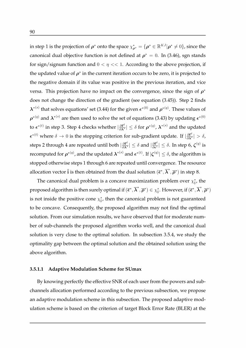
90
in step 1 is the projection of ρ∗ onto the space χ∗ρ∗ = ρ∗ ∈ RKJ |ρ∗ = 0, since the
canonical dual objective function is not defined at ρ∗ = 0. In (3.46), sgn stands
for sign/signum function and 0 < η << 1. According to the above projection, if
the updated value of ρ∗ in the current iteration occurs to be zero, it is projected to
the negative domain if its value was positive in the previous iteration, and vice
versa. This projection have no impact on the convergence, since the sign of ρ∗
does not change the direction of the gradient (see equation (3.45)). Step 2 finds
λ∗(s) that solves equations’ set (3.44) for the given ϵ∗(0) and ρ∗(q). These values of
ρ∗(q) and λ∗(s) are then used to solve the set of equations (3.43) by updating ϵ∗(0)
to ϵ∗(t) in step 3. Step 4 checks whether | ∂fd∂λ∗ | ≤ δ for ρ∗(q), λ∗(s) and the updated
ϵ∗(t) where δ → 0 is the stopping criterion for sub-gradient update. If | ∂fd∂λ∗ | > δ,
steps 2 through 4 are repeated until both | ∂fd∂λ∗ | ≤ δ and | ∂fd
∂ϵ∗| ≤ δ. In step 6, ζ(q) is
recomputed for ρ∗(q), and the updated λ∗(s) and ϵ∗(t). If |ζ(q)| ≤ δ, the algorithm is
stopped otherwise steps 1 through 6 are repeated until convergence. The resource
allocation vector i is then obtained from the dual solution (ϵ∗,λ∗,ρ∗) in step 8.
The canonical dual problem is a concave maximization problem over χ∗♯ , the
proposed algorithm is then surely optimal if (ϵ∗,λ∗,ρ∗) ∈ χ∗
♯ . However, if (ϵ∗,λ∗,ρ∗)
is not inside the positive cone χ∗♯ , then the canonical problem is not guaranteed
to be concave. Consequently, the proposed algorithm may not find the optimal
solution. From our simulation results, we have observed that for moderate num-
ber of sub-channels the proposed algorithm works well, and the canonical dual
solution is very close to the optimal solution. In subsection 3.5.4, we study the
optimality gap between the optimal solution and the obtained solution using the
above algorithm.
3.5.1.1 Adaptive Modulation Scheme for SUmax
By knowing perfectly the effective SNR of each user from the powers and sub-
channels allocation performed according to the previous subsection, we propose
an adaptive modulation scheme in this subsection. The proposed adaptive mod-
ulation scheme is based on the criterion of target Block Error Rate (BLER) at the
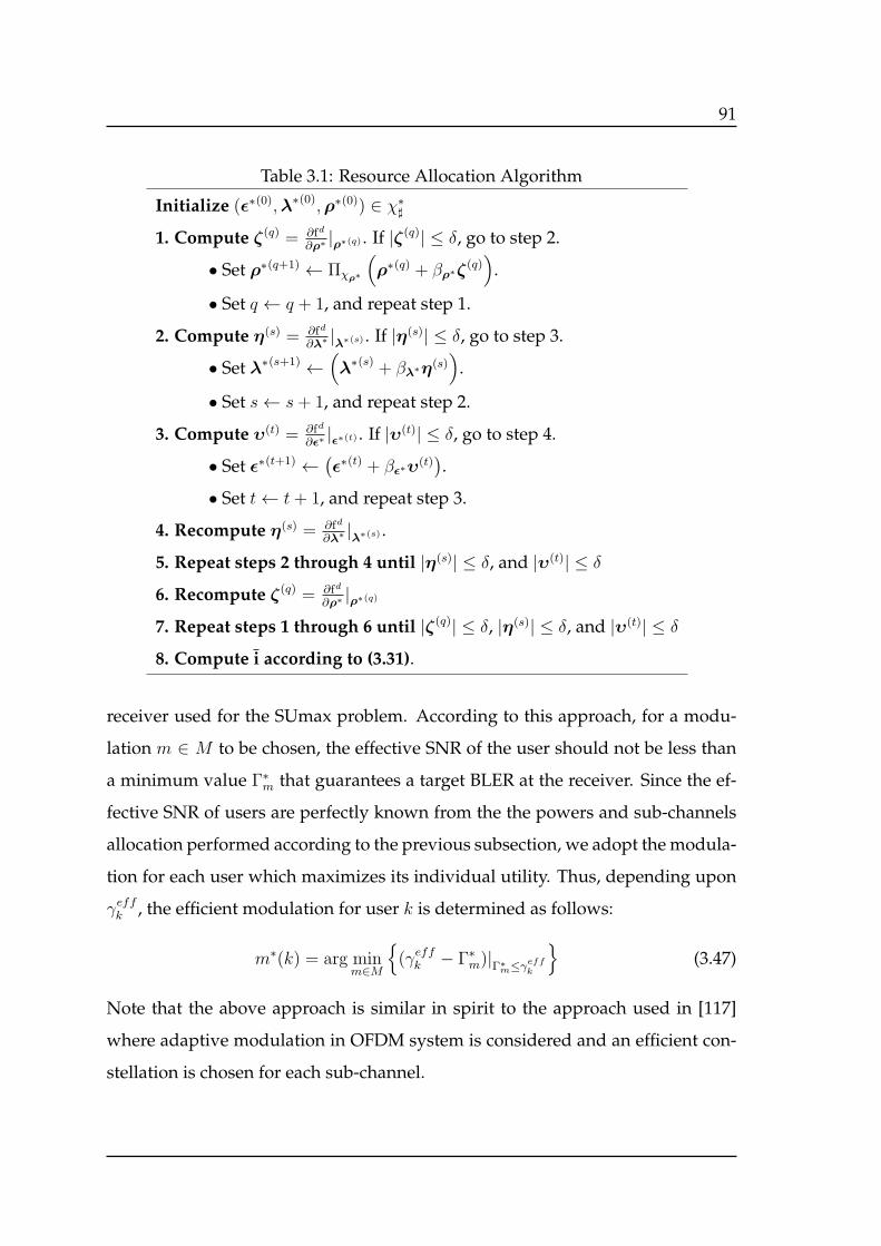
91
Table 3.1: Resource Allocation Algorithm
Initialize (ϵ∗(0),λ∗(0),ρ∗(0)) ∈ χ∗♯
1. Compute ζ(q) = ∂fd
∂ρ∗ |ρ∗(q) . If |ζ(q)| ≤ δ, go to step 2.
• Set ρ∗(q+1) ← Πχρ∗
(ρ∗(q) + βρ∗ζ(q)
).
• Set q ← q + 1, and repeat step 1.
2. Compute η(s) = ∂fd
∂λ∗ |λ∗(s) . If |η(s)| ≤ δ, go to step 3.
• Set λ∗(s+1) ←(λ∗(s) + βλ∗η(s)
).
• Set s← s+ 1, and repeat step 2.
3. Compute υ(t) = ∂fd
∂ϵ∗|ϵ∗(t) . If |υ(t)| ≤ δ, go to step 4.
• Set ϵ∗(t+1) ←(ϵ∗(t) + βϵ∗υ
(t)).
• Set t← t+ 1, and repeat step 3.
4. Recompute η(s) = ∂fd
∂λ∗ |λ∗(s) .
5. Repeat steps 2 through 4 until |η(s)| ≤ δ, and |υ(t)| ≤ δ
6. Recompute ζ(q) = ∂fd
∂ρ∗ |ρ∗(q)
7. Repeat steps 1 through 6 until |ζ(q)| ≤ δ, |η(s)| ≤ δ, and |υ(t)| ≤ δ
8. Compute i according to (3.31).
receiver used for the SUmax problem. According to this approach, for a modu-
lation m ∈ M to be chosen, the effective SNR of the user should not be less than
a minimum value Γ∗m that guarantees a target BLER at the receiver. Since the ef-
fective SNR of users are perfectly known from the the powers and sub-channels
allocation performed according to the previous subsection, we adopt the modula-
tion for each user which maximizes its individual utility. Thus, depending upon
γeffk , the efficient modulation for user k is determined as follows:
m∗(k) = arg minm∈M
(γeffk − Γ∗
m)|Γ∗m≤γeff
k
(3.47)
Note that the above approach is similar in spirit to the approach used in [117]
where adaptive modulation in OFDM system is considered and an efficient con-
stellation is chosen for each sub-channel.
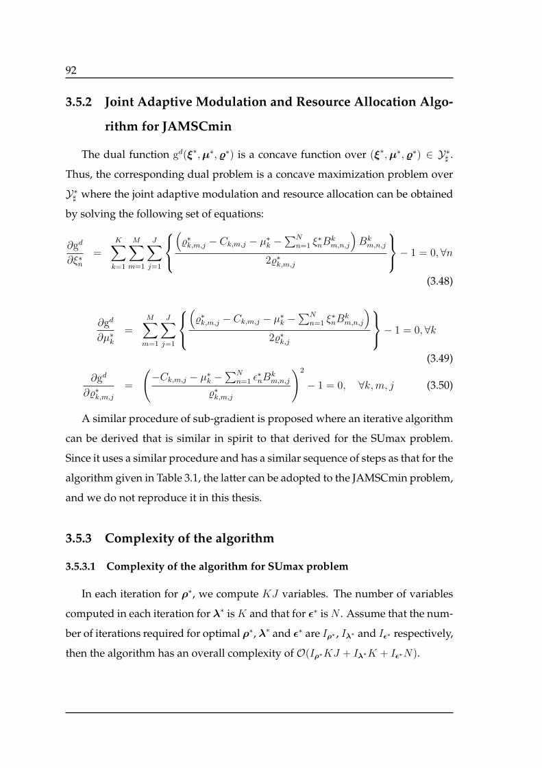
92
3.5.2 Joint Adaptive Modulation and Resource Allocation Algo-
rithm for JAMSCmin
The dual function gd(ξ∗,µ∗,ϱ∗) is a concave function over (ξ∗,µ∗,ϱ∗) ∈ Y∗♯ .
Thus, the corresponding dual problem is a concave maximization problem over
Y∗♯ where the joint adaptive modulation and resource allocation can be obtained
by solving the following set of equations:
∂gd
∂ξ∗n=
K∑k=1
M∑m=1
J∑j=1
(ϱ∗k,m,j − Ck,m,j − µ∗
k −∑N
n=1 ξ∗nB
km,n,j
)Bk
m,n,j
2ϱ∗k,m,j
− 1 = 0,∀n
(3.48)
∂gd
∂µ∗k
=M∑
m=1
J∑j=1
(ϱ∗k,m,j − Ck,m,j − µ∗
k −∑N
n=1 ξ∗nB
km,n,j
)2ϱ∗k,j
− 1 = 0,∀k
(3.49)
∂gd
∂ϱ∗k,m,j
=
(−Ck,m,j − µ∗
k −∑N
n=1 ϵ∗nB
km,n,j
ϱ∗k,m,j
)2
− 1 = 0, ∀k,m, j (3.50)
A similar procedure of sub-gradient is proposed where an iterative algorithm
can be derived that is similar in spirit to that derived for the SUmax problem.
Since it uses a similar procedure and has a similar sequence of steps as that for the
algorithm given in Table 3.1, the latter can be adopted to the JAMSCmin problem,
and we do not reproduce it in this thesis.
3.5.3 Complexity of the algorithm
3.5.3.1 Complexity of the algorithm for SUmax problem
In each iteration for ρ∗, we compute KJ variables. The number of variables
computed in each iteration for λ∗ is K and that for ϵ∗ is N . Assume that the num-
ber of iterations required for optimal ρ∗, λ∗ and ϵ∗ are Iρ∗ , Iλ∗ and Iϵ∗ respectively,
then the algorithm has an overall complexity of O(Iρ∗KJ + Iλ∗K + Iϵ∗N).

93
3.5.3.2 Complexity of the algorithm for JAMSCmin problem
The complexity of the proposed algorithm adopted to the JAMSCmin problem
isO(Iϱ∗KMJ + Iµ∗K + Iξ∗N) where Iϱ∗ , Iµ∗ and Iξ∗ are the numbers of iterations
needed for finding the optimal values of KMJ variables ϱ∗, K variables µ∗ and
the N variables ξ∗ respectively.
3.5.4 On the Optimality of the Algorithm
In this subsection, we analyze the gap between the optimal solution and the
solution obtained by using our proposed sub-gradient based algorithm. We per-
form the analysis for SUmax problem which is equally applicable to the JAM-
SCmin problem, and we will not repeat it in this paper. We start the analysis
by introducing a modified problem whose optimal solution is not necessary and
will not replace our actual problem but is used only to study the optimality gap
of our proposed algorithm. In our analysis, first we find the solution of the modi-
fied problem (which is a stationary point and may not be necessarily the optimal
solution of this modified problem). Then, we show in Theorem 3.5.1 that the so-
lution of this modified problem is equivalent to the optimal solution of the primal
problem with a slightly different values of the utilities Uk,j’s. Finally, in Corollary
3.5.1 we show that under certain conditions, the solution of the canonical dual
problem obtained using the algorithm in Table 3.1 provides the optimal solution
to the primal problem. Let us consider the following modified problem
(P) : maxϵ∗,λ∗,ρ∗
fd(ϵ∗,λ∗,ρ∗) (3.51)
s.t. ϵ∗ ≥ c (3.51a)
λ∗ ≥ d (3.51b)
where (c,d) ∈ (RN+ ,RK
+ ). We solve this problem using the standard Lagrangian
technique. Let (ϵ∗,λ∗,ρ∗) be the obtained solution. The corresponding Lagrangian
can be defined as
L(ϵ∗,λ∗,ρ∗,σϵ∗ ,σλ∗,σρ∗
) = fd(ϵ∗,λ∗,ρ∗)− (ϵ∗T − cT )σϵ∗ −σλ∗(λ∗T − dT ) (3.52)

94
where (σϵ∗ ,σλ∗) ∈ (RN ,RK) are the Lagrange multipliers associated to the con-
straints (3.51a-3.51b) respectively. The corresponding KKT conditions are:
∂L
∂ϵ∗= 0⇒
K∑k=1
J∑j=1
1
2ρ∗k,j
(Uk,j + ρ∗k,j − λ∗k −
N∑n=1
ϵ∗nAkn,j
)Ak
n,j
= 1 + σϵ∗
n ,∀n
(3.53)
∂L
∂λ∗ = 0⇒J∑
j=1
1
2ρ∗k,j
(Uk,j + ρ∗k,j − λ∗k −
N∑n=1
ϵ∗nAkn,j
)= 1 + σλ∗
k , ∀k (3.54)
∂L
∂ρ∗ = 0⇒
(Uk,j − λ∗k −
∑Nn=1 ϵ
∗nA
kn,j
ρ∗k,j
)2
− 1 = 0, ∀k, j (3.55)
The above equations can be solved using the sub-gradient based algorithm in
Table 3.1. Moreover, in order to ensure that the solution of (3.55) is obtained for
positive ρ∗, we can use the following projection in the update of ρ∗:
ρ∗(q) ← Πχρ∗
(Φ(q−1)
):= ρ∗k,j
(q) = argminρ∗k,j∈χ∗♯∥Φ(q−1)
k,j − ρ∗k,j∥ if Φk,j(q−1) ≤ 0,∀k, j
ρ∗k,j(q) = Φk,j
(q−1) otherwise.(3.56)
where Φ(q−1) = ρ∗(q−1)+βρ∗∂L∂ρ∗ |ρ∗(q−1) denotes the sub-gradient update, and where
βρ∗ is the step size. The above projection ensures the positivity of ρ∗.
Theorem 3.5.1. For Uk,j = Uk,j − 2θk,jρ∗k,j with θk,j ∈ −1, 0, 1, ∀k, j; there exists a
primal problem f(i) with utilities Uk,j replaced for Uk,j that can be solved optimally using
the algorithm in Table 3.1. The solution (ϵ∗,λ∗,ρ∗) of f(i) obtained using Table 3.1 is
equal to the solution of the modified problem
Proof. See Appendix A.3 for the proof.
Moreover, we have the following result which is the corollary of Theorem
3.5.1.
Corollary 3.5.1. If ρ∗k,j << Uk,j,∀k, j; then the solution of the canonical dual problem
obtained using the sub-gradient based algorithm (Table 3.1) provides a solution to the
primal problem which is very close to the optimal solution.
Proof. See Appendix A.4 for the proof.
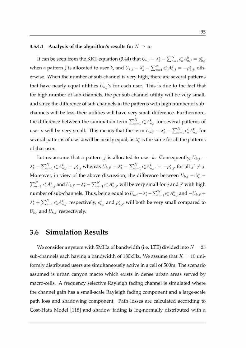
95
3.5.4.1 Analysis of the algorithm’s results for N →∞
It can be seen from the KKT equation (3.44) that Uk,j − λ∗k −∑N
n=1 ϵ∗nA
kn,j = ρ∗k,j
when a pattern j is allocated to user k, and Uk,j − λ∗k −∑N
n=1 ϵ∗nA
kn,j = −ρ∗k,j , oth-
erwise. When the number of sub-channel is very high, there are several patterns
that have nearly equal utilities Uk,j’s for each user. This is due to the fact that
for high number of sub-channels, the per sub-channel utility will be very small,
and since the difference of sub-channels in the patterns with high number of sub-
channels will be less, their utilities will have very small difference. Furthermore,
the difference between the summation term∑N
n=1 ϵ∗nA
kn,j for several patterns of
user k will be very small. This means that the term Uk,j − λ∗k −∑N
n=1 ϵ∗nA
kn,j for
several patterns of user k will be nearly equal, as λ∗k is the same for all the patterns
of that user.
Let us assume that a pattern j is allocated to user k. Consequently, Uk,j −
λ∗k −∑N
n=1 ϵ∗nA
kn,j = ρ∗k,j whereas Uk,j′ − λ∗k −
∑Nn=1 ϵ
∗nA
kn,j′ = −ρ∗k,j′ for all j′ = j.
Moreover, in view of the above discussion, the difference between Uk,j − λ∗k −∑Nn=1 ϵ
∗nA
kn,j and Uk,j′ − λ∗k −
∑Nn=1 ϵ
∗nA
kn,j′ will be very small for j and j′ with high
number of sub-channels. Thus, being equal to Uk,j−λ∗k−∑N
n=1 ϵ∗nA
kn,j and−Uk,j′+
λ∗k +∑N
n=1 ϵ∗nA
kn,j′ respectively, ρ∗k,j and ρ∗k,j′ will both be very small compared to
Uk,j and Uk,j′ respectively.
3.6 Simulation Results
We consider a system with 5MHz of bandwidth (i.e. LTE) divided intoN = 25
sub-channels each having a bandwidth of 180kHz. We assume that K = 10 uni-
formly distributed users are simultaneously active in a cell of 500m. The scenario
assumed is urban canyon macro which exists in dense urban areas served by
macro-cells. A frequency selective Rayleigh fading channel is simulated where
the channel gain has a small-scale Rayleigh fading component and a large-scale
path loss and shadowing component. Path losses are calculated according to
Cost-Hata Model [118] and shadow fading is log-normally distributed with a
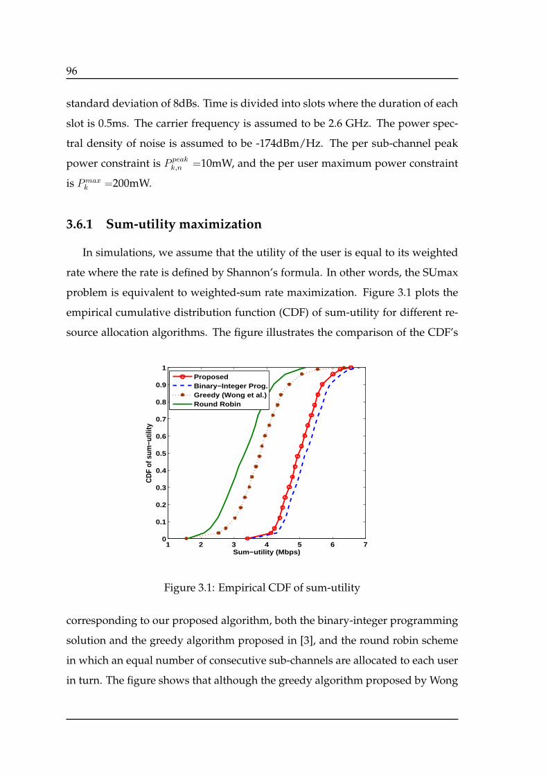
96
standard deviation of 8dBs. Time is divided into slots where the duration of each
slot is 0.5ms. The carrier frequency is assumed to be 2.6 GHz. The power spec-
tral density of noise is assumed to be -174dBm/Hz. The per sub-channel peak
power constraint is P peakk,n =10mW, and the per user maximum power constraint
is Pmaxk =200mW.
3.6.1 Sum-utility maximization
In simulations, we assume that the utility of the user is equal to its weighted
rate where the rate is defined by Shannon’s formula. In other words, the SUmax
problem is equivalent to weighted-sum rate maximization. Figure 3.1 plots the
empirical cumulative distribution function (CDF) of sum-utility for different re-
source allocation algorithms. The figure illustrates the comparison of the CDF’s
1 2 3 4 5 6 70
0.1
0.2
0.3
0.4
0.5
0.6
0.7
0.8
0.9
1
Sum−utility (Mbps)
CD
F of
sum
−util
ity
ProposedBinary−Integer Prog.Greedy (Wong et al.)Round Robin
Figure 3.1: Empirical CDF of sum-utility
corresponding to our proposed algorithm, both the binary-integer programming
solution and the greedy algorithm proposed in [3], and the round robin scheme
in which an equal number of consecutive sub-channels are allocated to each user
in turn. The figure shows that although the greedy algorithm proposed by Wong
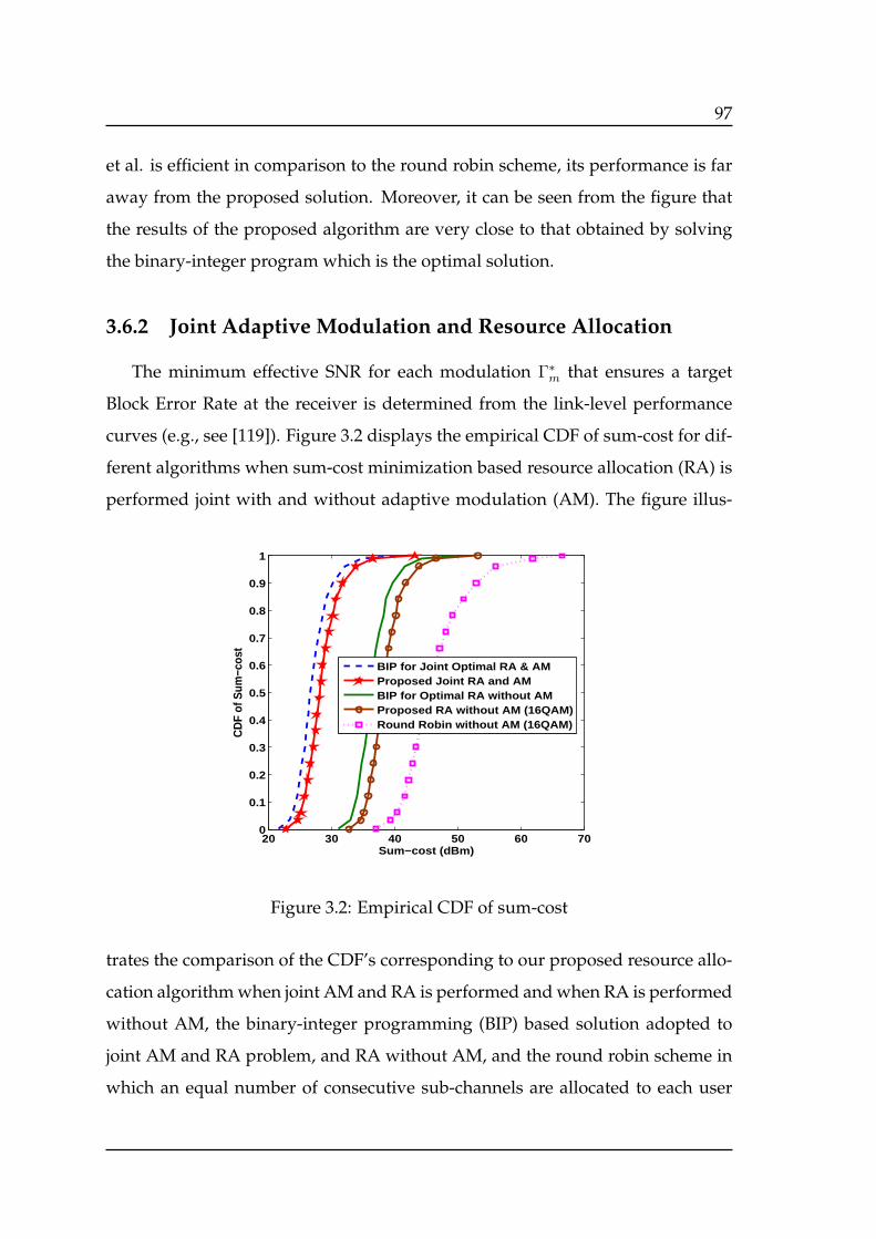
97
et al. is efficient in comparison to the round robin scheme, its performance is far
away from the proposed solution. Moreover, it can be seen from the figure that
the results of the proposed algorithm are very close to that obtained by solving
the binary-integer program which is the optimal solution.
3.6.2 Joint Adaptive Modulation and Resource Allocation
The minimum effective SNR for each modulation Γ∗m that ensures a target
Block Error Rate at the receiver is determined from the link-level performance
curves (e.g., see [119]). Figure 3.2 displays the empirical CDF of sum-cost for dif-
ferent algorithms when sum-cost minimization based resource allocation (RA) is
performed joint with and without adaptive modulation (AM). The figure illus-
20 30 40 50 60 700
0.1
0.2
0.3
0.4
0.5
0.6
0.7
0.8
0.9
1
Sum−cost (dBm)
CD
F of
Sum
−cos
t
BIP for Joint Optimal RA & AMProposed Joint RA and AMBIP for Optimal RA without AMProposed RA without AM (16QAM)Round Robin without AM (16QAM)
Figure 3.2: Empirical CDF of sum-cost
trates the comparison of the CDF’s corresponding to our proposed resource allo-
cation algorithm when joint AM and RA is performed and when RA is performed
without AM, the binary-integer programming (BIP) based solution adopted to
joint AM and RA problem, and RA without AM, and the round robin scheme in
which an equal number of consecutive sub-channels are allocated to each user
98
in turn and minimum possible power is allocated to the users while ensuring
their target data rates. The round robin scheme is used as a baseline scheme for
comparison. The RA without AM scenario considers 16QAM as the modulation
scheme. The proposed RA with fixed modulation outperforms the round robin
scheme which is not unexpected. The figure shows that the joint AM and RA
results in a significant performance improvement over the RA without AM. The
performance of the proposed algorithm can be depicted from the fact that the re-
sults of the proposed algorithm nearly overlap with that of the BIP based solution
both for joint AM and RA, and RA with fixed modulation scheme. We recall that
the BIP based solution is the optimal solution.
3.7 Conclusion
This chapter studies resource allocation and adaptive modulation in uplink
SC-FDMA systems. Sum-utility maximization, and joint adaptive modulation
and sum-cost minimization problems are considered whose optimal solutions
are exponentially complex in general. A polynomial-complexity optimization
framework that is inspired from the recently developed canonical duality the-
ory is derived for the solution of both the problems. Based on the resource allo-
cation performed by the proposed framework, an adaptive modulation scheme
is also proposed for the sum-utility maximization problem that determines the
best constellation for each user. The optimization problems are first formulated
as binary-integer programming problems and then, each binary-integer problem
is transformed into a canonical dual problem in the continuous space which is
a concave maximization problem. The transformation of the problem in con-
tinuous space significantly improves the performance of the system in terms of
complexity. The proposed continuous space optimization framework has a poly-
nomial complexity that is a significant improvement over exponential complex-
ity. It is proved analytically that that under certain conditions, the solution of the
canonical dual problem is identical to the solution of the primal problem. How-

99
ever, if the dual solution does not satisfy these conditions then the optimality can
not be guaranteed. Some bounds on the sub-optimality of the proposed algo-
rithms if these conditions are not satisfied are also explored. The performance of
the proposed canonical dual framework is assessed by comparing it with the ex-
isting algorithms in the literature. The numerical results show that the proposed
framework provides integer solution to each problem which is very close to that
obtained by solving its equivalent binary-integer program.

100
101
Chapter 4
Joint Power Control and Rate
Adaptation for Video Streaming in
Wireless Networks
4.1 Introduction
In this chapter, we consider a cross-layer optimization framework for joint
power control and rate adaptation for video streaming in wireless networks with
interference. We assume that in the network, each node demand for better qual-
ity video while its channel and the interference caused to it by the other nodes
are both time-varying. Since video streaming has stringent delay requirements,
the packets arrived in the queue of a node should be transmitted in a given tar-
get number of slots otherwise they will be dropped. In addition, there should
be a fairness/satisfaction criterion for faire utilization of the network resources
among the multiple nodes. In order to exploit the time diversity of the time-
varying channels, the video rate of each node should be adapted in accordance
to its channel conditions. Moreover, the transmit power of each node should be
controlled in order to efficiently utilize the power. The power control is not only
efficient in terms of power consumption but with the decrease in the transmit
power of a node, the interference caused to other nodes will also reduce. How-
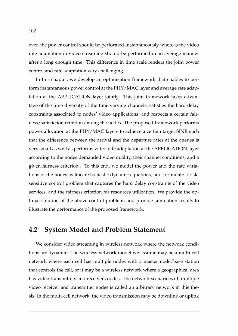
102
ever, the power control should be performed instantaneously whereas the video
rate adaptation in video streaming should be performed in an average manner
after a long enough time. This difference in time scale renders the joint power
control and rate adaptation very challenging.
In this chapter, we develop an optimization framework that enables to per-
form instantaneous power control at the PHY/MAC layer and average rate adap-
tation at the APPLICATION layer jointly. This joint framework takes advan-
tage of the time diversity of the time varying channels, satisfies the hard delay
constraints associated to nodes’ video applications, and respects a certain fair-
ness/satisfiction criterion among the nodes. The proposed framework performs
power allocation at the PHY/MAC layers to achieve a certain target SINR such
that the difference between the arrival and the departure rates at the queues is
very small as well as performs video rate adaptation at the APPLICATION layer
according to the nodes demanded video quality, their channel conditions, and a
given fairness criterion . To this end, we model the power and the rate varia-
tions of the nodes as linear stochastic dynamic equations, and formulate a risk-
sensitive control problem that captures the hard delay constraints of the video
services, and the fairness criterion for resources utilization. We provide the op-
timal solution of the above control problem, and provide simulation results to
illustrate the performance of the proposed framework.
4.2 System Model and Problem Statement
We consider video streaming in wireless network where the network condi-
tions are dynamic. The wireless network model we assume may be a multi-cell
network where each cell has multiple nodes with a master node/base station
that controls the cell, or it may be a wireless network where a geographical area
has video transmitters and receivers nodes. The network scenario with multiple
video receiver and transmitter nodes is called an arbitrary network in this the-
sis. In the multi-cell network, the video transmission may be downlink or uplink
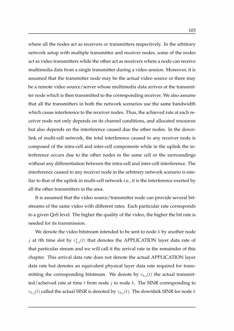
103
where all the nodes act as receivers or transmitters respectively. In the arbitrary
network setup with multiple transmitter and receiver nodes, some of the nodes
act as video transmitters while the other act as receivers where a node can receive
multimedia data from a single transmitter during a video session. Moreover, it is
assumed that the transmitter node may be the actual video source or there may
be a remote video source/server whose multimedia data arrives at the transmit-
ter node which is then transmitted to the corresponding receiver. We also assume
that all the transmitters in both the network scenarios use the same bandwidth
which cause interference to the receiver nodes. Thus, the achieved rate at each re-
ceiver node not only depends on its channel conditions, and allocated resources
but also depends on the interference caused due the other nodes. In the down-
link of multi-cell network, the total interference caused to any receiver node is
composed of the intra-cell and inter-cell components while in the uplink the in-
terference occurs due to the other nodes in the same cell or the surroundings
without any differentiation between the intra-cell and inter-cell interference. The
interference caused to any receiver node in the arbitrary network scenario is sim-
ilar to that of the uplink in multi-cell network i.e., it is the interference exerted by
all the other transmitters in the area.
It is assumed that the video source/transmitter node can provide several bit-
streams of the same video with different rates. Each particular rate corresponds
to a given QoS level. The higher the quality of the video, the higher the bit rate is
needed for its transmission.
We denote the video bitstream intended to be sent to node k by another node
j at tth time slot by r∗k,j(t) that denotes the APPLICATION layer data rate of
that particular stream and we will call it the arrival rate in the remainder of this
chapter. This arrival data rate does not denote the actual APPLICATION layer
data rate but denotes an equivalent physical layer data rate required for trans-
mitting the corresponding bitstream. We denote by rk,j(t) the actual transmit-
ted/acheived rate at time t from node j to node k. The SINR corresponding to
rk,j(t) called the actual SINR is denoted by γk,j(t). The downlink SINR for node k
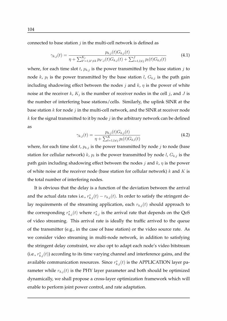
104
connected to base station j in the multi-cell network is defined as
γk,j(t) =pk,j(t)Gk,j(t)
η +∑Kj
k′=1,k′ =k pk′,j(t)Gk,j(t) +∑J
l=1,l =j pl(t)Gk,l(t)(4.1)
where, for each time slot t, pk,j is the power transmitted by the base station j to
node k, pl is the power transmitted by the base station l, Gk,j is the path gain
including shadowing effect between the nodes j and k, η is the power of white
noise at the receiver k, Kj is the number of receiver nodes in the cell j, and J is
the number of interfering base stations/cells. Similarly, the uplink SINR at the
base station k for node j in the multi-cell network, and the SINR at receiver node
k for the signal transmitted to it by node j in the arbitrary network can be defined
as
γk,j(t) =pk,j(t)Gk,j(t)
η +∑K
l=1,l =j pl(t)Gk,l(t)(4.2)
where, for each time slot t, pk,j is the power transmitted by node j to node (base
station for cellular network) k, pl is the power transmitted by node l, Gk,j is the
path gain including shadowing effect between the nodes j and k, η is the power
of white noise at the receiver node (base station for cellular network) k and K is
the total number of interfering nodes.
It is obvious that the delay is a function of the deviation between the arrival
and the actual data rates i.e., r∗k,j(t) − rk,j(t). In order to satisfy the stringent de-
lay requirements of the streaming application, each rk,j(t) should approach to
the corresponding r∗k,j(t) where r∗k,j is the arrival rate that depends on the QoS
of video streaming. This arrival rate is ideally the traffic arrived to the queue
of the transmitter (e.g., in the case of base station) or the video source rate. As
we consider video streaming in multi-node network, in addition to satisfying
the stringent delay constraint, we also opt to adapt each node’s video bitstream
(i.e., r∗k,j(t)) according to its time varying channel and interference gains, and the
available communication resources. Since r∗k,j(t) is the APPLICATION layer pa-
rameter while rk,j(t) is the PHY layer parameter and both should be optimized
dynamically, we shall propose a cross-layer optimization framework which will
enable to perform joint power control, and rate adaptation.
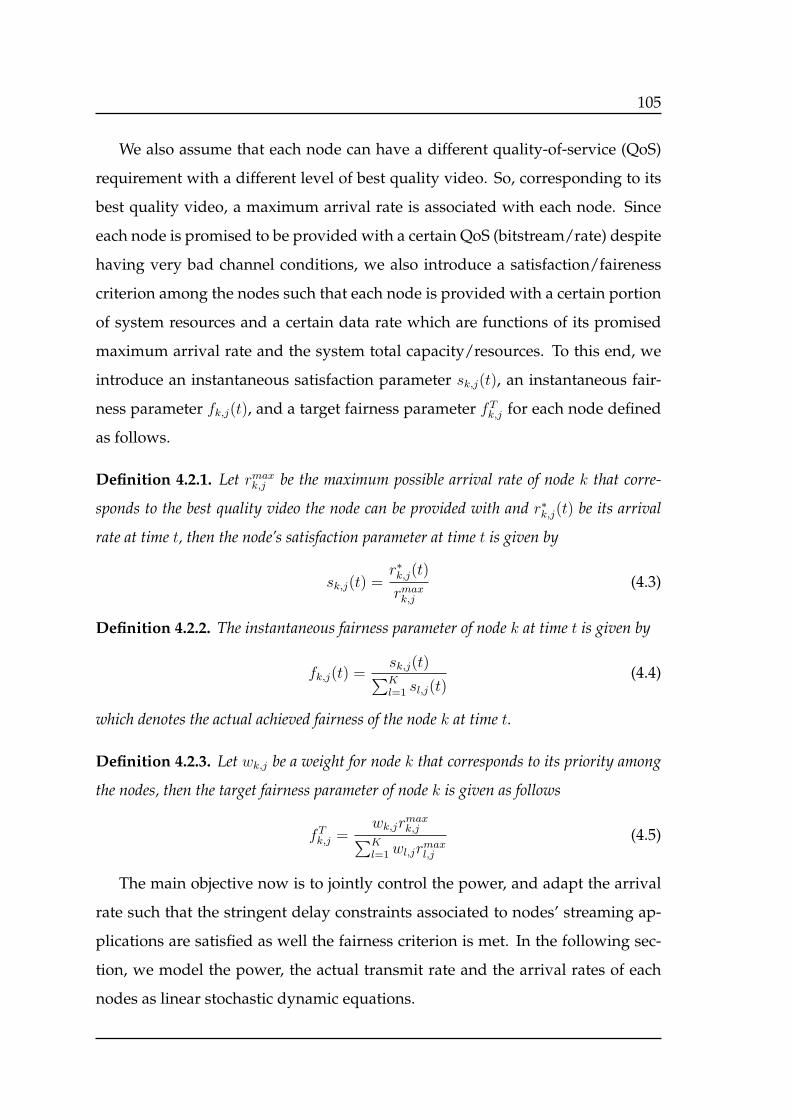
105
We also assume that each node can have a different quality-of-service (QoS)
requirement with a different level of best quality video. So, corresponding to its
best quality video, a maximum arrival rate is associated with each node. Since
each node is promised to be provided with a certain QoS (bitstream/rate) despite
having very bad channel conditions, we also introduce a satisfaction/faireness
criterion among the nodes such that each node is provided with a certain portion
of system resources and a certain data rate which are functions of its promised
maximum arrival rate and the system total capacity/resources. To this end, we
introduce an instantaneous satisfaction parameter sk,j(t), an instantaneous fair-
ness parameter fk,j(t), and a target fairness parameter fTk,j for each node defined
as follows.
Definition 4.2.1. Let rmaxk,j be the maximum possible arrival rate of node k that corre-
sponds to the best quality video the node can be provided with and r∗k,j(t) be its arrival
rate at time t, then the node’s satisfaction parameter at time t is given by
sk,j(t) =r∗k,j(t)
rmaxk,j
(4.3)
Definition 4.2.2. The instantaneous fairness parameter of node k at time t is given by
fk,j(t) =sk,j(t)∑Kl=1 sl,j(t)
(4.4)
which denotes the actual achieved fairness of the node k at time t.
Definition 4.2.3. Let wk,j be a weight for node k that corresponds to its priority among
the nodes, then the target fairness parameter of node k is given as follows
fTk,j =
wk,jrmaxk,j∑K
l=1wl,jrmaxl,j
(4.5)
The main objective now is to jointly control the power, and adapt the arrival
rate such that the stringent delay constraints associated to nodes’ streaming ap-
plications are satisfied as well the fairness criterion is met. In the following sec-
tion, we model the power, the actual transmit rate and the arrival rates of each
nodes as linear stochastic dynamic equations.
106
4.3 Stochastic Framework for Joint Power Control and
Rate Adaptation
We start our analysis by proving that the probability distribution function of
the Channel to Interference and Noise Ratio (CINR), gk,j(t) can be approximated
by a lognormal distribution. The relation between CINR and SINR is given by
γk,j(t) = pk,j(t)gk,j(t). We then use this result to formulate the dynamics of the
node’s power and data rate as stochastic linear equations.
4.3.1 CINR Probability Distribution Function
Proposition 4.3.1. The probability distribution function of CINR for the downlink
in the multi-cell network can be approximated by a Lognormal distribution.
Proof. The proof and evaluation of the mean and variance of the corresponding
lognormal distribution are given throughout this section.
We start our analysis by writing the expression of the CINR. The correspond-
ing CINR value at tth time slot between nodes k and j is determined as follows:
gk,j(t) =Gk,j(t)
η +∑Kj
k′=1,k′ =k pk′,j(t)Gk,j(t) +∑J
l=1,l =j pl(t)Gk,l(t)(4.6)
In general, Gk,j(t) is proportional to d−µk,j 10
sk,j/10|hk,j(t)|2 where dk,j is the distance
between user k and base station j, µ is the path loss slope (µ = 3, 4 in macro cell
and µ = 2 in micro cell) and 10sk,j/10 corresponds to Lognormal shadowing. The
variable sk,j has then a Gaussian distribution (10sk,j/10 is lognormal) with zero
mean and standard deviation σs (σ2s between 8 and 12 dB) [120]. The coefficient
hk,j(t) denotes the fast fading at tth time slot for the channel between node k and
base station j. Since we consider the instantaneous CINR, the time index t will
be ignored in this analysis for simplicity. The CINR inverse is then given by
1
gk,j=
∑Jl=1,l =j pl(
dk,ldk,j
)−µ10sk,l/10|hk,l|2
10sk,j/10|hk,j|2+
η
d−µk,j
10sk,j/10|hk,j|2+∑k′ =k
Pk′,j
107
Let us consider the variable yk,l = 10sk,l/10|hk,l|2. The variable yk,l is then the
product of two variables, lognormal and chi-square (|hk,j|2 has a central Chi-
Square distribution with two degrees of freedom since |hk,j| has a rayleigh dis-
tribution). The probability distribution function of yk,l is then given by
pdf(yk,l) =
∫ ∞
0
e−yk,l/z1
z
1√2πθσk,jz
e− (log(z)−θµs)
2
2θ2σ2s dz (4.7)
where θ = ln(10)/10. Using the following approximation (from [121])
∫ ∞
0
e−g/z 1
z
1√2πθσsz
e− (log(z)−θµs)
2
2θ2σ2s dz ≃ 1√
2πσfge
(−
(log(g)−µk,l)2
2σ2k,l
)(4.8)
Note that this approximation is valid for some values of the variance of log-
normally distributed variable 10sk,j/10. The distribution of yk,l is then given by
pdf(yk,l) =1√
2πσk,lyk,le−
(log(yk,l)−µk,l)2
2σ2k,l (4.9)
where µk,l = −C + θµs = −C and σ2k,l = ζ(2) + θ2σ2
s . C is the Euler Constant
(C=0.5772) and ζ(2) = π2/6 is the Riemann-Zeta function. This approximation
results from the fact that the product or the sum of a log-normal variable with
other variables of sharper frequency distributions (e.g., exponential, Chi-square,
etc.) is dominated at the higher order moments by the log-normal distribution
with largest logarithm variance [122]. Similarly, yk,j = 10sk,j/10|hk,j|2 can be ap-
proximated by a lognormal variable with parameters µk,j = −C + θµs = −C and
σ2k,j = ζ(2) + θ2σ2
s (yk,j can then be written as es′k where s′k is a gaussian variable
with mean µs′k= µk,j and variance σ2
s′k= σ2
k,j).
We now considerXk =η
d−µk,j
+∑J
l=1,l =j pl(dk,ldk,j
)−µ10sk,l/10|hk,l|2 which can be writ-
ten as follows
Xk =∑J
l=1,l =j(η
(J−1)d−µk,j
+ pl(dk,ldk,j
)−µ10sk,l/10|hk,l|2)
The variable ( η
(J−1)d−µk,j
+ pl(dk,ldk,j
)−µ10sk,l/10|hk,l|2) has a lognormal distribution with
mean valueEk,l =η
(J−1)d−µk,j
+pl(dk,ldk,j
)−µeµk,l+σ2k,l/2 and variance Vk,l = p2l (
dk,ldk,j
)−2µ(eσ2k,l−
1)e2µk,l+σ2k,l . Therefore, Xk is the sum of independent lognormal variables. Ac-
cording to [123], using the approximation of Fenton-Wilkinson, the sum of a
108
finite number of independent log-normal variables can be approximated by a
log-normal variable. The first two order moments (respectively u(1)k and u
(2)k ) of
the equivalent log-normal variable can be computed, using the Fenton-Wilkinson
(FW) approximation, as follows [123] [124]:
u(1)k =
∑Jl=1,l =j Ek,l (4.10)
u(2)k =
∑Jl=1,l =j(E
2k,l + Vk,l) + 2
∑J−1l=1,l =j
∑Jl′=l+1,l′ =j Ek,lEk,l′ (4.11)
Therefore, Xk = η
d−µk,j
+∑J
l=1,l =j pl(dk,ldk,j
)−µ10sk,l/10 can be modeled/represented by
es′′k where s′′k has now a gaussian distribution with mean µs′′k
and variance σ2s′′k
given by
µs′′k=
(2 ln(u
(1)k )− 1
2ln(u
(2)k )
)(4.12)
σ2s′′k
=
(ln(u
(2)k )− 2 ln(u
(1)k )
)(4.13)
The CINR expression can then be written as:
gk,j =1∑
k′ =k pk′,j + e(s′′k−s′k)
(4.14)
e(s′′k−s′k) has also a lognormal distribution with mean µk and variance σ2
k given by
µk = µs′′k− µs′k
(4.15)
σ2k = σ2
s′′k+ σ2
s′k(4.16)
The probability distribution function of CINR is then approximated by a lognor-
mal distribution with parameters µf and σ2f given respectively by
µf =1
2ln
∑k′ =k
pk′,j + eµk+σ2k/2
2
+(eσ
2k − 1
)e2µk+σ2
k
−2 ln
[∑k′ =k
pk′,j + eµk+σ2k/2
]
σ2f = ln
∑k′ =k
pk′,j + eµk+σ2k/2
2
+(eσ
2k − 1
)e2µk+σ2
k
− 2 ln
[∑k′ =k
pk′,j + eµk+σ2k/2
]
This completes the proof.
109
Proposition 4.3.2. The probability distribution function of the CINR for the arbitrary
network and for the uplink in the multi-cell network can be approximated by lognormal
distribution
Proof. The CINR value at tth time slot between nodes k and j is given as follows:
gk,j(t) =Gk,j(t)
η +∑J
l=1,l =j pl(t)Gk,l(t)(4.17)
By performing a similar procedure as performed for the analysis of the downlink
CINR, and by similar arguments, the inverse of the CINR (4.17) is given by
1
gk,j=
∑Jl=1,l =j pl(
dk,ldk,j
)−µ10sk,l/10|hk,l|2 + η
d−µk,j
10sk,j/10|hk,j|2(4.18)
The time index t is ignored for simplicity. Furthermore, the variables d−µk,j , sk,j , etc.,
have the same definitions as in the previous subsection. The denominator term
in (4.18) as proved in the previous subsection can be approximated by lognormal
distribution with parameter µk,j , and σ2k,j defined therein; and it (the denominator
term) can be written as es′k where s′k, is a Gaussian variable with mean µs′k= µk,j ,
and variance σ2s′k
= σ2k,j . Similarly, it is proved in the previous subsection that the
term in the nominator of (4.18) has a lognormal distribution with given values of
mean Ek,l, and variance Vk,l; and can be modeled as es′′k where s′′k, has Gaussian
distribution with mean µs′′k, and variance σ2
s′′k. By using the Fenton-Wilkinson
approximation, and following a similar procedure to that of the previous subsec-
tion, it can be established that the probability distribution function of the CINR
(4.17) can be approximated by a lognormal distribution with parameters µf , and
σ2f given respectively by
µf = µs′k− µs′′k
(4.19)
σ2f = σ2
s′k+ σ2
s′k(4.20)
This completes the proof of the proposition.
110
4.3.2 Stochastic Linear Dynamic Model for Power Control
In this subsection, we develop a stochastic linear dynamic framework for
adaptive power control.
Proposition 4.3.1. The fast power control can be written by the following linear stochas-
tic dynamic equation:
γk,j(t+ 1) = 1− βk,jγk,j(t) + βk,jγ∗k,j(t) + ng(t) (4.21)
where βk,j is a given step size, ng(t) is a zero mean noise term, and the notation (.) stands
for 10 log(.).
Proof. We provide here that how the above linear dynamic equation is obtained.
Let γ∗k,n(t) denotes the target SINR that corresponds to the arrival rate which
should be achieved at the receiver so that the video bitstream is successfully de-
coded with a given target bit error rate. Moreover, in order that the actual data
rate approaches the arrival rate, the only parameter that can be controlled is the
power such that the actual SINR γk,n(t) approaches the target SINR γ∗k,n(t). This is
due to that γk,n(t) = pk,n(t)gk,n(t) where gk,n(t) is channel dependent and can not
be controlled. Since controlling the power is equivalent to controlling the SINR,
we will perform our analysis in terms of SINR values throughout this chapter. To
this end, we proceed as follows. In view of the Shannon capacity formula, the
actual data rate rk,j(t) can be related to the SINR γk,j(t) as follows
rk,j(t) =1
2log2 (1 + γk,j(t)) (4.22)
Since video streaming requires high data rate rk,j(t), the corresponding SINR
γk,j(t) should be high during normal network operation. Therefore, we assume
that the network operates in high SINR regime where for successfully decoding
the video bitstream, the receiver node’s achieved SINR>> 1. Let x = 10 log x that
denotes the decibel (dB) value of the variable x. Thus, for γk,j(t) >> 1, the rate
rk,j(t) is proportional to γk,j(t).
In order to find the pk,j(t) such that the actual SINR γk,j(t) approaches the tar-
get level γ∗k,j(t), we will model the power variation from one time slot to another
111
as a stochastic linear dynamic equation. To this end, we use the adaptive power
control algorithm proposed in [125] which is inspired from [126]. We will then
introduce an artificial control upk,j(t) to this power control algorithm in order to
drive γk,j(t) towards γ∗k,j(t). The introduction of this control term will be per-
formed later in Section 4.4. In [126], an adaptive predictive power control algo-
rithm is developed which is based on the known idea of power control in wireless
communication where the receiver compares its achieved SINR to its target and
sends a one bit power signal to the transmitter for updating the transmit power
accordingly. Thus, we assume that each node adapts its power from one time slot
to another according to the following power control algorithm
pk,j(t+ 1) = ψbk,j(t)
k,j pk,j(t) (4.23)
where ψk,j > 1 is a parameter between 1 and 3 and may vary from one node to
another, and
bk,j(t+ 1) = sgn[γ∗k,j(t)− γk,j(t)] (4.24)
where sgn stands for sign/signum function. By taking the logarithm of both sides
of (4.23), and then multiplying it by 10, we arrive at
pk,j(t+ 1) = pk,j(t) + ψk,jγ∗k,j(t)− γk,j(t) (4.25)
where pk,j(t) = 10 log(pk,j(t)), ψk,j(t) = 10 log(ψk,j(t)), and where the notation
log(.) means the common logarithm i.e., logarithm to base 10. As logarithm is a
monotonically increasing function, an equivalent power control algorithm can be
written as follows
pk,j(t+ 1) = pk,j(t) + βk,jγ∗k,j(t)− γk,j(t) (4.26)
where γ∗k,j(t) = 10 log(γ∗k,j), and βk,j is a given step size that may vary from one
node to another. We now transform the power terms in the above power control
equation into respective SINR terms as follows. As γk,j(t) = pk,j(t)gk,j(t) then in
decibel scale we have
γk,j(t) = pk,j(t) + gk,j(t) (4.27)
112
where gk,j(t) = 10 log(gk,j(t)). As gk,j(t) has lognormal distribution, gk,j(t) has
then gaussian distribution and its variation can be modeled as follows
gk,j(t+ 1) = gk,j(t) + ng(t) (4.28)
where ng(t) is zero mean gaussian noise term. By combining (4.26), and (4.28), the
power control algorithm is then given in the form of an equivalent actual SINR
variation model as follows
γk,j(t+ 1) = 1− βk,jγk,j(t) + βk,jγ∗k,j(t) + ng(t) (4.29)
In the above power control algorithm we have not introduced any notion of
power constraint. Since by increasing its power, a node may severely affect other
nodes by causing them high level of interference, it should be assured that at
any time instant the nodes does not increase their power above a certain feasible
level. We assume that each node should choose its power from a given feasi-
ble set of powers pk,j(t) ≤ pmax where pmax is the maximum acceptable power a
node can transmit and it is the amount of power for which the SINR level of that
node reaches a given value γmax. Since the channels and interference gains are
time varying, the corresponding value of maximum feasible power will also vary
for each node and will be different for different nodes. Thus, in order to formu-
late this power constraint, we introduce a new variable pfk,j(t) called the feasible
power which denotes the maximum power a node j can transmit at time slot t.
Let γfk,j(t) denotes the value of SINR level when pfk,j(t) is transmitted, then, we
have the following result on the feasible power variation.
Proposition 4.3.2. The feasible power varies according to the following linear stochastic
dynamic model
γfk,j(t+ 1) = 1− ϵk,jγfk,j(t) + ϵk,j(t)γmax + ng(t) (4.30)
where ϵk,j is a given step size.
113
Proof. The feasible power variation can be modeled as follows
pfk,j(t+ 1) = pfk,j(t) + ϵk,jγmax − γfk,j(t) (4.31)
where ϵk,j is a given step size, and the notations (.) denote the decibel values.
By using a similar argument used for the transformation of (4.26) into (4.29), the
above feasible power variations can be written in terms of SINR level (in dBs) as
follows
γfk,j(t+ 1) = 1− ϵk,jγfk,j(t) + ϵk,j(t)γmax + ng(t) (4.32)
In order to ensure that pk,j(t) ≤ pfk,j(t) at any time slot t, the arrival rate r∗k,j(t)
should be adapted such that γ∗k,j(t) ≤ γfk,j(t). The procedure of integrating the
notion of feasible power into arrival rate adaptation is provided in the following
subsection.
4.3.3 Stochastic Linear Dynamic Model for Rate Adaptation
Proposition 4.3.3. The video rate/arrival rate can be adapted using the following stochas-
tic linear equation
γ∗k,j(t+ 1) = γ∗k,j(t) + ξk,j(t)γfk,j(t)− γ
∗k,j(t)
+ξk,j(t)
fTk,j − fk,j(t)
γ∗k,j(t) + δtnt(t) (4.33)
where ξk,j(t) is a given step size and δt, and nt(t) are small positive numbers.
Proof. As in video streaming, the video bitstream (i.e., r∗k,j(t)) for each node should
be chosen by truncating/switching the bitstream according to its varying channel
conditions and the available system resources, we now develop a stochastic lin-
ear dynamic model for arrival rate adaptation. We recall that the so-called arrival
rate r∗k,j(t) is not the actual application layer data rate but denotes an equiva-
lent physical layer data rate required for the corresponding bitstream. Due to the
114
inter-dependent nature of the video frames in video transmission, the video qual-
ity can be better determined by the total resource allocation during a time win-
dow, which should be long enough for the user to determine the best bitstream for
the video that could be supported by the physical layer. One way of dealing with
this sort of problems is to consider a time average model for resource allocation
such that the average actual/achieved data rate during the given time window
approaches to the average arrival rate. This time average model is suitable for
video rate adaptation but we aim to perform the power control instantaneously
joint with the video rate adaptation by developing a joint framework. Thus, we
will propose a model for arrival rate adaptation which will allow us to formulate
a joint power control and arrival rate adaptation framework that will enable to
adapt the arrival rate in an average sense while allowing the power control in-
stantaneously. We will also integrate the satisfaction/faireness criterion among
the nodes to our arrival rate adaptation model.
We start by writing the arrival rate adaptation model that is based on time
average values and will then convert it into an equivalent instantaneous model.
We denote by rfk,j(t) the feasible data rate that corresponds to γfk,j(t). Let denote
the time average of a variable x(t) by x(t) = 1WT
∑tτ=t0
x(τ) where WT = t − t0
is the time segment called the time window during which the arrival rate should
not change. Then, our time average model for arrival rate adaptation is given as
follows
r∗k,j(t+ 1) = r∗k,j(t) + ρk,jrfk,j(t)− r∗k,j(t)+ ρk,jfT
k,j − fk,j(t)r∗k,j(t) + nt(t)(4.34)
where ρk,j is a given positive step size. The second term to the R.H.S of the above
equation ensures that the average arrival rate of the node should be in the feasible
region such that the power transmitted does not exceed the maximum value of
its feasible power in average where as the third term ensures the fairness among
users. If both the feasible power constraint and fairness constraints are satisfied,
the arrival rate is still increased by nt(t) which has a very small value. This reflects
the desire of each receiver node to have the best possible quality video, and will
drive the system to converge at high possible arrival rates. The term nt(t) can be

115
assumed as a Gaussian-distributed variable of a positive mean and a very small
variance so that its value is always positive.
In order to be able to develop a joint framework which adapts the arrival rate
in average sense while performs instantaneous power control, we propose an
equivalent model for arrival rate adaptation as given by
r∗k,j(t+ 1) = r∗k,j(t) + ξk,j(t)rfk,j(t)− r∗k,j(t)
+ξk,j(t)fTk,j − fk,j(t)r∗k,j(t) + δtnt(t) (4.35)
where δt = 1/WT is a small number, and ξk,j(t) is a time varying step size defined
as
ξk,j(t) =
1 if t = mWT
0 elsewhere(4.36)
With the above choice of step size, for a positive integer m, the arrival rate will
vary at t = mWT in the real sense whereas its variation between t1 = mt, and
t2 = mt +WT − 1 is negligible. The idea of defining the above arrival rate con-
trol approach is that in video streaming the rate/bitstream is updated after large
enough time. Moreover, the above arrival rate control approach ensures that the
rate is adapted according to nodes’s varying channel and its promised share of
system’s total resources jointly. In other words, even having a very bad channel,
a node will be provided with enough resources to utilize its promised portion
of the system capacity. On the other hand, a node with very good channel will
be forced to reduce its arrival rate in order not to deprive the nodes with bad
channels from system resources.
Similar to the power control algorithm, we write the arrival rate adaptation
algorithm (4.35) in terms of SINR levels (in dBs) as follows
γ∗k,j(t+ 1) = γ∗k,j(t) + ξk,j(t)γfk,j(t)− γ
∗k,j(t)
+ξk,j(t)
fTk,j − fk,j(t)
γ∗k,j(t) + δtnt(t) (4.37)
where δt = 20δt/ log2(10).

116
The main objective now is to develop a joint framework for dynamically adapt-
ing γfk,j(t), and γ∗k,j(t), and adjusting the power such that γk,j(t) approaches to
γ∗k,j(t).
In the following section, we formulate the above three dynamic equations
(4.29), (4.32), and (4.37) as a risk-sensitive control problem in order to provide a
dynamic solution to the above joint power control, and rate adaptation problem
for each node.
4.4 Risk-sensitive Control Problem and its Optimal
Solution
In this section, we formulate the above design problem as a risk-sensitive con-
trol problem with exponential cost function. We then provide the optimal solu-
tion to the problem.
4.4.1 State Space Equation
The above problem is not a standard control problem. Thus, we transform the
problem, and formulate it as a linear stochastic problem in standard form. To this
end, we introduce a three-dimensional state vector defined as
zk,j(t) = [γ∗k,j(t) γk,j(t) γfk,j(t)]T (4.38)
Now, by combining (4.29), (4.32), and (4.37) we have the following state-space
model
zk,j(t+ 1) = Ak,j(t)zk,j(t) + fk,j(t) + nk,j(t) (4.39)
where fk,j(t) = [0 0 ϵk,jγmax]T , nk,j(t) =
[δtnt(t) ng(t) ng(t)
]T, and
Ak,j(t) =
1− ξk,j(t) + ξk,j(t)
fTk,j − fk,j(t)
0 ξk,j(t)
βk,j 1− βk,j 0
0 0 1− ϵk,j

117
Furthermore, we introduce a control vector uk,j(t) = [u∗k,j(t) upk,j(t) 0]T into
(4.39) in order to drive γk,j(t) towards γ∗k,j(t) and is given as follows
zk,j(t+ 1) = Ak,j(t)zk,j(t) + fk,j(t) + Buk,j(t) + nk,j(t) (4.40)
where B is a three-dimensional identity matrix. The above state space model can
be written in standard form as follows
xk,j(t+ 1) = Ak,j(t)xk,j(t) +Buk,j(t) + nk,j(t) (4.41)
where xk,j(t) =
zk,j(t)
1
, Ak,j(t) =
Ak,j(t) fk,j(t)
0 1
, B =
B 0
0 0
, uk,j(t) = uk,j(t)
0
, and nk,j(t) =
nk,j(t)
0
.
4.4.2 Cost Function Formulation
We now define the following quadratic cost function for node k:
Jk,j =τ∑
t=1
xTk,j(t)Qxk,j(t) + uT
k,j(t)Ruk,j(t)
(4.42)
where R =
R 0
0 1
which is a positive definite matrix, Q =
Q 0
0 0
, and
where R is a three-dimensional identity matrix, and
Q =
1 −1 0
−1 1 0
0 0 0
The above choice of Q results in
xTk,j(t)Qxk,j(t) =
γ∗k,j(t)− γk,j(t)
2 (4.43)
whose minimization is the main objective of the above control problem. One
can see that minimizing E(Jk,j), where E(.) is the expectation over time of Jk,j ,
will minimize the average rate deviation (as SINR deviation is equivalent to rate
118
deviation) defined in (4.43) and is suitable for non real time data transmission. In
our case, we deal with video transmission and therefore construct the following
exponential cost function,
Jk,j = E exp(Jk,j) (4.44)
The purpose of introducing the exponential cost function is to ensure that the rate
deviation is minimum so that the video quality changes smoothly with almost
zero jitter. The main idea is that due to the exponential cost, the impact of rate
deviation will be amplified and the controller will try to keep Jk,j very small
which will minimize the rate deviation and hence reduce the jitter in the video
transmission.
We then go further and improve the exponential cost function by defining a
more general cost function called risk-sensitive. In fact, in [5], the authors in-
troduces a so-called risk-sensitive parameter to the above exponential function
whose variation can change the cost function and for a large value can make
the cost function infinite irrespective of the control strategies. In context to our
problem this parameter is a design parameter which can be varied according to
a desired criterion and which in turn can give less or more weight to the rate
deviation term in the cost function. The problem with exponential cost and the
risk-sensitive parameter is then called risk-sensitive control problem. We there-
fore re-formulate our problem as a risk-sensitive control problem where the value
function is defined as
Vk,j = EeµJk,j
(4.45)
where µ > 0 is the risk-sensitive parameter. Then by applying the logarithmic
transformation we have
Wk,j = infuk,j(0)...,uk,j(T )
1
µlog Vk,j (4.46)
Our problem becomes then to find the sequence of control uk,j(0)...,uk,j(T ) that
minimizes the above cost function subject to the linear stochastic state equation
(4.41).
119
In the following two subsections, we provide a better interpretation of the
use of risk-sensitive control in our context and the solution of our risk-sensitive
control problem.
4.4.3 Intuitive View of the Risk-Sensitive Criterion
In order to have an intuitive view of the risk-sensitive criterion, let
Rµ :=1
µlogE
eµJk,j
,
we look at Taylor expansion ofRµ at µ close to zero. Then, it leads to
Rµ = EJk,j+µ
2var(Jk,j) + o(µ2)
This means that the risk-sensitive takes not only the expectation but also the
variance!. In other words, by minimizing the cost function Wk,j , one will mini-
mize the average value of Jk,j (i.e. the average rate deviation) and the variance of
the rate deviation. Besides, one can notice the following,
– If µ −→ 0, our problem becomes a risk-neutral. In other words, the mini-
mization of Wk,j is equivalent to the minimization of the average delay.
– If µ > 0, our problem is a risk-averse, i.e. depending on the value of µ, one
will increase or decrease the sensitivity of the system to the delay. One can
then optimize the system by varying the value of µ. Notice that the cost
Wk,j is not linear in µ.
Notice also that, in general, the risk-sensitive criterion is in the form
F−1 [EF(classical cost criterion)] .
where F is a bijective and continuous function.
4.4.4 Solution of the Problem
In the following, the receiver and transmitter indices k, and j will be dropped
for simplicity and the subscript of any variable will denote the time index. The
120
optimal solution of the control problem (4.41)-(4.46) can be obtained by the solu-
tion of the following Riccati equations [6]:
Pt = Q + ATt+1Pt+1At+1 −AT
t+1Pt+1B[R + BTPt+1B
]−1 BTPt+1At+1; PT = 0
(4.47)
Pµt = Q + AT
t+1Pµ
t+1At+1 −ATt+1P
µ
t+1B[R + BT P
µ
t+1B]−1
BT Pµ
t+1At+1; Pµ
T = 0
(4.48)
Pµ
t+1 = Pµt+1 + Pµ
t+1
(1
µI− Pµ
t+1
)−1
Pµt+1 (4.49)
The optimal value of the cost function is given as follows
W (xt) =1
2xTt Pµ
t xt +1
µlogFt;
1
µI− Pµ
t+1 ≥ 0,∀t (4.50)
where Ft is given by
Ft = Ft+1
√|(I− µPµ
t+1)−1|; FT = 1 (4.51)
The optimal control law is:
uµt = −
[R + BT P
µ
t+1B]−1
BT Pµ
t+1Atxt (4.52)
The state at each time t is then obtain using:
xt = At−1(xt−1)− B[R + BT P
µ
t B]−1
BT Pµ
t At−1xt−1 + nt (4.53)
We recall that the state xt = [γ∗k,j(t) γk,j(t) γfk,j(t) 1]T where γ∗k,j(t), γk,j(t),
and γfk,j(t) are the target, the actual, and the feasible SINR’s respectively. Thus,
the SINR values corresponding to the arrival, the actual transmit, and the feasible
data rates are obtained from which the corresponding arrival rate and power
allocation can be determined.
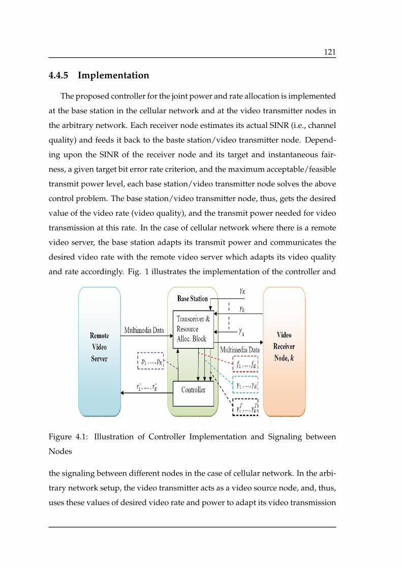
121
4.4.5 Implementation
The proposed controller for the joint power and rate allocation is implemented
at the base station in the cellular network and at the video transmitter nodes in
the arbitrary network. Each receiver node estimates its actual SINR (i.e., channel
quality) and feeds it back to the baste station/video transmitter node. Depend-
ing upon the SINR of the receiver node and its target and instantaneous fair-
ness, a given target bit error rate criterion, and the maximum acceptable/feasible
transmit power level, each base station/video transmitter node solves the above
control problem. The base station/video transmitter node, thus, gets the desired
value of the video rate (video quality), and the transmit power needed for video
transmission at this rate. In the case of cellular network where there is a remote
video server, the base station adapts its transmit power and communicates the
desired video rate with the remote video server which adapts its video quality
and rate accordingly. Fig. 1 illustrates the implementation of the controller and
Figure 4.1: Illustration of Controller Implementation and Signaling between
Nodes
the signaling between different nodes in the case of cellular network. In the arbi-
trary network setup, the video transmitter acts as a video source node, and, thus,
uses these values of desired video rate and power to adapt its video transmission
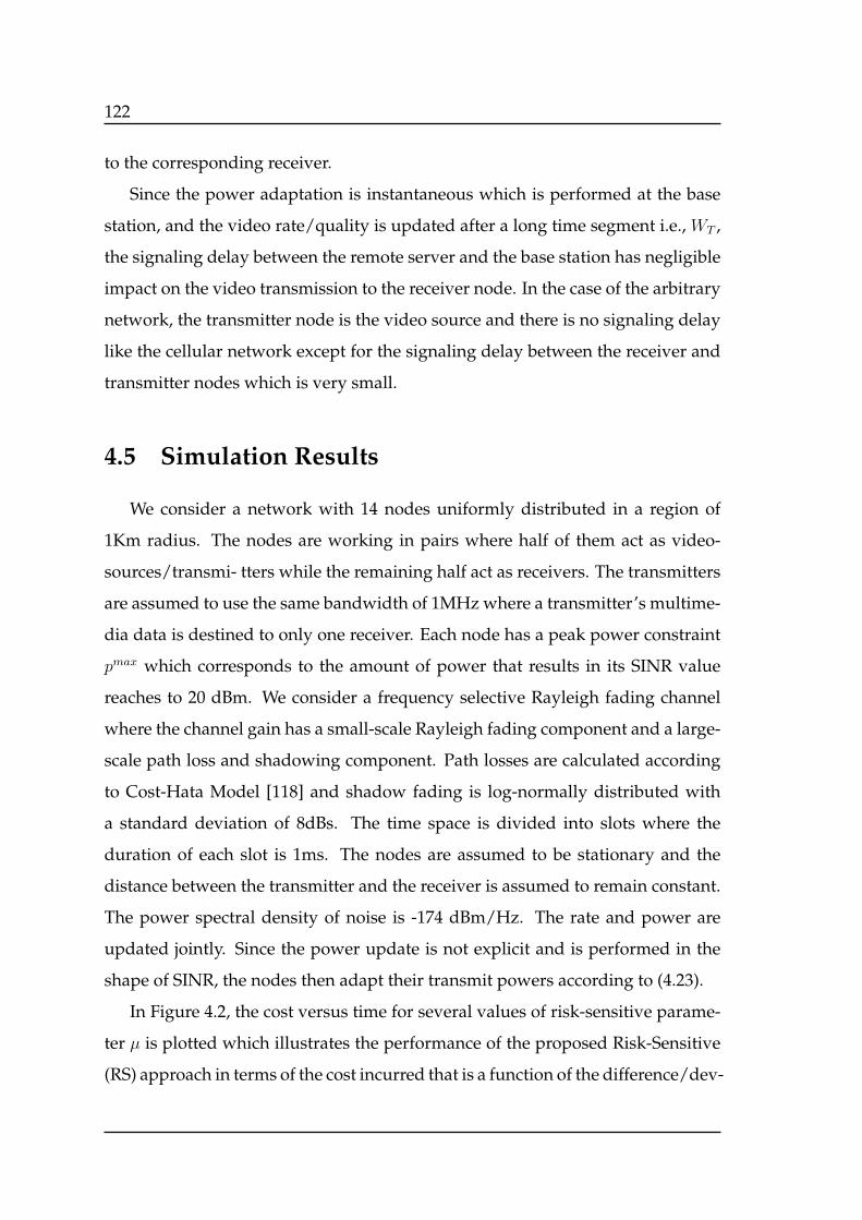
122
to the corresponding receiver.
Since the power adaptation is instantaneous which is performed at the base
station, and the video rate/quality is updated after a long time segment i.e., WT ,
the signaling delay between the remote server and the base station has negligible
impact on the video transmission to the receiver node. In the case of the arbitrary
network, the transmitter node is the video source and there is no signaling delay
like the cellular network except for the signaling delay between the receiver and
transmitter nodes which is very small.
4.5 Simulation Results
We consider a network with 14 nodes uniformly distributed in a region of
1Km radius. The nodes are working in pairs where half of them act as video-
sources/transmi- tters while the remaining half act as receivers. The transmitters
are assumed to use the same bandwidth of 1MHz where a transmitter’s multime-
dia data is destined to only one receiver. Each node has a peak power constraint
pmax which corresponds to the amount of power that results in its SINR value
reaches to 20 dBm. We consider a frequency selective Rayleigh fading channel
where the channel gain has a small-scale Rayleigh fading component and a large-
scale path loss and shadowing component. Path losses are calculated according
to Cost-Hata Model [118] and shadow fading is log-normally distributed with
a standard deviation of 8dBs. The time space is divided into slots where the
duration of each slot is 1ms. The nodes are assumed to be stationary and the
distance between the transmitter and the receiver is assumed to remain constant.
The power spectral density of noise is -174 dBm/Hz. The rate and power are
updated jointly. Since the power update is not explicit and is performed in the
shape of SINR, the nodes then adapt their transmit powers according to (4.23).
In Figure 4.2, the cost versus time for several values of risk-sensitive parame-
ter µ is plotted which illustrates the performance of the proposed Risk-Sensitive
(RS) approach in terms of the cost incurred that is a function of the difference/dev-
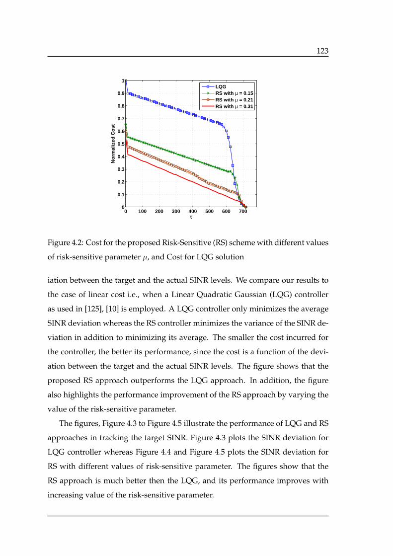
123
0 100 200 300 400 500 600 7000
0.1
0.2
0.3
0.4
0.5
0.6
0.7
0.8
0.9
1
t
No
rmal
ized
Co
st
LQGRS with µ = 0.15RS with µ = 0.21RS with µ = 0.31
Figure 4.2: Cost for the proposed Risk-Sensitive (RS) scheme with different values
of risk-sensitive parameter µ, and Cost for LQG solution
iation between the target and the actual SINR levels. We compare our results to
the case of linear cost i.e., when a Linear Quadratic Gaussian (LQG) controller
as used in [125], [10] is employed. A LQG controller only minimizes the average
SINR deviation whereas the RS controller minimizes the variance of the SINR de-
viation in addition to minimizing its average. The smaller the cost incurred for
the controller, the better its performance, since the cost is a function of the devi-
ation between the target and the actual SINR levels. The figure shows that the
proposed RS approach outperforms the LQG approach. In addition, the figure
also highlights the performance improvement of the RS approach by varying the
value of the risk-sensitive parameter.
The figures, Figure 4.3 to Figure 4.5 illustrate the performance of LQG and RS
approaches in tracking the target SINR. Figure 4.3 plots the SINR deviation for
LQG controller whereas Figure 4.4 and Figure 4.5 plots the SINR deviation for
RS with different values of risk-sensitive parameter. The figures show that the
RS approach is much better then the LQG, and its performance improves with
increasing value of the risk-sensitive parameter.
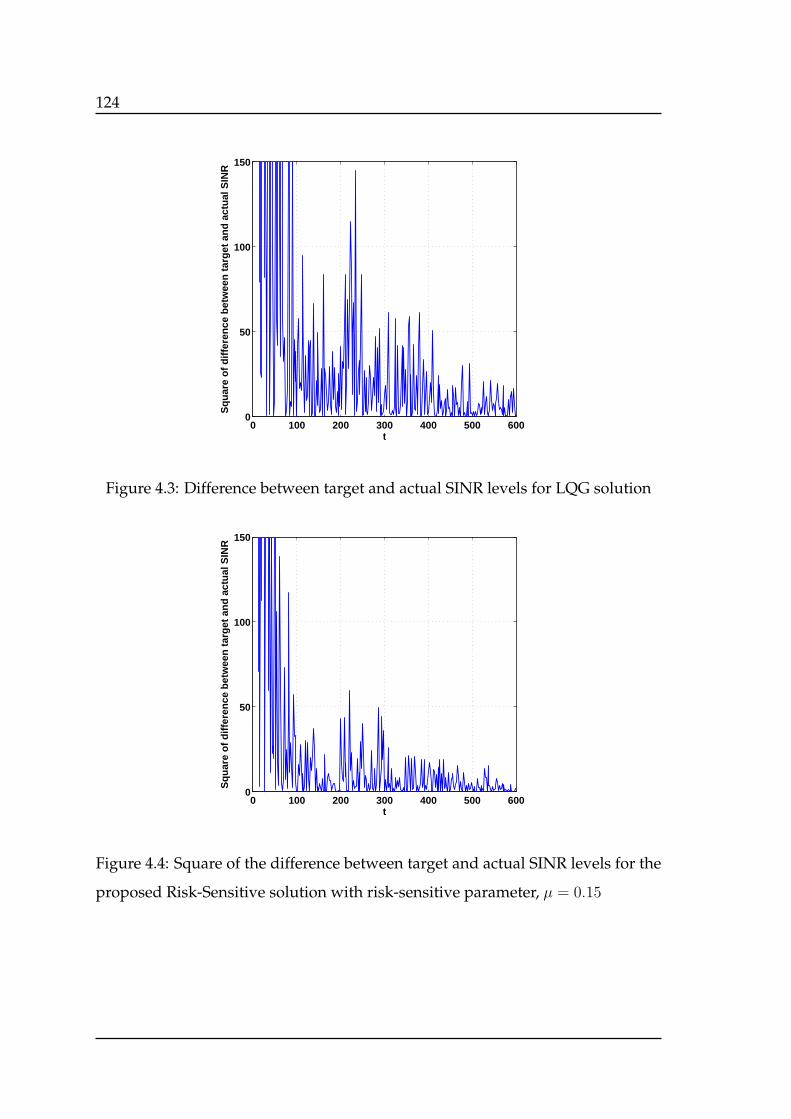
124
0 100 200 300 400 500 6000
50
100
150
t
Sq
uar
e o
f d
iffe
ren
ce b
etw
een
tar
get
an
d a
ctu
al S
INR
Figure 4.3: Difference between target and actual SINR levels for LQG solution
0 100 200 300 400 500 6000
50
100
150
t
Sq
uar
e o
f d
iffe
ren
ce b
etw
een
tar
get
an
d a
ctu
al S
INR
Figure 4.4: Square of the difference between target and actual SINR levels for the
proposed Risk-Sensitive solution with risk-sensitive parameter, µ = 0.15
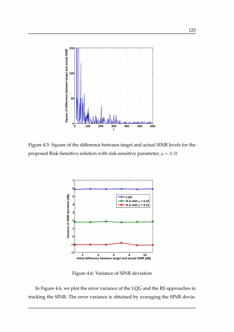
125
0 100 200 300 400 500 6000
50
100
150
t
Sq
uar
e o
f d
iffe
ren
ce b
etw
een
tar
get
an
d a
ctu
al S
INR
Figure 4.5: Square of the difference between target and actual SINR levels for the
proposed Risk-Sensitive solution with risk-sensitive parameter, µ = 0.31
2 4 6 8 10−2
−1
0
1
2
3
4
5
6
7
Initial difference between target and actual SINR (dB)
Var
ianc
e of
SIN
R d
evia
tion
(dB
)
LQGR.S with µ = 0.15R.S with µ = 0.31
Figure 4.6: Variance of SINR deviation
In Figure 4.6, we plot the error variance of the LQG and the RS approaches in
tracking the SINR. The error variance is obtained by averaging the SINR devia-
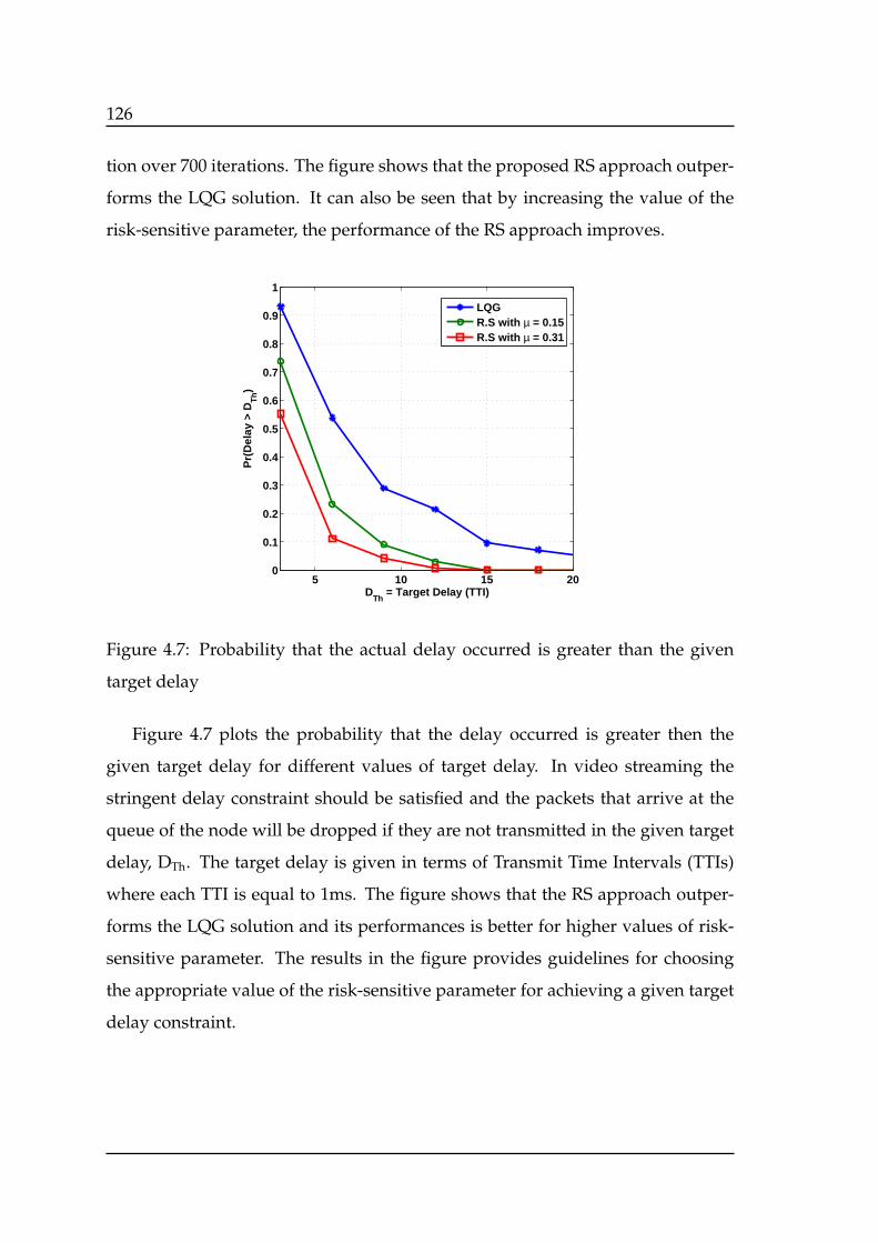
126
tion over 700 iterations. The figure shows that the proposed RS approach outper-
forms the LQG solution. It can also be seen that by increasing the value of the
risk-sensitive parameter, the performance of the RS approach improves.
5 10 15 200
0.1
0.2
0.3
0.4
0.5
0.6
0.7
0.8
0.9
1
DTh
= Target Delay (TTI)
Pr(
Del
ay >
DT
h)
LQGR.S with µ = 0.15R.S with µ = 0.31
Figure 4.7: Probability that the actual delay occurred is greater than the given
target delay
Figure 4.7 plots the probability that the delay occurred is greater then the
given target delay for different values of target delay. In video streaming the
stringent delay constraint should be satisfied and the packets that arrive at the
queue of the node will be dropped if they are not transmitted in the given target
delay, DTh. The target delay is given in terms of Transmit Time Intervals (TTIs)
where each TTI is equal to 1ms. The figure shows that the RS approach outper-
forms the LQG solution and its performances is better for higher values of risk-
sensitive parameter. The results in the figure provides guidelines for choosing
the appropriate value of the risk-sensitive parameter for achieving a given target
delay constraint.
127
4.6 Conclusion
In this chapter, we studied the challenging problem of power allocation, and
video bitstream adaptation for video streaming in multi-node wireless networks
with interference. We developed a cross-layer optimization framework that per-
forms instantaneous power control at the PHY/MAC layer joint with video rate
adaptation (in an average manner) at the APPLICATION layer. The proposed
joint power control and rate adaption framework exploits the time diversity of
the nodes’ channels, takes into account the stringent delay constraints of the
video services, and fairly distributes the limited available resources among the
users. In view of the time varying channels and interferences, stringent delay con-
straints, and a certain fairness/satisfiction criterion, we modeled our problem as a
stochastic control problem. We then developed a risk-sensitive control approach
for this problem by introducing a non-linear cost function called risk-sensitive
cost function. We then provided the optimal solution to the risk-sensitive prob-
lem and provided simulation results to assess the performance of our proposed
framework.

128
129
Chapter 5
Robust CQI Reporting Schemes for
Multi-carrier and Multi-user Systems
5.1 Introduction
In this chapter, we consider the best-M channel quality indicator (CQI) re-
porting scheme for a multi-carrier and multi-user system. We consider a realistic
scenario where a feedback delay occurs between the computation of the CQIs
and their use for resource allocation at the transmitter/base station. In addition,
we also consider that the users do not have the actual quality measures of the
channels (the actual capacity that the channels can support) but have only a noisy
estimation/observation at their disposal. This may occur due to the error in SINR
measurement due to the time-varying interferences, etc. We develop two novel
best-M CQI reporting schemes that consider the impact of the feedback delay and
the imperfect CQI estimation at the user terminal. In the first scheme, the number
of CQIs reported by each user is fixed whereas in the second scheme, the number
of CQIs to be reported by a user is determined dynamically by that user. Unlike
the traditional best-M scheme, instead of reporting the estimated CQIs, the pro-
posed schemes deal with the aforementioned imperfections at the CQI reporting
level and report so-called adapted CQIs. The adapted CQIs are computed at the
user terminals by accommodating the impact of both feedback delay and estima-
130
tion error, and are reported to the base station where their observations are used
for resource allocation. The computation of the adapted CQIs is performed in
such a way that based on the available adapted CQIs at the base station, the rate
allocated to a user at any time is as close as possible to its actual experienced rate
at that time.
First, we develop a best-M scheme where each user reports the individual
adapted CQIs of its best M sub-channel/sub-carriers, and an average adapted
CQIs value for the remaining sub-channels. In this scheme, the value of M may
vary from user to another but like the traditional best-M scheme, it is fixed for
each user. In order to obtain the adapted CQIs, we model the CQI variations as a
discrete time linear dynamic system, formulate a stochastic control problem with
quadratic cost function, and use stochastic control theory to solve this problem.
The quadratic cost function is formulated in such a way that its minimization re-
sults in obtaining the adapted CQIs for which the deviation between the user’s
actual experienced rate and the allocated rate at the base station is minimized. In
our stochastic framework, first we assume that the imperfections caused due to
feedback delay and CQI estimation error are Gaussian distributed. In this case,
we model the CQI variations as a discrete time linear dynamic system with Gaus-
sian noise, and use the Linear Quadratic Gaussian (LQG) controller to obtain the
adapted CQIs for each user. Then, we consider the more realistic scenario where
the distribution of the aforementioned imperfections is not known. In this case,
we model the CQI variations as a discrete time dynamic system with a noise
whose distribution is unknown. We then use H∞ controller to solve the corre-
sponding stochastic problem for obtaining the adapted CQIs. The H∞ controller
does not need information about the distribution of the noise.
Then, we develop another scheme called dynamic best-M CQI reporting scheme
which like the aforementioned scheme takes into account the feedback delay and
the estimation error at the CQIs reporting level, and dynamically determines the
efficient number M of adapted CQIs that should be reported by each user to the
base station. This scheme uses the same approach of stochastic control theory for

131
obtaining the adapted CQIs as used in the aforementioned best-M scheme with
fixed M. However, in addition, we develop a stochastic framework for obtaining
the efficient number M of the CQIs that should be reported by each user. Based on
this stochastic framework, we develop an efficient distributed constrained inter-
active trial and error algorithm that is implemented at the user terminal. Based on
its channel conditions, using the distributed algorithm, each user separately finds
the efficient number of CQIs that should be reported by him/her. This algorithm
also ensures that the system’s overall feedback overhead does not exceed a given
value. We prove the convergence of our distributed algorithm using stochastic
game theory.
We perform simulations in order to assess the performance of the proposed
schemes. The major contribution of this chapter are: the design of CQI report-
ing schemes that deal with feedback delay and estimation error at CQI reporting
level, the formulation of the problem as a stochastic control problem both with
Gaussian distributed noise and an unknown noise, and the development of a
distributed algorithm for determining the efficient value of M for each user.
5.2 System Description and Problem Statement
We consider a multi-carrier and multi-user system with N sub-channels, and
K simultaneously active users around the base station. A sub-channel is ex-
pected to experience specific propagation and interference levels and thus a spe-
cific channel conditions. In such a system, there are KN CQIs to be reported by
the users to the base station at each time. This hugely increases the signalling
overhead in the uplink and reduces the useful uplink data throughput especially
for high number of users K which is the case in practice. In the existing work
on the signalling overhead reduction in multi-carrier and multi-user system e.g.,
the 3GPP-LTE standard, the solution adapted is the best-M CQI reporting scheme
where each user feeds back the individual CQIs of its best M sub-channels where
the value of M is equal to 4 or 5, and an average CQI value for the remaining
132
N − M sub-channels to the base station. Moreover, in traditional schemes, the
users estimate/observe the CQIs, and feed these estimations/observations back
to the base station which are used for resource allocation. However, due to feed-
back delay, the CQI reported by users at time t will be used for resource resource
allocation at time t + τ where τ is the feedback delay. Since the channel is time-
varying, the channel conditions at t+ τ may be completely different from that at
time t. In addition, due to the time-varying interferences, etc., the CQIs estima-
tion/observation at the user terminal may not be perfect. Thus, at each time t, the
base station has delayed and imperfect estimates of CQIs at its disposal. There-
fore, having only this erroneous and outdated CQIs, it is difficult for the base
station to efficiently allocate the resources among the users and which in turn
may overwhelmingly degrade the system performance. Since the users have an
estimation of the CQI for each sub-channel, they can contribute to solve the above
problem if a CQI reporting scheme is designed which deals with the estimation
error and the feedback delay at the CQI reporting level at the user terminal.
In the traditional best-M CQI reporting scheme, the number M of CQIs re-
ported by all users is the same and fixed. The more the number of CQIs reported
for a user, the less the deviation between its actual experienced rate and the rate
allocated at the base station. In addition, for the same number of CQIs reported,
this rate deviation is less for users with good channel conditions compared to
users with relatively bad channel conditions. Thus, adapting the value of M (i.e.,
the number of CQIs to be reported) for each user according to its channel condi-
tions can further improve the system performance.
The SINR at time t associated with the nth sub-channel for the kth active user
connected to the jth base station is determined as follows
gnk,j(t) =P nj G
nk,j(t)
σ2 +∑J
l=1,l =j Pnl G
jk,l(t)
(5.1)
where P nj is the power transmitted by the jth cell on the nth sub-channel, Gj
k,l is
the path gain (including shadowing and fast fading) between the lth base station
and the kth user connected to the jth base station, σ2 is the receiver noise power,
133
and J is the number of interfering cells. The term∑J
l=1,l =j Pnl G
jk,l(t) denotes the
total interference caused to user k on sub-channel n.
In the following two sections, we develop two novel CQI reporting schemes
which address both the overhead reduction and the imperfection ( feedback delay
and CQI estimation error) issues jointly.
5.3 Robust best-M CQI Reporting Scheme
In this section, we develop a robust best-M CQI reporting scheme in which the
value of M is fixed for each user, and which takes into account the impact of the
estimation error and the feedback delay. In this scheme, first, each user computes
the so-called adapted CQIs for all its sub-channels. Then, each user selects the
best M adapted CQIs among its all N computed adapted CQIs and reports them
individually while reports an average value for the remaining N − M adapted
CQIs. We start our CQI reporting scheme development by formulating the user’s
achieved data rate variations as a linear discrete time stochastic equation. To this
end, we proceed as follows.
Let ϕnk,j(t) = σ2 +
∑Jl=1,l =j P
nl G
jk,l(t) denote the interference plus noise term in
the SINR expression (5.1). It is known from [7–11] that the interference plus noise
ϕnk,j(t) can be modeled as
ϕnk,j(t+ 1) = ϕn
k,j(t)qnk,j(t) (5.2)
where qnk,j(t) is a unit mean noise term that models the interference fluctuations.
Likewise, the dynamics of the total interference, and the useful received power
gain can be modeled as [9, 10]:
ϕnk,j(t+ 1) + P n
j Gnk,j(t+ 1) =
[ϕnk,j(t) + P n
j Gnk,j(t)
]snk,j(t) (5.3)
where snk,j(t) is a unit mean random variable which is correlated with qnk,j(t). Let
xnk,j(t) be the achieved bit rate of user k on the nth sub-channel at time t. To define

134
this rate, we use the Shannon’s upper bound for the achievable rate:
xnk,j(t) = log2(1 + gnk,j(t)) = log2
(ϕnk,j(t) + P n
j Gnk,j(t)
ϕnk,j(t)
)(5.4)
From equations (5.2) and (5.3), we get
xnk,j(t+ 1) = xnk,j(t) + log2(snk,j(t))− log2(q
nk,j(t))
= xnk,j(t) + wnk,j(t) (5.5)
where ωnk,j(t) = log2(s
nk,j(t)) − log2(q
nk,j(t)) is a zero mean disturbance of some
variance with some probability distribution. Since the above analysis is valid for
all cells, the subscript j will be omitted in the rest of this chapter, and the rate for
user k on the nth sub-channel at time t will be denoted by xtk,n. The rate and the
CQI are used in this chapter to denote the same quantity.
5.3.1 Reporting Scheme Design
We consider that the value of M may vary from one user to another and there-
fore denote it by Mk. The user does not know the actual rate xtk,n that the channel
can support but has an estimation/observation of the actual rate denoted by xtk,n
as given by
xtk,n = xtk,n + ϑtk,n (5.6)
where ϑtk,n denotes a zero mean estimation/obervation error. This estimation
/ observation error in the rate may reflect the error in the SINR measurement
due to variations in the interference, etc. Moreover, due to feedback delay, the
rate allocated at time t at the base station will depend on the rate estimation at
user terminal at time t − τ where τ is the feedback delay. In other words, the
CQI available at time t at the base station which the base station assumes to be
computed based on xtk,n is actually the CQI corresponding to xt−τk,n . From the base
station point of view, the impact of feedback delay at the user terminal can be
formulated as follows
xtk,n = xt−τk,n + νtk,n (5.7)
135
where νtk,n is a zero mean error term that reflects the impact of feedback delay.
The formulation of (5.7) and the introduction of the impact of the feedback delay
as a zero mean error follows from the rate variation model given by (5.5) where
the rates between two time instants varies by a zero mean noise. By combining
(5.6), and (5.7), we have
xt−τk,n = xtk,n + vtk,n (5.8)
where vtk,n = ϑtk,n−νtk,n accommodates the estimation error and the impact of feed-
back delay. As xt−τk,n is the observation/estimation which should be exploited for
computing the CQI that will be used for rate allocation at time t, we will denote
it by ytk,n. Note that this change of notation changes nothing but is performed for
avoiding confusions while formulating our problem as a standard control prob-
lem. The above equation now becomes
ytk,n = xtk,n + vtk,n (5.9)
Using the aforementioned analysis, the rate variations can be written according
to the following discrete time linear state space dynamic system
xt+1k,n = xtk,n + wt
k,n (5.10)
ytk,n = xtk,n + vtk,n (5.11)
In our scheme, user k will not feed back the actual CQI but an intelligently
computed CQI/rate denoted by xtk,n that is called the adapted CQI in this thesis.
The main idea of introducing the so-called adapted rate/CQI is to accommodate
for the impact of the imperfections (i.e., feedback delay and CQI estimation error)
on the user’s achievable rate. Due to feedback delay the adapted CQI computed
at time t − τ will arrive to the base station at time t where the observation of
this delayed CQI is then used for resource allocation. In view of its use at time t
for resource allocation at the base station and in order to avoid confusion in the
problem formulation, we will use superscript t instead of t−τ and will denote the
adapted CQI/rate computed at time t − τ by xtk,n. The user will compute xtk,n in
136
such a way that it accommodates the impact of both estimation error at the user
terminal and the feedback delay, and is as close as possible to xtk,n. Similar to that
of xtk,n, the time variations of xtk,n can be modeled as follows
xt+1k,n = xtk,n + wt
k,n (5.12)
where ωtk,n is a zero mean noise. This adapted CQI is then reported to the base
station where its observation is used for resource allocation. We propose a con-
trol theoretic approach to regulate/control the adapted rate/CQI such that it ap-
proaches the actual rate, and consequently the rate allocated at the base station
is very close to the actual experienced rate. The objective of our work is to make
xtk,n − xtk,n (i.e., the deviation between the allocated and the actual experienced
rate) as small as possible. In order to achieve this objective, we use linear control
theory with quadratic cost. To this end, we will model our problem as a standard
linear control problem, and define a quadratic cost function which will minimize
the rate deviation ∥xtk,n − xtk,n∥.
The dynamic system (5.10-5.11) has imperfect observation/measurement where
xtk,n in (5.12) is perfectly known. Thus, in order to formulate both the dynamic
systems (5.10-5.11), and (5.12) as a standard discrete time dynamic system, we
assume that we have an imperfect observation for xtk,n given by
ytk,n = xtk,n + ϵ0vtk,n (5.13)
where 0 < ϵ0 <<< 1 (i.e., almost equal to zero). With this value of ϵ0, the so-called
observation ytk,n is almost equal to xtk,n. Moreover, as xtk,n is the variable that shall
be controlled so that it approaches the actual rate xtk,n, we introduce a control utk,n
into (5.12), and model the adapted CQI/rate variations as the following space
state dynamic model
xt+1k,n = xtk,n + utk,n + wt
k,n (5.14)
ytk,n = xtk,n + ϵ0vtk,n (5.15)
In order to proceed with the problem formulation, we combine (5.10) with
(5.14), and (5.11) with (5.15). To this end, we introduce the following two-dimensional
137
state, observation, control, and noise vectors defined as
xtk,n = [xtk,n xtk,n]
T
ytk,n = [ytk,n ytk,n]
T
utk,n = [0 utk,n]
T
xtk,n = [wt
k,n wtk,n]
T
vtk,n = [vtk,n ϵ0v
tk,n]
T
The combine state space dynamic model for actual rate and adapted CQI/rate
can now be written as follows
xt+1k,n = xt
k,n + utk,n + wt
k,n (5.16)
ytk,n = xt
k,n + vtk,n (5.17)
Equation (5.16) represents the state while equation (5.17) represents the observa-
tion/measurement of a discrete time dynamic system affected by disturbance/noise
of some probability distribution. For each user, we get N linear state equations.
We then seek a control sequence utk,n that minimizes for each user the following
stochastic quadratic cost function
Lk =T∑t=1
N∑n=1
(∥xt
k,n∥2Q + ∥utk,n∥2R
)(5.18)
where the notation ∥b∥2S denotes the weighted norm of the vector b given as
bHSb, R is a two dimensional identity matrix, and
Q =
1 −1
− 1
The above choice of R, and Q results in
∥xtk,n∥2Q + ∥ut
k,n∥2R = ∥xtk,n − xtk,n∥2 + ∥utk,n∥2 (5.19)
which is equivalent to minimizing ∥xtk,n − xtk,n∥, and that is the main objective.
Thus, (5.16), (5.17), and (5.18) represents a linear discrete time imperfect-state
measurement disturbance attenuation problem [12].

138
In the following, we solve the above linear control problem by using two dif-
ferent approaches. First, we assume that the rate xtk,n varies according to gaussian
distribution where the noise wtk,n can be assumed to be Gaussian distributed [7]-
[11]. In this case, we solve the above problem using Linear Quadratic Gaussian
(LQG) controller [13,14]. Then, we approach the problem more realistically where
the probability distribution of the noise is unpredictable. In this case, we ap-
proach the above linear control problem by developing an H∞ controller based
solution [12].
5.3.2 Solution of the above Linear Control Problem
In order to proceed with the solution of the above linear control problem, we
define the following vectors:
ztk =[(xt
k,1)T , ..., (xt
k,N)T]T
utk =
[(ut
k,1)T , ..., (ut
k,N)T]T
ztk =[(yt
k,1)T , ..., (yt
k,N)T]T
wtk =
[(wt
k,1)T , ..., (wt
k,N)T]T
vtk =
[(vt
k,1)T , ..., (vt
k,N)T]T
where each of the above vector is of size 2N . We get the following linear state
vector system
zt+1k = Aztk +But
k +Dwtk (5.20)
ztk = Cztk + Evtk (5.21)
where A, B, C, D, and E are all identity matrices each of dimension 2N . The
covariance matrices of the noise vectors wtk and vt
k are both time-varying. We
introduce two other matrices Dt1, and Dt
2 which are both 2N dimensional time-
varying diagonal matrices. Each diagonal entry of Dt1 is equal to the square root
of the corresponding diagonal entry of the covariance matrix of wtk. Similarly,
each diagonal entry of Dt2 is equal to the square root of the corresponding diago-
nal entry of the covariance matrix of vtk. With these definitions of Dt
1 and Dt2, the

139
above state space model (5.20,5.21) can be written as
zt+1k = Aztk +But
k +Dt1γ
tk (5.22)
ztk = Cztk +Dt2ψ
tk (5.23)
where the covariance matrices of both γtk and ψt
k are now equal to an identity
matrix. The quadratic cost can now be written as
Lk =T∑t=1
(∥ztk∥2Q + ∥ut
k∥2R)
(5.24)
where R and Q are weighting matrices with R an identity matrix of dimension
2N , and Q a square matrix of dimension 2N defined as
Q =
Q 0 ... 0
0 Q ... 0
..........
0 0 ... Q
In this problem formulation, weighting matrix R is assumed to be an identity
matrix. However, a more general cost function can be obtained by appropriate
scaling of the weight matrix R.
5.3.2.1 LQG based solution
In this case, we assume that the noise has Gaussian distribution [7]- [11]. The
above problem (5.22-5.24) is then a standard discrete time linear control problem
with Gaussian noise and quadratic cost. The solution to this problem is known
as the LQG solution [13, 14]. As defined earlier, the matrices Dt1, and Dt
2 are
time-varying. Thus, in order to use the standard LQG solution with constant
covariance matrices of the noises, we transform the state space model (5.22,5.23)
into the following equivalent model:
zt+1k = Aztk +Btut
k + γtk (5.25)
ztk = Ctztk +ψtk (5.26)
140
where ztk = (Dt1)
−1ztk, ztk = (Dt2)
−1ztk, Bt = (Dt1)
−1B, and Ct = C(Dt2)
−1Dt1. In
view of the above transformation, the corresponding cost function now becomes:
Lk =T∑t=1
(∥ztk∥2Qt + ∥ut
k∥2R)
(5.27)
where Qt is a time-varying matrix of dimension 2N defined as
Qt = (Dt1)
2Q (5.28)
Let denote the covariance matrices of the noise vectors γtk, andψt
k by Wk, and Vk
respectively:
Wk = Eγtk(γ
tk)
T
Vk = Eψtk(ψ
tk)
T
The solution of the problem (5.25-5.27) is given by the following iterative algo-
rithm [13, 14]:
utk = −Dt
cztk (5.29)
zt+1k = (A−Dt
pCt)ztk +Dt
pztk +Btut
k; z0k = Ez0k (5.30)
where Dtc and Dt
p are given respectively by
Dtc = (I+ (Bt)TPt
cBt)−1BtPt
cA (5.31)
Dtp = APtCT (Vk +CPtC)−1 (5.32)
where I is an identity matrix of dimension 2N ; and Pt and Ptc are the solutions
obtained by the following Riccati Recursion:
Pt+1 = APtAT +BtWk(Bt)T −Dt
p(Vk +CtPtCt)TDtp; P0 = Ezk0(zk0)T
(5.33)
Ptc = Qt +ATPt+1
c A− (Dtc)
T (R+ (Bt)TPt+1c Bt)Dt
c; PTc = 0
(5.34)
Thus, for each user and at each time t, we get the optimal control vector utk
and the state vector ztk from which ztk is obtained. In other words, we get the

141
N variables xtk,n for all the N sub-channel of the user k which are the adapted
CQIs/rates. The user then reports the individual values of the best Mk adapted
CQIs and an average value for the remaining N − Mk adapted CQIs given by
xtk,m = 1N−Mk
∑Nn=Mk+1 x
tk,n to the base station.
5.3.2.2 H∞ Controller Based Solution
We now approach the problem more realistically where the probability distri-
bution of the noise is unknown. In this case, we propose an H∞ controller based
solution [12] for problem (5.22-5.24) for which we proceed as follows.
From (5.24), the instantaneous objective function can be written as
Ltk = ∥ztk∥2Q + ∥ut
k∥2R (5.35)
This is now a discrete time linear dynamic system modeled as a control problem
which is disturbed by an unknown noise process. The robust solution to this
control problem can be obtained by assuming the worst case noise. Therefore
instead of minimizing the cost function (5.24), one should consider the following
cost function [12]
Jπ =T∑t=1
(Ltk − π2∥γt
k∥2) (5.36)
where π2 is the level of attenuation. The cost function (5.36) can be viewed as the
cost function of a minimax optimization problem in which the cost is minimized
over the maximum value of the unknown disturbance. This minimax problem
can also be viewed as a zero sum game of two players. In this game, cost Jπ is
minimized by the first player which is the controller utk while it is maximized
by the second player which is the noise γtk. The optimal solution is obtained at
the appropriate value of the attenuation level π2. One can refer to [12] for more
general class of discrete time zero-sum games, with various information patterns,
where sufficient conditions for the existence of a saddle point are provided when
the information pattern is perfect and imperfect state.
With this insight the minimax optimization problem for a given value of π2

142
can now be written as
minutk
maxγtk
Jπ (5.37)
where Jπ is defined in (5.36) and ztk evolves according to (5.22). The solution to
this problem can be obtained according to the following theorem [12].
Theorem 5.3.1. [12] Consider the problem described by (5.22), (5.23), (5.24), and (5.36),
then for a given attenuation π2 there exists for all t a state feedback controller utk such
that
utk = −
[(Mt+1)−1 + I− π−2Dt
1(Dt1)
T]−1 [
I− π−2ΣtMt]−1
ztk (5.38)
where Mt, Σt and state estimate vector ztk are defined/given as,
1) Mt is a minimal non-negative definite solution obtained by the following Riccati Re-
cursion
Mt = Q +[Mt+1 + I− π−2Dt
1(Dt1)
T]−1
; MT +1 = 0 (5.39)
such that
Mt+1 − π−2Dt1(D
t1)
T > 0 (5.40)
2) Σt is a minimal non-negative definite solution obtained by the following Riccati Re-
cursion
Σt+1 = Dt2(D
t2)
T +[(Σt)−1 +
(Dt
2(Dt2)
T)−1 − π−2Q
]−1
; Σ1 = Q0 (5.41)
such that Q0 is positive definite and
(Σt)−1 − π−2Q > 0 (5.42)
2) the state estimate ztk is generated by,
ztk =[I+Σt
(Dt
2(Dt2)
T)−1 − π−2ΣtMt
]−1 [ztk +Σt
(Dt
2(Dt2)
T)−1
ztk
](5.43)
and
zt+1k = ztk + ut
k +[(Σt)−1 +
(Dt
2(Dt2)
T)−1 − π−2Q
]−1
×[(π−2Qztk +
(Dt
2(Dt2)
T)−1
(ztk − ztk)]; z1k = 0 (5.44)
In addition, the following constraint on the spectral radius of ΣtMt, i.e., ρ(ΣtMt) < π2,
should also be satisfied.
143
The above theorem states the existence of a controller utk. This controller is
called the H∞ controller and is obtained for a given value of π2.
Note that the matrices Dt1, and Dt
2 are time-variant, T is finite, and the problem
defined above is time-variant finite-horizon problem. If Dt1, and Dt
2 like A, B and
C are time-invariant and T → +∞, then the problem is called time-invariant
infinite horizon problem whose solution is more simple. This case corresponds
to the circumstances when the users mobility is low and the system is operating
in conditions close to steady state. For a given attenuation π2, the solution of
our problem for infinite horizon case can be obtained according to the following
theorem [12].
Theorem 5.3.2. [12] Consider the problem described by (5.22), (5.23), (5.24), and (5.36),
then for T → +∞ and a given attenuation π2 there exists for all t a state feedback
controller utk such that
utk = −
[M−1 + I− π−2D1D
T1
]−1 [I− π−2ΣMt
]−1ztk (5.45)
where M, Σ, D1, and D2 are all time-invariant; and where M, Σ, and state estimate vec-
tor ztk are defined/given as,
1) M is a minimal non-negative definite solution of the following Riccati Algebraic Equa-
tion (ARE)
M = Q +[M + I− π−2D1DT
1
]−1 (5.46)
such that
M− π−2D1DT1 > 0 (5.47)
2) Σ is a minimal non-negative definite solution of the following Riccati Algebraic Equa-
tion (ARE)
Σ = D2DT2 +
[(Σ)−1 +
(D2DT
2
)−1 − π−2Q]−1
(5.48)
such that
Σ−1 − π−2Q > 0 (5.49)
2) the state estimate ztk is generated by,
ztk =[I+Σ
(D2DT
2
)−1 − π−2ΣM]−1 [
ztk +Σ(D2(DT
2
)−1ztk
](5.50)
144
and
zt+1k = ztk + ut
k +[Σ−1 +
(D2DT
2
)−1 − π−2Q]−1
×[(π−2Qztk +
(D2DT
2
)−1(ztk − ztk)
]; z1k = 0 (5.51)
In addition, the following constraint on the spectral radius of ΣM, i.e., ρ(ΣM) < π2,
should also be satisfied.
Thus, for each user and at each time t, we get the optimal control vector utk
and the estimate for the state vector ztk. In other words, we get the estimates of
N variables xtk,n for all the N sub-channel of the user k which are the adapted
CQIs/rates.
5.3.3 Selection and Reporting of the Best Mk CQIs
By using the above methods i.e., the LQG and the H∞ approaches, each user
computes the so-called adapted CQIs for all its N sub-channels. Each user k then
selects its best Mk sub-channels and reports an individual CQI (i.e., xtk,n) on each
of these Mk best sub-channels. A single CQI for the remaining N − Mk sub-
channels is reported by each user which is obtained by calculating an average
value of the remaining N −Mk CQIs (i.e., xtk,m = 1N−Mk
∑Nn=Mk+1 x
tk,n).
The observations of these adapted CQIs/rates at the base station are then used
in the resource allocation.
5.3.4 Dealing with Noisy Feedback Channels
The CQI reporting scheme developed in this section considers the CQI/rate
estimation error at the user terminal, and the impact of the delay occurring be-
tween the computation of the CQIs and their use at the base station. However,
the feedback channel may be noisy, and the CQIs received at the base station may
have an additional noise term which is not studied in our scheme design. In this
subsection, we study the impact of the noisy feedback channel on the design of
our CQI reporting scheme. For simplicity purposes, we perform this analysis

145
for a single CQI reporting whose generalization to the above designed scheme is
straight forward.
We recall that the actual CQI/rate at time t is denoted by xtk,n. Moreover,
xtk,n denotes the adapted CQI/rate thats accommodates the impact of estimation
error and feedback delay, and which is computed at time t − τ , and are used for
resource allocation at the base station at time t. The observation of xtk,n is then
used for resource allocation at time t. By assuming that the feedback channel is
noisy, the observation of this adapted CQI at the base station can be written in
the following form
ytk,n = xtk,n + ntk,n (5.52)
where ntk,n is a zero mean noise term with some variance. The base station will
perform resource allocation on the basis of this noisy observation, thus, the devi-
ation between xtk,n and ytk,n should be made as small as possible. This deviation
minimization can be formulated as the following minimization problem
θk,n = min E∥ytk,n − xtk,n∥2
(5.53)
By putting (5.52) in (5.53), we arrive at
θk,n = minE∥xtk,n + nt
k,n − xtk,n∥2
= min[E∥xt−τ
k,n − xtk,n∥2
+ E∥nt
k,n∥2 − 2Extk,n − xtk,nEntk,n]
= min[E∥xtk,n − xtk,n∥2
+ E∥nt
k,n∥2]
= minE∥xtk,n − xtk,n∥2
(5.54)
which is the same as the CQI/rate deviation minimization objective of our CQI
reporting scheme. The last equality results due to the fact that as we have a zero
mean noise so the term with Entk,n is equal to zero, and E∥nt
k,n∥2 is a term that
can not be controlled, and has therefore considered as constant.
According to the above analysis, the best that can be done at the user termi-
nal in order to provide more accurate CQIs to the base station is to deal with
the CQI/rate estimation error and the feedback delay in the design of the CQI
reporting scheme.
146
5.4 Dynamic M-best CQI Reporting Scheme
In the previous section, we designed the reporting scheme while assuming
that the value ofMk is fixed for each user. In this section, we integrate a stochastic
framework to the adapted CQI reporting framework developed in the previous
section in order to dynamically determine the efficient Mk per user. Although
the value of Mk’s are dynamic in this scheme, the idea of reporting the adapted
rates/CQIs and their determination by the LQG/H∞ Controller proposed in the
previous section remains the same. Each user has the estimates of all its sub-
channels and will compute the adapted CQIs for all his/her sub-channels by
using the stochastic control approach developed in the previous section. Then,
based on his/her channel conditions, each user will dynamically determine the
efficient number of CQIs that should be reported to the base station. To this end,
we use stochastic potential game theory and develop a distributed framework for
finding the efficient number of the best sub-channels that should be reported for
each user.
5.4.1 Mk Determination Framework
We assume that each user sorts the sub-channels in decreasing order of their
CQI values (from the best CQI to the worst CQI). The order of sub-channels for
different users is therefore not the same. We define a KN indicator vector it =
[it1, ..., itK ]
T where itk = [itk,1, ..., itk,N ]
T . Each entry itk,n indicates that whether at time
t, the individual CQI of sub-channel n for user k is reported to the base station or
not, and that is defined as
itk,n =
1 If the CQI for nth sub-channel of the kth user is reported
0 Otherwise.(5.55)
We then introduce another indicator vector jt = [jt1, ..., jtK ]
T where jtk = [jtk,1, ..., jtk,N ]
T .
The elements jtk,m indicates the total number of sub-channels whose individual

147
CQIs are not reported to the base station for user k at time t:
jtk,m =
1 If the number of individually non-reported CQIs of user
k is equal to m
0 Otherwise.
(5.56)
The letter m in the subscript of jtk,m denotes the total number of individually
non-reported sub-channels and should not be confused with the letter n in the
subscript of itk,n which denotes the index of the nth best sub-channel for user k.
Since the total number of individually non-reported sub-channel for any user k is
equal to N −Mk with Mk =∑N
n=1 itk,n, we define its set of the feasible indicators
as follows
χk = itk, jtk ∈ 0, 1N | jtk,m = 1,∀m = N−Mk; jtk,m = 0,∀N−Mk+1 ≤ m < N−Mk
(5.57)
We now define the instantaneous deviation between the users’ actual expe-
rienced rates and the adapted rate/CQI reported to the base station. The rate
deviation for user k at time t is defined as
Lt
k =N∑
n=1
itk,n∥xtk,n∥2Q +
N∑m=1
jtk,mm∥xtk,m∥2Q (5.58)
where ∥xtk,n∥2Q = ∥xtk,n − xk,n∥2, ∥xt
k,m∥2Q = ∥xtk,m − xk,m∥2; and where xtk,n, xtk,n
and xtk,m = 1N−Mk
∑Nn=Mk+1 xk,n are the same as defined in the previous section,
and xtk,m = 1N−Mk
∑Nn=Mk+1 xk,n. As it is explained in the previous section that in
order to improve the efficiency of the CQIs reporting scheme, the above rate de-
viation should be made as small as possible. Since ∥xtk,m∥2Q represents the differ-
ence between the value of the average actual rate/CQI and the average adapted
rate/CQI over m sub-channel, it is multiplied by m in (5.58) in order that the
impact of the total rate deviation for the m sub-channels is accounted for in the
design of the reporting scheme.
In addition, we impose restrictions on the total sum of the CQIs reported by
all users to the base station since the objective of our work is not only to develop
an efficient reporting scheme but also to reduce the signalling overhead in the
148
uplink. Since in the traditional best-M CQI reporting scheme the total number
of CQIs reported by all the K user is equal to MK, we choose this figure as our
performance metric. In our framework, we introduce a constraint on the total
number of reported CQIs which ensures that this number is less than or equal to
MK most of the time and is defined by
Pr
(K∑k=1
N∑n=1
itk,n ≤MK
)≥ (1− ε) (5.59)
which determines that the probability that this constraint is satisfied is greater
then (1− ε) where 0 << (1− ε) < 1.
We now construct our optimization framework as follows
min E
K∑k=1
(N∑
n=1
itk,n∥xt
k,n∥2Q∥xtk,n∥
+N∑
m=1
jtk,mm∥xt
k,m∥2Q∥xtm,n∥
)(5.60)
s.t. Pr
(K∑k=1
N∑n=1
itk,n ≤MK
)≥ (1− ε) (5.61)
itk,n, jtk,m ∈ χk, ∀k, n,m (5.62)
where ∥xtk,n∥2Q = ∥xtk,n−xk,m∥, and ∥xt
k,m∥2Q = ∥xtk,m−xk,m∥ are obtained by using
the solution of the linear dynamic control problem presented in the previous sec-
tion. The actual value of the rate deviation for a good quality sub-channel may
be higher than that for bad quality sub-channel, thus, in order to avoid the selec-
tion of bad quality sub-channels, the normalization in the objective function of
the above minimization problem is performed. The above optimization problem
is a stochastic binary integer problem that should be solved separately by each
user (i.e., in a distributed way).
5.4.2 Distributed solution
In order to develop a distributed solution, we first transform our constrained
framework into an unconstrained relaxed problem as follows. Let S be the set of
itk,n’s that satisfy the common constraint∑K
k=1
∑Nn=1 i
tk,n ≤ MK and is defined as

149
follows
S =
it ∈ 0, 1KN |
K∑k=1
N∑n=1
itk,n ≤MK
(5.63)
Let 1itk∈S be an indicator for user k that is equal to 1 if itk = [itk,1, ..., itk,N ]
T ∈ S
and 0 otherwise. Let denote the average cost of a user k at time t by
Ltk = E
N∑
n=1
itk,n∥xt
k,n∥2Q∥xtk,n∥
+N∑
m=1
jtk,mm∥xt
k,m∥2Q∥xtm,n∥
(5.64)
The relaxed problem can now be described as follows: if it ∈ S i.e., if the
common constraint∑K
k=1
∑Nn=1 i
tk,n ≤ MK is satisfied then each user aims to
minimize his/her rate deviation Ltk as defined by (5.64) and which is called the
cost function hereafter. If the common constraint is not satisfied, then we add a
penalty cost Ψk which is big enough compared to Ltk. The new cost function that
each user has to minimize can now be written as
Ltk =
(Lt
k
)1itk∈S + (Ψk)1itk∈S
(5.65)
The main objective now is that each user separately minimize its cost as defined
above in a distributed manner. The above cost that each user k has to minimize
separately, depends upon the common constraint. Since the common constraint
not only depends upon the value of Mk chosen by user k but also on the values
of Mk’s for all the other K − 1 users, all the users are completely interdependent
in minimizing their individual costs. Thus, it is a distributed control problem
where the users are coupled by the common constraint but do not interact with
each other directly for their decisions on Mk’s. In this setting, it is thus impossi-
ble for the common constraint to be satisfied all the times. In the following, we
efficiently approach this distributed control problem by using some results from
game theory.
5.4.2.1 Efficient Interactive Trial and Error Learning Algorithm
We develop an efficient interactive trial and error learning algorithm which
solves the above distributed constrained problem optimally with high proportion
150
of time. The unconstrained version of the algorithm has been recently studied in
game theory (see [127] and the references therein). In our setting, the problem is
constrained and the number of actions is exponential. We consider a discrete time
space where the time variable t is defined at discrete values with unit discretiza-
tion step 1, 2, 3, . . .. In the constrained trial and error learning, users occasion-
ally try out new configurations itk, jtk ∈ χk i.e., the values of Mk’s and accept them
if and only if they lead to a lower cost. If the common constraint is violated, then
the users get a very high cost and they will change their configurations in the next
step. We assume that each user makes decisions to minimize its own objectives in
response to its own observations of Ltk and of the common constraint. Based on
this observation about the current value of the cost, each user k updates his/her
configuration: adapts a new configuration with probability qk that increases with
the realized gain in cost compared to the previous cost if the common constraint
was satisfied previously, and adopts a new configuration with probability pk that
decreases with the realized level of cost if the common constraint was not satis-
fied previously. This defines a Markov process over the set 0, 1KN . We denote
by Ltk the current reference which is the current cost of user k (as performance)
and Ltk the received cost which is the new cost if configuration is changed. Based
on the above Markov process, and the observed values of Ltk and Lt
k, we propose
an efficient interactive trial and error algorithm as given in Table 5.1.
Before proving the optimality of the proposed algorithm, we provide two use-
ful definition that are necessary to understand the game properties of our learn-
ing process.
Definition 1. A game G is interdependent if any proper subset P of players can
influence the payoff of at least one player not in P by some joint choice of actions. More
precisely, G is interdependent if, for every proper subset P and every action a, ∃ i ∈
P ,∃ a′p = ap such that ui(a
′p, a−p) = ui(ap, a−p)
Definition 2. A state set Z is a stochastically stable state set if it is the minimal
subset of states such that, given any small δ, there is a number ϵδ > 0 such that whenever
ϵ ∈ [0, ϵδ], the Markov chain will visit the set Z at least 1− δ proportion of all time t.
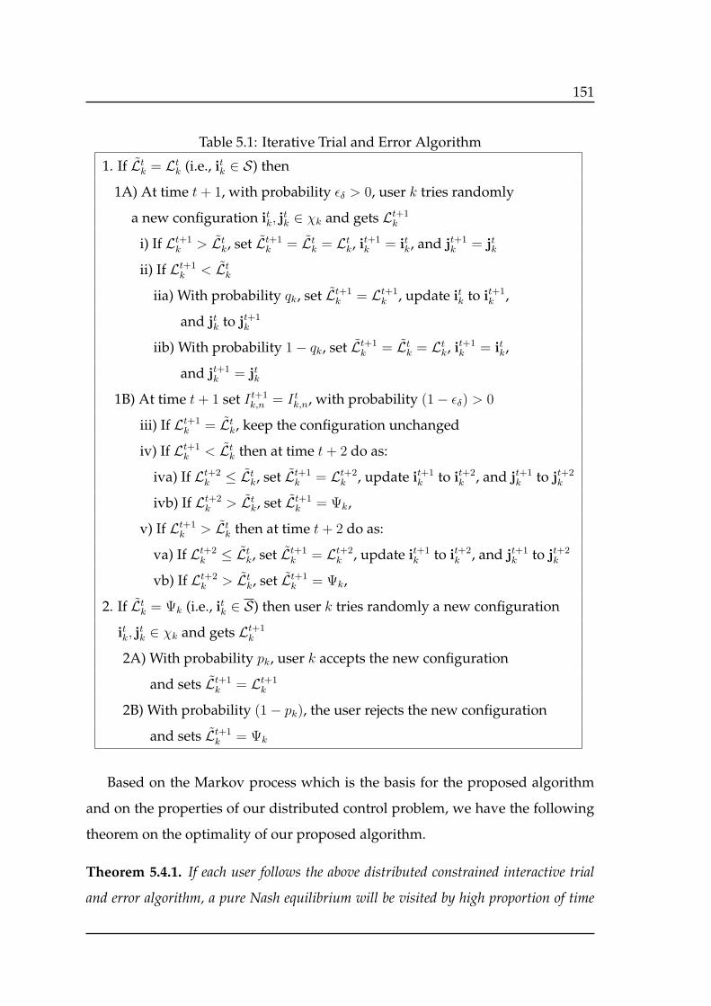
151
Table 5.1: Iterative Trial and Error Algorithm
1. If Ltk = Lt
k (i.e., itk ∈ S) then
1A) At time t+ 1, with probability ϵδ > 0, user k tries randomly
a new configuration itk, jtk ∈ χk and gets Lt+1
k
i) If Lt+1k > Lt
k, set Lt+1k = Lt
k = Ltk, it+1
k = itk, and jt+1k = jtk
ii) If Lt+1k < Lt
k
iia) With probability qk, set Lt+1k = Lt+1
k , update itk to it+1k ,
and jtk to jt+1k
iib) With probability 1− qk, set Lt+1k = Lt
k = Ltk, it+1
k = itk,
and jt+1k = jtk
1B) At time t+ 1 set I t+1k,n = I tk,n, with probability (1− ϵδ) > 0
iii) If Lt+1k = Lt
k, keep the configuration unchanged
iv) If Lt+1k < Lt
k then at time t+ 2 do as:
iva) If Lt+2k ≤ Lt
k, set Lt+1k = Lt+2
k , update it+1k to it+2
k , and jt+1k to jt+2
k
ivb) If Lt+2k > Lt
k, set Lt+1k = Ψk,
v) If Lt+1k > Lt
k then at time t+ 2 do as:
va) If Lt+2k ≤ Lt
k, set Lt+1k = Lt+2
k , update it+1k to it+2
k , and jt+1k to jt+2
k
vb) If Lt+2k > Lt
k, set Lt+1k = Ψk,
2. If Ltk = Ψk (i.e., itk ∈ S) then user k tries randomly a new configuration
itk, jtk ∈ χk and gets Lt+1
k
2A) With probability pk, user k accepts the new configuration
and sets Lt+1k = Lt+1
k
2B) With probability (1− pk), the user rejects the new configuration
and sets Lt+1k = Ψk
Based on the Markov process which is the basis for the proposed algorithm
and on the properties of our distributed control problem, we have the following
theorem on the optimality of our proposed algorithm.
Theorem 5.4.1. If each user follows the above distributed constrained interactive trial
and error algorithm, a pure Nash equilibrium will be visited by high proportion of time
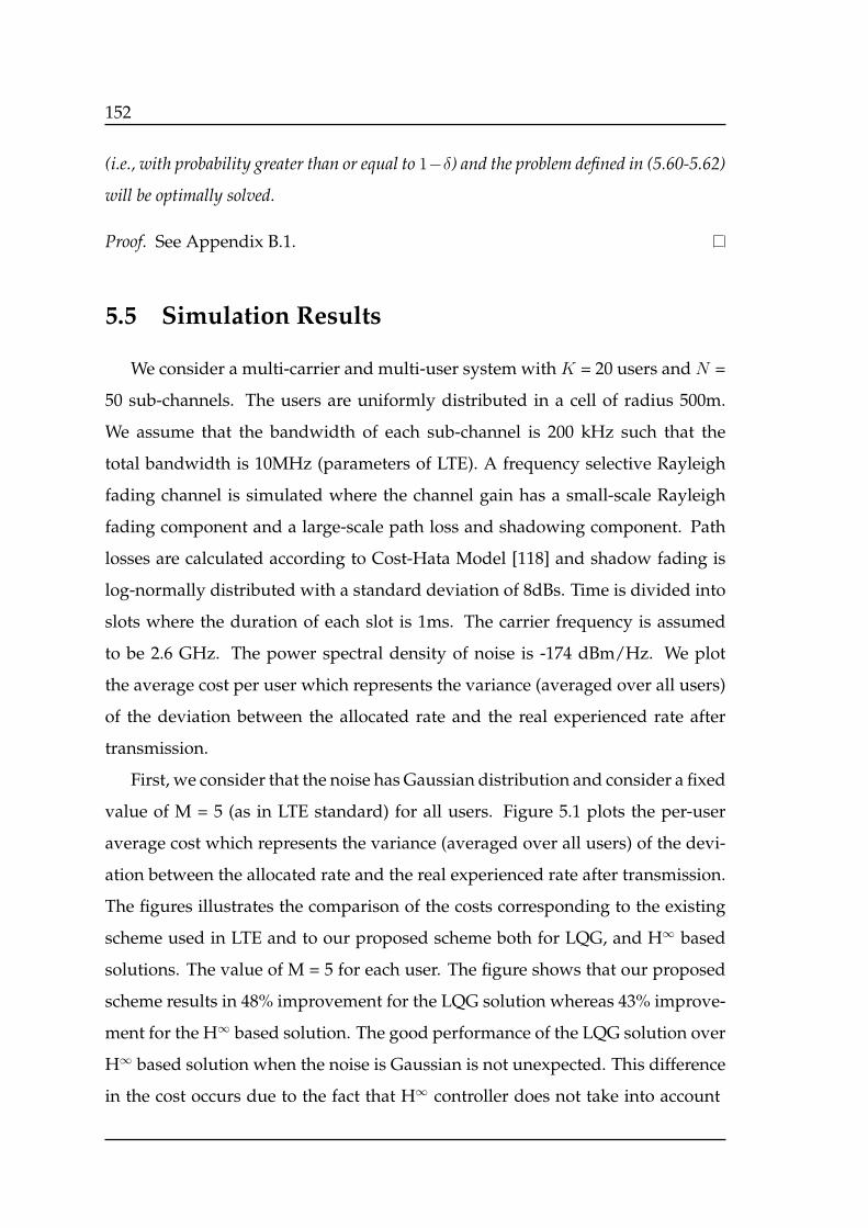
152
(i.e., with probability greater than or equal to 1−δ) and the problem defined in (5.60-5.62)
will be optimally solved.
Proof. See Appendix B.1.
5.5 Simulation Results
We consider a multi-carrier and multi-user system with K = 20 users and N =
50 sub-channels. The users are uniformly distributed in a cell of radius 500m.
We assume that the bandwidth of each sub-channel is 200 kHz such that the
total bandwidth is 10MHz (parameters of LTE). A frequency selective Rayleigh
fading channel is simulated where the channel gain has a small-scale Rayleigh
fading component and a large-scale path loss and shadowing component. Path
losses are calculated according to Cost-Hata Model [118] and shadow fading is
log-normally distributed with a standard deviation of 8dBs. Time is divided into
slots where the duration of each slot is 1ms. The carrier frequency is assumed
to be 2.6 GHz. The power spectral density of noise is -174 dBm/Hz. We plot
the average cost per user which represents the variance (averaged over all users)
of the deviation between the allocated rate and the real experienced rate after
transmission.
First, we consider that the noise has Gaussian distribution and consider a fixed
value of M = 5 (as in LTE standard) for all users. Figure 5.1 plots the per-user
average cost which represents the variance (averaged over all users) of the devi-
ation between the allocated rate and the real experienced rate after transmission.
The figures illustrates the comparison of the costs corresponding to the existing
scheme used in LTE and to our proposed scheme both for LQG, and H∞ based
solutions. The value of M = 5 for each user. The figure shows that our proposed
scheme results in 48% improvement for the LQG solution whereas 43% improve-
ment for the H∞ based solution. The good performance of the LQG solution over
H∞ based solution when the noise is Gaussian is not unexpected. This difference
in the cost occurs due to the fact that H∞ controller does not take into account
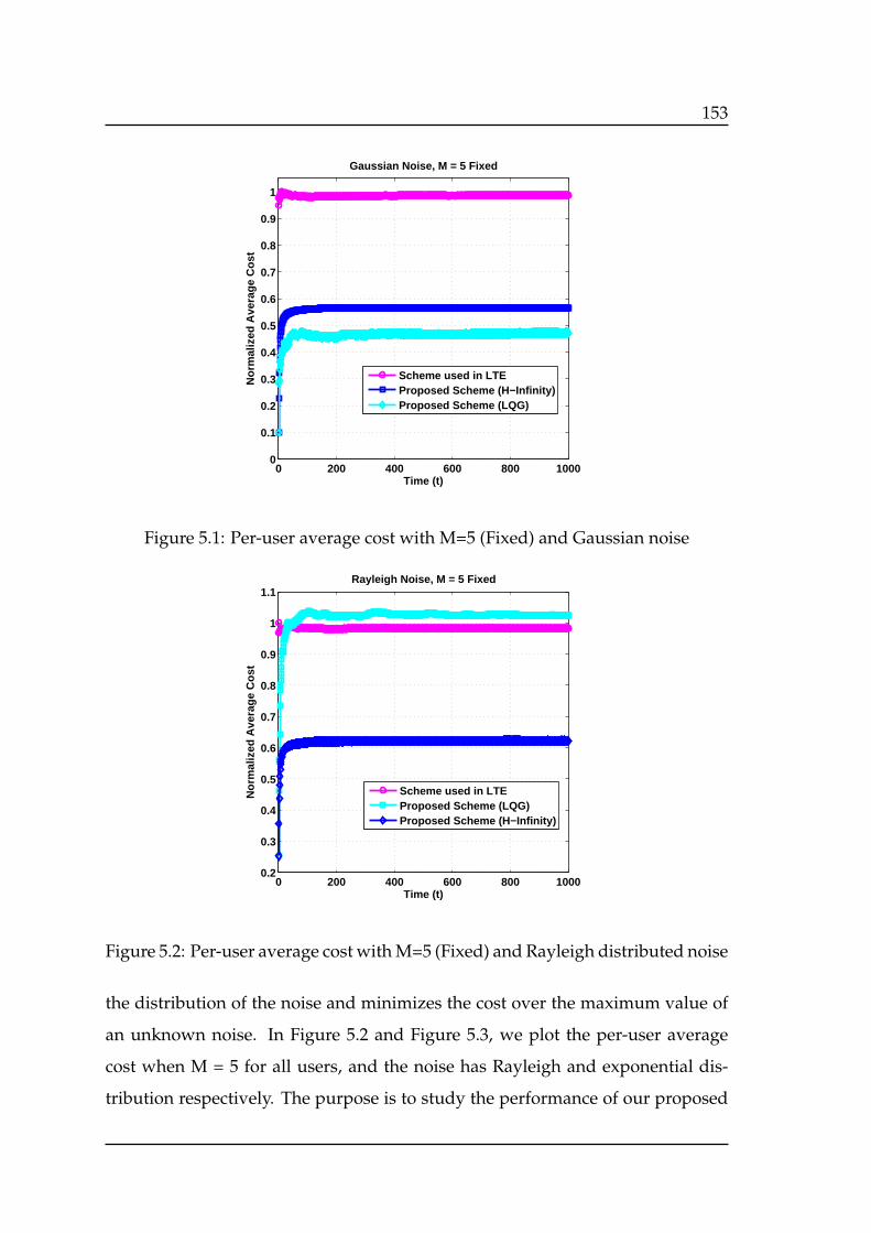
153
0 200 400 600 800 10000
0.1
0.2
0.3
0.4
0.5
0.6
0.7
0.8
0.9
1
Time (t)
Nor
mal
ized
Ave
rage
Cos
t
Gaussian Noise, M = 5 Fixed
Scheme used in LTEProposed Scheme (H−Infinity)Proposed Scheme (LQG)
Figure 5.1: Per-user average cost with M=5 (Fixed) and Gaussian noise
0 200 400 600 800 10000.2
0.3
0.4
0.5
0.6
0.7
0.8
0.9
1
1.1
Time (t)
Nor
mal
ized
Ave
rage
Cos
t
Rayleigh Noise, M = 5 Fixed
Scheme used in LTEProposed Scheme (LQG)Proposed Scheme (H−Infinity)
Figure 5.2: Per-user average cost with M=5 (Fixed) and Rayleigh distributed noise
the distribution of the noise and minimizes the cost over the maximum value of
an unknown noise. In Figure 5.2 and Figure 5.3, we plot the per-user average
cost when M = 5 for all users, and the noise has Rayleigh and exponential dis-
tribution respectively. The purpose is to study the performance of our proposed
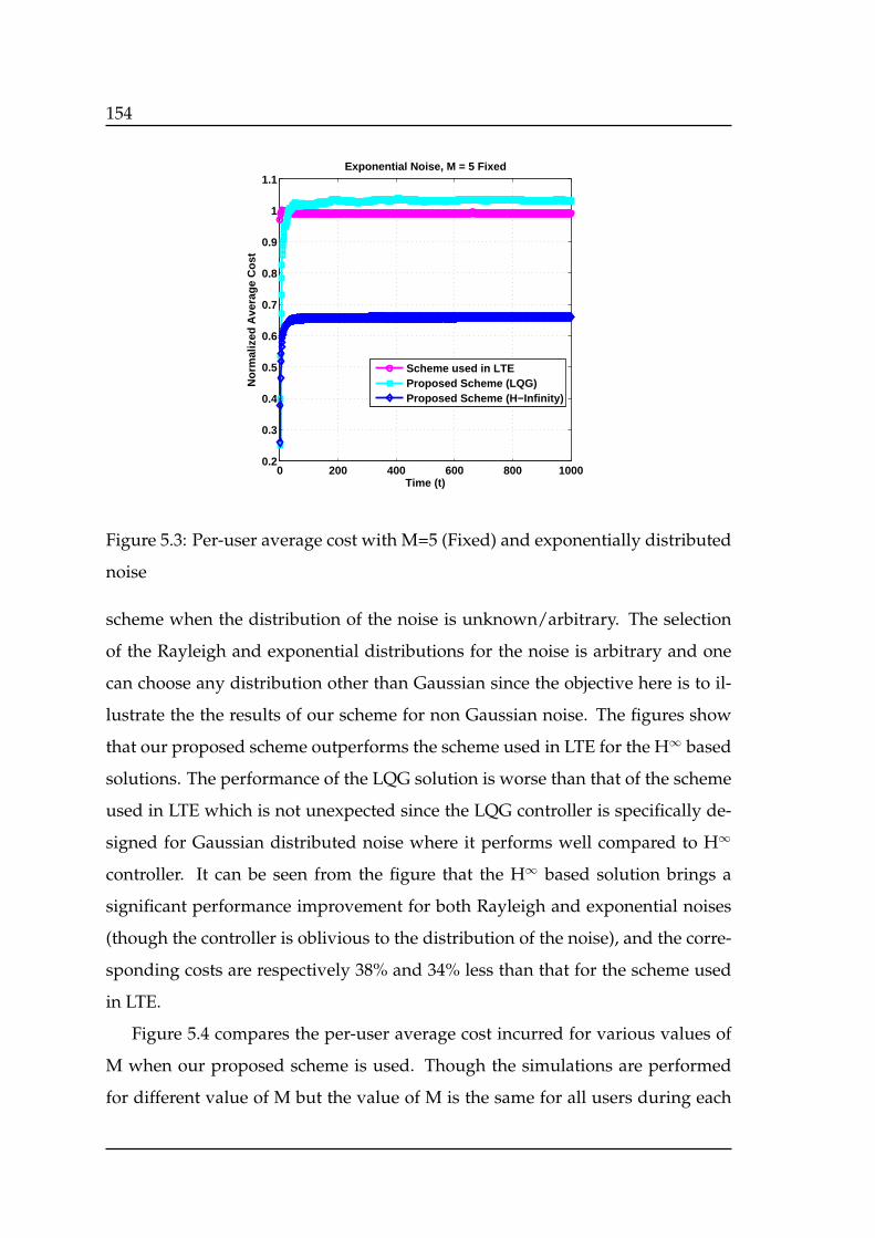
154
0 200 400 600 800 10000.2
0.3
0.4
0.5
0.6
0.7
0.8
0.9
1
1.1
Time (t)
Nor
mal
ized
Ave
rage
Cos
t
Exponential Noise, M = 5 Fixed
Scheme used in LTEProposed Scheme (LQG)Proposed Scheme (H−Infinity)
Figure 5.3: Per-user average cost with M=5 (Fixed) and exponentially distributed
noise
scheme when the distribution of the noise is unknown/arbitrary. The selection
of the Rayleigh and exponential distributions for the noise is arbitrary and one
can choose any distribution other than Gaussian since the objective here is to il-
lustrate the the results of our scheme for non Gaussian noise. The figures show
that our proposed scheme outperforms the scheme used in LTE for the H∞ based
solutions. The performance of the LQG solution is worse than that of the scheme
used in LTE which is not unexpected since the LQG controller is specifically de-
signed for Gaussian distributed noise where it performs well compared to H∞
controller. It can be seen from the figure that the H∞ based solution brings a
significant performance improvement for both Rayleigh and exponential noises
(though the controller is oblivious to the distribution of the noise), and the corre-
sponding costs are respectively 38% and 34% less than that for the scheme used
in LTE.
Figure 5.4 compares the per-user average cost incurred for various values of
M when our proposed scheme is used. Though the simulations are performed
for different value of M but the value of M is the same for all users during each
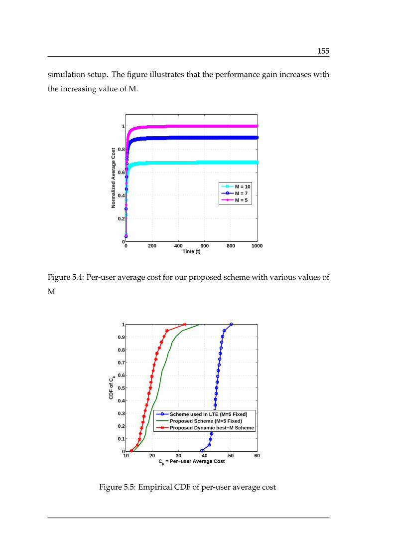
155
simulation setup. The figure illustrates that the performance gain increases with
the increasing value of M.
0 200 400 600 800 10000
0.2
0.4
0.6
0.8
1
Time (t)
No
rmal
ized
Ave
rag
e C
ost
M = 10M = 7M = 5
Figure 5.4: Per-user average cost for our proposed scheme with various values of
M
10 20 30 40 50 600
0.1
0.2
0.3
0.4
0.5
0.6
0.7
0.8
0.9
1
Ck = Per−user Average Cost
CD
F o
f Ck
Scheme used in LTE (M=5 Fixed)Proposed Scheme (M=5 Fixed)Proposed Dynamic best−M Scheme
Figure 5.5: Empirical CDF of per-user average cost
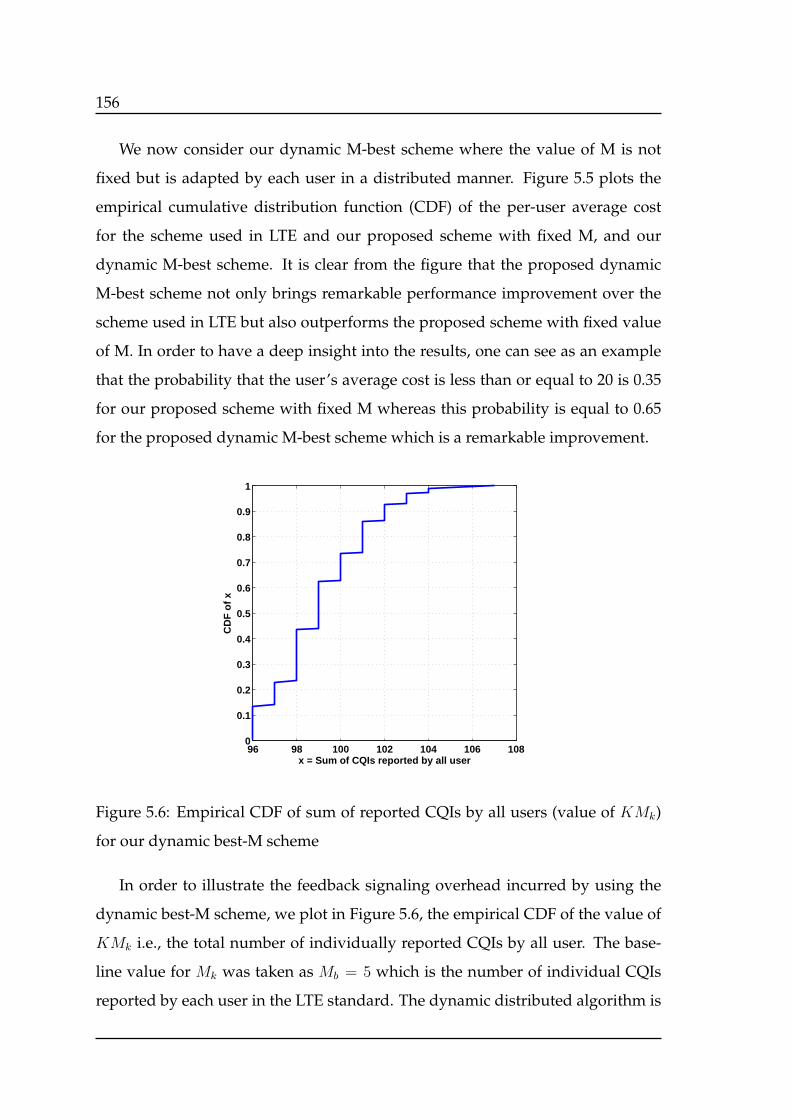
156
We now consider our dynamic M-best scheme where the value of M is not
fixed but is adapted by each user in a distributed manner. Figure 5.5 plots the
empirical cumulative distribution function (CDF) of the per-user average cost
for the scheme used in LTE and our proposed scheme with fixed M, and our
dynamic M-best scheme. It is clear from the figure that the proposed dynamic
M-best scheme not only brings remarkable performance improvement over the
scheme used in LTE but also outperforms the proposed scheme with fixed value
of M. In order to have a deep insight into the results, one can see as an example
that the probability that the user’s average cost is less than or equal to 20 is 0.35
for our proposed scheme with fixed M whereas this probability is equal to 0.65
for the proposed dynamic M-best scheme which is a remarkable improvement.
96 98 100 102 104 106 1080
0.1
0.2
0.3
0.4
0.5
0.6
0.7
0.8
0.9
1
x = Sum of CQIs reported by all user
CD
F o
f x
Figure 5.6: Empirical CDF of sum of reported CQIs by all users (value of KMk)
for our dynamic best-M scheme
In order to illustrate the feedback signaling overhead incurred by using the
dynamic best-M scheme, we plot in Figure 5.6, the empirical CDF of the value of
KMk i.e., the total number of individually reported CQIs by all user. The base-
line value for Mk was taken as Mb = 5 which is the number of individual CQIs
reported by each user in the LTE standard. The dynamic distributed algorithm is
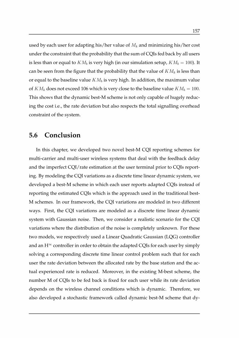
157
used by each user for adapting his/her value of Mk and minimizing his/her cost
under the constraint that the probability that the sum of CQIs fed back by all users
is less than or equal to KMb is very high (in our simulation setup, KMb = 100). It
can be seen from the figure that the probability that the value of KMk is less than
or equal to the baseline value KMb is very high. In addition, the maximum value
of KMk does not exceed 106 which is very close to the baseline value KMb = 100.
This shows that the dynamic best-M scheme is not only capable of hugely reduc-
ing the cost i.e., the rate deviation but also respects the total signalling overhead
constraint of the system.
5.6 Conclusion
In this chapter, we developed two novel best-M CQI reporting schemes for
multi-carrier and multi-user wireless systems that deal with the feedback delay
and the imperfect CQI/rate estimation at the user terminal prior to CQIs report-
ing. By modeling the CQI variations as a discrete time linear dynamic system, we
developed a best-M scheme in which each user reports adapted CQIs instead of
reporting the estimated CQIs which is the approach used in the traditional best-
M schemes. In our framework, the CQI variations are modeled in two different
ways. First, the CQI variations are modeled as a discrete time linear dynamic
system with Gaussian noise. Then, we consider a realistic scenario for the CQI
variations where the distribution of the noise is completely unknown. For these
two models, we respectively used a Linear Quadratic Gaussian (LQG) controller
and an H∞ controller in order to obtain the adapted CQIs for each user by simply
solving a corresponding discrete time linear control problem such that for each
user the rate deviation between the allocated rate by the base station and the ac-
tual experienced rate is reduced. Moreover, in the existing M-best scheme, the
number M of CQIs to be fed back is fixed for each user while its rate deviation
depends on the wireless channel conditions which is dynamic. Therefore, we
also developed a stochastic framework called dynamic best-M scheme that dy-

158
namically determines the efficient number M of CQIs that should be reported by
each user to the base station without increasing the system’s cumulative feedback
overhead. To this end, we developed a distributed constrained interactive trial
and error algorithm that is conducted separately by each user to determine the
efficient number of its best CQIs. We proved the convergence of our algorithm.
Results show that both our proposed schemes result in a huge reduction of the
rate deviation compared to the existing scheme used in the wireless standards.
159
Chapter 6
Conclusion
In modern wireless communication systems, adaptive resource allocation is
essential for the efficient utilization of the limited resources and supporting the
QoS requirements of the services. The design of resource allocation schemes
should consider the service type, since different services have different QoS de-
mands that are characterized in terms of data rates, delays, error rates, etc. More-
over, the availability of only erroneous and outdated channel estimations at the
transmitter should also be considered while developing any resource allocation
scheme.
This thesis addresses three resource allocation problems in wireless commu-
nication systems:
– A resource allocation and adaptive modulation framework that is based on
the recently developed canonical duality theory is presented for uplink SC-
FDMA systems.
– To study resource allocation for delay constrained applications, a frame-
work for joint power control at the PHY/MAC layer and rate adaptation at
the APPLICATION layer for video streaming in wireless networks is devel-
oped.
160
– In order to deal with the channel estimation error and feedback delay, two
novel best-M channel quality indicator (CQI) reporting schemes for multi-
carrier and multi-user systems are developed that consider these issues at
the CQI reporting level.
In the following, we summarize the major contributions of this thesis, and
highlight some future research directions.
6.1 Contributions
In this thesis, first we considered resource allocation and adaptive modula-
tion in SC-FDMA systems. Two different constraint optimization problems are
formulated: A sum-utility maximization (SUmax) problem that aims at maximiz-
ing the sum of users’s utilities in the system under constraints on the per-user and
per sub-channel transmit powers, and a joint adaptive modulation and sum-cost
minimization (JAMSCmin) problem whose objective is to minimize the sum of
transmitted power by all the users in the system under constraints on the user’s
achieved data rates. The solution of these problems needs joint power and sub-
channel allocation where a sub-channel is allowed to be allocated to a single user
at most, and the multiple sub-channels allocated to a user should be consecu-
tive. These constraints on the sub-channel allocation render these problems pro-
hibitively difficult combinatorial problems where the computational complexity
of finding the optimal solution is exponential.
In order to solve these problems, we developed a polynomial-complexity op-
timization framework that is inspired from the recently canonical duality theory.
To this end, we first transformed the primal optimization problems into equiva-
lent binary-integer programming problems. Then, each binary-integer program-
ming problem was transformed into a continuous domain canonical dual prob-
lem that is a concave maximization problem. The computational complexity of
the solution of the continuous space canonical dual problem is polynomial which
161
is a remarkable improvement over exponential complexity. We developed an it-
erative power and sub-channel allocation algorithm for SUmax problem that is
based on the solution of its corresponding canonical dual problem. A modu-
lation adaption scheme for SUmax is also developed that based on the power
and sub-channel allocation performed by the iterative algorithm (i.e., the effec-
tive SNR value of the users) chooses the appropriate modulation scheme for each
user. In a similar way, an iterative power and sub-channel allocation algorithm
joint with adaptive modulation for the JAMSCmin problem was also developed.
Performing modulation adaptation joint with power and sub-channel allocation
in JAMSCmin is essential for ensuring the target data rates achievement of the
users. The proposed iterative algorithms finds exact integer solutions to the cor-
responding binary-integer programs. We thoroughly studied the optimality of
the proposed algorithms, and proved analytically that under certain conditions,
the obtained solutions are optimal. If these optimality conditions are not satis-
fied, then the obtained solution may or may not be optimal. Therefore, we also
explored some bounds on the sub-optimality of the algorithm when the optimal-
ity conditions are not satisfied. However, the numerical results show that the
solution is optimal most of the times, and if not optimal, it is very close to the
optimal solution. The numerical results also show that the proposed algorithm
outperforms the existing algorithms in the literature.
Then, we considered a cross layer optimization framework for joint power
control and video rate adaptation for video streaming in wireless networks with
time-varying channel and interference. This is a challenging problem, since the
multiple nodes in the network demand for better quality video that needs high
data rate, the video applications have stringent delay requirements, the commu-
nication resources (bandwidth, power, etc.) are limited, and the wireless chan-
nel and interferences are time-varying. Due to the different, and time-varying
characteristics of the wireless channel for different nodes in multi-node wireless
networks, the video rate for each node should be adapted in accordance to its
channel conditions for video streaming. In addition, the multiple nodes com-
162
pete for network resources among them where the increased use of resources
by a node will not only deprive the other users from resources but its increased
transmit power will also increase the interference caused to the other nodes and
consequently decrease their achieved rate. Thus, the transmit power of each node
should be controlled as well as there should be a fairness criterion for sharing the
resources among the nodes. Moreover, the power control should be performed
instantaneously at the PHY/MAC layer while the video rate adaptation should
be done at the APPLICATION layer in an average manner. This difference of time
scale renders even the formulation of the joint framework very difficult.
In order to approach the above problem, we started by formulating a cross-
layer framework that allows joint instantaneous power control at the PHY/MAC
layer and average video rate adaptation at the APPLICATION layer. Moreover,
in order that the nodes fairly share the network resources among them, we intro-
duced a fairness/satisfaction criterion into the optimization framework. Then, in
view of the time-varying channels and interferences, stringent delay constraints
of the video applications, and the given fairness criterion, we modeled our prob-
lem as a stochastic control problem by modeling the nodes’ power and rate vari-
ations as linear discrete time dynamic system. In the formulation of stochastic
control problem, we used risk-sensitive control approach and introduced a non-
linear cost function called risk-sensitive cost function. We provided the optimal
solution to the above control problem and conducted numerical study to assess
the performance of the proposed framework.
Finally, we considered the best-M CQI reporting scheme in multi-carrier and
multi-user systems assuming imperfect channel estimation/observation at the
user terminal and the feedback delay occurred in estimating/observing the CQIs
and reporting them to the transmitter/base station. Each user in the multi-user
system estimates/observes its channel conditions on all sub-carriers and reports
the CQIs corresponding to its best M sub-carrier and an average CQI value for
the remaining sub-carriers to the transmitter/base station where they are used
for resource allocation. However, the channel estimation/observation at the user
163
terminal may not be perfect, and the CQI reported on the basis of these imperfect
channel estimations will be erroneous. Furthermore, due to the feedback delay
the CQI reported at any time t are used at time t + τ where τ is the feedback
delay. Using these erroneous and delayed/outdated CQIs for resource alloca-
tion can badly degrade the system performance. Unlike the underlying approach
of dealing these imperfections at the base station, we developed a novel frame-
work for the best-M CQI reporting that takes into account these imperfections
at the user terminal. This new framework considers the channel imperfection
at the CQI reporting level, and reports the CQIs that have already accommo-
dated for the errors in the channel estimation and the feedback delay. To this
end, unlike the traditional approach of reporting the estimated/observed CQIs,
so-called adapted CQIs are reported. The adapted CQIs are computed in such
a manner that the deviation between the actual allocated rate by the base sta-
tion based on these adapted CQIs and the actual experience rate is minimized.
In order to obtain the adapted CQIs, we modeled the CQI variations as a dis-
crete time linear dynamic systems, formulated a corresponding control problem,
and used stochastic control theory to solve this problem. In our framework, we
modeled the CQI variations in two different ways. First, assuming the channel
imperfections as Gaussian distributed, the CQI variations were modeled as a dis-
crete time linear dynamic system with Gaussian noise, and the Linear Quadratic
Gaussian (LQG) controller was used to obtain the adapted CQIs for each user.
Then, we considered a more realistic scenario where the probability distribution
of the channel imperfections is not known. In this case, the CQI variations were
modeled as a discrete time dynamic system where the probability distribution of
the noise is unknown, and an H∞ controller was used for obtaining the adapted
CQIs.
In the traditional best-M CQI reporting scheme, the number M of CQIs to be
reported is fixed for each user. In practice, the more the number of CQIs reported,
the less the rate deviation and the better the system performance. However, the
rate deviation also depends upon the channel conditions of each user. For the
164
same number of CQIs reported, the users having good channel conditions will
have lower rate deviation compared to the users with relatively bad channel con-
ditions. Thus, adapting the value of M (i.e., the number of CQIs to be reported)
for each user according to its channel conditions can further improve the system
performance. Therefore, in addition to developing the best-M scheme with fixed
M, we also developed a so-called dynamic best-M scheme that takes into account
the channel imperfections, and dynamically finds the efficient number of CQIs
that should be reported by each user according to his/her channel quality in a dis-
tributed manner. This scheme uses the same approach of reporting the adapted
CQIs obtained by using the stochastic control theory as mentioned earlier. Since
this is a distributed scheme where each user optimizes the number of its CQIs to
be reported, there is a risk that more users will send more number of CQIs which
will increase the feedback overhead. Thus, in order not to increase the feedback
overhead, we have introduced a probabilistic constraint that the sum of the CQIs
reported at any time by all users in the system should not exceed a certain value.
The proposed dynamic M-best ensures that this constraint on the sum of the CQIs
reported at any time by all users is satisfied with a very high probability (nearly
equal to 1). Numerical results show that both the proposed schemes outperform
the traditional best-M CQI reporting scheme while our dynamic best-M scheme
without increasing the system’s overall feedback overhead performs better than
our M-best scheme with fixed M for each user.
6.2 Future Work
The research carried out in this thesis suggests several interesting directions/
problems that need to be explored. In the following, we summarize a number of
them, and highlight some directions for future research.
The resource allocation and adaptive modulation framework for SC-FDMA
proposed in this thesis assumes that the users’ wireless channels conditions are
perfectly known to the transmitter/base station. However, due to errors in chan-
165
nel estimation at the user terminal, noisy feedback channels, and the delay in
channel reporting, the channel state information available at the base station may
be erroneous or/and outdated. Thus, there is a need to accommodate the impact
of imperfect channel knowledge in the resource allocation. To this end, we have
developed robust CQI reporting schemes that deals with these channel imperfec-
tions at the CQI reporting level. However, the traditional approach of dealing the
channel imperfections at the base station can also be used which is not studied
in this thesis. Due to the intervention of the statistical notions (the probability
distribution of the channel imperfection, etc.) necessary for including the im-
pact of channel imperfections, resource allocation and adaptive modulation with
channel imperfection needs a thorough study. Nevertheless, the proposed re-
source allocation framework in this thesis can be used as a baseline framework
for the optimal resource allocation and adaptive modulation with imperfect chan-
nel knowledge.
Moreover, the proposed resource allocation framework for SC-FDMA is a cen-
tralized framework wherein the power and sub-channel allocation among the
users and the modulation selection are performed at the transmitter/base station
and these decision are then communicated with the users. Since the users better
know their channel conditions, it is quite logical to perform resource allocation at
the users terminals in a distributed manner. The paradigm explored in this the-
sis can be extended to a distributed framework where the decisions on resource
allocation are taken at the user terminals.
The joint power and rate adaption framework for video streaming proposed
in this thesis is based on the assumption that all the nodes use the same wide
frequency band for transmission. The main aim of this work was to first de-
velop a resource allocation framework for a general wireless network and then
extend this framework to SC-FDMA systems. However, due to the time limi-
tations the extension of the general framework to SC-FDMA system was left as
a future work. Thus, an equivalent framework for multi-node wireless systems
with multi-carrier multiple access schemes like SC-FDMA and OFDMA can also
166
be developed.
In this thesis, the satisfaction/fairness criterion in resource allocation for video
streaming is based on the video/arrival data rate (i.e., the quality of the video) of
the nodes. Any other satisfaction/fairness criterion like the average peak-signal-
to-noise (PSNR) or video distortion rate of the nodes can also be incorporated
into the resource allocation framework proposed in this thesis. In addition, the
nodes’ SNRs are approximated as log-normal distributed random variables. A
more realistic scenario where the distribution of the SNR is unknown can also be
considered.
The resource allocation schemes developed in this thesis optimize the resources
at the transmitter side without considering the status of packets arrived at the
receiver. The wireless channels/links are unreliable, and it may happen that the
receiver has not received the packets or they are erroneous whose re-transmission
is needed. Therefore, to ensure the successful transmission of packets, some pro-
tocols for acknowledgement/error notification from other layers/sub-layers e.g.,
Automatic Repeat reQuest (ARQ), etc., should also be integrated into the resource
allocation framework.
The CQI reporting schemes developed in this thesis do not consider any com-
pression of the CQIs. However, in addition to reducing the feedback overhead by
sending only the M best CQIs for each user, the feedback data rate can be further
reduced by sending the compressed versions of the CQIs. In view of the recent
advances in data compression technology, using a compression technique in con-
junction to the best-M CQI reporting scheme is quite a compelling approach. The
CQIs reporting schemes proposed in this thesis has the potential to accommo-
date any CQI compression technique for the further reduction of the feedback
overhead.

167
Appendix A
Appendix chapter 2
A.1 Proof of Theorem 3.4.1
The proof of this theorem can be directly obtained from the proof given in
[116] but we provide it for the completeness of the chapter. We introduce La-
grange multipliers to relax the strict inequality constraints (ϵ∗,λ∗,ρ∗) > 0 in
χ∗♯ . We recall that the canonical dual method is different from the Lagrange
dual method and the Lagrange multipliers has nothing to do with the formu-
lation of the canonical dual problem but are used here to prove that the primal
and the corresponding conical dual problem have the same KKT points. Let
(δϵ∗, δλ
∗, δρ
∗) ∈ (RN ,RK ,RKJ) be the Lagrange multipliers associated to the in-
equality constraints (ϵ∗,λ∗,ρ∗) > 0, then the Lagrangian associated to the com-
plementarity function Ξ(i, ϵ∗,λ∗,ρ∗) can be defined as follows:
L(i, ϵ∗,λ∗,ρ∗, δϵ∗, δλ
∗, δρ
∗) = Ξ(i, ϵ∗,λ∗,ρ∗) + ϵ∗Tδϵ
∗+ λ∗Tδλ
∗+ ρ∗Tδρ
∗(A.1)
The KKT conditions of the primal problem are:
∂L
∂i= 0 ⇒ 2ρ∗k,jik,j +
(λ∗k − ρ∗k,j − Uk,j +
N∑n=1
ϵ∗nAkn,j
)= 0, ∀k, j(A.2)
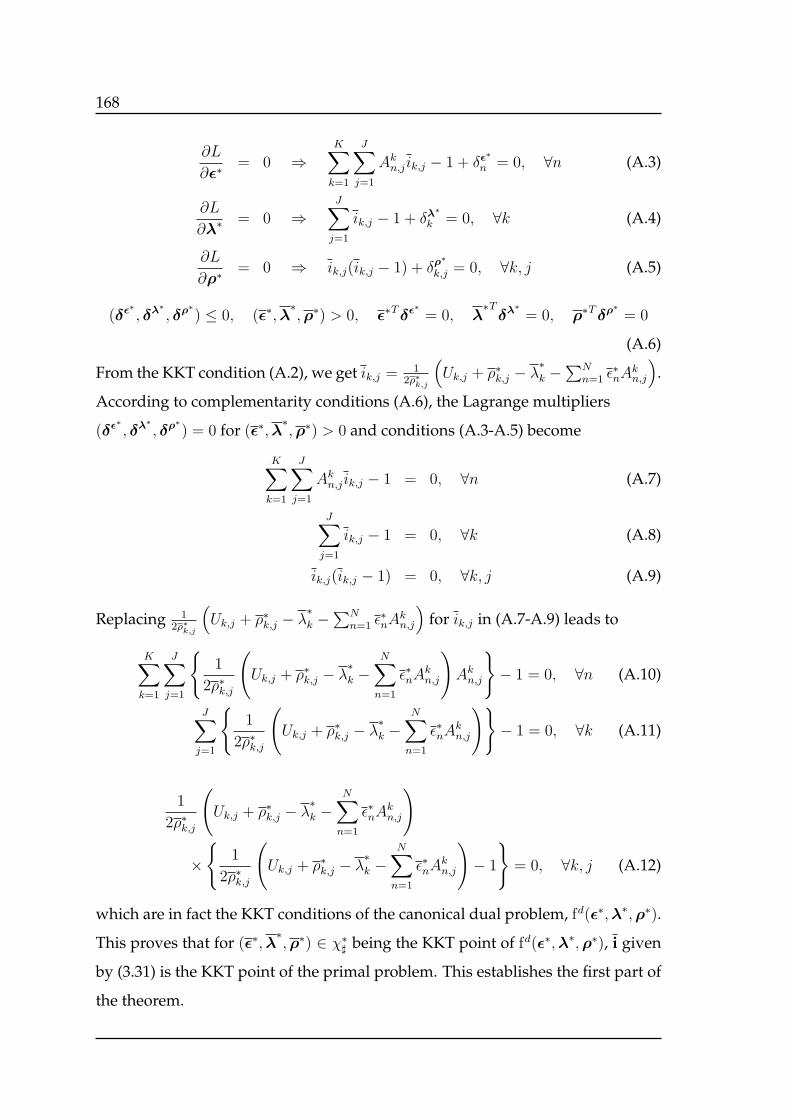
168
∂L
∂ϵ∗= 0 ⇒
K∑k=1
J∑j=1
Akn,jik,j − 1 + δϵ
∗
n = 0, ∀n (A.3)
∂L
∂λ∗ = 0 ⇒J∑
j=1
ik,j − 1 + δλ∗
k = 0, ∀k (A.4)
∂L
∂ρ∗ = 0 ⇒ ik,j(ik,j − 1) + δρ∗
k,j = 0, ∀k, j (A.5)
(δϵ∗, δλ
∗, δρ
∗) ≤ 0, (ϵ∗,λ
∗,ρ∗) > 0, ϵ∗Tδϵ
∗= 0, λ
∗Tδλ
∗= 0, ρ∗Tδρ
∗= 0
(A.6)
From the KKT condition (A.2), we get ik,j = 12ρ∗k,j
(Uk,j + ρ∗k,j − λ
∗k −
∑Nn=1 ϵ
∗nA
kn,j
).
According to complementarity conditions (A.6), the Lagrange multipliers
(δϵ∗, δλ
∗, δρ
∗) = 0 for (ϵ∗,λ
∗,ρ∗) > 0 and conditions (A.3-A.5) become
K∑k=1
J∑j=1
Akn,jik,j − 1 = 0, ∀n (A.7)
J∑j=1
ik,j − 1 = 0, ∀k (A.8)
ik,j(ik,j − 1) = 0, ∀k, j (A.9)
Replacing 12ρ∗k,j
(Uk,j + ρ∗k,j − λ
∗k −
∑Nn=1 ϵ
∗nA
kn,j
)for ik,j in (A.7-A.9) leads to
K∑k=1
J∑j=1
1
2ρ∗k,j
(Uk,j + ρ∗k,j − λ
∗k −
N∑n=1
ϵ∗nAkn,j
)Ak
n,j
− 1 = 0, ∀n (A.10)
J∑j=1
1
2ρ∗k,j
(Uk,j + ρ∗k,j − λ
∗k −
N∑n=1
ϵ∗nAkn,j
)− 1 = 0, ∀k (A.11)
1
2ρ∗k,j
(Uk,j + ρ∗k,j − λ
∗k −
N∑n=1
ϵ∗nAkn,j
)
×
1
2ρ∗k,j
(Uk,j + ρ∗k,j − λ
∗k −
N∑n=1
ϵ∗nAkn,j
)− 1
= 0, ∀k, j (A.12)
which are in fact the KKT conditions of the canonical dual problem, fd(ϵ∗,λ∗,ρ∗).
This proves that for (ϵ∗,λ∗,ρ∗) ∈ χ∗
♯ being the KKT point of fd(ϵ∗,λ∗,ρ∗), i given
by (3.31) is the KKT point of the primal problem. This establishes the first part of
the theorem.

169
According to (3.25), the total complementarity function at the KKT point (i, x∗)
can be written as
Ξ(i, ϵ∗,λ∗,ρ∗) = Λ(i)Tx∗ − V ♯(x∗)−
K∑k=1
J∑j=1
ik,jUk,j
= −K∑k=1
J∑j=1
ik,jUk,j = f(i) (A.13)
which is obvious from the fact that V ♯(x∗) = 0 for (ϵ∗,λ∗,ρ∗) > 0, and where
equations (A.7-A.9) imply that Λ(i) = 0. Similarly from (3.26), we have
Ξ(i, ϵ∗,λ∗,ρ∗) =
K∑k=1
J∑j=1
ρ∗k,ji
2
k,j +
(λ∗k − ρ∗k,j − Uk,j +
N∑n=1
ϵ∗nAkn,j
)ik,j
−N∑
n=1
ϵ∗n −K∑k=1
λ∗k
= −1
4
K∑k=1
J∑j=1
(Uk,j + ρ∗k,j − λ
∗k −
∑Nn=1 ϵ
∗nA
kn,j
)2ρ∗k,j
−
N∑n=1
ϵ∗n −K∑k=1
λ∗k
= fd(ϵ∗,λ∗,ρ∗) (A.14)
This shows that the canonical dual problem is dual to the primal problem. This
completes the proof.
A.2 Proof of Theorem 3.4.2
The total complementarity function Ξ(i, ϵ∗,λ∗,ρ∗) is convex in i and concave
(linear) in ϵ∗, λ∗ and ρ∗. Therefore, the stationary point (i, ϵ∗,λ∗,ρ∗) is a sad-
dle point of Ξ(i, ϵ∗,λ∗,ρ∗). Furthermore, fd(ϵ∗,λ∗,ρ∗) is defined by Ξ(i, ϵ∗,λ∗,ρ∗)
with i being a stationary point of Ξ(i, ϵ∗,λ∗,ρ∗) with respect to i ∈ Ia. Conse-
quently, fd(ϵ∗,λ∗,ρ∗) is concave on χ∗♯ and the KKT point (ϵ∗,λ
∗,ρ∗) ∈ χ∗
♯ must
be its global maximizer. Thus, by the saddle mini-max theorem:
170
fd(ϵ∗,λ∗,ρ∗) = max
ϵ∗>0maxλ∗>0
maxρ∗>0
fd(ϵ∗,λ∗,ρ∗)
= maxϵ∗>0
maxλ∗>0
maxρ∗>0
mini∈Ia
Ξ(i, ϵ∗,λ∗,ρ∗)
= maxϵ∗>0
maxλ∗>0
maxρ∗>0
mini∈Ia
f(i) + ϵTϵ∗ + λTλ∗ + ρTρ∗
= maxϵ∗>0
maxλ∗>0
mini∈Ia
f(i) + ϵTϵ∗ + λTλ∗ +max
ρ∗>0
K∑k=1
J∑j=1
ρ∗k,jik,j(ik,j − 1)
= maxϵ∗>0
mini∈Ia
f(i) + ϵTϵ∗ +max
λ∗>0
K∑k=1
λ∗k
(J∑
j=1
ik,j − 1
)s.t. ik,j(ik,j − 1) = 0,∀k, j
= mini∈Ia
f(i) + max
ϵ∗>0
N∑
n=1
ϵ∗n
(K∑k=1
J∑j=1
ik,jAkn,j − 1
)
s.t. ik,j(ik,j − 1) = 0,∀k, j;J∑
j=1
ik,j = 1, ∀k
= mini∈Ia
f(i) s.t.
ik,j(ik,j − 1) = 0, ∀k, j;
J∑j=1
ik,j = 1, ∀k;K∑k=1
J∑j=1
ik,jAkn,j = 1, ∀n
= min
i∈Iff(i) (A.15)
Note that the linear programming
maxρ∗>0
K∑k=1
J∑j=1
ρ∗k,jik,j(ik,j − 1)
has a finite solution in the open domain χ♯ if and only if ik,j(ik,j − 1) = 0, ∀k, j.
By a similar argument, the solution of maxλ∗>0
∑Kk=1 λ
∗k
(∑Jj=1 ik,j − 1
)and
maxϵ∗>0
∑Nn=1 ϵ
∗n
(∑Kk=1
∑Jj=1 ik,jA
kn,j − 1
)leads to the last equation (A.15). This
shows that the KKT point (ϵ∗,λ∗,ρ∗) maximizes fd(ϵ∗,λ∗,ρ∗) over χ∗
♯ if and only
if i is the global minimizer of f(i) over If . This completes the proof.
A.3 Proof of Theorem 3.5.1
By using sub-gradient method with projection defined by (3.56) ensures the
positive solution of KKT equation (3.55) which implies that the corresponding ik,j
171
is binary integer. However, respecting the positivity constraint on λ∗, equation
(3.54) can not ensure that a single sub-channel pattern is allocated to each user but
1 + σλ∗
k number of patterns will be allocated to each user k. Similarly, ensuring
that ϵ∗ > 0, equation (3.53) means that a sub-channel can be allocated to more
than one users.
In the following, we discuss that we can find another approximate problem
for which the above KKT equations not only provide binary integer solution but
also ensure that a user will be assigned with a single sub-channel pattern and
a sub-channel will be allocated to a single user. To this end, we proceed as fol-
lows. However, respecting the positivity constraint on λ∗, equation (3.54) can not
ensure that a single sub-channel pattern is allocated to each user but 1+σλ∗
k num-
ber of patterns will be allocated to each user k. Similarly, ensuring that ϵ∗ > 0,
equation (3.53) means that a sub-channel can be allocated to more than one users.
In the following, we discuss that we can find another approximate problem
for which the above KKT equations not only provide binary integer solution but
also ensure that a user will be assigned with a single sub-channel pattern and a
sub-channel will be allocated to a single user. To this end, we proceed as follows.
The KKT equation (3.55) can be written as
Uk,j − λ∗k −N∑
n=1
ϵ∗nAkn,j = ±ρ∗k,j, ∀k, j (A.16)
We introduce KJ new variables θk,j’s defined as follows
θk,j =
1, 0 if Uk,j − λ∗k −∑N
n=1 ϵ∗nA
kn,j = −ρ∗k,j
−1, 0 if Uk,j − λ∗k −∑N
n=1 ϵ∗nA
kn,j = +ρ∗k,j
(A.17)
From the above definition of θk,j , equations (A.16) can be written as
Uk,j − 2θk,jρ∗k,j − λ∗k −
N∑n=1
ϵ∗nAkn,j = ±ρ∗k,j, ∀k, j (A.18)
Let Uk,j = Uk,j − 2θk,jρ∗k,j , then the above equations take the form:
Uk,j − λ∗k −N∑
n=1
ϵ∗nAkn,j = ±ρ∗k,j, ∀k, j (A.19)
172
Although the utilities are changed from Uk,j to Uk,j = Uk,j − 2θk,jρ∗k,j , the solu-
tion of the above equations provide integer solution to ik,j’s. We now apply this
change in utilities to the equations (3.53-3.54). The KKT equations (3.54) can be
written asJ∑
j=1
1
2ρ∗k,j
(Uk,j − 2θk,jρ
∗k,j + 2θk,jρ
∗k,j + ρ∗k,j − λ∗k −
N∑n=1
ϵ∗nAkn,j
)= 1 + σλ∗
k ,∀k
(A.20)
Replacing Uk,j for Uk,j − 2θk,jρ∗k,j , the above equations become:
J∑j=1
1
2ρ∗k,j
(Uk,j + ρ∗k,j − λ∗k −
N∑n=1
ϵ∗nAkn,j
)+
J∑j=1
θk,j = 1 + σλ∗
k , ∀k (A.21)
There exist θk,j’s such that∑J
j=1 θk,j = σλ∗
k , then we have
J∑j=1
1
2ρ∗k,j
(Uk,j + ρ∗k,j − λ∗k −
N∑n=1
ϵ∗nAkn,j
)= 1, ∀k (A.22)
This implies that there exist another problem with a different set of utilities for
which the above solution ensures that a single pattern will be allocated to each
user. By using a similar procedure for the KKT equations (3.53), we get
K∑k=1
J∑j=1
1
2ρ∗k,j
(Uk,j + ρ∗k,j − λ∗k −
N∑n=1
ϵ∗nAkn,j
)Ak
n,j
= 1,∀n (A.23)
which enures that a sub-channel will be allocated to a single user at most when∑Kk=1
∑Jj=1 θk,jA
kn,j = σϵ∗
n , and the utilities are changed from Uk,j to Uk,j = Uk,j −
2θk,jρ∗k,j .
The above analysis shows that the solution of the problemP , namely (ϵ∗,λ∗,ρ∗)
that lies in the positive cone, is the solution of the above KKT equations (A.19,
A.22, and A.23). Moreover, the KTT equations (A.19,A.22,A.23) give the station-
ary point of a slightly modified problem fd(ϵ∗,λ∗,ρ∗) which the canonical dual
of a slightly modified primal problem with utilities Uk,j = Uk,j − 2θk,jρ∗k,j . Since
the solution (ϵ∗,λ∗,ρ∗) is positive and using Theorems 4.1 and 4.2, the proposed
sub-gradient based solution proposed in Table 3.1 optimally solves a correspond-
ing primal problem with utilities Uk,j’s and an objective function f(i). Note also
173
that the canonical dual fd(ϵ∗,λ∗,ρ∗) is concave (since the KKT solution is in the
positive cone). However, how far the solution of the modified problem will be
from that of the primal problem (3.5) depends upon the values of ρ∗k,j’s.
A.4 Proof of Corollary 3.5.1
If ρ∗k,j << Uk,j,∀k, j, then Uk,j ≈ Uk,j, ∀k, j, f(i) ≈ f(i), and
max(ϵ∗,λ∗,ρ∗)
fd ≈ max(ϵ∗,λ∗,ρ∗)
fd (A.24)
For ρ∗k,j << Uk,j, ∀k, j, the solution of the equations (A.19,A.22,A.23) is very close
to that of equations (3.43,3.44, 3.45). Furthermore, the solution of (A.19,A.22,A.23)
is the optimal solution of the corresponding primal problem with utilities Uk,j
(which is very close to the optimal solution of the primal problem with utilities
Uk,j). Consequently, the dual canonical problem obtained using the sub-gradient
based algorithm (Table 3.1) will provide solution to the primal problem which is
very close to the optimal solution. This completes the proof.

174
175
Appendix B
Appendix Chapter 4
B.1 Proof of Theorem 5.4.1
We start our proof by constructing a Markov chain for our proposed learning
process. Then we study the properties of our learning process according to Def-
inition 1 and 2. Finally, by using some results from [127] [128], we complete our
proof.
Each user has its own Markov chain which is interdependent with the Markov
chains of the other users via their decisions. This interdependency leads to an
interactive learning. In our framework a user is always in one of the four main
states denoted by c, c+, c−, and d. When the common constraint is not violated
and a user has to minimize his/her own cost i.e., rate deviation, then the user is
said to be “content" and this state is represented by c. The state d represents a
“discontent" state where the common constraint is not satisfied and a user gets
very high cost. The states c+ and c− are intermediary states before transitions
to discontent state d. We denote by Ltk the current reference which is the current
cost of user k (as performance) and Ltk the received cost which is the new cost if
configuration is changed. Next we describe the transitions of the Markov chains.
a) Transitions of the Markov chains
• Transitions from content state“c": In “c", we have four different cases. The
cases c1−c3 are dedicated for experimentation and the state c4 is for non-experim-
176
entation of new configurations.
c1 : A user can decide to experiment a new configuration or not. The user
experiments with probability ϵ > 0 and receives a cost Lt+1k . If Lt+1
k > Ltk, then the
reference is the same: Lt+1k = Lt
k and the user keeps the same configuration and
stays at the state denoted by c1. If Lt+1k < Lt
k then the chain of user k can go in a
probabilistic manner to any of the two state c2 or c3 explained as follows.
c2 : Accept the new references and configurations with probability qk = e−βkGk(−Lt+1k +Lt
k)
where βk > 0 and Gk is decreasing function which belongs to [0, 12] [128]. This
state of user’s chain is now denoted by c2.
c3 : Reject the new references and configurations with probability 1 − qk and
stay at state c3.
c4 : A user does not perform experimentation with probability (1− ϵ). In this
case, if Lt+1k = Lt
k then the chain stays at c. If Lt+1k < Lt
k the chain goes to c+ and
if Lt+1k > Lt
k the chain of user k goes to c− .
• Transitions from discontent state “c+": At state c+ the user compares the
new cost and the reference. IfLt+2k ≤ Lt
k, the chain goes back to c and the reference
Lt+1k = Lt+2
k . If Lt+2k > Lt
k the chain goes to c− .
• Transitions from discontent state “c−": At state c− the user compares again
the new cost and the reference. If Lt+2k < Lt
k, the chain goes back to c+, if
Lt+2k = Lt
k the chain goes to c and if Lt+2k > Lt
k then the chain of user k goes
to the discontent state d.
• Transitions from discontent state “d": At state d, the user randomly picks a
configuration and receives Ltk. The user accepts these new references with proba-
bility pk = e−βkFk(−Ltk) where Fk is a decreasing function such that KFk ∈ [0, 1/2],
the chain goes to content state c. The user rejects the new references with proba-
bility 1− pk and the chain stay at d.
b) Selection of the efficient outcomes
To proceed with the proof, we now present the main result of the proposed in-
teractive trial and error learning algorithm. Our learning process will be most
of time in a stochastically stable state [128]. Furthermore, our learning process

177
has the property of the interdependent game since each of the users can make a
change in the cost of the other users by changing its configuration. We also recall
that a pure Nash equilibrium of a finite game is a configuration such that no user
can improve its payoff by deviating unilaterally. A pure Nash equilibrium in our
context corresponds to a configuration where the states are content, the costs are
the references and are Nash equilibrium costs.
Based on the chain constructed, and the interdependency and the stochasti-
cally stable sets properties of our learning process, we can establish that if each
user follows our learning process, a pure equilibrium will be visited by high pro-
portion of time. Moreover, every stochastically stable state minimizes the sum
function∑
k Ltk i.e, the system cumulative cost. This result follows directly from
Theorem 1 and Theorem 2 in [127] which completes the proof of our theorem.

178
179
Bibliography
[1] 3rd Generation Partnership Project, “Technical Specification Group Radio
Access Network; Physical layer aspects for evolved Universal Terrestrial
Radio Access (UTRA),” 3GPP Std. TR 25.814, v. 7.0.0, 2006.
[2] H. G. Myung, J. Lim, and D. J. Goodman, “Single carrier fdma for uplink
wireless transmission,” Vehicular Technology Magazine, IEEE, vol. 1, pp. 30
–38, sept. 2006.
[3] I. Wong, O. Oteri, and W. Mccoy, “Optimal resource allocation in uplink
sc-fdma systems,” Wireless Communications, IEEE Transactions on, vol. 8,
pp. 2161 –2165, may 2009.
[4] S. Boyd and L. Vandenberghe, Convex Optimization. Cambridge University
Press, 2004.
[5] P. Whittle, Risk-Sensitive Optimal Control. New York: John Wiley, 1990.
[6] M. C. CAMPI and M. R. JAMES, “Nonlinear discrete-time risk-sensitive
optimal control,” International Journal of Robust and Nonlinear Control, vol. 6,
no. 1, pp. 1–19, 1996.
[7] S. Chen, N. Bambos, and G. Pottie, “Admission control schemes for wire-
less communication networks with adjustable transmitter powers,” in IN-
FOCOM ’94. Networking for Global Communications., 13th Proceedings IEEE,
pp. 21 –28 vol.1, jun 1994.
[8] A. Subramanian and A. Sayed, “Joint rate and power control algorithms for
wireless networks,” Signal Processing, IEEE Transactions on, vol. 53, pp. 4204
– 4214, nov. 2005.
180
[9] M. Gudmundson, “Correlation model for shadow fading in mobile radio
systems,” Electronics Letters, vol. 27, pp. 2145 –2146, nov. 1991.
[10] K. Leung, “Power control by interference prediction for broadband wire-
less packet networks,” Wireless Communications, IEEE Transactions on, vol. 1,
pp. 256 –265, apr 2002.
[11] K. Leung, “A kalman-filter method for power control in broadband wire-
less networks,” in INFOCOM ’99. Eighteenth Annual Joint Conference of
the IEEE Computer and Communications Societies. Proceedings. IEEE, vol. 2,
pp. 948 –956 vol.2, mar 1999.
[12] T. Baser and P. Bernhard, H-Infinity Optimal Control and Related Minimax
Design Problems: A Dynamic Game Approach. Boston, MA: Brikhauser, 1991.
[13] K. J. Astrom, Introduction to Stochastic Control Theory. New York: Academic,
1970.
[14] T. Kailath, A. H. Sayed, and B. Hassibi, Linear Estimation. NJ, Pentice Hall,
1970.
[15] R. V. Nee and R. Prasad, OFDM for Wireless Multimedia Communications.
Norwood, MA, USA: Artech House, Inc., 1st ed., 2000.
[16] J. Bingham, “Multicarrier modulation for data transmission: an idea whose
time has come,” Communications Magazine, IEEE, vol. 28, pp. 5 –14, may
1990.
[17] IEEE standard for local and metropolitan area networks, “Part 16: Air in-
terface for fixed broadband wireless access systems”, 1 October 2004.
[18] IEEE standard for local and metropolitan area networks, “Part 16: Air inter-
face for fixed and mobile broadband wireless access systems”, 28 February
2006.
[19] M. Etoh and T. Yoshimura, “Advances in wireless video delivery,” Proceed-
ings of the IEEE, vol. 93, pp. 111 –122, jan. 2005.
[20] L. Hanzo, P. Cherrimana, and J. Streit, Wireless Video Communications: Sec-
ond to Third Generation and Beyond. John Wiley, 2001.
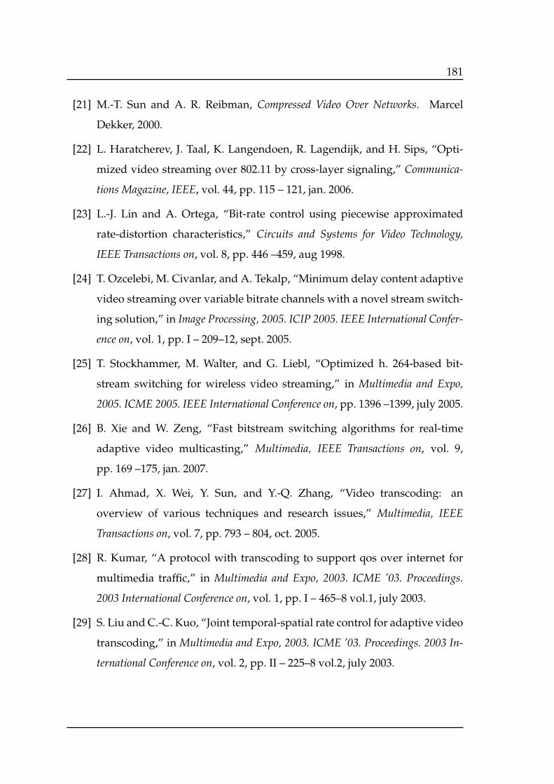
181
[21] M.-T. Sun and A. R. Reibman, Compressed Video Over Networks. Marcel
Dekker, 2000.
[22] L. Haratcherev, J. Taal, K. Langendoen, R. Lagendijk, and H. Sips, “Opti-
mized video streaming over 802.11 by cross-layer signaling,” Communica-
tions Magazine, IEEE, vol. 44, pp. 115 – 121, jan. 2006.
[23] L.-J. Lin and A. Ortega, “Bit-rate control using piecewise approximated
rate-distortion characteristics,” Circuits and Systems for Video Technology,
IEEE Transactions on, vol. 8, pp. 446 –459, aug 1998.
[24] T. Ozcelebi, M. Civanlar, and A. Tekalp, “Minimum delay content adaptive
video streaming over variable bitrate channels with a novel stream switch-
ing solution,” in Image Processing, 2005. ICIP 2005. IEEE International Confer-
ence on, vol. 1, pp. I – 209–12, sept. 2005.
[25] T. Stockhammer, M. Walter, and G. Liebl, “Optimized h. 264-based bit-
stream switching for wireless video streaming,” in Multimedia and Expo,
2005. ICME 2005. IEEE International Conference on, pp. 1396 –1399, july 2005.
[26] B. Xie and W. Zeng, “Fast bitstream switching algorithms for real-time
adaptive video multicasting,” Multimedia, IEEE Transactions on, vol. 9,
pp. 169 –175, jan. 2007.
[27] I. Ahmad, X. Wei, Y. Sun, and Y.-Q. Zhang, “Video transcoding: an
overview of various techniques and research issues,” Multimedia, IEEE
Transactions on, vol. 7, pp. 793 – 804, oct. 2005.
[28] R. Kumar, “A protocol with transcoding to support qos over internet for
multimedia traffic,” in Multimedia and Expo, 2003. ICME ’03. Proceedings.
2003 International Conference on, vol. 1, pp. I – 465–8 vol.1, july 2003.
[29] S. Liu and C.-C. Kuo, “Joint temporal-spatial rate control for adaptive video
transcoding,” in Multimedia and Expo, 2003. ICME ’03. Proceedings. 2003 In-
ternational Conference on, vol. 2, pp. II – 225–8 vol.2, july 2003.
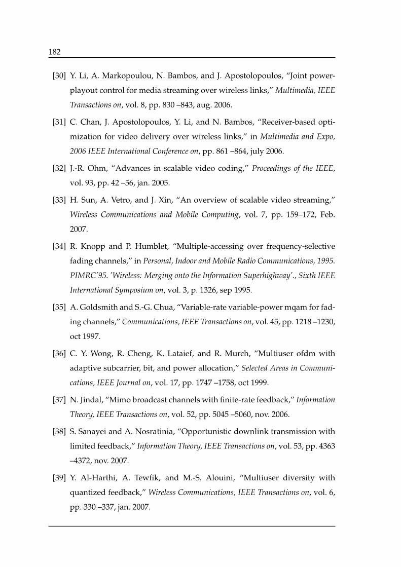
182
[30] Y. Li, A. Markopoulou, N. Bambos, and J. Apostolopoulos, “Joint power-
playout control for media streaming over wireless links,” Multimedia, IEEE
Transactions on, vol. 8, pp. 830 –843, aug. 2006.
[31] C. Chan, J. Apostolopoulos, Y. Li, and N. Bambos, “Receiver-based opti-
mization for video delivery over wireless links,” in Multimedia and Expo,
2006 IEEE International Conference on, pp. 861 –864, july 2006.
[32] J.-R. Ohm, “Advances in scalable video coding,” Proceedings of the IEEE,
vol. 93, pp. 42 –56, jan. 2005.
[33] H. Sun, A. Vetro, and J. Xin, “An overview of scalable video streaming,”
Wireless Communications and Mobile Computing, vol. 7, pp. 159–172, Feb.
2007.
[34] R. Knopp and P. Humblet, “Multiple-accessing over frequency-selective
fading channels,” in Personal, Indoor and Mobile Radio Communications, 1995.
PIMRC’95. ’Wireless: Merging onto the Information Superhighway’., Sixth IEEE
International Symposium on, vol. 3, p. 1326, sep 1995.
[35] A. Goldsmith and S.-G. Chua, “Variable-rate variable-power mqam for fad-
ing channels,” Communications, IEEE Transactions on, vol. 45, pp. 1218 –1230,
oct 1997.
[36] C. Y. Wong, R. Cheng, K. Lataief, and R. Murch, “Multiuser ofdm with
adaptive subcarrier, bit, and power allocation,” Selected Areas in Communi-
cations, IEEE Journal on, vol. 17, pp. 1747 –1758, oct 1999.
[37] N. Jindal, “Mimo broadcast channels with finite-rate feedback,” Information
Theory, IEEE Transactions on, vol. 52, pp. 5045 –5060, nov. 2006.
[38] S. Sanayei and A. Nosratinia, “Opportunistic downlink transmission with
limited feedback,” Information Theory, IEEE Transactions on, vol. 53, pp. 4363
–4372, nov. 2007.
[39] Y. Al-Harthi, A. Tewfik, and M.-S. Alouini, “Multiuser diversity with
quantized feedback,” Wireless Communications, IEEE Transactions on, vol. 6,
pp. 330 –337, jan. 2007.
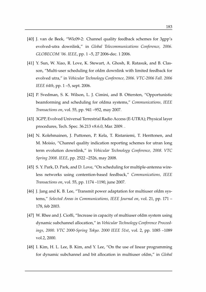
183
[40] J. van de Beek, “Wlc09-2: Channel quality feedback schemes for 3gpp’s
evolved-utra downlink,” in Global Telecommunications Conference, 2006.
GLOBECOM ’06. IEEE, pp. 1 –5, 27 2006-dec. 1 2006.
[41] Y. Sun, W. Xiao, R. Love, K. Stewart, A. Ghosh, R. Ratasuk, and B. Clas-
son, “Multi-user scheduling for ofdm downlink with limited feedback for
evolved utra,” in Vehicular Technology Conference, 2006. VTC-2006 Fall. 2006
IEEE 64th, pp. 1 –5, sept. 2006.
[42] P. Svedman, S. K. Wilson, L. J. Cimini, and B. Ottersten, “Opportunistic
beamforming and scheduling for ofdma systems,” Communications, IEEE
Transactions on, vol. 55, pp. 941 –952, may 2007.
[43] 3GPP, Evolved Universal Terrestrial Radio Access (E-UTRA); Physical layer
procedures, Tech. Spec. 36.213 v8.6.0, Mar. 2009. .
[44] N. Kolehmainen, J. Puttonen, P. Kela, T. Ristaniemi, T. Henttonen, and
M. Moisio, “Channel quality indication reporting schemes for utran long
term evolution downlink,” in Vehicular Technology Conference, 2008. VTC
Spring 2008. IEEE, pp. 2522 –2526, may 2008.
[45] S. Y. Park, D. Park, and D. Love, “On scheduling for multiple-antenna wire-
less networks using contention-based feedback,” Communications, IEEE
Transactions on, vol. 55, pp. 1174 –1190, june 2007.
[46] J. Jang and K. B. Lee, “Transmit power adaptation for multiuser ofdm sys-
tems,” Selected Areas in Communications, IEEE Journal on, vol. 21, pp. 171 –
178, feb 2003.
[47] W. Rhee and J. Cioffi, “Increase in capacity of multiuser ofdm system using
dynamic subchannel allocation,” in Vehicular Technology Conference Proceed-
ings, 2000. VTC 2000-Spring Tokyo. 2000 IEEE 51st, vol. 2, pp. 1085 –1089
vol.2, 2000.
[48] I. Kim, H. L. Lee, B. Kim, and Y. Lee, “On the use of linear programming
for dynamic subchannel and bit allocation in multiuser ofdm,” in Global
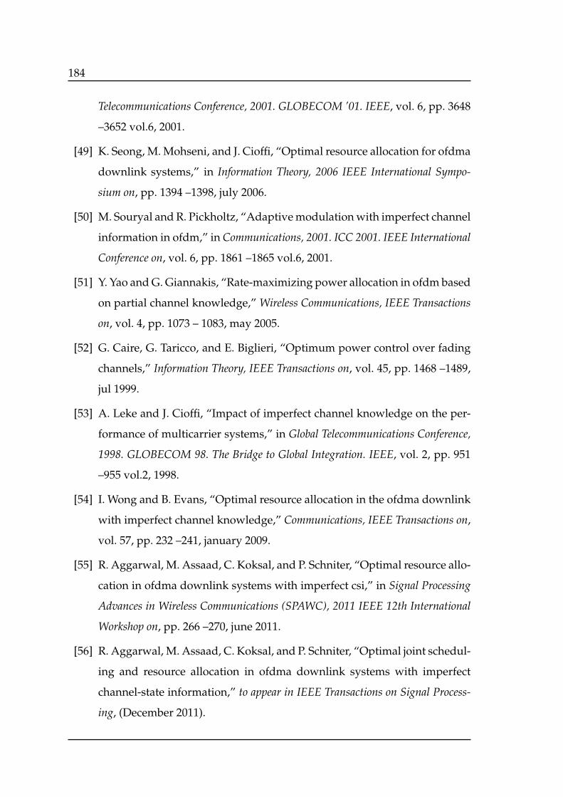
184
Telecommunications Conference, 2001. GLOBECOM ’01. IEEE, vol. 6, pp. 3648
–3652 vol.6, 2001.
[49] K. Seong, M. Mohseni, and J. Cioffi, “Optimal resource allocation for ofdma
downlink systems,” in Information Theory, 2006 IEEE International Sympo-
sium on, pp. 1394 –1398, july 2006.
[50] M. Souryal and R. Pickholtz, “Adaptive modulation with imperfect channel
information in ofdm,” in Communications, 2001. ICC 2001. IEEE International
Conference on, vol. 6, pp. 1861 –1865 vol.6, 2001.
[51] Y. Yao and G. Giannakis, “Rate-maximizing power allocation in ofdm based
on partial channel knowledge,” Wireless Communications, IEEE Transactions
on, vol. 4, pp. 1073 – 1083, may 2005.
[52] G. Caire, G. Taricco, and E. Biglieri, “Optimum power control over fading
channels,” Information Theory, IEEE Transactions on, vol. 45, pp. 1468 –1489,
jul 1999.
[53] A. Leke and J. Cioffi, “Impact of imperfect channel knowledge on the per-
formance of multicarrier systems,” in Global Telecommunications Conference,
1998. GLOBECOM 98. The Bridge to Global Integration. IEEE, vol. 2, pp. 951
–955 vol.2, 1998.
[54] I. Wong and B. Evans, “Optimal resource allocation in the ofdma downlink
with imperfect channel knowledge,” Communications, IEEE Transactions on,
vol. 57, pp. 232 –241, january 2009.
[55] R. Aggarwal, M. Assaad, C. Koksal, and P. Schniter, “Optimal resource allo-
cation in ofdma downlink systems with imperfect csi,” in Signal Processing
Advances in Wireless Communications (SPAWC), 2011 IEEE 12th International
Workshop on, pp. 266 –270, june 2011.
[56] R. Aggarwal, M. Assaad, C. Koksal, and P. Schniter, “Optimal joint schedul-
ing and resource allocation in ofdma downlink systems with imperfect
channel-state information,” to appear in IEEE Transactions on Signal Process-
ing, (December 2011).
185
[57] W. Yu and R. Lui, “Dual methods for nonconvex spectrum optimization
of multicarrier systems,” Communications, IEEE Transactions on, vol. 54,
pp. 1310 –1322, july 2006.
[58] H. Myung, J. Lim, and D. Goodman, “Peak-to-average power ratio of sin-
gle carrier fdma signals with pulse shaping,” in Personal, Indoor and Mobile
Radio Communications, 2006 IEEE 17th International Symposium on, pp. 1 –5,
sept. 2006.
[59] M. Schnell and I. De Broeck, “Application of ifdma to mobile radio trans-
mission,” in Universal Personal Communications, 1998. ICUPC ’98. IEEE 1998
International Conference on, vol. 2, pp. 1267 –1272 vol.2, oct 1998.
[60] R. Dinis, D. Falconer, C. T. Lam, and M. Sabbaghian, “A multiple access
scheme for the uplink of broadband wireless systems,” in Global Telecom-
munications Conference, 2004. GLOBECOM ’04. IEEE, vol. 6, pp. 3808 – 3812
Vol.6, nov.-3 dec. 2004.
[61] T. Shi, S. Zhou, and Y. Yao, “Capacity of single carrier systems with
frequency-domain equalization,” in Emerging Technologies: Frontiers of Mo-
bile and Wireless Communication, 2004. Proceedings of the IEEE 6th Circuits and
Systems Symposium on, vol. 2, pp. 429 – 432 Vol.2, may-2 june 2004.
[62] 3GPP TSG-RAN, Simulation methodology for EUTRA UL: IFDMA and
DFT-Spread-OFDMA, WG1 #42, R1-050718, Sept. 2005.
[63] M. Al-Rawi, R. Jantti, J. Torsner, and M. Sagfors, “Opportunistic uplilnk
scheduling for 3G LTE systems,” in Innovations in Information Technology,
2007. IIT ’07. 4th International Conference on, pp. 705 –709, nov. 2007.
[64] J. Lim, H. Myung, K. Oh, and D. Goodman, “Channel-dependent schedul-
ing of uplink single carrier fdma systems,” in Vehicular Technology Confer-
ence, 2006. VTC-2006 Fall. 2006 IEEE 64th, pp. 1 –5, sept. 2006.
[65] J. Lim, H. Myung, K. Oh, and D. Goodman, “Proportional fair scheduling
of uplink single-carrier fdma systems,” in Personal, Indoor and Mobile Radio
186
Communications, 2006 IEEE 17th International Symposium on, pp. 1 –6, sept.
2006.
[66] S.-B. Lee, I. Pefkianakis, A. Meyerson, S. Xu, and S. Lu, “Proportional fair
frequency-domain packet scheduling for 3gpp lte uplink,” in INFOCOM
2009, IEEE, pp. 2611 –2615, april 2009.
[67] O. Nwamadi, X. Zhu, and A. Nandi, “Dynamic subcarrier allocation for
single carrier- fdma systems,” in Eusipco 2008, 2008.
[68] M. Anas, Uplink Radio Resource Management for QoS Provisioning in Long
Term Evolution: With Emphasis on Admission Control and Handover. PhD the-
sis, Faculty of Engineering, Science and Medicine of Aalborg University,
Denmark, January 2009.
[69] F. D. Calabrese, Scheduling and Link Adaptation for Uplink SC-FDMA Systems:
A LTE Case Study. PhD thesis, Faculty of Engineering, Science and Medicine
of Aalborg University, Denmark, April 2009.
[70] F. Sokmen and T. Girici, “Uplink resource allocation algorithms for single-
carrier fdma systems,” in Wireless Conference (EW), 2010 European, pp. 339
–345, april 2010.
[71] W.-C. Pao and Y.-F. Chen, “Chunk allocation schemes for sc-fdma systems,”
in Vehicular Technology Conference (VTC 2010-Spring), 2010 IEEE 71st, pp. 1
–5, may 2010.
[72] J.-H. Noh and S.-J. Oh, “Distributed sc-fdma resource allocation algorithm
based on the hungarian method,” in Vehicular Technology Conference Fall
(VTC 2009-Fall), 2009 IEEE 70th, pp. 1 –5, sept. 2009.
[73] G. Cheung and A. Zakhor, “Bit allocation for joint source/channel coding
of scalable video,” Image Processing, IEEE Transactions on, vol. 9, pp. 340
–356, mar 2000.
[74] M. Goel, S. Appadwedula, N. Shambhag, K. Ramchandran, and D. Jones,
“A low-power multimedia communication system for indoor wireless ap-
187
plications,” in Signal Processing Systems, 1999. SiPS 99. 1999 IEEE Workshop
on, pp. 473 –482, 1999.
[75] Q. Zhang, Z. Ji, W. Zhu, and Y.-Q. Zhang, “Power-minimized bit allocation
for video communication over wireless channels,” Circuits and Systems for
Video Technology, IEEE Transactions on, vol. 12, pp. 398 –410, jun 2002.
[76] Q. Zhang, W. Zhu, Z. Ji, and Y.-Q. Zhang, “A power-optimized joint source
channel coding for scalable video streaming over wireless channel,” in Cir-
cuits and Systems, 2001. ISCAS 2001. The 2001 IEEE International Symposium
on, vol. 5, pp. 137 –140 vol. 5, 2001.
[77] Y. Eisenberg, C. Luna, T. Pappas, R. Berry, and A. Katsaggelos, “Joint
source coding and transmission power management for energy efficient
wireless video communications,” Circuits and Systems for Video Technology,
IEEE Transactions on, vol. 12, pp. 411 –424, jun 2002.
[78] Q. Zhang, W. Zhu, and Y.-Q. Zhang, “Channel-adaptive resource allocation
for scalable video transmission over 3g wireless network,” Circuits and Sys-
tems for Video Technology, IEEE Transactions on, vol. 14, pp. 1049 – 1063, aug.
2004.
[79] T. Nguyen and A. Zakhor, “Multiple sender distributed video streaming,”
Multimedia, IEEE Transactions on, vol. 6, pp. 315 – 326, april 2004.
[80] K. Kar, S. Sarkar, and L. Tassiulas, “Optimization based rate control for mul-
tirate multicast sessions,” in INFOCOM 2001. Twentieth Annual Joint Confer-
ence of the IEEE Computer and Communications Societies. Proceedings. IEEE,
vol. 1, pp. 123 –132 vol.1, 2001.
[81] A. K. Talukdar, B. R. Badrinath, and A. Acharya, “Rate adaptation schemes
in networks with mobile hosts,” in Proceedings of the 4th annual ACM/IEEE
international conference on Mobile computing and networking, MobiCom ’98,
(New York, NY, USA), pp. 169–180, ACM, 1998.
[82] A. Sampath, P. Sarath Kumar, and J. Holtzman, “Power control and re-
source management for a multimedia cdma wireless system,” in Personal,
188
Indoor and Mobile Radio Communications, 1995. PIMRC’95. ’Wireless: Merging
onto the Information Superhighway’., Sixth IEEE International Symposium on,
vol. 1, pp. 21 –25 vol.1, sep 1995.
[83] J. Liu, B. Li, and Y.-Q. Zhang, “An end-to-end adaptation protocol for lay-
ered video multicast using optimal rate allocation,” Multimedia, IEEE Trans-
actions on, vol. 6, pp. 87 – 102, feb. 2004.
[84] T. Kwon, Y. Choi, and S. K. Das, “Bandwidth adaptation algorithms for
adaptive multimedia services in mobile cellular networks,” Wirel. Pers.
Commun., vol. 22, pp. 337–357, September 2002.
[85] F. Zhai, C. Luna, Y. Eisenberg, T. Pappas, R. Berry, and A. Katsaggelos,
“Joint source coding and packet classification for real-time video transmis-
sion over differentiated services networks,” Multimedia, IEEE Transactions
on, vol. 7, pp. 716 – 726, aug. 2005.
[86] S. Zhao, Z. Xiong, and X. Wang, “Joint error control and power alloca-
tion for video transmission over cdma networks with multiuser detection,”
in Communications, 2002. ICC 2002. IEEE International Conference on, vol. 5,
pp. 3212 – 3216 vol.5, 2002.
[87] T. Yoo, E. Setton, X. Zhu, A. Goldsmith, and B. Girod, “Cross-layer design
for video streaming over wireless ad hoc networks,” in Multimedia Signal
Processing, 2004 IEEE 6th Workshop on, pp. 99 – 102, sept.-1 oct. 2004.
[88] W. Kumwilaisak, Y. Hou, Q. Zhang, W. Zhu, C.-C. Kuo, and Y.-Q. Zhang,
“A cross-layer quality-of-service mapping architecture for video delivery
in wireless networks,” Selected Areas in Communications, IEEE Journal on,
vol. 21, pp. 1685 – 1698, dec. 2003.
[89] M. van der Schaar, Y. Andreopoulos, and Z. Hu, “Optimized scalable video
streaming over ieee 802.11 a/e hcca wireless networks under delay con-
straints,” Mobile Computing, IEEE Transactions on, vol. 5, pp. 755 – 768, june
2006.
189
[90] O. I. Hillestad, A. Perkis, V. Genc, S. Murphy, and J. Murphy, “Adaptive
h.264/mpeg-4 svc video over ieee 802.16 broadband wireless networks,” in
Packet Video 2007, pp. 26 –35, nov. 2007.
[91] X. Zhu, P. Agrawal, J. Singh, T. Alpcan, and B. Girod, “Distributed rate
allocation policies for multihomed video streaming over heterogeneous ac-
cess networks,” Multimedia, IEEE Transactions on, vol. 11, pp. 752 –764, june
2009.
[92] S. Adlakha, X. Zhu, B. Girod, and A. Goldsmith, “Joint capacity, flow and
rate allocation for multiuser video streaming over wireless ad-hoc net-
works,” in Communications, 2007. ICC ’07. IEEE International Conference on,
pp. 1747 –1753, june 2007.
[93] Z. Ahmad, S. Worrall, and A. Kondoz, “Unequal power allocation for scal-
able video transmission over wimax,” in Multimedia and Expo, 2008 IEEE
International Conference on, pp. 517 –520, 23 2008-april 26 2008.
[94] J. Huang, Z. Li, M. Chiang, and A. Katsaggelos, “Joint source adaptation
and resource allocation for multi-user wireless video streaming,” Circuits
and Systems for Video Technology, IEEE Transactions on, vol. 18, pp. 582 –595,
may 2008.
[95] X. Ji, J. Huang, M. Chiang, G. Lafruit, and F. Catthoor, “Scheduling and
resource allocation for svc streaming over ofdm downlink systems,” Cir-
cuits and Systems for Video Technology, IEEE Transactions on, vol. 19, pp. 1549
–1555, oct. 2009.
[96] M. Johansson, “Benefits of multiuser diversity with limited feedback,” in
Signal Processing Advances in Wireless Communications, 2003. SPAWC 2003.
4th IEEE Workshop on, pp. 155 – 159, june 2003.
[97] F. Floren, O. Edfors, and B.-A. Molin, “The effect of feedback quantization
on the throughput of a multiuser diversity scheme,” in Global Telecommuni-
cations Conference, 2003. GLOBECOM ’03. IEEE, vol. 1, pp. 497 – 501 Vol.1,
dec. 2003.
190
[98] M. Johansson, “Diversity-enhanced equal access-considerable throughput
gains with 1-bit feedback,” in Signal Processing Advances in Wireless Commu-
nications, 2004 IEEE 5th Workshop on, pp. 6 – 10, july 2004.
[99] S. Sanayei and A. Nosratinia, “Exploiting multiuser diversity with only 1-
bit feedback,” in Wireless Communications and Networking Conference, 2005
IEEE, vol. 2, pp. 978 – 983 Vol. 2, march 2005.
[100] T. Eriksson and T. Ottosson, “Compression of feedback for adaptive trans-
mission and scheduling,” Proceedings of the IEEE, vol. 95, pp. 2314 –2321,
dec. 2007.
[101] H. Cheon, B. Park, and D. Hong, “Adaptive multicarrier system with re-
duced feedback information in wideband radio channels,” in Vehicular Tech-
nology Conference, 1999. VTC 1999 - Fall. IEEE VTS 50th, vol. 5, pp. 2880
–2884 vol.5, 1999.
[102] H. Nguyen and T. Lestable, “Compression of bit loading power vectors for
adaptive multi-carrier systems,” in Circuits and Systems, 2004. MWSCAS ’04.
The 2004 47th Midwest Symposium on, vol. 3, pp. iii – 243–6 vol.3, july 2004.
[103] T. Eriksson and T. Ottosson, “Compression of feedback in adaptive ofdm-
based systems using scheduling,” Communications Letters, IEEE, vol. 11,
pp. 859 –861, november 2007.
[104] V. Jimenez and A. Armada, “An adaptive mimo - ofdm system: Design and
performance evaluation,” in Wireless Communication Systems, 2006. ISWCS
’06. 3rd International Symposium on, pp. 809 –813, sept. 2006.
[105] A. Haghighat, G. Zhang, and Z. Lin, “Full-band cqi feedback by haar com-
pression in ofdma systems,” in Vehicular Technology Conference Fall (VTC
2009-Fall), 2009 IEEE 70th, pp. 1 –5, sept. 2009.
[106] H. Gao, R. Song, and J. Zhao, “Compression of cqi feedback with compres-
sive sensing in adaptive ofdm systems,” in Wireless Communications and Sig-
nal Processing (WCSP), 2010 International Conference on, pp. 1 –4, oct. 2010.
191
[107] D. Gesbert and M.-S. Alouini, “How much feedback is multi-user diver-
sity really worth?,” in Communications, 2004 IEEE International Conference
on, vol. 1, pp. 234 – 238, june 2004.
[108] V. Hassel, M.-S. Alouini, G. E. ∅ien, and D. Gesbert, “Rate-optimal mul-
tiuser scheduling with reduced feedback load and analysis of delay ef-
fects,” EURASIP J. Wirel. Commun. Netw., vol. 2006, pp. 53–53, April 2006.
[109] J. Vicario and C. Anton-Haro, “Robust exploitation of spatial and multi-
user diversity in limited-feedback systems,” in Acoustics, Speech, and Signal
Processing, 2005. Proceedings. (ICASSP ’05). IEEE International Conference on,
vol. 3, pp. iii/417 – iii/420 Vol. 3, march 2005.
[110] V. Hassel, M.-S. Alouini, D. Gesbert, and G. Oien, “Exploiting multiuser
diversity using multiple feedback thresholds,” in Vehicular Technology Con-
ference, 2005. VTC 2005-Spring. 2005 IEEE 61st, vol. 2, pp. 1302 – 1306 Vol. 2,
may-1 june 2005.
[111] J. Hamalainen and R. Wichman, “Performance of multiuser diversity in the
presence of feedback errors,” in Personal, Indoor and Mobile Radio Commu-
nications, 2004. PIMRC 2004. 15th IEEE International Symposium on, vol. 1,
pp. 599 – 603 Vol.1, sept. 2004.
[112] R. Aggarwal, M. Assaad, C. Koksal, and P. Schniter, “Ofdma downlink re-
source allocation via arq feedback,” in Signals, Systems and Computers, 2009
Conference Record of the Forty-Third Asilomar Conference on, pp. 1493 –1497,
nov. 2009.
[113] P. Svedman, S. Wilson, J. Cimini, L.J., and B. Ottersten, “A simplified oppor-
tunistic feedback and scheduling scheme for ofdm,” in Vehicular Technology
Conference, 2004. VTC 2004-Spring. 2004 IEEE 59th, vol. 4, pp. 1878 – 1882
Vol.4, may 2004.
[114] M. Agarwal, D. Guo, and M. Honig, “Multi-carrier transmission with lim-
ited feedback: Power loading over sub-channel groups,” in Communica-
tions, 2008. ICC ’08. IEEE International Conference on, pp. 981 –985, may 2008.
192
[115] D. Y. Gao, Duality Principles in Nonconvex Systems: Theory, Methods and Ap-
plications. Dordrecht / Boston / London: Kluwer Academic Publishers,
2000.
[116] S.-C. Fang, D. Y. Gao, R. L. Sheu, and S.-Y. Wu, “Canonical dual approach
for solving 0-1 quadratic programming problems,” J. Industrial and Manage-
ment Optimization, vol. 4, pp. 125–142, 2008.
[117] Y. Liu, Q. Ma, and H. Zhang, “Power allocation and adaptive modulation
for ofdm systems with imperfect csi,” in Vehicular Technology Conference,
2009. VTC Spring 2009. IEEE 69th, pp. 1 –4, april 2009.
[118] Cost-231, Urban transmission loss models for mobile radio in the 900 and 1800
MHz bands. Tech. Rep. TD(90)119 Rev. 2, Sept. 1991.
[119] 3rd Generation Partnership Project, Technical Specification Group Radio
Access Network; Feasibility study for Orthogonal Frequency Division Mul-
tiplexing (OFDM) for UTRAN enhancement (Release 6), 3GPP Std. TR
25.892 v. 6.0.0, 2004.
[120] J. G. Proakis, Digital Communication. McGraw-Hill, fourth ed., 2001.
[121] G. L. Stuber, Principles of Mobile Communication. Kluwer Academic, 1996.
[122] W. Janos, “Tail of the distribution of sums of log-normal variates,” Informa-
tion Theory, IEEE Transactions on, vol. 16, pp. 299 – 302, may 1970.
[123] L. Fenton, “The sum of log-normal probability distributions in scatter
transmission systems,” Communications Systems, IRE Transactions on, vol. 8,
pp. 57 –67, march 1960.
[124] P. Pirinen, “Statistical power sum analysis for nonidentically distributed
correlated lognormal signals,” in The 2003 Finnish Signal Processing Sympo-
sium (FINSIG’03), (Tempere, Finland), pp. 254–258, May 2003.
[125] A. Subramanian and A. Sayed, “Joint rate and power control algorithms for
wireless networks,” Signal Processing, IEEE Transactions on, vol. 53, pp. 4204
– 4214, nov. 2005.
193
[126] M. Aldajani and A. Sayed, “Adaptive predictive power control for the up-
link channel in ds-cdma cellular systems,” Vehicular Technology, IEEE Trans-
actions on, vol. 52, pp. 1447 – 1462, nov. 2003.
[127] H. P. Young, “Learning by trial and error,” Games and Economic Behavior,
vol. 65, pp. 626–643, March 2009.
[128] B. S. R. Pradelski and H. P. Young, “Learning efficient nash equilibria in
distributed systems,” University of Oxford, 2010.
Recommended