Embed Size (px)
Citation preview

PatriceBellotAix-MarseilleUniversité-CNRS(LSISUMR7296;OpenEdition)[email protected]
INFRASTRUCTURES ET RECOMMANDATIONS POUR LES SHS PR2I « BIG DATA » — NOV. 2015
LSIS-DIMAGteamhttp://www.lsis.org/dimagOpenEditionLab:http://lab.hypotheses.org

— Préservation et reproductibilité — Approches Big Data et SHS : quelles spécificités ?
— Des exemples
— Des infrastructures nationales et européennes
Infrastructures et Recommandations pour les SHS
2

QUELLES DONNÉES ?
3
4
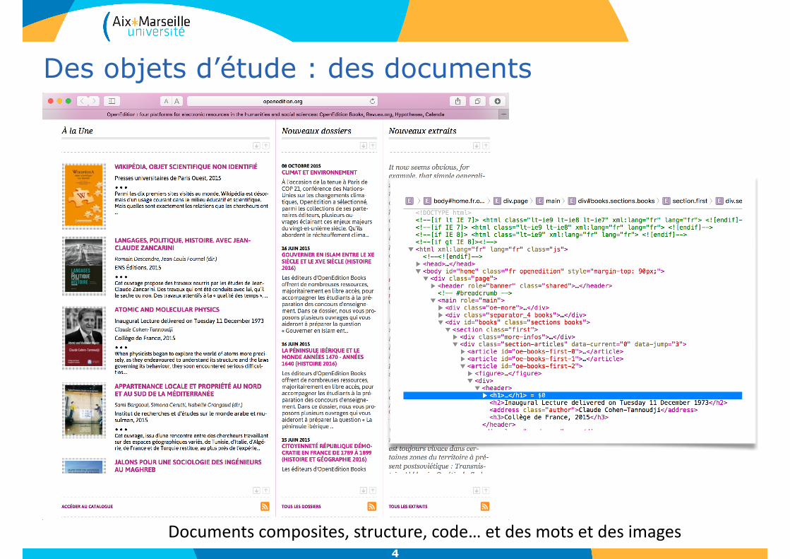
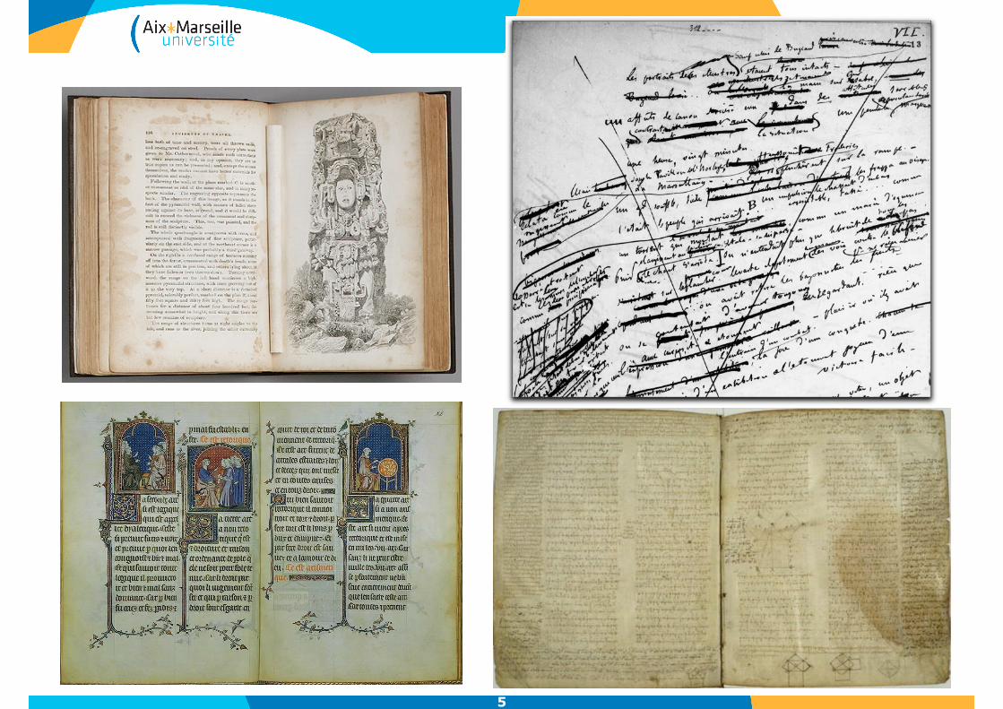
Documentscomposites,structure,code…etdesmotsetdesimages
Des objets d’étude : des documents
5

6
Equipement d’Excellence
- revues.org :
- crée en 1999
- 400 revues en ligne
- 95% en accès libre
- de 30 pays
- hypotheses :
- 1000 blogs
- calenda :
- 30 000 annonces
- books :
- 2300 livres en accès libre
>> 60 millions de visiteurs par an
>> 350 000 documents

7
© Eric Carroll, UMR TELEMME, CNRS, Aix-Marseille Université
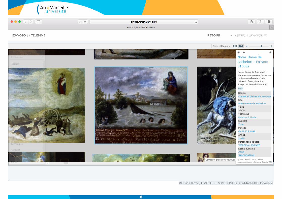
8
© Eric Carroll, UMR TELEMME, CNRS, Aix-Marseille Université
9
10
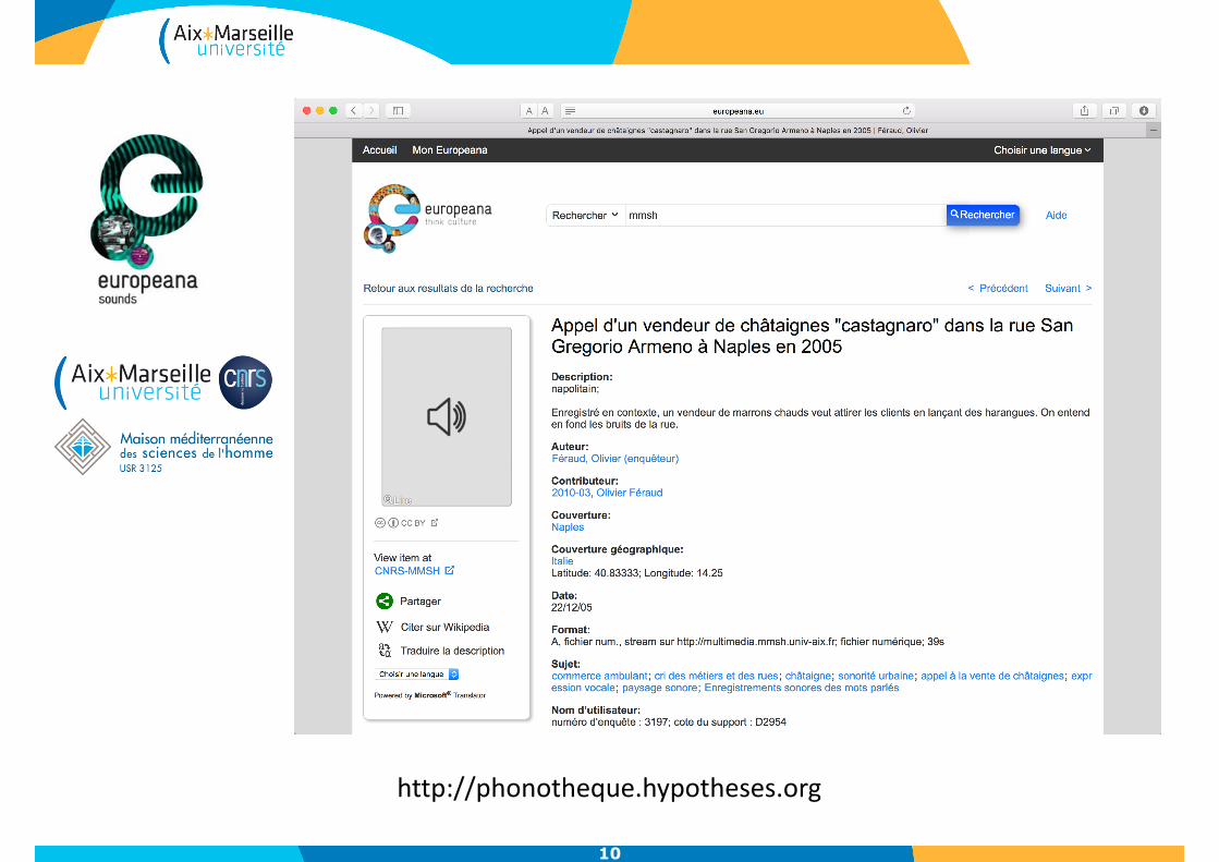
http://phonotheque.hypotheses.org
11
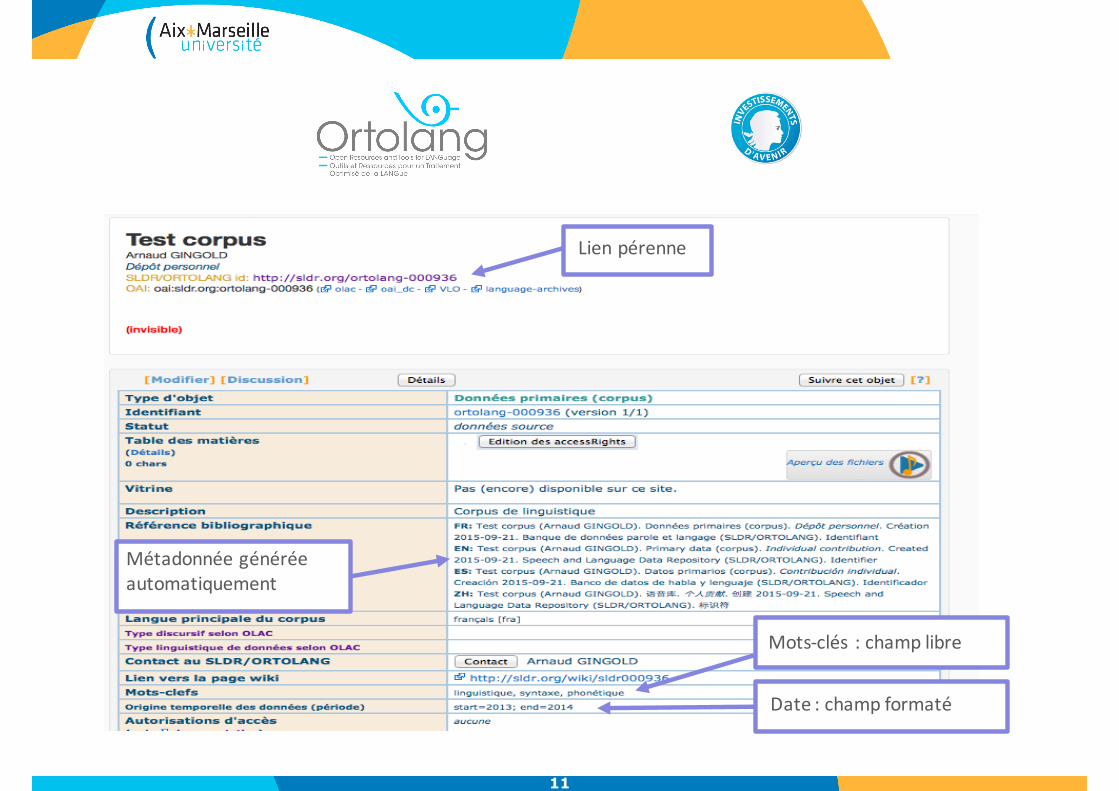
Lienpérenne
Mots-clés :champlibre
Date:champformaté
Métadonnéegénéréeautomatiquement
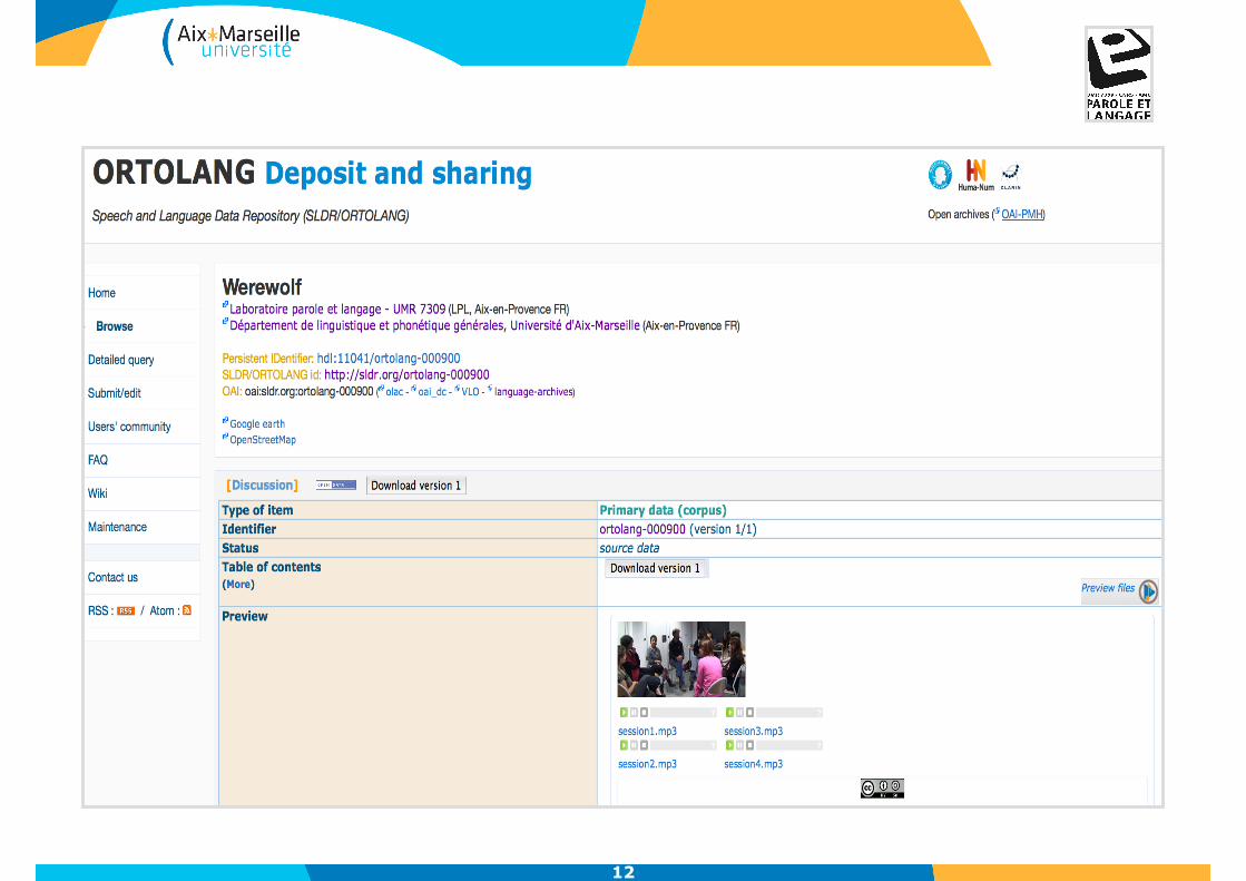
12
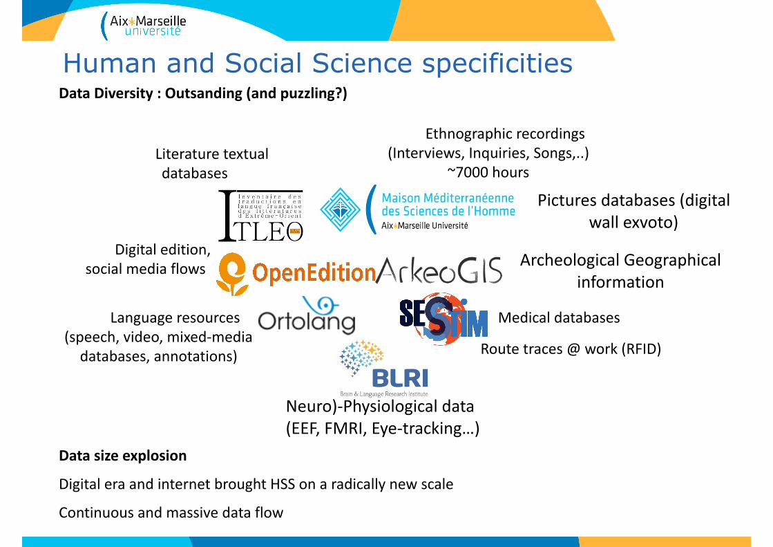
Human and Social Science specificities
Picturesdatabases(digitalwallexvoto)
Ethnographicrecordings(Interviews,Inquiries,Songs,..)
~7000hoursLiteraturetextualdatabases
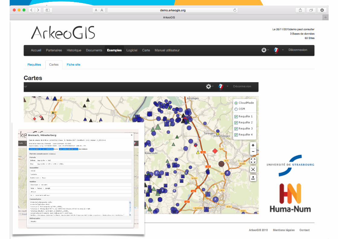
ArcheologicalGeographicalinformation
Digitaledition,socialmediaflows
Medicaldatabases
Neuro)-Physiologicaldata(EEF,FMRI,Eye-tracking…)
Routetraces@work(RFID)
DataDiversity:Outsanding(andpuzzling?)
Datasizeexplosion
DigitaleraandinternetbroughtHSSonaradicallynewscale
Continuousandmassivedataflow
Languageresources(speech,video,mixed-mediadatabases,annotations)
14

BIG DATA ? OUI
15

P.Bellot(AMU-CNRS,LSIS-OpenEdition)
Document retrieval : the Vector Space Model• Classical solution : the Vector Space Model
• In the index : a (non binary) weight is associated to every word in each document that contains it
• Every document d is represented as a vector • The query q is represented as a vector in the document space • The degree of similarity between a document and the query is
computed according to the weights w of the words m
16
~d
~q
~d =
0
BBB@
wm1,d
wm2,d.
.
.
wmn,d
1
CCCA
~q =
0
BBB@
wm1,q
wm2,q.
.
.
wmn,q
1
CCCA
wmi,d
mi
s(~d, ~q) =
i=nX
i=1
wmi,d · wmi,q (1)
wi,d =
wi,dqPnj=1 w2
j,d
(2)
s(~d, ~q) =
i=nX
i=1
wi,dqPnj=1 w2
j,d
· wi,qqPnj=1 w2
j,q
=
~d · ~q
kdk2 · kqk2= cos(
~d, ~q) (3)
1
The foundations of the rigorous study of analysis were laid in the nineteenth century, notably bythe mathematicians Cauchy and Weierstrass. Central to the study of this subject are the formaldefinitions of limits and continuity.
Let D be a subset of R and let f :D ! R be a real-valued function on D. The function f is said tobe continuous on D if, for all ✏ > 0 and for all x 2 D, there exists some � > 0 (which may dependon x) such that if y 2 D satisfies
|y � x| < �
then|f(y)� f(x)| < ✏.
One may readily verify that if f and g are continuous functions on D then the functions f + g,f � g and f.g are continuous. If in addition g is everywhere non-zero then f/g is continuous.
~
d
~q
~
d =
0
BBB@
wm1,d
wm2,d...
wmn,d
1
CCCA
1
The foundations of the rigorous study of analysis were laid in the nineteenth century, notably bythe mathematicians Cauchy and Weierstrass. Central to the study of this subject are the formaldefinitions of limits and continuity.
Let D be a subset of R and let f :D ! R be a real-valued function on D. The function f is said tobe continuous on D if, for all ✏ > 0 and for all x 2 D, there exists some � > 0 (which may dependon x) such that if y 2 D satisfies
|y � x| < �
then|f(y)� f(x)| < ✏.
One may readily verify that if f and g are continuous functions on D then the functions f + g,f � g and f.g are continuous. If in addition g is everywhere non-zero then f/g is continuous.
~
d
~q
~
d =
0
BBB@
wm1,d
wm2,d...
wmn,d
1
CCCA
~q =
0
BBB@
wm1,q
wm2,q...
wmn,q
1
CCCA
s(~d, ~q) =i=nX
i=1
wmi,d · wmi,q (1)
1
17
Information Retrieval and Web Search 63-3
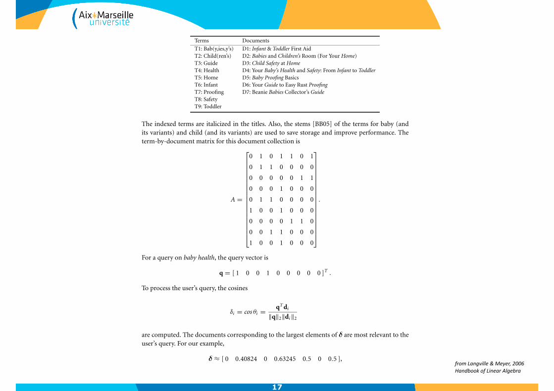
Terms Documents
T1: Bab(y,ies,y’s) D1: Infant & Toddler First AidT2: Child(ren’s) D2: Babies and Children’s Room (For Your Home)T3: Guide D3: Child Safety at HomeT4: Health D4: Your Baby’s Health and Safety: From Infant to ToddlerT5: Home D5: Baby Proofing BasicsT6: Infant D6: Your Guide to Easy Rust ProofingT7: Proofing D7: Beanie Babies Collector’s GuideT8: SafetyT9: Toddler
The indexed terms are italicized in the titles. Also, the stems [BB05] of the terms for baby (andits variants) and child (and its variants) are used to save storage and improve performance. Theterm-by-document matrix for this document collection is
A =
⎡
⎢⎢⎢⎢⎢⎢⎢⎢⎢⎢⎢⎢⎢⎢⎢⎢⎣
0 1 0 1 1 0 1
0 1 1 0 0 0 0
0 0 0 0 0 1 1
0 0 0 1 0 0 0
0 1 1 0 0 0 0
1 0 0 1 0 0 0
0 0 0 0 1 1 0
0 0 1 1 0 0 0
1 0 0 1 0 0 0
⎤
⎥⎥⎥⎥⎥⎥⎥⎥⎥⎥⎥⎥⎥⎥⎥⎥⎦
.
For a query on baby health, the query vector is
q = [ 1 0 0 1 0 0 0 0 0 ]T .
To process the user’s query, the cosines
δi = cos θi = qT di
∥q∥2∥di ∥2
are computed. The documents corresponding to the largest elements of δ are most relevant to theuser’s query. For our example,
δ ≈ [ 0 0.40824 0 0.63245 0.5 0 0.5 ],
so document vector 4 is scored most relevant to the query on baby health. To calculate the recalland precision scores, one needs to be working with a small, well-studied document collection. Inthis example, documents d4, d1, and d3 are the three documents in the collection relevant to babyhealth. Consequently, with τ = .1, the recall score is 1/3 and the precision is 1/4.
63.2 Latent Semantic Indexing
In the 1990s, an improved information retrieval system replaced the vector space model. This system iscalled Latent Semantic Indexing (LSI) [Dum91] and was the product of Susan Dumais, then at Bell Labs.LSI simply creates a low rank approximation Ak to the term-by-document matrix A from the vector spacemodel.
fromLangville&Meyer,2006HandbookofLinearAlgebra

18
Information Retrieval and Web Search 63-3
Terms Documents
T1: Bab(y,ies,y’s) D1: Infant & Toddler First AidT2: Child(ren’s) D2: Babies and Children’s Room (For Your Home)T3: Guide D3: Child Safety at HomeT4: Health D4: Your Baby’s Health and Safety: From Infant to ToddlerT5: Home D5: Baby Proofing BasicsT6: Infant D6: Your Guide to Easy Rust ProofingT7: Proofing D7: Beanie Babies Collector’s GuideT8: SafetyT9: Toddler
The indexed terms are italicized in the titles. Also, the stems [BB05] of the terms for baby (andits variants) and child (and its variants) are used to save storage and improve performance. Theterm-by-document matrix for this document collection is
A =
⎡
⎢⎢⎢⎢⎢⎢⎢⎢⎢⎢⎢⎢⎢⎢⎢⎢⎣
0 1 0 1 1 0 1
0 1 1 0 0 0 0
0 0 0 0 0 1 1
0 0 0 1 0 0 0
0 1 1 0 0 0 0
1 0 0 1 0 0 0
0 0 0 0 1 1 0
0 0 1 1 0 0 0
1 0 0 1 0 0 0
⎤
⎥⎥⎥⎥⎥⎥⎥⎥⎥⎥⎥⎥⎥⎥⎥⎥⎦
.
For a query on baby health, the query vector is
q = [ 1 0 0 1 0 0 0 0 0 ]T .
To process the user’s query, the cosines
δi = cos θi = qT di
∥q∥2∥di ∥2
are computed. The documents corresponding to the largest elements of δ are most relevant to theuser’s query. For our example,
δ ≈ [ 0 0.40824 0 0.63245 0.5 0 0.5 ],
so document vector 4 is scored most relevant to the query on baby health. To calculate the recalland precision scores, one needs to be working with a small, well-studied document collection. Inthis example, documents d4, d1, and d3 are the three documents in the collection relevant to babyhealth. Consequently, with τ = .1, the recall score is 1/3 and the precision is 1/4.
63.2 Latent Semantic Indexing
In the 1990s, an improved information retrieval system replaced the vector space model. This system iscalled Latent Semantic Indexing (LSI) [Dum91] and was the product of Susan Dumais, then at Bell Labs.LSI simply creates a low rank approximation Ak to the term-by-document matrix A from the vector spacemodel.
fromLangville&Meyer,2006HandbookofLinearAlgebra
Plusieursmillionsdecomposanteset…matricestrèscreuses
P.Bellot(AMU-CNRS,LSIS-OpenEdition)
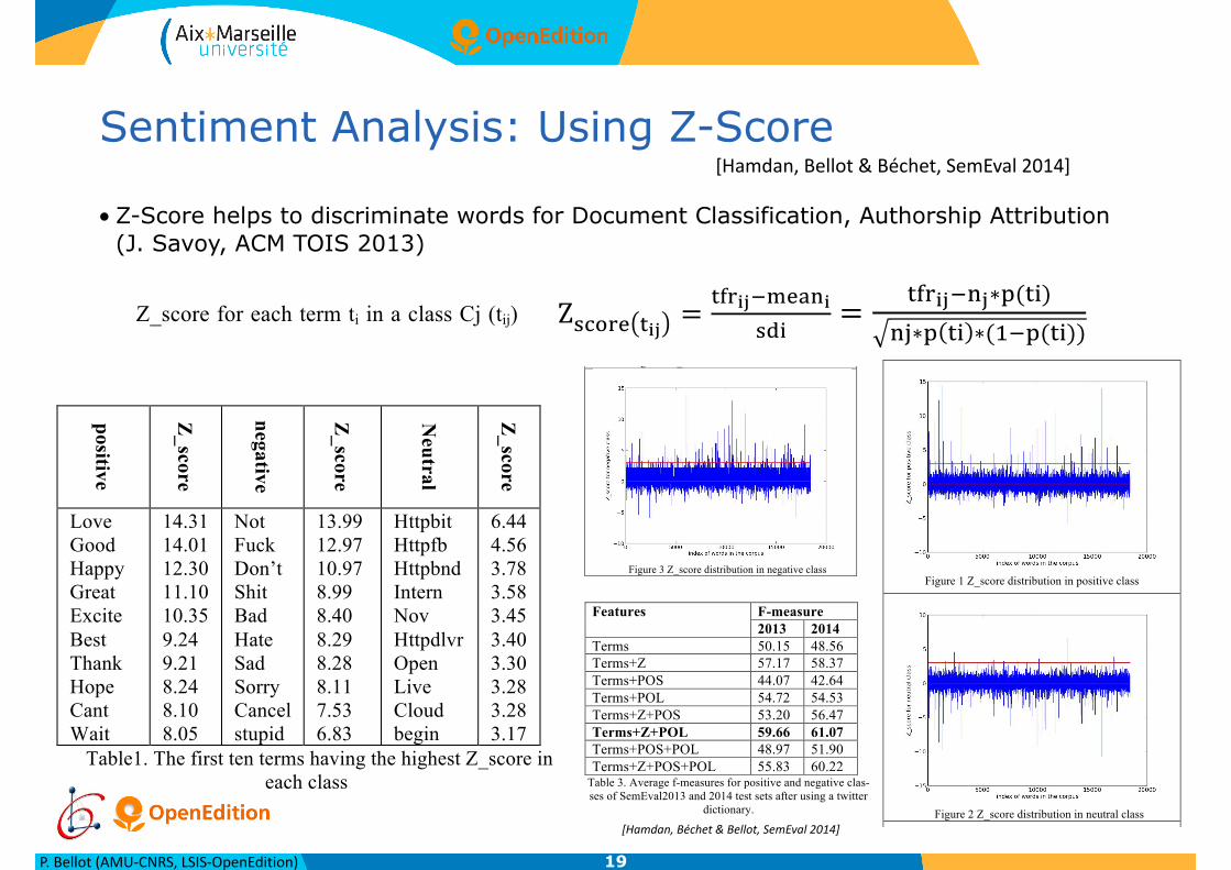
Sentiment Analysis: Using Z-Score
• Z-Score helps to discriminate words for Document Classification, Authorship Attribution (J. Savoy, ACM TOIS 2013)
19
Z_score for each term ti in a class Cj (tij) by cal-culating its term relative frequency tfrij in a par-ticular class Cj, as well as the mean (meani) which is the term probability over the whole cor-pus multiplied by nj the number of terms in the class Cj, and standard deviation (sdi) of term ti according to the underlying corpus (see Eq. (1,2)). Z!"#$% !!" =
!"#!"!!"#$!!"# Eq. (1)
Z!"#$% !!" =
!"#!"!!!∗!(!")!"∗! !" ∗(!!!(!")) Eq. (2)
The term which has salient frequency in a class in compassion to others will have a salient Z_score. Z_score was exploited for SA by (Zubaryeva and Savoy 2010) , they choose a threshold (>2) for selecting the number of terms having Z_score more than the threshold, then they used a logistic regression for combining these scores. We use Z_scores as added features for classification because the tweet is too short, therefore many tweets does not have any words with salient Z_score. The three following figures 1,2,3 show the distribution of Z_score over each class, we remark that the majority of terms has Z_score between -1.5 and 2.5 in each class and the rest are either vey frequent (>2.5) or very rare (<-1.5). It should indicate that negative value means that the term is not frequent in this class in comparison with its frequencies in other classes. Table1 demonstrates the first ten terms having the highest Z_scores in each class. We have test-ed to use different values for the threshold, the best results was obtained when the threshold is 3.
positive
Z_score
negative
Z_score
Neutral
Z_score
Love Good Happy Great Excite Best Thank Hope Cant Wait
14.31 14.01 12.30 11.10 10.35 9.24 9.21 8.24 8.10 8.05
Not Fuck Don’t Shit Bad Hate Sad Sorry Cancel stupid
13.99 12.97 10.97 8.99 8.40 8.29 8.28 8.11 7.53 6.83
Httpbit Httpfb Httpbnd Intern Nov Httpdlvr Open Live Cloud begin
6.44 4.56 3.78 3.58 3.45 3.40 3.30 3.28 3.28 3.17
Table1. The first ten terms having the highest Z_score in each class
- Sentiment Lexicon Features (POL) We used two sentiment lexicons, MPQA Subjec-tivity Lexicon(Wilson, Wiebe et al. 2005) and
Bing Liu's Opinion Lexicon which is created by (Hu and Liu 2004) and augmented in many latter works. We extract the number of positive, nega-tive and neutral words in tweets according to the-se lexicons. Bing Liu's lexicon only contains negative and positive annotation but Subjectivity contains negative, positive and neutral.
- Part Of Speech (POS) We annotate each word in the tweet by its POS tag, and then we compute the number of adjec-tives, verbs, nouns, adverbs and connectors in each tweet.
4 Evaluation
4.1 Data collection We used the data set provided in SemEval 2013 and 2014 for subtask B of sentiment analysis in Twitter(Rosenthal, Ritter et al. 2014) (Wilson, Kozareva et al. 2013). The participants were provided with training tweets annotated as posi-tive, negative or neutral. We downloaded these tweets using a given script. Among 9646 tweets, we could only download 8498 of them because of protected profiles and deleted tweets. Then, we used the development set containing 1654 tweets for evaluating our methods. We combined the development set with training set and built a new model which predicted the labels of the test set 2013 and 2014.
4.2 Experiments
Official Results The results of our system submitted for SemEval evaluation gave 46.38%, 52.02% for test set 2013 and 2014 respectively. It should mention that these results are not correct because of a software bug discovered after the submis-sion deadline, therefore the correct results is demonstrated as non-official results. In fact the previous results are the output of our classifier which is trained by all the features in section 3, but because of index shifting error the test set was represented by all the features except the terms.
Non-official Results We have done various experiments using the features presented in Section 3 with Multinomial Naïve-Bayes model. We firstly constructed fea-ture vector of tweet terms which gave 49%, 46% for test set 2013, 2014 respectively. Then, we augmented this original vector by the Z_score
features which improve the performance by 6.5% and 10.9%, then by pre-polarity features which also improve the f-measure by 4%, 6%, but the extending with POS tags decreases the f-measure. We also test all combinations with the-se previous features, Table2 demonstrates the results of each combination, we remark that POS tags are not useful over all the experiments, the best result is obtained by combining Z_score and pre-polarity features. We find that Z_score fea-tures improve significantly the f-measure and they are better than pre-polarity features.
Figure 1 Z_score distribution in positive class
Figure 2 Z_score distribution in neutral class
Figure 3 Z_score distribution in negative class
Features F-measure 2013 2014
Terms 49.42 46.31 Terms+Z 55.90 57.28 Terms+POS 43.45 41.14 Terms+POL 53.53 52.73 Terms+Z+POS 52.59 54.43 Terms+Z+POL 58.34 59.38 Terms+POS+POL 48.42 50.03 Terms+Z+POS+POL 55.35 58.58 Table 2. Average f-measures for positive and negative clas-
ses of SemEval2013 and 2014 test sets. We repeated all previous experiments after using a twitter dictionary where we extend the tweet by the expressions related to each emotion icons or abbreviations in tweets. The results in Table3 demonstrate that using that dictionary improves the f-measure over all the experiments, the best results obtained also by combining Z_scores and pre-polarity features. Features F-measure
2013 2014 Terms 50.15 48.56 Terms+Z 57.17 58.37 Terms+POS 44.07 42.64 Terms+POL 54.72 54.53 Terms+Z+POS 53.20 56.47 Terms+Z+POL 59.66 61.07 Terms+POS+POL 48.97 51.90 Terms+Z+POS+POL 55.83 60.22
Table 3. Average f-measures for positive and negative clas-ses of SemEval2013 and 2014 test sets after using a twitter
dictionary.
5 Conclusion
In this paper we tested the impact of using Twitter Dictionary, Sentiment Lexicons, Z_score features and POS tags for the sentiment classifi-cation of tweets. We extended the feature vector of tweets by all these features; we have proposed new type of features Z_score and demonstrated that they can improve the performance. We think that Z_score can be used in different ways for improving the Sentiment Analysis, we are going to test it in another type of corpus and using other methods in order to combine these features.
Reference Apoorv Agarwal,Boyi Xie,Ilia Vovsha,Owen
Rambow and Rebecca Passonneau (2011). Sentiment analysis of Twitter data. Proceedings of the Workshop on Languages
[Hamdan,Béchet&Bellot,SemEval2014]
[Hamdan,Bellot&Béchet,SemEval2014]
P.Bellot(AMU-CNRS,LSIS-OpenEdition)
the corpus. In order to give more importance tothe difference in how many times a term appear inboth classes, we used the normalized z-score de-scribed in Equation (4) with the measure � intro-duced in Equation (3)
� =tfC0 � tfC1
tfC0 + tfC1(3)
The normalization measure � is taken into accountto calculate normalized z-score as following:
Z
�(wi|Cj) =
8>>>>>>><
>>>>>>>:
Z(wi|Cj).(1 + |�(wi|Cj |)if Z > 0 and � > 0,or if Z 0 and � 0
Z(wi|Cj).(1� |�(wi|Cj |)if Z > 0 and � 0,or if Z 0 and � > 0
(4)In the table 3 we can observe the 30 highest nor-
malized Z scores for Review and Review classesfor the corpus after an unigram indexing schemewas performed. We can see that a lot of this fea-tures relate to the classe where they predominate.
Table 3: Distribution of the 30 highest normalizedZ scores across the corpus.
# Feature Z�
score# Feature Z�
score1 abandonne 30.14 16 winter 9.232 seront 30.00 17 cleo 8.883 biographie 21.84 18 visible 8.754 entranent 21.20 19 fondamentale 8.675 prise 21.20 20 david 8.546 sacre 21.20 21 pratiques 8.527 toute 20.70 22 signification 8.478 quitte 19.55 23 01 8.389 dimension 15.65 24 institutionnels 8.3810 les 14.43 25 1930 8.1611 commandement 11.01 26 attaques 8.1412 lie 10.61 27 courrier 8.0813 construisent 10.16 28 moyennes 7.9914 lieux 10.14 29 petite 7.8515 garde 9.75 30 adapted 7.84
In our training corpus, we have 106 911 wordsobtained from the Bag-of-Words approach. We se-lected all tokens (features) that appear more than5 times in each classes. The goal is therefore todesign a method capable of selecting terms thatclearly belong to one genre of documents. We ob-tained a vector space that contains 5 957 words(features). After calculating the normalized z-score of all features, we selected the first 1 000features according to this score.
5.3 Using Named Entity (NE) distribution asfeatures
Most of researches involve removing irrelevant de-scriptors. In this section, we describe a new ap-proach for better represent the documents in thecontext of this study. The purpose is to find ele-ments that characterize the Review class.
After a linguistic and statistical corpus analysis,we identified some common characteristics (illus-trated in Figure 3, 4 and 5). We have identifiedthat the presence of the bibliographical referenceor some its elements (title, author(s) and date) ofthe reviewed book is often in the title of the review,as in the following example:
[...]<title level="a" type="main"> Dean R. Hoge,Jacqueline E. Wenger,<hi rend="italic">
Evolving Visions of the Priesthood. Changes from Vatican IIto the Turn of the New Century</hi>
</title>
<title type="sub"> Collegeville (MIN), Liturgical Press,2003, 226 p.</title> [...]
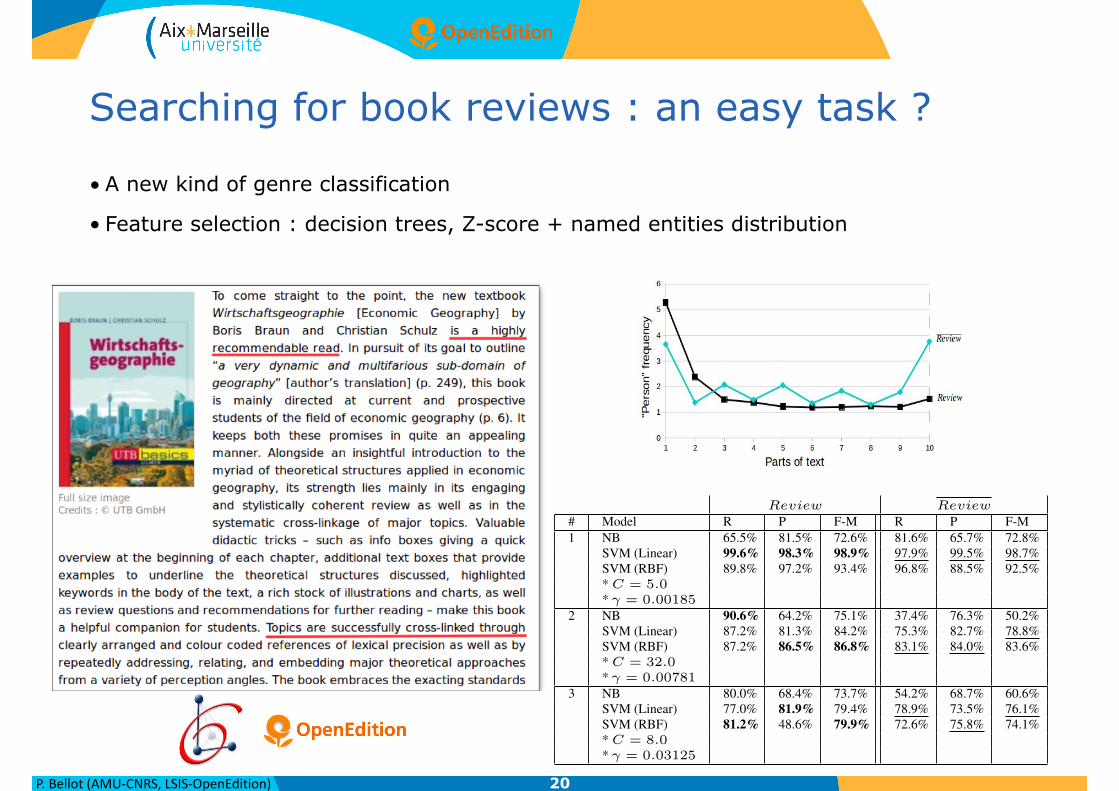
In the Review class, we found scientific arti-cles. In those documents, a bibliography sectionis generally present at the end of the text. As weknow, this section contains authors’ names, loca-tions, dates, etc... However, in the Review classthis section is quite often absent. Based on thisanalysis, we tagged all documents of each classusing the Named Entity Recognition tool TagEN(Poibeau, 2003). We aim to explore the distribu-tion of 3 named entities (”authors’ names”, ”loca-tions” and ”dates”) in the text after removing allXML-HTML tags. After that, we divided textsinto 10 parts (the size of each part = total num-ber of words / 10). The distribution ratio of eachnamed entity in each part is used as feature to buildthe new document representation and we obtaineda set of 30 features.
Figure 3: ”Person” named entity distribution
6 Experiments
In this section we describe results from experi-ments using a collection of documents from Re-vues.org and the Web. We use supervised learning
Searching for book reviews : an easy task ?
• A new kind of genre classification
• Feature selection : decision trees, Z-score + named entities distribution
20
Figure 4: ”Location” named entity distribution
Figure 5: ”Date” named entity distribution
methods to build our classifiers, and evaluate theresulting models on new test cases. The focus ofour work has been on comparing the effectivenessof different inductive learning algorithms (NaiveBayes, Support Vector Machines with RBF andLinear Kernels) in terms of classification accuracy.We also explored alternative document represen-tations (bag-of-words, feature selection using z-score, Named Entity repartition in the text).
6.1 Naive Bayes (NB)
In order to evaluate different classification mod-els, we have adopted as a baseline the naive Bayesapproach (Zubaryeva and Savoy, 2010). The clas-sification system has to choose between two pos-sible hypotheses: h0 = It is a Review and h1 =It is not a Review the class that has the maxi-mum value according to the Equation (5). Where|w| indicates the number of words included in thecurrent document and wj is the number of wordsthat appear in the document.
arg max
hi
P (hi).|w|Y
j=1
P (wj |hi) (5)
where P (wj |hi) =tfj,hinhi
We estimate the probabilities with the Equation(5) and get the relation between the lexical fre-quency of the word wj in the whole size of thecollection Thi (denoted tfj,hi) and the size of thecorresponding corpus.
6.2 Support Vector Machines (SVM)
SVM designates a learning approach introducedby Vapnik in 1995 for solving two-class patternrecognition problem (Vapnik, 1995). The SVMmethod is based on the Structural Risk Mini-mization principle (Vapnik, 1995) from computa-tional learning theory. In their basic form, SVMslearn linear threshold function. Nevertheless, bya simple plug-in of an appropriate kernel func-tion, they can be used to learn linear classifiers,radial basic function (RBF) networks, and three-layer sigmoid neural nets (Joachims, 1998). Thekey in such classifiers is to determine the opti-mal boundaries between the different classes anduse them for the purposes of classification (Ag-garwal and Zhai, 2012). Having the vectors formthe different representations presented below. weused the Weka toolkit to learning model. Thismodel with the use of the linear kernel and RadialBasic Function(RBF) sometimes allows to reacha good level of performance at the cost of fastgrowth of the processing time during the learningstage.(Kummer, 2012)
6.3 Results
We have used different strategies to represent eachtextual unit. First, the unigram model (Bag-of-Words) where all words are considered as features.We also used feature selection based on the nor-malized z-score by keeping the first 1000 wordsaccording to this score (after removing all wordsthat appear less than 5 times). As the third ap-proach, we suggested that the common featuresbetween the Review collection can be located inthe Named Entity distribution in the text.
Table 4: Results showing the performances ofthe classification models using different indexingschemes on the test set. The best values for theReview class are noted in bold and those forReview class are are underlined
Review Review# Model R P F-M R P F-M1 NB 65.5% 81.5% 72.6% 81.6% 65.7% 72.8%
SVM (Linear) 99.6% 98.3% 98.9% 97.9% 99.5% 98.7%SVM (RBF) 89.8% 97.2% 93.4% 96.8% 88.5% 92.5%* C = 5.0* � = 0.00185
2 NB 90.6% 64.2% 75.1% 37.4% 76.3% 50.2%SVM (Linear) 87.2% 81.3% 84.2% 75.3% 82.7% 78.8%SVM (RBF) 87.2% 86.5% 86.8% 83.1% 84.0% 83.6%* C = 32.0* � = 0.00781
3 NB 80.0% 68.4% 73.7% 54.2% 68.7% 60.6%SVM (Linear) 77.0% 81.9% 79.4% 78.9% 73.5% 76.1%SVM (RBF) 81.2% 48.6% 79.9% 72.6% 75.8% 74.1%* C = 8.0* � = 0.03125

P.Bellot(AMU-CNRS,LSIS-OpenEdition) 21
P.Bellot(AMU-CNRS,LSIS-OpenEdition) 22
Une donnée = un mot ?
23
Arbre
Une donnée = un mot ?
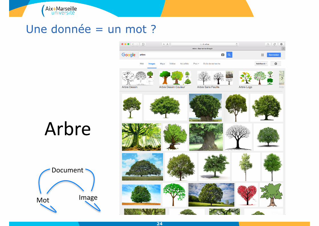
24
Arbre
Mot Image
Document

Une donnée = un mot ?
25
ArbreArbresForêt
Une donnée = un mot ?
26
Arbre
Une donnée = un mot ?
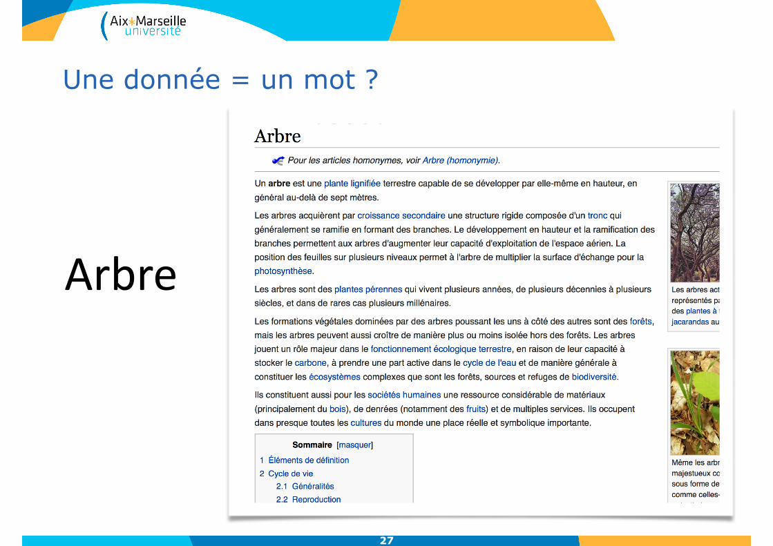
27
Arbre
Une donnée = un mot ?
28
Avocat
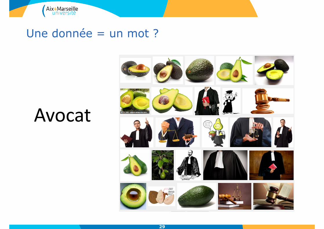
Une donnée = un mot ?
29
Avocat

Une donnée = un mot ?
30
Epuisette

Une donnée = un mot ?
31
Epuisette
32
33
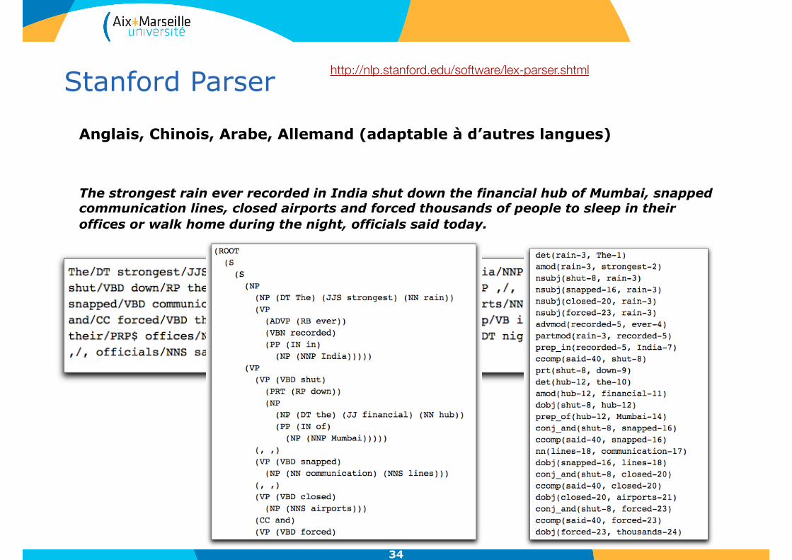
Stanford Parser
Anglais, Chinois, Arabe, Allemand (adaptable à d’autres langues)
The strongest rain ever recorded in India shut down the financial hub of Mumbai, snapped communication lines, closed airports and forced thousands of people to sleep in their offices or walk home during the night, officials said today.
34
http://nlp.stanford.edu/software/lex-parser.shtml
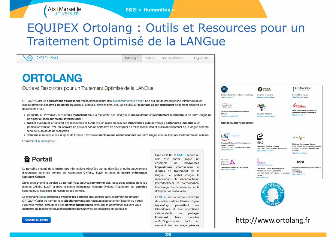
EQUIPEX Ortolang : Outils et Resources pour un Traitement Optimisé de la LANGue
35
http://www.ortolang.fr
PR2i « Humanités »
P.Bellot(AMU-CNRS,LSIS-OpenEdition)
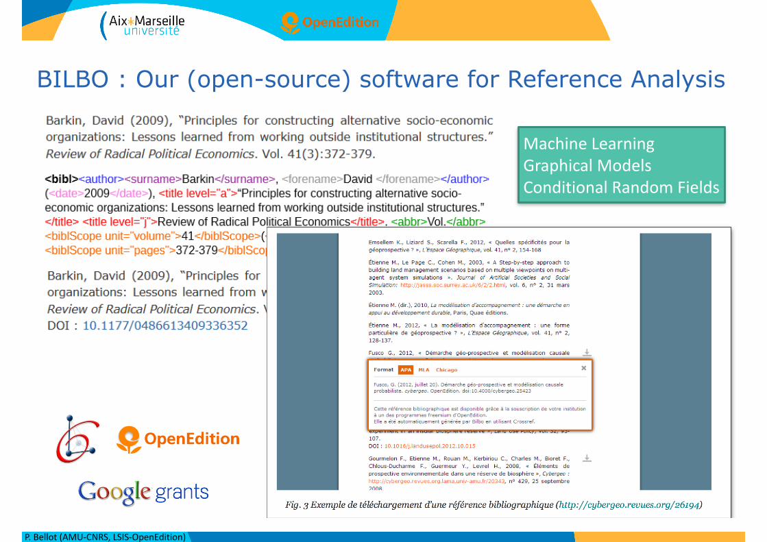
BILBO : Our (open-source) software for Reference Analysis
36
MachineLearningGraphicalModelsConditionalRandomFields
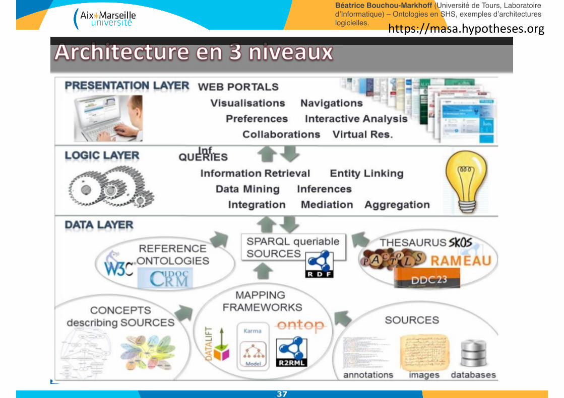
37
Béatrice Bouchou-Markhoff (Université de Tours, Laboratoire d’Informatique) – Ontologies en SHS, exemples d’architectures logicielles. https://masa.hypotheses.org
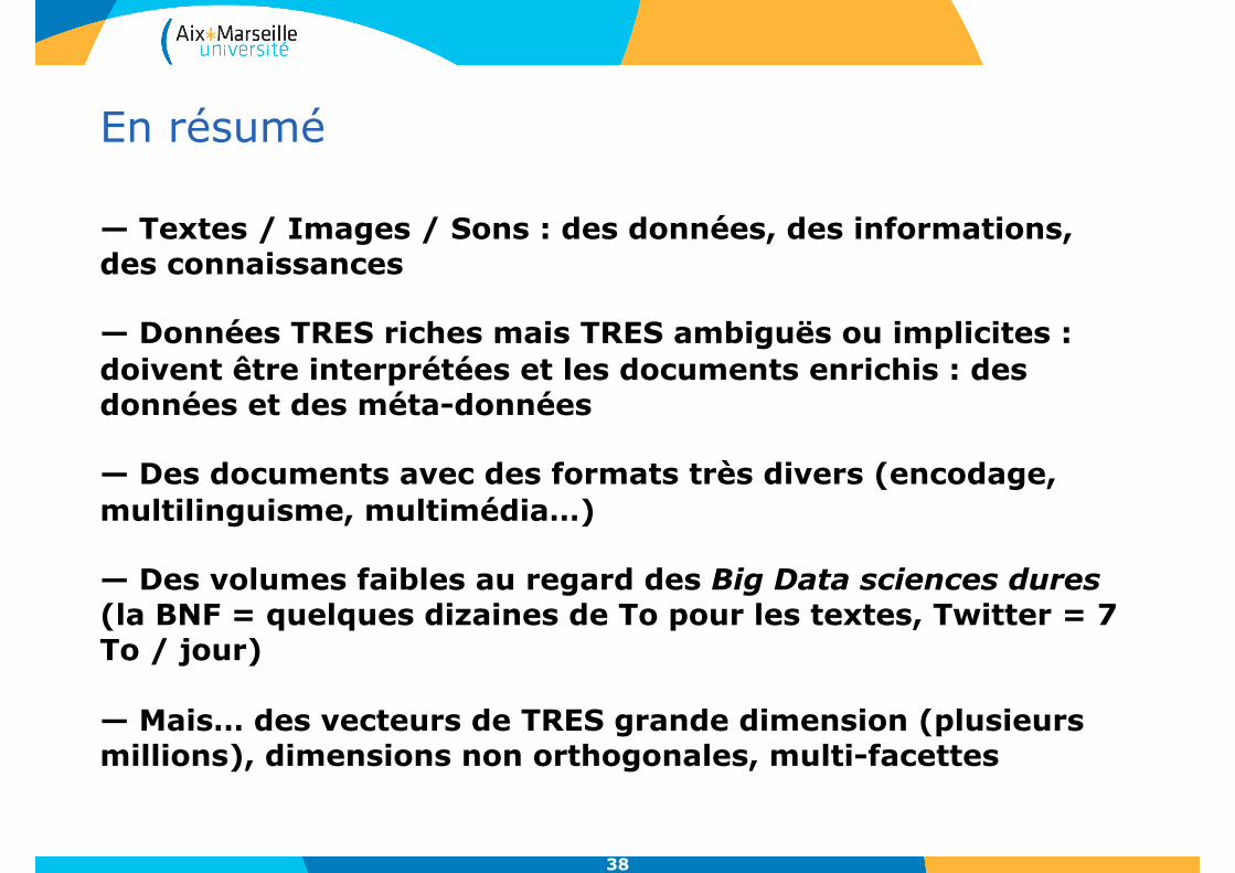
En résumé
— Textes / Images / Sons : des données, des informations, des connaissances
— Données TRES riches mais TRES ambiguës ou implicites : doivent être interprétées et les documents enrichis : des données et des méta-données
— Des documents avec des formats très divers (encodage, multilinguisme, multimédia…)
— Des volumes faibles au regard des Big Data sciences dures (la BNF = quelques dizaines de To pour les textes, Twitter = 7 To / jour)
— Mais… des vecteurs de TRES grande dimension (plusieurs millions), dimensions non orthogonales, multi-facettes
38

QUELLES INFRASTRUCTURES ?
39

40
http://huma-num.fr

42
43
44
45
P.Bellot(AMU-CNRS,LSIS-OpenEdition) 46
47
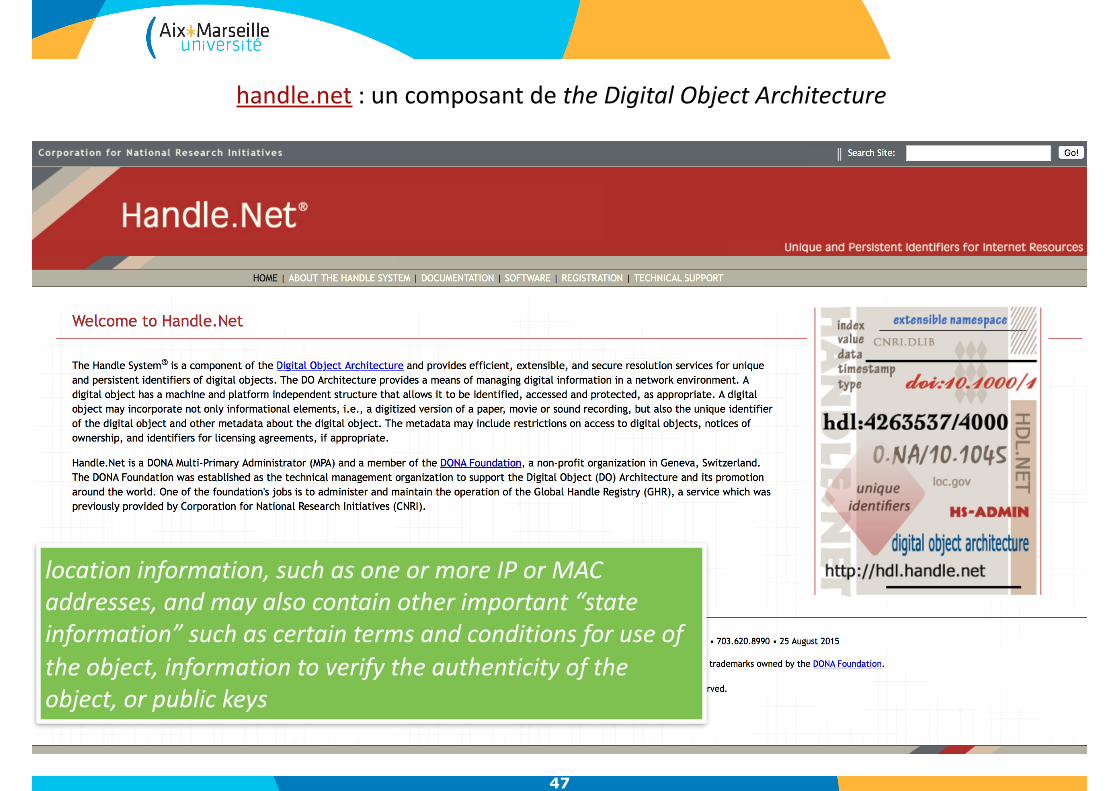
handle.net:uncomposantdetheDigitalObjectArchitecture
locationinformation,suchasoneormoreIPorMACaddresses,andmayalsocontainotherimportant“stateinformation”suchascertaintermsandconditionsforuseoftheobject,informationtoverifytheauthenticityoftheobject,orpublickeys

48
http://www.doi.org
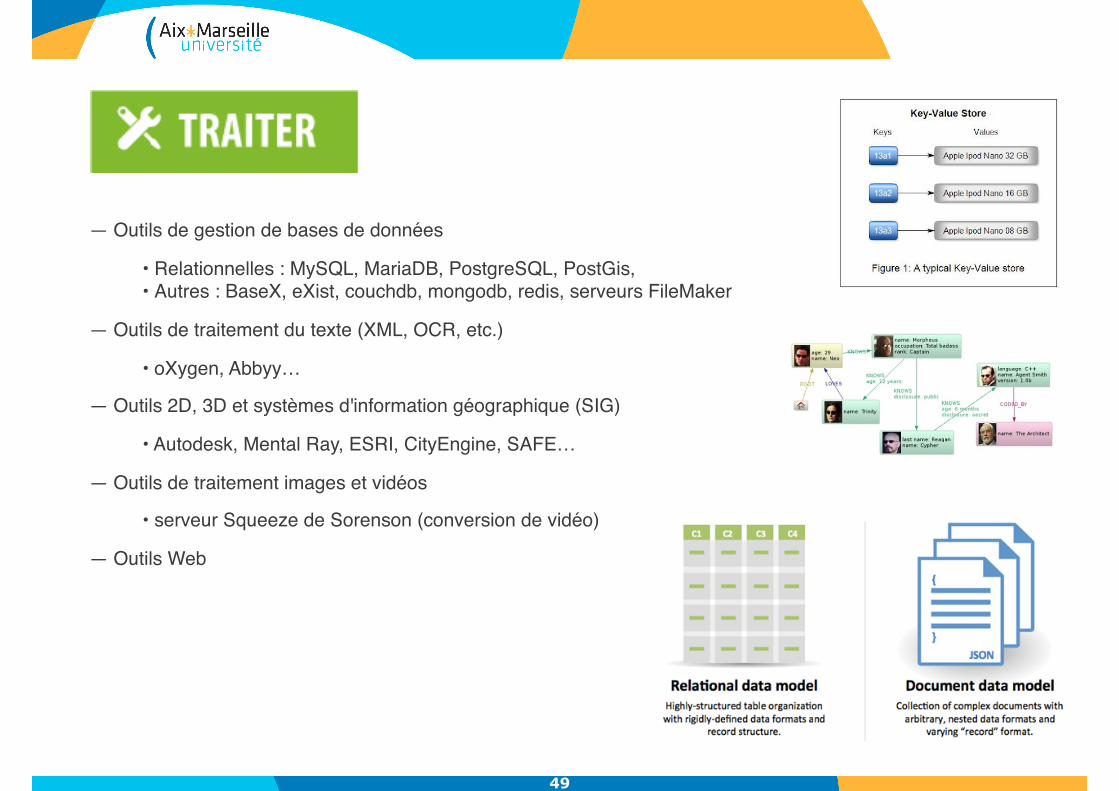
— Outils de gestion de bases de données
• Relationnelles : MySQL, MariaDB, PostgreSQL, PostGis, • Autres : BaseX, eXist, couchdb, mongodb, redis, serveurs FileMaker
— Outils de traitement du texte (XML, OCR, etc.)
• oXygen, Abbyy…
— Outils 2D, 3D et systèmes d'information géographique (SIG)
• Autodesk, Mental Ray, ESRI, CityEngine, SAFE…
— Outils de traitement images et vidéos
• serveur Squeeze de Sorenson (conversion de vidéo)
— Outils Web
49

50
API+interrogationSARQL

51

52

53
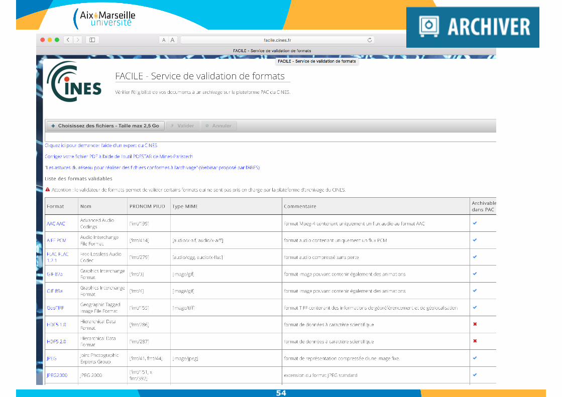
54

55

56

57

58
9.Nouslançonsunappelpourl’accèslibreauxdonnéesetauxmétadonnées.Celles-cidoiventêtredocumentéesetinteropérables,autanttechniquementqueconceptuellement.10.Noussommesfavorablesàladiffusion,àlacirculationetaulibreenrichissementdesméthodes,ducode,desformatsetdesrésultatsdelarecherche.