Embed Size (px)
Citation preview
N° d’ordre : 2012-16-TH
THÈSE DE DOCTORAT
DOMAINE : STIC Spécialité : Automatique
Ecole Doctorale « Sciences et Technologies de l’Inf ormation des Télécommunications et des Systèmes »
Présentée par :
Vu Tuan Hieu LE Sujet :
Commande prédictive robuste par des techniques d’observateurs à base d’ensembles zonotopiques
Soutenue le 22 Octobre 2012 devant les membres du jury : M. Teodoro ALAMO Universidad de Sevilla, Espagne Co-encadrant, invité
M. Eduardo CAMACHO Universidad de Sevilla, Espagne Co-encadrant
M. Christophe COMBASTEL ENSEA, Cergy-Pontoise Examinateur
Mme Estelle COURTIAL Université d’Orléans PRISME, Orléans Examinatrice
M. José Adrian DE DONÁ University of Newcastle, Australie Rapporteur
M. Didier DUMUR SUPELEC, Gif sur Yvette Directeur de thèse
Mme Françoise LAMNABHI-LAGARRIGUE LSS, CNRS, Gif sur Yvette Présidente du jury
M. Vicenç PUIG Universitat Politècnica de Catalunya, Espagne Rapporteur
Mme Cristina STOICA SUPELEC, Gif sur Yvette Co-encadrante


To my fatherTo my mother
To my wifeand my family

Acknowledgement
I would like first to thank my supervisors Didier Dumur, Cristina Stoica,Teodoro Alamo and Eduardo Camacho who have encouraged and supportedme since the beginning of my thesis. I am grateful for their help, theiravailability to correct my last minute papers.
I am grateful to As. Prof. José De Dona and Prof. Vincenç Puig forreviewing my thesis and to Prof. Françoise Lamnabhi-Lagarrigue, Dr. EstelleCourtial, and Dr. Christophe Combastel for being part of the examinationcommittee of my thesis.
I also would like to thank all professors and personnel of the AutomaticControl Department of Supélec, especially to Ms. Josiane Dartron and Mr.Léon Marquet for their help during my three years at Supélec. It is alsoa pleasure to thank the personnel of the Automatic Control Department ofUniversity of Seville for their support during my trips in Seville. I will notforget my colleagues who supported me with their pleasant presence duringcoffee breaks and badminton sessions, specially: Bien, Dung, Nam and Vy.
Special thank to my professors at ENSEA, Prof. Jean-Pierre Barbot andDr. Malek Ghanes who encouraged me to continue on the research direction.
Finally, I am grateful to my wife, my parents, my sister and my familyfor their support and their encouragements.
iii

Contents
1 Résumé 11.1 Chapitre 3 : Représentation des incertitudes par des ensembles
convexes . . . . . . . . . . . . . . . . . . . . . . . . . . . . . . 21.1.1 Intervalle . . . . . . . . . . . . . . . . . . . . . . . . . 21.1.2 Ellipsoïde . . . . . . . . . . . . . . . . . . . . . . . . . 31.1.3 Polytope . . . . . . . . . . . . . . . . . . . . . . . . . . 31.1.4 Zonotope . . . . . . . . . . . . . . . . . . . . . . . . . 4
1.2 Chapitre 4 : Estimation d’état par approche ensembliste fondéesur des zonotopes . . . . . . . . . . . . . . . . . . . . . . . . . 51.2.1 Système mono-sortie . . . . . . . . . . . . . . . . . . . 81.2.2 Système multi-sorties . . . . . . . . . . . . . . . . . . . 12
1.2.2.1 Approche ESO ("Equivalent Single-Output") 131.2.2.2 Approche ESOCE ("Equivalent Single-Output
with Coupling Effect") . . . . . . . . . . . . . 141.2.2.3 Approche PMI (Inégalité matricielle polyno-
miale) . . . . . . . . . . . . . . . . . . . . . . 151.2.3 Approche par intersection entre un polytope et un zono-
tope (PAZI) . . . . . . . . . . . . . . . . . . . . . . . . 161.3 Chapitre 4 : Commande prédictive robuste fondée sur l’esti-
mation ensembliste pour des systèmes incertains . . . . . . . . 191.3.1 Commande prédictive "boucle-ouverte" . . . . . . . . . 201.3.2 Commande prédictive robuste à base de tubes d’incer-
titudes . . . . . . . . . . . . . . . . . . . . . . . . . . . 211.4 Chapitre 5 : Application . . . . . . . . . . . . . . . . . . . . . 241.5 Conclusion . . . . . . . . . . . . . . . . . . . . . . . . . . . . . 27
2 Introduction 292.1 Context and motivations . . . . . . . . . . . . . . . . . . . . . 292.2 Outline and contributions of the thesis . . . . . . . . . . . . . 31
v
CONTENTS
3 Set theory for uncertainty representation 353.1 Basic set definitions . . . . . . . . . . . . . . . . . . . . . . . . 363.2 Basic matrix operation definitions . . . . . . . . . . . . . . . . 373.3 Interval set . . . . . . . . . . . . . . . . . . . . . . . . . . . . 393.4 Ellipsoidal set . . . . . . . . . . . . . . . . . . . . . . . . . . . 413.5 Polyhedral set . . . . . . . . . . . . . . . . . . . . . . . . . . . 423.6 Zonotopic set . . . . . . . . . . . . . . . . . . . . . . . . . . . 44
3.6.1 Zonotope definition . . . . . . . . . . . . . . . . . . . . 453.6.2 Properties of zonotopes . . . . . . . . . . . . . . . . . . 483.6.3 Complexity reduction of zonotopes . . . . . . . . . . . 49
3.6.3.1 Interval hull method . . . . . . . . . . . . . . 503.6.3.2 Parallelotope hull method . . . . . . . . . . . 503.6.3.3 Generators selection method . . . . . . . . . . 51
3.7 Conclusion . . . . . . . . . . . . . . . . . . . . . . . . . . . . . 56
4 Set-membership estimation via zonotope 574.1 Introduction . . . . . . . . . . . . . . . . . . . . . . . . . . . . 574.2 Problem formulation . . . . . . . . . . . . . . . . . . . . . . . 60
4.2.1 Singular Value Decomposition-based method . . . . . . 634.2.2 Optimization based method . . . . . . . . . . . . . . . 66
4.2.2.1 Minimizing the segments of the zonotope . . . 684.2.2.2 Minimizing the volume of the intersection . . 69
4.3 Minimizing the P -radius of the guaranteed state estimation . . 704.3.1 Linear Time Invariant Single-Output systems . . . . . 724.3.2 Single-Output systems with interval uncertainties . . . 834.3.3 Extension to Multi-Output uncertain systems . . . . . 92
4.3.3.1 General formulation . . . . . . . . . . . . . . 934.3.3.2 Equivalent Single-Output approach . . . . . . 954.3.3.3 Equivalent Single-Output with Coupling Ef-
fect approach . . . . . . . . . . . . . . . . . . 954.3.3.4 Polynomial Matrix Inequality approach . . . . 103
4.3.4 Polytope and Zonotope intersection approach for Multi-Output systems . . . . . . . . . . . . . . . . . . . . . . 111
4.4 Conclusion . . . . . . . . . . . . . . . . . . . . . . . . . . . . . 117
5 Model Predictive Control based on zonotopic set-membershipestimation 1215.1 Introduction . . . . . . . . . . . . . . . . . . . . . . . . . . . . 1215.2 General set-up . . . . . . . . . . . . . . . . . . . . . . . . . . . 1245.3 Open-loop MPC design . . . . . . . . . . . . . . . . . . . . . . 1255.4 Tube-based output feedback MPC design . . . . . . . . . . . . 129
vi
CONTENTS
5.5 Open problem for the control of systems with interval para-metric uncertainties . . . . . . . . . . . . . . . . . . . . . . . . 138
5.6 Conclusion . . . . . . . . . . . . . . . . . . . . . . . . . . . . . 141
6 Application 1436.1 Introduction . . . . . . . . . . . . . . . . . . . . . . . . . . . . 1436.2 System description . . . . . . . . . . . . . . . . . . . . . . . . 1436.3 Control problem . . . . . . . . . . . . . . . . . . . . . . . . . . 1466.4 Conclusion . . . . . . . . . . . . . . . . . . . . . . . . . . . . . 154
7 Conclusion and future works 1577.1 Contribution . . . . . . . . . . . . . . . . . . . . . . . . . . . . 1577.2 Future works . . . . . . . . . . . . . . . . . . . . . . . . . . . 159
vii

CONTENTS
viii
List of Figures
1.1 3-zonotope et ses générateurs en 2D . . . . . . . . . . . . . . . 51.2 Illustration de l’estimation ensembliste . . . . . . . . . . . . . 71.3 Estimation ensembliste fondée sur des zonotopes . . . . . . . . 71.4 Zonotope et ellipsoide associé au P -rayon du zonotope . . . . 101.5 Evolution de l’estimation d’état garantie . . . . . . . . . . . . 111.6 Evolution de l’ensemble contenant l’état obtenue par approche
PAZI . . . . . . . . . . . . . . . . . . . . . . . . . . . . . . . . 181.7 Comparaison des limites de x1 obtenues par plusieurs approches 181.8 Comparaison des limites de x2 obtenues par plusieurs approches 191.9 Maquette de la suspension magnétique . . . . . . . . . . . . . 241.10 Signal de commande appliqué au système de suspension mag-
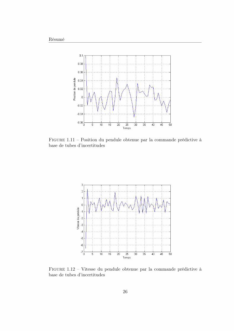
netique . . . . . . . . . . . . . . . . . . . . . . . . . . . . . . . 251.11 Position du pendule obtenue par la commande prédictive à
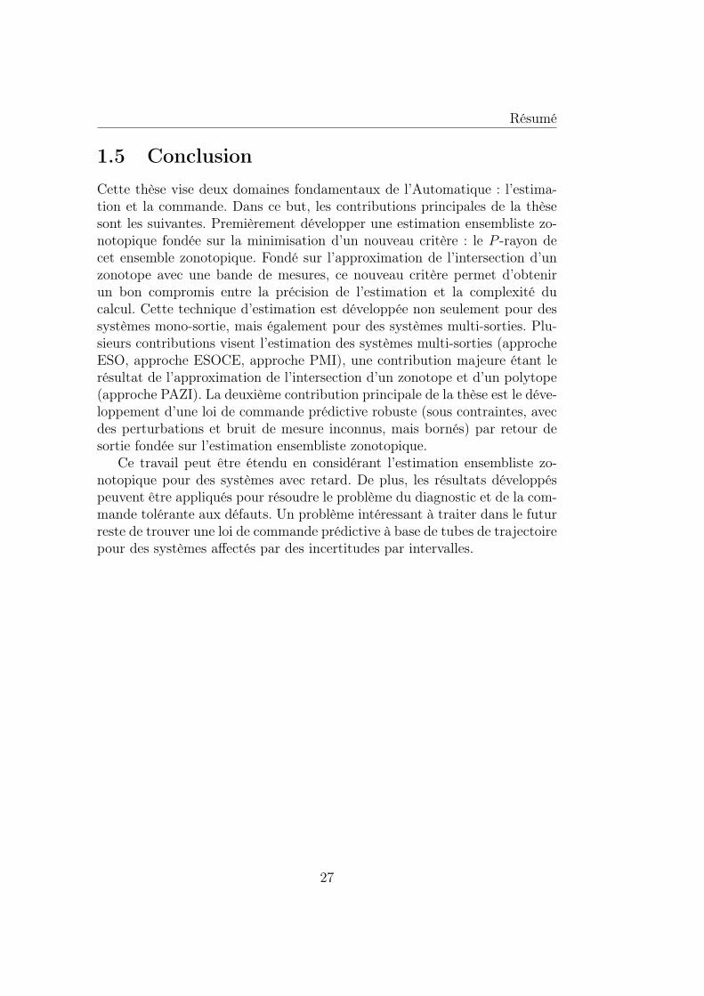
base de tubes d’incertitudes . . . . . . . . . . . . . . . . . . . 261.12 Vitesse du pendule obtenue par la commande prédictive à base
de tubes d’incertitudes . . . . . . . . . . . . . . . . . . . . . . 26
3.1 Difference between the "normal" distance and the Hausdorffdistance between two sets X and Y . . . . . . . . . . . . . . . 37
3.2 Wrapping effect in the interval analysis . . . . . . . . . . . . . 413.3 Ellipsoid . . . . . . . . . . . . . . . . . . . . . . . . . . . . . . 423.4 H-representation of polytope . . . . . . . . . . . . . . . . . . . 433.5 V -representation of polytope . . . . . . . . . . . . . . . . . . . 443.6 3-zonotope and its generators in 2D . . . . . . . . . . . . . . . 463.7 6-zonotope in 3D . . . . . . . . . . . . . . . . . . . . . . . . . 463.8 3-zonotope and its vertices in 2D . . . . . . . . . . . . . . . . 473.9 Intervall hull of a zonotope . . . . . . . . . . . . . . . . . . . . 513.10 Parallelotope hull of a zonotope . . . . . . . . . . . . . . . . . 523.11 Complexity reduction of a zonotope using the cascade reduction 543.12 Complexity reduction of a zonotope using the Euclidean norm-
based criterion . . . . . . . . . . . . . . . . . . . . . . . . . . . 55
ix
LIST OF FIGURES
3.13 Complexity reduction of a zonotope: comparing two criteria . 55
4.1 Set-membership estimation algorithm . . . . . . . . . . . . . . 624.2 Zonotopes and ellipsoids related to the associated P -radius . . 724.3 Evolution of the guaranteed state estimation . . . . . . . . . . 744.4 Evolution of the guaranteed state estimation by Method 4.1 . 784.5 Evolution of the guaranteed state estimation by Method 4.2 . 794.6 Bounds of x2 obtained by different approaches (Example 4.1) . 804.7 Zoom of the bounds of x2 obtained by different approaches
(Example 4.1) . . . . . . . . . . . . . . . . . . . . . . . . . . . 804.8 Comparison of the bound’s width of x1 obtained by different
approaches (Example 4.1) . . . . . . . . . . . . . . . . . . . . 814.9 Comparison of the bound’s width of x2 obtained by different
approaches (Example 4.1) . . . . . . . . . . . . . . . . . . . . 814.10 Comparison of the volume of guaranteed state estimation ob-
tained by different approaches (Example 4.1) . . . . . . . . . . 824.11 Evolution of the guaranteed state estimation Xk (Example 4.2) 874.12 Guaranteed bound of x1 obtained by different methods (Ex-
ample 4.2) . . . . . . . . . . . . . . . . . . . . . . . . . . . . . 884.13 Zoom of the guaranteed bound of x1 obtained by different
methods (Example 4.2) . . . . . . . . . . . . . . . . . . . . . . 884.14 Comparison of the bound’s width of x1 obtained by different
methods in percent (Example 4.2) . . . . . . . . . . . . . . . . 894.15 Comparison of the bound’s width of x2 obtained by different
methods in percent (Example 4.2) . . . . . . . . . . . . . . . . 894.16 Comparison of the volume of zonotopic state estimation set
obtained by different methods (Example 4.2) . . . . . . . . . . 904.17 Comparison of the volume of zonotopic state estimation set
obtained by different methods (Example 4.3) . . . . . . . . . . 924.18 Classification of proposed solution for Multi-Output systems . 934.19 State estimation for a two-output system . . . . . . . . . . . . 954.20 Intersection Xk between the predicted state set Xk and the
measurement Xyk using ESOCE approach . . . . . . . . . . . 994.21 Guaranteed bound of x1 obtained by different methods . . . . 994.22 Comparison of the bound’s width of x1 obtained by different
methods in percent . . . . . . . . . . . . . . . . . . . . . . . . 1004.23 Comparison of the bound’s width of x2 obtained by different
methods in percent . . . . . . . . . . . . . . . . . . . . . . . . 1004.24 Comparison of the volume of zonotopic state estimation set
obtained by different methods . . . . . . . . . . . . . . . . . . 101
x
LIST OF FIGURES
4.25 Comparison of the bound’s width of x1 with interchanged out-put measurements . . . . . . . . . . . . . . . . . . . . . . . . . 101
4.26 Comparison of the bound’s width of x2 with interchanged out-put measurements . . . . . . . . . . . . . . . . . . . . . . . . . 102
4.27 Guaranteed state estimation at the time instant k = 1 . . . . . 1084.28 Guaranteed state estimation at the time instant k = 8 . . . . . 1084.29 Guaranteed bounds of x1 by PMI-based approach . . . . . . . 1094.30 Guaranteed bounds of x2 by PMI-based approach . . . . . . . 1094.31 Evolution of the volume of the guaranteed state estimation
obtained by PMI-based approach . . . . . . . . . . . . . . . . 1104.32 Outer approximation of the the intersection between a zono-
tope and a polytope . . . . . . . . . . . . . . . . . . . . . . . 1134.33 Evolution of the guaranteed state estimation obtained by PAZI
approach . . . . . . . . . . . . . . . . . . . . . . . . . . . . . . 1164.34 Comparison of the bound’s width of x1 in Example 4.6 ob-
tained by different methods in percent . . . . . . . . . . . . . 1164.35 Comparison of the bound’s width of x2 in Example 4.6 ob-
tained by different methods in percent . . . . . . . . . . . . . 1174.36 Classification of the zonotopic guaranteed state estimation
methods . . . . . . . . . . . . . . . . . . . . . . . . . . . . . . 118
5.1 Strategy of Model Predictive Control . . . . . . . . . . . . . . 1225.2 Evolution of the state estimation set . . . . . . . . . . . . . . 1275.3 Evolution of the system output and reference output . . . . . 1285.4 Evolution of the constraint value in (5.10) . . . . . . . . . . . 1285.5 Evolution of the zonotopic state estimation set . . . . . . . . . 1355.6 Zoom of the evolution of the zonotopic state estimation set . . 1355.7 Tube trajectory of the closed-loop system . . . . . . . . . . . . 1365.8 Tube trajectory of the closed-loop system fulfilling the state
constraints . . . . . . . . . . . . . . . . . . . . . . . . . . . . . 1375.9 Closed-loop response of the system . . . . . . . . . . . . . . . 1375.10 Evolution of the system output . . . . . . . . . . . . . . . . . 1395.11 Evolution of the system state . . . . . . . . . . . . . . . . . . 1405.12 Control signal . . . . . . . . . . . . . . . . . . . . . . . . . . . 140
6.1 Magnetic levitation system . . . . . . . . . . . . . . . . . . . . 1446.2 Block diagram of the closed-loop system . . . . . . . . . . . . 1446.3 Comparison of the zonotopic guaranteed state estimation ob-
tained by different approaches . . . . . . . . . . . . . . . . . . 1476.4 Comparison of the zonotopic guaranteed state estimation ob-
tained by different approaches with zoom . . . . . . . . . . . . 147
xi
LIST OF FIGURES
6.5 Evolution of the guaranteed state estimation of the magneticlevitation system . . . . . . . . . . . . . . . . . . . . . . . . . 148
6.6 Control signal of the closed-loop magnetic levitation system . 1496.7 Pendulum position obtained by the open-loop MPC . . . . . . 1496.8 Pendulum speed obtained by the open-loop MPC . . . . . . . 1506.9 Tube trajectory of the controlled magnetic levitation system . 1516.10 Tube section bounding the system trajectory at the initial
instant time k = 1 . . . . . . . . . . . . . . . . . . . . . . . . 1516.11 Evolution of the guaranteed state estimation using the TMPC 1526.12 Real state and nominal state of the closed-loop pendulum system1526.13 Control signal of the closed-loop magnetic levitation system
computed by the TMPC . . . . . . . . . . . . . . . . . . . . . 1536.14 Pendulum position controlled by the TMPC . . . . . . . . . . 1536.15 Pendulum speed controlled by the TMPC . . . . . . . . . . . 154
xii
List of Tables
1.1 Temps de calcul pour 50 périodes d’échantillonnage . . . . . . 19
4.1 Total computation time of Example 4.1 after 50 time instants 834.2 Total computation time of Example 4.2 after 50 time instants 904.3 Table of recapitulation of different estimation approaches (Single-
Output case) . . . . . . . . . . . . . . . . . . . . . . . . . . . 914.4 Total computation time of Example 4.3 after 50 time instants 914.5 Total computation time of Example 4.4 after 50 time instants 1024.6 Total computation time of Example 4.5 after 50 time instants 1104.7 Table of recapitulation of different estimation approaches (Multi-
Output case) . . . . . . . . . . . . . . . . . . . . . . . . . . . 1104.8 Total computation time of Example 4.6 after 50 time instants 115
6.1 Total computation time of the estimation problem of the mag-netic levitation system after 50 time instants . . . . . . . . . . 148
xiii

LIST OF TABLES
xiv
List of symbols
R Set of real numbersR+ Set of strictly positive real numbersRn Set of n-dimensional real vectorBn Unitary box in Rn
A General notation for a matrixIn Identity matrix in Rn×n
[A] General notation for an interval matrixvert([A]) Vertices of interval matrix Amid([A]) Center of interval matrix Arad([A]) Radius of interval matrix AAT Transpose of matrix AA−1 Inverse of matrix Adet(A) Determinant of matrix Atr(A) Trace of matrix AIm(A) Image of matrix Adiag(σ1, . . . , σn) Diagonal matrix of dimension nZ = Z(p;H) = p⊕HBm General notation of a m-zonotopers(H) Round-sum of matrix Hbox(Z) Approximation of zonotope Z by a boxPar(Z) Approximation of zonotope Z by a parallelotope♦(Z) Zonotope inclusionA 0 General notation for strictly positive definite matrix AA 0 General notation for positive definite matrix AA ≺ 0 General notation for strictly negative definite matrix AA 0 General notation for negative definite matrix A| · | Absolute value‖ · ‖∞ Infinity norm‖ · ‖P P -norm‖ · ‖F Frobenius norm
xv
∈ It belongs to⊂ Subset∩ Intersection⊕ Minkowski sum Pontryagin differenceM(S) Image of a set Sd(X, Y ) Distance between X and Y (also called "normal" distance)dH(X, Y ) Hausdorff distance between X and Y(n
m
)n combination of m elements
n! Factorial of nyk/i i-th row of vector ykconv(·) Convex hullω ∼ N(0, Q) Random variable ω having zero means, normal distribution
and covariance matrix Q
xvi
Acronyms
BMI Bilinear Matrix InequalityCARIMA Controlled Auto-Regressive Integrated Moving AverageCRHPC Constrained Receding Horizon Predictive ControlDMC Dynamic Matrix ControlEHAC Extended Horizon Adaptive ControlEPSAC Extended Prediction Self-Adaptive ControlESO Equivalent Single-OutputESOCE Equivalent Single-Output with Coupling EffectEVP Eigenvalue problemGPC Generalized Predictive ControlLMI Linear Matrix InequalityLQ Linear Quadratic controlLQR Linear Quadratic RegulatorLTI Linear Time InvariantMAC Model Algorithmic ControlMHRC Model predictive heuristic controlMIMO Multi Input Multi OutputMPC Model Predictive ControlMPT Multi-Parametric ToolboxMURHAC Multi-predictor Receding Horizon Adaptive ControlMUSMAR Multi-step Multivariable Adaptive ControlPAZI Polytope and Zonotope IntersectionPFC Predictive Functional ControlPMI Polynomial Matrix InequalityQP Quadratic ProgrammingSISO Single Input Single OutputSOS Sum of SquaresSVD Singular Value Decomposition
xvii

TMPC Tube-based Model Predictive ControlUFC Unified Predictive Control
xviii
Chapitre 1
Résumé
Dans la majorité des applications réelles, la dynamique du système est sou-vent affectée par des variations de paramètres, des perturbations agissant surl’état et des bruits de mesure. De plus, certains paramètres physiques ne sontpas connus avec exactitude, seules les bornes (inférieure et supérieure) de va-riation étant disponibles. Ainsi, ces incertitudes peuvent avoir des influencesimportantes sur le comportement du système considéré. Dans ce contexte, lebut principal de cette thèse est de prendre en compte les différentes incer-titudes dans la modélisation des systèmes. Dans cet esprit, deux problèmesseront résolus dans ces travaux de thèse :
• Des méthodes d’estimation d’état pour des systèmes incertains fondéessur des méthodes ensemblistes, plus précisément des ensembles zonoto-piques, sont tout d’abord développées. Ces méthodes conduisent à ré-soudre de problèmes via un formalisme d’Inégalité Matricielle Linéaire(LMI), Inégalité Matricielle Bilinéaire (BMI) ou Inégalité MatriciellePolynomiale (PMI) selon le cas envisagé.
• En utilisant le résultat de l’estimation zonotopique, une commande pré-dictive robuste fondée sur des tubes d’incertitudes est ensuite proposée.
Cette thèse est structurée comme suit : le Chapitre 2 propose une in-troduction portant sur le contexte, les motivations, les contributions et lespublications issues des résultats obtenus pendant les travaux. Le Chapitre3 propose une introduction détaillée des méthodes de représentation d’in-certitudes (intervalle, ellipsoïde, polytope ou zonotope). Ensuite le Chapitre4 présente une nouvelle technique d’estimation ensembliste fondée sur deszonotopes pour des systèmes affectés par des perturbations, des bruits demesure et des incertitudes paramétriques. Utilisant les résultats de l’estima-tion zonotopique, le Chapitre 5 formule la mise en oeuvre de la commande
1
Résumé
prédictive robuste par retour de sortie pour le même type de système. Dansle Chapitre 5, les résultats théoriques développés sont implantés sur un sys-tème de suspension magnétique. Le résumé de chaque chapitre est proposéci-dessous.
1.1 Chapitre 3 : Représentation des incertitudespar des ensembles convexes
Le Chapitre 3 traite des différentes approches existant dans la littératurepour représenter des incertitudes : l’approche stochastique ou probabiliste etl’approche déterministe ou ensembliste. L’approche probabiliste [99], [12] estfondée sur l’hypothèse que les lois de probabilité sur des perturbations et desbruits de mesure sont connues. Pourtant, dans plusieurs applications, ces loisde probabilité ne sont pas toujours connues, seules les bornes de ces pertur-bations pouvant être déterminées. Dans ce contexte, l’approche déterministes’avère plus adaptée à la modélisation de perturbations. Dans cette approche,une variable incertaine est représentée par un ensemble convexe qui carac-térise le domaine de valeurs possibles de cette variable. Dans la littérature,plusieurs façons de représenter un ensemble en fonction de la complexité et laprécision existent, par exemple les représentations par : intervalle, ellipsoïde,polytope, parallélotope et zonotope. Les ensembles les plus représentatifs sontexposés par la suite.
1.1.1 Intervalle
La manière la plus simple pour caractériser un domaine de variation d’unparamètre est l’intervalle.
Définition 1.1. Un intervalle I = [a, b] est défini par un ensemble bornéx : a ≤ x ≤ b.
Définition 1.2. Le centre et le rayon d’un intervalle I = [a, b] sont repré-sentés par mid(I) = a+b
2et rad(I) = b−a
2, respectivement.
Définition 1.3. Un matrice intervalle [M ] ∈ In×m est une matrice qui ades intervalles comme éléments. Cela permet d’aboutir aux calculs simplesfondés sur l’analyse par intervalles. En revanche, la précision d’estimationest parfois dégradée du fait d’occurrences multiples (voir Exemple 3.1) et del’effet d’enveloppement (voir Exemple 3.2)[68].
2
Résumé
1.1.2 Ellipsoïde
Un autre famille d’ensembles utilisée dans la littérature du fait de son avan-tage de faible complexité est représentée par l’ellipsoïde.
Définition 1.4. Soit un vecteur c ∈ Rn et une matrice symétrique définiepositive P = P T 0, l’ellipsoïde E est défini par l’expression suivante :
E = x ∈ Rn : (x− c)TP−1(x− c) ≤ 1 (1.1)
Le vecteur c ∈ Rn est nommé le centre de l’ellipsoïde E et la matrice Pest appelée la matrice de forme de l’ellipsoïde E.
L’avantage de la représentation d’un ensemble de paramètres incertainspar ellipsoïdes est que la complexité est fixée par la dimension de l’espace(quadratique) [78]. Malgré cet avantage, la précision d’estimation dans lecontexte d’ellipsoïdes reste parfois conservative [66].
1.1.3 Polytope
Dans le domaine de l’automatique, une représentation très utilisée pour dé-crire des ensembles est le polytope. L’avantage du polytope est qu’il peutconduire à une approximation très précise de tout ensemble convexe [81],[26], [127]. Un polytope peut être défini de deux façons équivalentes quipermettent de choisir une représentation adaptée au problème particulierconsidéré.
Définition 1.5. (H-représentation) Un polyèdre P ∈ Rn est défini commel’intersection d’un nombre fini de demi-espaces :
P = x ∈ Rn : H · x ≤ K (1.2)
avec H ∈ Rm×n et K ∈ Rm. Si P est borné, alors P devient un polytope.
Définition 1.6. (V-représentation) Soit un ensemble fini de points V =v1, v2, . . . , vm ∈ Rn, un polytope P est défini par l’enveloppe convexe del’ensemble V :
P = conv(V ) = α1v1 + α2v2 + . . .+ αmvm : αi ∈ R+,
m∑i=1
αi = 1 (1.3)
Les deux représentations définies par les définitions 1.5 et 1.6 sont équiva-lentes [151]. L’inconvénient principal du polytope est lié à sa complexité quiaugmente exponentiellement avec le nombre de sommets. Cette propriété dupolytope rend souvent le calcul très coûteux au niveau du temps de calcul.
3
Résumé
1.1.4 Zonotope
Le zonotope est un cas particulier de polytope, plus précisément un poly-tope symétrique (d’où une diminution de complexité en comparaison avecle polytope quelconque). Comme un zonotope est un polytope, le zonotopepeut être mis sous forme d’une H-représentation ou d’une V -représentation.Cependant l’avantage du zonotope vient de ses propres définitions exposéesci-dessous.
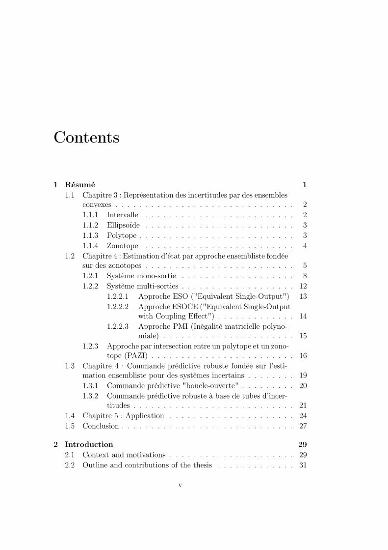
Définition 1.7. (G-représentation) Soit un vecteur p ∈ Rn et un ensemblede vecteurs G = g1, g2, ..., gm ⊂ Rn, m ≥ n. Un zonotope Z d’ordre m estdéfini par :
Z = (p; g1, g2, ..., gm) = x ∈ Rn : x = p+m∑i=1
αigi;−1 ≤ αi ≤ 1 (1.4)
Le vecteur p est appelé le centre du zonotope Z. Les vecteurs g1, . . ., gmsont appelés les générateurs du zonotope Z. L’ordre d’un zonotope est définipar le nombre de générateurs (m dans ce cas). Cette définition est équivalenteà la définition d’un zonotope par la somme de Minkowski d’un nombre finide segments définis par giB1, avec i = 1, . . . ,m :
Z = (p; g1, g2, ..., gm) = p⊕ g1B1 ⊕ . . .⊕ gmB1 (1.5)
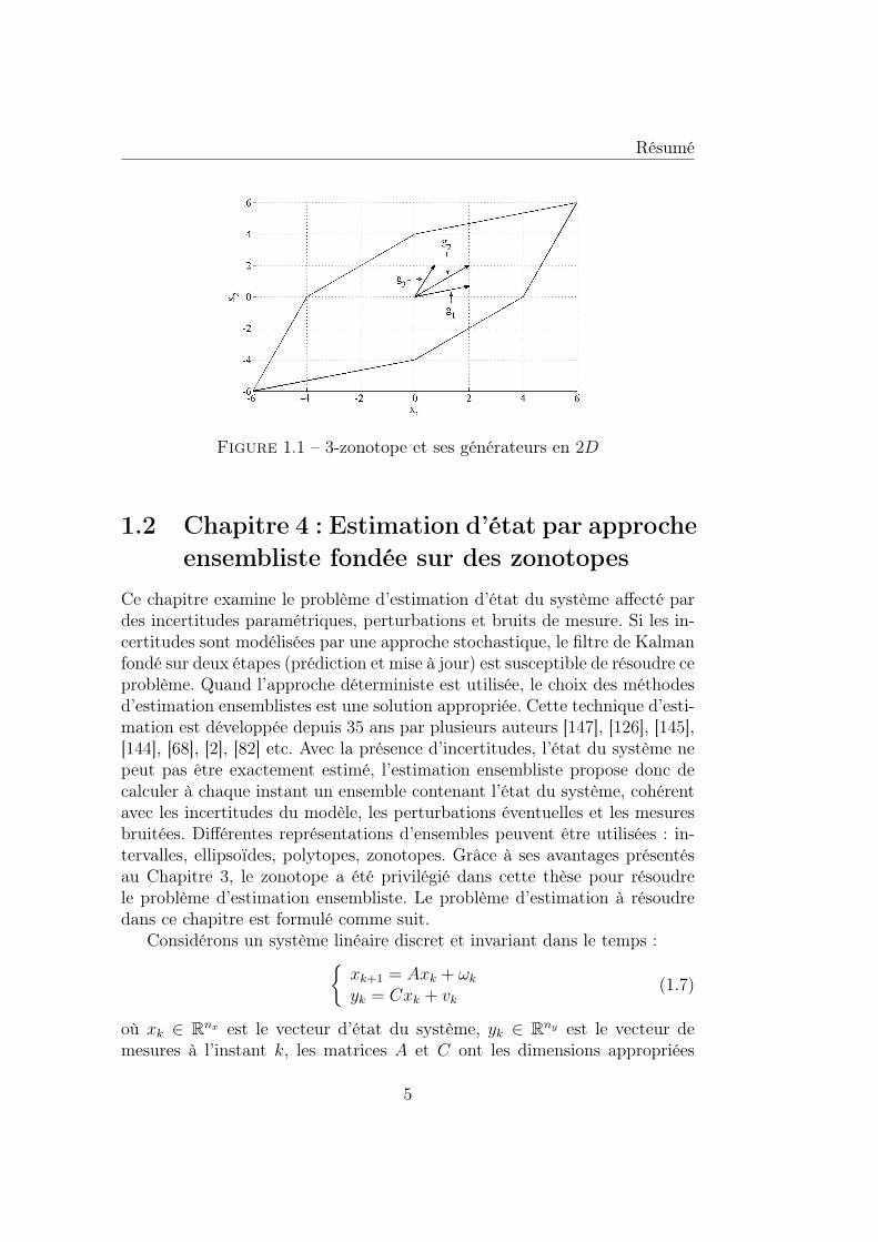
Un exemple de zonotope construit par 3 générateurs est présenté Figure 1.1.L’avantage principal du zonotope, qui facilite la résolution du problème
d’estimation d’état considéré dans cette thèse, vient de la définition suivante.
Définition 1.8. (Projection linéaire d’un hypercube) Un zonotope d’ordrem dans Rn (m ≥ n) est la translation de centre p ∈ Rn de l’image d’unhypercube de dimension m dans Rn par une application linéaire. Soit unematrice H ∈ Rn×m représentant l’application linéaire, le zonotope Z estdéfini par :
Z = (p;H) = p⊕HBm (1.6)
Grâce à cette définition, les opérations comme la somme de Minkowski oul’image linéaire du zonotope peuvent être effectuées facilement. Différentespropriétés intéressantes du zonotope sont regroupées dans [82]. Comme lezonotope propose un bon compromis entre la complexité du calcul et la pré-cision de la représentation, il a été privilégié dans cette thèse pour représenterdes incertitudes.
4
Résumé
Figure 1.1 – 3-zonotope et ses générateurs en 2D
1.2 Chapitre 4 : Estimation d’état par approcheensembliste fondée sur des zonotopes
Ce chapitre examine le problème d’estimation d’état du système affecté pardes incertitudes paramétriques, perturbations et bruits de mesure. Si les in-certitudes sont modélisées par une approche stochastique, le filtre de Kalmanfondé sur deux étapes (prédiction et mise à jour) est susceptible de résoudre ceproblème. Quand l’approche déterministe est utilisée, le choix des méthodesd’estimation ensemblistes est une solution appropriée. Cette technique d’esti-mation est développée depuis 35 ans par plusieurs auteurs [147], [126], [145],[144], [68], [2], [82] etc. Avec la présence d’incertitudes, l’état du système nepeut pas être exactement estimé, l’estimation ensembliste propose donc decalculer à chaque instant un ensemble contenant l’état du système, cohérentavec les incertitudes du modèle, les perturbations éventuelles et les mesuresbruitées. Différentes représentations d’ensembles peuvent être utilisées : in-tervalles, ellipsoïdes, polytopes, zonotopes. Grâce à ses avantages présentésau Chapitre 3, le zonotope a été privilégié dans cette thèse pour résoudrele problème d’estimation ensembliste. Le problème d’estimation à résoudredans ce chapitre est formulé comme suit.
Considérons un système linéaire discret et invariant dans le temps :xk+1 = Axk + ωkyk = Cxk + vk
(1.7)
où xk ∈ Rnx est le vecteur d’état du système, yk ∈ Rny est le vecteur demesures à l’instant k, les matrices A et C ont les dimensions appropriées
5
Résumé
avec la paire (C,A) détectable. Les notations ωk ∈ Rnx , vk ∈ Rny sont utili-sées pour les perturbations sur l’état et le bruit de mesure, respectivement.Les perturbations et les bruits de mesure sont supposés bornés par des zo-notopes ωk ∈ W, vk ∈ V . On suppose également que l’état initial appartientà un zonotope X0. Pour simplifier le calcul, les centres du zonotope V et dunx-zonotope W sont supposés être à l’origine. Si cette hypothèse n’est passatisfaite, un changement de coordonnées peut être utilisé pour ramener lescentres des zonotopes à l’origine. Avec ces hypothèses et à partir de la défini-tion du zonotope, les ensembles W et V peuvent être réécrits sous la forme :W = FBnx et V = ΣBny , où Σ ∈ Rny×ny une matrice diagonale. Avec ce mo-dèle, l’estimation ensembliste fondée sur des zonotopes calcule un ensemblezonotopique contenant de manière garantie l’état du système affecté par desincertitudes. Avant de détailler cette approche, quelques notions utiles sontdéfinies.
Définition 1.9. Soit le système (1.7), l’ensemble des états cohérents avecles mesures ("consistent state set") à l’instant k est défini par Xyk = x ∈Rn : |cTx− yk| ≤ σ.
Définition 1.10. Pour le système (1.7), l’ensemble exact des états incertains("exact uncertain state set") Xk est l’ensemble contenant les états cohérentsavec la sortie mesurée et l’ensemble des états initiaux possibles X0 : Xk =(AXk−1 ⊕W ) ∩Xyk , pour k ≥ 1.
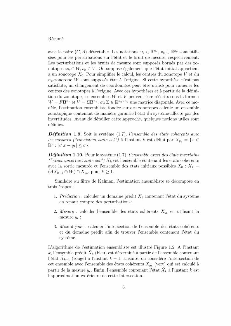
Similaire au filtre de Kalman, l’estimation ensembliste se décompose entrois étapes :
1. Prédiction : calculer un domaine prédit Xk contenant l’état du systèmeen tenant compte des perturbations ;
2. Mesure : calculer l’ensemble des états cohérents Xyk en utilisant lamesure yk ;
3. Mise à jour : calculer l’intersection de l’ensemble des états cohérentset du domaine prédit afin de trouver l’ensemble contenant l’état dusystème.
L’algorithme de l’estimation ensembliste est illustré Figure 1.2. A l’instantk, l’ensemble prédit Xk (bleu) est déterminé à partir de l’ensemble contenantl’état Xk−1 (rouge) à l’instant k − 1. Ensuite, on considère l’intersection decet ensemble avec l’ensemble des états cohérents Xyk (vert) qui est calculé àpartir de la mesure yk. Enfin, l’ensemble contenant l’état Xk à l’instant k estl’approximation extérieure de cette intersection.
6
Résumé
Figure 1.2 – Illustration de l’estimation ensembliste
Figure 1.3 – Estimation ensembliste fondée sur des zonotopes
7
Résumé
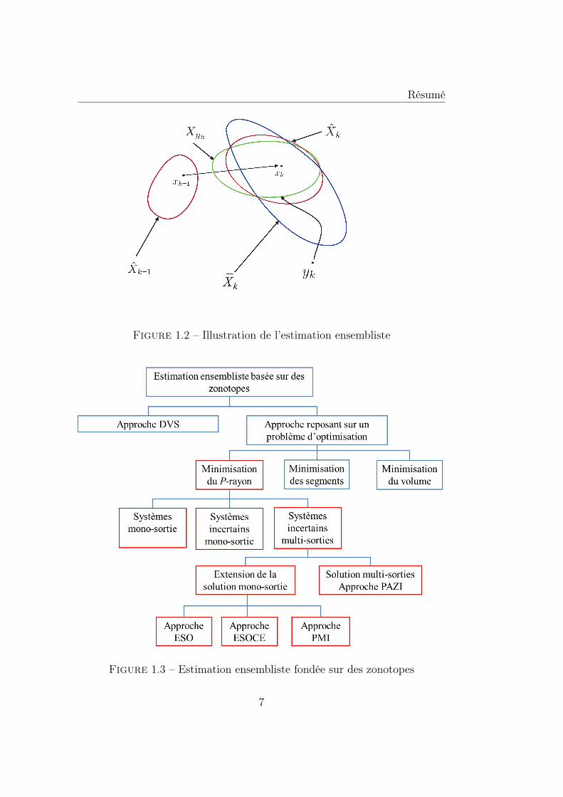
En pratique le calcul exact de l’intersection de l’ensemble des états cohé-rents et du domaine prédit est difficile, donc on cherche souvent à majorercette intersection par une approximation extérieure (zonotopique dans cettethèse) de cet ensemble. Quelques méthodes pour résoudre ce problème sontregroupées dans le schéma Figure 1.3. Les méthodes existant dans la litté-rature sont encadrées en bleu. L’approche fondée sur la minimisation dessegments d’un zonotope présentée dans [2] permet d’avoir un calcul simplemais la précision d’estimation est limitée. L’approche DVS présentée par[37] et l’approche reposant sur la minimisation du volume d’un zonotope [2]ont des bonnes précisions d’estimation mais les calculs sont complexes. Lescontributions de ce chapitre encadrées en rouge permettent d’avoir un boncompromis entre la précision et la complexité. Ces méthodes seront ensuitedétaillées dans les sections suivantes.
1.2.1 Système mono-sortie
Considérons tout d’abord un système linéaire mono-sortie invariant à tempsdiscret :
xk+1 = Axk + ωkyk = cTxk + vk
(1.8)
La perturbation et le bruit de mesure sont bornés par ωk ∈ W = FBnx ,vk ∈ V = σB1 ⊂ R, avec σ ∈ R+. Soit Xk−1 une approximation extérieurezonotopique de l’ensemble contenant l’état du système Xk−1 = pk−1⊕Hk−1Br
à l’instant k − 1 et la mesure de la sortie yk à l’instant k, l’ensemble préditXk peut être obtenu par la relation :
Xk = Apk−1 ⊕[AHk−1 F
]Br+nx = pk ⊕ HkBr+nx (1.9)
Avec la définition de l’ensemble V , l’ensemble des états cohérents Xyk à l’ins-tant k est une bande de contraintes : Xyk = x ∈ Rn : |cTx − yk| ≤ σ.Pour déterminer l’ensemble contenant l’état du système à l’instant k, il fautrechercher une approximation extérieure de l’intersection du zonotope Xk etde la bande de contraintes Xyk . Ce problème peut être résolu en utilisant lapropriété suivante :
Propriété 1. Soit un zonotope Z = p⊕HBr ⊂ Rn, une bande de contraintesS = x ∈ Rn : |cTx − d| ≤ σ et un vecteur λ ∈ Rn. Définissons une fa-mille de vecteurs p(λ) = p + λ(d − cTp) ∈ Rn et une famille de matricesH(λ) =
[(I − λcT )H σλ
]∈ Rn×(m+1). Alors l’expression suivante est satis-
faite Z ∩ S ⊆ X(λ) = p(λ)⊕ H(λ)Br+1.
8
Résumé
En utilisant cette propriété, on obtient l’approximation extérieure de l’en-semble contenant l’état à l’instant k :
Xk(λ) = pk(λ)⊕ Hk(λ)Br+nx+1 (1.10)
avec les notations suivantes :pk(λ) = Apk−1 + λ(yk − cTApk−1)Hk(λ) =
[(I − λcT )AHk−1 (I − λcT )F σλ
] (1.11)
Comme λ est un vecteur libre, (1.11) représente une famille de zonotopescontenant l’état à l’instant k. Donc la valeur du vecteur λ doit permettred’obtenir une meilleur précision de l’approximation. Les auteurs de [2] pro-posent deux méthodes basées sur différents critères pour calculer le vecteurλ. La première méthode minimise les segments du zonotope X(λ). Cette mé-thode aboutit à un calcul simple, mais le résultat est parfois conservatif. Ladeuxième méthode minimise le volume du zonotope en résolvant un problèmed’optimisation coûteux en temps de calcul avec un résultat plus performant.Dans ce chapitre, un nouveau critère d’optimisation est proposé permettantde gérer le compromis entre la complexité du calcul et la précision de l’esti-mation. Cette méthode est fondée sur la définition du P -rayon d’un zonotopecomme suit.
Définition 1.11. Soit un zonotope Z = p⊕HBm, le P -rayon de ce zonotopeest défini par l’expression suivante :
L = maxz∈Z
(‖z − p‖2P ) (1.12)
avec P = P T 0 une matrice symétrique définie positive.
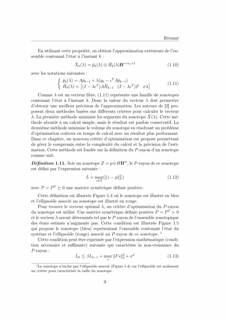
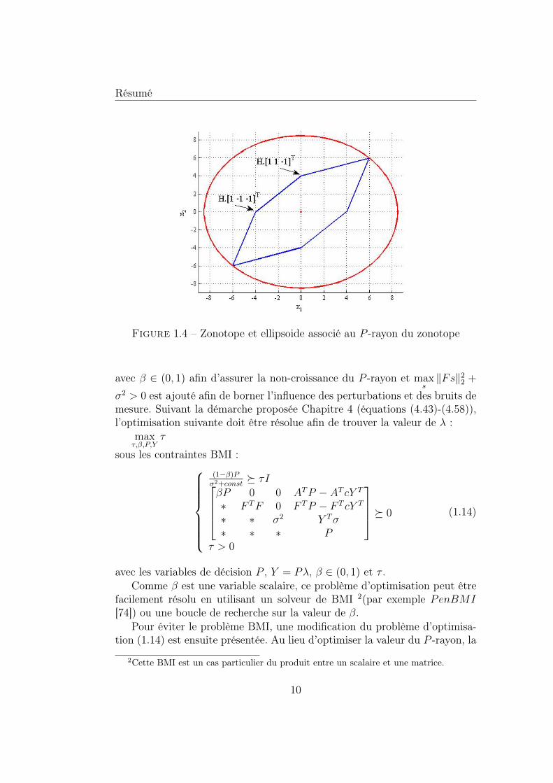
Cette définition est illustrée Figure 1.4 où le zonotope est illustré en bleuet l’ellipsoide associé au zonotope est illustré en rouge.
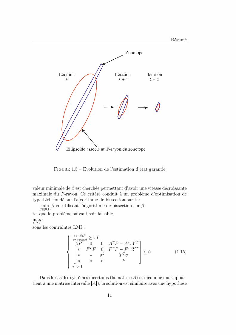
Pour trouver le vecteur optimal λ, un critère d’optimisation du P -rayondu zonotope est utilisé. Une matrice symétrique définie positive P = P T 0et le vecteur λ seront déterminés tel que le P -rayon de l’ensemble zonotopiquedes états estimés n’augmente pas. Cette condition est illustrée Figure 1.5qui propose le zonotope (bleu) représentant l’ensemble contenant l’état dusystème et l’ellipsoïde (rouge) associé au P -rayon de ce zonotope. 1
Cette condition peut être exprimée par l’expression mathématique (condi-tion nécessaire et suffisante) suivante qui caractérise la non-croissance duP -rayon :
Lk ≤ βLk−1 + maxs‖Fs‖22 + σ2 (1.13)
1Le zonotope n’inclut pas l’ellipsoïde associé (Figure 1.4) car l’ellipsoïde est seulementun critère pour caractériser la taille du zonotope.
9
Résumé
Figure 1.4 – Zonotope et ellipsoide associé au P -rayon du zonotope
avec β ∈ (0, 1) afin d’assurer la non-croissance du P -rayon et maxs‖Fs‖22 +
σ2 > 0 est ajouté afin de borner l’influence des perturbations et des bruits demesure. Suivant la démarche proposée Chapitre 4 (équations (4.43)-(4.58)),l’optimisation suivante doit être résolue afin de trouver la valeur de λ :
maxτ,β,P,Y
τ
sous les contraintes BMI :
(1−β)Pσ2+const
τIβP 0 0 ATP − AT cY T
∗ F TF 0 F TP − F T cY T
∗ ∗ σ2 Y Tσ∗ ∗ ∗ P
0
τ > 0
(1.14)
avec les variables de décision P , Y = Pλ, β ∈ (0, 1) et τ .Comme β est une variable scalaire, ce problème d’optimisation peut être
facilement résolu en utilisant un solveur de BMI 2(par exemple PenBMI[74]) ou une boucle de recherche sur la valeur de β.
Pour éviter le problème BMI, une modification du problème d’optimisa-tion (1.14) est ensuite présentée. Au lieu d’optimiser la valeur du P -rayon, la
2Cette BMI est un cas particulier du produit entre un scalaire et une matrice.
10
Résumé
Figure 1.5 – Evolution de l’estimation d’état garantie
valeur minimale de β est cherchée permettant d’avoir une vitesse décroissantemaximale du P -rayon. Ce critère conduit à un problème d’optimisation detype LMI fondé sur l’algorithme de bissection sur β :
minβ∈(0,1)
β en utilisant l’algorithme de bissection sur β
tel que le problème suivant soit faisablemaxτ,P,Y
τ
sous les contraintes LMI :
(1−β)Pσ2+const
τIβP 0 0 ATP − AT cY T
∗ F TF 0 F TP − F T cY T
∗ ∗ σ2 Y Tσ∗ ∗ ∗ P
0
τ > 0
(1.15)
Dans le cas des systèmes incertains (la matrice A est inconnue mais appar-tient à une matrice intervalle [A]), la solution est similaire avec une hypothèse
11
Résumé
supplémentaire (la matrice A est Schur stable). Comme (1.15) est convexeen A et [A] est un ensemble convexe, si (1.15) est vraie pour chaque sommetde [A], elle sera respectée pour tous les éléments A appartenant à la matriceintervalle [A] [122]. Donc la matrice P et le vecteur λ sont la solution duproblème d’optimisation suivant :
maxτ,β,P,Y
τ
sous les contraintes BMI :
(1−β)Pσ2+const
τIβP 0 0 ATi P − ATi cY T
∗ F TF 0 F TP − F T cY T
∗ ∗ σ2 Y Tσ∗ ∗ ∗ P
0
τ > 0
(1.16)
pour i = 1, ..., 2q, où Ai sont les sommets de la matrice intervalle [A], q estle nombre des éléments intervalles de [A] et Y = Pλ.
1.2.2 Système multi-sorties
Comme indiqué dans le schéma Figure 1.3, le problème d’estimation pourdes systèmes multi-sorties peut être résolu par deux familles de solutions. Lapremière famille regroupe les solutions qui sont des extensions directes de lasolution pour des systèmes mono-sorties.
Considérons le système multi-sorties (1.7) ; l’ensemble contenant l’étatdu système Xk peut être déterminé en répétant successivement l’intersectionentre l’ensemble prédit Xyk avec chaque élément du vecteur de mesure yk,noté yk/i :
yk/i = cTi xk + vk/i, i = 1, . . . , ny (1.17)
où cTi est la ligne i de la matrice C et le bruit vk/i est borné par l’intervalleVi = σiB1, avec σi = Σii (avec Σii élément de la matrice Σ).
Supposons l’ensemble contenant l’état du système Xk−1 = pk−1⊕Hk−1Br
à l’instant k − 1, alors l’ensemble prédit à l’instant suivant Xk est calculécomme (1.9). L’ensemble contenant l’état du système est déterminé commesuit.
De façon similaire à (1.10), une approximation extérieure de l’intersectionentre la bande de contraintes obtenue par le premier élément du vecteur demesure (yk/1) et l’ensemble prédit (Xk) est calculée par :
Xk/1(λ1) = pk/1(λ1)⊕ Hk/1(λ1)Br+nx+1 (1.18)
12
Résumé
avec pk/1(λ1) = Apk−1 + λ1(yk/1 − cT1Apk−1)et Hk/1(λ1) =
[(I − λ1cT1 )AHk−1 (I − λ1cT1 )F σ1λ1
].
Ensuite, on détermine l’intersection de cet ensemble Xk/1(λ1) avec la bandede contraintes obtenue par le deuxième élément du vecteur de mesure (yk/2) :
Xk/2(λ1, λ2) = pk/2(λ1, λ2)⊕ Hk/2(λ1, λ2)Br+nx+2 (1.19)
avec pk/2(λ1, λ2) = pk/1(λ1) + λ2(yk/2 − cT2 pk/1(λ1))et Hk/2(λ1, λ2) =
[(I − λ2cT2 )Hk/1(λ1) σ2λ2
].
Cette procédure est répétée jusqu’au dernier élément du vecteur de me-sure (yk/ny) conduisant à :
Xk/ny(λ1, ..., λny) = pk/ny(λ1, ..., λny)⊕⊕Hk/ny(λ1, ..., λny)Br+nx+ny
(1.20)
avec
pk/ny(λ1, ..., λny) = pk/ny−1(λ1, ..., λny−1)+
+ λny(yk/ny − cTnypk/ny−1(λ1, ..., λny−1)) (1.21)
et
Hk/ny(λ1, ..., λny) =[(I − λnyc
Tny
)Hk/ny−1(λ1, ..., λny−1) σnyλny
](1.22)
En conclusion, l’ensemble contenant l’état à l’instant k est le suivant :
Xk(λ1, ..., λny) = pk(λ1, ..., λny)⊕ Hk(λ1, ..., λny)Br+nx+ny (1.23)
avec pk(λ1, ..., λny) = pk/ny(λ1, ..., λny)
et Hk(λ1, ..., λny) = Hk/ny(λ1, ..., λny).Pour déterminer les vecteurs λi, i = 1, . . . , ny, trois approches sont pro-
posées dans ce chapitre et sont détaillées ci-dessous.
1.2.2.1 Approche ESO ("Equivalent Single-Output")
Dans cette approche, le système multi-sorties (1.7) est considéré commeun ensemble de ny systèmes mono-sortie indépendants. Donc, les vecteursλy sont indépendamment calculés en résolvant ny problèmes d’optimisation(1.14) séparés. L’algorithme suivant décrit la procédure proposée.
13
Résumé
Algorithme 1.1.
1. Pour j = 1, ..., nyEtape j : Calculer λj en utilisant la mesure yk/j ;
Fin.
2. L’ensemble contenant l’état est calculé par l’équation (1.23) avec lesvecteurs λ1,. . . ,λny connus.
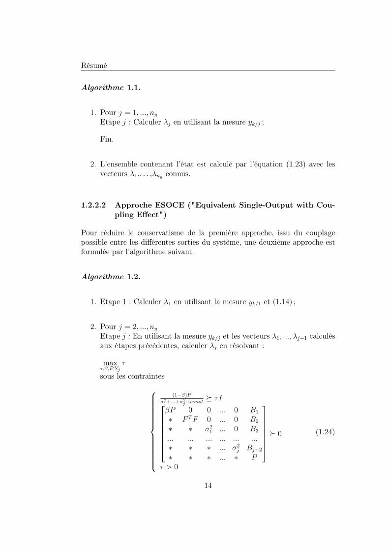
1.2.2.2 Approche ESOCE ("Equivalent Single-Output with Cou-pling Effect")
Pour réduire le conservatisme de la première approche, issu du couplagepossible entre les différentes sorties du système, une deuxième approche estformulée par l’algorithme suivant.
Algorithme 1.2.
1. Etape 1 : Calculer λ1 en utilisant la mesure yk/1 et (1.14) ;
2. Pour j = 2, ..., nyEtape j : En utilisant la mesure yk/j et les vecteurs λ1, ..., λj−1 calculésaux étapes précédentes, calculer λj en résolvant :
maxτ,β,P,Yj
τ
sous les contraintes
(1−β)Pσ21+...+σ
2j+const
τIβP 0 0 ... 0 B1
∗ F TF 0 ... 0 B2
∗ ∗ σ21 ... 0 B3
... ... ... ... ... ...∗ ∗ ∗ ... σ2
j Bj+2
∗ ∗ ∗ ... ∗ P
0
τ > 0
(1.24)
14
Résumé
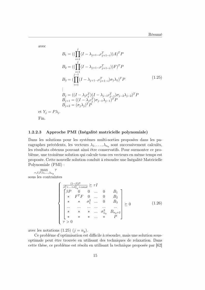
avec
B1 = ((
j∏i=1
(I − λj+1−icTj+1−i))A)TP
B2 = ((
j∏i=1
(I − λj+1−icTj+1−i))F )TP
B3 = (
j−1∏i=1
(I − λj+1−icTj+1−i)σ1λ1)
TP
...Bj = ((I − λjcTj )(I − λj−1cTj−1)σj−2λj−2)TPBj+1 = ((I − λjcTj )σj−1λj−1)
TPBj+2 = (σjλj)
TP
(1.25)
et Yj = Pλj.
Fin.
1.2.2.3 Approche PMI (Inégalité matricielle polynomiale)
Dans les solutions pour les systèmes multi-sorties proposées dans les pa-ragraphes précédents, les vecteurs λ1, . . . , λny sont successivement calculés,les résultats obtenus pouvant ainsi être conservatifs. Pour surmonter ce pro-blème, une troisième solution qui calcule tous ces vecteurs en même temps estproposée. Cette nouvelle solution conduit à résoudre une Inégalité MatriciellePolynomiale (PMI) :
maxτ,β,P,λ1,...,λny
τ
sous les contraintes
(1−β)Pσ21+...+σ
2ny
+const τI
βP 0 0 ... 0 B1
∗ F TF 0 ... 0 B2
∗ ∗ σ21 ... 0 B3
... ... ... ... ... ...∗ ∗ ∗ ... σ2
nyBny+2
∗ ∗ ∗ ... ∗ P
0
τ > 0
(1.26)
avec les notations (1.25) (j = ny).Ce problème d’optimisation est difficile à résoudre, mais une solution sous-
optimale peut être trouvée en utilisant des techniques de relaxation. Danscette thèse, ce problème est résolu en utilisant la technique proposée par [62]
15
Résumé
qui ajoute des variables supplémentaires pour transformer le problème PMIen un problème sous-optimal de type LMI.
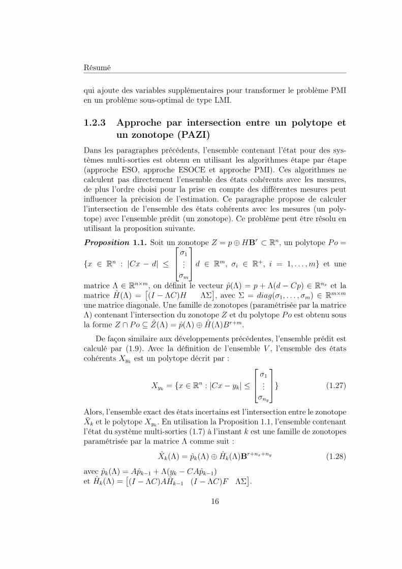
1.2.3 Approche par intersection entre un polytope etun zonotope (PAZI)
Dans les paragraphes précédents, l’ensemble contenant l’état pour des sys-tèmes multi-sorties est obtenu en utilisant les algorithmes étape par étape(approche ESO, approche ESOCE et approche PMI). Ces algorithmes necalculent pas directement l’ensemble des états cohérents avec les mesures,de plus l’ordre choisi pour la prise en compte des différentes mesures peutinfluencer la précision de l’estimation. Ce paragraphe propose de calculerl’intersection de l’ensemble des états cohérents avec les mesures (un poly-tope) avec l’ensemble prédit (un zonotope). Ce problème peut être résolu enutilisant la proposition suivante.
Proposition 1.1. Soit un zonotope Z = p⊕HBr ⊂ Rn, un polytope Po =
x ∈ Rn : |Cx − d| ≤
σ1...σm
d ∈ Rm, σi ∈ R+, i = 1, . . . ,m et une
matrice Λ ∈ Rn×m, on définit le vecteur p(Λ) = p + Λ(d − Cp) ∈ Rnx et lamatrice H(Λ) =
[(I − ΛC)H ΛΣ
], avec Σ = diag(σ1, . . . , σm) ∈ Rm×m
une matrice diagonale. Une famille de zonotopes (paramétrisée par la matriceΛ) contenant l’intersection du zonotope Z et du polytope Po est obtenu sousla forme Z ∩ Po ⊆ Z(Λ) = p(Λ)⊕ H(Λ)Br+m.
De façon similaire aux développements précédentes, l’ensemble prédit estcalculé par (1.9). Avec la définition de l’ensemble V , l’ensemble des étatscohérents Xyk est un polytope décrit par :
Xyk = x ∈ Rn : |Cx− yk| ≤
σ1...σny
(1.27)
Alors, l’ensemble exact des états incertains est l’intersection entre le zonotopeXk et le polytope Xyk . En utilisation la Proposition 1.1, l’ensemble contenantl’état du système multi-sorties (1.7) à l’instant k est une famille de zonotopesparamétrisée par la matrice Λ comme suit :
Xk(Λ) = pk(Λ)⊕ Hk(Λ)Br+nx+ny (1.28)
avec pk(Λ) = Apk−1 + Λ(yk − CApk−1)et Hk(Λ) =
[(I − ΛC)AHk−1 (I − ΛC)F ΛΣ
].
16
Résumé
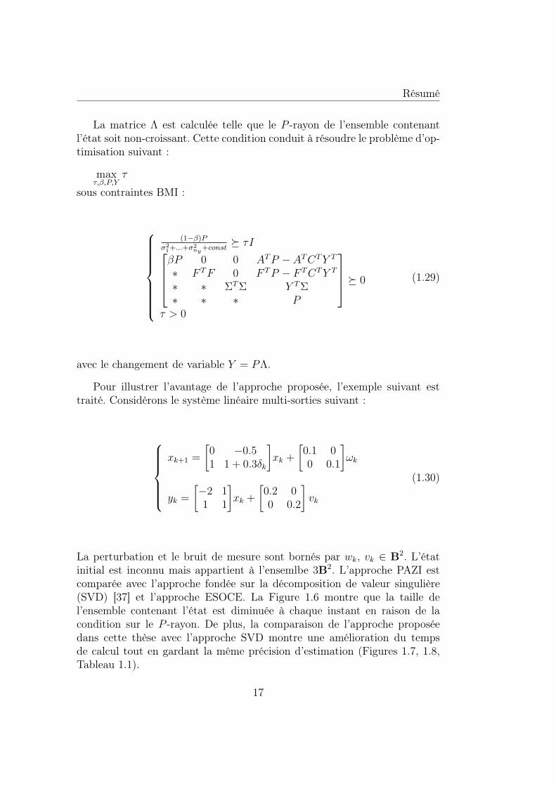
La matrice Λ est calculée telle que le P -rayon de l’ensemble contenantl’état soit non-croissant. Cette condition conduit à résoudre le problème d’op-timisation suivant :
maxτ,β,P,Y
τ
sous contraintes BMI :
(1−β)Pσ21+...+σ
2ny
+const τI
βP 0 0 ATP − ATCTY T
∗ F TF 0 F TP − F TCTY T
∗ ∗ ΣTΣ Y TΣ∗ ∗ ∗ P
0
τ > 0
(1.29)
avec le changement de variable Y = PΛ.
Pour illustrer l’avantage de l’approche proposée, l’exemple suivant esttraité. Considérons le système linéaire multi-sorties suivant :
xk+1 =
[0 −0.51 1 + 0.3δk
]xk +
[0.1 00 0.1
]ωk
yk =
[−2 11 1
]xk +
[0.2 00 0.2
]vk
(1.30)
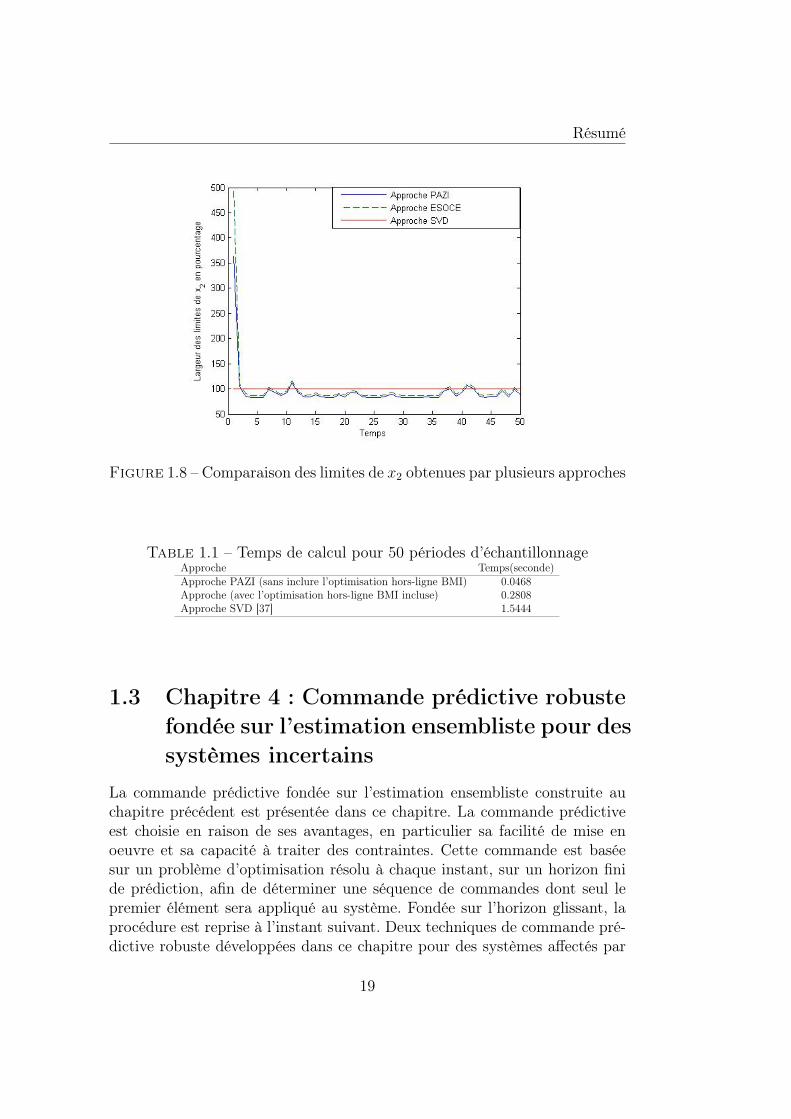
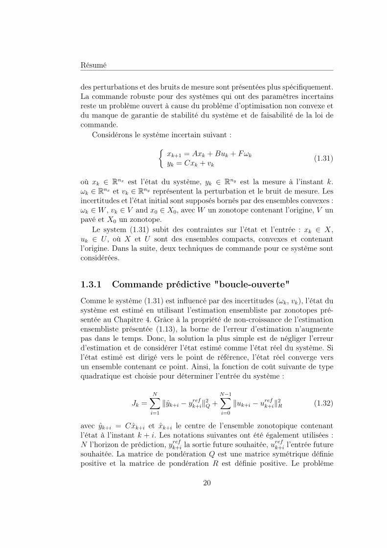
La perturbation et le bruit de mesure sont bornés par wk, vk ∈ B2. L’étatinitial est inconnu mais appartient à l’ensemlbe 3B2. L’approche PAZI estcomparée avec l’approche fondée sur la décomposition de valeur singulière(SVD) [37] et l’approche ESOCE. La Figure 1.6 montre que la taille del’ensemble contenant l’état est diminuée à chaque instant en raison de lacondition sur le P -rayon. De plus, la comparaison de l’approche proposéedans cette thèse avec l’approche SVD montre une amélioration du tempsde calcul tout en gardant la même précision d’estimation (Figures 1.7, 1.8,Tableau 1.1).
17
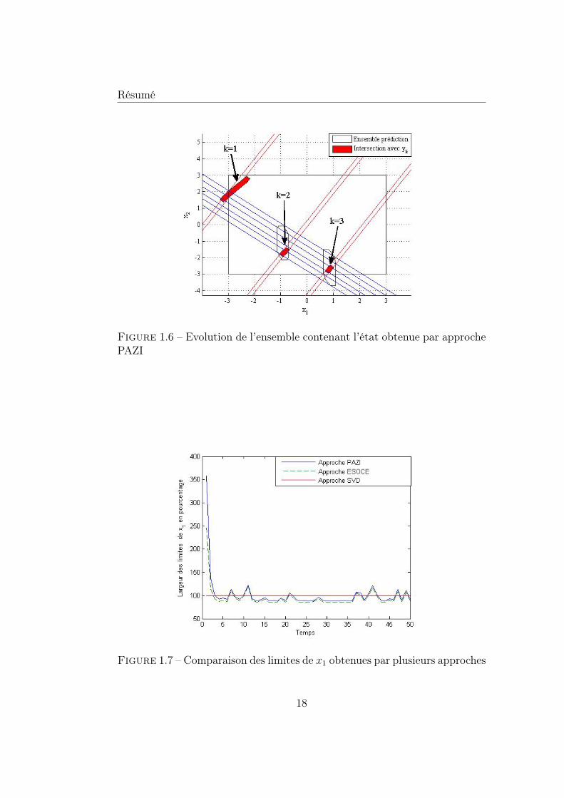
Résumé
Figure 1.6 – Evolution de l’ensemble contenant l’état obtenue par approchePAZI
Figure 1.7 – Comparaison des limites de x1 obtenues par plusieurs approches
18
Résumé
Figure 1.8 – Comparaison des limites de x2 obtenues par plusieurs approches
Table 1.1 – Temps de calcul pour 50 périodes d’échantillonnageApproche Temps(seconde)Approche PAZI (sans inclure l’optimisation hors-ligne BMI) 0.0468Approche (avec l’optimisation hors-ligne BMI incluse) 0.2808Approche SVD [37] 1.5444
1.3 Chapitre 4 : Commande prédictive robustefondée sur l’estimation ensembliste pour dessystèmes incertains
La commande prédictive fondée sur l’estimation ensembliste construite auchapitre précédent est présentée dans ce chapitre. La commande prédictiveest choisie en raison de ses avantages, en particulier sa facilité de mise enoeuvre et sa capacité à traiter des contraintes. Cette commande est baséesur un problème d’optimisation résolu à chaque instant, sur un horizon finide prédiction, afin de déterminer une séquence de commandes dont seul lepremier élément sera appliqué au système. Fondée sur l’horizon glissant, laprocédure est reprise à l’instant suivant. Deux techniques de commande pré-dictive robuste développées dans ce chapitre pour des systèmes affectés par
19
Résumé
des perturbations et des bruits de mesure sont présentées plus spécifiquement.La commande robuste pour des systèmes qui ont des paramètres incertainsreste un problème ouvert à cause du problème d’optimisation non convexe etdu manque de garantie de stabilité du système et de faisabilité de la loi decommande.
Considérons le système incertain suivant :xk+1 = Axk +Buk + Fωkyk = Cxk + vk
(1.31)
où xk ∈ Rnx est l’état du système, yk ∈ Rny est la mesure à l’instant k.ωk ∈ Rnx et vk ∈ Rny représentent la perturbation et le bruit de mesure. Lesincertitudes et l’état initial sont supposés bornés par des ensembles convexes :ωk ∈ W , vk ∈ V and x0 ∈ X0, avec W un zonotope contenant l’origine, V unpavé et X0 un zonotope.
Le system (1.31) subit des contraintes sur l’état et l’entrée : xk ∈ X,uk ∈ U , où X et U sont des ensembles compacts, convexes et contenantl’origine. Dans la suite, deux techniques de commande pour ce système sontconsidérées.
1.3.1 Commande prédictive "boucle-ouverte"
Comme le système (1.31) est influencé par des incertitudes (ωk, vk), l’état dusystème est estimé en utilisant l’estimation ensembliste par zonotopes pré-sentée au Chapitre 4. Grâce à la propriété de non-croissance de l’estimationensembliste présentée (1.13), la borne de l’erreur d’estimation n’augmentepas dans le temps. Donc, la solution la plus simple est de négliger l’erreurd’estimation et de considérer l’état estimé comme l’état réel du système. Sil’état estimé est dirigé vers le point de référence, l’état réel converge versun ensemble contenant ce point. Ainsi, la fonction de coût suivante de typequadratique est choisie pour déterminer l’entrée du système :
Jk =N∑i=1
‖yk+i − yrefk+i‖2Q +
N−1∑i=0
‖uk+i − urefk+i‖2R (1.32)
avec yk+i = Cxk+i et xk+i le centre de l’ensemble zonotopique contenantl’état à l’instant k + i. Les notations suivantes ont été également utilisées :N l’horizon de prédiction, yrefk+i la sortie future souhaitée, urefk+i l’entrée futuresouhaitée. La matrice de pondération Q est une matrice symétrique définiepositive et la matrice de pondération R est définie positive. Le problème
20
Résumé
d’optimisation doit inclure les contraintes suivantes sur l’entrée et l’état :uk+i ∈ U, i = 0, . . . , N − 1xk+i ∈ X, i = 1, . . . , N
(1.33)
Minimiser le critère (1.32) sous les contraintes (1.33) est un problème d’op-timisation convexe qui permet de déterminer la commande appliquée au sys-tème (1.31).
1.3.2 Commande prédictive robuste à base de tubesd’incertitudes
La commande prédictive "boucle-ouverte" est simple, mais elle ne garan-tie ni la stabilité du système, ni la faisabilité du problème d’optimisation.Pour cette raison, une deuxième technique de commande prédictive à basede tubes d’incertitudes est présentée dans ce chapitre. Dans cette approche,le problème d’optimisation de l’état réel du système est remplacé par le pro-blème d’optimisation de l’état nominal (l’état du système nominal qui n’estpas affecté par des incertitudes). De plus, l’erreur d’estimation est prise encompte dans la loi de commande afin de garantir la stabilité du systèmecommandé et la faisabilité de la loi de commande.
Si l’on note xk le centre de l’ensemble zonotopique des états estimés àl’instant k, alors on peut déduire l’équation suivante :
xk+1 = Axk +Buk + Λ(yk+1 − yk+1)
= Axk +Buk + Λ(yk+1 − C(Axk +Buk))(1.34)
avec Λ calculé par (1.29).3
Soit l’erreur d’estimation de l’observateur xk = xk − xk. L’erreur d’esti-mation à l’instant suivant xk+1 est calculée à partir des équations (1.31) et(1.34).
xk+1 = (I − ΛC)Axk + ωek (1.35)
avec ωek ∈ W e = (I − ΛC)W ⊕ (−ΛV ). En considérant que l’erreur d’esti-mation initiale appartient à un ensemble initial x0 ∈ Se0, l’équation récursivesuivante Sek+1 = (A−ΛCA)Sek⊕W e peut être déduite à partir de la relation(1.35). Comme la matrice Λ est calculée de sorte que l’ensemble des états
3La différence entre l’approche proposée dans cette thèse et celle dans [100] est l’uti-lisation de l’estimation ensembliste à la place de l’observateur de Luenberger [100] afind’améliorer la vitesse de convergence de l’erreur d’estimation, donc la performance de lacommande.
21
Résumé
estimés soit non croissant, la séquence d’ensembles Sek est monotone noncroissante.
L’équation de l’observateur peut maintenant être réécrite comme suit :
xk+1 = Axk +Buk + ωcok (1.36)
avec ωcok = Λ(CAxk + Cωk + vk+1). Comme xk ∈ Sek, on obtient l’équationsuivante :
ωcok ∈ W cok = ΛCASek ⊕ ΛCW ⊕ ΛV (1.37)
Comme la séquence des ensembles Sek est monotone non croissante et W cok
dépend linéairement de Sek, alors la séquence de l’ensemble W cok est aussi
monotone non croissante.Considérons maintenant le système nominal qui n’est pas affecté par des
perturbations :xk+1 = Axk +Buk (1.38)
où uk est la commande appliquée au système nominal. Pour réduire l’effet desperturbations, on souhaite que la trajectoire du système perturbé soit la plusproche possible de la trajectoire du système nominal (i.e. soit située à l’inté-rieur du tube des trajectoires possibles de rayon minimal). En appliquant lacommande prédictive robuste décrite ici, on peut montrer que la trajectoiredu système nominal converge vers l’origine et le centre de l’ensemble des étatsestimés converge vers un ensemble compact contenant l’origine et donc lesétats réels convergent aussi vers un ensemble compact contenant l’origine,ce qui prouve la stabilité entrée-état. En appliquant la commande suivanteuk = uk + K(xk − xk) au système, on peut déduire que la déviation entrel’état nominal xk et l’état estimé xk (notée ek = xk−xk) satisfait la relation :
ek+1 = (A+BK)ek + ωcok (1.39)
La matrice de retour d’état nominal K est choisie telle que A + BK soitstable. Si à l’instant k la déviation ek ∈ Scok , alors à l’instant k + 1 on aek+1 ∈ Scok+1, avec Scok+1 = (A+BK)Scok ⊕W co
k .De façon similaire à [100], la fonction de coût suivante correspondant à
une stratégie prédictive robuste est minimisée afin d’obtenir la séquence decommande :
VN(xk, u) =1
2Vf (xk+N) +
N−1∑i=0
1
2l(xk+i, uk+i) (1.40)
où N est l’horizon de prédiction et u est la séquence de commandes :
u = uk, uk+1, . . . , uk+N−1 (1.41)
22
Résumé
La fonction de coût d’état l(xk, uk) et la fonction de coût terminale Vf (xk+N)sont définies par :
l(xk, uk) = 12(xTkQxk + uTkRuk)
Vf (xk+N) = 12xTk+NPfxk+N
(1.42)
où Pf , Q, R sont des matrices définies positives. Avec ces notations, lescontraintes variant dans le temps à l’instant k sont :
uk+i ∈ Uk+i, i = 0, . . . , N − 1xk+i ∈ Xk+i, i = 0, . . . , N − 1xk+N ∈ Xf
(1.43)
avec Uk+i = U KScok+i et Xk+i = X Sk+i.Considérons maintenant l’ensemble admissible de commande à l’instant
k avec l’état nominal x :
UN(xk) = u : uk+i ∈ Uk+i, xk+i ∈ Xk+i, xk+N ∈ Xf ,
i = 0, . . . , N − 1 (1.44)
Pour déduire la commande du système, le problème d’optimisation suivantest résolu en ligne :
V ∗N(xk) = minxk,uVN(xk, u) : u ∈ UN(xk), xk ∈ xk ⊕ Scok (1.45)
La solution de ce problème d’optimisation est donnée par la paire (x∗, u∗) :
x∗k(xk), u∗(xk) = argmin
xk,uVN(xk, u) : u ∈ UN(xk), xk ∈ xk ⊕ Scok (1.46)
Ainsi la commande prédictive appliquée au système (1.31) à l’instant k est :
κN(xk) = u∗k(xk) +K(xk − x∗k(xk)) (1.47)
où u∗k(xk) est le premier élément de la séquence u∗(xk).Avec ces hypothèses et en utilisant cette loi de commande, nous pouvons
montrer que la paire (x, x) est pilotée de façon robuste vers (S∞, Sco∞), en sa-
tisfaisant toutes les contraintes. Malgré des résultats positifs de la commandeprédictive robuste à base de tubes d’incertitudes, son application dans le casde systèmes avec incertitudes paramétriques (la matrice A a des incertitudespar intervalle) reste un problème ouvert à cause du manque de garantie dela stabilité du système et de la faisabilité de la loi de commande.
23
Résumé
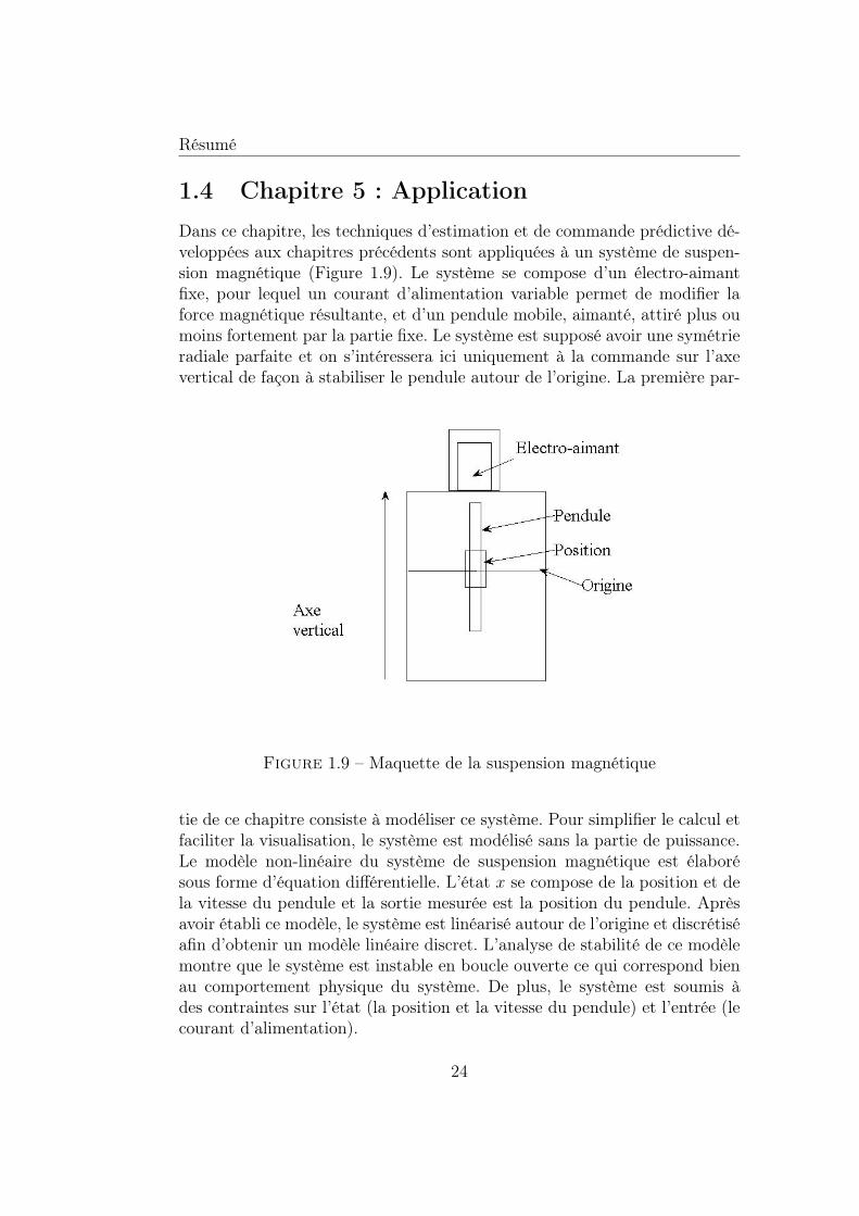
1.4 Chapitre 5 : ApplicationDans ce chapitre, les techniques d’estimation et de commande prédictive dé-veloppées aux chapitres précédents sont appliquées à un système de suspen-sion magnétique (Figure 1.9). Le système se compose d’un électro-aimantfixe, pour lequel un courant d’alimentation variable permet de modifier laforce magnétique résultante, et d’un pendule mobile, aimanté, attiré plus oumoins fortement par la partie fixe. Le système est supposé avoir une symétrieradiale parfaite et on s’intéressera ici uniquement à la commande sur l’axevertical de façon à stabiliser le pendule autour de l’origine. La première par-
Figure 1.9 – Maquette de la suspension magnétique
tie de ce chapitre consiste à modéliser ce système. Pour simplifier le calcul etfaciliter la visualisation, le système est modélisé sans la partie de puissance.Le modèle non-linéaire du système de suspension magnétique est élaborésous forme d’équation différentielle. L’état x se compose de la position et dela vitesse du pendule et la sortie mesurée est la position du pendule. Aprèsavoir établi ce modèle, le système est linéarisé autour de l’origine et discrétiséafin d’obtenir un modèle linéaire discret. L’analyse de stabilité de ce modèlemontre que le système est instable en boucle ouverte ce qui correspond bienau comportement physique du système. De plus, le système est soumis àdes contraintes sur l’état (la position et la vitesse du pendule) et l’entrée (lecourant d’alimentation).
24
Résumé
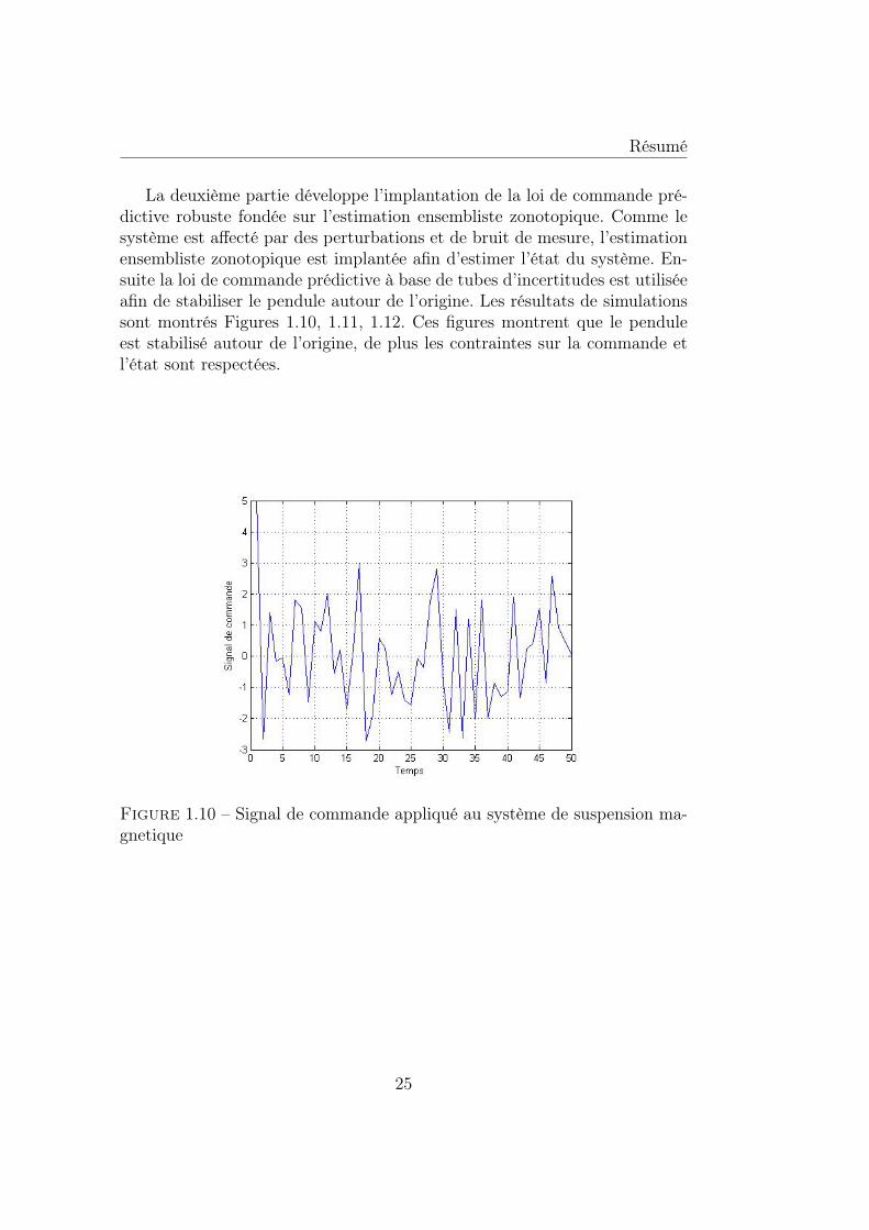
La deuxième partie développe l’implantation de la loi de commande pré-dictive robuste fondée sur l’estimation ensembliste zonotopique. Comme lesystème est affecté par des perturbations et de bruit de mesure, l’estimationensembliste zonotopique est implantée afin d’estimer l’état du système. En-suite la loi de commande prédictive à base de tubes d’incertitudes est utiliséeafin de stabiliser le pendule autour de l’origine. Les résultats de simulationssont montrés Figures 1.10, 1.11, 1.12. Ces figures montrent que le penduleest stabilisé autour de l’origine, de plus les contraintes sur la commande etl’état sont respectées.
Figure 1.10 – Signal de commande appliqué au système de suspension ma-gnetique
25
Résumé
Figure 1.11 – Position du pendule obtenue par la commande prédictive àbase de tubes d’incertitudes
Figure 1.12 – Vitesse du pendule obtenue par la commande prédictive àbase de tubes d’incertitudes
26
Résumé
1.5 ConclusionCette thèse vise deux domaines fondamentaux de l’Automatique : l’estima-tion et la commande. Dans ce but, les contributions principales de la thèsesont les suivantes. Premièrement développer une estimation ensembliste zo-notopique fondée sur la minimisation d’un nouveau critère : le P -rayon decet ensemble zonotopique. Fondé sur l’approximation de l’intersection d’unzonotope avec une bande de mesures, ce nouveau critère permet d’obtenirun bon compromis entre la précision de l’estimation et la complexité ducalcul. Cette technique d’estimation est développée non seulement pour dessystèmes mono-sortie, mais également pour des systèmes multi-sorties. Plu-sieurs contributions visent l’estimation des systèmes multi-sorties (approcheESO, approche ESOCE, approche PMI), une contribution majeure étant lerésultat de l’approximation de l’intersection d’un zonotope et d’un polytope(approche PAZI). La deuxième contribution principale de la thèse est le déve-loppement d’une loi de commande prédictive robuste (sous contraintes, avecdes perturbations et bruit de mesure inconnus, mais bornés) par retour desortie fondée sur l’estimation ensembliste zonotopique.
Ce travail peut être étendu en considérant l’estimation ensembliste zo-notopique pour des systèmes avec retard. De plus, les résultats développéspeuvent être appliqués pour résoudre le problème du diagnostic et de la com-mande tolérante aux défauts. Un problème intéressant à traiter dans le futurreste de trouver une loi de commande prédictive à base de tubes de trajectoirepour des systèmes affectés par des incertitudes par intervalles.
27

Résumé
28
Chapter 2
Introduction
2.1 Context and motivations
The work of this thesis is found at the intersection of two major problemsin automatic control: state estimation and robust constrained control fordiscrete-time uncertain systems subject to disturbances and measurementnoises. The goal of this thesis is to take into account uncertainties, distur-bances, measurement noises and constraints to build a state estimation andan output feedback control law which can guarantee the feasibility and thestability of the closed-loop system in this specific context.
In the literature, when an uncertain system is subjected to disturbances,there are two main ways to describe parameter uncertainties, disturbancesand noises acting on a dynamic system:
• Stochastic approach, which assumes that the disturbances, noises andparameter uncertainties are unknown but its probability distributionsare known.
• Deterministic approach, which assumes that disturbances, noises andparameter uncertainties are unknown but bounded by some convex sets.The main advantage of the deterministic approach is that disturbancesand noises are supposed to be bounded and this is often simpler to ver-ify than the criterion on the probability distribution. This is the mainreason why many authors [147], [126], [20] etc. have chosen the deter-ministic approach to model the disturbances and the noises affectingthe system behavior. Based on this remark, the deterministic approachhas been chosen in this thesis to model the parameter uncertainties, thedisturbances and the measurement noises.
29
Introduction
Due to the presence of measurement noises, the system state, which is nec-essary to build the control law, is not available. In this case the implemen-tation of a state estimator is necessary. This state estimation problem canbe solved by different methods such as Luenberger observer [94], functionnalobserver [109], moving-horizon estimation [57], set-membership estimation[147], [126], [20] etc. In this thesis the set-membership estimation methodis chosen because of its ability to deal with uncertainties and disturbances.The set-membership estimation has been applied to the problem of stateestimation of uncertain systems since 1960s [147], [126], [37], [2] etc. Thisapproach permits to obtain a set containing the real system state consistentwith the disturbances and measurement noises. With the development of ro-bust control theory, the set-membership estimation technique is shown to besuitable to deal with unknown but bounded uncertainties, disturbances andmeasurement noises. If constraints are added to the previous problem, thena predictive control feature should be added. This results in using robustpredictive control strategies based on set-membership estimation in order toanswer to the proposed problem. In particular, zonotopic sets will be useddue to its flexibility and low-complexity.
This thesis builds upon previous results on the zonotopic set-membershipstate estimation [37], [2] and the output feedback Tube-based Model Predic-tive Control [100]. The aim of the state estimation problem is to obtain asmall estimation set which contains the real state. The proposed method in[37] computes a zonotopic outer approximation of the set of states based ona Singular Value Decomposition of a matrix [140], which offers good perfor-mance of the estimation. In [2], the authors proposed a method to computethe zonotopic guaranteed state estimation based on two optimization prob-lems. The first solution is based on the minimization of the volume of azonotope and offers a high accuracy estimation with a complex computa-tion, while the second solution considers the minimization of the segmentsof the zonotope and proposes a simple computation but with a deteriora-tion of the estimation accuracy. For these reasons, the goal of this PhDthesis is to propose a new method permitting to improve the estimation per-formance, while keeping a low complexity level. Moreover, this zonotopicset-membership estimation is proposed to replace the Luenberger observer inthe output feedback Tube-based Model Predictive Control [100]. This asso-ciation permits us to improve the performance of the closed-loop system asit will be shown in the future sections.
30
Introduction
2.2 Outline and contributions of the thesis
In this section, the description of the main chapters (excluding this introduc-tive chapter) is given with highlights on the main contributions.
• Chapter 1: This chapter offers a synthesis in French of the mainresults presented in this thesis.
• Chapter 3: The goal of this chapter is to answer the question on howto represent the uncertainties, the disturbances and the noises in thedeterministic approach. The chapter starts with a short description ofthe deterministic approach in which the disturbances and noises areassumed to be bounded by known convex sets. After that, some ba-sic definitions and operations necessary to manipulate sets and matrixcomputations are presented. As the disturbances are bounded by a con-vex set, the next part consists in presenting a list of the most popularfamilies of sets which are used in the literature, with its advantages andweak points. Due to the advantages of zonotope, the family of zono-topic sets is further chosen to bound the disturbances and measurementnoises.
• Chapter 4: In this chapter, a zonotopic set-membership estimation isproposed to solve the problem of state estimation for interval uncertainsystems subject to unknown but bounded disturbances and measure-ment noises. This chapter proposes a new optimization criterion basedon the minimization of the P -radius of a zonotope (that will be definedlater on in this thesis) in order to obtain a zonotopic guaranteed stateestimation as a trade-off between the low computation complexity andthe performance of the state estimation. Moreover, this criterion per-mits to guarantee the non-increasing property of the guaranteed stateestimation at each time instant; to the best of the authors knowledge,this can not be found in the other approaches proposed in the liter-ature. The chapter proposes a pedagogical structure in three steps.It starts with the state estimation solution based on matrix inequali-ties optimization and zonotopic outer approximation of the intersectionbetween a zonotope and a strip for single-output linear discrete time in-variant systems subject to disturbances and measurement noises. Basedon this solution, in a second step the state estimation problem is ex-tended to the case of single-output linear discrete-time variant systems(i.e. it considers the case of systems with interval parametric uncer-tainties). To solve this new problem, the maximum principle [122] is
31
Introduction
used. The case of multi-output systems leads to two different classesof solutions:
– The first class is the direct application proposed for the single-output systems for each output of the multi-output system lead-ing to a conservative result. Several approaches belonging to thisfirst class will be developed and compared (Equivalent Single-Output approach, Equivalent Single-Output with Coupling Effectand Polynomial Matrix Inequality approach).
– The second class based on an original result on the zonotopicapproximation of the intersection between a polytope and a zono-tope permits to improve the performance of the estimation whileconsidering all the output measurements in the same time.
• Chapter 5: The problem of robust predictive control is discussed inthis chapter, in the context of zonotopic set-membership estimation.The performance of model predictive control is illustrated by many in-dustrial applications. This large application is explained by its abilityto deal with disturbances and constraints acting on the system. Basedon the zonotopic set-membership estimation built in Chapter 4, twopredictive control laws are presented. The first control law is an open-loop predictive control which has a simple implementation/structurebut does not guarantee the stability of the closed-loop system. Tooffer a stability proof, a second controller which is a feedback predic-tive control based on a tube of trajectories is proposed for the case oflinear discrete-time invariant systems with bounded disturbances andmeasurement noises, subject to constraints. Moreover, when intervalparametric uncertainties are added, the optimization problem in thefirst control law becomes non convex and the recursive feasibility inthe tube-based predictive control is lost. For these reasons, in this the-sis we have chosen to apply a modified open-loop predictive control foruncertain systems, the output feedback predictive control based on thezonotopic set-membership estimation still remaining an open problem.
• Chapter 6: This chapter proposes an application of the proposed ap-proaches to control a magnetic levitation system. The first step consistsin describing and modeling this non-linear unstable continuous-timesystem subject to bounded disturbances, measurement noises and con-straints. The proposed model is linearized around an equilibrium pointand discretized for a given sampling time. Based on this model, theopen-loop Model Predictive Control and the Tube-based Model Pre-
32
Introduction
dictive Control associated to the zonotopic set-membership estimationare used to stabilize this system around the equilibrium point.
• Chapter 7: The last chapter resumes the developed work in this PhDthesis and proposes some future directions both on theoretical devel-opments and on real applications.
The work in this thesis has resulted in several accepted/submitted pub-lications to prestigious international conferences and journals:
Published journal paper:
• V. T. H. Le, C. Stoica, D. Dumur, T. Alamo, E. F. Camacho, Com-mande prédictive robuste par des techniques d’observateurs basées surdes ensembles zonotopiques, Journal Européen des Systèmes Automa-tisés (JESA), no. 2-3/2012, pp. 235-250, DOI 10.3166/JESA.46.235-250, ISSN 1269-6935, ISBN 978-2-7462-3957-9, 2012.
Submitted journal paper:
• V. T. H. Le, C. Stoica, T. Alamo, E. F. Camacho, D. Dumur, Zono-topic guaranteed state estimation for uncertain systems, submitted toAutomatica (second review round), 2012.
Published conference papers:
• V. T. H. Le, T. Alamo, E. F. Camacho, C. Stoica, D. Dumur, A newapproach for guaranteed state estimation by zonotopes, Proceedings ofthe 18th IFAC World Congress, Milan, Italy, pp. 9242-9247, 28 August- 2 September 2011.
• V. T. H. Le, C. Stoica, D. Dumur, T. Alamo, E. F. Camacho, Robusttube-based constrained predictive control via zonotopic set-membershipestimation, Proceedings of the 50th IEEE Conference on Decision andControl and European Control Conference, Orlando, Florida, U.S.A.,pp. 4580-4585, 12-15 December 2011.
• V. T. H. Le, T. Alamo, E. F. Camacho, C. Stoica, D. Dumur, Zono-topic set-membership estimation for interval dynamic systems, Pro-ceedings of the 2012 IEEE American Control Conference, Montréal,Canada, pp. 6787-6792, 27-29 June 2012.
• V. T. H. Le, C. Stoica, D. Dumur, T. Alamo, E. F. Camacho, APolynomial Matrix Inequality approach for zonotopic set-membership
33
Introduction
estimation of multivariable systems, Proceedings of the 20th Mediter-ranean Conference on Control and Automation, Barcelona, Spain, pp.18-23, 3-6 July 2012.
Submitted conference paper:
• V. T. H. Le, C. Stoica, T. Alamo, E. F. Camacho, D. Dumur Zono-topic set-membership estimation for multi-output uncertain systems,submitted to Europeen Control Conference 2013.
Workshop (oral presentation):
• V. T. H. Le, C. Stoica, T. Alamo, E. F. Camacho, D. Dumur, Guar-anteed state estimation by zonotopes for systems with interval uncer-tainties, Small Workshop on Interval Methods (SWIM), Oldenburg,Germany, 4-6 June 2012.
34
Chapter 3
Set theory for uncertaintyrepresentation
In the control systems context, a mathematical model is frequently usedto describe the system behavior, offering the possibility to analyze and todesign control strategies for the considered system. The quality of the controldepends on the model accuracy, i.e. on how well the mathematical modeldeveloped on the theoretical side agrees with results of repeated experiments.But the mathematical model can not exactly represent the real system due toa lack of knowledge or unreliable information of the system. To validate thismodel some uncertainties can be added to the mathematical model. Moreoverperturbations influencing the real system have to be taken into account inthe mathematical model in order to ensure a similar behavior of the realsystem and the mathematical model. The importance of uncertainties insystem design can be seen in [99], [9], [10] and the references therein. In theliterature, there are two ways to represent uncertainties: the statistical (orstochastic) approach and the deterministic approach.
Stochastic approach: The uncertainty is modeled by a random processwith a known statistical property. This approach is widely used in differentscientific domains (e.g. economy [12], biology [143], engineering [99]), espe-cially when estimates of the probability distribution of the uncertain param-eters are available. But in many applications, this probability distributionof the uncertain parameters is not known; only bounds of this uncertaintycan be fixed. In this case the probabilistic assumption on the uncertaintyis not anymore validated, making this method not suitable for modeling theuncertainties.
Deterministic approach: The uncertainty is supposed belonging to aset: a classical (crisp) set (a set, wherein the degree of membership of anyobject in the set is either 0 or 1) or a fuzzy set (a set, wherein the degree of
35
Set theory for uncertainty representation
membership of any object in the set is between 0 and 1). In the literature,different families of classical sets are used depending on their accuracy andtheir complexity. Usually, the accuracy and the complexity of the uncertain-ties representation are inversely proportional, depending on the particularproblem related to the choice of a suitable geometric form. In the followingparts, some popular families of sets are presented with their advantages andtheir weaknesses. Note that in this thesis only convex (classical) sets areconsidered because of the role of convexity in the theory of optimization [19].
3.1 Basic set definitionsBefore presenting the most known families of sets, some basic set definitionsand operations are introduced. These definitions are used along this thesis.
Definition 3.1. A set S ⊂ Rn is called convex set if for any x1, x2, . . . , xk ∈
S and any α1, α2, . . . , αk ∈ R+ such thatk∑i=1
αi = 1, then the elementk∑i=1
αixi
is in S.
Definition 3.2. A convex hull of a given set S, denoted conv(S) is thesmallest convex set containing S.
Definition 3.3. A set S ⊂ Rn is called a C-set if S is compact, convex andcontains the origin. This is a proper set if its interior is not empty.
Definition 3.4. Inclusion operator : X ⊆ Y , if and only if ∀x ∈ X, thenx ∈ Y .
Definition 3.5. Intersection operator : X ∩ Y = z : z ∈ X and z ∈ Y .
Definition 3.6. The image of a set S under a map (projection) M is theset M(S) = y : y = M(x), x ∈ S.
Definition 3.7. The Minkowski sum of two sets X and Y is defined byX ⊕ Y = x+ y : x ∈ X, y ∈ Y .
Definition 3.8. The Pontryagin difference of two sets X and Y is definedby X Y = z : z + y ∈ X, ∀y ∈ Y .
Definition 3.9. Let X and Y be two non-empty sets, the distance of twosets X and Y is defined as d(X, Y ) = mind(x, y) : x ∈ X, y ∈ Y .
Definition 3.10. Let X and Y be two non-empty sets. The Hausdorffdistance of these two sets X and Y is defined by the following expressiondH(X, Y ) = maxdH(X, Y ), dH(Y,X), with dH(X, Y ) = max
x∈Xminy∈Y
d(x, y).
36
Set theory for uncertainty representation
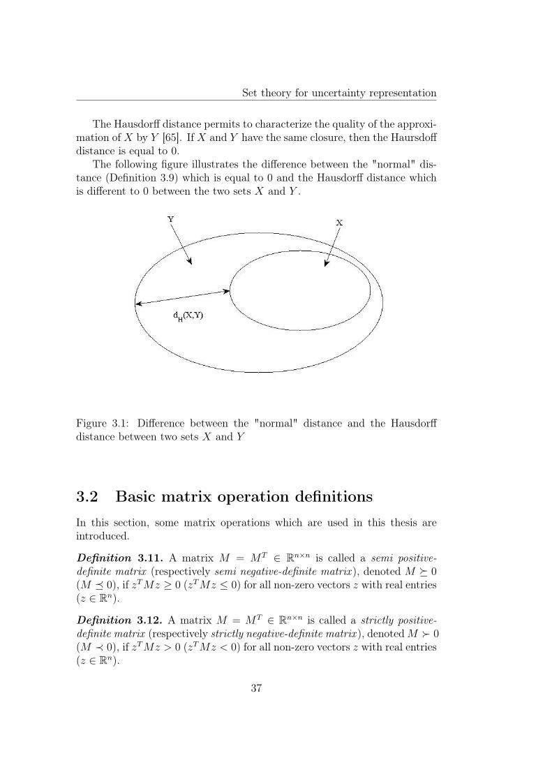
The Hausdorff distance permits to characterize the quality of the approxi-mation of X by Y [65]. If X and Y have the same closure, then the Haursdoffdistance is equal to 0.
The following figure illustrates the difference between the "normal" dis-tance (Definition 3.9) which is equal to 0 and the Hausdorff distance whichis different to 0 between the two sets X and Y .
Figure 3.1: Difference between the "normal" distance and the Hausdorffdistance between two sets X and Y
3.2 Basic matrix operation definitionsIn this section, some matrix operations which are used in this thesis areintroduced.
Definition 3.11. A matrix M = MT ∈ Rn×n is called a semi positive-definite matrix (respectively semi negative-definite matrix ), denoted M 0(M 0), if zTMz ≥ 0 (zTMz ≤ 0) for all non-zero vectors z with real entries(z ∈ Rn).
Definition 3.12. A matrix M = MT ∈ Rn×n is called a strictly positive-definite matrix (respectively strictly negative-definite matrix ), denotedM 0(M ≺ 0), if zTMz > 0 (zTMz < 0) for all non-zero vectors z with real entries(z ∈ Rn).
37
Set theory for uncertainty representation
Definition 3.13. A mathematical expression of the following form is calledLinear Matrix Inequality (LMI):
F (x) = F0 +n∑i=1
xiFi 0 (3.1)
where x =[x1 x2 . . . xn
]T ∈ Rn is the vector of decision variables andFi, i = 0, . . . , n are given symmetric matrices.
The two following problems related to LMI are considered in this thesis:
1. Feasibility problem: Does it exist a solution x ∈ Rn such that the LMIF (x) 0 is feasible?
2. Optimization problem: Minimize a linear cost function bTx subjectedto the LMI constraint F (x) 0.
Definition 3.14. (Schur complement [24], [124]) Consider the followingLMI: [
Q(x) S(x)ST (x) R(x)
] 0 (3.2)
where Q(x), R(x) are symmetric matrices and Q(x), R(x), S(x) are affineon x, then this LMI is equivalent to:
Q(x) 0Q(x)− S(x)R(x)−1ST (x) 0
(3.3)
or R(x) 0R(x)− ST (x)Q(x)−1S(x) 0
(3.4)
Definition 3.15. A Bilinear Matrix Inequality (BMI) is defined by the fol-lowing expression:
F (x) = F0 +n∑i=1
xiFi +n∑i=1
m∑j=1
xixjFij 0 (3.5)
where x =[x1 x2 . . . xn
]T ∈ Rn if n ≥ m or x =[x1 x2 . . . xm
]T ∈Rm if not, is the vector of decision variables and F0, Fi, Fij i, j = 1, . . . , nare given symmetric matrices.
38
Set theory for uncertainty representation
Definition 3.16. A Polynomial Matrix Inequality (PMI) is defined by thefollowing expression:
F (x) = xF 0 (3.6)
where x =[1 x1 ... xn x21 x1x2 ... x1xn ... xnn
]T ∈ Rn is the vectorof decision variables and F =
[F0 F1 ... Fn F11 F12 ... F1n ... Fn...n
],
with F∗ given symmetric matrices.Note that LMI and BMI are just a particular case of PMI.
3.3 Interval setA very simple way to define uncertainties is using the interval notion. Thisis based on the idea of enclosing numerical errors into an interval. In manycases obtaining the probability of occurrence of different uncertainties is notpossible. Therefore, it can be easier and thus suitable to bound the uncer-tainties by intervals. Moreover, the interval analysis permits to simplify mostof the standard operations [107], [60], [68]. This approach is developed inmany domains such as identification, diagnosis, estimation etc. especiallywhen a short computation time is required.
Definition 3.17. An interval I = [a, b] is defined as the set x : a ≤ x ≤ b.
Definition 3.18. The center and the radius of an interval I = [a, b] arerespectively defined as mid(I) = a+b
2and rad(I) = b−a
2.
Definition 3.19. An interval matrix [M ] ∈ In×m is a matrix whose elementsare intervals.
It means that each element Mij, with i = 1, ..., n, j = 1, ...,m of thismatrix is defined as the set Mij = mij : aij ≤ mij ≤ bij. In the matrixspace, the interval matrix is a hyper-rectangle and hence a convex set. Letvert([M ]) denote the set of all matrices A = [aij], with i = 1, ..., n, j =1, ...,m such that aij = aij or sij = bij. Thus vert([M ]) contains all thevertices of the interval matrix [M ]. The notations mid([M ])ij =
aij+bij2
andrad([M ])ij =
bij−aij2
define the coefficient of the center and the radius of aninterval matrix [M ], respectively.
Definition 3.20. The unitary interval is denoted B = [-1,1].
Definition 3.21. The set of real compact intervals [a, b], where a, b ∈ R anda ≤ b is denoted I.
Definition 3.22. A box ([a1, b1], ..., [an, bn])T is an interval vector.
39
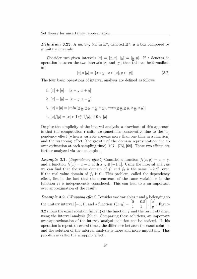
Set theory for uncertainty representation
Definition 3.23. A unitary box in Rn, denoted Bn, is a box composed byn unitary intervals.
Consider two given intervals [x] = [x, x], [y] = [y, y]. If denotes anoperation between the two intervals [x] and [y], then this can be formalizedas:
[x] [y] = x y : x ∈ [x], y ∈ [y] (3.7)
The four basic operations of interval analysis are defined as follows:
1. [x] + [y] = [x+ y, x+ y]
2. [x]− [y] = [x− y, x− y]
3. [x] ∗ [y] = [min(x.y, x.y, x.y, x.y),max(x.y, x.y, x.y, x.y)]
4. [x]/[y] = [x] ∗ [1/y, 1/y], if 0 /∈ [y]
Despite the simplicity of the interval analysis, a drawback of this approachis that the computation results are sometimes conservative due to the de-pendency effect (when a variable appears more than one time in a function)and the wrapping effect (the growth of the domain representation due toover-estimation at each sampling time) [107], [76], [68]. These two effects arefurther analyzed via two examples.
Example 3.1. (Dependency effect) Consider a function f1(x, y) = x − y,and a function f2(x) = x− x with x, y ∈ [−1, 1]. Using the interval analysiswe can find that the value domain of f1 and f2 is the same [−2, 2], evenif the real value domain of f2 is 0. This problem, called the dependencyeffect, lies in the fact that the occurrence of the same variable x in thefunction f2 is independently considered. This can lead to a an importantover approximation of the result.
Example 3.2. (Wrapping effect) Consider two variables x and y belonging to
the unitary interval [−1, 1], and a function f(x, y) =
[0 −0.51 1
].
[xy
]. Figure
3.2 shows the exact solution (in red) of the function f and the result obtainedusing the interval analysis (blue). Comparing these solutions, an importantover-approximation of the interval analysis solution can be noticed. If thisoperation is repeated several times, the difference between the exact solutionand the solution of the interval analysis is more and more important. Thisproblem is called the wrapping effect.
40
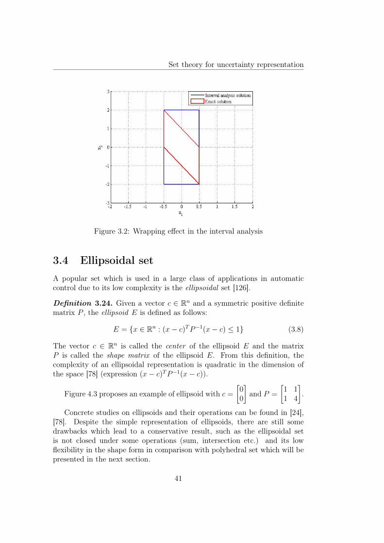
Set theory for uncertainty representation
Figure 3.2: Wrapping effect in the interval analysis
3.4 Ellipsoidal setA popular set which is used in a large class of applications in automaticcontrol due to its low complexity is the ellipsoidal set [126].
Definition 3.24. Given a vector c ∈ Rn and a symmetric positive definitematrix P , the ellipsoid E is defined as follows:
E = x ∈ Rn : (x− c)TP−1(x− c) ≤ 1 (3.8)
The vector c ∈ Rn is called the center of the ellipsoid E and the matrixP is called the shape matrix of the ellipsoid E. From this definition, thecomplexity of an ellipsoidal representation is quadratic in the dimension ofthe space [78] (expression (x− c)TP−1(x− c)).
Figure 4.3 proposes an example of ellipsoid with c =
[00
]and P =
[1 11 4
].
Concrete studies on ellipsoids and their operations can be found in [24],[78]. Despite the simple representation of ellipsoids, there are still somedrawbacks which lead to a conservative result, such as the ellipsoidal setis not closed under some operations (sum, intersection etc.) and its lowflexibility in the shape form in comparison with polyhedral set which will bepresented in the next section.
41
Set theory for uncertainty representation
Figure 3.3: Ellipsoid
3.5 Polyhedral setThe polyhedral set is one of the most popular geometrical form used inmany fields such as control and optimization. A polyhedral set in a finite-dimensional Euclidean space is the intersection of finitely many closed half-spaces [151]. A bounded polyhedral is denoted as a polytope. Due to itsflexibility, polytopes offer a good approximation of any convex set [81], [26],[127]. Another advantage of polytopes in comparison with ellipsoids is that itis closed under the mentioned operations. Moreover, its dual representation(half-space representation and vertex representation) permits to choose thesuitable form for a particular problem. The main disadvantage of polytopesis related to its complexity depending on the number of vertices, which is notfixed by the space dimension. Therefore, even if a polytope can well approx-imate any convex set, the complexity can quickly increase with the numberof vertices even in a low space dimension. Despite this weak point, polytopesare one of the most popular convex sets used in automatic control. In orderto formalize the notations, the main definitions of polytopes are summarizedbelow.
Definition 3.25. (Half-space representation) A polyhedral P ∈ Rn can bedefined as the intersection of a finite number of half-spaces:
P = x ∈ Rn : H · x ≤ K (3.9)
42
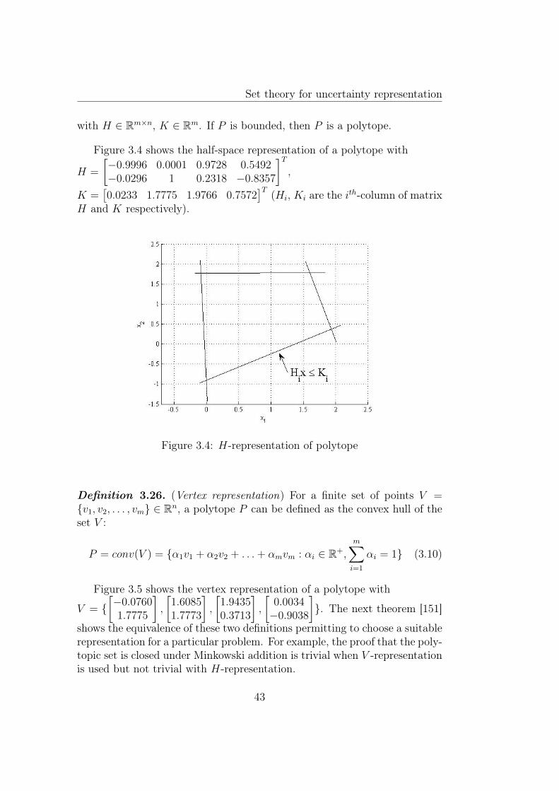
Set theory for uncertainty representation
with H ∈ Rm×n, K ∈ Rm. If P is bounded, then P is a polytope.
Figure 3.4 shows the half-space representation of a polytope with
H =
[−0.9996 0.0001 0.9728 0.5492−0.0296 1 0.2318 −0.8357
]T,
K =[0.0233 1.7775 1.9766 0.7572
]T (Hi, Ki are the ith-column of matrixH and K respectively).
Figure 3.4: H-representation of polytope
Definition 3.26. (Vertex representation) For a finite set of points V =v1, v2, . . . , vm ∈ Rn, a polytope P can be defined as the convex hull of theset V :
P = conv(V ) = α1v1 + α2v2 + . . .+ αmvm : αi ∈ R+,m∑i=1
αi = 1 (3.10)
Figure 3.5 shows the vertex representation of a polytope with
V = [−0.07601.7775
],
[1.60851.7773
],
[1.94350.3713
],
[0.0034−0.9038
]. The next theorem [151]
shows the equivalence of these two definitions permitting to choose a suitablerepresentation for a particular problem. For example, the proof that the poly-topic set is closed under Minkowski addition is trivial when V -representationis used but not trivial with H-representation.
43
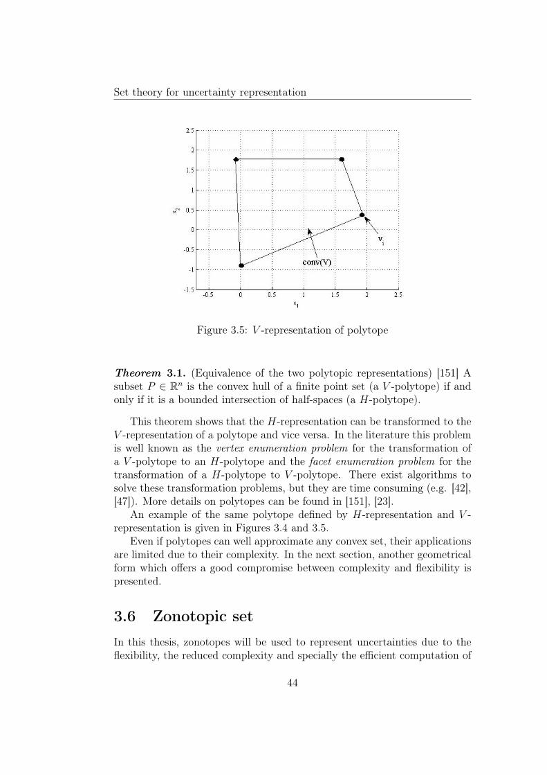
Set theory for uncertainty representation
Figure 3.5: V -representation of polytope
Theorem 3.1. (Equivalence of the two polytopic representations) [151] Asubset P ∈ Rn is the convex hull of a finite point set (a V -polytope) if andonly if it is a bounded intersection of half-spaces (a H-polytope).
This theorem shows that the H-representation can be transformed to theV -representation of a polytope and vice versa. In the literature this problemis well known as the vertex enumeration problem for the transformation ofa V -polytope to an H-polytope and the facet enumeration problem for thetransformation of a H-polytope to V -polytope. There exist algorithms tosolve these transformation problems, but they are time consuming (e.g. [42],[47]). More details on polytopes can be found in [151], [23].
An example of the same polytope defined by H-representation and V -representation is given in Figures 3.4 and 3.5.
Even if polytopes can well approximate any convex set, their applicationsare limited due to their complexity. In the next section, another geometricalform which offers a good compromise between complexity and flexibility ispresented.
3.6 Zonotopic setIn this thesis, zonotopes will be used to represent uncertainties due to theflexibility, the reduced complexity and specially the efficient computation of
44
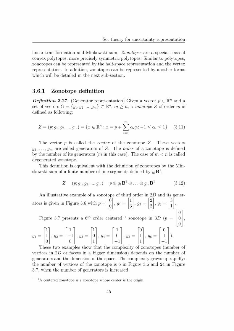
Set theory for uncertainty representation
linear transformation and Minkowski sum. Zonotopes are a special class ofconvex polytopes, more precisely symmetric polytopes. Similar to polytopes,zonotopes can be represented by the half-space representation and the vertexrepresentation. In addition, zonotopes can be represented by another formswhich will be detailed in the next sub-section.
3.6.1 Zonotope definition
Definition 3.27. (Generator representation) Given a vector p ∈ Rn and aset of vectors G = g1, g2, ..., gm ⊂ Rn, m ≥ n, a zonotope Z of order m isdefined as following:
Z = (p; g1, g2, ..., gm) = x ∈ Rn : x = p+m∑i=1
αigi;−1 ≤ αi ≤ 1 (3.11)
The vector p is called the center of the zonotope Z. These vectorsg1, . . ., gm are called generators of Z. The order of a zonotope is definedby the number of its generators (m in this case). The case of m < n is calleddegenerated zonotope.
This definition is equivalent with the definition of zonotopes by the Min-skowski sum of a finite number of line segments defined by giB1.
Z = (p; g1, g2, ..., gm) = p⊕ g1B1 ⊕ . . .⊕ gmB1 (3.12)
An illustrative example of a zonotope of third order in 2D and its gener-
ators is given in Figure 3.6 with p =
[00
], g1 =
[13
], g2 =
[22
], g3 =
[31
].
Figure 3.7 presents a 6th order centered 1 zonotope in 3D (p =
000
,g1 =
110
, g2 =
1−10
, g3 =
101
, g4 =
10−1
, g5 =
011
, g6 =
01−1
).These two examples show that the complexity of zonotopes (number of
vertices in 2D or facets in a bigger dimension) depends on the number ofgenerators and the dimension of the space. The complexity grows up rapidly:the number of vertices of the zonotope is 6 in Figure 3.6 and 24 in Figure3.7, when the number of generators is increased.
1A centered zonotope is a zonotope whose center is the origin.
45
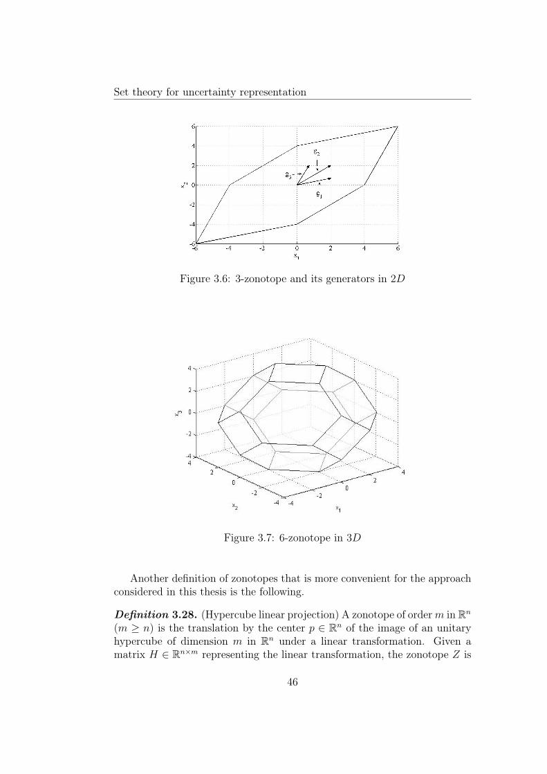
Set theory for uncertainty representation
Figure 3.6: 3-zonotope and its generators in 2D
Figure 3.7: 6-zonotope in 3D
Another definition of zonotopes that is more convenient for the approachconsidered in this thesis is the following.
Definition 3.28. (Hypercube linear projection) A zonotope of orderm in Rn
(m ≥ n) is the translation by the center p ∈ Rn of the image of an unitaryhypercube of dimension m in Rn under a linear transformation. Given amatrix H ∈ Rn×m representing the linear transformation, the zonotope Z is
46
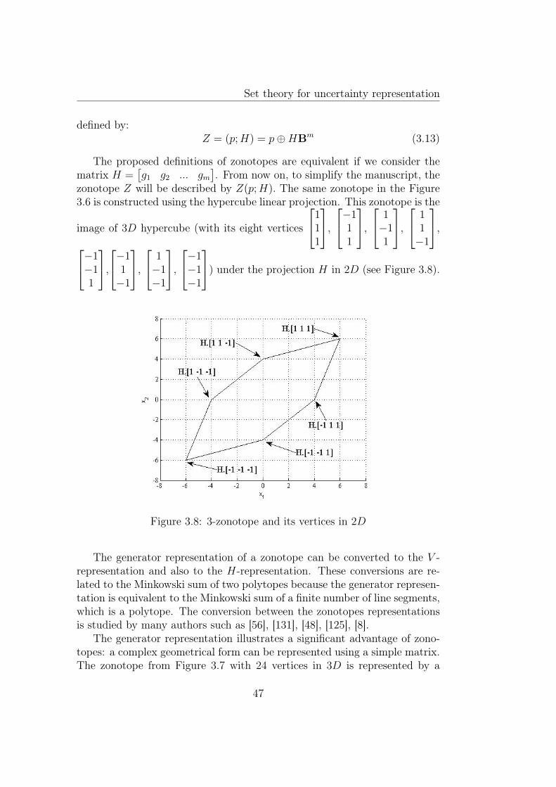
Set theory for uncertainty representation
defined by:Z = (p;H) = p⊕HBm (3.13)
The proposed definitions of zonotopes are equivalent if we consider thematrix H =
[g1 g2 ... gm
]. From now on, to simplify the manuscript, the
zonotope Z will be described by Z(p;H). The same zonotope in the Figure3.6 is constructed using the hypercube linear projection. This zonotope is the
image of 3D hypercube (with its eight vertices
111
,−1
11
, 1−11
, 1
1−1
,−1−11
,−1
1−1
, 1−1−1
,−1−1−1
) under the projection H in 2D (see Figure 3.8).
Figure 3.8: 3-zonotope and its vertices in 2D
The generator representation of a zonotope can be converted to the V -representation and also to the H-representation. These conversions are re-lated to the Minkowski sum of two polytopes because the generator represen-tation is equivalent to the Minkowski sum of a finite number of line segments,which is a polytope. The conversion between the zonotopes representationsis studied by many authors such as [56], [131], [48], [125], [8].
The generator representation illustrates a significant advantage of zono-topes: a complex geometrical form can be represented using a simple matrix.The zonotope from Figure 3.7 with 24 vertices in 3D is represented by a
47
Set theory for uncertainty representation
3 × 6 matrix H. This leads to simplify the mentioned basic set operationsby simple matrix computation as presented in the next part.
3.6.2 Properties of zonotopes
This part focuses on the main properties of zonotopes that will be used alongthis thesis.
Property 3.1. (Particular forms) Given a zonotope Z = HBm ∈ Rn. Dueto the properties of the matrix H, some particular forms of zonotope can beobtained. If H is the identity matrix, then Z is the unit box. If H is diagonal,orthogonal or invertible, then Z is a box, a hypercube or a parallelotope 2,respectively.
Property 3.2. (Generators permutation) The permutation of the matrixcolumns in the generators representation of a zonotope does not modify thezonotope.
Proof This property results from the commutativity of Minkowski sum.
Property 3.3. (Sum of two zonotopes) Given two centered zonotopes Z1 =H1Bm1 ∈ Rn and Z2 = H2Bm2 ∈ Rn, the Minkowski sum of two zonotopesis also a zonotope defined by Z = Z1 ⊕ Z2 =
[H1 H2
]Bm1+m2 .
Proof From the definition of the Minkowski sum, it results in: Z1⊕Z2 =H1z1+H2z2 : z1 ∈ Bm1 , z2 ∈ Bm2, that can be further rewritten in a matrix
formulation as Z1 ⊕ Z2 = [H1 H2
]·[z1z2
]:
[z1z2
]∈ Bm1+m2 = Z.
Property 3.4. (Linear image of a zonotope) The image of a centered zono-tope Z1 = H1Bm1 ∈ Rn by a linear mapping K can be computed by a stan-dard matrix product K · Z1 = (K ·H1)Bm1 .
Proof By using matrix multiplication the proof is similar to Property1.3.
Property 3.5. (Zonotope inclusion or Multiplication of a zonotope by aninterval matrix ) Consider a family of zonotopes represented by Z = p ⊕[M ]Bm where p ∈ Rn is a real vector and [M ] ∈ In×m is an interval matrix.
2A parallelotope is a special zonotope whose number of generators is equal to thedimension of the space.
48
Set theory for uncertainty representation
A zonotope inclusion ♦(Z) is an outer approximation of this family definedby:
♦(Z) = p⊕[mid([M ]) rs(rad([M ]))
]Bm+n (3.14)
with rs(rad(M)) a diagonal matrix and rs(rad(M))ii =∑m
j=1 |rad(M)ij|,i = 1, ..., n.
Proof [2] If z ∈ Z, then it is clear that there exists b ∈ Bm such thatz ∈ p⊕ [M ]b. Adding and subtracting mid([M ])b leads to:
z ∈ (p+mid([M ]b))⊕ ([M ]−mid([M ]))b
Note that the elements of [M ]−mid([M ]) satisfy:
Mij −mid([M ])ij = rad([M ])ijB1
and thus this leads to:
([M ]−mid([M ])b) ⊆ rs(rad([M ]))Bn.
Therefore the following expression holds:
z ∈ (p+mid([M ])b)⊕ rs(rad([M ]))Bn ⊆⊆ p⊕mid([M ])Bm ⊕ rs(rad([M ]))Bn = ♦(Z).
3.6.3 Complexity reduction of zonotopes
This subsection discusses some techniques to reduce the complexity of azonotope. These techniques permit to limit the number of generators of azonotope, which is an important problem in the computation of zonotopes.For example, if the problem of reachable set 3 is addressed using zonotopes,the complexity of this zonotope increases at each sample time due to theMinkowski sum operation. The complexity reduction problem leads to ap-proximate a high order zonotope by a lower order one. In this part, the overapproximated way is presented leading to compute a reduced order zonotopeenclosing the initial zonotope.
3This is the problem of computing all states visited by trajectories of a system startingfrom any x0 ∈ X0.
49
Set theory for uncertainty representation
3.6.3.1 Interval hull method
Proposition 3.1. Considering a zonotope Z = p⊕HBm ∈ Rn, the smallestbox containing this zonotope is computed by:
box(Z) = p⊕ rs(H)Bn (3.15)
with rs(H) a diagonal matrix such that rs(H)ii =∑m
j=1 |Hij|, i = 1, ..., n.
Proof As a box is an axis aligned set, the over approximation of a zono-tope by a box can be done by considering its extreme points in each direction.The extreme point in direction i can be easily computed by pi +
∑mj=1 |Hij|.
All extreme points in all n directions are similarly computed and the smallestbox containing the zonotope Z is obtained as box(Z) = p⊕ rs(H)Bn.
This proposition provides a simple and fast over-approximation of a zono-tope by a box. The result has a minimal complexity which is given by thedimension of the space. However, the result obtained with this propositionis conservative because the form of the zonotope is lost.
An example is proposed in the following in order to better illustrate thisproposition.
Example 3.3. Given a centered zonotope Z = HB3 ∈ R2, H =
[1 2 33 2 1
],
applying the interval hull approximation leads to a box (in blue) containingthe original zonotope (in red) (see Figure 3.9).
3.6.3.2 Parallelotope hull method
Proposition 3.2. Given a zonotope Z = p ⊕ HBm ∈ Rn (m > n), anover-approximation of this zonotope by a parallelotope is computed as:
Par(Z) = Γ · box(Γ−1H) (3.16)
where Γ ∈ Rn×n is an invertible matrix containing n columns taken from H.
Proof [8] This approach first transforms the coordinates of Z by the linearmapping Γ−1 where the new coordinate axes are the column vectors of Γ. Inthese new coordinates, the zonotope is over approximated by a box usingthe interval hull. This box is transformed back to the original coordinatesystem, resulting in a parallelotope. The over-approximation is guaranteedby the fact that the parallelotope is over-approximated in the transformedcoordinate system by the interval hull operator, such that it is also over-approximated after the transformation to the original coordinate system.
50
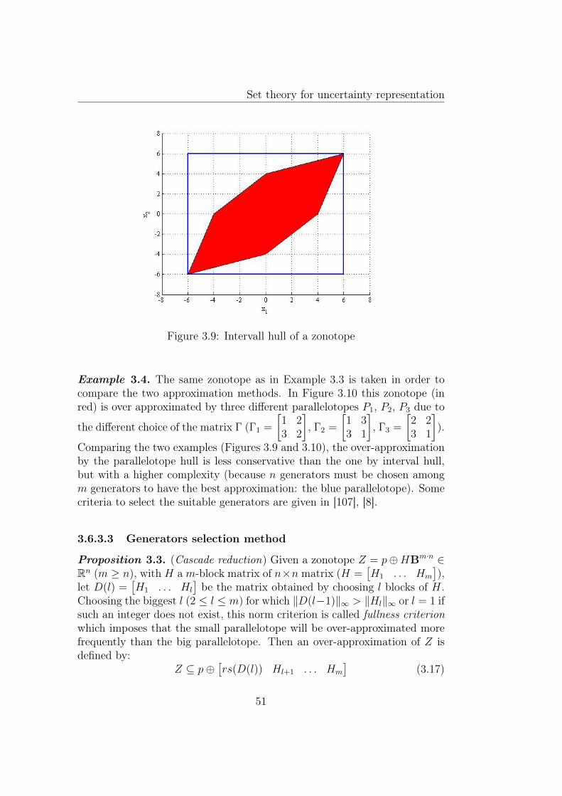
Set theory for uncertainty representation
Figure 3.9: Intervall hull of a zonotope
Example 3.4. The same zonotope as in Example 3.3 is taken in order tocompare the two approximation methods. In Figure 3.10 this zonotope (inred) is over approximated by three different parallelotopes P1, P2, P3 due to
the different choice of the matrix Γ (Γ1 =
[1 23 2
], Γ2 =
[1 33 1
], Γ3 =
[2 23 1
]).
Comparing the two examples (Figures 3.9 and 3.10), the over-approximationby the parallelotope hull is less conservative than the one by interval hull,but with a higher complexity (because n generators must be chosen amongm generators to have the best approximation: the blue parallelotope). Somecriteria to select the suitable generators are given in [107], [8].
3.6.3.3 Generators selection method
Proposition 3.3. (Cascade reduction) Given a zonotope Z = p⊕HBm·n ∈Rn (m ≥ n), with H a m-block matrix of n×n matrix (H =
[H1 . . . Hm
]),
let D(l) =[H1 . . . Hl
]be the matrix obtained by choosing l blocks of H.
Choosing the biggest l (2 ≤ l ≤ m) for which ‖D(l−1)‖∞ > ‖Hl‖∞ or l = 1 ifsuch an integer does not exist, this norm criterion is called fullness criterionwhich imposes that the small parallelotope will be over-approximated morefrequently than the big parallelotope. Then an over-approximation of Z isdefined by:
Z ⊆ p⊕[rs(D(l)) Hl+1 . . . Hm
](3.17)
51
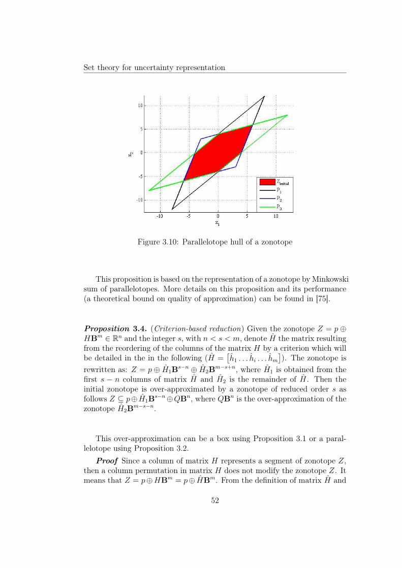
Set theory for uncertainty representation
Figure 3.10: Parallelotope hull of a zonotope
This proposition is based on the representation of a zonotope by Minkowskisum of parallelotopes. More details on this proposition and its performance(a theoretical bound on quality of approximation) can be found in [75].
Proposition 3.4. (Criterion-based reduction) Given the zonotope Z = p⊕HBm ∈ Rn and the integer s, with n < s < m, denote H the matrix resultingfrom the reordering of the columns of the matrix H by a criterion which willbe detailed in the in the following (H =
[h1 . . . hi . . . hm
]). The zonotope is
rewritten as: Z = p⊕ H1Bs−n ⊕ H2Bm−s+n, where H1 is obtained from thefirst s − n columns of matrix H and H2 is the remainder of H. Then theinitial zonotope is over-approximated by a zonotope of reduced order s asfollows Z ⊆ p⊕ H1Bs−n⊕QBn, where QBn is the over-approximation of thezonotope H2Bm−s−n.
This over-approximation can be a box using Proposition 3.1 or a paral-lelotope using Proposition 3.2.
Proof Since a column of matrix H represents a segment of zonotope Z,then a column permutation in matrix H does not modify the zonotope Z. Itmeans that Z = p⊕HBm = p⊕ HBm. From the definition of matrix H and
52
Set theory for uncertainty representation
applying Property 3.3, it results in:
Z = p⊕[H1 H2
]Bm =
= p⊕ H1Bs−n ⊕ H2Bm−s+n =
= p⊕ H1Bs−n ⊕[hs−n+1 . . . hm
]Bm−s+n
(3.18)
Propositions 3.1 and 3.2 show that the zonotope[hs−n+1 . . . hm
]Bm−s+n
can be approximated by QBn, where Q is a diagonal matrix (if an approxi-mation using box is used) or a full matrix (if an approximation using paral-lelotope is used). Therefore the following expression is true:
Z ⊆ p⊕ H1Bs−n ⊕QBn = p⊕[H1 Q
]Bs
The quality of the approximation depends on:
1. the value of s which limits the complexity;
2. the criterion used to split the zonotope Z;
3. the approximation method (box or parallelotope) used for the zonotopeH2Bm−s−n.
A big value of s means a high precision of the approximation but thecomplexity remains high.
Two methods can be found in the literature to split the zonotope Z.
• The first approach consists in sorting the generators of the zonotopein decreasing order of the Euclidean norm [37], [2], which is equivalentto dispose the segments of zonotope from the longest to the shortestsegment. Then the longest segments which have a more importantrole in the shape of the zonotope are kept and the contribution of theshortest segments is over-approximated by a box or a parallelotope inorder to limit the complexity.
• Another criterion on sorting the generators is presented in [53] andconsists in reordering the columns of matrix H in decreasing order ofthe term ‖hi‖1 − ‖hi‖∞. The chosen generators (whose contribution isapproximated) are close to vectors with only one non-zero componentand are therefore well approximated by an interval hull.
An example is proposed in order to better illustrate the quality of differentproposed methods of complexity reduction.
53
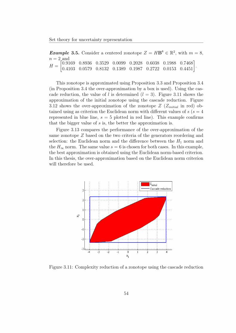
Set theory for uncertainty representation
Example 3.5. Consider a centered zonotope Z = HB8 ∈ R2, with m = 8,n = 2 andH =
[0.9169 0.8936 0.3529 0.0099 0.2028 0.6038 0.1988 0.74680.4103 0.0579 0.8132 0.1389 0.1987 0.2722 0.0153 0.4451
].
This zonotope is approximated using Proposition 3.3 and Proposition 3.4(in Proposition 3.4 the over-approximation by a box is used). Using the cas-cade reduction, the value of l is determined (l = 3). Figure 3.11 shows theapproximation of the initial zonotope using the cascade reduction. Figure3.12 shows the over-approximation of the zonotope Z (Zinitial in red) ob-tained using as criterion the Euclidean norm with different values of s (s = 4represented in blue line, s = 5 plotted in red line). This example confirmsthat the bigger value of s is, the better the approximation is.
Figure 3.13 compares the performance of the over-approximation of thesame zonotope Z based on the two criteria of the generators reordering andselection: the Euclidean norm and the difference between the H1 norm andtheH∞ norm. The same value s = 6 is chosen for both cases. In this example,the best approximation is obtained using the Euclidean norm-based criterion.In this thesis, the over-approximation based on the Euclidean norm criterionwill therefore be used.
Figure 3.11: Complexity reduction of a zonotope using the cascade reduction
54
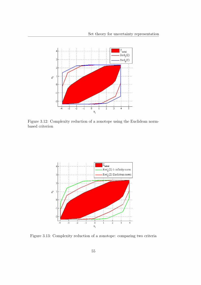
Set theory for uncertainty representation
Figure 3.12: Complexity reduction of a zonotope using the Euclidean norm-based criterion
Figure 3.13: Complexity reduction of a zonotope: comparing two criteria
55
Set theory for uncertainty representation
3.7 ConclusionThe above chapter gave a general presentation of some popular convex setsand their properties. The interval set and the interval analysis are strongtools allowing to deal with uncertainties but their application is limited dueto the flexibility, the dependency effect and the wrapping effect. Even ifthe ellipsoidal set is used by many authors due to its simplicity, its lowflexibility leads to a conservative computation result. The polytopic set canapproximate whatever convex set with a high precision but polytope can notbe used in fast processes due to its high complexity. The zonotopic set, aspecial class of polytope, offers a good compromise between complexity andflexibility (zonotope is a polytope, thus it is more flexible than an ellipsoid,and due to the symmetry property it is less complex than a polytope). Dueto its interesting properties presented in this section, zonotopes will be usedto represent the uncertainties in the context of set-membership estimation inthe next chapters.
56
Chapter 4
Set-membership estimation viazonotope
4.1 Introduction
The choice of the appropriate mathematical model, which best describes thebehavior of a given plant, has received increased attention in the control sys-tem literature. Mathematical models consist of several functions describingthe relations between the system inputs, outputs and the (internal) statesof the system at a given time instant. For example the states of the math-ematical model of a motor can be the current, the velocity or the positionof the motor. In different automatic control applications such as controlsystems, fault detection, knowledge about the system state is necessary tostudy the system behavior and to determine the control action. In practicalapplications, the measurement of the system states is not always available(due to the cost of the sensor or the harsh environnement) or can be affectedby measurement noises (sometimes introducing a significant error relative tothe real values of the states). For this reason, if the system is observable, astate estimator is set up to augment or replace measurement devices in thecontrol system. This estimator uses the knowledge of the system (mathemat-ical model, input and output signals) to produce the estimated states. Thestate estimator permits us to remove the sensor and thus, to reduce the costand improve the reliability of the system with good quality estimator. Sincethe ’60s, this problem has been studied by many authors, leading to dif-ferent estimation techniques such as Kalman filter [69], Luenberger observer[94], set-membership estimation [147], [126], functionnal observer [109], [106],moving-horizon estimation [57], [104], [67], [1]. Several popular approachesdiscussed in the literature are listed below according to the choice of the
57
Set-membership estimation via zonotope
system model:
• Luenberger observer: In the context of linear systems without un-certainty, a Luenberger observer can be easily implemented [94], [95]due to its simplicity and efficiency.
Consider a discrete-time-invariant linear system in the state-space rep-resentation: 1
xk+1 = Axk +Bukyk = Cxk +Duk
(4.1)
where xk ∈ Rnx is the system state, uk ∈ Rnu is the system input,yk ∈ Rny is the output measurement. The matrices A, B, C, Dhave appropriate dimensions A ∈ Rnx×nx , B ∈ Rnx×nu , C ∈ Rny×nx ,D ∈ Rny×nx . The system states can be estimated using the followingobserver model:
xk+1 = Axk +Buk + L(yk − yk)yk = Cxk +Duk
(4.2)
where xk, yk represent the state and output estimation at time k.
The estimation error ek is then computed by:
ek+1 = xk+1 − xk+1
= (A− LC)ek(4.3)
From the estimation error equation, it is proved that the estimationerror tends to 0 if the gains matrix L is chosen such that the matrixA− LC is Schur stable (all its eigenvalues are inside the unit circle).
• Kalman filter: If uncertainties are taken into account in the math-ematical model in the form of stochastic process, the Kalman filteris presented as an effective solution [69]. A complete introduction ofthe Kalman filter can be found in [99]. Consider a linear discrete-timeinvariant system:
xk = Axk−1 +Buk−1 + ωk−1yk = Cxk + vk
(4.4)
where ωk and vk represent the process and the measurement noises,respectively. These disturbances and noises are assumed to be inde-pendent, zero mean, with normal distribution and covariance Q, R
1The discrete-model is chosen due to its facility when systems are controlled via com-puter.
58
Set-membership estimation via zonotope
(ωk ∼ N(0, Q), vk ∼ N(0, R)). The Kalman filter is simply an optimalstochastic recursive estimator. At each time instant, it offers the valueof the estimated state xk and the error covariance matrix Pk which isa measure of the estimated accuracy of the estimated state. This is di-vided into two steps: prediction and update. The prediction step usesthe estimated state at the previous time instant xk−1 and the knowl-edge of the system (the matrices A, B and the input at the previousmoment uk−1) to produce a priori state estimation. In the update step,this a priori state estimation is combined with the information fromthe measurement to obtain a posteriori estimated state. This can besummarized in the following algorithm.
Algorithm 4.1.
1. Prediction step:
– Compute the a priori state estimation xk = Axk−1 +Buk−1.– Compute the a priori estimation error covariance:Pk = APk−1A
T +Q.
2. Update step:
– Compute the optimal Kalman gain:Kk = PkC
T (CPkCT +R)−1.
This gain is determined by minimizing the mean square of theestimation error. The detail of computation can be seen in[99].
– Update the state estimate xk = xk +Kk(yk − Cxk).– Update the estimate error covariance Pk = (I −KkC)Pk.
For the interested reader, a toolbox dedicated to this problem is de-veloped. footnotemark . In the parametric uncertainty context, it iswell known that the performance of the proposed Kalman filter can bedegraded [27]. To ensure the convergence behavior in the presence ofmodeling error, the robust Kalman filter is proposed, which guaranteesa bound of the performance of the Kalman filter [148], [134], [110],[46].
• Set-membership estimation: When a system is modeled by the de-terministic approach (uncertainties are bounded by some convex sets),
1http://www.cs.ubc.ca/ murphyk/Software/Kalman/kalman.html.
59
Set-membership estimation via zonotope
the set-membership estimation is a suitable solution for the state es-timation problem. This technique has been developed in the last 35years [147], [126], [20]. The estimator computes at each sample timea set containing all the possible system states that are consistent withthe perturbations, the uncertainties and the measurement noise. Basedon the prediction and correction step, the procedure of this technique issimilar to the Kalman filter. While the Kalman filter deals with the av-erage case, the set-membership estimation considers the worst case. Forthis reason, this approach is also called the worst-case estimation. Theproblem of set-membership estimation is that the complexity of this setis increased in time. To overcome this problem, the geometry of thesesets has to be fixed a priori: e.g. polytopes (boxes, parallelotopes)[145], [144], [32], [17], [50], [68], [71], [116], [118], [103]; ellipsoids [126],[147], [20], [77], [51], [45], [113], [14], [13], [15]; zonotopes [115], [37],[2], [3], [82]. Polytopes which were presented in the previous chapteroffer a good quality of approximation. In the linear context, polytopescan be used for an exact representation of the variation domains ofthe system state. However efficient results may be obtained only fora reasonable number of vertices of the polytopes [145]. Due to thelow complexity, ellipsoids have been used by many authors but theirlimited flexibility can lead to a conservative result of estimation. Aspresented in the previous chapter, zonotopes which are used in manyautomatic control applications such as reachability analysis [7], colli-sion detection [59], identification [25], state estimation [115], [37], [2],[3], fault detection [58], [66], [137] and fault diagnosis [40] offer a goodcompromise between the complexity and the flexibility. Moreover, theauthor of [75] shows that, by using zonotopes, the wrapping effect isreduced leading to a more precise result of the estimation. As the de-terministic approach is chosen to describe the modeling of the system,the set-membership estimation is considered as a suitable solution. Inthe next section, zonotopes are chosen to represent the set of all thepossible system states in the context of set-membership estimation dueto their advantages in comparison with other geometrical forms.
4.2 Problem formulation
To simplify the manuscript, the following linear discrete-time autonomoussystem is considered (this system can be easily generalized to controlled sys-
60
Set-membership estimation via zonotope
tem): xk+1 = Axk + ωkyk = Cxk + vk
(4.5)
where xk ∈ Rnx is the state of the system, yk ∈ Rny is the measured outputat sample time k, the matrices A and C have appropriate dimensions A ∈Rnx×nx , C ∈ Rny×nx and this couple (C,A) is detectable. The vector ωk ∈ Rnx
represents the state perturbation vector and vk ∈ Rny is the measurementperturbation (noise, offset, etc.). It is assumed that the uncertainties andthe initial state are bounded by zonotopes: ωk ∈ W, vk ∈ V and the initialstate belongs to a zonotope x0 ∈ X0 which can be large due to the lack ofknowledge on the system. The two zonotopes W and V are supposed tobe centered at the origin; if this assumption is not satisfied an appropriatechange of coordinates can be used to bring the center of the zonotopes to theorigin.
Consider the mathematical model (4.5) and these assumptions, the set-membership estimation technique leads to compute at each sample time ka domain of all the possible values of the unknown state xk. Similar to theKalman filter, the set-membership estimation algorithm is based on 3 steps:prediction, measurement and correction 2. The guaranteed state estimationis obtained in the correction step which is the combination of the state in-formation from the prediction and the information from the measurement.Before detailing this algorithm, some useful notations will be defined.
Definition 4.1. Given the system (4.5) and a measured output yk, themeasurement consistent state set at time instant k (the state set which isconsistent with the measured output yk) is defined as Xyk = x ∈ Rn :(yk − Cx) ∈ V .
Definition 4.2. Consider the system (4.5). The exact uncertain state setXk = (AXk−1 ⊕ W ) ∩ Xyk , k ≥ 1 is equal to the set of states that areconsistent with the measured output and the initial state set X0.
Thus, the exact uncertain state set Xk contains all the possible values ofthe system state consistent with the measurement. In practice, the compu-tation of the exact uncertain state set is difficult. Even if Xk−1 is assumedto have a particular geometrical form (for example: zonotope, ellipsoid etc.),it is not sure that at time instant k the exact uncertain state set Xk has thesame form. For this reason, in practice this set is approximated by an outerbound (the zonotopic set will be used along this PhD thesis). The followinghypotheses are considered at the time instant k:
2In the Kalman filter, the measurement step is included in the correction step, in theset-membership algorithm it is clear-cut for a better understanding.
61
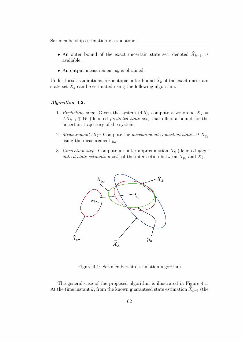
Set-membership estimation via zonotope
• An outer bound of the exact uncertain state set, denoted Xk−1, isavailable.
• An output measurement yk is obtained.
Under these assumptions, a zonotopic outer bound Xk of the exact uncertainstate set Xk can be estimated using the following algorithm.
Algorithm 4.2.
1. Prediction step: Given the system (4.5), compute a zonotope Xk =AXk−1 ⊕W (denoted predicted state set) that offers a bound for theuncertain trajectory of the system.
2. Measurement step: Compute the measurement consistent state set Xyk
using the measurement yk.
3. Correction step: Compute an outer approximation Xk (denoted guar-anteed state estimation set) of the intersection between Xyk and Xk.
Figure 4.1: Set-membership estimation algorithm
The general case of the proposed algorithm is illustrated in Figure 4.1.At the time instant k, from the known guaranteed state estimation Xk−1 (the
62
Set-membership estimation via zonotope
red set), the predicted state set Xk (the blue set) is determined. This setis intersected with the measurement consistent state set Xyk (the green set)which is induced by the output measurement yk. Thus, at time instant k theguaranteed state estimation Xk (the red set) is the outer approximation ofthis intersection.
To obtain a zonotope bounding the uncertain trajectory of the system instep 1 of Algorithm 4.2, Properties 1.1 and 1.2 are used. The predicted stateset computation using zonotopes relies on a simple matrix computation andis not subject to any approximation. However, this computation increasesthe order of the zonotope at each step. In order to control the domaincomplexity, a reduction step is implemented to bound a high-order zonotopeby a lower-order zonotope using the complexity reduction method presentedin Chapter 3.
In the literature, there are several authors interested in this estimationproblem [37], [38], [39], [2], [3]. In the linear context, the step 1 of the Algo-rithm 4.2 is similar in these methods. Based on different methods to realizethe correction step (the intersection between the predicted state set and themeasurement consistent state set), two different approaches presented in theliterature will be further detailed: the Singular Value Decomposition-basedmethod [37], the optimization-based method [2].
4.2.1 Singular Value Decomposition-based method
This method was firstly proposed in [37]. The zonotope bounding the dis-turbance is supposed to be a centered zonotope represented by W = FBnx .In this presented method, the measurement noise is supposed to belong toa centered parallelotope V , which can be described by V = ΣBny , withΣ ∈ Rny×ny an invertible matrix. With these notations, at each sample timek there exists a vector bk ∈ Bny such that the measurement noise at timeinstant k is computed by vk = Σbk.
Let us suppose that at the time instant k the zonotopic guaranteed stateestimation at k − 1 is available: Xk−1 = pk−1 ⊕ Hk−1Br, r ∈ R+. Us-ing the mathematical model, the predicted state set Xk in the first step ofAlgorithm 4.2, which contains the real state xk, can be computed by:
63
Set-membership estimation via zonotope
Xk = AXk−1 ⊕W= A(pk−1 ⊕ Hk−1Br)⊕ FBnx
= Apk−1 ⊕ AHk−1Br ⊕ FBnx
= Apk−1 ⊕[AHk−1 F
]Br+nx
= pk ⊕ HkBr+nx
(4.6)
with pk = Apk−1 and Hk =[AHk−1 F
].
Remark 4.1. From further on, in this chapter, the notation ∗ will be usedto specify the estimation of ∗ and ∗ will be used for the prediction of ∗.
The guaranteed state estimation is obtained from the intersection betweenthe measurement consistent state set Xyk and the predicted state set Xk.The method proposed in [37] considers a slightly different approach in whichthe measurement consistent state set Xyk is not explicitly computed. Thismethod consists in decomposing the extended space Rr+nx (called abstractspace in [37]) of Xk into two complementary sub-spaces using the singularvalue decomposition: one sub-space is influenced by the measurement, whilethe other sub-space is not influenced. Uniquely the outer approximation inthe sub-space containing the information coming from the measurement isconsidered.
A prediction of the measurement at time instant k can be obtained fromthe center of Xk−1:
yk = Cpk (4.7)
The real measurement is given from (4.5):
yk = Cxk + Σbk (4.8)
The difference between yk and yk reflects the supplementary informationcoming from the measurement.
yk − yk = C(xk − pk) + Σbk (4.9)
As Σ is an invertible matrix, by multiplying (4.9) with Σ−1 this is equivalentto:
Σ−1(yk − yk) = Σ−1C(xk − pk) + bk (4.10)
Denote η = Σ−1(yk−yk) andM = Σ−1C. Because the real state xk belongs tothe predicted state set Xk formulated by (4.6), there exists a value s ∈ Br+nx
64
Set-membership estimation via zonotope
such that xk = pk + Hks. Thus, the following equation is verified:
η − bk = M(xk − pk)= M(pk + Hks− pk)= MHks
(4.11)
Remark 4.2. The correction step focuses on the outer approximation of theintersection between Br+nx and the domain of possible values of s resultingfrom the measurement equation (4.8).
The procedure proposed in [37] for computing the zonotopic guaranteedstate estimation is based on the Singular Value Decomposition (SVD) of thematrix resulted from the product MHk ∈ Rny×(r+nx).
Find the Singular Value Decomposition of MHk:
MHk = USV T =[U1 U0
] [S1 00 0
] [V T1
V T0
](4.12)
with UTU = I and V TV = I and S1 a diagonal matrix with non-zero elementswhich are the singular values of MHk.
The initial measurement space is generated by U0 and U1 and the abstractspace is generated by V0 and V1 [37]. The sub-space generated by V0 is thekernel of MHk and is not influenced by the output measurement. The sub-space influenced by the output measurement is generated by V1.
In fact, V0 and V1 are the new base and, thus, in the new base, the vectors can be decomposed as:
s = V0δ0 + V1δ1 (4.13)
and δ0 = V T0 s, δ1 = V T
1 s with δ0, δ1 the coordinate of s in the new base.With these new notations, the equation (4.11) is equivalent to:
η − bk = MHk(V0δ0 + V1δ1) (4.14)
Replace MHk by its Singular Value Decomposition leads to:
η − bk = U1S1VT1 (V0δ0 + V1δ1) (4.15)
From the expressions UTU = I, V TV = I, it leads to UT1 U1 = I, V T
0 V0 =I, V T
1 V1 = I, V T1 V0 = 0, V T
0 V1 = 0. Thus, the equation (4.15) is equivalentto:
δ1 = S−11 UT1 η − S−11 UT
1 bk (4.16)
Because bk is an interval vector, from the definition of zonotope, a sufficientcondition for the equation (4.16) or (4.11) is the following:
δ1 ∈ Z1 = Z(S−11 UT1 η;S−11 UT
1 ) (4.17)
65
Set-membership estimation via zonotope
From the equation (4.13), the images of s in the sub-space generated by V1and the sub-space generated by V0 are shown by:
δ1 ∈ Z(0;V T1 ), δ0 ∈ Z(0;V T
0 ) (4.18)
Combining the results of (4.17) and (4.18), it leads to:
δ1 ∈ Z1 ∩ Z(0;V T1 ), δ0 ∈ Z(0;V T
0 ) (4.19)
The next step consists in finding the outer approximation of the intersectionbetween Z1 and Z(0;V T
1 ). This can be computed as the intersection of theinterval hulls of the two zonotopes Z1 and Z(0;V T
1 ) (i.e. the intersection oftwo boxes) which is an easy work:
Z(ptemp;Htemp) = Z(S−11 UT1 η; rs(S−11 UT
1 )) ∩ Z(0; rs(V T1 )) (4.20)
Coming back in the abstract space (4.13), the approximation of s can bedone by combining the information from (4.19) and (4.20):
s ∈ Z(V1ptemp;[V1Htemp V0V
T0
]) (4.21)
Thus the guaranteed state estimation at time instant k is determined by:
Xk = Z(p+ HkV1ptemp;[HkV1Htemp HkV0V
T0
]) (4.22)
Detailed explanations about this algorithm can be found in [37], [39]. Animproved version of this algorithm which consists in replacing the intersectionof two boxes (4.20) by a zonotopic outer approximation of the intersectionbetween two zonotopes is presented in [38]. The singular decompositionmethod permits to rapidly obtain a guaranteed state estimation but it cannot guarantee that the size of this guaranteed state estimation is optimized.For this reason, another method based on the solution of an optimizationproblem is presented in the next subsection.
4.2.2 Optimization based method
This method presented in [2] is based on the zonotopic approximation of theintersection between a zonotope and a strip. The algorithm presented in [2]is developed for single output systems(ny = 1 in (4.5)). The disturbancesare bounded by a centered zonotope W = FBnx . The measurement noiseis supposed to belong to a centered interval V = σB1, σ ∈ R+. With thisassumption, from the mathematical model (4.5) the output measurement canbe written in the form yk = cTxk + vk, with vk ∈ V and cT ∈ R1×nx .
66
Set-membership estimation via zonotope
Suppose the guaranteed state estimation at time instant k − 1 is knownat time instant k (Xk−1 = pk−1 ⊕ Hk−1Br). Similar to (4.6) the predictedstate set is determined as :
Xk = Apk−1 ⊕[AHk−1 F
]Br+nx = pk ⊕ HkBr+nx (4.23)
In this case the measurement consistent state set is computed as a strip:
Xyk = |cTx− yk| ≤ σ (4.24)
The guaranteed state estimation Xk can be obtained by intersecting thepredicted state set Xk with the measurement consistent state set Xyk . AsXk is a zonotope and Xyk is a strip, it is convenient to obtain a zonotopicouter bound of the intersection of a zonotope and a strip. The followingproposition provides a family of zonotopes (parameterized by a vector λ)that contains the intersection of a zonotope and a strip. Denoting that thismethod can be extended to the case of Multi-Output systems by consideringeach measurement gives us a strip in the state-space, then the guaranteedstate estimation is obtained by repeating the intersection with each strip ofmeasurement.
Proposition 4.1. ([2]). Given the zonotope Z = p ⊕HBr ⊂ Rn, the stripS = x ∈ Rn : |cTx− d| ≤ σ and the vector λ ∈ Rn, define:
• a vector p(λ) = p+ λ(d− cTp) ∈ Rn;
• a matrix H(λ) = [(I − λcT )H σλ] ∈ Rn×(r+1);
then the following expression holds Z ∩ S ⊆ Z(λ) = p(λ)⊕ H(λ)Br+1.
Proof Given an element x ∈ Z ∩ S, on one hand this means that x ∈Z = p⊕HBr. Using the definition of a m-zonotope implies that there existsa vector s ∈ Br such that:
x = p+Hs (4.25)
Adding and subtracting λcTHs to the previous equality leads to the fol-lowing expression:
x = p+ λcTHs+ (I − λcT )Hs (4.26)
On the other hand, x ∈ Z ∩S leads to x ∈ S = x ∈ Rn : |cTx− d| ≤ σ.Thus, there exists a value α ∈ [−1; 1] such that cTx − d = σα. Taking intoaccount the form of the vector x given by (4.25) leads to cT (p+Hs)−d = σα,which is equivalent to cTHs = d− cTp+ σα. Substituting cTHs in equation(4.26), the following expression is obtained:
x = p+ λ(d− cTp+ σα) + (I − λcT )Hs
= p+ λ(d− cTp) + λσα + (I − λcT )Hs(4.27)
67
Set-membership estimation via zonotope
After simple computations and using the notation defined in Proposition 4.1,the following form is obtained:
x = p(λ) +[(I − λcT )H σλ
] [sα
]= p(λ)⊕ H(λ)
[sα
](4.28)
and the following inclusion holds:
x = p(λ)⊕ H(λ)
[sα
]∈ p(λ)⊕ H(λ)Br+1 = Z(λ). (4.29)
Using Proposition 4.1, the guaranteed state estimation at time instant k,is the outer approximation of Xk ∩Xyk , formulated by:
Xk(λ) = pk(λ)⊕ Hk(λ)Br+nx+1 (4.30)
with pk(λ) = Apk−1 + λ(yk − cTApk−1)and Hk(λ) =
[(I − λcT )AHk−1 (I − λcT )F σλ
].
This equation describes a family of zonotopes parameterized by the vectorλ, which bounds the intersection between Xk and a Xyk . The vector λ isthen determined in order to optimize the size of this zonotope Xk(λ). Inthe following, two size-based criteria developed in [2] to compute λ will bepresented: the minimization of the segments of the zonotope Xk(λ) and theminimization of the volume of the zonotope Xk(λ).
4.2.2.1 Minimizing the segments of the zonotope
In this approach proposed in [2], the vector λ is computed such that the SumOf Squares (SOS) of the generators of the zonotope X(λ) is minimized (i.e.the SOS of the segments of the zonotope). This is equivalent to minimizethe Frobenius norm of the matrix H(λ). It is convenient to decompose thismatrix in the following form [2]:
H(λ) = M + λaT (4.31)
with M =[H 0
], aT =
[−cTH σ
].
The Frobenius norm of H(λ) is computed by:
‖H(λ)‖2F = ‖M + λaT‖2F= tr((MT + aλT )(M + λaT ))
= tr(MTM) + tr(aλTM) + tr(MTλaT ) + tr(aλTλaT )
= 2λTMa+ aTaλTλ+ tr(MTM)
(4.32)
68
Set-membership estimation via zonotope
The minimum of ‖H(λ)‖2F is obtained when d‖H(λ)‖2Fdλ
= 0. This means that:
d(2λTMa+ aTaλTλ+ tr(MTM))
dλ= 0 (4.33)
or:
2Ma+ 2aTaλ∗ = 0 (4.34)
The optimal value of vector λ is then computed by:
λ∗ =−Ma
aTa
=HHT c
cTHHT c+ σ2
(4.35)
This method permits a fast computation of the vector λ which can be usedin fast real-time systems; however the result of approximation is sometimesconservative as illustrated in [2].
4.2.2.2 Minimizing the volume of the intersection
In order to improve the performance of the guaranteed state estimation,another criterion is proposed. The vector λ is determined such that thevolume of the zonotope X(λ) is minimized. The volume of a zonotopeZ = p⊕HBm ∈ Rn, with m ≥ n is given by the following formula [132],[105]:
V ol(Z) = 2n
(n
m
)∑i=1
|det[Hs1(i) Hs2(i) . . . Hsn(i)
]| (4.36)
with(n
m
)the number of all the different ways of choosing n elements be-
tween m elements, Hi the ith column of H and sj(i) (j = 1, . . . , n and
i = 1, . . . ,
(n
m
)) denotes each one of different ways of choosing n elements
from a set of m. These integers satisfy 1 ≤ s1(i) < s2(i) < . . . < sn(i) ≤ m.Using this formula to compute the volume of the zonotope Xk(λ) =
69
Set-membership estimation via zonotope
pk(λ)⊕ Hk(λ)Br+nx+1 leads to:
V ol(Xk(λ)) = 2nx
(nx
r + nx
)∑i=1
|1− cTλ||det(Di)|+
+2nx
(nx − 1
r + nx
)∑i=1
σ|det[Ei qi
]||qTi σ|
(4.37)
where Di is each of different matrices obtained by choosing nx columns ofmatrix Hk, Ei is each of different matrices obtained by choosing nx − 1columns of matrix Hk and qi is orthonormal to Im(Ei) with qTi qi = 1 andqTi Ei = 0. The proof of this formula is presented in [2].
The vector λ is chosen to minimize the volume of the zonotope computedby (4.37). As the volume of Xk(λ) is a convex function of λ, the optimalvector λ∗ which minimizes the volume of Xk(λ) can be found by solving aconvex optimization problem. This volume based criterion gives an improvedresult of the approximation in comparison to the segment based criterion.But the complexity of the equation (4.37) leads to a considerable increaseof the computation time. Moreover, minimizing the volume of the zonotopecan lead to a very narrow zonotope (i.e. the uncertainty in some directionscan remain extremely large, even when the volume of the zonotope tends tozero). For these reasons, in the next section an original approach will beproposed, permitting to obtain a good result with a low complexity.
4.3 Minimizing the P -radius of the guaranteedstate estimation
These presented approaches have their advantages and their drawbacks. TheSingular Value Decomposition method and the minimization of the volume ofthe zonotope lead to a good result with a complex online computation. Theminimization of the segments of the zonotope offers a fast online computationtime with a conservative result. For these reasons, a major challenge is todesign an efficient algorithm that has reasonable complexity and precisionand can be used not only for Single-Output systems but also Multi-Outputsystems in the context of systems with interval uncertainties.
This section presents an original approach to obtain the guaranteed stateestimation based on the minimization of the P -radius of the zonotopic guar-
70
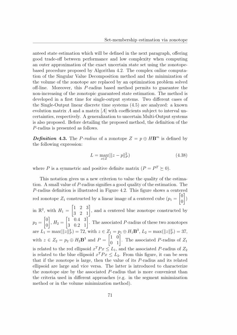
Set-membership estimation via zonotope
anteed state estimation which will be defined in the next paragraph, offeringgood trade-off between performance and low complexity when computingan outer approximation of the exact uncertain state set using the zonotope-based procedure proposed by Algorithm 4.2. The complex online computa-tion of the Singular Value Decomposition method and the minimization ofthe volume of the zonotope are replaced by an optimization problem solvedoff-line. Moreover, this P -radius based method permits to guarantee thenon-increasing of the zonotopic guaranteed state estimation. The method isdeveloped in a first time for single-output systems. Two different cases ofthe Single-Output linear discrete time systems (4.5) are analyzed: a knownevolution matrix A and a matrix [A] with coefficients subject to interval un-certainties, respectively. A generalization to uncertain Multi-Output systemsis also proposed. Before detailing the proposed method, the definition of theP -radius is presented as follows.
Definition 4.3. The P -radius of a zonotope Z = p ⊕ HBm is defined bythe following expression:
L = maxz∈Z
(‖z − p‖2P ) (4.38)
where P is a symmetric and positive definite matrix (P = P T 0).
This notation gives us a new criterion to value the quality of the estima-tion. A small value of P -radius signifies a good quality of the estimation. TheP -radius definition is illustrated in Figure 4.2. This figure shows a centered
red zonotope Z1 constructed by a linear image of a centered cube (p1 =
[00
])
in R2, with H1 =
[1 2 33 2 1
], and a centered blue zonotope constructed by
p2 =
[00
], H2 =
[1 0.4 33 0.2 1
]. The associated P -radius of these two zonotopes
are L1 = max(‖z‖2P ) = 72, with z ∈ Z1 = p1⊕H1B3, L2 = max(‖z‖2P ) = 37,
with z ∈ Z2 = p2 ⊕ H2B3 and P =
[1 00 1
]. The associated P -radius of Z1
is related to the red ellipsoid xTPx ≤ L1, and the associated P -radius of Z2
is related to the blue ellipsoid xTPx ≤ L2. From this figure, it can be seenthat if the zonotope is large, then the value of its P -radius and its relatedellipsoid are large and vice versa. The latter is introduced to characterizethe zonotope size by the associated P -radius that is more convenient thanthe criteria used in different approaches (e.g. in the segment minimizationmethod or in the volume minimization method).
71
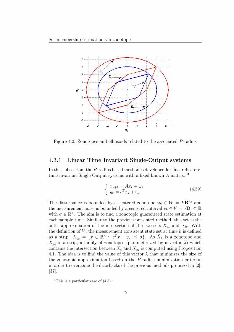
Set-membership estimation via zonotope
Figure 4.2: Zonotopes and ellipsoids related to the associated P -radius
4.3.1 Linear Time Invariant Single-Output systems
In this subsection, the P -radius based method is developed for linear discrete-time invariant Single-Output systems with a fixed known A matrix: 3
xk+1 = Axk + ωkyk = cTxk + vk
(4.39)
The disturbance is bounded by a centered zonotope ωk ∈ W = FBnx andthe measurement noise is bounded by a centered interval vk ∈ V = σB1 ⊂ Rwith σ ∈ R+. The aim is to find a zonotopic guaranteed state estimation ateach sample time. Similar to the previous presented method, this set is theouter approximation of the intersection of the two sets Xyk and Xk. Withthe definition of V , the measurement consistent state set at time k is definedas a strip: Xyk = x ∈ Rn : |cTx − yk| ≤ σ. As Xk is a zonotope andXyk is a strip, a family of zonotopes (parameterized by a vector λ) whichcontains the intersection between Xk and Xyk is computed using Proposition4.1. The idea is to find the value of this vector λ that minimizes the size ofthe zonotopic approximation based on the P -radius minimization criterionin order to overcome the drawbacks of the previous methods proposed in [2],[37].
3This is a particular case of (4.5).
72
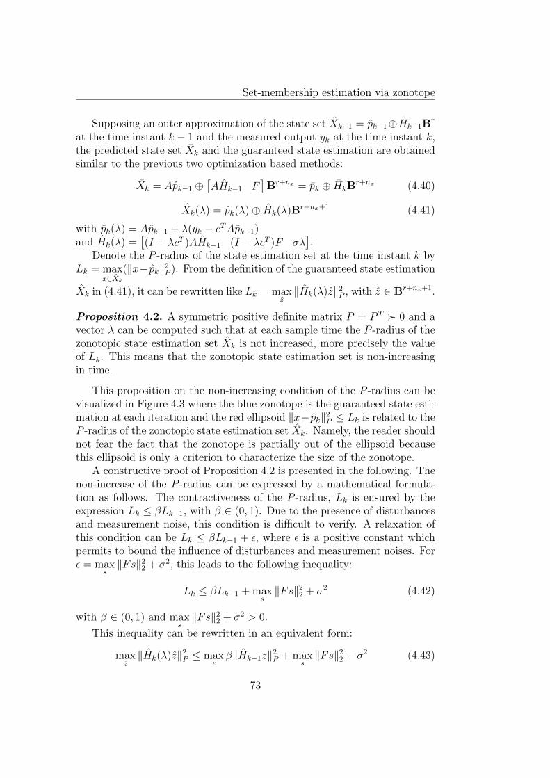
Set-membership estimation via zonotope
Supposing an outer approximation of the state set Xk−1 = pk−1⊕Hk−1Br
at the time instant k − 1 and the measured output yk at the time instant k,the predicted state set Xk and the guaranteed state estimation are obtainedsimilar to the previous two optimization based methods:
Xk = Apk−1 ⊕[AHk−1 F
]Br+nx = pk ⊕ HkBr+nx (4.40)
Xk(λ) = pk(λ)⊕ Hk(λ)Br+nx+1 (4.41)
with pk(λ) = Apk−1 + λ(yk − cTApk−1)and Hk(λ) =
[(I − λcT )AHk−1 (I − λcT )F σλ
].
Denote the P -radius of the state estimation set at the time instant k byLk = max
x∈Xk
(‖x− pk‖2P ). From the definition of the guaranteed state estimation
Xk in (4.41), it can be rewritten like Lk = maxz‖Hk(λ)z‖2P , with z ∈ Br+nx+1.
Proposition 4.2. A symmetric positive definite matrix P = P T 0 and avector λ can be computed such that at each sample time the P -radius of thezonotopic state estimation set Xk is not increased, more precisely the valueof Lk. This means that the zonotopic state estimation set is non-increasingin time.
This proposition on the non-increasing condition of the P -radius can bevisualized in Figure 4.3 where the blue zonotope is the guaranteed state esti-mation at each iteration and the red ellipsoid ‖x− pk‖2P ≤ Lk is related to theP -radius of the zonotopic state estimation set Xk. Namely, the reader shouldnot fear the fact that the zonotope is partially out of the ellipsoid becausethis ellipsoid is only a criterion to characterize the size of the zonotope.
A constructive proof of Proposition 4.2 is presented in the following. Thenon-increase of the P -radius can be expressed by a mathematical formula-tion as follows. The contractiveness of the P -radius, Lk is ensured by theexpression Lk ≤ βLk−1, with β ∈ (0, 1). Due to the presence of disturbancesand measurement noise, this condition is difficult to verify. A relaxation ofthis condition can be Lk ≤ βLk−1 + ε, where ε is a positive constant whichpermits to bound the influence of disturbances and measurement noises. Forε = max
s‖Fs‖22 + σ2, this leads to the following inequality:
Lk ≤ βLk−1 + maxs‖Fs‖22 + σ2 (4.42)
with β ∈ (0, 1) and maxs‖Fs‖22 + σ2 > 0.
This inequality can be rewritten in an equivalent form:
maxz‖Hk(λ)z‖2P ≤ max
zβ‖Hk−1z‖2P + max
s‖Fs‖22 + σ2 (4.43)
73
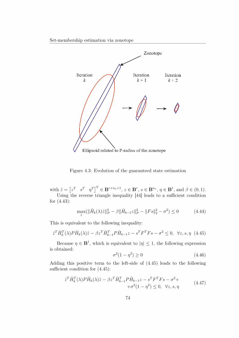
Set-membership estimation via zonotope
Figure 4.3: Evolution of the guaranteed state estimation
with z =[zT sT ηT
]T ∈ Br+nx+1, z ∈ Br, s ∈ Bnx , η ∈ B1, and β ∈ (0, 1).Using the reverse triangle inequality [44] leads to a sufficient condition
for (4.43):
maxz
(‖Hk(λ)z‖2P − β‖Hk−1z‖2P − ‖Fs‖22 − σ2) ≤ 0 (4.44)
This is equivalent to the following inequality:
zT HTk (λ)PHk(λ)z − βzT HT
k−1PHk−1z − sTF TFs− σ2 ≤ 0, ∀z, s, η (4.45)
Because η ∈ B1, which is equivalent to |η| ≤ 1, the following expressionis obtained:
σ2(1− η2) ≥ 0 (4.46)
Adding this positive term to the left-side of (4.45) leads to the followingsufficient condition for (4.45):
zT HTk (λ)PHk(λ)z − βzT HT
k−1PHk−1z − sTF TFs− σ2+
+σ2(1− η2) ≤ 0, ∀z, s, η(4.47)
74
Set-membership estimation via zonotope
Right multiplying the expression of Hk in (4.41) with the explicit form ofz leads to:
Hk(λ)z = (I − λcT )(AHk−1z + Fs) + σλη (4.48)
Denote θ = Hk−1z, then the inequality (4.47) can be written in the matrixformulation: θs
η
T A11 A12 A13
∗ A22 A23
∗ ∗ A33
θsη
≤ 0, ∀θ, s, η (4.49)
with ’∗’ denoting the terms required for the symmetry of the matrix and thefollowing additional notations:
A11 = ((I − λcT )A)TP (I − λcT )A− βPA12 = ((I − λcT )A)TP (I − λcT )FA13 = ((I − λcT )A)TPσλA22 = ((I − λcT )F )TP (I − λcT )F − F TFA23 = ((I − λcT )F )TPσλA33 = σ2λTPλ− σ2.
(4.50)
Using the Definition 3.11 of positive definite matrix allows to rewrite(4.49) as: A11 A12 A13
∗ A22 A23
∗ ∗ A33
0, ∀
θsη
6= 0 (4.51)
Multiplying (4.51) by −1, this is equivalent to:−A11 −A12 −A13
∗ −A22 −A23
∗ ∗ −A33
0, ∀
θsη
6= 0 (4.52)
Using the explicit notations (4.50) and doing some manipulations in (4.52),a matrix inequality is derived as:βP 0 0
∗ F TF 0∗ ∗ σ2
−−
(AT − AT cλT )P(F T − F T cλT )P
λTPσ
P−1(AT − AT cλT )P
(F T − F T cλT )PλTPσ
T 0 (4.53)
75
Set-membership estimation via zonotope
Using the Schur complement definition (3.14), the expression (4.53) isequivalent to the following matrix inequality:
βP 0 0 ATP − AT cY T
∗ F TF 0 F TP − F T cY T
∗ ∗ σ2 Y Tσ∗ ∗ ∗ P
0 (4.54)
with a change of variables Y = Pλ with P ∈ Rnx×nx , λ ∈ Rnx and Y ∈ Rnx .As the 2-norm is a convex function and W is a convex set, the term
maxs∈Bnx
‖Fs‖22, can be easily computed using the maximum principle [122].
Thus the value of ε = maxs‖Fs‖22 + σ2 can be obtained. Then the condition
(4.42) can be written as Lk ≤ βLk−1 + ε. At infinity, this expression isequivalent to:
L∞ = βL∞ + ε (4.55)
leading to:L∞ =
ε
1− β(4.56)
Let us consider an ellipsoid E = x : xTPx ≤ ε1−β which can be normalized
to E = x : xT (1−β)Pε
x ≤ 1. This ellipsoid is related to the P -radius of thezonotopic guaranteed state estimation at infinity. To minimize the P -radius(i.e. L∞) of the zonotope, one can find the ellipsoid of smallest diameter [24].This leads to solve the following Eigenvalue Problem (EVP):
maxτ,β,P
τ
subject to the BMI(1− β)P
ε τInx (4.57)
where Inx ∈ Rnx×nx is the identity matrix, τ ∈ R+ and β ∈ (0, 1) are scalar.Then the smallest diameter is computed by 2√
τ∗[24].
Finally, to find the values of P = P T 0 ∈ Rnx×nx and λ ∈ Rnx thefollowing optimization problem must be solved:
Method 4.1. maxτ,β,P,Y
τ
subject to
(1−β)Pε τI
βP 0 0 ATP − AT cY T
∗ F TF 0 F TP − F T cY T
∗ ∗ σ2 Y Tσ∗ ∗ ∗ P
0
τ > 0
(4.58)
76
Set-membership estimation via zonotope
Remark 4.3. As β is a scalar variable, this optimization problem can beefficiently solved by using a BMI solver (e.g. Penbmi [74]) or by executinga simple search-loop on β leading to a LMI problem. In this optimizationproblem (4.58), the decision variables are: P = P T ∈ Rnx×nx , Y ∈ Rnx ,β ∈ (0, 1) and τ ∈ R+. Thus, the total number of the scalar decision variablesis nx(nx+1)
2+nx + 2. The dimensions of the inequalities in (4.58) are nx×nx,
(3nx + 1)× (3nx + 1) and 1, respectively.
Remark 4.4. In [85], a modification of the problem (4.58) to avoid solvinga BMI optimization problem is presented. Instead of optimizing the valueof the P -radius, a minimum value of β is searched which permits to have amaximum decreasing speed of the P -radius. This criterion leads to a newLMI optimization problem based on the bisection algorithm [28] on β:
Method 4.2. minβ∈(0,1)
β
such thatmaxτ,P,Y
τ
subject to
(1−β)Pε τI
βP 0 0 ATP − AT cY T
∗ F TF 0 F TP − F T cY T
∗ ∗ σ2 Y Tσ∗ ∗ ∗ P
0
τ > 0
(4.59)
As β is computed by a bissection algorithm, then it is not a decisionvariable in (4.59). This means that, in this case, the matrix inequalities(4.59) are LMIs.
In order to better undertand the proposed methods, an illustrative exam-ple will be further presented.
Example 4.1. Consider the following linear discrete-time invariant system: xk+1 =
[1 10 1
]xk + 0.02
[−61
]ωk
yk =[−2 1
]xk + 0.2vk
(4.60)
with ‖vk‖∞ ≤ 1, ‖ωk‖∞ ≤ 1. The values of vk and ωk are generated byrandom functions with Matlab R©. The initial state belongs to the box 3B2.The guaranteed state estimation must be determined at each time instant.
77
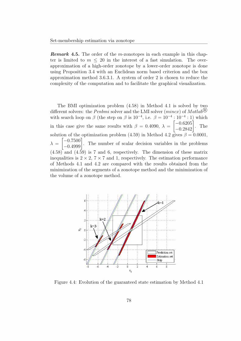
Set-membership estimation via zonotope
Remark 4.5. The order of the m-zonotopes in each example in this chap-ter is limited to m ≤ 20 in the interest of a fast simulation. The over-approximation of a high-order zonotope by a lower-order zonotope is doneusing Proposition 3.4 with an Euclidean norm based criterion and the boxapproximation method 3.6.3.1. A system of order 2 is chosen to reduce thecomplexity of the computation and to facilitate the graphical visualization.
The BMI optimization problem (4.58) in Method 4.1 is solved by twodifferent solvers: the Penbmi solver and the LMI solver (mincx) ofMatlab R©with search loop on β (the step on β is 10−4, i.e. β = 10−4 : 10−4 : 1) which
in this case give the same results with β = 0.4090, λ =
[−0.6205−0.2842
]. The
solution of the optimization problem (4.59) in Method 4.2 gives β = 0.0001,
λ =
[−0.7500−0.4999
]. The number of scalar decision variables in the problems
(4.58) and (4.59) is 7 and 6, respectively. The dimension of these matrixinequalities is 2 × 2, 7 × 7 and 1, respectively. The estimation performanceof Methods 4.1 and 4.2 are compared with the results obtained from theminimization of the segments of a zonotope method and the minimization ofthe volume of a zonotope method.
Figure 4.4: Evolution of the guaranteed state estimation by Method 4.1
78
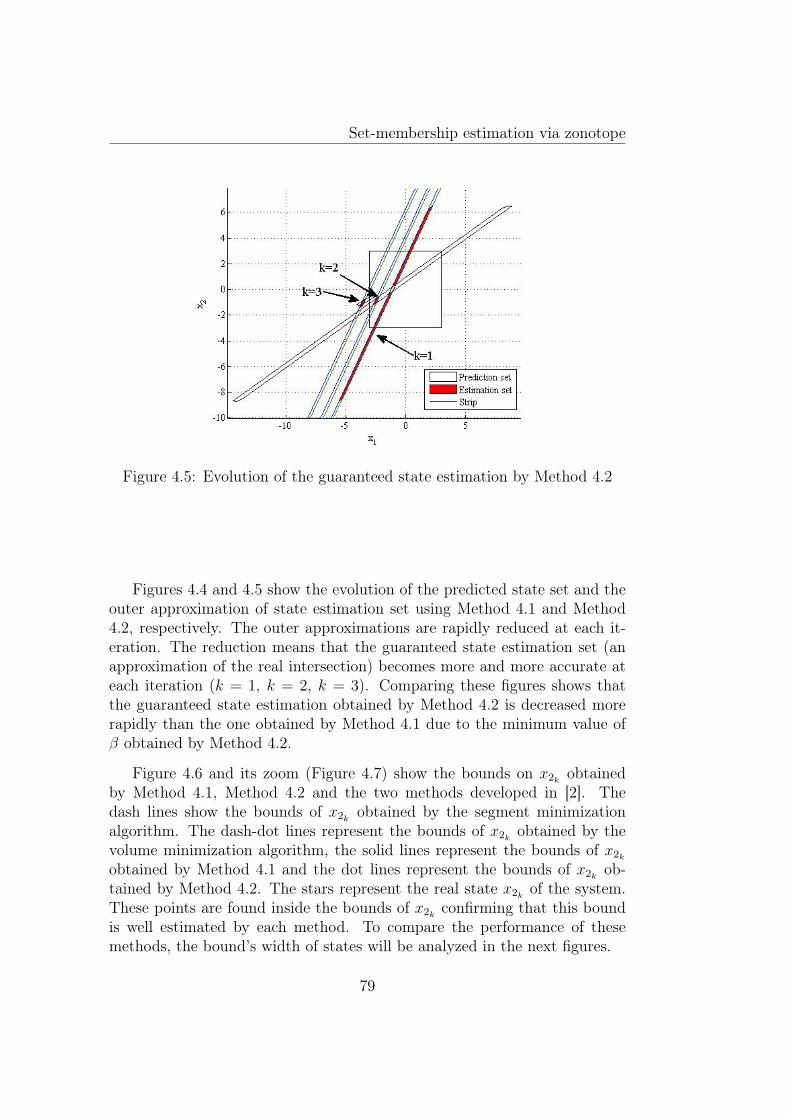
Set-membership estimation via zonotope
Figure 4.5: Evolution of the guaranteed state estimation by Method 4.2
Figures 4.4 and 4.5 show the evolution of the predicted state set and theouter approximation of state estimation set using Method 4.1 and Method4.2, respectively. The outer approximations are rapidly reduced at each it-eration. The reduction means that the guaranteed state estimation set (anapproximation of the real intersection) becomes more and more accurate ateach iteration (k = 1, k = 2, k = 3). Comparing these figures shows thatthe guaranteed state estimation obtained by Method 4.2 is decreased morerapidly than the one obtained by Method 4.1 due to the minimum value ofβ obtained by Method 4.2.
Figure 4.6 and its zoom (Figure 4.7) show the bounds on x2k obtainedby Method 4.1, Method 4.2 and the two methods developed in [2]. Thedash lines show the bounds of x2k obtained by the segment minimizationalgorithm. The dash-dot lines represent the bounds of x2k obtained by thevolume minimization algorithm, the solid lines represent the bounds of x2kobtained by Method 4.1 and the dot lines represent the bounds of x2k ob-tained by Method 4.2. The stars represent the real state x2k of the system.These points are found inside the bounds of x2k confirming that this boundis well estimated by each method. To compare the performance of thesemethods, the bound’s width of states will be analyzed in the next figures.
79
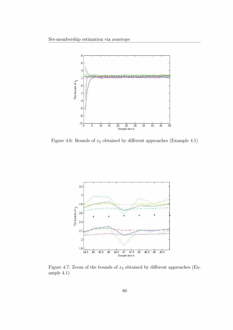
Set-membership estimation via zonotope
Figure 4.6: Bounds of x2 obtained by different approaches (Example 4.1)
Figure 4.7: Zoom of the bounds of x2 obtained by different approaches (Ex-ample 4.1)
80
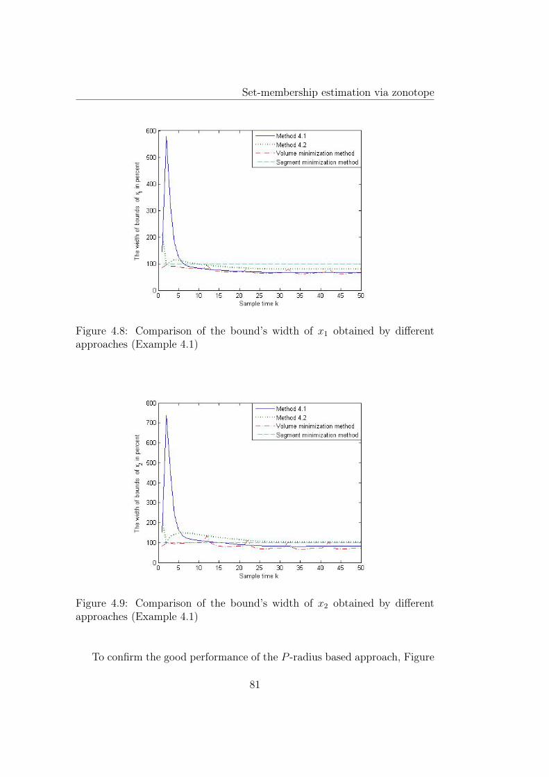
Set-membership estimation via zonotope
Figure 4.8: Comparison of the bound’s width of x1 obtained by differentapproaches (Example 4.1)
Figure 4.9: Comparison of the bound’s width of x2 obtained by differentapproaches (Example 4.1)
To confirm the good performance of the P -radius based approach, Figure
81
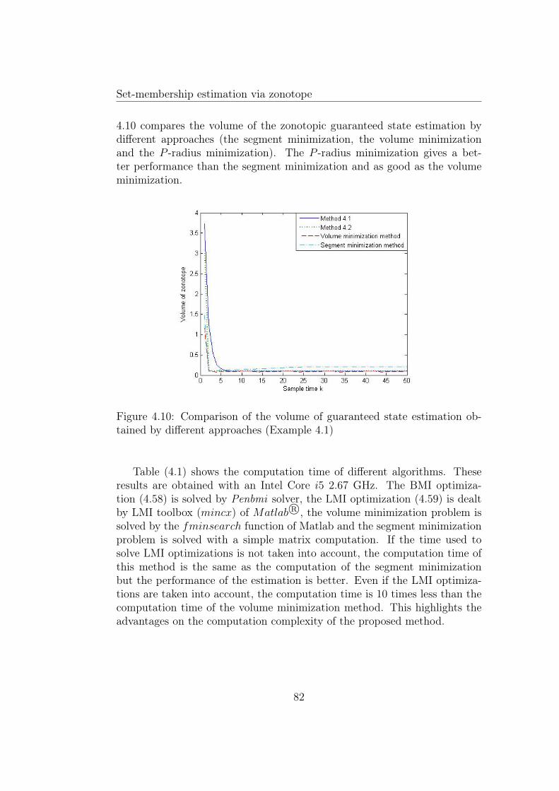
Set-membership estimation via zonotope
4.10 compares the volume of the zonotopic guaranteed state estimation bydifferent approaches (the segment minimization, the volume minimizationand the P -radius minimization). The P -radius minimization gives a bet-ter performance than the segment minimization and as good as the volumeminimization.
Figure 4.10: Comparison of the volume of guaranteed state estimation ob-tained by different approaches (Example 4.1)
Table (4.1) shows the computation time of different algorithms. Theseresults are obtained with an Intel Core i5 2.67 GHz. The BMI optimiza-tion (4.58) is solved by Penbmi solver, the LMI optimization (4.59) is dealtby LMI toolbox (mincx) of Matlab R©, the volume minimization problem issolved by the fminsearch function of Matlab and the segment minimizationproblem is solved with a simple matrix computation. If the time used tosolve LMI optimizations is not taken into account, the computation time ofthis method is the same as the computation of the segment minimizationbut the performance of the estimation is better. Even if the LMI optimiza-tions are taken into account, the computation time is 10 times less than thecomputation time of the volume minimization method. This highlights theadvantages on the computation complexity of the proposed method.
82
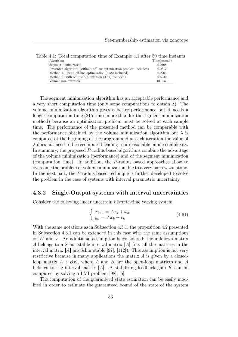
Set-membership estimation via zonotope
Table 4.1: Total computation time of Example 4.1 after 50 time instantsAlgorithm Time(second)Segment minimization 0.0468Presented algorithm (without off-line optimization problem included) 0.0312Method 4.1 (with off-line optimization (4.58) included) 0.9204Method 2 (with off-line optimization (4.59) included) 0.6240Volume minimization 10.0153
The segment minimization algorithm has an acceptable performance anda very short computation time (only some computations to obtain λ). Thevolume minimization algorithm gives a better performance but it needs alonger computation time (215 times more than for the segment minimizationmethod) because an optimization problem must be solved at each sampletime. The performance of the presented method can be comparable withthe performance obtained by the volume minimization algorithm but λ iscomputed at the beginning of the program and at each iteration the value ofλ does not need to be recomputed leading to a reasonable online complexity.In summary, the proposed P -radius based algorithms combine the advantageof the volume minimization (performance) and of the segment minimization(computation time). In addition, the P -radius based approaches allow toovercome the problem of volume minimization due to a very narrow zonotope.In the next part, the P -radius based technique is further developed to solvethe problem in the case of systems with interval parametric uncertainty.
4.3.2 Single-Output systems with interval uncertainties
Consider the following linear uncertain discrete-time varying system:xk+1 = Axk + ωkyk = cTxk + vk
(4.61)
With the same notations as in Subsection 4.3.1, the proposition 4.2 presentedin Subsection 4.3.1 can be extended in this case with the same assumptionson W and V . An additional assumption is considered: the unknown matrixA belongs to a Schur stable interval matrix [A] (i.e. all the matrices in theinterval matrix [A] are Schur stable [97], [112]). This assumption is not veryrestrictive because in many applications the matrix A is given by a closed-loop matrix A + BK, where A and B are the open-loop matrices and Abelongs to the interval matrix [A]. A stabilizing feedback gain K can becomputed by solving a LMI problem [98], [5].
The computation of the guaranteed state estimation can be easily mod-ified in order to estimate the guaranteed bound of the state of the system
83
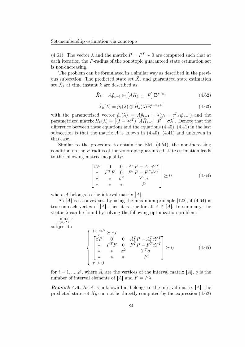
Set-membership estimation via zonotope
(4.61). The vector λ and the matrix P = P T 0 are computed such that ateach iteration the P -radius of the zonotopic guaranteed state estimation setis non-increasing.
The problem can be formulated in a similar way as described in the previ-ous subsection. The predicted state set Xk and guaranteed state estimationset Xk at time instant k are described as:
Xk = Apk−1 ⊕[AHk−1 F
]Br+nx (4.62)
Xk(λ) = pk(λ)⊕ Hk(λ)Br+nx+1 (4.63)
with the parametrized vector pk(λ) = Apk−1 + λ(yk − cTApk−1) and theparametrized matrix Hk(λ) =
[(I − λcT )
[AHk−1 F
]σλ]. Denote that the
difference between these equations and the equations (4.40), (4.41) in the lastsubsection is that the matrix A is known in (4.40), (4.41) and unknown inthis case.
Similar to the procedure to obtain the BMI (4.54), the non-increasingcondition on the P -radius of the zonotopic guaranteed state estimation leadsto the following matrix inequality:
βP 0 0 ATP − AT cY T
∗ F TF 0 F TP − F T cY T
∗ ∗ σ2 Y Tσ∗ ∗ ∗ P
0 (4.64)
where A belongs to the interval matrix [A].As [A] is a convex set, by using the maximum principle [122], if (4.64) is
true on each vertex of [A], then it is true for all A ∈ [A]. In summary, thevector λ can be found by solving the following optimization problem:
maxτ,β,P,Y
τ
subject to
(1−β)Pε τI
βP 0 0 ATi P − ATi cY T
∗ F TF 0 F TP − F T cY T
∗ ∗ σ2 Y Tσ∗ ∗ ∗ P
0
τ > 0
(4.65)
for i = 1, ..., 2q, where Ai are the vertices of the interval matrix [A], q is thenumber of interval elements of [A] and Y = Pλ.
Remark 4.6. As A is unknown but belongs to the interval matrix [A], thepredicted state set Xk can not be directly computed by the expression (4.62)
84
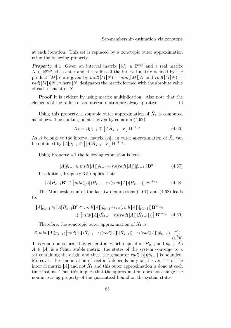
Set-membership estimation via zonotope
at each iteration. This set is replaced by a zonotopic outer approximationusing the following property.
Property 4.1. Given an interval matrix [M ] ∈ In×p and a real matrixN ∈ Rp×q, the center and the radius of the interval matrix defined by theproduct [M ]N are given by mid([M ]N) = mid([M ])N and rad([M ]N) =rad([M ])|N |, where |N | designates the matrix formed with the absolute valueof each element of N .
Proof It is evident by using matrix multiplication. Also note that theelements of the radius of an interval matrix are always positive.
Using this property, a zontopic outer approximation of Xk is computedas follows. The starting point is given by equation (4.62):
Xk = Apk−1 ⊕[AHk−1 F
]Br+nx (4.66)
As A belongs to the interval matrix [A], an outer approximation of Xk canbe obtained by [A]pk−1 ⊕
[[A]Hk−1 F
]Br+nx .
Using Property 4.1 the following expression is true:
[A]pk−1 ∈ mid([A])pk−1 ⊕ rs(rad([A])|pk−1|)Bnx (4.67)
In addition, Property 3.5 implies that:
[A]Hk−1Br ∈[mid([A])Hk−1 rs(rad([A])|Hk−1|)
]Br+nx (4.68)
The Minkowski sum of the last two expressions (4.67) and (4.68) leadsto:
[A]pk−1 ⊕ [A]Hk−1Br ⊂ mid([A])pk−1 ⊕ rs(rad([A])|pk−1|)Bnx⊕⊕[mid([A])Hk−1 rs(rad([A])|Hk−1|))
]Br+nx (4.69)
Therefore, the zonotopic outer approximation of Xk is:
Z(mid([A])pk−1;[mid([A])Hk−1 rs(rad([A])|Hk−1|) rs(rad([A])|pk−1|) F
])
(4.70)This zonotope is formed by generators which depend on Hk−1 and pk−1. AsA ∈ [A] is a Schur stable matrix, the states of the system converge to aset containing the origin and thus, the generator rad([A])|pk−1| is bounded.Moreover, the computation of vector λ depends only on the vertices of theinterval matrix [A] and not Xk and this outer approximation is done at eachtime instant. Thus this implies that the approximation does not change thenon-increasing property of the guaranteed bound on the system states.
85
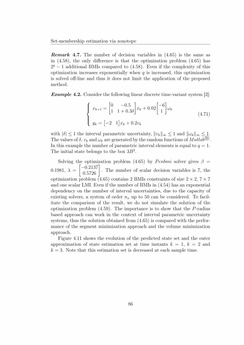
Set-membership estimation via zonotope
Remark 4.7. The number of decision variables in (4.65) is the same asin (4.58), the only difference is that the optimization problem (4.65) has2q − 1 additional BMIs compared to (4.58). Even if the complexity of thisoptimization increases exponentially when q is increased, this optimizationis solved off-line and thus it does not limit the application of the proposedmethod.
Example 4.2. Consider the following linear discrete time-variant system [2]:xk+1 =
[0 −0.51 1 + 0.3δ
]xk + 0.02
[−61
]ωk
yk =[−2 1
]xk + 0.2vk
(4.71)
with |δ| ≤ 1 the interval parametric uncertainty, ‖vk‖∞ ≤ 1 and ‖ωk‖∞ ≤ 1.The values of δ, vk and ωk are generated by the random functions ofMatlab R©.In this example the number of parametric interval elements is equal to q = 1.The initial state belongs to the box 3B2.
Solving the optimization problem (4.65) by Penbmi solver gives β =
0.1981, λ =
[−0.21370.5726
]. The number of scalar decision variables is 7, the
optimization problem (4.65) contains 2 BMIs constraints of size 2× 2, 7× 7and one scalar LMI. Even if the number of BMIs in (4.54) has an exponentialdependency on the number of interval uncertainties, due to the capacity ofexisting solvers, a system of order nx up to 50 can be considered. To facil-itate the comparison of the result, we do not simulate the solution of theoptimization problem (4.59). The importance is to show that the P -radiusbased approach can work in the context of interval parametric uncertaintysystems, thus the solution obtained from (4.65) is compared with the perfor-mance of the segment minimization approach and the volume minimizationapproach.
Figure 4.11 shows the evolution of the predicted state set and the outerapproximation of state estimation set at time instants k = 1, k = 2 andk = 3. Note that this estimation set is decreased at each sample time.
86
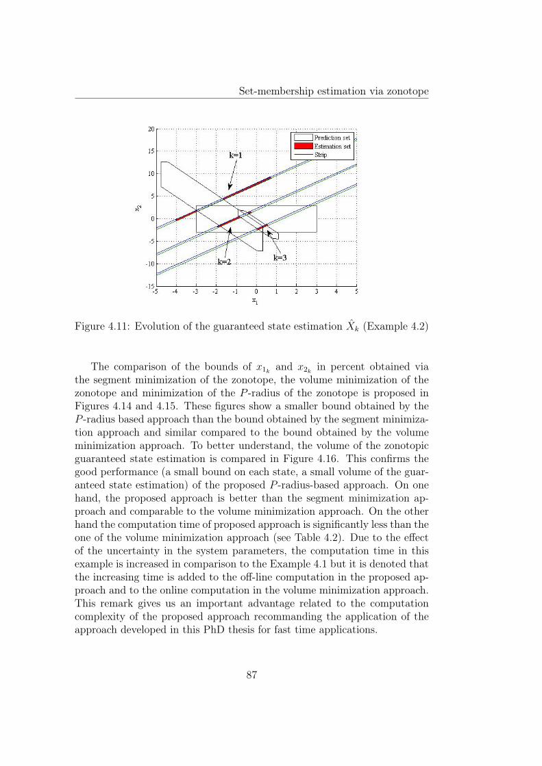
Set-membership estimation via zonotope
Figure 4.11: Evolution of the guaranteed state estimation Xk (Example 4.2)
The comparison of the bounds of x1k and x2k in percent obtained viathe segment minimization of the zonotope, the volume minimization of thezonotope and minimization of the P -radius of the zonotope is proposed inFigures 4.14 and 4.15. These figures show a smaller bound obtained by theP -radius based approach than the bound obtained by the segment minimiza-tion approach and similar compared to the bound obtained by the volumeminimization approach. To better understand, the volume of the zonotopicguaranteed state estimation is compared in Figure 4.16. This confirms thegood performance (a small bound on each state, a small volume of the guar-anteed state estimation) of the proposed P -radius-based approach. On onehand, the proposed approach is better than the segment minimization ap-proach and comparable to the volume minimization approach. On the otherhand the computation time of proposed approach is significantly less than theone of the volume minimization approach (see Table 4.2). Due to the effectof the uncertainty in the system parameters, the computation time in thisexample is increased in comparison to the Example 4.1 but it is denoted thatthe increasing time is added to the off-line computation in the proposed ap-proach and to the online computation in the volume minimization approach.This remark gives us an important advantage related to the computationcomplexity of the proposed approach recommanding the application of theapproach developed in this PhD thesis for fast time applications.
87
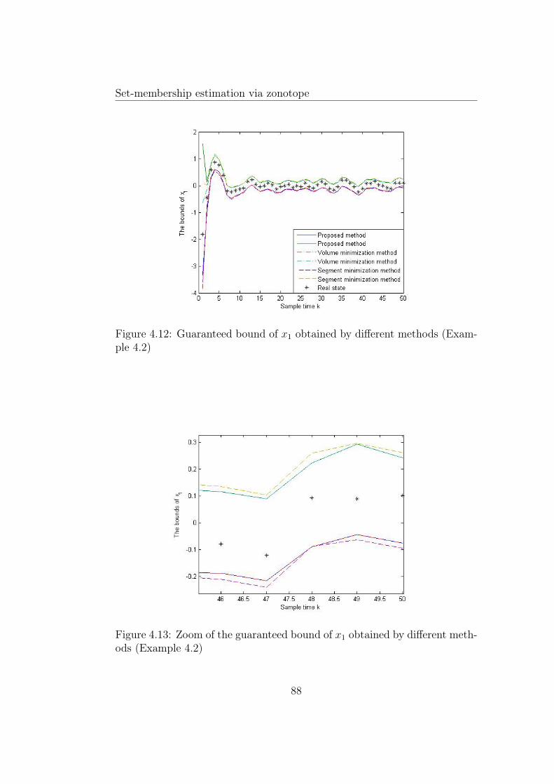
Set-membership estimation via zonotope
Figure 4.12: Guaranteed bound of x1 obtained by different methods (Exam-ple 4.2)
Figure 4.13: Zoom of the guaranteed bound of x1 obtained by different meth-ods (Example 4.2)
88
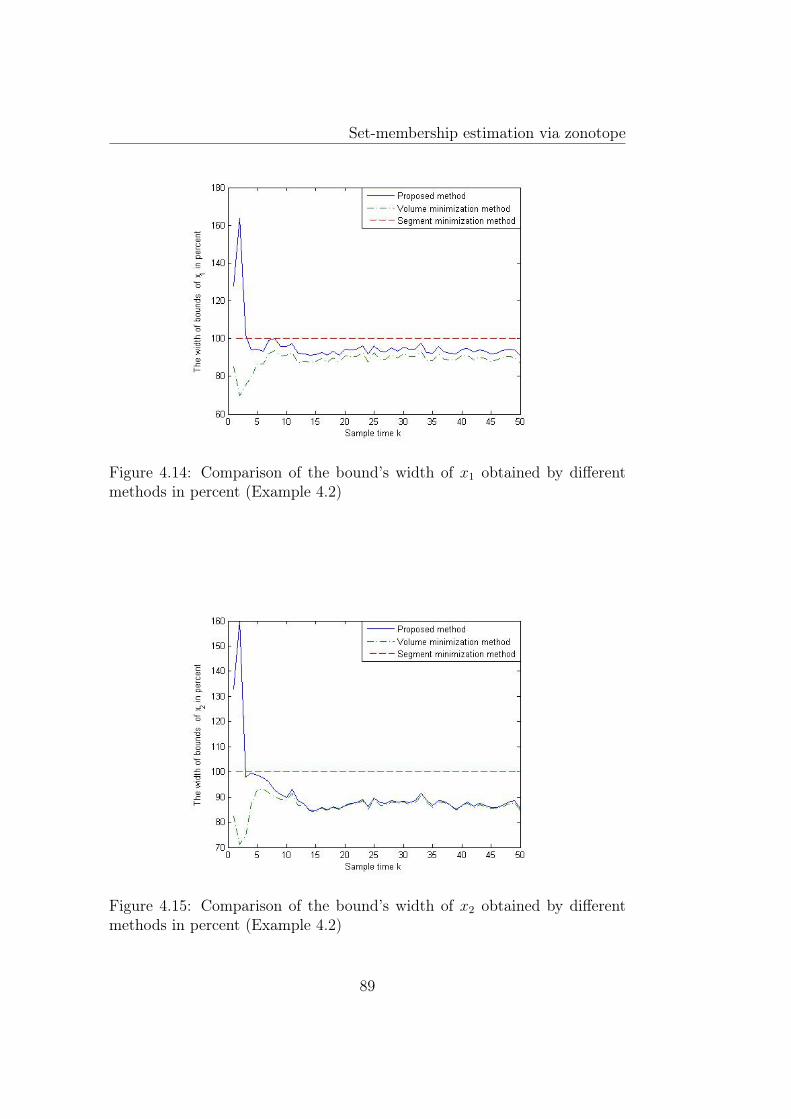
Set-membership estimation via zonotope
Figure 4.14: Comparison of the bound’s width of x1 obtained by differentmethods in percent (Example 4.2)
Figure 4.15: Comparison of the bound’s width of x2 obtained by differentmethods in percent (Example 4.2)
89
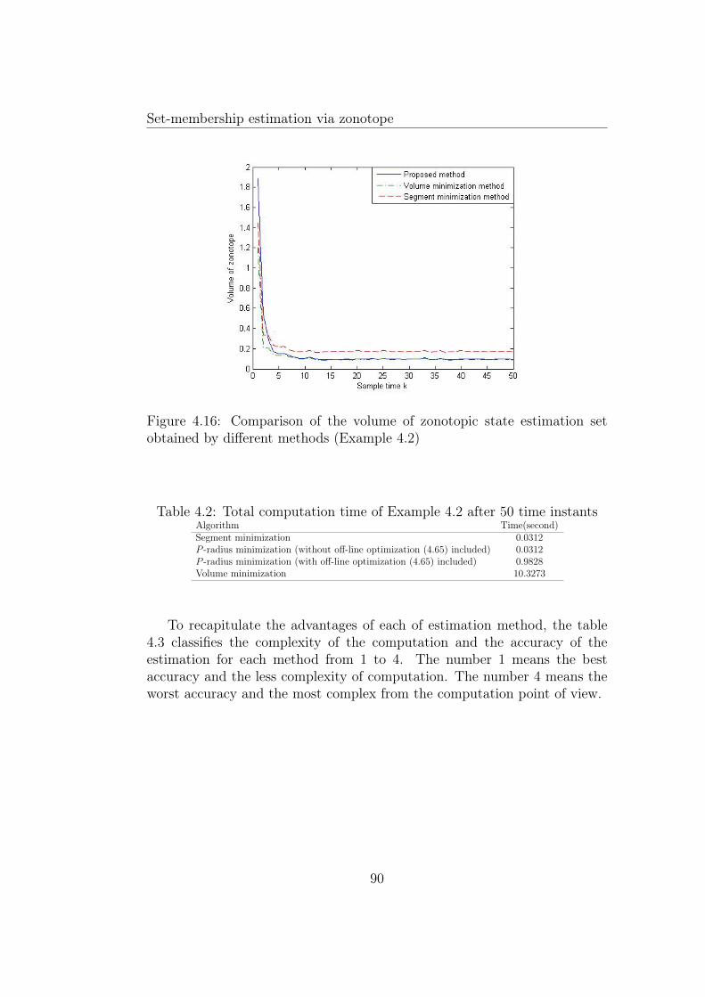
Set-membership estimation via zonotope
Figure 4.16: Comparison of the volume of zonotopic state estimation setobtained by different methods (Example 4.2)
Table 4.2: Total computation time of Example 4.2 after 50 time instantsAlgorithm Time(second)Segment minimization 0.0312P -radius minimization (without off-line optimization (4.65) included) 0.0312P -radius minimization (with off-line optimization (4.65) included) 0.9828Volume minimization 10.3273
To recapitulate the advantages of each of estimation method, the table4.3 classifies the complexity of the computation and the accuracy of theestimation for each method from 1 to 4. The number 1 means the bestaccuracy and the less complexity of computation. The number 4 means theworst accuracy and the most complex from the computation point of view.
90
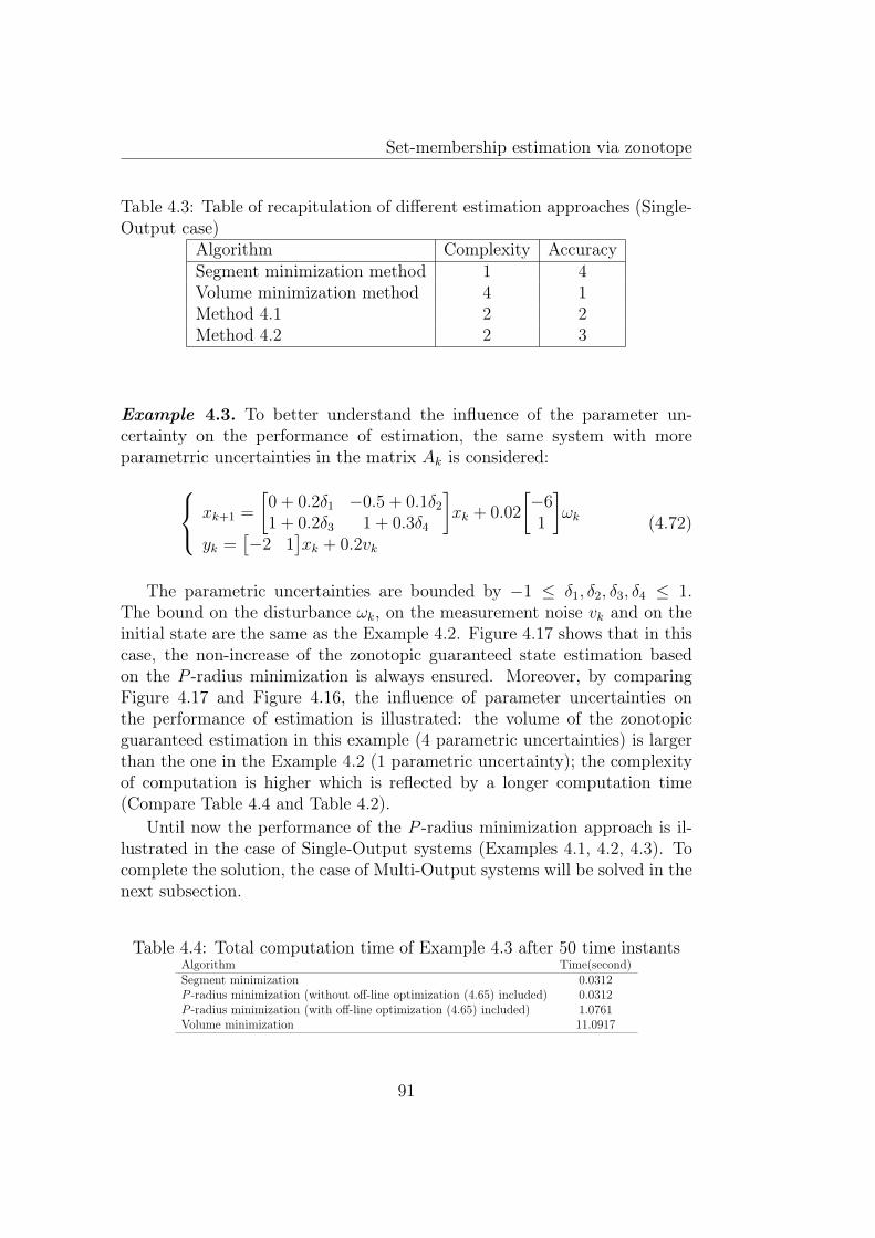
Set-membership estimation via zonotope
Table 4.3: Table of recapitulation of different estimation approaches (Single-Output case)
Algorithm Complexity AccuracySegment minimization method 1 4Volume minimization method 4 1Method 4.1 2 2Method 4.2 2 3
Example 4.3. To better understand the influence of the parameter un-certainty on the performance of estimation, the same system with moreparametrric uncertainties in the matrix Ak is considered: xk+1 =
[0 + 0.2δ1 −0.5 + 0.1δ21 + 0.2δ3 1 + 0.3δ4
]xk + 0.02
[−61
]ωk
yk =[−2 1
]xk + 0.2vk
(4.72)
The parametric uncertainties are bounded by −1 ≤ δ1, δ2, δ3, δ4 ≤ 1.The bound on the disturbance ωk, on the measurement noise vk and on theinitial state are the same as the Example 4.2. Figure 4.17 shows that in thiscase, the non-increase of the zonotopic guaranteed state estimation basedon the P -radius minimization is always ensured. Moreover, by comparingFigure 4.17 and Figure 4.16, the influence of parameter uncertainties onthe performance of estimation is illustrated: the volume of the zonotopicguaranteed estimation in this example (4 parametric uncertainties) is largerthan the one in the Example 4.2 (1 parametric uncertainty); the complexityof computation is higher which is reflected by a longer computation time(Compare Table 4.4 and Table 4.2).
Until now the performance of the P -radius minimization approach is il-lustrated in the case of Single-Output systems (Examples 4.1, 4.2, 4.3). Tocomplete the solution, the case of Multi-Output systems will be solved in thenext subsection.
Table 4.4: Total computation time of Example 4.3 after 50 time instantsAlgorithm Time(second)Segment minimization 0.0312P -radius minimization (without off-line optimization (4.65) included) 0.0312P -radius minimization (with off-line optimization (4.65) included) 1.0761Volume minimization 11.0917
91
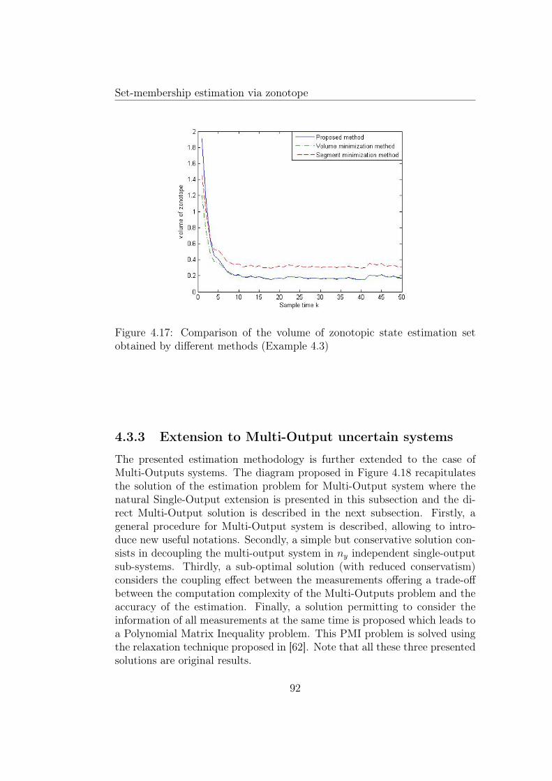
Set-membership estimation via zonotope
Figure 4.17: Comparison of the volume of zonotopic state estimation setobtained by different methods (Example 4.3)
4.3.3 Extension to Multi-Output uncertain systems
The presented estimation methodology is further extended to the case ofMulti-Outputs systems. The diagram proposed in Figure 4.18 recapitulatesthe solution of the estimation problem for Multi-Output system where thenatural Single-Output extension is presented in this subsection and the di-rect Multi-Output solution is described in the next subsection. Firstly, ageneral procedure for Multi-Output system is described, allowing to intro-duce new useful notations. Secondly, a simple but conservative solution con-sists in decoupling the multi-output system in ny independent single-outputsub-systems. Thirdly, a sub-optimal solution (with reduced conservatism)considers the coupling effect between the measurements offering a trade-offbetween the computation complexity of the Multi-Outputs problem and theaccuracy of the estimation. Finally, a solution permitting to consider theinformation of all measurements at the same time is proposed which leads toa Polynomial Matrix Inequality problem. This PMI problem is solved usingthe relaxation technique proposed in [62]. Note that all these three presentedsolutions are original results.
92
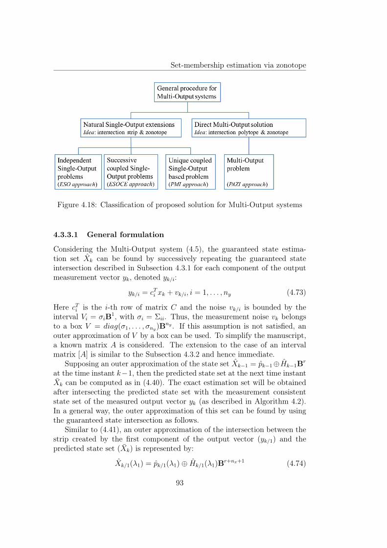
Set-membership estimation via zonotope
Figure 4.18: Classification of proposed solution for Multi-Output systems
4.3.3.1 General formulation
Considering the Multi-Output system (4.5), the guaranteed state estima-tion set Xk can be found by successively repeating the guaranteed stateintersection described in Subsection 4.3.1 for each component of the outputmeasurement vector yk, denoted yk/i:
yk/i = cTi xk + vk/i, i = 1, . . . , ny (4.73)
Here cTi is the i-th row of matrix C and the noise vk/i is bounded by theinterval Vi = σiB1, with σi = Σii. Thus, the measurement noise vk belongsto a box V = diag(σ1, . . . , σny)Bny . If this assumption is not satisfied, anouter approximation of V by a box can be used. To simplify the manuscript,a known matrix A is considered. The extension to the case of an intervalmatrix [A] is similar to the Subsection 4.3.2 and hence immediate.
Supposing an outer approximation of the state set Xk−1 = pk−1⊕Hk−1Br
at the time instant k−1, then the predicted state set at the next time instantXk can be computed as in (4.40). The exact estimation set will be obtainedafter intersecting the predicted state set with the measurement consistentstate set of the measured output vector yk (as described in Algorithm 4.2).In a general way, the outer approximation of this set can be found by usingthe guaranteed state intersection as follows.
Similar to (4.41), an outer approximation of the intersection between thestrip created by the first component of the output vector (yk/1) and thepredicted state set (Xk) is represented by:
Xk/1(λ1) = pk/1(λ1)⊕ Hk/1(λ1)Br+nx+1 (4.74)
93
Set-membership estimation via zonotope
where pk/1(λ1) = Apk−1 + λ1(yk/1 − cT1Apk−1)and Hk/1(λ1) =
[(I − λ1cT1 )AHk−1 (I − λ1cT1 )F σ1λ1
].
Then this set Xk/1(λ1) is intersected with the strip obtained from the secondcomponent of the measured output vector (yk/2) leading to:
Xk/2(λ1, λ2) = pk/2(λ1, λ2)⊕ Hk/2(λ1, λ2)Br+nx+2 (4.75)
with pk/2(λ1, λ2) = pk/1(λ1) + λ2(yk/2 − cT2 pk/1(λ1))and Hk/2(λ1, λ2) =
[(I − λ2cT2 )Hk/1(λ1) σ2λ2
].
This procedure is repeated until the last component of the measuredoutput vector (yk/ny) leading to the zonotopic guaranteed state estimationset at time instant k:
Xk/ny(λ1, ..., λny) = pk/ny(λ1, ..., λny)⊕⊕Hk/ny(λ1, ..., λny)Br+nx+ny
(4.76)
with the recursive notations:
pk/ny(λ1, ..., λny) = pk/ny−1(λ1, ..., λny−1)+
+ λny(yk/ny − cTnypk/ny−1(λ1, ..., λny−1)) (4.77)
and
Hk/ny(λ1, ..., λny) =[(I − λnyc
Tny
)Hk/ny−1(λ1, ..., λny−1) σnyλny
](4.78)
Finally, the zonotopic guaranteed state estimation set at instant k is providedby:
Xk(λ1, ..., λny) = pk(λ1, ..., λny)⊕ Hk(λ1, ..., λny)Br+nx+ny (4.79)
with pk(λ1, ..., λny) = pk/ny(λ1, ..., λny)
and Hk(λ1, ..., λny) = Hk/ny(λ1, ..., λny).This procedure can be visualized in Figure 4.19 for the case of two out-
puts. Suppose at the time instant k from the guaranteed state estimation setXk−1 the predicted state set is determined (represented by the green zonotopeXk). Firstly, this set is intersected with the first element of the measuredoutput denoted by the red strip |cT1 x − yk/1| ≤ σ1. Then this intersectionis approximated by the black zonotope Xk/1 by using Proposition 4.2. Theprocedure is repeated with the second element of the measured output (thestrip |cT2 x − yk/2| ≤ σ2). Proposition 4.2 is used again to obtain the outerapproximation of the intersection between Xk/1 and the second strip. Theguaranteed state estimation set is then the magenta zonotope Xk/2.
Further on, in the general case of ny outputs, three original proceduresare proposed to compute the vectors λ1,...,λny .
94
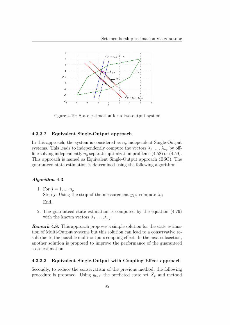
Set-membership estimation via zonotope
Figure 4.19: State estimation for a two-output system
4.3.3.2 Equivalent Single-Output approach
In this approach, the system is considered as ny independent Single-Outputsystems. This leads to independently compute the vectors λ1, ..., λny by off-line solving independently ny separate optimization problems (4.58) or (4.59).This approach is named as Equivalent Single-Output approach (ESO). Theguaranteed state estimation is determined using the following algorithm:
Algorithm 4.3.
1. For j = 1, ..., nyStep j: Using the strip of the measurement yk/j compute λj;
End.
2. The guaranteed state estimation is computed by the equation (4.79)with the known vectors λ1,. . . ,λny .
Remark 4.8. This approach proposes a simple solution for the state estima-tion of Multi-Output systems but this solution can lead to a conservative re-sult due to the possible multi-outputs coupling effect. In the next subsection,another solution is proposed to improve the performance of the guaranteedstate estimation.
4.3.3.3 Equivalent Single-Output with Coupling Effect approach
Secondly, to reduce the conservatism of the previous method, the followingprocedure is proposed. Using yk/1, the predicted state set Xk and method
95
Set-membership estimation via zonotope
4.1, method 4.2 or (4.65) in the case of interval parametric uncertainty leadsto λ1 and a smaller zonotope Xk/1. Intersecting this new zonotope withthe strip corresponding to yk/2 (supposing λ1 known from the previous step)leads to λ2 and another zonotope Xk/2. This procedure is repeated until thelast component of the output vector yk/ny (supposing all the previous vectorsλ1,..., λny−1 to be known). This approach is called as Equivalent Single-Output with Coupling Effect approach (ESOCE). The following algorithmdescribes this off-line procedure.
Algorithm 4.4.
1. Step 1: Using the measurement yk/1 and (4.65), compute λ1;
2. For j = 2, ..., nyStep j: Using the measurement yk/j and the previous obtained vectorsλ1, ..., λj−1, compute λj.
End.
The computation of λj is detailed as follows. The guaranteed state esti-mation set at Step j is computed as:
Xk/j(λ1, ..., λj) = pk/j(λ1, ..., λj)⊕ Hk/j(λ1, ..., λj)Br+nx+j (4.80)
The non-increasing condition on the P -radius of the zonotopic estimation setis applied leading to:
maxz‖Hk/j z‖2P ≤ max
zβ‖Hk−1z‖2P + max
s‖Fs‖22 + σ2
1 + ...+ σ2j (4.81)
with z =[zT sT η1 ... ηj
]T ∈ Br+nx+j, z ∈ Br, s ∈ Bnx , ηj ∈ B1, andβ ∈ (0, 1).
Using the reverse triangle inequality leads to a sufficient condition for(4.81):
maxz
(‖Hk/j z‖2P − β‖Hk−1z‖2P − ‖Fs‖22 − σ21 − ...− σ2
j ) ≤ 0 (4.82)
Because ηi ∈ Bny , with i = 1, . . . , j the following expression is obtained:
[σ21 ... σ2
j
](
1...1
−η
21...η2j
) ≥ 0 (4.83)
96
Set-membership estimation via zonotope
Adding this term to the left-side of (4.82) leads to the following sufficientcondition for (4.82):
zT HTk/jPHk/j z − βzT HT
k−1PHk−1z − sTF TFs−−σ2
1η21 − ...− σ2
j η2j ≤ 0
(4.84)
Similar to the Subsections 4.3.1 and 4.3.2, the expression (4.84) is equivalentto:
θsη1...ηj
TβP 0 0 ... 0 B1
∗ F TF 0 ... 0 B2
∗ ∗ σ21 ... 0 B3
... ... ... ... ... ...∗ ∗ ∗ ... σ2
j Bj+2
∗ ∗ ∗ ... ∗ P
θsη1...ηj
> 0,∀θ, s, η1, . . . , ηj (4.85)
with θ = Hk/jz and the notations:
B1 = ((
j∏i=1
(I − λj+1−icTj+1−i))A)TP
B2 = ((
j∏i=1
(I − λj+1−icTj+1−i))F )TP
B3 = (
j−1∏i=1
(I − λj+1−icTj+1−i)σ1λ1)
TP
...Bj = ((I − λjcTj )(I − λj−1cTj−1)σj−2λj−2)TPBj+1 = ((I − λjcTj )σj−1λj−1)
TPBj+2 = (σjλj)
TP
(4.86)
Using the definition of positive definite matrix, and the minimization of theP -radius, the following optimization problem is obtained:
maxτ,β,P,Yj
τ
subject to
(1−β)Pσ21+...+σ
2j+ max
s∈Bnx‖Fs‖22
τIβP 0 0 ... 0 B1
∗ F TF 0 ... 0 B2
∗ ∗ σ21 ... 0 B3
... ... ... ... ... ...∗ ∗ ∗ ... σ2
j Bj+2
∗ ∗ ∗ ... ∗ P
0
τ > 0
(4.87)
97
Set-membership estimation via zonotope
As the vectors λ1, . . ., λj−1 are computed in the previous steps, (4.86) is aBMI optimization problem whose decision variables are Yj = Pλj, P = P T ,β and τ .
Example 4.4. The same dynamic system with the same assumptions as inExample 4.2 is considered with a second output in order to compare theperformance in these two examples.
xk+1 =
[0 −0.51 1 + 0.3δ
]xk + 0.02
[−61
]ωk
yk =
[−2 11 1
]xk +
[0.2 00 0.2
]vk
(4.88)
In this example, the results obtained by the ESO approach in Subsec-tion 4.3.3.2 and ESOCE approach in Subsection 4.3.3.3 are compared withthe results obtained by the segment minimization approach and the volumeminimization approach [2] applied for the multivariable case. The ESO ap-
proach gives the correction factors λ1 =
[−0.21370.5726
]and λ2 =
[0.36840.3570
]. The
correction factors computed by Algorithm 4.4 (ESOCE) are λ1 =
[−0.21370.5726
]and λ2 =
[0.28390.5085
].
The simulation result shows a good performance of these proposed ap-proaches as in the previous examples. The volume minimization approachgives the best result of the estimation with an important online computa-tion time. The segment minimization approach offers a fast computationwith a degradation of the guaranteed state estimation set. The proposedapproaches give good compromise solutions between the complexity of thecomputation on one hand and the precision of the state estimation in theother hand (Figures 4.22, 4.23, 4.24, Table 4.5).
Figure 4.20 shows the decrease of the zonotopic guaranteed state estima-tion at each time instant (k = 1, k = 2, k = 3). Figures 4.22, 4.23, 4.24show that the performance of the ESOCE algorithm is better than the one ofthe ESO algorithm which confirms a less conservative result of the ESOCEmethod.
Moreover, the simulation results show that in Example 4.4 one moreoutput is added which induces a better state estimation in comparison withthe results of Example 4.2 (compare with Figures 4.11, 4.20 and 4.16, 4.24,respectively).
98
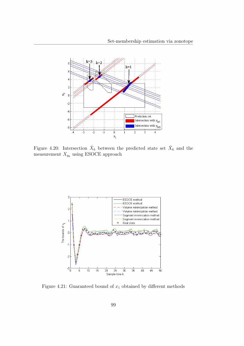
Set-membership estimation via zonotope
Figure 4.20: Intersection Xk between the predicted state set Xk and themeasurement Xyk using ESOCE approach
Figure 4.21: Guaranteed bound of x1 obtained by different methods
99
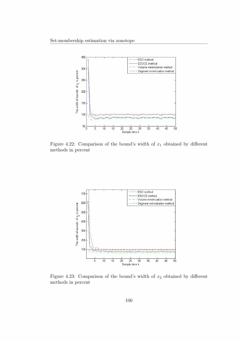
Set-membership estimation via zonotope
Figure 4.22: Comparison of the bound’s width of x1 obtained by differentmethods in percent
Figure 4.23: Comparison of the bound’s width of x2 obtained by differentmethods in percent
100
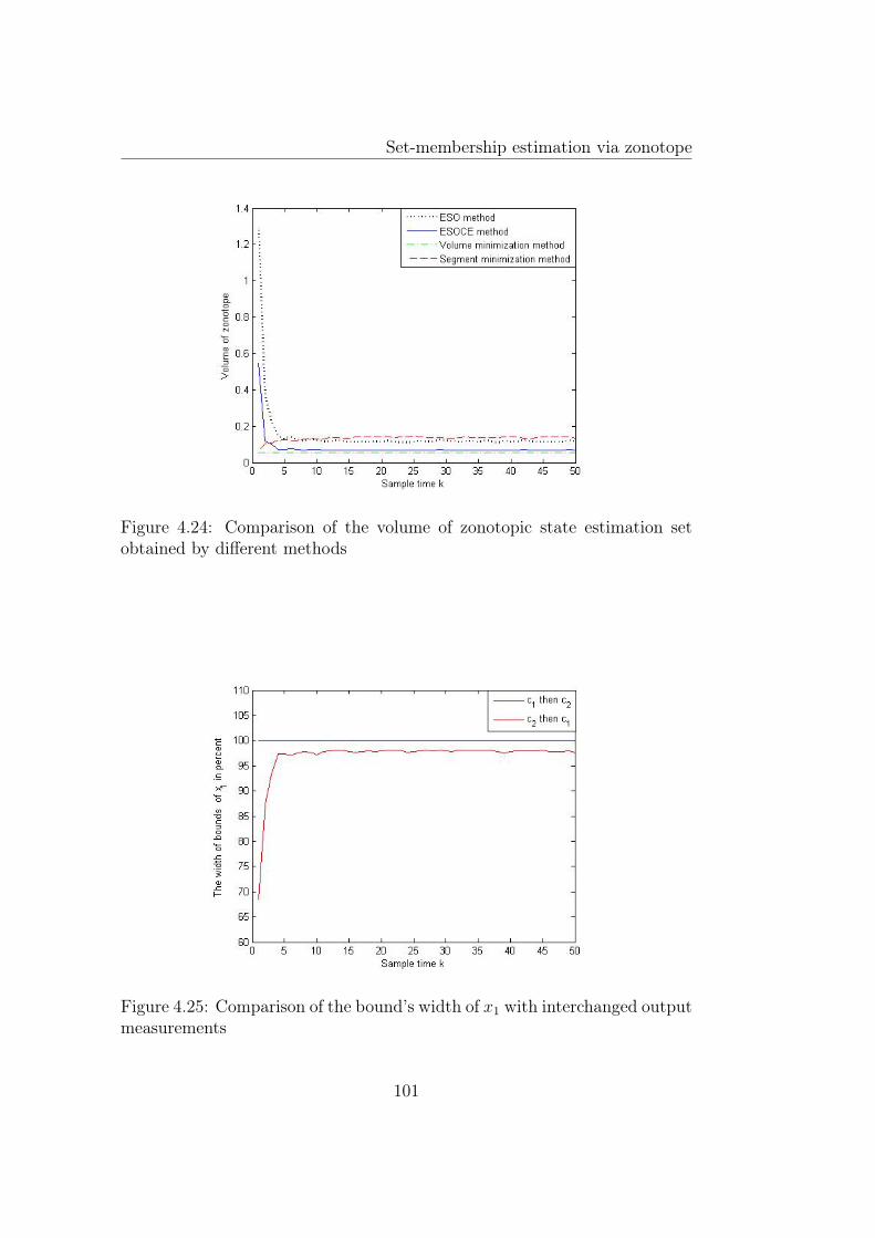
Set-membership estimation via zonotope
Figure 4.24: Comparison of the volume of zonotopic state estimation setobtained by different methods
Figure 4.25: Comparison of the bound’s width of x1 with interchanged outputmeasurements
101
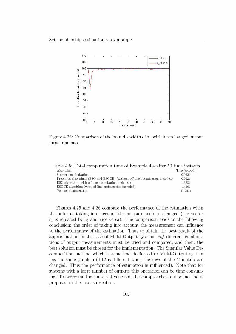
Set-membership estimation via zonotope
Figure 4.26: Comparison of the bound’s width of x2 with interchanged outputmeasurements
Table 4.5: Total computation time of Example 4.4 after 50 time instantsAlgorithm Time(second)Segment minimization 0.0624Presented algorithms (ESO and ESOCE) (without off-line optimization included) 0.0624ESO algorithm (with off-line optimization included) 1.3884ESOCE algorithm (with off-line optimization included) 1.4664Volume minimization 27.2534
Figures 4.25 and 4.26 compare the performance of the estimation whenthe order of taking into account the measurements is changed (the vectorc1 is replaced by c2 and vice versa). The comparison leads to the followingconclusion: the order of taking into account the measurement can influenceto the performance of the estimation. Thus to obtain the best result of theapproximation in the case of Multi-Output systems, ny! different combina-tions of output measurements must be tried and compared, and then, thebest solution must be chosen for the implementation. The Singular Value De-composition method which is a method dedicated to Multi-Output systemhas the same problem (4.12 is different when the rows of the C matrix arechanged. Thus the performance of estimation is influenced). Note that forsystems with a large number of outputs this operation can be time consum-ing. To overcome the conservativeness of these approaches, a new method isproposed in the next subsection.
102
Set-membership estimation via zonotope
4.3.3.4 Polynomial Matrix Inequality approach
In the previous approaches, the vectors λ1, . . ., λny are separately computedwhich can lead to a conservative result. To overcome this problem, thesolution proposed now is to compute λ1, . . ., λny in the same time. All thevectors λi, with i = 1, . . . , ny, are computed such that the condition on thenon-increasing property of the P -radius is ensured. This condition leads toa similar inequality as (4.82), with the modification that j is replaced by ny.
Similar to the ESOCE approach, the following optimization problem isobtained: max
τ,β,P,λ1,...,λny
τ
subject to
(1−β)Pσ21+...+σ
2ny
+ maxs∈Bnx
‖Fs‖22 τI
βP 0 0 ... 0 B1
∗ F TF 0 ... 0 B2
∗ ∗ σ21 ... 0 B3
... ... ... ... ... ...∗ ∗ ∗ ... σ2
nyBny+2
∗ ∗ ∗ ... ∗ P
0
τ > 0
(4.89)
with the notations:
B1 = ((
ny∏i=1
(I − λny+1−icTny+1−i))A)TP
B2 = ((
ny∏i=1
(I − λny+1−icTny+1−i))F )TP
B3 = (
ny−1∏i=1
(I − λny+1−icTny+1−i)σ1λ1)
TP
...Bny = ((I − λnyc
Tny
)(I − λny−1cTny−1)σny−2λny−2)
TP
Bny+1 = ((I − λnycTny
)σny−1λny−1)TP
Bny+2 = (σnyλny)TP
(4.90)
As the vectors λ1, . . ., λny are the unknown variables, the optimization prob-lem (4.89) is not any more a BMI optimization problem as the previoussubsection.
From the definition 3.15 of Polynomial Matrix Inequality, the problem(4.89) is a PMI optimization problem. PMI problems can be solved usingseveral relaxation techniques [31], [61], [72], [64], [62]. In this thesis themethod presented in [62] which is the most recent technique, is chosen to
103
Set-membership estimation via zonotope
solve the PMI optimization problem (4.90). This method is based on aninsertion of lifting variables to reduce the polynomial terms to linear terms.By using these new variables, the PMI problem becomes a LMI problem,which can be easily solved (see [62] for more details).
In the Polynomial Matrix inequality problem (4.89), with the notations(4.90), the decision variables are: P = P T ∈ Rnx×nx , λ1, ..., λny ∈ Rnx andthe scalar β and τ . Thus the total number of scalar decision variables is:nx(nx+1)
2+ nynx + 2. The degree of the PMI (4.89) is ny + 1. This PMI can
be solved by using the first order LMI relaxation methodology [62].
Example 4.5. To better understand, the first order LMI relaxation method[62] is illustrated in the following example:
minx
(x21 − x22)
subject to PMI:[1 + x1x2 x1
x1 1− x21 − x22
] 0
First, the following change of variables is done: y10 = x1, y01 = x2,y20 = x21, y02 = x22, y11 = x1x2.Using these new variables, the PMI optimization problem is relaxed by thefollowing LMIs:minx
(y20 − y02)subject to LMIs:
1 y10 y01∗ y20 y11∗ ∗ y02
0[1 + y11 y10∗ 1− y20 − y02
] 0
(4.91)
Using this technique, the PMI optimization (4.89) can be solved as in thefollowing algorithm:
Algorithm 4.5.
1. All the nx(nx+1)2
+ nynx + 2 scalar decision variables are denoted as fol-lows: τ , y10...0, y01...0, ..., y00...10, y00...01. For expression (4.89), this
leads to β = y100...0, P =
[y01...0 ... y00...1...0... ... ...
], λT1 =
[y00...1...0 ...
],...,
λTny=[y00...1...0 ... y00...01
].
2. The polynomial decision elements in (4.89) are rewritten as the resultof a change of variables based on the previous scalar decision variablessuch as: y20...0 = y10...0 · y10...0, y11...0 = y10...0 · y01...0 etc. In this way,
104

Set-membership estimation via zonotope
expression (4.89) becomes a LMI. If the LMI relaxation of the PMIoptimization problem (4.90) is used, then the following LMI problemmust be solved (see [62] for more details):
105
Set-membership estimation via zonotope
max τsubject to the LMIs
M1 =
1 ∗ ∗ ∗
y10...0 y20...0 ... ∗y01...0 y11...0 ... ∗...
... . . . ...y00..111 ... ... y00...222
0
M2 0
(4.92)
where M1 is called moment matrix and M2 denotes the equivalent LMIexpressions obtained from the PMI in (4.89) using the new scalar de-cision variables (y10...0, y20...0, etc.).
Remark 4.9. Denote l = nx(nx+1)2
+ nynx + 1. As the degree of the PMI in(4.89) is ny + 1, then the dimensions of LMIs (4.92) are:
• M1: q × q, with q = 1 + l +(2l
)+ ...+
(round(
ny+1
2)
l
);
• M2: nx × nx, (3nx + ny)× (3nx + ny) and 1 respectively.
The number of scalar decision variables in this optimization problem is q(q+1)2
.
Remark 4.10. Using the relaxation method proposed in [62] permits torelax the PMI optimization problem to a LMI optimization problem whichis easier to solve. Even if the obtained LMIs problem is solved off-line thismethod leads to a large size LMI problem (see the size of matrix M1 and thenumber of scalar decision variables) which limits its application.
Example 4.6. Consider the following linear discrete time system:xk+1 =
[0 −0.51 1
]xk + 0.02
[−61
]ωk
yk =
[−2 11 1
]xk + 0.2vk
(4.93)
with ‖vk‖∞ ≤ 1, ‖ωk‖∞ ≤ 1. The values of vk and ωk are generated by therandom functions of Matlab R©. The initial state is unknown and belongs tothe box 3B2.
Denote β = y10000000, P =
[y01000000 y00100000∗ y00010000
], λT1 =
[y00001000 y00000100
],
λT2 =[y00000010 y00000001
]. Thus the dimensions of the LMIs of the consid-
ered optimization problem (4.92) are:
106
Set-membership estimation via zonotope
• M1: 37× 37;
• M2: 2× 2, 7× 7 and 1.
As l = 8 and q = 37, the total number of scalar decision variables of the LMIproblem (4.92) is 37·38
2+1 = 704, which is still reasonable for any LMI solver.
Figures 4.27 and 4.28 show the evolution of the predicted state set and theouter approximation of the state estimation set at the time instant k = 1, k =8, respectively. Comparing these figures confirms the contractiveness of theguaranteed state estimation. Figures 4.29, 4.30 show the obtained guaranteedbounds on x1 and x2, respectively. The real states (black star) are foundinside these bounds, which confirms good performance of the estimation.Figure 4.31 shows the evolution of the zonotopic guaranteed state estimation.Note that these guaranteed bounds and the volume of zonotope are decreasedin time leading to a more and more accurate estimation.
Table 4.6 shows the computation time of the PMI approach after 50time instants. Even if the solution of the PMI problem is computed off-line,the computation time of this approach is significantly increased due to thebig number of decision variables in the LMIs problem (4.92) (the reader cancompare Table 4.5 and Table 4.6). Even if the contractiveness property of theguaranteed state estimation is always preserved, the proposed method givesan unsatisfying result of estimation. The poor result of estimation obtainedin this example may be due to the relaxation method used to solve the PMIoptimization problem. To reduce the conservatism of this solution, a higherorder of the LMI relaxation (a higher order ofthe moment matrix M1) canbe used leading to a more complex LMI optimization problem than the firstorder LMI relaxation (see [62]). In the recent paper [63], the author proposedan inner approximation of the PMI set instead of the outer approximation[62] used in this example which can lead to a less conservative result of theguaranteed state estimation.
To conclude, Table 4.6 recapitulates the complexity and the performanceof the proposed approaches to solve the estimation problem for the Multi-Output system, numbers from 1 to 5 being associated to each approach. Thenumber 1 means the best accuracy and the less complexity of the computa-tion. The number 5 means the worst accuracy and the most complex fromthe computation point of view.
107
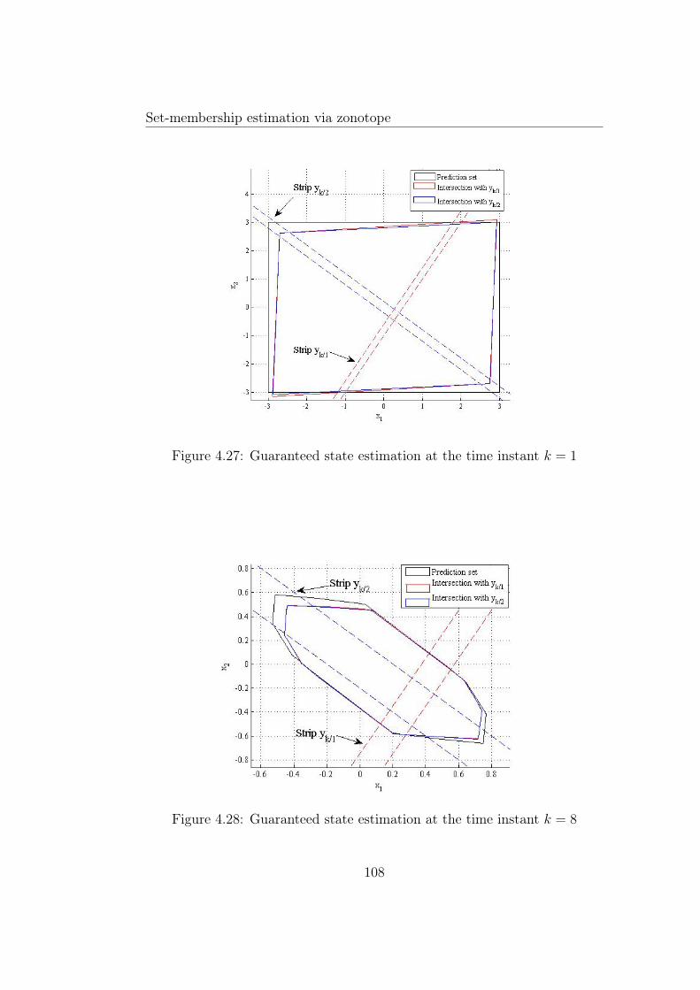
Set-membership estimation via zonotope
Figure 4.27: Guaranteed state estimation at the time instant k = 1
Figure 4.28: Guaranteed state estimation at the time instant k = 8
108
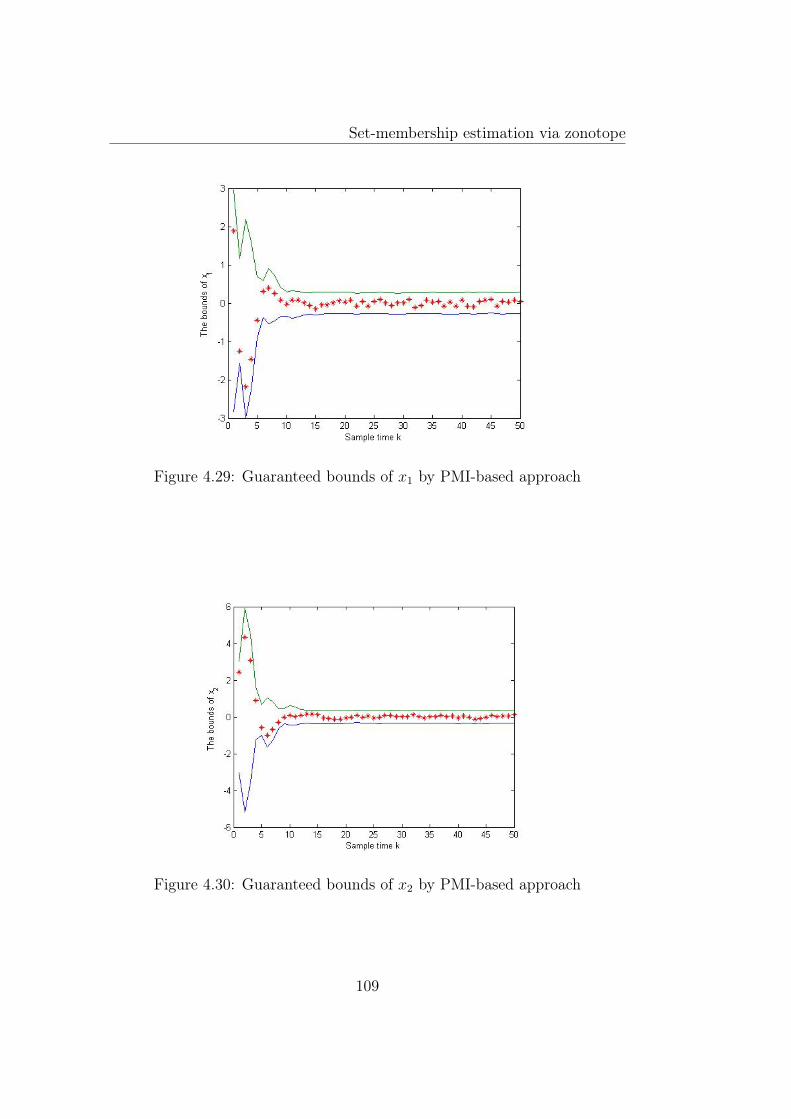
Set-membership estimation via zonotope
Figure 4.29: Guaranteed bounds of x1 by PMI-based approach
Figure 4.30: Guaranteed bounds of x2 by PMI-based approach
109
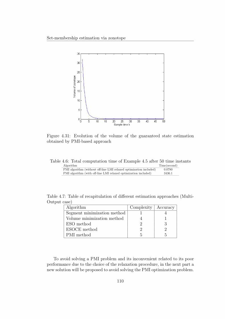
Set-membership estimation via zonotope
Figure 4.31: Evolution of the volume of the guaranteed state estimationobtained by PMI-based approach
Table 4.6: Total computation time of Example 4.5 after 50 time instantsAlgorithm Time(second)PMI algorithm (without off-line LMI relaxed optimization included) 0.0780PMI algorithm (with off-line LMI relaxed optimization included) 3436.1
Table 4.7: Table of recapitulation of different estimation approaches (Multi-Output case)
Algorithm Complexity AccuracySegment minimization method 1 4Volume minimization method 4 1ESO method 2 3ESOCE method 2 2PMI method 5 5
To avoid solving a PMI problem and its inconvenient related to its poorperformance due to the choice of the relaxation procedure, in the next part anew solution will be proposed to avoid solving the PMI optimization problem.
110
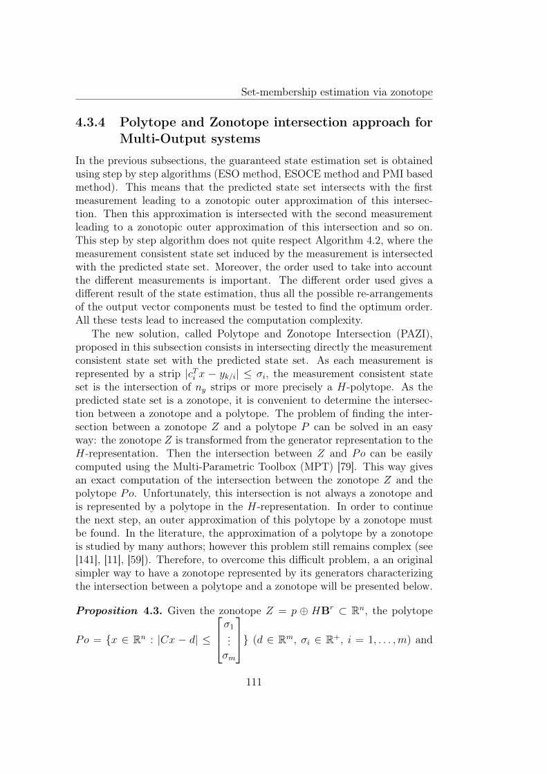
Set-membership estimation via zonotope
4.3.4 Polytope and Zonotope intersection approach forMulti-Output systems
In the previous subsections, the guaranteed state estimation set is obtainedusing step by step algorithms (ESO method, ESOCE method and PMI basedmethod). This means that the predicted state set intersects with the firstmeasurement leading to a zonotopic outer approximation of this intersec-tion. Then this approximation is intersected with the second measurementleading to a zonotopic outer approximation of this intersection and so on.This step by step algorithm does not quite respect Algorithm 4.2, where themeasurement consistent state set induced by the measurement is intersectedwith the predicted state set. Moreover, the order used to take into accountthe different measurements is important. The different order used gives adifferent result of the state estimation, thus all the possible re-arrangementsof the output vector components must be tested to find the optimum order.All these tests lead to increased the computation complexity.
The new solution, called Polytope and Zonotope Intersection (PAZI),proposed in this subsection consists in intersecting directly the measurementconsistent state set with the predicted state set. As each measurement isrepresented by a strip |cTi x − yk/i| ≤ σi, the measurement consistent stateset is the intersection of ny strips or more precisely a H-polytope. As thepredicted state set is a zonotope, it is convenient to determine the intersec-tion between a zonotope and a polytope. The problem of finding the inter-section between a zonotope Z and a polytope P can be solved in an easyway: the zonotope Z is transformed from the generator representation to theH-representation. Then the intersection between Z and Po can be easilycomputed using the Multi-Parametric Toolbox (MPT) [79]. This way givesan exact computation of the intersection between the zonotope Z and thepolytope Po. Unfortunately, this intersection is not always a zonotope andis represented by a polytope in the H-representation. In order to continuethe next step, an outer approximation of this polytope by a zonotope mustbe found. In the literature, the approximation of a polytope by a zonotopeis studied by many authors; however this problem still remains complex (see[141], [11], [59]). Therefore, to overcome this difficult problem, a an originalsimpler way to have a zonotope represented by its generators characterizingthe intersection between a polytope and a zonotope will be presented below.
Proposition 4.3. Given the zonotope Z = p ⊕ HBr ⊂ Rn, the polytope
Po = x ∈ Rn : |Cx − d| ≤
σ1...σm
(d ∈ Rm, σi ∈ R+, i = 1, . . . ,m) and
111
Set-membership estimation via zonotope
the matrix Λ ∈ Rn×m, define a vector p(Λ) = p + Λ(d − Cp) ∈ Rnx and a
matrix H(Λ) =[(I − ΛC)H ΛΣ
]with Σ =
σ1 0 . . . 00 σ2 . . . 0...
... . . . ...0 0 . . . σm
∈ Rm×m
a diagonal matrix . Then a family of zonotopes (parameterized by the matrixΛ) that contains the intersection of the zonotope Z and the polytope Po isobtained such as Z ∩ Po ⊆ Z(Λ) = p(Λ)⊕ H(Λ)Br+m.
Proof Consider an element x ∈ Z ∩ Po, on one hand this means thatx ∈ Z = p ⊕ HBr. Using the definition of a zonotope implies that thereexists a vector s1 ∈ Br such that:
x = p+Hs1 (4.94)
Adding and subtracting ΛCHs1 to the previous equality leads to the followingexpression:
x = p+ ΛCHs1 + (I − ΛC)Hs1 (4.95)
On the other hand, from x ∈ Z ∩ Po, it is inferred that:
x ∈ Pp = x ∈ Rn : |Cx− d| ≤
σ1...σm
(4.96)
Thus, there exists a vector s2 ∈ Bm such that Cx − d = Σs2. Taking intoaccount the form of the vector x given by (4.94) leads to C(p+Hs1)−d = Σs2,which is equivalent to CHs1 = d−Cp+Σs2. Substituting CHs1 in equation(4.95), the following expression is obtained:
x = p+ Λ(d− Cp+ Σs2) + (I − ΛC)Hs1
= p+ Λ(d− Cp) + ΛΣs2 + (I − ΛC)Hs1(4.97)
After simple computations and using the notation defined in Proposition 4.3,the following form is obtained:
x = p(Λ) +[(I − ΛC)H ΛΣ
] [s1s2
]= p(Λ)⊕ H(Λ)
[s1s2
](4.98)
and the following inclusion holds:
x = p(Λ)⊕ H(Λ)
[s1s2
]∈ p(Λ)⊕ H(Λ)Br+m = X(Λ). (4.99)
This proposition is illustrated in the following example.
112
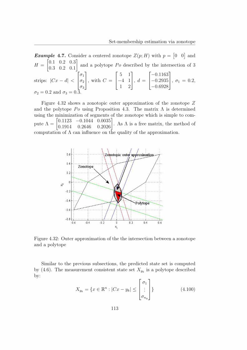
Set-membership estimation via zonotope
Example 4.7. Consider a centered zonotope Z(p;H) with p =[0 0
]and
H =
[0.1 0.2 0.30.3 0.2 0.1
]and a polytope Po described by the intersection of 3
strips: |Cx − d| <
σ1σ2σ3
, with C =
5 1−4 11 2
, d =
−0.1163−0.2935−0.6928
, σ1 = 0.2,
σ2 = 0.2 and σ3 = 0.3.
Figure 4.32 shows a zonotopic outer approximation of the zonotope Zand the polytope Po using Proposition 4.3. The matrix Λ is determinedusing the minimization of segments of the zonotope which is simple to com-
pute Λ =
[0.1123 −0.1044 0.00350.1914 0.2646 0.2026
]. As Λ is a free matrix, the method of
computation of Λ can influence on the quality of the approximation.
Figure 4.32: Outer approximation of the the intersection between a zonotopeand a polytope
Similar to the previous subsections, the predicted state set is computedby (4.6). The measurement consistent state set Xyk is a polytope describedby:
Xyk = x ∈ Rn : |Cx− yk| ≤
σ1...σny
(4.100)
113
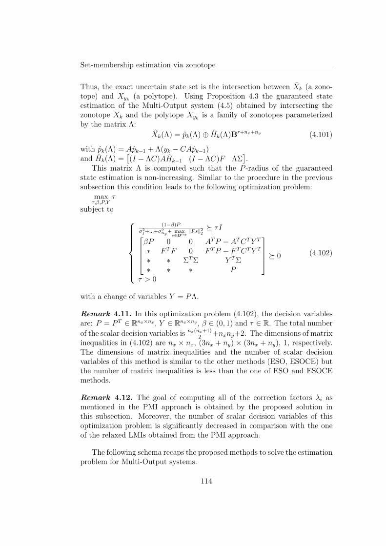
Set-membership estimation via zonotope
Thus, the exact uncertain state set is the intersection between Xk (a zono-tope) and Xyk (a polytope). Using Proposition 4.3 the guaranteed stateestimation of the Multi-Output system (4.5) obtained by intersecting thezonotope Xk and the polytope Xyk is a family of zonotopes parameterizedby the matrix Λ:
Xk(Λ) = pk(Λ)⊕ Hk(Λ)Br+nx+ny (4.101)
with pk(Λ) = Apk−1 + Λ(yk − CApk−1)and Hk(Λ) =
[(I − ΛC)AHk−1 (I − ΛC)F ΛΣ
].
This matrix Λ is computed such that the P -radius of the guaranteedstate estimation is non-increasing. Similar to the procedure in the previoussubsection this condition leads to the following optimization problem:
maxτ,β,P,Y
τ
subject to
(1−β)Pσ21+...+σ
2ny
+ maxs∈Bnx
‖Fs‖22 τI
βP 0 0 ATP − ATCTY T
∗ F TF 0 F TP − F TCTY T
∗ ∗ ΣTΣ Y TΣ∗ ∗ ∗ P
0
τ > 0
(4.102)
with a change of variables Y = PΛ.
Remark 4.11. In this optimization problem (4.102), the decision variablesare: P = P T ∈ Rnx×nx , Y ∈ Rnx×ny , β ∈ (0, 1) and τ ∈ R. The total numberof the scalar decision variables is nx(nx+1)
2+nxny+2. The dimensions of matrix
inequalities in (4.102) are nx × nx, (3nx + ny) × (3nx + ny), 1, respectively.The dimensions of matrix inequalities and the number of scalar decisionvariables of this method is similar to the other methods (ESO, ESOCE) butthe number of matrix inequalities is less than the one of ESO and ESOCEmethods.
Remark 4.12. The goal of computing all of the correction factors λi asmentioned in the PMI approach is obtained by the proposed solution inthis subsection. Moreover, the number of scalar decision variables of thisoptimization problem is significantly decreased in comparison with the oneof the relaxed LMIs obtained from the PMI approach.
The following schema recaps the proposed methods to solve the estimationproblem for Multi-Output systems.
114
Set-membership estimation via zonotope
Example 4.8. Consider the following linear variant Multi-Output system:xk+1 =
[0 −0.51 1 + 0.3δ
]xk +
[0.1 00 0.1
]ωk
yk =
[−2 11 1
]xk +
[0.2 00 0.2
]vk
(4.103)
The disturbances and the noises are always considered bounded by wk, vk∈ B2. The initial state is unknown but belongs to the box 3B2. The pro-posed method PAZI will be compared with the Singular Value Decompositionmethod [37], and the ESOCE method. Note that, the comparison is doneonly with the Singular Value Decomposition method because in the literatureonly this method can solve the case of Multi-Output systems.
The solution of the PAZI approach (4.102) obtained by Penbmi solver
gives β = 0.0452, Λ =
[−0.3136 0.26780.3591 0.5811
]and the solution of Algorithm 4.4
is λ1 =
[−0.21080.5784
], λ2 =
[0.29460.5420
].
The simulation results are shown in Figures 4.33, 4.34, 4.35. The guar-anteed state estimation obtained by the PAZI method is quickly decreasedat each sample time (Figure 4.33). Figures 4.34 and 4.35 compare the per-formance of the proposed method with the one of the Singular Value De-composition method (Subsection 4.2.1 and [37]) and the one of the ESOCEmethod. The bound obtained by the proposed method are smaller (com-pared in percent) than the one obtained by the singular value decompositionmethod with a reduced complexity of the computation (see Table 4.8). More-over, this polytope intersection solution obtains a similar performance of theestimation as the performance of the ESOCE method but the computationtime is significantly decreased (0.2808s and 1.4464s comparing the result ofTable 4.8).
Table 4.8: Total computation time of Example 4.6 after 50 time instantsAlgorithm Time(second)Polytope and Zonotope Intersection algorithm (without off-line optimization included) 0.0468Polytope and Zonotope Intersection algorithm (with off-line optimization included) 0.2808Singular Value Decomposition algorithm [37] 1.5444
115
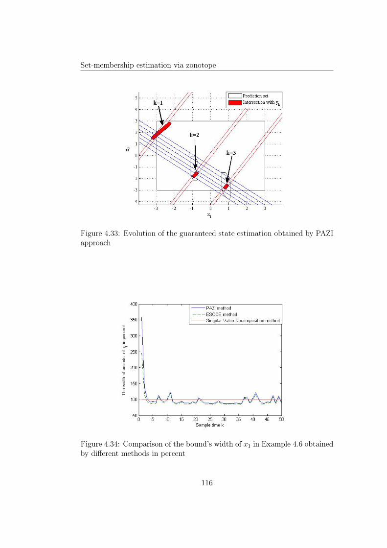
Set-membership estimation via zonotope
Figure 4.33: Evolution of the guaranteed state estimation obtained by PAZIapproach
Figure 4.34: Comparison of the bound’s width of x1 in Example 4.6 obtainedby different methods in percent
116
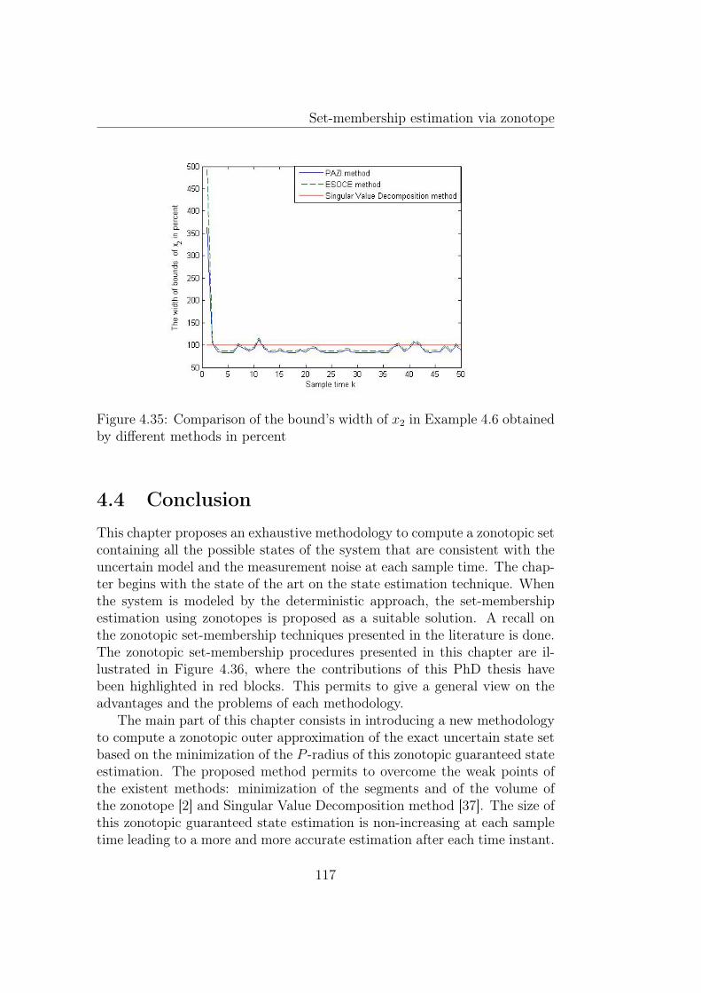
Set-membership estimation via zonotope
Figure 4.35: Comparison of the bound’s width of x2 in Example 4.6 obtainedby different methods in percent
4.4 ConclusionThis chapter proposes an exhaustive methodology to compute a zonotopic setcontaining all the possible states of the system that are consistent with theuncertain model and the measurement noise at each sample time. The chap-ter begins with the state of the art on the state estimation technique. Whenthe system is modeled by the deterministic approach, the set-membershipestimation using zonotopes is proposed as a suitable solution. A recall onthe zonotopic set-membership techniques presented in the literature is done.The zonotopic set-membership procedures presented in this chapter are il-lustrated in Figure 4.36, where the contributions of this PhD thesis havebeen highlighted in red blocks. This permits to give a general view on theadvantages and the problems of each methodology.
The main part of this chapter consists in introducing a new methodologyto compute a zonotopic outer approximation of the exact uncertain state setbased on the minimization of the P -radius of this zonotopic guaranteed stateestimation. The proposed method permits to overcome the weak points ofthe existent methods: minimization of the segments and of the volume ofthe zonotope [2] and Singular Value Decomposition method [37]. The size ofthis zonotopic guaranteed state estimation is non-increasing at each sampletime leading to a more and more accurate estimation after each time instant.
117
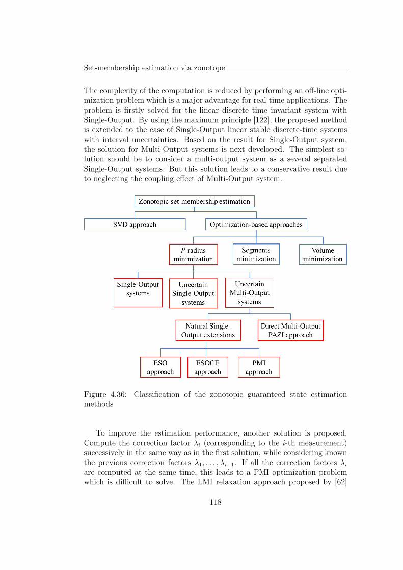
Set-membership estimation via zonotope
The complexity of the computation is reduced by performing an off-line opti-mization problem which is a major advantage for real-time applications. Theproblem is firstly solved for the linear discrete time invariant system withSingle-Output. By using the maximum principle [122], the proposed methodis extended to the case of Single-Output linear stable discrete-time systemswith interval uncertainties. Based on the result for Single-Output system,the solution for Multi-Output systems is next developed. The simplest so-lution should be to consider a multi-output system as a several separatedSingle-Output systems. But this solution leads to a conservative result dueto neglecting the coupling effect of Multi-Output system.
Figure 4.36: Classification of the zonotopic guaranteed state estimationmethods
To improve the estimation performance, another solution is proposed.Compute the correction factor λi (corresponding to the i-th measurement)successively in the same way as in the first solution, while considering knownthe previous correction factors λ1, . . . , λi−1. If all the correction factors λiare computed at the same time, this leads to a PMI optimization problemwhich is difficult to solve. The LMI relaxation approach proposed by [62]
118
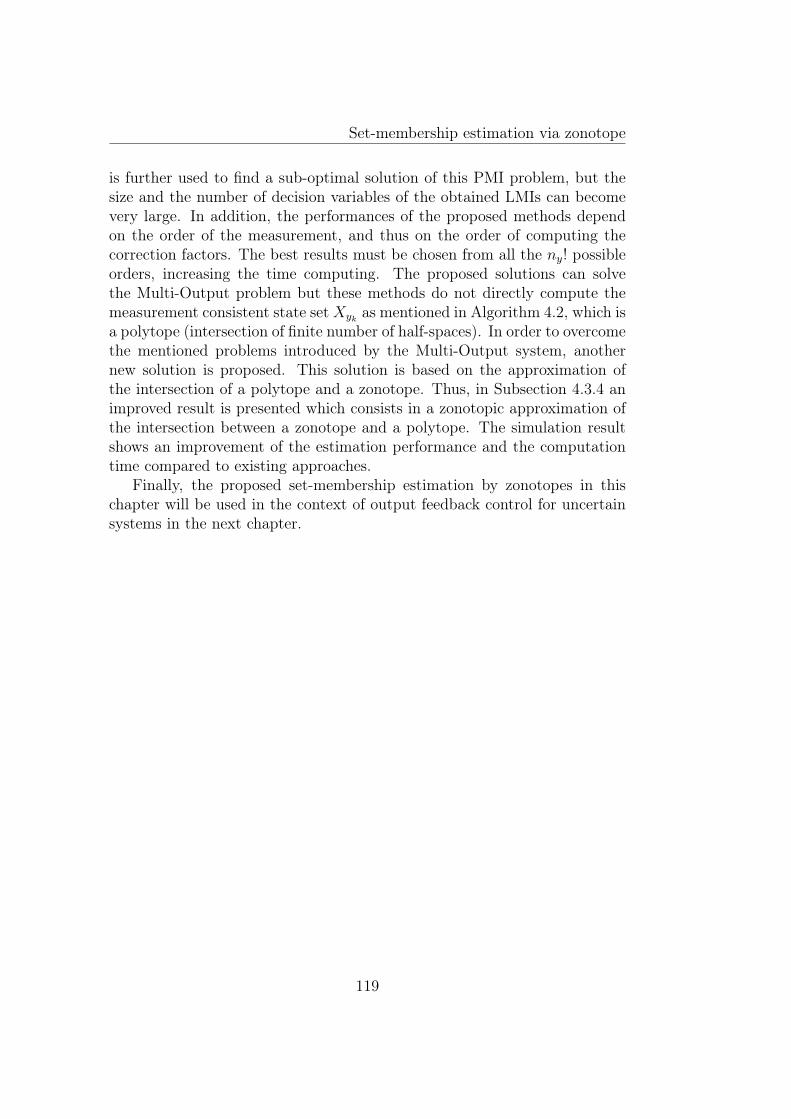
Set-membership estimation via zonotope
is further used to find a sub-optimal solution of this PMI problem, but thesize and the number of decision variables of the obtained LMIs can becomevery large. In addition, the performances of the proposed methods dependon the order of the measurement, and thus on the order of computing thecorrection factors. The best results must be chosen from all the ny! possibleorders, increasing the time computing. The proposed solutions can solvethe Multi-Output problem but these methods do not directly compute themeasurement consistent state setXyk as mentioned in Algorithm 4.2, which isa polytope (intersection of finite number of half-spaces). In order to overcomethe mentioned problems introduced by the Multi-Output system, anothernew solution is proposed. This solution is based on the approximation ofthe intersection of a polytope and a zonotope. Thus, in Subsection 4.3.4 animproved result is presented which consists in a zonotopic approximation ofthe intersection between a zonotope and a polytope. The simulation resultshows an improvement of the estimation performance and the computationtime compared to existing approaches.
Finally, the proposed set-membership estimation by zonotopes in thischapter will be used in the context of output feedback control for uncertainsystems in the next chapter.
119

Set-membership estimation via zonotope
120
Chapter 5
Model Predictive Control basedon zonotopic set-membershipestimation
5.1 IntroductionModel Predictive Control (MPC) can be considered today as a mature do-main, both from the research and the industrial applications points of view.The application of MPC can be found in many industrial processes (e.g.petroleum industry [49], aerospace [21]), specially when the trajectory to betracked by the system is given in advance, such as the trajectory of a robotarm [34]. The large application of MPC [117] is mainly due to an easy im-plementation, a generic solution that can deal both with SISO and MIMOsystems and, the most important, to its ability to handle hard constraints,which often appear when dealing with real plants [29], [54]. The strategy ofMPC can be decomposed into three steps:
1. Based on the appropriate system model the system output is predictedat a future time horizon;
2. A control sequence is computed by optimizing an objective function onthe future behavior of the system, and then only the first element ofthe control sequence is applied;
3. The horizon is receded into the future, and the computation is repeatedat the next time instant.
Due to the receding strategy, the MPC is also called receding horizon pre-dictive control or moving horizon control. From this algorithm, it must be
121
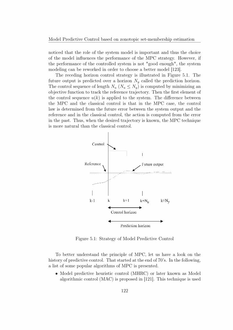
Model Predictive Control based on zonotopic set-membership estimation
noticed that the role of the system model is important and thus the choiceof the model influences the performance of the MPC strategy. However, ifthe performance of the controlled system is not "good enough", the systemmodeling can be reworked in order to choose a better model [123].
The receding horizon control strategy is illustrated in Figure 5.1. Thefuture output is predicted over a horizon Ny called the prediction horizon.The control sequence of length Nu (Nu ≤ Ny) is computed by minimizing anobjective function to track the reference trajectory. Then the first element ofthe control sequence u(k) is applied to the system. The difference betweenthe MPC and the classical control is that in the MPC case, the controllaw is determined from the future error between the system output and thereference and in the classical control, the action is computed from the errorin the past. Thus, when the desired trajectory is known, the MPC techniqueis more natural than the classical control.
Figure 5.1: Strategy of Model Predictive Control
To better understand the principle of MPC, let us have a look on thehistory of predictive control. That started at the end of 70’s. In the following,a list of some popular algorithms of MPC is presented.
• Model predictive heuristic control (MHRC) or later known as Modelalgorithmic control (MAC) is proposed in [121]. This technique is used
122
Model Predictive Control based on zonotopic set-membership estimation
to control a multivariable industrial process. The control which is basedon an impulse response model is computed by minimizing the trackingerror.
• Dynamic Matrix Control (DMC) proposed in [41] uses the step responseto predict the trajectory of the future output and then minimizes theprediction error.
• Extended Horizon Adaptive Control (EHAC) is developed in [149] basedon a parametric process model. This strategy elaborates a control se-quence in order to minimize the error between the reference and thefuture output which is computed by solving a Diophantine equation ata period of time after the process delay.
• Extended Prediction Self-Adaptive Control (EPSAC) proposed by DeKeyser and Van Cauwenberghe in [43] uses a discrete transfer func-tion and a constant control signal while using a sub-optimal predictorinstead of solving a Diophantine equation used in EHAC method.
• Generalized Predictive Control (GPC) is one of the most popular ap-proaches proposed in [35]. This technique is based on a ControlledAuto-Regressive Integrated Moving Average (CARIMA) model whichcan track both varying and constant future set-points. There are someother predictive controllers based on the same idea such as: Predic-tive Functional Control (PFC) [121], Multipredictor Receding HorizonAdaptive Control (MURHAC) [90], Multistep Multivariable AdaptiveControl (MUSMAR) [55], Unified Predictive Control (UPC) [133].
• Constrained Receding Horizon Predictive Control (CRHPC) developedby Clarke and Scatollini in [36] imposes an additional terminal equalityconstraints on the output over a finite horizon beyond the predictionhorizon.
• State-space Model Predictive Control is a mature predictive controltechnique [108] based on the use of a state-space model. This modelfacilitates the stability study [70], [128], [101] and the generalization ofMPC to multivariable systems, non-linear systems and systems withdisturbances and measurement noises. Moreover, when the systemstate is not available as mentioned in the previous chapter, it is moreconvenient to implement a state estimation (Luenberger observer,Kalman filter, set-membership estimation).
123
Model Predictive Control based on zonotopic set-membership estimation
Due to the existence of uncertainties in the mathematical model, the robust-ness of the MPC became a key problem. The robust MPC in the presence ofuncertainties and disturbances is studied by many authors [30], [73], [146],[96], [17] [101], [80], [102], [100], [33], [111], [135]. A simple way to deal withthe model uncertainty is to take into account these uncertainties in the op-timization problem, it means that the online optimization problem on theobjective function is transformed into a min-max problem with constraints(the worst case of the objective function is computed on the uncertaintyset and then this value of the worst case is minimized) [30]. In [73] and[146], an upper-bound of the worst case is determined and then the min-max problem is transformed to a LMI optimization problem. To simplifythe computation, [4] proposed a sub-optimal solution based on a quadraticprogramming (QP) problem. Other ways to enhance robustness are based onthe deterministic model predictive control by ignoring the disturbances overthe prediction horizon [129], [33], [92], [102], [100]. These methods requirefull knowledge of the state which usually cannot be reached due to measure-ment noises acting on real systems. In [146], [100], the Luenberger observeris implemented to estimate the system state. In the previous chapter, theset-membership estimation has proven its efficiency in estimating the systemstate in the presence of uncertainties. In addition, in [17], the author usedthe set-membership estimation based on parallelotopes to estimate the state.Due to the efficiency of the zonotopes, in this chapter the application of theset-membership estimation using zonotopes in the context of robust MPC isconsidered.
5.2 General set-upConsider the general description of a Multi-Output linear discrete-time in-variant system:
xk+1 = Axk +Buk + Fωkyk = Cxk + vk
(5.1)
where xk ∈ Rnx is the state of the system, yk ∈ Rny is the measured output attime instant k. The vector ωk ∈ Rnx represents the state perturbation vectorand vk ∈ Rny is the measurement noise. It is assumed that the uncertaintiesand the initial state are bounded by the following sets: ωk ∈ W , vk ∈ Vand x0 ∈ X0, with W a zonotope containing the origin, V a box and X0 azonotope.
The system (5.1) is subject to state and input constraints: xk ∈ X,uk ∈ U , where X and U are two compact and convex sets containing theorigin as an interior point. It is assumed that system (5.1) is stabilizable and
124
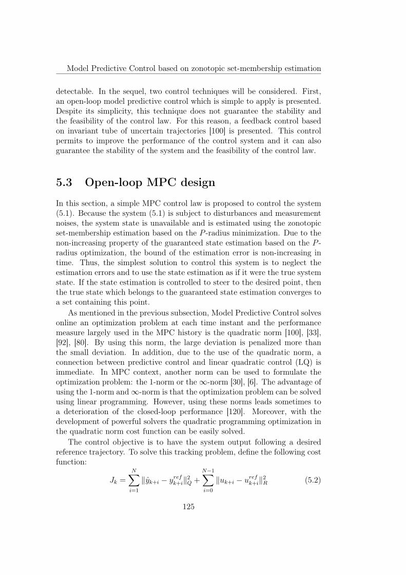
Model Predictive Control based on zonotopic set-membership estimation
detectable. In the sequel, two control techniques will be considered. First,an open-loop model predictive control which is simple to apply is presented.Despite its simplicity, this technique does not guarantee the stability andthe feasibility of the control law. For this reason, a feedback control basedon invariant tube of uncertain trajectories [100] is presented. This controlpermits to improve the performance of the control system and it can alsoguarantee the stability of the system and the feasibility of the control law.
5.3 Open-loop MPC design
In this section, a simple MPC control law is proposed to control the system(5.1). Because the system (5.1) is subject to disturbances and measurementnoises, the system state is unavailable and is estimated using the zonotopicset-membership estimation based on the P -radius minimization. Due to thenon-increasing property of the guaranteed state estimation based on the P -radius optimization, the bound of the estimation error is non-increasing intime. Thus, the simplest solution to control this system is to neglect theestimation errors and to use the state estimation as if it were the true systemstate. If the state estimation is controlled to steer to the desired point, thenthe true state which belongs to the guaranteed state estimation converges toa set containing this point.
As mentioned in the previous subsection, Model Predictive Control solvesonline an optimization problem at each time instant and the performancemeasure largely used in the MPC history is the quadratic norm [100], [33],[92], [80]. By using this norm, the large deviation is penalized more thanthe small deviation. In addition, due to the use of the quadratic norm, aconnection between predictive control and linear quadratic control (LQ) isimmediate. In MPC context, another norm can be used to formulate theoptimization problem: the 1-norm or the∞-norm [30], [6]. The advantage ofusing the 1-norm and∞-norm is that the optimization problem can be solvedusing linear programming. However, using these norms leads sometimes toa deterioration of the closed-loop performance [120]. Moreover, with thedevelopment of powerful solvers the quadratic programming optimization inthe quadratic norm cost function can be easily solved.
The control objective is to have the system output following a desiredreference trajectory. To solve this tracking problem, define the following costfunction:
Jk =N∑i=1
‖yk+i − yrefk+i‖2Q +
N−1∑i=0
‖uk+i − urefk+i‖2R (5.2)
125
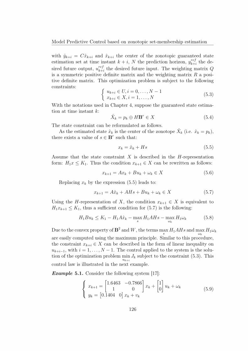
Model Predictive Control based on zonotopic set-membership estimation
with yk+i = Cxk+i and xk+i the center of the zonotopic guaranteed stateestimation set at time instant k + i, N the prediction horizon, yrefk+i the de-sired future output, urefk+i the desired future input. The weighting matrix Qis a symmetric positive definite matrix and the weighting matrix R a posi-tive definite matrix. This optimization problem is subject to the followingconstraints:
uk+i ∈ U, i = 0, . . . , N − 1xk+i ∈ X, i = 1, . . . , N
(5.3)
With the notations used in Chapter 4, suppose the guaranteed state estima-tion at time instant k:
Xk = pk ⊕HBr ∈ X (5.4)
The state constraint can be reformulated as follows.As the estimated state xk is the center of the zonotope Xk (i.e. xk = pk),
there exists a value of s ∈ Br such that:
xk = xk +Hs (5.5)
Assume that the state constraint X is described in the H-representationform: H1x ≤ K1. Thus the condition xk+1 ∈ X can be rewritten as follows:
xk+1 = Axk +Buk + ωk ∈ X (5.6)
Replacing xk by the expression (5.5) leads to:
xk+1 = Axk + AHs+Buk + ωk ∈ X (5.7)
Using the H-representation of X, the condition xk+1 ∈ X is equivalent toH1xk+1 ≤ K1, thus a sufficient condition for (5.7) is the following:
H1Buk ≤ K1 −H1Axk −maxsH1AHs−max
ωk
H1ωk (5.8)
Due to the convex property ofB2 andW , the terms maxsH1AHs and max
ωk
H1ωk
are easily computed using the maximum principle. Similar to this procedure,the constraint xk+i ∈ X can be described in the form of linear inequality onuk+i−1, with i = 1, . . . , N − 1. The control applied to the system is the solu-tion of the optimization problem min
uk+i
Jk subject to the constraint (5.3). This
control law is illustrated in the next example.
Example 5.1. Consider the following system [17]: xk+1 =
[1.6463 −0.7866
1 0
]xk +
[10
]uk + ωk
yk =[0.1404 0
]xk + vk
(5.9)
126
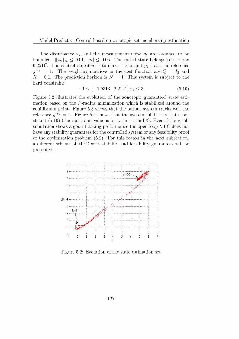
Model Predictive Control based on zonotopic set-membership estimation
The disturbance ωk and the measurement noise vk are assumed to bebounded: ‖ωk‖∞ ≤ 0.01, |vk| ≤ 0.05. The initial state belongs to the box0.25B2. The control objective is to make the output yk track the referenceyref = 1. The weighting matrices in the cost function are Q = I2 andR = 0.1. The prediction horizon is N = 4. This system is subject to thehard constraint:
−1 ≤[−1.9313 2.2121
]xk ≤ 3 (5.10)
Figure 5.2 illustrates the evolution of the zonotopic guaranteed state esti-mation based on the P -radius minimization which is stabilized around theequilibrium point. Figure 5.3 shows that the output system tracks well thereference yref = 1. Figure 5.4 shows that the system fulfills the state con-straint (5.10) (the constraint value is between −1 and 3). Even if the resultsimulation shows a good tracking performance the open loop MPC does nothave any stability guarantees for the controlled system or any feasibility proofof the optimization problem (5.2). For this reason in the next subsection,a different scheme of MPC with stability and feasibility guarantees will bepresented.
Figure 5.2: Evolution of the state estimation set
127
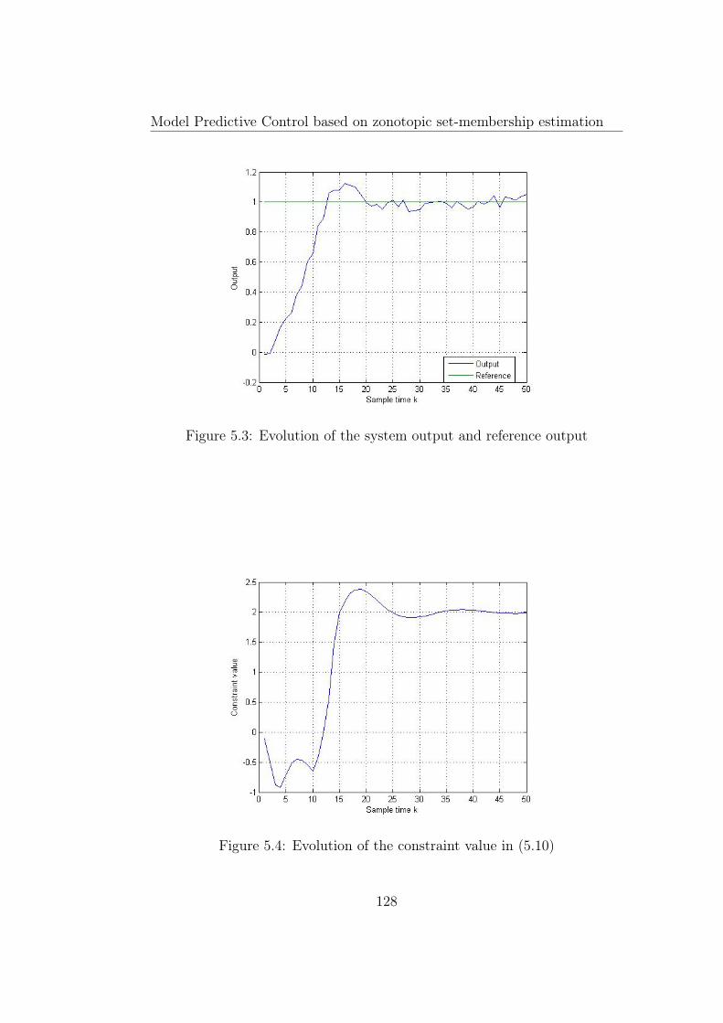
Model Predictive Control based on zonotopic set-membership estimation
Figure 5.3: Evolution of the system output and reference output
Figure 5.4: Evolution of the constraint value in (5.10)
128
Model Predictive Control based on zonotopic set-membership estimation
5.4 Tube-based output feedback MPC design
Different to the proposed control law in the previous section, which is anopen-loop MPC control, in this section another MPC technique is proposedbased on feedback control, which can be less conservative specially when un-certainties are present [89], [16], [18], [101]. In feedback MPC, the decisionvariable is a control policy, which is a sequence of control laws. In this sec-tion, a feedback MPC, called Tube-based Model Predictive Control (TMPC),is presented. The idea of the TMPC is to construct a tube of all the possibletrajectories around the nominal trajectory ensuring robust constraints satis-faction and stability guarantees of the controlled system, using invariant settechniques. During the last years, the TMPC has been investigated by manyauthors: [80], [33], [102], [92], [91], [100]. In the following part, the TMPCdeveloped in [102], [100] will be summarized. In this approach, the opti-mization problem of the true system state is replaced by the nominal stateone (the state of the nominal system which is not influenced by disturbancesand measurement noises). In addition, the nominal state is considered asa decision variable in the optimal control problem solved online. This con-sideration permits to facilitate the proof of stability and attractivity of theterminal set. Moreover, the complexity of the controller is similar to thatrequired for nominal MPC. This technique is developed for LTI systems withthe hypothesis that the system states are known [102]. When the systemstate is unknown, the state is estimated using an observer. Then the esti-mation error is considered as unknown but bounded uncertainty which canbe taken into account in the control law. In [100] the Luenberger observeris used to estimate the system state. The gain matrix of the Luenbergerobserver plays an important role for the performances of the observer, andthus the global performance of the controlled system. The main difficultycomes from the fact that the choice of this gain matrix is not unique. Forthis reason, in this section the set-membership estimation presented in theprevious chapter is chosen to replace the Luenberger observer to combinewith the TMPC. By using this zonotopic set membership estimation, thebound of the error estimation is minimized and, thus, the performance of thecontrolled system is improved.
Note that for pedagogical reason the same notations as in [100] have beenused. Consider now the system (5.1), due to the presence of the disturbancesand the measurement noise, the system state is estimated using the zonotopicguaranteed state estimation presented in the previous chapter. The centerof the zonotopic guaranteed state estimation at time instant k is consideredas the estimation state at time instant k: xk = pk. Similar to the equation(4.93) with the added control law uk, the dynamics of the estimation state
129
Model Predictive Control based on zonotopic set-membership estimation
is determined by the following equation:
xk+1 = Axk +Buk + Λ(yk+1 − yk+1)
= Axk +Buk + Λ(yk+1 − C(Axk +Buk))(5.11)
Replacing yk+1 = Cxk+1+vk+1, with xk+1 = Axk+Buk+ωk, this is equivalentto:
xk+1 = Axk +Buk + Λ(CAxk + CBuk + Cωk + vk+1 − CAxk − CBuk)= Axk +Buk + ΛCA(xk − xk) + ΛCωk + Λvk+1
(5.12)
Denote the estimation error as xk = xk − xk, from the equations (5.1) and(5.12) the dynamics of the estimation error is described by:
xk+1 = (I − ΛC)Axk + ωek (5.13)
with ωek = (I − ΛC)ωk − Λvk+1. From the hypotheses ωk ∈ W , vk ∈ V , thefollowing expression holds:
ωek ∈ W e = (I − ΛC)W ⊕ (−ΛV ) (5.14)
Consider that the estimation error at time instant k is bounded by a set Sek,the equation (5.13) leads to the following recursive expression:
xk+1 ∈ Sek+1 = (I − ΛC)ASek ⊕W e (5.15)
In order to ensure the stability of the controlled system, the estimation errormust be taken into account in the control law. The main idea behind thedesign of the TMPC control law comes from the non-increasing property ofthe set Sek+1 which bounds the future estimation error. In the following, thisproperty is provided by the robust positive invariance of the set Sek+1, whichis defined in the following.
Definition 5.1. [22] A set Ω is called robust positive invariant set for thesystem xk+1 = Axk + ωk subject to the constraints (xk, ωk) ∈ (X,W ), ifAxk + ωk ∈ Ω and Ω ∈ X, ∀ωk ⊆ W and ∀xk ∈ Ω.
Thus, the maximal robust positive invariant set Ωmax for the same sys-tem is the smallest robust positive invariant set that contains all the robustpositive invariant sets of this system. The minimal robust positive invariantset Ωmin of the same system is the robust positive invariant set which iscontained in any robust positive invariant set of this system.
130
Model Predictive Control based on zonotopic set-membership estimation
Proposition 5.1. [100] If the set Se0 is robust positively invariant for thesystem (5.13), then the sets Sek are robust positively invariant for the sys-tem (5.13), too. The set sequence Sek is monotonic non-increasing andconverges in the Hausdorff metric to a robust positively invariant set Se∞ =(I − ΛC)ASe∞ ⊕W e.
Denote that the original idea behind the use of the zonotopic set member-ship estimation in this PhD work in comparison with the use of Luenbergerobserver in [100] is that the matrix Λ is computed to optimize the size of theset Se∞.
The observer equation can be rewritten as:
xk+1 = Axk +Buk + ωcok (5.16)
with ωcok = Λ(CAxk + Cωk + vk+1). As xk ∈ Sek, the following expression istrue:
ωcok ∈ W cok = ΛCASek ⊕ ΛCW ⊕ ΛV (5.17)
Because the set sequence Sek is monotonic non-increasing as presented inProposition 5.1 and W co
k is linearly dependent on Sek, thus the set sequenceW co
k is monotonic non-increasing, too.Consider now the nominal system which is not affected by disturbances:
xk+1 = Axk +Buk (5.18)
To counteract the disturbances, the trajectory of the real system is desiredto lie close to the nominal system trajectory. If the nominal system is steeredto the origin, then the center of the zonotopic state estimation as well as thereal state of the system are bounded by a compact set. In order to haveall the possible trajectories inside a tube around the nominal trajectory, acontrol law uk can be defined as:
uk = uk +K(xk − xk) (5.19)
where uk is the control law applied to the nominal system (5.18) at timeinstant k.
Combining (5.16) and (5.18), the error between the estimation state andthe nominal state denoted by ek = xk − xk satisfies the difference equation:
ek+1 = xk+1 − xk+1
= (Axk +Buk + wcok )− (Axk +Buk)(5.20)
Replacing uk by (5.19), ek+1 can be further written as:
ek+1 = (A+BK)ek + wcok (5.21)
131
Model Predictive Control based on zonotopic set-membership estimation
The gain matrix K is chosen such that the matrix A + BK is Schur stable.Consequently, if at time k, ek lies in the set Scok , then ek+1 lies in the setScok+1 = (A+BK)Scok ⊕W co
k .
Proposition 5.2. [100] If e0 belongs to an initial set Sco0 , then the set se-quence Scok converges to a robust positive invariant set Sco∞ which satisfiesSco∞ = (A + BK)Sco∞ ⊕ W co
∞ . If Se0 is robust positive invariant for the sys-tem (5.13) and Sco0 is robust positive invariant for the system (5.21) withωco0 ∈ W co
0 , then the set sequence Scok is robust positive invariant for thesystem (5.21) with ωcok ∈ W co
k and monotonic non-increasing (Scok+1 ⊆ Scok ).
Based on the procedure proposed in [100], let us define Sk = Sek ⊕ Scok .Because Sek and Scok converge to Se∞ and Sco∞, respectively, then Sk tends toS∞ = Se∞ ⊕ Sco∞.
In this context, the robust TMPC can be summarized as follows. At timek a state estimation set is computed and a nominal optimal control problemis solved online. Define the cost function for the nominal system as:
VN(xk, u) =1
2Vf (xk+N) +
N−1∑i=0
1
2l(xk+i, uk+i) (5.22)
where N is the prediction horizon and u is the control sequence:
u = uk, uk+1, . . . , uk+N−1 (5.23)
The stage cost function l(xk, uk) and the terminal cost function Vf (xk+N) aredefined by:
l(xk, uk) = 12(xTkQxk + uTkRuk)
Vf (xk+N) = 12xTk+NPfxk+N
(5.24)
where Pf , Q, R are positive definite matrices. With these notations, the timevarying constraints at current time k are:
uk+i ∈ Uk+i, i = 0, . . . , N − 1xk+i ∈ Xk+i, i = 0, . . . , N − 1xk+N ∈ Xf
(5.25)
with Uk+i = UKScok+i (this tight constraint comes from the equation (5.19)),Xk+i = XSk+i (this constraint comes from the fact that xk = xk+ xk+ek).
To ensure the feasibility and the stability of this control law, the followingconditions are assumed [100].
Assumption 5.1. Consider S0 = Sco0 ⊕ Se0 ⊂ X and KSco0 ⊂ U .
132
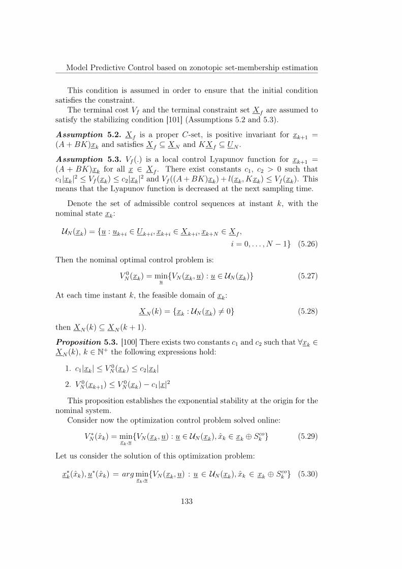
Model Predictive Control based on zonotopic set-membership estimation
This condition is assumed in order to ensure that the initial conditionsatisfies the constraint.
The terminal cost Vf and the terminal constraint set Xf are assumed tosatisfy the stabilizing condition [101] (Assumptions 5.2 and 5.3).
Assumption 5.2. Xf is a proper C-set, is positive invariant for xk+1 =(A+BK)xk and satisfies Xf ⊆ XN and KXf ⊆ UN .
Assumption 5.3. Vf (.) is a local control Lyapunov function for xk+1 =(A + BK)xk for all x ∈ Xf . There exist constants c1, c2 > 0 such thatc1|xk|2 ≤ Vf (xk) ≤ c2|xk|2 and Vf ((A+BK)xk) + l(xk, Kxk) ≤ Vf (xk). Thismeans that the Lyapunov function is decreased at the next sampling time.
Denote the set of admissible control sequences at instant k, with thenominal state xk:
UN(xk) = u : uk+i ∈ Uk+i, xk+i ∈ Xk+i, xk+N ∈ Xf ,
i = 0, . . . , N − 1 (5.26)
Then the nominal optimal control problem is:
V 0N(xk) = min
uVN(xk, u) : u ∈ UN(xk) (5.27)
At each time instant k, the feasible domain of xk:
XN(k) = xk : UN(xk) 6= 0 (5.28)
then XN(k) ⊆ XN(k + 1).
Proposition 5.3. [100] There exists two constants c1 and c2 such that ∀xk ∈XN(k), k ∈ N+ the following expressions hold:
1. c1|xk| ≤ V 0N(xk) ≤ c2|xk|
2. V 0N(xk+1) ≤ V 0
N(xk)− c1|x|2
This proposition establishes the exponential stability at the origin for thenominal system.
Consider now the optimization control problem solved online:
V ∗N(xk) = minxk,uVN(xk, u) : u ∈ UN(xk), xk ∈ xk ⊕ Scok (5.29)
Let us consider the solution of this optimization problem:
x∗k(xk), u∗(xk) = argmin
xk,uVN(xk, u) : u ∈ UN(xk), xk ∈ xk ⊕ Scok (5.30)
133
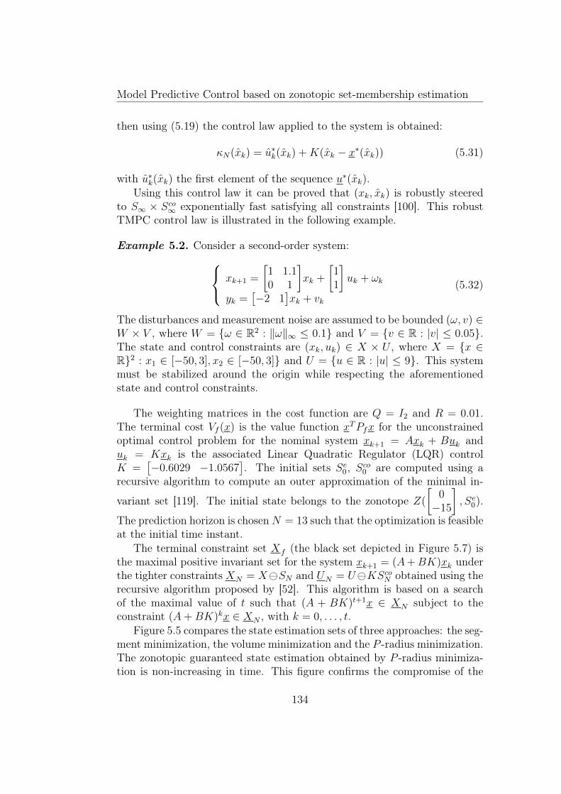
Model Predictive Control based on zonotopic set-membership estimation
then using (5.19) the control law applied to the system is obtained:
κN(xk) = u∗k(xk) +K(xk − x∗(xk)) (5.31)
with u∗k(xk) the first element of the sequence u∗(xk).Using this control law it can be proved that (xk, xk) is robustly steered
to S∞ × Sco∞ exponentially fast satisfying all constraints [100]. This robustTMPC control law is illustrated in the following example.
Example 5.2. Consider a second-order system: xk+1 =
[1 1.10 1
]xk +
[11
]uk + ωk
yk =[−2 1
]xk + vk
(5.32)
The disturbances and measurement noise are assumed to be bounded (ω, v) ∈W × V , where W = ω ∈ R2 : ‖ω‖∞ ≤ 0.1 and V = v ∈ R : |v| ≤ 0.05.The state and control constraints are (xk, uk) ∈ X × U , where X = x ∈R2 : x1 ∈ [−50, 3], x2 ∈ [−50, 3] and U = u ∈ R : |u| ≤ 9. This systemmust be stabilized around the origin while respecting the aforementionedstate and control constraints.
The weighting matrices in the cost function are Q = I2 and R = 0.01.The terminal cost Vf (x) is the value function xTPfx for the unconstrainedoptimal control problem for the nominal system xk+1 = Axk + Buk anduk = Kxk is the associated Linear Quadratic Regulator (LQR) controlK =
[−0.6029 −1.0567
]. The initial sets Se0, Sco0 are computed using a
recursive algorithm to compute an outer approximation of the minimal in-
variant set [119]. The initial state belongs to the zonotope Z(
[0−15
], Se0).
The prediction horizon is chosenN = 13 such that the optimization is feasibleat the initial time instant.
The terminal constraint set Xf (the black set depicted in Figure 5.7) isthe maximal positive invariant set for the system xk+1 = (A+BK)xk underthe tighter constraints XN = XSN and UN = UKScoN obtained using therecursive algorithm proposed by [52]. This algorithm is based on a searchof the maximal value of t such that (A + BK)t+1x ∈ XN subject to theconstraint (A+BK)kx ∈ XN , with k = 0, . . . , t.
Figure 5.5 compares the state estimation sets of three approaches: the seg-ment minimization, the volume minimization and the P -radius minimization.The zonotopic guaranteed state estimation obtained by P -radius minimiza-tion is non-increasing in time. This figure confirms the compromise of the
134
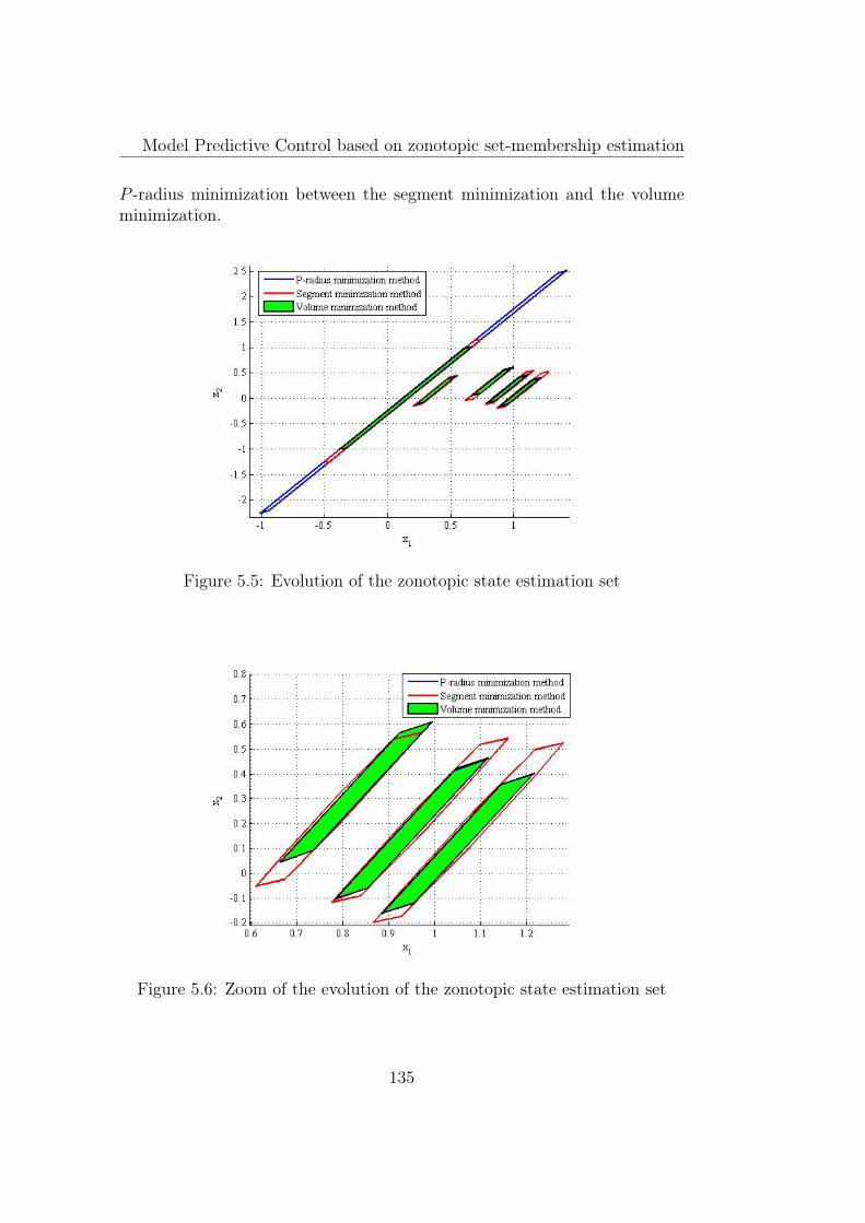
Model Predictive Control based on zonotopic set-membership estimation
P -radius minimization between the segment minimization and the volumeminimization.
Figure 5.5: Evolution of the zonotopic state estimation set
Figure 5.6: Zoom of the evolution of the zonotopic state estimation set
135
Model Predictive Control based on zonotopic set-membership estimation
Figure 5.7 shows the tube trajectory of the system. The largest zonotope(red) is the set x∗(xk, k)⊕ Sk. The real state is guaranteed to belong to thistube section centered at the nominal state. The smaller zonotope (green) isthe set x∗(xk, k)⊕Scok , the state estimation is guaranteed to belong to this set.The smallest (blue) is the guaranteed state estimation set xk ⊕ Sek. Denotethat the red zonotope which is the section of the tube trajectory at each timeinstant is the Minkowski sum of the blue zonotope and the green zonotopeSk = Scok ⊕ Sek. Due to the non-increase in time of the guaranteed stateestimation, the section of tube is non-increasing in time. This trajectoryis put in the box of the state contraint (Figure 5.8) in order to illustratethat the system respects the constraint. Figure 5.9 shows the stability ofthis output feedback system respecting the constraints. Due to the presenceof the uncertainty, the system state does not converge to the origin but itconverges, thus, to a set containing the origin.
Figure 5.7: Tube trajectory of the closed-loop system
136
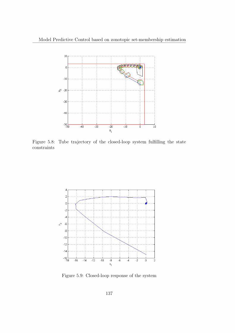
Model Predictive Control based on zonotopic set-membership estimation
Figure 5.8: Tube trajectory of the closed-loop system fulfilling the stateconstraints
Figure 5.9: Closed-loop response of the system
137
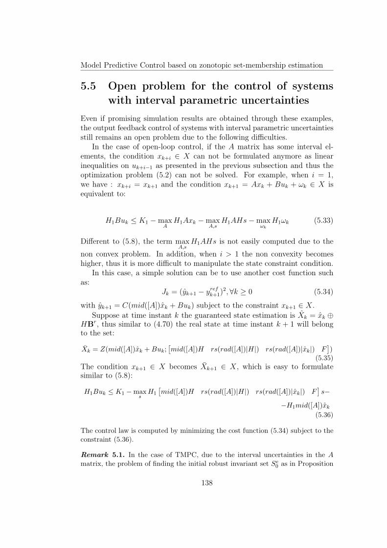
Model Predictive Control based on zonotopic set-membership estimation
5.5 Open problem for the control of systemswith interval parametric uncertainties
Even if promising simulation results are obtained through these examples,the output feedback control of systems with interval parametric uncertaintiesstill remains an open problem due to the following difficulties.
In the case of open-loop control, if the A matrix has some interval el-ements, the condition xk+i ∈ X can not be formulated anymore as linearinequalities on uk+i−1 as presented in the previous subsection and thus theoptimization problem (5.2) can not be solved. For example, when i = 1,we have : xk+i = xk+1 and the condition xk+1 = Axk + Buk + ωk ∈ X isequivalent to:
H1Buk ≤ K1 −maxA
H1Axk −maxA,s
H1AHs−maxωk
H1ωk (5.33)
Different to (5.8), the term maxA,s
H1AHs is not easily computed due to the
non convex problem. In addition, when i > 1 the non convexity becomeshigher, thus it is more difficult to manipulate the state constraint condition.
In this case, a simple solution can be to use another cost function suchas:
Jk = (yk+1 − yrefk+1)2,∀k ≥ 0 (5.34)
with yk+1 = C(mid([A])xk +Buk) subject to the constraint xk+1 ∈ X.Suppose at time instant k the guaranteed state estimation is Xk = xk ⊕
HBr, thus similar to (4.70) the real state at time instant k + 1 will belongto the set:
Xk = Z(mid([A])xk +Buk;[mid([A])H rs(rad([A])|H|) rs(rad([A])|xk|) F
])
(5.35)The condition xk+1 ∈ X becomes Xk+1 ∈ X, which is easy to formulatesimilar to (5.8):
H1Buk ≤ K1 −maxsH1
[mid([A])H rs(rad([A])|H|) rs(rad([A])|xk|) F
]s−
−H1mid([A])xk(5.36)
The control law is computed by minimizing the cost function (5.34) subject to theconstraint (5.36).
Remark 5.1. In the case of TMPC, due to the interval uncertainties in the Amatrix, the problem of finding the initial robust invariant set Se0 as in Proposition
138
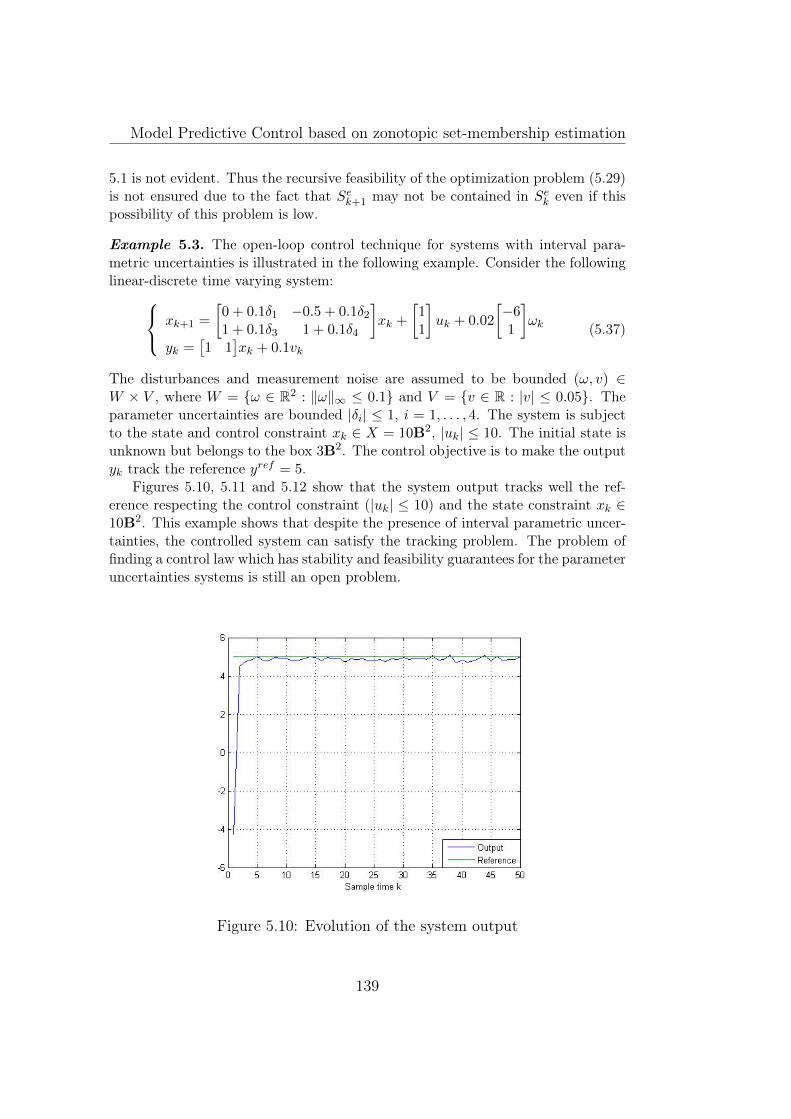
Model Predictive Control based on zonotopic set-membership estimation
5.1 is not evident. Thus the recursive feasibility of the optimization problem (5.29)is not ensured due to the fact that Sek+1 may not be contained in Sek even if thispossibility of this problem is low.
Example 5.3. The open-loop control technique for systems with interval para-metric uncertainties is illustrated in the following example. Consider the followinglinear-discrete time varying system: xk+1 =
[0 + 0.1δ1 −0.5 + 0.1δ21 + 0.1δ3 1 + 0.1δ4
]xk +
[11
]uk + 0.02
[−61
]ωk
yk =[1 1
]xk + 0.1vk
(5.37)
The disturbances and measurement noise are assumed to be bounded (ω, v) ∈W × V , where W = ω ∈ R2 : ‖ω‖∞ ≤ 0.1 and V = v ∈ R : |v| ≤ 0.05. Theparameter uncertainties are bounded |δi| ≤ 1, i = 1, . . . , 4. The system is subjectto the state and control constraint xk ∈ X = 10B2, |uk| ≤ 10. The initial state isunknown but belongs to the box 3B2. The control objective is to make the outputyk track the reference yref = 5.
Figures 5.10, 5.11 and 5.12 show that the system output tracks well the ref-erence respecting the control constraint (|uk| ≤ 10) and the state constraint xk ∈10B2. This example shows that despite the presence of interval parametric uncer-tainties, the controlled system can satisfy the tracking problem. The problem offinding a control law which has stability and feasibility guarantees for the parameteruncertainties systems is still an open problem.
Figure 5.10: Evolution of the system output
139
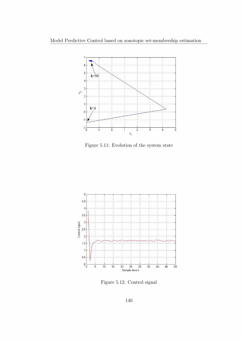
Model Predictive Control based on zonotopic set-membership estimation
Figure 5.11: Evolution of the system state
Figure 5.12: Control signal
140
Model Predictive Control based on zonotopic set-membership estimation
5.6 ConclusionThis chapter proposes a Model Predictive Control law based on the zonotopic set-membership estimation, when the state is not available. It starts with a generalpresentation of predictive control history. Due to its robustness and its ability todeal with constraints, predictive control is more and more used to control uncer-tain constraint system. When the state estimation is implemented, the simplestscheme control is to consider the state estimation as the real state and to min-imize a cost function. This solution is simple but it does not take into accountthe estimation error when designing the controller. Even if the control law andthe state estimation are stable, due to the presence of uncertainties the stability ofuncertain closed-loop system can not be guaranteed using the separation principle.For this reason, a feedback control law based on a tube of uncertain trajectories(around the nominal trajectory) of the uncertain system is presented. This controllaw considers the estimation error in the control problem using the invariant setapproach in order to guarantee the stability of the system. Based on these controltechniques, the control problem of systems with interval parametric uncertaintiesis considered. The interval uncertainties lead to solve a non convex optimizationproblem and thus the open-loop control can not be identical to the case of lineartime invariant system. A solution consists in modifying the cost function proposedto solve this problem. For systems with interval uncertainties, the Tube-basedModel Predictive Control method can not guarantee the recursive feasibility of thecontrol law and thus the stability of the closed-loop system. For these reasons, theproblem of finding an appropriate control law for system with interval parametricuncertainties subject to disturbances and measurement noise still remains an openproblem. In the next chapter, an application of the proposed set-membership esti-mation and control techniques are presented to illustrate the performances of theseapproaches, even if restricted configurations are considered (monovariable systemwith disturbances and measurement noise).
141

Model Predictive Control based on zonotopic set-membership estimation
142
Chapter 6
Application
6.1 IntroductionIn this chapter, the control and estimation approaches proposed in this thesiswill be applied to the model of a real system: the magnetic levitation system.The goal is to test the zonotopic set-membership estimation and the associationbetween this estimation and the open-loop Model Predictive Control or the Tube-based Model Predictive Control (TMPC). The chapter proposes first a generaldescription and the mathematical model of the magnetic levitation system. Basedon this model, in the next part the model predictive control law is built using thezonotopic set-membership estimation. First, the simulation is done with the open-loop Model Predictive Control method and then, the system is controlled by theTMPC. The simulation results show that these predictive control methods basedon the zonotopic set membership estimation can stabilize this system fulfilling theconsidered constraints, despite the disturbances and measurement noises acting onthe system.
6.2 System descriptionIn this section, the general description of the magnetic levitation device will bedone. This system is composed of a mobile iron pendulum in a vertical magneticfield created by a fixed electromagnet (Figure 6.1). This electromagnet is suppliedby a variable current which permits to vary the magnetic force and thus to varythe vertical position of the pendulum. This system is assumed to have a perfectradial symmetry.
The control goal is to stabilize the vertical position of the pendulum aroundthe equilibrium point. Figure 6.2 illustrates a general schematic block diagramof the closed-loop system with z the position of the pendulum relative to thesensor position center in an absolute reference frame, i the current given by theactuator. In the next part, the model of the magnetic levitation without the
143
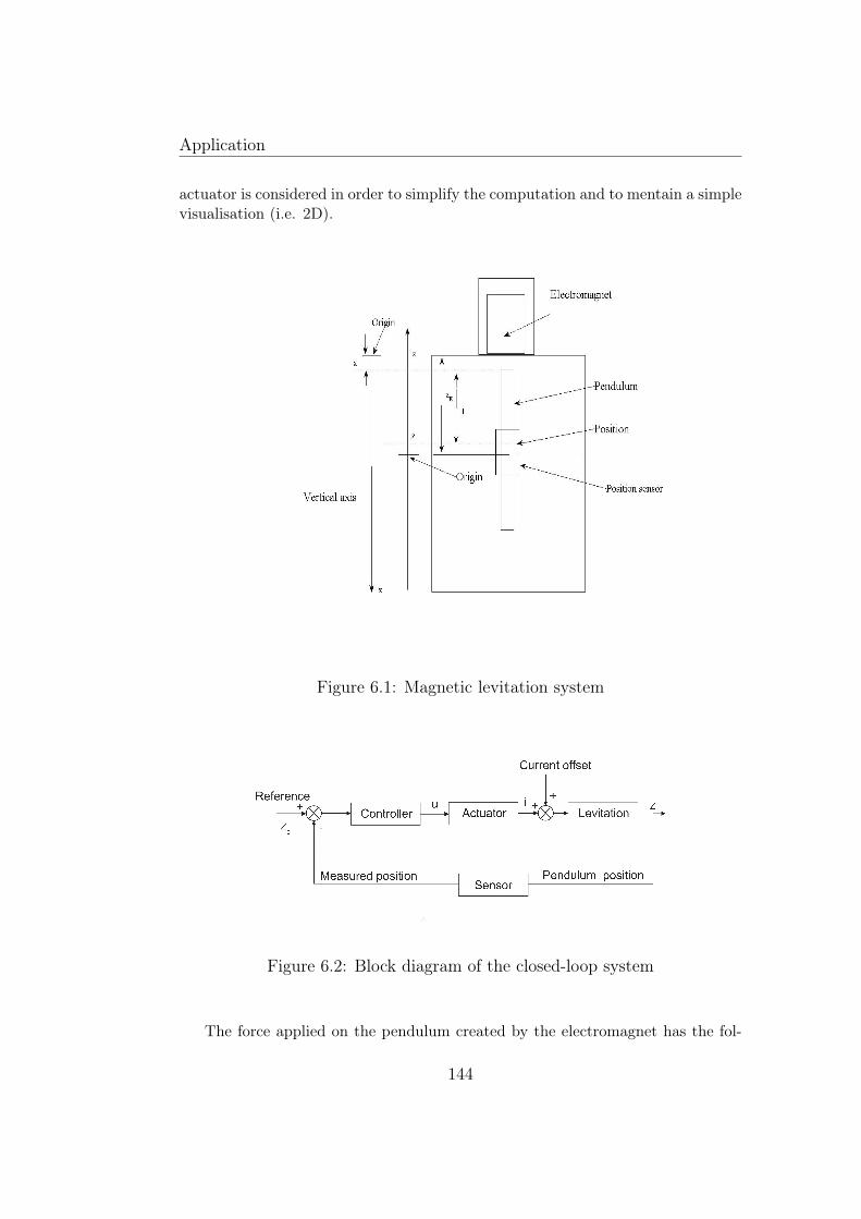
Application
actuator is considered in order to simplify the computation and to mentain a simplevisualisation (i.e. 2D).
Figure 6.1: Magnetic levitation system
Figure 6.2: Block diagram of the closed-loop system
The force applied on the pendulum created by the electromagnet has the fol-
144
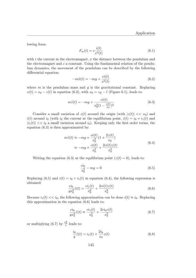
Application
lowing form:
Fm(t) = ci(t)
x2(t)(6.1)
with i the current in the electromagnet, x the distance between the pendulum andthe electromagnet and c a constant. Using the fundamental relation of the pendu-lum dynamics, the movement of the pendulum can be described by the followingdifferential equation:
−mx(t) = −mg +ci(t)
x2(t)(6.2)
where m is the pendulum mass and g is the gravitational constant. Replacingx(t) = x0 − z(t) in equation (6.2), with x0 = zE − l (Figure 6.1), leads to:
mz(t) = −mg +ci(t)
x20(1−z(t)x0
)2(6.3)
Consider a small variation of z(t) around the origin (with |z(t)| << x0) andi(t) around i0 (with i0 the current at the equilibrium point, i(t) = i0 + i1(t) and|i1(t)| << i0 a small variation around i0). Keeping only the first order terms, theequation (6.3) is then approximated by:
mz(t) ≈ −mg +ci(t)
x20(1 +
2z(t)
x0)
≈ −mg +ci(t)
x20+
2ci(t)z(t)
x30
(6.4)
Writing the equation (6.3) at the equilibrium point (z(t) = 0), leads to:
ci0x20−mg = 0 (6.5)
Replacing (6.5) and i(t) = i0 + i1(t) in equation (6.4), the following expression isobtained:
ci0gx20
z(t) =ci1(t)
x20+
2ci(t)z(t)
x30(6.6)
Because i1(t) << i0, the following approximation can be done i(t) ≈ i0. Replacingthis approximation in the equation (6.6) leads to:
ci0gx20
z(t) ≈ ci1(t)
x20+
2ci0z(t)
x30(6.7)
or multiplying (6.7) by x20c leads to:
i0gz(t) = i1(t) +
2i0x0z(t) (6.8)
145
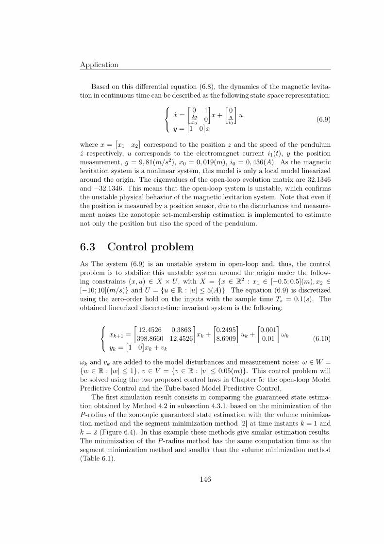
Application
Based on this differential equation (6.8), the dynamics of the magnetic levita-tion in continuous-time can be described as the following state-space representation: x =
[0 12gx0
0
]x+
[0gi0
]u
y =[1 0
]x
(6.9)
where x =[x1 x2
]correspond to the position z and the speed of the pendulum
z respectively, u corresponds to the electromagnet current i1(t), y the positionmeasurement, g = 9, 81(m/s2), x0 = 0, 019(m), i0 = 0, 436(A). As the magneticlevitation system is a nonlinear system, this model is only a local model linearizedaround the origin. The eigenvalues of the open-loop evolution matrix are 32.1346and −32.1346. This means that the open-loop system is unstable, which confirmsthe unstable physical behavior of the magnetic levitation system. Note that even ifthe position is measured by a position sensor, due to the disturbances and measure-ment noises the zonotopic set-membership estimation is implemented to estimatenot only the position but also the speed of the pendulum.
6.3 Control problemAs The system (6.9) is an unstable system in open-loop and, thus, the controlproblem is to stabilize this unstable system around the origin under the follow-ing constraints (x, u) ∈ X × U , with X = x ∈ R2 : x1 ∈ [−0.5; 0.5](m), x2 ∈[−10; 10](m/s) and U = u ∈ R : |u| ≤ 5(A). The equation (6.9) is discretizedusing the zero-order hold on the inputs with the sample time Ts = 0.1(s). Theobtained linearized discrete-time invariant system is the following:
xk+1 =
[12.4526 0.3863398.8660 12.4526
]xk +
[0.24958.6909
]uk +
[0.0010.01
]ωk
yk =[1 0
]xk + vk
(6.10)
ωk and vk are added to the model disturbances and measurement noise: ω ∈W =w ∈ R : |w| ≤ 1, v ∈ V = v ∈ R : |v| ≤ 0.05(m). This control problem willbe solved using the two proposed control laws in Chapter 5: the open-loop ModelPredictive Control and the Tube-based Model Predictive Control.
The first simulation result consists in comparing the guaranteed state estima-tion obtained by Method 4.2 in subsection 4.3.1, based on the minimization of theP -radius of the zonotopic guaranteed state estimation with the volume minimiza-tion method and the segment minimization method [2] at time instants k = 1 andk = 2 (Figure 6.4). In this example these methods give similar estimation results.The minimization of the P -radius method has the same computation time as thesegment minimization method and smaller than the volume minimization method(Table 6.1).
146
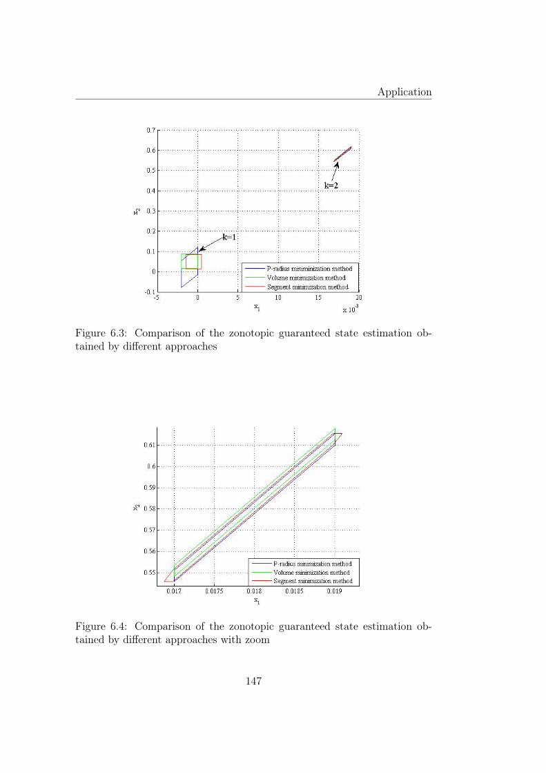
Application
Figure 6.3: Comparison of the zonotopic guaranteed state estimation ob-tained by different approaches
Figure 6.4: Comparison of the zonotopic guaranteed state estimation ob-tained by different approaches with zoom
147
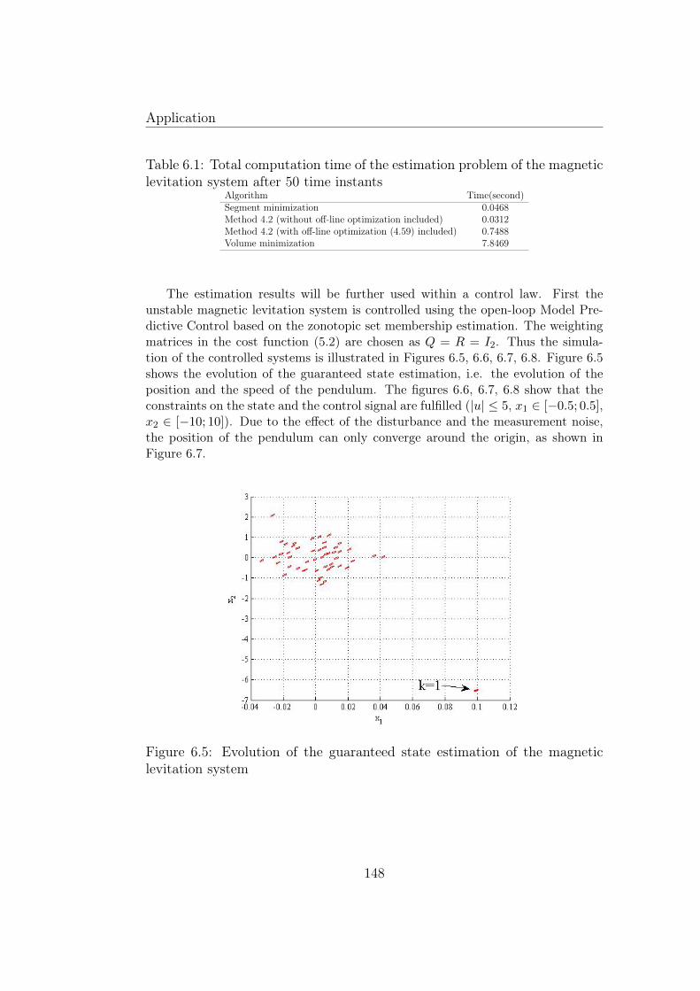
Application
Table 6.1: Total computation time of the estimation problem of the magneticlevitation system after 50 time instants
Algorithm Time(second)Segment minimization 0.0468Method 4.2 (without off-line optimization included) 0.0312Method 4.2 (with off-line optimization (4.59) included) 0.7488Volume minimization 7.8469
The estimation results will be further used within a control law. First theunstable magnetic levitation system is controlled using the open-loop Model Pre-dictive Control based on the zonotopic set membership estimation. The weightingmatrices in the cost function (5.2) are chosen as Q = R = I2. Thus the simula-tion of the controlled systems is illustrated in Figures 6.5, 6.6, 6.7, 6.8. Figure 6.5shows the evolution of the guaranteed state estimation, i.e. the evolution of theposition and the speed of the pendulum. The figures 6.6, 6.7, 6.8 show that theconstraints on the state and the control signal are fulfilled (|u| ≤ 5, x1 ∈ [−0.5; 0.5],x2 ∈ [−10; 10]). Due to the effect of the disturbance and the measurement noise,the position of the pendulum can only converge around the origin, as shown inFigure 6.7.
Figure 6.5: Evolution of the guaranteed state estimation of the magneticlevitation system
148
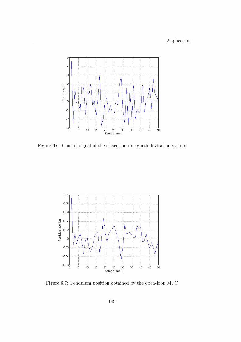
Application
Figure 6.6: Control signal of the closed-loop magnetic levitation system
Figure 6.7: Pendulum position obtained by the open-loop MPC
149
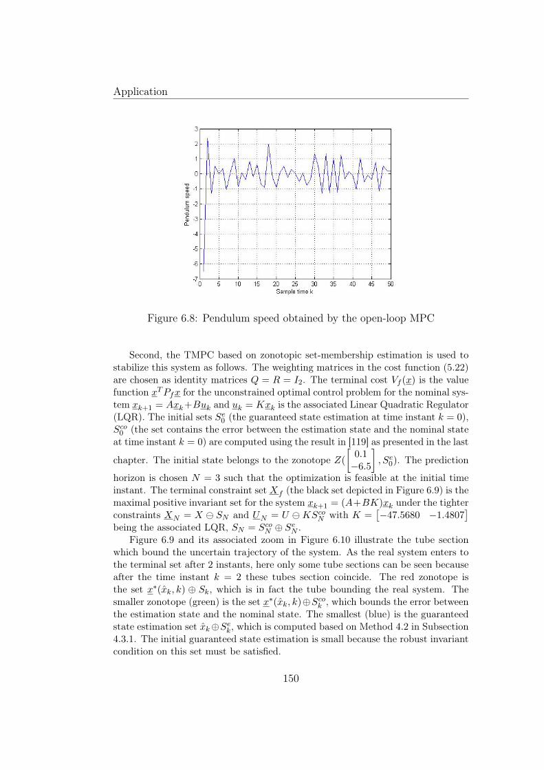
Application
Figure 6.8: Pendulum speed obtained by the open-loop MPC
Second, the TMPC based on zonotopic set-membership estimation is used tostabilize this system as follows. The weighting matrices in the cost function (5.22)are chosen as identity matrices Q = R = I2. The terminal cost Vf (x) is the valuefunction xTPfx for the unconstrained optimal control problem for the nominal sys-tem xk+1 = Axk+Buk and uk = Kxk is the associated Linear Quadratic Regulator(LQR). The initial sets Se0 (the guaranteed state estimation at time instant k = 0),Sco0 (the set contains the error between the estimation state and the nominal stateat time instant k = 0) are computed using the result in [119] as presented in the last
chapter. The initial state belongs to the zonotope Z(
[0.1−6.5
], Se0). The prediction
horizon is chosen N = 3 such that the optimization is feasible at the initial timeinstant. The terminal constraint set Xf (the black set depicted in Figure 6.9) is themaximal positive invariant set for the system xk+1 = (A+BK)xk under the tighterconstraints XN = X SN and UN = U KScoN with K =
[−47.5680 −1.4807
]being the associated LQR, SN = ScoN ⊕ SeN .
Figure 6.9 and its associated zoom in Figure 6.10 illustrate the tube sectionwhich bound the uncertain trajectory of the system. As the real system enters tothe terminal set after 2 instants, here only some tube sections can be seen becauseafter the time instant k = 2 these tubes section coincide. The red zonotope isthe set x∗(xk, k) ⊕ Sk, which is in fact the tube bounding the real system. Thesmaller zonotope (green) is the set x∗(xk, k)⊕Scok , which bounds the error betweenthe estimation state and the nominal state. The smallest (blue) is the guaranteedstate estimation set xk⊕Sek, which is computed based on Method 4.2 in Subsection4.3.1. The initial guaranteed state estimation is small because the robust invariantcondition on this set must be satisfied.
150
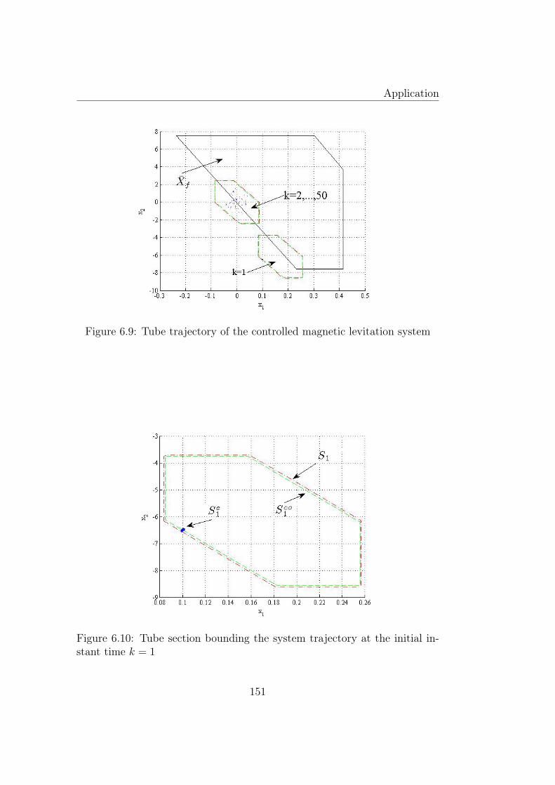
Application
Figure 6.9: Tube trajectory of the controlled magnetic levitation system
Figure 6.10: Tube section bounding the system trajectory at the initial in-stant time k = 1
151
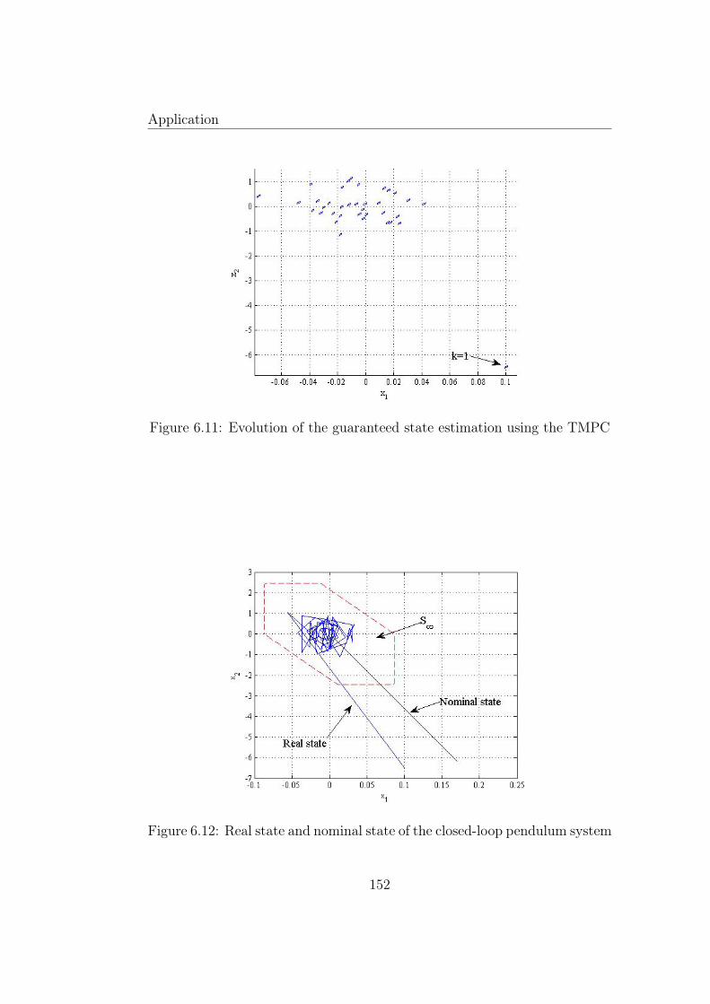
Application
Figure 6.11: Evolution of the guaranteed state estimation using the TMPC
Figure 6.12: Real state and nominal state of the closed-loop pendulum system
152
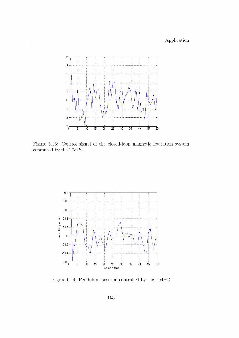
Application
Figure 6.13: Control signal of the closed-loop magnetic levitation systemcomputed by the TMPC
Figure 6.14: Pendulum position controlled by the TMPC
153
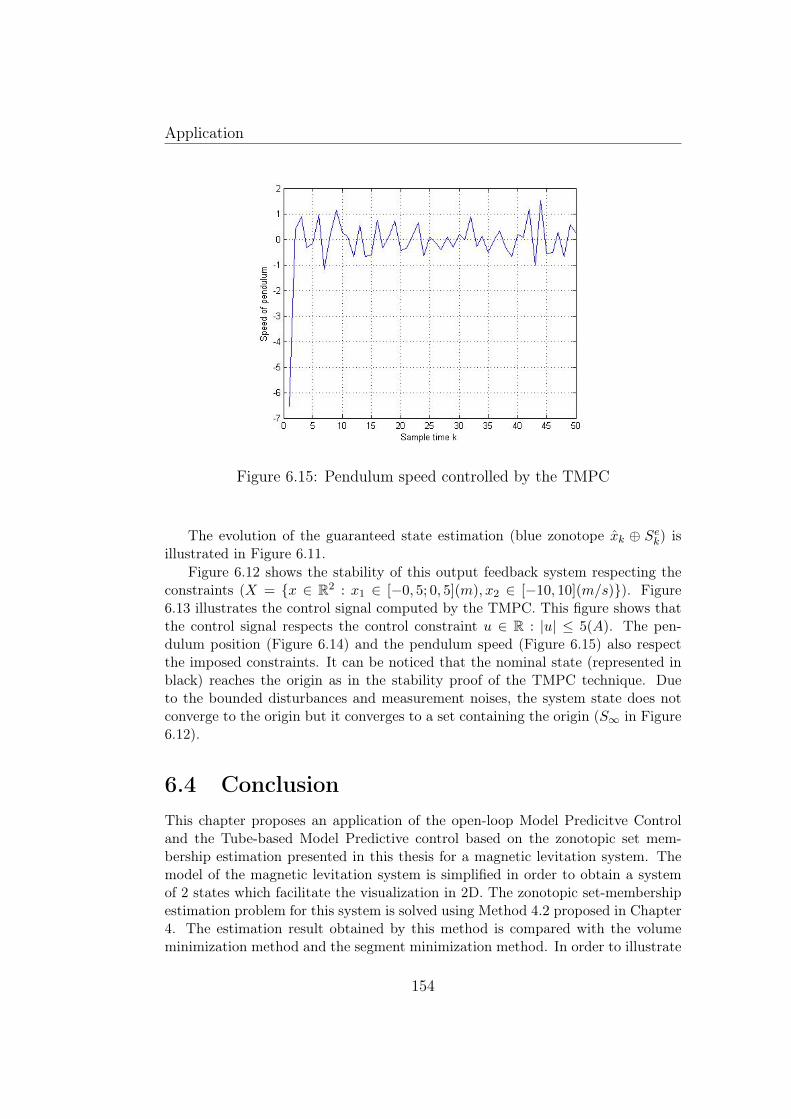
Application
Figure 6.15: Pendulum speed controlled by the TMPC
The evolution of the guaranteed state estimation (blue zonotope xk ⊕ Sek) isillustrated in Figure 6.11.
Figure 6.12 shows the stability of this output feedback system respecting theconstraints (X = x ∈ R2 : x1 ∈ [−0, 5; 0, 5](m), x2 ∈ [−10, 10](m/s)). Figure6.13 illustrates the control signal computed by the TMPC. This figure shows thatthe control signal respects the control constraint u ∈ R : |u| ≤ 5(A). The pen-dulum position (Figure 6.14) and the pendulum speed (Figure 6.15) also respectthe imposed constraints. It can be noticed that the nominal state (represented inblack) reaches the origin as in the stability proof of the TMPC technique. Dueto the bounded disturbances and measurement noises, the system state does notconverge to the origin but it converges to a set containing the origin (S∞ in Figure6.12).
6.4 ConclusionThis chapter proposes an application of the open-loop Model Predicitve Controland the Tube-based Model Predictive control based on the zonotopic set mem-bership estimation presented in this thesis for a magnetic levitation system. Themodel of the magnetic levitation system is simplified in order to obtain a systemof 2 states which facilitate the visualization in 2D. The zonotopic set-membershipestimation problem for this system is solved using Method 4.2 proposed in Chapter4. The estimation result obtained by this method is compared with the volumeminimization method and the segment minimization method. In order to illustrate
154

Application
its properties, the P -radius based estimation method is used for control purposes.The control law is implemented using the open-loop Model Predictive Control andthe Tube-based Model Predictive Control. The simulation results show that thecontrol problem is solved (the system is stabilized, the constraints are respected).The next chapter which is the last chapter of this PhD thesis presents some con-clusions, the contributions of this thesis and some future directions both on theoryand practical applications.
155

Application
156
Chapter 7
Conclusion and future works
7.1 ContributionThis thesis proposes a robust predictive control technique for uncertain systemssubject to constraints in the presence of bounded disturbances and measurementnoises. The contributions of this thesis are divided into two main parts:
• The first part consists in developing a zonotopic set-membership estimationfor systems with interval parametric uncertainties in the presence of distur-bances and measurement noises.
• The second part is based on the association of the proposed state estima-tion with a Model Predictive Control law in order to robustly control theconsidered system subject to state and input constraints.
In the first part, using the deterministic approach, disturbances and measurementnoises are assumed to be unknown but bounded by some zonotopes. Then a zono-topic set containing all the possible system states that are consistent with theuncertainties, the disturbances and the noises is computed at each time instantusing a set-membership estimation algorithm. One originality of this thesis is topresent a new optimization criterion to compute the zonotopic guaranteed stateestimation based on the minimization of the P -radius of the zonotopic estimationset offering a good accuracy of the estimation with a reasonable complexity of thecomputation. Using the P -radius based criterion in an original way leads to off-line solve a Bilinear Matrix Inequality optimization problem [82]. To solve thisproblem, the Penbmi solver [74] can be used. To overcome the use of BilinearMatrix Inequality solvers, in this thesis the contractiveness speed of the zonotopicstate estimation set is optimized leading to a Linear Matrix Inequality optimizationproblem which can be easily solved [85]. This method is first developed for lineartime invariant systems subject to disturbances and measurement noises, then it isextended to the case of systems with interval parametric uncertainties using themaximum principle [83]. Another contribution of this thesis consists in proposing
157
Conclusion and future works
different strategies for the case of Multi-Output systems that have been presentedin [88] and [87] or submitted to [84]. The first proposed solution is based on thedirect extension of the adopted solution for the case of Single-Output systems.This solution is shown to be conservative due to neglect the coupling effect ofMulti-Output systems. When the coupling effect is taken into account, the opti-mization problem becomes a Polynomial Matrix Inequality problem which is nonconvex and thus difficult to solve. In consequence, the proposed solution is to use arelaxation technique [62] to transform this Polynomial Matrix Inequality probleminto a Linear Matrix Inequality problem which can be solved using Linear MatrixInequality solvers. This results have been published in [88]. But this relaxationtechnique leads to an important increase of the number of scalar decision variables,and, thus, limits the application of the proposed approach to large scale systems.Moreover, the simulation result shows a poor estimation performance due to theused of this relaxation technique. In order to improve the overall performance forMulti-Output systems„ the next contribution of this thesis considers the zonotopicouter approximation of the intersection between a zonotope and a polytope [87].Using this result and the P -radius based optimization criterion leads to a signifi-cant improvement both on the estimation performance and the complexity of thecomputation in comparison with the previous proposed methods (the direct exten-sion of Single-Output case and the Polynomial Matrix Inequality based method).The comparative results are analyzed in different examples along the thesis.
The second part deals with the problem of robust control for constrained un-certain system in the predictive control context. First, an simple solution basedon the open-loop predictive control is proposed. The proposed control law leadsto solve a quadratic optimization problem subject to constraints at each sampletime. Even if the simulation shows a good result, this solution does not have theguarantees of stability and feasibility. A second solution is to use the Tube basedModel Predictive Control for systems with bounded disturbances and measurementnoises which build a tube trajectory of the real system around the nominal model.This control technique permits to guarantee the stability of the controlled system.When the system state is not available, the Tube-based Model Predictive Controlis usually associated to the Luenberger observer to obtain a state estimation [100].The next contribution consist in using the Tube based Model Predictive Controlin the context of the zonotopic set-membership estimation [85], which permits toimprove the estimation performance and thus the performance of the controlledsystem. To deal with the interval parametric uncertainties presence in the systemmodel, a modification of the cost function in the presented open-loop control isproposed. The solution of the Tube-based Model Predictive Control associated tothe set-membership estimation is still an open problem. Finally, the applicationof the proposed Tube-based Model Predictive Control to the magnetic levitationsystem shows the effectiveness of the developed technique [86].
158
Conclusion and future works
7.2 Future worksSeveral directions are proposed for future developments of this thesis.
As presented in Subsection 4.3.3.4 applying the P -radius based zonotopic set-membership estimation for Multi-Output linear discrete-time systems (with param-eter uncertainties or not) subject to bounded disturbances and measurement noisesleads to solve a Polynomial Matrix Inequality optimization problem. Due to thepoor performance obtained by the relaxation Linear Matrix Inequality technique[62] (outer approximation of the solution of the PMI optimization problem) appliedin this thesis, the first perspective consists in comparing the results obtained withthe relaxation procedure [62] with other existing techniques [64], [72], [31] or themost recent work [63] which offers an inner approximation of the solution of thePMI optimization problem. If the reader is interested by these results, anotherdirection to explore consists in developing new relaxation techniques that will leadto other sub-optimal solutions of the initial Polynomial Matrix Inequality problemin order to obtain a better performance of the estimation.
An interesting idea to pursue is the extension of the zonotopic set-membershipestimation for systems with time-delay and especially for systems with variabletime-delay [93]. If the delay can be taken into account in the mathematical modelas an interval parametric uncertainty [136], then the extension of this estimationtechnique should not be too complicated.
In the case of Multi-Output systems, the set-membership estimation is obtainedusing a multisensor system. Thus, a natural way to explore further is the faultdiagnosis problem of the multisensor system [138], [114] [142]. This problem canbe considered using the proposed zonotopic outer approximation of the intersectionbetween a zonotope and a polytope. If this intersection is zero it means that a faultis detected. Then a continuing study which can be considered is the fault tolerantcontrol [139], [130], [150].
A different perspective is to build an efficient output feedback control law(offering stability guarantees) which permits to control the system with intervalparametric uncertainties in the presence of disturbances, measurement noises andconstraints.
Finally, the application of the proposed work on a more complex system withthe experimental validation can be also considered.
159

Conclusion and future works
160
Bibliography
[1] M. Alamir. Nonlinear moving horizon observers: Theory and real-time imple-mentation. Lecture Notes in Control and Information Sciences, 363:139–179,2007.
[2] T. Alamo, J. M. Bravo, and E. F. Camacho. Guaranteed state estimation byzonotopes. Automatica, 41:1035–1043, 2005.
[3] T. Alamo, J. M. Bravo, M. J. Redondo, and E. F. Camacho. A set-membership state estimation algorithm based on dc programming. Auto-matica, 44(1):216–224, 2008.
[4] T. Alamo, D. R. Ramirez, D. Muñoz de la Peña, and E. F. Camacho. Minmaxmpc using a tractable qp problem. Automatica, 43:693–700, 2007.
[5] T. Alamo, R. Tempo, D. R. Ramírez, and E. F. Camacho. A new vertexresult for robustness problems with interval matrix uncertainty. Systems andControl Letters, 57:474–481, 2008.
[6] J. C. Allwright. Advances in Model-based predictive control. Oxford Univer-sity Press, 1994.
[7] M. Althoff, O. Stursberg, and M. Buss. Reachability analysis of linear systemswith uncertain parameters and inputs. In Proc. of the 46th IEEE Conferenceon Decision and Control, volume 41, pages 726–732, 2007. New Orleans, LA,USA.
[8] M. Althoff, O. Stursberg, and M. Buss. Computing reachable sets of hybridsystems using a combination of zonotopes and polytopes. Nonlinear Analysis:Hybrid Systems, 4(2):233–249, 2010.
[9] J. M. Aughenbaugh and C. J. J. Paredis. Why are intervals and impreci-sion important in engineering design? In Proc. of the Reliable EngineeringComputing Workshop, 2006. Savannah, USA.
[10] B. M. Ayyub and G. J. Klir. Uncertainty modeling and analysis in engineeringand the sciences. Chapman and Hall/CRC, 2006.
161
BIBLIOGRAPHY
[11] G. Barequet and S. Har-Peled. Efficiently approximating the minimum-volume bounding box of a point set in three dimensions. Journal of Al-gorithms, 38:91–109, 1999.
[12] A. A. Batabyal. Dynamic and stochastic approaches to the environment andeconomic development. World Scientific Publishing Company, 2008.
[13] Y. Becis-Aubry, D. Aubry, and N. Ramdani. Multisensor set-membershipstate estimation of nonlinear models with potentially failing measurements.In Proc. of the 18th World Congress IFAC, pages 12030–12035, Milan, Italy,2011.
[14] Y. Becis-Aubry, M. Boutayebb, and M. Darouach. State estimation in thepresence of bounded disturbances. Automatica, 44(7):1867–1873, 2008.
[15] Y. Becis-Aubry and N. Ramdani. State-bounding estimation for nonlinearmodels with multiple measurements. In Proc. of the 2012 American ControlConference ACC, pages 1883–1888, Montréal, Canada, 2012.
[16] A. Bemporad. Reducing conservativeness in predictive control of constrainedsystems with disturbances. In Proc. of the 37th IEEE Conference on Decisionand Control, pages 1384–1391, Tampa, USA, 1998.
[17] A. Bemporad and A. Garulli. Output feedback predictive control of con-strained linear systems via set-membership state estimation. InternationalJournal of Control, 73(8):655–665, 2000.
[18] A. Bemporad and M. Morari. Robust Model Predictive Control: A Survey.Robustness in Identification and Control, 245:207–226, 1999.
[19] D. P. Bertsekas, A. Nedíc, and A. E. Ozdaglar. Convex analysis and opti-mization. Athena Scientific, 2003.
[20] D. P. Bertsekas and I. B. Rhodes. Recursive state estimation for a set-membership description of uncertainty. IEEE Transactions on AutomaticControl, 16(2):117–128, 1971.
[21] R. Bhattacharya, G. J. Balas, M. A. Kaya, and A. Packard. Nonlinear re-ceding horizon control of an f-16 aircraft. Journal Guidance Control andDynamics, 25(5):924–931, 2002.
[22] F. Blanchini. Set invariance in control. Automatica, 35(11):1747–1767, 1999.
[23] F. Blanchini and S. Miani. Set-theoretic methods in control. Birkhauser,Boston, 2007.
[24] S. Boyd, L. El Ghaoui, E. Feron, and V. Balakrishnan. Linear matrix in-equalities in system and control theory. SIAM, Philadelphia, 1994.
162
BIBLIOGRAPHY
[25] J. M. Bravo, T. Alamo, and E. F. Camacho. Bounded error identificationof systems with time-varying parameters. IEEE Transactions on AutomaticControl, 51(7):1144–1150, 2006.
[26] E. M. Bronstein. Approximation of convex sets by polytopes. Journal ofMathematical Sciences, 153(6):727–762, 2008.
[27] R. G. Brown and P. Y. C. Hwang. Introduction to random signals and appliedKalman Filtering. John Wiley and Sons, 1997.
[28] R. L. Burden and J. D. Faires. Numerical analysis. Brooks Cole, 2000.
[29] E. F. Camacho and C. Bordons. Model predictive control. Springer-Verlag,London, 2004.
[30] P. J. Campo and M. Morari. Robust model predictive control. In Proc. of theAmerican Control Conference, pages 1021–1026, Minneapolis, USA, 1987.
[31] G. Chesi, A. Garulli, A. Tesi, and A. Vicino. An lmi-based approach forcharacterizing the solution set of polynomial systems. In Proc. of the 39thIEEE Conference Decision and Control, pages 1501–1506, Sydney, Australia,2000.
[32] L. Chisci, A. Garulli, and G. Zappa. Recursive state bounding by parallelo-topes. Automatica, 32:1049–1055, 1996.
[33] L. Chisci and G. Zappa. Feasibility in predictive control of constrained linearsystems: the output feedback case. International journal of robust and nonlinear control, 12:465–487, 2002.
[34] D. W. Clarke. Application of generalized predictive control to industrialprocesses. IEEE Control System Magazine, 122:49–55, 1988.
[35] D. W. Clarke, C. Mohtadi, and P. S. Tuffs. Generalized predictive control,part i: The basic algorithm; part ii: Extensions and interpretations. Auto-matica, 23(2):137–160, 1987.
[36] D. W. Clarke and R. Scatollini. Constrained receding horizon predictivecontrol. Proceedings IEE-D, 138:347–354, 1991.
[37] C. Combastel. A state bounding observer based on zonotopes. In Proc. ofEuropean Control Conference, Cambridge, UK, 2003.
[38] C. Combastel. Observation de systèmes non linéaires appliquée à un modèlede bioréacteur. une approche ensembliste basée sur les zonotopes. JournalEuropéen des Systèmes Automatisés, 38:933–957, 2004.
163
BIBLIOGRAPHY
[39] C. Combastel. A state bounding observer for uncertain non-linear continuous-time systems based on zonotopes. In Proc. of the 44th IEEE Conference onDecision and Control, and the European Control Conference, Sevilla, Spain,2005.
[40] C. Combastel, Q. Zhang, and A. Lalami. Fault diagnosis based on the enclo-sure of parameters estimated with an adaptive observer. In Proc. of the 17thWorld Congress IFAC, pages 7314–7319, Seoul, Korea, 2008.
[41] C. R. Cutler and B. C. Ramaker. Dynamic matrix control Ű a computer con-trol algorithm. In Proc. of the Automatic Control Conference, San Francisco,USA, 1980.
[42] G. B. Dantzig. Fourier-motzkin elimination and its dual. Technical report,DTIC document, 1972.
[43] R. M. C. de Keyser and A. R. Van Cauwenberghe. Extended predictionselfadapted control. In IFAC Symposium on Identification and System Pa-rameter Estimation, pages 1317–1322, York, 1985.
[44] J. Douchet and B. Zwahlen. Calcul différentiel et intégral. Presses Polytech-niques et Universitaires Romande, 2006.
[45] C. Durieu, E. Walter, and B. Polyak. Multi-input multi-output ellip-soidal state bounding. Journal of Optimization Theory and Applications,111(2):273–303, 2001.
[46] Y. K. Foo and Y. C. Soh. Robust kalman filtering for uncertain discrete-timesystems with probabilistic parameters bounded within a polytope. Systemsand Control Letters, 57(6):482–488, 2008.
[47] K. Fukuda. Cdd/cdd+ reference manual, 1999.
[48] K. Fukuda. From the zonotope construction to the minkowski addition ofconvex polytopes. Journal of Symbolic Computation, 38(4):1261–1272, 2004.
[49] C. E. García, D. M. Prett, and M. Morari. Model predictive control : Theoryand practice Ű a survey. Automatica, 25(3):335–348, 1989.
[50] A. Garulli and A. Vicino. Set membership localization of mobile robotsvia angle measurement. IEEE Transactions on Robotic and Automation,17(4):450 – 463, 2001.
[51] L. El Ghaoui and G. Calafiore. Worst-case state prediction under structureduncertainty. In Proc. of American Control Conference, pages 3402–3406, SanDiego, USA, 1999.
164
BIBLIOGRAPHY
[52] E. G. Gilbert and K. T. Tan. Linear systems with state and control con-straints: The theory and application of maximal output admissible sets.IEEE Transactions on Automatic Control, 36(9):1008–1020, 1991.
[53] A. Girard. Reachability of uncertain linear systems using zonotopes. InHybrid Systems: Computation and Control, March, 2005, volume 3414 ofLecture Notes in Computer Science, pages 291–305. Springer, March 2005.
[54] G. Goodwin, M. M. Seron, and J. A. De Doná. Constrained Control andEstimation: An Optimisation Approach. Springer, 2004.
[55] C. Greco, G. Menga, E. Mosca, and G. Zappa. Performance improvement ofself-tuning controllers by multistep horizons: The musmar approach. Auto-matica, 20:681–100, 1984.
[56] P. Gritzmann and B. Sturmfels. Minkowski addition of polytopes: Com-putational complexity and applications to gröbner bases. SIAM Journal onDiscrete Mathematic, 6(2):246–269, 1993.
[57] J. W. Grizzle and P. E. Moraal. Observer based control of nonlinear discrete-time systems. In Proc. of the 29th IEEE Conference on Decision and Control,pages 760–767, Honoluu, USA, 1990.
[58] P. Guerra, V. Puig, and M. Witczak. Robust fault detection with unknown-input interval observers using zonotopes. In Proc. of the 17th World CongressIFAC, pages 5557–5562, Seoul, Korea, 2008.
[59] L. J. Guibas, A. Nguyen, and L. Zhang. Zonotopes as bounding volume. InProc. of the Symposium on Discrete Algorithm, pages 803–812, 2005.
[60] E. R. Hansen. Interval arithmetic in matrix computations. SIAM Journalon Numerical Analysis: Series B, 2(2):308–320, 1965.
[61] D. Henrion and J. B. Lasserre. Gloptipoly: Global optimization over polyno-mials with matlab and sedumi. ACM Transactions on Mathematical Software,29:165–194, 2002.
[62] D. Henrion and J. B. Lasserre. Convergent relaxations of polynomial matrixinequalities and static output feedback. IEEE Transactions on AutomaticControl, 51(2):192 – 202, 2006.
[63] D. Henrion and J. B. Lasserre. Inner approximations for polynomial ma-trix inequalities and robust stability regions. Technical report, LAAS-report11210, 2011.
[64] C. W. J. Hol and C. W. Scherer. Sum of squares relaxations for polyno-mial semidefinite programming. In Proc. Symp. on Mathematical Theory ofNetworks and Systems, Leuven, Belgium, 2004.
165
BIBLIOGRAPHY
[65] D. P. Hunttenlocher, G. A. Klanderman, and W. J. Rucklidge. Comparingimages using the hausdorff distance. IEEE Transactions on Pattern Analysisand Machine Intelligence, 15(9):850 – 863, 1993.
[66] A. Ingimundarson, J. M. Bravo, V. Puig, T. Alamo, and P. Guerra. Robustfault detection using zonotope-based set-membership consistency. Interna-tional journal of adaptive control and signal processing, 23(4):311–330, 2008.
[67] J. A. De Doná J. B. Mare. Moving horizon estimation of constrained non-linear systems by carleman approximations. In Proc. of the 45th IEEE Con-ference on Decision and Control, pages 2147–2152, San Diego, USA, 2006.
[68] L. Jaulin, M. Kieffer, O. Didrit, and E. Walter. Interval analysis. Springer,2001.
[69] R. E. Kalman. A new approach to linear filtering and prediction problems.Transactions of the ASME–Journal of Basic Engineering, 82(Series D):35–45,1960.
[70] S. S. Keerthi and E. G. Gilbert. Optimal infinite-horizon feedback laws fora general class of constrained discrete-time systems: Stability and moving-horizon approximations. Journal of Optimization Theory and Applications,57(2):265–293, 1988.
[71] M. Kieffer, L. Jaulin, and E. Walter. Guaranteed recursive nonlinear state es-timation using interval analysis. International Journal of Adaptative Controland Signal Processing, 2002.
[72] M. Kojima. Sums of squares relaxations of polynomial semidefinite pro-grams. Technical report, Department of Mathematical and Computing Sci-ences, Tokyo Institute of Technology, 2003.
[73] M. V. Kothare, V. Balakrishnan, and M. Morari. Robust constrained modelpredictive control using linear matrix inequalities. Automatica, 32(10):1361–1379, 1996.
[74] M. Kočvara and S. Stingl. Pennon a code for convex nonlinear and semidefi-nite programming. Optimization Methods and Software, 18(3):317–333, 2003.
[75] W. Kühn. Rigorously computed orbits of dynamical systems without thewrapping effect. Computing, 61:47–67, 1998.
[76] W. Kühn. Toward an optimal control of wrapping effect. In InternationalSymposium on Scientific Computing, Computer Arithmetic and ValidatedNumerics, pages 125–134, 1998.
[77] A. B. Kurzhanski and I. Vályi. Ellipsoidal calculus for estimation and control.Birkhaüser Boston, 1996.
166
BIBLIOGRAPHY
[78] A. A. Kurzhanskiy and P. Varaiya. Ellipsoidal toolbox manual, 2006-2007.
[79] M. Kvasnica, P. Grieder, and M. Baotić. Multi-parametric toolbox (mpt),2004.
[80] W. Langson, I. Chryssochoos, S.V. Raković, and D.Q. Mayne. Robust modelpredictive control using tubes. Automatica, 40(1):125–133, 2004.
[81] S. R. Lay. Convex sets and their applications. Wiley, New york, 1982.
[82] V. T. H. Le, T. Alamo, E. F. Camacho, C. Stoica, and D. Dumur. A newapproach for guaranteed state estimation by zonotopes. In Proc. the 18thWorld Congress IFAC, pages 9242–9247, Milan, Italy, 2011.
[83] V. T. H. Le, T. Alamo, E. F. Camacho, C. Stoica, and D. Dumur. Zonotopicset-membership estimation for interval dynamic systems. In Proc of the 2012American Control Conference ACC, pages 6787–6792, Montréal, Canada,2012.
[84] V. T. H. Le, C. Stoica, T. Alamo, D. Dumur, and E. F. Camacho. Guaranteedstate estimation by zonotopes for systems with interval uncertainties. Insubmitted to Automatica, 2012.
[85] V. T. H. Le, C. Stoica, D. Dumur, T. Alamo, and E. F. Camacho. Robusttube-based constrained predictive control via zonotopic set-membership es-timation. In Proc. the 50th IEEE Conference on Decision and Control andEuropean Control Conference, pages 4580–4585, Orlando, USA, 2011.
[86] V. T. H. Le, C. Stoica, D. Dumur, T. Alamo, and E. F. Camacho. Commandeprédictive robuste par des techniques d’observateurs basées sur des ensembleszonotopiques. Journal Européen des Systèmes Automatisés, 2-3/2012:235–250, 2012.
[87] V. T. H. Le, C. Stoica, D. Dumur, T. Alamo, and E. F. Camacho. Guaranteedstate estimation by zonotopes for systems with interval uncertainties. In 2012Small Workshop on Interval Methods, Oldenburg, Germany, 2012.
[88] V. T. H. Le, C. Stoica, D. Dumur, T. Alamo, and E. F. Camacho. A poly-nomial matrix inequality approach for zonotopic set-membership estimationof multivariable systems. In Proc. of the 20th Mediterranean Conference onControl and Automation, pages 18–23, Barcelona, Spain, 2012.
[89] J. H. Lee and Z. Yu. Worst-case formulations of model predictive control forsystems with bounded parameters. Automatica, 33(5):763–781, 1997.
[90] J. M. Lemos and E. Mosca. A multipredictor-based lq self-tuning controller.In IFAC Symposium on Identification and System Parameter Estimation,pages 137–141, York, UK, 1985.
167
BIBLIOGRAPHY
[91] D. Limon, T. Alamo, J. M. Bravo, E. F. Camacho, D. R. Ramirez, D. Munoz de la Peña, I. Alvarado, and M. R. Arahal. Interval arithmetic in robustnonlinear mpc. Springer-Verlag, pages 317–326, 2007.
[92] D. Limon, T. Alamo, and E. F. Camacho. Stability analysis of systemswith bounded additive uncertainties based on invariant sets: Stability andfeasibility of mpc. In Proc. of American Control Conference, pages 364–369,Anchorage, USA, 2002.
[93] W. Lombardi, S. Olaru, and S. I. Niculescu. Invariant sets for a class oflinear systems with variable time-delay. In Proc. of the European ControlConference, Budapest, Hungary, 2009.
[94] D. G. Luenberger. Observing the state of a linear system. IEEE Transactionson Military Electronics, 8:74 – 80, 1964.
[95] D. G. Luenberger. Observers for multivariable systems. IEEE Transactionson Automatic Control, 11:190 – 197, 1965.
[96] J. M. Maciejowski. Predictive Control. A unified approach. Prentice-Hall,2000.
[97] M. Mansour. Simplified sufficient conditions for the asymptotic stability ofinterval matrices. International Journal of Control, 50(1):443–444, 1989.
[98] W-J. Mao and J. Chu. Quadratic stability and stabilization of dynamicinterval systems. IEEE Transactions on Automatic Control, 48(6):1007–1012,2003.
[99] P. S. Maybeck. Stochastic models, estimation and control. Academic Press,1979.
[100] D. Q. Mayne, S. V. Raković, R. Findeisen, and F. Allgöwer. Robust outputfeedback model predictive control of constrained linear system: Time varyingcase. Automatica, 45:2082–2087, 2009.
[101] D. Q. Mayne, J. B. Rawlings, C. V. Rao, and P. O. M Scokaert. Constrainedmodel predictive control: Stability and optimality. Automatica, 36:789–814,2000.
[102] D. Q. Mayne, M. M. Seron, and S. V. Raković. Robust model predictivecontrol of constrained linear system with bounded disturbances. Automatica,41:219–224, 2005.
[103] N. Meslem, N. Ramdani, and Y. Candau. Using hybrid automata for set-membership state estimation with uncertain nonlinear continuous-time sys-tems. Journal of Process Control, 20(4):481–489, 2010.
168
BIBLIOGRAPHY
[104] H. Michalska and D. Q. Mayne. Moving horizon observers. In Proc. IFACSymposium Nonlinear Control System Design, pages 576–581, Bordeaux,France, 1991.
[105] H. Montgomery. Computing the volume of a zonotope. The American Math-ematicals Monthly, 97:431, 1989.
[106] J. B. Moore and G. F. Ledwich. Minimal order observers for estimatinglinear functions of a state vector. IEEE Transactions on Automatic Control,20(5):623–632, 1975.
[107] R. E. Moore. Interval analysis. Englewood Cliff, New Jersey: Prentice-Hall,1966.
[108] M. Morari. Advances in model based predictive control. Oxford UniversityPress, 1994.
[109] P. Murdoch. Observer design for a linear functional of the state vector. IEEETransactions on Automatic Control, 18(3):308–310, 1973.
[110] K. Ohrn, A. Ahlen, and M. Sternard. A probabilistic approach to multivari-able robust filtering and open-loop control. IEEE Transactions on AutomaticControl, 40(3):405–418, 1995.
[111] S. Olaru. Contribution à l’étude de la commande prédictive sous contraintespar approache geometrique. PhD thesis, Université de Paris Sud-Supélec,2005.
[112] O. Pastravanu and M. Voicu. Necessary and sufficient conditions for compo-nentwise stability of interval matrix systems. IEEE Transactions on Auto-matic Control, 49(6):1016–1021, 2004.
[113] B. T. Polyak, S. A. Nazin, C. Durieu, and E. Walter. Ellipsoidal parameter orstate estimation under model uncertainty. Automatica, 40:1171–1179, 2004.
[114] V. Puig. Fault diagnosis and fault tolerant control using set-membership ap-proaches: Application to real case studies. Applied Mathematics and Com-puter Science, 20(4):619–635, 2010.
[115] V. Puig, P. Cugueró, and J. Quevedo. Worst-case estimation and simulationof uncertain discrete-time systems using zonotopes. In Proc. of EuropeenControl Conference, Portugal, 2001.
[116] V. Puig, J. Saludes, and J. Quevedo. Worst-case simulation of discrete lineartime-invariant interval dynamic systems. Reliable Computing, 9(4):251–290,2003.
169
BIBLIOGRAPHY
[117] S. J. Qin and T. A. Badgwell. A survey of industrial model predictive controltechnology. Control Engineering Practice, 11:733–764, 2003.
[118] T. Raïssi, N. Ramdani, and Y. Candau. Set membership state and parameterestimation for systems described by nonlinear differential equations. Auto-matica, 40(10):1771–1777, 2004.
[119] S. V. Raković, E. C. Kerrigan, K. I. Kouramas, and D. Q. Mayne. Invari-ant approximation of the minimal robustly positively invariant set. IEEETransactions on Automatic Control, 50(3):406–410, 2005.
[120] C. V. Rao and J. B. Rawlings. Linear programming and model predictivecontrol. Journal of Process Control, 10(2-3):283–289, 2000.
[121] J. Richalet, A. Rault, J. L. Testud, and J. Papon. Model predictive heuristiccontrol : application to industrial processes. Automatica, 14(5):413–428,1978.
[122] R. T. Rockafellar. Convex analysis. Princeton University Press, 1970.
[123] J. A. Rossiter. Model based predictive control. A practical approach. CRCPress LLC, 2003.
[124] C. S. Scherer and S. Weiland. Linear matrix inequalities in control.
[125] S. Schön and H. Kutterer. Using zonotopes for overestimation-free inter-val least-squaresŮsome geodetic applications. Reliable Computing Springer,11:137–155, 2005.
[126] F. C. Schweppe. Recursive state estimation: Unknown but bounded errorsand system inputs. IEEE Transactions on Automatic Control, 13(1):22–28,1968.
[127] F. Scibilia, S. Olaru, and M. Hovd. On feasible sets for mpc and theirapproximations. Automatica, 47(1):133–139, 2011.
[128] P. O. M. Scokaert, D. Q. Mayne, and J. B. Rawlings. Suboptimal modelpredictive control (feasibility implies stability). IEEE Transactions on Au-tomatic Control, 44(3):648–654, 1999.
[129] P. O. M. Scokaert and J. B. Rawlings. Stability of model predictive controlunder perturbations. In Proc. of the IFAC Symposium on nonlinear controlsystems design, pages 1317–1322, Lake Tahoe, CA, 1995.
[130] M. M. Seron, J. A. De Doná, and J. Richter. Fault tolerant control using vir-tual actuators and set-separation detection principles. International Journalof Robust and Nonlinear Control, 22:709–742, 2011.
170
BIBLIOGRAPHY
[131] P. Seymour. A note on hyperplane generation. Journal of CombinatorialTheory, Series B, 61(1):88–91, 1994.
[132] G. Shephard. Combinatorial properties of associated zonotopes. CanadianJournal of Mathematics, 26:302–321, 1974.
[133] R. Soeterboek. Predictive Control. A unified approach. Prentice-Hall, 1992.
[134] M. Sternad, K. Ohrn, and A. Ahlen. Robust h2 filtering for structureduncertainty: The performance of probabilistic and minimax schemes. InEuropean Control Conference, pages 87–92, Rome, Italy, 1995.
[135] C. Stoica. Robustification de lois de commande prédictives multivariables.PhD thesis, Université de Paris Sud-Supélec, 2008.
[136] C. Stoica, M. R. Arahal, D. E. Rivera, P. Rodriguez-Ayerbe, and D. Dumur.Application of robustified model predictive control to a production-inventorysystem. In Proc. the 48th IEEE Conference on Decision and Control and 28thChinese Control Conference, pages 3993–3998, Shanghai, China, 2009.
[137] F. Stoican. Fault tolerant control based on set-theoretic methods. PhD thesis,Université de Paris Sud-Supélec, 2011.
[138] F. Stoican, S. Olaru, and G. Bitsoris. A fault detection scheme based oncontrolled invariant sets for multi-sensor systems. In Proc. of the 2010 Con-ference on Control and Fault Tolerant Systems, pages 468–473, Nice, France,2010.
[139] F. Stoican, S. Olaru, M. M. Seron, and J. A. De Doná. A fault tolerantcontrol scheme based on sensor switching and dwell time. In Proc. the 49thIEEE Conference on Decision and Control, pages 756–761, Atlanta, USA,2010.
[140] G. Strang. Linear Algebra and Its Applications. Brooks Cole, 2005.
[141] O. Stursberg and B. Krogh. Efficient representation and computation ofreachable sets for hybrid systems. In Hybrid Systems: Computation andControl, volume 2623 of Lecture Notes in Computer Science, pages 482–497.Springer, 2003.
[142] S. Tornil-Sin, C. Ocampo-Martinez, V. Puig, and T. Escobet. Robust faultdetection of non-linear systems using set-membership state estimation basedon constraint satisfaction. Engineering Applications of Artificial Intelligence,25(1):1–10, 2012.
[143] M. Ullah and O. Wolkenhauer. Stochastic approaches for systems biology.Springer, 2011.
171
BIBLIOGRAPHY
[144] A. Vicino and G. Zappa. Sequential approximation of feasible parametersets for identification with set-membership uncertainty. IEEE Transactionson Automatic Control, 41:774–785, 1996.
[145] E. Walter and H. Piet-Lahanier. Exact recursive polyhedral description ofthe feasible parameter set for bounded-error models. IEEE Transactions onAutomatic Control, 34(8):911–915, 1989.
[146] Z. Wan and M. V. Kothare. Robust output feedback model predictive con-trol using off-line linear matrix inequalities. Journal of Process Control,12(7):763–774, 2001.
[147] S. H. Witsenhausen. Sets of possible states of linear systems given perturbedobservations. IEEE Transactions on Automatic Control, 13:556–558, 1968.
[148] L. Xie, Y. C. Soh, and C. E. de Souza. Robust kalman filtering for uncertaindiscrete time systems. IEEE Transactions on Automatic Control, 39(6):1310–1314, 1994.
[149] B. E. Ydstie. Extended horizon adaptive control. In Proc. of the 9th WorldCongress IFAC, Budapest, Hungary, 1984.
[150] A. Yetendje, J. A. De Doná, and M. M. Seron. Multisensor fusion faulttolerant control. Automatica, 47(7):1461–1466, 2011.
[151] G. M. Ziegler. Lecture on polytopes. Springer, 1995.
172

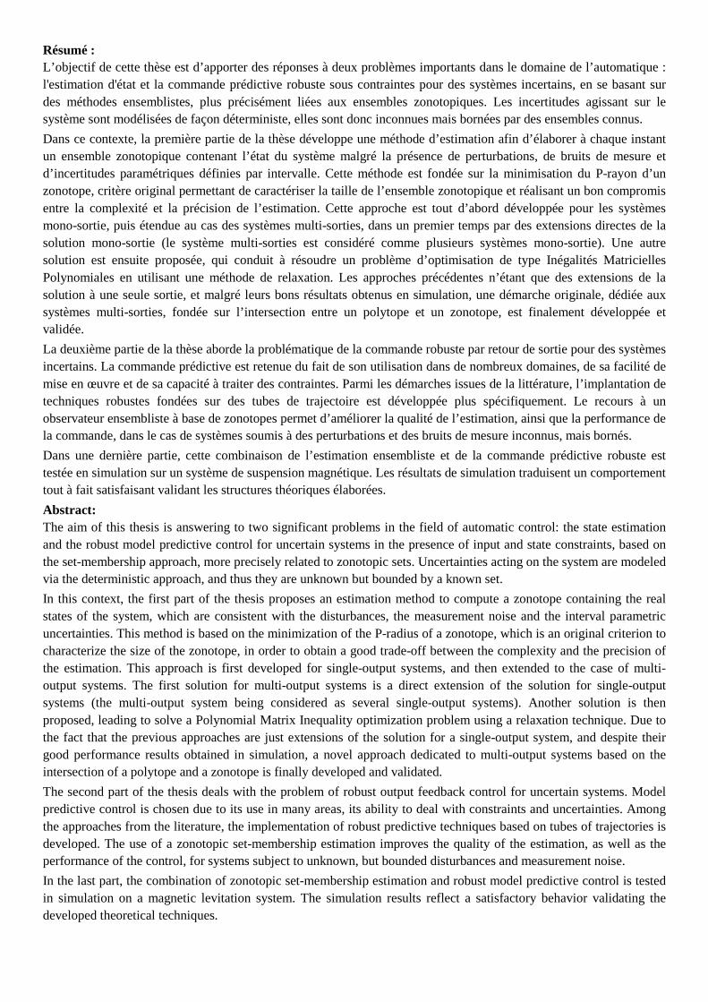
Résumé : L’objectif de cette thèse est d’apporter des réponses à deux problèmes importants dans le domaine de l’automatique : l'estimation d'état et la commande prédictive robuste sous contraintes pour des systèmes incertains, en se basant sur des méthodes ensemblistes, plus précisément liées aux ensembles zonotopiques. Les incertitudes agissant sur le système sont modélisées de façon déterministe, elles sont donc inconnues mais bornées par des ensembles connus.
Dans ce contexte, la première partie de la thèse développe une méthode d’estimation afin d’élaborer à chaque instant un ensemble zonotopique contenant l’état du système malgré la présence de perturbations, de bruits de mesure et d’incertitudes paramétriques définies par intervalle. Cette méthode est fondée sur la minimisation du P-rayon d’un zonotope, critère original permettant de caractériser la taille de l’ensemble zonotopique et réalisant un bon compromis entre la complexité et la précision de l’estimation. Cette approche est tout d’abord développée pour les systèmes mono-sortie, puis étendue au cas des systèmes multi-sorties, dans un premier temps par des extensions directes de la solution mono-sortie (le système multi-sorties est considéré comme plusieurs systèmes mono-sortie). Une autre solution est ensuite proposée, qui conduit à résoudre un problème d’optimisation de type Inégalités Matricielles Polynomiales en utilisant une méthode de relaxation. Les approches précédentes n’étant que des extensions de la solution à une seule sortie, et malgré leurs bons résultats obtenus en simulation, une démarche originale, dédiée aux systèmes multi-sorties, fondée sur l’intersection entre un polytope et un zonotope, est finalement développée et validée.
La deuxième partie de la thèse aborde la problématique de la commande robuste par retour de sortie pour des systèmes incertains. La commande prédictive est retenue du fait de son utilisation dans de nombreux domaines, de sa facilité de mise en œuvre et de sa capacité à traiter des contraintes. Parmi les démarches issues de la littérature, l’implantation de techniques robustes fondées sur des tubes de trajectoire est développée plus spécifiquement. Le recours à un observateur ensembliste à base de zonotopes permet d’améliorer la qualité de l’estimation, ainsi que la performance de la commande, dans le cas de systèmes soumis à des perturbations et des bruits de mesure inconnus, mais bornés.
Dans une dernière partie, cette combinaison de l’estimation ensembliste et de la commande prédictive robuste est testée en simulation sur un système de suspension magnétique. Les résultats de simulation traduisent un comportement tout à fait satisfaisant validant les structures théoriques élaborées.
Abstract: The aim of this thesis is answering to two significant problems in the field of automatic control: the state estimation and the robust model predictive control for uncertain systems in the presence of input and state constraints, based on the set-membership approach, more precisely related to zonotopic sets. Uncertainties acting on the system are modeled via the deterministic approach, and thus they are unknown but bounded by a known set.
In this context, the first part of the thesis proposes an estimation method to compute a zonotope containing the real states of the system, which are consistent with the disturbances, the measurement noise and the interval parametric uncertainties. This method is based on the minimization of the P-radius of a zonotope, which is an original criterion to characterize the size of the zonotope, in order to obtain a good trade-off between the complexity and the precision of the estimation. This approach is first developed for single-output systems, and then extended to the case of multi-output systems. The first solution for multi-output systems is a direct extension of the solution for single-output systems (the multi-output system being considered as several single-output systems). Another solution is then proposed, leading to solve a Polynomial Matrix Inequality optimization problem using a relaxation technique. Due to the fact that the previous approaches are just extensions of the solution for a single-output system, and despite their good performance results obtained in simulation, a novel approach dedicated to multi-output systems based on the intersection of a polytope and a zonotope is finally developed and validated.
The second part of the thesis deals with the problem of robust output feedback control for uncertain systems. Model predictive control is chosen due to its use in many areas, its ability to deal with constraints and uncertainties. Among the approaches from the literature, the implementation of robust predictive techniques based on tubes of trajectories is developed. The use of a zonotopic set-membership estimation improves the quality of the estimation, as well as the performance of the control, for systems subject to unknown, but bounded disturbances and measurement noise.
In the last part, the combination of zonotopic set-membership estimation and robust model predictive control is tested in simulation on a magnetic levitation system. The simulation results reflect a satisfactory behavior validating the developed theoretical techniques.