1

Modélisation des Effets Modélisation des Effets Cumulatifs des Expositions Cumulatifs des Expositions et des Facteurs Pronostiqueset des Facteurs Pronostiques

Michal Abrahamowicz, PhD*James McGill Professor

Department of Epidemiology & Biostatistics McGill University, Montreal, Quebec, CANADA

&

Marie-Pierre Sylvestre, PhDProfesseur Adjoint, Universite de Montreal, Quebec,

CANADA

2

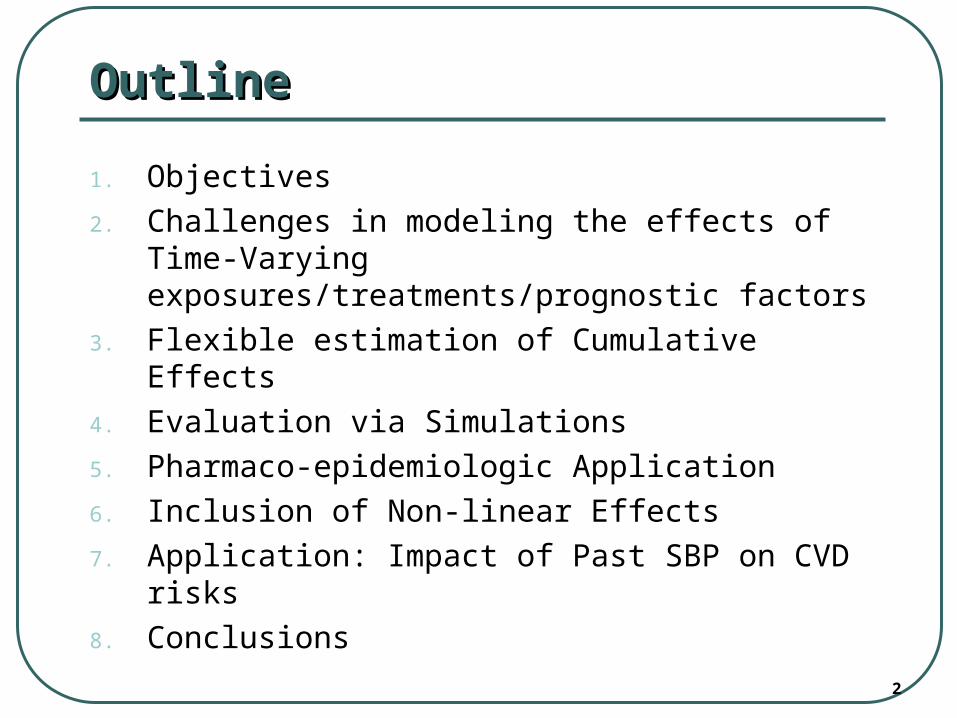
OutlineOutline

1. Objectives

2. Challenges in modeling the effects of Time-Varying exposures/treatments/prognostic factors

3. Flexible estimation of Cumulative Effects

4. Evaluation via Simulations

5. Pharmaco-epidemiologic Application

6. Inclusion of Non-linear Effects

7. Application: Impact of Past SBP on CVD risks

8. Conclusions

3

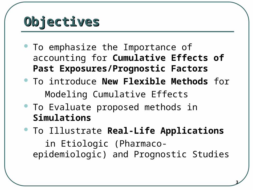
ObjectivesObjectives

To emphasize the Importance of accounting for Cumulative Effects of Past Exposures/Prognostic Factors

To introduce New Flexible Methods for

Modeling Cumulative Effects To Evaluate proposed methods in Simulations To Illustrate Real-Life Applications

in Etiologic (Pharmaco-epidemiologic) and Prognostic Studies

4

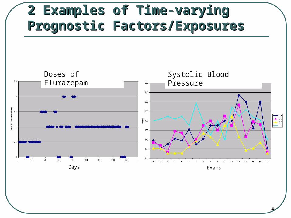
2 Examples of Time-varying 2 Examples of Time-varying Prognostic Factors/ExposuresPrognostic Factors/Exposures

Doses of Flurazepam Systolic Blood Pressure

Days Exams

5

Main Challenge in Modeling Effects of Main Challenge in Modeling Effects of Time-Varying Exposures/Risk FactorsTime-Varying Exposures/Risk Factors

How to relate the

Entire History of Past Values of the Exposure

with

Current Risk of the Outcome ?

6

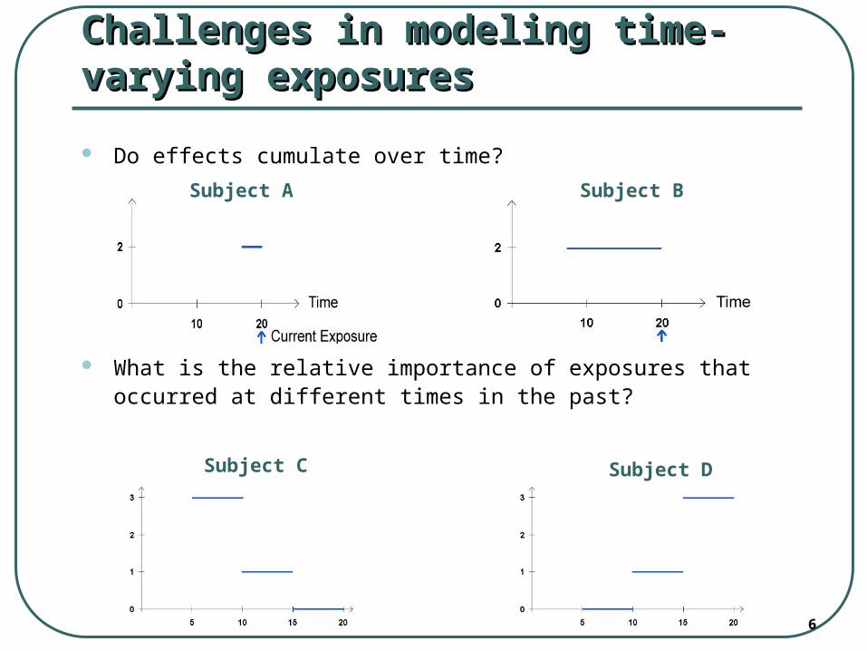
Do effects cumulate over time?

What is the relative importance of exposures that occurred at different times in the past?

Challenges in modeling time-varying Challenges in modeling time-varying exposuresexposures

Subject C Subject D

Subject A Subject B

7

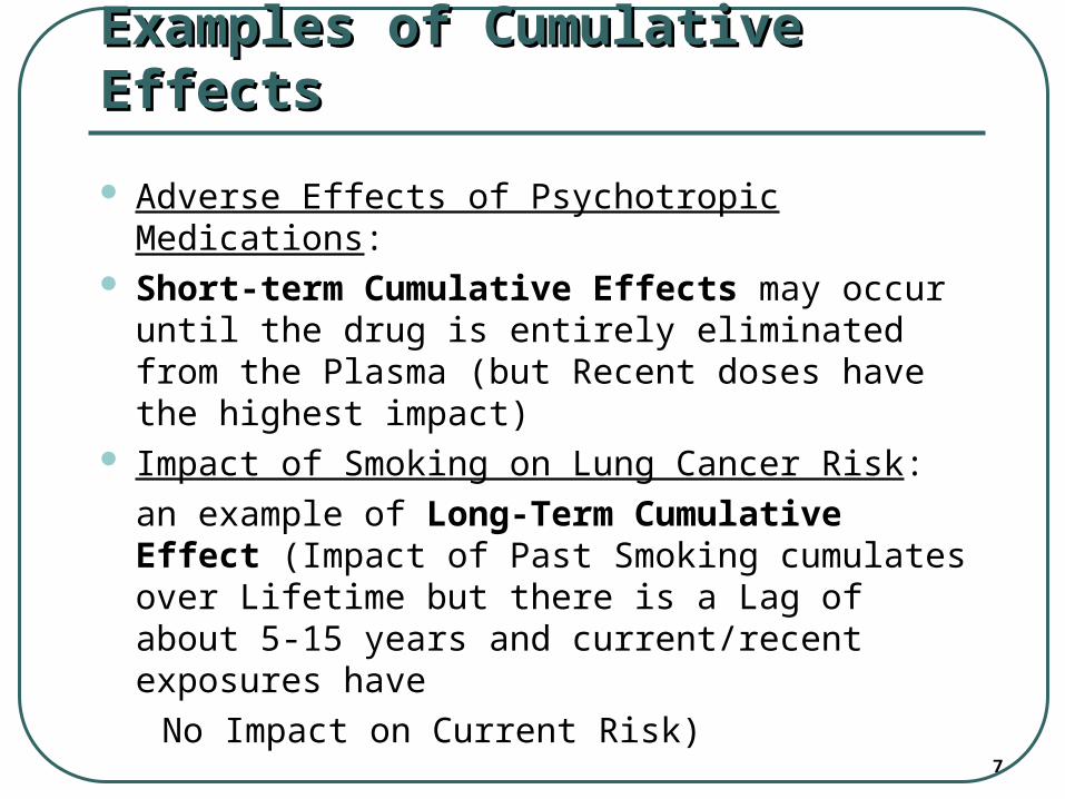
Examples of Cumulative EffectsExamples of Cumulative Effects

Adverse Effects of Psychotropic Medications: Short-term Cumulative Effects may occur until

the drug is entirely eliminated from the Plasma (but Recent doses have the highest impact)

Impact of Smoking on Lung Cancer Risk:

an example of Long-Term Cumulative Effect (Impact of Past Smoking cumulates over Lifetime but there is a Lag of about 5-15 years and current/recent exposures have

No Impact on Current Risk)

8

Conventional Models for Time-Varying Conventional Models for Time-Varying Prognostic FactorsPrognostic Factors

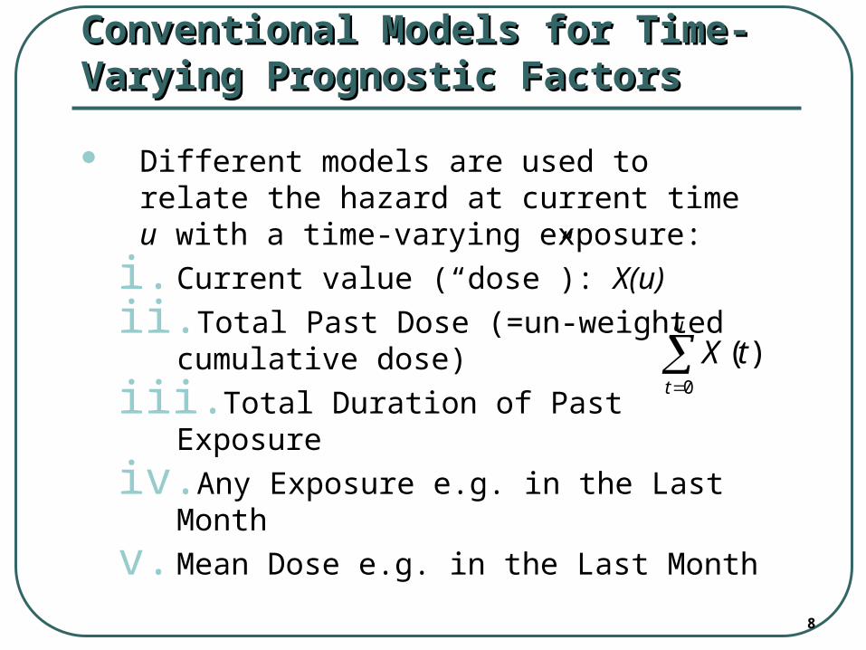
Different models are used to relate the hazard at current time u with a time-varying exposure:

i. Current value (“dose”): X(u)

ii. Total Past Dose (=un-weighted cumulative dose)

iii. Total Duration of Past Exposure

iv. Any Exposure e.g. in the Last Month

v. Mean Dose e.g. in the Last Month

u

t

tX0

)(

9

(Some) Limitations of Conventional (Some) Limitations of Conventional ModelsModels

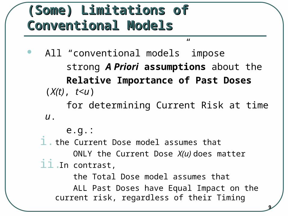
All “conventional models” impose

strong A Priori assumptions about the

Relative Importance of Past Doses (X(t), t<u)

for determining Current Risk at time u.

e.g.:i. the Current Dose model assumes that

ONLY the Current Dose X(u) does matter

ii. In contrast,

the Total Dose model assumes that

ALL Past Doses have Equal Impact on the current risk, regardless of their Timing

10

Weighted Cumulative Exposure (WCE) Weighted Cumulative Exposure (WCE) modelmodel

All conventional models (i)-(iii) are special cases

of a much more General Model,

based on the Concept of:

recency-Weighted Cumulative Exposure (WCE),where the Cumulative Effect is modeled as aWeighted Sum ** of all Past Doses,

[** these Weights describe how

the Relative Importance of Doses (Exposures)

changes as a function of the Time-since-Exposure]

11

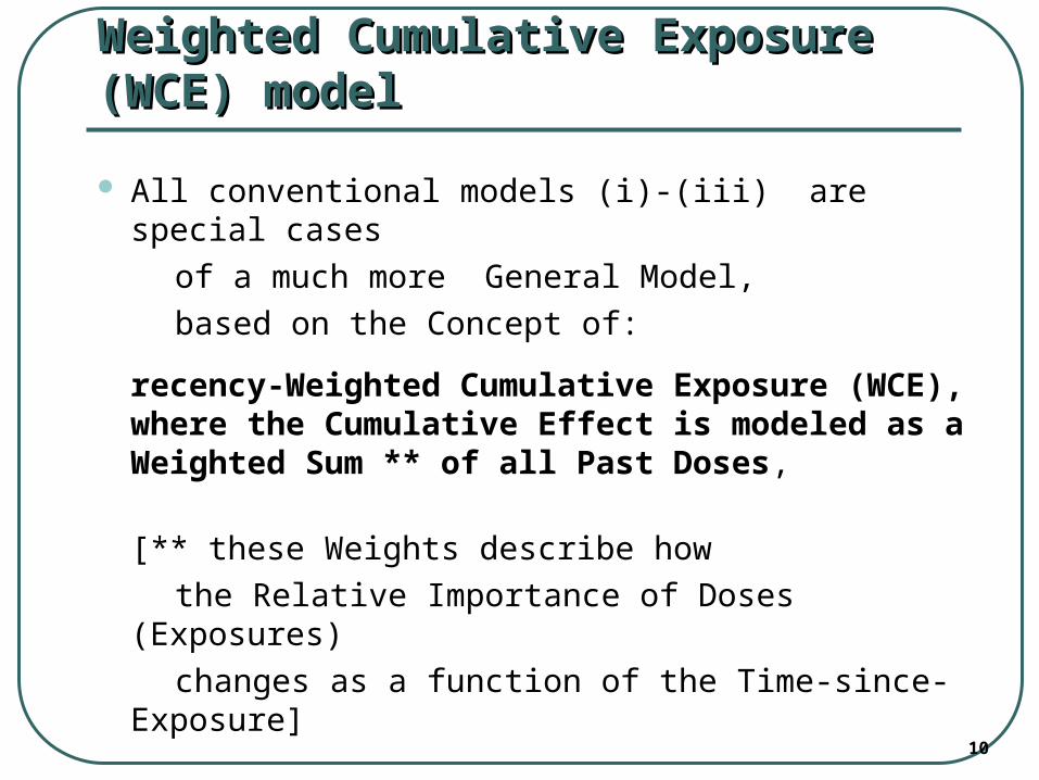
where:u= current time (when Risk is being assessed)

WCE(u)= Weighted Cumulative Effect of the Past Exposures on Risk at time u

X(t)= exposure intensity (dose) at time t(t≤u)

u-t= time elapsed since exposure X(t)

w(u-t)= Weight (Relative Importance) assigned to exposure X(t) as a function of Time-since-Exposure (u-t)

Recency-weighted cumulative exposure Recency-weighted cumulative exposure (WCE)(WCE)

(1)

ut

tXtuwuWCE

Abrahamowicz et al. (2006), Breslow et al. (1983), Hauptmann et al. (2000), Thomas (1988), Vacek (1997)

12

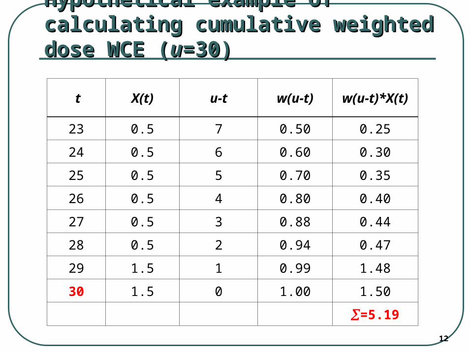
Hypothetical example of calculating Hypothetical example of calculating cumulative weighted dose WCE (cumulative weighted dose WCE (uu=30)=30)

t X(t) u-t w(u-t) w(u-t)*X(t)

23 0.5 7 0.50 0.25

24 0.5 6 0.60 0.30

25 0.5 5 0.70 0.35

26 0.5 4 0.80 0.40

27 0.5 3 0.88 0.44

28 0.5 2 0.94 0.47

29 1.5 1 0.99 1.48

30 1.5 0 1.00 1.50

=5.19

13

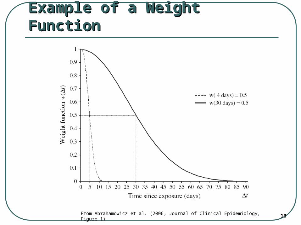
Example of a Weight FunctionExample of a Weight Function

From Abrahamowicz et al. (2006, Journal of Clinical Epidemiology, Figure 1)

14

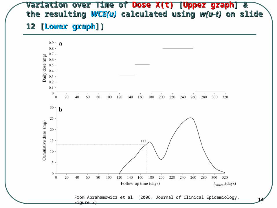
Variation over Time of Variation over Time of Dose X(t)Dose X(t) [ [Upper graphUpper graph] & the resulting ] & the resulting

WCE(u)WCE(u) calculated using calculated using w(u-t)w(u-t) on slide 12 [ on slide 12 [Lower graphLower graph])])

From Abrahamowicz et al. (2006, Journal of Clinical Epidemiology, Figure 2)

15

Need for Flexible Modeling of the Need for Flexible Modeling of the Weight FunctionWeight Function

In most real-life prognostic studies, there is little A priori knowledge about the (i) Exact Shape, and (ii) the Exact Values of the Weight Function

Therefore, it would be Advantageous to Estimate the Weight Function Directly from the Empirical Data

To this end, we need Flexible Assumptions-free methods such as Splines

16

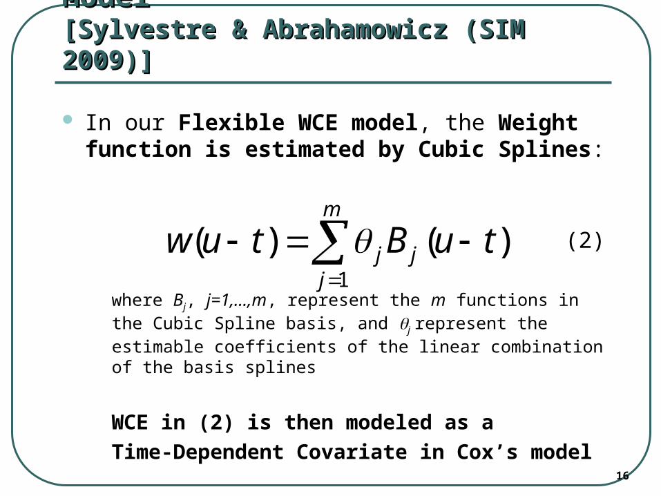
Flexible spline-based WCE ModelFlexible spline-based WCE Model[Sylvestre & Abrahamowicz (SIM 2009)][Sylvestre & Abrahamowicz (SIM 2009)]

In our Flexible WCE model, the Weight function is estimated by Cubic Splines:

(2)

where Bj, j=1,…,m, represent the m functions in the Cubic Spline basis, and j represent the estimable coefficients of the linear combination of the basis splines

WCE in (2) is then modeled as a

Time-Dependent Covariate in Cox’s model

m

jjj tuBtuw

1

)()(

17

0.0 0.2 0.4 0.6 0.8 1.0

0.0

0.2

0.4

0.6

0.8

1.0

x

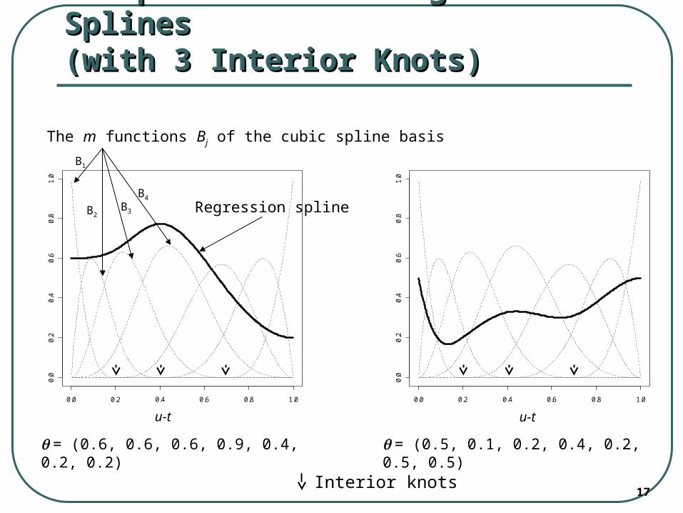
The m functions Bj of the cubic spline basis

Regression spline

B1

B2B3

B4

Examples of Cubic Regression Examples of Cubic Regression SplinesSplines(with 3 Interior Knots)(with 3 Interior Knots)

= (0.6, 0.6, 0.6, 0.9, 0.4, 0.2, 0.2)

0.0 0.2 0.4 0.6 0.8 1.00

.00

.20

.40

.60

.81

.0

x

= (0.5, 0.1, 0.2, 0.4, 0.2, 0.5, 0.5)

Interior knots

u-t u-t

18

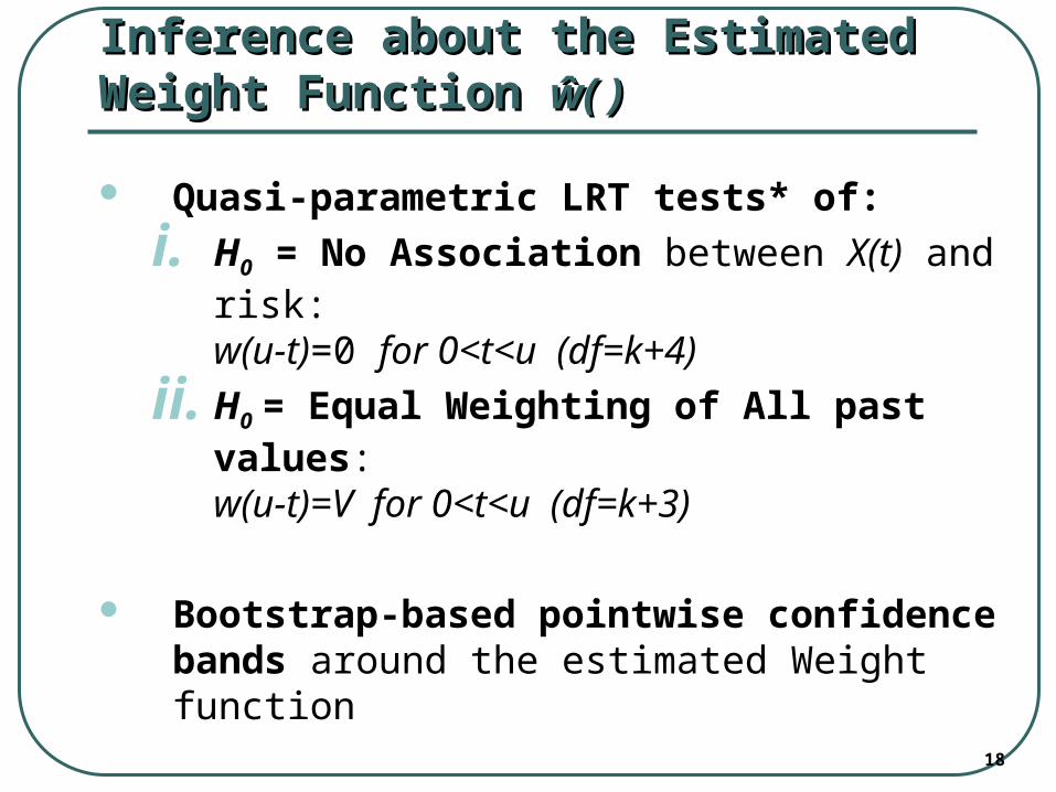
Inference about the Estimated Inference about the Estimated Weight Function Weight Function ŵ( )ŵ( )

Quasi-parametric LRT tests* of:

i. H0 = No Association between X(t) and risk: w(u-t)=0 for 0<t<u (df=k+4)

ii. H0 = Equal Weighting of All past values: w(u-t)=V for 0<t<u (df=k+3)

Bootstrap-based pointwise confidence bands around the estimated Weight function

19

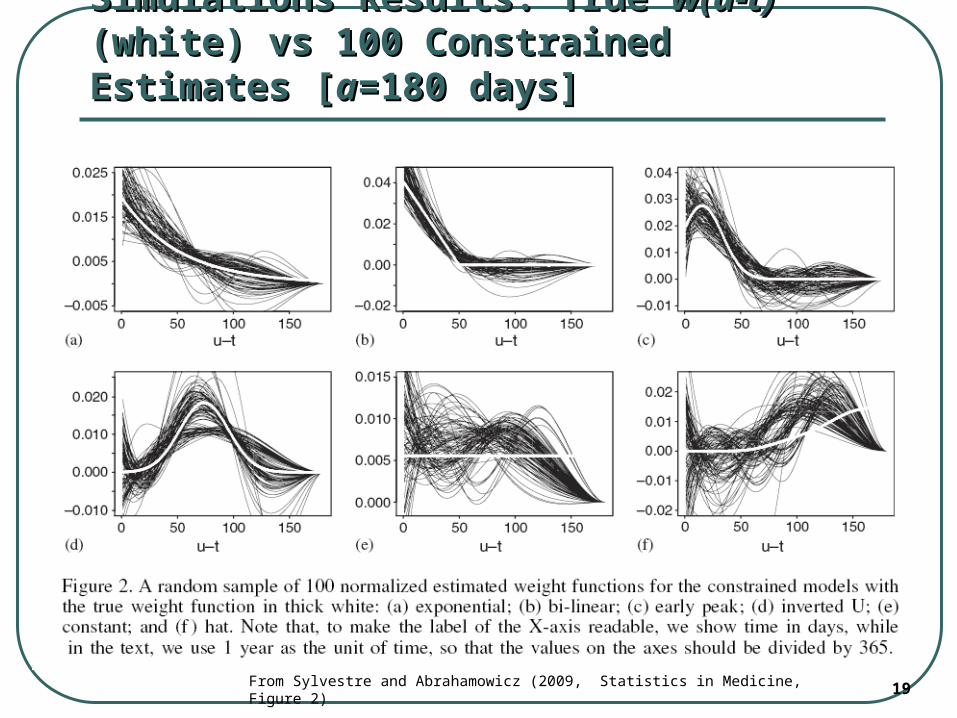
Simulations Results: True Simulations Results: True w(u-t)w(u-t) (white) vs (white) vs 100 Constrained Estimates [100 Constrained Estimates [aa=180 days]=180 days]

From Sylvestre and Abrahamowicz (2009, Statistics in Medicine, Figure 2)

20

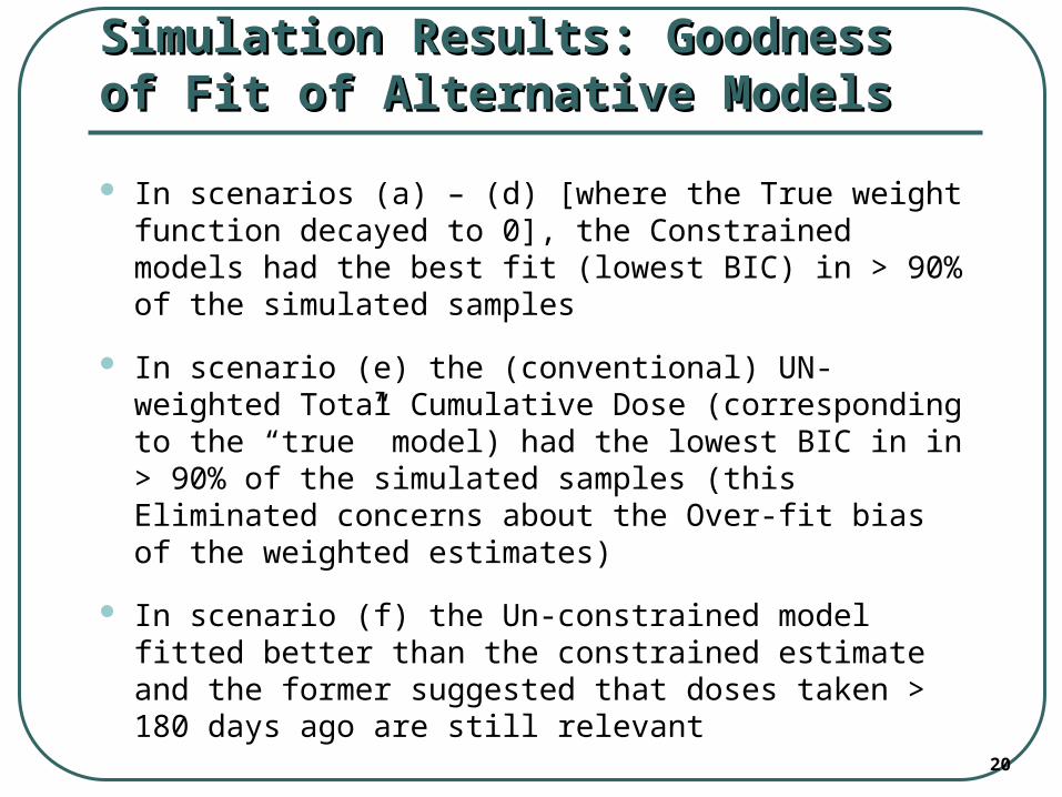
Simulation Results: Goodness of Fit of Simulation Results: Goodness of Fit of Alternative ModelsAlternative Models

In scenarios (a) – (d) [where the True weight function decayed to 0], the Constrained models had the best fit (lowest BIC) in > 90% of the simulated samples

In scenario (e) the (conventional) UN-weighted Total Cumulative Dose (corresponding to the “true” model) had the lowest BIC in in > 90% of the simulated samples (this Eliminated concerns about the Over-fit bias of the weighted estimates)

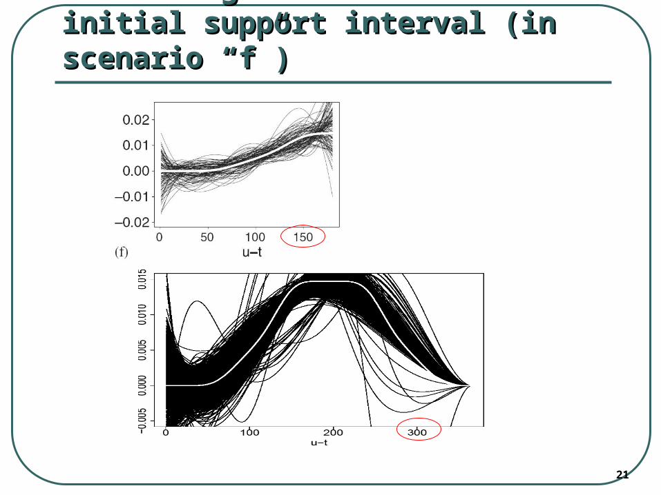
In scenario (f) the Un-constrained model fitted better than the constrained estimate and the former suggested that doses taken > 180 days ago are still relevant

21

Correcting for the “too short” initial Correcting for the “too short” initial support interval (in scenario “f”)support interval (in scenario “f”)

22

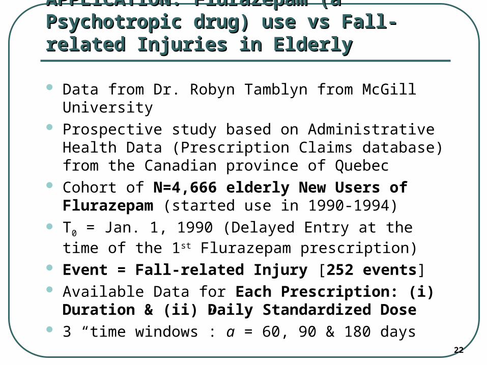
APPLICATION: Flurazepam (a Psychotropic APPLICATION: Flurazepam (a Psychotropic drug) use vs Fall-related Injuries in Elderlydrug) use vs Fall-related Injuries in Elderly

Data from Dr. Robyn Tamblyn from McGill University Prospective study based on Administrative Health

Data (Prescription Claims database) from the Canadian province of Quebec

Cohort of N=4,666 elderly New Users of Flurazepam (started use in 1990-1994)

T0 = Jan. 1, 1990 (Delayed Entry at the time of the 1st Flurazepam prescription)

Event = Fall-related Injury [252 events] Available Data for Each Prescription: (i) Duration

& (ii) Daily Standardized Dose 3 “time windows”: a = 60, 90 & 180 days

23

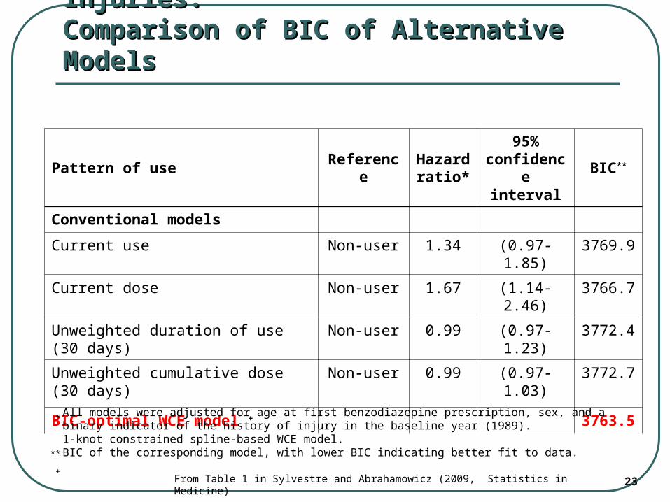
Flurazepam use vs Fall-related Injuries:Flurazepam use vs Fall-related Injuries:Comparison of BIC of Alternative ModelsComparison of BIC of Alternative Models

Pattern of use ReferenceHazard ratio*

95% confidence

intervalBIC**

Conventional models

Current use Non-user 1.34 (0.97-1.85) 3769.9

Current dose Non-user 1.67 (1.14-2.46) 3766.7

Unweighted duration of use (30 days) Non-user 0.99 (0.97-1.23) 3772.4

Unweighted cumulative dose (30 days) Non-user 0.99 (0.97-1.03) 3772.7

BIC-optimal WCE model + 3763.5

All models were adjusted for age at first benzodiazepine prescription, sex, and a binary indicator of the history of injury in the baseline year (1989). 1-knot constrained spline-based WCE model.BIC of the corresponding model, with lower BIC indicating better fit to data.

*

**

+From Table 1 in Sylvestre and Abrahamowicz (2009, Statistics in Medicine)

24

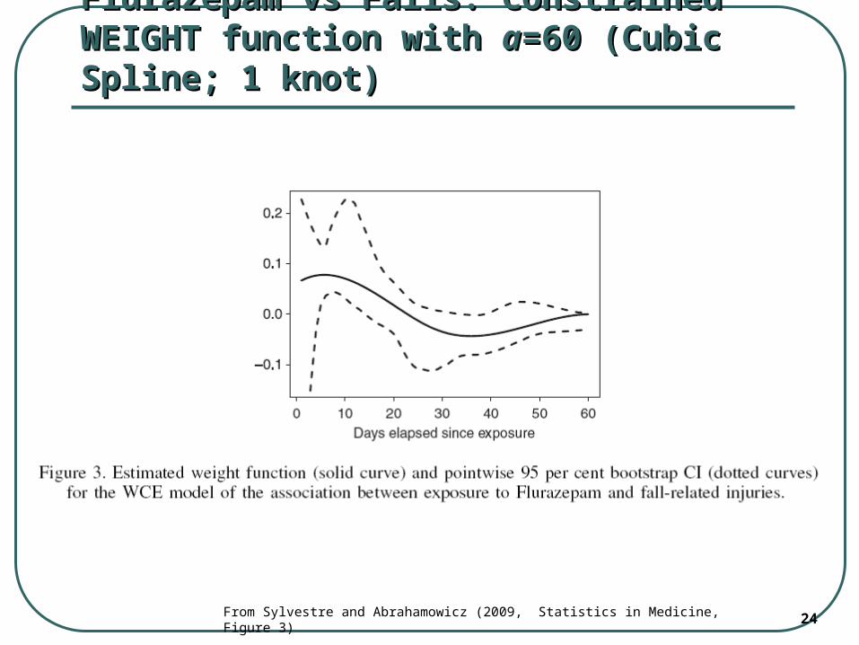
Flurazepam vs Falls: Constrained WEIGHT Flurazepam vs Falls: Constrained WEIGHT function with function with aa=60 (Cubic Spline; 1 knot)=60 (Cubic Spline; 1 knot)

From Sylvestre and Abrahamowicz (2009, Statistics in Medicine, Figure 3)

25

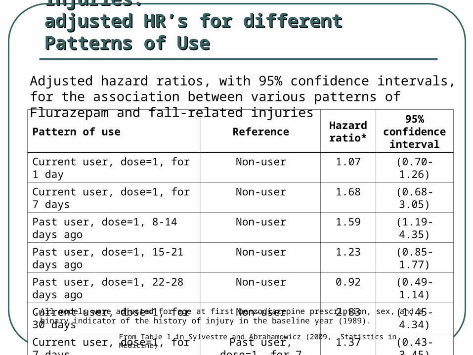
Flurazepam use vs Fall-related Injuries:Flurazepam use vs Fall-related Injuries:adjusted HR’s for different Patterns of Use adjusted HR’s for different Patterns of Use

Pattern of use ReferenceHazard ratio*

95% confidence

interval

Current user, dose=1, for 1 day Non-user 1.07 (0.70-1.26)

Current user, dose=1, for 7 days Non-user 1.68 (0.68-3.05)

Past user, dose=1, 8-14 days ago Non-user 1.59 (1.19-4.35)

Past user, dose=1, 15-21 days ago Non-user 1.23 (0.85-1.77)

Past user, dose=1, 22-28 days ago Non-user 0.92 (0.49-1.14)

Current user, dose=1, for 30 days Non-user 2.83 (1.45-4.34)

Current user, dose=1, for 7 days Past user, dose=1, for 7 days, between 14

and 7 days ago

1.37 (0.43-3.45)

All models were adjusted for age at first benzodiazepine prescription, sex, and a binary indicator of the history of injury in the baseline year (1989).

*

From Table 1 in Sylvestre and Abrahamowicz (2009, Statistics in Medicine)

Adjusted hazard ratios, with 95% confidence intervals, for the association between various patterns of Flurazepam and fall-related injuries

26

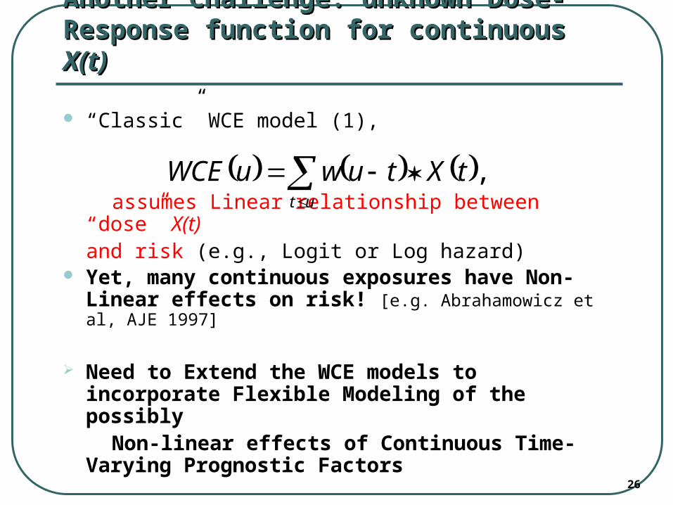
Another Challenge: unknown Dose-Another Challenge: unknown Dose-Response function for continuous Response function for continuous X(t)X(t)

“Classic” WCE model (1),

assumes Linear relationship between “dose” X(t)and risk (e.g., Logit or Log hazard)

Yet, many continuous exposures have Non-Linear effects on risk! [e.g. Abrahamowicz et al, AJE 1997]

Need to Extend the WCE models to incorporate Flexible Modeling of the possibly

Non-linear effects of Continuous Time-Varying Prognostic Factors

,

ut

tXtuwuWCE

27

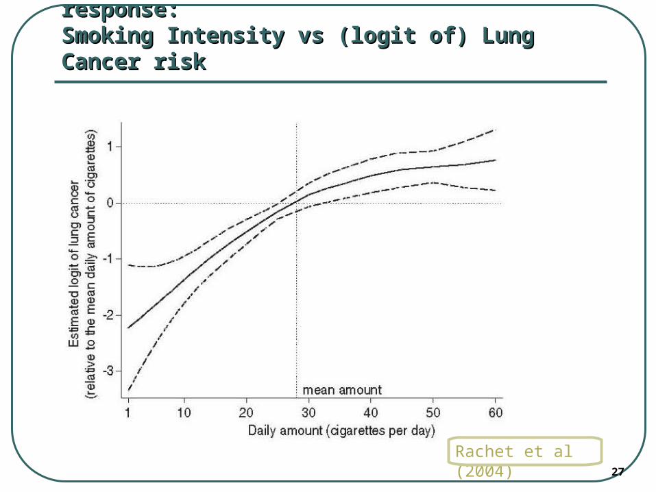
Example of NON-LINEARITY of dose-response: Example of NON-LINEARITY of dose-response: Smoking Intensity vs (logit of) Lung Cancer riskSmoking Intensity vs (logit of) Lung Cancer risk

Rachet et al (2004)

28

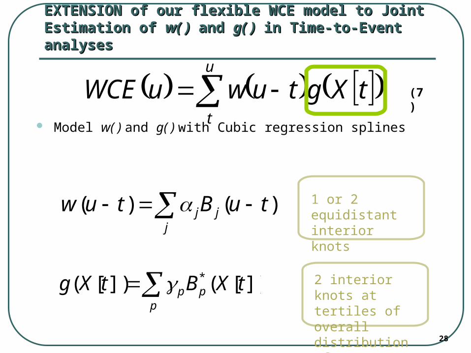
EXTENSION of our flexible WCE model to Joint EXTENSION of our flexible WCE model to Joint Estimation of Estimation of w( )w( ) and and g( )g( ) in Time-to-Event analyses in Time-to-Event analyses

Model w( ) and g( ) with Cubic regression splines

)()( tuBtuw jj

j

])[(])[( * tXBtXg pp

p 2 interior knots at tertiles of overall distribution of X[t]

1 or 2 equidistant interior knots

u

t

tXgtuwuWCE (7)

29

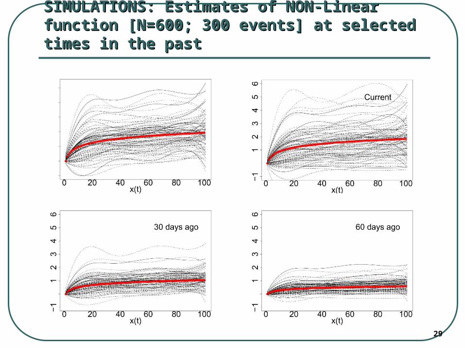
SIMULATIONS: Estimates of NON-Linear function SIMULATIONS: Estimates of NON-Linear function [N=600; [N=600; 300 events] at selected times in the past300 events] at selected times in the past

30

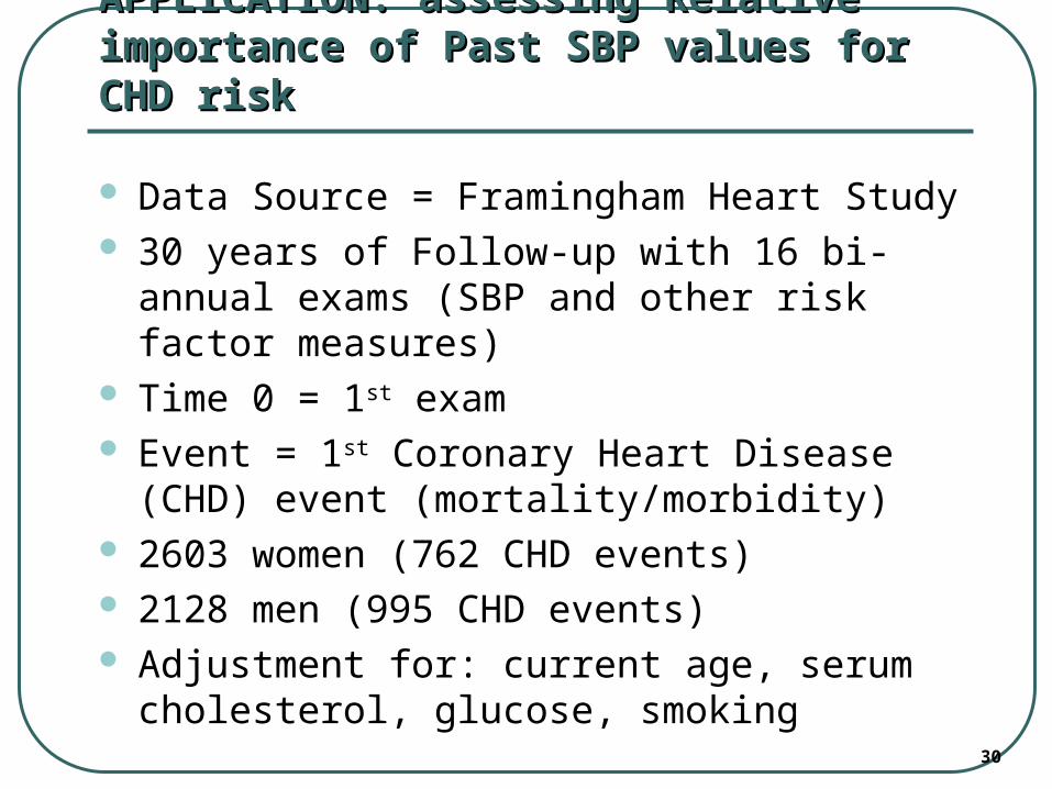
APPLICATION: assessing Relative APPLICATION: assessing Relative importance of Past SBP values for CHD riskimportance of Past SBP values for CHD risk

Data Source = Framingham Heart Study 30 years of Follow-up with 16 bi-annual exams

(SBP and other risk factor measures) Time 0 = 1st exam Event = 1st Coronary Heart Disease (CHD) event

(mortality/morbidity) 2603 women (762 CHD events) 2128 men (995 CHD events) Adjustment for: current age, serum cholesterol,

glucose, smoking

31

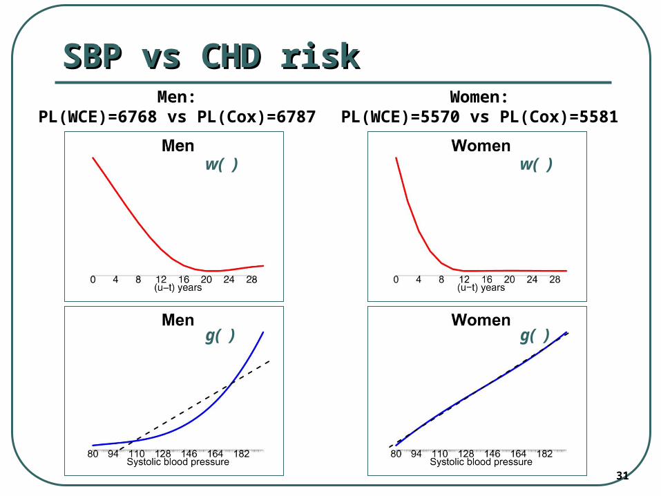
SBP vs CHD riskSBP vs CHD risk

w( ) w( )

g( ) g( )

Men:PL(WCE)=6768 vs PL(Cox)=6787

Women:PL(WCE)=5570 vs PL(Cox)=5581

32

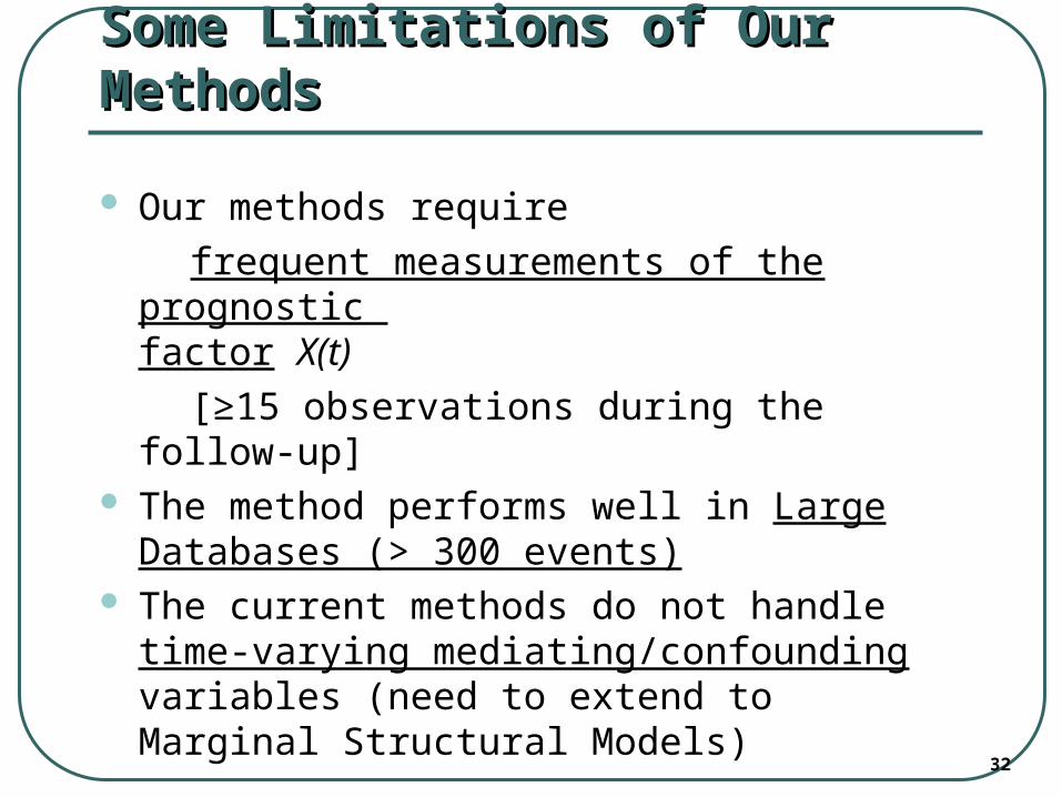
Some Limitations of Our MethodsSome Limitations of Our Methods

Our methods require

frequent measurements of the prognostic factor X(t)

[≥15 observations during the follow-up] The method performs well in Large Databases

(> 300 events) The current methods do not handle time-varying

mediating/confounding variables (need to extend to Marginal Structural Models)

33

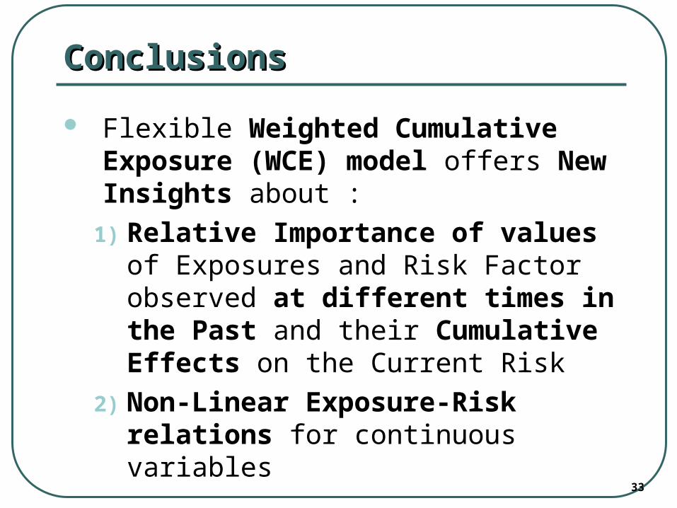
ConclusionsConclusions

Flexible Weighted Cumulative Exposure (WCE) model offers New Insights about :

1) Relative Importance of values of Exposures and Risk Factor observed at different times in the Past and their Cumulative Effects on the Current Risk

2) Non-Linear Exposure-Risk relations for continuous variables

34

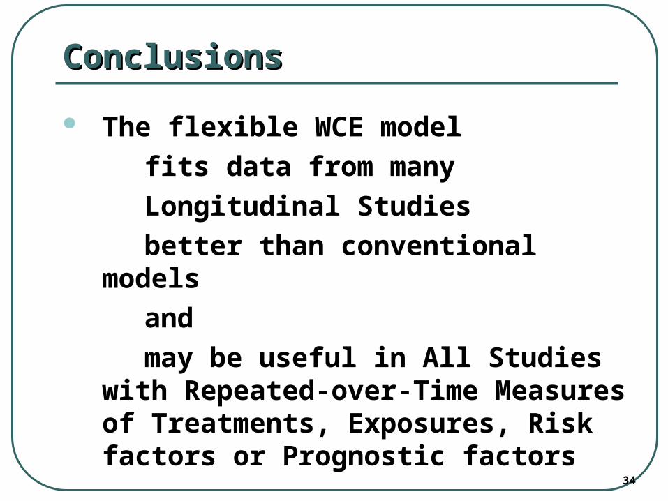
ConclusionsConclusions

The flexible WCE model

fits data from many

Longitudinal Studies

better than conventional models

and

may be useful in All Studies with Repeated-over-Time Measures of Treatments, Exposures, Risk factors or Prognostic factors

35

ReferencesReferences

Abrahamowicz M, Bartlett G, Tamblyn R, du Berger R. Modeling cumulative dose and exposure duration provided insights regarding the associations between benzodiazepines and injuries. Journal of Clinical Epidemiology. 2006;59(4):393-403.

Abrahamowicz M, du Berger R, Grover SA. Flexible modeling of the effects of serum cholesterol on coronary heart disease mortality. American Journal of Epidemiology 1997;145(8):714-729.

Abrahamowicz M, MacKenzie T, Esdaile JM. Time-dependent hazard ratio: modeling and hypothesis testing with application in lupus nephritis. Journal of the American Statistical Association. 1996;91(436):1432-39.

Breslow NE, Lubin JH, Marek P, Langholz B. Multiplicative models and cohort analysis. Journal of the American Statistical Society 1983; 78(381):1–12.

Hauptmann M, Wellmann J, Lubin JH, Rosenberg PS, Kreienbrock L. Analysis of exposure-time-response relationships using a spline weight function. Biometrics. 2000;56(4):1105-8.

MacKenzie T, Abrahamowicz M. Marginal and hazard ratio specific random data generation: applications to semi-parametric bootstrapping. Statistics and Computing. 2002;12(3):245-352.

Mahmud M, Abrahamowicz M, Leffondré K, Chaubey YP. Selecting the optimal transformation of a continuous covariate in Cox’s regression: Implications for hypothesis testing. Communication in Statistics 2006;35(1):27-45.

Rachet B, Siemiatycki J, Abrahamowicz M, Leffondré K. A flexible modeling approach to estimating the component effects of smoking behavior on lung cancer. Journal of Clinical Epidemiology 2004;57(10):1076-1085.

Sylvestre MP, Abrahamowicz M. Comparisons of algorithms to generate event times conditional on time-dependent covariates. Statistics in Medicine. 2008; 27(14):2618-34.

Sylvestre MP, Abrahamowicz M. Flexible modeling of the cumulative effects of time-dependent exposures on the hazard. Statistics in Medicine. 2009; 28(27):3437-53.

Thomas DC. Models for exposure-time-response relationships with applications to cancer epidemiology. Annual Reviews of Public Health 1988; 9:451-82.

Vacek PM. Assessing the effect of intensity when exposure varies over time. Statistics in Medicine. 1997;16(5):505-13.

36

MERCI !

Michal.Abrahamowicz@mcgill.ca

37

Additional materialAdditional material

38

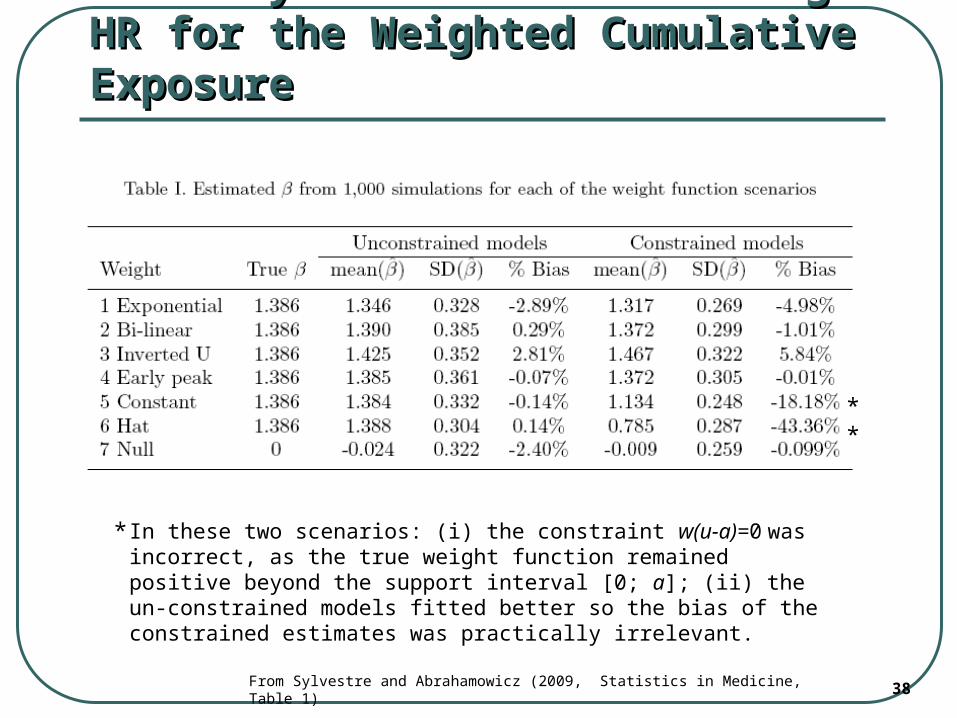
Accuracy of the Estimated log HR for Accuracy of the Estimated log HR for the Weighted Cumulative Exposurethe Weighted Cumulative Exposure

**

From Sylvestre and Abrahamowicz (2009, Statistics in Medicine, Table 1)

In these two scenarios: (i) the constraint w(u-a)=0 was incorrect, as the true weight function remained positive beyond the support interval [0; a]; (ii) the un-constrained models fitted better so the bias of the constrained estimates was practically irrelevant.

*

39

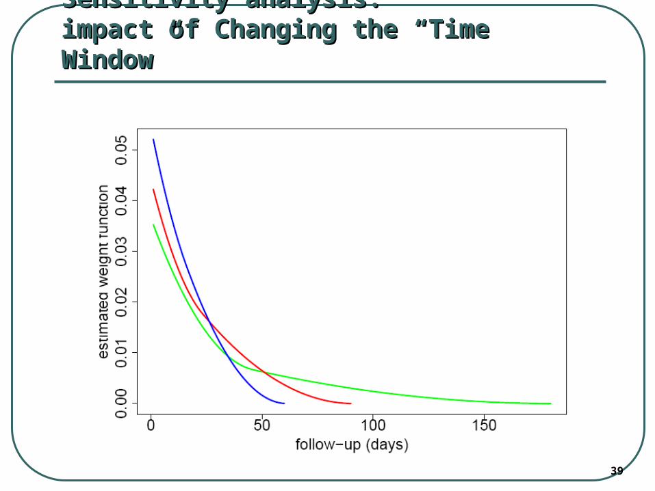
Sensitivity analysis: Sensitivity analysis: impact of Changing the “Time Window”impact of Changing the “Time Window”

40

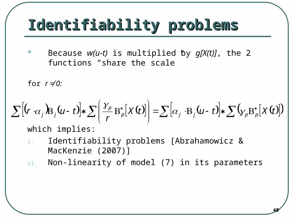
Identifiability problemsIdentifiability problems

Because w(u-t) is multiplied by g[X(t)], the 2 functions “share the scale”

for r ≠ 0:

which implies:

i. Identifiability problems [Abrahamowicz & MacKenzie (2007)]

ii. Non-linearity of model (7) in its parameters

tXtutX

rtur ppjjp

pjj

41

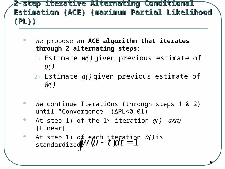
2-step iterative Alternating Conditional Estimation (ACE) 2-step iterative Alternating Conditional Estimation (ACE) (maximum Partial Likelihood (PL))(maximum Partial Likelihood (PL))

We propose an ACE algorithm that iterates through 2 alternating steps:

1) Estimate w( ) given previous estimate of ĝ( )

2) Estimate g( ) given previous estimate of ŵ( )

We continue Iterations (through steps 1 & 2) until “Convergence” (ΔPL<0.01)

At step 1) of the 1st iteration g( ) = αX(t) [Linear] At step 1) of each iteration ŵ( ) is standardized:

1)( dttuw

42

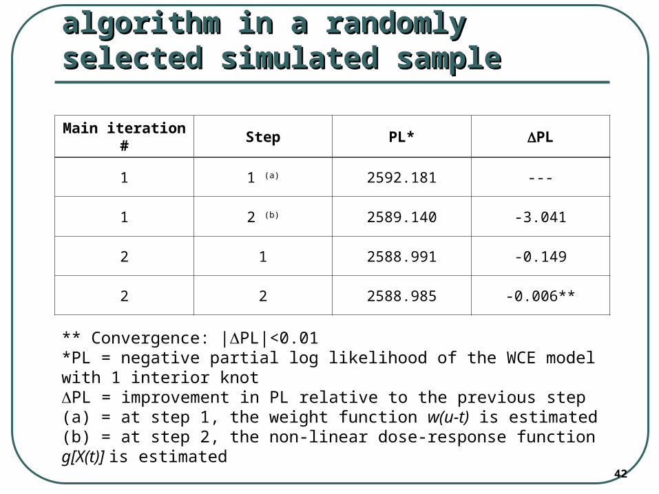
Performance of the ACE algorithm in a Performance of the ACE algorithm in a randomly selected simulated samplerandomly selected simulated sample

Main iteration # Step PL* PL

1 1 (a) 2592.181 ---

1 2 (b) 2589.140 -3.041

2 1 2588.991 -0.149

2 2 2588.985 -0.006**

** Convergence: |PL|<0.01*PL = negative partial log likelihood of the WCE model with 1 interior knotPL = improvement in PL relative to the previous step(a) = at step 1, the weight function w(u-t) is estimated(b) = at step 2, the non-linear dose-response function g[X(t)] is estimated

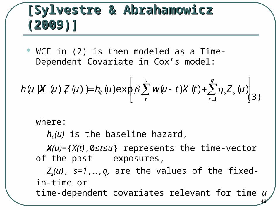
43

Flexible WCE ModelFlexible WCE Model[Sylvestre & Abrahamowicz (2009)][Sylvestre & Abrahamowicz (2009)]

WCE in (2) is then modeled as a Time-Dependent Covariate in Cox’s model:

(3)

where:

h0(u) is the baseline hazard,

X(u)={X(t),0≤t≤u} represents the time-vector of the past exposures,

Zs(u), s=1,…,q, are the values of the fixed-in-time or time-dependent covariates relevant for time u

q

sss

u

t

uZtXtuwuhuZuuh1

0 )()()(exp)())(),(|( X

44

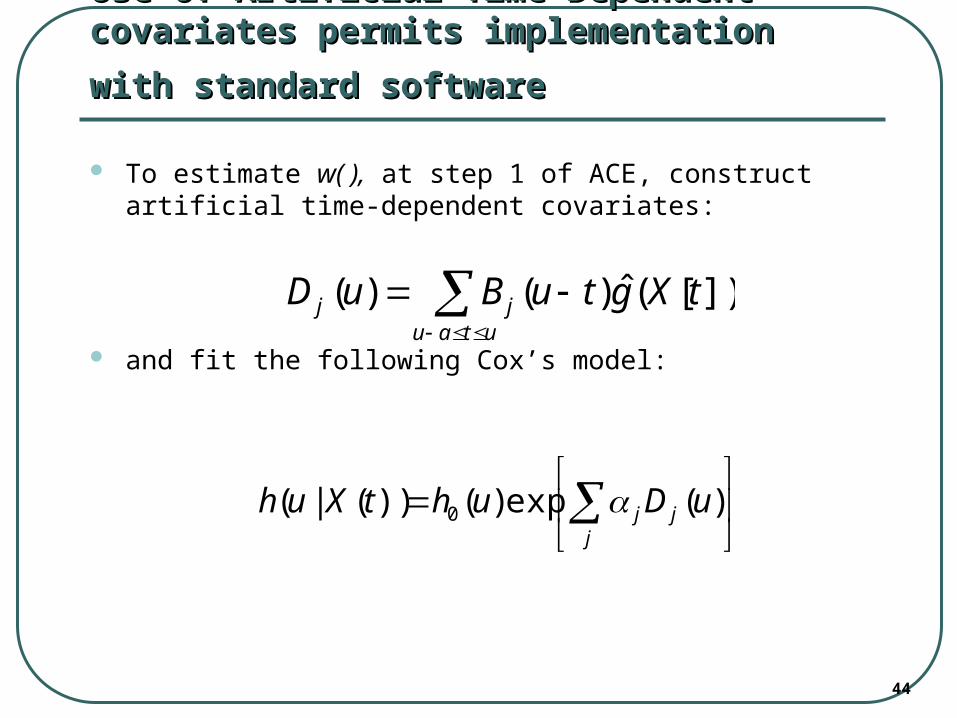
Use of Artificial Time-Dependent covariates Use of Artificial Time-Dependent covariates

permits implementation with standard softwarepermits implementation with standard software

To estimate w( ), at step 1 of ACE, construct artificial time-dependent covariates:

and fit the following Cox’s model:

utaujj tXgtuBuD ])[(ˆ)()(

jjj uDuhtXuh )(exp)())(|( 0

45

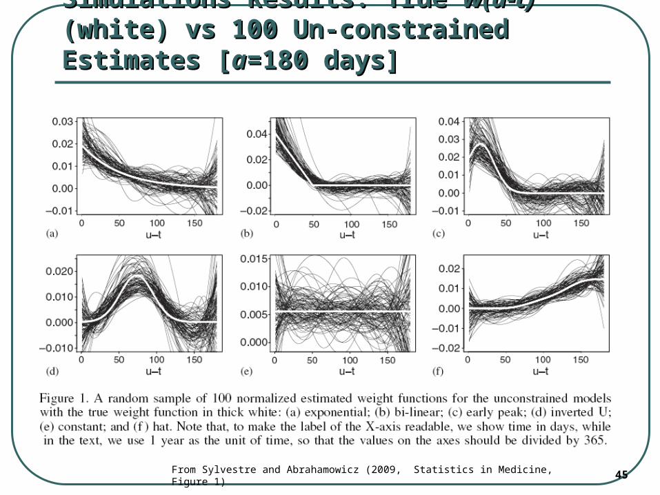
Simulations Results: True Simulations Results: True w(u-t)w(u-t) (white) vs (white) vs 100 Un-constrained Estimates [100 Un-constrained Estimates [aa=180 days]=180 days]

From Sylvestre and Abrahamowicz (2009, Statistics in Medicine, Figure 1)

46

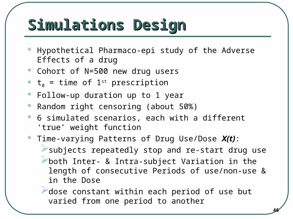
Simulations DesignSimulations Design

Hypothetical Pharmaco-epi study of the Adverse Effects of a drug

Cohort of N=500 new drug users t0 = time of 1st prescription Follow-up duration up to 1 year Random right censoring (about 50%) 6 simulated scenarios, each with a different ‘true’ weight

function Time-varying Patterns of Drug Use/Dose X(t):

subjects repeatedly stop and re-start drug use

both Inter- & Intra-subject Variation in the length of consecutive Periods of use/non-use & in the Dose

dose constant within each period of use but varied from one period to another

47

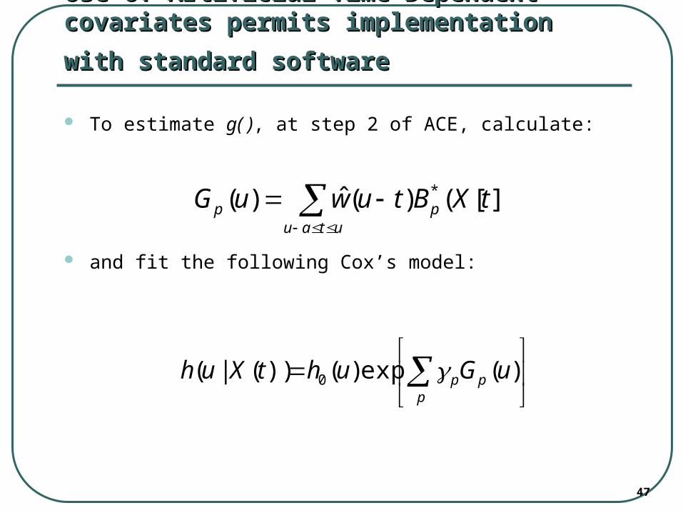
Use of Artificial Time-Dependent covariates Use of Artificial Time-Dependent covariates

permits implementation with standard softwarepermits implementation with standard software

To estimate g( ), at step 2 of ACE, calculate:

and fit the following Cox’s model:

utau

pp tXBtuwuG ])[()(ˆ)( *

ppp uGuhtXuh )(exp)())(|( 0

48

SimulationsSimulations

The Design and Methods of Simulations were Similar to slides 24-25, Except:

i. “dose” X(t) was generated from a Continuous Distribution U(0, 3);

ii. X(t) was assumed to have different Non-linear relationships with the logarithm of the hazard.

49

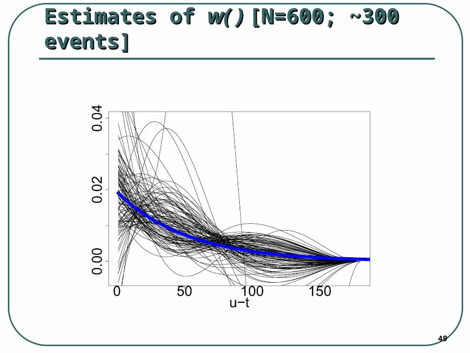
Estimates of Estimates of w( ) w( ) [N=600; [N=600; ~300 events]~300 events]

50

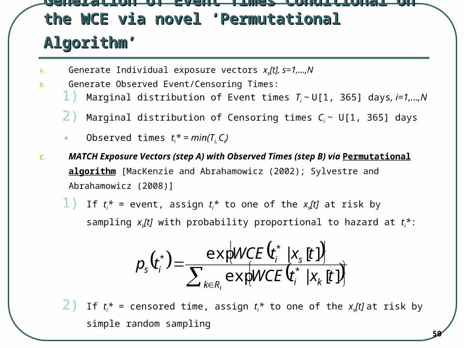
Generation of Event Times Conditional on the WCE Generation of Event Times Conditional on the WCE

via novel ‘Permutational Algorithm’ via novel ‘Permutational Algorithm’ A. Generate Individual exposure vectors xs[t], s=1,…,N

B. Generate Observed Event/Censoring Times:

1) Marginal distribution of Event times Ti ~ U[1, 365] days, i=1,…,N

2) Marginal distribution of Censoring times Ci ~ U[1, 365] days

• Observed times ti* = min(Ti, Ci)

C. MATCH Exposure Vectors (step A) with Observed Times (step B) via Permutational

algorithm [MacKenzie and Abrahamowicz (2002); Sylvestre and Abrahamowicz (2008)]

1) If ti* = event, assign ti* to one of the xs[t] at risk by sampling xs[t] with probability

proportional to hazard at ti*:

2) If ti* = censored time, assign ti* to one of the xs[t] at risk by simple random

sampling

iRk ki

siis txtWCE

txtWCEtp

][|exp

][|exp*

**

51

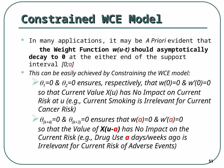
Constrained WCE ModelConstrained WCE Model

In many applications, it may be A Priori evident that

the Weight Function w(u-t) should asymptotically decay to 0 at the either end of the support interval [0;a]

This can be easily achieved by Constraining the WCE model:

1=0 & 2=0 ensures, respectively, that w(0)=0 & w’(0)=0so that Current Value X(u) has No Impact on Current Risk at u (e.g., Current Smoking is Irrelevant for Current Cancer Risk)

(k+4)=0 & (k+3)=0 ensures that w(a)=0 & w’(a)=0 so that the Value of X(u-a) has No Impact on the Current Risk (e.g., Drug Use a days/weeks ago is Irrelevant for Current Risk of Adverse Events)

52

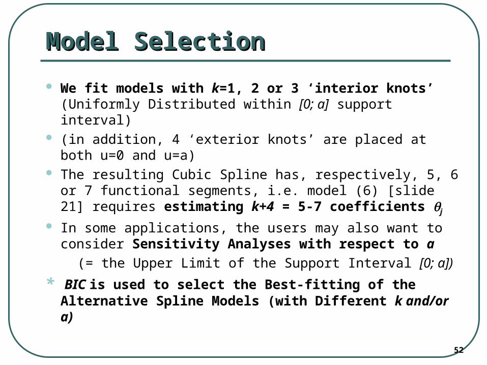
Model SelectionModel Selection

We fit models with k=1, 2 or 3 ‘interior knots’ (Uniformly Distributed within [0; a] support interval)

(in addition, 4 ‘exterior knots’ are placed at both u=0 and u=a)

The resulting Cubic Spline has, respectively, 5, 6 or 7 functional segments, i.e. model (6) [slide 21] requires estimating k+4 = 5-7 coefficients j

In some applications, the users may also want to consider Sensitivity Analyses with respect to a

(= the Upper Limit of the Support Interval [0; a])

* BIC is used to select the Best-fitting of the Alternative Spline Models (with Different k and/or a)

53

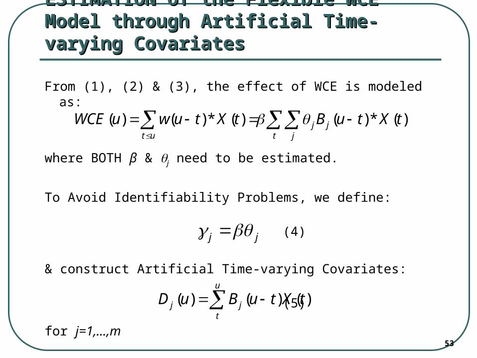
ESTIMATION of the Flexible WCE Model ESTIMATION of the Flexible WCE Model through Artificial Time-varying Covariatesthrough Artificial Time-varying Covariates

From (1), (2) & (3), the effect of WCE is modeled as:

where BOTH β & j need to be estimated.

To Avoid Identifiability Problems, we define:

(4)

& construct Artificial Time-varying Covariates:

(5)

for j=1,…,m

)(*)()(*)()( tXtuBtXtuwuWCE jt j

jut

jj

u

tjj tXtuBuD )()()(

54

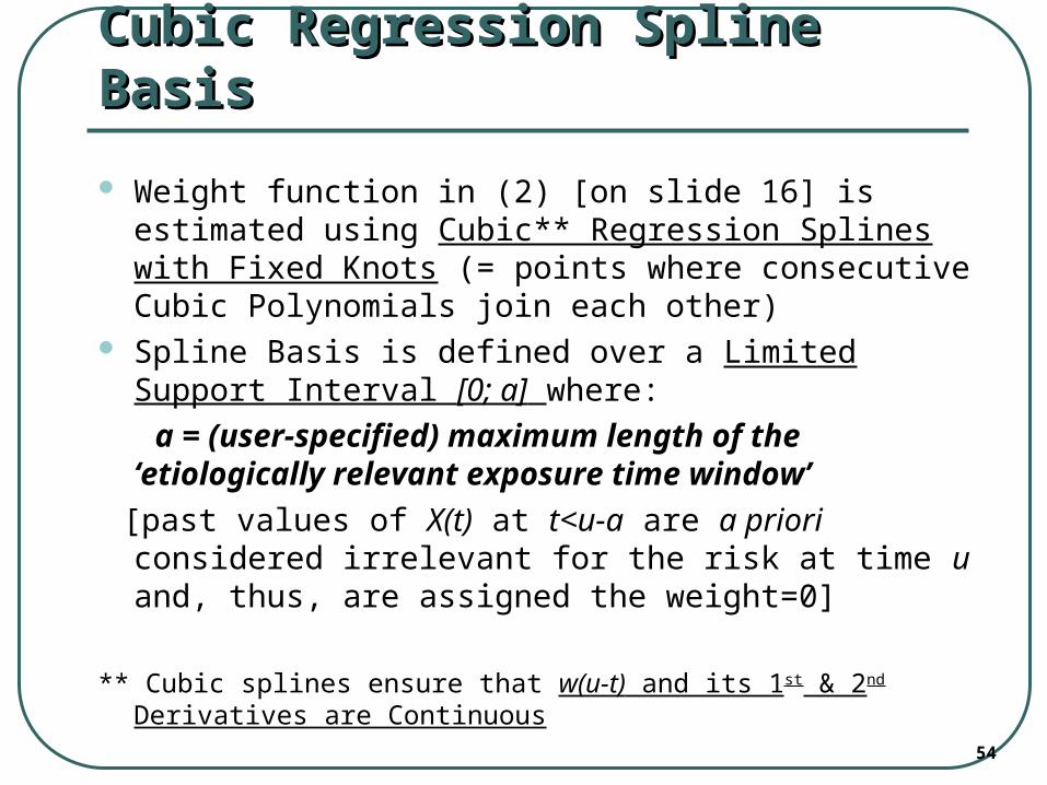
Cubic Regression Spline BasisCubic Regression Spline Basis

Weight function in (2) [on slide 16] is estimated using Cubic** Regression Splines with Fixed Knots (= points where consecutive Cubic Polynomials join each other)

Spline Basis is defined over a Limited Support Interval [0; a] where:

a = (user-specified) maximum length of the ‘etiologically relevant exposure time window’

[past values of X(t) at t<u-a are a priori considered irrelevant for the risk at time u and, thus, are assigned the weight=0]

** Cubic splines ensure that w(u-t) and its 1st & 2nd Derivatives are Continuous

55

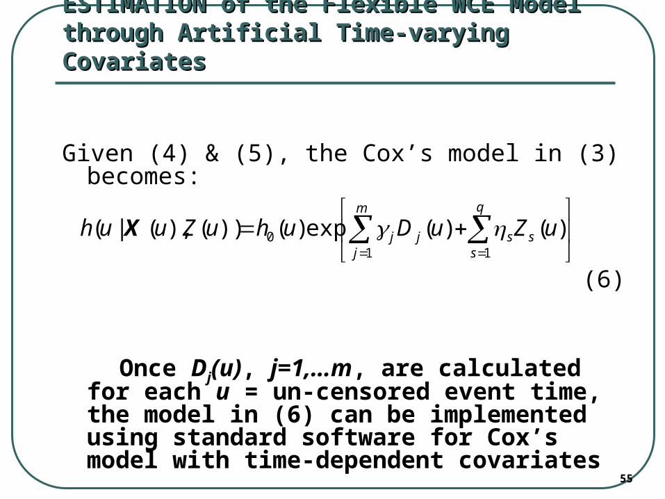
ESTIMATION of the Flexible WCE Model ESTIMATION of the Flexible WCE Model through Artificial Time-varying Covariatesthrough Artificial Time-varying Covariates

Given (4) & (5), the Cox’s model in (3) becomes:

(6)

Once Dj(u), j=1,…m, are calculated for each u = un-censored event time, the model in (6) can be implemented using standard software for Cox’s model with time-dependent covariates

q

sss

m

jjj uZuDuhuZuuh

110 )()(exp)())(),(|( X

56

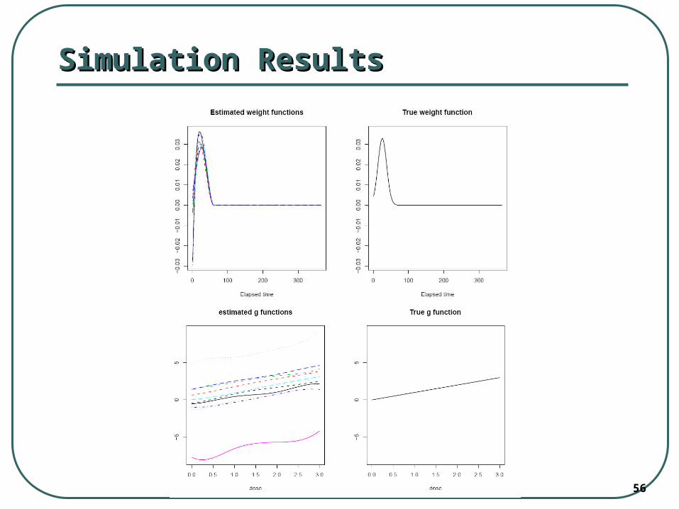
Simulation ResultsSimulation Results

57

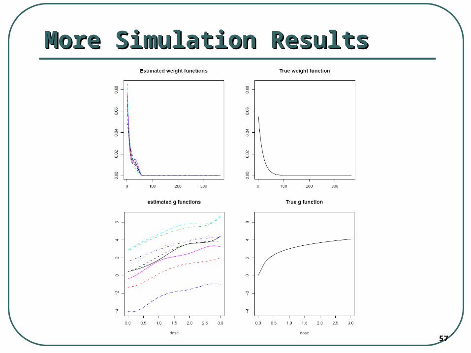
More Simulation ResultsMore Simulation Results