F

eder

al R

eser

ve B

ank

of C

hica

go

Can Structural Small Open Economy Models Account for the Influence of Foreign Disturbances?

Alejandro Justiniano and Bruce Preston

WP 2009-19

Can Structural Small Open Economy Models Account for theIn�uence of Foreign Disturbances?�

Alejandro Justinianoy Bruce Prestonz

November 30, 2009

Abstract

This paper demonstrates that an estimated, structural, small open-economy model ofthe Canadian economy cannot account for the substantial in�uence of foreign-sourced dis-turbances identi�ed in numerous reduced-form studies. The benchmark model assumesuncorrelated shocks across countries and implies that U.S. shocks account for less than3 percent of the variability observed in several Canadian series, at all forecast horizons.Accordingly, model-implied cross-correlation functions between Canada and U.S. are es-sentially zero. Both �ndings are at odds with the data. A speci�cation that assumescorrelated cross-country shocks partially resolves this discrepancy, but still falls well shortof matching reduced-form evidence.

�First Version: 2005. We are grateful to Gunter Coenen, Charles Engel, Jordi Gali, Paulo Giordani, ThomasLubik, Adrian Pagan, Giorgio Primiceri and two anonymous referees for discussions and detailed comments.We also thank seminar participants at the Federal Reserve Bank of Atlanta, Federal Reserve Bank of Chicago,Board of Governors of the Federal Reserve, Federal Reserve Bank of Cleveland Conference on �DSGE andFactor Models�, Duke University conference on �Identi�cation and estimation of structural models�, the jointECB, Lowy Institute and CAMA conference on �Globalization and Regionalism�, Reserve Bank of Australia,The Riksbank conference on �Structural Analysis of Business Cycles in the Open Economy� and Universityof Washington. Preston thanks the PER Seed Grant at Columbia University for �nancial support. The usualcaveat applies. The views expressed in this paper are those of the authors�and should not be interpreted asre�ecting the views of the Federal Reserve Bank of Chicago or any other person associated with the FederalReserve system.

yFederal Reserve Bank of Chicago, Research Department, 230 South La Salle St., Chicago, IL 60604. E-mail:ajustiniano@frbchi.org

zDepartment of Economics, Columbia University, 420 West 118th St, New York NY 10027 and CAMA,Australian National University. E-mail: bp2121@columbia.edu.

1

1 Introduction

This paper investigates whether an estimated microfounded semi-small open-economy model

can reproduce the observed comovements in international business cycles. Focusing on Canada

as the semi-small open economy, the starting point for the analysis is the large body of

empirical work that identi�es a signi�cant in�uence of U.S. shocks on Canadian economic

�uctuations.

There has been ample theoretical work seeking to replicate the observed comovements in

economic activity across countries. Until recently, the empirical validation of these models

largely relied on calibrations aimed at matching selected moments in the data � see the con-

tributions of Backus et al. (1992, 1995), Stockman and Tesar (1995) and Baxter (1995) for

a review. The New Open Economy Macroeconomics (NOEM) has since produced signi�cant

theoretical advancements in international macroeconomic modeling. Given the empirical suc-

cess of closed-economy models built on similar foundations, it is not surprising that there is

a growing literature estimating NOEM models. These include amongst others: Ambler et

al. (2003), Bergin (2003, 2004), Del Negro (2003), Ghironi (2000), Justiniano and Preston

(2008b), Lubik and Schorfheide (2003, 2005), Lubik and Teo (2005) and Rabanal and Tuesta

(2005).

To our knowledge, the ability of these NOEM models to explain the observed comovement

in economic �uctuations has not been previously systematically analyzed in this empirical

literature. This paper �lls this gap by evaluating a workhorse semi-small NOEM model in

this particular dimension. The focal point is the model�s ability to replicate the fraction of

the variance in Canadian macroeconomic series attributed to U.S. shocks. We also contrast

the cross-country correlation functions in the model and data, particularly for output.

The analysis is pursued using generalizations of the small open-economy framework pro-

posed by Gali and Monacelli (2005).1 Following Monacelli (2005), we allow for deviations from

the law of one price. In addition, we consider incomplete asset markets, a large set of dis-

turbances, and incorporate other real and nominal rigidities (e.g., wage stickiness, indexation

and habits) which have been found crucial in �tting closed-economy models as documented

by Christiano et al. (2005) and Smets and Wouters (2007).

The model is estimated using Bayesian methods with data for Canada and the United

1The model is technically a semi-small open economy model, where domestic goods producers have somemarket power, but we shall nonetheless refer to it as a small open economy. Note also that our analysis appealsto an earlier interpretation in Gali and Monacelli (2005) of a small-large country pair, rather than as an analysisof a continuum of small open economies.

1

States. Our baseline speci�cation assumes that shocks across these two countries are indepen-

dent. This contrasts with much of the international real business cycle literature which often

assumes correlated cross-country technology shocks, but is consistent with all of the empirical

NOEM studies cited above.2 Under independent shocks, the channels of transmission embed-

ded in the model (e.g. risk sharing and expenditure switching e¤ects) must account for the

cross-country comovement in aggregate �uctuations.

The main contribution of this paper is to document that the baseline speci�cation fails to

account for the in�uence of foreign shocks. A structural variance decomposition reveals that

all U.S. shocks combined cannot explain more than 3 percent of the variability in Canadian

output, interest rates or in�ation. Furthermore, model-implied cross-correlation functions

between these two countries are estimated to be essentially zero. Both �ndings are in stark

contrast with reduced-form empirical evidence in the same data. These results are shown to

be robust across alternative speci�cations, priors and detrending methods.

Model parameters chosen based on previous calibrated studies can deliver both large shares

of domestic variance being attributed to U.S. shocks and substantial cross-country correlation

in some series. Therefore, our �ndings indicate that the inability to reproduce some interna-

tional correlations � known as the quantity anomaly in the case of output (see Baxter and

Crucini (1995))� is exacerbated in estimated models. The results also suggest caution in

extrapolating to the international dimension the empirical success of related closed-economy

models.

A second contribution of this paper is to document that the international comovement

problem can only be partially resolved by introducing disturbances that are correlated across

countries. To do this, each Canadian structural shock is written as the sum of two orthogonal

components: a disturbance common to the same type of shock in the U.S. block, and a

country-speci�c disturbance. This decomposition can be viewed as a rough approximation to

reduced-form dynamic factor models that have been used for business cycle analysis.3

When all U.S. shocks are common to the domestic block the DSGE model gets closer to

matching the reduced-form variance decomposition. However, there are at least three reasons

for not viewing this speci�cation as a panacea for the model�s inability to replicate the observed

in�uence of foreign disturbances. First, at medium to long horizons, the fraction of output

2For example, Gali and Monacelli (2005) consider the role of technology spillovers in their calibration study.But likelihood-based empirical studies have typically excluded this possibility.

3 In a closed economy setting, Boivin and Giannoni (2006) establish a formal link between DSGE and dynamicfactor models.

2

variation explained by U.S. disturbances is still below the reduced-form evidence. Second,

this speci�cation engenders an extreme version of the exchange rate disconnect puzzle � see

Devereux and Engel (2002). Third, some of the induced correlations are di¢ cult to rationalize

on structural grounds.

A third contribution of our analysis is to elucidate reasons for the model�s failure in this

crucial dimension. The inability to match the comovement in the data is signaled by cross-

correlation amongst supposedly orthogonal innovations identi�ed in our baseline model. These

estimates point to a complex pattern of covariation, beyond pairing the same type of distur-

bance across countries. This explains the limited success of the common shocks models. More

promising guidance for future research is given by the observation that while U.S. shocks

can a priori match some bivariate cross-country correlations, they also have strong counter

factual predictions, particularly involving the real exchange rate and the terms of trade, as

well as domestic in�ation. This tension helps understand, at least in part, why the estimated

model shuts down international linkages and indicates ample scope to improve the transmission

mechanism of foreign disturbances in this class of model.

This paper broadly relates to the international business cycle literature and recent empir-

ical work with NOEM models. More closely related is Adolfson et al. (2007) who presents a

state-of-the-art model, more richly speci�ed than the one considered here. While their model

performs very well in several dimensions, an earlier version, Adolfson et al. (2005), reported

variance decompositions revealing little transmission of foreign-sourced disturbances from the

European Union to Sweden � a property that is not remarked upon. Similar observations

apply to an extension of this framework by Christiano et al. (2009) and also de Walque

et al. (2005) in a two-country model for the U.S. and the Euro Area. We also build on

Schmitt-Grohe (1998) who evaluates whether a calibrated small open-economy real business

cycle model can replicate impulse responses to a single foreign output shock, extracted from

a bivariate U.S.-Canada vector autoregression.4 Our results suggest that in estimation the

failure to capture international linkages may be worse than when the model is calibrated.

4Schmitt-Grohe (1998) concludes that �nancial and trade linkages are not capable of reproducing the strongresponse of Canadian hours, output and investment to innovations in U.S. GNP. She suggests that thesedi¢ culties might be alleviated by the introduction of sticky prices. Our analysis reveals that the inability tocapture the in�uence of foreign shocks persists in an estimated model even when various nominal rigidities areconsidered.

3

2 Evidence on International Linkages

A central empirical regularity that international business cycle models seek to explain is the

observed cross-country comovement amongst economic variables. This section documents a

number of statistics suggesting comovement is a salient feature of U.S. and Canadian business

cycles, understanding that earlier literature testi�es to the generality of these insights in other

economies. This close link is not surprising considering the U.S. accounts for 75 percent of

Canada�s average trade share.5

2.1 Data

We use data for twelve series that in section 4 constitute the observable states in the estimated

DSGE model. These are: real per-capita output, in�ation, nominal interest rates, real wages

and hours in both the U.S. and Canada, as well as the bilateral terms of trade and the real

exchange rate. Details of the data are in appendix A. Consistent with the model presented

later, output and real wages are expressed in log-deviations from a common linear trend. The

real exchange rate and the terms of trade are given in log-di¤erences. Section 6 evidences the

robustness of our results to alternative detrending of these series. In�ation and interest rates

are expressed as percentages and, like hours, are not transformed, except that all series are

demeaned. The sample runs from 1982q1 to 2007q1, although the �rst 8 quarters are used to

initialize the Kalman �lter.

2.2 Reduced-Form Evidence

The solid black lines in �gure 1 give the sample cross-correlations between Canadian and

lagged U.S. series, at lags zero through four. The remaining lines correspond to the estimated

DSGE model and are discussed in section 4. For presentation purposes only we exclude these

statistics for the terms of trade and the real exchange rate but discuss them later on.

For many series these cross-correlations are large at various lags and rarely equal to zero.

For example, the contemporaneous correlations between Canadian and U.S. output, in�ation,

nominal interest rates and wages are: 0.69, 0.45, 0.83 and 0.72, respectively. This is consistent

with earlier studies on international comovement, such as Backus et al. (1992), Stockman and

Tesar (1995) and Ambler at al. (2004).

5 In our sample, 1/2 the share of U.S. imports in total Canadian imports plus 1/2 the share of total Canadianexports oriented to the U.S. equals 75.1 percent.

4

We rely on two statistical models to compute the variance share of these Canadian series

that is attributable to U.S. shocks. The �rst model is a VAR subject to the exclusion restriction

of no feedback from Canada to the U.S. that is embedded in the DSGE model. It is formally a

seemingly unrelated regression (SUR). Variance decompositions are obtained with a Cholesky

decomposition of the SUR innovations with no attempt to identify any particular shock. We

only wish to infer the variance shares explained by disturbances also a¤ecting the U.S. block.6

The SUR is estimated with the e¢ cient block-recursive Gibbs algorithm proposed by Zha

(1999). Details are in appendix B.

Table 1 reports variance shares attributable to all foreign shocks in a SUR with 4 lags

at 1, 4, and 8 quarter horizons, and the stationary, or long-horizon, variance. We report

medians and 90 percent posterior probability bands. In the short, medium and long run, U.S.

disturbances account for a substantial fraction of variation in Canadian series. For example,

at a 4 quarter horizon, shares vary from 25 percent for hours to 44 percent for output. At long

horizons, contributions vary from 65 percent for in�ation to 76 percent for output. The latter

is almost identical to the 74 percent share for U.S. shocks in the smaller, but overidenti�ed,

structural SUR model of Cushman and Zha (1997).

The SUR analysis is limited by sample considerations to a dozen series. An alternative

is to estimate a dynamic moving average factor model, which can encompass richer sources

of shocks and channels of transmission by accommodating a larger number of series. Hence,

we also mention variance decomposition estimates from such a model, estimated for the U.S.

and Canada on a similar sample. The reader is referred to an earlier version of this paper,

Justiniano and Preston (2006), which builds on Justiniano (2007), for further details.

To explain a panel of 32 series (16 for each country) formal model comparisons dictate

including four factors, two of which are common to both countries (foreign factors), with the

remaining two exclusive to the Canadian economy (domestic). The factors and idiosyncratic,

series-speci�c, components follow independent autoregressive processes of order three. Mea-

sures of �t also suggest the presence of moving average dynamics in the loadings, indicating

that spillover e¤ects may be important for some variables.

Justiniano and Preston (2006) show that the median share of the long-horizon variance

of Canadian output, in�ation, interest rates, the terms of trade and the real exchange rate

explained by the two foreign factors is 0:71, 0:15, 0:31, 0:22 and 0:11. While di¤erences in

sample and data preclude direct comparisons with the SUR results, this distinct methodology

6The results obtained with this identi�cation procedure are invariant to re-ordering of the series.

5

clearly indicates an important role for U.S. shocks in explaining Canadian business cycles,

particularly for output. Similar �ndings are reported by Kose et al. (2003, 2008), Lumsdaine

and Prasad (2003) and Bowden and Martin (1995) with related methodologies.

Taken together, these various statistics suggest strong comovement between Canadian and

U.S. business cycles. The remainder of the paper explores whether a structural model can

similarly capture these international linkages.

3 The Model

Building on Gali and Monacelli (2005), Monacelli (2005) and Justiniano and Preston (2008b),

the following section details a small open-economy model, allowing for habit formation, in-

dexation of prices, labor market imperfections and incomplete markets. These papers extend

the microfoundations described by Clarida et al. (1999) and Woodford (2003) for analyzing

monetary policy in a closed-economy setting to an open-economy context.

3.1 Households

Each household maximizes

E0

1Xt=0

�t~"g;t

"(Ct �Ht)1�1=�

1� 1=� � ~"l;tN1+'t

1 + '

#

where Nt is the labor input; Ht � hCt�1 is an external habit taken as exogenous by the

household and 0 < h < 1; ��1; ' > 0 are the inverse elasticities of intertemporal substitution

and labor supply; and ~"g;t and ~"l;t denote preference and labor supply shocks respectively. Ct

is a composite consumption index

Ct =h(1� �)

1� (CH;t)

��1� + �

1� (CF;t)

��1�

i ���1

where CH;t and CF;t are Dixit-Stiglitz aggregates of the available domestic and foreign pro-

duced goods given by

CH;t =

24 1Z0

CH;t (i)��1� di

35�

��1

and CF;t =

24 1Z0

CF;t (i)��1� di

35�

��1

where � > 0 gives the elasticity of substitution between domestic and foreign goods; � > 1 is

the elasticity of substitution between types of di¤erentiated domestic or foreign goods; and �

the relative weight of these goods in the overall consumption bundle.

6

Assuming the only available assets are one-period domestic and foreign bonds, optimization

occurs subject to the �ow budget constraint

PtCt +Dt + StBt = Dt�1Rt�1 + StBt�1R�t�1�t (At) + �H;t +�F;t +WtNt + Tt (1)

for all t > 0, where Dt and Bt denote holdings of one-period domestic and foreign bonds with

gross interest rates Rt and R�t . St is the nominal exchange rate. The price indices Pt, PH;t and

P �t correspond to the domestic CPI, domestic goods prices and foreign prices and are de�ned

below. Households receive wages Wt for labor supplied and �H;t and �F;t denote pro�ts from

equity holdings in domestic and retails �rms. Tt denotes taxes and transfers.

Following Benigno (2001), Kollmann (2002) and Schmitt-Grohe and Uribe (2003), the

function �t (�) is interpretable as a debt elastic interest rate premium given by

�t = exph��

�At + ~�t

�iwhere At �

St�1Bt�1�CFPt�1

is the real quantity of outstanding foreign debt expressed in terms of domestic currency as a

fraction of steady state consumption of the imported good and ~�t a risk premium shock. This

ensures stationarity of the foreign debt level in a log-linear approximation to the model.

Implicitly underwriting this expression for the budget constraint is the assumption that

all households in the domestic economy receive an equal fraction of both domestic and retail

�rm pro�ts and that labor income risk is pooled across agents. Absent this assumption, which

imposes complete markets within the domestic economy, the analysis would require modeling

the distribution of wealth across agents. This assumption also ensures that households face

identical decision problems and choose identical state-contingent plans for consumption.

The household�s optimization problem requires allocation of expenditures across all types

of domestic and foreign goods both intratemporally and intertemporally. This yields the

following set of optimality conditions. The demand for each category of consumption good is

CH;t (i) = (PH;t (i) =PH;t)�� CH;t and CF;t (i) = (PF;t (i) =PF;t)

�� CF;t

for all i with associated aggregate price indexes for the domestic and foreign consumption

bundles given by PH;t and PF;t: The optimal allocation of expenditure across domestic and

foreign goods implies the demand functions

CH;t = (1� �) (PH;t=Pt)�� Ct and CF;t = � (PF;t=Pt)�� Ct (2)

7

where Pt =h(1� �)P 1��H;t + �P

1��F;t

i 11��

is the consumer price index. Allocation of expendi-

tures on the aggregate consumption bundle satis�es

�t = ~"g;t (Ct �Ht)�1=� (3)

and portfolio allocation is determined by the optimality conditions

�tStPt = �Et�R�t�t+1�t+1St+1Pt+1

�(4)

�tPt = �Et [Rt�t+1Pt+1] (5)

for Lagrange multiplier �t attached to the constraint (1) The latter when combined with (3)

gives the Euler equation.

The household problem in the foreign economy is similarly described with the exceptions

now noted. Because the foreign economy is approximately closed (the in�uence of the domestic

economy is negligible), the available consumption bundle comprises the continuum of foreign

produced goods C�F;t (j) for j 2 [0; 1] : Foreign households need only decide how to allocate

expenditures across these goods in any time period t and also over time. Foreign debt in the

foreign economy is in zero net supply, using the property that the domestic economy engages

in negligible �nancial asset trade. There is no access to domestic debt markets for foreign

agents. Conditions (3) and (5) continue to hold with all variables taking superscript �*�.

3.2 Optimal Labor Supply

Following Erceg et al. (2000) and Woodford (2003), assume a single economy-wide labor

market and that producers of the domestic good hire the same bundle of labor inputs at

common wage rates. Firm j produces good j with technology Yt (j) = ~"a;tf (Nt (j)) where

~"a;t is a neutral technology shock and f (�) satis�es the usual Inada conditions. The labor

input used in the production of each good j and associated aggregate wage index are given

by the CES aggregators

Nt (j) ��1R0

Nt (k)�w�1�w dk

� �w�w�1

and Wt =

�1R0

Wt (k)1��w dk

� 11��w

for �w > 1. Firm j�s demand for each type of labor k is determined by maximizing the former

index for a given level of wage payment. This gives the demand function

Nt (k) = Nt (j)

�Wt (k)

Wt

���w: (6)

8

Households supply their labor under monopolistic competition. They face a Calvo-style

wage-setting problem, having the opportunity to re-optimize their wage with probability 1��weach period, where 0 < �w < 1. As in Christiano et al. (2005) and Woodford (2003),

households not re-optimizing adjust their wage according to the indexation rule

logWt (k) = logWt�1 (k) + w�t�1

where 0 � w � 1 measures the degree of indexation to the previous-period�s in�ation rate

and �t = log (Pt=Pt�1). Since all households having the opportunity to reset their wage face

the same decision problem, they set a common wage, Wt.

The household�s wage-setting problem in period t is to maximize

Et1PT=t

(�w�)T�t

"�TWt (k)

�PT�1Pt�1

� wNT (k)�

~"l;tNT (k)1+'

1 + '

#

by choice of Wt (k) subject to the labor demand function (6). The �rst-order condition for

this problem is

Et1PT=t

(�w�)T�t

��T

�PT�1Pt�1

� w �NT (k) +Wt (k)

@NT (k)

@Wt (k)

�� ~"l;tN'

T

@NT (k)

@Wt (k)

�= 0: (7)

Households in the foreign block face an identical problem, with appropriate substitution of

foreign variables and technology and preference parameters.

3.3 Domestic Producers

There is a continuum of monopolistically competitive domestic �rms producing di¤erentiated

goods. Calvo-style price setting is assumed, allowing for indexation to past domestic goods-

price in�ation. In any period t, a fraction 1��H of �rms set prices optimally, while a fraction0 < �H < 1 of goods prices are adjusted according to the indexation rule

logPH;t (i) = logPH;t�1 (i) + H�H;t�1; (8)

where 0 � H � 1 measures the degree of indexation to the previous-period�s in�ation rate

and �H;t = log(PH;t=PH;t�1). Since all �rms having the opportunity to reset their price in

period t face the same decision problem, they set a common price P0H;t. Firms setting prices

in period t face a demand curve

yH;T (i) =

�PH;t (i)

PH;T��PH;T�1PH;t�1

� H��� �CH;T + C

�H;T

�(9)

9

for all t and take aggregate prices and consumption bundles as parametric.

The �rm�s price-setting problem in period t is to maximize the expected present discounted

value of pro�ts

Et

1XT=t

�T�tH Qt;T

�PH;t (i)

�PH;T�1PH;t�1

� HyH;T (i)�WT f

�1�yH;T (i)

~"a;t

��subject to the demand curve (9), where Qt;T is interpreted as a stochastic discount factor

evaluated at aggregate income. This implies the �rst-order condition

Et

1XT=t

�T�tH Qt;T yH;T (i)

�PH;t (i)

�PH;T�1PH;t�1

� H� �

� � 1PH;TMCT�= 0 (10)

where MCt is the marginal cost function of �rm i.

Foreign �rms face an analogous problem. Thus the optimality condition takes an identical

form, with all variables taking the superscript �*�and the subscript H being changed to F .

Preferences and shocks are allowed to di¤er and the small open-economy assumption implies

that P �t is equivalent to P�F;t.

3.4 Retail Firms

Retail �rms in the small open economy import foreign di¤erentiated goods for which the law

of one price holds at the docks. In determining the domestic currency price of imported goods

they are monopolistically competitive. Pricing power leads to a violation of the law of one

price in the short run.

Like domestic �rms, retail �rms face a Calvo-style price-setting problem allowing for in-

dexation to past in�ation. A fraction 1 � �F of �rms set prices optimally, while a fraction0 < �F < 1 of goods prices are adjusted according to an indexation rule analogous to (8) with

indexation parameter 0 < F < 1. Firms setting prices in period t face a demand curve

CF;T (i) =

�PF;t (i)

PF;T��PF;T�1PF;t�1

� F���CF;T (11)

for all t and take aggregate prices and consumption bundles as parametric. The �rm�s price-

setting problem in period t is to maximize the expected present discounted value of pro�ts

Et

1XT=t

�T�tF Qt;TCF;T (i)

�PF;t (i)

�PF;T�1PF;t�1

� F� STP �F;T (i)

�subject to the demand curve, (11), and implies the �rst-order condition

Et

1XT=t

�T�tF Qt;T

�PF;t (i)

�PF;T�1PF;t�1

� F� �

� � 1~eTP�H;T (i)

�= 0:

10

In the foreign economy there is no analogous optimal pricing problem. Because imports form

a negligible part of the foreign consumption bundle, variations in the import price have a

negligible e¤ect on the evolution of the foreign price index, P �t ; and need not be analyzed.

3.5 International Risk Sharing and Prices

Optimality conditions for domestic and foreign bond holdings imply the uncovered interest

rate parity condition

Et�t+1Pt+1[Rt �R�t (St+1=St)�t+1] = 0; (12)

placing a restriction on the relative movements of domestic and foreign interest rates, and

changes in the nominal exchange rate.

The terms of trade is de�ned as PF;t=PH;t. The real exchange rate is given by StP �t =Pt:

Since P �t = P�F;t, when the law of one price fails to hold ~F;t � StP �t =PF;t 6= 1, which de�nes

what Monacelli (2005) calls the law of one price gap. The models of Gali and Monacelli (2005)

and Monacelli (2005) are respectively characterized by whether or not ~F;t = 1.

3.6 Monetary and Fiscal Policy

Monetary policy is conducted according to a Taylor-type rule

Rt�R=

�Rt�1�R

��i "� PtPt�1

��� �Yt�Y

��y(YtYt�1

)��y(StSt�1

)�S

#(1��i)~"m;t

where �R and �Y are steady state values of nominal interest rates and output and ~"m;t is

an exogenous disturbance. Policy responds to contemporaneous values of in�ation, output,

output growth and the growth rate in the nominal exchange rate. Evidence for rules that

respond to exchange rates in various small open economies is found in Lubik and Schorfheide

(2005b) and Justiniano and Preston (2008b). Fiscal policy is speci�ed as a zero debt policy.

3.7 Exogenous Disturbances

All shocks have unit means. In log deviations from steady the following assumptions are made.

In the foreign block, the technology, preference and labor disutility shocks are �rst-order

autoregressive processes. The monetary policy innovation and cost-push shock in the pricing

of foreign goods are i.i.d. In the domestic block, technology, preference, labor disutility shocks

and the cost-push shock in imported goods pricing are �rst-order autoregressive processes, as is

the risk premium shock. The monetary policy shock and the cost-push shock to domestic price

11

setters are i.i.d. Justiniano and Preston (2006) discusses identi�cation issues which motivate

these speci�cations.

3.8 General Equilibrium

Equilibrium requires that all markets clear. Goods market clearing requires

YH;t = CH;t + C�H;t and Y

�t = C

�t (13)

in the domestic and foreign economies respectively. The model is closed assuming foreign

demand for the domestically produced good is speci�ed as

C�H;t =

�P �H;tP �t

���Y �t

where � > 0. This demand function is standard in small open economy models (see Kollmann

(2002) and McCallum and Nelson (2000)) and nests the speci�cation in Monacelli (2005)

by allowing � to be di¤erent from �, the domestic elasticity of substitution across goods in

the domestic economy, to give additional �exibility in the transmission mechanism of foreign

disturbances to the domestic economy. Our results are una¤ected by the parametrization of

this demand function.7 The dynamics of Y �t and other foreign variables remain speci�ed by

the structural relations developed above. Domestic debt is in zero net supply so that Dt = 0

for all t.8

The analysis considers a symmetric equilibrium in which all domestic producers setting

prices in period t set a common price PH;t. Similarly, all domestic retailers and foreign �rms

each choose a common price PF;t and P �t . Analogous conditions hold for wage setters in the

domestic and foreign economies. Finally, we assume households have identical initial wealth,

so that each faces the same period budget constraint and make identical consumption and

portfolio decisions.

4 Estimation Methodology and Data

4.1 Estimation and Priors

Model parameters are estimated using Bayesian methods now used extensively in the empirical

macroeconomics literature � see Schorfheide (2000) for a seminal reference and Justiniano

7Constraining � to equal � results in identical insights from the estimation.8A similar condition holds for the foreign economy once it is noted that domestic holdings of foreign debt,

Bt, is negligible relative to the size of the foreign economy.

12

and Preston (2006) for further details in the context of the model estimated here. We work

with a log-linear approximation of the model in a neighborhood of a non-stochastic steady

state. The observables used in estimation were described in section 2.

The �rst column of table 2 presents the priors for the coe¢ cients, indicating the density,

mean and standard deviation. They are motivated by earlier work reported in Justiniano and

Preston (2008b), are fairly uncontroversial, and accord with other studies adopting Bayesian

inference. Several parameters, not well identi�ed, are calibrated. The discount factor is �xed

at 0.99. The elasticities of demand across varieties of goods and labor inputs in both the

domestic and foreign block are set equal to 8, as in Woodford (2003). Following Benigno

(2001), the parameter governing the interest rate elasticity of debt is �xed at 0.01.9

Priors that are particularly germane to the transmission of foreign shocks deserve further

comment. The densities for the degree of openness, � , and the the elasticity of substitution

between home and foreign goods, �, are chosen to generate a tight distribution for the steady

state share of imports to GDP, centered at 0.27 as in the data.10 For � we specify a beta

density with mean 0.29, matching the average trade share in our sample, and a tight standard

deviation of 0.1. For � we choose a normal with mean 0.9 and also small dispersion of 0.1. Our

results are even stronger with looser priors on � ; which produce implausibly low estimates.11

For the exogenous shocks, priors are guided both by closed-economy estimates of similar

disturbances for the U.S. and consistency of the implied degree of volatility and persistence

with the corresponding observables in each country. Our baseline speci�cation also includes

a �tilt� towards foreign block disturbances, which are assumed twice as volatile and more

persistent than their domestic counterparts.

4.2 Estimates and Model Fit

Table 2 reports parameter estimates for the baseline model.12 The robustness of our results to

alternative priors and speci�cations is addressed later. Parameter estimates for the baseline

model are reasonable. The degree of price stickiness in home produced goods, both in the

domestic and foreign blocks of the model, is high. However, estimates for the foreign economy

agree with Levin et al. (2005). Note that cost-push shocks to the domestic and foreign Phillips�9 In the working paper version we evidenced the robustness of our results to alternative calibrations with the

elasticities of demand equal to 4 or when setting the interest elasticity of interest rate debt to 1e-4.10We are grateful to one of the referees for this suggestion.11None of our results are a¤ected when calibrating � at 0.29.12We initialize multiple chains using random starting values after launching 50 optimization runs to ensure

they all converge to the same mode. Convergence of the MCMC chains is diagnosed looking at trace plots andthe potential scale reduction factors for variances and 90% posterior bands.

13

curve are white noise and we do not rely on shocks to the in�ation target in order to impart

in�ationary inertia. The Calvo adjustment parameters for wages in the domestic and foreign

economies are similar to those reported in Del Negro et al. (2007) on a longer sample for the

U.S. Imported goods prices are re-optimized most frequently, every 2 quarters.

The degree of habit persistence is close to 0.6 in both countries, tightly estimated and

in line with values in Boldrin et al. (2001). The intertemporal elasticity of substitution

and elasticity of labor supply accord with earlier macroeconomic studies of this kind. The

estimated coe¢ cients of the Taylor rule align with conventional wisdom. Technology and

preference shocks are highly persistent in both countries. This is also true of risk premium

and imported goods cost-push shocks in Canada. The median estimate for the elasticity of

substitution across home and foreign goods is 0.86, below the value of 1.5 used in calibrations

by Chari et al. (2002) and Schmitt-Grohe (1998), but consistent with estimates in Gust et al.

(2008). Finally, the posterior density for the degree of openness lies well in the left tail of our

very tight prior.

In Justiniano and Preston (2006) we show that the model matches the volatility and

persistence of the data within blocks.13 The rest of the paper is devoted to the model�s

performance across blocks.

5 Accounting for the In�uence of Foreign Shocks

This section documents the central result of the paper: the baseline model with independent

shocks is unable to account for international comovement. Two pieces of evidence are adduced.

First, variance decompositions reveal that U.S. disturbances explain a negligible fraction of

variation in the domestic economy. Second, model-implied cross-country correlations are very

close to zero. Both �ndings are clearly at odds with the reduced-form evidence discussed in

section 2.

5.1 Variance Decompositions in the DSGE model

Using the draws from the posterior density of model parameters, table 3 reports the posterior

variance shares in the domestic series � including the real exchange rate and terms of trade

� that is attributable to all �ve foreign disturbances, at several forecast horizons.14 We report

13This is also evident from the unreported cross-correlation functions within each block.14According to the prior variance decomposition � see table 3 in Justiniano and Preston (2008a) � U.S.

shocks combined account for roughly 40% of Canadian output and hours �uctuations, half of the variability inin�ation, nominal interest, terms of trade and real exchange rate, and, about 30% of the variance in real wages,

14

medians and 90 percent posterior probability bands. Simulated moments which also account

for small-sample uncertainty are discussed in the on-line appendix yield similar conclusions.

Regardless of forecast horizon, virtually none of the observed variation in domestic series

is attributable to foreign disturbances. For output, interest rates, in�ation, hours and wages,

their maximum contribution at a horizon of 1 quarter is 3 percent. At longer horizons U.S.

shocks explain at most 1 percent. Furthermore, the 95 percentiles for the variance shares of

these series never exceeds 4 percent.15 For the real exchange rate and terms of trade, these

statistics reveal a slightly larger contribution of foreign shocks, but still, below 7 percent.

Compared with the reduced-form evidence in table 1, it is clear that this speci�cation of the

model cannot account for the in�uence of foreign shocks.

5.2 Cross-Country Correlations in the DSGE Model

Section 2 discussed the empirical cross-correlations between Canadian and U.S. series shown in

�gure 1 (solid). Here we revisit that �gure focusing on the moments implied by the estimated

model. These population statistics are computed using the posterior distribution of the DSGE

parameters and the model�s state-space solution. We report median (dotted) and [5,95] percent

posterior probability bands (dashed).

The median model-implied population cross-correlations are virtually zero at all horizons.

The DSGE model cannot replicate the common �uctuations of domestic series with U.S.

variables. Virtually all data cross-correlations lie outside the posterior probability bands of

the corresponding model moments. This mismatch between model and data is also evident

for the real exchange rate and the terms of trade (not shown for space considerations).16

Section 8 demonstrates that the lack of meaningful e¤ects from foreign shocks in the

domestic series is not an inherent feature of the DSGE model. Moreover, the inability to

explain the in�uence of foreign disturbances is not unique to the estimated model of this

paper. Adolfson et al. (2005) estimate a richer model which �ts the data very well in several

across di¤erent horizons.15A simulation-based decomposition of the stationary variance (using the same posterior draws) constructed

by feeding arti�cial sequences of domestic and foreign shocks one block at a time is presented in table 1A ofthe on-line appendix. There it is shown that the median shares are essentially identical to the those reportedhere, for all series, while the upper-ends of the posterior probability bands are roughly 0.02 points higher.16Figures 1A and 6A in the on-line appendix present simulated cross-correlations which account for small-

sample uncertainty. While the median estimates are virtually identical, the posterior probability bands areonly very slightly wider, so long as care is taken to decompose the correlations into a �true� componentand �spurious� component that arises in small samples, but vanishes in population. Failure to account forthis �spurious� small-sample correlation produces posterior probability bands that may seem too wide andinconsistent with all other evidence on the model�s inability to generate comovement. We are very grateful toone of the referees for pointing out this apparent inconsistency in an earlier version of the paper.

15

dimensions but also reveals, for Sweden, negligible variance shares for shocks originating in

the rest of the world. While the authors do not comment on this issue, their estimated

model includes features such as a stochastic trend, investment, variable capital utilization

and a working capital channel, whose absence here could have been suspected as culprit for

our results. This is also true of Christiano et. al. (2009) which advances that analysis by

including �nancial frictions and unemployment. Similarly, de Walque et al. (2005) fail to

identify signi�cant cross-country linkages in an estimated two-country model for the U.S. and

the Euro area, suggesting that the small open-economy assumption is not responsible for our

�ndings either.

6 Robustness

The benchmark speci�cation makes a range of assumptions, both on model structure and its

match with data. Table 4 presents the estimated contribution of foreign disturbances to the

variability of Canadian series for a number of alternative speci�cations. Further robustness

checks are conducted in Justiniano and Preston (2006). To present a worst-case scenario

against our �ndings, the numbers reported are for the horizon at which the share for output

is greatest. A comparison with the �rst column, which replicates our baseline speci�cation,

makes clear that our central result remains intact.

Column 2 presents the decomposition when the prior standard deviations of all shocks are

uniform between 1e-4 and 10, while the prior for the persistence parameters is a fairly �at Beta

density with mean 0.5 and dispersion 0.25. Compared with the benchmark results there is

clearly little di¤erence in the variance decompositions with this more agnostic prior. Column 3

estimates the model using maximum likelihood.17 Comovement again fails. The most notable

di¤erence in parameter estimates resides in the openness coe¢ cient which is found to be 0:01

� essentially shutting down open economy linkages. These two exercises suggest our priors

are not responsible for the absence of comovement.

The next two columns evaluate the sensitivity of our conclusions to the choice of observables

used to confront the model with data. Column 4 reports shares when output and wages are

in �rst di¤erences rather than in level deviations from a common trend. The results are

unchanged. Column 5 includes the observed terms of trade and the real exchange rate in

levels rather than di¤erences. This matters little for the contribution of U.S. shocks in Canada,

17Due to weak identi�cation the inverse Frisch elasticities are calibrated to 5 � the upper bound of admissiblevalues to which all MLE modes converged � without a¤ecting the results.

16

except for a somewhat larger share for the terms of trade and real exchange rate. Column

6 speci�es cost-push shocks in imports as i.i.d. as opposed to persistent disturbances. Once

again, the variance shares are small, dropping to zero for the terms of trade.

Coordinated policy responses could perhaps explain part of the comovement in Canadian

and U.S. business cycles. In the baseline speci�cation monetary policies are assumed to be

independently determined. However, interest rate decisions in Canada might be in�uenced by

changes in U.S. interest rates beyond what can be accounted for with an explicit response to the

exchange rate. Given the estimated degree of price stickiness, including a direct link between

U.S. and Canadian monetary policy decisions may better capture international comovement.

In this spirit, a log-linearized alternative speci�cation for Canadian monetary policy is

it = �iit�1 + (1� �i)��i�i

�t�1 + ���t + �yyt + ��y�yt

�+ "m;t

where there is now an explicit dependence on lagged realizations of U.S. interest rates. All

remaining modeling equations are unchanged.18 With a posterior mode estimate for �i� of

0.04, it is not surprising that the variance decompositions are largely unchanged (column

6). Identical conclusions obtain even when policy responds to contemporaneous U.S. interest

rates.

Finally, we consider a speci�cation that �rst independently estimates the foreign block of

the model.19 We then impose very tight priors (with dispersion 0.01) around the posterior

estimates of the foreign block, and choose the prior persistence and volatilities of domestic

innovations to match closely the moments observed in Canadian data. While in clear violation

of specifying prior beliefs before looking at the data, this model is quite informative on which

foreign disturbances are responsible for comovement a priori, a feature later exploited in section

8. The last column in table 4 evidences that this speci�cation cannot account for the in�uence

of foreign shocks either.

7 Common Shocks

The benchmark model assumes that all shocks in the U.S. and Canada are independent. How-

ever, the empirical evidence presented in section 2 is consistent with both spillovers from

U.S. speci�c disturbances and the existence of common shocks a¤ecting both countries. This

18The prior for �i� is normal with mean 0.3 and dispersion 0.2, allowing it to take negative values.19Priors are as in the baseline speci�cation, although for robustness we impose uniform priors [1e-4,10] on

the innovation standard deviations and a Beta density with mean 0.5 and dispersion 0.25.

17

section presents alternative model speci�cations that accommodate the latter. Such speci�-

cations are unusual in the new open-economy macroeconomics literature. Notable exceptions

are Adolfson et al. (2007) and de Walque et al. (2005) which include a common stochastic

trend in neutral technology.

7.1 Speci�cation

Common shocks are introduced by expressing the Canadian disturbances in the model as the

sum of two orthogonal shocks. The �rst one is shared with the same type of disturbance in

the U.S. block and referred to as the common shock. The second component a¤ects only the

domestic block and is labelled a country-speci�c shock. There is still no spillover from the

Canadian to the U.S. economy given the small open-economy assumption.

As an illustration, when modeling a common shock in neutral technology this disturbance

in Canada is written as at = a�t +adt where the common shock, a

�t , and country-speci�c shock,

adt , evolve as independent AR(1) processes. The common shock is the corresponding struc-

tural disturbance in the U.S. block. Its share of variability in Canadian neutral technology,

V ar(a�)=V ar(a), and implied correlation, corr(a; a�), can be readily computed.

In this way, common components are introduced between Canadian disturbances to prefer-

ences, labor disutility, home-goods in�ation and monetary policy, and their respective counter-

parts in the U.S. This can be viewed as a DSGE structural approximation to the decomposition

into common and idiosyncratic components using reduced-form dynamic factor models, as in

Kose et al. (2003, 2008). An advantage of this speci�cation relative to the direct estimation

of the correlations, corr(a; a�), is that it allows for a clean decomposition of the variance of

all series attributed to each component.

Given the emphasis on technology shocks in the international RBC literature, a natural

starting point for adding common shocks would be to introduce a common unit root in neutral

technology. A di¢ culty with this approach is strong evidence against a common stochastic

trend in U.S. and Canadian output, at least in our sample. Tests for cointegration between

log output per-capita in both countries do not reject the null hypothesis of no cointegration,

regardless of the speci�cation of lags and deterministic components.20 Similarly, the null of

20We use both the trace and maximum eigenvalue tests, allowing for 1-6 lags while also varying the pres-ence/absence of an intercept in the VAR or the cointegrating relationship, gauging relative �t using both theBIC and AIC. For each lag length, both information criteria prefer a speci�cation with an intercept in the VARand cointegrating equation (as expected) in which case the null of no cointegration cannot be rejected witheither test (for all lags considered). The p-values for the null of no cointegration are never below 0.2 and closeto 0.5 if the preferred lag lengths are used.

18

a unit root in the di¤erence in levels of these two series cannot be rejected, while the null of

stationarity is rejected.21 These results accord well with a persistent gap in labor productivity

across these two countries; a topic that has been the subject of substantial research and policy

discussion in Canada � see Eldridge and Sherwood (2001) and references therein.22

7.2 Posterior variance shares with common shocks

For each U.S. shock and Canadian counterpart we re-estimate the model when common com-

ponents are initially introduced one at a time. This permits identifying which common distur-

bances can help match the comovement in the data. A speci�cation with a common component

in all shocks is also presented. Priors are as in the baseline model with one exception. For

both common and country-speci�c shocks we specify the same density: a B(0:6; 2) for the

autoregressive coe¢ cients, and an IG for their standard deviations equal to that of the cor-

responding U.S. shock in table 1. Common and country-speci�c disturbances are on equal

footing.23 Results would be very similar using the prior from the baseline speci�cation.24

Panel A in table 5 reports posterior variance shares for speci�cations with a single common

shock. We report the horizon with the largest share for output. Comparing these results with

the baseline variance decomposition � reproduced in column 1 � yields several interesting

�ndings.

Introducing a common component in neutral technology alone does little to alter the

contribution of U.S. shocks, except for hours (column 2). Spillovers in neutral technology

here play a small role in reproducing comovement. The intuition for this �nding is that

in our model U.S. neutral technology shocks induce a negative comovement between output

and hours within the foreign block, as documented in closed-economy models by Gali (1999),

Ireland (2004) and Gali and Rabanal (2004). There is a tension between having technology

shocks as a source of international comovement and �tting the large hours-output comovement

21The null of a unit root is not rejected at the 10 percent signi�cance level when using the test of Elliot etal. (1996) or any of the test statistics proposed by Ng and Perron (2001), both with automatic lag selection.The null of stationarity under the KPSS tests is rejected at the 5 percent level.22Labor productivity is an observed state in our model since we are using data on output and hours for each

country. The �ltered series matches labor productivity from Statistics Canada (Table 383-0012).23The implied prior distribution of the correlation coe¢ cient between the aggregate Canadian disturbance

and its common component, is quite dispersed with a mean and median of roughly 0.7, standard deviation of0.23 and 5-95% bands covering 0.08 to 0.99. This is also the prior correlation with the country-speci�c part ofthe shock, e.g. corr(a; ad). By construction the sum of these two squared correlations equals 1.24 In this case with the tilt towards the foreign block, the mean and median prior variance shares of the U.S.

shocks would have jumped to 90% or above. Also, for each composite disturbance the median prior correlationwith its common component would have been tightly centered around 0.95. Nonetheless, the variance sharesare only 1 to 3 percentage points higher with this alternative, extreme prior.

19

observed in U.S data.

A common shock to the disutility of labor only (column 3) has a negligible e¤ect on the

variance decomposition of output, in�ation and interest rates, but helps improve the foreign

share in wages. Cost-push shocks (column 4) only bump up the foreign contribution to in�ation

variability. Meanwhile, with a common shock only in the monetary policy rules (column 5),

the fraction of the variance in Canadian interest rate and output attributable to foreign shocks

climbs to 23 and 10 percent. The largest increase in the share of output variability explained

by U.S. disturbances occurs with a common component in preference shocks (column 5), but

even in this case only 11 percent of output �uctuations are accounted for by all foreign shocks.

Panel B reports shares at various horizons in a speci�cation with common components in

all U.S. shocks and their respective Canadian counterparts. The fraction of variation explained

by all foreign disturbances is now larger than in the baseline, particularly for output, hours

and interest rates. These results show that the comovement observed in the data can be partly

reproduced by correlating domestic disturbances with all of their U.S. counterparts.

The last row in each panel of the table reports the marginal data density, computed us-

ing the modi�ed harmonic mean. Most speci�cations achieve a lower �t than the baseline

(-1003.3), even when all common shocks are added simultaneously (-1010.6). The �t is al-

most indistinguishable from the baseline when either monetary policy or cost-push shocks

are correlated across countries. While caution is warranted when comparing these marginals

due to di¤erences in priors, this suggests that neither of the common shocks speci�cations

substantially improves the model�s �t, relative to the baseline without common shocks.

There are at least three further reasons why these speci�cations with common shocks

should not be viewed as panacea for the model�s failure in accounting for the in�uence of

foreign shocks. First and foremost, while shares in panel B align well with those from the

SUR at a 1 quarter horizon, for longer horizons the SUR posterior bands do not encompass

the smaller DSGE estimates � compare table 2. Second, some of the common components

are hard to rationalize on structural grounds. Recall that neither a speci�cation of the Cana-

dian policy rule including a direct response to the exchange rate nor to U.S. interest rates

could explain comovement, unless shocks are correlated. This suggests that cross-equation

restrictions prevent the model from structurally explaining the cross-correlation in these two

series. Third, panel B demonstrates an extreme manifestation of the exchange rate disconnect

analyzed by Devereux and Engel (2002). Fluctuations in the real exchange rate and the terms

of trade are completely disconnected from the U.S. block and for the most part from the real

20

domestic variables as well.25 In summary, even with common shocks there is ample scope to

improve the model�s ability to capture the contribution of foreign shocks.

8 On the Source of Model Failure

The results so far have documented an important model failure with little said about its

determinants. This section provides several insights on model and data features which limit

comovement. We �rst show that the unaccounted correlation seen in the data translates into

correlated innovations � in violation of the maintained assumption of orthogonality. This

information, together with insights into which U.S. disturbances are a priori responsible for

comovement, guide a set of exercises attempting to understand which shocks, transmission

mechanisms and data series pose di¢ culties for the model.

8.1 Where Does the Correlation Go?

The adopted likelihood-based procedure provides estimates of structural parameters and un-

observed shocks that perfectly match the data. The large cross-country correlations in the

observables which are not explained by the model get re�ected in correlated innovations, a

clear indication of model misspeci�cation. This correlation is not picked up in the various

exercises conducted in this paper as, with the exception of the common shocks models of

the previous section, the disturbances are assumed to be orthogonal. This is the standard

assumption in empirical DSGE models.

Table 6 reports the cross-correlation between the supposedly orthogonal two-sided U.S. and

Canadian innovations to the exogenous shocks, in the baseline speci�cation. Seven of those

correlations are statistically di¤erent from zero (in bold). Interestingly, in �ve of these seven

cases, the correlation occurs across disturbances of di¤erent type (e.g. U.S. preference and

Canadian technology shocks). This helps explain why the common shock models estimated

in the previous section � which allow for correlation only amongst disturbances of the same

type � could not fully reconcile model and data. A more complex set of interactions across

disturbances is revealed.

We next turn to a prior and posterior comparison that provides evidence on why these

correlations cannot be captured by the transmission mechanisms embedded in the model.

25Risk-premium and import cost-push shocks account for roughly 90 and 85 percent of the variance of thereal exchange rate and the terms of trade, respectively, at all horizons, while explaining only about 5 percentof the variability in domestic output, real wages and hours.

21

8.2 The Transmission Role of Disturbances and Data

Identifying the mechanisms limiting comovement is a challenging task. It requires assessing

numerous cross-equation restrictions, the prior and posterior properties of a model with 47

estimated parameters and the statistical covariance properties of 12 observable time series. A

clean narrative would ideally attribute model failure to one cross-equation restriction or one

particular time series. Unfortunately matters are not so simple in a model of this dimension.

Having said that, we conduct additional exercises suggesting a few culprits which serve to

guide future research on this topic.

The prior-posterior comparisons here are based on the model discussed in section 6 which

pre-estimates and then �calibrates� the U.S. block of the economy. This is done for the fol-

lowing reasons. First, in contrast to the benchmark prior, this �prior� is highly informative

as to which shocks are most relevant for dynamics in the foreign block and therefore comove-

ment. In particular, U.S. preference shocks explain the bulk of U.S. output �uctuations and

a substantial portion of interest rate variability, especially at longer horizons. U.S. monetary

policy shocks are also important for U.S. interest rates, while cost-push shocks drive U.S.

in�ation. This highlights the same set of foreign disturbances suggested by the relative �t of

the common shocks speci�cations in table 5 and the analysis of section 8.1.26

Second, by �xing properties of the U.S. block, attention is focused on di¤erences between

the prior and posterior implications for the domestic block and its interaction with the foreign

block, narrowing the scope of inquiry. Third, a priori the average variance share explained

by all U.S. shocks is roughly 0.4 for all Canadian series � without recourse to correlated

innovations � with prior bands covering the interval 0.1 to 0.7. Clearly, the prior suggests

substantial comovement while, as documented in table 4, the posterior decomposition implies

a negligible role for U.S. shocks in the domestic economy.

To understand why the posterior severs cross-country linkages, we analyze the interna-

tional transmission of U.S. monetary policy, preference and cost-push shocks. Taking these

disturbances jointly and in isolation, we ask what are their prior implications for model-

implied cross-correlations and how do these square with the data. This uncovers a number of

counter factual prior implications which help explain why the posterior shuts down the role of

U.S. shocks. We provide a brief summary of our �ndings, with additional details and graphs

discussed in the on-line appendix.

26This variance decomposition for the foreign block is not surprisingly very similar to the posterior in thebaseline speci�cation.

22

� A priori output comovement can be captured by U.S. preference shocks. However, theyinduce a strong negative correlation between U.S. output and both Canadian in�ation

and interest rates. In the data these correlations are positive, particularly in the case

of the latter two series. Furthermore, U.S. preference shocks imply Canadian output is

negatively correlated with both Canadian in�ation and nominal interest rates, as well

as the terms of trade. Again this is strongly counter factual.

� Similarly, U.S. cost-push shocks a priori capture the comovement between U.S. in�ationwith Canadian in�ation and nominal interest rates. However, these disturbances imply

large positive correlations between U.S. and Canadian in�ation with each of the terms

of trade and real exchange rate. These correlations are somewhat negative in the data.

� Monetary policy shocks in the U.S. generate comovement with Canadian interest ratesand in�ation. But their key counter factual prediction is a positive correlation between

Canadian in�ation and both the terms of trade and real exchange rate. Since large U.S.

monetary policy shocks are required to match the substantial comovement between U.S.

and Canadian nominal interest rates this exacerbates the inability to match the terms

of trade and real exchange rate.

Taken together these observations permit several insights. First, while foreign preference,

cost-push and monetary policy shocks are important determinants of U.S. �uctuations, and in

principle Canadian �uctuations, they have signi�cant counter factual predictions for various

series vis-a-vis Canadian in�ation, the terms of trade and real exchange rate, as well as amongst

these three. Posterior inference reveals that once confronted with the data the ability of these

shocks to generate comovement is severely limited.

Second, and related, is that the shifting importance of shocks across the prior and posterior

implications of the model are consistent with exchange rate disconnect being a factor in the

model�s failure. Furthermore, posterior estimates from a model in which both series are

unobservable states improves the comovement properties to some degree � around 10 percent

of variation in Canadian series is attributed to U.S. originating disturbances, without resorting

to correlated shocks. Treating any other observable Canadian series (such as in�ation) in the

benchmark estimation as unobservable does not have similar implications.

The exchange rate disconnect hypothesis is provided further support given the importance

of imported goods cost-push shocks and risk premium shocks as a source of variation for these

two series, without a meaningful role for the remaining observables, domestic or foreign. This

23

issue is discussed in greater detail in an earlier version of this paper � see Justiniano and

Preston (2006).

To conclude we o¤er the following remarks on the model�s inability to explain the in�uence

of foreign shocks. First, some correlation in exogenous disturbances appears warranted, despite

the assumption of orthogonality being common practice in the DSGE literature.27 Second,

allowing for correlation across countries only amongst disturbances of the same type will

not fully resolve the comovement problem. Third, prior-posterior comparisons point to deeper

mechanisms, operative through particular cross-equation restrictions and evidenced by counter

factual implications for the terms of trade and the real exchange rate, particularly in regards to

their link with domestic in�ation. As to which cross-equation restrictions and model features

need to be re-considered to solve this disconnect is beyond the current exercise but clearly an

exciting area of research.

9 Conclusion

This paper shows that an empirical new open-economy model fails to account for one im-

portant dimension of Canadian data: the in�uence of U.S. disturbances. We initially assume

uncorrelated shocks across countries, as it is done in almost all the empirical literature with

this class of models. Variance decompositions reveal that the fraction of variation in Canadian

series attributed to all shocks originating in the U.S. economy is negligible at all forecast hori-

zons. Accordingly, the cross-country correlation functions implied by the model are close to

zero. These �ndings contrast sharply with earlier work documenting strong linkages between

these two countries and reduced-form evidence presented here.

Alternative speci�cations with common shocks can only partially resolve this problem. A

model in which all U.S. shocks have a common component with the corresponding Canadian

disturbance begins to reconcile the in�uence of foreign shocks in the model and the data.

However, the variance shares explained by all U.S. disturbances still fall short of those observed

in the data at medium and long horizons. While the empirical evidence is consistent with

both common shocks and spillovers, there remains the question of what economic e¤ects do

these common shocks capture in the model. In particular, whether they correspond to purely

exogenous disturbances or are instead simply capturing model misspeci�cation. Finally, any

gains with common shocks come at the expense of fully detaching �uctuations in the exchange

rate and the terms of trade from the foreign block.27An interesting recent contribution in the closed economy setting in this regard is Curdia and Reis (2009).

24

Analyzing the prior implications for the transmission of U.S. shocks indicates a role for

exchange rate disconnect in the model�s failure. In particular, we uncover a number of prior

counter factual correlations between U.S. and Canadian series (particularly in�ation) with the

real exchange rate and the terms of trade.

Overall our �ndings suggest that additional work on the international transmission mech-

anisms of various shocks could improve the empirical performance of these models in this

crucial dimension. An interesting exercise in this vein would be to alter the supply side of

the model to account for cross-country linkages at multiple stages of production as in Huang

and Liu (2007) and Burstein et al. (2008). Alternatively, expanding on international �nancial

linkages and the role of asset prices might help explain the importance of U.S. disturbances

abroad, as made evident by the current �nancial crisis.

10 Appendix A: Data

All series are downloaded from Haver Analytics. For the U.S., real per-capita GDP measures

output, in�ation corresponds to the log-di¤erence in the GDP de�ator, and the e¤ective federal

funds rate taken for interest rates. Nominal compensation per hour in the non-farm business

sector divided by the GDP de�ator measures wages. Total hours in the non-farm business

sector is divided by population.

For Canada, real per-capita GDP is constructed with data from Statistics Canada (Stat-

Can). The quarterly log di¤erence in the consumer price index excluding food and energy

(StatCan) measures overall in�ation. The o¢ cial discount rate published by the Bank of

Canada corresponds to interest rates. Hours worked in the total economy (StatCan table

383-0012) is divided by population. From the same table we obtain total compensation and

convert it into real terms. In accordance with the model, the GDP de�ator proxies for the

price of home produced goods, while CPI in�ation represents the aggregate price index.

For consistency, the log di¤erence in the bilateral real exchange rate is constructed as the

sum the log growth rates in the U.S. GDP de�ator and the nominal exchange rate (Canadian

dollars per U.S. dollars) minus Canadian aggregate in�ation, as measured above. An earlier

version of the paper used the bilateral real exchange rate constructed by the IMF with identical

�ndings.

Finally, for the terms of trade we take the ratio of the de�ator for imports to exports

(Statcan) matching in our model, log (PF;t=PH;t). According to Canada�s national accounts

data, this measure of the terms of trade would correspond more closely to log�P �F;tSt=PH;t

�,

25

but this would not be consistent with the real exchange rate using aggregate U.S. in�ation.

As there is no perfect match between model variables we adopted the former measure for

estimation. Inference with the latter interpretation does not a¤ect our results.

11 Appendix B: SUR model

To match the reduced-form representation of the DSGE model we impose on a VAR the same

zero restrictions of no feedback from Canada to the U.S. The resulting SUR model is estimated

on the same sample of twelve series used for inference with the DSGE model.

Inference is substantially more involved than with a standard VAR, as the explanatory

variables are not the same across all series. However, the estimation is feasible with the e¢ cient

block-recursive Gibbs algorithm proposed by Zha (1999), who documents the distortions to

inference from not imposing the exclusion restrictions in a SUR between Canada and the U.S.We simply outline the model and refer the readers to Zha (1999) for details. Partitioning

the vector of observables yt into U.S. and Canadian variables, yUSt and yCNt , respectively, thetwo blocks of the SUR are given by�

AUS;US(0)�ApUS;US(L) 0

ACN;US(0)�ApCN;US(L) ACN;CN (0)�ApCN;US(L)

��yUStyCNt

�=

��USt�CNt

�for matrices of conformable size, where Ai;j(0) corresponds to the impact matrix and A

pi;j(L)

denotes a matrix of lag-polynomials, of order p, in the positive powers of L: The structural

errors [�0USt ; �0CNt ]0 are orthogonal with unit variance.

Our goal is not to identify each of the structural disturbances but simply to compute

the variance shares of the Canadian series attributed to the sum of all U.S. disturbances,

�USt . To this end, we impose a lower triangular structure in the impact matrices AUS;US(0)

and ACN;CN (0). This is equivalent to a Cholesky decomposition of the reduced-form SUR

covariance matrix. Results on the sum of all block-speci�c disturbances are invariant to

ordering.

We report results with p = 4 in light of recent work by Fernandez-Villaverde et al. (2007)

and Del Negro et al. (2007) who have brought attention to the issue of lag truncation in VARs

as approximations to DSGE models. To deal with the large number of parameters relative

to sample length, we use priors that shrink coe¢ cients at distant lags. More speci�cally,

we specify the priors Aij(1) � N(0:9; 0:2) for i = j and N(0; 0:4) for i 6= j:28 There�s no

distinction between own and others� lags for k > 1 and assume a normal prior centered at

zero with a dispersion equal to 0.2 for k = 2, 0:15 for k = 3; and 0:1 for k = 4: The lower28For the exchange rate and terms of trade the mean is 0:3, since these are expressed in log-di¤erences.

26

triangular elements of the contemporaneous matrices are Aij(0) � N(0; 10): Results are largelyinsensitive to looser priors, and, when feasible (p is 1 or 2), pretty much identical to sampling a

single block SUR with an uninformative Inverse-Wishart prior on the reduced-form covariance

matrix.

The Gibbs sampler is initialized at random starting values from the prior (or a classical

SUR with 2 lags) and we run 3 chains, discarding, for each, the �rst 40,000 draws, and retaining

1 in 10 of the remaining 50000. For each draw we compute the fraction of the variability in

yCNt ; explained by the sum of all �ve U.S. shocks, at di¤erent horizons.

References

Adolfson, M., S. Laseen, J. Linde, and M. Villani (2005): �Bayesian Estimation of anOpen Economy DSGE Model with Incomplete Pass-Through,�Working Paper Series 179,Sveriges Riksbank.

(2007): �Bayesian Estimation of an Open Economy DSGE Model with IncompletePass-Through,�Journal of International Economics, 72(2), 481�511.

Ambler, S., E. Cardia, and C. Zimmerman (2004): �International Business Cycles: Whatare the Facts?,�Journal of Monetary Economics, (51), 257�276.

Backus, D. K., and P. J. Kehoe (1992): �International Evidence on the Historical Prop-erties of Business Cycles,�American Economic Review, 82, 864�888.

Backus, D. K., P. J. Kehoe, and F. E. Kydland (1992): �International Real BusinessCycles,�Journal of Political Economy, 100, 745�773.

(1995): �Internation Business Cycles: Theory and Evidence,�in Frontiers of BusinessCycle Research, ed. by T. F. Cooley, pp. 331�356.

Baxter, M. (1995): �International Trade and Business Cycles,�in Handbook of InternationEconomics, ed. by G. Grossman, and K. Rogo¤. North Holland.

Baxter, M., and M. Crucini (1995): �Business Cycles and the Asset Structure of ForeignTrade,�International Economic Review, 36, 821�854.

Benigno, P. (2001): �Price Stability with Imperfect Financial Integration,� unpublished,New York University.

Bergin, P. (2003): �Putting the �New Open Economy Macroeconomics�to a Test,�Journalof International Economics, 60(1), 3�34.

(2004): �How well can the New Open Economy Macroeconomics Explain the Ex-change Rate and the Current Account,�unpublished, University of California Davis.

Boivin, J., and M. Giannoni (2006): �DSGE Models in a Data-Rich Environment,�NBERWorking Paper no. 12772.

27

Boldrin, M., L. J. Christiano, and J. D. M. Fisher (2001): �Habit Persistence, AssetReturns, and the Business Cycle,�American Economic Review, 91(1), 149�166.

Bowden, R., and V. Martin (1995): �International Business Cycles and Financial Integra-tion,�The Review of Economics and Statistics, 77, 305�320.

Burstein, A., C. Kurz, and L. Tesar (2008): �Trade, Production Sharing, and the Inter-national Transmission of Business Cycles,�unpublished, UCLA.

Christiano, L. J., M. Eichenbaum, and C. L. Evans (2005): �Nominal Rigidities andthe Dynamic E¤ects of a Shock to Monetary Policy,�Journal of Political Economy, 113, 1.

Christiano, L. J., M. Trabandt, and K. Walentin (2009): �Introducing Financial Fric-tions and Unemployment into a Small Open Economy Model,�unpublished, NorthwesternUniversity.

Curdia, V., and R. Reis (2009): �Correlated Disturbances and U.S. Business Cycles,�unpublished, Columbia University.

Cushman, D. O., and T. Zha (1997): �Identifyiung monetary policy in a small open economyunder �exible exchange rates,�Journal of Monetary Economics, 39, 433�448.

de Walque, G., F. Smets, and R. Wouters (2005): �An Open Economy DSGE ModelLinking the Euro Area and the US Economy,�unpublished, National Bank of Belguim.

Del Negro, M. (2003): �Fear of Floating? A Structural Estimation of Monetary Policy inMexico,�unpublished, Federal Reserve Bank of Atlanta.

Devereux, M. B., and C. Engel (2002): �Exchange rate pass-through, exchange ratevolatility, and exchange rate disconnect,�Journal of Monetary Economics, 49, 913�940.

Eldridge, L. P., and M. K. Sherwood (2001): �A Perspective on U.S.-Canada Manufac-turing Productivity Gap,�Monthly Labor Review, pp. 31�48.

Elliot, G., J. Stock, and T. Rotehnberg (1996): �E¢ cient Tests for An AutoregressiveUnit Root,�Econometrica, (64), 813�836.

Erceg, C. J., D. W. Henderson, and A. T. Levin (2000): �Optimal Monetary Policywith Staggered Wage and Price Contracts,�Journal of Monetary Economics, 46(281-313).

Fernandez-Villaverde, J., J. F. Rubio-Ramirez, M. Watson, and T. Sargent(2006): �A, B, C�s and (D)�s For Understanding VARS,� American Economic Review,97(3), 1021.

Gali, J. (1999): �Technology, Employment and the Business Cycle: Do Technology ShocksExplain the Business Cycle,�American Economic Review, 249, 249�271.

Gali, J., and T. Monacelli (2005): �Monetary Policy and Exchange Rate Volatility in aSmall Open Economy,�Review of Economic Studies, 72.

Gali, J., and P. Rabanal (2004): �Technology Shocks and Aggregate Fluctuations: HowWell Does the RBC Model Fit Postwar U.S. Data?,�NBER Macroeconomics Annual.

28

Ghironi, F. (2000): �Towards and New Open Economy Macroeconometrics,�Boston CollegeEconomics Department Working Paper No. 469.

Gust, C., S. Leduc, and N. Sheets (2008): �The Adjustment of Global External Balances:Does Partial Exchange Rate Pass-Through to Trade Prices Matter?,�unpublished, FederalReserve Board of Governors.

Huang, K., and Z. Liu (2007): �Business Cycles with Staggered Prices and InternationalTrade in Intermediate Goods,�Journal of Monetary Economics, 54, 1271�1289.

Ireland, P. (2004): �Technology Shocks in the New Keynesian Model,� The Review ofEconomics and Statistics, 86(4), 923�936.

Justiniano, A. (2007): �Factoring In Canadian Cycles,� in Northern Star - Canada�s Pathto Economic Prosperity, ed. by T. Bayoumi. International Monetary Fund.

Justiniano, A., and B. Preston (2006): �Can Structural Small Open Economy ModelsAccount for the In�uence of Foreign Disturbances?,�CAMA Working Paper Series no. 12.

(2008a): �Can Structural Small Open Economy Models Account for the In�uence ofForeign Disturbances?,�NBER Working Paper 14547.

(2008b): �Monetary Policy and Uncertainty in an Empirical Small Open EconomyModel,�forthcoming, Journal of Applied Econometrics.

Kollmann, R. (2002): �Monetary Policy Rules in the Open Economy: E¤ects on Welfareand Business Cylces,�Journal of Monetary Economics, 49, 989�1015.

Kose, M. A., C. Otrok, and C. H. Whiteman (2003): �International Business Cycles:World, Region and Country-Speci�c Factors,�American Economic Review, 93, 1216�1239.

(2008): �Understanding the Evolution of World Business Cycles,�Journal of Inter-national Economics, 75(1), 110�130.

Levin, A., A. Onatski, J. C. Williams, and N. Williams (2005): �Monetary Policyunder uncertainty in Micro-Founded Macroeconometrics Models,�.

Lubik, T. A., and F. Schorfheide (2005a): �A Bayesian Look at New Open EconomyMacroeconomics,�in NBER Macroeconomics Annual, ed. by M. Gertler. NBER.

(2005b): �Do Central Banks Respond to Exchange Rate Movements? A StructuralInvestigation,�Journal of Monetary Economics, 54(4), 1069�1087.

Lubik, T. A., and W. L. Teo (2005): �Do World Shocks Drive Domestic Business Cycles?Some Evidenec from Structural Estimation,�unpublished, Johns Hopkins University.

Lumsdaine, R., and E. Prasad (2003): �Identifying the Common Component if Interna-tional Fluctuations: A New Approach,�The Economic Journal, 113, 101�127.

McCallum, B. T., and E. Nelson (2000): �Monetary Policy for an Open Economy: AnAlternative Framework with Optimizing Agents and Sticky Prices,�Oxford Review of Eco-nomic Policy, (16), 74�91.

29

Monacelli, T. (2005): �Monetary Policy in a Low Pass-through Environment,�Journal ofMoney, Credit and Banking, 37, 1047�1066.

Ng, S., and P. Perron (2001): �Lag Selection and the Construction of Unit Root Testswith Good Size and Power,�Econometrica, 69(6), 1519�1554.

Rabanal, P., and V. Tuesta (2005): �Euro-Dollar Real Exchange Rate Dynamics in anEstimated Two-country Model: What is Important and What is Not,�unpublished, Inter-national Monetary Fund and Banco Central de Reserva del Peru.

Schmitt-Grohe, S. (1998): �The International Transmission of Economic Fluctuations: Ef-fects of US Business Cycles on the Canadian Economy,�Journal of International Economics,44, 257�287.

Schmitt-Grohe, S., and M. Uribe (2003): �Closing Small Open Economy Models,�Jour-nal of International Economics, 61, 163�195.

Schorfheide, F. (2000): �Loss Function-Based Evaluation of DSGE Models,� Journal ofApplied Econometrics, 15, 645�670.

Smets, F., and R. Wouters (2007): �Shocks and Frictions in US Business Cycles: aBayesian DSGE Approach,�American Economic Review volume = 97, number = 3, pages= 586-606,.

Stockman, A. C., and L. L. Tesar (1995): �Tastes and Technology in a Two-countryModel of the Business Cycle: Explaining International Comovements,�American EconomicReview, 85(1), 168�185.

Woodford, M. (2003): Interest and Prices: Foundations of a Theory of Monetary Policy.Princeton University Press.

Zha, T. (1999): �Block Recursion and Structural Vector Autoregression,�Journal of Econo-metrics, 90, 291�316.

30

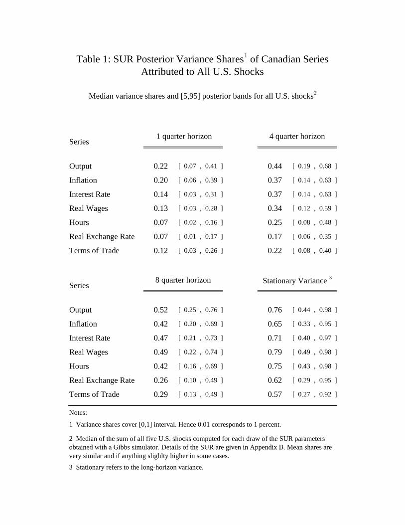
Series

Output 0.22 [ 0.07 , 0.41 ] 0.44 [ 0.19 , 0.68 ]

Inflation 0.20 [ 0.06 , 0.39 ] 0.37 [ 0.14 , 0.63 ]

Interest Rate 0.14 [ 0.03 , 0.31 ] 0.37 [ 0.14 , 0.63 ]

Real Wages 0.13 [ 0.03 , 0.28 ] 0.34 [ 0.12 , 0.59 ]

Hours 0.07 [ 0.02 , 0.16 ] 0.25 [ 0.08 , 0.48 ]

Real Exchange Rate 0.07 [ 0.01 , 0.17 ] 0.17 [ 0.06 , 0.35 ]

Terms of Trade 0.12 [ 0.03 , 0.26 ] 0.22 [ 0.08 , 0.40 ]

Series

Output 0.52 [ 0.25 , 0.76 ] 0.76 [ 0.44 , 0.98 ]

Inflation 0.42 [ 0.20 , 0.69 ] 0.65 [ 0.33 , 0.95 ]

Interest Rate 0.47 [ 0.21 , 0.73 ] 0.71 [ 0.40 , 0.97 ]

Real Wages 0.49 [ 0.22 , 0.74 ] 0.79 [ 0.49 , 0.98 ]

Hours 0.42 [ 0.16 , 0.69 ] 0.75 [ 0.43 , 0.98 ]

Real Exchange Rate 0.26 [ 0.10 , 0.49 ] 0.62 [ 0.29 , 0.95 ]

Terms of Trade 0.29 [ 0.13 , 0.49 ] 0.57 [ 0.27 , 0.92 ]

Notes:

1 Variance shares cover [0,1] interval. Hence 0.01 corresponds to 1 percent.

2 Median of the sum of all five U.S. shocks computed for each draw of the SUR parameters obtained with a Gibbs simulator. Details of the SUR are given in Appendix B. Mean shares are very similar and if anything slighlty higher in some cases.

3 Stationary refers to the long-horizon variance.

Table 1: SUR Posterior Variance Shares1 of Canadian Series Attributed to All U.S. Shocks

Median variance shares and [5,95] posterior bands for all U.S. shocks2

1 quarter horizon 4 quarter horizon

8 quarter horizon Stationary Variance 3

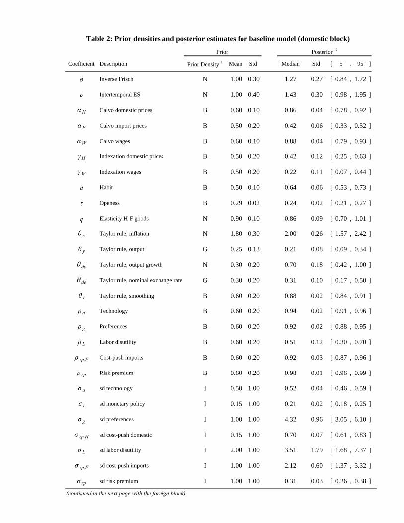
Coefficient Description Prior Density 1 Mean Std Median Std [ 5 , 95 ]

φ Inverse Frisch N 1.00 0.30 1.27 0.27 [ 0.84 , 1.72 ]

σ Intertemporal ES N 1.00 0.40 1.43 0.30 [ 0.98 , 1.95 ]

α H Calvo domestic prices B 0.60 0.10 0.86 0.04 [ 0.78 , 0.92 ]

α F Calvo import prices B 0.50 0.20 0.42 0.06 [ 0.33 , 0.52 ]

α W Calvo wages B 0.60 0.10 0.88 0.04 [ 0.79 , 0.93 ]

γ H Indexation domestic prices B 0.50 0.20 0.42 0.12 [ 0.25 , 0.63 ]

γ W Indexation wages B 0.50 0.20 0.22 0.11 [ 0.07 , 0.44 ]

h Habit B 0.50 0.10 0.64 0.06 [ 0.53 , 0.73 ]

τ Openess B 0.29 0.02 0.24 0.02 [ 0.21 , 0.27 ]

η Elasticity H-F goods N 0.90 0.10 0.86 0.09 [ 0.70 , 1.01 ]

θ π Taylor rule, inflation N 1.80 0.30 2.00 0.26 [ 1.57 , 2.42 ]

θ y Taylor rule, output G 0.25 0.13 0.21 0.08 [ 0.09 , 0.34 ]

θ dy Taylor rule, output growth N 0.30 0.20 0.70 0.18 [ 0.42 , 1.00 ]

θ de Taylor rule, nominal exchange rate G 0.30 0.20 0.31 0.10 [ 0.17 , 0.50 ]

θ i Taylor rule, smoothing B 0.60 0.20 0.88 0.02 [ 0.84 , 0.91 ]

ρ a Technology B 0.60 0.20 0.94 0.02 [ 0.91 , 0.96 ]

ρ g Preferences B 0.60 0.20 0.92 0.02 [ 0.88 , 0.95 ]

ρ L Labor disutility B 0.60 0.20 0.51 0.12 [ 0.30 , 0.70 ]

ρ cp,F Cost-push imports B 0.60 0.20 0.92 0.03 [ 0.87 , 0.96 ]

ρ rp Risk premium B 0.60 0.20 0.98 0.01 [ 0.96 , 0.99 ]

σ a sd technology I 0.50 1.00 0.52 0.04 [ 0.46 , 0.59 ]

σ i sd monetary policy I 0.15 1.00 0.21 0.02 [ 0.18 , 0.25 ]

σ g sd preferences I 1.00 1.00 4.32 0.96 [ 3.05 , 6.10 ]

σ cp,H sd cost-push domestic I 0.15 1.00 0.70 0.07 [ 0.61 , 0.83 ]

σ L sd labor disutility I 2.00 1.00 3.51 1.79 [ 1.68 , 7.37 ]

σ cp,F sd cost-push imports I 1.00 1.00 2.12 0.60 [ 1.37 , 3.32 ]

σ rp sd risk premium I 1.00 1.00 0.31 0.03 [ 0.26 , 0.38 ]

Table 2: Prior densities and posterior estimates for baseline model (domestic block)

Prior Posterior 2

(continued in the next page with the foreign block)

Coefficient Description Prior Density 1 Mean Std Median Std [ 5 , 95 ]

φ* Inverse Frisch N 1.00 0.30 1.19 0.27 [ 0.77 , 1.65 ]

σ* Intertemporal ES N 1.00 0.40 0.99 0.27 [ 0.62 , 1.48 ]

α H* Calvo prices B 0.60 0.10 0.91 0.02 [ 0.86 , 0.94 ]

α W* Calvo wages B 0.60 0.10 0.87 0.03 [ 0.81 , 0.91 ]

γ H* Indexation prices B 0.50 0.20 0.58 0.12 [ 0.40 , 0.79 ]

γ W* Indexation wages B 0.50 0.20 0.29 0.16 [ 0.09 , 0.60 ]

h* Habit B 0.50 0.10 0.56 0.07 [ 0.45 , 0.68 ]

λ* Elasticity foreign demand N 1.50 0.50 0.54 0.11 [ 0.38 , 0.74 ]

θ π* Taylor rule, inflation N 1.80 0.30 1.76 0.26 [ 1.35 , 2.19 ]

θ y* Taylor rule, output G 0.25 0.13 0.19 0.06 [ 0.09 , 0.28 ]

θ dy* Taylor rule, output growth N 0.30 0.20 0.77 0.15 [ 0.54 , 1.02 ]

θ i* Taylor rule, smoothing B 0.60 0.20 0.85 0.02 [ 0.81 , 0.88 ]

ρ a* Technology B 0.80 0.15 0.93 0.02 [ 0.90 , 0.97 ]

ρ g* Preferences B 0.80 0.15 0.90 0.03 [ 0.85 , 0.94 ]

ρ L* Labor disutility B 0.80 0.15 0.37 0.08 [ 0.23 , 0.51 ]

σ a* sd technology I 1.00 2.00 0.47 0.04 [ 0.42 , 0.53 ]

σ i* sd monetary policy I 0.25 2.00 0.13 0.01 [ 0.11 , 0.15 ]

σ g* sd preferences I 2.00 2.00 2.55 0.44 [ 1.92 , 3.35 ]

σ g* sd cost-push I 0.25 2.00 0.22 0.02 [ 0.19 , 0.26 ]

σL* sd labor disutility I 4.00 2.00 3.41 0.89 [ 2.33 , 5.22 ]

Relative to the text, the standard deviations of the innovations are scaled by 100 for the estimation, which is reflected in the prior and posterior estimates. 1 N stands for Normal, B Beta, G Gamma and I Inverted-Gamma1 distribution 2 Median and posterior percentiles from 4 chains of 100,000 draws generated using a Random walk Metropolis algorithm, where we discard the initial 50,000 and retain one in every 5 subsequent draws. For convergence we monitor trace plots as well as the potential scale reduction factors both for the variances and 90% posterior probability bands.

Table 2: Prior densities and posterior estimates for baseline model (foreign block)Prior Posterior 2

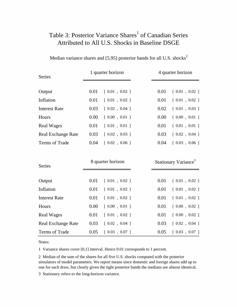
Series

Output 0.01 [ 0.01 , 0.02 ] 0.01 [ 0.01 , 0.02 ]

Inflation 0.01 [ 0.01 , 0.02 ] 0.01 [ 0.01 , 0.02 ]

Interest Rate 0.03 [ 0.02 , 0.04 ] 0.02 [ 0.01 , 0.03 ]

Hours 0.00 [ 0.00 , 0.01 ] 0.00 [ 0.00 , 0.01 ]

Real Wages 0.01 [ 0.01 , 0.01 ] 0.01 [ 0.01 , 0.01 ]

Real Exchange Rate 0.03 [ 0.02 , 0.03 ] 0.03 [ 0.02 , 0.04 ]

Terms of Trade 0.04 [ 0.02 , 0.06 ] 0.04 [ 0.03 , 0.06 ]

Series

Output 0.01 [ 0.01 , 0.02 ] 0.01 [ 0.01 , 0.02 ]

Inflation 0.01 [ 0.01 , 0.02 ] 0.01 [ 0.01 , 0.02 ]

Interest Rate 0.01 [ 0.01 , 0.02 ] 0.01 [ 0.01 , 0.02 ]

Hours 0.00 [ 0.00 , 0.01 ] 0.01 [ 0.00 , 0.02 ]

Real Wages 0.01 [ 0.01 , 0.02 ] 0.01 [ 0.00 , 0.02 ]

Real Exchange Rate 0.03 [ 0.02 , 0.04 ] 0.03 [ 0.02 , 0.04 ]

Terms of Trade 0.05 [ 0.03 , 0.07 ] 0.05 [ 0.03 , 0.07 ]

Notes:

Table 3: Posterior Variance Shares1 of Canadian Series Attributed to All U.S. Shocks in Baseline DSGE

Median variance shares and [5,95] posterior bands for all U.S. shocks2

1 quarter horizon 4 quarter horizon

8 quarter horizon Stationary Variance3

1 Variance shares cover [0,1] interval. Hence 0.01 corresponds to 1 percent.

2 Median of the sum of the shares for all five U.S. shocks computed with the posterior simulators of model parameters. We report means since domestic and foreign shares add up to one for each draw, but clearly given the tight posterior bands the medians are almost identical.

3 Stationary refers to the long-horizon variance.

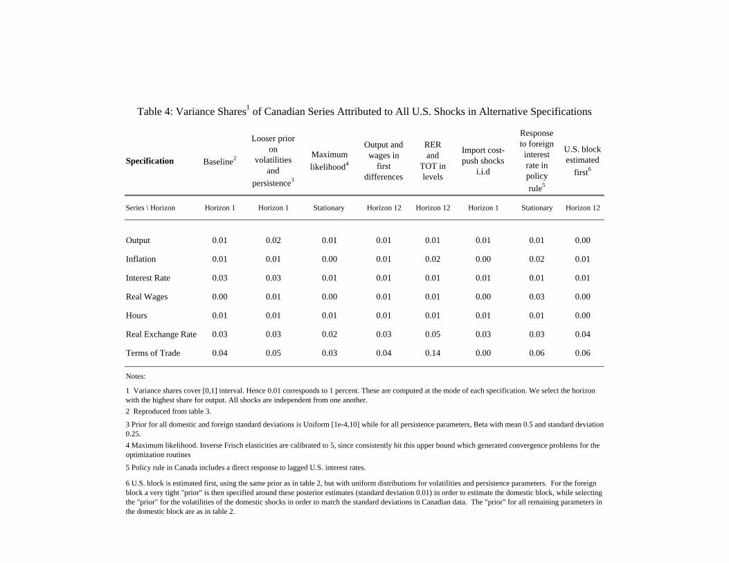
Specification Baseline2

Looser prior on

volatilities and

persistence3

Maximum

likelihood4

Output and wages in

first differences

RER and

TOT in levels

Import cost-push shocks

i.i.d

Response to foreign interest rate in policy

rule5

U.S. block estimated

first6

Series \ Horizon Horizon 1 Horizon 1 Stationary Horizon 12 Horizon 12 Horizon 1 Stationary Horizon 12

Output 0.01 0.02 0.01 0.01 0.01 0.01 0.01 0.00

Inflation 0.01 0.01 0.00 0.01 0.02 0.00 0.02 0.01

Interest Rate 0.03 0.03 0.01 0.01 0.01 0.01 0.01 0.01

Real Wages 0.00 0.01 0.00 0.01 0.01 0.00 0.03 0.00

Hours 0.01 0.01 0.01 0.01 0.01 0.01 0.01 0.00

Real Exchange Rate 0.03 0.03 0.02 0.03 0.05 0.03 0.03 0.04

Terms of Trade 0.04 0.05 0.03 0.04 0.14 0.00 0.06 0.06

Notes:

6 U.S. block is estimated first, using the same prior as in table 2, but with uniform distributions for volatilities and persistence parameters. For the foreign block a very tight "prior" is then specified around these posterior estimates (standard deviation 0.01) in order to estimate the domestic block, while selecting the "prior" for the volatilities of the domestic shocks in order to match the standard deviations in Canadian data. The "prior" for all remaining parameters in the domestic block are as in table 2.

Table 4: Variance Shares1 of Canadian Series Attributed to All U.S. Shocks in Alternative Specifications

1 Variance shares cover [0,1] interval. Hence 0.01 corresponds to 1 percent. These are computed at the mode of each specification. We select the horizon with the highest share for output. All shocks are independent from one another.

2 Reproduced from table 3.

3 Prior for all domestic and foreign standard deviations is Uniform [1e-4,10] while for all persistence parameters, Beta with mean 0.5 and standard deviation 0.25.

4 Maximum likelihood. Inverse Frisch elasticities are calibrated to 5, since consistently hit this upper bound which generated convergence problems for the optimization routines

5 Policy rule in Canada includes a direct response to lagged U.S. interest rates.

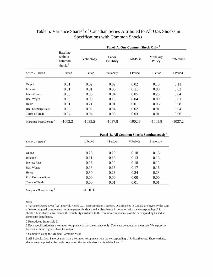
Baseline without common

shocks2

Technology Labor

Disutility Cost-Push

Monetary Policy

Preference

Series \ Horizon 1 Period 1 Period Stationary 1 Period 1 Period 1 Period

Output 0.01 0.02 0.02 0.02 0.10 0.11Inflation 0.01 0.01 0.06 0.11 0.00 0.02Interest Rate 0.03 0.03 0.04 0.05 0.23 0.04Real Wages 0.00 0.00 0.13 0.04 0.00 0.01Hours 0.01 0.21 0.01 0.01 0.06 0.08Real Exchange Rate 0.03 0.02 0.04 0.02 0.01 0.04Terms of Trade 0.04 0.04 0.08 0.03 0.01 0.06

Marginal Data Density 4 -1003.3 -1033.5 -1037.8 -1002.6 -1005.8 -1037.2

Series \ Horizon5 1 Period 4 Periods 8 Periods Stationary

Output 0.23 0.20 0.18 0.16Inflation 0.11 0.13 0.13 0.13Interest Rate 0.26 0.22 0.18 0.12Real Wages 0.13 0.16 0.17 0.16Hours 0.30 0.26 0.24 0.23Real Exchange Rate 0.00 0.00 0.00 0.00Terms of Trade 0.00 0.01 0.01 0.01

Marginal Data Density 4 -1010.6

Notes:

3 Each specification has a common component in that disturbance only. These are computed at the mode. We report the horizon with the highest share for output.

4 Computed using the Modied Harmonic Mean

5 All 5 shocks from Panel A now have a common component with the corresponding U.S. disturbances. These variance shares are computed at the mode. We report the same horizons as in tables 1 and 3.

Table 5: Variance Shares1 of Canadian Series Attributed to All U.S. Shocks in Specifications with Common Shocks

Panel A. One Common Shock Only 3

Panel B. All Common Shocks Simultaneously5

1 Variance shares cover [0,1] interval. Hence 0.01 corresponds to 1 percent. Disturbances in Canada are given by the sum of two orthogonal components: a country-specific shock and a disturbance in common with the corresponding U.S. shock. These shares now include the variability attributed to the common component(s) of the corresponding Canadian composite disturbance.

2 Reproduced from table 3.

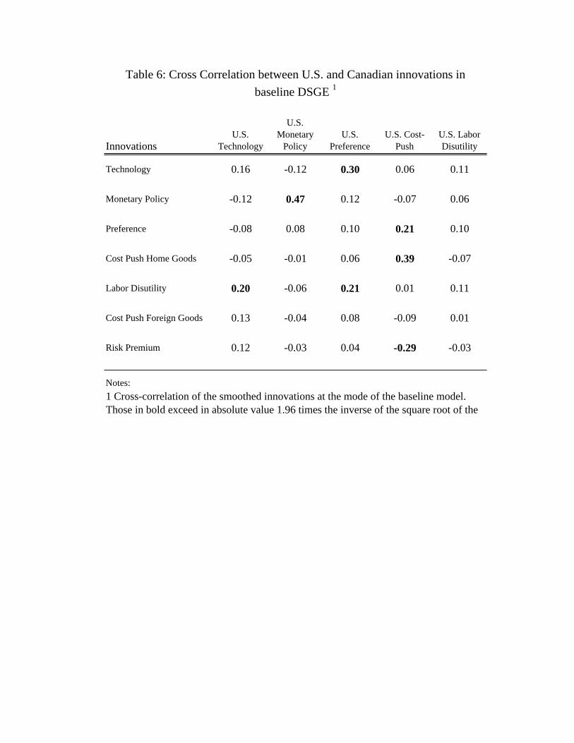
Innovations U.S.

Technology

U.S. Monetary

Policy U.S.

PreferenceU.S. Cost-

PushU.S. Labor Disutility

Technology 0.16 -0.12 0.30 0.06 0.11

Monetary Policy -0.12 0.47 0.12 -0.07 0.06

Preference -0.08 0.08 0.10 0.21 0.10

Cost Push Home Goods -0.05 -0.01 0.06 0.39 -0.07

Labor Disutility 0.20 -0.06 0.21 0.01 0.11

Cost Push Foreign Goods 0.13 -0.04 0.08 -0.09 0.01

Risk Premium 0.12 -0.03 0.04 -0.29 -0.03

Table 6: Cross Correlation between U.S. and Canadian innovations in

baseline DSGE 1

Notes:

1 Cross-correlation of the smoothed innovations at the mode of the baseline model. Those in bold exceed in absolute value 1.96 times the inverse of the square root of the

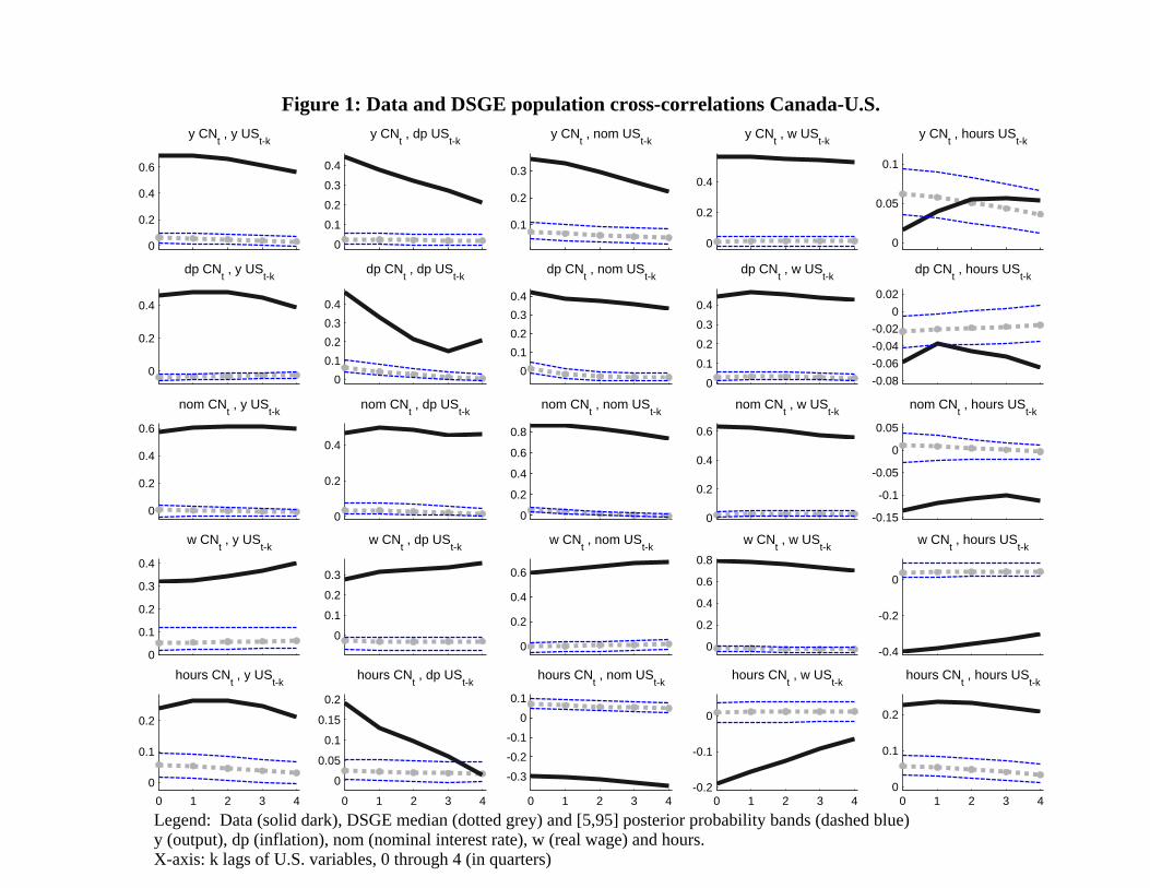
0

0.2

0.4

0.6

y CNt , y USt-k

0

0.1

0.2

0.3

0.4

y CNt , dp USt-k

0.1

0.2

0.3

y CNt , nom USt-k

0

0.2

0.4

y CNt , w USt-k

0

0.05

0.1

y CNt , hours USt-k

Legend: Data (solid dark), DSGE median (dotted grey) and [5,95] posterior probability bands (dashed blue) y (output), dp (inflation), nom (nominal interest rate), w (real wage) and hours. X-axis: k lags of U.S. variables, 0 through 4 (in quarters)

0

0.2

0.4

dp CNt , y USt-k

00.10.20.30.4

dp CNt , dp USt-k

00.10.20.30.4

dp CNt , nom USt-k

0

0.1

0.2

0.3

0.4

dp CNt , w USt-k

-0.08-0.06-0.04-0.02

00.02

dp CNt , hours USt-k

0

0.2

0.4

0.6

nom CNt , y USt-k

0

0.2

0.4

nom CNt , dp USt-k

0

0.2

0.4

0.6

0.8

nom CNt , nom USt-k

0

0.2

0.4

0.6

nom CNt , w USt-k

-0.15

-0.1

-0.05

0

0.05

nom CNt , hours USt-k

0

0.1

0.2

0.3

0.4

w CNt , y USt-k

0

0.1

0.2

0.3

w CNt , dp USt-k

0

0.2

0.4

0.6

w CNt , nom USt-k

0

0.2

0.4

0.6

0.8

w CNt , w USt-k

-0.4

-0.2

0

w CNt , hours USt-k

0 1 2 3 40

0.1

0.2

hours CNt , y USt-k

0 1 2 3 4

0

0.05

0.1

0.15

0.2

hours CNt , dp USt-k

0 1 2 3 4

-0.3

-0.2

-0.1

0

0.1

hours CNt , nom USt-k

0 1 2 3 4-0.2

-0.1

0

hours CNt , w USt-k

Figure 1: Data and DSGE population cross-correlations Canada-U.S.

0 1 2 3 40

0.1

0.2

hours CNt , hours USt-k

1

Working Paper Series

A series of research studies on regional economic issues relating to the Seventh Federal Reserve District, and on financial and economic topics.

U.S. Corporate and Bank Insolvency Regimes: An Economic Comparison and Evaluation WP-06-01 Robert R. Bliss and George G. Kaufman

Redistribution, Taxes, and the Median Voter WP-06-02 Marco Bassetto and Jess Benhabib

Identification of Search Models with Initial Condition Problems WP-06-03 Gadi Barlevy and H. N. Nagaraja

Tax Riots WP-06-04 Marco Bassetto and Christopher Phelan

The Tradeoff between Mortgage Prepayments and Tax-Deferred Retirement Savings WP-06-05 Gene Amromin, Jennifer Huang,and Clemens Sialm

Why are safeguards needed in a trade agreement? WP-06-06 Meredith A. Crowley

Taxation, Entrepreneurship, and Wealth WP-06-07 Marco Cagetti and Mariacristina De Nardi

A New Social Compact: How University Engagement Can Fuel Innovation WP-06-08 Laura Melle, Larry Isaak, and Richard Mattoon

Mergers and Risk WP-06-09 Craig H. Furfine and Richard J. Rosen

Two Flaws in Business Cycle Accounting WP-06-10 Lawrence J. Christiano and Joshua M. Davis

Do Consumers Choose the Right Credit Contracts? WP-06-11 Sumit Agarwal, Souphala Chomsisengphet, Chunlin Liu, and Nicholas S. Souleles

Chronicles of a Deflation Unforetold WP-06-12 François R. Velde

Female Offenders Use of Social Welfare Programs Before and After Jail and Prison: Does Prison Cause Welfare Dependency? WP-06-13 Kristin F. Butcher and Robert J. LaLonde

Eat or Be Eaten: A Theory of Mergers and Firm Size WP-06-14 Gary Gorton, Matthias Kahl, and Richard Rosen

2

Working Paper Series (continued) Do Bonds Span Volatility Risk in the U.S. Treasury Market? A Specification Test for Affine Term Structure Models WP-06-15 Torben G. Andersen and Luca Benzoni Transforming Payment Choices by Doubling Fees on the Illinois Tollway WP-06-16 Gene Amromin, Carrie Jankowski, and Richard D. Porter

How Did the 2003 Dividend Tax Cut Affect Stock Prices? WP-06-17 Gene Amromin, Paul Harrison, and Steven Sharpe

Will Writing and Bequest Motives: Early 20th Century Irish Evidence WP-06-18 Leslie McGranahan

How Professional Forecasters View Shocks to GDP WP-06-19 Spencer D. Krane

Evolving Agglomeration in the U.S. auto supplier industry WP-06-20 Thomas Klier and Daniel P. McMillen

Mortality, Mass-Layoffs, and Career Outcomes: An Analysis using Administrative Data WP-06-21 Daniel Sullivan and Till von Wachter

The Agreement on Subsidies and Countervailing Measures: Tying One’s Hand through the WTO. WP-06-22 Meredith A. Crowley

How Did Schooling Laws Improve Long-Term Health and Lower Mortality? WP-06-23 Bhashkar Mazumder

Manufacturing Plants’ Use of Temporary Workers: An Analysis Using Census Micro Data WP-06-24 Yukako Ono and Daniel Sullivan

What Can We Learn about Financial Access from U.S. Immigrants? WP-06-25 Una Okonkwo Osili and Anna Paulson

Bank Imputed Interest Rates: Unbiased Estimates of Offered Rates? WP-06-26 Evren Ors and Tara Rice

Welfare Implications of the Transition to High Household Debt WP-06-27 Jeffrey R. Campbell and Zvi Hercowitz

Last-In First-Out Oligopoly Dynamics WP-06-28 Jaap H. Abbring and Jeffrey R. Campbell

Oligopoly Dynamics with Barriers to Entry WP-06-29 Jaap H. Abbring and Jeffrey R. Campbell

Risk Taking and the Quality of Informal Insurance: Gambling and Remittances in Thailand WP-07-01 Douglas L. Miller and Anna L. Paulson

3

Working Paper Series (continued) Fast Micro and Slow Macro: Can Aggregation Explain the Persistence of Inflation? WP-07-02 Filippo Altissimo, Benoît Mojon, and Paolo Zaffaroni

Assessing a Decade of Interstate Bank Branching WP-07-03 Christian Johnson and Tara Rice

Debit Card and Cash Usage: A Cross-Country Analysis WP-07-04 Gene Amromin and Sujit Chakravorti

The Age of Reason: Financial Decisions Over the Lifecycle WP-07-05 Sumit Agarwal, John C. Driscoll, Xavier Gabaix, and David Laibson

Information Acquisition in Financial Markets: a Correction WP-07-06 Gadi Barlevy and Pietro Veronesi

Monetary Policy, Output Composition and the Great Moderation WP-07-07 Benoît Mojon

Estate Taxation, Entrepreneurship, and Wealth WP-07-08 Marco Cagetti and Mariacristina De Nardi

Conflict of Interest and Certification in the U.S. IPO Market WP-07-09 Luca Benzoni and Carola Schenone

The Reaction of Consumer Spending and Debt to Tax Rebates – Evidence from Consumer Credit Data WP-07-10 Sumit Agarwal, Chunlin Liu, and Nicholas S. Souleles

Portfolio Choice over the Life-Cycle when the Stock and Labor Markets are Cointegrated WP-07-11 Luca Benzoni, Pierre Collin-Dufresne, and Robert S. Goldstein Nonparametric Analysis of Intergenerational Income Mobility WP-07-12

with Application to the United States Debopam Bhattacharya and Bhashkar Mazumder

How the Credit Channel Works: Differentiating the Bank Lending Channel WP-07-13

and the Balance Sheet Channel Lamont K. Black and Richard J. Rosen

Labor Market Transitions and Self-Employment WP-07-14

Ellen R. Rissman

First-Time Home Buyers and Residential Investment Volatility WP-07-15

Jonas D.M. Fisher and Martin Gervais

Establishments Dynamics and Matching Frictions in Classical Competitive Equilibrium WP-07-16

Marcelo Veracierto

Technology’s Edge: The Educational Benefits of Computer-Aided Instruction WP-07-17

Lisa Barrow, Lisa Markman, and Cecilia Elena Rouse

4

Working Paper Series (continued) The Widow’s Offering: Inheritance, Family Structure, and the Charitable Gifts of Women WP-07-18

Leslie McGranahan

Demand Volatility and the Lag between the Growth of Temporary and Permanent Employment WP-07-19

Sainan Jin, Yukako Ono, and Qinghua Zhang

A Conversation with 590 Nascent Entrepreneurs WP-07-20

Jeffrey R. Campbell and Mariacristina De Nardi

Cyclical Dumping and US Antidumping Protection: 1980-2001 WP-07-21

Meredith A. Crowley

Health Capital and the Prenatal Environment: The Effect of Maternal Fasting During Pregnancy WP-07-22

Douglas Almond and Bhashkar Mazumder

The Spending and Debt Response to Minimum Wage Hikes WP-07-23

Daniel Aaronson, Sumit Agarwal, and Eric French

The Impact of Mexican Immigrants on U.S. Wage Structure WP-07-24

Maude Toussaint-Comeau

A Leverage-based Model of Speculative Bubbles WP-08-01

Gadi Barlevy

Displacement, Asymmetric Information and Heterogeneous Human Capital WP-08-02

Luojia Hu and Christopher Taber

BankCaR (Bank Capital-at-Risk): A credit risk model for US commercial bank charge-offs WP-08-03

Jon Frye and Eduard Pelz

Bank Lending, Financing Constraints and SME Investment WP-08-04

Santiago Carbó-Valverde, Francisco Rodríguez-Fernández, and Gregory F. Udell

Global Inflation WP-08-05

Matteo Ciccarelli and Benoît Mojon

Scale and the Origins of Structural Change WP-08-06

Francisco J. Buera and Joseph P. Kaboski

Inventories, Lumpy Trade, and Large Devaluations WP-08-07

George Alessandria, Joseph P. Kaboski, and Virgiliu Midrigan

School Vouchers and Student Achievement: Recent Evidence, Remaining Questions WP-08-08

Cecilia Elena Rouse and Lisa Barrow

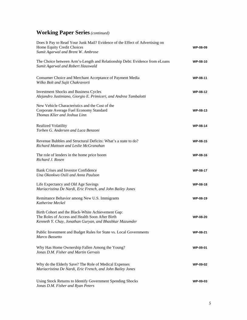
5

Working Paper Series (continued) Does It Pay to Read Your Junk Mail? Evidence of the Effect of Advertising on Home Equity Credit Choices WP-08-09

Sumit Agarwal and Brent W. Ambrose

The Choice between Arm’s-Length and Relationship Debt: Evidence from eLoans WP-08-10

Sumit Agarwal and Robert Hauswald

Consumer Choice and Merchant Acceptance of Payment Media WP-08-11

Wilko Bolt and Sujit Chakravorti Investment Shocks and Business Cycles WP-08-12

Alejandro Justiniano, Giorgio E. Primiceri, and Andrea Tambalotti New Vehicle Characteristics and the Cost of the Corporate Average Fuel Economy Standard WP-08-13

Thomas Klier and Joshua Linn

Realized Volatility WP-08-14

Torben G. Andersen and Luca Benzoni

Revenue Bubbles and Structural Deficits: What’s a state to do? WP-08-15

Richard Mattoon and Leslie McGranahan The role of lenders in the home price boom WP-08-16

Richard J. Rosen

Bank Crises and Investor Confidence WP-08-17

Una Okonkwo Osili and Anna Paulson Life Expectancy and Old Age Savings WP-08-18

Mariacristina De Nardi, Eric French, and John Bailey Jones Remittance Behavior among New U.S. Immigrants WP-08-19

Katherine Meckel Birth Cohort and the Black-White Achievement Gap: The Roles of Access and Health Soon After Birth WP-08-20

Kenneth Y. Chay, Jonathan Guryan, and Bhashkar Mazumder

Public Investment and Budget Rules for State vs. Local Governments WP-08-21

Marco Bassetto

Why Has Home Ownership Fallen Among the Young? WP-09-01

Jonas D.M. Fisher and Martin Gervais

Why do the Elderly Save? The Role of Medical Expenses WP-09-02

Mariacristina De Nardi, Eric French, and John Bailey Jones

Using Stock Returns to Identify Government Spending Shocks WP-09-03

Jonas D.M. Fisher and Ryan Peters

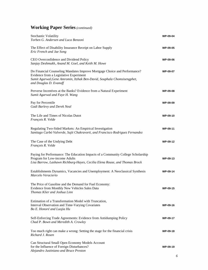
6

Working Paper Series (continued) Stochastic Volatility WP-09-04

Torben G. Andersen and Luca Benzoni The Effect of Disability Insurance Receipt on Labor Supply WP-09-05

Eric French and Jae Song CEO Overconfidence and Dividend Policy WP-09-06

Sanjay Deshmukh, Anand M. Goel, and Keith M. Howe Do Financial Counseling Mandates Improve Mortgage Choice and Performance? WP-09-07 Evidence from a Legislative Experiment

Sumit Agarwal,Gene Amromin, Itzhak Ben-David, Souphala Chomsisengphet, and Douglas D. Evanoff Perverse Incentives at the Banks? Evidence from a Natural Experiment WP-09-08

Sumit Agarwal and Faye H. Wang Pay for Percentile WP-09-09

Gadi Barlevy and Derek Neal

The Life and Times of Nicolas Dutot WP-09-10

François R. Velde

Regulating Two-Sided Markets: An Empirical Investigation WP-09-11

Santiago Carbó Valverde, Sujit Chakravorti, and Francisco Rodriguez Fernandez

The Case of the Undying Debt WP-09-12

François R. Velde

Paying for Performance: The Education Impacts of a Community College Scholarship Program for Low-income Adults WP-09-13

Lisa Barrow, Lashawn Richburg-Hayes, Cecilia Elena Rouse, and Thomas Brock

Establishments Dynamics, Vacancies and Unemployment: A Neoclassical Synthesis WP-09-14

Marcelo Veracierto

The Price of Gasoline and the Demand for Fuel Economy: Evidence from Monthly New Vehicles Sales Data WP-09-15

Thomas Klier and Joshua Linn

Estimation of a Transformation Model with Truncation, Interval Observation and Time-Varying Covariates WP-09-16

Bo E. Honoré and Luojia Hu

Self-Enforcing Trade Agreements: Evidence from Antidumping Policy WP-09-17

Chad P. Bown and Meredith A. Crowley

Too much right can make a wrong: Setting the stage for the financial crisis WP-09-18

Richard J. Rosen Can Structural Small Open Economy Models Account for the Influence of Foreign Disturbances? WP-09-19

Alejandro Justiniano and Bruce Preston