Embed Size (px)
Citation preview
et discipline ou spécialité
Jury :
le
Institut Supérieur de l’Aéronautique et de l’Espace (ISAE)
Pierre VUILLEMIN
lundi 24 novembre 2014
Approximation de modèles dynamiques de grande dimension surintervalles de fréquences limités
EDSYS : Automatique
Équipe d'accueil ISAE-ONERA CSDV
MmeMartine OLIVI, Chargée de Recherche INRIA - RapporteurM. Serkan GUGERCIN, Professeur Virginia Tech - Rapporteur
M. Didier HENRION, Directeur de Recherche CNRS - ExaminateurM. Michel ZASADZINSKI, Professeur Université de Lorraine - Examinateur
M. Daniel ALAZARD, Professeur Université de Toulouse - Directeur de thèseM. Charles POUSSOT-VASSAL, Ingénieur de Recherche Onera - Co-directeur de thèse
M. Daniel ALAZARD (directeur de thèse)M. Charles POUSSOT-VASSAL (co-directeur de thèse)


Frequency-limited model approximation of large-scale
dynamical models
Pierre Vuillemin


A mes parents


Acknowledgement
Firstly, I would like to express my warm thanks to my thesis advisors Charles Poussot-Vassaland Daniel Alazard for giving me the opportunity to achieve this PhD. thesis. I am also thank-ful for their guidance, constructive criticism and advice which have enabled me to successfullycomplete this project.
I would also like to thank Martine Olivi and Serkan Gugercin for accepting to review thismanuscript. Their constructive comments have given me keys to improve this work and leadsto extend it. Likewise, I would like to thank Didier Henrion and Michel Zasadzinski foraccepting to be part of my jury.
I am also grateful to all the people at Onera, and especially within the Flight Dynamics andSystems Control department, who have helped me during my thesis either for technical mattersor administrative tasks.
Special thanks to my fellow Phd. students of the department who have helped make thesethree years a very enjoyable and agreeable period through the numerous coffee breaks and otheractivities.
I could not end without expressing my gratitude to Marion for her foolproof support duringthese three years which has enabled me to be fully focused on my work.
i

Resume
Les systemes physiques sont representes par des modeles mathematiques qui peuvent etre utilisespour simuler, analyser ou controler ces systemes. Selon la complexite du systeme qu’il est censerepresenter, un modele peut etre plus ou moins complexe. Une complexite trop grande peuts’averer problematique en pratique du fait des limitations de puissance de calcul et de memoiredes ordinateurs. L’une des facons de contourner ce probleme consiste a utiliser l’approximation demodeles qui vise a remplacer le modele complexe par un modele simplifie dont le comportementest toujours representatif de celui du systeme physique.
Dans le cas des modeles dynamiques Lineaires et Invariants dans le Temps (LTI), la com-plexite se traduit par une dimension importante du vecteur d’etat et on parle alors de modelesde grande dimension. L’approximation de modele, encore appelee reduction de modele dans cecas, a pour but de trouver un modele dont le vecteur d’etat est plus petit que celui du modelede grande dimension tel que les comportements entree-sortie des deux modeles soient prochesselon une certaine norme. La norme H2 a ete largement consideree dans la litterature pourmesurer la qualite d’un modele reduit. Cependant, la bande passante limitee des capteurs et desactionneurs ainsi que le fait qu’un modele est generalement representatif d’un systeme physiquedans une certaine bande frequentielle seulement, laissent penser qu’un modele reduit dont lecomportement est fidele au modele de grande dimension dans un intervalle de frequences donne,peut etre plus pertinent. C’est pourquoi, dans cette etude, la norme H2 limitee en frequence,ou norme H2,Ω, qui est simplement la restriction de la norme H2 sur un intervalle de frequencesΩ, a ete consideree. En particulier, le probleme qui vise a trouver un modele reduit minimisantla norme H2,Ω de l’erreur d’approximation avec le modele de grande dimension a ete traite.
Deux approches ont ete proposees dans cette optique. La premiere est une approche em-pirique basee sur la modification d’une methode sous-optimale pour l’approximation H2. Enpratique, ses performances s’averent interessantes et rivalisent avec certaines methodes connuespour l’approximation de modeles sur intervalles de frequences limites.
La seconde est une methode d’optimisation basee sur la formulation poles-residus de lanorme H2,Ω. Cette formulation generalise naturellement celle existante pour la norme H2 etpermet egalement d’exprimer deux bornes superieures sur la norme H∞ d’un modele LTI, cequi est particulierement interessant dans le cadre de la reduction de modeles. Les conditionsd’optimalite du premier ordre pour le probleme d’approximation optimale en norme H2,Ω ont eteexprimees et utilisees pour creer un algorithme de descente visant a trouver un minimum local auprobleme d’approximation. Couplee aux bornes sur la norme H∞ de l’erreur d’approximation,cette methode est utilisee pour le controle de modeles de grande dimension.
D’un point de vue plus pratique, l’ensemble des methodes proposees dans cette etude ont eteappliquees, avec succes, dans un cadre industriel comme element d’un processus global visant acontroler un avion civil flexible.
Mots-cles : modeles lineaires invariants dans le temps, modeles de grande dimension, reductionde modeles, approximation de modeles, approximation de modeles sur intervalles de frequenceslimites
iii

Abstract
Physical systems are represented by mathematical models in order to be simulated, analysed orcontrolled. Depending on the complexity of the physical system it is meant to represent and onthe way it has been built, a model can be more or less complex. This complexity can become anissue in practice due to the limited computational power and memory of computers. One wayto alleviate this issue consists in using model approximation which is aimed at finding a simplermodel that still represents faithfully the physical system.
In the case of Linear Time Invariant (LTI) dynamical models, complexity translates into alarge dimension of the state vector and one talks about large-scale models. Model approximationis in this case also called model reduction and consists in finding a model with a smaller statevector such that the input-to-output behaviours of both models are close with respect to somemeasure. The H2-norm has been extensively used in the literature to evaluate the quality of areduced-order model. Yet, due to the limited bandwidth of actuators, sensors and the fact thatmodels are generally representative on a bounded frequency interval only, a reduced-order modelthat faithfully reproduces the behaviour of the large-scale one over a bounded frequency intervalonly, may be more relevant. That is why, in this study, the frequency-limited H2-norm, or H2,Ω-norm, which is the restriction of the H2-norm over a frequency interval Ω, has been considered.In particular, the problem of finding a reduced-order model that minimises the H2,Ω-norm ofthe approximation error with the large-scale model has been addressed here.
For that purpose, two approaches have been developed. The first one is an empirical approachbased on the modification of a sub-optimal H2 model approximation method. Its performancesare interesting in practice and compete with some well-known frequency-limited approximationmethods.
The second one is an optimisation method relying on the poles-residues formulation of theH2,Ω-norm. This formulation naturally extends the one existing for the H2-norm and can alsobe used to derive two upper bounds on the H∞-norm of LTI dynamical models which is ofparticular interest in model reduction. The first-order optimality conditions of the optimal H2,Ω
approximation problem are derived and used to built a complex-domain descent algorithm aimedat finding a local minimum of the problem. Together with the H∞ bounds on the approximationerror, this approach is used to perform control of large-scale models.
From a practical point of view, the methods proposed in this study have been successfullyapplied in an industrial context as a part of the global process aimed at controlling a flexiblecivilian aircraft.
Keywords : linear time invariant models, large-scale models, model reduction, model approx-imation, frequency-limited model approximation
v

Notations and acronyms
Mathematical Notations
j the square root of −1Re(z) the real part of the complex zIm(z) the imaginary part of the complex zMT the transpose of MM∗ the conjugate of MMH the conjugate transpose of M
[M ]i,k the element of M located at the i-th rown and k-th columnλi(M) the i-the eigenvalue of Mtr (M) the trace of MIn the identity matrix of size nei the i-th column canonical vector, i.e. the vector which entries are null
excepted a 1 at the i-th positionM N the Hadamard product, or element-wise product, between M and N
diag(M) the columns vector containing the diagonal of the square matrix M1n a column vector of size n full of ones
aω,λ denotes 2πatan(ωλ )
vec(M) denotes the vectorisation of the matrix M , i.e. the column vectorformed by vertically concatenating the columns of M
Fl() represents the lower Linear Fractional RepresentationFu() represents the upper Linear Fractional Representation
Acronyms
BT Balanced TruncationFW-BT Frequency-Weighted Balanced TruncationFL-BT Frequency-Limited Balanced TruncationIRKA Iterative Rational Krylov Algorithm,
also called Iterative Tangential Interpolation Algorithm (ITIA)ISRKA Iterative SVD-Rational Krylov Algorithm,
also called Iterative SVD-Tangential Interpolation Algorithm (ISTIA)FL-ISTIA Frequency-Limited SVD Tangential Interpolation AlgorithmDARPO Descent Algorithm for Residues and Poles Optimisation
LPV Linear Parameter VaryingLFR Linear Fractional RepresentationSISO Single Input Single OutputSIMO Single Input Multiple OutputMISO Multiple Input Single OutputMIMO Multiple Input Multiple Output
vii


Contents
Acknowledgement i
Resume iii
Abstract v
Notations and acronyms vii
I Introduction 1
1 Introduction to model approximation 31.1 Context and motivations . . . . . . . . . . . . . . . . . . . . . . . . . . . . . . . . 31.2 Motivating examples . . . . . . . . . . . . . . . . . . . . . . . . . . . . . . . . . . 4
1.2.1 Simulation of a 3D cantilever Timoshenko beam . . . . . . . . . . . . . . 41.2.2 Control of an industrial aircraft . . . . . . . . . . . . . . . . . . . . . . . . 61.2.3 Standard benchmarks . . . . . . . . . . . . . . . . . . . . . . . . . . . . . 8
1.3 Problem formulation . . . . . . . . . . . . . . . . . . . . . . . . . . . . . . . . . . 101.4 Overview of the contributions . . . . . . . . . . . . . . . . . . . . . . . . . . . . . 101.5 Manuscript overview . . . . . . . . . . . . . . . . . . . . . . . . . . . . . . . . . . 11
II State of the art 15
2 Preliminary in LTI systems theory 172.1 Generalities . . . . . . . . . . . . . . . . . . . . . . . . . . . . . . . . . . . . . . . 17
2.1.1 Representation of LTI dynamical models . . . . . . . . . . . . . . . . . . . 172.1.2 Gramians and balanced realisation . . . . . . . . . . . . . . . . . . . . . . 20
2.2 Norms of systems . . . . . . . . . . . . . . . . . . . . . . . . . . . . . . . . . . . . 252.2.1 H2-norm . . . . . . . . . . . . . . . . . . . . . . . . . . . . . . . . . . . . 252.2.2 Frequency-limited H2-norm . . . . . . . . . . . . . . . . . . . . . . . . . . 262.2.3 H∞-norm . . . . . . . . . . . . . . . . . . . . . . . . . . . . . . . . . . . . 29
3 Standard model approximation methods 313.1 Model approximation by truncation . . . . . . . . . . . . . . . . . . . . . . . . . 31
3.1.1 Truncation and residualisation of state-space representation . . . . . . . . 313.1.2 Modal and balanced truncation . . . . . . . . . . . . . . . . . . . . . . . . 32
3.2 Model approximation by moment matching . . . . . . . . . . . . . . . . . . . . . 383.2.1 Moment matching problem . . . . . . . . . . . . . . . . . . . . . . . . . . 393.2.2 Implicit moment matching : the SISO case . . . . . . . . . . . . . . . . . 403.2.3 Tangential interpolation . . . . . . . . . . . . . . . . . . . . . . . . . . . . 43
4 Optimal H2 model approximation 474.1 First order optimality conditions . . . . . . . . . . . . . . . . . . . . . . . . . . . 48
4.1.1 H2 approximation error . . . . . . . . . . . . . . . . . . . . . . . . . . . . 484.1.2 Formulation of the first-order optimality conditions . . . . . . . . . . . . . 49
4.2 Algorithms for optimal H2 approximation . . . . . . . . . . . . . . . . . . . . . . 544.2.1 Iterative Rational Krylov Algorithm (IRKA) . . . . . . . . . . . . . . . . 544.2.2 Iterative SVD Rational Krylov Algorithm (ISRKA) . . . . . . . . . . . . 584.2.3 Optimisation algorithm for optimal H2 model approximation . . . . . . . 59
ix

5 Frequency weighted and frequency-limited model approximation 635.1 Frequency weighted model approximation . . . . . . . . . . . . . . . . . . . . . . 63
5.1.1 Frequency weighted balanced truncation . . . . . . . . . . . . . . . . . . . 635.1.2 Frequency weighted H2 model approximation . . . . . . . . . . . . . . . . 65
5.2 Frequency-limited model approximation . . . . . . . . . . . . . . . . . . . . . . . 675.2.1 Frequency-limited balanced truncation . . . . . . . . . . . . . . . . . . . . 675.2.2 Gramian-based H2,Ω optimal model approximation . . . . . . . . . . . . . 69
III Frequency-limited approximation of linear dynamical models 73
6 Development of a first approach for frequency-limited model approximation 756.1 Modification of ISRKA . . . . . . . . . . . . . . . . . . . . . . . . . . . . . . . . 75
6.1.1 Presentation of the method . . . . . . . . . . . . . . . . . . . . . . . . . . 756.1.2 Properties . . . . . . . . . . . . . . . . . . . . . . . . . . . . . . . . . . . . 776.1.3 Numerical improvement of the method . . . . . . . . . . . . . . . . . . . . 78
6.2 Numerical illustrations . . . . . . . . . . . . . . . . . . . . . . . . . . . . . . . . . 796.2.1 Comparison with the standard version of ISRKA . . . . . . . . . . . . . 796.2.2 Impact of restart and error watching . . . . . . . . . . . . . . . . . . . . . 836.2.3 Comparison with other methods . . . . . . . . . . . . . . . . . . . . . . . 86
7 Formulation of the H2,Ω-norm with the poles and residues of the transferfunction 897.1 Case of models with semi-simple poles only . . . . . . . . . . . . . . . . . . . . . 89
7.1.1 Preliminary results on complex functions . . . . . . . . . . . . . . . . . . 907.1.2 Poles-residues formulation of the H2,Ω-norm . . . . . . . . . . . . . . . . . 917.1.3 Numerical illustration of the formulation . . . . . . . . . . . . . . . . . . . 93
7.2 Case of models with higher order poles . . . . . . . . . . . . . . . . . . . . . . . . 947.2.1 Poles-residues formulation of the H2,Ω-norm for models with high order
poles . . . . . . . . . . . . . . . . . . . . . . . . . . . . . . . . . . . . . . . 947.2.2 Special case 1 : n eigenvalues of multiplicity 1 (semi-simple case) . . . . . 977.2.3 Special case 2 : 1 eigenvalue of multiplicity n . . . . . . . . . . . . . . . . 97
7.3 Upper bounds of the H∞-norm . . . . . . . . . . . . . . . . . . . . . . . . . . . . 987.3.1 Formulation of the bounds . . . . . . . . . . . . . . . . . . . . . . . . . . . 987.3.2 Computation of the bounds . . . . . . . . . . . . . . . . . . . . . . . . . . 1007.3.3 Experimental study of the bounds quality . . . . . . . . . . . . . . . . . . 1027.3.4 Construction of a frequency template . . . . . . . . . . . . . . . . . . . . 104
8 Formulation of the H2,Ω error and differentiation of its gradient 1118.1 Expression of the approximation error with the poles and residues of the models 111
8.1.1 Poles-residues formulation of the H2,Ω approximation error . . . . . . . . 1118.1.2 About the computation of the approximation error . . . . . . . . . . . . . 117
8.2 Gradient of the error . . . . . . . . . . . . . . . . . . . . . . . . . . . . . . . . . . 1198.2.1 Reminder on Wirtinger Calculus . . . . . . . . . . . . . . . . . . . . . . . 1198.2.2 Gradient of the H2,Ω approximation error . . . . . . . . . . . . . . . . . . 122
9 Development of a descent algorithm for the optimal H2,Ω approximation prob-lem 1299.1 A descent algorithm in the complex domain . . . . . . . . . . . . . . . . . . . . . 129
9.1.1 Reminder of unconstrained optimisation . . . . . . . . . . . . . . . . . . . 1309.1.2 Descent Algorithm for Residues and Poles Optimisation . . . . . . . . . . 1339.1.3 Initialisation of DARPO . . . . . . . . . . . . . . . . . . . . . . . . . . . 137
9.2 Numerical illustration . . . . . . . . . . . . . . . . . . . . . . . . . . . . . . . . . 139
x
9.2.1 Illustration of the behaviour of DARPO . . . . . . . . . . . . . . . . . . 1399.2.2 Improvement provided by DARPO . . . . . . . . . . . . . . . . . . . . . 1469.2.3 Application for the control of a large-scale model . . . . . . . . . . . . . . 151
10 Industrial aeronautical use case 15910.1 Vibration control for one business jet aircraft model . . . . . . . . . . . . . . . . 160
10.1.1 General industrial framework . . . . . . . . . . . . . . . . . . . . . . . . . 16010.1.2 Problem formulation and business jet aircraft model approximation . . . 16110.1.3 Anti-vibration control design . . . . . . . . . . . . . . . . . . . . . . . . . 16210.1.4 Numerical results . . . . . . . . . . . . . . . . . . . . . . . . . . . . . . . . 166
10.2 Global stability validation of a parameter varying business jet aircraft . . . . . . 16710.2.1 Problem statement . . . . . . . . . . . . . . . . . . . . . . . . . . . . . . . 16710.2.2 Model approximation & error bounding . . . . . . . . . . . . . . . . . . . 16810.2.3 Low-order LFR model creation . . . . . . . . . . . . . . . . . . . . . . . . 17010.2.4 IQC-based global stability analysis . . . . . . . . . . . . . . . . . . . . . . 173
IV Conclusion 177
11 Discussion 17911.1 FL-ISTIA . . . . . . . . . . . . . . . . . . . . . . . . . . . . . . . . . . . . . . . 17911.2 Poles-residues formulation of the H2,Ω-norm . . . . . . . . . . . . . . . . . . . . . 180
11.2.1 Numerical robustness . . . . . . . . . . . . . . . . . . . . . . . . . . . . . 18011.2.2 Scalability . . . . . . . . . . . . . . . . . . . . . . . . . . . . . . . . . . . . 182
11.3 Bounds on the H∞-norm and its applications . . . . . . . . . . . . . . . . . . . . 18311.3.1 Improvement of the construction of frequency templates . . . . . . . . . . 18311.3.2 Other possible applications for the H∞ bound ΓΩ . . . . . . . . . . . . . 185
11.4 First-order optimality conditions for the H2,Ω approximation problem . . . . . . 18511.5 DARPO . . . . . . . . . . . . . . . . . . . . . . . . . . . . . . . . . . . . . . . . 186
11.5.1 Issues related to the poles-residues formulation of the H2,Ω-norm . . . . . 18611.5.2 Optimisation scheme . . . . . . . . . . . . . . . . . . . . . . . . . . . . . . 18811.5.3 Approximation for a fixed error . . . . . . . . . . . . . . . . . . . . . . . . 18911.5.4 Model approximation for the control of large-scale models . . . . . . . . . 190
12 Outlook 193
V Appendix 195
A Proofs related to the poles-residues expression of the H2,Ω-norm 197A.1 Poles-residues expression of the H2,Ω-norm in the semi-simple case . . . . . . . . 197A.2 Poles-residues expression of the H2,Ω-norm for models with higher order poles . . 199A.3 Poles-residues expression of the H2,Ω approximation error . . . . . . . . . . . . . 200
B Elements about the principal value of the complex arctangent 201B.1 Difference between the two definitions of the inverse tangent function . . . . . . . 201B.2 Limit of atan
(ωλ
)as ω tends towards infinity . . . . . . . . . . . . . . . . . . . . 201
C Code samples 205C.1 H2,Ω-norm computation . . . . . . . . . . . . . . . . . . . . . . . . . . . . . . . . 205C.2 Example 11 : non-linearity of the optimal H2 approximation problem . . . . . . 206C.3 Use of the FL-ISTIA . . . . . . . . . . . . . . . . . . . . . . . . . . . . . . . . . 206C.4 Example 15 : computation of the bounds on the H∞-norm . . . . . . . . . . . . 207
xi

C.5 Example 16 : construction of a frequency template . . . . . . . . . . . . . . . . . 208C.6 Example 17 : behaviour of the H2,Ω approximation error when approximating to
a second-order model . . . . . . . . . . . . . . . . . . . . . . . . . . . . . . . . . . 208C.7 Use of DARPO . . . . . . . . . . . . . . . . . . . . . . . . . . . . . . . . . . . . 210C.8 Use of DARPO for the control of a large-scale model . . . . . . . . . . . . . . . 210C.9 Use of DARPO for the approximation at a fixed error . . . . . . . . . . . . . . 213
xii

Part I
Introduction
1

Chapter 1
Introduction to model approxima-tion
1.1 Context and motivations
Physical systems or phenomena are generally represented by mathematical models in order tobe simulated, analysed or controlled. Depending on (i) the complexity of the physical system tobe modelled, (ii) the means used to build the mathematical model and (iii) the desired accuracyof the model, this model can be more or less complex and representative.
A very accurate model is intuitively desirable, however this often yields an important com-plexity which might not be tractable in practice. Indeed, the limited computational power ofcomputers and their limited storage capabilities might make some numerical tools not tractableor not in an acceptable time. In addition, the errors induced by the floating point arithmeticmight significantly perturb some theoretical results. Hence, the complexity of the model has tobe restrained.
It may seem adequate to restrain the complexity of a model from the very beginning, i.e.during its construction, however it is not always possible nor suitable. Indeed, in the one handnumerical modelling tools (such as identification methods, finite elements methods, etc.) donot necessarily enable to restrain the complexity without loosing too much information. Andin the other hand, models can be used for different purposes (simulation, control, analysis, etc.)which limitations with respect to the complexity vary. Hence, a standard process in industrialsettings consists in creating one single high-fidelity model which is then transformed to match theapplication. Thus, an a posteriori method is generally preferred to diminish the complexity of theoriginal, high-fidelity model. Model approximation serves this purpose. Indeed, the underlyingidea behind model approximation consists in replacing a complex model by a simpler one whichpreserves its main characteristics and which is suitable for a specific application (e.g. simulation,analysis or control).
In this study, dynamical systems are considered. They can be represented by finite differenceequations, ordinary differential equations, differential algebraic equations or partial differentialequations which can be linear, non-linear, time-invariant or time-variant. Linear Time Invariant(LTI) models are widely used, both in the industry and in research. Indeed, for many physicalsystems, they are sufficiently representative around an equilibrium point and numerous toolsexist in order to analyse and control them. For this kind of models, complexity results in a largestate-space vector and one talks of large-scale model.
Approximation of large-scale LTI models has been extensively studied over the years and twomain steps can be distinguished. In a first time, some well-known methods such as the BalancedTruncation and the Hankel norm approximation have been developed [Moore, 1981; Glover,1984]. Then, the extensive use of numerical modelling tools has led to modify the conceptionof large-scale models which can now have thousands or even millions of states. Standard modelapproximation methods (in their basic form) were not adapted anymore for very large casedue to their inherent numerical complexity. Hence, original techniques that are numericallycheaper have been developed. They are mainly based on interpolation through Krylov subspaces[Grimme, 1997] and have more recently led to some interesting development concerning optimalH2 model approximation [Gugercin et al., 2008; Van Dooren et al., 2008b]. This problem hasalso been addressed in a different way using non-linear optimisation schemes [Marmorat et al.,
3

Chapter 1. Introduction to model approximation
2002; Beattie and Gugercin, 2009]. Initially, these methods were developed to reproduce thebehaviour of the large-scale model over the whole frequency range. However, in some cases, itmay seem more relevant to match the behaviour of the large-scale model only on a boundedfrequency range.
Indeed (i) the limited bandwidth of sensors used to identify models from measured data mightlead to an inaccurate (and thus irrelevant) model at some frequencies, (ii) similarly, actuatorscannot act on some dynamics which make them less important for control purpose and (iii) byavoiding to take into accounts some dynamics, the large-scale model may be reduced even morewithout loosing accuracy in the considered frequency band. That is why we have chosen in thisthesis to address the problem of approximation over a bounded frequency range.
The most intuitive way to address such a problem consists in applying frequency filters to thelarge-scale model so that the reduced-order model is built in order to match the filtered large-scalemodel. This is called the frequency-weighted approximation problem and several methods havebeen developed to solve it [Enns, 1984; Lin and Chiu, 1990; Zhou, 1995; Leblond and Olivi, 1998;Wang et al., 1999; Breiten et al., 2014]. Note that the filtered large-scale model is augmented bythe order of the filters. Hence, and even if it is often marginal compared to the order of the model,the complexity is increased for the approximation algorithms. More importantly, the design ofadequate filters can be a tedious task. An approach that does not involve any explicit filtering,called the frequency-limited balanced truncation, has been proposed in [Gawronski and Juang,1990]. It is based on frequency-limited gramians which act as frequency-weighted gramians[Enns, 1984] considered with perfect filters.
This thesis tries to bring together the methodology used in optimal H2 model approxima-tion [Beattie and Gugercin, 2009] with the criterion derived from frequency-limited gramians[Gawronski and Juang, 1990] in order to perform optimal frequency-limited H2 model approxi-mation of large-scale LTI dynamical models. Note that a similar study has been conducted inparallel of this work in [Petersson, 2013] with another formulation of the criterion.
From a practical point of view, the methods developed during this study are meant to beapplied in an industrial aeronautic context which problematic are quite specific as presentedbelow in the second motivating example.
1.2 Motivating examples
In Section 1.2.1, the benefits of model approximation for the simulation1 of LTI models ishighlighted with a 3D cantilever Timoshenko beam model. Then in Section 1.2.2, some issuesencountered in the context of industrial aircraft control are introduced. These issues form theindustrial application of this thesis and are addressed more in depth in Chapter 10. Finally, inSection 1.2.3, the main models used as academic benchmarks in this thesis are introduced.
1.2.1 Simulation of a 3D cantilever Timoshenko beam
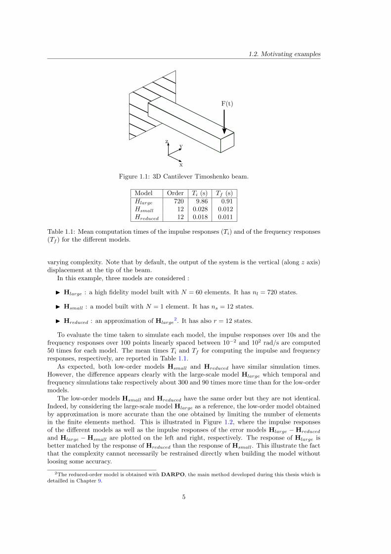
In [Panzer et al., 2009], a simple finite elements method to model a 3D Cantilever Timoshenkobeam (see Figure 1.1) loaded by some force F (t) at its tip is described. The provided script en-ables to arbitrarily choose some parameters as the number of elements N used for discretization,the length of the beam L, etc. Hence it can conveniently be used to build state-space models of
1The time measurement presented throughout this study are mainly aimed at being compared to each otherand should not be considered as absolute references but for sake of clarity, the technical details related to thenumerical computations are presented here.
All the numerical computations have been performed with Matlab R© R2013a on an Intel R© CoreTM i7-3610QMprocessor under a Linux environment and with 8Gb of RAM.
In Matlab R©, the Just In Time (JIT) compiler has been disabled in order to have stable time measurements.The elapsed time is measured through the CPU time.
4
1.2. Motivating examples
F(t)
x
yz
Figure 1.1: 3D Cantilever Timoshenko beam.
Model Order Ti (s) Tf (s)Hlarge 720 9.86 0.91Hsmall 12 0.028 0.012Hreduced 12 0.018 0.011
Table 1.1: Mean computation times of the impulse responses (Ti) and of the frequency responses(Tf ) for the different models.
varying complexity. Note that by default, the output of the system is the vertical (along z axis)displacement at the tip of the beam.
In this example, three models are considered :
I Hlarge : a high fidelity model built with N = 60 elements. It has nl = 720 states.
I Hsmall : a model built with N = 1 element. It has ns = 12 states.
I Hreduced : an approximation of Hlarge2. It has also r = 12 states.
To evaluate the time taken to simulate each model, the impulse responses over 10s and thefrequency responses over 100 points linearly spaced between 10−2 and 102 rad/s are computed50 times for each model. The mean times Ti and Tf for computing the impulse and frequencyresponses, respectively, are reported in Table 1.1.
As expected, both low-order models Hsmall and Hreduced have similar simulation times.However, the difference appears clearly with the large-scale model Hlarge which temporal andfrequency simulations take respectively about 300 and 90 times more time than for the low-ordermodels.
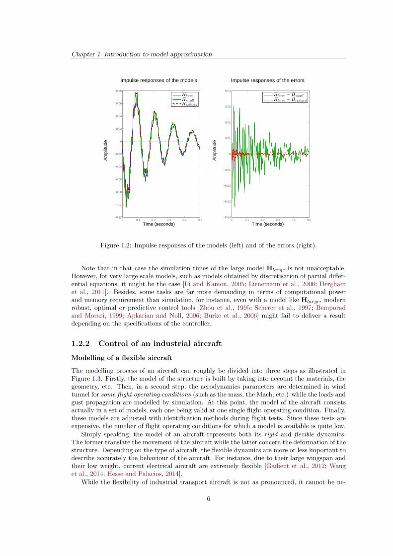
The low-order models Hsmall and Hreduced have the same order but they are not identical.Indeed, by considering the large-scale model Hlarge as a reference, the low-order model obtainedby approximation is more accurate than the one obtained by limiting the number of elementsin the finite elements method. This is illustrated in Figure 1.2, where the impulse responsesof the different models as well as the impulse responses of the error models Hlarge −Hreduced
and Hlarge −Hsmall are plotted on the left and right, respectively. The response of Hlarge isbetter matched by the response of Hreduced than the response of Hsmall. This illustrate the factthat the complexity cannot necessarily be restrained directly when building the model withoutloosing some accuracy.
2The reduced-order model is obtained with DARPO, the main method developed during this thesis which isdetailled in Chapter 9.
5
Chapter 1. Introduction to model approximation
0 0.1 0.2 0.3 0.4 0.5−0.12
−0.1
−0.08
−0.06
−0.04
−0.02
0
0.02
0.04
0.06
0.08
Impulse responses of the models
Time (seconds)
Am
plitu
de
H large
HsmallHreduced
0 0.1 0.2 0.3 0.4 0.5−0.04
−0.03
−0.02
−0.01
0
0.01
0.02
0.03
0.04
Impulse responses of the errors
Time (seconds)
Am
plitu
de
H large −Hsmall
H large −Hreduced
Figure 1.2: Impulse responses of the models (left) and of the errors (right).
Note that in that case the simulation times of the large model Hlarge is not unacceptable.However, for very large scale models, such as models obtained by discretisation of partial differ-ential equations, it might be the case [Li and Kamon, 2005; Lienemann et al., 2006; Derghamet al., 2011]. Besides, some tasks are far more demanding in terms of computational powerand memory requirement than simulation, for instance, even with a model like Hlarge, modernrobust, optimal or predictive control tools [Zhou et al., 1995; Scherer et al., 1997; Bemporadand Morari, 1999; Apkarian and Noll, 2006; Burke et al., 2006] might fail to deliver a resultdepending on the specifications of the controller.
1.2.2 Control of an industrial aircraft
Modelling of a flexible aircraft
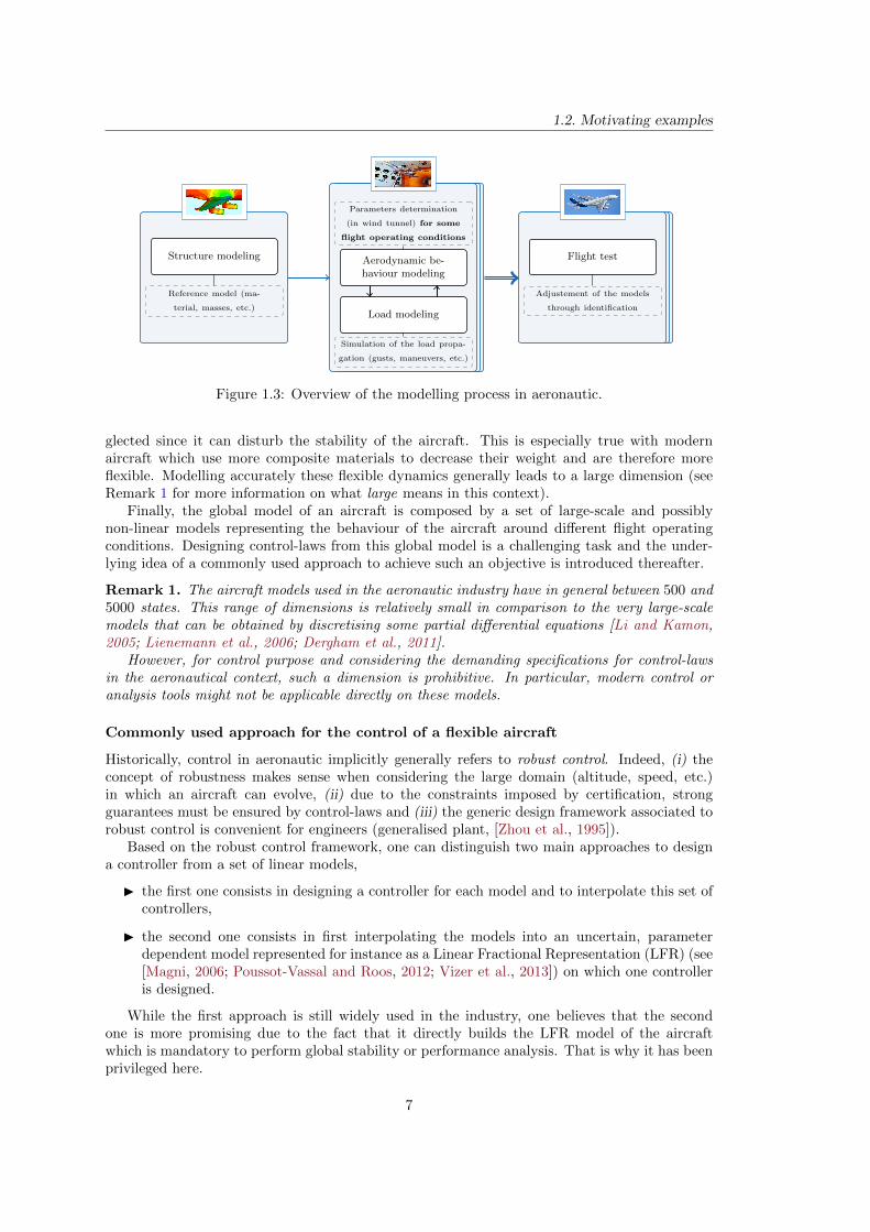
The modelling process of an aircraft can roughly be divided into three steps as illustrated inFigure 1.3. Firstly, the model of the structure is built by taking into account the materials, thegeometry, etc. Then, in a second step, the aerodynamics parameters are determined in windtunnel for some flight operating conditions (such as the mass, the Mach, etc.) while the loads andgust propagation are modelled by simulation. At this point, the model of the aircraft consistsactually in a set of models, each one being valid at one single flight operating condition. Finally,these models are adjusted with identification methods during flight tests. Since these tests areexpensive, the number of flight operating conditions for which a model is available is quite low.
Simply speaking, the model of an aircraft represents both its rigid and flexible dynamics.The former translate the movement of the aircraft while the latter concern the deformation of thestructure. Depending on the type of aircraft, the flexible dynamics are more or less important todescribe accurately the behaviour of the aircraft. For instance, due to their large wingspan andtheir low weight, current electrical aircraft are extremely flexible [Gadient et al., 2012; Wanget al., 2014; Hesse and Palacios, 2014].
While the flexibility of industrial transport aircraft is not as pronounced, it cannot be ne-
6
1.2. Motivating examples
Structure modeling
Reference model (ma-
terial, masses, etc.)
Aerodynamic be-haviour modeling
Load modeling
Parameters determination
(in wind tunnel) for some
flight operating conditions
Simulation of the load propa-
gation (gusts, maneuvers, etc.)
Flight test
Adjustement of the models
through identification
Figure 1.3: Overview of the modelling process in aeronautic.
glected since it can disturb the stability of the aircraft. This is especially true with modernaircraft which use more composite materials to decrease their weight and are therefore moreflexible. Modelling accurately these flexible dynamics generally leads to a large dimension (seeRemark 1 for more information on what large means in this context).
Finally, the global model of an aircraft is composed by a set of large-scale and possiblynon-linear models representing the behaviour of the aircraft around different flight operatingconditions. Designing control-laws from this global model is a challenging task and the under-lying idea of a commonly used approach to achieve such an objective is introduced thereafter.
Remark 1. The aircraft models used in the aeronautic industry have in general between 500 and5000 states. This range of dimensions is relatively small in comparison to the very large-scalemodels that can be obtained by discretising some partial differential equations [Li and Kamon,2005; Lienemann et al., 2006; Dergham et al., 2011].
However, for control purpose and considering the demanding specifications for control-lawsin the aeronautical context, such a dimension is prohibitive. In particular, modern control oranalysis tools might not be applicable directly on these models.
Commonly used approach for the control of a flexible aircraft
Historically, control in aeronautic implicitly generally refers to robust control. Indeed, (i) theconcept of robustness makes sense when considering the large domain (altitude, speed, etc.)in which an aircraft can evolve, (ii) due to the constraints imposed by certification, strongguarantees must be ensured by control-laws and (iii) the generic design framework associated torobust control is convenient for engineers (generalised plant, [Zhou et al., 1995]).
Based on the robust control framework, one can distinguish two main approaches to designa controller from a set of linear models,
I the first one consists in designing a controller for each model and to interpolate this set ofcontrollers,
I the second one consists in first interpolating the models into an uncertain, parameterdependent model represented for instance as a Linear Fractional Representation (LFR) (see[Magni, 2006; Poussot-Vassal and Roos, 2012; Vizer et al., 2013]) on which one controlleris designed.
While the first approach is still widely used in the industry, one believes that the secondone is more promising due to the fact that it directly builds the LFR model of the aircraftwhich is mandatory to perform global stability or performance analysis. That is why it has beenprivileged here.
7
Chapter 1. Introduction to model approximation
Set of large-scaleLTI models (one
for each flightoperating condition)
n ≤ 5000
Set of small-scaleLTI models (one
for each flightoperating condition)
model approximation
A B
C
A
C
B
r n
Small-scale uncer-tain model (LFR)
Interpolation ••
•
Controller K
e.g. Robust control
M
∆
u y
w z
Controller validation
High fidelitymodels
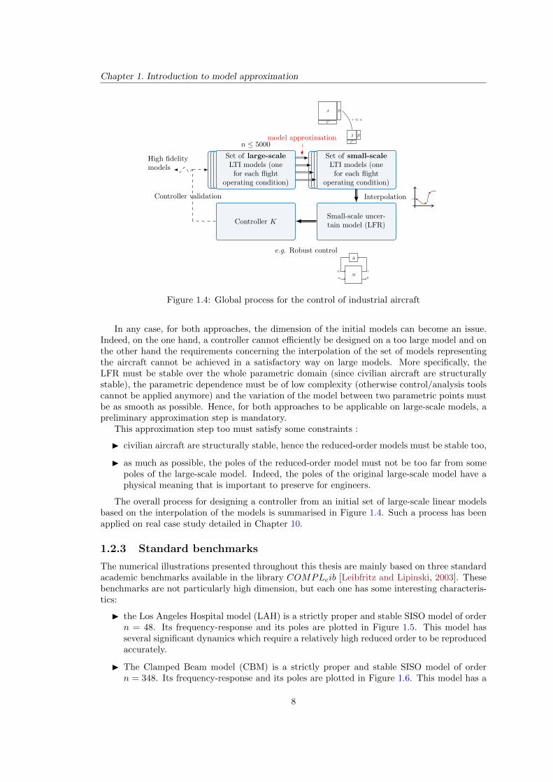
Figure 1.4: Global process for the control of industrial aircraft
In any case, for both approaches, the dimension of the initial models can become an issue.Indeed, on the one hand, a controller cannot efficiently be designed on a too large model and onthe other hand the requirements concerning the interpolation of the set of models representingthe aircraft cannot be achieved in a satisfactory way on large models. More specifically, theLFR must be stable over the whole parametric domain (since civilian aircraft are structurallystable), the parametric dependence must be of low complexity (otherwise control/analysis toolscannot be applied anymore) and the variation of the model between two parametric points mustbe as smooth as possible. Hence, for both approaches to be applicable on large-scale models, apreliminary approximation step is mandatory.
This approximation step too must satisfy some constraints :
I civilian aircraft are structurally stable, hence the reduced-order models must be stable too,
I as much as possible, the poles of the reduced-order model must not be too far from somepoles of the large-scale model. Indeed, the poles of the original large-scale model have aphysical meaning that is important to preserve for engineers.
The overall process for designing a controller from an initial set of large-scale linear modelsbased on the interpolation of the models is summarised in Figure 1.4. Such a process has beenapplied on real case study detailed in Chapter 10.
1.2.3 Standard benchmarks
The numerical illustrations presented throughout this thesis are mainly based on three standardacademic benchmarks available in the library COMPLeib [Leibfritz and Lipinski, 2003]. Thesebenchmarks are not particularly high dimension, but each one has some interesting characteris-tics:
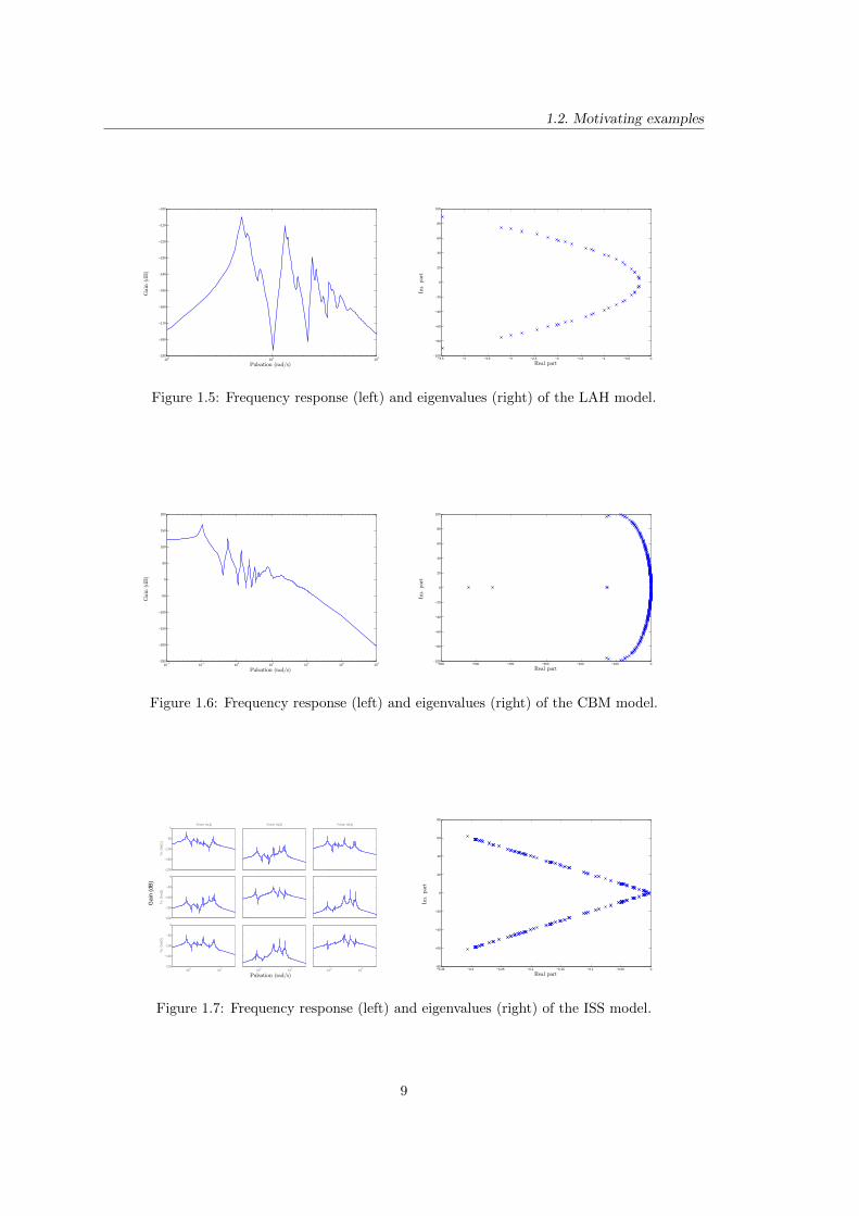
I the Los Angeles Hospital model (LAH) is a strictly proper and stable SISO model of ordern = 48. Its frequency-response and its poles are plotted in Figure 1.5. This model hasseveral significant dynamics which require a relatively high reduced order to be reproducedaccurately.
I The Clamped Beam model (CBM) is a strictly proper and stable SISO model of ordern = 348. Its frequency-response and its poles are plotted in Figure 1.6. This model has a
8
1.2. Motivating examples
100
101
102
−190
−180
−170
−160
−150
−140
−130
−120
−110
−100
Gain(dB)
Pulsation (rad/s)−4.5 −4 −3.5 −3 −2.5 −2 −1.5 −1 −0.5 0
−100
−80
−60
−40
−20
0
20
40
60
80
100
Im.part
Real part
Figure 1.5: Frequency response (left) and eigenvalues (right) of the LAH model.
10−2
10−1
100
101
102
103
104
−250
−200
−150
−100
−50
0
50
100
150
200
Gain(dB)
Pulsation (rad/s)−600 −500 −400 −300 −200 −100 0
−100
−80
−60
−40
−20
0
20
40
60
80
100
Im.part
Real part
Figure 1.6: Frequency response (left) and eigenvalues (right) of the CBM model.
−200
−150
−100
−50
0From: In(1)
To:
Out
(1)
−200
−150
−100
−50
0
To:
Out
(2)
100
102
−200
−150
−100
−50
0
To:
Out
(3)
From: In(2)
100
102
From: In(3)
100
102
Pulsation (rad/s)
Gai
n (d
B)
−0.35 −0.3 −0.25 −0.2 −0.15 −0.1 −0.05 0−80
−60
−40
−20
0
20
40
60
80
Im.part
Real part
Figure 1.7: Frequency response (left) and eigenvalues (right) of the ISS model.
9
Chapter 1. Introduction to model approximation
high gain dynamic at low frequency and several other small dynamics at higher frequencies.Catching accurately the low frequency dynamic directly yields a low approximation error.
I The International Space Station model (ISS) is a strictly proper and stable MIMO (ny =nu = 3) model of order n = 270. Its frequency-response and its poles are plotted in Figure1.7. Aside from being MIMO, this model has high gain dynamics at several frequencieswhich makes it particularly well suited to illustrate the relevance of frequency-limitedapproximation techniques.
Additional benchmarks are described when used if they are publicly available.
1.3 Problem formulation
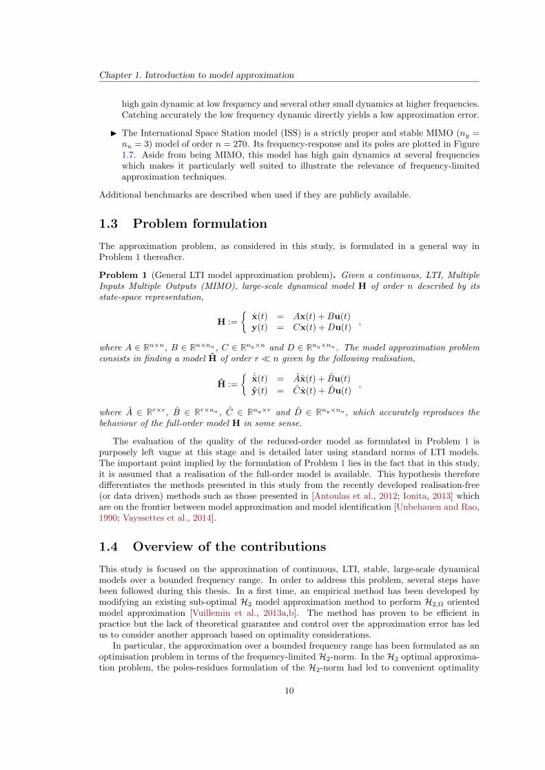
The approximation problem, as considered in this study, is formulated in a general way inProblem 1 thereafter.
Problem 1 (General LTI model approximation problem). Given a continuous, LTI, MultipleInputs Multiple Outputs (MIMO), large-scale dynamical model H of order n described by itsstate-space representation,
H :=
x(t) = Ax(t) +Bu(t)y(t) = Cx(t) +Du(t)
,
where A ∈ Rn×n, B ∈ Rn×nu , C ∈ Rny×n and D ∈ Rny×nu . The model approximation problemconsists in finding a model H of order r n given by the following realisation,
H :=
˙x(t) = Ax(t) + Bu(t)
y(t) = Cx(t) + Du(t),
where A ∈ Rr×r, B ∈ Rr×nu , C ∈ Rny×r and D ∈ Rny×nu , which accurately reproduces thebehaviour of the full-order model H in some sense.
The evaluation of the quality of the reduced-order model as formulated in Problem 1 ispurposely left vague at this stage and is detailed later using standard norms of LTI models.The important point implied by the formulation of Problem 1 lies in the fact that in this study,it is assumed that a realisation of the full-order model is available. This hypothesis thereforedifferentiates the methods presented in this study from the recently developed realisation-free(or data driven) methods such as those presented in [Antoulas et al., 2012; Ionita, 2013] whichare on the frontier between model approximation and model identification [Unbehauen and Rao,1990; Vayssettes et al., 2014].
1.4 Overview of the contributions
This study is focused on the approximation of continuous, LTI, stable, large-scale dynamicalmodels over a bounded frequency range. In order to address this problem, several steps havebeen followed during this thesis. In a first time, an empirical method has been developed bymodifying an existing sub-optimal H2 model approximation method to perform H2,Ω orientedmodel approximation [Vuillemin et al., 2013a,b]. The method has proven to be efficient inpractice but the lack of theoretical guarantee and control over the approximation error has ledus to consider another approach based on optimality considerations.
In particular, the approximation over a bounded frequency range has been formulated as anoptimisation problem in terms of the frequency-limited H2-norm. In the H2 optimal approxima-tion problem, the poles-residues formulation of the H2-norm had led to convenient optimality
10
1.5. Manuscript overview
conditions. Hence, we have firstly proposed a similar formulation for the frequency-limitedH2-norm [Vuillemin et al., 2012b, 2014c]. Then, based on this formulation of the norm, thefirst-order optimality conditions for the optimal frequency-limited approximation problem havebeen derived [Vuillemin et al., 2014b]. However, unlike the H2 problem, these optimality con-ditions could not be expressed as convenient interpolation conditions. Hence, an unconstrainedcomplex domain optimisation algorithm aimed at finding one optimal reduced-order model hasbeen developed [Vuillemin et al., 2014b]. Finally, this method has been brought one step furthertowards some control objective by using the two upper bounds on the H∞-norm that we haveproposed [Vuillemin et al., 2014d] in order to build a frequency template of the approximationerror that can be exploited in the robust control framework.
Besides, from a practical point of view, all the proposed methods and tools have been inte-grated in the MORE Toolbox3 [Poussot-Vassal and Vuillemin, 2012] and have successfully beenapplied in several industrial use cases. In a first time, the approximation methods developed inthis study have been applied on industrial large-scale aircraft models to evaluate their efficiencyon this type of models [Vuillemin et al., 2012a, 2013b]. Then, they have been used for the con-trol of large-scale models to design (i) an anti-vibration control law for a business jet aircraft[Poussot-Vassal et al., 2013], (ii) a control law ensuring flight performance and load clearancein presence of input saturation on a model representing the longitudinal behaviour of a flexiblecivilian aircraft [Burlion et al., 2014]. Additionally, a process for the creation of a low-orderuncertain, parameter varying model from a set of large-scale dynamical models has been devel-oped based on model approximation [Poussot-Vassal and Vuillemin, 2013; Poussot-Vassal et al.,2014]. Based on a similar method, the global stability and performance of the set of controlledlarge-scale models representing a business jet aircraft at different flight operating conditionssubject to actuator saturation have been proven by taking into account the error induced by theapproximation and the interpolation of the initial large-scale models [Vuillemin et al., 2014a].
1.5 Manuscript overview
This manuscript is divided into three parts in addition of the introduction that gather chapterswhich concern the state of the art, the contributions of this thesis with regard to frequency-limited model approximation and the conclusions of this study.
Part II : State of the Art
Chapter 2 : Preliminary in LTI systems theory
This chapter is aimed at recalling some general elements about linear systems theory and atintroducing the general notations used in this thesis. In particular, two elements that form thebasis of this thesis are recalled : the partial fraction decomposition of a transfer function andthe frequency-limited H2-norm of LTI models.
Chapter 3 : Standard model approximation methods
In this chapter, some well-known model approximation techniques based either on state-spacetruncation or moment matching are recalled. In particular, the balanced truncation is recalledsince it is one of the most popular approximation method and that it serves as reference inthe benchmarks. Implicit moment matching methods are presented as an introduction for theoptimal H2 model approximation methods.
3The toolbox is available from w3.onera.fr/more and its use is illustrated by several code samples availablein Appendix C.
11
Chapter 1. Introduction to model approximation
Chapter 4 : Optimal H2 model approximation
The optimal H2 approximation problem is introduced together with some methods to addressit. The methods that are presented are those based on the interpolation of the large-scale modelthrough projection on some specific Krylov subspaces and one optimisation method relying onthe partial fraction decomposition of the reduced-order transfer function.
Chapter 5 : Frequency-weighted and frequency-limited model approximation
In this chapter, some methods aimed at model approximation over a bounded frequency rangeare presented. Methods based on the use of filters are classified here as frequency-weighted modelapproximation methods while those that do not require any weight falls into the frequency-limitedmodel approximation methods. Among these methods, the frequency-weighted and frequency-limited balanced truncation are presented.
Part III : Frequency-limited approximation of linear dynamical models
Chapter 6 : development of a first approach for frequency-limited model approxi-mation
In this chapter, an empirical method built by modification of a sub-optimal H2 model approx-imation method to achieve model approximation over a bounded frequency-range is presented.The improvement of performances in terms of H2,Ω-norm in comparison to the original methodis illustrated through various examples. Its efficiency is also illustrated by comparison with thefrequency-limited balanced truncation.
Chapter 7 : Formulation of the H2,Ω-norm with the poles and residues of the transferfunction
The only formulation available for the computation of the frequency-limited H2-norm was thegramian one. In this chapter, a formulation based on the poles and residues of the transferfunction is developed thus generalising the poles-residues formulation of the H2-norm. This isdone both for models with semi-simple poles only and for model with higher order poles. Besides,two upper bounds on the H∞-norm of LTI dynamical models are derived from this formulation.
The results presented in this chapter constitute the basis of the major contributions of thisthesis. Hence, this chapter plays a pivotal role in this manuscript.
Chapter 8 : Formulation of the H2,Ω-norm of the error and differentiation of itsgradient
The poles-residues formulation of the H2,Ω-norm is used to express the approximation errorbetween the large-scale and reduced-order models thus leading to a formulation of the optimalH2,Ω model approximation problem in terms of the poles and residues of the reduced-ordermodel. The gradient of the error is derived with respect to the reduced-order model parametersand the first-order optimality conditions are presented.
Chapter 9 : Development of DARPO, a descent algorithm for the optimal H2,Ω
approximation problem
Since the first-order optimality conditions of the optimal H2,Ω problem cannot be expressed asconvenient interpolation conditions, an optimisation scheme is developed to find a local minimumof the approximation problem instead. In this chapter, this optimisation method is describedand compared to other frequency-limited approximation techniques on academic benchmarks. It
12
1.5. Manuscript overview
is also used to address a fictive problem of control of large-scale model by exploiting the boundson the H∞-norm of the approximation error.
Chapter 10 : Industrial aeronautical use case
In this chapter, the model approximation methods and tools developed in this thesis are usedwithin a global process aimed at designing an anti-vibration control-law for an industrial businessjet aircraft. More specifically, the preliminary study in which the control design problem isaddressed on one single large-scale model representing the business jet aircraft at one flightoperating condition is presented. Then, based on a controller designed with the extension ofthis approach, the global stability of the set of controlled large-scale models is assessed over thewhole parametric domain.
Part IV : Conclusion
Chapter 11 : Discussion
This chapter is aimed at recalling the contributions of this thesis as well as their limitations andto present some improvement leads to alleviate them. In addition, some short-term extensionsare presented.
Chapter 12 : Perspectives
In this chapter, some long-term outlook concerning the extension of the methods and toolsdeveloped in this thesis to other type of models or their application for control purpose aredrawn.
13


Part II
State of the art
15

Chapter 2
Preliminary in LTI systems theory
In this chapter, some general elements about LTI systems theory are recalled and the associatednotations introduced. The material is standard and can be found in many books such as [Zhouet al., 1995]. Additional references are mentioned for less standard material when required.
Section 2.1 is aimed at presenting some elements about model representation and gramians,and Section 2.2 concerns the norms of LTI models.
Contents2.1 Generalities . . . . . . . . . . . . . . . . . . . . . . . . . . . . . . . . . 17
2.1.1 Representation of LTI dynamical models . . . . . . . . . . . . . . . . . 17
2.1.2 Gramians and balanced realisation . . . . . . . . . . . . . . . . . . . . 20
2.2 Norms of systems . . . . . . . . . . . . . . . . . . . . . . . . . . . . . 25
2.2.1 H2-norm . . . . . . . . . . . . . . . . . . . . . . . . . . . . . . . . . . 25
2.2.2 Frequency-limited H2-norm . . . . . . . . . . . . . . . . . . . . . . . . 26
2.2.3 H∞-norm . . . . . . . . . . . . . . . . . . . . . . . . . . . . . . . . . . 29
2.1 Generalities
In Section 2.1.1, some elements about the representation of LTI models are recalled. In particular,the poles-residues representation of LTI models is presented. Then in Section 2.1.2, the infinitegramians, the balanced realisation and the frequency-limited gramians are detailled.
2.1.1 Representation of LTI dynamical models
Time-domain representation
A n-th order, MIMO (ny outputs and nu inputs) LTI dynamical model H can be represented inthe time-domain by a state-space realisation,
H :=
x(t) = Ax(t) +Bu(t)y(t) = Cx(t) +Du(t)
,
where A ∈ Rn×n, B ∈ Rn×nu , C ∈ Rny×n and D ∈ Rny×nu . This realisation may also be writtenas H := (A,B,C,D) or as
H :=
(A BC D
)∈ R(n+ny)×(n+nu).
Frequency-domain representation
The transfer function H(s) associated to the model H is given by
H(s) = C (sIn −A)−1B +D ∈ Cny×nu ,
and represents the model H in the frequency-domain. Depending on the multiplicity of the polesof the model, the transfer function can be written in different forms, in particular :
17
Chapter 2. Preliminary in LTI systems theory
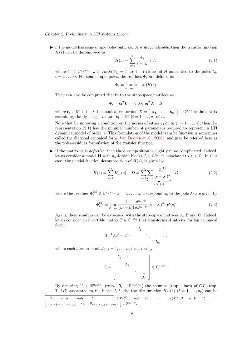
I if the model has semi-simple poles only, i.e. A is diagonalisable, then the transfer functionH(s) can be decomposed as
H(s) =
n∑i=1
Φis− λi
+D, (2.1)
where Φi ∈ Cny×nu with rank(Φi) = 1 are the residues of H associated to the poles λi,i = 1, . . . , n. For semi-simple poles, the residues Φi are defined as
Φi = lims→λi
(s− λi)H(s).
They can also be computed thanks to the state-space matrices as
Φi = ciTbi = CXeiei
TX−1B,
where ei ∈ Rn is the i-th canonical vector and X =[
x1 . . . xn
]∈ Cn×n is the matrix
containing the right eigenvectors xi ∈ Cn (i = 1, . . . , n) of A.
Note that by imposing a condition on the norms of either ci or bi (i = 1, . . . , n), then therepresentation (2.1) has the minimal number of parameters required to represent a LTIdynamical model of order n. This formulation of the model transfer function is sometimescalled the diagonal canonical form [Van Dooren et al., 2008a] and may be referred here asthe poles-residues formulation of the transfer function.
I If the matrix A is defective, then the decomposition is slightly more complicated. Indeed,let us consider a model H with nb Jordan blocks Ji ∈ Cni×ni associated to λi ∈ C. In thatcase, the partial fraction decomposition of H(s), is given by
H(s) =
nb∑i=1
Hλi(s) +D =
nb∑i=1
ni∑k=1
Φ(k)i
(s− λi)k︸ ︷︷ ︸Hλi (s)
+D, (2.2)
where the residues Φ(k)i ∈ Cny×nu k = 1, . . . , ni, corresponding to the pole λi are given by
Φ(k)i = lim
s→λi
1
(ni − k)!
dni−k
dsni−k(s− λi)ni H(s). (2.3)
Again, these residues can be expressed with the state-space matrices A, B and C. Indeed,let us consider an invertible matrix T ∈ Cn×n that transforms A into its Jordan canonicalform :
T−1AT = J =
J1
. . .
Jnb
,where each Jordan block Ji (i = 1, . . . , nb) is given by
Ji =
λi 1
λi. . .
. . . 1λi
∈ Cni×ni ,
By denoting Ci ∈ Rny×ni (resp. Bi ∈ Rni×nu) the columns (resp. lines) of CT (resp.T−1B) associated to the block Ji
1, the transfer function Hλi(s) (i = 1, . . . , nb) can be
1In other words, Ci = CTPTi and Bi = PiT−1B with Pi =[
0ni×(n1+...+ni−1) Ini 0ni×(ni+1+...+nb)
]∈ Rni×n.
18
2.1. Generalities
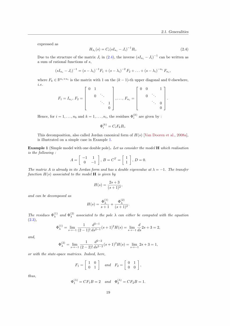
expressed as
Hλi(s) = Ci(sIni − Ji)−1Bi. (2.4)
Due to the structure of the matrix Ji in (2.4), the inverse (sIni − Ji)−1
can be written asa sum of rational functions of s,
(sIni − Ji)−1
= (s− λi)−1F1 + (s− λi)−2
F2 + . . .+ (s− λi)−ni Fni ,
where Fk ∈ Rni×ni is the matrix with 1 on the (k − 1)-th upper diagonal and 0 elsewhere,i.e.
F1 = Ini , F2 =
0 1
0. . .
. . . 10
, . . . , Fni =
0 0 1
0. . .
. . . 00
.
Hence, for i = 1, . . . , nb and k = 1, . . . , ni, the residues Φ(k)i are given by :
Φ(k)i = CiFkBi.
This decomposition, also called Jordan canonical form of H(s) [Van Dooren et al., 2008a],is illustrated on a simple case in Example 1.
Example 1 (Simple model with one double pole). Let us consider the model H which realisationis the following :
A =
[−1 10 −1
], B = CT =
[11
], D = 0.
The matrix A is already in its Jordan form and has a double eigenvalue at λ = −1. The transferfunction H(s) associated to the model H is given by
H(s) =2s+ 3
(s+ 1)2,
and can be decomposed as
H(s) =Φ
(1)λ
s+ 1+
Φ(2)λ
(s+ 1)2.
The residues Φ(1)λ and Φ
(2)λ associated to the pole λ can either be computed with the equation
(2.3),
Φ(1)λ = lim
s→−1
1
(2− 1)!
d2−1
ds2−1(s+ 1)2H(s) = lim
s→−1
d
ds2s+ 3 = 2,
and,
Φ(2)λ = lim
s→−1
1
(2− 2)!
d2−2
ds2−2(s+ 1)2H(s) = lim
s→−12s+ 3 = 1,
or with the state-space matrices. Indeed, here,
F1 =
[1 00 1
]and F2 =
[0 10 0
],
thus,
Φ(λ)1 = CF1B = 2 and Φ
(λ)2 = CF2B = 1.
19
Chapter 2. Preliminary in LTI systems theory
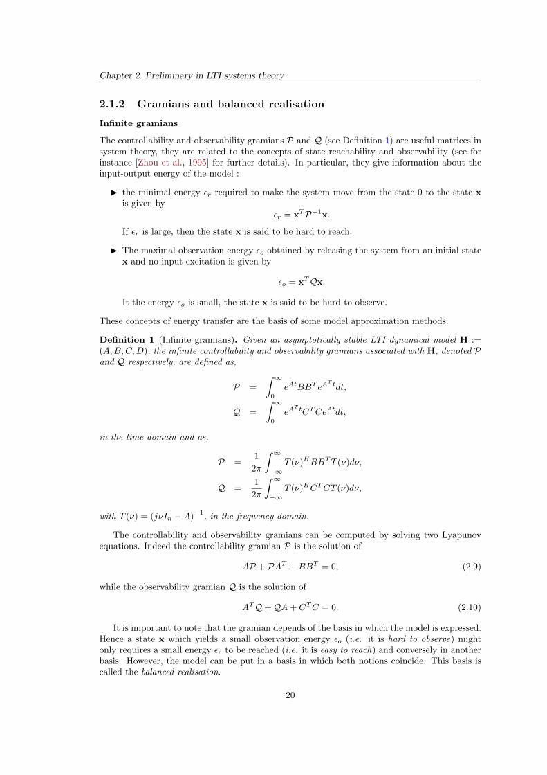
2.1.2 Gramians and balanced realisation
Infinite gramians
The controllability and observability gramians P and Q (see Definition 1) are useful matrices insystem theory, they are related to the concepts of state reachability and observability (see forinstance [Zhou et al., 1995] for further details). In particular, they give information about theinput-output energy of the model :
I the minimal energy εr required to make the system move from the state 0 to the state xis given by
εr = xTP−1x.
If εr is large, then the state x is said to be hard to reach.
I The maximal observation energy εo obtained by releasing the system from an initial statex and no input excitation is given by
εo = xTQx.
It the energy εo is small, the state x is said to be hard to observe.
These concepts of energy transfer are the basis of some model approximation methods.
Definition 1 (Infinite gramians). Given an asymptotically stable LTI dynamical model H :=(A,B,C,D), the infinite controllability and observability gramians associated with H, denoted Pand Q respectively, are defined as,
P =
∫ ∞0
eAtBBT eAT tdt,
Q =
∫ ∞0
eAT tCTCeAtdt,
in the time domain and as,
P =1
2π
∫ ∞−∞
T (ν)HBBTT (ν)dν,
Q =1
2π
∫ ∞−∞
T (ν)HCTCT (ν)dν,
with T (ν) = (jνIn −A)−1
, in the frequency domain.
The controllability and observability gramians can be computed by solving two Lyapunovequations. Indeed the controllability gramian P is the solution of
AP + PAT +BBT = 0, (2.9)
while the observability gramian Q is the solution of
ATQ+QA+ CTC = 0. (2.10)
It is important to note that the gramian depends of the basis in which the model is expressed.Hence a state x which yields a small observation energy εo (i.e. it is hard to observe) mightonly requires a small energy εr to be reached (i.e. it is easy to reach) and conversely in anotherbasis. However, the model can be put in a basis in which both notions coincide. This basis iscalled the balanced realisation.
20
2.1. Generalities
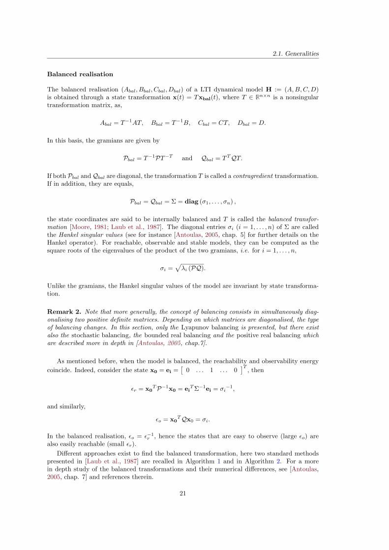
Balanced realisation
The balanced realisation (Abal, Bbal, Cbal, Dbal) of a LTI dynamical model H := (A,B,C,D)is obtained through a state transformation x(t) = Txbal(t), where T ∈ Rn×n is a nonsingulartransformation matrix, as,
Abal = T−1AT, Bbal = T−1B, Cbal = CT, Dbal = D.
In this basis, the gramians are given by
Pbal = T−1PT−T and Qbal = TTQT.
If both Pbal andQbal are diagonal, the transformation T is called a contragredient transformation.If in addition, they are equals,
Pbal = Qbal = Σ = diag (σ1, . . . , σn) ,
the state coordinates are said to be internally balanced and T is called the balanced transfor-mation [Moore, 1981; Laub et al., 1987]. The diagonal entries σi (i = 1, . . . , n) of Σ are calledthe Hankel singular values (see for instance [Antoulas, 2005, chap. 5] for further details on theHankel operator). For reachable, observable and stable models, they can be computed as thesquare roots of the eigenvalues of the product of the two gramians, i.e. for i = 1, . . . , n,
σi =√λi (PQ).
Unlike the gramians, the Hankel singular values of the model are invariant by state transforma-tion.
Remark 2. Note that more generally, the concept of balancing consists in simultaneously diag-onalising two positive definite matrices. Depending on which matrices are diagonalised, the typeof balancing changes. In this section, only the Lyapunov balancing is presented, but there existalso the stochastic balancing, the bounded real balancing and the positive real balancing whichare described more in depth in [Antoulas, 2005, chap.7].
As mentioned before, when the model is balanced, the reachability and observability energy
coincide. Indeed, consider the state x0 = ei =[
0 . . . 1 . . . 0]T
, then
εr = x0TP−1x0 = ei
TΣ−1ei = σi−1,
and similarly,
εo = x0TQx0 = σi.
In the balanced realisation, εo = ε−1r , hence the states that are easy to observe (large εo) are
also easily reachable (small εr).
Different approaches exist to find the balanced transformation, here two standard methodspresented in [Laub et al., 1987] are recalled in Algorithm 1 and in Algorithm 2. For a morein depth study of the balanced transformations and their numerical differences, see [Antoulas,2005, chap. 7] and references therein.
21
Chapter 2. Preliminary in LTI systems theory
Algorithm 1 Balanced Transformation
1: Compute directly the lower Cholesky factorizations of the gramians with the method pre-sented in [Hammarling, 1982] :
P = LcLTc and Q = LoL
To .
2: Compute the singular value decomposition of LTo Lc,
LTo Lc = UΣV T ,
where Σ is the diagonal matrix containing the Hankel singular values of H3: The balanced transformation is given by
T = LcV Σ−12 , and T−1 = Σ−
12UTLTo .
One can verify that the transformation T constructed in Algorithm 1 is indeed a contragre-dient transformation by projecting the gramians,
T−1PT−T = Σ−12UTLTo PLoUΣ−
12
= Σ−12UT LTo Lc︸ ︷︷ ︸
UΣV T
LTc Lo︸ ︷︷ ︸V ΣUT
UΣ−12 = Σ.
Similarly,
TTQT = Σ−12V TLTc QLcV Σ−
12
= Σ−12V T LTc Lo︸ ︷︷ ︸
V ΣUT
LTo Lc︸ ︷︷ ︸UΣV T
V Σ−12 = Σ.
Algorithm 2 Balanced Transformation
1: Compute the gramians P and Q with (2.9) and (2.10).2: Compute the lower Cholesky factorization of P,
P = LcLTc .
3: Solve the following symmetric eigenvalue problem :
LTc QLc = V Σ2V T ,
where Σ contains the Hankel singular values of the system.4: The balanced transformation is given by
T = LcV Σ−12 and T−1 = Σ
12V TLc
−1
Again, the transformation T given by the Algorithm 2 is a contragredient transformation,
T−1PT−T = Σ12V TLc
−1 P︸︷︷︸LcLTc
L−Tc V Σ12 = Σ,
andTTQT = Σ−
12V T LTc QLc︸ ︷︷ ︸
V Σ2V T
V Σ−12 = Σ.
In Algorithm 2, the gramians are explicitly computed whereas in Algorithm 1, only theirCholesky factorizations are required [Hammarling, 1982]. The latter method is numerically
22
2.1. Generalities
0 50 100 150 200 250 30010
−18
10−16
10−14
10−12
10−10
10−8
10−6
10−4
10−2
100
Han
kelsingu
larvalues
Index
Algorithm 1Algorithm 2
Figure 2.1: Hankel singular values of the ISS model obtained with Algorithm 1 and Algorithm2.
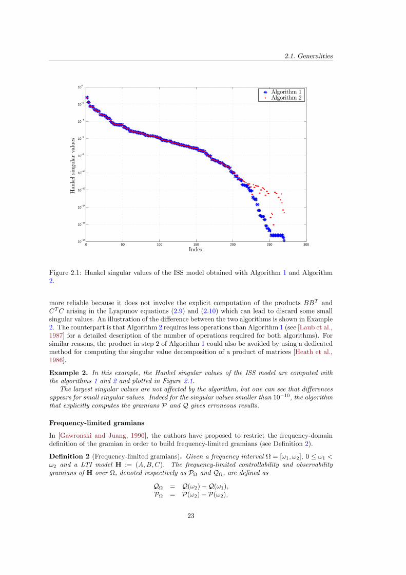
more reliable because it does not involve the explicit computation of the products BBT andCTC arising in the Lyapunov equations (2.9) and (2.10) which can lead to discard some smallsingular values. An illustration of the difference between the two algorithms is shown in Example2. The counterpart is that Algorithm 2 requires less operations than Algorithm 1 (see [Laub et al.,1987] for a detailed description of the number of operations required for both algorithms). Forsimilar reasons, the product in step 2 of Algorithm 1 could also be avoided by using a dedicatedmethod for computing the singular value decomposition of a product of matrices [Heath et al.,1986].
Example 2. In this example, the Hankel singular values of the ISS model are computed withthe algorithms 1 and 2 and plotted in Figure 2.1.
The largest singular values are not affected by the algorithm, but one can see that differencesappears for small singular values. Indeed for the singular values smaller than 10−10, the algorithmthat explicitly computes the gramians P and Q gives erroneous results.
Frequency-limited gramians
In [Gawronski and Juang, 1990], the authors have proposed to restrict the frequency-domaindefinition of the gramian in order to build frequency-limited gramians (see Definition 2).
Definition 2 (Frequency-limited gramians). Given a frequency interval Ω = [ω1, ω2], 0 ≤ ω1 <ω2 and a LTI model H := (A,B,C). The frequency-limited controllability and observabilitygramians of H over Ω, denoted respectively as PΩ and QΩ, are defined as
QΩ = Q(ω2)−Q(ω1),PΩ = P(ω2)− P(ω2),
23
Chapter 2. Preliminary in LTI systems theory
where
P(ω) =1
2π
∫ ω
−ωT (ν)BBTT ∗(ν)dν,
Q(ω) =1
2π
∫ ω
−ωT ∗(ν)CTCT (ν)dν,
with T (ν) = (jνIn −A)−1
.
P(ω) and Q(ω) are the solutions of the following Lyapunov equations
AP(ω) + P(ω)AT +Wc(ω) = 0,
ATQ(ω) +Q(ω)A+Wo(ω) = 0,
where the last terms are given by
Wc(ω) = S(ω)BBT +BBTSH(ω),
Wo(ω) = SH(ω)CTC + CTCS(ω),(2.11)
and where, by denoting logm(M) the matrix logarithm of M ,
S(ω) =1
2π
∫ ω
−ωT (ν)dν,
=j
2πlogm
((A+ jωIn) (A− jωIn)
−1).
By denoting Wc(Ω) = Wc(ω2) − Wc(ω1) and Wo(Ω) = Wo(ω2) − Wo(ω1), it turns out thatsimilarly to the infinite gramians, the frequency-limited gramians QΩ and PΩ can be computedby solving Lyapunov equations,
APΩ + PΩAT +Wc(Ω) = 0,
ATQΩ +QΩA+Wo(Ω) = 0.(2.12)
Alternatively, they can be computed directly from the infinite gramians as,
QΩ = Wo(Ω)HQ+QWo(Ω),
PΩ = PWc(Ω)H +Wc(Ω)P.
Remark 3 (Time limited gramians). By following the same idea, the authors in [Gawronskiand Juang, 1990] have also built time-limited gramians.
Remark 4 (Balancing of the frequency-limited gramians). Note that the last terms Wc(Ω) andWo(Ω) of the Lyapunov equations (2.12) are not necessarily positive definite, hence the Lyapunovsolver that directly gives the Cholesky factorisation of the gramians [Hammarling, 1982] is notapplicable here.
The frequency-limited gramians are also positive definite and can be balanced. Hence theycan be used to compute quantities similar to the Hankel singular values as illustrated in Example3.
Example 3 (Singular values obtained from frequency-limited gramians). The idea behind thisexample comes from [Gawronski, 2004, chap. 4]. Let us consider a 6-th order model which polesare λ1 = −0.1 + 3j, λ2 = −0.05 + 10j, λ3 = −0.01 + 20j and their complex conjugate. Thetransfer function associated to this model is given by
H(s) =1
(s2 + 0.2s+ 9.01) (s2 + 0.1s+ 100) (s2 + 0.02s+ 400).
24
2.2. Norms of systems
101
0
1
2
3
4
5x 10
−5Gain
Pulsation ω (rad/s)
101
0
0.5
1
1.5
2
2.5x 10
−5
Pulsation ω (rad/s)
Han
kelsingu
larvalues
FL-HSVHSV
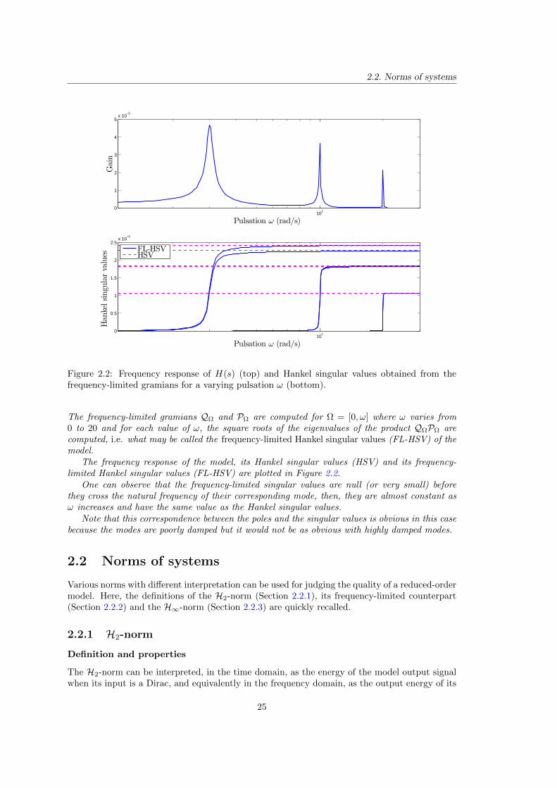
Figure 2.2: Frequency response of H(s) (top) and Hankel singular values obtained from thefrequency-limited gramians for a varying pulsation ω (bottom).
The frequency-limited gramians QΩ and PΩ are computed for Ω = [0, ω] where ω varies from0 to 20 and for each value of ω, the square roots of the eigenvalues of the product QΩPΩ arecomputed, i.e. what may be called the frequency-limited Hankel singular values (FL-HSV) of themodel.
The frequency response of the model, its Hankel singular values (HSV) and its frequency-limited Hankel singular values (FL-HSV) are plotted in Figure 2.2.
One can observe that the frequency-limited singular values are null (or very small) beforethey cross the natural frequency of their corresponding mode, then, they are almost constant asω increases and have the same value as the Hankel singular values.
Note that this correspondence between the poles and the singular values is obvious in this casebecause the modes are poorly damped but it would not be as obvious with highly damped modes.
2.2 Norms of systems
Various norms with different interpretation can be used for judging the quality of a reduced-ordermodel. Here, the definitions of the H2-norm (Section 2.2.1), its frequency-limited counterpart(Section 2.2.2) and the H∞-norm (Section 2.2.3) are quickly recalled.
2.2.1 H2-norm
Definition and properties
The H2-norm can be interpreted, in the time domain, as the energy of the model output signalwhen its input is a Dirac, and equivalently in the frequency domain, as the output energy of its
25
Chapter 2. Preliminary in LTI systems theory
transfer function when the input is a white noise. Its frequency domain definition is recalled inDefinition 3.
Due to its interesting physical interpretation, its properties and the relative simplicity tocompute it, the H2-norm has been widely considered in model approximation [Meier and Luen-berger, 1967; Wilson, 1974; Fulcheri and Olivi, 1998; Van Dooren et al., 2008b; Gugercin et al.,2008] (further information about optimal H2 model approximation are presented in Chapter 4).
Definition 3 (H2-norm). Given a LTI dynamical model H which transfer function is H(s) ∈Cny×nu , the H2-norm of H, denoted ‖H‖H2
is defined, in the frequency-domain, as
‖H‖2H2:=
1
2π
∫ ∞−∞
tr(H(jν)H(−jν)T
)dν.
TheH2-norm is infinite for unstable models or models which have a non-null direct feedthroughmatrix D.
Computation
The H2-norm of a model can be expressed either with the infinite gramians of the model aspresented in Theorem 1 or with its poles and residues, as shown in Theorem 2.
Theorem 1 (Gramian formulation of theH2-norm). Given an asymptotically stable LTI dynam-ical model H which infinite observability and controllability gramians are Q and P, respectively.The H2-norm of H, denoted ‖H‖H2 is given by
‖H‖2H2= tr
(CPCT
)= tr
(BTQB
).
Theorem 2 (Poles-residues formulation of the H2-norm). Given a n-th order asymptoticallystable and strictly proper LTI dynamical model H which transfer function is H(s) and whichhas only semi-simple eigenvalues. Then, by denoting Φi ∈ Cny×nu , the residues of the transferfunction associated to the pole λi ∈ C (i = 1, . . . , n), it comes that
‖H‖2H2=
n∑i=1
tr(ΦiH(−λi)T
)= −
n∑i=1
n∑k=1
tr(ΦiΦ
Tk
)λi + λk
.
The hypothesis on the multiplicity of the poles in Theorem 2 can be alleviated as shown in[Antoulas, 2005, chap 5.].
2.2.2 Frequency-limited H2-norm
Definition and properties
The frequency-limited H2-norm, denoted H2,Ω-norm, has been suggested in [Anderson et al.,1991] in order to estimate the H2-norm of nominally unstable models. Its definition is recalledbelow in Definition 4. It has been used recently in [Garulli et al., 2013] to perform robustnessanalysis on an aircraft model and in [Petersson, 2013] to perform optimal model approximation.Its behaviour is illustrated in Example 4.
Definition 4 (H2,Ω-norm). Given a LTI dynamical model H which transfer function is H(s) ∈Cny×nu and a frequency interval Ω = [0, ω], the frequency-limited H2-norm of H, denoted‖H‖H2,Ω
is defined as the restriction of its H2-norm over [−ω, ω], i.e.
‖H‖2H2,Ω:=
1
2π
∫ ω
−ωtr(H(jν)H(−jν)T
)dν
:=1
π
∫Ω
tr(H(jν)H(−jν)T
)dν
26
2.2. Norms of systems
100
101
102
−102.1
−102.2G
ain(dB)
Pulsation (rad/s)
Frequency response
100
101
102
0
1
2
3
4
5x 10
−3
Pulsation (rad/s)
Valueof
norms
Evolution of the H2,Ω-norm wrt to ω
H2-normH2,Ω-norm
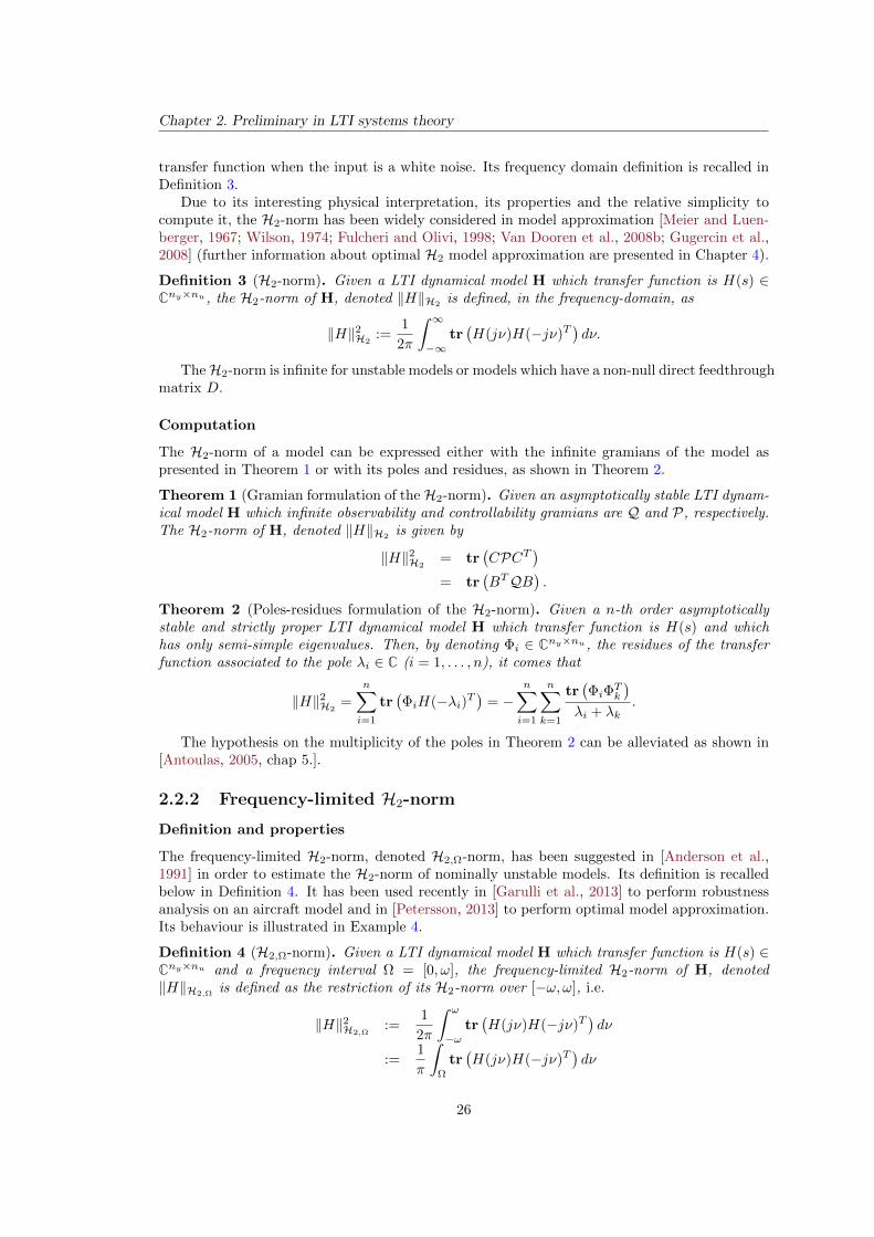
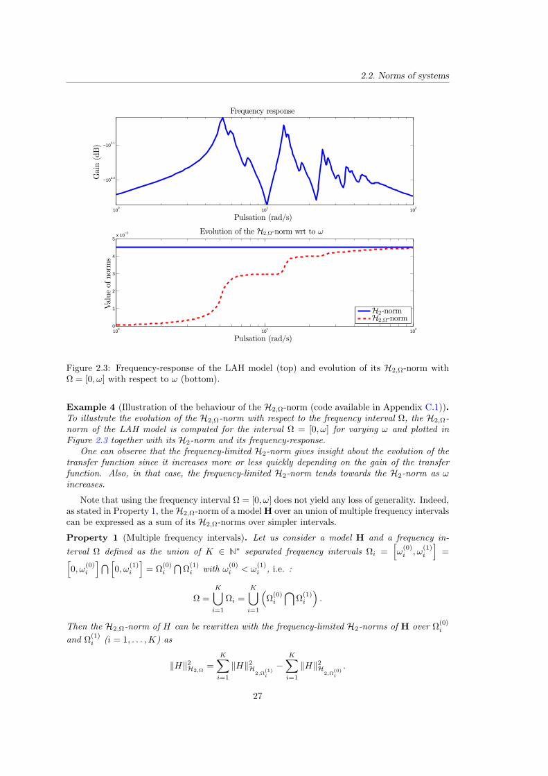
Figure 2.3: Frequency-response of the LAH model (top) and evolution of its H2,Ω-norm withΩ = [0, ω] with respect to ω (bottom).
Example 4 (Illustration of the behaviour of the H2,Ω-norm (code available in Appendix C.1)).To illustrate the evolution of the H2,Ω-norm with respect to the frequency interval Ω, the H2,Ω-norm of the LAH model is computed for the interval Ω = [0, ω] for varying ω and plotted inFigure 2.3 together with its H2-norm and its frequency-response.
One can observe that the frequency-limited H2-norm gives insight about the evolution of thetransfer function since it increases more or less quickly depending on the gain of the transferfunction. Also, in that case, the frequency-limited H2-norm tends towards the H2-norm as ωincreases.
Note that using the frequency interval Ω = [0, ω] does not yield any loss of generality. Indeed,as stated in Property 1, theH2,Ω-norm of a model H over an union of multiple frequency intervalscan be expressed as a sum of its H2,Ω-norms over simpler intervals.
Property 1 (Multiple frequency intervals). Let us consider a model H and a frequency in-
terval Ω defined as the union of K ∈ N∗ separated frequency intervals Ωi =[ω
(0)i , ω
(1)i
]=[
0, ω(0)i
]⋂[0, ω
(1)i
]= Ω
(0)i
⋂Ω
(1)i with ω
(0)i < ω
(1)i , i.e. :
Ω =
K⋃i=1
Ωi =
K⋃i=1
(Ω
(0)i
⋂Ω
(1)i
).
Then the H2,Ω-norm of H can be rewritten with the frequency-limited H2-norms of H over Ω(0)i
and Ω(1)i (i = 1, . . . ,K) as
‖H‖2H2,Ω=
K∑i=1
‖H‖2H2,Ω
(1)i
−K∑i=1
‖H‖2H2,Ω
(0)i
.
27

Chapter 2. Preliminary in LTI systems theory
2 4 6 8 10 12 14 16 18 202.4
2.45
2.5
2.55
2.6
2.65
2.7x 10
−3
Order of the bandpass filter
Valueof
thenorms
H2,Ω-normFrequency-weighted H2-norm
2 4 6 8 10 12 14 16 18 200
2
4
6
8
10
Relativeerrorbetweenthenorms(%
)
Order of the bandpass filter
Figure 2.4: H2,Ω-norm and frequency-weighted H2-norm of the LAH model computed overΩ = [10, 20] for varying order of the Butterworth filters.
A similar measurement to the frequency-limitedH2-norm is the frequency-weightedH2-norm,denoted H2,W -norm (see for instance [Anic et al., 2013]). The latter is defined as the H2-normof the model H weighted by a filter W ∈ H∞, i.e.
‖H‖H2,W= ‖HW‖H2 .
The frequency-limited H2-norm is equivalent to the frequency-weighted H2-norm consideredwith perfect filters. This point is illustrated in Example 5 where both norms are compared.
Example 5 (Comparison of the H2,Ω-norm and frequency-weighted H2-norm). In this example,the frequency-limited H2-norm of the LAH model is computed over the frequency interval Ω =[10, 20] and compared to the H2-norm computed on the weighted model obtained by applying aninput bandpass filter to it. The filter is constructed with two Butterworth filters which orders areincreased from 1 to 10. The top frame of Figure 2.4 shows the H2,Ω-norm and frequency-weightedH2-norm for varying order of the bandpass filter and the bottom frame represents the relativeerror of the frequency-weighted H2-norm compared to the H2,Ω-norm.
The frequency-weighted H2-norm tends towards the H2,Ω-norm as the order of the filter in-creases. With a 8-th order bandpass filter, the relative error falls below 5%. The frequency-weighted H2-norm is not necessarily inferior or superior to the H2,Ω-norm, both cases can beobserved, depending on the model. Note that the required order of the filter strongly depends onthe considered model and the frequency interval Ω. Besides, multiple frequency intervals mightbe difficult to handle with filters whereas they are indifferently handled with the H2,Ω-norm.
Computation
The frequency-limited H2-norm is closely related to the frequency-limited gramians introducedin [Gawronski and Juang, 1990] and recalled in Definition 2. Indeed, the frequency-limited H2-
28
2.2. Norms of systems
norm can be computed with the frequency-limited gramians similarly to the H2-norm as statedin Theorem 3.
Theorem 3 (Gramian formulation of the H2,Ω-norm). Given the frequency interval Ω and astrictly proper LTI dynamical model H. Let PΩ and QΩ be its frequency-limited controllabilityand observability gramians, then frequency-limited H2-norm of H is given as
‖H‖2H2,Ω= tr
(CPΩC
T)
= tr(BTQΩB
).
In Theorem 3, the hypothesis is made that the model is strictly proper. This assumptioncan be alleviated and the formulation of the norm adapted consequently as shown in [Petersson,2013].
2.2.3 H∞-norm
The definition of the H∞-norm of a LTI dynamical model is recalled below in Definition 5. ForSISO models, it represents the maximum gain of the transfer function across all frequenciesand for MIMO models, it is the maximum singular value of the transfer function across allfrequencies.
Definition 5 (H∞-norm). Given an asymptotically stable LTI dynamical model H which transferfunction is H(s) ∈ Cny×nu , the H∞-norm of H, denoted ‖H‖H∞ is defined as the maximum ofthe largest singular value over the imaginary axis, i.e.
‖H‖H∞ := maxω∈R
σmax (H(jω)) .
Computing the H∞-norm is a complex task that is usually achieved by an iterative bisectionalgorithm (see [Zhou et al., 1995, chap. 4]).
The problem that consists in finding a reduced-order model minimising the H∞-norm of theerror is complex and was still considered as unsolved in 2004 [Blondel and Megretski, 2004]. Infact, only few methods have been proposed to address this problem :
I the non-smooth H∞ control synthesis methods presented in [Apkarian and Noll, 2006;Burke et al., 2006] can also be used to perform optimal H∞ model approximation. Yet,they have not been designed for this purpose and might not be tractable in large-scalesettings.
I Methods based on Linear Matrix Inequalities (LMIs) that solve a relaxation of the H∞model approximation problem have been proposed (see for instance [Grigoriadis, 1995] andreference therein). Generally, these approaches are intractable in large-scale settings andthe published application examples are generally of low order (n ≤ 10).
I An approach that adjusts the feedthrough term D of the reduced-order model in an H∞-optimal way has been proposed in [Flagg et al., 2013]. This method relies on an efficientinterpolation framework that is tractable even in large-scale cases but does not solve theactual H∞ approximation problem.
Conclusion
In this chapter, some tools from LTI systems theory about the representation of models, theirgramians and their norms, have been recalled. Concerning the representation of LTI dynami-cal models, the poles-residues one is convenient for addressing the optimal H2 approximation
29

Chapter 2. Preliminary in LTI systems theory
problem described in Chapter 4 and is also the basis of several elements developed during thisthesis.
The infinite gramians and their energetic interpretation are the foundations of the well knownbalanced truncation and their frequency-limited counterpart is of particular interest for modelapproximation over a bounded frequency interval.
The metrics used throughout this study, namely the H2, H2,Ω and H∞ norms, have also beenrecalled. Each one of these norms has a different meaning and interest, but in the context ofmodel approximation, the H2-norm has been, by far, the most considered one. Here, due to theobjectives of this study, the contributions of the thesis are mainly focused on its frequency-limitedcounterpart.
The next chapter is dedicated at describing some well known model approximation methodswhich are important to understand more recent techniques.
30
Chapter 3
Standard model approximation meth-ods
This chapter is aimed at recalling some well-known model approximation techniques. In par-ticular, in Section 3.1, two methods based on the truncation of the state-space realisation, themodal truncation and the balanced truncation, are recalled and illustrated through some numer-ical examples. Then, in Section 3.2, model approximation methods based on implicit momentsmatching are presented. These methods are the basis of some of the H2 model approximationmethods presented in the next chapter.
Note that there exist many other model approximation methods and this chapter is notmeant to be an exhaustive overview of all these methods but rather a glimpse of the ones thathave, in some way, influenced this study. Therefore, some techniques such as the Hankel normapproximation [Glover, 1984] are not presented in this chapter. For a much wider overview ofall the approximation methods, refer to [Antoulas, 2005; Benner et al., 2005].
Contents3.1 Model approximation by truncation . . . . . . . . . . . . . . . . . . 31
3.1.1 Truncation and residualisation of state-space representation . . . . . . 31
3.1.2 Modal and balanced truncation . . . . . . . . . . . . . . . . . . . . . . 32
3.2 Model approximation by moment matching . . . . . . . . . . . . . 38
3.2.1 Moment matching problem . . . . . . . . . . . . . . . . . . . . . . . . 39
3.2.2 Implicit moment matching : the SISO case . . . . . . . . . . . . . . . 40
3.2.3 Tangential interpolation . . . . . . . . . . . . . . . . . . . . . . . . . . 43
3.1 Model approximation by truncation
In this Section, the modal truncation and the balanced truncation are presented. They are bothbased on the truncation of the state-space representation which principle is recalled in Section3.1.1. Then, the actual model approximation methods are described in Section 3.1.2 with somenumerical illustrations.
3.1.1 Truncation and residualisation of state-space representation
Truncation
Given a n-th order linear time-invariant (LTI) dynamical model H described by the followingstate-space representation :
H :=
x(t) = Ax(t) +Bu(t)y(t) = Cx(t) +Du(t)
, (3.1)
where A ∈ Rn×n, B ∈ Rn×nu , C ∈ Rny×n and D ∈ Rny×nu . The state vector x(t) can be dividedbetween the states which must be retained x1(t) and those which must be discarded x2(t), i.e.
x(t) =
[x1(t)x2(t)
].
31
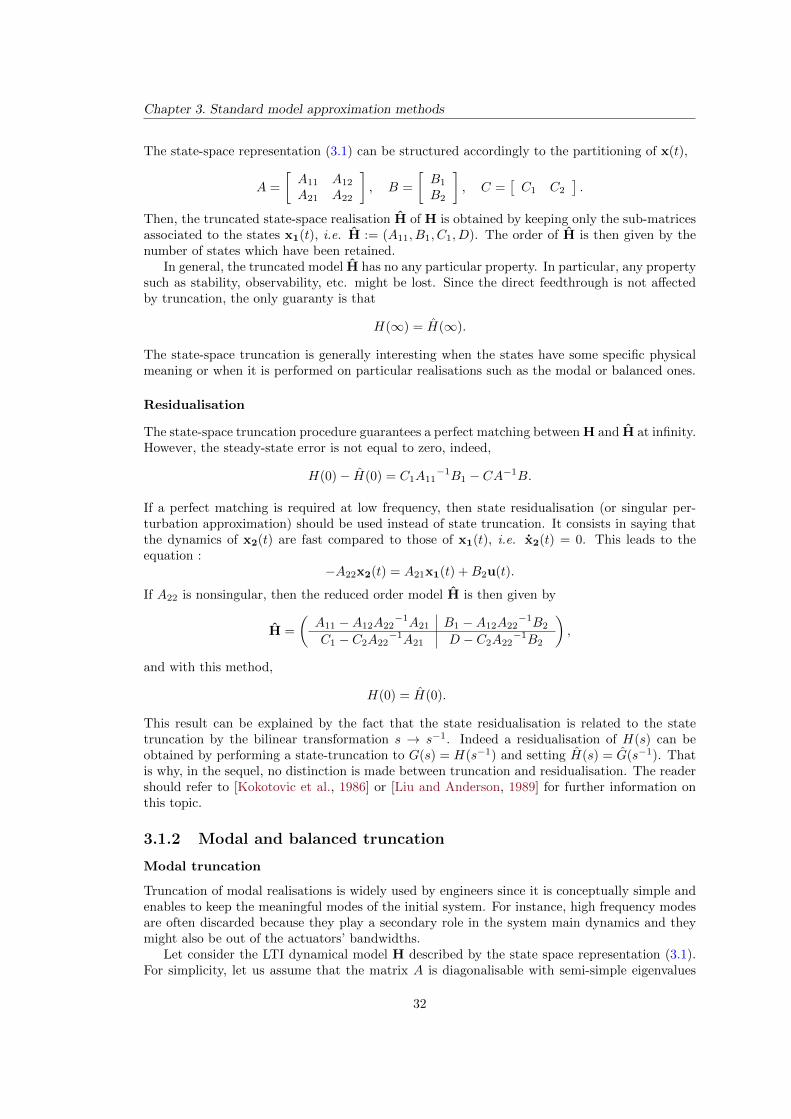
Chapter 3. Standard model approximation methods
The state-space representation (3.1) can be structured accordingly to the partitioning of x(t),
A =
[A11 A12
A21 A22
], B =
[B1
B2
], C =
[C1 C2
].
Then, the truncated state-space realisation H of H is obtained by keeping only the sub-matricesassociated to the states x1(t), i.e. H := (A11, B1, C1, D). The order of H is then given by thenumber of states which have been retained.
In general, the truncated model H has no any particular property. In particular, any propertysuch as stability, observability, etc. might be lost. Since the direct feedthrough is not affectedby truncation, the only guaranty is that
H(∞) = H(∞).
The state-space truncation is generally interesting when the states have some specific physicalmeaning or when it is performed on particular realisations such as the modal or balanced ones.
Residualisation
The state-space truncation procedure guarantees a perfect matching between H and H at infinity.However, the steady-state error is not equal to zero, indeed,
H(0)− H(0) = C1A11−1B1 − CA−1B.
If a perfect matching is required at low frequency, then state residualisation (or singular per-turbation approximation) should be used instead of state truncation. It consists in saying thatthe dynamics of x2(t) are fast compared to those of x1(t), i.e. x2(t) = 0. This leads to theequation :
−A22x2(t) = A21x1(t) +B2u(t).
If A22 is nonsingular, then the reduced order model H is then given by
H =
(A11 −A12A22
−1A21 B1 −A12A22−1B2
C1 − C2A22−1A21 D − C2A22
−1B2
),
and with this method,
H(0) = H(0).
This result can be explained by the fact that the state residualisation is related to the statetruncation by the bilinear transformation s → s−1. Indeed a residualisation of H(s) can beobtained by performing a state-truncation to G(s) = H(s−1) and setting H(s) = G(s−1). Thatis why, in the sequel, no distinction is made between truncation and residualisation. The readershould refer to [Kokotovic et al., 1986] or [Liu and Anderson, 1989] for further information onthis topic.
3.1.2 Modal and balanced truncation
Modal truncation
Truncation of modal realisations is widely used by engineers since it is conceptually simple andenables to keep the meaningful modes of the initial system. For instance, high frequency modesare often discarded because they play a secondary role in the system main dynamics and theymight also be out of the actuators’ bandwidths.
Let consider the LTI dynamical model H described by the state space representation (3.1).For simplicity, let us assume that the matrix A is diagonalisable with semi-simple eigenvalues
32
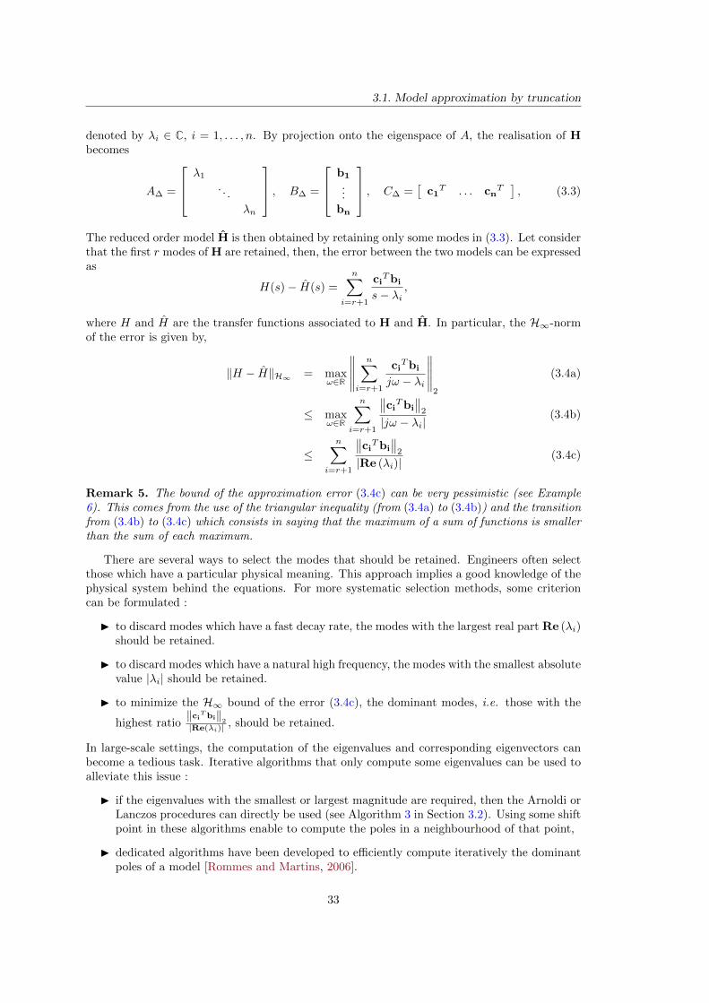
3.1. Model approximation by truncation
denoted by λi ∈ C, i = 1, . . . , n. By projection onto the eigenspace of A, the realisation of Hbecomes
A∆ =
λ1
. . .
λn
, B∆ =
b1
...bn
, C∆ =[
c1T . . . cn
T], (3.3)
The reduced order model H is then obtained by retaining only some modes in (3.3). Let considerthat the first r modes of H are retained, then, the error between the two models can be expressedas
H(s)− H(s) =
n∑i=r+1
ciTbi
s− λi,
where H and H are the transfer functions associated to H and H. In particular, the H∞-normof the error is given by,
‖H − H‖H∞ = maxω∈R
∥∥∥∥∥n∑
i=r+1
ciTbi
jω − λi
∥∥∥∥∥2
(3.4a)
≤ maxω∈R
n∑i=r+1
∥∥ciTbi
∥∥2
|jω − λi|(3.4b)
≤n∑
i=r+1
∥∥ciTbi
∥∥2
|Re (λi)|(3.4c)
Remark 5. The bound of the approximation error (3.4c) can be very pessimistic (see Example6). This comes from the use of the triangular inequality (from (3.4a) to (3.4b)) and the transitionfrom (3.4b) to (3.4c) which consists in saying that the maximum of a sum of functions is smallerthan the sum of each maximum.
There are several ways to select the modes that should be retained. Engineers often selectthose which have a particular physical meaning. This approach implies a good knowledge of thephysical system behind the equations. For more systematic selection methods, some criterioncan be formulated :
I to discard modes which have a fast decay rate, the modes with the largest real part Re (λi)should be retained.
I to discard modes which have a natural high frequency, the modes with the smallest absolutevalue |λi| should be retained.
I to minimize the H∞ bound of the error (3.4c), the dominant modes, i.e. those with the
highest ratio‖ci
Tbi‖2
|Re(λi)| , should be retained.
In large-scale settings, the computation of the eigenvalues and corresponding eigenvectors canbecome a tedious task. Iterative algorithms that only compute some eigenvalues can be used toalleviate this issue :
I if the eigenvalues with the smallest or largest magnitude are required, then the Arnoldi orLanczos procedures can directly be used (see Algorithm 3 in Section 3.2). Using some shiftpoint in these algorithms enable to compute the poles in a neighbourhood of that point,
I dedicated algorithms have been developed to efficiently compute iteratively the dominantpoles of a model [Rommes and Martins, 2006].
33
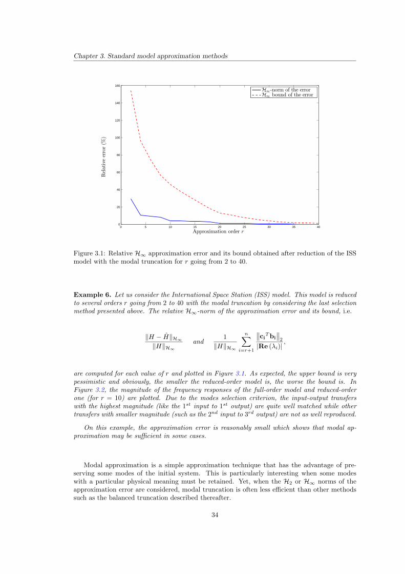
Chapter 3. Standard model approximation methods
0 5 10 15 20 25 30 35 400
20
40
60
80
100
120
140
160
Approximation order r
Relativeerror(%
)
H∞-norm of the errorH∞ bound of the error
Figure 3.1: Relative H∞ approximation error and its bound obtained after reduction of the ISSmodel with the modal truncation for r going from 2 to 40.
Example 6. Let us consider the International Space Station (ISS) model. This model is reducedto several orders r going from 2 to 40 with the modal truncation by considering the last selectionmethod presented above. The relative H∞-norm of the approximation error and its bound, i.e.
‖H − H‖H∞‖H‖H∞
and1
‖H‖H∞
n∑i=r+1
∥∥ciTbi
∥∥2
|Re (λi)|,
are computed for each value of r and plotted in Figure 3.1. As expected, the upper bound is verypessimistic and obviously, the smaller the reduced-order model is, the worse the bound is. InFigure 3.2, the magnitude of the frequency responses of the full-order model and reduced-orderone (for r = 10) are plotted. Due to the modes selection criterion, the input-output transferswith the highest magnitude (like the 1st input to 1st output) are quite well matched while othertransfers with smaller magnitude (such as the 2nd input to 3rd output) are not as well reproduced.
On this example, the approximation error is reasonably small which shows that modal ap-proximation may be sufficient in some cases.
Modal approximation is a simple approximation technique that has the advantage of pre-serving some modes of the initial system. This is particularly interesting when some modeswith a particular physical meaning must be retained. Yet, when the H2 or H∞ norms of theapproximation error are considered, modal truncation is often less efficient than other methodssuch as the balanced truncation described thereafter.
34
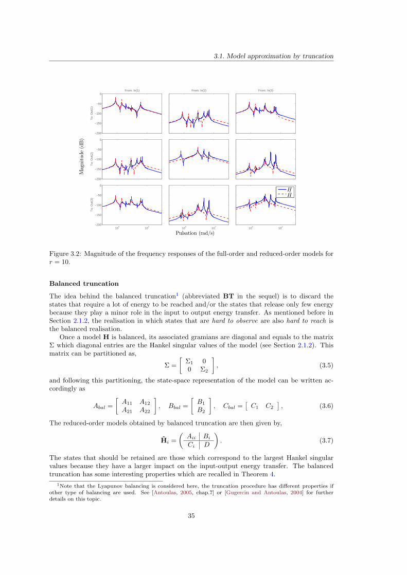
3.1. Model approximation by truncation
−200
−150
−100
−50
0From: In(1)
To:
Out
(1)
−200
−150
−100
−50
0
To:
Out
(2)
100
102
−200
−150
−100
−50
0
To:
Out
(3)
From: In(2)
100
102
From: In(3)
100
102
Pulsation (rad/s)
Magnitude(dB)
HH
Figure 3.2: Magnitude of the frequency responses of the full-order and reduced-order models forr = 10.
Balanced truncation
The idea behind the balanced truncation1 (abbreviated BT in the sequel) is to discard thestates that require a lot of energy to be reached and/or the states that release only few energybecause they play a minor role in the input to output energy transfer. As mentioned before inSection 2.1.2, the realisation in which states that are hard to observe are also hard to reach isthe balanced realisation.
Once a model H is balanced, its associated gramians are diagonal and equals to the matrixΣ which diagonal entries are the Hankel singular values of the model (see Section 2.1.2). Thismatrix can be partitioned as,
Σ =
[Σ1 00 Σ2
], (3.5)
and following this partitioning, the state-space representation of the model can be written ac-cordingly as
Abal =
[A11 A12
A21 A22
], Bbal =
[B1
B2
], Cbal =
[C1 C2
], (3.6)
The reduced-order models obtained by balanced truncation are then given by,
Hi =
(Aii BiCi D
). (3.7)
The states that should be retained are those which correspond to the largest Hankel singularvalues because they have a larger impact on the input-output energy transfer. The balancedtruncation has some interesting properties which are recalled in Theorem 4.
1Note that the Lyapunov balancing is considered here, the truncation procedure has different properties ifother type of balancing are used. See [Antoulas, 2005, chap.7] or [Gugercin and Antoulas, 2004] for furtherdetails on this topic.
35
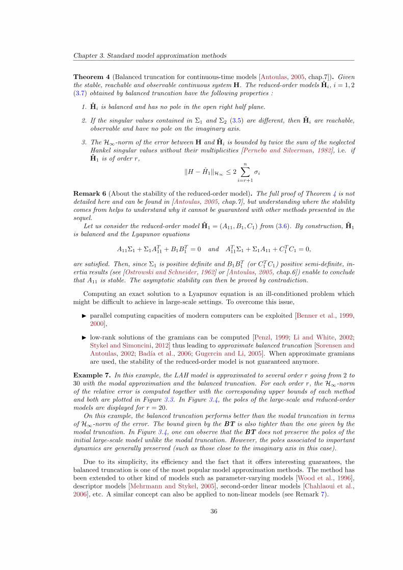
Chapter 3. Standard model approximation methods
Theorem 4 (Balanced truncation for continuous-time models [Antoulas, 2005, chap.7]). Giventhe stable, reachable and observable continuous system H. The reduced-order models Hi, i = 1, 2(3.7) obtained by balanced truncation have the following properties :
1. Hi is balanced and has no pole in the open right half plane.
2. If the singular values contained in Σ1 and Σ2 (3.5) are different, then Hi are reachable,observable and have no pole on the imaginary axis.
3. The H∞-norm of the error between H and Hi is bounded by twice the sum of the neglectedHankel singular values without their multiplicities [Pernebo and Silverman, 1982], i.e. ifH1 is of order r,
‖H − H1‖H∞ ≤ 2
n∑i=r+1
σi
Remark 6 (About the stability of the reduced-order model). The full proof of Theorem 4 is notdetailed here and can be found in [Antoulas, 2005, chap.7], but understanding where the stabilitycomes from helps to understand why it cannot be guaranteed with other methods presented in thesequel.
Let us consider the reduced-order model H1 = (A11, B1, C1) from (3.6). By construction, H1
is balanced and the Lyapunov equations
A11Σ1 + Σ1AT11 +B1B
T1 = 0 and AT11Σ1 + Σ1A11 + CT1 C1 = 0,
are satisfied. Then, since Σ1 is positive definite and B1BT1 (or CT1 C1) positive semi-definite, in-
ertia results (see [Ostrowski and Schneider, 1962] or [Antoulas, 2005, chap.6]) enable to concludethat A11 is stable. The asymptotic stability can then be proved by contradiction.
Computing an exact solution to a Lyapunov equation is an ill-conditioned problem whichmight be difficult to achieve in large-scale settings. To overcome this issue,
I parallel computing capacities of modern computers can be exploited [Benner et al., 1999,2000],
I low-rank solutions of the gramians can be computed [Penzl, 1999; Li and White, 2002;Stykel and Simoncini, 2012] thus leading to approximate balanced truncation [Sorensen andAntoulas, 2002; Badıa et al., 2006; Gugercin and Li, 2005]. When approximate gramiansare used, the stability of the reduced-order model is not guaranteed anymore.
Example 7. In this example, the LAH model is approximated to several order r going from 2 to30 with the modal approximation and the balanced truncation. For each order r, the H∞-normof the relative error is computed together with the corresponding upper bounds of each methodand both are plotted in Figure 3.3. In Figure 3.4, the poles of the large-scale and reduced-ordermodels are displayed for r = 20.
On this example, the balanced truncation performs better than the modal truncation in termsof H∞-norm of the error. The bound given by the BT is also tighter than the one given by themodal truncation. In Figure 3.4, one can observe that the BT does not preserve the poles of theinitial large-scale model unlike the modal truncation. However, the poles associated to importantdynamics are generally preserved (such as those close to the imaginary axis in this case).
Due to its simplicity, its efficiency and the fact that it offers interesting guarantees, thebalanced truncation is one of the most popular model approximation methods. The method hasbeen extended to other kind of models such as parameter-varying models [Wood et al., 1996],descriptor models [Mehrmann and Stykel, 2005], second-order linear models [Chahlaoui et al.,2006], etc. A similar concept can also be applied to non-linear models (see Remark 7).
36
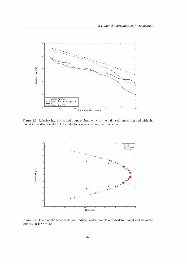
3.1. Model approximation by truncation
0 5 10 15 20 25 3010
−2
10−1
100
101
102
103
Approximation order r
Relativeerror(%
)
Modal approx.Bound for modal approx.BTBound for BT
Figure 3.3: Relative H∞ errors and bounds obtained with the balanced truncation and with themodal truncation on the LAH model for varying approximation order r.
−4.5 −4 −3.5 −3 −2.5 −2 −1.5 −1 −0.5 0−100
−80
−60
−40
−20
0
20
40
60
80
100
Real part
Imaginarypart
HHmodalHBT
Figure 3.4: Poles of the large-scale and reduced-order models obtained by modal and balancedtruncation for r = 20.
37
Chapter 3. Standard model approximation methods
Remark 7 (Empirical gramians and proper orthogonal decomposition). Empirical gramianscan be built from temporal simulations of a possibly non-linear model. Using these empiricalgramians to project the initial model leads to the so-called Proper Orthogonal Decomposition.See [Antoulas, 2005, chap.9] and references therein for further information on this method. Notealso that an open-source toolbox dedicated to model approximation based on empirical gramiansis available in [Himpe, 2014].
In the next Section, other projection methods are presented. The underlying idea is no longerto discard states that are barely involved in the input-output energy transfer but to match themoments of the initial transfer function at some specific interpolation points.
3.2 Model approximation by moment matching
The method described in this section greatly relies on the projection (see Remark 8 for furtherinformation on model approximation by projection) of the large-scale model over specific Krylovsubspaces. These subspaces, denoted Kk and defined as,
Kk (A,v) = span(v, Av, . . . , Ak−1v
),
arises in many areas of research and are of particular interest for large-scale problems since theycan be constructed iteratively. In particular, they are used
I to solve systems of linear equations Ax = b [Saad, 2003],
I to compute the eigenvalues of matrices [Ruhe, 1994; Sorensen, 1997],
I to compute approximate solutions of Lyapunov equations [Stykel and Simoncini, 2012],
I to reduce large-scale dynamical models [de Villemagne and Skelton, 1987; Grimme, 1997].
The last point is described in this Section. It consists in using the Krylov subspaces to performan implicit matching of the full-order model moments at some points.
In Section 3.2.1, the moments of a transfer function are defined and the problem of moment-matching is introduced. The problem is then addressed for SISO models with a rational in-terpolation framework in Section 3.2.2. Even if this framework can theoretically be directlygeneralised to MIMO models, the associated algorithms become very complex. Instead, theso-called tangential interpolation framework is used to address the MIMO case in Section 3.2.3.
Remark 8 (Model approximation by projection). Let us consider a LTI dynamical model H =(A,B,C,D). In many cases, the trajectories x(t) of H are contained in a low dimensionalsubspace S, that is to say x(t) can be expressed as,
x(t) = VS x(t),
where VS is a basis of S and x(t) is the reduced state vector. The exact basis of S is in generalnot known, so an approximation V ∈ Rn×r is used instead, thus,
x(t) ≈ V x(t).
Then the ordinary differential equation representing H becomes
V x(t) = AV x(t) +Bu(t) + res(t), (3.8)
where res(t) is a nonzero residue which comes from the approximation of the state x(t). ThePetrov-Galerkin conditions are then enforced by forcing the residue res(t) to be orthogonal to a
38

3.2. Model approximation by moment matching
subspace W. By denoting W ∈ Rn×r a basis of W and left-multiplying (3.8) by WT , it comesthat,
WTV x(t) = WTAV x(t) +WTBu(t) +WT res(t)︸ ︷︷ ︸=0
.
If WTV is nonsingular, the reduced-order differential equation becomes
x =(WTV
)−1WTAV x(t) +
(WTV
)−1WTBu(t),
and the associated output y(t) is given by
y = CV x(t) +Du(t).
If W = S, i.e. W = V , then one talks about orthogonal projection. Otherwise, one talks aboutoblique projection. See [Saad, 2003] for further information on projection.
The projectors W and V can then be built so that the projected model H = (A, B, C, D),
where A =(WTV
)−1WTAV , B =
(WTV
)−1WTB, C = CV and D = D, has some specific
properties. In this section, they are constructed as the basis of some Krylov subspaces to ensureinterpolation conditions.
3.2.1 Moment matching problem
The moments of a transfer function are presented in Definition 6 and the problem of modelapproximation by moment matching is introduced in Problem 2.
Definition 6 (Moments of a transfer function). Let us consider a model H, its transfer function
H(s) = C(sIn −A)−1B + D ∈ Cny×nu can be decomposed through a Laurent series expansion
around a given shift point σ ∈ C as,
H(s) =
∞∑i=0
ηi(σ)(s− σ)
i
i!,
where ηi(σ) ∈ Cny×nu , (i ∈ N) is the i-th moment of H(s) at σ associated to the model and isdefined as,
ηi(σ) = (−1)idiH(s)
dsi
∣∣∣s=σ
Problem 2 (Moment matching problem). Given a n-th order model H which transfer functionH(s) is decomposed at σ ∈ C as
H(s) =
∞∑i=0
ηi(σ)(s− σ)
i
i!,
the moment matching problem consists in finding a reduced-order model H which first r momentsηi(σ) at σ satisfy,
ηi(σ) = ηi(σ), i = 1, . . . , r.
Depending on the point σ around which the moments have to be matched, the problem havedifferent names :
I if σ = 0, it is called a Pade approximation and the associated moments to match are givenby
η0(0) = −CA−1B +D, and ηi(0) = (−1)(i+1)CA−(i+1)B, i > 0.
39

Chapter 3. Standard model approximation methods
I if σ =∞, then it is a partial realisation problem. In that case, the moments are called theMarkov parameters and are given by
η0(∞) = D, and ηi(∞) = CAi−1B, i > 0. (3.9)
I otherwise it is a rational interpolation problem.
The simplest approach to address Problem 2 consists in computing explicitly the moments ofthe initial model H and finding the reduced-order model that matches the first r ones [Grimme,1997, chap.2]. However, computing the moments is ill-conditioned because it implies to evaluatesuccessive power of the matrix A (see for instance equation (3.9)). Thus this method is notreliable. A more suitable approach consists in implicitly matching the moments of the full-ordermodel by projecting it onto particular Krylov subspaces.
3.2.2 Implicit moment matching : the SISO case
An in-depth study of the methods presented in this section can be found in [Grimme, 1997].The first way to use Krylov subspaces to perform rational interpolation consists in projecting
the full-order model H on the Krylov subspace Kr(
(σIn −A)−1, (σIn −A)
−1B)
. Indeed, as
stated in Theorem 5, this enables the reduced-order model to match the first r moments of Hat σ ∈ C. It is called one-sided moment matching since only one Krylov subspace is involved.
Theorem 5 (One-sided moment matching). Let us consider a SISO LTI dynamical model H :=(A,B,C,D) and an interpolation point σ ∈ C such that (σIn −A) is nonsingular. If V ∈ Cn×r
is a full-rank matrix that columns span the Krylov subspace Kr(
(σIn −A)−1, (σIn −A)
−1B)
,
i.e.Kr(
(σIn −A)−1, (σIn −A)
−1B)⊆ V = span (V ) ,
then the reduced-order model H =((V TV
)−1V TAV,
(V TV
)−1V TB,CV,D
)obtained by projec-
tion matches the first r moments of H at σ, i.e.
ηi(σ) = ηi(σ),
for i = 1, . . . , r.
To efficiently create a basis V ∈ Rn×r for the Krylov subspace used in Theorem 5, the Arnoldialgorithm can be used. Its basic version is presented in Algorithm 3. This procedure enables toconstruct an orthonormal basis for a Krylov subspace Kr (A,v1) without explicitly computingthe successive power of the matrix A.
At each iteration of Algorithm 3 a new vector w is created by multiplying the matrix Awith the Arnoldi vector vi, and by applying a simple Gram-Schmidt procedure, this vectorw is then orthogonalised with respect to the previous Arnoldi vectors vj, j = 1, . . . , i. Thenew Arnoldi vector vi+1 if finally obtained by normalising the orthogonal vector w⊥. Theorthogonalisation step is very important, so a more evolved orthogonalisation procedure thanthe simple Gram-Schmidt one can be used. For instance, the modified Gram-Schmidt or theHouseholder procedures [Saad, 2003, chap. 1] are more adapted from a numerical point of view.
Remark 9. A much more detailed presentation of the Arnoldi procedure and its properties canbe found in [Saad, 2003, chap.6].
By using the Arnoldi procedure with A ← (σIn −A)−1
and v1 ← (σIn −A)−1B then the
resulting matrix V ∈ Cn×r is a orthonormal basis for the Krylov subspace
Kr(
(σIn −A)−1, (σIn −A)
−1B).
40
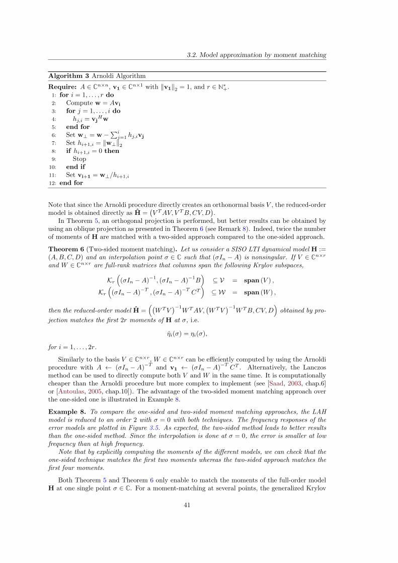
3.2. Model approximation by moment matching
Algorithm 3 Arnoldi Algorithm
Require: A ∈ Cn×n, v1 ∈ Cn×1 with ‖v1‖2 = 1, and r ∈ N∗+.1: for i = 1, . . . , r do2: Compute w = Avi
3: for j = 1, . . . , i do4: hj,i = vj
Hw5: end for6: Set w⊥ = w −
∑ij=1 hj,ivj
7: Set hi+1,i = ‖w⊥‖28: if hi+1,i = 0 then9: Stop
10: end if11: Set vi+1 = w⊥/hi+1,i
12: end for
Note that since the Arnoldi procedure directly creates an orthonormal basis V , the reduced-ordermodel is obtained directly as H =
(V TAV, V TB,CV,D
).
In Theorem 5, an orthogonal projection is performed, but better results can be obtained byusing an oblique projection as presented in Theorem 6 (see Remark 8). Indeed, twice the numberof moments of H are matched with a two-sided approach compared to the one-sided approach.
Theorem 6 (Two-sided moment matching). Let us consider a SISO LTI dynamical model H :=(A,B,C,D) and an interpolation point σ ∈ C such that (σIn −A) is nonsingular. If V ∈ Cn×r
and W ∈ Cn×r are full-rank matrices that columns span the following Krylov subspaces,
Kr(
(σIn −A)−1, (σIn −A)
−1B)⊆ V = span (V ) ,
Kr(
(σIn −A)−T
, (σIn −A)−T
CT)⊆ W = span (W ) ,
then the reduced-order model H =((WTV
)−1WTAV,
(WTV
)−1WTB,CV,D
)obtained by pro-
jection matches the first 2r moments of H at σ, i.e.
ηi(σ) = ηi(σ),
for i = 1, . . . , 2r.
Similarly to the basis V ∈ Cn×r, W ∈ Cn×r can be efficiently computed by using the Arnoldiprocedure with A ← (σIn −A)
−Tand v1 ← (σIn −A)
−TCT . Alternatively, the Lanczos
method can be used to directly compute both V and W in the same time. It is computationallycheaper than the Arnoldi procedure but more complex to implement (see [Saad, 2003, chap.6]or [Antoulas, 2005, chap.10]). The advantage of the two-sided moment matching approach overthe one-sided one is illustrated in Example 8.
Example 8. To compare the one-sided and two-sided moment matching approaches, the LAHmodel is reduced to an order 2 with σ = 0 with both techniques. The frequency responses of theerror models are plotted in Figure 3.5. As expected, the two-sided method leads to better resultsthan the one-sided method. Since the interpolation is done at σ = 0, the error is smaller at lowfrequency than at high frequency.
Note that by explicitly computing the moments of the different models, we can check that theone-sided technique matches the first two moments whereas the two-sided approach matches thefirst four moments.
Both Theorem 5 and Theorem 6 only enable to match the moments of the full-order modelH at one single point σ ∈ C. For a moment-matching at several points, the generalized Krylov
41
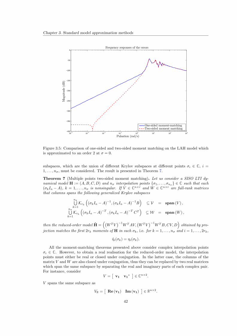
Chapter 3. Standard model approximation methods
10−4
10−3
10−2
10−1
100
101
102
103
−400
−350
−300
−250
−200
−150
−100
−50
0
Pulsation (rad/s)
Magnitude(dB)
Frequency responses of the errors
One-sided moment-matchingTwo-sided moment matching
Figure 3.5: Comparison of one-sided and two-sided moment matching on the LAH model whichis approximated to an order 2 at σ = 0.
subspaces, which are the union of different Krylov subspaces at different points σi ∈ C, i =1, . . . , nσ, must be considered. The result is presented in Theorem 7.
Theorem 7 (Multiple points two-sided moment matching). Let us consider a SISO LTI dy-namical model H := (A,B,C,D) and nσ interpolation points σ1, . . . , σnσ ∈ C such that each(σkIn −A), k = 1, . . . , nσ is nonsingular. If V ∈ Cn×r and W ∈ Cn×r are full-rank matricesthat columns spans the following generalized Krylov subspaces
nσ⋃k=1
Krk(
(σkIn −A)−1, (σkIn −A)
−1B)⊆ V = span (V ) ,
nσ⋃k=1
Krk(
(σkIn −A)−T
, (σkIn −A)−T
CT)⊆ W = span (W ) ,
then the reduced-order model H =((WTV
)−1WTAV,
(WTV
)−1WTB,CV,D
)obtained by pro-
jection matches the first 2rk moments of H in each σk, i.e. for k = 1, . . . , nσ and i = 1, . . . , 2rk,
ηi(σk) = ηi(σk).
All the moment-matching theorems presented above consider complex interpolation pointsσi ∈ C. However, to obtain a real realisation for the reduced-order model, the interpolationpoints must either be real or closed under conjugation. In the latter case, the columns of thematrix V andW are also closed under conjugation, thus they can be replaced by two real matriceswhich span the same subspace by separating the real and imaginary parts of each complex pair.For instance, consider
V =[
v1 v1∗ ] ∈ Cn×2.
V spans the same subspace as
VR =[
Re (v1) Im (v1)]∈ Rn×2.
42
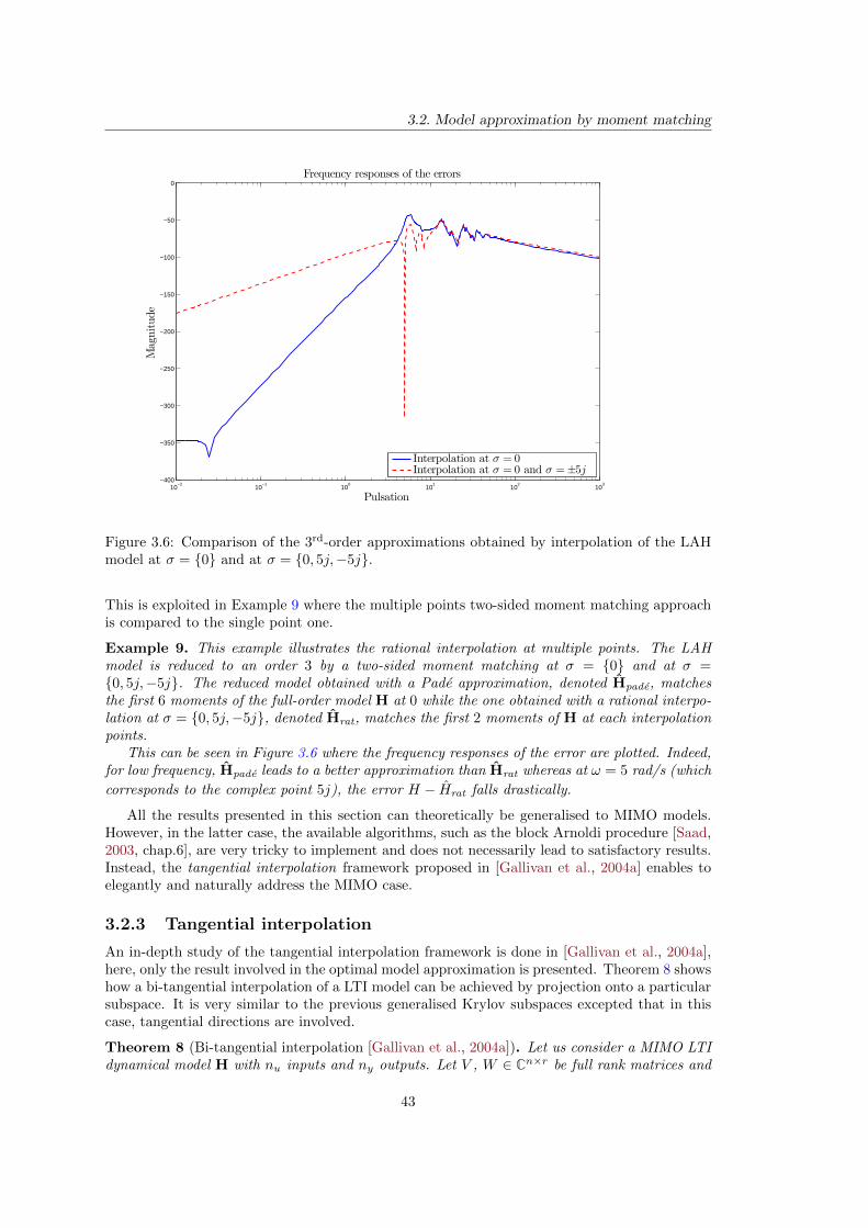
3.2. Model approximation by moment matching
10−2
10−1
100
101
102
103
−400
−350
−300
−250
−200
−150
−100
−50
0
Pulsation
Magnitude
Frequency responses of the errors
Interpolation at σ = 0Interpolation at σ = 0 and σ =±5j
Figure 3.6: Comparison of the 3rd-order approximations obtained by interpolation of the LAHmodel at σ = 0 and at σ = 0, 5j,−5j.
This is exploited in Example 9 where the multiple points two-sided moment matching approachis compared to the single point one.
Example 9. This example illustrates the rational interpolation at multiple points. The LAHmodel is reduced to an order 3 by a two-sided moment matching at σ = 0 and at σ =0, 5j,−5j. The reduced model obtained with a Pade approximation, denoted Hpade, matchesthe first 6 moments of the full-order model H at 0 while the one obtained with a rational interpo-lation at σ = 0, 5j,−5j, denoted Hrat, matches the first 2 moments of H at each interpolationpoints.
This can be seen in Figure 3.6 where the frequency responses of the error are plotted. Indeed,for low frequency, Hpade leads to a better approximation than Hrat whereas at ω = 5 rad/s (which
corresponds to the complex point 5j), the error H − Hrat falls drastically.
All the results presented in this section can theoretically be generalised to MIMO models.However, in the latter case, the available algorithms, such as the block Arnoldi procedure [Saad,2003, chap.6], are very tricky to implement and does not necessarily lead to satisfactory results.Instead, the tangential interpolation framework proposed in [Gallivan et al., 2004a] enables toelegantly and naturally address the MIMO case.
3.2.3 Tangential interpolation
An in-depth study of the tangential interpolation framework is done in [Gallivan et al., 2004a],here, only the result involved in the optimal model approximation is presented. Theorem 8 showshow a bi-tangential interpolation of a LTI model can be achieved by projection onto a particularsubspace. It is very similar to the previous generalised Krylov subspaces excepted that in thiscase, tangential directions are involved.
Theorem 8 (Bi-tangential interpolation [Gallivan et al., 2004a]). Let us consider a MIMO LTIdynamical model H with nu inputs and ny outputs. Let V , W ∈ Cn×r be full rank matrices and
43
Chapter 3. Standard model approximation methods
let σi ∈ C, bi ∈ C1×nu and ci ∈ C1×ny , i = 1, . . . , nσ be a given set of interpolation points andassociated right and left tangential directions, respectively. Suppose that the points σi are suchthat (σiIn −A) is nonsingular. If for i = 1, . . . , nσ,
(σiIn −A)−1BbTi ⊆ span (V ) ,
(σiIn −A)−T
CT cTi ⊆ span (W ) ,(3.10)
then the reduced order model H =((WTV
)−1WTAV,
(WTV
)−1WTB,CV,D
)satisfies the fol-
lowing bi-tangential interpolation equations,
ciH(σi) = ciH(σi),
H(σi)bTi = H(σi)b
Ti ,
ciH′(σi)b
Ti = ciH
′(σi)bTi .
for i = 1, . . . , nσ.
It is easy to check that a model satisfying one of the condition in equation (3.10) tangen-tially interpolates the initial model at σi from the left or the right. Indeed Let us consider rinterpolation points σi ∈ C such that (σiIn −A) is non-singular and r tangential directions bi.Suppose that V ∈ Cn×r is given as
V =[
(σ1In −A)−1BbT1 . . . (σrIn −A)
−1BbTr
].
Let us consider the matrix Z ∈ Cn×r defined as
ZT =(WT (σiIn −A)V
)−1WT (σiIn −A) .
It is clear that ZTV = Ir. The transfer function of the large-scale model evaluated at σi in thedirection bi is given by
H(σi)bTi = C(σiIn −A)
−1BbTi .
Since for i = 1, . . . , r, (σiIn −A)−1BbTi is a column of V , then by using Lemma 1, it comes that
H(σ1)bTi = CV ZT (σiIn −A)−1BbTi
= CV(WT (σiIn −A)V
)−1WTBbTi
= C(σiIr − A
)−1
BbTi
= H(σi)bTi .
The proof of the whole Theorem is more complex and the reader should refer to [Gallivan et al.,2004a] for further information. The projection matrices that enable to fulfil those interpolationconditions can either be built as before with iterative procedures but they can also be obtainedby solving some specific Sylvester equations [Gallivan et al., 2004b] or by contructing a Loewnermatrix [Mayo and Antoulas, 2007; Ionita, 2013]. An illustration of the tangential interpolationis presented in Example 10.
Lemma 1 (See [Gallivan et al., 2004a]). Let V ∈ Cn×r, if the vector v belongs to the columnspan of the matrix V . Then, for any matrix Z ∈ Cn×r such that ZTV = Ir,
v = V ZT v.
Example 10 (Illustration of the tangential interpolation). In this example, the ISS model, whichhas 3 inputs and 3 outputs, is considered. It is tangentially interpolated at the points σ1 and σ2
in the left directions c1, c2 and in the right directions bT1 , bT2 with
σ1 = 0.8j, b1 = c1 =[j 0 0
],
44
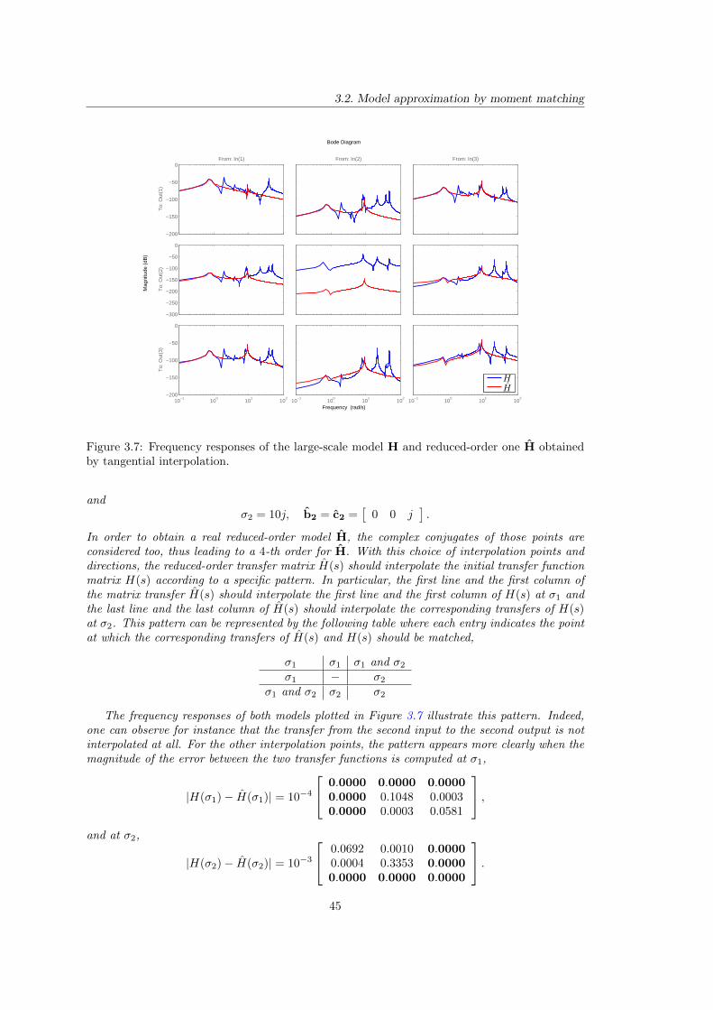
3.2. Model approximation by moment matching
−200
−150
−100
−50
0From: In(1)
To:
Out
(1)
−300
−250
−200
−150
−100
−50
0
To:
Out
(2)
10−1
100
101
102
−200
−150
−100
−50
0
To:
Out
(3)
From: In(2)
10−1
100
101
102
From: In(3)
10−1
100
101
102
Bode Diagram
Frequency (rad/s)
Mag
nitu
de (
dB)
HH
Figure 3.7: Frequency responses of the large-scale model H and reduced-order one H obtainedby tangential interpolation.
andσ2 = 10j, b2 = c2 =
[0 0 j
].
In order to obtain a real reduced-order model H, the complex conjugates of those points areconsidered too, thus leading to a 4-th order for H. With this choice of interpolation points anddirections, the reduced-order transfer matrix H(s) should interpolate the initial transfer functionmatrix H(s) according to a specific pattern. In particular, the first line and the first column ofthe matrix transfer H(s) should interpolate the first line and the first column of H(s) at σ1 andthe last line and the last column of H(s) should interpolate the corresponding transfers of H(s)at σ2. This pattern can be represented by the following table where each entry indicates the pointat which the corresponding transfers of H(s) and H(s) should be matched,
σ1 σ1 σ1 and σ2
σ1 − σ2
σ1 and σ2 σ2 σ2
The frequency responses of both models plotted in Figure 3.7 illustrate this pattern. Indeed,one can observe for instance that the transfer from the second input to the second output is notinterpolated at all. For the other interpolation points, the pattern appears more clearly when themagnitude of the error between the two transfer functions is computed at σ1,
|H(σ1)− H(σ1)| = 10−4
0.0000 0.0000 0.00000.0000 0.1048 0.00030.0000 0.0003 0.0581
,and at σ2,
|H(σ2)− H(σ2)| = 10−3
0.0692 0.0010 0.00000.0004 0.3353 0.00000.0000 0.0000 0.0000
.45
Chapter 3. Standard model approximation methods
Note that the maximum value among the terms in bold is around the machine precision.
Conclusion
In this chapter, two standard model approximation methods based on truncation have firstly beenrecalled. On the one hand, the modal truncation, which consists in keeping some relevant modesof the large-scale model, is conceptually simple and widespread among engineers which have agood knowledge of the physical systems below the models. On the other hand, the balancedtruncation, which is based on more systematic input-to-output energy transfer considerations, isoften considered as the golden standard of model approximation and is one of the most popularmodel approximation method. A lot of researches are still conducted on this method, especiallyto extend it to other kinds of models, such as LPV models, or to ease its numerical computationthrough the development of efficient sparse solvers for large-scale Lyapunov equations.
Then, a completely different framework based on the projection of the large-scale model ontospecific Krylov subspaces has been introduced. It enables to implicitly match several moments ofa dynamical model at several interpolation points. In practice, this framework relies on iterativealgorithms that are perfectly suited for very large-scale models. The choice of the interpolationpoints is of main interest since it determines the properties of the reduced-order model, but ithas not been discussed yet. This is done in the next chapter where the stationary points of theoptimal H2 model approximation problem are presented as tangential interpolation conditionsat the mirror images of the reduced-order model poles.
46
Chapter 4
Optimal H2 model approximation
In this chapter, the general model approximation problem formulated in the introduction (seeProblem 1) is refined in Problem 3 by using the H2-norm to evaluate the quality of the reduced-order model leading to the so-called optimal H2 model approximation problem.
Problem 3 (optimal H2 model approximation problem). Given a n-th order, asymptoticallystable and strictly proper continuous LTI dynamical model H, the problem of optimal modelreduction in the H2 norm consists in finding an asymptotically stable and strictly proper r-thorder model H (with r n) which minimises the H2-norm of the approximation error, i.e.
H = arg minG∈H2
‖H −G‖2H2︸ ︷︷ ︸JH2
.
Problem 3 has been extensively studied over the years, from a theoretical point of view in[Baratchart, 1986], where the existence of a solution as well a some other theoretical propertieshas been proven and also from a more practical point of view leading to several approaches toaddress it :
I approaches based on the projection of the large-scale model onto specific Krylov subspaces[Gugercin et al., 2008; Gugercin, 2007; Gallivan et al., 2004a],
I approaches grounded on non-linear optimisation procedures have been developed in thecontinuous case [Yan and Lam, 1999; Beattie and Gugercin, 2009] and in the discrete case[Baratchart et al., 1991; Fulcheri and Olivi, 1998; Marmorat et al., 2002]1,
I hybrid methods coupling both interpolation through Loewner matrices and optimisation[Beattie and Gugercin, 2012].
Here, the approaches based on projection presented in [Gugercin et al., 2008; Gugercin, 2007;Gallivan et al., 2004a] and the optimisation procedure [Beattie and Gugercin, 2009] are described.In Section 4.1, the first-order optimality conditions of the optimal H2 approximation problemare introduced. Then, the various algorithms are described in Section 4.2.
Contents4.1 First order optimality conditions . . . . . . . . . . . . . . . . . . . . 48
4.1.1 H2 approximation error . . . . . . . . . . . . . . . . . . . . . . . . . . 48
4.1.2 Formulation of the first-order optimality conditions . . . . . . . . . . . 49
4.2 Algorithms for optimal H2 approximation . . . . . . . . . . . . . . . 54
4.2.1 Iterative Rational Krylov Algorithm (IRKA) . . . . . . . . . . . . . . 54
4.2.2 Iterative SVD Rational Krylov Algorithm (ISRKA) . . . . . . . . . . 58
4.2.3 Optimisation algorithm for optimal H2 model approximation . . . . . 59
1The method is available in the software RARL2 [Marmorat and Olivi, 2002] at http://www-sop.inria.fr/
apics/RARL2/rarl2.html.
47
Chapter 4. Optimal H2 model approximation
4.1 First order optimality conditions
Minimizing JH2is a non-linear and non-convex problem (see Example 11), thus finding a global
minimum is a complex task. Instead, finding a local minimum is way more tractable. To thisgoal, first-order necessary optimality conditions have been derived :
I as interpolation conditions between the transfer functions of the full-order and reduced-order models for SISO systems with semi-simples poles only in [Meier and Luenberger,1967; Gugercin et al., 2008],
I in a state-space form which involves the gramians of the error model in [Wilson, 1974],
I more recently in [Gallivan et al., 2004a], tangential interpolation conditions have beenformulated thus generalizing the interpolation conditions of [Meier and Luenberger, 1967]to MIMO systems. These tangential interpolation conditions have then been revisited ina very comprehensive way in [Van Dooren et al., 2008b]. Finally, they have been extendedto the case of models with high order poles in [Van Dooren et al., 2010]2.
All the different formulations of the first-order optimality conditions have been shown to beequivalent and the links that exist between them has been highlighted in different ways in[Hyland and Bernstein, 1985; Gugercin et al., 2008; Van Dooren et al., 2008a].
One approach to obtain the first-order optimality conditions as interpolation conditions isdescribed below. In particular, in Section 4.1.1, the approximation error between the large-scale and reduced-order model is formulated through the poles-residues expression of the H2-norm and in Section 4.1.2, the stationary points of the optimal H2 approximation problem arecharacterised.
4.1.1 H2 approximation error
As presented in Section 2.2.1, the H2-norm can be computed either using the gramians of themodel or using its poles and associated residues. Since it directly leads to the interpolationconditions, the latter formulation is used. However, an equivalence can be made with the gramianformulation as shown in [Van Dooren et al., 2008b].
Let us consider asymptotically stable and strictly proper models H = (A,B,C) and H =(A, B, C of order n and r, respectively. Let us assume that both models have semi-simple polesonly, i.e. A and A are both diagonalisable.
Under these assumptions, their transfer functions H(s) and H(s) can be written as
H(s) =
n∑i=1
Φis+ λi
, and H(s) =
r∑k=1
Φk
s+ λk, (4.1)
where λi, λk ∈ C, and Φi, Φk ∈ Cny×nu (i = 1, . . . , n and k = 1, . . . , r) are the poles andassociated residues of the transfer functions H and H, respectively.
For the model H as expressed in equation (4.1) to be of order r, the residues Φk must be ofrank one. To explicitly show this constraint, the residues can be expressed as an outer productof vectors, i.e. for k = 1, . . . , r,
Φk = cTk bk,
where ck ∈ C1×ny and bk ∈ C1×nu . As mentioned in Section 2.1.1, the vectors ck and bk arelinked to the state-space representation of H, indeed
cTk = CXek, and bk = ekT X−1B,
2A previous version of this work with additional examples is available on arXiv [Van Dooren et al., 2008a].
48
4.1. First order optimality conditions
where X is the matrix which columns are the right eigenvectors of A.
Let us also consider the (n+ r)-th order error model H = H− H. The approximation errorJH2 between H and H is the square of the H2-norm of H and can be expressed as
‖H‖2H2= JH2
=
n+r∑i=1
tr(
ΦiH(−λi)T), (4.2)
where λi ∈ C and Φi ∈ Cny×nu are the poles and residues of the transfer function H of the errormodel.
The poles and residues of H are in fact composed of the poles and residues of the large-scaleand reduced-order transfer functions H and H. Let us assume that the elements are ordered asfollows
Φi =
Φi i = 1, . . . , n
−Φi i = n+ 1, . . . , n+ r,
and
λi =
λi i = 1, . . . , n
λi i = n+ 1, . . . , n+ r.
Equation (4.2) can then be reformulated as
JH2 =
n∑i=1
tr
(Φi
(H(−λi)− H(−λi)
)T)−
r∑k=1
tr
(Φk
(H(−λk)− H(−λk)
)T).
By expanding and separating all the sums, the approximation error JH2can finally be written
as
JH2=
n∑i=1
tr(ΦiH(−λi)T
)︸ ︷︷ ︸
‖H‖2H2
+
r∑k=1
tr(
ΦkH(−λk)T)
︸ ︷︷ ︸‖H‖2H2
−2
r∑i=1
tr(H(−λi)ΦTi
).
(4.3)
The H2 approximation error is composed of the H2-norms of the large-scale and reduced-ordermodels and of some cross terms between the two models.
4.1.2 Formulation of the first-order optimality conditions
The reduced-order model H is represented by its poles λk and its residues decomposed in twovectors ck and bk (k = 1, . . . , r). These parameters appear explicitly by expanding the transferfunction of the reduced-order model H and the residues Φk in equation (4.3)
JH2= ‖H‖2H2
−r∑i=1
r∑k=1
ckcTi bibTk
λi + λk− 2
r∑i=1
ciH(−λi)bTi . (4.4)
49
Chapter 4. Optimal H2 model approximation
By differentiating equation (4.4) with respect to λm, cm and bm (m = 1, . . . , r), one obtains
∂JH2
∂λm= −2cm
r∑k=1
cTk bk(λm + λk
)2 bTm + 2cm
n∑i=1
Φi(λm + λi
)2 bTm
= −2cm
(H ′(−λm)−H ′(−λm)
)bTm.
∂JH2
∂cm= −2
r∑k=1
cTk bk
λm + λkbTm − 2H(−λm)bTm
= 2(H(−λm)−H(−λm)
)bTm.
∂JH2
∂bm
= −2
r∑k=1
bTk ck
λm + λkcTm − 2H(−λm)cTm
= 2(H(−λm)−H(−λm)
)TcTm.
Finally, by setting∂JH2
∂λm= 0,
∂JH2
∂cm= 0 and
∂JH2
∂bm= 0, the stationary points of Problem 3 can be
characterised as presented in Theorem 9. See Remark 10 for some comments about the specificcase of SISO models and refer to Remark 11 for further information about the more generalcase of models with high order poles and for some remarks about the parametrisation of thisoptimisation problem.
Theorem 9 (First-order optimality conditions for the H2 model reduction problem). Let usconsider a n-th order asymptotically stable and strictly proper LTI dynamical model H whichtransfer function is H(s) ∈ Cny×nu and H a r-th order asymptotically stable and strictly proper
model with semi-simple poles which transfer function is H(s) = C(sIr − A)−1Br ∈ Cny×nu . If
H solves Problem 3, then, for i = 1, . . . , r,
ciH(−λi) = ciH(−λi),H(−λi)bTi = H(−λi)bTi ,
ciH′(−λi)bTi = ciH
′(−λi)bTi .(4.5)
where λi ∈ C are the poles of the reduced-order model and ci ∈ C1×ny , bi ∈ C1×nu , (i = 1, . . . , r)are tangential directions given as, [
cT1 . . . cTr]
= CX,
and [bT1 . . . bTr
]T= X−1B,
where X is the matrix which columns are the right eigenvectors of A.
Theorem 9 asserts that a solution of the optimal H2 model approximation problem must be abi-tangential Hermite interpolant of the large-scale model H at the opposite of the reduced-ordermodel poles. In [Van Dooren et al., 2010], it is proved that these first-order optimality conditionsimpose r (ny + nu) interpolations conditions which match the number of free parameters requiredto represent the reduced-order model expressed as
H(s) =
r∑i=1
cTi bi
s− λi,
with ||ci|| = 1 for i = 1, . . . , r.
The reduced-order model poles λi appear in a non-linear way in the approximation errorJH2
(4.4) while each ci and bi appear in a quadratic way. In the SISO case, the residues can
50
4.1. First order optimality conditions
be uniquely determined in an optimal way for fixed poles (see Remark 10) but in the MIMOcase, determining the optimal residues for fixed poles require an iterative optimisation algorithmitself. In [Beattie and Gugercin, 2012], the authors have suggested to use an alternating leastsquare method for achieving what they call residue correction.
Note that if either the ci or the bi are chosen so that one of the two first set of interpolationconditions in equation (4.5) is fulfilled then
r∑i=1
ciH(−λi)bTi =
r∑i=1
ciH(−λi)bTi = ‖H‖2H2,
thus, the H2 norm of the reduced-order model simplifies with the cross term in equation (4.4)and the approximation error becomes
JH2 = ‖H‖2H2− ‖H‖2H2
.
Remark 10 (First-order optimality conditions for SISO models). In the SISO case, the tangen-tial interpolation conditions expressed in Theorem 9 become the following rational interpolationconditions :
H(−λi) = H(−λi),H ′(−λi) = H ′(−λi)
(4.6)
for i = 1, . . . , r. In other words, the reduced-order model has to match the first two moments ofthe large-scale model at the mirror images of the reduced-order model poles.
In [Gugercin et al., 2008], it is shown that if H(s) interpolates H(s) at the opposite of itspoles, i.e. if it satisfies the first condition in equation (4.6), then the reduced-order model H isguaranteed to be an optimal H2 approximation of H among all the reduced-order models thathave the same poles as H.
This can also be seen from equation (4.3), indeed, in the SISO case, the scalar residues φi ∈ Care involved in a quadratic way in the approximation error. First let us rewrite the approximationerror as
JH2 = ‖H‖2H2−
r∑k=1
r∑i=1
φkφi
λk + λi− 2
r∑i=1
H(−λi)φi.
Notice that each complex couple λk, φk appears with its complex conjugate somewhere else inthe sum. Hence, by re-ordering the indexes, it comes that the double sum can also be written as,
r∑k=1
r∑i=1
φkφi
λk + λi=
r∑l=1
r∑i=1
φ∗l φi
λ∗l + λi.
Finally, the approximation error becomes
JH2=[φ∗1 . . . φ∗r
]H
φ1
...
φr
+ 2hT
φ1
...
φr
+ ‖H‖2H2, (4.7)
where the hermitian matrix H is defined as
H = −
1
2Re(λ1). . . 1
λ∗1+λr
.... . .
...1
λ∗r+λ1. . . 1
2Re(λr)
∈ Cr×r,
andh = −
[H(−λ1) . . . H(−λr)
]T ∈ Cr×1.
51

Chapter 4. Optimal H2 model approximation
The second-order term of the quadratic function (4.7) is the H2-norm of the reduced-order model.
By denoting v =[φ1 . . . φr
]T ∈ Cr×1,
vHHv = ‖H‖2H2≥ 0,
which means that H is positive semidefinite. Hence the quadratic function JH2(v) of equation
(4.7) is convex which makes the necessary conditions for optimality also sufficient to find a globalminimum of JH2 with respect to the residues.
To differentiate the first-order optimality conditions, let us undo the change of indexes andwrite the second-order term as
vHHv = vTLv,
where the symmetric matrix L is given as,
L = −
1
2λ1. . . 1
λ1+λr...
. . ....
1λr+λ1
. . . 12λr
∈ Cr×r.
Then, differentiating the approximation error,
JH2 = vTLv + 2hTv + ‖H‖2H2,
with respect to v yields the following optimality condition3
2Lv + 2h = 0. (4.8)
Note that L is a Cauchy matrix and that solving the linear system (4.8) is equivalent to find a
rational function with simple poles λi which has fixed values (given by −h) at the points −λi.Hence one retrieves the first part of the interpolation conditions (4.6) expressed under anotherform. This is illustrated in Example 11.
Example 11 (Non-convexity of the optimal H2 approximation problem - code available inAppendix C.2). To illustrate the non-convexity of Problem 3 with respect to the poles of thereduced-order model, the LAH model is approximated by a second order model H which transferfunction is
H(s) =φ
s− λ+
φ∗
s− λ∗
where the pole λ ∈ C is varying and the residue φ ∈ C is determined in an optimal way for eachvalue of the pole.
As explained in Remark 10, if the poles λ of the reduced-order model are fixed, then itsresidues φ can be uniquely determined in an optimal way by fulfilling the following interpolationconditions4 :
H(−λ) = H(−λ) and H(−λ∗) = H(−λ∗), (4.9)
which is equivalent to solve[ − 12λ
− 1
2Re(λ)− 1
2Re(λ)1
2λ∗
] [φ
φ∗
]=
[H(−λ)
H(−λ∗)
].
3See [Brandwood, 1983] or Section 8.2.1 for the differentiation of non-analytic functions.4A similar example has been provided in [Van Dooren et al., 2008a] where H is a second-order MIMO model.
In that case, the residue φ is decomposed in two vectors as φ = cT b and those vectors correspond to the dominantsingular vectors of H(−λ)T .
52
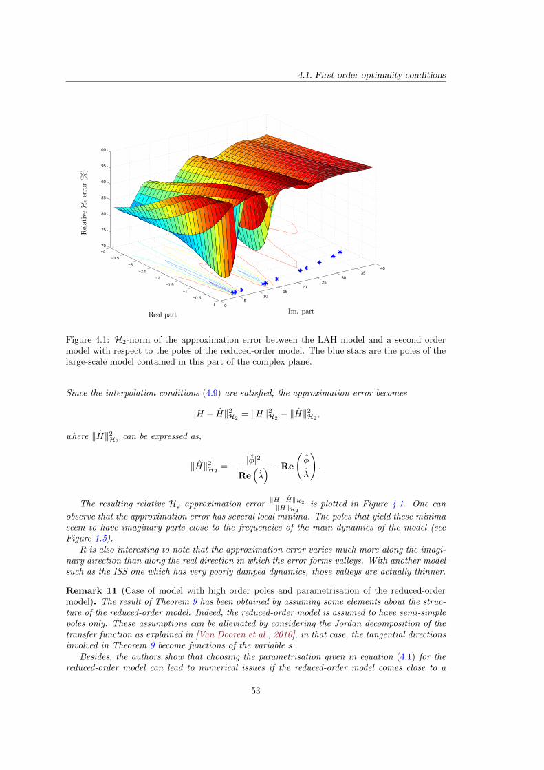
4.1. First order optimality conditions
−4
−3.5
−3
−2.5
−2
−1.5
−1
−0.5
0 05
1015
2025
3035
40
70
75
80
85
90
95
100
Im. partReal part
RelativeH
2error(%
)
Figure 4.1: H2-norm of the approximation error between the LAH model and a second ordermodel with respect to the poles of the reduced-order model. The blue stars are the poles of thelarge-scale model contained in this part of the complex plane.
Since the interpolation conditions (4.9) are satisfied, the approximation error becomes
‖H − H‖2H2= ‖H‖2H2
− ‖H‖2H2,
where ‖H‖2H2can be expressed as,
‖H‖2H2= − |φ|2
Re(λ) −Re
(φ
λ
).
The resulting relative H2 approximation error‖H−H‖H2
‖H‖H2is plotted in Figure 4.1. One can
observe that the approximation error has several local minima. The poles that yield these minimaseem to have imaginary parts close to the frequencies of the main dynamics of the model (seeFigure 1.5).
It is also interesting to note that the approximation error varies much more along the imagi-nary direction than along the real direction in which the error forms valleys. With another modelsuch as the ISS one which has very poorly damped dynamics, those valleys are actually thinner.
Remark 11 (Case of model with high order poles and parametrisation of the reduced-ordermodel). The result of Theorem 9 has been obtained by assuming some elements about the struc-ture of the reduced-order model. Indeed, the reduced-order model is assumed to have semi-simplepoles only. These assumptions can be alleviated by considering the Jordan decomposition of thetransfer function as explained in [Van Dooren et al., 2010], in that case, the tangential directionsinvolved in Theorem 9 become functions of the variable s.
Besides, the authors show that choosing the parametrisation given in equation (4.1) for thereduced-order model can lead to numerical issues if the reduced-order model comes close to a
53
Chapter 4. Optimal H2 model approximation
model with high order poles. Indeed, near a model with high order poles, some eigenvectors of Amight become linearly dependent thus making the interpolation conditions ill-conditionned.
To avoid this issue, the authors in [Van Dooren et al., 2010] recommend to work with a non-minimal parametrisation of the reduced-order model such a its state-space representation sincethe H2-norm of the error is smooth with respect to A, B and C.
In [Fulcheri and Olivi, 1998; Marmorat et al., 2002], a clever parametrisation of the reduced-order model state-space representation based on its Douglas-Shapiro-Shield factorisation (see forinstance [Fuhrmann, 1994]) is used. This enables to have a minimal (in terms of the number ofparameters) and smooth representation that directly embeds some properties like stability.
In the next section, some of the methods that enable to fulfil these first-order optimalityconditions are presented.
4.2 Algorithms for optimal H2 approximation
As it has been mentioned before, several approaches are now available to address the problemof optimal H2 approximation. In this section, the three approaches that have mainly inspiredthe methods developed during this study are presented :
I the MIMO version of the Iterative Rational Krylov Algorithm (IRKA) [Gugercin et al.,2008] in Section 4.2.1,
I the MIMO version of the Iterative SVD-Rational Krylov Algorithm (ISRKA) [Gugercin,2007; Poussot-Vassal, 2011] in Section 4.2.2,
I the optimisation procedure based on the poles-residues formulation of the reduced-ordermodel presented in [Beattie and Gugercin, 2009] in Section 4.2.3.
4.2.1 Iterative Rational Krylov Algorithm (IRKA)
This method has been proposed in [Gugercin et al., 2006] for SISO models based on the rationalinterpolation framework developed in [Grimme, 1997] (see Section 3.2.2). The MIMO extensionhas then been suggested in [Gugercin et al., 2008] and in [Van Dooren et al., 2008b] based on thetangential interpolation framework developed in [Gallivan et al., 2004a] (see Section 3.2.3). It isbased on the projection of the initial large-scale model on suitable Krylov subspaces in order tofind a reduced-order model that fulfil the first-order optimality conditions presented in Theorem9. The method, called Iterative Rational Krylov Algorithm (IRKA), is recalled thereafter inAlgorithm 4. Note that a similar iterative interpolation scheme had been developed in [Krajewskiet al., 1995] based on the frequency-domain representation of the models in terms of numeratorand denominator of the associated transfer functions.
In steps 1 and 2, the initial projectors V and W are constructed from the initial interpolationparameters. Then, until the interpolation points do not vary anymore, a reduced-order modelis built by projection of the large-scale one in step 5. The eigenvalues and right eigenvectors ofthis reduced-order model are computed at step 6 and used in steps 7 and 8 in order to build thenext interpolation points and directions which lead the new projectors in steps 9 and 10.
At each iteration i and based on the Theorem 8 concerning tangential interpolation, thereduced-order model Hi (step 5) tangentially interpolates the large-scale model at the oppositeof the previous reduced-order model eigenvalues, i.e.
c(i−1)k H(−λ(i−1)
k ) = c(i−1)k Hi(−λ(i−1)
k ),
H(−λ(i−1)k )b
(i−1)Tk = Hi(−λ(i−1)
k )b(i−1)Tk ,
c(i−1)k H ′(−λ(i−1)
k )b(i−1)Tk = c
(i−1)k H ′i(−λ
(i−1)k )b
(i−1)Tk .
54
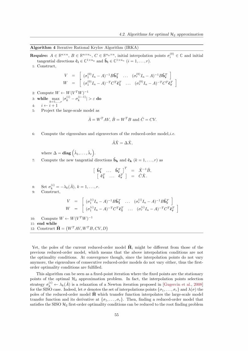
4.2. Algorithms for optimal H2 approximation
Algorithm 4 Iterative Rational Krylov Algorithm (IRKA)
Require: A ∈ Rn×n, B ∈ Rn×nu , C ∈ Rny×n, initial interpolation points σ(0)i ∈ C and initial
tangential directions ci ∈ C1×ny and bi ∈ C1×nu (i = 1, . . . , r).1: Construct,
V =[
(σ(0)1 In −A)−1BbT1 . . . (σ
(0)r In −A)−1BbTr
]W =
[(σ
(0)1 In −A)−TCT cT1 . . . (σ
(0)r In −A)−TCT cTr
]2: Compute W ←W (V TW )−1
3: while maxk=1,...,r
|σ(i)k − σ
(i−1)k | > ε do
4: i← i+ 15: Project the large-scale model as
A = WTAV, B = WTB and C = CV.
6: Compute the eigenvalues and eigenvectors of the reduced-order model,i.e.
AX = ∆X,
where ∆ = diag(λ1, . . . , λr
).
7: Compute the new tangential directions bk and ck (k = 1, . . . , r) as[bT1 . . . bTr
]T= X−1B,[
cT1 . . . cTr]
= CX.
8: Set σ(i)k = −λk(A), k = 1, . . . , r.
9: Construct,
V =[
(σ(i)1 In −A)−1BbT1 . . . (σ
(i)r In −A)−1BbTr
]W =
[(σ
(i)1 In −A)−TCT cT1 . . . (σ
(i)r In −A)−TCT cTr
]10: Compute W ←W (V TW )−1
11: end while12: Construct H =
(WTAV,WTB,CV,D
)
Yet, the poles of the current reduced-order model Hi might be different from those of theprevious reduced-order model, which means that the above interpolation conditions are notthe optimality conditions. At convergence though, since the interpolation points do not varyanymore, the eigenvalues of consecutive reduced-order models do not vary either, thus the first-order optimality conditions are fulfilled.
This algorithm can be seen as a fixed-point iteration where the fixed points are the stationarypoints of the optimal H2 approximation problem. In fact, the interpolation points selection
strategy σ(i)k ← λk(A) is a relaxation of a Newton iteration proposed in [Gugercin et al., 2008]
for the SISO case. Indeed, let σ denotes the set of interpolations points σ1, . . . , σr and λ(σ) thepoles of the reduced-order model H which transfer function interpolates the large-scale modeltransfer function and its derivative at σ1, . . . , σr. Then, finding a reduced-order model thatsatisfies the SISOH2 first-order optimality conditions can be reduced to the root finding problem
55
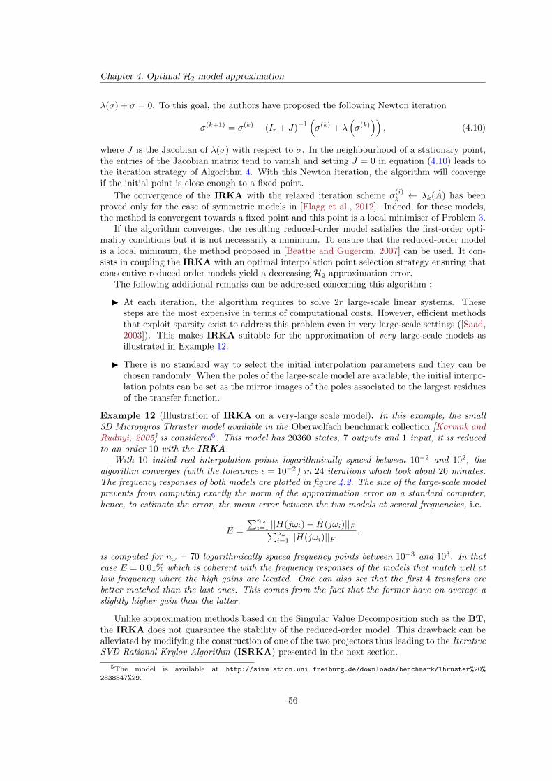
Chapter 4. Optimal H2 model approximation
λ(σ) + σ = 0. To this goal, the authors have proposed the following Newton iteration
σ(k+1) = σ(k) − (Ir + J)−1(σ(k) + λ
(σ(k)
)), (4.10)
where J is the Jacobian of λ(σ) with respect to σ. In the neighbourhood of a stationary point,the entries of the Jacobian matrix tend to vanish and setting J = 0 in equation (4.10) leads tothe iteration strategy of Algorithm 4. With this Newton iteration, the algorithm will convergeif the initial point is close enough to a fixed-point.
The convergence of the IRKA with the relaxed iteration scheme σ(i)k ← λk(A) has been
proved only for the case of symmetric models in [Flagg et al., 2012]. Indeed, for these models,the method is convergent towards a fixed point and this point is a local minimiser of Problem 3.
If the algorithm converges, the resulting reduced-order model satisfies the first-order opti-mality conditions but it is not necessarily a minimum. To ensure that the reduced-order modelis a local minimum, the method proposed in [Beattie and Gugercin, 2007] can be used. It con-sists in coupling the IRKA with an optimal interpolation point selection strategy ensuring thatconsecutive reduced-order models yield a decreasing H2 approximation error.
The following additional remarks can be addressed concerning this algorithm :
I At each iteration, the algorithm requires to solve 2r large-scale linear systems. Thesesteps are the most expensive in terms of computational costs. However, efficient methodsthat exploit sparsity exist to address this problem even in very large-scale settings ([Saad,2003]). This makes IRKA suitable for the approximation of very large-scale models asillustrated in Example 12.
I There is no standard way to select the initial interpolation parameters and they can bechosen randomly. When the poles of the large-scale model are available, the initial interpo-lation points can be set as the mirror images of the poles associated to the largest residuesof the transfer function.
Example 12 (Illustration of IRKA on a very-large scale model). In this example, the small3D Micropyros Thruster model available in the Oberwolfach benchmark collection [Korvink andRudnyi, 2005] is considered5. This model has 20360 states, 7 outputs and 1 input, it is reducedto an order 10 with the IRKA.
With 10 initial real interpolation points logarithmically spaced between 10−2 and 102, thealgorithm converges (with the tolerance ε = 10−2) in 24 iterations which took about 20 minutes.The frequency responses of both models are plotted in figure 4.2. The size of the large-scale modelprevents from computing exactly the norm of the approximation error on a standard computer,hence, to estimate the error, the mean error between the two models at several frequencies, i.e.
E =
∑nωi=1 ||H(jωi)− H(jωi)||F∑nω
i=1 ||H(jωi)||F,
is computed for nω = 70 logarithmically spaced frequency points between 10−3 and 103. In thatcase E = 0.01% which is coherent with the frequency responses of the models that match well atlow frequency where the high gains are located. One can also see that the first 4 transfers arebetter matched than the last ones. This comes from the fact that the former have on average aslightly higher gain than the latter.
Unlike approximation methods based on the Singular Value Decomposition such as the BT,the IRKA does not guarantee the stability of the reduced-order model. This drawback can bealleviated by modifying the construction of one of the two projectors thus leading to the IterativeSVD Rational Krylov Algorithm (ISRKA) presented in the next section.
5The model is available at http://simulation.uni-freiburg.de/downloads/benchmark/Thruster%20%
2838847%29.
56
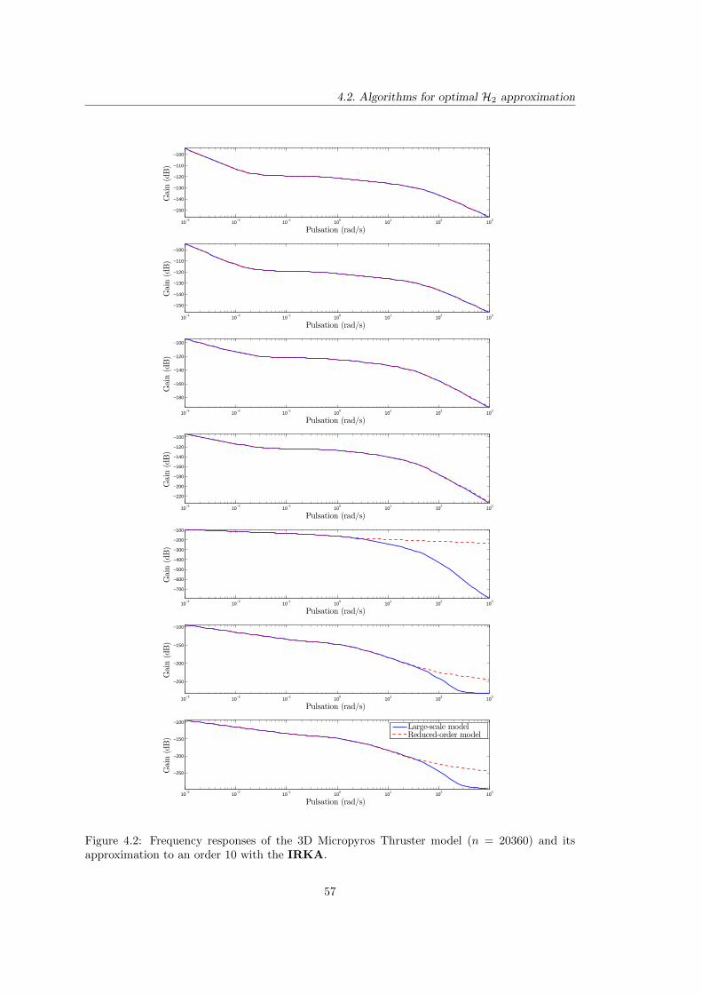
4.2. Algorithms for optimal H2 approximation
10−3
10−2
10−1
100
101
102
103
−150
−140
−130
−120
−110
−100
Gain(dB)
Pulsation (rad/s)
10−3
10−2
10−1
100
101
102
103
−150
−140
−130
−120
−110
−100
Gain(dB)
Pulsation (rad/s)
10−3
10−2
10−1
100
101
102
103
−180
−160
−140
−120
−100
Gain(dB)
Pulsation (rad/s)
10−3
10−2
10−1
100
101
102
103
−220
−200
−180
−160
−140
−120
−100
Gain(dB)
Pulsation (rad/s)
10−3
10−2
10−1
100
101
102
103
−700
−600
−500
−400
−300
−200
−100
Gain(dB)
Pulsation (rad/s)
10−3
10−2
10−1
100
101
102
103
−250
−200
−150
−100
Gain(dB)
Pulsation (rad/s)
10−3
10−2
10−1
100
101
102
103
−250
−200
−150
−100
Gain(dB)
Pulsation (rad/s)
Large-scale modelReduced-order model
Figure 4.2: Frequency responses of the 3D Micropyros Thruster model (n = 20360) and itsapproximation to an order 10 with the IRKA.
57
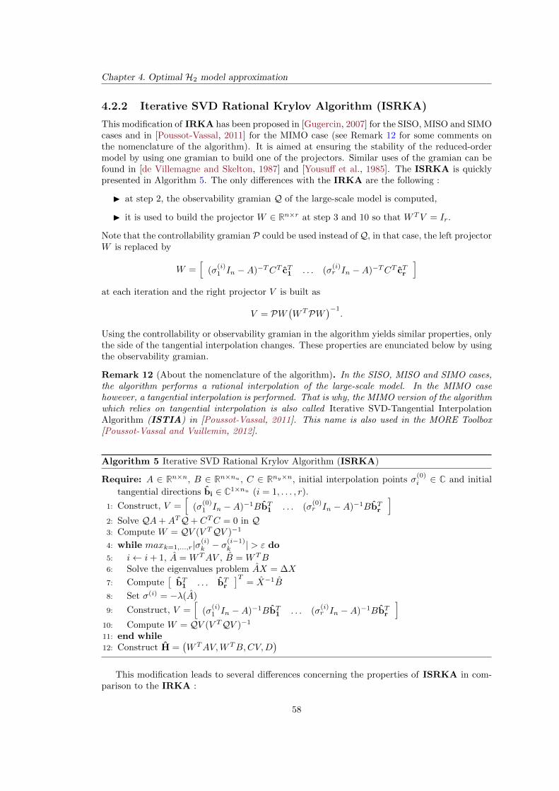
Chapter 4. Optimal H2 model approximation
4.2.2 Iterative SVD Rational Krylov Algorithm (ISRKA)
This modification of IRKA has been proposed in [Gugercin, 2007] for the SISO, MISO and SIMOcases and in [Poussot-Vassal, 2011] for the MIMO case (see Remark 12 for some comments onthe nomenclature of the algorithm). It is aimed at ensuring the stability of the reduced-ordermodel by using one gramian to build one of the projectors. Similar uses of the gramian can befound in [de Villemagne and Skelton, 1987] and [Yousuff et al., 1985]. The ISRKA is quicklypresented in Algorithm 5. The only differences with the IRKA are the following :
I at step 2, the observability gramian Q of the large-scale model is computed,
I it is used to build the projector W ∈ Rn×r at step 3 and 10 so that WTV = Ir.
Note that the controllability gramian P could be used instead ofQ, in that case, the left projectorW is replaced by
W =[
(σ(i)1 In −A)−TCT cT1 . . . (σ
(i)r In −A)−TCT cTr
]at each iteration and the right projector V is built as
V = PW(WTPW
)−1.
Using the controllability or observability gramian in the algorithm yields similar properties, onlythe side of the tangential interpolation changes. These properties are enunciated below by usingthe observability gramian.
Remark 12 (About the nomenclature of the algorithm). In the SISO, MISO and SIMO cases,the algorithm performs a rational interpolation of the large-scale model. In the MIMO casehowever, a tangential interpolation is performed. That is why, the MIMO version of the algorithmwhich relies on tangential interpolation is also called Iterative SVD-Tangential InterpolationAlgorithm (ISTIA) in [Poussot-Vassal, 2011]. This name is also used in the MORE Toolbox[Poussot-Vassal and Vuillemin, 2012].
Algorithm 5 Iterative SVD Rational Krylov Algorithm (ISRKA)
Require: A ∈ Rn×n, B ∈ Rn×nu , C ∈ Rny×n, initial interpolation points σ(0)i ∈ C and initial
tangential directions bi ∈ C1×nu (i = 1, . . . , r).
1: Construct, V =[
(σ(0)1 In −A)−1BbT1 . . . (σ
(0)r In −A)−1BbTr
]2: Solve QA+ATQ+ CTC = 0 in Q3: Compute W = QV (V TQV )−1
4: while maxk=1,...,r|σ(i)k − σ
(i−1)k | > ε do
5: i← i+ 1, A = WTAV , B = WTB6: Solve the eigenvalues problem AX = ∆X
7: Compute[
bT1 . . . bTr]T
= X−1B
8: Set σ(i) = −λ(A)
9: Construct, V =[
(σ(i)1 In −A)−1BbT1 . . . (σ
(i)r In −A)−1BbTr
]10: Compute W = QV (V TQV )−1
11: end while12: Construct H =
(WTAV,WTB,CV,D
)This modification leads to several differences concerning the properties of ISRKA in com-
parison to the IRKA :
58
4.2. Algorithms for optimal H2 approximation
I unlike the IRKA, if the initial large-scale model is asymptotically stable, then, the reduced-order model produced by the ISRKA is guaranteed to be asymptotically stable. The mainidea of the proof consists in projecting the large-scale Lyapunov equation. Indeed, let usassume that the large-scale model H is in a basis in which Q = In, then W = V and theobservability Lyapunov equation becomes
AT +A+ CTC = 0.
By projecting this equation with WT = V T and V , it comes that
AT + A+ CT C = 0,
which implies the stability of the reduced-order model through inertia results [Ostrowskiand Schneider, 1962]. The asymptotic stability is then proved by contradiction (see[Gugercin, 2007]).
I Since the ISRKA only uses one Krylov subspace instead of two, the reduced-order modelobtained with Algorithm 5 only interpolates the large-scale model from the right, i.e. ateach iteration i, for k = 1, . . . , r,
H(σ(i−1)k )b
(i−1)T
k = Hi(σ(i−1)k )b
(i−1)T
k .
This implies, that at convergence, the reduced-order model fulfils only one of the three first-order optimality conditions which yields weaker optimality properties than the IRKA. Inthe SISO case, the reduced-order model obtained with the ISRKA is the best (in the H2
sense) among all other models sharing the same poles. This is also valid in the SIMO caseand in the MISO case if the controllability gramian is used. In the MIMO case however,the ISRKA leads to reduced-order models that are the best among models that have thesame poles and the same left (or right) tangential directions.
I The ISRKA requires to solve r large-scale linear systems at each iteration instead of 2rbut one gramian of the large-scale model needs also to be computed. Hence the methodmight not be tractable in very large-scale settings similarly to the BT. However, as withthe latter method, a low-rank approximation of the gramian can be used (see Section3.1.2). In that case, and just like with the BT, the stability is no longer guaranteed.
A detailed cost comparison of the ISRKA with the BT is presented in [Gugercin, 2007].The ISRKA is expected to be cheaper than the BT when exact gramians are used butmore expensive when approximate gramians are used.
Similarly to the IRKA, (i) a Newton iteration can be used instead of the simple interpolationpoint selection of step 8, (ii) the convergence has not been proved in theory but does not seemto be an issue in practice and (iii) the initial interpolation parameters can be selected in variousdifferent ways.
4.2.3 Optimisation algorithm for optimal H2 model approximation
The method introduced in this section has been proposed in [Beattie and Gugercin, 2009]. Unlikethe IRKA or the ISRKA, it is not based on projection but on a more direct optimisationapproach.
The method is based on the poles-residues decomposition of the reduced-order model transferfunction. Indeed, let λk and Φk = φkc
Tk bk
6 (with φk > 0 and ||ck|| = ||bk|| = 1), k = 1, . . . , r
6For notations consistency with previous Sections, the vectors involved in the decomposition of the residuesΦk are line vectors, this differs from the notation in Beattie and Gugercin [2009] where column vectors are used.
59
Chapter 4. Optimal H2 model approximation
denote the (semi-simple) poles and associated residues of the reduced-order model, then, thetransfer function H(s) can be written as
H(s) =
r∑k=1
φk
s− λkcTk bk.
This representation varies slightly from what has been presented in Section 2.1.1 since thedirections ck and bk of the residues are separated from their norm φk. By imposing the normconstraints ||ck|| = ||bk|| = 1 for k = 1, . . . , r, this representation is minimal. The approximationerror JH2
between the large scale and reduced-order model induced by this formulation is veryclose to the one given in equation (4.4).
With this representation of the reduced-order model H, the optimal H2 approximation prob-lem (Problem 3) consists in finding the reduced-order model poles λk and residues φk, ck, bk(k = 1, . . . , r) that minimises the H2-norm of the approximation error.
More specifically, the authors have gathered the optimisation parameters in two overlappingsets : the degrees of freedom corresponding to the reduced residues φ, c, b and the degrees
of freedom corresponding to the reduced poles φ, λ. This structure is developed in order todecouple the optimisation of the residues from the optimisation of the poles because the latteris harder than the former. This also enables to decrease the number of optimisation parameterssimultaneously involved in the optimisation procedure. A conceptually similar division of theoptimisation parameters is also used in [Marmorat et al., 2002] but based on a completelydifferent representation of the reduced-order model as mentioned in Remark 11.
The optimisation scheme used by the authors is in two folds :
I Firstly, a trust-region7 step in applied to improve the reduced poles location for for fixedresidues. It consists in approximating the local behaviour of the approximation error JH2
by a quadratic function formed with the gradient ∇φ,λJH2and the Hessian ∇2
φ,λJH2
of the error with respect to the poles degrees of freedom. Some constraints on the poleslocation are also added here so that the reduced-order model stays stable.
I Secondly, the residues degrees of freedom φ, c, b are adjusted through a corrective step
for fixed poles λ. This can be done easily in the SISO case (see Remark 10) but require aoptimisation procedure in the MIMO case (see for instance [Beattie and Gugercin, 2012]).
At each iteration, this method yields a stable reduced-order model which achieves a lower H2
approximation error than the previous one. If in addition, upon convergence, the Hessian ispositive definite, then it has led to a local minimiser of Problem 3. Unlike the IRKA and theISRKA (as presented in the previous sections), this approach offers more control over the errorand more guarantees concerning the reduced-order model. These advantages are inherent to theoptimisation framework.
The computation of the approximation error JH2 requires to evaluate the large-scale modeltransfer function at the opposite of the reduced-order model poles. Its gradient and Hessian(with respect to the poles degrees of freedom) require in addition the value of the large-scaletransfer function first and second derivatives at these points, respectively. Depending on thenumber of trial in the trust-region step, a large number of evaluations of the objective functionmight be required. Hence, the computational burden of this method might be higher than forthe IRKA depending on the number of iterations before convergence of both methods.
7An in-depth description of optimisation methods is out of the scope of this thesis, for further details on thesetechniques, we refer to standard textbooks such as [Nocedal and Wright, 1999].
60
4.2. Algorithms for optimal H2 approximation
Conclusion
In this chapter, the H2 optimal approximation problem has been introduced together with someof the numerous methods available to address it. Among those methods, the IRKA is probablythe most suited for very large-scale model approximation. Its performances (and simplicity)make it increasingly popular and it has been extended to the approximation of other types ofmodels such as bi-linear or descriptor models [Benner and Breiten, 2012; Gugercin et al., 2013].However, for medium-scale model approximation, the methods based on optimisation may bemore adequate since they offer more guarantee on the reduced-order model.
In some cases, it is more relevant to preserve the behaviour of the large-scale model overa bounded frequency interval only. Then, the H2-norm and the associated optimal model ap-proximation methods are not completely relevant anymore and other approaches have to beconsidered. In the next chapter, the problem of approximation over a bounded frequency inter-val is introduced together with some existing methods to address it.
61

Chapter 5
Frequency weighted and frequency-limited model approximation
In this chapter, some methods aimed at approximating a large-scale model, so that its behaviourover a bounded frequency interval is reproduced, are briefly presented. Here, these methods areclassified into two groups
I the approaches based on the use of explicit filters which are referred here as frequency-weighted methods and
I those that do not involve explicitly any filter, called here frequency-limited methods.
The former class of methods is presented in Section 5.1 while the latter is described in Section5.2.
Contents5.1 Frequency weighted model approximation . . . . . . . . . . . . . . 63
5.1.1 Frequency weighted balanced truncation . . . . . . . . . . . . . . . . . 63
5.1.2 Frequency weighted H2 model approximation . . . . . . . . . . . . . . 65
5.2 Frequency-limited model approximation . . . . . . . . . . . . . . . . 67
5.2.1 Frequency-limited balanced truncation . . . . . . . . . . . . . . . . . . 67
5.2.2 Gramian-based H2,Ω optimal model approximation . . . . . . . . . . . 69
5.1 Frequency weighted model approximation
In this section, the methods based on the use of frequency filters are presented. Firstly, thefrequency-weighted extension of the balanced truncation is presented in Section 5.1.1. Then, inSection 5.1.2, the idea leading to the extension of the IRKA (see Section 4.2.1) to the optimalfrequency-weighted H2 model approximation problem is introduced.
5.1.1 Frequency weighted balanced truncation
The underlying principle of frequency-weighted model truncation methods is the same as for thebalanced truncation (see Section 3.1.2), i.e. the large-scale model is balanced with respect tosome positive definite matrices of interest and the states corresponding to the smallest singularvalues are discarded. The difference between the various balanced truncation methods lies inthe choice of the matrices with respect to which the model is balanced. Here, frequency-weightedgramians are considered.
Let us consider a large-scale model H and input and output filters Wi and Wo, respectively.The objective of frequency-weighted balanced truncation methods is to find a reduced-ordermodel H so that the filtered frequency error
‖Wo(H − H)Wi‖H∞ , (5.1)
is small.
63
Chapter 5. Frequency weighted and frequency-limited model approximation
Note that the construction of the input and output weightings Wi and Wo is a problem initself which is not covered here. Instead, one directly assumes that the realisations
Wi :=
(AWi
BWi
CWiDWi
)and Wo :=
(AWo
BWo
CWoDWo
)are available. Based on these realisations, and assuming that there is no pole-zero cancellation,one can build the minimal realisations of Hi(s) = H(s)Wi(s) and Ho(s) = Wo(s)H(s) as
Hi =
(Ai BiCi Di
)=
A BCWi BDWi
0 AWiBWi
C 0 DDWi
, (5.2)
and
Ho =
(Ao BoCo Do
)=
A 0 BBWo
C AWo0
DWoC CWo
DWoD
. (5.3)
Let us also consider the matrices Qo and Pi which are the solutions of
AiPi + PiATi +BiBTi = 0 and AToQo +QoAo + CTo Co = 0,
and which can be decomposed as,
Qo =
[Q11 Q12
QT12 Q22
]and Pi =
[P11 P12
PT12 P22
].
Q11 and P11 are called the frequency-weighted observability and reachability gramians (see[Antoulas, 2005, Sec. 7.6] for further information). Based on these gramians, different balancingstrategies can be considered,
I in [Enns, 1984], the authors have suggested to balance the model H such that Q11 andP11 are simultaneously diagonalised. The reduced-order model H is then obtained bydiscarding the states associated to the smallest frequency-weighted Hankel singular values.This method does not offer any guarantee concerning the stability of the reduced-ordermodel when two-sided weighting is considered.
In [Kim et al., 1995], an error bound on the weighted H∞-norm of the approximation error(5.1) is derived when H is asymptotically stable.
I In [Lin and Chiu, 1990], the balancing method is based on the simultaneous diagonalisationof the Schur complements of Pi and Qo, i.e. P11−P12P22
−1PT12 and Q11−Q12Q22−1QT12.
With this approach, the stability of the reduced-order model is guaranteed when the re-alisations (5.2) and (5.3) are minimal. An upper bound on (5.1) can also be derived withthis approach.
I In [Wang et al., 1999], different quantities are built for the balancing, in particular, let usconsider1
XB := BCWiP12 + PT12CTWiBT +BDWiD
TWiBT
XC := Q12BWoC + CTBTWo
QT12 + CTDTWoDWo
C.
If these two matrices are positive semi-definite, then the reduced-order model obtained byEnn’s frequency weighted balanced truncation is guaranteed to be stable. Otherwise, letus consider the eigen-decompositions of XB and XC , i.e.
XB = Mdiag (λ1, . . . , λn)MT ,
XC = Ndiag (δ1, . . . , δn)NT ,
1Those are the last terms in the Lyapunov equations associated to the frequency-weighted gramians P11 andQ11.
64
5.1. Frequency weighted model approximation
and define
B = Mdiag(|λ1|
12 , . . . , |λn|
12
),
C = diag(|δ1|
12 , . . . , |δn|
12
)NT .
The frequency-weighted gramians P and Q considered in this approach are then obtainedby solving
AP + PAT + BBT = 0 and AT Q+ QA+ CT C = 0.
Based on this approach, the stability of the reduced-order model H is guaranteed. If inaddition rank(
[B B
]) = rank(B) and rank(
[CT CT
]) = rank(CT ) then H is
asymptotically stable and there is a bound on the weighted H∞ error (5.1) given by
‖Wo(H − H)Wi‖H∞ ≤ 2‖WoL‖H∞‖KWi‖H∞n∑
i=r+1
σi,
where K = BTB and L = CCT and σi are the frequency-weighted singular values associ-ated to P and Q.
5.1.2 Frequency weighted H2 model approximation
In this section, the extension of the IRKA (see Section 4.2.1) to frequency-weighted H2 modelapproximation is presented. The first step towards this extension has been done in [Anic et al.,2013] where the first-order optimality conditions for the optimal frequency-weighted H2 modelapproximation problem have been formulated for SISO models as interpolation conditions. Anheuristic approach based on the IRKA has also been proposed inspired by these interpolationconditions. Then in [Breiten et al., 2014], the conditions have been extended to MIMO mod-els and the Krylov subspaces involved in IRKA have been modified accordingly. For sake ofsimplicity here, only the SISO case is considered.
The frequency-weighted H2-norm, denoted H2,W -norm here, of an asymptotically stablemodel H is defined as
‖H‖H2,W:= ‖HW‖H2
,
where W (s) ∈ H∞ is the transfer function associated to a weighting model W. The problemconsidered in [Breiten et al., 2014] is then to find an asymptotically stable reduced-order modelH of order r which minimises the frequency-weighted H2 approximation error with a large-scalemodel H, i.e.
H = arg minrank(G)=r
‖H −G‖H2,W. (5.4)
Let us assume here that H = (A,B,C,D), H = (A, B, C, D) and W = (AW , BW , CW , DW )have semi-simple poles only and that their associated transfer functions are given as,
H(s) =
n∑i=1
φis− λi
+D, H(s) =
r∑i=1
φi
s− λi+ D and W (s) =
p∑i=1
ψis− γi
+DW . (5.5)
where λi, φi, λk, φk and γl, ψl are the poles and associated residues of H, H and W,respectively.
First-order optimality conditions for the H2,W approximation problem
Let us define, for an asymptotically stable model H and a filter W such that DDW = 0,
F [H](s) = H(s)W (s)W (−s) +
p∑k=1
H(−γk)W (−γk)ψk
s+ γk.
65

Chapter 5. Frequency weighted and frequency-limited model approximation
If the reduced-order model H is a solution to (5.4), then, for k = 1, . . . , r,
F [H](−λk) = F [H](−λk),
F ′[H](−λk) = F ′[H](−λk),(5.6)
and in addition, for all n ∈ Ker(DTW )(∫ ∞
−∞F [H](jω)dω
)n =
(∫ ∞−∞
F [H](jω)dω
)n
For further information on F [.](s) and on these first-order optimality conditions, refer to [Breitenet al., 2014].
Use of IRKA for H2,W model approximation
The first-order optimality conditions (5.6) are similar to the optimality conditions arising in H2
model approximation (see Section 4.1) which suggest that an iterative scheme of the IRKAcan be used for the H2,W model approximation problem as well. Two approaches have beenconsidered,
I based on the notations of equation (5.5), the H2,W -norm of the approximation error be-
tween H and H can be written as,
‖H − H‖2H2,W=
n∑i=1
(H(−λi)− H(−λi)
)W (−λi)W (λi)φi
+
r∑k=1
(H(−λk)−H(−λk)
)W (−λk)W (λk)φk
+
p∑l=1
(H(−γl)− H(−γl)
)W (−γl)
(H(γl)− H(γl)
)ψl.
(5.7)
In [Anic et al., 2013], a specific choice of interpolation points is used in IRKA in order tomake some elements of the error (5.7) vanish. In particular, one of the projector in IRKA
is built so that at convergence H(−λk) = H(−λk) (which makes the second sum vanish)while the other projector is built with fixed interpolation points so that H interpolates Hat the mirror images of the poles λi and γl associated to the highest residues φi and ψl(which makes some elements of the first and third sums in (5.7) vanish).
However, with this approach, the first-order optimality conditions (5.6) are not fulfilled.
I In [Breiten et al., 2014], it is proven that F [H](s) has a realisation given by
F [H] =
(AF BF
CF DF
)=
A BCW ZCTW +BDWDTW
0 AW PWCTW +BWDTW
C DCW 0
,
where PW is the reachability gramian associated to W and Z is the solution of
AZ + ZATW +B(CWPW +DWBTW ) = 0.
Based on this state-space representation, the construction of the projectors W and V inIRKA has been modified so that at convergence, if Ran(Z) ⊂ Ran(V ), then the reduced-order model H fulfils the first-order optimality conditions (5.6).
The assumption Ran(Z) ⊂ Ran(V ) is not necessarily fulfilled by the algorithm proposedin [Breiten et al., 2014] which is why it is called Near Optimal Weighted Interpolation.
66
5.2. Frequency-limited model approximation
Indeed, an error might appear depending on the difference Z−V Z where Z is the solutionof
AZ + ZATW + B(CWPW +DWBTW ) = 0,
and can be viewed as the Petrov-Galerkin approximation of Z. The interpolation errorinduced by Z − V Z is expected to vanish as r increases.
5.2 Frequency-limited model approximation
In this section, model approximation methods that do not require the use of filters are presented.In particular, in Section 5.2.1, the Frequency-Limited Balanced Truncation (FL-BT) is describedand in Section 5.2.2, an optimal H2,Ω model approximation method is presented.
5.2.1 Frequency-limited balanced truncation
In [Gawronski and Juang, 1990], the authors have proposed to use the restriction of the frequencydefinition of the gramians, referred here as the frequency-limited gramians (see Section 2.1.2),to balance the initial large-scale model.
For the frequency interval Ω = [ω1, ω2], the frequency-limited observability and reachabilitygramians QΩ and PΩ, respectively, can be obtained, similarly to the infinite gramians, by solvingtwo Lyapunov equations,
APΩ + PΩAT +Wc(Ω) = 0,
ATQΩ +QΩA+Wo(Ω) = 0,(5.8)
where Wc(Ω) = Wc(ω2)−Wc(ω1) and Wo(Ω) = Wo(ω2)−Wo(ω1) with
Wc(ω) = S(ω)BBT +BBTS∗(ω) and Wo(ω) = S∗(ω)CTC + CTCS(ω),
and where S(ω) = j2π logm((A+ jωIn)(A− jωIn)
−1).
By definition (see Section 2.1.2), the frequency-limited gramians QΩ and PΩ are positivesemi-definite. Hence, they can be balanced (i.e. simultaneously diagonalised) so that in thisbasis, they are both equal and diagonal,
QΩ = PΩ = diag(σΩ
1 , . . . , σΩn
),
where σΩi are what may be called here the frequency-limited Hankel singular values (see Example
3 for an illustration of those singular values).The reduced-order model is then obtained by discarding the states of the large-scale model
associated with the smallest frequency-limited Hankel singular values. This approach can beshown (see [Gugercin and Antoulas, 2004]) to be equivalent to the frequency-weighted balancedtruncation method presented in Section 5.1.1 considered with perfect filters. The advantage hereis that no explicit weight is involved.
Note that since Wc(Ω) and Wo(Ω) are not necessarily positive semi-definite, the reduced-ordermodel obtained with the FL-BT is not guaranteed to be stable (see Remark 6). In addition,there is no upper bound on the H∞-norm of the approximation error. Both issues have beenalleviated by slightly modifying the method.
Modification of the FL-BT to ensure stability preservation
In [Gugercin and Antoulas, 2004], the authors have proposed a modification of the FL-BT inorder to ensure the stability of the reduced-order model. The idea is similar to the modificationof the frequency-weighted balanced truncation method from [Enns, 1984] proposed in [Wanget al., 1999] and introduced in Section 5.1.1.
67

Chapter 5. Frequency weighted and frequency-limited model approximation
10−1
100
101
102
−100
−90
−80
−70
−60
−50
−40
Pulsation ω (rad/s)
Magnitude(dB)
Frequency responses of the models
HHBT
HFLBT
Hmod.F LBT
10−1
100
101
102
−250
−200
−150
−100
−50
Pulsation ω (rad/s)
Magnitude(dB)
Frequency responses of the errors
BTFL-BTmod.FL-BT
Figure 5.1: Comparison of the FL-BT with the BT and the modified FL-BT by approximationof the LAH model to and order r = 10 over Ω = [0, 10].
It consists in replacing the last terms involved in the Lyapunov equations (5.8), Wc(Ω) andWo(Ω), by positive semi-definite matrices Wc(Ω) and Wo(Ω) which are constructed by takingthe absolute values of the eigenvalues of Wc(Ω) and Wo(Ω).
With this modification, the reduced-order model is guaranteed to be stable and with similarassumptions as in Section 5.1.1, the asymptotic stability can be proven as well and the existenceof a bound on theH∞-norm of the approximation error and on the frequency-weightedH∞-normof the error (5.1).
Numerical illustration and comparison of the FL-BT
The FL-BT is compared to the BT and the modified FL-BT on a simple case. The LAHmodel is reduced to an order r = 10 over Ω = [0, 10] with the three methods. The frequencyresponses of each models as well as the frequency responses of the errors are plotted in Figure5.1.
One can observe that in the considered frequency band Ω, the error corresponding to themodel obtained with FL-BT is clearly inferior to the error obtained with the BT or the mod-ified FL-BT. This is confirmed by H2,Ω norm of the errors, indeed,
‖H − HBT ‖H2,Ω
‖H‖H2,Ω
= 10.40%
‖H − Hmod.FLBT ‖H2,Ω
‖H‖H2,Ω
= 4.10%
‖H − HFLBT ‖H2,Ω
‖H‖H2,Ω
= 1.15× 10⁻⁴%.
On the frequency responses, the efficiency of the modified FL-BT with respect to the BT isnot obvious but it appears more clearly through the H2,Ω-norms of the errors. Even if it does not
68
5.2. Frequency-limited model approximation
reach the performance of the FL-BT, it is still more efficient that the BT when the H2,Ω-normis considered.
5.2.2 Gramian-based H2,Ω optimal model approximation
The approach presented here has been developed in [Petersson, 2013; Petersson and Lofberg,2014] in parallel of this thesis. It is an optimisation method aimed at finding a reduced-ordermodel which minimises the H2,Ω-norm of the approximation error where the latter is expressedwith the gramian-based formulation of the norm (see Section 2.2.2). To be more specific, letus consider the n-th order large-scale model H := (A,B,C,D), the objective of the method isto find a r-th order (r n) model H := (A, B, C, D) which minimises the H2,Ω-norm of the
approximation error between H and H, i.e.
H = arg minG‖E‖2H2,Ω
= arg minG‖H −G‖2H2,Ω
, (5.9)
where Ω = [0, ω]. Note that due to Property 1 from Section 2.2.2, more complex frequencyintervals can readily be considered.
For simplicity, let us assume here that both models H and H are strictly proper, i.e. D =D = 0, the realisation of the error model E = H− H is then given by
E :=
(AE BECE 0
)=
A 0 B
0 A B
C −C 0
(5.10)
The frequency-limited H2,Ω-norm of the approximation error can be expressed through thegramian-based formulation of the norm (see Section 2.2.2) as
‖E‖2H2,Ω= tr
(CEPE,ωCTE
)= tr
(BTEQE,ωBE
), (5.11)
where PE,ω and QE,ω are the frequency-limited gramians associated to E considered over Ω =[0, ω]. They are solutions of the following Lyapunov equations,
AEPE,ω + PE,ωATE +Wc(ω) = 0
ATEQE,ω +QE,ωAE +Wo(ω) = 0,(5.12)
whereWc(ω) = SE(ω)BEB
TE +BEB
TESE(ω)H ,
Wo(ω) = SE(ω)HCTECE + CTECESE(ω),
with
SE(ω) =j
2πlogm
((AE + jωIn+r) (AE − jωIn+r)
−1). (5.13)
For asymptotically stable models, (5.13) can be simplified as,
SE(ω) = Re
(j
πlogm (−AE − jωIn+r)
).
Note that due to the structure of the error model (5.10),
SE,ω =
[S(ω) 0
0 S(ω)
].
where S(ω) = Re( jπ logm(−A − jωIn)) and S(ω) = Re( jπ logm(−A − jωIr)). Similarly, bypartitioning the gramians as
PE,ω =
[Pω P12,ω
PT12,ω Pω
]and QE,ω =
[Qω Q12,ω
QT12,ω Qω
],
69
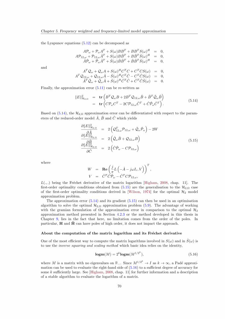
Chapter 5. Frequency weighted and frequency-limited model approximation
the Lyapunov equations (5.12) can be decomposed as
APω + PωAT + S(ω)BBT +BBTS(ω)H = 0,
AP12,ω + P12,ωAT + S(ω)BBT +BBT S(ω)H = 0,
APω + PωAT + S(ω)BBT + BBT S(ω)H = 0,
andATQω +QωA+ S(ω)HCTC + CTCS(ω) = 0,
ATQ12,ω +Q12,ωA− S(ω)HCT C − CT CS(ω) = 0,
AT Qω + QωA+ S(ω)HCT C + CT CS(ω) = 0.
Finally, the approximation error (5.11) can be re-written as
‖E‖2H2,Ω= tr
(BTQωB + 2BTQ12,ωB + BT QωB
)= tr
(CPωCT − 2CP12,ωC
T + CPωCT).
(5.14)
Based on (5.14), the H2,Ω approximation error can be differentiated with respect to the param-
eters of the reduced-order model A, B and C which yields
∂‖E‖2H2,Ω
∂A= 2
(QT12,ωP12,ω + QωPω
)− 2W
∂‖E‖2H2,Ω
∂B= 2
(QωB +Q12,ωB
)∂‖E‖2H2,Ω
∂C= 2
(CPω − CP12,ω
) (5.15)
where
W = Re
(j
πL(−A− jωIr, V
))T,
V = CT CPω − CTCP12,ω,
L(., .) being the Frechet derivative of the matrix logarithm [Higham, 2008, chap. 11]. Thefirst-order optimality conditions obtained from (5.15) are the generalisation to the H2,Ω caseof the first-order optimality conditions derived in [Wilson, 1974] for the optimal H2 modelapproximation problem.
The approximation error (5.14) and its gradient (5.15) can then be used in an optimisationalgorithm to solve the optimal H2,Ω approximation problem (5.9). The advantage of workingwith the gramian formulation of the approximation error in comparison to the optimal H2
approximation method presented in Section 4.2.3 or the method developed in this thesis inChapter 9, lies in the fact that here, no limitation comes from the order of the poles. Inparticular, H and H can have poles of high order, it does not impact the approach.
About the computation of the matrix logarithm and its Frechet derivative
One of the most efficient way to compute the matrix logarithms involved in S(ω) and in S(ω) isto use the inverse squaring and scaling method which basic idea relies on the identity,
logm(M) = 2klogm(M1/2k), (5.16)
where M is a matrix with no eigenvalues on R−. Since M1/2k → I as k → ∞, a Pade approxi-mation can be used to evaluate the right-hand side of (5.16) to a sufficient degree of accuracy forsome k sufficiently large. See [Higham, 2008, chap. 11] for further information and a descriptionof a stable algorithm to evaluate the logarithm of a matrix.
70

5.2. Frequency-limited model approximation
The computation of the Frechet derivative L(M,X) of the matrix logarithm is done througha similar idea (see [Al-Mohy et al., 2013] for an in-depth description of the algorithm). Indeed,similarly to identity (5.16),
L(M,X) = 2kL(M1/2k , Xk),
where X0 = X and the Xi (i = 1, . . . , k) are solutions of the Sylvester equations,
M1/2iXi +XiM1/2i = Xi−1 i = 1, . . . , k.
Similarly to the logarithm, its Frechet derivative L(M,X) is then approximated by the Pade
approximation of 2kL(M1/2k , Xk).
Conclusion
In this chapter, some methods for the approximation of a large-scale dynamical model over abounded frequency interval have been briefly presented. These methods have been classified hereinto two groups, the methods that rely on the use of frequency-filters called frequency-weightedmodel approximation methods and the ones that do not referred as frequency-limited modelapproximation methods.
The most popular frequency-weighted model approximation method is the FW-BT whichextends the standard BT by defining frequency-weighted gramians. Depending on the chosenapproach, the FW-BT can guarantee the asymptotic stability of the reduced-order model andgives an upper bound on the weighted H∞ approximation error. The use of filters has alsobeen considered to extend the IRKA in order to address the optimal frequency-weighted H2
model approximation problem. However, the resulting algorithm does not necessarily leads toan optimal reduced-order model due to some error appearing during the interpolation. Thesefrequency-weighted model approximation methods are efficient but the design of the filter add atuning parameter which can be avoided by using frequency-limited model approximation meth-ods.
The first one of these methods is the FL-BT which extends the BT by using frequency-limited gramians to balance the large-scale model. This method is equivalent to one of the FW-BT considered with perfect filters and is generally extremely efficient in practice. The otherapproach is a non-linear optimisation algorithm aimed at solving the optimalH2,Ω approximationproblem based on the gamian formulation of the norm. This method is of particular interestand a similar approach has been developed in this thesis based on the poles-residues of theH2,Ω-norm.
This chapter concludes the part dedicated to the state of the art. The next part gathers thecontributions of this thesis concerning the frequency-limited approximation of linear dynamicalmodels.
71

Part III
Frequency-limited approximationof linear dynamical models
73

Chapter 6
Development of a first approachfor frequency-limited model approx-imation
In this chapter, a first approach to address the problem ofH2,Ω model approximation is presented.It is an empirical method based on the Iterative SVD-Rational Krylov Algorithm (ISRKA, seeSection 4.2.2) and inspired by the Frequency-Limited Balanced Truncation (FL-BT, see Section5.2.1).
In Section 6.1, the principle of the method is described and the algorithm presented. Thenin Section 6.2, several numerical experiments are made in order to illustrate the behaviour ofthe algorithm and its performances.
This method has been presented and successfully applied on an industrial aircraft model in[Vuillemin et al., 2013a,b].
Contents6.1 Modification of ISRKA . . . . . . . . . . . . . . . . . . . . . . . . . . 75
6.1.1 Presentation of the method . . . . . . . . . . . . . . . . . . . . . . . . 75
6.1.2 Properties . . . . . . . . . . . . . . . . . . . . . . . . . . . . . . . . . . 77
6.1.3 Numerical improvement of the method . . . . . . . . . . . . . . . . . . 78
6.2 Numerical illustrations . . . . . . . . . . . . . . . . . . . . . . . . . . 79
6.2.1 Comparison with the standard version of ISRKA . . . . . . . . . . . 79
6.2.2 Impact of restart and error watching . . . . . . . . . . . . . . . . . . . 83
6.2.3 Comparison with other methods . . . . . . . . . . . . . . . . . . . . . 86
6.1 Modification of ISRKA
In Section 6.1.1, the principle of the method as well as the corresponding algorithm are presented.In Section 6.1.2, the properties of the method are discussed and in Section 6.1.3, some numericalimprovements are proposed to enhance the method.
6.1.1 Presentation of the method
This method is based on the sub-optimal H2 model approximation method ISRKA (see Section4.2.2) and has been inspired by the use of frequency-limited gramians in the BT which has ledto the FL-BT (see Section 5.2.1). In particular, it consists in using a frequency-limited gramianinstead of an infinite one in order to build one of the projector in ISRKA. The resultingalgorithm is called Frequency-Limited Iterative SVD Tangential Algorithm (FL-ISTIA) and ispresented in Algorithm 6. The algorithm has been integrated in the MORE Toolbox [Poussot-Vassal and Vuillemin, 2012] and an example of its use can be found in Appendix C.3.
Initial projectors are built from step 1 to step 3. In particular, V is built as a basis ofa Krylov subspace and W is built thanks to the frequency-limited observability gramian QΩ
so that WTV = Ir. Then, while the algorithm has not converged, a reduced-order model is
75
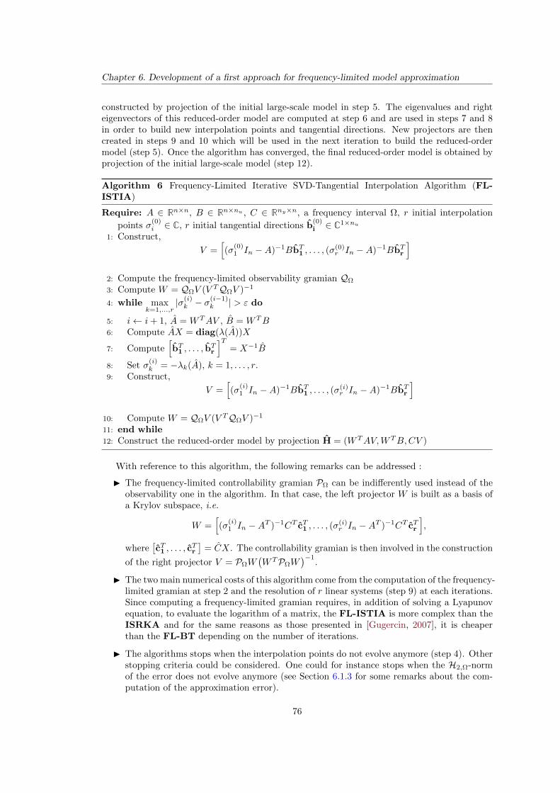
Chapter 6. Development of a first approach for frequency-limited model approximation
constructed by projection of the initial large-scale model in step 5. The eigenvalues and righteigenvectors of this reduced-order model are computed at step 6 and are used in steps 7 and 8in order to build new interpolation points and tangential directions. New projectors are thencreated in steps 9 and 10 which will be used in the next iteration to build the reduced-ordermodel (step 5). Once the algorithm has converged, the final reduced-order model is obtained byprojection of the initial large-scale model (step 12).
Algorithm 6 Frequency-Limited Iterative SVD-Tangential Interpolation Algorithm (FL-ISTIA)
Require: A ∈ Rn×n, B ∈ Rn×nu , C ∈ Rny×n, a frequency interval Ω, r initial interpolation
points σ(0)i ∈ C, r initial tangential directions b
(0)i ∈ C1×nu
1: Construct,
V =[(σ
(0)1 In −A)−1BbT1 , . . . , (σ
(0)r In −A)−1BbTr
]2: Compute the frequency-limited observability gramian QΩ
3: Compute W = QΩV (V TQΩV )−1
4: while maxk=1,...,r
|σ(i)k − σ
(i−1)k | > ε do
5: i← i+ 1, A = WTAV , B = WTB6: Compute AX = diag(λ(A))X
7: Compute[bT1 , . . . , b
Tr
]T= X−1B
8: Set σ(i)k = −λk(A), k = 1, . . . , r.
9: Construct,
V =[(σ
(i)1 In −A)−1BbT1 , . . . , (σ
(i)r In −A)−1BbTr
]10: Compute W = QΩV (V TQΩV )−1
11: end while12: Construct the reduced-order model by projection H = (WTAV,WTB,CV )
With reference to this algorithm, the following remarks can be addressed :
I The frequency-limited controllability gramian PΩ can be indifferently used instead of theobservability one in the algorithm. In that case, the left projector W is built as a basis ofa Krylov subspace, i.e.
W =[(σ
(i)1 In −AT )−1CT cT1 , . . . , (σ
(i)r In −AT )−1CT cTr
],
where[cT1 , . . . , c
Tr
]= CX. The controllability gramian is then involved in the construction
of the right projector V = PΩW(WTPΩW
)−1.
I The two main numerical costs of this algorithm come from the computation of the frequency-limited gramian at step 2 and the resolution of r linear systems (step 9) at each iterations.Since computing a frequency-limited gramian requires, in addition of solving a Lyapunovequation, to evaluate the logarithm of a matrix, the FL-ISTIA is more complex than theISRKA and for the same reasons as those presented in [Gugercin, 2007], it is cheaperthan the FL-BT depending on the number of iterations.
I The algorithms stops when the interpolation points do not evolve anymore (step 4). Otherstopping criteria could be considered. One could for instance stops when the H2,Ω-normof the error does not evolve anymore (see Section 6.1.3 for some remarks about the com-putation of the approximation error).
76
6.1. Modification of ISRKA
I To alleviate the computational complexity of the algorithm in very large-scale settings, alow-rank approximation of the gramian could be used (see for instance [Antoulas, 2005,chap. 12] and references therein). However, this has not been considered here.
I Note that as in other methods rooted on Krylov subspaces, to obtain real valued pro-jectors V and W , the interpolation points must either be real or closed under complexconjugation. Indeed, in the latter case, if two vectors are complex conjugate v2 = v1
∗,then they span the same subspace as their real and imaginary part, i.e. span v1,v2 =span Re(v1), Im(v1). This also implies that only one linear system has to be solved(step 1 and 9) for each pair of complex conjugate interpolation points, which reduces thecomputational complexity.
I In general, the initial points are linearly or logarithmically spaced points in the intervalof interest. They can also be chosen as the opposite of the poles of the large-scale modelwhich are associated to the r largest residues in the considered frequency interval.
I Direct feedthrough are not taken into account in this algorithm because it is based onprojection and direct feedthrough are not modified by projection. A simple way to handlenon strictly proper models is to set D = D. However, this is not the optimal choiceconsidering the gradient of the approximation error with respect to D (see Chapter 8).
6.1.2 Properties
The properties of FL-ISTIA concerning stability preservation and interpolation of the large-scale model are discussed below.
Stability
To prove the stability of the reduced-order models built by ISRKA [Gugercin, 2007], the Lya-punov equation of the initial large-scale model is projected thus leading to the reduced-ordermodel Lyapunov equation. And, due to inertia results, the reduced-order model is proved to bestable (see Section 4.2.2).
Here however, the same reasoning cannot be applied. Indeed, let assume that the basis issuch that QΩ = In, then, the large-scale Lyapunov equation is
AT +A+Wo (Ω) = 0.
By applying the projectors WT = V T and V to the equation, it comes that
AT + A+ V TWo (Ω)V = 0.
The last term of the reduced-order Lyapunov equation is not necessarily positive semi-definite,hence stability cannot be proved. In order to do so, the same modification that has been devel-oped for ensuring the stability with the FL-BT [Gugercin and Antoulas, 2004] could be applied(see Section 5.2.1). However, in the case of FL-BT, we have observed that this modification alsoleads to a loss of performances in terms of approximation error in the considered frequency inter-val. Since instability has rarely been observed in the reduced-order model built by FL-ISTIA,this modification is not applied to the algorithm in the sequel.
Interpolation
The Krylov subspace used in FL-ISTIA (steps 1 and 9) is the same as the one used in IRKAor ISRKA. It implies that at convergence, the reduced-order model interpolates tangentiallythe initial large-scale model H from the left or the right (depending on the Krylov subspace
77
Chapter 6. Development of a first approach for frequency-limited model approximation
that has been chosen) at −λi for all i = 1, . . . , n. For instance, if at convergence, V =[(λ1In −
A)−1BbT1 , . . . , (λrIn −A)−1BbT
r
], then for all i = 1, . . . , n,
H(−λi)bTi = H(−λi)bTi . (6.1)
Note that equation (6.1) is one of the first-order optimality conditions for the optimal H2
approximation problem (see Theorem 9 in Section 4.1.2). For SISO models, just like ISRKA,this implies that the reduced-order model built by FL-ISTIA is the best (in the H2-sense)among all the models which share the same eigenvalues. The same property holds in SIMOand MISO cases as well (depending on which side the Krylov subspace is built). In MIMOcases however, the optimality property is weaker since only one part of the first-order optimalityconditions is fulfilled. In all cases, fulfilling this optimality condition implies that at convergence,the H2-norm of the approximation error between the large-scale and reduced-order models isequal to the difference of their H2-norm (see Section 4.1), i.e.
‖H − H‖2H2= ‖H‖2H2
− ‖H‖2H2. (6.2)
Fulfilling H2 optimality conditions is not really relevant in the case of model approximationover a bounded frequency range and the choice of the Krylov subspace could be improved. Thisstands also for the shifts point selection strategy at step 8 which is a relaxation of a Newton’sscheme based on the optimality conditions of the H2 problem. However, as it will appear later inChapter 8, the optimality conditions for the H2,Ω approximation problem cannot be expressed asconvenient interpolation conditions and thus choosing a relevant Krylov subspace is not trivial.
6.1.3 Numerical improvement of the method
Below, two modifications are proposed for improving the behaviour of FL-ISTIA.
Error watch
One of the main drawback of FL-ISTIA lies in the fact that it does not give any informationabout the approximation error between the large-scale model and the reduced-order one. Thisissue can be alleviated by computing the approximation error at each iteration and keeping themodel which has yielded the smallest approximation error.
In order to keep the computation time to an acceptable level, the approximation error mustnot be computed directly, instead its decomposition,
‖H − H‖2H2,Ω= ‖H‖2H2,Ω
+ ‖H‖2H2,Ω− 1
π
∫ ω
−ωtr(H(jν)H(−jν)T
)dν,
can be exploited. Indeed, since ‖H‖2H2,Ωdoes not depend of the reduced-order model and
consequently, it does not need to be computed. The H2,Ω-norm of the reduced-order model iseasily computed since the order of the model is low. The cross term has to be computed at eachiteration and involves the large-scale model. Note that the H2,Ω-norm of the approximationerror cannot in general be simplified as in equation (6.2) since the optimality conditions are notthe same as in the H2 case (see Chapter 8).
Each term of the approximation error can either be computed by solving Lyapunov/Sylvesterequations (see for instance [Petersson, 2013]) or through the poles-residues formulation of theapproximation error (see Chapter 8). The advantage of the latter formulation lies in the factthat once the eigenvalue decomposition of each model is available, the computation of each termin the error is done through an explicit formulae. Its drawback is that both models must havesemi-simple poles only.
Note that both formulations still require at least one initial computationally demanding task,thus this modification can only be applied to models of moderate size.
78
6.2. Numerical illustrations
Restarting procedure
In order to make FL-ISTIA less sensitive to the initial shift point selection and to exploremore possibilities, a restarting procedure can be used. It consists in launching several timesthe algorithm with different initial interpolation points and to keep the best result. Note thatit implies that the approximation error must be computed at least at the end of each launch.Hence this modification also, is dedicated to models of medium size for which this informationcan be computed.
The new set of initial interpolation points can be chosen in many different ways, but here asimple perturbation of the final interpolation points is considered. This is done by adding somerandom numbers to the real and complex parts of the points. Note that this perturbation mustpreserve the fact that the interpolation points come in complex conjugate pairs and that theyhave a positive real part.
6.2 Numerical illustrations
In this section, several numerical tests are conducted in order to highlight the advantages of thefrequency-limited version of ISRKA. In particular, in Section 6.2.1, FL-ISTIA is compared toISRKA in order to illustrate the benefit provided by the use of a frequency-limited gramian.Then in Section 6.2.2, the improvement brought by the numerical improvement are estimated.In Section 6.2.3, the method is compared to other methods such as the FL-BT.
6.2.1 Comparison with the standard version of ISRKA
In order to estimate the gain of performance induced by the use of a frequency-limited gramian,the following experimental procedure is used.
Experimental procedure
Given a large-scale model H, it is approximated with ISRKA and FL-ISTIA for reducedorders r = 2, 4, 6, . . . , 20 and for the frequency interval Ω = [0, ω] where ω varies linearly fromωmin to ωmax (40 points) which depends on the considered model1. Both methods are used withthe same parameters, in particular, the restarting procedure is disabled, the gramian used is thecontrollability one, the maximum number of iterations is set to 30, the tolerance ε is set to 10−3,the error is not checked at each iteration and the initial shift points are selected as real pointslinearly spaced between minλ |Im (λ) | and maxλ |Im (λ) | where λ are the poles of H.
For each couple r, ω, the H2,Ω-norm of the approximation errors, i.e.
eISRKA = ‖H −HISRKA‖H2,Ωand eFLISTIA = ‖H −HFLISTIA‖H2,Ω
,
are computed. The improvement brought by FL-ISTIA is then measured by the followingquantity2
g =eISRKA − eFLISTIAeISRKA + eFLISTIA
,
which varies between −1 when eISRKA = 0 to 1 when eFLISTIA = 0. Note that given k ∈ R,such that eFLISTIA = keISRKA then k = 1−g
1+g . Hence, the ratio between the two errors can beretrieved from g quite easily.
This procedure is applied on the three test models from COMPLeib presented in the intro-duction, i.e. the LAH, the CBM and the ISS models where
1ωmin is chosen so that the first main dynamic of the model belongs to Ω and ωmax is chosen so that all thedynamics belong to Ω.
2The standard relative error (eISRKA − eFLISTIA) /eISRKA is not used because it is not symmetric and canlead to misleading statistics.
79
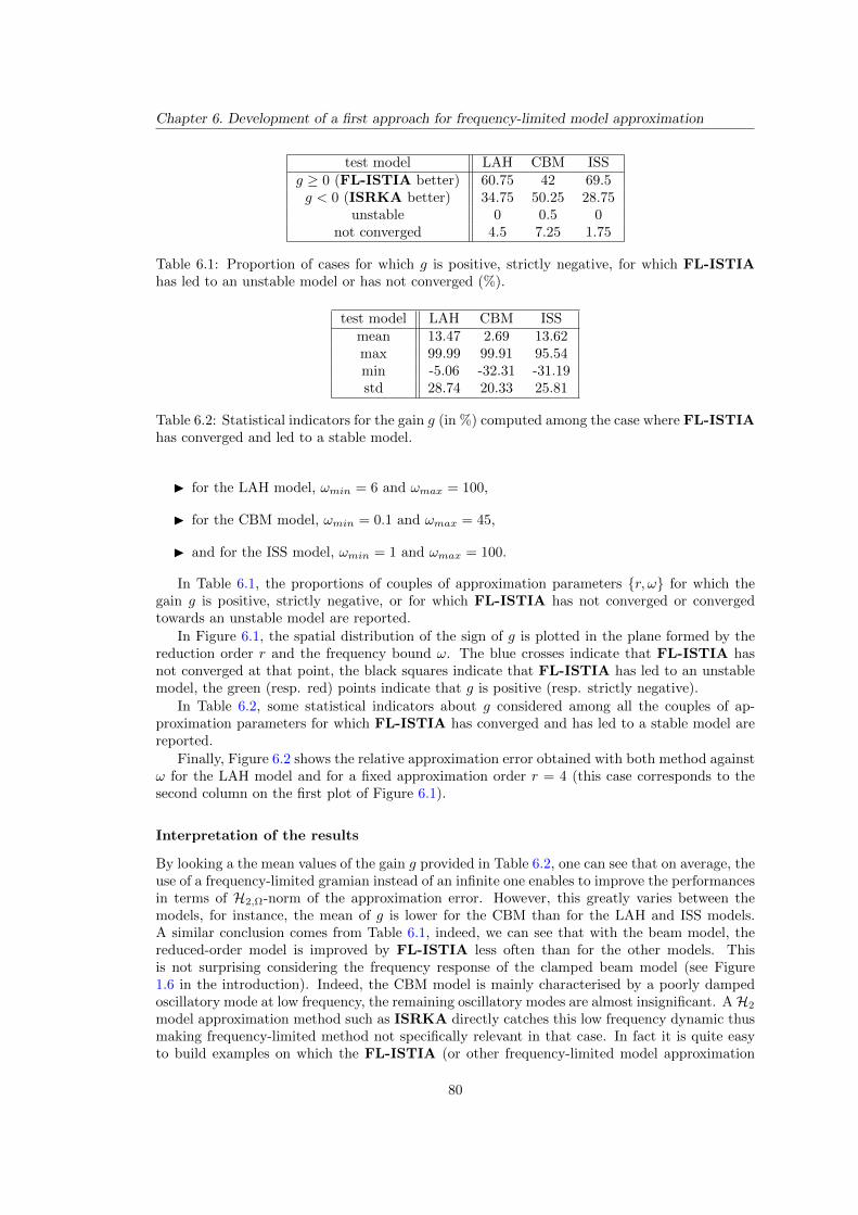
Chapter 6. Development of a first approach for frequency-limited model approximation
test model LAH CBM ISSg ≥ 0 (FL-ISTIA better) 60.75 42 69.5g < 0 (ISRKA better) 34.75 50.25 28.75
unstable 0 0.5 0not converged 4.5 7.25 1.75
Table 6.1: Proportion of cases for which g is positive, strictly negative, for which FL-ISTIAhas led to an unstable model or has not converged (%).
test model LAH CBM ISSmean 13.47 2.69 13.62max 99.99 99.91 95.54min -5.06 -32.31 -31.19std 28.74 20.33 25.81
Table 6.2: Statistical indicators for the gain g (in %) computed among the case where FL-ISTIAhas converged and led to a stable model.
I for the LAH model, ωmin = 6 and ωmax = 100,
I for the CBM model, ωmin = 0.1 and ωmax = 45,
I and for the ISS model, ωmin = 1 and ωmax = 100.
In Table 6.1, the proportions of couples of approximation parameters r, ω for which thegain g is positive, strictly negative, or for which FL-ISTIA has not converged or convergedtowards an unstable model are reported.
In Figure 6.1, the spatial distribution of the sign of g is plotted in the plane formed by thereduction order r and the frequency bound ω. The blue crosses indicate that FL-ISTIA hasnot converged at that point, the black squares indicate that FL-ISTIA has led to an unstablemodel, the green (resp. red) points indicate that g is positive (resp. strictly negative).
In Table 6.2, some statistical indicators about g considered among all the couples of ap-proximation parameters for which FL-ISTIA has converged and has led to a stable model arereported.
Finally, Figure 6.2 shows the relative approximation error obtained with both method againstω for the LAH model and for a fixed approximation order r = 4 (this case corresponds to thesecond column on the first plot of Figure 6.1).
Interpretation of the results
By looking a the mean values of the gain g provided in Table 6.2, one can see that on average, theuse of a frequency-limited gramian instead of an infinite one enables to improve the performancesin terms of H2,Ω-norm of the approximation error. However, this greatly varies between themodels, for instance, the mean of g is lower for the CBM than for the LAH and ISS models.A similar conclusion comes from Table 6.1, indeed, we can see that with the beam model, thereduced-order model is improved by FL-ISTIA less often than for the other models. Thisis not surprising considering the frequency response of the clamped beam model (see Figure1.6 in the introduction). Indeed, the CBM model is mainly characterised by a poorly dampedoscillatory mode at low frequency, the remaining oscillatory modes are almost insignificant. AH2
model approximation method such as ISRKA directly catches this low frequency dynamic thusmaking frequency-limited method not specifically relevant in that case. In fact it is quite easyto build examples on which the FL-ISTIA (or other frequency-limited model approximation
80
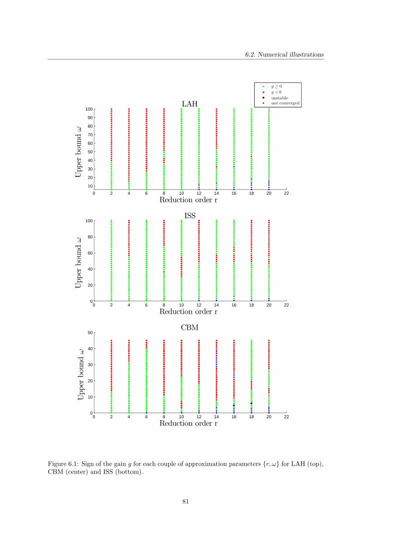
6.2. Numerical illustrations
0 2 4 6 8 10 12 14 16 18 20 22
10
20
30
40
50
60
70
80
90
100LAH
Reduction order r
Upper
bou
ndω
g ≥ 0
g < 0
unstablenot converged
0 2 4 6 8 10 12 14 16 18 20 220
20
40
60
80
100ISS
Upper
bou
ndω
Reduction order r
0 2 4 6 8 10 12 14 16 18 20 220
10
20
30
40
50CBM
Upper
bou
ndω
Reduction order r
Figure 6.1: Sign of the gain g for each couple of approximation parameters r, ω for LAH (top),CBM (center) and ISS (bottom).
81
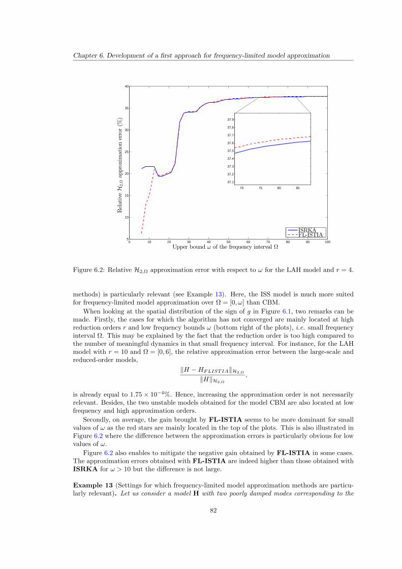
Chapter 6. Development of a first approach for frequency-limited model approximation
0 10 20 30 40 50 60 70 80 90 1005
10
15
20
25
30
35
40
Upper bound ω of the frequency interval Ω
RelativeH
2,Ω
approximationerror(%
)
ISRKAFL-ISTIA
70 75 80 85
37.1
37.2
37.3
37.4
37.5
37.6
37.7
37.8
37.9
Figure 6.2: Relative H2,Ω approximation error with respect to ω for the LAH model and r = 4.
methods) is particularly relevant (see Example 13). Here, the ISS model is much more suitedfor frequency-limited model approximation over Ω = [0, ω] than CBM.
When looking at the spatial distribution of the sign of g in Figure 6.1, two remarks can bemade. Firstly, the cases for which the algorithm has not converged are mainly located at highreduction orders r and low frequency bounds ω (bottom right of the plots), i.e. small frequencyinterval Ω. This may be explained by the fact that the reduction order is too high compared tothe number of meaningful dynamics in that small frequency interval. For instance, for the LAHmodel with r = 10 and Ω = [0, 6], the relative approximation error between the large-scale andreduced-order models,
‖H −HFLISTIA‖H2,Ω
‖H‖H2,Ω
,
is already equal to 1.75 × 10⁻⁴%. Hence, increasing the approximation order is not necessarilyrelevant. Besides, the two unstable models obtained for the model CBM are also located at lowfrequency and high approximation orders.
Secondly, on average, the gain brought by FL-ISTIA seems to be more dominant for smallvalues of ω as the red stars are mainly located in the top of the plots. This is also illustrated inFigure 6.2 where the difference between the approximation errors is particularly obvious for lowvalues of ω.
Figure 6.2 also enables to mitigate the negative gain obtained by FL-ISTIA in some cases.The approximation errors obtained with FL-ISTIA are indeed higher than those obtained withISRKA for ω > 10 but the difference is not large.
Example 13 (Settings for which frequency-limited model approximation methods are particu-larly relevant). Let us consider a model H with two poorly damped modes corresponding to the
82
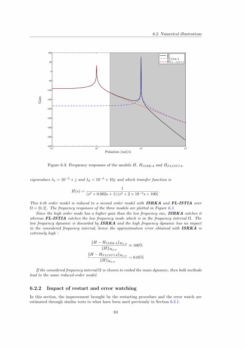
6.2. Numerical illustrations
10−1
100
101
102
−400
−350
−300
−250
−200
−150
−100
−50
0
50
100
Pulsation (rad/s)
Gain
HHISRKAHFL−IST IA
Figure 6.3: Frequency responses of the models H, HISRKA and HFLISTIA.
eigenvalues λ1 = 10−3 + j and λ2 = 10−5 + 10j and which transfer function is
H(s) =1
(s2 + 0.002s+ 1) (s2 + 2× 10⁻⁵s+ 100).
This 4-th order model is reduced to a second order model with ISRKA and FL-ISTIA overΩ = [0, 2]. The frequency responses of the three models are plotted in Figure 6.3.
Since the high order mode has a higher gain than the low frequency one, ISRKA catches itwhereas FL-ISTIA catches the low frequency mode which is in the frequency interval Ω. Thelow frequency dynamic is discarded by ISRKA and the high frequency dynamic has no impactin the considered frequency interval, hence the approximation error obtained with ISRKA isextremely high :
‖H −HISRKA‖H2,Ω
‖H‖H2,Ω
≈ 100%
‖H −HFLISTIA‖H2,Ω
‖H‖H2,Ω
= 0.05%
If the considered frequency interval Ω is chosen to embed the main dynamic, then both methodslead to the same reduced-order model.
6.2.2 Impact of restart and error watching
In this section, the improvement brought by the restarting procedure and the error watch areestimated through similar tests to what have been used previously in Section 6.2.1.
83
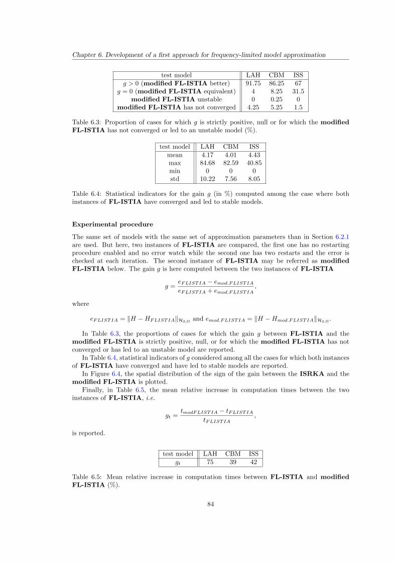
Chapter 6. Development of a first approach for frequency-limited model approximation
test model LAH CBM ISSg > 0 (modified FL-ISTIA better) 91.75 86.25 67
g = 0 (modified FL-ISTIA equivalent) 4 8.25 31.5modified FL-ISTIA unstable 0 0.25 0
modified FL-ISTIA has not converged 4.25 5.25 1.5
Table 6.3: Proportion of cases for which g is strictly positive, null or for which the modifiedFL-ISTIA has not converged or led to an unstable model (%).
test model LAH CBM ISSmean 4.17 4.01 4.43max 84.68 82.59 40.85min 0 0 0std 10.22 7.56 8.05
Table 6.4: Statistical indicators for the gain g (in %) computed among the case where bothinstances of FL-ISTIA have converged and led to stable models.
Experimental procedure
The same set of models with the same set of approximation parameters than in Section 6.2.1are used. But here, two instances of FL-ISTIA are compared, the first one has no restartingprocedure enabled and no error watch while the second one has two restarts and the error ischecked at each iteration. The second instance of FL-ISTIA may be referred as modifiedFL-ISTIA below. The gain g is here computed between the two instances of FL-ISTIA
g =eFLISTIA − emod.FLISTIAeFLISTIA + emod.FLISTIA
,
where
eFLISTIA = ‖H −HFLISTIA‖H2,Ωand emod.FLISTIA = ‖H −Hmod.FLISTIA‖H2,Ω
.
In Table 6.3, the proportions of cases for which the gain g between FL-ISTIA and themodified FL-ISTIA is strictly positive, null, or for which the modified FL-ISTIA has notconverged or has led to an unstable model are reported.
In Table 6.4, statistical indicators of g considered among all the cases for which both instancesof FL-ISTIA have converged and have led to stable models are reported.
In Figure 6.4, the spatial distribution of the sign of the gain between the ISRKA and themodified FL-ISTIA is plotted.
Finally, in Table 6.5, the mean relative increase in computation times between the twoinstances of FL-ISTIA, i.e.
gt =tmodFLISTIA − tFLISTIA
tFLISTIA,
is reported.
test model LAH CBM ISSgt 75 39 42
Table 6.5: Mean relative increase in computation times between FL-ISTIA and modifiedFL-ISTIA (%).
84
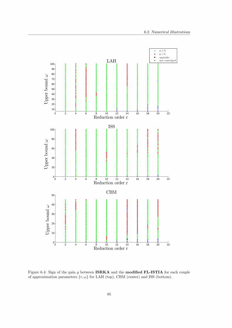
6.2. Numerical illustrations
0 2 4 6 8 10 12 14 16 18 20 22
10
20
30
40
50
60
70
80
90
100LAH
Reduction order r
Upper
bou
ndω
g ≥ 0
g < 0
unstablenot converged
0 2 4 6 8 10 12 14 16 18 20 220
20
40
60
80
100ISS
Upper
bou
ndω
Reduction order r
0 2 4 6 8 10 12 14 16 18 20 220
10
20
30
40
50CBM
Upper
bou
ndω
Reduction order r
Figure 6.4: Sign of the gain g between ISRKA and the modified FL-ISTIA for each coupleof approximation parameters r, ω for LAH (top), CBM (center) and ISS (bottom).
85
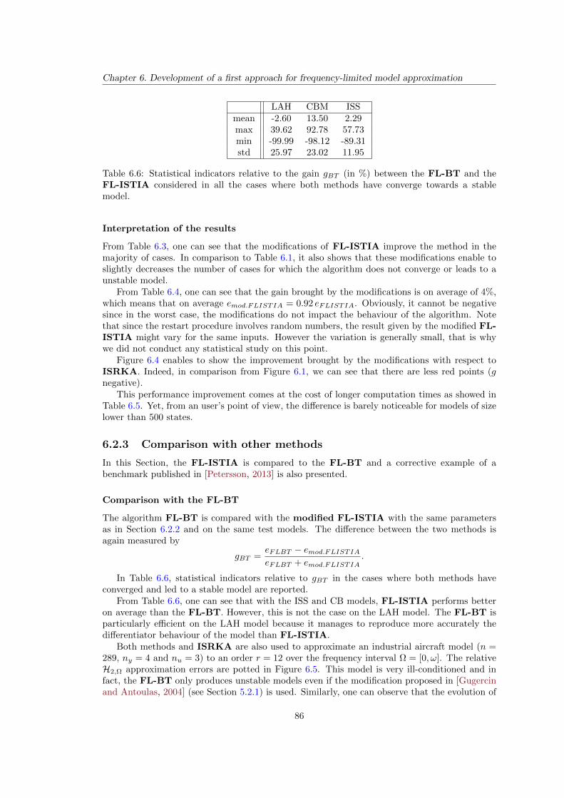
Chapter 6. Development of a first approach for frequency-limited model approximation
LAH CBM ISSmean -2.60 13.50 2.29max 39.62 92.78 57.73min -99.99 -98.12 -89.31std 25.97 23.02 11.95
Table 6.6: Statistical indicators relative to the gain gBT (in %) between the FL-BT and theFL-ISTIA considered in all the cases where both methods have converge towards a stablemodel.
Interpretation of the results
From Table 6.3, one can see that the modifications of FL-ISTIA improve the method in themajority of cases. In comparison to Table 6.1, it also shows that these modifications enable toslightly decreases the number of cases for which the algorithm does not converge or leads to aunstable model.
From Table 6.4, one can see that the gain brought by the modifications is on average of 4%,which means that on average emod.FLISTIA = 0.92 eFLISTIA. Obviously, it cannot be negativesince in the worst case, the modifications do not impact the behaviour of the algorithm. Notethat since the restart procedure involves random numbers, the result given by the modified FL-ISTIA might vary for the same inputs. However the variation is generally small, that is whywe did not conduct any statistical study on this point.
Figure 6.4 enables to show the improvement brought by the modifications with respect toISRKA. Indeed, in comparison from Figure 6.1, we can see that there are less red points (gnegative).
This performance improvement comes at the cost of longer computation times as showed inTable 6.5. Yet, from an user’s point of view, the difference is barely noticeable for models of sizelower than 500 states.
6.2.3 Comparison with other methods
In this Section, the FL-ISTIA is compared to the FL-BT and a corrective example of abenchmark published in [Petersson, 2013] is also presented.
Comparison with the FL-BT
The algorithm FL-BT is compared with the modified FL-ISTIA with the same parametersas in Section 6.2.2 and on the same test models. The difference between the two methods isagain measured by
gBT =eFLBT − emod.FLISTIAeFLBT + emod.FLISTIA
.
In Table 6.6, statistical indicators relative to gBT in the cases where both methods haveconverged and led to a stable model are reported.
From Table 6.6, one can see that with the ISS and CB models, FL-ISTIA performs betteron average than the FL-BT. However, this is not the case on the LAH model. The FL-BT isparticularly efficient on the LAH model because it manages to reproduce more accurately thedifferentiator behaviour of the model than FL-ISTIA.
Both methods and ISRKA are also used to approximate an industrial aircraft model (n =289, ny = 4 and nu = 3) to an order r = 12 over the frequency interval Ω = [0, ω]. The relativeH2,Ω approximation errors are potted in Figure 6.5. This model is very ill-conditioned and infact, the FL-BT only produces unstable models even if the modification proposed in [Gugercinand Antoulas, 2004] (see Section 5.2.1) is used. Similarly, one can observe that the evolution of
86
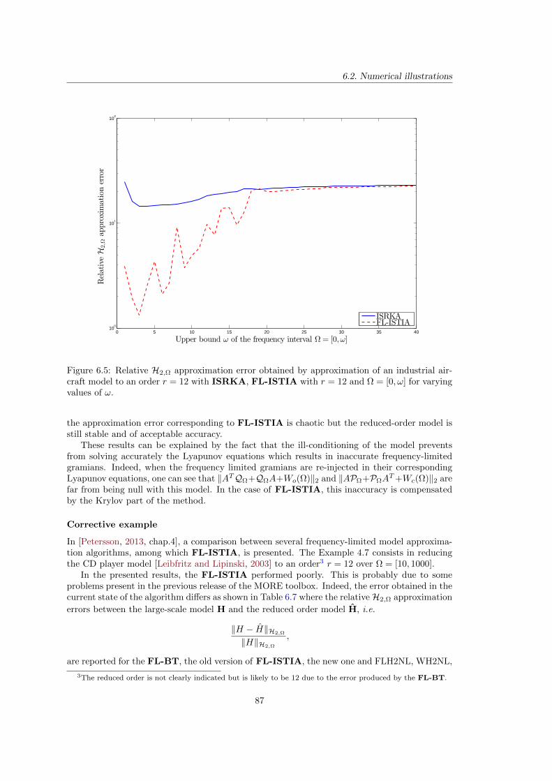
6.2. Numerical illustrations
0 5 10 15 20 25 30 35 4010
0
101
102
Upper bound ω of the frequency interval Ω= [0, ω]
RelativeH
2,Ω
approximationerror
ISRKAFL-ISTIA
Figure 6.5: Relative H2,Ω approximation error obtained by approximation of an industrial air-craft model to an order r = 12 with ISRKA, FL-ISTIA with r = 12 and Ω = [0, ω] for varyingvalues of ω.
the approximation error corresponding to FL-ISTIA is chaotic but the reduced-order model isstill stable and of acceptable accuracy.
These results can be explained by the fact that the ill-conditioning of the model preventsfrom solving accurately the Lyapunov equations which results in inaccurate frequency-limitedgramians. Indeed, when the frequency limited gramians are re-injected in their correspondingLyapunov equations, one can see that ‖ATQΩ+QΩA+Wo(Ω)‖2 and ‖APΩ+PΩA
T+Wc(Ω)‖2 arefar from being null with this model. In the case of FL-ISTIA, this inaccuracy is compensatedby the Krylov part of the method.
Corrective example
In [Petersson, 2013, chap.4], a comparison between several frequency-limited model approxima-tion algorithms, among which FL-ISTIA, is presented. The Example 4.7 consists in reducingthe CD player model [Leibfritz and Lipinski, 2003] to an order3 r = 12 over Ω = [10, 1000].
In the presented results, the FL-ISTIA performed poorly. This is probably due to someproblems present in the previous release of the MORE toolbox. Indeed, the error obtained in thecurrent state of the algorithm differs as shown in Table 6.7 where the relativeH2,Ω approximation
errors between the large-scale model H and the reduced order model H, i.e.
‖H − H‖H2,Ω
‖H‖H2,Ω
,
are reported for the FL-BT, the old version of FL-ISTIA, the new one and FLH2NL, WH2NL,
3The reduced order is not clearly indicated but is likely to be 12 due to the error produced by the FL-BT.
87
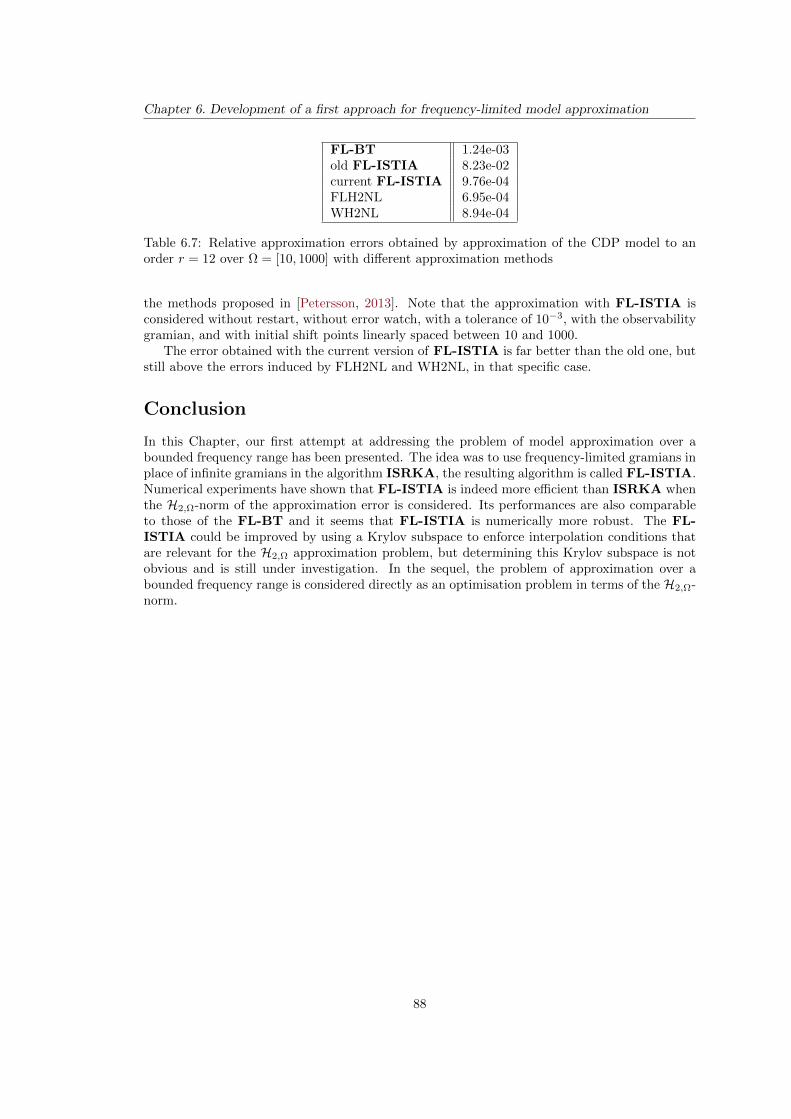
Chapter 6. Development of a first approach for frequency-limited model approximation
FL-BT 1.24e-03old FL-ISTIA 8.23e-02current FL-ISTIA 9.76e-04FLH2NL 6.95e-04WH2NL 8.94e-04
Table 6.7: Relative approximation errors obtained by approximation of the CDP model to anorder r = 12 over Ω = [10, 1000] with different approximation methods
the methods proposed in [Petersson, 2013]. Note that the approximation with FL-ISTIA isconsidered without restart, without error watch, with a tolerance of 10−3, with the observabilitygramian, and with initial shift points linearly spaced between 10 and 1000.
The error obtained with the current version of FL-ISTIA is far better than the old one, butstill above the errors induced by FLH2NL and WH2NL, in that specific case.
Conclusion
In this Chapter, our first attempt at addressing the problem of model approximation over abounded frequency range has been presented. The idea was to use frequency-limited gramians inplace of infinite gramians in the algorithm ISRKA, the resulting algorithm is called FL-ISTIA.Numerical experiments have shown that FL-ISTIA is indeed more efficient than ISRKA whenthe H2,Ω-norm of the approximation error is considered. Its performances are also comparableto those of the FL-BT and it seems that FL-ISTIA is numerically more robust. The FL-ISTIA could be improved by using a Krylov subspace to enforce interpolation conditions thatare relevant for the H2,Ω approximation problem, but determining this Krylov subspace is notobvious and is still under investigation. In the sequel, the problem of approximation over abounded frequency range is considered directly as an optimisation problem in terms of the H2,Ω-norm.
88
Chapter 7
Formulation of the H2,Ω-norm withthe poles and residues of the trans-fer function
The poles-residues representation of a LTI model is not the most numerically robust represen-tation that exists and it is dedicated (in order to be applicable) to models having semi-simplepoles only. But the associated formulation of the H2-norm had led to convenient first-orderoptimality conditions in the context of optimal H2 model approximation (see Chapter 4). Thatis why in this chapter, this representation is used to derive a poles-residues formulation for thefrequency-limited H2-norm for which only the gramian formulation existed (see Section 2.2).
Note that this poles-residues formulation of the norm is used in Chapters 8 and 9 to developan algorithm that minimises the JH2,Ω
-norm of the approximation error between a large-scalemodel and a reduced-order one. Hence, this Chapter plays a pivotal role in this manuscript.
In a first step in Section 7.1, the case of models with semi-simple poles only is addressed.The formulation is then generalised to models with high order poles in Section 7.2. This poles-residues formulation is finally used in Section 7.3 to derive two bounds on the H∞-norm of LTIdynamical models which are of great interest in the context of model approximation (see Section9.2.3 and Chapter 10).
The poles-residues formulations of the H2,Ω-norm has been presented in [Vuillemin et al.,2012b] and in [Vuillemin et al., 2014c] for the models with semi-simple and high order poles,respectively, and the bounds on the H∞-norm has been presented in [Vuillemin et al., 2014d].
Contents7.1 Case of models with semi-simple poles only . . . . . . . . . . . . . 89
7.1.1 Preliminary results on complex functions . . . . . . . . . . . . . . . . 90
7.1.2 Poles-residues formulation of the H2,Ω-norm . . . . . . . . . . . . . . . 91
7.1.3 Numerical illustration of the formulation . . . . . . . . . . . . . . . . . 93
7.2 Case of models with higher order poles . . . . . . . . . . . . . . . . 94
7.2.1 Poles-residues formulation of the H2,Ω-norm for models with high or-der poles . . . . . . . . . . . . . . . . . . . . . . . . . . . . . . . . . . 94
7.2.2 Special case 1 : n eigenvalues of multiplicity 1 (semi-simple case) . . . 97
7.2.3 Special case 2 : 1 eigenvalue of multiplicity n . . . . . . . . . . . . . . 97
7.3 Upper bounds of the H∞-norm . . . . . . . . . . . . . . . . . . . . . 98
7.3.1 Formulation of the bounds . . . . . . . . . . . . . . . . . . . . . . . . . 98
7.3.2 Computation of the bounds . . . . . . . . . . . . . . . . . . . . . . . . 100
7.3.3 Experimental study of the bounds quality . . . . . . . . . . . . . . . . 102
7.3.4 Construction of a frequency template . . . . . . . . . . . . . . . . . . 104
7.1 Case of models with semi-simple poles only
The poles-residues (or spectral) formulation of the frequency-limited H2-norm for LTI modelswith semi-simple poles only involves the principal value of the inverse tangent function which
89
Chapter 7. Formulation of the H2,Ω-norm with the poles and residues of the transfer function
is introduced in Section 7.1.1. The main Theorem is then stated in Section 7.1.2. Finally, thisformulation of the norm is compared in some numerical examples in Section 7.1.3.
7.1.1 Preliminary results on complex functions
The principal value1 of the inverse tangent function relies on the principal value of the complexlogarithm which relies itself on the principal value of the complex argument. Hence, the defini-tions of both functions are conditioned by the way the complex argument is defined, which ismerely a convention, but an important one. In this work, we have chosen a widely used con-vention (see [Abramowitz and Stegun, 1964, chap. 4] or [Corless et al., 2000]) for the principalvalue of the complex argument. The argument arg(z) of a non-null complex number z 6= 0 ischosen to lie in ]−π, π], i.e.
π < arg(z) ≤ π,
for z 6= 0. This definition induces a branch cut along the negative real axis (−∞, 0] which isinherited by the functions based on this convention. In particular, the principal value of thecomplex logarithm, which is presented in Definition 7, has the same branch cut as the complexargument.
Definition 7 (Principal value of the complex logarithm). The principal value of the logarithmof z, denoted log(z), is defined for z 6= 0 as
log(z) = ln (|z|) + jarg(z),
where ln(x) is the natural logarithm of x ∈ R∗+.
There exist various definitions for the complex inverse tangent function. Here, the definitionsuggested in [Kahan, 1987] is considered (see Remark 13 for some remarks about alternativeformulations). It is recalled in Definition 8. The function atan(z), z 6= ±j is single-valued andcontinuous excepted along two branch cuts (−j∞,−j]∪[j, j∞) (illustrated in Appendix B.1).
Definition 8 (Principal value of the complex inverse tangent). The principal value of the inversetangent of z, denoted atan(z), is defined for z 6= ±j as
atan(z) =1
2j(log(1 + jz)− log(1− jz)) .
Remark 13 (About the definition of the principal value of the complex inverse tangent). Theprincipal value of the complex inverse tangent can also be defined, for z 6= ±j as
1
2jlog
(1 + jz
1− jz
),
which yields the same branch cuts as Definition 8 but does not coincide everywhere in the complexplane. Indeed as shown in [Haber, 2012] (and illustrated in Appendix B.1),
log
(1 + jz
1− jz
)=
π + log(1 + jz)− log(1− jz) if z ∈ (−j∞,−j[
log(1 + jz)− log(1− jz) otherwise.
In this study, the use of the complex inverse tangent function is merely a notational conveniencethat enables to compact the expression of the H2,Ω-norm. The same results could have beenobtained by sticking with the complex logarithm. Moreover the hypothesis considered in Theorem10 on the value of ω ensures that one cannot be in a case where the two definitions are notequivalent.
1In this work, the principal values of complex functions are denoted by lower-case (and bold) names. Thenotation often varies in the literature, here it is the same as in [Abramowitz and Stegun, 1964, chap. 4] butdiffers, for instance, from the notation employed in the documentation of Mathematica.
90
7.1. Case of models with semi-simple poles only
Yet, generally speaking, special care must be taken when using atan(z) in practice becausethe convention of the function might vary between different software. Indeed, Mathematica doc-umentation explicitly mentions that Definition 8 is used2, but there is no indication in the doc-umentations of Matlab R©, Scilab and Octave.
7.1.2 Poles-residues formulation of the H2,Ω-norm
Theorem 10 (Spectral expression of the H2,Ω-norm). Given a frequency interval Ω = [0, ω]and a continuous MIMO LTI dynamical model H of degree n. Suppose that the two followinghypothesis are satisfied
1. The transfer function associated to H can be written as
H(s) =
n∑i=1
Φis− λi
+D ∈ Cny×nu ,
where D ∈ Rny×nu , Φi ∈ Cny×nu and λi ∈ C (i = 1, . . . , n).
2. If there are indexes j1, . . . , jK such that λj1 , . . . , λjK are purely imaginary, then the up-per bound ω of the interval Ω is smaller than their modulus, i.e. ω < min |λj1 |, . . . , |λjK |.
Then, the frequency-limited H2-norm of H can be written as
‖H‖2H2,Ω=
n∑i=1
n∑k=1
ai,k +ω
πtr(DDT
)− 2
π
n∑i=1
tr(ΦiD
T)atan
(ω
λi
)(7.1)
where
ai,k =
2
πtr
(ΦiΦ
Tk
λi + λk
)atan
(ω
λi
)if λi + λk 6= 0
− 1
πtr
(ωΦiΦ
Tk
ω2 + λiλi
)otherwise.
Proof. Since A is diagonalisable, the transfer function H(s) can be decomposed as (see Section2.1.1)
H(s) =
n∑i=1
Φis− λi
+D,
where Φi ∈ Cny×nu is the residue associated to the eigenvalue λi. Using this decomposition inthe definition of the H2,Ω-norm (Definition 4) enables to divide it into several elements than canbe integrated under some additional assumptions in particular cases. Indeed, if some poles areon the imaginary axis, the upper bound ω of the frequency interval Ω must be smaller than thesmallest modulus of those imaginary poles. The full proof can be found in Appendix A.1.
The two expressions for the ai,k ensure that (7.1) is continuous for every values of λi andλk. The second expression is the limit of the first one as |λi + λk| tends towards 0. Note thatλi = −λk happens if the model has purely imaginary poles and can also happen if it has polesin the right half-plane located symmetrically to some stable poles with respect to the imaginaryaxis. Those specific cases are discarded in the sequel. Besides both cases do not occur if stablemodels are considered.
Note that if λi + λk 6= 0 ∀ i, k = 1, . . . , n, then equation (7.1) can be rewritten as
‖H‖2H2,Ω=
n∑i=1
− 2
πtr(ΦiH(−λi)T
)atan
(ω
λi
)+ω
πtr(DDT
), (7.2)
2see http://mathworld.wolfram.com/InverseTangent.html
91
Chapter 7. Formulation of the H2,Ω-norm with the poles and residues of the transfer function
which is close to the poles-residues expression of the H2-norm (see Section 2.1.1)
‖H‖2H2=
n∑i=1
tr(ΦiH(−λi)T
). (7.3)
Apart from the non-proper terms, the difference between equations (7.2) and (7.3) comes fromthe coefficients atan( ωλi ) which acts as weightings on each contribution in the sum.
If the model H is strictly proper, then the limit of the H2,Ω-norm of H as ω tends towardsinfinity is determined by the limits of atan( ωλi ). The latter are presented in Corollary 1 and theformer in Theorem 11.
Corollary 1. Given λ ∈ C∗ and ω > 0, the limits of atan(ωλ
), where atan(z) is given by
Definition 8, are
limω→∞
atan(ωλ
)=
−π2 if Re (λ) < 0π2 if Re (λ) > 0π2 if Re (λ) = 0 and Im (λ) < 0−π2 if Re (λ) = 0 and Im (λ) > 0
.
Proof. See Appendix B.2.
Theorem 11 (Link with the H2-norm). Let us consider a frequency interval Ω = [0, ω] and astrictly proper model H with n− poles λ−i in the left half-plane and n+ poles λ+
k in the right-halfplane that satisfies λ−i + λ+
k 6= 0 ∀ i, k. The transfer function of H is written as
H(s) =
n−∑i=1
Φ−is− λ−i
+
n+∑k=1
Φ+k
s− λ+k
.
Then, the limit of the frequency-limited H2-norm as ω tends towards ∞ is given by
limω→∞
‖H‖H2,Ω=
n−∑i=1
tr(Φ+i H
T (−λ+i ))−
n+∑k=1
tr(Φ+kH
T (−λ+k )).
Proof. Using Corollary 1 in equation (7.2) leads to the result.
In the case of asymptotically stable models, Theorem 11 states that the frequency-limitedH2-norm of H tends towards its H2-norm as ω tends towards ∞. For a model H = (A,B,C)which poles are located in the right half-plane, theH2,Ω-norm of H tends towards theH2-norm ofthe model which realisation is (−A,B,C). This is not surprising, since the H2,Ω-norm measuresthe impact of the transfer function on the imaginary axis, whether the poles are located on theright or on the left of the axis does not modify this impact.
If the model H is not strictly proper or has poles on the imaginary axis, then the limit isinfinite.
About the computation of the H2,Ω-norm
To efficiently compute the H2,Ω-norm (7.2), the residues Φi should not explicitly be computed.Indeed, by noting X ∈ Cn×n the matrix which columns are the right eigenvectors of A, Y = X−1,and ei the canonical basis column vector, it turns out that
tr(ΦiΦ
Tk
)= tr
(CXeiei
TY B(CXekekTY B)T
)= ek
T (CX)TCX︸ ︷︷ ︸M1
eieiT Y B(Y B)T︸ ︷︷ ︸
M2
ek.
92
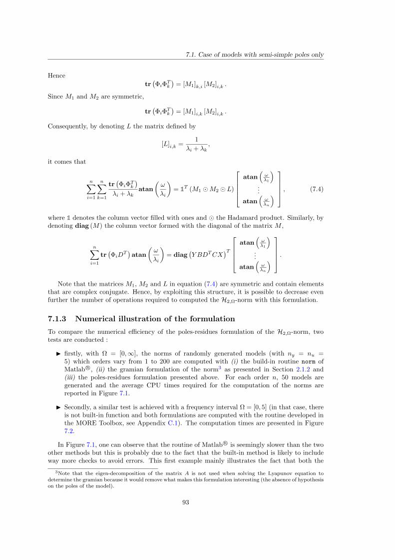
7.1. Case of models with semi-simple poles only
Hence
tr(ΦiΦ
Tk
)= [M1]k,i [M2]i,k .
Since M1 and M2 are symmetric,
tr(ΦiΦ
Tk
)= [M1]i,k [M2]i,k .
Consequently, by denoting L the matrix defined by
[L]i,k =1
λi + λk,
it comes that
n∑i=1
n∑k=1
tr(ΦiΦ
Tk
)λi + λk
atan
(ω
λi
)= 1T (M1 M2 L)
atan
(ωλ1
)...
atan(ωλn
) , (7.4)
where 1 denotes the column vector filled with ones and the Hadamard product. Similarly, bydenoting diag (M) the column vector formed with the diagonal of the matrix M ,
n∑i=1
tr(ΦiD
T)atan
(ω
λi
)= diag
(Y BDTCX
)T
atan(ωλ1
)...
atan(ωλn
) .
Note that the matrices M1, M2 and L in equation (7.4) are symmetric and contain elementsthat are complex conjugate. Hence, by exploiting this structure, it is possible to decrease evenfurther the number of operations required to computed the H2,Ω-norm with this formulation.
7.1.3 Numerical illustration of the formulation
To compare the numerical efficiency of the poles-residues formulation of the H2,Ω-norm, twotests are conducted :
I firstly, with Ω = [0,∞], the norms of randomly generated models (with ny = nu =5) which orders vary from 1 to 200 are computed with (i) the build-in routine norm ofMatlab R©, (ii) the gramian formulation of the norm3 as presented in Section 2.1.2 and(iii) the poles-residues formulation presented above. For each order n, 50 models aregenerated and the average CPU times required for the computation of the norms arereported in Figure 7.1.
I Secondly, a similar test is achieved with a frequency interval Ω = [0, 5] (in that case, thereis not built-in function and both formulations are computed with the routine developed inthe MORE Toolbox, see Appendix C.1). The computation times are presented in Figure7.2.
In Figure 7.1, one can observe that the routine of Matlab R© is seemingly slower than the twoother methods but this is probably due to the fact that the built-in method is likely to includeway more checks to avoid errors. This first example mainly illustrates the fact that both the
3Note that the eigen-decomposition of the matrix A is not used when solving the Lyapunov equation todetermine the gramian because it would remove what makes this formulation interesting (the absence of hypothesison the poles of the model).
93
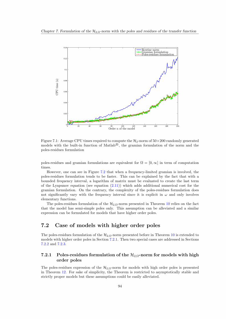
Chapter 7. Formulation of the H2,Ω-norm with the poles and residues of the transfer function
0 20 40 60 80 100 120 140 160 180 2000
0.02
0.04
0.06
0.08
0.1
0.12
0.14
CPU
time(s)
Order n of the model
Routine normGramian formulationPoles-residues formulation
Figure 7.1: Average CPU times required to compute theH2-norm of 50×200 randomly generatedmodels with the built-in function of Matlab R©, the gramian formulation of the norm and thepoles-residues formulation
poles-residues and gramian formulations are equivalent for Ω = [0,∞] in term of computationtimes.
However, one can see in Figure 7.2 that when a frequency-limited gramian is involved, thepoles-residues formulation tends to be faster. This can be explained by the fact that with abounded frequency interval, a logarithm of matrix must be evaluated to create the last termof the Lyapunov equation (see equation (2.11)) which adds additional numerical cost for thegramian formulation. On the contrary, the complexity of the poles-residues formulation doesnot significantly vary with the frequency interval since it is explicit in ω and only involveselementary functions.
The poles-residues formulation of the H2,Ω-norm presented in Theorem 10 relies on the factthat the model has semi-simple poles only. This assumption can be alleviated and a similarexpression can be formulated for models that have higher order poles.
7.2 Case of models with higher order poles
The poles-residues formulation of the H2,Ω-norm presented before in Theorem 10 is extended tomodels with higher order poles in Section 7.2.1. Then two special cases are addressed in Sections7.2.2 and 7.2.3.
7.2.1 Poles-residues formulation of the H2,Ω-norm for models with highorder poles
The poles-residues expression of the H2,Ω-norm for models with high order poles is presentedin Theorem 12. For sake of simplicity, the Theorem is restricted to asymptotically stable andstrictly proper models but these assumptions could be easily alleviated.
94
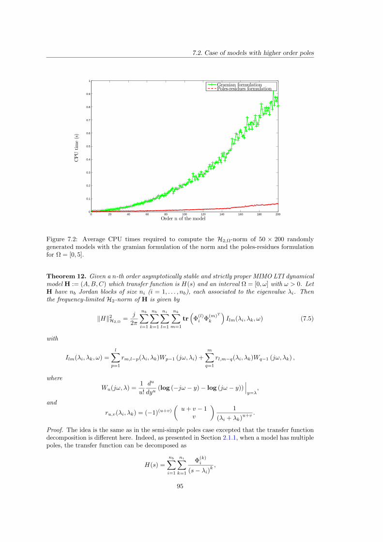
7.2. Case of models with higher order poles
0 20 40 60 80 100 120 140 160 180 2000
0.1
0.2
0.3
0.4
0.5
0.6
0.7
0.8
0.9
1
CPU
time(s)
Order n of the model
Gramian formulationPoles-residues formulation
Figure 7.2: Average CPU times required to compute the H2,Ω-norm of 50 × 200 randomlygenerated models with the gramian formulation of the norm and the poles-residues formulationfor Ω = [0, 5].
Theorem 12. Given a n-th order asymptotically stable and strictly proper MIMO LTI dynamicalmodel H := (A,B,C) which transfer function is H(s) and an interval Ω = [0, ω] with ω > 0. LetH have nb Jordan blocks of size ni (i = 1, . . . , nb), each associated to the eigenvalue λi. Thenthe frequency-limited H2-norm of H is given by
‖H‖2H2,Ω=
j
2π
nb∑i=1
nb∑k=1
ni∑l=1
nk∑m=1
tr(
Φ(l)i Φ
(m)T
k
)Ilm(λi, λk, ω) (7.5)
with
Ilm(λi, λk, ω) =
l∑p=1
rm,l−p(λi, λk)Wp−1 (jω, λi) +
m∑q=1
rl,m−q(λi, λk)Wq−1 (jω, λk) ,
where
Wu(jω, λ) =1
u!
du
dyu(log (−jω − y)− log (jω − y))
∣∣∣y=λ
,
and
ru,v(λi, λk) = (−1)(u+v)
(u+ v − 1
v
)1
(λi + λk)u+v .
Proof. The idea is the same as in the semi-simple poles case excepted that the transfer functiondecomposition is different here. Indeed, as presented in Section 2.1.1, when a model has multiplepoles, the transfer function can be decomposed as
H(s) =
nb∑i=1
ni∑k=1
Φ(k)i
(s− λi)k,
95
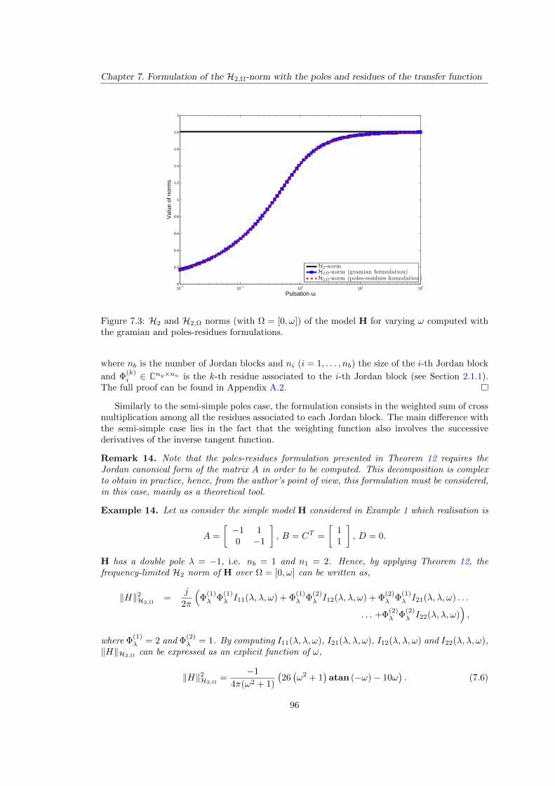
Chapter 7. Formulation of the H2,Ω-norm with the poles and residues of the transfer function
10−2
10−1
100
101
102
0
0.2
0.4
0.6
0.8
1
1.2
1.4
1.6
1.8
2
Pulsation ω
Val
ue o
f nor
ms
H2-normH2,Ω-norm (gramian formulation)H2,Ω-norm (poles-residues formulation)
Figure 7.3: H2 and H2,Ω norms (with Ω = [0, ω]) of the model H for varying ω computed withthe gramian and poles-residues formulations.
where nb is the number of Jordan blocks and ni (i = 1, . . . , nb) the size of the i-th Jordan block
and Φ(k)i ∈ Cny×nu is the k-th residue associated to the i-th Jordan block (see Section 2.1.1).
The full proof can be found in Appendix A.2.
Similarly to the semi-simple poles case, the formulation consists in the weighted sum of crossmultiplication among all the residues associated to each Jordan block. The main difference withthe semi-simple case lies in the fact that the weighting function also involves the successivederivatives of the inverse tangent function.
Remark 14. Note that the poles-residues formulation presented in Theorem 12 requires theJordan canonical form of the matrix A in order to be computed. This decomposition is complexto obtain in practice, hence, from the author’s point of view, this formulation must be considered,in this case, mainly as a theoretical tool.
Example 14. Let us consider the simple model H considered in Example 1 which realisation is
A =
[−1 10 −1
], B = CT =
[11
], D = 0.
H has a double pole λ = −1, i.e. nb = 1 and n1 = 2. Hence, by applying Theorem 12, thefrequency-limited H2 norm of H over Ω = [0, ω] can be written as,
‖H‖2H2,Ω=
j
2π
(Φ
(1)λ Φ
(1)λ I11(λ, λ, ω) + Φ
(1)λ Φ
(2)λ I12(λ, λ, ω) + Φ
(2)λ Φ
(1)λ I21(λ, λ, ω) . . .
. . . +Φ(2)λ Φ
(2)λ I22(λ, λ, ω)
),
where Φ(1)λ = 2 and Φ
(2)λ = 1. By computing I11(λ, λ, ω), I21(λ, λ, ω), I12(λ, λ, ω) and I22(λ, λ, ω),
‖H‖H2,Ωcan be expressed as an explicit function of ω,
‖H‖2H2,Ω=
−1
4π(ω2 + 1)
(26(ω2 + 1
)atan (−ω)− 10ω
). (7.6)
96
7.2. Case of models with higher order poles
The frequency-limited H2-norm of H is plotted in Figure 7.3 against the upper bound ω of thefrequency interval Ω. It is computed with equation (7.6) and with the gramian formulation ofthe norm (see Section 2.1.2). Obviously, both formulations are equivalent and since the model isasymptotically stable, its H2,Ω-norm tends towards its H2-norm as ω tends towards infinity.
7.2.2 Special case 1 : n eigenvalues of multiplicity 1 (semi-simple case)
Let us consider a stable and strictly proper model H with n simple eigenvalues which corre-
sponding residues are Φ(1)i (i = 1, . . . , n). Since ni = 1 (i = 1, . . . , n), the general expression of
the H2,Ω-norm (7.5) becomes
‖H‖2H2,Ω=
j
2π
n∑i=1
n∑k=1
tr(
Φ(1)i Φ
(1)T
k
)I11(λi, λk, ω),
where the weighting functions I11(λi, λk, ω) are only composed of two terms
I11(λi, λk, ω) = r1,0(λi, λk) (W0 (jω, λi) +W0 (jω, λk)) ,
with
W0(jω, λi) = log (−jω − λi)− log (jω − λi) := 2jatan
(ω
λi
),
and
r1,0(λi, λk) = − 1
(λi + λk).
Hence
‖H‖2H2,Ω=
j
2π
n∑i=1
n∑k=1
−2jtr
(Φ
(1)i Φ
(1)T
k
)(λi + λk)
(atan
(ω
λi
)+ atan
(ω
λk
))By reordering the sums so that the similar terms are grouped together, the poles-residues for-mulation of the H2,Ω-norm for model with semi-simple poles (7.1) is retrieved :
‖H‖2H2,Ω=
2
π
n∑i=1
n∑k=1
tr(
Φ(1)i Φ
(1)T
k
)λi + λk
atan
(ω
λi
)
7.2.3 Special case 2 : 1 eigenvalue of multiplicity n
Given an asymptotically stable and strictly proper model H with one single Jordan block of
size n associated to the eigenvalue λ which corresponding residues are Φ(i)λ (i = 1, . . . , n), the
expression presented in [Antoulas, 2005, chap. 5],
‖H‖2H2= tr
(n∑i=1
Φ(i)λ
(i− 1)!
di−1
dsi−1H(−s)T
∣∣∣s=λ
), (7.7)
is retrieved when ω tends towards infinity from equation (7.5). Indeed, first, note that, for u > 0,
Wu(jω, λ) =1
u
(1
(jω − λ)u −
1
(−jω − λ)u
),
hence for u > 0,limω→∞
|Wu(jω, λ)| = 0.
Besides, since H is assumed to be asymptotically stable (see Corollary 1),
limω→∞
W0(jω, λ) = −jπ.
97
Chapter 7. Formulation of the H2,Ω-norm with the poles and residues of the transfer function
The limits of the weighting functions Ilm(λ, λ, ω) (l = 1, . . . , n and m = 1, . . . , n) are thus givenby
limω→∞
Ilm(λ, λ, ω) = −j2πrl,k−1(λ, λ),
where
rl,k−1(λ, λ) = (−1)l+k−1
(l + k − 2k − 1
)1
(2λ)l+k−1
.
By replacing the weighting functions by their limits, it comes that
limω→∞
‖H‖2H2,Ω=
n∑k=1
n∑l=1
tr(
Φ(k)λ Φ
(l)T
λ
)rl,k−1(λ, λ).
Finally, noticing that
n∑l=1
Φ(l)T
λ rl,k−1(λ, λ) =1
(k − 1)!
dk−1
dsk−1H(−s)T
∣∣∣s=λ
,
leads to expression (7.7).
7.3 Upper bounds of the H∞-norm
In this section, the poles-residues formulation of the H2,Ω-norm is used to derive two upperbounds on the H∞-norm of LTI dynamical models which are of great interest in the approx-imation context. Theses bounds are formulated in Section 7.3.1. Their computation is thenpresented in Section 7.3.2 and an experimental study of their conservatism is performed in Sec-tion 7.3.3. And finally, in Section 7.3.4, a method aimed at building a frequency template ofLTI models is developed. Such a frequency template is useful in the context of model approx-imation to bound the approximation error so that the large-scale model can be represented byan uncertain low-order model and used for control or analysis purposes.
7.3.1 Formulation of the bounds
The link between the H∞-norm (Definition 5) and the H2,Ω-norm is presented in Theorem 13.It is grounded on the Frobenius norm which is firstly recalled in Definition 9.
Definition 9 (Frobenius norm). The Frobenius norm of a matrix M ∈ Cm×n is given by
‖M‖F :=√
tr (MMH) =
√√√√min(m,n)∑i=1
σ2i ,
where the σi, i = 1, . . . ,min (m,n) are the singular values of M .
Theorem 13 (H∞ upper bound). Let us consider an asymptotically stable MIMO LTI dynamicalmodel H which transfer function is H(s). Then its H∞-norm is upper bounded by the derivativewith respect to ω of its H2,Ω-norm (with Ω = [0, ω]) as follows
‖H‖H∞ ≤ maxω∈R
√πd‖H‖2H2,Ω
dω.
Moreover, the bound becomes an equality if H is SISO.
98
7.3. Upper bounds of the H∞-norm
Proof. Considering the definition of the H∞-norm, it comes that
‖H‖H∞ = maxω∈R
σmax(H(jω)) ≤ maxω∈R‖H(jω)‖F .
The H2,Ω-norm can be written as the integral of the transfer function’s Frobenius norm over[−ω, ω], i.e.
‖H‖2H2,Ω=
1
2π
∫ ω
−ω‖H(jν)‖2F dν.
Thus by differentiating this expression with respect to ω, it is clear that
‖H(jω)‖2F = πd‖H‖2H2,Ω
dω,
which concludes the proof.
The general bound presented in Theorem 13 can be conveniently expressed based on thespectral expression of the frequency-limited H2-norm. Indeed, by differentiating (7.2) withrespect to ω, it comes that
d‖H‖2H2,[0,ω]
dω= − 2
π
n∑i=1
tr(φiH(−λi)T
) λiλ2i + ω2
+1
πtr(DDT
)=
n∑i=1
fi(ω) +1
πtr(DDT
).
Each function fi is a scalar complex valued function and comes with its complex conjugate whichmakes the sum real. Therefore, only the real parts of the functions fi need to be considered, i.e.
gi(ω) = Re (fi(ω)) =ai(x
2i − y2
i + ω2) + 2biyixi(x2i − y2
i + ω2)2 + 4x2i y
2i
, (7.8)
wherexi + jyi = λi andai + jbi = − 2
π tr(φiH(−λi)T
)λi,
(7.9)
The general bound presented in Theorem 13 can then be reformulated and another bound canbe derived as presented in Theorem 14.
Theorem 14 (Upper bounds on the H∞-norm). Given a MIMO LTI dynamical system H oforder n with a diagonalisable realisation matrix A, its H∞-norm is upper bounded by Γ and Γas follows,
‖H‖H∞ ≤
√√√√tr (DDT ) + maxω∈R+
π
n∑i=1
gi(ω)
︸ ︷︷ ︸Γ
≤
√√√√tr (DDT ) + π
n∑i=1
maxω∈R+
gi(ω)
︸ ︷︷ ︸Γ
where the functions gi are defined as in (7.8).
Obviously, by restricting the domain of research in Theorem 14 from R+ to some frequencyinterval Ω, these bounds can be used to bound the maximal singular value of the transfer functionover Ω, i.e.
maxω∈Ω
σmax(H(jω)) ≤
√√√√tr (DDT ) + maxω∈Ω
π
n∑i=1
gi(ω)
︸ ︷︷ ︸ΓΩ
≤
√√√√tr (DDT ) + π
n∑i=1
maxω∈Ω
gi(ω)
︸ ︷︷ ︸ΓΩ
.
An illustration of the bounds ΓΩ and ΓΩ is presented in Example 15. Note that the subscript Ωmay be dropped when Ω = [0,∞].
99
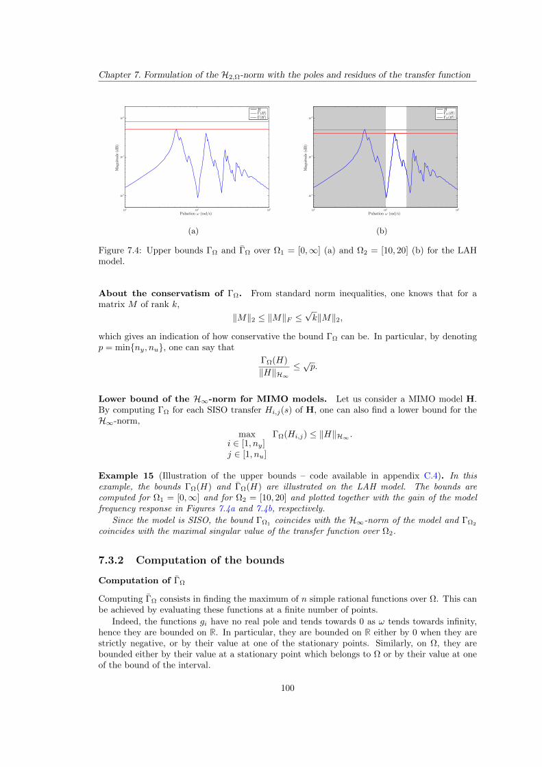
Chapter 7. Formulation of the H2,Ω-norm with the poles and residues of the transfer function
100
101
102
10−4
10−3
10−2
Magnitude(dB)
Pulsation ω (rad/s)
HΓ(H)Γ(H)
(a)
Pulsation ω (rad/s)
Magnitude(dB)
100
101
102
10−4
10−3
10−2
HΓΩ(H)ΓΩ(H)
(b)
Figure 7.4: Upper bounds ΓΩ and ΓΩ over Ω1 = [0,∞] (a) and Ω2 = [10, 20] (b) for the LAHmodel.
About the conservatism of ΓΩ. From standard norm inequalities, one knows that for amatrix M of rank k,
‖M‖2 ≤ ‖M‖F ≤√k‖M‖2,
which gives an indication of how conservative the bound ΓΩ can be. In particular, by denotingp = minny, nu, one can say that
ΓΩ(H)
‖H‖H∞≤ √p.
Lower bound of the H∞-norm for MIMO models. Let us consider a MIMO model H.By computing ΓΩ for each SISO transfer Hi,j(s) of H, one can also find a lower bound for theH∞-norm,
maxi ∈ [1, ny]j ∈ [1, nu]
ΓΩ(Hi,j) ≤ ‖H‖H∞ .
Example 15 (Illustration of the upper bounds – code available in appendix C.4). In thisexample, the bounds ΓΩ(H) and ΓΩ(H) are illustrated on the LAH model. The bounds arecomputed for Ω1 = [0,∞] and for Ω2 = [10, 20] and plotted together with the gain of the modelfrequency response in Figures 7.4a and 7.4b, respectively.
Since the model is SISO, the bound ΓΩ1coincides with the H∞-norm of the model and ΓΩ2
coincides with the maximal singular value of the transfer function over Ω2.
7.3.2 Computation of the bounds
Computation of ΓΩ
Computing ΓΩ consists in finding the maximum of n simple rational functions over Ω. This canbe achieved by evaluating these functions at a finite number of points.
Indeed, the functions gi have no real pole and tends towards 0 as ω tends towards infinity,hence they are bounded on R. In particular, they are bounded on R either by 0 when they arestrictly negative, or by their value at one of the stationary points. Similarly, on Ω, they arebounded either by their value at a stationary point which belongs to Ω or by their value at oneof the bound of the interval.
100
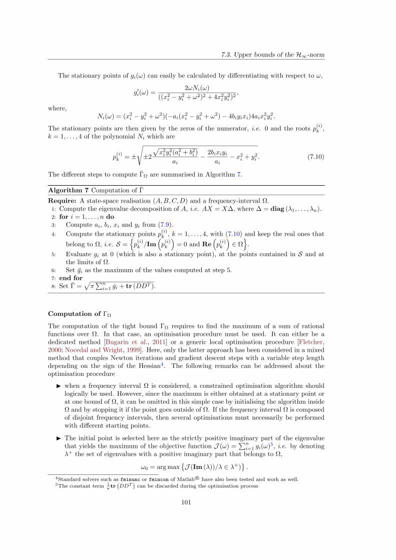
7.3. Upper bounds of the H∞-norm
The stationary points of gi(ω) can easily be calculated by differentiating with respect to ω,
g′i(ω) =2ωNi(ω)
((x2i − y2
i + ω2)2 + 4x2i y
2i )2
,
where,Ni(ω) = (x2
i − y2i + ω2)(−ai(x2
i − y2i + ω2)− 4biyixi)4aix
2i y
2i .
The stationary points are then given by the zeros of the numerator, i.e. 0 and the roots p(i)k ,
k = 1, . . . , 4 of the polynomial Ni which are
p(i)k = ±
ñ2
√x2i y
2i (a2
i + b2i )
ai− 2bixiyi
ai− x2
i + y2i . (7.10)
The different steps to compute ΓΩ are summarised in Algorithm 7.
Algorithm 7 Computation of Γ
Require: A state-space realisation (A,B,C,D) and a frequency-interval Ω.1: Compute the eigenvalue decomposition of A, i.e. AX = X∆, where ∆ = diag (λ1, . . . , λn).2: for i = 1, . . . , n do3: Compute ai, bi, xi and yi from (7.9).
4: Compute the stationary points p(i)k , k = 1, . . . , 4, with (7.10) and keep the real ones that
belong to Ω, i.e. S =p
(i)k /Im
(p
(i)k
)= 0 and Re
(p
(i)k
)∈ Ω
.
5: Evaluate gi at 0 (which is also a stationary point), at the points contained in S and atthe limits of Ω.
6: Set gi as the maximum of the values computed at step 5.7: end for8: Set Γ =
√π∑ni=1 gi + tr (DDT ).
Computation of ΓΩ
The computation of the tight bound ΓΩ requires to find the maximum of a sum of rationalfunctions over Ω. In that case, an optimisation procedure must be used. It can either be adedicated method [Bugarin et al., 2011] or a generic local optimisation procedure [Fletcher,2000; Nocedal and Wright, 1999]. Here, only the latter approach has been considered in a mixedmethod that couples Newton iterations and gradient descent steps with a variable step lengthdepending on the sign of the Hessian4. The following remarks can be addressed about theoptimisation procedure
I when a frequency interval Ω is considered, a constrained optimisation algorithm shouldlogically be used. However, since the maximum is either obtained at a stationary point orat one bound of Ω, it can be omitted in this simple case by initialising the algorithm insideΩ and by stopping it if the point goes outside of Ω. If the frequency interval Ω is composedof disjoint frequency intervals, then several optimisations must necessarily be performedwith different starting points.
I The initial point is selected here as the strictly positive imaginary part of the eigenvaluethat yields the maximum of the objective function J (ω) =
∑ni=1 gi(ω)5, i.e. by denoting
λ+ the set of eigenvalues with a positive imaginary part that belongs to Ω,
ω0 = arg maxJ (Im (λ))/λ ∈ λ+)
.
4Standard solvers such as fminunc or fmincon of Matlab R© have also been tested and work as well.5The constant term 1
πtr(DDT
)can be discarded during the optimisation process
101
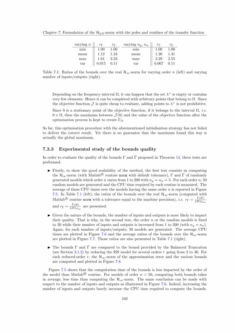
Chapter 7. Formulation of the H2,Ω-norm with the poles and residues of the transfer function
varying n rΓ rΓ
min 1.00 1.00mean 1.12 1.24max 1.61 2.23var 0.015 0.11
varying ny, nu rΓ rΓ
min 1.00 1.00mean 1.26 1.41max 2.29 2.55var 0.067 0.11
Table 7.1: Ratios of the bounds over the real H∞-norm for varying order n (left) and varyingnumber of inputs/outputs (right).
Depending on the frequency interval Ω, it can happen that the set λ+ is empty or containsvery few elements. Hence it can be completed with arbitrary points that belong to Ω. Sincethe objective function J is quite cheap to evaluate, adding points to λ+ is not prohibitive.
Since 0 is a stationary point of the objective function, if it belongs to the interval Ω, i.e.0 ∈ Ω, then the maximum between J (0) and the value of the objective function after theoptimisation process is kept to create ΓΩ.
So far, this optimisation procedure with the aforementioned initialisation strategy has not failedto deliver the correct result. Yet there is no guarantee that the maximum found this way isactually the global maximum.
7.3.3 Experimental study of the bounds quality
In order to evaluate the quality of the bounds Γ and Γ proposed in Theorem 14, three tests areperformed.
I Firstly, to show the good scalability of the method, the first test consists in computingthe H∞-norm (with Matlab R© routine norm with default tolerance), Γ and Γ of randomlygenerated models which order n varies from 1 to 200 with ny = nu = 5. For each order n, 50random models are generated and the CPU time required by each routine is measured. Theaverage of these CPU times over the models having the same order n is reported in Figure7.5. In Table 7.1 (left), the ratios of the bounds over the real H∞-norm (computed with
Matlab R© routine norm with a tolerance equal to the machine precision), i.e. rΓ = Γ(H)‖H‖H∞
and rΓ = Γ(H)‖H‖H∞
are presented.
I Given the nature of the bounds, the number of inputs and outputs is more likely to impacttheir quality. That is why, in the second test, the order n or the random models is fixedto 20 while their number of inputs and outputs is increased from 1 to 200 (with ny = nu).Again, for each number of inputs/outputs, 50 models are generated. The average CPUtimes are plotted in Figure 7.6 and the average ratios of the bounds over the H∞-normare plotted in Figure 7.7. Those ratios are also presented in Table 7.1 (right).
I The bounds Γ and Γ are compared to the bound provided by the Balanced Truncation(see Section 3.1.2) by reducing the ISS model for several orders r going from 2 to 30. Foreach reduced-order r, the H∞-norm of the approximation error and the various boundsare computed and plotted in Figure 7.8.
Figure 7.5 shows that the computation time of the bounds is less impacted by the order ofthe model than Matlab R© routine. For models of order n > 50, computing both bounds takesin average, less time than computing the H∞-norm. The same conclusion can be made withrespect to the number of inputs and outputs as illustrated in Figure 7.6. Indeed, increasing thenumber of inputs and outputs barely increase the CPU time required to compute the bounds.
102
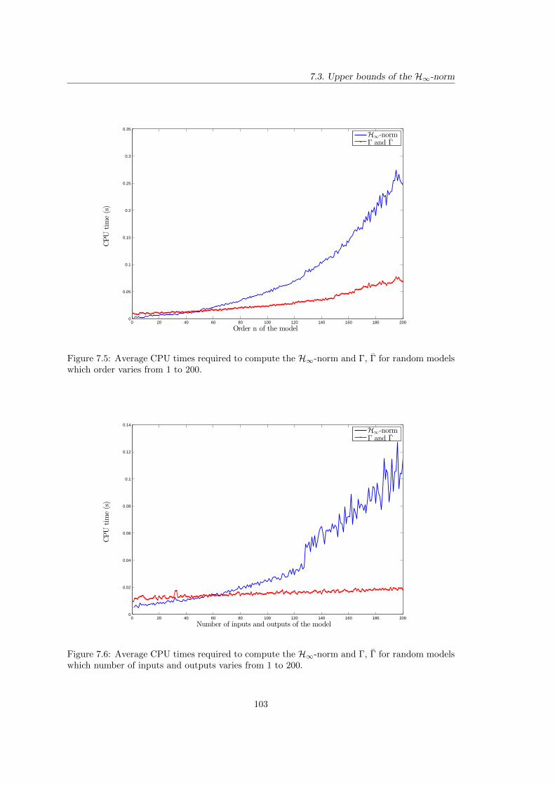
7.3. Upper bounds of the H∞-norm
0 20 40 60 80 100 120 140 160 180 2000
0.05
0.1
0.15
0.2
0.25
0.3
0.35
CPU
time(s)
Order n of the model
H∞-normΓ and Γ
Figure 7.5: Average CPU times required to compute the H∞-norm and Γ, Γ for random modelswhich order varies from 1 to 200.
0 20 40 60 80 100 120 140 160 180 2000
0.02
0.04
0.06
0.08
0.1
0.12
0.14
CPU
time(s)
Number of inputs and outputs of the model
H∞-normΓ and Γ
Figure 7.6: Average CPU times required to compute the H∞-norm and Γ, Γ for random modelswhich number of inputs and outputs varies from 1 to 200.
103
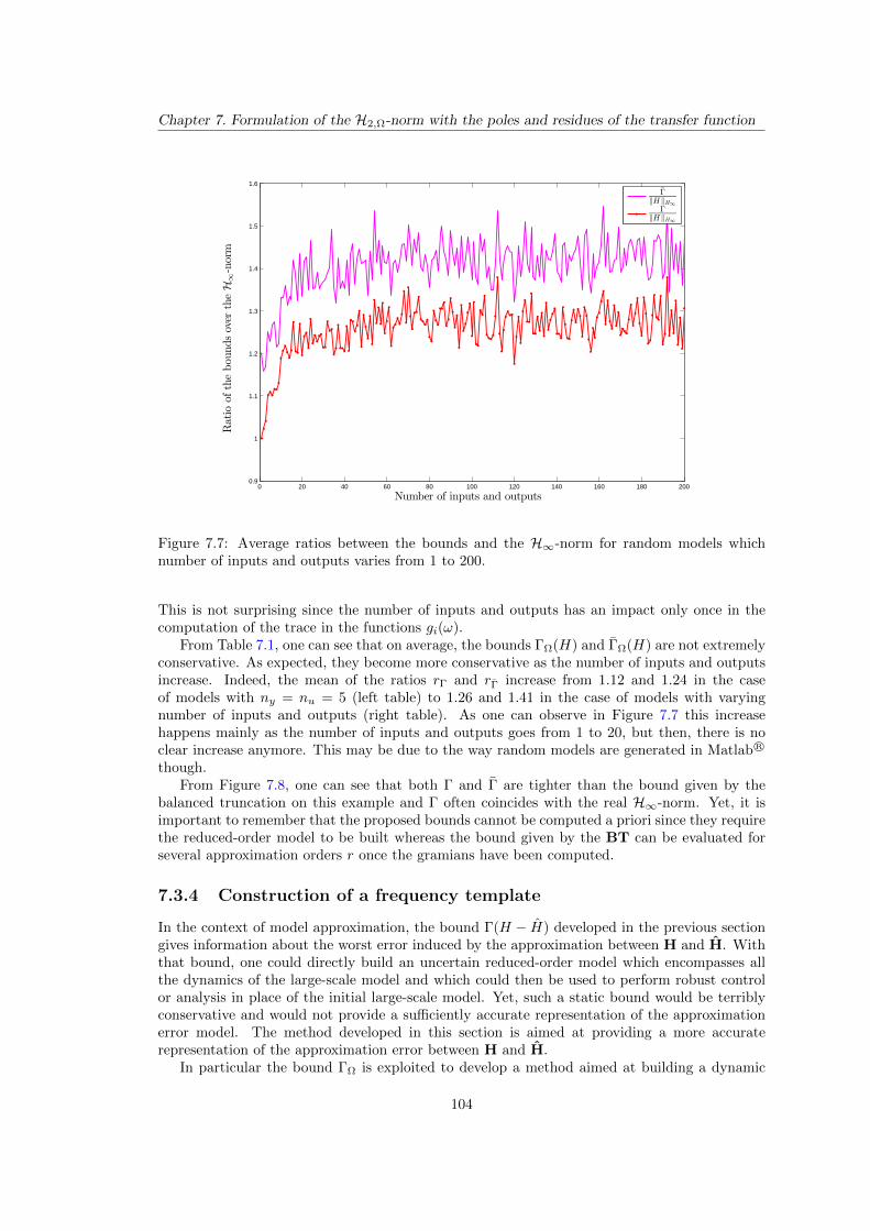
Chapter 7. Formulation of the H2,Ω-norm with the poles and residues of the transfer function
0 20 40 60 80 100 120 140 160 180 2000.9
1
1.1
1.2
1.3
1.4
1.5
1.6
Ratio
ofthebou
ndsover
theH
∞-norm
Number of inputs and outputs
Γ
‖H‖H∞
Γ
‖H‖H∞
Figure 7.7: Average ratios between the bounds and the H∞-norm for random models whichnumber of inputs and outputs varies from 1 to 200.
This is not surprising since the number of inputs and outputs has an impact only once in thecomputation of the trace in the functions gi(ω).
From Table 7.1, one can see that on average, the bounds ΓΩ(H) and ΓΩ(H) are not extremelyconservative. As expected, they become more conservative as the number of inputs and outputsincrease. Indeed, the mean of the ratios rΓ and rΓ increase from 1.12 and 1.24 in the caseof models with ny = nu = 5 (left table) to 1.26 and 1.41 in the case of models with varyingnumber of inputs and outputs (right table). As one can observe in Figure 7.7 this increasehappens mainly as the number of inputs and outputs goes from 1 to 20, but then, there is noclear increase anymore. This may be due to the way random models are generated in Matlab R©
though.From Figure 7.8, one can see that both Γ and Γ are tighter than the bound given by the
balanced truncation on this example and Γ often coincides with the real H∞-norm. Yet, it isimportant to remember that the proposed bounds cannot be computed a priori since they requirethe reduced-order model to be built whereas the bound given by the BT can be evaluated forseveral approximation orders r once the gramians have been computed.
7.3.4 Construction of a frequency template
In the context of model approximation, the bound Γ(H − H) developed in the previous sectiongives information about the worst error induced by the approximation between H and H. Withthat bound, one could directly build an uncertain reduced-order model which encompasses allthe dynamics of the large-scale model and which could then be used to perform robust controlor analysis in place of the initial large-scale model. Yet, such a static bound would be terriblyconservative and would not provide a sufficiently accurate representation of the approximationerror model. The method developed in this section is aimed at providing a more accuraterepresentation of the approximation error between H and H.
In particular the bound ΓΩ is exploited to develop a method aimed at building a dynamic
104
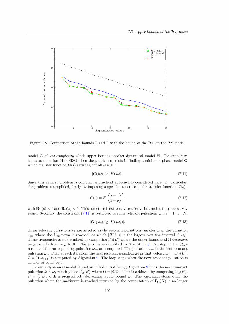
7.3. Upper bounds of the H∞-norm
0 5 10 15 20 25 3010
−4
10−3
10−2
10−1
100
Approximation order r
Valueof
thebou
nd/n
orm
H∞ errorBT boundΓΓ
Figure 7.8: Comparison of the bounds Γ and Γ with the bound of the BT on the ISS model.
model G of low complexity which upper bounds another dynamical model H. For simplicity,let us assume that H is SISO, then the problem consists in finding a minimum phase model Gwhich transfer function G(s) satisfies, for all ω ∈ R+
|G(jω)| ≥ |H(jω)|. (7.11)
Since this general problem is complex, a practical approach is considered here. In particular,the problem is simplified, firstly by imposing a specific structure to the transfer function G(s),
G(s) = K
(s− zs− p
)r, (7.12)
with Re(p) < 0 and Re(z) < 0. This structure is extremely restrictive but makes the process wayeasier. Secondly, the constraint (7.11) is restricted to some relevant pulsations ωk, k = 1, . . . , N ,
|G(jωk)| ≥ |H(jωk)|. (7.13)
These relevant pulsations ωk are selected as the resonant pulsations, smaller than the pulsationω∞ where the H∞-norm is reached, at which |H(jω)| is the largest over the interval [0, ωk].These frequencies are determined by computing ΓΩ(H) where the upper bound ω of Ω decreasesprogressively from ω∞ to 0. This process is described in Algorithm 8. At step 1, the H∞-norm and the corresponding pulsation ω∞ are computed. The pulsation ω∞ is the first resonantpulsation ω1. Then at each iteration, the next resonant pulsation ωk+1 that yields τk+1 = ΓΩ(H),Ω = [0, ωk+1] is computed by Algorithm 9. The loop stops when the next resonant pulsation issmaller or equal to 0.
Given a dynamical model H and an initial pulsation ωi, Algorithm 9 finds the next resonantpulsation ω < ωi which yields ΓΩ(H) where Ω = [0, ω]. This is achieved by computing ΓΩ(H),Ω = [0, ω], with a progressively decreasing upper bound ω. The algorithm stops when thepulsation where the maximum is reached returned by the computation of ΓΩ(H) is no longer
105
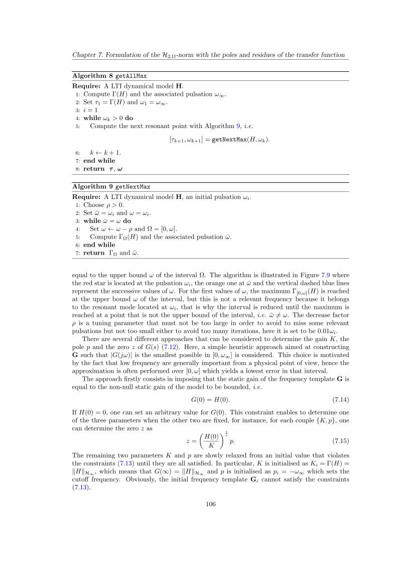
Chapter 7. Formulation of the H2,Ω-norm with the poles and residues of the transfer function
Algorithm 8 getAllMax
Require: A LTI dynamical model H.1: Compute Γ(H) and the associated pulsation ω∞.2: Set τ1 = Γ(H) and ω1 = ω∞.3: i = 14: while ωk > 0 do5: Compute the next resonant point with Algorithm 9, i.e.
[τk+1, ωk+1] = getNextMax(H,ωk).
6: k ← k + 1.7: end while8: return τ , ω
Algorithm 9 getNextMax
Require: A LTI dynamical model H, an initial pulsation ωi.1: Choose ρ > 0.2: Set ω = ωi and ω = ωi.3: while ω = ω do4: Set ω ← ω − ρ and Ω = [0, ω].5: Compute ΓΩ(H) and the associated pulsation ω.6: end while7: return ΓΩ and ω.
equal to the upper bound ω of the interval Ω. The algorithm is illustrated in Figure 7.9 wherethe red star is located at the pulsation ωi, the orange one at ω and the vertical dashed blue linesrepresent the successive values of ω. For the first values of ω, the maximum Γ[0,ω](H) is reachedat the upper bound ω of the interval, but this is not a relevant frequency because it belongsto the resonant mode located at ωi, that is why the interval is reduced until the maximum isreached at a point that is not the upper bound of the interval, i.e. ω 6= ω. The decrease factorρ is a tuning parameter that must not be too large in order to avoid to miss some relevantpulsations but not too small either to avoid too many iterations, here it is set to be 0.01ωi.
There are several different approaches that can be considered to determine the gain K, thepole p and the zero z of G(s) (7.12). Here, a simple heuristic approach aimed at constructingG such that |G(jω)| is the smallest possible in [0, ω∞] is considered. This choice is motivatedby the fact that low frequency are generally important from a physical point of view, hence theapproximation is often performed over [0, ω] which yields a lowest error in that interval.
The approach firstly consists in imposing that the static gain of the frequency template G isequal to the non-null static gain of the model to be bounded, i.e.
G(0) = H(0). (7.14)
If H(0) = 0, one can set an arbitrary value for G(0). This constraint enables to determine oneof the three parameters when the other two are fixed, for instance, for each couple K, p, onecan determine the zero z as
z =
(H(0)
K
) 1r
p. (7.15)
The remaining two parameters K and p are slowly relaxed from an initial value that violatesthe constraints (7.13) until they are all satisfied. In particular, K is initialised as Ki = Γ(H) =‖H‖H∞ , which means that G(∞) = ‖H‖H∞ and p is initialised as pi = −ω∞ which sets thecutoff frequency. Obviously, the initial frequency template Gi cannot satisfy the constraints(7.13).
106
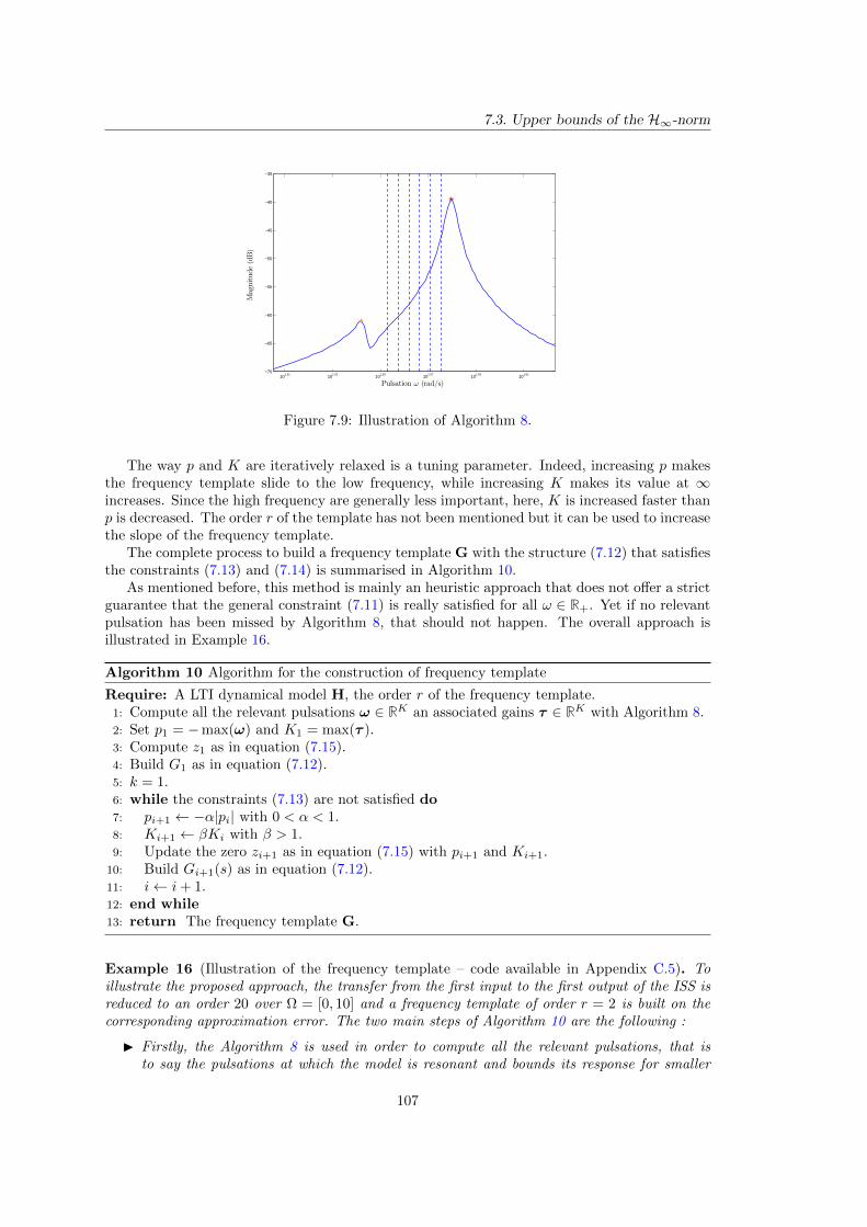
7.3. Upper bounds of the H∞-norm
101.51
101.53
101.55
101.57
101.59
101.61
−70
−65
−60
−55
−50
−45
−40
−35
Magnitude(dB)
Pulsation ω (rad/s)
Figure 7.9: Illustration of Algorithm 8.
The way p and K are iteratively relaxed is a tuning parameter. Indeed, increasing p makesthe frequency template slide to the low frequency, while increasing K makes its value at ∞increases. Since the high frequency are generally less important, here, K is increased faster thanp is decreased. The order r of the template has not been mentioned but it can be used to increasethe slope of the frequency template.
The complete process to build a frequency template G with the structure (7.12) that satisfiesthe constraints (7.13) and (7.14) is summarised in Algorithm 10.
As mentioned before, this method is mainly an heuristic approach that does not offer a strictguarantee that the general constraint (7.11) is really satisfied for all ω ∈ R+. Yet if no relevantpulsation has been missed by Algorithm 8, that should not happen. The overall approach isillustrated in Example 16.
Algorithm 10 Algorithm for the construction of frequency template
Require: A LTI dynamical model H, the order r of the frequency template.1: Compute all the relevant pulsations ω ∈ RK an associated gains τ ∈ RK with Algorithm 8.2: Set p1 = −max(ω) and K1 = max(τ ).3: Compute z1 as in equation (7.15).4: Build G1 as in equation (7.12).5: k = 1.6: while the constraints (7.13) are not satisfied do7: pi+1 ← −α|pi| with 0 < α < 1.8: Ki+1 ← βKi with β > 1.9: Update the zero zi+1 as in equation (7.15) with pi+1 and Ki+1.
10: Build Gi+1(s) as in equation (7.12).11: i← i+ 1.12: end while13: return The frequency template G.
Example 16 (Illustration of the frequency template – code available in Appendix C.5). Toillustrate the proposed approach, the transfer from the first input to the first output of the ISS isreduced to an order 20 over Ω = [0, 10] and a frequency template of order r = 2 is built on thecorresponding approximation error. The two main steps of Algorithm 10 are the following :
I Firstly, the Algorithm 8 is used in order to compute all the relevant pulsations, that isto say the pulsations at which the model is resonant and bounds its response for smaller
107
Chapter 7. Formulation of the H2,Ω-norm with the poles and residues of the transfer function
10−2
10−1
100
101
102
−130
−120
−110
−100
−90
−80
−70
−60
−50
−40
−30
Magnitude(dB)
Pulsation ω (rad/s)
1
2
3
456
789
Figure 7.10: Illustration of the Algorithm 10, computation of all the relevant pulsations.
pulsations. This is illustrated in Figure 7.10 where the numbers indicates the order in whichthe points have been found. The H∞-norm is found first, then the other maximums that arelocated at lower frequencies are computed. On can see that for each i, |H(jωi)| > |H(jω)|for ω ∈ [0, ωi].
I Then, the main loop of Algorithm 10 is executed and transforms the initial frequency tem-plate G1 by successive relaxation of its gain and pole, K and p, into the final one G. Bothfrequency templates are plotted in Figure 7.11 where G1 is the red curve and G is the greenone.
MIMO case
For MIMO models, two uses of Algorithm 10 can be considered,
I firstly, it can be used directly of the whole MIMO model. In that case however, the absolutevalues are replaced by Frobenius norms and the transfer function of the frequency templateG satisfies
‖G(jωk)‖F ≥ ‖H(jωk)‖F , k = 1, . . . , N,‖G(0)‖F = ‖H(0)‖F ,
(7.16)
instead of (7.13) and (7.14). Equation (7.16) induces more conservatism than in the SISOcase, but it enables to exploit the frequency template for control purposes (see Section9.2.3).
I Secondly, Algorithm 10 can be used on each SISO transfers separately. This can have aninterest for simulation since less conservatism than in the first case is introduced.
Conclusion
In this Chapter, the poles-residues formulation of the H2-norm has been extended to the H2,Ω-norm both for models with semi-simple poles only and for models with higher order poles. This
108
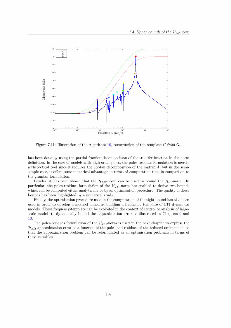
7.3. Upper bounds of the H∞-norm
10−2
10−1
100
101
102
103
−130
−120
−110
−100
−90
−80
−70
−60
−50
−40
−30
Magnitude(dB)
Pulsation ω (rad/s)
HG1G
Figure 7.11: Illustration of the Algorithm 10, construction of the template G from Gi.
has been done by using the partial fraction decomposition of the transfer function in the normdefinition. In the case of models with high order poles, the poles-residues formulation is merelya theoretical tool since it requires the Jordan decomposition of the matrix A, but in the semi-simple case, it offers some numerical advantage in terms of computation time in comparison tothe gramian formulation.
Besides, it has been shown that the H2,Ω-norm can be used to bound the H∞-norm. Inparticular, the poles-residues formulation of the H2,Ω-norm has enabled to derive two boundswhich can be computed either analytically or by an optimisation procedure. The quality of thesebounds has been highlighted by a numerical study.
Finally, the optimisation procedure used in the computation of the tight bound has also beenused in order to develop a method aimed at building a frequency template of LTI dynamicalmodels. These frequency-template can be exploited in the context of control or analysis of large-scale models to dynamically bound the approximation error as illustrated in Chapters 9 and10.
The poles-residues formulation of the H2,Ω-norm is used in the next chapter to express theH2,Ω approximation error as a function of the poles and residues of the reduced-order model sothat the approximation problem can be reformulated as an optimisation problems in terms ofthese variables.
109

Chapter 8
Formulation of the H2,Ω error and
differentiation of its gradient
In this Chapter, the poles-residues formulation of the H2,Ω-norm developed in Chapter 7 isexploited to express the H2,Ω-norm of the approximation error between a large-scale LTI model
H and a reduced-order model H which have both semi-simple poles only. The approach followedin this Chapter is very similar to what have been done to introduce the optimal H2 modelapproximation problem in Chapter 4. The similarities and the key differences between the H2,Ω
and H2 cases are highlighted.In Section 8.1, the formulation of the error is presented together with some practical im-
plementation concerns and in Section 8.2, the approximation error is differentiated in order toexpress the first-order optimality conditions of the optimal H2,Ω approximation problem.
The elements presented throughout this Chapter have partly been published in [Vuilleminet al., 2014b].
Contents8.1 Expression of the approximation error with the poles and residues
of the models . . . . . . . . . . . . . . . . . . . . . . . . . . . . . . . . 111
8.1.1 Poles-residues formulation of the H2,Ω approximation error . . . . . . 111
8.1.2 About the computation of the approximation error . . . . . . . . . . . 117
8.2 Gradient of the error . . . . . . . . . . . . . . . . . . . . . . . . . . . 119
8.2.1 Reminder on Wirtinger Calculus . . . . . . . . . . . . . . . . . . . . . 119
8.2.2 Gradient of the H2,Ω approximation error . . . . . . . . . . . . . . . . 122
8.1 Expression of the approximation error with the polesand residues of the models
This Section is aimed at presenting the poles-residues formulation of the H2,Ω approximation er-ror. The theoretical aspects are presented in Section 8.1.1 while the numerical ones are discussedin Section 8.1.2.
8.1.1 Poles-residues formulation of the H2,Ω approximation error
The poles-residues expression of the squared approximation error JH2,Ω = ‖H − H‖2H2,Ωbetween
a large-scale model and a reduced-order one is presented in Theorem 15 for MIMO models andin Remark 15, the SISO case is highlighted. In order to shorten the equations, the followingnotation is used from now on,
aω,λ =2
πatan
(ωλ
).
Theorem 15 (Poles-residues formulation of the H2,Ω approximation error). Let us consider afrequency interval Ω = [0, ω], a n-th order LTI dynamical model H and a r-th order LTI dynam-ical model H which have semi-simple poles only and which transfer functions are respectively
111
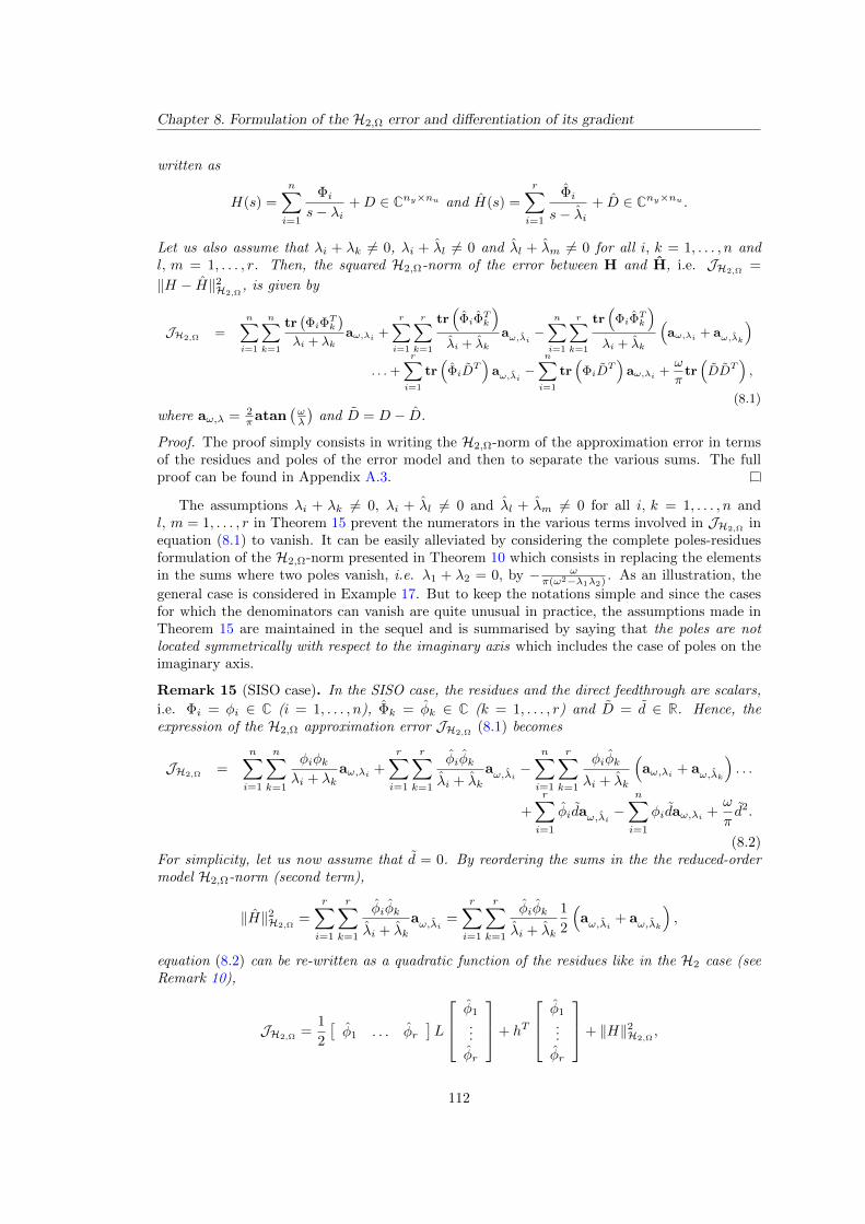
Chapter 8. Formulation of the H2,Ω error and differentiation of its gradient
written as
H(s) =
n∑i=1
Φis− λi
+D ∈ Cny×nu and H(s) =
r∑i=1
Φi
s− λi+ D ∈ Cny×nu .
Let us also assume that λi + λk 6= 0, λi + λl 6= 0 and λl + λm 6= 0 for all i, k = 1, . . . , n andl, m = 1, . . . , r. Then, the squared H2,Ω-norm of the error between H and H, i.e. JH2,Ω
=
‖H − H‖2H2,Ω, is given by
JH2,Ω =
n∑i=1
n∑k=1
tr(ΦiΦ
Tk
)λi + λk
aω,λi +
r∑i=1
r∑k=1
tr(
ΦiΦTk
)λi + λk
aω,λi −n∑i=1
r∑k=1
tr(
ΦiΦTk
)λi + λk
(aω,λi + aω,λk
). . .+
r∑i=1
tr(
ΦiDT)
aω,λi −n∑i=1
tr(
ΦiDT)
aω,λi +ω
πtr(DDT
),
(8.1)
where aω,λ = 2πatan
(ωλ
)and D = D − D.
Proof. The proof simply consists in writing the H2,Ω-norm of the approximation error in termsof the residues and poles of the error model and then to separate the various sums. The fullproof can be found in Appendix A.3.
The assumptions λi + λk 6= 0, λi + λl 6= 0 and λl + λm 6= 0 for all i, k = 1, . . . , n andl, m = 1, . . . , r in Theorem 15 prevent the numerators in the various terms involved in JH2,Ω
inequation (8.1) to vanish. It can be easily alleviated by considering the complete poles-residuesformulation of the H2,Ω-norm presented in Theorem 10 which consists in replacing the elementsin the sums where two poles vanish, i.e. λ1 + λ2 = 0, by − ω
π(ω2−λ1λ2) . As an illustration, the
general case is considered in Example 17. But to keep the notations simple and since the casesfor which the denominators can vanish are quite unusual in practice, the assumptions made inTheorem 15 are maintained in the sequel and is summarised by saying that the poles are notlocated symmetrically with respect to the imaginary axis which includes the case of poles on theimaginary axis.
Remark 15 (SISO case). In the SISO case, the residues and the direct feedthrough are scalars,
i.e. Φi = φi ∈ C (i = 1, . . . , n), Φk = φk ∈ C (k = 1, . . . , r) and D = d ∈ R. Hence, theexpression of the H2,Ω approximation error JH2,Ω
(8.1) becomes
JH2,Ω =
n∑i=1
n∑k=1
φiφkλi + λk
aω,λi +
r∑i=1
r∑k=1
φiφk
λi + λkaω,λi −
n∑i=1
r∑k=1
φiφk
λi + λk
(aω,λi + aω,λk
). . .
+
r∑i=1
φidaω,λi −n∑i=1
φidaω,λi +ω
πd2.
(8.2)For simplicity, let us now assume that d = 0. By reordering the sums in the the reduced-ordermodel H2,Ω-norm (second term),
‖H‖2H2,Ω=
r∑i=1
r∑k=1
φiφk
λi + λkaω,λi =
r∑i=1
r∑k=1
φiφk
λi + λk
1
2
(aω,λi + aω,λk
),
equation (8.2) can be re-written as a quadratic function of the residues like in the H2 case (seeRemark 10),
JH2,Ω=
1
2
[φ1 . . . φr
]L
φ1
...
φr
+ hT
φ1
...
φr
+ ‖H‖2H2,Ω,
112
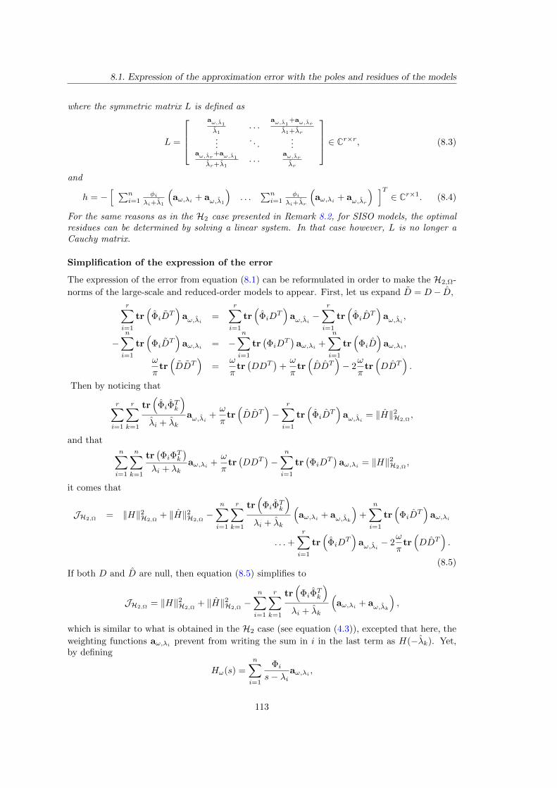
8.1. Expression of the approximation error with the poles and residues of the models
where the symmetric matrix L is defined as
L =
aω,λ1
λ1. . .
aω,λ1+aω,λr
λ1+λr...
. . ....
aω,λr+aω,λ1
λr+λ1. . .
aω,λrλr
∈ Cr×r, (8.3)
and
h = −[ ∑n
i=1φi
λi+λ1
(aω,λi + aω,λ1
). . .
∑ni=1
φiλi+λr
(aω,λi + aω,λr
) ]T∈ Cr×1. (8.4)
For the same reasons as in the H2 case presented in Remark 8.2, for SISO models, the optimalresidues can be determined by solving a linear system. In that case however, L is no longer aCauchy matrix.
Simplification of the expression of the error
The expression of the error from equation (8.1) can be reformulated in order to make the H2,Ω-
norms of the large-scale and reduced-order models to appear. First, let us expand D = D− D,
r∑i=1
tr(
ΦiDT)
aω,λi =
r∑i=1
tr(
ΦiDT)
aω,λi −r∑i=1
tr(
ΦiDT)
aω,λi ,
−n∑i=1
tr(
ΦiDT)
aω,λi = −n∑i=1
tr(ΦiD
T)aω,λi +
n∑i=1
tr(
ΦiD)
aω,λi ,
ω
πtr(DDT
)=
ω
πtr(DDT
)+ω
πtr(DDT
)− 2
ω
πtr(DDT
).
Then by noticing that
r∑i=1
r∑k=1
tr(
ΦiΦTk
)λi + λk
aω,λi +ω
πtr(DDT
)−
r∑i=1
tr(
ΦiDT)
aω,λi = ‖H‖2H2,Ω,
and thatn∑i=1
n∑k=1
tr(ΦiΦ
Tk
)λi + λk
aω,λi +ω
πtr(DDT
)−
n∑i=1
tr(ΦiD
T)aω,λi = ‖H‖2H2,Ω
,
it comes that
JH2,Ω= ‖H‖2H2,Ω
+ ‖H‖2H2,Ω−
n∑i=1
r∑k=1
tr(
ΦiΦTk
)λi + λk
(aω,λi + aω,λk
)+
n∑i=1
tr(
ΦiDT)
aω,λi
. . .+
r∑i=1
tr(
ΦiDT)
aω,λi − 2ω
πtr(DDT
).
(8.5)If both D and D are null, then equation (8.5) simplifies to
JH2,Ω= ‖H‖2H2,Ω
+ ‖H‖2H2,Ω−
n∑i=1
r∑k=1
tr(
ΦiΦTk
)λi + λk
(aω,λi + aω,λk
),
which is similar to what is obtained in the H2 case (see equation (4.3)), excepted that here, the
weighting functions aω,λi prevent from writing the sum in i in the last term as H(−λk). Yet,by defining
Hω(s) =
n∑i=1
Φis− λi
aω,λi ,
113
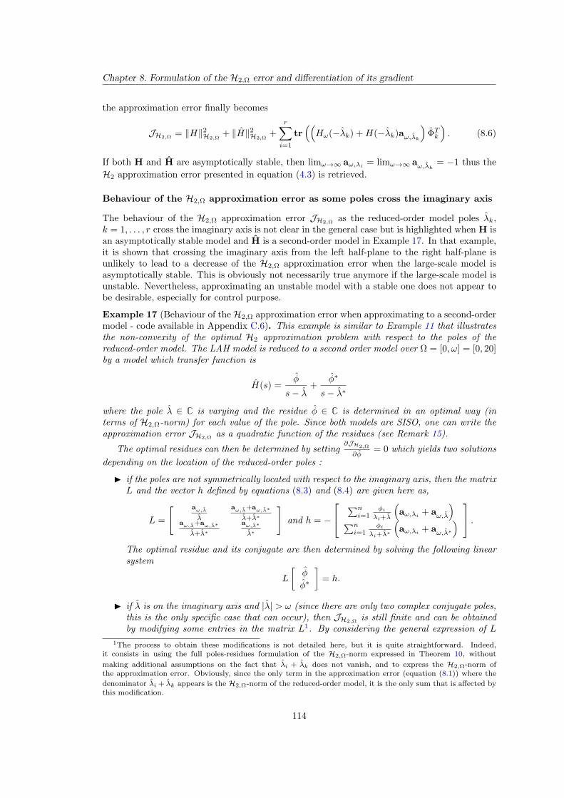
Chapter 8. Formulation of the H2,Ω error and differentiation of its gradient
the approximation error finally becomes
JH2,Ω = ‖H‖2H2,Ω+ ‖H‖2H2,Ω
+
r∑i=1
tr((Hω(−λk) +H(−λk)aω,λk
)ΦTk
). (8.6)
If both H and H are asymptotically stable, then limω→∞ aω,λi = limω→∞ aω,λk = −1 thus the
H2 approximation error presented in equation (4.3) is retrieved.
Behaviour of the H2,Ω approximation error as some poles cross the imaginary axis
The behaviour of the H2,Ω approximation error JH2,Ωas the reduced-order model poles λk,
k = 1, . . . , r cross the imaginary axis is not clear in the general case but is highlighted when H isan asymptotically stable model and H is a second-order model in Example 17. In that example,it is shown that crossing the imaginary axis from the left half-plane to the right half-plane isunlikely to lead to a decrease of the H2,Ω approximation error when the large-scale model isasymptotically stable. This is obviously not necessarily true anymore if the large-scale model isunstable. Nevertheless, approximating an unstable model with a stable one does not appear tobe desirable, especially for control purpose.
Example 17 (Behaviour of theH2,Ω approximation error when approximating to a second-ordermodel - code available in Appendix C.6). This example is similar to Example 11 that illustratesthe non-convexity of the optimal H2 approximation problem with respect to the poles of thereduced-order model. The LAH model is reduced to a second order model over Ω = [0, ω] = [0, 20]by a model which transfer function is
H(s) =φ
s− λ+
φ∗
s− λ∗
where the pole λ ∈ C is varying and the residue φ ∈ C is determined in an optimal way (interms of H2,Ω-norm) for each value of the pole. Since both models are SISO, one can write theapproximation error JH2,Ω
as a quadratic function of the residues (see Remark 15).
The optimal residues can then be determined by setting∂JH2,Ω
∂φ= 0 which yields two solutions
depending on the location of the reduced-order poles :
I if the poles are not symmetrically located with respect to the imaginary axis, then the matrixL and the vector h defined by equations (8.3) and (8.4) are given here as,
L =
[ aω,λ
λ
aω,λ+aω,λ∗
λ+λ∗aω,λ+aω,λ∗
λ+λ∗
aω,λ∗
λ∗
]and h = −
∑ni=1
φiλi+λ
(aω,λi + aω,λ
)∑ni=1
φiλi+λ∗
(aω,λi + aω,λ∗
) .The optimal residue and its conjugate are then determined by solving the following linearsystem
L
[φ
φ∗
]= h.
I if λ is on the imaginary axis and |λ| > ω (since there are only two complex conjugate poles,this is the only specific case that can occur), then JH2,Ω
is still finite and can be obtainedby modifying some entries in the matrix L1. By considering the general expression of L
1The process to obtain these modifications is not detailed here, but it is quite straightforward. Indeed,it consists in using the full poles-residues formulation of the H2,Ω-norm expressed in Theorem 10, without
making additional assumptions on the fact that λi + λk does not vanish, and to express the H2,Ω-norm ofthe approximation error. Obviously, since the only term in the approximation error (equation (8.1)) where the
denominator λi + λk appears is the H2,Ω-norm of the reduced-order model, it is the only sum that is affected bythis modification.
114
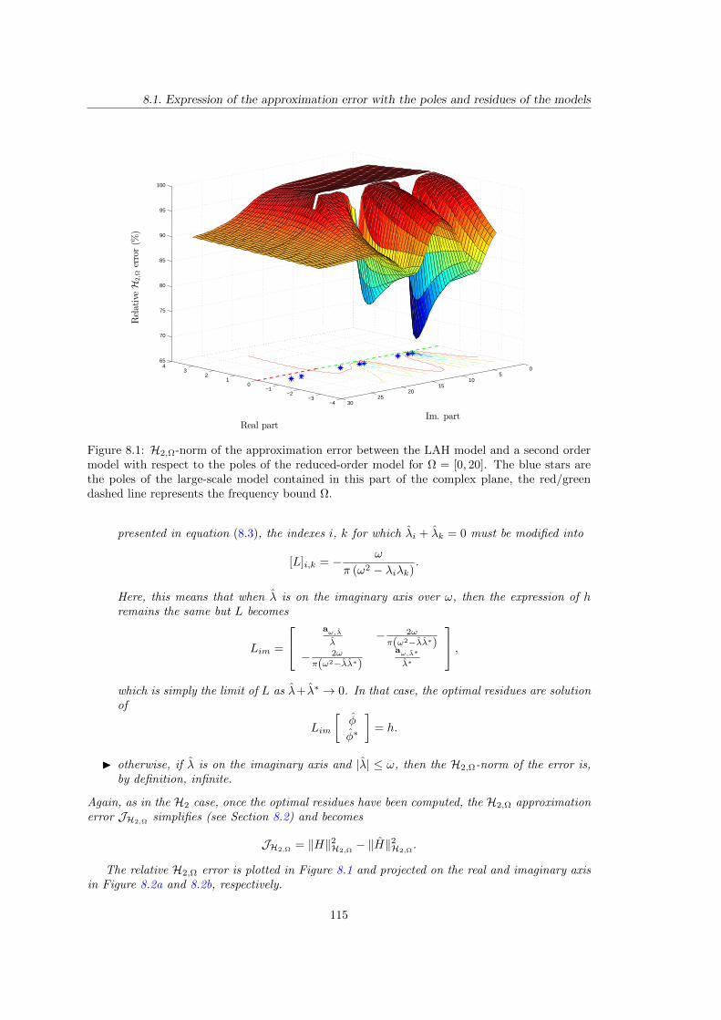
8.1. Expression of the approximation error with the poles and residues of the models
−4−3
−2−1
01
23
4 05
1015
2025
30
65
70
75
80
85
90
95
100
Im. partReal part
RelativeH
2,Ω
error(%
)
Figure 8.1: H2,Ω-norm of the approximation error between the LAH model and a second ordermodel with respect to the poles of the reduced-order model for Ω = [0, 20]. The blue stars arethe poles of the large-scale model contained in this part of the complex plane, the red/greendashed line represents the frequency bound Ω.
presented in equation (8.3), the indexes i, k for which λi + λk = 0 must be modified into
[L]i,k = − ω
π (ω2 − λiλk).
Here, this means that when λ is on the imaginary axis over ω, then the expression of hremains the same but L becomes
Lim =
aω,λ
λ− 2ω
π(ω2−λλ∗)− 2ω
π(ω2−λλ∗)aω,λ∗
λ∗
,which is simply the limit of L as λ+ λ∗ → 0. In that case, the optimal residues are solutionof
Lim
[φ
φ∗
]= h.
I otherwise, if λ is on the imaginary axis and |λ| ≤ ω, then the H2,Ω-norm of the error is,by definition, infinite.
Again, as in the H2 case, once the optimal residues have been computed, the H2,Ω approximationerror JH2,Ω
simplifies (see Section 8.2) and becomes
JH2,Ω= ‖H‖2H2,Ω
− ‖H‖2H2,Ω.
The relative H2,Ω error is plotted in Figure 8.1 and projected on the real and imaginary axisin Figure 8.2a and 8.2b, respectively.
115
Chapter 8. Formulation of the H2,Ω error and differentiation of its gradient
−3 −2 −1 0 1 2 3
70
75
80
85
90
95
100
Real part
Inside ΩOutside Ω
(a)
0 5 10 15 20 25 30
70
75
80
85
90
95
100
RelativeH
2,Ω
error(%
)
Imag part
(b)
Figure 8.2: Projection of theH2,Ω-norm presented in Figure 8.1 on the real axis (a) and imaginaryaxis (b).
In Figure 8.1, one can observe that the behaviour of JH2,Ωinside the frequency interval Ω is
similar to the behaviour of the H2 approximation error (see Figure 4.1) but outside the interval,the local minima present in the H2 case have completely vanished.
The behaviour of the objective function in the right-half plane depends on whether Im(λ)belongs to Ω or not. Indeed, as one can see in Figure 8.2a,
I when Im(λ) > ω (red line in Figure 8.2a), the objective function increases as Re(λ) < 0increases. It means that, with this asymptotically stable model, moving in the positive realdirection does not yield a decrease of the objective function and consequently is not likelyto represent a descent direction.
I If Im(λ) ∈ Ω (in green), one can see that JH2,Ωis slowly decreasing as Re(λ) > 0
increases. Yet, this decrease is generally slower than on the left half-plane2. It suggeststhat when Im(λ) ∈ Ω, switching from the right half-plane to the left half-plane is unlikelyto represent a descent direction.
These two points suggest that reducing an asymptotically stable model with a descent methodaimed at minimising JH2,Ω
is very unlikely to produces an unstable reduced-order model. Obvi-ously, this is not necessarily true anymore if the large-scale model is not stable.
In Figure 8.2b, one can see that if λ is in the right half-plane, then JH2,Ω does not evolve
along the imaginary axis as long as Im(λ) < ω. Then when Im(λ) > ω, the objective function
decreases slowly and appears to reach a limit. More specifically, let us consider λ = x + jy,y > 0, then the limit of JH2,Ω as y tends towards infinity is equal to the H2,Ω-norm of theoriginal large-scale model H. Indeed, by noticing that
1 + jω
λ= 1 +
ωy
x2 + y2+ j
ωx
x2 + y2,
it is clear that
limy→∞
ln
(∣∣∣∣1 + jω
λ
∣∣∣∣) = 0,
in addition, since 1 + j ωλ
tends towards 1 as y tends towards infinity,
limy→∞
arg
(1 + j
ω
λ
)= 0
2This assertion does not hold around the local maxima of JH2,Ω.
116
8.1. Expression of the approximation error with the poles and residues of the models
The same limits hold with 1− j ωλ
, thus
limy→∞
aω,λ = 0.
This means that limy→∞ L = 0 (and similarly, one can prove that limy→∞ Lim = 0). Obviously
limy→∞H(−λ) = 0 thus, limy→∞ h = 0 which implies that
limy→∞
JH2,Ω= ‖H‖2H2,Ω
.
This result is quite natural since if the reduced-order model poles move away from the frequency-band of interest, its influence in this frequency interval vanishes and only the influence of thelarge-scale model remains.
The fact that JH2,Ωreaches a plateau as the imaginary parts of the reduced-order model poles
increase lead to believe that if a descent optimisation method is used, one should probably notinitialise it with a reduced-order model which poles are located outside of Ω.
8.1.2 About the computation of the approximation error
In optimisation, the evaluation of the objective function can be a numerical burden if it is notfast enough. The first step towards a fast computation of JH2,Ω
is to express it with matrix andvector operations to exploit the standard and highly optimised linear algebra libraries used insoftware such as Matlab R©.
To this aim, let us define Wnn ∈ Cn×n, Wnr ∈ Cn×r and Wrr ∈ Cr×r as
[Wrr]i,k =1
2
aω,λi + aω,λk
λi + λk, (8.7)
[Wnr]i,k =aω,λi + aω,λk
λi + λk, (8.8)
[Wnn]i,k =aω,λiλi + λk
.
Each of these matrix can be easily built as follows
Wnr =
aω,λ1
...aω,λn
1Tn + 1r[
aω,λ1. . . ,aω,λr
]
1λ1+λ1
. . . 1λ1+λr
.... . .
...1
λn+λ1. . . 1
λn+λr
,where is the Hadamard product and 1n ∈ Rn×1 a column vector full of 1. Let C∆ ∈ Cny×n andC∆ ∈ Cny×r denote the matrices formed by horizontally concatenating ci
T and cTk , respectively,i.e.
C∆ =[
c1T . . . cn
T]
and C∆ =[
cT1 . . . cTr], (8.9)
and let B∆ ∈ Cn×nu and B∆ ∈ Cr×nu be the matrices built by vertically concatenating bi andbk, i.e.
B∆ =
b1
...bn
and B∆ =
b1
...
br
. (8.10)
Obviously, C∆ = CX, C∆ = CX, B∆ = X−1B and B∆ = X−1B, where X ∈ Cn×n andX ∈ Cr×r are the matrices which columns are the right eigenvectors of A and A, respectively.
117

Chapter 8. Formulation of the H2,Ω error and differentiation of its gradient
Then, as it has been shown in Section 7.1.2, the H2,Ω-norms of H and H, direct feedthroughexcluded, can be computed as
‖H‖2H2,Ω= 1Tn
((CT∆C∆) (B∆B
T∆)Wnn
)1n,
and‖H‖2H2,Ω
= 1Tr(
(CT∆C∆) (B∆BT∆)Wrr
)1r.
Note that [Wrr]i,k could have been directly defined asaω,λiλi+λk
(like in the poles-residues formula-
tion of the norm in Theorem 10), but here the fact that
‖H‖2H2,Ω=
r∑i=1
r∑k=1
tr(
ΦiΦk
)λi + λk
aω,λi =
r∑i=1
r∑k=1
tr(
ΦiΦk
)λi + λk
1
2
(aω,λi + aω,λk
),
has been exploited. This has no interest for the computation of ‖H‖2H2,Ωpresented above but it
is interesting for the the computation of the gradient in Section 8.2.2.Similarly, the cross term in the error can be computed as
−n∑i=1
r∑k=1
tr(
ΦiΦTk
)λi + λk
(aω,λi + aω,λk
)= −1Tn
((CT∆C∆) (B∆B
T∆)Wnr
)1r.
and by denoting diag(M) the column vector formed by the diagonal of the matrix M , the termsin JH2,Ω
(8.1) associated with the direct feedthrough D and D can be expressed as
−n∑i=1
tr(
ΦiDT)
aω,λi = −diag(B∆D
TC∆
)T aω,λ1
...aω,λn
,and
r∑i=1
tr(
ΦiDT)
aω,λi = diag(B∆D
T C∆
)T aω,λ1
...aω,λr
.Note that the number of operations required to compute JH2,Ω
can be decreased by exploitingthe structure of the matrices such as the symmetry of Wrr or Wnn or the fact that the complexelements come with their complex conjugate, but the benefit would not necessarily be significantin term of computation time, that is why it has not been considered here.
The second step towards a fast computation of JH2,Ω consists in avoiding to compute multipletimes the same things. Here, the matrices C∆, B∆, ‖H‖2H2,Ω
, the terms associated to D and
aω,λi (i = 1, . . . , n) can be stored throughout the whole optimisation process. Besides, in thecontext of minimisation of JH2,Ω
, it is worth noticing that computing ‖H‖H2,Ωis not mandatory
since minimising JH2,Ωis equivalent to minimise JH2,Ω
− ‖H‖2H2,Ω. Yet, since the computation
of the cross terms require the poles and residues of the large-scale model, computing JH2,Ω doesnot implies a lot of additional operations especially as it only needs to be done once.
Note that with respect to the computation time of the approximation error, the poles-residuesformulation of the H2,Ω approximation error offers some advantage compared to the gramianbased one (see Section 5.2.2). Indeed, with the gramian formulation, each evaluation of theapproximation error requires to solve a n× r Sylvester equation, a r× r Lyapunov equation, dueto the cross terms and the H2,Ω-norm of the reduced-order model respectively, while here, theerror is explicit in terms of the poles and residues of the reduced-order model. This advantagecomes from the additional hypothesis on the structure of the poles which must be semi-simpleand which is not made with the gramian-based formulation.
118
8.2. Gradient of the error
8.2 Gradient of the error
Based on the poles-residues formulation of the H2,Ω approximation error between a large-scale
model H and a reduced-order one H, the problem of optimal H2,Ω approximation can be re-formulated as follows.
Problem 4 (Poles-residues formulation of the H2,Ω optimal model approximation problem).Given an asymptotically stable LTI dynamical model H of order n. The problem of optimal H2,Ω
model approximation consists in finding the poles λi ∈ C, the vectors ci ∈ C1×ny and bi ∈ C1×nu
(i = 1, . . . , r) and the direct feedthrough D ∈ Rny×nu of the asymptotically stable reduced-ordermodel H that minimises the H2,Ω-norm of the approximation error JH2,Ω
.
Since only stable models have been considered in this study, Problem 4 is restricted toasymptotically stable models, but this assumption is more restrictive than what is required andused here to express the first-order optimality conditions. Indeed, the hypothesis used here isthat the poles of both models are not symmetrically located with respect to the imaginary axis.One could diminish these hypothesis even further by using the full expression of the H2,Ω-norm.However, this has not been considered here.
JH2,Ωis a function of r+rny+rnu+nynu variables, thus, Problem 4 is over-parametrised since
the minimal number of parameters to represent a LTI model of order r is rny+rnu+nynu. This
issue could be fixed by imposing some norm constraint on either the bi or the ci (i = 1, . . . , r),but in order to stick with the simpler unconstrained optimisation framework, no constraint isadded.
JH2,Ω is a real valued function of complex variables λi, bi, ci and their complex conjugates.As it does not satisfy the Cauchy-Riemann equations, such a function is not analytic. Thecommon way of dealing with such kind of functions consists in writing them as functions of thereal and imaginary parts of the variables. However here, it would break the structure of JH2,Ω
and that is why keeping it as a function of complex variables is preferred.
In that context, the Wirtinger calculus is used to derive the first order optimality conditionsfor the optimal H2,Ω approximation problem. A quick reminder of its main properties is donein Section 8.2.1. It is then applied to differentiate JH2,Ω in Section 8.2.2.
8.2.1 Reminder on Wirtinger Calculus
This Section is not meant to be an exhaustive description of the Wirtinger calculus but rathera quick reminder of the properties that are used in the next Section to express the first-orderoptimality conditions of the approximation problem. It is mainly based on [Brandwood, 1983;Remmert, 1991] where the complex gradient and conjugate gradient operators are defined. Ad-ditional useful elements about the use of Wirtinger calculus for optimisation can be found in[Kreutz-Delgado, 2009] and in [Sorber et al., 2012].
Partial complex-variable derivative
Let us consider g : C × C → C a function of z and its conjugate z∗ which is analytic withrespect to z and z∗ independently, i.e. g(z, a) and g(a, z) are analytic in z. Let us also considerh : R×R→ C, the function of real variables x and y such that z = x+ jy and g(z, z∗) = h(x, y),then
∂g
∂z:=
1
2
(∂h
∂x− j ∂h
∂y
),
∂g
∂z∗:=
1
2
(∂h
∂x+ j
∂h
∂y
),
(8.11)
119
Chapter 8. Formulation of the H2,Ω error and differentiation of its gradient
where ∂g∂z (respectively ∂g
∂z∗ ) is obtained by treating z∗ (respectively z) as a constant3. Equation(8.11) can easily be verified with simple functions, for instance,
∂z
∂z=∂z∗
∂z∗= 1 and
∂z
∂z∗=∂z∗
∂z= 0.
Let g(z, z∗) = u(x, y)+jv(x, y) where u and v are real functions, the Cauchy-Riemann conditionscan be retrieved, indeed, ∂g
∂z∗ = 0 can be rewritten with equation (8.11) as ∂u∂x+j ∂v∂x+j ∂u∂y−
∂v∂y = 0,
which yields, by identifying the real and imaginary parts, to
∂u
∂x=∂v
∂yand
∂v
∂x= −∂u
∂y.
This means that a complex function f : C → C is analytic in z if and only if it only dependsexclusively of z and not of z∗.
Stationary points of non-analytic functions
Let us now consider a real-valued function f : C→ R of a complex variable z and its conjugate.As mentioned above, such a function is not analytic in z. To characterise its stationary points,one must consider the function g : C×C→ R of two complex variables and analytic with respectto each variable such that f(z) = g(z, z∗). Then the stationary points of f are the points forwhich either ∂g
∂z = 0 or ∂g∂z∗ = 0.
This can be proved by setting g(z, z∗) = u(x, y)+ jv(x, y) where u and v are real functions ofthe real variables x and y. Since g is real valued, v(x, y) = 0 for all x, y ∈ R, thus from equation(8.11),
∂g
∂z=
1
2
(∂u
∂x− j ∂u
∂y
)and
∂g
∂z∗=
1
2
(∂u
∂x+ j
∂u
∂y
).
By identifying the real and imaginary parts, it is clear that
∂u
∂x=∂u
∂y= 0 ⇐⇒ ∂g
∂z= 0 and
∂u
∂x=∂u
∂y= 0 ⇐⇒ ∂g
∂z∗= 0.
Note that the differential of g is given as
dg =∂g
∂zdz +
∂g
∂z∗dz∗,
and since g is real valued, ∂g∂z∗ =
(∂g∂z
)∗, thus
dg = 2Re
(∂g
∂zdz
).
The differential dg is maximal when ∂g∂zdz is real, thus dz must be proportional to
(∂g∂z
)∗= ∂g
∂z∗ .
It means that ∂g∂z∗ is the steepest ascent direction. Hence, if one looks for a maximum of f , one
could set the following iteration scheme
zk+1 = zk + α∂g
∂z∗
∣∣∣z=zk
,
where α is the step length. Example 18 illustrates the various elements of the Wirtinger calculuspresented here on a simple function.
3In [Kreutz-Delgado, 2009], such derivatives are said to be formal because one cannot vary z while keeping z∗
constant.
120
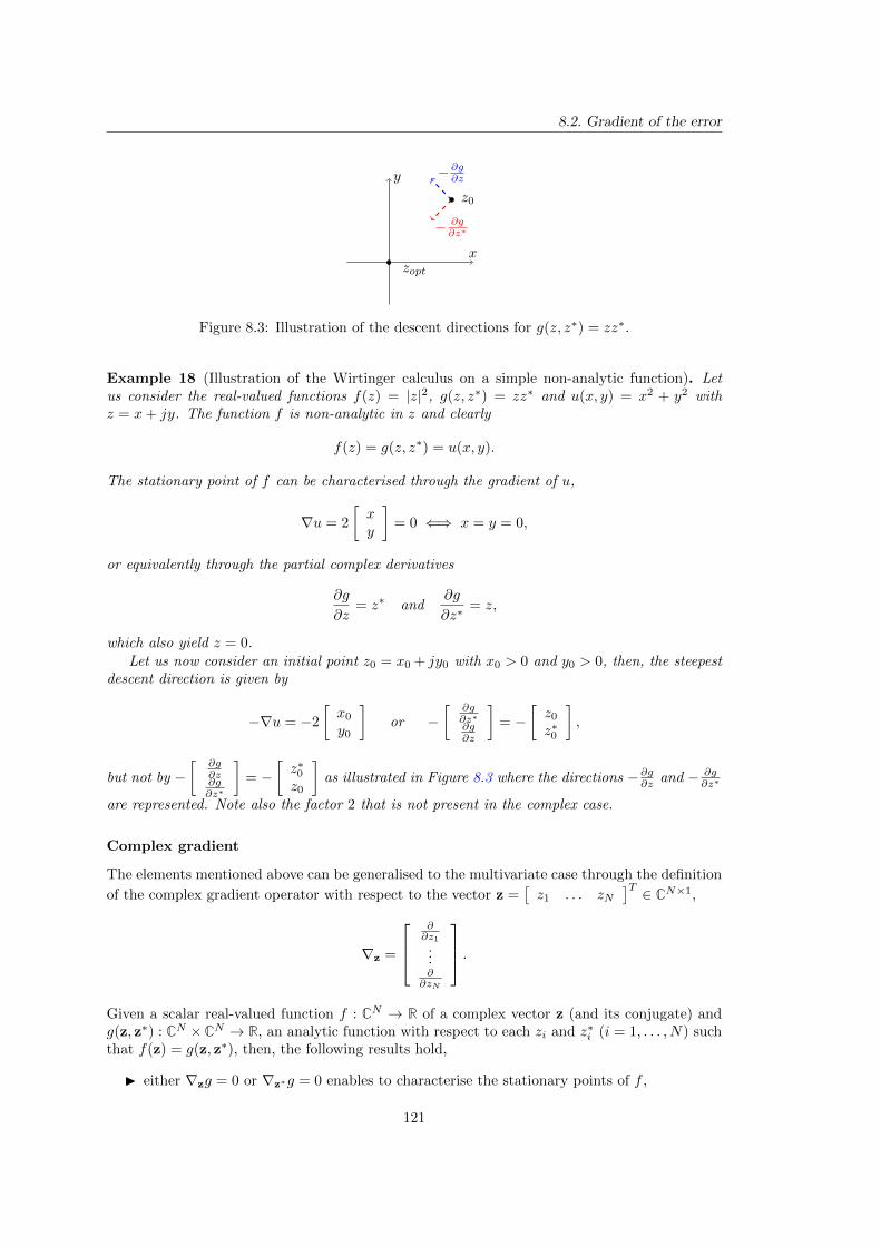
8.2. Gradient of the error
x
y
− ∂g∂z∗
−∂g∂z
zopt
z0
Figure 8.3: Illustration of the descent directions for g(z, z∗) = zz∗.
Example 18 (Illustration of the Wirtinger calculus on a simple non-analytic function). Letus consider the real-valued functions f(z) = |z|2, g(z, z∗) = zz∗ and u(x, y) = x2 + y2 withz = x+ jy. The function f is non-analytic in z and clearly
f(z) = g(z, z∗) = u(x, y).
The stationary point of f can be characterised through the gradient of u,
∇u = 2
[xy
]= 0 ⇐⇒ x = y = 0,
or equivalently through the partial complex derivatives
∂g
∂z= z∗ and
∂g
∂z∗= z,
which also yield z = 0.Let us now consider an initial point z0 = x0 + jy0 with x0 > 0 and y0 > 0, then, the steepest
descent direction is given by
−∇u = −2
[x0
y0
]or −
[∂g∂z∗∂g∂z
]= −
[z0
z∗0
],
but not by −[
∂g∂z∂g∂z∗
]= −
[z∗0z0
]as illustrated in Figure 8.3 where the directions −∂g∂z and − ∂g
∂z∗
are represented. Note also the factor 2 that is not present in the complex case.
Complex gradient
The elements mentioned above can be generalised to the multivariate case through the definition
of the complex gradient operator with respect to the vector z =[z1 . . . zN
]T ∈ CN×1,
∇z =
∂∂z1...∂∂zN
.Given a scalar real-valued function f : CN → R of a complex vector z (and its conjugate) andg(z, z∗) : CN ×CN → R, an analytic function with respect to each zi and z∗i (i = 1, . . . , N) suchthat f(z) = g(z, z∗), then, the following results hold,
I either ∇zg = 0 or ∇z∗g = 0 enables to characterise the stationary points of f ,
121
Chapter 8. Formulation of the H2,Ω error and differentiation of its gradient
I the differential of g is given by
dg = (∇zg)Tdz + (∇z∗g)
Tdz∗
= 2Re(
(∇z∗g)Tdz)
(g is real-valued),(8.12)
I by using the Cauchy-Schwarz inequality in equation (8.12), one can see that the differen-
tial Re((∇z∗g)Tdz) is maximal when dz is co-linear to ∇z∗g. Hence the steepest ascent
direction is given by ∇z∗g.
Note that complex Hessian matrices can similarly be defined (see [Van Den Bos, 1994; Kreutz-Delgado, 2009; Sorber et al., 2012]) but since the Hessian of JH2,Ω
is not exploited in the sequel,they are not described here.
8.2.2 Gradient of the H2,Ω approximation error
To highlight clearly the link with the previous section, let us focus on the reduced-order polesand consider that the approximation error JH2,Ω
is a function of the reduced-order model poles
λi (i = 1, . . . , r) only. Let us also assume that these poles are all complex and ordered as
λ1, λ2 = λ∗1, λ3, λ4 = λ∗3, . . . , λr−1, λr = λ∗r−1.
In that case, the approximation error JH2,Ω can either be seen as a function of r2 variables
λ1, λ3, . . . , λr−1 or as a function of r variables λ1, λ∗1, . . . , λr−1, λ
∗r−1. In the former case, JH2,Ω
is similar to the function f(z) of Section 8.2.1 while in the latter case, JH2,Ω is like g(z, z∗).To differentiate JH2,Ω
with respect to the poles, one must consider it as a function of w =[λ1 λ3 . . . λr−1
]Tand of w∗. The first-order optimality conditions of JH2,Ω with respect
to the reduced-order model poles are then either given by the r2 conditions
∂JH2,Ω
∂w = 0 or by
their conjugate∂JH2,Ω
∂w∗ = 0.
In order to avoid differentiating between the complex and complex conjugate variables, one
can also directly consider z =[
wT wH]T ∈ Cr×1 and
∂JH2,Ω
∂z =[
∂JH2,Ω
∂w
T ∂JH2,Ω
∂w∗
T]
= 0
which leads to the same optimality conditions, excepted that they are redundant.
This is what is done in Theorem 16 where JH2,Ω is differentiated with respect to λi, bi, ci
(i = 1, . . . , r) and D without distinction between the variables, conjugated variables and realvariables. Refer to Remark 16 for some comments on the notations used in Theorem 16.
The Wirtinger calculus has already been implicitly used in Section 4.1 to express the first-order optimality conditions of the optimalH2 approximation problem. It has not been mentionedbecause it does not modify the differentiation rules and it is not mentioned in the literature.
Theorem 16 (Poles-residues formulation of the necessary conditions for the optimal H2,Ω ap-
proximation problem). Let us consider two LTI dynamical models H and H of order n andr n, respectively, which poles are semi-simple and not symmetrically located with respect tothe imaginary axis and which associated transfer functions are given by
H(s) =
n∑i=1
ciTbi
s− λi+D and H(s) =
n∑i=1
cTi bi
s− λi+ D.
Let us also consider a frequency interval Ω = [0, ω], if H minimises JH2,Ω= ‖H − H‖2H2,Ω
, then
the derivatives of JH2,Ωwith respect to λm, bm, cm and D, given for m = 1, . . . , r by equations
122
8.2. Gradient of the error
(8.13), (8.14), (8.15) and (8.16), respectively, are equal to 0.
∂JH2,Ω
∂λm= −
r∑i=1
cmcTi bibTm
aω,λi + aω,λm(λi + λm
)2 +2
π
ω(λ2m + ω2
)(λi + λm
) . . .
+
n∑i=1
cmciTbib
Tm
aω,λi + aω,λm(λi + λm
)2 +2
π
ω(λ2m + ω2
)(λi + λm
) . . .
+2
πcmDbm
ω
ω2 + λ2m
,
(8.13)
∂JH2,Ω
∂bm
=
r∑i=1
bTi cicTm
λi + λm
(aω,λi + aω,λm
)−
n∑i=1
biT cic
Tm
λi + λm
(aω,λi + aω,λm
)+ DT cTmaω,λm , (8.14)
∂JH2,Ω
∂cm=
r∑i=1
cTi bibTm
λi + λm
(aω,λi + aω,λm
)−
n∑i=1
ciTbib
Tm
λi + λm
(aω,λi + aω,λm
)+ DbTmaω,λm , (8.15)
∂JH2,Ω
∂D= −
r∑i=1
cTi biaω,λi +
n∑i=1
ciTbiaω,λi −
2
πωD. (8.16)
Proof. The derivative are obtained by straight differentiation of the approximation error JH2,Ω
given in equation (8.1).
Remark 16 (About the notations in Theorem 16). When differentiating with respect to the line
vectors bm or cm, the resulting gradients are column vectors denoted by∂JH2,Ω
∂cm∈ Cny×1 and
∂JH2,Ω
∂bm∈ Cnu×1. Besides, the derivative with respect to D is performed element-wise and the
resulting derivative is a matrix∂JH2,Ω
∂D∈ Rny×nu . This inconsistency has no real impact on the
sequel and allows for more clarity, in particular, the derivatives are straightforwardly obtained.
Reformulation of the first-order optimality conditions as interpolation conditions
The first-order optimality conditions of the H2,Ω approximation problem can be reformulatedas interpolation conditions similar, in some way, to the interpolation conditions arising in theoptimal H2 model approximation problem (see Section 4.1). Let us define the filtered transferfunctions Hω(s) and Hω(s) as the transfer functions H(s) and H(s) considered without thedirect feedthrough D and D and which i-th modal contributions are weighted by aω,λi andaω,λi , respectively, i.e.
Hω(s) =
n∑i=1
ciTbi
s− λiaω,λi and Hω(s) =
r∑i=1
cTi bi
s− λiaω,λi .
Derivative with respect to bm. Let us consider the derivative of JH2,Ωwith respect to bm
of equation (8.14), the first sum can be written as
r∑i=1
bTi cicTm
λi + λm
(aω,λi + aω,λm
)− DT cTmaω,λm =
(r∑i=1
bTi ci
λi + λmaω,λi
. . . +
(n∑i=1
bTi ci
λi + λm− DT
)aω,λm
)cTm
=(−HT
ω (−λm)− H(−λm)Taω,λm
)cTm,
123
Chapter 8. Formulation of the H2,Ω error and differentiation of its gradient
and similarly, the second one can be written as
−n∑i=1
biT cic
Tm
λi + λm
(aω,λi + aω,λm
)+DcTmaω,λm =
(Hω(−λm)T +H(−λm)Taω,λm
)cTm.
Hence∂JH2,Ω
∂bm= 0 is equivalent to
cm
(Hω(−λm) + H(−λm)aω,λm
)= cm
(Hω(−λm) +H(−λm)aω,λm
). (8.17)
Derivative with respect to cm. Likewise,∂JH2,Ω
∂cm= 0 can also be written as(
Hω(−λm) + H(−λm)aω,λm
)bTm =
(Hω(−λm) +H(−λm)aω,λm
)bTm. (8.18)
Derivative with respect to λm. This reformulation process is not as obvious concerning thederivative of JH2,Ω with respect to λm. Let us consider the first sum in equation (8.13), notethat
r∑i=1
cmcTi bi(
λi + λm
)2 aω,λi bTm = cmH
′ω(−λm)bTm,
and thatr∑i=1
cmcTi bi(
λi + λm
)2 aω,λm bTm = cmH′(−λm)aω,λm bTm. (8.19)
The last element of the sum is in fact the derivative of aω,−s with respect to s, indeed by noticingthat d
dsatan(−ωs)
= ωω2+s2 , it comes
r∑i=1
cm
(cTi bi
λi + λm− D
)2
π
ω
ω2 + λ2m
bTm = cmH(−λm)2
π
d
dsatan
(ωs
) ∣∣s=−λm
bTm. (8.20)
Equations (8.19) and (8.20) can be grouped under the following formulation
cmH′(−λm)aω,λm bTm + cmH(−λm)
2
π
d
dsatan
(ωs
) ∣∣s=−λm
bTm = cmd
ds
[H(s)aω,−s
]s=−λm
bTm.
The same result holds for the second sum involved in∂JH2,Ω
∂λm. Thus
∂JH2,Ω
∂λm= 0 can finally be
re-written as
cm
(H ′ω(−λm) +
d
ds[H(s)aω,−s]s=−λm
)bTm = cm
(H ′ω(−λm) +
d
ds
[H(s)aω,−s
]s=−λm
)bTm
(8.21)
Interpolation conditions. Equations (8.17), (8.18) and (8.21) can be further simplified bydefining the two functions4
T (s) = Hω(s) +H(s)aω,−s and T (s) = Hω(s) + H(s)aω,−s.
4Since ∀z, atan(−z) = −atan(z), these functions can be written as T (s) = Hω(s) − H(s)aω,s and T (s) =
Hω(s)− H(s)aω,s also.
124
8.2. Gradient of the error
Indeed, with that notation, the first-order optimality conditions of the H2,Ω approximationproblem associated to the poles and the residues of the reduced-order model can then be writtenas
T (−λm)bTm = T (−λm)bTmcmT (−λm) = cmT (−λm)
cmT′(−λm)bTm = cmT
′(−λm)bTm,
(8.22)
which is similar to the H2 optimality conditions expressed in Theorem 9 excepted that here theinterpolation does not concern directly the large-scale and reduced-order transfer functions. Thefunctions T (s) and T (s) are probably related to the weighted functions involved in the frequencyweighted H2 optimality conditions derived in [Anic et al., 2013] (see Section 5.1.2) but a clearlink has not been established yet. Note that the function T (s) also appears in the approximationerror JH2,Ω
in equation (8.6) which becomes,
JH2,Ω = ‖H‖2H2,Ω+ ‖H‖2H2,Ω
+
n∑i=1
tr(T (−λk)ΦTk
).
Derivative with respect to D. The derivative of JH2,Ωwith respect to D leads to a quite
different optimality condition in terms of the transfer functions H(s) and H(s), indeed, setting∂JH2,Ω
∂D= 0 in equation (8.16) yields, for i = 1, . . . , ny and k = 1, . . . , nu,∫ ω
−ωHi,k(jν)dν =
∫ ω
−ωHi,k(jν)dν.
The direct feedthrough D of the reduced-order model is involved in a quadratic and strictlyconvex way in the H2,Ω approximation error JH2,Ω (8.1), indeed the second-order term is
tr(DDT ) = vec(D)Tvec(D) = vec(D)T Inynuvec(D),
where vec(D) is the vectorisation of D, i.e. the column vector formed by vertically concatenating
the columns of D. Hence the necessary condition of optimality∂JH2,Ω
∂D= 0 is also sufficient to
find the global minimum of JH2,Ωwith respect to D. The optimal D is uniquely determined as
a function of the residues and poles of both models H and H, the direct feedthrough D and theupper bound of the frequency interval ω,
Dopt =ωπ
2
(r∑i=1
cTi biaω,λi −n∑i=1
ciTbiaω,λi +
2
πωD
). (8.23)
This implies that D can be discarded as an optimisation variable and replaced by its optimalvalue in each one of the derivatives (8.13), (8.14) and (8.15).
Simplification of the H2,Ω approximation error
Let us consider the formulation of the approximation error JH2,Ω of equation (8.5). Let us
assume that either∂JH2,Ω
∂cm= 0 or
∂JH2,Ω
∂bm= 0 for m = 1, . . . , r, then
r∑k=1
bk
(n∑i=1
biT ci
λi + λk
(aω,λi + aω,λk
))cTk =
r∑k=1
bk
(r∑i=1
bTi ci
λi + λk
(aω,λi + aω,λk
)+ DTaω,λk
)cTk .
125
Chapter 8. Formulation of the H2,Ω error and differentiation of its gradient
By taking the trace and reordering the sums so that aω,λi +aω,λk is replaced by 2aω,λi , the H2,Ω
approximation error becomes
JH2,Ω = ‖H‖2H2,Ω+ ‖H‖2H2,Ω
− 2
r∑i=1
r∑k=1
tr(
ΦiΦTk
)λi + λk
aω,λi +
r∑i=1
tr(
ΦiDT)
aω,λi . . .
+
n∑i=1
tr(
ΦiDT)
aω,λi −2
πωtr
(DDT
).
If in addition∂JH2,Ω
∂D= 0, then
tr
((n∑i=1
Φiaω,λi −2
πωD
)DT
)= tr
((r∑i=1
Φiaω,λi −2
πωD
)DT
),
thus
JH2,Ω= ‖H‖2H2,Ω
+‖H‖2H2,Ω−2
r∑i=1
r∑k=1
tr(
ΦiΦTk
)λi + λk
aω,λi −r∑i=1
tr(
ΦiDT)
aω,λi +ω
πtr(DDT
) .
The last term is equal to ‖H‖2H2,Ω, hence if
∂JH2,Ω
∂D= 0 and either
∂JH2,Ω
∂cm= 0 or
∂JH2,Ω
∂bm= 0, the
squared H2,Ω approximation error JH2,Ω is equal to the difference of the squared H2,Ω-norms of
H and H,JH2,Ω = ‖H − H‖2H2,Ω
= ‖H‖2H2,Ω− ‖H‖2H2,Ω
.
About the computation of the gradient of JH2,Ω
The computation of the gradient is also an important part in an optimisation algorithm whichmust be efficient in order not to become a numerical burden for the process. The process hereis similar to what has been done for the computation of the approximation error JH2,Ω in theprevious section and the matrices built to compute JH2,Ω are also involved here. Indeed, let us
consider the matrices Wrr ∈ Cn×n, Wnr ∈ Cr×r, C∆ ∈ Cny×n, C∆ ∈ Cny×r, B∆ ∈ Cn×nu andB∆ ∈ Cr×nu defined in equations (8.7), (8.8), (8.9) and (8.10), respectively.
Let us consider∂JH2,Ω
∂bmwhich expression is
∂JH2,Ω
∂bm
=
r∑i=1
bTi cicTm
λi + λm
(aω,λi + aω,λm
)−
n∑i=1
biT cic
Tm
λi + λm
(aω,λi + aω,λm
)+ DT cTmaω,λm .
First, notice that
CT∆C∆ =
c1
...cr
[ cT1 . . . cTr]
=
c1cT1 . . . c1cTr...
. . ....
crcT1 . . . crc
Tr
∈ Cr×r,
By multiplying CT∆C∆, element-wise, with 2Wrr, one obtains, in the m-th column,
tm =[
c1cTm
(aω,λ1
+ aω,λm
). . . crc
Tm
(aω,λr + aω,λm
) ]T∈ Cr×1, (8.24)
which is a part of the elements involved in the first sum of∂JH2,Ω
∂bm. By left multiplying the vector
tm from equation (8.24) by BT∆, it comes
BT∆tm =[
bT1 . . . bTr]tm =
r∑i=1
bTi cicTm
λi + λm
(aω,λi + aω,λm
).
126
8.2. Gradient of the error
Thus the first sum of∂JH2,Ω
∂bmis the m-th column of BT∆
((CT∆C
) 2Wrr
), i.e.
[BT∆
((CT∆C
) 2Wrr
)]em =
r∑i=1
bTi cicTm
λi + λm
(aω,λi + aω,λm
). (8.25)
Similarly for the second sum,[BT∆
((CT∆C∆
) 2Wnr
)]em =
n∑i=1
biT cic
Tm
λi + λm
(aω,λi + aω,λm
). (8.26)
By following the same idea, it is easy to see that,
DT cTmaω,λm =[(DT C∆
)(1nu
[aω,λ1
. . . aω,λr])]
em. (8.27)
By coupling equations (8.25), (8.26) and (8.27), on finally obtains[∂JH2,Ω
∂b1. . .
∂JH2,Ω
∂br
]= BT∆
((CT∆C
) 2Wrr
)−BT∆
((CT∆C∆
) 2Wnr
). . .
+(DT C∆
)(1nu
[aω,λ1
. . . aω,λr]).
The same idea can be used for∂JH2,Ω
∂cmand leads to[
∂JH2,Ω
∂c1. . .
∂JH2,Ω
∂cr
]= C∆
((B∆B
T∆
) 2Wrr
)− C∆
((B∆B
T∆
) 2Wnr
). . .
+(DBT∆
)(1ny
[aω,λ1
. . . aω,λr]).
The derivative with respect to the reduced-order model poles,∂JH2,Ω
∂λm, is obtained in a very
similar way to the approximation error JH2,Ω . First, let us consider the matrices Lrr ∈ Cr×r
and Lnr ∈ Cn×r which elements are defined as,
[Lrr]i,k =aω,λi + aω,λk(λi + λk
)2 +2ω
π(λ2k + ω2
)(λi + λk
) ,and
[Lnr]i,k =aω,λi + aω,λk(λi + λk
)2 +2ω
π(λ2k + ω2
)(λi + λk
) .By multiplying Lrr (respectively Lnr), element-wise, by B∆B
T∆ (resp. B∆B
T∆) and by CT∆C∆
(resp. CT∆C∆), one obtains a matrix which m− th column contains the terms in the first (resp.
second) sum of∂JH2,Ω
∂λm, i.e.
[(B∆B
T∆
)(CT∆C∆
) Lrr
]i,m
= cmcTi bibTm
aω,λi + aω,λm(λi + λm
)2 +2
π
ω(λ2m + ω2
)(λi + λm
) ,
and
[(B∆B
T∆
)(CT∆C∆
) Lnr
]i,m
= cmciTbib
Tm
aω,λi + aω,λm(λi + λm
)2 +2
π
ω(λ2m + ω2
)(λi + λm
) .
127
Chapter 8. Formulation of the H2,Ω error and differentiation of its gradient
Besides, the term relative to the direct feedthrough can be obtained as
2
πcmDbm
ω
ω2 + λ2m
= emT
diag(B∆D
T C∆
)
2ω
π(λ21+ω2)...
2ω
π(λ2r+ω2)
.
Hence, it finally comes that[∂JH2,Ω
∂λ1. . .
∂JH2,Ω
∂λr
]= −1Tr
((B∆B
T∆
)(CT∆C∆
) Lrr
). . .
+1Tn((B∆B
T∆
)(CT∆C∆
) Lnr
)+diag
(B∆D
T C∆
)T[
2ω
π(λ21+ω2)
. . . 2ω
π(λ2r+ω2)
].
Just like the approximation error JH2,Ω, its gradient with respect to the reduced-order param-
eters can be easily computed with simple matrix and vector operations. Again, in comparison,with the gramian-based approach, in addition of what is required to compute the error, onen× r Sylvester equation and one r× r Lyapunov equation must be solved and the derivative ofa complex matrix logarithm must be computed (see Section 5.2.2).
Conclusion
In this Chapter, the poles-residues formulation of the H2,Ω-norm has been used to express theapproximation error JH2,Ω between a large-scale model and a reduced-order one as a function ofits poles and residues. There exist similarities between the structures of the H2 approximationerror (4.3) and JH2,Ω
(8.5) but in the frequency-limited case, additional weightings prevent fromformulating the cross terms as the transfer function of the large-scale model evaluated at theopposite of the reduced-order model poles.
The approximation error H2,Ω has then been differentiated with respect to the reduced-ordermodel poles and residues in order to express the necessary conditions for optimality. Similarlyto the H2 case, these optimality conditions can be expressed as interpolation ones. Yet theyconcern some modified transfer functions (8.22) and not directly the models transfer functions.Hence it is not clear if an iterative procedure as the IRKA (see Section 4.2.1) could be developedfor the H2,Ω approximation. That is why an optimisation procedure is developed in the nextChapter.
128
Chapter 9
Development of a descent algorithmfor the optimalH2,Ω approximation
problem
Since most of the readily available optimisation solvers do not handle real functions of complexvariables directly in the complex domain1, the poles-residues formulation of the JH2,Ω
error andits gradient derived in the previous chapter are used here to develop a complex-domain descentalgorithm. It is called Descent Algorithm for Residues and Poles Optimisation (DARPO) andrelies on the complex-domain optimisation framework developed in [Sorber et al., 2012]. It isaimed at finding a reduced-order model H that satisfies the first-order optimality conditions forthe optimal H2,Ω approximation problem. More specifically, by writing the transfer function
H(s) associated to H as
H(s) =
r∑i=1
cTi bi
s− λi+ D,
DARPO is aimed at finding the poles λi, the residues ci, bi (i = 1, . . . , r) and the directfeedthrough D that fulfil the necessary conditions for optimality presented in Theorem 16. Usingthis framework implies that both models H and H have semi-simple poles only and that theireigenvalues are not located symmetrically with respect to the imaginary axis. These hypothesison the structure of the poles restrict the models on which the method can be applied but enablesto efficiently compute the approximation error and its gradient.
The algorithm is described in Section 9.1 and its behaviour is illustrated on academic exam-ples in Section 9.2.
The results presented in this Chapter have partly been published in [Vuillemin et al., 2014b].
Contents9.1 A descent algorithm in the complex domain . . . . . . . . . . . . . 129
9.1.1 Reminder of unconstrained optimisation . . . . . . . . . . . . . . . . . 130
9.1.2 Descent Algorithm for Residues and Poles Optimisation . . . . . . . . 133
9.1.3 Initialisation of DARPO . . . . . . . . . . . . . . . . . . . . . . . . . 137
9.2 Numerical illustration . . . . . . . . . . . . . . . . . . . . . . . . . . . 139
9.2.1 Illustration of the behaviour of DARPO . . . . . . . . . . . . . . . . 139
9.2.2 Improvement provided by DARPO . . . . . . . . . . . . . . . . . . . 146
9.2.3 Application for the control of a large-scale model . . . . . . . . . . . . 151
9.1 A descent algorithm in the complex domain
In Section 9.1.1, a quick reminder of some aspects of unconstrained optimisation of real functionsof real variables are recalled. Then, in Section 9.1.2, the optimisation algorithm for optimal H2,Ω
model approximation is presented. Finally, the initialisation process used in the algorithm isdetailed in Section 9.1.3.
1L. Sorber and his colleagues have now proposed a complex-domain optimisation toolbox in [Sorber et al.,2013].
129
Chapter 9. Development of a descent algorithm for the optimal H2,Ω approximation problem
9.1.1 Reminder of unconstrained optimisation
In this Section, some elements about unconstrained optimisation are recalled. For sake of sim-plicity, only the case of real functions of real variables is presented, but the ideas are the samefor the unconstrained optimisation of real functions of complex variables and the correspondingalgorithms are similar.
Several algorithms are available to perform unconstrained optimisation (see for instance[Fletcher, 2000]). Here, a quasi-Newton method based on the Broyden–Fletcher–Goldfarb–Shanno(BFGS) update of the inverse Hessian approximation is considered. This method has been cho-sen because it does not require the Hessian of the objective function and is known for its goodperformances in practice [Li and Fukushima, 2001].
In the sequel, the ideas behind the BFGS update and the algorithm used to address theline-search sub-problem are presented.
The BFGS update
Let us consider a twice differentiable real-valued function, f : Rn → R of a real vector x thathas to be minimised. The idea behind the Newton iteration is to replace f by its quadraticapproximation qk around the iterate xk,
f(xk + p) ≈ qk(p) = fk + pTgk +1
2pTHkp,
where fk, gk and Hk are the function, its gradient and its Hessian at xk, respectively, and tominimise qk with respect to p instead of f . Since qk is quadratic in p the necessary conditionsfor optimality leads to
pk = −Hk−1gk,
which is a minimum if and only if Hk is positive definite. Then, the Newton iteration is givenby xk+1 = xk + αkpk with αk = 1.
The Hessian H can be large, hence computing and inverting it can be tedious. Alternatively,it can simply not be available. The quasi-Newton methods are aimed at alleviating these issuesby estimating the Hessian Hk or directly its inverse Hk
−1 from the successive values fk and gk.To this aim, let us define the position and gradient increments sk and yk, respectively, as,
sk = xk+1 − xk and yk = gk+1 − gk.
From a Taylor expansion, one obtains
yk = Hksk + o(sk). (9.1)
One looks for a matrix Bk+1 that mimics the property of the true Hessian (9.1), i.e. that satisfiesthe secant equation
yk = Bk+1sk. (9.2)
For n > 1, there is no unique solution to equation (9.2), thus there are several ways to computeBk+1 or its inverse. Two common methods are the Davidson-Fletcher-Powell (DFP) method andthe BFGS update (and its limited memory extension). The latter consists in selecting the nextinverse approximation of the Hessian, B−1
k+1, as the symmetric positive definite matrix satisfying
(9.2) which is the closest of B−1k with respect to the Frobenius norm. The inverse BFGS update
is given by
B−1k+1 =
(In −
skykT
ykT sk
)B−1k
(In −
ykskT
ykT sk
)+
skskT
ykT sk
.
With this quasi-Newton method, the search direction is given by pk = −B−1k gk. If Bk is positive
definite, thenpk
Tgk = −gkTB−1
k gk < 0,
130
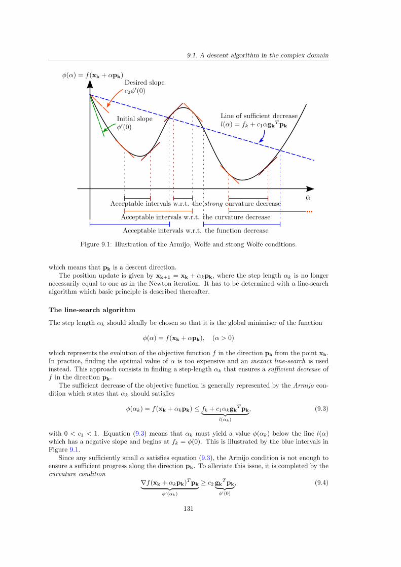
9.1. A descent algorithm in the complex domain
Figure 9.1: Illustration of the Armijo, Wolfe and strong Wolfe conditions.
which means that pk is a descent direction.The position update is given by xk+1 = xk + αkpk, where the step length αk is no longer
necessarily equal to one as in the Newton iteration. It has to be determined with a line-searchalgorithm which basic principle is described thereafter.
The line-search algorithm
The step length αk should ideally be chosen so that it is the global minimiser of the function
φ(α) = f(xk + αpk), (α > 0)
which represents the evolution of the objective function f in the direction pk from the point xk.In practice, finding the optimal value of α is too expensive and an inexact line-search is usedinstead. This approach consists in finding a step-length αk that ensures a sufficient decrease off in the direction pk.
The sufficient decrease of the objective function is generally represented by the Armijo con-dition which states that αk should satisfies
φ(αk) = f(xk + αkpk) ≤ fk + c1αkgkTpk︸ ︷︷ ︸
l(αk)
, (9.3)
with 0 < c1 < 1. Equation (9.3) means that αk must yield a value φ(αk) below the line l(α)which has a negative slope and begins at fk = φ(0). This is illustrated by the blue intervals inFigure 9.1.
Since any sufficiently small α satisfies equation (9.3), the Armijo condition is not enough toensure a sufficient progress along the direction pk. To alleviate this issue, it is completed by thecurvature condition
∇f(xk + αkpk)Tpk︸ ︷︷ ︸φ′(αk)
≥ c2 gkTpk︸ ︷︷ ︸
φ′(0)
, (9.4)
131
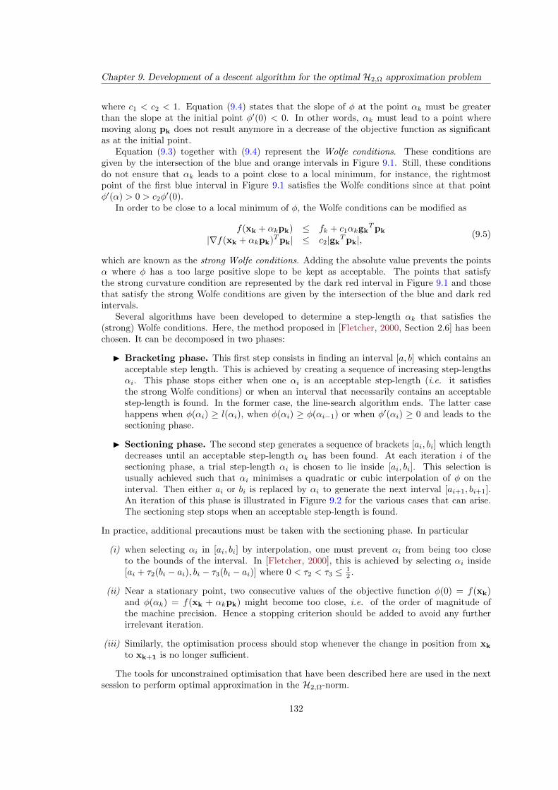
Chapter 9. Development of a descent algorithm for the optimal H2,Ω approximation problem
where c1 < c2 < 1. Equation (9.4) states that the slope of φ at the point αk must be greaterthan the slope at the initial point φ′(0) < 0. In other words, αk must lead to a point wheremoving along pk does not result anymore in a decrease of the objective function as significantas at the initial point.
Equation (9.3) together with (9.4) represent the Wolfe conditions. These conditions aregiven by the intersection of the blue and orange intervals in Figure 9.1. Still, these conditionsdo not ensure that αk leads to a point close to a local minimum, for instance, the rightmostpoint of the first blue interval in Figure 9.1 satisfies the Wolfe conditions since at that pointφ′(α) > 0 > c2φ
′(0).In order to be close to a local minimum of φ, the Wolfe conditions can be modified as
f(xk + αkpk) ≤ fk + c1αkgkTpk
|∇f(xk + αkpk)Tpk| ≤ c2|gkTpk|,
(9.5)
which are known as the strong Wolfe conditions. Adding the absolute value prevents the pointsα where φ has a too large positive slope to be kept as acceptable. The points that satisfythe strong curvature condition are represented by the dark red interval in Figure 9.1 and thosethat satisfy the strong Wolfe conditions are given by the intersection of the blue and dark redintervals.
Several algorithms have been developed to determine a step-length αk that satisfies the(strong) Wolfe conditions. Here, the method proposed in [Fletcher, 2000, Section 2.6] has beenchosen. It can be decomposed in two phases:
I Bracketing phase. This first step consists in finding an interval [a, b] which contains anacceptable step length. This is achieved by creating a sequence of increasing step-lengthsαi. This phase stops either when one αi is an acceptable step-length (i.e. it satisfiesthe strong Wolfe conditions) or when an interval that necessarily contains an acceptablestep-length is found. In the former case, the line-search algorithm ends. The latter casehappens when φ(αi) ≥ l(αi), when φ(αi) ≥ φ(αi−1) or when φ′(αi) ≥ 0 and leads to thesectioning phase.
I Sectioning phase. The second step generates a sequence of brackets [ai, bi] which lengthdecreases until an acceptable step-length αk has been found. At each iteration i of thesectioning phase, a trial step-length αi is chosen to lie inside [ai, bi]. This selection isusually achieved such that αi minimises a quadratic or cubic interpolation of φ on theinterval. Then either ai or bi is replaced by αi to generate the next interval [ai+1, bi+1].An iteration of this phase is illustrated in Figure 9.2 for the various cases that can arise.The sectioning step stops when an acceptable step-length is found.
In practice, additional precautions must be taken with the sectioning phase. In particular
(i) when selecting αi in [ai, bi] by interpolation, one must prevent αi from being too closeto the bounds of the interval. In [Fletcher, 2000], this is achieved by selecting αi inside[ai + τ2(bi − ai), bi − τ3(bi − ai)] where 0 < τ2 < τ3 ≤ 1
2 .
(ii) Near a stationary point, two consecutive values of the objective function φ(0) = f(xk)and φ(αk) = f(xk + αkpk) might become too close, i.e. of the order of magnitude ofthe machine precision. Hence a stopping criterion should be added to avoid any furtherirrelevant iteration.
(iii) Similarly, the optimisation process should stop whenever the change in position from xk
to xk+1 is no longer sufficient.
The tools for unconstrained optimisation that have been described here are used in the nextsession to perform optimal approximation in the H2,Ω-norm.
132
9.1. A descent algorithm in the complex domain
Figure 9.2: Illustration of the sectioning phase of the line-search algorithm.
9.1.2 Descent Algorithm for Residues and Poles Optimisation
The complex-domain optimisation algorithm developed here is mainly based on [Sorber et al.,2012] where the BFGS algorithm is formally extended for the optimisation of real functions ofcomplex variables. In practice, the resulting optimisation scheme is the same as its real counter-part described in the previous Section excepted that the gradient becomes the conjugate complexgradient, and that the transpose operations are replaced by conjugate transpose operations.
The method is called DARPO and is presented in Algorithm 11. Given the realisationof a large-scale model H := (A,B,C,D) and a frequency interval Ω, the first step consists incomputing the eigenvalue decomposition of the large-scale matrix A in order to build the matricesC∆ and B∆ involved in the computation of the approximation error and its gradient (see Remark17 for some comments on this step). Then an initial reduced-order model is chosen as a vector
z0 containing the poles λi and residues ci, bi (i = 1, . . . , r). The process of initialisation isdetailed in Section 9.1.3. Note that as explained in Remark 18, D does not need to be takeninto account among the optimisation variables.
Then, while a stationary point has not been reached, the approximation error JH2,Ωis com-
puted together with its gradient (step 6) at the current point zk. Then the conjugate of thegradient of JH2,Ω with respect to z is used, together with the current inverse Hessian approxima-
tion Bk−1 to set the descent direction pk. At step 8, the step-length αk that yields a sufficient
decrease of the objective function in the direction pk is determined with the inexact line-searchalgorithm described in Section 9.1.1. Then, at steps 9 and 10, the next point zk+1 is created andthe inverse Hessian approximation is updated. Finally, the reduced-order model is built fromthe optimal poles, residues and direct feedthrough at step 13.
Additionally, the tools developed in Section 7.3 can be used to bound the H∞-norm of theerror model and to build a frequency template that bounds the Frobenius norm of the errormodel transfer function (and thus its maximum singular value). Since the eigen-decompositionof the large-scale and reduced-order models are already available, these optional steps can beachieved with a limited computational cost.
As the method FL-ISTIA presented in Chapter 6, DARPO has been integrated to theMORE Toolbox [Poussot-Vassal and Vuillemin, 2012] and an example of its use can be found inAppendix C.7.
Remark 17 (Computation of the eigen-decomposition of the large-scale model). The first stepof DARPO requires to compute the full eigen-decomposition of the initial large-scale model H.This is computationally expensive and cannot be performed for too large models. And, unlike in
133
Chapter 9. Development of a descent algorithm for the optimal H2,Ω approximation problem
the H2-case, one cannot avoid this decomposition because here the eigenvalue of the large-scalemodel explicitly appear in the approximation error JH2,Ω
.Hence, and as the other results based on the poles-residues formulation of the H2,Ω-norm,
this algorithm is restricted to the cases for which the eigen-decomposition is actually available.This issue is not specific to this formulation though. Indeed, with the gramian formulation, thelogarithm of a complex n×n matrix has to be computed and at each iteration, two n×r Sylvesterequations have to be solved.
Some hints to alleviate the issue related to the computation of the full eigen-decompositionare presented as a perspective in Chapter 11.
Remark 18 (About the direct feedthrough D in DARPO). As mentioned in Section 8.2.2, theoptimal direct feedthrough D can be determined uniquely from equation (8.23). Hence in Algo-rithm 11, it is assumed that each time the objective function JH2,Ω
or its gradient is evaluated,
D is replaced with its optimal value.
The following remarks can be addressed about Algorithm 11
I Step 6 : one part of the gradient of the approximation error is the complex conjugate ofthe other. To decrease the number of operations required to evaluate the gradient, one cancompute it for the real variables and those which imaginary part is positive (or negative)only and then re-construct the complete gradient by conjugating its complex elements.
I Step 13 : the realisation of the reduced-order model H = (A, B, C) is obtained by creating
arbitrary complex vectors xi ∈ Cr×1 associated to the eigenvalues λi which respect thecomplex conjugation of the eigenvalues, i.e. if λj = λ∗i then xj = x∗i , and which are
linearly independent. Then, by denoting X ∈ Cr×r the matrix which columns are thevectors xi, ∆ ∈ Cr×r the diagonal matrix containing the eigenvalues λi, C∆ ∈ Cny×r
(respectively B∆ ∈ Cr×nu) the matrix which columns (lines) are the cTi (bi),
A = X∆X−1
B = XB∆
C = C∆X−1.
This is a basis change between the complex diagonal realisation (∆, B∆, C∆) of H anda real realisation. The vectors xi can for instance be chosen so that the real realisation(A, B, C) is block diagonal.
I Step 14 : since the poles and residues of both the large-scale and reduced-order models arealready known, the computation of the upper bounds ΓΩ(H − H) and ΓΩ(H − H) doesnot require to solve any additional large-scale eigenvalue problem. Indeed the poles of theerror model E = H− H are the poles of H and H while its residues are composed of theresidues of H and the opposite of the residues of H. The same remark holds for Step 15.
I Note that the stopping criterion ‖∂JH2,Ω
∂z |z=zk‖ ≤ ε is the ideal one2 and indicates that the
algorithm has reached a stationary point. Yet, as suggested in Section 9.1.1, one also checksthe progress made at each iteration in the direction pk through the difference between twoconsecutive iterates zk and zk+1 and between the corresponding values of the objectivefunction. One can also directly check the norm of the derivative of JH2,Ω
in the directionpk before performing a line-search, i.e.∥∥∥pH
k
∂JH2,Ω
∂z∗
∣∣∣z=zk
∥∥∥. (9.6)
2By ideal stopping criterion, one means that it is the most relevant criterion available here to determine if thecurrent point is close to a stationary point.
134
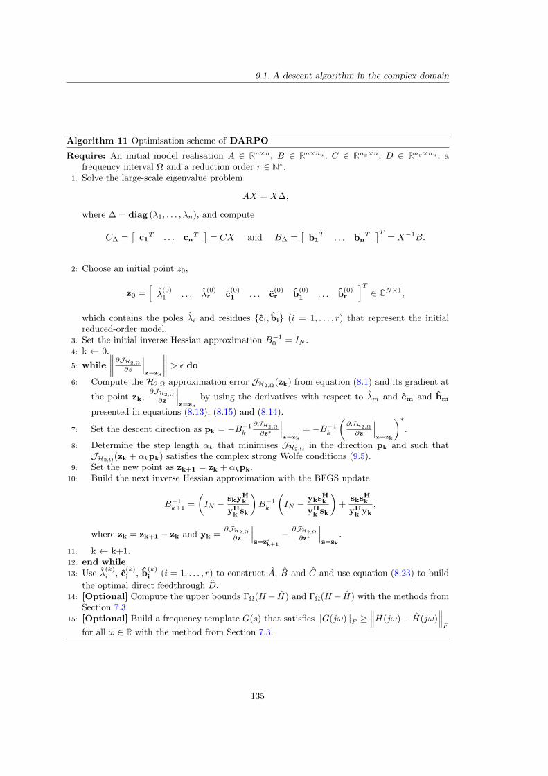
9.1. A descent algorithm in the complex domain
Algorithm 11 Optimisation scheme of DARPO
Require: An initial model realisation A ∈ Rn×n, B ∈ Rn×nu , C ∈ Rny×n, D ∈ Rny×nu , afrequency interval Ω and a reduction order r ∈ N∗.
1: Solve the large-scale eigenvalue problem
AX = X∆,
where ∆ = diag (λ1, . . . , λn), and compute
C∆ =[
c1T . . . cn
T]
= CX and B∆ =[
b1T . . . bn
T]T
= X−1B.
2: Choose an initial point z0,
z0 =[λ
(0)1 . . . λ
(0)r c
(0)1 . . . c
(0)r b
(0)1 . . . b
(0)r
]T∈ CN×1,
which contains the poles λi and residues ci, bi (i = 1, . . . , r) that represent the initialreduced-order model.
3: Set the initial inverse Hessian approximation B−10 = IN .
4: k ← 0.
5: while
∥∥∥∥∂JH2,Ω
∂z
∣∣∣z=zk
∥∥∥∥ > ε do
6: Compute the H2,Ω approximation error JH2,Ω(zk) from equation (8.1) and its gradient at
the point zk,∂JH2,Ω
∂z
∣∣∣z=zk
by using the derivatives with respect to λm and cm and bm
presented in equations (8.13), (8.15) and (8.14).
7: Set the descent direction as pk = −B−1k
∂JH2,Ω
∂z∗
∣∣∣z=zk
= −B−1k
(∂JH2,Ω
∂z
∣∣∣z=zk
)∗.
8: Determine the step length αk that minimises JH2,Ωin the direction pk and such that
JH2,Ω(zk + αkpk) satisfies the complex strong Wolfe conditions (9.5).9: Set the new point as zk+1 = zk + αkpk.
10: Build the next inverse Hessian approximation with the BFGS update
B−1k+1 =
(IN −
skyHk
yHk sk
)B−1k
(IN −
yksHk
yHk sk
)+
sksHk
yHk yk
,
where zk = zk+1 − zk and yk =∂JH2,Ω
∂z
∣∣∣z=z∗k+1
− ∂JH2,Ω
∂z∗
∣∣∣z=zk
.
11: k ← k+1.12: end while13: Use λ
(k)i , c
(k)i , b
(k)i (i = 1, . . . , r) to construct A, B and C and use equation (8.23) to build
the optimal direct feedthrough D.14: [Optional] Compute the upper bounds ΓΩ(H − H) and ΓΩ(H − H) with the methods from
Section 7.3.15: [Optional] Build a frequency template G(s) that satisfies ‖G(jω)‖F ≥
∥∥∥H(jω)− H(jω)∥∥∥F
for all ω ∈ R with the method from Section 7.3.
135
Chapter 9. Development of a descent algorithm for the optimal H2,Ω approximation problem
If (9.6) is low (of the order of magnitude of the machine precision), then it means that theobjective function is almost flat in the direction pk, i.e. that current point is a stationarypoint. Hence, the line-search algorithm is unlikely to find a significant step-length αk.
About the stability of the reduced-order model. In its current state, there is no formalguarantee that DARPO preserves the stability of the initial large-scale model. Even if anunstable reduced-order model is not expected to be obtained from an initial stable reduced-order model (see Example 17), two problematic cases can arise
(i) there is actually an unstable local minimum,
(ii) the local minimum is stable but the line-search algorithm produces a step-length αk thatmakes the poles switch from the left half-plane to the right half plane.
There is not much that can be done in case (i) without using constrained optimisation but case(ii) can be handled fairly easily in the unconstrained optimisation framework.
Indeed, let us consider a pole λ located in the left half-plane at the left (along the real axis)
of its optimal value λopt which is also in the left half-plane, i.e.
Re(λ) < Re(λopt) < 0.
In that case, the real part of the descent direction p ∈ C associated to the pole λ is positive. Ifa too large step is performed in the direction p, then the next iterate of the pole, λ+ αp, mightends up in the right half-plane. Whether this will happen depends on the line-search algorithmused to determine the step-length α (see Section 9.1.1).
First, note that the parameter 0 < c1 < 1 used in the definition of the line decrease l(α) inequation (9.3) controls the slope of l. More specifically, the smaller c1 is, the flatter the decreaseline is and the larger the interval of acceptable points with respect to the decrease condition is(this can be seen in Figure 9.1). The line l(α) is involved in both the bracketing and sectioningphase of the line-search algorithm and determines how far in the descent direction the algorithmcan look. The further one looks in the direction p, the more likely a large acceptable step-lengthα will be found.
The initial step-length trial used in the bracketing phase also contributes to determine the sizeof the initial interval containing an acceptable step length. Choosing 1 as initial value is standardsince the Newton iteration is mimicked when the approximate Hessian is representative enoughof the real Hessian. Yet this might directly leads to consider an interval containing step-lengthsufficiently large to make λ moves in the right half-plane.
Hence, to avoid selecting a step-length α that satisfies the strong Wolfe conditions but leadsλ in the right half-plane, two solutions can be considered,
I the first one consists in increasing c1 to prevent the line-search algorithm from looking toofar from the current point,
I the second one consists in verifying if the initial step-length trial α = 1 leads λ to move inthe right half-plane. If it does, then it can be replaced by
αmax = −Re(λ)
Re(p),
which represents the maximum allowed step-length for the next pole λ + αp to lies inthe left half-plane. One must then ensure that the line-search algorithm chose a point in[0, αmax[.
Note that if Im(λ+ αmaxp) ∈ Ω, then αmax is necessarily an acceptable upper bound forthe bracketing phase since the objective function is, by definition, infinite when some polesof the reduced-order model are on the imaginary axis inside Ω.
136
9.1. A descent algorithm in the complex domain
About the convergence. The optimisation method used in DARPO produces a sequences ofreduced-order models that yield monotonically decreasing H2,Ω approximation errors. Whetherthe final reduced-order model is a local minimum or not cannot be ensured without preciseknowledge of the curvature of the objective function. Indeed, the global convergence of theBFGS update used here is not fully known for non-convex functions. However in practice, theBFGS update is known to be efficient and in [Li and Fukushima, 2001], the authors show thatthe BFGS update is a specific case of their cautious BFGS update which is proven to makethe optimisation method globally convergent. Hence, DARPO is expected to lead to a localminimum of the optimal H2,Ω approximation problem.
9.1.3 Initialisation of DARPO
Unlike the FL-BT or the FL-ISTIA, a relevant reduced-order model should be used as ini-tial point with DARPO. Hence this algorithm should be considered as a refinement processwhich cannot be considered separately from how it is initialised. Indeed, DARPO is a localoptimisation algorithm applied to a non-linear and non-convex optimisation problem, thus theselection of the initial reduced-order model is extremely important and determines the qualityof the solution.
Various initialisation strategies can be considered :
I Random initialisation. The simplest strategy consists in using a randomly generatedmodel as initial point.
This initialisation method is straightforward but should not be used because (i) it is not de-terministic and might produce different reduced-order models through successive launcheson an identical use case, (ii) it does not take into account the frequency interval Ω overwhich the initial large-scale model has to be reduced and (iii) it does not exploit anyinformation about the initial large-scale model while its eigenvalues and eigenvectors areknown from step 1. In practice, this initialisation strategy performs poorly on non-trivialapplications and leads to a local minimum far from being satisfactory.
I Initialisation with another method. The second initialisation strategy consists inusing another model approximation method to produce an initial reduced-order model.Since the aim here is to perform optimal H2,Ω approximation, the model approximationmethod should take into account the frequency interval Ω. For instance, one could use oneof the methods presented in Chapter 5 (such as the FW-BT or the FL-BT) or one couldalso use FL-ISTIA, the empirical method developed during this thesis and presented inChapter 6.
This strategy generally leads to reduced-order model of good quality (with respect to theH2,Ω-norm of the error) and, depending on the initial model approximation that is used, itcan be deterministic and exploit the eigen-decomposition of the matrix A (for computingthe gramians for instance).
Yet, since it implies to use two different model approximation methods, this strategy is notcompletely satisfactory but it may be considered when computation time is not an issue.
I Initialisation with a modal truncation. This initialisation strategy consists in settingthe initial reduced-order model as a modal truncation of the initial large-scale model. Thisinitial reduced-order model is the most natural since the eigen-decomposition of the initialmodel is computed at step 1 of Algorithm 11. As the objective here is to minimise JH2,Ω
,a relevant criterion must be built to determine the poles that must be retained. To thataim, various criteria have been considered and the most relevant are,
137
Chapter 9. Development of a descent algorithm for the optimal H2,Ω approximation problem
– to keep the poles λi and associated residues Φi that maximise
J (1)init(λi,Φi) =
∥∥∥Φiatan
(ω
λi
)∥∥∥2.
where Ω = [0, ω] (see Remark 19 for more complex intervals). This criterion is similarto what can appear in standard modal approximation with in addition the weightingterm which decreases the influence of the residues associated to poles which imaginary
part is outside of Ω. J (1)init can easily be evaluated and does not add much computation.
– The second criterion consists in keeping the poles λi and associated residues Φi thathave the maximum influence in the H2,Ω-norm of H, i.e. those that yield the largest
J (2)init(λi,Φi) = −Re
(tr(ΦiH(−λi)T
)atan
(ω
λi
)), (9.7)
where Ω = [0, ω]. Again, the function J (1)init can easily be evaluated3.
– The third criterion consists in keeping the poles λi and associated residues Φi thatwould make the best second-order (or first-order if the pole is real) approximation ofH over Ω, i.e. by denoting Hi(s) the transfer functions defined as
Hi(s) =Φi
s− λi+
Φ∗is− λ∗i
,
the poles to retain are those that maximise
J (3)init(λi,Φi) = −‖H − Hi‖2H2,Ω
.
This selection method is computationally more demanding than the two others sinceit requires to evaluate several approximation errors.
None of these poles selection method really stands out of the other in term of global
performance but the two first ones are cheaper. The criterion J (1)init tends to be more
relevant than J (2)init when the considered frequency interval contains only poles associated
to small residues in comparison to other areas but might fail on simple unbounded intervals
like [0,∞). Hence, J (2)init is considered as the default initialisation procedure in the sequel
if nothing else is specified.
Independently of the poles selection method, this initialisation strategy based on the modaltruncation fully exploits the fact that the eigen-decomposition of the matrix A is computed
in DARPO and in addition it does not add much extra computation if J (1)init or J (2)
init isused. Besides, the poles of the reduced-order model are generally not too far from the polesof the initial large-scale model which can be attractive from a practical point of view.
The main flaw of this initialisation strategy is that if the frequency interval Ω does notcontain enough poles, then irrelevant poles outside of Ω are selected and they might notbe able to move inside the frequency interval of interest as suggested by Example 17.
From a practical point of view, this initialisation strategy must also be completed with asafeguard procedure dealing with the incoherence that can appear between the reductionorder r and the poles selected. For instance, when r is odd while the candidate poles areall complex, etc.
3Indeed, since the eigen-decomposition of the initial model is known, H(−λi) can be expressed with the
poles and residues of the transfer function and the criterion J (2)init can thus be computed in a similar way to the
approximation error JH2,Ωin Section 8.1.2.
138
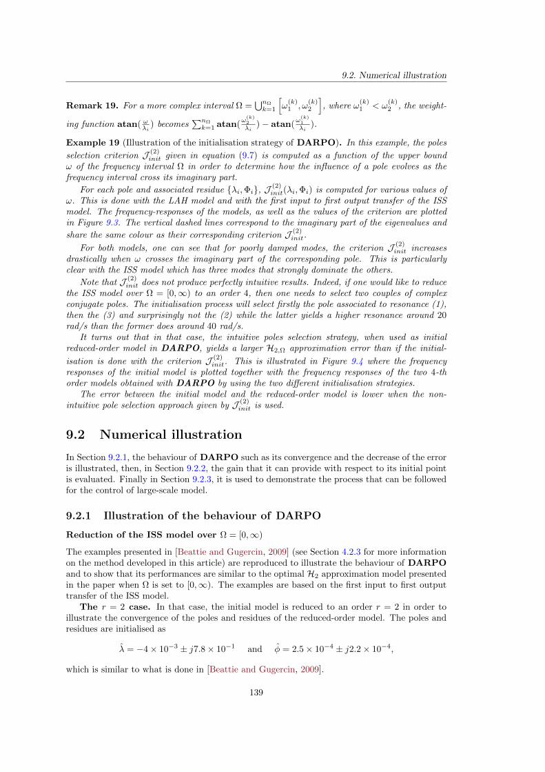
9.2. Numerical illustration
Remark 19. For a more complex interval Ω =⋃nΩ
k=1
[ω
(k)1 , ω
(k)2
], where ω
(k)1 < ω
(k)2 , the weight-
ing function atan( ωλi ) becomes∑nΩ
k=1 atan(ω
(k)2
λi)− atan(
ω(k)1
λi).
Example 19 (Illustration of the initialisation strategy of DARPO). In this example, the poles
selection criterion J (2)init given in equation (9.7) is computed as a function of the upper bound
ω of the frequency interval Ω in order to determine how the influence of a pole evolves as thefrequency interval cross its imaginary part.
For each pole and associated residue λi,Φi, J (2)init(λi,Φi) is computed for various values of
ω. This is done with the LAH model and with the first input to first output transfer of the ISSmodel. The frequency-responses of the models, as well as the values of the criterion are plottedin Figure 9.3. The vertical dashed lines correspond to the imaginary part of the eigenvalues and
share the same colour as their corresponding criterion J (2)init.
For both models, one can see that for poorly damped modes, the criterion J (2)init increases
drastically when ω crosses the imaginary part of the corresponding pole. This is particularlyclear with the ISS model which has three modes that strongly dominate the others.
Note that J (2)init does not produce perfectly intuitive results. Indeed, if one would like to reduce
the ISS model over Ω = [0,∞) to an order 4, then one needs to select two couples of complexconjugate poles. The initialisation process will select firstly the pole associated to resonance (1),then the (3) and surprisingly not the (2) while the latter yields a higher resonance around 20rad/s than the former does around 40 rad/s.
It turns out that in that case, the intuitive poles selection strategy, when used as initialreduced-order model in DARPO, yields a larger H2,Ω approximation error than if the initial-
isation is done with the criterion J (2)init. This is illustrated in Figure 9.4 where the frequency
responses of the initial model is plotted together with the frequency responses of the two 4-thorder models obtained with DARPO by using the two different initialisation strategies.
The error between the initial model and the reduced-order model is lower when the non-intuitive pole selection approach given by J (2)
init is used.
9.2 Numerical illustration
In Section 9.2.1, the behaviour of DARPO such as its convergence and the decrease of the erroris illustrated, then, in Section 9.2.2, the gain that it can provide with respect to its initial pointis evaluated. Finally in Section 9.2.3, it is used to demonstrate the process that can be followedfor the control of large-scale model.
9.2.1 Illustration of the behaviour of DARPO
Reduction of the ISS model over Ω = [0,∞)
The examples presented in [Beattie and Gugercin, 2009] (see Section 4.2.3 for more informationon the method developed in this article) are reproduced to illustrate the behaviour of DARPOand to show that its performances are similar to the optimal H2 approximation model presentedin the paper when Ω is set to [0,∞). The examples are based on the first input to first outputtransfer of the ISS model.
The r = 2 case. In that case, the initial model is reduced to an order r = 2 in order toillustrate the convergence of the poles and residues of the reduced-order model. The poles andresidues are initialised as
λ = −4× 10⁻³ ± j7.8× 10−1 and φ = 2.5× 10⁻⁴ ± j2.2× 10−4,
which is similar to what is done in [Beattie and Gugercin, 2009].
139
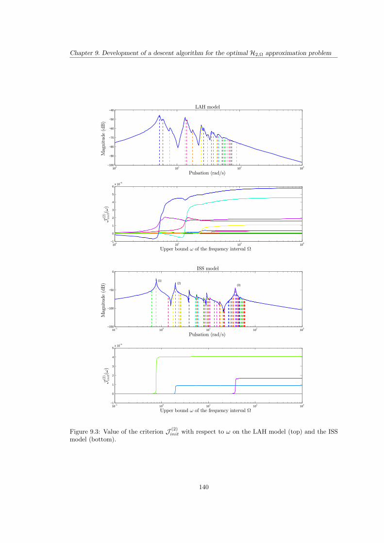
Chapter 9. Development of a descent algorithm for the optimal H2,Ω approximation problem
100
101
102
103
−100
−90
−80
−70
−60
−50
−40LAH model
Magnitude(dB)
Pulsation (rad/s)
100
101
102
103
−1
0
1
2
3
4
5
6x 10
−6
J(2)
init(ω)
Upper bound ω of the frequency interval Ω
10−1
100
101
102
103
−150
−100
−50
0ISS model
Magnitude(dB)
Pulsation (rad/s)
10−1
100
101
102
103
−1
0
1
2
3
4
5x 10
−5
J(2)
init(ω)
Upper bound ω of the frequency interval Ω
(1)(2)
(3)
Figure 9.3: Value of the criterion J (2)init with respect to ω on the LAH model (top) and the ISS
model (bottom).
140
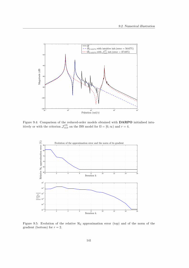
9.2. Numerical illustration
10−1
100
101
102
103
−120
−100
−80
−60
−40
−20
0
Magnitude(dB
Pulsation (rad/s)
HHDARPO with intuitive init.(error = 50.67%)
HDARPO with J(2)init init.(error = 37.02%)
Figure 9.4: Comparison of the reduced-order models obtained with DARPO initialised intu-
itively or with the criterion J (2)init on the ISS model for Ω = [0,∞) and r = 4.
0 2 4 6 8 10 12 14 1660
65
70
75
80
85Evolution of the approximation error and the norm of its gradient
RelativeH
2ap
proximationerror(%
)
Iteration k
0 2 4 6 8 10 12 14 1610
−10
10−8
10−6
10−4
10−2
100
∥ ∥ ∥
∂JH2
∂z
∥ ∥ ∥
Iteration k
Figure 9.5: Evolution of the relative H2 approximation error (top) and of the norm of thegradient (bottom) for r = 2.
141
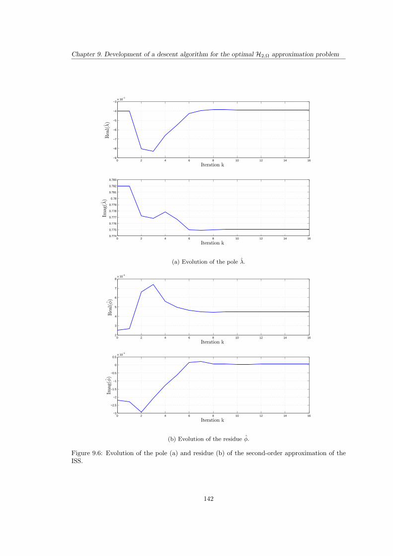
Chapter 9. Development of a descent algorithm for the optimal H2,Ω approximation problem
0 2 4 6 8 10 12 14 16−9
−8
−7
−6
−5
−4
−3x 10
−3
Real(λ)
Iteration k
0 2 4 6 8 10 12 14 160.774
0.775
0.776
0.777
0.778
0.779
0.78
0.781
0.782
0.783
Imag(λ)
Iteration k
(a) Evolution of the pole λ.
0 2 4 6 8 10 12 14 162
3
4
5
6
7
8x 10
−4
Real(φ)
Iteration k
0 2 4 6 8 10 12 14 16−3
−2.5
−2
−1.5
−1
−0.5
0
0.5x 10
−4
Imag(φ)
Iteration k
(b) Evolution of the residue φ.
Figure 9.6: Evolution of the pole (a) and residue (b) of the second-order approximation of theISS.
142
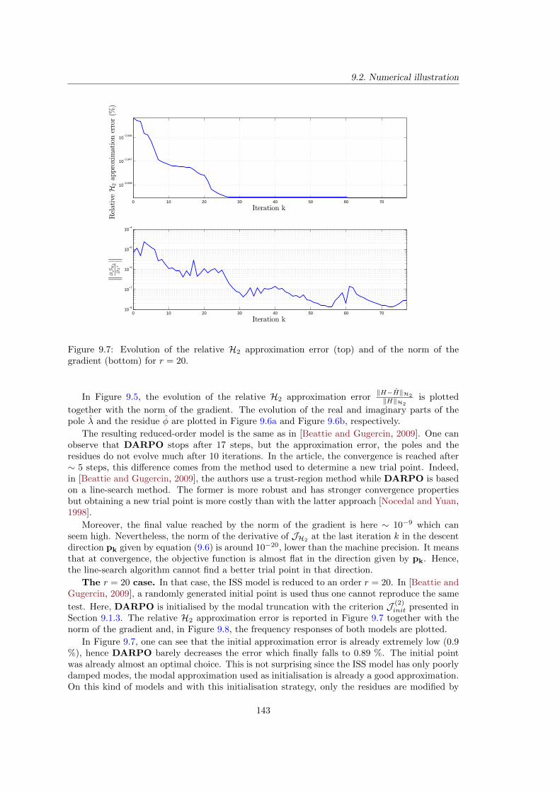
9.2. Numerical illustration
0 10 20 30 40 50 60 70
10−2.048
10−2.047
10−2.046
RelativeH
2ap
proximationerror(%
)
Iteration k
0 10 20 30 40 50 60 7010
−8
10−7
10−6
10−5
10−4
∥ ∥ ∥
∂JH2
∂z∗
∥ ∥ ∥
Iteration k
Figure 9.7: Evolution of the relative H2 approximation error (top) and of the norm of thegradient (bottom) for r = 20.
In Figure 9.5, the evolution of the relative H2 approximation error‖H−H‖H2
‖H‖H2is plotted
together with the norm of the gradient. The evolution of the real and imaginary parts of thepole λ and the residue φ are plotted in Figure 9.6a and Figure 9.6b, respectively.
The resulting reduced-order model is the same as in [Beattie and Gugercin, 2009]. One canobserve that DARPO stops after 17 steps, but the approximation error, the poles and theresidues do not evolve much after 10 iterations. In the article, the convergence is reached after∼ 5 steps, this difference comes from the method used to determine a new trial point. Indeed,in [Beattie and Gugercin, 2009], the authors use a trust-region method while DARPO is basedon a line-search method. The former is more robust and has stronger convergence propertiesbut obtaining a new trial point is more costly than with the latter approach [Nocedal and Yuan,1998].
Moreover, the final value reached by the norm of the gradient is here ∼ 10−9 which canseem high. Nevertheless, the norm of the derivative of JH2
at the last iteration k in the descentdirection pk given by equation (9.6) is around 10−20, lower than the machine precision. It meansthat at convergence, the objective function is almost flat in the direction given by pk. Hence,the line-search algorithm cannot find a better trial point in that direction.
The r = 20 case. In that case, the ISS model is reduced to an order r = 20. In [Beattie andGugercin, 2009], a randomly generated initial point is used thus one cannot reproduce the same
test. Here, DARPO is initialised by the modal truncation with the criterion J (2)init presented in
Section 9.1.3. The relative H2 approximation error is reported in Figure 9.7 together with thenorm of the gradient and, in Figure 9.8, the frequency responses of both models are plotted.
In Figure 9.7, one can see that the initial approximation error is already extremely low (0.9%), hence DARPO barely decreases the error which finally falls to 0.89 %. The initial pointwas already almost an optimal choice. This is not surprising since the ISS model has only poorlydamped modes, the modal approximation used as initialisation is already a good approximation.On this kind of models and with this initialisation strategy, only the residues are modified by
143
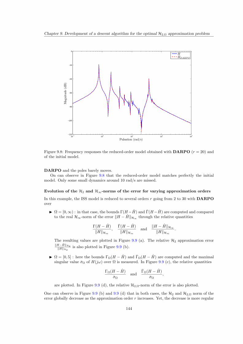
Chapter 9. Development of a descent algorithm for the optimal H2,Ω approximation problem
10−1
100
101
102
103
−120
−100
−80
−60
−40
−20
0
Magnitude(dB)
Pulsation (rad/s)
HHDARPO
Figure 9.8: Frequency responses the reduced-order model obtained with DARPO (r = 20) andof the initial model.
DARPO and the poles barely moves.On can observe in Figure 9.8 that the reduced-order model matches perfectly the initial
model. Only some small dynamics around 10 rad/s are missed.
Evolution of the H2 and H∞-norms of the error for varying approximation orders
In this example, the ISS model is reduced to several orders r going from 2 to 30 with DARPOover
I Ω = [0,∞) : in that case, the bounds Γ(H−H) and Γ(H−H) are computed and comparedto the real H∞-norm of the error ‖H − H‖H∞ through the relative quantities
Γ(H − H)
‖H‖H∞,
Γ(H − H)
‖H‖H∞and
‖H − H‖H∞‖H‖H∞
.
The resulting values are plotted in Figure 9.9 (a). The relative H2 approximation error‖H−H‖H2
‖H‖H2is also plotted in Figure 9.9 (b).
I Ω = [0, 5] : here the bounds ΓΩ(H − H) and ΓΩ(H − H) are computed and the maximalsingular value σΩ of H(jω) over Ω is measured. In Figure 9.9 (c), the relative quantities
ΓΩ(H − H)
σΩand
ΓΩ(H − H)
σΩ,
are plotted. In Figure 9.9 (d), the relative H2,Ω-norm of the error is also plotted.
One can observe in Figure 9.9 (b) and 9.9 (d) that in both cases, the H2 and H2,Ω norm of theerror globally decrease as the approximation order r increases. Yet, the decrease is more regular
144
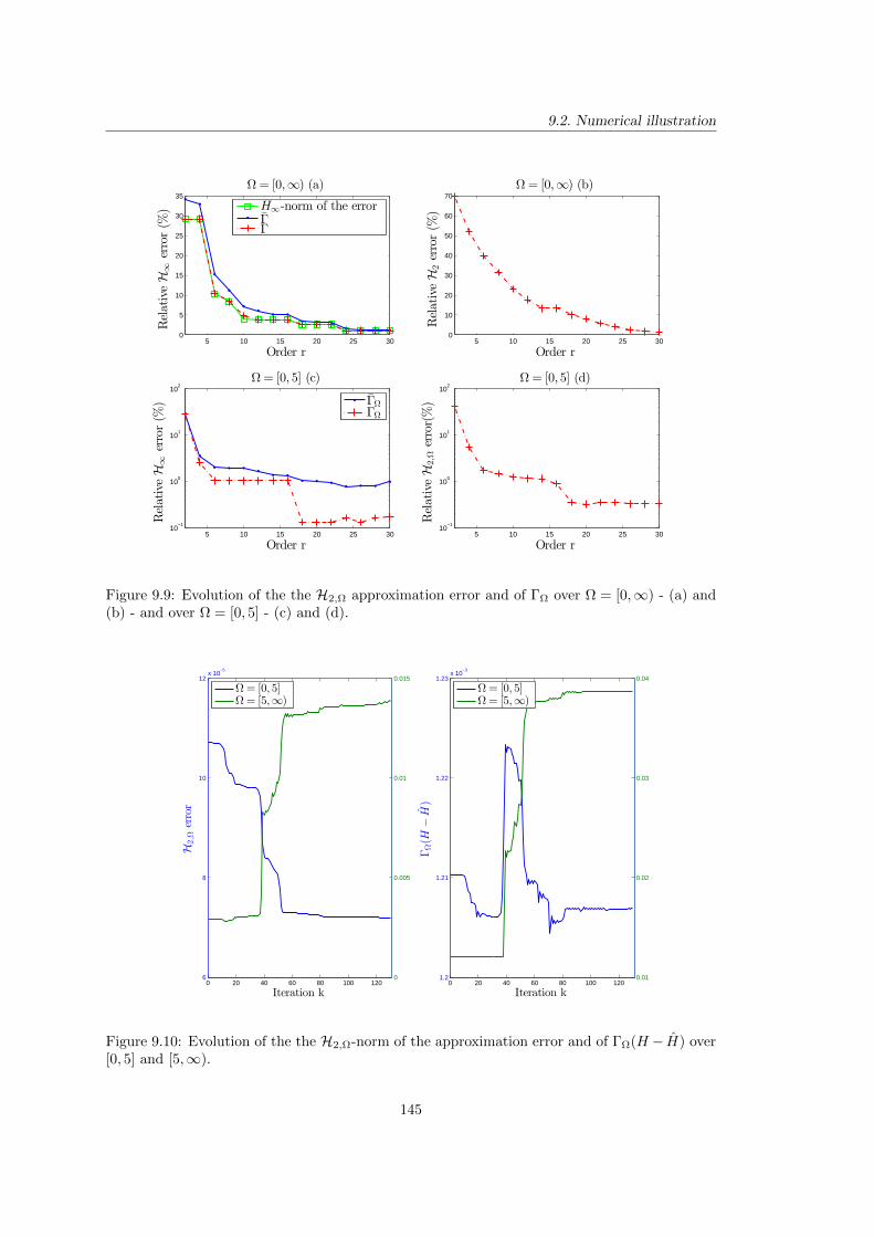
9.2. Numerical illustration
5 10 15 20 25 300
5
10
15
20
25
30
35Ω= [0,∞) (a)
Order r
RelativeH
∞error(%
)
H∞-norm of the errorΓΓ
5 10 15 20 25 300
10
20
30
40
50
60
70Ω= [0,∞) (b)
RelativeH
2error(%
)
Order r
5 10 15 20 25 3010
−1
100
101
102
Ω= [0, 5] (c)
Order r
RelativeH
∞error(%
)
ΓΩ
ΓΩ
5 10 15 20 25 3010
−1
100
101
102
Ω= [0, 5] (d)
RelativeH
2,Ω
error(%)
Order r
Figure 9.9: Evolution of the the H2,Ω approximation error and of ΓΩ over Ω = [0,∞) - (a) and(b) - and over Ω = [0, 5] - (c) and (d).
0 20 40 60 80 100 1206
8
10
12x 10
−5
H2,Ω
error
Iteration k
0
0.005
0.01
0.015
Ω= [0, 5]Ω= [5,∞)
0 20 40 60 80 100 1201.2
1.21
1.22
1.23x 10
−3
ΓΩ(H
−H)
Iteration k
0.01
0.02
0.03
0.04
Ω= [0, 5]Ω= [5,∞)
Figure 9.10: Evolution of the the H2,Ω-norm of the approximation error and of ΓΩ(H − H) over[0, 5] and [5,∞).
145
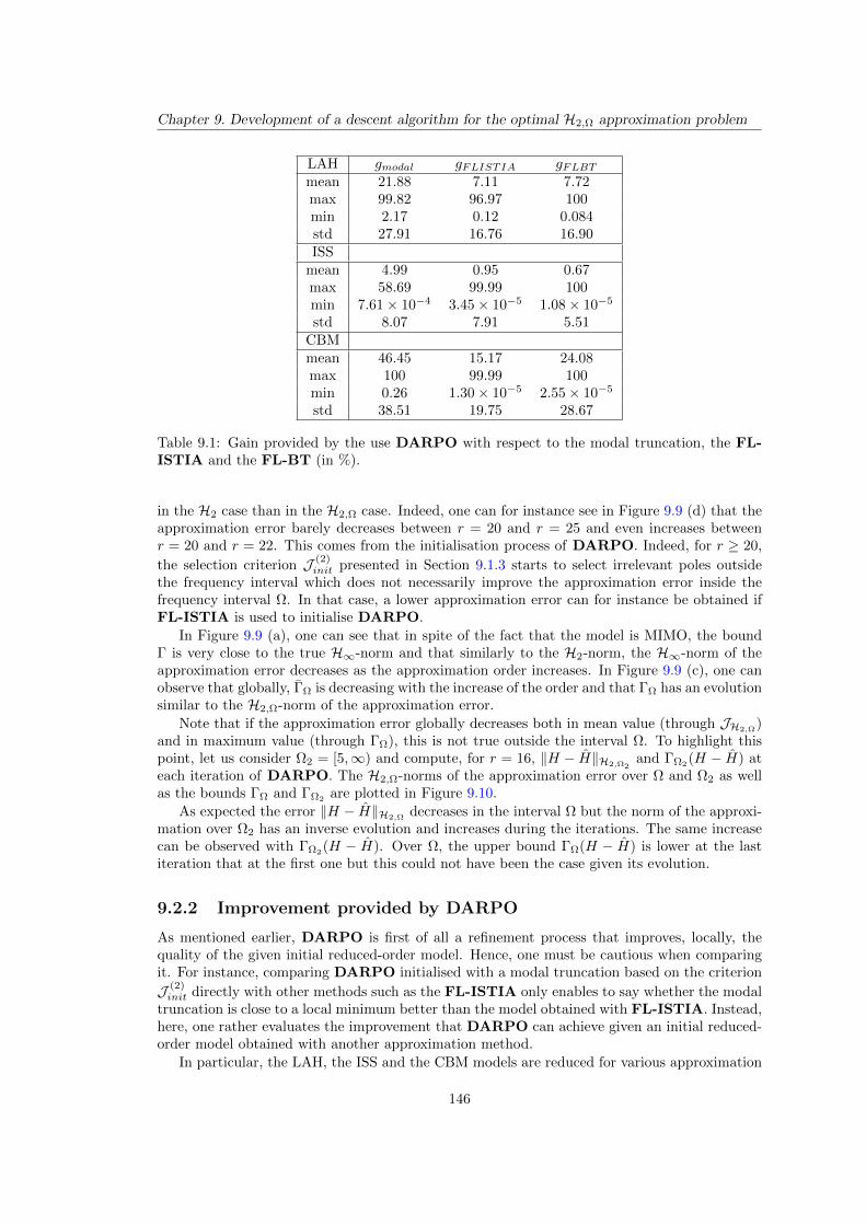
Chapter 9. Development of a descent algorithm for the optimal H2,Ω approximation problem
LAH gmodal gFLISTIA gFLBTmean 21.88 7.11 7.72max 99.82 96.97 100min 2.17 0.12 0.084std 27.91 16.76 16.90ISS
mean 4.99 0.95 0.67max 58.69 99.99 100min 7.61× 10⁻⁴ 3.45× 10⁻⁵ 1.08× 10⁻⁵
std 8.07 7.91 5.51CBMmean 46.45 15.17 24.08max 100 99.99 100min 0.26 1.30× 10⁻⁵ 2.55× 10⁻⁵
std 38.51 19.75 28.67
Table 9.1: Gain provided by the use DARPO with respect to the modal truncation, the FL-ISTIA and the FL-BT (in %).
in the H2 case than in the H2,Ω case. Indeed, one can for instance see in Figure 9.9 (d) that theapproximation error barely decreases between r = 20 and r = 25 and even increases betweenr = 20 and r = 22. This comes from the initialisation process of DARPO. Indeed, for r ≥ 20,
the selection criterion J (2)init presented in Section 9.1.3 starts to select irrelevant poles outside
the frequency interval which does not necessarily improve the approximation error inside thefrequency interval Ω. In that case, a lower approximation error can for instance be obtained ifFL-ISTIA is used to initialise DARPO.
In Figure 9.9 (a), one can see that in spite of the fact that the model is MIMO, the boundΓ is very close to the true H∞-norm and that similarly to the H2-norm, the H∞-norm of theapproximation error decreases as the approximation order increases. In Figure 9.9 (c), one canobserve that globally, ΓΩ is decreasing with the increase of the order and that ΓΩ has an evolutionsimilar to the H2,Ω-norm of the approximation error.
Note that if the approximation error globally decreases both in mean value (through JH2,Ω)
and in maximum value (through ΓΩ), this is not true outside the interval Ω. To highlight thispoint, let us consider Ω2 = [5,∞) and compute, for r = 16, ‖H − H‖H2,Ω2
and ΓΩ2(H − H) at
each iteration of DARPO. The H2,Ω-norms of the approximation error over Ω and Ω2 as wellas the bounds ΓΩ and ΓΩ2 are plotted in Figure 9.10.
As expected the error ‖H − H‖H2,Ωdecreases in the interval Ω but the norm of the approxi-
mation over Ω2 has an inverse evolution and increases during the iterations. The same increasecan be observed with ΓΩ2
(H − H). Over Ω, the upper bound ΓΩ(H − H) is lower at the lastiteration that at the first one but this could not have been the case given its evolution.
9.2.2 Improvement provided by DARPO
As mentioned earlier, DARPO is first of all a refinement process that improves, locally, thequality of the given initial reduced-order model. Hence, one must be cautious when comparingit. For instance, comparing DARPO initialised with a modal truncation based on the criterion
J (2)init directly with other methods such as the FL-ISTIA only enables to say whether the modal
truncation is close to a local minimum better than the model obtained with FL-ISTIA. Instead,here, one rather evaluates the improvement that DARPO can achieve given an initial reduced-order model obtained with another approximation method.
In particular, the LAH, the ISS and the CBM models are reduced for various approximation
146
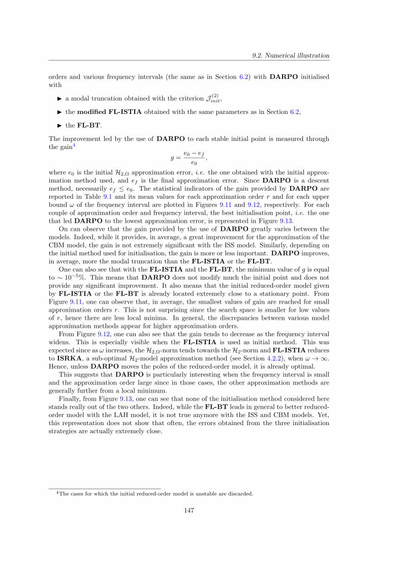
9.2. Numerical illustration
orders and various frequency intervals (the same as in Section 6.2) with DARPO initialisedwith
I a modal truncation obtained with the criterion J (2)init,
I the modified FL-ISTIA obtained with the same parameters as in Section 6.2,
I the FL-BT.
The improvement led by the use of DARPO to each stable initial point is measured throughthe gain4
g =e0 − efe0
,
where e0 is the initial H2,Ω approximation error, i.e. the one obtained with the initial approx-imation method used, and ef is the final approximation error. Since DARPO is a descentmethod, necessarily ef ≤ e0. The statistical indicators of the gain provided by DARPO arereported in Table 9.1 and its mean values for each approximation order r and for each upperbound ω of the frequency interval are plotted in Figures 9.11 and 9.12, respectively. For eachcouple of approximation order and frequency interval, the best initialisation point, i.e. the onethat led DARPO to the lowest approximation error, is represented in Figure 9.13.
On can observe that the gain provided by the use of DARPO greatly varies between themodels. Indeed, while it provides, in average, a great improvement for the approximation of theCBM model, the gain is not extremely significant with the ISS model. Similarly, depending onthe initial method used for initialisation, the gain is more or less important. DARPO improves,in average, more the modal truncation than the FL-ISTIA or the FL-BT.
One can also see that with the FL-ISTIA and the FL-BT, the minimum value of g is equalto ∼ 10−5%. This means that DARPO does not modify much the initial point and does notprovide any significant improvement. It also means that the initial reduced-order model givenby FL-ISTIA or the FL-BT is already located extremely close to a stationary point. FromFigure 9.11, one can observe that, in average, the smallest values of gain are reached for smallapproximation orders r. This is not surprising since the search space is smaller for low valuesof r, hence there are less local minima. In general, the discrepancies between various modelapproximation methods appear for higher approximation orders.
From Figure 9.12, one can also see that the gain tends to decrease as the frequency intervalwidens. This is especially visible when the FL-ISTIA is used as initial method. This wasexpected since as ω increases, theH2,Ω-norm tends towards theH2-norm and FL-ISTIA reducesto ISRKA, a sub-optimal H2-model approximation method (see Section 4.2.2), when ω → ∞.Hence, unless DARPO moves the poles of the reduced-order model, it is already optimal.
This suggests that DARPO is particularly interesting when the frequency interval is smalland the approximation order large since in those cases, the other approximation methods aregenerally further from a local minimum.
Finally, from Figure 9.13, one can see that none of the initialisation method considered herestands really out of the two others. Indeed, while the FL-BT leads in general to better reduced-order model with the LAH model, it is not true anymore with the ISS and CBM models. Yet,this representation does not show that often, the errors obtained from the three initialisationstrategies are actually extremely close.
4The cases for which the initial reduced-order model is unstable are discarded.
147
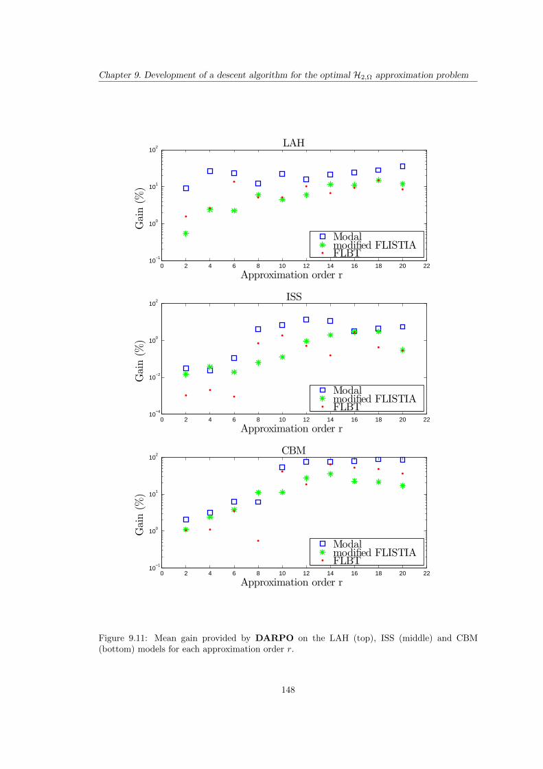
Chapter 9. Development of a descent algorithm for the optimal H2,Ω approximation problem
0 2 4 6 8 10 12 14 16 18 20 2210
−1
100
101
102
Approximation order r
Gain(%
)LAH
Modalmodified FLISTIAFLBT
0 2 4 6 8 10 12 14 16 18 20 2210
−4
10−2
100
102
Approximation order r
Gain(%
)
ISS
Modalmodified FLISTIAFLBT
0 2 4 6 8 10 12 14 16 18 20 2210
−1
100
101
102
Approximation order r
Gain(%
)
CBM
Modalmodified FLISTIAFLBT
Figure 9.11: Mean gain provided by DARPO on the LAH (top), ISS (middle) and CBM(bottom) models for each approximation order r.
148
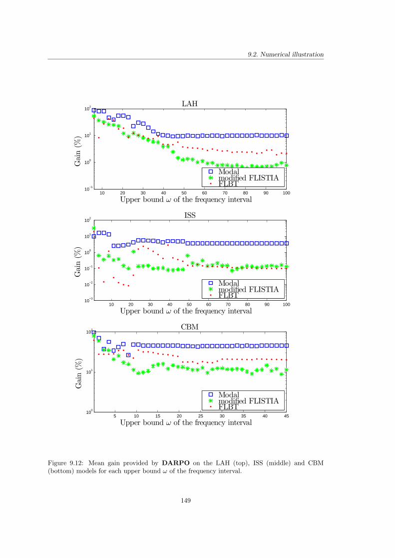
9.2. Numerical illustration
10 20 30 40 50 60 70 80 90 10010
−1
100
101
102
Upper bound ω of the frequency interval
Gain(%
)
LAH
Modalmodified FLISTIAFLBT
10 20 30 40 50 60 70 80 90 10010
−3
10−2
10−1
100
101
102
Upper bound ω of the frequency interval
Gain(%
)
ISS
Modalmodified FLISTIAFLBT
5 10 15 20 25 30 35 40 4510
0
101
102
Upper bound ω of the frequency interval
Gain(%
)
CBM
Modalmodified FLISTIAFLBT
Figure 9.12: Mean gain provided by DARPO on the LAH (top), ISS (middle) and CBM(bottom) models for each upper bound ω of the frequency interval.
149
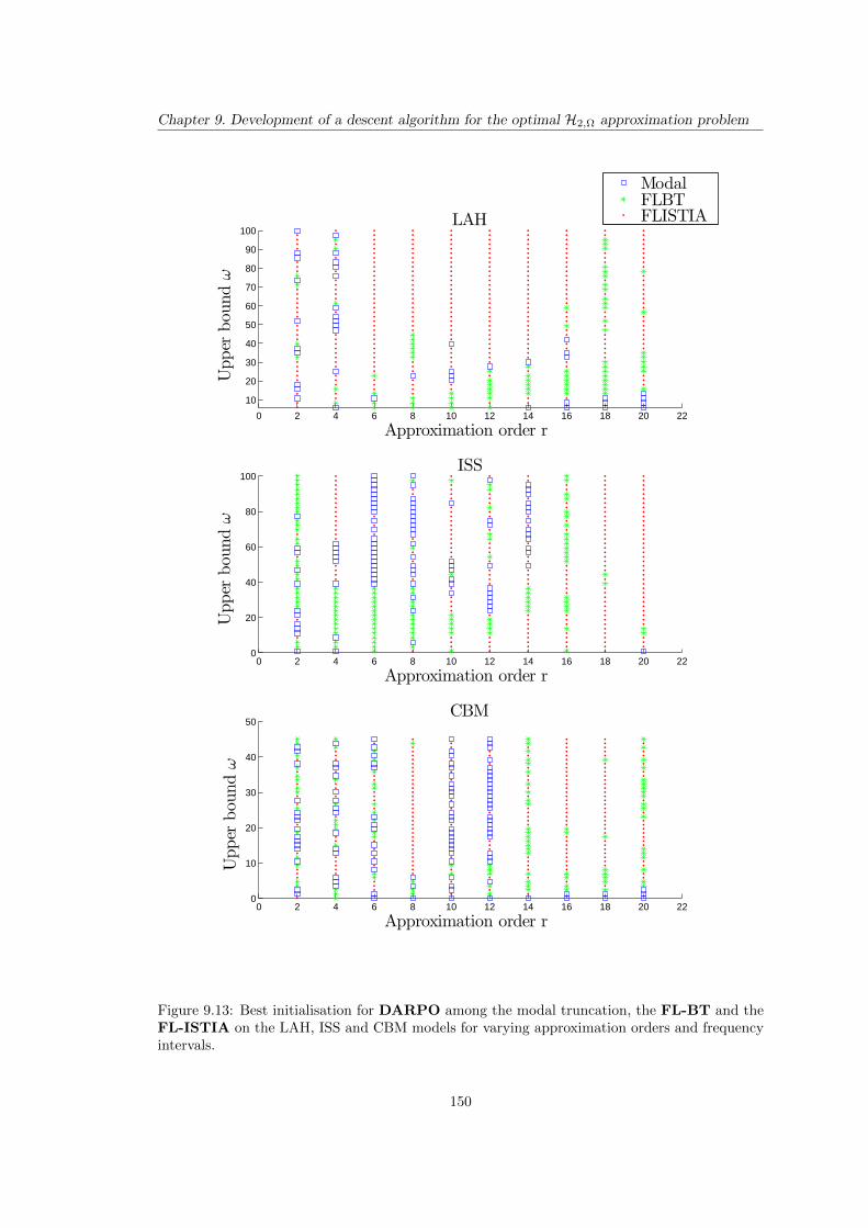
Chapter 9. Development of a descent algorithm for the optimal H2,Ω approximation problem
0 2 4 6 8 10 12 14 16 18 20 22
10
20
30
40
50
60
70
80
90
100
Approximation order r
Upper
bou
ndω
LAH
ModalFLBTFLISTIA
0 2 4 6 8 10 12 14 16 18 20 220
20
40
60
80
100
Upper
bou
ndω
Approximation order r
ISS
0 2 4 6 8 10 12 14 16 18 20 220
10
20
30
40
50
Upper
bou
ndω
Approximation order r
CBM
Figure 9.13: Best initialisation for DARPO among the modal truncation, the FL-BT and theFL-ISTIA on the LAH, ISS and CBM models for varying approximation orders and frequencyintervals.
150
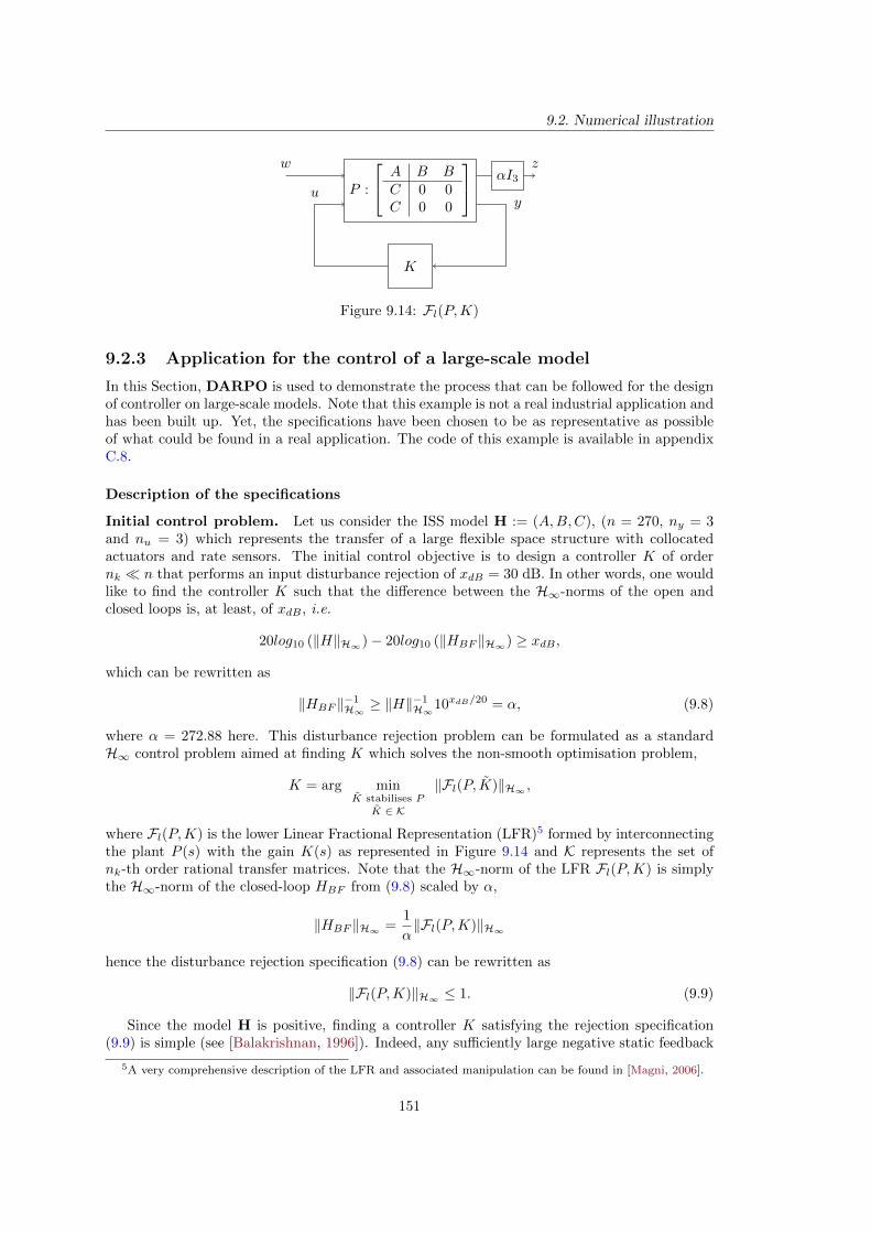
9.2. Numerical illustration
P :
A B BC 0 0C 0 0
K
zwαI3
yu
Figure 9.14: Fl(P,K)
9.2.3 Application for the control of a large-scale model
In this Section, DARPO is used to demonstrate the process that can be followed for the designof controller on large-scale models. Note that this example is not a real industrial application andhas been built up. Yet, the specifications have been chosen to be as representative as possibleof what could be found in a real application. The code of this example is available in appendixC.8.
Description of the specifications
Initial control problem. Let us consider the ISS model H := (A,B,C), (n = 270, ny = 3and nu = 3) which represents the transfer of a large flexible space structure with collocatedactuators and rate sensors. The initial control objective is to design a controller K of ordernk n that performs an input disturbance rejection of xdB = 30 dB. In other words, one wouldlike to find the controller K such that the difference between the H∞-norms of the open andclosed loops is, at least, of xdB , i.e.
20log10 (‖H‖H∞)− 20log10 (‖HBF ‖H∞) ≥ xdB ,
which can be rewritten as
‖HBF ‖−1H∞ ≥ ‖H‖
−1H∞10xdB/20 = α, (9.8)
where α = 272.88 here. This disturbance rejection problem can be formulated as a standardH∞ control problem aimed at finding K which solves the non-smooth optimisation problem,
K = arg minK stabilises P
K ∈ K
‖Fl(P, K)‖H∞ ,
where Fl(P,K) is the lower Linear Fractional Representation (LFR)5 formed by interconnectingthe plant P (s) with the gain K(s) as represented in Figure 9.14 and K represents the set ofnk-th order rational transfer matrices. Note that the H∞-norm of the LFR Fl(P,K) is simplythe H∞-norm of the closed-loop HBF from (9.8) scaled by α,
‖HBF ‖H∞ =1
α‖Fl(P,K)‖H∞
hence the disturbance rejection specification (9.8) can be rewritten as
‖Fl(P,K)‖H∞ ≤ 1. (9.9)
Since the model H is positive, finding a controller K satisfying the rejection specification(9.9) is simple (see [Balakrishnan, 1996]). Indeed, any sufficiently large negative static feedback
5A very comprehensive description of the LFR and associated manipulation can be found in [Magni, 2006].
151
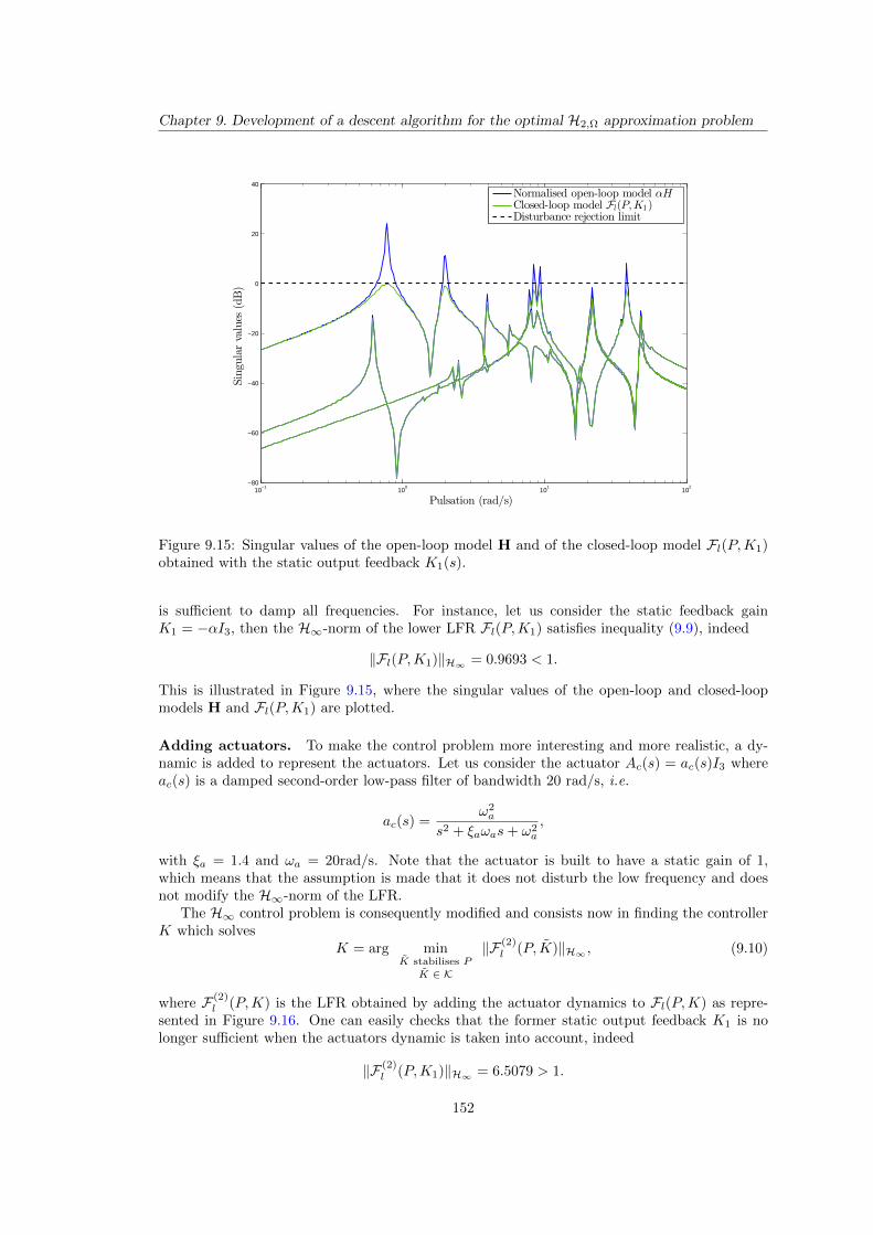
Chapter 9. Development of a descent algorithm for the optimal H2,Ω approximation problem
10−1
100
101
102
−80
−60
−40
−20
0
20
40
Pulsation (rad/s)
Singu
larvalues
(dB)
Normalised open-loop model αHClosed-loop model Fl(P,K1)Disturbance rejection limit
Figure 9.15: Singular values of the open-loop model H and of the closed-loop model Fl(P,K1)obtained with the static output feedback K1(s).
is sufficient to damp all frequencies. For instance, let us consider the static feedback gainK1 = −αI3, then the H∞-norm of the lower LFR Fl(P,K1) satisfies inequality (9.9), indeed
‖Fl(P,K1)‖H∞ = 0.9693 < 1.
This is illustrated in Figure 9.15, where the singular values of the open-loop and closed-loopmodels H and Fl(P,K1) are plotted.
Adding actuators. To make the control problem more interesting and more realistic, a dy-namic is added to represent the actuators. Let us consider the actuator Ac(s) = ac(s)I3 whereac(s) is a damped second-order low-pass filter of bandwidth 20 rad/s, i.e.
ac(s) =ω2a
s2 + ξaωas+ ω2a
,
with ξa = 1.4 and ωa = 20rad/s. Note that the actuator is built to have a static gain of 1,which means that the assumption is made that it does not disturb the low frequency and doesnot modify the H∞-norm of the LFR.
The H∞ control problem is consequently modified and consists now in finding the controllerK which solves
K = arg minK stabilises P
K ∈ K
‖F (2)l (P, K)‖H∞ , (9.10)
where F (2)l (P,K) is the LFR obtained by adding the actuator dynamics to Fl(P,K) as repre-
sented in Figure 9.16. One can easily checks that the former static output feedback K1 is nolonger sufficient when the actuators dynamic is taken into account, indeed
‖F (2)l (P,K1)‖H∞ = 6.5079 > 1.
152
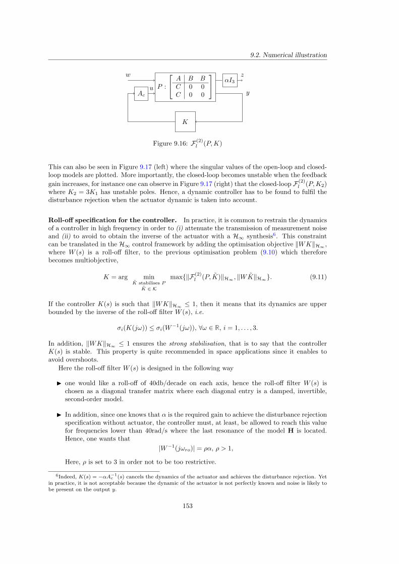
9.2. Numerical illustration
P :
A B BC 0 0C 0 0
K
zwαI3
Ac yu
Figure 9.16: F (2)l (P,K)
This can also be seen in Figure 9.17 (left) where the singular values of the open-loop and closed-loop models are plotted. More importantly, the closed-loop becomes unstable when the feedback
gain increases, for instance one can observe in Figure 9.17 (right) that the closed-loop F (2)l (P,K2)
where K2 = 3K1 has unstable poles. Hence, a dynamic controller has to be found to fulfil thedisturbance rejection when the actuator dynamic is taken into account.
Roll-off specification for the controller. In practice, it is common to restrain the dynamicsof a controller in high frequency in order to (i) attenuate the transmission of measurement noiseand (ii) to avoid to obtain the inverse of the actuator with a H∞ synthesis6. This constraintcan be translated in the H∞ control framework by adding the optimisation objective ‖WK‖H∞ ,where W (s) is a roll-off filter, to the previous optimisation problem (9.10) which thereforebecomes multiobjective,
K = arg minK stabilises P
K ∈ K
max‖F (2)l (P, K)‖H∞ , ‖WK‖H∞. (9.11)
If the controller K(s) is such that ‖WK‖H∞ ≤ 1, then it means that its dynamics are upperbounded by the inverse of the roll-off filter W (s), i.e.
σi(K(jω)) ≤ σi(W−1(jω)), ∀ω ∈ R, i = 1, . . . , 3.
In addition, ‖WK‖H∞ ≤ 1 ensures the strong stabilisation, that is to say that the controllerK(s) is stable. This property is quite recommended in space applications since it enables toavoid overshoots.
Here the roll-off filter W (s) is designed in the following way
I one would like a roll-off of 40db/decade on each axis, hence the roll-off filter W (s) ischosen as a diagonal transfer matrix where each diagonal entry is a damped, invertible,second-order model.
I In addition, since one knows that α is the required gain to achieve the disturbance rejectionspecification without actuator, the controller must, at least, be allowed to reach this valuefor frequencies lower than 40rad/s where the last resonance of the model H is located.Hence, one wants that
|W−1(jωro)| = ρα, ρ > 1,
Here, ρ is set to 3 in order not to be too restrictive.
6Indeed, K(s) = −αA−1c (s) cancels the dynamics of the actuator and achieves the disturbance rejection. Yet
in practice, it is not acceptable because the dynamic of the actuator is not perfectly known and noise is likely tobe present on the output y.
153
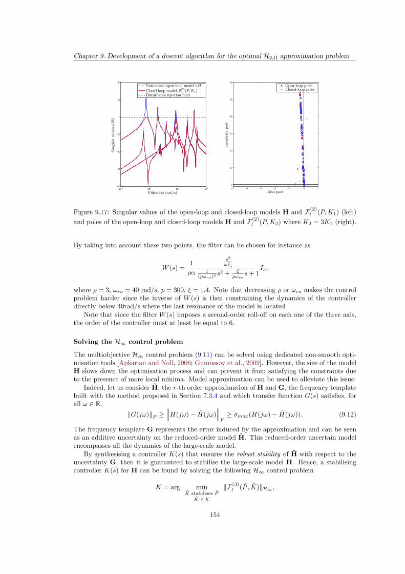
Chapter 9. Development of a descent algorithm for the optimal H2,Ω approximation problem
10−1
100
101
102
−80
−60
−40
−20
0
20
40
Pulsation (rad/s)
Singu
larvalues
(dB)
Normalised open-loop model αH
Closed-loop model F(2)l (P,K1)
Disturbance rejection limit
−5 −4 −3 −2 −1 0 1
0
10
20
30
40
50
60
Real part
Imaginarypart
Open-loop polesClosed-loop poles
Figure 9.17: Singular values of the open-loop and closed-loop models H and F (2)l (P,K1) (left)
and poles of the open-loop and closed-loop models H and F (2)l (P,K2) where K2 = 3K1 (right).
By taking into account these two points, the filter can be chosen for instance as
W (s) =1
ρα
s2
ω2ro
1(pωro)2 s2 + ξ
pωros+ 1
I3,
where ρ = 3, ωro = 40 rad/s, p = 300, ξ = 1.4. Note that decreasing ρ or ωro makes the controlproblem harder since the inverse of W (s) is then constraining the dynamics of the controllerdirectly below 40rad/s where the last resonance of the model is located.
Note that since the filter W (s) imposes a second-order roll-off on each one of the three axis,the order of the controller must at least be equal to 6.
Solving the H∞ control problem
The multiobjective H∞ control problem (9.11) can be solved using dedicated non-smooth opti-misation tools [Apkarian and Noll, 2006; Gumussoy et al., 2009]. However, the size of the modelH slows down the optimisation process and can prevent it from satisfying the constraints dueto the presence of more local minima. Model approximation can be used to alleviate this issue.
Indeed, let us consider H, the r-th order approximation of H and G, the frequency templatebuilt with the method proposed in Section 7.3.4 and which transfer function G(s) satisfies, forall ω ∈ R,
‖G(jω)‖F ≥∥∥∥H(jω)− H(jω)
∥∥∥F≥ σmax(H(jω)− H(jω)). (9.12)
The frequency template G represents the error induced by the approximation and can be seenas an additive uncertainty on the reduced-order model H. This reduced-order uncertain modelencompasses all the dynamics of the large-scale model.
By synthesising a controller K(s) that ensures the robust stability of H with respect to theuncertainty G, then it is guaranteed to stabilise the large-scale model H. Hence, a stabilisingcontroller K(s) for H can be found by solving the following H∞ control problem
K = arg minK stabilises P
K ∈ K
‖F (3)l (P , K)‖H∞ ,
154
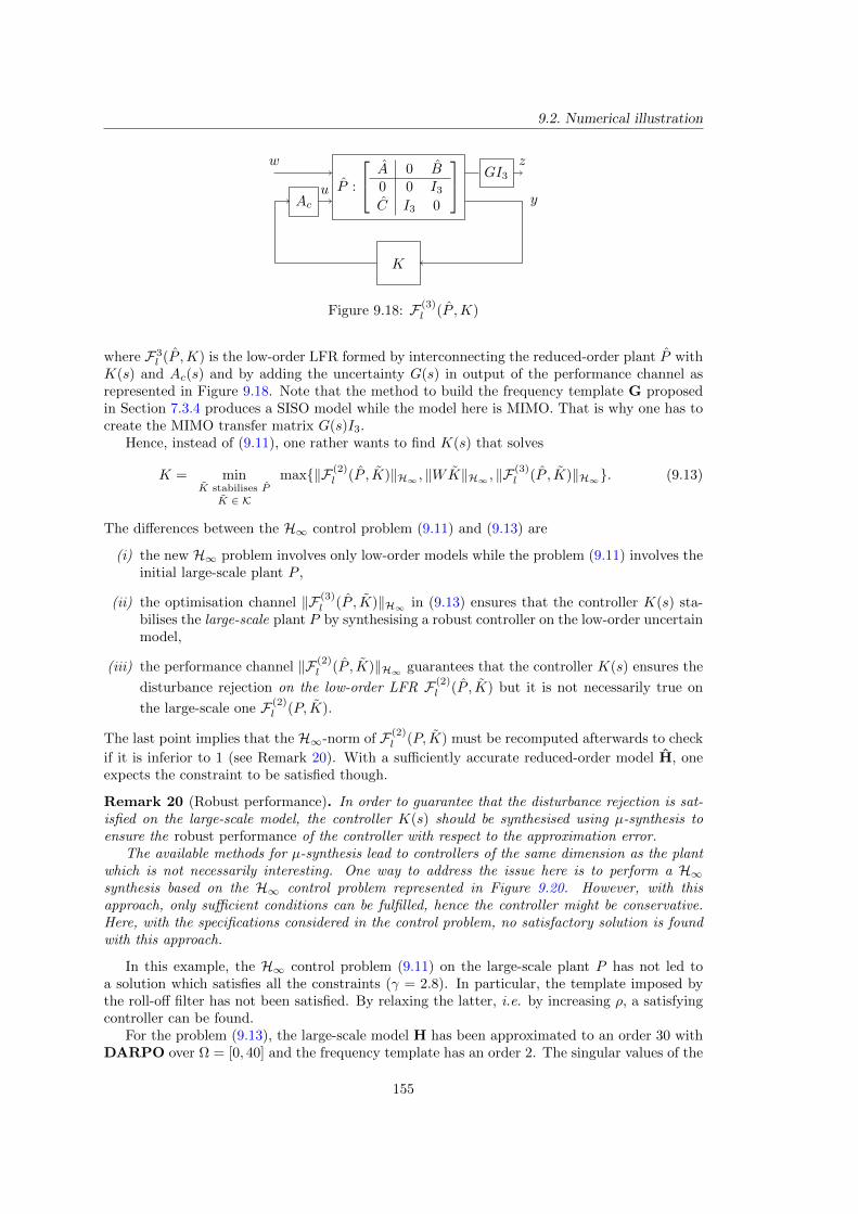
9.2. Numerical illustration
P :
A 0 B0 0 I3C I3 0
K
zwGI3
Ac yu
Figure 9.18: F (3)l (P ,K)
where F3l (P ,K) is the low-order LFR formed by interconnecting the reduced-order plant P with
K(s) and Ac(s) and by adding the uncertainty G(s) in output of the performance channel asrepresented in Figure 9.18. Note that the method to build the frequency template G proposedin Section 7.3.4 produces a SISO model while the model here is MIMO. That is why one has tocreate the MIMO transfer matrix G(s)I3.
Hence, instead of (9.11), one rather wants to find K(s) that solves
K = minK stabilises P
K ∈ K
max‖F (2)l (P , K)‖H∞ , ‖WK‖H∞ , ‖F
(3)l (P , K)‖H∞. (9.13)
The differences between the H∞ control problem (9.11) and (9.13) are
(i) the new H∞ problem involves only low-order models while the problem (9.11) involves theinitial large-scale plant P ,
(ii) the optimisation channel ‖F (3)l (P , K)‖H∞ in (9.13) ensures that the controller K(s) sta-
bilises the large-scale plant P by synthesising a robust controller on the low-order uncertainmodel,
(iii) the performance channel ‖F (2)l (P , K)‖H∞ guarantees that the controller K(s) ensures the
disturbance rejection on the low-order LFR F (2)l (P , K) but it is not necessarily true on
the large-scale one F (2)l (P, K).
The last point implies that the H∞-norm of F (2)l (P, K) must be recomputed afterwards to check
if it is inferior to 1 (see Remark 20). With a sufficiently accurate reduced-order model H, oneexpects the constraint to be satisfied though.
Remark 20 (Robust performance). In order to guarantee that the disturbance rejection is sat-isfied on the large-scale model, the controller K(s) should be synthesised using µ-synthesis toensure the robust performance of the controller with respect to the approximation error.
The available methods for µ-synthesis lead to controllers of the same dimension as the plantwhich is not necessarily interesting. One way to address the issue here is to perform a H∞synthesis based on the H∞ control problem represented in Figure 9.20. However, with thisapproach, only sufficient conditions can be fulfilled, hence the controller might be conservative.Here, with the specifications considered in the control problem, no satisfactory solution is foundwith this approach.
In this example, the H∞ control problem (9.11) on the large-scale plant P has not led toa solution which satisfies all the constraints (γ = 2.8). In particular, the template imposed bythe roll-off filter has not been satisfied. By relaxing the latter, i.e. by increasing ρ, a satisfyingcontroller can be found.
For the problem (9.13), the large-scale model H has been approximated to an order 30 withDARPO over Ω = [0, 40] and the frequency template has an order 2. The singular values of the
155
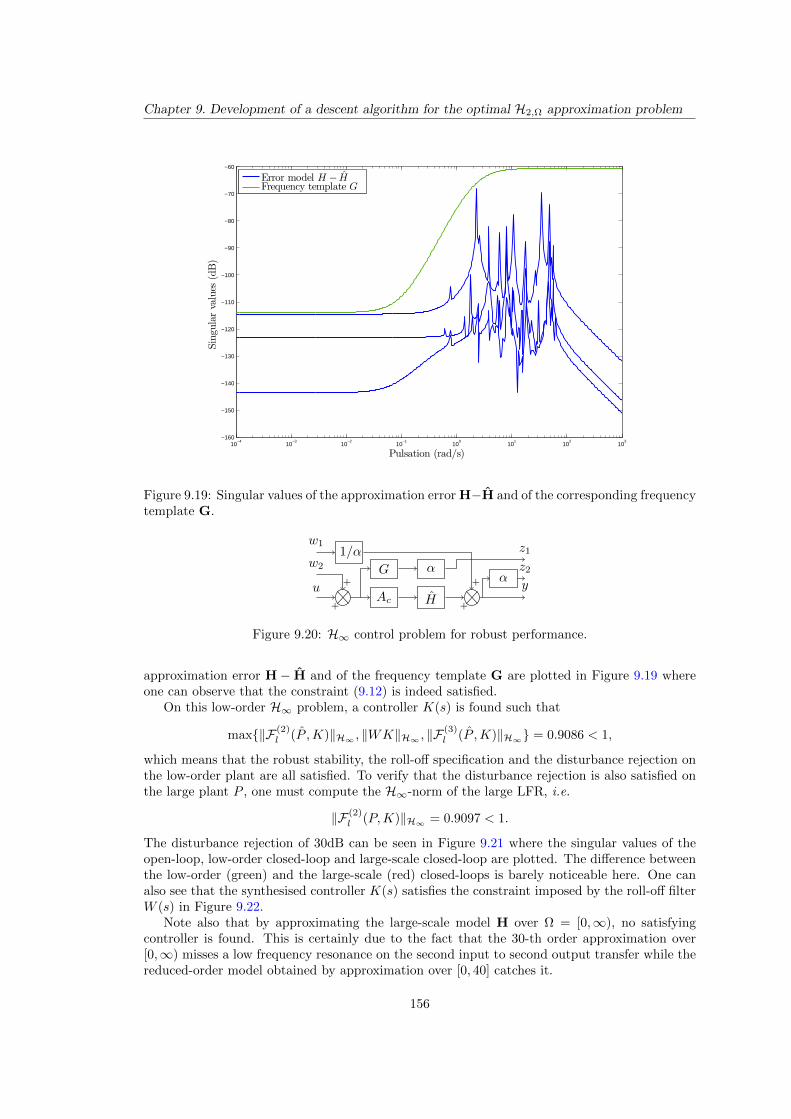
Chapter 9. Development of a descent algorithm for the optimal H2,Ω approximation problem
10−4
10−3
10−2
10−1
100
101
102
103
−160
−150
−140
−130
−120
−110
−100
−90
−80
−70
−60
Pulsation (rad/s)
Singu
larvalues
(dB)
Error model H − HFrequency template G
Figure 9.19: Singular values of the approximation error H−H and of the corresponding frequencytemplate G.
HAc
G α1/α
αu
w1
w2
y
z1
z2
+ +
+ +
Figure 9.20: H∞ control problem for robust performance.
approximation error H − H and of the frequency template G are plotted in Figure 9.19 whereone can observe that the constraint (9.12) is indeed satisfied.
On this low-order H∞ problem, a controller K(s) is found such that
max‖F (2)l (P ,K)‖H∞ , ‖WK‖H∞ , ‖F
(3)l (P ,K)‖H∞ = 0.9086 < 1,
which means that the robust stability, the roll-off specification and the disturbance rejection onthe low-order plant are all satisfied. To verify that the disturbance rejection is also satisfied onthe large plant P , one must compute the H∞-norm of the large LFR, i.e.
‖F (2)l (P,K)‖H∞ = 0.9097 < 1.
The disturbance rejection of 30dB can be seen in Figure 9.21 where the singular values of theopen-loop, low-order closed-loop and large-scale closed-loop are plotted. The difference betweenthe low-order (green) and the large-scale (red) closed-loops is barely noticeable here. One canalso see that the synthesised controller K(s) satisfies the constraint imposed by the roll-off filterW (s) in Figure 9.22.
Note also that by approximating the large-scale model H over Ω = [0,∞), no satisfyingcontroller is found. This is certainly due to the fact that the 30-th order approximation over[0,∞) misses a low frequency resonance on the second input to second output transfer while thereduced-order model obtained by approximation over [0, 40] catches it.
156
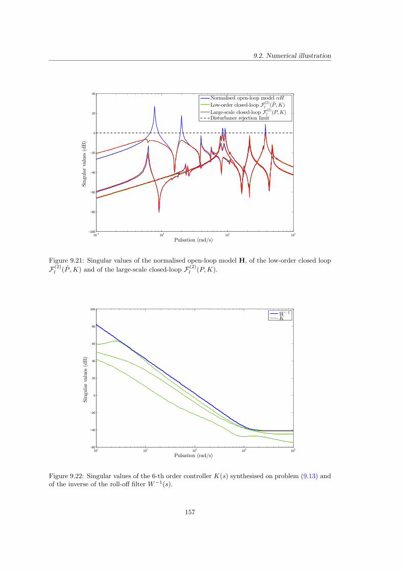
9.2. Numerical illustration
10−1
100
101
102
−100
−80
−60
−40
−20
0
20
40
Pulsation (rad/s)
Singu
larvalues
(dB)
Normalised open-loop model αH
Low-order closed-loop F(2)l (P ,K)
Large-scale closed-loop F(2)l (P,K)
Disturbance rejection limit
Figure 9.21: Singular values of the normalised open-loop model H, of the low-order closed loop
F (2)l (P ,K) and of the large-scale closed-loop F (2)
l (P,K).
101
102
103
104
105
−60
−40
−20
0
20
40
60
80
100
Pulsation (rad/s)
Singu
larvalues
(dB)
W−1
K
Figure 9.22: Singular values of the 6-th order controller K(s) synthesised on problem (9.13) andof the inverse of the roll-off filter W−1(s).
157
Chapter 9. Development of a descent algorithm for the optimal H2,Ω approximation problem
Conclusion
The poles-residues formulation of the H2,Ω approximation error between a large-scale model anda reduced-order one together with its gradient, developed in Chapter 8, have been used here ina complex-domain, quasi-Newton optimisation algorithm. This optimisation algorithm relies onthe BFGS update of the approximate inverse Hessian and on an inexact line-search method sat-isfying the strong Wolfe conditions. The resulting approximation algorithm DARPO producesa sequence of reduced-order model which yields a monotonically decreasing H2,Ω approximationerror with the initial large-scale model and is expected to converge towards a local minimum.
DARPO is a local optimisation procedure and is therefore particularly dependent of theinitial point it is given. The modal truncation is the most natural initial reduced-order modelthat can be used but other frequency-limited methods can also be used. Depending of theproximity of the initial reduced-order model to a local minimum, DARPO can bring substantialimprovement with respect to the initial point.
DARPO has also been used in a simple process for designing a stabilising controller for alarge-scale model. It consists in building a frequency template upper bounding the approximationerror with the method proposed in Section 7.3.4 and to consider it as an additive uncertainty onthe reduced-order model. A robust controller can then be designed on this low-order uncertainmodel and is guaranteed to stabilise the initial large-scale model.
In the following Chapter, DARPO is used together with FL-ISTIA on an industrial appli-cation as part of a global process used to design control laws on large-scale aircraft models.
158
Chapter 10
Industrial aeronautical use case
The study detailed in this chapter has been motivated by the increasing dimension of the modelsrepresenting civilian aircraft which prevents standard control design methods from being directlyused. An approximation step is mandatory and this step must not weaken the robustness andperformance properties of the controllers that are designed. Indeed, in the aeronautical context,strong constraints can exist on the control laws in order to satisfy safety specifications. Severalsteps have been taken towards this goal,
I in a first time, the performances of several model approximation methods, including FL-ISTIA, have been evaluated on the large-scale models representing the longitudinal be-haviour of a long-range flexible civilian aircraft in [Vuillemin et al., 2012a, 2013b],
I then FL-ISTIA and DARPO have been used to enable the design of (i) an anti-vibra-tion control law for a business jet aircraft [Poussot-Vassal et al., 2013] and (ii) a controllaw ensuring flight performance and load clearance in presence of input saturation on alongitudinal aircraft model [Burlion et al., 2014].
I Model approximation has also been used as the starting point in a modelling processaimed at creating a low-order uncertain, parameter varying model from a set of large-scaledynamical models [Poussot-Vassal and Vuillemin, 2013; Poussot-Vassal et al., 2014],
I thanks to this process, the global stability and performance of the set of controlled large-scale models representing the business jet aircraft subject to actuator saturation have beenproven by taking into account the error induced by the approximation and the interpolationof the initial large-scale models [Vuillemin et al., 2014a].
In this Chapter, the global process used for the design and validation of an anti-vibrationcontrol law for a business jet aircraft is detailed. In particular, in Section 10.1, the preliminaryapproach used to design an anti-vibration control law for one model representing a businessjet aircraft at one single flight operating condition is described. The stability of the controllerobtained from the generalisation of this approach to the set of models representing the aircraftat different Mach-numbers is then assessed in Section 10.2 in presence of input saturation.
Note that this process involves way more methods and tools than model approximation onlywhich are out of the scope of this study. Hence all the steps cannot be covered in depth, butadequate references are pointed out when required.
Contents10.1 Vibration control for one business jet aircraft model . . . . . . . . 160
10.1.1 General industrial framework . . . . . . . . . . . . . . . . . . . . . . . 160
10.1.2 Problem formulation and business jet aircraft model approximation . 161
10.1.3 Anti-vibration control design . . . . . . . . . . . . . . . . . . . . . . . 162
10.1.4 Numerical results . . . . . . . . . . . . . . . . . . . . . . . . . . . . . . 166
10.2 Global stability validation of a parameter varying business jetaircraft . . . . . . . . . . . . . . . . . . . . . . . . . . . . . . . . . . . . 167
10.2.1 Problem statement . . . . . . . . . . . . . . . . . . . . . . . . . . . . . 167
10.2.2 Model approximation & error bounding . . . . . . . . . . . . . . . . . 168
10.2.3 Low-order LFR model creation . . . . . . . . . . . . . . . . . . . . . . 170
10.2.4 IQC-based global stability analysis . . . . . . . . . . . . . . . . . . . . 173
159
Chapter 10. Industrial aeronautical use case
10.1 Vibration control for one business jet aircraft model
The motivations and general industrial framework of this study are described in Section 10.1.1.The general control problem is then formulated in Section 10.1.2 and addressed in Section 10.1.3.Finally, the numerical results are presented in Section 10.1.4.
10.1.1 General industrial framework
In aeronautics, engineers have often to cope with many technical and practical problems for thedesign of a control laws caused by the complexity of the underlying models which are referredas aeroservoelastic models. Such models take into account
I the physic involved in the aeroelastic phenomena such as the structural loads (e.g. ma-noeuvres) or the aerodynamics loads (e.g. gusts),
I the flight control system behaviour, i.e. the dynamics of the actuators (aerodynamic con-trol surfaces) and the sensors (e.g. accelerometers and gyrometers), eventual measurementsdelays, etc.
I uncertainties concerning the characteristics and state of the aircraft such as its mass (whichvaries during the flight due to the tanks filling), its speed, its flight altitude, etc.
For industrial civilian aircraft, these models are generally composed by a set of large-scale modelsrepresenting the aircraft at different flight operating conditions.
Based on these aeroservoelastic models, nominal flight control laws are designed such that(i) the robustness (stability and performances) of the aircraft over the whole parametric domain(speed, altitude, etc.) is guaranteed, (ii) flying quality specifications (i.e. fast and smoothresponse to pilot commands and rejection of gust disturbances) are satisfied.
In addition, comfort control laws1 are designed in order to attenuate the undesirable vibra-tions which are likely to appear due to aerodynamics disturbances. For instance, disturbanceson the rear part of the aircraft can generate vibrations in the cockpit or in the cabin. Theseanti-vibration control laws must also satisfy some constraints, in particular (i) they are requiredto reduce the vibrations to a specified level, (ii) they must have a negligible effect on the nominalcontrol law and (iii) they must be of low complexity.
Here, the preliminary study for the design of such an anti-vibration control law for an indus-trial business jet aircraft (denoted BizJet in the sequel), in the context of a collaboration betweenOnera and Dassault-Aviation, is presented. More specifically, and with reference to Figure 10.1,the objective is to design an anti-vibration control law (in red) for a large-scale BizJet modelcontrolled by its nominal flight control law (in blue) which respects the specifications mentionedabove. This objective is challenging for several reasons,
I the large dimension of the model (n ≈ 600) prevents from applying directly standardcontrol tools,
I the undesirable vibrations should be attenuated over a specific frequency range only (re-lated to passenger and pilot comfort specifications),
I the nominal flight control law performances must be preserved and high frequency lightlydamped modes must remain sufficiently stable,
I the anti-vibration control is based on the deflection of existing control surfaces which meansthat no dedicated actuators are available to achieve the objective.
1Actually, these control-laws also enable to decrease the loads on the structure of the aircraft.
160

10.1. Vibration control for one business jet aircraft model
Naturalaircraft(BizJet)
Actuator
Sensors
acont(t)qcont(t)apil(t)
ua(t)
wa(t)
Nominal flightcontroller
Anti-vibrationcontroller
Large-scale BizJet generic model (H)
Figure 10.1: BizJet model (H) and anti-vibration controller.
The approach used to achieve that objective is in three steps (i) first, the large-scale modelis reduced, (ii) then, a general control problem is formulated by using suitable weighting filterswhich capture the frequency-limited nature of the objectives, (iii) finally, a structured controllerbased on non-smooth H∞ synthesis is designed. At this stage, the approximation step doesnot offer any kind of guarantee for the controller designed on the reduced-order model, hence,the anti-vibration control law must be validated experimentally on the large-scale BizJet model.This issue is alleviated in Section 10.2 by a rigorous global stability analysis.
10.1.2 Problem formulation and business jet aircraft model approxi-mation
Control problem formulation
The initial BizJet aircraft model is of order n = 597, has nu = 2 inputs,
I wa(t), the external disturbance input representing the aerodynamic disturbance affectingthe rear part of the aircraft,
I ua(t), the anti-vibration control output, i.e. the input of the elevator on the rear part,
and ny = 3 outputs,
I acont(t), the vertical acceleration output, used by the nominal flight controller,
I qcont(t), the pitch rate of the aircraft, used by the nominal flight controller,
I apil(t), the acceleration sensor located close to the pilot’s seat, which has to be monitoredfor comfort issues.
Let us denote by Twa→apil and Twa→acont the transfers, in the nominal case (i.e. without theanti-vibration control law) from the disturbance input to the acceleration of the pilot and to thevertical acceleration, respectively. An let us denote by Fl(H,K)wa→apil and Fl(H,K)wa→acontthe same transfers when the anti-vibration loop is closed with the controller K.
Let us reformulate the objectives and constraints related to the desired controller,
161
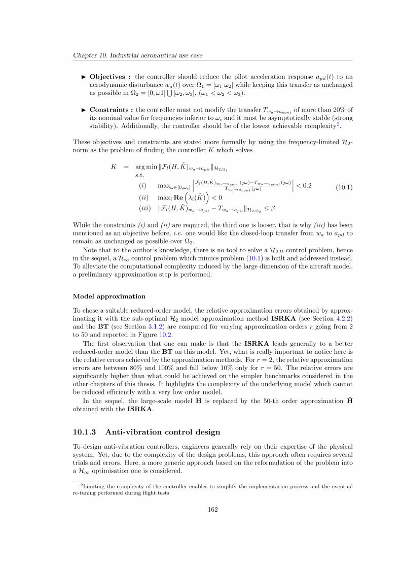
Chapter 10. Industrial aeronautical use case
I Objectives : the controller should reduce the pilot acceleration response apil(t) to anaerodynamic disturbance wa(t) over Ω1 = [ω1 ω2] while keeping this transfer as unchangedas possible in Ω2 = [0, ω1]
⋃[ω2, ω3], (ω1 < ω2 < ω3).
I Constraints : the controller must not modify the transfer Twa→acont of more than 20% ofits nominal value for frequencies inferior to ωc and it must be asymptotically stable (strongstability). Additionally, the controller should be of the lowest achievable complexity2.
These objectives and constraints are stated more formally by using the frequency-limited H2-norm as the problem of finding the controller K which solves
K = arg min ‖Fl(H, K)wa→apil‖H2,Ω1
s.t.
(i) maxω∈[0,ωc]
∣∣∣Fl(H,K)wa→acont (jω)−Twa→acont (jω)
Twa→acont (jω)
∣∣∣ < 0.2
(ii) maxi Re(λi(K)
)< 0
(iii) ‖Fl(H, K)wa→apil − Twa→apil‖H2,Ω2≤ β
(10.1)
While the constraints (i) and (ii) are required, the third one is looser, that is why (iii) has beenmentioned as an objective before, i.e. one would like the closed-loop transfer from wa to apil toremain as unchanged as possible over Ω2.
Note that to the author’s knowledge, there is no tool to solve a H2,Ω control problem, hencein the sequel, a H∞ control problem which mimics problem (10.1) is built and addressed instead.To alleviate the computational complexity induced by the large dimension of the aircraft model,a preliminary approximation step is performed.
Model approximation
To chose a suitable reduced-order model, the relative approximation errors obtained by approx-imating it with the sub-optimal H2 model approximation method ISRKA (see Section 4.2.2)and the BT (see Section 3.1.2) are computed for varying approximation orders r going from 2to 50 and reported in Figure 10.2.
The first observation that one can make is that the ISRKA leads generally to a betterreduced-order model than the BT on this model. Yet, what is really important to notice here isthe relative errors achieved by the approximation methods. For r = 2, the relative approximationerrors are between 80% and 100% and fall below 10% only for r = 50. The relative errors aresignificantly higher than what could be achieved on the simpler benchmarks considered in theother chapters of this thesis. It highlights the complexity of the underlying model which cannotbe reduced efficiently with a very low order model.
In the sequel, the large-scale model H is replaced by the 50-th order approximation Hobtained with the ISRKA.
10.1.3 Anti-vibration control design
To design anti-vibration controllers, engineers generally rely on their expertise of the physicalsystem. Yet, due to the complexity of the design problems, this approach often requires severaltrials and errors. Here, a more generic approach based on the reformulation of the problem intoa H∞ optimisation one is considered.
2Limiting the complexity of the controller enables to simplify the implementation process and the eventualre-tuning performed during flight tests.
162
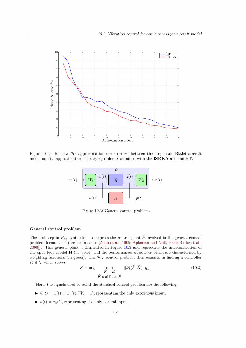
10.1. Vibration control for one business jet aircraft model
0 5 10 15 20 25 30 35 40 45 500
10
20
30
40
50
60
70
80
90
100RelativeH
2error(%
)
Approximation order r
BTISRKA
Figure 10.2: Relative H2 approximation error (in %) between the large-scale BizJet aircraftmodel and its approximation for varying orders r obtained with the ISRKA and the BT.
H WoWi
z(t)w(t)z(t)w(t)
K y(t)u(t)
P
Figure 10.3: General control problem.
General control problem
The first step in H∞-synthesis is to express the control plant P involved in the general controlproblem formulation (see for instance [Zhou et al., 1995; Apkarian and Noll, 2006; Burke et al.,2006]). This general plant is illustrated in Figure 10.3 and represents the interconnection ofthe open-loop model H (in violet) and the performances objectives which are characterised byweighting functions (in green). The H∞ control problem then consists in finding a controllerK ∈ K which solves
K = arg minK ∈ K
K stabilises P
‖Fl(P , K)‖H∞ . (10.2)
Here, the signals used to build the standard control problem are the following,
I w(t) = w(t) = wa(t) (Wi = 1), representing the only exogenous input,
I u(t) = ua(t), representing the only control input,
163
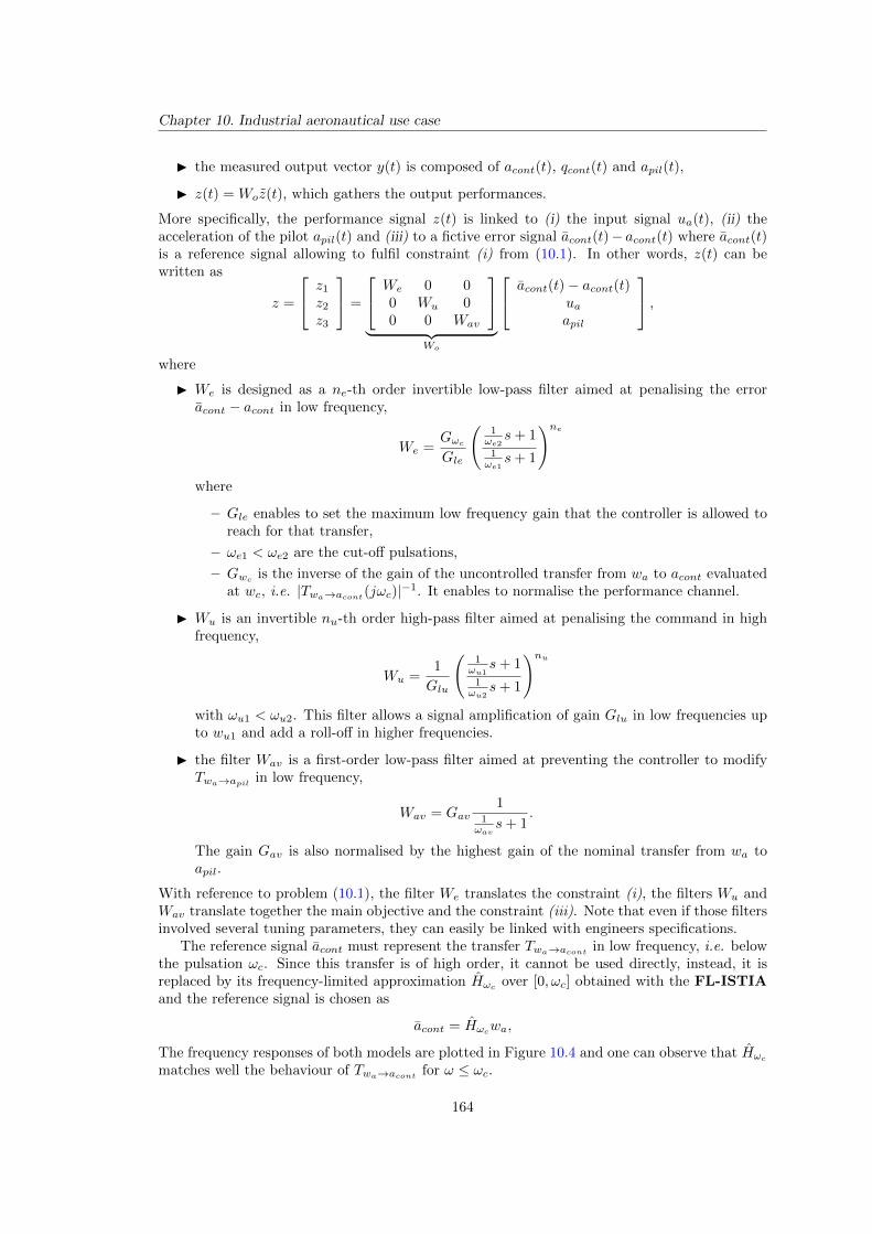
Chapter 10. Industrial aeronautical use case
I the measured output vector y(t) is composed of acont(t), qcont(t) and apil(t),
I z(t) = Woz(t), which gathers the output performances.
More specifically, the performance signal z(t) is linked to (i) the input signal ua(t), (ii) theacceleration of the pilot apil(t) and (iii) to a fictive error signal acont(t)− acont(t) where acont(t)is a reference signal allowing to fulfil constraint (i) from (10.1). In other words, z(t) can bewritten as
z =
z1
z2
z3
=
We 0 00 Wu 00 0 Wav
︸ ︷︷ ︸
Wo
acont(t)− acont(t)uaapil
,where
I We is designed as a ne-th order invertible low-pass filter aimed at penalising the erroracont − acont in low frequency,
We =GωcGle
(1ωe2
s+ 11ωe1
s+ 1
)newhere
– Gle enables to set the maximum low frequency gain that the controller is allowed toreach for that transfer,
– ωe1 < ωe2 are the cut-off pulsations,
– Gwc is the inverse of the gain of the uncontrolled transfer from wa to acont evaluatedat wc, i.e. |Twa→acont(jωc)|−1. It enables to normalise the performance channel.
I Wu is an invertible nu-th order high-pass filter aimed at penalising the command in highfrequency,
Wu =1
Glu
(1ωu1
s+ 11ωu2
s+ 1
)nuwith ωu1 < ωu2. This filter allows a signal amplification of gain Glu in low frequencies upto wu1 and add a roll-off in higher frequencies.
I the filter Wav is a first-order low-pass filter aimed at preventing the controller to modifyTwa→apil in low frequency,
Wav = Gav1
1ωav
s+ 1.
The gain Gav is also normalised by the highest gain of the nominal transfer from wa toapil.
With reference to problem (10.1), the filter We translates the constraint (i), the filters Wu andWav translate together the main objective and the constraint (iii). Note that even if those filtersinvolved several tuning parameters, they can easily be linked with engineers specifications.
The reference signal acont must represent the transfer Twa→acont in low frequency, i.e. belowthe pulsation ωc. Since this transfer is of high order, it cannot be used directly, instead, it isreplaced by its frequency-limited approximation Hωc over [0, ωc] obtained with the FL-ISTIAand the reference signal is chosen as
acont = Hωcwa,
The frequency responses of both models are plotted in Figure 10.4 and one can observe that Hωc
matches well the behaviour of Twa→acont for ω ≤ ωc.
164
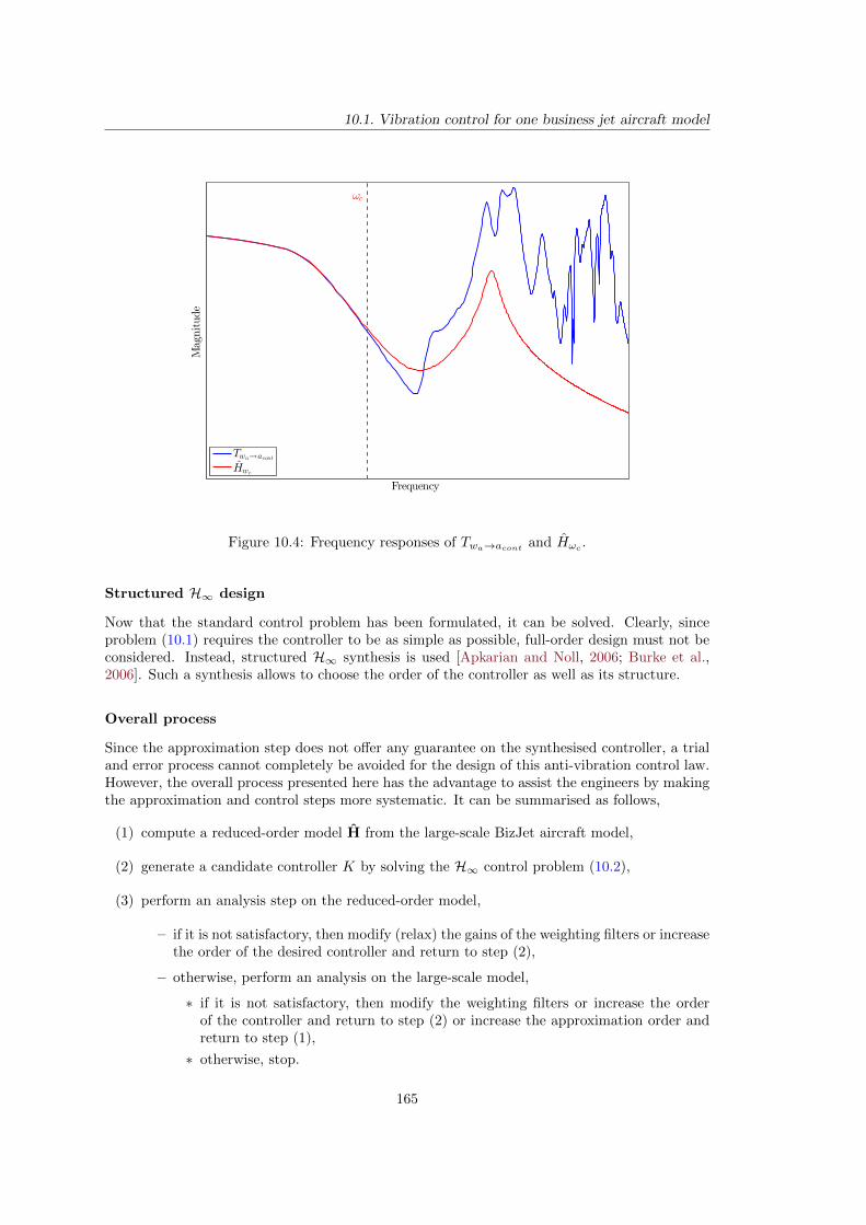
10.1. Vibration control for one business jet aircraft model
ωcMagnitude
Frequency
Twa→acont
Hwc
Figure 10.4: Frequency responses of Twa→acont and Hωc .
Structured H∞ design
Now that the standard control problem has been formulated, it can be solved. Clearly, sinceproblem (10.1) requires the controller to be as simple as possible, full-order design must not beconsidered. Instead, structured H∞ synthesis is used [Apkarian and Noll, 2006; Burke et al.,2006]. Such a synthesis allows to choose the order of the controller as well as its structure.
Overall process
Since the approximation step does not offer any guarantee on the synthesised controller, a trialand error process cannot completely be avoided for the design of this anti-vibration control law.However, the overall process presented here has the advantage to assist the engineers by makingthe approximation and control steps more systematic. It can be summarised as follows,
(1) compute a reduced-order model H from the large-scale BizJet aircraft model,
(2) generate a candidate controller K by solving the H∞ control problem (10.2),
(3) perform an analysis step on the reduced-order model,
– if it is not satisfactory, then modify (relax) the gains of the weighting filters or increasethe order of the desired controller and return to step (2),
– otherwise, perform an analysis on the large-scale model,
∗ if it is not satisfactory, then modify the weighting filters or increase the orderof the controller and return to step (2) or increase the approximation order andreturn to step (1),
∗ otherwise, stop.
165
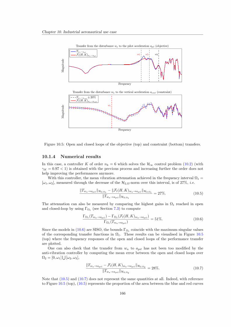
Chapter 10. Industrial aeronautical use case
ω1 ω2 ω3
Transfer from the disturbance wa to the pilot acceleration apil (objective)
Magnitude
Frequency
Twa→apil
Fl(H,K)wa→apil
ωc
Magnitude
Frequency
Transfer from the disturbance wa to the vertical acceleration acont (constraint)
Twa→acont ± 20%Fl(H,K)wa→acont
Figure 10.5: Open and closed loops of the objective (top) and constraint (bottom) transfers.
10.1.4 Numerical results
In this case, a controller K of order nk = 6 which solves the H∞ control problem (10.2) (withγK = 0.97 < 1) is obtained with the previous process and increasing further the order does nothelp improving the performances anymore.
With this controller, the mean vibration attenuation achieved in the frequency interval Ω1 =[ω1, ω2], measured through the decrease of the H2,Ω-norm over this interval, is of 27%, i.e.
‖Twa→apil‖H2,Ω1− ‖Fl(H,K)wa→apil‖H2,Ω1
‖Twa→apil‖H2,Ω1
= 27%. (10.5)
The attenuation can also be measured by comparing the highest gains in Ω1 reached in openand closed-loop by using ΓΩ1 (see Section 7.3) to compute
ΓΩ1(Twa→apil)− ΓΩ1
(Fl(H,K)wa→apil)
ΓΩ1(Twa→apil)
= 51%. (10.6)
Since the models in (10.6) are SISO, the bounds ΓΩ1coincide with the maximum singular values
of the corresponding transfer functions in Ω1. These results can be visualised in Figure 10.5(top) where the frequency responses of the open and closed loops of the performance transferare plotted.
One can also check that the transfer from wa to apil has not been too modified by theanti-vibration controller by computing the mean error between the open and closed loops overΩ2 = [0, ω1]
⋃[ω2, ω3],
‖Twa→apil −Fl(H,K)wa→apil‖H2,Ω2
‖Twa→apil‖H2,Ω2
= 28%. (10.7)
Note that (10.5) and (10.7) does not represent the same quantities at all. Indeed, with referenceto Figure 10.5 (top), (10.5) represents the proportion of the area between the blue and red curves
166
10.2. Global stability validation of a parameter varying business jet aircraft
in Ω1 in comparison to the area below the blue curve in the same interval while (10.7) representsthe proportion of the mean absolute gap between the red and blue curves over Ω2 in comparisonto the area below the blue curve over Ω2. The high value of (10.7) comes from the gap betweenthe open and closed loops which appears just before ω1 and just after ω2 (the scale is logarithmicin Figure 10.5). Yet, the error has been judged acceptable and the controller validated.
Besides, in Figure 10.5 (bottom), one can observe that for frequencies ω ≤ ωc, the closed-loopFl(H,K)wa→acont remains in the envelope formed by ±20% of the open-loop transfer Twa→acont .
Conclusion
In this section, the approach that has been followed in order to design an anti-vibration controllaw for one large-scale BizJet aircraft model has been presented. Although it is not completelygeneric, the approach has greatly simplified the process of designing a controller subject tovarious constraints.
The design process presented here represents only a preliminary study to what has finallybeen used in practice. Indeed, here, only one model representing the aircraft at one singleflight operating condition has been considered. The final controller K has been obtained bygeneralising this control process through a multi-model H∞ synthesis (not detailed here). Theglobal stability of this final controller is assessed in the next section through a global stabilityanalysis.
10.2 Global stability validation of a parameter varyingbusiness jet aircraft
In this Section, the anti-vibration controller K generated by the multi-model extension of theprocess described in Section 10.1.3 is considered. Its stability must be assessed over the fullparametric domain in presence of actuator saturation. The problem is stated more formallyin Section 10.2.1 while Sections 10.2.2, 10.2.3 and 10.2.4 describe the three steps involved toaddress this problem.
10.2.1 Problem statement
Let us consider the set of large-scale models H1, . . . ,HN (in blue in Figure 10.6), whichrepresent the BizJet aircraft model at different flight operating conditions, interconnected withthe controller K (in purple), which output is subject to a magnitude saturation (in red). Theobjective here is to prove the stability of this large-scale controlled aircraft model over thecontinuum of parameter variation when the actuator is subject to a saturation. In this study,the Mach-number is the only varying parameter considered and there are N = 3 large-scalemodels.
To this aim, a three steps methodology is followed
(i) first, in Section 10.2.2, each large-scale model is approximated over a frequency-limitedinterval and a frequency template is built to bound the worst approximation error3,
(ii) then, the set of reduced-order models are interpolated into an LFR with a bound on theinterpolation error in Section 10.2.3,
(iii) finally, the stability validation is performed in Section 10.2.4 with an irrational multipliers-based Integral Quadratic Constraint (IQC) approach.
3The robust controller designed by multi-model H∞ synthesis considered in this section is based on thesefrequency-limited reduced-order models.
167
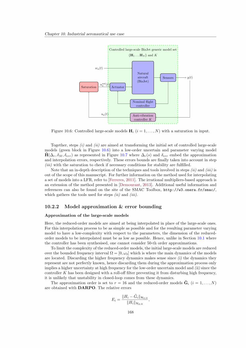
Chapter 10. Industrial aeronautical use case
Naturalaircraft(BizJet)
Actuator
Sensors
Saturation
y(t)
wa(t)
Nominal flightcontroller
Anti-vibrationcontroller K
usata (t)
ua(t)
H1 . . .HN and K
Controlled large-scale BizJet generic model set
Figure 10.6: Controlled large-scale models Hi (i = 1, . . . , N) with a saturation in input.
Together, steps (i) and (ii) are aimed at transforming the initial set of controlled large-scalemodels (green block in Figure 10.6) into a low-order uncertain and parameter varying modelH(∆r, δM , δerr) as represented in Figure 10.7 where ∆r(s) and δerr embed the approximationand interpolation errors, respectively. These errors bounds are finally taken into account in step(iii) with the saturation to check if necessary conditions for stability are fulfilled.
Note that an in-depth description of the techniques and tools involved in steps (ii) and (iii) isout of the scope of this manuscript. For further information on the method used for interpolatinga set of models into a LFR, refer to [Ferreres, 2011]. The irrational multipliers-based approach isan extension of the method presented in [Demourant, 2013]. Additional useful information andreferences can also be found on the site of the SMAC Toolbox, http://w3.onera.fr/smac/,which gathers the tools used for steps (ii) and (iii).
10.2.2 Model approximation & error bounding
Approximation of the large-scale models
Here, the reduced-order models are aimed at being interpolated in place of the large-scale ones.For this interpolation process to be as simple as possible and for the resulting parameter varyingmodel to have a low-complexity with respect to the parameters, the dimension of the reduced-order models to be interpolated must be as low as possible. Hence, unlike in Section 10.1 wherethe controller has been synthesised, one cannot consider 50-th order approximations.
To limit the complexity of the reduced-order models, the initial large-scale models are reducedover the bounded frequency interval Ω = [0, ω3] which is where the main dynamics of the modelsare located. Discarding the higher frequency dynamics makes sense since (i) the dynamics theyrepresent are not perfectly known, hence discarding them during the approximation process onlyimplies a higher uncertainty at high frequency for the low-order uncertain model and (ii) since thecontroller K has been designed with a roll-off filter preventing it from disturbing high frequency,it is unlikely that unstability in closed-loop comes from these dynamics.
The approximation order is set to r = 16 and the reduced-order models Gi (i = 1, . . . , N)are obtained with DARPO. The relative errors
Ei =‖Hi − Gi‖H2,Ω
‖Hi‖H2,Ω
,
168
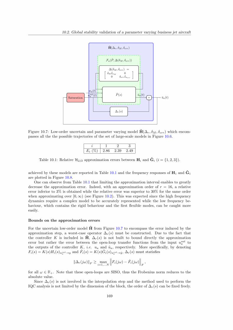
10.2. Global stability validation of a parameter varying business jet aircraft
P (s)Saturation +
ua(t)
∆(δM , δerr) =[δMInM 0
0 δerrInerr
]
wa(t)
usata (t)ua(t)
∆r(s)
Fu(P ,∆(δM , δerr))
H(∆r, δM , δerr)
Figure 10.7: Low-order uncertain and parameter varying model H(∆r, δM , δerr) which encom-passes all the the possible trajectories of the set of large-scale models in Figure 10.6.
i 1 2 3Ei (%) 2.86 2.39 2.49
Table 10.1: Relative H2,Ω approximation errors between Hi and Gi (i = 1, 2, 3).
achieved by these models are reported in Table 10.1 and the frequency responses of H1 and G1
are plotted in Figure 10.8.One can observe from Table 10.1 that limiting the approximation interval enables to greatly
decrease the approximation error. Indeed, with an approximation order of r = 16, a relativeerror inferior to 3% is obtained while the relative error was superior to 30% for the same orderwhen approximating over [0,∞) (see Figure 10.2). This was expected since the high frequencydynamics require a complex model to be accurately represented while the low frequency be-haviour, which contains the rigid behaviour and the first flexible modes, can be caught moreeasily.
Bounds on the approximation errors
For the uncertain low-order model H from Figure 10.7 to encompass the error induced by theapproximation step, a worst-case operator ∆r(s) must be constructed. Due to the fact thatthe controller K is included in H, ∆r(s) is not built to bound directly the approximationerror but rather the error between the open-loop transfer functions from the input usata tothe outputs of the controller K, i.e. ua and ua, respectively. More specifically, by denotingFi(s) = K(s)Hi(s)usata →y and Fi(s) = K(s)Gi(s)usata →y, ∆r(s) must statisfies
‖∆r(jω)‖F ≥ maxi=1,...N
∥∥∥Fi(jω)− Fi(jω)∥∥∥F,
for all ω ∈ R+. Note that these open-loops are SISO, thus the Frobenius norm reduces to theabsolute value.
Since ∆r(s) is not involved in the interpolation step and the method used to perform theIQC analysis is not limited by the dimension of the block, the order of ∆r(s) can be fixed freely.
169
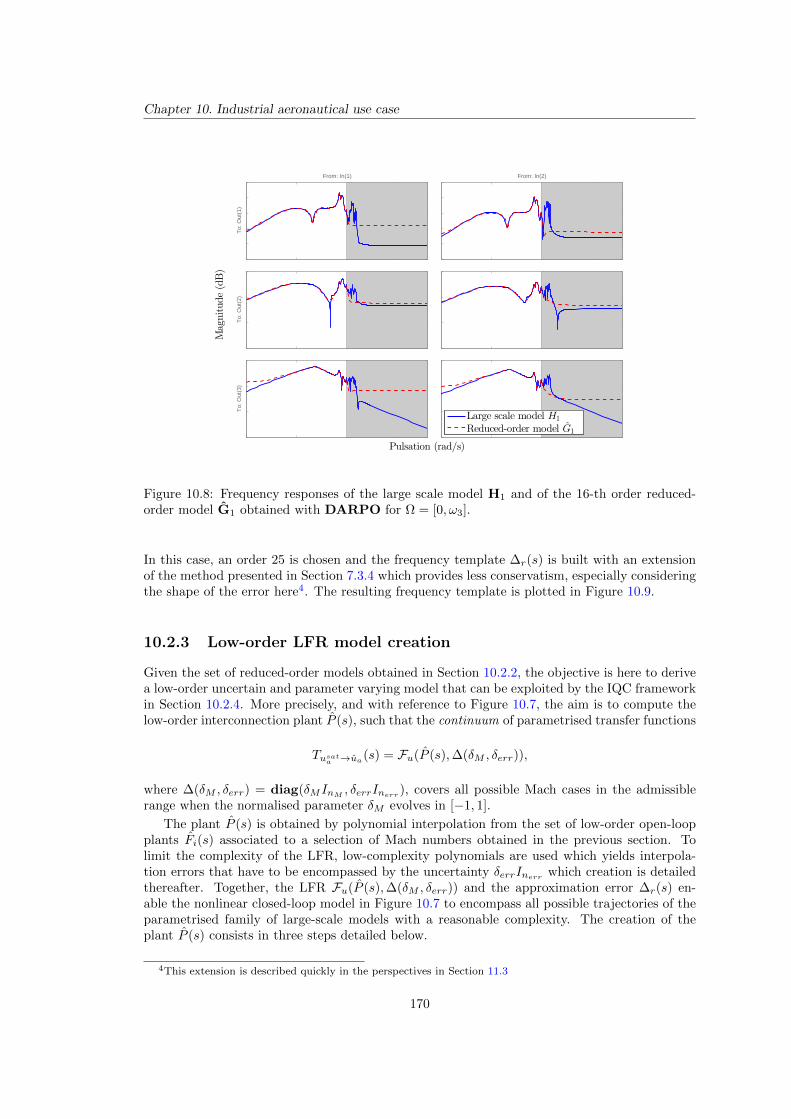
Chapter 10. Industrial aeronautical use case
From: In(1)
To:
Out
(1)
To:
Out
(2)
To:
Out
(3)
From: In(2)
Pulsation (rad/s)
Magnitude(dB)
Large scale model H1
Reduced-order model G1
Figure 10.8: Frequency responses of the large scale model H1 and of the 16-th order reduced-order model G1 obtained with DARPO for Ω = [0, ω3].
In this case, an order 25 is chosen and the frequency template ∆r(s) is built with an extensionof the method presented in Section 7.3.4 which provides less conservatism, especially consideringthe shape of the error here4. The resulting frequency template is plotted in Figure 10.9.
10.2.3 Low-order LFR model creation
Given the set of reduced-order models obtained in Section 10.2.2, the objective is here to derivea low-order uncertain and parameter varying model that can be exploited by the IQC frameworkin Section 10.2.4. More precisely, and with reference to Figure 10.7, the aim is to compute thelow-order interconnection plant P (s), such that the continuum of parametrised transfer functions
Tusata →ua(s) = Fu(P (s),∆(δM , δerr)),
where ∆(δM , δerr) = diag(δMInM , δerrInerr ), covers all possible Mach cases in the admissiblerange when the normalised parameter δM evolves in [−1, 1].
The plant P (s) is obtained by polynomial interpolation from the set of low-order open-loopplants Fi(s) associated to a selection of Mach numbers obtained in the previous section. Tolimit the complexity of the LFR, low-complexity polynomials are used which yields interpola-tion errors that have to be encompassed by the uncertainty δerrInerr which creation is detailedthereafter. Together, the LFR Fu(P (s),∆(δM , δerr)) and the approximation error ∆r(s) en-able the nonlinear closed-loop model in Figure 10.7 to encompass all possible trajectories of theparametrised family of large-scale models with a reasonable complexity. The creation of theplant P (s) consists in three steps detailed below.
4This extension is described quickly in the perspectives in Section 11.3
170
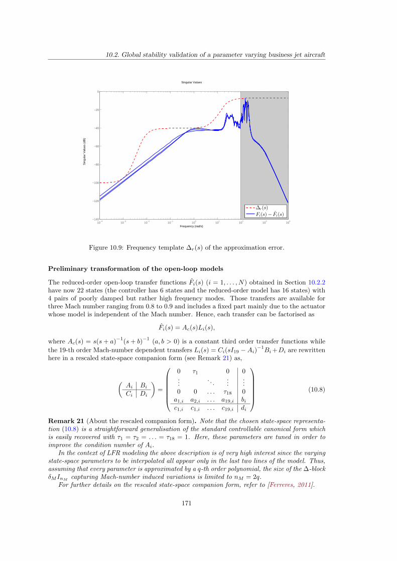
10.2. Global stability validation of a parameter varying business jet aircraft
10−4
10−3
10−2
10−1
100
101
102
103
104
−140
−120
−100
−80
−60
−40
−20
0
Singular Values
Frequency (rad/s)
Sin
gula
r V
alue
s (d
B)
∆r(s)
Fi(s)− Fi(s)
Figure 10.9: Frequency template ∆r(s) of the approximation error.
Preliminary transformation of the open-loop models
The reduced-order open-loop transfer functions Fi(s) (i = 1, . . . , N) obtained in Section 10.2.2have now 22 states (the controller has 6 states and the reduced-order model has 16 states) with4 pairs of poorly damped but rather high frequency modes. Those transfers are available forthree Mach number ranging from 0.8 to 0.9 and includes a fixed part mainly due to the actuatorwhose model is independent of the Mach number. Hence, each transfer can be factorised as
Fi(s) = Ac(s)Li(s),
where Ac(s) = s(s+ a)−1
(s+ b)−1
(a, b > 0) is a constant third order transfer functions while
the 19-th order Mach-number dependent transfers Li(s) = Ci(sI19 −Ai)−1Bi+Di are rewritten
here in a rescaled state-space companion form (see Remark 21) as,
(Ai BiCi Di
)=
0 τ1 0 0...
. . ....
...0 0 . . . τ18 0a1,i a2,i . . . a19,i bic1,i c1,i . . . c19,i di
(10.8)
Remark 21 (About the rescaled companion form). Note that the chosen state-space representa-tion (10.8) is a straightforward generalisation of the standard controllable canonical form whichis easily recovered with τ1 = τ2 = . . . = τ18 = 1. Here, these parameters are tuned in order toimprove the condition number of Ai.
In the context of LFR modeling the above description is of very high interest since the varyingstate-space parameters to be interpolated all appear only in the last two lines of the model. Thus,assuming that every parameter is approximated by a q-th order polynomial, the size of the ∆-blockδMInM capturing Mach-number induced variations is limited to nM = 2q.
For further details on the rescaled state-space companion form, refer to [Ferreres, 2011].
171
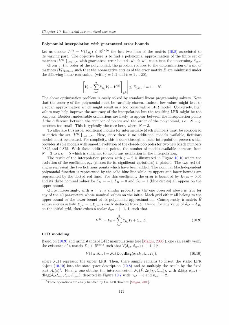
Chapter 10. Industrial aeronautical use case
Polynomial interpolation with guaranteed error bounds
Let us denote V (i) = V (δMi) ∈ R2×20 the last two lines of the matrix (10.8) associated toits varying part. The objective here is to find a polynomial approximation of the finite set ofmatrices V (i)i=1...N with guaranteed error bounds which will constitute the uncertainty δerr.
Given q, the order of the polynomial, the problem reduces to the determination of a set ofmatrices Vll=0...q such that the nonnegative entries of the error matrix E are minimised underthe following linear constraints (with j = 1, 2 and k = 1 . . . 20),∣∣∣∣∣∣
[V0 +
q∑l=1
δlMiVl − V (i)
]j,k
∣∣∣∣∣∣ ≤ Ej,k , i = 1 . . . N.
The above optimisation problem is easily solved by standard linear programming solvers. Notethat the order q of the polynomial must be carefully chosen. Indeed, low values might lead toa rough approximation which might result in a too conservative LFR model. Conversely, highvalues may help improve the accuracy of the interpolation but the resulting LFR might be toocomplex. Besides, undesirable oscillations are likely to appear between the interpolation pointsif the difference between the number of points and the order of the polynomial, i.e. N − q,becomes too small. This is typically the case here, where N = 3.
To alleviate this issue, additional models for intermediate Mach numbers must be consideredto enrich the set V (i)i=1...N . Here, since there is no additional models available, fictitiousmodels must be created. For simplicity, this is done through a linear interpolation process whichprovides stable models with smooth evolution of the closed-loop poles for two new Mach numbers0.825 and 0.875. With these additional points, the number of models available increases fromN = 3 to nM = 5 which is sufficient to avoid any oscillation in the interpolation.
The result of the interpolation process with q = 2 is illustrated in Figure 10.10 where theevolution of the coefficient c19 (chosen for its significant variations) is plotted. The two red tri-angles represent the two fictitious points which have been added. The nominal Mach-dependentpolynomial function is represented by the solid blue line while its uppers and lower bounds arerepresented by the dotted red lines. For this coefficient, the error is bounded by E2,19 = 0.04and its three nominal values for δM = −1, δM = 0 and δM = 1 (blue circles) all appear on theupper-bound.
Quite interestingly, with n = 2, a similar property as the one observed above is true forany of the 40 parameters whose nominal values on the initial Mach grid either all belong to theupper-bound or the lower-bound of its polynomial approximation. Consequently, a matrix Ewhose entries satisfy Ej,k = ±Ej,k is easily deduced from E. Hence, for any value of δM = δMi
on the initial grid, there exists a scalar δerr ∈ [−1, 1] such that
V (i) = V0 +
2∑l=1
δlMiVl + δerrE. (10.9)
LFR modeling
Based on (10.9) and using standard LFR manipulations (see [Magni, 2006]), one can easily verifythe existence of a matrix ΣV ∈ R8×48 such that ∀(δM , δerr) ∈ [−1, 1]2,
V (δM , δerr) = Fu(ΣV ,diag(δMI5, δerrI2)), (10.10)
where Fu() represent the upper LFR. Then, there simply remains to insert the static LFRobject (10.10) into the state-space description (10.8) and to multiply the result by the fixedpart Ac(s)
5. Finally, one obtains the interconnection Fu(P ,∆(δM , δerr)), with ∆(δM , δerr) =diag(δMInM , δerrInerr ), depicted in Figure 10.7 with nM = 5 and nerr = 2.
5These operations are easily handled by the LFR Toolbox [Magni, 2006].
172
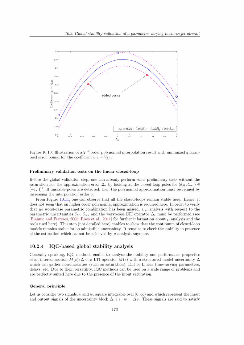
10.2. Global stability validation of a parameter varying business jet aircraft
−1 −0.8 −0.6 −0.4 −0.2 0 0.2 0.4 0.6 0.8 10.3
0.35
0.4
0.45
0.5
0.55
0.6
0.65
0.7
0.75
0.8
δM
Coeffi
cientc 1
9=V2,19
c19 = 0.75 +0.055δM − 0.32δ2M +0.04δerr
added points
Figure 10.10: Illustration of a 2nd order polynomial interpolation result with minimized guaran-teed error bound for the coefficient c19 = V2,19.
Preliminary validation tests on the linear closed-loop
Before the global validation step, one can already perform some preliminary tests without thesaturation nor the approximation error ∆r by looking at the closed-loop poles for (δM , δerr) ∈[−1, 1]2. If unstable poles are detected, then the polynomial approximation must be refined byincreasing the interpolation order q.
From Figure 10.11, one can observe that all the closed-loops remain stable here. Hence, itdoes not seem that an higher order polynomial approximation is required here. In order to verifythat no worst-case parametric combination has been missed, a µ analysis with respect to theparametric uncertainties δM , δerr and the worst-case LTI operator ∆r must be performed (see[Biannic and Ferreres, 2005; Roos et al., 2011] for further information about µ analysis and thetools used here). This step (not detailed here) enables to show that the continuum of closed-loopmodels remains stable for an admissible uncertainty. It remains to check the stability in presenceof the saturation which cannot be achieved by µ analysis anymore.
10.2.4 IQC-based global stability analysis
Generally speaking, IQC methods enable to analyse the stability and performance propertiesof an interconnection M(s)/∆ of a LTI operator M(s) with a structured model uncertainty ∆which can gather non-linearities (such as saturation), LTI or Linear time-varying parameters,delays, etc. Due to their versatility, IQC methods can be used on a wide range of problems andare perfectly suited here due to the presence of the input saturation.
General principle
Let us consider two signals, v and w, square integrable over [0,∞) and which represent the inputand output signals of the uncertainty block ∆, i.e. w = ∆v. These signals are said to satisfy
173
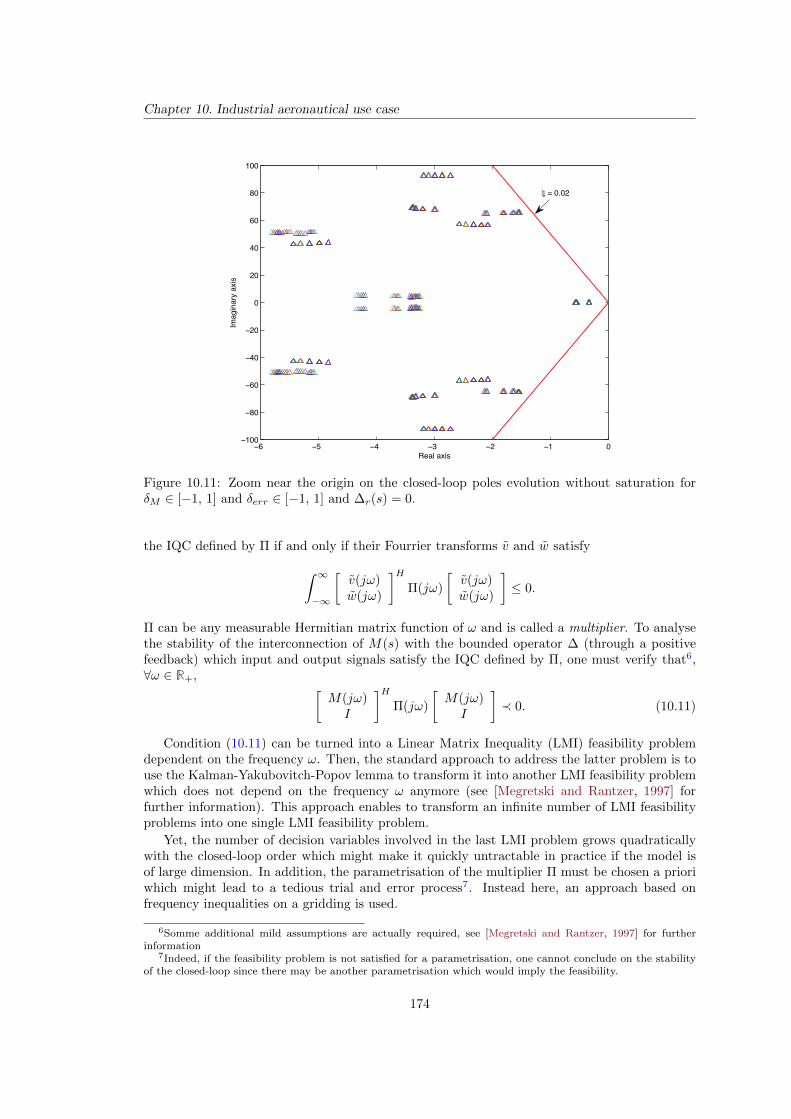
Chapter 10. Industrial aeronautical use case
6 5 4 3 2 1 0100
80
60
40
20
0
20
40
60
80
100
Real axis
Imag
inar
y ax
is
= 0.02
Figure 10.11: Zoom near the origin on the closed-loop poles evolution without saturation forδM ∈ [−1, 1] and δerr ∈ [−1, 1] and ∆r(s) = 0.
the IQC defined by Π if and only if their Fourrier transforms v and w satisfy∫ ∞−∞
[v(jω)w(jω)
]HΠ(jω)
[v(jω)w(jω)
]≤ 0.
Π can be any measurable Hermitian matrix function of ω and is called a multiplier. To analysethe stability of the interconnection of M(s) with the bounded operator ∆ (through a positivefeedback) which input and output signals satisfy the IQC defined by Π, one must verify that6,∀ω ∈ R+, [
M(jω)I
]HΠ(jω)
[M(jω)I
]≺ 0. (10.11)
Condition (10.11) can be turned into a Linear Matrix Inequality (LMI) feasibility problemdependent on the frequency ω. Then, the standard approach to address the latter problem is touse the Kalman-Yakubovitch-Popov lemma to transform it into another LMI feasibility problemwhich does not depend on the frequency ω anymore (see [Megretski and Rantzer, 1997] forfurther information). This approach enables to transform an infinite number of LMI feasibilityproblems into one single LMI feasibility problem.
Yet, the number of decision variables involved in the last LMI problem grows quadraticallywith the closed-loop order which might make it quickly untractable in practice if the model isof large dimension. In addition, the parametrisation of the multiplier Π must be chosen a prioriwhich might lead to a tedious trial and error process7. Instead here, an approach based onfrequency inequalities on a gridding is used.
6Somme additional mild assumptions are actually required, see [Megretski and Rantzer, 1997] for furtherinformation
7Indeed, if the feasibility problem is not satisfied for a parametrisation, one cannot conclude on the stabilityof the closed-loop since there may be another parametrisation which would imply the feasibility.
174
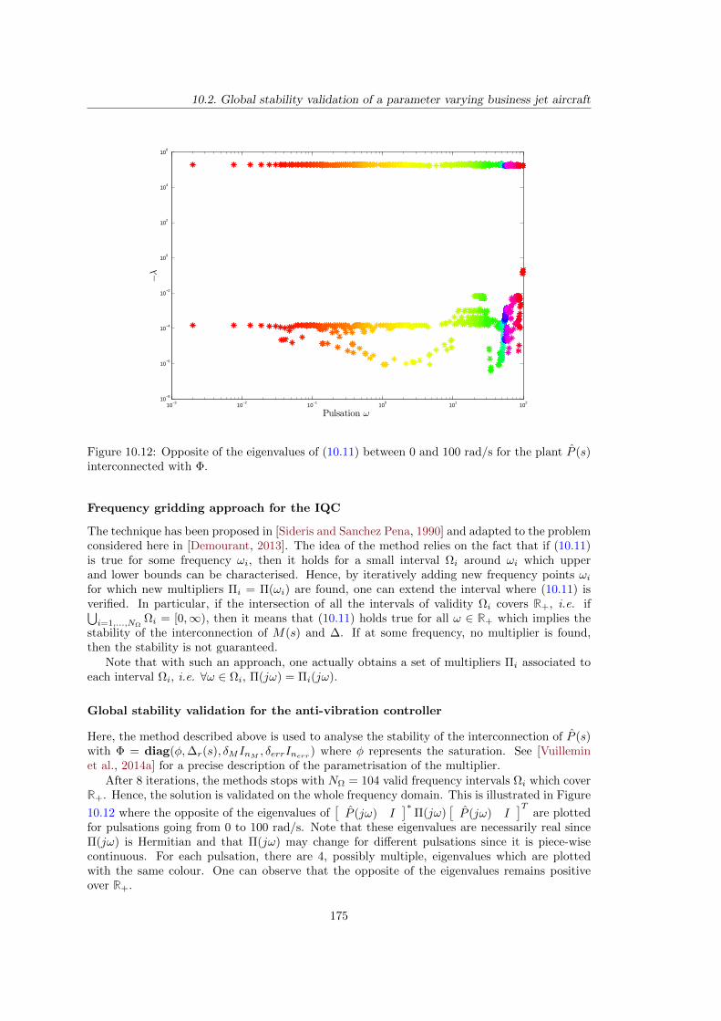
10.2. Global stability validation of a parameter varying business jet aircraft
10−3
10−2
10−1
100
101
102
10−8
10−6
10−4
10−2
100
102
104
106
−λ
Pulsation ω
Figure 10.12: Opposite of the eigenvalues of (10.11) between 0 and 100 rad/s for the plant P (s)interconnected with Φ.
Frequency gridding approach for the IQC
The technique has been proposed in [Sideris and Sanchez Pena, 1990] and adapted to the problemconsidered here in [Demourant, 2013]. The idea of the method relies on the fact that if (10.11)is true for some frequency ωi, then it holds for a small interval Ωi around ωi which upperand lower bounds can be characterised. Hence, by iteratively adding new frequency points ωifor which new multipliers Πi = Π(ωi) are found, one can extend the interval where (10.11) isverified. In particular, if the intersection of all the intervals of validity Ωi covers R+, i.e. if⋃i=1,...,NΩ
Ωi = [0,∞), then it means that (10.11) holds true for all ω ∈ R+ which implies thestability of the interconnection of M(s) and ∆. If at some frequency, no multiplier is found,then the stability is not guaranteed.
Note that with such an approach, one actually obtains a set of multipliers Πi associated toeach interval Ωi, i.e. ∀ω ∈ Ωi, Π(jω) = Πi(jω).
Global stability validation for the anti-vibration controller
Here, the method described above is used to analyse the stability of the interconnection of P (s)with Φ = diag(φ,∆r(s), δMInM , δerrInerr ) where φ represents the saturation. See [Vuilleminet al., 2014a] for a precise description of the parametrisation of the multiplier.
After 8 iterations, the methods stops with NΩ = 104 valid frequency intervals Ωi which coverR+. Hence, the solution is validated on the whole frequency domain. This is illustrated in Figure
10.12 where the opposite of the eigenvalues of[P (jω) I
]∗Π(jω)
[P (jω) I
]Tare plotted
for pulsations going from 0 to 100 rad/s. Note that these eigenvalues are necessarily real sinceΠ(jω) is Hermitian and that Π(jω) may change for different pulsations since it is piece-wisecontinuous. For each pulsation, there are 4, possibly multiple, eigenvalues which are plottedwith the same colour. One can observe that the opposite of the eigenvalues remains positiveover R+.
175
Chapter 10. Industrial aeronautical use case
This enables to conclude on the stability of the low-order uncertain and parameter varyingmodel H(∆r, δM , δerr) subject to the input saturation. Since the trajectories of this modelalso encompass all the possible trajectories of the parametrised family of large-scale models Hi
(i = 1, . . . , N), one can conclude on the global stability of the large-scale parameter varyingmodel subject to input saturation for all normalised Mach numbers δM ∈ [−1, 1].
Conclusion
In this chapter, the global process followed for the design and global stability validation of ananti-vibration control law for an industrial business jet aircraft represented by a family of large-scale LTI models subject to input saturation has been presented. Model approximation merelyrepresents a preliminary step in both the design and validation process, but still a mandatoryone.
Indeed, in the design step, model approximation has enabled to consider a control problemwith complex constraints which would have been difficult to address directly with the initiallarge-scale model. Similarly, in the analysis step, model approximation has enabled to greatlydecrease the complexity of the family of large-scale models which could not have been interpo-lated otherwise. In addition, by bounding the approximation error, the stability of the initiallarge-scale models can still be guaranteed.
This chapter concludes the contributions of this thesis and the next (and last) part concludesthis thesis.
176

Part IV
Conclusion
177

Chapter 11
Discussion
In this Chapter, the main contributions of the thesis are recalled and their limitations arediscussed. In addition, solutions or, at least hints, are proposed to alleviate these drawbacks andto extend the range of application of the results.
Contents11.1 FL-ISTIA . . . . . . . . . . . . . . . . . . . . . . . . . . . . . . . . . . 179
11.2 Poles-residues formulation of the H2,Ω-norm . . . . . . . . . . . . . 180
11.2.1 Numerical robustness . . . . . . . . . . . . . . . . . . . . . . . . . . . 180
11.2.2 Scalability . . . . . . . . . . . . . . . . . . . . . . . . . . . . . . . . . . 182
11.3 Bounds on the H∞-norm and its applications . . . . . . . . . . . . . 183
11.3.1 Improvement of the construction of frequency templates . . . . . . . . 183
11.3.2 Other possible applications for the H∞ bound ΓΩ . . . . . . . . . . . 185
11.4 First-order optimality conditions for the H2,Ω approximation prob-lem . . . . . . . . . . . . . . . . . . . . . . . . . . . . . . . . . . . . . . 185
11.5 DARPO . . . . . . . . . . . . . . . . . . . . . . . . . . . . . . . . . . . 186
11.5.1 Issues related to the poles-residues formulation of the H2,Ω-norm . . . 186
11.5.2 Optimisation scheme . . . . . . . . . . . . . . . . . . . . . . . . . . . . 188
11.5.3 Approximation for a fixed error . . . . . . . . . . . . . . . . . . . . . . 189
11.5.4 Model approximation for the control of large-scale models . . . . . . . 190
11.1 FL-ISTIA
In Chapter 6, an empirical method for frequency-limited model approximation has been pro-posed. The core of the method is the same as the sub-optimal H2 model approximation methodISRKA presented in Section 4.2.2, excepted that frequency-limited gramians are used in placeof the infinite gramians. This modification has been inspired by the way the FL-BT has beenobtained from the BT (see Sections 5.2.1 and 3.1.2, respectively).
In spite of its simplicity, this modification has led to improve the overall performances of theISRKA in terms of the H2,Ω-norm of the error. Yet, two fundamentals elements of the methodare directly inherited from the ISRKA and have not been modified
I the Krylov subspaces involved in the interpolation,
I the selection of the new interpolation points as the mirror images of the current reduced-order model poles.
More specifically, the Krylov subspaces and the interpolation points are such that at convergence,the reduced-order model tangentially interpolates the large-scale model from the left (or theright) at the mirror images of its poles, i.e.
H(−λi)bTi = H(−λi)bTi , (i = 1, . . . , r), (11.1)
which is one of the first order optimality condition of the optimal H2 approximation problem(see Section 4.1).
179
Chapter 11. Discussion
However, as it has been shown in Chapter 8, the optimality conditions for the optimalH2,Ω approximation problem are not equivalent to the H2 ones, hence fulfilling (11.1) is clearlyirrelevant for the approximation over a bounded frequency range. Hence, FL-ISTIA couldgreatly be improved by considering meaningful Krylov subspaces and interpolation points.
To this aim, one should determine whether the interpolation conditions expressed for theoptimal H2,Ω approximation problem in Chapter 8 can be fulfilled through projection on Krylovsubspaces. If not possible, an approximation of these interpolation conditions may be usedinstead, or, simply another interpolation framework such as the Loewner framework [Antoulaset al., 2012; Ionita, 2013].
11.2 Poles-residues formulation of the H2,Ω-norm
In Chapter 7, the H2,Ω-norm of a LTI dynamical model has been formulated through the useof the poles and residues of its transfer function both when the model has semi-simple polesand when it has high order poles. This formulation naturally extends the one existing for theH2-norm (see Section 2.2) and enables to express the H2,Ω-norm of a model in a closed forminvolving only elementary functions as soon as the poles and residues of the model are available.It has proven to be numerically very efficient for the computation of the H2,Ω-norm of modelswith semi-simple poles only and has enabled to derive the most significant results in this thesis.
11.2.1 Numerical robustness
The poles-residues formulation of the H2,Ω-norm is mainly limited by two elements in the large-scale framework,
I the eigenvalue decomposition is not particularly numerically robust,
I the formulation is not convenient when the model has Jordan blocks. Indeed, the com-putation of the Jordan decomposition is only possible on ”toy models” and should not beconsidered in larger settings.
When Jordan blocks are involved, two workarounds can be considered,
(i) if the residues of a transfer function can be efficiently computed knowing the eigenvaluesbut not the eigenvectors, then the H2,Ω-norm may be computed by evaluating the transferfunction and its derivative as in the H2-case (see Section 7.2.3). Evaluating the deriva-tive of the transfer function is not particularly simple either but remains preferable thancomputing the Jordan canonical form.
(ii) It is well-known that matrices with Jordan blocks are extremely sensitive to perturbations,however, one may want to consider the impact of this sensitivity for the computation ofthe H2,Ω-norm. As illustration, let us consider a n-th order model H = (A,B,C) where
A =
−1 1
−1. . .
. . . 1−1
∈ Rn×n, C = BT =[
1 . . . 1]∈ R1×n,
i.e. λ = −1 is an eigenvalue of order n. Let us also consider the perturbed model Hε =(Aε, B,C), where
Aε =
−1 1
−1. . .
. . . 1ε −1
∈ Rn×n,
180
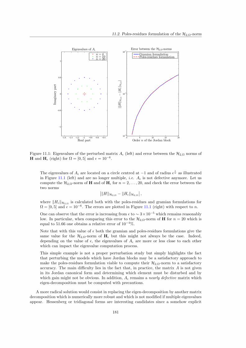
11.2. Poles-residues formulation of the H2,Ω-norm
−1.6 −1.4 −1.2 −1 −0.8 −0.6 −0.4
−1
−0.5
0
0.5
1
Eigenvalues of Aε
Imaginarypart
Real part
n = 4n = 10n = 20
0 5 10 15 2010
−6
10−5
10−4
Error between the H2,Ω-norms
|‖H‖H
2,Ω−‖H
ε‖H
2,Ω|
Order n of the Jordan block
Gramian formulationPoles-residues formulation
Figure 11.1: Eigenvalues of the perturbed matrix Aε (left) and error between the H2,Ω norms ofH and Hε (right) for Ω = [0, 5] and ε = 10−6.
The eigenvalues of Aε are located on a circle centred at −1 and of radius ε1n as illustrated
in Figure 11.1 (left) and are no longer multiple, i.e. Aε is not defective anymore. Let uscompute the H2,Ω-norm of H and of Hε for n = 2, . . . , 20, and check the error between thetwo norms ∣∣‖H‖H2,Ω
− ‖Hε‖H2,Ω
∣∣ ,where ‖Hε‖H2,Ω
is calculated both with the poles-residues and gramian formulations forΩ = [0, 5] and ε = 10−6. The errors are plotted in Figure 11.1 (right) with respect to n.
One can observe that the error is increasing from ε to ∼ 3×10⁻⁵ which remains reasonablylow. In particular, when comparing this error to the H2,Ω-norm of H for n = 20 which isequal to 51.66 one obtains a relative error of 10−4%.
Note that with this value of ε both the gramian and poles-residues formulations give thesame value for the H2,Ω-norm of Hε but this might not always be the case. Indeed,depending on the value of ε, the eigenvalues of Aε are more or less close to each otherwhich can impact the eigenvalue computation process.
This simple example is not a proper perturbation study but simply highlights the factthat perturbing the models which have Jordan blocks may be a satisfactory approach tomake the poles-residues formulation viable to compute their H2,Ω-norm to a satisfactoryaccuracy. The main difficulty lies in the fact that, in practice, the matrix A is not givenin its Jordan canonical form and determining which element must be disturbed and bywhich gain might not be obvious. In addition, Aε remains a nearly defective matrix whicheigen-decomposition must be computed with precautions.
A more radical solution would consist in replacing the eigen-decomposition by another matrixdecomposition which is numerically more robust and which is not modified if multiple eigenvaluesappear. Hessenberg or tridiagonal forms are interesting candidates since a somehow explicit
181
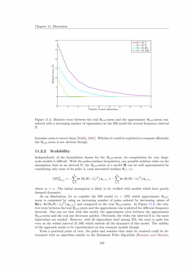
Chapter 11. Discussion
2 4 6 8 10 12 14 16 18 20−5
0
5
10
15
20
25
30
Number of used eigenvalues
Relativeerror(%
)
Ω= [0, 1]Ω= [0, 5]Ω= [0, 20]Ω= [0, 100]
Figure 11.2: Relative error between the real H2,Ω-norm and the approximate H2,Ω-norm con-sidered with a increasing number of eigenvalues on the ISS model for several frequency intervalΩ.
formulae exists to invert them [Mallik, 2001]. Whether it could be exploited to compute efficientlythe H2,Ω-norm is not obvious though.
11.2.2 Scalability
Independently of the formulation chosen for the H2,Ω-norm, its computation for very large-scale models is difficult. With the poles-residues formulation, one possible solution relies on theassumption that on an interval Ω, the H2,Ω-norm of a model H can be well approximated byconsidering only some of its poles λi (and associated residues Φi), i.e.
‖H‖2H2,Ω= −
n∑i=1
tr(ΦiH(−λi)T
)aω,λi ≈ −
m∑i=1
tr(ΦiH(−λi)T
)aω,λi ,
where m < n. The initial assumption is likely to be verified with models which have poorlydamped dynamics.
As an illustration, let us consider the ISS model (n = 270) which approximate H2,Ω-norm is computed by using an increasing number of poles ordered by decreasing values ofRe(−tr
(ΦiH(−λi)T
)aω,λi
)and compared to the true H2,Ω-norm. In Figure 11.2, the rela-
tive error between the real H2,Ω-norm and the approximate one is plotted for different frequencyintervals. One can see that with this model, the approximate error between the approximateH2,Ω-norm and the real one decreases quickly. Obviously, the wider the interval Ω is, the moreeigenvalues are needed. However, with 20 eigenvalues used among 270, the error is quite loweven on the widest interval [0, 100] which embeds all the dynamics of this model. The validityof the approach needs to be experimented on less resonant models though.
From a practical point of view, the poles and residues that must be retained could be de-termined with an algorithm similar to the Dominant Poles Algorithm [Rommes and Martins,
182
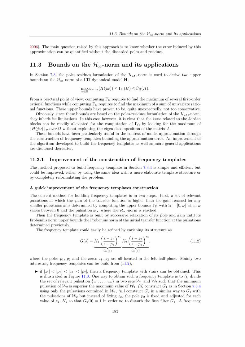
11.3. Bounds on the H∞-norm and its applications
2006]. The main question raised by this approach is to know whether the error induced by thisapproximation can be quantified without the discarded poles and residues.
11.3 Bounds on the H∞-norm and its applications
In Section 7.3, the poles-residues formulation of the H2,Ω-norm is used to derive two upperbounds on the H∞-norm of a LTI dynamical model H,
maxω∈Ω
σmax(H(jω)) ≤ ΓΩ(H) ≤ ΓΩ(H).
From a practical point of view, computing ΓΩ requires to find the maximum of several first-orderrational functions while computing ΓΩ requires to find the maximum of a sum of univariate ratio-nal functions. These upper bounds have proven to be, quite unexpectedly, not too conservative.
Obviously, since these bounds are based on the poles-residues formulation of the H2,Ω-norm,they inherit its limitations. In this case however, it is clear that the issue related to the Jordanblocks can be readily alleviated for the computation of ΓΩ by looking for the maximum of‖H(jω)‖F over Ω without exploiting the eigen-decomposition of the matrix A.
These bounds have been particularly useful in the context of model approximation throughthe construction of frequency templates bounding the approximation error. An improvement ofthe algorithm developed to build the frequency templates as well as more general applicationsare discussed thereafter.
11.3.1 Improvement of the construction of frequency templates
The method proposed to build frequency template in Section 7.3.4 is simple and efficient butcould be improved, either by using the same idea with a more elaborate template structure orby completely reformulating the problem.
A quick improvement of the frequency templates construction
The current method for building frequency templates is in two steps. First, a set of relevantpulsations at which the gain of the transfer function is higher than the gain reached for anysmaller pulsations ω is determined by computing the upper bounds ΓΩ with Ω = [0, ω] when ωvaries between 0 and the pulsation ω∞ where the H∞-norm is reached.
Then the frequency template is built by successive relaxation of its pole and gain until itsFrobenius norm upper bounds the Frobenius norm of the initial transfer function at the pulsationsdetermined previously.
The frequency template could easily be refined by enriching its structure as
G(s) = K1
(s− z1
s− p1
)r1︸ ︷︷ ︸
G1(s)
K2
(s− z2
s− p2
)r2︸ ︷︷ ︸
G2(s)
, (11.2)
where the poles p1, p2 and the zeros z1, z2 are all located in the left half-plane. Mainly twointeresting frequency templates can be build from (11.2),
I if |z1| < |p1| < |z2| < |p2|, then a frequency template with stairs can be obtained. Thisis illustrated in Figure 11.3. One way to obtain such a frequency template is to (i) dividethe set of relevant pulsation w1, . . . , wk in two sets W1 and W2 such that the minimumpulsation ofW2 is superior the maximum value ofW1, (ii) construct G1 as in Section 7.3.4using only the pulsations contained in W1, (iii) construct G2 in a similar way to G1 withthe pulsations of W2 but instead of fixing z2, the pole p2 is fixed and adjusted for eachvalue of z2, K2 so that G2(0) = 1 in order no to disturb the first filter G1. A frequency
183
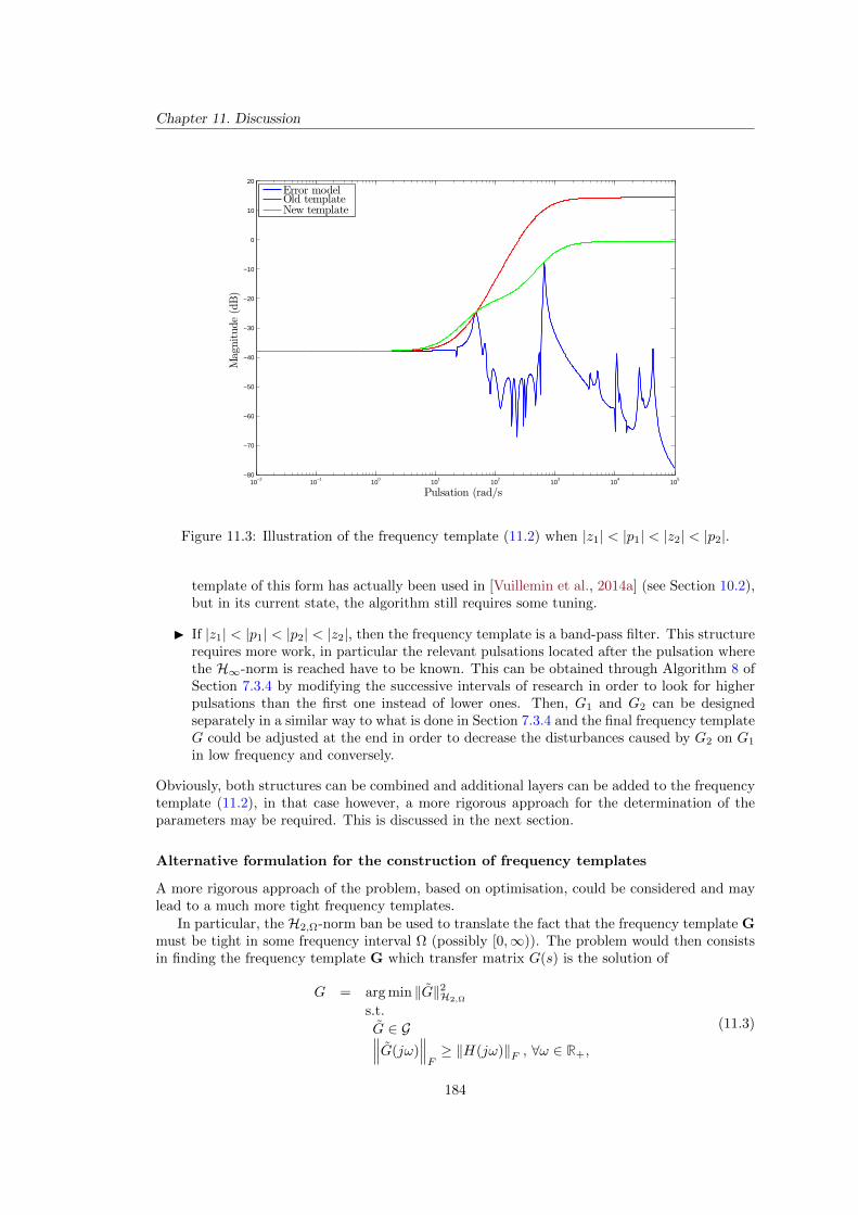
Chapter 11. Discussion
10−2
10−1
100
101
102
103
104
105
−80
−70
−60
−50
−40
−30
−20
−10
0
10
20
Magnitude(dB)
Pulsation (rad/s
Error modelOld templateNew template
Figure 11.3: Illustration of the frequency template (11.2) when |z1| < |p1| < |z2| < |p2|.
template of this form has actually been used in [Vuillemin et al., 2014a] (see Section 10.2),but in its current state, the algorithm still requires some tuning.
I If |z1| < |p1| < |p2| < |z2|, then the frequency template is a band-pass filter. This structurerequires more work, in particular the relevant pulsations located after the pulsation wherethe H∞-norm is reached have to be known. This can be obtained through Algorithm 8 ofSection 7.3.4 by modifying the successive intervals of research in order to look for higherpulsations than the first one instead of lower ones. Then, G1 and G2 can be designedseparately in a similar way to what is done in Section 7.3.4 and the final frequency templateG could be adjusted at the end in order to decrease the disturbances caused by G2 on G1
in low frequency and conversely.
Obviously, both structures can be combined and additional layers can be added to the frequencytemplate (11.2), in that case however, a more rigorous approach for the determination of theparameters may be required. This is discussed in the next section.
Alternative formulation for the construction of frequency templates
A more rigorous approach of the problem, based on optimisation, could be considered and maylead to a much more tight frequency templates.
In particular, the H2,Ω-norm ban be used to translate the fact that the frequency template Gmust be tight in some frequency interval Ω (possibly [0,∞)). The problem would then consistsin finding the frequency template G which transfer matrix G(s) is the solution of
G = arg min ‖G‖2H2,Ω
s.t.
G ∈ G∥∥∥G(jω)∥∥∥F≥ ‖H(jω)‖F , ∀ω ∈ R+,
(11.3)
184
11.4. First-order optimality conditions for the H2,Ω approximation problem
where G represents the space of frequency templates with a defined structure (stable, fixed order,minimum phase, etc.). In addition, problem (11.3) may be completed with a constraint on theH∞-norm of G(s) in order to avoid any unwanted local resonance or unbounded behaviouroutside of Ω. Note that if G in equation (11.3) is given the same structure as in Section 7.3.4,then the poles-residues formulation of the H2,Ω-norm for models with high order poles developedin Section 7.2.1 may be used and since the Jordan block is directly known, it does not representan issue here.
The inequality constraint on the Frobenius norm might be difficult to fulfil. Indeed, unlike inSection 7.3.4 and depending on the structure chosen for G(s), it cannot necessarily be restrictedto some relevant pulsations ωk in order to be true for all ω ∈ R+ especially if resonant modesare involved.
A valid frequency template could certainly be obtained by solving an adequate H∞ problem,yet in an approximation context, H is of large-scale, hence (11.3) seems to be a more modestand reachable objective. Alternatively, the bound ΓΩ could be used instead of the H2,Ω-normin problem (7.3.4).
11.3.2 Other possible applications for the H∞ bound ΓΩ
Since ΓΩ upper bounds the H∞-norm and is faster to compute than the latter, it could be usedas a surrogate when the computation of the H∞-norm becomes an issue. In particular
I for model approximation, one could look for the reduced-order model H which transfermatrix H(s) solves
H = arg minrank(G)=r
ΓΩ (H(jω)−G(jω)) ,
I for robust control of large-scale models, whether ΓΩ can represent a valid replacement ofthe H∞-norm in tools such as HIFOO [Burke et al., 2006] should be investigated. Thiswould enable large-scale control problem such as the one presented in Section 9.2.3 to behandled directly.
Some preliminary experiments have been conducted during this study concerning the secondpoint but they do not enable to conclude on the validity of the approach, yet.
11.4 First-order optimality conditions for the H2,Ω approx-imation problem
In Chapter 8, the H2,Ω-norm of the approximation error between a large-scale model H and
a reduced-order one H has been expressed with the poles and residues of both models underthe assumption that both models have semi-simple poles only. Then, the first-order optimalityconditions of the optimal H2,Ω approximation problem have been derived with respect to thepoles and residues of the reduced-order model.
Both the approximation error and its gradient can efficiently be computed through elementaryoperations once the poles and residues of both models are available. This point is particularlyinteresting in an optimisation context which usually involves many evaluations of the objectivefunction and its gradient.
Moreover, it has also been shown how these first-order optimality conditions can be for-mulated as interpolation conditions similar to those arising in the optimal H2 approximationproblem (see Section 4.1.2). Indeed, if H is a r-th order minimum of the H2,Ω approximation
185
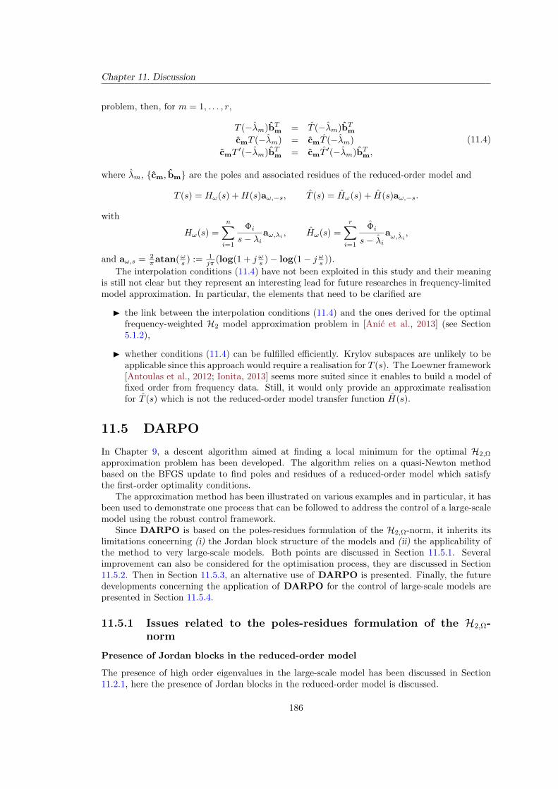
Chapter 11. Discussion
problem, then, for m = 1, . . . , r,
T (−λm)bTm = T (−λm)bTmcmT (−λm) = cmT (−λm)
cmT′(−λm)bTm = cmT
′(−λm)bTm,
(11.4)
where λm, cm, bm are the poles and associated residues of the reduced-order model and
T (s) = Hω(s) +H(s)aω,−s, T (s) = Hω(s) + H(s)aω,−s.
with
Hω(s) =
n∑i=1
Φis− λi
aω,λi , Hω(s) =
r∑i=1
Φi
s− λiaω,λi ,
and aω,s = 2πatan(ωs ) := 1
jπ (log(1 + j ωs )− log(1− j ωs )).
The interpolation conditions (11.4) have not been exploited in this study and their meaningis still not clear but they represent an interesting lead for future researches in frequency-limitedmodel approximation. In particular, the elements that need to be clarified are
I the link between the interpolation conditions (11.4) and the ones derived for the optimalfrequency-weighted H2 model approximation problem in [Anic et al., 2013] (see Section5.1.2),
I whether conditions (11.4) can be fulfilled efficiently. Krylov subspaces are unlikely to beapplicable since this approach would require a realisation for T (s). The Loewner framework[Antoulas et al., 2012; Ionita, 2013] seems more suited since it enables to build a model offixed order from frequency data. Still, it would only provide an approximate realisationfor T (s) which is not the reduced-order model transfer function H(s).
11.5 DARPO
In Chapter 9, a descent algorithm aimed at finding a local minimum for the optimal H2,Ω
approximation problem has been developed. The algorithm relies on a quasi-Newton methodbased on the BFGS update to find poles and residues of a reduced-order model which satisfythe first-order optimality conditions.
The approximation method has been illustrated on various examples and in particular, it hasbeen used to demonstrate one process that can be followed to address the control of a large-scalemodel using the robust control framework.
Since DARPO is based on the poles-residues formulation of the H2,Ω-norm, it inherits itslimitations concerning (i) the Jordan block structure of the models and (ii) the applicability ofthe method to very large-scale models. Both points are discussed in Section 11.5.1. Severalimprovement can also be considered for the optimisation process, they are discussed in Section11.5.2. Then in Section 11.5.3, an alternative use of DARPO is presented. Finally, the futuredevelopments concerning the application of DARPO for the control of large-scale models arepresented in Section 11.5.4.
11.5.1 Issues related to the poles-residues formulation of the H2,Ω-norm
Presence of Jordan blocks in the reduced-order model
The presence of high order eigenvalues in the large-scale model has been discussed in Section11.2.1, here the presence of Jordan blocks in the reduced-order model is discussed.
186

11.5. DARPO
−6−5
−4−3
−2−1
0
−5
0
5
0
20
40
60
80
100
Real partImaginary part
H2ap
proximationerror
Figure 11.4: Apparition of a Jordan block in the reduced-order model with DARPO.
Jordan blocks can appear in the reduced-order model when two poles cross each other. Ingeneral, this does not happen, but one can build examples in which it should happen. In partic-ular, if a second-order model with a pair of complex conjugate poles is approximated to an order2 and that DARPO is initialised with a second-order model with real poles. The correspondingH2 approximation error is represented in Figure 11.4 where the successive positions of the polesare represented by blue and red dots.
The expected behaviour is that the poles move along the real axis until they reach each otherand at this point, they should split as complex conjugate poles. When the poles are at theexact same location, the semi-simple poles-residues formulation of the approximation error andits gradient are no longer valid. Instead, the generalised formulation must be used.
Here, what happens in practice is that both poles stop moving before they reach the samelocation. The exact explanation is still not clear, but it is likely that the line-search algorithmdoes not find a suitable step-length along the real axis.
In theory, using the poles-residues formulation generalised to model with high-order poleswould be sufficient to alleviate the issue. Yet in practice, it might be difficult to determine whensome poles are close enough to switch (in the algorithmic procedure) to this formulation.
Very-large scale models
In order for the algorithm DARPO to be applicable, the full eigenvalue decomposition ofthe initial large-scale model is required. This is an important limitation in the context of modelapproximation since it is expensive to compute. In addition, the eventual sparsity of the matricesC and B of the large-scale model is lost when changing to the modal realisation of the large-scale model. These issues are inherent to the framework used in the study and cannot fully bealleviated but still, some hints are presented here in order to decrease the complexity associatedwith the algorithm.
The idea here relies on the same assumption as in Section 11.2.2, i.e. that the H2,Ω-normof a model can be well estimated by computing only some of its poles and associated residues.
187
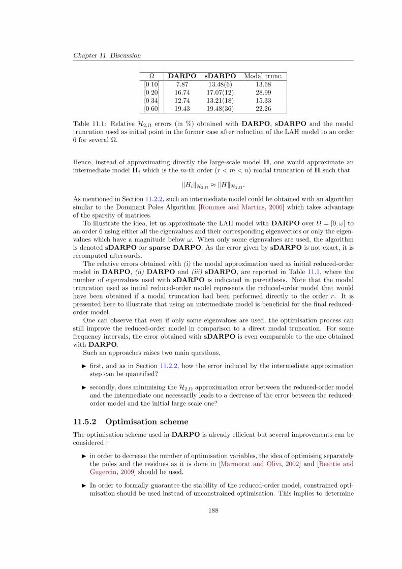
Chapter 11. Discussion
Ω DARPO sDARPO Modal trunc.[0 10] 7.87 13.48(6) 13.68[0 20] 16.74 17.07(12) 28.99[0 34] 12.74 13.21(18) 15.33[0 60] 19.43 19.48(36) 22.26
Table 11.1: Relative H2,Ω errors (in %) obtained with DARPO, sDARPO and the modaltruncation used as initial point in the former case after reduction of the LAH model to an order6 for several Ω.
Hence, instead of approximating directly the large-scale model H, one would approximate anintermediate model Hi which is the m-th order (r < m < n) modal truncation of H such that
‖Hi‖H2,Ω≈ ‖H‖H2,Ω
.
As mentioned in Section 11.2.2, such an intermediate model could be obtained with an algorithmsimilar to the Dominant Poles Algorithm [Rommes and Martins, 2006] which takes advantageof the sparsity of matrices.
To illustrate the idea, let us approximate the LAH model with DARPO over Ω = [0, ω] toan order 6 using either all the eigenvalues and their corresponding eigenvectors or only the eigen-values which have a magnitude below ω. When only some eigenvalues are used, the algorithmis denoted sDARPO for sparse DARPO. As the error given by sDARPO is not exact, it isrecomputed afterwards.
The relative errors obtained with (i) the modal approximation used as initial reduced-ordermodel in DARPO, (ii) DARPO and (iii) sDARPO, are reported in Table 11.1, where thenumber of eigenvalues used with sDARPO is indicated in parenthesis. Note that the modaltruncation used as initial reduced-order model represents the reduced-order model that wouldhave been obtained if a modal truncation had been performed directly to the order r. It ispresented here to illustrate that using an intermediate model is beneficial for the final reduced-order model.
One can observe that even if only some eigenvalues are used, the optimisation process canstill improve the reduced-order model in comparison to a direct modal truncation. For somefrequency intervals, the error obtained with sDARPO is even comparable to the one obtainedwith DARPO.
Such an approaches raises two main questions,
I first, and as in Section 11.2.2, how the error induced by the intermediate approximationstep can be quantified?
I secondly, does minimising the H2,Ω approximation error between the reduced-order modeland the intermediate one necessarily leads to a decrease of the error between the reduced-order model and the initial large-scale one?
11.5.2 Optimisation scheme
The optimisation scheme used in DARPO is already efficient but several improvements can beconsidered :
I in order to decrease the number of optimisation variables, the idea of optimising separatelythe poles and the residues as it is done in [Marmorat and Olivi, 2002] and [Beattie andGugercin, 2009] should be used.
I In order to formally guarantee the stability of the reduced-order model, constrained opti-misation should be used instead of unconstrained optimisation. This implies to determine
188
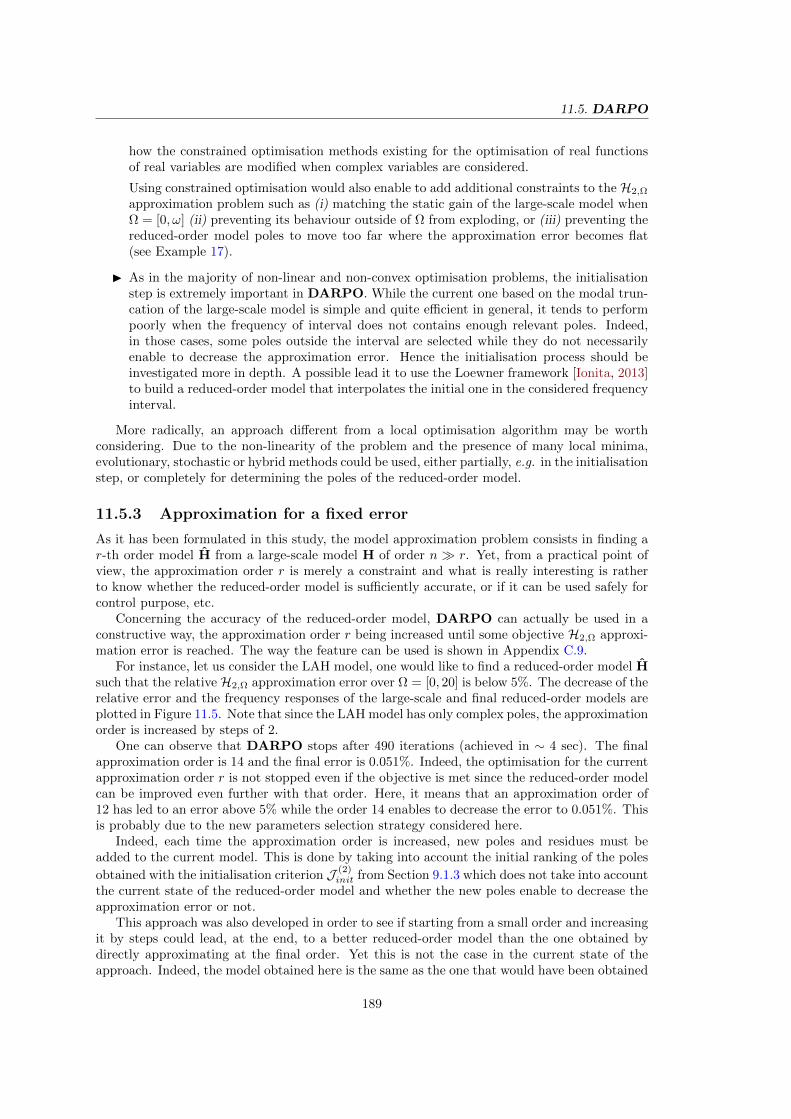
11.5. DARPO
how the constrained optimisation methods existing for the optimisation of real functionsof real variables are modified when complex variables are considered.
Using constrained optimisation would also enable to add additional constraints to the H2,Ω
approximation problem such as (i) matching the static gain of the large-scale model whenΩ = [0, ω] (ii) preventing its behaviour outside of Ω from exploding, or (iii) preventing thereduced-order model poles to move too far where the approximation error becomes flat(see Example 17).
I As in the majority of non-linear and non-convex optimisation problems, the initialisationstep is extremely important in DARPO. While the current one based on the modal trun-cation of the large-scale model is simple and quite efficient in general, it tends to performpoorly when the frequency of interval does not contains enough relevant poles. Indeed,in those cases, some poles outside the interval are selected while they do not necessarilyenable to decrease the approximation error. Hence the initialisation process should beinvestigated more in depth. A possible lead it to use the Loewner framework [Ionita, 2013]to build a reduced-order model that interpolates the initial one in the considered frequencyinterval.
More radically, an approach different from a local optimisation algorithm may be worthconsidering. Due to the non-linearity of the problem and the presence of many local minima,evolutionary, stochastic or hybrid methods could be used, either partially, e.g. in the initialisationstep, or completely for determining the poles of the reduced-order model.
11.5.3 Approximation for a fixed error
As it has been formulated in this study, the model approximation problem consists in finding ar-th order model H from a large-scale model H of order n r. Yet, from a practical point ofview, the approximation order r is merely a constraint and what is really interesting is ratherto know whether the reduced-order model is sufficiently accurate, or if it can be used safely forcontrol purpose, etc.
Concerning the accuracy of the reduced-order model, DARPO can actually be used in aconstructive way, the approximation order r being increased until some objective H2,Ω approxi-mation error is reached. The way the feature can be used is shown in Appendix C.9.
For instance, let us consider the LAH model, one would like to find a reduced-order model Hsuch that the relative H2,Ω approximation error over Ω = [0, 20] is below 5%. The decrease of therelative error and the frequency responses of the large-scale and final reduced-order models areplotted in Figure 11.5. Note that since the LAH model has only complex poles, the approximationorder is increased by steps of 2.
One can observe that DARPO stops after 490 iterations (achieved in ∼ 4 sec). The finalapproximation order is 14 and the final error is 0.051%. Indeed, the optimisation for the currentapproximation order r is not stopped even if the objective is met since the reduced-order modelcan be improved even further with that order. Here, it means that an approximation order of12 has led to an error above 5% while the order 14 enables to decrease the error to 0.051%. Thisis probably due to the new parameters selection strategy considered here.
Indeed, each time the approximation order is increased, new poles and residues must beadded to the current model. This is done by taking into account the initial ranking of the poles
obtained with the initialisation criterion J (2)init from Section 9.1.3 which does not take into account
the current state of the reduced-order model and whether the new poles enable to decrease theapproximation error or not.
This approach was also developed in order to see if starting from a small order and increasingit by steps could lead, at the end, to a better reduced-order model than the one obtained bydirectly approximating at the final order. Yet this is not the case in the current state of theapproach. Indeed, the model obtained here is the same as the one that would have been obtained
189
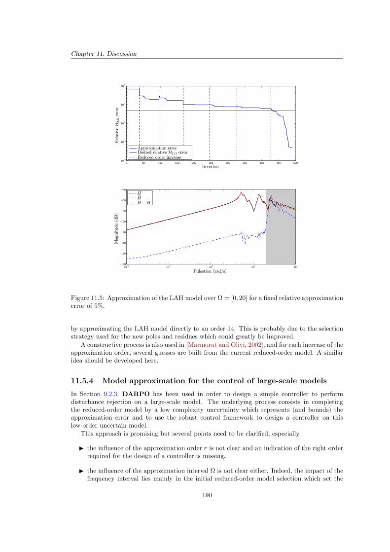
Chapter 11. Discussion
0 50 100 150 200 250 300 350 400 450 50010
−2
10−1
100
101
102
Iteration
RelativeH
2,Ω
error
Approximation errorDesired relative H2,Ω errorReduced order increase
10−2
10−1
100
101
102
−180
−160
−140
−120
−100
−80
−60
−40
Pulsation (rad/s)
Magnitude(dB)
HHH − H
Figure 11.5: Approximation of the LAH model over Ω = [0, 20] for a fixed relative approximationerror of 5%.
by approximating the LAH model directly to an order 14. This is probably due to the selectionstrategy used for the new poles and residues which could greatly be improved.
A constructive process is also used in [Marmorat and Olivi, 2002], and for each increase of theapproximation order, several guesses are built from the current reduced-order model. A similaridea should be developed here.
11.5.4 Model approximation for the control of large-scale models
In Section 9.2.3, DARPO has been used in order to design a simple controller to performdisturbance rejection on a large-scale model. The underlying process consists in completingthe reduced-order model by a low complexity uncertainty which represents (and bounds) theapproximation error and to use the robust control framework to design a controller on thislow-order uncertain model.
This approach is promising but several points need to be clarified, especially
I the influence of the approximation order r is not clear and an indication of the right orderrequired for the design of a controller is missing,
I the influence of the approximation interval Ω is not clear either. Indeed, the impact of thefrequency interval lies mainly in the initial reduced-order model selection which set the
190
11.5. DARPO
dynamics that will be preserved. Hence, the real, non-trivial, question is to determine thedynamics that matter for the closed-loop.
A completely different approach would consists in using the gap or ν-gap metrics [Vidyasagar,1984; Vinnicombe, 1992] as criterion for the approximation as it has been done in [Sootla, 2011].Yet, the resulting approximation problem is difficult and whether it can be solved efficiently onlarge-scale models is not clear due to the complexity of the evaluation of this norm which isbased on the H∞ one.
Conclusion
The main limitation of the proposed model approximation method lies in the use of the poles-residues formulation of the models and of the approximation error. Indeed, this formulationrequires the full eigen-decomposition of the large-scale model and becomes ill-conditioned if highorder poles are involved. Hence, a formulation of the state-space may appear more suitable,however (i) the computational complexity does not vanish since the eigenvalue decompositionis replaced by the need to solve various Sylvester equations, which is a complex task whenperformed exactly, (ii) in the frequency-limited context, the logarithm of a matrix as well as itsderivative are required, which are not trivial to compute either. The core of the problem whenusing an optimisation algorithm to perform large-scale model reduction lies in the computationof the approximation error and its gradient which reduces here to the computation of the inverse(sIn −A)
−1arising in the transfer function (and thus in the H2,Ω-norm).
As pointed out in [Moler and Van Loan, 1978], a trade-off must be considered between theeigen-decomposition (or Jordan form) which offers the easiest, but most ill-conditioned, way tocompute a matrix function, and another decomposition which is well-conditioned but does notyield a particularly easy computation of the function (such as the Schur decomposition). In[Moler and Van Loan, 1978], a block diagonal matrix where nearly confluent eigenvalues areclustered is presented as an interesting candidate. Such a decomposition may be considered forthe computation of the H2,Ω-norm and in the optimal H2,Ω approximation problem in futureresearches.
Besides, the other interesting lead for further development lies in the first-order optimalityconditions expressed as interpolation conditions. Indeed, generalising interpolation methods suchas the IRKA to the optimal H2,Ω approximation would be particularly interesting given theperformance and simplicity of the approach. In the next chapter, some longer term perspectivesare pointed out.
191

Chapter 12
Outlook
The perspectives of this thesis can be considered along two major lines : model approximationand control of large-scale models. The former concerns the extension and further developmentof the proposed methods while the latter focuses rather on the adaptation and application ofthese methods for the control of large-scale models.
More specifically, concerning model approximation, and in addition of the technical pointsraised in the previous chapter :
I the different contributions of this thesis mainly result of the formulation of the H2,Ω-normwith the poles and residues of the transfer function associated to a LTI dynamical model.Whether this formulation can be extended to other types of models should be investigated.In particular, it may be extended to descriptor models by using the Weierstrass canonicalform of a matrix pencil and to some time-delays models by using the Lambert function tocompute the poles of the transfer function.
I More generally, H2,Ω model approximation represents the natural generalisation of the H2
model approximation and it should be extended to other types of models such as LPVmodels, bilinear models (such as in [Shaker and Tahavori, 2014]), etc.
Concerning the control of large-scale models :
I the global process for the control of large-scale model used in Chapter 10 may be sim-plified by merging the approximation and interpolation steps. To that goal, multi-modelapproximation, i.e. low-order LPV modelling, could be investigated.
I Alternatively, a constructive approach which successively include additional dynamics ofthe large-scale model until a satisfactory controller is found may also be considered.
I In this thesis, only robust control has been considered, but other control methods suchas predictive or optimal control may also benefit from the use of model approximationmethods to alleviate the numerical burden associated to large-scale models.
The model approximation problem is far from being solved and the increasing use of numericaltools for the modelling of complex dynamical systems is likely to make this subject a centralelement for the practical implementation of theoretical tools.
193


Part V
Appendix
195

Appendix A
Proofs related to the poles-residuesexpression of the H2,Ω-norm
A.1 Poles-residues expression of theH2,Ω-norm in the semi-simple case
Let us consider the Definition of the H2,Ω-norm of H with Ω = [0, ω],
‖H‖2H2,Ω:= tr
(1
2π
∫ ω
−ωH(jν)H(−jν)T dν
). (A.1)
The assumption is made that H(s) can be written as,
H(s) =
n∑i=1
φis− λi
+D, (A.2)
where D ∈ Rny×nu , φi ∈ Cny×nu and λi ∈ C (i = 1, . . . , n). In other words, we assume that Hhas only semi-simple poles. By noting H(s) =
∑ni=1
φis−λi and replacing H by its decomposition
(A.2), in (A.1), it comes that
‖H‖2H2,Ω=
1
2πtr
(∫ ω
−ωDDT + H(jν)DT +DH(−jν)T + H(jν)H(−jν)T dν
). (A.3)
Each term of this integral is then considered separately:
(i) Considering the first term, it follows that
1
2π
∫ ω
−ωDDT dν =
ω
πDDT . (A.4)
(ii) Greater attention should be given to the following (second) integral
1
2π
∫ ω
−ωH(jν)DT dν =
1
2π
n∑i=1
∫ ω
−ω
φijν − λi
DT dν.
Indeed, if Re (λi) = 0, then φijν−λi is integrable over [−ω, ω] if and only if ω < |λi|. Hence,
in the sequel, the following assumption is made:
ω < min |λi|/Re (λi) = 0 . (A.5)
It implies that φijν−λi is integrable over [−ω, ω] for all i = 1, . . . , n. Under this assumption
and based on the definition of the complex arctangent (Definition 8), it comes that∫ ω
−ω
φijν − λi
DT dν = jφi [log (−jω − λi)− log (jω − λi)]DT
:= −2φiatan
(ω
λi
)DT .
197
Chapter A. Proofs related to the poles-residues expression of the H2,Ω-norm
Thus1
2π
∫ ω
−ωH(jν)DT dν = − 1
π
n∑i=1
φiDTatan
(ω
λi
). (A.8)
(iii) In a similar way
1
2π
∫ ω
−ωDH(−jν)T dν = − 1
π
n∑i=1
DφTi atan
(ω
λi
). (A.9)
(iv) Regarding the last term of (A.3), one has
H(jν)H(−jν)T =
n∑i=1
n∑k=1
φiφTk
(jν − λi) (−jν − λk)
and it follows that
1
2π
∫ ω
−ωH(jν)H(−jν)T dν =
n∑i=1
n∑k=1
1
2π
∫ ω
−ω
φiφTk
(jν − λi) (−jν − λk)dν︸ ︷︷ ︸
ai,k
.
From here, two cases must be considered :
(a) If λi + λk 6= 0, then
ai,k =1
2π
∫ ω
−ω
φiφTk
(jν − λi) (−jν − λk)dν =
1
2π
∫ ω
−ω
(pi,k
jν − λi+
pi,k−jν − λk
rν
),
with pi,k = − φiφTk
λi+λk. Because of assumption (A.5), each term can then be integrated
as previously and one gets
ai,k =1
π
φiφTk
λi + λkatan
(ω
λi
)+
1
π
φiφTk
λi + λkatan
(ω
λk
).
Since pi,k = pTk,i, the sums can be reordered as follows
ai,k =1
π
φiφTk + φkφ
Ti
λi + λkatan
(ω
λi
). (A.10)
(b) If λi + λk = 0, then
ai,k =1
2π
∫ ω
−ω
φiφTk
(jν − λi) (−jν − λk)dν =
1
2π
∫ ω
−ω− φiφ
Tk
(jν − λi)2 dν.
After integration, one obtains
ai,k =1
2π
(−j φiφ
Tk
jω − λi+ j
φiφTk
−jω − λi
)= − 1
π
ωφiφTk
w2 + λiλi.
(A.11)
Taking the trace of (A.4), (A.8), (A.9) and (A.10) (or (A.11)) and adding them up leadsto the result of Theorem 10.
198
A.2. Poles-residues expression of the H2,Ω-norm for models with higher order poles
A.2 Poles-residues expression of the H2,Ω-norm for modelswith higher order poles
Let us consider an asymptotically stable and strictly proper MIMO LTI dynamical model Hwith nb eigenvalues λi of multiplicity ni described by its transfer function H(s). The H2,Ω-normof H is defined as,
‖H‖2H2,Ω=
1
2jπ
∫ jω
−jωtr(H(s)H(−s)T
)ds. (A.12)
By replacing H(s) by its partial fraction expansion (2.2), it comes that
tr(H(s)H(−s)T
)=
nb∑i=1
nb∑k=1
ni∑l=1
nj∑m=1
tr(
Φ(l)i Φ
(m)Tk
)(s− λi)l (−s− λk)
m.
The integral (A.12) comes down to the following integrals for each i, k, l and m,∫ jω
−jω
tr(
Φ(l)i Φ
(m)Tk
)(s− λi)l (−s− λk)
mds = tr
(Φ
(l)i Φ
(m)Tk
)∫ jω
−jωfiklm(s)ds︸ ︷︷ ︸
Ilm(λi,λk,ω)
.
By noticing that the functions fiklm has two poles, λi and −λk, of order l and m, respectively,their partial fraction decomposition are given by
fiklm(s) =
l∑p=1
ap(s− λi)p
+
m∑q=1
bq(−s− λk)
q , (A.13)
where
ap =1
(l − p)!dl−p
dsl−p(s− λi)l fiklm(s)
∣∣∣s=λi
for p = 1, . . . , l and
bq = (−1)m−q1
(m− q)!dm−q
dsm−q(−s− λk)
mfiklm(s)
∣∣∣s=−λk
,
for q = 1, . . . ,m. Note that the sign (−1)m−q is introduced due to the specific form of the partialfraction decomposition (A.13) which uses 1
(−s−λk)q instead of (−1)q 1(s+λk)q .
The residues ap and bq can be written in similar forms. Indeed ap = rm,l−p(λi, λk) andbq = rl,m−q(λi, λk) where
ru,v(λi, λk) = (−1)(u+v)
(u+ v − 1
v
)1
(λi + λk)u+v .
Since the system H is assumed to be asymptotically stable, each integral composing Ilm(λi, λk, ω)can be directly calculated. Indeed,∫ jω
−jω
a1
s− λi= a1 [log (s− λi)]jω−jω ,∫ jω
−jω
a2
(s− λi)2 = a2
[− 1s−λi
]jω−jω
,
and so on for each value of p = 1, . . . , l and q = 1, . . . ,m. Finally, the resulting functions of ωcan be written in a more convenient way as Wp−1(jω, λi) and Wq−1(jω, λk) where
Wu(jω, λ) =1
u!
du
dyu(log (−jω − y)− log (jω − y))
∣∣∣y=λ
.
199
Chapter A. Proofs related to the poles-residues expression of the H2,Ω-norm
A.3 Poles-residues expression of the H2,Ω approximationerror
The proof comes from writing the H2,Ω-norm of the error in terms of the residues Φi and poles
λi, i = 1, . . . , n+ r of transfer function H of the error system H = H− H,
JH2,Ω=
n+r∑i=1
n+r∑k=1
tr(
ΦiΦTk
)λi + λk
aω,λi −n+r∑i=1
tr(
ΦiDT)
aω,λi +1
πωtr
(DDT
). (A.14)
The poles/residues of H are composed of the poles/residues of H and −H. By supposing theyare ordered as
λi =
λi if i = 1, . . . , n
λi if i = n+ 1, . . . , n+ r,
Φi =
Φi if i = 1, . . . , n
−Φi if i = n+ 1, . . . , n+ r,
the sums in (A.14) can then be divided as follow,
JH2,Ω =
n∑i=1
n∑k=1
tr(ΦiΦ
Tk
)λi + λk
aω,λi −n∑i=1
tr(
ΦiDT)
aω,λi . . .
+
n∑i=1
r∑k=1
tr(−ΦiΦ
Tk
)λi + λk
aω,λi +
r∑i=1
n∑k=1
tr(−ΦiΦ
Tk
)λi + λk
aω,λi . . .
+
r∑i=1
r∑k=1
tr(
ΦiΦTk
)λi + λk
aω,λi +
r∑i=1
tr(
ΦiDT)
aω,λi . . .
+1
πωtr
(DDT
).
Finally, regrouping the cross sums leads to the result,
JH2,Ω=
n∑i=1
n∑k=1
tr(ΦiΦ
Tk
)λi + λk
aω,λi −n∑i=1
tr(
ΦiDT)
aω,λi . . .
−n∑i=1
r∑k=1
tr(
ΦiΦTk
)λi + λk
(aω,λi + aω,λk
)+
1
πωtr
(DDT
). . .
+
r∑i=1
r∑k=1
tr(
ΦiΦTk
)λi + λk
aω,λi +
r∑i=1
tr(
ΦiDT)
aω,λi .
200

Appendix B
Elements about the principal valueof the complex arctangent
B.1 Difference between the two definitions of the inversetangent function
The principal value of the complex inverse tangent function can either be defined as
atan(z) =1
2j(log (1 + jz)− log (1− jz)) , (B.1)
or as
atan(z) =1
2j
(log
(1 + jz
1− jz
)). (B.2)
The two definitions yield the same branch cuts but (−j∞,−j]∪[j, j∞) but do not coincide on(−j∞,−j[ (see [Haber, 2012] for the proof). This is illustrated in Figure B.1 where the real part,imaginary part and absolute value of both functions are plotted with respect to the real andimaginary parts of z ∈ C and where the red (respectively black) line represents the imaginary(respectively real) axis.
B.2 Limit of atan(ωλ
)as ω tends towards infinity
By definition, atan(ωλ
), λ ∈ C∗ can be written in terms of the principal value of the complex
logarithm, i.e.
atan(ωλ
):=
1
2j
[log
(1 + j
ω
λ
)− log
(1− j ω
λ
)]:=
1
2j
[ln(∣∣∣1 + j
ω
λ
∣∣∣)− ln(∣∣∣1− j ω
λ
∣∣∣)+ j(arg
(1 + j
ω
λ
)− arg
(1− j ω
λ
))](B.3)
By denoting λ = x+ jy, the imaginary part of (B.3) becomes
ln(∣∣∣1 + j
ω
λ
∣∣∣)− ln(∣∣∣1− j ω
λ
∣∣∣) = ln
(∣∣∣∣λ+ jω
λ− jω
∣∣∣∣)=
1
2ln
(ω2 + 2ωy + y2 − x2
ω2 − 2ωy + y2 + x2
),
which tends towards 0 as ω tends towards ∞.Let us now consider the real part of (B.3) and set the following notations :
z1(ω) = 1 + jω
λ= 1 +
ω
|λ|2y︸ ︷︷ ︸
a1(ω)
+jω
|λ|2x︸ ︷︷ ︸
b1(ω)
,
z2(ω) = 1− j ωλ
= 1− ω
|λ|2y︸ ︷︷ ︸
a2(ω)
+j−ω|λ|2
x︸ ︷︷ ︸b2(ω)
.
201
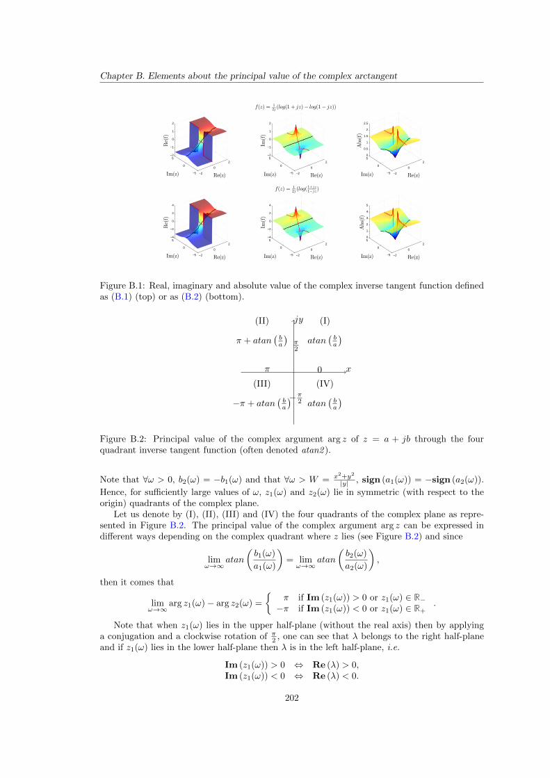
Chapter B. Elements about the principal value of the complex arctangent
−2
0
2
−5
0
5−2
−1
0
1
2
Re(z)Im(z)
Re(f)
−2
0
2
−5
0
5−2
−1
0
1
2
Re(z)
f(z) = 12j (log(1 + jz)− log(1− jz))
Im(z)
Im(f)
−2
0
2
−5
0
50
0.5
1
1.5
2
2.5
Re(z)Im(z)
Abs(f)
−2
0
2
−5
0
5−4
−2
0
2
4
Re(z)Im(z)
Re(f)
−2
0
2
−5
0
5−4
−2
0
2
4
Re(z)
f(z) = 12j (log(
1+jz
1−jz)
Im(z)Im
(f)
−2
0
2
−5
0
50
1
2
3
4
5
Re(z)Im(z)
Abs(f)
Figure B.1: Real, imaginary and absolute value of the complex inverse tangent function definedas (B.1) (top) or as (B.2) (bottom).
x
jy
atan(ba
)
−π + atan(ba
)atan
(ba
)
π + atan(ba
) (I)(II)
(III) (IV)
0
π2
π
−π2
Figure B.2: Principal value of the complex argument arg z of z = a + jb through the fourquadrant inverse tangent function (often denoted atan2 ).
Note that ∀ω > 0, b2(ω) = −b1(ω) and that ∀ω > W = x2+y2
|y| , sign (a1(ω)) = −sign (a2(ω)).
Hence, for sufficiently large values of ω, z1(ω) and z2(ω) lie in symmetric (with respect to theorigin) quadrants of the complex plane.
Let us denote by (I), (II), (III) and (IV) the four quadrants of the complex plane as repre-sented in Figure B.2. The principal value of the complex argument arg z can be expressed indifferent ways depending on the complex quadrant where z lies (see Figure B.2) and since
limω→∞
atan
(b1(ω)
a1(ω)
)= limω→∞
atan
(b2(ω)
a2(ω)
),
then it comes that
limω→∞
arg z1(ω)− arg z2(ω) =
π if Im (z1(ω)) > 0 or z1(ω) ∈ R−−π if Im (z1(ω)) < 0 or z1(ω) ∈ R+
.
Note that when z1(ω) lies in the upper half-plane (without the real axis) then by applyinga conjugation and a clockwise rotation of π
2 , one can see that λ belongs to the right half-planeand if z1(ω) lies in the lower half-plane then λ is in the left half-plane, i.e.
Im (z1(ω)) > 0 ⇔ Re (λ) > 0,Im (z1(ω)) < 0 ⇔ Re (λ) < 0.
202
B.2. Limit of atan(ωλ
)as ω tends towards infinity
Thus
limω→∞
atan(ωλ
)=
π2 if Re (λ) > 0−π2 if Re (λ) < 0
To determine the limits on the imaginary axis, let us assume that λ = jγ with γ ∈ R, then
arg z1(ω)− arg z2(ω) = arg(1 +ω
γ)− arg(1− ω
γ),
which tends towards −π is γ > 0 and to π if γ < 0 as ω tends towards ∞. Finally, the limits ofatan(ωλ ) are given by
limω→∞
atan(ωλ
)=
−π2 if Re (λ) < 0π2 if Re (λ) > 0π2 if Re (λ) = 0 and Im (λ) < 0−π2 if Re (λ) = 0 and Im (λ) > 0
which is coherent with the limits of acot(z) = atan( 1z ) derived in [Haber, 2012].
203

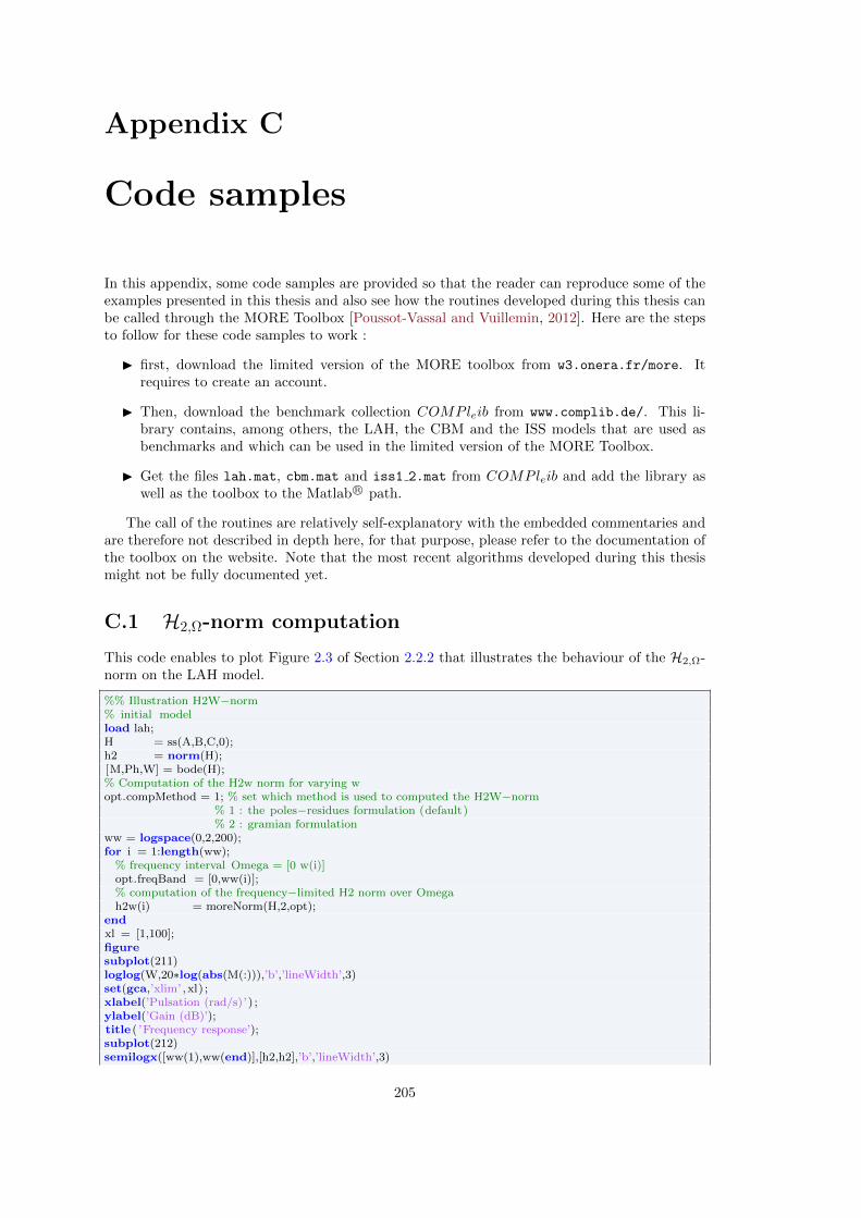
Appendix C
Code samples
In this appendix, some code samples are provided so that the reader can reproduce some of theexamples presented in this thesis and also see how the routines developed during this thesis canbe called through the MORE Toolbox [Poussot-Vassal and Vuillemin, 2012]. Here are the stepsto follow for these code samples to work :
I first, download the limited version of the MORE toolbox from w3.onera.fr/more. Itrequires to create an account.
I Then, download the benchmark collection COMPleib from www.complib.de/. This li-brary contains, among others, the LAH, the CBM and the ISS models that are used asbenchmarks and which can be used in the limited version of the MORE Toolbox.
I Get the files lah.mat, cbm.mat and iss1 2.mat from COMPleib and add the library aswell as the toolbox to the Matlab R© path.
The call of the routines are relatively self-explanatory with the embedded commentaries andare therefore not described in depth here, for that purpose, please refer to the documentation ofthe toolbox on the website. Note that the most recent algorithms developed during this thesismight not be fully documented yet.
C.1 H2,Ω-norm computation
This code enables to plot Figure 2.3 of Section 2.2.2 that illustrates the behaviour of the H2,Ω-norm on the LAH model.
%% Illustration H2W−norm% initial modelload lah;H = ss(A,B,C,0);h2 = norm(H);[M,Ph,W] = bode(H);% Computation of the H2w norm for varying wopt.compMethod = 1; % set which method is used to computed the H2W−norm
% 1 : the poles−residues formulation (default)% 2 : gramian formulation
ww = logspace(0,2,200);for i = 1:length(ww);
% frequency interval Omega = [0 w(i)]opt.freqBand = [0,ww(i)];% computation of the frequency−limited H2 norm over Omegah2w(i) = moreNorm(H,2,opt);
endxl = [1,100];figuresubplot(211)loglog(W,20∗log(abs(M(:))),’b’,’lineWidth’,3)set(gca,’xlim’ , xl) ;xlabel(’Pulsation (rad/s)’) ;ylabel(’Gain (dB)’);title ( ’Frequency response’);subplot(212)semilogx([ww(1),ww(end)],[h2,h2],’b’,’lineWidth’,3)
205

Chapter C. Code samples
hold onsemilogx(ww,h2w,’r−−’,’lineWidth’,3);set(gca,’xlim’ , xl) ;l = legend(’H 2−norm’,’H 2,\Omega−norm’);xlabel(’Pulsation (rad/s)’) ;ylabel(’Value of norms’)title ( ’Evolution of the H 2,\Omega−norm wrt to \omega’)
C.2 Example 11 : non-linearity of the optimal H2 approx-imation problem
This is the code that has been used to produce the figure of Example 11 aimed at illustratingthe non-linearity of the optimal H2 approximation problem
%% Illustration of the non−convexity of the optimal H2 approximation pb.% load large−scale modelload lah;H = ss(A,B,C,0);normH = norm(H);% real and imaginary parts of the reduced−order model polesrp = linspace(−3,−0.1,30);ip = linspace(1,40,40);% preallocatingerror = zeros(length(rp),length(ip));squaredNormHr = error;for i = 1:length(rp)
for j = 1:length(ip)% fix the poles of the reduced−order modelP(i, j) = complex(rp(i),ip(j)) ;p = P(i,j) ;% determine the associated optimal residuesM = [1/(−2∗p) , 1/(−2∗real(p));
1/(−2∗real(p)) , 1/(−2∗p’)];rhs = [freqresp(H,−p);
freqresp(H,−p’)];phi opt = M\rhs;phi = phi opt(1);% compute the H2 approximation errorsquaredNormHr(i,j) = −abs(phi)ˆ2/real(p)−real(phiˆ2/(p));error(i, j) = sqrt(normHˆ2−squaredNormHr(i,j));
endendsurf(real(P),imag(P),error/normH∗100)zlabel(’Relative H2 error’)xlabel(’Real part’)ylabel(’Im. part’)view(55,34)
C.3 Use of the FL-ISTIA
In this example, the LAH model is reduced to an order r = 10 over Ω = [10, 20] with theFL-ISTIA. The frequency responses of the large-scale model, the reduced order model and theerror model are plotted (see Figure C.1) and the relative H2,Ω-norm of the approximation errorcomputed.
%% Example FL−ISTIA%% Model and approximation parametersload lah;H = ss(A,B,C,0); % initial model
206
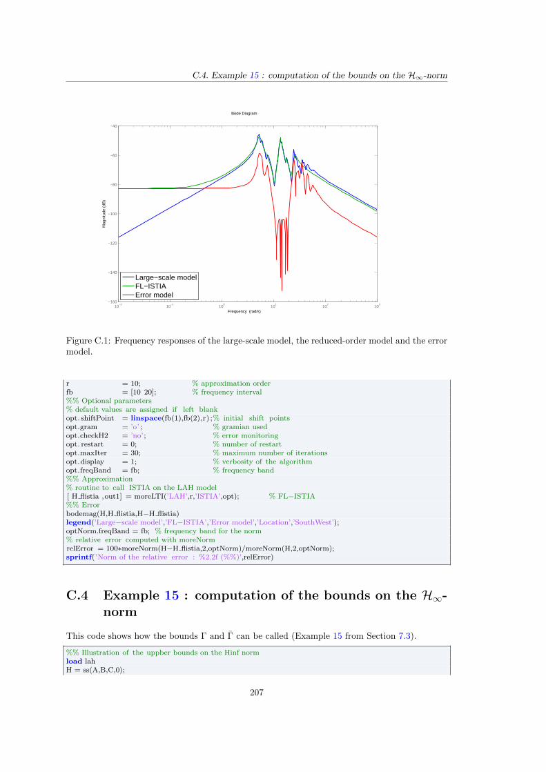
C.4. Example 15 : computation of the bounds on the H∞-norm
10−2
10−1
100
101
102
103
−160
−140
−120
−100
−80
−60
−40
Mag
nitu
de (
dB)
Bode Diagram
Frequency (rad/s)
Large−scale modelFL−ISTIAError model
Figure C.1: Frequency responses of the large-scale model, the reduced-order model and the errormodel.
r = 10; % approximation orderfb = [10 20]; % frequency interval%% Optional parameters% default values are assigned if left blankopt. shiftPoint = linspace(fb(1),fb(2),r) ;% initial shift pointsopt.gram = ’o’ ; % gramian usedopt.checkH2 = ’no’; % error monitoringopt. restart = 0; % number of restartopt.maxIter = 30; % maximum number of iterationsopt.display = 1; % verbosity of the algorithmopt.freqBand = fb; % frequency band%% Approximation% routine to call ISTIA on the LAH model[ H flistia ,out1] = moreLTI(’LAH’,r,’ISTIA’,opt); % FL−ISTIA%% Errorbodemag(H,H flistia,H−H flistia)legend(’Large−scale model’,’FL−ISTIA’,’Error model’,’Location’,’SouthWest’);optNorm.freqBand = fb; % frequency band for the norm% relative error computed with moreNormrelError = 100∗moreNorm(H−H flistia,2,optNorm)/moreNorm(H,2,optNorm);sprintf(’Norm of the relative error : %2.2f (%%)’,relError)
C.4 Example 15 : computation of the bounds on the H∞-norm
This code shows how the bounds Γ and Γ can be called (Example 15 from Section 7.3).
%% Illustration of the uppber bounds on the Hinf normload lahH = ss(A,B,C,0);
207
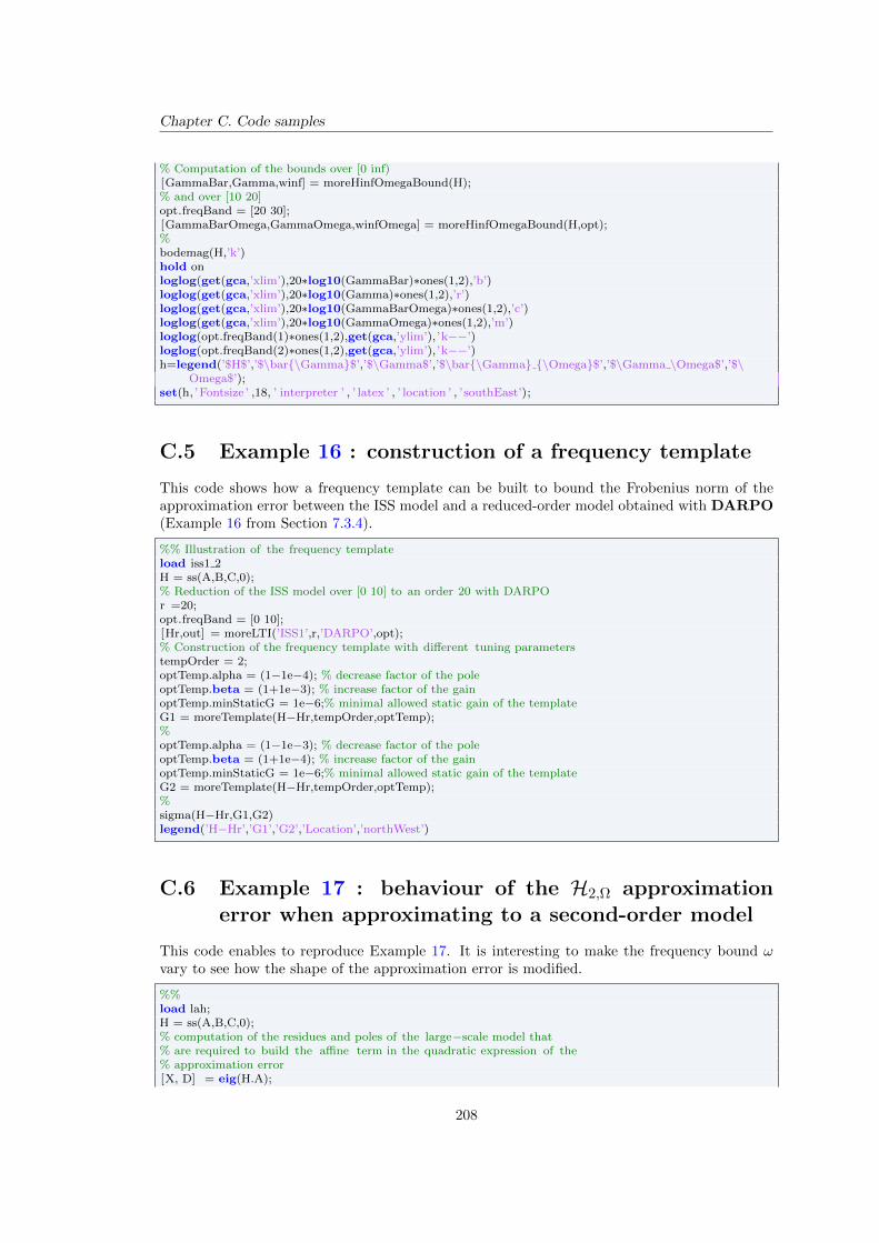
Chapter C. Code samples
% Computation of the bounds over [0 inf)[GammaBar,Gamma,winf] = moreHinfOmegaBound(H);% and over [10 20]opt.freqBand = [20 30];[GammaBarOmega,GammaOmega,winfOmega] = moreHinfOmegaBound(H,opt);%bodemag(H,’k’)hold onloglog(get(gca,’xlim’),20∗log10(GammaBar)∗ones(1,2),’b’)loglog(get(gca,’xlim’),20∗log10(Gamma)∗ones(1,2),’r’)loglog(get(gca,’xlim’),20∗log10(GammaBarOmega)∗ones(1,2),’c’)loglog(get(gca,’xlim’),20∗log10(GammaOmega)∗ones(1,2),’m’)loglog(opt.freqBand(1)∗ones(1,2),get(gca,’ylim’),’k−−’)loglog(opt.freqBand(2)∗ones(1,2),get(gca,’ylim’),’k−−’)h=legend(’$H$’,’$\bar\Gamma$’,’$\Gamma$’,’$\bar\Gamma \Omega$’,’$\Gamma \Omega$’,’$\
Omega$’);set(h, ’Fontsize ’ ,18, ’ interpreter ’ , ’ latex ’ , ’ location ’ , ’southEast’);
C.5 Example 16 : construction of a frequency template
This code shows how a frequency template can be built to bound the Frobenius norm of theapproximation error between the ISS model and a reduced-order model obtained with DARPO(Example 16 from Section 7.3.4).
%% Illustration of the frequency templateload iss1 2H = ss(A,B,C,0);% Reduction of the ISS model over [0 10] to an order 20 with DARPOr =20;opt.freqBand = [0 10];[Hr,out] = moreLTI(’ISS1’,r,’DARPO’,opt);% Construction of the frequency template with different tuning parameterstempOrder = 2;optTemp.alpha = (1−1e−4); % decrease factor of the poleoptTemp.beta = (1+1e−3); % increase factor of the gainoptTemp.minStaticG = 1e−6;% minimal allowed static gain of the templateG1 = moreTemplate(H−Hr,tempOrder,optTemp);%optTemp.alpha = (1−1e−3); % decrease factor of the poleoptTemp.beta = (1+1e−4); % increase factor of the gainoptTemp.minStaticG = 1e−6;% minimal allowed static gain of the templateG2 = moreTemplate(H−Hr,tempOrder,optTemp);%sigma(H−Hr,G1,G2)legend(’H−Hr’,’G1’,’G2’,’Location’,’northWest’)
C.6 Example 17 : behaviour of the H2,Ω approximationerror when approximating to a second-order model
This code enables to reproduce Example 17. It is interesting to make the frequency bound ωvary to see how the shape of the approximation error is modified.
%%load lah;H = ss(A,B,C,0);% computation of the residues and poles of the large−scale model that% are required to build the affine term in the quadratic expression of the% approximation error[X, D] = eig(H.A);
208
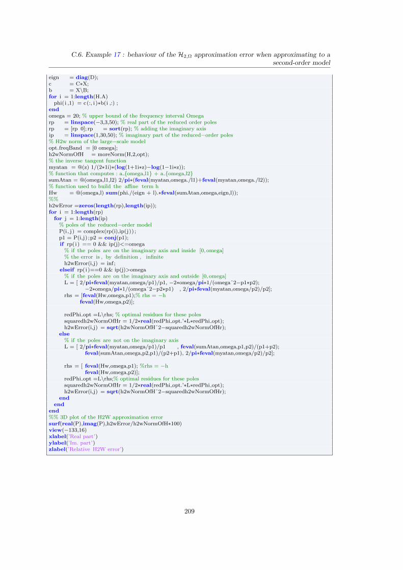
C.6. Example 17 : behaviour of the H2,Ω approximation error when approximating to asecond-order model
eign = diag(D);c = C∗X;b = X\B;for i = 1:length(H.A)
phi(i ,1) = c(:, i )∗b(i ,:) ;endomega = 20; % upper bound of the frequency interval Omegarp = linspace(−3,3,50); % real part of the reduced order polesrp = [rp 0]; rp = sort(rp); % adding the imaginary axisip = linspace(1,30,50); % imaginary part of the reduced−order poles% H2w norm of the large−scale modelopt.freqBand = [0 omega];h2wNormOfH = moreNorm(H,2,opt);% the inverse tangent functionmyatan = @(z) 1/(2∗1i)∗(log(1+1i∗z)−log(1−1i∗z));% function that computes : a omega,l1 + a omega,l2sumAtan = @(omega,l1,l2) 2/pi∗(feval(myatan,omega./l1)+feval(myatan,omega./l2));% function used to build the affine term hHw = @(omega,l) sum(phi./(eign + l).∗feval(sumAtan,omega,eign,l));%%h2wError =zeros(length(rp),length(ip));for i = 1:length(rp)
for j = 1:length(ip)% poles of the reduced−order modelP(i, j) = complex(rp(i),ip(j)) ;p1 = P(i,j) ;p2 = conj(p1);if rp(i ) == 0 && ip(j)<=omega
% if the poles are on the imaginary axis and inside [0, omega]% the error is , by definition , infiniteh2wError(i,j) = inf;
elseif rp(i )==0 && ip(j)>omega% if the poles are on the imaginary axis and outside [0, omega]L = [ 2/pi∗feval(myatan,omega/p1)/p1, −2∗omega/pi∗1/(omegaˆ2−p1∗p2);
−2∗omega/pi∗1/(omegaˆ2−p2∗p1) , 2/pi∗feval(myatan,omega/p2)/p2];rhs = [feval(Hw,omega,p1);% rhs = −h
feval(Hw,omega,p2)];
redPhi opt =L\rhs; % optimal residues for these polessquaredh2wNormOfHr = 1/2∗real(redPhi opt.’∗L∗redPhi opt);h2wError(i,j) = sqrt(h2wNormOfHˆ2−squaredh2wNormOfHr);
else% if the poles are not on the imaginary axisL = [ 2/pi∗feval(myatan,omega/p1)/p1 , feval(sumAtan,omega,p1,p2)/(p1+p2);
feval(sumAtan,omega,p2,p1)/(p2+p1), 2/pi∗feval(myatan,omega/p2)/p2];
rhs = [ feval(Hw,omega,p1); %rhs = −hfeval(Hw,omega,p2)];
redPhi opt =L\rhs;% optimal residues for these polessquaredh2wNormOfHr = 1/2∗real(redPhi opt.’∗L∗redPhi opt);h2wError(i,j) = sqrt(h2wNormOfHˆ2−squaredh2wNormOfHr);
endend
end%% 3D plot of the H2W approximation errorsurf(real(P),imag(P),h2wError/h2wNormOfH∗100)view(−133,16)xlabel(’Real part’)ylabel(’Im. part’)zlabel(’Relative H2W error’)
209
Chapter C. Code samples
C.7 Use of DARPO
In this example, the LAH model is reduced to an order r = 10 over Ω = [10, 20] with theDARPO (see Chapter 9) and the frequency responses of the models are plotted together withthe frequency response of the error.
%% Example FL−ISTIA%% Model and approximation parametersload lah;H = ss(A,B,C,0); % initial modelr = 10; % approximation orderfb = [10 20]; % frequency interval%% Optional parameters% default values are assigned if left blankopt.maxIter = 500; % maximum number of iterationsopt.display = 1; % verbosity of the algorithmopt.freqBand = fb; % frequency bandopt. tol = 1e−12; % tolerance%% Approximation% routine to call DARPO on the LAH model[H darpo,out1] = moreLTI(’LAH’,r,’DARPO’,opt);%% Errorbodemag(H,H darpo,H−H darpo)legend(’Large−scale model’,’DARPO’,’Error model’,’Location’,’SouthWest’);% relative error (in %) given by the algorithm directlyrelError = out1.h2wError(end);sprintf(’Norm of the relative error : %2.2f (%%)’,relError)
C.8 Use of DARPO for the control of a large-scale model
This code enables to reproduce the example presented in Section 9.2.3. Note that for conve-nience, the H∞ problems are solved with the method available in the Robust Control Toolboxof Matlab R©, but one could also have used HIFOO which is available at http://www.cs.nyu.
edu/overton/software/hifoo/.
clear all ;close all ;clc ;%% Illustration of the process for the control of large−scale model%% initial model and parametersload iss1 2H ol = ss(A,B,C,0);I3 = eye(3);Z3 = zeros(3,3);doLargeSynthesis = 0; % set to 1 to make the synthesis on the large−scale model%% P for the hinf control problemP large = ss(A,[B B],[C;C],0);%Xdb = 30;alpha = (10ˆ(Xdb/20))/norm(H ol,inf);% actuatorAct = tf(20∗20,[1 1.4∗20 20∗20])∗I3;% roll off filterwrl = 40;W = 1/(3∗alpha)∗tf([1/wrlˆ2 0 0],[1/(300∗wrl)ˆ2 1.4/(300∗wrl) 1])∗I3;% hinf control problem with actuatorP large act = P large∗append(I3,Act);% Static gain for the disturbance rejection on the large plant without% actuators :BF1 = alpha∗lft(P large,−alpha∗eye(3));% Static gain for the disturbance rejection on the large plant with% actuators :BFa1 = alpha∗lft(P large,−alpha∗eye(3)∗Act);
210
C.8. Use of DARPO for the control of a large-scale model
%% Control on the large plantif doLargeSynthesis == 1K6th1 = ltiblock . ss( ’K6 large’ ,6,3,3) ;%% LFR for the ’large’ Hinf problemCL large = alpha∗lft(P large act ,K6th1);t = cputime;[CL large opt,gamma large]=hinfstruct(blkdiag(CL large,W∗K6th1));dt large = cputime−t;K large = ss(CL large opt.blocks.K6 large);% Checks that the controller synthesised on the large plant% stabilises the large plantisstable ( lft (P large act ,K large))% satisfies the disturbance rejection on the large plantnorm(alpha∗lft(P large act,K large),Inf)end%% Control on the low order plant with uncertaintyK6th small = ltiblock . ss( ’K6 small’ ,6,3,3) ;%r = 30; % approximation orderopt.freqBand = [0 40]; % frequency interval of reductionHr = moreLTI(’ISS1’,r,’DARPO’,opt); % reduction of the large−scale modelHe = H ol−Hr; % approximation erroroptTemp.alpha = 1−1e−5; % decrease of the pole of the templateoptTemp.beta = 1+1e−4; % increase of the gain of the templateoptTemp.minStaticG = 1e−8; % minimal static gainG = moreTemplate(He,2,optTemp); % construction of the frequency templateG = G∗I3;%% Low order Hinf control problem%P small = ss(Hr.a,[Hr.b Hr.b ],[ Hr.c;Hr.c ],0) ;P small act = P small∗append(I3,Act);%P small2 = ss(Hr.a,[0∗Hr.b Hr.b],[0∗Hr.c;Hr.c ],[ Z3 I3;I3 Z3]);P small error act = append(G,I3)∗P small2∗append(I3,Act);% LFRs for the low−order Hinf problemCL small act = alpha∗lft(P small act,K6th small); % disturbance rejection on the
% low−order plantCL small error act = lft(P small error act ,K6th small); % robust stability channel%t = cputime;[CL small opt,gamma small,info] = hinfstruct(blkdiag(CL small act,CL small error act,W∗K6th small));dt small = cputime−t;K small = ss(CL small opt.blocks.K6 small);% Checks that the controller synthesised on the low−order plant% stabilises the large plantisstable ( lft (P large act ,K small))% satisfies the disturbance rejection on the large−plantnorm(alpha∗lft(P large act,K small),Inf)%% PLOTWF = sort([logspace(−1,2,400) linspace(30,100,100)]);[svBO1] = sigma(alpha∗H ol,WF);
% Open loop vs closed loop without actuatorfiguregreen = 1/256∗[97 186 26];[svBF1] = sigma(BF1,WF);p1 = semilogx(WF,20∗log10(svBO1),’b’);hold onp2 = semilogx(WF,20∗log10(svBF1),’color’,green);p3 = semilogx(get(gca,’xlim’),zeros(1,2),’k−−’);hh=legend([p1(1) p2(1) p3],’Normalised open−loop model $\alpha H$’,’Closed−loop model $\mathcalF l(
P,K 1)$’,’Disturbance rejection limit’);set(hh,’ interpreter ’ , ’ latex ’ ) ;xlabel(’Pulsation (rad/s)’) ;ylabel(’Singular values (dB)’);% Open loop vs closed loop with actuatorevBO1 = eig(H ol.A);K2 = −3∗alpha∗I3;
211
Chapter C. Code samples
BF2 = alpha∗lft(P large act,K2);evBF2= eig(BF2.A);
figuresubplot(121)[svBFa1] = sigma(BFa1,WF);p1 =semilogx(WF,20∗log10(svBO1),’b’);hold onp2 = semilogx(WF,20∗log10(svBFa1),’r’);set(gca,’xlim’ ,[ min(WF),max(WF)])p3 = semilogx(get(gca,’xlim’),zeros(1,2),’k−−’);hh=legend([p1(1),p2(1),p3(1)],’Normalised open−loop model $\alpha H$’,’Closed−loop model $\mathcalF l
ˆ(2)(P,K 1)$’,’Disturbance rejection limit’);set(hh,’ interpreter ’ , ’ latex ’ ) ;xlabel(’Pulsation (rad/s)’) ;ylabel(’Singular values (dB)’);subplot(122)plot(real(evBO1),imag(evBO1),’bx’);hold onplot(real(evBF2),imag(evBF2),’r.’);axis([−5 1 −1 60])plot(get(gca,’xlim’),[0 0], ’k’)plot([0 0],get(gca,’ylim’), ’k’)hh=legend(’Open−loop poles’,’Closed−loop poles’);set(hh,’ interpreter ’ , ’ latex ’ ) ;xlabel(’Real part’) ;ylabel(’Imaginary part’);
% Frequency template on the approximation errorWFe = logspace(−4,3,500);figuresvError = sigma(He,WFe);svG = sigma(G(1,1),WFe);p1 = semilogx(WFe,20∗log10(svError),’b’);hold onp2 = semilogx(WFe,20∗log10(svG),’color’,green);h = legend([p1(1),p2(1)],’Error model $H−\hatH$’,’Frequency template $G$’);set(h, ’Location’, ’NorthWest’,’interpreter ’ , ’ latex ’ ) ;xlabel(’Pulsation (rad/s)’) ;ylabel(’Singular values (dB)’);set(gca,’xlim’ ,[ min(WFe),max(WFe)])
% Final closed loopfiguresvBFr = sigma(alpha∗lft(P small act,K small),WF);svBFf = sigma(alpha∗lft(P large act,K small),WF);p1 = semilogx(WF,20∗log10(svBO1),’b’);hold onp2 = semilogx(WF,20∗log10(svBFr),’color’,green);p3 = semilogx(WF,20∗log10(svBFf),’r’);p4 = semilogx(get(gca,’xlim’),zeros(1,2),’k−−’);hh = legend([p1(1),p2(1),p3(1),p4(1)],’Normalised open−loop model $\alpha H$’,’Low−order closed−loop $\
mathcalF lˆ(2) (\hatP,K)$’,’Large−scale closed−loop $\mathcalF lˆ(2) (P,K)$’,’Disturbancerejection limit’);
set(hh,’ interpreter ’ , ’ latex ’ ) ;xlabel(’Pulsation (rad/s)’) ;ylabel(’Singular values (dB)’);
% Controller dynamicfigureWF2 = logspace(1,5,200);
[svW] =sigma(1/W,WF2);[svK] = sigma(K small,WF2);p1 = semilogx(WF2,20∗log10(svW),’b’);hold onp2 = semilogx(WF2,20∗log10(svK),’color’,green);hh=legend([p1(1),p2(1)],’$Wˆ−1$’,’$K$’);set(hh,’ interpreter ’ , ’ latex ’ ) ;xlabel(’Pulsation (rad/s)’) ;ylabel(’Singular values (dB)’);
212
C.9. Use of DARPO for the approximation at a fixed error
C.9 Use of DARPO for the approximation at a fixed error
This code illustrates how DARPO can be used to approximate a model at a given relative H2,Ω
error instead of a given approximation order r (see Section 11.5.3).
%% Illustration of the use of DARPO at fixed approximation error% Initial modelload lahH = ss(A,B,C,0);% Model approximationopt.freqBand = [0 20]; % frequency intervalopt.h2wError = 5; % Desired relative H2w approximation error (in %)% The order r must be left blank when calling the routine[Hr,out] = moreLTI(’LAH’,[],’DARPO’,opt);%figuresemilogy([1:length(out.h2wError)],out.h2wError)hold onsemilogy(get(gca,’xlim’),5∗[1 1],’r−’)yl = get(gca,’ylim’);for i = 1:length(out.rIncreased)
semilogy(out.rIncreased(i)∗[1 1], yl , ’k−−’);endlegend(’Approximation error’,’Desired relative H2W error’,’Reduced order increase’);xlabel(’Iteration ’ ) ;ylabel(’Relative error ’ ) ;figurebodemag(H,’k’,Hr,’r−−’,H−Hr,’b−.’)legend(’H’,’Hr’, ’H−Hr’);
213

Bibliography
Abramowitz, M. and Stegun, I. (1964). Hanbook of mathematical functions with formulas, graphsand mathematical tables. US Government Printing Office.
Al-Mohy, A., Higham, N., and Relton, S. (2013). Computing the Frechet derivative of the matrixlogarithm and estimating the condition number. SIAM Journal on Scientific Computing,35(4):C394 – C410.
Anderson, M. R., Emami-Naeni, A., and Vincent, J. (1991). Measures of merit for multivariableflight control. Technical report, Systems Control Technology Inc, Palo Alto, California, USA.
Anic, B., Beattie, C., Gugercin, S., and Antoulas, A. (2013). Interpolatory weighted-H2 modelreduction. Automatica, 49(5):1275 – 1280.
Antoulas, A. (2005). Approximation of large-scale dynamical systems. SIAM.
Antoulas, A., Ionita, A., and Lefteriu, S. (2012). On two-variable rational interpolation. LinearAlgebra and its Applications, 436(8):2889 – 2915. Special Issue dedicated to Danny Sorensen’s65th birthday.
Apkarian, P. and Noll, D. (2006). Nonsmooth H∞ synthesis. IEE Transactions on AutomaticControl, 51(1):71 – 86.
Badıa, J., Benner, P., Mayo, R., and Quintana-Ortı, E. (2006). Parallel algorithms for balancedtruncation model reduction of sparse systems. In Dongarra, J., Madsen, K., and Wasniewski,J., editors, Applied Parallel Computing. State of the Art in Scientific Computing, volume 3732of Lecture Notes in Computer Science, pages 267 – 275. Springer.
Balakrishnan, A. (1996). Robust stabilizing compensators for flexible structures with collocatedcontrols. Applied Mathematics and Optimization, 33(1):35 – 60.
Baratchart, L. (1986). Existence and generic properties of L2 approximants for linear systems.IMA Journal of Mathematical Control and Information, 3(2-3):89 – 101.
Baratchart, L., Cardelli, M., and Olivi, M. (1991). Identification and rational L2 approximation: A gradient algorithm. Automatica, 27(2):413 – 417.
Beattie, C. and Gugercin, S. (2007). Krylov-based minimization for optimal H2 model reduction.In Proceedings of the Conference on Decision and Control, pages 4385 – 4390.
Beattie, C. and Gugercin, S. (2009). A trust region method for optimal H2 model reduction. Inproceedings of the Joint Conference on Decision and Control and Chinese Control Conference,pages 5370 – 5375.
Beattie, C. and Gugercin, S. (2012). Realization-independent H2 approximation. In Proceedingsof the Conference on Decision and Control, pages 4953 – 4958.
Bemporad, A. and Morari, M. (1999). Robust model predictive control: A survey. In Garulli,A. and Tesi, A., editors, Robustness in identification and control, volume 245 of Lecture Notesin Control and Information Sciences, pages 207 – 226. Springer.
Benner, P. and Breiten, T. (2012). Krylov-subspace based model reduction of nonlinear circuitmodels using bilinear and quadratic-linear approximations. In Gunther, M., Bartel, A., Brunk,M., Schops, S., and Striebel, M., editors, Progress in Industrial Mathematics at ECMI 2010,Mathematics in Industry, pages 153 – 159. Springer.
215
BIBLIOGRAPHY
Benner, P., Claver, J., and Quintana-Ortı, E. (1999). Parallel distributed solvers for large stablegeneralized Lyapunov equations. Parallel Processing Letters, 9(01):147 – 158.
Benner, P., Mehrmann, V., and Sorensen, D. (2005). Dimension reduction of large-scale systems,volume 45. Springer.
Benner, P., Quintana-Ortı, E., and Quintana-Ortı, G. (2000). Balanced truncation model reduc-tion of large-scale dense systems on parallel computers. Mathematical and Computer Modellingof Dynamical Systems, 6(4):383 – 405.
Biannic, J. and Ferreres, G. (2005). Efficient computation of a guaranteed robustness margin.In Proceedings of the IFAC World Congress.
Blondel, V. and Megretski, A., editors (2004). Unsolved problems in mathematical systems andcontrol theory. Princeton University Press.
Brandwood, D. (1983). A complex gradient operator and its application in adaptive array theory.In Proceedings of the Conference on Communications, Radar and Signal Processing, volume130, pages 11 – 16.
Breiten, T., Beattie, C., and Gugercin, S. (2014). Near-optimal frequency-weighted interpolatorymodel reduction. Available as arXiv:1309.0136.
Bugarin, F., Henrion, D., and Lasserre, J. (2011). Minimizing the sum of many rational functions.Available as arXiv:1102.49544.
Burke, J., Henrion, D., Lewis, A., and Overton, M. (2006). HIFOO-a Matlab package for fixed-order controller design and H∞ optimization. In Proceedings of the IFAC Symposium onRobust Control Design.
Burlion, L., Poussot-Vassal, C., Vuillemin, P., Leitner, M., and Kier, T. (2014). Longitudinalmanoeuvre load control of a flexible large-scale aircraft. In Proceedings of the IFAC WorldCongress, pages 3413 – 3418.
Chahlaoui, Y., Lemonnier, D., Vandendorpe, A., and Van Dooren, P. (2006). Second-orderbalanced truncation. Linear Algebra and its Applications, 415(2–3):373 – 384. Special issueon order reduction of large-scale systems.
Corless, R. M., Jeffrey, D. J., Watt, S. M., and Davenport, J. H. (2000). ”According toAbramowitz and Stegun” or arccoth needn’t be uncouth. ACM SIGSAM Bulletin, 34:58– 65.
de Villemagne, C. and Skelton, R. (1987). Model reductions using a projection formulation. InProceeding of the Conference on Decision and Control, volume 26, pages 461 – 466.
Demourant, F. (2013). New algorithmic approach based on integral quadratic constraints forstability analysis of high order models. In Proceedings of the European Control Conference,pages 359 – 364.
Dergham, G., Sipp, D., Robinet, J.-C., and Barbagallo, A. (2011). Model reduction for fluidsusing frequential snapshots. Physics of Fluids, 23(6).
Enns, D. (1984). Model reduction with balanced realizations: An error bound and a frequencyweighted generalization. In Proceedings of the Conference on Decision and Control, pages 127– 132.
Ferreres, G. (2011). Computation of a flexible aircraft LPV/LFT model using interpolation.IEEE Transactions on Control Systems Technology, 19(1):132 – 139.
216

BIBLIOGRAPHY
Flagg, G., Beattie, C., and Gugercin, C. (2012). Convergence of the iterative rational Krylovalgorithm. Systems & Control Letters, 61(6):688 – 691.
Flagg, G., Beattie, C., and Gugercin, S. (2013). Interpolatory H∞ model reduction. Systems &Control Letters, 62(7):567 – 574.
Fletcher, R. (2000). Practical methods of optimization. John Wiley & Sons.
Fuhrmann, P. (1994). A duality theory for robust stabilization and model reduction. LinearAlgebra and its Applications, 203-204(0):471 – 578.
Fulcheri, P. and Olivi, M. (1998). Matrix rational H2 approximation: A gradient algorithmbased on Schur analysis. SIAM Journal on Control and Optimization, 36(6):2103 – 2127.
Gadient, R., Lavrtsky, E., and Wise, K. (2012). Very flexible aircraft control challenge problem.In Proceedings of the AIAA guidance, Navigation and Control Conference.
Gallivan, K., Vandendorpe, A., and Van Dooren, P. (2004a). Model reduction of MIMO systemsvia tangential interpolation. SIAM Journal on Matrix Analysis and Applications, 26(2):328 –349.
Gallivan, K., Vandendorpe, A., and Van Dooren, P. (2004b). Sylvester equations and projection-based model reduction. Journal of Computational and Applied Mathematics, 162(1):213 – 229.
Garulli, A., Hansson, A., Pakazad, S., Masi, A., and Wallin, R. (2013). Robust finite-frequencyanalysis of uncertain systems with application to flight comfort analysis. Control EngineeringPractice, 21(6):887 – 897.
Gawronski, W. (2004). Advanced structural dynamics and active control of structures. Springer.
Gawronski, W. and Juang, J. (1990). Model reduction in limited time and frequency intervals.International Journal of Systems Science, 21(2):349 – 376.
Glover, K. (1984). All optimal Hankel-norm approximations of linear multivariable systems andtheir L∞-error bounds. International Journal of Control, 39(6):1115 – 1193.
Grigoriadis, K. (1995). Optimal H∞ model reduction via linear matrix inequalities: continuous-and discrete-time cases. Systems & Control Letters, 26(5):321 – 333.
Grimme, E. (1997). Krylov projection methods for model reduction. PhD thesis, University ofIllinois at Ubarna-Champaign.
Gugercin, S. (2007). An iterative SVD-Krylov based method for model reduction of large-scaledynamical systems. Linear Algebra and its Applications, 428(8-9):1964 – 1986.
Gugercin, S. and Antoulas, A. (2004). A survey of model reduction by balanced truncation andsome new results. International Journal of Control, 77(8):748 – 766.
Gugercin, S., Antoulas, A., and Beattie, C. (2006). A rational Krylov iteration for optimal H2
model reduction. In Proceedings of the International Symposium on Mathematical Theory ofNetworks and Systems, pages 1665 – 1667.
Gugercin, S., Antoulas, A., and Beattie, C. (2008). H2 model reduction for large-scale lineardynamical systems. SIAM Journal on Matrix Analysis and Applications, 30(2):609 – 638.
Gugercin, S. and Li, J. (2005). Smith-type methods for balanced truncation of large sparsesystems. In Benner, P., Sorensen, D., and Mehrmann, V., editors, Dimension reduction oflarge-scale systems, volume 45 of Lecture Notes in Computational Science and Engineering,pages 49 – 82. Springer.
217
BIBLIOGRAPHY
Gugercin, S., Stykel, T., and Wyatt, S. (2013). Model reduction of descriptor systems byinterpolatory projection methods. Available as arXiv:1301.4524.
Gumussoy, S., Henrion, D., Millstone, M., and Overton, M. (2009). Multiobjective robust controlwith HIFOO 2.0. In Proceedings of the 6th IFAC symposium on robust control design.
Haber, H. (2012). The complex inverse trigonometric and hyperbolic functions. http://scipp.ucsc.edu/~haber/webpage/arc.pdf. University of California.
Hammarling, S. (1982). Numerical solution of the stable, non-negative definite Lyapunov equa-tion. IMA Journal of Numerical Analysis, 2(3):303 – 323.
Heath, M., Laub, A., Paige, C., and Ward, R. (1986). Computing the singular value decompo-sition of a product of two matrices. SIAM Journal on Scientific and Statistical Computing,7(4):1147 – 1159.
Hesse, H. and Palacios, R. (2014). Reduced-order aeroelastic models for dynamics of maneuveringflexible aircraft. AIAA Journal, 52(8):1717 – 1732.
Higham, N. (2008). Functions of matrices : Theory and computation. SIAM.
Himpe, C. (2014). emgr - Empirical Gramian Framework. http://gramian.de.
Hyland, D. and Bernstein, D. (1985). The optimal projection equations for model reduction andthe relationships among the methods of Wilson, Skelton, and Moore. IEEE Transactions onAutomatic Control, 30(12):1201 – 1211.
Ionita, A. (2013). Lagrange rational interpolation and its application to approximation of large-scale dynamical systems. PhD thesis, Rice University.
Kahan, W. (1987). Branch cuts for complex elementary functions, or much ado about noth-ing’s sign bit. In Proceedings of the Joint IMA/SIAM Conference on the State of the Art inNumerical Analysis, pages 165 – 211.
Kim, S., Anderson, B., and Madievski, A. (1995). Error bound for transfer function orderreduction using freqeuncy weighted balanced truncation. Systems & Control Letters, 24(3):183– 192.
Kokotovic, P., Khalil, H., and O’Reilly, J. (1986). Singular perturbation methods in control:analysis and design. SIAM.
Korvink, J. and Rudnyi, E. (2005). Oberwolfach benchmark collection. In Benner, P., Sorensen,D., and Mehrmann, V., editors, Dimension reduction of large-scale systems, volume 45 ofLecture Notes in Computational Science and Engineering, pages 311 – 315. Springer.
Krajewski, W., Lepschy, A., Redivo-Zaglia, M., and Viaro, U. (1995). A program for solvingthe L2 reduced-order model problem with fixed denominator degree. Numerical Algorithms,9(2):355 – 377.
Kreutz-Delgado, K. (2009). The complex gradient operator and the CR-calculus. Available asarXiv:0906.4835.
Laub, A., Heath, M., Paige, C., and Ward, R. (1987). Computation of system balancing transfor-mations and other applications of simultaneous diagonalization algorithms. IEEE Transactionson Automatic Control, 32(2):115 – 122.
Leblond, J. and Olivi, M. (1998). WeightedH2 approximation of transfer functions. Mathematicsof Control, Signals and Systems, 11(1):28 – 39.
218
BIBLIOGRAPHY
Leibfritz, F. and Lipinski, W. (2003). Description of the benchmark examples in COMP leib 1.0.Technical report, University of Trier.
Li, D. and Fukushima, M. (2001). On the global convergence of the BFGS method for nonconvexunconstrained optimization problems. SIAM Journal on Optimization, 11(4):1054 – 1064.
Li, J. and Kamon, M. (2005). PEEC model of a spiral inductor generated by Fasthenry. InBenner, P., Sorensen, D., and Mehrmann, V., editors, Dimension reduction of large-scalesystems, volume 45 of Lecture Notes in Computational Science and Engineering, pages 373 –377. Springer Berlin Heidelberg.
Li, J. and White, J. (2002). Low rank solution of Lyapunov equations. SIAM Journal on MatrixAnalysis and Applications, 24(1):260 – 280.
Lienemann, J., Rudnyi, E., and Korvink, J. (2006). MST MEMS model order reduction: Re-quirements and benchmarks. Linear Algebra and its Applications, 415(2–3):469 – 498. Specialissue on order reduction of large-scale systems.
Lin, C.-A. and Chiu, T.-Y. (1990). Model reduction via frequency weighted balanced realization.In American Control Conference, pages 2069 – 2070.
Liu, Y. and Anderson, B. D. (1989). Singular perturbation approximation of balanced systems.In Proceedings of the Conference On Decision and Control, pages 1355 – 1360.
Magni, J. (2006). Linear fractional representation toolbox for use with Matlab. Available athttp://w3.onera.fr/smac/.
Mallik, R. (2001). The inverse of a tridiagonal matrix. Linear Algebra and its Applications,325(1-3):109 – 139.
Marmorat, J. and Olivi, M. (2002). The rarl2 software: Realizations and rational approximationin L2-norm. http://www-sop.inria.fr/apics/RARL2/rarl2.html. Project APICS, INRIA,Sophia Antipolis.
Marmorat, J.-P., Olivi, M., Hanzon, B., and Peeters, R. (2002). Matrix rational H2 approxi-mation: A state-space approach using Schur parameters. In Proceedings of the Conference onDecision and Control, volume 4, pages 4244 – 4249.
Mayo, A. and Antoulas, A. (2007). A framework for the solution of the generalized realizationproblem. Linear Algebra and its Applications, 425(2–3):634 – 662. Special Issue in honor ofPaul Fuhrmann.
Megretski, A. and Rantzer, A. (1997). System analysis via integral quadratic constraints. IEEETransactions on Automatic Control, 42(6):819 – 830.
Mehrmann, V. and Stykel, T. (2005). Balanced truncation model reduction for large-scale sys-tems in descriptor form. In Benner, P., Sorensen, D., and Mehrmann, V., editors, DimensionReduction of Large-Scale Systems, volume 45 of Lecture Notes in Computational Science andEngineering, pages 83–115.
Meier, L. and Luenberger, D. (1967). Approximation of linear constant systems. IEEE Trans-actions on Automatic Control, 12(5):585 – 588.
Moler, C. and Van Loan, C. (1978). Nineteen dubious ways to compute the exponential of amatrix. SIAM Review, 20:801 – 836.
Moore, B. (1981). Principal component analysis in linear systems: controllability, observability,and model reduction. IEEE Transactions on Automatic Control, 26(1):17 – 32.
219
BIBLIOGRAPHY
Nocedal, J. and Wright, S. (1999). Numerical optimization. Springer.
Nocedal, J. and Yuan, Y. (1998). Combining trust region and line search techniques.
Ostrowski, A. and Schneider, H. (1962). Some theorems on the inertia of general matrices.Journal of Mathematical Analysis and Applications, pages 72 – 84.
Panzer, H., Hubele, J., Eid, R., and Lohmann, B. (2009). Generating a parametric finite ele-ment model of a 3d cantilever timoshenko beam using Matlab. Technical report, TechnischeUniversitat Munchen.
Penzl, T. (1999). A cyclic low-rank Smith method for large sparse Lyapunov equations. SIAMJournal on Scientific Computing, 21(4):1401 – 1418.
Pernebo, L. and Silverman, L. (1982). Model reduction via balanced state space representations.IEEE Transactions on Automatic Control, 27(2):382 – 387.
Petersson, D. (2013). A nonlinear optimization approach to H2-optimal modeling and control.PhD thesis, Linkoping University.
Petersson, D. and Lofberg, J. (2014). Model reduction using a frequency-limitedH2-cost. Systems& Control Letters, 67(0):32 – 39.
Poussot-Vassal, C. (2011). An iterative SVD-tangential interpolation method for medium-scaleMIMO systems approximation with application on flexible aircraft. In Proceedings of theConference on Decision and Control and European Control Conference, pages 7117 – 7122.
Poussot-Vassal, C., Loquen, T., Vuillemin, P., Cantinaud, O., and Lacoste, J. (2013). Businessjet large-scale model approximation and vibration control. In Proceedings of the IFAC In-ternational Workshop on Adaptation Learning in Control and Signal Processing, pages 199 –204.
Poussot-Vassal, C. and Roos, C. (2012). Generation of a reduced-order LPV/LFT model from aset of large-scale MIMO LTI flexible aircraft models. Control Engineering Practice, 20(9):919– 930.
Poussot-Vassal, C., Ross, C., Vuillemin, P., Cantinaud, O., and Lacoste, J. (2014). Control-oriented aeroelastic bizjet low-order LFT modeling. In Control-oriented modeling and identi-fication : theory and practice. The Institution of Engineering and Technology. To appear.
Poussot-Vassal, C. and Vuillemin, P. (2012). Introduction to MORE: a MOdel REduction Tool-box. In Proceedings of the Multi-conference on Systems and Control, pages 776 – 781.
Poussot-Vassal, C. and Vuillemin, P. (2013). An iterative eigenvector tangential interpolationalgorithm for large-scale LTI and a class of LPV model approximation. In Proceedings of theEuropean Control Conference, pages 4490 – 4495.
Remmert, R. (1991). Theory of complex functions, volume 122. Springer.
Rommes, J. and Martins, N. (2006). Efficient computation of multivariable transfer functiondominant poles using subspace acceleration. IEEE Transactions on Power Systems, 21:1471– 1483.
Roos, C., Lescher, F., Biannic, J., Doll, C., and Ferreres, G. (2011). A set of µ-analysis basedtools to evaluate the robustness properties of high-dimensional uncertain systems. In Proceed-ings of the Multiconference on Systems and Control, pages 644 – 649.
Ruhe, A. (1994). Rational Krylov algorithms for nonsymmetric eigenvalue problems. II. matrixpairs. Linear Algebra and its Applications, 197-198(0):283 – 295.
220
BIBLIOGRAPHY
Saad, Y. (2003). Iterative methods for sparse linear systems. SIAM, 2nd edition.
Scherer, C., Gahinet, P., and Chilali, M. (1997). Multiobjective output-feedback control via LMIoptimization. IEEE Transactions on Automatic Control, 42(7):896 – 911.
Shaker, H. and Tahavori, M. (2014). Frequency-interval model reduction of bilinear systems.IEEE Transactions on Automatic Control, 59(7):1948 – 1953.
Sideris, A. and Sanchez Pena, R. (1990). Robustness margin calculation with dynamic and realparametric uncertainty. IEEE Transactions on Automatic Control, 35(8):970 – 974.
Sootla, A. (2011). Nu-gap model reduction in the frequency domain. In American ControlConference, pages 5025 – 5030.
Sorber, L., Van Barel, M., and De Lathauwer, L. (2012). Unconstrained optimization of realfunctions in complex variables. SIAM Journal on Optimization, 22(3):879 – 898.
Sorber, L., Van Barel, M., and De Lathauwer, L. (2013). Complex optimization toolbox v1.0.http://esat.kuleuven.be/stadius/cot/.
Sorensen, D. (1997). Implicitly restarted Arnoldi/Lanczos methods for large scale eigenvaluecalculations. In Keyes, D., Sameh, A., and Venkatakrishnan, V., editors, Parallel NumericalAlgorithms, volume 4 of ICASE/LaRC Interdisciplinary Series in Science and Engineering,pages 119 – 165. Springer.
Sorensen, D. and Antoulas, A. (2002). The Sylvester equation and approximate balanced re-duction. Linear Algebra and its Applications, 351–352(0):671 – 700. Fourth Special Issue onLinear Systems and Control.
Stykel, T. and Simoncini, V. (2012). Krylov subspace methods for projected Lyapunov equations.Applied Numerical Mathematics, 62(1):35 – 50.
Unbehauen, H. and Rao, G. (1990). Continuous-time approaches to system identification - asurvey. Automatica, 26(1):23 – 35.
Van Den Bos, A. (1994). Complex gradient and hessian. volume 141, pages 380 – 383.
Van Dooren, P., Gallivan, K., and Absil, P. (2008a). H2 optimal approximation of MIMO lineardynamical systems. Available as arXiv:0807.4807.
Van Dooren, P., Gallivan, K., and Absil, P. (2008b). H2-optimal model reduction of MIMOsystems. Applied Mathematics Letters, 21(12):1267 – 1273.
Van Dooren, P., Gallivan, K., and Absil, P. (2010). H2-optimal model reduction with higher-order poles. SIAM Journal on Matrix Analysis and Applications, 31(5):2738 – 2753.
Vayssettes, J., Mercere, G., Vacher, P., and De Callafon, R. (2014). Frequency-domain identifi-cation of aircraft structural modes from short-duration flight tests. International Journal ofControl, 87(7):1352 – 1372.
Vidyasagar, M. (1984). The graph metric for unstable plants and robustness estimates forfeedback stability. IEEE Transactions on Automatic Control, 29(5):403 – 418.
Vinnicombe, G. (1992). Measuring robustness of feedback systems. PhD thesis, University ofCambridge.
Vizer, D., Mercere, G., Prot, O., Laroche, E., and Lovera, M. (2013). Linear fractional LPVmodel identification from local experiments: An H∞-based optimization technique. In Pro-ceedings of the Conference on Decision and Control, pages 4559 – 4564.
221
BIBLIOGRAPHY
Vuillemin, P., Demourant, F., Biannic, J.-M., and Poussot-Vassal, C. (2014a). Global stabilityvalidation of an uncertain large-scale aircraft model. In Proceedings of the Multi-conferenceon Systems and Control.
Vuillemin, P., Poussot-Vassal, C., and Alazard, D. (2012a). Reduction de modele de grandedimension, application a un avion souple de transport civil. In Proceedings of the 7emeConference Internationale Francophone d’Automatique.
Vuillemin, P., Poussot-Vassal, C., and Alazard, D. (2012b). A spectral expression for thefrequency-limited H2-norm. Available as arXiv:1211.1858.
Vuillemin, P., Poussot-Vassal, C., and Alazard, D. (2013a). A frequency-limited H2 model ap-proximation method with application to a medium-scale flexible aircraft. In Chu, Q., Mulder,B., Choukroun, D., van Kampen, E., de Visser, C., and Looye, G., editors, Advances inAerospace Guidance, Navigation and Control, pages 569 – 583. Springer.
Vuillemin, P., Poussot-Vassal, C., and Alazard, D. (2013b). H2 optimal and frequency limitedapproximation methods for large-scale LTI dynamical systems. In Proceedings of the IFACSymposium on Systems Structure and Control, pages 719 – 724.
Vuillemin, P., Poussot-Vassal, C., and Alazard, D. (2014b). Poles residues descent algorithm foroptimal frequency-limited H2 model approximation. In Proceedings of the European ControlConference, pages 1080 – 1085.
Vuillemin, P., Poussot-Vassal, C., and Alazard, D. (2014c). Spectral expression for the frequency-limited H2-norm of LTI dynamical systems with high order poles. In Proceedings of theEuropean Control Conference, pages 55 – 60.
Vuillemin, P., Poussot-Vassal, C., and Alazard, D. (2014d). Two upper bounds on the H∞-normof LTI dynamical systems. In Proceedings of the IFAC World Congress, pages 5562 – 5567.
Wang, G., Sreeram, V., and Liu, W. Q. (1999). A new frequency-weighted balanced truncationmethod and an error bound. IEEE Transactions on Automatic Control, 44(9):1734 – 1737.
Wang, Y., Andrew, W., and Palacios, R. (2014). Nonlinear model reduction for aeroelasticcontrol of flexible aircraft described by large finite-element models. In Proceedings of theAIAA/ASMe/ASCE/AHS/SC Structures, Structural Dynamics, and Materials Conference.
Wilson, D. (1974). Model reduction for multivariable systems. International Journal of Control,20(1):57 – 64.
Wood, G., Goddard, P., and Glover, K. (1996). Approximation of linear parameter-varyingsystems. In Proceedings of the Conference on Decision and Control, pages 406 – 411.
Yan, W.-Y. and Lam, J. (1999). An approximate approach to H2 optimal model reduction.IEEE Transactions on Automatic Control, 44(7):1341 – 1358.
Yousuff, A., Wagie, D., and Skelton, R. (1985). Linear system approximation via covarianceequivalent realizations. Journal of Mathematical Analysis and Applications, 106(1):91 – 115.
Zhou, K. (1995). Frequency-weighted L∞ norm and optimal Hankel norm model reduction.IEEE Transactions on Automatic Control, 40(10):1687 – 1699.
Zhou, K., Doyle, J. C., and Glover, K. (1995). Robust and optimal control. Pentice Hall.
222


Frequency-limited model approximation of large-scale dynamical models
Abstract. Physical systems are represented by mathematical models in order to be simulated, analysed orcontrolled. Depending on the complexity of the physical system it is meant to represent and on the way it hasbeen built, a model can be more or less complex. This complexity can become an issue in practice due to thelimited computational power and memory of computers. One way to alleviate this issue consists in using modelapproximation which is aimed at finding a simpler model that still represents faithfully the physical system.In the case of Linear Time Invariant (LTI) dynamical models, complexity translates into a large dimension ofthe state vector and one talks about large-scale models. Model approximation is in this case also called modelreduction and consists in finding a model with a smaller state vector such that the input-to-output behaviours ofboth models are close with respect to some measure. The H2-norm has been extensively used in the literature toevaluate the quality of a reduced-order model. Yet, due to the limited bandwidth of actuators, sensors and thefact that models are generally representative on a bounded frequency interval only, a reduced-order model thatfaithfully reproduces the behaviour of the large-scale one over a bounded frequency interval only, may be morerelevant. That is why, in this study, the frequency-limited H2-norm, or H2,Ω-norm, which is the restriction of theH2-norm over a frequency interval Ω, has been considered. In particular, the problem of finding a reduced-ordermodel that minimises the H2,Ω-norm of the approximation error with the large-scale model has been addressedhere. For that purpose, two approaches have been developed. The first one is an empirical approach based on themodification of a sub-optimal H2 model approximation method. Its performances are interesting in practice andcompete with some well-known frequency-limited approximation methods. The second one is an optimisationmethod relying on the poles-residues formulation of the H2,Ω-norm. This formulation naturally extends the oneexisting for the H2-norm and can also be used to derive two upper bounds on the H∞-norm of LTI dynamicalmodels which is of particular interest in model reduction. The first-order optimality conditions of the optimalH2,Ω approximation problem are derived and used to built a complex-domain descent algorithm aimed at findinga local minimum of the problem. Together with the H∞ bounds on the approximation error, this approach isused to perform control of large-scale models. From a practical point of view, the methods proposed in thisstudy have been successfully applied in an industrial context as a part of the global process aimed at controllinga flexible civilian aircraft.
Keywords : linear time invariant models, large-scale models, model reduction, model approximation, frequency-limited model approximation
Approximation de modeles dynamiques de grande dimension sur intervalles de frequences limites
Resume. Les systemes physiques sont representes par des modeles mathematiques qui peuvent etre utilisespour simuler, analyser ou controler ces systemes. Selon la complexite du systeme qu’il est cense representer, unmodele peut etre plus ou moins complexe. Une complexite trop grande peut s’averer problematique en pratiquedu fait des limitations de puissance de calcul et de memoire des ordinateurs. L’une des facons de contournerce probleme consiste a utiliser l’approximation de modeles qui vise a remplacer le modele complexe par unmodele simplifie dont le comportement est toujours representatif de celui du systeme physique. Dans le cas desmodeles dynamiques Lineaires et Invariants dans le Temps (LTI), la complexite se traduit par une dimensionimportante du vecteur d’etat et on parle alors de modeles de grande dimension. L’approximation de modele,encore appelee reduction de modele dans ce cas, a pour but de trouver un modele dont le vecteur d’etat est pluspetit que celui du modele de grande dimension tel que les comportements entree-sortie des deux modeles soientproches selon une certaine norme. La norme H2 a ete largement consideree dans la litterature pour mesurer laqualite d’un modele reduit. Cependant, la bande passante limitee des capteurs et des actionneurs ainsi que lefait qu’un modele est generalement representatif d’un systeme physique dans une certaine bande frequentielleseulement, laissent penser qu’un modele reduit dont le comportement est fidele au modele de grande dimensiondans un intervalle de frequences donne, peut etre plus pertinent. C’est pourquoi, dans cette etude, la normeH2 limitee en frequence, ou norme H2,Ω, qui est simplement la restriction de la norme H2 sur un intervalle defrequences Ω, a ete consideree. En particulier, le probleme qui vise a trouver un modele reduit minimisant lanorme H2,Ω de l’erreur d’approximation avec le modele de grande dimension a ete traite. Deux approches ont eteproposees dans cette optique. La premiere est une approche empirique basee sur la modification d’une methodesous-optimale pour l’approximation H2. En pratique, ses performances s’averent interessantes et rivalisent aveccertaines methodes connues pour l’approximation de modeles sur intervalles de frequences limites. La seconde estune methode d’optimisation basee sur la formulation poles-residus de la norme H2,Ω. Cette formulation generalisenaturellement celle existante pour la norme H2 et permet egalement d’exprimer deux bornes superieures sur lanorme H∞ d’un modele LTI, ce qui est particulierement interessant dans le cadre de la reduction de modeles.Les conditions d’optimalite du premier ordre pour le probleme d’approximation optimale en norme H2,Ω ontete exprimees et utilisees pour creer un algorithme de descente visant a trouver un minimum local au problemed’approximation. Couplee aux bornes sur la norme H∞ de l’erreur d’approximation, cette methode est utiliseepour le controle de modeles de grande dimension. D’un point de vue plus pratique, l’ensemble des methodesproposees dans cette etude ont ete appliquees, avec succes, dans un cadre industriel comme element d’un processusglobal visant a controler un avion civil flexible.
Mots-cles : modeles lineaires invariants dans le temps, modeles de grande dimension, reduction de modeles,approximation de modeles, approximation de modeles sur intervalles de frequences limites

et discipline ou spécialité
Jury :
le
Institut Supérieur de l’Aéronautique et de l’Espace (ISAE)
Pierre VUILLEMIN
lundi 24 novembre 2014
Approximation de modèles dynamiques de grande dimension surintervalles de fréquences limités
EDSYS : Automatique
Équipe d'accueil ISAE-ONERA CSDV
MmeMartine OLIVI, Chargée de Recherche INRIA - RapporteurM. Serkan GUGERCIN, Professeur Virginia Tech - Rapporteur
M. Didier HENRION, Directeur de Recherche CNRS - ExaminateurM. Michel ZASADZINSKI, Professeur Université de Lorraine - Examinateur
M. Daniel ALAZARD, Professeur Université de Toulouse - Directeur de thèseM. Charles POUSSOT-VASSAL, Ingénieur de Recherche Onera - Co-directeur de thèse
M. Daniel ALAZARD (directeur de thèse)M. Charles POUSSOT-VASSAL (co-directeur de thèse)


À mes parents


Avant-propos
Conformément aux règles en vigueur dans mon université, ce document est le résumé enfrançais de mon manuscrit de thèse, écrit en anglais.
Bien que ce document comprenne l’ensemble des contributions de la thèse, son caractère syn-thétique implique que le détail des développements n’y figure pas. Ainsi, pour toute informationcomplémentaire, le lecteur est invité à se référer à la version anglaise du manuscrit. À noter quele plan de ce document reprend le plan de la version anglaise, ainsi, il suffit de se référer auchapitre correspondant dans la version anglaise.
i

Résumé
Les systèmes physiques sont représentés par des modèles mathématiques qui peuvent êtreutilisés pour simuler, analyser ou contrôler ces systèmes. Selon la complexité du système qu’il estcensé représenter, un modèle peut être plus ou moins complexe. Une complexité trop grande peuts’avérer problématique en pratique du fait des limitations de puissance de calcul et de mémoiredes ordinateurs. L’une des façons de contourner ce problème consiste à utiliser l’approximation demodèles qui vise à remplacer le modèle complexe par un modèle simplifié dont le comportementest toujours représentatif de celui du système physique.
Dans le cas des modèles dynamiques Linéaires et Invariants dans le Temps (LTI), la com-plexité se traduit par une dimension importante du vecteur d’état et on parle alors de modèlesde grande dimension. L’approximation de modèle, encore appelée réduction de modèle dans cecas, a pour but de trouver un modèle dont le vecteur d’état est plus petit que celui du modèlede grande dimension tel que les comportements entrée-sortie des deux modèles soient prochesselon une certaine norme. La norme H2 a été largement considérée dans la littérature pour me-surer la qualité d’un modèle réduit. Cependant, la bande passante limitée des capteurs et desactionneurs ainsi que le fait qu’un modèle est généralement représentatif d’un système physiquedans une certaine bande fréquentielle seulement, laissent penser qu’un modèle réduit dont lecomportement est fidèle au modèle de grande dimension dans un intervalle de fréquences donné,peut être plus pertinent. C’est pourquoi, dans cette étude, la norme H2 limitée en fréquence, ounorme H2,Ω, qui est simplement la restriction de la norme H2 sur un intervalle de fréquences Ω,a été considérée. En particulier, le problème qui vise à trouver un modèle réduit minimisant lanorme H2,Ω de l’erreur d’approximation avec le modèle de grande dimension a été traité.
Deux approches ont été proposées dans cette optique. La première est une approche em-pirique basée sur la modification d’une méthode sous-optimale pour l’approximation H2. Enpratique, ses performances s’avèrent intéressantes et rivalisent avec certaines méthodes connuespour l’approximation de modèles sur intervalles de fréquences limités.
La seconde est une méthode d’optimisation basée sur la formulation pôles-résidus de la normeH2,Ω. Cette formulation généralise naturellement celle existante pour la norme H2 et permetégalement d’exprimer deux bornes supérieures sur la norme H∞ d’un modèle LTI, ce qui estparticulièrement intéressant dans le cadre de la réduction de modèles. Les conditions d’opti-malité du premier ordre pour le problème d’approximation optimale en norme H2,Ω ont étéexprimées et utilisées pour créer un algorithme de descente visant à trouver un minimum localau problème d’approximation. Couplée aux bornes sur la norme H∞ de l’erreur d’approximation,cette méthode est utilisée pour le contrôle de modèles de grande dimension.
D’un point de vue plus pratique, l’ensemble des méthodes proposées dans cette étude ont étéappliquées, avec succès, dans un cadre industriel comme élément d’un processus global visant àcontrôler un avion civil flexible.
Mots-clés : modèles linéaires invariants dans le temps, modèles de grande dimension, réductionde modèles, approximation de modèles, approximation de modèles sur intervalles de fréquenceslimités
iii

Abstract
Physical systems are represented by mathematical models in order to be simulated, analysedor controlled. Depending on the complexity of the physical system it is meant to represent andon the way it has been built, a model can be more or less complex. This complexity can becomean issue in practice due to the limited computational power and memory of computers. One wayto alleviate this issue consists in using model approximation which is aimed at finding a simplermodel that still represents faithfully the physical system.
In the case of Linear Time Invariant (LTI) dynamical models, complexity translates into alarge dimension of the state vector and one talks about large-scale models. Model approximationis in this case also called model reduction and consists in finding a model with a smaller statevector such that the input-to-output behaviours of both models are close with respect to somemeasure. The H2-norm has been extensively used in the literature to evaluate the quality of areduced-order model. Yet, due to the limited bandwidth of actuators, sensors and the fact thatmodels are generally representative on a bounded frequency interval only, a reduced-order modelthat faithfully reproduces the behaviour of the large-scale one over a bounded frequency intervalonly, may be more relevant. That is why, in this study, the frequency-limited H2-norm, or H2,Ω-norm, which is the restriction of the H2-norm over a frequency interval Ω, has been considered.In particular, the problem of finding a reduced-order model that minimises the H2,Ω-norm ofthe approximation error with the large-scale model has been addressed here.
For that purpose, two approaches have been developed. The first one is an empirical approachbased on the modification of a sub-optimal H2 model approximation method. Its performancesare interesting in practice and compete with some well-known frequency-limited approximationmethods.
The second one is an optimisation method relying on the poles-residues formulation of theH2,Ω-norm. This formulation naturally extends the one existing for the H2-norm and can alsobe used to derive two upper bounds on the H∞-norm of LTI dynamical models which is ofparticular interest in model reduction. The first-order optimality conditions of the optimal H2,Ω
approximation problem are derived and used to built a complex-domain descent algorithm aimedat finding a local minimum of the problem. Together with the H∞ bounds on the approximationerror, this approach is used to perform control of large-scale models.
From a practical point of view, the methods proposed in this study have been successfullyapplied in an industrial context as a part of the global process aimed at controlling a flexiblecivilian aircraft.
Keywords : linear time invariant models, large-scale models, model reduction, model approxi-mation, frequency-limited model approximation
v


Table des matières
Avant-propos i
Résumé iii
Abstract v
I Introduction 1
1 Introduction 31.1 Contexte et motivations . . . . . . . . . . . . . . . . . . . . . . . . . . . . . . . . 31.2 Formulation générale du problème . . . . . . . . . . . . . . . . . . . . . . . . . . 41.3 Vue d’ensemble des contributions . . . . . . . . . . . . . . . . . . . . . . . . . . . 51.4 Plan du manuscrit . . . . . . . . . . . . . . . . . . . . . . . . . . . . . . . . . . . 6
II État de l’art 9
2 Élements préliminaires concernant la théorie des systèmes linéaires 112.1 Décomposition en éléments simples d’une fonction de transfert . . . . . . . . . . 112.2 Norme H2 limitée . . . . . . . . . . . . . . . . . . . . . . . . . . . . . . . . . . . . 12
3 Méthodes classiques pour l’approximation de modèles 133.1 Méthodes d’approximation basées sur la troncature de la représentation d’état . 133.2 Approximation par égalisation des moments . . . . . . . . . . . . . . . . . . . . . 14
4 Approximation optimale en norme H2 174.1 Conditions d’optimalité du premier ordre . . . . . . . . . . . . . . . . . . . . . . 174.2 Quelques méthodes pour l’approximation optimale en norme H2 . . . . . . . . . 18
5 Approximation pondérée et limitée en fréquences 215.1 Méthodes d’approximation pondérées en fréquences . . . . . . . . . . . . . . . . . 215.2 Méthodes d’approximation limitées en fréquences . . . . . . . . . . . . . . . . . . 22
III Approximation de modèles linéaires dynamiques sur intervallesde fréquences limités 25
6 Première approche pour l’approximation sur intervalles de fréquences limités 276.1 Principe de la méthode . . . . . . . . . . . . . . . . . . . . . . . . . . . . . . . . . 276.2 Propriétés de l’algorithme . . . . . . . . . . . . . . . . . . . . . . . . . . . . . . . 27
7 Formulation de la norme H2,Ω avec les pôles et les résidus d’une fonction detransfert 297.1 Cas des modèles ayant des pôles semi-simples . . . . . . . . . . . . . . . . . . . . 297.2 Cas des modèles ayant des pôles multiples . . . . . . . . . . . . . . . . . . . . . . 307.3 Deux bornes supérieures sur la norme H∞ . . . . . . . . . . . . . . . . . . . . . . 30
vii
8 Formulation de la norme H2,Ω de l’erreur d’approximation et dérivation deson gradient 338.1 Formulation pôles-résidus de la norme H2,Ω de l’erreur d’approximation . . . . . 338.2 Conditions d’optimalité du premier ordre . . . . . . . . . . . . . . . . . . . . . . 34
9 Développement d’un algorithme de descente pour l’approximation optimaleen norme H2,Ω 379.1 Algorithme de descente pour l’optimisation des pôles et des résidus . . . . . . . . 379.2 Utilisation de DARPO pour le contrôle d’un modèle de grande dimension . . . . 37
10 Cas d’étude industriel 4110.1 Conception d’une loi de commande anti-vibrations sur un modèle d’avion d’affaires
de grande dimension . . . . . . . . . . . . . . . . . . . . . . . . . . . . . . . . . . 4110.2 Validation globale de la stabilité du modèle d’avion d’affaires à paramètres variants 42
IV Conclusion 43
11 Discussion 45
12 Perspectives 47
viii

Première partie
Introduction
1

Chapitre 1
Introduction
1.1 Contexte et motivations
Les phénomènes ou systèmes physiques sont généralement représentés par des modèles mathé-matiques afin d’être simulés, analysés ou contrôlés. Selon (i) la complexité du système physiqueà modéliser, (ii) la façon dont est construit le modèle et (iii) la précision désirée du modèle, cedernier peut être plus ou moins complexe et plus ou moins représentatif.
Un modèle très précis est intuitivement souhaitable, cependant, une grande précision s’ac-compagne généralement d’une grande complexité qui peut poser des problèmes en pratique. Eneffet, la puissance de calcul et la mémoire des ordinateurs étant limitées, certains outils numé-riques risquent de ne pas pouvoir être utilisés, ou pas dans un temps raisonnable, sur des modèlestrop complexes. De plus, les erreurs de calculs induites par l’arithmétique en nombres flottantspeuvent perturber grandement certains résultats théoriques. C’est pourquoi la complexité desmodèles doit être maîtrisée.
S’il peut sembler adéquat de limiter la complexité d’un modèle dès sa construction, cettesolution n’est pas toujours possible ni même appropriée. En effet, d’une part, les outils demodélisation (tels que les méthodes d’identification, d’éléments finis, etc.) ne permettent pasnécessairement de restreindre la complexité du modèle sans omettre des éléments représenta-tifs du système physique sous-jacent. Et d’autre part, les modèles peuvent être utilisés à desfins différentes (simulation, contrôle, analyse, etc.) qui sont plus ou moins affectées par la com-plexité du modèle. Ainsi, une approche standard dans l’industrie consiste à créer un modèle trèsreprésentatif, dit haute fidélité, qui est ensuite adapté selon l’application considérée. Par consé-quent, une approche diminuant la complexité d’un modèle a posteriori est préférable dans ce cas.C’est précisément le rôle de l’approximation de modèles. Effectivement, l’idée maîtresse derrièrel’approximation de modèles est de remplacer un modèle complexe par un modèle plus simplequi préserve les principales caractéristiques de ce dernier et qui est adapté à une applicationspécifique comme la simulation, le contrôle, l’analyse, etc.
Cette étude porte sur les systèmes dynamiques. Ils peuvent être représentés par des équa-tions aux différences finies, des équations différentielles algébriques, des équations différentiellesordinaires ou par des équations aux dérivées partielles. Ces équations peuvent être linéaires,non-linéaires, invariantes dans le temps ou au contraire dépendantes du temps. Les modèles li-néaires et invariants dans le temps (LTI) sont largement utilisés dans l’industrie et en recherche.En effet, pour de nombreux systèmes physiques, ces modèles sont suffisamment représentatifsautour d’un point d’équilibre et de nombreux outils ont été développés pour les analyser ou lescontrôler. Pour ce genre de modèles, la complexité se traduit par un vecteur d’état de grandedimension et on parle alors de modèles de grande dimension.
L’approximation des modèles LTI de grande dimension a fait l’objet de nombreuses étudeset on peut distinguer deux étapes majeures. Dans un premier temps, certaines méthodes trèspopulaires comme la troncature équilibrée ou l’approximation optimale en norme de Hankelont été développées [Moore, 1981; Glover, 1984]. Par la suite, l’utilisation massive d’outils nu-mériques pour la modélisation des systèmes physiques complexes a modifié la conception degrande dimension. En effet, lest modèles de grande dimension peuvent maintenant avoir plu-sieurs milliers, ou même millions, d’états. Les méthodes classiques d’approximation (dans leurforme basique) n’étaient plus adaptées pour ces dimensions du fait de leur complexité numé-rique. C’est pourquoi, des techniques originales et moins coûteuses en termes de calcul ont étédéveloppées. Elles reposent principalement sur des techniques d’interpolation via une projection
3
Chapitre 1. Introduction
sur des sous-espaces de Krylov [Grimme, 1997] et ont menées récemment à des développementsintéressants concernant l’approximation optimale en norme H2 [Gugercin et al., 2008; Van Doo-ren et al., 2008b]. A noter que ce problème d’approximation optimale a également été traitéd’une façon tout à fait différente grâce à des algorithmes d’optimisation non-linéaire [Marmoratet al., 2002; Beattie and Gugercin, 2009]. Ces méthodes ont été initialement développées pourtrouver un modèle réduit qui reproduit le comportement du modèle de grande dimension surl’ensemble du spectre fréquentiel. Cependant, dans certains cas, il peut être plus pertinent de seconcentrer uniquement sur le comportement du modèle de grande dimension sur un intervallede fréquences borné.
En effet (i) les bandes passantes limitées des capteurs utilisés pour construire le modèled’après des données mesurées peuvent rendre le modèle de grande dimension non représentatifà certaines fréquences, (ii) de même, les actionneurs ne peuvent pas agir sur tout le spectrefréquentiel ce qui rend certaines fréquences non pertinentes pour des objectifs de contrôle et(iii) considérer uniquement un intervalle de fréquences permet de réduire davantage le modèle degrande dimension sans perte de précision dans l’intervalle considéré. C’est pourquoi, dans cettethèse, le problème d’approximation sur intervalles de fréquences bornés a été considéré.
La façon la plus directe pour traiter ce problème consiste à filtrer le modèle de grandedimension et à construire un modèle réduit reproduisant le comportement de ce modèle filtré.Cette approche est appelée problème d’approximation pondéré en fréquences et diverses méthodesont été développées pour le traiter [Enns, 1984; Lin and Chiu, 1990; Zhou, 1995; Leblond andOlivi, 1998; Wang et al., 1999; Breiten et al., 2014]. À noter que la dimension du modèle de grandedimension filtré est augmentée par la dimension du filtre, ainsi avec cette approche, la complexitéest augmenté pour les algorithmes d’approximation. De plus, la conception de filtres adéquatspeut s’avérer délicate. Dans [Gawronski and Juang, 1990], une méthode ne faisant pas intervenirexplicitement des filtres fréquentiels, appelée troncature équilibrée limitée en fréquences, a étéproposée. Cette méthode est basée sur l’utilisation des gramiens limités en fréquences associésau modèle qui agissent comme des gramiens pondéré en fréquences [Enns, 1984] dans lesquelsles filtres seraient des filtres parfaits.
L’objectif de cette thèse est de réunir la méthodologie utilisée dans l’approximation optimaleen normeH2 [Beattie and Gugercin, 2009] avec le critère dérivé des gramiens limités en fréquences[Gawronski and Juang, 1990] afin de traiter le problème d’approximation optimale en norme H2
limitée de modèles LTI de grande dimension. Une étude similaire a été conduite en parallèlede ce travail dans [Petersson, 2013] où l’auteur utilise une formulation différente du critèred’approximation.
1.2 Formulation générale du problème
Le problème d’approximation considéré dans cette étude est formulé ci dessous d’une façontrès générale dans le Problème 1.
Problème 1 (Approximation de modèles LTI). Étant donné un modèle continu LTI de grandedimension H et d’ordre n décrit par sa représentation d’état
H :=
x(t) = Ax(t) +Bu(t)y(t) = Cx(t) +Du(t)
,
où A ∈ Rn×n, B ∈ Rn×nu , C ∈ Rny×n et D ∈ Rny×nu . Le problème d’approximation consiste àtrouver un modèle H d’ordre r n dont la représentation d’état est,
H :=
˙x(t) = Ax(t) + Bu(t)
y(t) = Cx(t) + Du(t),
avec A ∈ Rr×r, B ∈ Rr×nu , C ∈ Rny×r et D ∈ Rny×nu qui reproduit fidèlement le comportementdu modèle de grande dimension H selon une certaine norme.
4
1.3. Vue d’ensemble des contributions
L’évaluation de la qualité du modèle réduit dans le Problème 1 n’est pas détaillée à ce stadeet sera précisée dans les chapitres suivant de la thèse en utilisant des normes usuelles pour lesmodèles LTI.
L’élément essentiel induit par la formulation du Problème 1 réside dans le fait que l’on supposequ’une réalisation du modèle de grande dimension est disponible. Cette hypothèse différenciedonc cette étude de celles se basant uniquement sur des données fréquentielles [Antoulas et al.,2012; Ionita, 2013] qui sont à la frontière entre l’approximation de modèles et l’identification[Unbehauen and Rao, 1990; Vayssettes et al., 2014].
1.3 Vue d’ensemble des contributions
Cette thèse est dédiée à l’étude du problème d’approximation de modèles continus, LTI,stables, de grande dimension sur un ou plusieurs intervalles de fréquences limités. Différentesétapes ont été suivies pour aborder ce problème. Dans un premier temps, une méthode sous-optimale pour l’approximation en norme H2 a été modifiée et adaptée à l’approximation surintervalles de fréquences limités [Vuillemin et al., 2013a,b]. Cette approche s’est révélée efficaceen pratique, mais le manque de garanties théoriques sur le modèle réduit et l’absence de contrôlesur l’erreur d’approximation nous ont poussé à considérer une autre approche reposant sur desconsidérations d’optimalité.
En particulier, le problème d’approximation sur intervalles de fréquences limités a été formulécomme un problème d’optimisation basé sur la norme H2 limitée. Dans le cadre de l’approxima-tion optimale en norme H2, la formulation pôles-résidus de cette norme avait permis d’exprimerles conditions d’optimalité sous forme de conditions d’interpolation. Ainsi, dans notre cas, nousavons proposé une formulation similaire pour la norme H2 limitée [Vuillemin et al., 2012b,2014c]. En s’appuyant sur cette formulation, nous avons ensuite exprimé les conditions d’opti-malité pour l’approximation optimale en norme H2 limitée [Vuillemin et al., 2014b]. Cependant,contrairement au cas de l’approximation en norme H2, ces conditions d’optimalité n’ont paspu être formulées comme des conditions d’interpolation factilement exploitables en pratique.C’est pourquoi, dans ce cas, un algorithme d’optimisation sans contrainte fonctionnant dansle domaine complexe et dont le but est de trouver un modèle réduit optimal a été développé[Vuillemin et al., 2014b]. Finalement, grâce à deux bornes supérieures sur la norme H∞ de mo-dèles LTI [Vuillemin et al., 2014d], une méthode permettant de construire un gabarit de l’erreurd’approximation a été développée et exploitée dans le cadre du contrôle robuste pour permettrela création de lois de commandes pour des modèles de grande dimension.
Par ailleurs, d’un point de vue pratique, l’ensemble des méthodes et outils proposés ont étéintégrés dans la Toolbox MORE 1 et ont également été utilisés avec succès dans divers cas d’ap-plication industriels. En effet, dans un premier temps, l’efficacité des méthodes d’approximationdéveloppées durant cette thèse a été évaluée sur des modèles industriels de grande dimension re-présentant des avions civils [Vuillemin et al., 2012a, 2013b]. Dans un second temps, ces méthodesd’approximation ont été utilisées pour la conception (i) d’une loi de contrôle anti-vibration pourun jet d’affaires [Poussot-Vassal et al., 2013], (ii) d’une loi de contrôle assurant les performancesde vol en présence d’une saturation en entrée pour un modèle représentant le comportementlongitudinal d’un avion de transport civil [Burlion et al., 2014]. De plus, une méthode visantà transformer un ensemble de modèles dynamiques de grande dimension en un modèle réduitincertain à paramètres variants à été développée, basée, entre autre, sur l’approximation de mo-dèles [Poussot-Vassal and Vuillemin, 2013; Poussot-Vassal et al., 2014]. Cette approche a permisde prouver la stabilité d’un ensemble de modèles de grande dimension représentant un jet d’af-faires à différents points de vol en présence d’une saturation sur les actionneurs [Vuillemin et al.,2014a].
1. Cet outil logiciel est disponible sur w3.onera.fr/more et son utilisation est illustrée par de nombreuxexemples présents dans les annexes de la version anglaise de ce document.
5

Chapitre 1. Introduction
1.4 Plan du manuscrit
Ce document est divisé en trois parties en plus de l’introduction qui regroupent des chapitresconcernant l’état de l’art, les contributions de la thèse et les conclusions.
Partie II : État de l’art
Chapitre 2 : Élements préliminaires concernant la théorie des systèmes linéaires
Dans ce chapitre sont rappelés quelques éléments de la théorie des systèmes linéaires. Enparticulier, deux éléments constituent la base de cette thèse et sont récurrents tout au long dece document : la décomposition en éléments simples d’une fonction de transfert et la norme H2
limitée.
Chapitre 3 : Méthodes classiques pour l’approximation de modèles
Dans ce chapitre, des méthodes d’approximation classiques reposant sur la troncature de lareprésentation d’état ou sur l’égalisation de moments sont rappelées. Plus particulièrement, latroncature équilibrée est rappelée ainsi que les méthodes d’égalisation de moments implicitesdont les principes constituent la base de certaines méthodes d’approximation optimale en normeH2.
Chapitre 4 : Approximation optimale en norme H2
Le problème d’approximation optimale en norme H2 est introduit ici avec quelques méthodespour le traiter. Les techniques présentées sont celles basées sur l’interpolation du modèle degrande dimension par projection sur des sous-espaces de Krylov particuliers et une méthoded’optimisation basée sur la décomposition en éléments simples de la fonction de transfert dumodèle réduit.
Chapitre 5 : Approximation pondérée et limitée en fréquences
Dans ce chapitre, certaines méthodes développées pour l’approximation sur intervalles defréquences sont présentées. Les techniques qui utilisent des filtres fréquentiels sont appelées iciméthodes d’approximation pondérées en fréquences tandis que celles qui n’en utilisent pas sontappelées méthodes d’approximation limitées en fréquences.
Partie III : Approximation de modèles linéaires dynamiques sur inter-valles de fréquences limités
Chapitre 6 : Première approche pour l’approximation sur intervalles de fréquenceslimités
Dans ce chapitre, une méthode heuristique obtenue par modification d’une méthode sous-optimale H2 et destiné à l’approximation sur intervalles fréquentiels limités est développée.
Chapitre 7 : Formulation de la norme H2,Ω avec les pôles et les résidus d’une fonctionde transfert
L’unique formulation disponible pour calculer la norme H2 limitée était celle basée sur lesgramiens. Dans ce chapitre, une formulation basée sur les pôles et les résidus d’une fonction detransfert est développée généralisant ainsi la formulation pôles-résidus de la norme H2. Cetteformulation est proposée à la fois pour les modèles ayant des pôles semi-simples uniquement et
6
1.4. Plan du manuscrit
pour les modèles ayant des pôles d’ordre plus élevé. De plus, deux bornes sur la norme H∞ demodèles dynamiques LTI sont également obtenues à l’aide de cette formulation.
Les résultats de ce chapitre constituent la base des contributions majeures de cette thèse.Ainsi, ce chapitre joue un rôle central dans ce document.
Chapitre 8 : Formulation de la norme H2,Ω de l’erreur d’approximation et dérivationde son gradient
La formulation pôles-résidus de la normeH2,Ω est utilisée pour exprimer l’erreur d’approxima-tion entre un modèle de grande dimension et son approximant. Ceci mène à formuler le problèmed’approximation optimale en norme H2,Ω à l’aide des pôles et des résidus du modèle réduit. Enexprimant le gradient de l’erreur d’approximation, les conditions d’optimalité du premier ordresont également présentées.
Chapitre 9 : Développement d’un algorithme de descente pour l’approximation op-timale en norme H2,Ω
Comme les conditions d’optimalité du premier ordre associées au problème d’approximationoptimale en norme H2,Ω ne s’expriment pas comme des conditions d’interpolation directementexploitables, un algorithme d’optimisation est utilisé. Ce dernier a pour but de trouver un mini-mum local au problème d’approximation. De plus, couplé aux bornes sur la normeH∞ de l’erreurd’approximation, cet algorithme est également utilisé pour traiter un problème de contrôle degrande dimension.
Chapitre 10 : Cas d’étude industriel
Dans ce chapitre, les méthodes d’approximation et les outils développés durant cette thèsesont utilisés au sein du processus global mis en place pour la conception d’une loi de contrôleanti-vibrations pour un avion d’affaires. Plus particulièrement, l’étude préliminaire dans laquellele problème de contrôle est traité sur un seul modèle de grande dimension représentant l’avionen un point de vol est présentée. Puis, la stabilité globale de la loi de commande obtenue parl’extension de cette approche est validée sur l’ensemble du domaine de vol.
Partie IV : Conclusion
Chapitre 11 : Discussion
Dans ce chapitre, les principales contributions de la thèse sont rappelées ainsi que leurslimitations. Des pistes pour contounrer ces limitations ainsi que des extensions sont égalementprésentées.
Chapitre 12 : Perspectives
Dans ce chapitre, des perspectives à plus long terme sont proposées pour les méthodes etoutils développés dans cette thèse.
7


Deuxième partie
État de l’art
9

Chapitre 2
Élements préliminaires concernant lathéorie des systèmes linéaires
Dans ce chapitre, quelques éléments généraux de la théorie des systèmes ainsi que les notationsassociées sont rappelés. En particulier, la décomposition en éléments simples d’une fonction detransfert est présentée dans la Section 2.1 et la norme H2 limitée, ou norme H2,Ω, est rappeléedans la Section 2.2.
2.1 Décomposition en éléments simples d’une fonction detransfert
Les éléments présentés dans cette section sont standards et peuvent être trouvés dans deslivres de référence tel que [Zhou et al., 1995].
Un modèle LTI dynamique H d’ordre n ayant ny sorties et nu entrées peut se représenterdans le domaine temporel par une réalisation,
H :=
x(t) = Ax(t) +Bu(t)y(t) = Cx(t) +Du(t)
, (2.1)
avec A ∈ Rn×n, B ∈ Rn×nu , C ∈ Rny×n et D ∈ Rny×nu et par sa fonction de transfert H(s)dans le domaine fréquentiel,
H(s) = C (sIn −A)−1B +D ∈ Cny×nu .
Selon la multiplicité de ses pôles, la fonction de transfert H(s) peut être réécrite de différentesfaçons :
— si tous les pôles sont semi-simples, i.e. A est diagonalisable, alors
H(s) =
n∑i=1
Φis− λi
+D, (2.2)
où Φi ∈ Cny×nu avec rang(Φi) = 1 sont les résidus de H associés aux pôles λi, i = 1, . . . , n.Dans ce cas, les résidus Φi sont définis comme
Φi = lims→λi
(s− λi)H(s).
— si A n’est pas diagonalisable, elle peut toujours être mise sous forme de Jordan. Supposonsque A possède nb blocs de Jordan Ji ∈ Cni×ni . Chaque bloc Ji est associé à la valeurpropre λi. Alors, la fonction de transfert H(s) s’écrit
H(s) =
nb∑i=1
Hλi(s) +D =
nb∑i=1
ni∑k=1
Φ(k)i
(s− λi)k+D, (2.3)
où les résidus Φ(k)i ∈ Cny×nu k = 1, . . . , ni associés au pôle λi sont donnés par
Φ(k)i = lim
s→λi
1
(ni − k)!
dni−k
dsni−k(s− λi)ni H(s).
11
Chapitre 2. Élements préliminaires concernant la théorie des systèmes linéaires
Dans la suite, les formulations (2.2) et (2.3) sont appelées formulation pôles-résidus de lafonction de transfert.
2.2 Norme H2 limitée
La norme H2 a été largement utilisée pour l’approximation de modèles de grande dimension.Dans le cadre de l’approximation sur intervalles de fréquences limités, la restriction de cettedernière est particulièrement adaptée.
La norme H2 limitée, notée norme H2,Ω ici, a été suggérée dans [Anderson et al., 1991]pour estimer la norme H2 de modèles instables. Sa définition est rappelée ci-dessous dans laDéfinition 1. Cette métrique a été utilisée récemment dans [Garulli et al., 2013] pour effectuer del’analyse de robustesse sur un modèle d’avion et dans [Petersson, 2013] pour de l’approximationde modèles.
Définition 1 (Norme H2,Ω). Étant donné un modèle dynamique LTI H dont la fonction detransfert est H(s) ∈ Cny×nu et un intervalle fréquentiel Ω = [0, ω], la norme H2 limitée de H,notée ‖H‖H2,Ω
, est définie comme la restriction de sa norme H2 sur [−ω, ω],
‖H‖2H2,Ω:=
1
2π
∫ ω
−ωtr(H(jν)H(−jν)T
)dν
:=1
π
∫Ω
tr(H(jν)H(−jν)T
)dν
À noter que l’utilisation de l’intervalle fréquentiel Ω = [0, ω] dans Définition 1 n’est pasréducteur, des intervalles plus complexes peuvent en effet être considérés très simplement du faitdes relations de Chasles.
Calcul de la norme H2,Ω
La norme H2 limitée est liée aux gramiens limités en fréquences proposés dans [Gawronskiand Juang, 1990]. En effet, la norme H2,Ω peut être calculée à l’aide de ces gramiens limités enfréquences de la même façon que la norme H2 comme rappelé dans le Théorème 1.
Théorème 1 (Formulation de la norme H2,Ω à l’aide des gramiens limités). Étant donné l’in-tervalle fréquentiel Ω et un modèle LTI H. Soient PΩ et QΩ les gramiens de commandabilité etd’observabilité limités en fréquences associés à H pour l’intervalle Ω, alors la norme H2,Ω de Hest donnée par
‖H‖2H2,Ω= tr
(CPΩC
T)
= tr(BTQΩB
).
À noter que l’hypothèse est faite dans le Théorème 1 que le modèle H est strictement propre.Cette hypothèse peut être levée aisément comme montré dans [Petersson, 2013].
Conclusion
Les décompositions en éléments simples d’une fonction de transfert données dans les équations(2.2) et (2.3) sont utilisées dans le Chapitre 7 pour exprimer la normeH2,Ω d’un modèle LTI (voirDéfinition 1) à l’aide des pôles et résidus de la fonction de transfert associée. Cette formulationest ensuite utilisée dans les Chapitres 8 et 9 pour traiter le problème d’approximation optimaleen norme H2,Ω.
Dans le chapitre suivant, quelques méthodes classiques pour l’approximation de modèles degrande dimension sont rappelées.
12
Chapitre 3
Méthodes classiques pour l’approxi-mation de modèles
Dans ce chapitre, quelques méthodes d’approximation très répandues sont rappelées. En par-ticulier, dans la Section 3.1, deux méthodes basées sur la troncature de la réalisation d’un modèlesont rappelées et dans la Section 3.2, les méthodes d’approximation basées sur l’égalisation im-plicite des moments d’une fonction de transfert sont rappelées. Ces dernières représentent labase de certaines techniques d’approximation optimale en norme H2 présentées dans le prochainchapitre.
3.1 Méthodes d’approximation basées sur la troncature dela représentation d’état
Étant donné un modèle LTI H représenté par une réalisation d’état (2.1). Le vecteur d’étatx(t) peut être partitionné entre les états x1(t) qui doivent être retenus et ceux qui doivent êtrelaissés x2(t), i.e.
x(t) =
[x1(t)x2(t)
].
La représentation d’état (2.1) peut être structurée en accord avec le partitionnement du vecteurd’état x(t),
A =
[A11 A12
A21 A22
], B =
[B1
B2
], C =
[C1 C2
].
Alors, le modèle réduit H est obtenu par troncature de la réalisation de H, c’est à dire en neconservant que les sous matrices associées au vecteur d’état x1(t), i.e. H := (A11, B1, C1, D).L’ordre de H est donné par le nombre d’états qui ont été conservés.
Pour avoir des propriétés particulières, la troncature d’une représentation d’état doit êtreréalisée dans une base spécifique
— si le modèle H est dans la base modale, alors on parle de troncature modale,
— si le modèle est dans sa base équilibrée [Moore, 1981; Laub et al., 1987], alors on parle detroncature équilibrée, voir [Gugercin and Antoulas, 2004] ou [Antoulas, 2005, chap. 7] pourplus d’informations sur cette approche qui est une des méthodes d’approximation les pluspopulaire.
Dans le cas de modèles de très grande dimension, la troncature modale peut être obtenue parune méthode itérative [Rommes and Martins, 2006] et les gramiens nécessaires à la troncatureéquilibrée peuvent être remplacés par des gramiens approchés [Penzl, 1999; Li and White, 2002;Sorensen and Antoulas, 2002; Stykel and Simoncini, 2012; Gugercin and Li, 2005; Badía et al.,2006].
La troncature équilibrée est généralement très efficace, de plus elle préserve la stabilité dumodèle de grande dimension et une borne de la norme H∞ de l’erreur d’approximation peutêtre calculée [Pernebo and Silverman, 1982]. Cette approche a également été étendue à diversautres types de modèles [Wood et al., 1996; Mehrmann and Stykel, 2005; Chahlaoui et al., 2006;Himpe, 2014].
13
Chapitre 3. Méthodes classiques pour l’approximation de modèles
3.2 Approximation par égalisation des moments
Les méthodes présentées dans cette section reposent sur la projection [Saad, 2003] du modèlede grande dimension sur des sous-espaces de Krylov particuliers. Ces sous-espaces de Krylov,notés Kk et définis comme
Kk (A,v) = span(v, Av, . . . , Ak−1v
),
sont utilisés pour traiter de nombreux problèmes tels que
— la résolution de systèmes linéaires Ax = b [Saad, 2003],
— le calcul des valeurs propres d’une matrice [Ruhe, 1994; Sorensen, 1997],
— le calcul de solutions approchées à des équations de Lyapunov [Stykel and Simoncini, 2012],
— la réduction de modèles de grande dimension [de Villemagne and Skelton, 1987; Grimme,1997].
Dans le cadre de l’approximation de modèles de grande dimension l’idée est de projeter lemodèle de grande dimension sur des espaces de Krylov particuliers afin que le modèle réduit ainsiobtenu égalise les moments [Antoulas, 2005, chap.11] du modèle initial de grande dimension encertains points sans avoir à les calculer explicitement comme formalisé dans le Théorème 2.
Théorème 2 (Égalisation de moments par projection). Étant donné un modèle LTI SISO H :=(A,B,C,D) et nσ points d’interpolation σ1, . . . , σnσ ∈ C tels que (σkIn −A), k = 1, . . . , nσsoient non singulières. Si V ∈ Cn×r et W ∈ Cn×r sont des matrices de rang plein dont lescolonnes engendrent les espaces de Krylov généralisés suivants
nσ⋃k=1
Krk(
(σkIn −A)−1, (σkIn −A)
−1B)⊆ V = span (V ) ,
nσ⋃k=1
Krk(
(σkIn −A)−T
, (σkIn −A)−T
CT)⊆ W = span (W ) ,
alors le modèle réduit H =((WTV
)−1WTAV,
(WTV
)−1WTB,CV,D
)obtenu par projection du
modèle initial égalise les 2rk premiers moments de H en chaque point σk, i.e. pour k = 1, . . . , nσet i = 1, . . . , 2rk,
ηi(σk) = ηi(σk),
où ηi(σk) et ηi(σk) représentent, respectivement, les i-ème moments, au point σk, des fonctionsde transfert associées aux modèles réduit et de grande dimension.
Le Théorème 2 peut théoriquement se généraliser au cas des modèles MIMO, mais les al-gorithmes deviennent alors plus délicats à implémenter et il est préférable d’utiliser le cadred’interpolation tangentielle proposé dans [Gallivan et al., 2004] et dont un des résultats estrappelé dans le Théorème 3.
Théorème 3 (Interpolation tangentielle). Étant donné un modèle LTI MIMO H := (A,B,C,D)avec nu entrées et ny sorties. Soient V , W ∈ Cn×r des matrices de rang plein et σi ∈ C,bi ∈ C1×nu , ci ∈ C1×ny , i = 1, . . . , nσ un ensemble de points d’interpolation et de directions tan-gentielles associées. Supposons que les points σi sont tels que (σiIn −A) soient non-singulières.Si pour i = 1, . . . , nσ,
(σiIn −A)−1BbTi ⊆ span (V ) ,
(σiIn −A)−T
CT cTi ⊆ span (W ) ,
alors le modèle réduit H =((WTV
)−1WTAV,
(WTV
)−1WTB,CV,D
)satisfait les conditions
d’interpolations tangentielles suivantes, pour i = 1, . . . , nσ,
14
3.2. Approximation par égalisation des moments
ciH(σi) = ciH(σi),
H(σi)bTi = H(σi)b
Ti ,
ciH′(σi)b
Ti = ciH
′(σi)bTi .
Conclusion
La troncature modale est une méthode simple qui est intéressante d’un point de vue pratiquecar elle permet de conserver certains modes du modèle de grande dimension. Cependant, elles’avère généralement moins performante que la troncature équilibrée dont le principe est deconserver les états qui interviennent le plus dans le transfert d’énergie entre l’entrée et la sortiedu modèle de grande dimension. Cette méthode est considérée comme la référence des méthodesd’approximation.
Les méthodes d’égalisation de moments sont des méthodes d’interpolation qui permettent decréer un modèle réduit reproduisant localement le comportement du modèle de grande dimension.En pratique, ces méthodes reposent sur des algorithmes itératifs extrêmement performants quiles rendent particulièrement adaptées pour l’approximation de modèles de très grande dimension.Avec un choix spécifique des points d’interpolation, ces méthodes permettent, en outre, de réaliserde l’approximation optimale en norme H2.
15

Chapitre 4
Approximation optimale en normeH2
Dans ce chapitre, le modèle d’approximation général formulé dans l’introduction (voir Pro-blème 1) est affiné dans le Problème 2 en utilisant la norme H2 pour évaluer la qualité du modèleréduit. Le problème devient dans ce cas celui de l’approximation optimale en norme H2.
Problème 2 (Problème d’approximation optimale en norme H2). Étant donné un modèle LTIasymptotiquement stable et strictement propre H d’ordre n. Le problème d’approximation opti-male en norme H2 consiste à trouver un modèle réduit H d’ordre r n asymptotiquement stableet strictement propre qui minimise la norme H2 de l’erreur d’approximation, i.e.
H = arg minG∈H2
‖H −G‖2H2︸ ︷︷ ︸JH2
.
Problème 2 a été largement étudié, à la fois d’un point de vue théorique comme dans [Barat-chart, 1986] où l’existence d’une solution a été prouvée et d’un point de vue plus pratique avecle développement de divers approches pour résoudre ce problème :
— des méthodes basées sur la projection du modèle de grande dimension sur des sous-espacesde Krylov [Gugercin et al., 2008; Gugercin, 2007; Gallivan et al., 2004],
— des méthodes basées sur des procédure d’optimisation non-linéaires dans le cas des modèlesà temps continus [Yan and Lam, 1999; Beattie and Gugercin, 2009] et à temps discret[Baratchart et al., 1991; Fulcheri and Olivi, 1998; Marmorat et al., 2002] 1,
— des méthodes hybrides couplant l’interpolation par des matrices de Loewner avec des pro-cédures d’optimisation [Beattie and Gugercin, 2012].
Dans la Section 4.1, les conditions d’optimalité du premier ordre pour le Problème 2 sontrappelées et dans la Section 4.2, quelques méthodes pour traiter le problème sont présentées.
4.1 Conditions d’optimalité du premier ordre
Minimiser JH2est un problème non-linéaire et non-convexe, ainsi, trouver un minimum global
s’avère être une tâche complexe et trouver un minimum local est un objectif plus raisonnable.Pour ce faire, les conditions d’optimalité du premier ordre ont été exprimées :
— comme des conditions d’interpolation entre les fonctions de transfert associées aux modèlesde grande dimension et réduit pour les modèles SISO ayant des pôless semi-simples [Meierand Luenberger, 1967; Gugercin et al., 2008],
— à l’aide de la représentation d’état des modèles et de leurs gramiens associés [Wilson, 1974],
— dans [Gallivan et al., 2004], des conditions d’interpolation tangentielles ont été formulées gé-néralisant ainsi les conditions d’interpolation rationnelles de [Meier and Luenberger, 1967]aux modèles MIMO. Ces conditions d’interpolation tangentielle ont été revisité d’une façontrès compréhensible dans [Van Dooren et al., 2008b]. Finalement, elles ont été étenduesaux cas des modèles ayant des pôles multiples dans [Van Dooren et al., 2010].
1. Cette méthode est disponible dans le programme RARL2 [Marmorat and Olivi, 2002] à l’adresse http://www-sop.inria.fr/apics/RARL2/rarl2.html.
17
Chapitre 4. Approximation optimale en norme H2
Les différentes formulations des conditions d’optimalité du premier ordre sont équivalentes et lesliens qui existent entre les différentes formulations ont été soulignés de différentes façons dans[Hyland and Bernstein, 1985; Gugercin et al., 2008; Van Dooren et al., 2008a].
Ici, les conditions d’optimalité du premier ordre formulées comme des conditions d’interpo-lation tangentielles sont rappelées dans le Théorème 4.
Théorème 4 (Conditions d’optimalité du premier ordre pour l’approximation optimale H2).Étant donné un modèle LTI H := (A,B,C) d’ordre n, asymptotiquement stable et strictementpropre et un modèle réduit H := (A, B, C) d’ordre r, asymptotiquement stable et strictementpropre ayant des pôles semi-simples uniquement. Si H est un minimum local du Problème 2,alors, pour i = 1, . . . , r,
ciH(−λi) = ciH(−λi),H(−λi)bTi = H(−λi)bTi ,
ciH′(−λi)bTi = ciH
′(−λi)bTi .où λi ∈ C sont les pôles du modèle réduit et ci ∈ C1×ny , bi ∈ C1×nu , (i = 1, . . . , r) les directionstangentielles données par, [
cT1 . . . cTr]
= CX,
et [bT1 . . . bTr
]T= X−1B,
où X est la matrice dont les colonnes sont les vecteurs propres à droite de la matrice A.
Théorème 4 implique qu’un modèle réduit optimal doit interpoler tangentiellement le modèlede grande dimension à l’opposé des valeurs propres du modèle réduit. Dans la section suivantes,quelques méthodes permettant de trouver un modèle réduit satisfaisant toute ou une partie desconditions d’interpolation du Théorème 4 sont présentées.
4.2 Quelques méthodes pour l’approximation optimale ennorme H2
Parmi les nombreuses méthodes d’approximation optimales, celles qui ont le plus inspiréescette thèse sont :
— la version MIMO de Iterative Rational Krylov Algorithm (IRKA) [Gugercin et al., 2008;Van Dooren et al., 2008b]. Les conditions d’interpolation présentées dans le Theorème 4dépendent du modèle réduit optimal qui n’est pas connu a priori, ainsi, elles ne peuvent pasêtre satisfaites directement. L’idée de IRKA est de construire une suite de modèles réduitsqui interpolent tangentiellement (à l’aide du Théorème 3) le modèle de grande dimensionà l’opposé des valeurs propres du modèle réduit précédent. Si l’algorithme converge, alorsun modèle réduit satisfaisant les conditions d’optimalité du premier ordre est obtenu.
— L’algorithme IRKA ne préserve pas nécessairement la stabilité du modèle de grande di-mension. Pour pallier ce problème, un gramien est utilisé comme projecteur menant ainsià Iterative SVD-Rational Krylov Algorithm (ISRKA) [Gugercin, 2007; Poussot-Vassal,2011]. Cet algorithme permet d’obtenir un modèle réduit optimal parmi tous les autresmodèles du même ordre ayant les mêmes pôles et qui est asymptotiquement stable si lemodèle de grande dimension l’est.
— Enfin, dans [Beattie and Gugercin, 2009], une procédure d’optimisation basée sur la for-mulation pôles-résidus de la norme H2 est utilisée et permet de construire une séquencede modèles réduit de plus en plus précis jusqu’à ce qu’un minimum local du Problème 2soit atteint.
18

4.2. Quelques méthodes pour l’approximation optimale en norme H2
Conclusion
Dans ce chapitre, le problème d’approximation optimale en norme H2 a été introduit avecquelques méthodes pour le traiter. Ces méthodes reposent toutes sur les conditions d’optimalitédu premier ordre associées au problème d’approximation optimale qui permettent de caractériserles points stationnaires du problème. Parmis les différentes méthodes existantes pour l’approxi-mation optimale en norme H2, IRKA est probablement la plus adaptée pour les modèles detrès grande dimension, mais des méthodes basées sur des procédures d’optimisation offrent plusde garanties et sont préférables quand la taille des modèles n’est pas rédhibitoire.
Dans certains cas, il est plus pertinent de se concentrer uniquement sur une partie du com-portement fréquentiel du modèle de grande dimension. Dans ce cas, la norme H2 et les conditionsd’optimalité qui lui sont associées ne sont plus pertinentes et d’autres méthodes ont été déve-loppées.
19

Chapitre 5
Approximation pondérée et limitée enfréquences
Dans ce chapitre, certaines méthodes d’approximation qui permettent de reproduire le com-portement d’un modèle de grande dimension sur un intervalle de fréquence borné sont présentées.Ces méthodes sont classifiées en deux groupes,
— les approches basées sur l’utilisation explicite de filtres fréquentiels, nommées ici méthodesd’approximation pondérées en fréquences et
— les méthodes qui n’implique pas explicitement de filtres et qui sont appelées méthodesd’approximation limitées en fréquences.
La première classe de méthodes est présentée dans la Section 5.1 tandis que la deuxième estdécrite dans la Section 5.2.
5.1 Méthodes d’approximation pondérées en fréquences
Deux méthodes sont présentées ici concernant l’approximation pondérée en fréquences : latroncature équilibrée pondéré en fréquences qui est l’extension de la troncature équilibrée (voirSection 3.1) et l’approximation optimale en norme H2 pondérée pour laquelle un algorithmedérivé de IRKA (voir Section 4.2) a été proposé.
Troncature équilibrée pondéré en fréquences
L’idée de la troncature équilibrée pondérée en fréquences est de construire un modèle réduitH tel que, étant donné des filtres en entrée et en sortie Wo et Wi, respectivement, l’erreurd’approximation pondérée
‖Wo(H − H)Wi‖H∞ , (5.1)
soit faible. Pour ce faire, les gramiens de commandabilité et d’observabilité de la troncature équi-librée classique sont remplacés par des gramiens pondérés en fréquences. Ces gramiens peuventêtre définis de diverses manières ce qui donne à l’algorithme de réduction des propriétés diffé-rentes :
— la méthode proposée dans [Enns, 1984] est la plus directe mais ne garantit pas nécessai-rement la stabilité du modèle réduit. Une borne sur l’erreur d’approximation pondérée(5.1) a été proposée pour cette méthode dans [Kim et al., 1995] lorsque les modèles sontasymptotiquement stables.
— Une méthode garantissant la stabilité du modèle réduit sous certaines conditions et offrantune borne sur (5.1) a ensuite été proposée dans [Lin and Chiu, 1990].
— Finalement dans [Wang et al., 1999], une modification est apportée à la méthode proposéedans [Enns, 1984] qui permet de guarantir directement la stabilité du modèle réduit etd’offrir une borne sur (5.1).
21
Chapitre 5. Approximation pondérée et limitée en fréquences
Approximation optimale en norme H2 pondérée
La norme H2 pondérée, notée ici norme H2,W , d’un modèle asymptotiquement stable H estdéfinie comme la norme H2 du modèle filtré,
‖H‖H2,W:= ‖HW‖H2
,
où W ∈ H∞ est la fonction de transfert du filtre de pondération W. L’idée ici est donc detrouver le modèle réduit H qui minimise la norme H2,W de l’erreur d’approximation,
H = arg minrank(G)=r
‖H −G‖H2,W. (5.2)
Les conditions d’optimalité du premier ordre pour le Problème (5.2) ont été exprimées dans le casSISO dans [Anić et al., 2013] et une heuristique basée sur une sélection de points d’interpolationspécifiques dans IRKA a été proposée. Puis, dans [Breiten et al., 2014], ces conditions ont étéétendues au cas des modèles MIMO et les sous-espaces de Krylov intervenant dans l’algorithmeIRKA ont été modifiés en conséquences. L’algorithme permet de trouver un modèle sous-optimalpour le Problème 5.2.
5.2 Méthodes d’approximation limitées en fréquences
Ici, les méthodes existantes pour la réduction sur un intervalle de fréquences bornée et quin’impliquent pas de filtre sont présentées. En particulier, la troncature équilibrée limitée en fré-quences qui est l’extension de la troncature équilibrée et l’approximation optimale en norme H2
limitée basée sur la formulation de la norme H2,Ω avec les gramiens (voir Section 2.2).
Troncature équilibrée limitée en fréquences
Cette méthode a été proposée dans [Gawronski and Juang, 1990] où des gramiens limités enfréquences sont définis comme la restriction sur un intervalle Ω de la définition fréquentielle desgramiens classiques. Le modèle réduit est obtenu par troncature du modèle de grande dimensionéquilibré par rapport à ses gramiens limités en fréquences.
Contrairement à la troncature équilibrée classique, cette méthode ne garantit pas néces-sairement la stabilité du modèle réduit et n’offre pas de borne sur la norme H∞ de l’erreurd’approximation. Dans [Gugercin and Antoulas, 2004], il a été prouvé que la troncature équili-brée limitée en fréquences [Gawronski and Juang, 1990] est équivalente à la troncature équilibréepondérée en fréquences [Enns, 1984] considérée avec des filtres parfaits.
Dans [Gugercin and Antoulas, 2004], les auteurs ont également proposés une modification dela troncature équilibrée limitée en fréquences qui permet de garantir la stabilité du modèle réduitet offre une borne supérieure sur la norme H∞ de l’erreur d’approximation. Cette modificationest similaire à celle apportée dans [Wang et al., 1999] à la troncature équilibrée pondérée enfréquences de [Enns, 1984].
Approximation optimale en norme H2 limitée
Cette approche a été développée dans [Petersson, 2013; Petersson and Löfberg, 2014] enparallèle de cette thèse. L’idée est de trouver le modèle réduit H := (A, B, C, D) qui minimisela norme H2,Ω de l’erreur d’approximation entre le modèle de grande dimension H et H,
H = arg minrang(G)=r
‖H −G‖2H2,Ω. (5.3)
Grâce à la formulation basée sur les gramiens limités en fréquences de la norme H2,Ω (voirSection 2.2), l’erreur d’approximation (5.3) peut être simplifiée. En dérivant cette erreur d’ap-proximation par rapport aux matrices de la représentation d’état du modèle réduit A, B, C et
22
5.2. Méthodes d’approximation limitées en fréquences
D, les conditions d’optimalité du premier order pour le problème (5.3) sont dérivées. Ces condi-tions sont la généralisation des conditions de Wilson pour l’approximation optimale en normeH2 [Wilson, 1974].
Un algorithme d’optimisation peut ensuite être utilisé pour trouver un minimum local auproblème (5.3). À noter que contrairement à l’approche développée dans cette thèse, utiliserla représentation d’état du modèle réduit comme variables d’optimisation n’implique pas defaire des hypothèses sur la structure des pôles du modèle réduit comme c’est le cas avec laformulation proposée dans le Chapitre 7. Cependant, l’évaluation de l’erreur d’approximationet de son gradient est plus coûteuse car des équations de Sylvester et de Lyapunov doiventêtre résolues et un logarithme matriciel ainsi que sa dérivée doivent être estimés [Higham, 2008;Al-Mohy et al., 2013].
Conclusion
Les méthodes d’approximation pondérées en fréquences, et notamment la troncature équi-librée pondérée en fréquences, sont les méthodes les plus populaires pour traiter du problèmed’approximation sur intervalles de fréquences limités. Cependant, la conception de filtres fréquen-tiels adéquats peut s’avérer délicate et le problème d’approximation original ne fait généralementpas intervenir ces filtres. L’approximation limitée en fréquences apparaît plus adaptée.
En particulier, l’approximation optimale en norme H2,Ω présente un intérêt certain et uneapproche similaire à celle développée dans [Petersson, 2013] est présentée dans la suite de cedocument en se basant sur une formulation alternative de la norme H2,Ω.
Ce chapitre conclut la partie dédiée à l’état de l’art. La prochaine partie regroupe les contribu-tions de cette thèse concernant l’approximation de modèles sur intervalles de fréquences limités.
23

Troisième partie
Approximation de modèles linéairesdynamiques sur intervalles de
fréquences limités
25

Chapitre 6
Première approche pour l’approxima-tion sur intervalles de fréquences li-mités
Dans ce chapitre, une première approche pour traiter le problème d’approximation en normeH2,Ω est développée. C’est une méthode empirique basée sur la méthode sous-optimale H2
ISRKA (voir Section 4.2) et inspirée par l’utilisation de gramiens limités en fréquences dans latroncature équilibrée qui a permis d’obtenir la troncature équilibrée limitée en fréquences (voirSection 5.2). Le principe de la méthode est présenté dans la Section 6.1 et ses propriétés sontévoquées dans la Section 6.2.
Cette méthode a été présentée et appliquée avec succès à un modèle d’avion industriel dans[Vuillemin et al., 2013a,b].
6.1 Principe de la méthode
L’idée de la méthode consiste à remplacer le gramien utilisé dans l’algorithme ISRKA par ungramien limité en fréquences. L’algorithme résultant s’appelle Frequency-limited Iterative SVD-Tangential Interpolation Algorithm (FL-ISTIA) et est présenté ci-dessous dans l’Algorithme1.
Des projecteurs initiaux sont construits pendant les étapes 1 à 3. En particulier, V estconstruit comme la base d’un sous-espace de Krylov et W est construit à l’aide du gramiend’observabilité limité en fréquences tel que WTV = Ir. Ensuite, tant que l’algorithme n’a pasconvergé, un modèle réduit est construit en projetant le modèle initial de grande dimension àl’étape 5. Les valeurs propres et les vecteurs propres de ce modèle réduit sont calculés à l’étape6 et utilisés dans les étapes 7 et 8 pour construire les nouveaux points d’interpolation et lesnouvelles directions tangentielles. Les nouveaux projecteurs sont ensuite construits aux étapes9 et 10 pour être utilisés à l’itération suivante. Une fois que l’algorithme a convergé, le modèleréduit final est obtenu par projection à l’étape 12.
L’algorithme 1 peut être complété par des procédures de redémarrage ainsi que par uneprocédure de vérification de la norme H2,Ω de l’erreur d’approximation qui permet d’assurer uneamélioration du modèle réduit obtenu.
6.2 Propriétés de l’algorithme
Deux remarques sur les propriétés de l’algorithme concernant la stabilité du modèle réduitet ses propriétés d’interpolation peuvent être faites :
— À l’instar de la troncature équilibrée limitée en fréquences qui ne garantit pas la stabilité dumodèle réduit, contrairement à la troncature équilibrée classique, FL-ISTIA ne garantitpas la stabilité du modèle réduit, contrairement à l’algorithme ISRKA. Cela vient del’utilisation des gramiens limités en fréquences qui ne permettent pas de conclure sur lastabilité du modèle réduit.
27
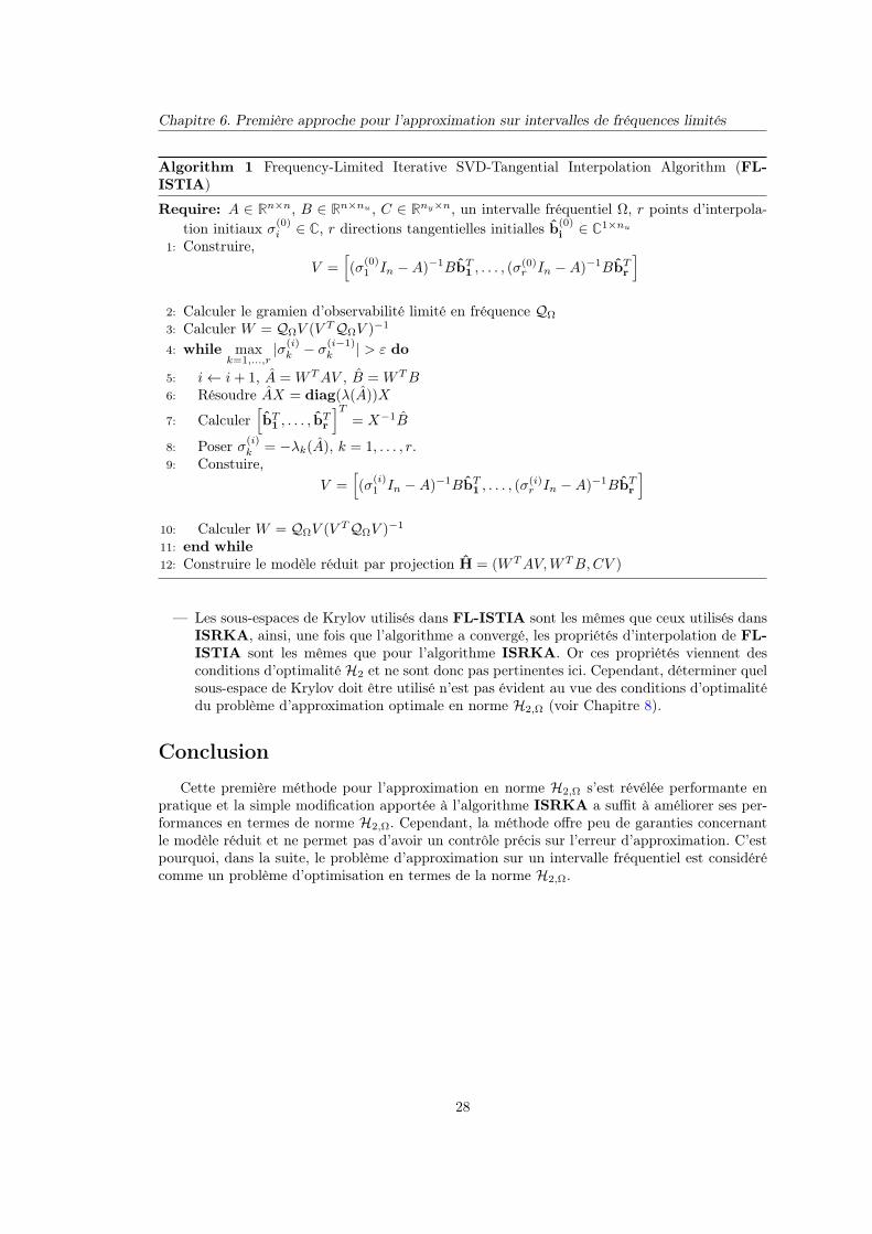
Chapitre 6. Première approche pour l’approximation sur intervalles de fréquences limités
Algorithm 1 Frequency-Limited Iterative SVD-Tangential Interpolation Algorithm (FL-ISTIA)
Require: A ∈ Rn×n, B ∈ Rn×nu , C ∈ Rny×n, un intervalle fréquentiel Ω, r points d’interpola-tion initiaux σ(0)
i ∈ C, r directions tangentielles initialles b(0)i ∈ C1×nu
1: Construire,V =
[(σ
(0)1 In −A)−1BbT1 , . . . , (σ
(0)r In −A)−1BbTr
]2: Calculer le gramien d’observabilité limité en fréquence QΩ
3: Calculer W = QΩV (V TQΩV )−1
4: while maxk=1,...,r
|σ(i)k − σ
(i−1)k | > ε do
5: i← i+ 1, A = WTAV , B = WTB6: Résoudre AX = diag(λ(A))X
7: Calculer[bT1 , . . . , b
Tr
]T= X−1B
8: Poser σ(i)k = −λk(A), k = 1, . . . , r.
9: Constuire,V =
[(σ
(i)1 In −A)−1BbT1 , . . . , (σ
(i)r In −A)−1BbTr
]10: Calculer W = QΩV (V TQΩV )−1
11: end while12: Construire le modèle réduit par projection H = (WTAV,WTB,CV )
— Les sous-espaces de Krylov utilisés dans FL-ISTIA sont les mêmes que ceux utilisés dansISRKA, ainsi, une fois que l’algorithme a convergé, les propriétés d’interpolation de FL-ISTIA sont les mêmes que pour l’algorithme ISRKA. Or ces propriétés viennent desconditions d’optimalité H2 et ne sont donc pas pertinentes ici. Cependant, déterminer quelsous-espace de Krylov doit être utilisé n’est pas évident au vue des conditions d’optimalitédu problème d’approximation optimale en norme H2,Ω (voir Chapitre 8).
Conclusion
Cette première méthode pour l’approximation en norme H2,Ω s’est révélée performante enpratique et la simple modification apportée à l’algorithme ISRKA a suffit à améliorer ses per-formances en termes de norme H2,Ω. Cependant, la méthode offre peu de garanties concernantle modèle réduit et ne permet pas d’avoir un contrôle précis sur l’erreur d’approximation. C’estpourquoi, dans la suite, le problème d’approximation sur un intervalle fréquentiel est considérécomme un problème d’optimisation en termes de la norme H2,Ω.
28
Chapitre 7
Formulation de la norme H2,Ω avecles pôles et les résidus d’une fonctionde transfert
La formulation pôles-résidus d’une fonction de transfert (voir Section 2.1) n’est pas la re-présentation la plus robuste et est limitée, pour être applicable, aux modèles ayant des pôlessemi-simples uniquement. Cependant, dans le cadre de l’approximation optimale en norme H2,cette formulation a permis d’exprimer les conditions d’optimalité du premier ordre comme desconditions d’interpolation (voir Section 4.1) d’un grand intérêt pour le développement d’algo-rithmes d’approximation. C’est pourquoi, une formulation similaire a été développée pour lanorme H2 limitée.
En particulier, le cas des modèles ayant des pôles semi-simples est présenté dans la Section7.1 et le cas des modèles ayant des pôles multiples est traité dans la Section 7.2. Finalement,dans la Section 7.3, la formulation pôles-résidus de la norme H2,Ω est utilisée pour formuler deuxbornes sur la norme H∞ d’un modèle LTI.
Les éléments de ce chapitre ont été publiés dans [Vuillemin et al., 2012b, 2014c,d].
7.1 Cas des modèles ayant des pôles semi-simples
La formulation pôles-résidus de la norme H2,Ω fait intervenir la branche principale de l’arc-tangente complexe atan(z), z ∈ C\±j [Kahan, 1987; Corless et al., 2000] et est présentée dansle Théorème 5.
Théorème 5 (Formulation pôles-résidus de la norme H2,Ω). Étant donné un intervalle fréquen-tiel Ω = [0, ω] et un modèle LTI H de dimension n. Supposons que les deux hypothèses suivantessoient satisfaites
1. La fonction de transfert associée à H peut s’écrire comme
H(s) =
n∑i=1
Φis− λi
+D ∈ Cny×nu ,
où D ∈ Rny×nu , Φi ∈ Cny×nu et λi ∈ C (i = 1, . . . , n).2. Si certains pôles λj1 , . . . , λjK sont imaginaires purs, alors la borne supérieure ω de l’in-
tervalle fréquentiel Ω est plus petit que leur module, i.e. ω < min |λj1 |, . . . , |λjK |.Alors, la norme H2 limitée de H peut s’écrire comme
‖H‖2H2,Ω=
n∑i=1
n∑k=1
ai,k +ω
πtr(DDT
)− 2
π
n∑i=1
tr(ΦiD
T)atan
(ω
λi
)(7.1)
où
ai,k =
2
πtr
(ΦiΦ
Tk
λi + λk
)atan
(ω
λi
)si λi + λk 6= 0
− 1
πtr
(ωΦiΦ
Tk
ω2 + λiλi
)sinon.
29
Chapitre 7. Formulation de la norme H2,Ω avec les pôles et les résidus d’une fonction detransfert
La formulation de la norme H2,Ω présentée dans le Théorème 5 repose sur le fait que lafonction de transfert associée au modèle a des pôles semi-simples uniquement. Cette hypothèsepeut être levée comme décrit dans la section suivante.
7.2 Cas des modèles ayant des pôles multiples
En utilisant la représentation pôles-résidus d’une fonction de transfert ayant des blocs de Jor-dan (voir Section 2.1), le Théorème 5 peut être généralisé aux modèles ayant des pôles multiplescomme montré dans le Théorème 6.
Théorème 6. Étant donné un modèle H := (A,B,C) strictement propre et asymptotiquementstable ainsi qu’un intervalle fréquentiel Ω = [0, ω], ω > 0. Supposons que A possède nb blocs deJordan de tailles ni (i = 1, . . . , nb), chaque bloc étant associé à la valeur propre λi. Alors, lanorme H2 limitée de H est donnée par
‖H‖2H2,Ω=
j
2π
nb∑i=1
nb∑k=1
ni∑l=1
nk∑m=1
tr(
Φ(l)i Φ
(m)T
k
)Ilm(λi, λk, ω)
avec
Ilm(λi, λk, ω) =
l∑p=1
rm,l−p(λi, λk)Wp−1 (jω, λi) +
m∑q=1
rl,m−q(λi, λk)Wq−1 (jω, λk) ,
oùWu(jω, λ) =
1
u!
du
dyu(log (−jω − y)− log (jω − y))
∣∣∣y=λ
,
etru,v(λi, λk) = (−1)(u+v)
(u+ v − 1
v
)1
(λi + λk)u+v .
La formulation pôles-résidus de la norme H2,Ω dans le cas de pôles multiples est avant toutun outil théorique dans la mesure où la décomposition de Jordan d’une matrice est très complexeà obtenir en pratique.
7.3 Deux bornes supérieures sur la norme H∞La norme H∞ d’un modèle LTI est bornée par le maximum de la norme de Frobenius de la
réponse fréquentielle sur l’axe imaginaire. Comme la norme H2,Ω est l’intégrale du carré de lanorme de Frobenius de la fonction de transfert, elle peut être utilisée pour formuler une bornesupérieure sur la norme H∞ comme présenté dans le Théorème 7.
Théorème 7 (Borne sur la norme H∞). Étant donné un modèle LTI H asymptotiquementstable, sa norme H∞ est bornée par le maximum de la dérivée par rapport à ω de sa norme H2,Ω
(avec Ω = [0, ω]) de la façon suivante
‖H‖H∞ ≤ maxω∈R
√πd‖H‖2H2,Ω
dω.
Si H est SISO alors la borne est atteinte.
La borne générale présentée dans le Théorème 7 peut être exprimée à l’aide de l’expressionpôles-résidus de la norme H2,Ω. En effet, la dérivée de (7.1) par rapport à ω peut s’écrire comme
d‖H‖2H2,[0,ω]
dω= − 2
π
n∑i=1
tr(φiH(−λi)T
) λiλ2i + ω2
+1
πtr(DDT
)=
n∑i=1
fi(ω) +1
πtr(DDT
).
30
7.3. Deux bornes supérieures sur la norme H∞
Cette formulation permet ensuite d’exprimer deux bornes supérieures sur la norme H∞ commeexprimé dans le Théorème 8.
Théorème 8 (Deux bornes supérieures sur la norme H∞). Étant donné un modèle LTI H :=(A,B,C,D) asymptotiquement stable, d’ordre n, ayant des pôles semi-simples uniquement, sanorme H∞ est bornée par Γ et Γ de la façon suivante
‖H‖H∞ ≤
√√√√tr (DDT ) + maxω∈R+
π
n∑i=1
gi(ω)
︸ ︷︷ ︸Γ
≤
√√√√tr (DDT ) + π
n∑i=1
maxω∈R+
gi(ω)
︸ ︷︷ ︸Γ
où gi(ω) = Re (fi(ω)).
Dans le Théorème 8, en restreignant le domaine de recherche de R+ à un intervalle quelconqueΩ, les bornes peuvent être utilisées pour borner la valeur singulière maximum de la fonction detransfert sur Ω.
À noter que ces bornes sur la norme H∞ peuvent être utilisées dans une procédure itérativepermettant de construire un gabarit fréquentiel sur un modèle LTI. Ceci s’avère particulièrementutile pour le contrôle où l’analyse comme illustré dans les chapitres 9 et 10.
Conclusion
La formulation pôles-résidus de la norme H2 a été étendue à la norme H2,Ω pour des modèlesayant des pôles semi-simples ou des pôles multiples. Dans le dernier cas, la formulation est avanttout un outil théorique et l’hypothèse est faite dans le reste de ce document que les modèlesconsidérés ont des pôles semi-simples uniquement. La formulation pôles-résidus de la normeH2,Ω a également été utilisée pour dériver deux bornes sur la norme H∞ d’un modèle LTI ce quipermet, dans le cadre de l’approximation, de quantifier la pire erreur d’approximation.
Dans le chapitre suivant, la formulation pôles-résidus de la norme H2,Ω est utilisée pourexprimer l’erreur d’approximation entre un modèle de grande dimension et un modèle réduit.
31

Chapitre 8
Formulation de la norme H2,Ω de l’er-reur d’approximation et dérivation deson gradient
Dans ce chapitre, la formulation pôles-résidus de la norme H2,Ω est utilisée pour exprimerl’erreur d’approximation entre un modèle de grande dimension et un modèle réduit ainsi que pourreformuler le problème d’approximation optimale en norme H2,Ω. En particulier, la formulationpôles-résidus de l’erreur d’approximation est présentée dans la Section 8.1 et son gradient estexprimé dans la Section 8.2.
Les éléments de ce chapitre ont été en partie publiés dans [Vuillemin et al., 2014b].
8.1 Formulation pôles-résidus de la norme H2,Ω de l’erreurd’approximation
Le Théorème 5 est utilisé ici pour exprimer la norme H2,Ω du carré l’erreur d’approximationJH2,Ω
= ‖H − H‖2H2,Ωentre un modèle de grande dimension et un modèle réduit en fonction
des pôles et résidus des deux modèles comme exprimé dans le Théorème 9.À noter que pour simplifier les équations, la notation suivante est adoptée dans la suite
aω,λ =2
πatan
(ωλ
).
Théorème 9 (Formulation pôles-résidus de l’erreur d’approximation H2,Ω). Étant donné unintervalle fréquentiel Ω = [0, ω], un modèle LTI H d’ordre n et un modèle LTI H d’ordre r quiont tous les deux des pôles semi-simples et dont les fonctions de transfet associées s’écriventcomme
H(s) =
n∑i=1
Φis− λi
+D ∈ Cny×nu et H(s) =
r∑i=1
Φi
s− λi+ D ∈ Cny×nu .
Supposons également que λi + λk 6= 0, λi + λl 6= 0 et λl + λm 6= 0 pour tout i, k = 1, . . . , n etl, m = 1, . . . , r 1. Alors, le carré de la norme H2,Ω de l’erreur d’approximation entre H et H,i.e. JH2,Ω = ‖H − H‖2H2,Ω
, est donnée par
JH2,Ω =
n∑i=1
n∑k=1
tr(ΦiΦ
Tk
)λi + λk
aω,λi +r∑i=1
r∑k=1
tr(
ΦiΦTk
)λi + λk
aω,λi −n∑i=1
r∑k=1
tr(
ΦiΦTk
)λi + λk
(aω,λi + aω,λk
). . .+
r∑i=1
tr(
ΦiDT)aω,λi −
n∑i=1
tr(
ΦiDT)aω,λi +
ω
πtr(DDT
),
(8.1)où aω,λ = 2
πatan(ωλ
)et D = D − D.
1. Ces hypothèses impliquent que les deux modèles n’ont pas de pôles placés symétriquement par rapport àl’axe imaginaire dans le plan complexe.
33
Chapitre 8. Formulation de la norme H2,Ω de l’erreur d’approximation et dérivation de songradient
8.2 Conditions d’optimalité du premier ordre
Basée sur la formulation pôles-résidus de la norme H2,Ω de l’erreur d’approximation expriméedans le Théorème 9, le problème d’approximation optimale en norme H2,Ω peut être reformulécomme suit.
À noter que les résidus du modèle réduit H sont ici décomposés comme un produit de deuxvecteurs, Φi = cTi bi (i = 1, . . . , r).
Problème 3 (Formulation pôles-résidus du problème d’approximation optimale en normeH2,Ω).Étant donné un modèle LTI H asymptotiquement stable et d’ordre n. Le problème d’approxima-tion optimale en norme H2,Ω consiste à trouver les pôles λi ∈ C, les vecteurs ci ∈ C1×ny etbi ∈ C1×nu (i = 1, . . . , r) et le transfert direct D ∈ Rny×nu du modèle asymptotiquement stableH qui minimisent la norme H2,Ω de l’erreur d’approximation JH2,Ω
.
La fonction JH2,Ωest une fonction réelles de variables complexes et de leurs conjugués. Une
telle fonction ne satisfait pas les conditions de Cauchy-Riemann et est par conséquent non-analytique. Pour dériver ce type de fonctions, les parties réelles et imginaires des variables sontgénéralement considérées séparément. Cependant, ici, pour garder la structure de JH2,Ω
, le calculde Wirtinger est utilisé [Brandwood, 1983; Remmert, 1991; Kreutz-Delgado, 2009; Sorber et al.,2012] et permet d’exprimer directement les conditions d’optimalité du premier ordre pour leProblème 3.
Théorème 10 (Formulation pôles-résidus des conditions d’optimalité du premier ordre pour leproblème d’approximation optimale en norme H2,Ω). Étant donné deux modèles LTI H et Hd’ordres n et r n, respectivement, et dont les pôles sont semi-simples et ne sont pas situéssymétriquement par rapport à l’axe imaginaire et dont les fonctions de transfert sont donnéespar
H(s) =
n∑i=1
ciTbi
s− λi+D et H(s) =
n∑i=1
cTi bi
s− λi+ D.
Considérons également un intervalle fréquentiel Ω = [0, ω], si H minimise JH2,Ω= ‖H − H‖2H2,Ω
,alors les dérivées de JH2,Ω
par rapport à λm, bm, cm et D, données pour m = 1, . . . , r par leséquations (8.2), (8.3), (8.4) et (8.5), respectivement, s’annulent.
∂JH2,Ω
∂λm= −
r∑i=1
cmcTi bibTm
aω,λi + aω,λm(λi + λm
)2 +2
π
ω(λ2m + ω2
)(λi + λm
) . . .
+
n∑i=1
cmciTbib
Tm
aω,λi + aω,λm(λi + λm
)2 +2
π
ω(λ2m + ω2
)(λi + λm
) . . .
+2
πcmDbm
ω
ω2 + λ2m
,
(8.2)
∂JH2,Ω
∂bm
=
r∑i=1
bTi cicTm
λi + λm
(aω,λi + aω,λm
)−
n∑i=1
biT cic
Tm
λi + λm
(aω,λi + aω,λm
)+ DT cTmaω,λm , (8.3)
∂JH2,Ω
∂cm=
r∑i=1
cTi bibTm
λi + λm
(aω,λi + aω,λm
)−
n∑i=1
ciTbib
Tm
λi + λm
(aω,λi + aω,λm
)+ DbTmaω,λm , (8.4)
34
8.2. Conditions d’optimalité du premier ordre
∂JH2,Ω
∂D= −
r∑i=1
cTi biaω,λi +
n∑i=1
ciTbiaω,λi −
2
πωD. (8.5)
Ces conditions d’optimalité du premier ordre peuvent se reformuler comme les conditionsd’interpolation suivantes
T (−λm)bTm = T (−λm)bTmcmT (−λm) = cmT (−λm)
cmT′(−λm)bTm = cmT
′(−λm)bTm,
oùT (s) = Hω(s) +H(s)aω,−s et T (s) = Hω(s) + H(s)aω,−s,
avec
Hω(s) =
n∑i=1
ciTbi
s− λiaω,λi et Hω(s) =
r∑i=1
cTi bi
s− λiaω,λi .
Conclusion
La formulation pôles-résidus de la norme H2,Ω a été utilisée pour exprimer la norme H2,Ω del’erreur d’approximation et pour caractériser les points stationnaires du problème d’approxima-tion optimale en norme H2,Ω. Bien que ces conditions puissent se formuler comme des conditionsd’interpolation, développer un algorithme similaire à IRKA (voir Section 4.2) n’est pas évidentdans ce cas. C’est pourquoi dans le prochain chapitre, un algorithme d’optimisation est déve-loppé.
35

Chapitre 9
Développement d’un algorithme dedescente pour l’approximation opti-male en norme H2,Ω
La plupart des solveurs de problèmes d’optimisation ne gèrent pas les fonctions réelles devariables complexe directement dans le domaine complexe. Ainsi, la formulation pôles-résidus del’erreur d’approximation H2,Ω et son gradient exprimés dans le chapitre précédent sont utilisésici pour construire un algorithme d’optimisation sans contrainte appelé Descent Algorithm forResdiues and Poles Optimisation (DARPO) et dont le but est de trouver les pôles et résidusdu modèle réduit qui minimisent la norme H2,Ω de l’erreur d’approximation.
Cet algorithme est présenté dans la Section 9.1 et son application pour le contrôle d’unmodèle de grande dimension est décrite dans la Section 9.2.
Les éléments de ce chapitre ont été en partie publiés dans [Vuillemin et al., 2014b].
9.1 Algorithme de descente pour l’optimisation des pôles etdes résidus
De nombreux algorithmes existent pour l’optimisation sans contrainte [Fletcher, 2000]. Ici,une méthode quasi-Newton basée sur la mise à jour de Broyden–Fletcher–Goldfarb–Shanno(BFGS) de l’inverse du Hessien est utilisée. Cette méthode est choisie car elle ne requière pas leHessien de la fonction cible et est connue en pratique pour ses très bonnes performances [Li andFukushima, 2001]. Le sous-problème de recherche dans une direction est réalisé par l’algorithmeprésenté dans [Fletcher, 2000, Section 2.6] de telle sorte que la longueur du pas dans une direc-tion satisfait les conditions fortes de Wolfe. La mise à jour BFGS a été généralisée au cas desfonctions réelles à variables complexes dans [Sorber et al., 2012] et est utilisée ici dans DARPOdont le fonctionnement est présenté dans l’Algorithme 2.
À chaque itération,DARPO produit un modèle réduit dont l’erreur d’approximation est plusfaible que celle correspondante au modèle précédent. Quand l’algorithme a convergé, le modèleréduit obtenu est normalement un minimum local du problème d’approximation optimale ennorme H2,Ω.
9.2 Utilisation de DARPO pour le contrôle d’un modèle degrande dimension
À l’aide d’un gabarit fréquentiel construit sur l’erreur d’approximation, DARPO peut servirpour le contrôle de modèles de grande dimension. Ici, le problème de rejet de perturbation d’unestructure spatiale flexible dont le modèle est de grande dimension est considéré. Ce problèmepeut s’écrire sous la forme d’une problème de synthèse H∞ tel que
K = arg minK stabilise P
K ∈ K
max‖F (2)l (P, K)‖H∞ , ‖WK‖H∞, (9.1)
37
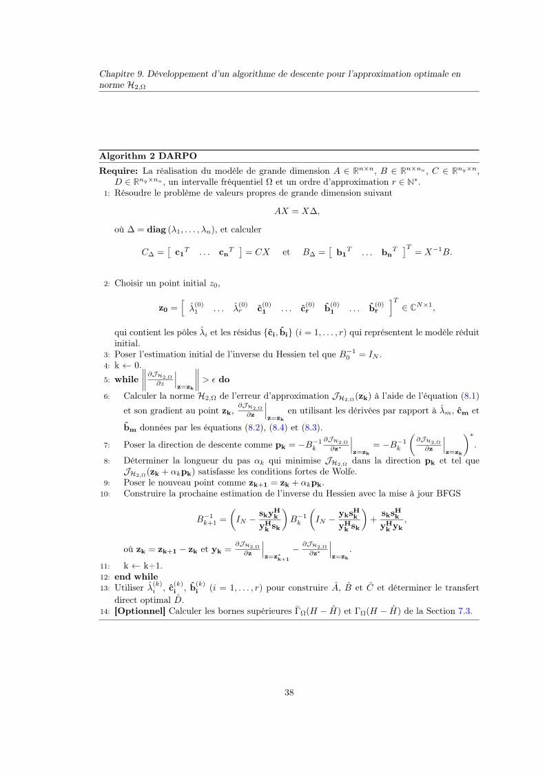
Chapitre 9. Développement d’un algorithme de descente pour l’approximation optimale ennorme H2,Ω
Algorithm 2 DARPO
Require: La réalisation du modèle de grande dimension A ∈ Rn×n, B ∈ Rn×nu , C ∈ Rny×n,D ∈ Rny×nu , un intervalle fréquentiel Ω et un ordre d’approximation r ∈ N∗.
1: Résoudre le problème de valeurs propres de grande dimension suivant
AX = X∆,
où ∆ = diag (λ1, . . . , λn), et calculer
C∆ =[c1T . . . cn
T]
= CX et B∆ =[b1
T . . . bnT]T
= X−1B.
2: Choisir un point initial z0,
z0 =[λ
(0)1 . . . λ
(0)r c
(0)1 . . . c
(0)r b
(0)1 . . . b
(0)r
]T∈ CN×1,
qui contient les pôles λi et les résidus ci, bi (i = 1, . . . , r) qui représentent le modèle réduitinitial.
3: Poser l’estimation initial de l’inverse du Hessien tel que B−10 = IN .
4: k ← 0.5: while
∥∥∥∥∂JH2,Ω
∂z
∣∣∣z=zk
∥∥∥∥ > ε do
6: Calculer la norme H2,Ω de l’erreur d’approximation JH2,Ω(zk) à l’aide de l’équation (8.1)
et son gradient au point zk,∂JH2,Ω
∂z
∣∣∣z=zk
en utilisant les dérivées par rapport à λm, cm et
bm données par les équations (8.2), (8.4) et (8.3).
7: Poser la direction de descente comme pk = −B−1k
∂JH2,Ω
∂z∗
∣∣∣z=zk
= −B−1k
(∂JH2,Ω
∂z
∣∣∣z=zk
)∗.
8: Déterminer la longueur du pas αk qui minimise JH2,Ω dans la direction pk et tel queJH2,Ω
(zk + αkpk) satisfasse les conditions fortes de Wolfe.9: Poser le nouveau point comme zk+1 = zk + αkpk.
10: Construire la prochaine estimation de l’inverse du Hessien avec la mise à jour BFGS
B−1k+1 =
(IN −
skyHk
yHk sk
)B−1k
(IN −
yksHk
yHk sk
)+
sksHk
yHk yk
,
où zk = zk+1 − zk et yk =∂JH2,Ω
∂z
∣∣∣z=z∗k+1
− ∂JH2,Ω
∂z∗
∣∣∣z=zk
.
11: k ← k+1.12: end while13: Utiliser λ(k)
i , c(k)i , b(k)
i (i = 1, . . . , r) pour construire A, B et C et déterminer le transfertdirect optimal D.
14: [Optionnel] Calculer les bornes supérieures ΓΩ(H − H) et ΓΩ(H − H) de la Section 7.3.
38
9.2. Utilisation de DARPO pour le contrôle d’un modèle de grande dimension
où W représente un filtre de roll-off, F (2)l (P,K) est la représentation inférieure linéaire fraction-
naire (LFR) [Magni, 2006] permettant d’interconnecter le modèle généralisé P avec le contrôleurK et K est l’ensemble des contrôleurs ayant une structure donnée.
Ce problème de synthèse H∞ multi-objectifs peut être traité directement à l’aide de méthoded’optimisation non-lisses dédiées [Apkarian and Noll, 2006; Gumussoy et al., 2009]. Cependant,la dimension de P empêche les algorithmes de trouver une solution satisfaisante dans ce cas. Unproblème alternatif est résolu à l’aide de l’approximation de modèles. En particulier, le problème(9.1) est remplacé par
K = minK stabilise P
K ∈ K
max‖F (2)l (P , K)‖H∞ , ‖WK‖H∞ , ‖F
(3)l (P , K)‖H∞. (9.2)
où P est le modèle généralisé créé à l’aide du modèle réduit obtenu avec DARPO. Ce nou-veau problème de synthèse H∞ inclut un canal d’optimisation supplémentaire qui englobe l’er-reur d’approximation mais ce problème ne fait intervenir que des modèles de faibles dimensioncontrairement à (9.1). Résoudre (9.2) permet de garantir la stabilité du modèle de grande di-mension et de satisfaire la contrainte imposée par le filtre de roll-off. La performance robuste nepeut pas être garantie mais s’avère vérifiée dans ce cas.
Conclusion
La formulation pôles-résidus de la norme H2,Ω et son gradient ont été utilisés pour créer unalgorithme de descente dans le domaine complexe : DARPO. Cet algorithme permet de trouverun minimum local au problème d’approximation optimale en norme H2,Ω. Comme le problèmeest non-linéaire et non-convexe, l’algorithme est très dépendant de son initialisation, mais il s’estavéré efficace en pratique. De plus, la formulation pôles-résidus permet d’exploiter pleinementles outils pour borner la norme H∞ de l’erreur développés dans la Section 7.3 ce qui est un atoutpar rapports aux autres méthodes.
Dans le chapitre suivant, l’utilisation des outils développés durant cette thèse sur des casd’études industriels est présentée.
39

Chapitre 10
Cas d’étude industriel
L’étude détaillée dans ce chapitre a été motivée par la dimension croissante des modèlesreprésentant des avions civils qui empêche l’utilisation de méthodes de conception de lois decommande classiques. Une étape préliminaire d’approximation est nécessaire et ne doit pasaffaiblir les propriétés de robustesse et de performances des contrôleurs qui sont conçus. Eneffet, dans un contexte aéronautique, de fortes contraintes existent sur les lois de commandequi doivent satisfaire diverses spécifications. Plusieurs étapes ont été réalisées dans cette optiquedurant cette thèse,
— dans une premier temps, les performances de diverses méthodes d’approximation, dontFL-ISTIA, ont été évaluées sur des modèles de grande dimension représentant le com-portement longitudinal d’une avion long-courrier flexible dans [Vuillemin et al., 2012a,2013b],
— ensuite, FL-ISTIA et DARPO ont été utilisés dans le cadre de la conception (i) d’uneloi de commande anti-vibration pour un avion d’affaires [Poussot-Vassal et al., 2013] et(ii) d’une loi de commande garantissant les performances de vol en présence d’une satura-tion en entrée pour un avion civil [Burlion et al., 2014].
— L’approximation de modèles a également été utilisée comme la base d’un processus demodélisation destiné à créer un modèle d’ordre réduit, incertain et à paramètres variantsà partir d’un ensemble de modèles de grande dimension [Poussot-Vassal and Vuillemin,2013; Poussot-Vassal et al., 2014],
— grâce à ce processus, la stabilité globale et les performance d’un ensemble de modèles degrande dimension représentant l’avion d’affaires à différents points de vol en présence d’unesaturation sur l’actionneur a été prouvée [Vuillemin et al., 2014a].
Dans ce chapitre, le processus global suivi pour la conception et la validation de la loi decommande anti-vibration pour un avion d’affaires est présentée. En particulier, dans la Section10.1, l’étude préliminaire utilisée pour la conception de la loi de contrôle anti-vibrations basé surun seul modèle représentant l’avion d’affaires à un unique point de vol est décrite. La stabilité del’ensemble de modèles représentant l’avion à différents points de vol en présence d’une saturationest ensuite évaluée dans la Section 10.2.
10.1 Conception d’une loi de commande anti-vibrations surun modèle d’avion d’affaires de grande dimension
La conception de lois de commande anti-vibrations est à la fois une question de confort despassagers et du pilote mais permet également de réduire les efforts sur la structure de l’avion cequi permet d’augmenter sa durabilité. Une telle loi de commande doit satisfaire de nombreusescontraintes, en particulier, elle ne doit pas perturber la loi de contrôle nominale de l’avionmais elle doit permettre une réduction substantielle des vibrations dans une certaine plage defréquences.
Pour traiter ce problème, les outils de synthèse H∞ modernes [Apkarian and Noll, 2006;Gumussoy et al., 2009] sont utilisés. Cependant, le modèle représentant l’avion d’affaires est degrande dimension ce qui empêche d’utiliser les algorithmes directement. Un modèle réduit estdonc utilisé à la place du modèle de grande dimension pour générer un contrôleur satisfaisantles contraintes imposées par le problème de contrôle.
41

Chapitre 10. Cas d’étude industriel
La loi de commande finale est ensuite conçue en complétant cette approche et en prenant encompte l’ensemble des modèles de grande dimension représentant l’avion d’affaires en différentspoints de vol. La stabilité de l’ensemble des modèles ainsi contrôlés est validée dans la sectionsuivante.
10.2 Validation globale de la stabilité du modèle d’aviond’affaires à paramètres variants
Pour valider la stabilité du modèle d’avion controlé, sur l’ensemble du continuum paramé-trique et en présence d’une saturation en entrée, à partir d’un ensemble de modèles de grandedimension représentants l’avion en différents points de vol, une méthodologie en trois étape aété suivie :(i) dans un premier temps, les différents modèles de grande dimension sont réduits sur un
intervalle fréquentiel borné, ce qui permet d’atteindre une complexité très faible, et ungabarit fréquentiel est construit pour borner la pire erreur d’approximation,
(ii) ensuite, l’ensemble de modèles réduits sont interpolés en une LFR [Ferreres, 2011] de façonà ce que l’erreur d’interpolation soit, elle aussi, bornée,
(iii) enfin, la stabilité globale est évaluée grâce au formalisme des contraintes intégrales qua-dratiques (IQC) dans lequel des multiplieurs irrationnels sont utilisés [Sideris and San-chez Pena, 1990; Demourant, 2013].
Les étapes (i) et (ii) permettent de transformer l’ensemble initial de modèles de grandedimension en un modèle incertain et à paramètres variants de faible complexité dont les trajec-toires englobent nécessairement celles de l’ensemble des modèles de grande dimension du fait dela prise en compte des erreurs d’approximation et d’interpolation.
Conclusion
Dans le processus global mis en place pour concevoir et valider une loi de commande anti-vibrations, l’approximation est l’outil qui permet d’appliquer les autres outils et techniques desynthèse et d’analyse. De plus, en bornant les erreurs induites lors de l’approximation, il estpossible d’obtenir des garanties sur le modèle contrôlé de grande dimension.
Ce chapitre clos la partie dédiée aux contributions de cette thèse et la prochaine partieprésentes les conclusions et perspectives de ce travail.
42
Quatrième partie
Conclusion
43


Chapitre 11
Discussion
Les différentes contributions de cette thèse, ainsi que leurs limitations sont les suivantes :— FL-ISTIA (Chapitre 6) : cette méthode empirique est performante en pratique mais
pourrait être grandement améliorée en prenant en compte des sous-espaces de Krylovpertinent pour l’approximation en norme H2,Ω. Ainsi, il faut étudier s’il est possible decréer un sous-espace de Krylov pour satisfaire les conditions d’interpolation présentéesdans le Chapitre 8.
— Formulation pôles-résidus de la norme H2,Ω (Sections 7.1 et 7.2) : cette formulation s’estavérée très pratique pour l’approximation optimale en norme H2,Ω mais n’est pas particu-lièrement robuste numériquement. De plus, les matrices non-diagonalisables sont problé-matiques dans la mesure où la décomposition de Jordan peut difficilement être obtenueen pratique. D’autres décomposition comme une décomposition diagonale par blocs, outridiagonale pourraient être considérées à la place.D’autres part, calculer la décomposition en valeurs propres d’une matrice est une tâchecomplexe en grande dimension. Cependant il peut être suffisant de calculer uniquementquelques valeurs propres et vecteurs propres pour estimer avec précision la norme H2,Ω
d’un modèle.— Bornes sur la norme H∞ (Section 7.3) : Ces bornes sur la norme H∞ pourraient être
utilisées à la place de cette dernière quand sa détermination est numériquement trop coû-teuse. Par exemple pour du contrôle ou de l’analyse. Ces bornes pourraient également êtredirectement utilisées pour l’approximation de modèles de grande dimension.
— Conditions d’optimalité du premier ordre pour le problème d’approximation optimale ennorme H2,Ω (Chapitre 8) : le lien entre ces conditions d’optimalité, exprimées comme desconditions d’interpolation, et les conditions d’interpolation pour l’approximation optimaleen norme H2 pondérée [Anić et al., 2013] reste à clarifier et s’avère être une piste derecherche particulièrement intéressante pour la suite.
— DARPO (Chapitre 9) : de nombreuses pistes d’amélioration sont envisageables concernantl’algorithme d’optimisation proposé. En effet, la structure du problème n’a pas complète-ment été exploitée, l’étape d’initialisation est cruciale et une stratégie plus performante quecelle utilisée actuellement peut être développée. Par ailleurs, pour appliquer cette méthodeà des modèles de très grande dimension, ici aussi, seule une partie des valeurs propres etvecteurs propres du modèle initial de grande dimension pourrait être pris en compte.Par ailleurs, cette méthode peut également être utilisée d’une façon constructive pour ré-duire un modèle de grande dimension tel que l’erreur d’approximation soit en dessous d’uncertain seuil. Cependant, cette approche souffre de la stratégie d’initialisation considéréeet peut être améliorée.Aussi, l’utilisation de DARPO pour le contrôle de modèles de grande dimension s’estavérée être efficace, mais une méthode globale et systématique reste à développer.
45


Chapitre 12
Perspectives
Les perspectives de cette thèse s’articulent autour de deux lignes directrices : l’approximationet le contrôle de modèles de grande dimension. Le premier axe concerne l’extension et les futursdéveloppements des méthodes proposées tandis que le second axe concerne plutôt l’adaptationet l’application de ces méthodes pour le contrôle de modèles de grande dimension.
Plus précisément, concernant l’approximation de modèles :— les différentes contributions de cette thèse sont principalement basées sur la formulation
pôles-résidus de la norme H2,Ω. L’extension de cette formulation pour d’autres types demodèles devrait être étudiée. En particulier, elle pourrait s’étendre aux équations différen-tielles algébriques à l’aide de la forme canonique de Weierstrass et à certains modèles àretard en utilisant la fonction de Lambert pour calculer les pôles de la fonction de transfert.
— Plus généralement, l’approximation en normeH2,Ω représente la généralisation naturelle del’approximation en normeH2 et devrait être étendue à d’autres types de modèles comme lesmodèles à paramètres variants, les modèles bilinéaires (comme dans [Shaker and Tahavori,2014]), etc.
Concernant le contrôle des modèles de grande dimension— le processus global utilisé pour la conception et validation d’une loi de commande pour
un ensemble de modèles de grande dimension développée dans le Chapitre 10 peut éven-tuellement être simplifiée en couplant les étapes d’approximation et d’interpolation en uneseule. Pour cela, l’approximation multi-modèles, ou ensemble la modélisation sous formede modèle incertain à paramètres variants d’ordre réduit doit être considérée.
— Une approche constructive qui inclut de plus en plus de dynamiques du modèle de grandedimension jusqu’à ce qu’un contrôleur satisfaisant soit trouvé pourrait également être consi-dérée.
— Par ailleurs dans cette thèse, seul le contrôle robuste a été considéré mais d’autres tech-niques de contrôle telles que le contrôle prédictif ou le contrôle optimal pourraient proba-blement bénéficier de l’approximation de modèles pour alléger la charge de calcul associéeaux modèles de grande dimension.
Le problème d’approximation est loin d’être résolu et l’utilisation croissante d’outils numé-riques pour la modélisation de systèmes complexes va probablement faire de cette thématiqueun élément central pour l’implémentation pratique d’outils théoriques.
47

Bibliographie
Al-Mohy, A., Higham, N., and Relton, S. (2013). Computing the Fréchet derivative of the matrixlogarithm and estimating the condition number. SIAM Journal on Scientific Computing,35(4) :C394 – C410.
Anderson, M. R., Emami-Naeni, A., and Vincent, J. (1991). Measures of merit for multivariableflight control. Technical report, Systems Control Technology Inc, Palo Alto, California, USA.
Anić, B., Beattie, C., Gugercin, S., and Antoulas, A. (2013). Interpolatory weighted-H2 modelreduction. Automatica, 49(5) :1275 – 1280.
Antoulas, A. (2005). Approximation of large-scale dynamical systems. Advances in Design andControl. SIAM.
Antoulas, A., Ionita, A., and Lefteriu, S. (2012). On two-variable rational interpolation. LinearAlgebra and its Applications, 436(8) :2889 – 2915. Special Issue dedicated to Danny Sorensen’s65th birthday.
Apkarian, P. and Noll, D. (2006). Nonsmooth H∞ synthesis. IEE Transactions on AutomaticControl, 51(1) :71 – 86.
Badía, J., Benner, P., Mayo, R., and Quintana-Ortí, E. (2006). Parallel algorithms for balancedtruncation model reduction of sparse systems. In Dongarra, J., Madsen, K., and Waśniewski,J., editors, Applied Parallel Computing. State of the Art in Scientific Computing, volume 3732of Lecture Notes in Computer Science, pages 267 – 275. Springer.
Baratchart, L. (1986). Existence and generic properties of L2 approximants for linear systems.IMA Journal of Mathematical Control and Information, 3(2-3) :89 – 101.
Baratchart, L., Cardelli, M., and Olivi, M. (1991). Identification and rational L2 approximation :A gradient algorithm. Automatica, 27(2) :413 – 417.
Beattie, C. and Gugercin, S. (2009). A trust region method for optimal H2 model reduction. Inproceedings of the Joint Conference on Decision and Control and Chinese Control Conference,pages 5370 – 5375.
Beattie, C. and Gugercin, S. (2012). Realization-independent H2 approximation. In Proceedingsof the Conference on Decision and Control, pages 4953 – 4958.
Brandwood, D. (1983). A complex gradient operator and its application in adaptive array theory.In Proceedings of the Conference on Communications, Radar and Signal Processing, volume130, pages 11 – 16.
Breiten, T., Beattie, C., and Gugercin, S. (2014). Near-optimal frequency-weighted interpolatorymodel reduction. Available as arXiv :1309.0136.
Burlion, L., Poussot-Vassal, C., Vuillemin, P., Leitner, M., and Kier, T. (2014). Longitudinalmanoeuvre load control of a flexible large-scale aircraft. In Proceedings of the IFAC WorldCongress, pages 3413 – 3418.
Chahlaoui, Y., Lemonnier, D., Vandendorpe, A., and Van Dooren, P. (2006). Second-orderbalanced truncation. Linear Algebra and its Applications, 415(2–3) :373 – 384. Special issueon order reduction of large-scale systems.
Corless, R. M., Jeffrey, D. J., Watt, S. M., and Davenport, J. H. (2000). "According to Abra-mowitz and Stegun" or arccoth needn’t be uncouth. ACM SIGSAM Bulletin, 34 :58 – 65.
49
BIBLIOGRAPHIE
de Villemagne, C. and Skelton, R. (1987). Model reductions using a projection formulation. InProceeding of the Conference on Decision and Control, volume 26, pages 461 – 466.
Demourant, F. (2013). New algorithmic approach based on integral quadratic constraints forstability analysis of high order models. In Proceedings of the European Control Conference,pages 359 – 364.
Enns, D. (1984). Model reduction with balanced realizations : An error bound and a frequencyweighted generalization. In Proceedings of the Conference on Decision and Control, pages 127– 132.
Ferreres, G. (2011). Computation of a flexible aircraft LPV/LFT model using interpolation.IEEE Transactions on Control Systems Technology, 19(1) :132 – 139.
Fletcher, R. (2000). Practical methods of optimization. John Wiley & Sons.
Fulcheri, P. and Olivi, M. (1998). Matrix rational H2 approximation : A gradient algorithmbased on Schur analysis. SIAM Journal on Control and Optimization, 36(6) :2103 – 2127.
Gallivan, K., Vandendorpe, A., and Van Dooren, P. (2004). Model reduction of MIMO systemsvia tangential interpolation. SIAM Journal on Matrix Analysis and Applications, 26(2) :328– 349.
Garulli, A., Hansson, A., Pakazad, S., Masi, A., and Wallin, R. (2013). Robust finite-frequencyanalysis of uncertain systems with application to flight comfort analysis. Control EngineeringPractice, 21(6) :887 – 897.
Gawronski, W. and Juang, J. (1990). Model reduction in limited time and frequency intervals.International Journal of Systems Science, 21(2) :349 – 376.
Glover, K. (1984). All optimal Hankel-norm approximations of linear multivariable systems andtheir L∞-error bounds. International Journal of Control, 39(6) :1115 – 1193.
Grimme, E. (1997). Krylov projection methods for model reduction. PhD thesis, University ofIllinois at Ubarna-Champaign.
Gugercin, S. (2007). An iterative SVD-Krylov based method for model reduction of large-scaledynamical systems. Linear Algebra and its Applications, 428(8-9) :1964 – 1986.
Gugercin, S. and Antoulas, A. (2004). A survey of model reduction by balanced truncation andsome new results. International Journal of Control, 77(8) :748 – 766.
Gugercin, S., Antoulas, A., and Beattie, C. (2008). H2 model reduction for large-scale lineardynamical systems. SIAM Journal on Matrix Analysis and Applications, 30(2) :609 – 638.
Gugercin, S. and Li, J. (2005). Smith-type methods for balanced truncation of large sparsesystems. In Benner, P., Sorensen, D., and Mehrmann, V., editors, Dimension reduction oflarge-scale systems, volume 45 of Lecture Notes in Computational Science and Engineering,pages 49 – 82. Springer.
Gumussoy, S., Henrion, D., Millstone, M., and Overton, M. (2009). Multiobjective robust controlwith HIFOO 2.0. In Proceedings of the 6th IFAC symposium on robust control design.
Higham, N. (2008). Functions of matrices : Theory and computation. SIAM.
Himpe, C. (2014). emgr - Empirical Gramian Framework. http://gramian.de.
50
BIBLIOGRAPHIE
Hyland, D. and Bernstein, D. (1985). The optimal projection equations for model reduction andthe relationships among the methods of Wilson, Skelton, and Moore. IEEE Transactions onAutomatic Control, 30(12) :1201 – 1211.
Ionita, A. (2013). Lagrange rational interpolation and its application to approximation of large-scale dynamical systems. PhD thesis, Rice University.
Kahan, W. (1987). Branch cuts for complex elementary functions, or much ado about nothing’ssign bit. In Proceedings of the Joint IMA/SIAM Conference on the State of the Art in Nume-rical Analysis, pages 165 – 211.
Kim, S., Anderson, B., and Madievski, A. (1995). Error bound for transfer function orderreduction using freqeuncy weighted balanced truncation. Systems & Control Letters, 24(3) :183– 192.
Kreutz-Delgado, K. (2009). The complex gradient operator and the CR-calculus. Available asarXiv :0906.4835.
Laub, A., Heath, M., Paige, C., and Ward, R. (1987). Computation of system balancing transfor-mations and other applications of simultaneous diagonalization algorithms. IEEE Transactionson Automatic Control, 32(2) :115 – 122.
Leblond, J. and Olivi, M. (1998). WeightedH2 approximation of transfer functions. Mathematicsof Control, Signals and Systems, 11(1) :28 – 39.
Li, D. and Fukushima, M. (2001). On the global convergence of the BFGS method for nonconvexunconstrained optimization problems. SIAM Journal on Optimization, 11(4) :1054 – 1064.
Li, J. and White, J. (2002). Low rank solution of Lyapunov equations. SIAM Journal on MatrixAnalysis and Applications, 24(1) :260 – 280.
Lin, C.-A. and Chiu, T.-Y. (1990). Model reduction via frequency weighted balanced realization.In American Control Conference, pages 2069 – 2070.
Magni, J. (2006). Linear fractional representation toolbox for use with Matlab. Available athttp ://w3.onera.fr/smac/.
Marmorat, J. and Olivi, M. (2002). The rarl2 software : Realizations and rational approximationin L2-norm. http://www-sop.inria.fr/apics/RARL2/rarl2.html. Project APICS, INRIA,Sophia Antipolis.
Marmorat, J.-P., Olivi, M., Hanzon, B., and Peeters, R. (2002). Matrix rational H2 approxima-tion : A state-space approach using Schur parameters. In Proceedings of the Conference onDecision and Control, volume 4, pages 4244 – 4249.
Mehrmann, V. and Stykel, T. (2005). Balanced truncation model reduction for large-scale sys-tems in descriptor form. In Benner, P., Sorensen, D., and Mehrmann, V., editors, DimensionReduction of Large-Scale Systems, volume 45 of Lecture Notes in Computational Science andEngineering, pages 83–115.
Meier, L. and Luenberger, D. (1967). Approximation of linear constant systems. IEEE Tran-sactions on Automatic Control, 12(5) :585 – 588.
Moore, B. (1981). Principal component analysis in linear systems : controllability, observability,and model reduction. IEEE Transactions on Automatic Control, 26(1) :17 – 32.
Penzl, T. (1999). A cyclic low-rank Smith method for large sparse Lyapunov equations. SIAMJournal on Scientific Computing, 21(4) :1401 – 1418.
51
BIBLIOGRAPHIE
Pernebo, L. and Silverman, L. (1982). Model reduction via balanced state space representations.IEEE Transactions on Automatic Control, 27(2) :382 – 387.
Petersson, D. (2013). A nonlinear optimization approach to H2-optimal modeling and control.PhD thesis, Linköping University.
Petersson, D. and Löfberg, J. (2014). Model reduction using a frequency-limitedH2-cost. Systems& Control Letters, 67(0) :32 – 39.
Poussot-Vassal, C. (2011). An iterative SVD-tangential interpolation method for medium-scaleMIMO systems approximation with application on flexible aircraft. In Proceedings of theConference on Decision and Control and European Control Conference, pages 7117 – 7122.
Poussot-Vassal, C., Loquen, T., Vuillemin, P., Cantinaud, O., and Lacoste, J. (2013). Businessjet large-scale model approximation and vibration control. In Proceedings of the IFAC In-ternational Workshop on Adaptation Learning in Control and Signal Processing, pages 199 –204.
Poussot-Vassal, C., Ross, C., Vuillemin, P., Cantinaud, O., and Lacoste, J. (2014). Control-oriented aeroelastic bizjet low-order LFT modeling. In Control-oriented modeling and identi-fication : theory and practice. The Institution of Engineering and Technology. To appear.
Poussot-Vassal, C. and Vuillemin, P. (2013). An iterative eigenvector tangential interpolationalgorithm for large-scale LTI and a class of LPV model approximation. In Proceedings of theEuropean Control Conference, pages 4490 – 4495.
Remmert, R. (1991). Theory of complex functions, volume 122. Springer.
Rommes, J. and Martins, N. (2006). Efficient computation of multivariable transfer functiondominant poles using subspace acceleration. IEEE Transactions on Power Systems, 21 :1471– 1483.
Ruhe, A. (1994). Rational Krylov algorithms for nonsymmetric eigenvalue problems. II. matrixpairs. Linear Algebra and its Applications, 197-198(0) :283 – 295.
Saad, Y. (2003). Iterative methods for sparse linear systems. SIAM, 2nd edition.
Shaker, H. and Tahavori, M. (2014). Frequency-interval model reduction of bilinear systems.IEEE Transactions on Automatic Control, 59(7) :1948 – 1953.
Sideris, A. and Sanchez Pena, R. (1990). Robustness margin calculation with dynamic and realparametric uncertainty. IEEE Transactions on Automatic Control, 35(8) :970 – 974.
Sorber, L., Van Barel, M., and De Lathauwer, L. (2012). Unconstrained optimization of realfunctions in complex variables. SIAM Journal on Optimization, 22(3) :879 – 898.
Sorensen, D. (1997). Implicitly restarted Arnoldi/Lanczos methods for large scale eigenvaluecalculations. In Keyes, D., Sameh, A., and Venkatakrishnan, V., editors, Parallel NumericalAlgorithms, volume 4 of ICASE/LaRC Interdisciplinary Series in Science and Engineering,pages 119 – 165. Springer.
Sorensen, D. and Antoulas, A. (2002). The Sylvester equation and approximate balanced re-duction. Linear Algebra and its Applications, 351–352(0) :671 – 700. Fourth Special Issue onLinear Systems and Control.
Stykel, T. and Simoncini, V. (2012). Krylov subspace methods for projected Lyapunov equations.Applied Numerical Mathematics, 62(1) :35 – 50.
52
BIBLIOGRAPHIE
Unbehauen, H. and Rao, G. (1990). Continuous-time approaches to system identification - asurvey. Automatica, 26(1) :23 – 35.
Van Dooren, P., Gallivan, K., and Absil, P. (2008a). H2 optimal approximation of MIMO lineardynamical systems. Available as arXiv :0807.4807.
Van Dooren, P., Gallivan, K., and Absil, P. (2008b). H2-optimal model reduction of MIMOsystems. Applied Mathematics Letters, 21(12) :1267 – 1273.
Van Dooren, P., Gallivan, K., and Absil, P. (2010). H2-optimal model reduction with higher-order poles. SIAM Journal on Matrix Analysis and Applications, 31(5) :2738 – 2753.
Vayssettes, J., Mercère, G., Vacher, P., and De Callafon, R. (2014). Frequency-domain identifi-cation of aircraft structural modes from short-duration flight tests. International Journal ofControl, 87(7) :1352 – 1372.
Vuillemin, P., Demourant, F., Biannic, J.-M., and Poussot-Vassal, C. (2014a). Global stabilityvalidation of an uncertain large-scale aircraft model. In Proceedings of the Multi-conferenceon Systems and Control.
Vuillemin, P., Poussot-Vassal, C., and Alazard, D. (2012a). Réduction de modèle de grandedimension, application à un avion souple de transport civil. In Proceedings of the 7ème Confé-rence Internationale Francophone d’Automatique.
Vuillemin, P., Poussot-Vassal, C., and Alazard, D. (2012b). A spectral expression for thefrequency-limited H2-norm. Available as arXiv :1211.1858.
Vuillemin, P., Poussot-Vassal, C., and Alazard, D. (2013a). A frequency-limited H2 model ap-proximation method with application to a medium-scale flexible aircraft. In Chu, Q., Mulder,B., Choukroun, D., van Kampen, E., de Visser, C., and Looye, G., editors, Advances in Ae-rospace Guidance, Navigation and Control, pages 569 – 583. Springer.
Vuillemin, P., Poussot-Vassal, C., and Alazard, D. (2013b). H2 optimal and frequency limitedapproximation methods for large-scale LTI dynamical systems. In Proceedings of the IFACSymposium on Systems Structure and Control, pages 719 – 724.
Vuillemin, P., Poussot-Vassal, C., and Alazard, D. (2014b). Poles residues descent algorithm foroptimal frequency-limited H2 model approximation. In Proceedings of the European ControlConference, pages 1080 – 1085.
Vuillemin, P., Poussot-Vassal, C., and Alazard, D. (2014c). Spectral expression for the frequency-limited H2-norm of LTI dynamical systems with high order poles. In Proceedings of theEuropean Control Conference, pages 55 – 60.
Vuillemin, P., Poussot-Vassal, C., and Alazard, D. (2014d). Two upper bounds on the H∞-normof LTI dynamical systems. In Proceedings of the IFAC World Congress, pages 5562 – 5567.
Wang, G., Sreeram, V., and Liu, W. Q. (1999). A new frequency-weighted balanced truncationmethod and an error bound. IEEE Transactions on Automatic Control, 44(9) :1734 – 1737.
Wilson, D. (1974). Model reduction for multivariable systems. International Journal of Control,20(1) :57 – 64.
Wood, G., Goddard, P., and Glover, K. (1996). Approximation of linear parameter-varyingsystems. In Proceedings of the Conference on Decision and Control, pages 406 – 411.
Yan, W.-Y. and Lam, J. (1999). An approximate approach to H2 optimal model reduction.IEEE Transactions on Automatic Control, 44(7) :1341 – 1358.
53

BIBLIOGRAPHIE
Zhou, K. (1995). Frequency-weighted L∞ norm and optimal Hankel norm model reduction.IEEE Transactions on Automatic Control, 40(10) :1687 – 1699.
Zhou, K., Doyle, J. C., and Glover, K. (1995). Robust and optimal control. Pentice Hall.
54

Frequency-limited model approximation of large-scale dynamical models
Abstract. Physical systems are represented by mathematical models in order to be simulated, analysed orcontrolled. Depending on the complexity of the physical system it is meant to represent and on the way it hasbeen built, a model can be more or less complex. This complexity can become an issue in practice due to thelimited computational power and memory of computers. One way to alleviate this issue consists in using modelapproximation which is aimed at finding a simpler model that still represents faithfully the physical system.In the case of Linear Time Invariant (LTI) dynamical models, complexity translates into a large dimension ofthe state vector and one talks about large-scale models. Model approximation is in this case also called modelreduction and consists in finding a model with a smaller state vector such that the input-to-output behaviours ofboth models are close with respect to some measure. The H2-norm has been extensively used in the literature toevaluate the quality of a reduced-order model. Yet, due to the limited bandwidth of actuators, sensors and thefact that models are generally representative on a bounded frequency interval only, a reduced-order model thatfaithfully reproduces the behaviour of the large-scale one over a bounded frequency interval only, may be morerelevant. That is why, in this study, the frequency-limited H2-norm, or H2,Ω-norm, which is the restriction of theH2-norm over a frequency interval Ω, has been considered. In particular, the problem of finding a reduced-ordermodel that minimises the H2,Ω-norm of the approximation error with the large-scale model has been addressedhere. For that purpose, two approaches have been developed. The first one is an empirical approach based on themodification of a sub-optimal H2 model approximation method. Its performances are interesting in practice andcompete with some well-known frequency-limited approximation methods. The second one is an optimisationmethod relying on the poles-residues formulation of the H2,Ω-norm. This formulation naturally extends the oneexisting for the H2-norm and can also be used to derive two upper bounds on the H∞-norm of LTI dynamicalmodels which is of particular interest in model reduction. The first-order optimality conditions of the optimalH2,Ω approximation problem are derived and used to built a complex-domain descent algorithm aimed at findinga local minimum of the problem. Together with the H∞ bounds on the approximation error, this approach isused to perform control of large-scale models. From a practical point of view, the methods proposed in thisstudy have been successfully applied in an industrial context as a part of the global process aimed at controllinga flexible civilian aircraft.
Keywords : linear time invariant models, large-scale models, model reduction, model approximation, frequency-limited model approximation
Approximation de modeles dynamiques de grande dimension sur intervalles de frequences limites
Resume. Les systemes physiques sont representes par des modeles mathematiques qui peuvent etre utilisespour simuler, analyser ou controler ces systemes. Selon la complexite du systeme qu’il est cense representer, unmodele peut etre plus ou moins complexe. Une complexite trop grande peut s’averer problematique en pratiquedu fait des limitations de puissance de calcul et de memoire des ordinateurs. L’une des facons de contournerce probleme consiste a utiliser l’approximation de modeles qui vise a remplacer le modele complexe par unmodele simplifie dont le comportement est toujours representatif de celui du systeme physique. Dans le cas desmodeles dynamiques Lineaires et Invariants dans le Temps (LTI), la complexite se traduit par une dimensionimportante du vecteur d’etat et on parle alors de modeles de grande dimension. L’approximation de modele,encore appelee reduction de modele dans ce cas, a pour but de trouver un modele dont le vecteur d’etat est pluspetit que celui du modele de grande dimension tel que les comportements entree-sortie des deux modeles soientproches selon une certaine norme. La norme H2 a ete largement consideree dans la litterature pour mesurer laqualite d’un modele reduit. Cependant, la bande passante limitee des capteurs et des actionneurs ainsi que lefait qu’un modele est generalement representatif d’un systeme physique dans une certaine bande frequentielleseulement, laissent penser qu’un modele reduit dont le comportement est fidele au modele de grande dimensiondans un intervalle de frequences donne, peut etre plus pertinent. C’est pourquoi, dans cette etude, la normeH2 limitee en frequence, ou norme H2,Ω, qui est simplement la restriction de la norme H2 sur un intervalle defrequences Ω, a ete consideree. En particulier, le probleme qui vise a trouver un modele reduit minimisant lanorme H2,Ω de l’erreur d’approximation avec le modele de grande dimension a ete traite. Deux approches ont eteproposees dans cette optique. La premiere est une approche empirique basee sur la modification d’une methodesous-optimale pour l’approximation H2. En pratique, ses performances s’averent interessantes et rivalisent aveccertaines methodes connues pour l’approximation de modeles sur intervalles de frequences limites. La seconde estune methode d’optimisation basee sur la formulation poles-residus de la norme H2,Ω. Cette formulation generalisenaturellement celle existante pour la norme H2 et permet egalement d’exprimer deux bornes superieures sur lanorme H∞ d’un modele LTI, ce qui est particulierement interessant dans le cadre de la reduction de modeles.Les conditions d’optimalite du premier ordre pour le probleme d’approximation optimale en norme H2,Ω ontete exprimees et utilisees pour creer un algorithme de descente visant a trouver un minimum local au problemed’approximation. Couplee aux bornes sur la norme H∞ de l’erreur d’approximation, cette methode est utiliseepour le controle de modeles de grande dimension. D’un point de vue plus pratique, l’ensemble des methodesproposees dans cette etude ont ete appliquees, avec succes, dans un cadre industriel comme element d’un processusglobal visant a controler un avion civil flexible.
Mots-cles : modeles lineaires invariants dans le temps, modeles de grande dimension, reduction de modeles,approximation de modeles, approximation de modeles sur intervalles de frequences limites


![Mod`eles physiques particulaires en environnement temps-r ... · pourP = 1,2et−2.Bas :Rigidit´eclassiqueetimpl´ementation de l’´equation de Cooper [CM97] ... Ce forma-lisme](https://img.pdfslide.fr/doc/110x75/60a38501a80ce536b4135d13/modeles-physiques-particulaires-en-environnement-temps-r-pourp-12eta2bas.jpg)