Embed Size (px)
Citation preview

THESEPour obtenir le diplome de
DOCTEUR DE L’UNIVERSITE DE GRENOBLESpecialite : Physique/Physique Subatomique & Astroparticules
Arrete ministerial : 7 aout 2006
Presentee par
AMBROISE ESPARGILI ERE
These dirigee par Catherine A DLOFFet codirigee par Yannis K ARYOTAKIS
preparee au Laboratoire d’Annecy-le-vieux de Physique des Particuleset de l’ Ecole Doctorale de Physique de Grenoble
Chambres MICROMEGAS pour laCalorim etrie Hadronique,Recherche d’une Nouvelle
Physique dans le Domaine duQuark Top
R&D pour un futur collisionneur lineaire
These soutenue publiquement le 21 septembre 2011 ,devant le jury compose de :
Dr. Jean-Jacques B LAISINGDirecteur de Recherche au LAPP, Annecy-le-Vieux, PresidentDr. Felix S EFKOWDirecteur de Recherche a DESY, Hambourg, RapporteurDr. Paul C OLASDirecteur de Recherche au CEA, Saclay, RapporteurDr. Yorgos T SIPOLITISProfesseur associe au N.T.U.A., Athenes, ExaminateurDr. Lucie L INSSENDirecteur de Recherche au CERN, Geneve, ExaminateurDr. Yannis K ARYOTAKISDirecteur du LAPP, Annecy-le-Vieux, ExaminateurDr. Catherine A DLOFFMaitre de Conference a l’Universite de Savoie, Chambery, Directeur de these


Thesis of Ambroise Espargiliere
Under the direction of Dr. Catherine Adloff and Dr. Yannis
Karyotakis.
MICROMEGAS Chambersfor Hadronic Calorimetry,
Search for New Physicsin the Field of the Top Quark
R&D towards a future linear collider


A ma famille, mes amis et mes professeursqui m’ont construit
et me permettent aujourd’hui d’ecrire ces quelques lignes.Et a Dorothee et Celestin,
pour qui j’ecris toutes les autres ...
iComplete document v1.7 31/08/2011

iiComplete document v1.7 31/08/2011
Contents
Introduction 1
I Introductory Topics 3
1 Fundamental particles 5
1.1 Glimpse of Particle Physics . . . . . . . . . . . . . . . . . . . . . . . . . . 5
1.1.1 Particles and their interactions . . . . . . . . . . . . . . . . . . . . 5
1.1.2 The quarks . . . . . . . . . . . . . . . . . . . . . . . . . . . . . . . 7
1.1.3 Standard Model . . . . . . . . . . . . . . . . . . . . . . . . . . . . 9
1.2 Today’s questions and experiments . . . . . . . . . . . . . . . . . . . . . . 9
1.3 New Physics . . . . . . . . . . . . . . . . . . . . . . . . . . . . . . . . . . . 11
1.3.1 Super Symmetry . . . . . . . . . . . . . . . . . . . . . . . . . . . . 12
1.3.2 Kaluza-Klein models . . . . . . . . . . . . . . . . . . . . . . . . . . 13
1.3.3 The expected role of the top quark . . . . . . . . . . . . . . . . . . 14
Resume du chapitre . . . . . . . . . . . . . . . . . . . . . . . . . . . . . . . . . 15
2 Particle colliders and detectors 17
2.1 Accelerating particles . . . . . . . . . . . . . . . . . . . . . . . . . . . . . 17
2.2 Colliding particles . . . . . . . . . . . . . . . . . . . . . . . . . . . . . . . 17
2.3 Future colliders . . . . . . . . . . . . . . . . . . . . . . . . . . . . . . . . . 18
2.3.1 The International Linear Collider . . . . . . . . . . . . . . . . . . . 19
2.3.2 The Compact Linear Collider . . . . . . . . . . . . . . . . . . . . . 20
2.4 Recording collisions . . . . . . . . . . . . . . . . . . . . . . . . . . . . . . . 21
2.5 Calorimetry . . . . . . . . . . . . . . . . . . . . . . . . . . . . . . . . . . . 23
2.5.1 Particle showers . . . . . . . . . . . . . . . . . . . . . . . . . . . . 24
2.5.2 Energy measurement and resolution . . . . . . . . . . . . . . . . . 27
2.6 Particle Flow Algorithm . . . . . . . . . . . . . . . . . . . . . . . . . . . . 31
Resume du chapitre . . . . . . . . . . . . . . . . . . . . . . . . . . . . . . . . . 34
iii

CONTENTS
II Characterisation and Development of MICROMEGAS Cham-bers for Hadronic Calorimetry at a Future Linear Collider 37
3 MICROMEGAS chambers for hadronic calorimetry 39
3.1 A brief overview of gaseous detectors . . . . . . . . . . . . . . . . . . . . . 39
3.1.1 MWPC . . . . . . . . . . . . . . . . . . . . . . . . . . . . . . . . . 40
3.1.2 Some electron amplifying gaseous detectors . . . . . . . . . . . . . 41
3.2 MICROMEGAS technology . . . . . . . . . . . . . . . . . . . . . . . . . . 43
3.2.1 Description and basic principle . . . . . . . . . . . . . . . . . . . . 43
3.2.2 The MICROMEGAS signal . . . . . . . . . . . . . . . . . . . . . . 44
3.2.3 Bulk MICROMEGAS . . . . . . . . . . . . . . . . . . . . . . . . . 45
3.3 Context of the R&D project . . . . . . . . . . . . . . . . . . . . . . . . . . 46
3.4 R&D project outline . . . . . . . . . . . . . . . . . . . . . . . . . . . . . . 47
3.5 Description of the prototypes . . . . . . . . . . . . . . . . . . . . . . . . . 48
3.5.1 Common features . . . . . . . . . . . . . . . . . . . . . . . . . . . . 48
3.5.2 Analogue prototypes . . . . . . . . . . . . . . . . . . . . . . . . . . 48
3.5.3 Digital prototypes . . . . . . . . . . . . . . . . . . . . . . . . . . . 48
Resume du chapitre . . . . . . . . . . . . . . . . . . . . . . . . . . . . . . . . . 49
4 X-ray tests 53
4.1 Experimental setup . . . . . . . . . . . . . . . . . . . . . . . . . . . . . . . 53
4.2 Electron collection efficiency . . . . . . . . . . . . . . . . . . . . . . . . . . 54
4.3 Gas gain . . . . . . . . . . . . . . . . . . . . . . . . . . . . . . . . . . . . . 54
4.4 Method for pressure and temperature correction . . . . . . . . . . . . . . 56
4.4.1 Gas Gain Model . . . . . . . . . . . . . . . . . . . . . . . . . . . . 56
4.4.2 Application to Ar/iC4H10 and Ar/CO2 . . . . . . . . . . . . . . . 57
4.5 Environmental study in Ar/CO2 (80/20) . . . . . . . . . . . . . . . . . . . 57
4.5.1 Experimental conditions . . . . . . . . . . . . . . . . . . . . . . . . 57
4.5.2 Pressure corrections . . . . . . . . . . . . . . . . . . . . . . . . . . 57
4.5.3 Temperature corrections . . . . . . . . . . . . . . . . . . . . . . . . 58
4.5.4 Corrections using the ratio of pressure over temperature . . . . . . 59
4.5.5 Conclusion of the study . . . . . . . . . . . . . . . . . . . . . . . . 59
Resume du chapitre . . . . . . . . . . . . . . . . . . . . . . . . . . . . . . . . . 60
5 Tests in particle beams 63
5.1 Experimental layout . . . . . . . . . . . . . . . . . . . . . . . . . . . . . . 63
5.1.1 Detector stack . . . . . . . . . . . . . . . . . . . . . . . . . . . . . 63
5.1.2 Readout system . . . . . . . . . . . . . . . . . . . . . . . . . . . . . 63
5.1.3 Calibration . . . . . . . . . . . . . . . . . . . . . . . . . . . . . . . 64
5.1.4 Particle sources . . . . . . . . . . . . . . . . . . . . . . . . . . . . . 65
5.2 Data quality . . . . . . . . . . . . . . . . . . . . . . . . . . . . . . . . . . . 66
5.2.1 Environmental and noise conditions . . . . . . . . . . . . . . . . . 66
5.2.2 Event tags . . . . . . . . . . . . . . . . . . . . . . . . . . . . . . . . 67
5.2.3 Chambers alignment . . . . . . . . . . . . . . . . . . . . . . . . . . 67
5.2.4 Noise contamination . . . . . . . . . . . . . . . . . . . . . . . . . . 68
5.3 Gain distribution measurement . . . . . . . . . . . . . . . . . . . . . . . . 70
ivComplete document v1.7 31/08/2011

CONTENTS
5.4 Efficiency measurement . . . . . . . . . . . . . . . . . . . . . . . . . . . . 71
5.5 Multiplicity measurement . . . . . . . . . . . . . . . . . . . . . . . . . . . 75
5.6 MICROMEGAS in high energy hadronic showers . . . . . . . . . . . . . . 75
5.7 Calorimetry measurements . . . . . . . . . . . . . . . . . . . . . . . . . . . 78
5.7.1 Experimental setup . . . . . . . . . . . . . . . . . . . . . . . . . . . 78
5.7.2 Event selection . . . . . . . . . . . . . . . . . . . . . . . . . . . . . 79
5.7.3 Electron shower profile . . . . . . . . . . . . . . . . . . . . . . . . . 80
5.7.4 Interpretation in terms of electromagnetic calorimetry . . . . . . . 81
5.7.5 Hadron shower profile . . . . . . . . . . . . . . . . . . . . . . . . . 83
5.7.6 Interpretation in terms of hadronic calorimetry . . . . . . . . . . . 84
5.7.7 Predictions for 4 GeV/c data . . . . . . . . . . . . . . . . . . . . . . 86
5.7.8 Conclusion of the study . . . . . . . . . . . . . . . . . . . . . . . . 87
Resume du chapitre . . . . . . . . . . . . . . . . . . . . . . . . . . . . . . . . . 87
6 Development of the project 89
6.1 Embedded readout chip . . . . . . . . . . . . . . . . . . . . . . . . . . . . 89
6.1.1 Readout chips catalog . . . . . . . . . . . . . . . . . . . . . . . . . 89
6.1.2 Performance of the DIRAC1 prototype . . . . . . . . . . . . . . . . 90
6.1.3 DIRAC2 performance . . . . . . . . . . . . . . . . . . . . . . . . . 90
6.2 Large area MICROMEGAS for a DHCAL . . . . . . . . . . . . . . . . . . 91
6.2.1 Square meter prototype design and assembly process . . . . . . . . 92
6.2.2 Mechanical prototype . . . . . . . . . . . . . . . . . . . . . . . . . 94
6.2.3 Physical prototype . . . . . . . . . . . . . . . . . . . . . . . . . . . 94
6.2.4 Power pulsing . . . . . . . . . . . . . . . . . . . . . . . . . . . . . . 97
6.2.5 Preliminary results on the second square meter prototype . . . . . 98
6.3 Expected performance of a MICROMEGAS DHCAL prototype . . . . . . 99
6.3.1 Cubic meter project . . . . . . . . . . . . . . . . . . . . . . . . . . 99
6.3.2 Mini-calorimeter alternative . . . . . . . . . . . . . . . . . . . . . . 100
6.4 Layout studies towards the SiD DHCAL . . . . . . . . . . . . . . . . . . . 101
6.4.1 Global geometry . . . . . . . . . . . . . . . . . . . . . . . . . . . . 101
6.4.2 Alternative DHCAL layout . . . . . . . . . . . . . . . . . . . . . . 101
Resume du chapitre . . . . . . . . . . . . . . . . . . . . . . . . . . . . . . . . . 102
7 Conclusion 105
III Search for New Physics in the Field of the Top Quark at CLIC109
8 The top quark at CLIC 111
8.1 e+e− collisions at 3 TeV . . . . . . . . . . . . . . . . . . . . . . . . . . . . 111
8.1.1 Initial State Radiation . . . . . . . . . . . . . . . . . . . . . . . . . 111
8.1.2 Beamstrahlung . . . . . . . . . . . . . . . . . . . . . . . . . . . . . 112
8.1.3 Machine induced background . . . . . . . . . . . . . . . . . . . . . 113
8.2 tt events at CLIC . . . . . . . . . . . . . . . . . . . . . . . . . . . . . . . . 114
8.2.1 Total cross section as a function of the centre of mass energy . . . 115
8.2.2 tt pair energy spectrum . . . . . . . . . . . . . . . . . . . . . . . . 116
vComplete document v1.7 31/08/2011

CONTENTS
8.3 Top-tagging . . . . . . . . . . . . . . . . . . . . . . . . . . . . . . . . . . . 118
8.3.1 Background channels . . . . . . . . . . . . . . . . . . . . . . . . . . 119
8.3.2 Discriminative variables . . . . . . . . . . . . . . . . . . . . . . . . 119
8.3.3 WW background rejection . . . . . . . . . . . . . . . . . . . . . . . 121
8.3.4 tt event selection performance . . . . . . . . . . . . . . . . . . . . . 122
Resume du chapitre . . . . . . . . . . . . . . . . . . . . . . . . . . . . . . . . . 122
9 Search for a light Z ′ in 3TeV tt events 127
9.1 The Right Handed Neutrino Model . . . . . . . . . . . . . . . . . . . . . . 127
9.2 Cross section study . . . . . . . . . . . . . . . . . . . . . . . . . . . . . . . 128
9.2.1 Channel e+e− → ννZ ′ . . . . . . . . . . . . . . . . . . . . . . . . . 129
9.2.2 Channel e+e− → HZ ′ . . . . . . . . . . . . . . . . . . . . . . . . . 129
9.2.3 Channel e+e− → τ+τ−Z ′ . . . . . . . . . . . . . . . . . . . . . . . 130
9.2.4 Choice of the channel . . . . . . . . . . . . . . . . . . . . . . . . . 131
9.2.5 Choice of the decay mode . . . . . . . . . . . . . . . . . . . . . . . 132
9.3 Event selection . . . . . . . . . . . . . . . . . . . . . . . . . . . . . . . . . 132
9.3.1 Background . . . . . . . . . . . . . . . . . . . . . . . . . . . . . . . 133
9.3.2 Event generation . . . . . . . . . . . . . . . . . . . . . . . . . . . . 134
9.3.3 Discriminative variables . . . . . . . . . . . . . . . . . . . . . . . . 134
9.3.4 Classifier training and testing . . . . . . . . . . . . . . . . . . . . . 135
9.4 Measurements . . . . . . . . . . . . . . . . . . . . . . . . . . . . . . . . . . 136
9.4.1 Z ′ mass measurement method . . . . . . . . . . . . . . . . . . . . . 136
9.4.2 Z ′ mass measurement results . . . . . . . . . . . . . . . . . . . . . 137
9.4.3 Cross section measurement . . . . . . . . . . . . . . . . . . . . . . 142
9.5 Performance estimation with full detector simulation . . . . . . . . . . . . 143
Resume du chapitre . . . . . . . . . . . . . . . . . . . . . . . . . . . . . . . . . 144
10 Conclusion 147
Appendices and back matter 151
A MICROMEGAS signal computation 151
B tt production in the SM together with neutrinos 155
B.1 Production diagrams . . . . . . . . . . . . . . . . . . . . . . . . . . . . . . 155
B.1.1 e+e− → ttνeνe . . . . . . . . . . . . . . . . . . . . . . . . . . . . . 155
B.1.2 e+e− → ttνµνµ . . . . . . . . . . . . . . . . . . . . . . . . . . . . . 156
B.1.3 e+e− → ttντ ντ . . . . . . . . . . . . . . . . . . . . . . . . . . . . . 157
B.2 Cross section . . . . . . . . . . . . . . . . . . . . . . . . . . . . . . . . . . 158
C Toy Model of tt event energy spectrum 159
D Appendix to the RHNM generator level study 163
D.1 Dark matter relic density and detection rate . . . . . . . . . . . . . . . . . 163
D.2 Summary of the cross sections and statistics for the signal. . . . . . . . . . 163
D.3 Index of the final state variables . . . . . . . . . . . . . . . . . . . . . . . 164
viComplete document v1.7 31/08/2011

CONTENTS
D.4 Final state correlation matrix . . . . . . . . . . . . . . . . . . . . . . . . . 165D.5 Summary of the analysis variables . . . . . . . . . . . . . . . . . . . . . . 166D.6 BDT variable importance ranking . . . . . . . . . . . . . . . . . . . . . . . 167D.7 Z ′ mass (MZP) measurement error calculation. . . . . . . . . . . . . . . . 167D.8 MVA input variable spectrum . . . . . . . . . . . . . . . . . . . . . . . . . 168
D.8.1 Signal versus background 1 . . . . . . . . . . . . . . . . . . . . . . 168D.8.2 Signal versus background 2 . . . . . . . . . . . . . . . . . . . . . . 169
E Smearing techniques 171E.1 Basic single particle smearing . . . . . . . . . . . . . . . . . . . . . . . . . 171E.2 Jet smearing . . . . . . . . . . . . . . . . . . . . . . . . . . . . . . . . . . 171E.3 Single particle smearing . . . . . . . . . . . . . . . . . . . . . . . . . . . . 172E.4 Final state variables smearing . . . . . . . . . . . . . . . . . . . . . . . . . 174
E.4.1 Description of the method . . . . . . . . . . . . . . . . . . . . . . . 174E.4.2 Performance of the method . . . . . . . . . . . . . . . . . . . . . . 175
Acknowledgement — Remerciements 179
Bibliography 180
List of figures 193
List of tables 196
Acronyms glossary 197
viiComplete document v1.7 31/08/2011

CONTENTS
viiiComplete document v1.7 31/08/2011

Introduction
This document reports on the work performed during my thesis at LAPP under thedirection of Dr. Catherine Adloff and Dr. Yannis Karyotakis for the period startingfrom October 2008 to the end of September 2011. My thesis lies in the framework of thepreparation of future linear e+e− collider experiments. This manuscript is divided intothree parts.
The first part introduces various topics useful for the understanding of the two otherparts. It offers in chapter 1 an overview of what is particle physics and why largeexperiments like LHC or ILC are designed. Chapter 2 is an introduction to particleacceleration and collision and then to detectors, with emphasis on calorimetry.
The second part reports on the R&D for prototypes of gaseous detectors calledMICROMEGAS. Chapter 3 introduces the concept of gaseous detectors through a briefhistory of their development and then presents in details the MICROMEGAS technologyand the R&D project. X-ray laboratory tests of our prototypes are described in chapter4 and beam tests at CERN in chapter 5. Chapter 6 presents the global activities andmain results of our group at LAPP in the global effort towards future linear colliders.Chapter 7 concludes this part.
The third part reports on physics simulation studies in the framework of the CLICexperiment. Chapter 8 describes the production and detection of top quark pairs at CLICand chapter 9 shows how the top quark becomes a window to new physics through thestudy of a non SUSY model predicting an additional Z ′ boson together with a DarkMatter candidate. Chapter 10 concludes the last part.
Ce document rapporte le travail realise au cours de ma these au LAPP sous la di-rection des Dr. Catherine Adloff et Yannis Karyotakis pour la periode allant d’octobre2008 a septembre 2011. Ma these reside dans le cadre de la preparation des experiencesaupres des futurs collisionneurs lineaires e+e−. Ce manuscrit est divise en trois parties.A la fin de chaque chapitre, un resume en langue francaise rassemble les principauxpoints abordes dans celui-ci.
La premiere partie introduit divers sujets utiles a la comprehension des deux autresparties. Elle offre dans le chapitre 1 un apercu de ce qu’est la physique des particules etde pourquoi de grandes experiences comme LHC et ILC sont concues. Le chapitre 2 est
1

CONTENTS
une introduction a l’acceleration et a la collision des particules puis aux detecteurs avecun accent particulier sur la calorimetrie.
La seconde partie relate l’activite de R&D sur des prototypes de detecteurs gazeuxnommes MICROMEGAS. Le chapitre 3 introduit le concept de detecteur gazeux a traversun bref historique de leur developpement et presente ensuite la technologie MICROMEGASainsi que notre projet de R&D. Des tests en rayons X de nos prototypes sont decrits dansle chapitre 4 et des tests en faisceaux au CERN dans le chapitre 5. Le chapitre 6 presenteplus globalement les activites du groupe ainsi que les principaux resultats. Le chapitre 7conclut cette partie.
La troisieme partie relate des etudes de simulation de physique dans le cadre del’experience CLIC. Le chapitre 8 decrit la production et la detection de paires de quarkstop a CLIC et le chapitre 9 montre comment le quark top devient une fenetre sur lanouvelle physique a travers l’etude d’un modele non super-symetrique predisant un bosonadditionnel ainsi qu’un candidat de matiere noire. Le chapitre 10 conclut cette dernierepartie. Des resumes en francais de chaque chapitre sont fournis a la fin de ces derniers.Dans le cas des chapitres de conclusion une simple traduction est donnee.
2Complete document v1.7 31/08/2011

Part I
Introductory Topics
3


CHAPTER 1
Fundamental particles
In this chapter, a brief description of particle physics is given together with a landscapeof today experiments in particle and astro-particle physics and their main goals.
1.1 Glimpse of Particle Physics
Particle physics is the field of physics dealing with the smallest and most fundamentalconstituents of our universe and the laws governing their behaviour and properties.Matter divisibility has been studied for centuries and Democritus (460 BC – 370 BC) wasalready speaking of atoms and building a theory of their interactions1. The fundamentalquestion concerning the origin of the Universe has been also present in the human mindsince thought began. Such questions are the basis of fundamental science and especiallyparticle physics. More and more complex theories and experiments have been conceivedin the hope one day to unveil some of the deepest mysteries of nature.
In the following a succinct overview of the present day knowledge about the funda-mental particles and the way they interact with each other is presented.
1.1.1 Particles and their interactions
Fundamental particles The particles that are dealt with in this field are the mostbasic constituents of matter. Imagine scratching a piece of wood, say. You would getsmall fragments that you can break into smaller and smaller fragments, if you spentenough time on it. With improving technology you would obtain molecules composingthe wood (e.g. cellulose, water, ...) and you would manage to break it further intofragments as well until you break them into single atoms. These atoms were originallyconsidered to be the most basic bricks of matter (atoms (ατoµoζ) = “what can’t besplit”). Since then, they were also found to be composed of tinier particles, electrons and
1Democritus’ atomism presents the universe as a discontinuous assembly of undividable elementaryparticles baptised “atoms”. These atoms differ from each other only by their shape. Their shape deffinesthe way they can assemble into larger compounds i.e. the way they interact with each other.
5

Fundamental particles
nucleons. Today the electrons are still considered as fundamental but the nucleons areknown to be composed of quarks bound together by gluons (Murray Gell-Mann, Nobelprice in 1969). The 20th century has seen the birth of the modern theory of fundamentalparticles and their interactions, namely the Standard Model (SM). The fundamentalparticles are divided into two groups, namely the fermions, which constitute the matter,and the bosons, which transmit the interactions. The group of the fermions is dividedinto two families: the leptons and the quarks. For each of the stable fermions some “bigbrothers” have also been discovered (e.g. the muon for the electron or the strange quarkfor the down quark). These have similar properties but a higher mass and a shorterlifetime.However, the case of neutrinos is somehow different since their mass is unknownand they are all stable. Three generations of particles have thus been established. Thelepton and the quark families are thus further divided into those three generations, eachcomprising a pair of particle. The electron and his heavier siblings, the muon and thetau, are paired with their corresponding neutrino to constitute the lepton family. Theelectron, the muon and the tau have the same electric charge Qe = 1.6 · 10−19C whilethe neutrinos are electrically neutral. The quarks constitute the second family, eachgeneration is also organised in pair of one quark of positive charge (Qup = 2/3Qe) andone quark of negative charge (Qdown = −1/3Qe). The structure of the particle familiesis represented in table 1.1 where the list of the bosons is also given.
Table 1.1: Summary of the known fundamental particlesFermions Bosons
leptonsElectron Muon Tau Photon
Neutrino e Neutrino µ Neutrino τ Z0
quarksUp Charm Top W±
Down Strange Bottom Gluon
HiggsGraviton
Fundamental interactions Interactions between fundamental particles are due toan exchange of another class of particles, called vector bosons. There are four waysfor those particles to interact: the four fundamental interactions, characterised by thenature of the vector boson responsible for it. In the following, the four interactions arequalitatively described and their relative intensity is given for low energy scales2.
- The electromagnetic interaction: every charged particle is sensitive to the electro-magnetic interaction. This means that they are able to emit and capture a photon,which is the vector boson of this interaction. The electric charge is a scalar number.
- The strong interaction: only the quarks and the particles composed of them (thehadrons) are sensitive to this interaction. The vector boson is the gluon. Their isan analogous of the electric charge called the colour charge with the difference that
2The relative intensity of the interactions evolves with the energy at which the experiment is per-formed, for instance the weak and electromagnetic end up with the same intensity above energies around200GeV (electroweak scale) and merge into the so-called electroweak force.
6Complete document v1.7 31/08/2011

Fundamental particles
it is not a scalar number. There are three “colours” that can be handled like theset of complex numbers 1, 1+i
√3
2 , 1−i√
32 . There are 8 different gluons carrying
the colour charge from one quark to another. The intensity of this interaction is100 times higher than the electromagnetic force.
- The weak interaction: all fermions are sensitive to this interaction. It allowsunstable particles to decay into lighter and more stable ones, it plays then a majorrole in radioactivity and in flavour physics. There are three vector bosons, namelythe Z0, the W+ and the W−. The intensity of this interaction is 1000 times weakerthan the electromagnetic interaction (justifying the name).
- The gravitational interaction: Well described by classic and relativistic mechanics,all particles feel gravity. Particle physics expects also that a vector boson forthis interaction should exist, the graviton. It has not been discovered yet. Theintensity of the gravitation is extraordinary feeble, 10−37 times the electromagneticinteraction intensity.
Composite particles Fundamental particles are often (or always for some of them)bound into systems of particles which can appear as particles on their own. In nature,electrons are usually found bound into the electronic cloud of an atom, the other leptonsare usually free3. However, the case of quarks is different because the strong interaction isso intense, and even increasing with distance, that quarks are always confined into somekind of composite systems. In terms of the colour charge carried by quarks, schematically,a system must be white, i.e. hold an equal amount of the three colours or one colourfor one quark together with the corresponding anti-colour carried by an anti-quark. Ifsufficient energy was given to tear apart a system of quarks, the binding energy betweenthem would be enough to create a pair of quark/anti-quark so that each out-going quarkfinds a new partner and recreates a new “white” particle. This explains why neitherquarks, nor any coloured object, have been observed freely so far, with the exception ofthe top quark, as described in [1].
The most classical example of such a composite system is the proton, which consistof three light quarks (up, up, down) bound together by the strong interaction. Thesame stands for the neutron, differing only by the nature of one of the three quarks (up,down, down). The proton and the neutron are the most stable members of a family ofcomposite particles known as the baryon family. The baryon family gathers togetherall the composite particles made of three quarks. The particles composed of one quarkbound to an anti-quark are classified into the meson family. The most stable of these arecharged pions and kaons. Baryons and mesons are two subdivisions of a broader familycalled hadrons, that gathers together all the particles subject to the strong interaction(i.e. made of quarks).
1.1.2 The quarks
During the 50’s and the early 60’s a large number of new particles were discovered incosmic rays as well as in particle accelerators. To explain this large number of observed
3The muon, due to it’s rather long life time (≈2 µs), might form transient electromagnetic boundstates before decaying — e.g. muonic hydrogen
7Complete document v1.7 31/08/2011

Fundamental particles
particles, in 1964 Murray Gell-Mann [2] and George Zweig [3] proposed a model involv-ing only a few fundamental particles. These particles were capable of forming manycombinations, representing all the so-called hadrons already detected as well as more ofthem waiting to be discovered. These fundamental particles were fancily called “quark”4
by Gell-Mann whereas Zweig named them “Aces”. Gell-Mann’s name prevailed and themodel proved very successful. The large range of new particles gave birth to the particlefamily called hadron (from the Greek hadros meaning strength). The hadrons are notfundamental particles, they are made out of quarks and anti-quarks bound together bythe strong nuclear interaction.
The observations called for three different quarks: the up quark u, the down quarkd and the strange quark s, with the properties shown in table 1.2.
name symbol spin charge
up u 1/2 2/3 e
down d 1/2 -1/3 e
strange s 1/2 -1/3 e
Table 1.2: The three quarks in 1964. Symbol e denotes the electronic elementary charge.
Nevertheless, this model was not fully satisfactory. Although the three flavours wereable to explain and predict the diversity of the hadrons, they posed a theoretical issueregarding for instance the weak interaction. The weak current should be written in theform
Jµ = q1γµ(1 + γ5)q2 ,
but the weak interaction should not discriminate the down quark from the strange one,so q1 can be replaced by u, but q2 should stand for a mixing of d and s. If one defines amixing angle θ, two mixed states then appear:
- dmix = cos θ d+ sin θ s
- smix = − sin θ d+ cos θ s
One of them must be chosen to write the expression of the weak current, say dmix. Then:
Jµ = uγµ(1 + γ5)dmix
and smix is left free by the weak interaction. This idea was a bit disturbing and Shel-don Glashow, Jean Iliopoulos and Luciano Maiani, in 1970 [4], proposed to magically5
introduce a fourth quark, called charm, denoted c, to restore the symmetry betweenthe up-like quarks and the down-like ones. This assumption was not warmly welcomed.However, this model predicted a new scope of hadrons not yet discovered and was there-fore experimentally verifiable. In 1974, the J/ψ6 was discovered to prove them right.
4Gell-Mann introduced this name by simply evoking the book from James Joyce, Finnegan’s Wake
(reference number 6 in [2]), the word “quark” appears once in chapter 4 of the second volume in thesentence: “three quarks for Muster Marks”, which exact meaning is not obvious.
5Like casting a spell, or a charm. This is the actual origin of the name charm for the fourth quark.6The charm/anti-charm meson (cc).
8Complete document v1.7 31/08/2011
Fundamental particles
With the discovery of the charm quark, the model was fully symmetric and satisfac-tory. But in 1976 at Stanford Linear Accelerator Center, California (SLAC) and 1976 atFermi National Accelerator Laboratory, Illinois (FNAL) respectively, the tau lepton andthe b quark were also discovered. Together with the tau lepton, a tau-flavoured neutrinowas expected and, to restore the symmetry, an up-like companion of the bottom quarkwas already baptised “top”. According to the mass hierarchy between the known quarks,the mass of the top quark was expected of the order of 10 GeV/c2. But only in 1993,Large Electron Positron collider (LEP) electroweak data predicted the top mass around166 GeV/c2 [5] and the latter was finally discovered in 1995, in the 2 TeV pp collisions ofthe Tevatron at Fermilab with a mass of 175 GeV/c2.
1.1.3 Standard Model
The so-called Standard Model (SM) is the theoretical framework encompassing all thelaws describing the behaviour and interactions of the particles described above exceptgravitation. Particles are represented by quantised fields (generalisation of the quantumwave functions) and their interactions correspond to transformations of those fields.Each interaction corresponds to a different set of symmetries of the SM Lagrangian7.These sets of symmetries have the properties of algebraic groups.
- Electromagnetic interaction corresponds to the unitary group U(1)
- Weak interaction, to the special unitary group of dimension 2, SU(2),
- Strong interaction to the special orthogonal group of dimension 3, SU(3).
The SM is therefore based on the cross product of these three groups as:
GSM = SU(3) ⊗ SU(2) ⊗ U(1)
So far this model have described with outstanding precision most of the observedphenomena in particle physics. However, many reasons (described later in sections 1.2)lead to the conclusion that a deeper theory should exist.
1.2 Today’s questions and experiments
Today’s questions are somehow the same as ever. Where do we come from? , what arewe made of? ... But the way to ask them has evolved. Today, particle physicists wonderabout the final block of the SM, namely the Higgs boson, and about the physics beyondit. Many theories have been imagined with the ultimate aim to gather within a singleframework all fundamental laws of nature from which every phenomenon would derive.Such theories are often referred to as the Grand Unified Theory (GUT) or Theory OfEverything (TOE). In this section, some hints about why the present SM is not sufficientare summarised, and therefore why a new theory is needed.
With the start of the Large Hadron Collider (LHC) at the Organisation Europeennepour la Recherche Nucleaire (CERN), the discovery of the last missing SM particle, the
7A Lagrangian is a mathematical quantity, having the dimension of an energy, to which the Euler-Lagrange equation is applied to produce the equation of evolution of the system.
9Complete document v1.7 31/08/2011

Fundamental particles
Higgs boson, is perhaps just around the corner. Its existence or non-existence will bedefinitively proven. But particle physics will not come to an end when this question isanswered. The SM, as suggested by the name, is a model and not a complete theory.Although its predictive power is stunningly precise, the SM still relies on several freeparameters that are only given by experimental measurements. A satisfactory theorywould link them altogether to very few fundamental constants. However, this is perhapsmainly an aesthetic argument. Another argument is yet only false assumption of the SM.Neutrinos are taken massless but the observed oscillation phenomenon is only possibleif they have mass.
There are two other arguments towards the non-completeness of the SM. Each one issufficient on its own to prove that the SM is not complete. The first one is the existenceof black holes, predicted and described by general relativity but completely absent fromthe SM which does not include gravitational interaction. What may happen in thevicinity of the centre of a black hole is completely beyond our current knwoledge. Sucha concern addresses gravity and microscopic physics at once and would be studied in theframework of some quantum gravity theory. Quantum gravity has been addressed sincethe thirties and was already a step beyond the present SM (see an historical review ofquantum gravity in [6]). The second argument is the mystery of Dark Matter (DM): oneof the main components of our universe and which seems only sensitive to gravitation.The first clues of invisible matter influencing the behaviour of galaxies was given in 1933thanks to the observation of the coma galaxy cluster and was first considered as dueto imprecisions in the computation methods [7]. The mass of the galaxies computedfrom light emission did not match the mass computed from the star velocity profiles forat least one order of magnitude. It is now broadly admitted that the Universe energybudget holds about 5% of stable baryonic “ordinary” matter and ≈25% of this DM theremaining beeing the so-called dark energy. About 90% of the mass of the galaxies isdue to DM and no particle within the SM gathers the properties of a DM particle.
Therefore, there is physics expected beyond the SM. There exist many models de-scribing as many possible extensions or even replacements of the SM. They predict awide range of effects that might be detected in current of future experiments. Amongthese, the Super Symmetry (SUSY), one of the most popular, predicts that to everypresently known particle corresponds a “super-partner” with spin shifted of 1/2. Thistheory, based on a symmetry of the SM Lagrangian, naturally predicts a particle thatgather the expected properties of DM. Aside of those fundamental questions, there isalso a need to measure ever more precisely the SM parameters, for the knowledge itselfbut as well because new physics models expect deviations from the SM predictions thatcan only be detected if the SM parameters are very well known.
The only way to get answers to those questions is to conceive and build dedicatedexperimental instruments. Today’s most famous one is the LHC with its four largeexperiments “A Toroidal Large System” (ATLAS), “Compact Muon Solenoid” (CMS),“A Large Ion Collider Experiment” (ALICE) and “LHC experiment for B physics”(LHCb). The older American pp accelerator Tevatron is running as well, at a lowerenergy and lower luminosity with two experiments D0 and CDF. Its stop is scheduled forthe end of the year 2011. The LHCb detector is optimised for the study of the b quarkthrough the observation of B mesons, it takes over the Babar and Belle experimentsthat ended recently and is now the only running B-factory. ALICE is dedicated to the
10Complete document v1.7 31/08/2011

Fundamental particles
observation of heavy ion collisions to study the physics of the very first moments ofthe universe, immediately after the big-bang. More precisely ALICE has the objectiveto study the plasma of quarks and gluons that should elusively appear in multi-TeVcollisions of gold or lead nuclei. ATLAS, CMS, CDF, and D0 are generalist experimentsdesigned for a wide range of studies with a high discovery potential. CDF and D0 havediscovered the top quark in the mid 90’s [8] and they still have a chance to get hintson the Higgs boson. But, with the LHC high luminosity, ATLAS and CMS are now atthe front line for the next discoveries. Those two experiments will allow cross checkedmeasurements towards the discovery of the Higgs boson, but as well many aspects of newphysics. If SUSY happens to be a true symmetry of nature, then it will be discovered inthe years to come. The experimental measurements may soon discriminate among themany new physics scenarios.
Particle physics does not only take place in collider facilities. Fixed targets exper-iments are developed for neutrino physics for instance (OPERA, T2K), large neutrinotelescopes are being built as well (ANTARES, AMANDA). Ground gamma observato-ries are set for the study of the cosmic rays and the search for DM (HESS, MAGIC).The detector AMS looks for DM and anti-matter anomalies in the cosmic rays directlyfrom space. Giant interferometers (VIRGO, LIGO) are “listening” to gravitational wavebursts predicted by general relativity at the coalescence of two compact object (neutronstars or black holes).
Since the SM has been established, for the first time in history, new theories andmodels have grown without experimental facts neither to guide them nor to validate orinvalidate them. With all the present day starting experiments in particle and astro-particle physics, new experimental data will soon be made available and will give a stronginput to theories and might deeply affects our understanding of the universe.
1.3 New Physics
The needs for physics beyond the Standard Model have been mentioned in section 1.2.The main reasons are summarised here:
- Gravitation is not described in the standard model, but compact cosmic objectslike black holes need a quantum description of gravitation. The description of thevery early universe also calls for quantum gravity [6].
- Luminous matter only accounts for ≈ 1% of the universe mass (≈ 5% if consideringall ordinary baryonic matter), 25% of universe energy content is made of the so-called Dark Matter (DM) and wich is mainly due to unknown particles, absentfrom the SM. The remaining 70% is accounted for by the so called Dark Energyabout which very little is known.
- Neutrino flavour oscillations prove these particles to have a non zero mass, but inthe minimal SM they must be massless [9].
- The coupling constants of the fundamental interactions tend to shift towards eachother at higher energies giving a hint of unification of all interactions at very highenergies (O(1016 GeV)). But within the SM they do not converge, whereas inextensions like Super Symmetry (SUSY) they do.
11Complete document v1.7 31/08/2011
Fundamental particles
- The hierarchy problem concerns the apparent huge gap between scales in laws ofnature like the difference between gravity intensity and the other forces, or thePlank energy scale (O(1019 GeV)), the grand unification scale (O(1016 GeV)) andthe electroweak symmetry breaking scale(O(200 GeV)). The SM does not provideany answer to this problem, whereas many extensions do.
Many solutions have been envisioned to solve these problems and unify all fundamen-tal interactions into a single framework called Grand Unified Theory (GUT) or Theory OfEverything (TOE). Among the most promising ones are the Super Symmetric (SUSY)theories like String Theory and the M-Theory and the Universal Extra Dimension (UED)theories like Kaluza-Klein (KK) and Randall-Sundrum (RS) theories.
1.3.1 Super Symmetry
SUSY is probably the most studied solution towards physics beyond the SM. SUSY isan external transformation extending the the Poincare transformation group8. It wasdemonstrated in 1967 by Coleman and Mandula [10] that no symmetries of nature couldbe added to the Poincare group. However this theorem is bound to assumptions thatmight be loosened. The Poincare algebra relies solely on commutation relations, but,by allowing anti-commutation relations as well, a new transformation becomes possible.This new transformation casts fermonic states onto completely identical bosonic onesand vice versa. This transformation was soon envisioned as a new (broken) symmetryof nature in the framework of the String theory.
By considering the minimal SUSY extension of the SM (Minimal Super-symmetricStandard Model (MSSM)), no new interaction is proposed, the only modification isdue to the fermion/boson matching. As the SM particles can’t be super-partners ofeach others, new particles must be included, the number of particles must therefore bedoubled and the SM Higgs boson is replaced by a system of 5 Higgs bosons (a pseudoscalar A, two neutral scalar, H0
1 and H02 , and two charged ones, H+ and H−). Another
quantity is necessary to maintain the proton stability, an additional quantum numberof the particles, called R-parity, that must be conserved in any interaction, defined as:
Rp = (−1)3(B−L)+2S ,
where B is the baryonic number, L the leptonic number and S the spin of the particle.Immediately, one can verify that the R-parity takes the value 1 for all SM particles andthe value -1 for all their super-partners.
Naming convention and notation The bosonic super-partners have the same nameas their SM fermionic partner but with the ’s’ letter prefixed. For instance, the super-partner of the electron is named “selectron”. The fermionic super partners have thesame name as their SM bosonic partner but with the ’ino’ suffix. The super partner ofthe photon is then the “photino” and the one of the Higgs boson is the Higgsino. Thesymbols denoting the super-partners are the same as the corresponding SM particles butwith a tilde accentuation, e.g. e for the selectron.
8Usual group of classical rotations, translations in space and time and relativistic Lorentz boost
12Complete document v1.7 31/08/2011

Fundamental particles
In addition to the proton stability, the conservation of R-parity prevents the LightestSUSY Particle (LSP) to decay into SM particles and therefore ensures its stability aswell. The LSP arises from the mixing of the bino ( B super-partner of the B boson),the wino (W ) and the two neutral Higgsinos (H±) and is called neutralino 1 (χ0
1). Thisneutralino has the right properties to play the role of dark matter particle. Much moreabout SUSY can be found for instance in [11, 12, 13] and references therein.
1.3.2 Kaluza-Klein models
Through a completely different, however compatible approach, the SM incompletenessmay be solved by considering that space is not three dimensional but that extra di-mensions, invisible to us, are influencing the microscopic realm. The first use of extraspace dimensions was aimed to unify Einstein equations of gravity with those of elec-tromagnetism. The idea was first evoked in 1914 by Gunnar Nordstrom [14], then,independently, by Theodor Kaluza in 1921 [15] and Oscar Klein in 1926 [16] who ex-plained the non-observability of a fifth dimension by requiring it to be periodic arounda tiny radius. They found that considering a fifth dimension (i.e. a fourth space di-mension) allows an action to be built that could, on the one hand, lead to Einstein’sequation of General Relativity
Rµν − 1
2gµνR = 0 ,
where Rµν is the Ricci tensor9, gµν is the space time metric and R = Rµµ the scalar cur-
vature, and on the other hand, this 5-dimensional action also led to Maxwell’s relativisticequations of electromagnetism
∂µFµν = 0
∂µ∗Fµν = 0 ,
with Fµν = ∂µAν − ∂νAµ is the Electromagnetic tensor, ∗Fµν = 12ǫµνρσF
ρσ it’s Hodge
dual, Aµ = (V/c, ~A)T being the electromagnetic potential four-vector and ǫµνρσ thekrœnecker tensor10.
However, these early theories did not take into account of the weak and strong nuclearforces which were not known before the 70’s. The present day SM unifies into a singletheoretical frame the electromagnetic, the weak and the strong interactions, but so farhas failed to include gravitation.
More recently, an original approach to extra dimensions was proposed by Lisa Randaland Raman Sundrum [17] where a single compact curled dimension is added as a phase.Namely, an elementary path length ds2, which in the conventional four-dimensional spacetime reads
ds2 = gµνdxµdxν ,
would now readds2 = e−2krcφgµνdx
µdxν + r2cdφ2 ,
9The Ricci tensor only depends on the space-time metric: Rαβ = Γǫαβ,ǫ − Γǫ
αǫ,β + ΓǫǫσΓσ
αβ − ΓǫβσΓσ
ǫα ,
with Γαβγ = 1
2gαǫ(gβǫ,γ + gγǫ,β + gβγ,ǫ) , XY Z,α = ∂XY Z
∂qα being the derivative of XY Z along the αth
dimension.10ǫµνρσ = 1 for µνρσ in circular permutation of 1234, -1 for anti-circular permutation and 0 otherwise.
13Complete document v1.7 31/08/2011

Fundamental particles
where φ ∈ [0, π] is the extra-dimension coordinate11, rc is the radius of this circularextra-dimension and k is a scaling constant that should be of the order of the Planckscale. The first success of this theory was to explain the large hierarchy between TeVand Planck scales (O(1019 GeV)) as a consequence of this small extra dimension and anda very small hierarchy between fundamental parameters, namely krc ∼ 10.
The framework of RS theory has led further theoretical investigation to raise it as aGUT. Some details are expressed in [18, 19] where a non SUSY dark matter candidateis identified in RS context in the form of a right handed neutrino.
1.3.3 The expected role of the top quark
After its discovery in 1995, its intrinsic properties were carefully measured (mass, width,couplings, decay channel branching ratios). Because of its surprisingly large mass (≈the mass of a gold nucleus), the top quark is expected to play a key role in the physicsbeyond the standard model. This high mass of the top quark goes together with anincredibly short life time of 5 · 10−25 s [20] which falls below the characteristic QuantumChromo-Dynamics (QCD) hadronisation time of 2.8 · 10−24 s. This aspect implies thatthe top quark does not have time to form any bound state before decaying and thereforethe top quarks is so far the only observable free coloured object. A glimpse of someaspects of the top physics is presented in this section. An overview of top physics canbe found in [21] and references therein and in [1].
- Many non SUSY models predict anomalous coupling of the top quark to the weakgauge bosons Z0 and W . The International Linear Collider (ILC), for instance, isexpected to measure those couplings at a 1% accuracy.
- The largely dominant decay mode of the top is into W and b, taken to be 100%presently. The large mass of the top quark may allow it to decay into a lightHiggs boson, therefore rare decays may be observed in this sense and give preciousinformation on the type of Higgs boson faced (SM, charged Higgs, multi-Higgs).
- A non SUSY model inspired from Randall and Sundrum [22] described in section9.1 predicts a right handed Dirac neutrino as DM candidate together with anadditional Z ′ boson. This Z ′ links the new physics sector to the SM sector thanksto a strong coupling to the top quark and a very small mixing with the standardZ0 with all other standard couplings suppressed. This Z ′ could then be seen inan excess of four top events if it is heavy enough12 to be able to decay in twotops, or as a subtle signal of tt + missing energy when the Z ′ decays into WeaklyInteractive Massive Particles (WIMPs).
All those aspects show that the top quark physics should play a key role in the under-standing of the physics beyond the SM.
11The extra-dimension is supposed symmetric around 0: −φ = φ12Scenario well disfavoured by the LHC data.
14Complete document v1.7 31/08/2011

Fundamental particles
Resume du chapitre
Ce chapitre fournit une description succincte des particules fondamentales et de leursinteractions. Le paysage actuel des experiences de physique des particules et des as-troparticules ainsi que leurs principaux enjeux y sont resumes.
La Physique des Particules
La physique des particules est une branche de la physique dont l’objet est l’etude desconstituants les plus infimes de notre univers ainsi que des lois qui regissent leurs inter-actions. La divisibilite de la matiere fut etudiee par les grecs anciens et deja Democriteparla d’atomes (“ceux qu’on ne peut scinder”). La question de l’origine de l’universtaraude l’esprit humain depuis la nuit des temps. Ces questions, entre autres, sont auxfondements de la physique des particules qui construit des modeles, des theories, et desexperiences de plus en plus complexes dans l’espoir d’elucider un jour les mysteres de lanature.
Les particules dont nous parlons ici sont les constituants les plus infimes de la matiere.Pour comprendre de quoi il s’agit, imaginons que l’on essaye d’emietter un morceau dematiere, du bois par exemple, on pourra en obtenir des morceaux de plus en plus petitsau prix d’efforts de plus en plus importants. Il viendra un moment ou les miettes dematiere deviennent a peine visibles a l’œil nu, voire invisibles, mais on peut continuerd’emietter notre morceau de bois en utilisant d’abord une loupe et des pincettes puis unmicroscope ... Il arrivera un moment ou ce que nous subdivisons ne sera plus du boisa proprement parler mais un groupe de molecules, de cellulose par exemple, celles-cipourront etre separees (au prix d’effort encore plus importants) et on pourra les isolerune a une et les fragmenter elles aussi jusqu’a obtenir des atomes individuels, les briqueselementaires de tous les materiaux qui nous entourent, qu’ils soient solides, liquides ougazeux. Ces atomes si chers a Democrite, s’averent etre eux aussi des assemblages deconstituants plus petits encore. Ces constituants sont de deux especes, les electrons, dela famille des leptons et les nucleons, de la famille des hadrons. Ces nucleons, commeleur nom l’indique forment le noyau des atomes, ils sont de deux sortes : les protons etles neutrons. Ce noyau est environ dix mille fois plus petit que l’atome dont le volume estfinalement assure par les electrons uniquement. Cette structure de l’atome fut au cœurdes preoccupations a la fin du 19e et au debut du 20e siecle. Plus tard, une structureinterne a ete decouverte pour les nucleons qui sont finalement constitues de quarks liesensemble par des gluons (Murray Gell-Mann — prix Nobel en 1969). Aujourd’hui, onconnaıt 12 fermions: 6 leptons et 6 quarks, ainsi qu’un systeme de bosons, particulestransmettant l’interaction entre les fermions (cf. tableau 1.1). On y trouve le photon,transmettant l’interaction electromagnetique entre les particules chargees, les bosonsZ0, W+ et W− assurant l’interaction nucleaire faible et les gluons, responsables del’interaction forte. On voit aussi dans le tableau 1.1 le graviton, boson hypothetiquesense etre responsable de la gravitation au niveau quantique ainsi que le boson de Higgsdont le role serait d’expliquer les masses des particules.
15Complete document v1.7 31/08/2011

Fundamental particles
Questions d’actualite
Les questions qui animent la recherche fondamentale sont finalement les memes depuisque l’homme est capable de penser : D’ou venons nous ?, De quoi sommes nous faits ? ...Mais la maniere d’y repondre a beaucoup evolue au fil du temps. Les lois qui regissent lecomportement des particules quantiques sont rassemblees dans le “Modele Standard” dela Physique des Particules. Ce modele decrit quasiment tous les phenomenes connus a cejour a l’exception de la gravitation. Une autre lacune, de taille, est l’absence d’explicationquant a la matiere noire, qui compose pres d’un quart du bilan energetique de l’univers.C’est notamment pour pallier a ces manquements que de nombreuses extensions auModele Standard ont ete echafaudees. Avec le demarrage recent du Grand Collisionneurde Hadron (LHC) au CERN, de nombreuses reponses sont attendues. Le boson de Higgs,la cle de voute du Modele Standard, assurant sa coherence, devrait y etre decouvert s’ilexiste bel et bien. La super-symetrie, une extension du modele standard predisant unlarge spectre de nouvelles particules, pourra aussi y etre decouverte et donner de precieuxindices notamment sur la nature de la matiere noire.
De nombreuses autres experiences investiguent les secrets de l’univers. AMS depuisla station spatiale internationale scrute le rayonnement cosmique en quete d’antimatiere.Des reseaux de telescopes comme HESS(2), VERITAS, CANGAROO observent le cieldans le domaine des rayons gamma. VIRGO et LIGO guettent les ondes gravitation-nelles produites par des cataclysmes cosmiques et predites par la relativite generale.ANTARES et AMANDA observent les sources de neutrinos cosmiques. OPERA et T2Ketudient les oscillations de saveurs des neutrinos.
Depuis l’etablissement du Modele Standard, pour la premiere fois dans l’histoire,des constructions theoriques ont foisonne sans aucun support experimental. Avec ledemarrage de toutes ces experiences, de nouvelles observations vont tres bientot dis-criminer entre les differentes theories et probablement modifier profondement notrecomprehension de l’Univers.
Nouvelle Physique
Le terme “Nouvelle Physique” designe tout phenomene et toute theorie s’ecartant duModele Standard de la Physique des Particules. Les principaux scenarios de NouvellePhysique sont la super symetrie (SUSY) et les theories de dimensions supplementaires.La quete de la Nouvelle Physique peut s’accomplir de multiple facon, comme la recherchedirecte de nouvelle particules (particules super-symetriques, resonances de Kaluza-Klein,...) ou la mesure tres precise de certains couplages dans le but de trouver des incoherencesavec le Modele Standard, signes de mecanismes exotiques a l’œuvre. On introduit ici lequark top, qui de part sa masse tres elevee est soupconne de jouer un role cle dans lesmecanismes au dela du Modele Standard.
16Complete document v1.7 31/08/2011

CHAPTER 2
Particle colliders and detectors
In science, direct observation of nature provide precious informations and are usuallypreliminary to any laboratory investigation. In particle physics, this observation isdone thanks to astroparticle experiments. Laboratory experiments, whatever the fieldof science, give complementary informations through observations in a controlled envi-ronment. In particle physics those laboratory experiments are mainly done thanks toparticle colliders.
2.1 Accelerating particles
Even if beams of neutral particles can be produced, mainly charged particles are used incollider experiments. They can be directly accelerated and steered and their trajectorycan be easily monitored. Such operations are done thanks to electric and magneticfields. Namely, magnets are used to generate a magnetic field to bend the beam particletrajectories. In the early 30’s the first techniques to accelerate particles used some veryhigh voltage power supplies intended to transfer the highest possible energy to a bunchof particle in a constant homogeneous electric field (Cockroft-Walton in 1930, Van deGraaff in 1931). Nowadays resonant cavities are used to provide an electric field thataccelerates them. The oscillating field provided by Radio Frequency (RF) resonanceallows much higher accelerating power.
2.2 Colliding particles
A particle collider basic working principle is rather simple. It accelerates two beams ofparticles until a given energy. Then, it crosses the beams at one or more given locationswhere detectors are placed. The detectors are set to record what happen when beamparticles eventually collide.
To increase the collision rate, the beam particles are arranged into compact bunches
17
Particle colliders and detectors
where a very large number1 of particles are gathered. Therefore a collider does not launchone single particle towards another but rather drives two bunches of particles towardsone another. The compactness and the geometry of the bunch together with the bunchcrossing rate define a crucial parameter of particle colliders called luminosity. It denotesthe number of collision trial per time unit and per area unit, a simple computation is:
L =f N1N2
4π σx σy,
where L stands for the luminosity, f the bunch crossing frequency, N1,2 for the number ofparticles composing the bunches and σx,y the transverse dispersions of the bunches. Theluminosity has the dimension of an inverse area per unit of time (e.g. cm−2 s−1). Thisformula is however rather idealistic because it suppose identical bunches and neglect theeffect of a possible crossing angle but gives a rather good approximation and an intuitiveidea of what is luminosity.
The rate r of a physics process is related to luminosity via the so-called cross sectionof the process σ:
r = σL .The cross section is the analogy of what would be the projected area of an incomingparticle if it’s probability of interacting were proportional to its size. The cross section istherefore measured in area unit. The usual unit is the barn (1 barn = 10−24 cm2). Thisquantity depends on the process to observe.
2.3 Future colliders
The next generation of particle colliders is already being designed to succeed the LHC.The LHC, as a hadron collider, has a very large discovery potential, but as a drawback, itsuffers from limited precision in certain areas of measurement because the exact energy ofthe collision is unknown. This is due to the composite aspect of the proton. The energyof a proton is shared between its constituents and, at high energy, the collision occursbetween constituents rather than entire protons. Therefore, only a small random fractionof the proton energy is involved in the hard collision. This leads to large uncertainty inthe initial state of the collisions resulting in a limited precision of the measurements. Onthe other hand, the possibility of continuously browsing a wide scope of collision energieswithout modifying the machine settings gives a high discovery potential. Moreover, giventhe large mass of the proton (compared to electron), the synchrotron radiation is muchlower and therefore much higher energies are possible. These are major advantage ofhadron colliders, sometimes dubbed “discovery machines”.
As electrons are elementary particles, the initial energy of an e+e− collision is wellknown. Limited discrepancies from nominal energy come from energy spread withinparticle bunches and electromagnetic radiation of the incoming particles before the col-lision. Nevertheless, the initial centre of mass energy precisely peaks at the nominalvalue. Such a knowledge of the initial state opens to measurements impossible or verydifficult at hadron colliders.Therefore, e+e− colliders are envisioned to succeed the LHCto obtain precise measurements on its discoveries and perhaps even more.
1e.g. LHC: 5 · 1011 protons per bunch, CLIC: 4–7·109 e± per bunch
18Complete document v1.7 31/08/2011

Particle colliders and detectors
Two projects are currently under development: the ILC[23] and the Compact LinearCollider (CLIC)[24]. These are based on different acceleration technologies, each ofwhich will reach different energies with a very different collision environment. ILC isdesigned to run at centre of mass energies from the Z0 resonance (91 GeV) to 500 GeVwith a possible upgrade to 1 TeV. CLIC is meant to operate at a centre of mass energyof 3 TeV. However, whilst both projects have their own discovery potential, their fate isbound to the LHC discoveries. The scale of the new physics will choose whether ILC orCLIC will be built.
Why linear? To be prepared for a collision, the particles must be accelerated anddriven towards an interaction point; this is why only charged particles are used in col-liders. A property of charged particles is that they radiate when they are accelerated(including when they are forced into a circular trajectory), i.e. they loose a part ofthe energy transferred to them in the form of photon emission. This energy loss, calledsynchrotron radiation on a circular trajectory, or bremsstrahlung in case of straight ac-celerations, increases with the energy of the particle, the bending of the trajectory andis highly dependent on the particle mass: the lighter the particle, the stronger the radi-ation. For electrons, the highest energy that has been reached was in the LEP tunnel(presently LHC, ≈ 27 km circumference) at about 200 GeV. Above this value, the energyloss due to synchrotron radiation in a tunnel such as the LEP or LHC one becomes toohigh. The only solutions are either to build a much larger ring, but it’s unlikely to bedone on earth, either to build a linear collider where the electrons will be accelerated atcollision energy in only one passage.
What physics? The discovery potential of the LHC is incredibly broad. If the massesof the particles are indeed generated by the Higgs mechanism, if super symmetry is atrue broken symmetry of nature, if our universe is fundamentally higher dimensionalthan four and if there are additional fundamental interactions, the LHC will be able tofigure it out. But all those answers give rise to new questions: what kind of Higgs? whatparameters for SUSY? what structure for the extra-dimensions? what properties for thenew interaction? To answer all those new questions an e+e− collider could be the idealtool.
2.3.1 The International Linear Collider
The ILC [23] is intended to collide e− on e+ at a nominal centre of mass energy of500 GeV, tunable by little energy steps from the Z0 mass resonance to perform thresholdscans. Low energy collisions allow the rediscovery of all the particles already known,which is very useful for calibration purpose, as has already been done by CMS andATLAS experiments with early LHC data (See figure 2.1). Low energy collisions alsoallow to perform new measurements on already known process to improve the currentprecision and perhaps find out some anomalies indicating new physics signature? Forthis purpose ILC has considered the so-called “GigaZ option” which schedules a highluminosity run at the Z0 mass resonance (see [21] and references therein).
The ILC will accelerate e± with a nominal gradient of ≈ 35 MV m−1 necessitat-ing therefore more than 14 km of acceleration to reach 500 GeV. The baseline design,
19Complete document v1.7 31/08/2011

Particle colliders and detectors
(a) (b)
Figure 2.1: Di-muon invariant mass spectrum from ATLAS (a) and CMS (b) experimentearly data. Taken from LHC public plots.
sketched in figure 2.2, includes two branches, more than 15 km long each. The baselinebeam parameters are summarised in table 2.1. An upgrade is envisioned to reach acentre of mass energy of 1 TeV by doubling the machine size.
Figure 2.2: layout of the ILC machine.
2.3.2 The Compact Linear Collider
CLIC is a e+e− linear collider designed to operate at energies between 0.5TeV to 3 TeVand very high luminosity (5.9 · 1034 cm−2 s−1). The CLIC project relies on an innovativeacceleration technology functioning at room temperature, under development at CERNby the CLIC Test Facility 3 (CTF3) collaboration [26]. The so-called main beam, in-tended for the high energy physics experimental collisions, is accelerated thanks to asecondary beam called drive beam. The drive beam is an intense low energy beam run-ning parallel to the main beam (a 28 MeV, 3.5 A beam is used by CTF3 [27], nominalCLIC drive beam would be 2.37 GeV and 4.2 A). Its purpose is to interact with theso-called Power Extraction and Transfer Structure (PETS) to convert its kinetic energyinto a 12 GHz electromagnetic wave. This wave is driven by wave-guides to the main
20Complete document v1.7 31/08/2011

Particle colliders and detectors
Table 2.1: ILC baseline beam parameters [25]Centre of mass energy range 200–500 GeV
Peak Luminosity 2·1034 cm−2 s−1
Pulse rate 5 HzPulse duration ≈1 ms
Number of bunch / pulse 1000–5400Number of e±/ bunch ≈2·1010
beam RF accelerating structures that provide an accelerating gradient for the main beamof about 100 MV· m−1. For comparison, the accelerating gradient foreseen in the ILCproject [23], using supra-conductive cold technologies, would be of around 35 MV· m−1.The very high beam accelerating gradient of CLIC allows much shorter acceleratingdistance to reach a given energy and hence justifies the name of the machine. For com-parison again, the 500 GeV ILC length would be ≈ 31 km whereas the 500 GeV CLIClength would be only ≈ 13 km. The overall Layout of the CLIC machine for operationat a nominal centre of mass energy 3 TeV is displayed in figure 2.3.
The complete list of CLIC parameters can be found in [28]. The main parametersconcerning the 3 TeV physics beam are summarised in table 2.2. All informations aboutCLIC are available in dedicated documentations (e.g.: [24, 28, 29]).
Table 2.2: CLIC main beam parameters (extracted from [28]).Luminosity 5.9·1034 cm−2 s−1
Number of particles per bunch 3.72·109
Bunch separation 0.5 nsNumber of bunches per train 312
Train repetition rate 50 Hz
2.4 Recording collisions
Accelerating and colliding particles is one step. To learn from collisions, sophisticatedsensors are placed around the collision point (also called primary vertex or interactionpoint (IP)) and record a maximum of relevant information. The first problem is thatthe interesting phenomena implies in general very short lived particles that travel nomore than a few microns or even much less before decaying. There is no possibility toplace a sensor so close to the interaction point. The strategy is therefore to look at thestable2 particles emanating from the IP. These can be directly produced in the collisionbut are more generally decay products of IP emanating particles. For instance, if aτ+τ− lepton pair is produced in a collision, the two τ leptons will travel a few µm andtherefore will not be detectable, but they decay for instance in a muon and a pair of
2Stable means here that they live long enough to travel across the detectors, e.g. the muon whichlives about 2 µs is actually considered very stable, kaons and charged pions can as well travel severalmeters before decaying.
21Complete document v1.7 31/08/2011

Particle colliders and detectors
(a)
(b)
Figure 2.3: Layout of the low energy (a) and the nominal (b) version of the CLICmachine.
neutrinos (Br(τ− → µ−νµντ ) ≈ 18%). The neutrinos are stable but completely invisibleto detectors3 whereas the muons are charged and may travel hundreds of meters beforedecaying, leaving a clear signal in the detectors. In addition, the tracks of the two muonswill not point exactly at the IP but at the place where the mother particles decayed,called a secondary vertex. A detailed and carefull analysis of such final states allows theunderstanding of the events which occured at the IP. The detectable particles and theirbasic properties are summarised in table 2.3.
Physics detectors at particle colliders comprise several sub-detectors aimed at veryspecific tasks. A magnetic field bends the charged particle trajectories allowing chargedistinction and momentum measurement. The sub-detectors are organised in concentriclayers from innermost to outermost as follows:
- Tracking system: it records the trajectory of the charged particles and which isfurther divided into two sub-systems:
3They are nevertheless detectable at a very low rate in dedicated experiments.
22Complete document v1.7 31/08/2011

Particle colliders and detectors
Table 2.3: Detectable particle characteristics, see [30] for further details.Particle name Symbol mass [ MeV/c2 ] |Charge| [e] Mean life cτ
photon γ 0 0 ∞ ∞electron e± 0.511 1 ∞ ∞muon µ± 105.7 1 2.197µs 658.7 mpion π± 139.6 1 26.0 ns 7.8 m
charged kaon K± 493.7 1 12.3 ns 3.7 mneutral kaon K0
L 497.6 0 51.2 ns 15.3 mproton p,p 938.3 1 ∞ ∞neutron n,n 939.6 0 885.7 s 2.65 · 108 km
– Inner tracker or vertex detector: usually made of very fine segmented sili-con detectors which determines the starting point of the tracks to identifysecondary vertexes.
– Outer tracker: it measures the momentum of the charged particles thanks tothe bending of the trajectory in the magnetic field. The outer tracker mustrepresent the lowest possible material budget in order to minimise the rate ofinteractions within its scope and limit the scattering that would degrade themomentum measurement. This apparatus can be made of a few silicon layersgiving point collections to reconstruct the particle tracks. It can as well bea Time Projection Chamber (TPC), a gaseous chamber providing a detailed3-dimensional image of the particle trajectories.
- Electromagnetic Calorimeter (ECAL): it is made of dense material to stop the so-called electromagnetic particles (photons, electrons and positrons). Their energy iscompletely absorbed and hence measured. An ECAL can be either “homogeneous”when the dense material is also sensitive or “sampling” when instrumented sensorsare interleaved with dense material layers. The ECAL is generally rather thin toreduce the probability that hadrons might start showering in it. Details aboutcalorimetry are developed in section 2.5.
- Hadronic Calorimeter (HCAL): it is also made of dense material and is the heaviestpart of a collider detector. It is usually of the “sampling” kind and hence consists ofpassive dense layers (lead, iron ...) interleaved with instrumented detection layers(active layers). Its role is to stop the hadrons and measure their original energyby sampling their energy loss across the detector.
A summary of the detectable particles and their signal in the various sub-detectors ispresented in table 2.4 and illustrated in figure 2.4.
2.5 Calorimetry
In particle physics, calorimetry is the general concept of particle energy measurementand a calorimeter is the apparatus responsible for this task. The interaction of particlesand radiations in matter is a complete field on its own. Many dedicated books and
23Complete document v1.7 31/08/2011

Particle colliders and detectors
Table 2.4: Detectable particles and their signal in the sub-detectors. “—”: Nothing isseen ; “Track”: the particle passage can be detected and the trajectory can be monitored ;“E.M.Sh” : the particle is stopped and its energy absorbed via electromagnic showering ;“H.Sh” : the particle is stopped and its energy absorbed via hadronic showering.
Sub-detector
Particle name Symbol Tracker ECAL HCAL Muon chamber
photon γ — E.M.Sh. — —electron e± Track E.M.Sh. — —muon µ± Track Track Track Trackpion π± Track Track H.Sh. —
charged kaon K± Track Track H.Sh. —neutral kaon K0
L — — H.Sh. —proton p,p Track Track H.Sh. —neutron n,n — — H.Sh. —
Figure 2.4: Schematic view of the detectable particles and their signal in the sub-detectors.
courses are available and the reader is referred for instance to [30] or [31] and referencestherein for more details about calorimetry and the related physics. Some basic principlesof classical calorimetry are presented as follows.
2.5.1 Particle showers
Calorimeters are instrumented blocks of dense matter in which particles interact and de-posit all their energy by producing a cascade of secondary particles of decreasing energy.This cascade is called a “shower”. There are two types of such showers: elecromagneticand hadronic depending on the type of particle initiating it.
24Complete document v1.7 31/08/2011

Particle colliders and detectors
2.5.1.1 Calorimeters
Calorimeters can be classified in different ways:
- According to their function:
– Electromagnetic Calorimeter (ECAL): intended for the energy measurementof electrons, positron and photons.
– Hadronic Calorimeter (HCAL): intended for the energy measurement of allkind of hadrons.
- According to their structure:
– Sampling calorimeter: thin sensitive layers (Si, Gas, Scintillator), so-calledactive layers, are interleaved with thick dense plates (W, Fe, Pb, ...), so-called passive layers or absorber, where the particle interactions occur. Themain part of the incoming energy is deposited into the passive layers but theenergy sampled in the active layers is related to the total energy and thereforeallows its measurement.
– Homogeneous calorimeter: the dense material responsible for the particle en-ergy dissipation is also sensitive and instrumented (e.g. dense scintillatingcrystals: PbO, PbWO4, or Cherenkov materials like PbF2) and a direct mea-surement of the deposited energy is therefore possible.
- According to their readout technique:
– Analogue readout: the energy deposited in the active medium is preciselymeasured and used to reconstruct the incoming particle or incoming jet en-ergy.
– Digital readout: The number of calorimeter cells activated by the passage ofparticles, or hits, are counted. For high transverse and longitudinal granu-larity the number of hits recorded is proportional to the incoming particleenergy.
The calorimeter functioning principle relies on the proportionality of the calorimeterresponse to the initial particle energy. This condition is well realised for ECALs but ismore difficult for hadrons in which case an energy dependent fraction of the energy goesto pure electromagnetic contribution via emission of π0 mesons4. Electromagnetic con-tribution gives a higher calorimeter response than the purely hadronic one and thereforethe conversion factor between the visible energy and the initial hadron energy is energydependent: the calorimeter response is no longer linear.
2.5.1.2 Electromagnetic showers
Electromagnetic showers are generated by electromagnetic particles, namely electrons,positrons and photons. Quantum Electrodynamics (QED) describes very well their
4The π0 decays extremely quickly into two photons (mean life: 8.4 · 10−17s).
25Complete document v1.7 31/08/2011

Particle colliders and detectors
dynamics and an analytical description is even possible in principle. However, the com-plexity of the shower process is such that simplified models are generally used. Herefollows a brief description of the phenomena implied in electromagnetic showers to givean intuitive picture of the process.
When an electromagnetic particle enters the dense medium of the calorimeter, itinteracts electromagnetically to produce either bremsstrahlung photons, e+e− pairs orionization of the medium. In the case of an incoming electron (or positron) the primaryenergy is lost through a successive emission of bremsstrahlung5 photons until the primaryparticle energy becomes too low and the remaining energy is lost only via ionisation andexcitation of the medium. The emitted bremsstrahlung photons can convert into e+e−
pairs if their energy is sufficient or ionise the medium through Compton or photoelectriceffect at lower energies.
In the case of an incoming photon, the first interaction is likely to be an e+e−
pair creation (dominant at hight energy, the other effects are Compton scattering andphotoelectric effect). The so-created particles initiate the same process as described justbefore. Photon and electron or positron showers have very similar properties. Eventdisplays of electromagnetic showers are given in figure 2.5(a) and (b) for a 20 GeV electronand a 20 GeV photon respectively. The typical size of an electromagnetic shower dependson the calorimeter absorbing material. The radiation length X0 is the mean distanceover which the incoming particle energy is reduced by a factor 1/e and the Moliere radiusRM is the distance from the shower axis conaining 80% of the shower. Both quatitiesrelates via an empirical relation:
RM = 0.0265 X0(Z + 1.2) ,
where Z stands for the atomic number of the absorbing material. This and other formulascan be found in [31].
2.5.1.3 Hadronic showers
Hadronic showers are initiated by hadronic particles. The hadron family gathers togetherall the particles that are sensitive the strong interaction which is described by QCD. Forthis reason, their interaction in matter is not very well understood because of the lackof precision achievable in QCD6. A qualitative description of hadronic showers follows.
When a hadron enters the dense medium of a calorimeter, it has a probability tointeract with the atomic nuclei of the medium. This probability is characterised by theso-called interaction length λI relating the path length x to the interaction probabilityP through:
P (x) = e−x/ λI .
Such an interaction generally leads to the destruction of the incoming hadron and thetargeted nucleus projecting a number of energetic hadronic fragments. Those fragments
5Bremsstrahlung is the light emission by a charged particle that occurs when it is accelerated orslew down (from German: braking radiation). The same phenomenon happen when the particle is bent(centripetal acceleration) but is called in this case synchrotron radiation.
6A precise description of the Strong Interaction is possible at very high energy (idealy about thePlank energy) thanks to the asymptotic freedom because the strong coupling constant becomes low andallows perturbative calculations. At lower energies, the pertubative calculations are less reliable and anon-perturbative description is needed, like lattice QCD (however yet limited to small systems).
26Complete document v1.7 31/08/2011
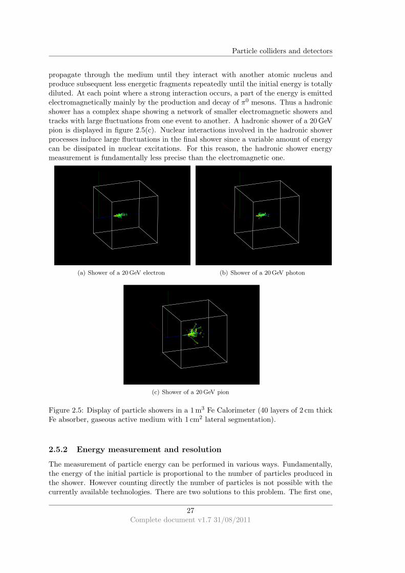
Particle colliders and detectors
propagate through the medium until they interact with another atomic nucleus andproduce subsequent less energetic fragments repeatedly until the initial energy is totallydiluted. At each point where a strong interaction occurs, a part of the energy is emittedelectromagnetically mainly by the production and decay of π0 mesons. Thus a hadronicshower has a complex shape showing a network of smaller electromagnetic showers andtracks with large fluctuations from one event to another. A hadronic shower of a 20 GeVpion is displayed in figure 2.5(c). Nuclear interactions involved in the hadronic showerprocesses induce large fluctuations in the final shower since a variable amount of energycan be dissipated in nuclear excitations. For this reason, the hadronic shower energymeasurement is fundamentally less precise than the electromagnetic one.
(a) Shower of a 20 GeV electron (b) Shower of a 20GeV photon
(c) Shower of a 20GeV pion
Figure 2.5: Display of particle showers in a 1 m3 Fe Calorimeter (40 layers of 2 cm thickFe absorber, gaseous active medium with 1 cm2 lateral segmentation).
2.5.2 Energy measurement and resolution
The measurement of particle energy can be performed in various ways. Fundamentally,the energy of the initial particle is proportional to the number of particles produced inthe shower. However counting directly the number of particles is not possible with thecurrently available technologies. There are two solutions to this problem. The first one,
27Complete document v1.7 31/08/2011

Particle colliders and detectors
and the most used so far in high energy physics experiments, consists simply in measur-ing the energy deposited by the shower in the sensitive medium of the calorimeter. Themeasured deposited energy is therefore close to the initial particle energy in the caseof homogeneous calorimeters or proportional to it in the case of sampling ones. Thesecond solution, possible only with a highly granular calorimeter, consists in countingthe number of calorimeter cells activated by the shower particles (or hits, for short).In this case, the number of hits is proportional to the initial particle energy. This so-lution is called digital calorimetry and is one of the options foreseen for future linearcolliders. The report focuses on sampling calorimeter properties. At first, electromag-netic calorimetry aspects are discussed and then applied to the more complicated caseof hadronic calorimetry.
2.5.2.1 Energy measurement in electromagnetic calorimetry
As already mentioned, in the case of electromagnetic particles, the calorimeter response,or visible energy Evis is proportional to the initial energy E. The proportionality factordepends on the calorimeter structure and material. Two energy independent factorsrelate Evis to E, the “sampling fraction” and the e/mip ratio.
- The sampling fraction FS is the fraction of a Minimum Ionizing Particle (MIP)energy loss specific to the calorimeter active medium. It reads:
FS =
(dEdx
)
activ.LS
(dEdx
)
passiv.Labs
, (2.1)
with Labs the absorber thickness, LS the active layer thickness and in the limit(
dEdx
)
activ.≪(
dEdx
)
passiv., which is generally true for sampling calorimeters. Note
that the quantity E · FS represents the visible energy from a MIP loosing theenergy E in the complete calorimeter. FS can not be directly measured and hasto be computed from the calorimeter layout.
- The e/mip ratio denotes the relative intensity of the calorimeter response to elec-tromagnetic particles in unit of its response to MIPs. It is defined as the ratiobetween the calorimeter response to an electron Evis and its response to an idealMIP7 loosing in the calorimeter the same energy E. It is given by:
e/mip =Evis
E FS,
and can be directly measured from calibration data from the considered calorime-ter.
Now, the relation between the visible and the initial energy reads:
Evis = (e/mip)FSE . (2.2)
7An ideal Minimum Ionizing Particle (MIP) is a particle traversing matter with a constant and min-imal energy loss without emission of secondary radiation. Real muons constitute a good approximationof ideal MIPs. They are really at the minimum of ionisation when their energy is ≈ 0.35 GeV and areonly slightly above for higher energies up to ≈ 1TeV. They also traverse matter without any showeringprocess.
28Complete document v1.7 31/08/2011

Particle colliders and detectors
Energy resolution The question of how precise is the relation 2.2 to determine theinitial energy from the calorimeter response arises. The shower process is a stochasticphenomenon and therefore the precise shape and the number of particles fluctuate onan event by event basis and the relation 2.2 is only an average. The error dependsobviously on the one hand on the precision of the estimate of FS and e/mip, but onthe other hand, the intrinsic energy resolution comes from statistical effects. The visibleenergy is closely related to the number of particles traversing the active medium andtherefore its fluctuations as well. Let Np be the number of particles crossing the activelayers and
√Np be its error. To have an estimate of Np, divide the visible energy Evis
by the average energy loss of an electron in an active layer Eel:
Np ≈ Evis
Eel.
Eel is given by:
Eel = k
(dE
dx
)
passiv.LS
1
〈cos θ〉 , (2.3)
with the k = 1.1 factor accounting for the fact that(
dEdx
)
passiv.is evaluated for MIPs
and real electrons give roughly a 10% higher signal, LS is the active layer thickness and〈cos θ〉 is the average cosine of the particle incidence angle in the active medium. Fromthis follows:
σE
E=
σEvis
Evis
= K
√τ
E, (2.4)
with
K =
√
10−3ǫcae/mip 〈cos θ〉 ,
ǫca being the critical energy of the absorbing medium corresponding the the thresholdenergy of an electron at which radiative energy losses are equivalent to collision energylosses. This threshold is of the order of 10 to 100 MeV depending on the material. The
value of 〈cos θ〉 is given by 〈cos θ〉 ≈ cos(
E FS
πǫca
)
.
2.5.2.2 Energy measurement in hadronic calorimetry
The basic principle of hadronic calorimetry is the same as in the electromagnetic casebut the main difference is that the visible energy is usually not linearly proportional tothe initial particle energy. This is due to the fact that hadronic showers are composedof a pure hadronic component but also of an electromagnetic one. Both componentsgive different response, the electromagnetic one being usually higher, and the relativecontribution of both components is energy dependent leading to the non linearity ofhadron energy measurement.
29Complete document v1.7 31/08/2011
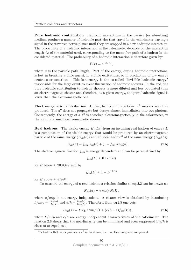
Particle colliders and detectors
Pure hadronic contribution Hadronic interactions in the passive (or absorbing)medium produce a number of hadronic particles that travel in the calorimeter leaving asignal in the traversed active planes until they are stopped in a new hadronic interaction.The probability of a hadronic interaction in the calorimeter depends on the interactionlength λI of the material used, corresponding to the mean free path of a hadron in theconsidered material. The probability of a hadronic interaction is therefore given by:
P (x) = e−x/ λI ,
where x is the particle path length. Part of the energy, during hadronic interactions,is lost in breaking atomic nuclei, in atomic excitations, or in production of low energyneutrons or neutrinos. This lost energy is the so-called “invisible hadronic energy”responsible for the large event to event fluctuation of hadronic showers. In the end, thepure hadronic contribution to hadron showers is more diluted and less populated thanan electromagnetic shower and therefore, at a given energy, the pure hadronic signal islower than the electromagnetic one.
Electromagnetic contribution During hadronic interactions, π0 mesons are oftenproduced. The π0 does not propagate but decays almost immediately into two photons.Consequently, the energy of a π0 is absorbed electromagnetically in the calorimeter, inthe form of a small electromagnetic shower.
Real hadrons The visible energy Evis(π) from an incoming real hadron of energy Eis a combination of the visible energy that would be produced by an electromagneticparticle of the same energy (Evis(e)) and an ideal hadron8 of the same energy (Evis(h)):
Evis(π) = femEvis(e) + (1 − fem)Evis(h) . (2.5)
The electromagnetic fraction fem is energy dependent and can be parametrised by:
fem(E) ≈ 0.1 ln(E)
for E below ≈ 200 GeV and by
fem(E) ≈ 1 − E−0.15
for E above ≈ 5 GeV.To measure the energy of a real hadron, a relation similar to eq. 2.2 can be drawn as:
Evis(π) = π/mipFSE ,
where π/mip is not energy independent. A clearer view is obtained by introducing
h/mip = Evis(h)E FS
and e/h = Evis(e)Evis(h) . Therefore, from eq 2.5 one gets:
Evis(π) = E FS h/mip (1 + (e/h− 1)fem(E)) , (2.6)
where h/mip and e/h are energy independent characteristics of the calorimeter. Therelation 2.6 shows that the non-linearity can be minimised and even suppressed if e/h isclose to or equal to 1.
8A hadron that never produce a π0 in its shower, i.e. no electromagnetic component.
30Complete document v1.7 31/08/2011

Particle colliders and detectors
e/h ratio, compensation and energy resolution constant term As shown above
the e/h ratio, defined by e/h = Evis(e)Evis(h) , if equal to one, restores the linearity of the
calorimeter. This condition is called “compensation”, in the sense that the differencebetween electromagnetic and hadronic response is compensated. However, reaching thecompensating condition is not trivial. A careful choice of the calorimeter material canlead to the compensation. For instance, Uranium absorbers produce additional neutronsand thus enhance the hadronic response of the calorimeter to reach compensation. Thee/mip ratio can be tuned as well by a careful choice of the calorimeter materials andlayout, a lower e/mip ratio correspond to a lower response to electromagnetic signal andtherefore a smaller hierarchy between Evis(e) and Evis(h) is achieved.
The e/h ratio, contribute to a constant term in the energy resolution of a hadroniccalorimeter through the e/π ratio which relates to e/h via:
e/π =Evis(e)
Evis(π)=
e/h
1 + fem(e/h− 1)
which gives the calorimeter energy resolution constant term φ(e/π), that vanishes fore/h = e/π = 1:
φ(e/π) ≈ −0.207ln(e/π) − 4.5 · 10−3 for e/π < 0.955 ,
φ(e/π) ≈ −0.281ln(e/π) − 2.1 · 10−2 for e/π > 1.115 .
This constant term is the main contribution to energy resolution at high energy. Theother term, the stochastic term, decreases as 1/
√E and takes into account the sampling
fluctuations and the intrinsic hadronic invisible energy fluctuations. They are summedquadratically as:
Stochastic term =
√
σ2intr. + σ2
sampl.
E=
C√E
Finally the hadron calorimeter energy resolution reads:
σE
E=
C√E
⊕ φ(e/π)
2.6 Particle Flow Algorithm
An event reconstruction and analysis method called Particle Flow Algorithm (PFA) isenvisioned for future linear collider experiments to achieve the excellent jet energy resolu-tion (stochastic term below 30%/
√E) required for the foreseen precision measurements
[32, 33].The concept of particle flow techniques is to consider the physics events in terms of
reconstructed particles rather than signal in detectors and use the most suitable sub-detector to measure a particle four-vector. As mentioned in table 2.4 (p. 24), differentkinds of particles give specific signals in the different sub-detectors allowing them tobe individually identified. In a PFA, the electron energy is deduced from its momen-tum measurement in the tracker rather than from the direct energy measurement inthe ECAL. The same stands for charged hadrons. Only neutral particle energies aremeasured in calorimeters.
31Complete document v1.7 31/08/2011

Particle colliders and detectors
A detector optimised for the application of particle flow techniques must be ableto distinguish single particle signals in every sub-detector. This task is already wellundertaken by trackers, which can easily distinguish separate particle tracks providedthey don’t completely overlap. On the contrary, calorimeters are usually made out oflarge tiles representing a certain segmentation of the solid angle (e.g. segmentationof ∆Φ∆η = 0.1 × 0.1 in ATLAS HCAL[34]) making single particle shower separationimpossible. To allow single particle recognition, a particle flow optimised calorimetermust have an unprecedented lateral and longitudinal segmentation (3 × 3 cm2 for theAnalog Hadronic Calorimeter (AHCAL) project and 1× 1 cm2 for the Digital HadronicCalorimeter (DHCAL) ones), giving rise to the concept of “imaging calorimetry”. Thisway, hit clusters in calorimeters can be isolated and matched with tracks from the trackerto reconstruct the entire signal from individual particles. Placing the magnet coil outsideof the HCAL would be necessary to allow an efficient matching of reconstructed trackswith clusters and is therefore mandatory for a particle flow optimised detector.
The main successive steps of the PFA are summarised as follows:
1. Reconstruct tracks
2. Regroup calorimeter hits in clusters
3. Match together clusters and tracks pointing to them to build the charged particles
4. Isolated clusters remaining must be taken as neutral particles
5. Charged particle energy is deduced from its precise momentum measurement andthe deduction of its mass after the particle identification:
- Cluster mainly in ECAL: electron
- Cluster mainly in HCAL: pion
- Track across the whole detector: muon
6. Charged clusters are removed and the energy of neutral particles only is measuredthanks to classical calorimetry
Figure 2.7 illustrate the interest of imaging calorimetry. The capability to clearlyidentify and separate contribution from different particles is a fundamental aspect ofPFA.
Jet energy resolution using PFA In traditional calorimetry, the jet energy reso-lution is governed at low energy by a stochastic term of the order of 50% – 100%/
√E
and by leakage at high energy (∝ log(E)). Many interesting processes at future linearcolliders require a good discrimination between W and Z0 bosons in their hadronic de-cay, wich in turn require a jet energy resolution better that 30%/
√E [32]. The PFA,
by optimising the energy measurement, allows a reduction of the impact of leakage andstockastic terms and fulfils the requirement. Nevertheless, a new source of uncertaintyis introduced because of the probability of errors and mismatch in the hit clustering andthe cluster/track association. This effect is called “confusion”. Its various consequencesare:
32Complete document v1.7 31/08/2011

Particle colliders and detectors
- hadronic showers may be split into one charged cluster (matched with a track) andone or more neutral clusters
- true neutral clusters can be associated with a charged one and therefore missed,
- in case of partial overlap between charged and neutral clusters the association ofhits to one cluster or another is subject to uncertainties,
- photon clusters close to a charged hadron cluster could be merged with the latterand missed.
Confusion mainly affects the resolution on the energy of the neutrals and is thereforebalanced by the low proportion of neutral particles within a jet, as given in table 2.5. Asemi-empirical formula is given in [33] to describe the overall jet energy resolution. Itreads:
rms90E
=21%√E
⊕ 0.7%
︸ ︷︷ ︸
classical stochasticand constant terms
⊕ 0.004E︸ ︷︷ ︸
leakage andthreshold effect
⊕ 2.1%
(E
100 GeV
)0.3
︸ ︷︷ ︸
confusion term
, (2.7)
where rms90 represent the standard deviation of the energy distribution containing 90%of the entries around the mean value. The various contributions to jet energy resolutionare represented in figure 2.6, left, and the right side show a comparison of the PFAjet energy resolution with classical calorimetry. Above 400 – 500 GeV, the confusiondominates and reduces the advantage of PFA against classical calorimetry. To balancethis, one solution is to stop the topological separation of the particles when the overlapis too large and simply measure the energy of the global cluster. The contribution ofthe charged particles is subtracted and the remaining energy is attributed to neutrals.This method is called “energy flow”.
Table 2.5: Average composition of jets (figures from [33])Type of particle Proportion Energy resolution Contrib. to jet energy resolution
Charged 62% 10−4E2 < 3.6 · 10−5E2j
Photon 27% 0.15√E 0.08
√Ej
Neutral hadron 10% 0.55√E 0.17
√Ej
invisible ∼1% — —
PFA is in the backdrop of all the work reported in this thesis. The optimisation of aDHCAL for the application of PFA calls for compact and highly segmented active layersto achieve the required imaging capability. This is precisely the context of the first part ofthis thesis, reporting on Research and Development (R&D) on gaseous detectors, calledMICROMEGAS, as condidate for PFA optimised DHCAL active layer. The PFA hasbeen implemented (among others) in a software called PandoraPFA [33] which is usedfor the benchmark studies of the CLIC Conceptual Design Report (CDR) preparationphysics studies. The data for the top quark study described in the second part of thisthesis are taken from the CLIC CDR production data. Therefore the PFA is used andits performance in a realistic physics case are illustrated.
33Complete document v1.7 31/08/2011

Particle colliders and detectors
Figure 2.6: Contributions to jet energy resolution with the PFA (left); Comparison ofPFA against classical calorimetry (right). Taken from [33]
(a)
(b) (c)
Figure 2.7: Illustration of particles interaction in the various subdetectors (a), of thecorresponding signal in classical detectors (b) and in a PFA optimised detector (c).
Resume du chapitre
De maniere generale, en sciences, l’observation directe des phenomenes naturels precedeles etudes en laboratoire qui, quant a elles, fournissent de precieux renseignements grace
34Complete document v1.7 31/08/2011

Particle colliders and detectors
a des mesures en environnement controle. En Physique des Particules, cette observationde la nature est faite par exemple grace a l’etude des rayons cosmiques, et les experiencesen laboratoire sont faites a l’aide d’accelerateurs de particules.
On s’interessera plus particulierement aux collisionneurs de particules, appareils con-stitues de deux systemes d’acceleration, conduisant les particules accelerees vers un ouplusieurs points de collision, ou des systemes de detection sophistiques enregistrent l’issuedes collisions.
A l’heure actuelle le LHC (Large Hadron Collider) tient le devant de la scene enphysique des particules et devrait permettre des avancees decisives dans cette quete deNouvelle Physique. Cependant, les decouvertes eventuelles du LHC appelleront a desmesures de precisions complementaires impossibles aupres d’un collisionneur de hadronsqu’est le LHC. Pour ce faire, des collisionneurs lineaires electron/positron sont envisages.Deux projets sont en developpement : ILC (Internationnal Linear Collider) et CLIC(Compact Linear Collider) differencies en pratique par la gamme d’energie accessiblepour les collisions e+e− (energie nominale : 500 GeV pour ILC et 3 TeV pour CLIC).
Detecteurs et calorimetrie Un collisionneur utilise des champs electriques et magne-tiques pour accelerer et controler les particules, pour les amener a une energie donnee,a un point de collision. Le point de collision d’un collisionneur est equipe d’un systemede detection sophistique constitue de plusieurs sous-detecteurs organises en peluresd’oignon. Dans l’ordre, du cœur vers l’exterieur, on trouve : les trajectographes, tresprecis mais sensibles seulement aux particules chargees ; les calorimetres, composes demateriaux denses, ils ont pour role de stopper les particules afin de mesurer leur energie,leur resolution est bien moins bonne que celle d’un trajectographe ; les chambres amuons, seuls les muons parviennent a traverser les calorimetres et peuvent alors etreobserves dans ses detecteurs. Un champ magnetique est utilise pour courber la trajec-toire des particules chargees et ainsi mesurer leur impulsion dans les trajectographes.Ce champ magnetique est genere par un aimant solenoıdal.
Flux de particules et calorimetrie Pour realiser les mesures de precision prevuesaupres de ces futurs collisionneurs lineaires, une technique de reconstruction des evene-ments appelee algorithme de flux de particules est envisagee et implique de fortes con-traintes sur la conception des detecteurs aux points de collision de ces collisionneurs.
Un algorithme de flux de particules signifie penser l’etude de l’issue d’une collisionen terme de particules sortantes plutot qu’en terme de depots d’energie. Ceci impliquede reconstruire integralement et fidelement les particules de l’evenement. L’interet estqu’une fois que tous les signaux de chaque sous detecteur sont attribues a un ensemblede particules reconstruite, l’energie des chargees pourra etre deduite de la mesure tresprecise de leur impulsion et de la connaissance de leur masse suite a leur identificationlors de le reconstruction. Sachant que dans un jet, environ 60% de l’energie est porteepar des hadrons charges, la mesure de l’energie d’un jet a beaucoup a gagner a mesurercette contribution a l’aide du trajectographe plutot que des calorimetres. La resolutionatteignable serait meilleure que 3–4% sur toute la gamme d’energie envisagee, soit envi-ron deux fois meilleure que l’etat de l’art actuel. L’utilisation optimale d’un algorithmede flux de particules implique de fortes contraintes sur la conception des detecteurs.Entre autre, le calorimetre hadronique doit etre place a l’interieur de l’aimant et donc
35Complete document v1.7 31/08/2011

Particle colliders and detectors
doit etre le plus compact possible. Le calorimetre doit aussi disposer d’une segmentationtransverse et longitudinale sans precedent en calorimetrie hadronique (ex : 40 coucheslongitudinalement et 1×1 cm2 lateralement) et les zones mortes doivent etre minimisees.
36Complete document v1.7 31/08/2011

Part II
Characterisation andDevelopment of MICROMEGAS
Chambers for HadronicCalorimetry at a Future Linear
Collider
37


CHAPTER 3
MICROMEGAS chambers for hadronic calorimetry
After a brief introduction on gaseous detectors, the MICRO MEsh GAseous Structure(MICROMEGAS) technology is presented. The Research and Development (R&D)project on large area MICROMEGAS chambers using bulk technology for application todigital hadronic calorimetry is introduced. The different prototypes are described andthe road map of the project is presented.
3.1 A brief overview of gaseous detectors
The principle of particle detection with gas is based on electromagnetic interactions. Asa charged particle moves close to an atom, an energy transfer occurs and, if sufficient,can result in its ionisation. Depending on the detection technique, this ionization leadsto a phase transition (cloud or bubble chambers) or, by applying an electric field, ionisedelectrons can be manoeuvred and multiplied to produce an electric signal that can beprocessed by an electronic circuit.
The first gaseous detector was the well known Geiger-Muller tube, or Geiger counter.Its principle was described by Hans Geiger in 1908 [35] and the first counter was builtin 1928 [36]. A Geiger counter consists of a grounded conductive tube enclosing a lowpressure gas volume in the middle of which a high voltage wire is stretched. Any ionisingradiation penetrating the gas volume provokes a discharge in the gas and therefore allowsthe detection of the radiation. Such devices are very rate limited, a dead time of about200µs occurs after a discharge. Because of the saturated functioning, no signal amplitudeis measured. These simple detectors are still largely in use nowadays for measurementsof weak activity sources.
Among the first gaseous detectors were also the cloud chambers developed by theScottish physicist Charles Thomas Rees Wilson in the early 20th century [37]. They al-lowed several great discoveries, like anti-matter (1933 [38]) or new particles in the cosmicrays (e.g. the muon in 1937 [39]). Originally, physics events were recorded thanks toemulsions or cloud chambers coupled to cameras furnishing photographs of events that
39

MICROMEGAS chambers for hadronic calorimetry
had to be carefully analysed one by one. In 1968, Georges Charpak invented the Multi-Wire Proportional Counter (MWPC) [40] allowing particle positions or trajectories tobe electronically recorded and hence processed thanks to the development of early com-puters. This innovation revolutionised experimentation in particle physics. High rateexperiments were then possible allowing massive data acquisition.
The main limitation of electron multiplying gaseous detectors is their rate capabilitydetermined by ion occupancy in the amplification region. As long as the ions are notcollected, they are screening the electric field responsible for electron multiplicationwhich is hence nearly suppressed, resulting in a dead time causing a drop of detectionefficiency. The performance of the first of these detectors however complied with theneed of the early collider experiments.
Some gaseous detectors are presented now, namely the Multi-Wire ProportionalCounter (MWPC) being the first electron amplifying gaseous detector, the Micro-StripGas Chamber (MSGC) and the Micro-Gap Chambers (MGC) as major evolutions thatpreceded the development of the MICRO MEsh GAseous Structure (MICROMEGAS).This presentation is non-exhaustive and aims at illustrating the evolution of gaseousdetector technologies.
3.1.1 Multi-Wire Proportional Counter
The Multi-Wire Proportional Counter (MWPC) [41] is a chamber filled with a noblegas based mixture. Two cathode planes define a drift gap in the middle of which thin(≈20–50µm) anode wires at high voltage generate an accelerating electric field at theirvicinity. The MWPC working principle resides in the drifting of ionised electrons towardsthe anode wires where the intense electric field at the wire surface multiplies them viaan avalanche process. The so-produced moving charges induce a signal on the wires thatcan be electronically read out.
Figure 3.1 illustrates the electric field configuration in a MWPC. Figure 3.1(a)emphasises the drift region far from the wires where the field is uniform. Figure 3.1(b)focuses on the amplification region close to the wires where the electric field equipotentiallines are concentric. The field strength close to the wires depends on the applied voltageand on the wire diameter and can reach several 105 V· cm−1.
However, the MWPCs have certain limitations. The spatial resolution is limited bythe wire spacing, limited itself by mechanical constraints due to electrostatic repulsionbetween the thin wires. The best spatial resolution is of the order of 1 mm. The rateof the MWPCs is limited by a drop of the gain due to the avalanche ions drifting backfrom the anode wires towards the cathode planes and thus compensating the electricfield. Rates about 105 Hz/wire can be achieved [40].
Efforts have been made to improve the MWPC spatial resolution and rate capabil-ity. The use of a segmented ion collecting cathode (with pads or strips) can improvethe spatial resolution together with providing two dimensional information. The finesegmentation allows the computation of the barycentre of the charge deposition on thecathode and thus provide very precise two dimensional spatial information. Resolutionof a few tens of microns have been achieved this way.
The use of a grid as intermediate electrode between the drift region, where the fieldlines are parallel, and the amplification region, where they start to bend towards the
40Complete document v1.7 31/08/2011

MICROMEGAS chambers for hadronic calorimetry
(a) (b)
Figure 3.1: Field line configuration in a MWPC[41].
wires, allows the drift field to be raised thus increasing the drift velocity of the primaryelectrons. The intermediate grid can also reduce the ion back-flow towards the driftregion. With a higher electron drift velocity, a slightly higher rate capability can beachieved. Details about developments of this solution are found in [41].
Along with the development of electronics, particle physics could take great advan-tage of the possibilities of particle accelerators, and called for detectors with higher ratecapabilities than those of the MWPC.
Among various different types of gaseous detectors (see [42] for a broader overviewof the different types of gaseous detectors), some were especially designed to outperformthe MWPCs in terms of rate capability.
3.1.2 Some electron amplifying gaseous detectors
3.1.2.1 Micro-Strip Gas Chamber
In 1988, almost twenty years after the invention of MWPC, the Micro-Strip Gas Chamber(MSGC) [43], a new design of detector, was introduced based on the same principle: elec-tron amplification resulting from the high electric field in the vicinity of thin electrodes.
To obtain a better spatial resolution than the basic MWPC, wires are replaced bystrips of the same thickness printed by photolithography on a insulating substrate ora Printed Circuit Board (PCB). Thus the mechanical constraints concerning the wirespacing does not hold anymore and the MSGC strips can be much closer to each otherthan the MWPC wires. As displayed in figure 3.2(a), the strips can be set as close toeach other as ≈ 200µm, leading to a spatial resolution of ≈ 60µm orthogonal to thestrips. Using a segmented ion collecting cathode still brings the same advantages as forthe MWPC.
To improve the rate capability, a solution has been found to more rapidly evacuatethe ions: cathode strips are interleaved with anode ones (see schematics in figure 3.2(a).In this case, ionised electrons are driven to the amplification strips from anywhere in thegas volume along the field lines and the ions, produced in the vicinity of the amplifyingstrips are attracted and quickly collected by the nearby cathode strips. The electric field
41Complete document v1.7 31/08/2011

MICROMEGAS chambers for hadronic calorimetry
configuration is displayed in figure 3.2(b).
(a) (b)
Figure 3.2: MSGC principle (taken from [43]).
Unfortunately, this development produced a new issue: the ions moving between thestrips are very close to the substrate surface and tend to get stuck on it by diffusionand thus to tend to charge the substrate up. This charging up causes a distortion ofthe electric field configuration, lowering progressively the detector gain and increasingthe breakdown probability. Several solutions where tested (electrode at the back of thePCB to repulse the ions from the substrate surface, resistive coating of the substrate ...)leading to some improvement, but the ageing of the MSGCs remained a problem.
3.1.2.2 Micro-Gap Chambers
In 1993, Micro-Gap Chambers (MGC) [44] were introduced as a successor of the MSGCs,with comparable or even better performance and no charging up problem. The basicprinciple is still the same as MWPC and MSGC, but here the anode strips are notdirectly deposited on the substrate, they stand on wider insulating strips (only a fewmicrons wider) which lie on a conductive plane fixed on the substrate. This metallicplane plays the role of the ion collecting cathode. The very small surface of the insulatordoes not lead to any charging up and the proximity of the cathode to the anode (a fewmicrons) leads to faster evacuation of the ions, a lower ion back-flow towards the driftelectrode and a higher field near the anode strips. A scheme of the MGC is sketched infigure 3.3.
42Complete document v1.7 31/08/2011

MICROMEGAS chambers for hadronic calorimetry
Figure 3.3: Scheme of the MGC principle [44].
3.2 MICROMEGAS technology
Another generation of gaseous electron amplifying detectors is now presented. For thesedetectors, drift and amplification of ionised electrons occur in different gas regions sep-arated by a conductive mesh nearly transparent to electrons. Ionization takes place inthe large (few mm to 1 meter or more) drift volume and electrons are driven to the≈ 50–150µm thick amplification volume where the high electric field lying between themesh and the segmented anode plane allows electron avalanche amplification.
3.2.1 Description and basic principle
The MICRO MEsh GAseous Structure (MICROMEGAS) chamber was introduced in1996 [45] as a fast signal, position-sensitive, radiation hard gaseous detector. It consists ofa gas chamber where two asymmetric gaps are defined by three electrodes. The drift gaplies between the drift electrode and a conductive mesh, and is usually a few millimetresthick1. The amplification gap is located between the mesh and the segmented anodeand is only about a few tens of microns thick. The drift gap is also called conversiongap because the ionization of the gas by incoming radiation occurs mainly in it.
In both gaps, a specific electric field is defined by the voltage applied to each electrode.The field in the drift space is rather low (around 100 V· cm−1) and is meant to driftionised electrons to the mesh. The field in the amplification gap is very high (severaltens of kV· cm−1) and catches the free electrons from the drift gap to forcefully acceleratethem through the small amplification gap. They then acquire enough energy to ionisesurrounding gas. The newly ionised electrons gain as well sufficient energy to ionise thegas again and again, thus forming an avalanche and leading to a measurable electricsignal on the anode and on the mesh. The MICROMEGAS principle is illustrated infigure 3.4.
1MICROMEGAS TPCs present a much larger drift gap, up to several meters.
43Complete document v1.7 31/08/2011

MICROMEGAS chambers for hadronic calorimetry
Figure 3.4: Scheme of MICROMEGAS principle.
3.2.2 The MICROMEGAS signal
Electron amplification The electron avalanche occurring in the amplification gap(see working principle in section 3.2.1) produces a high number of ionisations (up tomore than 25 000 per primary electron). The average of this number is called themultiplication factor or (gas) gain of the chamber. The size of the avalanche showslarge variations around its average value. A model of gas amplification, establishedin [46], gave the number of electrons n in an avalanche through a simple exponentialprobability distribution (valid for n≫ 1):
p(n) =1
nexp
(
−nn
)
. (3.1)
where n is the average number of electron in the avalanche. n is given by :
n = exp
(∫ x
0α(x′) dx′
)
, (3.2)
where x denotes the distance covered by the avalanche and α(x) is the first Townsendcoefficient which depend on the gas mixture and the electric field configuration. Typicalvalues of this coefficient, in the present application are expected around ≈ 0.075µm−1.
Induced signal The current generated by the moving charges in the amplification gaphas two contributions:
- A brief and fast signal due to the electrons, generated mostly close to the anodeplane and quickly collected (1–2 ns). The drift velocity of electron in gas is ofseveral cm·µs−1.
44Complete document v1.7 31/08/2011
MICROMEGAS chambers for hadronic calorimetry
- A long signal due to the ions moving slowly towards the mesh (100–200 ns), theirdrift velocity is at least two order of magnitude lower than the electrons’ one.
Figure 3.5 illustrates the calculation in annex A (page 151) of the time developmentof the MICROMEGAS signal and the integration of the anode deposited charge. It isinteresting to note that the total charge is simply the gain multiplied by the primarycharge (see equation A.13), and that in fact the amplified electrons do not contributemuch to the final detected charge. The main contribution is clearly due to ions.
s)µTime (-410 -310 -210 -110
Cu
rre
nt (
nA
) / A
ccu
mu
late
d c
harg
e (
fC)
-110
1
10
210
310
Induced current
Accumulated charge
Figure 3.5: Plots of the MICROMEGAS induced current and accumulated charge versustime.
The proportion between the two contributions relates directly to the gain of thechamber. The fraction ηe of the signal due to electrons is given by (see equation A.15recalled here):
ηe =Qe
QTOT=
1
α g=
1
ln(G),
with Qe, the charged induced by electrons, QTOT, the total induced charge, α, the firstTownsend coefficient, g the gap width and G the gas gain.
3.2.3 Bulk MICROMEGAS
The fabrication process of the first MICROMEGAS chambers did not allow the massproduction of sensitive areas larger than a few square centimetres The largest MI-CROMEGAS chambers built with electroformed nickel meshes are used in the COM-PASS experiment [47, 48]. Eleven 40 × 40 cm2 MICROMEGAS chambers are part ofthe experiment tracking system. [45, 49, 50]. In 2006, a new way to manufacture MI-CROMEGAS chambers was established based on the PCB technology [51]. This so-called“bulk” technology consists of laminating one or more thin layers of photo-resistive film onthe anode PCB, then laminating the micro mesh and another layer of the same film (see
45Complete document v1.7 31/08/2011

MICROMEGAS chambers for hadronic calorimetry
figure 3.6). The photo-resistive film is then irradiated with UV light to print insulatingpillars by photo-lithography. The top photo-resistive layer, after the photolithographyprocess, ensures a strong encapsulation of the mesh giving a robust final device. Theformer thin electroformed nickel micro-mesh is then replaced by an industrial stainlesssteel micro-woven mesh made of 30µm thick wires.
Figure 3.6: The MICROMEGAS bulk fabrication process [51].
This industrial process allows massive production of cheap and robust MICROMEGASchambers and thus to evolve towards very large area detectors needed for instance inhadronic calorimetry at future linear colliders (≈3000 m2 for the SiD detector [52]).
3.3 Context of the R&D project
The use of the Particle Flow Algorithm (PFA) technique [32, 33] for event reconstructionand analysis at future linear colliders calls for detectors to be optimised for this purpose.One of the main requirements is that the signal induced by single particles must beindividually identifiable. This calls for highly segmented calorimeters together with ahigh efficiency and low hit multiplicity in order to topologically separate the contributionof each particle in the calorimeters and to efficiently spot shower starts and hadronicinteractions. To efficiently match a charged track with a calorimeter cluster, a primerequirement is that the Hadronic Calorimeter (HCAL) must be inside the solenoid andthus minimisation of the HCAL thickness is highly desired. For the sake of compactness,another requirement is that the power consumption of the readout electronics must bebelow 10µW per channel in order to limit the size of the cooling system.
The final calorimeter will hold several thousands of square meters of active mediumindicating a need for developments directed at very large area detectors.
Several technological solutions are envisaged to fulfil those requirements [52, 53],scintillators with analog readout or gaseous detectors with digital readout (Gas ElectronMultipliers (GEMs), Resistive Plate Chambers (RPCs) and MICROMEGAS). The digi-tal readout is needed to reduce the impact of the data handling and storage and thus thepower consumption together with allowing a thinner lateral segmentation. Additionally,the digital readout tends to reduce the effect of energy deposition fluctuations in gas andtherefore increase precision of gaseous detectors for this application. All these develop-ments are carried out within the Calorimetry for Linear Colliders Experiments (CAL-
46Complete document v1.7 31/08/2011

MICROMEGAS chambers for hadronic calorimetry
ICE) collaboration [54]. The GEM and MICROMEGAS activities are as well part of theRD51 collaboration [55]. These solutions need to be carefully analysed in order to selectthe one best suited for the final application. A detailed evaluation of the advantages anddrawbacks of each is mandatory. In the following, a study of bulk MICROMEGAS cham-bers as a candidate for the active medium of a Digital Hadronic Calorimeter (DHCAL)is presented.
3.4 R&D project outline
The bulk technique makes MICROMEGAS an appealing solution for equipping a HCALand calls for further study in this direction. A R&D project was therefore started at theLaboratoire d’Annecy-le-vieux de Physique des Particules (LAPP) in 2007 to investigatethe application of bulk MICROMEGAS to hadronic calorimetry.
The study of bulk MICROMEGAS chambers as candidate for the active medium ofa DHCAL can be imagined in several distinct phases, as follows:
1. Successfully assemble a MICROMEGAS chamber satisfying the thickness require-ments
2. Perform a series of tests on small prototypes to evaluate their basic performance
3. Test the chip embedding process for MICROMEGAS chambers
4. Develop dedicated digital readout chips and a Data Acquisition System (DAQ)
5. Evolve towards larger area detectors: produce a functional square meter prototypewith embedded readout electronics and verify the conservation of performance
6. Build a cubic meter calorimeter to evaluate its performance and perform physicsmeasurements
Phase 1 has already been done during my Master internship where the detectionof cosmic signals was achieved with the first prototypes [56]. The second phase is themain topic of this part of the thesis and is detailed in chapter 4, where laboratory X-ray tests are described, and in chapter 5, where beam test studies are presented. Theremaining phases will be addressed in the last chapter of this part (chapter 6). Phasenumber 5 shares problems common to other experiments using similar MICROMEGASchambers (mainly T2K experiment [57]). Phases 3 and 5 are key stages in the devel-opment of the project to prove the feasibility of large area MICROMEGAS chamberswith embedded readout electronics, showing the very good performance promised bythe small prototypes used in phase 2. Phase 4 is undergo in tight collaboration withour electronics engineers who designed a key element of the common CALICE DAQ,namely the Detector Interface (DIF) board. They also developed a high gain, low noiseApplication Specific Integrated Circuit (ASIC) in collaboration with the Laboratoire del’Accelerateur Lineaire, Paris (LAL). The last phase of the list is of particular inter-est since the hadronic showering process has only very recently been observed with agranularity as fine as 1 × 1 cm2[58] and only with RPCs as active medium.
47Complete document v1.7 31/08/2011

MICROMEGAS chambers for hadronic calorimetry
3.5 Description of the prototypes
3.5.1 Common features
Each prototype consists of a bulk MICROMEGAS chamber with a 3mm drift gap and a128µm amplification gap. The drift cathode is a 5µm thick copper foil fixed on a 75µmthick Kapton2 film. The whole is glued on a 2 mm thick steel plate, forming the device’slid. The steel cover plate is part of the absorber and therefore would not contribute tothe HCAL active layer’s thickness. The 3 mm drift gap is ensured by a 3 mm thick resinframe enclosing the chamber and providing the gas inlet and outlet (see photography infigure 3.7(a)).
The mesh used is an industrial micro woven stainless steel mesh made of 30µmdiameter wires interwoven at a pitch of 80µm. The mesh is held at 128µm above theanode plane by 300µm diameter pillars placed on a square lattice with a 2 mm pitch. Theanode plane consists of 0.98×0.98 cm2 pads separated by 200µm lying on the detector’sPCB. The 1 cm2 pattern made of a pad and the free space around will be denotedhereafter as a 1 pad area where ‘pad’ will be the area unit symbol.
3.5.2 Analogue prototypes
Before building large digital prototypes, a detailed characterisation of the technology isneeded. For this purpose, four small prototypes with an analogue readout have beenbuilt and extensively tested.
Three of them have a 6×16 cm2 active area (96 pads) and the fourth one is four timeslarger with a 12×32 cm2 active area (384 pads). The mesh voltage of the small chambersis supplied through a dedicated pad while a 4 mm2 sidelong mesh voltage pad is used forthe large chamber (see figure 3.7). The analogue readout is provided by GASSIPLEXboards [59]. (see detailed description in section 5.1.2, page 63) In the following, the threesmall chambers will be denoted CH0, CH1 and CH2 and the large one, CH3.
3.5.3 Digital prototypes
Several readout chips have been designed and tested on various PCB designs. Theinnovative aspect is that the chips must be embedded on the detector PCB to minimisethe detector thickness and the dead zones due to readout boards outside the detectors.The readout chips are designed to ensure signal collection and preamplification veryclose to the detector, its digitisation and storage in a multi-event memory. The base-linedesign is that a single chip can handle 64 detector readout channels. The chip must beable to be power pulsed, namely, it will be switched on and off repeatedly in order tobe on only during the bunch trains3 and off the rest of the time. The aim of the powerpulsing is to reduce the average power consumption, minimise the cooling needs andthus the amount of dead material inside the detector.
The readout chips involved in this project are summarised in table 3.1.
2polyimide: C22H10N2O53The beam is not continuously delivered but the particle bunches are organised in trains of given
durations. Bunch trains are sometimes separated by long dead times.
48Complete document v1.7 31/08/2011

MICROMEGAS chambers for hadronic calorimetry
(a) (b)
Figure 3.7: Analogue readout prototypes. The left sketch gives CH0 to CH2 dimensionsand can be straightforwardly extended to CH3. The right picture shows the bulk, theresin frame and the electronic board connectors of CH3 before its lid was glued.
Table 3.1: Summary of the digital chipsChip Info. Developer Detector
DIRAC(2) [60]([61]) LAPP and IPNL 8 × 8 pad
HARDROC [62] LAL/Omega 8 × 32 pad and 32 × 48 pad
HARDROC2(b) [62] LAL/Omega 32 × 48 pad
MICROROC [63] LAPP and LAL/Omega 8 × 8 pad
One of the challenges of this project is that the chips have to be cabled in a solderingoven, but the bulk pillars do not tolerate this treatment. So the lamination process forthe bulk installation must take place after the chip soldering. But these latter are waynot robust enough to resist such a process. The solution is to solder the electronics onthe naked PCB and then place a rigid mask on the electronic side to protect it duringthe lamination phase. Using this technique the first MICROMEGAS with embeddeddigital readout has been successfully assembled and tested [64]. All following prototypeshave been mounted using this technique.
Resume du chapitre
Dans ce chapitre, on introduit le principe des detecteurs gazeux, dans lequel un ray-onnement ionisant cree des paires electron-ion qui sont ensuite amplifiees afin d’induireun signal electrique mesurable dans un systeme de lecture ad hoc. On s’interessera enparticulier a la technologie MICROMEGAS.
MICROMEGAS Un detecteur MICROMEGAS est une chambre remplie d’un melangegazeux a base d’un gaz noble tel que l’Argon. Le volume gazeux est separe en deuxregions asymetriques definies par trois electrodes planes : la cathode ou electrode de
49Complete document v1.7 31/08/2011

MICROMEGAS chambers for hadronic calorimetry
derive, la micro-grille et l’anode. La premiere region, epaisse de quelques millimetres aquelques metres (chambres a derive), situee entre l’electrode de derive et la micro-grille,est appelee “espace de derive”, elle est le siege de l’ionisation du gaz et de la derive deselectrons primaires vers la micro-grille separant les deux regions. La deuxieme region, ap-pelee “espace d’amplification”, situee entre la micro-grille et le plan d’anode, ne mesureque quelques dizaines de microns (50 – 100µm), il y regne un champ electrique suff-isamment intense (40 – 50 kV· cm−1) pour que les electrons primaires traversant la grillesoient amplifies (× ≈ 10 000) par ionisations en cascade, induisant ainsi un signal sur lagrille et sur le plan d’anode. Les ions generes lors du processus d’avalanche sont captespar la micro-grille et donc, grace a la faible epaisseur de l’espace d’amplification, sontrapidement (≈ 100 ns) evacues, permettant ainsi des utilisations a haut flux.
Prototypes MICROMEGAS pour la calorimetrie hadronique aupres d’un fu-tur collisionneur lineaire Pour satisfaire aux pre-requis d’un calorimetre hadroniqueoptimise pour l’application d’un PFA, des prototypes de detecteurs gazeux MICROME-GAS sont developpes au LAPP. Nos prototypes sont construits suivant la recente tech-nologie bulk. Deux couches de film photoresistif (64µm chacun) sont laminees sur lecircuit imprime supportant le plan d’anode, puis la micro-grille, tendue sur un cadrele temps de l’installation, subit le meme processus, et enfin une troisieme couche de cememe film est encore laminee par dessus. Par photolithographie, des piliers destines asoutenir la grille sont imprimes dans le film et maintienne la grille fermement en placea une distance constante de l’anode. Le produit final s’avere robuste et industrialisable,ideal pour une production a grande echelle.
Le plan d’anode est segmente en carreaux de 1 × 1 cm2, l’espace d’amplificationmesure 128µm d’epaisseur et l’espace de derive est assure par un cadre en resine de3 mm d’epaisseur fournissant egalement les entree et sortie du gaz. L’electrode de deriveest collee sur une plaque d’acier de 2 mm fermant la chambre. Ces deux millimetresd’acier comptent dans le budget du milieu passif du calorimetre.
Ce design doit subir differentes etapes de developpement et de test avant une pro-duction a grande echelle :
1. Construction d’un premier prototype fonctionnel.
2. Evaluation des performances.
3. Test de l’embarquement de l’electronique de lecture.
4. Developpement d’une electronique de lecture dediee optimisee.
5. Evolution vers de plus grandes surfaces : production de prototypes d’un metrecarre avec electronique de lecture embarquee et conservation des performances.
6. Construction d’un calorimetre d’un metre cube.
Les etapes de caracterisation des performances sont effectuees a l’aide de prototypes alecture analogique. Ces prototypes sont au nombre de quatre, trois d’entre eux presententune surface active de 6 × 16 cm2 et le dernier, une surface active de 12 × 32 cm2. Lalecture est assuree par des cartes GASSIPLEX montees en mezzanine sur le cote du plan
50Complete document v1.7 31/08/2011
MICROMEGAS chambers for hadronic calorimetry
d’anode (cf. fig. 3.7). Cette caracterisation est l’objet des deux prochains chapitres dece manuscrit.
Les differentes puces de lecture digitale, impliquees dans le projet a ce jour, sontpresentees dans la table 3.1. Lors de la fabrication des prototypes digitaux, l’installationde puces de lecture sur le circuit imprime d’anode se fait prealablement a la pose dubulk car ce dernier ne supporte pas un passage en four a soudure. Ensuite un masque deprotection en resine est installe sur le cote composant du circuit imprime afin de protegerl’electronique lors du passage en laminoir pour la pose du bulk.
51Complete document v1.7 31/08/2011

MICROMEGAS chambers for hadronic calorimetry
52Complete document v1.7 31/08/2011

CHAPTER 4
X-ray tests
X-ray tests using an 55Fe source have been performed to measure the basic performanceof our MICROMEGAS prototypes. For each of the prototypes, holes are drilled into thesteel lid in a few locations to allow X-ray injection through the thin cathode and Kaptonfoil.
Electron collection efficiency1 and gas gain in Ar/iC4H10 (95/5) and Ar/CO2 (80/20)were deduced from the 55Fe Kα photopeak value given by a fit of three gaussian functionsto the 55Fe spectrum (figure 4.1). Gain measurements were used to predict gain depen-dency versus pressure, temperature and amplification gap thickness variations. Thosepredictions are compared to direct measurements in section 4.5.
4.1 Experimental setup
For the X-ray study, only one chamber with a readout system based on the mesh signalwas used. The mesh signal was read out by an ORTEC 142C charge preamplifier linkedto its corresponding amplifier/shaper. The amplifier output was recorded with a CAENV550 10-bit ADCs (VME modules) sequenced by a CAEN V551B C-RAMS sequencerVME module. Data was then collected by the computer through an optical VME/PCIbridge. A Labview based software, called CENTAURE [65], was used to timestamp therecorded events for condition database matching. This software was optimised for thedata acquisition and on-line monitoring of the pad readout of the prototypes but wasperfectly usable for the mesh readout as well. The calibration constant of the meshreadout chain was precisely measured to be 2.199±0.026 ADU/fC (Analog to DigitalUnit).
1Or equivalently: mesh transparency to electrons
53

X-ray tests
ADU0 200 400 600 800 1000
Num
ber
of e
vent
s
0
50
100
150
200
250 / ndf 2χ 232 / 142
Cst_P 95.3± 8228 Mean_P 0.9± 439.1 Sigma_P 0.87± 69.58 Cst_E 60.3± 1143 Mean_E 2.8± 248.3 Sigma_E 2.16± 41.49
/ ndf 2χ 232 / 142Cst_P 95.3± 8228 Mean_P 0.9± 439.1 Sigma_P 0.87± 69.58 Cst_E 60.3± 1143 Mean_E 2.8± 248.3 Sigma_E 2.16± 41.49
DataTriple gaus fit
photopeakαK photopeakβK
Escape peak
Figure 4.1: 55Fe spectrum with gaussian fits of the two photopeaks and of the escapepeak.
4.2 Electron collection efficiency
The ratio between amplification and drift electric fields affects the mesh transparency tothe electrons (or collection efficiency) by contracting the field lines so that the electronsare mostly driven through the center of the mesh’s holes and reach the amplification gap.Figure 4.2 shows the variation of the 55Fe peak value versus the field ratio in Ar/iC4H10
(95/5) and Ar/CO2 (80/20). The amplification field was kept constant while the driftfield varied to set the field ratio. The mesh voltage was 420 V in Ar/iC4H10 (95/5) and570 V in Ar/CO2 (80/20).
The curves displayed in figure 4.2 (right) show a maximum at a field ratio of about150 – 200 for both gas mixtures. The measurements reported in the following wereperformed at ratios within this range.
A explanation for the decline at high field ratio observed in figure 4.2 is the attach-ment of some primary electrons in the drift region by electronegative impurities (e.g.oxygen, water vapour). For a constant amplification field, a higher ratio means a lowerdrift field and consequently the primary electrons tend to have less energy. Since the at-tachment cross section of some impurities peaks at low energy (e.g. ≈ 0.1 eV for oxygen[66]), a lower drift field can therefore lead to a higher attachment probability, resultingin a reduction of the number of electrons reaching the amplification region.
4.3 Gas gain
The amplification gap gain, so-called gas gain, is determined through a fit of three gaus-sian functions to the 55Fe spectrum (figure 4.1) assuming 230 and 209 primary electronsin the Ar/iC4H10 (95/5) and Ar/CO2 (80/20) mixtures respectively and using the mesh
54Complete document v1.7 31/08/2011

X-ray tests
Field Ratio0 100 200 300 400 500 600
Fe
Pea
k va
lue
(AD
U)
55
200
300
400
500
600
700
800
95/510H4Ar/iC
80/202Ar/CO
Figure 4.2: 55Fe peak value variation versus field ratio.
readout calibration constant (2.19 ADU/fC). Keeping the drift field at 150 V· cm−1, aset of measurements at 954 mbar in the Ar/iC4H10 mixture, 961 mbar in Ar/CO2 andat a temperature of 293 K with various voltage settings gave the curves displayed infigure 4.3. The maximum gas gain for each gas mixture is given by the last point of thegain curves and corresponds to a spark rate of about one per minute. A much highermaximum gain (4·104) can be achieved in Ar/iC4H10 than in Ar/CO2. Also the meshvoltage, for a given gain, is 180 V lower in Ar/iC4H10.
Mesh Voltage (V)380 390 400 410 420 430 440
Gas
gai
n
0
5000
10000
15000
20000
25000
30000
35000
40000
(a)
Mesh voltage (V)520 530 540 550 560 570 580 590 600
Gas
gai
n
2000
4000
6000
8000
10000
(b)
Figure 4.3: Gas gain versus mesh voltage fitted with the gas gain formula in Ar/iC4H10
(95/5) [4.3(a)] and in Ar/CO2 (80/20) [4.3(b)].
55Complete document v1.7 31/08/2011

X-ray tests
4.4 Method for pressure and temperature correction
4.4.1 Gas Gain Model
The gas gain of the chambers is given by the exponential of the average number ofprimary ionizations from a single avalanche initiating electron. In a uniform field, thisnumber is given by the first Townsend coefficient, denoted α, multiplied by the amplifi-cation gap thickness, denoted g:
G = eα·g . (4.1)
The Townsend coefficient can be parameterised by the Rose and Korff formula [67]:
α = n ·A0e−B0n/E , (4.2)
where A0 and B0 are constants that depends on the gas mixture, E is the electric fieldand n the gas density. Using the ideal gas law to express n and combining equations 4.1and 4.2, one obtain:
G = exp
[APg
T· exp
(
−BPgTV
)]
, (4.3)
with A = A0/kB, B = B0/kB and V = E · g, where kB is the Boltzmann constant.Equation 4.3 leads to the variation of the gas gain versus pressure (P ), temperature (T )and amplification gap thickness (g) through
∆G/G = CP ∆P + CT ∆T + Cg∆g ,
where Cx, x ∈ C,P, T, are the environmental dependency coefficients, expressed asfollows:
CP =1
G
∂G
∂P=
(
Ag
T− ABPg2
T 2V
)
exp
(
−BPgTV
)
(4.4)
CT =1
G
∂G
∂T=
(
ABP 2g2
T 3V− APg
T 2
)
exp
(
−BPgTV
)
(4.5)
Cg =1
G
∂G
∂g=
(
AP
T− ABP 2g
T 2V
)
exp
(
−BPgTV
)
. (4.6)
In practice, it is convenient to apply one single correction for pressure and temperaturevariations using the coefficient:
CP/T =1
G
∂G
∂(P/T )=
(
Ag − ABPg2
TV
)
exp
(
−BPgTV
)
. (4.7)
A correction is applied by multiplying the gain by the correction factor fx given by:
fx = 1 − Cx · ∆ (x) , (4.8)
where x stands for g, P , T or P/T .
56Complete document v1.7 31/08/2011

X-ray tests
Table 4.1: Gas gain model fit results.Gas A (K mbar−1 µm−1) B (K V mbar−1 µm−1)
Ar/iC4H10 0.14 ± 0.01 1.8 ± 0.1
Ar/CO2 0.10 ± 0.01 2.1 ± 0.2
Table 4.2: Environmental dependency coefficients predicted from the gain curves inAr/iC4H10 (95/5) and Ar/CO2 (80/20).
Gas CP (% mbar−1) CT (% K−1) Cg (%µm−1) CP/T (% K mbar−1)
Ar/iC4H10 −0.8 ± 0.1 2.6 ± 0.3 −6.6 ± 0.6 −236 ± 24
Ar/CO2 −0.5 ± 0.1 1.6 ± 0.4 −3.8 ± 0.9 −145 ± 35
4.4.2 Application to Ar/iC4H10 and Ar/CO2
The gain dependencies on P, T, P/T and g can be predicted from a gain curve byadjusting the constants A and B on the measured trend via formula 4.3. The fit resultsare gathered in table 4.1 and the dependencies calculated using the formulae 4.4 – 4.7are gathered in table 4.2.
The predicted values of CP , CT and CP/T in Ar/CO2 are compared to direct mea-surements in the next section. Over a period of about two weeks, natural temperaturevariations are about 5 K and pressure variations are around 20 mbar, daily variations ofthe P/T ratio are of the order of 3 mbar · K−1 climbing to 8 mbar · K−1 over a 2 weekperiod. Those natural variations hence induce typical natural gain fluctuations of theorder of 10% over a two week period.
4.5 Environmental study in Ar/CO2 (80/20)
4.5.1 Experimental conditions
During two weeks, the amplitude of some 108 pulses from 55Fe quanta conversions inAr/CO2 (80/20) were recorded, enabling a precise monitoring of the detector gain asa function of time. In parallel, gas pressure and temperature were also recorded. Themesh voltage was set to 570 V at which a gain of about 5·103 was measured (see figure4.3(b)). The drift field was kept at 100 V· cm−1. The Ar and CO2 gas flows were equalto 0.97 and 0.24 l/h, yielding a total flow of 1.21 l/h. The mean pressure was 959.7 mbarand the mean temperature was 298.2 K. The temperature was controlled with the help ofan air conditioner and the gas pressure fluctuated according to the atmospheric pressurevariations.
4.5.2 Pressure corrections
During part of the run, the gas temperature was maintained around 298 K to examinethe gas gain dependency on pressure only. Figure 4.4 shows the 55Fe peak value versuspressure recorded at a temperature T = (298.0± 0.5)K. A linear behaviour is observed
57Complete document v1.7 31/08/2011

X-ray tests
and fitted with a slope αP which relates to the CP coefficient according to:
αP = v · CP ,
where v is the average 55Fe peak value over the fitted range. With αP = (−2.686 ±0.004)mbar−1 ADU−1 and v ≈ 440 ADU, computation gives:
CP = (−0.61 ± 0.01)% mbar−1 ,
which is consistent with the predicted value (section 4.5.1).
Pressure (mbar)935 940 945 950 955 960 965 970 975
Fe
Pea
k (A
DU
)55
390
400
410
420
430
440
450
460
470
480
490
Entries 6030
/ ndf 2χ 9954 / 1325
Intercept 3.303± 3005
Slope 0.003451± -2.686
Entries 6030
/ ndf 2χ 9954 / 1325
Intercept 3.303± 3005
Slope 0.003451± -2.686
Figure 4.4: 55Fe peak value versus atmospheric pressure at constant temperature(T=298 K).
4.5.3 Temperature corrections
Data recorded during a period with temperature variations of a few kelvins have beencorrected for pressure variations using CP from section 4.5.2 and formula 4.8. Thecorrected 55Fe peak value, vcorrP , is given by:
vcorrP = v · (1 − CP · ∆P ) , (4.9)
where v is the raw peak value, and is plotted in figure 4.5. A linear fit was performed andits slope αT gave the CT coefficient through αT = v · CT . With αT = 5.75 K−1 ADU−1
and v ≈ 420 ADU, computation leads to:
CT = (−1.37 ± 0.01)% K−1 ,
which is consistent with the value predicted in section 4.5.1.
58Complete document v1.7 31/08/2011

X-ray tests
Temperature (K)21 22 23 24 25 26 27 28 29
Fe
Pea
k (A
DU
)55
390
400
410
420
430
440
450
Entries 671
/ ndf 2χ 598.4 / 193
Intercept 1.335± 275.8
Slope 0.05367± 5.752
Entries 671
/ ndf 2χ 598.4 / 193
Intercept 1.335± 275.8
Slope 0.05367± 5.752
Figure 4.5: Pressure corrected 55Fe peak value versus temperature.
4.5.4 Corrections using the ratio of pressure over temperature
The evolution of the 55Fe peak value along the whole data set versus the ratio of pressureover temperature is plotted in figure 4.6. A straight line was adjusted on the pointsand its slope αP/T gave the CP/T coefficient through αP/T = v · CP/T . With αP/T =
−722 K−1 ADU−1 and v ≈ 440 ADU, its value is:
CP/T = (−164 ± 1)% K mbar−1 ,
which is within the error range of the value predicted in section 4.5.1.
4.5.5 Conclusion of the study
Direct measurement of the coefficients CP , CT and CP/T have shown good agreementwith the gas gain model prediction (table 4.3). Using those coefficients, the 55Fe peakvalue has been corrected for pressure and temperature variations according to:
vcorrP = v · (1 − CP · ∆P ) (4.10)
vcorrT = v · (1 − CP · ∆P ) · (1 − CT · ∆T ) (4.11)
vcorrP/T= v ·
(
1 − CP/T · ∆ (P/T ))
. (4.12)
The effect of those corrections are illustrated in figure 4.7. The 55Fe peak value isvery scattered before applying any correction. The successive corrections for pressureand temperature leads to a major improvement of the 55Fe peak value regularity. Thedirect correction using the ratio of pressure over temperature is also valuable. Thecorrection yielding the strongest reduction of the distribution r.m.s. is the one basedon CP because the temperature was controlled during the data acquisition and showedlimited variations.
59Complete document v1.7 31/08/2011

X-ray tests
/T (mbar/K)atmP3.14 3.16 3.18 3.2 3.22 3.24 3.26 3.28
Fe
Pea
k (A
DU
)55
390
400
410
420
430
440
450
460
470
480Entries 9348Entries 9348Entries 9348
p0 2830.1
p1 -746.9
Intercept
Slope
Figure 4.6: 55Fe peak value versus the ratio of pressure over temperature, using all datawithout any correction.
Table 4.3: Summary of predicted and measured values for environmental coefficients inAr/CO2(80/20)
Coefficient CP CT CP/T
Predicted Value (−0.5 ± 0.1)% mbar−1 (1.6 ± 0.4)% K−1 (−145 ± 35)% K mbar−1
Measured Value (−0.61 ± 0.01)% mbar−1 (1.37 ± 0.01)% K−1 (−164 ± 1)% K mbar−1
Those results validate the gas gain model and the method for environmental correc-tions of the data. It also opens the possibility of an on-line correction of the gas gain viathe control of the mesh voltage to compensate for the environmental induced variations.
Resume du chapitre
Les tests en rayons X decrits dans ce chapitre ont permis d’etablir le point de fonc-tionnement de nos prototypes, d’une part par des mesures d’efficacite de collection deselectrons primaires et d’autre part par des mesures de gain. Les etudes en rayons X ontegalement permis d’etablir la sensibilite du gain de nos prototypes vis a vis de parametresenvironnementaux tels que la pression atmospherique et la temperature. Les tests ontete realises a l’aide d’une source de 55Fe emettant des photons de 5.9 keV injectes dansl’espace de derive des prototypes a travers l’electrode de derive via des trous amenagesdans le capot d’acier refermant le detecteur. Lors de ce type de test, la valeur centraledu pic Kα du spectre de la reponse du detecteur (voir fig. 4.1) est prise comme indicateurdu facteur de conversion du detecteur entre l’energie deposee dans le gaz et le signal desortie de l’electronique de lecture. Ce facteur correspond au gain de detecteur multipliepar les constantes de calibration de la chaine de lecture et par l’efficacite de collection
60Complete document v1.7 31/08/2011
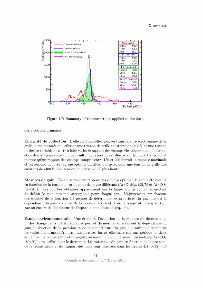
X-ray tests
UncorrectedEntries 9394Mean 426.9RMS 18.31
Fe Peak (ADU)55 380 400 420 440 460 480
Num
ber
of e
vent
s
0
500
1000
1500
2000
2500Uncorrected
Entries 9394Mean 426.9RMS 18.31
P_CorrectedEntries 9394Mean 426.3RMS 4.544
PT_CorrectedEntries 9394Mean 426.3RMS 4.068
Uncorrected data
P corrected data
P and T corrected data
P/T corrected data
PoverT_CorrectedEntries 9394Mean 426.1RMS 4.96
Figure 4.7: Summary of the corrections applied to the data.
des electrons primaires.
Efficacite de collection L’efficacite de collection, ou transparence electronique de lagrille, a ete mesuree en utilisant une tension de grille constante de -400 V et une tensionde derive variable de sorte a faire varier le rapport des champs electriques d’amplificationet de derive a gain constant. Le resultat de la mesure est illustre sur la figure 4.2 (p. 55) etmontre qu’un rapport des champs compris entre 150 et 200 fournit la reponse maximaleet correspond donc au reglage optimal du detecteur avec, pour une tension de grille auxenvirons de -400 V, une tension de derive -50 V plus haute.
Mesures de gain En conservant un rapport des champs optimal, le gain a ete mesureen fonction de la tension de grille pour deux gaz differents (Ar/iC4H10 (95/5) et Ar/CO2
(80/20)). Les courbes obtenues apparaissent sur la figure 4.3 (p. 55) et permettentde definir le gain maximal atteignable pour chaque gaz. L’ajustement sur chacunedes courbes de la fonction 4.3 permet de determiner les proprietes du gaz quant a ladependance du gain vis a vis de la pression (eq. 4.4) et de la temperature (eq. 4.5) dugaz ou encore de l’epaisseur de l’espace d’amplification (eq. 4.6).
Etude environnementale Une etude de l’evolution de la reponse du detecteur aufil des changements meteorologiques permet de mesurer directement la dependance dugain en fonction de la pression et de la temperature du gaz, qui suivent directementles variations atmospheriques. Les mesures furent effectuees sur une periode de deuxsemaines. La temperature etait regulee au moyen d’un climatiseur. Un melange Ar/CO2
(80/20) a ete utilise dans le detecteur. Les variations du gain en fonction de la pression,de la temperature et du rapport des deux sont illustrees dans les figures 4.4 (p. 58), 4.5
61Complete document v1.7 31/08/2011

X-ray tests
(p. 59) et 4.6 (p. 60) respectivement. La mesure directe est comparee au calcul dansla table 4.3 (p. 60) et montre un bon accord au regard des incertitudes sur les valeurscalculees. Ces coefficients de dependance permettent d’envisager une correction desdonnees analogiques ou, dans le cas d’une lecture digitale, une correction en ligne dela tension de grille afin de compenser les fluctuations atmospheriques et ainsi reguler legain du detecteur.
62Complete document v1.7 31/08/2011

CHAPTER 5
Tests in particle beams
Tests in particle beams are a crucial step in the characterization of a detector. Thefirst MIP spectra obtained with cosmic particles have proven the detector functionality(work performed in my master internship). Then, tests in particle beams at the Organ-isation Europeenne pour la Recherche Nucleaire (CERN) facilities allows detailed andsystematic studies of the detector characteristics.
5.1 Experimental layout
5.1.1 Detector stack
The detector stack has been set up with the small chambers at the front and the largeone at the rear (figure 5.1). The distance between each chamber has been set to 10 cm.Three scintillator paddles have been placed in front of the stack, producing the triggersignal by the triple time coincidence of their output. Two of them are 8×32 cm2 and thelast one has the exact dimensions of the small chambers (6×16 cm2).
A pre-mixed Ar/iC4H10 (95/5) gas has been used and the voltage applied on theprototype meshes has been set to -420 V, -420 V, -430 V and -410 V, for CH0 to CH3,respectively. These voltage values have been considered as a trade off between a highgain and a spark rate below about one per hour1. The drift voltages have been setto 50 V below the mesh ones so that the field ratios were always corresponding to themaximum collection efficiency (see section 4.2).
5.1.2 Readout system
The anode analogue readout was provided by 16-channel ASICs called GASSIPLEX[59]. Boards2, each equipped with 6 GASSIPLEX chips, were mounted on the side of
1Here we are speaking about sparks causing a high voltage power supply trip.2CEA DAPNIA Board N613V, 96 channels, 6 GASSIPLEX chips 0.7 v3.
63

Tests in particle beams
Figure 5.1: The test beam layout, including detectors, scintillator paddles and mechan-ical structure (left). A corresponding schematic view (right).
the chambers. (see black components on the photography in figure 3.7(b)). One boardwas used for each of the small chambers and four for the large one.
GASSIPLEX chips, when triggered, gather signal from each channel and build onesingle multiplexed differential output with a nominal conversion factor of 3.6 mV/fC anda peaking time of 1.2µs.
The multiplexed signal from GASSIPLEX boards was digitised by CAEN V550 10-bit ADCs (VME modules) sequenced by a CAEN V551B C-RAMS sequencer VMEmodule. Data was then collected by the computer through an optical VME/PCI bridge.A Labview based software, called CENTAURE [65], was used for on-line monitoring anddata recording. Some developments were made to customise this software to a dedicateduse for our setup. A very similar readout system was used for the CAST experimentand is described in [68]. The global conversion ratio of the GASSIPLEX-based readoutchain was measured to be (4.69±0.25)ADU/fC. Its r.m.s. over all 672 channels is 2.5%.
5.1.3 Calibration
A calibrated pulse was injected through the GASSIPLEX internal test capacitance. Theoutput was stored for further analysis. This process was repeated for three values of theinput charge (voltage of 250, 80 and 25 mV). For any particular charge injection, thespectrum showed a peak clearly above pedestal (see figure 5.2(a)). A straight line wasobtained by plotting this peak mean value versus the injected charge (see figure 5.2(b)).Its slope corresponds to the electronic gain in Analog to Digital Unit (ADU) per fC.
The gains for all channels of each board are gathered on the histogram in figure5.3(a).
The overall gain disparity showed a 2.5% disparity (see figure 5.3(a)), thus no inter-calibration have been applied and a global conversion factor for all readout channels hasbeen set. The gain for boards number 55, 30 and 59 is 4% higher than the average ofthe other boards and thus induces a 2% increase of the average gain. Three chambers
64Complete document v1.7 31/08/2011
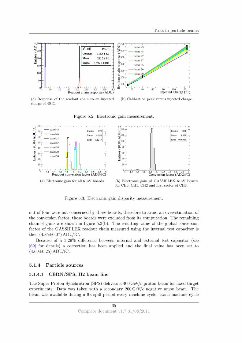
Tests in particle beams
/ ndf 2χ 196 / 3
Constant 6.9± 116.4
Mean 0.1± 211.2
Sigma 0.096± 1.722
Readout chain response (ADU)0 50 100 150 200 250 300 350 400
Ent
ries
/ AD
U
0
50
100
150
200
250
300
/ ndf 2χ 196 / 3
Constant 6.9± 116.4
Mean 0.1± 211.2
Sigma 0.096± 1.722
(a) Response of the readout chain to an injectedcharge of 40 fC.
Injected Charge (fC)20 40 60 80 100 120R
eado
ut c
hain
res
pons
e (A
DU
)
100
200
300
400
500
600
700board 43
board 45
board 27
board 57
board 55
board 30
board 59
(b) Calibration peak versus injected charge.
Figure 5.2: Electronic gain measurement.
frameEntries 672Mean 0RMS 0
Readout conversion factor (ADU/fC)4 4.2 4.4 4.6 4.8 5 5.2 5.4 5.6 5.8 6
Ent
ries
/ (0.
04 A
DU
/fC)
0
10
20
30
40
50
60
70
80
frameEntries 672Mean 0RMS 0
Entries 672
Mean 4.958
RMS 0.1247
board 43
board 45
board 27
board 57
board 55
board 30
board 59
(a) Electronic gain for all 613V boards.
Entries 384
Mean 4.851
RMS 0.06983
Convertion factor (ADU/fC)4 4.2 4.4 4.6 4.8 5 5.2 5.4 5.6 5.8 6
Ent
ries
/ (0.
04 A
DU
/fC)
0
20
40
60
80
100
120
140Entries 384
Mean 4.851
RMS 0.06983
(b) Electronic gain of GASSIPLEX 613V boardsfor CH0, CH1, CH2 and first sector of CH3.
Figure 5.3: Electronic gain disparity measurement.
out of four were not concerned by these boards, therefore to avoid an overestimation ofthe conversion factor, those boards were excluded from its computation. The remainingchannel gains are shown in figure 5.3(b). The resulting value of the global conversionfactor of the GASSIPLEX readout chain measured using the internal test capacitor isthen (4.85±0.07)ADU/fC.
Because of a 3.29% difference between internal and external test capacitor (see[69] for details) a correction has been applied and the final value has been set to(4.69±0.25)ADU/fC.
5.1.4 Particle sources
5.1.4.1 CERN/SPS, H2 beam line
The Super Proton Synchrotron (SPS) delivers a 400 GeV/c proton beam for fixed targetexperiments. Data was taken with a secondary 200 GeV/c negative muon beam. Thebeam was available during a 9 s spill period every machine cycle. Each machine cycle
65Complete document v1.7 31/08/2011
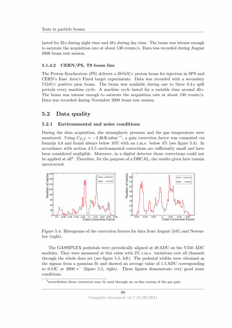
Tests in particle beams
lasted for 33 s during night time and 48 s during day time. The beam was intense enoughto saturate the acquisition rate at about 130 events/s. Data was recorded during August2008 beam test session.
5.1.4.2 CERN/PS, T9 beam line
The Proton Synchrotron (PS) delivers a 28 GeV/c proton beam for injection in SPS andCERN’s East Area’s Fixed target experiments. Data was recorded with a secondary7 GeV/c positive pion beam. The beam was available during one to three 0.4 s spillperiods every machine cycle. A machine cycle lasted for a variable time around 40 s.The beam was intense enough to saturate the acquisition rate at about 130 events/s.Data was recorded during November 2008 beam test session.
5.2 Data quality
5.2.1 Environmental and noise conditions
During the data acquisition, the atmospheric pressure and the gas temperature weremonitored. Using CP/T = −2.36 K mbar−1, a gain correction factor was computed viaformula 4.8 and found always below 10% with an r.m.s. below 4% (see figure 5.4). Inaccordance with section 4.5.5 environmental corrections are sufficiently small and havebeen considered negligible. Moreover, in a digital detector those corrections could notbe applied at all3. Therefore, for the purpose of a DHCAL, the results given here remainuncorrected.
Mean -4.829e-09
RMS 0.03799
Gain Correction Factor-0.1 -0.08 -0.06 -0.04 -0.02 0 0.02 0.04 0.06 0.08
Num
ber
of e
ntrie
s
0
20
40
60
80
100
120
140
160Mean -4.829e-09
RMS 0.03799
Mean 7.656e-09
RMS 0.03241
Gain Correction Factor-0.06 -0.04 -0.02 0 0.02 0.04 0.06
Num
ber
of e
ntrie
s
0
10
20
30
40
50
60
70
80 Mean 7.656e-09
RMS 0.03241
Figure 5.4: Histograms of the correction factors for data from August (left) and Novem-ber (right).
The GASSIPLEX pedestals were periodically aligned at 20 ADU on the V550 ADCmodules. They were measured at this value with 2% r.m.s. variations over all channelsthrough the whole data set (see figure 5.5, left). The pedestal widths were obtained asthe sigmas from a gaussian fit and showed an average value of 1.5 ADU correspondingto 0.3 fC or 2000 e− (figure 5.5, right). These figures demonstrate very good noiseconditions.
3nevertheless those correction may be used through an on-line tuning of the gas gain.
66Complete document v1.7 31/08/2011

Tests in particle beams
Entries 672
Mean 19.97
RMS 0.4082
Pedestal Mean (ADU)15 16 17 18 19 20 21 22 23 24 25
Ent
ries
/ AD
U
0
50
100
150
200
250
300
350Entries 672
Mean 19.97
RMS 0.4082
CH0CH1CH2CH3
Entries 672
Mean 1.518
RMS 0.1251
Pedestal sigma (ADU)0.6 0.8 1 1.2 1.4 1.6 1.8 2 2.2 2.4
Ent
ries
/ (0.
1 A
DU
)
0
20
40
60
80
100
120
140
160
180
200Entries 672
Mean 1.518
RMS 0.1251
CH0CH1CH2CH3
Figure 5.5: Pedestal Mean (left) and sigma (right) distributions.
5.2.2 Event tags
All channels have been recorded without any threshold. A hit is defined by applyingan off-line threshold equal to 1.5 fC (7 ADU above pedestal). Events were categorisedregarding some basic criteria on the hit distribution. The categories are enumeratedand described below. Dedicated data files were produced for each category in order tosimplify the analysis.
- Platinum events: an event is tagged as “platinum” by requiring one single hit ineach of the four chambers. These events were used for gain and pedestal studiessince they ensure a very low noise hit contamination. An example of platinumevent is shown in figure 5.6(a).
- Golden events: a “golden” event is selected by requiring one single hit in threeout of the four chambers. These events were used for efficiency and multiplicitystudies. An example of golden event is shown in figure 5.6(b).
- Silver Events: in these events, several hits are allowed per chamber but only ina 3×3 pad area around the hottest one, we have the option to apply this conditionon all chambers (“platinum” like) or on three of them (“gold” like). Multiple hitsallow computing a weighted position for the hit, thus increasing tracking accuracy.Such events have been used to check chamber alignment. An example of silverevent is shown in figure 5.6(c).
5.2.3 Chambers alignment
The precise position of each chamber relatively to each other can be computed usingparticle tracks. Silver Events (Platinum-like) have been used to compute the hit posi-tion by considering the mean between the actual hits weighted by their correspondingdeposited energy. This method is supposed to be more accurate than attributing hit po-sition at pad centres. After hit positions have been computed within a particular event,a straight line was fitted through them. Afterwards, the distance, separately along xand y axis, between effective hits and the fitted straight line was computed and plotted
67Complete document v1.7 31/08/2011

Tests in particle beams
in figure 5.7. If the chambers were perfectly aligned the resulting distribution would becentred on zero.
This study revealed a 2 mm misalignment along x axis of CH3, 1.6 mm along y axisfor CH1 and 5.7 mm for CH2. Because the tracking capability of such a stack of detectoris too limited, an off-line correction of the chambers position in the analysis programs isunable to prevent from inefficiencies biases due to misalignment. The particle positioncan only be considered being at the centre of the pad. Hence, a small misalignment leadthe particles passing on pad borders to induce signal on a pad alongside the expectedone. Such an information can’t be retrieved in the data and there is therefore no wayto identify this kind of events (see scheme in figure 5.8). This information implied toperform efficiency measurements with a 3×3 pad target area and omit the border padsof the chambers.
5.2.4 Noise contamination
While performing efficiency or multiplicity measurements, hits are searched in the 3 ×3 pad area around the predicted position. As there is a probability that a counted hitresults from noise contamination instead of physical signal, the contribution must beevaluated in order to correct the raw measurement.
Direct measurement For each processed event, the target area has been taken asthe area unit. The number of hits outside the target area was normalised to the areaunit and stored. The mean of this number over all the events is then the average numberof fortuitous4 hits per area unit and per event. If the detectors were completely noisy(e.g. by setting the threshold below pedestal) this number would then be about 9, butfor a reasonable threshold the average number of fortuitous hits per area unit and perevent is expected to be relatively low and would then coincide with the probability ofcounting at least one fortuitous hit in a 3×3 pad target area, denoted p hereafter. Thisassumption has been made for the estimation of the noise contribution to efficiency andmultiplicity measurements.
Computation from single pad noise Another possibility was to compute the singlepad fortuitous hit probability p1 and then deduce the corresponding 3×3 pad probabilityof spotting at least one hit. This probability is given at the second order in p1 by:
p = 9p1(1 − p1)8 + 36p2
1(1 − p1)7 + o(p3
1) , (5.1)
with error:
∆p = ∆(9 · p1(1 − p1)8) + ∆(36 · p2
1(1 − p1)7)
= 9 · p1(1 − p1)8(
∆p1
p1+ 8
∆p1
(1 − p1)
)
+ 36 · p21(1 − p1)
7(
2∆p1
p1+ 7
∆p1
(1 − p1)
)
. (5.2)
4’Fortuitous’ hits denotes hits that appeared randomly, likely from electronic noise contamination butany other potential source is included (radioactivity, cosmic rays, sparks ...)
68Complete document v1.7 31/08/2011

Tests in particle beams
(a) Platinum event (b) Golden event
(c) Silver event
Figure 5.6: Display of events of each type.
Entries 112617Mean 0.3388RMS 0.4149
Distance to fitted straight line (cm) in Chamber 2 along X axis-8 -6 -4 -2 0 2 4 6 8
Ent
ries
/ cm
0
20
40
60
80
100
310×
Entries 112617Mean 0.3388RMS 0.4149
Entries 112617Mean 0.4424RMS 0.2353
Distance to fitted straight line (cm) in Chamber 0 along Y axis-8 -6 -4 -2 0 2 4 6 8
Ent
ries
/ cm
0
20
40
60
80
100
310×
Entries 112617Mean 0.4424RMS 0.2353
Entries 112617Mean 0.1985RMS 0.5737
Distance to fitted straight line (cm) in Chamber 1 along Y axis-8 -6 -4 -2 0 2 4 6 8
Ent
ries
/ cm
0
20
40
60
80
100
310×
Entries 112617Mean 0.1985RMS 0.5737
Entries 112617Mean 0.4777RMS 0.374
Distance to fitted straight line (cm) in Chamber 2 along Y axis-8 -6 -4 -2 0 2 4 6 8
Ent
ries
/ cm
0
20
40
60
80
100
310×
Entries 112617Mean 0.4777RMS 0.374
Entries 112617Mean 0.4234RMS 0.5253
Distance to fitted straight line (cm) in Chamber 3 along Y axis-8 -6 -4 -2 0 2 4 6 8
Ent
ries
/ cm
0
20
40
60
80
100
310×
Entries 112617Mean 0.4234RMS 0.5253
Entries 112617Mean 0.3867RMS 0.3241
Distance to fitted straight line (cm) in Chamber 1 along X axis-8 -6 -4 -2 0 2 4 6 8
Ent
ries
/ cm
0
20
40
60
80
100
310×
Entries 112617Mean 0.3867RMS 0.3241
Entries 112617Mean 0.1432RMS 0.6757
Distance to fitted straight line (cm) in Chamber 3 along X axis-8 -6 -4 -2 0 2 4 6 8
Ent
ries
/ cm
0
20
40
60
80
100
310×
Entries 112617Mean 0.1432RMS 0.6757
Entries 112617Mean 0.3551RMS 0.352
Distance to fitted straight line (cm) in Chamber 0 along X axis-8 -6 -4 -2 0 2 4 6 8
Ent
ries
/ cm
0
20
40
60
80
100
310×
Entries 112617Mean 0.3551RMS 0.352
Figure 5.7: Measurement of all chambers relative misalignment.
69Complete document v1.7 31/08/2011

Tests in particle beams
Figure 5.8: Geometrical inefficiency
Table 5.1: Comparison between 3×3 pad fortuitous hit probability direct measurementand 3×3 pad fortuitous hit probability computation from single pad noise.
Chamber direct computed
CH0 (1.30±0.08)% (1.71±0.28)%CH1 (1.33±0.08)% (1.87±0.29)%CH2 (2.00±0.10)% (2.60±0.33)%CH3 (1.65±0.09)% (1.39±0.26)%
The results are compatible, but the error margin on the computed values are higherthan for the directly measured ones, and the values are mainly higher as well. Thisdifference can be explained by the fact that by looking at only one pad to search for noisecontribution, any secondary hit due to signal multiplicity is automatically considered asnoise. Computed values are therefore biased by the hit multiplicity. The direct methodhas been kept to perform the correction to efficiency and multiplicity. A quantity Q,standing either for efficiency or multiplicity, is corrected for noise contribution using thesimple formula:
Qcorr = Q · (1 − p) , (5.3)
where p is the noise hit probability of the chamber.
5.3 Gain distribution measurement
For every channel, a Landau function has been fitted to the data from platinum events(see figure 5.9 (left)) and its Most Probable Value (MPV) has been defined as thedetector global gain for charged particles (conversion, mesh amplification and electronicsamplification). The resulting values are mapped in figure 5.10.
The most probable deposited charge, averaged over all channels of each chamber hasbeen measured at 22.6, 22.9, 24.5 and 17.5 fC for CH0 to CH3 respectively. The relative
70Complete document v1.7 31/08/2011

Tests in particle beams
gain distribution of all the channels is shown in figure 5.9 (right) having an r.m.s. of11.25%. Since the electronics gain distribution has a very low r.m.s. (see section 5.1.2and 5.1.3), this value is expected to be mainly due to drift and/or amplification gapnon-uniformity.
/ ndf = 40.41 / 382χ
Constant 18.2± 361.8
MPV 0.7± 25
Sigma 0.393± 9.093
Deposited charge (fC)0 20 40 60 80 100 120 140
Ent
ries
/ (3.
41 fC
)
0
20
40
60
80
100
120
140
/ ndf = 40.41 / 382χ
Constant 18.2± 361.8
MPV 0.7± 25
Sigma 0.393± 9.093
(a)
Entries 384Mean 99.6RMS 11.25
Landau MPV (relative variation in %)50 60 70 80 90 100 110 120 130 140 150
Ent
ries
/ (2
%)
0
2
4
6
8
10
12
14 Entries 384Mean 99.6RMS 11.25
CH0CH1CH2CH3
(b)
Figure 5.9: Fit of a Landau function to the data for a single channel, the pedestal hasbeen scaled to fit in the vertical range. The spectrum was built using Platinum events(left). Landau MPV distribution normalised to 100, for all chambers (right).
y (cm)0 5 10 15 20 25 30
x (c
m)
0
5
10
0
20
40
60
80
100
120
140
160
CH0
y (cm)0 5 10 15 20 25 30
x (c
m)
0
5
10
0
20
40
60
80
100
120
140
160
CH1
y (cm)0 5 10 15 20 25 30
x (c
m)
0
5
10
0
20
40
60
80
100
120
140
160
CH2
y (cm)0 5 10 15 20 25 30
x (c
m)
0
5
10
0
20
40
60
80
100
120
140
160
CH3
Figure 5.10: Landau MPV maps of all prototypes (colour axis in ADU).
5.4 Efficiency measurement
In order to measure the efficiency of a given chamber, the three others have been taken asa tracker. A sample of golden events was selected by requesting three aligned hits in thethree “tracking” chambers to define a particle track. A safety threshold of 12.5 fC wasapplied for the three reference chamber hits to completely avoid taking noise hits intoaccount. In each processed event, a hit has been searched in a 3×3 pad area centred atthe intersection between the extrapolated reconstructed particle track and the chamber
71Complete document v1.7 31/08/2011

Tests in particle beams
plane. The predicted position was stored in a 2D histogram (see example in upper leftmap of figure 5.11), if a hit was actually found, the same bin in a second 2D histogramwas filled (example in upper right map of fig 5.11). The ratio of those two histogramsgave the chamber efficiency map. The resulting efficiencies are mapped in figure 5.12 andtheir distribution is shown in figure 5.13. The error on efficiency is computed throughthe usual formula:
∆ǫ =
√
ǫ · (1 − ǫ)
Ntot, (5.4)
where ǫ is the efficiency and ∆ǫ its error, Ntot is the total number of events in the selectedsub-sample when computing global efficiency and the number of times a pad has beentested when computing local efficiency.
0 0 0 0 0 0 0 0 0 0 0 0 0 0 0 0 0 0 0 0 0 0 0 0 0 0 0 0 0 0 0 0
0 0 0 0 0 0 0 0 0 0 0 0 0 0 0 0 0 0 0 0 0 0 0 0 0 0 0 0 0 0 0 0
0 0 0 0 0 0 0 0 0 0 0 0 0 0 0 0 0 0 0 0 0 0 0 0 0 0 0 0 0 0 0 0
0 0 0 0 0 0 0 0 0 0 0 0 0 0 0 0 0 0 0 0 0 0 0 0 0 0 0 0 0 0 0 0
0 0 0 0 0 0 0 0 0 832 1156 942 543 450 224 10501017 617 423 425 431 493 808 0 0 0 0 0 0 0 0 0
0 0 0 0 0 0 0 0 0 12491359 953 672 646 628 10891111 668 448 447 464 493 955 0 0 0 0 0 0 0 0 0
0 0 0 0 0 0 0 0 0 14781289 859 758 885 621 863 902 625 500 452 497 573 1154 0 0 0 0 0 0 0 0 0
0 0 0 0 0 0 0 0 0 15001096 823 670 352 714 715 646 562 498 512 509 548 888 0 0 0 0 0 0 0 0 0
0 0 0 0 0 0 0 0 0 0 0 0 0 0 0 0 0 0 0 0 0 0 0 0 0 0 0 0 0 0 0 0
0 0 0 0 0 0 0 0 0 0 0 0 0 0 0 0 0 0 0 0 0 0 0 0 0 0 0 0 0 0 0 0
0 0 0 0 0 0 0 0 0 0 0 0 0 0 0 0 0 0 0 0 0 0 0 0 0 0 0 0 0 0 0 0
0 0 0 0 0 0 0 0 0 0 0 0 0 0 0 0 0 0 0 0 0 0 0 0 0 0 0 0 0 0 0 0
y (cm)0 5 10 15 20 25 30
x (c
m)
0
2
4
6
8
10
12
Entries 42082Entries 42082Expected Hits
0 0 0 0 0 0 0 0 0 0 0 0 0 0 0 0 0 0 0 0 0 0 0 0 0 0 0 0 0 0 0 0
0 0 0 0 0 0 0 0 0 0 0 0 0 0 0 0 0 0 0 0 0 0 0 0 0 0 0 0 0 0 0 0
0 0 0 0 0 0 0 0 0 0 0 0 0 0 0 0 0 0 0 0 0 0 0 0 0 0 0 0 0 0 0 0
0 0 0 0 0 0 0 0 0 0 0 0 0 0 0 0 0 0 0 0 0 0 0 0 0 0 0 0 0 0 0 0
0 0 0 0 0 0 0 0 0 781 1104 882 508 422 201 1001 978 595 411 409 412 479 790 0 0 0 0 0 0 0 0 0
0 0 0 0 0 0 0 0 0 12191319 936 656 637 615 10591079 654 437 428 450 480 931 0 0 0 0 0 0 0 0 0
0 0 0 0 0 0 0 0 0 14401258 834 733 863 604 846 882 612 488 441 480 563 1121 0 0 0 0 0 0 0 0 0
0 0 0 0 0 0 0 0 0 14661068 798 652 345 697 697 634 552 486 502 487 534 856 0 0 0 0 0 0 0 0 0
0 0 0 0 0 0 0 0 0 0 0 0 0 0 0 0 0 0 0 0 0 0 0 0 0 0 0 0 0 0 0 0
0 0 0 0 0 0 0 0 0 0 0 0 0 0 0 0 0 0 0 0 0 0 0 0 0 0 0 0 0 0 0 0
0 0 0 0 0 0 0 0 0 0 0 0 0 0 0 0 0 0 0 0 0 0 0 0 0 0 0 0 0 0 0 0
0 0 0 0 0 0 0 0 0 0 0 0 0 0 0 0 0 0 0 0 0 0 0 0 0 0 0 0 0 0 0 0
y (cm)0 5 10 15 20 25 30
x (c
m)
0
2
4
6
8
10
12
Entries 40812Entries 40812Counted Hits
Efficiency
Y (cm)0 5 10 15 20 25 30
X (
cm)
0
2
4
6
8
10
12
Entries 40812
0.86
0.88
0.9
0.92
0.94
0.96
0.98
1
Entries 40812
Y (cm)0 5 10 15 20 25 30
X (
cm)
0
2
4
6
8
10
12
Entries 384
0
0.002
0.004
0.006
0.008
0.01
0.012
0.014
0.016
0.018
0.02
Entries 384Efficiency error
Figure 5.11: Efficiency map, principle of calculation.
The hit background was estimated by counting the number of hits outside the3×3 pad area. This number, normalised to the 3×3 pad area, was subtracted to measurethe final efficiency (Table 5.2). Because of the very low threshold, three chambers showan excellent efficiency, larger than 97%. CH2 shows a lower efficiency (91%). The deadchannel in the readout GASSIPLEX board, as shown on the MPV map in figure 5.10(CH2, lower left) should be responsible for a ≈ 2% loss of the global efficiency. The re-maining loss of efficiency might be due to the lower tension of its mesh or to the broaderpedestals of its electronics.
72Complete document v1.7 31/08/2011

Tests in particle beams
y (cm)0 5 10 15 20 25 30
x (c
m)
0
5
10
0.9
0.91
0.92
0.93
0.94
0.95
0.96
0.97
0.98
0.99
1
CH1
y (cm)0 5 10 15 20 25 30
x (c
m)
0
5
10
0.8
0.82
0.84
0.86
0.88
0.9
0.92
0.94
0.96
0.98
1
CH2
y (cm)0 5 10 15 20 25 30
x (c
m)
0
5
10
0.9
0.91
0.92
0.93
0.94
0.95
0.96
0.97
0.98
0.99
1
CH3
y (cm)0 5 10 15 20 25 30
x (c
m)
0
5
10
0.9
0.91
0.92
0.93
0.94
0.95
0.96
0.97
0.98
0.99
1
CH0
Figure 5.12: Maps of prototype efficiencies. The measurement was performed for afiducial area omitting all border pads and using a 3×3 pad area around the expected hitto avoid misalignment issues.
Efficiency0.9 0.91 0.92 0.93 0.94 0.95 0.96 0.97 0.98 0.99 1
Num
ber
of e
ntrie
s
0
2
4
6
8
10
12
14
16
18
20
CH0CH1CH2CH3
Figure 5.13: Pad efficiency distribution for each chamber.
Table 5.2: Efficiency measurements for a 1.5 fC threshold.Chamber Raw efficiency Noise hit fraction Noise corrected efficiency
CH0 (99.0±0.1)% (1.3±0.1)% (97.7±0.1)%
CH1 (99.0±0.1)% (1.3±0.1)% (97.7±0.1)%
CH2 (93.0±0.1)% (2.0±0.1)% (91.2±0.1)%
CH3 (98.8±0.1)% (1.6±0.1)% (97.2±0.1)%
In a DHCAL, the threshold is a fundamental parameter, the same study was there-fore carried out for each chamber varying the threshold from 1.5 fC to 200 fC. Thedependency between efficiency and threshold is represented in figure 5.14. A steep dropof efficiency with threshold is observed. A maximum efficiency above 97% is reached at
73Complete document v1.7 31/08/2011
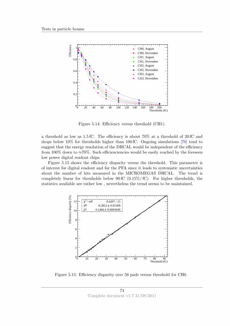
Tests in particle beams
Thresholds (fC)0 20 40 60 80 100 120 140 160 180 200
Effi
cien
cy
0
0.2
0.4
0.6
0.8
1 CH0, August
CH0, NovemberCH1, August
CH1, NovemberCH2, August
CH2, NovemberCH3, August
CH3, November
Figure 5.14: Efficiency versus threshold (CH1).
a threshold as low as 1.5 fC. The efficiency is about 70% at a threshold of 20 fC anddrops below 10% for thresholds higher than 100 fC. Ongoing simulations [70] tend tosuggest that the energy resolution of the DHCAL would be independent of the efficiencyfrom 100% down to ≈70%. Such efficienciencies would be easily reached by the foreseenlow power digital readout chips.
Figure 5.15 shows the efficiency disparity versus the threshold. This parameter isof interest for digital readout and for the PFA since it leads to systematic uncertaintiesabout the number of hits measured in the MICROMEGAS DHCAL. The trend iscompletely linear for thresholds below 90 fC (0.15%/ fC). For higher thresholds, thestatistics available are rather low , nevertheless the trend seems to be maintained.
Threshold (fC)0 10 20 30 40 50 60 70 80 90
Effi
cien
cy d
ispa
rity
(%)
0
2
4
6
8
10
12 / ndf 2χ 0.4207 / 15p0 0.01209± -0.2812 p1 0.0003049± 0.1466
/ ndf 2χ 0.4207 / 15p0 0.01209± -0.2812 p1 0.0003049± 0.1466
Figure 5.15: Efficiency disparity over 56 pads versus threshold for CH0.
74Complete document v1.7 31/08/2011
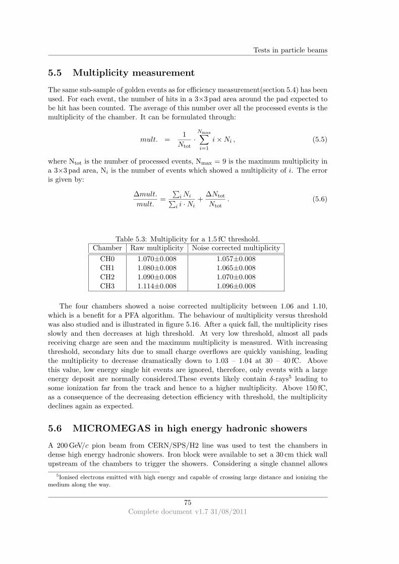
Tests in particle beams
5.5 Multiplicity measurement
The same sub-sample of golden events as for efficiency measurement(section 5.4) has beenused. For each event, the number of hits in a 3×3 pad area around the pad expected tobe hit has been counted. The average of this number over all the processed events is themultiplicity of the chamber. It can be formulated through:
mult. =1
Ntot·
Nmax∑
i=1
i×Ni , (5.5)
where Ntot is the number of processed events, Nmax = 9 is the maximum multiplicity ina 3×3 pad area, Ni is the number of events which showed a multiplicity of i. The erroris given by:
∆mult.
mult.=
∑
iNi∑
i i ·Ni+
∆Ntot
Ntot. (5.6)
Table 5.3: Multiplicity for a 1.5 fC threshold.Chamber Raw multiplicity Noise corrected multiplicity
CH0 1.070±0.008 1.057±0.008CH1 1.080±0.008 1.065±0.008CH2 1.090±0.008 1.070±0.008CH3 1.114±0.008 1.096±0.008
The four chambers showed a noise corrected multiplicity between 1.06 and 1.10,which is a benefit for a PFA algorithm. The behaviour of multiplicity versus thresholdwas also studied and is illustrated in figure 5.16. After a quick fall, the multiplicity risesslowly and then decreases at high threshold. At very low threshold, almost all padsreceiving charge are seen and the maximum multiplicity is measured. With increasingthreshold, secondary hits due to small charge overflows are quickly vanishing, leadingthe multiplicity to decrease dramatically down to 1.03 – 1.04 at 30 – 40 fC. Abovethis value, low energy single hit events are ignored, therefore, only events with a largeenergy deposit are normally considered.These events likely contain δ-rays5 leading tosome ionization far from the track and hence to a higher multiplicity. Above 150 fC,as a consequence of the decreasing detection efficiency with threshold, the multiplicitydeclines again as expected.
5.6 MICROMEGAS in high energy hadronic showers
A 200 GeV/c pion beam from CERN/SPS/H2 line was used to test the chambers indense high energy hadronic showers. Iron block were available to set a 30 cm thick wallupstream of the chambers to trigger the showers. Considering a single channel allows
5Ionised electrons emitted with high energy and capable of crossing large distance and ionizing themedium along the way.
75Complete document v1.7 31/08/2011
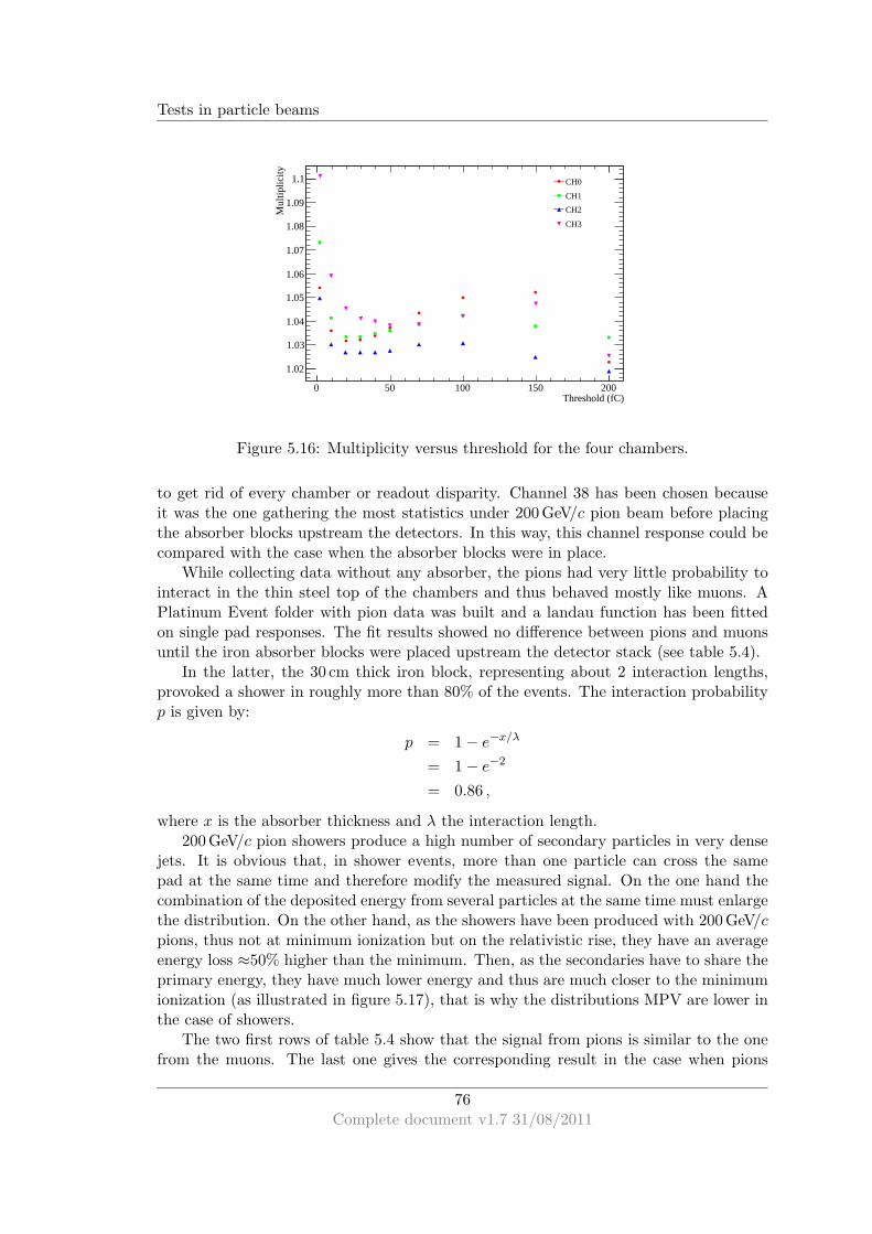
Tests in particle beams
Threshold (fC)0 50 100 150 200
Mul
tiplic
ity
1.02
1.03
1.04
1.05
1.06
1.07
1.08
1.09
1.1 CH0
CH1
CH2
CH3
Figure 5.16: Multiplicity versus threshold for the four chambers.
to get rid of every chamber or readout disparity. Channel 38 has been chosen becauseit was the one gathering the most statistics under 200 GeV/c pion beam before placingthe absorber blocks upstream the detectors. In this way, this channel response could becompared with the case when the absorber blocks were in place.
While collecting data without any absorber, the pions had very little probability tointeract in the thin steel top of the chambers and thus behaved mostly like muons. APlatinum Event folder with pion data was built and a landau function has been fittedon single pad responses. The fit results showed no difference between pions and muonsuntil the iron absorber blocks were placed upstream the detector stack (see table 5.4).
In the latter, the 30 cm thick iron block, representing about 2 interaction lengths,provoked a shower in roughly more than 80% of the events. The interaction probabilityp is given by:
p = 1 − e−x/λ
= 1 − e−2
= 0.86 ,
where x is the absorber thickness and λ the interaction length.200 GeV/c pion showers produce a high number of secondary particles in very dense
jets. It is obvious that, in shower events, more than one particle can cross the samepad at the same time and therefore modify the measured signal. On the one hand thecombination of the deposited energy from several particles at the same time must enlargethe distribution. On the other hand, as the showers have been produced with 200 GeV/cpions, thus not at minimum ionization but on the relativistic rise, they have an averageenergy loss ≈50% higher than the minimum. Then, as the secondaries have to share theprimary energy, they have much lower energy and thus are much closer to the minimumionization (as illustrated in figure 5.17), that is why the distributions MPV are lower inthe case of showers.
The two first rows of table 5.4 show that the signal from pions is similar to the onefrom the muons. The last one gives the corresponding result in the case when pions
76Complete document v1.7 31/08/2011

Tests in particle beams
Table 5.4: Summary of the results given by the fit of a landau function on single padsignal for the three small chambers for three different situations.
Muons MPV (ADU) σ (ADU)
CH0 132.7±3.2 42.3±2.1CH1 124.4±3.2 42.0±2.0CH2 137.3±4.4 54.4±3.0
Pions MPV(ADU) σ(ADU)
CH0 130.0±2.7 40.8±1.7CH1 122.4±2.6 42.5±1.7CH2 137.7±3.4 51.1±2.2
Showers MPV(ADU) σ(ADU)
CH0 126.8±3.2 78.6±1.4CH1 108.2±3.4 70.2±1.4CH2 124.3±3.0 68.9±1.4
interacted with iron blocks placed in front of the chambers. In the two first cases, theσ of the distributions are identical for CH0 and CH1 and a little higher for CH2. Inthe shower case the σ are decreasing from CH0 to CH2, accordingly to their distancefrom the interaction point. This is in agreement with a decreasing particle density.Figure 5.18 has been made using some toy Monte Carlo (MC) and shows the energyloss distribution of a single Minimum Ionizing Particle (MIP) crossing the detector (redcurve). The one in green shows the energy loss distribution of two MIPs crossing thedetector simultaneously and the black one is the same for three MIPs at once
ADU0 100 200 300 400 500 600
Num
ber
of e
vent
s
0
20
40
60
80
100
120
140
160
180 0.37 Gev (MIP)
1 GeV
200 GeV
Figure 5.17: GEANT4 simulation of distribution of energy loss for muons crossing 3 mmof Ar/iC4H10 (95/5)
77Complete document v1.7 31/08/2011

Tests in particle beams
Entries 10000Mean 258.2RMS 196.6
/ ndf 2χ 228.9 / 222Constant 9.7± 572 MPV 1.7± 128.8 Sigma 1.12± 67.67
Response (ADU)0 100 200 300 400 500 600 700 800 900
Num
ber
of e
vent
s / (
4 A
DU
)
0
20
40
60
80
100
120Entries 10000Mean 258.2RMS 196.6
/ ndf 2χ 228.9 / 222Constant 9.7± 572 MPV 1.7± 128.8 Sigma 1.12± 67.67
Entries 10000Mean 442.9RMS 209.8
/ ndf 2χ 230.6 / 222Constant 4.6± 281.9 MPV 4.2± 359.8 Sigma 2.5± 137.4
Entries 10000Mean 567.3RMS 183.5
/ ndf 2χ 217.6 / 205Constant 3.4± 207.8 MPV 8.2± 581.6 Sigma 4.6± 178.5
One particleTwo particlesThree particles
Figure 5.18: Distribution of energy loss for one, two and three particles at once in thesame readout pad.
5.7 Calorimetry measurements
As part of the study, a “mini” calorimeter was set up and sprayed with electrons andpions at various energies in June 2009 at CERN/PS/T10 test facility. Shower profilesand further interpretation are presented for 2 GeV/c electrons and pions as a preliminarystudy. A few analysis benchmarks are presented (like e/mip and e/h ratios) and call forfurther analysis.
5.7.1 Experimental setup
The four prototypes described in section 3.5 (p. 48) were used to set up a “mini” calorime-ter. They have a 1 × 1 cm2 segmentation, a 3 mm drift gap and a 128µm amplificationgap. They are closed by a 2 mm steel top which counts as part of the absorber. Thethree small chambers (6×16 pad) played the role of a beam telescope for event selectionwhilst the large one (12× 32 pad) was used as the calorimeter active medium. The dataacquisition was triggered by the coincidence of three scintillator paddles. The layout ofthe set-up is sketched in figure 5.19. To perform measurements of particle showers, avarying number (ranging from 0 to 12) of 2 cm steel plates where placed between theset of the three small chambers and the large one. The absorber plates where equippedwith 8 mm spacers to ensure a regular and rather realistic imitation of the completecalorimeter. MC simulations have driven those choices, they are summarised in [71].
The readout used V613 boards equipped with GASSIPLEX chips [59], read by VMEADC and sequencer. Data was recorded by the CENTAURE software from SUBATECH[65]. The readout system and its calibration are described in details in sections 5.1.2and 5.1.3.
78Complete document v1.7 31/08/2011

Tests in particle beams
Figure 5.19: Scheme of beam test set-up.
5.7.2 Event selection
Data from the small chambers was used to perform the event selection. A pre-selectionwas done first by requesting one single cluster of hits in each of the three small chambers,regardless of the response of the large one (≈ 50–60% yield). As a second step, for eachchamber, a weighted hit position was computed from each hit and its value and theposition of those hits is requested in the 2× 4 cm2 central area of the chambers to selectcentral events in order to maximise the shower containment in the selected sample.Afterwards, a straight line has been fitted through the weighted hits and the followingcuts have been applied: the χ2/NDF of this fit below 5 and the slopes below 0.1. Figure5.20 shows the values of those variables and indicates that the major cut was actuallydone by the pre-selection.
Entries 109127
Mean 0.05544
RMS 0.03676
2χ-1 0 1 2 3 4 5 6
Num
ber
of e
vent
s
1
10
210
310
410
510 Entries 109127
Mean 0.05544
RMS 0.03676
Entries 109127
Mean 0.1237
RMS 0.2309
X direction
Y direction
Entries 109119
Mean 0.008146
RMS 0.01606
Slope-0.4 -0.2 0 0.2 0.4
Num
ber
of e
vent
s
10
210
310
410
510Entries 109119
Mean 0.008146
RMS 0.01606
Entries 109119
Mean -0.01441
RMS 0.02562
Slope in X-Z plane
Slope in Y-Z plane
Figure 5.20: Straight line fit χ2 before applying cuts and slopes after the χ2 cut for allpreselected events in the three small chambers (electron sample).
79Complete document v1.7 31/08/2011

Tests in particle beams
5.7.3 Electron shower profile
Data was recorded from 2 GeV/c electrons with 0, 2, 3, 4, 5, 6, 8, 10 and 12 layers ofabsorber plates upstream the large chamber. For cross checking the results, the samemeasurement were simulated with GEANT4 using LHEP physics list. The resultingcurves are displayed in figure 5.21. The agreement was rather good and suffered only fromsmall deficit in the simulated values. Nevertheless, this did not detract from consideringthe event selection and shower profile reconstruction as trustworthy.
Figure 5.21: Electron shower profile from data and GEANT4 simulation.
In order to estimate the deposited energy in a 12 layer calorimeter made of MI-CROMEGAS chambers interleaved with 2 cm thick steel plates, the deposited energy inthe missing active layers, namely the layers 1, 7, 9 and 11, were interpolated thanks tothe data fitted curve:
f(z) = p0 · zp1 · e−p2·z , (5.7)
where z denotes the depth in unit of absorber plate thickness (namely 2.2 cm, 1.25 X0 or0.13λI) denoted abs hereafter. The values of p0, p1 and p2 have been fitted to the dataand summarise in table 5.5.
Table 5.5: Summary of electron shower profile fit parameters.Parameter Value from fit
p0 10.03 ± 0.53 keVp1 1.44 ± 0.14p2 0.55 ± 0.04 abs−1
The interpolated points appear in figure 5.21 as the error-less points of the databased plot. The average energy deposited by 2 GeV/c electrons in such a 12 layer MI-
80Complete document v1.7 31/08/2011

Tests in particle beams
CROMEGAS calorimeter is:
Emes(e) = 54.27 ± 0.30 keV , (5.8)
with a containment of (98 ± 5)%.Afterwards, one can also extrapolate what energy would be measured in a 40 layer
such calorimeter by multiplying Emes(e) by the ratio of the integrals of f(z) for z ∈ [0, 12]and z ∈ [0, 40], ie:
Evis(e) = Emes(e) ×∫ 120 f(z)dz∫ 400 f(z)dz
(5.9)
= 55.41 ± 2.88 keV , (5.10)
where the error takes the fit uncertainties into account. As a 40 layer calorimeter issufficient to contain 2 GeV showers, the energy given in eq. 5.9 corresponds to the oneappearing in eq. 2.2 (p. 28). The two other parameters of eq. 2.2, namely FS and e/mip,are calculated in the next section to characterise the electromagnetic response of our“mini” MICROMEGAS calorimeter.
5.7.4 Interpretation in terms of electromagnetic calorimetry
5.7.4.1 The MIP shared energy
The so-called MIP shared Energy, denoted ES, is defined as the energy fraction that islost in the active medium by an ideal Minimum Ionizing Particle (MIP) of energy E.
ES =E × (dE/dx)readout × Lreadout
∑
i (dE/dx)i × Li
≈ E × (dE/dx)readout × Lreadout
(dE/dx)absorber × Labsorber, (5.11)
with all energy losses given for minimum ionizing particles, E is the incoming particleenergy and LX is the thickness of component X. One also introduce the MIP sharedfraction FS given by:
FS =ES
E
=(dE/dx)readout × Lreadout
(dE/dx)absorber × Labsorber, (5.12)
with all energy losses given for minimum ionizing particles. FS is independent ofthe energy and is thus a intrinsic constant of the calorimeter. In the present case,with (dE/dx)readout = 2.68 keV cm−1, Lreadout = 0.3 cm, (dE/dx)absorber = 11.46 ·103 keV cm−1 and Labsorber = 2.0 cm, one obtains:
FS = 3.19 · 10−5 . (5.13)
Therefore, at E = 2 GeV:
ES = 63.8 keV (5.14)
81Complete document v1.7 31/08/2011

Tests in particle beams
5.7.4.2 The e/mip ratio
The e/mip ratio is defined as:
e/mip =Evis(e)
ES, (5.15)
which gives, by taking the measured values of Evis(e) and ES from eq. 5.10 and 5.14respectively:
e/mip = 0.87 ± 0.05 . (5.16)
The e/mip ratio is energy independent and is, as such, an intrinsic characteristic of acalorimeter, many details about this feature lies in [31]. For instance this ratio relatesto the electromagnetic energy measurement and its resolution, as introduced in section2.5 and illustrated in the following section.
5.7.4.3 Energy measurement and resolution
Energy measurement The proportionality between the visible energy in our “mini”calorimeter (extrapolated to 40 layers) and the incoming energy lies in the definition ofthe e/mip ratio (eq. 5.15) which leads to:
Evis(e) = e/mip ES
= e/mip FS E (5.17)
Evis(e) = (2.77 ± 0.16) · 10−5 E . (5.18)
Energy resolution The prediction of energy resolution involves a number of con-stants. Let τ = 1.25 X0 be the sampling fraction of the calorimeter in unit of radiationlength. Let ǫc be the critical energy of a given medium, this is the energy of a particlefor which the radiation and the collision energy losses in this medium are equivalent.For iron: ǫc = 21.04 MeV ([31], page 44, table 2.3). 〈cosθ〉 is the cosine of the averageangle of the particles crossing the active medium and is defined by:
〈cosθ〉 = cos
(21.2 MeV
πǫc
)
〈cosθ〉 = 0.949 . (5.19)
The above constants combine to predict the electromagnetic energy resolution of thecalorimeter via:
σ(E)
E= 3.16%
√
ǫc τ
e/mip 〈cosθ〉 ×1√E, (5.20)
which gives the electromagnetic resolution of our “mini” calorimeter:
σ(E)
E=
(18 ± 1)%√E
. (5.21)
The predictions performed in this section can be used for further study of 2009 beamtest data to compare the coherence of the results.
82Complete document v1.7 31/08/2011

Tests in particle beams
5.7.5 Hadron shower profile
The data acquired with the June 2009 set-up does not give access to the event-by-event shower start. In the case of the electrons this was not a problem, since electronsinteracted mostly at the very beginning of the calorimeter and the spread of the showerstart can be neglected. However, in the hadron case, showers can start anywhere in thecalorimeter following the law:
P (z) = e−z/λI , (5.22)
where P (z) is the probability that a pion had not interacted at depth z and λI = 16.78 cmis the iron interaction length. Figure 5.22 illustrates this probability law using unit ofabsorber plate thickness.
Layer number0 2 4 6 8 10 12
Fra
ctio
n of
had
ron
rem
aini
ng
0.2
0.3
0.4
0.5
0.6
0.7
0.8
0.9
1
exp(-x/[0])
Figure 5.22: Hadron fraction which haven’t interacted versus depth in unit of absorberplate thickness.
For a preliminary study, the raw data was not corrected for shower start position.The obtained profile is displayed in figure 5.23 and its interpretation is derived in thenext section. The experimental points were fitted with expression 5.7 to interpolate thedeposited energy in the missing layers, namely layers 1, 5, 7, 9 and 11, and to estimate theshower containment as in eq. 5.10. The simulated profile was obtained with a GEometryANd Tracking, version 4 (GEANT4) simulation based on the LHEP physics list as forthe electron case. However, this physics list happen to be imprecise for hadronic physics.This explains the disagreement between data and simulation in figure 5.23.
The measurement thus gives:
Emes(π) = (16.51 ± 0.12) keV .
With the same method as in the electron case, the shower containment in the 12 layer“mini” calorimeter is (43 ± 12)% and therefore:
Evis(π) = (38.3 ± 10.8) keV . (5.23)
83Complete document v1.7 31/08/2011
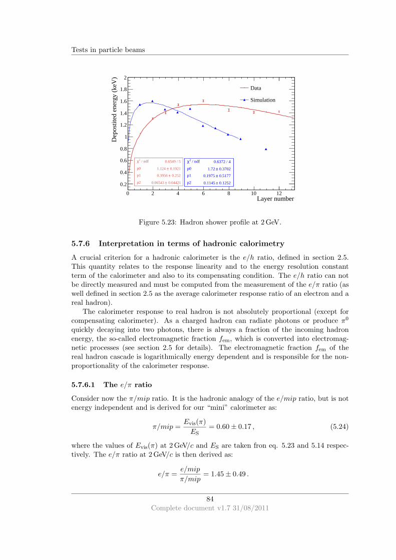
Tests in particle beams
Layer number0 2 4 6 8 10 12
Dep
ostit
ed e
nerg
y (k
eV)
0.2
0.4
0.6
0.8
1
1.2
1.4
1.6
1.8
2
/ ndf 2χ 0.6549 / 5
p0 0.1921± 1.124
p1 0.252± 0.3956
p2 0.04421± 0.06543
/ ndf 2χ 0.6549 / 5
p0 0.1921± 1.124
p1 0.252± 0.3956
p2 0.04421± 0.06543
/ ndf 2χ 0.6372 / 4
p0 0.3702± 1.72
p1 0.5177± 0.1975
p2 0.1252± 0.1145
/ ndf 2χ 0.6372 / 4
p0 0.3702± 1.72
p1 0.5177± 0.1975
p2 0.1252± 0.1145
Data
Simulation
Figure 5.23: Hadron shower profile at 2 GeV.
5.7.6 Interpretation in terms of hadronic calorimetry
A crucial criterion for a hadronic calorimeter is the e/h ratio, defined in section 2.5.This quantity relates to the response linearity and to the energy resolution constantterm of the calorimeter and also to its compensating condition. The e/h ratio can notbe directly measured and must be computed from the measurement of the e/π ratio (aswell defined in section 2.5 as the average calorimeter response ratio of an electron and areal hadron).
The calorimeter response to real hadron is not absolutely proportional (except forcompensating calorimeter). As a charged hadron can radiate photons or produce π0
quickly decaying into two photons, there is always a fraction of the incoming hadronenergy, the so-called electromagnetic fraction fem, which is converted into electromag-netic processes (see section 2.5 for details). The electromagnetic fraction fem of thereal hadron cascade is logarithmically energy dependent and is responsible for the non-proportionality of the calorimeter response.
5.7.6.1 The e/π ratio
Consider now the π/mip ratio. It is the hadronic analogy of the e/mip ratio, but is notenergy independent and is derived for our “mini” calorimeter as:
π/mip =Evis(π)
ES= 0.60 ± 0.17 , (5.24)
where the values of Evis(π) at 2 GeV/c and ES are taken fron eq. 5.23 and 5.14 respec-tively. The e/π ratio at 2 GeV/c is then derived as:
e/π =e/mip
π/mip= 1.45 ± 0.49 .
84Complete document v1.7 31/08/2011

Tests in particle beams
Energy resolution constant term The constant term of the hadron calorimeterenergy resolution at 2 GeV/c, for e/π > 1.115, is given by ([31], p. 510):
Φ(e/π) ≈ 0.281 ln(e/π) − 2.1 · 10−2
= (8.3 ± 9.5)% . (5.25)
The large error bar finally only permits a prediction of the constant term below about18%.
5.7.6.2 The e/h ratio
The electromagnetic fraction of the real hadron cascade (fem) is involved in the calcu-lation of the e/h ratio. The fem is given by empirical formulas. According to varioussources [31, 30], the value of fem ranges from 7.6% to 12.9%. The value 7.6% comesfrom the formula:
fem = 0.11 ln(E) , (5.26)
which is considered to be more accurate at “low” energy [31], and is used hereafter. Thee/h ratio is then given by:
e/h =e/π(1 − fem)
1 − feme/π(5.27)
= 1.51 ± 0.52 .
The uncertainty on e/h is too large to make any assumption on the compensating con-dition of the calorimeter.
Calorimeter response The calorimeter response to real hadron, Evis(π), relates, onethe one hand, to the incoming energy via:
Evis(π) = π/mipFSE
= π/e e/mipFSE , (5.28)
and on the other hand, by:
Evis(π) = femEvis(e) + (1 − fem)Evis(h)
⇔ π/mip = feme/mip+ (1 − fem)h/mip
⇔ π/e = fem + (1 − fem)h/e
= fem(1 − h/e) + h/e . (5.29)
From eq. 5.28 and 5.29, the real hadron visible energy can be written as:
Evis(π) = NL(E) · E + h/mipFS · E , (5.30)
with NL(E), the energy dependent non linear term, expressed as:
NL(E) =
(e/h− 1
e/h
)
e/mipFS fem(E) . (5.31)
85Complete document v1.7 31/08/2011
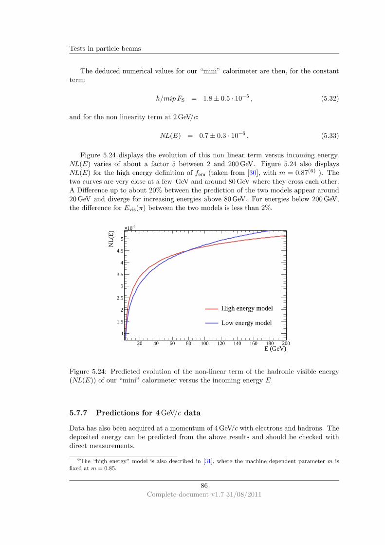
Tests in particle beams
The deduced numerical values for our “mini” calorimeter are then, for the constantterm:
h/mipFS = 1.8 ± 0.5 · 10−5 , (5.32)
and for the non linearity term at 2 GeV/c:
NL(E) = 0.7 ± 0.3 · 10−6 . (5.33)
Figure 5.24 displays the evolution of this non linear term versus incoming energy.NL(E) varies of about a factor 5 between 2 and 200 GeV. Figure 5.24 also displaysNL(E) for the high energy definition of fem (taken from [30], with m = 0.87(6) ). Thetwo curves are very close at a few GeV and around 80 GeV where they cross each other.A Difference up to about 20% between the prediction of the two models appear around20 GeV and diverge for increasing energies above 80 GeV. For energies below 200 GeV,the difference for Evis(π) between the two models is less than 2%.
E (GeV)20 40 60 80 100 120 140 160 180 200
NL(
E)
1
1.5
2
2.5
3
3.5
4
4.5
5
-610×[0]*(1-pow(x,-0.15))
High energy model
Low energy model
Figure 5.24: Predicted evolution of the non-linear term of the hadronic visible energy(NL(E)) of our “mini” calorimeter versus the incoming energy E.
5.7.7 Predictions for 4GeV/c data
Data has also been acquired at a momentum of 4 GeV/c with electrons and hadrons. Thedeposited energy can be predicted from the above results and should be checked withdirect measurements.
6The “high energy” model is also described in [31], where the machine dependent parameter m isfixed at m = 0.85.
86Complete document v1.7 31/08/2011

Tests in particle beams
Showers from 4GeV/c electrons By simply applying eq. 5.18, one predicts for 4 GeV/celectron:
Evis(e) = 2.77 ± 0.16 · 10−5 × 4 GeV
= 11.1 ± 0.7 · 10−5 GeV
= 111 ± 7 keV . (5.34)
Showers from 4GeV/c hadrons The same way, by using formula 5.30, the 4 GeV/chadron shower visible energy can be predicted:
Evis(π) = (NL(4 GeV/c)
+(1.8 ± 0.5) · 10−5) × 4 GeV
= ((1.4 ± 0.6) · 10−6
+(1.8 ± 0.5) · 10−5) × 4 GeV
= 1.9 ± 0.6 · 10−5 × 4 GeV
= 76 ± 24 keV . (5.35)
The analysis described in section 5.7.5 should be redone for the 4 GeV data in orderto compare with these predictions.
5.7.8 Conclusion of the study
The average shower profile of 2 GeV/c electrons and hadrons has been measured in beamtest at CERN. The simulation of hadron shower profile need to be improved to get betteragreement with data and understand the reason of this large difference. A better choiceof the GEANT4 physics list for the simulation might greatly improve the result in thehadronic case, possible promising list could be “QGSP BERT” or “BIC FTP”.
The “mini” calorimeter characteristics give preliminary predictions of the character-istics of a real MICROMEGAS calorimeter. The limitations of the set-up used forbid toreach very precise results but the calculations performed here may serve as guidelinesfor a future MICROMEGAS calorimeter prototype characterisation.
Resume du chapitre
Un ensemble de quatre chambres MICROMEGAS a lecture analogique (carte de lec-ture GASSIPLEX, trois chambres 6 × 16 cm2 et une 12 × 32 cm2) maintenues dans unestructure metallique a ete expose a un faisceau de muons afin de mesurer l’efficacite desdetecteurs sur les signaux faibles laisses par les muons (particules au minimum ionisant— MIP) ainsi que la multiplicite de ce signal et encore l’homogeneite de la reponse. Pourl’application de la technologie MICROMEGAS dans un calorimetre optimise pour l’usagedu PFA une efficacite proche de 100% et une multiplicite proche de 1 sont preferables.
Les evenements ont ete classes en differentes categories (voir fig. 5.6). Les evenementsde type gloden et platinum sont utilises pour cette etude. Ils correspondent respective-ment a des evenements ou chacune des chambres ne presente qu’un et un seul hit et a des
87Complete document v1.7 31/08/2011

Tests in particle beams
evenements ou trois des chambres ne presentent qu’un et un seul hit independammentde la derniere.
Les evenements platinum ont ete utilises pour scanner l’homogeneite des chambresen mesurant la reponse aux muons dans chacun des canaux de lecture. Une amplitudetypique pour le signal des MIPs a ete mesuree de l’ordre de 20 fC (voir exemple surfig. 5.9 a gauche) avec une disparite relative de 11.25% sur les 384 canaux en jeu (voirfig. 5.9 a droite).
Dans le reste, des evenements golden ont ete utilises. Pour mesurer l’efficacite, unedroite est ajustee a travers les trois hits des chambres de reference et est extrapolee versla quatrieme chambre pour definir une zone cible de 3 × 3 pad dans laquelle on verifiela presence ou l’absence du hit attendu. Le rapport du nombre d’evenement ou le hit aete trouve sur le nombre total d’evenements utilises pour l’analyse donne l’efficacite dudetecteur. Des valeurs superieures a 97% apres correction pour le bruit ont ete etabliespour trois des quatre chambres. De la meme maniere on peut compter le nombre moyende hits present dans la zone cible de la chambre a tester (en ignorant les 0) et obtenir lamultiplicite moyenne du detecteur au signal des MIPs. Une mutiplicite inferieure a 1.1a ete etablie.
Ces deux grandeurs dependent du seuil de detection applique, les valeurs ci-dessuscorrespondent a un seuil de 1.5 fC. Les valeurs en fonction du seuil sont illustrees surla figure 5.14 pour l’efficacite et sur la figure 5.16 pour la multiplicite. Ces resultatsmontrent qu’une bonne efficacite peut etre atteinte avec une lecture autorisant des seuilsde l’ordre du femto-coulomb et que la multiplicite reste toujours proche de 1 quelquesoit le seuil au dessus de 1.5 fC.
La non-uniformite de l’efficacite a aussi ete mesuree et, malgre une disparite du gainde l’ordre de 10%, celle de l’efficacite est inferieure a 1% pour un seuil de 1.5 fC et croitlineairement avec le seuil. Hors, dans un calorimetre digital, l’uniformite de l’efficacitedonne celle du calorimetre, ainsi pour de bas seuils, une excellente uniformite pourraetre atteinte.
Tous ces resultats montrent l’excellent accord entre la technologie MICROMEGASet les besoins d’un calorimetre optimise pour l’application du PFA.
88Complete document v1.7 31/08/2011

CHAPTER 6
Development of the project
Results on the development of the MICROMEGAS DHCAL project are presented here.They address the points 5–6 of the list in section 3.4 (p. 47).
6.1 Embedded readout chip
6.1.1 Readout chips catalog
At the beginning of the project, two types of readout chips were envisioned, the HARDROCand the DIRAC chips. A third type of chips called MICROROC were developed laterand benefited from the experience earned from the former ones.
- HARDROC [62]: Developed by LAL, they exist in three successive versions: 1,2, 2b. These chips were available in their first version from the beginning. Theywere especially designed towards application to ILC experiments (ILC synchronousclock, power pulsing) but were optimised for the use of RPC detectors and offereda tunable shaping time of about 10–20 ns whereas 150–250 ns would have been suit-able for MICROMEGAS application. This shaping time issue results in a partialcollection of the MICROMEGAS signal estimated around 10%. As R&D chips,they suffered from a number of malfunctions which were resolved in subsequentversions. The first version chips were very fragile and tended to die during tests.No significant measurements were achieved (only beam profiles and rough efficiencyestimations). The HARDROC2 version was much more robust and was used tobuild the first 32 × 48 cm2 Active Sensor Units (ASUs) holding one mesh and 24chips. However, they suffered from a tendency to fail to transmit the configurationsignals. This was solved in the 2b version.
- DIRAC [60, 61]: Developed by LAPP and Institut de Physique Nucleaire de Lyon(IPNL), this chip is meant to be much simpler and cheaper than the HARDROCand offers two functioning modes: low gain for RPC readout and high gain forGEM or MICROMEGAS readout. The first version showed promising results and
89

Development of the project
has represented a key step in the LAPP project by demonstrating the feasibility ofa bulk MICROMEGAS with embedded readout electronics [72] (see photographyin figure 6.1). The second version of this chip solved a few minor defaults butsuffered unfortunately from a harsh weakness against sparks.
- MICROROC: This chip, developed in collaboration between LAL/Omega andLAPP, corresponds to the integration of the optimised and debugged DIRAC inputstage into the HARDROC frame. Extensive tests have shown excellent results [63]and therefore, in summer 2011, the 2nd MICROMEGAS square meter was equippedwith 144 MICROROC. This new prototype is under test in particle beam at CERNat the time of writing.
6.1.2 Performance of the DIRAC1 prototype
The first MICROMEGAS chamber with embedded readout electronics was built andsuccessfully tested in a particle beam during august 2008 beam tests. A unique 8×8 padchamber equipped with DIRAC chips [60] was exposed to 200 GeV/c muons. Data wasacquired with a 19 fC threshold, in Ar/iC4H10 (95/5), at a mesh voltage of 410 V anda drift voltage of 460 V. The data acquisition was self-triggered by the ASIC using anexternal clock with a 200 ns period. The chip has proved to survive the laminationprocess by showing the beam profile displayed in figure 6.2. A raw hit multiplicity of1.1 has been measured. The related study is described in details in [72].
(a) (b) (c)
Figure 6.1: DIRAC MICROMEGAS prototype. View from chip side without (a) andwith (b) protection mask. View from mesh side (c).
6.1.3 DIRAC2 performance
A second version of the DIRAC chip has been developed at LAPP. A stack of four 8 ×8 pad MICROMEGAS chambers equipped with DIRAC2 chips was mounted and exposedto 6 GeV/c hadron beam at CERN/PS/T9 facility in 2009. Unfortunately, a weaknessagainst sparks in the chambers resulted in the loss of readout channels. The chipsbecame completely blind after a few hours functioning. Very little data was acquired
90Complete document v1.7 31/08/2011
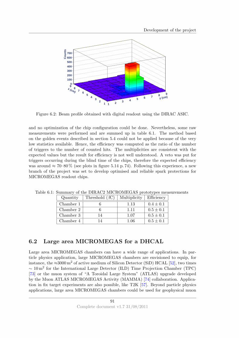
Development of the project
y (cm)
1 2 3 4 5 6 7 8 9
x (cm)
12
34
56
78
9
Cou
nts
0
100
200
300
400
500
600
700
Figure 6.2: Beam profile obtained with digital readout using the DIRAC ASIC.
and no optimization of the chip configuration could be done. Nevertheless, some rawmeasurements were performed and are summed up in table 6.1. The method basedon the golden events described in section 5.4 could not be applied because of the verylow statistics available. Hence, the efficiency was computed as the ratio of the numberof triggers to the number of counted hits. The multiplicities are consistent with theexpected values but the result for efficiency is not well understood. A veto was put fortriggers occurring during the blind time of the chips, therefore the expected efficiencywas around ≈ 70–80 % (see plots in figure 5.14 p. 74). Following this experience, a newbranch of the project was set to develop optimised and reliable spark protections forMICROMEGAS readout chips.
Table 6.1: Summary of the DIRAC2 MICROMEGAS prototypes measurementsQuantity Threshold ( fC) Multiplicity Efficiency
Chamber 1 6 1.13 0.4 ± 0.1
Chamber 2 6 1.11 0.5 ± 0.1
Chamber 3 14 1.07 0.5 ± 0.1
Chamber 4 14 1.06 0.5 ± 0.1
6.2 Large area MICROMEGAS for a DHCAL
Large area MICROMEGAS chambers can have a wide range of applications. In par-ticle physics application, large MICROMEGAS chambers are envisioned to equip, forinstance, the ≈3000 m2 of active medium of Silicon Detector (SiD) HCAL [52], two times∼ 10 m2 for the International Large Detector (ILD) Time Projection Chamber (TPC)[73] or the muon system of “A Toroidal Large System” (ATLAS) upgrade developedby the Muon ATLAS MICROMEGAS Activity (MAMMA) [74] collaboration. Applica-tion in fix target experiments are also possible, like T2K [57]. Beyond particle physicsapplications, large area MICROMEGAS chambers could be used for geophysical muon
91Complete document v1.7 31/08/2011

Development of the project
imaging [75]or as neutron detectors [76] for territorial safety to scan large containers forradioactive freight. Medical imaging is also demanding for efficient, cheap and reliabledetectors (see a first test of application of MICROMEGAS to medical imaging [77]).
The capability for large area bulk production is limited to 150×50 cm2 by CERN’s in-frastructure dedicated to Micro-Pattern Gaseous Detector (MPGD). T2K and MAMMAcollaborations are demanding for even larger area and an upgrade of the facility is fore-seen for producing 200 × 100 cm2 individual bulks. This new infrastructure will allowthe production of larger MPGD of all types [78].
In the context of the DHCAL active medium, embedded readout electronics is re-quired to optimize the detector compactness and minimize dead zones. Therefore, de-spite the possibility to provide bulks as large as 200 × 100 cm2, such large area bulkMICROMEGAS with embedded readout electronics can not be presently produced. Thereason comes from the complexity of the involved PCBs. Embedding chips on a PCB im-plies the routing of a large number of tracks for physics and electronics control signals,ground layers, shielding between signals and power supply for electronic components.Moreover, the PCB must be gas tight, as part of the envelope of the gas volume of agaseous detector. This results in multi-layer PCBs (6–8 layers) with very thin printingsand blind and buried vias. Today’s available equipment in the industry does not allowthe production of such PCBs larger than ∼ 50 × 50 cm2 at a sensible price.
6.2.1 Square meter prototype design and assembly process
6.2.1.1 Design
The extension to larger area bulk MICROMEGAS with embedded readout electronicshas however been performed by sharing a larger gas volume between several moderatesized ASUs. The square meter prototype consists of six 32 × 48 cm2 ASUs sharing thesame gas volume. Each ASU bears its own mesh and 24 ASICs. Segmenting the mesh assuch reduces by a factor 6 the energy released in case of spark (< 1 mJ instead of 6 mJ)thus providing safer condition for the readout electronics (compared to a 1 m2 mesh).DIF boards are employed to pilot the configuration of the chips and the data transfer.A single DIF can handle a range of chained ASUs. It is connected to the first ASUby an intermediate board playing the role of a plug adaptor and also providing voltagedistribution. The ASUs are chained together by relaying data and control signals viaflexible connectors. The last ASU of the chain is terminated to send back the signalthrough the chain to the DIF. To achieve a square meter chamber, three independentchains consisting of one DIF, one intermediate board and two chained ASUs, are fixedonto a 2 mm thick square meter iron base. A 5 mm gap is maintained between all ASUsthanks to 3 mm high resin walls proving support to the 2 mm thick iron top lid. Inaddition, the 3 mm MICROMEGAS drift gap is ensured by a 3 mm high resin frameenclosing the chamber, providing gas inlet and outlet, and by the spacer walls betweenthe ASUs. The total thickness of the prototype is 11.5 mm. The final device is robustand a square meter prototype, even encapsulated between 2 mm thick steel plates canbe manipulated by hands. The design is illustrated in figure 6.3.
92Complete document v1.7 31/08/2011

Development of the project
(a)
(b)
Figure 6.3: (a): Design of the m2 prototype ; (b): Spacer wall scheme.
6.2.1.2 Assembly process
The ASUs needed to mount a square meter prototype are built and tested separately.The PCB production and the electronics cabling are done by industrial subcontractors.The MICROMEGAS meshes are installed by lamination at CERN MPGD workshop.Each ASU is then cooked in clean room and inserted in a dedicated test box. The testbox allows to verify the good functioning of the ASUs by providing all electrical andgaseous services in a gas tight volume temporarily housing the ASU. The response ofthe ASU to cosmic rays and to 55Fe can be checked and hence validate the ASU fordefinitive insertion in the square meter prototype. A photograph of an ASU lying in theopened test box in the clean room is shown in figure 6.4(a). An example of a test resultis displayed in 6.4(b).
93Complete document v1.7 31/08/2011

Development of the project
(a) (b)
Figure 6.4: Test box for single ASU validation. (a) one ASU inserted in the opened testbox. (b) 55Fe profile of an ASU in the test box.
6.2.2 Mechanical prototype
The mechanical square meter prototype did not house any real ASUs. In this versionthey were replaced by naked and very simple PCBs called ghost ASUs. It was intended totest the assembly process and the gas tightness of the final device. During the assembly,some minor possible improvement were found and therefore applied to the assembly ofthe physical prototype. A photograph of the mechanical prototype under constructionis displayed in figure 6.5, the ghost ASUs at the foreground and the resin mask for theprotection of the ASICs at the background are clearly seen. The spacer walls maintainingthe drift volume are also seen at the border of each ASU. The mechanical prototypewas gas tight and the assembly procedure was validated.
Figure 6.5: Photograph of the me-chanical square meter prototypeunder assembly.
6.2.3 Physical prototype
Using the technical skill developed by our technicians on the mechanical prototype, thefirst physical square meter prototype was assembled. The first physical square meterprototype housed four HARDROC2 ASUs, one HARDROC2b ASU and one ghost ASU
94Complete document v1.7 31/08/2011
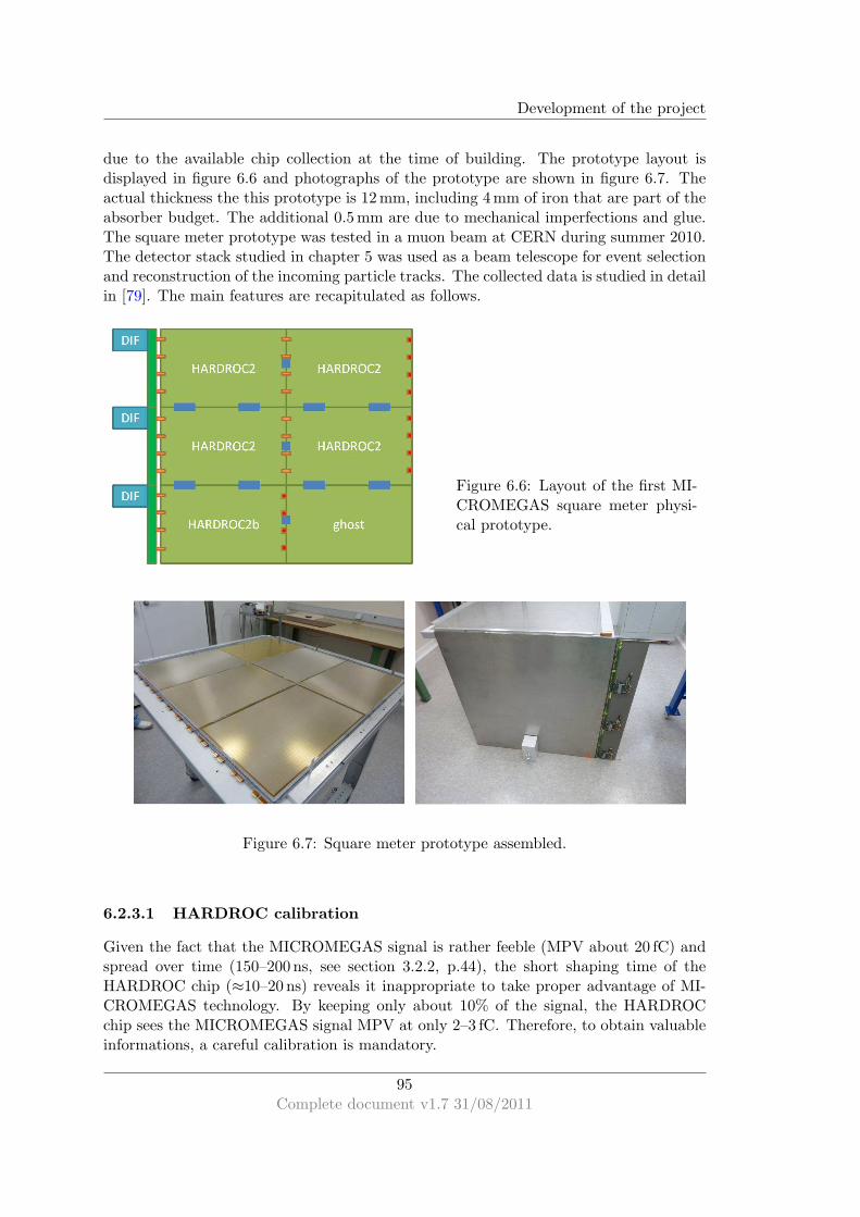
Development of the project
due to the available chip collection at the time of building. The prototype layout isdisplayed in figure 6.6 and photographs of the prototype are shown in figure 6.7. Theactual thickness the this prototype is 12 mm, including 4 mm of iron that are part of theabsorber budget. The additional 0.5 mm are due to mechanical imperfections and glue.The square meter prototype was tested in a muon beam at CERN during summer 2010.The detector stack studied in chapter 5 was used as a beam telescope for event selectionand reconstruction of the incoming particle tracks. The collected data is studied in detailin [79]. The main features are recapitulated as follows.
Figure 6.6: Layout of the first MI-CROMEGAS square meter physi-cal prototype.
Figure 6.7: Square meter prototype assembled.
6.2.3.1 HARDROC calibration
Given the fact that the MICROMEGAS signal is rather feeble (MPV about 20 fC) andspread over time (150–200 ns, see section 3.2.2, p.44), the short shaping time of theHARDROC chip (≈10–20 ns) reveals it inappropriate to take proper advantage of MI-CROMEGAS technology. By keeping only about 10% of the signal, the HARDROCchip sees the MICROMEGAS signal MPV at only 2–3 fC. Therefore, to obtain valuableinformations, a careful calibration is mandatory.
95Complete document v1.7 31/08/2011

Development of the project
Calibration data A LabView program developed at LAPP allowed the control of theinjection of calibrated pulses into the chip entry stage and to control the chip configura-tion. Calibration data was acquired while varying the chip threshold within its dynamicrange (0–1023 DAC) and recording the chip response to the input charge. The processhas been repeated for four values of the input charge: 0 (no charge, pedestal study),10 fC, 50 fC and 100 fC.
S-curves The plot of the chip efficiency versus threshold is called an S-curve becauseof its specific shape showing a higher level plateau and a lower level one linked togetherby a continuous slope (recalling the shape of the letter ‘s’). The raw S-curves obtainedfor no charge injection for one single chip are displayed in figure 6.8(a). The pedestal ofa channel is defined as the inflection point abscissa of its S-curves. The electronic noiseof a channel is rendered by the width of its S-curve.
Calibration procedure Given that 1 DAC corresponds roughly to 1 fC, figure 6.8(a)shows that the pedestals are quite spread and present irregular widths. The calibra-tion process is aimed at allowing the lowest possible threshold with the lowest possibleelectronic noise contamination in order to achieve the highest efficiency. The tunable pa-rameters are the gain of each channel and the global chip threshold. It has been noticedin [79] that the pedestal value is linearly dependent on the channel gain and that theS-curve width on the contrary does not change much for different gains. Therefore it hasbeen possible to align the S-curve lower levels so that they all start at the same Digitalto Analog Count (DAC) value; the result is plotted in figure 6.8(b). This technique al-lows the threshold for each readout channel to be minimized but is disadvantaged by thespread of channel gains. However, it has been shown in chapter 5 that despite a certaindisparity of the gain (gas gain in the former case, electronic gain in the present one)the efficiency disparity was strictly proportional to the value of the detection threshold.This assumption would not hold in the case of a multi-threshold readout.
threshold (DAC)80 82 84 86 88 90
effic
ienc
y (%
)
0
20
40
60
80
100
(a)
threshold (DAC)80 82 84 86 88 90
effic
ienc
y (%
)
0
20
40
60
80
100
(b)
Figure 6.8: Pedestal S-curves for chip #124 before (a) and after (b) calibration [79].
96Complete document v1.7 31/08/2011

Development of the project
6.2.3.2 Square meter performance
It is worth recalling here that the results presented in this section do not reflect anywherenear the full potential of the bulk MICROMEGAS chambers. This first square meterprototype has played the role of a training tool allowing to develop all the skills neededfor the next ones. The best performance was achieved with a 420 V amplification voltage,corresponding to a gas gain of ≈ 104, at a channel threshold1 of 1–2 DAC; see table 6.2.Performance with a more conservative amplification voltage of 410 V is displayed in table6.3. Four positions in the prototype, denoted by the corresponding chip number, havebeen scanned.
Table 6.2: Best performance of the first square meter prototypeMean efficiency Efficiency disparity Multiplicity Multiplicity disparity
43.8% 5% 1.06 0.003
Table 6.3: Performance of the first square meter prototype at 410 V.Chip Mean channel threshold Mean efficiency Efficiency disparity Multiplicity
114 4 DAC 11.2% 1.7% 1.07
112 5 DAC 11.9% 1.9% 1.06
134 12 DAC 4.5% 0.9% 1.09
138 12 DAC 3.8% 0.9% 1.08
6.2.4 Power pulsing
The power pulsing technique consists of powering off a device during a given idle timeand switching it on when needed. If the idle time is sufficient, this technique allowsa significant reduction of the average power consumption in comparison to having allthe electronics working all the time. The target consumption for calorimeters at ILC is≤ 25µW/channel [52, 53]. The motivation for power pulsed electronics at future linearcolliders is the need for calorimeter compactness. Cooling systems usually representa large amount of cumbersome dead material in detectors. A lower power consump-tion results in a lower heat dissipation and hence a decreased need for cooling and, byconsequence, smaller cooling systems.
The possibility to use the power pulsing technique comes from the beam clock cycleforeseen for the future linear colliders, as summarised in table 6.4. As shown in table6.5 the electronics would be idling most of the time. The performance impact of the useof power pulsing technique i stherefore important to be investigated. A suitable readoutchip should be able to be switched on and off sufficiently quickly to allow a significantoff time and no impact on performance during on time. All the chips are designed for apower pulsed usage.
1A channel threshold is defined as the difference between the global chip threshold and the channelpedestal.
97Complete document v1.7 31/08/2011

Development of the project
Table 6.4: Beam clock cycle at future linear colliders (500 GeV version) [80, 25]Machine bunches separation train length repetition period
CLIC 500 ps 177 ns 20 ms
ILC 369 ns 1 ms 200 ms
Table 6.5: Idle time at future linear colliders (500 GeV version)Machine Idle time between bunch trains Duty time fraction
CLIC 19.998 ms 1 · 10−5
ILC 199.00 ms 5 · 10−3
A preliminary test of the effect of HARDROC2 power pulsing has been performedin a muon beam [79]. The square meter prototype was operated with a conservativeamplification voltage of 410 V. During the test, the beam was kept on only one positionin the square meter prototype corresponding to chip #124 with average channel thresholdof 7 DAC, but all the chips were set to record data. The corresponding beam profilesare displayed in figure 6.9 and show no significant difference.
The detector efficiency has been measured with power pulsing activated and withpower pulsing deactivated. In power pulsing mode, the chip was off during 10 ms andon during 2 ms, the external trigger was vetoed during the off periods of the chips. Thecorresponding pulsed current was about 7.5 A. The measured efficiencies are shown intable 6.6. The low efficiency is due to the short shaping time of the HARDROC chipsallowing to see only about 10% of the MICROMEGAS signal. The ratio of the efficiencywith over without power pulsing is compatible with 1.
Table 6.6: Effect of power pulsing on detection efficiency.Power pulsing mode Channel-to-channelOFF ON ON/OFF ratio
8.7 ± 0.4% 9.3 ± 0.6% 1.06 ± 0.05
A crucial step in the development of the power pulsing technique will be the possi-bility to powering the apparatus with an averaged current rather than a peaked pulsedcurrent. This may be done by powering with a low current an ad hoc capacitance closeto the power pulsed electronics that will then deliver the power pulse in due time. Theinterest is then that the cabling between external power and the readout electronicswould be reduced therefore some dead material would be saved.
6.2.5 Preliminary results on the second square meter prototype
The second square meter prototype has been built and is under beam tests at CERN/H4Abeam line at the time of writing. It is composed of 6 ASUs bearing a total of 144 MICRO-ROC chips and is designed 1 mm thinner than the previous prototype, 10.5 mm instead of11.5 mm, thanks to a protective mask of 2 mm instead of 3 mm. The actual thickness of
98Complete document v1.7 31/08/2011

Development of the project
(a) (b)
Figure 6.9: Beam profiles without (a) and with (b) power pulsing activated. The redmarks represent the ghost ASU.
this prototype is 11.5 mm. The thickness difference with the design is due to glue and tomechanical tolerances and also to aluminium adhesive ribbon used for ElectromagneticCompatibility (EMC). The electronic side steel lid is fixed with only screws and can beremoved to access the embedded electronics for tests or maintenance or simply removedto give back the corresponding 2 mm of steel to the absorber structure of the calorimeterto increase its mechanical robustness. The gas tightness is insured by glue between theASUs. The prototype’s assembly took great advantage of the experience earned with theprevious prototypes. It shows already preliminary performance beyond expectations: anefficiency up to 99% with a noise bias below 0.1% and a response multiplicity below 1.2.
6.3 Expected performance of a MICROMEGAS DHCALprototype
6.3.1 Cubic meter project
In order to test the performance of International Linear Collider (ILC) or CompactLinear Collider (CLIC) calorimeters the natural idea is to build a small part of it as aprototype. The depth of the prototype should be the same as the baseline design of thefinal calorimeter in order have a realistic longitudinal containment of particle showers.The transverse dimensions should be sufficient to avoid lateral leakage. It has thereforebeen chosen to build a 4.5λI deep calorimeter with a 1 × 1 m2 transverse area. Sucha prototype will consist of 40 instrumented layers (8 mm each) and 40 layers of steel(1.86 cm) giving a total thickness of 106.4 cm. This class of prototypes is therefore calleda “cubic meter”.
Several cubic meter prototypes involving different detection technologies are currentlybeing built within the CALICE collaboration [54]. The main ones are the scintillatorcubic meter from the Analog Hadronic Calorimeter (AHCAL) project held at DeutschesElectronen Sychrotron, Hamburg (DESY) and the RPC cubic meter from the DHCALproject at Argonne national laboratory, Illinois. Those two projects correspond to thebaseline of the ILD and SiD detectors respectively.
99Complete document v1.7 31/08/2011

Development of the project
Simulations have been performed to evaluate the performance of a MICROMEGASbased cubic meter. To do so, the geometry has been implemented in a GEANT4 appli-cation and the MICROMEGAS response was simulated separately.
MICROMEGAS response simulation The GEANT4 simulation only provides theamount of energy deposited in the 3 mm MICROMEGAS conversion gap. To achievea more realistic simulation, the development of the MICROMEGAS signal was imple-mented step by step in a digitisation driver.
1. The raw deposited energy is divided by the effective ionisation potential of the gasWI = 25.8 eV for Ar/iC4H10 (95/5) to obtain the number of primary electrons.
2. Each electron is tested to determine if it will reach the amplification gap or not.The size of the pillars give a probability of ≈ 4% for an electron to crash on them.The mesh transparency was conservatively taken at 70%.
3. Each electron passing the previous tests is amplified following an exponential distri-bution (model described in [46] valid for field of a few tens of kV· cm−1). The gainis given as input parameter and the actual number of electrons in the avalanche isdetermined randomly in accordance with the fluctuation formula 3.1.
4. The induced charge on the anode pad corresponds to the sum of the charge of theavalanche of all the primary electrons (see appendix A for details)
5. A smearing factor is applied to the induced charge corresponding to the globaldetector energy resolution (7.5%) measured with 5.9 keV X-ray (see figure 4.1,p.54)
6. Electronics conversion factors are applied to the deposited charge to get an outputin ADU (GASSIPLEX-like readout).
The following features will need to be be taken into account in a refined future versionof this digitisation driver:
- Transverse diffusion of primary electrons (to induce the hit multiplicity, neglectedso far)
- Time development of the signal (to allow modelisation of the electronics shapingof the signal and time stamping studies)
- Tunable probability of noise hit contamination
6.3.2 Mini-calorimeter alternative
Low energy showers can be studied with a calorimeter much smaller than 1 m3. Forinstance, in [81] and [58] studies of electromagnetic and hadronic showers respectivelyfor energies below 16 GeV are presented. Those studies were done with RPC chambersmounted in a six layer stack interleaved with 2 cm thick steel plates. With only sixASUs such an experiment could be redone, offering cross checked measurements and afair comparison between RPC and MICROMEGAS technologies.
(gather details from jan’s simulation, when available... if ever available)
100Complete document v1.7 31/08/2011

Development of the project
6.4 Layout studies towards the SiD DHCAL
6.4.1 Global geometry
LAPP has proposed the baseline design for SiD hadronic calorimeter geometry [82,83, 52]. The principle was that projective cracks have a probability to hide informationabout tracks passing through them. The proposed geometry completely avoids projectivecracks by being constituted of two types of module: rectangular and trapezoidal. Seefigure 6.10 for a comparative view of the classical projective geometry and the proposednon projective one. Simulation studies at LAPP[84] demonstrate that the non projectivegeometry in the vicinity of the cracks present better performance than the projectiveone. Such a conclusion was anticipated. Global improvement is evaluated by consideringincoming particles not just in the immediate vicinity of the cracks. The same simulationmodel is used with a wider spacial dispersion of the incoming particles and conclude alsoin favour of the non-projective geometry.
Figure 6.10: Comparative view of projective and non-projective HCAL barrel geometries.
6.4.2 Alternative DHCAL layout
Three alternative geometries have been considered beyond the baseline. The baselinedesign is a 40 layer calorimeter of 1.89 cm of stainless steel between MICROMEGASplanes as shown on figure 6.11(a). The question is if alternatives can be envisioned toincrease mechanical robustness and to simplify integration with no degradations of thephysics performances. Figure 6.11 sums up the different alternatives considered here.The overall dimension are conserved in each design: depth = 4.5 λI, 107.6 cm.
- Thick back plate geometry: the last active layer is removed and the two lastabsorber plates are merged to make a double thickness steel layer at the outsideshell of the calorimeter to increase the detector robustness. The scheme is shownin figure 6.11(b).
101Complete document v1.7 31/08/2011

Development of the project
- Progressive absorber thickness geometry: the 30 first layers are standard, then 5layers are 2.09 cm thick and then 4 layers are 2.29 cm thick. See scheme in figure6.11(c).
- Brass absorber geometry: As brass is way easier to machine than steel, only thefirst and last absorber layers are made of steel with standard thickness of 1.89 cmand the others are 1.85 cm thick brass layers. See scheme in figure 6.11(d).
(a) Standard geometry (b) Thick back plate geometry
(c) Progressive absorber thickness geometry (d) Brass absorber geometry
Figure 6.11: Scheme and summary of the considered alternative geometries.
Resume du chapitre
Les differentes etapes cles du projet de developpement de chambres MICROMEGASen tant qu’element actif d’un calorimetre hadronique digital optimise pour l’applicationd’un PFA aupres d’un futur collisionneur lineaire, apres les mesures de caracterisationseffectuees dans les deux chapitres precedents, sont resumees ici.
Electronique embarquee Les premiers prototypes de chambre MICROMEGAS avecbulk et electronique de lecture embarquee sur le PCB d’anode ont ete assembles et testesavec succes validant ainsi la technique d’assemblage. La puce de lecture, DIRAC1, etles autres composants sont soudes au four puis un masque de protection en resine est
102Complete document v1.7 31/08/2011

Development of the project
installe sur l’electronique afin de lui permettre de resister a l’etape de lamination lors dela pose du bulk.
Apres cette validation, une puce electronique optimisee pour la lecture des signaux dechambre MICROMEGAS a ete developpee en collaboration entre le LAPP et le LAL/Ω.Apres plusieurs modeles testes, la puce MICROROC a ete selectionnee pour equiper lesfuturs prototypes de chambre MICROMEGAS de grande surface.
Chambre MICROMEGAS de grande surface pour la calorimetrie hadroniquedigitale Pour des raisons a la fois de limitation dans la taille des bulks et dans la tailledes circuits imprimes de la complexite de ceux utilises ici, un prototype d’un metrecarre consiste en six unites de detection independentes (Active Sensor Unit — ASU)partageant un unique volume de gaz. Les ASUs representent des surfaces actives de32 × 48 cm2 chaines deux a deux dans la longueur et controles par une carte d’interface(Detector interface — DIF). Trois de ces assemblages sont juxtaposes pour forme un plande 96 × 96 cm2 (soit 9 216 voies, voir schemas sur fig. 6.3 et photos sur fig. 6.7). Le pre-mier prototype “Metre Carre” equipe de l’electronique de lecture optimise MICROROCmontre des performances remarquables en accord avec les mesures de caracterisation.
Prototype “Metre Cube” Des etudes de simulations d’un calorimetre d’un metrecube (env. 40 plan de 1 m2), utilisant des chambres MICROMEGAS en tant que milieuxactifs, sont menees afin de predire les caracteristiques d’un tel calorimetre en terme deresolution en energie, linearite, ou encore contenance de l’energie. Plusieurs prototypes“Metre Cube” sont deja construits avec d’autres technologies (Scintillateur, RPC). Lesexcellentes performances des chambres MICROMEGAS encouragent a la constructiond’un Metre Cube MICROMEGAS afin de comparer les differentes technologies envisageesde maniere objective.
Design du calorimetre Hadronique de SiD Une etude mecanique menee au LAPPa conduit, lors de la redaction de la lettre d’intention de SiD, au choix d’une geometrienon projective pour le calorimetre hadronique. Le schema propose est donne sur la figure6.10. Des geometries alternatives de l’empilement absorbeur / couche active ont aussiete etudiees (voir fig. 6.11) et fournissent toutes differents avantages mecaniques sansdeterioration de performance.
103Complete document v1.7 31/08/2011

Development of the project
104Complete document v1.7 31/08/2011

CHAPTER 7
Conclusion
MICROMEGAS chambers using bulk technology were built and tested with the objectof evolving towards large area detectors for multiple applications, but most importantlyas an active medium of a future linear collider (semi-)digital hadronic calorimeter. Smallprototypes of 6×16 cm2 (and one of 12×32 cm2) with analog readout were first assembledfor a detailed evaluation before evolving towards larger area with dedicated electronics.
The optimal working point was determined in X-ray laboratory tests. A mesh voltageof 420 V with a drift voltage of 470 V assure a high gas gain (≈ 104) and an optimalmesh transparency to electrons in Ar/iC4H10 (95/5). At the same time, a method of datacorrection for environmental gain fluctuations was proposed. This may be used for on-line gain control to ensure gain stability during long runs of data acquisition. This wouldbe useful for operation at intermediate or high detection thresholds (≥1 MIP MPV)where gain fluctuation has an impact on efficiency.
Beam tests at CERN at CERN allowed a series of detailed measurements. Thegain non-uniformity, the MIP efficiency, its homogeneity and the hit multiplicity weremeasured. The MICROMEGAS prototypes were also exposed to high energy hadronsand showed very good behaviour even in very dense showers.
The key results are summed up below (for 1.5 fC detection threshold):
- MIP signal amplitude ≈ 20 fC
- Efficiency ≥ 97%
- Efficiency disparity ≤ 1%
- Gain disparity ∼ 7–13%
- Multiplicity ≤ 1.1
Performance of the PFA in function of the active medium MIP efficiency was not availableat the time of writing. However, PFA calls for calorimeters with tracking capabilitiesand therefore a very high efficiency is likely to be useful. A low multiplicity (close to 1)
105
Conclusion
should be very important for the PFA to clearly identify the hadronic shower startingpositions and then match calorimeter hit clusters to charged tracks. Therefore, thoseresults prove that the bulk MICROMEGAS is very suitable for application in PFAoriented digital calorimetry. The gain disparity is relatively high, but in the context ofdigital calorimetry, the efficiency disparity at the working threshold is the fundamentaltrait and is below 1%.
Collaborative results The first bulk MICROMEGAS chamber with embedded read-out electronics has been successfully built and tested. This has validated the embeddingprocess based on using a resin mask to protect the readout chips during the laminationof the bulk. ASUs with embedded readout electronics of size up to 32×48 cm2 have beenproduced and then assembled into a square meter MICROMEGAS prototype tested inmuon beam in 2009. The electronics used however was not optimal and the performanceachieved were well below the full MICROMEGAS potential. However, precious technicalexperience has been earned and has already served for the second square meter proto-type equipped with optimised readout electronics. This second square meter prototypeis under beam tests at CERN at the time of writing and shows preliminary performanceoutperforming the expectations.
A proposal of non projective geometry, supported by simulation studies has beenaccepted as the SiD baseline for its hadronic calorimeter. Several alternative HCALlayouts have been also studied with MC simulations. The different layouts show variousmechanical advantages compared to the baseline without any loss of performance.
Des chambres MICROMEGAS utilisant la technologie bulk ont ete construites ettestees avec succes.Des mesures de caracterisation en rayons X ont permis d’etablir lepoint de fonctionnement des detecteurs : tensions de grille applicables (autour de 400Ven Ar/iC4H10 (95/5), de 580 en Ar/CO2 (80/20)), rapport des champs d’amplificationet de derive entre 150 et 200 (difference de potentiel de 50V en Ar/iC4H10 (95/5)). Unemethode de correction des donnees pour les fluctuations de pression et temperature dugaz a ete proposee. Cette methode peut servir aussi a controler directement le gain lorsde la prise de donnees afin de compenser les modifications des proprietes du gaz dans lecas de donnees digitales difficilement corrigeable. Des tests en faisceaux de muons ontfourni une serie de mesures detaillees resumees ci-dessous pour un seuil de 1.5 fC.
- Amplitude du signal des MIP ≈ 20 fC (pole de la distribution)
- Efficacite ≥ 97%
- Non-uniformite de l’efficacite ≤ 1%
- Non-uniformite du gain ∼ 7–13%
- Multiplicite ≤ 1.1
Ces resultats demontrent que la technologie MICROMEGAS est appropriee pour unecalorimetrie digitale optimisee pour l’application d’un PFA.
Les chambres ont aussi ete exposees a des gerbes electromagnetiques et hadroniquesde diverses energies. Des profils de gerbes ont ete mesures illustrant la bonne tenue deces chambres lors de l’exposition aux gerbes.
106Complete document v1.7 31/08/2011

Conclusion
Resultats collaboratifs les etapes suivantes du developpement du projet ont ete realiseespar le groupe au LAPP parallelement et conjointement aux travaux principalement per-sonnels decrit precedemment.
- Validation de la methode d’assemblage des prototypes a electronique de lecture em-barquee
- Developpement d’une puce de lecture optimisee pour les signaux MICROMEGAS
- Assemblage d’un prototype “Metre Carre” et conservation des performances (MetreCarre MICROROC)
Mais aussi, le design de base pour le calorimetre hadronique de SiD a ete concuau LAPP avec l’appui d’etudes de simulations. D’autres etudes de simulations ont in-vestigue diverses geometries alternatives ouvrant de multiples fenetres pour les choixmecaniques futurs pour la construction de SiD.
Ces realisations, outre le dynamisme et la motivation de toute l’equipe, montrentla competitivite de la technologie MICROMEGAS, tres prometteuse pour de multiplesapplications dont la calorimetrie hadronique a imagerie pour les futures experiences dephysique des particules.
107Complete document v1.7 31/08/2011

Conclusion
108Complete document v1.7 31/08/2011

Part III
Search for New Physics in theField of the Top Quark at CLIC
109


CHAPTER 8
The top quark at CLIC
The condition of e+e− collisions at Compact Linear Collider (CLIC) are described beforefocusing on the case of the tt pair production in such collisions. Then, a method for ttevent selection is proposed and evaluated.
8.1 e+e− collisions at 3TeV
8.1.1 Initial State Radiation
Initial State Radiation (ISR) occurs in every process involving charged and/or colouredparticles and can have a large influence on the outcome of the collision. It consist ofthe emission of a photon (in the case of electomagnetic particles) or a gluon (in thecase of coloured particles) just before the collison. This tendency increases dramaticallywith higher energy and with smaller masses. Therefore, when an electron is to collidewith a positron they both radiate a more or less energetic photon. This phenomena iscalled ISR. It induces a continuous smearing of the centre of mass energy of the actualcollision, presenting a peak at the nominal centre of mass energy and a tail towards thelower values. Moreover, It introduces a random asymmetry in the collision, since theenergy loss of the incoming particles is independent of each other, resulting in a boostof the centre of mass frame along the beam direction.
The calcHEP program [85] models this radiative energy loss of the collision initialstate through the following formula giving the incoming particle energy spectrum, x,ranging from 0 to 1, being the fraction of the nominal beam energy carried by theincoming electron and F the corresponding probability density function:
F (x) = exp (κ · (3/4 − γEuler
)) · κ · (1 − x)κ−1
×(1 + x2) − 1
2 · κ ·((
1 + 3x2) ln(x)
2 + (1 − x)2)
2Γ(1 + κ), (8.1)
where γEuler
≈ 0.5772156649 is the Euler-Mascheroni constant, Γ is the gamma function
111

The top quark at CLIC
andκ =
α
π(2 ln(Escale/me) − 1) ,
with α, the fine structure constant, me the electron mass and Escale, the energy scale ofthe process, i.e. the nominal collision energy in case of e+e− collisions. The function 8.1is represented for Escale = 3 TeV in figure 8.1(a), the shape of the distribution is mainlydefined by the contribution κ · (1−x)κ−1 which is plotted in figure 8.1(b) and which hasthe property that
∫ 1
0κ · (1 − x)κ−1 dx = 1 .
Energy fraction0 0.1 0.2 0.3 0.4 0.5 0.6 0.7 0.8 0.9 1
Pro
babi
lity
dens
ity
0
2
4
6
8
10
(a)
x0 0.1 0.2 0.3 0.4 0.5 0.6 0.7 0.8 0.9 1
-1κ (
1-x)
κ
0
2
4
6
8
10
(b)
Figure 8.1: Distribution of fraction of nominal energy available for the collisions
Luminosity spectrum The full luminosity takes all collisions into account, regardlessof the amount of initial state energy that is lost. An interesting question arises: whatwould be the luminosity if we only consider the collision that occur at the nominal energyor very close (say 1%)? The values for CLIC are for instance :
- Full luminosity: L = 5.9 · 1034 cm−2 s−1
- Luminosity in 1% of energy: L99% = 2.0 · 1034 cm−2 s−1
The luminosity dependency on the considered energy is referred to as “Luminosity spec-trum”.
8.1.2 Beamstrahlung
The Beamstrahlung (BS) is an electromagnetic energy loss due to the interaction ofan incoming particle with the electromagnetic field of the oncoming bunch. This phe-nomenon depends on the structure of the bunches. If a Gaussian shape is assumed, theresulting energy spectrum depends essentially on the two quantities Ncl and Υ, definedas follow:
Ncl =25α2N
12me(σx + σy), (8.2)
Υ =5αN Ecm
6m3eσz(σx + σy)
, (8.3)
112Complete document v1.7 31/08/2011

The top quark at CLIC
where α is the fine structure constant, me the electron mass, N the number of particlesin the bunch, σi, i ∈ x, y, z are the bunch dimension in term of Gaussian sigmas andEcm is the nominal centre of mass energy.
The energy spectrum, in calcHEP, is given by:
F (x) =1
Ncl
[
(1 − E−Nclcm )δ(1 − x) +
e−η(x)
1 − xh(η(x)1/3, Ncl)
]
, (8.4)
where δ is the Dirac function and η(x) and h(z,Ncl) are functions of the quantities 8.2and 8.3 defined as:
η(x) =2
3Υ(1/x− 1) , (8.5)
h(z,Ncl) =∑
n≥1
zn
n!Γ(n/3)γ(n+ 1, Ncl) , (8.6)
with Γ, the gamma function and γ the lower incomplete gamma function. A detailed andpedagogical approach to BS at future linear colliders is presented in [86]. The effect ofBS on the initial energy spectrum is rather similar to that of ISR and its implementationin calcHEP is simply an increase of the ISR effect. The nominal parameters for BS atCLIC are presented in table 8.1 (taken from [28], Ncl and Υ computed with calcHEP).Note that the large values of Υ (≥ 1) indicate that the energy losses of the incomingparticles can amount up to the particle total energy with significant probability.
Table 8.1: CLIC parameters used for BS calculation in calcHEP.σx σy σz N Ncl Υ
Nominal 45 nm 1 nm 44µm 3.72·109 3.47 4.89Conservative 83 nm 2 nm 44µm 3.72·109 1.88 2.65
8.1.3 Machine induced background
The very high luminosity foreseen at CLIC (5.9·1034 cm−2 s−1) implies the use ofdense and compact bunches of electrons and positrons. Beyond a significant BS effect,the high number of photons resulting from the beam-beam interaction will potentiallyproduce a significant amount of e+e− and qq pairs. The diagram of the process of hadronproduction from γγ collisions is represented in figure 8.2(a), the same for coherent e+e−
pair production in figure 8.2(b) and incoherent pair in figure 8.2(c). Table 8.2 shows theexpected number of such interactions per bunch crossing (BX).
Table 8.2: Main machine background process contribution.Process Number of events/BX
γγ →hadrons 2.7γ → e+e− 3.8 · 108
γγ → e+e− ≈ 105
113Complete document v1.7 31/08/2011
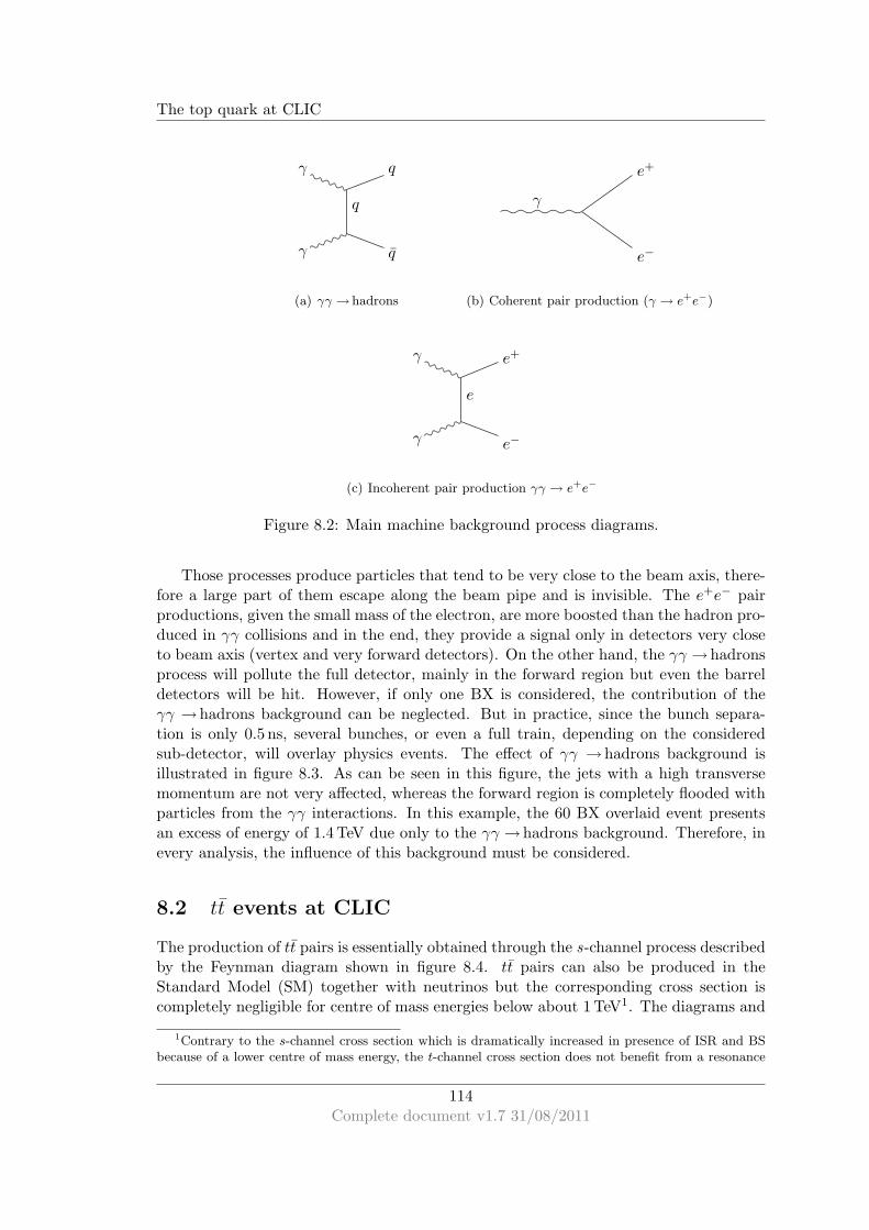
The top quark at CLIC
γ
γ
q
q
q
(a) γγ → hadrons
γ
e+
e−
(b) Coherent pair production (γ → e+e−)
γ
γ
e
e+
e−
(c) Incoherent pair production γγ → e+e−
Figure 8.2: Main machine background process diagrams.
Those processes produce particles that tend to be very close to the beam axis, there-fore a large part of them escape along the beam pipe and is invisible. The e+e− pairproductions, given the small mass of the electron, are more boosted than the hadron pro-duced in γγ collisions and in the end, they provide a signal only in detectors very closeto beam axis (vertex and very forward detectors). On the other hand, the γγ →hadronsprocess will pollute the full detector, mainly in the forward region but even the barreldetectors will be hit. However, if only one BX is considered, the contribution of theγγ →hadrons background can be neglected. But in practice, since the bunch separa-tion is only 0.5 ns, several bunches, or even a full train, depending on the consideredsub-detector, will overlay physics events. The effect of γγ →hadrons background isillustrated in figure 8.3. As can be seen in this figure, the jets with a high transversemomentum are not very affected, whereas the forward region is completely flooded withparticles from the γγ interactions. In this example, the 60 BX overlaid event presentsan excess of energy of 1.4 TeV due only to the γγ →hadrons background. Therefore, inevery analysis, the influence of this background must be considered.
8.2 tt events at CLIC
The production of tt pairs is essentially obtained through the s-channel process describedby the Feynman diagram shown in figure 8.4. tt pairs can also be produced in theStandard Model (SM) together with neutrinos but the corresponding cross section iscompletely negligible for centre of mass energies below about 1 TeV1. The diagrams and
1Contrary to the s-channel cross section which is dramatically increased in presence of ISR and BSbecause of a lower centre of mass energy, the t-channel cross section does not benefit from a resonance
114Complete document v1.7 31/08/2011

The top quark at CLIC
(a) No γγ →hadrons (b) 60 BX overlaid
Figure 8.3: Illustration of the effect of γγ →hadrons event overlay on a 1 TeV Z0 eventover 60 BX in the CLIC ILD detector (taken from [87])
cross sections for tt pair production together with SM neutrinos are given for referencein appendix B.
e−
e+
γ, Z
t, t
t, t
Figure 8.4: tt pair production diagram.
8.2.1 Total cross section as a function of the centre of mass energy
The total cross section of the channel e+e− → tt is computed with calcHEP [85] infunction of the centre of mass energy and displayed in figure 8.5. The dashed line in figure8.5 is an interpolation of the points with a exponential added to a first order polynomial.This calculation shows that after the resonance (for Ecm ≈ 350 – 400 GeV) the crosssection drops very quickly. This feature makes the low energy region an interesting fieldfor studies dedicated to top quarks near the production threshold. Whereas the highenergy region, more sensitive to variations of tt event statistics, would be favourable tosearches for new physics signatures, such as tt pair plus missing energy, where the SMtt pairs would be the major background.
The total cross section for tt pair production at a centre of mass of 3 TeV, computedby calcHEP, is (19, 87 ± 8 · 10−4) fb. But this number does not correspond to the crosssection that would be observed at a 3 TeV CLIC. As shown in sections 8.1.1 and 8.1.2,
effect and stays very low.
115Complete document v1.7 31/08/2011

The top quark at CLIC
[GeV]cmE500 1000 1500 2000 2500 3000
Cro
ss s
ectio
n [fb
]
0
100
200
300
400
500
600
Figure 8.5: e+e− → tt total cross section in function of centre of mass energy (interpo-lated with an exponential added to a first order polynomial).
the effective energy available in a 3 TeV e+e− collisions tends to be smaller than thenominal one because of electromagnetic energy losses of the incoming particles beforethe collision (ISR and BS). Therefore, according to the cross section dependency againstcentre of mass energy shown in figure 8.5, the average cross section of tt events in real3 TeV e+e− collision will be higher than the raw prediction. The cross section predictedby calcHEP with ISR and BS are summed up in table 8.3. The nominal and conservativeBS parameters are recalled in table 8.4. Table 8.3 illustrates well the impact of BS onthe initial state: the dramatic increase of cross section is due to the large smearing ofthe initial collision energy, resulting from the beam-beam interaction at 2 × 1.5 TeV.
Table 8.3: Cross section of tt events for various level of electromagnetic initial stateenergy losses.
σ [fb]
Raw 19.9ISR included 26.2ISR + Nominal BS 181.0ISR + conservative BS 91.2
8.2.2 tt pair energy spectrum
The energy spectrum of the 3 TeV tt events produced at CLIC with nominal beamparameters, displayed in figure 8.6, presents a rather singular shape.The same shape isseen even more clearly when looking at the Monte Carlo (MC) centre of mass energydistribution of the tt events (figure 8.7).
116Complete document v1.7 31/08/2011

The top quark at CLIC
Table 8.4: Beamstrahlung parameters for CLIC at 3 TeVNominal Conservative
x+ y 46 nm 85 nmz 44µm 44µm
Num. of part. 3.72·109 3.72·109
Ncl 3.47 1.88Υ 4.89 2.65
Event total energy [GeV]0 500 1000 1500 2000 2500 3000
Frr
actio
n of
eve
nts
/ 30
GeV
0
0.005
0.01
0.015
0.02
0.025
Figure 8.6: Total event energy spectrum of the tt events at CLIC (ISR and BS included).
The energy distribution of the colliding particles initial state has a shape close theone represented in figure 8.1 (p. 112) that might lead to expect a similar shape in thett event energy spectrum. But such a shape corresponds to the energy spectrum of allthe incoming e±, regardless of the process or the final state of each event, whereas thespectrum of figure 8.7 corresponds to a selection of those collisions which have led to a ttevent. Therefore, when the incoming particles collide at the nominal and most probableenergy, the probability of obtaining a tt event is minimal (cf. figure 8.5). But whenthe centre of mass energy happens to be lower, the rate of tt events takes off. Thus,when considering a sample of tt events and checking at which centre of mass energy theyhave been produced, one will see that some of them have been produced at the nominalenergy, whilst many of them at a much lower energy, due to a convolution betweenluminosity spectrum and cross section.
Now a second question arise: why is the secondary peak at about 1.5 TeV ratherthan around the tt resonance (≈ 350 GeV). The explanation is due to the fact thatthe initial state energy losses (ISR and BS) occur independently for the two collidingparticles. Therefore, since the most probable energy of the incoming particles is nearlythe nominal one, significant reductions of the initial state energy are achieved, most ofthe time, when only one of the two incoming particles has lost a large amount of energy.This situation results in highly asymmetric collisions, where one initial particle is at
117Complete document v1.7 31/08/2011

The top quark at CLIC
Centre of mass energy [GeV]0 500 1000 1500 2000 2500 3000
Fra
ctio
n of
eve
nts
/ 30
GeV
0
0.01
0.02
0.03
0.04
0.05
Figure 8.7: Initial energy spectrum of the tt events at CLIC (ISR and BS included).
nominal energy and the other one sometimes nearly at rest. Let E1 ≈ 1500 GeV be theenergy of the first particle and E2 ≪ E1 the energy of the second one. The resonanceoccurs when the effective centre of mass energy equals twice the top quark mass, i.e.:
4E1E2 = (2Mt)2 ,
Which gives:
E2 =M2
t
E1≈ 20 GeV .
Therefore, in the laboratory reference frame the energy of such en event is E1 + E2 =1520 GeV leading to the observed peak at 1.5 – 1.6 TeV of figure 8.7 and consequentlythe one observed in the event total energy spectrum of figure 8.6.
8.3 Top-tagging
In the framework of the CLIC Conceptual Design Report (CDR) preparation, tt eventsand other SM processes were simulated in detail. For the present study, the eventswere simulated at a nominal energy of 3 TeV and the simulation includes the ISR andthe BS. Events were generated using WHIZARD [88] and a GEometry ANd Tracking,version 4 (GEANT4) [89] based program called MOKKA [90] was used to simulate theresponse of the CLIC ILD detector2. Pythia 6 was used to simulate the propagationand the decay of the particles from the events generated by WHIZARD in the detectorimplemented in MOKKA. The data are then reconstructed using PandoraPFA [33] andModular Analysis & Reconstruction for the LINear collider (MARLIN)[91]. All detailsabout the simulation framework for the preparation of the CLIC CDR can be found in[92]
2CLIC version of the International Large Detector (ILD)
118Complete document v1.7 31/08/2011

The top quark at CLIC
Using these data, a method to discriminate tt events from other SM processes isproposed. The method relies only on multi-variable analysis and no B-tagging3 is used.
8.3.1 Background channels
In this section, the main background channels for a top quark study will be presented.To identify which physics channel would mimic the tt events, one identifies what charac-terises the final state of tt events, and then list all the physics processes with a significantcross section that would show similarities. The main characteristic of tt events relies onthe top quark decay channel (only one observed so far):
t→W+ b , (8.7)
which gives a six jet final state in case of hadronic decay of the W bosons, and a largenumber of particles. The tt events may also show some missing energy due to semi-leptonic decays of the B mesons coming from the hadronisation of the b quarks or incase of leptonic decay of the W bosons. The cross section of tt event in 3 TeV e+e−
collision is ≈ 20 fb.
The background channels considered are the SM processes having a non negligiblecross section together with some features comparable to tt events. They are listed asfollow (cross sections are given for e+e− collision at 3 TeV computed with calcHEP [85]):
- e+e− → W+W− with W± → hadr. is the largely dominant background channelbecause of its large cross section (212 fb in the hadronic decay modes) and a fourjet structure with a high particle multiplicity and high hemisphere masses withtails ranging in the top quark mass vicinity.
- e+e− → W+W−Z0 with W±, Z0 → hadr. has the closest structure to tt eventsand a hadronic cross section of 10.3 fb.
- e+e− → Z0Z0 with Z0 → hadr. is very similar to the W+ W− events describedin the first item, this process mainly just adds to the W+ W− background with ahadronic cross section of 12.4 fb.
- e+e− → bb is a secondary background with a cross section of 10.2 fb.
8.3.2 Discriminative variables
The dominant background is the e+e− →W+W− process mainly in the case of hadronicdecays of at least one of the W±. Eighteen variables are used to discriminate the signalfrom the background, they are summarized in table 8.5. A few comments about themare given as follows.
3B-tagging consists of identifying the jets produced by B-mesons, their main characteristic is thatthey tend to emanate from a secondary vertex because of the “long” lifetime of B-mesons. The B-taggingcan be useful to tag tt events since the top quark always decays into a b quark and a W . This methodhowever becomes less powerful in the case of very boosted decaying top quarks since the b quark fromthe top decay tends to be very close to the W and not easily reconstructed.
119Complete document v1.7 31/08/2011

The top quark at CLIC
- Number of particles: The number of reconstructed particles or Particle FlowObjects (PFOs). The reliability of Particle Flow Algorithm (PFA) is very im-portant for this variable which happens to be the most discriminative one.
- Average cosine of polar angle: The average absolute value of the polar angle θ of allthe reconstructed particles of the event. It also relies strongly on PFA reliability.
- Hemisphere related variables: All event particles are attributed to one or the otherhemisphere. The hemispheres are separated by the plane orthogonal to the so-called event axis and containing the interaction point (IP). To each hemispherecorresponds then a four-vector from which the hemisphere related variables result.The two hemispheres are order in function of the energy they contain.
- Inclusive jets related variables: The event particles are clustered into jets usingthe kt algorithm using a R parameter of 0.74. See [93] for details about the kt
algorithm and other jet clustering algorithms. The resulting jets are sorted indecreasing order of energy. Inclusive jets (opposed to exclusive jets) result fromthe direct usage of the algorithm which gives a variable number of jets depending onthe configuration of the event. Exclusive jets result from the attempt to constrainan event into a given number of jets, in this case the R parameter is recursivelymodified until the target number of jet is matched. The particle content of theexclusive jets depends on the type of kt algorithm used. There are two of them,the “standard” kt and the “ee” kt which differ mainly in the definition of theexclusive jets. The ee algorithm clusters all the event particles into the requestednumber of jets, it is designed for application in the clean environment of e+e−
collisions. Whereas the “standard” uses an additional so-called beam jet to whichparticles can be associated and discarded. The “standard” version is designed forhadronic collisions, where the beam jet is supposed to fetch all the beam remnants.The standard version happens to be very robust against CLIC γγ background (seesection 8.1.3) and is therefore used instead of the ee algorithm.
- Event shape variables: They all relates to the generalised sphericity tensor eigen-values λ1, λ2 and λ3 with λ1 > λ2 > λ3. The generalised sphericity tensor Sab isdefined as:
Sab =
∑
i
∣∣∣~pi
2∣∣∣
r−2pa
i pbi
∑
i
∣∣∣~pi
2∣∣∣
, (8.8)
with a, b ∈ x, y, z, i ∈ event particles and pi being the ith particle momentum,r is a formal parameter used to tune the momentum power. The event shapevariables used here are defined as follows:
– Sphericity (S): r = 2, S = 3/2(λ2 + λ3) ∈ [0, 1], S = 0 ↔ pure di-jet event,S = 1 ↔ isotropic event.
4Jet clustering associates together particles of the final state according to some distance definitionand a distance threshold given here by the R parameter. Many algorithms exist and mainly differ bythe definition of the distance.
120Complete document v1.7 31/08/2011

The top quark at CLIC
Table 8.5: Summary of the discriminative variables used for tt event selection.Variable Description Separation
nPart Number of particles 6.773e-01cosTheta Average cosine of polar angle 2.640e-01jet1M Mass of hardest hemisphere 6.562e-01jet2M Mass of second hemisphere 3.271e-01jet1P Momentum of hardest hemisphere 3.712e-01jet2P Momentum of second hemisphere 1.473e-01jet1PT Trans. mom. of 1st hemisphere 2.441e-01jet2PT Trans. mom. of 2nd hemisphere 2.415e-01iJet1M Mass of hardest inclusive jet 4.350e-01iJet1P Mom. of hardest inclusive jet 2.996e-01iJet1PT Trans. mom. of 1st inclusive jet 4.011e-01iJet2M Mass of second inclusive jet 4.253e-01iJet2P Mom. of second inclusive jet 3.402e-01iJet2PT Trans. mom. of 2nd inclusive jet 3.865e-01coefC Event shape coefficient C 8.462e-02coefD Event shape coefficient D 3.062e-02sphericity Event sphericity 1.718e-01aplanarity Event aplanarity 1.196e-01
– Aplanarity (A): r = 2, A = 3/2λ3 ∈ [0, 0.5], A = 0 ↔ plane event, A = 0.5 ↔isotropic event.
– C coefficient: r = 1, C = 3(λ1λ2 + λ1λ3 + λ2λ3) ∈ [0, 1], C increases as theevent tends to be closer to a perfect tri-jet
– D coefficient: r = 1, D = 27λ1λ2λ3 ∈ [0, 1], D increases as the event tendsto be closer to a perfect quadri-jet.
Table 8.5 also shows the separation power of each variables, given for WW backgroundseparation. The C and D coefficient reveals themselves rather weakly discriminating,but as Boosted Decision Trees (BDTs) do not suffer from a high number of variables butrather benefit from every bit of information fed to them, those two variables have beenkept in the analysis.
8.3.3 WW background rejection
The variables described above are fed to a BDT using the parameters given in table 8.6.The Toolkit for Multi-Variate Analysis (TMVA) [94] framework is used. See [95] for alltehnical details about BDTs and other multivariate algorithms. A total of 50 000 fullysimulated tt events and as much of WW eventswere used for the training and testing ofthe BDT. The separation is illustrated by the BDT response distribution for signal andbackground displayed in figure 8.8 and the BDT performance is given in table 8.7.
121Complete document v1.7 31/08/2011

The top quark at CLIC
Table 8.6: BDT parameters for W+ W− events rejection.Boost type Adaptative
Number of trees 1000Maximum depth 10
Minimum events per leaf 60Prune method Cost complexityPrune strength < 0 (auto)
toptagBDT_width response-0.8 -0.6 -0.4 -0.2 0 0.2 0.4
dx / (1
/N)
dN
0
2
4
6
8
10
12
14 Signal (test sample)
Background (test sample)
Signal (training sample)
Background (training sample)
Kolmogorov-Smirnov test: signal (background) probability = 3.42e-05 (0.0243)
U/O
-flo
w (
S,B
): (
0.0,
0.0
)% /
(0.0
, 0.0
)%
TMVA overtraining check for classifier: toptagBDT_w idth
Figure 8.8: BDT responsedistribution for tt eventsand for WW events (allhadronic mode).
8.3.4 tt event selection performance
The selection cut should be able to reject much more than the WW background. Actu-ally, the ZZ background should be rejected equivalently, the WWZ background shouldbe significantly reduced and the bb background should be almost completely wiped out.This is illustrated in figure 8.9 where the BDT output spectra for tt signal and all theconsidered background are stacked. Each channel contribution is scaled to its cross sec-tion for an integrated luminosity of 275 fb−1. From the histograms of figure 8.9, thecut corresponding to the maximal significance (see definition in section 9.3) is foundat 0.32. The statistics used, the cut efficiency and the event yield for each channel isgiven in table 8.8 together with the considered channel cross sections. The overall ttevent selection efficiency of the method is 68.6% for a purity of 72.9%. For clarity, thetop-tagging main performance is also given in lower part of table 8.7.
Resume du chapitre
On decrira brievement l’environnement des collisions e+e− a 3 TeV a CLIC, puis onresumera differents aspects des evenements tt et enfin leur identification a CLIC.
Collision e+e− a 3TeV et a CLIC La faible masse de l’electron le rend partic-ulierement sensible a divers phenomenes de perte d’energie. D’une part, au moment de
122Complete document v1.7 31/08/2011

The top quark at CLIC
Table 8.7: tt events selection performance.∫
ROC stands for the ROC curve integral,Smax denotes the maximal significance, cut@Smax denotes the BDT value leading tothe cut with he highest significance. ǫ is the signal efficiency and B is the backgroundefficiency, ǫ and B are evaluated for the specified cut.
Training/Testing performance∫
ROC 0.992
Application with all backgrounds
Smax 159cut@Smax 0.32ǫ@Smax 68.6%purity 72.9%
MVA Response-0.8 -0.6 -0.4 -0.2 0 0.2 0.4 0.6 0.8
Num
ber
of e
vent
s / 0
.01
0
500
1000
1500
2000
2500
3000
3500
4000
4500
5000
MVA Response-0.8 -0.6 -0.4 -0.2 0 0.2 0.4 0.6 0.8
Num
ber
of e
vent
s / 0
.01
0
500
1000
1500
2000
2500
3000
3500
4000
4500
5000
WW→-e+eb b→-e+e
ZZ→-e+e WWZ→-e+e
t t→-e+e
Figure 8.9: Stack of BDT response distributions for tt events and for all backgroundchannels (all decay channels included). Histograms are scaled to match their respectivecross sections (computed by calcHEP) for an integrated luminosity of 275 fb−1.
la collision les electrons peuvent emettre un photon et ainsi perdre une partie potentielle-ment importante de leur energie. On parle de radiation de l’etat initial (Initial StateRadiation — ISR), le spectre de la fraction en energie de l’electron apres emission des ISRest represente figure 8.1 (p. 112). D’autre part, en raison du grand nombre d’electronspar paquet lors des collisions, l’interaction d’une particule d’un paquet avec le champelectro-magnetique du paquet oppose occasionne une perte d’energie supplementaire. Lespectre en energie dans le centre de masse des collisions reste pique a la valeur nominalemais presente une large queue vers les basses valeurs ou les collisions peuvent etre haute-ment asymetriques. La grande quantite de photons emise lors de ces radiations provoquedes reactions parasites (voir processus fig. 8.2 et table 8.2, p. 114 et 113 resp.). Le bruitde fond γγ → hadrons peut s’averer problematique en raison de l’impulsion transversefaible mais non negligeable (0.9 GeV/c en moyenne) des hadrons sortant d’une part, etd’autre part en raison de la cadence des collisions a CLIC (0.5 ns) superposant plusieurs
123Complete document v1.7 31/08/2011

The top quark at CLIC
Table 8.8: Statistics for an integrated luminosity of 275 fb−1, cut efficiency and eventyield for each channel, cross sections for 3 TeV e+e− collision with ISR and CLIC BS ascalculated by calcHEP are also given for each process.
Channel cross section ( fb) Statistics Efficiency (%) Evt. yield
e+e− → tt 181 50000 68.6 34 300e+e− →WW 4145 1 139 875 0.64 7 295e+e− → ZZ 235 64 625 1.17 751e+e− → bb 3370 926 750 0.14 1 297
e+e− →WWZ 42 11 495 29.6 3 402
croisements de faisceau dans les donnees d’un seul evenement et induisant ainsi une ac-cumulation des hadrons parasites dans les calorimetres (voir illustration fig. 8.3, p. 115).Des coupures sur l’impulsion transverse ainsi que sur l’information temporelle sur lesparticules reconstruites permettent toutefois de grandement limiter l’impact de ce bruitde fond sur les analyses.
Le quark top a CLIC Le quark top se desintegre essentiellement en un boson W etun quark b. A son tour, le W se desintegre principalement soit en deux quarks legerssoit en un lepton charge et un neutrino. Les quarks finaux, s’hadronisant, conduisentchacun a un jet de particule dans l’etat final. Les evenement tt sont donc des evenementspresentant de 2 a 6 jets pouvant presenter de l’energie manquante. Ils incluent typique-ment un grand nombre de particules.
Le principal canal de production du quark top sous forme de paire tt est donnefigure 8.4 (p. 115). Les principaux bruits de fond qui contaminent l’identification desevenements tt sont les processus avec une section efficace de l’ordre de, ou superieurea celle du signal, donnant un etat final multi-jet, des jets lourds et un grand nombrede particules. La liste de ces canaux est donnee table 8.8 (p. 124) avec leur sectionefficace respective et celle du signal. On trouve dans cette meme table les efficacites deselection/rejection de chacun des canaux a l’issu de l’analyse.
L’analyse visant a identifier les evenements tt parmi les differents bruits de fond estbasee sur un algorithme multi-variable de type “arbre de decision” et un echantillonde donnees issus de simulations detaillees incluant les effets de machine et le detecteur,pour le signal et les bruits de fond. Ces donnees proviennent de la production officiellepour le CDR (Conceptual Design Report) de CLIC. Au total, 18 variables, resumee etdecrites dans la table 8.5 (p. 121) sont utilisees pour parvenir a une efficacite de selectionde 68.6% pour une purete de 72.9%.
A 3 TeV les produits de desintegration du top tendent a etre tres collimes et lareconstruction des jets tend a rassembler toutes les particules issus d’un quarks tops dansun meme jet (fat jet). On notera aussi que le spectre en energie totale des evenementstt suit une distribution singuliere (voir fig. 8.6, p. 117 et 8.7, p. 118) due a la convolutionentre la distribution de l’energie des electrons et positrons incidents et la section efficacede production des paires tt (fig. 8.5, p. 116).
Cette etude demontre l’observabilite du quark top a CLIC dans les collisions e+e−
a 3 TeV et ouvre la porte a de nouvelles analyses telles que, par exemple, la recherche
124Complete document v1.7 31/08/2011

The top quark at CLIC
d’un boson de jauge neutre additionnel leger decrite dans le chapitre suivant.
125Complete document v1.7 31/08/2011

The top quark at CLIC
126Complete document v1.7 31/08/2011
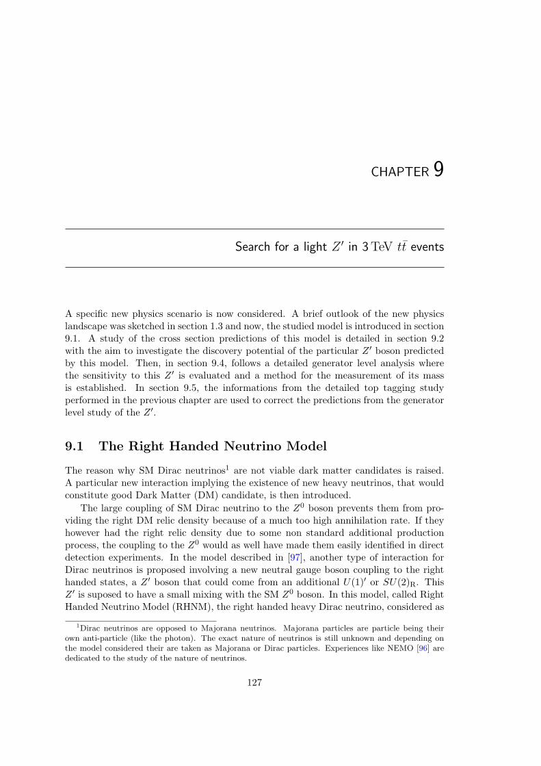
CHAPTER 9
Search for a light Z ′ in 3 TeV tt events
A specific new physics scenario is now considered. A brief outlook of the new physicslandscape was sketched in section 1.3 and now, the studied model is introduced in section9.1. A study of the cross section predictions of this model is detailed in section 9.2with the aim to investigate the discovery potential of the particular Z ′ boson predictedby this model. Then, in section 9.4, follows a detailed generator level analysis wherethe sensitivity to this Z ′ is evaluated and a method for the measurement of its massis established. In section 9.5, the informations from the detailed top tagging studyperformed in the previous chapter are used to correct the predictions from the generatorlevel study of the Z ′.
9.1 The Right Handed Neutrino Model
The reason why SM Dirac neutrinos1 are not viable dark matter candidates is raised.A particular new interaction implying the existence of new heavy neutrinos, that wouldconstitute good Dark Matter (DM) candidate, is then introduced.
The large coupling of SM Dirac neutrino to the Z0 boson prevents them from pro-viding the right DM relic density because of a much too high annihilation rate. If theyhowever had the right relic density due to some non standard additional productionprocess, the coupling to the Z0 would as well have made them easily identified in directdetection experiments. In the model described in [97], another type of interaction forDirac neutrinos is proposed involving a new neutral gauge boson coupling to the righthanded states, a Z ′ boson that could come from an additional U(1)′ or SU(2)R. ThisZ ′ is suposed to have a small mixing with the SM Z0 boson. In this model, called RightHanded Neutrino Model (RHNM), the right handed heavy Dirac neutrino, considered as
1Dirac neutrinos are opposed to Majorana neutrinos. Majorana particles are particle being theirown anti-particle (like the photon). The exact nature of neutrinos is still unknown and depending onthe model considered their are taken as Majorana or Dirac particles. Experiences like NEMO [96] arededicated to the study of the nature of neutrinos.
127

Search for a light Z ′ in 3 TeV tt events
a Weakly Interactive Massive Particle (WIMP) and denoted ν ′ in the following, becomesan interesting DM candidate because it has no coupling with the Z0 (except throughthe small Z0/Z ′ mixing). Therefore, with a suitable parametrisation, the model leads tothe correct DM relic density and complies with the experimental direct detection con-straints. The Z ′ may be observed at the Large Hadron Collider (LHC) [97] or at futurelinear colliders as studied hereafter. The Z ′ boson is supposed to couple mainly to theheaviest states of the SM, thus to the third SM fermion family. As top factories, theLHC and future linear colliders should be the best laboratories to discover and studythose processes.
In the following, the work focuses on the Z ′ production in e+e− collisions. In thefirst section, a cross section study leads to the choice of the channel that will be studiedat the generator level. The detailed analysis is done at a centre of mass energy of 3 TeV.
9.2 Cross section study
Three channels have been considered for the study of the Z ′ production. They arediscussed below and their Feynman diagrams are displayed in figure 9.1. Cross sectionshave been computed using the software calcHEP (version 2.5.5) described in [85, 98] andreferences therein. The model is named: “RH neutrino/RS-inspired”. Centre of massenergy ranging from 0.5 – 3 TeV and Z ′ mass (MZP) from 200 GeV/c2 to 3 TeV/c2 havebeen considered. The out-going Z ′ boson decays in heavy leptons or in WIMPs. At thisstep, all model parameters have been taken to arbitrary default values (couplings at 1,Z ′/Z0 mixing at 1%).
e− νe
W−
e+ νe
W+
Z ′
(a) W+ W− fusion: e+e− → ννZ′.
e−
e+
γ, Z
Z ′
H
(b) “Pseudo-Higgsstrahlung”: e+e− → HZ′.
e−
e+
γ, Z
t, t, τ±
t, t, τ∓
Z ′
(c) Emission by an out-going fermion: e+e− → τ+τ−Z′.
Figure 9.1: Z ′ production channels.
128Complete document v1.7 31/08/2011

Search for a light Z ′ in 3 TeV tt events
9.2.1 Channel e+e− → ννZ ′
Figure 9.2 maps the Z ′ production cross section for the complete MZP and centre ofmass energy ranges. Some values are tabulated in table 9.1. The values are computedwith a 1% mixing. The dependency of the production cross section on the Z0/Z ′ mixingis linear. The Z0/Z ′ mixing and the Z ′ mass are the only non SM parameters involved inthis process. The fact that the cross section keeps rising with the centre of mass energytends to indicate a UV divergence. This hypothesis was verified by computing the crosssection at energies up to 30 TeV. The result is plotted in figure 9.3 and clearly confirmsthe UV divergence. Therefore, this effective model is not appropriate to describe thisprocess.
Z’ mass (GeV)500 1000 1500 2000 2500 3000
/2 (
Bea
m e
nerg
y) (
GeV
)s
400
600
800
1000
1200
1400
0
0.0002
0.0004
0.0006
0.0008
0.001
0.0012
0.0014
0.0016
Cross section [pb]
Figure 9.2: Map of the Z ′
cross section production inW+ W− fusion process.
Table 9.1: Cross section of the Z ′ production through W+ W− fusion.MZP 200 500 1000√s = 3 TeV 1.7 fb 1.2 fb 1.4 fb√s = 1 TeV 0.27 fb 0.14 fb —√s = 0.5 TeV 0.05 fb — —
9.2.2 Channel e+e− → HZ ′
The Higgs boson mass has been set to 120 GeV/c2. The cross section of the Z ′ productionin this channels is mapped in figure 9.4 and tabulated in table 9.2. This process dependson the Higgs mass and Z ′ coupling to the Higgs boson as displayed in table 9.3. Thedependency on the Higgs mass is mild but constitutes an extra parameter in the study.Provided the Higgs coupling to the Z ′ is not too low, this channel would have a largecross section and therefore this will be an interesting area of investigation when resultsabout Higgs are made available by the LHC.
129Complete document v1.7 31/08/2011

Search for a light Z ′ in 3 TeV tt events
Center of mass energy (GeV)0 5000 10000 15000 20000 25000 30000
Cro
ss s
ectio
n (p
b)
0
0.002
0.004
0.006
0.008
0.01
0.012
0.014
0.016
0.018
Figure 9.3: Divergence ofthe Z ′ cross section pro-duction in W+ W− fusionprocess in the RHNM.
MZp (GeV)500 1000 1500 2000 2500 3000
Bea
m E
nerg
y (G
eV)
400
600
800
1000
1200
1400
-410
-310
-210
Cross section [pb]
Figure 9.4: Map ofthe Z ′ production crosssection via ”pseudo-Higgstrahlung”
Table 9.2: Cross section of the Z ′ production through ”pseudo-Higgstrahlung”.MZP 200 500 1000√s = 3 TeV 2.2 fb 0.4 fb 0.2 fb√s = 1 TeV 25.6 fb 8.1 fb —√s = 0.5 TeV 157.5 fb — —
9.2.3 Channel e+e− → τ+τ−Z ′
Figure 9.5 shows the maps of the Z ′ production via emission by an out-going top quark(figure 9.5(a)) or an out-going τ lepton (figure 9.5(b)). Cross section values are alsotabulated in table 9.4. The behaviour of the Z ′ production cross section is very similarin both cases. The difference resides in the mass of the involved fermion. The crosssection maps clearly indicate that the detection of a rather light Z ′ (below 1 TeV) isfavoured.
130Complete document v1.7 31/08/2011

Search for a light Z ′ in 3 TeV tt events
Table 9.3: Cross section dependency on Higgs mass and Higgs coupling to the Z ′.H0 mass 120 150 300
gZH = 0.5 6.4 fb 6.3 fb 5.2 fbgZH = 1 25.6 fb 25.1 fb 20.8 fbgZH = 2 102 fb 100 fb 83 fb
Z’ mass (GeV)200 400 600 800 1000 1200 1400 1600 1800 2000
/2 (
Bea
m e
nerg
y) (
GeV
)s
400
600
800
1000
1200
1400
-510
-410
-310
Cross section [pb]
(a) case of an out-going top quark
Z’ mass (GeV)200 400 600 800 1000 1200 1400 1600 1800 2000
/2 (
Bea
m e
nerg
y) (
GeV
)s
400
600
800
1000
1200
1400
-510
-410
-310
Cross section [pb]
(b) case of an out-going τ lepton
Figure 9.5: Map of the Z ′ production cross section via emission by an out-going fermion.
Table 9.4: Cross section of the Z ′ production via emission by an out-going fermion.case of the top quarkMZP 200 500 1000√s = 3 TeV 3.4 fb 1.0 fb 0.2 fb√s = 1 TeV 3.0 fb 0.04 fb —√s = 0.5 TeV — — —
case of the τ leptonMZP 200 500 1000√s = 3 TeV 2.5 fb 0.7 fb 0.1 fb√s = 1 TeV 4.4 fb 0.2 fb —√s = 0.5 TeV 2.3 fb — —
9.2.4 Choice of the channel
The three channels considered to study the Z ′ production in high energy e+e− collisionshave been discussed in the previous sections. Its production through W+ W− fusionhas been discarded because of its UV divergence. The “pseudo-Higgsstrahlung” intro-duces extra parameters and its study should be resumed when the Higgs boson mass ismeasured (and if it actually exists). Moreover, the cross section is significantly larger at500 GeV and therefore the study of this process would be a better case for International
131Complete document v1.7 31/08/2011

Search for a light Z ′ in 3 TeV tt events
Linear Collider (ILC). Remains the Z ′ production by emission from a fermion pair. TheRHNM described in [97] is very general and a fixed set of parameter values based onphysical arguments is needed. In [99] a parametrisation is proposed, where the Z ′ bosononly couples to the SM only via the top quark. This argument has therefore driven thechoice of the channel e+e− → ttZ ′ for a detailed analysis. The modified parameters aresummarized in table 9.5. The mass of the ν ′ does not influence the Z ′ cross section andtherefore its precise value is not critical and must only be below MZP/2. It appears, forMZP = 200 GeV/c2 and m′
ν = 85 GeV/c2, that this choice of parameter values gives thecorrect DM density and complies with the currrent experimental detection limits (seeappendix D.1).
Table 9.5: Summary of the model parameters set to non default values.parameter name description value
mixzzp Z0/Z ′ mixing 0.01
gZp Z ′- ν ′ coupling 3
gtr Z ′- tR coupling 3
gUp Z ′- τ coupling 0
gtl Z-(tL, bL) coupling 0
gll Z ′- τ coupling 0
9.2.5 Choice of the decay mode
The Z ′ boson has two decay modes:
1. Z ′ → invisible, where “invisible” stands for the DM candidate, since the modelparameter settings have suppressed the other possibilities (if one neglects the effectof the small Z0/Z ′ mixing).
2. Z ′ → tt, leading to four-top final states.
The corresponding total cross section and branching ratios times cross section are shownin table 9.6 for different mass of the Z ′. The SM cross section for four-top events in e+e−
collision at 3 TeV is about 20 ab. Thus, provided the four top events can be correctlytagged and reconstructed, this channel will have almost no background, but this scenariois very disfavoured by LHC data. For a DM candidate taken with a mass below MZP/2,the decay of the Z ′ into ν ′ν ′ will always be allowed. Therefore, for MZP below 2×mtop,the invisible decay channel will be the only available channel. In the following, the studyfocuses on the invisible decay of the Z ′.
9.3 Event selection
The signal is the process e+e− → ttZ ′ , Z ′ → inv.: after the e+e− interaction, one ofthe top is virtual and becomes on-shell by emitting a Z ′ more likely with a low energy,which in turn decays into WIMPs. Signal events therefore consist of multi-jet events
132Complete document v1.7 31/08/2011

Search for a light Z ′ in 3 TeV tt events
Table 9.6: Total process cross sections and Z ′ decay branching ratios times cross section.MZP Cross sect. σZ′→inv. σZ′→tt
200 GeV/c2 14.9 fb 14.9 fb 0
300 GeV/c2 8.7 fb 8.7 fb 0
400 GeV/c2 5.6 fb 2.4 fb 3.2 fb
500 GeV/c2 3.7 fb 1.2 fb 2.5 fb
600 GeV/c2 2.6 fb 0.8 fb 1.8 fb
700 GeV/c2 1.8 fb 0.5 fb 1.3 fb
with a large number of particles and missing energy. It is expected to be very close toSM s-channel tt events which constitute the main background. The cross sections fordifferent mass of the Z ′ are shown in table 9.6. The considered background processesare presented, then a method to discriminate the signal events is proposed.
9.3.1 Background
The signal is extracted from a sample of events tagged as tt events. In a first step, thetagging of the top events is assumed to have a full efficiency and purity. Therefore, thebackground considered for this study consists only of the SM inclusive tt events. Thefollowing background channels are leftover (total cross sections at 3 TeV):
- e+e− →W+W− (576 fb)
- e+e− → Z0Z0 (32 fb)
- e+e− →W+W−Z0 (33 fb)
- e+e− → bb (10 fb)
The present results shall then be scaled according to the realistic top tagging performanceas studied in section 8.3.3 (p. 121).
Both s and t channels tt production are considered, their respective Feynman dia-grams are displayed below.
1. background 1: e+e− → tt
e−
e+
γ, Z
t
t
133Complete document v1.7 31/08/2011

Search for a light Z ′ in 3 TeV tt events
2. background 2: e+e− → tt+ νν
e− νe
W−
e+ νe
W+
γ, Z t
t
Their respective cross sections are summed up in table 9.7.
Table 9.7: background channel cross sections.Channel Cross sect.
e+e− → tt 19.87 fbe+e− → tt+ νν 5 fb
9.3.2 Event generation
The program calcHEP was used to simulate the e+e− collisions and generate the result-ing out-going particles. The information was stored in the “Les Houches Event” (LHE)format and fed to a Pythia8 instance [100, 101] which propagates and decays the parti-cles.
The statistics generated correspond to the integrated luminosity of 1 ab−1, i.e.: aboutthree years of operation at a luminosity of about 1034 cm−2 s−1. In this study, the initialstate energy spread takes into account the ISR only.
9.3.3 Discriminative variables
The final state variables listed in appendix D.5 were evaluated for each channel and theirvalues were stored in a ROOT tree [102].
To give an intuitive idea of which variables are the most discriminating, the super-imposition of the final state variables for the signal and the two backgrounds togetherwith their correlations are displayed in appendix D.4 in the form of a correlation matrixwith the variable spectra on the diagonal cells. Such a view leads to the conclusion thatno direct cut on the variables would lead to a satisfactory separation between the signaland the two backgrounds. Some improvements are achieved by applying slanted cutsin the correlation planes of the variables, but no satisfactory discrimination is reached.The complexity of the problem together with the number of variables involved called forthe use of Multi-Variate Analysis (MVA) tools. The TMVA framework [95, 103] offersmany functionalities which are used in this study.
Background, as well as signal, events involve a tt pair. It is rather obvious thatvariables like jet masses, or the number of visible particles (or any particle counter fromappendix D.3) will not discriminate between signal and background. The difference lies
134Complete document v1.7 31/08/2011

Search for a light Z ′ in 3 TeV tt events
rather in the event dynamics, shape and variables related to missing energy. The finalvariable set retained for performing the event selection is shown in the table of appendixD.5 and superimpositions of their spectrum for the signal and the two background chan-nels, are displayed in appendix D.8.
9.3.4 Classifier training and testing
A BDT was trained separately on the two backgrounds. The training and testing havebeen done on 2×4500 events of each type. The input variables spectra are displayed inappendix D.8.1 for background 1, and in D.8.2 for background 2. The BDT settings areshown in table 9.8 and the performance of the training are given in table 9.9. The ROCintegral is a good indicator of the classifier’s performance but, in the present case, themost important aspect is the discriminating power of the classifier when cutting at themaximum significance. The significance is given by:
S =ǫNsignal
√ǫNsignal +BNbg.
,
where ǫ is the signal efficiency at the given cut, Nsignal is the total number of signalevents, B is the background efficiency and Nbg. the total number of background events.Table 9.9 shows that in our case the classifier gives good performance.
Table 9.8: BDT parametersBoost type Adaptative
Number of trees 1000Maximum depth 20
Prune method Cost complexityPrune strength 90
Table 9.9: BDT performance.∫
ROC stands for the ROC curve integral, Smax denotesthe maximal significance, cut@Smax denotes the BDT value leading to the cut with hehighest significance. ǫ is the signal efficiency and B is the background efficiency, ǫ andB are evaluated for the specified cut.
BDT-BG1 cut BDT-BG2 cutSig. vs Bg1 Sig. vs Bg2
∫ROC 0.955 0.971
Smax 99.6 113.8
cut@Smax -0.0378 -0.3391
ǫ@Smax 90.8% 97.4%
B@Smax 18.0% 14.6%
The BDT output for both discrimination steps are shown in figures 9.6(a) and 9.6(b)for signal vs. background 1 and signal vs. background 2 respectively. The outputs
135Complete document v1.7 31/08/2011

Search for a light Z ′ in 3 TeV tt events
computed with the training event sample are superimposed to those computed with thetesting one. A small difference between the two spectra is noticeable and is reflectedby the low Kolmogorov-Smirnov probability. This indicates a slight over-training of thealgorithm. A higher prune strength can avoid this (a value of 95 instead of 90 is sufficienthere) but at the price of lower separation even on the test sample. Therefore, it has beenconsidered reasonable to tolerate this slight over-training. The global efficiency of theevent selection is 0.884 ± 0.004.
BDT-bg1 response-0.6 -0.4 -0.2 0 0.2 0.4 0.6
dx / (1
/N)
dN
0
1
2
3
4
5Signal (test sample)
Background (test sample)
Signal (training sample)
Background (training sample)
Kolmogorov-Smirnov test: signal (background) probability = 9.47e-07 (4.77e-05)
BDT-bg1 response-0.6 -0.4 -0.2 0 0.2 0.4 0.6
dx / (1
/N)
dN
0
1
2
3
4
5
U/O
-flo
w (
S,B
): (
0.0,
0.0
)% /
(0.0
, 0.0
)%
TMVA overtraining check for classifier: BDT-bg1
(a)
BDT-bg2 response-0.8 -0.6 -0.4 -0.2 0 0.2 0.4 0.6 0.8
dx / (1
/N)
dN0
1
2
3
4
5
6
7Signal (test sample)
Background (test sample)
Signal (training sample)
Background (training sample)
Kolmogorov-Smirnov test: signal (background) probability = 0.0554 (0.247)
BDT-bg2 response-0.8 -0.6 -0.4 -0.2 0 0.2 0.4 0.6 0.8
dx / (1
/N)
dN0
1
2
3
4
5
6
7
U/O
-flo
w (
S,B
): (
0.0,
0.0
)% /
(0.0
, 0.0
)%
TMVA overtraining check for classifier: BDT-bg2
(b)
Figure 9.6: Response of BDT trained for bg1 rejection (9.6(a)) and for bg2 rejection(9.6(b)) .
In the next section, the trained MVA methods are used to apply the two successivecuts given in table 9.9 on the different event samples to select the event sample fromwhich the Z ′ production cross section and mass is to be measured.
9.4 Measurements
The Z ′ boson mass and the e+e− → ttZ ′, Z ′ → inv. process cross section were measuredsubsequently to the event selection just described. A background subtraction is describedbelow and applied before performing the mass and the cross section measurement asfollows.
9.4.1 Z ′ mass measurement method
The mass of the Z ′ is measured using the event invariant mass spectrum obtained afterthe event selection described above. Given that the Z ′ decays to invisible and tend tobe emitted at rest or very low energy, the event total invariant mass spectrum shouldshow a sharp upper edge corresponding to the value of the nominal centre of mass energyof 3 TeV/c2 minus the mass of the Z ′. Nevertheless, the ISR induces a smearing of theevent total invariant mass spectrum and then a smoothing of the spectrum upper edge.A function, called “smooth gate” in the following, defined in eq. 9.1, is fitted to the eventtotal invariant mass spectrum without presence of the signal. This way the backgroundcontribution is modelled and is subtracted from the total spectrum. The area of theremaining spectrum is then proportional to the cross section of the e+e− → ttZ ′ process
136Complete document v1.7 31/08/2011

Search for a light Z ′ in 3 TeV tt events
(see section 9.4.3). To measure the Z ′ mass, the “smooth gate” is fitted to this spectrumand the s2 parameter, corresponding to the upper slope inflexion point, is related toMZP through the relation 9.4 established in section 9.4.2.2.
The “smooth gate” is defined as:
f(x) =A
(es1−x
p1 + 1)(ex−s2
p2 + 1), (9.1)
where si, i ∈ 1, 2 are the inflection point abscissae and pi, i ∈ 1, 2 are the slopesteepnesses, see graphical representation with arbitrary values of the parameters in figure9.7.
x0 500 1000 1500 2000 2500 3000
f(x)
0
10
20
30
40
50
Figure 9.7: Smooth gatefunction with arbitraryparameter values.
After event selection, the cross section is calculated subtracting the background andcorrecting for event selection efficiency and then dividing by the 1 ab−1 luminosity.
9.4.2 Z ′ mass measurement results
The analysis procedure is detailed in the next seection for MZP = 200 GeV/c2. Then, insection 9.4.2.2, this analysis is repeated for several values of MZP and its measurementis described. Finally, in section 9.4.2.3, the resolution on the Z ′ mass is estimated.
9.4.2.1 Details for MZP = 200GeV/c2
All events from the two backgrounds (20000 and 5000 for background 1 and 2 respec-tively) and the signal (15000) are tested with the two BDT cuts. The cut for background2 rejection is applied first. The event invariant mass spectrum is plotted with the re-maining events and displayed in figure 9.8. The contributions from the different sourcesare represented with different colours. The second background has almost vanished andthe signal represents a clear excess with respect to the SM background.
The number of background events remaining after the Z ′ selection cut is 4714 ±69. The background contribution alone is plotted in figure 9.9 and the “smooth gate”
137Complete document v1.7 31/08/2011
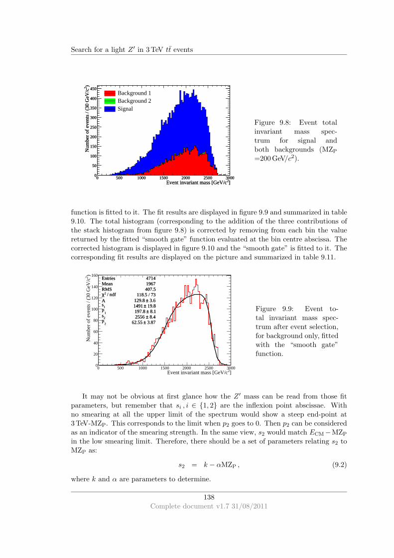
Search for a light Z ′ in 3 TeV tt events
]2Event invariant mass [GeV/c0 500 1000 1500 2000 2500 3000
)2 N
umbe
r of
eve
nts
/ (30
GeV
/c
0
50
100
150
200
250
300
350
400
450
]2Event invariant mass [GeV/c0 500 1000 1500 2000 2500 3000
)2 N
umbe
r of
eve
nts
/ (30
GeV
/c
0
50
100
150
200
250
300
350
400
450Background 1Background 2Signal
Figure 9.8: Event totalinvariant mass spec-trum for signal andboth backgrounds (MZP
=200 GeV/c2).
function is fitted to it. The fit results are displayed in figure 9.9 and summarized in table9.10. The total histogram (corresponding to the addition of the three contributions ofthe stack histogram from figure 9.8) is corrected by removing from each bin the valuereturned by the fitted “smooth gate” function evaluated at the bin centre abscissa. Thecorrected histogram is displayed in figure 9.10 and the “smooth gate” is fitted to it. Thecorresponding fit results are displayed on the picture and summarized in table 9.11.
Entries 4714Mean 1967RMS 407.5
/ ndf 2χ 118.5 / 73A 3.6± 129.8
1s 19.8± 1491
1p 8.1± 197.8
2s 8.4± 2556
2p 3.87± 62.55
]2Event invariant mass [GeV/c0 500 1000 1500 2000 2500 3000
)2 N
umbe
r of
eve
nts
/ (30
GeV
/c
0
20
40
60
80
100
120
140
160Entries 4714Mean 1967RMS 407.5
/ ndf 2χ 118.5 / 73A 3.6± 129.8
1s 19.8± 1491
1p 8.1± 197.8
2s 8.4± 2556
2p 3.87± 62.55
Figure 9.9: Event to-tal invariant mass spec-trum after event selection,for background only, fittedwith the “smooth gate”function.
It may not be obvious at first glance how the Z ′ mass can be read from those fitparameters, but remember that si , i ∈ 1, 2 are the inflexion point abscissae. Withno smearing at all the upper limit of the spectrum would show a steep end-point at3 TeV-MZP. This corresponds to the limit when p2 goes to 0. Then p2 can be consideredas an indicator of the smearing strength. In the same view, s2 would match ECM−MZP
in the low smearing limit. Therefore, there should be a set of parameters relating s2 toMZP as:
s2 = k − αMZP , (9.2)
where k and α are parameters to determine.
138Complete document v1.7 31/08/2011

Search for a light Z ′ in 3 TeV tt events
Table 9.10: Fit results for background contribution.χ2/ndf 118.5/73A 129.8 ± 3.6s1 1491 ± 19.8p1 197.8 ± 8.1s2 2556 ± 8.4p2 62.6 ± 3.9
Entries 12094Mean 1824RMS 473.9
/ ndf 2χ 433.8 / 95A 4.5± 286.4
1s 14.2± 1263
1p 6.2± 245.9
2s 5.1± 2529
2p 2.59± 54.65
]2Event invariant mass [GeV/c0 500 1000 1500 2000 2500 3000
)2 N
umbe
r of
eve
nts
/ (30
GeV
/c
0
50
100
150
200
250
300
Entries 12094Mean 1824RMS 473.9
/ ndf 2χ 433.8 / 95A 4.5± 286.4
1s 14.2± 1263
1p 6.2± 245.9
2s 5.1± 2529
2p 2.59± 54.65
Figure 9.10: Event to-tal invariant mass spec-trum after event selec-tion and background sub-traction fitted with the“smooth gate” functionfor MZP = 200 GeV/c2.
Table 9.11: Fit results for the corrected event invariant mass spectrum.χ2/ndf 118.5/73A 286.4 ± 4.5s1 1263 ± 15p1 245.9 ± 6.2s2 2529 ± 5.1p2 54.7 ± 2.6
In the next section, the same procedure was repeated for various values of MZP todetermine the values of the parameters of eq. 9.2.
9.4.2.2 Sensitivity to MZP
The procedure described in the previous section is applied for MZP from 200 to 700 GeV/c2
with a constant statistics before Z ′ selection cut. The use of a constant statistics is meantto probe the s2 dependence to MZP only. The resulting event invariant mass spectraare displayed in figure 9.11. Their fitted “smooth gate” upper inflexion point abscissaare summed up in table 9.12 and plotted in figure 9.12. This figure also shows how astraight line is fitted to the data point and the residuals are shown in the figure corner
139Complete document v1.7 31/08/2011
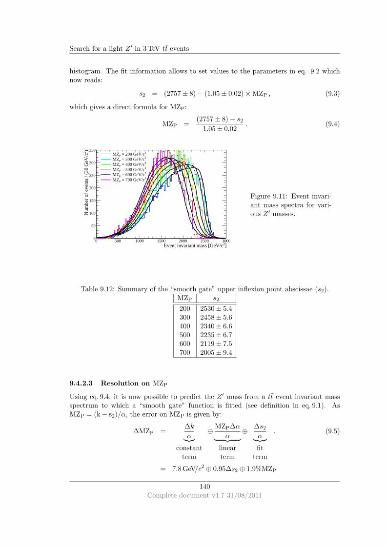
Search for a light Z ′ in 3 TeV tt events
histogram. The fit information allows to set values to the parameters in eq. 9.2 whichnow reads:
s2 = (2757 ± 8) − (1.05 ± 0.02) × MZP , (9.3)
which gives a direct formula for MZP:
MZP =(2757 ± 8) − s2
1.05 ± 0.02. (9.4)
]2Event invariant mass [GeV/c0 500 1000 1500 2000 2500 3000
)2 N
umbe
r of
eve
nts
/ (30
GeV
/c
0
50
100
150
200
250
300
3502 = 200 GeV/cPMZ2 = 300 GeV/cPMZ2 = 400 GeV/cPMZ2 = 500 GeV/cPMZ2 = 600 GeV/cPMZ2 = 700 GeV/cPMZ
Figure 9.11: Event invari-ant mass spectra for vari-ous Z ′ masses.
Table 9.12: Summary of the “smooth gate” upper inflexion point abscissae (s2).MZP s2
200 2530 ± 5.4300 2458 ± 5.6400 2340 ± 6.6500 2235 ± 6.7600 2119 ± 7.5700 2005 ± 9.4
9.4.2.3 Resolution on MZP
Using eq. 9.4, it is now possible to predict the Z ′ mass from a tt event invariant massspectrum to which a “smooth gate” function is fitted (see definition in eq. 9.1). AsMZP = (k − s2)/α, the error on MZP is given by:
∆MZP =∆k
α︸︷︷︸
constantterm
⊕ MZP∆α
α︸ ︷︷ ︸
linearterm
⊕ ∆s2α︸ ︷︷ ︸
fitterm
. (9.5)
= 7.8 GeV/c2 ⊕ 0.95∆s2 ⊕ 1.9%MZP
140Complete document v1.7 31/08/2011
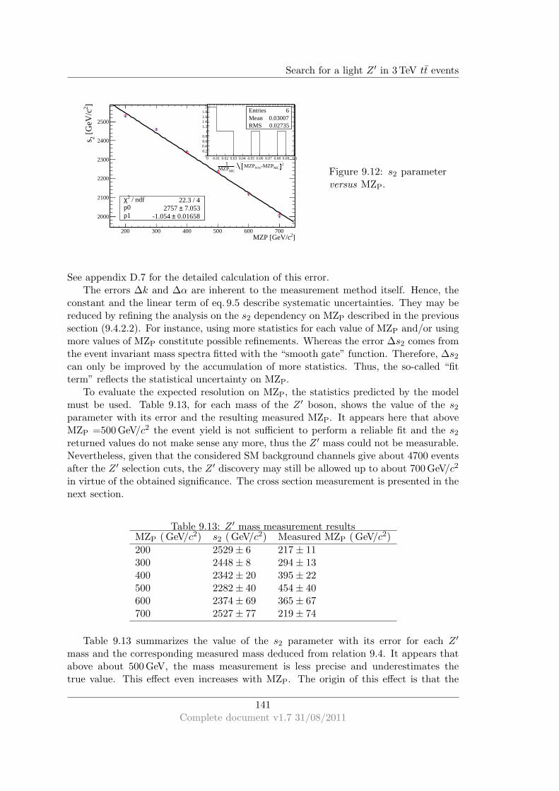
Search for a light Z ′ in 3 TeV tt events
]2MZP [GeV/c200 300 400 500 600 700
]2 [G
eV/c
2s
2000
2100
2200
2300
2400
2500
/ ndf 2χ 22.3 / 4p0 7.053± 2757 p1 0.01658± -1.054
/ ndf 2χ 22.3 / 4p0 7.053± 2757 p1 0.01658± -1.054
Entries 6Mean 0.03007RMS 0.02735
2MC-MZPrecoMZP .
MCMZP1
0 0.01 0.02 0.03 0.04 0.05 0.06 0.07 0.08 0.09 0.10
0.20.40.60.8
11.21.41.61.8
2Entries 6Mean 0.03007RMS 0.02735
Figure 9.12: s2 parameterversus MZP.
See appendix D.7 for the detailed calculation of this error.The errors ∆k and ∆α are inherent to the measurement method itself. Hence, the
constant and the linear term of eq. 9.5 describe systematic uncertainties. They may bereduced by refining the analysis on the s2 dependency on MZP described in the previoussection (9.4.2.2). For instance, using more statistics for each value of MZP and/or usingmore values of MZP constitute possible refinements. Whereas the error ∆s2 comes fromthe event invariant mass spectra fitted with the “smooth gate” function. Therefore, ∆s2can only be improved by the accumulation of more statistics. Thus, the so-called “fitterm” reflects the statistical uncertainty on MZP.
To evaluate the expected resolution on MZP, the statistics predicted by the modelmust be used. Table 9.13, for each mass of the Z ′ boson, shows the value of the s2parameter with its error and the resulting measured MZP. It appears here that aboveMZP =500 GeV/c2 the event yield is not sufficient to perform a reliable fit and the s2returned values do not make sense any more, thus the Z ′ mass could not be measurable.Nevertheless, given that the considered SM background channels give about 4700 eventsafter the Z ′ selection cuts, the Z ′ discovery may still be allowed up to about 700 GeV/c2
in virtue of the obtained significance. The cross section measurement is presented in thenext section.
Table 9.13: Z ′ mass measurement resultsMZP (GeV/c2) s2 (GeV/c2) Measured MZP (GeV/c2)
200 2529 ± 6 217 ± 11300 2448 ± 8 294 ± 13400 2342 ± 20 395 ± 22500 2282 ± 40 454 ± 40600 2374 ± 69 365 ± 67700 2527 ± 77 219 ± 74
Table 9.13 summarizes the value of the s2 parameter with its error for each Z ′
mass and the corresponding measured mass deduced from relation 9.4. It appears thatabove about 500 GeV, the mass measurement is less precise and underestimates thetrue value. This effect even increases with MZP. The origin of this effect is that the
141Complete document v1.7 31/08/2011

Search for a light Z ′ in 3 TeV tt events
lower signal statistics at higher MZP makes the fit of the “smooth gate” more sensitiveto background fluctuations and introduces a bias not taken into account by the MZP
uncertainty formula (eq. 9.5). A bin to bin background subtraction may reduce this effectbut the accumulation of more data would be the best solution to reduce it. However, theconclusion is that additionnal care must be taken for background subtraction to makethis method reliable in the case of fewer than about 1000 events passing the selectioncuts.
]2 [GeV/cPMZ200 250 300 350 400 450 500
P/M
ZP
MZ
∆
0.04
0.045
0.05
0.055
0.06
0.065
0.07
0.075
0.08
Figure 9.13: MZP error vs.MZP.
9.4.3 Cross section measurement
The cross section of the e+e− → ttZ ′, Z ′ → inv. process is calculated as the number ofevents passing the Z ′ selection cut and surviving the background subtraction used forthe mass measurement divided by the integrated luminosity of 1 ab−1. The measuredcross sections are shown in table 9.14. The present method tends to underestimate theprocess cross section for low MZP and slightly over-estimate it at higher values.
Table 9.14: Z ′ cross section measurement results.MZP True cross sect. events yield significance Measured cross sect.
200 14.9 fb 12094 ± 110 92.7 13.7 ± 0.2 fb300 8.7 fb 7411 ± 87 66.6 8.4 ± 0.1 fb400 2.4 fb 2150 ± 47 24.6 2.4 ± 0.1 fb500 1.2 fb 1192 ± 35 13.5 1.3 ± 0.1 fb600 0.8 fb 815 ± 29 8.4 0.9 ± 0.1 fb700 0.5 fb 642 ± 26 5.6 0.7 ± 0.1 fb
142Complete document v1.7 31/08/2011
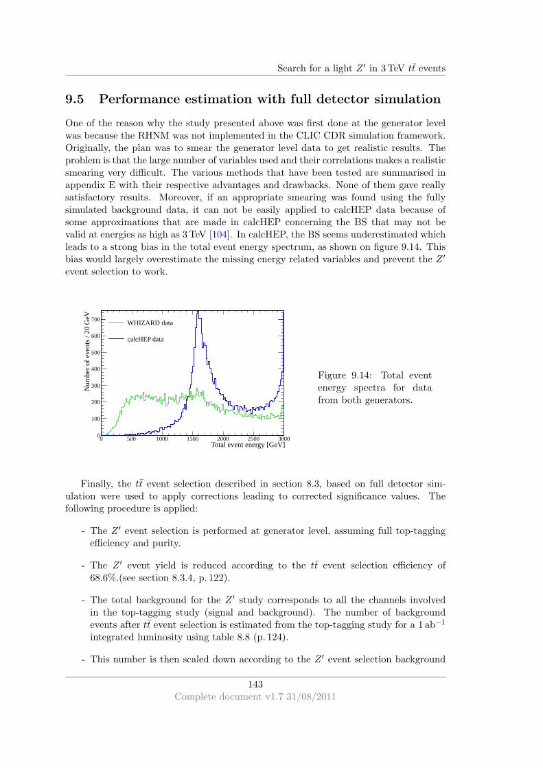
Search for a light Z ′ in 3 TeV tt events
9.5 Performance estimation with full detector simulation
One of the reason why the study presented above was first done at the generator levelwas because the RHNM was not implemented in the CLIC CDR simulation framework.Originally, the plan was to smear the generator level data to get realistic results. Theproblem is that the large number of variables used and their correlations makes a realisticsmearing very difficult. The various methods that have been tested are summarised inappendix E with their respective advantages and drawbacks. None of them gave reallysatisfactory results. Moreover, if an appropriate smearing was found using the fullysimulated background data, it can not be easily applied to calcHEP data because ofsome approximations that are made in calcHEP concerning the BS that may not bevalid at energies as high as 3 TeV [104]. In calcHEP, the BS seems underestimated whichleads to a strong bias in the total event energy spectrum, as shown on figure 9.14. Thisbias would largely overestimate the missing energy related variables and prevent the Z ′
event selection to work.
Total event energy [GeV]0 500 1000 1500 2000 2500 3000
Num
ber
of e
vent
s / 2
0 G
eV
0
100
200
300
400
500
600
700 WHIZARD data
calcHEP data
Figure 9.14: Total eventenergy spectra for datafrom both generators.
Finally, the tt event selection described in section 8.3, based on full detector sim-ulation were used to apply corrections leading to corrected significance values. Thefollowing procedure is applied:
- The Z ′ event selection is performed at generator level, assuming full top-taggingefficiency and purity.
- The Z ′ event yield is reduced according to the tt event selection efficiency of68.6%.(see section 8.3.4, p. 122).
- The total background for the Z ′ study corresponds to all the channels involvedin the top-tagging study (signal and background). The number of backgroundevents after tt event selection is estimated from the top-tagging study for a 1 ab−1
integrated luminosity using table 8.8 (p. 124).
- This number is then scaled down according to the Z ′ event selection background
143Complete document v1.7 31/08/2011

Search for a light Z ′ in 3 TeV tt events
rejection of 82% (see table 9.9, p. 135, displaying the s-channel background con-tamination of 18%) resulting in a value of 13 339 ± 115.
The corrected significances for various Z ′ masses are displayed in table 9.15.In view of the corrected significances, a discovery of the studied Z ′ is possible for
a 1 ab−1 integrated luminosity if its mass is below about 600 GeV/c2. The Z ′ massmeasurement window is likely to be reduced from [200, 500] GeV/c2 to [200, 400] GeV/c2,corresponding to the mass window where the significance is above 10. A completesimulation of the Z ′ events and a refined Z ′ event selection procedure including all theSM background channels listed in section 8.3, may lead to more precise results andbetter performance. Such a refined analysis would be mandatory if the LHC happen todiscover hints of new physics in the search for massive invisible particles (like gravitonsearch [105] in which a massive invisible particle is actively searched).
Table 9.15: Z ′ signal significance correction using the tt event selection performance.Statistics are based on a 1 ab−1 integrated luminosity. Z ′ cross sections are calculatedusing calcHEP with ISR and CLIC nominal BS.
MZP σ ( fb) Event yield Corrected significance (uncorreceted)
200 13.07 7 929 54.4 (92.7)300 5.35 3 246 25.2 (66.6)400 2.65 1 608 13.2 (24.6)500 1.45 880 7.4 (13.7)600 0.86 522 4.4 (8.5)700 0.53 321 2.7 (5.6)
Resume du chapitre
Dans ce chapitre, un modele particulier de physique au dela du Modele Standard estenvisage. Il s’agit d’un modele effectif non-supersymetrique, proposant une solutionalternative au probleme de la matiere noire dans les theories de Randall et Sundrum.La phenomenologie qui en decoule ne se limite cependant pas a ces modeles et impliquenotamment un boson de jauge neutre additionnel Z ′ couplant aux particules d’helicitedroite ainsi qu’une particule ayant les proprietes d’un neutrino d’helicite droite ν ′ quidevient dans ce contexte un bon candidat pour la matiere noire. On se propose d’etudierce Z ′ a travers des simulations de physique au niveau generateur.
Le choix de parametres considere implique que la seule particule du Modele Standardcouplant directement au Z ′ soit le quark top d’helicite droite, un faible couplage avec lereste des particules du Modele Standard est possible a travers un faible melange entrele boson faible Z0 et le Z ′. Le canal privilegie pour cette etude est donc la productionde paires tt ou l’un des tops, d’abord virtuel, emet un Z ′ afin de retourner sur sa couchede masse (voir diagramme fig. 9.1(c) p. 128). Le Z ′ ainsi emis peut se desintegrer soit enpaire ν ′ ν ′ soit en paire tt si sa masse est suffisante. On se focalisera sur l’etude du casZ ′ → ν ′ν ′ ou l’etat final consiste en evenements tt presentant de l’energie manquante.
On cherchera tout d’abord a separer le signal Z ′ d’evenements tt purement standardsavec et sans energie manquante (cf diagrammes p. 133). Cette selection se fait a l’aide
144Complete document v1.7 31/08/2011
Search for a light Z ′ in 3 TeV tt events
d’un algorithme multi-variable de type “arbre de decision”. Au total, 13 variables sontutilisees, basees sur l’energie manquante ou la geometrie de l’evenement, enumerees etdecrites dans la table en appendice D.5. Une coupure est realisee sur chaque bruit defond pour une efficacite totale de 88.4%. Le bruit de fond remanant pourra etre modeliseet soustrait.
Le spectre de la masse totale du systeme tt est utilise pour pratiquer une serie demesures. Apres les coupures de selection, la contribution du bruit de fond peut etreevaluee, modelisee et enfin soustraite afin de mesurer la section efficace du processusetudie. La mesure comparee au calcul direct est donnee dans la table 9.14 p. 142, unedecouverte du boson Z ′ est envisageable jusqu’a une masse d’environ 700 GeV/c2 dansle cadre du modele etudie. Ce spectre permet aussi de mesurer la masse du Z ′ sila statistique disponible est suffisante (baisse de fiabilite pour moins d’environ 1000evenements tt Z ′). Pour ce faire, la fonction (eq. 9.1, representation graphique fig. 9.7,p. 137) utilisee pour la modelisation de la contribution au bruit de fond est a nouveauutilisee et ajustee sur le spectre ou la contribution du fond a ete soustraite. Le pointd’inflexion superieur de la courbe ainsi obtenue est directement lie a la masse du Z ′
(voir fig. 9.11 et 9.12, p. 140 et 141) par la formule 9.4 avec une resolution estimee parpropagation des erreurs sur les differents parametres donnee par la formule 9.5. Laresolution attendue est meilleure que 8% sur toute la gamme de masse du Z ′ etudieeavec un optimum d’environ 4% autour de 300 GeV/c2 et un biais tendant a une sous-estimation de la masse si celle-ci est elevee. Ce biais, du aux fluctuations statistiques dubruit de fond, n’est pas pris en compte dans l’estimation de la resolution.
Cependant ces resultats sont un peu idealises. En effet, etudier la separation desevenements Z ′ des evenements tt standards revient a supposer une parfaite selectiondes evenements tt. Or nous avons vu au chapitre precedent qu’une efficacite de 69%et une purete de 73% etaient envisageables. L’etude du Z ′ au niveau generateur s’estfaite sans simulation du beamstrahlung, celle-ci n’etant pas optimisee dans calcHEPpour les conditions de CLIC, Pour cette raison, les donnees completement simuleeset les donnees au niveau generateur sont tres difficilement melangeables. De ce fait,les performances de selection des evenements tt peuvent seulement etre utilisees pourcorriger les significances obtenues en fonction de la masse du Z ′. Cette correction se faiten reduisant le nombre d’evenements tt et tt Z ′ de l’efficacite de selection des evenementstt et ensuite en augmentant le nombre d’evenements de bruit de fond utilise dans lecalcul de la significance en fonction de la purete de la selection tt (voir resultats table9.15, p. 144). On observe une diminution de la significance d’un facteur proche de 2diminuant le potentiel de decouverte du Z ′ etudie a la gamme de masse 200 – 500 GeV/c2
(significance superieure a 7).
145Complete document v1.7 31/08/2011

Search for a light Z ′ in 3 TeV tt events
146Complete document v1.7 31/08/2011
CHAPTER 10
Conclusion
The collision environment at CLIC has been described. The smearing of the initialstate due to electromagnetic interaction between incoming particles (ISR) and betweenincoming bunches (BS) has been presented. The machine induced backgrounds havealso been described, the most problematic one beeing the γγ → hadrons process.
The main top physics issues have been sketched and the production condition of ttevents at CLIC have been depicted. The work has been done on fully simulated events of3 TeV e+e− collisions at CLIC with CLIC ILD detector. A method for tt event selectionat the detector level, based on multivariate analysis, has been proposed and showed asignal efficiency of 68.6% for 99.2% of WW background rejection regardless of the ttpair decay mode. This performance indicates that tt events can be selected with a goodpurity without major loss of signal. The WW rejection allows as well to cut the ZZ andbb backgrounds and also reduce the WWZ background to finally achieve a purity of thett event sample of 72.9%.
A glimpse of the new physics landscape have been given to introduce a specificRandall-Sundrum-inspired New Physics scenario predicting a new vector boson denotedZ ′ and a dark matter candidate in the form of a heavy right handed neutrino. Thenew physics signal was extracted from samples of SM tt events. The study focused onthe e+e− → ttZ ′ channel at a centre of mass energy of 3 TeV, with the Z ′ decayinginto WIMPs. The study was done at generator level. The proposed event selectionmethod shows an efficiency of 88.4% and a background rejection above 80% for the twobackground channels considered, namely the s and t channel SM tt events. An excess overthe background is measurable for Z ′ masses ranging from 200 to 800 GeV. For Z ′ massesbelow 500 GeV, the mass can be measured with an uncertainty better than 8% and withan optimum around 300 GeV of 4%. The full detector simulation of the SM backgroundchannels has allowed to correct the results obtained with generator level simulation. Themaximum measurable Z ′ mass is decrease to about 400 GeV/c2 instead of 500 GeV/c2
and the discovery potential becomes very low above 600 GeV/c2 (significance below 5).However, the detector level study of the background give rather conservative resultsandreal performance should then lie between the raw and the corrected performance.
147
Conclusion
Many refinements of the presented analysis are possible. Concerning the taggingof tt events: a B-tagging information may improve the tagging of the less boosted topquarks and a jet sub-structure analysis can improve the tagging of highly boosted topquark jets (for hadronic decay modes). In a near future, the CLIC simulation frameworkwill provide the possibility to fully simulate and reconstruct Z ′ events. A new study forsignal and background, including the improvements listed above, could lead to betterperformance of the Z ′ cross section and mass measurement.
Differents aspects des collisions e+e− a haute energie ont ete abordes dans le contextede l’experience CLIC. Des pertes significatives d’energie des particules incidentes con-duisent a de grandes fluctuations de l’energie initiale. Les interactions entre les photonsainsi generes produisent de grandes quantites de particules parasites dont des hadronspouvant polluer significativement le signal releve dans les detecteurs.
Dans cet environnement, par des simulations detaillees, la production de pairesquark/anti-quark top a ete etudiee et la selection des evenements tt, parmi une serie decanaux de bruits de fond (WW , ZZ, bb, WWZ), par une approche multi-variable, a eteevaluee. Une efficacite de 68.6% ainsi qu’une purete de l’echantillon final de 72.9% ontete determinees demontrant aisni l’observabilite du quark top aupres de CLIC, a 3TeV.
Un modele de physique au dela du modele standard, predisant notamment un bosonZ ′ ainsi qu’un candidat de matiere noire couple a celui-ci, a ete considere. La detectionde ce Z ′ decroissant en particules de matiere noire a ete etudiee au niveau generateur.Le canal etudie (e+e− → ttZ ′, Z ′ → ν ′ν ′) consiste en une production de paires ttpresentant de l’energie manquante. Une methode de selection de ces evenements parmides evenements tt purement standards, basee sur des algorithmes multi-variables, a eteetablie. Une efficacite de 88.4% sur le signal a ete atteinte. Le bruit de fond irreductibleest ensuite modelise et retranche du spectre de la masse invariante du systeme tt per-mettant a la fois de mesurer la section efficace du processus observe et la masse de laparticule invisible emise. On observe toutefois quelques biais dus aux fluctuations dubruit de fond. La section efficace tend a etre legerement sous-estimee pour une faiblemasse du Z ′ et legerement surestimee pour les plus hautes masses. De meme, la massedu Z ′ tend a etre sous-estimee au dela d’environ 500GeV/c2. En dessous de cette valeur,la resolution sur la masse du Z ′ est meilleure que 8% avec un optimum de 4% autourde 300GeV/c2.
Dans l’incapacite d’utiliser des donnees Z ′ completement simulees, a l’instar desdonnees de l’etude du quark top, une situation ideale aurait ete d’utiliser ces dernierespour le bruit de fond de l’etude du Z ′ et d’appliquer un ajustement des donnees Z ′
pour mimer les effets de bruit de fond machine et de resolution des detecteurs. Maisune difference dans la simulation du beamstrahlung, et par consequent dans le spec-tre de l’energie de centre de masse des evenements, rendait une telle combinaison desdonnees impossible. Ainsi, seule une simple correction des significances du signal Z ′,basee sur les performances de selection des evenements tt peut etre appliquee a uneetude du Z ′ au niveau generateur avec les canaux de production de paire tt comme bruitde fond de reference. Cette correction conduit a une diminution de moitie environ dessignificances attendues reduisant l’observabilite du Z ′ a la fenetre 200 – 500GeV/c2.D’autres degradations du meme ordre sont a prevoir, mais ne peuvent etre evaluees avecles moyens disponibles lors de ces travaux.
148Complete document v1.7 31/08/2011

Appendices and back matter
149

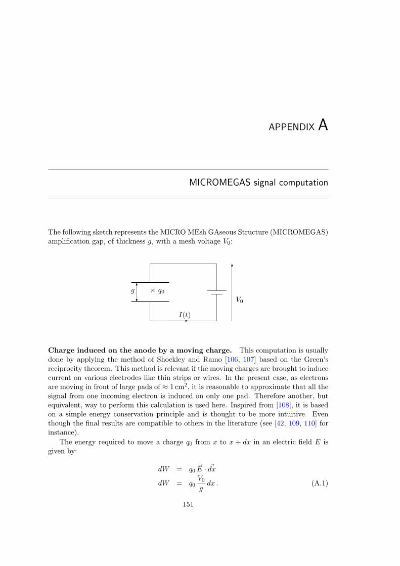
APPENDIX A
MICROMEGAS signal computation
The following sketch represents the MICRO MEsh GAseous Structure (MICROMEGAS)amplification gap, of thickness g, with a mesh voltage V0:
× q0
6
V0?
6g
-I(t)
Charge induced on the anode by a moving charge. This computation is usuallydone by applying the method of Shockley and Ramo [106, 107] based on the Green’sreciprocity theorem. This method is relevant if the moving charges are brought to inducecurrent on various electrodes like thin strips or wires. In the present case, as electronsare moving in front of large pads of ≈ 1 cm2, it is reasonable to approximate that all thesignal from one incoming electron is induced on only one pad. Therefore another, butequivalent, way to perform this calculation is used here. Inspired from [108], it is basedon a simple energy conservation principle and is thought to be more intuitive. Eventhough the final results are compatible to others in the literature (see [42, 109, 110] forinstance).
The energy required to move a charge q0 from x to x + dx in an electric field E isgiven by:
dW = q0 ~E · ~dxdW = q0
V0
gdx . (A.1)
151

MICROMEGAS signal computation
The movement of q0 initiates a current I(t) that must be conserved throughout thecircuit. It relates directly to the movement of q0 by the expression of its energy:
dW = P dt
dW = V0 I(t) dt
dW = V0 dQin , (A.2)
where P is the power and dQin is the charge put in movement along the circuit. Thusone get, by identifying A.1 and A.2:
q0V0
gdx = V0 dQin (A.3)
ie : dQin =1
gq0(x) dx . (A.4)
The total charge induced on the anode plane by a MICROMEGAS cascade is thengiven by:
Qin =1
g
∫ g
0q0(x) dx
Qin =1
g
∫ g
0q−(x) + q+(x) dx , (A.5)
where q−(x) stands for the electron contribution and q+(x) for the ion one.
Number of moving charge in the amplification gap. The charge q±(x) relatesto the number of moving charge n±(t) via:
q±(x) dx = −e n±(t) v± dt , (A.6)
where e is the elementary electric charge and v± the average speed of the electrons/ions.Note that the minus sign holds for both electron and ion contributions, it comes fromelectron charge on the one hand, and from the ion speed on the other hand. The speedof ions is at least two order of magnitude below the electron one.
Let T− be the time for the electrons to cross the amplification gap and get collectedon the anode and T+ be the time for the ions to drift towards the mesh and get collected.T+ will coincide with the total duration of the MICROMEGAS signal.
Following the gas amplification model described in section 3.2.2 (page 44), the num-ber of electron n−(t), for t < T−, is given by:
n−(t) = n0 eαv− t , (A.7)
where it is assumed that all electrons are collected at the same time T−. The number ofions results from two contributions:
- creation along the path of the electrons,
- collection as they progressively reach the mesh.
152Complete document v1.7 31/08/2011
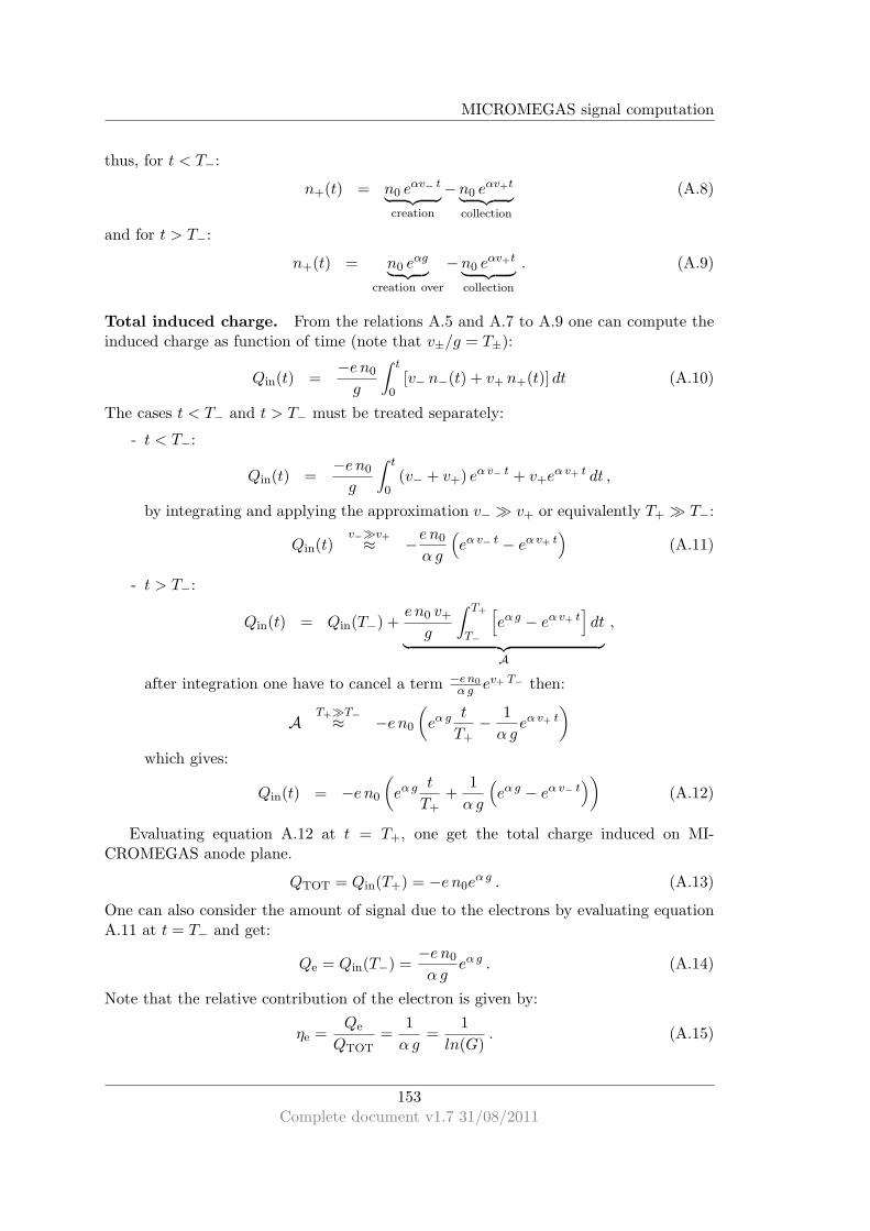
MICROMEGAS signal computation
thus, for t < T−:
n+(t) = n0 eαv− t
︸ ︷︷ ︸
creation
−n0 eαv+t
︸ ︷︷ ︸
collection
(A.8)
and for t > T−:
n+(t) = n0 eαg
︸ ︷︷ ︸
creation over
−n0 eαv+t
︸ ︷︷ ︸
collection
. (A.9)
Total induced charge. From the relations A.5 and A.7 to A.9 one can compute theinduced charge as function of time (note that v±/g = T±):
Qin(t) =−e n0
g
∫ t
0[v− n−(t) + v+ n+(t)] dt (A.10)
The cases t < T− and t > T− must be treated separately:
- t < T−:
Qin(t) =−e n0
g
∫ t
0(v− + v+) eα v− t + v+e
α v+ t dt ,
by integrating and applying the approximation v− ≫ v+ or equivalently T+ ≫ T−:
Qin(t)v−≫v+≈ −e n0
α g
(
eα v− t − eα v+ t)
(A.11)
- t > T−:
Qin(t) = Qin(T−) +e n0 v+g
∫ T+
T−
[
eα g − eα v+ t]
dt
︸ ︷︷ ︸
A
,
after integration one have to cancel a term −e n0
α g ev+ T− then:
A T+≫T−≈ −e n0
(
eα g t
T+− 1
α geα v+ t
)
which gives:
Qin(t) = −e n0
(
eα g t
T++
1
α g
(
eα g − eα v− t))
(A.12)
Evaluating equation A.12 at t = T+, one get the total charge induced on MI-CROMEGAS anode plane.
QTOT = Qin(T+) = −e n0eα g . (A.13)
One can also consider the amount of signal due to the electrons by evaluating equationA.11 at t = T− and get:
Qe = Qin(T−) =−e n0
α geα g . (A.14)
Note that the relative contribution of the electron is given by:
ηe =Qe
QTOT=
1
α g=
1
ln(G). (A.15)
153Complete document v1.7 31/08/2011

MICROMEGAS signal computation
154Complete document v1.7 31/08/2011

APPENDIX B
tt production in the SM together with neutrinos
All diagrams and cross sections are computed with calcHEP [85]. The Higgs boson mass,when implied, is taken at 120 GeV.
B.1 Production diagrams
The leading channel is e+e− → ttνeνe, giving higher cross sections as well as morediagrams. the channels with τ and µ neutrinos are completely symmetric.
B.1.1 e+e− → ttνeνe
e−γ
t
t
e−
e+ Zνe
νe
e−γ
t
te−
νeW+
e+
νe
e−
e+
γt
t t
Z νe
νe
e−
e+
γt
t t
Z νe
νe
e−Z
νe
νe
e−
e+γ
t
t
e−Z
νe
νe
e−
e+ Zt
t
e−Z
t
t
e−
e+ Zνe
νe
e−Z
t
te−
νeW+
e+
νe
155

tt production in the SM together with neutrinos
e−
e+
ZZ
νe
νe
h t
t
e−
e+
Zνe
νe νe
Z t
t
e−
e+
Zνe
νe νe
Z t
t
e−
e+
Zt
t t
Z νe
νe
e−
e+
Zt
t t
Z νe
νe
e−νe
νe
Z t
tW+
e+
νe
e−νe
W+
γt
tW+
e+
νe
e−νe
W+
Zt
tW+
e+
νe
e−νe
W+
ht
tW+
e+
νe
e−νe
W+
e+νe
νe
Z t
t
e−νe
W+ νe
e−
e+γ
t
t
e−νe
W+ νe
e−
e+ Zt
t
e− νe
W+
td
t
W+
e+ νe
e− νe
W+
ts
t
W+
e+ νe
e− νe
W+
tb
t
W+
e+ νe
B.1.2 e+e− → ttνµνµ
e−γ
t
t
e−
e+ Zνµ
νµ
e−
e+
γt
t t
Z νµ
νµ
e−
e+
γt
t t
Z νµ
νµ
e−Z
νµ
νµ
e−
e+γ
t
t
156Complete document v1.7 31/08/2011

tt production in the SM together with neutrinos
e−Z
νµ
νµ
e−
e+ Zt
t
e−Z
t
t
e−
e+ Zνµ
νµ
e−
e+
ZZ
νµ
νµ
h t
t
e−
e+
Zνµ
νµ νµ
Z t
t
e−
e+
Zνµ
νµ νµ
Z t
t
e−
e+
Zt
t t
Z νµ
νµ
e−
e+
Zt
t t
Z νµ
νµ
B.1.3 e+e− → ttντ ντ
e−γ
t
t
e−
e+ Zντ
ντ
e−
e+
γt
t t
Z ντ
ντ
e−
e+
γt
t t
Z ντ
ντ
e−Z
ντ
ντ
e−
e+γ
t
t
e−Z
ντ
ντ
e−
e+ Zt
t
e−Z
t
t
e−
e+ Zντ
ντ
e−
e+
ZZ
ντ
ντ
h t
t
e−
e+
Zντ
ντ ντ
Z t
t
e−
e+
Zντ
ντ ντ
Z t
t
e−
e+
Zt
t t
Z ντ
ντ
e−
e+
Zt
t t
Z ντ
ντ
157Complete document v1.7 31/08/2011

tt production in the SM together with neutrinos
B.2 Cross section
The cross sections of the three SM channels of tt production with neutrinos are summedup in the following table. All numbers are given in unit of femto-barn.
Table B.1: Cross section of tt plus neutrinos in the SM. Numbers are given in femto-barn.Ecm e+e− → ttνeνe e+e− → ttνµνµ e+e− → ttντ ντ
400 5·10−5 2·10−8 2·10−8
800 0.2 0.2 0.21200 1.0 0.3 0.32000 2.7 0.1 0.13000 5.1 5·10−2 5·10−2
158Complete document v1.7 31/08/2011
APPENDIX C
Toy Model of tt event energy spectrum
The following piece of code is to be run, as is, as a ROOT macro. It illustrates theexplanations of the tt event energy spectrum given in section 8.2.2 (p.116). The firsttunable is the beam energy Ebeam in order to test various energies. The second andmost important parameter is strength, which values would reasonably range between 0and ≈ 1 – 2, allows to tune the intensity of the initial state energy losses (ISR andBS).The default values proposed hereafter reproduce roughly the observed spectrum. Thett cross section used here are the one already presented in section 8.2.1 (p.115). Thedistribution is extended thanks to a sigmoid to simulate the threshold as shown in fig-ure C.1. The initial state energy losses are modelised by a simple analytical function1
100 tan(x π
2
)1/strengthdisplayed for strength = 1 in figure C.2 together with its re-
ciprocal 2π atan(100xstrength). Results for different values of the strength parameter
are displayed in figure C.3.
/*
Toy model to understand
the spectrum of the total energy of the ttbar events
a peak appear at Ecm/2:
it is due to the competition between
the decreasing probability to have a collision at lower energy
and the increasing probability that this collision give a ttbar event
*/
//Parameter giving the nominal beam energy:
const int Ebeam=1500;
//Parameter allowing to tune the ‘‘strength’’ of the initial state energy losses:
const float strength=1.9;
//Raw ttbar cross section vs Ecm (no ISR no BS) from calcHEP:
159

Toy Model of tt event energy spectrum
TGraph * ttxs = new TGraph(9);
ttxs->SetPoint(0,400,628);
ttxs->SetPoint(1,600,435);
ttxs->SetPoint(2,800,260);
ttxs->SetPoint(3,1000,173);
ttxs->SetPoint(4,1200,121);
ttxs->SetPoint(5,1400,69);
ttxs->SetPoint(6,2000,44);
ttxs->SetPoint(7,2400,31);
ttxs->SetPoint(8,3000,20);
//Modelisation of ttbar production cross section versus Ecm:
TF1 * fitxs = new TF1("fitxs","expo(0)+pol1(2)");fitxs->SetParLimits(3,-1,0);
ttxs->Fit("fitxs","","",400,3000);
double p0 = fitxs->GetParameter(0);
double p1 = fitxs->GetParameter(1);
double p2 = fitxs->GetParameter(2);
double p3 = fitxs->GetParameter(3);
TF1 * fxs = new TF1("fxs","(expo(0)+pol1(2))/(exp(([4]-x)/[5]) + 1)",0,3000);
fxs->SetParameters(p0,p1,p2,p3,350,10);
fxs->SetTitle(";E_cm [GeV];#sigma [fb]");
//Toy approximation of QED initial state energy losses (ISR + BS):
TF1 * ISRBS = new TF1("ISRBS","(0.01*tan(TMath::PiOver2()*x))**[0]",0,0.999);
TF1 * ISRBSp = new TF1("ISRBS","2/TMath::Pi()*atan(100*x**[0])",0,0.999);
ISRBS->SetParameter(0,1/strength);
ISRBSp->SetParameter(0,strength);
//Histogram to hold the simulated energy spectrum:
TH1F * ttbarE = new TH1F("ttbarE",";t#bart energy [GeV];a. u.",100,0,2*Ebeam);
//Get the random energy of each beam
//and fill histogram with weight = ‘‘ttbar xsect. at the corresponding Ecm’’.
for(int i=0;i<100000;i++)
float E1 = Ebeam*ISRBSp->Eval(gRandom->Uniform(0,0.999));
float E2 = Ebeam*ISRBSp->Eval(gRandom->Uniform(0,0.999));
float Ecm = sqrt(4*E1*E2);
float Etot = E1+E2;
ttbarE->Fill(Etot,fxs->Eval(Ecm));
ttbarE->DrawNormalized();
160Complete document v1.7 31/08/2011

Toy Model of tt event energy spectrum
[GeV]cmE0 500 1000 1500 2000 2500 3000
[fb]
σ
0
100
200
300
400
500
600
Figure C.1: tt event cross section for the toy model.
X0 0.1 0.2 0.3 0.4 0.5 0.6 0.7 0.8 0.9
P(X
)
0
0.1
0.2
0.3
0.4
0.5
0.6
0.7
0.8
0.9
1
Toy ISR + BS function
Inverse function for random number generation
Figure C.2: Distribution of initial state energy losses (strength = 1) and its reciprocalfor random number generation for the toy model.
161Complete document v1.7 31/08/2011

Toy Model of tt event energy spectrum
energy [GeV]tt0 500 1000 1500 2000 2500 3000
Fra
ctio
n of
eve
nts
/ 20
GeV
0
0.02
0.04
0.06
0.08
0.1strength = 3.0strength = 1.9strength = 1.0
Figure C.3: Output of the toy model for different values of the strength parameter.
162Complete document v1.7 31/08/2011

APPENDIX D
Appendix to the RHNM generator level study
D.1 Dark matter relic density and detection rate
The DM relic density and the direct detection event rate are calculated using mi-crOMEGAS2.2, with MZP = 200 GeV/c2 and mν′ = 85 GeV/c2.
Ων′ = 0.11
WIMP-nucleon spin independent scattering cross section:
σν′−p = 5.8 · 10−9
σν′−n = 5.3 · 10−7
Direct detection event rate for 73Ge and 131Xe targets:
73Ge: 0.058 /day/kg131Xe: 0.12 /day/kg
D.2 Summary of the cross sections and statistics for thesignal.
MZP (GeV/c2) Cross sect. Width(Z ′ → inv.) Width(Z ′ → tt) Br(Z ′ → inv.) Z ′ → inv.
200 15.0 fb 19.4 GeV 0 GeV 100% 15000
300 8.7 fb 32.8 GeV 0 GeV 100% 8700
400 5.6 fb 45.5 GeV 60.3 GeV 43.0% 2408
500 3.7 fb 57.9 GeV 115.0 GeV 33.0% 1240
600 2.6 fb 70.1 GeV 162.0 GeV 30.2% 785
700 1.8 fb 82.3 GeV 205.5 GeV 28.6% 515
163

Appendix to the RHNM generator level study
D.3 Index of the final state variables
Variable name Description Range
ttM tt system invariant mass 0–3000 GeV/c2
evtM Event invariant mass 0–3000 GeV/c2
missE Missing energy 0–3000 GeV
missP Missing momentum 0–3000 GeV/c
missA Cosine of polar angle of missing momentum -1–1
missPT Missing transverse momentum 0–3000 GeV/c
missM Missing mass 0–3000 GeV/c2
sphericity Event sphericity 0–1
aplanarity Event aplanarity 0–0.5
jet1P First jet momentum 0–3000 GeV/c
jet1PT First jet transverse momentum 0–3000 GeV/c
jet1E First jet energy 0–3000 GeV
jet1M First jet mass 0–3000 GeV/c2
jet2P Second jet momentum 0–3000 GeV/c
jet2PT Second jet transverse momentum 0–3000 GeV/c
jet2E Second jet energy 0–3000 GeV
jet2M Second jet mass 0–3000 GeV/c2
nPart Number of particles ∈ NnTrack Number of charged particles ∈ NnHadr Number of hadrons ∈ NnHadrC Number of charged hadrons ∈ NnGamma Number of photons ∈ NnElect Number of electrons ∈ NnMu Number of muons ∈ N
164Complete document v1.7 31/08/2011

Appendix to the RHNM generator level study
D.4 Final state correlation matrix
165Complete document v1.7 31/08/2011

Appendix to the RHNM generator level study
D.5 Summary of the analysis variables
Variable name Description Discriminating power
missPT Missing transverse momentum 3.462e-01
missE Missing energy 3.114e-01
jet1E First jet energy 3.012e-01
jet2E Second jet energy 2.496e-01
jet2P Second jet momentum 2.365e-01
missP Missing momentum 2.250e-01
jet1P First jet momentum 2.138e-01
jetPTdiff:=jet1P-jet2P jet PT diffrence 2.122e-01
missA Angle of missing momentum 1.134e-01
jet2PT Second jet transverse momentum 1.078e-01
sphericity Sphericity 1.024e-01
aplanarity Aplanarity 9.443e-02
jetEratio:=jet2E/jet1E Jets energy ratio 9.302e-02
Jet1PT First jet transverse momentum 7.763e-02
jetEdiff:=jet1E-jet2E Jets energy difference 6.089e-02
166Complete document v1.7 31/08/2011

Appendix to the RHNM generator level study
D.6 BDT variable importance ranking
Rank Variable Importance
1 missPT 1.929e-01
2 missE 1.366e-01
3 jet1P 1.069e-01
4 jet1E 8.365e-02
5 jet1PT 6.978e-02
6 missA 5.944e-02
7 missP 5.346e-02
8 jet2E 4.576e-02
9 jetEratio 4.288e-02
10 jetPTdiff 4.001e-02
11 jet2PT 3.919e-02
12 jet2P 3.636e-02
13 sphericity 3.534e-02
14 jetEdiff 2.973e-02
15 aplanarity 2.799e-02
D.7 MZP measurement error calculation.
As described in section 9.4.2.2, the Z ′ mass relates to the upper inflection point abscissaof the “smooth gate” fitted on the event invariant mass spectrum, denoted s2. The erroris derived from this relation:
mZ′(s2) =k − s2α
⇒ ∆2mZ′
(mZ′)2=
∆2(k − s2)
(k − s2)2+
∆2α
α2with ∆2(k − s2) = ∆2k + ∆2s2
⇒ ∆2mZ′
(mZ′)2=
∆2k
(k − s2)2+
∆2s2(k − s2)2
+∆2α
α2but (k − s2)
2 = α2(mZ′)2
⇒ ∆2mZ′ =∆2k
α2+
∆2s2α2
+mZ′∆2α
α2
⇒ ∆mZ′ =
√
∆2k
α2+
∆2s2α2
+mZ′∆2α
α2which also reads :
∆mZ′ =∆k
α⊕ ∆s2
α⊕ mZ′∆α
α
167Complete document v1.7 31/08/2011
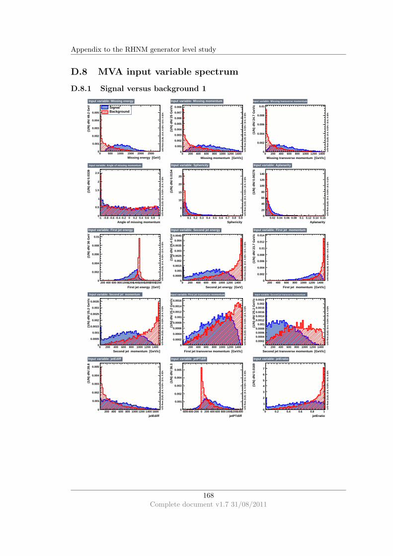
Appendix to the RHNM generator level study
D.8 MVA input variable spectrum
D.8.1 Signal versus background 1
Missing energy [GeV]0 500 1000 1500 2000 2500
49.2
GeV
/ (1
/N)
dN
0
0.001
0.002
0.003
0.004
0.005
SignalBackground
U/O
-flo
w (
S,B
): (
0.0,
0.0
)% /
(0.0
, 0.0
)%
Input variable: Missing energy
Missing momentum [GeV/c]0 200 400 600 800 1000 1200 1400
25 G
eV/c
/ (1
/N)
dN
0
0.001
0.002
0.003
0.004
0.005
0.006
0.007
0.008
U/O
-flo
w (
S,B
): (
0.0,
0.0
)% /
(0.0
, 0.0
)%
Input variable: Missing momentum
Missing transverse momentum [GeV/c]0 200 400 600 800 1000 1200 1400
24.7
GeV
/c /
(1/N
) dN
0
0.002
0.004
0.006
0.008
0.01
U/O
-flo
w (
S,B
): (
0.0,
0.0
)% /
(0.0
, 0.0
)%
Input variable: Missing transverse momentum
Angle of missing momentum-1 -0.8 -0.6 -0.4 -0.2 0 0.2 0.4 0.6 0.8 1
0.03
39
/ (1
/N)
dN
0
0.5
1
1.5
2
2.5
U/O
-flo
w (
S,B
): (
0.0,
0.0
)% /
(0.0
, 0.0
)%
Input variable: Angle of missing momentum
Sphericity0.1 0.2 0.3 0.4 0.5 0.6 0.7 0.8 0.9
0.01
54
/ (1
/N)
dN
0
5
10
15
20
25
U/O
-flo
w (
S,B
): (
0.0,
0.0
)% /
(0.0
, 0.0
)%
Input variable: Sphericity
Aplanarity0.02 0.04 0.06 0.08 0.1 0.12 0.14 0.16
0.00
276
/ (1
/N)
dN
0
20
40
60
80
100
120
140
U/O
-flo
w (
S,B
): (
0.0,
0.0
)% /
(0.3
, 0.1
)%
Input variable: Aplanarity
Second jet energy [GeV]
0 200 400 600 800 1000 1200 1400
25.4
GeV
/ (1
/N)
dN
0
0.0005
0.001
0.0015
0.002
0.0025
0.003
0.0035
0.004
0.0045
U/O
-flo
w (
S,B
): (
0.0,
0.0
)% /
(0.0
, 0.0
)%
Input variable: Second jet energy
First jet momentum [GeV/c]
200 400 600 800 1000 1200 1400
23.7
GeV
/c /
(1/N
) dN
0
0.002
0.004
0.006
0.008
0.01
0.012
0.014
U/O
-flo
w (
S,B
): (
0.0,
0.0
)% /
(0.0
, 0.0
)%
Input variable: First jet momentum
Second jet momentum [GeV/c]0 200 400 600 800 1000 1200 1400
25.2
GeV
/c /
(1/N
) dN
0
0.0005
0.001
0.0015
0.002
0.0025
0.003
0.0035
U/O
-flo
w (
S,B
): (
0.0,
0.0
)% /
(0.0
, 0.0
)%
Input variable: Second jet momentum
Second jet transverse momentum [GeV/c]0 200 400 600 800 1000 1200 1400
25.2
GeV
/c /
(1/N
) dN
00.0002
0.00040.00060.0008
0.0010.00120.00140.0016
0.00180.002
0.0022
U/O
-flo
w (
S,B
): (
0.0,
0.0
)% /
(0.0
, 0.0
)%
Input variable: Second jet transverse momentum
First jet energy [GeV]
200 400 600 8001000120014001600180020002200
36 G
eV /
(1/N
) dN
0
0.002
0.004
0.006
0.008
0.01
U/O
-flo
w (
S,B
): (
0.0,
0.0
)% /
(0.0
, 0.0
)%
Input variable: First jet energy
First jet transverse momentum [GeV/c]200 400 600 800 1000 1200 1400
25.2
GeV
/c /
(1/N
) dN
0
0.0002
0.0004
0.0006
0.0008
0.001
0.0012
0.0014
0.0016
U/O
-flo
w (
S,B
): (
0.0,
0.0
)% /
(0.0
, 0.0
)%
Input variable: First jet transverse momentum
jetEdiff200 400 600 800 1000 1200 1400 1600
28.8
/
(1/N
) dN
0
0.001
0.002
0.003
0.004
0.005
U/O
-flo
w (
S,B
): (
0.0,
0.0
)% /
(0.0
, 0.0
)%
Input variable: jetEdiff
jetPTdiff-600-400-200 0 200 400 600 800100012001400
36.3
/
(1/N
) dN
0
0.001
0.002
0.003
0.004
0.005
U/O
-flo
w (
S,B
): (
0.0,
0.0
)% /
(0.0
, 0.0
)%
Input variable: jetPTdiff
jetEratio0 0.2 0.4 0.6 0.8 1
0.01
69
/ (1
/N)
dN
0
1
2
3
4
5
6
7
U/O
-flo
w (
S,B
): (
0.0,
0.0
)% /
(0.0
, 0.0
)%
Input variable: jetEratio
168Complete document v1.7 31/08/2011

Appendix to the RHNM generator level study
D.8.2 Signal versus background 2
Missing energy [GeV]500 1000 1500 2000 2500
46.5
GeV
/ (1
/N)
dN
0
0.0002
0.0004
0.0006
0.0008
0.001
0.0012
0.0014
0.0016
0.0018
0.002 SignalBackground
U/O
-flo
w (
S,B
): (
0.0,
0.0
)% /
(0.0
, 0.0
)%
Input variable: Missing energy
Missing momentum [GeV/c]200 400 600 800 1000 1200 1400
24.8
GeV
/c /
(1/N
) dN
0
0.0002
0.00040.0006
0.0008
0.001
0.00120.0014
0.0016
0.00180.002
U/O
-flo
w (
S,B
): (
0.0,
0.0
)% /
(0.0
, 0.0
)%
Input variable: Missing momentum
Missing transverse momentum [GeV/c]200 400 600 800 1000 1200 1400
24.7
GeV
/c /
(1/N
) dN
0
0.001
0.002
0.003
0.004
0.005
U/O
-flo
w (
S,B
): (
0.0,
0.0
)% /
(0.0
, 0.0
)%
Input variable: Missing transverse momentum
Angle of missing momentum-1 -0.8 -0.6 -0.4 -0.2 0 0.2 0.4 0.6 0.8 1
0.03
39
/ (1
/N)
dN
0
1
2
3
4
5
6
U/O
-flo
w (
S,B
): (
0.0,
0.0
)% /
(0.0
, 0.0
)%
Input variable: Angle of missing momentum
Sphericity0.1 0.2 0.3 0.4 0.5 0.6 0.7 0.8 0.9
0.01
54
/ (1
/N)
dN
0
1
2
3
4
5
6
7
8
9
U/O
-flo
w (
S,B
): (
0.0,
0.0
)% /
(0.0
, 0.0
)%
Input variable: Sphericity
Aplanarity0.05 0.1 0.15 0.2 0.25 0.3 0.35 0.4
0.00
692
/ (1
/N)
dN
0
10
20
30
40
50
60
U/O
-flo
w (
S,B
): (
0.0,
0.0
)% /
(0.0
, 0.0
)%
Input variable: Aplanarity
First jet energy [GeV]200 400 600 800 100012001400160018002000
32.8
GeV
/ (1
/N)
dN
0
0.0005
0.001
0.0015
0.002
0.0025
U/O
-flo
w (
S,B
): (
0.0,
0.0
)% /
(0.0
, 0.0
)%
Input variable: First jet energy
Second jet energy [GeV]0 200 400 600 800 1000 1200 1400
23.9
GeV
/ (1
/N)
dN
0
0.001
0.002
0.003
0.004
0.005
0.006
0.007U
/O-f
low
(S
,B):
(0.
0, 0
.0)%
/ (0
.0, 0
.0)%
Input variable: Second jet energy
First jet momentum [GeV/c]200 400 600 800 1000 1200 1400
24.1
GeV
/c /
(1/N
) dN
0
0.0005
0.001
0.0015
0.002
0.0025
U/O
-flo
w (
S,B
): (
0.0,
0.0
)% /
(0.0
, 0.0
)%
Input variable: First jet momentum
Second jet momentum [GeV/c]0 200 400 600 800 1000 1200 1400
23.5
GeV
/c /
(1/N
) dN
0
0.001
0.002
0.003
0.004
0.005
0.006
0.007
0.008
U/O
-flo
w (
S,B
): (
0.0,
0.0
)% /
(0.0
, 0.0
)%
Input variable: Second jet momentum
First jet transverse momentum [GeV/c]200 400 600 800 1000 1200 1400
24.8
GeV
/c /
(1/N
) dN
0
0.001
0.002
0.003
0.004
0.005
U/O
-flo
w (
S,B
): (
0.0,
0.0
)% /
(0.0
, 0.0
)%
Input variable: First jet transverse momentum
Second jet transverse momentum [GeV/c]0 200 400 600 800 1000 1200
22.6
GeV
/c /
(1/N
) dN
0
0.002
0.004
0.006
0.008
0.01
0.012
U/O
-flo
w (
S,B
): (
0.0,
0.0
)% /
(0.0
, 0.0
)%
Input variable: Second jet transverse momentum
jetEdiff200 400 600 800 1000 1200 1400 1600
28.8
/
(1/N
) dN
0
0.0002
0.0004
0.0006
0.0008
0.001
0.0012
0.0014
0.0016
0.0018
0.002
U/O
-flo
w (
S,B
): (
0.0,
0.0
)% /
(0.0
, 0.0
)%
Input variable: jetEdiff
jetPTdiff-600-400-200 0 200 400 600 800100012001400
36.3
/
(1/N
) dN
0
0.0005
0.001
0.0015
0.002
0.0025
0.003
0.0035
0.004
0.0045
U/O
-flo
w (
S,B
): (
0.0,
0.0
)% /
(0.0
, 0.0
)%
Input variable: jetPTdiff
jetEratio0 0.2 0.4 0.6 0.8 1
0.01
69
/ (1
/N)
dN
0
1
2
3
4
5
6
7
8
U/O
-flo
w (
S,B
): (
0.0,
0.0
)% /
(0.0
, 0.0
)%
Input variable: jetEratio
169Complete document v1.7 31/08/2011

Appendix to the RHNM generator level study
170Complete document v1.7 31/08/2011

APPENDIX E
Smearing techniques
E.1 Basic single particle smearing
The first attempt to apply a smearing to generator level data in order to simulate theeffect of PFA reconstruction and detector resolution is to apply the suitable sub-detectorresolution on the four-vector (~p,E)T of each final state particle.
- Charged particles are smeared according to a tracker resolution of the the order of∆p/p2 = 2 · 10−5.
- Photons four-vector are smeared according to a Electromagnetic Calorimeter (ECAL)resolution which is about σE/E = 10%/
√E.
- Neutral hadrons are smeared according to a Hadronic Calorimeter (HCAL) reso-lution of about σE/E = 40%/
√E.
This very straightforward technique is roughly valid if the energy scale is of the orderof a few hundred GeV (100–300 GeV) allowing the PFA confusion to be neglected. Thistechnique is therefore not applicable at CLIC energies (O(1–3 TeV)).
E.2 Jet smearing
At CLIC energies the confusion term is a foreground issue. Therefore, the simple tech-nique described above is not realistic but the jet energy resolution semi-empirical formula(eq. 2.7, p. 33) proposed in [33] can be applied to smear reconstructed jet four-vectors.This formula is recalled as follows:
rms90E
=21%√E
⊕ 0.7%
︸ ︷︷ ︸
classical stochasticand constant terms
⊕ 0.004E︸ ︷︷ ︸
leakage andthreshold effect
⊕ 2.1%
(E
100 GeV
)0.3
︸ ︷︷ ︸
confusion term
.
171

Smearing techniques
This formula has been derived from prefect di-jet events, namely e+e− → Z0 →u (d, s)u (d, s). Therefore, its application to multi-jet final state processes is not straight-forward. The question weather to apply the smearing to the hemisphere-jets or to the kt
inclusive jets (see section 8.3.2, p. 119) is hard to answer and once a choice is made, thequestion remains how to smear the jets of the other definition. The reasonable choice isto apply the formula to the lightest jets, namely the kt inclusive jets, and then rebuildthe hemispheres from the smeared light jets. This technique does not allow any smearingof non-jet-related variables (see table 8.5, p. 121 and D.5, p. 166 for lists of the involvedvariables). And finally, even if the smearing of the non-jet-related variables is neglected,the formula only gives an energy smearing whereas a jet mass and/or momentum res-olution are compulsory complementary information. Therefore, as this technique leadsto a large number of approximations, it has been considered unreliable and discarded.
E.3 Single particle smearing
The information available in [33] allows to envision including confusion effects in thesingle particle smearing already sketched in section E.1. The confusion mainly comesfrom three distinct sources:
- photon hits lost from association to charged hadron clusters,
- hits from neutral hadrons lost from association to charged hadron clusters,
- hits from charged hadrons lost from association to neutral clusters.
These effects, as well as leakage effect, contribute to the jet energy resolution as shownin figure E.1, where the point are taken from [33] and where the interpolation is donewith the following functions:
- photon to charged hadron:
fγ→C = 0.99 ± 0.03
(E
100
)0.27±0.04
- neutral to charged hadron:
fN→C = 0.54 ± 0.04 logE − 1.18 ± 0.18
- charged neutral hadron:
fC→N = 1.67 ± 0.18 e−E/128.8±19.6
- leakage:fleak = 0.520 ± 0.013 logE − 1.887 ± 0.062
These functions can therefore be used to extrapolate the various contributions to arbi-trary energy and therefore provide a more realistic smearing than in section E.1. Such anextrapolation is obviously subject to large uncertainties that can not be easily estimatedat this step.
172Complete document v1.7 31/08/2011

Smearing techniques
Energy [GeV]50 100 150 200 250
[%]
EEσ
0
0.2
0.4
0.6
0.8
1
1.2
1.4
1.6
1.8
2
/ ndf 2χ 0.00425 / 2
p0 0.03537± 0.5444
p1 0.1707± 1.178
/ ndf 2χ 0.00425 / 2
p0 0.03537± 0.5444
p1 0.1707± 1.178
/ ndf 2χ 0.01434 / 2
p0 0.1767± 1.67
p1 19.58± 128.8
/ ndf 2χ 0.01434 / 2
p0 0.1767± 1.67
p1 19.58± 128.8
/ ndf 2χ 0.004697 / 2
p0 0.02697± 0.9857
p1 0.03941± 0.2711
/ ndf 2χ 0.004697 / 2
p0 0.02697± 0.9857
p1 0.03941± 0.2711
/ ndf 2χ 0.0005433 / 2
p0 0.01265± 0.5201
p1 0.06103± -1.887
/ ndf 2χ 0.0005433 / 2
p0 0.01265± 0.5201
p1 0.06103± -1.887
charged hadr.→Neutral neutral hadr.→Charged
charged→ γLeakage
Figure E.1: Individual contribution to jet energy resolution for each confusion effectsand for leakage.
This method, as a refinement of the basic single particle smearing of section E.1,is more realistic for CLIC energies in principle. However, the extrapolation at CLICenergies of the confusion term contributions is very uncertain. In [111], a CLIC optimisedPFA has been announced. It provides a jet energy resolution below 3.6% for the wholeILC and CLIC energy range by relying on a trade-off between particle and energy flows.Therefore, the previous conclusions became obsolete and an equivalent study shouldbe done on this CLIC optimised PFA. Moreover, this technique has two additionaldrawbacks:
- As in the method described in section E.2, the performance is evaluated on veryclean di-jet events, from the process e+e− → Z0 → u (d, s)u (d, s), and may benot completely exact for more complex final states with different jet clusteringstrategies.
- This method only affects the resolution on the final state particle four-vectors, butin the PFA it is possible that particles are completely missed as well as completelyinvented. This uncertainty, that actually induces a smearing in the number ofparticles in the event, can not be rendered by this method. Moreover, in realisticconditions, the number of particles in the event should be affected as well by themachine induced γγ → hadrons background.
Those drawbacks led this method to be discarded to explore another possibility, describedin the next section.
173Complete document v1.7 31/08/2011

Smearing techniques
E.4 Final state variables smearing
A last smearing method was envisioned in the aim to get the most realistic possibleresults. The method is based on the eventwise comparison, for each variable of theanalysis, of its value at the generator level and its value at the detector level using asample of fully simulated data. This could be done with tt events from CLIC CDRproduction. This method is meant to include every possible effects since it somehowsimply transforms the generator level information into the detector level informationusing random coefficients.
E.4.1 Description of the method
For each event, the ratio between generator and detector level values is plotted versusthe generator level value, giving a 2D histogram called smearing map. The exampleof the total event invariant mass of tt events is displayed in figure E.2(a). Once thismap is obtained, it is cut into vertical slices to give distributions of the ratio betweengenerator and detector level values of the variables, for a given generator level value. Thesmearing is then done by considering the generator level value to smear and selecting thecorresponding slice of the smearing map to generate a random coefficient to be multipliedwith the generator level value.
Building a slice A slice is simply an 1D histogram of the map entries correspondingto a given horizontal range projected on the vertical axis. It is built as follows. Itconsists at first of the content of all the y-axis bins corresponding to only one x-axis bin.If the number of entries is too low, the next x-axis bin is considered and all its entriesare added to the slice histogram and so forth until the minimum statistics is matched.If the last slice can’t reach the minimum statistics, it is merged with the previous one.Examples of such slices from the map of figure E.2(a) are shown in figure E.2(b). Theslice histograms are slightly smoothed before generating a random smearing coefficient.
Generator level value0 500 1000 1500 2000 2500 3000
Det
ecto
r le
vel /
Gen
erat
or le
vel
0
0.2
0.4
0.6
0.8
1
1.2
1.4
1.6
1.8
2
0
5
10
15
20
25
30
35
40
45
(a) Smearing map for the total event invariantmass.
Detector level / Generator level0.6 0.8 1 1.2 1.4
Ent
ries
/ 0.0
1
0
10
20
30
40
50
60
70
80
90
100
from bin 97 to 100
from bin 196 to 200
from bin 393 to 400
from bin 606 to 610
(b) Example of slice histograms from the totalevent invariant mass smearing map.
Figure E.2: Illustration of the working principle of the smearing map method.
174Complete document v1.7 31/08/2011
Smearing techniques
Low value divergence and smeared value calculation For values of the variablespectrum which are close to 0, the ratio between generator and detector level values tendto diverge. This is avoided by shifting the distribution away from 0. So the ratio r isactually calculated as
r =xdet + k
xgen + k,
where xdet is the detector level value of the variable x and xgen, the generator level one, kis the arbitrary offset taken here as the difference between maximum xmax and minimumvalue xmin of the variable x:
k = xmax − xmin .
A too large offset induces a compression of the distributions and would cause the smear-ing coefficients to be undervalued. More refined definitions of k can allow to insure agood distance to 0 without going to too high values either. The smeared value xsmeared
is therefore calculated as
xsmeared = ((xgen + k) × rrand) − k ,
where rrand is the random smearing coefficient generated from the smearing map slicecorresponding to xgen.
E.4.2 Performance of the method
Figures E.3 and E.4 illustrate respectively the achievable quality of the smearing thanksto this method and the possible problems that may be encountered. This method canbe very effective to smear generator level data for which a fully simulated sample existsin order to increase the statistics. However, it appears that when using a large numberof variables, the distribution of some of them are not well rendered. Moreover, thecorrelation between variables is lost when using this method directly. The correlationscan be approximatively restored if the smearing coefficients of correlated variables arededuced from each others or, in the case of simple relation between variables, if thesmeared value of a correlated variable is directly computed from the smeared value ofanother correlated variable obtained through the smearing map method.
This method should therefore be more reliable when using few uncorrelated variablesor with simple correlations. In the case of the studies described in chapters 8 and 9,given the number of involved variables and their sometimes complex correlations, a goodstrategy could be to apply the smearing only on the output of the BDTs. The exampleof the top-tagging BDT output is displayed in figure E.5.
Evaluating the generator level Z ′ event selection BDT on tt events from CLIC CDRsimulated data do not give a reliable smearing map because the distribution are toodifferent due to the large difference of the centre of mass energy spectra explain insection 9.5. The latter argument prevented from using this method for the smearing ofthe Z ′ study results.
175Complete document v1.7 31/08/2011

Smearing techniques
Event invariant mass-500 0 500 1000 1500 2000 2500 3000 3500 40000
1000
2000
3000
4000
5000 Smeared values
MC truth
PFA rec
(a)]2Second hemisph. mass [GeV/
0 200 400 600 800 1000 1200 1400
)2N
umbe
r of
eve
nts
/ (15
.0 G
eV/
0
1000
2000
3000
4000
5000
6000
7000
8000Smeared values
PFA Rec. values
Generator level values
(b)
First hemisph. tr. momentum [GeV/c]0 200 400 600 800 1000 1200 1400 1600 1800 2000
Num
ber
of e
vent
s / (
20.0
GeV
/c)
1
10
210
310
410 Smeared values
PFA Rec. values
Generator level values
(c)
Figure E.3: Illustration of the achievablequality of the smearing on single vari-ables. (a) illustrates the performance ofthe technique on the total event invari-ant mass which has been taken as exam-ple above. (b) illustrates the ability ofthe method to deal with a complicatedspectrum. (c) illustrates how the methodallow to populate distribution tails evenwith limited initial statistics.
176Complete document v1.7 31/08/2011

Smearing techniques
Hardest kt07 jet energy [GeV]0 200 400 600 800 1000 1200 1400 1600 1800 2000
Num
ber
of e
vent
s / (
20.0
GeV
)
0
200
400
600
800
1000
1200
1400
1600
1800
2000
Smeared values
PFA Rec. values
Generator level values
(a)Second hemisph. momentum [GeV/c]
0 500 1000 1500 2000 2500 3000
Num
ber
of e
vent
s / (
30.0
GeV
/c)
0
500
1000
1500
2000
2500
3000
3500
4000 Smeared values
PFA Rec. values
Generator level values
(b)
Missing momentum [GeV/c]0 500 1000 1500 2000 2500 3000
Num
ber
of e
vent
s / (
30.0
GeV
/c)
0
500
1000
1500
2000
2500
3000
Smeared values
PFA Rec. values
Generator level values
(c)
Figure E.4: Illustration of some prob-lems that may occur when smearing singlevariables. (a) illustrates how the methodcan overvalue the smearing around asteep end point. (b) shows as well theend point problem and also a low valuediscrepancy due to the low value diver-gence of the smearing coefficient. (c) dis-plays an artefact of this technique wherea bump appear with no obvious reason,attempts to tune the method parametershave failed to suppress this effect.
Top-tagging BDT output-0.8 -0.6 -0.4 -0.2 0 0.2 0.4 0.6 0.8 1 1.2
Ent
ries
/ 0.0
11
0
1000
2000
3000
4000
5000
6000
7000
8000
9000 Smeared values
Generator level values
PFA Rec. values
Figure E.5: Smearing ofthe BDT output
177Complete document v1.7 31/08/2011

Smearing techniques
178Complete document v1.7 31/08/2011
Acknowledgement — Remerciements
Dans ces quelques lignes je vais essayer de mentionner tous ceux qui, dans mon entourage,ont joue un role positif autour de cette these et avant tout je voudrais remercier tousceux qui, peut etre a mon insu et/ou au leur, ont contribue a l’aboutissement de ceprojet et serait peut etre alors absents de ces lignes.
Je commencerai par la fin et par consequent les premiers remerciements vont auxmembres de mon jury, qui ont bien voulu se reunir a Annecy et m’octroyer le titre de“Docteur de l’Universite de Grenoble” suite a la soutenance. Des remerciements plusparticuliers vont a mes rapporteurs, Felix Sefkov et Paul Colas, qui sont parvenus a lireet analyser mon manuscrit en un temps record et ainsi permettre l’accomplissement dutravail dans les delais impartis. Je voudrais aussi remercier tout particulierement Jean-Jacques Blaising, qui a pris tres au serieux son role de president de jury et qui a veille,avec bienveillance et rigueur, a me pousser pour ameliorer la qualite du manuscrit et dela presentation pour la soutenance. Jean-Jacques fut aussi d’une aide precieuse et d’unconseil avise durant tout mon travail d’etude de simulation sur quark top et le Z ′.
Un des remerciements les plus importants est pour Catherine Adloff qui m’a donnema chance et m’a soutenu deja lors de mon stage de Master en 2007 puis pour l’obtentionde ce poste de doctorant au LAPP. Catherine a su m’accompagner dans les premierstemps et me laisser prendre mon autonomie au fur et a mesure, elle fut a la fois unedirectrice de these impliquee et une voisine de bureau amicale. Des remerciements vontaussi bien sur a Yannis Karyotakis, qui malgre sa charge de directeur du laboratoire, abeaucoup contribue a l’equilibre du travail.
Je voudrais aussi mentionner toute l’equipe DHCAL MICROMEGAS du LAPP enincluant aussi bien les acteurs passes que j’ai connus. Merci donc a Denis Fougeronspour les PCB des chambres a lecture analogique et pour les discussions instructives etsympathiques. Merci a Jean-Marc Dubois pour ce systeme de gaz qui alimente tou-jours et encore nos detecteurs, merci aussi pour ta sympathie, ta bonne humeur et tadisponibilite en cas de besoin. Merci a Ino Monteiro pour la structure porteuse desdetecteurs sans laquelle fort peu aurait pu etre accompli. En ce qui concerne l’equipeactuelle, la liste des hauts faits de chacun serait immense ... Il y a Jean Jacquemier,
179

Smearing techniques
heros de l’informatique, disponible et pedagogue. Nicolas Geffroy et Fabrice Peltier quiont concu et realise tant de pieces mecaniques et ainsi materialise ce projet, le tout dansla bonne humeur et la convivialite, Fabrice qui a aussi assemble tous les prototypes MI-CROMEGAS et meme les scintillateurs decrits dans ce manuscrit. Du cote electronique,Julie Prast, Cyril Drancourt, Sebastien Cap, Guillaume Vouters et Renaud Gaglione,dont le savoir faire et l’implication ont permis la bonne evolution du projet (design descircuits imprimes des detecteurs, des cartes intermediaires et d’interface, des puces, testselectroniques, calibrations, etc ...).
Du cote administratif, je souhaite remercier en particulier Brigitte Putanier et Marie-Claude Lacombe a la fois pour leur efficacite, leur disponibilite et leur sympathie, faisantde la preparation des missions une formalite finalement plaisante. Je voudrais aussiremercier ce cher support-info qui m’a depanne a tant de reprises avec efficacite etsympathie. De maniere plus general je tiens a saluer la cordialite et l’efficacite de tousles personnels du laboratoire, qui contribuent a faire du LAPP un endroit ou il fait bontravailler.
Je voudrais encore remercier au passage certains collegues exterieurs au groupe duLAPP: Stephane Poss (CERN), disponible, efficace, merci pour les donnees CLIC ILD ;Frank Simon (MPI), thank you for the tips about top physics ; Louis Helari (LAPP),merci pour tous les tuyaux administratifs sans lesquels j’aurais surement ete bien plusen retard pour mes inscriptions a l’universite ; David Attie (CEA), merci pour ton aideprecieuse dans la quete pour joindre Paul lors de ses deplacements ;). Thanks as well toTorbjorn Sjostrand and Peter Skands for their help with Pythia 8. The little collaborationwith Peter Skands was a great pleasure and helped me well even if we didn’t have thetime to make it lead to a real contribution to Pythia 8 code.
Certains collegues en particulier ont joue un role fondamental au quotidien, humaine-ment autant que scientifiquement, au cours de ses annees au LAPP. Nous formions uneveritable equipe, soudee et dynamique tant dans le travail qu’a la fete ! Le noyau dur :Jan Blaha , Max Chefdeville et Guillaume Vouters survit encore apres que Jan et moiayons quitte le LAPP. Merci les gars pour tous ces bon moments !
Du cote de la famille, il est juste que je commence par remercier profondement mesgrand-parents, Claude et Bernard, qui m’ont heberges lors des mois de mon stage deMaster 2, puis qui ont su rester presents mais discrets, toujours disponibles et d’un grandsoutien au cours de ses annees de these. Dans les derniers mois, Belle maman Solangem’a donne un precieux coup de pouce, merci pour les fleurs de Bach ! Dans la fin dela redaction du manuscrit, merci a Miko pour la relecture de l’anglais !! Et enfin mercia mes parents et beau parents pour l’organisation du pot de soutenance. Je souhaiteaussi finalement remercier tout particulierement Dorothee, qui m’a epaule, accompagne,encourage, supporte et bien plus encore ! Elle a autant que moi endure ces annees delabeurs de stress et de doutes et a pourtant apporte un soleil indescriptible sur toutecette periode ... Et merci a Celestin d’avoir ete le plus adorable des bebes !!
180Complete document v1.7 31/08/2011

Bibliography
[1] Sven Heinemeyer, Sabine Kraml, Werner Porod, and Georg Weiglein. Physicsimpact of a precise determination of the top quark mass at an e+e− linear collider.JHEP, September 2003. 7, 14
[2] Murray Gell-Mann. A schematic model of baryons and mesons. Phys. Lett., 8,1964. 8
[3] Georges Zweig. An su(3) model for interaction symmetry and its breaking. CERNLibraries, 1964. 8
[4] Sheldon Glashow, Jean Iliopoulos, and Luciano Maiani. Weak interactions withlepton-hadron symmetry. Phys. Rev. D, 11, 1970. 8
[5] LEP Collaborations. Updated parameters of the Z0 resonance from combinedpreliminary data of the LEP experiments. CERN preprint: CERN/PPE/93-157http: // aseps. in2p3. fr/ cgi-bin/ twiki. source/ pub/ FAPPS/ StudentPresentations/ LEP_ comb. pdf ,1993. 9
[6] Carlo Rovelli. Notes for a brief history of quantum gravity. In World Scientific,editor, Proceedings of the ninth Marcel Grossmann Meeting on General RelativityR.T. Jantzen, R. Ruffini, V. G. Gurzadyan editors, pages 742–768, Singapore,2002. 10, 11
[7] F. Zwicky. On the Masses of Nebulae and of Clusters of Nebulae. AstrophysicsJournal, 86:217–+, October 1937. Provided by the SAO/NASA Astrophysics DataSystem. 10
[8] Bill Carithers and Paul Grannis. Discovery of the Top Quark, 1995.http://www.slac.stanford.edu/pubs/beamline/25/3/25-3-carithers.pdf. 11
[9] E. Kh. Akhmedov. Neutrino physics. arXiv:hep-ph/0001264v2, 2000. 11
[10] Sidney coleman and Jeffrey Mandula. All possible symmetries of the s matrix.Physical Review, 159(5), july 1967. 12
181

BIBLIOGRAPHY
[11] Adel Bilal. Introduction to supersymmetry. arXiv:hep-th/0101055v1, 2001. 13
[12] Manuel Drees. An introduction to supersymmetry. arXiv:hep-ph/9611409v1, 1996.13
[13] JOSEPH D. LYKKEN. Introduction to supersymmetry. arXiv:hep-th/9612114v1,1996. 13
[14] Gunnar Nordstrom. Uber die moglichkeit, das elektromagnetische feld und dasgravitationsfeld zu vereinigen. Physikalische Zeitschrift, 1914. 13
[15] Theodor Kaluza. On the problem of unity in physics. Sitzungsber. Preuss. Akad.Wiss. Berlin. (Math. Phys.), 1921. 13
[16] Oskar Klein. Quantum theory and five dimensional theory of relativity. Z. Phys.,37, 1926. doi:10.1007/BF01397481. 13
[17] Lisa Randall and Raman Sundrum. A Large Mass Hierarchy from a Small ExtraDimension. Phys. Rev. Lett., 83, 1999. [arXiv:hep-ph/9905221]. 13
[18] Kaustubh Agashe and Geraldine Servant. Warped unification, proton stability,and dark matter. Phys. Rev. Lett., 93(23):231805, Dec 2004. 14
[19] Kaustubh Agashe and Geraldine Servant. Baryon number in warped grand unifiedtheories: model building and (dark matter related) phenomenology. Journal ofCosmology and Astroparticle Physics, 2005(02):002, 2005. 14
[20] The D∅ Collaboration. Determination of the width of the top quark. D∅ Note6034-CONF, 2010.http://www-d0.fnal.gov/Run2Physics/WWW/results/prelim/TOP/T87/T87.pdf. 14
[21] ILC collaboration. Reference design report, volume 2: Physics at the ilc. Technicalreport, ILC Global Design Effort and Worldwide Study, 2007.url:http://arxiv.org/PS_cache/arxiv/pdf/0709/0709.1893v1.pdf. 14, 19
[22] Lisa Randall and Raman Sundrum. Large mass hierarchy from a small extradimension. Phys. Rev. Lett., 83(17):3370–3373, Oct 1999. 14
[23] ILC home page.http://www.linearcollider.org/. 19, 21
[24] CLIC home page.http://clic-study.org/. 19, 21
[25] ILC collaboration. Reference design report, volume 3: Accelerator. Technicalreport, ILC Global Design Effort and Worldwide Study, 2007.http://ilcdoc.linearcollider.org/record/6321/files/ILC_RDR_Volume_3-Accelerator.pdf?version=4.21, 98, 195
[26] CTF3 Collaboration. Ctf3 home page.http://ctf3.home.cern.ch/ctf3/CTFindex.htm. 20
182Complete document v1.7 31/08/2011

BIBLIOGRAPHY
[27] CTF3 Collaboration. Ctf3 parameter list.http://ctf3.home.cern.ch/ctf3/New_parameters.htm. 20
[28] CLIC Study Team. CLIC CDR baseline parameter list, 2010.http://clic-meeting.web.cern.ch/clic-meeting/clictable2010.html. 21, 113, 195
[29] CLIC Study Team. A 3 tev e+e− linear collider based on clic technology. CERNdocument server, 2000.http://cdsweb.cern.ch/record/461450?ln=fr. 21
[30] Particle Data Group. Particle Physics Booklet. Extracted from Physics Letters B667, 1, 2008. 23, 24, 85, 86
[31] Claude Leroy and Pier-Giorgio Rancoita. Principles of Radiation Interaction InMatter And Detection. World Scientific, 2004. 24, 26, 82, 85, 86
[32] Jean-Claude Brient. Improving the jet reconstruction with the particle flowmethod: An introduction. In Proceedings of 11th International Conference onCalorimetry in High-Energy Physics (Calor 2004),Perugia, Italy, March 2004.http://hal.archives-ouvertes.fr/docs/00/02/82/00/PDF/ParticleFlow-Brient-V2.pdf.31, 32, 46
[33] M. A. Thomson. Particle Flow Calorimetry and the PandoraPFA Algorithm.Nuclear Instruments and Methods in Physics Research A, 611, july 2009.[arXiv:0907.3577v1]. 31, 33, 34, 46, 118, 171, 172
[34] ATLAS/Tile Calorimeter Collaboration. Atlas tile calorimeter technical designreport, 1996.http://atlas.web.cern.ch/Atlas/SUB_DETECTORS/TILE/TDR/TDR.html. 32
[35] E. Rutherford and H. Geiger. An electrical method of counting the number of aparticles from radioactive substances. Proceedings of the Royal Society (London)Series A, 81(546), 1908. 39
[36] H. Geiger and W. Muller. Elektronenzahlrohr zur messung schwachster aktivitaten.Naturwissenschaften, 16:617–618, 1928. 10.1007/BF01494093. 39
[37] N. N. Das Gupta and S. K. Ghosh. A report on the wilson cloud chamber and itsapplications in physics. Rev. Mod. Phys., 18(2):225–290, Apr 1946. 39
[38] Carl D. Anderson. Physical Review, 43, 1933. 39
[39] Seth H. Neddermeyer and Carl D. Anderson. Note on the nature of cosmic-rayparticles. Phys. Rev., 51(10):884–886, May 1937. 39
[40] G. Charpak, R. Bouclier, T. Bressani, J. Favier, and C. Zupancic. The use ofmultiwire proportional counters to select and localize charged particles. NuclearInstruments and Methods, 62(3):262 – 268, 1968. 40
[41] G. Charpak, D. Rahm, and H. Steiner. Some developments in the operation ofmultiwire proportional chambers. Nuclear Instruments and Methods, 80(1):13 –34, 1970. 40, 41
183Complete document v1.7 31/08/2011

BIBLIOGRAPHY
[42] Gilles Barouch. Analyse des Phenomenes Physiques Lies au Fonctionnement duDetecteur Gazeux a Micropistes MICROMEGAS. PhD thesis, Universite de Paris-Sud, UFR scientifique d’Orsay, 2001. 41, 151
[43] A. Oed. position-sensitive detector with microstrip anode for electron multiplica-tion with gases. Nucl. Instr. Meth. A, 263, 1987. 41, 42
[44] F. Angelini, R. Bellazzini, A. Brez, M.M. Massai, R. Raffo, G. Spandre, and M.A.Spezziga. The micro-gap chamber. Nucl. Instr. Meth. A, 335, 1993. 42, 43
[45] Ioannis Giomataris, Ph. Rebourgeard, J. P. Robert, and Georges Charpak.MICROMEGAS: a high-granularity position-sensitive gaseous detector for highparticle-flux environments. NIM A, 376:29–35, 1996. 43, 45
[46] Robert A. Wijsman. Breakdown Probability of a Low Pressure Gas Discharge.Phys. Rev., 75(5):833–838, Mar 1949. 44, 100
[47] P. Abbon at al. The compass experiment at cern. Nuclear Instruments and Meth-ods in Physics Research Section A: Accelerators, Spectrometers, Detectors andAssociated Equipment, 577(3):455 – 518, 2007. 45
[48] F. Kunn, P. Abbon, J. Ball, Y. Bedfer, C. Bernet, E. Delagnes, A. Giganon,J. M. Le Goff, A. Magnon, D. Neyret, H. Pereira, S. Platchkov, P. Rebourgeard,G. Tarte, and D. Thers. The gaseous microstrip detector micromegas for thecompass experiment at cern. Nuclear Physics A, 721:C1087 – C1090, 2003. 45
[49] J. Dere, Georges Charpak, A. Gigagnon, Ioannis Giomataris, D. Jourde,C. Koshowski, S. Loucatos, G. Puill, Ph. Rebourgeard, and J. P. Robert. Firstbeam test with Micromegas, a high rate, high resolution detector. NIM A, 412:47–60, 1998. 45
[50] J. Dere, Gilles Barouch, A. Bay, S. Bouchigny, Georges Charpak, F. Didierjean,J. C. Faivre, Ioannis Giomataris, C. Koshowski, F. Kunne, J.-M. Le Goff, F. Lehar,Y. Lemoigne, S. Loucatos, J.-C. Lugol, A. Magnon, B. Mayer, J.-P Perroud,S. Platchkov, G. Puill, Ph. Rebourgeard, Y. Terrien, D. Thers, and H. Zaccone.Development of a fast gaseous detector: ’MICROMEGAS’. NIM A, 423:32–48,1999. 45
[51] I. Giomataris, R. De Oliveira, S. Andriamonje, S. Aune, G. Charpak, P. Colas,G. Fanourakis, E. Ferrer, A. Giganon, Ph. Rebourgeard, and P. Salin. Micromegasin a bulk. NIM A, 560:405–408, 2006. 45, 46
[52] SiD. Letter of Intent, March 2009.http://silicondetector.org/download/attachments/46170132/SiliconDetectorLetterOfIntent.pdf.46, 91, 97, 101
[53] ILD Concept Group. The International Large Detector Letter of Intent, March2009.http://www.ilcild.org/documents/ild-letter-of-intent. 46, 97
184Complete document v1.7 31/08/2011

BIBLIOGRAPHY
[54] Calice official web page.https://twiki.cern.ch/twiki/bin/view/CALICE/WebHome. 47, 99
[55] Rd51 home page.http://rd51-public.web.cern.ch/rd51-public/Welcome.html. 47
[56] A. Espargiliere. Micromegas, caracterisation d’un detecteur pour le futur ILC.LAPP internship report, 2007. 47
[57] Yuri Kudenko. The near neutrino detector for the T2K experiment. NuclearInstruments and Methods in Physics Research A, 598, 2009. 47, 91
[58] Jose Repond et al. Hadron showers in a digital hadron calorimeter. JINST 4P10008, 2009. 47, 100
[59] J. C. Santiard and K. Marent. The Gassiplex0.7-2 Integrated Front-End AnalogProcessor for the HMPID and the Dimuon Spectrometer of ALICE. In 5th Con-ference on Electronics for LHC Experiments, Snowmass, CO, USA, pages 431 –435, 20 – 24 Sep. 1999.http://cdsweb.cern.ch/record/523473/files/p431.pdf. 48, 63, 78
[60] Herve Mathez Renaud Gaglione. DIRAC: A DIgital Readout Asic for hAdronicCalorimeter. In Nuclear Science Symposium Conference Record, pages 1815 – 1819,19 – 25 Oct. 2008. doi:10.1109/NSSMIC.2008.4774745. 49, 89, 90
[61] R. Gaglione et al. Dirac v2 : a digital readout asic for hadronic calorimeter. InTWEPP, pages 117–121, Nov. 2009. 49, 89
[62] S. Callier et al. Hardroc1, readout chip of the digital hadronic calorimeter of ilc. InIEEE Nuclear Science Symposium Conference Record, volume 3, pages 1851–1856,2007. 49, 89
[63] R. Gaglione. Microroc and DAQ status. Presentation at CALICE collaborationmeeting, 19-21 May 2011 CERNhttp://indico.cern.ch/getFile.py/access?contribId=21&sessionId=7&resId=0&materialId=slides&confId=136864,2011. 49, 90
[64] C. Adloff, D. Attie, J. Blaha, S. Cap, M. Chefdeville, P. Colas, A. Dalmaz,C. Drancourt, A. Espargiliere, R. Gaglione, R. Gallet, N. Geffroy, I. Giomataris,J. Jacquemier, Y. Karyotakis, F. Peltier, J. Prast, and G. Vouters. MICROMEGASchambers for hadronic calorimetry at a future linear collider. JINST, Nov. 2009.49
[65] Didier Roy. Manuel utilisateur, CENTAURE version 21lv 8.5, 2009.http://www-subatech.in2p3.fr/~electro/infoaq/CENTAURE21lv85/pdfdoctxt/centaure21lv85.pdf.53, 64, 78
[66] Magboltz cross sections web page.http://rjd.web.cern.ch/rjd/cgi-bin/cross. 54
185Complete document v1.7 31/08/2011

BIBLIOGRAPHY
[67] Fabio Sauli. Principle of operation of multiwire proportionnal and drift cham-bers,“yellow report”. CERN, 1977. 56
[68] T. Geralis, G. Fanourakis, Y. Giomataris, and K. Zachariadou. The data acquisi-tion of the MICROMEGAS detector for the CAST experiment. 19 – 25 Oct. 2003.64
[69] C. Adloff, M. Chefdeville, A. Espargiliere, and R. Gaglione. Calibration of elec-tronic readout chains for MICROMEGAS chambers. Technical report, LAPP Tech-nical note, 2009. LAPP-TECH-2009-02, HAL: in2p3-00400295. 65
[70] C. Adloff, J. Blaha, J.-J. Blaising, M. Chefdeville, A. Espargiliere, and Y. Kary-otakis. Monte Carlo study of the physics performance of a digital hadroniccalorimeter. Submitted to JINST (JINST 002P 0809), 2009. arXiv:0910.2636v1.74
[71] Jan Blaha. Study of shower profile for a test beam. LAPP internal meeting, 2009.http://lappweb.in2p3.fr/~blaha/talks/lapp240509.pdf. 78
[72] R. Gaglione, C. Adloff, M. Chefdeville, A. Espargiliere, N. Geffroy, Y. Karyotakis,and R. De Oliveira. A micromegas chamber with embedded dirac asic for hadroniccalorimeter. In 1st International Conference On Micro Pattern Gaseous Detectors,page JINST 4 P11011, 2009. 90
[73] ILD Joint steering board. Definition of the ild reference detector.http://ilcild.org/documents/misc-doc/ILDreferencedetector-20081113.pdf/view, 2008.91
[74] T. Alexopoulos, A.A. Altintas, M. Alviggi, M. Arik, S.A. Cetin, V. Chernya-tine, E. Cheu, D. Della Volpe, M. Dris, D. Fassouliotis, E.N. Gazis, R. Giordano,V. Gratchev, L. Guan, P. Iengo, P. Ioannou, C. Li, K. Johns, V. Kaushik, A. Khodi-nov, C. Kourkoumelis, S. Maltezos, K. Mermigka, H. Muller, K. Nikolopoulos,W. Park, S. Persembe, C. Petridou, R. Petti, V. Polychronakos, M.V. Purohit,D. Sampsonidis, G. Sekhniaidze, M. Shao, Y.J. Sun, G. Tsipolitis, R. Veenhof,X.L. Wang, J. Wotschack, S.X. Wu, T. Zhao, and Z.G. Zhao. Development oflarge size micromegas detector for the upgrade of the atlas muon system. NuclearInstruments and Methods in Physics Research Section A: Accelerators, Spectrom-eters, Detectors and Associated Equipment, 617(1-3):161 – 165, 2010. 11th PisaMeeting on Advanced Detectors - Proceedings of the 11th Pisa Meeting on Ad-vanced Detectors. 91
[75] N. Lesparre et al. Geophysical muon imaging: feasibility and limits. GeophysicalJournal International, 2010. doi: 10.1111/j.1365-246X.2010.04790.x. 92
[76] S. Andriamonje et al. Experimental studies of a micromegas neutron detector.Nuclear Instruments and Methods in Physics Research A, 481, 2002. 92
[77] G. K. Fanourakis, T. Geralis, K. Kousouris, K. Zachariadou, I. Giomataris,N. Giokaris, G. Loudos, M. Lebessi, and E. Stiliaris. The use of the micromegas
186Complete document v1.7 31/08/2011

BIBLIOGRAPHY
technology for a new imaging system. Nuclear Instruments and Methods in PhysicsResearch Section A: Accelerators, Spectrometers, Detectors and Associated Equip-ment, 527(1-2):62 – 67, 2004. Proceedings of the 2nd International Conference onImaging Technologies in Biomedical Sciences. 92
[78] Leszek Ropelewski and Maxim Titov. Leszek ropelewski, November 6, 2009.http://rd51-public.web.cern.ch/RD51-Public/Activities/Documents/CERN_ENICE_06112009.pdf.92
[79] Maximilien Chefdeville et al. Test of a 1 m2 micromegas prototype in a muonbeam. To be released, 2011.related slides:http://indico.in2p3.fr/getFile.py/access?contribId=4&resId=0&materialId=slides&confId=5087.95, 96, 98
[80] CLIC study group. 500 GeV to 3 tev evolution, 2010.http://clic-meeting.web.cern.ch/clic-meeting/clic500-3000.html. 98, 195
[81] Jose Repond et al. Measurement of positron showers with a digital hadroncalorimeter. JINST 4 P04006, 2009. 100
[82] N. Geffroy, C. Girard, Y. Karyotakis, M. Oriunno, M. Breidenbach, and K. Krem-petz. Proposal of a new hcal geometry avoiding cracks in the calorimeter. Technicalreport, LAPP, 2008. LAPP-TECH-2008-02http://hal.in2p3.fr/docs/00/32/48/23/PDF/LAPP-TECH-2008-02.pdf. 101
[83] N. Geffroy, C. Girard, Y. Karyotakis, M. Oriunno, M. Breidenbach, and K. Krem-petz. Proposal of a new hcal forward geometry without crack. Technical report,LAPP, 2008. LAPP-TECH-2008-07http://hal.in2p3.fr/docs/00/33/93/57/PDF/LAPP-TECH-2008-07.pdf. 101
[84] J. Blaha, N. Geffroy, and Y. Karyotakis. Impact of dead zones on the response of ahadron calorimeter with projective and non-projective geometry. Technical report,LAPP, 2011. LAPP-TECH-2011-01 and CALICE Note CIN-018, arXiv:1102.1363.101
[85] Alexander Pukhov. CalcHEP 2.3: MSSM, structure functions, event genera-tion, batchs, and generation of matrix elements for other packages. arXiv:hep-ph/0412191, 2004. 111, 115, 119, 128, 155
[86] Daniel V. Schroeder. Beamstrahlung and QED backgrounds at future linear col-liders. SLAC-0371.available at http://www.slac.stanford.edu/pubs/slacreports/slac-r-371.html. 113
[87] Mark Thomson. CLIC ILD reconstruction status.http://indico.cern.ch/getFile.py/access?contribId=10&resId=1&materialId=slides&confId=125936,CLIC meeting, 16 Feb. 2011. 115, 192
[88] Wolfgang Kilian, Jurgen Reuter, Thorsten Ohl, and Christian Speckner.WHIZARD web page.http://projects.hepforge.org/whizard/. 118
187Complete document v1.7 31/08/2011

BIBLIOGRAPHY
[89] S. Agostinelli et al. Geant4 - a simulation toolkit. Nuclear Instruments and MethodsA, 506, 2003. 118
[90] Mokka home page.http://polzope.in2p3.fr:8081/MOKKA/. 118
[91] ILC soft team. MARLIN web page.http://ilcsoft.desy.de/portal/software_packages/marlin/index_eng.html. 118
[92] CLIC collaboration. CLIC conceptual design report vol. 2: Physics and detectorsat CLIC.https://edms.cern.ch/file/1160419/1/CLIC_CDR_Review_080911.pdf, 2011. 118
[93] Stephen D. Ellis and Davison E. Soper. Successive combination jet algorithm forhadron collisions. Phys. Rev. D, 48(7):3160–3166, Oct 1993. 120
[94] Andreas Hoecker, Peter Speckmayer, Joerg Stelzer, Jan Therhaag, Eckhard vonToerne, and Helge Voss. TMVA: Toolkit for Multivariate Data Analysis. PoS,ACAT:040, 2007. 121
[95] A. Hoecker, P. Speckmayer, J. Stelzer, J. Therhaag, E. von Toerne, and H. Voss.TMVA 4 User Guide, arxiv:physics/0703039 edition, November 2007.http://tmva.sourceforge.net/docu/TMVAUsersGuide.pdf. 121, 134
[96] NEMO Collaboration. Home page.http://www.hep.ucl.ac.uk/nemo/index.html. 127
[97] Genevieve Belanger, Alexander Pukhov, and Geraldine Servant. Dirac neutrinodark matter. Journal of Cosmology and Astroparticle Physics, january 2008. doi:10.1088/1475-7516/2008/01/009. 127, 128, 132
[98] A. Pukhov. Calchep - calculator for high energy physics - a package for evaluationof feynman diagrams, integration over multi-particle phase space, and event gen-eration, 2005. User’s manual for version 2.3.5 downloadable at:http://theory.sinp.msu.ru/~puckov/calchep.html. 128
[99] C.B. Jackson, Geraldine Servant, Gabe Shaughnessy, Tim M.P. Tait, and MarcoTaoso. Higgs in space! Journal of Cosmology and Astroparticle Physics,2010(04):004, 2010. 132
[100] Pythia 8 home page.http://home.thep.lu.se/~torbjorn/Pythia.html. 134
[101] Torbjorn Sjostrand. Introduction to pythia8. Talk at Nordic Workshop on LHCand Beyond, June 2008.http://home.thep.lu.se/~torbjorn/talks/nordita08.pdf. 134
[102] ROOT home page.http://root.cern.ch. 134
188Complete document v1.7 31/08/2011

BIBLIOGRAPHY
[103] TMVA home page.https://twiki.cern.ch/twiki/bin/view/TMVA/WebHome. 134
[104] Alexander Puckov. Private communications. 143
[105] Kaoru Hagiwara, Partha Konar, Qiang Li, Kentarou Mawatari, and Dieter Zep-penfeld. Graviton production with 2 jets at the lhc in large extra dimensions.Journal of High Energy Physics, 2008(04):019, 2008. 144
[106] W. Shockley. Currents to conductors induced by a moving point charge. Journalof Applied Physics, 9, October 1938. 151
[107] Simon Ramo. Currents induced by electron motion. Proceedings of the I.R.E.,September 1939. 151
[108] Marc Labalme. Etude d’un systeme de trajectographie Micromegas pour le spec-trometre dimuon d’ALICE. PhD thesis, Universite de Nantes, 2001. 151
[109] Gael Puill. Le Developpement de MICROMEGAS, Un Nouveau Detecteur Gazeuxde Position a Microgrille. PhD thesis, Universite de Caen/Basse Normandie, 2000.151
[110] Maximilien Chefdeville. Development of a Micromegas-like gaseous detector us-ing a pixel readout chip as collecting anode. PhD thesis, University of Amster-dam/Universite Paris Sud XI, 2009. 151
[111] Mark Thomson. Pandora PFA at high energies. Talk at IWLC 2010http://ilcagenda.linearcollider.org/getFile.py/access?contribId=93&sessionId=56&resId=1&materialId=slides&confId=4507
2010. 173
189Complete document v1.7 31/08/2011

BIBLIOGRAPHY
190Complete document v1.7 31/08/2011
List of Figures
2.1 Di-muon invariant mass spectrum from ATLAS (a) and CMS (b) experi-ment early data. Taken from LHC public plots. . . . . . . . . . . . . . . . 20
2.2 layout of the ILC machine. . . . . . . . . . . . . . . . . . . . . . . . . . . 20
2.3 Layout of the low energy (a) and the nominal (b) version of the CLICmachine. . . . . . . . . . . . . . . . . . . . . . . . . . . . . . . . . . . . . . 22
2.4 Schematic view of the detectable particles and their signal in the sub-detectors . . . . . . . . . . . . . . . . . . . . . . . . . . . . . . . . . . . . . 24
2.5 Display of particle showers in a 1 m3 Fe Calorimeter . . . . . . . . . . . . 27
2.6 jet energy resolution with the PFA . . . . . . . . . . . . . . . . . . . . . . 34
2.7 Illustration of particles interaction in the various subdetectors (a), of thecorresponding signal in classical detectors (b) and in a PFA optimiseddetector (c). . . . . . . . . . . . . . . . . . . . . . . . . . . . . . . . . . . . 34
3.1 Multi-Wire Proportional Counter (MWPC) field lines . . . . . . . . . . . 41
3.2 MSGC principle . . . . . . . . . . . . . . . . . . . . . . . . . . . . . . . . 42
3.3 Scheme of the MGC principle . . . . . . . . . . . . . . . . . . . . . . . . . 43
3.4 Scheme of MICROMEGAS principle. . . . . . . . . . . . . . . . . . . . . . 44
3.5 MICROMEGAS signal . . . . . . . . . . . . . . . . . . . . . . . . . . . . . 45
3.6 The MICROMEGAS bulk fabrication process . . . . . . . . . . . . . . . . 46
3.7 Prototype scheme and photography . . . . . . . . . . . . . . . . . . . . . . 49
4.1 55Fe spectrum with gaussian fits . . . . . . . . . . . . . . . . . . . . . . . 54
4.2 55Fe peak value variation versus field ratio. . . . . . . . . . . . . . . . . . 55
4.3 Gas gain versus mesh voltage . . . . . . . . . . . . . . . . . . . . . . . . . 55
4.4 55Fe peak value versus atmospheric pressure . . . . . . . . . . . . . . . . . 58
4.5 Pressure corrected 55Fe peak value versus temperature. . . . . . . . . . . . 59
4.6 55Fe peak value versus the ratio of pressure over temperature . . . . . . . 60
4.7 Summary of the corrections applied to the data. . . . . . . . . . . . . . . 61
5.1 The test beam layout, including detectors, scintillator paddles and me-chanical structure (left). A corresponding schematic view (right). . . . . . 64
191

LIST OF FIGURES
5.2 Electronic gain measurement. . . . . . . . . . . . . . . . . . . . . . . . . . 65
5.3 Electronic gain disparity measurement. . . . . . . . . . . . . . . . . . . . . 65
5.4 Histograms of the correction factors for data . . . . . . . . . . . . . . . . . 66
5.5 Pedestal Mean and sigma distributions. . . . . . . . . . . . . . . . . . . . 67
5.6 Display of events of each type. . . . . . . . . . . . . . . . . . . . . . . . . 69
5.7 Measurement of all chambers relative misalignment. . . . . . . . . . . . . 69
5.8 Geometrical inefficiency . . . . . . . . . . . . . . . . . . . . . . . . . . . . 70
5.9 Channel response and disparity . . . . . . . . . . . . . . . . . . . . . . . . 71
5.10 Landau MPV maps of all prototypes . . . . . . . . . . . . . . . . . . . . 71
5.11 Efficiency map, principle of calculation. . . . . . . . . . . . . . . . . . . . 72
5.12 Maps of prototype efficiencies . . . . . . . . . . . . . . . . . . . . . . . . . 73
5.13 Pad efficiency distribution for each chamber. . . . . . . . . . . . . . . . . 73
5.14 Efficiency versus threshold (CH1). . . . . . . . . . . . . . . . . . . . . . . 74
5.15 Efficiency disparity versus threshold . . . . . . . . . . . . . . . . . . . . . 74
5.16 Multiplicity versus threshold for the four chambers. . . . . . . . . . . . . . 76
5.17 GEANT4 simulation of distribution of energy loss for muons crossing3 mm of Ar/iC4H10 (95/5) . . . . . . . . . . . . . . . . . . . . . . . . . . . 77
5.18 Distribution of energy loss for one, two and three particles at once in thesame readout pad. . . . . . . . . . . . . . . . . . . . . . . . . . . . . . . . 78
5.19 Scheme of beam test set-up. . . . . . . . . . . . . . . . . . . . . . . . . . . 79
5.20 Straight line fit χ2 before applying cuts and slopes after the χ2 cut for allpreselected events in the three small chambers (electron sample). . . . . . 79
5.21 Electron shower profile from data and GEANT4 simulation. . . . . . . . . 80
5.22 Hadron fraction which haven’t interacted versus depth in unit of absorberplate thickness. . . . . . . . . . . . . . . . . . . . . . . . . . . . . . . . . . 83
5.23 Hadron shower profile at 2 GeV. . . . . . . . . . . . . . . . . . . . . . . . . 84
5.24 Predicted evolution of the non-linear term of the hadronic visible energy(NL(E)) of our “mini” calorimeter versus the incoming energy E. . . . . . 86
6.1 DIRAC MICROMEGAS prototype . . . . . . . . . . . . . . . . . . . . . . 90
6.2 Beam profile obtained with digital readout using the DIRAC ASIC. . . . 91
6.3 (a): Design of the m2 prototype ; (b): Spacer wall scheme. . . . . . . . . 93
6.4 Test box for single ASU validation. . . . . . . . . . . . . . . . . . . . . . . 94
6.5 Photograph of the mechanical square meter prototype under assembly. . . 94
6.6 Layout of the first MICROMEGAS square meter physical prototype. . . . 95
6.7 Square meter prototype assembled. . . . . . . . . . . . . . . . . . . . . . . 95
6.8 Pedestal S-curves for chip #124 . . . . . . . . . . . . . . . . . . . . . . . . 96
6.9 Beam profiles without and with power pulsing activated . . . . . . . . . . 99
6.10 Comparative view of projective and non-projective HCAL barrel geometries.101
6.11 Scheme and summary of the considered alternative geometries. . . . . . . 102
8.1 Distribution of fraction of nominal energy available for the collisions . . . 112
8.2 Main machine background process diagrams. . . . . . . . . . . . . . . . . 114
8.3 Illustration of the effect of γγ →hadrons event overlay on a 1 TeV Z0
event over 60 BX in the CLIC ILD detector (taken from [87]) . . . . . . . 115
8.4 tt pair production diagram. . . . . . . . . . . . . . . . . . . . . . . . . . . 115
192Complete document v1.7 31/08/2011

LIST OF FIGURES
8.5 e+e− → tt total cross section in function of centre of mass energy (inter-polated with an exponential added to a first order polynomial). . . . . . . 116
8.6 Total event energy spectrum of the tt events at CLIC (ISR and BS included).1178.7 Initial energy spectrum of the tt events at CLIC (ISR and BS included). . 1188.8 BDT response distribution for tt events and for WW events (all hadronic
mode). . . . . . . . . . . . . . . . . . . . . . . . . . . . . . . . . . . . . . . 1228.9 BDT response distribution for tt events and for all background channels . 123
9.1 Z ′ production channels. . . . . . . . . . . . . . . . . . . . . . . . . . . . . 1289.2 Map of the Z ′ cross section production in W+ W− fusion process. . . . . 1299.3 Divergence of the Z ′ cross section production in W+ W− fusion process
in the RHNM. . . . . . . . . . . . . . . . . . . . . . . . . . . . . . . . . . 1309.4 Map of the Z ′ production cross section via ”pseudo-Higgstrahlung” . . . . 1309.5 Map of the Z ′ production cross section via emission by an out-going fermion.1319.6 Response of BDT trained for bg1 rejection (9.6(a)) and for bg2 rejection
(9.6(b)) . . . . . . . . . . . . . . . . . . . . . . . . . . . . . . . . . . . . . 1369.7 Smooth gate function with arbitrary parameter values. . . . . . . . . . . . 1379.8 Event total invariant mass spectrum for signal and both backgrounds
(MZP =200 GeV/c2). . . . . . . . . . . . . . . . . . . . . . . . . . . . . . . 1389.9 Event total invariant mass spectrum after event selection, for background
only, fitted with the “smooth gate” function. . . . . . . . . . . . . . . . . 1389.10 Event total invariant mass spectrum after event selection and background
subtraction fitted with the “smooth gate” function for MZP = 200 GeV/c2. 1399.11 Event invariant mass spectra for various Z ′ masses. . . . . . . . . . . . . . 1409.12 s2 parameter versus MZP. . . . . . . . . . . . . . . . . . . . . . . . . . . . 1419.13 MZP error vs. MZP. . . . . . . . . . . . . . . . . . . . . . . . . . . . . . . 1429.14 Total event energy spectra for data from both generators. . . . . . . . . . 143
C.1 tt event energy toy model cross section function . . . . . . . . . . . . . . . 161C.2 tt event energy toy model cross section function . . . . . . . . . . . . . . . 161C.3 tt event energy toy model output . . . . . . . . . . . . . . . . . . . . . . . 162
E.1 Individual contribution to jet energy resolution for each confusion effectsand for leakage. . . . . . . . . . . . . . . . . . . . . . . . . . . . . . . . . . 173
E.2 Illustration of the working principle of the smearing map method. . . . . . 174E.3 Illustration of the achievable quality of the smearing on single variables. . 176E.4 Illustration of some possible problems of the smearing map method . . . . 177E.5 Smearing of the BDT output . . . . . . . . . . . . . . . . . . . . . . . . . 177
193Complete document v1.7 31/08/2011

LIST OF FIGURES
194Complete document v1.7 31/08/2011

List of Tables
1.1 Standard Model particles . . . . . . . . . . . . . . . . . . . . . . . . . . . 6
1.2 The three quarks in 1964. . . . . . . . . . . . . . . . . . . . . . . . . . . . 8
2.1 ILC baseline beam parameters [25] . . . . . . . . . . . . . . . . . . . . . . 21
2.2 CLIC main beam parameters (extracted from [28]). . . . . . . . . . . . . . 21
2.3 Detectable particle characteristics . . . . . . . . . . . . . . . . . . . . . . . 232.4 Detectable particles and their signal in the sub-detectors . . . . . . . . . . 24
2.5 Average composition of jets . . . . . . . . . . . . . . . . . . . . . . . . . . 33
3.1 Summary of the digital chips . . . . . . . . . . . . . . . . . . . . . . . . . 49
4.1 Gas gain model fit results. . . . . . . . . . . . . . . . . . . . . . . . . . . . 57
4.2 Environmental dependency coefficients predicted from the gain curves inAr/iC4H10 (95/5) and Ar/CO2 (80/20). . . . . . . . . . . . . . . . . . . . 57
4.3 Summary of predicted and measured values for environmental coefficientsin Ar/CO2(80/20) . . . . . . . . . . . . . . . . . . . . . . . . . . . . . . . 60
5.1 Noise contribution . . . . . . . . . . . . . . . . . . . . . . . . . . . . . . . 705.2 Efficiency measurements for a 1.5 fC threshold. . . . . . . . . . . . . . . . 73
5.3 Multiplicity for a 1.5 fC threshold. . . . . . . . . . . . . . . . . . . . . . . 75
5.4 Summary of the results given by the fit of a landau function on single padsignal for the three small chambers for three different situations. . . . . . 77
5.5 Summary of electron shower profile fit parameters. . . . . . . . . . . . . . 80
6.1 Summary of the DIRAC2 MICROMEGAS prototypes measurements . . 916.2 Best performance of the first square meter prototype . . . . . . . . . . . . 97
6.3 Performance of the first square meter prototype at 410 V. . . . . . . . . . 97
6.4 Beam clock cycle at future linear colliders (500 GeV version) [80, 25] . . . 986.5 Idle time at future linear colliders (500 GeV version) . . . . . . . . . . . . 98
6.6 Effect of power pulsing on detection efficiency. . . . . . . . . . . . . . . . . 98
8.1 CLIC parameters used for BS calculation in calcHEP. . . . . . . . . . . . 113
195

LIST OF TABLES
8.2 Main machine background process contribution. . . . . . . . . . . . . . . . 1138.3 Cross section of tt events for various level of electromagnetic initial state
energy losses. . . . . . . . . . . . . . . . . . . . . . . . . . . . . . . . . . . 1168.4 Beamstrahlung parameters for CLIC at 3 TeV . . . . . . . . . . . . . . . . 1178.5 Summary of the discriminative variables used for tt event selection. . . . . 1218.6 BDT parameters for W+ W− events rejection. . . . . . . . . . . . . . . . 1228.7 tt events selection performance. . . . . . . . . . . . . . . . . . . . . . . . . 1238.8 Statistics for an integrated luminosity of 275 fb−1, cut efficiency and event
yield for each channel, cross sections for 3 TeV e+e− collision with ISRand CLIC BS as calculated by calcHEP are also given for each process. . 124
9.1 Cross section of the Z ′ production through W+ W− fusion. . . . . . . . . 1299.2 Cross section of the Z ′ production through ”pseudo-Higgstrahlung”. . . . 1309.3 Cross section dependency on Higgs mass and Higgs coupling to the Z ′. . . 1319.4 Cross section of the Z ′ production via emission by an out-going fermion. . 1319.5 Summary of the model parameters set to non default values. . . . . . . . 1329.6 Total process cross sections and Z ′ decay branching ratios times cross
section. . . . . . . . . . . . . . . . . . . . . . . . . . . . . . . . . . . . . . 1339.7 background channel cross sections. . . . . . . . . . . . . . . . . . . . . . . 1349.8 BDT parameters . . . . . . . . . . . . . . . . . . . . . . . . . . . . . . . . 1359.9 BDT performance . . . . . . . . . . . . . . . . . . . . . . . . . . . . . . . 1359.10 Fit results for background contribution. . . . . . . . . . . . . . . . . . . . 1399.11 Fit results for the corrected event invariant mass spectrum. . . . . . . . . 1399.12 Summary of the “smooth gate” upper inflexion point abscissae (s2). . . . 1409.13 Z ′ mass measurement results . . . . . . . . . . . . . . . . . . . . . . . . . 1419.14 Z ′ cross section measurement results. . . . . . . . . . . . . . . . . . . . . . 1429.15 Z ′ signal significance correction using the tt event selection performance. . 144
B.1 Cross section of tt plus neutrinos in the SM. . . . . . . . . . . . . . . . . . 158
196Complete document v1.7 31/08/2011

Acronyms glossary
ADU Analog to Digital Unit . . . . . . . . . . . . . . . . . . . . . . . . . . . . . . . . . . . . . . . . . . . . . . . . . . . . . . 64
AHCAL Analog Hadronic Calorimeter . . . . . . . . . . . . . . . . . . . . . . . . . . . . . . . . . . . . . . . . . . . . 99
ALICE “A Large Ion Collider Experiment”. . . . . . . . . . . . . . . . . . . . . . . . . . . . . . . . . . . . . . . .10
AMS Alpha Magnetic Spectrometer
ASIC Application Specific Integrated Circuit . . . . . . . . . . . . . . . . . . . . . . . . . . . . . . . . . . . . . . 47
ASU Active Sensor Unit . . . . . . . . . . . . . . . . . . . . . . . . . . . . . . . . . . . . . . . . . . . . . . . . . . . . . . . . . . .89
ATLAS “A Toroidal Large System” . . . . . . . . . . . . . . . . . . . . . . . . . . . . . . . . . . . . . . . . . . . . . . . 91
BDT Boosted Decision Tree . . . . . . . . . . . . . . . . . . . . . . . . . . . . . . . . . . . . . . . . . . . . . . . . . . . . . . 121
BS Beamstrahlung . . . . . . . . . . . . . . . . . . . . . . . . . . . . . . . . . . . . . . . . . . . . . . . . . . . . . . . . . . . . . . . 112
BX bunch crossing . . . . . . . . . . . . . . . . . . . . . . . . . . . . . . . . . . . . . . . . . . . . . . . . . . . . . . . . . . . . . . . 113
CALICE Calorimetry for Linear Colliders Experiments. . . . . . . . . . . . . . . . . . . . . . . . . . . .46
CDR Conceptual Design Report. . . . . . . . . . . . . . . . . . . . . . . . . . . . . . . . . . . . . . . . . . . . . . . . . .118
197

ACRONYMS GLOSSARY
CERN Organisation Europeenne pour la Recherche Nucleaire . . . . . . . . . . . . . . . . . . . . . 63
CLIC Compact Linear Collider . . . . . . . . . . . . . . . . . . . . . . . . . . . . . . . . . . . . . . . . . . . . . . . . . . . 111
CMS “Compact Muon Solenoid” . . . . . . . . . . . . . . . . . . . . . . . . . . . . . . . . . . . . . . . . . . . . . . . . . . 10
CTF3 CLIC Test Facility 3 . . . . . . . . . . . . . . . . . . . . . . . . . . . . . . . . . . . . . . . . . . . . . . . . . . . . . . . . 20
DAC Digital to Analog Count . . . . . . . . . . . . . . . . . . . . . . . . . . . . . . . . . . . . . . . . . . . . . . . . . . . . . 96
DAQ Data Acquisition System . . . . . . . . . . . . . . . . . . . . . . . . . . . . . . . . . . . . . . . . . . . . . . . . . . . . 47
DESY Deutsches Electronen Sychrotron, Hamburg . . . . . . . . . . . . . . . . . . . . . . . . . . . . . . . . .99
DHCAL Digital Hadronic Calorimeter . . . . . . . . . . . . . . . . . . . . . . . . . . . . . . . . . . . . . . . . . . . . 47
DIF Detector Interface . . . . . . . . . . . . . . . . . . . . . . . . . . . . . . . . . . . . . . . . . . . . . . . . . . . . . . . . . . . . 47
DM Dark Matter . . . . . . . . . . . . . . . . . . . . . . . . . . . . . . . . . . . . . . . . . . . . . . . . . . . . . . . . . . . . . . . . . 127
ECAL Electromagnetic Calorimeter . . . . . . . . . . . . . . . . . . . . . . . . . . . . . . . . . . . . . . . . . . . . . . 171
EMC Electromagnetic Compatibility . . . . . . . . . . . . . . . . . . . . . . . . . . . . . . . . . . . . . . . . . . . . . . 99
FNAL Fermi National Accelerator Laboratory, Illinois . . . . . . . . . . . . . . . . . . . . . . . . . . . . . . 9
GEANT4 GEometry ANd Tracking, version 4 . . . . . . . . . . . . . . . . . . . . . . . . . . . . . . . . . . . 118
GEM Gas Electron Multiplier . . . . . . . . . . . . . . . . . . . . . . . . . . . . . . . . . . . . . . . . . . . . . . . . . . . . . 46
GUT Grand Unified Theory . . . . . . . . . . . . . . . . . . . . . . . . . . . . . . . . . . . . . . . . . . . . . . . . . . . . . . . . 9
HCAL Hadronic Calorimeter . . . . . . . . . . . . . . . . . . . . . . . . . . . . . . . . . . . . . . . . . . . . . . . . . . . . . 171
198Complete document v1.7 31/08/2011
ACRONYMS GLOSSARY
ILC International Linear Collider . . . . . . . . . . . . . . . . . . . . . . . . . . . . . . . . . . . . . . . . . . . . . . . . . 131
ILD International Large Detector . . . . . . . . . . . . . . . . . . . . . . . . . . . . . . . . . . . . . . . . . . . . . . . . .118
IPNL Institut de Physique Nucleaire de Lyon . . . . . . . . . . . . . . . . . . . . . . . . . . . . . . . . . . . . . .89
IP interaction point . . . . . . . . . . . . . . . . . . . . . . . . . . . . . . . . . . . . . . . . . . . . . . . . . . . . . . . . . . . . . . 120
ISR Initial State Radiation . . . . . . . . . . . . . . . . . . . . . . . . . . . . . . . . . . . . . . . . . . . . . . . . . . . . . . . 111
KK Kaluza-Klein . . . . . . . . . . . . . . . . . . . . . . . . . . . . . . . . . . . . . . . . . . . . . . . . . . . . . . . . . . . . . . . . . . 12
LAL Laboratoire de l’Accelerateur Lineaire, Paris . . . . . . . . . . . . . . . . . . . . . . . . . . . . . . . . . 47
LAPP Laboratoire d’Annecy-le-vieux de Physique des Particules . . . . . . . . . . . . . . . . . . . 47
LEP Large Electron Positron collider . . . . . . . . . . . . . . . . . . . . . . . . . . . . . . . . . . . . . . . . . . . . . . . 9
LHCb “LHC experiment for B physics” . . . . . . . . . . . . . . . . . . . . . . . . . . . . . . . . . . . . . . . . . . . 10
LHC Large Hadron Collider . . . . . . . . . . . . . . . . . . . . . . . . . . . . . . . . . . . . . . . . . . . . . . . . . . . . . . 128
LHE “Les Houches Event” . . . . . . . . . . . . . . . . . . . . . . . . . . . . . . . . . . . . . . . . . . . . . . . . . . . . . . . 134
LSP Lightest Super Symmetric (SUSY) Particle . . . . . . . . . . . . . . . . . . . . . . . . . . . . . . . . . . . 13
MAMMA Muon ATLAS MICROMEGAS Activity. . . . . . . . . . . . . . . . . . . . . . . . . . . . . . . .91
MARLIN Modular Analysis & Reconstruction for the LINear collider . . . . . . . . . . . . 118
MC Monte Carlo . . . . . . . . . . . . . . . . . . . . . . . . . . . . . . . . . . . . . . . . . . . . . . . . . . . . . . . . . . . . . . . . . 116
MGC Micro-Gap Chambers . . . . . . . . . . . . . . . . . . . . . . . . . . . . . . . . . . . . . . . . . . . . . . . . . . . . . . . 40
199Complete document v1.7 31/08/2011

ACRONYMS GLOSSARY
MIP Minimum Ionizing Particle . . . . . . . . . . . . . . . . . . . . . . . . . . . . . . . . . . . . . . . . . . . . . . . . . . . 77
MICROMEGAS MICRO MEsh GAseous Structure . . . . . . . . . . . . . . . . . . . . . . . . . . . . . 151
MPGD Micro-Pattern Gaseous Detector . . . . . . . . . . . . . . . . . . . . . . . . . . . . . . . . . . . . . . . . . . 92
MPV Most Probable Value . . . . . . . . . . . . . . . . . . . . . . . . . . . . . . . . . . . . . . . . . . . . . . . . . . . . . . . . 70
MSGC Micro-Strip Gas Chamber . . . . . . . . . . . . . . . . . . . . . . . . . . . . . . . . . . . . . . . . . . . . . . . . . 40
MSSM Minimal Super-symmetric Standard Model . . . . . . . . . . . . . . . . . . . . . . . . . . . . . . . . 12
MVA Multi-Variate Analysis . . . . . . . . . . . . . . . . . . . . . . . . . . . . . . . . . . . . . . . . . . . . . . . . . . . . . 134
MWPC Multi-Wire Proportional Counter . . . . . . . . . . . . . . . . . . . . . . . . . . . . . . . . . . . . . . . .191
MZP Z ′ mass . . . . . . . . . . . . . . . . . . . . . . . . . . . . . . . . . . . . . . . . . . . . . . . . . . . . . . . . . . . . . . . . . . . . . 128
PCB Printed Circuit Board . . . . . . . . . . . . . . . . . . . . . . . . . . . . . . . . . . . . . . . . . . . . . . . . . . . . . . . 41
PETS Power Extraction and Transfer Structure . . . . . . . . . . . . . . . . . . . . . . . . . . . . . . . . . . . 20
PFA Particle Flow Algorithm . . . . . . . . . . . . . . . . . . . . . . . . . . . . . . . . . . . . . . . . . . . . . . . . . . . . 120
PFO Particle Flow Object . . . . . . . . . . . . . . . . . . . . . . . . . . . . . . . . . . . . . . . . . . . . . . . . . . . . . . . . 120
PS Proton Synchrotron . . . . . . . . . . . . . . . . . . . . . . . . . . . . . . . . . . . . . . . . . . . . . . . . . . . . . . . . . . . . 66
QCD Quantum Chromo-Dynamics . . . . . . . . . . . . . . . . . . . . . . . . . . . . . . . . . . . . . . . . . . . . . . . . 14
QED Quantum Electrodynamics. . . . . . . . . . . . . . . . . . . . . . . . . . . . . . . . . . . . . . . . . . . . . . . . . . .25
R&D Research and Development . . . . . . . . . . . . . . . . . . . . . . . . . . . . . . . . . . . . . . . . . . . . . . . . . . 39
200Complete document v1.7 31/08/2011

ACRONYMS GLOSSARY
RF Radio Frequency. . . . . . . . . . . . . . . . . . . . . . . . . . . . . . . . . . . . . . . . . . . . . . . . . . . . . . . . . . . . . . .17
RHNM Right Handed Neutrino Model . . . . . . . . . . . . . . . . . . . . . . . . . . . . . . . . . . . . . . . . . . . 127
ROC Receiver Operating Characteristic
RPC Resistive Plate Chamber . . . . . . . . . . . . . . . . . . . . . . . . . . . . . . . . . . . . . . . . . . . . . . . . . . . . . 46
RS Randall-Sundrum . . . . . . . . . . . . . . . . . . . . . . . . . . . . . . . . . . . . . . . . . . . . . . . . . . . . . . . . . . . . . . 12
SLAC Stanford Linear Accelerator Center, California . . . . . . . . . . . . . . . . . . . . . . . . . . . . . . . 9
SM Standard Model . . . . . . . . . . . . . . . . . . . . . . . . . . . . . . . . . . . . . . . . . . . . . . . . . . . . . . . . . . . . . . 114
SPS Super Proton Synchrotron . . . . . . . . . . . . . . . . . . . . . . . . . . . . . . . . . . . . . . . . . . . . . . . . . . . . 65
SUSY Super Symmetric . . . . . . . . . . . . . . . . . . . . . . . . . . . . . . . . . . . . . . . . . . . . . . . . . . . . . . . . . . 199
SUSY Super Symmetry . . . . . . . . . . . . . . . . . . . . . . . . . . . . . . . . . . . . . . . . . . . . . . . . . . . . . . . . . . . 10
SiD Silicon Detector . . . . . . . . . . . . . . . . . . . . . . . . . . . . . . . . . . . . . . . . . . . . . . . . . . . . . . . . . . . . . . . 91
TMVA Toolkit for Multi-Variate Analysis . . . . . . . . . . . . . . . . . . . . . . . . . . . . . . . . . . . . . . . . 121
TOE Theory Of Everything . . . . . . . . . . . . . . . . . . . . . . . . . . . . . . . . . . . . . . . . . . . . . . . . . . . . . . . . 9
TPC Time Projection Chamber . . . . . . . . . . . . . . . . . . . . . . . . . . . . . . . . . . . . . . . . . . . . . . . . . . . 91
UED Universal Extra Dimension . . . . . . . . . . . . . . . . . . . . . . . . . . . . . . . . . . . . . . . . . . . . . . . . . . 12
WIMP Weakly Interactive Massive Particle . . . . . . . . . . . . . . . . . . . . . . . . . . . . . . . . . . . . . . 128
201Complete document v1.7 31/08/2011