Embed Size (px)
Citation preview
COMPLEX MULTIPLICATION OF ABELIAN SURFACES
Proefschrift
ter verkrijging vande graad van Doctor aan de Universiteit Leiden,
op gezag van Rector Magnificus prof. mr. P.F. van der Heijden,volgens besluit van het College voor Promoties
te verdedigen op dinsdag 1 juni 2010klokke 15:00 uur
door
Theodorus Cornelis Streng
geboren te IJsselsteinin 1982

Samenstelling van de promotiecommissie:
Promotor
prof. dr. Peter Stevenhagen
Overige leden
prof. dr. Gunther Cornelissen (Universiteit Utrecht)prof. dr. Bas Edixhovenprof. dr. David R. Kohel (Universite de la Mediterranee)prof. dr. Hendrik W. Lenstra Jr.dr. Ronald van Luijk
Complex multiplication of abelian surfaces
Marco Streng
Marco StrengComplex multiplication of abelian surfaces
ISBN-13 / EAN: 978-90-5335-291-5AMS subj. class.: 11G15, 14K22NUR: 921
c© Marco Streng, Leiden [email protected]
Typeset using LaTeXPrinted by Ridderprint, RidderkerkAsteroids, of which a screen shot is shown on page 188, is due toAtari, 1979.
The cover illustration shows the complex curve C : y2 = x5 + 1 in thecoordinates (Rex, Imx,Re y). Its Jacobian J(C) is an abelian surfacewith complex multiplication by Z[ζ5] induced by the curve automor-phism ζ5 : (x, y) 7→ (ζ5x, y). The colored curves are the real locus of Cand its images under 〈ζ5〉. The illustration was created using Sage [70]and Tachyon.
Contents
Contents 5
Introduction 9
I Complex multiplication 171 Kronecker’s Jugendtraum . . . . . . . . . . . . . . . . . 172 CM-fields . . . . . . . . . . . . . . . . . . . . . . . . . . 183 CM-types . . . . . . . . . . . . . . . . . . . . . . . . . . 204 Complex multiplication . . . . . . . . . . . . . . . . . . 215 Complex abelian varieties . . . . . . . . . . . . . . . . . 23
5.1 Complex tori and polarizations . . . . . . . . . . 235.2 Ideals and polarizations . . . . . . . . . . . . . . 245.3 Another representation of the ideals . . . . . . . 27
6 Jacobians of curves . . . . . . . . . . . . . . . . . . . . 287 The reflex of a CM-type . . . . . . . . . . . . . . . . . 308 The type norm . . . . . . . . . . . . . . . . . . . . . . . 329 The main theorem of complex multplication . . . . . . 3310 The class fields of quartic CM-fields . . . . . . . . . . . 35
II Computing Igusa class polynomials 391 Introduction . . . . . . . . . . . . . . . . . . . . . . . . 392 Igusa class polynomials . . . . . . . . . . . . . . . . . . 41
2.1 Igusa invariants . . . . . . . . . . . . . . . . . . . 422.2 Alternative definitions . . . . . . . . . . . . . . . 43
3 Abelian varieties with CM . . . . . . . . . . . . . . . . 443.1 The general algorithm . . . . . . . . . . . . . . . 453.2 Quartic CM-fields . . . . . . . . . . . . . . . . . 463.3 Implementation details . . . . . . . . . . . . . . . 47
4 Symplectic bases . . . . . . . . . . . . . . . . . . . . . . 494.1 A symplectic basis for Φ(a) . . . . . . . . . . . . 49
6 Contents
4.2 A symplectic basis for (z, b) . . . . . . . . . . . . 515 The fundamental domain of the Siegel upper half space 52
5.1 The genus-1 case . . . . . . . . . . . . . . . . . . 525.2 The fundamental domain for genus two . . . . . 555.3 The reduction algorithm for genus 2 . . . . . . . 575.4 Identifying points on the boundary . . . . . . . . 62
6 Bounds on the period matrices . . . . . . . . . . . . . . 646.1 The bound on the period matrix . . . . . . . . . 646.2 A good pair (z, b) . . . . . . . . . . . . . . . . . 65
7 Theta constants . . . . . . . . . . . . . . . . . . . . . . 677.1 Igusa invariants in terms of theta constants . . . 687.2 Bounds on the theta constants . . . . . . . . . . 707.3 Evaluating Igusa invariants . . . . . . . . . . . . 727.4 Evaluating theta constants . . . . . . . . . . . . 74
8 The degree of the class polynomials . . . . . . . . . . . 769 Denominators . . . . . . . . . . . . . . . . . . . . . . . 76
9.1 The bounds of Goren and Lauter . . . . . . . . . 779.2 The bounds of Bruinier and Yang . . . . . . . . . 809.3 Counterexample to a conjectured formula . . . . 82
10 Recovering a polynomial from its roots . . . . . . . . . 8210.1 Polynomial multiplication . . . . . . . . . . . . . 8210.2 Recovering a polynomial from its roots . . . . . . 8410.3 Recognizing rational coefficients . . . . . . . . . 86
11 The algorithm . . . . . . . . . . . . . . . . . . . . . . . 87
III The irreducible components of the CM locus 911 The moduli space of CM-by-K points . . . . . . . . . . 922 The irreducible components of CMK,Φ . . . . . . . . . 923 Computing the irreducible components . . . . . . . . . 944 The CM method . . . . . . . . . . . . . . . . . . . . . . 985 Double roots . . . . . . . . . . . . . . . . . . . . . . . . 101
IV Abelian varieties with prescribed embedding degree 1051 Introduction . . . . . . . . . . . . . . . . . . . . . . . . 1052 Weil numbers yielding prescribed embedding degrees . 1073 Performance of the algorithm . . . . . . . . . . . . . . . 1124 Constructing abelian varieties with given Weil numbers 1175 Numerical examples . . . . . . . . . . . . . . . . . . . . 119
Contents 7
V Abelian surfaces with p-rank 1 1231 Introduction . . . . . . . . . . . . . . . . . . . . . . . . 1232 Characterization of abelian surfaces with p-rank one . . 1253 Existence of suitable Weil numbers . . . . . . . . . . . 1274 The algorithms . . . . . . . . . . . . . . . . . . . . . . . 1305 Constructing curves with given Weil numbers . . . . . 1366 A sufficient and necessary condition . . . . . . . . . . . 1377 Factorization of class polynomials mod p . . . . . . . . 1418 Examples . . . . . . . . . . . . . . . . . . . . . . . . . . 143
Appendix 1451 The Fourier expansion of Igusa invariants . . . . . . . . 1472 An alternative algorithm for enumerating CM varieties 151
2.1 Reduced pairs (z, b) . . . . . . . . . . . . . . . . 1512.2 Real quadratic fields . . . . . . . . . . . . . . . . 1532.3 Analysis of Algorithm 2.5 . . . . . . . . . . . . . 1562.4 Generalization of Spallek’s formula . . . . . . . . 157
3 Experimental results . . . . . . . . . . . . . . . . . . . 1593.1 Good absolute Igusa invariants . . . . . . . . . . 1593.2 Asymptotics of bit sizes . . . . . . . . . . . . . . 163
Bibliography 167
List of notation 177
Index of terms 179
Index of people 182
Nederlandse samenvatting 1851 Priemgetallen . . . . . . . . . . . . . . . . . . . . . . . 1852 Een probleem uit de getaltheorie . . . . . . . . . . . . . 1853 De oplossing . . . . . . . . . . . . . . . . . . . . . . . . 1864 Een variant op het probleem . . . . . . . . . . . . . . . 1875 Fietsbanden . . . . . . . . . . . . . . . . . . . . . . . . 1886 Elliptische krommen . . . . . . . . . . . . . . . . . . . . 1897 Pinpassen en slimme prijskaartjes . . . . . . . . . . . . 1908 Dubbele donuts . . . . . . . . . . . . . . . . . . . . . . 1929 Wat staat er in dit proefschrift? . . . . . . . . . . . . . 192
Dankwoord / Acknowledgements 195
Curriculum vitae 197

Introduction
The theory of complex multiplication makes it possible to constructcertain class fields and abelian varieties. The main theme of this thesisis making these constructions explicit for the case where the abelianvarieties have dimension 2.
Elliptic curves over finite fields
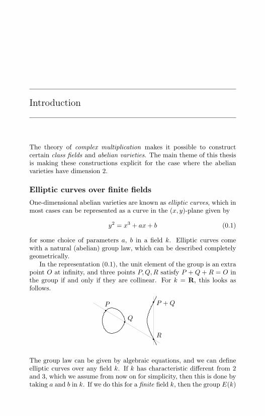
One-dimensional abelian varieties are known as elliptic curves, which inmost cases can be represented as a curve in the (x, y)-plane given by
y2 = x3 + ax+ b (0.1)
for some choice of parameters a, b in a field k. Elliptic curves comewith a natural (abelian) group law, which can be described completelygeometrically.
In the representation (0.1), the unit element of the group is an extrapoint O at infinity, and three points P,Q,R satisfy P + Q + R = O inthe group if and only if they are collinear. For k = R, this looks asfollows.
P
Q
R
P + Q
The group law can be given by algebraic equations, and we can defineelliptic curves over any field k. If k has characteristic different from 2and 3, which we assume from now on for simplicity, then this is done bytaking a and b in k. If we do this for a finite field k, then the group E(k)
10 Introduction
of points defined over k is finite. Indeed, the number of elements #E(k)of E(k) can be computed simply by testing for every x-coordinate in kwhether x3 + ax+ b is a square in k.
If the order q = #k of k gets large, then this method of pointcounting takes too much time. However, there are faster methods basedon the properties of the Frobenius endomorphism F : (x, y) 7→ (xq, yq)of E. The points in E(k) are exactly those points over an algebraicclosure of k that are left invariant by F . In particular, they are thepoints in the kernel of the endomorphism (F − id), where subtractiontakes place in the ring of endomorphisms End(E) of E. It is known thatF is (as an element of the endomorphism ring) a root of a quadraticWeil polynomial
f = X2 − tX + q ∈ Z[X], (0.2)
and that we have
#E(k) = deg(F − id) = f(1) = q + 1− t.
The trace of Frobenius t is bounded in size by |t| ≤ 2√q, and indicates to
which extent #E(k) differs from the number q+1 of points on a straightline. Schoof realized in 1985 that the reductions (t mod l) at smallprimes l can be computed by looking at the action of F on the l-torsionpoints of E, and that this allows one to compute the number t, andtherefore #E(k), efficiently. This yields a polynomial time algorithmthat, for large q, is much faster than the exponential time method ofdirect point counting.
Cryptography
Suppose one has a finite group G in which the group operation can beefficiently implemented, but the discrete logarithm problem is thoughtto be hard. This means that given x, y ∈ G, finding an integer msuch that y = xm holds is hard. Then the Diffie-Hellman key exchangeprotocol from 1976 allows one to agree upon a cryptographic key in sucha way that eavesdroppers, who intercept the entire communication, arebelieved to be unable to derive the key from it. The original exampleof such a group G is the unit group G = k∗ for a prime finite field k =Fp. Index calculus methods like the number field sieve provide a sub-exponential method for solving the discrete logarithm problem in k∗.To protect the protocol against this algorithm until the year 2030, it isgenerally recommended to use primes p of over 3000 bits.
As for G = k∗, the group order of G = E(k) for an elliptic curveE is of size approximately #k = q. However, it seems that the dis-crete logarithm problem for the group E(k) is harder, as 35 years of
The CM method 11
research has not led to a sub-exponential method for it. For this rea-son, the recommended key sizes for achieving the same level of securitywith elliptic curve cryptography are much smaller: q is recommended tohave 256 bits. This difference of a factor 12 in key length is importantin practical situations such as on ‘RFID tags’ with limited computingpower. The optimal elliptic curves for cryptography are the ones ofprime group order, and we will now describe how they can be obtained.
The CM method
One can construct elliptic curves of prime order over a finite field kby ‘random curves and point counting’, that is, by taking random a’sand b’s in k and computing #E(k) using Schoof’s algorithm until oneencounters an elliptic curve of prime order.
An alternative method is the CM method, which starts with a Weilpolynomial f (as in equation (0.2)) with f(1) a large prime, and com-putes an elliptic curve corresponding to that. Let π be a root of fand let O be the maximal order in the field Q(π). One constructs, e.g.from the torus C/O using analytic means, a complex elliptic curve Ewith complex multiplication (CM) by O, i.e., endomorphism ring iso-morphic to O. This curve E can be defined over a number field, and itsreduction modulo a prime over p has π (up to units) as its Frobeniusendomorphism.
Actually, instead of the curve E itself, one needs only its j-invariantj(E), since that completely describes the isomorphism class of E over C.The fact that E can be defined over a number field is reflected by the factthat j(E) is an algebraic number. In fact, it is an algebraic integer, andthe CM method computes its minimal polynomial HO ∈ Z[X], calledthe Hilbert class polynomial of O. The reduction of j(E) is obtainedby computing a root of (HO mod p), and finding the appropriate curvewith that j-invariant is easy.
Both methods have various advantages and disadvantages. The bitsize of the Hilbert class polynomial HO grows about linearly with thediscriminant of O, so the CM method is restricted to number fields Q(π)of small discriminant. In other words, it is restricted to p and t suchthat p2−4t is a square times a small integer. The CM method thereforeprovides partial control over p, t, and #E(k), and the interplay betweenthese numbers. This could be compared to random curves and pointcounting, where one has full control over p, but hardly any control over t.
From a cryptographic perspective, an advantage of the CM methodand the control it provides is the possibility to construct curves forpairing based cryptography, which is impossible with random curves.
12 Introduction
Some cryptographers are a bit hesitant towards curves with too muchstructure and prefer random curves over the small-discriminant curvesproduced by the CM method, while others think that special curvesmight actually be safer than random ones.
Curves of genus two
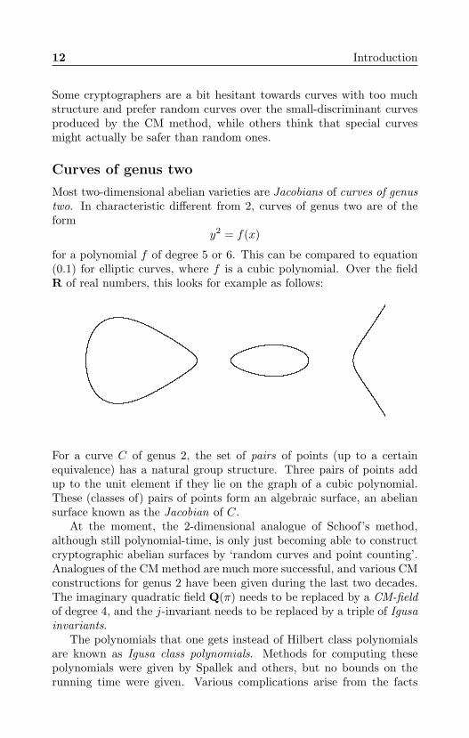
Most two-dimensional abelian varieties are Jacobians of curves of genustwo. In characteristic different from 2, curves of genus two are of theform
y2 = f(x)
for a polynomial f of degree 5 or 6. This can be compared to equation(0.1) for elliptic curves, where f is a cubic polynomial. Over the fieldR of real numbers, this looks for example as follows:
For a curve C of genus 2, the set of pairs of points (up to a certainequivalence) has a natural group structure. Three pairs of points addup to the unit element if they lie on the graph of a cubic polynomial.These (classes of) pairs of points form an algebraic surface, an abeliansurface known as the Jacobian of C.
At the moment, the 2-dimensional analogue of Schoof’s method,although still polynomial-time, is only just becoming able to constructcryptographic abelian surfaces by ‘random curves and point counting’.Analogues of the CM method are much more successful, and various CMconstructions for genus 2 have been given during the last two decades.The imaginary quadratic field Q(π) needs to be replaced by a CM-fieldof degree 4, and the j-invariant needs to be replaced by a triple of Igusainvariants.
The polynomials that one gets instead of Hilbert class polynomialsare known as Igusa class polynomials. Methods for computing thesepolynomials were given by Spallek and others, but no bounds on therunning time were given. Various complications arise from the facts
Class fields 13
that these polynomials are rational, rather than integral, and that themoduli space of genus-2 curves is three-dimensional rather than one-dimensional. We study and improve the algorithms in Chapters IIand III, and derive the first bound on their running time.
In Chapters IV and V, we describe how to use CM constructionsto construct specific kinds of genus-2 curves with Jacobians suitable forcryptography.
Class fields
Apart from the relatively recent cryptographic applications of CM con-structions, the theory of complex multiplication is a beautiful part ofpure mathematics that connects number theory, algebra, and geometry.
The Kronecker-Weber theorem from the second half of the 19th cen-tury states that every finite abelian extension L of Q, i.e., every Galoisextension L/Q with finite abelian Galois group, is contained in Q(ζn)for some n, where ζn is a primitive n-th root of unity. In other words,every abelian extension L/Q is a subfield of a field M generated bytorsion elements ζn = exp(2πi/n) of the group C∗.
The problem of finding similar constructions when Q is replaced byother base fields K is known as Kronecker’s Jugendtraum and is number12 of Hilbert’s famous list of 23 problems from the year 1900.
Kronecker found that the j-invariants of elliptic curves with CM byorders in an imaginary quadratic field K together with the roots of unitygenerate almost all abelian extensions of K (indeed, they generate an ex-tension over which the maximal abelian extension has exponent 2). Thiswas later generalized to the theory of complex multiplication of ellipticcurves, which gives a complete solution to Kronecker’s Jugendtraum forK imaginary quadratic. The main theorem of complex multiplicationstates that for any elliptic curve E with CM by K, every finite abelianextension L/K is a subfield of a field M generated by j(E) and thecoordinates of torsion points of E.
The theory of complex multiplication of abelian varieties was de-veloped by Shimura and Taniyama in the 1950’s and describes abelianextensions of CM-fields K. The CM-fields of degree 2 are exactly theimaginary quadratic fields, and this case is the classical case, describingall abelian extensions of imaginary quadratic fields.
For CM-fields K of degree > 2, the theory of complex multiplicationby itself does not produce all abelian extensions of K. It does describewhich fields are obtained in terms of class field theory, and Shimurashowed in the 1960’s how to obtain all abelian extensions of any CM-field K by using a combination of complex multiplication and the class
14 Introduction
fields of the maximal totally real subfield of K. For most CM-fieldsof degree 4, Shimura’s construction requires the use of 4-dimensionalabelian varieties. We show in Chapter I that it is possible to constructclass fields of quartic CM-fields using, besides the class fields of the realquadratic subfield, CM theory only for abelian varieties of dimension atmost 2.
Overview
Chapter I is mainly an introduction to the theory of complex multipli-cation. We define notions that occur in every chapter of this thesis, andwe state the ‘main theorem’ of the theory of complex multiplication.We also show that a general result of Shimura [76] can be improved forthe case of CM-fields of degree 4.
Chapter II needs only theory from Sections 1–6 of Chapter I and doesnot require familiarity with class field theory, which Sections I.9 and I.10do.
We define class polynomials for primitive quartic CM-fields and givean algorithm for computing them. The algorithm is based on an algo-rithm of Spallek [79] and van Wamelen [88]. We make the algorithmmore explicit, and derive the first bounds on the absolute values of thecoefficients of the polynomials. Together with recent bounds on the de-nominators of these coefficients, this provides us with the first runningtime bound and proof of correctness of an algorithm that computes thesepolynomials. In fact, no bounds on the height of these polynomials wereknown yet, so that we also get the first bound on their height.
Chapter III shows that there exist better objects than Igusa classpolynomials, both from a theoretical perspective and in view of appli-cations. This chapter studies and computes the irreducible componentsof the modular variety of abelian surfaces with CM by a given primitivequartic CM-field. We show how to adapt the algorithms of Chapter IIto compute these irreducible components. We do not do that in Chap-ter II to avoid making that chapter too heavy, and because Igusa classpolynomials are the objects used in existing literature. We also givecomputational examples in this chapter. Chapter III uses results fromboth Chapters I and II.
Chapters IV and V, which were written to be read independently ofeach other and of the other chapters, construct certain ‘Weil numbers’inside CM-fields. These Weil numbers correspond to abelian varieties,
Overview 15
which in the dimension-2 case can be constructed using the class poly-nomials of Chapter II. The Weil numbers in Chapters IV and V haveproperties that are number theoretic in nature and are motivated bycryptography, since the abelian varieties that they correspond to havea subgroup of ‘cryptographic’ size and hence can be used for crypto-graphic purposes.
Chapter IV is joint work with David Freeman and Peter Stevenhagenand appeared as Abelian varieties with prescribed embedding degree [26].The abelian varieties in it have a prescribed small ‘embedding degree’with respect to a subgroup of large prescribed order. For small dimen-sion, say at most 3, they can be used for ‘pairing based cryptography’.
Chapter V is joint work with Laura Hitt O’Connor, Gary McGuire,and Michael Naehrig and appeared as A CM construction for curves ofgenus 2 with p-rank 1 [43]. This chapter is about Jacobians of curves ofgenus 2. The p-rank of the abelian surfaces in this chapter, an invariantthat is 0 or 2 for all previous cryptographic constructions, is 1.
Appendices 1–3 give extra background for Chapter II.Appendix 1 obtains integrality results for Fourier expansions of Igusa
invariants directly from formulas in Section II.7.Appendix 2 gives an alternative to an algorithm in Section II.3 and
gives a generalization of much-cited formulas of Spallek [79].Appendix 3 studies experimentally how fast Igusa class polynomi-
als grow with the discriminant of the CM-field. We also see that ourchoice of Igusa invariants is better in practice than the invariants usedin existing literature.

ChapterIComplex multiplication
Abstract. In this chapter, we give an introduction tothe theory of complex multiplication. We define notions likeCM-fields, CM-types, and the reflex type that occur in everychapter of this thesis, and we state the ‘main theorem’ ofcomplex multiplication. We show in Theorem 10.3 that ageneral result of Shimura [76] can be improved for the caseof CM-fields of degree 4
1 Kronecker’s Jugendtraum
The following classical result describes all finite abelian extensions of Qvia Galois theory.
Theorem 1.1 (Kronecker-Weber Theorem). Let K/Q be a finite abeli-an Galois extension. Then there is a positive integer n such that wehave an embedding
K → Q(ζn) = Q(t : t ∈ Gm(Q)[n]) = Q(exp( 2πin )).
The Galois group of Q(ζn)/Q is (Z/nZ)∗, where (k mod n) maps ζnto ζkn.
Kronecker’s Jugendtraum (a.k.a. Hilbert’s twelfth problem) is to findan analogue of this result when Q is replaced by an arbitrary numberfield F .
18 Chapter I. Complex multiplication
Class field theory implicitly describes all finite abelian extensionsof F and their Galois groups in terms of certain groups of equivalenceclasses of ideals. These groups are called class groups, and to each classgroup of F , there corresponds an abelian extension of F , which we callthe class field corresponding to the group. The Galois group of anabelian extension of F is isomorphic to the corresponding class groupvia the Artin map.
All class fields can be constructed from their class groups using Kum-mer theory. Suppose we want to construct the finite abelian extensionM of F corresponding to a class group G. If e is the exponent of G,then by Kummer theory, we find that M is a subfield of F (ζe)(
e√S) for
some finite set S ⊂ F (ζe). As the Artin map tells us much about thedecomposition of primes in M/F , this allows us to find M . For details,see Cohen and Stevenhagen [18].
The approach of finding the abelian extensions of F via Kummertheory is arguably not in the spirit of Kronecker’s Jugendtraum, sinceit is not of the form of a single function that parametrizes generatorsof the abelian extensions of F , like the analytic map z 7→ exp(2πiz) forF = Q.
If F is imaginary quadratic, then the theory of complex multiplica-tion of elliptic curves does provide a complete solution to Kronecker’sJugendtraum in terms of the j-invariant and the coordinates of tor-sion points. These torsion points can be parametrized by a normalizedversion of the Weierstrass ℘-function, or ‘better’ modular functions asin [18]. This approach does not suffer from the need for extra roots ofunity ζe, as Kummer theory does.
With the theory of complex multiplication of abelian varieties, Shi-mura and Taniyama [78] generalized the full answer for imaginary qua-dratic fields to a partial answer for CM-fields.
For a CM-field F , we obtain many abelian extensions of F by replac-ing Gm above by an abelian variety that has complex multiplication bythe reflex field K of F . Which abelian extensions are obtained is ex-pressed in terms of the reflex type. We will first define these notions.
2 CM-fields
Definition 2.1. A CM-field is a totally imaginary quadratic extensionK of a totally real number field K0.
By ‘totally imaginary’ we mean that K has no embeddings into R.In other words, a CM-field is a field K = K0(
√r) for some totally real
number field K0 and some totally negative element r ∈ K0. CM-fields
2. CM-fields 19
clearly have even degree, and the CM-fields of degree 2 are exactly theimaginary quadratic number fields.
The following result gives some classical properties of CM-fields.
Lemma 2.2. Let K be a number field. The following are equivalent.
(1) The field K is totally real or a CM-field.
(2) There exists an automorphism · : x 7→ x of K such that for everyembedding σ : K → C, the automorphism · is the restriction ofcomplex conjugation on C to K via σ, i.e., we have · σ = σ ·.
Moreover, the following holds:
(a) any composite of finitely many CM-fields and totally real fieldscontaining at least one CM-field is a CM-field,
(b) the normal closure of a CM-field is a CM-field,
(c) if φ is an embedding of CM-fields K1 → K2, then we have · φ =φ · with · as in (2),
(d) any subfield of a CM-field is totally real or a CM-field.
Following part (c) of the lemma, we denote · φ by φ.
Proof. If K is totally real, then (1) and (2) are both trivially true.Otherwise, the equivalence of (1) and (2) follows by taking K0 to be thefixed field of ·. Using (2), we also find (c) since the composite of φ withan embedding K2 → C is an embedding K1 → C. For details, see [52,§I.2], [78, Lemma 3 in §8.1], or [64, Prop. 1.4].
The existence and uniqueness of the complex conjugation morphism· of (2) easily shows that a composite of fields satisfying (2) also satis-fies (2). In particular, such a composite is a CM-field if one of the fieldsis a CM-field.
Part (b) follows from (a) as the normal closure is the composite ofthe conjugates. See also [64, Prop. 1.5].
For part (d), let K be a subfield of L, where L satisfies (2) for someautomorphism ·. By (b), we can assume without loss of generality thatL is normal over Q, so let H = Gal(L/K) ⊂ Gal(L/Q). By (c), wehave · H = H ·, so · restricts to an automorphism of K. Since everyembedding K → C extends to an embedding L → C, we find that ·satisfies (2) also on K.
Example 2.3. The cyclotomic field Q(ζn) satisfies (2) for ζn = ζ−1n . It
is a CM-field of degree ϕ(n) for n > 2 and equals Q for n ∈ 1, 2. Itstotally real subfield is the fixed field Q(ζn+ζ−1
n ) of complex conjugation.
20 Chapter I. Complex multiplication
3 CM-types
Let K be a CM-field of degree 2g and L′/Q a field that contains asubfield isomorphic to a normal closure of K.
Definition 3.1. A CM-type of K with values in L′ is a subset Φ ⊂Hom(K,L′) consisting of exactly one element from each of the g complexconjugate pairs of embeddings φ, φ : K → L′.
There are 2g CM-types of K with values in L′. If K is imaginaryquadratic, then a CM-type of K with values in L′ is the same as anembedding of K into L′.
Let K2/K1 be an extension of CM-fields and assume L′ contains asubfield isomorphic to a normal closure of K2. Then every CM-type ofK1 has a natural extension to a CM-type of K2 as follows.
Definition 3.2. Let K1,K2, L′ be as above, and let Φ be a CM-type
of K1 with values in L′. The CM-type of K2 induced by Φ is
ΦK2 = φ ∈ Hom(K1, L′) : φ|K1 ∈ Φ.
We say that a CM-type is primitive if it is not induced from a CM-typeof a strict CM-subfield.
Example 3.3. The cyclic CM-field K = Q(ζ7) of degree 6 has subfieldsK0 = Q(ζ7 + ζ−1
7 ), K1 = Q(√−7), and Q. We see that K has 23 =
8 CM-types of which 2 are induced from K1, hence 6 CM-types areprimitive.
We call two CM-types Φ1,Φ2 of K equivalent if there is an automor-phism σ of K such that Φ2 = Φ1σ holds.
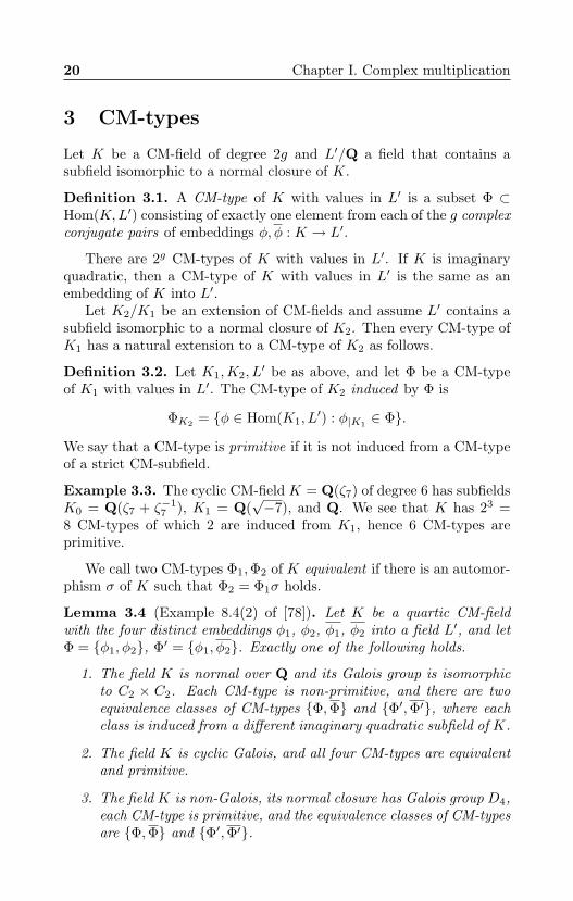
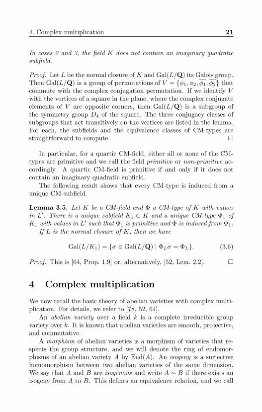
Lemma 3.4 (Example 8.4(2) of [78]). Let K be a quartic CM-fieldwith the four distinct embeddings φ1, φ2, φ1, φ2 into a field L′, and letΦ = φ1, φ2, Φ′ = φ1, φ2. Exactly one of the following holds.
1. The field K is normal over Q and its Galois group is isomorphicto C2 × C2. Each CM-type is non-primitive, and there are twoequivalence classes of CM-types Φ,Φ and Φ′,Φ′, where eachclass is induced from a different imaginary quadratic subfield of K.
2. The field K is cyclic Galois, and all four CM-types are equivalentand primitive.
3. The field K is non-Galois, its normal closure has Galois group D4,each CM-type is primitive, and the equivalence classes of CM-typesare Φ,Φ and Φ′,Φ′.
4. Complex multiplication 21
In cases 2 and 3, the field K does not contain an imaginary quadraticsubfield.
Proof. Let L be the normal closure of K and Gal(L/Q) its Galois group.Then Gal(L/Q) is a group of permutations of V = φ1, φ2, φ1, φ2 thatcommute with the complex conjugation permutation. If we identify Vwith the vertices of a square in the plane, where the complex conjugateelements of V are opposite corners, then Gal(L/Q) is a subgroup ofthe symmetry group D4 of the square. The three conjugacy classes ofsubgroups that act transitively on the vertices are listed in the lemma.For each, the subfields and the equivalence classes of CM-types arestraightforward to compute.
In particular, for a quartic CM-field, either all or none of the CM-types are primitive and we call the field primitive or non-primitive ac-cordingly. A quartic CM-field is primitive if and only if it does notcontain an imaginary quadratic subfield.
The following result shows that every CM-type is induced from aunique CM-subfield.
Lemma 3.5. Let K be a CM-field and Φ a CM-type of K with valuesin L′. There is a unique subfield K1 ⊂ K and a unique CM-type Φ1 ofK1 with values in L′ such that Φ1 is primitive and Φ is induced from Φ1.
If L is the normal closure of K, then we have
Gal(L/K1) = σ ∈ Gal(L/Q) | ΦLσ = ΦL. (3.6)
Proof. This is [64, Prop. 1.9] or, alternatively, [52, Lem. 2.2].
4 Complex multiplication
We now recall the basic theory of abelian varieties with complex multi-plication. For details, we refer to [78, 52, 64].
An abelian variety over a field k is a complete irreducible groupvariety over k. It is known that abelian varieties are smooth, projective,and commutative.
A morphism of abelian varieties is a morphism of varieties that re-spects the group structure, and we will denote the ring of endomor-phisms of an abelian variety A by End(A). An isogeny is a surjectivehomomorphism between two abelian varieties of the same dimension.We say that A and B are isogenous and write A ∼ B if there exists anisogeny from A to B. This defines an equivalence relation, and we call
22 Chapter I. Complex multiplication
a non-zero abelian variety A simple if it is not isogenous to a productof lower-dimensional abelian varieties.
We say that an abelian variety A of dimension g has complex multi-plication (CM) by a number field M if M has degree 2g and there is anembedding ι : M → End(A) ⊗Q. We say that A has CM by an orderO ⊂M if the same holds with ι−1(End(A)) = O.
The tangent space T0A of A at the unit point 0 of A is a vector spaceover k of dimension g. Differentiation defines a ring homomorphismD : End(A)→ Endk(T0A).
Now let K be a CM-field of degree 2g and A an abelian variety withCM by K via the embedding ι : K → End(A) ⊗Q. Suppose the basefield k has characteristic 0. Then the composite map
ρ = D ι : K → EndkT0A
is a g-dimensional k-linear representation of the ring K.
Lemma 4.1. Let the notation be as above, and assume that the basefield k has characteristic 0. There exists a unique CM-type Φ of K withvalues in the algebraic closure k of k such that the representation ρ isequivalent over k to the direct sum representation ⊕φ∈Φφ.
Proof. See [78, §5.2], [52, Thm. 1.3.4], or [64, 3.11].
The CM-type Φ is uniquely determined by (A, ι) and we call it theCM-type of (A, ι). Furthermore, we say that (A, ι) and A are of type Φ.Note that if σ is an automorphism of K and (A, ι) is of type Φ, then(A, ι σ) is of type Φ σ. In particular, the variety A is both of type Φand of type Φ σ.
Given any element τ ∈ Gal(k/Q), we define
τι : K → End(τA)⊗Q
x 7→ τ(ι(x)).
We write τ(A, ι) = (τA, τι).
Lemma 4.2. With τ as above, if (A, ι) has type Φ, then τ(A, ι) hastype τΦ.
Proof. Follows directly from the definition. See also the proof of Propo-sition 31 in §8.5 of [78].
The reflex field Kr ⊂ k of (K,Φ) is the fixed field of the group
G = τ ∈ Gal(k/Q) : τΦ = Φ.
5. Complex abelian varieties 23
We find that for any CM-type (K,Φ), the group G = Gal(k/Kr) actson the set of abelian varieties of type Φ. The main theorem of complexmultiplication, which we will state later, describes this action.
In what follows, we will actually work with polarized abelian vari-eties, which are abelian varieties together with some extra data calleda polarization. We give the definition of a polarization for a complexabelian variety in Section 5.1. We will not need the general definitionof a polarization in this thesis, but see [62, §13] for details.
5 Complex abelian varieties
5.1 Complex tori and polarizations
If A is a g-dimensional abelian variety over the field C of complex num-bers, then it is known that there exists a natural complex analytic grouphomomorphism from the tangent space V = T0A to A. Its kernel Λ isa lattice of rank 2g. This shows that every complex abelian variety iscomplex analytically a complex torus, i.e., a complex vector space mod-ulo a lattice of full rank. A polarization of A induces an anti-symmetricR-bilinear form
E : V × V → R
such that we have E(Λ,Λ) ⊂ Z and such that (u, v) 7→ E(iu, v) issymmetric and positive definite. By a polarization on a complex torus,we will mean such a form.
A complex torus V/Λ is (complex analytically isomorphic to) anabelian variety if and only if it admits a polarization (see [4]).
The derivative of any morphism f : A → B of abelian varieties isa morphism of complex tori, i.e., a C-linear map of the complex vectorspaces that restricts to a map of the lattices. Conversely, any morphismof tori T0A/ΛA → T0B/ΛB induces a morphism of abelian varieties. Inparticular, the category of abelian varieties over C is equivalent to thecategory of complex tori that admit a polarization.
The degree of a polarization is the determinant detM of a matrixM that expresses E in terms of a basis of Λ. We call a polarizationprincipal if its degree is 1, and a (principally) polarized abelian varietyis a pair consisting of an abelian variety together with a (principal)polarization.
An isomorphism f : (Cg/Λ, E)→ (Cg/Λ′, E′) of (principally) polar-ized abelian varieties is a C-linear isomorphism f : Cg → Cg such thatf(Λ) = Λ′ and f∗E′ = E hold, where f∗E′ is defined by f∗E′(u, v) =E(f(u), f(v)) for all u, v ∈ Cg.
24 Chapter I. Complex multiplication
5.2 Ideals and polarizations
Let K be any CM-field of degree 2g and let Φ = φ1, . . . , φg be aCM-type of K with values in C. By abuse of notation, we interpret Φas a map Φ : K → Cg by setting Φ(α) = (φ1(α), . . . , φg(α)) ∈ Cg forα ∈ K.
Let DK/Q be the different of K. Let a be a fractional OK-ideal, andsuppose that there exists a generator ξ ∈ K of the fractional OK-ideal(aaDK/Q)−1 such that φ(ξ) lies on the positive imaginary axis for everyφ ∈ Φ. Then the map E = EΦ,ξ : Φ(K)× Φ(K)→ Q given by
E(Φ(α),Φ(β)) = TrK/Q(ξαβ) for α, β ∈ K (5.1)
is integer valued on Φ(a) × Φ(a), and can be extended uniquely R-linearly to an R-bilinear form E = EΦ,ξ : Cg ×Cg → R.
Theorem 5.2. Suppose Φ is a CM-type of a CM-field K of degree 2g.Then the following holds.
1. For any triple (Φ, a, ξ) as above, the pair (Cg/Φ(a), E) defines aprincipally polarized abelian variety A(Φ, a, ξ) with CM by OK oftype Φ.
2. Every principally polarized abelian variety over C with CM by OKof type Φ is isomorphic to A(Φ, a, ξ) for some triple (Φ, a, ξ) as inpart 1.
3. The abelian variety A(Φ, a, ξ) is simple if and only if Φ is primi-tive. If this is the case, then the embedding ι : K → End(A)⊗Qis an isomorphism.
4. For every pair of triples (Φ, a, ξ) and (Φ, a′, ξ′) as above with thesame type Φ, the principally polarized abelian varieties A(Φ, a, ξ)and A(Φ, a′, ξ′) are isomorphic if there exists γ ∈ K∗ such that
(a) a′ = γa and
(b) ξ′ = (γγ)−1ξ.
If Φ is primitive, then the converse holds.
Proof. This result can be derived from Shimura-Taniyama [78], and firstappeared in a form similar to the above in Spallek [79, Satze 3.13, 3.14,3.19] We quickly give a proof. See van Wamelen [88, Thms. 1, 3, 5] fordetails.
A straightforward calculation shows that E is anti-symmetric andthat (u, v) 7→ E(iu, v) is symmetric and positive definite (see [78, Thm. 4
5. Complex abelian varieties 25
in §6.2]). The fact that E : Φ(a) × Φ(a) → Q takes values in Z andhas determinant 1 follows from the fact that ξaa = D−1
K/Q is the dual ofOK for the trace form K ×K → Z given by (x, y) 7→ TrK/Q(xy). Thisproves part 1.
Now let (A, ι) have type Φ. By definition of the type of (A, ι) wecan choose a basis of T0A such that ι(α) is given by the diagonal matrixwith diagonal Φ(α). Take any element x ∈ Λ and scale the basis of T0Asuch that we have x = (1, . . . , 1). As Λ is an OK-module via Φ, we findthat Λ⊗Q is a vector space over K via Φ. The dimension of this vectorspace is (2g)/(2g) = 1, so Φ−1(Λ) ⊂ K is a fractional OK-ideal, whichwe denote by a.
For the details of why a polarization of (A, ι) takes the form of (5.1),see [78, Thm. 4 in §6.2]. The identity ξaa = D−1
K/Q follows from the factthat E maps Φ(a)× Φ(a) to Z with determinant 1. This proves part 2
The fact that an abelian variety of type Φ is simple if and only ifΦ is primitive is [52, Thm. 1.3.5]. It then follows from [52, Thm. 1.3.3]that ι is bijective.
Theorem 5 of [88] gives the condition for when abelian varieties areisomorphic.
We call two triples (Φ, a, ξ) with the same type Φ equivalent if theysatisfy the conditions 4a and 4b of Theorem 5.2.
Let K be any CM-field with maximal totally real subfield K0. Leth (resp. h0) be the class number of K (resp. K0) and let h1 = h/h0.
Proposition 5.3. The number of pairs (Φ, A), where Φ is a CM-typeand A is an isomorphism class of abelian varieties over C with CM byOK of type Φ, is
h1 ·#O∗K0/NK/K0(O∗K).
Proof. Let I be the group of invertible OK-ideals and S the set of pairs(a, ξ) with a ∈ I and ξ ∈ K∗ such that ξ2 is totally negative and ξOK =(aaDK/Q)−1. The group K∗ acts on S via x(a, ξ) = (xa, x−1x−1ξ) forx ∈ K∗. By Theorem 5.2, the set that we need to count is in bijectionwith the set K∗\S of orbits.
We claim first that S is non-empty. Proof of the claim: Let z ∈K∗ be such that z2 is a totally negative element of K0. The normmap NK/K0 : Cl(K) → Cl(K0) is surjective by [91, Thm. 10.1] andthe fact that the infinite primes ramify in K/K0. As DK/Q and xOKare invariant under complex conjugation, surjectivity of N implies thatthere exist an element y ∈ K∗0 and a fractional OK-ideal a0 such thatya0a0 = z−1D−1
K/Q holds, so (a0, yz) is an element of S.
26 Chapter I. Complex multiplication
Let S′ be the group of pairs (b, u), consisting of a fractional OK-ideal b and a totally positive generator u ∈ K∗0 of bb. The group K∗
acts on S′ via x(b, u) = (xb, xxu) for x ∈ K∗, and we denote the groupof orbits by C = K∗\S′. The map C → K∗\S : (b, u) 7→ (ba0, u
−1yz)is a bijection and the sequence
0 −→ O∗K0/NK/K0(O∗K) −→
u 7→(OK ,u)C −→
(b,u)7→bCl(K)−→
NCl(K0) −→ 0
is exact, so K∗\S has the correct order.
The following two lemmas show what happens with distinct CM-types and thus answers a question of van Wamelen [88].
Lemma 5.4. For any triple (Φ, a, ξ) as above and σ ∈ Aut(K), we have
A(Φ, a, ξ) ∼= A(Φ σ, σ−1(a), σ−1(ξ)).
Proof. We find twice the same complex torus Cg/Φ(a). The first haspolarization
E : (Φ(α),Φ(β)) 7→ TrK/Q(ξαβ) (5.5)
for α, β ∈ a while the polarization of the second maps (Φ(α),Φ(β)) toTrK/Q(σ−1(ξαβ)), which equals the right hand side of (5.5).
Lemma 5.6. Suppose A and B are abelian varieties over C with CM byK of types Φ and Φ′. If Φ′ is primitive and Φ and Φ′ are not equivalent,then A and B are not isogenous. In particular, they are not isomorphic.
Proof. Suppose f : A → B are isogenous. The isogeny induces anisomorphism ϕ : End(A)⊗Q→ End(B)⊗Q given by g 7→ fgf−1. LetιA : K → End(A) ⊗Q and ιB : K → End(B) ⊗Q be the embeddingsof types Φ and Φ′. Let σ = ι−1
B ϕιA (where ιB is an isomorphism byTheorem 5.2.3 because Φ′ is primitive). Then (A, ιA) and (B, ιB σ)have types Φ and Φ′σ. As f induces an isomorphism of the tangentspaces, we also see that these types are equal, so Φ and Φ′ are equivalent.
Definition 5.7. We call two triples (Φ, a, ξ) and (Φ′, a′, ξ′) equivalentif there is an automorphism σ ∈ Aut(K) such that Φ σ = Φ′ holdsand (Φ, σ(a′), σ(ξ′)) is equivalent to (Φ, a, ξ) as in our definition aboveLemma 5.4.
If Φ is primitive, then it follows from Theorem 5.2.4 and Lemmas5.4 and 5.6 that A(Φ, a, ξ) and A(Φ′, a′, ξ′) are isomorphic if and onlyif (Φ, a, ξ) and (Φ′, a′, ξ′) are equivalent.
5. Complex abelian varieties 27
5.3 Another representation of the ideals
Let K be any CM-field of degree 2g and assume g ≤ 2, or, more gen-erally, that the different DK0/Q is principal and generated by δ ∈ K0.For g = 1 we take δ = 1, and for g = 2 we take δ =
√∆0.
We will now show that we can take the triple (Φ, a, ξ) to be of aspecial form. This special form is important to us in Section II.6, wherewe use it to give bounds on the absolute values of matrices occurring inour algorithm.
Theorem 5.8. Let K be a CM-field and K0 its maximal real subfieldand suppose that DK0/Q is principal and generated by δ.
For every triple (Φ, a, ξ) as in Section 5.2, there exists an elementz ∈ K such that (up to equivalence of the triple (Φ, a, ξ)) we have a =zOK0 +OK0 ⊂ K, ξ = (z−z)−1δ−1, and Φ = φ : K → C | Imφξ > 0.
Proof. As a is a projective module of rank 2 over the Dedekind domainOK0 , we can write it as a = zc+yOK0 for someOK0 -ideal c and z, y ∈ K.By part 4 of Theorem 5.2, we can replace a by y−1a and ξ by yyξ, hencewe can assume without loss of generality that we have y = 1.
Recall that we have an alternating Z-bilinear form E : a × a → Z,given by (u, v) 7→ TrK/Q(ξuv). This form is trivial on zc × zc andOK0×OK0 , and is alternating, hence is completely defined by its actionon zc×OK0 . Let T : K0×K0 → Q be the Q-linear trace form (a, b) 7→TrK0/Q(ab), so we have E(za, b) = T (ξ(z−z)a, b) for all a ∈ c, b ∈ OK0 .Note that here ξ(z − z) is an element of K0.
The fact that E is principal (i.e., has determinant 1) implies thatξ(z−z)c is the dual ofOK0 with respect to the form T , which is D−1
K0/Q=
δ−1OK0 by [66, §III.2]. It follows that c is principal, so without loss ofgenerality we have c = OK0 and hence ξ = (z − z)−1δ−1.
The following result gives the converse of Theorem 5.8. In fact,it gives a slightly more general representation that will be useful inSection II.6.
Theorem 5.9. Let K, K0, and δ be as mentioned at the beginning ofSection 5.3.
Suppose z ∈ K is such that a = zb + b−1 is an OK-submodule of K.Let ξ = (z − z)−1δ−1 and Φ = φ : K → C : Imφξ > 0. Then (Φ, a, ξ)is a triple as in Section 5.2.
Proof. The dual of b for the trace form (as defined in the proof ofTheorem 5.8) is δ−1b−1. The result now follows by retracing the stepsin the proof of Theorem 5.8.
28 Chapter I. Complex multiplication
We call two pairs (z, b) equivalent if they give rise to equivalenttriples (Φ, a, ξ).
Remark 5.10. The element z ∈ K can be interpreted as a point
−(sign(φiδ)φiz)gi=1
in the Hilbert upper half space Hg, which is the g-fold cartesian productof the upper half plane H = z ∈ C | Im z > 0.
The group SL2(OK0) acts on Hg by acting on the i-th coordinate ziof z ∈ Hg as (
a bc d
)zi =
φi(a)zi + φi(b)φi(c)zi + φi(d)
.
The Hilbert moduli space SL2(OK0)\Hg parametrizes the set of isomor-phism classes of principally polarized abelian varieties with real multi-plication by OK0 , of which principally polarized abelian varieties withcomplex multiplication by OK are special cases.
6 Jacobians of curves
An important example of a principally polarized abelian variety is theJacobian of a curve. By curve, we will always mean a smooth projectivegeometrically irreducible algebraic curve over a field. The Jacobian ofa curve C over a field k is an abelian variety J(C) such that we haveJ(C)(l) = Pic0(Cl) for every field extension l/k with C(l) 6= ∅. For theexact definition or more details, see [63]. The dimension of J(C) equalsthe genus g of C.
If we fix a divisor E of degree g on C, then by the Riemann-Rochtheorem, every degree-0 divisor on C is equivalent to D − E for aneffective divisor D of C of degree g, i.e., for a sum D of g points. Thisgives a cover of J(C) by the g-fold symmetric product of C, and showsthat we can view J(C) as a set of equivalence classes of g-tuples ofpoints.
The Jacobian comes with a natural principal polarization. For de-tails, see [63]. We say that a curve C has complex multiplication if J(C)does.
Now suppose C is defined over k = C. We give the definition of theJacobian as in [4]. Let H0(ωC) be the complex vector space of holomor-phic 1-forms on C and denote its dual by H0(ωC)∗. The homology groupH1(C,Z) is a free abelian group of rank 2g, and we get a canonical injec-tion H1(C,Z)→ H0(ωC)∗, given by γ 7→ (ω 7→
∫γω), where the integral
is taken over any representative cycle of the class γ ∈ H1(C,Z). The
6. Jacobians of curves 29
image of H1(C,Z) in H0(ωC)∗ is a lattice of rank 2g in a g-dimensionalcomplex vector space, and the quotient J(C) = H0(ωC)∗/H1(C,Z),which is a complex torus, is the Jacobian of C.
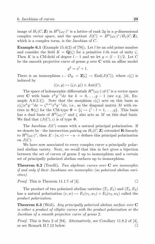
Example 6.1 (Example 15.4(2) of [78]). Let l be an odd prime numberand consider the field K = Q(ζ) for a primitive l-th root of unity ζ.Then K is a CM-field of degree l − 1 and we let g = (l − 1)/2. Let Cbe the smooth projective curve of genus g over C with an affine model
y2 = xl + 1.
There is an isomorphism ι : OK = Z[ζ] → End(J(C)), where ι(ζ) isinduced by
((x, y) 7→ (ζx, y)) ∈ Aut(C).
The space of holomorphic differentials H0(ωC) of C is a vector spaceover C with basis xky−1dx for k = 0, . . . , g − 1 (see e.g. [41, Ex-ample A.6.2.1]). Note that the morphism ι(ζ) acts on this basis asι(ζ)xky−1dx = ζk+1xky−1dx, i.e., as the diagonal matrix M with en-tries in Φ(ζ) for the CM-type Φ = ζ 7→ ζl : l = 1, . . . , g. This basishas a dual basis of H0(ωC)∗ and ζ also acts as M on this dual basis.We find that (J(C), ι) is of type Φ.
The Jacobian J(C) comes with a natural principal polarization. Ifwe denote by · the intersection pairing on H1(C,Z) extended R-linearlyto H0(ωC)∗, then E : (u, v) 7→ −u · v defines this principal polarizationon J(C).
We have now associated to every complex curve a principally polar-ized abelian variety. Next, we recall that this in fact gives a bijectionbetween the set of curves of genus 2 up to isomorphism and a certainset of principally polarized abelian surfaces up to isomorphism.
Theorem 6.2 (Torelli). Two algebraic curves over C are isomorphicif and only if their Jacobians are isomorphic (as polarized abelian vari-eties).
Proof. This is Theorem 11.1.7 of [4].
The product of two polarized abelian varieties (T1, E1) and (T2, E2)has a natural polarization (v, w) 7→ E1(v1, w1) + E2(v2, w2) called theproduct polarization.
Theorem 6.3 (Weil). Any principally polarized abelian surface over Cis either a product of elliptic curves with the product polarization or theJacobian of a smooth projective curve of genus 2.
Proof. This is Satz 2 of [94]. Alternatively, see Corollary 11.8.2 of [4],or see Remark II.7.12 below.
30 Chapter I. Complex multiplication
7 The reflex of a CM-type
Let K be a CM-field and let Φ be a CM-type of K with values in L′.Let L ⊃ K be the normal closure of K. Then by making L′ smaller, wecan assume L′ ∼= L.
The reflex (Kr,Φr) of (K,Φ) is defined as follows. Let ΦL be theCM-type of L with values in L′ induced by Φ. Note that ΦL is a set ofisomorphisms L→ L′, so we can take its set Φ−1
L of inverses, which is aset of isomorphisms L′ → L.
It follows easily from Lemma 2.2(c) that Φ−1L is a CM-type of L′
with values in L (see also [64, Example 1.28] or [52, Thm. I.5.1(ii)]).By Lemma 3.5, there is a unique primitive pair (Kr,Φr) that induces(L′,Φ−1
L ). We show in Lemma 7.3 that this definition of Kr is equivalentto the one given in Section 4.
Definition 7.1. The pair (Kr,Φr) is called the reflex of (K,Φ), thefield Kr is called the reflex field of (K,Φ), and the CM-type Φr is calledthe reflex type of (K,Φ).
Lemma 7.2. The CM-type Φr is a primitive CM-type of Kr. If wedenote the reflex of (Kr,Φr) by (Krr,Φrr), then Krr is a subfield of Kand Φ is induced by Φrr. If Φ is primitive, then we have Krr = K andΦrr = Φ.
Proof. Primitivity and the facts that Krr ⊂ K holds and Φrr induces Φfollow directly from our definition. If Φ is primitive, then this impliesKrr = K and hence Φrr = Φ. See also [78, paragraph above Prop. 29 in§8.3] or [52, Thm. 5.2].
The following result shows that the definition of the reflex field inthe current section coincides with the one given in Section 4.
Lemma 7.3. The reflex field Kr satisfies
Gal(L′/Kr) = σ ∈ Gal(L′/Q) | σΦ = Φ.
Proof. This is exactly what follows from equation (3.6) and the defini-tion of Kr. See also [64, Example 1.28].
Example 7.4 (Example 8.4(1) of [78]). If a CM-field K is abelian overQ and Φ is a primitive CM-type, then Kr is isomorphic to K. Indeed,if we choose an isomorphism L→ L′, then commutativity of the Galoisgroup implies that the groups of Lemmas 3.5 and 7.3 coincide.
7. The reflex of a CM-type 31
Example 7.5 (Example 8.4(2)(C) of [78]). Let K be a non-Galois quar-tic CM-field. By Lemma 3.4, the normal closure L of K has Galois groupD4 = 〈r, s〉 with r4 = s2 = (rs)2 = e. The complex conjugation auto-morphism · equals r2 in this notation. Without loss of generality, wehave that s is the generator of Gal(L/K).
For simplicity, we consider CM-types with values in L. In otherwords, we identify L′ with L via an isomorphism. The CM-types up toequivalence are Φ = id, r|K and Φ′ = id, r3
|K (see Lemma 3.4).The CM-type induced by Φ on L is Φ〈s〉 = e, r, s, rs, which has
inverse e, r3, s, rs = e, r3〈rs〉. In particular, the reflex field Kr
of Φ is the fixed field of 〈rs〉, which is a quartic CM-field that is notisomorphic to K. The reflex type of Φ is the CM-type id, r3
|Kr of Kr.Similarly, the reflex field of Φ′ is the fixed field of 〈r3s〉, which is
conjugate, but not equal, to Kr.
Lemma 7.6. The reflex field Kr is generated over Q by the elementsof L′ of the form
∑φ∈Φ φ(x) for x ∈ K.
Proof. This is [78, Prop. 28 in §8.3].
Example 7.7. Let K be a non-Galois quartic CM-field, and write
K = Q(α) with α =√−a+ b
√d.
Let Φ be a CM-type of K with values in a field L′, and let α1, α2 ∈ L′be the images of α under the embeddings of Φ. We have
α1 =√−a+ b
√d and α2 =
√−a− b
√d
for some choice of the square roots.By Lemma 7.6, we have β1 = α1 + α2 ∈ Kr, where
β21 = α2
1 + α22 + 2α1α2 = −2a+ 2w (7.8)
for some square root w ∈ L′ of a2 − b2d.We claim that β1 =
√−2a+ 2w generates Kr over Q. Indeed, the
field Q(β1) contains w = α1α2, which is not rational because K isnot normal over Q, and which is real because α1 and α2 are purelyimaginary. We also find β2
1 < 0 for every embedding into R by equation(7.8), which shows that Q(β1) is a quartic CM-field. As β1 is containedin Kr, which is quartic by Example 7.5, this proves the claim.
Note that the element w = α1α2 ∈ L′, and hence the quartic fieldKr = Q(β1) ⊂ L′, are uniquely determined by Φ.
32 Chapter I. Complex multiplication
The reflex field of Φ′ is then the conjugate Q(β2) of Kr with β2 =√−2a− 2w.
The reflex type Φr of Φ consists of the two embeddings Kr → Lgiven by β1 7→ α ± α′ ∈ L′, where α′ ∈ L \K is a conjugate of α (seeExample 7.5).
8 The type norm
Definition 8.1. Let Φ be a CM-type of K with values in L′. The typenorm of Φ is the map
NΦ : K → Kr ⊂ L′
x 7→∏φ∈Φ
φ(x).
The image of the type norm lies in Kr by Lemma 7.3.
Example 8.2. The element w ∈ Kr of Example 7.7 is the type normNΦ(α) of the element α ∈ K of that example.
The type norm is multiplicative and hence restricts to a homomor-phism of unit groups K∗ → Kr∗.
For any number field M , let IM denote the group of non-zero frac-tional ideals of OM and let ClM = K∗\IM be the class group.
Lemma 8.3. The type norm induces homomorphisms
NΦ : IK → IKr
a 7→ a′ where a′OL′ =∏φ∈Φ
φ(a)OL′ , and
NΦ : ClK → ClKr .
Proof. On the groups of ideals IK , this is [52, Remark on page 63]. Seealso [78, Prop. 29 in §8.3]. As elements of K∗ are mapped to Kr∗, wefind the map on class groups.
It is easy to see that we have
NΦ(x)NΦ(x) = NK/Q(x) for all x ∈ K∗, and
NΦ(a)NΦ(a) = NK/Q(a) for all a ∈ IK ,
where NK/Q is the norm, taking positive values in Q∗ and · is com-plex conjugation on Kr (which doesn’t depend on a choice of complexembedding since Kr is a CM-field).
9. The main theorem of complex multplication 33
For quartic CM-fields, the type norm of the type norm will be auseful tool.
Lemma 8.4. Let a be an ideal in a primitive quartic CM-field K andΦ a CM-type. Then we have
NΦrNΦ(a) = NK/Q(a)a
a.
Proof. By choosing an isomorphism L → L′, we have without loss ofgenerality Φ = id, r|K with r ∈ Gal(L/Q) of order 4. If K is non-Galois, then this is Example 7.5, otherwise it is analogous.
We then have Φr = id, r3|Kr, hence
NΦrNΦ(a)OL = (a)2(ra)(r3a)OL.
As id, r|K , r2|K , r
3|K is the set of all embeddings K → L and we have
a = r2a, the result follows.
9 The main theorem ofcomplex multplication
The main theorem of complex multiplication shows how to obtain cer-tain class fields from abelian varieties with complex multiplication. Wewill now describe which fields they are.
Given a CM-field F with primitive CM-type Ψ, let (K,Φ) be thereflex. Given any ideal b ⊂ OK , let bZ = b ∩ Z and let IF (b) be thegroup of invertible fractional ideals of F that are coprime to b. Let
HF,Ψ(b) =
a ∈ IF (b) :
∃µ ∈ K∗ such thatNΨ(a) = µOK ,µµ = NF/Q(a),µ ≡ 1 (mod∗b)
⊃ PF (b) = xOF : x ∈ F ∗, x ≡ 1 (mod∗b),
where the inclusion ‘⊃’ follows by taking µ = NΨ(x). Then the classfield CMF,Ψ(b) corresponding to the ideal group
IF (b)/HF,Ψ(b)
can be obtained using complex multiplication. For the case b = 1, weomit (b) from the notation.
Here are the details of how to obtain this field. Embed F into Cand let A be a polarized abelian variety over C with CM by OK via ι
34 Chapter I. Complex multiplication
of type Φ. Let t ∈ A(k) be a point with annihilator b. (Such a pointexists by [78, Prop. 21 in §7.5].)
To the pair (A, t), one can assign a point j = j(A, t) in a an algebraicmoduli space. This point is defined over Q ⊂ C and can be expressedexplicitly in terms of theta functions, which are modular forms for aSiegel modular group. We do this explicitly for the case b = 1 in thenext two chapters. See especially Section II.7 and Theorem III.5.2.
Theorem 9.1. With the notation above, we have
CMF,Ψ(b) = F (j(A, t)) ⊂ k.
The action of the Galois group IF (b)/HF,Ψ(b) is as follows. Let(Φ, a, ξ) be a triple as in Section 5.2, and write t = Φ(x) with x ∈ K/a.Use the notation j(Φ, a, ξ, x) = j((A(Φ, a, ξ),Φ(x))). Then for any [c] ∈IF (b)/HF,Ψ(b) with c−1 ⊂ OF , we have
[c]j(Φ, a, ξ, x) = j(Φ, NΨ(c)−1a, NF/Q(c)ξ, (x mod NΨ(c)−1a)
).
Proof. If Ψ is a primitive CM-type of F , then this result is Main Theo-rems 1 and 2 in Sections 15.3 and 16.3 of Shimura and Taniyama [78].The Galois action is given in the proof of those results. See also [52,Thm. 3.6.1] or [64, Thm. 9.17].
We can also look at the action of complex conjugation. Then theresult (for b = 1) is the following.
Lemma 9.2 ([52, Prop. 3.5.5]). We have A(Φ, a, ξ) ∼= A(Φ, a, ξ).
Corollary 9.3. Suppose F (and hence K) is a primitive quartic CM-field. If A/C is a principally polarized abelian surface with CM byOK of type Φ, then every Gal(CMF,Ψ/F0)-conjugate of j(A) is also aGal(CMF,Ψ/F )-conjugate.
Moreover, the field F0(j(A)) does not contain F .
Proof. Write A as A(Φ, a, ξ) with a−1 ⊂ OK and take c = NΦ(a).Theorem 9.1 states
[c]j(Φ, a, ξ) = j(Φ, NΨ(c)−1a, NK/Q(c)ξ),
which by Lemma 8.4 is
j(Φ, NK/Q(a)−1a, NK/Q(a)−2ξ) = j(Φ, a, ξ).
By Lemma 9.2, this is exactly the complex conjugate of j(A), so complexconjugation acts on j(A) as [c] ∈ Gal(CMF,Ψ/F ).
10. The class fields of quartic CM-fields 35
Note that the set id, · is a complete set of representatives for thequotient group Gal(CMF,Ψ/F0)/Gal(CMF,Ψ/F ).
The length of the Gal(CMF,Ψ/F0)-orbit of j(A) is the degree ofF0(j(A))/F0, and the same holds with F0 everywhere replaced by F .We find degF0(j(A))/F0 = degF (j(A))/F = 1
2 degF (j(A))/F0, henceF (j(A)) is not equal to F0(j(A)), which proves that F0(J(A)) does notcontain F .
10 The class fields of quartic CM-fields
Next, let us see which class fields we can obtain using complex multi-plication. Suppose first that F is imaginary quadratic. Then Ψ is anisomorphism F → K and Φ is its inverse, so we identify F and K viathese maps. We find that in that case
HF,Ψ(b) = PF (b) := xOF : x ∈ F ∗, x ≡ 1 (mod∗b)
holds, so CMF,Ψ(b) is the ray class field of F = K of modulus b. In par-ticular, every finite abelian extension of F is a subfield of some HF,Ψ(b),so CM theory can construct all such fields.
If F is a CM-field of degree > 2, then CM theory by itself is insuf-ficient for constructing all class fields. However, Shimura [76] describeshow to obtain all abelian extensions of F using a combination of
(1) CM theory,
(2) the ray class fields of the maximal totally real subfield F0 ⊂ F ,and
(3) quadratic Kummer extensions of the fields that one obtains with(1) and (2).
Remark 10.1. For imaginary quadratic F , we have F0 = Q, and theclass fields of Q are contained in the cyclotomic fields by the Kronecker-Weber Theorem 1.1. These cyclotomic fields can be obtained from thetorsion points via the Weil pairing, which explains why we do not needto separately consider the class fields of F0 for imaginary quadraticfields F .
Theorem 10.2 (Theorem 1 of Shimura [76]). Let F be a CM-field, Ψa CM-type of F , and ψ ∈ Ψ an element such that the reflex field of(F,Ψ) is contained in ψ(F ). Let Ψ′ be obtained from Ψ by replacing ψby its complex conjugate ψ. Let b be a positive integer and HF (b) (resp.
36 Chapter I. Complex multiplication
HF0(b)) be the ray class field of modulus b of F (resp. F0). Then theabelian extension
HF (b) ⊃ HF0(b) · CMF,Ψ(b) · CMF,Ψ′(b)
has exponent 1 or 2.
Note that Kummer extensions of exponent 2 can be constructed with-out adjoining additional roots of unity. So far so good. However, The-orem 10.2 doesn’t apply to non-Galois quartic CM-fields, because theyhave a reflex field that is quartic and not isomorphic to F .
Shimura then fixes this by applying Theorem 10.2 to a CM-typeΨ′ of an extension E of F instead of to F itself (see [76, Prop. 8 andThm. 4]). In the quartic case, the field E is the normal closure of Fand Ψ′ is primitive, hence the reflex field of Ψ′ is isomorphic to L,which has degree 8. This implies that Shimura’s construction for non-Galois quartic CM-fields requires simple abelian varieties of dimension 4instead of only abelian surfaces!
We can however replace Theorem 10.2 by the following simpler resultthat does apply to all primitive quartic CM-fields.
Theorem 10.3. Let F be a primitive quartic CM-field and Ψ a primi-tive CM-type of F . Let b be a positive integer and HF (b) (resp. HF0(b))be the ray class field of modulus b of F (resp. F0). Then the abelianextension
HF (b) ⊃ HF0(b) · CMF,Ψ(b)
has exponent 1 or 2.
Proof. First recall that the composite HF0(b) · F is the class field of Fcorresponding to IF (b)/H0(b), where
H0(b) = a ∈ IF (b) : aa = vOF , v ∈ F ∗0 , v ≡ 1 (mod∗b).
As HF (b) has Galois group IF (b)/PF (b), it has exponent 1 or 2 over theclass field corresponding to the group IF (b)/B with
B = a ∈ IF (b) : a2 ∈ PF (b).
Therefore, it suffices to prove H0(b) ∩HF,Ψ(b) ⊂ B.Let a ∈ H0(b) ∩HF,Ψ(b) be any element. Let v and µ be as in the
definitions of H0(b) and HF,Ψ(b). Then we have by Lemma 8.4,
a2 = NΨrNΨ(a)aa
NF/Q(a)
= NΨr(µ)v
NF0/Q(v)OF .
10. The class fields of quartic CM-fields 37
As the generators µ and v are 1 (mod∗b), so is the generator of a2 thatwe have just given.
Example 10.4. The non-Galois quartic CM-field
F = Q(√−27 + 4
√13)
has class number 7 and a real quadratic subfield F0 = Q(√
13) of classnumber 1. We conclude from Theorem 10.3 that CMF,Ψ equals theHilbert class field of F , because 7 is odd and we have HF0 = F0 ⊂ F .We will compute a defining polynomial of CMF,Ψ in Example III.3.2.
A non-primitive quartic CM-field F has two imaginary quadraticsubfields F1 and F2 by Lemma 3.4. The ray class fields of these fieldscan be obtained by complex multiplication of elliptic curves. The rayclass fields of F itself can be obtained from the ray class fields of F0,F1, and F2 using the following general result.
Theorem 10.5. Let F/N be a Galois extension of number fields withGalois group V4, and let F0, F1, F2 be the intermediate fields. Let b bea positive integer and let HF (b) (resp. HFj (b)) be the ray class field ofmodulus b of F (resp. Fj). Then the abelian extension
HF (b) ⊃ HF0(b) ·HF1(b) ·HF2(b)
has exponent 1 or 2.
Proof. As in the proof of Theorem 10.3, it suffices to show that theintersection of the three groups
Hi(b) = a ∈ IF (b) : a(ai(a)) = vOF , v ∈ F ∗i , v ≡ 1 (mod∗b)
is contained in the group
B = a ∈ IF (b) : a2 ∈ PF (b).
Let a be any element of this intersection, and take vi as in thedefinition of Hi(b). Let ai ∈ Gal(F/Fi) be a generator, so we haveviOF = a(aia) and Gal(F/N) = id, a0, a1, a2 ∼= C2 × C2. We get
a2 = v1v2a1(v0)−1OF ,
and v1v2a1(v0)−1 ≡ 1 (mod∗b).

ChapterIIComputing Igusa class polynomials
Abstract. We give an algorithm that computes the genus-two class polynomials of a primitive quartic CM-field K, andwe give a running time bound and a proof of correctnessof this algorithm. This is the first proof of correctness andthe first running time bound of any algorithm that computesthese polynomials.
1 Introduction
The Hilbert class polynomial HK ∈ Z[X] of an imaginary quadraticnumber field K has as roots the j-invariants of complex elliptic curveshaving complex multiplication (CM) by the ring of integers of K. Theseroots generate the Hilbert class field of K, and Weber [93] computed HK
for many small K. The CM method uses the reduction of HK modulolarge primes to construct elliptic curves over Fp with a prescribed num-ber of points, for example for cryptography. The bit size of HK growsexponentially with the bit size of K: it grows like the discriminant ∆of K, and so does the running time of the algorithms that compute it([22, 2]).
If we go from elliptic curves (genus 1) to genus-2 curves, we getthe Igusa class polynomials HK,n ∈ Q[X] (n = 1, 2, 3) of a quarticCM-field K. Their roots are the Igusa invariants of all complex genus-
40 Chapter II. Computing Igusa class polynomials
2 curves having CM by the ring of integers of K. As in the case ofgenus 1, these roots generate class fields and the reduction of Igusa classpolynomials modulo large primes p yields cryptographically interestingcurves of genus 2. Computing Igusa class polynomials is considerablymore complicated than computing Hilbert class polynomials, in partbecause of their denominators. Recently, various algorithms have beendeveloped: a complex analytic method by Spallek [79] and van Wame-len [88], a p-adic method by Gaudry, Houtmann, Kohel, Ritzenthaler,and Weng [31, 32] and Carls, Kohel, and Lubicz [13, 14], and a Chineseremainder method by Eisentrager and Lauter [21], but no running timeor precision bounds were available.
This chapter describes a complete and correct algorithm that com-putes Igusa class polynomials HK,n ∈ Q[X] of quartic CM-fields K =Q(√
∆0,√−a+ b
√∆0), where ∆0 is a real quadratic fundamental dis-
criminant and a, b ∈ Z are such that −a + b√
∆0 is totally negative.Our algorithm is based on the complex analytic method of Spallek andvan Wamelen. The discriminant ∆ of K is of the form ∆ = ∆1∆2
0
for a positive integer ∆1. We may and will assume 0 < a < ∆, asLemma 9.9 below shows that each quartic CM-field has such a repre-sentation. We disregard the degenerate case of non-primitive quarticCM-fields, i.e., those that can be given with b = 0, as abelian varietieswith CM by non-primitive quartic CM-fields are isogenous to productsof CM elliptic curves, which can be obtained already using Hilbert classpolynomials. We give the following running time bound for our algo-rithm, where we use O(g) to mean “at most g times a polynomial inlog g”.
Main Theorem. Algorithm 11.1 computes HK,n (n = 1, 2, 3) for anyprimitive quartic CM-field K. It has a running time of O(∆7/2
1 ∆11/20 )
and the bit size of the output is O(∆21∆3
0).
An essential part of the proof is the denominator bound, as providedby Goren and Lauter [35, 36].
We do not claim that the bound on our running time is optimal, butan exponential running time is unavoidable, because the degree of theIgusa class polynomials (as with Hilbert class polynomials) is alreadybounded from below by a power of the discriminant.
Overview
Section 2 provides a precise definition of the Igusa class polynomialsthat we will work with, and mentions other definitions occurring in
2. Igusa class polynomials 41
the literature. Our main theorem is valid for all types of Igusa classpolynomials.
Instead of enumerating curves, it is easier to enumerate their Jaco-bians, which are principally polarized abelian varieties. Van Wamelen[88] gave a method for enumerating all isomorphism classes of princi-pally polarized abelian varieties with CM by a given order. We give animprovement of his results in Section 3.
Section 4 shows how principally polarized abelian varieties give riseto points in the Siegel upper half space H2. These points are matricesknown as period matrices. Two period matrices correspond to isomor-phic principally polarized abelian varieties if and only if they are in thesame orbit under the action of the symplectic group Sp4(Z).
In Section 5, we analyze a reduction algorithm that replaces periodmatrices by Sp4(Z)-equivalent period matrices in a fundamental domainF2 ⊂ H2. In Section 6, we give an upper bound on the entries of thereduced period matrices computed in Section 5.
Absolute Igusa invariants can be computed from period matricesby means of theta constants. Section 7 introduces theta constants andgives formulas that express Igusa invariants in terms of theta constants.The formulas that we give are much simpler than those that appearin [79, 97] or the textbook [27], reducing the formulas from more thana full page to only a few lines. We then give bounds on the absolutevalues of theta constants and Igusa invariants in terms of the entries ofthe reduced period matrices computed in Section 5. We finish Section 7by showing how to evaluate the theta constants, and hence the absoluteIgusa invariants, to a given precision.
Section 8 bounds the degree of Igusa class polynomials and Section 9gives the bounds of Goren and Lauter [35, 36] on the denominators.Section 10 shows how to reconstruct a rational polynomial from itscomplex roots, and the precision needed for that in terms of an upperbound on the denominator of the polynomial and the absolute values ofthe zeroes.
Finally, Section 11 puts all the results together into a single algo-rithm and a proof of the main theorem.
2 Igusa class polynomials
The Hilbert class polynomial of an imaginary quadratic number field Kis the polynomial of which the roots in C are the j-invariants of theelliptic curves over C with complex multiplication by the ring of integersOK of K. For a genus-2 curve, one needs three invariants, the absolute
42 Chapter II. Computing Igusa class polynomials
Igusa invariants i1, i2, i3, instead of one, to fix its isomorphism class.
2.1 Igusa invariants
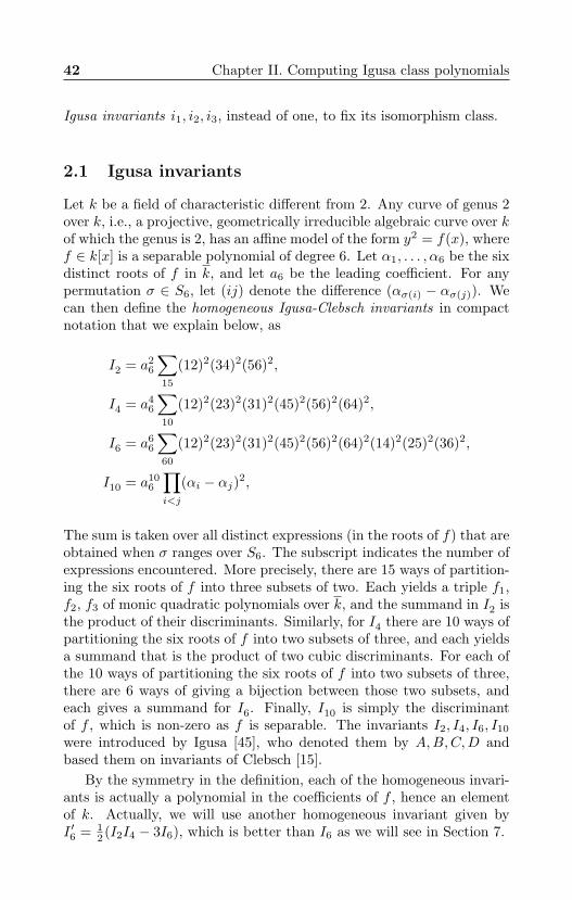
Let k be a field of characteristic different from 2. Any curve of genus 2over k, i.e., a projective, geometrically irreducible algebraic curve over kof which the genus is 2, has an affine model of the form y2 = f(x), wheref ∈ k[x] is a separable polynomial of degree 6. Let α1, . . . , α6 be the sixdistinct roots of f in k, and let a6 be the leading coefficient. For anypermutation σ ∈ S6, let (ij) denote the difference (ασ(i) − ασ(j)). Wecan then define the homogeneous Igusa-Clebsch invariants in compactnotation that we explain below, as
I2 = a26
∑15
(12)2(34)2(56)2,
I4 = a46
∑10
(12)2(23)2(31)2(45)2(56)2(64)2,
I6 = a66
∑60
(12)2(23)2(31)2(45)2(56)2(64)2(14)2(25)2(36)2,
I10 = a106
∏i<j
(αi − αj)2,
The sum is taken over all distinct expressions (in the roots of f) that areobtained when σ ranges over S6. The subscript indicates the number ofexpressions encountered. More precisely, there are 15 ways of partition-ing the six roots of f into three subsets of two. Each yields a triple f1,f2, f3 of monic quadratic polynomials over k, and the summand in I2 isthe product of their discriminants. Similarly, for I4 there are 10 ways ofpartitioning the six roots of f into two subsets of three, and each yieldsa summand that is the product of two cubic discriminants. For each ofthe 10 ways of partitioning the six roots of f into two subsets of three,there are 6 ways of giving a bijection between those two subsets, andeach gives a summand for I6. Finally, I10 is simply the discriminantof f , which is non-zero as f is separable. The invariants I2, I4, I6, I10
were introduced by Igusa [45], who denoted them by A,B,C,D andbased them on invariants of Clebsch [15].
By the symmetry in the definition, each of the homogeneous invari-ants is actually a polynomial in the coefficients of f , hence an elementof k. Actually, we will use another homogeneous invariant given byI ′6 = 1
2 (I2I4 − 3I6), which is better than I6 as we will see in Section 7.
2. Igusa class polynomials 43
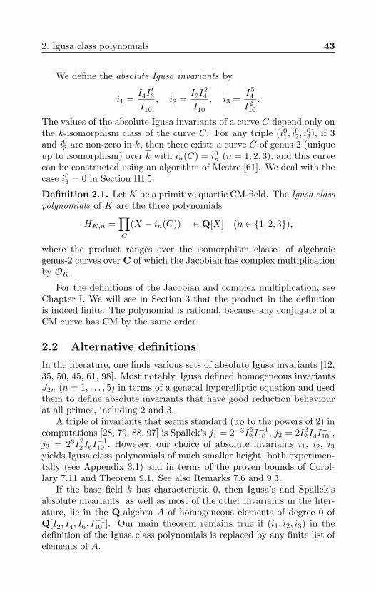
We define the absolute Igusa invariants by
i1 =I4I′6
I10
, i2 =I2I
24
I10
, i3 =I54
I210
.
The values of the absolute Igusa invariants of a curve C depend only onthe k-isomorphism class of the curve C. For any triple (i01, i
02, i
03), if 3
and i03 are non-zero in k, then there exists a curve C of genus 2 (uniqueup to isomorphism) over k with in(C) = i0n (n = 1, 2, 3), and this curvecan be constructed using an algorithm of Mestre [61]. We deal with thecase i03 = 0 in Section III.5.
Definition 2.1. Let K be a primitive quartic CM-field. The Igusa classpolynomials of K are the three polynomials
HK,n =∏C
(X − in(C)) ∈ Q[X] (n ∈ 1, 2, 3),
where the product ranges over the isomorphism classes of algebraicgenus-2 curves over C of which the Jacobian has complex multiplicationby OK .
For the definitions of the Jacobian and complex multiplication, seeChapter I. We will see in Section 3 that the product in the definitionis indeed finite. The polynomial is rational, because any conjugate of aCM curve has CM by the same order.
2.2 Alternative definitions
In the literature, one finds various sets of absolute Igusa invariants [12,35, 50, 45, 61, 98]. Most notably, Igusa defined homogeneous invariantsJ2n (n = 1, . . . , 5) in terms of a general hyperelliptic equation and usedthem to define absolute invariants that have good reduction behaviourat all primes, including 2 and 3.
A triple of invariants that seems standard (up to the powers of 2) incomputations [28, 79, 88, 97] is Spallek’s j1 = 2−3I5
2I−110 , j2 = 2I3
2I4I−110 ,
j3 = 23I22I6I
−110 . However, our choice of absolute invariants i1, i2, i3
yields Igusa class polynomials of much smaller height, both experimen-tally (see Appendix 3.1) and in terms of the proven bounds of Corol-lary 7.11 and Theorem 9.1. See also Remarks 7.6 and 9.3.
If the base field k has characteristic 0, then Igusa’s and Spallek’sabsolute invariants, as well as most of the other invariants in the liter-ature, lie in the Q-algebra A of homogeneous elements of degree 0 ofQ[I2, I4, I6, I
−110 ]. Our main theorem remains true if (i1, i2, i3) in the
definition of the Igusa class polynomials is replaced by any finite list ofelements of A.
44 Chapter II. Computing Igusa class polynomials
Interpolation formulas
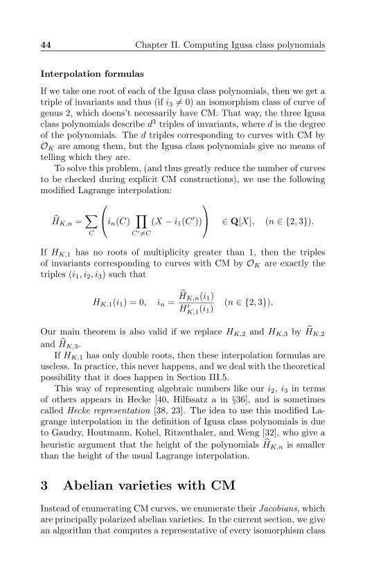
If we take one root of each of the Igusa class polynomials, then we get atriple of invariants and thus (if i3 6= 0) an isomorphism class of curve ofgenus 2, which doens’t necessarily have CM. That way, the three Igusaclass polynomials describe d3 triples of invariants, where d is the degreeof the polynomials. The d triples corresponding to curves with CM byOK are among them, but the Igusa class polynomials give no means oftelling which they are.
To solve this problem, (and thus greatly reduce the number of curvesto be checked during explicit CM constructions), we use the followingmodified Lagrange interpolation:
HK,n =∑C
in(C)∏C′ 6=C
(X − i1(C ′))
∈ Q[X], (n ∈ 2, 3).
If HK,1 has no roots of multiplicity greater than 1, then the triplesof invariants corresponding to curves with CM by OK are exactly thetriples (i1, i2, i3) such that
HK,1(i1) = 0, in =HK,n(i1)H ′K,1(i1)
(n ∈ 2, 3).
Our main theorem is also valid if we replace HK,2 and HK,3 by HK,2
and HK,3.If HK,1 has only double roots, then these interpolation formulas are
useless. In practice, this never happens, and we deal with the theoreticalpossibility that it does happen in Section III.5.
This way of representing algebraic numbers like our i2, i3 in termsof others appears in Hecke [40, Hilfssatz a in §36], and is sometimescalled Hecke representation [38, 23]. The idea to use this modified La-grange interpolation in the definition of Igusa class polynomials is dueto Gaudry, Houtmann, Kohel, Ritzenthaler, and Weng [32], who give aheuristic argument that the height of the polynomials HK,n is smallerthan the height of the usual Lagrange interpolation.
3 Abelian varieties with CM
Instead of enumerating CM curves, we enumerate their Jacobians, whichare principally polarized abelian varieties. In the current section, we givean algorithm that computes a representative of every isomorphism class
3. Abelian varieties with CM 45
of complex principally polarized abelian varieties with CM by the ringof integers OK of a primitive quartic CM-field K.
Section 3.1 gives the general algorithm, for CM-fields of arbitrarydegree, Section 3.2 specializes to the case of quartic CM-fields, and Sec-tion 3.3 gives details on how ideals should be represented and computed.
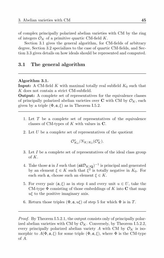
3.1 The general algorithm
Algorithm 3.1.Input: A CM-field K with maximal totally real subfield K0 such thatK does not contain a strict CM-subfield.Output: A complete set of representatives for the equivalence classesof principally polarized abelian varieties over C with CM by OK , eachgiven by a triple (Φ, a, ξ) as in Theorem I.5.2.
1. Let T be a complete set of representatives of the equivalenceclasses of CM-types of K with values in C.
2. Let U be a complete set of representatives of the quotient
O∗K0/NK/K0(O∗K).
3. Let I be a complete set of representatives of the ideal class groupof K.
4. Take those a in I such that (aaDK/Q)−1 is principal and generatedby an element ξ ∈ K such that ξ2 is totally negative in K0. Foreach such a, choose such an element ξ ∈ K.
5. For every pair (a, ξ) as in step 4 and every unit u ∈ U , take theCM-type Φ consisting of those embeddings of K into C that mapuξ to the positive imaginary axis.
6. Return those triples (Φ, a, uξ) of step 5 for which Φ is in T .
Proof. By Theorem I.5.2.1, the output consists only of principally polar-ized abelian varieties with CM by OK . Conversely, by Theorem I.5.2.2,every principally polarized abelian variety A with CM by OK is iso-morphic to A(Φ, a, ξ) for some triple (Φ, a, ξ), where Φ is the CM-typeof A.
46 Chapter II. Computing Igusa class polynomials
By Lemmas I.5.4 and I.5.6, the CM-type Φ is unique exactly up toequivalence of CM-types. This uniquely determines Φ in T .
By Theorem I.5.2.4, we can get a ∈ I. We get that A is isomorphic toA(Φ, a, uξ) for some u ∈ O∗K0
and a unique triple (Φ, a, ξ) with Φ ∈ T , ain the set of step 4, and ξ as found in step 4. Only the choice of u ∈ O∗K0
is left and by Theorem I.5.2.4, the isomorphism class of A(Φ, a, uξ)depends exactly on the class of u in O∗K0
/NK/K0(O∗K).
Remark 3.2. Algorithm 3.1 is basically Algorithm 1 of van Wame-len [88] with the difference that we do not have any duplicate abelianvarieties.
3.2 Quartic CM-fields
We now describe, in the quartic case, the sets T and U of Algorithm 3.1,and the number of isomorphism classes of principally polarized CMabelian surfaces.
By Lemma I.3.4, we can take the set T to consist of a single CM-type if K is cyclic and we can take T = Φ,Φ′ if K is non-Galois. Thecorollary to the following lemma gives the set U .
Lemma 3.3. If K is a primitive quartic CM-field, then
O∗K = µKO∗K0,
where µK ⊂ O∗K is the group of roots of unity, which has order 2 or 10.
Proof. As K has degree 4 and does not contain a primitive third orfourth root of unity, it is either Q(ζ5) or does not contain a root ofunity different from ±1. This proves that µK has order 2 or 10. Adirect computation shows that the lemma is true for K = Q(ζ5), so weassume that we have µK = ±1.
Let ε (resp. ε0) be a generator of O∗K (resp. O∗K0) modulo torsion.
Then without loss of generality, we have ε0 = εk for some positiveinteger k. so either k = 1 and we are done, or k = 2.
Suppose that we have k = 2. As K = K0(√ε0) is a CM-field, we
find that ε0 is totally negative, and hence ε−10 is the conjugate of ε0.
Let x = ε − ε−1 ∈ K. Then x2 = −2 + ε0 + ε−10 = −2 + Tr(ε0) ∈ Z is
negative, so Q(x) ⊂ K is imaginary quadratic, contradicting primitivityof K.
Corollary 3.4. If K is a primitive quartic CM-field, then we have
O∗K0/NK/K0(O∗K) = O∗K0
/O∗2K0= ±1,±c,
where c is the class of the fundamental unit ε of K0.
3. Abelian varieties with CM 47
Proof. This follows from Lemma 3.3, because of NK/K0(µK) = 1.
Lemma 3.5. Let K be a quartic CM-field. If K is cyclic, then thereare h1 isomorphism classes of principally polarized abelian surfaces withCM by OK . If K is non-Galois, then there are 2h1 such isomorphismclasses.
Proof. Proposition I.5.3 gives the number h1 ·#O∗K0/NK/K0(O∗K), but
counts every abelian variety twice if K is non-Galois and four times ifK is cyclic Galois (see Lemma I.3.4). Corollary 3.4 shows that we have#O∗K0
/NK/K0(O∗K) = 4.
3.3 Implementation details
In practice, Algorithm 3.1 takes up only a very small portion of thetime needed for Igusa class polynomial computation. The purpose ofthis section is to show that, for primitive quartic CM-fields, indeedAlgorithm 3.1 can be run in time O(∆) and to show that the size of theoutput for each isomorphism class is small: only polynomial in log ∆.
It is well known that lists of representatives for the class groupsof number fields K of fixed degree can be computed in time O(|∆|
12 ),
where ∆ is the discriminant of K. For details, see Schoof [73]. The rep-resentatives of the ideal classes that are given in the output are integralideals of norm below the Minkowski bound, which is 3/(2π2) |∆|1/2 fora quartic CM-field.
The algorithms in [73] show that for each a, we can check in timeO(|∆|
12 ) if aaDK/Q is principal and, if so, write down a generator ξ.
As O∗K = µKO∗K0, it suffices to check, for each of the roots of unity ζ
in K, if ζξ is totally imaginary (note that Q(ζ5) is the only primitivequartic CM-field with more than 2 roots of unity). Then the set T andthe group O∗K0
/NK/K0(O∗K) are already given in Section 3.2, where thefundamental unit ε is a by-product of the class group computations.In particular, it takes time at most O(|∆|) to perform all the steps ofAlgorithm 3.1.
A priori, the bit size of ξ can be as large as the regulator of K, butwe can easily make it much smaller as follows. We identify K ⊗R withC2 via the embeddings φ1, φ2 in the CM-type Φ, and we consider thestandard Euclidean norm on C2. Then we find a short vector
b |ξ|−1/2 =(φ1(b) |φ1(ξ)|−1/2
, φ2(b) |φ2(ξ)|−1/2)
in the lattice OK |ξ|−1/2 ⊂ C2 using the LLL-algorithm (see [57]) andreplace a by ba and ξ by (bb)−1ξ. By part 4 of Theorem I.5.2, this does
48 Chapter II. Computing Igusa class polynomials
not change the corresponding isomorphism class of principally polarizedabelian varieties. This also doesn’t change the fact that ξ−1 is in OKand that a is an integral ideal. Finally, we compute an LLL-reducedbasis of a ⊂ OK ⊗R = C2. We get the following result.
Lemma 3.6. If we run Algorithm 3.1 in the way we have just described,then on input of a primitive quartic CM-field K, given as
K = Q(√
∆0,
√−a+ b
√∆0)
for integers a, b,∆0 with 0 < a < ∆, it takes time O(∆). For each triple(Φ, a, ξ) in the output, the ideal a is given by an LLL-reduced basis, andboth ξ ∈ K and the basis of a have bit size O(log ∆).
Proof. First, compute the ring of integers OK of K using the algorithmof Buchmann and Lenstra [9]. This takes polynomial time plus the timeneeded to factor the discriminant of the defining polynomial of K, whichis small enough because of the assumption 0 < a < ∆. Then do theclass group computations as explained above.
For each triple (Φ, a, ξ), before we apply the LLL-reduction, we canassume that a is an integral ideal of norm below the Minkowski bound,hence we have
NK/Q(ξ−1) = NK/Q(a)2NK/Q(DK/Q) ≤ C∆3
for some constant C.The covolume of the lattice
|ξ|−1/2OK ⊂ OK ⊗R = C2
is NK/Q(ξ−1)∆1/2, so we find a vector b |ξ|−1/2 ∈ |ξ|−1/2OK of lengthat most C ′NK/Q(ξ−1)1/8∆1/8 for some constant C ′. In particular, bbξ−1
has all absolute values below C ′2NK/Q(ξ−1)1/4∆1/4. Therefore, bbξ−1
has bit size O(log ∆) and norm at most C ′8NK/Q(ξ−1)∆, so b has normat most C ′4∆1/2.
This implies that ba has norm at most C ′′∆, so an LLL-reducedbasis has bit size O(log(covol(ba))) = O(log ∆).
All elements x ∈ K that we encounter can be given (up to multipli-cation by units in O∗K0
) with all absolute values below√NK/Q(a) |ε|.
Therefore, the bit size of the numbers that are input to the LLL-algorithm is O(RegK) = O(∆1/2), hence every execution of the LLLalgorithm takes time only O(∆1/2) for each ideal class.
4. Symplectic bases 49
4 Symplectic bases
Let (Cg/Λ, E) be a principally polarized abelian variety. For any basisb1, . . . , b2g of Λ, we associate to the form E the matrix N = (nij)ij ∈Mat2g(Z) given by E(bi, bj) = nij . We say that E is given with respectto the basis b1, . . . , b2g by the matrix N .
The lattice Λ has a basis that is symplectic with respect to E, i.e.,a Z-basis e1, . . . , eg, v1, . . . , vg with respect to which E is given by thematrix Ω, given in terms of (g × g)-blocks as
Ω =(
0 1g−1g 0
). (4.1)
The vectors vi form a C-basis of Cg and if we rewrite Cg and Λ interms of this basis, then Λ becomes ZZg + Zg, where Z is a periodmatrix, i.e., a symmetric matrix over C with positive definite imaginarypart. The set of all g × g period matrices is called the Siegel upper halfspace and denoted by Hg. It is a topological subspace of the Euclidean2g2-dimensional real vector space Matg(C).
There is an action on this space by the symplectic group
Sp2g(Z) = M ∈ GL2g(Z) : M tΩM = Ω ⊂ GL2g(Z),
given in terms of (g × g)-blocks by(A BC D
)(Z) = (AZ +B)(CZ +D)−1.
The association of Z to (Cg/ZZg +Zg, E) gives a bijection between theset Sp2g(Z)\Hg of orbits and the set of principally polarized abelianvarieties over C up to isomorphism. We call this set of orbits the Siegelmoduli space.
4.1 A symplectic basis for Φ(a)
Now it is time to compute symplectic bases. In Algorithm 3.1, we com-puted a set of abelian varieties over C, each given by a triple (Φ, a, ξ),where a is an ideal inOK , given by a basis, ξ is in K∗ and Φ is a CM-typeof K. We now identify a with the lattice Λ = Φ(a) ⊂ Cg and recall thatthe bilinear form E : a × a → Z is given by E : (x, y) 7→ TrK/Q(ξxy).We can write down the matrix N ∈ Mat2g(Z) of E with respect tothe basis of a. Computing a symplectic basis of a now comes down tocomputing a change of basis M ∈ GL2g(Z) of a such that M tNM = Ω,with Ω as in (4.1). This is done by the following algorithm.
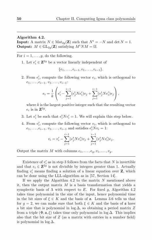
50 Chapter II. Computing Igusa class polynomials
Algorithm 4.2.Input: A matrix N ∈ Mat2g(Z) such that N t = −N and detN = 1.Output: M ∈ GL2g(Z) satisfying M tNM = Ω.
For i = 1, . . . , g, do the following.
1. Let e′i ∈ Z2g be a vector linearly independent of
e1, . . . , ei−1, v1, . . . , vi−1.
2. From e′i, compute the following vector ei, which is orthogonal toe1, . . . , ei−1, v1, . . . , vi−1:
ei =1k
e′i − i−1∑j=1
(etjNe
′i)vj +
i−1∑j=1
(vtjNe
′i)ej
,
where k is the largest positive integer such that the resulting vectorei is in Z2g.
3. Let v′i be such that etiNv
′i = 1. We will explain this step below.
4. From v′i, compute the following vector vi, which is orthogonal toe1, . . . , ei−1, v1, . . . , vi−1 and satisfies et
iNvi = 1:
vi = v′i −i−1∑j=1
(etjNv
′i)vj +
i−1∑j=1
(vtjNv
′i)ej .
Output the matrix M with columns e1, . . . , eg, v1, . . . , vg.
Existence of v′i as in step 3 follows from the facts that N is invertibleand that ei ∈ Z2g is not divisible by integers greater than 1. Actuallyfinding v′i means finding a solution of a linear equation over Z, whichcan be done using the LLL-algorithm as in [57, Section 14].
If we apply the Algorithm 4.2 to the matrix N mentioned aboveit, then the output matrix M is a basis transformation that yields asymplectic basis of Λ with respect to E. For fixed g, Algorithm 4.2takes time polynomial in the size of the input, hence polynomial timein the bit sizes of ξ ∈ K and the basis of a. Lemma 3.6 tells us thatfor g = 2, we can make sure that both ξ ∈ K and the basis of a havea bit size that is polynomial in log ∆, so obtaining a period matrix Zfrom a triple (Φ, a, ξ) takes time only polynomial in log ∆. This impliesalso that the bit size of Z (as a matrix with entries in a number field)is polynomial in log ∆.
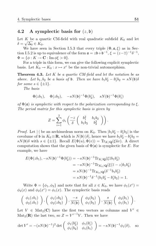
4. Symplectic bases 51
4.2 A symplectic basis for (z, b)
Let K be a quartic CM-field with real quadratic subfield K0 and letδ =√
∆0 ∈ K0.We have seen in Section I.5.3 that every triple (Φ, a, ξ) as in Sec-
tion I.5.2 is up to equivalence of the form a = zb+b−1, ξ = (z−z)−1δ−1,Φ = φ : K → C : Imφξ > 0.
For a triple in this form, we can give the following explicit symplecticbasis. Let K0 → K0 : x 7→ xc be the non-trivial automorphism.
Theorem 4.3. Let K be a quartic CM-field and let the notation be asabove. Let b1, b2 be a basis of b. Then we have b1bc2 − bc1b2 = sN(b)δfor some s ∈ ±1.
The basis
Φ(zb1), Φ(zb2), −sN(b)−1Φ(bc2), sN(b)−1Φ(bc1)
of Φ(a) is symplectic with respect to the polarization corresponding to ξ.The period matrix for this symplectic basis is given by
Z =2∑i=1
φi
(−zδ
(b21 b1b2b1b2 b22
)).
Proof. Let |·| be an archimedean norm on K0. Then |b1bc2 − bc1b2| is thecovolume of b in K0⊗R, which is N(b) |δ|, hence we have b1bc2− bc1b2 =sN(b)δ with s ∈ ±1. Recall E(Φ(u),Φ(v)) = TrK/Q(ξuv). A directcomputation shows that the given basis of Φ(a) is symplectic for E. Forexample, we have
E(Φ(zb1),−sN(b)−1Φ(bc2)) = −sN(b)−1TrK/Q(ξzb1bc2)
= −sN(b)−1TrK0/Q(ξ(z − z)b1bc2)
= sN(b)−1TrK0/Q(δ−1b1bc2)
= sN(b)−1δ−1(b1bc2 − bc1b2) = 1.
Write Φ = φ1, φ2 and note that for all x ∈ K0, we have φ1(xc) =φ2(x) and φ2(xc) = φ1(x). The symplectic basis reads(
φ1(zb1)φ2(zb1)
),
(φ1(zb2)φ2(zb2)
),−sN(b)
(φ2(b2)φ1(b2)
),
s
N(b)
(φ2(b1)φ1(b1)
).
Let V ∈ Mat2(C) have the first two vectors as columns and V ′ ∈Mat2(R) the last two, so Z = V ′
−1V . Then we have
detV ′ = −(sN(b)−1)2 det(φ1(bc2) φ1(bc1)φ1(b2) φ1(b1)
)= −sN(b)−1φ1(δ), so
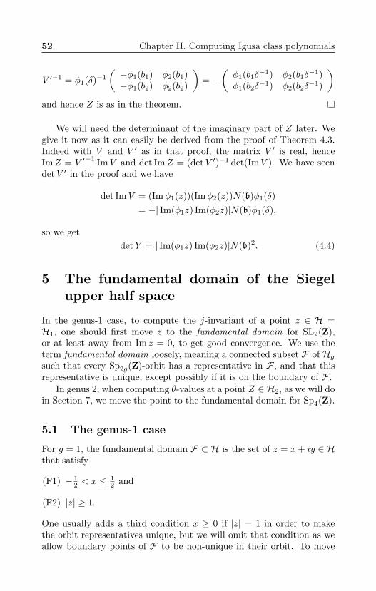
52 Chapter II. Computing Igusa class polynomials
V ′−1 = φ1(δ)−1
(−φ1(b1) φ2(b1)−φ1(b2) φ2(b2)
)= −
(φ1(b1δ−1) φ2(b1δ−1)φ1(b2δ−1) φ2(b2δ−1)
)and hence Z is as in the theorem.
We will need the determinant of the imaginary part of Z later. Wegive it now as it can easily be derived from the proof of Theorem 4.3.Indeed with V and V ′ as in that proof, the matrix V ′ is real, henceImZ = V ′
−1 ImV and det ImZ = (detV ′)−1 det(ImV ). We have seendetV ′ in the proof and we have
det ImV = (Imφ1(z))(Imφ2(z))N(b)φ1(δ)= −| Im(φ1z) Im(φ2z)|N(b)φ1(δ),
so we getdetY = | Im(φ1z) Im(φ2z)|N(b)2. (4.4)
5 The fundamental domain of the Siegelupper half space
In the genus-1 case, to compute the j-invariant of a point z ∈ H =H1, one should first move z to the fundamental domain for SL2(Z),or at least away from Im z = 0, to get good convergence. We use theterm fundamental domain loosely, meaning a connected subset F of Hgsuch that every Sp2g(Z)-orbit has a representative in F , and that thisrepresentative is unique, except possibly if it is on the boundary of F .
In genus 2, when computing θ-values at a point Z ∈ H2, as we will doin Section 7, we move the point to the fundamental domain for Sp4(Z).
5.1 The genus-1 case
For g = 1, the fundamental domain F ⊂ H is the set of z = x+ iy ∈ Hthat satisfy
(F1) − 12 < x ≤ 1
2 and
(F2) |z| ≥ 1.
One usually adds a third condition x ≥ 0 if |z| = 1 in order to makethe orbit representatives unique, but we will omit that condition as weallow boundary points of F to be non-unique in their orbit. To move
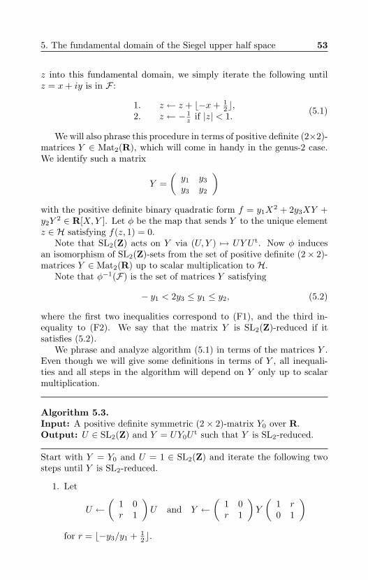
5. The fundamental domain of the Siegel upper half space 53
z into this fundamental domain, we simply iterate the following untilz = x+ iy is in F :
1. z ← z + b−x+ 12c,
2. z ← − 1z if |z| < 1. (5.1)
We will also phrase this procedure in terms of positive definite (2×2)-matrices Y ∈ Mat2(R), which will come in handy in the genus-2 case.We identify such a matrix
Y =(y1 y3
y3 y2
)with the positive definite binary quadratic form f = y1X
2 + 2y3XY +y2Y
2 ∈ R[X,Y ]. Let φ be the map that sends Y to the unique elementz ∈ H satisfying f(z, 1) = 0.
Note that SL2(Z) acts on Y via (U, Y ) 7→ UY U t. Now φ inducesan isomorphism of SL2(Z)-sets from the set of positive definite (2× 2)-matrices Y ∈ Mat2(R) up to scalar multiplication to H.
Note that φ−1(F) is the set of matrices Y satisfying
− y1 < 2y3 ≤ y1 ≤ y2, (5.2)
where the first two inequalities correspond to (F1), and the third in-equality to (F2). We say that the matrix Y is SL2(Z)-reduced if itsatisfies (5.2).
We phrase and analyze algorithm (5.1) in terms of the matrices Y .Even though we will give some definitions in terms of Y , all inequali-ties and all steps in the algorithm will depend on Y only up to scalarmultiplication.
Algorithm 5.3.Input: A positive definite symmetric (2× 2)-matrix Y0 over R.Output: U ∈ SL2(Z) and Y = UY0U
t such that Y is SL2-reduced.
Start with Y = Y0 and U = 1 ∈ SL2(Z) and iterate the following twosteps until Y is SL2-reduced.
1. Let
U ←(
1 0r 1
)U and Y ←
(1 0r 1
)Y
(1 r0 1
)for r = b−y3/y1 + 1
2c.
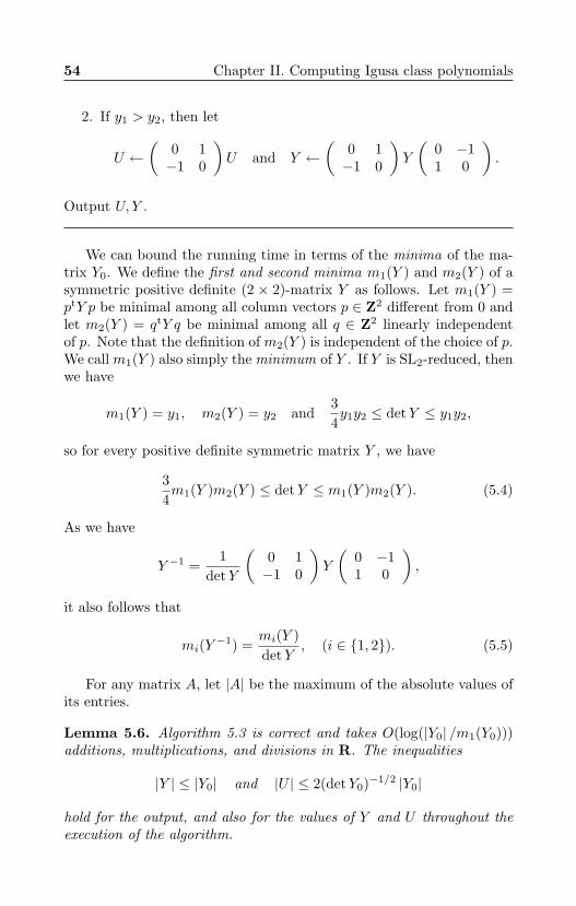
54 Chapter II. Computing Igusa class polynomials
2. If y1 > y2, then let
U ←(
0 1−1 0
)U and Y ←
(0 1−1 0
)Y
(0 −11 0
).
Output U, Y .
We can bound the running time in terms of the minima of the ma-trix Y0. We define the first and second minima m1(Y ) and m2(Y ) of asymmetric positive definite (2 × 2)-matrix Y as follows. Let m1(Y ) =ptY p be minimal among all column vectors p ∈ Z2 different from 0 andlet m2(Y ) = qtY q be minimal among all q ∈ Z2 linearly independentof p. Note that the definition of m2(Y ) is independent of the choice of p.We call m1(Y ) also simply the minimum of Y . If Y is SL2-reduced, thenwe have
m1(Y ) = y1, m2(Y ) = y2 and34y1y2 ≤ detY ≤ y1y2,
so for every positive definite symmetric matrix Y , we have
34m1(Y )m2(Y ) ≤ detY ≤ m1(Y )m2(Y ). (5.4)
As we have
Y −1 =1
detY
(0 1−1 0
)Y
(0 −11 0
),
it also follows that
mi(Y −1) =mi(Y )detY
, (i ∈ 1, 2). (5.5)
For any matrix A, let |A| be the maximum of the absolute values ofits entries.
Lemma 5.6. Algorithm 5.3 is correct and takes O(log(|Y0| /m1(Y0)))additions, multiplications, and divisions in R. The inequalities
|Y | ≤ |Y0| and |U | ≤ 2(detY0)−1/2 |Y0|
hold for the output, and also for the values of Y and U throughout theexecution of the algorithm.
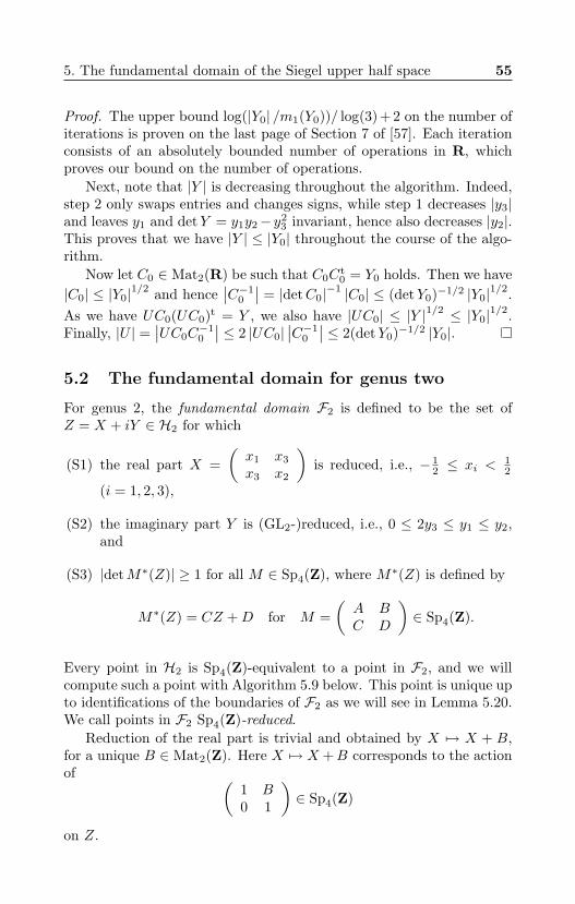
5. The fundamental domain of the Siegel upper half space 55
Proof. The upper bound log(|Y0| /m1(Y0))/ log(3) + 2 on the number ofiterations is proven on the last page of Section 7 of [57]. Each iterationconsists of an absolutely bounded number of operations in R, whichproves our bound on the number of operations.
Next, note that |Y | is decreasing throughout the algorithm. Indeed,step 2 only swaps entries and changes signs, while step 1 decreases |y3|and leaves y1 and detY = y1y2−y2
3 invariant, hence also decreases |y2|.This proves that we have |Y | ≤ |Y0| throughout the course of the algo-rithm.
Now let C0 ∈ Mat2(R) be such that C0Ct0 = Y0 holds. Then we have
|C0| ≤ |Y0|1/2 and hence∣∣C−1
0
∣∣ = |detC0|−1 |C0| ≤ (detY0)−1/2 |Y0|1/2.As we have UC0(UC0)t = Y , we also have |UC0| ≤ |Y |1/2 ≤ |Y0|1/2.Finally, |U | =
∣∣UC0C−10
∣∣ ≤ 2 |UC0|∣∣C−1
0
∣∣ ≤ 2(detY0)−1/2 |Y0|.
5.2 The fundamental domain for genus two
For genus 2, the fundamental domain F2 is defined to be the set ofZ = X + iY ∈ H2 for which
(S1) the real part X =(x1 x3
x3 x2
)is reduced, i.e., − 1
2 ≤ xi <12
(i = 1, 2, 3),
(S2) the imaginary part Y is (GL2-)reduced, i.e., 0 ≤ 2y3 ≤ y1 ≤ y2,and
(S3) |detM∗(Z)| ≥ 1 for all M ∈ Sp4(Z), where M∗(Z) is defined by
M∗(Z) = CZ +D for M =(A BC D
)∈ Sp4(Z).
Every point in H2 is Sp4(Z)-equivalent to a point in F2, and we willcompute such a point with Algorithm 5.9 below. This point is unique upto identifications of the boundaries of F2 as we will see in Lemma 5.20.We call points in F2 Sp4(Z)-reduced.
Reduction of the real part is trivial and obtained by X 7→ X + B,for a unique B ∈ Mat2(Z). Here X 7→ X +B corresponds to the actionof (
1 B0 1
)∈ Sp4(Z)
on Z.
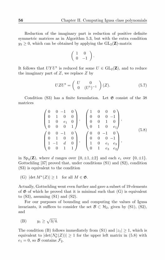
56 Chapter II. Computing Igusa class polynomials
Reduction of the imaginary part is reduction of positive definitesymmetric matrices as in Algorithm 5.3, but with the extra conditiony3 ≥ 0, which can be obtained by applying the GL2(Z)-matrix(
1 00 −1
).
It follows that UY U t is reduced for some U ∈ GL2(Z), and to reducethe imaginary part of Z, we replace Z by
UZU t =(U 00 (U t)−1
)(Z). (5.7)
Condition (S3) has a finite formulation. Let G consist of the 38matrices
0 0 −1 00 1 0 01 0 e1 00 0 0 1
,
1 0 0 00 0 0 −10 0 1 00 1 0 e1
,
0 0 −1 00 1 0 01 −1 d 00 0 1 1
,
0 0 −1 00 0 0 −11 0 e1 e3
0 1 e3 e2
,
(5.8)
in Sp4(Z), where d ranges over 0,±1,±2 and each ei over 0,±1.Gottschling [37] proved that, under conditions (S1) and (S2), condition(S3) is equivalent to the condition
(G) |detM∗(Z)| ≥ 1 for all M ∈ G.
Actually, Gottschling went even further and gave a subset of 19 elementsof G of which he proved that it is minimal such that (G) is equivalentto (S3), assuming (S1) and (S2).
For our purposes of bounding and computing the values of Igusainvariants, it suffices to consider the set B ⊂ H2, given by (S1), (S2),and
(B) y1 ≥√
3/4.
The condition (B) follows immediately from (S1) and |z1| ≥ 1, which isequivalent to |det(N∗0 (Z))| ≥ 1 for the upper left matrix in (5.8) withe1 = 0, so B contains F2.
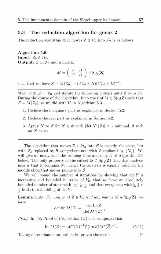
5. The fundamental domain of the Siegel upper half space 57
5.3 The reduction algorithm for genus 2
The reduction algorithm that moves Z ∈ H2 into F2 is as follows.
Algorithm 5.9.Input: Z0 ∈ H2.Output: Z in F2 and a matrix
M =(A BC D
)∈ Sp4(Z)
such that we have Z = M(Z0) = (AZ0 +B)(CZ0 +D)−1.
Start with Z = Z0 and iterate the following 3 steps until Z is in F2.During the course of the algorithm, keep track of M ∈ Sp4(Z) such thatZ = M(Z0), as we did with U in Algorithm 5.3.
1. Reduce the imaginary part as explained in Section 5.2.
2. Reduce the real part as explained in Section 5.2.
3. Apply N to Z for N ∈ G with |detN∗(Z)| < 1 minimal, if suchan N exists.
The algorithm that moves Z ∈ H2 into B is exactly the same, butwith F2 replaced by B everywhere and with G replaced by N0. Wewill give an analysis of the running time and output of Algorithm 5.9below. The only property of the subset G ⊂ Sp4(Z) that this analysisuses is that it contains N0, hence the analysis is equally valid for themodification that moves points into B.
We will bound the number of iterations by showing that detY isincreasing and bounded in terms of Y0, that we have an absolutelybounded number of steps with |y1| ≥ 1
2 , and that every step with |y1| <12 leads to a doubling of detY .
Lemma 5.10. For any point Z ∈ H2 and any matrix M ∈ Sp4(Z), wehave
det ImM(Z) =det ImZ
|detM∗(Z)|2.
Proof. In [48, Proof of Proposition 1.1] it is computed that
ImM(Z) = (M∗(Z)−1)t(ImZ)M∗(Z)−1. (5.11)
Taking determinants on both sides proves the result.
58 Chapter II. Computing Igusa class polynomials
Steps 1 and 2 of Algorithm 5.9 do not change detY , and Lemma 5.10shows that step 3 increases detY , so detY is increasing throughout thealgorithm.
The following result allows us to bound m2(Y ) and detY during thealgorithm. It is also crucial in Section 6, where we use it to bound theentries of the reduced period matrix.
Lemma 5.12. For any point Z = X + iY ∈ H2 and any matrix M ∈Sp4(Z), we have
m2(ImM(Z)) ≤ 43
maxm1(Y )−1,m2(Y ).
Proof. We imitate part of the proof of [48, Lemma 3.1]. If we replaceM by (
(U t)−1 00 U
)M
for U ∈ GL2(Z), then the matrix (ImM(Z))−1 gets replaced by thematrix U(ImM(Z))−1U t, so we can assume without loss of generalitythat (ImM(Z))−1 is reduced. By (5.11), we have
(ImM(Z))−1 = (CX − iCY +D)Y −1(CX + iCY +D)t
= (CX +D)Y −1(XCt +Dt) + CY Ct, (5.13)
where M =(A BC D
).
As the left hand side of (5.13) is reduced, its minimum m1 is its upperleft entry. Let (c1, c2, d1, d2) ∈ Z4 be the third row of M and let c =(c1, c2), d = (d1, d2) ∈ Z2. We compute that the upper left entry of(5.13) is m1((ImM(Z))−1) = (cX + d)Y −1(Xct + dt) + cY ct.
The matrix M is invertible, so if c is zero, then d is non-zero. Asboth Y −1 and Y are positive definite, this implies that
m1((ImM(Z))−1) ≥ minm1(Y ),m1(Y −1).
By (5.4) and (5.5), we get
m2(ImM(Z)) ≤ 4 det ImM(Z)3m1(ImM(Z))
=4
3m1((ImM(Z))−1)
≤ 43
max 1m1(Y )
,detYm1(Y )
≤ 43
maxm1(Y )−1,m2(Y ),
which proves the result.
5. The fundamental domain of the Siegel upper half space 59
Lemma 5.14. There is an absolute upper bound c, independent of theinput Z0, on the number of iterations of Algorithm 5.9 in which Z sat-isfies y1 ≥ 1
2 at the beginning of step 3.
Proof. Let C be the set of points in H2 that satisfy (S1), (S2) andy1 ≥ 1
2 . At the beginning of step 3, both (S1) and (S2) hold, so we needto bound the number of iterations for which Z is in C at the beginningof step 3. Suppose that such an iteration exists, and denote the value ofZ at the beginning of step 3 of that iteration by Z ′. As detY increasesduring the algorithm, each iteration has a different value of Z, so itsuffices to bound the number of Z ∈ Sp4(Z)(Z ′) ∩ C. By [48, Theorem3.1], the set
C = M ∈ Sp4(Z) : C ∩M(C) 6= ∅
is finite. As C surjects onto Sp4(Z)(Z ′)∩C via M 7→M(Z ′), we get theabsolute upper bound #C on the number of iterations with Z ∈ C.
Lemma 5.15. At every iteration of step 3 of Algorithm 5.9 in whichwe have y1 <
12 , the value of detY increases by a factor of at least 2.
Proof. If y1 <12 , then for the element N0 ∈ G, we have |detN∗0 (Z)|2 =
|z1|2 = |x1|2 + |y1|2 ≤ 12 , so by Lemma 5.10, the value of detY increases
by a factor ≥ 2.
We can now bound the number of iterations. For any matrix Z =X + iY ∈ H2, let t(Z) = log maxm1(Y )−1,m2(Y ).
Proposition 5.16. The number of iterations of Algorithm 5.9 is atmost O(t(Z0)) for every input Z0.
Proof. Let c be the constant of Lemma 5.14, let Z0 be the input ofAlgorithm 5.9 and let Z be the value after k iterations. By Lemmas5.15 and 5.12, we have
2k−c detY0 ≤ detY ≤ m2(Y )2 ≤ (43
)2 maxm1(Y0)−2,m2(Y0)2,
hence (5.4) implies
2k−c ≤ (43
)3 maxm1(Y0)−3m2(Y0)−1,m1(Y0)−1m2(Y0).
To avoid a laborious error analysis, all computations are performedinside some number field L ⊂ C of absolutely bounded degree. Indeed,for an abelian surface A with CM by OK , any period matrix Z ∈ H2
that represents A is in Mat2(L), where L is the normal closure of K,
60 Chapter II. Computing Igusa class polynomials
which has degree at most 8. For a running time analysis, we need tobound the height of the numbers involved. Such height bounds are alsoused for lower bounds on the off-diagonal part of the output Z, whichwe will need in Section 7.
The height h(x) of an element x ∈ L∗ is defined as follows. LetS be the set of absolute values of L that extend either the standardarchimedean absolute value of Q or one of the non-archimedean absolutevalues |x| = p−ordp(x). For each v ∈ S, let deg(v) = [Lv : Qv] be thedegree of the completion Lv of L at v. Then
h(x) =∑v
deg(v) maxlog |x|v , 1.
We denote the maximum of the heights of all entries of a matrix Z ∈ H2
by h(Z).Next, we give bounds on the value of |M | during the execution of
the algorithm. This will provide us with a bound on the height ofthe entries of Z. Indeed, if we have Z = M(Z0), then it follows thath(Z) ≤ 2(log |M |+ h(Z0) + log 4).
Lemma 5.17. There exists an absolute constant c > 0 such that thefollowing holds. The value of log |M | is at most cmaxlog |Z0| , 1 dur-ing the first iteration of Algorithm 5.9 and, in each iteration, increasesby at most cmaxt(Z0), 1, where t is as above Proposition 5.16.
Proof. For step 1, it follows from equation (5.7) and Lemma 5.6 thatthe value of log |M | increases by at most log |Z|+ t(Z)+log 8. In step 2,the value of log |M | increases by at most log(1 + 2 |Z|). In step 3, thevalue of log |M | increases by at most log 4 by the definition of G.
Therefore, it suffices to bound log |Z| appropriately at the beginningof steps 1 and 2. Note that log |Y | decreases during step 1, while log |X|increases by at most maxlog |Z| , 0 + log 16. Therefore, it suffices togive a bound for log |Z| only at the beginning of step 1. Note that forthe first iteration, the bound log |Z| = log |Z0| suffices.
At the beginning of step 3, we have |xi| ≤ 12 , and Y is reduced.
We can thus use Lemma 5.12 to bound the coefficients of Y , and get|Y | ≤ 4et(Z0)/3. This proves that we have log |Z| ≤ 3 maxt(Z0), 1.During step 3, the matrix Z gets replaced by
N(Z) = (AZ +B)(CZ +D)−1
= 1det(CZ+D) (AZ +B)
(0 1−1 0
)(CZ +D)
(0 −11 0
),
where
N =(A BC D
)
5. The fundamental domain of the Siegel upper half space 61
is in the set G. We have |N(Z)| ≤ |det(CZ +D)|−1 (2 |Z| + 1)2 |N |2.We have already bounded |Z|, and we also have |N | ≤ 4, so we onlyneed to bound |det(CZ +D)|−1. Lemma 5.10 gives
|det(CZ +D)|−2 = (det ImN(Z))(det Im(Z))−1.
Let M ′ be such that we have Z = M ′(Z0) and let M = NM ′, thenLemma 5.12 tells us that the numerator is at most
4 maxm1(Y0)−1,m2(Y0)/3.
Applying the fact that the determinant of Im(Z) increases during theexecution of the algorithm, we thus find
|det(CZ +D)|−2 = 4 maxm1(Y0)−1,m2(Y0)/(3 det Im(Z0)),
which is at most 16/9 maxm1(Y0),m2(Y0)3 by (5.4). Therefore, forZ and N as in step 3, we have log |N(Z)| = c′maxt(Z0), 1, hence wefind that c′maxt(Z0), 1 is an upper bound for log |Z| at the beginningof step 1 for every iteration but the first.
Theorem 5.18. Let L ⊂ C be a number field. Algorithm 5.9, on inputZ0 ∈ Mat2(L) ∩ H2, returns an Sp4(Z)-equivalent matrix Z ∈ F2. Therunning time is O(h(Z0) log |Z0|) + O(t(Z0)4). Moreover, the output Zsatisfies
h(Z) = c′maxh(Z0), t(Z0)2, 1,
for some absolute constant c′.
Proof. By Proposition 5.16 and Lemma 5.17, the value of log |M | isbounded by O(log |Z0|) + O(t(Z0)2) throughout the algorithm, so theheight of every entry of Z is bounded by O(t(Z0)2) + O(h(Z0)). Thisimplies that each basic arithmetic operation in the algorithm takes timeat most O(t(Z0)2) + O(h(Z0)). By Lemma 5.6, the first iteration takesO(log |Z0|) + O(t(Z0)) such operations, and all other O(t(Z0)) itera-tions take O(t(Z0)) operations, so there are O(log |Z0|) + O(t(Z0)2)arithmetic operations, yielding a total running time for the algorithmof O(t(Z0)4) + O(h(Z0) log |Z0|)
In Section 7, we bound the Igusa invariants in terms of the entriesof the period matrix Z. One of the bounds that we need in that sectionis a lower bound on the absolute value of the off-diagonal entry z3 of Z.It is supplied by the following corollary.
62 Chapter II. Computing Igusa class polynomials
Corollary 5.19. Let Z0 ∈ Mat2(L) ∩ H2 be the input of Algorithm5.9 and let z3 be the off-diagonal entry of the output. Then either z3
is zero or we have − log |z3| ≤ c′maxh(Z0), t(Z0)2, 1 for an absoluteconstant c′.
Proof. The field L is a subfield of C, which gives us a standard absolutevalue v. If z3 is non-zero, then the product formula tells us that wehave − log |z3| = − log |z3|v =
∑w 6=v log |z3|w ≤ h(z3), which is at most
c′maxh(Z0), t(Z0)2, 1 by Theorem 5.18.
5.4 Identifying points on the boundary
Now that we know how to move points to the fundamental domain F2,the following lemma shows how to see if two points in F2 are Sp4(Z)-equivalent. Using this lemma, one could, for example, eliminate du-plicate abelian varieties if one chooses to use a non-proven alternativemethod for the class group computations in Algorithm 3.1. We do notneed this lemma for the proof of the main theorem.
Lemma 5.20. For every element Z of F2, the set Sp4(Z)(Z)∩F2 canbe computed as follows.
1. Let S3 = N(Z) ∈ H2 | N ∈ G, |detN∗(Z)| = 1.
2. For Z ′′′ ∈ S3, let SZ′′′ be the set of U ∈ GL2(Z)/±1 such thatUZ ′′′U t satisfies (S2).
We can compute SZ′′′ as follows.
(a) Let U be one element of SZ′′′ , which can be found usingGL2(Z)-reduction of ImZ ′′′ as explained in Section 5.2, andlet Y = UZ ′′′U t.
(b) Write
Y =(y1 y3
y3 y2
)∈ Mat2(R)
and let G ⊂ GL2(Z)/±1 be the stabilizer of Y , which isgiven as follows. Let V be the subset of GL2(Z) that contains(
0 11 0
)if and only if y1 = y2,(
1 −10 −1
)if and only if 2y3 = y1,(
1 00 −1
)if and only if y3 = 0,
5. The fundamental domain of the Siegel upper half space 63
and no other elements, so V has 0, 1, or 2 elements. Thenwe have G = 〈V 〉 ⊂ GL2(Z)/±1, which has order 1, 2, 4,or 6.
(c) We have SZ′′′ = GU .
Let S2 = UZ ′′′U t | Z ′′′ ∈ S1, U ∈ SZ′′′.
3. Let S1 = Z ′′ + T (Z ′′) ∈ H2 | Z ′′ ∈ S2, where T (Z ′′) ∈ Mat2(Z)is the unique matrix such that Z ′ = Z ′′ + T (Z ′′) satisfies (S1).
We have S1 = Sp4(Z)(Z) ∩ F2.
Proof. Let Z ′ be an element of S1 and let M ∈ Sp4(Z) be the matrix
M =(
1 T0 1
)(U 00 (U t)−1
)N, (5.21)
where N , U , and T = T (Z ′′) are as in steps 1, 2, and 3, hence we haveM(Z) = Z ′. By construction, Z ′ is Sp4(Z)-equivalent to Z and satisfies(S1) and (S2). Moreover, we have |detM∗(Z)| = |detN∗(Z)| = 1, andZ satisfies (S3), so for any M ′ ∈ Sp4(Z), we compute
|detM ′∗(Z ′)| = |det(M ′M)∗(Z)| |detM∗(Z)|−1 ≥ 1.
Therefore, Z ′ also satisfies (S3) and we have S1 ⊂ Sp4(Z)(Z) ∩ F2.Conversely, let M ∈ Sp2g(Z) be such that M(Z) is in F2. For any
M ′ ∈ Sp4(Z), let l(M ′) be the lower half of M ′, i.e., the (2× 4)-matrixhaving as rows the third and fourth row of M ′. As both Z and M(Z)lie in F2, we have |detM∗(Z)| = 1, and Z satisfies (S1), (S2), and|z1| , |z2| ≥ 1. The proof of [37, Satz 1] shows that this implies that wehave l(M) = (U t)−1l(N) for some U ∈ GL2(Z) and some N ∈ G.
Now M and (U 00 (U t)−1
)N
are symplectic matrices with the same lower half, and this implies that(5.21) holds for some symmetric integer matrix T . In particular, thematrix
U(ImN(Z))U t = ImM(Z)
satisfies (S2), hence Z ′′ = U(N(Z))U t is an element of S2. Finally, byuniqueness of T (Z ′′), we have T = T (Z ′′) and hence M(Z) is an elementof S1.
It remains to show that the set SZ′′′ computed in steps a–c is correct.This follows from the fact that if both UY U t and Y are reduced, then(U mod ±1) is in the stabilizer G of Y .
64 Chapter II. Computing Igusa class polynomials
6 Bounds on the period matrices
This section is needed only for the proof of the runtime bound of ouralgorithm, not for the algorithm itself. In Sections 3 – 5, we gave analgorithm that computes one period matrix Z in the fundamental do-main F2 of the Siegel upper half space H2 for every isomorphism classof principally polarized abelian surface over C with CM by OK . In Sec-tion 7, we give bounds on the Igusa invariants in terms of the minimaof ImZ. The purpose of the current section is therefore to bound theseminima. The main result is Corollary 6.2 below.
6.1 The bound on the period matrix
The period matrix Z was computed via a reduction algorithm, startingfrom the fairly arbitrary period matrix obtained in Algorithm 4.2. Asa result, we are unable to obtain optimal bounds via an analysis of theway Z was computed. Instead, use a period matrix Z ′ coming from apair (z, b) as in Section I.5.3 on which we can get certain bounds, andtransfer those bounds to Z using Lemma 5.12. Working directly withthe period matrix Z ′ instead of Z in our algorithms is not an option,because Z ′ will not always be in the fundamental domain F2, whereSection 7 needs it to be.
The bounds on Z and Z ′ are given by the following two results. Fora quartic CM-field K, let ∆ be the discriminant of K and let ∆0 be thediscriminant of its real quadratic subfield K0, so we have ∆ = ∆1∆2
0,where ∆1 is the norm of the relative discriminant of K/K0.
Proposition 6.1. Let K be a primitive quartic CM-field. Every prin-cipally polarized abelian surface with complex multiplication by OK hasa symplectic basis for which the period matrix Z ′ = X ′ + iY ′ satisfies
π2
6∆0≤ detY ′ ≤ ∆1/2
1
4and
2π√6∆0
≤ m1(Y ′) ≤ m2(Y ′) ≤ ∆1/41 ∆1/2
0
3.
We will prove Proposition 6.1 later.
Corollary 6.2. Let K be a primitive quartic CM-field and let Z be anyperiod matrix corresponding to a principally polarized abelian surfacewith CM by OK . Then we have
m2(ImZ) ≤ max
2√
2√3π
∆0,49
∆1/41 ∆1/2
0
.
6. Bounds on the period matrices 65
Proof of Corollary 6.2. Any such period matrix Z can be obtained viaSp4(Z)-transformation from the matrix Z ′ of Proposition 6.1. Lemma5.12 bounds the second minimum m2(ImZ) in terms of the minimaof Y ′:
m2(ImZ) ≤ 43
maxm1(Y ′)−1,m2(Y ′).
6.2 A good pair (z, b)
Let K be a primitive quartic CM-field and let (z, b) be a pair as inSection I.5.3, so z is an element of K and b is a fractional ideal in K0.Let I(z) =
∏φ |Imφz|, where the product ranges over the embeddings
φ : K → C up to complex conjugation, so I(z)2 = NK/Q( 12 (z − z)).
The following lemma bounds the consecutive minima of the imagi-nary part of the period matrix corresponding to the symplectic basis ofTheorem 4.3.
Lemma 6.3. Let (z, b) be as in Section I.5.3. Let Z = X + iY bethe period matrix corresponding to the symplectic basis of Theorem 4.3.Then we have detY = I(z)N(b)2 and
2
∆1/20
N(b)I(z)1/2 ≤ m1(Y ) ≤ m2(Y ) ≤ 2∆1/20
3N(b)I(z)1/2.
Proof. The period matrix is given by
Z =2∑i=1
φi
(z
δ
(b21 b1b2b1b2 b22
))for some basis b1, b2 of b. Let Y = ImZ. Recall that the first minimumm1(Y ) of Y is the minimal value of (m,n)Y (m,n)t for (m,n) ∈ Z2 \(0, 0). Let t = mb1 + nb2 ∈ b−1. Then we have
(m,n)Y (m,n)t = Im(φ1(zt2δ−1)) + Im(φ2(zt2δ−1))
≥ 2I(zt2δ−1)1/2
= 2I(z)1/2∆−1/20
∣∣NK0/Q(t)∣∣ .
As we have∣∣NK0/Q(t)
∣∣ ≥ N(b) for t 6= 0, we get
m1(Y ) ≥ 2N(b)∆−1/20 I(z)1/2.
The determinant of Y is given in (4.4). Finally, the inequalitym1(Y )m2(Y ) ≤ 4
3 detY gives the upper bound on m2(Y ).
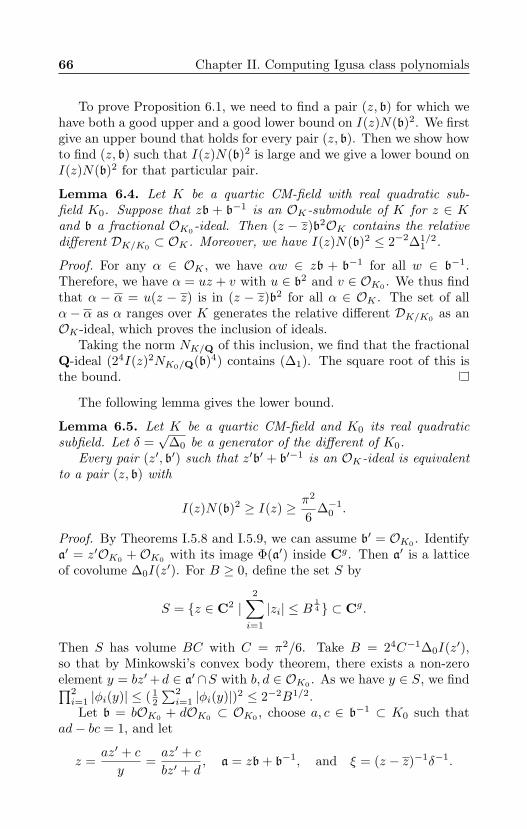
66 Chapter II. Computing Igusa class polynomials
To prove Proposition 6.1, we need to find a pair (z, b) for which wehave both a good upper and a good lower bound on I(z)N(b)2. We firstgive an upper bound that holds for every pair (z, b). Then we show howto find (z, b) such that I(z)N(b)2 is large and we give a lower bound onI(z)N(b)2 for that particular pair.
Lemma 6.4. Let K be a quartic CM-field with real quadratic sub-field K0. Suppose that zb + b−1 is an OK-submodule of K for z ∈ Kand b a fractional OK0-ideal. Then (z − z)b2OK contains the relativedifferent DK/K0 ⊂ OK . Moreover, we have I(z)N(b)2 ≤ 2−2∆1/2
1 .
Proof. For any α ∈ OK , we have αw ∈ zb + b−1 for all w ∈ b−1.Therefore, we have α = uz + v with u ∈ b2 and v ∈ OK0 . We thus findthat α − α = u(z − z) is in (z − z)b2 for all α ∈ OK . The set of allα − α as α ranges over K generates the relative different DK/K0 as anOK-ideal, which proves the inclusion of ideals.
Taking the norm NK/Q of this inclusion, we find that the fractionalQ-ideal (24I(z)2NK0/Q(b)4) contains (∆1). The square root of this isthe bound.
The following lemma gives the lower bound.
Lemma 6.5. Let K be a quartic CM-field and K0 its real quadraticsubfield. Let δ =
√∆0 be a generator of the different of K0.
Every pair (z′, b′) such that z′b′ + b′−1 is an OK-ideal is equivalentto a pair (z, b) with
I(z)N(b)2 ≥ I(z) ≥ π2
6∆−1
0 .
Proof. By Theorems I.5.8 and I.5.9, we can assume b′ = OK0 . Identifya′ = z′OK0 +OK0 with its image Φ(a′) inside Cg. Then a′ is a latticeof covolume ∆0I(z′). For B ≥ 0, define the set S by
S = z ∈ C2 |2∑i=1
|zi| ≤ B14 ⊂ Cg.
Then S has volume BC with C = π2/6. Take B = 24C−1∆0I(z′),so that by Minkowski’s convex body theorem, there exists a non-zeroelement y = bz′+d ∈ a′ ∩S with b, d ∈ OK0 . As we have y ∈ S, we find∏2i=1 |φi(y)| ≤ ( 1
2
∑2i=1 |φi(y)|)2 ≤ 2−2B1/2.
Let b = bOK0 + dOK0 ⊂ OK0 , choose a, c ∈ b−1 ⊂ K0 such thatad− bc = 1, and let
z =az′ + c
y=az′ + c
bz′ + d, a = zb + b−1, and ξ = (z − z)−1δ−1.
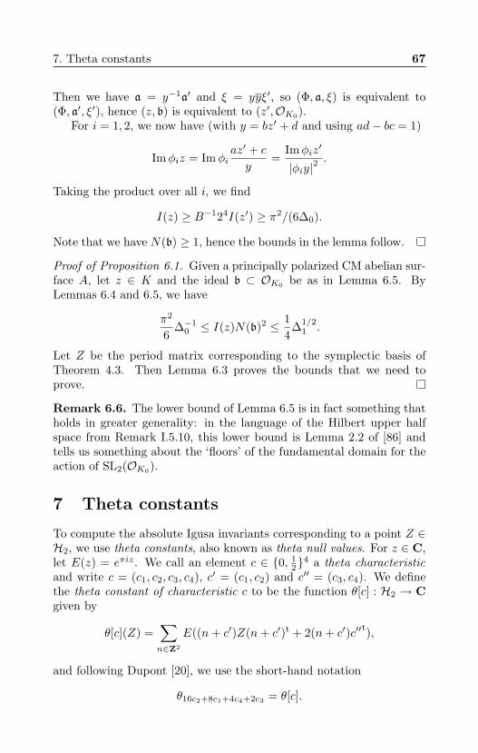
7. Theta constants 67
Then we have a = y−1a′ and ξ = yyξ′, so (Φ, a, ξ) is equivalent to(Φ, a′, ξ′), hence (z, b) is equivalent to (z′,OK0).
For i = 1, 2, we now have (with y = bz′ + d and using ad− bc = 1)
Imφiz = Imφiaz′ + c
y=
Imφiz′
|φiy|2.
Taking the product over all i, we find
I(z) ≥ B−124I(z′) ≥ π2/(6∆0).
Note that we have N(b) ≥ 1, hence the bounds in the lemma follow.
Proof of Proposition 6.1. Given a principally polarized CM abelian sur-face A, let z ∈ K and the ideal b ⊂ OK0 be as in Lemma 6.5. ByLemmas 6.4 and 6.5, we have
π2
6∆−1
0 ≤ I(z)N(b)2 ≤ 14
∆1/21 .
Let Z be the period matrix corresponding to the symplectic basis ofTheorem 4.3. Then Lemma 6.3 proves the bounds that we need toprove.
Remark 6.6. The lower bound of Lemma 6.5 is in fact something thatholds in greater generality: in the language of the Hilbert upper halfspace from Remark I.5.10, this lower bound is Lemma 2.2 of [86] andtells us something about the ‘floors’ of the fundamental domain for theaction of SL2(OK0).
7 Theta constants
To compute the absolute Igusa invariants corresponding to a point Z ∈H2, we use theta constants, also known as theta null values. For z ∈ C,let E(z) = eπiz. We call an element c ∈ 0, 1
24 a theta characteristic
and write c = (c1, c2, c3, c4), c′ = (c1, c2) and c′′ = (c3, c4). We definethe theta constant of characteristic c to be the function θ[c] : H2 → Cgiven by
θ[c](Z) =∑n∈Z2
E((n+ c′)Z(n+ c′)t + 2(n+ c′)c′′t),
and following Dupont [20], we use the short-hand notation
θ16c2+8c1+4c4+2c3 = θ[c].
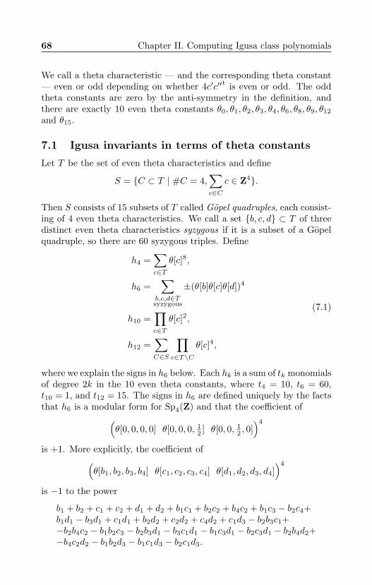
68 Chapter II. Computing Igusa class polynomials
We call a theta characteristic — and the corresponding theta constant— even or odd depending on whether 4c′c′′t is even or odd. The oddtheta constants are zero by the anti-symmetry in the definition, andthere are exactly 10 even theta constants θ0, θ1, θ2, θ3, θ4, θ6, θ8, θ9, θ12
and θ15.
7.1 Igusa invariants in terms of theta constants
Let T be the set of even theta characteristics and define
S = C ⊂ T | #C = 4,∑c∈C
c ∈ Z4.
Then S consists of 15 subsets of T called Gopel quadruples, each consist-ing of 4 even theta characteristics. We call a set b, c, d ⊂ T of threedistinct even theta characteristics syzygous if it is a subset of a Gopelquadruple, so there are 60 syzygous triples. Define
h4 =∑c∈T
θ[c]8,
h6 =∑
b,c,d∈Tsyzygous
±(θ[b]θ[c]θ[d])4
h10 =∏c∈T
θ[c]2,
h12 =∑C∈S
∏c∈T\C
θ[c]4,
(7.1)
where we explain the signs in h6 below. Each hk is a sum of tk monomialsof degree 2k in the 10 even theta constants, where t4 = 10, t6 = 60,t10 = 1, and t12 = 15. The signs in h6 are defined uniquely by the factsthat h6 is a modular form for Sp4(Z) and that the coefficient of(
θ[0, 0, 0, 0] θ[0, 0, 0, 12 ] θ[0, 0, 1
2 , 0])4
is +1. More explicitly, the coefficient of(θ[b1, b2, b3, b4] θ[c1, c2, c3, c4] θ[d1, d2, d3, d4]
)4
is −1 to the power
b1 + b2 + c1 + c2 + d1 + d2 + b1c1 + b2c2 + b4c2 + b1c3 − b2c4+b1d1 − b3d1 + c1d1 + b2d2 + c2d2 + c4d2 + c1d3 − b2b3c1+−b2b4c2 − b1b2c3 − b2b3d1 − b3c1d1 − b1c3d1 − b2c3d1 − b2b4d2+−b4c2d2 − b1b2d3 − b1c1d3 − b2c1d3.
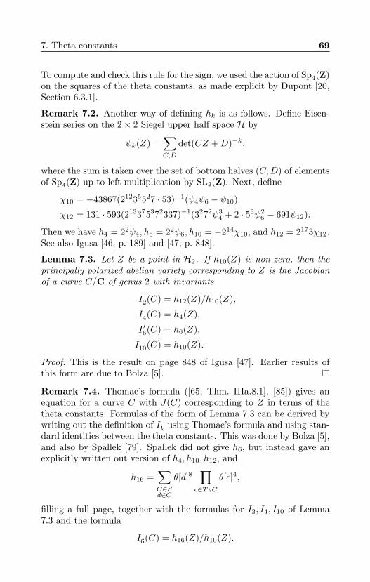
7. Theta constants 69
To compute and check this rule for the sign, we used the action of Sp4(Z)on the squares of the theta constants, as made explicit by Dupont [20,Section 6.3.1].
Remark 7.2. Another way of defining hk is as follows. Define Eisen-stein series on the 2× 2 Siegel upper half space H by
ψk(Z) =∑C,D
det(CZ +D)−k,
where the sum is taken over the set of bottom halves (C,D) of elementsof Sp4(Z) up to left multiplication by SL2(Z). Next, define
χ10 = −43867(21235527 · 53)−1(ψ4ψ6 − ψ10)
χ12 = 131 · 593(213375372337)−1(3272ψ34 + 2 · 53ψ2
6 − 691ψ12).
Then we have h4 = 22ψ4, h6 = 22ψ6, h10 = −214χ10, and h12 = 2173χ12.See also Igusa [46, p. 189] and [47, p. 848].
Lemma 7.3. Let Z be a point in H2. If h10(Z) is non-zero, then theprincipally polarized abelian variety corresponding to Z is the Jacobianof a curve C/C of genus 2 with invariants
I2(C) = h12(Z)/h10(Z),
I4(C) = h4(Z),
I ′6(C) = h6(Z),
I10(C) = h10(Z).
Proof. This is the result on page 848 of Igusa [47]. Earlier results ofthis form are due to Bolza [5].
Remark 7.4. Thomae’s formula ([65, Thm. IIIa.8.1], [85]) gives anequation for a curve C with J(C) corresponding to Z in terms of thetheta constants. Formulas of the form of Lemma 7.3 can be derived bywriting out the definition of Ik using Thomae’s formula and using stan-dard identities between the theta constants. This was done by Bolza [5],and also by Spallek [79]. Spallek did not give h6, but instead gave anexplicitly written out version of h4, h10, h12, and
h16 =∑C∈Sd∈C
θ[d]8∏
c∈T\C
θ[c]4,
filling a full page, together with the formulas for I2, I4, I10 of Lemma7.3 and the formula
I6(C) = h16(Z)/h10(Z).
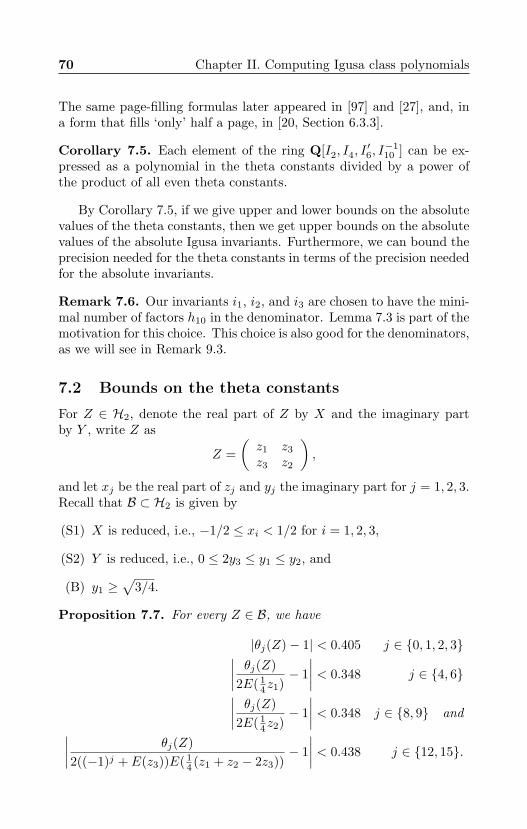
70 Chapter II. Computing Igusa class polynomials
The same page-filling formulas later appeared in [97] and [27], and, ina form that fills ‘only’ half a page, in [20, Section 6.3.3].
Corollary 7.5. Each element of the ring Q[I2, I4, I′6, I−110 ] can be ex-
pressed as a polynomial in the theta constants divided by a power ofthe product of all even theta constants.
By Corollary 7.5, if we give upper and lower bounds on the absolutevalues of the theta constants, then we get upper bounds on the absolutevalues of the absolute Igusa invariants. Furthermore, we can bound theprecision needed for the theta constants in terms of the precision neededfor the absolute invariants.
Remark 7.6. Our invariants i1, i2, and i3 are chosen to have the mini-mal number of factors h10 in the denominator. Lemma 7.3 is part of themotivation for this choice. This choice is also good for the denominators,as we will see in Remark 9.3.
7.2 Bounds on the theta constants
For Z ∈ H2, denote the real part of Z by X and the imaginary partby Y , write Z as
Z =(z1 z3
z3 z2
),
and let xj be the real part of zj and yj the imaginary part for j = 1, 2, 3.Recall that B ⊂ H2 is given by
(S1) X is reduced, i.e., −1/2 ≤ xi < 1/2 for i = 1, 2, 3,
(S2) Y is reduced, i.e., 0 ≤ 2y3 ≤ y1 ≤ y2, and
(B) y1 ≥√
3/4.
Proposition 7.7. For every Z ∈ B, we have
|θj(Z)− 1| < 0.405 j ∈ 0, 1, 2, 3∣∣∣∣ θj(Z)2E( 1
4z1)− 1∣∣∣∣ < 0.348 j ∈ 4, 6∣∣∣∣ θj(Z)
2E( 14z2)
− 1∣∣∣∣ < 0.348 j ∈ 8, 9 and∣∣∣∣ θj(Z)
2((−1)j + E(z3))E( 14 (z1 + z2 − 2z3))
− 1∣∣∣∣ < 0.438 j ∈ 12, 15.
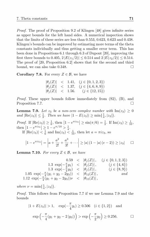
7. Theta constants 71
Proof. The proof of Proposition 9.2 of Klingen [48] gives infinite seriesas upper bounds for the left hand sides. A numerical inspection showsthat the limits of these series are less than 0.553, 0.623, 0.623 and 0.438.Klingen’s bounds can be improved by estimating more terms of the thetaconstants individually and thus getting a smaller error term. This hasbeen done in Propositions 6.1 through 6.3 of Dupont [20], improving thefirst three bounds to 0.405, 2 |E(z1/2)| ≤ 0.514 and 2 |E(z2/2)| ≤ 0.514.The proof of [20, Proposition 6.2] shows that for the second and thirdbound, we can also take 0.348.
Corollary 7.8. For every Z ∈ B, we have
|θj(Z)| < 1.41, (j ∈ 0, 1, 2, 3)|θj(Z)| < 1.37, (j ∈ 4, 6, 8, 9)|θj(Z)| < 1.56. (j ∈ 12, 15)
Proof. These upper bounds follow immediately from (S2), (B), andProposition 7.7.
Lemma 7.9. Let z3 be a non-zero complex number with Im(z3) ≥ 0and |Re(z3)| ≤ 1
2 . Then we have |1− E(z3)| ≥ min 14 , |z3|.
Proof. If |Re(z3)| ≥ 16 , then
∣∣1− eπiz3∣∣ ≥ sin(π/6) = 12 . If Im(z3) ≥ 1
10 ,then
∣∣1− eπiz3∣∣ ≥ 1− eπ/10 > 14 .
If |Re(z3)| < 16 and Im(z3) < 1
10 , then let a = πiz3, so
∣∣1− eπiz3∣∣ =∣∣∣∣a+
a2
2!+a3
3!+ · · ·
∣∣∣∣ ≥ |a| (1− |a| (e− 2)) ≥ |z3|
Lemma 7.10. For every Z ∈ B, we have
0.59 < |θj(Z)| , (j ∈ 0, 1, 2, 3)1.3 exp(−π4 y1) < |θj(Z)| , (j ∈ 4, 6)1.3 exp(−π4 y2) < |θj(Z)| , (j ∈ 8, 9)
1.05 exp(−π4 (y1 + y2 − 2y3)) < |θ12(Z)| , and1.12 exp(−π4 (y1 + y2 − 2y3))ν < |θ15(Z)| ,
where ν = min 14 , |z3|.
Proof. This follows from Proposition 7.7 if we use Lemma 7.9 and thebounds
|1 + E(z3)| > 1, exp(−π4yi) ≥ 0.506 (i ∈ 1, 2) and
exp(−π
4(y1 + y2 − 2 |y3|)
)> exp
(−π
2y2
)≥ 0.256.
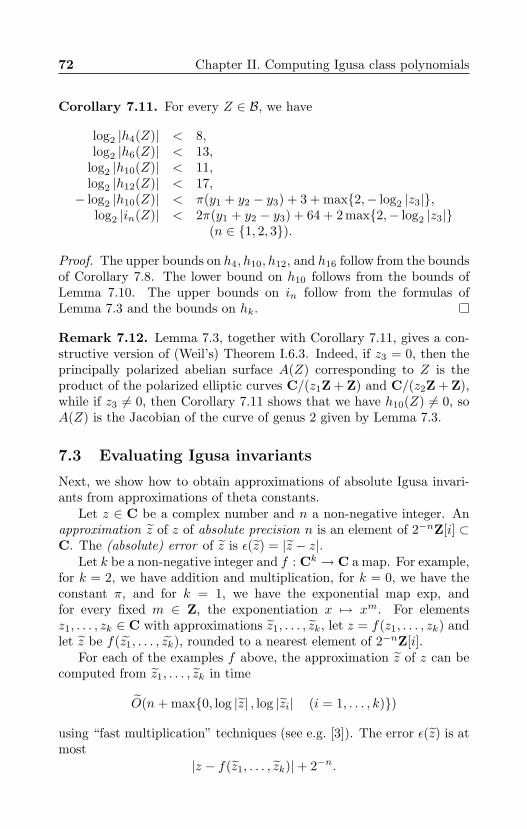
72 Chapter II. Computing Igusa class polynomials
Corollary 7.11. For every Z ∈ B, we have
log2 |h4(Z)| < 8,log2 |h6(Z)| < 13,
log2 |h10(Z)| < 11,log2 |h12(Z)| < 17,− log2 |h10(Z)| < π(y1 + y2 − y3) + 3 + max2,− log2 |z3|,
log2 |in(Z)| < 2π(y1 + y2 − y3) + 64 + 2 max2,− log2 |z3|(n ∈ 1, 2, 3).
Proof. The upper bounds on h4, h10, h12, and h16 follow from the boundsof Corollary 7.8. The lower bound on h10 follows from the bounds ofLemma 7.10. The upper bounds on in follow from the formulas ofLemma 7.3 and the bounds on hk.
Remark 7.12. Lemma 7.3, together with Corollary 7.11, gives a con-structive version of (Weil’s) Theorem I.6.3. Indeed, if z3 = 0, then theprincipally polarized abelian surface A(Z) corresponding to Z is theproduct of the polarized elliptic curves C/(z1Z + Z) and C/(z2Z + Z),while if z3 6= 0, then Corollary 7.11 shows that we have h10(Z) 6= 0, soA(Z) is the Jacobian of the curve of genus 2 given by Lemma 7.3.
7.3 Evaluating Igusa invariants
Next, we show how to obtain approximations of absolute Igusa invari-ants from approximations of theta constants.
Let z ∈ C be a complex number and n a non-negative integer. Anapproximation z of z of absolute precision n is an element of 2−nZ[i] ⊂C. The (absolute) error of z is ε(z) = |z − z|.
Let k be a non-negative integer and f : Ck → C a map. For example,for k = 2, we have addition and multiplication, for k = 0, we have theconstant π, and for k = 1, we have the exponential map exp, andfor every fixed m ∈ Z, the exponentiation x 7→ xm. For elementsz1, . . . , zk ∈ C with approximations z1, . . . , zk, let z = f(z1, . . . , zk) andlet z be f(z1, . . . , zk), rounded to a nearest element of 2−nZ[i].
For each of the examples f above, the approximation z of z can becomputed from z1, . . . , zk in time
O(n+ max0, log |z| , log |zi| (i = 1, . . . , k))
using “fast multiplication” techniques (see e.g. [3]). The error ε(z) is atmost
|z − f(z1, . . . , zk)|+ 2−n.
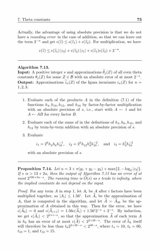
7. Theta constants 73
Actually, the advantage of using absolute precision is that we do nothave a rounding error in the case of addition, so that we can leave outthe term 2−n and get ε(z) ≤ ε(z1) + ε(z2). For multiplication, we have
ε(z) ≤ ε(z1) |z2|+ ε(z2) |z1|+ ε(z1)ε(z2) + 2−n.
Algorithm 7.13.Input: A positive integer s and approximations θj(Z) of all even thetaconstants θj(Z) for some Z ∈ B with an absolute error of at most 2−s.Output: Approximations in(Z) of the Igusa invariants in(Z) for n =1, 2, 3.
1. Evaluate each of the products A in the definition (7.1) of thefunctions h4, h10, h12, and h16 by factor-by-factor multiplicationwith an absolute precision of s, i.e., start with A ← 1 and letA← AB for every factor B.
2. Evaluate each of the sums of in the definitions of h4, h6, h10, andh12 by term-by-term addition with an absolute precision of s.
3. Evaluate
i1 = 28h4h6h−110 , i2 = 25h12h
24h−210 , and i3 = h5
4h−210
with an absolute precision of s.
Proposition 7.14. Let u = 3 + π(y1 + y2 − y3) + max2,− log2 |z3|.If s is > 13 + 2u, then the output of Algorithm 7.13 has an error of atmost 2100+3u−s. The running time is O(s) as s tends to infinity, wherethe implied constants do not depend on the input.
Proof. For any term A in step 1, let Ai be A after i factors have beenmultiplied together, so |Ai| ≤ 1.56i. Let Ai be the approximation ofAi that is computed in the algorithm, and let A = A2k be the ap-proximation of A obtained in this way. Then for the error, we haveε(A0) = 0 and ε(Ai+1) = 1.56ε(Ai) + 1.56i2−s + 2−s. By induction,we get ε(Ai) < 22+i−s, so that the approximation A of each term A
in hk has an error of at most ε(A) < 22+2k−s. The error of hk itselfwill therefore be less than tk22+2k−s < 240−s, where t4 = 10, t6 = 60,t10 = 1, and t12 = 15.
74 Chapter II. Computing Igusa class polynomials
Next, we evaluate h−110 . Let h10 be the approximation that we have
just computed, so |h10 − h10| < 212−s and |h10| > 2−u. As we haves > 13 + u, we find
|h−110 − h
−110 | =
|h10 − h10||h10h10|
≤ 212−s
2−u2−u(1− 212−s+u)< 214+2u−s,
so we find an approximation of h−210 with an error of at most 214+2u−s.
Finally, we evaluate i1, i2, and i3, and the bound on their errorsfollows from the absolute value and error bounds on hk and h−1
10 .
7.4 Evaluating theta constants
The following algorithm is the naive way of evaluating theta constants,which we will use in our running time bound. Its running time is quasi-quadratic, while Dupont’s (AGM-)method [20, Section 10.2] is heuris-tically quasi-linear. We will not prove bounds on the running time orprecision of Dupont’s method in this thesis.
Algorithm 7.15.Input: A positive integer s, an approximation Z of a matrix Z ∈ Bwith sufficiently small error, and the theta characteristic c ∈ 0, 1
22g.
Output: An approximation A of θ[c](Z) with absolute error at most2−s.
1. ComputeR =
⌈(0.4s+ 2.2)1/2
⌉∈ Z.
2. With an absolute precision of t = s+1+b2 log2(2R+1)c, computean approximation A of
A =∑n∈Z2
|ni|≤R
E(
(n+ c′)Z(n+ c′)t + 2(n+ c′)c′′t).
3. Output A.
7. Theta constants 75
Theorem 7.16. The output of Algorithm 7.15 is correct if the inputis given with an absolute error of at most 2−t−1. The algorithm takestime O(s2).
Proof. A precision of t in the input and the evaluation ensures that eachterm of the output approximation A of A has an error of at most 2−t,so that we have ∣∣∣A− A∣∣∣ ≤ (2R+ 1)22−t ≤ 2−s−1.
Next, we have
|A− θ[c](Z)| ≤∑n∈Z2
|n1|>R or |n2|>R
exp(−3π
4((n1 + c1)2y1 + (n2 + c2)2y2)
),
because 0 ≤ 2y3 ≤ y1 ≤ y2 implies n21y1+n1n2y3+n2
2y2 ≥ 34 (n2
1y1+n22y2)
for all n ∈ R2. Now for positive real numbers t and non-negativeintegers l, let
f(t, l) =∞∑k=l
exp(−34πk2t),
so that we find
|A− θ[c](Z)| ≤ 4f(y1, R)f(y2, 0) + 4f(y1, 0)f(y2, R),
If t ≥√
3/4, then we have
f(t, l) ≤∞∑k=l2
exp(−34πtk) < 1.15 exp(−3
4πtl2),
so
|A− θ[c](Z)| < 5.292∑i=1
exp(−34πyiR
2) < 2−s−2.
Therefore, we have ∣∣∣A− θ[c](Z)∣∣∣ < 2−s−1.
For each term, it takes time O(t) = O(s) to evaluate the term andadd it to the result. The number of terms is (2R + 1)2 = O(s), whichproves the running time.
76 Chapter II. Computing Igusa class polynomials
8 The degree of the class polynomials
Let K be a primitive quartic CM-field. In this section we give asymp-totic upper and lower bounds on the degree of Igusa class polynomialsof K. These bounds are not used in the algorithm itself, but are usedin the analysis of the algorithm.
Denote the class numbers of K and K0 by h and h0 respectively,and let h1 = h/h0. The degree of the Igusa class polynomials HK,n forn = 1, 2, 3 is the number h′ of isomorphism classes of curves of genus 2with CM by OK . By Lemma 3.5 we have h′ = h1 if K is cyclic andh′ = 2h1 otherwise. The degree of the class polynomials HK,n is h′− 1.The following result gives an asymptotic bound on h1, and hence on thedegree h′.
Lemma 8.1 (Louboutin [58]). There exist effective constants d > 0and N such that for all primitive quartic CM-fields K with ∆ > N , wehave
∆1/21 ∆1/2
0 (log ∆)−d ≤ h1 ≤ ∆1/21 ∆1/2
0 (log ∆)d.
Proof. Louboutin [58, Theorem 14] gives bounds∣∣∣∣ log h1
log(∆1∆0)− 1
2
∣∣∣∣ ≤ d log log ∆log ∆
for ∆ > N . As we have ∆ > ∆0∆1, this proves the result.
9 Denominators
Let K be a primitive quartic CM-field. In this section we give upperbounds on the denominators of the Igusa class polynomials of K. By thedenominator of a polynomial f ∈ Q[X], we mean the smallest positiveinteger c such that cf is in Z[X].
A prime p occurs in the denominator of H1 if and only if there isa curve C with CM by OK such that C has stable bad reduction at aprime p over p. It is known that abelian varieties with complex multi-plication have potential good reduction at all primes, but this doesn’timply that Jacobians reduce as Jacobians: the reduction of the Jacobianof a smooth curve C of genus two can be a polarized product of ellipticcurves E1 × E2. The stable reduction of C is then the union of thoseelliptic curves intersecting transversely. For details, we refer to Gorenand Lauter [35, 36], who study this phenomenon and use the embedding
OK → End(E1 × E2)
9. Denominators 77
to bound both p and the valuation of the denominator of H1 at p.We will first give the bounds of Goren and Lauter [35, 36] which
hold in general, but are expected to be far from asymptotically optimal.These are the only bounds that we will use in our running time analysis.Then we give optimal bounds conjectured by Bruinier and Yang [8] forspecial cases and proven by Yang [98] in cases that are even more special.We end this section by giving a counterexample to a bound conjecturedby Lauter [54].
9.1 The bounds of Goren and Lauter
The bounds of Goren and Lauter are given in terms of integers a, b, dsuch that K is given by K = Q(
√−a+ b
√d). For d, one can take the
discriminant d = ∆0 of the real quadratic subfield K0. We will provein Lemma 9.9 below that one can take a < 8π−1(∆1∆0)1/2, where∆1 = NK0/Q(∆K/K0) is the norm of the relative discriminant. Thedenominator itself does not depend on the choice of a, so we can replacea by this bound on a in all denominator bounds below.
The main result of this section is the following.
Theorem 9.1. Let K be a primitive quartic CM-field and write
K = Q(√−a+ b
√d)
with a, b, d ∈ Z.
The denominator of each of the Igusa class polynomials of K divides214h′D2 for
D =
( ∏p<4da2
p prime
pb4f(p)(1+log(2da2)/ log p)c
)h′,
where f(p) is given by f(p) = 8 if p ramifies in K/Q and satisfies p ≤ 3,and given by f(p) = 1 otherwise.
Furthermore, the result above remains true if we replace d by ∆0 anda by b8π−1(∆1∆0)1/2c in the definition of D. We then have logD =O(h′∆) = O(∆3/2
1 ∆5/20 ) as ∆ tends to infinity.
We will prove this result below.
Remark 9.2. Theorem 9.1 as stated holds for the absolute Igusa in-variants i1, i2, i3 of Section 2. For another choice of a set S of absoluteIgusa invariants, take positive integers c3 and k such that c3(2−12I10)kSconsists of modular forms of degree k with integral Fourier expansion.
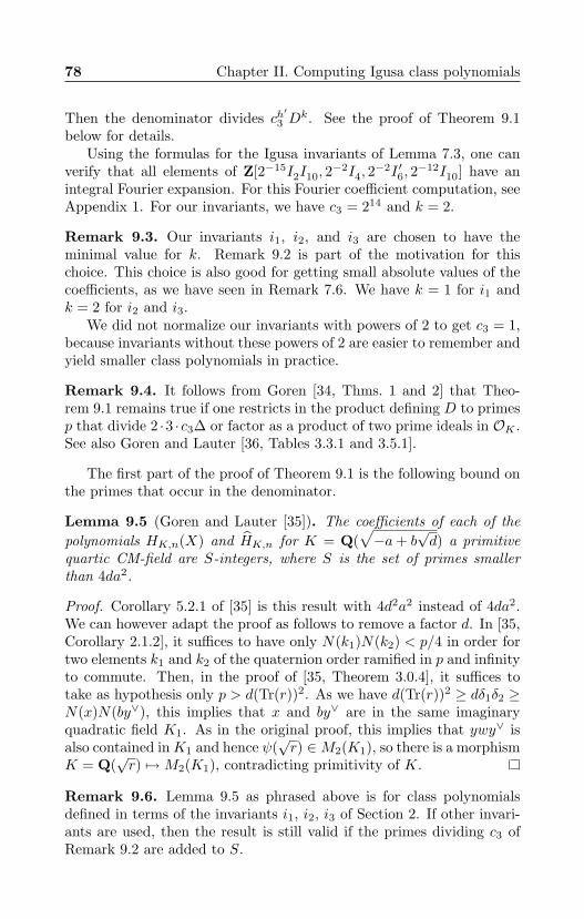
78 Chapter II. Computing Igusa class polynomials
Then the denominator divides ch′
3 Dk. See the proof of Theorem 9.1
below for details.Using the formulas for the Igusa invariants of Lemma 7.3, one can
verify that all elements of Z[2−15I2I10, 2−2I4, 2
−2I ′6, 2−12I10] have an
integral Fourier expansion. For this Fourier coefficient computation, seeAppendix 1. For our invariants, we have c3 = 214 and k = 2.
Remark 9.3. Our invariants i1, i2, and i3 are chosen to have theminimal value for k. Remark 9.2 is part of the motivation for thischoice. This choice is also good for getting small absolute values of thecoefficients, as we have seen in Remark 7.6. We have k = 1 for i1 andk = 2 for i2 and i3.
We did not normalize our invariants with powers of 2 to get c3 = 1,because invariants without these powers of 2 are easier to remember andyield smaller class polynomials in practice.
Remark 9.4. It follows from Goren [34, Thms. 1 and 2] that Theo-rem 9.1 remains true if one restricts in the product defining D to primesp that divide 2 ·3 ·c3∆ or factor as a product of two prime ideals in OK .See also Goren and Lauter [36, Tables 3.3.1 and 3.5.1].
The first part of the proof of Theorem 9.1 is the following bound onthe primes that occur in the denominator.
Lemma 9.5 (Goren and Lauter [35]). The coefficients of each of thepolynomials HK,n(X) and HK,n for K = Q(
√−a+ b
√d) a primitive
quartic CM-field are S-integers, where S is the set of primes smallerthan 4da2.
Proof. Corollary 5.2.1 of [35] is this result with 4d2a2 instead of 4da2.We can however adapt the proof as follows to remove a factor d. In [35,Corollary 2.1.2], it suffices to have only N(k1)N(k2) < p/4 in order fortwo elements k1 and k2 of the quaternion order ramified in p and infinityto commute. Then, in the proof of [35, Theorem 3.0.4], it suffices totake as hypothesis only p > d(Tr(r))2. As we have d(Tr(r))2 ≥ dδ1δ2 ≥N(x)N(by∨), this implies that x and by∨ are in the same imaginaryquadratic field K1. As in the original proof, this implies that ywy∨ isalso contained inK1 and hence ψ(
√r) ∈M2(K1), so there is a morphism
K = Q(√r) 7→M2(K1), contradicting primitivity of K.
Remark 9.6. Lemma 9.5 as phrased above is for class polynomialsdefined in terms of the invariants i1, i2, i3 of Section 2. If other invari-ants are used, then the result is still valid if the primes dividing c3 ofRemark 9.2 are added to S.
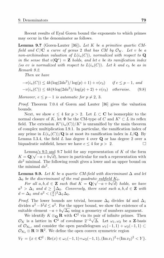
9. Denominators 79
Recent results of Eyal Goren bound the exponents to which primesmay occur in the denominator as follows.
Lemma 9.7 (Goren-Lauter [36]). Let K be a primitive quartic CM-field and C/C a curve of genus 2 that has CM by OK . Let v be anon-archimedean valuation of L(in(C)), normalized with respect to Qin the sense that v(Q∗) = Z holds, and let e be its ramification index(so ev is normalized with respect to L(in(C)). Let k and c3 be as inRemark 9.2.
Then we have
−v(in(C)) ≤ 4k(log(2da2)/ log(p) + 1) + v(c3) if e ≤ p− 1, and
−v(in(C)) ≤ 4k(8 log(2da2)/ log(p) + 2) + v(c3) otherwise. (9.8)
Moreover, e ≤ p− 1 is automatic for p 6= 2, 3.
Proof. Theorem 7.0.4 of Goren and Lauter [36] gives the valuationbounds.
Next, we show e ≤ 4 for p > 2. Let L ⊂ C be isomorphic to thenormal closure of K, let Φ be the CM-type of C and Kr ⊂ L its reflexfield. The extension Kr(in(C))/Kr is unramified by the main theoremof complex multiplication I.9.1. In particular, the ramification index ofany prime in L(in(C))/Q is at most its ramification index in L/Q. ByLemma I.3.4, the field L has degree 4 over Q or has degree 2 over abiquadratic subfield, hence we have e ≤ 4 for p > 2.
Lemma’s 9.5 and 9.7 hold for any representation of K of the formK = Q(
√−a+ b
√d), hence in particular for such a representation with
da2 minimal. The following result gives a lower and an upper bound onthe minimal da2.
Lemma 9.9. Let K be a quartic CM-field with discriminant ∆ and let∆0 be the discriminant of the real quadratic subfield K0.
For all a, b, d ∈ Z such that K = Q(√−a+ b
√d) holds, we have
a2 > ∆1 and d ≥ 14∆0. Conversely, there exist such a, b, d ∈ Z with
d = ∆0 and a2 < ( 8π )2∆1∆0.
Proof. The lower bounds are trivial, because ∆0 divides 4d and ∆1
divides a2− b2d ≤ a2. For the upper bound, we show the existence of asuitable element −a+ b
√∆0 using a geometry of numbers argument.
We identify K ⊗Q R with C2 via its pair of infinite primes. ThenOK is a lattice in C2 of covolume 2−2
√∆. Let ω1, ω2 be a Z-basis
of OK0 , and consider the open parallelogram ω1(−1, 1) + ω2(−1, 1) ⊂OK0 ⊗R ∼= R2. We define the open convex symmetric region
VY = x ∈ C2 : Re(x) ∈ ω1(−1, 1)+ω2(−1, 1), (Imx1)2+(Imx2)2 < Y .
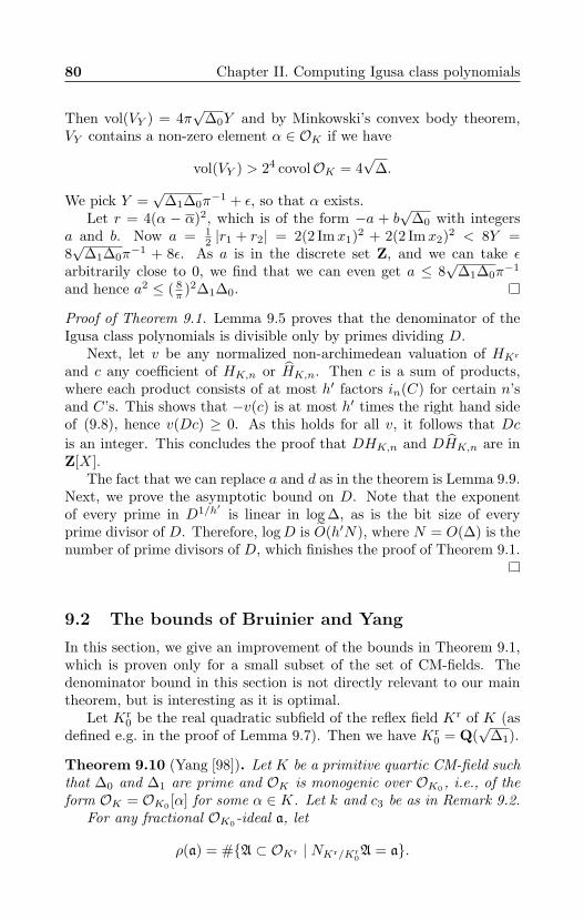
80 Chapter II. Computing Igusa class polynomials
Then vol(VY ) = 4π√
∆0Y and by Minkowski’s convex body theorem,VY contains a non-zero element α ∈ OK if we have
vol(VY ) > 24 covolOK = 4√
∆.
We pick Y =√
∆1∆0π−1 + ε, so that α exists.
Let r = 4(α − α)2, which is of the form −a + b√
∆0 with integersa and b. Now a = 1
2 |r1 + r2| = 2(2 Imx1)2 + 2(2 Imx2)2 < 8Y =8√
∆1∆0π−1 + 8ε. As a is in the discrete set Z, and we can take ε
arbitrarily close to 0, we find that we can even get a ≤ 8√
∆1∆0π−1
and hence a2 ≤ ( 8π )2∆1∆0.
Proof of Theorem 9.1. Lemma 9.5 proves that the denominator of theIgusa class polynomials is divisible only by primes dividing D.
Next, let v be any normalized non-archimedean valuation of HKr
and c any coefficient of HK,n or HK,n. Then c is a sum of products,where each product consists of at most h′ factors in(C) for certain n’sand C’s. This shows that −v(c) is at most h′ times the right hand sideof (9.8), hence v(Dc) ≥ 0. As this holds for all v, it follows that Dcis an integer. This concludes the proof that DHK,n and DHK,n are inZ[X].
The fact that we can replace a and d as in the theorem is Lemma 9.9.Next, we prove the asymptotic bound on D. Note that the exponentof every prime in D1/h′ is linear in log ∆, as is the bit size of everyprime divisor of D. Therefore, logD is O(h′N), where N = O(∆) is thenumber of prime divisors of D, which finishes the proof of Theorem 9.1.
9.2 The bounds of Bruinier and Yang
In this section, we give an improvement of the bounds in Theorem 9.1,which is proven only for a small subset of the set of CM-fields. Thedenominator bound in this section is not directly relevant to our maintheorem, but is interesting as it is optimal.
Let Kr0 be the real quadratic subfield of the reflex field Kr of K (as
defined e.g. in the proof of Lemma 9.7). Then we have Kr0 = Q(
√∆1).
Theorem 9.10 (Yang [98]). Let K be a primitive quartic CM-field suchthat ∆0 and ∆1 are prime and OK is monogenic over OK0 , i.e., of theform OK = OK0 [α] for some α ∈ K. Let k and c3 be as in Remark 9.2.
For any fractional OK0-ideal a, let
ρ(a) = #A ⊂ OKr | NKr/Kr0A = a.
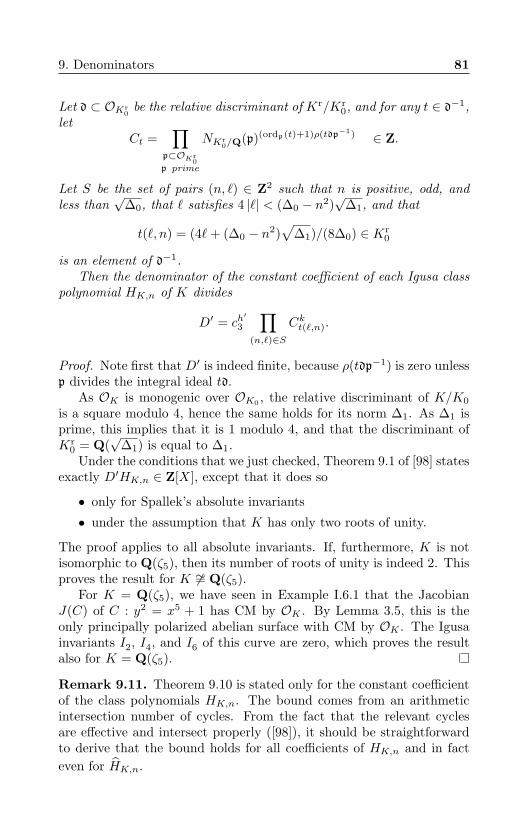
9. Denominators 81
Let d ⊂ OKr0
be the relative discriminant of Kr/Kr0, and for any t ∈ d−1,
letCt =
∏p⊂OKr
0p prime
NKr0/Q
(p)(ordp(t)+1)ρ(tdp−1) ∈ Z.
Let S be the set of pairs (n, `) ∈ Z2 such that n is positive, odd, andless than
√∆0, that ` satisfies 4 |`| < (∆0 − n2)
√∆1, and that
t(`, n) = (4`+ (∆0 − n2)√
∆1)/(8∆0) ∈ Kr0
is an element of d−1.Then the denominator of the constant coefficient of each Igusa class
polynomial HK,n of K divides
D′ = ch′
3
∏(n,`)∈S
Ckt(`,n).
Proof. Note first that D′ is indeed finite, because ρ(tdp−1) is zero unlessp divides the integral ideal td.
As OK is monogenic over OK0 , the relative discriminant of K/K0
is a square modulo 4, hence the same holds for its norm ∆1. As ∆1 isprime, this implies that it is 1 modulo 4, and that the discriminant ofKr
0 = Q(√
∆1) is equal to ∆1.Under the conditions that we just checked, Theorem 9.1 of [98] states
exactly D′HK,n ∈ Z[X], except that it does so
• only for Spallek’s absolute invariants
• under the assumption that K has only two roots of unity.
The proof applies to all absolute invariants. If, furthermore, K is notisomorphic to Q(ζ5), then its number of roots of unity is indeed 2. Thisproves the result for K 6∼= Q(ζ5).
For K = Q(ζ5), we have seen in Example I.6.1 that the JacobianJ(C) of C : y2 = x5 + 1 has CM by OK . By Lemma 3.5, this is theonly principally polarized abelian surface with CM by OK . The Igusainvariants I2, I4, and I6 of this curve are zero, which proves the resultalso for K = Q(ζ5).
Remark 9.11. Theorem 9.10 is stated only for the constant coefficientof the class polynomials HK,n. The bound comes from an arithmeticintersection number of cycles. From the fact that the relevant cyclesare effective and intersect properly ([98]), it should be straightforwardto derive that the bound holds for all coefficients of HK,n and in facteven for HK,n.
82 Chapter II. Computing Igusa class polynomials
Remark 9.12. The denominator bound D′ is sharp in the sense that(by [98, Corollary 1.6]) the set of primes dividing D′ are exactly theprimes p such that there exists a curve with CM by OK of stable badreduction at a prime over p.
Remark 9.13. If Bruinier and Yang’s conjecture ([8, equation (1.10)],[98, Conjecture 1.1]) is true, then Theorem 9.10 holds in slightly greatergenerality.
9.3 Counterexample to a conjectured formula
A conjecture of Lauter [54] also bounds the primes dividing the de-nominators of Igusa class polynomials by stating that each such primedivides ∆ − x2 for some non-negative integer x < ∆1/2. However, thefield K = Q[X]/(X4 + 558X2 + 31873) with ∆0 = 17 and ∆1 = 31873is a counterexample, as demonstrated by the corresponding entry inthe ECHIDNA database [50]. The prime 7499 divides the denomina-tors of the class polynomials, but does not divide ∆− x2 for any smallenough x. The conjecture did not go down without a fight: our searchof the database reveiled only 17 counterexamples among thousands ofCM-fields, and we know no counterexamples with class number h ≤ 14.
10 Recovering a polynomial from its roots
In this section, we show how to compute a polynomial from complexapproximations of its roots. This will tell us the precision to which weneed to know these roots. The algorithms in this section are well knownto the experts, but we did not find an error analysis in the literature.
We will compute an approximation of a polynomial from approxi-mations of its roots in Sections 10.1 and 10.2. Then in Section 10.3,we compute numerators and denominators of the coefficients from theirapproximations.
10.1 Polynomial multiplication
For a complex polynomial g, let |g|1 (resp. |g|∞) be the sum (resp.maximum) of the absolute values of the coefficients of g. We find|g1g2|∞ ≤ |g1|∞ |g2|1 and |g|1 ≤ (deg(g) + 1) |g|∞.
The following algorithm computes products of integer polynomials.
10. Recovering a polynomial from its roots 83
Algorithm 10.1.Input: Polynomials g1, g2 ∈ Z[X], given by the binary expansions oftheir coefficients.Output: The product g1g2 ∈ Z[X].
1. Let k = dlog2 |g1|∞e+ dlog2 |g2|∞e+ dlog2(deg(g1) + 1)e.
2. Evaluate the polynomials at 2k by writing the binary expansionsof their coefficients after each other with the appropriate numberof zeroes between them.
3. Multiply the results of step 2 using fast integer multiplication.
4. Read off the binary expansions of the coefficients of g1g2 from theresult of step 3.
This algorithm has a running time ofM((deg(g1g2)+1) log2 |g1g2|∞),whereM(n) = O(n log n log log n) is the time needed for a multiplicationof n-bit integers. See also [90, Corollary 8.27].
For a complex polynomial g ∈ C[X] and a positive integer p, anapproximation g of g with absolute precision p is an object of the form2−p(a + ib), where a and b are polynomials in Z[x] given by the bi-nary expansions of their coefficients. Complex numbers are complexpolynomials of degree 0 and have approximations as such, which is ex-actly the notion of approximation from Section 7.3. The error of anapproximation g of a polynomial g is ε(g) = |g − g|∞. Suppose we haveapproximations gk = 2−p(ak+ibk) of gk for k = 1, 2 with absolute preci-sion p. The following algorithm computes an approximation g1g2 of theproduct g1g2 with the same absolute precision. It does so by computingthe product g1g2 exactly, and then reducing the precision back to p.
Algorithm 10.2.Input: Approximations g1 = 2−p(a1 + ib1) and g2 = 2−p(a2 + ib2) ofcomplex polynomials g1, g2.Output: An approximation g1g2 = 2−p(a+ ib) of g1g2.
1. Compute a′ = a1a2 − b1b2 and b′ = a1b2 + b1a2 in Z[X] usingAlgorithm 10.1.
84 Chapter II. Computing Igusa class polynomials
2. Let a ∈ Z[X] be obtained from a′/2p ∈ Q[X] by rounding eachcoefficient to the nearest integer. Let b ∈ Z[X] be obtained fromb′/2p in the same way.
Lemma 10.3. Algorithm 10.2 takes time
M((deg(g1g2) + 1)(log2 |g1g2|∞ + 2p)).
The error ε(g1g2) is at most
|g1|1 ε(g2) + |g2|1 ε(g1) + (deg(g1) + 1)ε(g1)ε(g2) + 2−p.
Proof. The running time bound follows from the fact that we simplyapply Algorithm 10.1 four times. The triangle inequality for |·|∞ givesus the bound on the error.
10.2 Recovering a polynomial from its roots
Let z1, . . . , zn be complex numbers. The purpose of this section is tocompute an approximation of f =
∏ni=1(X − zi) ∈ C[X] from an ap-
proximation of z1, . . . , zn. Suppose that we know si ∈ Q satisfying|zi|+ 1 ≤ si for i = 1, . . . , n, and let s =
∏si.
Algorithm 10.4.Input: an integer u > 0 and approximations z1, . . . , zn of z1, . . . , znwith error
ε(zi) ≤ 2−u−∑j 6=i log2 sj−3 log2 n−3.
Output: an approximation f of f =∏ni=1(X − zi) ∈ C[X] with error
ε(f) ≤ 2−u.
1. Build a binary tree of depth l = dlog2 ne with at n of the leavesthe n linear polynomials X− zi, and at the remaining 2l−n leavesthe constant polynomial 1.
2. From the leaves up to the root, at every node t of the tree, put theproduct gt of the two nodes below it, computed by Algorithm 10.2with absolute precision p = u +
∑j log2 sj + 3 log2 n + 3, where
the sum is taken over those j that are not below the node t.
3. Output the root of the tree.
10. Recovering a polynomial from its roots 85
Theorem 10.5. Algorithm 10.4 is correct and has a running time of
O(nm log(nm)2 log log(nm)),
where m = maxu, log n, log s.
Proof of Theorem 10.5. For every node t of the tree, denote by d(t)the set of leaves i below t. For every node t of the tree, let gt be thepolynomial
gt =∏i∈d(t)
(X − zi)
of which the polynomial gt computed in the algorithm is an approxima-tion. Let bk be the maximum over all nodes t at distance at most k tothe leaves of
|gt|1∏i∈d(t)
s−1i .
Similarly, let κk be the maximum over all nodes t at distance at mostk to the leaves of
max2−p, ε(gt)∏i∈d(t)
s−1i .
Then bk ≤ 1 for all k. Therefore, by Lemma 10.3, we have
κk+1 ≤ 2κk + (2k + 1)κ2k + 2−p ≤ 3κk + (2k + 1)κ2
k.
If κ0 ≤ n−3, then by induction this implies that κk ≤ 4kκ0 for all k, soκl < (2n)2κ0. In particular, the error of each coefficient of the outputis at most (2n)2κ0s.
This means that κ0 = 2−u−3 logn−3−log2 s is sufficient. At the k-thlevel of the tree, there are 2l−k polynomial multiplications of degree atmost 2k where each coefficient has a bit size of O(m), so each of the l <1+log2 n levels takes time O(M(nm)), which proves the complexity.
Remark 10.6. Algorithm 10.4 is Algorithm 10.3 of [90], except that weround the coefficients back to a fixed precision after every polynomialmultiplication. A direct application of the algorithm in [90] would yieldexactly the product
n∏k=1
(X − zk)
with a very large denominator in time that is quasi-quadratic ratherthan quasi-linear.
86 Chapter II. Computing Igusa class polynomials
10.3 Recognizing rational coefficients
There are various ways of recognizing a polynomial f ∈ Q[X] from anapproximation f . If one knows an integer D such that the denominatorof f divides D, and the error ε(f) is less than (2D)−1, then Df isobtained from Df by rounding the coefficients to the nearest integers.
Other methods to compute f from f are based on continued frac-tions, where the coefficients of f are obtained via the continued fractionexpansion of the coefficients of f , or on the LLL-algorithm, where thecoefficients of an integral multiple of f arise as coordinates of a smallvector in a lattice [57, Section 7]. Such methods have the advantagethat only a bound B on the denominator needs to be known, instead ofan actual multiple D. This is very useful in practical implementations,because one can guess a small value for B, which may be much smallerthan any proven D. In the case of Igusa class polynomials, there ex-ist a few good heuristic checks of the output when using a non-provenbound B, such as smoothness of the denominators, and successfulnessof explicit CM constructions.
For our purpose of giving a proven running time bound however, weprefer the first method of rounding Df , since it is easy to analyze andasymptotically fast. The following algorithm computes D for the caseof Igusa class polynomials.
Algorithm 10.7.Input: The discriminant ∆ of a primitive quartic CM-field K and thedegree h′ of the Igusa class polynomials of K.Output: The integer D of Theorem 9.1, which satisfies DHK,n ∈ Z[X]for n = 1, 2, 3.
1. List all primes up to the number 4da2 as in Theorem 9.1.
2. Raise each prime in the list to the exponent in Theorem 9.1.
3. Compute the product of the integers of step 2 using a binary tree,just as we used a binary tree to compute a product of polynomialsin Algorithm 10.4. See also [90, Exercise 10.8].
Algorithm 10.7 takes time O(logD), so we conclude that we cancompute HK,n from an approximation HK,n in time O(logD) plus timelinear in the bit size of HK,n, provided that we have ε(HK,n) < (2D)−1.
11. The algorithm 87
11 The algorithm
Algorithm 11.1.Input: A positive quadratic fundamental discriminant ∆0 and positiveintegers a and b such that the the field
K = Q(√−a+ b
√∆0)
is a primitive quartic CM-field of discriminant greater than a.Output: The Igusa class polynomials HK,n for n = 1, 2, 3.
1. Compute a Z-basis of OK using the algorithm of Buchmann andLenstra [9] and use this to compute the discriminant ∆ of K.
2. Compute a complete set A1, . . . , Ah′ of representatives of the h′
isomorphism classes of principally polarized abelian surfaces overC with CM by OK , using Algorithm 3.1. Here each Aj is givenby a triple (Φj , aj , ξj) as in Section 3.3.
3. From ∆ and h′, compute a number D such that DHK,n is in Z[X]for n = 1, 2, 3, using Algorithm 10.7.
4. For j = 1, . . . , h′, do the following.
(a) Compute a symplectic basis of aj using Algorithm 4.2. Thisprovides us with a period matrix Wj ∈ H2 ∩Mat2(L), whereL ⊂ C is the normal closure of K.
(b) Replace the period matrix Wj by an Sp4(Z)-equivalent pe-riod matrix Zj ∈ F2 ∩Mat2(L), using Algorithm 5.9.
(c) Let uj = d3 + (y1 + y2 − y3)π + max2,− log2 |z3|e, where
Zj =(z1 z3
z3 z2
)and yk = Im zk (k = 1, 2, 3).
5. Let p = dlog2D + 3 log2 h′ + 4e +
∑h′
j=1(2uj + 40). This is theprecision with which we will approximate the Igusa invariants.
6. For j = 1, . . . , h′, do the following.
(a) Evaluate the theta constants in Zj , using Algorithm 7.15, toa precision rj = 101 + 7uj + p.
88 Chapter II. Computing Igusa class polynomials
(b) Use Algorithm 7.13 to evaluate in(Aj) for (n = 1, 2, 3) toprecision p.
7. For n = 1, 2, 3, do the following.
(a) Use Algorithm 10.4 to compute an approximation HK,n ofHK,n for n = 1, 2, 3 from the approximations of Igusa invari-ants of step 6b.
(b) Compute DHK,n by rounding the coefficients of DHK,n tonearest integers.
(c) Output HK,n.
The polynomials HK,n (n = 2, 3) of Section 2.2 can be computed fromthe approximations of in(C) and i1(C) efficiently using Algorithm 10.9of [90] (see also [23, Section 4]). However, instead of doing a detailedrounding error analysis of that algorithm, we give a more naive andslower algorithm that is still much faster than the running time in ourMain Theorem. To compute the polynomials HK,n, we simply modifystep 7a as follows:
1. Evaluate each summand in the definition of the polynomial HK,n
using Algorithm 10.4.
2. Evaluate HK,n using a binary tree as in Algorithm 10.4 with ad-dition instead of multiplication.
We now recall and prove the main theorem.
Main Theorem. Algorithm 11.1 computes HK,n (n = 1, 2, 3) for anyprimitive quartic CM-field K. It has a running time of O(∆7/2
1 ∆11/20 )
and the bit size of the output is O(∆21∆3
0).
Proof. We start by proving that the output is correct. By Proposi-tion 7.14, the precision rj for the theta constants suffices to get theabsolute Igusa invariants with precision p. Corollary 7.11 tells us thatwe have |in(Zj)| ≤ 26uj+77. These bounds and Theorem 10.5 show thatit suffices to know the absolute Igusa invariants to precision p in order toget a precision of 1 + log2D bits for the coefficients of HK,n. By Theo-rem 9.1, the polynomials DHK,n have integer coefficients, so a precisionof 1 + log2D for the coefficients of HK,n suffices for recognizing thesecoefficients and getting a correct output. This proves that the outputof Algorithm 11.1 is correct.
11. The algorithm 89
Next, we bound the precisions p and rj . We start by bounding uj ,for which we need an upper bound on y1 + y2 − y3 and a lower boundon z3. We have y2 ≥ y1 and y3 ≥ 0, hence y1 + y2 − y3 ≤ 2y2, andCorollary 6.2 gives the upper bound
y2 ≤ max 2√
2√3π
∆0,49
∆1/41 ∆1/2
0 .
We claim that the off-diagonal entry z3 of Zj ∈ H2 is non-zero.Indeed, if z3 = 0, then Zj = diag(z1, z2) with z1, z2 ∈ H = H1 andAj is the product of the elliptic curves corresponding to z1 and z2,contradicting the fact that Aj is simple (Theorem I5.2). The claim andCorollary 5.19 together now give an upper bound on log(1/z3), whichis polynomial in log ∆ by Lemma 3.6.
We now have
uj = O(max 2√
2√3π
∆0,49
∆1/41 ∆1/2
0 ),
h′ = O(∆1/21 ∆1/2
0 ), and by Theorem 9.1 also logD = O(∆3/21 ∆5/2
0 ).We find that p is dominated by our bounds on logD, hence we havep = O(∆3/2
1 ∆5/20 ) and also rj = O(∆3/2
1 ∆5/20 ).
Finally, we can bound the running time. Under the assumption thatK is given as K = Q(
√−a+ b
√∆0), where ∆0 is a positive fundamen-
tal discriminant and a, b are positive integers such that a < ∆0, we canfactor (a2 − b2∆0)∆2
0 and hence find the ring of integers in step 1 intime O(∆).
As shown in Section 3.3, step 2 takes time O(∆1/2). Step 3 takestime O(D) = O(∆3/2
1 ∆5/20 ).
For every j, step 4a takes time polynomial in log ∆ by Lemma 3.6and Theorem 5.18. The same holds for steps 4b and 4c and each sum-mand of step 5. The number of iterations or summands of these stepsis 2h′ = O(∆1/2
1 ∆1/20 ) by Lemmas 8.1 and 3.5. In particular, steps 4
and 5 take time O(∆1/21 ∆1/2
0 ).We now come to the most costly step. By Theorem 7.16, it takes
time O(r2j ) to do a single iteration of step 6a. In particular, all iterations
of this step together take time O(∆7/21 ∆11/2
0 ).The j-th iteration of step 6b takes time O(r) and hence all iterations
of this step together take time O(∆21∆3
0). Finally, by Theorem 10.5, step7a takes time O(h′) times O(p), which is O(∆2
1∆30). The same amount
of time is needed for the final two steps.The output consists of h′+ 1 rational coefficients, each of which has
a bit size of O(∆3/21 ∆5/2
0 ), hence the size of the output is O(∆21∆3
0).
90 Chapter II. Computing Igusa class polynomials
This proves the main theorem, except when using the polynomialsHK,n (n = 2, 3) of Section 2.2. With the naive method of evaluat-ing HK,n that we described in Algorithm 11.1, it takes O(h1) times asmuch time to evaluate HK,n from the Igusa invariants as it does to eval-uate HK,n. This O(∆5/2
1 ∆7/20 ) is still dominated by the running time of
the rest of the algorithm.
It also follows that, if one uses Dupont’s [20] quasi-linear methodof evaluating theta constants as mentioned in Section 7.4, the heuristicrunning time of Algorithm 11.1 is O(∆2
1∆30), which can still be improved
if better bounds on the denominators are found. In fact, if we also usea guess for the height of the class polynomials, then we can computeclass polynomials in quasi-linear time without proof of correctness.
If the goal is to construct a genus-two curve C/k with a pointP ∈ J(C)(k) of prime order N (as it is in the cryptographic appli-cations), then correctness of the output (C,P ) can be proven efficientlyafterwards by checking P 6= [N ]P = 0. By doubling the precision everytime the output is incorrect, and assuming Dupont’s method is quasi-linear in the required precision, this yields a method that is quasi-linearin the bit size of the class polynomials.
ChapterIIIThe irreducible components of the CM locus
Abstract. In this chapter, we show how to replace genus-2class polynomials by smaller and more natural objects: theirreducible components of the CM-by-K locus in the modulispace.
In Chapter II, we gave an algorithm to compute the Igusa classpolynomials of any primitive quartic CM-field K. Though Igusa classpolynomials are the objects that are studied in the literature on explicitCM constructions of curves of genus 2, it is actually much better froma practical perspective to work with their irreducible factors over Kr
0.We will explain why in Example 3.1 and Section 4 below.
At the same time, though Igusa class polynomials HK,1, HK,2, HK,3
of K in practice specify exactly what the abelian surfaces with CM byOK are, and though in practice they define the field CMKr,Φr , this isnot guaranteed, as the polynomial HK,1 might not have a simple root.To get actual theorems about computing CM abelian surfaces or thefield CMKr,Φr , we will need to look at the moduli space of CM-by-Kpoints.
The current chapter combines these approaches: we study the irre-ducible components over Kr
0 of the moduli space of CM-by-K points.We then show what to change in the algorithms of Chapter II in orderto compute these components.
We did not work directly with these irreducible components in Chap-
92 Chapter III. The irreducible components of the CM locus
ter II to avoid making that chapter too heavy, and because Igusa classpolynomials are the objects used in existing literature.
1 The moduli space of CM-by-K points
The quotient Sp2g(Z)\Hg of Section II.4 parametrizes the isomorphismclasses of complex principally polarized abelian varieties of dimension gin an analytic way. This (coarse) moduli space has an algebraic modelAg/Q that parametrizes these isomorphism classes algebraically.
For g = 1, the variety Ag is simply the affine line A1 with the j-invariant as its coordinate. For g = 2, we take the moduli space M2
of curves of genus 2 and embed it into Ag by taking Jacobians. Thespace M2 is given in terms of the Igusa invariants of Section II.2 asthe I10 6= 0 locus of the 3-dimensional weighted projective space withcoordinates I2, I4, I6, I10 (see Igusa [45]).
Let K be a CM-field of degree 2g and Φ a CM-type of K with valuesin Q ⊂ C. We will restrict to primitive quartic CM-fields soon, butgive general definitions now because we want to give an 8-dimensionalexample later. Let (Kr,Φr) be the reflex of (K,Φ) and let Kr
0 be themaximal totally real subfield of K. For the definitions, see Chapter I.
We define the CM-by-(K,Φ)-locus CMK,Φ ⊂ Ag(Q) to be the setof points A ∈ Ag(Q) such that there exists an embedding ι : OK →End(A) of type Φ. Two CM-types Φ and Φ′ of K are called equivalentif there is an automorphism σ of K such that Φ′ = Φσ holds. Recallfrom Section I.4 that CMK,Φ and CMK,Φ′ coincide if Φ and Φ′ areequivalent.
The CM-by-K-locus CMK is the union of CMK,Φ over all equiva-lence classes of CM-types Φ of K.
Lemma 1.1. The set CMK,Φ is finite and stable under Gal(Q/Kr0).
Proof. Finiteness is Proposition I.5.3. The set is stable under the actionof Gal(Q/Kr) by the definition of Kr in Section I.4. It is stable undercomplex conjugation by Lemma I.9.2.
2 The irreducible components of CMK,Φ
Now let K be a primitive quartic CM-field. As the CM-types of Kare primitive, we know that all abelian varieties with CM by OK aresimple (Theorem I.5.2.3), hence are Jacobians by Weil’s Theorem I.6.3.In particular, the set CMK,Φ is contained in M2 ⊂ A2, hence can begiven in terms of Igusa invariants.
2. The irreducible components of CMK,Φ 93
Lemma 2.1. If K/Q is cyclic quartic Galois, then all 4 CM-types Φof K are equivalent and we have CMK = CMK,Φ.
If K/Q is quartic non-Galois, then there are two equivalence classesof CM-types Φ and Φ′. The sets CMK,Φ and CMK,Φ′ are disjoint,defined over the quadratic field Kr
0 and Galois conjugate to each other.
Proof. The equivalence classes of CM-types are given in Example I.7.5.The set CMK,Φ depends only on the equivalence class of Φ by 1.
In the non-Galois case, as Φ is primitive and not equivalent to Φ′,we find that CMK,Φ and CMK,Φ′ are disjoint by Lemma I.5.6. The factthat they are defined over Kr
0 is Lemma 1.1.Finally, if σ ∈ Gal(Q/Q) is non-trivial on Kr
0, then σΦ is equivalentto Φ′, hence by Lemma I.4.2, we have σCMK,Φ = CMK,σΦ = CMK,Φ′ .
Let G = Gal(Q/Kr0). We partition the set CMK,Φ into its G-orbits
B1, . . . , Bn. Each Bi can be defined in terms of equations with co-efficients in Kr
0. Note that these G-orbits are irreducible over Kr byCorollary I.9.3. These orbits do not have an analogue in the genus-onecase, since the action of Gal(K/K) on CMK is transitive there.
In the case n ≥ 2, a set of defining equations for Bi can be smallerand easier to handle than a set of defining equations for all of CMK orall of CMK,Φ. Moreover, there are advantages of working with Bi orCMK,Φ as opposed to CMK , as we will see in Section 4.
The following result was observed experimentally together with An-dreas Enge while looking at the ECHIDNA database [50].
Theorem 2.2. Let K be a primitive quartic CM-field. Then the numberof irreducible components of CMK,Φ over Kr
0 is a power of 2.
Proof. As we just mentioned, by Corollary I.9.3, the irreducible compo-nents over Kr are exactly the irreducible components over Kr
0. The setCMK,Φ is non-empty because the union CMK of CMK,Φ and its Galoisconjugate CMK,Φ′ is non-empty by Proposition I.5.3.
Let S+ be the group of pairs (a, u) with a a fractional OK-idealand u ∈ K∗0 a totally positive element such that aa = uOK . Then wehave a natural homomorphism K∗ → S+ given by v 7→ (vOK , vv). LetC+ = S+/K
∗ be the set of K∗-orbits. The set of equivalence classesof triples (Φ, a, ξ) from Section I.5.2 with Φ fixed and a, ξ varying is aC+-torsor under the action
(b, u) · (Φ, a, ξ) = (Φ, b−1a, uξ).
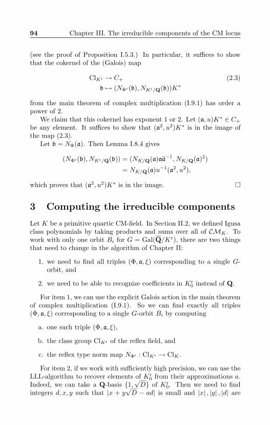
94 Chapter III. The irreducible components of the CM locus
(see the proof of Proposition I.5.3.) In particular, it suffices to showthat the cokernel of the (Galois) map
ClKr → C+ (2.3)b 7→ (NΦr(b), NKr/Q(b))K∗
from the main theorem of complex multiplication (I.9.1) has order apower of 2.
We claim that this cokernel has exponent 1 or 2. Let (a, u)K∗ ∈ C+
be any element. It suffices to show that (a2, u2)K∗ is in the image ofthe map (2.3).
Let b = NΦ(a). Then Lemma I.8.4 gives
(NΦr(b), NKr/Q(b)) = (NK/Q(a)aa−1, NK/Q(a)2)
= NK/Q(a)u−1(a2, u2),
which proves that (a2, u2)K∗ is in the image.
3 Computing the irreducible components
Let K be a primitive quartic CM-field. In Section II.2, we defined Igusaclass polynomials by taking products and sums over all of CMK . Towork with only one orbit Bi for G = Gal(Q/Kr), there are two thingsthat need to change in the algorithm of Chapter II:
1. we need to find all triples (Φ, a, ξ) corresponding to a single G-orbit, and
2. we need to be able to recognize coefficients in Kr0 instead of Q.
For item 1, we can use the explicit Galois action in the main theoremof complex multiplication (I.9.1). So we can find exactly all triples(Φ, a, ξ) corresponding to a single G-orbit Bi by computing
a. one such triple (Φ, a, ξ),
b. the class group ClKr of the reflex field, and
c. the reflex type norm map NΦr : ClKr → ClK .
For item 2, if we work with sufficiently high precision, we can use theLLL-algorithm to recover elements of Kr
0 from their approximations a.Indeed, we can take a Q-basis 1,
√D of Kr
0. Then we need to findintegers d, x, y such that |x + y
√D − ad| is small and |x| , |y| , |d| are
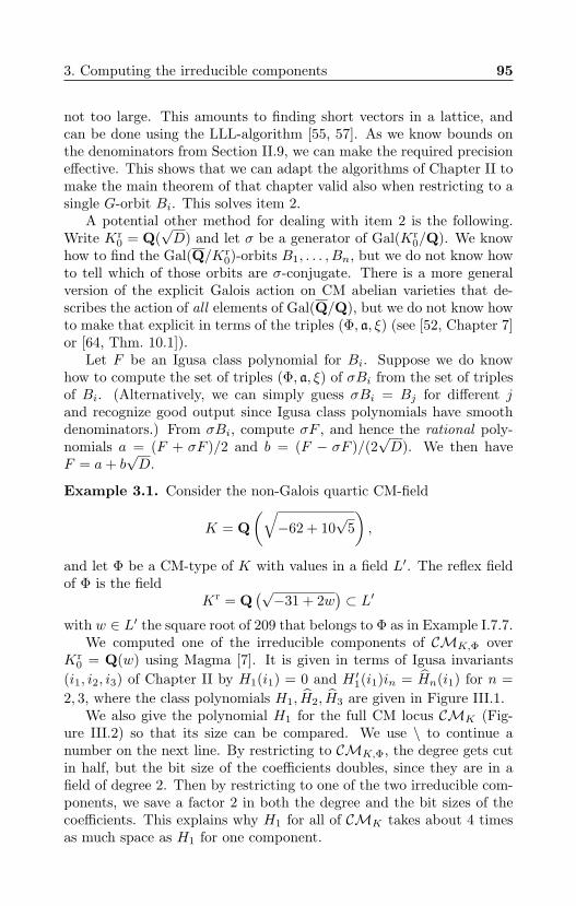
3. Computing the irreducible components 95
not too large. This amounts to finding short vectors in a lattice, andcan be done using the LLL-algorithm [55, 57]. As we know bounds onthe denominators from Section II.9, we can make the required precisioneffective. This shows that we can adapt the algorithms of Chapter II tomake the main theorem of that chapter valid also when restricting to asingle G-orbit Bi. This solves item 2.
A potential other method for dealing with item 2 is the following.Write Kr
0 = Q(√D) and let σ be a generator of Gal(Kr
0/Q). We knowhow to find the Gal(Q/Kr
0)-orbits B1, . . . , Bn, but we do not know howto tell which of those orbits are σ-conjugate. There is a more generalversion of the explicit Galois action on CM abelian varieties that de-scribes the action of all elements of Gal(Q/Q), but we do not know howto make that explicit in terms of the triples (Φ, a, ξ) (see [52, Chapter 7]or [64, Thm. 10.1]).
Let F be an Igusa class polynomial for Bi. Suppose we do knowhow to compute the set of triples (Φ, a, ξ) of σBi from the set of triplesof Bi. (Alternatively, we can simply guess σBi = Bj for different jand recognize good output since Igusa class polynomials have smoothdenominators.) From σBi, compute σF , and hence the rational poly-nomials a = (F + σF )/2 and b = (F − σF )/(2
√D). We then have
F = a+ b√D.
Example 3.1. Consider the non-Galois quartic CM-field
K = Q(√−62 + 10
√5),
and let Φ be a CM-type of K with values in a field L′. The reflex fieldof Φ is the field
Kr = Q(√−31 + 2w
)⊂ L′
with w ∈ L′ the square root of 209 that belongs to Φ as in Example I.7.7.We computed one of the irreducible components of CMK,Φ over
Kr0 = Q(w) using Magma [7]. It is given in terms of Igusa invariants
(i1, i2, i3) of Chapter II by H1(i1) = 0 and H ′1(i1)in = Hn(i1) for n =2, 3, where the class polynomials H1, H2, H3 are given in Figure III.1.
We also give the polynomial H1 for the full CM locus CMK (Fig-ure III.2) so that its size can be compared. We use \ to continue anumber on the next line. By restricting to CMK,Φ, the degree gets cutin half, but the bit size of the coefficients doubles, since they are in afield of degree 2. Then by restricting to one of the two irreducible com-ponents, we save a factor 2 in both the degree and the bit sizes of thecoefficients. This explains why H1 for all of CMK takes about 4 timesas much space as H1 for one component.
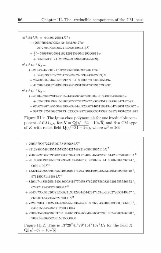
96 Chapter III. The irreducible components of the CM locus
4141512H1 = 64430176561X2+
+ (205979078609524124783186427w
− 2977804995699524132924128431)X
+ 12
(−5989798058911821291359304620360613w
+ 86593506017412522675907964506455189),
254161514H2 =
(−2454824558012170122865050318993532473w
+ 35488986976522847855248253994749432769)X
+ 28768580464678570992891511300020790788865449w
− 415902543137343993908045193128947052915790897,
244161514H3 =
(−46704828432019435152440758726755388043516900604046875w
+ 675203871999156667302727347262228663935171080625421875)X
+ 679079867385550495809638344092030714651189434647926317296875w
− 9817343757568579773462300542972200305315399159578183102671875.
Figure III.1: The Igusa class polynomials for one irreducible com-ponent of CMK,Φ for K = Q(
√−62 + 10
√5) and Φ a CM-type
of K with reflex field Q(√−31 + 2w), where w2 = 209.
+ 269367906727345961584860889X8
− 33128880546035571578256427748821805963065110X7
+ 760725219835798482803057024121173485345642256181420678103101X6
− 201836841928853870869673149461673014490785144130607309326594 \
00091100X5
+ 133215353686803856040610047747939496199893025334951028522948 \
971180071435884X4
− 829347448567954740436008416770958878225775808266301555556353 \
6247717943492256000X3
+ 464337306516263812668271334283446442447453436180272653149457 \
8699071343804782750000X2
+ 732462014111027434438225593367846913026584394848893801366481 \643515834623557125000000X
+ 220093549307982637631998652937565840956847210136744902156820 \90021485695620015625000000
Figure III.2: This is 13429241479215121672H1 for the field K =Q(√−62 + 10
√5).
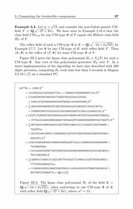
3. Computing the irreducible components 97
Example 3.2. Let w =√
13, and consider the non-Galois quartic CM-field F = Q(
√−27 + 4w). We have seen in Example I.10.4 that the
class field CMF,Ψ for any CM-type Ψ of F equals the Hilbert class fieldHF of F .
The reflex field of such a CM-type Ψ is K = Q(√−54 + 2
√521) by
Example I.7.7. Let Φ be any CM-type of K with reflex field F . Then(K,Φ) is the reflex of (F,Ψ) for some CM-type Ψ of F .
Figure III.3 gives the Igusa class polynomial H1 ∈ F0[X] for such aCM-type Φ. Any root of this polynomial generates HF over F . In anaive implementation of the algorithm we have just described with 200digits precision, computing H1 took time less than 3 seconds in MagmaV2.16-1 [7] on a standard PC.
1012H1 = 10201X7
+ (155205162116358647755w + 559600170220938887110)X6
+ (152407687697460195175920750535594152550w
+ 549513732768094956258970636118192859400)X5
+ 12
(2201909580030523730272623848434538048317834513875w
+ 7939097894735431844153019089320973153011210882125)X4
+ (1047175262927393182849164587480891367594710449395570625w
+ 3775644104882200832865729346429752069380200097845736875)X3
+ 12
(90739291480049485513675299110604131111640471324738060 \
7234375w
+ 327165168130591119268893142372375309476346120037916993 \
8284375)X2
+ (1501416604965651986004588022297124411339065052590506998 \7454062500w
+ 541343455503671907856059844455869398930835318514053659 \78411062500)X
+ 12
(32085417029115132212877701052175189051312077050549053 \
7777676328984375w
+ 115685616293120067038709321144324285012570966768326545 \9917987279296875) ∈ Q(w)[X]
Figure III.3: The Igusa class polynomial H1 of the field K =Q(√−54 + 2
√521), when restricting to one CM-type Φ of K
with reflex field Q(√−27 + 4w), where w2 = 13.
98 Chapter III. The irreducible components of the CM locus
To compute HF using Kummer theory, one needs to take a 7-throot of an element in the degree-24 number field F (ζ7). On the samemachine, with the Magma function HilbertClassField, it takes about2 minutes to compute the Hilbert class field of F . This is a lot longerthan the 3 seconds we needed for computing H1. The output is the fieldHF = F [X]/P with
P = X7 + (−49w − 133)X5
+ (8036w − 10955)X4
+ (247401w − 880005)X3
+ 12 (24737797w − 68979519)X2
+ 12 (533791741w − 1896276501)X
+ 12 (6759148445w − 11784293007) ∈ F0[X].
4 The CM method
Now let g be an arbitrary positive integer again. Suppose we wantto construct a g-dimensional abelian variety over a finite field with aprescribed irreducible characteristic polynomial f of the Frobenius en-domorphism. The field K = Q[X]/(f) is a CM-field of degree 2g andthe constant coefficient f(0) = pm is a prime power.
Take any point A of CMK and look at the reduction A of A moduloa prime P/p of a field of definition k ⊃ Kr of A. Let Φ be the CM-typeof A, and let Frob ∈ End(A) be the Frobenius endomorphism. Then wehave the following result.
Theorem 4.1 (Shimura-Taniyama formula [78, Thm. 1 in §1]). Themorphism Frob is an element of the ring OK ⊂ End(A) and generatesthe ideal NΦr(Nk/Kr(P)) of OK .
Corollary 4.2. The abelian variety A is isomorphic over Fp to anabelian variety with characteristic polynomial f if and only if a powerof π = (X mod f) ∈ K generates the ideal NΦr(Nk/Kr(P)) of OK .
Proof. See Honda and Tate [84].
The corollary shows that, when doing CM constructions as above, itis good to first find out for which CM-type Φ the element π generatesthe reflex type norm of an ideal and then restrict to A ∈ CMK,Φ.
4. The CM method 99
Example 4.3. Suppose we want to construct an abelian surface A overthe finite field of q = pk elements with a given Frobenius endomorphismπ in a non-Galois CM-field K. Let Φ be a CM-type of K.
A common case is that p splits completely in K. Indeed, this is oneof the only two unramified decomposition types of p in K for which A isordinary (Goren [34]). Moreover, this is what will happen by construc-tion in Chapter IV.
If p splits completely in K, then it factors as pOK = p1p1p2p2.The 4 primes q/p of Kr have the 4 distinct type norms given up tocomplex conjugation by NΦr(q) = p1p2 and NΦr(q) = p1p2. We thusfind NΦr(q)k = πOK for at most one q. To get an abelian surface A withFrobenius endomorphism π (up to complex conjugation), it is essentialthat we reduce modulo a prime above such a prime q. This amounts totaking A to be a point of
CMK,Φ mod (q ∩Kr0).
By Theorem 4.1, we know Frob to be a generator of NΦr(q)k. Thisfact and the fact Frob · Frob = pk determine Frob uniquely up to rootsof unity in O∗K . As non-Galois quartic CM-fields do not have non-trivialroots of unity, we find that Frob is determined uniquely up to ±1, thatis, up to quadratic twists of A.
In Example 3.1, reducing modulo a prime above q amounts to replac-ing w ∈ Kr
0 by (w mod q) ∈ Fp, and then taking a solution (i1, i2, i3) ∈F3pk to H1(i1) = 0 and in = Hn(i1)/H ′1(i1) for n = 2, 3.
For the prime p = 2128 + 463, which splits completely in K, thereis a unique element π ∈ OK with ππ = p and such that NK/Q(π − 1),which is the order of the corresponding abelian variety, is a prime timesa small integer. For that element π, we have that NK/Q(π − 1) is 4times the prime
N = 2254 − 5632861158402111064848197526240511442172628827329154462023.
We computed the appropriate prime q in Kr and found
w ≡ 247135999804258747492727825167682242163 (mod q).
We substitute this root modulo p in the class polynomials of Exam-ple 3.1, and find a solution
i1 = 186664603574701364556020498489782319955,i2 = 248015365398797493486326534484503677658,i3 = 92979908727002348130966293837941380436 ∈ Fp.
Mestre’s algorithm [61] (available in Magma [7]) allows us to construct acurve C : y2 = f(x) from this solution. Either the Jacobian of C or the
100 Chapter III. The irreducible components of the CM locus
Jacobian of its quadratic twist C ′ has order 4N . The quadratic twist isgiven by C ′ : y2 = cf(x) for a non-square c ∈ Fp. By taking randompoints on the Jacobians of C and C ′ and multiplying them by 4N , wecan check which of the two has the appropriate number of points. Wefind that the Jacobian of the curve
C : y2 = x6 + 194876360407882453864339562084283578641x4
+ 72507634844552606901950607039139106841x3
+ 215701338546912274238542720250901753991x2
+ 149128889692643278587362953981454162789x+ 277144679648822640993017616187904126204
over Fp has a point of order N . In particular, the Frobenius endomor-phism of this Jacobian is π.
Example 4.4. Let l be an odd prime number and consider the fieldK = Q(ζ) for a primitive l-th root of unity ζ. Then K is a CM-fieldof degree l − 1 and we let g = (l − 1)/2. We know one point in CMK
explicitly as the Jacobian of a hyperelliptic curve: the Jacobian J(C) ofthe curve C : y2 = xl + 1 of genus g given in Example I.6.1. We knowby that example that J(C) has type Φ = ζ 7→ ζl : l = 1, . . . , g.
Suppose we want to use this curve to construct an abelian varietyover a finite field with a prescribed Frobenius endomorphism π ∈ K.By Corollary 4.2, this is possible only if we can write a power of πOKas a type norm for the reflex type Φr of the CM-type Φ.
Composing ι on the right with an automorphism σ of K replaces Φby Φ σ and Φr by Φr σ−1. This does not change the possible valuesof NΦr . We thus find that there is one “correct” equivalence class ofCM-type Φ.
Example 4.5. In Chapter IV, we construct Weil numbers π as typenorms with respect to the reflex of a CM-type Φ1. When that chapterwas published as [26], we were unaware of Corollary 4.2.
Example 5.4 of that chapter uses the the curve
y2 = x17 + 1.
We used random CM-types Φ1 of Q(ζ17) for constructing π, and thentried to use the curve C of Example 4.4 to construct an abelian varietywith Frobenius endomorphism π. We found that with some CM-typesΦ1, we always failed, while with others, we always succeeded.
The CM-type Φ1 = ζ17 7→ ζk17 : k = 1, 3, 5, 6, 8, 10, 13, 15 was oneof the ‘successful’ ones. It turns out that this CM-type Φ1 is equivalent
5. Double roots 101
to the type Φ of Example 4.4 above. Indeed, with σ(ζ17) = ζ517, we have
Φ1 = Φ σ.By Corollary 4.2, we could have started out with Φ immediately
instead of trying random CM-types Φ1 until successful.
5 Double roots
In this section, let K be a primitive quartic CM-field. The Igusa classpolynomials HK,2, HK,3 of Section II.2.2 are useful only if HK,1 has asimple root. In practice, it never seems to happen that HK,1 has a non-simple root. This is not surprising as the coefficients grow exponentiallywith the degree of these polynomials.
If we want a proven algorithm for computing CMK,Φ or an irre-ducible factor, then this argument isn’t strong enough. In this section,we prove the following results.
Theorem 5.1. Algorithm II.11.1 can be adapted so that it computes aset of defining polynomials for CMK,Φ in time O(∆7/2
1 ∆11/20 ) for any
primitive quartic CM-field K and CM-type Φ. The output is given as aset of polynomial equations for the irreducible factors over Kr
0.
Theorem 5.2. Algorithm II.11.1 can be adapted so that it computesthe field CMKr,Φr of Chapter I in time O(∆7/2
1 ∆11/20 ) for any primitive
quartic CM-field K and CM-type Φ of K.
The output in Theorem 5.2 is an ordered set of generators and aminimal polynomial of each generator in terms of the earlier ones.
If i1(C) is distinct for all C ∈ CMK , then the field extensionCMKr,Φr/Kr
0 is simply given over Kr0 by the polynomial HK,1 for one
Gal(Q/Kr0)-orbit in CMK,Φ. If moreover i3(C) is non-zero for all C ∈
CMK , then the points of a component Bj of CMK,Φ ⊂ M2 are thosepoints with HK,1(i1) = 0, HK,n(i1) = inH
′K,1(i1) for n = 2, 3, where
the sums and products in the definitions of the class polynomials arerestricted to Bj . In practice, this is the whole story, though it is nota proof. The rest of this section proves the theorems without theseassumptions.
As explained in Section 3, we can restrict to the irreducible compo-nents of CMK,Φ. Note that all i3(C)’s for one component are Galoisconjugate, so that one is zero if and only if all are. It is therefore possi-ble to check i3(C) 6= 0 simply by checking HK,3(0) = 0. In particular,we can use the absolute invariants (i1, i2, i3) of Section II.2 if i3(C) 6= 0,
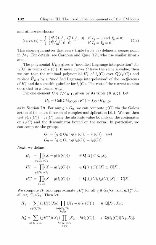
102 Chapter III. The irreducible components of the CM locus
and otherwise choose
(i1, i2, i3) =
(I22I′6I−110 , I
′56 I−310 , 0) if I4 = 0 and I ′6 6= 0;
(I52I−110 , 0, 0) if I4 = I ′6 = 0.
(5.3)
This choice guarantees that every triple (i1, i2, i3) defines a unique pointin M2. For details, see Cardona and Quer [12], who use similar invari-ants.
The polynomial HK,2 gives a “modified Lagrange interpolation” fori2(C) in terms of i1(C). If more curves C have the same i1-value, thenwe can take the minimal polynomial H∗2 of i2(C) over Q(i1(C)) andreplace HK,2 by a “modified Lagrange interpolation” of the coefficientsof H∗2 and do something similar for i3(C). The rest of the current sectiondoes that in a formal way.
Fix one element C ∈ CMK,Φ, given by its triple (Φ, a, ξ). Let
G0 = Gal(CMKr,Φr/Kr) = IKr/HKr,Φr
as in Section I.9. For any g ∈ G0, we can compute g(C) via the Galoisaction of the main theorem of complex multiplication I.9.1. We can thentest g(i1(C)) = i1(C) using the absolute value bounds on the conjugateson i1(C) and the denominator bound on the norm. In particular, wecan compute the groups
G1 = g ∈ G0 : g(i1(C)) = i1(C) andG2 = g ∈ G1 : g(i2(C)) = i2(C).
Next, we define
H1 =∏
g∈G0/G1
(X − g(i1(C))) ∈ Q[X] ⊂ C[X],
H∗2 =∏
g∈G1/G2
(X − g(i2(C))) ∈ Q(i1(C))[X] ⊂ C[X],
H∗∗3 =∏g∈G2
(X − g(i3(C))) ∈ Q(i1(C), i2(C))[X] ⊂ C[X].
We compute H1 and approximate gH∗2 for all g ∈ G0/G1 and gH∗∗3 forall g ∈ G0/G2. Then let
H2 =∑
g∈G/G1
(gH∗2 )(X2)∏
h∈G0/G1h6=g
(X1 − h(i1(C))) ∈ Q[X1, X2],
H∗3 =∑
g∈G1/G2
(gH∗∗3 )(X3)∏
h∈G1/G2h6=g
(X2 − h(i2(C))) ∈ Q(i1(C))[X2, X3].
5. Double roots 103
Again, we compute H2 and approximate gH∗3 for all g ∈ G/G1.Finally, let
H3 =∑
g∈G/G1
(gH∗3 )(X2, X3)∏
h∈G0/G1h6=g
(X1 − h(i1(C))) ∈ Q[X1, X2, X3].
Finally, we compute H3. As all computations mentioned above can bedone in the time mentioned in Theorem 5.1, the following lemma provesthat theorem.
Lemma 5.4. The zero set of (H1, H2, H3) ⊂ Q[X1, X2, X3] in Q3 isexactly the orbit of C ∈ CMK,Φ under the action of G = Gal(Q/Kr).
Proof. The polynomial H1 is the minimal polynomial of C, hence hasas its roots exactly the values of i1(g(C)) when g ranges over G.
If we substitute one of these values i01 = i1(g(C)) for X1, then H2
becomes a univariate polynomial in X = X2. In fact, this univariatepolynomial is a non-zero constant times gH∗2 , hence its roots are thevalues of ghi2(C) where h ranges over G1/G2. As hG1 leaves gi1(C)invariant, the roots of gH∗2 are exactly the values of i2 correspondingto i01.
Suppose we substitute one of these pairs (i01, i02) = gh(i1, i2)(C) for
(X1, X2) in H3. Then H3 becomes a univariate polynomial in X =X3. In fact, it becomes a non-zero constant times H∗∗3 . By the sameargument as above, we find that the roots of this polynomial are exactlythe i3-values corresponding to our pair (i01, i
02).
As mentioned just below equation (5.3), the triples (i1, i2, i3)(g(C))determine g(C) completely.
Proof of Theorem 5.2. By Lemma 5.4, we have a tower of fields
Kr ⊂ Kr(i1(C)) ⊂ Kr(i1(C), i2(C)) ⊂ Kr(i1(C), i2(C), i3(C)),
where the minimal polynomials of i1(C), i2(C), and i3(C) are given byH1, H2(i1(C), X), and H3(i1(C), i2(C), X). As the largest field in thistower equals CMKr,Φr , this proves Theorem 5.2.

ChapterIVAbelian varieties with prescribed embeddingdegree
This chapter appeared as David Freeman, Peter Stevenhagen, and Mar-co Streng, Abelian Varieties with Prescribed Embedding Degree [26] inAlgorithmic Number Theory, ANTS-VIII, volume 5011 of Lecture Notesin Computer Science, 2008.
Abstract. We present an algorithm that, on input of aCM-field K, an integer k ≥ 1, and a prime r ≡ 1 mod k,constructs a q-Weil number π ∈ OK corresponding to anordinary, simple abelian variety A over the field F of q ele-ments that has an F-rational point of order r and embeddingdegree k with respect to r. We then discuss how CM-methodscan be used to explicitly construct A.
1 Introduction
Let A be an abelian variety defined over a finite field F, and r 6= char(F)a prime number dividing the order of the group A(F). Then the em-bedding degree of A with respect to r is the degree of the field extensionF ⊂ F(ζr) obtained by adjoining a primitive r-th root of unity ζr to F.
The embedding degree is a natural notion in pairing-based cryptog-raphy, where A is taken to be the Jacobian of a curve defined over F.
106 Chapter IV. Abelian varieties with prescribed embedding degree
In this case, A is principally polarized and we have the non-degenerateWeil pairing
er : A[r]×A[r] −→ µr
on the subgroup scheme A[r] of r-torsion points of A with values in ther-th roots of unity. If F contains ζr, we also have the non-trivial Tatepairing
tr : A[r](F)×A(F)/rA(F)→ F∗/(F∗)r.
The Weil and Tate pairings can be used to ‘embed’ r-torsion subgroupsof A(F) into the multiplicative group F(ζr)∗, and thus the discrete loga-rithm problem in A(F)[r] can be ‘reduced’ to the same problem in F(ζr)∗
[60, 29]. In pairing-based cryptographic protocols [67], one chooses theprime r and the embedding degree k such that the discrete logarithmproblems in A(F)[r] and F(ζr)∗ are computationally infeasible, and ofroughly equal difficulty. This means that r is typically large, whereas kis small. Jacobians of curves meeting such requirements are often saidto be pairing-friendly.
If F has order q, the embedding degree k = [F(ζr) : F] is simplythe multiplicative order of q in (Z/rZ)∗. As ‘most’ elements in (Z/rZ)∗
have large order, the embedding degree of A with respect to a largeprime divisor r of #A(F) will usually be of the same size as r, andA will not be pairing-friendly. One is therefore led to the questionof how to efficiently construct A and F such that A(F) has a (large)prime factor r and the embedding degree of A with respect to r has aprescribed (small) value k. The current paper addresses this questionon two levels: the existence and the actual construction of A and F.
Section 2 focuses on the question whether, for given r and k, thereexist abelian varieties A that are defined over a finite field F, have anF-rational point of order r, and have embedding degree k with respectto r. We consider only abelian varieties A that are simple, that is, notisogenous (over F) to a product of lower-dimensional varieties, as wecan always reduce to this case. By Honda-Tate theory [84], isogenyclasses of simple abelian varieties A over the field F of q elements arein one-to-one correspondence with Gal(Q/Q)-conjugacy classes of q-Weil numbers, which are algebraic integers π with the property that allembeddings of π into C have absolute value
√q. This correspondence is
given by the map sending A to its q-th power Frobenius endomorphismπ inside the number field Q(π) ⊂ End(A)⊗Q. The existence of abelianvarieties with the properties we want is thus tantamount to the existenceof suitable Weil numbers.
Our main result, Algorithm 2.12, constructs suitable q-Weil numbersπ in a given CM-field K. It exhibits π as a type norm of an element in
2. Weil numbers yielding prescribed embedding degrees 107
a reflex field of K satisfying certain congruences modulo r. The abelianvarieties A in the isogeny classes over F that correspond to these Weilnumbers have an F-rational point of order r and embedding degree kwith respect to r. Moreover, they are ordinary, i.e., #A(F)[p] = pg,where p is the characteristic of F. Theorem 3.1 shows that for fixed K,the expected run time of our algorithm is heuristically polynomial inlog r.
For an abelian variety of dimension g over the field F of q elements,the group A(F) has roughly qg elements, and one compares this size tor by setting
ρ =g log qlog r
. (1.1)
In cryptographic terms, ρ measures the ratio of a pairing-based system’srequired bandwidth to its security level, so small ρ-values are desirable.Supersingular abelian varieties can achieve ρ-values close to 1, but theirembedding degrees are limited to a few values that are too small to bepractical [30, 69]. Theorem 3.4 discusses the distribution of the (larger)ρ-values we obtain.
In Section 4, we address the issue of the actual construction ofabelian varieties corresponding to the Weil numbers found by our algo-rithm. This is accomplished via the construction in characteristic zeroof the abelian varieties having CM by the ring of integers OK of K,a hard problem that is far from being algorithmically solved. We dis-cuss the elliptic case g = 1, for which reasonable algorithms exist, andthe case g = 2, for which such algorithms are still in their infancy. Forgenus g ≥ 3, we restrict attention to a few families of curves that we canhandle at this point. Our final Section 5 provides numerical examples.
2 Weil numbers yielding prescribedembedding degrees
Let F be a field of q elements, A a g-dimensional simple abelian varietyover F, and K = Q(π) ⊂ End(A) ⊗Q the number field generated bythe Frobenius endomorphism π. Then π is a q-Weil number in K: analgebraic integer with the property that all of its embeddings in Q havecomplex absolute value
√q.
The q-Weil number π determines the group order of A(F): the F-rational points of A form the kernel of the endomorphism π− 1, and inthe case where K = Q(π) is the full endomorphism algebra End(A)⊗Qwe have
#A(F) = NK/Q(π − 1).
108 Chapter IV. Abelian varieties with prescribed embedding degree
In the case K = End(A)⊗Q we will focus on, K is a CM-field of degree2g as in [84, Section 1], i.e., a totally complex quadratic extension of atotally real subfield K0 ⊂ K.
Proposition 2.1. Let A, F and π be as above, and assume K = Q(π)equals EndF(A)⊗Q. Let k be a positive integer, Φk the k-th cyclotomicpolynomial, and r - qk a prime number. If we have
NK/Q(π − 1) ≡ 0 (mod r),Φk(ππ) ≡ 0 (mod r),
then A has embedding degree k with respect to r.
Proof. The first condition tells us that r divides #A(F), the second thatthe order of ππ = q in (Z/rZ)∗, which is the embedding degree of Awith respect to r, equals k.
By Honda-Tate theory [84], all q-Weil numbers arise as Frobeniuselements of abelian varieties over F. Thus, we can prove the existenceof an abelian variety A as in Proposition 2.1 by exhibiting a q-Weilnumber π ∈ K as in that proposition. The following lemma states whatwe need.
Lemma 2.2. Let π be a q-Weil number. Then there exists a uniqueisogeny class of simple abelian varieties A/F with Frobenius π. If K =Q(π) is totally imaginary of degree 2g and q is prime, then such A havedimension g, and K is the full endomorphism algebra EndF(A)⊗Q. Iffurthermore q is unramified in K, then A is ordinary.
Proof. The main theorem of [84] yields existence and uniqueness, andshows that E = EndF(A)⊗Q is a central simple algebra over K = Q(π)satisfying
2 · dim(A) = [E : K]12 [K : Q].
For K totally imaginary of degree 2g and q prime, Waterhouse [92,Theorem 6.1] shows that we have E = K and dim(A) = g. By [92,Prop. 7.1], A is ordinary if and only if π+ π is prime to q = ππ in OK .Thus if A is not ordinary, the ideals (π) and (π) have a common divisorp ⊂ OK with p2 | q, so q ramifies in K.
Example 2.3. Our general construction is motivated by the case whereK is a Galois CM-field of degree 2g, with cyclic Galois group generatedby σ. Here σg is complex conjugation, so we can construct an elementπ ∈ OK satisfying πσg(π) = ππ ∈ Z by choosing any ξ ∈ OK and
2. Weil numbers yielding prescribed embedding degrees 109
letting π =∏gi=1 σ
i(ξ). For such π, we have ππ = NK/Q(ξ) ∈ Z. IfNK/Q(ξ) is a prime q, then π is a q-Weil number in K.
Now we wish to impose the conditions of Proposition 2.1 on π. Letr be a rational prime that splits completely in K, and r a prime of OKover r. For i = 1, . . . , 2g, put ri = σ−i(r); then the factorization of rin OK is rOK =
∏2gi=1 ri. If αi ∈ Fr = OK/ri is the residue class of
ξ modulo ri, then σi(ξ) modulo r is also αi, so the residue class of πmodulo r is
∏gi=1 αi. Furthermore, the residue class of ππ modulo r is∏2g
i=1 αi. If we choose ξ to satisfy∏gi=1 αi = 1 ∈ Fr, (2.4)
we find π ≡ 1 (mod r) and thus NK/Q(π−1) ≡ 0 (mod r). By choosingξ such that in addition
ζ =∏2gi=1 αi =
∏2gi=g+1 αi (2.5)
is a primitive k-th root of unity in F∗r , we guarantee that ππ = q is aprimitive k-th root of unity modulo r. Thus we can try to find a Weilnumber as in Proposition 2.1 by picking residue classes αi ∈ F∗r fori = 1, . . . , 2g meeting the two conditions above, computing some ‘small’lift ξ ∈ OK with (ξ mod ri) = αi, and testing whether π =
∏gi=1 σ
i(ξ)has prime norm. As numbers of moderate size have a high probabil-ity of being prime by the prime number theorem, a small number ofchoices (αi)i should suffice. There are (r − 1)2g−2ϕ(k) possible choicesfor (αi)
2gi=1, where ϕ is the Euler totient function, so for g > 1 and large
r we are very likely to succeed. For g = 1, there are only a few choices(α1, α2) = (1, ζ), but one can try various lifts and thus recover whatis known as the Cocks-Pinch algorithm [25, Theorem 4.1] for findingpairing-friendly elliptic curves.
For arbitrary CM-fields K, the appropriate generalization of the map
ξ 7→∏gi=1 σ
i(ξ)
in Example 2.3 is provided by the type norm. A CM-type of a CM-field K of degree 2g is a set Φ = φ1, . . . , φg of embeddings of K intoits normal closure L such that Φ ∪ Φ = φ1, . . . , φg, φ1, . . . , φg is thecomplete set of embeddings of K into L. The type norm NΦ : K → Lwith respect to Φ is the map
NΦ : x 7−→∏gi=1 φi(x),
which clearly satisfies
NΦ(x)NΦ(x) = NK/Q(x) ∈ Q. (2.6)
110 Chapter IV. Abelian varieties with prescribed embedding degree
If K is not Galois, the type norm NΦ does not map K to itself, but toits reflex field K with respect to Φ. To end up in K, we can howevertake the type norm with respect to the reflex type Ψ, which we willdefine now (cf. [77, Section 8]).
Let G be the Galois group of L/Q, and H the subgroup fixing K.Then the 2g left cosets of H in G can be viewed as the embeddings ofK in L, and this makes the CM-type Φ into a set of g left cosets of Hfor which we have G/H = Φ ∪ Φ. Let S be the union of the left cosetsin Φ, and put S = σ−1 : σ ∈ S. Let H = γ ∈ G : γS = S be thestabilizer of S in G. Then H defines a subfield K of L, and as we haveH = γ ∈ G : Sγ = S we can interpret S as a union of left cosets of Hinside G. These cosets define a set of embeddings Ψ of K into L. Wecall K the reflex field of (K,Φ) and we call Ψ the reflex type.
Lemma 2.7. The field K is a CM-field. It is generated over Q by thesums
∑φ∈Φ φ(x) for x ∈ K, and Ψ is a CM-type of K. The type norm
NΦ maps K to K.
Proof. The first two statements are proved in [77, Chapter II, Proposi-tion 28] (though the definition of H differs from ours, because Shimuralets G act from the right). For the last statement, notice that for γ ∈ H,we have γS = S, so γ
∏φ∈Φ φ(x) =
∏φ∈Φ φ(x).
A CM-type Φ of K is induced from a CM-subfield K ′ ⊂ K if itis of the form Φ = φ : φ|K′ ∈ Φ′ for some CM-type Φ′ of K ′. Inother words, Φ is induced from K ′ if and only if S as above is a unionof left cosets of Gal(L/K ′). We call Φ primitive if it is not inducedfrom a strict subfield of K; primitive CM-types correspond to simpleabelian varieties [77]. Notice that the reflex type Ψ is primitive bydefinition of K, and that (K,Φ) is induced from the reflex of its reflex.In particular, if Φ is primitive, then the reflex of its reflex is (K,Φ)itself. For K Galois and Φ primitive we have K = K, and the reflextype of Φ is Ψ = φ−1 : φ ∈ Φ.
For CM-fields K of degree 2 or 4 with primitive CM-types, the reflexfield K has the same degree as K. This fails to be so for g ≥ 3.
Lemma 2.8. If K has degree 2g, then the degree of K divides 2gg!.
Proof. We have K = K0(√η), with K0 totally real and η ∈ K totally
negative. The normal closure L of K is obtained by adjoining to thenormal closure K0 of K0, which has degree dividing g!, the square rootsof the g conjugates of η. Thus L is of degree dividing 2gg!, and K is asubfield of L.
2. Weil numbers yielding prescribed embedding degrees 111
For a ‘generic’ CM-field K the degree of L is exactly 2gg!, and Kis a field of degree 2g generated by
∑σ
√σ(η), with σ ranging over
Gal(K0/Q).From (2.6) and Lemma 2.7, we find that for every ξ ∈ OK , the
element π = NΨ(ξ) is an element of OK that satisfies ππ ∈ Z. To makeπ satisfy the conditions of Proposition 2.1, we need to impose conditionsmodulo r on ξ in K. Suppose r splits completely in K, and therefore inits normal closure L and in the reflex field K with respect to Φ. Picka prime R over r in L, and write rψ = ψ−1(R) ∩ OK for ψ ∈ Ψ. Thenthe factorization of r in OK is
rOK =∏ψ∈Ψ rψrψ. (2.9)
Theorem 2.10. Let (K,Φ) be a CM-type and (K,Ψ) its reflex. Letr ≡ 1 (mod k) be a prime that splits completely in K, and write itsfactorization in OK as in (2.9). Given ξ ∈ OK , write (ξ mod rψ) =αψ ∈ Fr and (ξ mod rψ) = βψ ∈ Fr for ψ ∈ Ψ. If we have∏
ψ∈Ψ αψ = 1 and∏ψ∈Ψ βψ = ζ (2.11)
for some primitive k-th root of unity ζ ∈ F∗r, then π = NΨ(ξ) ∈ OKsatisfies ππ ∈ Z and
NK/Q(π − 1) ≡ 0 (mod r),Φk(ππ) ≡ 0 (mod r).
Proof. This is a straightforward generalization of the argument in Ex-ample 2.3. The conditions (2.11) generalize (2.4) and (2.5), and implyin the present context that π−1 ∈ OK and Φk(ππ) ∈ Z are in the primeR ⊂ OL over r that underlies the factorization (2.9).
If the element π in Theorem 2.10 generates K and NK/Q(π) is aprime q that is unramified in K, then by Lemma 2.2 π is a q-Weil num-ber corresponding to an ordinary abelian variety A over F = Fq withendomorphism algebra K and Frobenius element π. By Proposition 2.1,A has embedding degree k with respect to r. This leads to the followingalgorithm.
Algorithm 2.12.Input: a CM-field K of degree 2g ≥ 4, a primitive CM-type Φ of K,a positive integer k, and a prime r ≡ 1 (mod k) that splits completelyin K.Output: a prime q and a q-Weil number π ∈ K corresponding to an
112 Chapter IV. Abelian varieties with prescribed embedding degree
ordinary, simple abelian variety A/F with embedding degree k withrespect to r.
1. Compute a Galois closure L of K and the reflex (K,Ψ) of (K,Φ).Set g ← 1
2 deg K and write Ψ = ψ1, ψ2, . . . , ψg.
2. Fix a prime R | r of OL, and compute the factorization of r inOK as in (2.9).
3. Compute a primitive k-th root of unity ζ ∈ F∗r .
4. Choose random α1, . . . , αg−1, β1, . . . , βg−1 ∈ F∗r .
5. Set αg ←∏g−1i=1 α
−1i ∈ F∗r and βg ← ζ
∏g−1i=1 β
−1i ∈ F∗r .
6. Compute ξ ∈ OK such that (ξ mod rψi) = αi and (ξ mod rψi) =βi for i = 1, 2, . . . , g.
7. Set q ← NK/Q(ξ). If q is not prime, go to Step (4).
8. Set π ← NΨ(ξ). If q is not unramified in K, or π does not gener-ate K, go to Step (4).
9. Return q and π.
Remark 2.13. We require g ≥ 2 in Algorithm 2.12, as the case g = 1is already covered by Example 2.3, and requires a slight adaptation.
The condition that r be prime is for simplicity of presentation only;the algorithm easily extends to square-free values of r that are given asproducts of splitting primes. Such r are required, for example, by thecryptosystem of [6].
3 Performance of the algorithm
Theorem 3.1. If the field K is fixed, then the heuristic expected runtime of Algorithm 2.12 is polynomial in log r.
Proof. The algorithm consists of a precomputation for the field K inSteps (1)–(3), followed by a loop in Steps (4)–(7) that is performeduntil an element ξ is found that has prime norm NK/Q(ξ) = q, andwe also find in Step (8) that q is unramified in K and the type normπ = NΨ(ξ) generates K.
3. Performance of the algorithm 113
The primality condition in Step (7) is the ‘true’ condition that be-comes harder to achieve with increasing r, whereas the conditions inStep (8), which are necessary to guarantee correctness of the output,are so extremely likely to be fulfilled (especially in cryptographic appli-cations where K is small and r is large) that they will hardly ever failin practice and only influence the run time by a constant factor.
As ξ is computed in Step (6) as the lift to OK of an element ξ ∈OK/rOK ∼= (Fr)2g, its norm can be bounded by a constant multipleof r2g. Heuristically, q = NK/Q(ξ) behaves as a random number, soby the prime number theorem it will be prime with probability at least(2g log r)−1, and we expect that we need to repeat the loop in Steps(4)–(7) about 2g log r times before finding ξ of prime norm q. As eachof the steps is polynomial in log r, so is the expected run time up toStep (7), and we are done if we show that the conditions in Step (8)are met with some positive probability if K is fixed and r is sufficientlylarge.
For q being unramified in K, one simply notes that only finitelymany primes ramify in the field K (which is fixed) and that q tends toinfinity with r, since r divides NK/Q(π − 1) ≤ (
√q + 1)2g.
Finally, we show that π generates K with probability tending to 1as r tends to infinity. Suppose that for every vector v ∈ 0, 1g that isnot all 0 or 1, we have ∏g
i=1(αi/βi)vi 6= 1. (3.2)
This set of 2g − 2 (dependent) conditions on the 2g − 2 independentrandom variables αi, βi for 1 ≤ i < g is satisfied with probability atleast 1− (2g − 2)/(r − 1). For any automorphism φ of L, the set φ Ψis a CM-type of K and there is a v ∈ 0, 1g such that vi = 0 if φ Ψcontains ψi and vi = 1 otherwise. Then αi is (ψi(ξ) mod R), while βi is(ψi(ξ) mod R), so (π/φ(π) mod R) is
∏gi=1(αi/βi)vi . By (3.2), if this
expression is 1 then v = 0 or v = 1, so φ Ψ = Ψ or φ Ψ = Ψ, whichby definition of the reflex is equivalent to φ or φ being trivial on K, i.e.,to φ being trivial on the maximal real subfield K0. Thus if (3.2) holds,then φ(π) = π implies that φ is trivial on K0, hence K0 ⊂ Q(π). Sinceπ ∈ K is not real (otherwise, q = π2 ramifies in K), this implies thatK = Q(π).
In order to maximize the likelihood of finding prime norms, oneshould minimize the norm of the lift ξ computed in the Chinese Re-mainder Step (6). This involves minimizing a norm function of degree2g in 2g integral variables, which is already infeasible for g = 2.
114 Chapter IV. Abelian varieties with prescribed embedding degree
In practice, for given r, one lifts a standard basis of OK/rOK ∼=(Fr)2g to OK . Multiplying those lifts by integer representatives for theelements αi and βi of Fr, one quickly obtains lifts ξ. We also choose,independently of r, a Z-basis of OK consisting of elements that are‘small’ with respect to all absolute values of K. We translate ξ bymultiples of r to lie in rF , where F is the fundamental parallelotopein K ⊗R consisting of those elements that have coordinates in (− 1
2 ,12 ]
with respect to our chosen basis.If we denote the maximum on F ∩ K of all complex absolute values
of K by MK , we have q = NK/Q(ξ) ≤ (rMK)2g. For the ρ-value (1.1)we find
ρ ≤ 2gg(1 + logMK/ log r), (3.3)
which is approximately 2gg if r gets large with respect to MK . Wewould like ρ to be small, but this is not what one obtains by liftingrandom admissible choices of ξ.
Theorem 3.4. If the field K is fixed and r is large, we expect that (1)the output q of Algorithm 2.12 yields ρ ≈ 2gg, and (2) an optimal choiceof ξ ∈ OK satisfying the conditions of Theorem 2.10 yields ρ ≈ 2g.
Open problem 3.5. Find an efficient algorithm to compute an elementξ ∈ OK satisfying the conditions of Theorem 2.10 for which ρ ≈ 2g.
We will prove Theorem 3.4 via a series of lemmas. Let Hr,k be thesubset of the parallelotope rF ⊂ K⊗R consisting of those ξ ∈ rF ∩OKthat satisfy the two congruence conditions (2.11) for a given embeddingdegree k. Heuristically, we will treat the elements of Hr,k as randomelements of rF with respect to the distributions of complex absolutevalues and norm functions. We will also use the fact that, as K is totallycomplex of degree 2g, the R-algebra K ⊗R is naturally isomorphic toCg. We assume throughout that g ≥ 2.
Lemma 3.6. Fix the field K. Under our heuristic assumption, thereexists a constant c1 > 0 such that for all ε > 0, the probability that arandom ξ ∈ Hr,k satisfies q < r2(g−ε) is less than c1r
−ε.
Proof. The probability that a random ξ lies in the set V = z ∈ Cg :∏|zi|2 ≤ r2(g−ε)∩rF is the quotient of the volume of V by the volume
2−g√∣∣∆K
∣∣r2g of rF , where ∆K is the discriminant of K. Now V is
contained inside W = z ∈ Cg :∏|zi|2 ≤ r2(g−ε), |zi| ≤ rMK, which
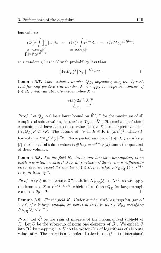
3. Performance of the algorithm 115
has volume
(2π)g∫
x∈[0,rMK
]g∏|xi|2≤r2(g−ε)
∏|xi|dx < (2π)g
∫x∈[0,rM
K]g
rg−εdx = (2πMK)gr2g−ε,
so a random ξ lies in V with probability less than
(4πMK)g∣∣∆K
∣∣−1/2r−ε.
Lemma 3.7. There exists a number QK , depending only on K, suchthat for any positive real number X < rQK , the expected number ofξ ∈ Hr,k with all absolute values below X is
ϕ(k)(2π)g∣∣∆K
∣∣ X2g
r2.
Proof. Let QK > 0 be a lower bound on K \ F for the maximum of allcomplex absolute values, so the box VX ⊂ K ⊗ R consisting of thoseelements that have all absolute values below X lies completely inside(X/QK)F ⊂ rF . The volume of VX in K ⊗ R is (πX2)g, while rF
has volume 2−g√∣∣∆K
∣∣r2g. The expected number of ξ ∈ Hr,k satisfying
|ξ| < X for all absolute values is #Hr,k = r2g−2ϕ(k) times the quotientof these volumes.
Lemma 3.8. Fix the field K. Under our heuristic assumption, thereexists a constant c2 such that for all positive ε < 2g−2, if r is sufficientlylarge, then we expect the number of ξ ∈ Hr,k satisfying NK/Q(ξ) < r2+ε
to be at least c2rε.
Proof. Any ξ as in Lemma 3.7 satisfies NK/Q(ξ) < X2g, so we applythe lemma to X = r(1/g+ε/2g), which is less than rQK for large enoughr and ε < 2g − 2.
Lemma 3.9. Fix the field K. Under our heuristic assumption, for allε > 0, if r is large enough, we expect there to be no ξ ∈ Hr,k satisfyingNK/Q(ξ) < r2−ε.
Proof. Let O be the ring of integers of the maximal real subfield ofK. Let U be the subgroup of norm one elements of O∗. We embed Uinto Rg by mapping u ∈ U to the vector l(u) of logarithms of absolutevalues of u. The image is a complete lattice in the (g − 1)-dimensional
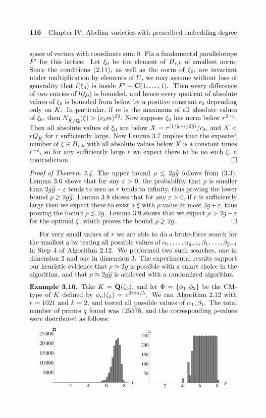
116 Chapter IV. Abelian varieties with prescribed embedding degree
space of vectors with coordinate sum 0. Fix a fundamental parallelotopeF ′ for this lattice. Let ξ0 be the element of Hr,k of smallest norm.Since the conditions (2.11), as well as the norm of ξ0, are invariantunder multiplication by elements of U , we may assume without loss ofgenerality that l(ξ0) is inside F ′ + C(1, . . . , 1). Then every differenceof two entries of l(ξ0) is bounded, and hence every quotient of absolutevalues of ξ0 is bounded from below by a positive constant c3 dependingonly on K. In particular, if m is the maximum of all absolute valuesof ξ0, then NK/Q(ξ) > (c3m)2g. Now suppose ξ0 has norm below r2−ε.Then all absolute values of ξ0 are below X = r(1/g−ε/2g)/c3, and X <rQK for r sufficiently large. Now Lemma 3.7 implies that the expectednumber of ξ ∈ Hr,k with all absolute values below X is a constant timesr−ε, so for any sufficiently large r we expect there to be no such ξ, acontradiction.
Proof of Theorem 3.4. The upper bound ρ > 2gg follows from (3.3).Lemma 3.6 shows that for any ε > 0, the probability that ρ is smallerthan 2gg− ε tends to zero as r tends to infinity, thus proving the lowerbound ρ ? 2gg. Lemma 3.8 shows that for any ε > 0, if r is sufficientlylarge then we expect there to exist a ξ with ρ-value at most 2g+ ε, thusproving the bound ρ > 2g. Lemma 3.9 shows that we expect ρ > 2g− εfor the optimal ξ, which proves the bound ρ ? 2g.
For very small values of r we are able to do a brute-force search forthe smallest q by testing all possible values of α1, . . . , αg−1, β1, . . . , βg−1
in Step 4 of Algorithm 2.12. We performed two such searches, one indimension 2 and one in dimension 3. The experimental results supportour heuristic evidence that ρ ≈ 2g is possible with a smart choice in thealgorithm, and that ρ ≈ 2gg is achieved with a randomized algorithm.
Example 3.10. Take K = Q(ζ5), and let Φ = φ1, φ2 be the CM-type of K defined by φn(ζ5) = e2πin/5. We ran Algorithm 2.12 withr = 1021 and k = 2, and tested all possible values of α1, β1. The totalnumber of primes q found was 125578, and the corresponding ρ-valueswere distributed as follows:
2 4 6 8Ρ
5000
10 000
15 000
20 000
25 000ð
2 4 6 8Ρ
50
100
150
200
250ð
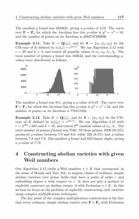
4. Constructing abelian varieties with given Weil numbers 117
The smallest q found was 2023621, giving a ρ-value of 4.19. The curveover F = Fq for which the Jacobian has this ρ-value is y2 = x5 + 18,and the number of points on its Jacobian is 4092747290896.
Example 3.11. Take K = Q(ζ7), and let Φ = φ1, φ2, φ3 be theCM-type of K defined by φi(ζ7) = e2πi/7. We ran Algorithm 2.12 withr = 29 and k = 4, and tested all possible values of α1, α2, β1, β2. Thetotal number of primes q found was 162643, and the corresponding ρ-values were distributed as follows:
5 10 15Ρ0
2000
4000
6000
8000ð
0 5 10 15Ρ
50
100
150
200
250ð
The smallest q found was 911, giving a ρ-value of 6.07. The curve overF = Fq for which the Jacobian has this ρ-value is y2 = x7 + 34, and thenumber of points on its Jacobian is 778417333.
Example 3.12. Take K = Q(ζ5), and let Φ = φ1, φ2 be the CM-type of K defined by φi(ζ5) = e2πi/5. We ran Algorithm 2.12 withr = 2160 + 685 and k = 10, and tested 220 random values of α1, β1. Thetotal number of primes q found was 7108. Of these primes, 6509 (91.6%)produced ρ-values between 7.9 and 8.0, while 592 (8.3%) had ρ-valuesbetween 7.8 and 7.9. The smallest q found had 623 binary digits, givinga ρ-value of 7.78.
4 Constructing abelian varieties with givenWeil numbers
Our Algorithm 2.12 yields q-Weil numbers π ∈ K that correspond, inthe sense of Honda and Tate [84], to isogeny classes of ordinary, simpleabelian varieties over prime fields that have a point of order r andembedding degree k with respect to r. It does not give a method toexplicitly construct an abelian variety A with Frobenius π ∈ K. In thissection we focus on the problem of explicitly constructing such varietiesusing complex multiplication techniques.
The key point of the complex multiplication construction is the factthat every ordinary, simple abelian variety over F = Fq with Frobenius
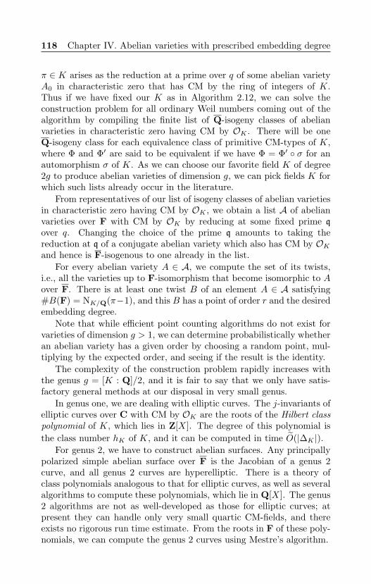
118 Chapter IV. Abelian varieties with prescribed embedding degree
π ∈ K arises as the reduction at a prime over q of some abelian varietyA0 in characteristic zero that has CM by the ring of integers of K.Thus if we have fixed our K as in Algorithm 2.12, we can solve theconstruction problem for all ordinary Weil numbers coming out of thealgorithm by compiling the finite list of Q-isogeny classes of abelianvarieties in characteristic zero having CM by OK . There will be oneQ-isogeny class for each equivalence class of primitive CM-types of K,where Φ and Φ′ are said to be equivalent if we have Φ = Φ′ σ for anautomorphism σ of K. As we can choose our favorite field K of degree2g to produce abelian varieties of dimension g, we can pick fields K forwhich such lists already occur in the literature.
From representatives of our list of isogeny classes of abelian varietiesin characteristic zero having CM by OK , we obtain a list A of abelianvarieties over F with CM by OK by reducing at some fixed prime qover q. Changing the choice of the prime q amounts to taking thereduction at q of a conjugate abelian variety which also has CM by OKand hence is F-isogenous to one already in the list.
For every abelian variety A ∈ A, we compute the set of its twists,i.e., all the varieties up to F-isomorphism that become isomorphic to Aover F. There is at least one twist B of an element A ∈ A satisfying#B(F) = NK/Q(π−1), and this B has a point of order r and the desiredembedding degree.
Note that while efficient point counting algorithms do not exist forvarieties of dimension g > 1, we can determine probabilistically whetheran abelian variety has a given order by choosing a random point, mul-tiplying by the expected order, and seeing if the result is the identity.
The complexity of the construction problem rapidly increases withthe genus g = [K : Q]/2, and it is fair to say that we only have satis-factory general methods at our disposal in very small genus.
In genus one, we are dealing with elliptic curves. The j-invariants ofelliptic curves over C with CM by OK are the roots of the Hilbert classpolynomial of K, which lies in Z[X]. The degree of this polynomial isthe class number hK of K, and it can be computed in time O(|∆K |).
For genus 2, we have to construct abelian surfaces. Any principallypolarized simple abelian surface over F is the Jacobian of a genus 2curve, and all genus 2 curves are hyperelliptic. There is a theory ofclass polynomials analogous to that for elliptic curves, as well as severalalgorithms to compute these polynomials, which lie in Q[X]. The genus2 algorithms are not as well-developed as those for elliptic curves; atpresent they can handle only very small quartic CM-fields, and thereexists no rigorous run time estimate. From the roots in F of these poly-nomials, we can compute the genus 2 curves using Mestre’s algorithm.
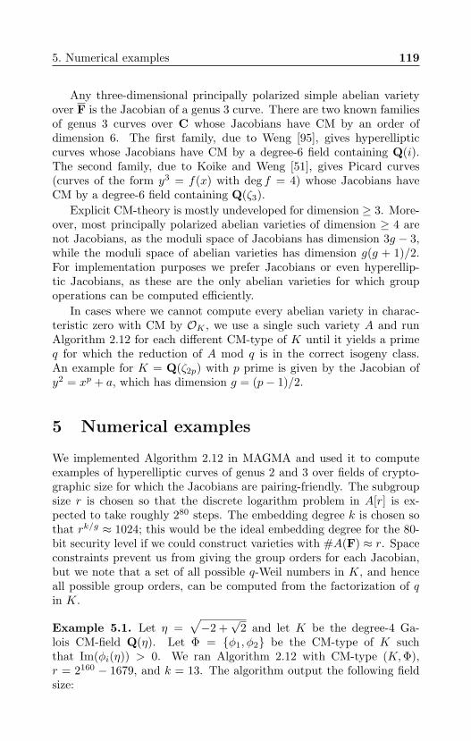
5. Numerical examples 119
Any three-dimensional principally polarized simple abelian varietyover F is the Jacobian of a genus 3 curve. There are two known familiesof genus 3 curves over C whose Jacobians have CM by an order ofdimension 6. The first family, due to Weng [95], gives hyperellipticcurves whose Jacobians have CM by a degree-6 field containing Q(i).The second family, due to Koike and Weng [51], gives Picard curves(curves of the form y3 = f(x) with deg f = 4) whose Jacobians haveCM by a degree-6 field containing Q(ζ3).
Explicit CM-theory is mostly undeveloped for dimension ≥ 3. More-over, most principally polarized abelian varieties of dimension ≥ 4 arenot Jacobians, as the moduli space of Jacobians has dimension 3g − 3,while the moduli space of abelian varieties has dimension g(g + 1)/2.For implementation purposes we prefer Jacobians or even hyperellip-tic Jacobians, as these are the only abelian varieties for which groupoperations can be computed efficiently.
In cases where we cannot compute every abelian variety in charac-teristic zero with CM by OK , we use a single such variety A and runAlgorithm 2.12 for each different CM-type of K until it yields a primeq for which the reduction of A mod q is in the correct isogeny class.An example for K = Q(ζ2p) with p prime is given by the Jacobian ofy2 = xp + a, which has dimension g = (p− 1)/2.
5 Numerical examples
We implemented Algorithm 2.12 in MAGMA and used it to computeexamples of hyperelliptic curves of genus 2 and 3 over fields of crypto-graphic size for which the Jacobians are pairing-friendly. The subgroupsize r is chosen so that the discrete logarithm problem in A[r] is ex-pected to take roughly 280 steps. The embedding degree k is chosen sothat rk/g ≈ 1024; this would be the ideal embedding degree for the 80-bit security level if we could construct varieties with #A(F) ≈ r. Spaceconstraints prevent us from giving the group orders for each Jacobian,but we note that a set of all possible q-Weil numbers in K, and henceall possible group orders, can be computed from the factorization of qin K.
Example 5.1. Let η =√−2 +
√2 and let K be the degree-4 Ga-
lois CM-field Q(η). Let Φ = φ1, φ2 be the CM-type of K suchthat Im(φi(η)) > 0. We ran Algorithm 2.12 with CM-type (K,Φ),r = 2160 − 1679, and k = 13. The algorithm output the following fieldsize:
120 Chapter IV. Abelian varieties with prescribed embedding degree
q = 31346057808293157913762344531005275715544680219641338497449500238872\30035061716540892530853973205578151445285706963588204818794198739264\123849002104890399459807463132732477154651517666755702167 (640 bits)
There is a single Fq-isomorphism class of curves over Fq whose Jaco-bians have CM by OK and it has been computed in [88]; the desiredtwist turns out to be C : y2 = −x5 + 3x4 + 2x3 − 6x2 − 3x + 1. Theρ-value of Jac(C) is 7.99.
Example 5.2. Let η =√−30 + 2
√5 and let K be the degree-4 non-
Galois CM field Q(η). The reflex field K is Q(ω) where
ω =√−15 + 2
√55.
Let Ψ be the CM-type of K such that Im(φi(η)) > 0. We ran Algorithm2.12 with the CM-type (K,Φ), subgroup size r = 2160 − 1445, andembedding degree k = 13. The algorithm output the following fieldsize:
q = 11091654887169512971365407040293599579976378158973405181635081379157\07830213092751652003623786192531077127388944453303584091334492452752\69309408919298654153381935518866167783400231181308345981461 (645 bits)
The class polynomials for K can be found in the preprint version of [97].We used the roots of the class polynomials mod q to construct curvesover Fq with CM by OK . As K is non-Galois with class number 4,there are 8 isomorphism classes of curves in 2 isogeny classes. We founda curve C in the correct isogeny class with equation y2 = x5 + a3x
3 +a2x
2 + a1x+ a0, with
a3 = 37909827361040902434390338072754918705969566622865244598340785379492\06229349302307887220632471591953460261515915189503199574055791975955\8344078795784842127002632600401437108457032108586548189769
a2 = 18960350992731066141619447121681062843951822341216980089632110294900\98526734892756700435114431697785479098782721806327279074708206429263\7519831093512508318537351901282000421070182572671506056432
a1 = 69337488142924022910219499907432470174331183248226721112535199929650\66326048728150177351432967251207037416196614255668796808046612641767\9222737491253665415344405882465731376523304907041006464504
a0 = 31678142561939596895646021753607012342277658384169880961095701825776\70412620481848230687778916790603969757571449880417861689471274167016\3886087129669411781204243813332617272038494020178561119564.
The ρ-value of Jac(C) is 8.06.
5. Numerical examples 121
Example 5.3. Let K be the degree-6 Galois CM-field Q(ζ7), and letΦ = φ1, φ2, φ3 be the CM type of K such that φn(ζ7) = e2πin/7. Weused the CM-type (K,Φ) to construct a curve C whose Jacobian hasembedding degree 17 with respect to r = 2180 − 7427. Since K hasclass number 1 and one equivalence class of primitive CM-types, thereis a unique isomorphism class of curves in characteristic zero whoseJacobians are simple and have CM by K; these curves are given byy2 = x7 + a. Algorithm 2.12 output the following field size:
q = 15755841381197715359178780201436879305777694686713746395506787614025\00812175974972634937716254216816917600718698808129260457040637146802\81270204406861277269259077188966205156107806823000096120874915612017\18492420684320462175923294626335763719251697987740263891168971441085\53148110927632874029911153126048408269857121431033499 (1077 bits)
The equation of the curve C is y2 = x7 + 10. The ρ-value of Jac(C) is17.95.
We conclude with an example of an 8-dimensional abelian variety foundusing our algorithms. We started with a single CM abelian variety A incharacteristic zero and applied our algorithm to different CM-types untilwe found a prime q for which the reduction has the given embeddingdegree.
Example 5.4. Let K = Q(ζ17). We set r = 1021 and k = 10 andran Algorithm 2.12 repeatedly with different CM-types1 for K. Giventhe output, we tested the Jacobians of twists of y2 = x17 + 1 for thespecified number of points. We found that the curve y2 = x17 + 30 hasembedding degree 10 with respect to r over the field F of order
q = 6869603508322434614854908535545208978038819437.
The CM-type was
Φ = φ1, φ3, φ5, φ6, φ8, φ10, φ13, φ15,
where φn(ζ17) = e2πin/17. The ρ-value of Jac(C) is 121.9.
1 Originally, we tried different random CM-types until it worked. The CM-typeΦ written in the example turned out to work. Actually, we could have predicted thiscorrect CM-type. See Example III.4.5.

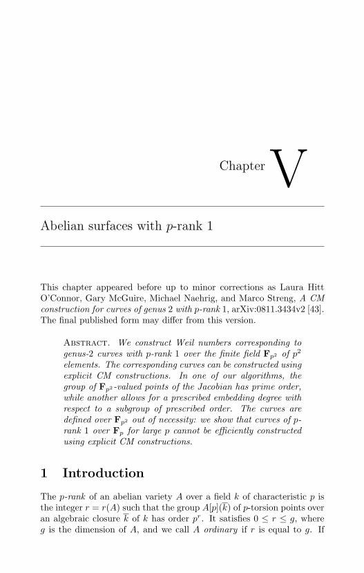
ChapterVAbelian surfaces with p-rank 1
This chapter appeared before up to minor corrections as Laura HittO’Connor, Gary McGuire, Michael Naehrig, and Marco Streng, A CMconstruction for curves of genus 2 with p-rank 1, arXiv:0811.3434v2 [43].The final published form may differ from this version.
Abstract. We construct Weil numbers corresponding togenus-2 curves with p-rank 1 over the finite field Fp2 of p2
elements. The corresponding curves can be constructed usingexplicit CM constructions. In one of our algorithms, thegroup of Fp2-valued points of the Jacobian has prime order,while another allows for a prescribed embedding degree withrespect to a subgroup of prescribed order. The curves aredefined over Fp2 out of necessity: we show that curves of p-rank 1 over Fp for large p cannot be efficiently constructedusing explicit CM constructions.
1 Introduction
The p-rank of an abelian variety A over a field k of characteristic p isthe integer r = r(A) such that the group A[p](k) of p-torsion points overan algebraic closure k of k has order pr. It satisfies 0 ≤ r ≤ g, whereg is the dimension of A, and we call A ordinary if r is equal to g. If
124 Chapter V. Abelian surfaces with p-rank 1
A is supersingular, that is, if A becomes isogenous over k to a productof supersingular elliptic curves, then we have r = 0, and the converseholds for abelian surfaces: if r = 0 and g = 2, then A is supersingular.
This shows that for an abelian surface A, besides the ordinary andsupersingular cases, there is only one intermediate case: the case whereA has p-rank 1. Most CM constructions of curves of genus two [79, 97,24, 26] generate curves that are ordinary with probability tending to 1,while another [69] constructs only supersingular curves. We focus onthe intermediate case, for which no constructions existed yet.
The p-rank r(A) depends only on the isogeny class of A over k, andany simple abelian surface A of p-rank 1 over a finite field k is isogenousto the Jacobian of a curve over k of genus 2 (see Section 2). By thep-rank of a curve C, we mean the p-rank of its Jacobian JC .
Let k be the finite field of order q = pn. The Frobenius endomor-phism π of a simple abelian variety over k is a Weil q-number, i.e., analgebraic integer π such that |π|2 = q holds for every embedding of thefield K = Q(π) into the complex numbers. A theorem of Honda andTate [84] states that this defines a bijection between the set of isogenyclasses of simple abelian varieties over k and the set of Weil q-numbersup to Galois conjugacy.
We characterize those Weil numbers corresponding to abelian sur-faces with p-rank 1 in Section 2, show their existence in Section 3 andgive algorithms for finding them in Section 4. In Section 3 we also ex-plain why curves of p-rank 1 over Fp for large p cannot be efficientlyconstructed using explicit CM constructions.
The construction of an abelian variety A corresponding to a givenWeil q-number π dates back to Shimura and Taniyama [78] and Honda[44]. It exhibits A as the reduction of a characteristic-0 abelian varietywith complex multiplication (CM) by Z[π] and is also known as the CMmethod. We explain this explicit CM construction in Section 5. For now,it suffices to say that the computational complexity of this constructiongrows very rapidly with the size of the field K = Q(π). Therefore,our algorithms will look for Weil q-numbers π only in fixed small inputfields K.
Let A be an abelian variety over the finite field k and suppose thatA(k) has a subgroup of prime order r. The embedding degree of A withrespect to r is the degree of the field extension k(ζr)/k, where ζr is aprimitive r-th root of unity. The Weil and Tate pairings on A withrespect to r have their image in 〈ζr〉 ⊂ k(ζr)∗, and in order to computethese pairings, one needs to work with k(ζr). As the embedding degreeis the order of q in (Z/rZ)∗, it is close to r for most curves, while forpairing-based cryptography, one wants r to be large and the embedding
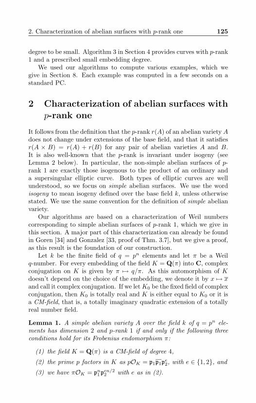
2. Characterization of abelian surfaces with p-rank one 125
degree to be small. Algorithm 3 in Section 4 provides curves with p-rank1 and a prescribed small embedding degree.
We used our algorithms to compute various examples, which wegive in Section 8. Each example was computed in a few seconds on astandard PC.
2 Characterization of abelian surfaces withp-rank one
It follows from the definition that the p-rank r(A) of an abelian variety Adoes not change under extensions of the base field, and that it satisfiesr(A × B) = r(A) + r(B) for any pair of abelian varieties A and B.It is also well-known that the p-rank is invariant under isogeny (seeLemma 2 below). In particular, the non-simple abelian surfaces of p-rank 1 are exactly those isogenous to the product of an ordinary anda supersingular elliptic curve. Both types of elliptic curves are wellunderstood, so we focus on simple abelian surfaces. We use the wordisogeny to mean isogeny defined over the base field k, unless otherwisestated. We use the same convention for the definition of simple abelianvariety.
Our algorithms are based on a characterization of Weil numberscorresponding to simple abelian surfaces of p-rank 1, which we give inthis section. A major part of this characterization can already be foundin Goren [34] and Gonzalez [33, proof of Thm. 3.7], but we give a proof,as this result is the foundation of our construction.
Let k be the finite field of q = pn elements and let π be a Weilq-number. For every embedding of the field K = Q(π) into C, complexconjugation on K is given by π 7→ q/π. As this automorphism of Kdoesn’t depend on the choice of the embedding, we denote it by x 7→ xand call it complex conjugation. If we letK0 be the fixed field of complexconjugation, then K0 is totally real and K is either equal to K0 or it isa CM-field, that is, a totally imaginary quadratic extension of a totallyreal number field.
Lemma 1. A simple abelian variety A over the field k of q = pn ele-ments has dimension 2 and p-rank 1 if and only if the following threeconditions hold for its Frobenius endomorphism π:
(1) the field K = Q(π) is a CM-field of degree 4,
(2) the prime p factors in K as pOK = p1p1pe2, with e ∈ 1, 2, and
(3) we have πOK = pn1 pen/22 with e as in (2).
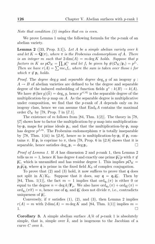
126 Chapter V. Abelian surfaces with p-rank 1
Note that condition (3) implies that en is even.
We prove Lemma 1 using the following formula for the p-rank of anabelian variety.
Lemma 2 ([33, Prop. 3.1]). Let A be a simple abelian variety over kand let K = Q(π), where π is the Frobenius endomorphism of A. Thereis an integer m such that 2 dim(A) = m degK holds. Suppose that pfactors in K as pOK =
∏i peii and let fi be given by #(OK/pi) = pfi .
Then we have r(A) =∑meifi, where the sum is taken over those i for
which π 6∈ pi holds.
Proof. The degree deg g and separable degree degs g of an isogeny g :A → B of abelian varieties are defined to be the degree and separabledegree of the induced embedding of function fields g∗ : k(B) → k(A).We have #(ker g)(k) = degs g, hence pr(A) is the separable degree of themultiplication-by-p map on A. As the separable degree is multiplicativeunder composition, we find that the p-rank of A depends only on itsisogeny class, hence we can assume that EndkA contains the maximalorder OK by [78, Prop. 7 in §7.1].
The existence of m follows from [84, Thm. 1(2)]. The theory in [78,§7] shows how to factor the multiplication-by-p map into multiplication-by-pi maps for prime ideals pi, and that the multiplication-by-pi maphas degree pfim. The Frobenius endomorphism π is totally inseparableby [78, Thm. 1(iii) in §2.8], hence so is multiplication-by-pi if pi con-tains π. If pi is coprime to π, then [78, Prop. 6 in §2.8] shows that it isseparable, hence satisfies degs pi = deg pi.
Proof of Lemma 1. If A has dimension 2 and p-rank 1, then Lemma 2tells usm = 1, henceK has degree 4 and exactly one prime p1|p with π 6∈p1, which is unramified and has residue degree 1. This implies pOK =p1p1q, where q is prime in the fixed field K0 of complex conjugation.
To prove that (2) and (3) hold, it now suffices to prove that q doesnot split in K/K0. Suppose that it does, say q = q1q1. Then by[84, Thm. 1(1)], the fact m = 1 implies that ordq1(π) is either 0 orequal to the degree n = deg k/Fp. We also have ordq1(π) + ordq1(π) =ordq1(ππ) = n, hence one of q1 and q1 does not divide π, i.e., contradictsuniqueness of p1.
Conversely, if π satisfies (1), (2), and (3), then Lemma 2 impliesr(A) = m with 2 dim(A) = m degK and [84, Thm. 1(1)] implies m =1.
Corollary 3. A simple abelian surface A/k of p-rank 1 is absolutelysimple, that is, simple over k, and is isogenous to the Jacobian of acurve C over k.
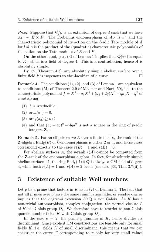
3. Existence of suitable Weil numbers 127
Proof. Suppose that k′/k is an extension of degree d such that we haveAk′ ∼ E × F . The Frobenius endomorphism of Ak′ is πd and thecharacteristic polynomial of its action on the `-adic Tate module of Afor l 6= p is the product of the (quadratic) characteristic polynomials ofthe action on the Tate modules of E and F .
On the other hand, part (3) of Lemma 1 implies that Q(πd) is equalto K, which is a field of degree 4. This is a contradiction, hence A isabsolutely simple.
By [59, Theorem 4.3], any absolutely simple abelian surface over afinite field k is isogenous to the Jacobian of a curve.
Remark 4. The conditions (1), (2), and (3) of Lemma 1 are equivalentto conditions (M) of Theorem 2.9 of Maisner and Nart [59], i.e., to thecharacteristic polynomial f = X4− a1X
3 + (a2 + 2q)X2− qa1X + q2 ofπ satisfying
(1) f is irreducible,
(2) ordp(a1) = 0,
(3) ordp(a2) ≥ n/2,
(4) and that (a2 + 4q)2 − 4qa21 is not a square in the ring of p-adic
integers Zp.
Remark 5. For an elliptic curve E over a finite field k, the rank of theZ-algebra Endk(E) of k-endomorphisms is either 2 or 4, and these casescorrespond exactly to the cases r(E) = 1 and r(E) = 0.
For abelian surfaces A, the p-rank r(A) cannot be computed fromthe Z-rank of the endomorphism algebra. In fact, for absolutely simpleabelian surfaces A, the ring Endk(A)⊗Q is always a CM-field of degree4, while both r(A) = 1 and r(A) = 2 occur (see also [33, Thm 3.7(ii)]).
3 Existence of suitable Weil numbers
Let p be a prime that factors in K as in (2) of Lemma 1. The fact thatnot all primes over p have the same ramification index or residue degreeimplies that the degree-4 extension K/Q is not Galois. As K has anon-trivial automorphism, complex conjugation, the normal closure Lof K has Galois group D4. We therefore have to restrict to non-Galoisquartic number fields K with Galois group D4.
In the case e = 2, the prime p ramifies in K, hence divides itsdiscriminant. Since explicit CM constructions are feasible only for smallfields K, i.e., fields K of small discriminant, this means that we canconstruct the curve C corresponding to π only for very small values
128 Chapter V. Abelian surfaces with p-rank 1
of p. For such small values of p, not only are the curves less interesting,especially from a cryptographic point of view, it also becomes possibleto construct them using a more direct approach such as by enumeratingall curves C of genus 2 over Fp and computing the group orders of theirJacobians. Therefore, we will focus on the case e = 1. For e = 1,condition (3) of Lemma 1 implies 2|n, so that curves are defined onlyover fields containing Fp2 . This is the reason why we construct ourcurves over Fp2 and not over Fp, and this is why curves of p-rank 1over Fp for large p cannot be efficiently constructed using explicit CMconstructions.
We have found that all fields with p-rank-1 Weil p2-numbers arequartic non-Galois CM-fields. However, not all quartic non-Galois CM-fields have p-rank-1 Weil p2-numbers, and we give a complete charac-terization in Section 6.
For now, we give two lemmas that put a condition on the CM-fieldsK that is slightly too strong, but is easy to check and is satisfied by‘most’ non-Galois quartic CM-fields.
Lemma 6. Let K be a quartic CM-field and let p be a prime thatfactors in K as pOK = p1p1p2. Suppose that p1 = αOK is principal.Then π = αα−1p is a Weil p2-number that satisfies the conditions ofLemma 1.
Proof. The number π satisfies ππ = p2, hence is a Weil p2-number. Con-ditions (1) and (2) of Lemma 1 are satisfied by assumption. Moreover,we have p2 = p(p1p1)−1 = p(αα)−1OK , so that we have πOK = p2
1p2,i.e., condition (3) is also satisfied.
The condition on p of Lemma 6 is stronger than the condition thatthere exists a Weil p2-number in K with e = 1. The following lemmagives a necessary and sufficient criterion on K for the existence of primesp satisfying this stronger condition.
For a non-Galois quartic CM-field K, let L be its normal closureover Q and let d be the discriminant of the real quadratic subfield K0
of K. Then we have K = K0(√r) for a totally negative element r ∈ K0,
and s = NK0/Q(r) ∈ Q is not a square, because K is non-Galois. Letdr be the discriminant of the real quadratic field Kr
0 = Q(√s). Note
that this field is independent of the choice of r. Indeed, the element r iswell-defined up to squares in K∗0 , hence s is well-defined up to squaresin Q∗.
A prime discriminant is a number that is −4 or ±8 or is ±p ≡ 1(mod 4) for an odd prime p. The discriminant of a quadratic field can bewritten uniquely as a product of distinct prime discriminants in whichat most one even factor occurs.
3. Existence of suitable Weil numbers 129
Lemma 7. Let K be a non-Galois quartic CM-field. The following areequivalent
(1) there exists a prime p that factors in K as pOK = p1p1p2 withp1 principal;
(2) the Dirichlet density of the set of primes p as in (1) is (4hK)−1,where hK is the class number of K;
(3) there is a prime that ramifies in L/K;
(4) not all prime discriminants in the discriminant factorization ofdr occur in that of d.
Proof. The implication (2)⇒ (1) is trivial. Now suppose that (1) holds,so the decomposition group of p1 in Gal(L/Q) is Gal(L/K) and the idealclass of p1 is trivial. By the Artin isomorphism ClK → Gal(H/K),this implies that the decomposition group of p1 in Gal(H/K) is trivialfor the Hilbert class field H of K. As the decomposition group of p1
in Gal(L/K) is non-trivial, this implies that L is not contained in themaximal unramified abelian extension H of K, so L/K ramifies at someprime and (3) holds.
For the proof of (3)⇒ (2), we use again that the primes p as in (1)are those for which there exists a prime in L over p with decompositiongroup Gal(L/K) in L/Q and trivial decomposition group H/K. LetM ⊃ H be Galois over Q. Since (3) implies L ∩ H = K, we findGal(HL/K) = Gal(H/K) × Gal(L/K) and hence that exactly 1 inevery 8hK elements σ ∈ Gal(M/Q) satisfies 〈σ|L〉 = Gal(L/K) andσ|H = 1. The conjugation class of Gal(L/K) in Gal(L/Q) has twoelements, hence the set of all σ yielding the appropriate factorization istwice as large, i.e., consists of 1 in every 4hK elements of Gal(M/Q). ByChebotarev’s density theorem [66, Theorem 13.4], this implies that thedensity of primes with this factorization is (4hK)−1, which proves (2).
Now, it remains to prove (3) ⇔ (4). Let L0 be the compositum ofK0 and Kr
0 in L. A prime q ∈ Z ramifies in L/K if and only if its inertiagroup in Gal(L/Q) contains Gal(L/K) or its conjugate. This is equiv-alent to q ramifying in L0/K0, that is, to the prime discriminant in dr
corresponding to q not occurring in the prime discriminant factorizationof d.
Example 8. The field K = Q[X]/(X4 +12X2 +2) does not satisfy theconditions of Lemma 7, because it has d = 8 · 17 and dr = 8.
For ‘most’ non-Galois quartic CM-fields K, the discriminant dr doesnot divide d, in which case the conditions of Lemma 7 hold. This meansthat if we try to find our Weil numbers by taking random primes p and
130 Chapter V. Abelian surfaces with p-rank 1
checking if there exists a Weil p2-number π ∈ K as in Lemma 1, thenwe have a probability (4hK)−1 of success.
4 The algorithms
The discussion in Section 3 leads to the following algorithm.
Algorithm 1.Input: A non-Galois CM-field K of degree 4 and a positive integer `.Output: A prime p of ` bits and a Weil p2-number π corresponding tothe Jacobian JC of a curve of genus 2 over Fp2 such that #JC(Fp2) isprime.
(1) Take a random positive integer p of ` bits.
(2) If p is prime, continue. Otherwise, go to Step 1.
(3) If pOK factors as p1p1p2, continue. Otherwise, go to Step 1.
(4) If p21p2 is principal, let π0 be a generator and let v = π0π0p
−2 ∈O∗K0
. Otherwise, go to Step 1.
(5) If we have v = NK/K0(w) for some w ∈ O∗K , then put π = w−1π0.Otherwise, go to Step 1.
(6) If N(uπ − 1) is prime for some u ∈ ±1, then replace π by uπ.Otherwise, go to Step 1.
(7) return p, π.
Note that the group order N(π − 1) of JC has about 4` bits sincewe have N(π − 1) ≈ N(π) = p4.
Theorem 9. If Algorithm 1 terminates, then the output is correct.Fix the input field K and assume that it satisfies the conditions of
Lemma 7. If K has no prime ideal of norm 2, and no prime above 2 isramified in K/K0, then the heuristic expected runtime of the algorithmis polynomial in `.
Proof. The output π is a Weil p2-number satisfying the conditions ofLemma 1, and the corresponding abelian surface A has #A(Fp2) =N(π − 1) rational points, which proves that the output is correct.
All numbers we encounter have logarithmic absolute values andheights that are bounded linearly in `, while the field K is fixed. This
4. The algorithms 131
shows that, using the algorithms of [16], all steps, including the pri-mality and principality tests, as well as finding a generator of p2
1p2 andtrying to extract a square root of v, take time polynomial in `. It there-fore suffices to prove that the heuristic expected number of iterations ofStep 1 is quadratic in `.
The number p has a heuristic probability 1/(` log 2) to be prime bythe Prime Number Theorem. This shows that for each time Step 3 isreached, one expects to run Step 1 about ` log 2 times.
We will ‘prove’ that the heuristic bound holds even if we restrictin Step 3 to p1 principal and generated by α. By Lemma 7, the den-sity of the set of primes p that factor in the appropriate way and forwhich α exists is (4hK)−1, so we arrive at Step 4 (with p1 = (α)) withprobability (4hK)−1.
Note that π = −αα−1p is a generator of p21p2, so we pass Step 4
with π0 = wπ for some unit w ∈ O∗K .Note that we have p2 = ππ, hence v = ww, proving that we pass
Step 5 as well.We now only need to show that N(π − 1) is prime with sufficiently
high probability. Treating α as a random element of O = OK , we wishto know the probability that X = N(π − 1) is prime, i.e., not divisibleby any prime q < X. For each such q, we consider the homomorphism
ϕ : (O/qO)∗ → (O/qO)∗ : x 7→ xx−1N(x),
which sends (α mod q) to (−π mod q). Now we have q|N(π − 1) ifand only if π ≡ 1 (mod q) for some prime q|q of K. Let ϕq be thecomposition of ϕ with the natural map (O/qO)∗ → (O/q)∗. Note thatwe have π ≡ 1 (mod q) if and only if α is an element of ϕ−1
q (−1). If wedefine
Pq = 1−#⋃
q|q ϕ−1q (−1)
#(O/qO)∗,
then the heuristic probability of q - N(π − 1) equals Pq. As the homo-morphism ϕ sends 1 to 1, we find Pq > 0 for all q > 2.
For q = 2, note that we have N(x) = 1. Then for all q | q withq = q, take (x mod q) ∈ (O/q)∗ with x 6= x, which is possible, because2 is unramified in K/K0. For q | q with q 6= q, take exactly one of(x mod q) and (x mod q) equal to 1, which is possible because q hasnorm ≥ 4. Then xx−1 6≡ 1 ≡ −1 (mod q) for all q | q, which provesP2 > 0.
We use the lower bound Pq > 0 for q ≤ 17.
132 Chapter V. Abelian surfaces with p-rank 1
For q ≥ 19, note that we have
Pq ≥ 1−∑q|q
# kerϕq
#(O/qO)∗≥ 1−
∑q|q
1# imϕq
and that imϕq ⊃ ϕq(F∗q) = (F∗q)4 has order ≥ (q− 1)/4, hence we have
Pq ≥ 1− 44
q − 1> 1− 17
q.
We thus find heuristically that N(π − 1) is prime with probabilityat least a positive constant times
Y =∏
19≤q<Xprime
(1− 17
q
).
We find log(Y ) > −∑q
17q , and the right hand side, by Mertens’ theo-
rem [39, Thm. 427 in 22.7], is 17 log logX plus something that convergesto a constant if X tends to infinity. In particular, we find that 1/Y is atmost polynomial in logX ≈ 4`, which is what we needed to prove.
Remark 10. For more detailed heuristics on prime order Jacobians ofcurves of genus 2 than what is in the proof of Theorem 9, see Weng [96,§5.2.2].
Remark 11. The conditions of Lemma 7 are sufficient in Theorem 9and, as we said before, they hold for ‘most’ non-Galois quartic CM-fields. They are however not necessary, and we give strictly weakerconditions in Section 6.
The following lemma shows that the conditions on the decompositionof 2 in K are necessary in Theorem 9, and that these conditions are notspecific to p-rank 1, or even to abelian surfaces. These conditions vanishhowever if one allows the group order to be ‘almost prime’ in the sensethat it is a prime times a ‘small’ (say ≤ 16) positive integer.
Lemma 12. Let π be the Frobenius endomorphism of an abelian varietyA over a finite field k of odd characteristic, and let K = Q(π). If oneof the following conditions holds, then the order of A(k) is even.
(1) K has a prime ideal q of norm 2,
(2) K is totally real, or
(3) K is a CM-field with totally real subfield K0 and K has a primeideal q|2 that is ramified in K/K0.
4. The algorithms 133
Proof. If q has norm 2, then we have π 6≡ 0 (mod q), hence π − 1 ≡ 0(mod q), which implies 2|N(π − 1).
In the other two cases, complex conjugation is trivial on the group(O/q)∗ of odd order. Note that ππ ∈ Q implies that π2 = ππ is trivialin that group, hence so is π. We see again that π − 1 ≡ 0 (mod q)implies 2|N(π − 1).
Our second algorithm is a modification of Algorithm 1 in which westart with an element α ∈ OK , instead of with a prime p, and checkif p = N(α) is a prime that decomposes in the appropriate manner.We use Algorithm 2 as a stepping stone towards Algorithm 3, whichallows one to prescribe the embedding degree of the output by imposingcongruence conditions on α.
Algorithm 2.Input: A non-Galois CM-field K of degree 4 and a positive integer `.Output: A prime p of ` bits and a Weil p2-number corresponding tothe Jacobian JC of a curve C of genus 2 over Fp2 such that JC hasp-rank 1 and a prime number of Fp2-rational points.
(1) Take a random element α of OK of which the norm N(α) has `bits.
(2) If p = N(α) is prime in Z, continue. Otherwise, go to Step 1.
(3) If the prime β = pα−1α−1 of OK0 remains prime in OK , then letπ = α2β. Otherwise, go to Step 1.
(4) If N(uπ − 1) is prime for some u ∈ ±1, then replace π by uπ.Otherwise, go to Step 1.
(5) return p, π.
Theorem 13. If Algorithm 2 terminates, then the output is correct.Fix the input field K and assume that it satisfies the conditions of
Lemma 7. If K has no prime ideal of norm 2, and no prime above 2 isramified in K/K0, then the heuristic expected runtime of the algorithmis polynomial in `.
Proof. By Lemma 6, the output π is a Weil p2-number satisfying theconditions of Lemma 1, and the corresponding abelian surface A has#A(Fp2) = N(π − 1) rational points, which proves that the output iscorrect.
134 Chapter V. Abelian surfaces with p-rank 1
Lemma 7 shows that among the elements α of OK of prime norm,at least about 1 in every 4hK has the appropriate factorization, so if wetreat N(α) and N(π − 1) as random integers as we did in the proof ofTheorem 9, then we find again that the heuristic expected runtime ispolynomial in `.
Remark 14. Actually, the heuristic probability of passing from Step 3to Step 4 in Algorithm 2 is 1/2 instead of only (4hK)−1 as can be seenby applying Chebotarev’s density theorem to the quadratic extensionLH/H from the proof of Lemma 7.
Algorithm 3 constructs p-rank-1 curves with prescribed embeddingdegree by imposing congruence conditions on α in a way that is similar towhat is done in the algorithm of Freeman, Stevenhagen, and Streng [26].
Algorithm 3.Input: A non-Galois CM-field K of degree 4, a positive integer κ anda prime number r ≡ 1 (mod 2κ) that splits completely in K.Output: A prime p and a Weil p2-number π corresponding to theJacobian JC of a curve C of genus 2 over Fp2 that has p-rank 1 andembedding degree κ with respect to a subgroup of order r.
(1) Let r be a prime of K dividing r, let s = rr−1r−1 and compute abasis b of OK .
(2) Take a random element x of F∗r and a primitive 2κ-th root ofunity ζ ∈ F∗r .
(3) Take the ‘small’ α ∈ OK such that α mod r = x, α mod r = xζand α mod s = x−1. Here ‘small’ means that the coordinateswith respect to the basis b are ≤ r/2.
(4) If p = NK/Q(α) is prime in Z, continue. Otherwise, go to Step 2.
(5) If the prime β = pα−1α−1 of OK0 remains prime in OK , letπ = α2β. Otherwise, go to Step 2.
(6) return p, π.
Theorem 15. If Algorithm 3 terminates, then the output is correct. Ifthe input field K is fixed and satisfies the conditions of Lemma 7, thenthe heuristic expected runtime of the algorithm is polynomial in r.
4. The algorithms 135
Proof. The facts that the output has p-rank 1 and a Jacobian of orderN(π − 1) are proven as in the proof of Theorem 13.
If r divides the group order N(π− 1), then the embedding degree isthe order of (p2 mod r) in the group F∗r (see also [26, Proposition 2.1]).So to prove that JC has embedding degree κ with respect to r, it sufficesto prove that p2 mod r is a primitive κ-th root of unity in F∗r and thatr divides N(π − 1).
Let φ be the non-trivial automorphism of K0. Then we have β =φ(αα), hence π mod r = (α mod r)2(φ(αα) mod r). Inside Fr, we have
(φ(αα) mod r) = (αα mod s) = (α mod s)(α mod s)= (α mod s)2 = x−2,
hence we have (π mod r) = 1, so r divides N(π − 1). Moreover,
(p2 mod r) = (p2 mod r) = (α mod r)2(α mod r)2(φ(αα) mod r)2
= (α mod r)2(α mod r)2x−4 = ζ2
is a primitive κ-th root of unity.This finishes the proof of the correctness of the output. Next we
prove the heuristic runtime. As r splits completely, α is a lift of someelement modulo r. We treat its norm p = N(α) as a random integer of4 log2 r bits. The rest of the proof is as the proof of Theorem 13.
Remark 16. Actually, the prime r does not need to split completelyin Algorithm 3. It suffices to have rOK = rrs, where r is prime and smay be prime or composite.
Remark 17. Note that if Algorithm 2 or 3 terminates, then K satisfiesthe conditions of Lemma 7, which are therefore not only sufficient, butalso necessary for each of these algorithms to terminate.
Let A be a g-dimensional abelian variety over the finite field k ofq elements. Its ρ-value with respect to a subgroup of A(k) of order ris defined to be ρ = g log q/ log r. As we have log #A(k) ≈ g log q, theρ-value measures the ratio between the bit size of r and the bit size ofthe order of the full group of rational points on A. It is at least about1 if q is large. If we have A = JC , then a point on A can be representedby a g-tuple of points on C, hence ρ is also the ratio between the bitsize of a group element of A and the bit size of r. For cryptography, onewants the ρ-value to be as small as possible to save bandwidth whentransmitting points on JC .
The prime p, computed as the norm of the element α in Step 4, isexpected to satisfy log(p) ≈ 4 log(r). Since our p-rank-1 curve is de-fined over Fp2 , its ρ-value is ρ = 2 log(p2)/ log(r) ≈ 16. For a more
136 Chapter V. Abelian surfaces with p-rank 1
detailed version of this heuristic analysis of the ρ-value, see Freeman,Stevenhagen, and Streng [26], who compute a ρ-value of about 8 fortheir ordinary abelian surfaces with prescribed embedding degree. Forcryptographic applications, a ρ-value of 16 or even 8 is larger than de-sired, but it does show that pairing-based cryptography is possible forcurves of genus 2 with p-rank 1.
When working with odd embedding degree κ, the embedding fieldFp(ζr) could be smaller than the field Fp2(ζr) = Fp2κ that is suggestedby the embedding degree κ (see also Hitt [42]). This may influence thesecurity of pairing-based cryptography, but can easily be avoided byrestricting to even embedding degree κ, or by only accepting primes psuch that r does not divide pκ − 1.
5 Constructing curves with givenWeil numbers
We will now explain the explicit CM construction of a curve C/Fp2such that J(C) corresponds to our Weil p2-number π. A more detailedexposition can be found in [27].
Honda’s CM construction of the abelian variety corresponding to agiven Weil q-number π is based on the theory of complex multiplicationof abelian varieties of Shimura and Taniyama [78, in particular §13,Thm. 1]. The analogous theory for elliptic curves is even more clas-sical and dates back to the early 19th century. The first algorithmicapplication of the CM construction of elliptic curves is its applicationto primality proving by Atkin and Morain [1].
The construction starts by taking an abelian variety A over a numberfield F such that we have End(A) ∼= OK , where K is a field containingπ, and reduces this variety modulo an appropriate prime P of F . Forour p-rank-1 Weil numbers π, one can take K = Q(π) and any primeP dividing p.
In the dimension-2 case, instead of writing down the abelian surfaceA itself, one only writes down the absolute Igusa invariants j1, j2, j3 ∈ Fof the curve C of which A is the Jacobian. These invariants are the firstthree of a set of 10 invariants given on page 641 of [45]. One thenreduces the invariants modulo P and, assuming (j1 mod P) is a unit,constructs C = (C mod P) from the reduced invariants using Mestre’salgorithm [61]. Honda’s construction shows that J(C) or its quadratictwist corresponds to our Weil p2-number π.
In all practical implementations, the invariants jn ∈ F are repre-
6. A sufficient and necessary condition 137
sented by polynomials H1, H2, H3 or H1, H2, H3 called Igusa class poly-nomials. We explain the polynomials Hn later, but the polynomials Hn
are given byHn =
∏C
(X − jn(C)),
where the product ranges over isomorphism classes of curves C suchthat we have End(J(C)) ∼= OK . For every triple (j1, j2, j3) of zeroesjn ∈ Fp of Hn with j1 6= 0, one thus obtains a unique Fp-isomorphismclass of curves. Assuming j1(C) 6∈ P for some C, a twist of at leastone of the curves we obtain has Weil number π. Let C be such a curve.As we know the group order N(π − 1) of J(C)(Fp2), we can quicklycheck whether we have the correct curve by taking random points onits Jacobian and multiplying them by N(π − 1).
As the field K is fixed, so are its class polynomials. They can there-fore be precomputed using any of the three known algorithms: the com-plex analytic method of Spallek [79] and van Wamelen [88], for whichStreng [82] recently gave the first runtime analysis and proof of correct-ness, the 2-adic method of Gaudry, Houtmann, Kohel, Ritzenthaler, andWeng [32], and the Chinese remainder method of Eisentrager and Lauter[21]. Alternatively, class polynomials can be found in the ECHIDNAdatabase [50].
The alternative class polynomials Hn are given by
Hn =∑C
jn(C)∏C′ 6∼=C
(X − j1(C ′)), (n = 2, 3)
where both the product and the sum range over isomorphism classes ofcurves C for which End(J(C)) ∼= OK holds. For any such C, we havejn(C)H ′1(j1(C)) = Hn(j1(C)). This implies that if every coefficientof H1 has a denominator that is not divisible by p, and (H1 mod p)has a non-zero root of multiplicity 1, then we can compute the Igusainvariants of a curve C, which is automatically either the curve wewant or a quadratic twist. The idea of using Hn and not the morestandard Lagrange interpolation is due to Gaudry, Houtmann, Kohel,Ritzenthaler, and Weng, who show in [32] that Hn heuristically has amuch smaller height.
6 A sufficient and necessary condition
As said before, the condition of Lemma 7 are sufficient for all threealgorithms to work and necessary for Algorithms 2 and 3. They are
138 Chapter V. Abelian surfaces with p-rank 1
also easy to check and true for ‘most’ non-Galois quartic CM-fields.The current section gives a weaker condition that is both sufficient andnecessary for Algorithm 1 to work. We also give examples to show thatthis condition is non-trivial and strictly weaker than that of Lemma 7.
Let K be a non-Galois CM-field of degree 4. Let C/K be a curveof genus 2 over the algebraic closure K of K such that End(JC) ∼= OKholds. Such C are known to exist. The field Q(j) ⊂ K generated overQ by all 10 absolute Igusa invariants j1(C), . . . , j10(C) of [45, page 641]is called the field of moduli of C. For any subfield X ⊂ K, let X(j) bethe compositum X ·Q(j). Write K = K0(
√r) for some r ∈ K0 and let
Kr0 = Q(
√NK0/Q(r)) (as before).
Lemma 18. Let K,Kr0,K(j) be as above and let G be the Galois group
of the normal closure of K(j) over Q. Let S be the set of primes pthat factor in K as pOK = p1p1p2 and such that there exists a Weilp2-number π such that we have πOK = p2
1p2.The Dirichlet density of S is
#σ ∈ G | ordσ = 2, σ|Kr06= idKr
0
#G.
If S is non-empty, then it has positive density.
Corollary 19. If Algorithm 1 terminates on input K, then σ as inLemma 18 exists for K. Conversely, if K is fixed and σ exists for K,then Algorithm 1 heuristically has a polynomial runtime.
Proof of Corollary 19. If Algorithm 1 terminates, then S is non-empty,hence σ exists by Lemma 18. If σ exists, then the proof of Theorem 9is valid, so Algorithm 1 heuristically has a polynomial runtime.
To prove Lemma 18, we need some more theory. Let L be the normalclosure of K. A CM-type of K is a set Φ of two embeddings ϕ : K → Lthat satisfies Φ∩Φ = ∅. Let C be a curve as above, and let Φ = ϕ1, ϕ2be its CM-type as defined in [78, §5.2]. The exact definition of this CM-type will not be important to us.
The reflex field
Kr = Q(∑i ϕi(x) : x ∈ K) ⊂ L
of K with respect to Φ is one of the two non-Galois CM subfields ofL of degree 4 that are not conjugates of K. Its real quadratic subfieldKr
0 does not depend on Φ and is exactly the field Kr0 that we have seen
above Lemma 7. By [77, Prop. 20.3(i)], we have Kr0 ⊂ Q(j), so that we
have the inclusions of fields shown in Figure V.1.
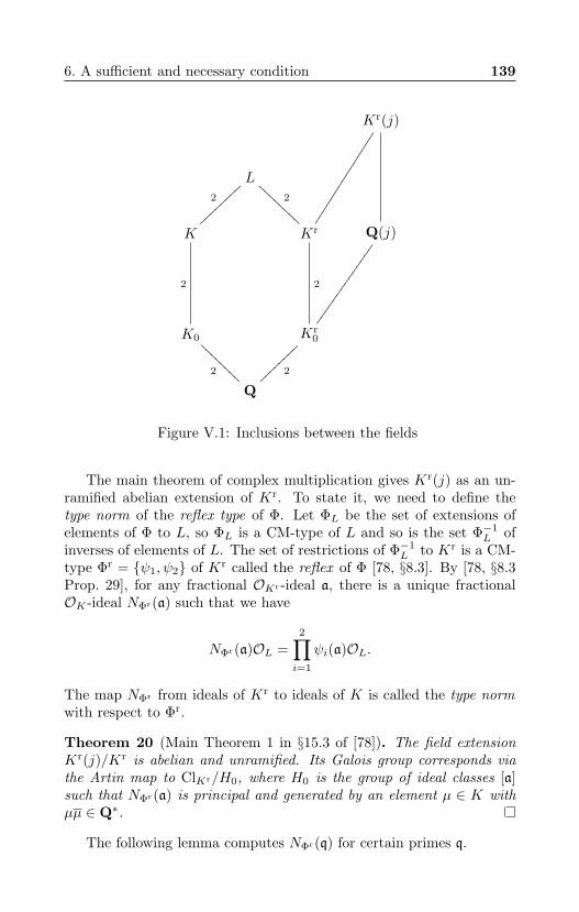
6. A sufficient and necessary condition 139
Kr(j)
L
K
2
Kr
2
AAAAAAAA
Q(j)
K0
2
Kr0
2
Q2
@@@@@@@@ 2
~~~~~~~~
Figure V.1: Inclusions between the fields
The main theorem of complex multiplication gives Kr(j) as an un-ramified abelian extension of Kr. To state it, we need to define thetype norm of the reflex type of Φ. Let ΦL be the set of extensions ofelements of Φ to L, so ΦL is a CM-type of L and so is the set Φ−1
L ofinverses of elements of L. The set of restrictions of Φ−1
L to Kr is a CM-type Φr = ψ1, ψ2 of Kr called the reflex of Φ [78, §8.3]. By [78, §8.3Prop. 29], for any fractional OKr-ideal a, there is a unique fractionalOK-ideal NΦr(a) such that we have
NΦr(a)OL =2∏i=1
ψi(a)OL.
The map NΦr from ideals of Kr to ideals of K is called the type normwith respect to Φr.
Theorem 20 (Main Theorem 1 in §15.3 of [78]). The field extensionKr(j)/Kr is abelian and unramified. Its Galois group corresponds viathe Artin map to ClKr/H0, where H0 is the group of ideal classes [a]such that NΦr(a) is principal and generated by an element µ ∈ K withµµ ∈ Q∗.
The following lemma computes NΦr(q) for certain primes q.
140 Chapter V. Abelian surfaces with p-rank 1
Lemma 21. Let K be a quartic CM-field and p a prime that factors inK as pOK = p1p1p
e2.
(1) The prime p factors in Kr0 as se for a prime s, which splits in
Kr as sOKr = qq; and
(2) we have NΦr(q) = p2/e1 p2 (up to complex conjugation).
Proof. Let P ⊂ OL be the unique prime over p1. Part (1) follows fromthe fact that the decomposition group of P is Gal(L/K) and that theinertia group has order e.
For part (2), let s be the generator of Gal(L/K), let s′ be the genera-tor of Gal(L/Kr) and set r = ss′. Then ΦL ⊂ Gal(L/Q) has 4 elementsand satisfies ΦL〈s〉 = ΦL and Φ−1
L 〈s′〉 = Φ−1L , hence Φ−1
L is 1, s, s′, ss′or its complex conjugate, and we have Φr = 1, s|Kr up to complexconjugation. Take ψ1 = 1, ψ2 = s. We compute
NΦr(q)OL = (qOL)(sqOL) =(P(s
′P))(
(sP)(ss′P))
= P2(
(s′P)(ss
′P))
= (p2/e1 OL)(p2OL),
up to complex conjugation, which proves (2).
Proof of Lemma 18. Let p be a prime number that is unramified in K.We prove that p is in S if and only if its decomposition group in thenormal closure of K(j) is of order 2 and acts non-trivially on Kr
0. Cheb-otarev’s density theorem [66, Theorem 13.4] then proves the formula forthe density. Moreover, if S is non-empty, then σ exists, hence the den-sity is positive.
Let p be a prime number and let σ ∈ G be its p-th power Frobenius.Suppose p is in S and write pOK = p1p1p2. The image of σ in Gal(L/Q)generates Gal(L/K) or its conjugate, hence has order 2. It follows thatp is inert in Kr
0/Q and splits into two factors q and q in Kr. Lemma 21shows that the type norm of q is NΦr(q) = p2
1p2 = πOK or its complexconjugate, and we have ππ ∈ Q∗, so we find [q] ∈ H0, hence σ2 is trivialon Kr(j) and in particular on Q(j).
Recall that Q(j) is the field generated over Q by the absolute Igusainvariants of C and that C is any curve with CM by OK . In particular,we can replace C by τC for any automorphism τ of K/Q. This showsthat σ2 is also trivial on τQ(j) for any τ , and hence σ2 is trivial on thenormal closure of Q(j). As it is also trivial on the normal closure L ofK, we find that it is trivial on the normal closure of K(j) and hence σis in the set of Lemma 18.
Conversely, suppose that σ2 is trivial and σ is non-trivial on Kr0.
As σ|L generates Gal(L/K) or a conjugate, we find that p factors as
7. Factorization of class polynomials mod p 141
pOK = p1p1p2. Again, the prime p is inert in Kr0/Q and splits into two
factors q and q in Kr with type norms p21p2 and its complex conjugate.
As we have σ2 = 1, we find by Theorem 20 that p21p2 = πOK holds for
some π ∈ OK that satisfies ππ ∈ Q∗. Since also ππ is positive and hasabsolute value p2, it is a Weil p2-number and p is in S.
Example 22. For the field K = Q[X]/(X4 + 12X2 + 2) of Example 8,we can find Q(j) in the ECHIDNA database [50] and compute thatQ(j) contains the field F = Q(
√2 +√
2), which is cyclic Galois over Qand contains Kr
0 = Q(√
2). Any automorphism of F of order 2 is trivialon Kr
0, so the density of S in Lemma 18 is 0 and none of our algorithmsworks for this field.
Example 23. For the field K = Q[X]/(X4+20X2+5), we have 13 ∈ S,so that S has positive density and Algorithm 1 works for K. However,the discriminant dr = 5 of Kr
0 = Q(√
5) is a prime discriminant andoccurs in the prime discriminant factorization d = (−4) · (5) · (−19) ofK0. This shows that K does not satisfy the conditions of Lemma 7,which are therefore too strong for Algorithm 1.
7 Factorization of class polynomials mod p
While experimenting with the explicit CM construction for curves ofp-rank 1, we found that in the (ramified) case e = 2 of Lemma 1,the polynomial H1 mod p has no roots of multiplicity 1 in Fp, whichmade working with Hn impossible. The current section explains thisphenomenon, and shows how to adapt H1, H2, H3 to deal with thissituation. We also explain the analogue of this for the situation e = 1,for which there is no problem.
Let K, C, and j be as in Section 6. If j1(C) 6= 0 is a simple rootof H1, which is ‘usually’ the case, then we have Q(j) = Q(j1(C)) sincewe can compute jn(C) from j1(C) using the polynomials H2 and H3 aswe have seen in Section 5. The Kummer-Dedekind theorem thus relatesthe factorization of (H1 mod p) ∈ Fp[X] to the factorization of p in (anorder in) Q(j).
Lemma 24. Let p be a prime that factors in K as pOK = p1p1p2, andlet n be the smallest positive integer such that en is even and (p1p
e/22 )n
is generated by a Weil pn-number π. Then any prime q of Kr lying overp decomposes in Kr(j)/Kr into distinct primes of residue degree en/2.
142 Chapter V. Abelian surfaces with p-rank 1
Proof. Recall from Theorem 20 that Kr(j) is the unramified abelianextension of Kr such that the Artin map induces an isomorphism
ClK/H0 → Gal(Kr(j)/Kr),
where H0 ⊂ ClK is the subgroup of ideal classes [a] such that NΦr(a) isprincipal and generated by an element µ ∈ K with µµ ∈ Q∗.
The Artin isomorphism sends [q] to a generator of the decompositiongroup of q, so it suffices to prove that [q] has order en/2 in the quotientgroup ClKr/H0. Lemma 21 computes that NΦr(qm) is either (p2/e
1 p2)m
or its complex conjugate, so the smallest integer m with [qm] ∈ H0 isexactly m = en/2.
Corollary 25. Let p, n be as in Lemma 24. Then p splits into primefactors of residue degree n in Q(j)/Q. Each factor occurs exactly etimes.
Proof. Each prime factor p has residue degree en/2 in Kr(j)/Kr byLemma 24 and 2/e in Kr/Q by Lemma 21, hence n in Kr(j)/Q. Asall ramification of p takes place in Kr
0/Q, we find that the ramificationindex of p in Kr(j)/Q is e.
We have seen in Figure V.1 on page 139 that Q(j) contains Kr0. As
the residue degree and ramification index of p in Kr/Kr0 are 1, we find
that the residue degree and ramification index of p are also n and e inQ(j)/Q.
Corollary 26. If p factors in K as pOK = p1p1p22, then (H1 mod p) ∈
Fp[X] has no roots of multiplicity 1 in Fp.
Proof. The polynomial H1 ∈ Q[X] is monic and the denominators ofthe coefficients are not divisible by p because they are Igusa invariantsof a curve that has potential good reduction modulo p. Let c ∈ Z notdivisible by p be such that H1(cX) is in Z[X] and let f ∈ Z[X] bean arbitrary irreducible factor of H1(cX) ∈ Z[X]. We find an orderO = Z[X]/f in Q(j). Each irreducible factor g ∈ Fp[X] of (H1 mod p)corresponds to the prime ideal p = (p, g(X)) of O. As every prime overp ramifies in Q(j)/Q by Corollary 25, we find that p is either ramifiedor singular. By the Kummer-Dedekind theorem (Theorem 8.2 of [81]),both cases imply that the roots of g have multiplicity at least 2 as rootsof H1.
This shows that H1, H1, H2 cannot be used for the case e = 2. Toget around this, we replace H1 by an irreducible factor f ∈ Kr
0[X]and Hn by the unique polynomial Sn of degree at most deg(f) − 1
8. Examples 143
that is congruent modulo f to Hn(H1/f)−1. If we write pOKr = s2,then (f mod s), (S2 mod s), (S3 mod s) ∈ Fp[X] can be used in exactlythe same way as (H1 mod p), (H2 mod p), (H3 mod p) and do not sufferfrom Corollary 26.
Corollary 27. For all but finitely many of the primes p that decomposeas pOK = p1p1p
e2, the reduction (H1 mod p) ∈ Fp[X] is a product of
distinct irreducible polynomials in Fp[X] of degree n for n given inLemma 24 (and depending on p).
Proof. We exclude the primes dividing the denominator of any coeffi-cient of H1, as well as those dividing the discriminant. Then all rootsof (H1 mod p) in Fp are simple roots. Let f,O be as in the proof ofCorollary 26. Then p does not divide the index of O in its maximalorder. The fact that every prime of Q(j) has residue degree n impliesthat every irreducible factor of f mod p has degree n.
8 Examples
Algorithm 1
We provide examples of p-rank-1 curves C/Fp2 such that the JacobianJC is simple and has prime order. The CM-field for all examples isK = Q(α), where α is a root of the polynomial X4+34X2+217 ∈ Q[X],which satisfies the conditions of Lemma 7. We give the prime p, thecoefficients a1 and a2 of the minimal polynomial
f = X4 − a1X3 + (a2 + 2p2)X2 − a1p
2X + p4
of the Frobenius endomorphism and the coefficients ci ∈ Fp2 of thecurve equation
C : y2 = c6x6 + c4x
4 + c3x3 + c2x
2 + c1x+ c0.
The group order of the Jacobian is #JC(Fp2) = N(π − 1) = f(1). Thefield Fp2 is given as Fp(σ), where σ2 = −3. Section headings describethe number of bits of the group order #JC(Fp2).
Each example was generated in a few seconds on a standard PC afterpre-computation of the Igusa class polynomials of K.
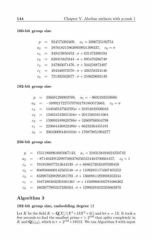
144 Chapter V. Abelian surfaces with p-rank 1
160-bit group size
p = 924575392409, a1 = 3396725192754a2 = 2876182159630959921399337, c6 = σ
c4 = 349419850452 · σ + 621473390194c3 = 638315825844 · σ + 895470286740c2 = 247903071476 · σ + 504258872407c1 = 494346973570 · σ + 326558224146c0 = 721392332677 · σ + 210623692149
192-bit group size
p = 236691298903769, a1 = −9692493559086a2 = −58992172275797931791883572663, c6 = σ
c4 = 144046547562595σ + 31854049506043c3 = 134634542821316σ + 20155601614364c2 = 159093189820788σ + 52669766944798c1 = 223684436822489σ + 66232364455191c0 = 206430094481010σ + 170879851904277
256-bit group size
p = 15511800964685067143, a1 = 2183138494024250742a2 = −871403391229975003782565554464700664457, c6 = 1c4 = 7019198877313644539 · σ + 8886572032497699458c3 = 8069566800142565548 · σ + 11092851174307405252c2 = 8339873208295381793 · σ + 13688811293938352344c1 = 10474983032301001361 · σ + 14509908493781086362c0 = 4803877905347330504 · σ + 12900291622358663970
Algorithm 3
192-bit group size, embedding degree 12
Let K be the field K = Q[X]/(X4+13X2+41) and let κ = 12. It took afew seconds to find the smallest prime r > 2192 that splits completely inK and Q(ζ12), which is r = 2192+18513. We ran Algorithm 3 with input
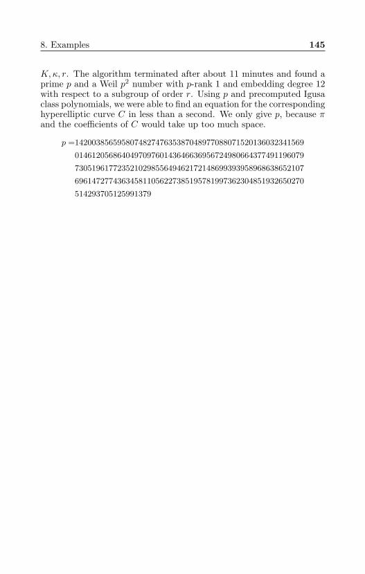
8. Examples 145
K,κ, r. The algorithm terminated after about 11 minutes and found aprime p and a Weil p2 number with p-rank 1 and embedding degree 12with respect to a subgroup of order r. Using p and precomputed Igusaclass polynomials, we were able to find an equation for the correspondinghyperelliptic curve C in less than a second. We only give p, because πand the coefficients of C would take up too much space.
p =142003856595807482747635387048977088071520136032341569
014612056864049709760143646636956724980664377491196079
730519617723521029855649462172148699393958968638652107
696147277436345811056227385195781997362304851932650270
514293705125991379

Appendix 1. The Fourier expansions of Igusainvariants
Abstract. We show by which integers we can divide theIgusa modular forms I4, I ′6, I10, and I2I10 so that the quo-tient still has integral Fourier coefficients.
Every theta constant θ[c] has a Fourier expansion
θ[c](Z) =∑
T∈Mat2(Q)
aT · exp(2πi Tr(ZT )
).
In fact, the definition of θ[c] in Section II.7 already tells us that this istrue with
aT =∑n∈Z2
(n+c′)(n+c′)t=T
(−1)2(n+c′)tc′′ ∈ Z,
where c is written as c = (c′, c′′), with column vectors n, c′, and c′′.The functions h4, h6, h12, and h10, defined in terms of theta con-
stants in equation II.(7.1) are modular forms for Sp4(Z). It is knownthat this implies that they have a unique Fourier expansion, that more-over aT 6= 0 implies that 2T has integral entries and even integral diag-onal entries, and that we have
aT = aUtTU for all U ∈ GL2(Z).
Following Lemma II.7.3, we identify the Igusa invariants I4, I6, I10,and I2I10 with the modular forms h4, h6, h10, and h12. Section II.9requires us to use modular forms with integral Fourier expansion, andwe would like to choose these functions as small as possible. In otherwords, we want their Fourier coefficients to be integral with gcd equalto 1. The following result supplies such functions.
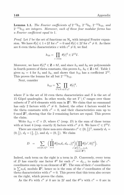
148 Appendix
Lemma 1.1. The Fourier coefficients of 2−2h4, 2−2h6, 2−12h10, and2−15h12 are integers. Moreover, each of these four modular forms hasa Fourier coefficient equal to 1.
Proof. Let I be the set of functions on Hg with integral Fourier expan-sion. We have θ[c] ∈ 1+2I for c′′ = 0 and θ[c] ∈ 2I for c′′ 6= 0. As thereare 6 even theta characteristics c with c′′ 6= 0, we find
h10 =∏c even
θ[c]2 ∈ 212I.
Moreover, we have θ[c]4 ∈ Z + 8I, and since h4 and h6 are polynomialsin fourth powers of theta constants, this proves h4, h6 ∈ Z+8I. Table 1gives a0 = 4 for h4 and h6, and shows that h10 has a coefficient 212.This proves the lemma for all but 2−15h12.
Next, consider
h12 =∑C∈S
∏c∈T\C
θ[c]4,
where T is the set of 10 even theta characteristics and S is the set of15 Gopel quadruples. In other words, the set T \ C ranges over thosesubsets of T of 6 elements with sum in Z2. We claim that no summandhas only 2 factors with c′′ 6= 0. Indeed, the other 4 factors would bethe theta constants with c′′ = 0, and their characteristics sum up to0 mod Z2, showing that the 2 remaining factors are equal. This provesthe claim.
Write h12 = C + D, where C (resp. D) is the sum of those termswith at least 4 (resp. exactly 3) factors with c′′ 6= 0. We have C ∈ 216I.
There are exactly three non-zero elements c′′ ∈ 0, 12
2, namely d1 =(0, 1
2 ), d2 = ( 12 ,
12 ), and d3 = (0, 1
2 ). We claim
D =∑
a∈0,13
( 3∏i=1
θ[(aidi, d4−i)]4)(∏c′ 6≡
∑3i=1 aidi
(mod Z2)
θ[(c′, 0)]4).
Indeed, each term on the right is a term in D. Conversely, every termof D has exactly one factor θ4 for each c′′ = d3−i to make the c′′-coordinates sum up to an element of Z2. The sum of their c′-coordinatesis∑aidi modulo Z2, hence so is the sum of the c′-coordinates of the
theta characteristics with c′′ = 0. This proves that this term also occurson the right, which proves the claim.
As the θ’s with c′′ 6= 0 are in 2I and the θ4’s with c′′ = 0 are in
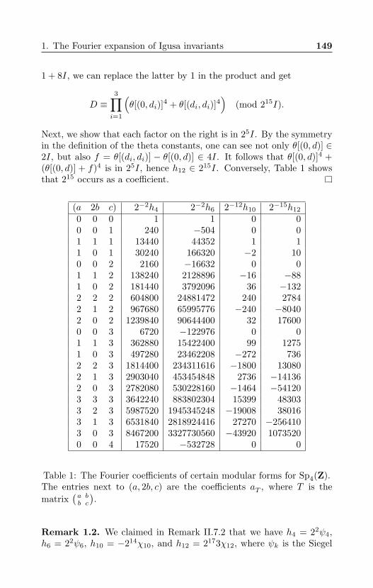
1. The Fourier expansion of Igusa invariants 149
1 + 8I, we can replace the latter by 1 in the product and get
D ≡3∏i=1
(θ[(0, di)]4 + θ[(di, di)]4
)(mod 215I).
Next, we show that each factor on the right is in 25I. By the symmetryin the definition of the theta constants, one can see not only θ[(0, d)] ∈2I, but also f = θ[(di, di)] − θ[(0, d)] ∈ 4I. It follows that θ[(0, d)]4 +(θ[(0, d)] + f)4 is in 25I, hence h12 ∈ 215I. Conversely, Table 1 showsthat 215 occurs as a coefficient.
(a 2b c) 2−2h4 2−2h6 2−12h10 2−15h12
0 0 0 1 1 0 00 0 1 240 −504 0 01 1 1 13440 44352 1 11 0 1 30240 166320 −2 100 0 2 2160 −16632 0 01 1 2 138240 2128896 −16 −881 0 2 181440 3792096 36 −1322 2 2 604800 24881472 240 27842 1 2 967680 65995776 −240 −80402 0 2 1239840 90644400 32 176000 0 3 6720 −122976 0 01 1 3 362880 15422400 99 12751 0 3 497280 23462208 −272 7362 2 3 1814400 234311616 −1800 130802 1 3 2903040 453454848 2736 −141362 0 3 2782080 530228160 −1464 −541203 3 3 3642240 883802304 15399 483033 2 3 5987520 1945345248 −19008 380163 1 3 6531840 2818924416 27270 −2564103 0 3 8467200 3327730560 −43920 10735200 0 4 17520 −532728 0 0
Table 1: The Fourier coefficients of certain modular forms for Sp4(Z).The entries next to (a, 2b, c) are the coefficients aT , where T is thematrix
(abbc
).
Remark 1.2. We claimed in Remark II.7.2 that we have h4 = 22ψ4,h6 = 22ψ6, h10 = −214χ10, and h12 = 2173χ12, where ψk is the Siegel
150 Appendix
Eisenstein series of weight k and χk is defined in terms of Eisensteinseries in that remark. Table 1 allows us to give a proof of this claim.
Indeed, the graded ring of modular forms for Sp4(Z) is equal toC[ψ4, ψ6, ψ10, ψ12] by [47], so we see h4 = c4ψ4 and h6 = c6ψ6 forcertain constants c4 and c6, and we see that there are linear relationsbetween h10, ψ4ψ6, and χ10, and between h12, ψ3
4 , ψ26 , and χ12. Using
tables containing coefficients of ψ4, ψ6, χ10, and χ12, such as those ofResnikoff and Saldana [68], we can find the appropriate linear relations.
It seems that the entry with (a, 2b, c) = (3, 3, 3) for χ10 has a missingsign in the tables of Resnikoff and Saldana, since it is the only one thatdoes not agree with our table.
Appendix 2. An alternative algorithm forenumerating CM abelian varieties
Abstract. We give an alternative for Algorithm II.3.1for computing all triples (Φ, a, ξ). It uses the pairs (z, b) ofSection I.5.3. We also generalize a much cited result fromSpallek’s thesis [79].
2.1 Reduced pairs (z, b)
Let K be a CM-field of degree 2g with maximal totally real subfield K0.Suppose we have g = 2 or, more generally, that the different of K0 isprincipal.
In Section I.5.2, we saw that the principally polarized abelian vari-eties with CM byOK correspond to equivalence classes of triples (Φ, a, ξ)consisting of a CM-type Φ of K, an fractional OK-ideal a, and an el-ement ξ ∈ K with DK/Qaaξ = OK and Imφξ > 0 for all φ ∈ Φ.Two such triples (Φ, a, ξ) and (Φ, a′, ξ′) with the same type Φ are calledequivalent if there is an element u ∈ K∗ with a′ = ua and ξ′ = (uu)−1ξ.
In Section I.5.3, we saw that each triple (Φ, a, ξ) is given up to equiv-alence by a = zb+b−1, ξ = (z−z)−1δ−1, and Φ = φ : K → C | Imφξ >0 with z ∈ K and b a fractional OK0 -ideal such that zb + b−1 is anOK0-submodule of K. We call two such pairs (z, b) equivalent if theygive rise to equivalent triples (Φ, a, ξ) with the same CM-type Φ.
Let S be a complete set of representatives for the ideal class group ofOK0 . For every b ∈ S, let Tb be a half-open fundamental parallelepipedfor translation by b−2 in K0⊗R. Let V be a union of 2g half-open conessuch that V is a fundamental domain for multiplication by (O∗K0
)2 inK0 ⊗R. Recall I(z) =
∏φ∈Φ |Imφz| and let N = NK0/Q.
Lemma 2.3. Every equivalence class of pairs (z, b) contains a pair with
1. I(z)N(b)2 maximal in the equivalence class,
152 Appendix
2. b ∈ S,
3. Im z ∈ V ,
4. Re z ∈ Tb.
Proof. For the fact that a maximum exists, see the analogous case ofthe Hilbert fundamental domain. That is, see Remark I.5.10 and [86,§I.2].
Next, note that for u ∈ K∗0 , we have u−1(zb + b−1) = (u−2z)(ub) +(ub)−1, which does not change I(x)N(b), so b can be taken in S. Bytaking u to be a unit in O∗K0
, we even find Im z ∈ V . Next, we cantranslate z by any element of b−2, which gives us Re z ∈ Tb.
Remark 2.4. The conditions in Lemma 2.3 are bounds of a fundamen-tal domain for the action of SL2(OK0) mentioned in Remark I.5.10. See[86, §I.3].
The pairs (z, b) of Lemma 2.3 satisfy I(z)N(b)2 > Cg∆−10 for some
constant Cg depending only on g. For g = 2, this is Lemma II.6.5with C2 = π2/6, and for other g, it is a straightforward generalization.Moreover, if we write K = K0(
√D) for some D ∈ OK0 , then we find√
D = az + b with a ∈ b2, b ∈ OK0 . In other words, we have
z =√D − ba
.
We find a ∈ b2∩V ′ for the union of cones V ′ =√DV −1 ⊂ K0⊗R, and
N(a)2 < I(√D)N(b)2C−1
g ∆0, so there are finitely many possibilitiesfor a. We also find b ∈ OK0∩aTb, which yields finitely many possibilitiesfor b.
Assuming we can compute the unit group and class group of K0, aswell as all elements a ∈ b2 below a given norm bound up to multiplica-tion by (O∗K0
)2, this gives us the following algorithm.
Algorithm 2.5.Input: A CM-field K = K0(
√D) such that the different of the totally
real subfield K0 is principal, and a CM-type Φ of K. A Z-basis of OK .Output: At least one representative (z, b) of every equivalence class.
1. Compute a set of representatives S of the class group of K0.
2. Write each element of the Z-basis of OK in the form xi + yi√D
with xi, yi ∈ K0.
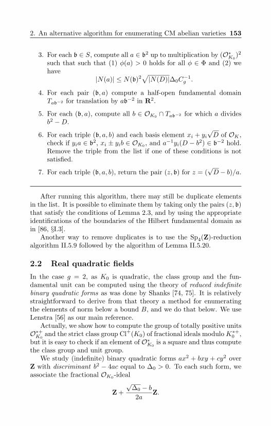
2. An alternative algorithm for enumerating CM abelian varieties 153
3. For each b ∈ S, compute all a ∈ b2 up to multiplication by (O∗K0)2
such that such that (1) φ(a) > 0 holds for all φ ∈ Φ and (2) wehave
|N(a)| ≤ N(b)2√|N(D)|∆0C
−1g .
4. For each pair (b, a) compute a half-open fundamental domainTab−2 for translation by ab−2 in R2.
5. For each (b, a), compute all b ∈ OK0 ∩ Tab−2 for which a dividesb2 −D.
6. For each triple (b, a, b) and each basis element xi + yi√D of OK ,
check if yia ∈ b2, xi ± yib ∈ OK0 , and a−1yi(D − b2) ∈ b−2 hold.Remove the triple from the list if one of these conditions is notsatisfied.
7. For each triple (b, a, b), return the pair (z, b) for z = (√D− b)/a.
After running this algorithm, there may still be duplicate elementsin the list. It is possible to eliminate them by taking only the pairs (z, b)that satisfy the conditions of Lemma 2.3, and by using the appropriateidentifications of the boundaries of the Hilbert fundamental domain asin [86, §I.3].
Another way to remove duplicates is to use the Sp4(Z)-reductionalgorithm II.5.9 followed by the algorithm of Lemma II.5.20.
2.2 Real quadratic fields
In the case g = 2, as K0 is quadratic, the class group and the fun-damental unit can be computed using the theory of reduced indefinitebinary quadratic forms as was done by Shanks [74, 75]. It is relativelystraightforward to derive from that theory a method for enumeratingthe elements of norm below a bound B, and we do that below. We useLenstra [56] as our main reference.
Actually, we show how to compute the group of totally positive unitsO∗+K0
and the strict class group Cl+(K0) of fractional ideals modulo K∗+0 ,but it is easy to check if an element of O∗K0
is a square and thus computethe class group and unit group.
We study (indefinite) binary quadratic forms ax2 + bxy + cy2 overZ with discriminant b2 − 4ac equal to ∆0 > 0. To each such form, weassociate the fractional OK0-ideal
Z +√
∆0 − b2a
Z.
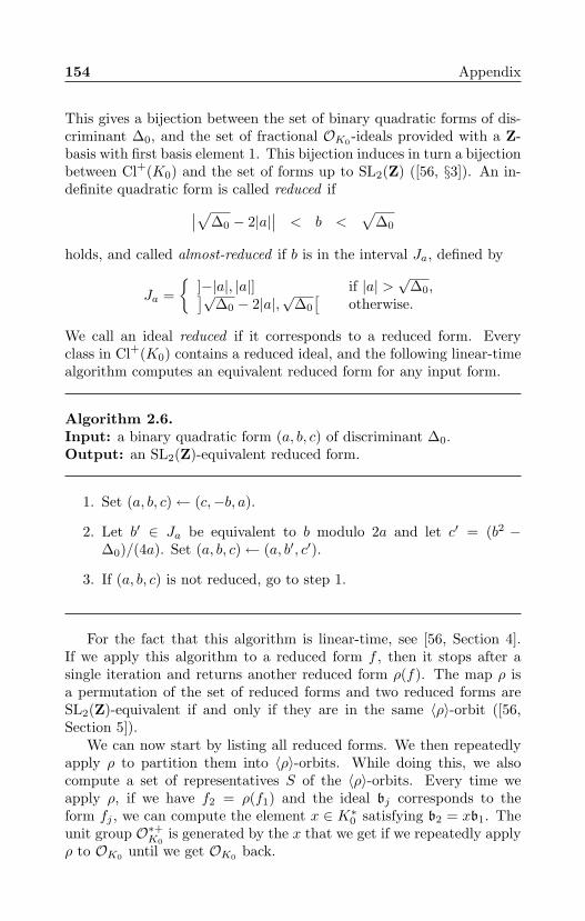
154 Appendix
This gives a bijection between the set of binary quadratic forms of dis-criminant ∆0, and the set of fractional OK0 -ideals provided with a Z-basis with first basis element 1. This bijection induces in turn a bijectionbetween Cl+(K0) and the set of forms up to SL2(Z) ([56, §3]). An in-definite quadratic form is called reduced if∣∣√∆0 − 2|a|
∣∣ < b <√
∆0
holds, and called almost-reduced if b is in the interval Ja, defined by
Ja =
]−|a|, |a|] if |a| >√
∆0,]√∆0 − 2|a|,
√∆0
[otherwise.
We call an ideal reduced if it corresponds to a reduced form. Everyclass in Cl+(K0) contains a reduced ideal, and the following linear-timealgorithm computes an equivalent reduced form for any input form.
Algorithm 2.6.Input: a binary quadratic form (a, b, c) of discriminant ∆0.Output: an SL2(Z)-equivalent reduced form.
1. Set (a, b, c)← (c,−b, a).
2. Let b′ ∈ Ja be equivalent to b modulo 2a and let c′ = (b2 −∆0)/(4a). Set (a, b, c)← (a, b′, c′).
3. If (a, b, c) is not reduced, go to step 1.
For the fact that this algorithm is linear-time, see [56, Section 4].If we apply this algorithm to a reduced form f , then it stops after asingle iteration and returns another reduced form ρ(f). The map ρ isa permutation of the set of reduced forms and two reduced forms areSL2(Z)-equivalent if and only if they are in the same 〈ρ〉-orbit ([56,Section 5]).
We can now start by listing all reduced forms. We then repeatedlyapply ρ to partition them into 〈ρ〉-orbits. While doing this, we alsocompute a set of representatives S of the 〈ρ〉-orbits. Every time weapply ρ, if we have f2 = ρ(f1) and the ideal bj corresponds to theform fj , we can compute the element x ∈ K∗0 satisfying b2 = xb1. Theunit group O∗+K0
is generated by the x that we get if we repeatedly applyρ to OK0 until we get OK0 back.
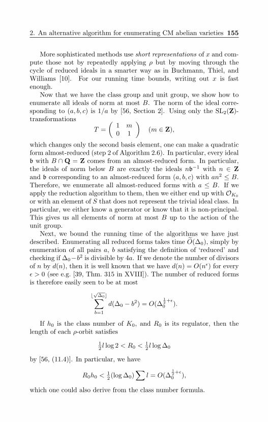
2. An alternative algorithm for enumerating CM abelian varieties 155
More sophisticated methods use short representations of x and com-pute those not by repeatedly applying ρ but by moving through thecycle of reduced ideals in a smarter way as in Buchmann, Thiel, andWilliams [10]. For our running time bounds, writing out x is fastenough.
Now that we have the class group and unit group, we show how toenumerate all ideals of norm at most B. The norm of the ideal corre-sponding to (a, b, c) is 1/a by [56, Section 2]. Using only the SL2(Z)-transformations
T =(
1 m0 1
)(m ∈ Z),
which changes only the second basis element, one can make a quadraticform almost-reduced (step 2 of Algorithm 2.6). In particular, every idealb with B ∩Q = Z comes from an almost-reduced form. In particular,the ideals of norm below B are exactly the ideals nb−1 with n ∈ Zand b corresponding to an almost-reduced form (a, b, c) with an2 ≤ B.Therefore, we enumerate all almost-reduced forms with a ≤ B. If weapply the reduction algorithm to them, then we either end up with OK0
or with an element of S that does not represent the trivial ideal class. Inparticular, we either know a generator or know that it is non-principal.This gives us all elements of norm at most B up to the action of theunit group.
Next, we bound the running time of the algorithms we have justdescribed. Enumerating all reduced forms takes time O(∆0), simply byenumeration of all pairs a, b satisfying the definition of ‘reduced’ andchecking if ∆0−b2 is divisible by 4a. If we denote the number of divisorsof n by d(n), then it is well known that we have d(n) = O(nε) for everyε > 0 (see e.g. [39, Thm. 315 in XVIII]). The number of reduced formsis therefore easily seen to be at most
b√
∆0c∑b=1
d(∆0 − b2) = O(∆12 +ε0 ).
If h0 is the class number of K0, and R0 is its regulator, then thelength of each ρ-orbit satisfies
12 l log 2 < R0 <
12 l log ∆0
by [56, (11.4)]. In particular, we have
R0h0 <12 (log ∆0)
∑l = O(∆
12 +ε0 ),
which one could also derive from the class number formula.
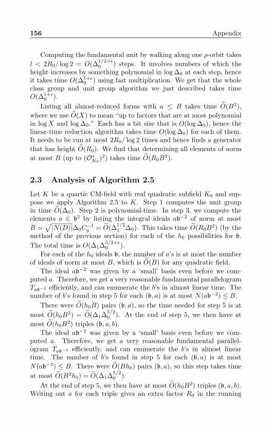
156 Appendix
Computing the fundamental unit by walking along one ρ-orbit takesl < 2R0/ log 2 = O(∆1/2+ε
0 ) steps. It involves numbers of which theheight increases by something polynomial in log ∆0 at each step, henceit takes time O(∆1+ε
0 ) using fast multiplication. We get that the wholeclass group and unit group algorithm we just described takes timeO(∆1+ε
0 ).Listing all almost-reduced forms with a ≤ B takes time O(B2),
where we use O(X) to mean “up to factors that are at most polynomialin logX and log ∆0.” Each has a bit size that is O(log ∆0), hence thelinear-time reduction algorithm takes time O(log ∆0) for each of them.It needs to be run at most 2R0/ log 2 times and hence finds a generatorthat has height O(R0). We find that determining all elements of normat most B (up to (O∗K0
)2) takes time O(R0B2).
2.3 Analysis of Algorithm 2.5
Let K be a quartic CM-field with real quadratic subfield K0 and sup-pose we apply Algorithm 2.5 to K. Step 1 computes the unit groupin time O(∆0). Step 2 is polynomial-time. In step 3, we compute theelements a ∈ b2 by listing the integral ideals ab−2 of norm at mostB =
√|N(D)|∆0C
−1g = O(∆1/2
1 ∆0). This takes time O(R0B2) (by the
method of the previous section) for each of the h0 possibilities for b.The total time is O(∆1∆5/2+ε
0 ).For each of the h0 ideals b, the number of a’s is at most the number
of ideals of norm at most B, which is O(B) for any quadratic field.The ideal ab−2 was given by a ‘small’ basis even before we com-
puted a. Therefore, we get a very reasonable fundamental parallelogramTab−2 efficiently, and can enumerate the b’s in almost linear time. Thenumber of b’s found in step 5 for each (b, a) is at most N(ab−2) ≤ B.
There were O(h0B) pairs (b, a), so the time needed for step 5 is atmost O(h0B
2) = O(∆1∆5/20 ). At the end of step 5, we then have at
most O(h0B2) triples (b, a, b).
The ideal ab−2 was given by a ‘small’ basis even before we com-puted a. Therefore, we get a very reasonable fundamental parallel-ogram Tab−2 efficiently, and can enumerate the b’s in almost lineartime. The number of b’s found in step 5 for each (b, a) is at mostN(ab−2) ≤ B. There were O(Bh0) pairs (b, a), so this step takes timeat most O(B2h0) = O(∆1∆5/2
0 ).At the end of step 5, we then have at most O(h0B
2) triples (b, a, b).Writing out a for each triple gives an extra factor R0 in the running
2. An alternative algorithm for enumerating CM abelian varieties 157
time, so we get a running time of O(h0R0B2) = O(∆1∆5/2+ε
0 ), whichproves the following result.
Theorem 2.7. On input a quartic CM-field K, Algorithm 2.5 runs intime O(∆1∆5/2+ε
0 ).
2.4 Generalization of Spallek’s formula
Spallek, in her thesis [79], gave a formula for the period matrices ofa complete set of representatives of the isomorphism classes of abeliansurfaces with CM by a given primitive quartic CM-field K of which thereal quadratic subfield K0 has class number one. This formula has beenthe method of choice of other authors and even made it into a textbook[27, 97]. The theory of the Section I.5.3 allows us to simplify Spallek’sresults and to generalize them to arbitrary primitive quartic CM-fields.
Let K be a primitive quartic CM-field with real quadratic subfieldK0 and let ω ∈ K0 be such that OK0 = Z[ω].
Lemma 2.8. Suppose that z ∈ K is such that zOK0 +OK0 is an OK-ideal. Let φ1, φ2 be the embeddings of K into C given by φ1ω > φ2ωand Imφ1(z) > 0 > Imφ2(z). Then the abelian variety correspondingto the pair (z, b) has a period matrix
Zz =2∑i=1
φi
(zδ−1
(ω2 ωω 1
))∈ H2.
Proof. Choose b1 = ω and b2 = 1 in Theorem II.4.3.
Theorem 2.9. Let K be a primitive quartic CM-field. A complete setof representatives for the isomorphism classes of abelian varieties overC with CM by OK can be obtained as follows.
1. Let Φ = φ1, φ2 be a CM-type of K.
2. Let ε ∈ O∗K0be such that 〈−1〉 × 〈ε〉 has odd index in O∗K0
.
3. Let K′ ⊂ K be such that zOK0 +OK0 : z ∈ K′ is a complete setof representatives of the ideal classes of K that contain an idealof the form zOK0 +OK0 .
4. Let K = ±K′ ∪ ±εK′.
5. If K is cyclic Galois, return
Zz | z ∈ K, Imφ1z > 0 > Imφ2z.
158 Appendix
6. If K is non-Galois, return
Zz | z ∈ K, Imφ1z > 0.
Proof. Algorithm II.3.1 gives a complete set of representatives of theisomorphism classes of principally polarized abelian varieties over Cwith CM by OK . Theorems I.5.8 and I.5.9 show that the ideal classesa of step 4 of Algorithm II.3.1 are exactly the ones that contain a rep-resentative of the form zOK0 +OK0 . Moreover, ξ = (z − z)−1δ−1 givesa choice of ξ as in step 4 of Algorithm II.3.1.
We use Corollary II.3.4 to compute O∗K0/NK/K0(O∗K) (which con-
sists of the classes of ±1 and ±ε) and Lemma I.3.4 to compute a com-plete set of representatives for the equivalence classes of CM-types (Φif K is cyclic Galois and Φ, φ1, φ2 if K is non-Galois).
Multiplication of ξ by u ∈ O∗K0corresponds exactly to multiplication
of z by u−1, so K corresponds exactly to the set of triples (a, ξ, u) ofstep 5 of Algorithm II.3.1. Steps 5 and 6 are the same as step 6 ofAlgorithm II.3.1.
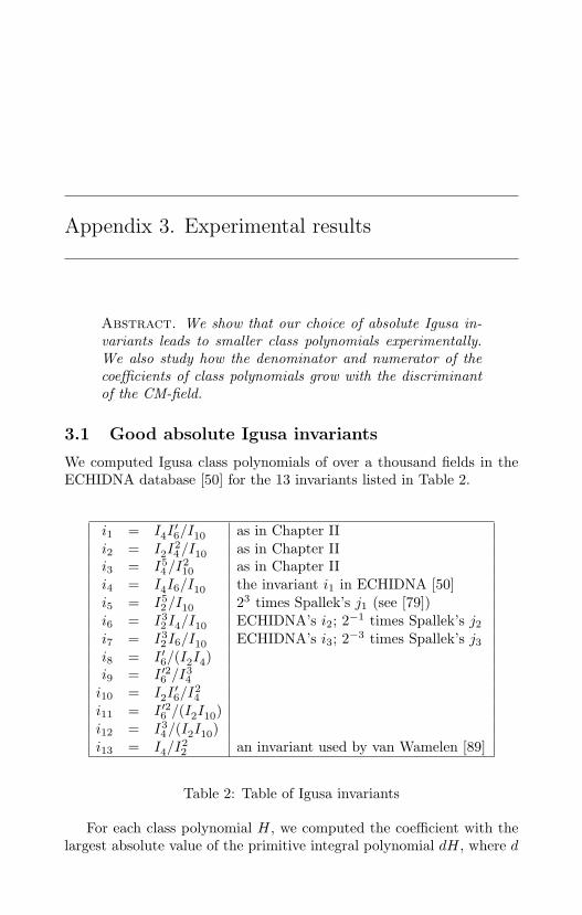
Appendix 3. Experimental results
Abstract. We show that our choice of absolute Igusa in-variants leads to smaller class polynomials experimentally.We also study how the denominator and numerator of thecoefficients of class polynomials grow with the discriminantof the CM-field.
3.1 Good absolute Igusa invariants
We computed Igusa class polynomials of over a thousand fields in theECHIDNA database [50] for the 13 invariants listed in Table 2.
i1 = I4I′6/I10 as in Chapter II
i2 = I2I24/I10 as in Chapter II
i3 = I54/I
210 as in Chapter II
i4 = I4I6/I10 the invariant i1 in ECHIDNA [50]i5 = I5
2/I10 23 times Spallek’s j1 (see [79])i6 = I3
2I4/I10 ECHIDNA’s i2; 2−1 times Spallek’s j2i7 = I3
2I6/I10 ECHIDNA’s i3; 2−3 times Spallek’s j3i8 = I ′6/(I2I4)i9 = I ′26 /I
34
i10 = I2I′6/I
24
i11 = I ′26 /(I2I10)i12 = I3
4/(I2I10)i13 = I4/I
22 an invariant used by van Wamelen [89]
Table 2: Table of Igusa invariants
For each class polynomial H, we computed the coefficient with thelargest absolute value of the primitive integral polynomial dH, where d
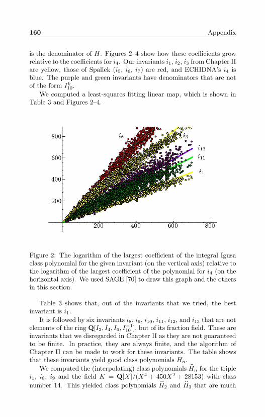
160 Appendix
is the denominator of H. Figures 2–4 show how these coefficients growrelative to the coefficients for i4. Our invariants i1, i2, i3 from Chapter IIare yellow, those of Spallek (i5, i6, i7) are red, and ECHIDNA’s i4 isblue. The purple and green invariants have denominators that are notof the form Ik10.
We computed a least-squares fitting linear map, which is shown inTable 3 and Figures 2–4.
Figure 2: The logarithm of the largest coefficient of the integral Igusaclass polynomial for the given invariant (on the vertical axis) relative tothe logarithm of the largest coefficient of the polynomial for i4 (on thehorizontal axis). We used SAGE [70] to draw this graph and the othersin this section.
Table 3 shows that, out of the invariants that we tried, the bestinvariant is i1.
It is followed by six invariants i8, i9, i10, i11, i12, and i13 that are notelements of the ring Q[I2, I4, I6, I−1
10 ], but of its fraction field. These areinvariants that we disregarded in Chapter II as they are not guaranteedto be finite. In practice, they are always finite, and the algorithm ofChapter II can be made to work for these invariants. The table showsthat these invariants yield good class polynomials Hn.
We computed the (interpolating) class polynomials Hn for the triplei1, i8, i9 and the field K = Q[X]/(X4 + 450X2 + 28153) with classnumber 14. This yielded class polynomials H2 and H3 that are much
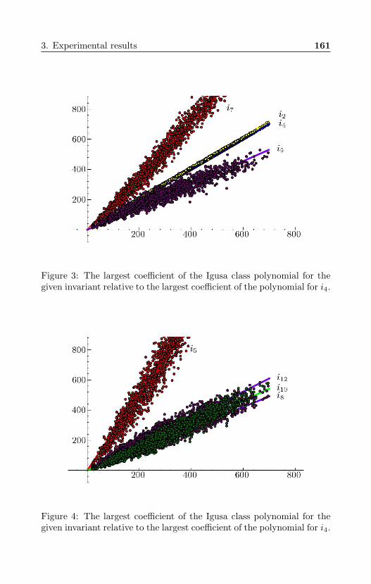
3. Experimental results 161
Figure 3: The largest coefficient of the Igusa class polynomial for thegiven invariant relative to the largest coefficient of the polynomial for i4.
Figure 4: The largest coefficient of the Igusa class polynomial for thegiven invariant relative to the largest coefficient of the polynomial for i4.
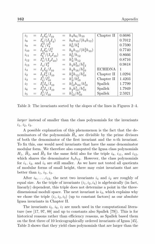
162 Appendix
i1 = I4I′6/I10 = h4h6/h10 Chapter II 0.6686
i8 = I ′6/(I2I4) = h6h10/(h4h12) 0.7012i9 = I ′26 /I
34 = h2
6/h34 0.7590
i10 = I2I′6/I
24 = h6h12/(h
24h10) 0.7740
i11 = I ′26 /(I2I10) = h26/h12 0.8666
i12 = I34/(I2I10) = h3
4/h12 0.8716i13 = I4/I
22 = h4h
210/h
212 0.9818
i4 = I4I6/I10 = h4h16/h210 ECHIDNA 1
i2 = I2I24/I10 = h2
4h12/h210 Chapter II 1.0294
i3 = I54/I
210 = h5
4/h210 Chapter II 1.4203
i7 = I22I6/I10 = h2
12h16/h410 Spallek 1.7799
i6 = I32I4/I10 = h4h
312/h
410 Spallek 1.7949
i5 = I52/I10 = h5
12/h610 Spallek 2.5921
Table 3: The invariants sorted by the slopes of the lines in Figures 2–4.
larger instead of smaller than the class polynomials for the invariantsi1, i2, i3.
A possible explanation of this phenomenon is the fact that the de-nominators of the polynomials Hn are divisible by the prime divisorsof both the denominator of the first invariant and the n-th invariant.To fix this, one would need invariants that have the same denominatormodular form. We therefore also computed the Igusa class polynomialsH1, H2, and H3 for the same field also for the triple i8, i11, and i12,which shares the denominator h4h12. However, the class polynomialsfor i1, i2, and i3 are still smaller. As we have not tested all quotientsof modular forms of small height, there may exist invariants that arebetter than i1, i2, i3.
After i8, . . . , i13, the next two invariants i4 and i2 are roughly ofequal size. As the triple of invariants (i1, i2, i4) is algebraically (in fact,linearly) dependent, this triple does not determine a point in the three-dimensional moduli space. The next invariant is i3, which explains whywe chose the triple (i1, i2, i3) (up to constant factors) as our absoluteIgusa invariants in Chapter II.
The invariants i5, i6, i7 are much used in the computational litera-ture (see [17, 97, 88] and up to constants also Spallek [79]). This is forhistorical reasons rather than efficiency reasons, as Spallek based themon the first three of 10 lexicographically ordered invariants of Igusa [45].Table 3 shows that they yield class polynomials that are larger than the
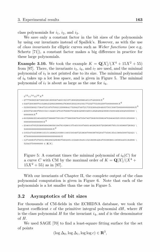
3. Experimental results 163
class polynomials for i1, i2, and i3.We save only a constant factor in the bit sizes of the polynomials
by using our invariants instead of Spallek’s. However, as with the useof class invariants for elliptic curves such as Weber functions (see e.g.Schertz [71]), a constant factor makes a big difference in practice forthese large polynomials.
Example 3.10. We took the example K = Q[X]/(X4 + 15X2 + 55)from [97]. There, the invariants i5, i6, and i7 are used, and the minimalpolynomial of i5 is not printed due to its size. The minimal polynomialof i6 takes up a lot less space, and is given in Figure 5. The minimalpolynomial of i7 is about as large as the one for i6.
31211141316X8
−27779096536726653818950674601921971890292396045107400000X7
+346720036970164864520633999647836053021001931772327731602397500000000X6
−323935892173647531870709212399984173294274072173523094304605750150875000000000000X5
−209372188379501941132201276457668070320842985529512926296239981565946640625000000 \
0000000X4
+603288625340422507388887591081772665967647934740738205039824762464032519531250000 \
00000000000000X3
−234016705253685894380561947610280137543191874931402823057202858579513193969726562 \
500000000000000000000X2
+105347345309814515146862103901160150349725383070903879520477458135413894500732421 \
875000000000000000000000000X
−127166837276051396256529080756023511024819431152186984264705390881185904455184936 \
52343750000000 ∈ Z[X].
Figure 5: A constant times the minimal polynomial of i6(C) fora curve C with CM by the maximal order of K = Q[X]/(X4 +15X2 + 55) as in [97].
With our invariants of Chapter II, the complete output of the classpolynomial computation is given in Figure 6. Note that each of thepolynomials is a lot smaller than the one in Figure 5.
3.2 Asymptotics of bit sizes
For thousands of CM-fields in the ECHIDNA database, we took thelargest coefficient c of the primitive integral polynomial dH, where His the class polynomial H for the invariant i4, and d is the denominatorof H.
We used SAGE [70] to find a least-square fitting surface for the setof points
(log ∆0, log ∆1, log log c) ∈ R3,
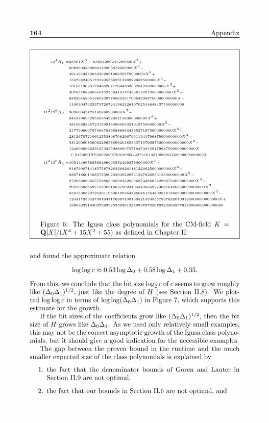
164 Appendix
134H1 =28561X8 − 63024286247286000X7+
5089603200935139203672250000X6−
491194385305230285106635375000000X5+
15070824051791205356231328929687500000X4−
161861362817640620712844383632812500000000X3+
307857688685507527504191774536132812500000000X2+
68920458051660239778562561706542968750000000000X−
11003047923373720724198232610702514648437500000000
112136H2 =90966043775189898900000X7−
8453896932952685422851138300000000X6+
4810669345723139916396063321918750000000X5−
217790660707366708688888934365271875000000000X4+
2812670721061255380870829679611341796875000000000X3−
5812006085609229658899261853637167968750000000000000X2−
1248060962351653325988960727184738159179687500000000000X
+ 215389197036958387031899522270161437988281250000000000000
112136H3 =10544496589569296093552499375000000X7−
918790071418575878284368261181220625000000000X6+
88671860116857539020294922874122782695312500000000X5−
2720629806557588039359833283968744866542968750000000000X4+
29219693869772398316627802410434325592736816406250000000000X3−
55575385207252011052618036472504817648925781250000000000000000X2−
12441725942738194717698740313052143355579376220703125000000000000X+
1986302919403709292533996122809376722078323364257812500000000000000
Figure 6: The Igusa class polynomials for the CM-field K =Q[X]/(X4 + 15X2 + 55) as defined in Chapter II.
and found the approximate relation
log log c ≈ 0.53 log ∆0 + 0.58 log ∆1 + 0.35.
From this, we conclude that the bit size log2 c of c seems to grow roughlylike (∆0∆1)1/2, just like the degree of H (see Section II.8). We plot-ted log log c in terms of log log(∆0∆1) in Figure 7, which supports thisestimate for the growth.
If the bit sizes of the coefficients grow like (∆0∆1)1/2, then the bitsize of H grows like ∆0∆1. As we used only relatively small examples,this may not be the correct asymptotic growth of the Igusa class polyno-mials, but it should give a good indication for the accessible examples.
The gap between the proven bound in the runtime and the muchsmaller expected size of the class polynomials is explained by
1. the fact that the denominator bounds of Goren and Lauter inSection II.9 are not optimal,
2. the fact that our bounds in Section II.6 are not optimal, and
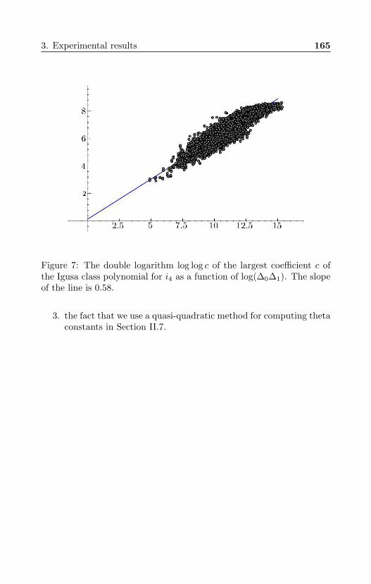
3. Experimental results 165
Figure 7: The double logarithm log log c of the largest coefficient c ofthe Igusa class polynomial for i4 as a function of log(∆0∆1). The slopeof the line is 0.58.
3. the fact that we use a quasi-quadratic method for computing thetaconstants in Section II.7.

Bibliography
[1] A. Oliver L. Atkin and Francois Morain. Elliptic curves and pri-mality proving. Mathematics of Computation, 61(203):29–68, 1993.http://www.inria.fr/rrrt/rr-1256.html. (cited on page 136)
[2] Juliana Belding, Reinier Broker, Andreas Enge, and Kristin Lauter.Computing Hilbert class polynomials. In Algorithmic Number The-ory – ANTS-VIII (Banff, 2008), volume 5011 of LNCS, pages 282–295. Springer, 2008. (cited on page 39)
[3] Daniel J. Bernstein. Fast multiplication and its applications. InJ. Buhler and P. Stevenhagen, editors, Surveys in AlgorithmicNumber Theory [11], pages 325–384, 2008. (cited on page 72)
[4] Christina Birkenhake and Herbert Lange. Complex abelian va-rieties, volume 302 of Grundlehren der mathematischen Wis-senschaften. Springer, second edition, 2004. The first part of thisbook appeared as [53]. (cited on pages 23, 28, 29, and 172)
[5] Oskar Bolza. Darstellung der rationalen ganzen Invarianten derBinarform sechsten Grades durch die Nullwerthe der zugehorigenϑ-Functionen. Math. Ann., 30(4):478–495, 1887. (cited on page 69)
[6] Dan Boneh, Eu-Jin Goh, and Kobbi Nissim. Evaluating 2-DNFformulas on ciphertexts. In TCC ‘05, volume 3378 of Lecture Notesin Computer Science, pages 325–341. Springer, 2005. (cited onpage 112)
[7] Wieb Bosma, John Cannon, and Catherine Playoust. The Magmaalgebra system I: The user language. J. Symbolic Comput., 24(3-4):235–265, 1997. Computational algebra and number theory (Lon-don, 1993). (cited on pages 95, 97, and 99)
168 Bibliography
[8] Jan Hendrik Bruinier and Tonghai Yang. CM-values of Hilbertmodular functions. Invent. Math., 163(2):229–288, 2006. (cited onpages 77 and 82)
[9] Johannes Buchmann and Hendrik W. Lenstra, Jr. Approximatingrings of integers in number fields. Journal de Theorie des Nombresde Bordeaux, 6:221–260, 1994. (cited on pages 48 and 87)
[10] Johannes Buchmann, Christoph Thiel, and Hugh Williams. Shortrepresentation of quadratic integers. In Computational algebra andnumber theory (Sydney, 1992), volume 325 of Math. Appl., pages159–185. Kluwer Acad. Publ., 1995. (cited on page 155)
[11] Joe P. Buhler and Peter Stevenhagen, editors. Surveys in Algorith-mic Number Theory, volume 44 of MSRI Publications. CambridgeUniversity Press, 2008. (cited on pages 167, 168, 172, 174, and 175)
[12] Gabriel Cardona and Jordi Quer. Field of moduli and field of defi-nition for curves of genus 2. In Computational aspects of algebraiccurves, volume 13 of Lecture Notes Ser. Comput., pages 71–83.World Scientific, 2005. (cited on pages 43 and 102)
[13] Robert Carls, David Kohel, and David Lubicz. Higher-dimensional3-adic CM construction. J. Algebra, 319(3):971–1006, 2008. (citedon page 40)
[14] Robert Carls and David Lubicz. A p-adic quasi-quadratic timepoint counting algorithm. Int. Math. Res. Not. IMRN, (4):698–735, 2009. (cited on page 40)
[15] Alfred Clebsch. Zur Theorie der binaren algebraischen Formen.Math. Ann., 3(2):265–267, 1870. (cited on page 42)
[16] Henri Cohen. A Course in Computational Algebraic Number The-ory, volume 138 of Graduate Texts in Mathematics. Springer, 1993.(cited on page 131)
[17] Henri Cohen, Gerhard Frey, Roberto Avanzi, Christophe Doche,Tanja Lange, Kim Nguyen, and Frederik Vercauteren, editors.Handbook of elliptic and hyperelliptic curve cryptography. Chap-man & Hall/CRC, Boca Raton, FL, 2006. (cited on pages 162,169, and 170)
[18] Henri Cohen and Peter Stevenhagen. Computational class fieldtheory. In J. Buhler and P. Stevenhagen, editors, Surveys in Al-gorithmic Number Theory [11], pages 497–534, 2008. (cited onpage 18)
Bibliography 169
[19] David A. Cox. Primes of the form x2 + ny2. John Wiley & Sons,1989. (cited on page 190)
[20] Regis Dupont. Moyenne arithmetico-geometrique, suites deBorchardt et applications. PhD thesis, Ecole Polytechnique,2006. http://www.lix.polytechnique.fr/Labo/Regis.Dupont/these_soutenance.pdf. (cited on pages 67, 69, 70, 71, 74, and 90)
[21] Kirsten Eisentrager and Kristin Lauter. A CRT algorithm for con-structing genus 2 curves over finite fields. To appear in Arithmetic,Geometry and Coding Theory, AGCT-10 (Marseille, 2005), 2005.(cited on pages 40 and 137)
[22] Andreas Enge. The complexity of class polynomial computationvia floating point approximations. Mathematics of Computation,78(266):1089–1107, 2009. (cited on page 39)
[23] Andreas Enge and Francois Morain. Fast decomposition of polyno-mials with known Galois group. In Applied algebra, algebraic algo-rithms and error-correcting codes (Toulouse, 2003), volume 2643of Lecture Notes in Comput. Sci., pages 254–264, Berlin, 2003.Springer. (cited on pages 44 and 88)
[24] David Freeman. Constructing pairing-friendly genus 2 curves overprime fields with ordinary Jacobians. In Pairing-Based Cryptog-raphy – Pairing 2007, volume 4575 of Lecture Notes in ComputerScience, pages 152– 176, Berlin, 2007. Springer-Verlag. (cited onpage 124)
[25] David Freeman, Michael Scott, and Edlyn Teske. A taxonomy ofpairing-friendly elliptic curves. Cryptology ePrint Archive, Report2006/372, 2006. http://eprint.iacr.org/2006/372. (cited onpage 109)
[26] David Freeman, Peter Stevenhagen, and Marco Streng. Abelianvarieties with prescribed embedding degree. In Algorithmic NumberTheory, 8th International Symposium, ANTS-VIII, Banff, Canada,May 17-22, 2008, Proceedings [87], pages 60–73, 2008. Appears asChapter IV in this thesis. (cited on pages 15, 100, 105, 124, 134,135, and 136)
[27] Gerhard Frey and Tanja Lange. Complex multiplication. In Hand-book of elliptic and hyperelliptic curve cryptography [17], pages455–473. Chapman & Hall/CRC, 2006. (cited on pages 41, 70, 136,and 157)

170 Bibliography
[28] Gerhard Frey and Tanja Lange. Varieties over special fields. InHandbook of elliptic and hyperelliptic curve cryptography [17],pages 87–113. Chapman & Hall/CRC, 2006. (cited on page 43)
[29] Gerhard Frey and Hans-Georg Ruck. A remark concerning m-divisibility and the discrete logarithm in the divisor class group ofcurves. Mathematics of Computation, 62:865–874, 1994. (cited onpage 106)
[30] Steven Galbraith. Supersingular curves in cryptography. In ASI-ACRYPT ‘01, volume 2248 of Lecture Notes in Computer Science,pages 495–513. Springer, 2001. (cited on page 107)
[31] Pierrick Gaudry, Thomas Houtmann, David Kohel, ChristopheRitzenthaler, and Annegret Weng. The p-adic CM-method forgenus 2, 2005. arXiv:math/0503148, see also [32]. (cited on pages40 and 170)
[32] Pierrick Gaudry, Thomas Houtmann, David Kohel, ChristopheRitzenthaler, and Annegret Weng. The 2-adic CM method forgenus 2 curves with application to cryptography. In Advances inCryptology – ASIACRYPT 2006, volume 4284 of Lecture Notes inComputer Science, pages 114–129, Berlin, 2006. Springer-Verlag.see also [31]. (cited on pages 40, 44, 137, and 170)
[33] Josep Gonzalez. On the p-rank of an abelian variety and its en-domorphism algebra. Pub. Math., 42(1):119–130, 1998. (cited onpages 125, 126, and 127)
[34] Eyal Z. Goren. On certain reduction problems concerning abeliansurfaces. manuscripta mathematica, 94(1):33–43, 1997. (cited onpages 78, 99, and 125)
[35] Eyal Z. Goren and Kristin Lauter. Class invariants for quartic CMfields. Annales de l’Institut Fourier, 57(2):457–480, 2007. (cited onpages 40, 41, 43, 76, 77, and 78)
[36] Eyal Z. Goren and Kristin Lauter. Genus 2 curves with complexmultiplication. arXiv:1003.4759v1, 2010. (cited on pages 40, 41,76, 77, 78, and 79)
[37] Erhard Gottschling. Die Randflachen des Fundamentalbereichesder Modulgruppe. Math. Annalen, 138:103–124, 1959. (cited onpages 56 and 63)
Bibliography 171
[38] Guillaume Hanrot and Francois Morain. Solvability by radicalsfrom an algorithmic point of view. In Proceedings of the 2001 In-ternational Symposium on Symbolic and Algebraic Computation,pages 175–182 (electronic), New York, 2001. ACM. (cited onpage 44)
[39] Godfrey Harold Hardy and Edward Maitland Wright. An Intro-duction to the Theory of Numbers. Oxford University Press, 1938.(cited on pages 132 and 155)
[40] Erich Hecke. Vorlesungen uber die Theorie der algebraischenZahlen. Chelsea Publishing Co., Bronx, N.Y., 1970. Second editionof the 1923 original, with an index. (cited on page 44)
[41] Marc Hindry and Joseph H. Silverman. Diophantine geometry,volume 201 of Graduate Texts in Mathematics. Springer-Verlag,New York, 2000. An introduction. (cited on page 29)
[42] Laura Hitt. On the minimal embedding field. In Pairing-BasedCryptography – Pairing 2007, volume 4575 of Lecture Notes inComputer Science, pages 294–301. Springer-Verlag, 2007. (citedon page 136)
[43] Laura Hitt O’Connor, Gary McGuire, Michael Naehrig, and MarcoStreng. A CM construction for curves of genus 2 with p-rank 1.To be published by Journal of Number Theory, arXiv:0811.3434v2,appears as Chapter V in this thesis, 2008. (cited on pages 15and 123)
[44] Taira Honda. Isogeny classes of abelian varieties over finite fields.J. Math. Soc. Japan, 20:83–95, 1968. (cited on page 124)
[45] Jun-Ichi Igusa. Arithmetic variety of moduli for genus two. Annalsof Mathematics, 72(3):612–649, 1960. (cited on pages 42, 43, 92,136, 138, and 162)
[46] Jun-Ichi Igusa. On siegel modular forms of genus two. AmericanJournal of Mathematics, 84(1):175–200, 1962. (cited on page 69)
[47] Jun-Ichi Igusa. Modular forms and projective invariants. AmericanJournal of Mathematics, 89(3):817–855, 1967. http://www.jstor.org/stable/2373243. (cited on pages 69 and 150)
[48] Helmut Klingen. Introductory lectures on Siegel modular forms,volume 20 of Cambridge Studies in Advanced Mathematics. Cam-bridge University Press, Cambridge, 1990. (cited on pages 57, 58,59, and 71)
172 Bibliography
[49] Ann Hibner Koblitz, Neal Koblitz, and Alfred Menezes. Ellipticcurve cryptography: The serpentine course of a paradigm shift.Cryptology ePrint Archive, Report 2008/390, 2008. To appear inJournal of Number Theory, http://eprint.iacr.org/2008/390.
[50] David Kohel et al. ECHIDNA algorithms for algebra and geometryexperimentation. http://echidna.maths.usyd.edu.au/~kohel/dbs/complex_multiplication2.html. (cited on pages 43, 82, 93,137, 141, and 159)
[51] Kenji Koike and Annegret Weng. Construction of CM Picardcurves. Mathematics of Computation, 74:499–518, 2004. (citedon page 119)
[52] Serge Lang. Complex Multiplication, volume 255 of Grundlehrender mathematischen Wissenschaften. Springer, 1983. (cited onpages 19, 21, 22, 25, 30, 32, 34, and 95)
[53] Herbert Lange and Christina Birkenhake. Complex abelian va-rieties, volume 302 of Grundlehren der mathematischen Wis-senschaften. Springer, 1992. reappeared in [4]. (cited on page 167)
[54] Kristin Lauter. Primes in the denominators of Igusa class polyno-mials. 2003. (cited on pages 77 and 82)
[55] Arjen K. Lenstra, Hendrik W. Lenstra, Jr., and Laszlo Lovasz.Factoring polynomials with rational coefficients. Math. Ann.,261(4):515–534, 1982. (cited on page 95)
[56] Hendrik W. Lenstra, Jr. On the calculation of regulators and classnumbers of quadratic fields. In Journees Arithmetiques 1980, pages123–150. Cambridge University Press, 1982. (cited on pages 153,154, and 155)
[57] Hendrik W. Lenstra, Jr. Lattices. In J. Buhler and P. Stevenhagen,editors, Surveys in Algorithmic Number Theory [11], pages 127–181, 2008. (cited on pages 47, 50, 55, 86, and 95)
[58] Stephane Louboutin. Explicit lower bounds for residues at s = 1of Dedekind zeta functions and relative class numbers of CM-fields. Trans. Amer. Math. Soc., 355(8):3079–3098 (electronic),2003. (cited on page 76)
[59] Daniel Maisner and Enric Nart. Abelian surfaces over finite fieldsas Jacobians. Experiment. Math., 11(3):321–337, 2002. With anappendix by Everett W. Howe. (cited on page 127)
Bibliography 173
[60] Alfred Menezes, Tatsuaki Okamoto, and Scott A. Vanstone. Reduc-ing elliptic curve logarithms to logarithms in a finite field. IEEETransactions on Information Theory, 39:1639–1646, 1993. (citedon page 106)
[61] Jean-Francois Mestre. Construction de courbes de genre 2 a par-tir de leurs modules. In Effective methods in algebraic geometry(Castiglioncello, 1990), volume 94 of Progr. Math., pages 313–334,Boston, MA, 1991. Birkhauser Boston. (cited on pages 43, 99,and 136)
[62] James S. Milne. Abelian varieties. In Arithmetic Geometry, pages103–150, New York, 1986. Springer. (cited on page 23)
[63] James S. Milne. Jacobian varieties. In Arithmetic Geometry, pages167–212, New York, 1986. Springer. (cited on page 28)
[64] James S. Milne. Complex multiplication. Version 0.00. Availableat http://www.jmilne.org/math/, 2006. (cited on pages 19, 21,22, 30, 34, and 95)
[65] David Mumford. Tata lectures on theta II, volume 43 of Progressin Mathematics. Birkhauser, 1984. (cited on page 69)
[66] Jurgen Neukirch. Algebraische Zahlentheorie. Springer, 1992. (citedon pages 27, 129, and 140)
[67] Kenny Paterson. Cryptography from pairings. In I.F. Blake,G. Seroussi, and N.P. Smart, editors, Advances in Elliptic CurveCryptography, pages 215–251. Cambridge University Press, 2005.(cited on page 106)
[68] H.L. Resnikoff and R.L. Saldana. Some properties of Fourier coef-ficients of Eisenstein series of degree two. J. Reine Angew. Math.,265:90–109, 1974. (cited on page 150)
[69] Karl Rubin and Alice Silverberg. Supersingular abelian varietiesin cryptology. In Proceedings of the 22nd Annual InternationalCryptology Conference on Advances in Cryptology, volume 2442 ofLecture Notes In Computer Science, pages 336–353, 2002. (citedon pages 107 and 124)
[70] SAGE. SAGE mathematics software, version 4.0.1. http://www.sagemath.org/. (cited on pages 4, 160, and 163)
174 Bibliography
[71] Reinhard Schertz. Die singularen Werte der Weberschen Funktio-nen f, f1, f2, γ2, γ3. J. Reine Angew. Math., 286/287:46–74, 1976.(cited on page 163)
[72] Rene Schoof. Elliptic curves over finite fields and the computationof square roots mod p. Math. Comp., 44(170):483–494, 1985.
[73] Rene Schoof. Computing Arakelov class groups. In J. Buhler andP. Stevenhagen, editors, Surveys in Algorithmic Number Theory[11], pages 447–495, 2008. (cited on page 47)
[74] Daniel Shanks. Class number, a theory of factorization, and genera.In 1969 Number Theory Institute (Proc. Sympos. Pure Math., Vol.XX, State Univ. New York, Stony Brook, N.Y., 1969), pages 415–440, Providence, R.I., 1971. Amer. Math. Soc. (cited on page 153)
[75] Daniel Shanks. The infrastructure of a real quadratic field andits applications. In Proceedings of the Number Theory Conference(Univ. Colorado, Boulder, Colo., 1972), pages 217–224, Boulder,Colo., 1972. Univ. Colorado. (cited on page 153)
[76] Goro Shimura. On the class-fields obtained by complex multipli-cation of abelian varieties. Osaka Math. J., 14:33–44, 1962. (citedon pages 14, 17, 35, and 36)
[77] Goro Shimura. Abelian Varieties with Complex Multiplication andModular Functions. Princeton University Press, 1998. Sections 1–16 essentially appeared before in [78]. (cited on pages 110, 138,and 174)
[78] Goro Shimura and Yutaka Taniyama. Complex multiplication ofabelian varieties and its applications to number theory, volume 6of Publications of the Mathematical Society of Japan. The Math-ematical Society of Japan, Tokyo, 1961. Sections 1–16 essentiallyreappeared in [77]. (cited on pages 18, 19, 20, 21, 22, 24, 25, 29,30, 31, 32, 34, 98, 124, 126, 136, 138, 139, and 174)
[79] Anne-Monika Spallek. Kurven vom Geschlecht 2 und ihre An-wendung in Public-Key-Kryptosystemen. PhD thesis, Institut furExperimentelle Mathematik, Universitat GH Essen, 1994. http://www.uni-due.de/zahlentheorie/theses_de.shtml. (cited onpages 14, 15, 24, 40, 41, 43, 69, 124, 137, 157, 159, and 162)
[80] Peter Stevenhagen. Hilbert’s 12th problem, complex multiplicationand Shimura reciprocity. In Class field theory – its centenary and
Bibliography 175
prospect (Tokyo, 1998), volume 30 of Adv. Stud. Pure Math., pages161–176. Math. Soc. Japan, Tokyo, 2001.
[81] Peter Stevenhagen. The arithmetic of number rings. In J. Buh-ler and P. Stevenhagen, editors, Surveys in Algorithmic NumberTheory [11], 2008. (cited on page 142)
[82] Marco Streng. Computing Igusa class polynomials. arXiv:0903.4766, appears as Chapter II in this thesis, 2008. (cited on page 137)
[83] Marco Streng. Divisibility sequences for elliptic curves with com-plex multiplication. Algebra & Number Theory, 2(2):183–208,2008.
[84] John Tate. Classes d’isogenie des varietes abeliennes sur un corpsfini (d’apres T. Honda). Semin. Bourbaki 1968/69, No.352, pages95–110, 1971. (cited on pages 98, 106, 108, 117, 124, and 126)
[85] Carl Johannes Thomae. Beitrag zur Bestimmung von ϑ(0, · · · , 0)durch die Klassenmoduln algebraischer Funktionen. J. reine angew.Math., 71:201–222, 1870. (cited on page 69)
[86] Gerard van der Geer. Hilbert modular surfaces, volume 16 of Ergeb-nisse der Mathematik und ihrer Grenzgebiete (3). Springer, Berlin,1988. (cited on pages 67, 152, and 153)
[87] Alfred J. van der Poorten and Andreas Stein, editors. Algorith-mic Number Theory, 8th International Symposium, ANTS-VIII,Banff, Canada, May 17-22, 2008, Proceedings, volume 5011 of Lec-ture Notes in Computer Science. Springer-Verlag, 2008. (cited onpage 169)
[88] Paul van Wamelen. Examples of genus two CM curves defined overthe rationals. Mathematics of Computation, 68(225):307–320, 1999.(cited on pages 14, 24, 25, 26, 40, 41, 43, 46, 120, 137, and 162)
[89] Paul van Wamelen. Computing with the analytic Jacobian ofa genus 2 curve. In Discovering mathematics with Magma, vol-ume 19 of Algorithms Comput. Math., pages 117–135, Berlin, 2006.Springer. (cited on page 159)
[90] Joachim von zur Gathen and Jurgen Gerhard. Modern computeralgebra. Cambridge University Press, Cambridge, second edition,2003. (cited on pages 83, 85, 86, and 88)
176 Bibliography
[91] Lawrence C. Washington. Introduction to Cyclotomic Fields. Num-ber 83 in Graduate Texts in Mathematics. Springer, 1982. (citedon page 25)
[92] William C. Waterhouse. Abelian varieties over finite fields. Ann.Sci. Ecole Norm. Sup. (4), 2:521–560, 1969. (cited on page 108)
[93] Heinrich Weber. Algebraische Zahlen, volume 3 of Lehrbuch derAlgebra. Braunschweig, Friedrich Vieweg, 1908. (cited on page 39)
[94] Andre Weil. Zum Beweis des Torellischen Satzes. Nachr. Akad.Wiss. Gottingen. Math.-Phys. Kl. IIa., 1957:33–53, 1957. (cited onpage 29)
[95] Annegret Weng. Hyperelliptic CM-curves of genus 3. Journal ofthe Ramanujan Mathematical Society, 16(4):339–372, 2001. (citedon page 119)
[96] Annegret Weng. Konstruktion kryptographisch geeigneter Kur-ven mit komplexer Multiplikation. PhD thesis, Institut fur Ex-perimentelle Mathematik, Universitat GH Essen, 2001. http://www.uni-due.de/zahlentheorie/theses_de.shtml. (cited onpage 132)
[97] Annegret Weng. Constructing hyperelliptic curves of genus 2 suit-able for cryptography. Mathematics of Computation, 72(241):435–458, 2002. (cited on pages 41, 43, 70, 120, 124, 157, 162, and 163)
[98] Tonghai Yang. Arithmetic intersection on a Hilbert modularsurface and the Faltings height. http://www.math.wisc.edu/
~thyang/RecentPreprint.html, 2007. (cited on pages 43, 77, 80,81, and 82)
List of notation
\ this indicates that a large number is continued onthe next line . . . . . . . . . . . . . . . . . . . . . . . . . . . . . . . . . . . . 95
A(Φ, a, ξ) the principally polarized abelian variety given by(Cg/Φ(a), EΦ,ξ) . . . . . . . . . . . . . . . . . . . . . . . . . . . . . . . . 24
c, c′, c′′ a theta characteristic c = (c1, c2, c3, c4) is writtenas c = (c′, c′′) with c′ = (c1, c2) and c′′ = (c3, c4) 67
CMF,Ψ the unramified class field CMF,Ψ(1) of F generatedby complex multiplication . . . . . . . . . . . . . . . . . . . . . . 33
CMF,Ψ(b) a class field of F generated by complex multipli-cation . . . . . . . . . . . . . . . . . . . . . . . . . . . . . . . . . . . . . . . . . . 33
CMK,Φ the CM-of-type-Φ locus in the moduli space ofabelian varieties . . . . . . . . . . . . . . . . . . . . . . . . . . . . . . . . 92
CMK the CM-by-K locus in the moduli space of abelianvarieties . . . . . . . . . . . . . . . . . . . . . . . . . . . . . . . . . . . . . . . . 92
∆ the discriminant of K . . . . . . . . . . . . . . . . . . . . . . . . . . 39∆0 the discriminant of K0 . . . . . . . . . . . . . . . . . . . . . . . . . . 40∆1 the norm of the relative discriminant of K/K0, so
∆ = ∆1∆20 . . . . . . . . . . . . . . . . . . . . . . . . . . . . . . . . . . . . . 40
E a polarization of a complex torus, sometimes shortfor EΦ,ξ . . . . . . . . . . . . . . . . . . . . . . . . . . . . . . . . . . . . . . . . 23
EΦ,ξ the polarization that is given by the bilinear map(Φ(u),Φ(v)) 7→ TrK/Q(ξuv) . . . . . . . . . . . . . . . . . . . . . 24
F a CM-field . . . . . . . . . . . . . . . . . . . . . . . . . . . . . . . . . . . . . . 33F0 the maximal totally real subfield of F . . . . . . . . . . 33h the class number of K . . . . . . . . . . . . . . . . . . . . . . . . . . 25h′ the number of isomorphism classes of principally
polarized abelian varieties with CM by a givenCM-field . . . . . . . . . . . . . . . . . . . . . . . . . . . . . . . . . . . . . . . 76
h0 the class number of K0 . . . . . . . . . . . . . . . . . . . . . . . . . 25h1 h/h0 . . . . . . . . . . . . . . . . . . . . . . . . . . . . . . . . . . . . . . . . . . . 25
178 List of notation
hk homogeneous Igusa invariant as a modular form(h4 = I4, h6 = I ′6, h10 = I10, h12 = I2I10, h16 =I6I10) . . . . . . . . . . . . . . . . . . . . . . . . . . . . . . . . . . . . . . . . . . 68
HF,Ψ short for HF,Ψ(1) . . . . . . . . . . . . . . . . . . . . . . . . . . . . . . . 33HF,Ψ(b) an ideal group related to complex multiplication 33HK,n the n-th Hilbert class polynomial, of which the
roots are the values of in for the genus-2 curveswith CM by OK . . . . . . . . . . . . . . . . . . . . . . . . . . . . . . . . 43
HK,n a version of the n-th Hilbert class polynomial thatgives in in terms of i1 via a modified Lagrangeinterpolation . . . . . . . . . . . . . . . . . . . . . . . . . . . . . . . . . . . 44
H the upper half plane in C . . . . . . . . . . . . . . . . . . . . . . . 28Hg the g-fold product of H . . . . . . . . . . . . . . . . . . . . . . . . . 28Hg the Siegel upper half space . . . . . . . . . . . . . . . . . . . . . 49in the n-th absolute Igusa invariant
(i1 = I4I′6I−110 , i2 = I2I
24I−110 , i3 = I5
4I−210 ) . . . . . . . . 43
I(z) I(z) =∏φ |Imφz|, where the product ranges over
the embeddings φ : K → C up to complex conju-gation . . . . . . . . . . . . . . . . . . . . . . . . . . . . . . . . . . . . . . . . . . 65
Ik a homogeneous Igusa invariant . . . . . . . . . . . . . . . . . 42I ′6
12 (I2I4 − 3I6) . . . . . . . . . . . . . . . . . . . . . . . . . . . . . . . . . . . 42
K a CM-field, sometimes the reflex of F . . . . . . . . . . . 18K0 the maximal totally real subfield of a CM-field . . 18(Kr,Φr) the reflex of the pair (K,Φ) . . . . . . . . . . . . . . . . . . . . 30NΦ the type norm with respect to a CM-type Φ . . . . 32O the notation f = O(g) means that f is at most g
times a polynomial in g . . . . . . . . . . . . . . . . . . . . . . . . . 40φ the complex conjugate ·φ = φ· of an embedding
φ of CM-fields . . . . . . . . . . . . . . . . . . . . . . . . . . . . . . . . . . 19Φ a CM-type . . . . . . . . . . . . . . . . . . . . . . . . . . . . . . . . . . . . . 20ΦK the CM-type of K induced by Φ . . . . . . . . . . . . . . . . 20(Φ, a, ξ) a triple defining a complex CM abelian variety as
in Section I.5.2. . . . . . . . . . . . . . . . . . . . . . . . . . . . . . . . . 24ρ the ρ-value (g log q)/ log r . . . . . . . . . . . . . . . . . . . . . . . 107SP2g(Z) the symplectic group . . . . . . . . . . . . . . . . . . . . . . . . . . . 49T0A the tangent space of A at 0 . . . . . . . . . . . . . . . . . . . . . 22θ[c] a half-integral weight modular form on Hg known
as the theta constant of characteristic c . . . . . . . . . 67θk short for θ[(c1, c2, c3, c4)] with ci ∈ 0, 1
2 and k =16c2 + 8c1 + 4c4 + 2c3 . . . . . . . . . . . . . . . . . . . . . . . . . . 67
(z, b) a pair defining a complex CM abelian variety asin Section I.5.3. . . . . . . . . . . . . . . . . . . . . . . . . . . . . . . . . 27
Index of terms
abelian extension, 13abelian variety, 21
over C, 23absolute Igusa invariants, 42, 43almost prime, 132approximation, 72, 83Artin map, 18
class field, 18class group, 18class polynomial
Hilbert, 11, 39, 41, 118Igusa, 12, 39, 43, 137
CM, see complex multiplicationCM method, 11, 98, 124, 136CM-field, 12, 18, 40, 108, 125CM-type, 20, 109, 138
equivalent, 20induced, 20, 110
complex multiplication, 9, 13, 18,22, 124
for curves, 28for elliptic curves, 11, 13main theorem, 33–34
complex torus, 23curve, 28
of genus two, 12
degree of a polarization, 23denominator of a polynomial, 76
Diffie-Hellman key exchange, 10discrete logarithm problem, 10
ECHIDNA, see [50]Eisenstein series, 69elliptic curve, 9elliptic curve cryptography, 11embedding degree, 105, 124embedding field, 136equivalent
CM-type, 20pair (z, b), 28triple (Φ, a, ξ), 25, 26
error, 72, 83even theta constant, 68
fast multiplication, 83field of moduli, 138Fourier expansion, 147fundamental domain
classical, 52Hilbert, 153Siegel, 41, 52, 55
Gopel quadruple, 68
Hecke representation, 44Hilbert
class polynomial, 11, 39, 41,118
fundamental domain, 153
180 Index of terms
moduli space, 28upper half space, 28
Hilbert’s 12th problem, 13, 17
Igusaclass polynomials, 12, 39,
43, 137invariants, 39, 41–43
absolute, 42, 43Igusa-Clebsch invariants, 42index calculus, 10induced CM-type, 20, 110intermediate abelian variety, 124interpolation, 44isogenous, 21isogeny, 21, 125isomorphism
of polarized abelian varieties,23
j-invariant, 11Jacobian, 12, 28
Kronecker’s Jugendtraum, 13, 17Kronecker-Weber Theorem, 13,
17Kummer theory, 18
MAGMA, see [7]main theorem of CM, 33–34minima of a matrix, 54modified Lagrange interpolation,
44moduli space, 92
Hilbert, 28Siegel, 49
morphismof abelian varieties, 21of complex tori, 23
number field sieve, 10
of type Φ, 22
ordinary abelian variety, 107, 123
p-rank, 123of a curve, 124
pair (z, b), 27pairing, 124pairing-friendly, 106period matrix, 41, 49polarization, 23
over C, 23polarized abelian variety, 23precision, 72, 83prime discriminant, 128Prime Number Theorem, 131primitive
CM-type, 20, 110quartic CM-field, 21, 40
principal polarization, 23product polarization, 29
q-number, see Weil number
real multiplication, 28reduced
for GL2(Z), 55for SL2(Z), 53for Sp4(Z), 55ideal, 154quadratic form, 154
reflexCM-type, 30, 110, 139field, 22, 30, 110, 138(quartic case), 31
RFID, 11ρ-value, 107, 135rounding error, 73
SAGE, see [70]Siegel
fundamental domain, 41, 52,55
moduli space, 49upper half space, 41, 49
Index of terms 181
simple abelian variety, 22, 106,125
supersingular, 124symplectic
basis, 49group, 41, 49
syzygous, 68
Tate pairing, 106theta characteristic, 67theta constant, 41, 67
even, 68theta null, 67trace form, 25, 27trace of Frobenius, 10triple (Φ, a, ξ), 24type Φ, 22type norm, 32, 109, 139
upper half spaceHilbert, 28Siegel, 41, 49
Weil number, 106, 107, 124Weil pairing, 106Weil polynomial, 10
Index of people
Numbers with square bracketsrefer to the bibliography onpages 167–176. Numbers with-out brackets are a selection ofpage numbers where the personis mentioned. For more pagenumbers, see the bibliography.
Atkin, A. Oliver L., [1]
Belding, Juliana, [2]Bernstein, Daniel J., [3]Birkenhake, Christina, [4, 53]Bolza, Oskar, 69, [5]Boneh, Dan, [6]Bruinier, Jan Hendrik, 77, 80,
82, [8]Broker, Reinier, [2]Buchmann, Johannes, 48, 87, 155,
[9, 10]
Cardona, Gabriel, 102, [12]Carls, Robert, 40, [13, 14]Clebsch, Alfred, 42, [15]Cohen, Henri, 18, [16, 17, 18]Cox, David A., [19]
Diffie, Whitfield, 10Dupont, Regis, 90
Eisentrager, Kirsten, 40, [21]Enge, Andreas, 93, [2, 22, 23]
Freeman, David, 15, 105, [24,25, 26]
Frey, Gerhard, [17, 27, 28, 29]
Galbraith, Steven, [30]Gaudry, Pierrick, 40, [31, 32]Gerhard, Jurgen, [90]Goh, Eu-Jin, [6]Gonzalez, Josep, [33]Goren, Eyal Z., 40, 76–80, 99,
[34, 35, 36]Gottschling, Erhard, 56, [37]
Hanrot, Guillaume, [38]Hardy, Godfrey Harold, [39]Hecke, Erich, 44, [40]Hellman, Martin, 10Hilbert, David, 13, 17Hindry, Marc, [41]Hitt, Laura, 15, 123, [42, 43]Honda, Taira, 98, 136, [44, 84]Houtmann, Thomas, 40, [31, 32]
Igusa, Jun-Ichi, 42, 69, 92, 162,[45, 46, 47]
Klingen, Helmut, [48]Koblitz, Ann Hibner, [49]
Index of people 183
Koblitz, Neal, [49]Kohel, David, 40, [13, 31, 32,
50]Koike, Kenji, [51]Kronecker, Leopold, 13, 17
Lang, Serge, [52]Lange, Herbert, [4, 53]Lange, Tanja, [17, 27, 28]Lauter, Kristin, 40, 76–80, 82,
[2, 21, 35, 36, 54]Lenstra, Arjen K., [55]Lenstra, Hendrik W., Jr., 48, 87,
153, [9, 55, 56, 57]Louboutin, Stephane, 76, [58]Lovasz, Laszlo, [55]Lubicz, David, 40, [13, 14]
Maisner, Daniel, [59]McGuire, Gary, 15, 123, [43]Menezes, Alfred, [49, 60]Mestre, Jean-Francois, 43, 99,
[61]Milne, James S., [62, 63, 64]Minkowski, Hermann, 80Morain, Francois, [1, 23, 38]Mumford, David, [65]
Naehrig, Michael, 15, 123, [43]Nart, Enric, [59]Neukirch, Jurgen, [66]Nissim, Kobbi, [6]
Okamoto, Tatsuaki, [60]
Paterson, Kenny, [67]
Quer, Jordi, 102, [12]
Resnikoff, H.L., 150, [68]Ritzenthaler, Christophe, 40, [31,
32]Rubin, Karl, [69]Ruck, Hans-Georg, [29]
Saldana, R.L., 150, [68]Schertz, Reinhard, 163, [71]Schoof, Rene, 10, 47, [72, 73]Scott, Michael, [25]Shanks, Daniel, 153, [74, 75]Shimura, Goro, 13, 14, 18, 24,
34, 35, 98, [76, 77, 78]Silverberg, Alice, [69]Silverman, Joseph H., [41]Spallek, Anne-Monika, 12, 14,
15, 24, 40, 43, 69, 157,159, 162, [79]
Stevenhagen, Peter, 15, 18, 105,[11, 18, 26, 80, 81]
Taniyama, Yutaka, 13, 18, 24,34, 98, [78]
Tate, John, 98, [84]Teske, Edlyn, [25]Thiel, Christoph, 155, [10]Thomae, Carl Johannes, 69, [85]
Vanstone, Scott A., [60]van der Geer, Gerard, [86]van Wamelen, Paul, 14, 24, 26,
40, 46von zur Gathen, Joachim, [90]
Washington, Lawrence C., [91]Waterhouse, William C., [92]Weber, Heinrich, 13, 17, 39, 163,
[93]Weil, Andre, 29, 72, [94]Weng, Annegret, 40, 132, [51,
95, 96, 97]Williams, Hugh, 155, [10]Wright, Edward Maitland, [39]
Yang, Tonghai, 77, 80–82, [8,98]

Nederlandse samenvatting
1 Priemgetallen
De getaltheorie is de studie van de “positieve gehele getallen” 1, 2, 3,4, . . ..
Met de “delers” van zo’n getal bedoelen we de positieve gehele getal-len waardoor je het kan delen zodat de uitkomst weer een geheel getalis. De delers van 6 zijn bijvoorbeeld 1, 2, 3, 6. Het getal 4 is geen delervan 6, omdat 6/4 = 3
2 geen geheel getal is.Als een geheel getal groter dan 1 is, en geen andere delers heeft
dan 1 en zichzelf, dan noemen we het getal een “priemgetal”. Zo isbijvoorbeeld 5 een priemgetal, want de enige delers van 5 zijn 1 en 5.Het getal 6 is geen priemgetal, omdat niet alleen 1 en 6, maar ook 2 en3 delers van 6 zijn.
Elk positief geheel getal is te krijgen door priemgetallen met elkaarte vermenigvuldigen. Zo is bijvoorbeeld 2010 te schrijven als 2010 =2 · 3 · 5 · 67. (We gebruiken hier een punt (·) om vermenigvuldiging aante duiden.) Het is bekend dat zo’n schrijfwijze voor elk getal uniek is,en in die zin zijn de priemgetallen dus de bouwstenen van de gehelegetallen voor vermenigvuldiging.
2 Een probleem uit de getaltheorie
Laten we eens een voorbeeld bekijken van een probleem waar een getal-theoreticus zich mee bezig zou kunnen houden.
De kwadraten zijn de getallen die te schrijven zijn als een getal maalzichzelf, zoals
1 · 1 = 1, 3 · 3 = 9,2 · 2 = 4, 4 · 4 = 16.
186 Nederlandse samenvatting
Als a een geheel getal is, dan schrijven we vanaf nu voor het gemak a2
in plaats van a · a.Nu kun je je bijvoorbeeld afvragen welke priemgetallen er te krijgen
zijn door twee kwadraten bij elkaar op te tellen. Een aantal voorbeelden:
2 = 12 + 12, 17 = 42 + 12,
5 = 22 + 12, 29 = 52 + 22,
13 = 32 + 22, 37 = 62 + 12.
Met de priemgetallen 3, 7, 11, 19, 23 en 31 kan dit niet (probeer maaruit). Zit er een patroon in deze getallen?
3 De oplossing
Deel je de bovenstaande priemgetallen door 4 en bekijk je de rest, danvalt er iets op: de priemgetallen 2, 5, 13, 17, 29 en 37, die te schrijvenzijn als som van twee kwadraten, hebben allemaal rest 1 of 2, en depriemgetallen 3, 7, 11, 19, 23 en 31, die niet zo te schrijven zijn, heb-ben allemaal rest 3. Dit patroon blijkt zich voort te zetten en is eenwiskundige stelling:
Stelling 1. Gegeven een priemgetal p. Als de rest van p bij deling door4 gelijk is aan 1 of 2, dan is p te krijgen door twee kwadraten bij elkaarop te tellen. Als de rest van p bij deling door 4 niet gelijk is aan 1 of 2,dan is p niet te krijgen door twee kwadraten bij elkaar op te tellen.
Deze stelling werd in 1640 door de Franse jurist Pierre de Fermatgeformuleerd. Het oudste bekende bewijs werd in 1749 gegeven door deZwitser Leonhard Euler. Men bewijst zo’n stelling niet door heel veelpriemgetallen uit te proberen, maar door via een logische beredeneringte beargumenteren dat de bewering waar is voor elk priemgetal p.
Het geven van zo’n bewijs gaat te ver voor deze samenvatting, maarwe kunnen wel het belangrijkste ingredient van een modern bewijs noe-men: de wortel i van −1. Met een “wortel” van een getal n bedoelenwe een getal m zodat geldt m2 = n. Het getal 3 is bijvoorbeeld eenwortel van 9, want er geldt 32 = 9. Voor n = −1 of n = 2 bestaatzo’n wortel helemaal niet in de gehele getallen, maar wiskundigen la-ten zich hierdoor niet tegenhouden en introduceren gewoon een nieuwgetal i =
√−1 waarvoor geldt i2 = −1. Door de gehele getallen uit
te breiden met dit soort “algebraısche getallen” ontstaat het vakgebiedvan de algebraısche getaltheorie. We kunnen die getallen ook optellenen vermenigvuldigen en krijgen dan getallen als 3 + 2 · i.
4. Een variant op het probleem 187
Voor getallen van de vorm a+ b ·√−n met gehele getallen a, b en n,
gebruikt men de “norm”a2 + b2 · n.
Het feit dat het priemgetal 13 te schrijven is als som van de twee kwa-draten 32 en 22 correspondeert zo met het feit dat 13 de norm is van3 + 2 · i. Met wat meer werk kan je getallen als 3 + 2 · i gebruiken omStelling 1 te bewijzen.
4 Een variant op het probleem
Wat nu als we willen weten welke priemgetallen te schrijven zijn als eenkwadraat plus 2 maal een kwadraat? Zo hebben we
3 = 12 + 2 · 12, 17 = 32 + 2 · 22,
11 = 32 + 2 · 12, 19 = 12 + 2 · 32,
maar zijn de getallen 5, 7, 13 en 23 niet zo te schrijven.Voor dit probleem kijken we eenvoudigweg naar een wortel van −2,
die we schrijven als√−2. Het bewijs van Stelling 1 (dat we niet gege-
ven hebben) blijkt te veralgemeniseren te zijn en levert een soortgelijkestelling op:
Stelling 2 (Euler). Gegeven een priemgetal p. Als de rest van p bijdeling door 8 gelijk is aan 1, 2 of 3, dan is p te schrijven als som vaneen kwadraat en 2 maal een kwadraat. Als de rest van p bij deling door8 niet gelijk is aan 1, 2 of 3, dan is p niet zo te schrijven.
Vervolgens kan je je afvragen welke priemgetallen te schrijven zijnals een kwadraat plus 3 maal een kwadraat, of als een kwadraat plus4 maal een kwadraat. Dat kan allemaal met ongeveer hetzelfde bewijs,gebruikmakend van de wortel van −3 of juist van −4.
Maar bij 5 gaat het mis! Als je op de manier van Stellingen 1 en 2wilt zeggen welke priemgetallen er te schrijven zijn als een kwadraat plus5 maal een kwadraat, dan blijkt dat je niet meer genoeg hebt aan alleende wortel van −5. Gelukkig blijkt er toch een enigszins soortgelijkestelling te bestaan, maar voor het bewijs daarvoor gebruikt men naastde wortel van −5 opeens ook de wortel van 5.
Als je de 5 vervangt door nog grotere getallen n, dan heb je vaaknog veel ingewikkeldere algebraısche getallen nodig dan de wortel van 5.Welke, daar kun je achter komen met de theorie van de “complexe ver-menigvuldiging van elliptische krommen”. Dit is de “complex multipli-cation” die ook in de titel van dit proefschrift voorkomt.
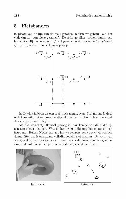
188 Nederlandse samenvatting
5 Fietsbanden
In plaats van de lijn van de reele getallen, maken we gebruik van hetvlak van de “complexe getallen”. De reele getallen vormen daarin eenhorizontale lijn, en een getal
√−n leggen we recht boven de 0 op afstand√
n van 0, zoals in het volgende plaatje.
√−5
√−5 + 1
0
√−5 + 2
√−5− 1
1 2−1
2√−5 + 1
2√−5 2
√−5 + 2
2√−5− 1
3
√−5 + 3
2√−5 + 3
In dit vlak hebben we een rechthoek aangegeven. Stel nu dat je dezerechthoek uitknipt en langs de stippellijnen aan zichzelf plakt. Je krijgtdan een soort wc-rolletje.
Als dat wc-rolletje flexibel genoeg is, dan kan je ook de dikke lij-nen aan elkaar plakken. Wat je dan krijgt, lijkt nog het meest op eenfietsband. Buiten Nederland zouden we zeggen: het oppervlak van eendonut. Stel dat je een donut volledig bedekt met glazuur. De vorm vanons geplakte rechthoekje is dan dezelfde als de vorm van het glazuurvan de donut. Wiskundigen noemen dit oppervlak een torus.
Een torus. Asteroids.
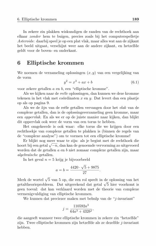
6. Elliptische krommen 189
In zekere zin plakken wiskundigen de randen van de rechthoek aanelkaar zonder hem te buigen, precies zoals bij het computerspelletjeAsteroids: daarbij speel je op een plat vlak, maar alles wat aan de zijkanthet beeld uitgaat, verschijnt weer aan de andere zijkant, en hetzelfdegeldt voor de boven- en onderkant.
6 Elliptische krommen
We noemen de verzameling oplossingen (x, y) van een vergelijking vande vorm
y2 = x3 + ax+ b (6.1)
voor zekere getallen a en b, een “elliptische kromme”.Als we kijken naar de reele oplossingen, dan kunnen we deze kromme
tekenen in het vlak met coordinaten x en y. Dat levert dan een plaatjeop als op pagina 9.
Als we de lijn van de reele getallen vervangen door het vlak van decomplexe getallen, dan is de oplossingsverzameling geen kromme, maareen oppervlak. En als we er op de juiste manier naar kijken, dan blijktdit oppervlak ook weer de vorm van een torus te hebben.
Het omgekeerde is ook waar: elke torus die we krijgen door eenrechthoekje van complexe getallen te plakken is (binnen de regels vande “complexe analyse”) om te vormen tot een elliptische kromme!
Er blijkt nog meer waar te zijn: als je begint met de rechthoek diehoort bij een getal
√−n, dan kan de genoemde vervorming zo uitgevoerd
worden dat de getallen a en b niet zomaar complexe getallen zijn, maaralgebraısche getallen.
In het geval n = 5 krijg je bijvoorbeeld
a = b =4420 ·
√5 + 9875
27.
Merk de wortel√
5 van 5 op, die een rol speelt in de oplossing van hetgetaltheorieprobleem. Dat uitgerekend dat getal
√5 hier voorkomt is
geen toeval: dat kan verklaard worden met de theorie van complexevermenigvuldiging van elliptische krommen.
We kunnen dat preciezer maken met behulp van de “j-invariant”
j =110592a3
64a3 + 432b2,
die aangeeft wanneer twee elliptische krommen in zekere zin “hetzelfde”zijn. Twee elliptische krommen zijn hetzelfde als ze dezelfde j-invarianthebben.
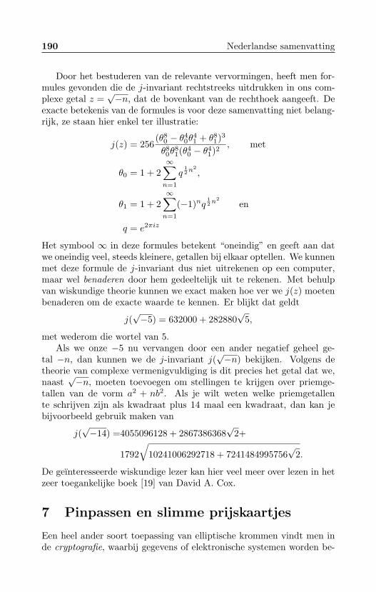
190 Nederlandse samenvatting
Door het bestuderen van de relevante vervormingen, heeft men for-mules gevonden die de j-invariant rechtstreeks uitdrukken in ons com-plexe getal z =
√−n, dat de bovenkant van de rechthoek aangeeft. De
exacte betekenis van de formules is voor deze samenvatting niet belang-rijk, ze staan hier enkel ter illustratie:
j(z) = 256(θ8
0 − θ40θ
41 + θ8
1)3
θ80θ
81(θ4
0 − θ41)2
, met
θ0 = 1 + 2∞∑n=1
q12n
2,
θ1 = 1 + 2∞∑n=1
(−1)nq12n
2en
q = e2πiz
Het symbool ∞ in deze formules betekent “oneindig” en geeft aan datwe oneindig veel, steeds kleinere, getallen bij elkaar optellen. We kunnenmet deze formule de j-invariant dus niet uitrekenen op een computer,maar wel benaderen door hem gedeeltelijk uit te rekenen. Met behulpvan wiskundige theorie kunnen we exact maken hoe ver we j(z) moetenbenaderen om de exacte waarde te kennen. Er blijkt dat geldt
j(√−5) = 632000 + 282880
√5,
met wederom die wortel van 5.Als we onze −5 nu vervangen door een ander negatief geheel ge-
tal −n, dan kunnen we de j-invariant j(√−n) bekijken. Volgens de
theorie van complexe vermenigvuldiging is dit precies het getal dat we,naast
√−n, moeten toevoegen om stellingen te krijgen over priemge-
tallen van de vorm a2 + nb2. Als je wilt weten welke priemgetallente schrijven zijn als kwadraat plus 14 maal een kwadraat, dan kan jebijvoorbeeld gebruik maken van
j(√−14) =4055096128 + 2867386368
√2+
1792√
10241006292718 + 7241484995756√
2.
De geınteresseerde wiskundige lezer kan hier veel meer over lezen in hetzeer toegankelijke boek [19] van David A. Cox.
7 Pinpassen en slimme prijskaartjes
Een heel ander soort toepassing van elliptische krommen vindt men inde cryptografie, waarbij gegevens of elektronische systemen worden be-
7. Pinpassen en slimme prijskaartjes 191
veiligd met behulp van wiskunde. Deze beveiliging is erop gebaseerddat sommige berekeningen eenvoudig uit te voeren, maar moeilijk terugte draaien zijn. Zo kan je met een computer heel snel twee grote priem-getallen p en q met elkaar vermenigvuldigen. De uitkomst is dan eengroot getal N en ondanks decennia van onderzoek is er nog geen snellemanier bekend om achter p en q te komen als je alleen N weet.
Tegenwoordig worden de magneetstrips van bankpasjes op vrij groteschaal gekopieerd door criminelen die betaalautomaten ombouwen. Deoplossing daarvoor is op de meeste passen al aanwezig in de vorm vande EMV-chip. Die chip bevat twee priemgetallen die alleen in de chipbeschikbaar zijn. Bij elke betaling kan je bankpasje dankzij het “RSA-protocol” bewijzen dat het echt jouw bankpasje is. De chip gebruiktdaarvoor de priemgetallen p en q zonder ze te verraden. Dit maakt het(met de huidige stand van de wetenschap) onmogelijk om de chips vandeze passen te kopieren.
De laatste tijd worden ook passen die op afstand leesbaar zijn steedspopulairder. Denk aan de OV-chipkaart die je niet meer uit je por-temonnee hoeft te halen, je paspoort waar je foto en vingerafdruk opzijn opgeslagen, en misschien wel de pas waarmee je het kantoor in enuit kan. Verder wordt het steeds meer mogelijk om streepjescodes inbijvoorbeeld winkels, apotheken en magazijnen te vervangen door goed-kope chips die RFID-tags heten.
Doordat deze pasjes en RFID-tags op afstand uit te lezen zijn, zijn erveel veiligheids- en privacyrisico’s. Goede beveiliging is dus belangrijk.
Aan de andere kant hebben juist deze passen veel minder energietot hun beschikking dan bijvoorbeeld de chip op een bankpasje. Er isnamelijk geen plaats voor een batterij en ze kunnen ook geen contactmaken met netstroom. Ze moeten al hun energie daarom via een kleineantenne uit het magnetische veld van het leesapparaat halen.
Door de beperkte hoeveelheid energie is een RFID-tag niet in staathet RSA-protocol van je bankpasje uit te voeren. Hier bieden elliptischekrommen, die we hierboven al tegenkwamen, uitkomst.
Er bestaat namelijk ook cryptografie die gebruik maakt van ellip-tische krommen. Die biedt, voor zover bekend, evenveel veiligheid alsRSA met veel lichtere berekeningen. Cryptografie met elliptische krom-men kan wel op RFID-tags uitgevoerd worden.
Om elliptische krommen te maken die geschikt zijn voor cryptografie,kan je gebruik maken van dezelfde theorie van “complexe vermenigvul-diging” die eerder al genoemd werd. Daarbij gebruikt men dezelfdespeciale waarden van de j-functie die we hierboven al tegenkwamen.
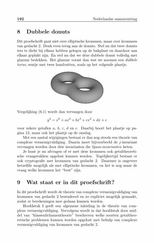
192 Nederlandse samenvatting
8 Dubbele donuts
Dit proefschrift gaat niet over elliptische krommen, maar over krommenvan geslacht 2. Denk even terug aan de donuts. Stel nu dat twee donutsiets te dicht bij elkaar hebben gelegen op de bakplaat en daardoor aanelkaar geplakt zijn. En stel nu dat we deze dubbele donut volledig metglazuur bedekken. Het glazuur vormt dan wat we noemen een dubbeletorus, eentje met twee handvatten, zoals op het volgende plaatje.
Vergelijking (6.1) wordt dan vervangen door
y2 = x6 + ax4 + bx3 + cx2 + dx+ e
voor zekere getallen a, b, c, d en e. Daarbij hoort het plaatje op pa-gina 12, maar ook het plaatje op de omslag.
Met een aantal wijzigingen bestaat er dan nog steeds een theorie vancomplexe vermenigvuldiging. Daarin moet bijvoorbeeld de j-invariantvervangen worden door drie invarianten die Igusa-invarianten heten.
Je kunt je nu afvragen of er met deze krommen ook getaltheoreti-sche vraagstukken opgelost kunnen worden. Tegelijkertijd bestaat erook cryptografie met krommen van geslacht 2. Daarmee is ongeveerhetzelfde mogelijk als met elliptische krommen, en het is nog maar devraag welke krommen het “best” zijn.
9 Wat staat er in dit proefschrift?
In dit proefschrift wordt de theorie van complexe vermenigvuldiging vankrommen van geslacht 2 bestudeerd en zo expliciet mogelijk gemaakt,zodat er berekeningen mee gedaan kunnen worden.
Hoofdstuk I geeft een algemene inleiding in de theorie van com-plexe vermenigvuldiging. Vervolgens wordt in dat hoofdstuk door mid-del van “klassenlichamentheorie” beschreven welke soorten getaltheo-retische problemen kunnen worden opgelost met behulp van complexevermenigvuldiging van krommen van geslacht 2.
9. Wat staat er in dit proefschrift? 193
Hoofdstuk II beschrijft hoe je de exacte waarden van de bovenge-noemde Igusa-invarianten krijgt. Dat wil zeggen, er wordt beschrevenen hoe, en hoe nauwkeurig, je ze moet benaderen om ze exact te be-palen. Het belangrijkste resultaat van dit (langste) hoofdstuk is eenbovengrens op hoe lang deze berekeningen duren.
Hoofdstuk III geeft nog wat extra theorie en wijst belangrijke verbe-teringen aan voor de berekeningen van hoofdstuk II. Die verbeteringenzijn weggelaten in hoofdstuk II, omdat dat hoofdstuk al lang genoeg is.
Hoofdstuk IV, geschreven samen met David Freeman en Peter Ste-venhagen, beschrijft hoe je de Igusa-invarianten gebruikt om krommente maken die geschikt zijn voor cryptografische protocollen gebaseerdop “bilineaire afbeeldingen”.
Hoofdstuk V, geschreven met Laura Hitt, Gary McGuire en MichaelNaehrig, beschrijft een soortgelijke constructie, maar dan voor een speci-aal soort krommen van geslacht 2: die waarvan de p-rang, een invariantdie voor alle eerdere constructies 0 of 2 is, gelijk is aan 1.

Dankwoord / Acknowledgements
Op deze pagina wil ik graag kort een aantal mensen bedanken die be-trokken zijn bij de totstandkoming van dit proefschrift. Als eerste mijnvrouw, Marina, voor al haar steun, vooral tijdens de drukke laatsteweken.
Mijn kantoorgenoot, Peter Bruin, voor vier jaar geduldig luisterennaar mijn onderbrekingen en vragen over meetkunde.
Mijn promotor, Peter Stevenhagen, zonder wiens gedetailleerde com-mentaar dit proefschrift niet zou zijn wat het nu is. En naast hem ookmijn andere co-auteur van hoofdstuk IV, David Freeman, die inmiddelsvoldoende Nederlands leest om dit te begrijpen: bedankt voor de goedesamenwerking.
Nu zal ik helaas toch op het Engels over moeten gaan. Thanks alsoto my co-authors Laura Hitt, Gary McGuire, and Michael Naehrig forthe collaboration on Chapter V.
Thank you Andreas Enge for inviting me to Bordeaux, and for yourhospitality and our inspiring collaboration.
Thank you Jens Putzka for the same things, with Bonn instead ofBordeaux.
Thank you Kristin Lauter for letting me be your intern at Mi-crosoft Research, and for your hospitality and our collaboration. ReinierBroker, die laatste dingen gelden natuurlijk ook voor jou, maar dan inhet Nederlands.
Finally, thanks to everyone who gave suggestions and corrections forthe improvement of the manuscript, including Reinier Broker, AndreasEnge, David Freeman, and the members of the committee.

Curriculum vitae
Marco Streng werd geboren op 26 november 1982 in IJsselstein. Hijverhuisde al snel naar Benschop, waar hij meer dan de helft van zijnleven tot nu toe heeft gewoond. Na de basisschool ging hij naar hetVWO van het Cals College in IJsselstein en Nieuwegein.
In 2001 begon hij zijn studie wiskunde aan de Universiteit Utrecht.In de eerste jaren volgde hij daarnaast ook vakken bij natuurkundeen informatica en haalde hij een propedeusediploma in de informatica.Onder begeleiding van dr. Gunther Cornelissen schreef hij zijn afstu-deerscriptie Elliptic Divisibility Sequences with Complex Multiplication,waarop hij in 2006 cum laude afstudeerde in de wiskunde.
Vervolgens begon hij als promovendus aan het Mathematisch Insti-tuut van de Universiteit Leiden. Het promotieonderzoek werd gedaanonder begeleiding van prof. dr. Peter Stevenhagen. Naast zijn promo-tieonderzoek was Marco werkzaam in het wiskundeonderwijs van deuniversiteit. Verder heeft hij gedurende 11 weken in het najaar van2008 als stagiair onderzoek gedaan in de cryptografiegroep van Micro-soft Research in Redmond in de Verenigde Staten.
Sinds 20 augustus 2008 is hij gehuwd met Marina Blokland, en op11 april 2009 werden zij de trotse ouders van Tijmen. Hun tweede zoonwordt in juli 2010 verwacht.
Per 1 september 2010 is Marco als Research Fellow verbonden aande University of Warwick.