Embed Size (px)
Citation preview

Université du Québec Institut National de la Recherche Scientifique
Centre Eau Terre Environnement
DÉLIMITATION DE ZONES D’AMÉNAGEMENT À L’AIDE DE CAPTEURS PROXIMAUX DU SOL DANS DEUX CHAMPS DE CULTURE
INTENSIVE DE LA POMME DE TERRE
Par
Miguel Felipe Vargas Gutierrez
Mémoire présenté pour l’obtention du grade de Maître ès sciences (M.Sc.)
en sciences de l’eau
Jury d’évaluation
Président du jury et Erwan Gloaguen
examinateur interne INRS Centre Eau Terre Environnement Examinateur externe Yacine Bourobi Effigis Geo-solutions Directeur de recherche Karem Chokmani INRS Centre Eau Terre Environnement Codirectrice de recherche Athyna Cambouris Agriculture et Agroalimentaire Canada
© Droits réservés de Miguel Felipe Vargas Gutierrez, 2017

iii
REMERCIEMENTS
Je tiens à remercier mes directeurs de recherche, Karem Chokmani et Athyna Cambouris pour
leur appui pendant ce projet au sein l’INRS et Agriculture et Agroalimentaire Canada AAC, ainsi
que Mme Isabelle Perron Messieurs Bernie Zebarth, Asim Biswas et Viacheslav Adamchuk pour
leurs précieuses contributions dans le développement de ce document. Je tiens à souligner la
contribution de toute l’équipe des Laboratoires AAC, particulièrement Mario Deschênes, Claude
Lévesque et Sarah-Maude Parent pour leur précieuse aide à la prise des mesures au champ et
aux analyses de laboratoire. Merci aux producteurs des fermes SVP et SVS et McCain Foods
compagnie qui ont fourni les champs pour l’expérimentation. À Claudia, mon épouse, pour sa
compagnie inconditionnelle dans ce défi.

v
RÉSUMÉ
L’utilisation des zones d’aménagement (ZA) dans la culture de la pomme de terre permet
contrôler la variabilité spatiale du sol et est une des approches dans la gestion localisée des
propriétés du sol. L’objectif de cette étude était d’évaluer la capacité de trois capteurs proximaux
du sol (CPS) pour délimiter des ZA pour deux champs (Champ SVP et champ SVS ; 12 hectares)
en culture commerciale de pomme de terre (Solanum tuberosum L.) dans la province de
Nouveau-Brunswick, Canada. La conductivité électrique apparente du sol (CEa) ont été mesurés
avec deux CPS i.e. le VERIS (modèle MSP3) et le DUALEM (modèle 21S). En plus, des mesures
de haute fréquence électromagnétique ont été prises avec un géoradar (GPR;GSSI modèle SIR-
3000; antenne 400 MHz) pour déterminer l’épaisseur des horizons de sol et la profondeur de la
roche-mère. Les propriétés physicochimiques (texture, matière organique, pH, Mehlich-3) de 154
échantillons de sol pour les champs SVP et 141 échantillons pour le champ SVS ont été analysés.
Le rendement total en tubercule a été mesuré pour les années 2013, 2014 et 2016 pour le champ
SVP et 2014 et 2016 pour le champ SVS à l’aide d’un capteur de rendement. L’algorithme fuzzy
k-means a été utilisé pour délimiter les ZA. Une corrélation significative entre le rendement et les
CPS a été obtenue (r= -0.52, 0.19 pour les champs SVP et SVS). L’argile a été la propriété la
plus corrélée avec le rendement (r= -0.85 rx= -0.41, pour les champs SVP et SVS). Deux ZA ont
été considérés comme optimales pour les deux champs. Celles-ci ont montré un équilibre entre
la variation spatiale des propriétés du sol, le rendement et une représentation spatiale gérable.
Mots-clés: Solanum tuberosum L., conductivité électrique apparente des sols, VERIS, DUALEM,
induction électromagnétique

vii
ABSTRACT
The use of management zones MZ in potato production is an alternative in the localized
management of the soil properties. The objective of this study was to evaluate the ability of three
proximal soil sensors (PSS) to delineate MZ for two commercial potato fields (referred as field
SVP and field SVS, 12 hectares) (Solanum tuberosum L.) in New Brunswick, Canada. Soil
electrical conductivity (EC) was measured with tho PSS, i.e, VERIS (model MSP3) and DUALEM
(model 21 S). Additionally, high frequency EM was measured using a ground penetrating radar
(GPR system; GSSI model SIR-3000; 400 MHz antenna) to determine the thickness of the soil
horizons and the depth to bedrock. The physicochemical properties (texture, organic matter, pH,
Mehlich-3) of 154 soil samples for the field SVP and 141 soil samples for the field SVS were
analyzed. The total yield of tuber was measured for the years 2013, 2014 and 2016 for the field
SVP and 2014 and 2016 for the field SVS using a yield monitor. The fuzzy k-means algorithm
was used to delineate MZ. A significant correlation between the yield and the PSS was obtained
(r = - 0.52, 0.19 for the field SVP and SVS, respectively). Clay was the property most correlated
with the yield (r =-0.85, please and r = - 0.41, for the fields SVP and SVS, respectively). Two MZ
were considered as optimal for both sites. These showed a balance between the spatial variation
of soil properties, yield and a manageable spatial representation.
Key words: Solanum tuberosum L., VERIS, apparent soil electrical conductivity, DUALEM,
Ground Penetrating Radar, pH, Mehlich, ρmax electromagnetic induction.

ix
TABLE DES MATIÈRES
RÉSUME ....................................................................................................................................................... V
ABSTRACT................................................................................................................................................. VII
TABLE DES MATIÈRES ............................................................................................................................. IX
LISTE DE TABLEAUX ................................................................................................................................ XI
LISTE DE FIGURES .................................................................................................................................. XIII
PARTIE 1 : SYNTHÈSE ............................................................................................................................... 1
1 INTRODUCTION ......................................................................................................................... 3
1.1 CONTEXTE .................................................................................................................................... 3
1.2 PROBLEMATIQUE ........................................................................................................................... 5
1.3 OBJECTIFS DE LA RECHERCHE ........................................................................................................ 6
2 REVUE DE LITTÉRATURE ........................................................................................................ 7
2.1 AGRICULTURE DE PRECISION .......................................................................................................... 7
2.2 VARIABILITE SPATIALE-TEMPORELLE INTRAPARCELLAIRE .................................................................. 8
2.3 ZONES D’AMENAGEMENT .............................................................................................................. 10
2.3.1 Délimitation des zones d’aménagement ............................................................................... 12
2.4 CAPTEURS PROXIMAUX DE SOL..................................................................................................... 14
2.4.1 L’agriculture de précision, utilisation des capteurs proximaux de sol ................................... 14
2.4.2 Capteurs mesurant la conductivité électrique apparente ...................................................... 16
2.4.3 Capteurs mesurant la résistivité électrique ........................................................................... 18
2.4.4 Géoradar ............................................................................................................................... 18
3 MATÉRIEL ET MÉTHODES ..................................................................................................... 21
3.1 SITE D’ETUDE ET ECHANTILLONNAGES DE SOLS ............................................................................. 21
3.2 ACQUISITION DES DONNEES DES CAPTEURS PROXIMAUX DE SOL .................................................... 21
3.3 ANALYSES STATISTIQUES ET GEOSTATISTIQUES ............................................................................ 22
4 RÉSULTATS ET DISCUSSION ................................................................................................ 25
4.1 STRUCTURES SPATIALES ET RELATIONS ENTRE LES CAPTEURS PROXIMAUX DU SOL, LES
PROPRIETES PHYSICOCHIMIQUES DU SOL ET LE RENDEMENT EN TUBERCULE ................................... 25
4.2 DETERMINATION DU NOMBRE OPTIMUM DE ZONES D’AMENAGEMENT ............................................... 25
4.3 APPLICATION PRATIQUE DE LA GESTION LOCALISEE ....................................................................... 28
x
5 CONCLUSION ET RECOMMANDATIONS ............................................................................. 29
PARTIE 2 : ARTICLE ................................................................................................................................. 31
1 INTRODUCTION ....................................................................................................................... 41
2 MATERIALS AND METHODS ................................................................................................. 45
2.1 EXPERIMENTAL SITE .................................................................................................................... 45
2.2 SOIL SAMPLING AND ANALYSES .................................................................................................... 46
2.3 DATA COLLECTION USING PROXIMAL SOIL SENSORS ..................................................................... 47
2.4 TUBER YIELD ............................................................................................................................... 49
2.5 STATISTICAL AND GEOSTATISTICAL ANALYSIS ............................................................................... 49
3 RESULTS AND DISCUSSION ................................................................................................. 51
3.1 EXPLANATORY DATA ANALYSIS .................................................................................................... 51
3.2 SPATIAL VARIABILITY ................................................................................................................... 54
3.3 KRIGING ...................................................................................................................................... 57
3.4 RELATIONSHIPS BETWEEN PSS, SOIL PROPERTIES AND CROP YIELD ............................................ 62
3.5 DETERMINATION OF THE OPTIMUM NUMBER OF MANAGEMENT ZONES ............................................. 68
3.6 PRACTICAL APPLICATIONS OF MANAGEMENT ZONE WITHIN THESE FIELDS ...................................... 75
4 CONCLUSIONS ........................................................................................................................ 80
5 REFERENCES .......................................................................................................................... 81
xi
LISTE DES TABLEAUX
PARTIE 1 : SYNTHÈSE
TABLEAU 2.1 APPLICATION DE LA METHODE DE ZA POUR LA GESTION DES CULTURES. ................................ 11
TABLEAU 2.2 PROPRIETES UTILISEES LORS DE DIFFERENTES ETUDES PORTANT SUR LA DELIMITATION DE ZA
DANS DES CHAMPS AGRICOLES, ADAPTES DE KHOSLA ET AL., (KHOSLA ET AL., 2010). .............................. 12
TABLEAU 2.3 CAPTEURS PROXIMAUX UTILISEES DANS LE CADRE AGRICOLE, VERSION ADAPTEE (ADAMCHUK ET
AL., 2015) 15
TABLEAU 4.1 ANOVA POUR LES CHAMPS SVP ET SVS ............................................................................ 27
PARTIE 2 : ARTICLE TABLE 3.1 DESCRIPTIVE STATISTICS OF THE SOIL PHYSICOCHEMICAL PROPERTIES. ..................................... 52
TABLE 3.2 DESCRIPTIVE STATISTICS OF THE ALTITUDE (DGPS), SOIL ELECTRICAL CONDUCTIVITY (VERIS AND
DUALEM), SOIL LAYER THICKNESSES (GPR) AND TUBER YIELD (YIELD MONITOR) FOR THE SVP AND SVS
FIELDS. 53
TABLE 3.3 GEOSTATISTICAL PARAMETERS OF THE SOIL PHYSICOCHEMICAL PROPERTIES FOR THE SVP AND
SVS FIELDS.......................................................................................................................................... 55
TABLE 3.4 GEOSTATISTICAL PARAMETERS OF ALTITUDE (DGPS), SOIL ELECTRICAL CONDUCTIVITY (VERIS AND
DUALEM), SOIL LAYER THICKNESSES (GPR) AND TUBER YIELD (YIELD MONITOR) FOR THE SVP AND SVS
FIELDS. 56
TABLE 3.5 PEARSON CORRELATION COEFFICIENTS BETWEEN PROXIMAL SOIL SENSOR SYSTEMS AT THE SVP
AND SVS FIELDS. .................................................................................................................................. 63
TABLE 3.6 PEARSON CORRELATION COEFFICIENTS AT THE SVP FIELD. ....................................................... 64
TABLE 3.7 PEARSON CORRELATION COEFFICIENTS AT THE SVS FIELD. ....................................................... 65
TABLE 3.8 COMPARISON OF SOIL ELECTRICAL CONDUCTIVITY (EC) AND THE SOIL LAYERS THICKNESS (SLT)
INTO TWO MZ AT THE SVP AND SVS SITE. ............................................................................................. 76
TABLE 3.9 COMPARISON OF SOIL ELECTRICAL CONDUCTIVITY (EC) AND THE SOIL LAYERS THICKNESS (SLT)
INTO TWO MZ AT THE SVP AND SVS SITE. ............................................................................................. 77

xiii
LISTE DES FIGURES
PARTIE 1 : SYNTHÈSE FIGURE 1.1 HISTORIQUE DE LA PRODUCTION, DE LA POMME DE TERRE AU COURS DES 75 DERNIÈRES ANNÉES
(CANSIM, TABLEAU 001-0014). ............................................................................................................. 3
FIGURE 2.1 CONCEPT DE L’AGRICULTURE DE PRÉCISION (CAMBOURIS ET AL., 2014)....................................... 7
FIGURE 2.2 CAPTEURS PROXIMAUX A) VERIS-MSP3, B) DUALEM-21S, C) EM38, MESURANT EN CONTINU LA
CONDUCTIVITÉ ÉLECTRIQUE APPARENTE. ............................................................................................... 17
FIGURE 2.3 GEORADAR (GSSI SIR-3000) MESURANT LA CONSTANTE DIELECTRIQUE. .................................. 19
FIGURE 2.1 SOIL SERIES, DRAINAGE CLASSES AND SAMPLING GRID AT THE A) SVP AND B) SVS FIELDS. ........ 46
PARTIE 2 : ARTICLE
FIGURE 3.1 KRIGING MAPS OF THE SOIL ELECTRICAL CONDUCTIVITY (EC) MEASURED WITH THE A) VERIS
(DEPTH 0-1 M; EC0-1M) B) DUALEM (DEPTH 0-0.9 M; PRPP0-0.9M) AND THE SOIL LAYER THICKNESS (SLT)
DERIVED WITH THE GROUND PENETRATING RADAR (GPR) C) SLTSURFACE AND D) THE DEPTH TO THE BEDROCK
AT THE SVP FIELD. ............................................................................................................................... 59
FIGURE 3.2 KRIGING MAPS OF THE SOIL ELECTRICAL CONDUCTIVITY (EC) MEASURED WITH THE A) VERIS
(DEPTH 0-1.0 M; EC0-1M) B) DUALEM (DEPTH 0-0.9 M; PRPP0-0.9M) AND SOIL LAYER THICKNESS (SLT)
DERIVED WITH THE GROUND PENETRATING RADAR (GPR) C) SLTSURFACE AND D) THE DEPTH TO THE BEDROCK
AT THE SVS FIELD. ............................................................................................................................... 60
FIGURE 3.3 KRIGING MAPS OF THE TUBER YIELD A) 2013, B) 2014 AND C) 2016; AND D) CLAY, E) SOIL
MOISTURE AND F) PHOSPHORUS CONTENTS OF THE SVP FIELD. .............................................................. 61
FIGURE 3.4 KRIGING MAPS OF THE TUBER YIELD A) 2014, AND B) 2016; AND C) CALCIUM AND D) PHOSPHORUS
CONTENTS OF THE SVS FIELD. .............................................................................................................. 61
FIGURE 3.5 MANAGEMENT ZONE DELINEATED USING THE VERIS (EC0-0.3M AND EC0-1M), DUALEM (PRPP0-0.4M,
PRPP0-0.9M, HCPV0-1.4M AND HCPV0-3.1M) AND GPR (SLTSURFACE, SLTSUBSURFACE AND DEPTH TO BEDROCK)
KRIGED DATA MATRIX WITH THE FUZZY K-MEANS ANALYSIS WITH NO SPATIAL CONSTRAINT OF PROXIMITY AT
THE SVP FIELD. .................................................................................................................................... 69
FIGURE 3.6 MANAGEMENT ZONE DELINEATED USING THE VERIS (EC0-0.3M AND EC0-1M), DUALEM (PRPP0-0.4M,
PRPP0-0.9M, HCPV0-1.4M AND HCPV0-3.1M) AND GPR (SLTSURFACE, SLTSUBSURFACE AND DEPTH TO BEDROCK)
KRIGED DATA MATRIX WITH THE FUZZY K-MEANS ANALYSIS WITH NO SPATIAL CONSTRAINT OF PROXIMITY AT
THE SVS FIELD. .................................................................................................................................... 70
FIGURE 3.7 DECREASE OF THE TOTAL WITHIN-ZONE VARIANCE OF A) SOIL ELECTRICAL CONDUCTIVITY USING
THE VERIS, B) THE DUALEM, C) THE THICKNESS OF SOIL LAYERS DERIVED WITH THE GPR PARAMETERS, D-E-
F) YIELD 2013, 2014 AND 2016 FROM YIELD MONITOR, G-H-I) SOIL PARTICLES SIZES (CLAY, SILT, SAND),
xiv
GRAVEL AND SOIL MOISTURE, J-K-L) MEHLICH-3 EXTRACTABLE ELEMENTS (P, K, CA, MG AND AL) INTO
MANAGEMENT ZONE BASED ON THE MZ DELINEATED WITH THE VERIS, THE DUALEM AND THE GPR AT THE
SVP FIELD, RESPECTIVELY. ................................................................................................................... 72
FIGURE 3.8 DECREASE OF THE TOTAL WITHIN-ZONE VARIANCE OF A) SOIL ELECTRICAL CONDUCTIVITY USING
THE VERIS, B) THE DUALEM, C) THE THICKNESS OF SOIL LAYERS DERIVED WITH THE GPR PARAMETERS, D-E-
F) YIELDS 2014 AND 2016 FROM YIELD MONITOR, G-H-I) SOIL PARTICLES SIZES (CLAY, SILT, SAND), GRAVEL
AND SOIL MOISTURE, J-K-L) MEHLICH-3 EXTRACTABLE ELEMENTS (P, K, CA, MG AND AL) INTO MANAGEMENT
ZONE BASED ON THE MZ DELINEATED WITH THE VERIS, THE DUALEM AND THE GPR AT THE SVS FIELD,
RESPECTIVELY. ..................................................................................................................................... 74

1
PARTIE 1 : SYNTHÈSE

3
1 INTRODUCTION
1.1 Contexte
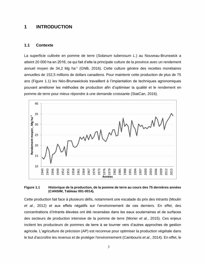
La superficie cultivée en pomme de terre (Solanum tuberosum L.) au Nouveau-Brunswick a
atteint 20 000 ha en 2016, ce qui fait d’elle la principale culture de la province avec un rendement
annuel moyen de 34,2 Mg ha-1 (GNB, 2016). Cette culture génère des recettes monétaires
annuelles de 152,5 millions de dollars canadiens. Pour maintenir cette production de plus de 75
ans (Figure 1.1) les Néo-Brunswickois travaillent à l’implantation de techniques agronomiques
pouvant améliorer les méthodes de production afin d’optimiser la qualité et le rendement en
pomme de terre pour mieux répondre à une demande croissante (StatCan, 2016).
Figure 1.1 Historique de la production, de la pomme de terre au cours des 75 dernières années (CANSIM, Tableau 001-0014).
Cette production fait face à plusieurs défis, notamment une escalade du prix des intrants (Moulin
et al., 2012) et aux effets négatifs sur l’environnement de ces derniers. En effet, des
concentrations d’intrants élevées ont été recensées dans les eaux souterraines et de surfaces
des secteurs de production intensive de la pomme de terre (Morier et al., 2015). Ces enjeux
incitent les producteurs de pommes de terre à se tourner vers d’autres approches de gestion
agricole. L’agriculture de précision (AP) est reconnue pour optimiser la production végétale dans
le but d'accroître les revenus et de protéger l'environnement (Cambouris et al., 2014). En effet, le
10
15
20
25
30
35
40
19
40
19
43
19
46
19
49
19
52
19
55
19
58
19
61
19
64
19
67
19
70
19
73
19
76
19
79
19
82
19
85
19
88
19
91
19
94
19
97
20
00
20
03
20
06
20
09
20
12
20
15
Re
nd
em
en
t m
oye
n ,
Mg
ha-1
Années
4
concept à la base de l’AP est de considérer la variabilité spatiale inhérente d’un champ en culture
et d’appliquer les intrants agricoles en bonne quantité, au bon endroit et au bon moment (D De
Benedetto et al., 2013b). La pertinence de cette approche consiste en une gestion spécifique des
intrants (engrais, pesticides, insecticides, etc.) et de l'eau (irrigation, drainage) des champs
agricoles. Cette gestion requiert une connaissance de la variabilité spatiale des propriétés
physicochimique des sols et des cultures du champ (Havlin et al., 2009).
Donc, l'acquisition d'informations sur la variabilité spatiale des propriétés des cultures et des sols
est essentielle. La détection proximale du sol est envisagée en AP pour compléter ou même
substituer les méthodes conventionnelles d'estimation de la variabilité des sols et des cultures
(Viscarra Rossel et al., 2011). Une meilleure caractérisation de la variation spatiale des propriétés
du sol dans les champs peut améliorer la gestion des terres à l'échelle de la parcelle en
cartographiant les propriétés des sols et des cultures à des résolutions plus élevées que celles
traditionnellement faites. Par conséquent, elle permet de délimiter les zones d’aménagement (ZA)
homogènes qui reflètent mieux les variations réelles (Halcro et al., 2013).
La culture de la pomme de terre est sensible aux carences en phosphore et en potassium, en
raison de sa capacité limitée à absorber ces éléments (Cambouris et al., 2014). Une gestion
homogène peut donc entraîner une fertilisation insuffisante et excessive, avec des pertes de
rendement dans certaines zones du champ et des pertes d'éléments nutritifs environnementaux
dans d'autres zones (Simard et al., 1998). Selon Gasser et al. (2000), afin d'obtenir des
rendements permettant d'atteindre la rentabilité de l'entreprise la production de pomme de terre
nécessite une utilisation relativement élevée d'engrais azotés. Toutefois, lorsque le taux d'azote
appliqué est supérieur aux besoins nutritionnels de la culture, la maturation est retardée et les
travaux de défanage et de récolte sont moins élevés (GNB, 2016). Une fertilisation azotée
optimale est essentielle pour obtenir de bon rendement en termes de tubercules de qualité et de
calibre commercial, en plus de produire une rentabilité maximale (Zebarth et al., 2007).
L’implantation de zones d’aménagement (ZA) s’avère alors une solution potentielle pour optimiser
le rendement en tubercules et la qualité de la production de la pomme de terre (Cambouris et al.,
2006).
Les résultats d’une étude de Lund et al. (2011), ont démontré qu’une gestion spécifique par ZA
de l’azote permettait d’augmenter le rendement en blé de 11,3 % par rapport à une application
uniforme. Cette même étude sur la gestion spécifique de l’azote dans une culture de coton a
permis de démontrer qu’il était possible de réduire de 30 % la fertilisation azotée par rapport à
une application uniforme, permettant ainsi d’éviter une surfertilisation. Dans la pomme de terre,
5
une étude menée au Québec par Cambouris et al. (2014) a démontré que la gestion localisée du
P et du K a permis d’augmenter significativement le rendement total et commercialisable en
tubercule par rapport à l'application uniforme. L'AP constitue une des avenues qui permettrait une
gestion optimale de la production de la pomme de terre au Nouveau-Brunswick de façon à
minimiser les pertes environnementales d’intrants tout en maintenant des rendements optimaux
et de qualités (Morier et al., 2015).
1.2 Problématique
La pratique conventionnelle en agriculture consiste à gérer les champs de manière uniforme sans
tenir compte de la variation spatiale du sol et des cultures. Cela peut avoir un impact sur la qualité,
le rendement, et sur l'environnement (Corwin et al., 2010). Il en résulte que des doses d’azote,
de phosphore et de potassium sont appliquées sur des superficies parfois importantes sans
correspondre à la demande nécessaire d'engrais pour la culture de la pomme de terre (Cambouris
et al., 2006). Le risque de surfertilisation est toujours présent, en effet, une trop grande quantité
de potassium réduit la densité des tubercules. Un apport excessif en azote réduit le poids
spécifique des tubercules et retarde sa maturité, rendant plus difficile l'opération de défanage. Un
surplus d'azote se lessive rapidement (Zebarth et al., 2007) et se retrouve dans les nappes d’eau
souterraine. Cette situation remet en question la pratique conventionnelle en agriculture.
L'incapacité de l'agriculture conventionnelle à aborder les variations dans le champ a non
seulement un impact économique sur le sol en raison d'un rendement réduit dans certaines zones
des champs agricoles, mais elle affecte également l'environnement en raison de l'application
excessive de produits agrochimiques (Oshunsanya et al., 2017). L’AP intègre la variabilité
spatiale des sols et des cultures pour une gestion intraparcellaire des cultures. Cette approche
vise à accroître la rentabilité de la production, à améliorer la qualité des produits et à protéger
l'environnement (Adamchuk et al., 2004). En AP, il existe deux modes de gestion localisée,
l’application à taux variable et la gestion localisée (zone d’aménagement; ZA). Cette dernière est
considérée comme l’une des approches les plus prometteuses dans le contrôle de la variabilité
spatiale intraparcellaire des sols. L’utilisation des ZA dans la culture de la pomme de terre est
une alternative de gestion localisée des propriétés du sol et le rendement des cultures. De
nouveaux outils technologiques permettent de développer de nouvelles méthodes pour améliorer
la performance de la gestion agricole. Il existe un potentiel important de capteurs proximaux actifs
pour délimiter des ZA afin d’améliorer davantage l'efficacité économique des systèmes de
production culturale.

6
1.3 Objectifs de la recherche
L’objectif général de ce mémoire était d’étudier et de comparer la capacité des capteurs
proximaux du sol pour délimiter des zones de gestion homogène dans un cadre de production
intensive de culture de la pomme de terre au Nouveau-Brunswick. Pour répondre à cet objectif,
les objectifs spécifiques étaient :
1. Caractériser la variabilité spatiale des propriétés physicochimiques des sols;
2. Comparer la capacité des capteurs proximaux du sol (CPS) :
a. Évaluer la variabilité spatiale des CPS;
b. Déterminer s’il existe une relation entre les CPS et les propriétés
physicochimiques des sols et du rendement;
c. Délimiter les ZA à partir des CPS;
d. Valider les ZA crée à partir des CPS avec les propriétés physicochimiques de sol
et du rendement.
7
2 REVUE DE LITTÉRATURE
2.1 Agriculture de précision
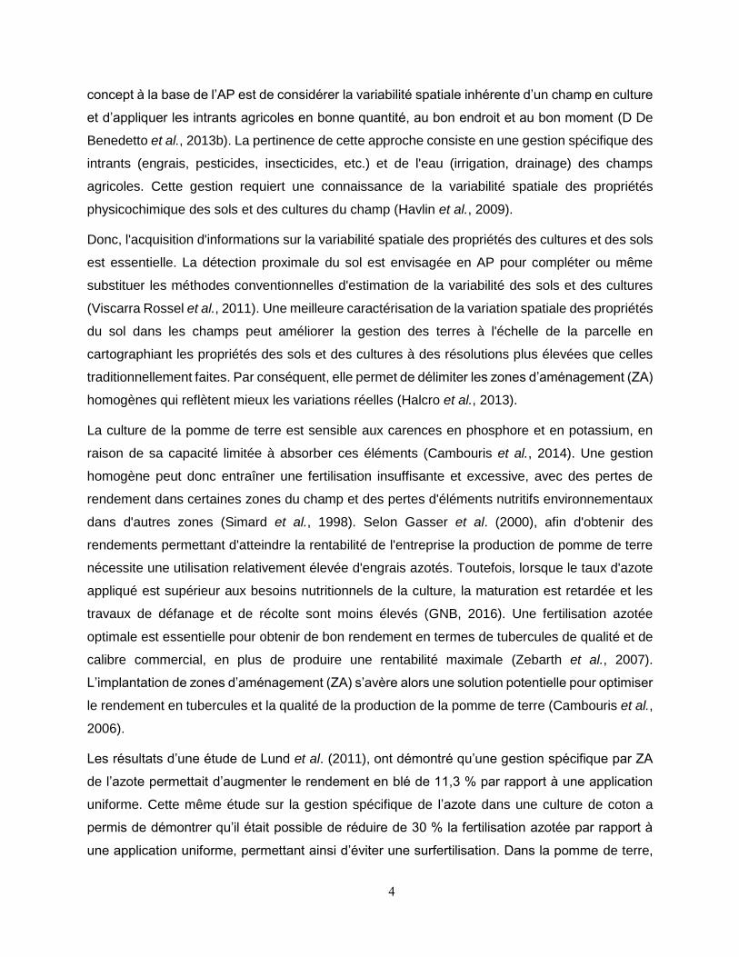
L’agriculture de précision (AP) repose sur le principe d'appliquer la bonne source et la dose
d’intrant, au bon moment, et au bon endroit. Dans l’objectif d’optimiser le rendement et la
rentabilité de la culture, tout en protégeant l’environnement (Arvalis, 2015). Cambouris et al.
(2014) résument le concept de l’AP en trois étapes (Figure 2.1) : 1- quantifier, modéliser et
cartographier la variabilité spatiale des sols et des cultures, en utilisant des techniques
d'échantillonnage intensives du sol, des moniteurs de rendement et/ou des capteurs distants et
proximaux; 2- comprendre la variabilité spatiale des sols et des cultures d’où l'importance de faire
un diagnostic solide de gestion de la culture en faisant appel à l'expertise d’un agronome qui
pourra dresser un bilan complet(causes, processus et impacts) de la variabilité spatiale des sols
et des cultures ; 3- contrôler la variabilité spatiale en utilisant l'une de ces deux approches: a-
faire des applications à taux variable en mode continu ou b- faire une gestion localisée en
délimitant des zones d’aménagement (ZA).
Figure 2.1 Concept de l’agriculture de précision (Cambouris et al., 2014).
8
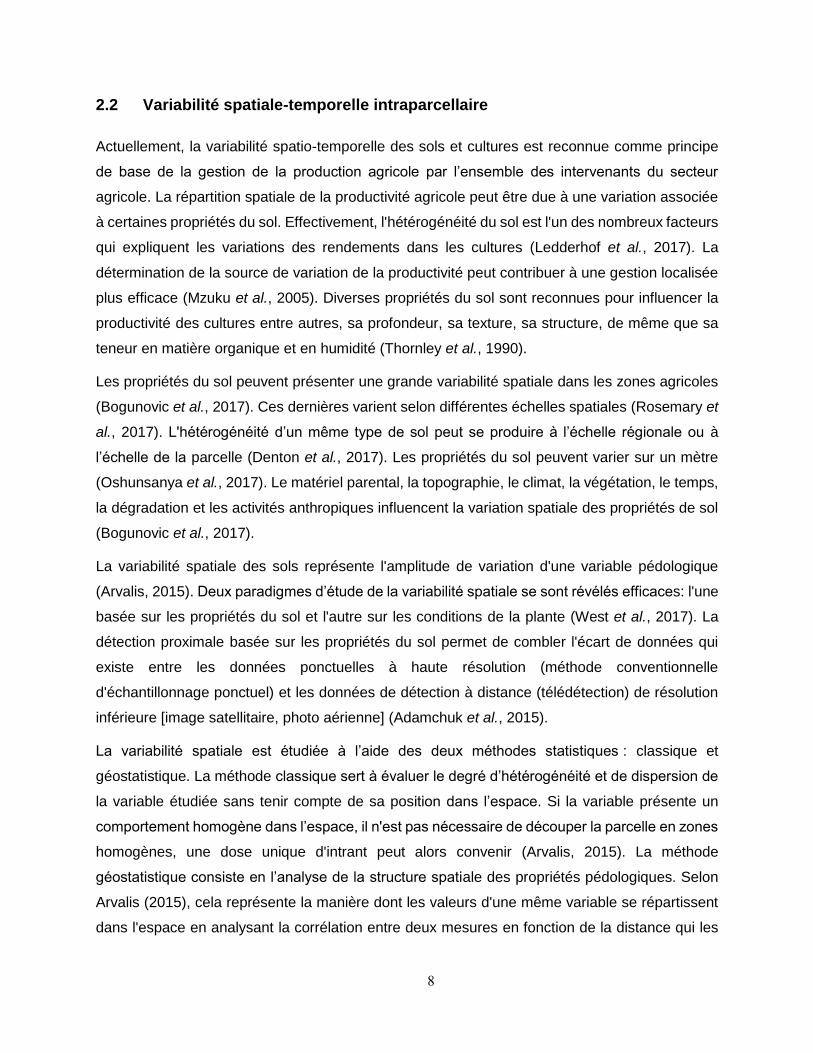
2.2 Variabilité spatiale-temporelle intraparcellaire
Actuellement, la variabilité spatio-temporelle des sols et cultures est reconnue comme principe
de base de la gestion de la production agricole par l’ensemble des intervenants du secteur
agricole. La répartition spatiale de la productivité agricole peut être due à une variation associée
à certaines propriétés du sol. Effectivement, l'hétérogénéité du sol est l'un des nombreux facteurs
qui expliquent les variations des rendements dans les cultures (Ledderhof et al., 2017). La
détermination de la source de variation de la productivité peut contribuer à une gestion localisée
plus efficace (Mzuku et al., 2005). Diverses propriétés du sol sont reconnues pour influencer la
productivité des cultures entre autres, sa profondeur, sa texture, sa structure, de même que sa
teneur en matière organique et en humidité (Thornley et al., 1990).
Les propriétés du sol peuvent présenter une grande variabilité spatiale dans les zones agricoles
(Bogunovic et al., 2017). Ces dernières varient selon différentes échelles spatiales (Rosemary et
al., 2017). L'hétérogénéité d’un même type de sol peut se produire à l’échelle régionale ou à
l’échelle de la parcelle (Denton et al., 2017). Les propriétés du sol peuvent varier sur un mètre
(Oshunsanya et al., 2017). Le matériel parental, la topographie, le climat, la végétation, le temps,
la dégradation et les activités anthropiques influencent la variation spatiale des propriétés de sol
(Bogunovic et al., 2017).
La variabilité spatiale des sols représente l'amplitude de variation d'une variable pédologique
(Arvalis, 2015). Deux paradigmes d’étude de la variabilité spatiale se sont révélés efficaces: l'une
basée sur les propriétés du sol et l'autre sur les conditions de la plante (West et al., 2017). La
détection proximale basée sur les propriétés du sol permet de combler l'écart de données qui
existe entre les données ponctuelles à haute résolution (méthode conventionnelle
d'échantillonnage ponctuel) et les données de détection à distance (télédétection) de résolution
inférieure [image satellitaire, photo aérienne] (Adamchuk et al., 2015).
La variabilité spatiale est étudiée à l’aide des deux méthodes statistiques : classique et
géostatistique. La méthode classique sert à évaluer le degré d’hétérogénéité et de dispersion de
la variable étudiée sans tenir compte de sa position dans l’espace. Si la variable présente un
comportement homogène dans l’espace, il n'est pas nécessaire de découper la parcelle en zones
homogènes, une dose unique d'intrant peut alors convenir (Arvalis, 2015). La méthode
géostatistique consiste en l’analyse de la structure spatiale des propriétés pédologiques. Selon
Arvalis (2015), cela représente la manière dont les valeurs d'une même variable se répartissent
dans l'espace en analysant la corrélation entre deux mesures en fonction de la distance qui les
9
sépare. Selon Nyiraneza et al. (2011), s'il y a une dépendance spatiale entre deux mesures, il y
a absence de structure spatiale, la variabilité est dite aléatoire.
La gestion spécifique du sol nécessite une compréhension approfondie de la variabilité spatiale.
La production de cartes détaillées permet d’améliorer la prédiction de la répartition spatiale des
éléments nutritifs du sol (Blanchet et al., 2017). La variabilité spatiale peut être cartographiée et
étudiée à l'aide du variogramme ou du corrélogramme (Cambardella et al., 1999). Il existe de
nombreuses méthodes d’interpolations des variables du sol, dont le krigeage. Cette méthode peut
être appliquée selon plusieurs variantes [ordinaire, bloc, disjonctif, indicateurs] (Bogunovic et al.,
2017). L'estimation de la propriété de sol par l’interpolation permet de localiser la variabilité
spatiale sur une carte (Pedrera-Parrilla et al., 2017). Cette dernière joue un rôle important dans
la représentation des propriétés de sol utilisées pour la gestion des sols agricoles (Denton et al.,
2017).
L'analyse géostatistique permet une évaluation précise de la variabilité spatiale en considérant
les composants d'autocorrélation et de variation aléatoire (Rosemary et al., 2017). Les outils
géostatistiques peuvent être utilisés efficacement pour cartographier les paramètres de fertilité
du sol (Vasu et al., 2017). Selon Guan et al. (2017), les zones déficitaires en éléments nutritifs
(e.g. N, P et K) sont des macronutriments importants pour la croissance et la productivité des
plantes et peuvent être identifiées à l'aide de ces cartes de prédiction. Pedrera-Parrila et al. (2017)
ont aussi souligné l’importance de cet outil dans la gestion et la planification efficaces de
l'irrigation en réduisant la contamination des eaux de surface et souterraines par les engrais et
pesticides.
La connaissance de la variabilité spatiale est importante pour la prise de décision dans la gestion
agricole (Santos et al., 2017). Une bonne compréhension de la répartition des propriétés du sol
contribuera à une gestion précise des sols dans les zones agricoles (Pedrera-Parrilla et al., 2017).
L'information sur la variabilité des propriétés du sol est une condition préalable à l'évaluation des
terres agricoles (Rosemary et al., 2017). La variabilité spatiale devrait être surveillée et quantifiée
pour comprendre les effets de l'utilisation des sols et des systèmes de gestion des sols (Denton
et al., 2017).
La connaissance et l’évaluation de la variabilité spatiale à l’échelle de la parcelle sont essentielles
pour identifier les zones nécessitant une gestion spécifique du site (Medina et al., 2017). On sait
que les propriétés physiques et chimiques du sol présentent une variation considérable à cette
échelle (Rosemary et al., 2017). Cela permettra aux gestionnaires d'élaborer des stratégies pour
la gestion des éléments nutritifs spécifiques au site en fonction des besoins des cultures (Vasu
10
et al., 2017). Une irrigation modulée pourrait être implémentée en se basant de la distribution de
l'eau dans la culture. (West et al., 2017). Cette variabilité détaillée des sols n'est souvent pas
prise en compte dans les procédures traditionnelles en raison des limites d'échelle
cartographique (Rosemary et al., 2017).
Les récents progrès technologiques en matière d’agriculture de précision ont permis d'identifier,
d'analyser et de gérer la variabilité spatiale à l'échelle du champ. Les objectifs principaux de cette
approche consistaient à accroître la rentabilité de la production végétale augmentant l'efficacité
des intrants nutritifs et à améliorer la qualité des produits et à protéger l'environnement
(Adamchuk et al., 2004). L'adoption de l'agriculture de précision est un moyen par lequel les
agriculteurs peuvent limiter la application d’intrant dans la production végétale, tels que l'eau
d'irrigation et les nutriments. En utilisant ceci, il est possible de déterminer un gestion spécifique
selon les conditions spatialement localisées au préalable (West et al., 2017).
Selon Dampney et al. (2004), la démocratisation des prix des technologies en agriculture de
précision (p.exe. GPS, capteur de rendement, autoguidage, applicateur à taux variable, capteurs
proximaux, etc.) permettra l’adoption de celles-ci par les producteurs. Ces outils leurs permettront
d’élaborer des cartes illustrant les variations intraparcellaire des sols et des cultures. Ces cartes
pourront être utilisées pour développer des stratégies de gestion des cultures plus complexes.
Elles permettant d’éviter une surfertilisation en éléments nutritifs (Blanchet et al., 2017), une
meilleure gestion de l'irrigation, de la protection des cultures et de la conservation des sols
(Pedrera-Parrilla et al., 2017). L'AP implique de combiner les fonctions de ces technologies pour
aider à la prise de décision pour une gestion des sols et des cultures selon des zones spécifiques
d’aménagement (West et al., 2017).
2.3 Zones d’aménagement
Plusieurs études ont démontré l’efficacité de l’approche de la gestion spécifique par ZA dans
l'application des intrants (e.g. engrais, des pesticides) pour accroitre autant que possible la
productivité agricole (Moshia et al., 2015). La gestion par ZA est une approche utilisée pour
améliorer la prise de décision dans la gestion et le contrôle de la variabilité spatiale des sols et
des cultures, y compris la fertilité des sols, la disponibilité en eau pour la plante et le rendement
des cultures (Mulla, 1989). Cette approche nécessite l'identification de sous-zones présentant
des caractéristiques homogènes (Peralta et al., 2015) ayant une combinaison similaire de
facteurs limitants le rendement, afin de déterminer une gestion précise dans des régions
11
secondaires de potentiel productive similaire (Moral et al., 2011) pour lesquels, un taux unique
d’intrants agricoles serait approprié (Ortiz et al., 2011).
Selon Johnson et al. (2003), l’approche par ZA doit satisfaire deux critères : 1- il doit exister une
forte relation entre les zones de gestions identifiées, les propriétés de sol et le rendement
potentiel; 2- les zones doivent être temporairement cohérentes, compte tenu des fluctuations
normales des propriétés dynamiques du sol tel que la teneur en humidité. Ce concept agricole
est fondé sur l'existence d'une variabilité spatiale structurale des propriétés de sol et des cultures
(Cambouris et al., 2006). Dans ce contexte, chaque zone peut être gérée différemment en
fonction des facteurs limitants (Khosla et al., 2010). Chacune des zones indiquent différents
besoins dans le champ, ce qui entraîne la mise en œuvre de stratégies spécifiques de gestion
pour chacune de ces zones (Ortiz et al., 2011). Les buts visés par l'application de différentes
doses d’intrants dans les ZA consistent à l’économie des ressources, l’optimisation du rendement
et la protection de l’environnement (Haghverdi et al., 2015). Le nombre de ZA dans un champ est
fonction de la variabilité naturelle intraparcellaire, de la taille du champ et de certains facteurs de
gestion (Saleh et al., 2014). Corwin et Lesch (2010) ont constaté que la gestion par ZA permettait
de résoudre la variation spatiale de divers facteurs affectant la variation du rendement des
cultures. (e.g.. salinité du sol, profondeur des couches riches en argile ainsi que la teneur en
argile, en eau ou en matière organique).
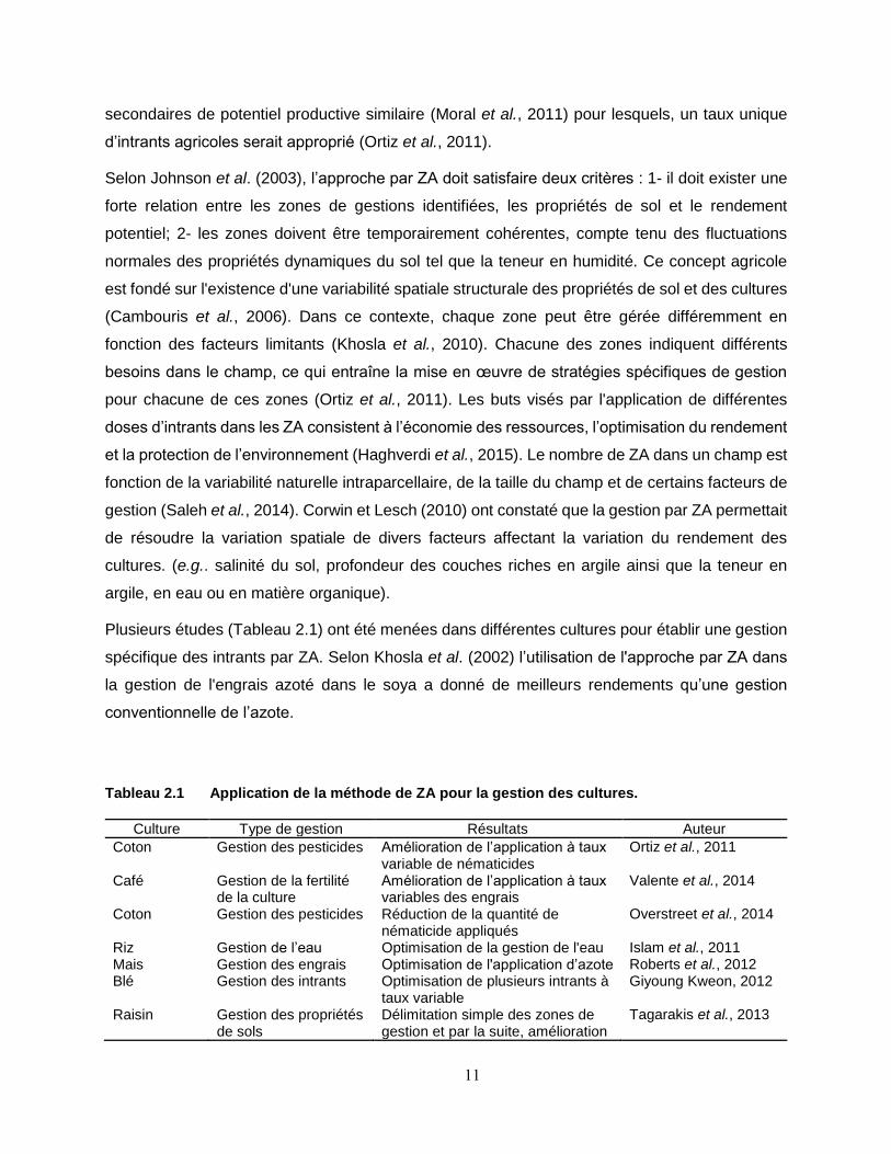
Plusieurs études (Tableau 2.1) ont été menées dans différentes cultures pour établir une gestion
spécifique des intrants par ZA. Selon Khosla et al. (2002) l’utilisation de l'approche par ZA dans
la gestion de l'engrais azoté dans le soya a donné de meilleurs rendements qu’une gestion
conventionnelle de l’azote.
Tableau 2.1 Application de la méthode de ZA pour la gestion des cultures.
Culture Type de gestion Résultats Auteur
Coton Gestion des pesticides Amélioration de l’application à taux variable de nématicides
Ortiz et al., 2011
Café Gestion de la fertilité de la culture
Amélioration de l’application à taux variables des engrais
Valente et al., 2014
Coton Gestion des pesticides Réduction de la quantité de nématicide appliqués
Overstreet et al., 2014
Riz Gestion de l’eau Optimisation de la gestion de l'eau Islam et al., 2011 Mais Gestion des engrais Optimisation de l'application d’azote Roberts et al., 2012 Blé Gestion des intrants Optimisation de plusieurs intrants à
taux variable Giyoung Kweon, 2012
Raisin Gestion des propriétés de sols
Délimitation simple des zones de gestion et par la suite, amélioration
Tagarakis et al., 2013
12
Culture Type de gestion Résultats Auteur
de la gestion des intrants des vignobles
Blé Gestion des engrais Amélioration de la qualité des sols par l’application à taux variable
Moshia et al., 2015
Blé Gestion des propriétés de sols
Amélioration de l’échantillonnage des sols
Peralta et al., 2015
Des études antérieures menées par Cambouris et al. (2006, 2014) ont démontré que le concept
par ZA est une approche prometteuse pour la gestion de la fertilisation dans la production
intensive de pommes de terre dans la province de Québec. Le coût élevé des intrants, en plus de
la sensibilité du rendement et de la qualité de la pomme de terre, ont incité les producteurs à
évaluer une gestion des cultures qui permet contrôler la variation des intrants dans les champs
pendant la saison de croissance pour produire un rendement commercial élevé(Allaire et al.,
2014, Morier et al., 2015).
2.3.1 Délimitation des zones d’aménagement
Diverses propriétés ont été proposées pour délimiter les champs en ZA. Celles-ci peuvent être
subdivisées avec une seule ou plusieurs propriétés du sol affectant le rendement (Haghverdi et
al., 2015). Les données spatiales stables dans le temps (Ortiz et al., 2011) sont les plus souvent
utilisées, tel que l’utilisation de cartes pédologiques (Fleming et al., 2004, Kweon, 2012, Molin et
al., 2008, Roberts et al., 2012, Saey et al., 2009, Valente et al., 2014) de même de nombreuses
propriétés physiques et chimiques des sols, les propriétés de modèles numériques de terrain
ainsi que les propriétés mesurées par les capteurs proximaux (Tableau 2.2). La combinaison de
données de rendement annuel ou pluriannuel avec d'autres informations auxiliaires permet
d’illustrer la variation spatiale des rendements et de générer des ZA fiables et stables dans le
temps (Haghverdi et al., 2015).
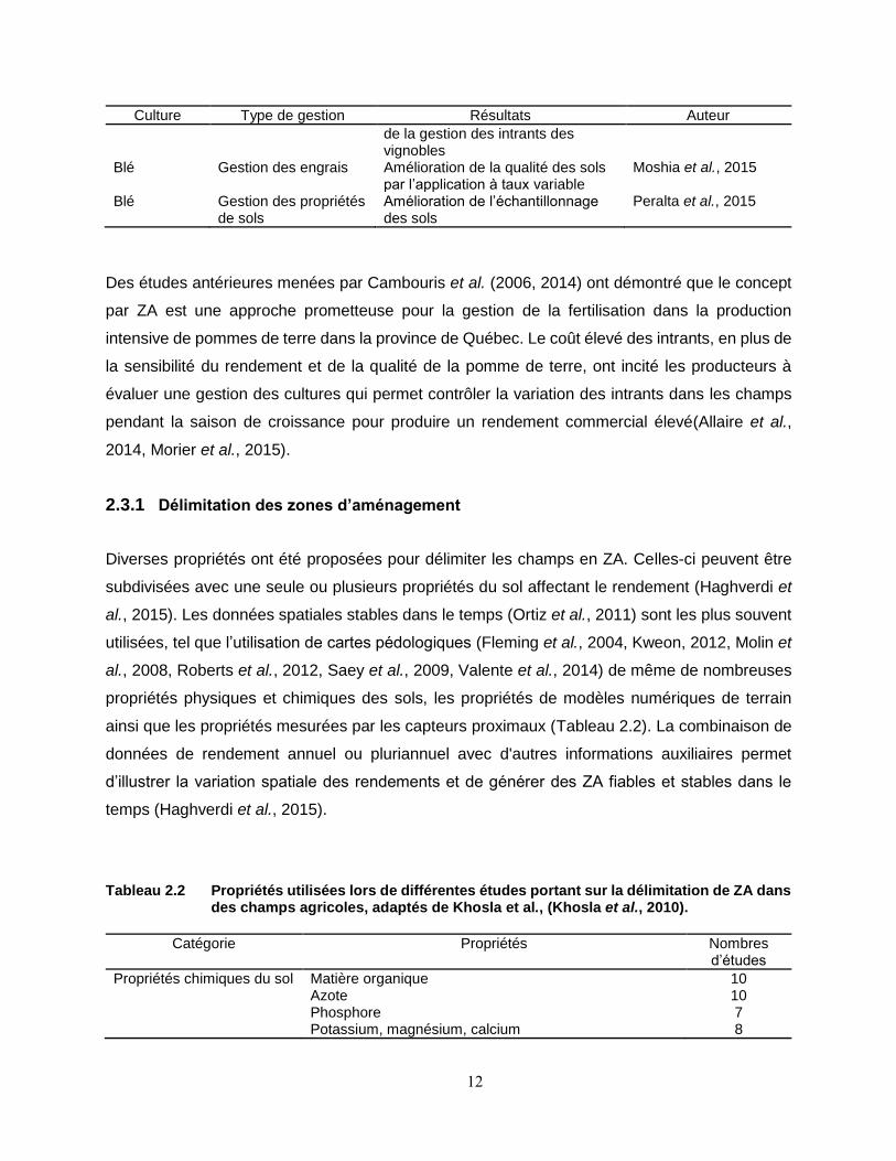
Tableau 2.2 Propriétés utilisées lors de différentes études portant sur la délimitation de ZA dans des champs agricoles, adaptés de Khosla et al., (Khosla et al., 2010).
Catégorie Propriétés Nombres d’études
Propriétés chimiques du sol Matière organique Azote Phosphore Potassium, magnésium, calcium
10 10 7 8
13
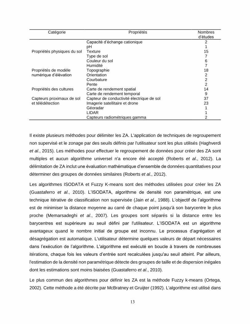
Catégorie Propriétés Nombres d’études
Capacité d’échange cationique pH
2 1
Propriétés physiques du sol Texture Type de sol Couleur du sol Humidité
15 7 6 7
Propriétés de modèle numérique d’élévation
Topographie Orientation Courbature Pente
18 2 2 2
Propriétés des cultures Carte de rendement spatial Carte de rendement temporal
14 9
Capteurs proximaux de sol et télédétection
Capteur de conductivité électrique de sol Imagerie satellitaire et drone Géoradar LIDAR Capteurs radiométriques gamma
37 23 1 1 2
Il existe plusieurs méthodes pour délimiter les ZA. L'application de techniques de regroupement
non supervisé et le zonage par des seuils définis par l'utilisateur sont les plus utilisés (Haghverdi
et al., 2015). Les méthodes pour effectuer le regroupement de données pour créer des ZA sont
multiples et aucun algorithme universel n'a encore été accepté (Roberts et al., 2012). La
délimitation de ZA inclut une évaluation mathématique d’ensemble de données quantitatives pour
déterminer des groupes de données similaires (Roberts et al., 2012).
Les algorithmes ISODATA et Fuzzy K-means sont des méthodes utilisées pour créer les ZA
(Guastaferro et al., 2010). L’ISODATA, algorithme de densité non paramétrique, est une
technique itérative de classification non supervisée (Jain et al., 1988). L’objectif de l’algorithme
est de minimiser la distance moyenne au carré de chaque point jusqu'à son barycentre le plus
proche (Memarsadeghi et al., 2007). Les groupes sont séparés si la distance entre les
barycentres est supérieure au seuil défini par l'utilisateur. L’ISODATA est un algorithme
avantageux quand le nombre initial de groupe est inconnu. Le processus d’agrégation et
désagrégation est automatique. L'utilisateur détermine quelques valeurs de départ nécessaires
dans l’exécution de l’algorithme. L'algorithme est exécuté en boucle à travers de nombreuses
itérations, chaque fois les valeurs d’entrée sont recalculées jusqu'au seuil atteint. Par ailleurs,
l'estimation de la densité non paramétrique détecte des groupes de taille et de dispersion inégales
dont les estimations sont moins biaisées (Guastaferro et al., 2010).
Le plus commun des algorithmes pour définir les ZA est la méthode Fuzzy k-means (Ortega,
2002). Cette méthode a été décrite par McBratney et Gruijter (1992). L'algorithme est utilisé dans
14
le but de partitionner n observations de données dans l'espace de fonctionnalité en c groupes (Li
et al., 2007). Fuzzy k-means est une procédure de classification continue non supervisée (Xin-
Zhong et al., 2009) pour diviser le champ en différentes zones. Le k-mean a été jugé efficace
pour la génération de zones de gestion par plusieurs auteurs (McBratney et al., 1992, Ortiz et al.,
2011). L’algorithme permet de partager une même donnée entre deux ou plusieurs classes en
contrôlant le degré d'appartenance de la donnée, par un exposant de pondération (Kweon, 2012).
La procédure de classification elle-même détermine les limites des zones en fonction de la
structure spatiale des variables d'entrée (Fraisse et al., 2001). Contrairement à l'algorithme
ISODATA, l'algorithme Fuzzy k-means n'exige pas que les variables ont une distribution normale
ou des variances similaires dans l'ensemble de données (Kweon, 2012). Les deux méthodes de
classification variaient en termes de temps et d'effort requis. Les méthodes utilisent les mêmes
attributs, mais l'exigence de distribution gaussienne pour ISODATA nécessitait un travail
supplémentaire pour diviser l'ensemble de données (Irvin et al., 1997). Cependant, ceci pourrait
aider de centrer et normaliser les variances dans le cas de variables ayant des amplitudes
différentes. D’autre part, la méthode Fuzzy k-means peut fournir des informations plus précises
que celles fournies par l'utilisation des classes discrètes (ISODATA). Les phénomènes naturels
tels que les données sur les sols ont été efficacement décrits en utilisant une classification
continue comme le Fuzzy k-means (Bezdek, 2013).
2.4 Capteurs proximaux de sol
2.4.1 L’agriculture de précision, utilisation des capteurs proximaux de sol
La détermination de ZA dans les champs est laborieuse en raison de la variabilité spatiale des
propriétés du sol et de la complexité des relations entre les propriétés elles-mêmes. La
concentration des nutriments peut être un des éléments responsables de la variation du
rendement des cultures (Peralta et al., 2013). Actuellement, il est possible d'obtenir des
caractéristiques du sol rapidement et à moindre coût. La détection proximale du sol est de plus
en plus utilisée afin d'obtenir de l’information sur les propriétés du sol. Ces techniques permettent
de combler l'écart de données qui existe entre les données ponctuelles à haute résolution et les
données de télédétection à faible résolution (Adamchuk et al., 2015). L'échantillonnage intensif
du sol est coûteux et laborieux (Shaner et al., 2008). Cette méthode est aussi invasive et se limite
à des mesures ponctuelles (Toy et al., 2010). Selon, Khiari (2014), cette méthode n’est pas
efficace dans une gestion par ZA. Valente et al. (2014) confirme que les propriétés physiques et
chimiques du sol exigent une grande densité d’échantillonnage pour déterminer efficacement la
15
variabilité spatiale des propriétés. Tripathi et al. (2015) ont révélé que des outils efficaces,
rentables et faciles à utiliser sont nécessaires pour la gestion spécifique des sols. L'utilisation et
le développement de capteur proximal des sols (CPS) permettant d'acquérir rapidement une forte
densité de données sur une base continue sont essentiels pour la délimitation de ZA. Les CPS
offrent une densité de mesure accrue et une couverture complète du terrain (Corwin et al., 2010).
Les CPS peuvent être divisés en différents groupes selon le type de capteur utilisé, soit électrique,
électromagnétique, optique, radiométrique, mécanique, acoustique, pneumatique et
électrochimique (Adamchuk et al., 2015). La détection proximale du sol est, en général, un
amalgame de technologie qui utilise un capteur proche ou en contact direct avec le sol pour
mesurer directement ou indirectement une propriété du sol (Adamchuk et al., 2004). Entre autres,
l’induction électromagnétique utilise le champ électromagnétique induit dans la colonne de sol
dans le calcul de la conductivité électrique apparente pour établir indirectement la variabilité des
différentes propriétés du sol telles que la texture, l’humidité, la salinité (Doolittle et al., 2014). Les
capteurs optiques utilisent la capacité de refléter la lumière directement à la surface du sol ou en
profondeur et mesure indirectement la variation des propriétés de sol comme la composition
minérale, la couleur du sol, le carbone organique (Christy, 2008). Les capteurs mécaniques
utilisent, quant à eux, la résistance mécanique du sol pour mesurer la variabilité horizontale de
compaction du sol selon différentes profondeurs.
Il existe actuellement sur le marché une variété de capteurs proximaux utilisée dans le cadre
agricole (Tableau 2.3). Les nouveaux outils et technologies apportent de nouvelles possibilités
pour améliorer la gestion agricole et sont à la base de la délimitation de ZA. Il existe un bon
potentiel pour améliorer encore l'efficacité, l'économie et les systèmes globaux de production
végétale (Khosla et al., 2010).
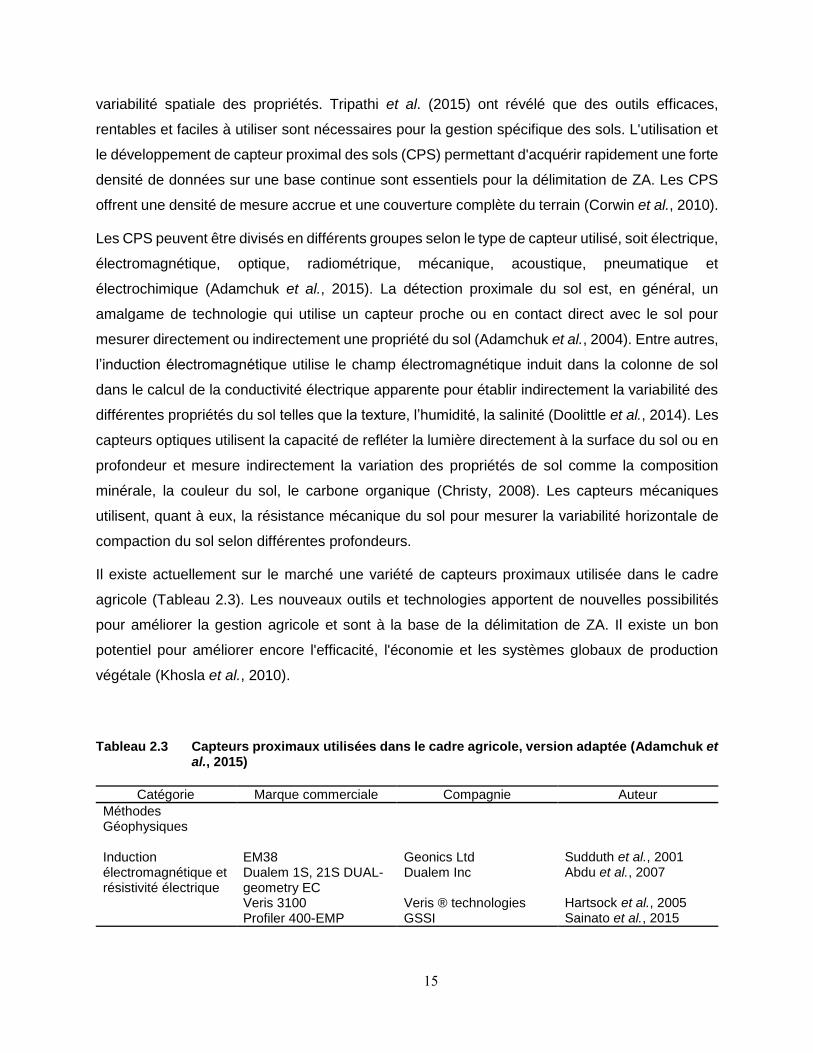
Tableau 2.3 Capteurs proximaux utilisées dans le cadre agricole, version adaptée (Adamchuk et al., 2015)
Catégorie Marque commerciale Compagnie Auteur
Méthodes Géophysiques
Induction électromagnétique et résistivité électrique
EM38 Geonics Ltd Sudduth et al., 2001 Dualem 1S, 21S DUAL-geometry EC
Dualem Inc Abdu et al., 2007
Veris 3100 Veris ® technologies Hartsock et al., 2005 Profiler 400-EMP GSSI Sainato et al., 2015
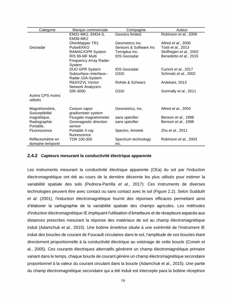
16
Catégorie Marque commerciale Compagnie Auteur EM31-MK2, EM34-3, EM38-MK2
Geonics limited Robinson et al., 2009
OhmMapper TR1 Geometrics Inc. Allred et al., 2006 Georadar PulseEKKO Sensors & Software Inc Tosti et al., 2013
RAMAC/GPR System Terraplus Inc. Stoffregen et al., 2002 RIS 99-MF Multi Frequency Array Radar-System
IDS Georadar Benedetto et al., 2015
DUO GPR System IDS Georadar Curioni et al., 2017 Subsurface–Interface–Radar-10A-System
GSSI Schmalz et al., 2002
R&S®ZVL Vector Network Analyzers
Rohde & Schwarz Ardekani, 2013
SIR-3000 GSSI Gormally et al., 2011 Autres CPS moins utilisés
Magnétométrie, Susceptibilité magnétique, Radiographie Portable, Fluorescence
Cesium vapor gradiometer system
Geometrics, Inc. Allred et al., 2004
Fluxgate magnetometer sans spécifier Benson et al., 1998 Geomagnetic direction sensor
sans spécifier Benson et al., 1998
Portable X-ray fluorescence
Spectro, Ametek Zhu et al., 2011
Réflectométrie en domaine temporel
TDR 100-300 Spectrum technology inc.
Robinson et al., 2003
2.4.2 Capteurs mesurant la conductivité électrique apparente
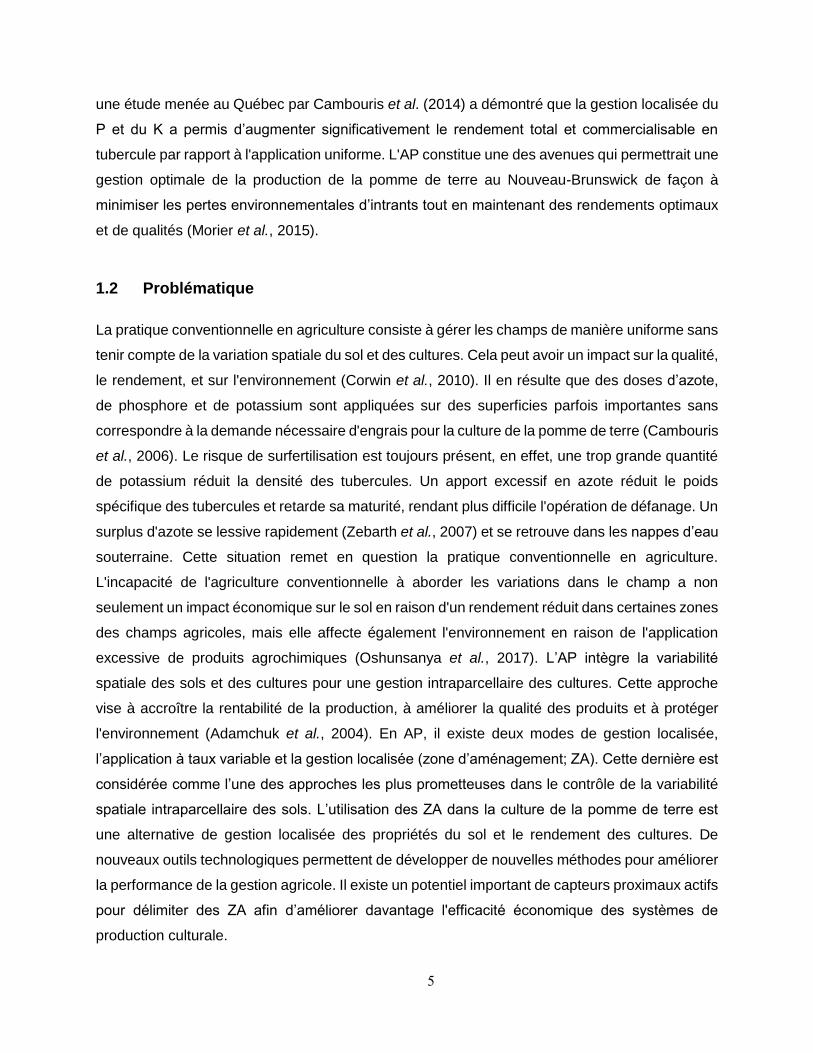
Les instruments mesurant la conductivité électrique apparente (CEa) du sol par l'induction
électromagnétique ont été au cours de la dernière décennie les plus utilisés pour estimer la
variabilité spatiale des sols (Pedrera-Parrilla et al., 2017). Ces instruments de diverses
technologies peuvent être avec contact ou sans contact avec le sol (Figure 2.2). Selon Sudduth
et al. (2001), l'induction électromagnétique fournit des réponses efficaces permettant ainsi
d’élaborer la cartographie de la variabilité spatiale des champs agricoles. Les méthodes
d'induction électromagnétique IE impliquent l'utilisation d’émetteurs et de récepteurs espacés aux
distances prescrites mesurant la réponse des matériaux de sol au champ électromagnétique
induit (Adamchuk et al., 2015). Une bobine émettrice située à une extrémité de l'instrument IE
induit des boucles de courant de Foucault circulaires dans le sol, l'amplitude de ces boucles étant
directement proportionnelle à la conductivité électrique au voisinage de cette boucle (Corwin et
al., 2005). Ces courants électriques alternatifs génèrent un champ électromagnétique primaire
variant dans le temps, chaque boucle de courant génère un champ électromagnétique secondaire
proportionnel à la valeur du courant circulant dans la boucle (Adamchuk et al., 2015). Une partie
du champ électromagnétique secondaire qui a été induit est intercepte para la bobine réceptrice
17
de l’instrument IE, le champ secondaire est proportionnel au courant du sol et est utilisé pour
calculer la conductivité électrique apparente du sol CEa (Corwin et al., 2005).
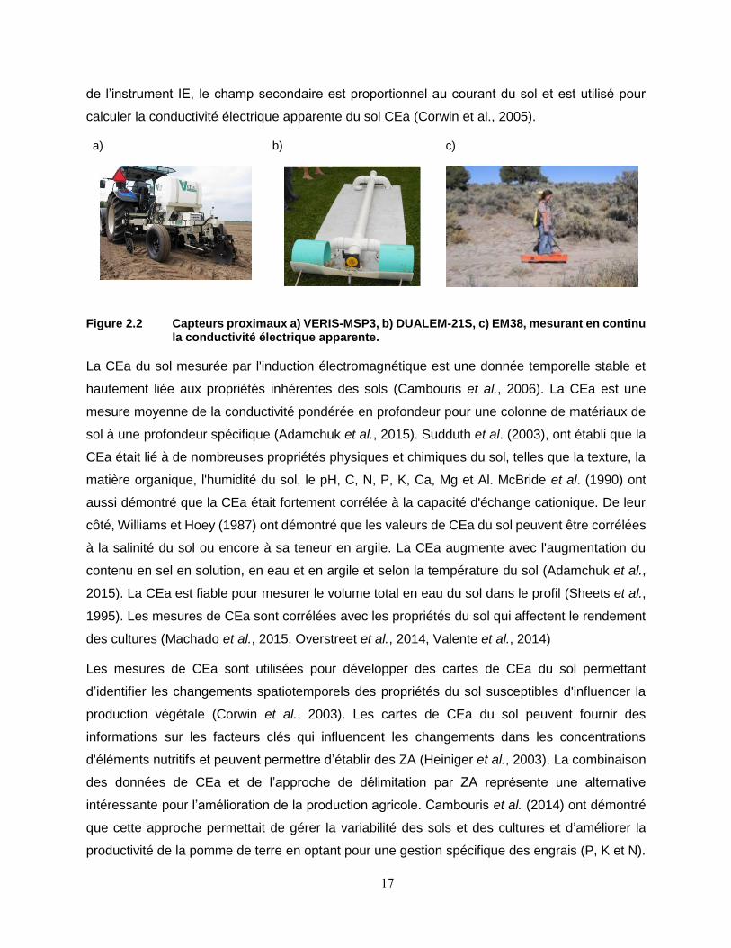
a)
b)
c)
Figure 2.2 Capteurs proximaux a) VERIS-MSP3, b) DUALEM-21S, c) EM38, mesurant en continu la conductivité électrique apparente.
La CEa du sol mesurée par l'induction électromagnétique est une donnée temporelle stable et
hautement liée aux propriétés inhérentes des sols (Cambouris et al., 2006). La CEa est une
mesure moyenne de la conductivité pondérée en profondeur pour une colonne de matériaux de
sol à une profondeur spécifique (Adamchuk et al., 2015). Sudduth et al. (2003), ont établi que la
CEa était lié à de nombreuses propriétés physiques et chimiques du sol, telles que la texture, la
matière organique, l'humidité du sol, le pH, C, N, P, K, Ca, Mg et Al. McBride et al. (1990) ont
aussi démontré que la CEa était fortement corrélée à la capacité d'échange cationique. De leur
côté, Williams et Hoey (1987) ont démontré que les valeurs de CEa du sol peuvent être corrélées
à la salinité du sol ou encore à sa teneur en argile. La CEa augmente avec l'augmentation du
contenu en sel en solution, en eau et en argile et selon la température du sol (Adamchuk et al.,
2015). La CEa est fiable pour mesurer le volume total en eau du sol dans le profil (Sheets et al.,
1995). Les mesures de CEa sont corrélées avec les propriétés du sol qui affectent le rendement
des cultures (Machado et al., 2015, Overstreet et al., 2014, Valente et al., 2014)
Les mesures de CEa sont utilisées pour développer des cartes de CEa du sol permettant
d’identifier les changements spatiotemporels des propriétés du sol susceptibles d'influencer la
production végétale (Corwin et al., 2003). Les cartes de CEa du sol peuvent fournir des
informations sur les facteurs clés qui influencent les changements dans les concentrations
d'éléments nutritifs et peuvent permettre d’établir des ZA (Heiniger et al., 2003). La combinaison
des données de CEa et de l’approche de délimitation par ZA représente une alternative
intéressante pour l’amélioration de la production agricole. Cambouris et al. (2014) ont démontré
que cette approche permettait de gérer la variabilité des sols et des cultures et d’améliorer la
productivité de la pomme de terre en optant pour une gestion spécifique des engrais (P, K et N).
18
2.4.3 Capteurs mesurant la résistivité électrique
La résistivité électrique RE du sol représente la capacité des matériaux du sol à résister à la
circulation du courant électrique. Les méthodes de résistivité électrique introduisent un courant
électrique à travers les électrodes de courant à la surface du sol (Corwin et al., 2005). Avec la
RE, la résistivité électrique apparente est calculée en utilisant la loi d'Ohm et le courant injecté
mesuré, la différence de potentiel mesurée, et un facteur géométrique, qui est fonction de
l'espacement ou de la configuration des électrodes (Adamchuk et al., 2015). La profondeur de
pénétration du courant électrique et le volume de mesure augmentent en fonction de
l'espacement inter-électrodes (Corwin et al., 2005). La résistivité électrique apparente est
communément exprimée en ohm-mètres (Ωm). La résistivité est une fonction complexe de la
composition et de l'arrangement des constituants solides du sol, de la porosité, de la saturation
de l'eau interstitielle, de la conductivité de l'eau interstitielle et de la température (Adamchuk et
al., 2015).
Les méthodes de résistivité électrique peuvent être divisées en celles qui injectent des courants
dans le sol par couplage direct (méthode de source galvanique invasive, e.g. Veris Technologies,
Salina, Kansas) et celles qui le font par couplage capacitif (électriques capacitives, e.g. The
OhmMapper). Ces dernières moins utilisés dans le cadre agricoles pour des raisons de mise en
place du dispositif en relation avec les obstacles sur le terrain (Adamchuk et al., 2015).
Typiquement, les deux méthodes mesurent la résistivité électrique apparente, qui en milieux
homogènes est ensuite convertie en son inverse, la conductivité électrique apparente du sol
(Corwin et al., 2003).
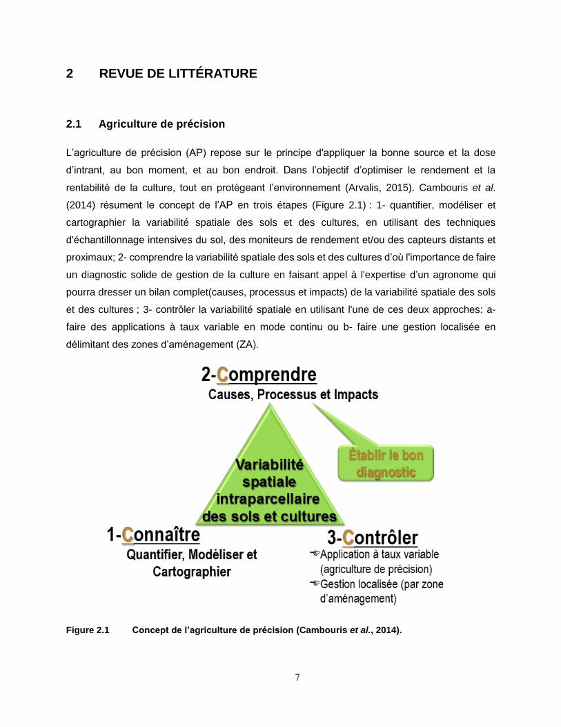
2.4.4 Géoradar
Le géoradar est une méthode géophysique non destructive (Figure 2.3) qui permet l’acquisition
d’une mesure en continu de contrastes de propriétés électromagnétiques, et dans les sols
non anthropisés de la constante diélectrique principalement. Cette mesure peut ensuite être
utilisée pour déterminer la profondeur du sol et des couches de roche (Xu et al., 2014). Pour
interpréter la profondeur d'une interface, il faut déterminer la vitesse de l'onde électromagnétique
à travers le sol ou obtenir des données réelles recueillies au sol de la profondeur de l'interface
(Adamchuk et al., 2015).
19
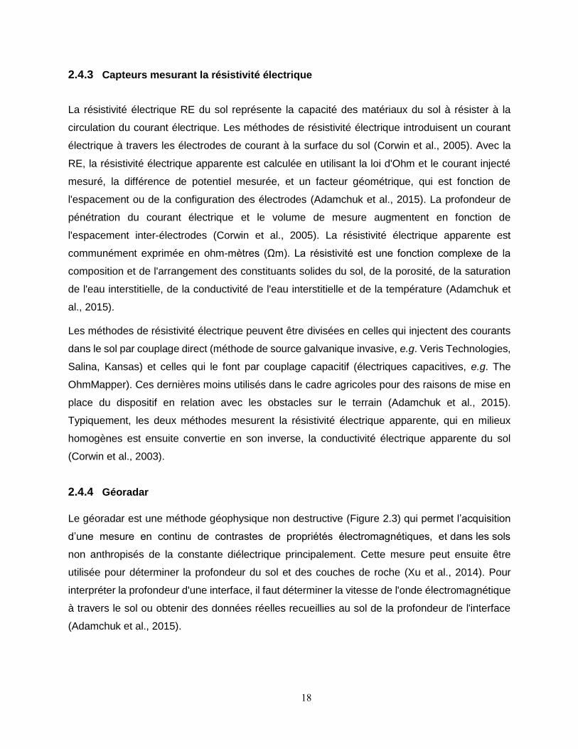
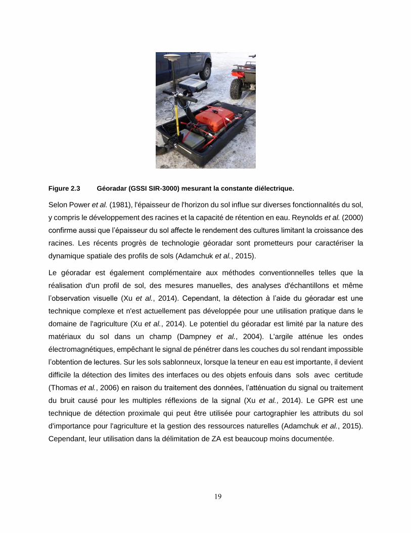
Figure 2.3 Géoradar (GSSI SIR-3000) mesurant la constante diélectrique.
Selon Power et al. (1981), l'épaisseur de l'horizon du sol influe sur diverses fonctionnalités du sol,
y compris le développement des racines et la capacité de rétention en eau. Reynolds et al. (2000)
confirme aussi que l’épaisseur du sol affecte le rendement des cultures limitant la croissance des
racines. Les récents progrès de technologie géoradar sont prometteurs pour caractériser la
dynamique spatiale des profils de sols (Adamchuk et al., 2015).
Le géoradar est également complémentaire aux méthodes conventionnelles telles que la
réalisation d'un profil de sol, des mesures manuelles, des analyses d'échantillons et même
l’observation visuelle (Xu et al., 2014). Cependant, la détection à l’aide du géoradar est une
technique complexe et n'est actuellement pas développée pour une utilisation pratique dans le
domaine de l'agriculture (Xu et al., 2014). Le potentiel du géoradar est limité par la nature des
matériaux du sol dans un champ (Dampney et al., 2004). L'argile atténue les ondes
électromagnétiques, empêchant le signal de pénétrer dans les couches du sol rendant impossible
l’obtention de lectures. Sur les sols sablonneux, lorsque la teneur en eau est importante, il devient
difficile la détection des limites des interfaces ou des objets enfouis dans sols avec certitude
(Thomas et al., 2006) en raison du traitement des données, l’atténuation du signal ou traitement
du bruit causé pour les multiples réflexions de la signal (Xu et al., 2014). Le GPR est une
technique de détection proximale qui peut être utilisée pour cartographier les attributs du sol
d'importance pour l'agriculture et la gestion des ressources naturelles (Adamchuk et al., 2015).
Cependant, leur utilisation dans la délimitation de ZA est beaucoup moins documentée.

21
3 MATÉRIEL ET MÉTHODES
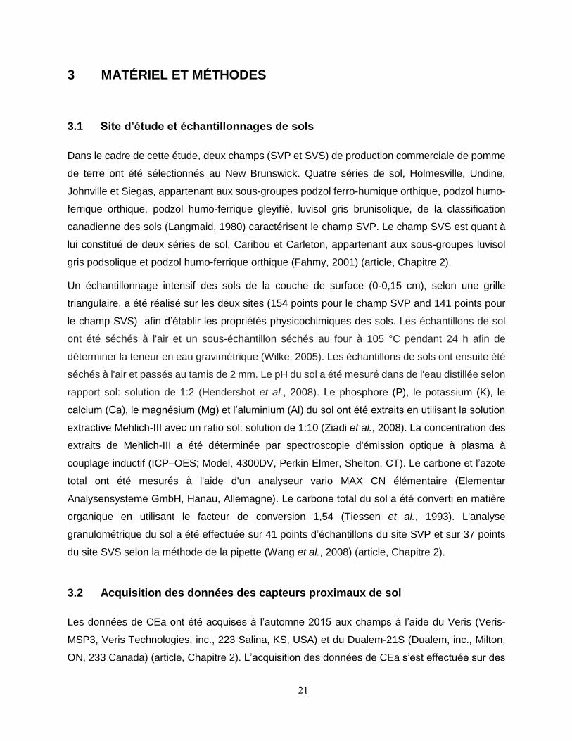
3.1 Site d’étude et échantillonnages de sols
Dans le cadre de cette étude, deux champs (SVP et SVS) de production commerciale de pomme
de terre ont été sélectionnés au New Brunswick. Quatre séries de sol, Holmesville, Undine,
Johnville et Siegas, appartenant aux sous-groupes podzol ferro-humique orthique, podzol humo-
ferrique orthique, podzol humo-ferrique gleyifié, luvisol gris brunisolique, de la classification
canadienne des sols (Langmaid, 1980) caractérisent le champ SVP. Le champ SVS est quant à
lui constitué de deux séries de sol, Caribou et Carleton, appartenant aux sous-groupes luvisol
gris podsolique et podzol humo-ferrique orthique (Fahmy, 2001) (article, Chapitre 2).
Un échantillonnage intensif des sols de la couche de surface (0-0,15 cm), selon une grille
triangulaire, a été réalisé sur les deux sites (154 points pour le champ SVP and 141 points pour
le champ SVS) afin d’établir les propriétés physicochimiques des sols. Les échantillons de sol
ont été séchés à l'air et un sous-échantillon séchés au four à 105 °C pendant 24 h afin de
déterminer la teneur en eau gravimétrique (Wilke, 2005). Les échantillons de sols ont ensuite été
séchés à l'air et passés au tamis de 2 mm. Le pH du sol a été mesuré dans de l'eau distillée selon
rapport sol: solution de 1:2 (Hendershot et al., 2008). Le phosphore (P), le potassium (K), le
calcium (Ca), le magnésium (Mg) et l’aluminium (Al) du sol ont été extraits en utilisant la solution
extractive Mehlich-III avec un ratio sol: solution de 1:10 (Ziadi et al., 2008). La concentration des
extraits de Mehlich-III a été déterminée par spectroscopie d'émission optique à plasma à
couplage inductif (ICP–OES; Model, 4300DV, Perkin Elmer, Shelton, CT). Le carbone et l’azote
total ont été mesurés à l'aide d'un analyseur vario MAX CN élémentaire (Elementar
Analysensysteme GmbH, Hanau, Allemagne). Le carbone total du sol a été converti en matière
organique en utilisant le facteur de conversion 1,54 (Tiessen et al., 1993). L'analyse
granulométrique du sol a été effectuée sur 41 points d’échantillons du site SVP et sur 37 points
du site SVS selon la méthode de la pipette (Wang et al., 2008) (article, Chapitre 2).
3.2 Acquisition des données des capteurs proximaux de sol
Les données de CEa ont été acquises à l’automne 2015 aux champs à l’aide du Veris (Veris-
MSP3, Veris Technologies, inc., 223 Salina, KS, USA) et du Dualem-21S (Dualem, inc., Milton,
ON, 233 Canada) (article, Chapitre 2). L’acquisition des données de CEa s’est effectuée sur des
22
profils parallèles espacés d'environ 10 m à des intervalles de 1 s, ce qui correspond à une mesure
tous les 2 à 3 m.
La prise de mesures du GPR a été réalisée en février 2016 à l’aide du modèle GSSI SIR-3000
(Geophysical Survey Systems, Inc., Nashua, NH, USA) avec une antenne de 400 MHz connectée
à un récepteur DGPS d’une précision centimétrique (GPS Novatel, antenne GTR-G2 L1 / L2)
(article, Chapitre 2). L’acquisition des données ont été effectués en 252 profils à environ 10 m
d'intervalle, le taux de capture de registres a été (30 scan sec-1). L'épaisseur des couches de sol
a été évaluée en utilisant le module interactif (RADAN 7-2D) (article, partie 2, Chapitre 2). Le
calcul de la permittivité électrique a été réalisé en utilisant le module interactif (RADAN 7, ground
truth) en utilisant les mesures de profondeurs de la couche indurée obtenues par le Veris P4000
probe (Veris 216 Technologies, inc., Salina, KS, USA).
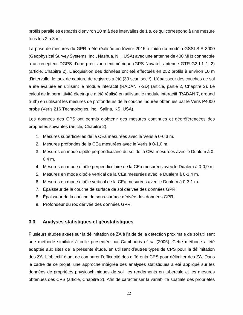
Les données des CPS ont permis d’obtenir des mesures continues et géoréférencées des
propriétés suivantes (article, Chapitre 2):
1. Mesures superficielles de la CEa mesurées avec le Veris à 0-0,3 m.
2. Mesures profondes de la CEa mesurées avec le Veris à 0-1,0 m.
3. Mesures en mode dipôle perpendiculaire du sol de la CEa mesurées avec le Dualem à 0-
0,4 m.
4. Mesures en mode dipôle perpendiculaire de la CEa mesurées avec le Dualem à 0-0,9 m.
5. Mesures en mode dipôle vertical de la CEa mesurées avec le Dualem à 0-1,4 m.
6. Mesures en mode dipôle vertical de la CEa mesurées avec le Dualem à 0-3,1 m.
7. Épaisseur de la couche de surface de sol dérivée des données GPR.
8. Épaisseur de la couche de sous-surface dérivée des données GPR.
9. Profondeur du roc dérivée des données GPR.
3.3 Analyses statistiques et géostatistiques
Plusieurs études axées sur la délimitation de ZA à l’aide de la détection proximale de sol utilisent
une méthode similaire à celle présentée par Cambouris et al. (2006). Cette méthode a été
adaptée aux sites de la présente étude, en utilisant d’autres types de CPS pour la délimitation
des ZA. L’objectif étant de comparer l’efficacité des différents CPS pour délimiter des ZA. Dans
le cadre de ce projet, une approche intégrée des analyses statistiques a été appliqué sur les
données de propriétés physicochimiques de sol, les rendements en tubercule et les mesures
obtenues des CPS (article, Chapitre 2). Afin de caractériser la variabilité spatiale des propriétés
23
physicochimiques des sols, du rendement en tubercule et des CPS, le module d’analyses
géostatistique ArcGIS 9.3.1 (ESRI, Redlands, CA, États-Unis) a été utilisé pour effectuer tous les
calculs géostatistiques et la validation des modèles. L’analyse de structure spatiale des
différentes propriétés et les ajustements des paramètres des semivariogrammes pour chaque
modèle théorique ont été évalués en détail dans l’article (article, Chapitre 3).
Afin de déterminer s’il existe une relation entre les CPS et les propriétés physicochimiques des
sols et du rendement, les coefficients de corrélation de Pearson (r) et leur niveau de signification
ont été calculés en utilisant différentes fonctions statistiques disponibles sur Matlab 8.3
(Mathworks, 2014a). Par la suite, pour délimiter les ZA à partir des données des CPS, l’algorithme
de regroupement fuzzy k-means sans contrainte de proximité spatiale a été appliqué à l'aide du
logiciel FuzME (Australian Centre for Precision Agriculture, 2002). Les ensembles de données
des capteurs proximaux ont été utilisés pour délimiter des ZA. Le ZA devrait produire des groupes
homogènes minimisant la variabilité intragroupe et maximisant la variabilité intergroupe (Tripathi
et al., 2015). Comme décrit par Cambouris et al. (2006), la décroissance de la variance a été
adoptée (article, Chapitre 3) pour déterminer le nombre optimal de ZA dans les sites à l’étude.
L’analyse de variance (ANOVA) et une analyse comparative multiple (Multcompare statistical
analysis, Matlab) ont été effectuées pour déterminer si les ZA étaient significativement différents
(ρ ≤ 0,05). Puisque l’analyse de la variance représente un test paramétrique, la normalité de la
distribution de l’erreur expérimentale a préalablement été testée par une analyse graphique des
résidus de boîte à moustaches et diagramme de probabilité normale ainsi que par le test
Kolmogorov-Smirnov sur Matlab.

25
4 RÉSULTATS ET DISCUSSION
4.1 Structures spatiales et relations entre les capteurs proximaux du sol, les propriétés physicochimiques du sol et le rendement en tubercule
Les analyses statistiques ont révélé une plus grande pédodiversité du champ SVP par rapport au
champ SVS, dont la variabilité pédologique était plus uniforme. Les analyses géostatistiques ont
démontrées qu’en général les propriétés physicochimiques du sol, le rendement en tubercule
ainsi que les paramètres mesurés avec les capteurs proximaux présentaient une structure
spatiale permettant ainsi de délimiter les champs à l’étude en zone de gestion plus homogène.
L’analyse de corrélation a aussi permis d’établir certaines relations significatives avec les
mesures acquises par les capteurs proximaux. En effet, les mesures de CEa acquises avec le
Veris et le Dualem étaient significativement corrélées avec plusieurs propriétés de sol et le
rendement en tubercule. Les relations étaient plus élevées entre la CEa et les propriétés
physiques pour le champ présentant une pédodiversité élevée (SVP) par rapport au champ
présentant une pédodiversité plus faible (SVS). En effet, les corrélations entre la CEa étaient
toutes significatives et plus élevées avec les propriétés texturales (r ≥ 0,68) pour le champ SVP
contrairement su champ SVS dont les corrélations n’étaient pas toutes significatives et plus faible
à (r < 0,41). Les relations entre les mesures de CEa et les rendements en tubercule de 2013,
2014 et 2016 étaient aussi significatives pour le champ SVP alors qu’elles ne l’étaient pas pour
le champ SVS (article, Chapitre 3). En ce qui concerne le GPR, la majorité des paramètres dérivés
de cet appareil n’était pas significativement corrélés avec les propriétés physicochimiques du sol
et le rendement du tubercule dans les champs étudiés. Une analyse plus approfondie a été
résumée dans l’article (article, Chapitre 3).
À la lumière des résultats obtenus, il est clair que les appareils Veris et Dualem permettent de
mieux caractériser les sols des champs qui présentent une pédodiversité plus élevée. Une
pédodiversité élevée révèle aussi une meilleure structure spatiale et donc un potentiel plus élevé
pour utiliser l’approche de gestion localisée.
4.2 Détermination du nombre optimum de zones d’aménagement
Pour les deux champs à l’étude, l’algorithme fuzzy K-means a été utilisé pour subdiviser les
champs de deux à cinq zones pour chacun des capteurs proximaux en utilisant l’ensemble des
26
paramètres de chacun des capteurs. Par la suite, pour déterminer le nombre optimal de zones
d’aménagement l’analyse de décroissance de la variance a été utilisée. L’analyse a permis
d’établir que dans le cas des deux champs et pour les trois capteurs utilisés, deux zones étaient
optimales. Les résultats de l’analyse de décroissance de la variance pour les propriétés de sol et
le rendement étaient similaires. La réduction totale de la variance intrazone pour deux ZA était
de 70% pour le champ SVP et de 40% pour le champ SVS. Les deux ZA obtenus ont révélé un
patron spatial similaire dans le cas des capteurs de mesures de CEa pour le champ SVP, alors
qu’ils étaient différents pour le champ SVS. Les ZA délimités par le Veris et le Dualem
permettaient une gestion simple alors que les ZA délimités par le GPR étaient complexes et une
gestion localisée n’était pas pratique dans un cadre agricole (article, Chapitre 3.6).
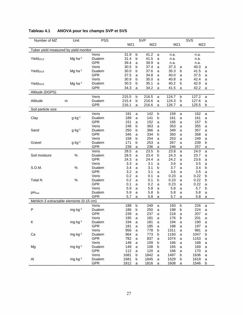
En plus, les trois années de rendements des deux zones délimitées avec le Veris et le Dualem
étaient statistiquement différentes pour le champ SVP alors que seul le Dualem a permis d’obtenir
des différences significatives pour le champ SVS. Les propriétés physiques étaient
significativement différentes pour le champ SVP tandis qu’ils ne l’étaient pas pour le champ SVS,
lorsque subdivisé avec les capteurs Veris et Dualem, révélant une fois de plus l’influence du
facteur pédodiversité (Tableau 4.1). Pour les zones délimitées par le GPR les zones ne
présentaient pas de différences significatives pour la majorité des propriétés physicochimiques
de même que pour le rendement, et ce pour les deux champs.
27
Tableau 4.1 ANOVA pour les champs SVP et SVS
Number of MZ Unit PSS SVP SVS
MZ1 MZ2 MZ1 MZ2
Tuber yield measured by yield monitor
Yield2013 Mg ha-1 Veris 31.9 b 41.2 a n.a. n.a. Dualem 31.4 b 41.5 a n.a. n.a. GPR 39.4 a 39.9 a n.a. n.a.
Yield2014 Mg ha-1 Veris 30.5 b 37.4 a 37.3 a 40.0 a Dualem 30.0 b 37.6 a 35.3 b 41.5 a GPR 37.5 a 34.8 a 40.0 a 37.5 a
Yield2016 Mg ha-1
Veris 30.9 b 35.0 a 40.8 a 42.4 a Dualem 30.5 b 35.1 a 40.2 b 42.9 a
GPR 34.3 a 34.2 a 41.5 a 42.2 a
Altitude (DGPS)
Altitude m Veris 215.5 b 216.5 a 124.7 b 127.2 a Dualem 215.4 b 216.6 a 124.3 b 127.6 a GPR 216.1 a 216.6 a 126.7 a 125.5 b
Soil particle size
Clay g kg-1 Veris 191 a 142 b 159 a 162 a Dualem 189 a 141 b 161 a 161 a GPR 151 a 152 a 165 a 157 b
Sand g kg-1 Veris 248 b 363 a 353 a 355 a Dualem 250 b 366 a 349 a 357 a GPR 345 a 334 b 350 a 358 a
Gravel g kg-1 Veris 158 b 254 a 253 a 249 a Dualem 171 b 253 a 267 a 239 b GPR 239 a 236 a 246 a 257 a
Soil moisture % Veris 28.5 a 23.5 b 23.8 a 24.0 a Dualem 28.5 a 23.4 b 24.3 a 23.7 a GPR 24.3 a 24.4 a 24.2 a 23.6 a
S.O.M. % Veris 3.3 a 3.1 a 3.6 a 3.5 a Dualem 3.4 a 3.1 b 3.7 a 3.4 b GPR 3.2 a 3.1 a 3.6 a 3.5 a
Total N % Veris 0.2 a 0.1 a 0.23 a 0.22 b Dualem 0.2 a 0.1 b 0.23 a 0.22 b GPR 0.1 a 0.2 a 0.23 a 0.22 a
pHeau Veris 5.9 a 5.8 a 5.8 a 5.7 b Dualem 5.9 a 5.8 b 5.8 a 5.8 a GPR 5.7 a 5.8 a 5.7 a 5.8 a
Mehlich-3 extractable elements (0-15 cm)
P mg kg-1 Veris 188 b 249 a 193 b 226 a Dualem 186 b 250 a 198 b 224 a GPR 239 a 237 a 218 a 207 a
K mg kg-1 Veris 195 a 181 a 176 b 201 a Dualem 194 a 181 a 194 a 190 a GPR 181 a 185 a 188 a 197 a
Ca mg kg-1 Veris 956 a 778 b 1311 a 981 a Dualem 964 a 773 b 1193 a 1047 b GPR 782 a 837 a 1074 a 1153 a
Mg mg kg-1 Veris 148 a 109 b 166 a 168 a Dualem 149 a 108 b 165 a 169 a GPR 112 a 120 a 166 a 170 a
Al mg kg-1 Veris 1681 b 1842 a 1497 b 1636 a Dualem 1681 b 1845 a 1529 b 1619 a GPR 1812 a 1816 a 1608 a 1546 b
28
4.3 Application pratique de la gestion localisée
L'utilisation des capteurs Veris et Dualem a été la plus recommandée pour la délimitation des ZA
dans le cadre de cette étude. Ces capteurs ont permis de délimiter des ZA qui caractérisant les
propriétés physicochimiques du sol et le rendement des cultures, principalement dans le champ
à pédodiversité élevée, soit le champ SVP. Pour ce champ, la ZA avec les valeurs de CEa les
plus élevées était caractérisée par un sol plus humide, une texture de sol plus fine et un
rendement en tubercule plus faible. Cette ZA à rendement plus faible, pourrait être géré avec un
drainage ou un nivellement spécifique afin de réduire la plus grande quantité d'eau présente dans
cette partie du champ SVP. Cet aménagement pourrait permettre d’augmenter le potentiel de
rendement en tubercules dans cette zone. La gestion localisée de ce champ témoigne
l’importance d’une méthode adaptée pour la gestion et le suivi temporel des champs agricoles.
Les résultats pour le GPR ont été les moins performants (article, Chapitre 3.6). Contrairement
aux capteurs de la CEa, le GPR n'a pas produit de zones homogènes (ZA spatialement
complexes) pour les deux champs et les résultats du GPR n'étaient pas significativement
différents, en grand partie dû à la distribution spatiale en tranches des données interpolées. Ces
résultats peuvent s’expliquer par une densité d'échantillonnage élevée du GPR dans la direction
des profils. Des traitements supplémentaires de lissage des données de départ pourraient être
adoptés améliorant les donnes pour de futures recherches ainsi comme la densification de profils
d’échantillonnage en direction perpendiculaire. D’autres études seraient nécessaires afin
d’investiguer les méthodes de traitements et la façon de dériver les variables du GPR. Une
méthodologie différente serait peut-être plus appropriée pour détecter la variabilité spatiale des
propriétés de sol dans une culture de pomme de terre.
29
5 CONCLUSION ET RECOMMANDATIONS
L’objectif du projet était d’étudier et de comparer différents CPS pour la délimitation de ZA dans
des champs de culture de pomme de terre au Nouveau-Brunswick. Afin d’atteindre cet objectif,
trois capteurs proximaux de sol ont été utilisés soit le Veris, le Dualem et le GPR dans deux
champs agricoles. Le premier objectif consistait à caractériser la variabilité spatiale des propriétés
physicochimiques des sols. Parmi les deux sites étudiés, le champ SVP a révélé une variabilité
plus élevée que le site SVS. Ces résultats peuvent s’expliquer par une pédodiversité différente
entre les deux champs. Le champ SVP ayant une pédodiversité plus élevée que le champ SVS.
Le deuxième objectif visait à étudier la capacité des capteurs proximaux du sol en évaluant leur
variabilité spatiale, leur niveau de corrélation avec les propriétés physicochimiques des sols et du
rendement. De plus, délimiter les ZA à partir des mesures dérivées des CPS et valider leur niveau
d’homogénéité et déterminer si celles-ci ont été significativement différentes. À ce niveau, les
paramètres du Veris et du Dualem se sont révélés, les plus significativement et fortement corrélés
avec les propriétés physicochimiques de sol et du rendement. Deux ZA obtenus à partir de ces
capteurs se sont avérés optimaux selon l’analyse de décroissance de la variance et les deux
zones se sont révélées significativement différentes (ANOVA).
Au contraire, le GPR n'a pas produit de zones homogènes (ZA spatialement complexe) pour les
deux champs et les résultats du GPR n'étaient pas significativement différents. La densité
d'échantillonnage élevée du GPR par rapport aux autres CPS (plus de 200 000 échantillons)
pourrait être mise en cause. Ces résultats peuvent s’expliquer par une densité
d'échantillonnage élevée du GPR dans la direction de chacun des profils et un faible
échantillonnage entre eux. À ce sujet, des traitements complémentaires de lissage et filtrage des
données GPR de départ et une densification de profils d’échantillonnage en direction
perpendiculaire pourraient être adoptés. Ceci pourrait contribuer dans l’amélioration des
interpolations des épaisseurs de la couche de sol dérivées du GPR, ce qui les rendrait plus
adaptées dans la délimitation des ZA.
L’avènement de nouveaux outils et technologies apporte de nouvelles approches pour améliorer
la gestion en agriculture. Il existe un potentiel important des capteurs actifs proximaux du sol pour
délimiter des ZA pour améliorer davantage l'efficacité, l'économie et les systèmes de production
des cultures.


31
PARTIE 2 : ARTICLE


33
AVANT-PROPOS
L’article sera soumis pour une publication dans la revue Canadian Journal of Soil Science. Cette
revue est publiée par la Société Canadienne en Science du Sol.
Felipe Vargas :
• Définition du sujet et des objectifs
• Développement de la méthodologie
• Analyse statistique des données et interprétation des résultats
• Écriture et révision de l’article
Athyna Cambouris
• Aide à la définition du sujet et des objectifs
• Aide au développement de la méthodologie
• Aide à l’interprétation des résultats
• Révision de l’article
Karem Chokmani :
• Aide à la définition du sujet et des objectifs
• Aide au développement de la méthodologie
• Aide à l’interprétation des résultats

34
35
RÉSUMÉ
La délimitation de zones d’aménagement ZA dans des champs agricoles peut être utilisée comme
base dans la gestion spécifique des intrants, ceci offre une alternative efficace à l’application
uniforme et à taux variable. Cette étude a évalué l'efficacité de trois capteurs proximaux de sol
(CPS) pour délimiter ZA dans des champs commerciaux de pommes de terre (Solanum
tuberosum L.) de 21 et 18 ha situés à Saint-André et Centreville (N.-B.), désignés comme les
champs SVP et SVS. Les capteurs proximaux du sol de modelé VERIS (modelé MSP3) et Dualem
(modelé 21S) ont été utilisés pour la mesure de la conductivité électrique apparente du sol
pendant l'automne 2015. Le géoradar (GPR, modèle GSSI SIR-3000, antenne 400 MHz, 30 sec-
1 scan) a été utilisé pour dériver l’épaisseur des couches de sol à partir le contraste diélectrique
de surfaces en février 2016. Les données CPS ont été utilisées pour stratifier les champs en ZA
en utilisant un algorithme de regroupement fuzzy k-means non supervisés. Des échantillons de
sol (0-0,15 m) recueillis à partir de 154 (SVP) et 141 (SVS) points d'échantillonnage géoréférence
ont été analysés pour les propriétés physicochimiques (matière organique, pH, éléments
extractibles de Mehlich-3). L'analyse granulométrique du sol a été effectuée pour 41 et 37
échantillons de sol. Les rendements des tubercules ont été mesurés en utilisant un moniteur de
rendements en 2013 (champs SVP, SVS), 2014 et 2016. Le champ SVP a montré une
pédodiversité plus élevée que le champ SVS. Dans le site SVP, le Veris et le Dualem étaient
efficaces, tandis que le Dualem était plus performant que le Veris dans la délimitation de ZA dans
le champ SVS. Le GPR n'était pas efficace pour délimiteur ZA dans les deux champs. Les deux
ZA délimités avec l’ECa ont montré des différences significatives dans les propriétés
physicochimiques du sol et la productivité du rendement des tubercules pour les deux champs.
Des différences significatives dans le rendement de la pomme de terre (7,1 Mg ha-1) ont été
attribuées à la texture (argile : 141 g kg-1 vs 189 g kg-1) et à l'humidité du sol (23,5% vs 28,5%)
dans le champ SVP. Dans le site SVS, le patron de rendement des tubercules n'était pas similaire
avec les propriétés psychochimiques du sol. Ceci est probablement lié à la plus faible variabilité
spatiale du champ. Les capteurs ECa du sol pourraient être utilisés pour délimiter des ZA
efficaces afin de gérer la variabilité du rendement. La performance de la méthode proposée est
prometteuse dans la production de pommes de terre au Nouveau-Brunswick, particulièrement
lorsque le champ présente un niveau élevé de pédodiversité.

36
37
ABSTRACT
Subdividing agricultural fields into soil management zones MZ with relatively homogeneous soil
properties and yield potential can be used as the basis of site-specific nutrient management, and
offers an effective alternative to uniform and variable rate applications. This study evaluated the
efficiency of three proximal soil sensors (PSS) to delineate MZ in a 21-ha and 18-ha commercial
potato (Solanum tuberosum L.) fields located in Saint-André and Centreville (NB) referred as SVP
and SVS, respectively. The Veris (model MSP3) and Dualem (model 21S) were utilized for the
measurement of the soil electrical conductivity in fall of 2015. Ground penetrating radar (GPR
system; GSSI SIR-3000 model; 400 MHz antenna; 30 sec-1 scan) was utilized for the
measurement of the soil dielectric constant in February 2016. The PSS data were used to stratify
the fields into MZ using an unsupervised fuzzy k-means clustering algorithm. Soil samples (0-
0.15 m) collected from 154 (SVP) and 141 (SVS) georeferenced sampling points were analyzed
for physicochemical properties (S.O.M, pH, Mehlich-3 extractable elements). The soil particle size
analysis was completed only on 41 and 37 soil samples. Tuber yields were measured using a
yield monitor in 2013 (SVP field only), 2014, and 2016. The SVP field showed higher pedodiversity
than the SVS field. In SVP field the Veris and the Dualem were both effective while the Dualem
performed better than the Veris in delineating MZ in the SVS field. The GPR was not effective in
delineating MZ in both fields. The two MZ delineated with the soil EC showed significant
differences in soil physicochemical properties and tuber yield productivity for both fields.
Significant differences in potato yield (7.1 Mg ha-1) were attributed to texture (clay: 141 g kg-1 vs
189 g kg-1) and soil moisture (23.5% vs 28.5%) in the SVP field. In the SVS field, tuber yield
pattern wasn’t similar over time and soil psychochemical properties behaviour was not the same
if the field was delineated with the Veris or the Dualem. This is probably related to lowest spatial
variability of the field. Soil EC sensors could be used to delineate efficient MZ to manage yield
variability. The performance of the proposed method is promising in potato production in New
Brunswick especially when the field shows high pedodiversity level.

38
39
DELINEATED MANAGEMENT ZONES WITH THREE PROXIMAL SOIL SENSORS
TO EXPLAIN SOIL SPATIAL VARIABILITY IN TWO POTATO FIELDS
F. Vargas1,2, A.N. Cambouris2*, K. Chokmani1, I. Perron2, B.J. Zebarth3, A. Biswas4 and V.
Adamchuck5
1Institut national de la recherche scientifique, Centre – Eau Terre Environnement, 490, rue de la
Couronne, Quebec City, Quebec, Canada, G1K 9A9
2Agriculture and Agri-Food Canada, Quebec Research and Development Centre, 2560
Hochelaga Boulevard, Quebec City, Quebec, Canada, G1V2J3
3Agriculture and Agri-Food Canada, Fredericton Research and Development Centre, 850 Lincoln
Road, Fredericton, New Brunswick, Canada, E3B 4Z7
4University of Guelph, School of Environmental Sciences, 50 Stone Road East, Guelph, Ontario,
Canada, N1G 2W1
5McGill University, Department of Bioresource Engineering, 21111 Lakeshore Road, Ste-Anne-
de-Bellevue, Quebec, Canada, H9X 3V9
*Corresponding author: [email protected]

40
41
1 INTRODUCTION
Currently, the spatiotemporal variability of soil and crop properties is recognized by all agricultural
stakeholders as the cornerstone of precision agriculture (PA). The main goals of this approach
consisted in increasing profitability of crop production, improving product quality, and protecting
the environment (Adamchuk et al., 2004). Recent technological advances in PA have made it
possible to identify, analyze and manage soil variability at field scale. The adoption, rapid
development and price democratization of precision farming technologies (e.g. GPS, yield
monitors, automatic guidance of farm machinery and variable rate application technologies, soil
and crop proximal sensors) help farmers to create maps of intra-field soil and crop variations.
These maps will be taken into account for their managing strategies (Dampney et al., 2004).
Despite the importance of within-field soil variability, the conventional practice consists in
managing fields uniformly without taking the spatial variation of soil and crop into consideration.
This can impact yield quality and productivity, natural resources as well as environmental
protection (Corwin et al., 2010). The management zone MZ approach is used to improve decision-
making for the management of soil and crop variability, including soil fertility, plant-available water
and crop yield (Mulla, 1989). This approach requires the identification of subfield regions with
homogeneous characteristics (Peralta et al., 2013), to determine how best to act at subfield
regions of similar production potential (Moral et al., 2011).
This agricultural concept is based on the existence of within-field spatial structured soil and crop
variability (Cambouris et al., 2006). Khosla et al. (2002) showed that using MZ approach to
manage nitrogen fertilizer in a corn (Zea mays L.) field gave better result than managing the field
following the conventional approach. In this context, each zone can be managed differently based
upon the limiting factor of that zone (Khosla et al., 2010). Corwin and Lesch (2010) found that MZ
was a way of controlling the spatial variation of various factors (i.e. soil, climate, management,
pests and crops) that affect variation in crop yield. In previous studies, Cambouris et al. (2006,
2014) showed that MZ is a promising approach to fertilization management in intensive potato
production (Solanum tuberosum L.) in the province of Quebec. The high cost of inputs, the
sensitivity of potato tuber yield and quality to crop management and environmental conditions
have prompted producers to assess the potential to vary inputs within fields during the growing
season to produce higher yield (Allaire et al., 2014, Morier et al., 2015).
However, identifying spatial variations in soil properties within a field is currently a challenge in
agriculture. The determination of subfield areas is difficult because of complex correlations and
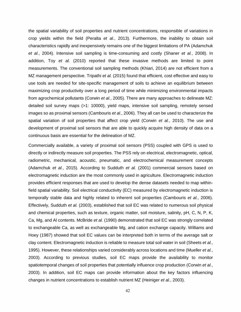
42
the spatial variability of soil properties and nutrient concentrations, responsible of variations in
crop yields within the field (Peralta et al., 2013). Furthermore, the inability to obtain soil
characteristics rapidly and inexpensively remains one of the biggest limitations of PA (Adamchuk
et al., 2004). Intensive soil sampling is time-consuming and costly (Shaner et al., 2008). In
addition, Toy et al. (2010) reported that these invasive methods are limited to point
measurements. The conventional soil sampling methods (Khiari, 2014) are not efficient from a
MZ management perspective. Tripathi et al. (2015) found that efficient, cost effective and easy to
use tools are needed for site-specific management of soils to achieve an equilibrium between
maximizing crop productivity over a long period of time while minimizing environmental impacts
from agrochemical pollutants (Corwin et al., 2005). There are many approaches to delineate MZ:
detailed soil survey maps (>1: 10000), yield maps, intensive soil sampling, remotely sensed
images so as proximal sensors (Cambouris et al., 2006). They all can be used to characterize the
spatial variation of soil properties that affect crop yield (Corwin et al., 2010). The use and
development of proximal soil sensors that are able to quickly acquire high density of data on a
continuous basis are essential for the delineation of MZ.
Commercially available, a variety of proximal soil sensors (PSS) coupled with GPS is used to
directly or indirectly measure soil properties. The PSS rely on electrical, electromagnetic, optical,
radiometric, mechanical, acoustic, pneumatic, and electrochemical measurement concepts
(Adamchuk et al., 2015). According to Sudduth et al. (2001) commercial sensors based on
electromagnetic induction are the most commonly used in agriculture. Electromagnetic induction
provides efficient responses that are used to develop the dense datasets needed to map within-
field spatial variability. Soil electrical conductivity (EC) measured by electromagnetic induction is
temporally stable data and highly related to inherent soil properties (Cambouris et al., 2006).
Effectively, Sudduth et al. (2003), established that soil EC was related to numerous soil physical
and chemical properties, such as texture, organic matter, soil moisture, salinity, pH, C, N, P, K,
Ca, Mg, and Al contents. McBride et al. (1990) demonstrated that soil EC was strongly correlated
to exchangeable Ca, as well as exchangeable Mg, and cation exchange capacity. Williams and
Hoey (1987) showed that soil EC values can be interpreted both in terms of the average salt or
clay content. Electromagnetic induction is reliable to measure total soil water in soil (Sheets et al.,
1995). However, these relationships varied considerably across locations and time (Mueller et al.,
2003). According to previous studies, soil EC maps provide the availability to monitor
spatiotemporal changes of soil properties that potentially influence crop production (Corwin et al.,
2003). In addition, soil EC maps can provide information about the key factors influencing
changes in nutrient concentrations to establish nutrient MZ (Heiniger et al., 2003).
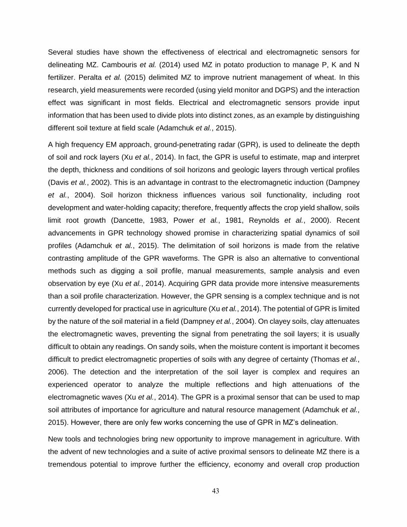
43
Several studies have shown the effectiveness of electrical and electromagnetic sensors for
delineating MZ. Cambouris et al. (2014) used MZ in potato production to manage P, K and N
fertilizer. Peralta et al. (2015) delimited MZ to improve nutrient management of wheat. In this
research, yield measurements were recorded (using yield monitor and DGPS) and the interaction
effect was significant in most fields. Electrical and electromagnetic sensors provide input
information that has been used to divide plots into distinct zones, as an example by distinguishing
different soil texture at field scale (Adamchuk et al., 2015).
A high frequency EM approach, ground-penetrating radar (GPR), is used to delineate the depth
of soil and rock layers (Xu et al., 2014). In fact, the GPR is useful to estimate, map and interpret
the depth, thickness and conditions of soil horizons and geologic layers through vertical profiles
(Davis et al., 2002). This is an advantage in contrast to the electromagnetic induction (Dampney
et al., 2004). Soil horizon thickness influences various soil functionality, including root
development and water-holding capacity; therefore, frequently affects the crop yield shallow, soils
limit root growth (Dancette, 1983, Power et al., 1981, Reynolds et al., 2000). Recent
advancements in GPR technology showed promise in characterizing spatial dynamics of soil
profiles (Adamchuk et al., 2015). The delimitation of soil horizons is made from the relative
contrasting amplitude of the GPR waveforms. The GPR is also an alternative to conventional
methods such as digging a soil profile, manual measurements, sample analysis and even
observation by eye (Xu et al., 2014). Acquiring GPR data provide more intensive measurements
than a soil profile characterization. However, the GPR sensing is a complex technique and is not
currently developed for practical use in agriculture (Xu et al., 2014). The potential of GPR is limited
by the nature of the soil material in a field (Dampney et al., 2004). On clayey soils, clay attenuates
the electromagnetic waves, preventing the signal from penetrating the soil layers; it is usually
difficult to obtain any readings. On sandy soils, when the moisture content is important it becomes
difficult to predict electromagnetic properties of soils with any degree of certainty (Thomas et al.,
2006). The detection and the interpretation of the soil layer is complex and requires an
experienced operator to analyze the multiple reflections and high attenuations of the
electromagnetic waves (Xu et al., 2014). The GPR is a proximal sensor that can be used to map
soil attributes of importance for agriculture and natural resource management (Adamchuk et al.,
2015). However, there are only few works concerning the use of GPR in MZ’s delineation.
New tools and technologies bring new opportunity to improve management in agriculture. With
the advent of new technologies and a suite of active proximal sensors to delineate MZ there is a
tremendous potential to improve further the efficiency, economy and overall crop production

44
systems (Khosla et al., 2010). The aim of this study was to compare PSS to characterize and map
soil spatial variability and therefore to delineate soil MZ in intensive potato production in New
Brunswick.
45
2 MATERIALS AND METHODS
2.1 Experimental Site
The study was conducted in two commercial fields under intensive potato production located in
Saint-André (referred as SVP: 47.06′N; 67.48′W) and Centreville (referred as SVS, 46.23′N;
67.43′W), New Brunswick, Canada. The SVP field area was 21 ha while SVS field was 18 ha.
The mean annual air temperature is 4.4C and 7.0C, and the mean annual rainfall rates are
1099 mm and 966 mm at the SVP and SVS fields, respectively (Environment Canada, 2016). The
30-years average precipitations during the period of crop growth are 640 mm and 600 mm at the
SVP and SVS fields, respectively.
The SVP field soils are classified as Holmesville (Orthic Ferro-Humic Podzol), Undine (Orthic
Humo-Ferric Podzol), Johnville (Gleyed Humo-Ferric Podzol) and Siegas (Brunisolic Gray
Luvisol), which are good to poorly drained, sandy loam to clay loam of glacial till origin (Figure
2.1a) (Langmaid, 1980). The SVS field soils belonged to two soil series, namely Caribou (Podzolic
Gray Luvisol) and Carleton (Orthic Humo-Ferric Podzol), which are moderately well drained, loam
to silt loam of glacial till origin (Figure 2.1b) (Fahmy, 2001). Both sites are gravelly, from 15% to
35% of gravels. According to Milburn et al. (1989) soil depths varied from 0.30-0.65 m for all soil
series, except for Caribou soil series which depth varied from 0.65-1.00 m. The topography of
SVP site varied from 0.5% to 5.0% while SVS site varied from 0.5% to 9.0%. The SVP field
showed highest pedodiversity than the SVS site.
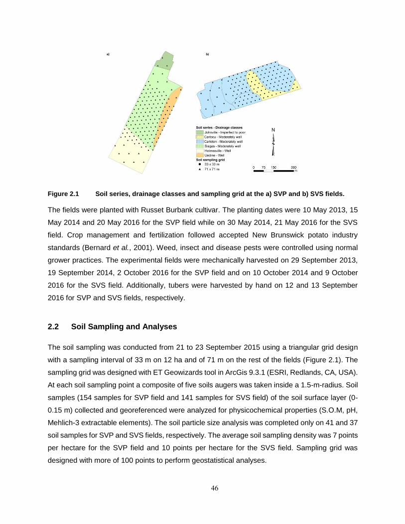
46
Figure 2.1 Soil series, drainage classes and sampling grid at the a) SVP and b) SVS fields.
The fields were planted with Russet Burbank cultivar. The planting dates were 10 May 2013, 15
May 2014 and 20 May 2016 for the SVP field while on 30 May 2014, 21 May 2016 for the SVS
field. Crop management and fertilization followed accepted New Brunswick potato industry
standards (Bernard et al., 2001). Weed, insect and disease pests were controlled using normal
grower practices. The experimental fields were mechanically harvested on 29 September 2013,
19 September 2014, 2 October 2016 for the SVP field and on 10 October 2014 and 9 October
2016 for the SVS field. Additionally, tubers were harvested by hand on 12 and 13 September
2016 for SVP and SVS fields, respectively.
2.2 Soil Sampling and Analyses
The soil sampling was conducted from 21 to 23 September 2015 using a triangular grid design
with a sampling interval of 33 m on 12 ha and of 71 m on the rest of the fields (Figure 2.1). The
sampling grid was designed with ET Geowizards tool in ArcGis 9.3.1 (ESRI, Redlands, CA, USA).
At each soil sampling point a composite of five soils augers was taken inside a 1.5-m-radius. Soil
samples (154 samples for SVP field and 141 samples for SVS field) of the soil surface layer (0-
0.15 m) collected and georeferenced were analyzed for physicochemical properties (S.O.M, pH,
Mehlich-3 extractable elements). The soil particle size analysis was completed only on 41 and 37
soil samples for SVP and SVS fields, respectively. The average soil sampling density was 7 points
per hectare for the SVP field and 10 points per hectare for the SVS field. Sampling grid was
designed with more of 100 points to perform geostatistical analyses.
47
Soil samples were air-dried and a subsample oven-dried at 105°C for 24 h to determine
gravimetric water content. Air-dried samples were subsequently passed through a 2-mm sieve
soil. Soil pH was measured in distilled water with 1:2 soil to solution ratio (Hendershot et al.,
2008). Soil particle size distribution was determined using the pipette method (Sheldrick et al.,
2008). Soil P, K, Ca, Mg, and Al were extracted with a soil solution ratio of 1:10 using Mehlich-3
solution (Ziadi et al., 2008). The concentration of the Mehlich-3 extracts was determined by
inductively-coupled plasma optical emission spectroscopy (ICP–OES; Model, 4300DV, Perkin
Elmer, Shelton, CT). Indurated layer depth was determined by the Veris P4000 probe (Veris
Technologies, Inc., Salina, KS, USA). Total soil carbon (TOC) was converting into soil organic
matter (S.O.M) using the factor 1.54. Total nitrogen (N, mg kg–1) contents of the soil surface layer
(0–0.15 m) were measured with an elemental vario MAX CN analyzer (Elementar
Analysensysteme GmbH, Hanau, Germany).
2.3 Data Collection using Proximal Soil Sensors
Soil electrical conductivity (EC) measurements were collected during the fall of 2015 for all
sensors. The Veris mapping unit (Veris-MSP3, Veris Technologies, Inc., Salina, KS, USA),
contact-type sensor, has six coulter electrodes mounted on a platform that is pulled by a tractor
(Katsigiannis et al., 2016). The system simultaneously investigates soil at two depths, 0-0.3 m
(EC0-0.3m) and 0-1.0 m (EC0-1m) (Kweon, 2012). The Veris is a highly commercial mobile
system for measuring ECa using the principles of ER (Corwin et al., 2005). The Veris is configured
in a continuous-recording towed-electrode array ER systems configured in a modified Wenner
array and programed to simultaneously map ECa (Adamchuk et al., 2015). The EC module
measures EC values directly using rolling coulters inserted into the soil. Data were collected
on parallel transects spaced approximately 10 m apart on 1s intervals, corresponding to a
measurement every 2 to 3 m. Data density was about 400 points per hectare. Global positioning
system (Garmin 17x HVS; Garmin International, Olathe, Kansas, USA) provided spatial
coordinates for each soil EC measurement according to the NMEA 0183 protocol. Outliers
resulting from instruments reading errors were excluded (the mean plus or minus two standard
deviations).
Soil EC was also measured by the Dualem-21S (Dualem, Inc., Milton, ON, Canada). The Dualem-
21S (Dualem) sensor uses a contactless electromagnetic induction system (Saey et al., 2009) in
a georeferencing mobile version (internal WAAS-enabled GPS receiver) pulled with pickup truck.
The Dualem was operated at a height of 0.1 m above the soil surface because of the sled
48
configuration. As the Veris data, the Dualem data were collected on parallel transects spaced
approximately 10 m apart on 1s intervals, corresponding to a measurement every 2 to 3 m. Data
density was about 375 points per hectare.
The receiver coils are oriented in a perpendicular (PRP) geometry that generates a shallower
reading or in a horizontal co-planar (HCP) geometry that giving the deeper readings. Each
transmitter-receiver combination provides integrated soil EC values for the corresponding
explored soil volumes (Simpson et al., 2009). The sensor recorded simultaneously the data from
four soil layers: 0-0.5 m, 0-1.0 m, 0-1.5 m and 0-3.2 m for Dualem. Given the height of the sled
(0.10 m) and assuming that the EC of the air is zero, the soil EC readings were effectively made
from the top 0-0.4 m, 0-0.9 m, 0-1.4 m and 0-3.1 m.
The ground penetrating radar (GPR) campaign was done in February 2016, using GSSI model
SIR-3000 (Geophysical Survey Systems, Inc., Nashua, NH, USA) with a 400 MHz antenna
attached to a receiver and a DGPS receiver with submeter accuracy (Novatel GPS, GTR-G2
antenna L1/L2). Data were collected (30 scan sec-1) on parallel transects approximately 10-m
apart and the density about 20 500 points per hectare. The dielectric contrast of the GPR was
adjusted using the maximum depth penetration of the Veris P4000 probe (Veris Technologies
Inc., Salina, Kansas) at 41 and 37 sampling sites in the SVP and SVS fields, respectively. A field-
specific GPR calibration was completed using the signal of a metallic plate installed at a depth of
0.75 m in the soil.
The GPR data was post-processed with RADAN 7 software (Geophysical Survey Systems, Inc.,
Nashua, NH, USA). The treatment was performed using processing tool bar, removing noise from
data and improving data interpretation using the adjustment of the zero time, horizontal filters
such as background removal and stacking and vertical low pass filter to eliminate high frequency
noise (Kim et al., 2007). Manual adjustment of the gain has been made to improve the
visualization of profiles. The soil layer thickness was assessed using the 2D interactive module in
the conversion of time-depth for reflection profiles. To interpret the depth to an interface, the
velocity of the electromagnetic wave through the soil must be determined or ground-truth
measurements of the interface depth must be obtained (Adamchuk et al., 2015). Using the ground
truth tool (2D interactive module), it was possible to individually adjust depth of picks based on a
true measured depth. As depths were entered (Veris p4000), this module allowed us to computed
an approximate dielectric constant for each field. In this way, the depth of the interfaces was
adjusted by converting the GPR data from time to depth. The approximate dielectric constant
obtained by this method was compared with the manual calibration of the device, obtaining a
49
similar dielectric constant between both calculations. In both fields, depth to bedrock and two soil
layer thicknesses (SLT) referred to SLTsurface and SLTsubsurface limited by rock depth, showed
contrasting relative amplitude. The results obtained were stored in lines format DZT and
georeferenced with the assembled data file module.
2.4 Tuber Yield
Spatial distributions of tuber yield were measured in 2013, 2014 and 2016 for SVP field and for
2014 and 2016 for SVS field. Two four-row harvesters equipped with yield monitors worked in
tandem across each field. A six-row side digger was used which dug six rows and deposited the
potatoes between four adjacent rows yet to be harvested was used for SVP field, while a four-row
side digger was used for SVS field. Then, SVP potato harvester yield monitor picked up
simultaneously 15 m (16 rows x 0.914 m) while SVS picked up 11 m (12 rows x 0.914 m). The
yield monitor install on the potato harvesters were the RiteYield system (Greentronics, Elmira,
ON, Canada) for both sites. The tractors pulling the potato harvesters were equipped with RTK
GPS systems (Trimble Navigation, inc.) which were supplying the GPS signal to the Trimble FmX
potato yield monitor data unit. Yield monitors were calibrated once against weighed truckloads of
tubers at the beginning of the harvest season, and then the yield monitor load cells were re-zeroed
each morning.
To validate the delineated MZ, tubers were harvested by hand on two 3 m-rows in each field at
50 sampling location to determine the total (TY) and marketable yield (MY). In each MZ, sampling
points were determined in a random grid with a density of at least two points per hectare.
2.5 Statistical and Geostatistical Analysis
Descriptive statistics were carried out with the MATLAB® 8.3 software (Mathworks, 2014b).
According to the chi-square goodness-of-fit test the non-normal distributed data were transformed
using logarithmic or Box-Cox to stabilize the variance. The Pearson correlation coefficient (r)
between the PSS, tuber yield, altitude and physicochemical soil property was conducted using
Matlab's corr function. A 5-m buffer around the sampling points was established to perform the
correlation. One-way analysis of variance (ANOVA) and Multcompare statistical analysis were
performed to determine significantly statistical difference ( ≤ 0.05) between the MZ using
Matlab's function. Means separation was done using least significant differences (LSD).
50
Geostatistical Analyst in ArcGIS 9.3.1 (ESRI, Redlands, CA, USA) was used to perform all the
geostatistical computations and model validations. The spatial structure of the different properties
was evaluated via isotropic and anisotropic semivariograms. Experimental semivariograms, the
main component of kriging, are an effective tool for evaluating spatial variability (Wu et al., 2009).
Semivariogram parameters for each theoretical model such as spherical, exponential and
Gaussian were generated. The corresponding sill, nugget, and range values of the best-fitting
theoretical model were calculated. The nugget variance expressed as a percentage of the total
semivariance (Nugget ratio = nugget semivariance/total semivariance) was used to define distinct
classes of spatial dependence. Therefore, nugget ratio was used to define for spatial dependency
of soil variables. If the ratio was ≤ 25%, 25% and 75%, ≥ 75% variables were accepted as strongly,
moderately and weakly dependent, respectively (Cambardella et al., 1999). If the slope of the
semivariogram was close to zero, regardless of the nugget ratio, the variable was considered to
be randomly distributed (Cambardella et al., 1994). After selection of the suitable theoretical
model for each dataset and the corresponding semivariogram parameters, spatial variability
maps were generated using ordinary kriging. Ordinary kriging was chosen because it limits the
imposition of stationarity in the neighborhood. Then, cross-validation procedure leave-one-out
was used as a method of validating the kriging predictions.
The proximal sensor datasets were used to delineate the MZ to identify naturally occurring
clusters in the data (Chang et al., 2014). The MZ should produce homogeneous groups
minimizing the within-group variability while maximizing the among-group variability (Tripathi et
al., 2015). A k-means clustering with a non-spatial constraint of proximity was carried out using
FuzME software (Australian Centre for Precision Agriculture, 2002). Mahalanobis metric distance,
cluster analysis has been used to determine the similarity between two random multidimensional
variables taking into account the correlation between the variables. The technique of fuzzy
clustering and the application of generalized fuzzy k-means has been described by McBratney
and Gruijter (1992). As describe by Cambouris et al. (2006), the variance reduction due to zone
partitioning (stratified vs simple random sampling) was used as a method to determine the optimal
number of MZ in the experimental site.
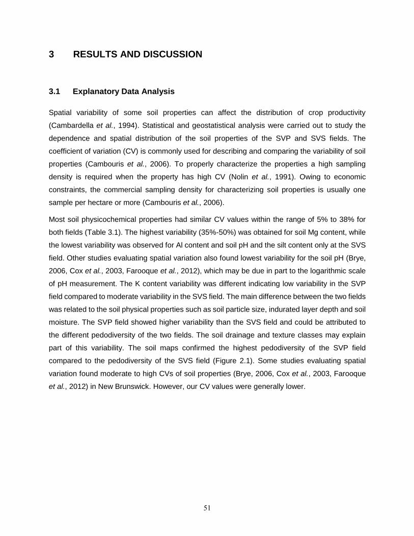
51
3 RESULTS AND DISCUSSION
3.1 Explanatory Data Analysis
Spatial variability of some soil properties can affect the distribution of crop productivity
(Cambardella et al., 1994). Statistical and geostatistical analysis were carried out to study the
dependence and spatial distribution of the soil properties of the SVP and SVS fields. The
coefficient of variation (CV) is commonly used for describing and comparing the variability of soil
properties (Cambouris et al., 2006). To properly characterize the properties a high sampling
density is required when the property has high CV (Nolin et al., 1991). Owing to economic
constraints, the commercial sampling density for characterizing soil properties is usually one
sample per hectare or more (Cambouris et al., 2006).
Most soil physicochemical properties had similar CV values within the range of 5% to 38% for
both fields (Table 3.1). The highest variability (35%-50%) was obtained for soil Mg content, while
the lowest variability was observed for Al content and soil pH and the silt content only at the SVS
field. Other studies evaluating spatial variation also found lowest variability for the soil pH (Brye,
2006, Cox et al., 2003, Farooque et al., 2012), which may be due in part to the logarithmic scale
of pH measurement. The K content variability was different indicating low variability in the SVP
field compared to moderate variability in the SVS field. The main difference between the two fields
was related to the soil physical properties such as soil particle size, indurated layer depth and soil
moisture. The SVP field showed higher variability than the SVS field and could be attributed to
the different pedodiversity of the two fields. The soil drainage and texture classes may explain
part of this variability. The soil maps confirmed the highest pedodiversity of the SVP field
compared to the pedodiversity of the SVS field (Figure 2.1). Some studies evaluating spatial
variation found moderate to high CVs of soil properties (Brye, 2006, Cox et al., 2003, Farooque
et al., 2012) in New Brunswick. However, our CV values were generally lower.
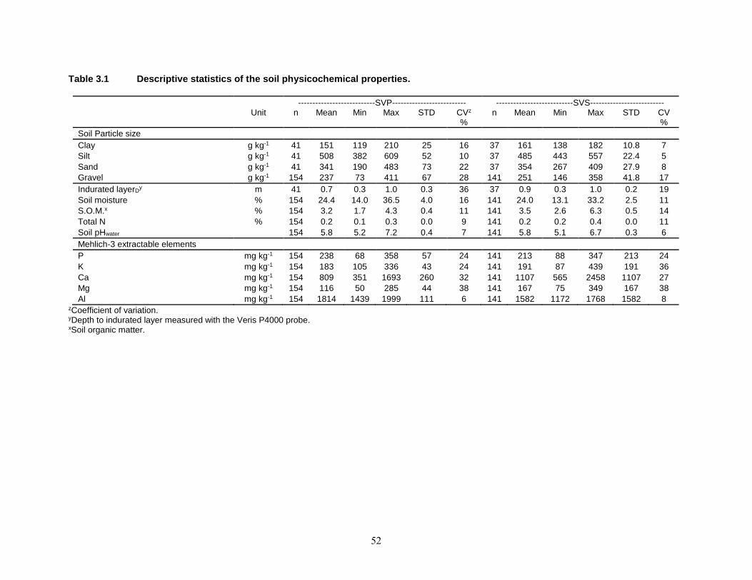
52
Table 3.1 Descriptive statistics of the soil physicochemical properties.
---------------------------SVP-------------------------- ---------------------------SVS-------------------------- Unit n Mean Min Max STD CVz
% n Mean Min Max STD CV
%
Soil Particle size
Clay g kg-1 41 151 119 210 25 16 37 161 138 182 10.8 7
Silt g kg-1 41 508 382 609 52 10 37 485 443 557 22.4 5
Sand g kg-1 41 341 190 483 73 22 37 354 267 409 27.9 8
Gravel g kg-1 154 237 73 411 67 28 141 251 146 358 41.8 17
Indurated layerDy m 41 0.7 0.3 1.0 0.3 36 37 0.9 0.3 1.0 0.2 19
Soil moisture % 154 24.4 14.0 36.5 4.0 16 141 24.0 13.1 33.2 2.5 11
S.O.M.x % 154 3.2 1.7 4.3 0.4 11 141 3.5 2.6 6.3 0.5 14
Total N % 154 0.2 0.1 0.3 0.0 9 141 0.2 0.2 0.4 0.0 11
Soil pHwater 154 5.8 5.2 7.2 0.4 7 141 5.8 5.1 6.7 0.3 6
Mehlich-3 extractable elements
P mg kg-1 154 238 68 358 57 24 141 213 88 347 213 24
K mg kg-1 154 183 105 336 43 24 141 191 87 439 191 36
Ca mg kg-1 154 809 351 1693 260 32 141 1107 565 2458 1107 27
Mg mg kg-1 154 116 50 285 44 38 141 167 75 349 167 38
Al mg kg-1 154 1814 1439 1999 111 6 141 1582 1172 1768 1582 8 zCoefficient of variation. yDepth to indurated layer measured with the Veris P4000 probe. xSoil organic matter.
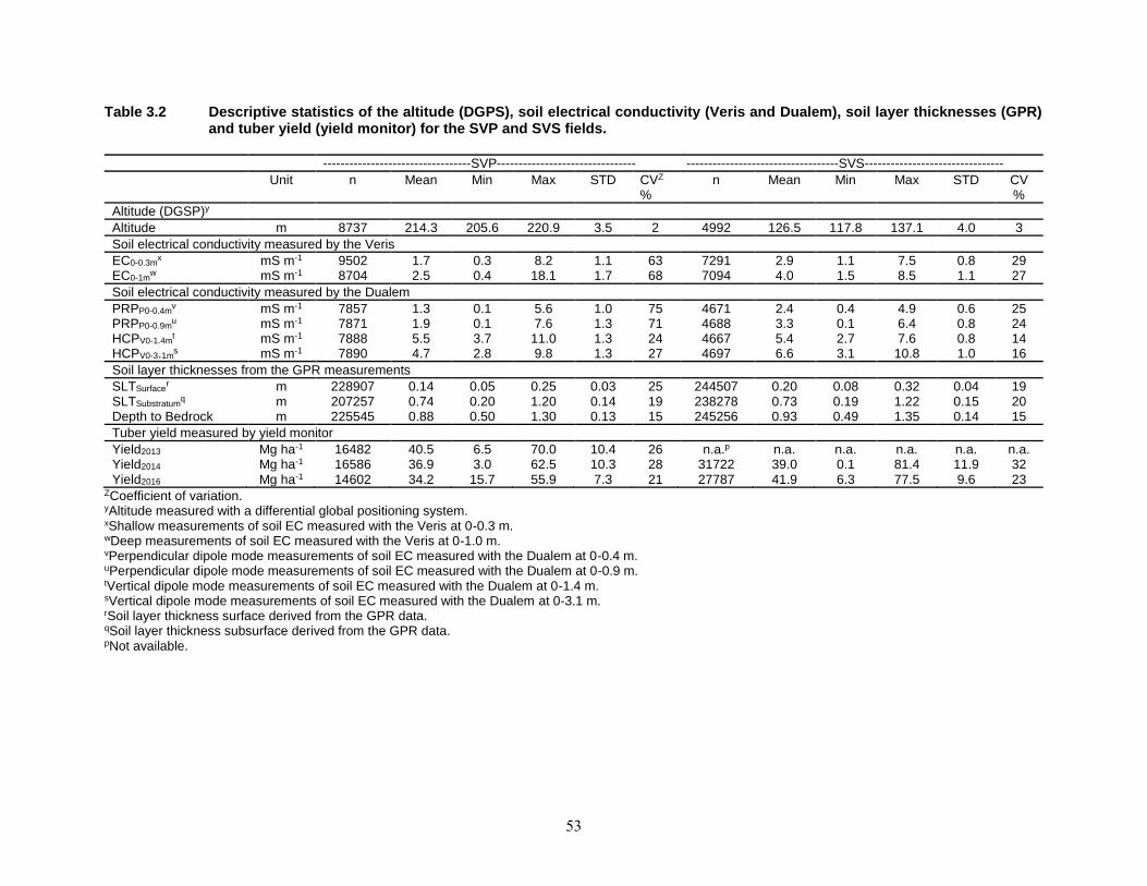
53
Table 3.2 Descriptive statistics of the altitude (DGPS), soil electrical conductivity (Veris and Dualem), soil layer thicknesses (GPR) and tuber yield (yield monitor) for the SVP and SVS fields.
----------------------------------SVP-------------------------------- -----------------------------------SVS--------------------------------
Unit n Mean Min Max STD CVZ %
n Mean Min Max STD CV %
Altitude (DGSP)y
Altitude m 8737 214.3 205.6 220.9 3.5 2 4992 126.5 117.8 137.1 4.0 3
Soil electrical conductivity measured by the Veris
EC0-0.3mx mS m-1 9502 1.7 0.3 8.2 1.1 63 7291 2.9 1.1 7.5 0.8 29
EC0-1mw mS m-1 8704 2.5 0.4 18.1 1.7 68 7094 4.0 1.5 8.5 1.1 27
Soil electrical conductivity measured by the Dualem
PRPP0-0.4mv mS m-1 7857 1.3 0.1 5.6 1.0 75 4671 2.4 0.4 4.9 0.6 25
PRPP0-0.9mu mS m-1 7871 1.9 0.1 7.6 1.3 71 4688 3.3 0.1 6.4 0.8 24
HCPV0-1.4mt mS m-1 7888 5.5 3.7 11.0 1.3 24 4667 5.4 2.7 7.6 0.8 14
HCPV0-3.1ms mS m-1 7890 4.7 2.8 9.8 1.3 27 4697 6.6 3.1 10.8 1.0 16
Soil layer thicknesses from the GPR measurements
SLTSurfacer m 228907 0.14 0.05 0.25 0.03 25 244507 0.20 0.08 0.32 0.04 19
SLTSubstratumq m 207257 0.74 0.20 1.20 0.14 19 238278 0.73 0.19 1.22 0.15 20
Depth to Bedrock m 225545 0.88 0.50 1.30 0.13 15 245256 0.93 0.49 1.35 0.14 15
Tuber yield measured by yield monitor
Yield2013 Mg ha-1 16482 40.5 6.5 70.0 10.4 26 n.a.p n.a. n.a. n.a. n.a. n.a. Yield2014 Mg ha-1 16586 36.9 3.0 62.5 10.3 28 31722 39.0 0.1 81.4 11.9 32 Yield2016 Mg ha-1 14602 34.2 15.7 55.9 7.3 21 27787 41.9 6.3 77.5 9.6 23
ZCoefficient of variation. yAltitude measured with a differential global positioning system. xShallow measurements of soil EC measured with the Veris at 0-0.3 m. wDeep measurements of soil EC measured with the Veris at 0-1.0 m. vPerpendicular dipole mode measurements of soil EC measured with the Dualem at 0-0.4 m. uPerpendicular dipole mode measurements of soil EC measured with the Dualem at 0-0.9 m. tVertical dipole mode measurements of soil EC measured with the Dualem at 0-1.4 m. sVertical dipole mode measurements of soil EC measured with the Dualem at 0-3.1 m. rSoil layer thickness surface derived from the GPR data. qSoil layer thickness subsurface derived from the GPR data. pNot available.
54
The CVs for all soil EC measurements (Table 3.2) were higher in the SVP field than in the SVS
field. These results could be associated to highest pedodiversity within the SVP field, which was
attributed to highest variability in soil texture, soil moisture and depth to the indurated layer (Table
3.1). The Dualem perpendicular dipole (PRPp0-0.4m and PRPp0-0.9m) showed higher variability than
the horizontal dipole (HCPv0-1.4m and HCPv0-3.1m) for both fields. This result suggests that the
deeper sensing depth of the signal leads to lower soil EC variability. A main assumption of a
model with a two-layered soil and a more uniform soil in clay and moisture in depth (Saey et al.,
2009).
The soil layers thickness derived from the GPR showed moderate variability from 15% to 26% in
the SVP and SVS fields (Table 3.1). Both fields depth to the bedrock varied between 0.49 m and
1.35 m which is corroborated with Milburn et al. (1989) finding. The soils of the studied area are
generally shallows due to the presence of bedrock or compact subsoil (0.40–0.60 m) layers
(Fahmy, 2001).
The descriptive statistics of the tuber yield (Table 3.2) suggested that tuber yield was moderately
variable with CVs ranging from 21% to 28% and 23% to 32% for the SVP and SVS fields,
respectively. Tuber yield for the SVP field was 40.5 Mg ha-1 in 2013, 36.9 Mg ha-1 in 2014 and
34.2 Mg ha-1 in 2016. The tuber yield variability at this site may be due to the variations of the
precipitation during the period of crop growth. Total precipitation was 1048 mm in 2013, 662 mm
in 2014 and 608 mm in 2016 (GNB, 2016). The tuber yield for the SVS field was lower in 2013
than 2016. Total precipitation was 662 mm in 2014 and 608 in 2016 (GNB, 2016).
Higher variability in the fields would have required more samples to achieve good prediction
accuracy (Nyiraneza et al., 2011). In this study, the moderate variability on the soil
physicochemical properties seems to be promising for mapping these agricultural fields. The CV
values are good indicators of variability, but not of its nature (structured or randomized variability)
(Cambouris et al., 2006).
3.2 Spatial Variability
Semivariogram analyzes were conducted to study the nature of the variability of the fields under
study. Gaussian models for the SVP field or exponential models for the SVS field were the best
fit for most of the soil physicochemical properties and altitude (Table 3.3 and Table 3.4). However,
the pure nugget models were the best fit for indurated layer depth and K content at the SVP field
and clay at the SVS field. The pure nugget effect may be a result of sampling errors, random
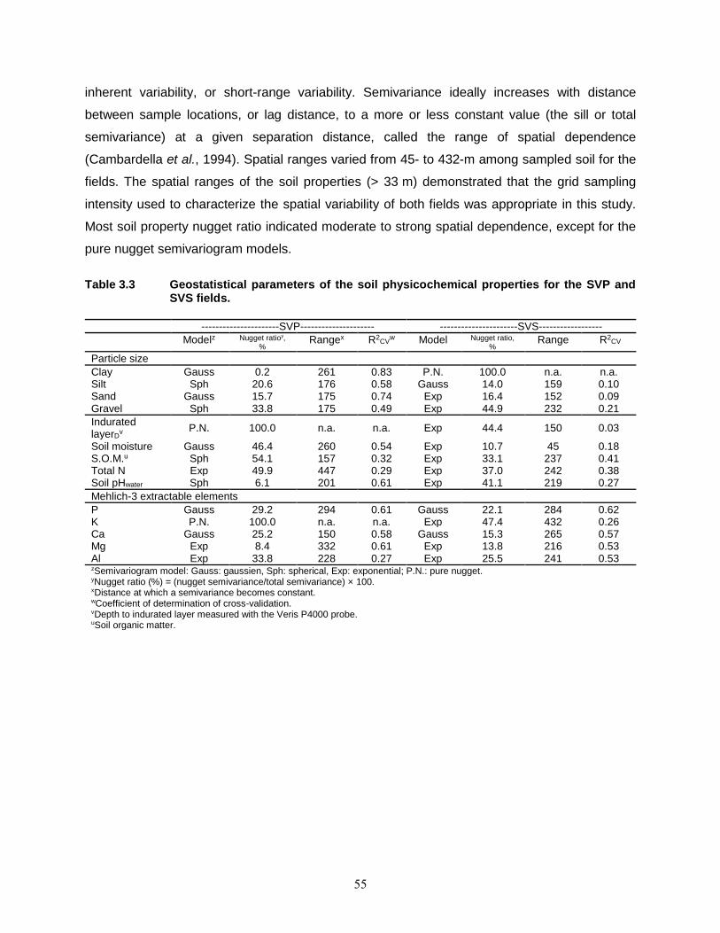
55
inherent variability, or short-range variability. Semivariance ideally increases with distance
between sample locations, or lag distance, to a more or less constant value (the sill or total
semivariance) at a given separation distance, called the range of spatial dependence
(Cambardella et al., 1994). Spatial ranges varied from 45- to 432-m among sampled soil for the
fields. The spatial ranges of the soil properties (> 33 m) demonstrated that the grid sampling
intensity used to characterize the spatial variability of both fields was appropriate in this study.
Most soil property nugget ratio indicated moderate to strong spatial dependence, except for the
pure nugget semivariogram models.
Table 3.3 Geostatistical parameters of the soil physicochemical properties for the SVP and SVS fields.
----------------------SVP--------------------- ----------------------SVS------------------
Modelz Nugget ratioy, %
Rangex R2CV
w Model Nugget ratio, %
Range R2CV
Particle size
Clay Gauss 0.2 261 0.83 P.N. 100.0 n.a. n.a. Silt Sph 20.6 176 0.58 Gauss 14.0 159 0.10 Sand Gauss 15.7 175 0.74 Exp 16.4 152 0.09 Gravel Sph 33.8 175 0.49 Exp 44.9 232 0.21
Indurated layerD
v P.N. 100.0 n.a. n.a. Exp 44.4 150 0.03
Soil moisture Gauss 46.4 260 0.54 Exp 10.7 45 0.18 S.O.M.u Sph 54.1 157 0.32 Exp 33.1 237 0.41 Total N Exp 49.9 447 0.29 Exp 37.0 242 0.38 Soil pHwater Sph 6.1 201 0.61 Exp 41.1 219 0.27
Mehlich-3 extractable elements
P Gauss 29.2 294 0.61 Gauss 22.1 284 0.62 K P.N. 100.0 n.a. n.a. Exp 47.4 432 0.26 Ca Gauss 25.2 150 0.58 Gauss 15.3 265 0.57 Mg Exp 8.4 332 0.61 Exp 13.8 216 0.53 Al Exp 33.8 228 0.27 Exp 25.5 241 0.53 zSemivariogram model: Gauss: gaussien, Sph: spherical, Exp: exponential; P.N.: pure nugget. yNugget ratio (%) = (nugget semivariance/total semivariance) × 100. xDistance at which a semivariance becomes constant. wCoefficient of determination of cross-validation. vDepth to indurated layer measured with the Veris P4000 probe. uSoil organic matter.
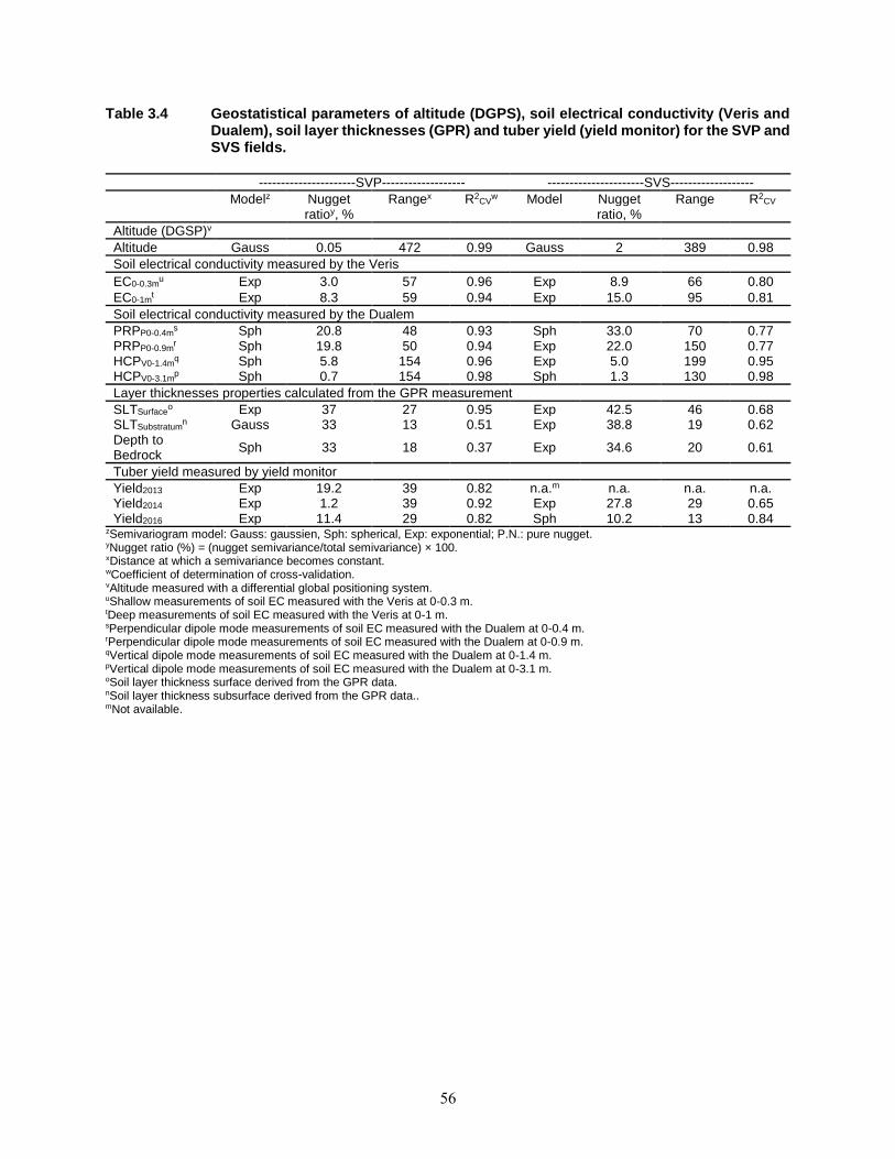
56
Table 3.4 Geostatistical parameters of altitude (DGPS), soil electrical conductivity (Veris and Dualem), soil layer thicknesses (GPR) and tuber yield (yield monitor) for the SVP and SVS fields.
----------------------SVP------------------- ----------------------SVS-------------------
Modelz Nugget
ratioy, % Rangex R2
CVw Model Nugget
ratio, % Range R2
CV
Altitude (DGSP)v
Altitude Gauss 0.05 472 0.99 Gauss 2 389 0.98
Soil electrical conductivity measured by the Veris
EC0-0.3mu Exp 3.0 57 0.96 Exp 8.9 66 0.80
EC0-1mt Exp 8.3 59 0.94 Exp 15.0 95 0.81
Soil electrical conductivity measured by the Dualem
PRPP0-0.4ms Sph 20.8 48 0.93 Sph 33.0 70 0.77
PRPP0-0.9mr Sph 19.8 50 0.94 Exp 22.0 150 0.77
HCPV0-1.4mq Sph 5.8 154 0.96 Exp 5.0 199 0.95
HCPV0-3.1mp Sph 0.7 154 0.98 Sph 1.3 130 0.98
Layer thicknesses properties calculated from the GPR measurement
SLTSurfaceo Exp 37 27 0.95 Exp 42.5 46 0.68
SLTSubstratumn Gauss 33 13 0.51 Exp 38.8 19 0.62
Depth to Bedrock
Sph 33 18 0.37 Exp 34.6 20 0.61
Tuber yield measured by yield monitor
Yield2013 Exp 19.2 39 0.82 n.a.m n.a. n.a. n.a. Yield2014 Exp 1.2 39 0.92 Exp 27.8 29 0.65 Yield2016 Exp 11.4 29 0.82 Sph 10.2 13 0.84
zSemivariogram model: Gauss: gaussien, Sph: spherical, Exp: exponential; P.N.: pure nugget. yNugget ratio (%) = (nugget semivariance/total semivariance) × 100. xDistance at which a semivariance becomes constant. wCoefficient of determination of cross-validation. vAltitude measured with a differential global positioning system.
uShallow measurements of soil EC measured with the Veris at 0-0.3 m.
tDeep measurements of soil EC measured with the Veris at 0-1 m. sPerpendicular dipole mode measurements of soil EC measured with the Dualem at 0-0.4 m. rPerpendicular dipole mode measurements of soil EC measured with the Dualem at 0-0.9 m. qVertical dipole mode measurements of soil EC measured with the Dualem at 0-1.4 m. pVertical dipole mode measurements of soil EC measured with the Dualem at 0-3.1 m. oSoil layer thickness surface derived from the GPR data. nSoil layer thickness subsurface derived from the GPR data..
mNot available.
57
The best fitted semivariogram models for the PSS and the tuber yield were generally exponential
and spherical (Table 3.4). For soil EC measurements using the Veris and Dualem, the range
varied from 48 to 199 m and the nugget ratio was ≤ 33% for both fields (Table 3.4). This suggests
that the nugget effect (C0 = random variance) was very low and reliably modelled by the sampling
strategies (Cambouris et al., 2006). Similar results were reported by Moran et al. (2010) in silt
loam soils. For soil EC measurements using the Dualem, the perpendicular dipole (PRPp0-0.4m and
PRPp0-0.9m) showed lower spatial variability (range) than the horizontal dipole (HCPv0-1.4m and
HCPv0-3.1m) for both fields. This indicates that in this two-layered soil, the subsoil can be considered
more conductive and less heterogeneous than the topsoil. The nugget ratio of the GPR
parameters were between 33% and 43% for both fields, indicating moderate spatial dependency
according to the classification used by Cambardella et al. (1994). The ranges of the GPR
parameters (19- to 46-m) were lower than the one obtained from the Veris and Dualem. The
results obtained were mainly due to an intrinsic variation of subsoil structure. Short-range
variability generally decreased as a function of the GPR signal attenuation(D De Benedetto et al.,
2013b). The tuber yield nugget ratio varied from 1% to 28% and the range varied from 13- to 39-
m for both fields.
Strong spatial dependent properties may be controlled by intrinsic factor (soil texture, structure,
mineralogy and microorganisms) (Cambardella et al., 1994). Lowest spatial dependence
indicated that properties may be controlled by extrinsic variations presumably due to fertilizer
application technique and timing, row orientation, and environmental conditions (Nyiraneza et al.,
2011).
3.3 Kriging
Kriged map reliability can be evaluated with the cross-validation analysis (R2CV), is defined as the
estimation error divided by the square root of the kriging estimation variance (Cambouris et al.,
2006, Pachepsky et al., 2003). High R2CV values indicated good fits (> 0.60) were obtained for
most of the densely measured properties (altitude, soil EC, layer thickness and tuber yield),
except for the SLTsubstratum and the depth to the bedrock in the SVP field (Table 3.4). This result
suggested that these properties can then be used to delineated management zone. Good fit
models were also obtained for the particle sizes and soil moisture for the SVP field (R2CV = 0.49
to 0.83) compared to the SVS field (R2CV = 0.03 to 0.21). The results suggest that the spatial
dependence in the SVP field could be influenced by soil intrinsic factors (Cambardella et al.,
1999).
58
The maps of the spatial variation of soil EC measured with the Veris and the Dualem showed
visual similitude for each field (Figure 3.1a, b and Figure 3.2a, b). Most of the northern part of the
SVP field showed the highest EC values while the central and southern parts of the field were
characterized by the lowest values. Low and high values of soil EC were sparsely distributed
zones in the SVS field Figure 3.2). Kriged maps of the GPR properties (Figure 3.1c, d and Figure
3.2c, d) showed substantial spatial variation across the fields, which was also indicated by the
lower ranges. These results can be explained by a high sampling density of the GPR in the
direction of each of the profiles and a low sampling between them. In this regard, additional
processing of smoothing and filtering of the raw GPR data and densification of perpendicular
sampling profiles could be adopted. A visual pattern of shallow soil on the map of the depth to the
bedrock (Figure 3.1d) and the SLTsubsurface (map not shown) could be observed toward the west
of the SVP field.
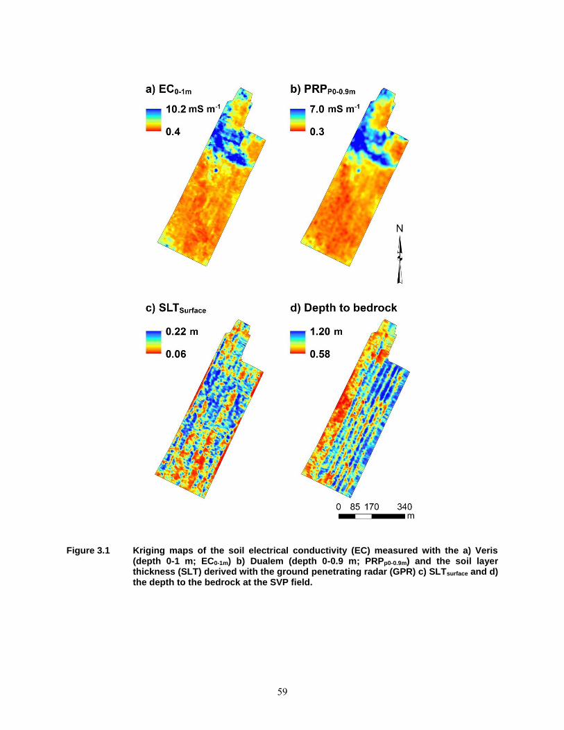
59
Figure 3.1 Kriging maps of the soil electrical conductivity (EC) measured with the a) Veris (depth 0-1 m; EC0-1m) b) Dualem (depth 0-0.9 m; PRPp0-0.9m) and the soil layer thickness (SLT) derived with the ground penetrating radar (GPR) c) SLTsurface and d) the depth to the bedrock at the SVP field.
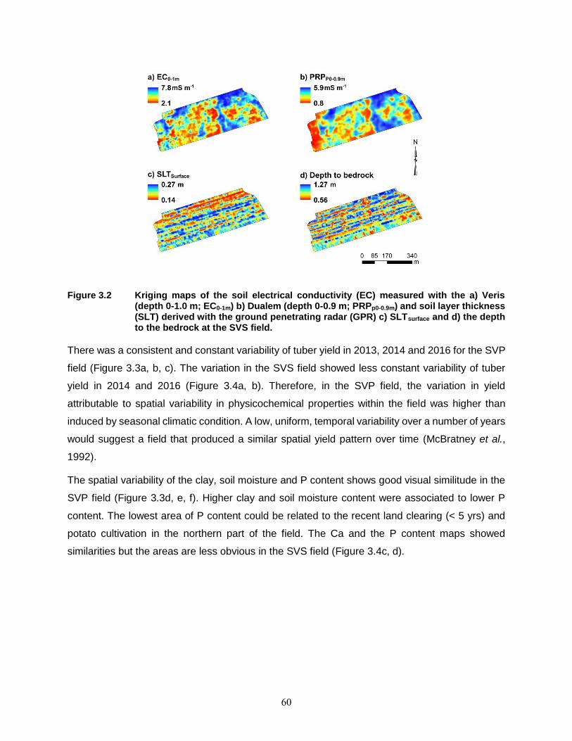
60
Figure 3.2 Kriging maps of the soil electrical conductivity (EC) measured with the a) Veris (depth 0-1.0 m; EC0-1m) b) Dualem (depth 0-0.9 m; PRPp0-0.9m) and soil layer thickness (SLT) derived with the ground penetrating radar (GPR) c) SLTsurface and d) the depth to the bedrock at the SVS field.
There was a consistent and constant variability of tuber yield in 2013, 2014 and 2016 for the SVP
field (Figure 3.3a, b, c). The variation in the SVS field showed less constant variability of tuber
yield in 2014 and 2016 (Figure 3.4a, b). Therefore, in the SVP field, the variation in yield
attributable to spatial variability in physicochemical properties within the field was higher than
induced by seasonal climatic condition. A low, uniform, temporal variability over a number of years
would suggest a field that produced a similar spatial yield pattern over time (McBratney et al.,
1992).
The spatial variability of the clay, soil moisture and P content shows good visual similitude in the
SVP field (Figure 3.3d, e, f). Higher clay and soil moisture content were associated to lower P
content. The lowest area of P content could be related to the recent land clearing (< 5 yrs) and
potato cultivation in the northern part of the field. The Ca and the P content maps showed
similarities but the areas are less obvious in the SVS field (Figure 3.4c, d).
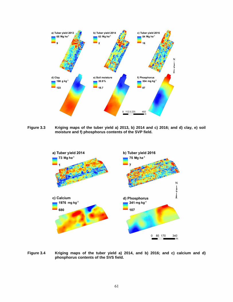
61
Figure 3.3 Kriging maps of the tuber yield a) 2013, b) 2014 and c) 2016; and d) clay, e) soil moisture and f) phosphorus contents of the SVP field.
Figure 3.4 Kriging maps of the tuber yield a) 2014, and b) 2016; and c) calcium and d) phosphorus contents of the SVS field.
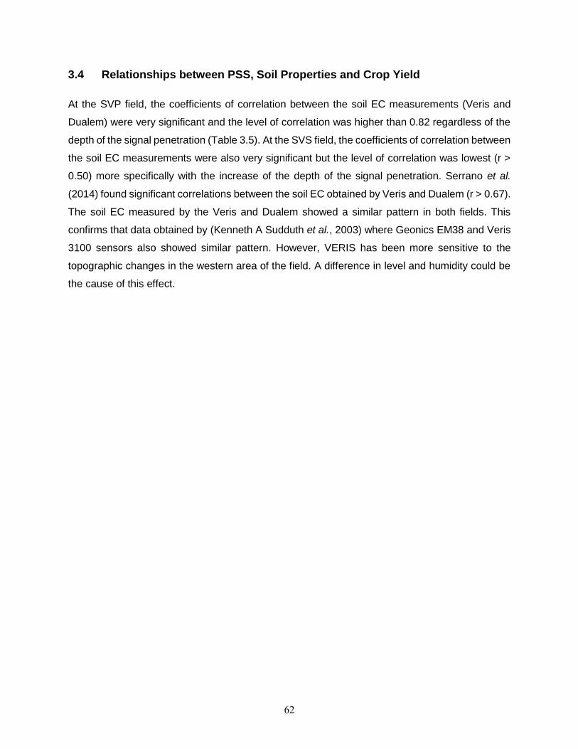
62
3.4 Relationships between PSS, Soil Properties and Crop Yield
At the SVP field, the coefficients of correlation between the soil EC measurements (Veris and
Dualem) were very significant and the level of correlation was higher than 0.82 regardless of the
depth of the signal penetration (Table 3.5). At the SVS field, the coefficients of correlation between
the soil EC measurements were also very significant but the level of correlation was lowest (r >
0.50) more specifically with the increase of the depth of the signal penetration. Serrano et al.
(2014) found significant correlations between the soil EC obtained by Veris and Dualem (r > 0.67).
The soil EC measured by the Veris and Dualem showed a similar pattern in both fields. This
confirms that data obtained by (Kenneth A Sudduth et al., 2003) where Geonics EM38 and Veris
3100 sensors also showed similar pattern. However, VERIS has been more sensitive to the
topographic changes in the western area of the field. A difference in level and humidity could be
the cause of this effect.
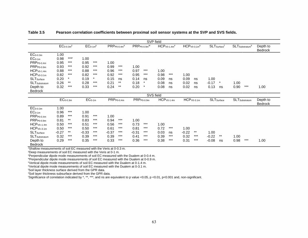
63
Table 3.5 Pearson correlation coefficients between proximal soil sensor systems at the SVP and SVS fields.
SVP field
EC0-0.3m
z
EC0-1m
y
PRPP0-0.4mx
PRPP0-0.9m
w
HCPV0-1.4mv
HCPV0-3.1m
u
SLTSurfacet
SLTSubstratum
s
Depth to Bedrock
EC0-0.3m 1.00
EC0-1m 0.98 ***r 1.00
PRPP0-0.4m 0.95 *** 0.95 *** 1.00
PRPP0-0.9m 0.93 *** 0.92 *** 0.99 *** 1.00
HCPV0-1.4m 0.88 *** 0.88 *** 0.96 *** 0.97 *** 1.00
HCPV0-3.1m 0.82 *** 0.82 *** 0.92 *** 0.95 *** 0.98 *** 1.00
SLTSurface 0.20 * 0.19 * 0.15 ns 0.14 ns 0.09 ns 0.09 ns 1.00 SLTSubstratum 0.26 ** 0.28 *** 0.21 ** 0.18 * 0.08 ns 0.02 ns -0.17 * 1.00 Depth to Bedrock
0.32 *** 0.33 *** 0.24 ** 0.20 * 0.08 ns 0.02 ns 0.13 ns 0.90 *** 1.00
SVS field
EC0-0.3m
EC0-1m
PRPP0-0.4m
PRPP0-0.9m
HCPV0-1.4m
HCPV0-3.1m
SLTSurface
SLTSubstratum
Depth to Bedrock
EC0-0.3m 1.00
EC0-1m 0.96 *** 1.00
PRPP0-0.4m 0.89 *** 0.91 *** 1.00
PRPP0-0.9m 0.81 ** 0.83 *** 0.94 *** 1.00
HCPV0–1.4m 0.50 *** 0.51 *** 0.56 *** 0.73 *** 1.00
HCPV0–3.1m 0.50 *** 0.50 *** 0.61 *** 0.81 *** 0.72 *** 1.00
SLTSurface -0.27 ** -0.33 *** -0.37 *** -0.31 *** 0.03 ns -0.22 ** 1.00 SLTSubstratum 0.32 *** 0.39 *** 0.39 *** 0.41 *** 0.39 *** 0.32 *** -0.22 ** 1.00 Depth to Bedrock
0.29 *** 0.35 *** 0.33 *** 0.36 *** 0.38 *** 0.31 *** -0.08 ns 0.98 *** 1.00
zShallow measurements of soil EC measured with the Veris at 0-0.3 m. yDeep measurements of soil EC measured with the Veris at 0-1 m. xPerpendicular dipole mode measurements of soil EC measured with the Dualem at 0-0.4 m. wPerpendicular dipole mode measurements of soil EC measured with the Dualem at 0-0.9 m. vVertical dipole mode measurements of soil EC measured with the Dualem at 0-1.4 m. uVertical dipole mode measurements of soil EC measured with the Dualem at 0-3.1 m. tSoil layer thickness surface derived from the GPR data. sSoil layer thickness subsurface derived from the GPR data. rSignificance of correlation indicated by *, **, ***, and ns are equivalent to p value <0.05, p <0.01, p<0.001 and, non-significant.
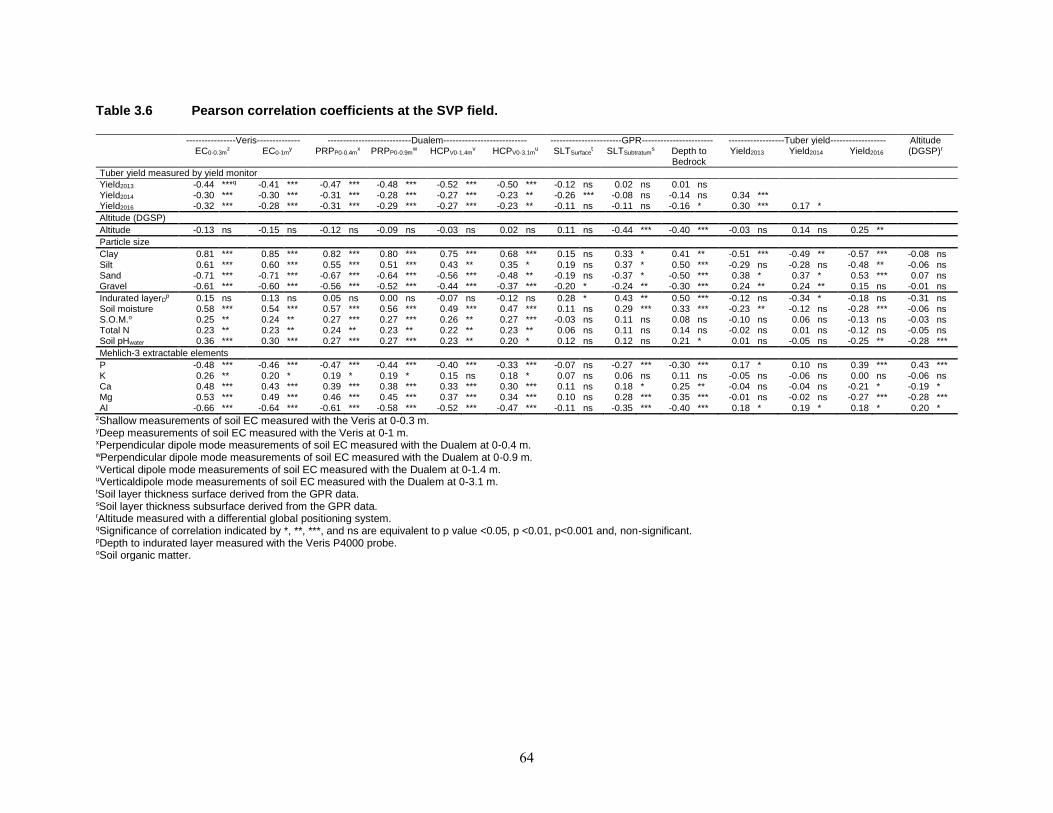
64
Table 3.6 Pearson correlation coefficients at the SVP field.
----------------Veris-------------- ---------------------------Dualem--------------------------- -----------------------GPR----------------------- ------------------Tuber yield------------------ Altitude (DGSP)r EC0-0.3m
z EC0-1my PRPP0-0.4m
x PRPP0-0.9mw HCPV0-1.4m
v HCPV0-3.1mu SLTSurface
t SLTSubtratums Depth to
Bedrock Yield2013 Yield2014 Yield2016
Tuber yield measured by yield monitor
Yield2013 -0.44 ***q -0.41 *** -0.47 *** -0.48 *** -0.52 *** -0.50 *** -0.12 ns 0.02 ns 0.01 ns
Yield2014 -0.30 *** -0.30 *** -0.31 *** -0.28 *** -0.27 *** -0.23 ** -0.26 *** -0.08 ns -0.14 ns 0.34 ***
Yield2016 -0.32 *** -0.28 *** -0.31 *** -0.29 *** -0.27 *** -0.23 ** -0.11 ns -0.11 ns -0.16 * 0.30 *** 0.17 *
Altitude (DGSP)
Altitude -0.13 ns -0.15 ns -0.12 ns -0.09 ns -0.03 ns 0.02 ns 0.11 ns -0.44 *** -0.40 *** -0.03 ns 0.14 ns 0.25 **
Particle size
Clay 0.81 *** 0.85 *** 0.82 *** 0.80 *** 0.75 *** 0.68 *** 0.15 ns 0.33 * 0.41 ** -0.51 *** -0.49 ** -0.57 *** -0.08 ns Silt 0.61 *** 0.60 *** 0.55 *** 0.51 *** 0.43 ** 0.35 * 0.19 ns 0.37 * 0.50 *** -0.29 ns -0.28 ns -0.48 ** -0.06 ns Sand -0.71 *** -0.71 *** -0.67 *** -0.64 *** -0.56 *** -0.48 ** -0.19 ns -0.37 * -0.50 *** 0.38 * 0.37 * 0.53 *** 0.07 ns Gravel -0.61 *** -0.60 *** -0.56 *** -0.52 *** -0.44 *** -0.37 *** -0.20 * -0.24 ** -0.30 *** 0.24 ** 0.24 ** 0.15 ns -0.01 ns
Indurated layerDp 0.15 ns 0.13 ns 0.05 ns 0.00 ns -0.07 ns -0.12 ns 0.28 * 0.43 ** 0.50 *** -0.12 ns -0.34 * -0.18 ns -0.31 ns
Soil moisture 0.58 *** 0.54 *** 0.57 *** 0.56 *** 0.49 *** 0.47 *** 0.11 ns 0.29 *** 0.33 *** -0.23 ** -0.12 ns -0.28 *** -0.06 ns S.O.M.o 0.25 ** 0.24 ** 0.27 *** 0.27 *** 0.26 ** 0.27 *** -0.03 ns 0.11 ns 0.08 ns -0.10 ns 0.06 ns -0.13 ns -0.03 ns Total N 0.23 ** 0.23 ** 0.24 ** 0.23 ** 0.22 ** 0.23 ** 0.06 ns 0.11 ns 0.14 ns -0.02 ns 0.01 ns -0.12 ns -0.05 ns Soil pHwater 0.36 *** 0.30 *** 0.27 *** 0.27 *** 0.23 ** 0.20 * 0.12 ns 0.12 ns 0.21 * 0.01 ns -0.05 ns -0.25 ** -0.28 ***
Mehlich-3 extractable elements
P -0.48 *** -0.46 *** -0.47 *** -0.44 *** -0.40 *** -0.33 *** -0.07 ns -0.27 *** -0.30 *** 0.17 * 0.10 ns 0.39 *** 0.43 *** K 0.26 ** 0.20 * 0.19 * 0.19 * 0.15 ns 0.18 * 0.07 ns 0.06 ns 0.11 ns -0.05 ns -0.06 ns 0.00 ns -0.06 ns Ca 0.48 *** 0.43 *** 0.39 *** 0.38 *** 0.33 *** 0.30 *** 0.11 ns 0.18 * 0.25 ** -0.04 ns -0.04 ns -0.21 * -0.19 * Mg 0.53 *** 0.49 *** 0.46 *** 0.45 *** 0.37 *** 0.34 *** 0.10 ns 0.28 *** 0.35 *** -0.01 ns -0.02 ns -0.27 *** -0.28 *** Al -0.66 *** -0.64 *** -0.61 *** -0.58 *** -0.52 *** -0.47 *** -0.11 ns -0.35 *** -0.40 *** 0.18 * 0.19 * 0.18 * 0.20 *
zShallow measurements of soil EC measured with the Veris at 0-0.3 m. yDeep measurements of soil EC measured with the Veris at 0-1 m. xPerpendicular dipole mode measurements of soil EC measured with the Dualem at 0-0.4 m. wPerpendicular dipole mode measurements of soil EC measured with the Dualem at 0-0.9 m. vVertical dipole mode measurements of soil EC measured with the Dualem at 0-1.4 m. uVerticaldipole mode measurements of soil EC measured with the Dualem at 0-3.1 m. tSoil layer thickness surface derived from the GPR data. sSoil layer thickness subsurface derived from the GPR data. rAltitude measured with a differential global positioning system. qSignificance of correlation indicated by *, **, ***, and ns are equivalent to p value <0.05, p <0.01, p<0.001 and, non-significant. pDepth to indurated layer measured with the Veris P4000 probe. oSoil organic matter.
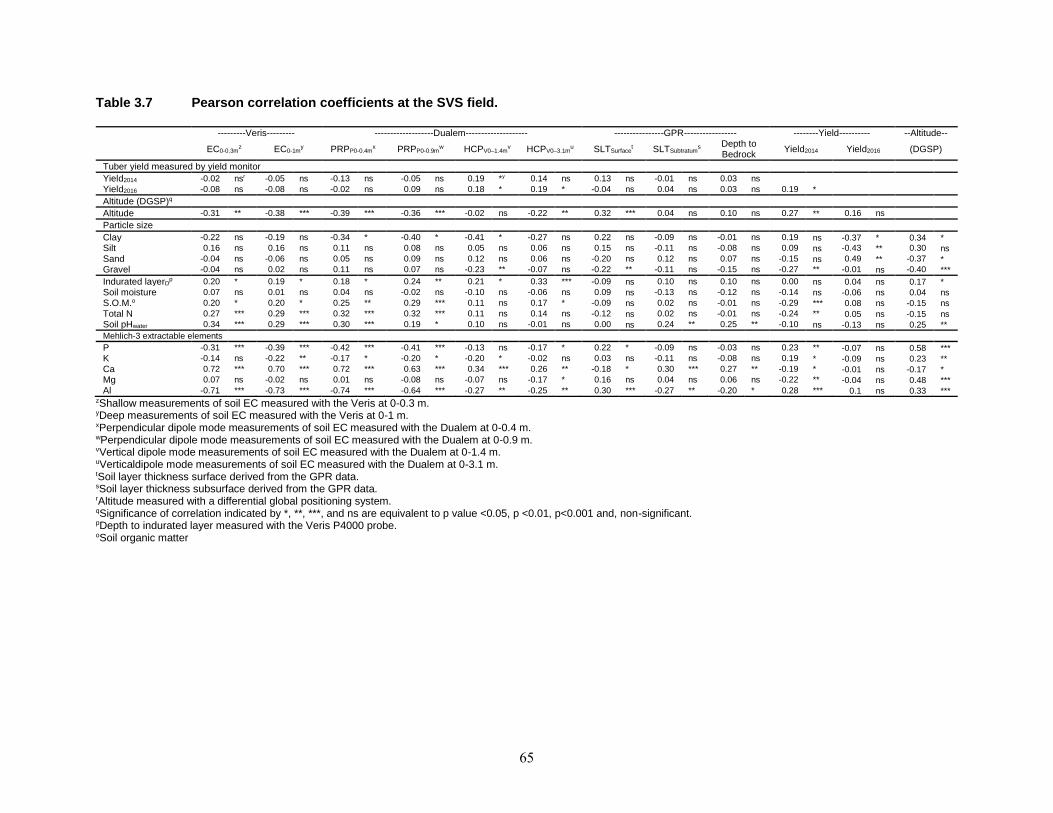
65
Table 3.7 Pearson correlation coefficients at the SVS field.
---------Veris--------- -------------------Dualem-------------------- ----------------GPR----------------- --------Yield---------- --Altitude--
EC0-0.3m
z EC0-1my PRPP0-0.4m
x PRPP0-0.9mw HCPV0–1.4m
v HCPV0–3.1mu SLTSurface
t SLTSubtratums
Depth to Bedrock
Yield2014 Yield2016 (DGSP)
Tuber yield measured by yield monitor
Yield2014 -0.02 nsr -0.05 ns -0.13 ns -0.05 ns 0.19 *y 0.14 ns 0.13 ns -0.01 ns 0.03 ns
Yield2016 -0.08 ns -0.08 ns -0.02 ns 0.09 ns 0.18 * 0.19 * -0.04 ns 0.04 ns 0.03 ns 0.19 *
Altitude (DGSP)q
Altitude -0.31 ** -0.38 *** -0.39 *** -0.36 *** -0.02 ns -0.22 ** 0.32 *** 0.04 ns 0.10 ns 0.27 ** 0.16 ns
Particle size
Clay -0.22 ns -0.19 ns -0.34 * -0.40 * -0.41 * -0.27 ns 0.22 ns -0.09 ns -0.01 ns 0.19 ns -0.37 * 0.34 *
Silt 0.16 ns 0.16 ns 0.11 ns 0.08 ns 0.05 ns 0.06 ns 0.15 ns -0.11 ns -0.08 ns 0.09 ns -0.43 ** 0.30 ns
Sand -0.04 ns -0.06 ns 0.05 ns 0.09 ns 0.12 ns 0.06 ns -0.20 ns 0.12 ns 0.07 ns -0.15 ns 0.49 ** -0.37 *
Gravel -0.04 ns 0.02 ns 0.11 ns 0.07 ns -0.23 ** -0.07 ns -0.22 ** -0.11 ns -0.15 ns -0.27 ** -0.01 ns -0.40 ***
Indurated layerDp 0.20 * 0.19 * 0.18 * 0.24 ** 0.21 * 0.33 *** -0.09 ns 0.10 ns 0.10 ns 0.00 ns 0.04 ns 0.17 *
Soil moisture 0.07 ns 0.01 ns 0.04 ns -0.02 ns -0.10 ns -0.06 ns 0.09 ns -0.13 ns -0.12 ns -0.14 ns -0.06 ns 0.04 ns
S.O.M.o 0.20 * 0.20 * 0.25 ** 0.29 *** 0.11 ns 0.17 * -0.09 ns 0.02 ns -0.01 ns -0.29 *** 0.08 ns -0.15 ns
Total N 0.27 *** 0.29 *** 0.32 *** 0.32 *** 0.11 ns 0.14 ns -0.12 ns 0.02 ns -0.01 ns -0.24 ** 0.05 ns -0.15 ns
Soil pHwater 0.34 *** 0.29 *** 0.30 *** 0.19 * 0.10 ns -0.01 ns 0.00 ns 0.24 ** 0.25 ** -0.10 ns -0.13 ns 0.25 **
Mehlich-3 extractable elements
P -0.31 *** -0.39 *** -0.42 *** -0.41 *** -0.13 ns -0.17 * 0.22 * -0.09 ns -0.03 ns 0.23 ** -0.07 ns 0.58 ***
K -0.14 ns -0.22 ** -0.17 * -0.20 * -0.20 * -0.02 ns 0.03 ns -0.11 ns -0.08 ns 0.19 * -0.09 ns 0.23 **
Ca 0.72 *** 0.70 *** 0.72 *** 0.63 *** 0.34 *** 0.26 ** -0.18 * 0.30 *** 0.27 ** -0.19 * -0.01 ns -0.17 *
Mg 0.07 ns -0.02 ns 0.01 ns -0.08 ns -0.07 ns -0.17 * 0.16 ns 0.04 ns 0.06 ns -0.22 ** -0.04 ns 0.48 ***
Al -0.71 *** -0.73 *** -0.74 *** -0.64 *** -0.27 ** -0.25 ** 0.30 *** -0.27 ** -0.20 * 0.28 *** 0.1 ns 0.33 *** zShallow measurements of soil EC measured with the Veris at 0-0.3 m. yDeep measurements of soil EC measured with the Veris at 0-1 m. xPerpendicular dipole mode measurements of soil EC measured with the Dualem at 0-0.4 m. wPerpendicular dipole mode measurements of soil EC measured with the Dualem at 0-0.9 m. vVertical dipole mode measurements of soil EC measured with the Dualem at 0-1.4 m. uVerticaldipole mode measurements of soil EC measured with the Dualem at 0-3.1 m. tSoil layer thickness surface derived from the GPR data. sSoil layer thickness subsurface derived from the GPR data. rAltitude measured with a differential global positioning system. qSignificance of correlation indicated by *, **, ***, and ns are equivalent to p value <0.05, p <0.01, p<0.001 and, non-significant. pDepth to indurated layer measured with the Veris P4000 probe. oSoil organic matter
66
In general, the coefficients of correlation between the SLT and depth to bedrock were also
correlated with the soil EC data, however, the values were higher in the SVS field than SVP field
(r > 0.22). These results confirmed findings by Toy et al. (2010) concerning significant
relationship between properties derived by GPR (antenna Frequency = 450 MHz) and
electromagnetic induction in a silt loam texture. When considering GPR properties themselves,
the highest correlation coefficients were found between SLTSubstratum and depth to bedrock (r
> 0.90). The positive correlations between SLTSubstratum and depth to bedrock were in
accordance with thickest SLTSubstratum and deepest bedrock. These correlation coefficients
were generally much lowest for the SVP field. Again, the higher landscape variation of the SVS
field affected the thickness of the soil layers compared to the SVP field which has a moderate
slope with contrasting slight slope characteristics.
The coefficients of correlations were calculated using soil physicochemical properties for both
fields to understand which factors influenced the spatial pattern of the tuber yield, soil EC, layer
thickness and altitude (Table 3.6 and Table 3.7). Tuber yield in 2013, 2014 and 2016 was
negatively correlated with soil EC measurements (Table 3.6) obtained by the Veris and Dualem
for the SVP field. Higher correlations were obtained in 2013 and could be associated to higher
amount of precipitation during the growing season. The correlation coefficient between the soil
EC measurements and tuber yield were similar to the one obtained by Cambouris et al. (2006).
For the soil properties, soil EC values were strongly correlated to particle size and soil moisture
in the SVP field. Soil EC values, clay and soil moisture contents were higher in the areas
characterized by poorly drained soils. Previous studies reported similar relationships between soil
EC values and soil particle size in similar soil texture and topographic conditions (Landrum et al.,
2015, Moral et al., 2010). Mehlich-3 extractable elements, S.O.M., total N and soil pH were also
generally significantly correlated to the soil EC values in the SVP field. Overall the positive
correlations of soil properties with soil EC values suggested that ground conductivity can be used
to predict soil property, to visualize its impact on the yield and ameliorate productive and
unproductive areas within a field. The SLT derived with the GPR was not significantly correlated
and no linear relationship was found with tuber yield in the SVP field. However, the SLTsubsurface
and the depth to bedrock were significantly correlated with most of the soil properties (altitude,
particle size, indurated layer depth, soil moisture, P, Ca, Mg and Al content). In opposite, the
relationship of the SLTsurface with the soil properties was generally non‐ significant. The strongest
relationships were obtained with altitude, particle size and indurated layer depth. High correlation
with the altitude could be related to the fact that the GPS data entry used during the radar data
processing in assembling data files on 2D grid. High correlation obtained between the SLT with
67
indurated layer depth could be related to the fact this property was used to adjust the dielectric
contrast of the GPR.
In the same field, no significant correlations were found between tuber yield over all three years
and soil physicochemical properties, excepted for particle size. Clay content was the soil property
most strongly correlated with the tuber year over all year. Highest areas of clay content
corresponding to the lowest areas of tuber yield. As state previously low yield areas were also
characterized by high soil moisture content corresponding to poorly drained soil. Impeded
drainage is a severe limitation to potato production. Excessive water in soil also decreases the
efficiency of nutrient uptake (GNB, 2016). In 2016, the tuber was significantly correlated with P
content. This positive relationship suggested highest tubers yield when the P is highest.
Phosphorus is essential for root development, therefore an adequate amount in the soil is better
during crop development (GNB, 2016).
Tuber yield in 2014 and 2016 was not related to Veris, Dualem and GPR parameters as well as
with altitude in the SVS field (Table 3.7). Significant negative correlations of soil EC values, except
for HCPV0-3.1m, with the altitude suggested the linear trend indicating that the ground conductivity
values are influenced greatly by the topography in the SVS field. As oppose to the SVP field, no
relationships existed for the soil EC values of the Veris with particle size in the SVS field. The soil
EC of the Dualem had the same results except that the three lower depth measurements (two
PRP and HCPV0-1.4m) indicated a significant negative correlation with the clay content. The
strongest correlation with the Mehlich-3 extractable elements with the soil EC values, except with
HCPV0-1.4m and HCPV0-3.1m, was with Ca and Al content. The deeper the soil EC measurements
were taken with the Dualem the lowest were the relationships with the soil parameters. These
results could be associated to the fact that the soil properties were measured at the soil surface
layer (0-0.15 m). No significant relationships were found between the SLT values and soil
properties, except for soil pH, Ca and Al content in the SVS field. The correlations were higher
with SLTsubsurface and depth to bedrock than with SLTsurface. The SLTsurface was also related to the
altitude suggesting that areas with deeper soil were normally located in the higher areas of the
field and vice versa. These results are in opposition with the results found by Fraisse et al. (2001).
This may be related to land levelling. Tuber yield in 2014 was also significantly influence by
altitude suggesting that highest yield areas were normally located to highest altitude areas. Since
altitude is an underlying factor in the distribution of soil moisture relationship of that property with
tuber yield was expected. However, no such relation was found. Tuber yield in 2016 were only
68
significantly correlated to particle size. The greatest correlation was with sand which suggesting
the highest sand content areas resulted in highest tuber yield areas.
In accordance with previous results, PSS has shown good performance explaining spatial
variability in the studied fields. Most of the sensors, soil physicochemical properties and yields
were correlated. Clearly, the respond of the PSS to the spatial variability in the agricultural fields
and their data could be used to delineate MZ (Castrignano et al., 2012).
3.5 Determination of the optimum number of management zones
The fuzzy k-means clustering algorithm was used to delineate the fields into two to five MZ (SVP
field: Figure 3.5 and SVS field Figure 3.6). The analysis without spatial constraint was carried out
because artificial regions were obtained with the application of a spatial constraint (data not
shown). Also, an artificial pattern was obtained for Dualem MZ in SVS, an arbitrary subdivision
was obtained for 2 MZ. In this case it seems that the used algorithm does not work properly. This
could attributed to several characteristics of the data such as unequal populations, elongated
chains, and the lack of intensity data (Bezdek, 2013).
Previous studies (Li et al., 2007, Moral et al., 2010, Xin-Zhong et al., 2009) have shown
relationship between decreasing variance and the optimum number of MZ. Effectively, by
increasing the number of MZ from one to five, the total within-zone variance of the soil and yield
properties decreased (Cambouris et al., 2006).
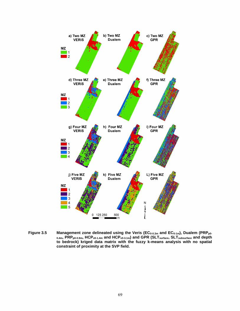
69
Figure 3.5 Management zone delineated using the Veris (EC0-0.3m and EC0-1m), Dualem (PRPp0-
0.4m, PRPp0-0.9m, HCPv0-1.4m and HCPv0-3.1m) and GPR (SLTsurface, SLTsubsurface and depth to bedrock) kriged data matrix with the fuzzy k-means analysis with no spatial constraint of proximity at the SVP field.
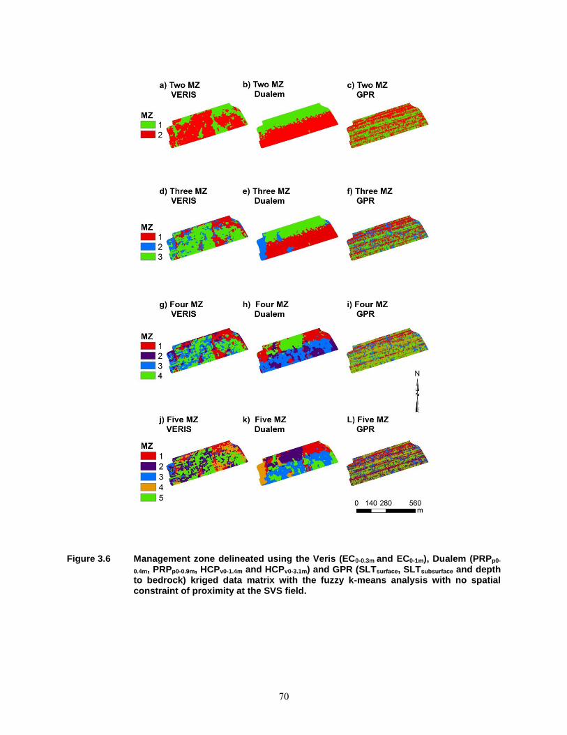
70
Figure 3.6 Management zone delineated using the Veris (EC0-0.3m and EC0-1m), Dualem (PRPp0-
0.4m, PRPp0-0.9m, HCPv0-1.4m and HCPv0-3.1m) and GPR (SLTsurface, SLTsubsurface and depth to bedrock) kriged data matrix with the fuzzy k-means analysis with no spatial constraint of proximity at the SVS field.

71
As a result of the clustering analysis for the SVP field, the optimal number of MZ with regard to
the soil EC proximal sensors, soil properties and tuber yields were similar (Figure 3.7).
Comparable results in the decrease of variance for the soil EC values were obtained for
Cambouris et al. (2006) and Corwin and Lesch (2005). By increasing the number of zones from
one to two, the total within-zone variance of the soil EC values decreased from 71% to 77% and
from 65% to 79% with the Veris and the Dualem, respectively (Table 3.7a, b). With these two
PSS, two MZ seem to be most suitable. Based on the SLT, the stratification of the field from one
to three MZ decreased the total variance from 55% to 65% (Figure 3.7c) and three MZ seem to
be most suitable.
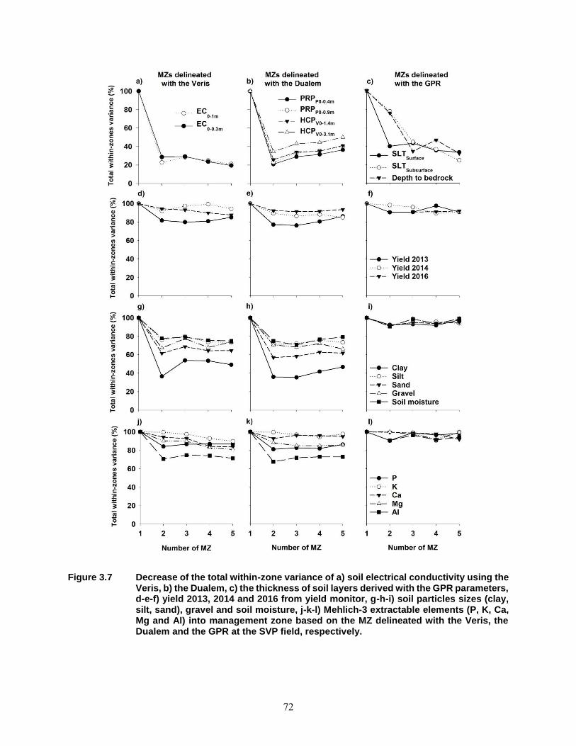
72
Figure 3.7 Decrease of the total within-zone variance of a) soil electrical conductivity using the Veris, b) the Dualem, c) the thickness of soil layers derived with the GPR parameters, d-e-f) yield 2013, 2014 and 2016 from yield monitor, g-h-i) soil particles sizes (clay, silt, sand), gravel and soil moisture, j-k-l) Mehlich-3 extractable elements (P, K, Ca, Mg and Al) into management zone based on the MZ delineated with the Veris, the Dualem and the GPR at the SVP field, respectively.
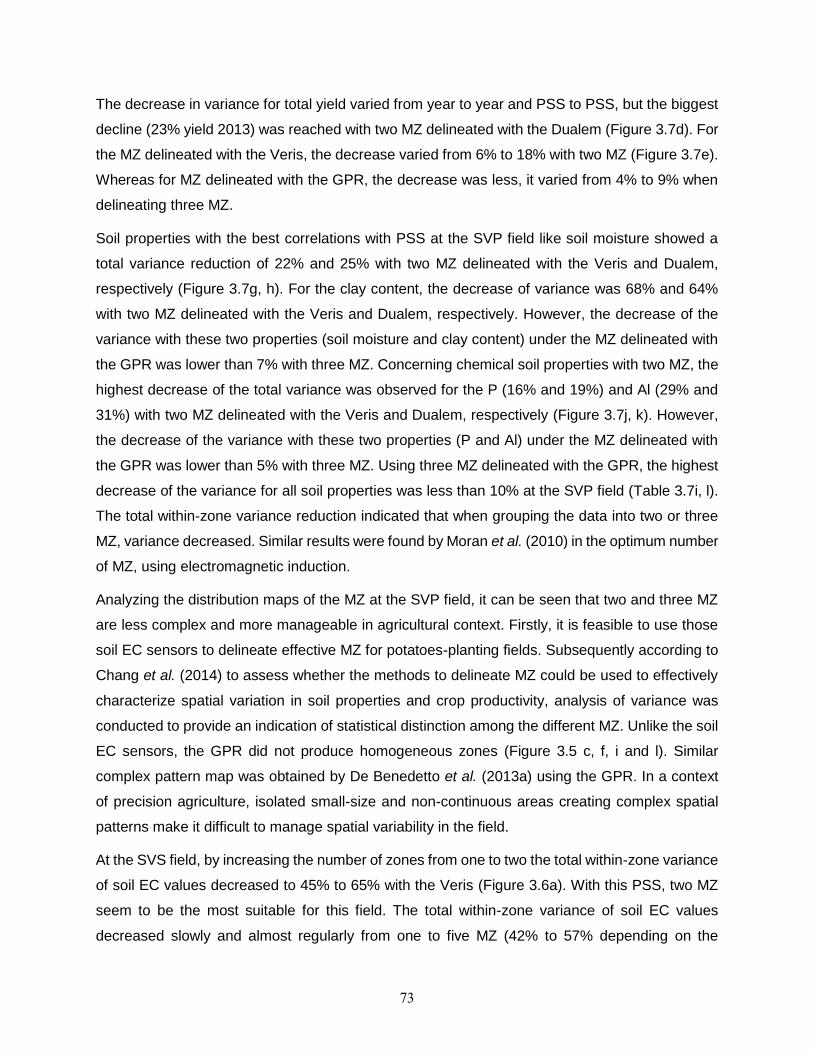
73
The decrease in variance for total yield varied from year to year and PSS to PSS, but the biggest
decline (23% yield 2013) was reached with two MZ delineated with the Dualem (Figure 3.7d). For
the MZ delineated with the Veris, the decrease varied from 6% to 18% with two MZ (Figure 3.7e).
Whereas for MZ delineated with the GPR, the decrease was less, it varied from 4% to 9% when
delineating three MZ.
Soil properties with the best correlations with PSS at the SVP field like soil moisture showed a
total variance reduction of 22% and 25% with two MZ delineated with the Veris and Dualem,
respectively (Figure 3.7g, h). For the clay content, the decrease of variance was 68% and 64%
with two MZ delineated with the Veris and Dualem, respectively. However, the decrease of the
variance with these two properties (soil moisture and clay content) under the MZ delineated with
the GPR was lower than 7% with three MZ. Concerning chemical soil properties with two MZ, the
highest decrease of the total variance was observed for the P (16% and 19%) and Al (29% and
31%) with two MZ delineated with the Veris and Dualem, respectively (Figure 3.7j, k). However,
the decrease of the variance with these two properties (P and Al) under the MZ delineated with
the GPR was lower than 5% with three MZ. Using three MZ delineated with the GPR, the highest
decrease of the variance for all soil properties was less than 10% at the SVP field (Table 3.7i, l).
The total within-zone variance reduction indicated that when grouping the data into two or three
MZ, variance decreased. Similar results were found by Moran et al. (2010) in the optimum number
of MZ, using electromagnetic induction.
Analyzing the distribution maps of the MZ at the SVP field, it can be seen that two and three MZ
are less complex and more manageable in agricultural context. Firstly, it is feasible to use those
soil EC sensors to delineate effective MZ for potatoes-planting fields. Subsequently according to
Chang et al. (2014) to assess whether the methods to delineate MZ could be used to effectively
characterize spatial variation in soil properties and crop productivity, analysis of variance was
conducted to provide an indication of statistical distinction among the different MZ. Unlike the soil
EC sensors, the GPR did not produce homogeneous zones (Figure 3.5 c, f, i and l). Similar
complex pattern map was obtained by De Benedetto et al. (2013a) using the GPR. In a context
of precision agriculture, isolated small-size and non-continuous areas creating complex spatial
patterns make it difficult to manage spatial variability in the field.
At the SVS field, by increasing the number of zones from one to two the total within-zone variance
of soil EC values decreased to 45% to 65% with the Veris (Figure 3.6a). With this PSS, two MZ
seem to be the most suitable for this field. The total within-zone variance of soil EC values
decreased slowly and almost regularly from one to five MZ (42% to 57% depending on the
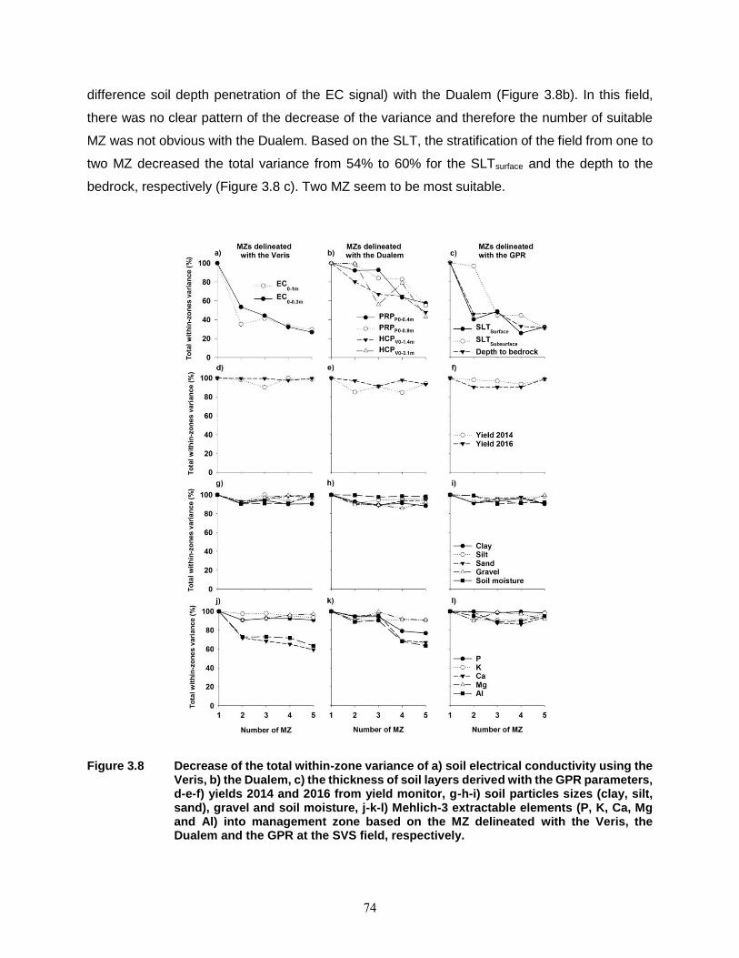
74
difference soil depth penetration of the EC signal) with the Dualem (Figure 3.8b). In this field,
there was no clear pattern of the decrease of the variance and therefore the number of suitable
MZ was not obvious with the Dualem. Based on the SLT, the stratification of the field from one to
two MZ decreased the total variance from 54% to 60% for the SLTsurface and the depth to the
bedrock, respectively (Figure 3.8 c). Two MZ seem to be most suitable.
Figure 3.8 Decrease of the total within-zone variance of a) soil electrical conductivity using the Veris, b) the Dualem, c) the thickness of soil layers derived with the GPR parameters, d-e-f) yields 2014 and 2016 from yield monitor, g-h-i) soil particles sizes (clay, silt, sand), gravel and soil moisture, j-k-l) Mehlich-3 extractable elements (P, K, Ca, Mg and Al) into management zone based on the MZ delineated with the Veris, the Dualem and the GPR at the SVS field, respectively.
75
Regardless of the PSS at the SVS field, the highest decrease in variance for total yield was 15%
and was reached with the decreased of one to two MZ delineated with the Dualem (Figure 3.8d,
e, and f). Again, regardless of the PSS, the decrease of the variance for the particle size, soil
moisture or gravel content was less than 10% in all cases (Figure 3.8g, h, and i). The decrease
of the total variance from one to five MZ, no matter of the PSS, was less than 10%. However, the
total variance for Ca and Mg content showed a decrease of 28% and 27%, respectively with the
MZ delineated with the Veris going from one to two MZ. Using the one delineated with the Dualem,
the total variance for Ca and Mg content showed a decrease of 31% and 32%, respectively from
three to four MZ.
For the SVS field, the decrease in variance follow a less homogeneous behaviour than in the SVP
field and did not show any clear pattern of MZ. Hypothetically, this could be attributed to
homogeneous spatial variability and a low spatial structure observed in soil properties of the field.
The MZ delineated with the Dualem at the SVS field showed a decrease in variance also beyond
three zones but the maximum of decrease was obtained at two or three zones. The soil EC
sensors behaviour was completely different from one field to the other. Corwin and Lesch (2005)
noticed that soil EC sensors tend to vary from field to field. This especially occurred when the field
is dominated by one or two factors intrinsic factors such as soil moisture or clay content making
the interpretation of soil EC values highly specific to the site.
3.6 Practical Applications of Management Zone within These Fields
Spatial variation in crops is the result of a complex interaction of biological, edaphic,
anthropogenic, topographic, and climatic factors (Corwin et al., 2003). Measurements of the soil
EC and SLT have been used at field scale to map soil spatial variability by MZ. According to
Cambouris et al. (2006) the optimal number of MZ must show a balance between the spatial
variation of soil properties, yield stability over time and a manageable spatial representation.
In general, three and plus MZ are not considered significant at the chosen 5% level (data not
shown) when comparing the zones of the soil EC values and SLT issued from the PSS for the
two fields of the study. Effectively, two MZ were significantly different when using the PSS to
delineate the SVP field with the exception of two SLT parameters (SLTsubstratum and depth to
bedrock) and all three SLT parameters for SVS field (Table 3.8).
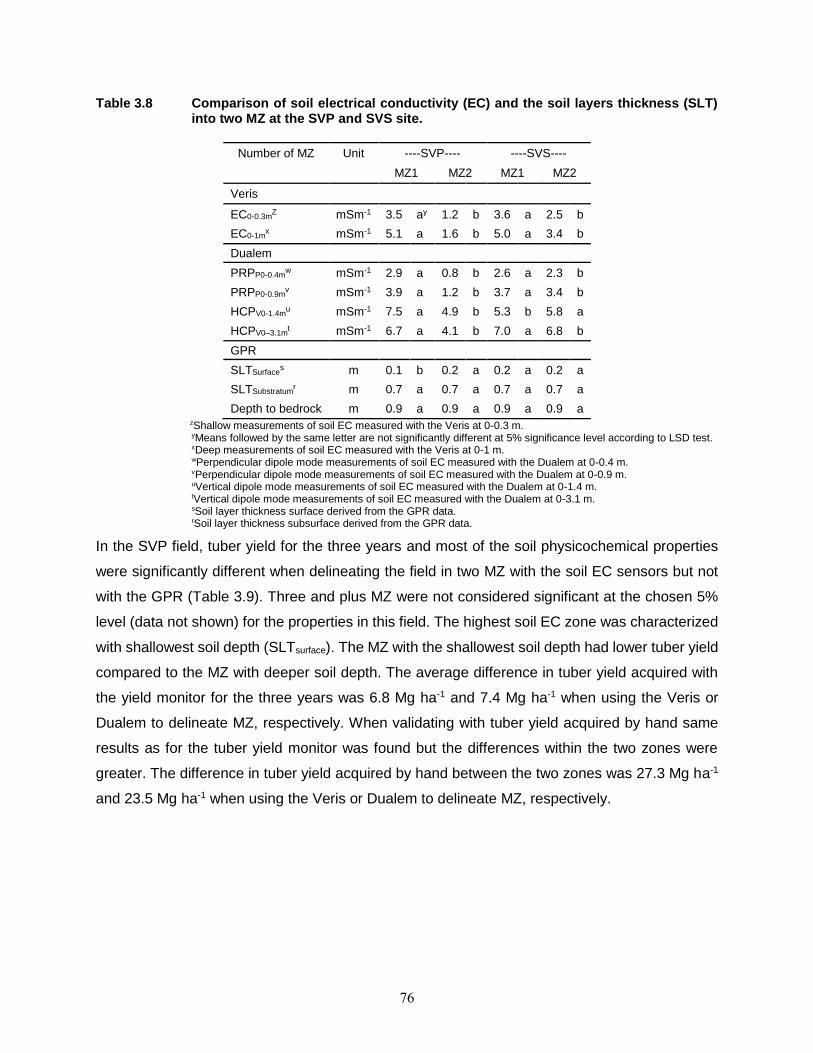
76
Table 3.8 Comparison of soil electrical conductivity (EC) and the soil layers thickness (SLT) into two MZ at the SVP and SVS site.
Number of MZ Unit ----SVP---- ----SVS----
MZ1 MZ2 MZ1 MZ2
Veris
EC0-0.3mZ mSm-1 3.5 ay 1.2 b 3.6 a 2.5 b
EC0-1mx mSm-1 5.1 a 1.6 b 5.0 a 3.4 b
Dualem
PRPP0-0.4mw mSm-1 2.9 a 0.8 b 2.6 a 2.3 b
PRPP0-0.9mv mSm-1 3.9 a 1.2 b 3.7 a 3.4 b
HCPV0-1.4mu mSm-1 7.5 a 4.9 b 5.3 b 5.8 a
HCPV0–3.1mt mSm-1 6.7 a 4.1 b 7.0 a 6.8 b
GPR
SLTSurfaces m 0.1 b 0.2 a 0.2 a 0.2 a
SLTSubstratumr m 0.7 a 0.7 a 0.7 a 0.7 a
Depth to bedrock m 0.9 a 0.9 a 0.9 a 0.9 a zShallow measurements of soil EC measured with the Veris at 0-0.3 m. yMeans followed by the same letter are not significantly different at 5% significance level according to LSD test. xDeep measurements of soil EC measured with the Veris at 0-1 m. wPerpendicular dipole mode measurements of soil EC measured with the Dualem at 0-0.4 m. vPerpendicular dipole mode measurements of soil EC measured with the Dualem at 0-0.9 m. uVertical dipole mode measurements of soil EC measured with the Dualem at 0-1.4 m. tVertical dipole mode measurements of soil EC measured with the Dualem at 0-3.1 m. sSoil layer thickness surface derived from the GPR data. rSoil layer thickness subsurface derived from the GPR data.
In the SVP field, tuber yield for the three years and most of the soil physicochemical properties
were significantly different when delineating the field in two MZ with the soil EC sensors but not
with the GPR (Table 3.9). Three and plus MZ were not considered significant at the chosen 5%
level (data not shown) for the properties in this field. The highest soil EC zone was characterized
with shallowest soil depth (SLTsurface). The MZ with the shallowest soil depth had lower tuber yield
compared to the MZ with deeper soil depth. The average difference in tuber yield acquired with
the yield monitor for the three years was 6.8 Mg ha-1 and 7.4 Mg ha-1 when using the Veris or
Dualem to delineate MZ, respectively. When validating with tuber yield acquired by hand same
results as for the tuber yield monitor was found but the differences within the two zones were
greater. The difference in tuber yield acquired by hand between the two zones was 27.3 Mg ha-1
and 23.5 Mg ha-1 when using the Veris or Dualem to delineate MZ, respectively.
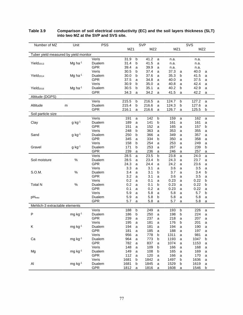
77
Table 3.9 Comparison of soil electrical conductivity (EC) and the soil layers thickness (SLT) into two MZ at the SVP and SVS site.
Number of MZ Unit PSS SVP SVS
MZ1 MZ2 MZ1 MZ2
Tuber yield measured by yield monitor
Yield2013 Mg ha-1 Veris 31.9 b 41.2 a n.a. n.a. Dualem 31.4 b 41.5 a n.a. n.a. GPR 39.4 a 39.9 a n.a. n.a.
Yield2014 Mg ha-1 Veris 30.5 b 37.4 a 37.3 a 40.0 a Dualem 30.0 b 37.6 a 35.3 b 41.5 a GPR 37.5 a 34.8 a 40.0 a 37.5 a
Yield2016 Mg ha-1
Veris 30.9 b 35.0 a 40.8 a 42.4 a Dualem 30.5 b 35.1 a 40.2 b 42.9 a
GPR 34.3 a 34.2 a 41.5 a 42.2 a
Altitude (DGPS)
Altitude m Veris 215.5 b 216.5 a 124.7 b 127.2 a Dualem 215.4 b 216.6 a 124.3 b 127.6 a GPR 216.1 a 216.6 a 126.7 a 125.5 b
Soil particle size
Clay g kg-1 Veris 191 a 142 b 159 a 162 a Dualem 189 a 141 b 161 a 161 a GPR 151 a 152 a 165 a 157 b
Sand g kg-1 Veris 248 b 363 a 353 a 355 a Dualem 250 b 366 a 349 a 357 a GPR 345 a 334 b 350 a 358 a
Gravel g kg-1 Veris 158 b 254 a 253 a 249 a Dualem 171 b 253 a 267 a 239 b GPR 239 a 236 a 246 a 257 a
Soil moisture % Veris 28.5 a 23.5 b 23.8 a 24.0 a Dualem 28.5 a 23.4 b 24.3 a 23.7 a GPR 24.3 a 24.4 a 24.2 a 23.6 a
S.O.M. % Veris 3.3 a 3.1 a 3.6 a 3.5 a Dualem 3.4 a 3.1 b 3.7 a 3.4 b GPR 3.2 a 3.1 a 3.6 a 3.5 a
Total N % Veris 0.2 a 0.1 a 0.23 a 0.22 b Dualem 0.2 a 0.1 b 0.23 a 0.22 b GPR 0.1 a 0.2 a 0.23 a 0.22 a
pHeau Veris 5.9 a 5.8 a 5.8 a 5.7 b Dualem 5.9 a 5.8 b 5.8 a 5.8 a GPR 5.7 a 5.8 a 5.7 a 5.8 a
Mehlich-3 extractable elements
P mg kg-1 Veris 188 b 249 a 193 b 226 a Dualem 186 b 250 a 198 b 224 a GPR 239 a 237 a 218 a 207 a
K mg kg-1 Veris 195 a 181 a 176 b 201 a Dualem 194 a 181 a 194 a 190 a GPR 181 a 185 a 188 a 197 a
Ca mg kg-1 Veris 956 a 778 b 1311 a 981 a Dualem 964 a 773 b 1193 a 1047 b GPR 782 a 837 a 1074 a 1153 a
Mg mg kg-1 Veris 148 a 109 b 166 a 168 a Dualem 149 a 108 b 165 a 169 a GPR 112 a 120 a 166 a 170 a
Al mg kg-1 Veris 1681 b 1842 a 1497 b 1636 a Dualem 1681 b 1845 a 1529 b 1619 a GPR 1812 a 1816 a 1608 a 1546 b
78
The shallowest soil depth and lowest yield zone were also characterized by highest amount of
clay, soil moisture, S.O.M, total N, pH, Ca and Mg content while it had lowest amount of sand,
gravel, P and Al content. Since the soil physicochemical properties varied significantly in both MZ,
it suggests that it is relevant to manage soil properties using the selected MZ. The highest soil
EC zone was characterized by the wettest soil, finest soil texture and lowest tuber yield measured
by the yield monitor and hand while in the lowest EC zone the opposite pattern was established.
The MZ with the wettest soil conditions could be managed with specific drainage or land levelling
to reduce the greatest amount of water in the soil in this area, which could increase the tuber yield
potential in this zone. Under those circumstances, identifying the underlying factors responsible
for the variation in crop yield, it would be possible for potatoes producers to use MZ in order to
optimize their profitability (De Caires et al., 2015).
As for the SVP field in the SVS field, three and plus MZ were not considered significant at the
chosen 5% level (data not shown). Tuber yield for the two years and most of the soil
physicochemical properties were significantly different when delineating the field in two MZ with
the Veris and/or the Dualem but not with the GPR (Table 3.9). The highest soil EC zone was
characterized with the lowest tuber yield when delineating zone with the Dualem. The average
difference in tubers yield for the two years was 4.5 Mg ha-1. Tuber yield did not vary significantly
when delineating this field with the Veris. When validating with tuber yield acquired by hand no
significant differences were found within the MZ for all the PSS. The zone established with the
Dualem showed significant difference within the two zones for the gravel and S.O.M content.
Highest soil EC indicated highest content for these properties and vice versa in the other lowest
soil EC zone. The two MZ delineated with the Veris showed significant difference for the pH, Ca
and K content. Highest soil EC indicated highest content of pH and Ca content while lowest K
content and vice versa in the other lowest soil EC zone. Total N, P and Al varied significantly
when delineating two zones with the Veris and the Dualem. Highest soil EC indicated highest
content of total N while lowest P and Al content and vice versa in the other lowest soil EC zone.
As oppose to the SVP field, in the SVS field, the Veris and the Dualem were not associated to the
same significant difference for the tuber yield and soil physicochemical properties. These results
for the SVS field could be attributed to lower spatial variability of the data acquired with the PSS.
The Dualem performed better than the Veris in this field.
For both fields, the GPR results were not significantly different; this could be associated to the
fact that this instrument recorded short range spatial variability. For the SVP field the GPR
parameters range was between 13- and 27-m and from 20- to 46-m for the SVS field. Those
79
ranges were the smallest obtained within all the PSS. Similar results (0.9- to 8-m) have been
shown by De Benedetto et al. (2013a) mainly due to an intrinsic variation of subsoil structure.
Short-range variability generally decreased as a function of the depth because of the GPR signal
attenuation. Additionally, given the high-sampling density of the GPR compared to the other PSS
(more than 200 000 samples) an improvement of raw data could be applied. A more specialized
treatment like mathematical models could contribute to the simulation of the hyperbolic signatures
of soil layer thickness making them more discernible. Resents research has shown that neural
networks are a powerful tool applied in radar detection available to approximate functions from a
large number of inputs to simulate depth and dielectric constant of the underground medium using
signal amplitude and time. Zhang et al. (2016) results indicate that the method improves accuracy
estimate depth and contrast dielectric of subsurface medium. Neural network seems a promising
method and it might apply in future research to GPR data.
A site-specific crop management can be implemented in agricultural fields to manage plant
breeding, pest management, weed management, soil fertility and crops based upon spatial
variations within a field (Lal et al., 1997). In the two fields, the use of soil EC sensors is most
recommended in delineating MZ. Soil EC was successful in delineating MZ describing the tuber
yield potential and to characterize the soil physicochemical properties (Johnson et al., 2001). Two
MZ could be determined in both field and the Dualem performed better in the SVS characterized
by less spatial variability. This zone delineation potentially facilitates cost-effective,
environmentally friendly and energy efficient management of the fields (De Caires et al., 2015).
80
4 CONCLUSIONS
Managing the complexity of the within-field variability of the soil properties and crop yield is a
current challenge in the precision agriculture to protect environment, increase profitability of crop
production and improve yield quality. The aim of this study was to compare PSS to characterize
soil and crop yield spatial variability and therefore to delineate soil MZ in intensive potato
production in New Brunswick. The SVP field showed higher variability than the SVS field.
Effectively, the results showed that the SVP field presented highest pedodiversity attributable to
higher variability of soil texture and soil moisture. In this study, soil EC obtained with the Veris
and the Dualem was effective in delineating field differences in soil physicochemical properties
for both fields. Consequently, at these sites, soil EC was efficient to subdivide the fields into two
significant homogeneous MZ based on soil physicochemical characteristics and behaviour and
tuber yield productivity. For the SVP field the differences were particularly related to soil texture
and moisture. These soil properties influenced soil water availability, and consequently potato
yield. In the SVS field, the Veris and the Dualem behaviour were not the same and significant
differences for tuber yield and soil physicochemical properties were different if soil EC was
measured from one instrument or the other. These results could be attributable to lower spatial
variability of the data acquired with the PSS. This lower spatial variability was also revealed by
the intensive soil sampling for the intrinsic properties, especially soil texture. In the SVS field, the
Dualem performed better in than the Veris in delineating efficient MZ. For both fields, the GPR
results were not significantly different likely due to the fact that this instrument recorded short
range spatial variability. The soil EC sensors could be used to delineate MZ and the performance
of the proposed method is promising in potato production in New Brunswick especially when the
field shows high pedodiversity.

81
5 REFERENCES
Adamchuk V et al. (2015) Tools for proximal soil sensing. Book Chapter.
Adamchuk V et al. (2004) On-the-go soil sensors for precision agriculture. Computers and Electronics in Agriculture 44(1):71-91.
Allaire SE et al. (2014) Spatial variability of potato tuber yield and plant nitrogen uptake related to soil properties. Agronomy Journal 106(3):851-859.
Arvalis I (2015) Agriculture de précision, positionnement GPS, Gestion intraparcellaire, evaluation des performances. Edition Arvalis.
Australian Centre for Precision Agriculture (2002) FuzME version 3.0, The University of Sydney, Australia.
Bernard G et al. (2001) Atlantic Canada potato guide. Atlantic Provinces Agriculture Services Coordinating Committee publication 1300:93.
Bezdek JC (2013) Pattern recognition with fuzzy objective function algorithms. Springer Science & Business Media,
Blanchet G et al. (2017) Spatial variability of potassium in agricultural soils of the canton of Fribourg, Switzerland. Geoderma 290:107-121.
Bogunovic I et al. (2017) Spatial distribution of soil chemical properties in an organic farm in Croatia. Science of The Total Environment 584:535-545.
Brye KR (2006) Soil physiochemical changes following 12 years of annual burning in a humid–subtropical tallgrass prairie: a hypothesis. Acta Oecologica 30(3):407-413.
Cambardella C et al. (1999) Spatial analysis of soil fertility parameters. Precision Agriculture 1(1):5-14.
Cambardella C et al. (1994) Field-scale variability of soil properties in central Iowa soils. Soil science society of America journal 58(5):1501-1511.
Cambouris A et al. (2006) Soil management zones delineated by electrical conductivity to characterize spatial and temporal variations in potato yield and in soil properties. American journal of potato research 83(5):381-395.
Cambouris A et al. (2014) Precision Agriculture in Potato Production. Potato Research 57(3-4):249-262.
Castrignano A et al. (2012) Use of EMI, gamma-ray emission and GPS height as multi-sensor data for soil characterisation. Geoderma 175:78-89.
Chang D et al. (2014) Delineation of management zones using an active canopy sensor for a tobacco field. Computers and Electronics in Agriculture 109:172-178.
Christy CD (2008) Real-time measurement of soil attributes using on-the-go near infrared reflectance spectroscopy. Computers and electronics in agriculture 61(1):10-19.
Corwin D et al. (2003) Application of soil electrical conductivity to precision agriculture. Agronomy journal 95(3):455-471.
Corwin D et al. (2005) Apparent soil electrical conductivity measurements in agriculture. Computers and electronics in agriculture 46(1):11-43.
82
Corwin D et al. (2010) Delineating site-specific management units with proximal sensors. Geostatistical applications for precision agriculture, Springer. p 139-165.
Cox M et al. (2003) Variability of selected soil properties and their relationships with soybean yield. Soil Science Society of America Journal 67(4):1296-1302.
Dampney P et al. (2004) Non-intrusive sensors for measuring soil physical properties.
Dancette C (1983) Estimation des besoins en eau des principales cultures pluviales en zone soudano-sahélienne. L’Agronomie Tropicale 38(4):281-294.
Davis J et al. (2002) Ground penetrating radar to measure soil water content. Methods of soil analysis. Part 4:446-463.
De Benedetto D et al. (2013a) Field partition by proximal and remote sensing data fusion. Biosystems engineering 114(4):372-383.
De Benedetto D et al. (2013b) An approach for delineating homogeneous zones by using multi-sensor data. Geoderma 199:117-127.
De Caires SA et al. (2015) Spatial analysis for management zone delineation in a humid tropic cocoa plantation. Precision Agriculture 16(2):129-147.
Denton OA et al. (2017) Assessment of spatial variability and mapping of soil properties for sustainable agricultural production using Geographic Information System Techniques (GIS). Cogent Food & Agriculture (just-accepted).
Doolittle JA et al. (2014) The use of electromagnetic induction techniques in soils studies. Geoderma 223:33-45.
Environment Canada (2016) Canadian Climate Normals or Averages 1981-2010. Available online at: http://www.climat.meteo.ec.gc. ca/climate normals/index_e.html [Accessed 26 September 2016].Available online at: http://www.climat.meteo.ec.gc.
Fahmy SH, Rees, H. W. Soley, T. J (2001) Soils of the Woodstock–Florenceville area,
Carleton County, New Brunswick. . Vol. 4. :20 p.
Farooque AA et al. (2012) Delineating management zones for site specific fertilization in wild blueberry fields. Applied Engineering in Agriculture 28(1):57-70.
Fleming K et al. (2004) Evaluating soil color with farmer input and apparent soil electrical conductivity for management zone delineation. Agronomy Journal 96(6):1581-1587.
Fraisse C et al. (2001) Delineation of site-specific management zones by unsupervised classification of topographic attributes and soil electrical conductivity. Transactions of the ASAE 44(1):155.
Gasser M et al. (2000) Influence des facteurs de production sur la régie de la fertilisation azotée de la pomme de terre. Agriculture intensive et écosystèmes régionaux: du diagnostic aux interventions. Les Presses de l’Université Laval, Québec, Québec, Canada:197-217.
GNB (2016) Gouvernement du Nouveau-Brunswick, Portrait Agriculture, Aquaculture et Pêches, Pommes de terre.
Guan F et al. (2017) Spatial variability of soil nitrogen, phosphorus and potassium contents in Moso bamboo forests in Yong'an City, China. Catena 150:161-172.
Guastaferro F et al. (2010) A comparison of different algorithms for the delineation of management zones. Precision agriculture 11(6):600-620.
83
Haghverdi A et al. (2015) Perspectives on delineating management zones for variable rate irrigation. Computers and Electronics in Agriculture 117:154-167.
Halcro G et al. (2013) Site-specific land management of cereal crops based on management zone delineation by proximal soil sensing. Precision agriculture’13, Springer. p 475-482.
Havlin J et al. (2009) A variable-rate decision support tool. Precision agriculture 10(4):356-369.
Heiniger RW et al. (2003) Using soil electrical conductivity to improve nutrient management. Agronomy Journal 95(3):508-519.
Hendershot W et al. (2008) Soft reaction and exchangeable acidity. MR Carter (ed) Soil Sampling and Methods of Analysis. (Lewis Publishers, Boca Raton):141-146.
Irvin BJ et al. (1997) Fuzzy and isodata classification of landform elements from digital terrain data in Pleasant Valley, Wisconsin. Geoderma 77(2-4):137-154.
Jain AK et al. (1988) Algorithms for clustering data. Prentice-Hall, Inc.,
Johnson CK et al. (2001) Field-scale electrical conductivity mapping for delineating soil condition. Soil Science Society of America Journal 65(6):1829-1837.
Johnson CK et al. (2003) Site-specific management zones based on soil electrical conductivity in a semiarid cropping system. Agronomy journal 95(2):303-315.
Katsigiannis P et al. (2016) Fusion of spatio-temporal UAV and proximal sensing data for an agricultural decision support system. Fourth International Conference on Remote Sensing and Geoinformation of the Environment. International Society for Optics and Photonics, p 96881R-96881R-96811.
Khiari L (2014) Échantillonnage conventionnel des sols agricoles au Québec – De la planification à l’envoi au laboratoire.20.
Khosla R et al. (2002) Use of site-specific management zones to improve nitrogen management for precision agriculture. Journal of Soil and Water Conservation 57(6):513-518.
Khosla R et al. (2010) Spatial variation and site-specific management zones. Geostatistical applications for precision agriculture, Springer. p 195-219.
Kim J-H et al. (2007) Removal of ringing noise in GPR data by signal processing. Geosciences Journal 11(1):75-81.
Kweon G (2012) Delineation of site-specific productivity zones using soil properties and topographic attributes with a fuzzy logic system. Biosystems engineering 112(4):261-277.
Lal R et al. (1997) Soil management for sustainability. Future horizons: recent literature in sustainable agriculture:175.
Landrum C et al. (2015) An approach for delineating homogeneous within-field zones using proximal sensing and multivariate geostatistics. Agricultural Water Management 147:144-153.
Langmaid KK, MacMillan, J.K., Losicr, J.G. (1980) Soils of Madawaska County. The New Brunswick Soil Survey. Agriculture Canada, 8th Report p. 186.
Ledderhof D et al. (2017) Spatial Variability in Ontario Pinot noir Vineyards: Use of Geomatics and Implications for Precision Viticulture. American Journal of Enology and Viticulture:ajev. 2016.16062.
Li Y et al. (2007) Delineation of site-specific management zones using fuzzy clustering analysis in a coastal saline land. Computers and Electronics in Agriculture 56(2):174-186.
84
Lund E et al. (2011) Proximal sensing of soil organic matter using the Veris® OpticMapper™. 2nd Global Workshop on Proximal Soil Sensing, Montreal, Quebec, Canada. p 15-19.
Machado FC et al. (2015) Spatial DepenDence of electrical conDuctivity anD chemical propertieS of the Soil by electromagnetic inDuction. Revista Brasileira de Ciência do Solo 39(4):1112-1120.
Mathworks (2014a) Releases products.
Mathworks (2014b) Statistics MATLAB, Natick, Massachusetts.
McBratney A et al. (1992) A continuum approach to soil classification by modified fuzzy k‐means with extragrades. Journal of Soil Science 43(1):159-175.
McBride R et al. (1990) Estimating forest soil quality from terrain measurements of apparent electrical conductivity. Soil Science Society of America Journal 54(1):290-293.
Medina H et al. (2017) Regional-scale variability of soil properties in Western Cuba. Soil and Tillage Research 166:84-99.
Memarsadeghi N et al. (2007) A fast implementation of the ISODATA clustering algorithm. International Journal of Computational Geometry & Applications 17(01):71-103.
Milburn P et al. (1989) Soil depth groups for agricultural land development planning in New Brunswick. Can. Agric. Eng 31:1-5.
Molin JP et al. (2008) Establishing management zones using soil electrical conductivity and other soil properties by the fuzzy clustering technique. Scientia Agricola 65(6):567-573.
Moral F et al. (2010) Delineation of management zones using mobile measurements of soil apparent electrical conductivity and multivariate geostatistical techniques. Soil and Tillage Research 106(2):335-343.
Moral F et al. (2011) Site-specific management zones based on the Rasch model and geostatistical techniques. Computers and Electronics in Agriculture 75(2):223-230.
Morier T et al. (2015) In-season nitrogen status assessment and yield estimation using hyperspectral vegetation indices in a potato crop. Agronomy Journal 107(4):1295-1309.
Moshia M et al. (2015) Precision manure management on site-specific management zones: Topsoil quality and environmental impact. Communications in Soil Science and Plant Analysis 46(2):235-258.
Moulin A et al. (2012) Yield response of potatoes to variable nitrogen management by landform element and in relation to petiole nitrogen–A case study. Canadian Journal of Plant Science 92(4):771-781.
Mueller T et al. (2003) Soil electrical conductivity map variability in limestone soils overlain by loess. Agronomy Journal 95(3):496-507.
Mulla D (1989) Soil spatial variability and methods of analysis. In: Soft, Crop, and Water Management Systems for Rainfed Agriculture in the Sudano-Sahelian Zone. Proc Internat Workshop Jan 1987:241-252.
Mzuku M et al. (2005) Spatial variability of measured soil properties across site-specific management zones. Soil Science Society of America Journal 69(5):1572-1579.
Nolin M et al. (1991) Variabilité des sols et stratégie d'échantillonnage dans les études pédologiques détaillées de la plaine de Montréal. Canadian Journal of Soil Science 71(4):439-451.

85
Nyiraneza J et al. (2011) Short-range variability of nitrate and phosphate desorbed from anionic exchange membranes. Soil Science Society of America Journal 75(6):2242-2250.
Ortega J (2002) Definición de sub-rodales para una silvicultura de precisión: una aplicación del método Fuzzy K-Means.
Ortiz B et al. (2011) Delineation of management zones for southern root-knot nematode using fuzzy clustering of terrain and edaphic field characteristics. Communications in soil science and plant analysis 42(16):1972-1994.
Oshunsanya S et al. (2017) Use of GIS to Delineate Site-Specific Management Zone for Precision Agriculture. Communications in Soil Science and Plant Analysis (just-accepted).
Overstreet C et al. (2014) Site specific nematode management—Development and success in cotton production in the United States. Journal of nematology 46(4):309.
Pachepsky Y et al. (2003) Scaling methods in soil physics. CRC press,
Pedrera-Parrilla A et al. (2017) Concurrent temporal stability of the apparent electrical conductivity and soil water content. Journal of Hydrology 544:319-326.
Peralta NR et al. (2013) Delineation of management zones with soil apparent electrical conductivity to improve nutrient management. Computers and electronics in agriculture 99:218-226.
Peralta NR et al. (2015) Delineation of management zones to improve nitrogen management of wheat. Computers and Electronics in Agriculture 110:103-113.
Power J et al. (1981) Effects of topsoil and subsoil thickness on soil water content and crop production on a disturbed soil. Soil Science Society of America Journal 45(1):124-129.
Reynolds C et al. (2000) Estimating soil water-holding capacities by linking the Food and Agriculture Organization soil map of the world with global pedon databases and continuous pedotransfer functions. Water Resour. Res 36(12):3653-3662.
Roberts DF et al. (2012) Relationships between soil-based management zones and canopy sensing for corn nitrogen management. Agronomy journal 104(1):119-129.
Rosemary F et al. (2017) Exploring the spatial variability of soil properties in an Alfisol soil catena. Catena 150:53-61.
Saey T et al. (2009) Comparing the EM38DD and DUALEM-21S sensors for depth-to-clay mapping. Soil Science Society of America Journal 73(1):7-12.
Saleh A et al. (2014) Delineation of site-specific management zones by fuzzy clustering of soil and topographic attributes: A case study of East Nile Delta, Egypt. IOP Conference Series: Earth and Environmental Science. IOP Publishing, p 012046.
Santos ROd et al. (2017) Spatial variability of soil fertility and its relation with cocoa yield. Revista Brasileira de Engenharia Agrícola e Ambiental 21(2):88-93.
Serrano J et al. (2014) Spatial and temporal patterns of apparent electrical conductivity: DUALEM vs. Veris sensors for monitoring soil properties. Sensors 14(6):10024-10041.
Shaner D et al. (2008) How well does zone sampling based on soil electrical conductivity maps represent soil variability? Agronomy Journal 100(5):1472-1480.
Sheets KR et al. (1995) Noninvasive soil water content measurement using electromagnetic induction. Water resources research 31(10):2401-2409.
86
Sheldrick B et al. (2008) Particle size distribution. Soil sampling and methods of analysis (2008):490-511.
Simard R et al. (1998) Application of precision farming to potato production in Québec. Better Crops 82(2):22-24.
Simpson D et al. (2009) Evaluating the multiple coil configurations of the EM38DD and DUALEM‐21S sensors to detect archaeological anomalies. Archaeological Prospection 16(2):91-102.
StatCan (2016) Statistique Canada, Superficie, production et valeur à la ferme des pommes de terre. Bulletin de service 22-008-X au catalogue:http://www5.statcan.gc.ca/cansim/a47.
Sudduth K et al. (2001) Accuracy issues in electromagnetic induction sensing of soil electrical conductivity for precision agriculture. Computers and electronics in agriculture 31(3):239-264.
Sudduth KA et al. (2003) Comparison of electromagnetic induction and direct sensing of soil electrical conductivity. Agronomy Journal 95(3):472-482.
Thomas A et al. (2006) Ground penetrating radar interpretation as a function of soil response complexity in utility mapping. Proceedings of the 11th International Conference on Ground Penetrating Radar.
Thornley JH et al. (1990) A mathematical approach to plant and crop physiology. A mathematical approach to plant and crop physiology.
Tiessen H et al. (1993) Total and organic carbon. Soil sampling and methods of analysis:187-199.
Toy CW et al. (2010) Comparing electromagnetic induction and ground penetrating radar techniques for estimating soil moisture content. Ground Penetrating Radar (GPR), 2010 13th International Conference on. IEEE, p 1-6.
Tripathi R et al. (2015) Delineation of soil management zones for a rice cultivated area in eastern India using fuzzy clustering. Catena 133:128-136.
Valente DSM et al. (2014) Spatial variability of apparent electrical conductivity and soil properties in a coffee production field. Engenharia Agrícola 34(6):1224-1233.
Vasu D et al. (2017) Assessment of spatial variability of soil properties using geospatial techniques for farm level nutrient management. Soil and Tillage Research 169:25-34.
Viscarra Rossel R et al. (2011) Proximal soil sensing: an effective approach for soil measurements in space and time. Advances in agronomy.
Wang X et al. (2008) In vitro differentiation of mouse embryonic stem (mES) cells using the hanging drop method. JoVE (Journal of Visualized Experiments) (17):e825-e825.
West GH et al. (2017) Addressing Groundwater Declines with Precision Agriculture: An Economic Comparison of Monitoring Methods for Variable-Rate Irrigation. Water 9(1):28.
Wilke B-M (2005) Determination of chemical and physical soil properties. Monitoring and Assessing Soil Bioremediation:47-95.
Williams BG et al. (1987) The use of electromagnetic induction to detect the spatial variability of the salt and clay contents of soils. Soil Research 25(1):21-27.
Xin-Zhong W et al. (2009) Determination of management zones for a tobacco field based on soil fertility. Computers and Electronics in Agriculture 65(2):168-175.
87
Xu X et al. (2014) Measuring soil layer thickness in land rearrangement with GPR data. Measurement Science and Technology 25(7):075802.
Zebarth B et al. (2007) Gestion de l'azote pour la pomme de terre : Recommandations générales. Programme d’atténuation des gaz à effet de serre (GES) 83(5):1-4.
Zhang Y et al. (2016) Single-image crowd counting via multi-column convolutional neural network. Proceedings of the IEEE Conference on Computer Vision and Pattern Recognition. p 589-597.
Ziadi N et al. (2008) Soil Sampling and Methods of Analysis Lewis publishers Toronto.


![[]Vargas(Sd) Coule La Seine](https://img.pdfslide.fr/doc/110x75/577cddaa1a28ab9e78ad81ab/vargassd-coule-la-seine.jpg)