Embed Size (px)
Citation preview

Universite Lille 1 Sciences et Technologies
THESE
pour obtenir le grade de :
Docteur de l’Universite de Lille 1
Specialite:
Sciences de la Matiere, du Rayonnementet de l’Environnement
Soutenue le 16 decembre 2013 par
Yana KAROL
Titre :
Determination of optical and microphysicalproperties of atmospheric aerosols from
multi-wavelength airborne sun photometer
Jury :
Aliaksandr SINYUK RapporteurVictoria E. CACHORRO REVILLA RapporteurJean-Claude ROGER ExaminateurHerve DELBARRE ExaminateurDidier TANRE Directeur de theseAnatoly CHAIKOVSKY Directeur de thesePhilippe GOLOUB Co-directeur de these
Laboratoire d’Optique AtmospheriqueU.F.R de Physique Fondamentale
Universite Lille 1 Sciences et Technologies59655 Villeneuve d’Ascq, France
Laboratory of Optics of Scattering MediaB.I. Stepanov Institute of Physics, National Academy of Sciences of Belarus
220072 Minsk, Belarus

The earth has music for those who listen.
George Santayana
Acknowledgements
This work was possible trough everyday help of many people.
First of all, I would like to express my gratitude to my supervisor Didier Tanre
for his guidance of my thesis and support in my personal problems. I thank my
belarusian supervisor Anatoly Chaikovsky, through whom I had the opportunity
to work in LOA as well as for his advices. Of course, my work would not be
possible without fellowship provided by CNRS and CNES.
I am grateful to Philippe Goloub for his great organizational skills which made
possible our field experiments with PLASMA.
I thank Oleg Dubovik, an outstanding scientist and my countryman, for his in-
valuable assistance in my work with his inversion code.
I especially thank Christian Vervaerde, talent engineer, who created PLASMA and
an experienced pilot, with whom we spent many hours in the sky.
I am grateful to engineers Luc Blarel and Thierry Podvin for their continued
technical support of the instrument and for their attention to all of my numerous
requests.
I will never forget the assistance of Tatiana Lapionak and Yevgeni Derimian in the
development of the inversion code, as well as essential advices of Anton Fedarenka
and Anton Lapatsin.
I thank Augustin Mortier for providing lidar data and handling of PLASMA during
DRAGON campaign and also Benjamin Torres for his work with the PLASMA in
my absence and for his assistance in analyzing the data.
I thank Isabelle Jankoviak for her hearty participation and assistance in my first
steps in the laboratory and in general in France.
And finally, thanks to all laboratory staff for their hospitality and friendliness that
I was surrounded by all the 3 years in LOA.

Abstract
Atmospheric aerosols still represents one of the greatest uncertainty in the study
of the processes of climate change. The diversity of aerosol sources and their
formation mechanisms make the spatial distribution of aerosols very inhomogenous
and requires numerous instruments and different approaches for their analysis.
A new multi-wavelength airborne sun photometer PLASMA (Photometre Leger
Aeroporte pour la Surveillance des Masses d’Air) developed in the Laboratory of
Atmospheric Optics, Lille University of Sciences and Technologies allows providing
on-board measurements of aerosol optical depth over a wide (0.34 − 2.25 µm)
spectral range and at different altitudes (Karol et al., 2013). The information
of vertical distribution of aerosol optical properties can be then used to validate
the lidar processing algorithms. Moreover, it is possible to retrieve from PLASMA
measurements the size distribution of the aerosol particles at different levels. Also,
the instrument can be installed on an automobile in order to measure the horizontal
profiles of AOT.
This study is dedicated to characterization and calibration of PLASMA and to the
analysis of several data sets. Numerous ground-based (Lille, Izana, Beijing, Wash-
ington, Dakar, Cagliari), airborne (Lille, Dakar) and automobile (Izana, Wash-
ington) measurements were held and compared with other instruments (sun pho-
tometers, lidars).
Sensitivity study of the Dubovik’s inversion algorithm (Dubovik and King, 2000;
Holben et al., 1998) showed that it is possible to get the particle’s size distri-
bution from only AOD measurements in the range of 0.34 − 1.64 µm (in some
cases 0.34 − 1.02 µm) assuming a value of the refractive index within a limited
domain. Airborne PLASMA measurements were inverted and size distributions of
the aerosol particles were obtained at different altitudes. This new information is
helpful to better understand the formation and spatial distribution of aerosols in
the atmosphere.

Resume
Les aerosols atmospheriques constituent l’une des plus grandes incertitudes dans
l’etude des processus de changement climatique. La diversite des sources d’aerosols
et de leurs mecanismes de formation rendent la distribution spatiale des aerosols
tres inhomogene ce qui necessite la mise en place d’une instrumentation et de
methodes d’observation sophistiquees.
Un nouveau photometre solaire aeroporte avec 15 longueur d’onde PLASMA (Pho-
tometre Leger Aeroporte pour la Surveillance des Masses d’Air) developpe au
Laboratoire d’Optique Atmospherique, permet d’effectuer des mesures d’epaisseur
optique des aerosols sur une large gamme spectrale (0.34−2.25 µm) et a differentes
altitudes (Karol et al., 2013). La determination de la distribution verticale des pro-
prietes optiques des aerosols peut ainsi etre utilisee pour valider les algorithmes
d’inversion des mesures lidar. En outre, il est possible de remonter a la distribution
de taille des particules d’aerosol a differents niveaux. En outre, l’instrument peut
etre installe sur un vehicule afin de mesurer les profils horizontaux du contenu et
de la granulometrie des aerosols.
Cette etude est consacree a la caracterisation et a l’etalonnage de l’instrument
et a l’analyse de plusieurs jeux de donnees. De nombreuses mesures au sol (Lille,
Izana, Pekin, Washington, Dakar, Cagliari), aeroportees (Lille, Dakar) et depuis un
vehicule (Izana, Washington) ont realisees et sont comparees aux mesures d’autres
instruments (photometres solaires, lidars).
L’etude de la sensibilite de l’algorithme d’inversion de Oleg Dubovik (Dubovik and
King, 2000; Holben et al., 1998) a montre qu’il est possible d’obtenir la distribution
en tailles des particules sur une gamme de rayons a partir de mesures d’epaisseur
optique sur le domaine spectral de 0.34 − 1.64 µm (dans certains cas de 0.34 −
1.02 µm) quand l’indice de refraction est connu avec une certaine precision. Les

mesures aeroportees ont ainsi ete inversees et les distributions de tailles obtenues
pour differentes altitudes. Cette information permettra de mieux comprendre les
processus de formation et la repartition spatiale des aerosols dans l’atmosphere.
Contents
1 Introduction 15
1.1 Scientific interest . . . . . . . . . . . . . . . . . . . . . . . . . . . . 15
1.2 Thesis context . . . . . . . . . . . . . . . . . . . . . . . . . . . . . . 18
2 Aerosol properties and impact 21
2.1 Physical properties of aerosols . . . . . . . . . . . . . . . . . . . . . 21
2.1.1 Aerosol origin . . . . . . . . . . . . . . . . . . . . . . . . . . 21
2.1.2 Chemical composition . . . . . . . . . . . . . . . . . . . . . 23
2.1.3 Size distribution . . . . . . . . . . . . . . . . . . . . . . . . . 25
2.1.4 Refractive index . . . . . . . . . . . . . . . . . . . . . . . . . 28
2.1.5 Vertical distribution . . . . . . . . . . . . . . . . . . . . . . 29
2.2 Optical properties of aerosols . . . . . . . . . . . . . . . . . . . . . 30
2.2.1 Aerosol optical depth and extinction coefficient . . . . . . . 31
2.2.2 Angstrom parameter . . . . . . . . . . . . . . . . . . . . . . 32
2.2.3 Single-scattering albedo . . . . . . . . . . . . . . . . . . . . 33
2.2.4 Phase function . . . . . . . . . . . . . . . . . . . . . . . . . 35
2.3 Aerosol impact . . . . . . . . . . . . . . . . . . . . . . . . . . . . . 36
2.3.1 Radiative impact . . . . . . . . . . . . . . . . . . . . . . . . 36
2.3.2 Impact to the environment and peoples’ health . . . . . . . . 37
2.4 Instruments and methods . . . . . . . . . . . . . . . . . . . . . . . 39
2.4.1 Sunphotometer CIMEL CE-318 . . . . . . . . . . . . . . . . 40
2.4.2 Lidars . . . . . . . . . . . . . . . . . . . . . . . . . . . . . . 42
2.4.3 Airborne instruments . . . . . . . . . . . . . . . . . . . . . . 43
2.4.4 Space-borne instruments . . . . . . . . . . . . . . . . . . . . 45
2.4.5 In-situ measurements . . . . . . . . . . . . . . . . . . . . . . 46
3 Airborne sun photometer PLASMA 49
3.1 Introduction and objectives . . . . . . . . . . . . . . . . . . . . . . 49
3.2 Technical description . . . . . . . . . . . . . . . . . . . . . . . . . . 51
3.3 Data processing . . . . . . . . . . . . . . . . . . . . . . . . . . . . . 55
3.4 Calibration . . . . . . . . . . . . . . . . . . . . . . . . . . . . . . . 56
3.4.1 Langley calibration . . . . . . . . . . . . . . . . . . . . . . . 56
3.4.2 Intercalibration . . . . . . . . . . . . . . . . . . . . . . . . . 58
3.4.3 Evolution of the instrument and calibration campaigns . . . 59
6

Contents 7
3.5 Analysis of PLASMA ground-based, airborne and automobile mea-surements. Comparison with other instruments. . . . . . . . . . . . 61
3.5.1 Ground-based measurements . . . . . . . . . . . . . . . . . . 61
3.5.2 Airborne measurements . . . . . . . . . . . . . . . . . . . . 64
3.5.2.1 Airborne measurements in Lille region . . . . . . . 65
3.5.2.2 M’Bour airborne experiment . . . . . . . . . . . . . 69
3.5.3 Automobile measurements . . . . . . . . . . . . . . . . . . . 74
3.5.3.1 Tenerife experiment . . . . . . . . . . . . . . . . . 75
3.5.3.2 DRAGON campaign . . . . . . . . . . . . . . . . . 77
3.6 Conclusion . . . . . . . . . . . . . . . . . . . . . . . . . . . . . . . . 81
4 Inversion of aerosol size distribution from spectral AOD measure-ments 83
4.1 Introduction . . . . . . . . . . . . . . . . . . . . . . . . . . . . . . . 83
4.2 Inversion algorithm . . . . . . . . . . . . . . . . . . . . . . . . . . . 84
4.2.1 Forward problem . . . . . . . . . . . . . . . . . . . . . . . . 85
4.2.2 Inversion problem . . . . . . . . . . . . . . . . . . . . . . . . 87
4.2.3 Inversion products . . . . . . . . . . . . . . . . . . . . . . . 91
4.3 Sensitivity study of the inversion code . . . . . . . . . . . . . . . . 94
4.3.1 Description of the chosen aerosol types . . . . . . . . . . . . 94
4.3.2 Methodology of the sensitivity study . . . . . . . . . . . . . 98
4.3.3 Sensitivity to the refractive index . . . . . . . . . . . . . . . 100
4.3.4 Sensitivity to the AOD noise . . . . . . . . . . . . . . . . . . 104
4.3.4.1 Sensitivity to the AOD noise ∆τ = 0.05τ . . . . . . 105
4.3.4.2 Sensitivity to the AOD noise ∆τ = 0.1τ . . . . . . 105
4.3.4.3 Sensitivity of the inversion code with τ =< τ >and standard instrumental noise ∆τ = 0.005 and∆τ = 0.01 . . . . . . . . . . . . . . . . . . . . . . . 107
4.3.5 Conclusion of the sensitivity study . . . . . . . . . . . . . . 109
4.4 Inversion of PLASMA ground-based measurements . . . . . . . . . 110
4.5 Inversion of the DRAGON campaign data . . . . . . . . . . . . . . 111
4.6 Inversion of airborne measurements . . . . . . . . . . . . . . . . . . 113
4.6.1 Flights over Lille . . . . . . . . . . . . . . . . . . . . . . . . 113
4.6.2 Flights over M’Bour –Dakar . . . . . . . . . . . . . . . . . . 115
4.7 Conclusion of PLASMA data inversion . . . . . . . . . . . . . . . . 118
5 General conclusion 119
A Illustrations for the sensitivity study to the refractive index andAOD noise 123
B The paper published during the study 161
Bibliography 169
List of Figures
1.1 Global average radiative forcing in 2005 (From IPCC, 2007). . . . . 17
2.1 Schematic view of the size ranges of atmospheric aerosols in thevicinity of the source and the principal processes involved A: ul-tra fine particles; B: accumulation mode; C: coarse particles (afterKacenelenbogen (2008). . . . . . . . . . . . . . . . . . . . . . . . . . 26
2.2 Schema of the vertical structure of the troposphere: the area nearthe Earth surface define the atmospheric boundary layer and therest is called free troposphere (after Stull (1988)). . . . . . . . . . . 30
2.3 Aerosol radiative forcing. (From IPCC, 2007, modified from Hay-wood and Boucher, 2000). . . . . . . . . . . . . . . . . . . . . . . . 36
2.4 Sunphotometer CIMEL CE-318. . . . . . . . . . . . . . . . . . . . . 40
2.5 Distribution of AERONET stations in the world (September 2012). 41
2.6 Micro Lidar CIMEL CE 370-2 . . . . . . . . . . . . . . . . . . . . . 42
2.7 NASA Ames Airborne Tracking Sunphotometer AATS-14. . . . . . 44
2.8 FUBISS-ASA2 . . . . . . . . . . . . . . . . . . . . . . . . . . . . . 45
2.9 A-Train constellation. . . . . . . . . . . . . . . . . . . . . . . . . . . 46
3.1 PLASMA scheme. . . . . . . . . . . . . . . . . . . . . . . . . . . . . 51
3.2 PLASMA filter’s transmission. . . . . . . . . . . . . . . . . . . . . . 51
3.3 PLASMA without jacket. . . . . . . . . . . . . . . . . . . . . . . . . 52
3.4 Scheme of the main hardware blocks. . . . . . . . . . . . . . . . . . 53
3.5 Screenshot of the program. . . . . . . . . . . . . . . . . . . . . . . . 54
3.6 Langley plot provided by Demonstrat 26/03/2010. . . . . . . . . . . 57
3.7 Illustration of the automatic calibration in Demonstrat. . . . . . . . 59
3.8 PLASMA vs. CIMEL digital count. . . . . . . . . . . . . . . . . . . 59
3.9 Examples of PLASMA ground-based measurements in Lille, Beijingand Dakar stations compared to CIMEL measurements at the samelocation. . . . . . . . . . . . . . . . . . . . . . . . . . . . . . . . . . 62
3.10 Comparison of simultaneous ground-based measurements ofPLASMA (colored lines) and CIMEL CE-318 (black lines)18/04/2011. . . . . . . . . . . . . . . . . . . . . . . . . . . . . . . . 63
3.11 PLASMA on the plane. . . . . . . . . . . . . . . . . . . . . . . . . . 65
3.12 PLASMA AOD at 550 nm (left) and extinction coefficient comparedwith lidar (right) 28th of May 2010. . . . . . . . . . . . . . . . . . . 66
3.13 Timebase of lidar measurements in Lille 28th of May 2010. . . . . . 66
8
List of Figures 9
3.14 The picture taken durinf the flight over Lille 28th of May 2010 froman altitude around 1500 m. . . . . . . . . . . . . . . . . . . . . . . . 67
3.15 PLASMA AOD (left), aerosol extinction coefficient (center) at 7channels and aerosol extinction coefficient compared with lidar(right) as a function of the altitude acquired near Lille region the12th October 2010, 28th September, 29th September and 15th Oc-tober 2011. . . . . . . . . . . . . . . . . . . . . . . . . . . . . . . . 68
3.16 PLASMA AOD (left) and aerosol extinction coefficient (right) at 8channels as a function of the altitude acquired near M’Bour regionthe 27th of March 2013. . . . . . . . . . . . . . . . . . . . . . . . . 69
3.17 PLASMA AOD (left) and aerosol extinction coefficient (right) at 8channels as a function of the altitude acquired near M’Bour regionthe 28th of March 2013. . . . . . . . . . . . . . . . . . . . . . . . . 70
3.18 PLASMA AOD (left) and aerosol extinction coefficient (right) at 8channels as a function of the altitude acquired near M’Bour regionthe 30th of March 2013. . . . . . . . . . . . . . . . . . . . . . . . . 71
3.19 PLASMA AOD (left) and aerosol extinction coefficient (right) at 8channels as a function of the altitude acquired near M’Bour regionthe 3rd of April 2013. . . . . . . . . . . . . . . . . . . . . . . . . . . 71
3.20 PLASMA AOD (left) and aerosol extinction coefficient (right) at 8channels as a function of the altitude acquired near M’Bour regionthe 4th of April 2013. . . . . . . . . . . . . . . . . . . . . . . . . . . 72
3.21 PLASMA AOD (left) and aerosol extinction coefficient (right) at 8channels as a function of the altitude acquired near M’Bour regionthe 5th of April 2013. . . . . . . . . . . . . . . . . . . . . . . . . . . 73
3.22 a) Installation on the AEMET car; b) PLASMA route on Tenerifeand AERONET cites. . . . . . . . . . . . . . . . . . . . . . . . . . . 75
3.23 Vertical profiles of AOD during car experiment 13/01/2011 inTenerife island, Spain. . . . . . . . . . . . . . . . . . . . . . . . . . 76
3.24 Installation of PLASMA and mobile lidar in the roof of the automo-bile (a) and PLASMA route 20/07/2011 and the closest AERONETstations during DRAGON campaign (b). . . . . . . . . . . . . . . . 77
3.25 Comparison of PLASMA and AERONET AOD. AERONET mea-surements were at the distance 2-10 km. . . . . . . . . . . . . . . . 78
3.26 Comparison of PLASMA and AERONET Angstrom exponent. . . . 78
3.27 Attenuated backscattered lidar signal measured between Hyattsville(G) and Edgewood (E) with PLASMA AOD (white diamonds).From Mortier et al. (2012) . . . . . . . . . . . . . . . . . . . . . . . 79
4.1 Size distributions of aerosol standard types when AOD(440) = 0.2(biomass burning and urban aerosols) and AOD(1020) = 0.2 (desertdust and maritime aerosols). . . . . . . . . . . . . . . . . . . . . . . 98
4.2 Scheme of the sensitivity study. . . . . . . . . . . . . . . . . . . . . 99
4.3 Effective radii retrieved from 8 and 11wl with different fixed refrac-tive indices (desert dust). . . . . . . . . . . . . . . . . . . . . . . . . 101
List of Figures 10
4.4 Effective radii retrieved from 8 and 11wl with different fixed refrac-tive indices (biomass burning). . . . . . . . . . . . . . . . . . . . . . 102
4.5 Effective radii retrieved from 8 and 11wl with different fixed refrac-tive indices (urban clean). . . . . . . . . . . . . . . . . . . . . . . . 102
4.6 Effective radii retrieved from 8 and 11wl with different fixed refrac-tive indices (urban industrial). . . . . . . . . . . . . . . . . . . . . . 103
4.7 Effective radii retrieved from 8 and 11wl with different fixed refrac-tive indices (maritime). . . . . . . . . . . . . . . . . . . . . . . . . . 104
4.8 Distribution of the AOD noise. . . . . . . . . . . . . . . . . . . . . 104
4.9 Size distributions of aerosol standard types when AOD(λ) =<AOD(λ) >. . . . . . . . . . . . . . . . . . . . . . . . . . . . . . . . 107
4.10 Aerosol size distribution derived from PLASMA ground-based mea-surements in Lille 19/04/2011. . . . . . . . . . . . . . . . . . . . . . 110
4.11 Aerosol size distribution derived from PLASMA ground-based mea-surements in Beijing 11/05/2011. . . . . . . . . . . . . . . . . . . . 111
4.12 Comparison between PLASMA inversion on 7 and 8 wavelengthswith the AERONET inversion. . . . . . . . . . . . . . . . . . . . . 112
4.13 Size distributions at different altitudes obtained during the airbornemeasurements by PLASMA sunphotometer over Lille. . . . . . . . . 114
4.14 Example of the size distribution retrieved from airborne measure-ments including 1640 nm channel that has wrong calibration. . . . . 115
4.15 Size distributions at different altitudes obtained during the air-borne measurements by PLASMA sunphotometer over M’Bour on28/03/2013. . . . . . . . . . . . . . . . . . . . . . . . . . . . . . . . 116
4.16 Size distributions at different altitudes obtained during the air-borne measurements by PLASMA sunphotometer over M’Bour on06/04/2013. . . . . . . . . . . . . . . . . . . . . . . . . . . . . . . . 116
4.17 Size distributions at different altitudes obtained during the air-borne measurements by PLASMA sunphotometer over M’Bour on07/04/2013. . . . . . . . . . . . . . . . . . . . . . . . . . . . . . . . 117
A.1 Size distributions retrieved from 8 wl with different refractive in-dices (fixed) - Solar Village. . . . . . . . . . . . . . . . . . . . . . . 125
A.2 Size distributions retrieved from 11 wl with different refractive in-dices (fixed) - Solar Village. . . . . . . . . . . . . . . . . . . . . . . 127
A.3 Size distributions retrieved from 8 wl with different initial refractiveindices (retrieved together with size distributions) - Solar Village. . 128
A.4 Size distributions retrieved from 8 wl with different refractive in-dices (fixed) - Mongu. . . . . . . . . . . . . . . . . . . . . . . . . . 130
A.5 Size distributions retrieved from 11 wl with different refractive in-dices (fixed) - Mongu. . . . . . . . . . . . . . . . . . . . . . . . . . 132
A.6 Size distributions retrieved from 8 wl with different initial refractiveindices (retrieved together with size distributions) - Mongu. . . . . 133
A.7 Size distributions retrieved from 8 wl with different refractive in-dices (fixed) - GSFC. . . . . . . . . . . . . . . . . . . . . . . . . . . 135

List of Figures 11
A.8 Size distributions retrieved from 11 wl with different refractive in-dices (fixed) - GSFC. . . . . . . . . . . . . . . . . . . . . . . . . . . 137
A.9 Size distributions retrieved from 8 wl with different initial refractiveindices (retrieved together with size distributions) - GSFC. . . . . . 138
A.10 Size distributions retrieved from 8 wl with different refractive in-dices (fixed) - Mexico. . . . . . . . . . . . . . . . . . . . . . . . . . 140
A.11 Size distributions retrieved from 11 wl with different refractive in-dices (fixed) - Mexico. . . . . . . . . . . . . . . . . . . . . . . . . . 142
A.12 Size distributions retrieved from 8 wl with different initial refractiveindices (retrieved together with size distributions) - Mexico. . . . . 143
A.13 Size distributions retrieved from 8 wl with different refractive in-dices (fixed) - Lanai. . . . . . . . . . . . . . . . . . . . . . . . . . . 145
A.14 Size distributions retrieved from 11 wl with different refractive in-dices (fixed) - Lanai. . . . . . . . . . . . . . . . . . . . . . . . . . . 147
A.15 Size distributions retrieved from 8 wl with different initial refractiveindices (retrieved together with size distributions) - Lanai. . . . . . 148
A.16 Sensitivity to the AOD noise ∆τ = 0.05τ - Solar Village. . . . . . . 149
A.17 Sensitivity to the AOD noise ∆τ = 0.05τ - Mongu. . . . . . . . . . 149
A.18 Sensitivity to the AOD noise ∆τ = 0.05τ - GSFC. . . . . . . . . . . 150
A.19 Sensitivity to the AOD noise ∆τ = 0.05τ - Mexico. . . . . . . . . . 150
A.20 Sensitivity to the AOD noise ∆τ = 0.05τ - Lanai. . . . . . . . . . . 151
A.21 Sensitivity to the AOD noise ∆τ = 0.1τ - Solar Village. . . . . . . . 152
A.22 Sensitivity to the AOD noise ∆τ = 0.1τ - Mongu. . . . . . . . . . . 153
A.23 Sensitivity to the AOD noise ∆τ = 0.1τ - GSFC. . . . . . . . . . . 154
A.24 Sensitivity to the AOD noise ∆τ = 0.1τ - Mexico. . . . . . . . . . . 155
A.25 Sensitivity to the AOD noise ∆τ = 0.1τ - Lanai. . . . . . . . . . . . 156
A.26 Sensitivity of 11 wl inversion to the AOD noise ∆τ = 0.005 whenτ =< τ >. . . . . . . . . . . . . . . . . . . . . . . . . . . . . . . . . 157
A.27 Sensitivity of 8 wl inversion to the AOD noise ∆τ = 0.005 whenτ =< τ >. . . . . . . . . . . . . . . . . . . . . . . . . . . . . . . . . 158
A.28 Sensitivity of 11 wl inversion to the AOD noise ∆τ = 0.01 whenτ =< τ >. . . . . . . . . . . . . . . . . . . . . . . . . . . . . . . . . 159
A.29 Sensitivity of 8 wl inversion to the AOD noise ∆τ = 0.01 whenτ =< τ >. . . . . . . . . . . . . . . . . . . . . . . . . . . . . . . . . 160

List of Tables
2.1 Estimated annual global emission of the main types of aerosols((IPCC, 2001, 2007)) . . . . . . . . . . . . . . . . . . . . . . . . . . 22
2.2 Aerosol refractive index from AERONET network (Dubovik et al.,2002a). . . . . . . . . . . . . . . . . . . . . . . . . . . . . . . . . . . 29
2.3 Range of aerosol optical thickness and average AOT fromAERONET network (Dubovik et al., 2002a). . . . . . . . . . . . . . 32
2.4 Range of Angstrom parameter from AERONET network (Duboviket al., 2002a). . . . . . . . . . . . . . . . . . . . . . . . . . . . . . . 33
2.5 Range single-scattering albedo parameter from AERONET network(Dubovik et al., 2002a). . . . . . . . . . . . . . . . . . . . . . . . . 34
3.1 PLASMA ground-based measurements. . . . . . . . . . . . . . . . . 61
3.2 PLASMA airborne measurements. . . . . . . . . . . . . . . . . . . . 64
3.3 PLASMA automobile measurements. . . . . . . . . . . . . . . . . . 74
4.1 Optical properties of aerosol in Solar Village (after Dubovik et al.(2002a)). . . . . . . . . . . . . . . . . . . . . . . . . . . . . . . . . . 95
4.2 Optical properties of aerosol in Mongu (after Dubovik et al. (2002a)). 95
4.3 Optical properties of aerosol in GSFC (after Dubovik et al. (2002a)). 96
4.4 Optical properties of aerosol in Mexico (after Dubovik et al. (2002a)). 97
4.5 Optical properties of aerosol in Lanai (after Dubovik et al. (2002a)). 97
A.1 Sensitivity study results: 8 wl inversion (Solar Village) . . . 124
A.2 Sensitivity study results: 11 wl inversion (Solar Village) . . 126
A.3 Sensitivity study results: 8 wl inversion (Mongu) . . . . . . 129
A.4 Sensitivity study results: 11 wl inversion (Mongu) . . . . . . 131
A.5 Sensitivity study results: 8 wl inversion (GSFC) . . . . . . . 134
A.6 Sensitivity study results: 11 wl inversion (GSFC) . . . . . . 136
A.7 Sensitivity study results: 8 wl inversion (Mexico) . . . . . . 139
A.8 Sensitivity study results: 11 wl inversion (Mexico) . . . . . 141
A.9 Sensitivity study results: 8 wl inversion (Lanai) . . . . . . . 144
A.10 Sensitivity study results: 11 wl inversion (Lanai) . . . . . . . 146
12

Chapter 1
Introduction
Science never solves a problem
without creating ten more.
George Bernard Shaw
1.1 Scientific interest
Interest to the aerosols originated in the late nineteenth - early twentieth century
after the works of R. Millikan in determining the value of a single electric charge
(Millikan, 1910), and J. Wilson in the creation of an ionization chamber (Wilson,
1901). The great stimulus for the development of research of physicochemical
properties of aerosols was their use for military purposes (in the form of smoke and
masking agents). As part of the science of the Earth’s atmosphere aerosol physics
began to develop in last few decades, when it became obvious that studies of
optical phenomena in the atmosphere and cloud processes can not proceed further
without an understanding of the physical picture of formation and transformation
of aerosols (Meszaros, 1999).
The value of the various components of the atmosphere in atmospheric pro-
cesses is determined not only by their relative content in the air. Aerosol particles
are tiny particles (dust, fumes, etc.) present in the atmosphere. In very dusty
13
Chapter 1. Introduction 14
regions their amount is less than 10−6 of air mass in which they are contained,
and for the entire atmosphere, this value does not exceed 10−9. It is three to four
orders of magnitude smaller than the mass fraction of water vapor. And despite
this, the role of aerosols in atmospheric processes is very important, especially
in the processes of clouds formation and aerosol particles interaction with water
vapor. Aerosols are condensation nuclei for clouds, without them clouds might
occur in the atmosphere only at high altitude due to condensation of water vapor
on the ions. The fact that the mass of water vapor per unit volume of air is several
orders of magnitude greater than the mass of aerosol particles has a considerable
effect on the variability of aerosol optical properties: for example, even at a con-
stant concentration of solid aerosol particles with the change of external conditions
(e.g. ambient temperature, and therefore, relative humidity, intensity and spec-
trum of incident solar radiation) the transformation of the size and composition
of aerosol particles can occur due to conversion of water from a gaseous state into
aerosol. The mechanisms of the growth of aerosol particles is not clear when the
humidity changes, especially when it is quite far from saturation. In some cases
this is determined by the specific physical and chemical properties of some aerosol
particles.
The phenomena of atmospheric electricity are closely related to the presence
of atmospheric aerosol particles. J. Frenkel suggested that the oriented adsorption
of water molecules can cause charged particles (Frenkel, 1944). Also, the adhesion
of light ions to aerosol particles leads to a decrease in the conductivity of air.
Moreover, collecting the charge of definite sign on large aerosol particles (R >
0.1µm) could lead to the formation of a large volume charge in the air. Aerosol
particles are also the carriers of radioactivity. In this sense, they are dangerous
because of the high concentration of radioactivity transport over long distances
and because of the relatively rapid lowering of radioactive aerosol particles from
the upper to the lower layers of the atmosphere.
It should be emphasized that the role of aerosol particles of different sizes in
atmospheric phenomena is quite different. Thus, the initial charge of the drops
and electrical properties of air are determined by the content of the ions with the

Chapter 1. Introduction 15
radius 0.001 < R < 0.055µm. In the optics of atmospheric aerosol larger parti-
cles comparable to the wavelength of the radiation have major influence on the
processes of scattering and absorption of radiation. For the processes of cloud
formation the presence of atmospheric cloud condensation nuclei and sublimation,
which have a particle size R > 1µm is important. This particles also determine
the chemical composition of atmospheric aerosols and precipitation (Junge, 1963).
The presence of aerosol particles is important for atmospheric optical phenomena:
in almost whole optical range the values of aerosol extinction, scattering and ab-
sorption coefficients are approximately of the same order as for all atmospheric
gases taken together, but the aerosol optical properties are much more variable
both in time and in space. In addition, the angular optical characteristics of
aerosols (e.g., the scattering indicatrix) are significantly different from those char-
acteristics of gases. As a consequence, such optical phenomena as galos, rainbows,
crowns, gloria, etc. are observed in the atmosphere (McCartney, 1976).
39
Topic 2 Causes of change
Radiative forcing components
Figure 2.4. Global average radiative forcing (RF) in 2005 (best estimates and 5 to 95% uncertainty ranges) with respect to 1750 for CO2, CH4, N2O and otherimportant agents and mechanisms, together with the typical geographical extent (spatial scale) of the forcing and the assessed level of scientific understand-ing (LOSU). Aerosols from explosive volcanic eruptions contribute an additional episodic cooling term for a few years following an eruption. The range forlinear contrails does not include other possible effects of aviation on cloudiness. WGI Figure SPM.2
Most of the observed increase in global average tempera-tures since the mid-20th century is very likely due to theobserved increase in anthropogenic GHG concentrations.8
This is an advance since the TAR’s conclusion that “mostof the observed warming over the last 50 years is likely tohave been due to the increase in GHG concentrations” (Fig-ure 2.5). WGI 9.4, SPM
The observed widespread warming of the atmosphere and ocean,together with ice mass loss, support the conclusion that it is ex-tremely unlikely that global climate change of the past 50 years canbe explained without external forcing and very likely that it is notdue to known natural causes alone. During this period, the sum ofsolar and volcanic forcings would likely have produced cooling,not warming. Warming of the climate system has been detected inchanges in surface and atmospheric temperatures and in tempera-tures of the upper several hundred metres of the ocean. The ob-served pattern of tropospheric warming and stratospheric cooling
is very likely due to the combined influences of GHG increases andstratospheric ozone depletion. It is likely that increases in GHGconcentrations alone would have caused more warming than ob-served because volcanic and anthropogenic aerosols have offsetsome warming that would otherwise have taken place. WGI 2.9, 3.2,3.4, 4.8, 5.2, 7.5, 9.4, 9.5, 9.7, TS.4.1, SPM
It is likely that there has been significant anthropogenicwarming over the past 50 years averaged over each conti-nent (except Antarctica) (Figure 2.5). WGI 3.2, 9.4, SPM
The observed patterns of warming, including greater warmingover land than over the ocean, and their changes over time, aresimulated only by models that include anthropogenic forcing. Nocoupled global climate model that has used natural forcing onlyhas reproduced the continental mean warming trends in individualcontinents (except Antarctica) over the second half of the 20th cen-tury. WGI 3.2, 9.4, TS.4.2, SPM
8 Consideration of remaining uncertainty is based on current methodologies.
Figure 1.1: Global average radiative forcing in 2005 (From IPCC, 2007).
Atmospheric aerosols play an important role in the earth radiative budget
Chapter 1. Introduction 16
(Hansen et al., 1997). Due to their interaction with solar and thermal radiation,
aerosols first cool the atmosphere-surface system (aerosol direct effect) and by
absorbing sunlight in the atmosphere, they further cool the surface but warm the
atmosphere and change the temperature and humidity profiles (semi-direct effect).
They also impact the cloud properties by acting as cloud condensation nuclei and
ice nuclei (indirect effects) (Ramanathan et al., 2001; Kaufman et al., 2002).
Fig. 1.1 shows the sign and the intensity of radiative forcing of the main con-
stituents of the atmosphere. It shows in particular that the total radiative forcing
caused by the emission of anthropogenic greenhouse gas and aerosols is considered
positive to 1.6 W/m2 (from 0.6 to 2.4 W/m2) showing the influence of human
activities on warming. From the fig. 1.1, increasing of greenhouse gas emissions
in the troposphere due to human activities leads to a positive radiative forcing
estimated at about 2.99 W/m2 (from 2.62 to 3.56) (with 1.66 ± 0.17 W/m2 of
carbon dioxide, 0.48 ± 0.05 W/m2 of the methane, 0.16 ± 0.02 W/m2 of nitrous
oxide, 0.34 ± 0.03 W/m2 of the gas halocarbons and 0.35 W/m2 (from 0.25 to
0.65 W/m2) of ozone). The radiative forcing due to greenhouse gas emissions is
estimated with a ”strong” level of scientific understanding (”Level of Scientific
Understanding”, LOSU), apart from an ”average” level for ozone. On the other
hand the aerosols have cooling effect (−0.5 W/m2 for direct and −0.7 W/m2 for
indirect effects in average) but the uncertainty in cooling effect estimation is high
and respectively LOSU is low.
1.2 Thesis context
To understand the variability of aerosol it is important to measure the 3D dis-
tribution of its properties at global scale. The most accessible and informative
methods for this are optical methods divided into active (lidar) and passive (pho-
tometer) techniques. Both active and passive instruments could be ground-based
ore space-borne. Middle position have airborne instruments.

Chapter 1. Introduction 17
Each instrument has its own scope and limitations. Lidar measures the verti-
cal profile of extinction coefficient but has limitation in quantitative measurement
because the lidar equation cannot be solved without an assumption on aerosol
optical characteristics or some additional constraint such as independent optical
depth measurement. Photometer gives the optical depth and particle size distribu-
tion but only in the total atmospheric column. There are several satellite sensors
(imagers or scanners) that provide a 2D distribution but the vertical aerosol repar-
tition is poorly sampled. Satellite missions that include lidars such as CALIPSO
(Winker et al., 2010) are useful tools for measuring vertical profiles of aerosols
on the satellite track, however, it has the same lidar limitations as ground-based
instruments. Currently, serious attempts are done to combine the data of differ-
ent instruments into one algorithm of processing to get more complete picture of
aerosol processes in the atmosphere.
An airborne sun-tracking photometer named PLASMA (that stands for Pho-
tometre Leger Aeroporte pour la Surveillance des Masses d’Air) was developed for
validation of lidar and satellite measurements. xAerosol optical depths (AOD) in
several wavelengths over a large spectral range are derived from measurements of
the extinction of solar radiation by molecular and aerosol scattering and absorp-
tion processes. Of course, flying at different altitudes provides the corresponding
vertical profiles of both quantities.
Algorithmically, the use of photometer is quite simple since there is no as-
sumption regarding aerosol properties and type. With an airborne version like
PLASMA, we can easily sample different locations within few minutes, which is
valuable for validating AOD derived from satellite sensors like MODIS (Remer
et al., 2005), MISR (Kahn et al., 2010) or PARASOL (Tanre et al., 2011). It can
also be used to validate extinction vertical profiles obtained by ground-based or
space-borne lidars such as CALIOP on CALIPSO (Winker et al., 2010).
Last decades similar airborne sunphotometers were successfully developed
(Matsumoto et al., 1987; Schmid et al., 2003; Asseng et al., 2004). Compared
to AATS-14 (Ames Airborne Tracking Sunphotometer) and FUBISS-ASA2 (Free
Chapter 1. Introduction 18
University Berlin Integrated Spectrographic System Aureole and Sun Adapter),
the spectral range is similar. The main advantage of PLASMA is its small size and
lightness. The weight of the optical head (mobile part) is 3.5kg and the weight
of the electronic modules is around 4kg. The optical head has been designed to
be easily set up on any mobile platform like a small aircraft or an automobile. It
can be used for sampling in few minutes aerosol plumes that are not horizontally
uniform or for precisely retrieving aerosol vertical profile.
The first part of thesis project consisted of experimental work with the instru-
ment, its characterization, data analysis and comparison. The goal was to obtain
the tool that would provide precise measurements of solar radiation in wide spec-
tral range. The second part was the theoretical work on inversion problem. The
spectral dependence of AOD gives information on the aerosol size distribution
when the spectral range is large enough (King et al., 1978). There is a well-
known algorithm of O. Dubovik used in AErosol RObotic NETwork (Dubovik
and King, 2000; Holben et al., 1998) for inversion of optical parameters of atmo-
spheric aerosol. Previously the inversion was made with direct-sun and angular
measurements (almucantar and principal plane) in 4 channels in 0.44 − 1.02µm.
In this study we implement the algorithm for only direct-sun measurements but
with 11 channels in wider spectral range.
The structure of the manuscript follows the chronology of the work on the-
sis project. The second chapter of the thesis is devoted to physical and optical
properties of the aerosol, their radiative effect. In the second chapter we also
introduce optical instruments and methodology for aerosol studies. In the chap-
ter 3 we present new airborne sun photometer PLASMA which data we used in
our research, its technical characteristics, calibration and evolution, the results of
measurements and comparison with other instruments. Our objective is to obtain
accurate vertical profiles of aerosol optical depth and aerosol extinction coefficient
to use them further for validation lidar and satellite measurements. Finally, the
chapter 4 consists original study of inversion of aerosol size distribution from spec-
tral AOD and its implementation for PLASMA measurements in order to obtain
this characteristics on different altitudes.
Chapter 2
Aerosol properties and impact
Study the past, if you would
divine the future.
Confucius
2.1 Physical properties of aerosols
2.1.1 Aerosol origin
The wide variety of sources and formation mechanisms leads to a significant vari-
ability in size of aerosol particles and their chemical composition. Thus, we can
classify them according to their origin (natural or anthropogenic sources) or their
mode of formation (primary or secondary aerosols) (Table 2.1).
Primary aerosols correspond to the direct emission of particles to the atmo-
sphere. Natural aerosols come from mechanical effect of wind on the land surface
(soil erosion and remobilization), the sea surface (sea spray), or vegetation (bio-
genic aerosols) (Hinds, 1999). Occasionally, the volcanoes are also natural sources
of aerosols emitted during eruptions (sulphate ash).
19
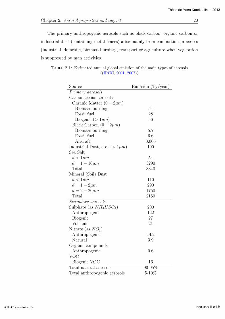
Chapter 2. Aerosol properties and impact 20
The primary anthropogenic aerosols such as black carbon, organic carbon or
industrial dust (containing metal traces) arise mainly from combustion processes
(industrial, domestic, biomass burning), transport or agriculture when vegetation
is suppressed by man activities.
Table 2.1: Estimated annual global emission of the main types of aerosols((IPCC, 2001, 2007))
Source Emission (Tg/year)Primary aerosolsCarbonaceous aerosols
Organic Matter (0− 2µm)Biomass burning 54Fossil fuel 28Biogenic (> 1µm) 56
Black Carbon (0− 2µm)Biomass burning 5.7Fossil fuel 6.6Aircraft 0.006
Industrial Dust, etc. (> 1µm) 100Sea Saltd < 1µm 54d = 1− 16µm 3290Total 3340
Mineral (Soil) Dustd < 1µm 110d = 1− 2µm 290d = 2− 20µm 1750Total 2150
Secondary aerosolsSulphate (as NH4HSO4) 200
Anthropogenic 122Biogenic 27Volcanic 21
Nitrate (as NO3)Anthropogenic 14.2Natural 3.9
Organic compoundsAnthropogenic 0.6
VOCBiogenic VOC 16
Total natural aerosols 90-95%Total anthropogenic aerosols 5-10%

Chapter 2. Aerosol properties and impact 21
Secondary inorganic aerosols (sulphates, nitrates, ammonium) or organic come
from gas-particle transformation processes through the phenomena of nucleation,
condensation or adsorption. The precursor gas can come from emissions from
the soil (e.g. due to the use of fertilizers), vegetation (biogenic VOC) or human
activities (combustion of fossil fuels in energy production, transport, industrial
activities, etc.).
Table 2.1 reveals that only 5 to 10% of the total mass of aerosols emitted an-
nually in the world come from human activities. However, we see that some coarse
particles and the majority of fine particles having an impact on health, environ-
ment and climate as carbon soot and sulfates, are derived from anthropogenic
emissions.
2.1.2 Chemical composition
Chemical composition of aerosols depends on sources of emission and the trans-
formations they undergo in the atmosphere. We describe here the main chemical
species constituting the aerosol (following IPCC, 2001). To estimate the radiative
effects of aerosol, information is required about particle size, refractive index, and
whether the minerals are mixed externally or as aggregates (Tegen et al., 1996;
Sokolik and Toon, 1999; Jacobson, 2001).
Soil dust. Soil dust is a major contributor to aerosol loading and optical thick-
ness. Median diameters of dust particles are 2 < d < 4µm. The atmospheric
lifetime of dust depends on particle size; large particles are quickly removed from
the atmosphere by gravitational settling, while sub-micron sized particles can have
atmospheric lifetimes of several weeks (Marticorena et al., 1997; Miller and Tegen,
1998).
Sea salt. The emission of sea salt depends of wind on the surface of the ocean.
Sea salt particles cover a wide size range (0.05 < d < 10µm), and have a cor-
respondingly wide range of atmospheric lifetimes. This aerosol is dominant con-
tributor to both light scattering and cloud nuclei. It is very efficient CCN (cloud
Chapter 2. Aerosol properties and impact 22
condensation nuclei), and therefore characterization of their surface production is
of importance for aerosol indirect effects (Gong et al., 1998).
Industrial dust, primary anthropogenic aerosols. These aerosol sources are
responsible for the most conspicuous impact of anthropogenic aerosols on environ-
mental quality, and have been widely monitored and regulated.
Carbonaceous aerosols (organic and black carbon). Organic carbon can be emit-
ted directly into the atmosphere (OC) by sources of anthropogenic origin (burning
of petroleum, wood, garbage, cooking meat, etc.) or natural (leaf abrasion by the
wind). But it can also be formed by nucleation or condensation of products of
photochemical degradation of volatile organic compounds (VOCs). This is called
secondary organic aerosol (SOA). VOCs can come from the vegetation (terpenes,
limonene, etc.) or be derived from anthropogenic sources (benzene, toluene, etc.).
It comes from combustion processes (fossil fuel and biomass) and has little chem-
ical reactivity (Andreae and Crutzen, 1997). Of particular importance for the
direct effect is the light-absorbing character of some carbonaceous species, such as
soot and tarry substances (Hansen et al., 1997; Haywood and Ramaswamy, 1998;
Penner et al., 1998).
Primary biogenic aerosols. They consist of plant debris and microbial particles
(cuticular waxes, leaf fragments, bacteria, fungi, viruses, algae, pollen, spores,
etc.). The presence of humic-like substances makes this aerosol light-absorbing in
the UV region (Havers et al., 1998). Primary biogenic particles are able to act
both as cloud droplet and ice nuclei (Schnell and Vali, 1976). Therefore, they are
important for both direct and indirect climate effects.
Sulfates. This species are formed mainly in the aqueous phase by condensa-
tion of sulfuric acid emitted primarily by industrial activities appear as particles
when the droplets evaporate without precipitation. Sulphate in aerosol particles
is present as sulphuric acid, ammonium sulphate, and intermediate compounds,
depending on the availability of gaseous ammonia to neutralize the sulphuric acid
formed from SO2 (Adams et al., 1999). The chemical pathway of conversion of
precursors to sulphate is important because it changes the radiative effects. Most
Chapter 2. Aerosol properties and impact 23
SO2 is converted to sulphate either in the gas phase or in cloud droplets that later
evaporate (Weber et al., 1999).
Nitrates. The nitric acid has two ways of formation. Firstly, it appears in the
gas phase, and secondly, on heterogeneous phase in particles or water droplets in
clouds. Ammonia is a base that will neutralize part of nitric acid to form particu-
late ammonium nitrate according to temperature and ambient relative humidity.
Nitrates are not considered in assessments of the radiative effects of aerosols be-
cause they cause only 2% of the total direct forcing (Andreae, 1995). They are
important only at a regional scale (ten Brink et al., 1996).
Volcanic aerosols. There are two main components of volcanic emissions: pri-
mary dust and gaseous sulphur (mainly in the form of SO2) (Graf et al., 1997).
Continuous eruptive activity is about 4 Tg/yr (Jones et al., 1994), that is three
orders of magnitude smaller than soil dust emission but big eruptions can lead to
significant climate effects. The well-known example is Pinatubo eruption in 1991
(Stenchikov et al., 1998).
2.1.3 Size distribution
The size of the aerosol extends over a wide range of radii ranging from several
nanometers to several tens of microns. Size varies with the nature of the source of
particle production and according to reactions undergone by aerosols during the
time they are present in the atmosphere (nucleation, coagulation, and condensa-
tion of gas to the particulate state). Suitable for the characterization of the size
of a population of aerosols, the size distribution is used to quantify the number
of particles of a certain radius. It presents one or more modes. The aspect of a
multi-modal distribution of aerosols in the troposphere has been shown by Junge
(1955) and more recently updated by Whitby (1978).
Fig. 2.1 presents the mass distribution of a population of particles of different
aerodynamic diameters. The aerodynamic diameter is the diameter of a spherical
particle with a density of 1 g/cm3 should be to present the same settling velocity
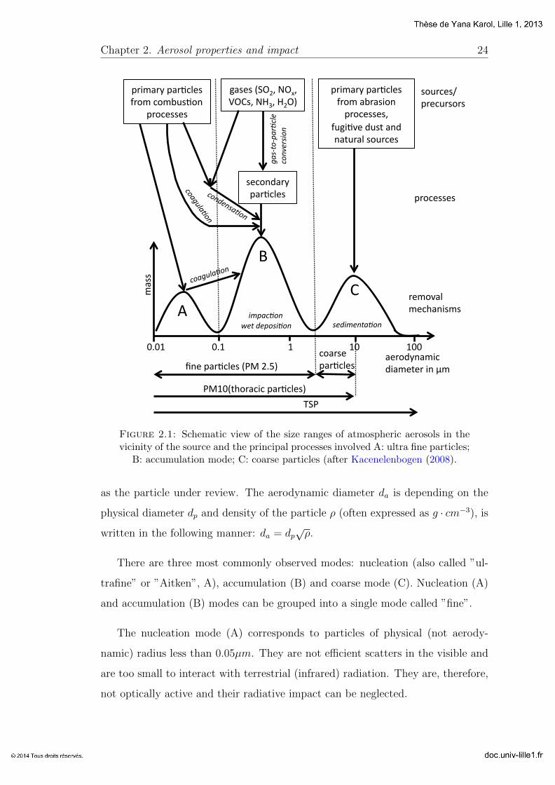
Chapter 2. Aerosol properties and impact 24
!"
#"
$"
%&%'""""""""""""""""""""%&'"""""""""""""""""""""""""""'""""""""""""""""""""""""'%""""""""""""""""""""'%%""""""()*+,-.(/01",0(/)2)*"0."3/"
1+(*4)"5(*617)4"8.)"5(*617)4"9:;"<&=>"
?@:"
:;'%92A+*(101"5(*617)4>"
/(44"
5*+1)44)4"
*)/+B(7"/)1A(.04/4"
4)1+.,(*-"5(*617)4"
C(4)4"9@D<E"FDGE"HD$4E"FIJE"I<D>"
5*0/(*-"5(*617)4"K*+/"(L*(40+."5*+1)44)4E"
KMC06B)",M42"(.,".(2M*(7"4+M*1)4"
4+M*1)4N"5*)1M*4+*4"
!"#$%&$'"()*+,-
*&./,(#0&.
-
5*0/(*-"5(*617)4"K*+/"1+/LM46+."
5*+1)44)4"
*&"!1+")&
.-
02'"*)&.-3,%-4,'�)&.- #,402,.%")&.-
Figure 2.1: Schematic view of the size ranges of atmospheric aerosols in thevicinity of the source and the principal processes involved A: ultra fine particles;
B: accumulation mode; C: coarse particles (after Kacenelenbogen (2008).
as the particle under review. The aerodynamic diameter da is depending on the
physical diameter dp and density of the particle ρ (often expressed as g · cm−3), is
written in the following manner: da = dp√ρ.
There are three most commonly observed modes: nucleation (also called ”ul-
trafine” or ”Aitken”, A), accumulation (B) and coarse mode (C). Nucleation (A)
and accumulation (B) modes can be grouped into a single mode called ”fine”.
The nucleation mode (A) corresponds to particles of physical (not aerody-
namic) radius less than 0.05µm. They are not efficient scatters in the visible and
are too small to interact with terrestrial (infrared) radiation. They are, therefore,
not optically active and their radiative impact can be neglected.
Chapter 2. Aerosol properties and impact 25
The accumulation mode (B) represents a physical particle radius between
0.05µm and 1µm. They come from the aggregation of smaller particles, from
the condensation of gases or the re-evaporation of droplets. Aerosols of this type
are of great importance from the climate viewpoint because their interaction with
the light is maximal (since their size is of the order of the wavelength in the visible
part of the solar spectrum) and their presence time in the atmosphere is significant.
Moreover, droplets form from the accumulation mode of the aerosols.
Finally, the coarse mode (C) corresponds to particles of radius more than 1µm
that mostly have natural and primary type. Note that close to a source of aerosols,
the size distribution of particles’ population is often observed as mono-modal. The
size distribution evolves into a bi-modal when the residence time of particles in
the atmosphere increases or in the presence of two distinct sources of aerosols of
different types.
Mathematically, the lognormal distribution can well characterize a population
covering a wide range of sizes. Variation in the number of particles n as a function
of the natural logarithm of the radius r can be written such as
n(r) =dN
d lnr=
n0
σ0
√2π
exp[− (lnr − lnr0)2
2σ20
](2.1)
where n(r) is the number of particles, the natural logarithm of the radius is between
lnr and lnr + d lnr, r0 is the modal radius, σ0 is the standard deviation of the
natural logarithm of the radius (the width of the distribution) and n0 is the number
of particles in the mode considered.
A multi-modal distribution is simply described by a sum of log-normal distri-
butions. The most used is bi-modal lognormal size distribution.
It is not always relevant to use the distribution of the number of particles.
The distribution of the surface is more appropriate if we are interested in chemical
Chapter 2. Aerosol properties and impact 26
reactions involving aerosols:
dS
d lnr=
S0
σ2
√2π
exp[− (lnr − lnr2)2
2σ22
](2.2)
If one seeks to evaluate the mass of aerosols, the distribution of volume V will
be interesting. This can be written
dV
d lnr=
V0
σ3
√2π
exp[− (lnr − lnr3)2
2σ23
](2.3)
where r3 and σ3 are defined in the same way as above, and V0 is the volume
concentration of particles. Knowing that the radius of the modal distribution of
the n-th power of the radius is given for the log-normal r0exp(−nσ20) and the
standard deviations remain unchanged (σ3 = σ0), we pass from modal radius
distribution volume for that of the distribution of the number by
r0 = r3 exp(−3σ20) (2.4)
r3 is higher than r0, which reflects the fact that the volume distribution is shifted
towards larger particles, which contribute the most.
2.1.4 Refractive index
The refractive index is a major property of the aerosol since it impacts the phase
matrix and the single scattering albedo. Its complex value is determined as:
m = n+ ik (2.5)
where n = Re(m) is real part and k = Im(m) is imaginary part of complex
refractive index.
Chapter 2. Aerosol properties and impact 27
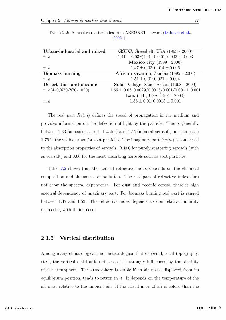
Table 2.2: Aerosol refractive index from AERONET network (Dubovik et al.,2002a).
Urban-industrial and mixed GSFC, Greenbelt, USA (1993 - 2000)n, k 1.41− 0.03τ(440)± 0.01; 0.003± 0.003
Mexico city (1999 - 2000)n, k 1.47± 0.03; 0.014± 0.006Biomass burning African savanna, Zambia (1995 - 2000)n, k 1.51± 0.01; 0.021± 0.004Desert dust and oceanic Solar Vilage, Saudi Arabia (1998 - 2000)n, k(440/670/870/1020) 1.56± 0.03; 0.0029/0.0013/0.001/0.001± 0.001
Lanai, HI, USA (1995 - 2000)n, k 1.36± 0.01; 0.0015± 0.001
The real part Re(m) defines the speed of propagation in the medium and
provides information on the deflection of light by the particle. This is generally
between 1.33 (aerosols saturated water) and 1.55 (mineral aerosol), but can reach
1.75 in the visible range for soot particles. The imaginary part Im(m) is connected
to the absorption properties of aerosols. It is 0 for purely scattering aerosols (such
as sea salt) and 0.66 for the most absorbing aerosols such as soot particles.
Table 2.2 shows that the aerosol refractive index depends on the chemical
composition and the source of pollution. The real part of refractive index does
not show the spectral dependence. For dust and oceanic aerosol there is high
spectral dependency of imaginary part. For biomass burning real part is ranged
between 1.47 and 1.52. The refractive index depends also on relative humidity
decreasing with its increase.
2.1.5 Vertical distribution
Among many climatological and meteorological factors (wind, local topography,
etc.), the vertical distribution of aerosols is strongly influenced by the stability
of the atmosphere. The atmosphere is stable if an air mass, displaced from its
equilibrium position, tends to return in it. It depends on the temperature of the
air mass relative to the ambient air. If the raised mass of air is colder than the
Chapter 2. Aerosol properties and impact 28
surrounding air, it will be denser and will go down again to its starting level. We
say, in this case, the atmosphere is stable.
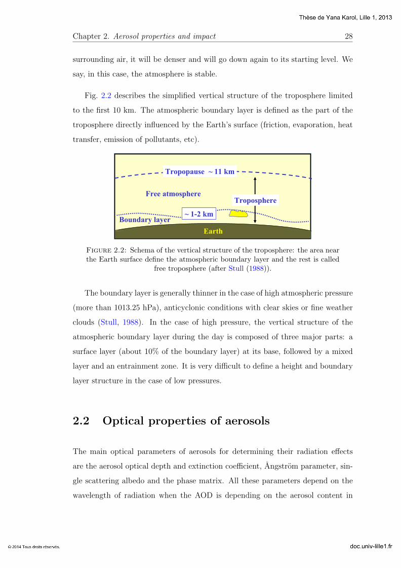
Fig. 2.2 describes the simplified vertical structure of the troposphere limited
to the first 10 km. The atmospheric boundary layer is defined as the part of the
troposphere directly influenced by the Earth’s surface (friction, evaporation, heat
transfer, emission of pollutants, etc).
J. R. Garratt The atmospheric boundary layer Cambridge University Press, 1992
R. B. Stull An introduction to boundary layer meteorologyKluwer Academic Publishers, Dordrecht, 1988
A comprehensive list of textbooks is given by Garratt (see pp12-13)
Literature
Boundary layer
Free atmosphere
Tropopause ~ 11 km
~ 1-2 km
Troposphere
Earth
Often only the lowest 2 km are directly modified by the boundary layer (BL).
The boundary layer is that part of the troposphere that is directly influenced by the presence of the earth’s surface, and responds to surface forcing with a timescale of about an hour or less.
Figure 2.2: Schema of the vertical structure of the troposphere: the area nearthe Earth surface define the atmospheric boundary layer and the rest is called
free troposphere (after Stull (1988)).
The boundary layer is generally thinner in the case of high atmospheric pressure
(more than 1013.25 hPa), anticyclonic conditions with clear skies or fine weather
clouds (Stull, 1988). In the case of high pressure, the vertical structure of the
atmospheric boundary layer during the day is composed of three major parts: a
surface layer (about 10% of the boundary layer) at its base, followed by a mixed
layer and an entrainment zone. It is very difficult to define a height and boundary
layer structure in the case of low pressures.
2.2 Optical properties of aerosols
The main optical parameters of aerosols for determining their radiation effects
are the aerosol optical depth and extinction coefficient, Angstrom parameter, sin-
gle scattering albedo and the phase matrix. All these parameters depend on the
wavelength of radiation when the AOD is depending on the aerosol content in
Chapter 2. Aerosol properties and impact 29
the atmosphere. It is also necessary to know the horizontal and vertical distri-
bution of aerosol layers. For computing the aerosol radiative impact, the albedo
of the cloud or of the underlying Earth’s surface is required. The presence of
aerosols in the atmosphere generally leads to a negative effect, i.e. to the cooling
of the Earth’s surface. However, partially absorbing aerosol over bright (scatter-
ing) surfaces (clouds, snow, ice, deserts) may contribute to the warming of the
surface-atmosphere system.
2.2.1 Aerosol optical depth and extinction coefficient
From the Bouguer-Lambert-Beer law, the sun irradiance E(λ, z) at wavelength λ
at an altitude z above sea level is written (Bohren and Huffman, 1998):
E(λ, z) = tg(λ, z)E0(λ)e−τ(λ,z)m (2.6)
where E0(λ) is the extraterrestrial sun irradiance; tg(λ, z) is the gaseous transmis-
sion; m is an airmass proportional to 1/ cos(θs) when refraction is neglected; θs is
a solar zenith angle; τ(λ, z) is the spectral total optical depth of the atmospheric
layer from altitude z to the top of the atmosphere (TOA) and is the sum of aerosol
extinction and molecular (Rayleigh) scattering optical depths:
τ(λ, z) = τaext(λ, z) + τmext(λ, z) (2.7)
The aerosol optical thickness τaext (AOT) is the sum of the thickness of optical
absorption and scattering: τaext = τdiff + τabs represents the extinction of radiation
by aerosol layer integrated along the atmospheric column. It is defined as follows:
τaext(λ, z) =
TOA∫z
σaext(λ, z′)dz′ (2.8)
And then
σaext =dτaext
dz(2.9)

Chapter 2. Aerosol properties and impact 30
For a set of spherical aerosols, the extinction coefficient σaext(λ, z) (m−1) is
written:
σext(λ, z) =
∞∫0
πr2Qext(m, r, z, λ)n(r, z)dr (2.10)
where the extinction efficiency factor Qext depends on the refractive index m, the
particle size r, the wavelength λ and altitude z The size distribution of a set of
particles n(r, z) is also, strictly speaking, depending on the altitude.
It is useful to introduce the extinction cross section sext (m2) that is the product
of the geometric section of the particle (equal to πr2 for a spherical particle of
radius r) by the efficiency factor for extinction Qext.
As in the case of the extinction optical thickness one can write:
σext = σdiff + σabs, Qext = Qdiff +Qabs, sext = sdiff + sabs.
Table 2.3 represents the values of AOD for different types of aerosols measured
in AERONET network.
Table 2.3: Range of aerosol optical thickness and average AOT fromAERONET network (Dubovik et al., 2002a).
Urban-industrial and mixed GSFC, Greenbelt, USA (1993 - 2000)0.1 6 τ(440) 6 1.0; 〈τ(440)〉 = 0.24
Mexico city (1999 - 2000)0.1 6 τ(440) 6 1.8; 〈τ(440)〉 = 0.43
Biomass burning African savanna, Zambia (1995 - 2000)0.1 6 τ(440) 6 1.5; 〈τ(440)〉 = 0.38
Desert dust and oceanic Solar Vilage, Saudi Arabia (1998 - 2000)0.1 6 τ(1020) 6 1.5; 〈τ(1020)〉 = 0.17
Lanai, HI, USA (1995 - 2000)0.01 6 τ(1020) 6 0.2; 〈τ(1020)〉 = 0.04
2.2.2 Angstrom parameter
Angstrom parameter (Angstrom, 1929) α provides information on the particle size
(Schuster et al., 2006) through the spectral dependence of the AOD. It can be

Chapter 2. Aerosol properties and impact 31
expressed by
τ(λ) = τ(λ0)( λλ0
)−α(2.11)
Larger the spectral dependence of the AOT, larger the Angstrom coefficient,
smaller are the particles.
In the case of molecules (Rayleigh scattering), AOT approximately follows a
law λ−4. Regarding aerosols, the Angstrom parameter ranges from 0 (very large
particles, for example, desert dust) to 3 (very fine particles like urban pollution
aerosol). Note that a population of large particles whose number is distributed on
a single mode can have a slightly negative Angstrom parameter.
Table 2.4: Range of Angstrom parameter from AERONET network (Duboviket al., 2002a).
Urban-industrial and mixed GSFC, Greenbelt, USA (1993 - 2000)1.2 6 α 6 2.5
Mexico city (1999 - 2000)1.0 6 α 6 2.3
Biomass burning African savanna, Zambia (1995 - 2000)1.4 6 α 6 2.2
Desert dust and oceanic Solar Vilage, Saudi Arabia (1998 - 2000)0.1 6 α 6 0.9
Lanai, HI, USA (1995 - 2000)0 6 α 6 1.55
Examples of Angstrom parameter in different regions are presented in table 2.4.
In urban-polluted cities α reaches 2.5, places with only natural aerosol represent
usually α < 1.
2.2.3 Single-scattering albedo
The part of scattering in the extinction is given by the single-scattering albedo ω0
(SSA). It is the ratio of the scattering coefficient and the extinction coefficient of
a set of particles:
ω0 =σscatσext
(2.12)
Chapter 2. Aerosol properties and impact 32
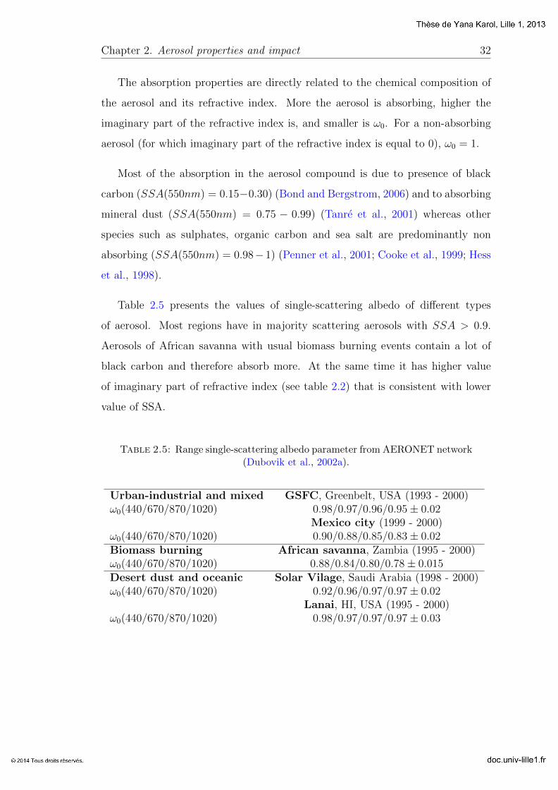
The absorption properties are directly related to the chemical composition of
the aerosol and its refractive index. More the aerosol is absorbing, higher the
imaginary part of the refractive index is, and smaller is ω0. For a non-absorbing
aerosol (for which imaginary part of the refractive index is equal to 0), ω0 = 1.
Most of the absorption in the aerosol compound is due to presence of black
carbon (SSA(550nm) = 0.15−0.30) (Bond and Bergstrom, 2006) and to absorbing
mineral dust (SSA(550nm) = 0.75 − 0.99) (Tanre et al., 2001) whereas other
species such as sulphates, organic carbon and sea salt are predominantly non
absorbing (SSA(550nm) = 0.98− 1) (Penner et al., 2001; Cooke et al., 1999; Hess
et al., 1998).
Table 2.5 presents the values of single-scattering albedo of different types
of aerosol. Most regions have in majority scattering aerosols with SSA > 0.9.
Aerosols of African savanna with usual biomass burning events contain a lot of
black carbon and therefore absorb more. At the same time it has higher value
of imaginary part of refractive index (see table 2.2) that is consistent with lower
value of SSA.
Table 2.5: Range single-scattering albedo parameter from AERONET network(Dubovik et al., 2002a).
Urban-industrial and mixed GSFC, Greenbelt, USA (1993 - 2000)ω0(440/670/870/1020) 0.98/0.97/0.96/0.95± 0.02
Mexico city (1999 - 2000)ω0(440/670/870/1020) 0.90/0.88/0.85/0.83± 0.02Biomass burning African savanna, Zambia (1995 - 2000)ω0(440/670/870/1020) 0.88/0.84/0.80/0.78± 0.015Desert dust and oceanic Solar Vilage, Saudi Arabia (1998 - 2000)ω0(440/670/870/1020) 0.92/0.96/0.97/0.97± 0.02
Lanai, HI, USA (1995 - 2000)ω0(440/670/870/1020) 0.98/0.97/0.97/0.97± 0.03
Chapter 2. Aerosol properties and impact 33
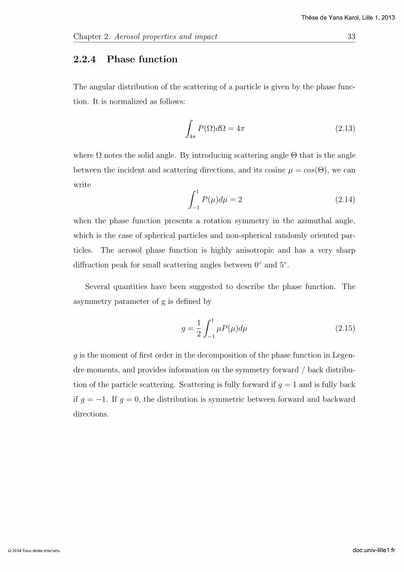
2.2.4 Phase function
The angular distribution of the scattering of a particle is given by the phase func-
tion. It is normalized as follows:
∫4π
P (Ω)dΩ = 4π (2.13)
where Ω notes the solid angle. By introducing scattering angle Θ that is the angle
between the incident and scattering directions, and its cosine µ = cos(Θ), we can
write ∫ 1
−1
P (µ)dµ = 2 (2.14)
when the phase function presents a rotation symmetry in the azimuthal angle,
which is the case of spherical particles and non-spherical randomly oriented par-
ticles. The aerosol phase function is highly anisotropic and has a very sharp
diffraction peak for small scattering angles between 0 and 5.
Several quantities have been suggested to describe the phase function. The
asymmetry parameter of g is defined by
g =1
2
∫ 1
−1
µP (µ)dµ (2.15)
g is the moment of first order in the decomposition of the phase function in Legen-
dre moments, and provides information on the symmetry forward / back distribu-
tion of the particle scattering. Scattering is fully forward if g = 1 and is fully back
if g = −1. If g = 0, the distribution is symmetric between forward and backward
directions.
Chapter 2. Aerosol properties and impact 34
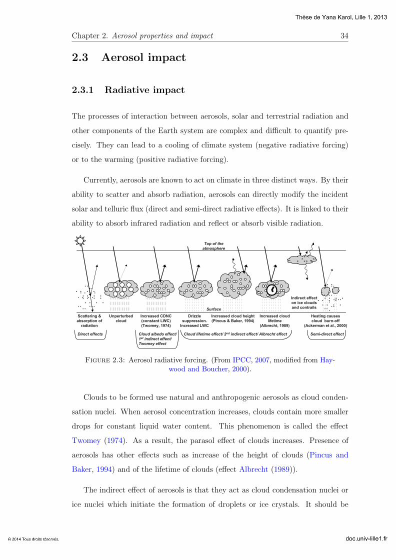
2.3 Aerosol impact
2.3.1 Radiative impact
The processes of interaction between aerosols, solar and terrestrial radiation and
other components of the Earth system are complex and difficult to quantify pre-
cisely. They can lead to a cooling of climate system (negative radiative forcing)
or to the warming (positive radiative forcing).
Currently, aerosols are known to act on climate in three distinct ways. By their
ability to scatter and absorb radiation, aerosols can directly modify the incident
solar and telluric flux (direct and semi-direct radiative effects). It is linked to their
ability to absorb infrared radiation and reflect or absorb visible radiation.
154
Changes in Atmospheric Constituents and in Radiative Forcing Chapter 2
!"#$"% &'(% &)*% +,-.% /0-12--(/% 3'(% 045+13% .6% +73'8.5.9(701%+(8.-.,-% .7% 3'(% 6.84+30.7% +7/% 4./0!%1+30.7% .6% 3'(% 5':-01+,%+7/% 8+/0+30;(% 58.5(830(-% .6% 01(% 1,.2/-% <=(77(8! (3% +,">% ?@@A$>%+,3'.29'% B2+730!%1+30.7% .6% +7% *C% 68.4% 3'0-% 4(1'+70-4% D+-%7.3%1.7-0/(8(/%+558.580+3(%90;(7%3'(%'.-3%.6%271(83+0730(-%+7/%27E7.D7-%-288.27/079%01(%1,.2/%721,(+30.7%+7/%5':-01-"&'(%&)*%/0/%7.3%071,2/(%+7:%+--(--4(73%.6%3'(%-(40F/08(13%
(66(13% <("9">% G+7-(7% (3% +,">% AHH!I% )1E(84+7% (3% +,">% ?@@@+I%J+1.K-.7>% ?@@?I% L(7.7% (3% +,">% ?@@MI% N..E% +7/% G09'D../>%?@@OI%J.'7-.7%(3%+,">%?@@O$>%D'01'%0-%3'(%4(1'+70-4%K:%D'01'%+K-.8530.7% .6% -'.83D+;(% 8+/0+30.7% K:% 38.5.-5'(801% +(8.-.,-%,(+/-% 3.% '(+3079% .6% 3'(% 38.5.-5'(8(% 3'+3% 07% 3287% 1'+79(-% 3'(%8(,+30;(% '240/03:% +7/% 3'(% -3+K0,03:% .6% 3'(% 38.5.-5'(8(% +7/%3'(8(K:%07"%2(71(-%1,.2/%6.84+30.7%+7/%,06(304("%P7%3'0-%8(5.83>%3'(%-(40F/08(13%(66(13%0-%7.3%-38013,:%1.7-0/(8(/%+7%*C%K(1+2-(%.6%4./0!%1+30.7-%3.%3'(%':/8.,.901+,%1:1,(>%+-%/0-12--(/%07%Q(130.7%!"#%<-((%+,-.%Q(130.7-%?"?>%?"R%+7/%?"O"#$"Q071(%3'(%&)*>%3'(8(%'+;(%K((7%-2K-3+730+,%/(;(,.54(73-%07%
.K-(8;+30.7-%+7/%4./(,,079%.6%38.5.-5'(801%+(8.-.,-I%3'(-(%+8(%/0-12--(/%07%3287%07%3'(%6.,,.D079%-(130.7-"
2.4.2 Developments Related to Aerosol Observations
Q286+1(FK+-(/% 4(+-28(4(73-% .6% +(8.-.,% 58.5(830(-% -21'%+-% -0S(% /0-380K230.7>% 1'(401+,% 1.45.-030.7>% -1+33(8079% +7/%+K-.8530.7%1.73072(%3.%K(%5(86.84(/%+3%+%724K(8%.6%-03(->%(03'(8%+3%,.79F3(84%4.703.8079%-03(->%.8%-5(10!%1+,,:%+-%5+83%.6%073(7-0;(%!%(,/%1+45+097-"%&'(-(%"#!$"%&%4(+-28(4(73-%58.;0/(%(--(730+,%;+,0/+30.7% 6.8% 9,.K+,% 4./(,->% 6.8% (T+45,(>% K:% 1.7-38+07079%+(8.-.,% 1.71(738+30.7-% +3% 3'(% -286+1(% +7/% K:% 58.;0/079% '09'F
B2+,03:% 076.84+30.7% +K.23% 1'(401+,% 1.45.-030.7% +7/% ,.1+,%38(7/-"% P7% +//030.7>% 3'(:% 58.;0/(% E(:% 076.84+30.7% +K.23%;+80+K0,03:% .7% ;+80.2-% 304(% -1+,(-"% N.45+80-.7-% .6% "#! $"%&%4(+-28(4(73-% +9+07-3% 3'.-(% 68.4%9,.K+,% +34.-5'(801%4./(,-%+8(%1.45,01+3(/%K:%/066(8(71(-%07%4(3(.8.,.901+,%1.7/030.7-%+7/%K(1+2-(%"#!$"%&%4(+-28(4(73-%+8(%8(58(-(73+30;(%.6%1.7/030.7-%4.-3,:%+3%.8%7(+8%3'(%-286+1(%D'0,(%3'(%/08(13%+7/%07/08(13%*C-%/(5(7/%.7%3'(%+(8.-.,%;(8301+,%58.!%,("%C.8%(T+45,(>%3'(%-5+30+,%8(-.,230.7%.6%9,.K+,%4./(,%980/%K.T(-%0-%3:501+,,:%+%6(D%/(98((-%.6%,+3032/(%+7/%,.79032/(%+7/%3'(%304(%-3(5-%6.8%3'(%+34.-5'(801%/:7+401-%+7/%8+/0+30.7%1+,12,+30.7-%4+:%K(%40723(-% 3.%'.28-%/(5(7/079%.7%3'(%58.1(--%3.%K(%-32/0(/I%3'0-%5.-(-%,0403+30.7-%D'(7% 1.45+8079% D03'% .K-(8;+30.7-% 1.7/213(/% .;(8% -4+,,(8%-5+30+,%(T3(73%+7/%-'.83(8%304(%/28+30.7"N.4K07+30.7-% .6% -+3(,,03(% +7/% -286+1(FK+-(/% .K-(8;+30.7-%
58.;0/(%7(+8F9,.K+,%8(380(;+,-%.6%+(8.-.,%58.5(830(-"%&'(-(%+8(%/0-12--(/% 07% 3'0-% -2K-(130.7I% 3'(% (40--0.7-% (-304+3(->% 38(7/-%+7/%"#!$"%&%4(+-28(4(73-%.6%3'(%5':-01+,%+7/%.5301+,%58.5(830(-%+8(%/0-12--(/%D03'%8(-5(13%3.%3'(08%07"%2(71(%.7%*C%07%Q(130.7%?"O"O"% C283'(8% /(3+0,(/% /0-12--0.7-% .6% 3'(% 8(1(73% -+3(,,03(%.K-(8;+30.7-%.6%+(8.-.,%58.5(830(-%+7/%+%-+3(,,03(F4(+-28(4(73%K+-(/%+--(--4(73%.6% 3'(%+(8.-.,%/08(13%*C%+8(%90;(7%K:%U2%(3%+,"%<?@@V$"%
!"#"!"$% &'()**+()%,)(-+).'*/
Q+3(,,03(% 8(380(;+,-% .6% +(8.-.,% .5301+,% /(53'% 07% 1,.2/F68((%8(90.7-%'+;(%0458.;(/%;0+%7(D%9(7(8+30.7%-(7-.8-%<W+264+7%(3%+,">%?@@?$%+7/%+7%(T5+7/(/%9,.K+,%;+,0/+30.7%58.98+4%<G.,K(7%(3%+,">%?@@A$"%)/;+71(/%+(8.-.,%8(380(;+,%58./213-%-21'%+-%+(8.-.,%!%7(F4./(% 68+130.7% +7/% (66(130;(% 5+8301,(% 8+/02-% '+;(% K((7%
Figure 2.10. Schematic diagram showing the various radiative mechanisms associated with cloud effects that have been identifi ed as signifi cant in relation to aerosols (modifi ed from Haywood and Boucher, 2000). The small black dots represent aerosol particles; the larger open circles cloud droplets. Straight lines represent the incident and refl ected solar radiation, and wavy lines represent terrestrial radiation. The fi lled white circles indicate cloud droplet number concentration (CDNC). The unperturbed cloud con-tains larger cloud drops as only natural aerosols are available as cloud condensation nuclei, while the perturbed cloud contains a greater number of smaller cloud drops as both natural and anthropogenic aerosols are available as cloud condensation nuclei (CCN). The vertical grey dashes represent rainfall, and LWC refers to the liquid water content.
Figure 2.3: Aerosol radiative forcing. (From IPCC, 2007, modified from Hay-wood and Boucher, 2000).
Clouds to be formed use natural and anthropogenic aerosols as cloud conden-
sation nuclei. When aerosol concentration increases, clouds contain more smaller
drops for constant liquid water content. This phenomenon is called the effect
Twomey (1974). As a result, the parasol effect of clouds increases. Presence of
aerosols has other effects such as increase of the height of clouds (Pincus and
Baker, 1994) and of the lifetime of clouds (effect Albrecht (1989)).
The indirect effect of aerosols is that they act as cloud condensation nuclei or
ice nuclei which initiate the formation of droplets or ice crystals. It should be
Chapter 2. Aerosol properties and impact 35
noted that their indirect effect is important because a significant part of clouds do
not precipitate and the chemical composition of aerosols is modified after passing
through the liquid phase in the clouds (see Fig. 2.3).
The semi-direct effect is due to the solar absorption by aerosols that can modify
the temperature profile of the atmosphere. This affects the conditions of cloud
formation (Ackerman et al., 2000).
Precipitating clouds containing only large drops are not disturbed by an excess
of aerosols. Therefore, the radiative properties of these clouds are not modified
and return to space a small amount of light.
2.3.2 Impact to the environment and peoples’ health
Aerosols can have harmful effects on human health when they are inhaled. Tox-
icological studies have shown their role in some lung functions, the outbreak of
asthma and the increasing number of deaths due to cardiovascular deseases (Liao
et al., 1999; Donaldson et al., 2001). Aerosol particles can carry toxic compounds,
allergens, mutagens or carcinogens, such as polycyclic aromatic hydrocarbons and
heavy metals, which can reach the lungs, where they are absorbed in the blood
and tissues. The harmfulness of aerosols also depends on their concentration and
size (Ramgolam et al., 2009) because the finest particles (diameter inferior to 2.5
microns) can penetrate deeply the respiratory system to reach the lung alveoli.
Health effects of air pollution were sometimes dramatic in the past. The first
evident event that showed the relationship between particulate air pollution and
health impacts took place in Glasgow in 1909 when nearly 1000 deaths were at-
tributed to the sharp increase in concentrations of sulfur dioxide and particulate
matter caused by very stable meteorological conditions. The term ”smog” (smoke-
contraction of smoke and fog, mist) was used for the first time to characterize this
episode. We can identify other tragic events of the same nature, such as Donora
Chapter 2. Aerosol properties and impact 36
(USA) on 26-31 October 1948 (20 dead) or infamous episode of pollution of Lon-
don that had 4000 deaths between 5 and 9 December 1952. During the episode,
the particle concentrations reached 3000µg/m3 (Davis et al., 2002).
These health crisis relating to the excessive use of fossil fuels (especially coal),
lead in most industrialized countries to develop policies for reducing emissions
of gaseous pollutants and particulate. However, the use of fossil fuels in huge
megalopolises in India, China or Africa still make the alarming pollution in these
regions.
Today, in most of the major agglomerations of Western Europe, aerosol con-
centrations are of the order of a few tens of micrograms per cubic meter (in daily
average) following the reduction efforts recently undertaken in industrial countries.
However, the impact on the health of low to moderate concentrations events is not
recognized. Indeed, a 2009 report by the French Agency for Health, Environment
and Labour (l’Agence Francaise de Securite Sanitaire, de l’Environnement et du
Travail, AFSSET) on the effects of particles on health (InVS/Afsse, 2005; Mullot
et al., 2009) shows that there is no threshold concentration of fine particles in
ambient air below which there would be no health impact.
The experts from AFSSET specify that frequent exposure at moderate levels
are more dangerous than occasional exposure of peak concentrations. According
to them, only 3% of health impacts would be caused by high concentrations of
particles. Epidemiologists of the French Institute for Public Health Surveillance
(de l’Institut francais de Veille Sanitaire, InVS) define them as to the impact of
exposure to particulate matter as being ”of the same order as passive smoking”.
In addition, fast development of nanotechnology, more and most used in indus-
try (including nanoparticles of heavy metals) and presented way of growing in
commercial products could pose an additional risk for the health (InVS/Afsse,
2005).
Chapter 2. Aerosol properties and impact 37
2.4 Instruments and methods
Optical measurements for the study of atmospheric aerosols are divided into active
and passive methods. The active methods include laser (lidar) sensing when the
most popular passive method is sunphotometry based on solar radiation measure-
ments after passing through the atmosphere.
Both active and passive instruments can be performed from the surface, from
space or from airplanes. Let us mention additional information to the optical
measurements can be provided by in-situ measurements.
To fully describe the aerosols radiative impact on climate the following infor-
mation have to be available (Veefkind, 1999; Lacis and Mishchenko, 1995):
• the optical constants (complex refractive index) for the chemical compounds
contained in aerosols, at all relevant wavelengths;
• the chemical composition, particle shape, and size distribution of aerosols
species;
• a physical model to describe the effect of hygroscopical particle growth with
changing relative humidity on the aerosol optical properties;
• a cloud microphysical model to determine changes in cloud droplet size, cloud
optical depth, and lifetimes in response to changes in the CCN concentration.
It is clear that such information is not available on a global scale. In fact,
most of the data available on aerosol properties is measured during short-term
campaigns, which might not be relevant for other regions or other seasons, or
even other conditions than encountered during the measurement campaign. Fre-
quent global monitoring of aerosol properties is only achievable by satellite remote
sensing. Therefore a combined effort of ground-based, airborne, satellite remote
sensing, short-term intensive field observations, and three-dimensional chemistry
transport modeling is needed to adequately describe the aerosols impact on cli-
mate.
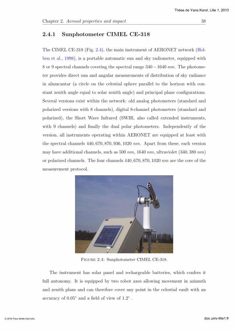
Chapter 2. Aerosol properties and impact 38
2.4.1 Sunphotometer CIMEL CE-318
The CIMEL CE-318 (Fig. 2.4), the main instrument of AERONET network (Hol-
ben et al., 1998), is a portable automatic sun and sky radiometer, equipped with
8 or 9 spectral channels covering the spectral range 340−1640 nm. The photome-
ter provides direct sun and angular measurements of distribution of sky radiance
in almucantar (a circle on the celestial sphere parallel to the horizon with con-
stant zenith angle equal to solar zenith angle) and principal plane configurations.
Several versions exist within the network: old analog photometers (standard and
polarized versions with 8 channels), digital 8-channel photometers (standard and
polarized), the Short Wave Infrared (SWIR, also called extended instruments,
with 9 channels) and finally the dual polar photometers. Independently of the
version, all instruments operating within AERONET are equipped at least with
the spectral channels 440, 670, 870, 936, 1020 nm. Apart from these, each version
may have additional channels, such as 500 nm, 1640 nm, ultraviolet (340, 380 nm)
or polarized channels. The four channels 440, 670, 870, 1020 nm are the core of the
measurement protocol.
Figure 2.4: Sunphotometer CIMEL CE-318.
The instrument has solar panel and rechargeable batteries, which confers it
full autonomy. It is equipped by two robot axes allowing movement in azimuth
and zenith plans and can therefore cover any point in the celestial vault with an
accuracy of 0.05 and a field of view of 1.2 .

Chapter 2. Aerosol properties and impact 39
The data are transmitted via geostationary satellites (or via internet link)
every hour to a processing center (NASA Goddard Space Flight Center). There
are different levels of data processing available: level 1 (raw data), Level 1.5 (cloud
screening is automatically applied but final calibration is not necessarily available)
and level 2 (the cloud screening and the final calibration are applied and data are
screened manually).
The global network of photometers AERONET (AErosol RObotic NETwork)
(Holben et al., 1998) has been operating since early 1990s. The approximate
total number of permanent sites is currently over 200 and around 50 sites are
seasonal (like in the Amazon site where photometers are not installed during the
rainy season). Fig. 2.5 presents the overall distribution of all available stations
measuring network AERONET.
Figure 2.5: Distribution of AERONET stations in the world(September 2012).
The network are managed simultaneously in the United States by NASA
(GSFC) and in Lille by the Laboratory of Atmospheric Optics (LOA). LOA also
ensures the calibration, on-site installation and maintenance of several sites (in-
cluding Europe and Africa). The original French component of the network is the
AERONET PHOTONS network (PHOtometrie pour le Traitement Operationnel
de Normalisation Satellitaire).
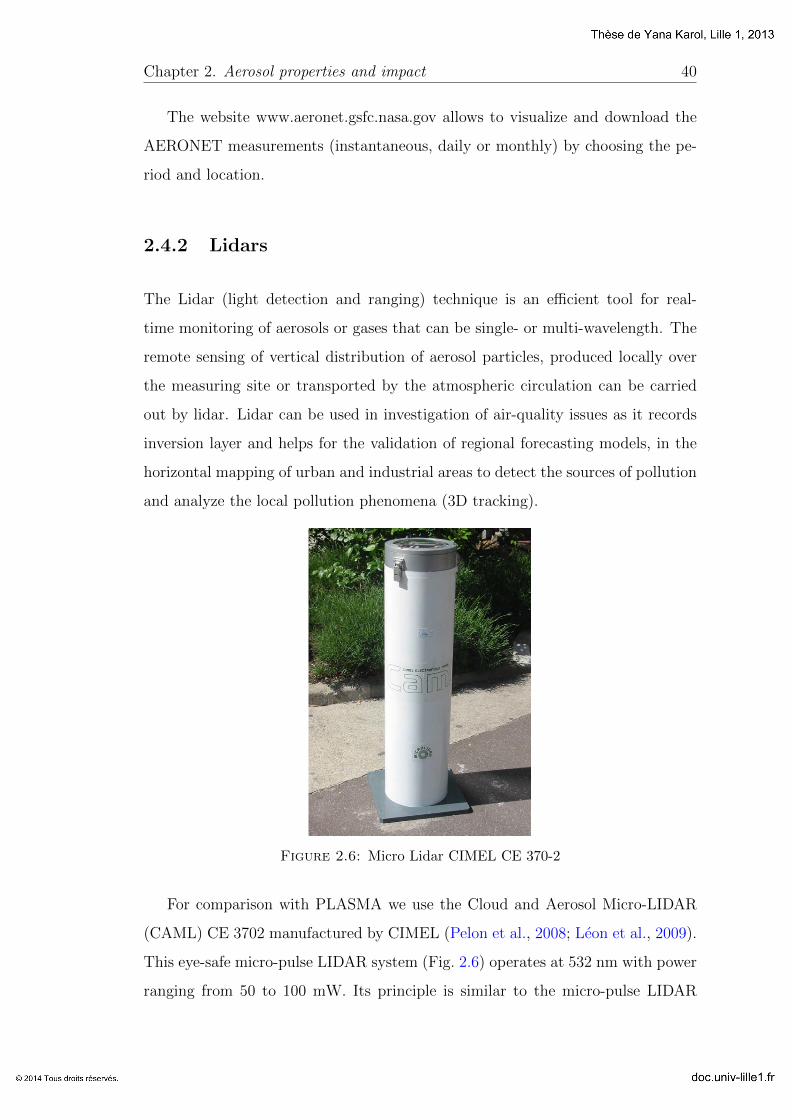
Chapter 2. Aerosol properties and impact 40
The website www.aeronet.gsfc.nasa.gov allows to visualize and download the
AERONET measurements (instantaneous, daily or monthly) by choosing the pe-
riod and location.
2.4.2 Lidars
The Lidar (light detection and ranging) technique is an efficient tool for real-
time monitoring of aerosols or gases that can be single- or multi-wavelength. The
remote sensing of vertical distribution of aerosol particles, produced locally over
the measuring site or transported by the atmospheric circulation can be carried
out by lidar. Lidar can be used in investigation of air-quality issues as it records
inversion layer and helps for the validation of regional forecasting models, in the
horizontal mapping of urban and industrial areas to detect the sources of pollution
and analyze the local pollution phenomena (3D tracking).
!!!!
!"#$%&'"()$&&*+&,-./0
!"#$%#&'&!()*+&,-+&"./)0)(/)&$1+,/&
!"#$%&'&"() *+#,-#+((&'."/) 0!123) 40!/%() 1&(&#(.$") 2"5) 3+"/."/6-7-(&8-) +'&) ,&7) ($$9-) ($) '&('.&:&) -;+(.+9) 5.-('.*<(.$") +"5) $;(.#+9;'$;&'(.&-) $=) +&'$-$9) +"5) #9$<5->) ?<#%) ."=$'8+(.$") .-) #'.(.#+9) ($$;&'+(.$"+9) =.&95) +"5) 9+*) +;;9.#+(.$"-) '&9+(&5) ($) 8&(&$'$9$/7) +"5&":.'$"8&"(>)
!"#$%#&!'&()*+,&-./0121034156-&!
"#$%&'())*#! !"#$%&'&()'*+,-&./,&012&34&
+,)-,)!.$/*0*%1)2! 345!%'!+,)-,)!*%*#16!-*#!-,0&*! 7!89!:*-*)()(;%!#$)*! 3!<=>!?,0&*!@,#$)(;%! !A!%&!BCC*D)(/*!$-*#),#*! 4A7!D'E!F(*0@!;C!/(*.!GC,00!$%10*H! 33!8#$@!F(0)*#!I$%@.(@)2! JK3!%'!L*)*D);#! M?L!L*)*D)(;%!';@*! ?2;);%!D;,%)(%1!MDN,(&()(;%!)('*! O!JKP!&!Q*#)(D$0!#*&;0,)(;%! A3!'!R(>*!G@($'*)*#!S!2*(12)H! 55J!S!AJJJ!''!T*(12)! A5K3!<1!
!
#316&2/3478/-&&!!
R*0CU$0(1%*'*%)!;C!)2*!*'(&&(;%!$%@!#*D*-)(;%!$S(&!B6*!&$C*)6!=(12!@*)*D)(;%!#$%1*!=(12!)*'-;#$0!$%@!/*#)(D$0!#*&;0,)(;%!V;'-,)*#!D;%)#;00*@!GWR!T(%@;.&!+RH!V;%%*D)!)2#;.!$%!XRY!-;#)!V;'-$D)!$%@!-;#)$I0*!
"&6/9&!:57;&36;&"/85-5:н&$1;38&285<&!=#'$&Z%! )2$)! #*&-*D)[! )2*! %*.! VMW\"W! (%&)#,'*%)! 2$&! I**%! @*/*0;-*@! I6! VZWB\! B0*D)#;%(N,*[! (%D;00$I;#$)(;%!.()2!)2*!V*%)#*!]$)(;%$0!@*!0$!:*D2*#D2*!RD(*%)(C(N,*!GV]:RHK!"2*! VMW\"W! VB! 4^JU5[! (&! $! -;#)$I0*[! *6*! &$C*! $%@! ,%$))*%@*@! I$D<&D$))*#(%1! 0(@$#! )2$)! C*$),#*&! )2*$I(0()6! );! -#;C(0*! $)';&-2*#(D! D0;,@! $%@! $*#;&;0! &)#,D),#*&[! $%@! );! #*)#(*/*! $*#;&;0! ;-)(D$0! $%@!@6%$'(D-#;-*#)(*&K!56$&4"73&8$"9:%$#&;8&967#&73#9%:4$39&"%$&96$&#$<8="<7>34$39&;8&96$&$47##7;3&"3)&%$?$@97;3"A7#&"3)&96$&$B$=#"8$9BC!!
1"2"345&6#7"85&
!"#$%&'(%)(%*+,&-..(%/%"01!!%23456%/%7(8%9:;;<%!=;>=?">@;;%/%A,B%9:;;<%!=;>=?C>#C!%
*&9&!&+&'&&&+&4&5&#&7&$&%&:&"&;&<&5& !"""#$%&'(#)*&Figure 2.6: Micro Lidar CIMEL CE 370-2
For comparison with PLASMA we use the Cloud and Aerosol Micro-LIDAR
(CAML) CE 3702 manufactured by CIMEL (Pelon et al., 2008; Leon et al., 2009).
This eye-safe micro-pulse LIDAR system (Fig. 2.6) operates at 532 nm with power
ranging from 50 to 100 mW. Its principle is similar to the micro-pulse LIDAR
Chapter 2. Aerosol properties and impact 41
system (Welton et al., 2001). The link from the rack to the telescope is ensured
by a 10 m optical fiber and the same telescope is used for both emission and
reception avoiding the alignment problem. The aerosol extinction profile as well
as the effective extinction-to-backscatter ratio are retrieved using combination of
lidar data and sun-photometer AOD (Leon et al., 2009).
In the European region, regular monitoring of the state of the atmosphere are
carried out in the framework of international lidar and combine lidar-photometer
networks EARLINET -European Aerosol Research Lidar Network (Bosenberg,
2003; Rocadenbosch et al., 2008), CIS-LiNet - CIS Lidar Network (Chaikovsky
et al., 2005), GALION - GAW Aerosol Lidar Observation Network (Bosenberg
and Hoff, 2007), GAW - Global Atmospheric Watch (WMO/GAW, 2007), EMEP
- Cooperative Programme for Monitoring and Evaluation of the Long-range Trans-
mission of Air Pollutants in Europe http://www.emep.int/, NDACC - Network
for the Detection of Atmospheric Composition Change http://www.ndsc.ncep.
noaa.gov/.
2.4.3 Airborne instruments
Several airborne sunphotometer were recently developed and we shortly describe
these instruments.
AATS-6 and AATS-14
The 6- and 14-channel NASA Ames Airborne Tracking Sunphotometer AATS-6
(Matsumoto et al., 1987) and AATS-14 (Schmid et al., 2003) measure the transmis-
sion of the solar beam in 6 or 14 spectral channels. Azimuth and elevation motors
controlled by differential sun sensors rotate a tracking head, locking onto the solar
beam and keeping detectors normal to it. The AATS tracking head mounts out-
side the aircraft skin, to minimize blockage by aircraft structures and avoid data
contamination by aircraft-window effects. The spectral range is 380−1021 nm for
AATS-6 and 354− 2139 nm for AATS-14.
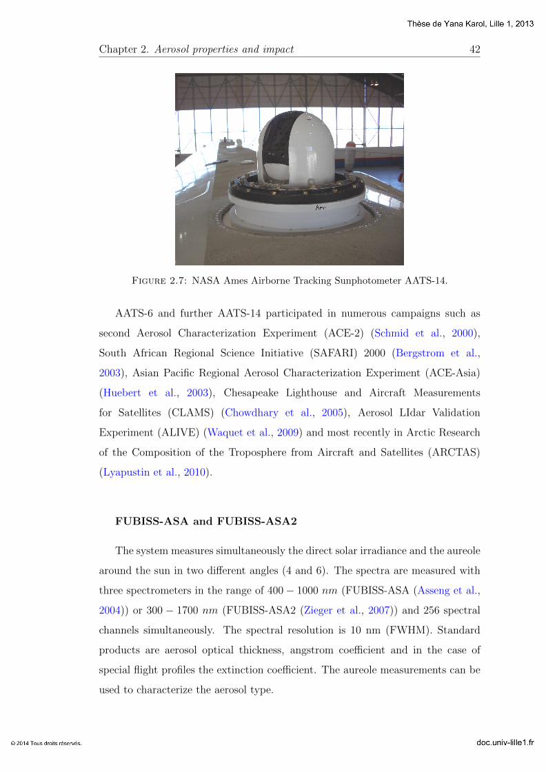
Chapter 2. Aerosol properties and impact 42
Figure 2.7: NASA Ames Airborne Tracking Sunphotometer AATS-14.
AATS-6 and further AATS-14 participated in numerous campaigns such as
second Aerosol Characterization Experiment (ACE-2) (Schmid et al., 2000),
South African Regional Science Initiative (SAFARI) 2000 (Bergstrom et al.,
2003), Asian Pacific Regional Aerosol Characterization Experiment (ACE-Asia)
(Huebert et al., 2003), Chesapeake Lighthouse and Aircraft Measurements
for Satellites (CLAMS) (Chowdhary et al., 2005), Aerosol LIdar Validation
Experiment (ALIVE) (Waquet et al., 2009) and most recently in Arctic Research
of the Composition of the Troposphere from Aircraft and Satellites (ARCTAS)
(Lyapustin et al., 2010).
FUBISS-ASA and FUBISS-ASA2
The system measures simultaneously the direct solar irradiance and the aureole
around the sun in two different angles (4 and 6). The spectra are measured with
three spectrometers in the range of 400− 1000 nm (FUBISS-ASA (Asseng et al.,
2004)) or 300 − 1700 nm (FUBISS-ASA2 (Zieger et al., 2007)) and 256 spectral
channels simultaneously. The spectral resolution is 10 nm (FWHM). Standard
products are aerosol optical thickness, angstrom coefficient and in the case of
special flight profiles the extinction coefficient. The aureole measurements can be
used to characterize the aerosol type.
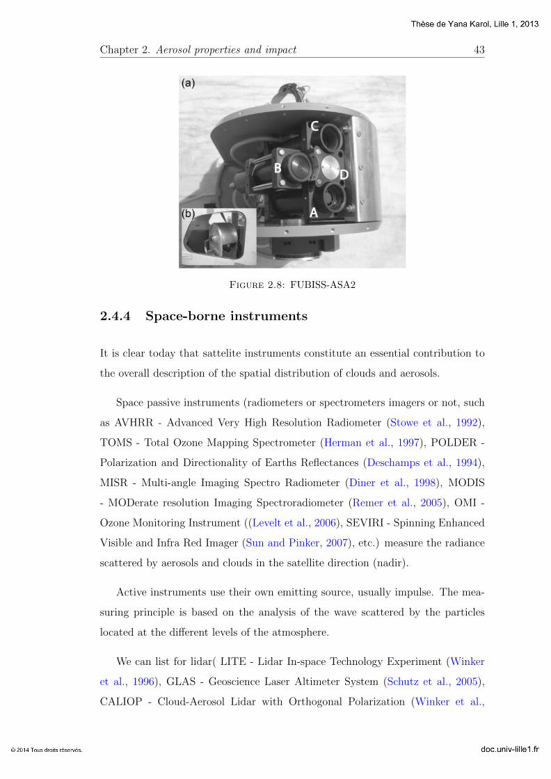
Chapter 2. Aerosol properties and impact 43
Figure 2.8: FUBISS-ASA2
2.4.4 Space-borne instruments
It is clear today that sattelite instruments constitute an essential contribution to
the overall description of the spatial distribution of clouds and aerosols.
Space passive instruments (radiometers or spectrometers imagers or not, such
as AVHRR - Advanced Very High Resolution Radiometer (Stowe et al., 1992),
TOMS - Total Ozone Mapping Spectrometer (Herman et al., 1997), POLDER -
Polarization and Directionality of Earths Reflectances (Deschamps et al., 1994),
MISR - Multi-angle Imaging Spectro Radiometer (Diner et al., 1998), MODIS
- MODerate resolution Imaging Spectroradiometer (Remer et al., 2005), OMI -
Ozone Monitoring Instrument ((Levelt et al., 2006), SEVIRI - Spinning Enhanced
Visible and Infra Red Imager (Sun and Pinker, 2007), etc.) measure the radiance
scattered by aerosols and clouds in the satellite direction (nadir).
Active instruments use their own emitting source, usually impulse. The mea-
suring principle is based on the analysis of the wave scattered by the particles
located at the different levels of the atmosphere.
We can list for lidar( LITE - Lidar In-space Technology Experiment (Winker
et al., 1996), GLAS - Geoscience Laser Altimeter System (Schutz et al., 2005),
CALIOP - Cloud-Aerosol Lidar with Orthogonal Polarization (Winker et al.,
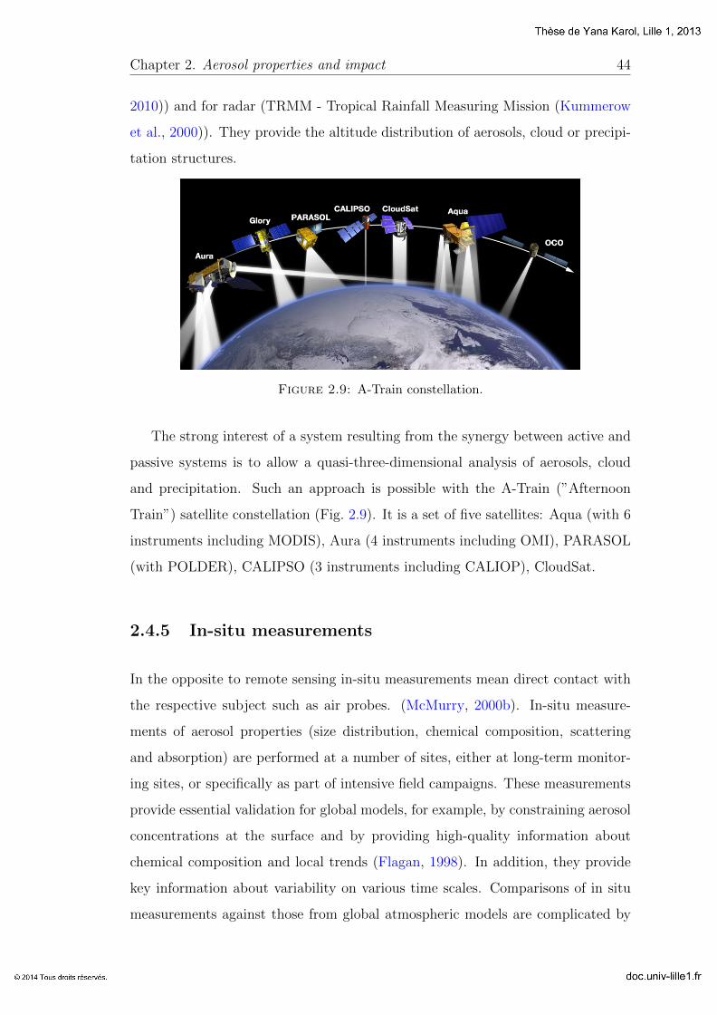
Chapter 2. Aerosol properties and impact 44
2010)) and for radar (TRMM - Tropical Rainfall Measuring Mission (Kummerow
et al., 2000)). They provide the altitude distribution of aerosols, cloud or precipi-
tation structures.
Figure 2.9: A-Train constellation.
The strong interest of a system resulting from the synergy between active and
passive systems is to allow a quasi-three-dimensional analysis of aerosols, cloud
and precipitation. Such an approach is possible with the A-Train (”Afternoon
Train”) satellite constellation (Fig. 2.9). It is a set of five satellites: Aqua (with 6
instruments including MODIS), Aura (4 instruments including OMI), PARASOL
(with POLDER), CALIPSO (3 instruments including CALIOP), CloudSat.
2.4.5 In-situ measurements
In the opposite to remote sensing in-situ measurements mean direct contact with
the respective subject such as air probes. (McMurry, 2000b). In-situ measure-
ments of aerosol properties (size distribution, chemical composition, scattering
and absorption) are performed at a number of sites, either at long-term monitor-
ing sites, or specifically as part of intensive field campaigns. These measurements
provide essential validation for global models, for example, by constraining aerosol
concentrations at the surface and by providing high-quality information about
chemical composition and local trends (Flagan, 1998). In addition, they provide
key information about variability on various time scales. Comparisons of in situ
measurements against those from global atmospheric models are complicated by
Chapter 2. Aerosol properties and impact 45
differences in meteorological conditions and because in situ measurements are rep-
resentative of conditions mostly at or near the surface while the direct and indirect
radiative forcings depend on the aerosol vertical profile. (IPCC, 2007).
Some of the available in situ measurement techniques are: Aerosol Mass Spec-
trometer (AMS) (Nash et al., 2006), Differential Mobility Analyzer (DMA) (Fla-
gan, 1998), Aerodynamic Particle Sizer (APS) (Volckens and Peters, 2005), Wide
Range Particle Spectrometer (WPS) (Liu et al., 2010), Micro-Orifice Uniform De-
posit Impactor (MOUDI) (Marple et al., 1991), Condensation Particle Counter
(CPC) (McMurry, 2000a), Epiphaniometer (Gaggeler et al., 1989).
Chapter 3
Airborne sun photometer
PLASMA
Experiment is the only means of
knowledge at our disposal.
Everything else is poetry,
imagination.
Max Planck
3.1 Introduction and objectives
The initial purpose of the development of airborne multi-wavelength sun photome-
ter was to have an instrument that would directly measure the vertical profiles
of AOD at different wavelengths in order to make these data for validation of
ground-based and space-borne lidar measurements. Lidar measures the backscat-
tered laser light and the lidar equation cannot be solved without an additional
constraint such as independent optical depth measurements easy to derive as long
as the photometer is well calibrated. Thus, the first objective of PLASMA was to
have a tool for the validation of lidar data.
46
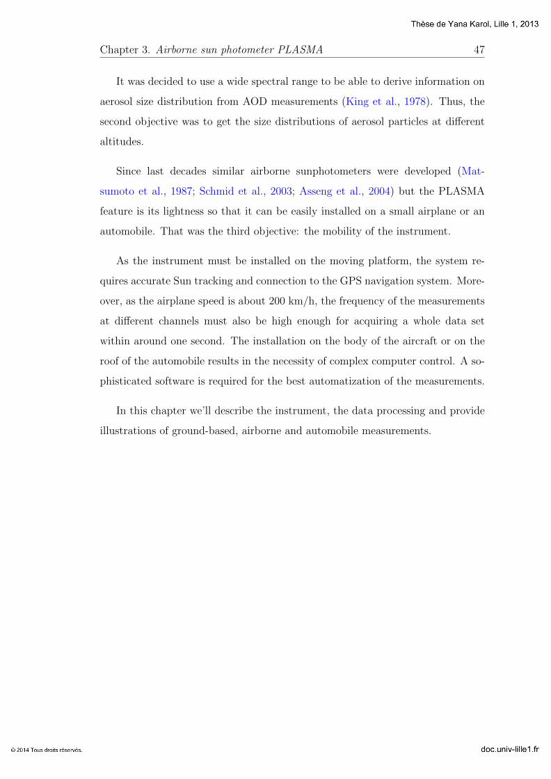
Chapter 3. Airborne sun photometer PLASMA 47
It was decided to use a wide spectral range to be able to derive information on
aerosol size distribution from AOD measurements (King et al., 1978). Thus, the
second objective was to get the size distributions of aerosol particles at different
altitudes.
Since last decades similar airborne sunphotometers were developed (Mat-
sumoto et al., 1987; Schmid et al., 2003; Asseng et al., 2004) but the PLASMA
feature is its lightness so that it can be easily installed on a small airplane or an
automobile. That was the third objective: the mobility of the instrument.
As the instrument must be installed on the moving platform, the system re-
quires accurate Sun tracking and connection to the GPS navigation system. More-
over, as the airplane speed is about 200 km/h, the frequency of the measurements
at different channels must also be high enough for acquiring a whole data set
within around one second. The installation on the body of the aircraft or on the
roof of the automobile results in the necessity of complex computer control. A so-
phisticated software is required for the best automatization of the measurements.
In this chapter we’ll describe the instrument, the data processing and provide
illustrations of ground-based, airborne and automobile measurements.
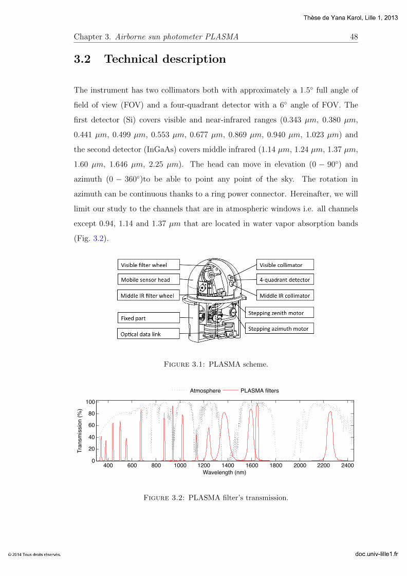
Chapter 3. Airborne sun photometer PLASMA 48
3.2 Technical description
The instrument has two collimators both with approximately a 1.5 full angle of
field of view (FOV) and a four-quadrant detector with a 6 angle of FOV. The
first detector (Si) covers visible and near-infrared ranges (0.343 µm, 0.380 µm,
0.441 µm, 0.499 µm, 0.553 µm, 0.677 µm, 0.869 µm, 0.940 µm, 1.023 µm) and
the second detector (InGaAs) covers middle infrared (1.14 µm, 1.24 µm, 1.37 µm,
1.60 µm, 1.646 µm, 2.25 µm). The head can move in elevation (0 − 90) and
azimuth (0 − 360)to be able to point any point of the sky. The rotation in
azimuth can be continuous thanks to a ring power connector. Hereinafter, we will
limit our study to the channels that are in atmospheric windows i.e. all channels
except 0.94, 1.14 and 1.37 µm that are located in water vapor absorption bands
(Fig. 3.2).
Figure 3.1: PLASMA scheme.
400 600 800 1000 1200 1400 1600 1800 2000 2200 24000
20
40
60
80
100
Wavelength (nm)
Tran
smis
sion
(%)
Atmosphere PLASMA filters
Figure 3.2: PLASMA filter’s transmission.
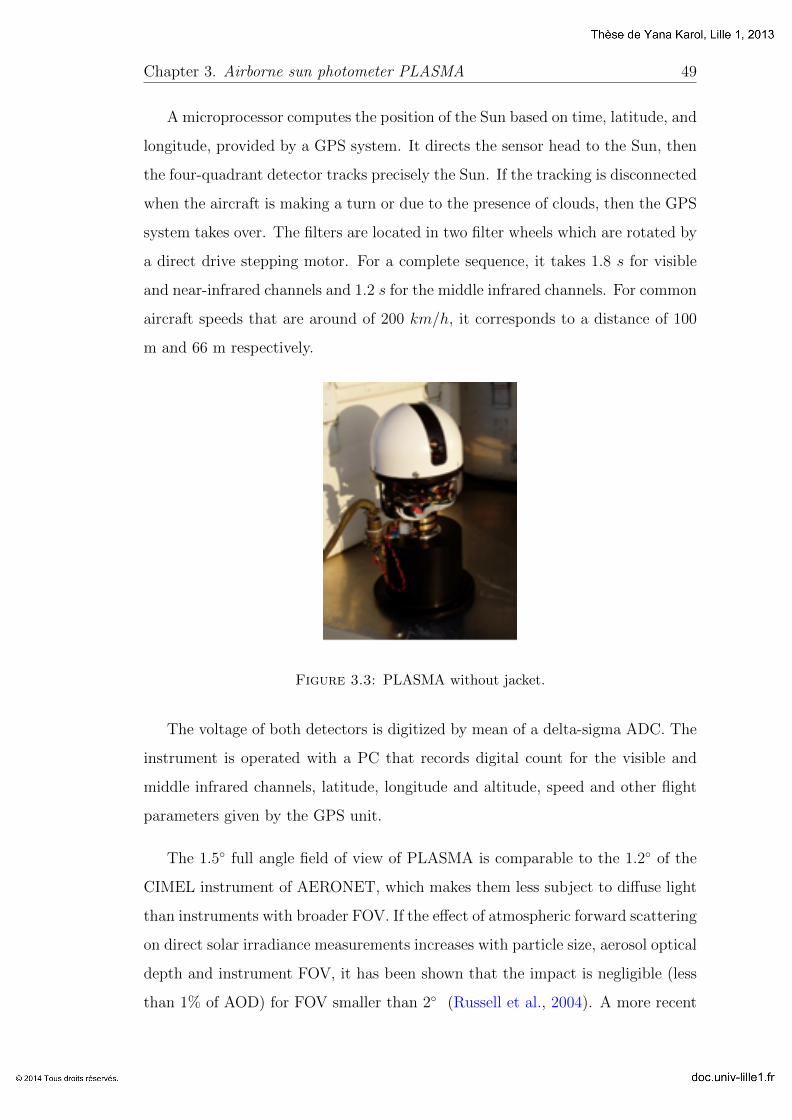
Chapter 3. Airborne sun photometer PLASMA 49
A microprocessor computes the position of the Sun based on time, latitude, and
longitude, provided by a GPS system. It directs the sensor head to the Sun, then
the four-quadrant detector tracks precisely the Sun. If the tracking is disconnected
when the aircraft is making a turn or due to the presence of clouds, then the GPS
system takes over. The filters are located in two filter wheels which are rotated by
a direct drive stepping motor. For a complete sequence, it takes 1.8 s for visible
and near-infrared channels and 1.2 s for the middle infrared channels. For common
aircraft speeds that are around of 200 km/h, it corresponds to a distance of 100
m and 66 m respectively.
Figure 3.3: PLASMA without jacket.
The voltage of both detectors is digitized by mean of a delta-sigma ADC. The
instrument is operated with a PC that records digital count for the visible and
middle infrared channels, latitude, longitude and altitude, speed and other flight
parameters given by the GPS unit.
The 1.5 full angle field of view of PLASMA is comparable to the 1.2 of the
CIMEL instrument of AERONET, which makes them less subject to diffuse light
than instruments with broader FOV. If the effect of atmospheric forward scattering
on direct solar irradiance measurements increases with particle size, aerosol optical
depth and instrument FOV, it has been shown that the impact is negligible (less
than 1% of AOD) for FOV smaller than 2 (Russell et al., 2004). A more recent
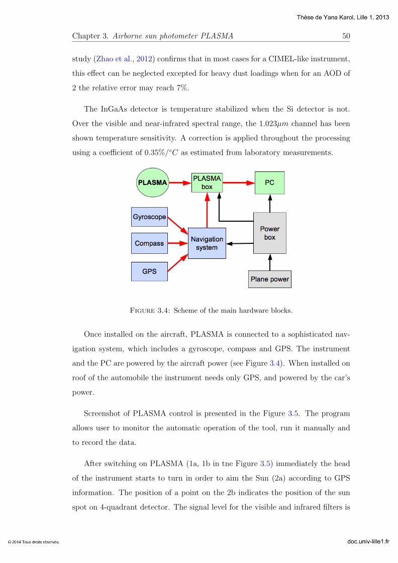
Chapter 3. Airborne sun photometer PLASMA 50
study (Zhao et al., 2012) confirms that in most cases for a CIMEL-like instrument,
this effect can be neglected excepted for heavy dust loadings when for an AOD of
2 the relative error may reach 7%.
The InGaAs detector is temperature stabilized when the Si detector is not.
Over the visible and near-infrared spectral range, the 1.023µm channel has been
shown temperature sensitivity. A correction is applied throughout the processing
using a coefficient of 0.35%/C as estimated from laboratory measurements.
Figure 3.4: Scheme of the main hardware blocks.
Once installed on the aircraft, PLASMA is connected to a sophisticated nav-
igation system, which includes a gyroscope, compass and GPS. The instrument
and the PC are powered by the aircraft power (see Figure 3.4). When installed on
roof of the automobile the instrument needs only GPS, and powered by the car’s
power.
Screenshot of PLASMA control is presented in the Figure 3.5. The program
allows user to monitor the automatic operation of the tool, run it manually and
to record the data.
After switching on PLASMA (1a, 1b in tne Figure 3.5) immediately the head
of the instrument starts to turn in order to aim the Sun (2a) according to GPS
information. The position of a point on the 2b indicates the position of the sun
spot on 4-quadrant detector. The signal level for the visible and infrared filters is
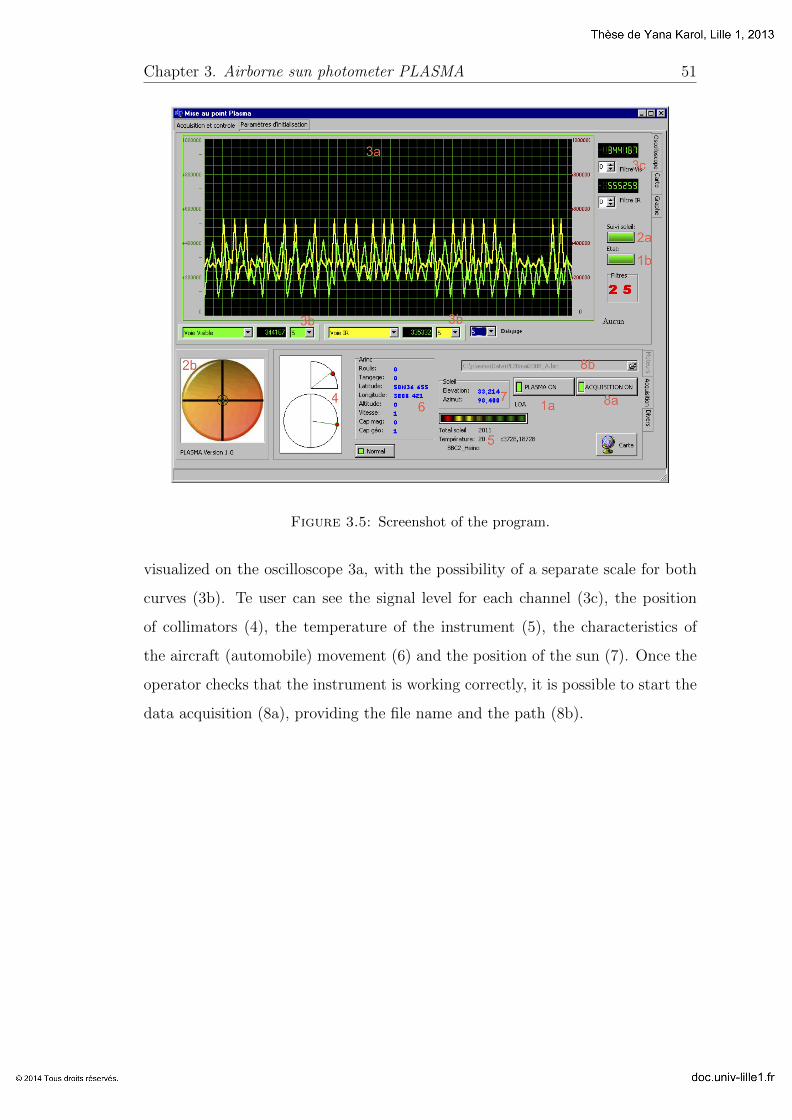
Chapter 3. Airborne sun photometer PLASMA 51
Figure 3.5: Screenshot of the program.
visualized on the oscilloscope 3a, with the possibility of a separate scale for both
curves (3b). Te user can see the signal level for each channel (3c), the position
of collimators (4), the temperature of the instrument (5), the characteristics of
the aircraft (automobile) movement (6) and the position of the sun (7). Once the
operator checks that the instrument is working correctly, it is possible to start the
data acquisition (8a), providing the file name and the path (8b).

Chapter 3. Airborne sun photometer PLASMA 52
3.3 Data processing
The digital signal (DN(λ, z)) measured by the instrument is proportional to sun
irradiance E(λ, z) (the relative Earth-Sun distance is taken to be imbedded in the
extraterrestrial DN value in order to simplify the nomenclature) one can write:
DN(λ, z) = tg(λ, z, θs)DN0(λ)e−τ(λ,z)/ cos(θs) (3.1)
From Eqs. (3.1) and (2.7) and after gaseous absorption correction we can obtain
aerosol extinction optical depth:
τaext(λ, z) =1
m[ln(DN(λ)/tg(λ, z))− ln(DN0(λ))]− τmext(λ, z) (3.2)
To calculate gaseous absorption, i.e. absorption by oxygen, ozone, water vapor
and other gases, we use spectral absorption lines provided in the 5S code and the
mid-latitude summer atmospheric model (Tanre et al., 1990).
Molecular scattering optical depth at the altitude z is given by:
τmext(λ, z) = τmext(λ, z0)P (z)
P (z0)(3.3)
where τmext(λ, z0) is the molecular optical depth at the surface level z0 and P (z0)
the associated pressure.
In the UV spectral range the Rayleigh AOD is significant and has to be known
with a good accuracy to be properly corrected for. Since it depends on the atmo-
spheric pressure, a pressure gauge has been included in the PLASMA instrument.
A pressure gauge was not installed on the early version of the instrument, so the
pressure was estimated using the equation: P (z) = P (z0) exp(−z/8.5), where z
is the altitude of the aircraft expressed in km and 8.5 is the height scale for a
standard molecular atmosphere.

Chapter 3. Airborne sun photometer PLASMA 53
3.4 Calibration
Calibration of a sun photometer consists in determining DN0(λ) in Eq. 3.1 for each
spectral band. As band pass filters can degrade and instrument characteristics may
change over time (Ichoku et al., 2002) the calibration has to be performed on a
regular basis.
There are two ways to calibrate sun photometers as routinely done within the
Aerosol Robotic Network (AERONET) (Holben et al., 1998): Langley method
and intercalibration with master instrument (Lenoble et al., 2011). For PLASMA
calibration we applied both methods. For intercalibration we used a master in-
strument of the AERONET/PHOTONS network.
3.4.1 Langley calibration
The typical approach to calibration is the so-called Langley (or Bouguer-Langley)
method (Shaw et al., 1973), measuring the irradiance for a large range of solar
zenith angles, and plotting lnDN(λ) versus airmass m. The extrapolation of the
plotted line to m = 0 provides DN0(λ), and the slope is −τ(λ):
ln(DN(λ)/tg) = ln(DN0(λ))− τ(λ)m (3.4)
Usually plots are made during the day for the airmass range between 5 and 2.
The calibration site has to be located in an area with very stable aerosol regime.
The Langley method assumes that, during the measurements at different eleva-
tion angles, the atmosphere is temporally invariant and horizontally homogeneous
(within about 50 km of the observer). Almost all calibrations of sunphotome-
ters conducted at continental locations have the probability of being not accurate
enough because of time-changing drifts in atmospheric properties. The solution
is to use high-altitude mountain observatories known to present excellent optical
conditions, such as the Mauna Loa (Hawaii, USA) and Izana (Tenerife, Spain)
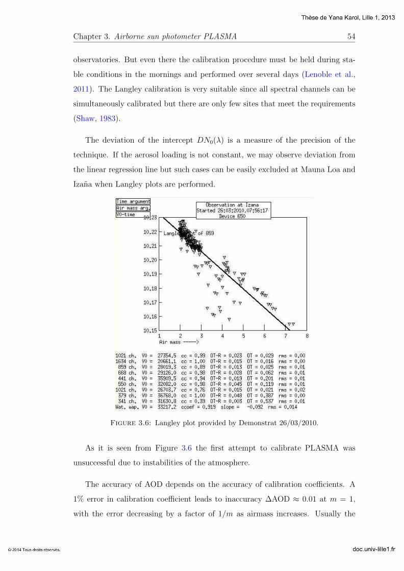
Chapter 3. Airborne sun photometer PLASMA 54
observatories. But even there the calibration procedure must be held during sta-
ble conditions in the mornings and performed over several days (Lenoble et al.,
2011). The Langley calibration is very suitable since all spectral channels can be
simultaneously calibrated but there are only few sites that meet the requirements
(Shaw, 1983).
The deviation of the intercept DN0(λ) is a measure of the precision of the
technique. If the aerosol loading is not constant, we may observe deviation from
the linear regression line but such cases can be easily excluded at Mauna Loa and
Izana when Langley plots are performed.
Figure 3.6: Langley plot provided by Demonstrat 26/03/2010.
As it is seen from Figure 3.6 the first attempt to calibrate PLASMA was
unsuccessful due to instabilities of the atmosphere.
The accuracy of AOD depends on the accuracy of calibration coefficients. A
1% error in calibration coefficient leads to inaccuracy ∆AOD ≈ 0.01 at m = 1,
with the error decreasing by a factor of 1/m as airmass increases. Usually the
Chapter 3. Airborne sun photometer PLASMA 55
profile flights last around 30 min around from 11 to 13 UTC; during this period
the change of airmass is less than 5%. Since a miscalibration results in a bias in
AOD but for constant airmass the value of the extinction coefficient that is the
derivative of AOD is not impacted (see Eq. 3.2 and 2.9).
3.4.2 Intercalibration
When aerosol varies in time we cannot use the Langley method and calibra-
tionderived by inter comparing with another well calibrated instrument.
When the instruments are not perfectly identical, the pass bands and detector
sensitivities of the two instruments (master and instrument undergoing calibra-
tion) have to be known and carefully considered in the comparison. When filters
have slight differences in pass band characteristics, gaseous absorption feature can
be different for one of the insrtuments (Lenoble et al., 2011).
Our intercalibration is performed using near-simultaneous measurements of
sun irradiance by PLASMA and CIMEL sunphotometers at the same location.
Spectral calibration coefficients can be found from the relation:
DNPLASMA0 (λ)
DNCIMEL0 (λ)
=DNPLASMA(λ)
DNCIMEL(λ)(3.5)
Several tools have been developed within the AERONET project for perform-
ing intercomparsion exercise. In Fig. 3.7 we illustrate a tool included in the
Demonstrat software that automatically compares AOD taken by two different
instrument. In Fig. 3.8, we illustrate a second tool that computes the ratio of
calibration coefficients for any spectral band.

Chapter 3. Airborne sun photometer PLASMA 56
Figure 3.7: Illustration of the automatic calibration in Demonstrat.
Figure 3.8: PLASMA vs. CIMEL digital count.
3.4.3 Evolution of the instrument and calibration cam-
paigns
The first calibration campaign was organized in Izana (28.3N 16.5W Elevation:
2391.0 m) Atmospheric Observatory (October 2009) and in Carpentras (44.1N
5.1E Elevation: 100.0 m) in March 2009.
The calibration coefficients calculated with Izana and Carpentras data were
applied to all data collected in Lille (50.6N 3.1E Elevation: 60.0 m) until March
2010 to obtain aerosol optical depth (AOD). The comparison with CIMEL at com-
mon wavelengths (0.34µm, 0.38µm, 0.44µm, 0.67µm, 0.86µm, 1.20µm, 1.64µm)
Chapter 3. Airborne sun photometer PLASMA 57
showed a good agreement between these two instruments with an accuracy ∆AOD
from 0.01 to 0.02.
After modifications of some mechanical elements, a new calibration campaign
was organized at Izana in March 2010. Several measurements were then performed
in LOA for different atmospheric conditions during 12 days in April–June 2010.
A better agreement with CIMEL master instrument was obtained with rms AOD
differences ∼ 0.01. The PLASMA calibration is not too far from the calibration
requirements of AERONET master instruments (0.002 < ∆AOD < 0.009) (Eck
et al., 1999). A new campaign for Langley calibration was organized once again
in Izana in January 2011.
Once the technical development has been achieved, PLASMA was refurbished
in March 2011. The stepping azimuth and zenith motors were replaced for better
pointing capability and signal processing steps taken to improve the signal to
noise ratio. We also replace all the filters, which required a new calibration of
the instrument. After calibration the difference of AOD retrieved by PLASMA
and CIMEL master instrument is less than 0.005 for all channels except 0.34 µm
channel (see Fig. 3.10 in the Section 3.5.1).
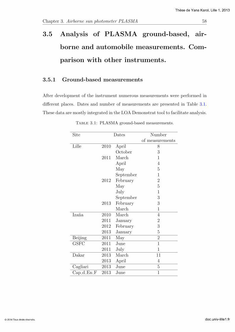
Chapter 3. Airborne sun photometer PLASMA 58
3.5 Analysis of PLASMA ground-based, air-
borne and automobile measurements. Com-
parison with other instruments.
3.5.1 Ground-based measurements
After development of the instrument numerous measurements were performed in
different places. Dates and number of measurements are presented in Table 3.1.
These data are mostly integrated in the LOA Demonstrat tool to facilitate analysis.
Table 3.1: PLASMA ground-based measurements.
Site Dates Numberof measurements
Lille 2010 April 8October 3
2011 March 1April 4May 5September 1
2012 February 2May 5July 1September 3
2013 February 3March 1
Izana 2010 March 42011 January 22012 February 32013 January 5
Beijing 2011 May 2GSFC 2011 June 1
2011 July 1Dakar 2013 March 11
2013 April 4Cagliari 2013 June 5Cap d En F 2013 June 1
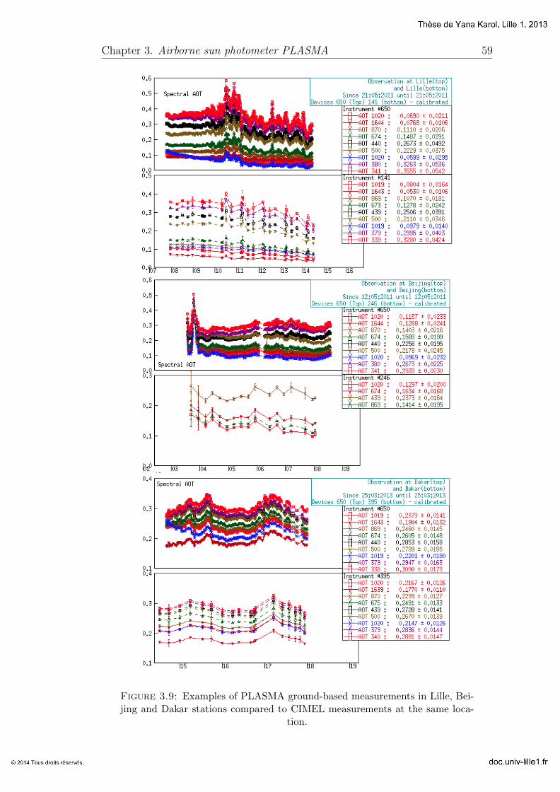
Chapter 3. Airborne sun photometer PLASMA 59
Figure 3.9: Examples of PLASMA ground-based measurements in Lille, Bei-jing and Dakar stations compared to CIMEL measurements at the same loca-
tion.
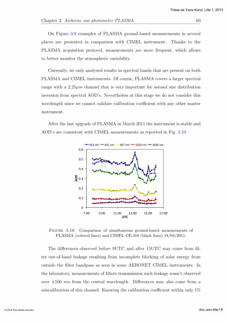
Chapter 3. Airborne sun photometer PLASMA 60
On Figure 3.9 examples of PLASMA ground-based measurements in several
places are presented in comparison with CIMEL instrument. Thanks to the
PLASMA acquisition protocol, measurements are more frequent, which allows
to better monitor the atmospheric variability.
Currently, we only analyzed results in spectral bands that are present on both
PLASMA and CIMEL instruments. Of course, PLASMA covers a larger spectral
range with a 2.25µm channel that is very important for aerosol size distribution
inversion from spectral AOD’s. Nevertheless at this stage we do not consider this
wavelength since we cannot validate calibration coefficient with any other master
instrument.
After the last upgrade of PLASMA in March 2011 the instrument is stable and
AOD’s are consistent with CIMEL measurements as reported in Fig. 3.10.
0
0.1
0.2
0.3
0.4
0.5
0.6
7.00 9.00 11.00 13.00 15.00 17.00
AOD
UTC
343 nm 441 nm 667 nm 1024 nm 1646 nm
Figure 3.10: Comparison of simultaneous ground-based measurements ofPLASMA (colored lines) and CIMEL CE-318 (black lines) 18/04/2011.
The differences observed before 9UTC and after 15UTC may come from fil-
ter out-of-band leakage resulting from incomplete blocking of solar energy from
outside the filter bandpass as seen in some AERONET CIMEL instruments. In
the laboratory, measurements of filters transmission such leakage wasn’t observed
over ±100 nm from the central wavelength. Differences may also come from a
miscalibration of this channel. Knowing the calibration coefficient within only 1%
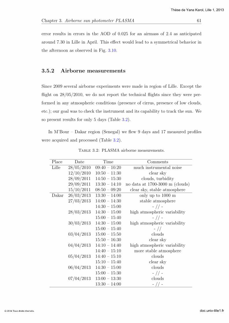
Chapter 3. Airborne sun photometer PLASMA 61
error results in errors in the AOD of 0.025 for an airmass of 2.4 as anticipated
around 7.30 in Lille in April. This effect would lead to a symmetrical behavior in
the afternoon as observed in Fig. 3.10.
3.5.2 Airborne measurements
Since 2009 several airborne experiments were made in region of Lille. Except the
flight on 28/05/2010, we do not report the technical flights since they were per-
formed in any atmospheric conditions (presence of cirrus, presence of low clouds,
etc.); our goal was to check the instrument and its capability to track the sun. We
so present results for only 5 days (Table 3.2).
In M’Bour – Dakar region (Senegal) we flew 9 days and 17 measured profiles
were acquired and processed (Table 3.2).
Table 3.2: PLASMA airborne measurements.
Place Date Time CommentsLille 28/05/2010 09:40 – 10:20 much instrumental noise
12/10/2010 10:50 – 11:30 clear sky28/09/2011 14:50 – 15:30 clouds, turbidity29/09/2011 13:30 – 14:10 no data at 1700-3000 m (clouds)15/10/2011 08:50 – 09:20 clear sky, stable atmosphere
Dakar 26/03/2013 13:30 – 14:00 only up to 1000 m27/03/2013 14:00 – 14:30 stable atmosphere
14:30 – 15:00 - // -28/03/2013 14:30 – 15:00 high atmospheric variability
15:00 – 15:40 - // -30/03/2013 14:30 – 15:00 high atmospheric variability
15:00 – 15:40 - //03/04/2013 15:00 – 15:50 clouds
15:50 – 16:30 clear sky04/04/2013 14:10 – 14:40 high atmospheric variability
14:40 – 15:10 more stable atmosphere05/04/2013 14:40 – 15:10 clouds
15:10 – 15:40 clear sky06/04/2013 14:30 – 15:00 clouds
15:00 – 15:30 - // -07/04/2013 13:00 – 13:30 clouds
13:30 – 14:00 - // -
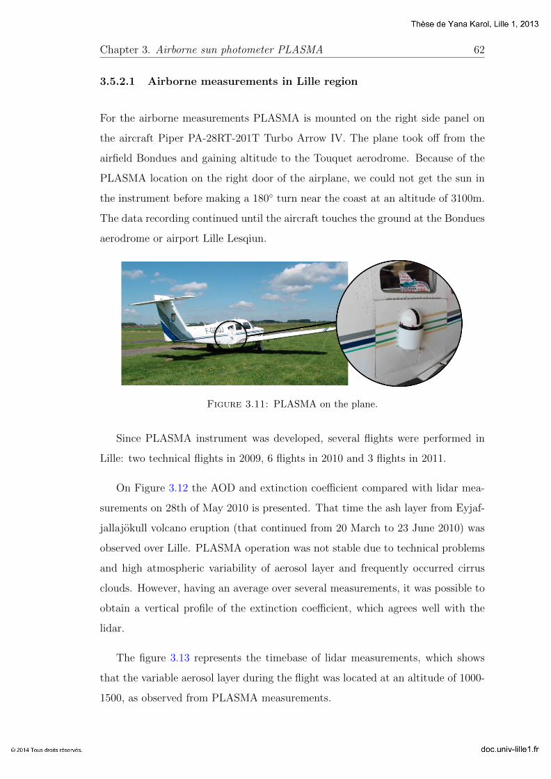
Chapter 3. Airborne sun photometer PLASMA 62
3.5.2.1 Airborne measurements in Lille region
For the airborne measurements PLASMA is mounted on the right side panel on
the aircraft Piper PA-28RT-201T Turbo Arrow IV. The plane took off from the
airfield Bondues and gaining altitude to the Touquet aerodrome. Because of the
PLASMA location on the right door of the airplane, we could not get the sun in
the instrument before making a 180 turn near the coast at an altitude of 3100m.
The data recording continued until the aircraft touches the ground at the Bondues
aerodrome or airport Lille Lesqiun.
Figure 3.11: PLASMA on the plane.
Since PLASMA instrument was developed, several flights were performed in
Lille: two technical flights in 2009, 6 flights in 2010 and 3 flights in 2011.
On Figure 3.12 the AOD and extinction coefficient compared with lidar mea-
surements on 28th of May 2010 is presented. That time the ash layer from Eyjaf-
jallajokull volcano eruption (that continued from 20 March to 23 June 2010) was
observed over Lille. PLASMA operation was not stable due to technical problems
and high atmospheric variability of aerosol layer and frequently occurred cirrus
clouds. However, having an average over several measurements, it was possible to
obtain a vertical profile of the extinction coefficient, which agrees well with the
lidar.
The figure 3.13 represents the timebase of lidar measurements, which shows
that the variable aerosol layer during the flight was located at an altitude of 1000-
1500, as observed from PLASMA measurements.
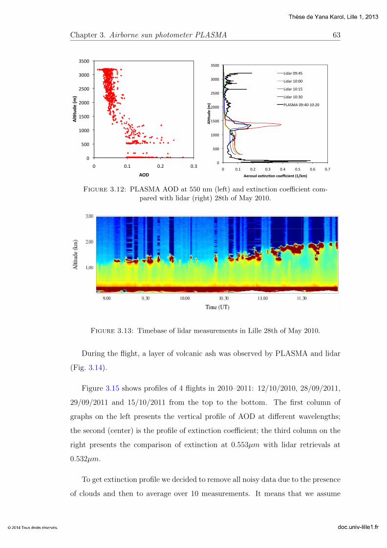
Chapter 3. Airborne sun photometer PLASMA 63
0
500
1000
1500
2000
2500
3000
3500
0 0.1 0.2 0.3
Al#tude
(m)
AOD
0
500
1000
1500
2000
2500
3000
3500
0 0.1 0.2 0.3 0.4 0.5 0.6 0.7
Al#tude
(m)
Aerosol ex#nc#on coefficient (1/km)
Lidar 09:45
Lidar 10:00
Lidar 10:15
Lidar 10:30
PLASMA 09:40-‐10:20
Figure 3.12: PLASMA AOD at 550 nm (left) and extinction coefficient com-pared with lidar (right) 28th of May 2010.
Figure 3.13: Timebase of lidar measurements in Lille 28th of May 2010.
During the flight, a layer of volcanic ash was observed by PLASMA and lidar
(Fig. 3.14).
Figure 3.15 shows profiles of 4 flights in 2010–2011: 12/10/2010, 28/09/2011,
29/09/2011 and 15/10/2011 from the top to the bottom. The first column of
graphs on the left presents the vertical profile of AOD at different wavelengths;
the second (center) is the profile of extinction coefficient; the third column on the
right presents the comparison of extinction at 0.553µm with lidar retrievals at
0.532µm.
To get extinction profile we decided to remove all noisy data due to the presence
of clouds and then to average over 10 measurements. It means that we assume
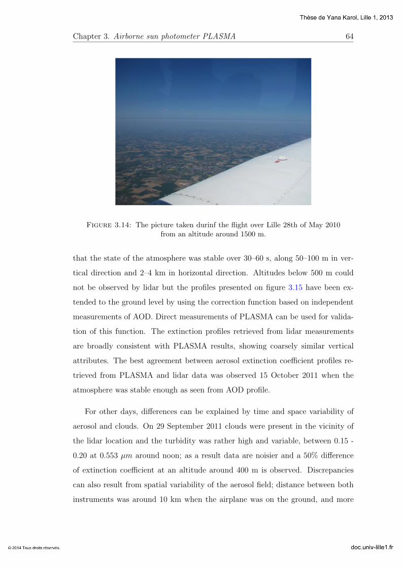
Chapter 3. Airborne sun photometer PLASMA 64
Figure 3.14: The picture taken durinf the flight over Lille 28th of May 2010from an altitude around 1500 m.
that the state of the atmosphere was stable over 30–60 s, along 50–100 m in ver-
tical direction and 2–4 km in horizontal direction. Altitudes below 500 m could
not be observed by lidar but the profiles presented on figure 3.15 have been ex-
tended to the ground level by using the correction function based on independent
measurements of AOD. Direct measurements of PLASMA can be used for valida-
tion of this function. The extinction profiles retrieved from lidar measurements
are broadly consistent with PLASMA results, showing coarsely similar vertical
attributes. The best agreement between aerosol extinction coefficient profiles re-
trieved from PLASMA and lidar data was observed 15 October 2011 when the
atmosphere was stable enough as seen from AOD profile.
For other days, differences can be explained by time and space variability of
aerosol and clouds. On 29 September 2011 clouds were present in the vicinity of
the lidar location and the turbidity was rather high and variable, between 0.15 -
0.20 at 0.553 µm around noon; as a result data are noisier and a 50% difference
of extinction coefficient at an altitude around 400 m is observed. Discrepancies
can also result from spatial variability of the aerosol field; distance between both
instruments was around 10 km when the airplane was on the ground, and more
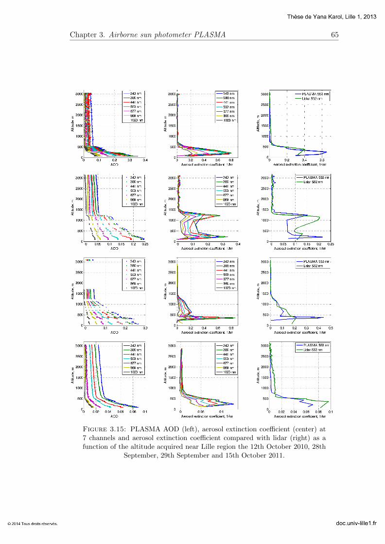
Chapter 3. Airborne sun photometer PLASMA 65
Figure 3.15: PLASMA AOD (left), aerosol extinction coefficient (center) at7 channels and aerosol extinction coefficient compared with lidar (right) as afunction of the altitude acquired near Lille region the 12th October 2010, 28th
September, 29th September and 15th October 2011.
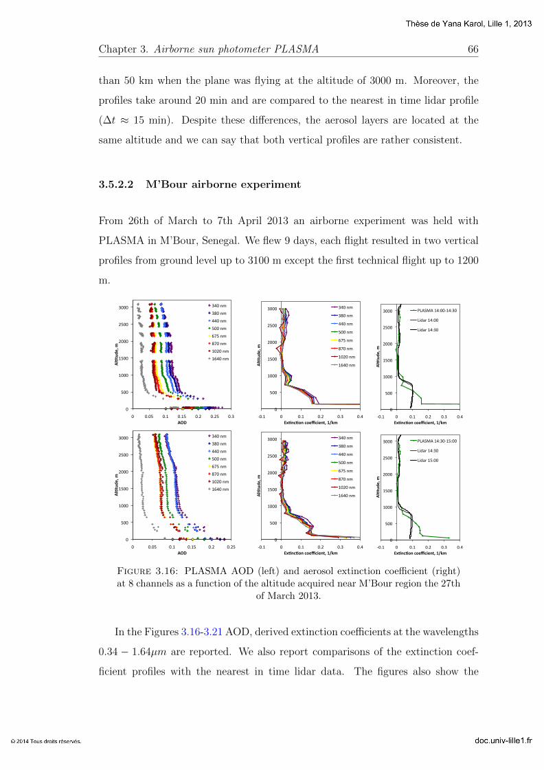
Chapter 3. Airborne sun photometer PLASMA 66
than 50 km when the plane was flying at the altitude of 3000 m. Moreover, the
profiles take around 20 min and are compared to the nearest in time lidar profile
(∆t ≈ 15 min). Despite these differences, the aerosol layers are located at the
same altitude and we can say that both vertical profiles are rather consistent.
3.5.2.2 M’Bour airborne experiment
From 26th of March to 7th April 2013 an airborne experiment was held with
PLASMA in M’Bour, Senegal. We flew 9 days, each flight resulted in two vertical
profiles from ground level up to 3100 m except the first technical flight up to 1200
m.
0
500
1000
1500
2000
2500
3000
0 0.05 0.1 0.15 0.2 0.25 0.3
Al#tude
, m
AOD
340 nm
380 nm
440 nm
500 nm
675 nm
870 nm
1020 nm
1640 nm
0
500
1000
1500
2000
2500
3000
-‐0.1 0 0.1 0.2 0.3 0.4
Al#tude
, m
Ex#nc#on coefficient, 1/km
340 nm
380 nm
440 nm
500 nm
675 nm
870 nm
1020 nm
1640 nm
0
500
1000
1500
2000
2500
3000
-‐0.1 0 0.1 0.2 0.3 0.4
Al#tude
, m
Ex#nc#on coefficient, 1/km
PLASMA 14:00-‐14:30
Lidar 14:00
Lidar 14:30
0
500
1000
1500
2000
2500
3000
0 0.05 0.1 0.15 0.2 0.25
Al#tude
, m
AOD
340 nm
380 nm
440 nm
500 nm
675 nm
870 nm
1020 nm
1640 nm
0
500
1000
1500
2000
2500
3000
-‐0.1 0 0.1 0.2 0.3 0.4
Al#tude
, m
Ex#nc#on coefficient, 1/km
340 nm
380 nm
440 nm
500 nm
675 nm
870 nm
1020 nm
1640 nm
0
500
1000
1500
2000
2500
3000
-‐0.1 0 0.1 0.2 0.3 0.4
Al#tude
, m
Ex#nc#on coefficient, 1/km
PLASMA 14:30-‐15:00
Lidar 14:30
Lidar 15:00
Figure 3.16: PLASMA AOD (left) and aerosol extinction coefficient (right)at 8 channels as a function of the altitude acquired near M’Bour region the 27th
of March 2013.
In the Figures 3.16-3.21 AOD, derived extinction coefficients at the wavelengths
0.34 − 1.64µm are reported. We also report comparisons of the extinction coef-
ficient profiles with the nearest in time lidar data. The figures also show the
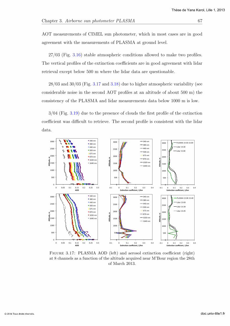
Chapter 3. Airborne sun photometer PLASMA 67
AOT measurements of CIMEL sun photometer, which in most cases are in good
agreement with the measurements of PLASMA at ground level.
27/03 (Fig. 3.16) stable atmospheric conditions allowed to make two profiles.
The vertical profiles of the extinction coefficients are in good agreement with lidar
retrieval except below 500 m where the lidar data are questionable.
28/03 and 30/03 (Fig. 3.17 and 3.18) due to higher atmospheric variability (see
considerable noise in the second AOT profiles at an altitude of about 500 m) the
consistency of the PLASMA and lidar measurements data below 1000 m is low.
3/04 (Fig. 3.19) due to the presence of clouds the first profile of the extinction
coefficient was difficult to retrieve. The second profile is consistent with the lidar
data.
0
500
1000
1500
2000
2500
3000
0 0.05 0.1 0.15 0.2 0.25 0.3
Al#tude
, m
AOD
340 nm
380 nm
440 nm
500 nm
675 nm
870 nm
1020 nm
1640 nm
0
500
1000
1500
2000
2500
3000
-‐0.1 0 0.1 0.2 0.3 0.4
Al#tude
, m
Ex#nc#on coefficient, 1/km
340 nm
380 nm
440 nm
500 nm
675 nm
870 nm
1020 nm
1640 nm
0
500
1000
1500
2000
2500
3000
-‐0.1 0 0.1 0.2 0.3 0.4
Al#tude
, m
Ex#nc#on coefficient, 1/km
PLASMA 14:30-‐15:00
Lidar 14:30
Lidar 15:00
0
500
1000
1500
2000
2500
3000
0 0.05 0.1 0.15 0.2 0.25 0.3
Al#tude
, m
AOD
340 nm
380 nm
440 nm
500 nm
675 nm
870 nm
1020 nm
1640 nm
0
500
1000
1500
2000
2500
3000
-‐0.1 0 0.1 0.2 0.3 0.4
Al#tude
, m
Ex#nc#on coefficient, 1/km
340 nm
380 nm
440 nm
500 nm
675 nm
870 nm
1020 nm
1640 nm
0
500
1000
1500
2000
2500
3000
-‐0.1 0 0.1 0.2 0.3 0.4
Al#tude
, m
Ex#nc#on coefficient, 1/km
PLASMA 15:00-‐15:40
Lidar 15:00
Lidar 15:30
Lidar 15:45
Figure 3.17: PLASMA AOD (left) and aerosol extinction coefficient (right)at 8 channels as a function of the altitude acquired near M’Bour region the 28th
of March 2013.
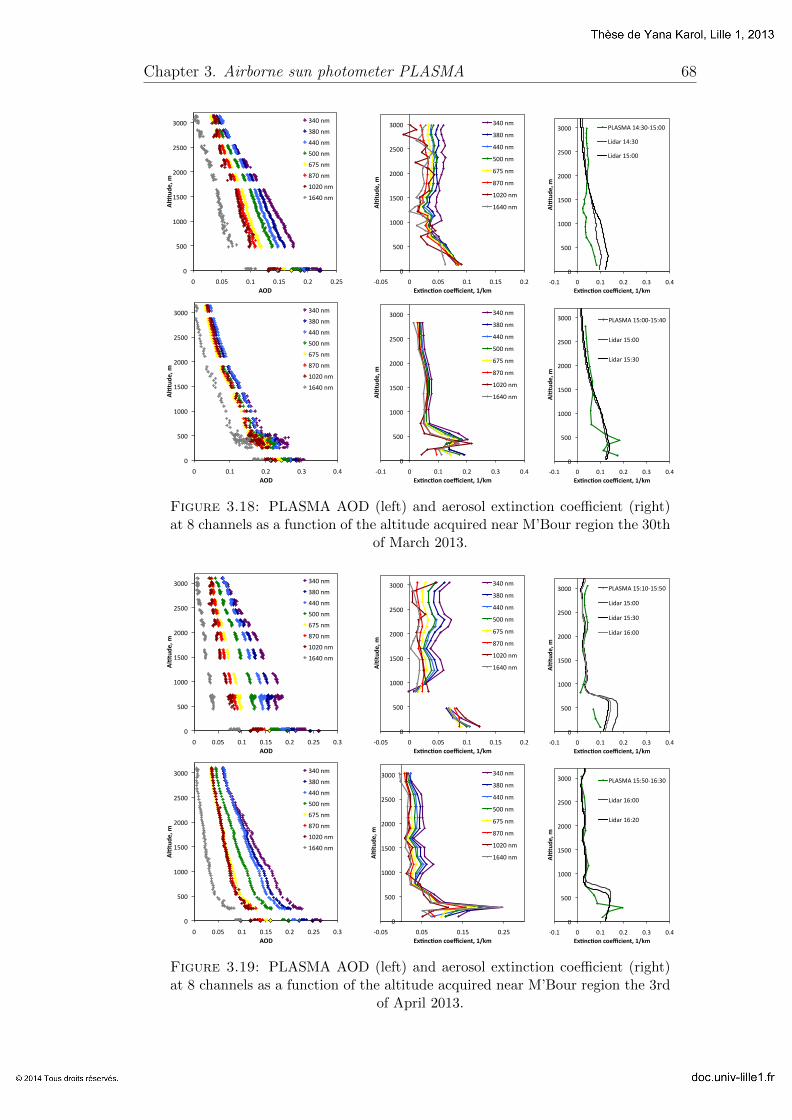
Chapter 3. Airborne sun photometer PLASMA 68
0
500
1000
1500
2000
2500
3000
0 0.05 0.1 0.15 0.2 0.25
Al#tude
, m
AOD
340 nm
380 nm
440 nm
500 nm
675 nm
870 nm
1020 nm
1640 nm
0
500
1000
1500
2000
2500
3000
-‐0.05 0 0.05 0.1 0.15 0.2
Al#tude
, m
Ex#nc#on coefficient, 1/km
340 nm
380 nm
440 nm
500 nm
675 nm
870 nm
1020 nm
1640 nm
0
500
1000
1500
2000
2500
3000
-‐0.1 0 0.1 0.2 0.3 0.4
Al#tude
, m
Ex#nc#on coefficient, 1/km
PLASMA 14:30-‐15:00
Lidar 14:30
Lidar 15:00
0
500
1000
1500
2000
2500
3000
0 0.1 0.2 0.3 0.4
Al#tude
, m
AOD
340 nm
380 nm
440 nm
500 nm
675 nm
870 nm
1020 nm
1640 nm
0
500
1000
1500
2000
2500
3000
-‐0.1 0 0.1 0.2 0.3 0.4
Al#tude
, m
Ex#nc#on coefficient, 1/km
340 nm
380 nm
440 nm
500 nm
675 nm
870 nm
1020 nm
1640 nm
0
500
1000
1500
2000
2500
3000
-‐0.1 0 0.1 0.2 0.3 0.4
Al#tude
, m
Ex#nc#on coefficient, 1/km
PLASMA 15:00-‐15:40
Lidar 15:00
Lidar 15:30
Figure 3.18: PLASMA AOD (left) and aerosol extinction coefficient (right)at 8 channels as a function of the altitude acquired near M’Bour region the 30th
of March 2013.
0
500
1000
1500
2000
2500
3000
0 0.05 0.1 0.15 0.2 0.25 0.3
Al#tude
, m
AOD
340 nm
380 nm
440 nm
500 nm
675 nm
870 nm
1020 nm
1640 nm
0
500
1000
1500
2000
2500
3000
-‐0.05 0 0.05 0.1 0.15 0.2
Al#tude
, m
Ex#nc#on coefficient, 1/km
340 nm
380 nm
440 nm
500 nm
675 nm
870 nm
1020 nm
1640 nm
0
500
1000
1500
2000
2500
3000
-‐0.1 0 0.1 0.2 0.3 0.4
Al#tude
, m
Ex#nc#on coefficient, 1/km
PLASMA 15:10-‐15:50
Lidar 15:00
Lidar 15:30
Lidar 16:00
0
500
1000
1500
2000
2500
3000
0 0.05 0.1 0.15 0.2 0.25 0.3
Al#tude
, m
AOD
340 nm
380 nm
440 nm
500 nm
675 nm
870 nm
1020 nm
1640 nm
0
500
1000
1500
2000
2500
3000
-‐0.05 0.05 0.15 0.25
Al#tude
, m
Ex#nc#on coefficient, 1/km
340 nm
380 nm
440 nm
500 nm
675 nm
870 nm
1020 nm
1640 nm
0
500
1000
1500
2000
2500
3000
-‐0.1 0 0.1 0.2 0.3 0.4
Al#tude
, m
Ex#nc#on coefficient, 1/km
PLASMA 15:50-‐16:30
Lidar 16:00
Lidar 16:20
Figure 3.19: PLASMA AOD (left) and aerosol extinction coefficient (right)at 8 channels as a function of the altitude acquired near M’Bour region the 3rd
of April 2013.
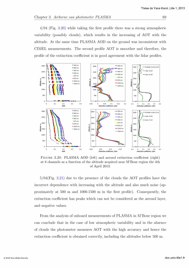
Chapter 3. Airborne sun photometer PLASMA 69
4/04 (Fig. 3.20) while taking the first profile there was a strong atmospheric
variability (possibly clouds), which results in the increasing of AOT with the
altitude. At the same time PLASMA AOD on the ground was inconsistent with
CIMEL measurements. The second profile AOT is smoother and therefore, the
profile of the extinction coefficient is in good agreement with the lidar profiles.
0
500
1000
1500
2000
2500
3000
0 0.1 0.2 0.3 0.4
Al#tude
, m
AOD
340 nm
380 nm
440 nm
500 nm
675 nm
870 nm
1020 nm
1640 nm
0
500
1000
1500
2000
2500
3000
-‐0.05 0 0.05 0.1 0.15 0.2
Al#tude
, m
Ex#nc#on coefficient, 1/km
340 nm
380 nm
440 nm
500 nm
675 nm
870 nm
1020 nm
1640 nm
0
500
1000
1500
2000
2500
3000
-‐0.1 0 0.1 0.2 0.3 0.4
Al#tude
, m
Ex#nc#on coefficient, 1/km
PLASMA 14:10-‐14:40
Lidar 14:20
Lidar 14:30
0
500
1000
1500
2000
2500
3000
0 0.1 0.2 0.3 0.4
Al#tude
, m
AOD
340 nm
380 nm
440 nm
500 nm
675 nm
870 nm
1020 nm
1640 nm
0
500
1000
1500
2000
2500
3000
-‐0.05 0.05 0.15 0.25
Al#tude
, m
Ex#nc#on coefficient, 1/km
340 nm
380 nm
440 nm
500 nm
675 nm
870 nm
1020 nm
1640 nm
0
500
1000
1500
2000
2500
3000
-‐0.1 0 0.1 0.2 0.3 0.4
Al#tude
, m
Ex#nc#on coefficient, 1/km
PLASMA 14:40-‐15:10
Lidar 15:00
Lidar 15:10
Figure 3.20: PLASMA AOD (left) and aerosol extinction coefficient (right)at 8 channels as a function of the altitude acquired near M’Bour region the 4th
of April 2013.
5/04(Fig. 3.21) due to the presence of the clouds the AOT profiles have the
incorrect dependence with increasing with the altitude and also much noise (ap-
proximately at 500 m and 1000-1500 m in the first profile). Consequently, the
extinction coefficient has peaks which can not be considered as the aerosol layer,
and negative values.
From the analysis of onboard measurements of PLASMA in M’Bour region we
can conclude that in the case of low atmospheric variability and in the absence
of clouds the photometer measures AOT with the high accuracy and hence the
extinction coefficient is obtained correctly, including the altitudes below 500 m.

Chapter 3. Airborne sun photometer PLASMA 70
0
500
1000
1500
2000
2500
3000
0 0.1 0.2 0.3 0.4
Al#tude
, m
AOD
340 nm
380 nm
440 nm
500 nm
675 nm
870 nm
1020 nm
1640 nm
0
500
1000
1500
2000
2500
3000
-‐0.05 0 0.05 0.1 0.15 0.2
Al#tude
, m
Ex#nc#on coefficient, 1/km
340 nm
380 nm
440 nm
500 nm
675 nm
870 nm
1020 nm
1640 nm
0
500
1000
1500
2000
2500
3000
-‐0.1 0 0.1 0.2 0.3 0.4
Al#tude
, m
Ex#nc#on coefficient, 1/km
PLASMA 14:40-‐15:10
Lidar 14:40
Lidar 15:00
0
500
1000
1500
2000
2500
3000
0 0.1 0.2 0.3 0.4 0.5 0.6
Al#tude
, m
AOD
340 nm
380 nm
440 nm
500 nm
675 nm
870 nm
1020 nm
1640 nm
0
500
1000
1500
2000
2500
3000
-‐0.05 0.05 0.15 0.25 0.35
Al#tude
, m
Ex#nc#on coefficient, 1/km
340 nm
380 nm
440 nm
500 nm
675 nm
870 nm
1020 nm
1640 nm
0
500
1000
1500
2000
2500
3000
-‐0.1 0 0.1 0.2 0.3 0.4
Al#tude
, m
Ex#nc#on coefficient, 1/km
PLASMA 15:10-‐15:40
Lidar 15:00
Lidar 15:40
Figure 3.21: PLASMA AOD (left) and aerosol extinction coefficient (right)at 8 channels as a function of the altitude acquired near M’Bour region the 5th
of April 2013.
This provides a basis for further corrections of processing algorithms of lidar
measurements. The figures show that below 500 m the lidar profile of the extinc-
tion coefficient may not be reliable. The PLASMA data give a more complete
picture of the distribution of aerosols at these altitudes. For example, 27/03, we
believe that the PLASMA profiles are more accurate than lidar ones.
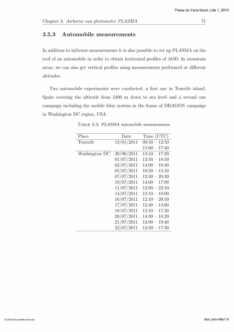
Chapter 3. Airborne sun photometer PLASMA 71
3.5.3 Automobile measurements
In addition to airborne measurements it is also possible to set up PLASMA on the
roof of an automobile in order to obtain horizontal profiles of AOD. In mountain
areas, we can also get vertical profiles using measurements performed at different
altitudes.
Two automobile experiments were conducted, a first one in Tenerife island,
Spain covering the altitude from 2400 m down to sea level and a second one
campaign including the mobile lidar system in the frame of DRAGON campaign
in Washington DC region, USA.
Table 3.3: PLASMA automobile measurements.
Place Date Time (UTC)Tenerife 13/01/2011 09:50 – 12:50
15:00 – 17:40Washington DC 30/06/2011 13:10 – 17:30
01/07/2011 13:50 – 18:5002/07/2011 14:00 – 18:3005/07/2011 10:50 – 15:1007/07/2011 12:30 – 20:3010/07/2011 14:00 – 17:0011/07/2011 12:00 – 22:1014/07/2011 12:10 – 18:0016/07/2011 12:10 – 20:5017/07/2011 12:30 – 14:0018/07/2011 12:10 – 17:3020/07/2011 14:30 – 18:2021/07/2011 12:00 – 19:4022/07/2011 13:20 – 17:30

Chapter 3. Airborne sun photometer PLASMA 72
3.5.3.1 Tenerife experiment
In January 2011 an experiment was successfully carried out on the island of Tener-
ife, Spain. In Tenerife island there are good conditions to carry out car experiment:
altitude difference from the sea level to 2400 m is easily covered in around 1 hour,
and there is only 30 km horizontal distance between the top and the bottom of
the mountain.
PLASMA was installed on the top of a car of the Izana Atmospheric Observa-
tory (Fig. 3.22a). A trip to El Medano and back to the Observatory was performed
for obtaining two profiles of AOD. The itenerary (Fig. 3.22a) was chosen for having
less shadow. We had the opportunity to compare the PLASMA AOD with the
Izana AERONET site (alt. 2391m) very close to the road- way. There are also
two additional AERONET sites, La Laguna (alt. 590 m) and Santa Cruz (alt. 54
m), that were located at a distance of 40 km from our measurements.
a) b)
Figure 3.22: a) Installation on the AEMET car; b) PLASMA route on Tenerifeand AERONET cites.
In the process of car-based measurements, PLASMA perfectly followed the Sun
despite the shocks during the experiment. When passed through a shade with
simultaneous turn of a road PLASMA looked at the sun again in few seconds.
However, at an altitude of 200 m the electronic part of the instrument failed and
data were very noisy. After restarting at the sea level PLASMA at the sea level,
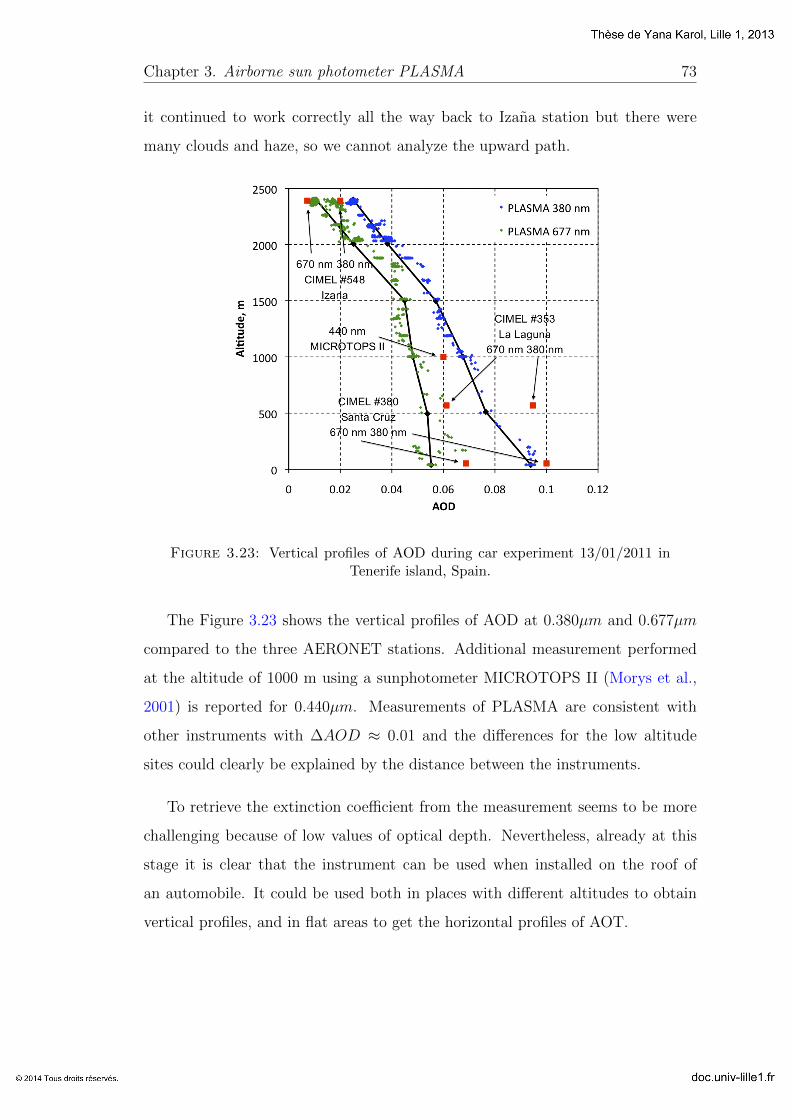
Chapter 3. Airborne sun photometer PLASMA 73
it continued to work correctly all the way back to Izana station but there were
many clouds and haze, so we cannot analyze the upward path.
Figure 3.23: Vertical profiles of AOD during car experiment 13/01/2011 inTenerife island, Spain.
The Figure 3.23 shows the vertical profiles of AOD at 0.380µm and 0.677µm
compared to the three AERONET stations. Additional measurement performed
at the altitude of 1000 m using a sunphotometer MICROTOPS II (Morys et al.,
2001) is reported for 0.440µm. Measurements of PLASMA are consistent with
other instruments with ∆AOD ≈ 0.01 and the differences for the low altitude
sites could clearly be explained by the distance between the instruments.
To retrieve the extinction coefficient from the measurement seems to be more
challenging because of low values of optical depth. Nevertheless, already at this
stage it is clear that the instrument can be used when installed on the roof of
an automobile. It could be used both in places with different altitudes to obtain
vertical profiles, and in flat areas to get the horizontal profiles of AOT.
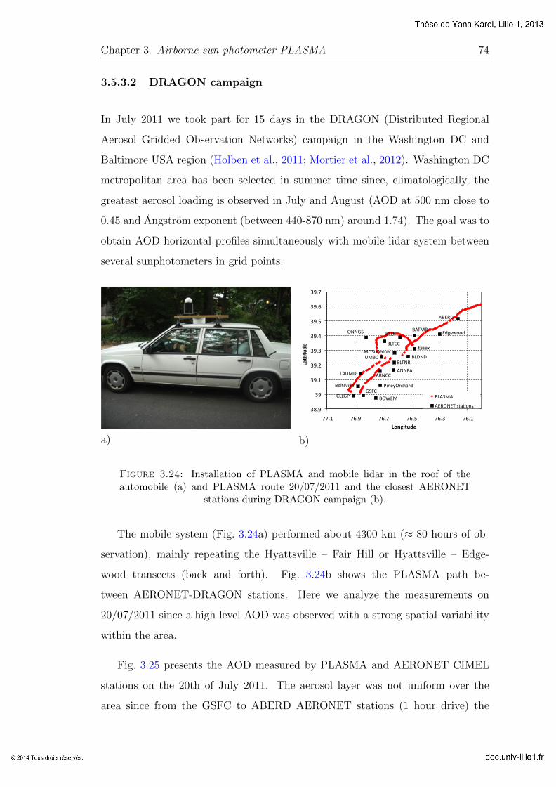
Chapter 3. Airborne sun photometer PLASMA 74
3.5.3.2 DRAGON campaign
In July 2011 we took part for 15 days in the DRAGON (Distributed Regional
Aerosol Gridded Observation Networks) campaign in the Washington DC and
Baltimore USA region (Holben et al., 2011; Mortier et al., 2012). Washington DC
metropolitan area has been selected in summer time since, climatologically, the
greatest aerosol loading is observed in July and August (AOD at 500 nm close to
0.45 and Angstrom exponent (between 440-870 nm) around 1.74). The goal was to
obtain AOD horizontal profiles simultaneously with mobile lidar system between
several sunphotometers in grid points.
a)
CLLGP
LAUMD ARNCC ANNEA
BLTNR
BLTCC
BLLRT BATMR
ABERD
BLDND
GSFC
MDScCenter
BOWEM
Beltsville PineyOrchard
UMBC
ONNGS
Essex
Edgewood
38.9
39
39.1
39.2
39.3
39.4
39.5
39.6
39.7
-‐77.1 -‐76.9 -‐76.7 -‐76.5 -‐76.3 -‐76.1
La#tude
Longitude
PLASMA
AERONET staOons
b)
Figure 3.24: Installation of PLASMA and mobile lidar in the roof of theautomobile (a) and PLASMA route 20/07/2011 and the closest AERONET
stations during DRAGON campaign (b).
The mobile system (Fig. 3.24a) performed about 4300 km (≈ 80 hours of ob-
servation), mainly repeating the Hyattsville – Fair Hill or Hyattsville – Edge-
wood transects (back and forth). Fig. 3.24b shows the PLASMA path be-
tween AERONET-DRAGON stations. Here we analyze the measurements on
20/07/2011 since a high level AOD was observed with a strong spatial variability
within the area.
Fig. 3.25 presents the AOD measured by PLASMA and AERONET CIMEL
stations on the 20th of July 2011. The aerosol layer was not uniform over the
area since from the GSFC to ABERD AERONET stations (1 hour drive) the
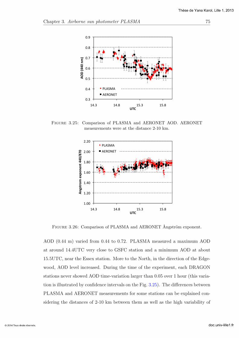
Chapter 3. Airborne sun photometer PLASMA 75
0.3$
0.4$
0.5$
0.6$
0.7$
0.8$
0.9$
14.3$ 14.8$ 15.3$ 15.8$
AOD$(4
40$nm)$
UTC$
PLASMA$
AERONET$
Figure 3.25: Comparison of PLASMA and AERONET AOD. AERONETmeasurements were at the distance 2-10 km.
!"##$
!"%#$
!"&#$
!"'#$
!"(#$
%"##$
%"%#$
!&")$ !&"($ !*")$ !*"($
!"#$%&'()*+,'"
*"%)-
-./01.)
234)
+,-./-$
-012304$
Figure 3.26: Comparison of PLASMA and AERONET Angstrom exponent.
AOD (0.44 m) varied from 0.44 to 0.72. PLASMA measured a maximum AOD
at around 14.4UTC very close to GSFC station and a minimum AOD at about
15.5UTC, near the Essex station. More to the North, in the direction of the Edge-
wood, AOD level increased. During the time of the experiment, each DRAGON
stations never showed AOD time-variation larger than 0.05 over 1 hour (this varia-
tion is illustrated by confidence intervals on the Fig. 3.25). The differences between
PLASMA and AERONET measurements for some stations can be explained con-
sidering the distances of 2-10 km between them as well as the high variability of

Chapter 3. Airborne sun photometer PLASMA 76
the aerosol field. The agreement observed again between the two data sets con-
firms that PLASMA provides reliable measurements with an accuracy comparable
to AERONET.
The Angstrom exponent derived from PLASMA is compared to level 2
AERONET data in Fig. 3.26. While the AOD varies by more than 50%, the
Angstrom exponent is more stable. The moderate variations around the mean
value of 1.70 can result from cloud contamination or possible humidity effects.
Both instruments display consistent spatial/temporal variations.!"#$%&'&(!$)*$&+,-./012&,1034.-5&
*1.6-.&-3&789:&"!%;:&<=><&>?&
Figure 3.27: Attenuated backscattered lidar signal measured between Hy-attsville (G) and Edgewood (E) with PLASMA AOD (white diamonds). From
Mortier et al. (2012)
.
As PLASMA was installed on the automobile together with mobile lidar system
we present here an example of combined measurements plot on Fig. 3.27 (Mortier
et al., 2012). The high variability of aerosol along the path is also well observed.
The vertical profiles show aerosol particles distributed up to 3,5-4 km with maxi-
mum particle concentration occurred near the ground, within the first kilometer.
However, there was some secondary maximum between 1,5 and 2,5 km, as for ex-
ample over Baltimore city (point B in Fig. 3.27). AOD measured over Baltimore
city (0.4) smaller compared to the value (G, 0.54) measured near GSFC at the
beginning of this transect. It can be explained by a lower particle concentration
Chapter 3. Airborne sun photometer PLASMA 77
within the first kilometer as shown by lidar on Fig. 3.27 over Baltimore. From B
to M AOD continues to decrease and reaches a minimum of about 0.31. According
to lidar profile, the atmospheric layer over point M is in general more transparent,
especially over 1 km. Finally, from point M to Edgewood (E), at the end of this
transect, AOD value increased up to 0.42 which can be mostly attributed to higher
particle concentration within the first kilometer.
So, using mobile lidar-sunphotometer system we can obtain information about
aerosol layer which is especially useful in areas with atmospheric inhomogeneites.

Chapter 3. Airborne sun photometer PLASMA 78
3.6 Conclusion
After three years of effort for improving the PLASMA technical part (adjust-
ment, testing and calibration), we can now state that instrument performs high-
precision measurements of AOT over a wide spectral range. The tests and com-
parisons with AERONET sunphotometer showed that the measurement error is
only ∆(AOD) = 0.005. This corresponds to the accuracy of master CIMEL
instrument.
When installed on an aircraft or on an automobile, PLASMA accurately track
the Sun through the 4-quadrant detector and provide high speed measurements of
vertical or horizontal profiles of AOT in 15 wavelengths. The measurement error
is 0.005 ≤ ∆(AOD) ≤ 0.01.
PLASMA measurements can be used as reference data for the validation of lidar
measurements, since it provides direct sun measurements down to the ground level,
while the lidar cannot observe below 300-500 m. Let us mention that using the
mobile lidar-photometric system for taking horizontal transects of the atmosphere
is very promising.
Chapter 4
Inversion of aerosol size
distribution from spectral AOD
measurements
The study and knowledge of the
universe would somehow be lame
and defective were no practical
results to follow.
Marcus Tullius Cicero
4.1 Introduction
As airborne sunphotometer PLASMA has 15 channels over a wide spectral range,
it is possible to retrieve the aerosol size distribution over a given size range which
depends on the lower and upper wavelengths. Thanks to airborne data, we can
obtain the size distribution of aerosol particles at different wavelengths at different
altitudes.
79
Chapter 4. Inversion 80
A similar problem is solved in the framework of the AERONET network but
both direct sun (over a smaller spectral range compared to PLASMA) and angu-
lar measurements of CIMEL CE-318 sunphotometer are used, and the retrieved
vertically integrated parameters are the particle size distribution, refractive index,
single scattering albedo and shape. The approach is attractive since it provides
additional information on the vertical distribution of particle sizes.
In general, of course, in the absence of angular measurements the number of
input data is too small for inversion of multiple parameters. For instance, it is
not expected to retrieve the refractive index but in order to find out what are
the limitations of the inversion technique of the atmospheric aerosol microphysical
parameters using only the direct sun measurements, it is necessary to conduct a
sensitivity study of the algorithm to changes in the various input parameters, in
particular the complex refractive index and the noise level.
First, we describe the inversion algorithm, the sensitivity study to the refractive
index (section 4.3.3) and to the measurement noise (Section 4.3.4). Then the
results of measurement inversion are provided: the Section 4.4 is dedicated to the
inversion of PLASMA data from ground-based measurements with its comparison
with AERONET inversion; the results of DRAGON data retrieval are discussed
in the Section 4.5; the most important results of airborne measurements inversion
are reported in the Section 4.6.
4.2 Inversion algorithm
There are two steps in retrieving optical and microphysical properties of atmo-
spheric aerosols from radiation measurements. The first is so-called ”forward
model” where the retrieval algorithm is used to simulate the atmospheric radi-
ation assuming known atmospheric and surface properties. The second called
”inversion” procedure where the inverse transformation is used for retrieving the
aerosol properties from the radiation field.
Chapter 4. Inversion 81
At present, the forward-modeling doesn’t present strong difficulties thanks to
the powerful computers with fast operational processing. The inversion process is
much more complicated especially for the case of simultaneous retrieval of many
unknowns. Theoretically, the best solution of the problem is given by the best
fitting of the measurements through the continuous space of all possible solu-
tions. Unfortunately, often several different combinations of aerosol parameters
produce the same, or nearly the same, radiation distribution. Therefore, the gen-
eral solution is fundamentally nonunique mainly in the presence of noise in the
measurements (Dubovik, 2004).
There are numerous inversion methods widely adopted in atmospheric remote
sensing and other geophysical applications, such as the methods given by Kalman
(1960); Philips (1962); Tikhonov (1963); Twomey (1963, 1975); Strand and West-
water (1968); Chanine (1968); Turchin and Nozik (1969); Rodgers (1976).
The inversion procedure presented by Dubovik and King (2000) proposes
adding a priori assumptions on smoothness of the size distribution or spectral
smoothness of the optical properties in the inversion procedure to constrain the
solution while reproducing the measurement field within the error bars established
for the measurements. This method is the one used in AERONET network to re-
trieve the aerosol properties from the measurements of the ground-based CIMEL
sun-photometers. The modification of this method by excluding the angular mea-
surements from input parameters is used in the present study. Its short description
is presented below.
4.2.1 Forward problem
The atmospheric aerosol particles can be modeled as a mix of spherical particles.
For a constant refractive index m at all wavelengths the relationship between the
spectral AOD and the aerosol size distribution is given by the integral relation

Chapter 4. Inversion 82
(King et al., 1978):
τa(λ) =
∞∫0
z2∫z1
πr2Qext(r, λ,m)n(r, z)dzdr (4.1)
where r is particle radius; n(r, z) is particles size distribution, i.e. aerosol number
density in the radius range r to r + dr; m(λ) is complex refractive index; Qext is
extinction efficiency factor derived from Mie theory.
Assuming the same aerosol type along the vertical, we can write
τa(λ) =
rmax∫rmin
Kτ (r, λ,m)nl(r)dr (4.2)
where nl(r) is the size distribution in a layer of the atmosphere and Kτ (r, λ,m) =
πr2Qext(r, λ,m) is the kernel function of optical thickness which can be computed
from Mie theory for homogeneous spherical particles when the refractive index is
known.
Eq. 4.2 can be rewritten in terms of a volume size distribution v(ln r) =
dV (r)/dv ln r where v(ln r) represents the volume of particles per unit area per
unit log radius interval:
τa(λ) =
rmax∫rmin
3
4πr3Kτ (r, λ,m)v(ln r)d ln r,
=
q∑j=1
rj+1∫rj
3
4πr3Kτ (r, λ,m)v(ln r)d ln r,
≈ A(r, λ, r)fl(ln r) (4.3)
The variation of the optical thickness kernel function (3/(4πr3))Kτ (r, λ,m)
depends on r3 in case of small particles (Rayleigh scattering limit) and on r−1 in
case of large particles (geometric optics limit).
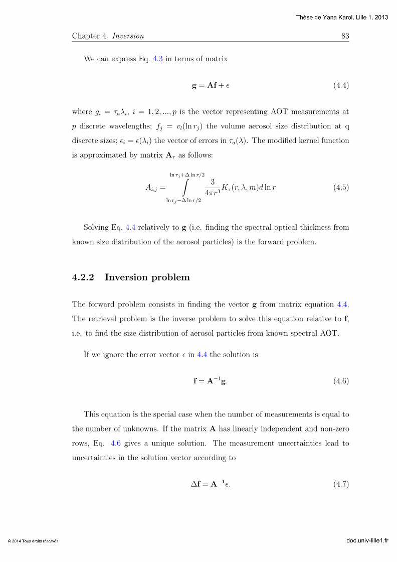
Chapter 4. Inversion 83
We can express Eq. 4.3 in terms of matrix
g = Af + ε (4.4)
where gi = τaλi, i = 1, 2, ..., p is the vector representing AOT measurements at
p discrete wavelengths; fj = vl(ln rj) the volume aerosol size distribution at q
discrete sizes; εi = ε(λi) the vector of errors in τa(λ). The modified kernel function
is approximated by matrix Aτ as follows:
Ai,j =
ln rj+∆ ln r/2∫ln rj−∆ ln r/2
3
4πr3Kτ (r, λ,m)d ln r (4.5)
Solving Eq. 4.4 relatively to g (i.e. finding the spectral optical thickness from
known size distribution of the aerosol particles) is the forward problem.
4.2.2 Inversion problem
The forward problem consists in finding the vector g from matrix equation 4.4.
The retrieval problem is the inverse problem to solve this equation relative to f,
i.e. to find the size distribution of aerosol particles from known spectral AOT.
If we ignore the error vector ε in 4.4 the solution is
f = A−1g. (4.6)
This equation is the special case when the number of measurements is equal to
the number of unknowns. If the matrix A has linearly independent and non-zero
rows, Eq. 4.6 gives a unique solution. The measurement uncertainties lead to
uncertainties in the solution vector according to
∆f = A−1ε. (4.7)
Chapter 4. Inversion 84
The size distribution solution is stable if the rows of the matrix A are linearly
independent and very different. Usually the kernel function for one individual
measurement is broad and overlaps the measurement next to it, the rows of the
matrix A differ slightly from one to another and are nearly linearly dependent, and
by considering uncertainties ∆f can be quite large, and the solution is unstable.
If the system of equations is overdetermined, i.e. there are more equations,
or measurements, than unknowns (q), such situation can be used to minimize the
solution errors. Usually the properties of the noise in the observations f are known,
and then the best solution of the overdetermined system of equations can be found
by choosing the fitting errors as close as possible to the expected distribution of
errors in f.
The agreement of the fitting errors ∆g with a known error distribution can be
evaluated using the probability density function (PDF) as a function of modeled
errors P (∆g): the higher the P (∆g) the closer the modeled ∆g is to the known
statistical properties. Thus, the best solution abest should result in modeled errors
corresponding to the most probable error realization, i.e., to the PDF maximum:
P (∆g) = P (g*(a) - g) = P (g*(a) |g) = max (4.8)
where g*(a) is the vector of retrieved measurements using the derived aerosol
properties a (aerosol size distribution, spectral real and imaginary refractive in-
dices).
This principle is the well-known Maximum Likelihood Method (MLM). The
PDF written as a function of measurements P(g*(a) |g) is called the Likelihood
Function. The MLM is one of the strategic principles of statistical estimation that
provides statistically the best solution in many senses.
If the error PDF is described by a normal distribution, then the MLM is reduced
to a particular case widely known as the least-square solution. The basic principle
of this method relies on the fact that the normal (or Gaussian) distribution is the
expected and most appropriate function for describing random noise. Hence the
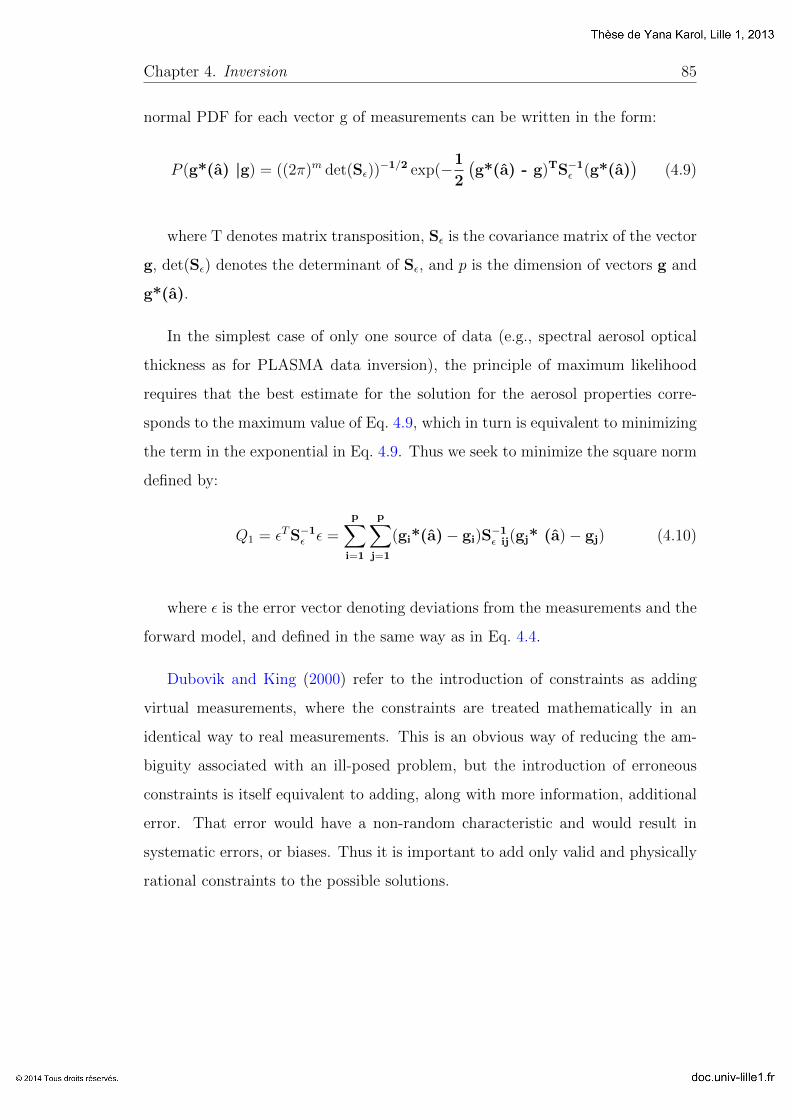
Chapter 4. Inversion 85
normal PDF for each vector g of measurements can be written in the form:
P (g*(a) |g) = ((2π)m det(Sε))−1/2 exp(−1
2
(g*(a) - g)TS−1ε (g*(a)
)(4.9)
where T denotes matrix transposition, Sε is the covariance matrix of the vector
g, det(Sε) denotes the determinant of Sε, and p is the dimension of vectors g and
g*(a).
In the simplest case of only one source of data (e.g., spectral aerosol optical
thickness as for PLASMA data inversion), the principle of maximum likelihood
requires that the best estimate for the solution for the aerosol properties corre-
sponds to the maximum value of Eq. 4.9, which in turn is equivalent to minimizing
the term in the exponential in Eq. 4.9. Thus we seek to minimize the square norm
defined by:
Q1 = εTS−1ε ε =
p∑i=1
p∑j=1
(gi*(a)− gi)S−1ε ij(gj* (a)− gj) (4.10)
where ε is the error vector denoting deviations from the measurements and the
forward model, and defined in the same way as in Eq. 4.4.
Dubovik and King (2000) refer to the introduction of constraints as adding
virtual measurements, where the constraints are treated mathematically in an
identical way to real measurements. This is an obvious way of reducing the am-
biguity associated with an ill-posed problem, but the introduction of erroneous
constraints is itself equivalent to adding, along with more information, additional
error. That error would have a non-random characteristic and would result in
systematic errors, or biases. Thus it is important to add only valid and physically
rational constraints to the possible solutions.
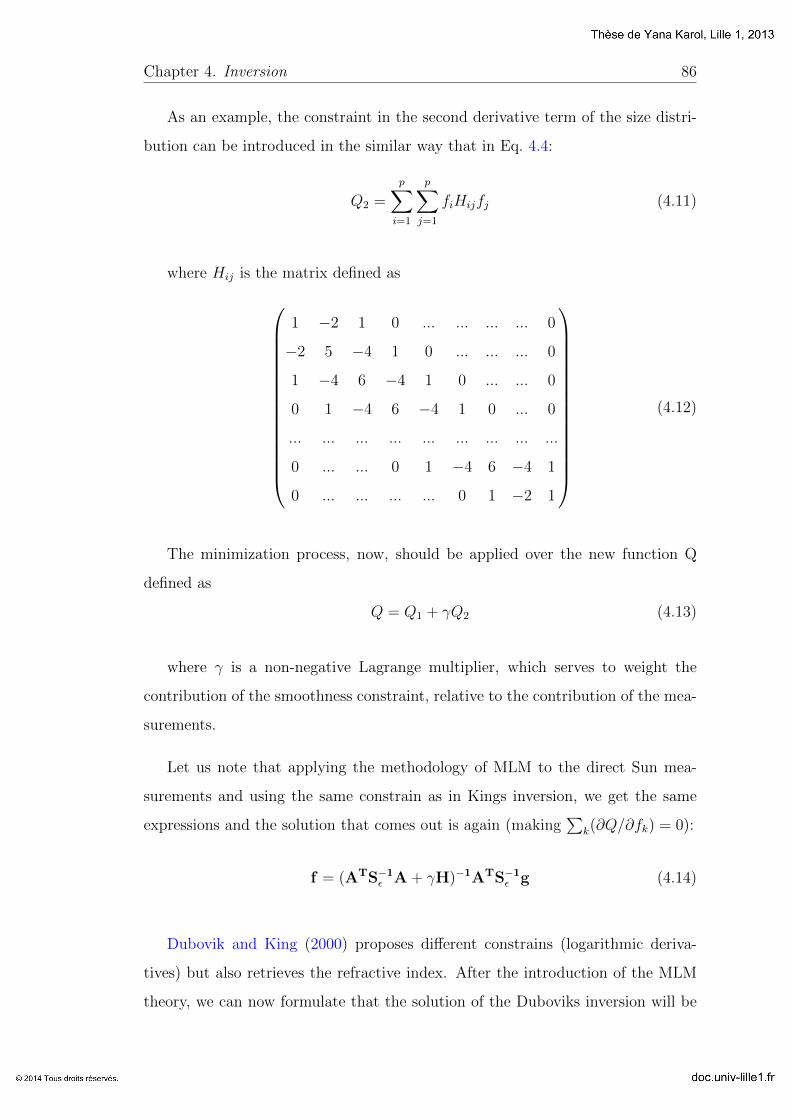
Chapter 4. Inversion 86
As an example, the constraint in the second derivative term of the size distri-
bution can be introduced in the similar way that in Eq. 4.4:
Q2 =
p∑i=1
p∑j=1
fiHijfj (4.11)
where Hij is the matrix defined as
1 −2 1 0 ... ... ... ... 0
−2 5 −4 1 0 ... ... ... 0
1 −4 6 −4 1 0 ... ... 0
0 1 −4 6 −4 1 0 ... 0
... ... ... ... ... ... ... ... ...
0 ... ... 0 1 −4 6 −4 1
0 ... ... ... ... 0 1 −2 1
(4.12)
The minimization process, now, should be applied over the new function Q
defined as
Q = Q1 + γQ2 (4.13)
where γ is a non-negative Lagrange multiplier, which serves to weight the
contribution of the smoothness constraint, relative to the contribution of the mea-
surements.
Let us note that applying the methodology of MLM to the direct Sun mea-
surements and using the same constrain as in Kings inversion, we get the same
expressions and the solution that comes out is again (making∑
k(∂Q/∂fk) = 0):
f = (ATS−1ε A + γH)−1ATS−1ε g (4.14)
Dubovik and King (2000) proposes different constrains (logarithmic deriva-
tives) but also retrieves the refractive index. After the introduction of the MLM
theory, we can now formulate that the solution of the Duboviks inversion will be
Chapter 4. Inversion 87
given by the minimum of the function:
Q =5∑
k=1
γk[f∗k − fk(a)]T (Wk)
−1[f ∗k − fk(a)] (4.15)
where the vector f1 correspond to the logarithms of τ(λ) at the selected wave-
lengths, the vector f2 correspond to the logarithms of the normalized radiance at
the selected wavelengths, the vector f3 includes the values of the size distribution
smoothing function, and f4 and f1 include the values of n(λ) and k(λ) smoothing
functions. The matrix Wk are the weight matrices of random error in the input
data sets. The vector a includes the logarithm of the retrieved values of the size
distribution in the grid points and the values of the real and the imaginary part of
the refractive index at the selected wavelengths. Finally, the Lagrange coefficients
γk are defined from statistical considerations as the ratios of the error variances
∆k = ε21/ε22. The multivariable search for the minimum of Eq. 4.15 is implemented
by a stable numerical procedure combining matrix inversion and univariant relax-
ation according to Dubovik et al. (1998).
4.2.3 Inversion products
The AERONET inversion code provides aerosol optical properties in the to-
tal atmospheric column derived from the direct and diffuse radiation measured
by AERONET Cimel sun/sky-radiometers. AERONET inversion development
and research activities are described in the papers by Dubovik and King (2000);
Dubovik et al. (2000, 2002a,b, 2006); Sinyuk et al. (2007). Hereinafter, we only
consider AOD measurements but the assumption concerning aerosol properties are
the same.
It was shown in many studies that a bimodal lognormal function is the most
appropriate model for aerosol particle size distributions (Whitby, 1978; Shettle
Chapter 4. Inversion 88
and Fenn, 1979; Remer and Kaufman, 1998):
dV (r)
d ln r=
2∑i=1
CV,i√2πσi
exp[− (ln r − ln rV,i)
2
2σ2i
](4.16)
where CV,i is the particle volume concentration, rV,i is the median radius, and σi
is the standard deviation.
For both modes aerosol particles are assumed to be partitioned into two com-
ponents: spherical and non-spherical. The spherical component is modeled by
an ensemble of polydisperse, homogeneous spheres (complex index of refraction is
the same for particles of all sizes). The non-spherical component is a mixture of
polydisperse, randomly-oriented homogeneous spheroids. Atmosphere is assumed
plane-parallel and vertical distribution of aerosol is assumed homogeneous in the
almucantar inversion and bi-layered for the principal plane inversion. The statisti-
cally optimized inversion and corresponding retrieval error estimates are obtained
under the assumption of uncorrelated log-normally distributed errors. This opti-
mization accounts for different levels of accuracy in the measurements (e.g. the
standard deviation for error in τ(λ) is assumed 0.01 for standard instrument and
0.005 for master instrument).
The AERONET retrieval provides aerosol parameters (i.e., size distribution,
complex refractive index and partition of spherical/non-spherical particles) and
products computed from the retrieved aerosol properties (e.g. phase function,
single scattering albedo, spectral and broad-band fluxes, etc.). In addition, the
output provides random and possible systematic (resulted from possible biases in
measurements) errors for most of the retrieved characteristics.
The volume particle size distribution dV (r)/d ln r (µm3/µm2) is retrieved in
22 logarithmically equidistant bins in the range of sizes 0.05µm ≤ r ≤ 15µm. The
real n(λ) (1.33 ≤ n(λ) ≤ 1.6) and imaginary k(λ) parts of the complex refractive
index (0.0005 ≤ k(λ) ≤ 0.5) are retrieved from the sky radiance measurements
that are not available in our case, which requires to conduct a sensitivity study for
this parameter (see next section). The inversion code finds the minimum within
Chapter 4. Inversion 89
the size interval from 0.194 to 0.576 µm. This minimum is used as a separation
point between fine and coarse mode particles. Furthermore, the retrieval provides
estimates of effective radius reff , standard deviation σ and volume concentrations
CV (µm3/µm2) for both fine and coarse modes of the retrieved size distribution.
Chapter 4. Inversion 90
4.3 Sensitivity study of the inversion code
When the capabilities and limitations of the Dubovik’s algorithm has been already
largely described, the ability to retrieve microphysical parameters based on spec-
tral AOD only using the same algorithm (as in the case of airborne sunphotometer
PLASMA measurements) is not fully understood. Obviously, the inversion of the
refractive index in this case is impossible, so we have to assume that it is known
in advance. Such an assumption requires detailed consideration and sensitivity
study to the refractive index for estimating the corresponding impact on the size
parameters.
4.3.1 Description of the chosen aerosol types
We chose five types of aerosol (desert dust, biomass burning, urban clean, urban
industrial and maritime aerosols) that cover most of the possible aerosol condi-
tions. Long-term measurements of AERONET network show that these aerosol
types in their pure forms are observed in the following sites: Solar Village (Saudi
Arabia), Mongu (Zambia), Goddard Space Flight Center (Maryland, USA), Mex-
ico (Mexico), Lanai (Hawaii, USA). The optical and microphysical parameters of
these types were obtained and fully described by Dubovik et al. (2002a).
Solar Village - Desert dust aerosol
Solar Village (24.9N, 46.40E, Elevation: 790 m) is an important solar powered
electricity generating system situated in the Arabian desert approximately 50 km
northwest of Riyadh. The aerosol registered in this site present optical properties
representative of the so-called pure desert dust, without contamination by urban
pollution.
The size distribution is the function of the aerosol optical depth at 1020 nm.
Values of the parameters for the fine and the coarse mode are computed using
the expressions given in Table 4.1. The values of the imaginary part of the

Chapter 4. Inversion 91
refractive index at other wavelengths (340, 380, 500, 550, 1240, 1640, 2250 nm)
were computed by the linear interpolation.
Table 4.1: Optical properties of aerosol in Solar Village(after Dubovik et al. (2002a)).
Range of optical thickness; 〈τ〉 0.1 ≤ τ(1020) ≤ 1.5; 〈τ(1020)〉 = 0.17n 1.56± 0.03k(440/670/870/1020) 0.0029/0.0013/0.001/0.001± 0.001rV f (µm);σf 0.12± 0.05; 0.40± 0.05rV c(µm);σc 2.32± 0.03; 0.60± 0.03CV f (µm
3/µm2) 0.02 + 0.02τ(1020)± 0.03CV c(µm
3/µm2) −0.02 + 0.98τ(1020)± 0.04
Mongu - Biomass burning aerosol
The AERONET station Mongu (15.25S, 23.15E, Elevation: 1107 m) is located
in the airport of Mongu, the capital of the western region in Zambia. The aerosol
in this region contains a lot of high-absorbing smoke due to the savanna burning
annually from July to November.
Concentrations and radii of both modes of the size distribution are the
functions of the aerosol optical depth at 440 nm (table 4.2). The values of the
refractive index do not depend on the aerosol optical depth, its the imaginary
part is one order of magnitude higher than in the other aerosol types.
Table 4.2: Optical properties of aerosol in Mongu(after Dubovik et al. (2002a)).
Range of optical thickness; 〈τ〉 0.1 ≤ τ(440) ≤ 1.5; 〈τ(440)〉 = 0.38n; k 1.51± 0.01; 0.021± 0.004rV f (µm);σf 0.12 + 0.025τ(440)± 0.01; 0.40± 0.01rV c(µm);σc 3.22 + 0.71τ(440)± 0.043; 0.73± 0.03CV f (µm
3/µm2) 0.12τ(440)± 0.04CV c(µm
3/µm2) 0.09τ(440)± 0.02
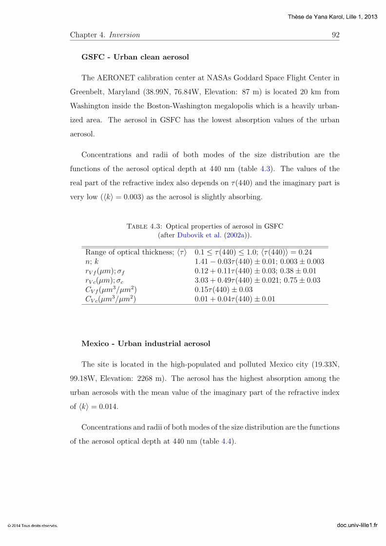
Chapter 4. Inversion 92
GSFC - Urban clean aerosol
The AERONET calibration center at NASAs Goddard Space Flight Center in
Greenbelt, Maryland (38.99N, 76.84W, Elevation: 87 m) is located 20 km from
Washington inside the Boston-Washington megalopolis which is a heavily urban-
ized area. The aerosol in GSFC has the lowest absorption values of the urban
aerosol.
Concentrations and radii of both modes of the size distribution are the
functions of the aerosol optical depth at 440 nm (table 4.3). The values of the
real part of the refractive index also depends on τ(440) and the imaginary part is
very low (〈k〉 = 0.003) as the aerosol is slightly absorbing.
Table 4.3: Optical properties of aerosol in GSFC(after Dubovik et al. (2002a)).
Range of optical thickness; 〈τ〉 0.1 ≤ τ(440) ≤ 1.0; 〈τ(440)〉 = 0.24n; k 1.41− 0.03τ(440)± 0.01; 0.003± 0.003rV f (µm);σf 0.12 + 0.11τ(440)± 0.03; 0.38± 0.01rV c(µm);σc 3.03 + 0.49τ(440)± 0.021; 0.75± 0.03CV f (µm
3/µm2) 0.15τ(440)± 0.03CV c(µm
3/µm2) 0.01 + 0.04τ(440)± 0.01
Mexico - Urban industrial aerosol
The site is located in the high-populated and polluted Mexico city (19.33N,
99.18W, Elevation: 2268 m). The aerosol has the highest absorption among the
urban aerosols with the mean value of the imaginary part of the refractive index
of 〈k〉 = 0.014.
Concentrations and radii of both modes of the size distribution are the functions
of the aerosol optical depth at 440 nm (table 4.4).
Chapter 4. Inversion 93
Table 4.4: Optical properties of aerosol in Mexico(after Dubovik et al. (2002a)).
Range of optical thickness; 〈τ〉 0.1 ≤ τ(440) ≤ 1.8; 〈τ(440)〉 = 0.43n; k 1.47± 0.03; 0.014± 0.006rV f (µm);σf 0.12 + 0.04τ(440)± 0.02; 0.43± 0.03rV c(µm);σc 2.72 + 0.60τ(440)± 0.23; 0.63± 0.05CV f (µm
3/µm2) 0.12τ(440)± 0.03CV c(µm
3/µm2) 0.11τ(440)± 0.03
Lanai - Maritime aerosol
The site is situated on the cost of Lanai island (20.74N, 156.92W, Elevation:
20 m) approximately 100 km from Honolulu. The aerosol in that location has
very low optical thickness: τ(1020) varies from 0.01 to 0.2 with a mean value of
〈τ(1020)〉 = 0.04.
The concentration of the fine and coarse modes of the size distribution is the
function of the aerosol optical depth at 1020 nm (table 4.5). The values of the
imaginary part of the refractive index are the lowest among five examples chosen.
Table 4.5: Optical properties of aerosol in Lanai(after Dubovik et al. (2002a)).
Range of optical thickness; 〈τ〉 0.01 ≤ τ(1020) ≤ 0.2; 〈τ(1020)〉 = 0.04n; k 1.36± 0.01; 0.0015± 0.001rV f (µm);σf 0.16± 0.02; 0.48± 0.04rV c(µm);σc 2.70± 0.04; 0.68± 0.04CV f (µm
3/µm2) 0.40τ(1020)± 0.01CV c(µm
3/µm2) 0.80τ(1020)± 0.02
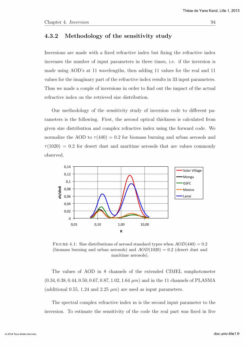
Chapter 4. Inversion 94
4.3.2 Methodology of the sensitivity study
Inversions are made with a fixed refractive index but fixing the refractive index
increases the number of input parameters in three times, i.e. if the inversion is
made using AOD’s at 11 wavelengths, then adding 11 values for the real and 11
values for the imaginary part of the refractive index results in 33 input parameters.
Thus we made a couple of inversions in order to find out the impact of the actual
refractive index on the retrieved size distribution.
Our methodology of the sensitivity study of inversion code to different pa-
rameters is the following. First, the aerosol optical thickness is calculated from
given size distribution and complex refractive index using the forward code. We
normalize the AOD to τ(440) = 0.2 for biomass burning and urban aerosols and
τ(1020) = 0.2 for desert dust and maritime aerosols that are values commonly
observed.
0
0,02
0,04
0,06
0,08
0,1
0,12
0,14
0,01 0,10 1,00 10,00
dV/dlnR
R
Solar Village
Mongu
GSFC
Mexico
Lanai
Figure 4.1: Size distributions of aerosol standard types when AOD(440) = 0.2(biomass burning and urban aerosols) and AOD(1020) = 0.2 (desert dust and
maritime aerosols).
The values of AOD in 8 channels of the extended CIMEL sunphotometer
(0.34, 0.38, 0.44, 0.50, 0.67, 0.87, 1.02, 1.64 µm) and in the 11 channels of PLASMA
(additional 0.55, 1.24 and 2.25 µm) are used as input parameters.
The spectral complex refractive index m is the second input parameter to the
inversion. To estimate the sensitivity of the code the real part was fixed in five
Chapter 4. Inversion 95
values: average value 〈n〉,〈n〉 ± 0.01, 〈n〉 ± 0.05; the imaginary part was fixed in
three values: average value 〈k〉, 〈k〉/2, 〈k〉 ∗ 2 (see Fig. 4.2).
Aerosol'models:''Desert'dust'(Solar'Village)'Biomass'burning'(Mongu)'Urban'clean'(GSFC)'Urban'industrial'(Mexico)'Mari?me'(Lanai)'
Forward'code'
Backward'code'
τa(λ)&
dV/dln(R),&n(λ),&k(λ)&
dV*/dln(R),&n*(λ),&k*(λ)&
Comparison' + n(λ),&k(λ)&
Figure 4.2: Scheme of the sensitivity study.
In all cases the same parameters of smoothness and the initial guess of the size
distribution are used. Obviously, it is possible to predict with some precision the
type of the aerosol in given region and then to change the input parameters in
order to make the inversion results more accurate.
We present in the Appendix A the illustrations for the results discussed below.
For two cases (8 and 11 wl inversion) first there are the tables with retrieved
concentrations and effective radii of fine and coarse mode and the optical residual
are given when the inversion is made with different refractive indices. Then the
plots of size distributions are shown. At the end there are illustrations of 8 wl
inversions with refractive index retrieved together with the size distribution. The
second part of the Appendix A (Figures A.21-A.27) consists the illustrations of
the sensitivity study of the inversion code to the noise level.
As seen from the Figures A.3, A.6, A.9, A.12, A.15 the inversion results when
the refractive index is not fixed are not very different that when we fix the refractive
index, but the retrieved value of the refractive index itself is not reliable. The real
part, for example, can reach either maximum (1.6) or minimum (1.33) limits.
However, AOD residual is smaller (usually it doesn’t exceed 1%) than with fixed
refractive index since the entire error goes to the wrong retrieval of the refractive
index. Since the retrieval of the refractive index using only the AOD as input
parameters is not possible we make the inversion with fixed refractive index.

Chapter 4. Inversion 96
4.3.3 Sensitivity to the refractive index
To illustrate the results of the study we compare the ”model” and inverted
size distributions assuming different refractive indices. Moreover, we calculated
the concentrations of the fine and coarse mode and their effective radii:
reff =
rmax∫rmin
r3 dN(r)d ln r
d ln r
rmax∫rmin
r2 dN(r)d ln r
d ln r
(4.17)
As it is well seen from the tables and figures (see Appendix A), the sensitivity
of the inversion to real and imaginary parts of the refractive index varies with the
aerosol type. Hereinafter, we present the impact on the effective radii. On the
corresponding figures 4.3-4.7, the red points represent the model values, blue are
the radii obtained with ”true” values of refractive index and black points show
the radii retrieved when the refractive index has been changed. The appropriate
values are given in tables together with concentrations and AOD residual.
Desert dust aerosol (see Tables A.1, A.2 and Figures A.1, A.2) has low
sensitivity to the variations of both real and imaginary parts from their true val-
ues. The effective radii of both fine (Reff,f ) and coarse (Reff,c) modes are un-
derestimated (Fig. 4.3). The values of effective radius are not sensitive to the
changes of Re(m) to 0.01 and Im(m) part when the inversion is made at 11 wl
with ∆Reff,c/Reff,c = 0.13 − 0.14 and ∆Reff,f/Reff,f = 0.05 − 0.06 (Table A.2,
Fig. A.2). The concentration of the fine mode is overestimated by 10-15% and
the coarse mode is underestimated by 33-35%. The coarse mode is less underes-
timated when inversion is made at 11 wl than at 8 wl. When inversion is made
using 8 wl (Fig. 4.3) the effective radius of coarse mode is almost independent of
the refractive index, while the underestimation is higher than at 11 wl inversion
(∆Reff,c/Reff,c = 0.26 − 0.28), because of the high sensitivity of the inversion
to 2.25µm channel. When Re(m) is overestimated, the underestimate of the fine
mode is maximum with ∆Reff,f/Reff,f = 0.13 − 0.14 for the inversion with 8 wl
and ∆Reff,f/Reff,f = 0.09−0.13 for the inversion with 11 wl (orange circles on the
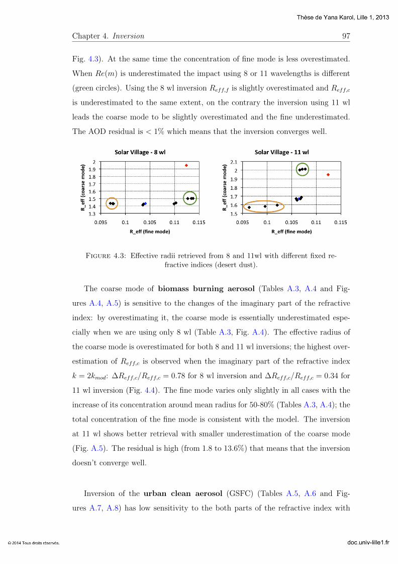
Chapter 4. Inversion 97
Fig. 4.3). At the same time the concentration of fine mode is less overestimated.
When Re(m) is underestimated the impact using 8 or 11 wavelengths is different
(green circles). Using the 8 wl inversion Reff,f is slightly overestimated and Reff,c
is underestimated to the same extent, on the contrary the inversion using 11 wl
leads the coarse mode to be slightly overestimated and the fine underestimated.
The AOD residual is < 1% which means that the inversion converges well.
Figure 4.3: Effective radii retrieved from 8 and 11wl with different fixed re-fractive indices (desert dust).
The coarse mode of biomass burning aerosol (Tables A.3, A.4 and Fig-
ures A.4, A.5) is sensitive to the changes of the imaginary part of the refractive
index: by overestimating it, the coarse mode is essentially underestimated espe-
cially when we are using only 8 wl (Table A.3, Fig. A.4). The effective radius of
the coarse mode is overestimated for both 8 and 11 wl inversions; the highest over-
estimation of Reff,c is observed when the imaginary part of the refractive index
k = 2kmod: ∆Reff,c/Reff,c = 0.78 for 8 wl inversion and ∆Reff,c/Reff,c = 0.34 for
11 wl inversion (Fig. 4.4). The fine mode varies only slightly in all cases with the
increase of its concentration around mean radius for 50-80% (Tables A.3, A.4); the
total concentration of the fine mode is consistent with the model. The inversion
at 11 wl shows better retrieval with smaller underestimation of the coarse mode
(Fig. A.5). The residual is high (from 1.8 to 13.6%) that means that the inversion
doesn’t converge well.
Inversion of the urban clean aerosol (GSFC) (Tables A.5, A.6 and Fig-
ures A.7, A.8) has low sensitivity to the both parts of the refractive index with
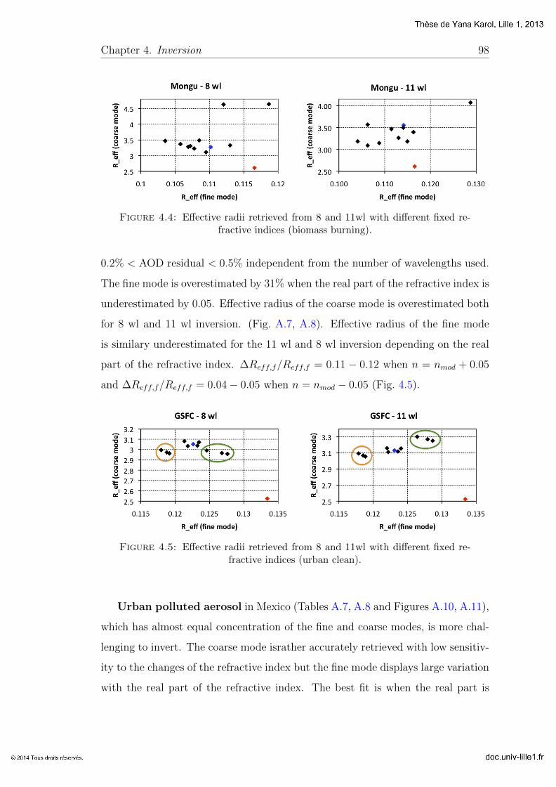
Chapter 4. Inversion 98
Figure 4.4: Effective radii retrieved from 8 and 11wl with different fixed re-fractive indices (biomass burning).
0.2% < AOD residual < 0.5% independent from the number of wavelengths used.
The fine mode is overestimated by 31% when the real part of the refractive index is
underestimated by 0.05. Effective radius of the coarse mode is overestimated both
for 8 wl and 11 wl inversion. (Fig. A.7, A.8). Effective radius of the fine mode
is similary underestimated for the 11 wl and 8 wl inversion depending on the real
part of the refractive index. ∆Reff,f/Reff,f = 0.11 − 0.12 when n = nmod + 0.05
and ∆Reff,f/Reff,f = 0.04− 0.05 when n = nmod − 0.05 (Fig. 4.5).
Figure 4.5: Effective radii retrieved from 8 and 11wl with different fixed re-fractive indices (urban clean).
Urban polluted aerosol in Mexico (Tables A.7, A.8 and Figures A.10, A.11),
which has almost equal concentration of the fine and coarse modes, is more chal-
lenging to invert. The coarse mode israther accurately retrieved with low sensitiv-
ity to the changes of the refractive index but the fine mode displays large variation
with the real part of the refractive index. The best fit is when the real part is

Chapter 4. Inversion 99
overestimated by 0.05 when the fine mode is overestimated by 32% for a under-
estimate of the real part (Figures A.10, A.11). The residual varies in the range
between 0.1% and 4.1% (Tables A.7, A.8). Effective radius of the coarse mode is
less overestimated using the 11 wl inversion (∆Reff,c/Reff,c = 0.10 − 0.35) than
using the 8 wl inversion (∆Reff,c/Reff,c = 0.14 − 0.61). Reff,f is underestimated
for the 11 wl inversion (∆Reff,f/Reff,f = 0.03− 0.15). Using 8 wl inversion Reff,f
is retrieved accurately when n = nmod (Fig. 4.6 and Tables A.7, A.8).
Figure 4.6: Effective radii retrieved from 8 and 11wl with different fixed re-fractive indices (urban industrial).
The inversion of the maritime aerosol (Lanai) is the most difficult since it
presents high sensitivity to the changes of the real part of the refractive index (Ta-
bles A.9, A.10 and Figures A.13, A.14). The underestimation of the real part by
0.05 leads to the overestimation of the fine mode by 42% and of the coarse mode by
55%. At the same time the residual increases up to 35%. Overestimation of the real
part leads to the underestimation of the coarse mode by 28%. There is no sensitiv-
ity to the changes of the imaginary part of the refractive index (Fig. A.13, A.14).
The effective radius of the coarse mode is underestimated for 11 wl inversion with
lower value ∆Reff,c/Reff,c = 0.12 when n = nmod + 0.05. For 8 wl inversion Reff,c
is respectively underestimated (overestimated) with overestimation (underestima-
tion) of the real part of refractive index and overestimated with its underestima-
tion (∆Reff,c/Reff,c = 0.09). Reff,f is underestimated when n = nmod + 0.05
and overestimated when n = nmod − 0.05 with ∆Reff,f/Reff,f = 0.01 − 0.05 and
∆Reff,f/Reff,f = 0.14− 0.15 respectively (Fig. 4.7).
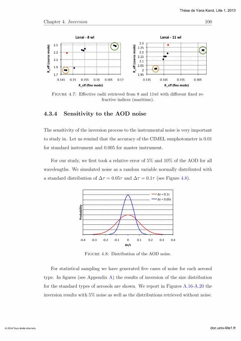
Chapter 4. Inversion 100
Figure 4.7: Effective radii retrieved from 8 and 11wl with different fixed re-fractive indices (maritime).
4.3.4 Sensitivity to the AOD noise
The sensitivity of the inversion process to the instrumental noise is very important
to study in. Let us remind that the accuracy of the CIMEL sunphotometer is 0.01
for standard instrument and 0.005 for master instrument.
For our study, we first took a relative error of 5% and 10% of the AOD for all
wavelengths. We simulated noise as a random variable normally distributed with
a standard distribution of ∆τ = 0.05τ and ∆τ = 0.1τ (see Figure 4.8).
-‐0.4 -‐0.3 -‐0.2 -‐0.1 0 0.1 0.2 0.3 0.4
Prob
ability
∆τ/τ
∆τ = 0.1τ
∆τ = 0.05τ
Figure 4.8: Distribution of the AOD noise.
For statistical sampling we have generated five cases of noise for each aerosol
type. In figures (see Appendix A) the results of inversion of the size distribution
for the standard types of aerosols are shown. We report in Figures A.16-A.20 the
inversion results with 5% noise as well as the distributions retrieved without noise.
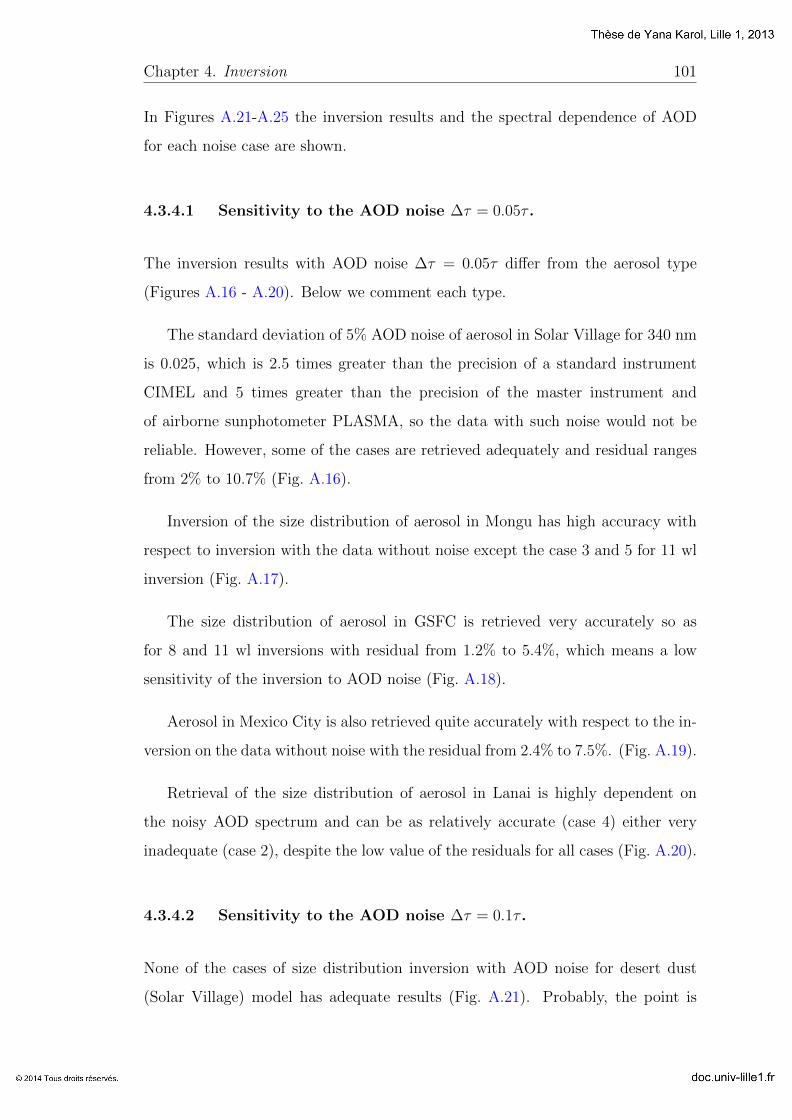
Chapter 4. Inversion 101
In Figures A.21-A.25 the inversion results and the spectral dependence of AOD
for each noise case are shown.
4.3.4.1 Sensitivity to the AOD noise ∆τ = 0.05τ .
The inversion results with AOD noise ∆τ = 0.05τ differ from the aerosol type
(Figures A.16 - A.20). Below we comment each type.
The standard deviation of 5% AOD noise of aerosol in Solar Village for 340 nm
is 0.025, which is 2.5 times greater than the precision of a standard instrument
CIMEL and 5 times greater than the precision of the master instrument and
of airborne sunphotometer PLASMA, so the data with such noise would not be
reliable. However, some of the cases are retrieved adequately and residual ranges
from 2% to 10.7% (Fig. A.16).
Inversion of the size distribution of aerosol in Mongu has high accuracy with
respect to inversion with the data without noise except the case 3 and 5 for 11 wl
inversion (Fig. A.17).
The size distribution of aerosol in GSFC is retrieved very accurately so as
for 8 and 11 wl inversions with residual from 1.2% to 5.4%, which means a low
sensitivity of the inversion to AOD noise (Fig. A.18).
Aerosol in Mexico City is also retrieved quite accurately with respect to the in-
version on the data without noise with the residual from 2.4% to 7.5%. (Fig. A.19).
Retrieval of the size distribution of aerosol in Lanai is highly dependent on
the noisy AOD spectrum and can be as relatively accurate (case 4) either very
inadequate (case 2), despite the low value of the residuals for all cases (Fig. A.20).
4.3.4.2 Sensitivity to the AOD noise ∆τ = 0.1τ .
None of the cases of size distribution inversion with AOD noise for desert dust
(Solar Village) model has adequate results (Fig. A.21). Probably, the point is
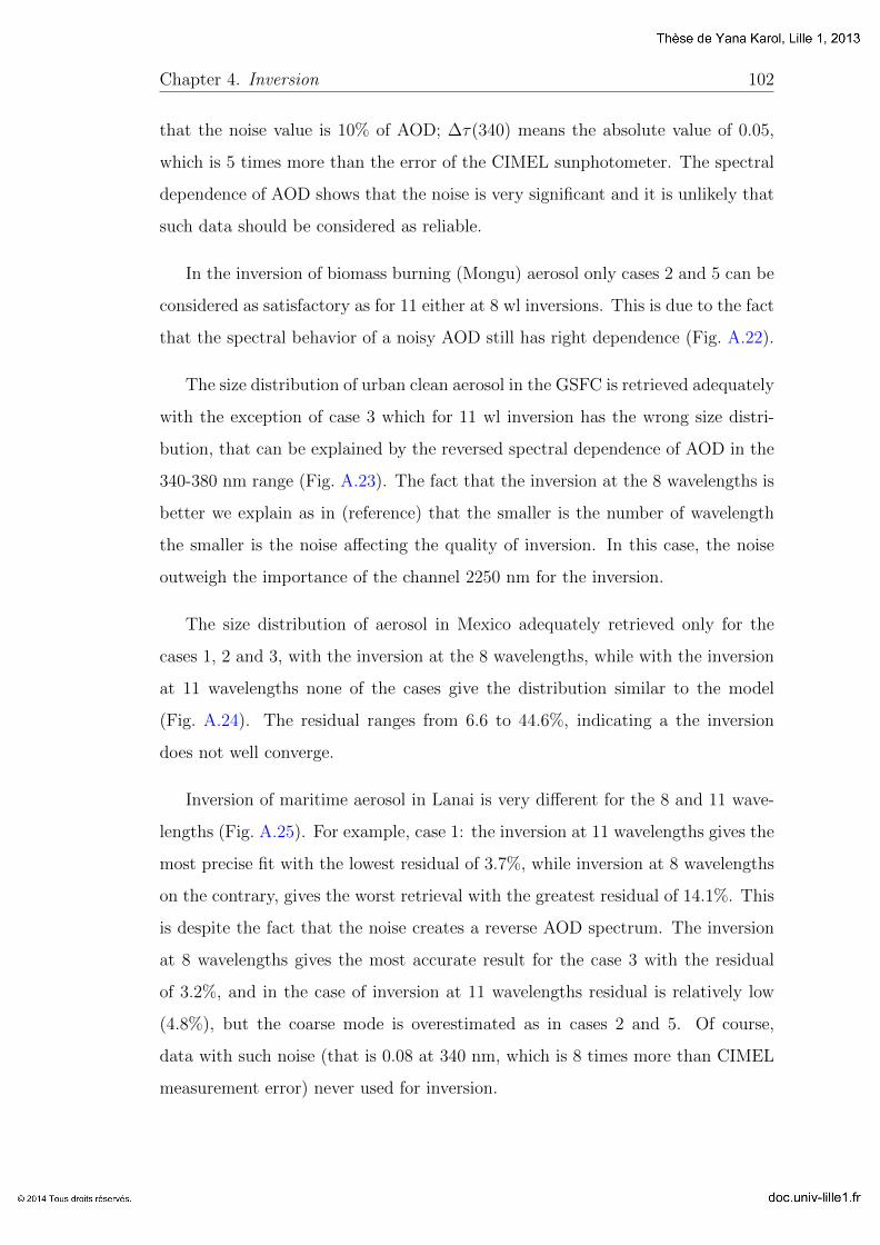
Chapter 4. Inversion 102
that the noise value is 10% of AOD; ∆τ(340) means the absolute value of 0.05,
which is 5 times more than the error of the CIMEL sunphotometer. The spectral
dependence of AOD shows that the noise is very significant and it is unlikely that
such data should be considered as reliable.
In the inversion of biomass burning (Mongu) aerosol only cases 2 and 5 can be
considered as satisfactory as for 11 either at 8 wl inversions. This is due to the fact
that the spectral behavior of a noisy AOD still has right dependence (Fig. A.22).
The size distribution of urban clean aerosol in the GSFC is retrieved adequately
with the exception of case 3 which for 11 wl inversion has the wrong size distri-
bution, that can be explained by the reversed spectral dependence of AOD in the
340-380 nm range (Fig. A.23). The fact that the inversion at the 8 wavelengths is
better we explain as in (reference) that the smaller is the number of wavelength
the smaller is the noise affecting the quality of inversion. In this case, the noise
outweigh the importance of the channel 2250 nm for the inversion.
The size distribution of aerosol in Mexico adequately retrieved only for the
cases 1, 2 and 3, with the inversion at the 8 wavelengths, while with the inversion
at 11 wavelengths none of the cases give the distribution similar to the model
(Fig. A.24). The residual ranges from 6.6 to 44.6%, indicating a the inversion
does not well converge.
Inversion of maritime aerosol in Lanai is very different for the 8 and 11 wave-
lengths (Fig. A.25). For example, case 1: the inversion at 11 wavelengths gives the
most precise fit with the lowest residual of 3.7%, while inversion at 8 wavelengths
on the contrary, gives the worst retrieval with the greatest residual of 14.1%. This
is despite the fact that the noise creates a reverse AOD spectrum. The inversion
at 8 wavelengths gives the most accurate result for the case 3 with the residual
of 3.2%, and in the case of inversion at 11 wavelengths residual is relatively low
(4.8%), but the coarse mode is overestimated as in cases 2 and 5. Of course,
data with such noise (that is 0.08 at 340 nm, which is 8 times more than CIMEL
measurement error) never used for inversion.

Chapter 4. Inversion 103
We can conclude from the above that the least sensitivity to AOD noise when
retrieving the size distribution of particles has the urban aerosol even with ∆τ =
0.1τ . The inversion results are highly dependent not only on the noise value, but
also on its configuration. Thus, the reversed spectral dependence in some segments
of the AOD leads to the inaccurate inversion of the size distribution.
4.3.4.3 Sensitivity of the inversion code with τ =< τ > and standard
instrumental noise ∆τ = 0.005 and ∆τ = 0.01
As it is shown in Chapter 4, the measurement error of PLASMA is 0.005 in the case
of ground-based measurements and 0.01 in the case of automobile and airborne
measurements. CIMEL sunphotometer has a standard error of 0.01 for the usual
device and 0.005 for the master instrument. Therefore, we have chosen two more
versions of noise ∆τ = 0.005 and ∆τ = 0.01.
In addition, we have chosen the average values of AOD and the size distri-
butions of the studied typical aerosols. The figure 4.9 shows the distribution of
these average distributions. So we have standard aerosols and the standard noise.
The refractive index is assumed to be known. Inversion is made out for 11 and 8
wavelengths as usual.
0 0.01 0.02 0.03 0.04 0.05 0.06 0.07 0.08 0.09 0.1
0.01 0.10 1.00 10.00
dV/dlnR
R
Solar Village
Mongu
GSFC
Mexico
Lanai
Figure 4.9: Size distributions of aerosol standard types whenAOD(λ) =< AOD(λ) >.

Chapter 4. Inversion 104
Aerosol in Solar Village is retrieved much more accurately if compared with
previous retrievals. When inversion is made with the noise ∆τ = 0.005 the results
are better for 11 wl than for 8 wl inversion (Fig. A.26 - A.27). Three from five cases
of 11 wl inversion with the noise ∆τ = 0.01 are adequate (Fig. A.28). However
inversion at 8 wl with the same noise has four accurate distributions (Fig. A.29).
Optical residuals vary from minimum 0.6% – 2.5% when inversion is made using
11 wl with the noise ∆τ = 0.005 to maximum 1.4% – 10.6% when inversion is
made using 11 wl with the noise ∆τ = 0.01.
Biomass burning aerosol in Mongu is retrieved accurately for all cases of noise
and number of wavelengths despite the high value of AOD residual which varies
from 2.4% to 38% (Figures A.28 - A.27).
The best inversion results of urban aerosol in GSFC is for 8 wl inversion with
the noise ∆τ = 0.005 when AOD residual varies from 0.24% to 7.9% and for 11
wl inversion with the noise ∆τ = 0.005 when AOD residual varies from 1.4% to
10.5%. Inversions with the noise ∆τ = 0.01 for 11 wl inversion have residual up
to 27.8%.
Inversion of urban aerosol in Mexico has underestimation of the coarse mode
when made at 8 wl with the noise ∆τ = 0.01. Other cases have enough accurate
results of size distributions however the AOD residual varies from 0.71% to 15.9%.
The worst results have inversions of maritime aerosol in Lanai because of its
low optical depth. Most of the cases results in inaccurate distribution with high
AOD residual. Only few cases are retrieved adequately (e.g. case 5 on Fig. A.27).

Chapter 4. Inversion 105
4.3.5 Conclusion of the sensitivity study
Sensitivity study of the inversion have shown that under certain conditions it is
possible to derive the size distribution of aerosol particles from measurements of
the optical thickness in the range of 0.34− 2.25 µm or 0.34− 1.64 µm.
Different aerosol types have various sensitivity to the refractive index changes
and to measurement noise. Desert dust aerosol is not sensitive to changes of the
complex refractive index but the coarse mode is constantly underestimated for
around 30%. Biomass burning aerosol is not sensitive to the changes of the real
part of the refractive index. Only the fine mode of urban clean and urban polluted
aerosols are sensitive to the underestimation of the real part of the refractive index
for 0.05. The change of n for 0.01 does not affect the shape of the distribution.
The maritime aerosol is sensitive to the changes of the real part of the refractive
index: with its underestimation for 0.05 both modes are overestimated and with its
overestimation the coarse mode is underestimated. The change for 0.01 affects only
slightly to the shape of the distribution. Only the biomass burning aerosol show
the sensitivity to the imaginary part of the refractive index: with overestimation
of k the coarse mode is underestimated.
Thus, we conclude that it is possible to derive the size distribution from
PLASMA data with the assumption that the real part of the refractive index
is known with the accuracy of 0.05 (0.01 for maritime aerosol), and the imaginary
part within ±50%.
Study of the sensitivity to AOD noise showed that with the instrumental noise
of 0.005, all aerosol types except maritime aerosol with low optical depth (Lanai)
are retrieved with a sufficient accuracy. With the noise of 0.01 only certain aerosol
types (biomass burning and urban clean) could be retrieved accurately.
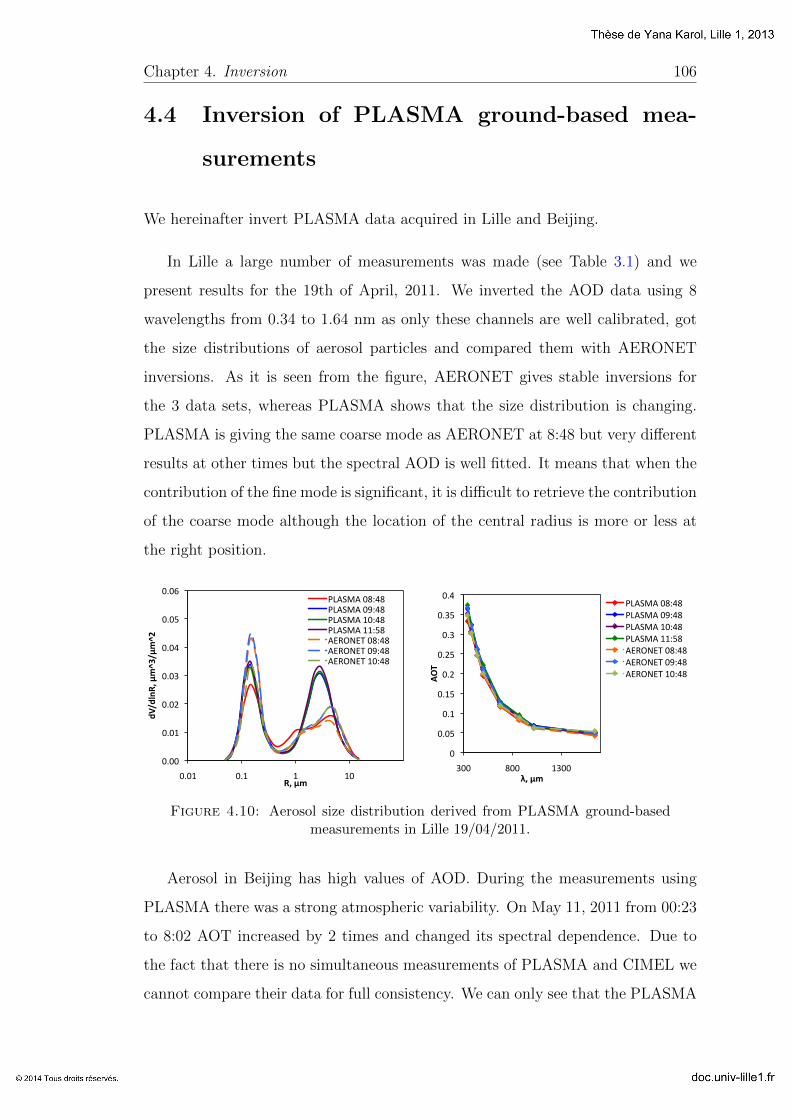
Chapter 4. Inversion 106
4.4 Inversion of PLASMA ground-based mea-
surements
We hereinafter invert PLASMA data acquired in Lille and Beijing.
In Lille a large number of measurements was made (see Table 3.1) and we
present results for the 19th of April, 2011. We inverted the AOD data using 8
wavelengths from 0.34 to 1.64 nm as only these channels are well calibrated, got
the size distributions of aerosol particles and compared them with AERONET
inversions. As it is seen from the figure, AERONET gives stable inversions for
the 3 data sets, whereas PLASMA shows that the size distribution is changing.
PLASMA is giving the same coarse mode as AERONET at 8:48 but very different
results at other times but the spectral AOD is well fitted. It means that when the
contribution of the fine mode is significant, it is difficult to retrieve the contribution
of the coarse mode although the location of the central radius is more or less at
the right position.
0.00
0.01
0.02
0.03
0.04
0.05
0.06
0.01 0.1 1 10
dV/dlnR, μm^3/μm^2
R, μm
PLASMA 08:48 PLASMA 09:48 PLASMA 10:48 PLASMA 11:58 AERONET 08:48 AERONET 09:48 AERONET 10:48
0
0.05
0.1
0.15
0.2
0.25
0.3
0.35
0.4
300 800 1300
AOT
λ, μm
PLASMA 08:48 PLASMA 09:48 PLASMA 10:48 PLASMA 11:58 AERONET 08:48 AERONET 09:48 AERONET 10:48
Figure 4.10: Aerosol size distribution derived from PLASMA ground-basedmeasurements in Lille 19/04/2011.
Aerosol in Beijing has high values of AOD. During the measurements using
PLASMA there was a strong atmospheric variability. On May 11, 2011 from 00:23
to 8:02 AOT increased by 2 times and changed its spectral dependence. Due to
the fact that there is no simultaneous measurements of PLASMA and CIMEL we
cannot compare their data for full consistency. We can only see that the PLASMA

Chapter 4. Inversion 107
size distribution is in the range of the AERONET distribution. The discrepancy
is less than 3%. Also there is underestimation of the coarse mode and the central
radius moved towards fine particles. This means that the algorithm is insensitive
to the AOD measurement s at 1640 nm wavelength and for determining the coarse
mode angular measurements are required.
0.0
0.1
0.2
0.3
0.4
0.5
0.6
0.7
0.8
0.9
1.0
0.01 0.1 1 10
dV/dlnR, μm^3/μm^2
R, μm
PLASMA 02:19
PLASMA 02:25
AERONET 00:23
AERONET 01:12
AERONET 08:02
0
0.5
1
1.5
2
2.5
300 800 1300
AOT
λ, μm
PLASMA 02:19 PLASMA 02:25 AERONET 01:12 AERONET 08:02 AERONET 00:23
Figure 4.11: Aerosol size distribution derived from PLASMA ground-basedmeasurements in Beijing 11/05/2011.
4.5 Inversion of the DRAGON campaign data
During the DRAGON campaign, PLASMA was installed on the roof of the au-
tomobile together with a mobile lidar. We present below the results of inversion
for July 20, 2011. The comparison of PLASMA AOD and Angstrom exponent
was presented in Section 3.5.3.2. We selected five locations on the PLASMA route
close in time and space to AERONET stations. Thus, we can compare the size dis-
tributions of aerosol particles retrieved from direct sun PLASMA measurements at
8 wavelengths with AERONET inversion at direct sun and angular measurements
at 4 wavelengths. We also performed an inversion at 7 wavelengths (excluding
1640 nm channel) to show the ability of the inversion code to retrieve the size dis-
tribution from direct sun measurements of standard instrument CIMEL CE-318.
Inversion results are shown in Fig. 4.12. The fine mode is retrieved with good
precision, while the coarse mode has a lower accuracy. So, near the Aldino,
Beltsville and Kentsland stations the inversion of PLASMA data overestimates

Chapter 4. Inversion 108
the coarse mode, and the central radius shifted towards the large particles. In-
version at 7 wavelengths gives the central radius more shifted towards large par-
ticles. Near the station Edgewood concentration of the coarse mode is accurately
retrieved but the central radius does not match the AERONET value. At the
UMBC station the concentration of the coarse mode was higher than at other
places, and is underestimated.
0
0.01
0.02
0.03
0.04
0.05
0.06
0.07
0.01 0.1 1 10
dV/dlnR ( µm^3/µm^2)
Radius (µm)
Aldino 2011-07-20 13:15
AERONET
8 wl inversion (0.34-‐1.64 µm)
7 wl inversion (0.34-‐1.02 µm)
0 0.01 0.02 0.03 0.04 0.05 0.06 0.07 0.08 0.09 0.1
0.01 0.1 1 10
dV/dlnR ( µm^3/µm^2)
Radius (µm)
Beltsville 2011-07-20 13:15
AERONET
8 wl inversion (0.34-‐1.64 µm)
7 wl inversion (0.34-‐1.02 µm)
0 0.01 0.02 0.03 0.04 0.05 0.06 0.07 0.08 0.09 0.1
0.01 0.1 1 10
dV/dlnR ( µm^3/µm^2)
Radius (µm)
Edgewood 2011-07-20 13:15
AERONET
8 wl inversion (0.34-‐1.64 µm)
7 wl inversion (0.34-‐1.02 µm)
0 0.01 0.02 0.03 0.04 0.05 0.06 0.07 0.08 0.09
0.01 0.1 1 10
dV/dlnR ( µm^3/µm^2)
Radius (µm)
Kentlsland 2011-07-20 13:15
AERONET
8 wl inversion (0.34-‐1.64 µm)
7 wl inversion (0.34-‐1.02 µm)
0 0.01 0.02 0.03 0.04 0.05 0.06 0.07 0.08 0.09
0.01 0.1 1 10
dV/dlnR ( µm^3/µm^2)
Radius (µm)
UMBC 2011-07-20 13:15
AERONET
8 wl inversion (0.34-‐1.64 µm)
7 wl inversion (0.34-‐1.02 µm)
Figure 4.12: Comparison between PLASMA inversion on 7 and 8 wavelengthswith the AERONET inversion.

Chapter 4. Inversion 109
4.6 Inversion of airborne measurements
The innovative contribution of PLASMA (from the point of view of new infor-
mation on aerosols in the atmosphere) is the retrieval of the size distribution of
aerosol particles at different altitudes. The multi-wavelenth lidars could provide
only information about the total concentration of separate fine and coarse mode
and this issue is still under development (Cuesta et al., 2008; Chaikovsky et al.,
2012; Lopatin et al., 2013).
Study of the sensitivity of the inversion code to different parameters (refractive
index, noise) led to the conclusion that the available spectral range and number of
wavelengths is sufficient to retrieve the size distribution of aerosol particles with
enough accuracy.
4.6.1 Flights over Lille
Fig. 4.13 shows the size distribution retrieved from PLASMA airborne measure-
ments in the region of Lille at different altitudes. The figures also shows the
size distributions from AERONET at the surface level which corresponds to the
vertical integrated size distribution.
It should be noted that PLASMA ground-based measurements were carried
out at a distance of about 10 km from the station in Lille, so we cannot expect
full consistency with AERONET. The concentrations of both small and coarse
modes differ. Thus, the inversion on PLASMA data on 12/10/2010 gives a large
concentration of both modes, and a much smaller 28/09/2011. On 28/09/2011
and 15/10/2011 the fine modes are moreless similar, but the coarse modes from
PLASMA are smaller.
To retrieve the size distributions we have taken the following points: ground
level (65 - 90 m), 250 m, 500 m, 1000 m, 2000 m and a maximum altitude (3000
- 3100 m).
The discrepancy in the AOD was not more 5%.
Chapter 4. Inversion 110
12/10/2010 as we see from the size distribution plots most of the aerosols
contained below the altitude of 500 m. The coarse mode is defined in the layer of
250-500 m, and the fine mode probably uniformly distributed. Over 500 m there
was a slight amount of aerosol.
28/09/2011 the fine mode was uniformly distributed over the whole atmo-
spheric column (at least below 3000 m). The coarse mode is constant at altitudes
of 90-500 m, and after 1000 m there is a decrease of its concentration. This suggests
that the larger particles were at the altitude between 500 m and 2000.
15/10/2011 aerosols were uniformly distributed. Coarse and fine modes de-
crease with approximately the same intensity. Most of the coarse mode is at the
altitudes below 250 m.
0
0.005
0.01
0.015
0.02
0.025
0.03
0.035
0.04
0.01 0.1 1 10 100
dV/d
ln(R
) (µ
m3 /µ
m2 )
radius (µm)
Flight 12/10/2010
65 m250 m500 m
1000 m2000 m3000 m
AERONET
0
0.005
0.01
0.015
0.02
0.025
0.03
0.01 0.1 1 10 100
dV/d
ln(R
) (µ
m3 /µ
m2 )
radius (µm)
Flight 28/09/2011
90 m250 m500 m
1000 m2000 m3100 m
AERONET
0 0.001 0.002 0.003 0.004 0.005 0.006 0.007 0.008 0.009
0.01 0.1 1 10 100
dV/d
ln(R
) (µ
m3 /µ
m2 )
radius (µm)
Flight 15/10/2011
90 m250 m500 m
1000 m2000 m3000 m
AERONET
Figure 4.13: Size distributions at different altitudes obtained during the air-borne measurements by PLASMA sunphotometer over Lille.

Chapter 4. Inversion 111
4.6.2 Flights over M’Bour –Dakar
The distribution of aerosol particles in the region M’bour – Dakar is very different
from Lille continental aerosol. This region is characterized by a constant presence
of desert dust, i.e. there is high concentration of large particles.
The figures show the retrieved particle’s size distributions at different altitudes
compared to AERONET retrievals at ground level. The inversion was performed
at 7 wavelengths in the range 340 - 1020 nm. Unfortunately due to the incorrect
calibration of infrared channels, the 1640 nm wavelength could not be included in
the inversion. The calibration coefficient for this wavelength was underestimated
and so the inversion results are very much different from the expected with the
AOD residual up to 20%. An example of such retrieval is shown on Fig. 4.14.
0
0.01
0.02
0.03
0.04
0.05
0.06
0.07
0.01 0.1 1 10 100
dV/d
ln(R
) (µ
m3 /µ
m2 )
radius (µm)
Flight #1 28/03/2013
35 m300 m500 m
1000 m2000 m3100 m
AERONET
Figure 4.14: Example of the size distribution retrieved from airborne mea-surements including 1640 nm channel that has wrong calibration.
Because it was necessary to exclude 1640 nm that is sensitive to large particles
the majority of retrievals underestimate the coarse mode. However, it is possible
to determine the general trend of aerosol vertical distribution if not quantitatively
but at least qualitatively.
We report below three days of measurements i.e. six inversions that are the
most representative: 28/03/2013, 6/04/2013, 7/04/2013.
28/03 (Fig. 4.15) there was a uniform decrease of both modes with the altitude.
Between 1000 m and 2000 m the coarse mode remained stable, so we can assume
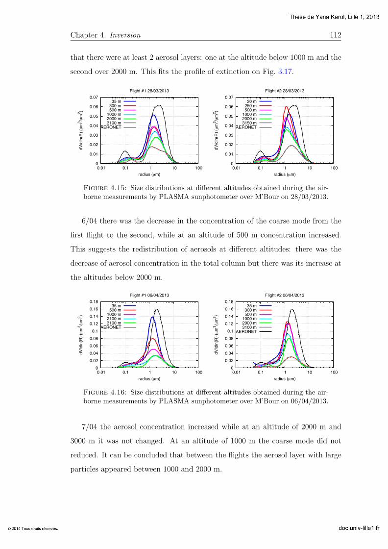
Chapter 4. Inversion 112
that there were at least 2 aerosol layers: one at the altitude below 1000 m and the
second over 2000 m. This fits the profile of extinction on Fig. 3.17.
0
0.01
0.02
0.03
0.04
0.05
0.06
0.07
0.01 0.1 1 10 100
dV/d
ln(R
) (µ
m3 /µ
m2 )
radius (µm)
Flight #1 28/03/2013
35 m300 m500 m
1000 m2000 m3100 m
AERONET
0
0.01
0.02
0.03
0.04
0.05
0.06
0.07
0.01 0.1 1 10 100
dV/d
ln(R
) (µ
m3 /µ
m2 )
radius (µm)
Flight #2 28/03/2013
20 m250 m500 m
1000 m2000 m3150 m
AERONET
Figure 4.15: Size distributions at different altitudes obtained during the air-borne measurements by PLASMA sunphotometer over M’Bour on 28/03/2013.
6/04 there was the decrease in the concentration of the coarse mode from the
first flight to the second, while at an altitude of 500 m concentration increased.
This suggests the redistribution of aerosols at different altitudes: there was the
decrease of aerosol concentration in the total column but there was its increase at
the altitudes below 2000 m.
0 0.02 0.04 0.06 0.08
0.1 0.12 0.14 0.16 0.18
0.01 0.1 1 10 100
dV/d
ln(R
) (µ
m3 /µ
m2 )
radius (µm)
Flight #1 06/04/2013
35 m500 m
1000 m2100 m3100 m
AERONET
0 0.02 0.04 0.06 0.08
0.1 0.12 0.14 0.16 0.18
0.01 0.1 1 10 100
dV/d
ln(R
) (µ
m3 /µ
m2 )
radius (µm)
Flight #2 06/04/2013
35 m300 m500 m
1000 m2000 m3100 m
AERONET
Figure 4.16: Size distributions at different altitudes obtained during the air-borne measurements by PLASMA sunphotometer over M’Bour on 06/04/2013.
7/04 the aerosol concentration increased while at an altitude of 2000 m and
3000 m it was not changed. At an altitude of 1000 m the coarse mode did not
reduced. It can be concluded that between the flights the aerosol layer with large
particles appeared between 1000 and 2000 m.

Chapter 4. Inversion 113
0
0.02
0.04
0.06
0.08
0.1
0.12
0.14
0.16
0.01 0.1 1 10 100
dV/d
ln(R
) (µ
m3 /µ
m2 )
radius (µm)
Flight #1 07/04/2013
350 m500 m
1000 m2050 m3100 m
AERONET
0
0.02
0.04
0.06
0.08
0.1
0.12
0.14
0.16
0.01 0.1 1 10 100
dV/d
ln(R
) (µ
m3 /µ
m2 )
radius (µm)
Flight #2 07/04/2013
25 m300 m650 m
1000 m2150 m3100 m
AERONET
Figure 4.17: Size distributions at different altitudes obtained during the air-borne measurements by PLASMA sunphotometer over M’Bour on 07/04/2013.
We see that with several airborne measurements in one day the evolution of
the aerosol layers can be observed. This information can help to better understand
the processes that aerosols undergo in the atmosphere.
Chapter 4. Inversion 114
4.7 Conclusion of PLASMA data inversion
From the sensitivity study the inversion code can be used for deriving the size
distribution of aerosol particles from only spectral AOD measurements. First,
we inverted PLASMA ground-based measurements and compared the results with
AERONET inversions. Then we inverted automobile and airborne measurements.
The size distributions at different altitudes cannot be compared with any other
measurements but from their shapes and decreasing behavior with the altitude we
can conclude that the results are promising.
The inversion code used for this study performs high precision for the ranges
0.34−1.64 µm and 0.34−1.02 µm and so it can be used not only for PLASMA data
processing but also for derivation of the size distribution of aerosol particles from
sun measurements of CIMEL instrument. Sun measurements are more frequent
than sky measurements, so the inversion of spectral AOD data can supplement
the standard AERONET inversion.

Chapter 5
General conclusion
Realists do not fear the results of
their study.
Fyodor Dostoevsky
Last years significant work was done in the development of new instrumen-
tation for atmospheric aerosol investigation. International photometric and lidar
observation networks were established, several satellites with research instruments
on board were launched. It is believed that measurements from one instrument
complement the others and used in synergy for getting a clear picture of complex
atmospheric processes.
Airborne sun photometer PLASMA was developed to validate and complement
data from other instruments such as lidar data. Furthermore, PLASMA can be
used independently from other systems as a reliable source of information about
the distribution of aerosol particles in the atmosphere.
During the development of the instrument a number of technical problems were
solved and the current version meets our goal, AOD accuracy is around 0.005 <
∆(AOD) < 0.01, which is comparable to the accuracy of sun photometers CIMEL
CE- 318. A large number of ground-based, airborne, and automobile experiments
were carried out all over the world (Lille, Tenerife, Beijing, Dakar, Washington
115
Chapter 5. General conclusion 116
DC, Cagliari) and the PLASMA data were compared with the photometric and
lidar data.
PLASMA ground-based measurements are consistent with AERONET data.
When installed on an aircraft or on an automobile, PLASMA accurately tracks
the Sun through the 4-quadrant detector and provides high speed measurements
of vertical or horizontal profiles of AOT in 15 wavelengths. Airborne measure-
ments of vertical profiles of aerosol extinction coefficient were compared to the
lidar profiles. In most cases measurements are consistent. When discrepancies are
observed, part of them can be explained by various environmental factors such as
atmospheric variability or time and space differences between the two instruments
(Section 3.5.2). We observe the largest discrepancies near the surface (300-500 m)
where the lidar cannot measure and requires an extrapolation procedure in the
retrieval algorithm. PLASMA measurements can be used as reference data for
the validation of lidar measurements, since it provides direct sun measurements
down to the ground level, while the lidar cannot observe below 300-500 m. The
instrument was also used to obtain horizontal (DRAGON campaign) profiles of
AOD being installed on the roof of automobile. During the campaign, mobile lidar
system was used together with PLASMA and the photometric data were imple-
mented as independent AOD measurements in lidar data processing. Using the
mobile lidar-photometric system for taking horizontal transects of the atmosphere
is very promising.
Inversion code of spectral AOD to retrieve aerosol size distribution has been
developed. Oleg Dubovik’s code used in AERONET network has been adapted
to the process the AOD data over a wide spectral range for retrieving the size
distribution of aerosol particles without the use of angular measurements. Using
only spectral AOD’s, it is impossible to retrieve simultaneously the aerosol size as
well as the complex refractive index. Since we have to assume a priori values, a
sensitivity study of the retrieval to changes of the refractive index was performed.
It turned out that for some aerosol type it is possible to retrieve the size distribu-
tion without knowing the refractive index precisely but with the assumption that
the real part of the refractive index is known with the accuracy of 0.05 (0.01 for
Chapter 5. General conclusion 117
maritime aerosol), and the imaginary part within ±50%. (Section 4.3). Study of
the sensitivity to AOD noise showed that with the instrumental noise of 0.005, all
aerosol types except maritime aerosol with low optical depth (Lanai) are retrieved
with a sufficient accuracy.
A comparison of PLASMA and AERONET size distributions from stations
in Lille, Beijing and Cagliari have shown that the inversion algorithm performs
well. The inversion code used for this study performs high precision for the ranges
0.34−1.64 µm and 0.34−1.02 µm and so it can be used not only for PLASMA data
processing but also for derivation of the size distribution of aerosol particles from
sun measurements of CIMEL instrument. Sun measurements are more frequent
than sky measurements, so the inversion of spectral AOD data can supplement
the standard AERONET inversion.
Inversion of DRAGON automobile experiment presents good consistency with
AERONET retrievals. Finally we applied the code to retrieve the size distributions
at different altitudes from airborne measurements in Lille and Dakar; although
the accuracy of the measurements still needs to be improved, the variation of
the derived size as a function of the altitude is consistent with expected physical
process.
Appendix A
Illustrations for the sensitivity
study to the refractive index and
AOD noise
In this appendix the tables and figures concerning the sensitivity study of the
inversion code to the complex refractive index and AOD noise are shown.
118
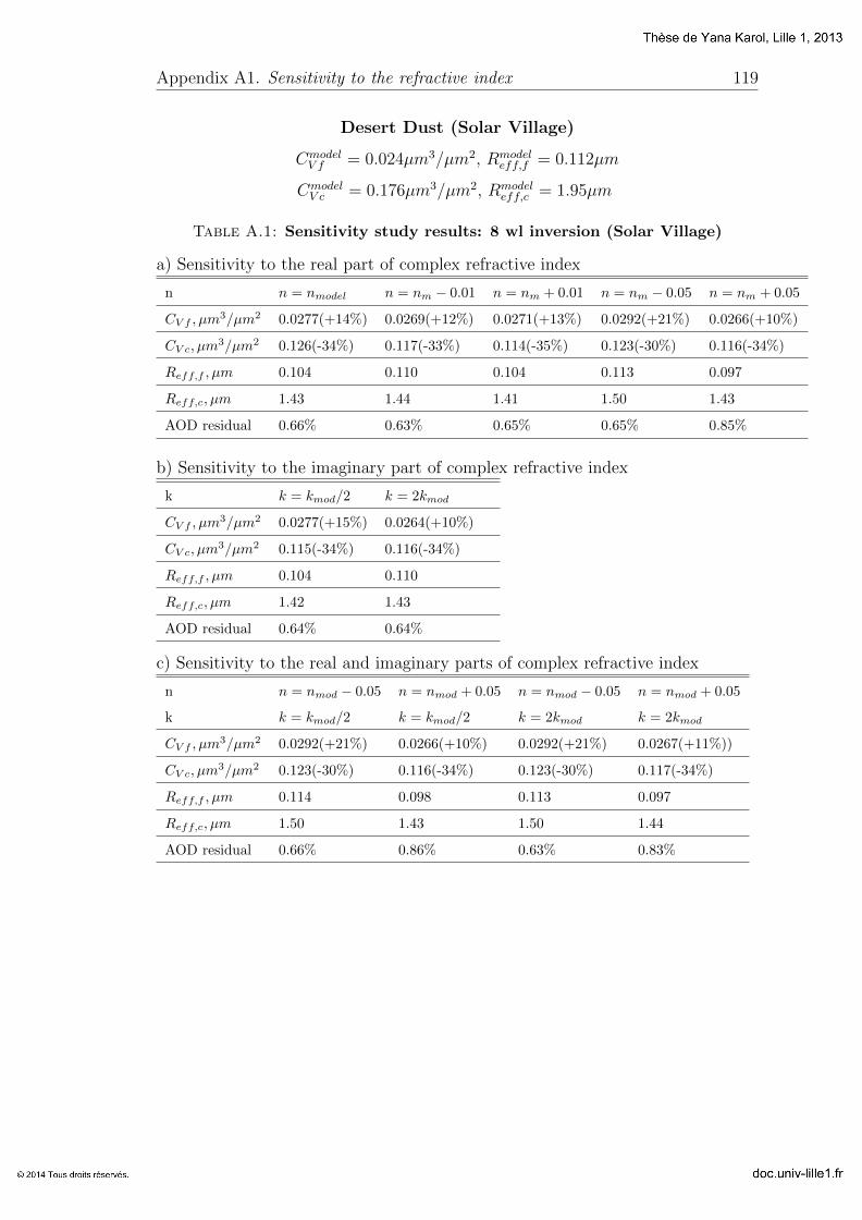
Appendix A1. Sensitivity to the refractive index 119
Desert Dust (Solar Village)
CmodelV f = 0.024µm3/µm2, Rmodel
eff,f = 0.112µm
CmodelV c = 0.176µm3/µm2, Rmodel
eff,c = 1.95µm
Table A.1: Sensitivity study results: 8 wl inversion (Solar Village)
a) Sensitivity to the real part of complex refractive index
n n = nmodel n = nm − 0.01 n = nm + 0.01 n = nm − 0.05 n = nm + 0.05
CV f , µm3/µm2 0.0277(+14%) 0.0269(+12%) 0.0271(+13%) 0.0292(+21%) 0.0266(+10%)
CV c, µm3/µm2 0.126(-34%) 0.117(-33%) 0.114(-35%) 0.123(-30%) 0.116(-34%)
Reff,f , µm 0.104 0.110 0.104 0.113 0.097
Reff,c, µm 1.43 1.44 1.41 1.50 1.43
AOD residual 0.66% 0.63% 0.65% 0.65% 0.85%
b) Sensitivity to the imaginary part of complex refractive index
k k = kmod/2 k = 2kmod
CV f , µm3/µm2 0.0277(+15%) 0.0264(+10%)
CV c, µm3/µm2 0.115(-34%) 0.116(-34%)
Reff,f , µm 0.104 0.110
Reff,c, µm 1.42 1.43
AOD residual 0.64% 0.64%
c) Sensitivity to the real and imaginary parts of complex refractive index
n n = nmod − 0.05 n = nmod + 0.05 n = nmod − 0.05 n = nmod + 0.05
k k = kmod/2 k = kmod/2 k = 2kmod k = 2kmod
CV f , µm3/µm2 0.0292(+21%) 0.0266(+10%) 0.0292(+21%) 0.0267(+11%))
CV c, µm3/µm2 0.123(-30%) 0.116(-34%) 0.123(-30%) 0.117(-34%)
Reff,f , µm 0.114 0.098 0.113 0.097
Reff,c, µm 1.50 1.43 1.50 1.44
AOD residual 0.66% 0.86% 0.63% 0.83%

Appendix A1. Sensitivity to the refractive index 120
0
0.02
0.04
0.06
0.08
0.1
0.12
0.01 0.1 1 10 100
dV
/dln
(R)
(µm
3/µ
m2)
R (µm)
Desert dust (Solar Village)
model nmod=1.56; kmod(1020)=0.001inversion n=nmod k=kmod
inversion n=nmod-0.01; k=kmodinversion n=nmod+0.01; k=kmodinversion n=nmod-0.05; k=kmodinversion n=nmod+0.05; k=kmod
0
0.02
0.04
0.06
0.08
0.1
0.12
0.01 0.1 1 10 100
dV
/dln
(R)
(µm
3/µ
m2)
radius (µm)
Desert dust (Solar Village)
model nmod=1.56; kmod(1020)=0.001inversion n=nmod k=kmod/2
inversion n=nmod; k=kmod*2
0
0.02
0.04
0.06
0.08
0.1
0.12
0.01 0.1 1 10 100
dV
/dln
(R)
(µm
3/µ
m2)
R (µm)
Desert dust (Solar Village)
model nmod=1.56; kmod(1020)=0.001inversion n=nmod-0.05; k=kmod/2inversion n=nmod+0.05; k=kmod/2inversion n=nmod-0.05; k=kmod*2inversion n=nmod+0.05; k=kmod*2
Figure A.1: Size distributions retrieved from 8 wl with different refractiveindices (fixed) - Solar Village.
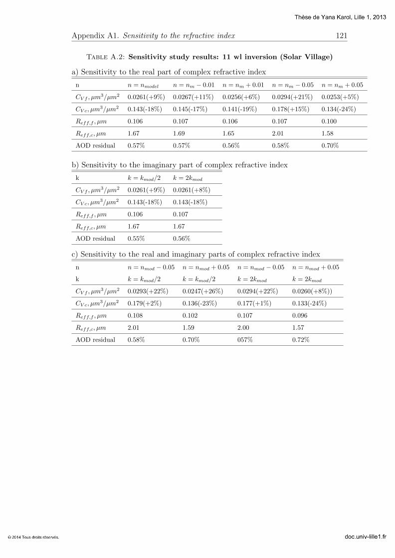
Appendix A1. Sensitivity to the refractive index 121
Table A.2: Sensitivity study results: 11 wl inversion (Solar Village)
a) Sensitivity to the real part of complex refractive index
n n = nmodel n = nm − 0.01 n = nm + 0.01 n = nm − 0.05 n = nm + 0.05
CV f , µm3/µm2 0.0261(+9%) 0.0267(+11%) 0.0256(+6%) 0.0294(+21%) 0.0253(+5%)
CV c, µm3/µm2 0.143(-18%) 0.145(-17%) 0.141(-19%) 0.178(+15%) 0.134(-24%)
Reff,f , µm 0.106 0.107 0.106 0.107 0.100
Reff,c, µm 1.67 1.69 1.65 2.01 1.58
AOD residual 0.57% 0.57% 0.56% 0.58% 0.70%
b) Sensitivity to the imaginary part of complex refractive index
k k = kmod/2 k = 2kmod
CV f , µm3/µm2 0.0261(+9%) 0.0261(+8%)
CV c, µm3/µm2 0.143(-18%) 0.143(-18%)
Reff,f , µm 0.106 0.107
Reff,c, µm 1.67 1.67
AOD residual 0.55% 0.56%
c) Sensitivity to the real and imaginary parts of complex refractive index
n n = nmod − 0.05 n = nmod + 0.05 n = nmod − 0.05 n = nmod + 0.05
k k = kmod/2 k = kmod/2 k = 2kmod k = 2kmod
CV f , µm3/µm2 0.0293(+22%) 0.0247(+26%) 0.0294(+22%) 0.0260(+8%))
CV c, µm3/µm2 0.179(+2%) 0.136(-23%) 0.177(+1%) 0.133(-24%)
Reff,f , µm 0.108 0.102 0.107 0.096
Reff,c, µm 2.01 1.59 2.00 1.57
AOD residual 0.58% 0.70% 057% 0.72%
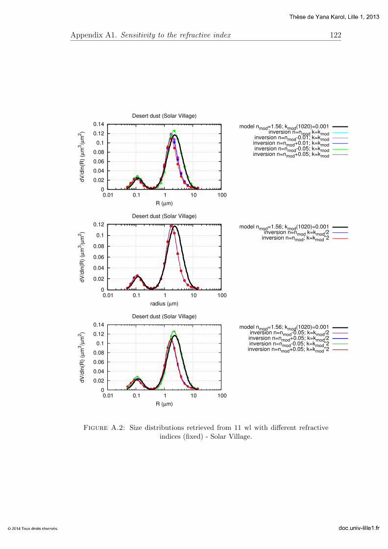
Appendix A1. Sensitivity to the refractive index 122
0
0.02
0.04
0.06
0.08
0.1
0.12
0.14
0.01 0.1 1 10 100
dV
/dln
(R)
(µm
3/µ
m2)
R (µm)
Desert dust (Solar Village)
model nmod=1.56; kmod(1020)=0.001inversion n=nmod k=kmod
inversion n=nmod-0.01; k=kmodinversion n=nmod+0.01; k=kmodinversion n=nmod-0.05; k=kmodinversion n=nmod+0.05; k=kmod
0
0.02
0.04
0.06
0.08
0.1
0.12
0.01 0.1 1 10 100
dV
/dln
(R)
(µm
3/µ
m2)
radius (µm)
Desert dust (Solar Village)
model nmod=1.56; kmod(1020)=0.001inversion n=nmod k=kmod/2
inversion n=nmod; k=kmod*2
0
0.02
0.04
0.06
0.08
0.1
0.12
0.14
0.01 0.1 1 10 100
dV
/dln
(R)
(µm
3/µ
m2)
R (µm)
Desert dust (Solar Village)
model nmod=1.56; kmod(1020)=0.001inversion n=nmod-0.05; k=kmod/2inversion n=nmod+0.05; k=kmod/2inversion n=nmod-0.05; k=kmod*2inversion n=nmod+0.05; k=kmod*2
Figure A.2: Size distributions retrieved from 11 wl with different refractiveindices (fixed) - Solar Village.
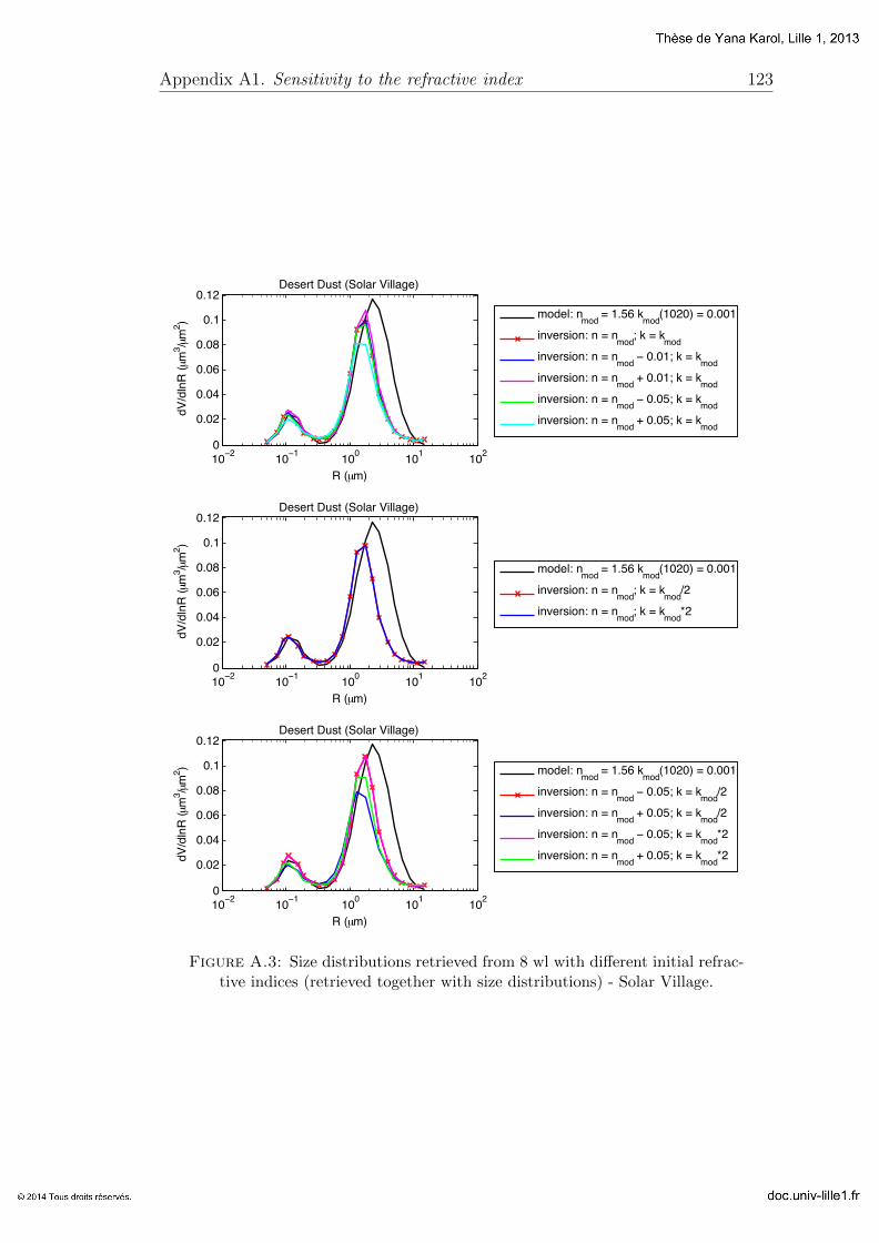
Appendix A1. Sensitivity to the refractive index 123
10−2 10−1 100 101 1020
0.02
0.04
0.06
0.08
0.1
0.12
dV/d
lnR
(µm
3 /µm2 )
R (µm)
Desert Dust (Solar Village)
model: nmod = 1.56 kmod(1020) = 0.001
inversion: n = nmod; k = kmodinversion: n = nmod − 0.01; k = kmodinversion: n = nmod + 0.01; k = kmodinversion: n = nmod − 0.05; k = kmodinversion: n = nmod + 0.05; k = kmod
10−2 10−1 100 101 1020
0.02
0.04
0.06
0.08
0.1
0.12
dV/d
lnR
(µm
3 /µm2 )
R (µm)
Desert Dust (Solar Village)
model: nmod = 1.56 kmod(1020) = 0.001
inversion: n = nmod; k = kmod/2
inversion: n = nmod; k = kmod*2
10−2 10−1 100 101 1020
0.02
0.04
0.06
0.08
0.1
0.12
dV/d
lnR
(µm
3 /µm2 )
R (µm)
Desert Dust (Solar Village)
model: nmod = 1.56 kmod(1020) = 0.001
inversion: n = nmod − 0.05; k = kmod/2
inversion: n = nmod + 0.05; k = kmod/2
inversion: n = nmod − 0.05; k = kmod*2
inversion: n = nmod + 0.05; k = kmod*2
Figure A.3: Size distributions retrieved from 8 wl with different initial refrac-tive indices (retrieved together with size distributions) - Solar Village.
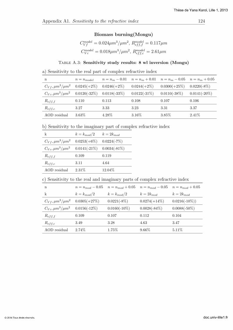
Appendix A1. Sensitivity to the refractive index 124
Biomass burning(Mongu)
CmodelV f = 0.024µm3/µm2, Rmodel
eff,f = 0.117µm
CmodelV c = 0.018µm3/µm2, Rmodel
eff,c = 2.61µm
Table A.3: Sensitivity study results: 8 wl inversion (Mongu)
a) Sensitivity to the real part of complex refractive index
n n = nmodel n = nm − 0.01 n = nm + 0.01 n = nm − 0.05 n = nm + 0.05
CV f , µm3/µm2 0.0245(+2%) 0.0246(+2%) 0.0244(+2%) 0.0300(+25%) 0.0220(-8%)
CV c, µm3/µm2 0.0120(-32%) 0.0118(-33%) 0.0122(-31%) 0.0110(-38%) 0.0141(-20%)
Reff,f 0.110 0.113 0.108 0.107 0.106
Reff,c 3.27 3.33 3.23 3.31 3.37
AOD residual 3.63% 4.28% 3.16% 3.85% 2.41%
b) Sensitivity to the imaginary part of complex refractive index
k k = kmod/2 k = 2kmod
CV f , µm3/µm2 0.0253(+6%) 0.0224(-7%)
CV c, µm3/µm2 0.0141(-21%) 0.0034(-81%)
Reff,f 0.109 0.119
Reff,c 3.11 4.64
AOD residual 2.31% 12.04%
c) Sensitivity to the real and imaginary parts of complex refractive index
n n = nmod − 0.05 n = nmod + 0.05 n = nmod − 0.05 n = nmod + 0.05
k k = kmod/2 k = kmod/2 k = 2kmod k = 2kmod
CV f , µm3/µm2 0.0305(+27%) 0.0221(-8%) 0.0274(+14%) 0.0216(-10%))
CV c, µm3/µm2 0.0156(-12%) 0.0160(-10%) 0.0028(-84%) 0.0088(-50%)
Reff,f 0.109 0.107 0.112 0.104
Reff,c 3.49 3.28 4.63 3.47
AOD residual 2.74% 1.75% 9.66% 5.11%

Appendix A1. Sensitivity to the refractive index 125
0
0.005
0.01
0.015
0.02
0.025
0.03
0.035
0.04
0.045
0.01 0.1 1 10 100
dV
/dln
(R)
(µm
3/µ
m2)
R (µm)
Biomass Burning (Mongu)
model nmod=1.51; kmod=0.021inversion n=nmod k=kmod
inversion n=nmod-0.01; k=kmodinversion n=nmod+0.01; k=kmodinversion n=nmod-0.05; k=kmodinversion n=nmod+0.05; k=kmod
0
0.005
0.01
0.015
0.02
0.025
0.03
0.035
0.01 0.1 1 10 100
dV
/dln
(R)
(µm
3/µ
m2)
radius (µm)
Biomass Burning (Mongu)
model nmod=1.51; kmod=0.021inversion n=nmod k=kmod/2
inversion n=nmod; k=kmod*2
0
0.005
0.01
0.015
0.02
0.025
0.03
0.035
0.04
0.045
0.01 0.1 1 10 100
dV
/dln
(R)
(µm
3/µ
m2)
R (µm)
Biomass Burning (Mongu)
model nmod=1.51; kmod=0.021inversion n=nmod-0.05; k=kmod/2inversion n=nmod+0.05; k=kmod/2inversion n=nmod-0.05; k=kmod*2inversion n=nmod+0.05; k=kmod*2
Figure A.4: Size distributions retrieved from 8 wl with different refractiveindices (fixed) - Mongu.
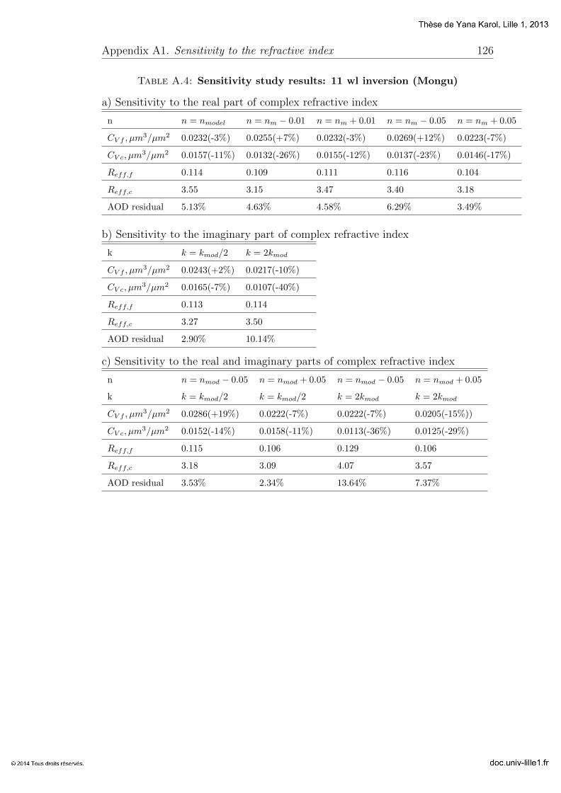
Appendix A1. Sensitivity to the refractive index 126
Table A.4: Sensitivity study results: 11 wl inversion (Mongu)
a) Sensitivity to the real part of complex refractive index
n n = nmodel n = nm − 0.01 n = nm + 0.01 n = nm − 0.05 n = nm + 0.05
CV f , µm3/µm2 0.0232(-3%) 0.0255(+7%) 0.0232(-3%) 0.0269(+12%) 0.0223(-7%)
CV c, µm3/µm2 0.0157(-11%) 0.0132(-26%) 0.0155(-12%) 0.0137(-23%) 0.0146(-17%)
Reff,f 0.114 0.109 0.111 0.116 0.104
Reff,c 3.55 3.15 3.47 3.40 3.18
AOD residual 5.13% 4.63% 4.58% 6.29% 3.49%
b) Sensitivity to the imaginary part of complex refractive index
k k = kmod/2 k = 2kmod
CV f , µm3/µm2 0.0243(+2%) 0.0217(-10%)
CV c, µm3/µm2 0.0165(-7%) 0.0107(-40%)
Reff,f 0.113 0.114
Reff,c 3.27 3.50
AOD residual 2.90% 10.14%
c) Sensitivity to the real and imaginary parts of complex refractive index
n n = nmod − 0.05 n = nmod + 0.05 n = nmod − 0.05 n = nmod + 0.05
k k = kmod/2 k = kmod/2 k = 2kmod k = 2kmod
CV f , µm3/µm2 0.0286(+19%) 0.0222(-7%) 0.0222(-7%) 0.0205(-15%))
CV c, µm3/µm2 0.0152(-14%) 0.0158(-11%) 0.0113(-36%) 0.0125(-29%)
Reff,f 0.115 0.106 0.129 0.106
Reff,c 3.18 3.09 4.07 3.57
AOD residual 3.53% 2.34% 13.64% 7.37%
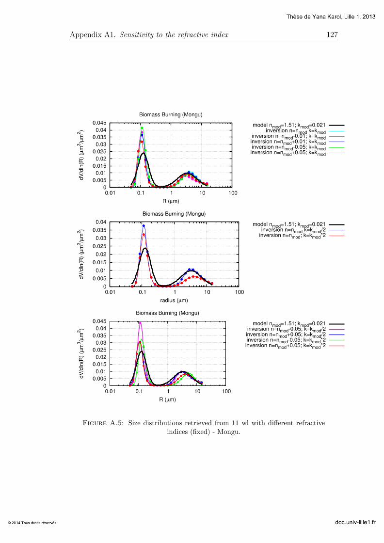
Appendix A1. Sensitivity to the refractive index 127
0
0.005
0.01
0.015
0.02
0.025
0.03
0.035
0.04
0.045
0.01 0.1 1 10 100
dV
/dln
(R)
(µm
3/µ
m2)
R (µm)
Biomass Burning (Mongu)
model nmod=1.51; kmod=0.021inversion n=nmod k=kmod
inversion n=nmod-0.01; k=kmodinversion n=nmod+0.01; k=kmodinversion n=nmod-0.05; k=kmodinversion n=nmod+0.05; k=kmod
0
0.005
0.01
0.015
0.02
0.025
0.03
0.035
0.04
0.01 0.1 1 10 100
dV
/dln
(R)
(µm
3/µ
m2)
radius (µm)
Biomass Burning (Mongu)
model nmod=1.51; kmod=0.021inversion n=nmod k=kmod/2
inversion n=nmod; k=kmod*2
0
0.005
0.01
0.015
0.02
0.025
0.03
0.035
0.04
0.045
0.01 0.1 1 10 100
dV
/dln
(R)
(µm
3/µ
m2)
R (µm)
Biomass Burning (Mongu)
model nmod=1.51; kmod=0.021inversion n=nmod-0.05; k=kmod/2inversion n=nmod+0.05; k=kmod/2inversion n=nmod-0.05; k=kmod*2inversion n=nmod+0.05; k=kmod*2
Figure A.5: Size distributions retrieved from 11 wl with different refractiveindices (fixed) - Mongu.
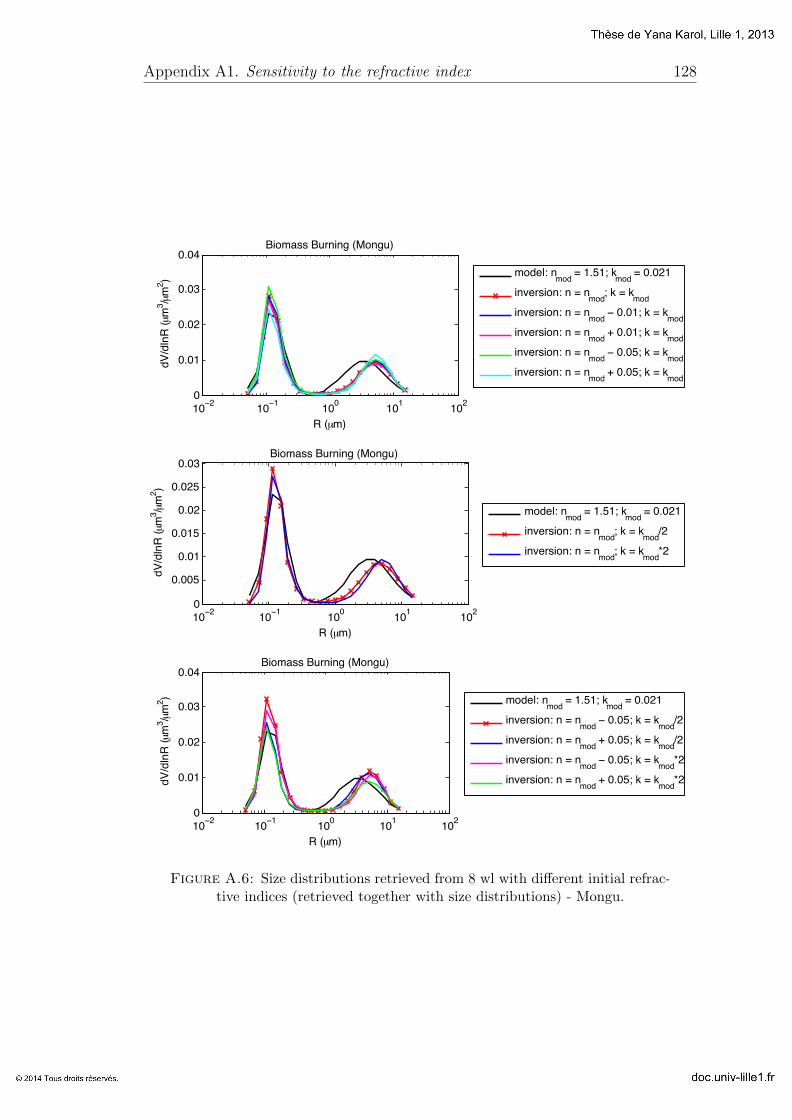
Appendix A1. Sensitivity to the refractive index 128
10−2 10−1 100 101 1020
0.01
0.02
0.03
0.04
dV/d
lnR
(µm
3 /µm2 )
R (µm)
Biomass Burning (Mongu)
model: nmod = 1.51; kmod = 0.021
inversion: n = nmod; k = kmodinversion: n = nmod − 0.01; k = kmodinversion: n = nmod + 0.01; k = kmodinversion: n = nmod − 0.05; k = kmodinversion: n = nmod + 0.05; k = kmod
10−2 10−1 100 101 1020
0.005
0.01
0.015
0.02
0.025
0.03
dV/d
lnR
(µm
3 /µm2 )
R (µm)
Biomass Burning (Mongu)
model: nmod = 1.51; kmod = 0.021
inversion: n = nmod; k = kmod/2
inversion: n = nmod; k = kmod*2
10−2 10−1 100 101 1020
0.01
0.02
0.03
0.04
dV/d
lnR
(µm
3 /µm2 )
R (µm)
Biomass Burning (Mongu)
model: nmod = 1.51; kmod = 0.021
inversion: n = nmod − 0.05; k = kmod/2
inversion: n = nmod + 0.05; k = kmod/2
inversion: n = nmod − 0.05; k = kmod*2
inversion: n = nmod + 0.05; k = kmod*2
Figure A.6: Size distributions retrieved from 8 wl with different initial refrac-tive indices (retrieved together with size distributions) - Mongu.
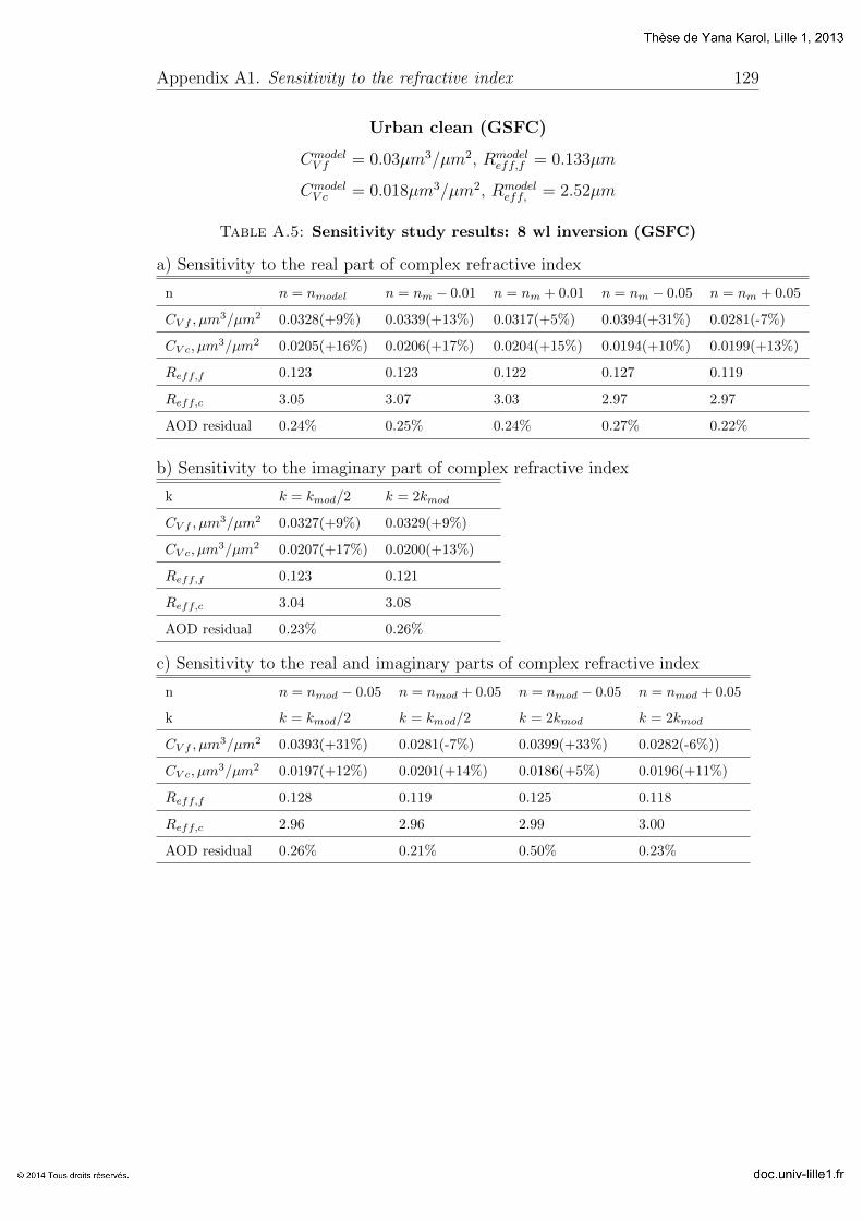
Appendix A1. Sensitivity to the refractive index 129
Urban clean (GSFC)
CmodelV f = 0.03µm3/µm2, Rmodel
eff,f = 0.133µm
CmodelV c = 0.018µm3/µm2, Rmodel
eff, = 2.52µm
Table A.5: Sensitivity study results: 8 wl inversion (GSFC)
a) Sensitivity to the real part of complex refractive index
n n = nmodel n = nm − 0.01 n = nm + 0.01 n = nm − 0.05 n = nm + 0.05
CV f , µm3/µm2 0.0328(+9%) 0.0339(+13%) 0.0317(+5%) 0.0394(+31%) 0.0281(-7%)
CV c, µm3/µm2 0.0205(+16%) 0.0206(+17%) 0.0204(+15%) 0.0194(+10%) 0.0199(+13%)
Reff,f 0.123 0.123 0.122 0.127 0.119
Reff,c 3.05 3.07 3.03 2.97 2.97
AOD residual 0.24% 0.25% 0.24% 0.27% 0.22%
b) Sensitivity to the imaginary part of complex refractive index
k k = kmod/2 k = 2kmod
CV f , µm3/µm2 0.0327(+9%) 0.0329(+9%)
CV c, µm3/µm2 0.0207(+17%) 0.0200(+13%)
Reff,f 0.123 0.121
Reff,c 3.04 3.08
AOD residual 0.23% 0.26%
c) Sensitivity to the real and imaginary parts of complex refractive index
n n = nmod − 0.05 n = nmod + 0.05 n = nmod − 0.05 n = nmod + 0.05
k k = kmod/2 k = kmod/2 k = 2kmod k = 2kmod
CV f , µm3/µm2 0.0393(+31%) 0.0281(-7%) 0.0399(+33%) 0.0282(-6%))
CV c, µm3/µm2 0.0197(+12%) 0.0201(+14%) 0.0186(+5%) 0.0196(+11%)
Reff,f 0.128 0.119 0.125 0.118
Reff,c 2.96 2.96 2.99 3.00
AOD residual 0.26% 0.21% 0.50% 0.23%
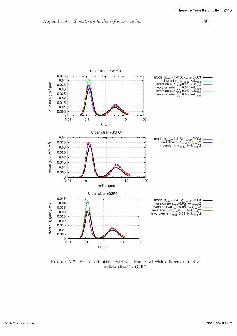
Appendix A1. Sensitivity to the refractive index 130
0
0.005
0.01
0.015
0.02
0.025
0.03
0.035
0.04
0.045
0.01 0.1 1 10 100
dV
/dln
(R)
(µm
3/µ
m2)
R (µm)
Urban clean (GSFC)
model nmod=1.416; kmod=0.003inversion n=nmod k=kmod
inversion n=nmod-0.01; k=kmodinversion n=nmod+0.01; k=kmodinversion n=nmod-0.05; k=kmodinversion n=nmod+0.05; k=kmod
0
0.005
0.01
0.015
0.02
0.025
0.03
0.035
0.04
0.01 0.1 1 10 100
dV
/dln
(R)
(µm
3/µ
m2)
radius (µm)
Urban clean (GSFC)
model nmod=1.416; kmod=0.003inversion n=nmod k=kmod/2
inversion n=nmod; k=kmod*2
0
0.005
0.01
0.015
0.02
0.025
0.03
0.035
0.04
0.045
0.01 0.1 1 10 100
dV
/dln
(R)
(µm
3/µ
m2)
R (µm)
Urban clean (GSFC)
model nmod=1.416; kmod=0.003inversion n=nmod-0.05; k=kmod/2inversion n=nmod+0.05; k=kmod/2inversion n=nmod-0.05; k=kmod*2inversion n=nmod+0.05; k=kmod*2
Figure A.7: Size distributions retrieved from 8 wl with different refractiveindices (fixed) - GSFC.
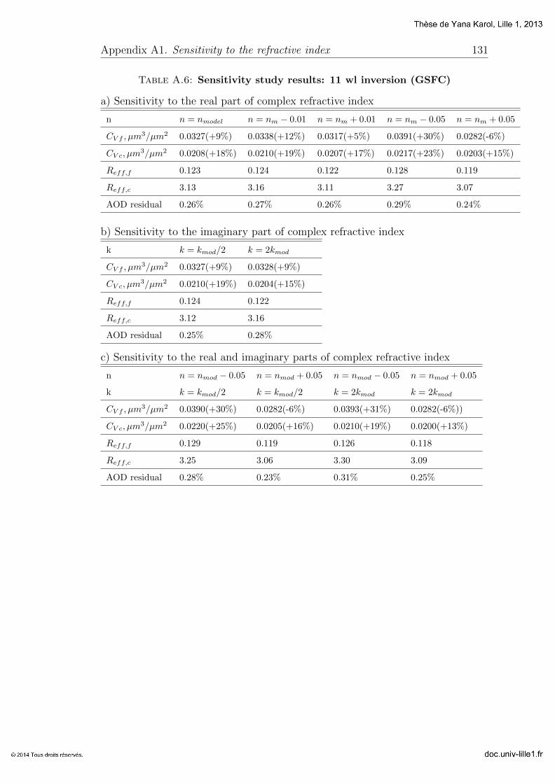
Appendix A1. Sensitivity to the refractive index 131
Table A.6: Sensitivity study results: 11 wl inversion (GSFC)
a) Sensitivity to the real part of complex refractive index
n n = nmodel n = nm − 0.01 n = nm + 0.01 n = nm − 0.05 n = nm + 0.05
CV f , µm3/µm2 0.0327(+9%) 0.0338(+12%) 0.0317(+5%) 0.0391(+30%) 0.0282(-6%)
CV c, µm3/µm2 0.0208(+18%) 0.0210(+19%) 0.0207(+17%) 0.0217(+23%) 0.0203(+15%)
Reff,f 0.123 0.124 0.122 0.128 0.119
Reff,c 3.13 3.16 3.11 3.27 3.07
AOD residual 0.26% 0.27% 0.26% 0.29% 0.24%
b) Sensitivity to the imaginary part of complex refractive index
k k = kmod/2 k = 2kmod
CV f , µm3/µm2 0.0327(+9%) 0.0328(+9%)
CV c, µm3/µm2 0.0210(+19%) 0.0204(+15%)
Reff,f 0.124 0.122
Reff,c 3.12 3.16
AOD residual 0.25% 0.28%
c) Sensitivity to the real and imaginary parts of complex refractive index
n n = nmod − 0.05 n = nmod + 0.05 n = nmod − 0.05 n = nmod + 0.05
k k = kmod/2 k = kmod/2 k = 2kmod k = 2kmod
CV f , µm3/µm2 0.0390(+30%) 0.0282(-6%) 0.0393(+31%) 0.0282(-6%))
CV c, µm3/µm2 0.0220(+25%) 0.0205(+16%) 0.0210(+19%) 0.0200(+13%)
Reff,f 0.129 0.119 0.126 0.118
Reff,c 3.25 3.06 3.30 3.09
AOD residual 0.28% 0.23% 0.31% 0.25%
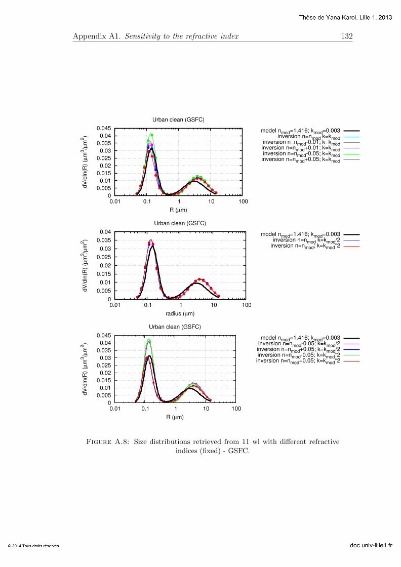
Appendix A1. Sensitivity to the refractive index 132
0
0.005
0.01
0.015
0.02
0.025
0.03
0.035
0.04
0.045
0.01 0.1 1 10 100
dV
/dln
(R)
(µm
3/µ
m2)
R (µm)
Urban clean (GSFC)
model nmod=1.416; kmod=0.003inversion n=nmod k=kmod
inversion n=nmod-0.01; k=kmodinversion n=nmod+0.01; k=kmodinversion n=nmod-0.05; k=kmodinversion n=nmod+0.05; k=kmod
0
0.005
0.01
0.015
0.02
0.025
0.03
0.035
0.04
0.01 0.1 1 10 100
dV
/dln
(R)
(µm
3/µ
m2)
radius (µm)
Urban clean (GSFC)
model nmod=1.416; kmod=0.003inversion n=nmod k=kmod/2
inversion n=nmod; k=kmod*2
0
0.005
0.01
0.015
0.02
0.025
0.03
0.035
0.04
0.045
0.01 0.1 1 10 100
dV
/dln
(R)
(µm
3/µ
m2)
R (µm)
Urban clean (GSFC)
model nmod=1.416; kmod=0.003inversion n=nmod-0.05; k=kmod/2inversion n=nmod+0.05; k=kmod/2inversion n=nmod-0.05; k=kmod*2inversion n=nmod+0.05; k=kmod*2
Figure A.8: Size distributions retrieved from 11 wl with different refractiveindices (fixed) - GSFC.
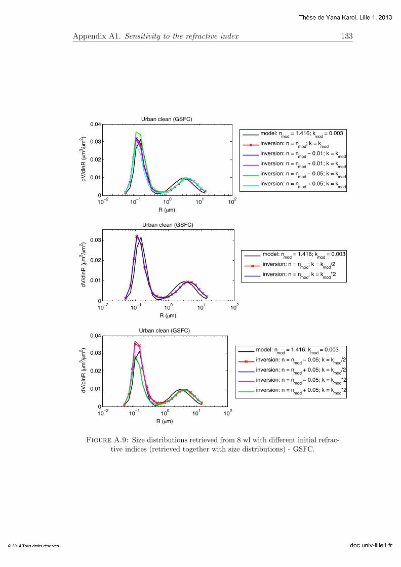
Appendix A1. Sensitivity to the refractive index 133
10−2 10−1 100 101 1020
0.01
0.02
0.03
0.04
dV/d
lnR
(µm
3 /µm2 )
R (µm)
Urban clean (GSFC)
model: nmod = 1.416; kmod = 0.003
inversion: n = nmod; k = kmodinversion: n = nmod − 0.01; k = kmodinversion: n = nmod + 0.01; k = kmodinversion: n = nmod − 0.05; k = kmodinversion: n = nmod + 0.05; k = kmod
10−2 10−1 100 101 1020
0.01
0.02
0.03
dV/d
lnR
(µm
3 /µm2 )
R (µm)
Urban clean (GSFC)
model: nmod = 1.416; kmod = 0.003
inversion: n = nmod; k = kmod/2
inversion: n = nmod; k = kmod*2
10−2 10−1 100 101 1020
0.01
0.02
0.03
0.04
dV/d
lnR
(µm
3 /µm2 )
R (µm)
Urban clean (GSFC)
model: nmod = 1.416; kmod = 0.003
inversion: n = nmod − 0.05; k = kmod/2
inversion: n = nmod + 0.05; k = kmod/2
inversion: n = nmod − 0.05; k = kmod*2
inversion: n = nmod + 0.05; k = kmod*2
Figure A.9: Size distributions retrieved from 8 wl with different initial refrac-tive indices (retrieved together with size distributions) - GSFC.
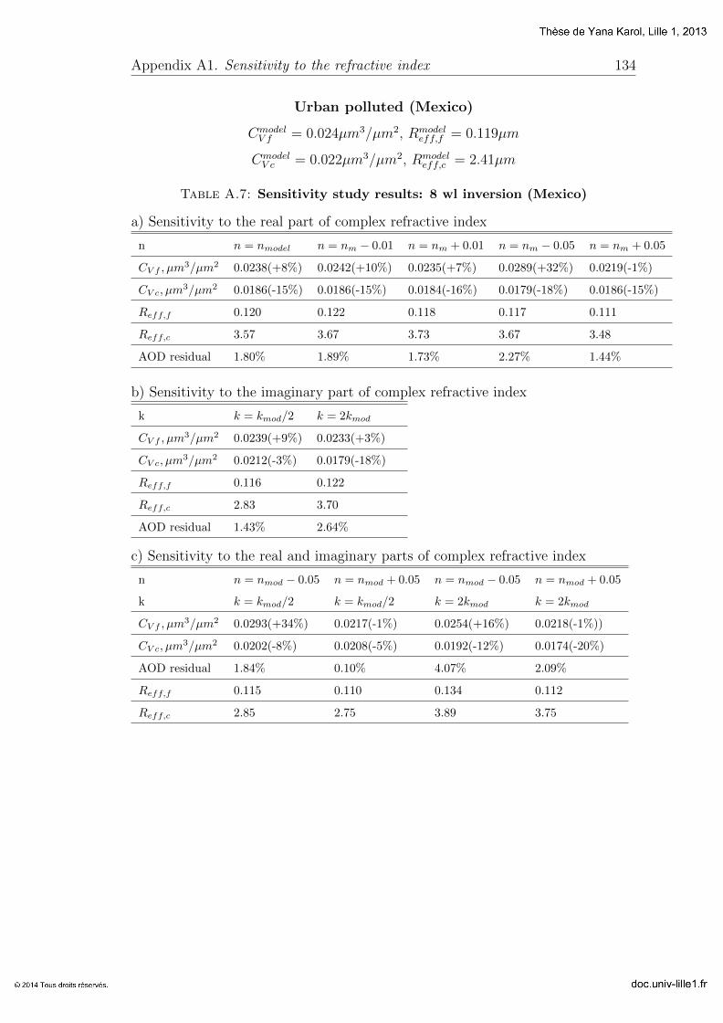
Appendix A1. Sensitivity to the refractive index 134
Urban polluted (Mexico)
CmodelV f = 0.024µm3/µm2, Rmodel
eff,f = 0.119µm
CmodelV c = 0.022µm3/µm2, Rmodel
eff,c = 2.41µm
Table A.7: Sensitivity study results: 8 wl inversion (Mexico)
a) Sensitivity to the real part of complex refractive index
n n = nmodel n = nm − 0.01 n = nm + 0.01 n = nm − 0.05 n = nm + 0.05
CV f , µm3/µm2 0.0238(+8%) 0.0242(+10%) 0.0235(+7%) 0.0289(+32%) 0.0219(-1%)
CV c, µm3/µm2 0.0186(-15%) 0.0186(-15%) 0.0184(-16%) 0.0179(-18%) 0.0186(-15%)
Reff,f 0.120 0.122 0.118 0.117 0.111
Reff,c 3.57 3.67 3.73 3.67 3.48
AOD residual 1.80% 1.89% 1.73% 2.27% 1.44%
b) Sensitivity to the imaginary part of complex refractive index
k k = kmod/2 k = 2kmod
CV f , µm3/µm2 0.0239(+9%) 0.0233(+3%)
CV c, µm3/µm2 0.0212(-3%) 0.0179(-18%)
Reff,f 0.116 0.122
Reff,c 2.83 3.70
AOD residual 1.43% 2.64%
c) Sensitivity to the real and imaginary parts of complex refractive index
n n = nmod − 0.05 n = nmod + 0.05 n = nmod − 0.05 n = nmod + 0.05
k k = kmod/2 k = kmod/2 k = 2kmod k = 2kmod
CV f , µm3/µm2 0.0293(+34%) 0.0217(-1%) 0.0254(+16%) 0.0218(-1%))
CV c, µm3/µm2 0.0202(-8%) 0.0208(-5%) 0.0192(-12%) 0.0174(-20%)
AOD residual 1.84% 0.10% 4.07% 2.09%
Reff,f 0.115 0.110 0.134 0.112
Reff,c 2.85 2.75 3.89 3.75
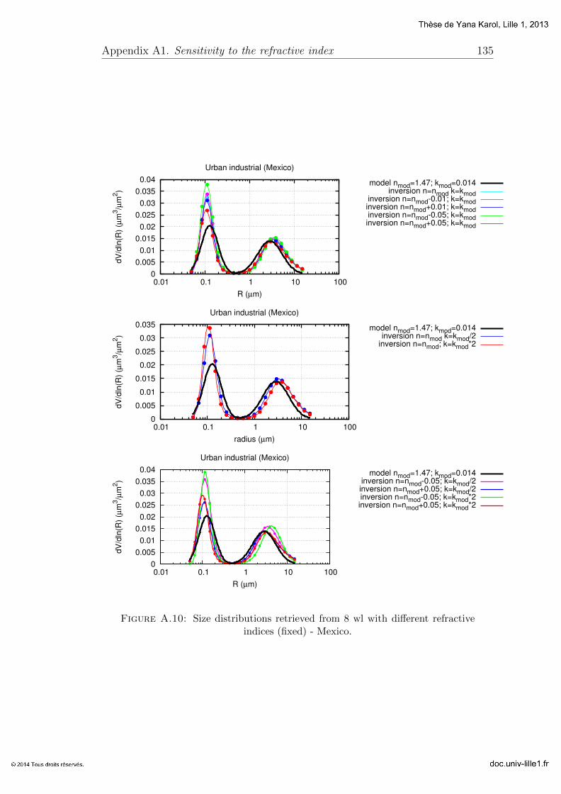
Appendix A1. Sensitivity to the refractive index 135
0
0.005
0.01
0.015
0.02
0.025
0.03
0.035
0.04
0.01 0.1 1 10 100
dV
/dln
(R)
(µm
3/µ
m2)
R (µm)
Urban industrial (Mexico)
model nmod=1.47; kmod=0.014inversion n=nmod k=kmod
inversion n=nmod-0.01; k=kmodinversion n=nmod+0.01; k=kmodinversion n=nmod-0.05; k=kmodinversion n=nmod+0.05; k=kmod
0
0.005
0.01
0.015
0.02
0.025
0.03
0.035
0.01 0.1 1 10 100
dV
/dln
(R)
(µm
3/µ
m2)
radius (µm)
Urban industrial (Mexico)
model nmod=1.47; kmod=0.014inversion n=nmod k=kmod/2
inversion n=nmod; k=kmod*2
0
0.005
0.01
0.015
0.02
0.025
0.03
0.035
0.04
0.01 0.1 1 10 100
dV
/dln
(R)
(µm
3/µ
m2)
R (µm)
Urban industrial (Mexico)
model nmod=1.47; kmod=0.014inversion n=nmod-0.05; k=kmod/2inversion n=nmod+0.05; k=kmod/2inversion n=nmod-0.05; k=kmod*2inversion n=nmod+0.05; k=kmod*2
Figure A.10: Size distributions retrieved from 8 wl with different refractiveindices (fixed) - Mexico.

Appendix A1. Sensitivity to the refractive index 136
Table A.8: Sensitivity study results: 11 wl inversion (Mexico)
a) Sensitivity to the real part of complex refractive index
n n = nmodel n = nm − 0.01 n = nm + 0.01 n = nm − 0.05 n = nm + 0.05
CV f , µm3/µm2 0.0250(+14%) 0.0258(+18%) 0.0229(+4%) 0.0310(+42%) 0.0217(-1%)
CV c, µm3/µm2 0.0222(+1%) 0.0224(+2%) 0.0232(+6%) 0.0229(+5%) 0.0213(-3%)
Reff,f 0.111 0.111 0.116 0.108 0.108
Reff,c 2.84 2.88 3.25 3.02 2.70
AOD residual 1.54% 1.65% 0.012% 2.22% 1.05%
b) Sensitivity to the imaginary part of complex refractive index
k k = kmod/2 k = 2kmod
CV f , µm3/µm2 0.0245(+12%) 0.0257(+17%)
CV c, µm3/µm2 0.0227(+4%) 0.0208(-5%)
Reff,f 0.114 0.105
Reff,c 2.79 2.96
AOD residual 0.93% 2.96%
c) Sensitivity to the real and imaginary parts of complex refractive index
n n = nmod − 0.05 n = nmod + 0.05 n = nmod − 0.05 n = nmod + 0.05
k k = kmod/2 k = kmod/2 k = 2kmod k = 2kmod
CV f , µm3/µm2 0.0301(+37%) 0.0213(-3%) 0.0316(+44%) 0.0227(+4%))
CV c, µm3/µm2 0.0240(+10%) 0.0216(-2%) 0.0204(-7%) 0.0208(-5%)
Reff,f 0.113 0.111 0.103 0.101
Reff,c 2.97 2.66 3.13 2.85
AOD residual 1.48% 0.54% 3.98% 2.34%
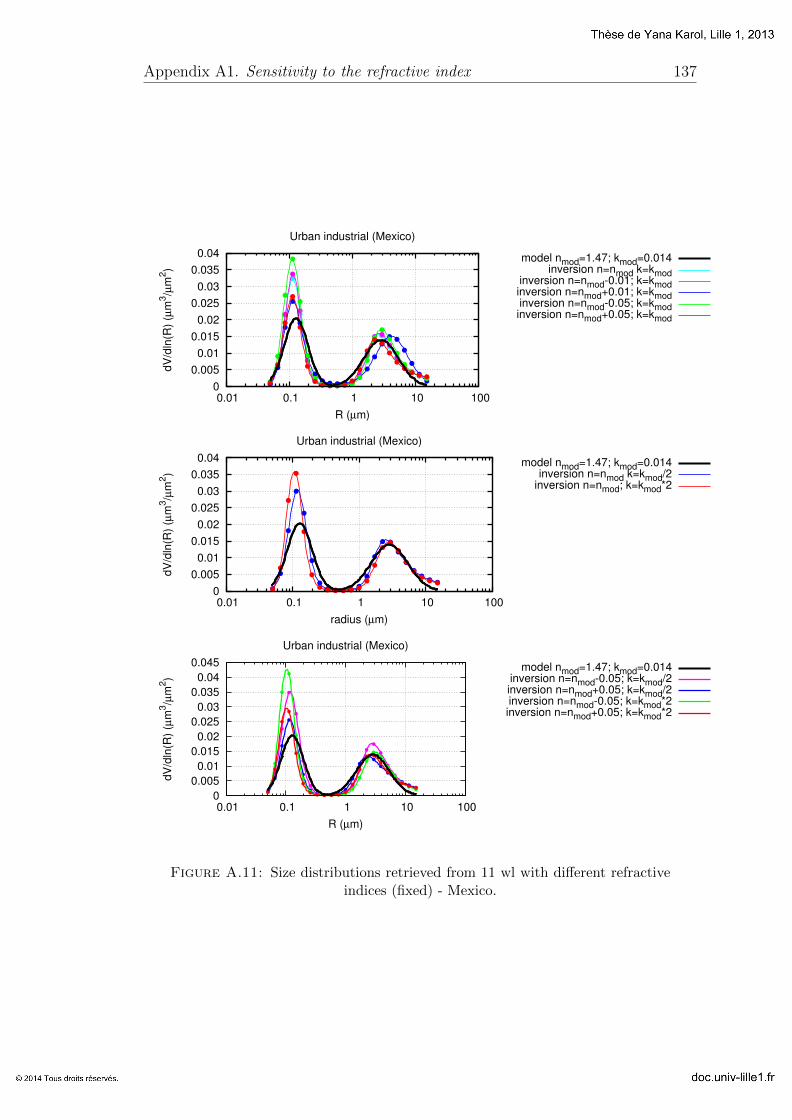
Appendix A1. Sensitivity to the refractive index 137
0
0.005
0.01
0.015
0.02
0.025
0.03
0.035
0.04
0.01 0.1 1 10 100
dV
/dln
(R)
(µm
3/µ
m2)
R (µm)
Urban industrial (Mexico)
model nmod=1.47; kmod=0.014inversion n=nmod k=kmod
inversion n=nmod-0.01; k=kmodinversion n=nmod+0.01; k=kmodinversion n=nmod-0.05; k=kmodinversion n=nmod+0.05; k=kmod
0
0.005
0.01
0.015
0.02
0.025
0.03
0.035
0.04
0.01 0.1 1 10 100
dV
/dln
(R)
(µm
3/µ
m2)
radius (µm)
Urban industrial (Mexico)
model nmod=1.47; kmod=0.014inversion n=nmod k=kmod/2
inversion n=nmod; k=kmod*2
0
0.005
0.01
0.015
0.02
0.025
0.03
0.035
0.04
0.045
0.01 0.1 1 10 100
dV
/dln
(R)
(µm
3/µ
m2)
R (µm)
Urban industrial (Mexico)
model nmod=1.47; kmod=0.014inversion n=nmod-0.05; k=kmod/2inversion n=nmod+0.05; k=kmod/2inversion n=nmod-0.05; k=kmod*2inversion n=nmod+0.05; k=kmod*2
Figure A.11: Size distributions retrieved from 11 wl with different refractiveindices (fixed) - Mexico.
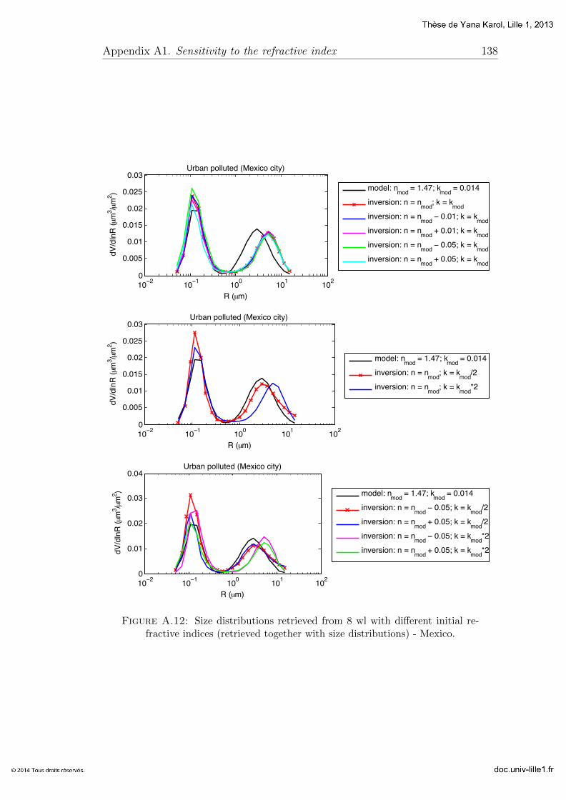
Appendix A1. Sensitivity to the refractive index 138
10−2 10−1 100 101 1020
0.005
0.01
0.015
0.02
0.025
0.03
dV/d
lnR
(µm
3 /µm2 )
R (µm)
Urban polluted (Mexico city)
model: nmod = 1.47; kmod = 0.014
inversion: n = nmod; k = kmodinversion: n = nmod − 0.01; k = kmodinversion: n = nmod + 0.01; k = kmodinversion: n = nmod − 0.05; k = kmodinversion: n = nmod + 0.05; k = kmod
10−2 10−1 100 101 1020
0.005
0.01
0.015
0.02
0.025
0.03
dV/d
lnR
(µm
3 /µm2 )
R (µm)
Urban polluted (Mexico city)
model: nmod = 1.47; kmod = 0.014
inversion: n = nmod; k = kmod/2
inversion: n = nmod; k = kmod*2
10−2 10−1 100 101 1020
0.01
0.02
0.03
0.04
dV/d
lnR
(µm
3 /µm2 )
R (µm)
Urban polluted (Mexico city)
model: nmod = 1.47; kmod = 0.014
inversion: n = nmod − 0.05; k = kmod/2
inversion: n = nmod + 0.05; k = kmod/2
inversion: n = nmod − 0.05; k = kmod*2
inversion: n = nmod + 0.05; k = kmod*2
Figure A.12: Size distributions retrieved from 8 wl with different initial re-fractive indices (retrieved together with size distributions) - Mexico.
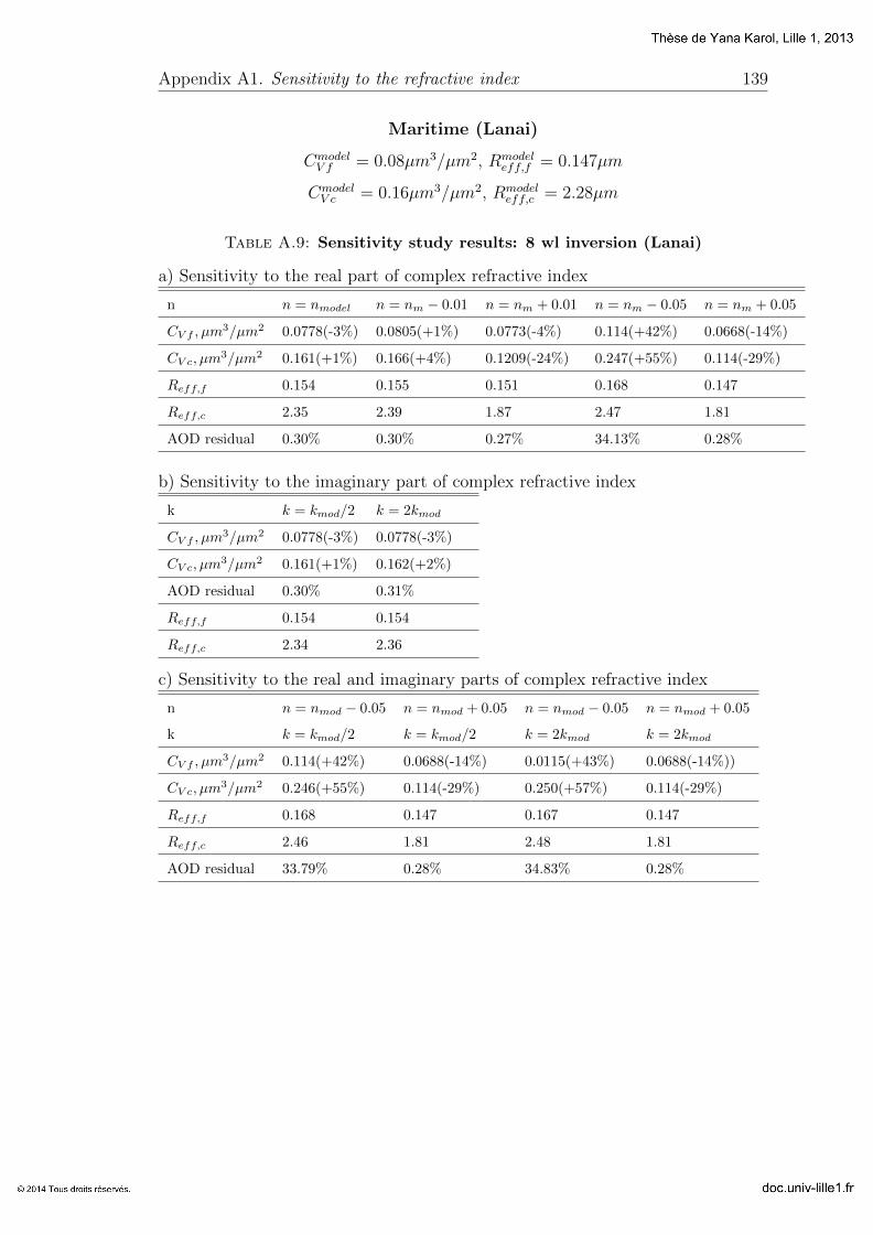
Appendix A1. Sensitivity to the refractive index 139
Maritime (Lanai)
CmodelV f = 0.08µm3/µm2, Rmodel
eff,f = 0.147µm
CmodelV c = 0.16µm3/µm2, Rmodel
eff,c = 2.28µm
Table A.9: Sensitivity study results: 8 wl inversion (Lanai)
a) Sensitivity to the real part of complex refractive index
n n = nmodel n = nm − 0.01 n = nm + 0.01 n = nm − 0.05 n = nm + 0.05
CV f , µm3/µm2 0.0778(-3%) 0.0805(+1%) 0.0773(-4%) 0.114(+42%) 0.0668(-14%)
CV c, µm3/µm2 0.161(+1%) 0.166(+4%) 0.1209(-24%) 0.247(+55%) 0.114(-29%)
Reff,f 0.154 0.155 0.151 0.168 0.147
Reff,c 2.35 2.39 1.87 2.47 1.81
AOD residual 0.30% 0.30% 0.27% 34.13% 0.28%
b) Sensitivity to the imaginary part of complex refractive index
k k = kmod/2 k = 2kmod
CV f , µm3/µm2 0.0778(-3%) 0.0778(-3%)
CV c, µm3/µm2 0.161(+1%) 0.162(+2%)
AOD residual 0.30% 0.31%
Reff,f 0.154 0.154
Reff,c 2.34 2.36
c) Sensitivity to the real and imaginary parts of complex refractive index
n n = nmod − 0.05 n = nmod + 0.05 n = nmod − 0.05 n = nmod + 0.05
k k = kmod/2 k = kmod/2 k = 2kmod k = 2kmod
CV f , µm3/µm2 0.114(+42%) 0.0688(-14%) 0.0115(+43%) 0.0688(-14%))
CV c, µm3/µm2 0.246(+55%) 0.114(-29%) 0.250(+57%) 0.114(-29%)
Reff,f 0.168 0.147 0.167 0.147
Reff,c 2.46 1.81 2.48 1.81
AOD residual 33.79% 0.28% 34.83% 0.28%

Appendix A1. Sensitivity to the refractive index 140
0 0.02 0.04 0.06 0.08
0.1 0.12 0.14 0.16 0.18
0.2
0.01 0.1 1 10 100
dV
/dln
(R)
(µm
3/µ
m2)
R (µm)
Maritime (Lanai)
model nmod=1.36; kmod=0.0015inversion n=nmod k=kmod
inversion n=nmod-0.01; k=kmodinversion n=nmod+0.01; k=kmodinversion n=nmod-0.05; k=kmodinversion n=nmod+0.05; k=kmod
0
0.02
0.04
0.06
0.08
0.1
0.12
0.01 0.1 1 10 100
dV
/dln
(R)
(µm
3/µ
m2)
radius (µm)
Maritime (Lanai)
model nmod=1.36; kmod=0.0015inversion n=nmod k=kmod/2
inversion n=nmod; k=kmod*2
0 0.02 0.04 0.06 0.08
0.1 0.12 0.14 0.16 0.18
0.2
0.01 0.1 1 10 100
dV
/dln
(R)
(µm
3/µ
m2)
R (µm)
Maritime (Lanai)
model nmod=1.36; kmod=0.0015inversion n=nmod-0.05; k=kmod/2inversion n=nmod+0.05; k=kmod/2inversion n=nmod-0.05; k=kmod*2inversion n=nmod+0.05; k=kmod*2
Figure A.13: Size distributions retrieved from 8 wl with different refractiveindices (fixed) - Lanai.
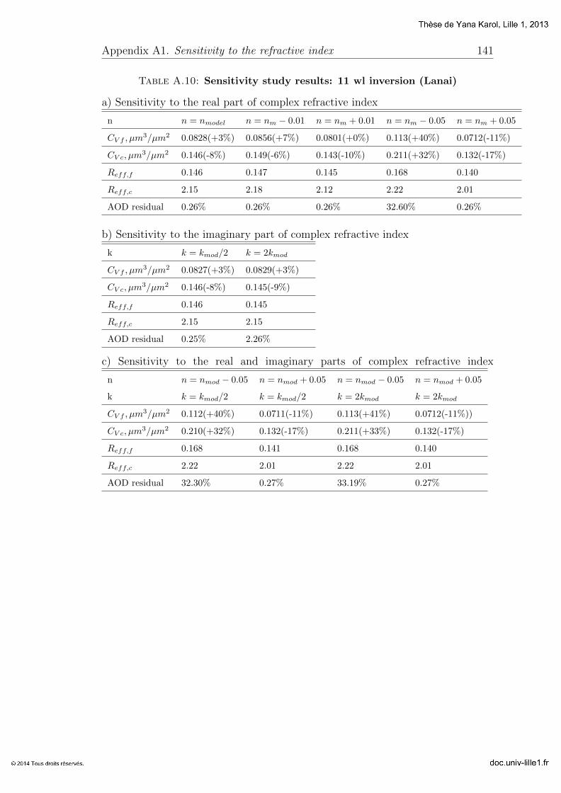
Appendix A1. Sensitivity to the refractive index 141
Table A.10: Sensitivity study results: 11 wl inversion (Lanai)
a) Sensitivity to the real part of complex refractive index
n n = nmodel n = nm − 0.01 n = nm + 0.01 n = nm − 0.05 n = nm + 0.05
CV f , µm3/µm2 0.0828(+3%) 0.0856(+7%) 0.0801(+0%) 0.113(+40%) 0.0712(-11%)
CV c, µm3/µm2 0.146(-8%) 0.149(-6%) 0.143(-10%) 0.211(+32%) 0.132(-17%)
Reff,f 0.146 0.147 0.145 0.168 0.140
Reff,c 2.15 2.18 2.12 2.22 2.01
AOD residual 0.26% 0.26% 0.26% 32.60% 0.26%
b) Sensitivity to the imaginary part of complex refractive index
k k = kmod/2 k = 2kmod
CV f , µm3/µm2 0.0827(+3%) 0.0829(+3%)
CV c, µm3/µm2 0.146(-8%) 0.145(-9%)
Reff,f 0.146 0.145
Reff,c 2.15 2.15
AOD residual 0.25% 2.26%
c) Sensitivity to the real and imaginary parts of complex refractive index
n n = nmod − 0.05 n = nmod + 0.05 n = nmod − 0.05 n = nmod + 0.05
k k = kmod/2 k = kmod/2 k = 2kmod k = 2kmod
CV f , µm3/µm2 0.112(+40%) 0.0711(-11%) 0.113(+41%) 0.0712(-11%))
CV c, µm3/µm2 0.210(+32%) 0.132(-17%) 0.211(+33%) 0.132(-17%)
Reff,f 0.168 0.141 0.168 0.140
Reff,c 2.22 2.01 2.22 2.01
AOD residual 32.30% 0.27% 33.19% 0.27%
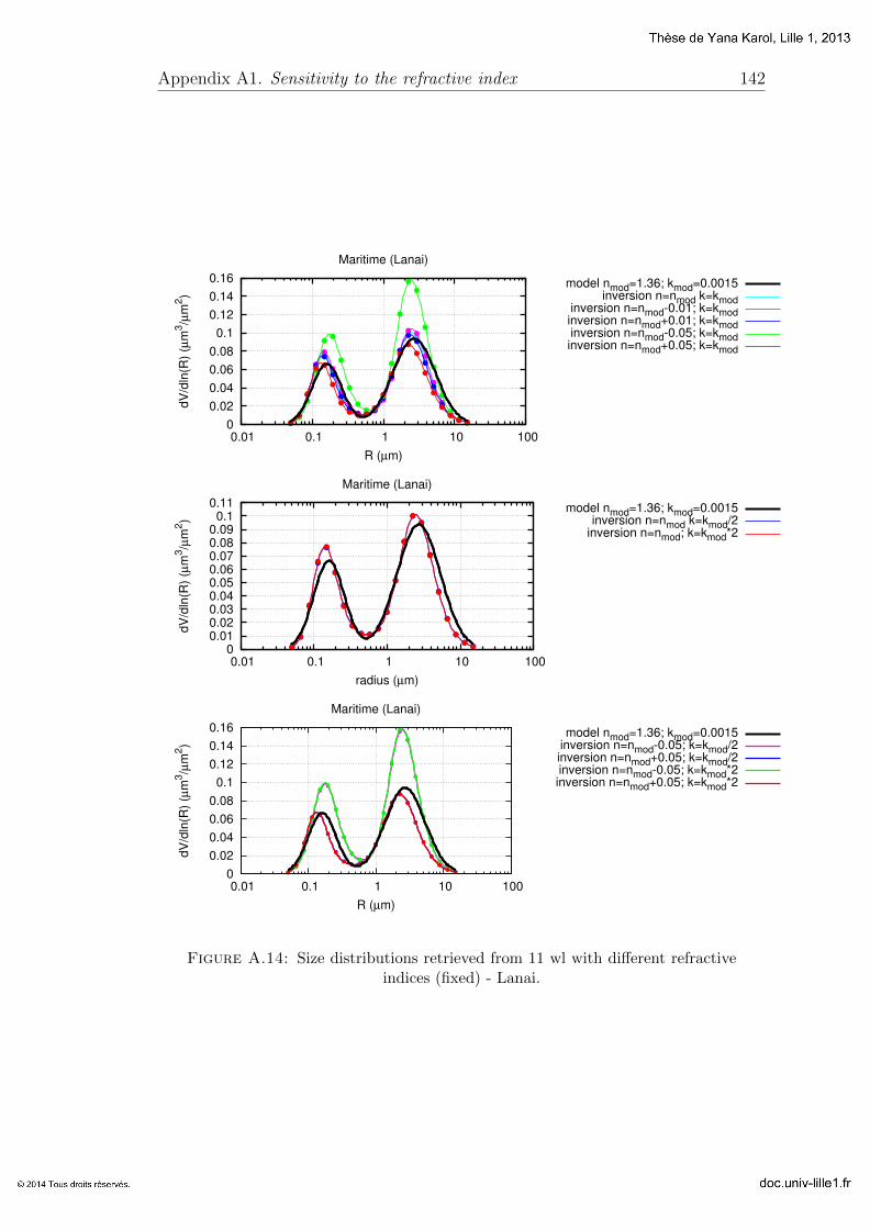
Appendix A1. Sensitivity to the refractive index 142
0
0.02
0.04
0.06
0.08
0.1
0.12
0.14
0.16
0.01 0.1 1 10 100
dV
/dln
(R)
(µm
3/µ
m2)
R (µm)
Maritime (Lanai)
model nmod=1.36; kmod=0.0015inversion n=nmod k=kmod
inversion n=nmod-0.01; k=kmodinversion n=nmod+0.01; k=kmodinversion n=nmod-0.05; k=kmodinversion n=nmod+0.05; k=kmod
0 0.01 0.02 0.03 0.04 0.05 0.06 0.07 0.08 0.09
0.1 0.11
0.01 0.1 1 10 100
dV
/dln
(R)
(µm
3/µ
m2)
radius (µm)
Maritime (Lanai)
model nmod=1.36; kmod=0.0015inversion n=nmod k=kmod/2
inversion n=nmod; k=kmod*2
0
0.02
0.04
0.06
0.08
0.1
0.12
0.14
0.16
0.01 0.1 1 10 100
dV
/dln
(R)
(µm
3/µ
m2)
R (µm)
Maritime (Lanai)
model nmod=1.36; kmod=0.0015inversion n=nmod-0.05; k=kmod/2inversion n=nmod+0.05; k=kmod/2inversion n=nmod-0.05; k=kmod*2inversion n=nmod+0.05; k=kmod*2
Figure A.14: Size distributions retrieved from 11 wl with different refractiveindices (fixed) - Lanai.
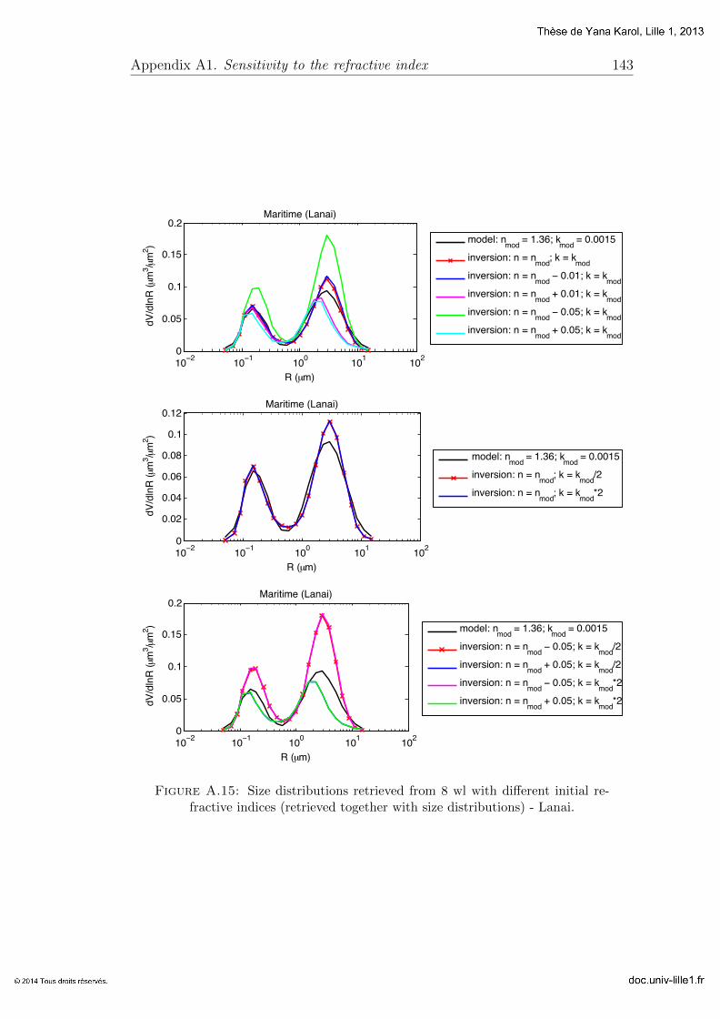
Appendix A1. Sensitivity to the refractive index 143
10−2 10−1 100 101 1020
0.05
0.1
0.15
0.2
dV/d
lnR
(µm
3 /µm2 )
R (µm)
Maritime (Lanai)
model: nmod = 1.36; kmod = 0.0015
inversion: n = nmod; k = kmodinversion: n = nmod − 0.01; k = kmodinversion: n = nmod + 0.01; k = kmodinversion: n = nmod − 0.05; k = kmodinversion: n = nmod + 0.05; k = kmod
10−2 10−1 100 101 1020
0.02
0.04
0.06
0.08
0.1
0.12
dV/d
lnR
(µm
3 /µm2 )
R (µm)
Maritime (Lanai)
model: nmod = 1.36; kmod = 0.0015
inversion: n = nmod; k = kmod/2
inversion: n = nmod; k = kmod*2
10−2 10−1 100 101 1020
0.05
0.1
0.15
0.2
dV/d
lnR
(µm
3 /µm2 )
R (µm)
Maritime (Lanai)
model: nmod = 1.36; kmod = 0.0015
inversion: n = nmod − 0.05; k = kmod/2
inversion: n = nmod + 0.05; k = kmod/2
inversion: n = nmod − 0.05; k = kmod*2
inversion: n = nmod + 0.05; k = kmod*2
Figure A.15: Size distributions retrieved from 8 wl with different initial re-fractive indices (retrieved together with size distributions) - Lanai.
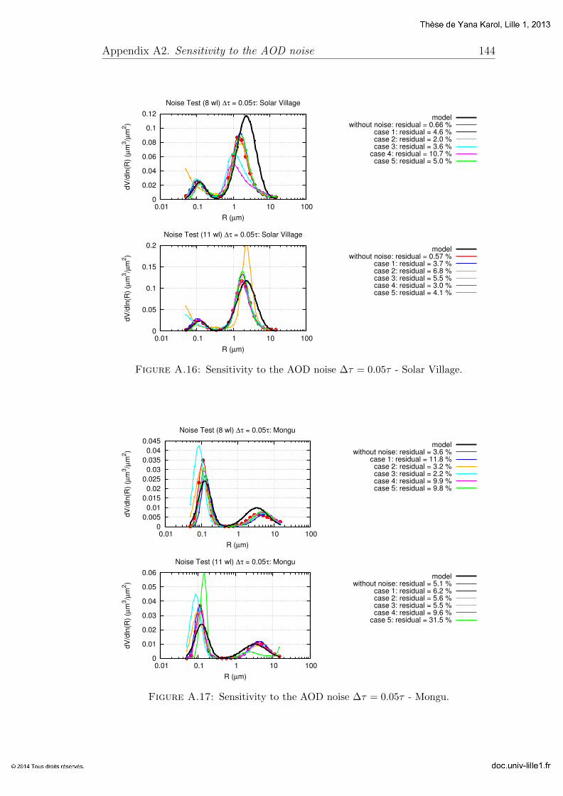
Appendix A2. Sensitivity to the AOD noise 144
0
0.02
0.04
0.06
0.08
0.1
0.12
0.01 0.1 1 10 100
dV
/dln
(R)
(µm
3/µ
m2)
R (µm)
Noise Test (8 wl) ∆τ = 0.05τ: Solar Village
modelwithout noise: residual = 0.66 %
case 1: residual = 4.6 %case 2: residual = 2.0 %case 3: residual = 3.6 %
case 4: residual = 10.7 %case 5: residual = 5.0 %
0
0.05
0.1
0.15
0.2
0.01 0.1 1 10 100
dV
/dln
(R)
(µm
3/µ
m2)
R (µm)
Noise Test (11 wl) ∆τ = 0.05τ: Solar Village
modelwithout noise: residual = 0.57 %
case 1: residual = 3.7 %case 2: residual = 6.8 %case 3: residual = 5.5 %case 4: residual = 3.0 %case 5: residual = 4.1 %
Figure A.16: Sensitivity to the AOD noise ∆τ = 0.05τ - Solar Village.
0
0.005
0.01
0.015
0.02
0.025
0.03
0.035
0.04
0.045
0.01 0.1 1 10 100
dV
/dln
(R)
(µm
3/µ
m2)
R (µm)
Noise Test (8 wl) ∆τ = 0.05τ: Mongu
modelwithout noise: residual = 3.6 %
case 1: residual = 11.8 %case 2: residual = 3.2 %case 3: residual = 2.2 %case 4: residual = 9.9 %case 5: residual = 9.8 %
0
0.01
0.02
0.03
0.04
0.05
0.06
0.01 0.1 1 10 100
dV
/dln
(R)
(µm
3/µ
m2)
R (µm)
Noise Test (11 wl) ∆τ = 0.05τ: Mongu
modelwithout noise: residual = 5.1 %
case 1: residual = 6.2 %case 2: residual = 5.6 %case 3: residual = 5.5 %case 4: residual = 9.6 %
case 5: residual = 31.5 %
Figure A.17: Sensitivity to the AOD noise ∆τ = 0.05τ - Mongu.
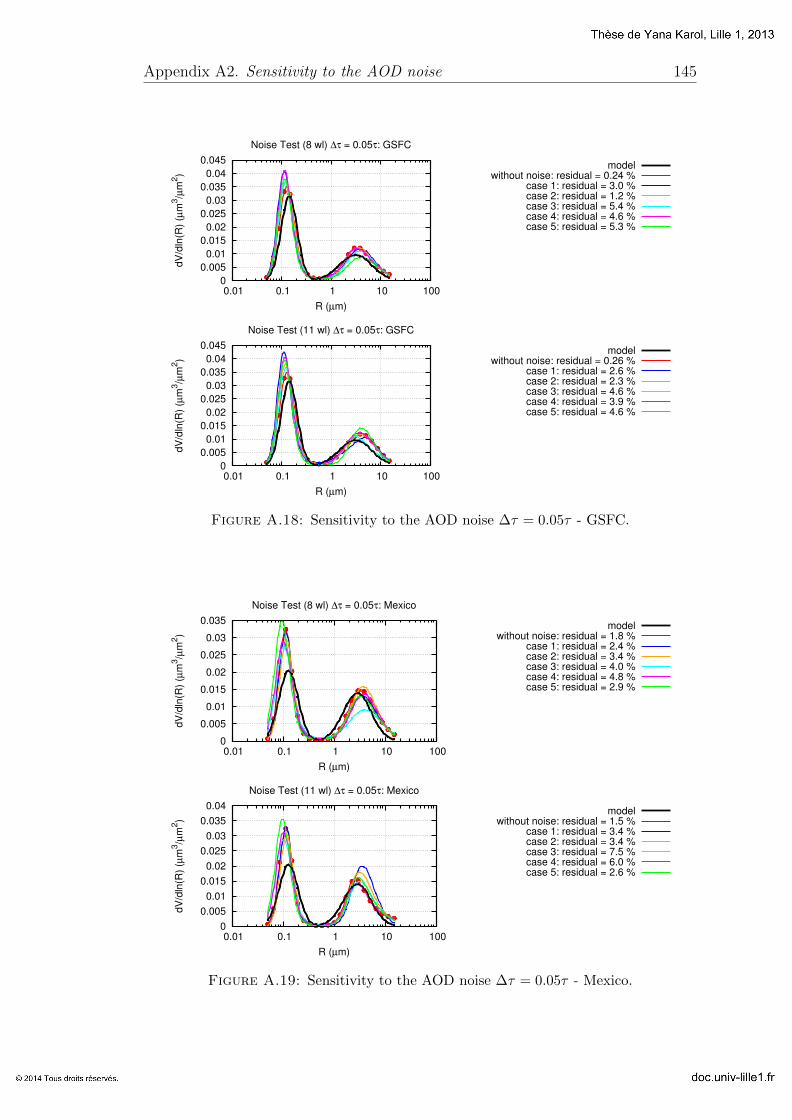
Appendix A2. Sensitivity to the AOD noise 145
0
0.005
0.01
0.015
0.02
0.025
0.03
0.035
0.04
0.045
0.01 0.1 1 10 100
dV
/dln
(R)
(µm
3/µ
m2)
R (µm)
Noise Test (8 wl) ∆τ = 0.05τ: GSFC
modelwithout noise: residual = 0.24 %
case 1: residual = 3.0 %case 2: residual = 1.2 %case 3: residual = 5.4 %case 4: residual = 4.6 %case 5: residual = 5.3 %
0
0.005
0.01
0.015
0.02
0.025
0.03
0.035
0.04
0.045
0.01 0.1 1 10 100
dV
/dln
(R)
(µm
3/µ
m2)
R (µm)
Noise Test (11 wl) ∆τ = 0.05τ: GSFC
modelwithout noise: residual = 0.26 %
case 1: residual = 2.6 %case 2: residual = 2.3 %case 3: residual = 4.6 %case 4: residual = 3.9 %case 5: residual = 4.6 %
Figure A.18: Sensitivity to the AOD noise ∆τ = 0.05τ - GSFC.
0
0.005
0.01
0.015
0.02
0.025
0.03
0.035
0.01 0.1 1 10 100
dV
/dln
(R)
(µm
3/µ
m2)
R (µm)
Noise Test (8 wl) ∆τ = 0.05τ: Mexico
modelwithout noise: residual = 1.8 %
case 1: residual = 2.4 %case 2: residual = 3.4 %case 3: residual = 4.0 %case 4: residual = 4.8 %case 5: residual = 2.9 %
0
0.005
0.01
0.015
0.02
0.025
0.03
0.035
0.04
0.01 0.1 1 10 100
dV
/dln
(R)
(µm
3/µ
m2)
R (µm)
Noise Test (11 wl) ∆τ = 0.05τ: Mexico
modelwithout noise: residual = 1.5 %
case 1: residual = 3.4 %case 2: residual = 3.4 %case 3: residual = 7.5 %case 4: residual = 6.0 %case 5: residual = 2.6 %
Figure A.19: Sensitivity to the AOD noise ∆τ = 0.05τ - Mexico.
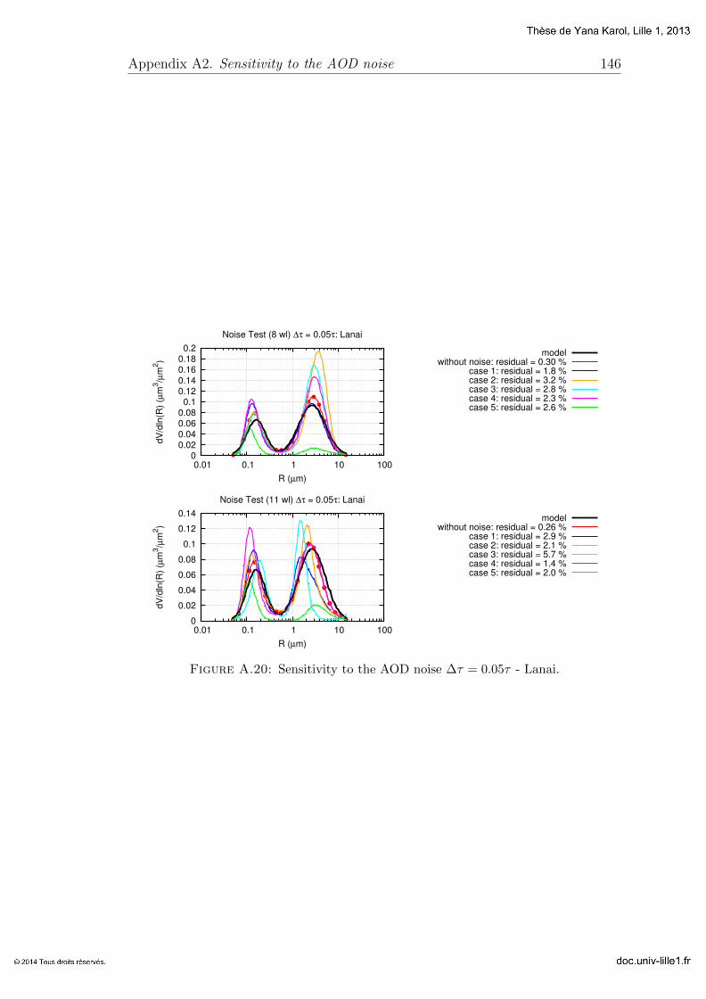
Appendix A2. Sensitivity to the AOD noise 146
0 0.02 0.04 0.06 0.08 0.1
0.12 0.14 0.16 0.18 0.2
0.01 0.1 1 10 100
dV
/dln
(R)
(µm
3/µ
m2)
R (µm)
Noise Test (8 wl) ∆τ = 0.05τ: Lanai
modelwithout noise: residual = 0.30 %
case 1: residual = 1.8 %case 2: residual = 3.2 %case 3: residual = 2.8 %case 4: residual = 2.3 %case 5: residual = 2.6 %
0
0.02
0.04
0.06
0.08
0.1
0.12
0.14
0.01 0.1 1 10 100
dV
/dln
(R)
(µm
3/µ
m2)
R (µm)
Noise Test (11 wl) ∆τ = 0.05τ: Lanai
modelwithout noise: residual = 0.26 %
case 1: residual = 2.9 %case 2: residual = 2.1 %case 3: residual = 5.7 %case 4: residual = 1.4 %case 5: residual = 2.0 %
Figure A.20: Sensitivity to the AOD noise ∆τ = 0.05τ - Lanai.

Appendix A2. Sensitivity to the AOD noise 147
0
0.02
0.04
0.06
0.08
0.1
0.12
0.14
0.16
0.01 0.1 1 10 100
dV
/dln
(R)
(µm
3/µ
m2)
R (µm)
Noise Test (8 wl) ∆τ = 0.1τ: Solar Village
modelwithout noise: residual = 0.66 %
case 1: residual = 9.4 %case 2: residual = 5.5 %case 3: residual = 5.6 %
case 4: residual = 14.5 %case 5: residual = 9.1 %
0
0.05
0.1
0.15
0.2
0.01 0.1 1 10 100
dV
/dln
(R)
(µm
3/µ
m2)
R (µm)
Noise Test (11 wl) ∆τ = 0.1τ: Solar Village
modelwithout noise: residual = 0.57 %
case 1: residual = 14.7 %case 2: residual = 10.9 %case 3: residual = 4.8 %
case 4: residual = 12.4 %case 5: residual = 8.9 %
0.15
0.2
0.25
0.3
0.35
0.4
0.45
0.5
0.2 0.4 0.6 0.8 1 1.2 1.4 1.6 1.8 2 2.2 2.4
AO
D
Wavelength (µm)
Noise Test: Solar Village - AOD fit (without noise)
model8 wl inversion
11 wl inversion
0.15
0.2
0.25
0.3
0.35
0.4
0.45
0.5
0.55
0.6
0.2 0.4 0.6 0.8 1 1.2 1.4 1.6 1.8 2 2.2 2.4
AO
D
Wavelength (µm)
Noise Test: Solar Village - AOD fit (case 1)
modelnoise: ∆τ = 0.1τ
8 wl inversion11 wl inversion
0.15
0.2
0.25
0.3
0.35
0.4
0.45
0.5
0.2 0.4 0.6 0.8 1 1.2 1.4 1.6 1.8 2 2.2 2.4
AO
D
Wavelength (µm)
Noise Test: Solar Village - AOD fit (case 2)
modelnoise: ∆τ = 0.1τ
8 wl inversion11 wl inversion
0.15
0.2
0.25
0.3
0.35
0.4
0.45
0.5
0.2 0.4 0.6 0.8 1 1.2 1.4 1.6 1.8 2 2.2 2.4
AO
D
Wavelength (µm)
Noise Test: Solar Village - AOD fit (case 3)
modelnoise: ∆τ = 0.1τ
8 wl inversion11 wl inversion
0.15
0.2
0.25
0.3
0.35
0.4
0.45
0.5
0.55
0.2 0.4 0.6 0.8 1 1.2 1.4 1.6 1.8 2 2.2 2.4
AO
D
Wavelength (µm)
Noise Test: Solar Village - AOD fit (case 4)
modelnoise: ∆τ = 0.1τ
8 wl inversion11 wl inversion
0.15
0.2
0.25
0.3
0.35
0.4
0.45
0.5
0.55
0.2 0.4 0.6 0.8 1 1.2 1.4 1.6 1.8 2 2.2 2.4
AO
D
Wavelength (µm)
Noise Test: Solar Village - AOD fit (case 5)
modelnoise: ∆τ = 0.1τ
8 wl inversion11 wl inversion
Figure A.21: Sensitivity to the AOD noise ∆τ = 0.1τ - Solar Village.
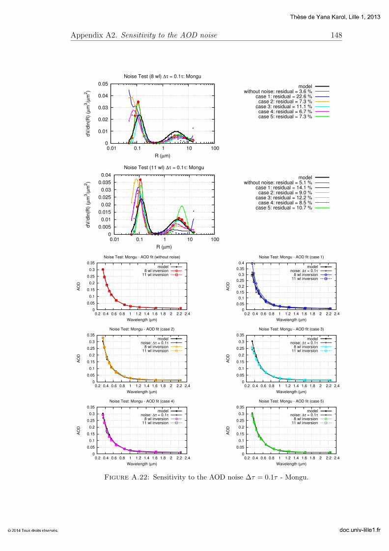
Appendix A2. Sensitivity to the AOD noise 148
0
0.01
0.02
0.03
0.04
0.05
0.01 0.1 1 10 100
dV
/dln
(R)
(µm
3/µ
m2)
R (µm)
Noise Test (8 wl) ∆τ = 0.1τ: Mongu
modelwithout noise: residual = 3.6 %
case 1: residual = 22.6 %case 2: residual = 7.3 %
case 3: residual = 11.1 %case 4: residual = 6.7 %case 5: residual = 7.3 %
0
0.005
0.01
0.015
0.02
0.025
0.03
0.035
0.04
0.01 0.1 1 10 100
dV
/dln
(R)
(µm
3/µ
m2)
R (µm)
Noise Test (11 wl) ∆τ = 0.1τ: Mongu
modelwithout noise: residual = 5.1 %
case 1: residual = 14.1 %case 2: residual = 9.0 %
case 3: residual = 12.2 %case 4: residual = 8.5 %
case 5: residual = 10.7 %
0
0.05
0.1
0.15
0.2
0.25
0.3
0.35
0.2 0.4 0.6 0.8 1 1.2 1.4 1.6 1.8 2 2.2 2.4
AO
D
Wavelength (µm)
Noise Test: Mongu - AOD fit (without noise)
model8 wl inversion
11 wl inversion
0
0.05
0.1
0.15
0.2
0.25
0.3
0.35
0.4
0.2 0.4 0.6 0.8 1 1.2 1.4 1.6 1.8 2 2.2 2.4
AO
D
Wavelength (µm)
Noise Test: Mongu - AOD fit (case 1)
modelnoise: ∆τ = 0.1τ
8 wl inversion11 wl inversion
0
0.05
0.1
0.15
0.2
0.25
0.3
0.35
0.2 0.4 0.6 0.8 1 1.2 1.4 1.6 1.8 2 2.2 2.4
AO
D
Wavelength (µm)
Noise Test: Mongu - AOD fit (case 2)
modelnoise: ∆τ = 0.1τ
8 wl inversion11 wl inversion
0
0.05
0.1
0.15
0.2
0.25
0.3
0.35
0.2 0.4 0.6 0.8 1 1.2 1.4 1.6 1.8 2 2.2 2.4
AO
D
Wavelength (µm)
Noise Test: Mongu - AOD fit (case 3)
modelnoise: ∆τ = 0.1τ
8 wl inversion11 wl inversion
0
0.05
0.1
0.15
0.2
0.25
0.3
0.35
0.2 0.4 0.6 0.8 1 1.2 1.4 1.6 1.8 2 2.2 2.4
AO
D
Wavelength (µm)
Noise Test: Mongu - AOD fit (case 4)
modelnoise: ∆τ = 0.1τ
8 wl inversion11 wl inversion
0
0.05
0.1
0.15
0.2
0.25
0.3
0.35
0.2 0.4 0.6 0.8 1 1.2 1.4 1.6 1.8 2 2.2 2.4
AO
D
Wavelength (µm)
Noise Test: Mongu - AOD fit (case 5)
modelnoise: ∆τ = 0.1τ
8 wl inversion11 wl inversion
Figure A.22: Sensitivity to the AOD noise ∆τ = 0.1τ - Mongu.

Appendix A2. Sensitivity to the AOD noise 149
0
0.005
0.01
0.015
0.02
0.025
0.03
0.035
0.04
0.01 0.1 1 10 100
dV
/dln
(R)
(µm
3/µ
m2)
R (µm)
Noise Test (8 wl) ∆τ = 0.1τ: GSFC
modelwithout noise: residual = 0.24 %
case 1: residual = 8.9 %case 2: residual = 7.4 %case 3: residual = 6.6 %
case 4: residual = 10.9 %case 5: residual = 5.7 %
0
0.005
0.01
0.015
0.02
0.025
0.03
0.035
0.04
0.01 0.1 1 10 100
dV
/dln
(R)
(µm
3/µ
m2)
R (µm)
Noise Test (11 wl) ∆τ = 0.1τ: GSFC
modelwithout noise: residual = 0.26 %
case 1: residual = 19.9 %case 2: residual = 6.4 %
case 3: residual = 11.8 %case 4: residual = 10.3 %case 5: residual = 7.5 %
0
0.05
0.1
0.15
0.2
0.25
0.3
0.35
0.2 0.4 0.6 0.8 1 1.2 1.4 1.6 1.8 2 2.2 2.4
AO
D
Wavelength (µm)
Noise Test: GSFC - AOD fit (without noise)
model8 wl inversion
11 wl inversion
0
0.05
0.1
0.15
0.2
0.25
0.3
0.35
0.2 0.4 0.6 0.8 1 1.2 1.4 1.6 1.8 2 2.2 2.4
AO
D
Wavelength (µm)
Noise Test: GSFC - AOD fit (case 1)
modelnoise: ∆τ = 0.1τ
8 wl inversion11 wl inversion
0
0.05
0.1
0.15
0.2
0.25
0.3
0.35
0.2 0.4 0.6 0.8 1 1.2 1.4 1.6 1.8 2 2.2 2.4
AO
D
Wavelength (µm)
Noise Test: GSFC - AOD fit (case 2)
modelnoise: ∆τ = 0.1τ
8 wl inversion11 wl inversion
0
0.05
0.1
0.15
0.2
0.25
0.3
0.35
0.2 0.4 0.6 0.8 1 1.2 1.4 1.6 1.8 2 2.2 2.4
AO
D
Wavelength (µm)
Noise Test: GSFC - AOD fit (case 3)
modelnoise: ∆τ = 0.1τ
8 wl inversion11 wl inversion
0
0.05
0.1
0.15
0.2
0.25
0.3
0.35
0.2 0.4 0.6 0.8 1 1.2 1.4 1.6 1.8 2 2.2 2.4
AO
D
Wavelength (µm)
Noise Test: GSFC - AOD fit (case 4)
modelnoise: ∆τ = 0.1τ
8 wl inversion11 wl inversion
0
0.05
0.1
0.15
0.2
0.25
0.3
0.35
0.2 0.4 0.6 0.8 1 1.2 1.4 1.6 1.8 2 2.2 2.4
AO
D
Wavelength (µm)
Noise Test: GSFC - AOD fit (case 5)
modelnoise: ∆τ = 0.1τ
8 wl inversion11 wl inversion
Figure A.23: Sensitivity to the AOD noise ∆τ = 0.1τ - GSFC.
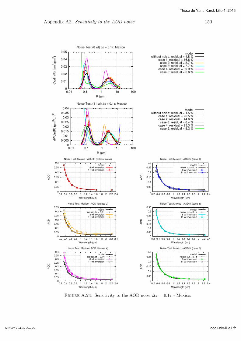
Appendix A2. Sensitivity to the AOD noise 150
0
0.01
0.02
0.03
0.04
0.05
0.01 0.1 1 10 100
dV
/dln
(R)
(µm
3/µ
m2)
R (µm)
Noise Test (8 wl) ∆τ = 0.1τ: Mexico
modelwithout noise: residual = 1.8 %
case 1: residual = 16.6 %case 2: residual = 8.7 %case 3: residual = 7.7 %
case 4: residual = 39.9 %case 5: residual = 6.6 %
0
0.005
0.01
0.015
0.02
0.025
0.03
0.035
0.04
0.01 0.1 1 10 100
dV
/dln
(R)
(µm
3/µ
m2)
R (µm)
Noise Test (11 wl) ∆τ = 0.1τ: Mexico
modelwithout noise: residual = 1.5 %
case 1: residual = 26.5 %case 2: residual = 44.6 %case 3: residual = 6.4 %
case 4: residual = 25.3 %case 5: residual = 8.2 %
0
0.05
0.1
0.15
0.2
0.25
0.3
0.2 0.4 0.6 0.8 1 1.2 1.4 1.6 1.8 2 2.2 2.4
AO
D
Wavelength (µm)
Noise Test: Mexico - AOD fit (without noise)
model8 wl inversion
11 wl inversion
0
0.05
0.1
0.15
0.2
0.25
0.3
0.2 0.4 0.6 0.8 1 1.2 1.4 1.6 1.8 2 2.2 2.4
AO
D
Wavelength (µm)
Noise Test: Mexico - AOD fit (case 1)
modelnoise: ∆τ = 0.1τ
8 wl inversion11 wl inversion
0
0.05
0.1
0.15
0.2
0.25
0.3
0.35
0.2 0.4 0.6 0.8 1 1.2 1.4 1.6 1.8 2 2.2 2.4
AO
D
Wavelength (µm)
Noise Test: Mexico - AOD fit (case 2)
modelnoise: ∆τ = 0.1τ
8 wl inversion11 wl inversion
0
0.05
0.1
0.15
0.2
0.25
0.3
0.35
0.2 0.4 0.6 0.8 1 1.2 1.4 1.6 1.8 2 2.2 2.4
AO
D
Wavelength (µm)
Noise Test: Mexico - AOD fit (case 3)
modelnoise: ∆τ = 0.1τ
8 wl inversion11 wl inversion
0
0.05
0.1
0.15
0.2
0.25
0.3
0.35
0.4
0.2 0.4 0.6 0.8 1 1.2 1.4 1.6 1.8 2 2.2 2.4
AO
D
Wavelength (µm)
Noise Test: Mexico - AOD fit (case 4)
modelnoise: ∆τ = 0.1τ
8 wl inversion11 wl inversion
0
0.05
0.1
0.15
0.2
0.25
0.3
0.2 0.4 0.6 0.8 1 1.2 1.4 1.6 1.8 2 2.2 2.4
AO
D
Wavelength (µm)
Noise Test: Mexico - AOD fit (case 5)
modelnoise: ∆τ = 0.1τ
8 wl inversion11 wl inversion
Figure A.24: Sensitivity to the AOD noise ∆τ = 0.1τ - Mexico.
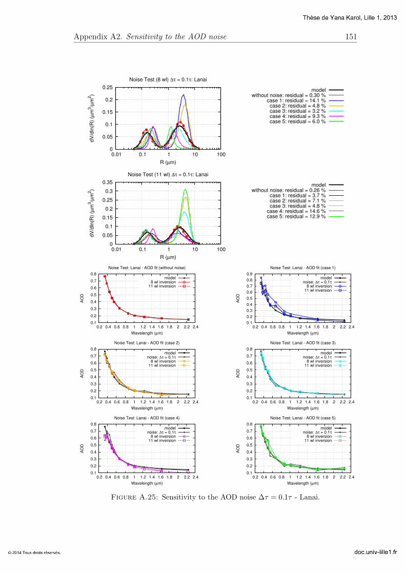
Appendix A2. Sensitivity to the AOD noise 151
0
0.05
0.1
0.15
0.2
0.25
0.01 0.1 1 10 100
dV
/dln
(R)
(µm
3/µ
m2)
R (µm)
Noise Test (8 wl) ∆τ = 0.1τ: Lanai
modelwithout noise: residual = 0.30 %
case 1: residual = 14.1 %case 2: residual = 4.8 %case 3: residual = 3.2 %case 4: residual = 9.3 %case 5: residual = 6.0 %
0
0.05
0.1
0.15
0.2
0.25
0.3
0.35
0.01 0.1 1 10 100
dV
/dln
(R)
(µm
3/µ
m2)
R (µm)
Noise Test (11 wl) ∆τ = 0.1τ: Lanai
modelwithout noise: residual = 0.26 %
case 1: residual = 3.7 %case 2: residual = 7.1 %case 3: residual = 4.8 %
case 4: residual = 14.6 %case 5: residual = 12.9 %
0.1
0.2
0.3
0.4
0.5
0.6
0.7
0.8
0.2 0.4 0.6 0.8 1 1.2 1.4 1.6 1.8 2 2.2 2.4
AO
D
Wavelength (µm)
Noise Test: Lanai - AOD fit (without noise)
model8 wl inversion
11 wl inversion
0.1
0.2
0.3
0.4
0.5
0.6
0.7
0.8
0.9
0.2 0.4 0.6 0.8 1 1.2 1.4 1.6 1.8 2 2.2 2.4
AO
D
Wavelength (µm)
Noise Test: Lanai - AOD fit (case 1)
modelnoise: ∆τ = 0.1τ
8 wl inversion11 wl inversion
0.1
0.2
0.3
0.4
0.5
0.6
0.7
0.8
0.2 0.4 0.6 0.8 1 1.2 1.4 1.6 1.8 2 2.2 2.4
AO
D
Wavelength (µm)
Noise Test: Lanai - AOD fit (case 2)
modelnoise: ∆τ = 0.1τ
8 wl inversion11 wl inversion
0.1
0.2
0.3
0.4
0.5
0.6
0.7
0.8
0.2 0.4 0.6 0.8 1 1.2 1.4 1.6 1.8 2 2.2 2.4
AO
D
Wavelength (µm)
Noise Test: Lanai - AOD fit (case 3)
modelnoise: ∆τ = 0.1τ
8 wl inversion11 wl inversion
0.1
0.2
0.3
0.4
0.5
0.6
0.7
0.8
0.2 0.4 0.6 0.8 1 1.2 1.4 1.6 1.8 2 2.2 2.4
AO
D
Wavelength (µm)
Noise Test: Lanai - AOD fit (case 4)
modelnoise: ∆τ = 0.1τ
8 wl inversion11 wl inversion
0.1
0.2
0.3
0.4
0.5
0.6
0.7
0.8
0.2 0.4 0.6 0.8 1 1.2 1.4 1.6 1.8 2 2.2 2.4
AO
D
Wavelength (µm)
Noise Test: Lanai - AOD fit (case 5)
modelnoise: ∆τ = 0.1τ
8 wl inversion11 wl inversion
Figure A.25: Sensitivity to the AOD noise ∆τ = 0.1τ - Lanai.
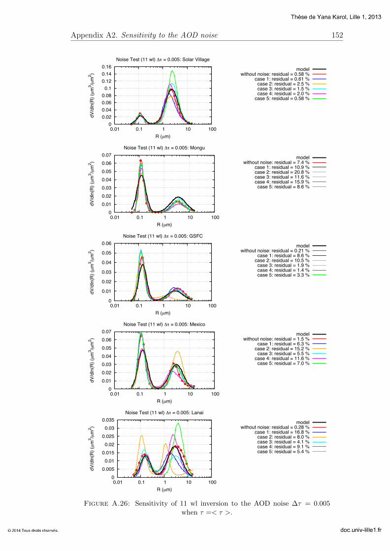
Appendix A2. Sensitivity to the AOD noise 152
0 0.02 0.04 0.06 0.08
0.1 0.12 0.14 0.16
0.01 0.1 1 10 100
dV/d
ln(R
) (µ
m3 /µ
m2 )
R (µm)
Noise Test (11 wl) = 0.005: Solar Village
modelwithout noise: residual = 0.58 %
case 1: residual = 0.61 %case 2: residual = 2.5 %case 3: residual = 1.5 %case 4: residual = 2.0 %
case 5: residual = 0.58 %
0 0.01 0.02 0.03 0.04 0.05 0.06 0.07
0.01 0.1 1 10 100
dV/d
ln(R
) (µ
m3 /µ
m2 )
R (µm)
Noise Test (11 wl) = 0.005: Mongu
modelwithout noise: residual = 7.4 %
case 1: residual = 10.9 %case 2: residual = 20.8 %case 3: residual = 11.6 %case 4: residual = 15.9 %
case 5: residual = 8.6 %
0
0.01
0.02
0.03
0.04
0.05
0.06
0.01 0.1 1 10 100
dV/d
ln(R
) (µ
m3 /µ
m2 )
R (µm)
Noise Test (11 wl) = 0.005: GSFC
modelwithout noise: residual = 0.21 %
case 1: residual = 8.6 %case 2: residual = 10.5 %
case 3: residual = 1.9 %case 4: residual = 1.4 %case 5: residual = 3.3 %
0 0.01 0.02 0.03 0.04 0.05 0.06 0.07
0.01 0.1 1 10 100
dV/d
ln(R
) (µ
m3 /µ
m2 )
R (µm)
Noise Test (11 wl) = 0.005: Mexico
modelwithout noise: residual = 1.5 %
case 1: residual = 6.3 %case 2: residual = 15.2 %
case 3: residual = 5.5 %case 4: residual = 11.6 %
case 5: residual = 7.0 %
0 0.005
0.01 0.015
0.02 0.025
0.03 0.035
0.01 0.1 1 10 100
dV/d
ln(R
) (µ
m3 /µ
m2 )
R (µm)
Noise Test (11 wl) = 0.005: Lanai
modelwithout noise: residual = 0.28 %
case 1: residual = 16.8 %case 2: residual = 8.0 %case 3: residual = 4.1 %case 4: residual = 9.1 %case 5: residual = 5.4 %
Figure A.26: Sensitivity of 11 wl inversion to the AOD noise ∆τ = 0.005when τ =< τ >.
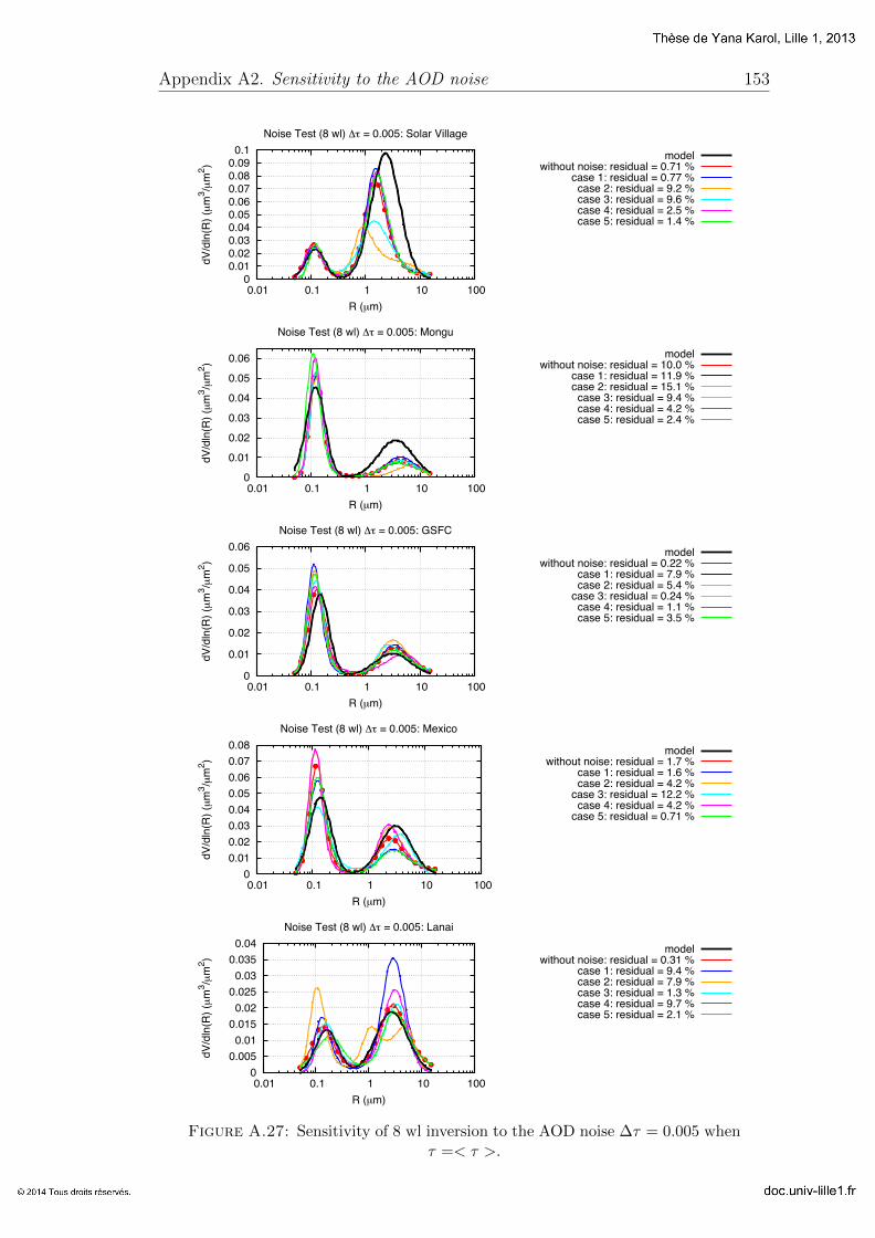
Appendix A2. Sensitivity to the AOD noise 153
0 0.01 0.02 0.03 0.04 0.05 0.06 0.07 0.08 0.09
0.1
0.01 0.1 1 10 100
dV/d
ln(R
) (µ
m3 /µ
m2 )
R (µm)
Noise Test (8 wl) = 0.005: Solar Village
modelwithout noise: residual = 0.71 %
case 1: residual = 0.77 %case 2: residual = 9.2 %case 3: residual = 9.6 %case 4: residual = 2.5 %case 5: residual = 1.4 %
0
0.01
0.02
0.03
0.04
0.05
0.06
0.01 0.1 1 10 100
dV/d
ln(R
) (µ
m3 /µ
m2 )
R (µm)
Noise Test (8 wl) = 0.005: Mongu
modelwithout noise: residual = 10.0 %
case 1: residual = 11.9 %case 2: residual = 15.1 %
case 3: residual = 9.4 %case 4: residual = 4.2 %case 5: residual = 2.4 %
0
0.01
0.02
0.03
0.04
0.05
0.06
0.01 0.1 1 10 100
dV/d
ln(R
) (µ
m3 /µ
m2 )
R (µm)
Noise Test (8 wl) = 0.005: GSFC
modelwithout noise: residual = 0.22 %
case 1: residual = 7.9 %case 2: residual = 5.4 %
case 3: residual = 0.24 %case 4: residual = 1.1 %case 5: residual = 3.5 %
0 0.01 0.02 0.03 0.04 0.05 0.06 0.07 0.08
0.01 0.1 1 10 100
dV/d
ln(R
) (µ
m3 /µ
m2 )
R (µm)
Noise Test (8 wl) = 0.005: Mexico
modelwithout noise: residual = 1.7 %
case 1: residual = 1.6 %case 2: residual = 4.2 %
case 3: residual = 12.2 %case 4: residual = 4.2 %
case 5: residual = 0.71 %
0 0.005
0.01 0.015
0.02 0.025
0.03 0.035
0.04
0.01 0.1 1 10 100
dV/d
ln(R
) (µ
m3 /µ
m2 )
R (µm)
Noise Test (8 wl) = 0.005: Lanai
modelwithout noise: residual = 0.31 %
case 1: residual = 9.4 %case 2: residual = 7.9 %case 3: residual = 1.3 %case 4: residual = 9.7 %case 5: residual = 2.1 %
Figure A.27: Sensitivity of 8 wl inversion to the AOD noise ∆τ = 0.005 whenτ =< τ >.
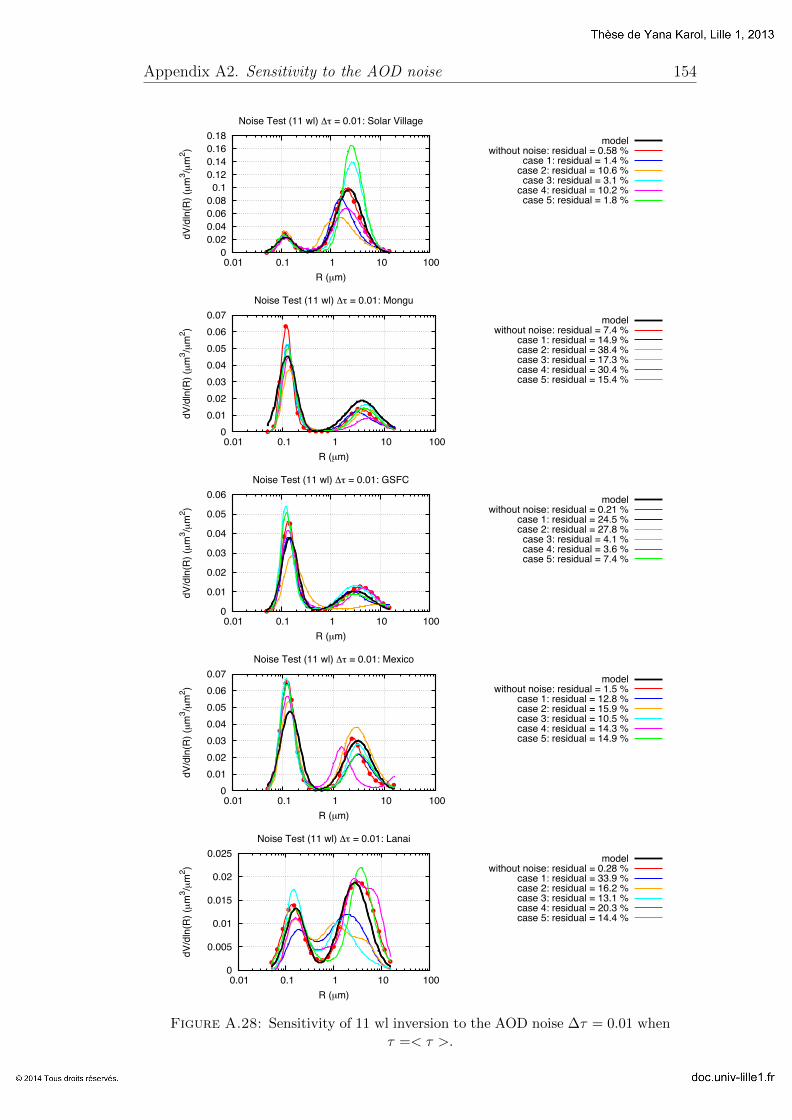
Appendix A2. Sensitivity to the AOD noise 154
0 0.02 0.04 0.06 0.08
0.1 0.12 0.14 0.16 0.18
0.01 0.1 1 10 100
dV/d
ln(R
) (µ
m3 /µ
m2 )
R (µm)
Noise Test (11 wl) = 0.01: Solar Village
modelwithout noise: residual = 0.58 %
case 1: residual = 1.4 %case 2: residual = 10.6 %
case 3: residual = 3.1 %case 4: residual = 10.2 %
case 5: residual = 1.8 %
0 0.01 0.02 0.03 0.04 0.05 0.06 0.07
0.01 0.1 1 10 100
dV/d
ln(R
) (µ
m3 /µ
m2 )
R (µm)
Noise Test (11 wl) = 0.01: Mongu
modelwithout noise: residual = 7.4 %
case 1: residual = 14.9 %case 2: residual = 38.4 %case 3: residual = 17.3 %case 4: residual = 30.4 %case 5: residual = 15.4 %
0
0.01
0.02
0.03
0.04
0.05
0.06
0.01 0.1 1 10 100
dV/d
ln(R
) (µ
m3 /µ
m2 )
R (µm)
Noise Test (11 wl) = 0.01: GSFC
modelwithout noise: residual = 0.21 %
case 1: residual = 24.5 %case 2: residual = 27.8 %
case 3: residual = 4.1 %case 4: residual = 3.6 %case 5: residual = 7.4 %
0 0.01 0.02 0.03 0.04 0.05 0.06 0.07
0.01 0.1 1 10 100
dV/d
ln(R
) (µ
m3 /µ
m2 )
R (µm)
Noise Test (11 wl) = 0.01: Mexico
modelwithout noise: residual = 1.5 %
case 1: residual = 12.8 %case 2: residual = 15.9 %case 3: residual = 10.5 %case 4: residual = 14.3 %case 5: residual = 14.9 %
0
0.005
0.01
0.015
0.02
0.025
0.01 0.1 1 10 100
dV/d
ln(R
) (µ
m3 /µ
m2 )
R (µm)
Noise Test (11 wl) = 0.01: Lanai
modelwithout noise: residual = 0.28 %
case 1: residual = 33.9 %case 2: residual = 16.2 %case 3: residual = 13.1 %case 4: residual = 20.3 %case 5: residual = 14.4 %
Figure A.28: Sensitivity of 11 wl inversion to the AOD noise ∆τ = 0.01 whenτ =< τ >.

Appendix A2. Sensitivity to the AOD noise 155
0 0.01 0.02 0.03 0.04 0.05 0.06 0.07 0.08 0.09
0.1
0.01 0.1 1 10 100
dV/d
ln(R
) (µ
m3 /µ
m2 )
R (µm)
Noise Test (8 wl) = 0.01: Solar Village
modelwithout noise: residual = 0.71 %
case 1: residual = 1.4 %case 2: residual = 6.8 %case 3: residual = 9.5 %case 4: residual = 5.1 %case 5: residual = 2.1 %
0
0.01
0.02
0.03
0.04
0.05
0.06
0.01 0.1 1 10 100
dV/d
ln(R
) (µ
m3 /µ
m2 )
R (µm)
Noise Test (8 wl) = 0.01: Mongu
modelwithout noise: residual = 10.0 %
case 1: residual = 31.6 %case 2: residual = 35.1 %
case 3: residual = 9.8 %case 4: residual = 5.3 %case 5: residual = 5.6 %
0 0.005
0.01 0.015
0.02 0.025
0.03 0.035
0.04 0.045
0.05
0.01 0.1 1 10 100
dV/d
ln(R
) (µ
m3 /µ
m2 )
R (µm)
Noise Test (8 wl) = 0.01: GSFC
modelwithout noise: residual = 0.22 %
case 1: residual = 24.8 %case 2: residual = 12.6 %case 3: residual = 0.76 %
case 4: residual = 3.1 %case 5: residual = 7.5 %
0 0.01 0.02 0.03 0.04 0.05 0.06 0.07 0.08
0.01 0.1 1 10 100
dV/d
ln(R
) (µ
m3 /µ
m2 )
R (µm)
Noise Test (8 wl) = 0.01: Mexico
modelwithout noise: residual = 1.7 %
case 1: residual = 2.1 %case 2: residual = 8.6 %
case 3: residual = 11.7 %case 4: residual = 9.2 %case 5: residual = 2.2 %
0 0.005
0.01 0.015
0.02 0.025
0.03 0.035
0.01 0.1 1 10 100
dV/d
ln(R
) (µ
m3 /µ
m2 )
R (µm)
Noise Test (8 wl) = 0.01: Lanai
modelwithout noise: residual = 0.31 %
case 1: residual = 20.3 %case 2: residual = 6.1 %case 3: residual = 2.8 %
case 4: residual = 21.3 %case 5: residual = 9.1 %
Figure A.29: Sensitivity of 8 wl inversion to the AOD noise ∆τ = 0.01 whenτ =< τ >.
Appendix B
The paper published during the
study
The paper published in 2013 in ”Atmospheric Measurement Techniques”, volume
6, pages 2383 – 2389. It concerns to PLASMA technical description, calibration,
first results and is the part of the Chapter 4.
156
Atmos. Meas. Tech., 6, 2383–2389, 2013www.atmos-meas-tech.net/6/2383/2013/doi:10.5194/amt-6-2383-2013© Author(s) 2013. CC Attribution 3.0 License.
EGU Journal Logos (RGB)
Advances in Geosciences
Open A
ccess
Natural Hazards and Earth System
Sciences
Open A
ccess
Annales Geophysicae
Open A
ccess
Nonlinear Processes in Geophysics
Open A
ccess
Atmospheric Chemistry
and Physics
Open A
ccess
Atmospheric Chemistry
and Physics
Open A
ccess
Discussions
Atmospheric Measurement
TechniquesO
pen Access
Atmospheric Measurement
Techniques
Open A
ccess
Discussions
Biogeosciences
Open A
ccess
Open A
ccess
BiogeosciencesDiscussions
Climate of the Past
Open A
ccess
Open A
ccess
Climate of the Past
Discussions
Earth System Dynamics
Open A
ccess
Open A
ccess
Earth System Dynamics
Discussions
GeoscientificInstrumentation
Methods andData Systems
Open A
ccess
GeoscientificInstrumentation
Methods andData Systems
Open A
ccess
Discussions
GeoscientificModel Development
Open A
ccess
Open A
ccess
GeoscientificModel Development
Discussions
Hydrology and Earth System
Sciences
Open A
ccess
Hydrology and Earth System
Sciences
Open A
ccess
Discussions
Ocean Science
Open A
ccess
Open A
ccess
Ocean ScienceDiscussions
Solid Earth
Open A
ccess
Open A
ccess
Solid EarthDiscussions
The Cryosphere
Open A
ccess
Open A
ccess
The CryosphereDiscussions
Natural Hazards and Earth System
Sciences
Open A
ccess
Discussions
Airborne sun photometer PLASMA: concept, measurements,comparison of aerosol extinction vertical profile with lidar
Y. Karol 1,2, D. Tanre1, P. Goloub1, C. Vervaerde1, J. Y. Balois1, L. Blarel1, T. Podvin1, A. Mortier 1, andA. Chaikovsky2
1Laboratoire d’Optique Atmospherique (LOA), UMR8518, CNRS – Universite des Sciences et Technologies de Lille,59655 Villeneuve d’Ascq, France2B. I. Stepanov Institute of Physics National Academy of Sciences of Belarus, 68, Nezavisimosti av., 220072 Minsk, Belarus
Correspondence to:Y. Karol ([email protected])
Received: 1 August 2012 – Published in Atmos. Meas. Tech. Discuss.: 19 September 2012Revised: 5 August 2013 – Accepted: 5 August 2013 – Published: 16 September 2013
Abstract. A 15-channel airborne sun-tracking photometerhas been developed. The instrument provides aerosol opti-cal depths over a wide spectral range (0.34–2.25 µm) with anaccuracy (1AOD) of approximately 0.01. Taking measure-ments at different altitudes allow us to derive the aerosol ex-tinction vertical profile. Thanks to the wide spectral range ofthe instrument, information on the aerosol size distributionalong the vertical is also available.
1 Introduction
Atmospheric aerosols play a role in the earth radiative bud-get (see, for example,Hansen et al., 1997; Ramanathanet al., 2001 or Kaufman et al., 2002). Due to their inter-action with solar and thermal radiation, aerosols first coolthe atmosphere–surface system (aerosol direct effect) andby absorbing sunlight in the atmosphere, they further coolthe surface but warm the atmosphere. They also modify thetemperature and humidity profiles which creates a more sta-ble temperature profile that results in less cumulus cloudcover (semi-direct effect) (Hansen et al., 1997; Koren et al.,2004). Aerosols also impact the cloud properties by act-ing as cloud condensation nuclei and ice nuclei (indirecteffects). To investigate aerosol–cloud interactions, it is im-portant to determine the 3-D distribution of aerosol proper-ties. There are several satellite sensors (imagers or scanners)that provide a 2-D distribution but the aerosol vertical repar-tition is not sampled. Satellite missions that include lidarssuch as CALIPSO (Winker et al., 2010) are useful tools for
measuring vertical profiles of aerosols on the satellite track;however, elastic backscatter lidars have limitations since thelidar equation cannot be solved without an additional con-straint such as independent optical depth measurement.
An airborne sun-tracking photometer named PLASMA(for Photometre Leger Aeroporte pour la Surveillance desMasses d’Air) has been developed. Aerosol optical depths(AOD) at several wavelengths are derived from measure-ments of the extinction of solar radiation by molecular andaerosol scattering and absorption processes. Aerosol size dis-tribution information can be retrieved from the AOD spectraldependence when the spectral range is large enough (Kinget al., 1978). Naturally, flying at different altitudes providesthe information along the vertical.
Deriving photometric AODs is quite obvious as long asthe instrument is well calibrated. There is no analog to the re-strictive satellite constraint of signal contamination by highlyreflective pixels and there is comparatively little dependenceon particle properties of the aerosols. Indeed sun photometricmeasurements such as those made by AERONET (Holbenet al., 1998) are the principal means of validating satellite-based AOD retrievals (Remer et al., 2005; Kahn et al., 2010;Tanre et al., 2011). With an airborne version like PLASMA,we can easily sample different locations within a few min-utes. It can also be used to validate extinction vertical pro-files obtained from ground-based or space-borne lidars suchas CALIOP on CALIPSO (Winker et al., 2010).
Similar airborne sun photometers from last decades weresuccessfully developed (Matsumoto et al., 1987; Schmidet al., 2003; Asseng et al., 2004). Compared to AATS-14
Published by Copernicus Publications on behalf of the European Geosciences Union.
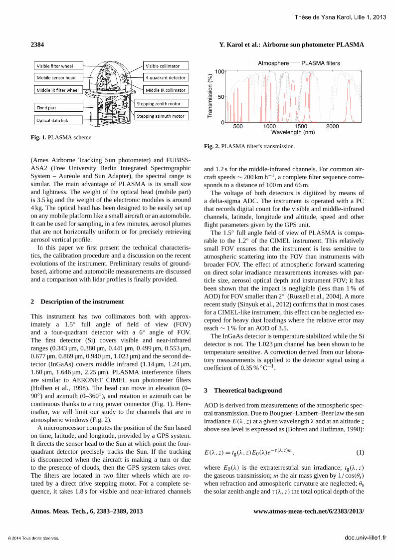
2384 Y. Karol et al.: Airborne sun photometer PLASMA
2 Y. Karol et al.: Airborne sunphotometer PLASMA
In this paper we first present the technical characteris-70
tics, the calibration procedure and a discussion on the recentevolutions of the instrument. Preliminary results of ground-based, airborne and automobile measurements are discussedand a comparison with lidar profiles is finally provided.
2 Description of the Instrument75
This instrument has two collimators both with approxi-mately a 1.5 full angle of field of view (FOV) and a four-quadrant detector with a 6 angle of FOV. The first detec-tor (Si) covers visible and near-infrared ranges (0.343 µm,0.380 µm, 0.441 µm, 0.499 µm, 0.553 µm, 0.677 µm,80
0.869 µm, 0.940 µm, 1.023 µm) and the second detector (In-GaAs) covers middle infrared (1.14 µm, 1.24 µm, 1.60 µm,1.646 µm, 2.25 µm). PLASMA interference filters are sim-ilar to AERONET CIMEL sunphotometer filters (Holbenet al., 1998). The head can move in elevation (0–90) and85
azimuth (0–360), and rotation in azimuth can be continuousthanks to a ring power connector. Hereinafter, we will limitour study to the channels that are in atmospheric windows(Fig. 2).
Fig. 1. PLASMA scheme.
500 1000 1500 20000
50
100
Wavelength (nm)
Tran
smis
sion
(%)
Atmosphere PLASMA filters
Fig. 2. PLASMA filter’s transmission.
A microprocessor computes the position of the Sun based90
on time, latitude, and longitude, provided by a GPS system.It directs the sensor head to the Sun at which point the four-quadrant detector precisely tracks the Sun. If the tracking
is disconnected when the aircraft is making a turn or dueto the presence of clouds, then the GPS system takes over.95
The filters are located in two filter wheels which are rotatedby a direct drive stepping motor. For a complete sequence,it takes 1.8 s for visible and near-infrared channels and 1.2 sfor the middle infrared channels. For common aircraft speeds∼ 200 km/h, a complete filter sequence corresponds to a dis-100
tance of 100 m and 66 m respectively.The voltage of both detectors is digitized by mean of
a delta-sigma ADC. The instrument is operated with a PCthat records digital count for the visible and middle infraredchannels, latitude, longitude and altitude, speed and other105
flight parameters given by the GPS unit.The 1.5 full angle field of view of PLASMA is compa-
rable to the 1.2 of the CIMEL instrument. This relativelysmall FOV ensures that the instrument is less sensitive toatmospheric scattering into the FOV than instruments with110
broader FOV. The effect of atmospheric forward scatteringon direct solar irradiance measurements increases with par-ticle size, aerosol optical depth and instrument FOV, it hasbeen shown that the impact is negligible (less than 1% ofAOD) for FOV smaller than 2 (Russell et al., 2004). A more115
recent study (Sinyuk et al., 2012) confirms that in most casesfor a CIMEL-like instrument, this effect can be neglected ex-cepted for heavy dust loadings where the relative error mayreach ∼ 1% for an AOD of 3.5.
The InGaAs detector is temperature stabilized while the Si120
detector is not. The 1.023 µm channel has been shown to betemperature sensitive. A correction derived from our labora-tory measurements is applied to the detector signal using acoefficient of 0.35%/C.
3 Theoretical Background125
AOD is derived from measurements of the atmospheric spec-tral transmission. Due to Bouguer-Lambert-Beer law the sunirradiance E(λ,z) at a given wavelength λ and at an alti-tude z above sea level is expressed as (Bohren and Huffman,1998):130
E(λ,z) = tg(λ,z)E0(λ)e−τ(λ,z)m (1)
where E0(λ) is the extraterrestrial sun irradiance; tg(λ,z)the gaseous transmission; m the airmass given by 1/cos(θs)when refraction and atmospheric curvature are neglected; θsthe solar zenith angle and τ(λ,z) the total optical depth of the135
atmosphere that is the sum of aerosol extinction and molecu-lar (Rayleigh) optical depths:
τ(λ,z) = τaext(λ,z)+τmext(λ,z) (2)
The digital signal (DN(λ,z)) measured by the instrumentis proportional to sun irradiance E(λ,z) (the relative Earth-140
Sun distance is taken to be imbedded in the extraterrestrial
Fig. 1.PLASMA scheme.
(Ames Airborne Tracking Sun photometer) and FUBISS-ASA2 (Free University Berlin Integrated SpectrographicSystem – Aureole and Sun Adapter), the spectral range issimilar. The main advantage of PLASMA is its small sizeand lightness. The weight of the optical head (mobile part)is 3.5 kg and the weight of the electronic modules is around4 kg. The optical head has been designed to be easily set upon any mobile platform like a small aircraft or an automobile.It can be used for sampling, in a few minutes, aerosol plumesthat are not horizontally uniform or for precisely retrievingaerosol vertical profile.
In this paper we first present the technical characteris-tics, the calibration procedure and a discussion on the recentevolutions of the instrument. Preliminary results of ground-based, airborne and automobile measurements are discussedand a comparison with lidar profiles is finally provided.
2 Description of the instrument
This instrument has two collimators both with approx-imately a 1.5 full angle of field of view (FOV)and a four-quadrant detector with a 6 angle of FOV.The first detector (Si) covers visible and near-infraredranges (0.343 µm, 0.380 µm, 0.441 µm, 0.499 µm, 0.553 µm,0.677 µm, 0.869 µm, 0.940 µm, 1.023 µm) and the second de-tector (InGaAs) covers middle infrared (1.14 µm, 1.24 µm,1.60 µm, 1.646 µm, 2.25 µm). PLASMA interference filtersare similar to AERONET CIMEL sun photometer filters(Holben et al., 1998). The head can move in elevation (0–90) and azimuth (0–360), and rotation in azimuth can becontinuous thanks to a ring power connector (Fig.1). Here-inafter, we will limit our study to the channels that are inatmospheric windows (Fig.2).
A microprocessor computes the position of the Sun basedon time, latitude, and longitude, provided by a GPS system.It directs the sensor head to the Sun at which point the four-quadrant detector precisely tracks the Sun. If the trackingis disconnected when the aircraft is making a turn or dueto the presence of clouds, then the GPS system takes over.The filters are located in two filter wheels which are ro-tated by a direct drive stepping motor. For a complete se-quence, it takes 1.8 s for visible and near-infrared channels
2 Y. Karol et al.: Airborne sunphotometer PLASMA
In this paper we first present the technical characteris-70
tics, the calibration procedure and a discussion on the recentevolutions of the instrument. Preliminary results of ground-based, airborne and automobile measurements are discussedand a comparison with lidar profiles is finally provided.
2 Description of the Instrument75
This instrument has two collimators both with approxi-mately a 1.5 full angle of field of view (FOV) and a four-quadrant detector with a 6 angle of FOV. The first detec-tor (Si) covers visible and near-infrared ranges (0.343 µm,0.380 µm, 0.441 µm, 0.499 µm, 0.553 µm, 0.677 µm,80
0.869 µm, 0.940 µm, 1.023 µm) and the second detector (In-GaAs) covers middle infrared (1.14 µm, 1.24 µm, 1.60 µm,1.646 µm, 2.25 µm). PLASMA interference filters are sim-ilar to AERONET CIMEL sunphotometer filters (Holbenet al., 1998). The head can move in elevation (0–90) and85
azimuth (0–360), and rotation in azimuth can be continuousthanks to a ring power connector. Hereinafter, we will limitour study to the channels that are in atmospheric windows(Fig. 2).
Fig. 1. PLASMA scheme.
500 1000 1500 20000
50
100
Wavelength (nm)
Tran
smis
sion
(%)
Atmosphere PLASMA filters
Fig. 2. PLASMA filter’s transmission.
A microprocessor computes the position of the Sun based90
on time, latitude, and longitude, provided by a GPS system.It directs the sensor head to the Sun at which point the four-quadrant detector precisely tracks the Sun. If the tracking
is disconnected when the aircraft is making a turn or dueto the presence of clouds, then the GPS system takes over.95
The filters are located in two filter wheels which are rotatedby a direct drive stepping motor. For a complete sequence,it takes 1.8 s for visible and near-infrared channels and 1.2 sfor the middle infrared channels. For common aircraft speeds∼ 200 km/h, a complete filter sequence corresponds to a dis-100
tance of 100 m and 66 m respectively.The voltage of both detectors is digitized by mean of
a delta-sigma ADC. The instrument is operated with a PCthat records digital count for the visible and middle infraredchannels, latitude, longitude and altitude, speed and other105
flight parameters given by the GPS unit.The 1.5 full angle field of view of PLASMA is compa-
rable to the 1.2 of the CIMEL instrument. This relativelysmall FOV ensures that the instrument is less sensitive toatmospheric scattering into the FOV than instruments with110
broader FOV. The effect of atmospheric forward scatteringon direct solar irradiance measurements increases with par-ticle size, aerosol optical depth and instrument FOV, it hasbeen shown that the impact is negligible (less than 1% ofAOD) for FOV smaller than 2 (Russell et al., 2004). A more115
recent study (Sinyuk et al., 2012) confirms that in most casesfor a CIMEL-like instrument, this effect can be neglected ex-cepted for heavy dust loadings where the relative error mayreach ∼ 1% for an AOD of 3.5.
The InGaAs detector is temperature stabilized while the Si120
detector is not. The 1.023 µm channel has been shown to betemperature sensitive. A correction derived from our labora-tory measurements is applied to the detector signal using acoefficient of 0.35%/C.
3 Theoretical Background125
AOD is derived from measurements of the atmospheric spec-tral transmission. Due to Bouguer-Lambert-Beer law the sunirradiance E(λ,z) at a given wavelength λ and at an alti-tude z above sea level is expressed as (Bohren and Huffman,1998):130
E(λ,z) = tg(λ,z)E0(λ)e−τ(λ,z)m (1)
where E0(λ) is the extraterrestrial sun irradiance; tg(λ,z)the gaseous transmission; m the airmass given by 1/cos(θs)when refraction and atmospheric curvature are neglected; θsthe solar zenith angle and τ(λ,z) the total optical depth of the135
atmosphere that is the sum of aerosol extinction and molecu-lar (Rayleigh) optical depths:
τ(λ,z) = τaext(λ,z)+τmext(λ,z) (2)
The digital signal (DN(λ,z)) measured by the instrumentis proportional to sun irradiance E(λ,z) (the relative Earth-140
Sun distance is taken to be imbedded in the extraterrestrial
Fig. 2.PLASMA filter’s transmission.
and 1.2 s for the middle-infrared channels. For common air-craft speeds∼ 200 km h−1, a complete filter sequence corre-sponds to a distance of 100 m and 66 m.
The voltage of both detectors is digitized by means ofa delta-sigma ADC. The instrument is operated with a PCthat records digital count for the visible and middle-infraredchannels, latitude, longitude and altitude, speed and otherflight parameters given by the GPS unit.
The 1.5 full angle field of view of PLASMA is compa-rable to the 1.2 of the CIMEL instrument. This relativelysmall FOV ensures that the instrument is less sensitive toatmospheric scattering into the FOV than instruments withbroader FOV. The effect of atmospheric forward scatteringon direct solar irradiance measurements increases with par-ticle size, aerosol optical depth and instrument FOV; it hasbeen shown that the impact is negligible (less than 1 % ofAOD) for FOV smaller than 2 (Russell et al., 2004). A morerecent study (Sinyuk et al., 2012) confirms that in most casesfor a CIMEL-like instrument, this effect can be neglected ex-cepted for heavy dust loadings where the relative error mayreach∼ 1 % for an AOD of 3.5.
The InGaAs detector is temperature stabilized while the Sidetector is not. The 1.023 µm channel has been shown to betemperature sensitive. A correction derived from our labora-tory measurements is applied to the detector signal using acoefficient of 0.35 %C−1.
3 Theoretical background
AOD is derived from measurements of the atmospheric spec-tral transmission. Due to Bouguer–Lambert–Beer law the sunirradianceE(λ,z) at a given wavelengthλ and at an altitudezabove sea level is expressed as (Bohren and Huffman, 1998):
E(λ,z) = tg(λ,z)E0(λ)e−τ(λ,z)m, (1)
whereE0(λ) is the extraterrestrial sun irradiance;tg(λ,z)
the gaseous transmission;m the air mass given by 1/cos(θs)
when refraction and atmospheric curvature are neglected;θsthe solar zenith angle andτ(λ,z) the total optical depth of the
Atmos. Meas. Tech., 6, 2383–2389, 2013 www.atmos-meas-tech.net/6/2383/2013/
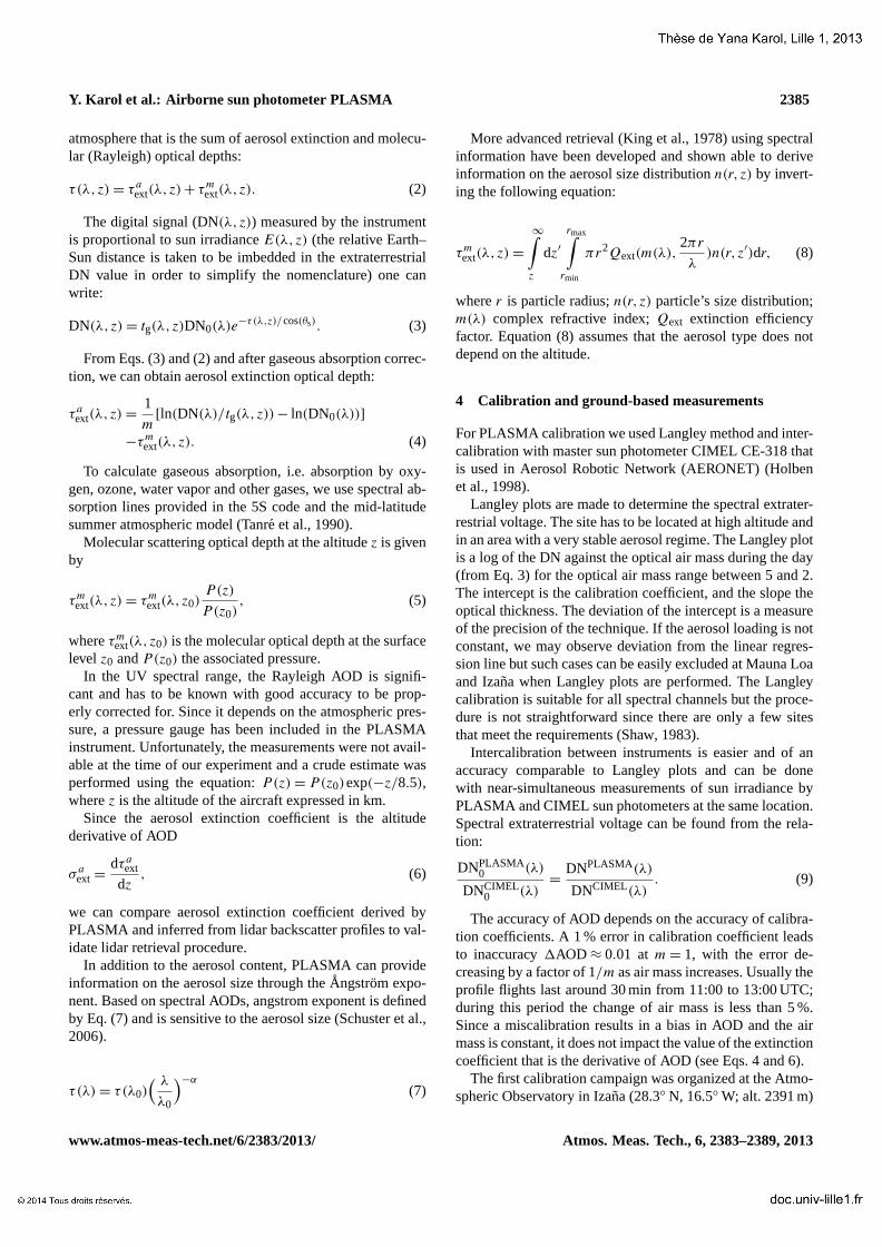
Y. Karol et al.: Airborne sun photometer PLASMA 2385
atmosphere that is the sum of aerosol extinction and molecu-lar (Rayleigh) optical depths:
τ(λ,z) = τ aext(λ,z) + τm
ext(λ,z). (2)
The digital signal (DN(λ,z)) measured by the instrumentis proportional to sun irradianceE(λ,z) (the relative Earth–Sun distance is taken to be imbedded in the extraterrestrialDN value in order to simplify the nomenclature) one canwrite:
DN(λ,z) = tg(λ,z)DN0(λ)e−τ(λ,z)/cos(θs). (3)
From Eqs. (3) and (2) and after gaseous absorption correc-tion, we can obtain aerosol extinction optical depth:
τ aext(λ,z) =
1
m[ln(DN(λ)/tg(λ,z)) − ln(DN0(λ))]
−τmext(λ,z). (4)
To calculate gaseous absorption, i.e. absorption by oxy-gen, ozone, water vapor and other gases, we use spectral ab-sorption lines provided in the 5S code and the mid-latitudesummer atmospheric model (Tanre et al., 1990).
Molecular scattering optical depth at the altitudez is givenby
τmext(λ,z) = τm
ext(λ,z0)P (z)
P (z0), (5)
whereτmext(λ,z0) is the molecular optical depth at the surface
level z0 andP(z0) the associated pressure.In the UV spectral range, the Rayleigh AOD is signifi-
cant and has to be known with good accuracy to be prop-erly corrected for. Since it depends on the atmospheric pres-sure, a pressure gauge has been included in the PLASMAinstrument. Unfortunately, the measurements were not avail-able at the time of our experiment and a crude estimate wasperformed using the equation:P(z) = P(z0)exp(−z/8.5),wherez is the altitude of the aircraft expressed in km.
Since the aerosol extinction coefficient is the altitudederivative of AOD
σ aext =
dτ aext
dz, (6)
we can compare aerosol extinction coefficient derived byPLASMA and inferred from lidar backscatter profiles to val-idate lidar retrieval procedure.
In addition to the aerosol content, PLASMA can provideinformation on the aerosol size through theAngstrom expo-nent. Based on spectral AODs, angstrom exponent is definedby Eq. (7) and is sensitive to the aerosol size (Schuster et al.,2006).
τ(λ) = τ(λ0)( λ
λ0
)−α
(7)
More advanced retrieval (King et al., 1978) using spectralinformation have been developed and shown able to deriveinformation on the aerosol size distributionn(r,z) by invert-ing the following equation:
τmext(λ,z) =
∞∫z
dz′
rmax∫rmin
πr2Qext(m(λ),2πr
λ)n(r,z′)dr, (8)
wherer is particle radius;n(r,z) particle’s size distribution;m(λ) complex refractive index;Qext extinction efficiencyfactor. Equation (8) assumes that the aerosol type does notdepend on the altitude.
4 Calibration and ground-based measurements
For PLASMA calibration we used Langley method and inter-calibration with master sun photometer CIMEL CE-318 thatis used in Aerosol Robotic Network (AERONET) (Holbenet al., 1998).
Langley plots are made to determine the spectral extrater-restrial voltage. The site has to be located at high altitude andin an area with a very stable aerosol regime. The Langley plotis a log of the DN against the optical air mass during the day(from Eq.3) for the optical air mass range between 5 and 2.The intercept is the calibration coefficient, and the slope theoptical thickness. The deviation of the intercept is a measureof the precision of the technique. If the aerosol loading is notconstant, we may observe deviation from the linear regres-sion line but such cases can be easily excluded at Mauna Loaand Izana when Langley plots are performed. The Langleycalibration is suitable for all spectral channels but the proce-dure is not straightforward since there are only a few sitesthat meet the requirements (Shaw, 1983).
Intercalibration between instruments is easier and of anaccuracy comparable to Langley plots and can be donewith near-simultaneous measurements of sun irradiance byPLASMA and CIMEL sun photometers at the same location.Spectral extraterrestrial voltage can be found from the rela-tion:
DNPLASMA0 (λ)
DNCIMEL0 (λ)
=DNPLASMA(λ)
DNCIMEL(λ). (9)
The accuracy of AOD depends on the accuracy of calibra-tion coefficients. A 1 % error in calibration coefficient leadsto inaccuracy1AOD ≈ 0.01 at m = 1, with the error de-creasing by a factor of 1/m as air mass increases. Usually theprofile flights last around 30 min from 11:00 to 13:00 UTC;during this period the change of air mass is less than 5 %.Since a miscalibration results in a bias in AOD and the airmass is constant, it does not impact the value of the extinctioncoefficient that is the derivative of AOD (see Eqs.4 and6).
The first calibration campaign was organized at the Atmo-spheric Observatory in Izana (28.3 N, 16.5 W; alt. 2391 m)
www.atmos-meas-tech.net/6/2383/2013/ Atmos. Meas. Tech., 6, 2383–2389, 2013

2386 Y. Karol et al.: Airborne sun photometer PLASMA
in October 2009 for Langley approach and in Carpentras(44.1 N, 5.1 E; alt. 100 m) in March 2009 for intercalibra-tion.
The calibration coefficients calculated with Izana and Car-pentras data in 2009 were applied to all data collected inLille (50.6 N, 3.1 E; alt. 60 m) until March 2010 to obtainaerosol optical depth (AOD). The comparison with CIMELmeasurements at common wavelengths (0.34 µm, 0.38 µm,0.44 µm, 0.67 µm, 0.86 µm, 1.02 µm, 1.64 µm) showed a goodagreement between the two instruments with with rms AODdifferences being between 0.01 and 0.02.
After modifications of some mechanical elements, a newcalibration campaign was organized at Izana in March 2010.Several measurements were then performed in LOA to sam-ple different atmospheric conditions during 12 days in April–June 2010 and a better agreement with CIMEL master instru-ment was obtained with rms AOD differences∼ 0.01. ThePLASMA calibration is not too far from the calibration ofAERONET reference instruments (0.002< 1AOD < 0.009)(Eck et al., 1999).
Once the technical development has been achieved,PLASMA was refurbished in March 2011. The stepping az-imuth and zenith motors were replaced for better pointingcapability and signal processing steps taken to improve thesignal to noise ratio. We also replace all the filters, which re-quired a new calibration of the instrument. After calibrationthe difference of AOD retrieved by PLASMA and CIMELmaster instrument is less than 0.005 for all channels except0.34 µm channel (see Fig.3).
The differences observed before 09:00 UTC and after15:00 UTC may come from filter out-of-band leakage result-ing from incomplete blocking of solar energy from outsidethe filter bandpass as seen in some AERONET CIMEL in-struments. In the laboratory measurements of filters trans-mission, such leakage was not observed over±100 nm fromthe central wavelength. Differences may also come from amiscalibration of this channel. Knowing the calibration co-efficient within 1 % error only results in errors in the AODof 0.025 for an air mass of 2.4 as anticipated around 07:30in Lille in April. This effect would lead to a symmetrical be-havior in the afternoon as observed in Fig.3.
Since PLASMA has the same interference filters asCIMEL, we follow the AERONET calibration policy and theinstrument is going to be calibrated every year.
Currently, we analyze only results in spectral bands thatare present on both PLASMA and CIMEL instruments.Of course, PLASMA covers a larger spectral range witha 2.25 µm channel that is very important for AOD inver-sion. Nevertheless at this stage we do not consider this wave-length since we cannot validate calibration coefficient withany other instrument.
4 Y. Karol et al.: Airborne sunphotometer PLASMA
0
0.1
0.2
0.3
0.4
0.5
0.6
7.00 9.00 11.00 13.00 15.00 17.00
AOD
UTC
343 nm 441 nm 667 nm 1024 nm 1646 nm
Fig. 3. Comparison of simultaneous ground-based measurementsof PLASMA (colored lines) and CIMEL CE-318 (black lines)18/04/2011.
Several measurements were then performed in LOA to sam-ple different atmospheric conditions during 12 days in April–June 2010 and a better agreement with CIMEL master in-strument was obtained with rms AOD differences ∼ 0.01.The PLASMA calibration is not too far from the calibration240
of AERONET reference instruments (0.002 < ∆AOD <0.009) (Eck et al., 1999).
Once the technical development has been achieved,PLASMA was refurbished in March 2011. The stepping az-imuth and zenith motors were replaced for better pointing245
capability and signal processing steps taken to improve thesignal to noise ratio. We also replace all the filters, which re-quired a new calibration of the instrument. After calibrationthe difference of AOD retrieved by PLASMA and CIMELmaster instrument is less than 0.005 for all channels except250
0.34 µm channel (see Fig. 3).The differences observed before 9UTC and after 15UTC
may come from filter out-of-band leakage resulting fromincomplete blocking of solar energy from outside the fil-ter bandpass as seen in some AERONET CIMEL instru-255
ments. In the laboratory measurements of filters transmissionsuch leakage wasn’t observed over ±100 nm from the cen-tral wavelength. Differences may also come from a miscal-ibration of this channel. Knowing the calibration coefficientwithin 1% error only results in errors in the AOD of 0.025260
for an airmass of 2.4 as anticipated around 7.30 in Lille inApril. This effect would lead to a symmetrical behavior inthe afternoon as observed in Fig. 3.
Since PLASMA has the same interference filters asCIMEL we follow the AERONET calibration policy and the265
instrument is going to be calibrated every year.Currently, we analyze only results in spectral bands that
are present on both PLASMA and CIMEL instruments.Of course, PLASMA covers a larger spectral range witha 2.25 µm channel that is very important for AOD inver-270
sion. Nevertheless at this stage we do not consider this wave-length since we cannot validate calibration coefficient withany other instrument.
5 Airborne Measurements
In addition to ground-based measurements, several flights275
were performed in Lille: two technical flights in 2009, 6flights in 2010 and 3 flights in 2011. We provide here-inafter results for flights performed after first improvements,i.e. since October 2010 only.
Figure 4 shows profiles of 4 flights in 2010–2011:280
12/10/2010, 28/09/2011, 29/09/2011 and 15/10/2011 fromthe top to the bottom. The first column of graphs on theleft presents the vertical profile of AOD at different wave-lengths; the second is the profile of extinction coefficient;the third column on the right presents the comparison of ex-285
tinction at 0.553 µm with lidar retrievals at 0.532 µm. Weuse the Cloud and Aerosol Micro-LIDAR (CAML) CE 3702manufactured by CIMEL. The instrument has been alreadydescribed in Pelon et al. (2008) and Leon et al. (2009). Theaerosol extinction profile as well as the effective extinction-290
to-backscatter ratio are retrieved using combination of lidardata and sun-photometer AOD (Leon et al., 2009).
To get extinction profile we decided to remove all noisydata due to the presence of clouds and then to average over10 measurements. It means that we assume that the state295
of the atmosphere was stable over 30–60 s, along 50–100 min vertical direction and 2–4 km in horizontal direction. Al-titudes below 500 m could not be observed by lidar. Lidarprofiles presented on figure 4 are extended to the ground levelby using the correction function based on independent mea-300
surements of AOD. Direct measurements of PLASMA canbe used for validation of this function. The extinction pro-files retrieved from lidar measurements are broadly consis-tent with PLASMA results, showing coarsely similar verti-cal attributes. The best agreement between aerosol extinc-305
tion coefficient profiles retrieved from PLASMA and lidardata was observed 15 October 2011 when the atmospherewas stable enough as seen from AOD profile.
For other days, differences might be explained by time andspace variability of aerosol and clouds. On 29 September310
2011 clouds were present in the vicinity and the turbiditywas rather high and variable, between 0.15 - 0.20 at 0.553 µmaround noon; as a result the data are noisier and a 50 % dif-ference of extinction coefficient at an altitude around 400 mis observed. Discrepancies can also result from spatial vari-315
ability of the aerosol field; distance between both instrumentswas around 10 km when the airplane was on the ground, andmore than 50 km when the plane was flying at the altitude of3000 m. Moreover, the profiles take around 20 min and are
Fig. 3. Comparison of simultaneous ground-based measurementsof PLASMA (colored lines) and CIMEL CE-318 (black lines)18 April 2011.
5 Airborne measurements
In addition to ground-based measurements, several flightswere performed in Lille: two technical flights in 2009, 6flights in 2010 and 3 flights in 2011. We provide hereinafterresults for flights performed after first improvements, i.e.since October 2010 only.
Figure4 shows profiles of 4 flights in 2010–2011: 12 Oc-tober 2010, 28 September 2011, 29 September 2011 and15 October 2011 from the top to the bottom. The first col-umn of graphs on the left presents the vertical profile of AODat different wavelengths; the second is the profile of extinc-tion coefficient; the third column on the right presents thecomparison of extinction at 0.553 µm with lidar retrievalsat 0.532 µm. We use the Cloud and Aerosol Micro-LIDAR(CAML) CE 3702 manufactured by CIMEL. The instrumenthas been already described inPelon et al.(2008) andLeonet al. (2009). The aerosol extinction profile as well as theeffective extinction-to-backscatter ratio are retrieved usingcombination of lidar data and sun-photometer AOD (Leonet al., 2009).
To get extinction profile we decided to remove all noisydata due to the presence of clouds and then to average over10 measurements. It means that we assume that the state ofthe atmosphere was stable over 30–60 s, along 50–100 m invertical direction and 2–4 km in horizontal direction. Alti-tudes below 500 m could not be observed by lidar. Lidar pro-files presented on Fig.4 are extended to the ground levelby using the correction function based on independent mea-surements of AOD. Direct measurements of PLASMA canbe used for validation of this function. The extinction pro-files retrieved from lidar measurements are broadly consis-tent with PLASMA results, showing coarsely similar vertical
Atmos. Meas. Tech., 6, 2383–2389, 2013 www.atmos-meas-tech.net/6/2383/2013/
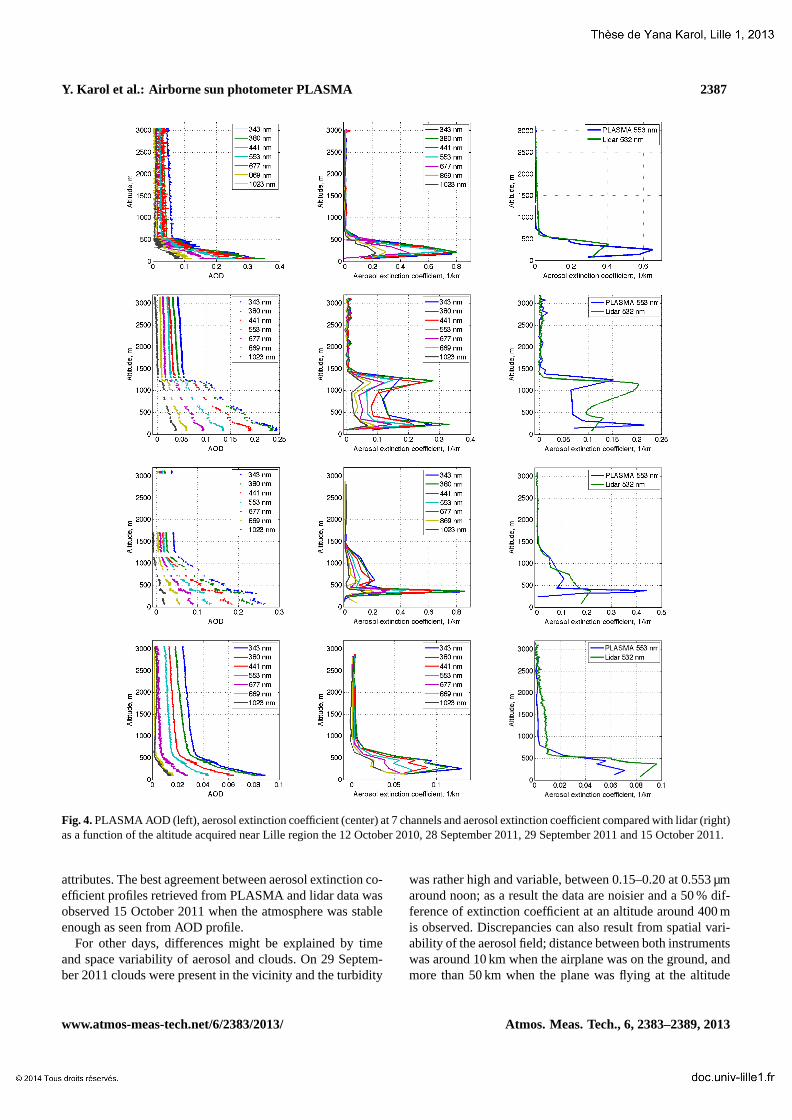
Y. Karol et al.: Airborne sun photometer PLASMA 2387Y. Karol et al.: Airborne sunphotometer PLASMA 5
Figure 3: PLASMA AOD (left), aerosol extinction coefficient (center) at 7 channels and aerosol extinctioncoefficient compared with lidar (right) as a function of the altitude acquired near Lille region the 12thOctober 2010, 28th September, 29th September and 15th October 2011.
Fig. 4. PLASMA AOD (left), aerosol extinction coefficient (center) at 7 channels and aerosol extinction coefficient compared with lidar(right) as a function of the altitude acquired near Lille region the 12/10/2010, 28/09/2011, 29/09/2011 and 15/10/2011.
Fig. 4.PLASMA AOD (left), aerosol extinction coefficient (center) at 7 channels and aerosol extinction coefficient compared with lidar (right)as a function of the altitude acquired near Lille region the 12 October 2010, 28 September 2011, 29 September 2011 and 15 October 2011.
attributes. The best agreement between aerosol extinction co-efficient profiles retrieved from PLASMA and lidar data wasobserved 15 October 2011 when the atmosphere was stableenough as seen from AOD profile.
For other days, differences might be explained by timeand space variability of aerosol and clouds. On 29 Septem-ber 2011 clouds were present in the vicinity and the turbidity
was rather high and variable, between 0.15–0.20 at 0.553 µmaround noon; as a result the data are noisier and a 50 % dif-ference of extinction coefficient at an altitude around 400 mis observed. Discrepancies can also result from spatial vari-ability of the aerosol field; distance between both instrumentswas around 10 km when the airplane was on the ground, andmore than 50 km when the plane was flying at the altitude
www.atmos-meas-tech.net/6/2383/2013/ Atmos. Meas. Tech., 6, 2383–2389, 2013

2388 Y. Karol et al.: Airborne sun photometer PLASMA
6 Y. Karol et al.: Airborne sunphotometer PLASMA
compared to the nearest in time lidar profile (∆t≈ 15 min).320
Despite these differences, the aerosol layers are located atthe same altitude and we can say that both vertical profilesare coarsely consistent.
6 Automobile Measurements
In addition to airborne measurements it is also possible to325
set up PLASMA on the roof of an automobile in order toobtain horizontal transects of AOD. In mountain areas, wecan also get vertical profiles using measurements performedat different altitudes.
Fig. 5. Vertical profiles of AOD during automobile experiment13/01/2011 on Tenerife island, Spain.
In January 2011 an experiment was successfully carried330
out on the island of Tenerife, Spain. The measurementswere made from sea level to an altitude of 2400 m in onehour. Horizontal coverage area was about 30 km and wehad the opportunity to compare the PLASMA AOD with theIzana AERONET site (alt. 2391 m) very close to the road-335
way. There are also two additional AERONET sites, La La-guna (alt. 590 m) and Santa Cruz (alt. 54 m), that were lo-cated at a distance of 40 km from our measurements.
The vertical profiles of AOD at 0.380 µm and 0.677 µm iscompared to the three AERONET stations in Fig. 5. Addi-340
tional measurement performed at the altitude of 1000 m us-ing a sunphotometer MICROTOPS II (Morys et al., 2001) isreported for 0.44 µm. Measurements of PLASMA are con-sistent with other instruments with ∆AOD∼ 0.01 and thedifferences for the low altitude sites could be explained by345
the distance between the instruments.
7 Conclusions
The new sunphotometer that we have developed has beenfully described. Following the calibration procedure recom-mended by AERONET, PLASMA provides AOD measure-350
ments with an accuracy of 0.005<∆AOD < 0.01 over awide spectral range.
Its capability to follow the sun when it moves is very at-tractive. Installed on an aircraft, vertical profiles of AODand aerosol extinction coefficient can be so derived and com-355
pared to lidar retrievals. Overall, PLASMA is a user-friendlyinstrument, easy to install on moving platforms and perform-ing well compared to other instruments.
Acknowledgements. This study has been funded by CNES (Cen-tre National d’Etudes Spatiales), CNRS (Centre National de la360
Recherche Scientifique), the University of Lille, and Region Nord-Pas-de-Calais. Y. Karol is supported by a fellowship fromCNES and CNRS. PLASMA calibration was performed at Izanaobservatory using AERONET-EUROPE calibration center, sup-ported by ACTRIS from European Union Seventh Framework365
Program (FP7/2007-2013) under grant agreement no. 262254.Emilio Cuevas-Agullo from the Meteorological State Agency ofSpain (AEMET) is acknowledged for his help during the experi-ment in Tenerife. The authors are very thankful to AERONET forestablishing and maintaining the sites used in this work.370
Institut national des sciences de l'UniversINSU
The publication of this article is financed by CNRS-INSU.
References
Asseng, H., Ruhtz, T., and Fischer, J.: Sun and Aureole Spectrome-375
ter for Airborne Measurements to Derive Aerosol Optical Prop-erties, Appl. Opt., 43, 2146–2155, doi:10.1364/AO.43.002146,2004.
Bohren, C. and Huffman, D.: Absorption and Scattering of Light bySmall Particles (Wiley science paperback series), Wiley-VCH,380
1998.Eck, T. F., Holben, B. N., Reid, J. S., Dubovik, O., Smirnov,
A., O’Neill, N. T., Slutsker, I., and Kinne, S.: Wavelength de-pendence of the optical depth of biomass burning, urban, anddesert dust aerosols, J. Geophys. Res., 104, 31 333–31 349, doi:385
10.1029/1999JD900923, 1999.Hansen, J., Sato, M., and Ruedy, R.: Radiative forcing and climate
response, Journal of Geophysical Research, 102, 6831–6864,doi:10.1029/96JD03436, 1997.
Holben, B., Eck, T., Slutsker, I., Tanre, D., Buis, J., Setzer, A.,390
Vermote, E., Reagan, J., Kaufman, Y., Nakajima, T., Lavenu,F., Jankowiak, I., and Smirnov, A.: AERONET - A Feder-ated Instrument Network and Data Archive for Aerosol Char-
Fig. 5. Vertical profiles of AOD during automobile experiment13 January 2011 on Tenerife island, Spain.
of 3000 m. Moreover, the profiles take around 20 min andare compared to the nearest in the time lidar profile (1t ≈
15 min). Despite these differences, the aerosol layers are lo-cated at the same altitude and we can say that both verticalprofiles are coarsely consistent.
6 Automobile measurements
In addition to airborne measurements it is also possible toset up PLASMA on the roof of an automobile in order toobtain horizontal transects of AOD. In mountain areas, wecan also get vertical profiles using measurements performedat different altitudes.
In January 2011 an experiment was successfully carriedout on the island of Tenerife, Spain. The measurements weremade from sea level to an altitude of 2400 m in one hour.Horizontal coverage area was about 30 km and we had theopportunity to compare the PLASMA AOD with the IzanaAERONET site (alt. 2391 m) very close to the roadway.There are also two additional AERONET sites, La Laguna(alt. 590 m) and Santa Cruz (alt. 54 m), that were located at adistance of 40 km from our measurements.
The vertical profiles of AOD at 0.380 µm and 0.677 µmis compared to the three AERONET stations in Fig.5. Anadditional measurement performed at the altitude of 1000 musing a sun photometer MICROTOPS II (Morys et al., 2001)is reported for 0.44 µm. Measurements of PLASMA are con-sistent with other instruments with1AOD ∼ 0.01 and thedifferences for the low altitude sites could be explained bythe distance between the instruments.
7 Conclusions
The new sun photometer that we have developed has beenfully described. Following the calibration procedure recom-mended by AERONET, PLASMA provides AOD measure-ments with an accuracy of 0.005< 1AOD < 0.01 over awide spectral range.
Its capability to follow the sun when it moves is very at-tractive. Installed on an aircraft, vertical profiles of AOD andaerosol extinction coefficient can be so derived and comparedto lidar retrievals. Overall, PLASMA is a user-friendly in-strument, easy to install on moving platforms and performingwell compared to other instruments.
Acknowledgements.This study has been funded by CNES (CentreNational d’Etudes Spatiales), CNRS (Centre National de laRecherche Scientifique), the University of Lille, and RegionNord-Pas-de-Calais. Y. Karol is supported by a fellowship fromCNES and CNRS. PLASMA calibration was performed at Izanaobservatory using AERONET-EUROPE calibration center, sup-ported by ACTRIS from European Union Seventh FrameworkProgram (FP7/2007-2013) under grant agreement no. 262254.Emilio Cuevas-Agullo from the Meteorological State Agency ofSpain (AEMET) is acknowledged for his help during the experi-ment in Tenerife. The authors are very thankful to AERONET forestablishing and maintaining the sites used in this work.
Edited by: O. Dubovik
The publication of this articleis financed by CNRS-INSU.
References
Asseng, H., Ruhtz, T., and Fischer, J.: Sun and Aureole Spectrome-ter for Airborne Measurements to Derive Aerosol Optical Prop-erties, Appl. Optics, 43, 2146–2155, doi:10.1364/AO.43.002146,2004.
Bohren, C. and Huffman, D.: Absorption and Scattering of Lightby Small Particles, Wiley science paperback series, Wiley-VCH,1998.
Eck, T. F., Holben, B. N., Reid, J. S., Dubovik, O., Smirnov,A., O’Neill, N. T., Slutsker, I., and Kinne, S.: Wavelengthdependence of the optical depth of biomass burning, urban,and desert dust aerosols, J. Geophys. Res., 104, 31333–31349,doi:10.1029/1999JD900923, 1999.
Hansen, J., Sato, M., and Ruedy, R.: Radiative forcingand climate response, J. Geophys. Res., 102, 6831–6864,doi:10.1029/96JD03436, 1997.
Holben, B., Eck, T., Slutsker, I., Tanre, D., Buis, J., Setzer, A.,Vermote, E., Reagan, J., Kaufman, Y., Nakajima, T., Lavenu,F., Jankowiak, I., and Smirnov, A.: AERONET – A FederatedInstrument Network and Data Archive for Aerosol Character-
Atmos. Meas. Tech., 6, 2383–2389, 2013 www.atmos-meas-tech.net/6/2383/2013/
Y. Karol et al.: Airborne sun photometer PLASMA 2389
ization, Remote Sens. Environ., 66, 1–16, doi:10.1016/S0034-4257(98)00031-5, 1998.
Kahn, R., Gaitley, B., Garay, M., Diner, D., Eck, T., Smirnov,A., and Holben, B.: Multiangle Imaging SpectroRadiometerglobal aerosol product assessment by comparison with theAerosol Robotic Network, J. Geophys. Res., 115, D23209,doi:10.1029/2010JD014601, 2010.
Kaufman, Y. J., Tanre, D., and Boucher, O.: A satellite view ofaerosols in the climate system, Nature, 419, 215–223, 2002.
King, M., Byrne, D., Herman, B., and Reagan, J.: Aerosol Size Dis-tributions Obtained by Inversions of Spectral Optical Depth Mea-surements, J. Atmos. Sci., 35, 2153–2167, doi:10.1175/1520-0469(1978)035<2153:ASDOBI>2.0.CO;2, 1978.
Koren, I., Kaufman, Y. J., Remer, L. A., and Martins, J. V.: Measure-ment of the Effect of Amazon Smoke on Inhibition of Cloud For-mation, Science, 303, 1342–1345, doi:10.1126/science.1089424,2004.
Leon, J.-F., Derimian, Y., Chiapello, I., Tanre, D., Podvin, T.,Chatenet, B., Diallo, A., and Deroo, C.: Aerosol vertical distri-bution and optical properties over M’Bour (16.96 W; 14.39 N),Senegal from 2006 to 2008, Atmos. Chem. Phys., 9, 9249–9261,doi:10.5194/acp-9-9249-2009, 2009.
Matsumoto, T., Russell, P., Mina, C., Ark, W. V., and Banta, V.:Airborne Tracking Sunphotometer, J. Atmos. Ocean. Tech., 4,336–339, 1987.
Morys, M., Forrest, M., Hagerup, S., Anderson, S., Baker, A., Kia,J., and Walkup, T.: Design, calibration, and performance of MI-CROTOPS II handheld ozone monitor and Sun photometer, J.Geophys. Res., 106, 14573–14582, 2001.
Pelon, J., Mallet, M., Mariscal, A., Goloub, P., Tanre, D., Karam,D. B., Flamant, C., Haywood, J., Pospichal, B., and Vic-tori, S.: Microlidar observations of biomass burning aerosolover Djougou (Benin) during African Monsoon Multidisci-plinary Analysis Special Observation Period 0: Dust andBiomass-Burning Experiment, J. Geophys. Res., 113, D00C18,doi:10.1029/2008JD009976, 2008.
Ramanathan, V., Crutzen, P., Kiehl, J., and Rosenfeld, D.: Aerosols,Climate, and the Hydrological Cycle, Science, 294, 2119–2124,doi:10.1126/science.1064034, 2001.
Remer, L., Kaufman, Y., Tanre, D., Mattoo, S., Chu, D., Martins, J.,Li, R., Ichoku, C., Levy, R., Kleidman, R., Eck, T., Vermote, E.,and Holben, B.: The MODIS Aerosol Algorithm, Products, andValidation, J. Atmos. Sci., 62, 947–973, doi:10.1175/JAS3385.1,2005.
Russell, P. B., Livingston, J. M., Dubovik, O., Ramirez, S. A.,Wang, J., Redemann, J., Schmid, B., Box, M., and Holben, B. N.:Sunlight transmission through desert dust and marine aerosols:Diffuse light corrections to Sun photometry and pyrheliometry, J.Geophys. Res., 109, D08207, doi:10.1029/2003JD004292, 2004.
Schmid, B., Redemann, J., Russell, P., Hobbs, P., Hlavka, D.,Mcgill, M., Holben, B., Welton, E., Campbell, J., Torres, O.,Kahn, R., Diner, D., Helmlinger, M., Chu, D., Robles-Gonzalez,C., and de Leeuw, G.: Coordinated airborne, spaceborne, andground-based measurements of massive thick aerosol layers dur-ing the dry season in southern Africa, J. Geophys. Res.-Atmos.,108, 8496, doi:10.1029/2002JD002297, 2003.
Schuster, G. L., Dubovik, O., and Holben, B. N.: Angstrom expo-nent and bimodal aerosol size distributions, J. Geophys. Res.,111, D07207, doi:10.1029/2005JD006328, 2006.
Shaw, G.: Sun Photometry, Bulletin of the AmericanMeteorological Society, 64, 4–10, doi:10.1175/1520-0477(1983)064<0004:SP>2.0.CO;2, 1983.
Sinyuk, A., Holben, B., Smirnov, A., Eck, T., Slutsker, I.,Schafer, J., Giles, D., and Sorokin, M.: Assessment of er-ror in aerosol optical depth measured by AERONET due toaerosol forward scattering, Geophys. Res. Lett., 39, L23806,doi:10.1029/2012GL053894, 2012.
Tanre, D., Deroo, C., Duhaut, P., Herman, M., Morcrette, J., Perbos,J., and Deschamps, P.: Description of a computer code to simu-late the satellite signal in the solar spectrum: the 5S Code, Int. J.Remote Sens., 11, 659–668, 1990.
Tanre, D., Breon, F. M., Deuze, J. L., Dubovik, O., Ducos,F., Francois, P., Goloub, P., Herman, M., Lifermann, A., andWaquet, F.: Remote sensing of aerosols by using polarized,directional and spectral measurements within the A-Train:the PARASOL mission, Atmos. Meas. Tech., 4, 1383–1395,doi:10.5194/amt-4-1383-2011, 2011.
Winker, D., Pelon, J., Coakley, J., Ackerman, S., Charlson, R., Co-larco, P., Flamant, P., Fu, Q., Hoff, R., Kittaka, C., Kubar, T.,Le Treut, H., McCormick, M., Megie, G., Poole, L., Powell, K.,Trepte, C., Vaughan, M., and Wielicki, B.: The CALIPSO Mis-sion: A Global 3D View of Aerosols and Clouds, B. Am. Meteo-rol. Soc., 91, 1211–1229, doi:10.1175/2010BAMS3009.1, 2010.
www.atmos-meas-tech.net/6/2383/2013/ Atmos. Meas. Tech., 6, 2383–2389, 2013
Bibliography
Ackerman, A. S., Toon, O. B., Taylor, J. P., Johnson, D. W., Hobbs, P. V., andFerek, R. J.: Effects of aerosols on cloud albedo: evaluation of twomey’s param-eterization of cloud susceptibility using measurements of ship tracks, J. Atmos.Sci., 57, 2684–2695, URL http://dx.doi.org/10.1175/1520-0469(2000)
057<2684:EOAOCA>2.0.CO;2, 2000.
Adams, P., Seinfeld, J., and Koch, D.: Global concentrations of tropospheric sul-phate, nitrate and ammonium aerosol simulated in a general circulation model,J. Geophys. Res., 104, 13 79113 823, 1999.
Albrecht, B.: Aerosols, Cloud Microphysics, and Fractional Cloudiness, Science,245, 1227–1230, doi:10.1126/science.245.4923.1227, 1989.
Andreae, M.: Climatic effects of changing atmospheric aerosol levels, in: WorldSurvey of Climatology, edited by Henderson-Sellers, A., vol. 16: Future Climatesof the World, pp. 341–392, Elsevier, Amsterdam, 1995.
Andreae, M. and Crutzen, P.: Atmospheric Aerosols: Biogeochemical Sources andRole in Atmospheric Chemistry, Science, 276, 1052–1058, doi:10.1126/science.276.5315.1052, 1997.
Angstrom, A. K.: On the atmospheric transmission of Sun radiation and on dustin the air, Geogr. Ann., 11, 156–166, 1929.
Asseng, H., Ruhtz, T., and Fischer, J.: Sun and Aureole Spectrometer for Air-borne Measurements to Derive Aerosol Optical Properties, Appl. Opt., 43,2146–2155, doi:10.1364/AO.43.002146, URL http://ao.osa.org/abstract.
cfm?URI=ao-43-10-2146, 2004.
Bergstrom, R., Pilewskie, P., Schmid, B., and Russell, P.: Estimates of the spectralaerosol single scattering albedo and aerosol radiative effects during SAFARI2000, Journal of Geophysical Research, 108, 8474, doi:10.1029/2002JD002435,2003.
Bohren, C. and Huffman, D.: Absorption and Scattering of Light by Small Parti-cles (Wiley science paperback series), Wiley-VCH, 1998.
Bond, T. and Bergstrom, R.: Light Absorption by Carbonaceous Particles: AnInvestigative Review, Aerosol Science and Technology, 40, 27–67, doi:10.1080/02786820500421521, 2006.
164
Bibliography 165
Bosenberg, J.: EARLINET: A European Aerosol Research Lidar Network to Es-tablish an Aerosol Climatology, Max-Planck-Institut Report No. 348, 2003.
Bosenberg, J. and Hoff, R.: Plan for the implementation of the GAW AerosolLidar Observation Network GALION, GAW report 178, World MeteorogicalOrganization, Hamburg, Germany, 2007.
Chaikovsky, A., Dubovik, O., Goloub, P., Tanre, D., Chaikovskaya, L., Denisov,S., Grudo, Y., Lopatsin, A., Karol, Y., Lapyonok, T., Korol, M., Osipenko,F., Savitski, D., and Slesar, A.: Combined lidar and radiometric sounding ofatmospheric aerosol: algorithm of data processing, software, dessimination, in:Proceedings of XVIII International symposium “Atmospheric and ocean optics.Atmosphere physics ”, Irkutsk, Russian Federation, 2—6 July, pp. C1—C4,2012.
Chaikovsky, A. P., Ivanov, A. P., Balin, Y. S., Elnikov, A. V., Tulinov, G. F.,Plusnin, I. I., Bukin, O. A., and Chen, B. B.: CIS-LiNet lidar network formonitoring aerosol and ozone: methodology and instrumentation, Atmosphericand oceanic optics, 18, 2005.
Chanine, M.: Determination of the Temperature Profile in an Atmospherefrom its Outgoing Radiance, J. Opt. Soc. Am., 58, 1634–1637, doi:10.1364/JOSA.58.001634, URL http://www.opticsinfobase.org/abstract.
cfm?URI=josa-58-12-1634, 1968.
Chowdhary, J., Cairns, B., Mishchenko, M., Hobbs, P., Cota, G., Redemann,J., Rutledge, K., Holben, B., and Russell, E.: Retrieval of Aerosol Scatteringand Absorption Properties from Photopolarimetric Observations over the Oceanduring the CLAMS Experiment, Journal of the Atmospheric Sciences, 62, 1093–1117, doi:10.1175/JAS3389.1, 2005.
Cooke, W. F., Liousse, C., Cachier, H., and Feichter, J.: Construction of a 1× 1
fossil fuel emission data set for carbonaceous aerosol and implementation andradiative impact in the ECHAM4 model, J. Geophys. Res., 104(D18), 22 137–22 162, 1999.
Cuesta, J., Flamant, H. P., and Flamant, C.: Synergetic technique combining elas-tic backscatter lidar data and sunphotometer AERONET inversion for retrievalby layer of aerosol optical and microphysical properties, APPLIED OPTICS,47, 4598–4611, 2008.
Davis, D. L., Bell, M. L., , and Fletcher, T.: A look back at the London smog of1952 and the half century since, Environ. Health Perspect., 110, 734–735, 2002.
Deschamps, P.-Y., Breon, F.-M., Leroy, M., Podaire, A., Bricaud, A., Buriez, J.-C.,and Seze, G.: The POLDER mission: instrument characteristics and scientificobjectives, Geoscience and Remote Sensing, IEEE, 32, 598–615, 1994.
Diner, D., Beckert, J., Reilly, T., Bruegge, C., Conel, J., Kahn, R., Martonchik,J., Ackerman, T., Davies, R., Gerstl, S., Gordon, H., Muller, J.-P., Myneni,
Bibliography 166
R., Sellers, R., Pinty, B., and Verstraete, M.: Multi-angle Imaging Spectro-Radiometer (MISR) description and experiment overview, IEEE Trans. Geosci.Rem. Sens., 36(4), 1072–1087, 1998.
Donaldson, K., Stone, V., Seaton, A., and MacNee, W.: Ambient particle inhala-tion and the cardiovascular system : potential mechanisms, Environ. HealthPerspect., 109, 523–527, 2001.
Dubovik, O.: Optimization of Numerical Inversion in Photopolarimetric Re-mote Sensing, in: Photopolarimetry in Remote Sensing, edited by Videen, G.,Yatskiv, Y., and Mishchenko, M., pp. 65–106, Kluwer Academic Publishers,Dordrecht, The Netherlands, 2004.
Dubovik, O. and King, M.: A flexible inversion algorithm for retrieval of aerosoloptical properties from Sun and sky radiance measurements, Journal of Geo-physical Research, 105, 20 673–20 696, 2000.
Dubovik, O., Yokota, T., and Sasano, Y.: Improved technique for datainversion and its application to the retrieval algorithm for ADEOS/I-LAS, Advances in Space Research, 21, 397 – 403, doi:http://dx.doi.org/10.1016/S0273-1177(97)00920-4, URL http://www.sciencedirect.com/
science/article/pii/S0273117797009204, 1998.
Dubovik, O., Smirnov, A., Holben, B., King, M., Kaufman, Y., Eck, T., andSlutsker, I.: Accuracy assessments of aerosol optical properties retrieved fromAerosol Robotic Network (AERONET) Sun and sky radiance measurements,Journal of Geophysical Research, 105, doi:10.1029/2000JD900040, 2000.
Dubovik, O., Holben, B., Eck, T., Smirnov, A., Kaufman, Y., King, M., Tanre,D., and Slutsker, I.: Variability of Absorption and Optical Properties of KeyAerosol Types Observed in Worldwide Locations, J. Atmos. Sci., 59, 590–608,doi:10.1175/1520-0469(2002)059〈0590:VOAAOP〉2.0.CO;2, 2002a.
Dubovik, O., Holben, B. N., Lapyonok, T., Sinyuk, A., Mishchenko, M. I., Yang,P., and Slutsker, I.: Non-spherical aerosol retrieval method employing lightscattering by spheroids, Geophys. Res. Lett., 10, doi:10.1029/2001GL014506,2002b.
Dubovik, O., Sinyuk, A., Lapyonok, T., Holben, B. N., Mishchenko, M., Yang, P.,Eck, T. F., Volten, H., Munoz, O., Veihelmann, B., van der Zander, W., Sorokin,M., and Slutsker, I.: Application of light scattering by spheroids for accountingfor particle non-sphericity in remote sensing of desert dust, J. Geophys. Res.,111, doi:10.1029/2005D006619, 2006.
Eck, T. F., Holben, B. N., Reid, J. S., Dubovik, O., Smirnov, A., O’Neill, N. T.,Slutsker, I., and Kinne, S.: Wavelength dependence of the optical depth ofbiomass burning, urban, and desert dust aerosols, J. Geophys. Res., 104, 31 333–31 349, doi:10.1029/1999JD900923, 1999.
Flagan, R.: History of Electrical Aerosol Measurements, Aerosol Science and Tech-nology, 28, 301–380, doi:10.1080/02786829808965530, 1998.

Bibliography 167
Frenkel, J.: A theory of the fundamental phenomena of atmospheric electricity,Journal of Physics, 8, 285–304, 1944.
Gaggeler, H. W., Baltensperger, U., Emmenegger, M., Jost, D. T., Schmidt-Ott,A., Haller, P., and Hofmann, M.: The epiphaniometer, a new device for contin-uous aerosol monitoring, Journal of Aerosol Science, 20, 557–564, URL http:
//www.sciencedirect.com/science/article/pii/0021850289901018, 1989.
Gong, S., Barrie, L., Blanchet, J.-P., and Spacek, L.: Modeling size-distributed seasalt aerosols in the atmosphere: An application using Canadian climate models,in: Air Pollution Modeling and Its Applications XII, edited by Gryning, S.-E.and Chaumerliac, N., Plenum Press, New York, 1998.
Graf, H.-F., Feichter, J., and Langmann, B.: Volcanic sulphur emissions: Esti-mates of source strength and its contribution to the global sulphate distribution,J. Geophys. Res., 102, 10 72710 738, 1997.
Hansen, J., Sato, M., and Ruedy, R.: Radiative forcing and climate response,Journal of Geophysical Research, 102, 6831–6864, doi:10.1029/96JD03436, 1997.
Havers, N., Burba, P., Lambert, J., and Klockow, D.: Spectroscopic Charac-terization of Humic-Like Substances in Airborne Particulate Matter, Journalof Atmospheric Chemistry, 29, 45–54, URL http://dx.doi.org/10.1023/A:
1005875225800, 10.1023/A:1005875225800, 1998.
Haywood, J. and Boucher, O.: Estimates of the direct and indirect radiativeforcing due to tropospheric aerosols: A review, Reviews of Geophysics, 38, 513–543, 2000.
Haywood, J. and Ramaswamy, V.: Global sensitivity studies of the direct radia-tive forcing due to anthropogenic sulfate and black carbon aerosols, Journal ofGeophysical Research, 103, 6043–6058, doi:10.1029/97JD03426, 1998.
Herman, J., Bhartia, P. K., Torres., O., Hsu, C., Seftor, C., and Celarier, E.:Global distributions of UV-absorbing aerosols from Nimbus 7/TOMS data, J.Geophys. Res., 102, 16 911 –16 923, 1997.
Hess, M., Koepke, P., and Schult, I.: Optical Properties of Aerosols and Clouds:The Software Package OPAC., Bulletin of the American Meteorological Society,79, 831–844, 1998.
Hinds, W.: Aerosol Technology: Properties, Behavior, and Measurement of Air-borne Particles (Wiley-Interscience), Wiley-Interscience, 1999.
Holben, B., Eck, T., Slutsker, I., Tanre, D., Buis, J., Setzer, A., Vermote,E., Reagan, J., Kaufman, Y., Nakajima, T., Lavenu, F., Jankowiak, I.,and Smirnov, A.: AERONET - A Federated Instrument Network and DataArchive for Aerosol Characterization, Remote Sensing of Environment, 66, 1– 16, doi:10.1016/S0034-4257(98)00031-5, URL http://www.sciencedirect.
com/science/article/pii/S0034425798000315, 1998.

Bibliography 168
Holben, B., Eck, T., Schafer, J., Giles, D., and Sorokin, M.: Distributed Re-gional Aerosol Gridded Observation Networks (DRAGON) White Paper, avail-able from http://aeronet.gsfc.nasa.gov/new web/dragon.html, 2011.
Huebert, B., Bates, T., Russell, P., Shi, G., Kim, Y., Kawamura, K., Carmichael,G., and Nakajima, T.: An overview of ACE-Asia: Strategies for quantifyingthe relationships between Asian aerosols and their climatic impacts, Journal ofGeophysical Research, 108, 8633, doi:10.1029/2003JD003550, 2003.
Ichoku, C., Levy, R., Kaufman, Y., Remer, L., Li, R.-R., Martins, V., Holben,B., Abuhassan, N., Slutsker, I., Eck, T., and Pietras, C.: Analysis of the per-formance characteristics of the five-channel Microtops II Sun photometer formeasuring aerosol optical thickness and precipitable water vapor, Journal ofGeophysical Research, 107, 4179, doi:10.1029/2001jd001302, 2002.
InVS/Afsse: Estimation de l’impact sanitaire d’une pollution environnementale etevaluation quantitative des risques sanitaires, Tech. Rep. 157 p., Ed. InVS/Af-sse, 2005.
IPCC: Climate Change 2001 : The Scientific Basis, Cambridge University Press,2001.
IPCC: Climate Change 2007: The Physical Science Basis, Cambridge UniversityPress, 2007.
Jacobson, M. Z.: Global direct radiative forcing due to multicomponent anthro-pogenic and natural aerosols, J. Geophys. Res., 106, 1551–1568, doi:10.1029/2000JD900514, URL http://dx.doi.org/10.1029/2000JD900514, 2001.
Jones, A., Roberts, D. L., and Slingo, A.: A climate model study of indirectradiative forcing by anthropogenic sulphate aerosols, Nature, 370, 450–453, URLhttp://dx.doi.org/10.1038/370450a0, 1994.
Junge, C. E.: The size distribution and aging of natural aerosols as determinedfrom electrical and optical data on the atmosphere, J. Meteorol., 12, 13–25,1955.
Junge, C. E.: Air chemistry and radioactivity, vol. 4 of International GeophysicsSeries , Academic Press, 1963.
Kacenelenbogen, M.: Application de la teledetection spatiale a la surveillance dela pollution en aerosols, Ph.D. thesis, Universite de Lille 1, Villeneuve d’Ascq,France, 2008.
Kahn, R., Gaitley, B., Garay, M., Diner, D., Eck, T., Smirnov, A., and Holben, B.:Multiangle Imaging SpectroRadiometer global aerosol product assessment bycomparison with the Aerosol Robotic Network, Journal of Geophysical Research,115, D23 209, doi:10.1029/2010JD014601, 2010.
Kalman, R.: A new approach to linear filtering and prediction problems, Journalof Basic Engineering, 82, 35–45, doi:10.1115/1.3662552, 1960.
Bibliography 169
Karol, Y., Tanre, D., Goloub, P., Vervaerde, C., Balois, J. Y., Blarel, L.,Podvin, T., Mortier, A., and Chaikovsky, A.: Airborne sun photometerPLASMA: concept, measurements, comparison of aerosol extinction verticalprofile with lidar, Atmospheric Measurement Techniques, 6, 2383–2389, doi:10.5194/amt-6-2383-2013, URL http://www.atmos-meas-tech.net/6/2383/
2013/, 2013.
Kaufman, Y. J., Tanre, D., and Boucher, O.: A satellite view of aerosols in theclimate system, Nature, 419, 215–223, URL http://www.nature.com/nature/
journal/v419/n6903/full/nature01091.html?lang=en, 2002.
King, M. D., Byrne, D. M., Herman, B. M., and Reagan, J. A.: AerosolSize Distributions Obtained by Inversions of Spectral Optical Depth Mea-surements, Journal of the Atmospheric Sciences, 35, 2153–2167, doi:10.1175/1520-0469(1978)035〈2153:ASDOBI〉2.0.CO;2, URL http://dx.doi.org/
10.1175/1520-0469(1978)035<2153:ASDOBI>2.0.CO;2, 1978.
Kummerow, C., Simpson, J., Thiele, O., Barnes, W., Chang, A. T. C., Stocker,E., Adler, R. F., Hou, A., Kakar, R., Wentz, F., Ashcroft, P., Kozu, T., Hong,Y., Okamoto, K., Iguchi, T., Kuroiwa, H., Im, E., Haddad, Z., Huffman, G.,Ferrier, B., Olson, W. S., Zipser, E., Smith, E. A., Wilheit, T. T., North, G.,Krishnamurti, T., and Nakamura, K.: The Status of the Tropical Rainfall Mea-suring Mission (TRMM) after Two Years in Orbit, Journal of Applied Meteorol-ogy, 39, 1965–1982, doi:10.1175/1520-0450(2001)040〈1965:TSOTTR〉2.0.CO;2,URL http://dx.doi.org/10.1175/1520-0450(2001)040<1965:TSOTTR>2.0.
CO;2, 2000.
Lacis, A. A. and Mishchenko, M. I.: Climate forcing, sensitivity and response, in:Aerosol forcing of climate, edited by Charlson, R. J. and Heintzenberg, J., pp.11–42, John Wiley, New York, 1995.
Lenoble, J., Remer, J., Remer, L., and Tanre, D.: Aerosol Remote Sens-ing, Springer Praxis Books, Springer London, Limited, URL http://books.
google.by/books?id=QeWvkgEACAAJ, 2011.
Leon, J., Derimian, Y., Chiapello, I., Tanre, D., Podvin, T., Chatenet, B., Diallo,A., and Deroo, C.: Aerosol vertical distribution and optical properties overM’Bour, Senegal from 2006 to 2008, Atmospheric Chemistry and Physics, 9(23),9249–9261, 2009.
Levelt, P. F., Hilsenrath, E., Leppelmeier, G. W., van den Ooord, G. H. J., Bhartia,P. K., de Haan, J. T. J. F., and Veefkind, J. P.: Science objectives of the OzoneMonitoring Instrument, IEEE Trans. Geosci. Remote Sens., 44(5), 1093–1101,2006.
Liao, D., Creason, J., Shy, C., Williams, R., Watts, R., and Zweidinger, R.: Dailyvariation of particulate air pollution and poor cardiac autonomic control in theelderly, Environ. Health Perspect., 107, 521–525, 1999.
Bibliography 170
Liu, B. Y., Romay, F. J., Dick, W. D., Woo, K.-S., and Chiruta, M.: A Wide-Range Particle Spectrometer for Aerosol Measurement from 0.010 µm to 10 µm,Aerosol and Air Quality Research, 10, 125–139, 2010.
Lopatin, A., Dubovik, O., Chaikovsky, A., Goloub, P., Lapyonok, T., Tanre, D.,and Litvinov, P.: Enhancement of aerosol characterization using synergy of lidarand sun-photometer coincident observations: the GARRLiC algorithm, Atmo-spheric Measurement Techniques, 6, 2065–2088, doi:10.5194/amt-6-2065-2013,URL http://www.atmos-meas-tech.net/6/2065/2013/, 2013.
Lyapustin, A., Gatebe, C. K., Kahn, R., Brandt, R., Redemann, J., Russell, P.,King, M. D., Pedersen, C. A., Gerland, S., Poudyal, R., Marshak, A., Wang, Y.,Schaaf, C., Hall, D., and Kokhanovsky, A.: Analysis of snow bidirectional re-flectance from ARCTAS spring-2008 campaign, Atmos. Chem. Phys., 10, 4359–4375, 2010.
Marple, V. A., Rubow, K. L., and Behm, S. M.: A Microorifice Uniform DepositImpactor (MOUDI): Description, Calibration, and Use, Aerosol Science andTechnology, 14, 434–446, 1991.
Marticorena, B., Bergametti, G., Aumont, B., Callot, Y., Ndoume, C., andLegrand, M.: Modeling the atmospheric dust cycle. 2. Simulation of Saharandust sources, J. Geophys. Res. Atmos., 102, 43874404, 1997.
Matsumoto, T., Russell, P., Mina, C., Ark, W. V., and Banta, V.: AirborneTracking Sunphotometer, J. Atmos. Ocean . Tech., 4, 336–339, 1987.
McCartney, E. J.: Optics of the Atmosphere, Wiley, New York, 1976.
McMurry, P.: The history of CPCs, Aerosol Sci. Technol., 33, 297–322, 2000a.
McMurry, P.: A review of atmospheric aerosol measurements, Atmospheric Envi-ronment, 34, 1959–1999, doi:10.1016/S1352-2310(99)00455-0, 2000b.
Meszaros, E.: Fundamentals of atmospheric aerosol chemistry, Akademiai Kiado,Budapest, 1999.
Miller, R. L. and Tegen, I.: Climate Response to Soil Dust Aerosols, Journal of Cli-mate, 11, 3247–3267, doi:10.1175/1520-0442(1998)011〈3247:CRTSDA〉2.0.CO;2, URL http://dx.doi.org/10.1175/1520-0442(1998)011<3247:CRTSDA>2.
0.CO;2, 1998.
Millikan, R. A.: The Isolation of an Ion, a Precision Measurement of its Charge,and the Correction of Stokes’s Law, Science, 32, 436–448, doi:10.1126/science.32.822.436, URL http://www.sciencemag.org/content/32/822/436.short,1910.
Mortier, A., Goloub, P., Holben, B., Podvin, T., Blarel, L., Verwaerde, C., Karol,Y., Slutsker, I., Balois, J.-Y., Tanre, D., Berkoff, T., Victori, S., and Math-ieu, R.: Aerosol Spatial Distribution during DRAGON experiment as seen bya mobile ground-based LIDAR-sunphotometer system-Preliminary results, in:
Bibliography 171
Reviewed and revised papers of the 26th International Lidar Radar Conference,pp. 411–414, Porto Heli, Peloponnesus, Greece, 2012.
Morys, M., Forrest, Hagerup, S., Anderson, S., Baker, A., Kia, J., and Walkup,T.: Design, calibration, and performance of MICROTOPS II handheld ozonemonitor and Sun photometer, Journal of Geophysical Research, 106, 14 573–14 582, 2001.
Mullot, J. U., Baeza, A., Blanchard, O., Delmas, V., Elichegaray, C., Lefranc, A.,Ramel, M., Slama, R., and Vendel, J.: Pollution par les particules dans l’airambiant. Syntheses des elements sanitaires en vue d’un appui a l’elaboration deseuils d’information et d’alerte du public pour les particules dans l’air ambiant.,Rapport d’expertise collective de l’AFFSET, 2009.
Nash, D. G., Baer, T., and Johnston, M. V.: Aerosol mass spectrometry: An in-troductory review, International Journal of Mass Spectrometry, 258, 2 – 12, doi:10.1016/j.ijms.2006.09.017, URL http://www.sciencedirect.com/science/
article/pii/S1387380606004362, 2006.
Pelon, J., Mallet, M., Mariscal, A., Goloub, P., Tanre, D., Karam, D. B., Fla-mant, C., Haywood, J., Pospichal, B., and Victori, S.: Microlidar observationsof biomass burning aerosol over Djougou (Benin) during African Monsoon Multi-disciplinary Analysis Special Observation Period 0: Dust and Biomass-BurningExperiment, J. Geophys. Res., 113, D00C18, doi:10.1029/2008JD009976, 2008.
Penner, J. E., Chuang, C. C., and Grant, K.: Climate forcing by carbonaceousand sulfate aerosols, Climate Dynamics, 14, 839–851, URL http://dx.doi.
org/10.1007/s003820050259, 10.1007/s003820050259, 1998.
Penner, J. E., Hegg, D., and Leaitch, R.: Unravelling the role of aerosols in climatechange, Environ. Sci. Technol., 35, 332 A–340 A, 2001.
Philips, D.: A technique for the numerical solution of certain integral equationsof the first king, J. Assoc. Comp. Mach., 9, 84–97, 1962.
Pincus, R. and Baker, M.: Effect of precipitation on the albedo susceptibilityof clouds in the marine boundary layer, Nature, 372, 250–252, doi:10.1038/372250a0, 1994.
Ramanathan, V., Crutzen, P., Kiehl, J., and Rosenfeld, D.: Aerosols, Climate, andthe Hydrological Cycle, Science, 294, 2119–2124, doi:10.1126/science.1064034,2001.
Ramgolam, K., Favez, O., Cachier, H., Gaudichet, A., Marano, F., Martinon, L.,and Baeza-Squiban, A.: Size-partitioning of an urban aerosol to identify particledeterminants involved in the proinflammatory response induced in airway ep-ithelial cells, Particle and Fibre Toxicology, 6, 10, doi:10.1186/1743-8977-6-10,2009.
Remer, L. and Kaufman, Y.: Dynamic aerosol model: Urban/industrial aerosol,Journal of Geophysical Research, 103, doi:10.1029/98JD00994, 1998.
Bibliography 172
Remer, L., Kaufman, Y., Tanre, D., Mattoo, S., Chu, D., Martins, J., Li, R.,Ichoku, C., Levy, R., Kleidman, R., Eck, T., Vermote, E., and Holben, B.: TheMODIS Aerosol Algorithm, Products, and Validation, Journal of the Atmo-spheric Sciences, 62, 947–973, doi:10.1175/JAS3385.1, 2005.
Rocadenbosch, F., Mattis, I., Ansmann, A., Wandinger, U., Bockmann, C., Pap-palardo, G., Amodeo, A., Bosenberg, J., Alados-Arboledas, L., Apituley, A.,Balis, D., Chaikovsky, A., Comeron, A., Munoz, C., Sicard, M., Freuden-thaler, V., Wiegner, M., Gustafsson, O., Hansen, G., Mamouri, R.-E., Pa-payannis, A., Mitev, V., Nicolae, D., Perez, C., Perrone, M., Pietruczuk, A.,Pujadas, M., Putaud, J.-P., Ravetta, F., Rizi, V., Simeonov, V., Spinelli, N.,Stoyanov, D., and Trickl, T.: The European Aerosol Research Lidar Net-work (EARLINET): An Overview, in: Geoscience and Remote Sensing Sym-posium, 2008. IGARSS 2008. IEEE International, vol. 2, pp. II–410 –II–413,doi:10.1109/IGARSS.2008.4779015, 2008.
Rodgers, C. D.: Retrieval of Atmospheric Temperature and Composition FromRemote Measurements of Thermal Radiation, Rev. Geophys. and Space Phys.,14, 609 – 624, 1976.
Russell, P. B., Livingston, J. M., Dubovik, O., Ramirez, S. A., Wang, J.,Redemann, J., Schmid, B., Box, M., and Holben, B. N.: Sunlight trans-mission through desert dust and marine aerosols: Diffuse light correctionsto Sun photometry and pyrheliometry, J. Geophys. Res., 109, D08 207, doi:10.1029/2003JD004292, 2004.
Schmid, B., Livingston, J. M., Russell, P. B., Durkee, P. A., Jonsson, H. H.,Collins, D. R., Flagan, R. C., Seinfeld, J. H., Gasso, S., Hegg, D. A., Ostrom,E., Noone, K. J., Welton, E. J., Voss, K. J., Gordon, H. R., Formenti, P.,and Andreae, M. O.: Clear sky closure studies of lower tropospheric aerosoland water vapor during ACE-2 using airborne sunphotometer, airborne in-situ,space-borne, and ground-based measurements, Tellus B, 52, 568–593, 2000.
Schmid, B., Redemann, J., Russell, P., Hobbs, P., Hlavka, D., Mcgill, M., Holben,B., Welton, E., Campbell, J., Torres, O., Kahn, R., Diner, D., Helmlinger,M., Chu, D., Robles-Gonzalez, C., and de Leeuw, G.: Coordinated airborne,spaceborne, and ground-based measurements of massive thick aerosol layersduring the dry season in southern Africa, Journal of Geophysical Research -Atmospheres, 108, 8496, doi:10.1029/2002JD002297, 2003.
Schnell, R. C. and Vali, G.: Biogenic ice nuclei: Part I. Terrestrial and marinesources, J. Atmos. Sci., 33, 15541564, 1976.
Schuster, G. L., Dubovik, O., and Holben, B. N.: Angstrom exponent and bi-modal aerosol size distributions, J. Geophys. Res., 111, D07 207, doi:10.1029/2005JD006328, URL http://dx.doi.org/10.1029/2005JD006328, 2006.
Schutz, B. E., Zwally, H. J., Shuman, C. A., Hancock, D., and DiMarzio, J. P.:Overview of the ICESat Mission, Geophys. Res. Lett., 32, L21S01, doi:10.1029/2005GL024009, URL http://dx.doi.org/10.1029/2005GL024009, 2005.

Bibliography 173
Shaw, G.: Sun Photometry, Bulletin of the American Meteorological Society, 64,4–10, doi:10.1175/1520-0477(1983)064〈0004:SP〉2.0.CO;2, 1983.
Shaw, G. E., Reagan, J. A., and Herman, B. M.: Investigations of atmosphericextinction using direct solar radiation measurements made with multiple wave-length radiometer, J. Appl. Meteor., 12 374, 1973.
Shettle, E. P. and Fenn, R. W.: Models of aerosols of lower troposphere and theeffect of humidity variations on their optical properties, AFCRL Tech. Rep. 790214, 100 pp., Air Force Cambridge Res. Lab., Hanscom, Air Force Base, Mass.,1979.
Sinyuk, A., Dubovik, O., Holben, B., Eck, T. F., Breon, F.-M., Martonchik,J., Kahn, R., Diner, D. J., Vermote, E. F., Roger, J.-C., Lapyonok, T., andSlutsker, I.: Simultaneous retrieval of aerosol and surface properties from acombination of AERONET and satellite data, Remote Sensing of Environment,107, 90 – 108, doi:http://dx.doi.org/10.1016/j.rse.2006.07.022, URL http://
www.sciencedirect.com/science/article/pii/S0034425706004111, 2007.
Sokolik, I. N. and Toon, O. B.: Incorporation of mineralogical composition intomodels of the radiative properties of mineral aerosol from UV to IR wavelengths,J. Geophys. Res., 104, 9423–9444, doi:10.1029/1998JD200048, URL http://dx.
doi.org/10.1029/1998JD200048, 1999.
Stenchikov, G., Kirchner, I., Robock, A., Graf, H.-F., Antuna, J., Grainger,R., Lambert, A., and Thomason, L.: Radiative forcing from the 1991 MountPinatubo volcanic eruption, Journal of Geophysical Research, 103, 13 837–13 857, doi:10.1029/98JD00693, 1998.
Stowe, L. L., Carey, R. M., and Pellegrino, P. P.: Monitoring the Mt. Pinatuboaerosol layer with NOAA/AVHRR data, Remote Sens. Envron., 60, 22–34, 1992.
Strand, O. N. and Westwater, E. R.: Statistical Estimation of the NumericalSolution of a Fredholm Integral Equation of the First Kind, J. Assoc. Comp.Mach., 15, doi:10.1145/321439.321445, 1968.
Stull, R. B.: An introduction to boundary layer meteorology, Kluwer AcademicPublishers, Dordrecht, 1988.
Sun, D. and Pinker, R.: Retrieval of surface temperature from the MSG-SEVIRIobservations: Part I. Methodology, International Journal of Remote Sensing,28, 5255–5272, doi:10.1080/01431160701253246, 2007.
Tanre, D., Deroo, C., Duhaut, P., Herman, M., Morcrette, J., Perbos, J., andDeschamps, P.: Description of a computer code to simulate the satellite signalin the solar spectrum: the 5S Code, Int. J. Remote Sensing, 11, 659–668, 1990.
Tanre, D., Kaufman, Y. J., Holben, B. N., Chatenet, B., Karnieli, A., Lavenu, F.,Blarel, L., Dubovik, O., Remer, L. A., and Smirnov, A.: Climatology of dustaerosol size distribution and optical properties derived from remotely senseddata in the solar spectrum, J. Geophys. Res., 106(D16), 18 205–18 217, 2001.
Bibliography 174
Tanre, D., Breon, F. M., Deuze, J. L., Dubovik, O., Ducos, F., Francois, P.,Goloub, P., Herman, M., Lifermann, A., and Waquet, F.: Remote sensing ofaerosols by using polarized, directional and spectral measurements within the A-Train: the PARASOL mission, Atmospheric Measurement Techniques, 4, 1383–1395, doi:10.5194/amt-4-1383-2011, URL http://www.atmos-meas-tech.net/
4/1383/2011/, 2011.
Tegen, I., Lacis, A., and Fung, I.: The influence on climate forcing of mineralaerosols from disturbed soils, Nature, 380, 419–422, doi:10.1038/380419a0, 1996.
ten Brink, H. M., Veefkind, J. P., Waijers-Ijpelaan, A., and van der Hage, J. C.:Aerosol light-scattering in the Netherlands, Atmos. Environ., 30, 4251–4261,1996.
Tikhonov, A. N.: On the solution of ill-posed problems and the method of regu-larization, Dokl. Akad. Nauk SSSR, 151, 1963.
Turchin, V. and Nozik, V.: Statistical regularization of solution of noncorrec prob-lems, Izv. Akad. Nauk SSSR, Ser. Fiz. Atmos. Okeana, 5, 1969.
Twomey, S.: On the Numerical Solution of Fredholm Integral Equations of theFirst Kind by the Inversion of the Linear System Produced by Quadrature, J.ACM, 10, 97–101, doi:10.1145/321150.321157, 1963.
Twomey, S.: Pollution and the planetary albedo, Atmospheric Environment(1967), 8, 1251–1256, doi:10.1016/0004-6981(74)90004-3, 1974.
Twomey, S.: Comparison of constrained linear inversion and an iterative nonlinearalgorithm applied to the indirect estimation of particle size distributions, Jour-nal of Computational Physics, 18, 188–200, doi:10.1016/0021-9991(75)90028-5,1975.
Veefkind, J. P.: Aerosol Satellite Remote Sensing, Ph.D. thesis, UniversiteitUtrecht, 1999.
Volckens, J. and Peters, T.: Counting and particle transmission efficiency of theaerodynamic particle sizer, Journal of Aerosol Science, 36, 1400–1408, doi:10.1016/j.jaerosci.2005.03.009, 2005.
Waquet, F., Cairns, B., Knobelspiesse, K., Chowdhary, J., Travis, L., Schmid, B.,and Mishchenko, M.: Polarimetric remote sensing of aerosols over land, Journalof Geophysical Research, 114, D01 206, doi:10.1029/2008JD010619, 2009.
Weber, R., McMurry, P., Mauldin III, R., Tanner, D., Eisele, F., Clarke, A., andKapustin, V.: New particle formation in the remote troposphere: A comparisonof observations at various sites, Geophys. Res. Lett., 26, 307–310, 1999.
Welton, E. J., J. R. Campbell, J. D. S., and Scott, V. S.: Global monitoringof clouds and aerosols using a network of micro-pulse lidar systems, in LidarRemote Sensing for Industry and Environmental Monitoring, Proc. SPIE, 4153,151–158, 2001.

Bibliography 175
Whitby, K.: The physical characteristics of sulfate aerosols, Atmospheric Environ-ment, 12, 135–159, 1978.
Wilson, C. T. R.: On the ionisation of atmospheric air, Royal Soc., London, 1901.
Winker, D., Pelon, J., Coakley, J., Ackerman, S., Charlson, R., Colarco, P., Fla-mant, P., Fu, Q., Hoff, R., Kittaka, C., Kubar, T., Le Treut, H., McCormick, M.,Megie, G., Poole, L., Powell, K., Trepte, C., Vaughan, M., and Wielicki, B.: TheCALIPSO Mission: A Global 3D View of Aerosols and Clouds, Bulletin of theAmerican Meteorological Society, 91, 1211–1229, doi:10.1175/2010BAMS3009.1,2010.
Winker, D. M., Couch, R. H., and McCormick, M. P.: An overview of LITE:NASA’s Lidar In-space Technology Experiment, Proc. IEEE, 84, 164–180, 1996.
WMO/GAW: Strategic Plan: 2008-2015 - A Contribution to the Implementationof the WMO Strategic Plan: 2008-2011 (WMO TD No. 1384), GAW report 172,World Meteorogical Organization, 2007.
Zhao, F., Tan, Y., Li, Z., and Gai, C.: The effect and correction of aerosol forwardscattering on retrieval of aerosol optical depth from Sun photometer measure-ments, Geophysical Research Letters, doi:10.1029/2012GL052135, 2012.
Zieger, P., Ruhtz, T., Preusker, R., and Fischer, J.: Dual-aureole and sun spec-trometer system for airborne measurements of aerosol optical properties, Appl.Opt., 46, 8542–8552, doi:10.1364/AO.46.008542, URL http://ao.osa.org/
abstract.cfm?URI=ao-46-35-8542, 2007.