Embed Size (px)
Citation preview
arX
iv:n
ucl-
th/0
0120
77v1
20
Dec
200
0
Shell model study of the isobaric chains
A = 50, A = 51 and A = 52
A. Poves and J. Sanchez-Solano
Departamento de Fısica Teorica C-XI, Universidad Autonoma de Madrid,
E–28049 Madrid, Spain
E. Caurier and F. Nowacki
Groupe de Physique Theorique, Centre de Recherches Nucleaires, Institut National
de Physique Nucleaire et de Physique des Particles, Centre National de la
Recherche Scientifique, Universite Louis Pasteur, Boıte Postale 28, F–67037
Strasbourg Cedex 2, France
Abstract
Shell model calculations in the full pf -shell are carried out for the A=50, 51 and 52isobars. The most frequently used effective interactions for the pf -shell, KB3 andFPD6 are revisited and their behaviour at the N=28 and Z=28 closures examined.Cures to their -relatively minor- defaults are proposed, and a new mass dependentversion called KB3G is released. Energy spectra, electromagnetic transitions andmoments as well as beta decay properties are computed and compared with the ex-periment and with the results of the earlier interactions. A high quality descriptionis achieved. Other miscellaneous topics are addressed; the Coulomb energy differ-ences of the yrast states of the mirror pair 51Mn-51Fe and the systematics of themagnetic moments of the N=28 isotones.
Key words: A=50, A=51, A=52, Shell Model, Effective interactions, Full pf -shellspectroscopy, Level schemes and transition probabilities, Gamow-Teller betadecays, Half-lives, Magnetic moments, Coulomb energy differences.PACS: 21.10.–k, 27.40.+z, 21.60.Cs, 23.40.–s
1 Introduction
The pf -shell has been the focus of a lot of activity in nuclear structure duringthe last years. Prompted in some cases by the large scale shell model results,that indicated the presence of a region of deformation around 48Cr [1–3], a lotof new experiments and calculations have been carried out, addressing many
Preprint submitted to Elsevier Preprint 30 October 2018
different issues; deformed bands and band termination [4], yrast traps [5],high K isomers [6], coexistence of deformed bands of natural and non-naturalparity [7], effects of neutron proton pairing [8], etc. A very recent highlighthas been the discovery of an excited deformed band in 56Ni [9] coexisting withthe spherical states based in the doubly magic ground state. In addition to theexact shell model diagonalizations, the new Monte Carlo techniques, SMMCand MCSM have been extensively applied to this region [10–13]. Mean fielddescriptions of various kinds have also been used to explore different issuesconcerning this deformation region [14,15].
In this article we extend the full pf -shell calculations up to A=52. Detailedresults for 50Cr, 50Mn and 52Fe using KB3 have been already published in refs[5,16,17] and we will not deal with them here because the new interactionKB3G gives equivalent results. In the cases of 51Cr, 52Cr, 51Mn and 52Mnwe have carried out the full pf -shell calculation for the yrast states only. Toperform detailed spectroscopy in the full space would have demanded a hugeamount of computer time, not justified by the improvement on the results,as we have checked. Hence, for the non-yrast states we shall present resultsin a truncated (t=5) space (no more than 5 particles are allowed to excitefrom the 1f7/2 subshell). At this truncation level, the most relevant states aresufficiently converged.
As we have discussed in detail elsewhere [3] our usual effective interactionKB3 [18,19] produces a quasiparticle gap in 56Ni about 1MeV too large. Ap-proaching the doubly magic closure, the effects of this default become morevisible. That is the reason why, in a recent study of the deformed excited bandof 56Ni [9], we used a preliminary modified version of KB3 in order to havethe correct gap. This modified version of KB3 was also used in the study ofthe M1 strength functions of the N=28 isotones in ref. [20]. We shall exam-ine the interaction issues in section II. In sections III, IV and V we presentthe spectroscopic results for A=50, 51 and 52 respectively. In section VI wegather the beta decay results. In section VII we discuss the Coulomb EnergyDifferences (CED) between the yrast states of the mirror pair A=51. Finally,in section VIII we study the behaviour of the magnetic moments of the N=28isotones. We close with the conclusions.
Throughout the paper f stands for f7/2 (except, of course, when we speak ofthe pf shell) and r, generically, for any or all of the other subshells (p1/2 p3/2 f5/2).Spaces of the type
fn−n0rn0 + fn−n0−1rn0+1 + · · ·+ fn−n0−trn0+t (1)
represent possible truncations: n0 is different from zero if more than 8 neutrons(or protons) are present and when t = n− n0 we have the full space (pf)n forA = 40 + n.
2
The interaction KB3 is a (mostly) monopole modification of the original Kuo-Brown one [18]. The modifications are described in detail in [3].
In what follows, and unless specified otherwise, we use
• harmonic oscillator wave functions with b = 1.01A1/6 fm;• bare electromagnetic factors in M1 transitions; effective charges of 1.5 e forprotons and 0.5 e for neutrons in the electric quadrupole transitions andmoments;
• Gamow-Teller (GT) strength defined through
B(GT ) =
(
gAgV
)2
eff
〈στ〉2, 〈στ〉 = 〈f ||∑k σktk
±||i〉√
2Ji + 1, (2)
where the matrix element is reduced with respect to the spin operator only(Racah convention [21]), ± refers to β± decay, t± = (τx ± iτy)/2, witht+p = n and (gA/gV )eff is the effective axial to vector ratio for GT decays,
(
gAgV
)
eff
= 0.77
(
gAgV
)
bare
, (3)
with (gA/gV )bare = 1.2599(25) [22];• for Fermi decays we have
B(F ) = 〈τ〉2, 〈τ〉 = 〈f ||∑k tk±||i〉√
2Ji + 1; (4)
• half-lives, T1/2, are found through
(fA + f ǫ) T1/2 =6146± 6
(fV /fA)B(F ) +B(GT ). (5)
We follow ref. [23] in the calculation of the fA and fV integrals and ref. [24]for f ǫ. The experimental energies are used.
• The intrinsic quadrupole moments Q0 are extracted from the spectroscopicones through
Q0 =(J + 1) (2J + 3)
3K2 − J(J + 1)Qspec(J), for K 6= 1 (6)
or from the BE2’s through the rotational model prescription
B(E2, J → J − 2) =5
16πe2|〈JK20|J − 2, K〉|2Q2
0, for K 6= 1
2, 1. (7)
The diagonalizations are performed in the m-scheme using a fast implementa-tion of the Lanczos algorithm through the code antoine [25] or in J-coupledscheme using the code nathan [26]. Some details may be found in ref. [27].
3
The strength functions are obtained using Whitehead’s prescription [28], ex-plained and illustrated in refs. [29–31].
All the experimental results for which no explicit credit is given come fromthe electronic version of Nuclear Data Sheets compiled by Burrows [32].
2 The Interactions
Following ref. [33], we shall treat the effective interaction as a sum of amonopole and a multipole part. The monopole part is responsible for theenergies of the closed shells (CS) and the closed shells plus or minus one par-ticle (CS±1). In our valence space, the starting point (or vacuum) is the 40Cacore, and the single particle energies are provided by the levels of 41Ca. Theharmonic oscillator closure should be 80Zr and its corresponding hole statesin 79Y. Nevertheless, and taking care of the effect of correlations, 48Ca and56Ni can be also taken as reference closed shells. In this we are lucky, becausethe information given by 80Zr is rather useless. For N,Z>32 the influence ofthe 1g9/2 orbit is very strong and the pf valence space is no longer valid.Around 80Zr, the occupation of the orbits 1g9/2 and 2d5/2 drives the nucleiinto deformed shapes [34,35]. There are no experimental results available forthe single hole states in 79Y. Even if some excited levels were accessible, aparticle plus rotor spectrum should be expected, coming from the coupling ofthe holes to the 80Zr deformed core. With this information missing, we haveto rely on indirect indications, as those coming from spherical Hartree Fockcalculations (not very accurate) or from the new monopole formulae fitted tothe real shell closures and their particle and hole partners [36]. Hence, ourmain guidance to adjust the monopole part of our interactions comes fromthe gaps around 48Ca and 56Ni and from the single particle states of 49Ca and57Ni. The multipole part of the interactions will be also analysed in terms of“coherent” multipoles, as proposed in ref. [33]. This part of the interaction isleft unchanged.
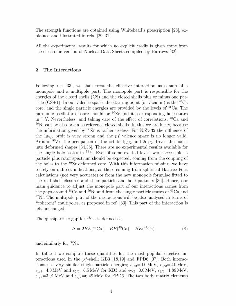
The quasiparticle gap for 48Ca is defined as
∆ = 2BE(48Ca)−BE(49Ca)− BE(47Ca) (8)
and similarly for 56Ni.
In table 1 we compare these quantities for the most popular effective in-teractions used in the pf -shell; KB3 [18,19] and FPD6 [37]. Both interac-tions use very similar single particle energies; ǫ7/2=0.0MeV, ǫ3/2=2.0MeV,ǫ1/2=4.0MeV and ǫ5/2=6.5MeV for KB3 and ǫ7/2=0.0MeV, ǫ3/2=1.89MeV,ǫ1/2=3.91MeV and ǫ5/2=6.49MeV for FPD6. The two body matrix elements
4
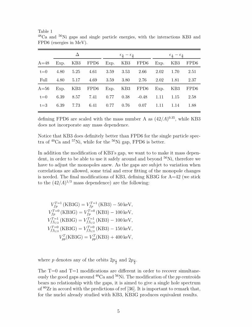
Table 148Ca and 56Ni gaps and single particle energies, with the interactions KB3 andFPD6 (energies in MeV).
∆ ǫ 5
2
− ǫ 3
2
ǫ 1
2
− ǫ 3
2
A=48 Exp. KB3 FPD6 Exp. KB3 FPD6 Exp. KB3 FPD6
t=0 4.80 5.25 4.61 3.59 3.53 2.66 2.02 1.70 2.51
Full 4.80 5.17 4.69 3.59 3.80 2.76 2.02 1.81 2.37
A=56 Exp. KB3 FPD6 Exp. KB3 FPD6 Exp. KB3 FPD6
t=0 6.39 8.57 7.41 0.77 0.38 -0.48 1.11 1.15 2.58
t=3 6.39 7.73 6.41 0.77 0.76 0.07 1.11 1.14 1.88
defining FPD6 are scaled with the mass number A as (42/A)0.35, while KB3does not incorporate any mass dependence.
Notice that KB3 does definitely better than FPD6 for the single particle spec-tra of 49Ca and 57Ni, while for the 56Ni gap, FPD6 is better.
In addition the modification of KB3’s gap, we want to to make it mass depen-dent, in order to be able to use it safely around and beyond 56Ni, therefore wehave to adjust the monopoles anew. As the gaps are subjet to variation whencorrelations are allowed, some trial and error fitting of the monopole changesis needed. The final modifications of KB3, defining KB3G for A=42 (we stickto the (42/A)1/3 mass dependence) are the following:
V T=1fp (KB3G) = V T=1
fp (KB3)− 50 keV,
V T=0fp (KB3G) = V T=0
fp (KB3)− 100 keV,
V T=1ff5/2
(KB3G) = V T=1ff5/2
(KB3)− 100 keV,
V T=0ff5/2
(KB3G) = V T=0ff5/2
(KB3)− 150 keV,
V Tpp(KB3G) = V T
pp(KB3) + 400 keV,
where p denotes any of the orbits 2p 1
2
and 2p 3
2
.
The T=0 and T=1 modifications are different in order to recover simultane-ously the good gaps around 48Ca and 56Ni. The modification of the pp centroidsbears no relationship with the gaps, it is aimed to give a single hole spectrumof 80Zr in accord with the predictions of ref [36]. It is important to remark that,for the nuclei already studied with KB3, KB3G produces equivalent results.
5
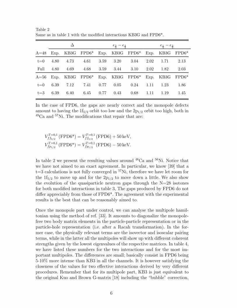
Table 2Same as in table 1 with the modified interactions KB3G and FPD6*.
∆ ǫ 5
2
− ǫ 3
2
ǫ 1
2
− ǫ 3
2
A=48 Exp. KB3G FPD6* Exp. KB3G FPD6* Exp. KB3G FPD6*
t=0 4.80 4.73 4.61 3.59 3.20 3.04 2.02 1.71 2.13
Full 4.80 4.69 4.68 3.59 3.44 3.10 2.02 1.82 2.03
A=56 Exp. KB3G FPD6* Exp. KB3G FPD6* Exp. KB3G FPD6*
t=0 6.39 7.12 7.41 0.77 0.05 0.24 1.11 1.23 1.86
t=3 6.39 6.40 6.45 0.77 0.43 0.68 1.11 1.19 1.45
In the case of FPD6, the gaps are nearly correct and the monopole defectsamount to having the 1f5/2 orbit too low and the 2p1/2 orbit too high, both in49Ca and 57Ni. The modifications that repair that are:
V T=0,1ff5/2
(FPD6*) = V T=0,1ff5/2
(FPD6) + 50 keV,
V T=0,1fp1/2
(FPD6*) = V T=0,1fp1/2
(FPD6)− 50 keV.
In table 2 we present the resulting values around 48Ca and 56Ni. Notice thatwe have not aimed to an exact agreement. In particular, we know [39] that at=3 calculations is not fully converged in 57Ni, therefore we have let room forthe 1f5/2 to move up and for the 2p1/2 to move down a little. We also showthe evolution of the quasiparticle neutron gaps through the N=28 isotonesfor both modified interactions in table 3, The gaps produced by FPD6 do notdiffer appreciably from those of FPD6*. The agreement with the experimentalresults is the best that can be reasonably aimed to.
Once the monopole part under control, we can analyse the multipole hamil-tonian using the method of ref. [33]. It amounts to diagonalize the monopole-free two body matrix elements in the particle-particle representation or in theparticle-hole representation (i.e. after a Racah transformation). In the for-mer case, the physically relevant terms are the isovector and isoscalar pairingterms, while in the latter all the multipoles will show up with different coherentstrengths given by the lowest eigenvalues of the respective matrices. In table 4,we have listed these numbers for the two interactions and for the most im-portant multipoles. The differences are small; basically consist in FPD6 being5-10% more intense than KB3 in all the channels. It is however satisfying thecloseness of the values for two effective interactions derived by very differentprocedures. Remember that for its multipole part, KB3 is just equivalent tothe original Kuo and Brown G-matrix [18] including the “bubble” correction,
6
Table 3Theoretical quasiparticle neutron gaps of the N=28 isotones (in MeV) comparedwith experiment. For Z>23 we list t=3 results, for the rest, full pf -shell results(energies in MeV).
∆ δ = ∆(exp)−∆(th)
Nucleus FPD6* EXP. KB3G FPD6* KB3G
48Ca 4.68 4.81 4.70 0.13 0.11
49Sc 4.05 4.07 3.99 0.02 0.08
50Ti 4.66 4.57 4.41 -0.09 0.16
51V 3.61 3.74 3.53 0.13 0.21
52Cr 4.03 4.10 3.76 0.07 0.34
53Mn 3.20 3.12 3.00 -0.08 0.12
54Fe 4.30 4.08 4.02 -0.22 0.06
55Co 4.00 4.01 4.16 0.01 -0.15
56Ni 6.45 6.39 6.41 -0.06 -0.02
Table 4Strengths (in MeV) of the coherent terms of the multipole Hamiltonian.
Interaction particle-particle particle-hole
JT=01 JT=10 λτ=20 λτ=40 λτ=11
KB3 -4.75 -4.46 -2.79 -1.39 +2.46
FPD6 -5.06 -5.08 -3.11 -1.67 +3.17
GOGNY -4.07 -5.74 -3.23 -1.77 +2.46
while FPD6 was obtained via a potential fit to selected energy levels in thepf -shell. This supports of the conclusions in [33] about the universality of themultipole shell model Hamiltonian.
We have purposely left to the end the line labeled GOGNY. It comes from thesame analysis applied to the pf -shell two body matrix elements obtained usingthe density dependent interaction of Gogny [40]. The calculation was carriedout using the single particle wave function obtained in a spherical Hartree-Fock calculation for 48Cr in the uniform filling approximation in ref. [41].In spite of the rather hybrid approach, the most important terms are againvery similar to those arising from a G-matrix or from a shell model fit. Inparticular the agreement for the quadrupole and the spin-isospin terms isexcellent. When it comes to pairing, this way of looking to the interaction
7
can help to overcome some language barriers between mean field and shellmodel practitioners. As it is evident from the table, the Gogny interaction hasessentially the same amount of isovector and isoscalar pairing than the realisticinteractions. Therefore, it contains the right proton-neutron pairing. Thus, ifthere is something to blame in the mean field calculations for N=Z nuclei, itshould be rather the mean field approximations and not the interaction itself.
In what follows we shall use mainly the interaction KB3G. We will comparein some cases with KB3 in order to evaluate the importance of the changesmade in the monopole behaviour. The comparison with FPD6 will show towhat extent the residual differences between good behaved interactions canhave spectroscopic consequences. We have not attempted to compute all thestates not even to draw those we have computed. Those not shown here canbe obtained on request to the authors.
3 The isobars A=50
We have carried out the full pf -shell calculations for all the isobars. Theresults for 50Cr and 50Mn have been already published in refs. [16,4,17]. Theexperimental data for which no specific credit is given are taken from ref. [32].
3.1 Spectroscopy of 50Ca
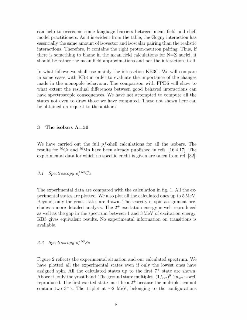
The experimental data are compared with the calculation in fig. 1. All the ex-perimental states are plotted. We also plot all the calculated ones up to 5MeV.Beyond, only the yrast states are drawn. The scarcity of spin assignment pre-cludes a more detailed analysis. The 2+ excitation energy is well reproducedas well as the gap in the spectrum between 1 and 3MeV of excitation energy.KB3 gives equivalent results. No experimental information on transitions isavailable.
3.2 Spectroscopy of 50Sc
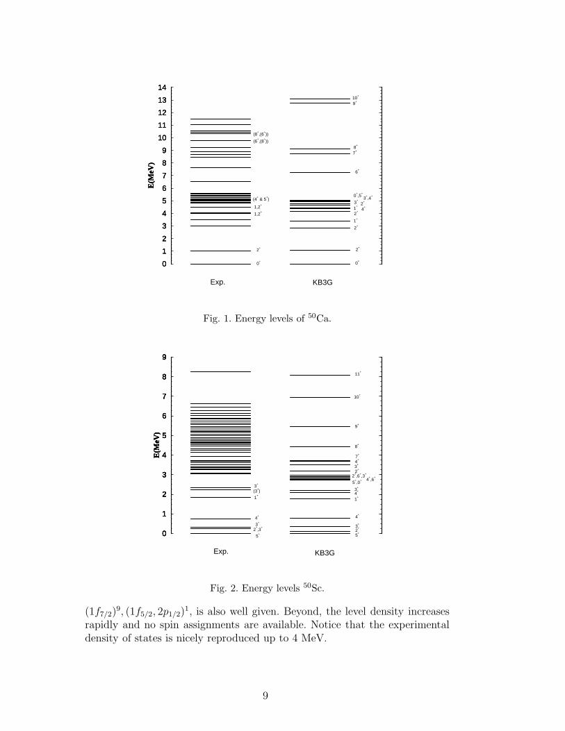
Figure 2 reflects the experimental situation and our calculated spectrum. Wehave plotted all the experimental states even if only the lowest ones haveassigned spin. All the calculated states up to the first 7+ state are shown.Above it, only the yrast band. The ground state multiplet, (1f7/2)
9, 2p3/2 is wellreproduced. The first excited state must be a 2+ because the multiplet cannotcontain two 3+’s. The triplet at ∼2 MeV, belonging to the configurations
8
0
1
2
3
4
5
6
7
8
9
10
11
12
13
14
E(M
eV)
0
1
2
3
4
5
6
7
8
9
10
11
12
13
14
E(M
eV)
0
1
2
3
4
5
6
7
8
9
10
11
12
13
14
E(M
eV)
Exp. KB3G
0+
2+
1,2+
1,2+
(4+ & 5
+)
(6+,(8
+))
(8+,(6
+))
0+
2+
2+
1+
2+
3+
4+1
+
0+,5
+
2+3
+,4
+
6+
7+
8+
9+
10+
Fig. 1. Energy levels of 50Ca.
0
1
2
3
4
5
6
7
8
9
E(M
eV)
0
1
2
3
4
5
6
7
8
9
E(M
eV)
0
1
2
3
4
5
6
7
8
9
E(M
eV)
0
1
2
3
4
5
6
7
8
9
E(M
eV)
Exp. KB3G
5+
2+,3
+3
+
4+
1+
(3+)
3+ 5
+,0
+
5+
2+3+
4+
1+
4+3+
4+
4+,6
+2+,6
+,3
+
3+
2+
8+
9+
10+
11+
7+
Fig. 2. Energy levels 50Sc.
(1f7/2)9, (1f5/2, 2p1/2)
1, is also well given. Beyond, the level density increasesrapidly and no spin assignments are available. Notice that the experimentaldensity of states is nicely reproduced up to 4 MeV.
9
0
1
2
3
4
5
6
7
8
9
10
E(M
eV)
0
1
2
3
4
5
6
7
8
9
10
E(M
eV)
0
1
2
3
4
5
6
7
8
9
10
Exp. KB3G
0+
2+
4+
6+
2+,3
+(0
+)
4+2+
(2+)
2+5+4+
(4+)
(0+)
7+
8+
9+
10+
(11)+
0+
2+
4+
6+
4+
4+
3+
2+
2+
5+
0+
4+
4+
7+
8+
9+
10+
11+
0+
0+
2+
4+
6+
4+ 2
+3+ 0
+2+5
+
4+4
+ 0+4
+
7+
8+9
+
10+
11+
FPD6
Fig. 3. Energy levels of 50Ti.
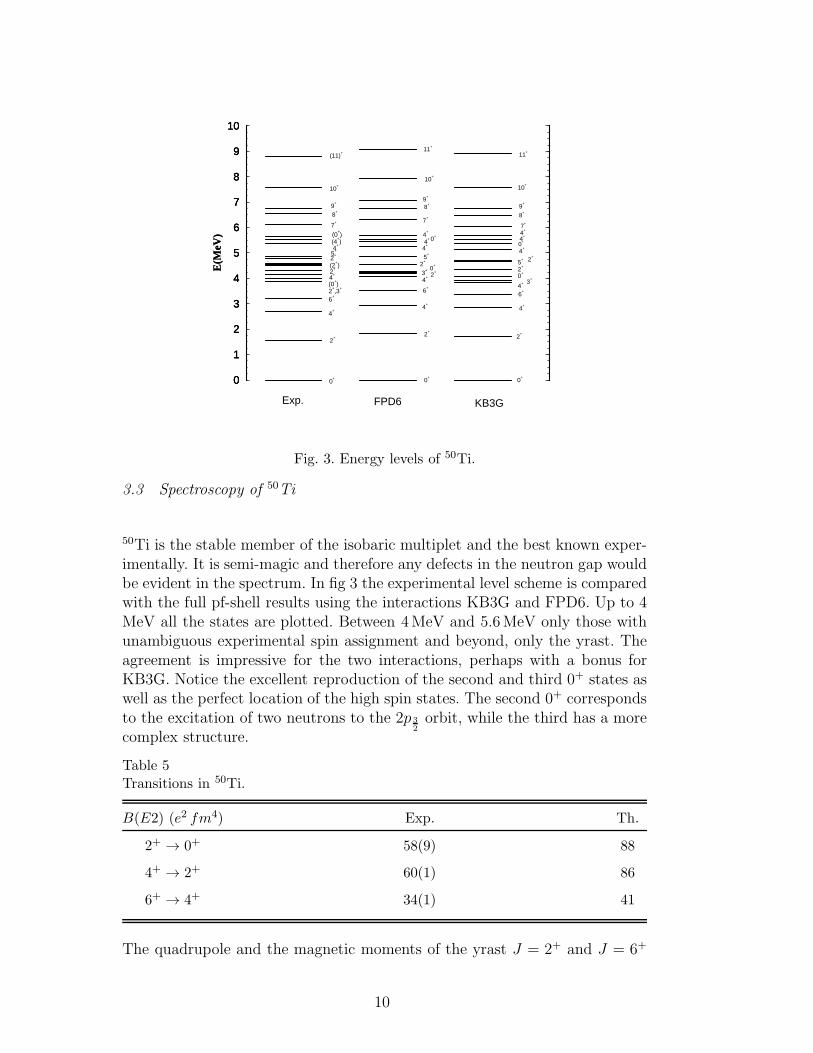
3.3 Spectroscopy of 50Ti
50Ti is the stable member of the isobaric multiplet and the best known exper-imentally. It is semi-magic and therefore any defects in the neutron gap wouldbe evident in the spectrum. In fig 3 the experimental level scheme is comparedwith the full pf-shell results using the interactions KB3G and FPD6. Up to 4MeV all the states are plotted. Between 4MeV and 5.6MeV only those withunambiguous experimental spin assignment and beyond, only the yrast. Theagreement is impressive for the two interactions, perhaps with a bonus forKB3G. Notice the excellent reproduction of the second and third 0+ states aswell as the perfect location of the high spin states. The second 0+ correspondsto the excitation of two neutrons to the 2p 3
2
orbit, while the third has a morecomplex structure.
Table 5Transitions in 50Ti.
B(E2) (e2 fm4) Exp. Th.
2+ → 0+ 58(9) 88
4+ → 2+ 60(1) 86
6+ → 4+ 34(1) 41
The quadrupole and the magnetic moments of the yrast J = 2+ and J = 6+
10
states are known [42]. Their values, µexp(2+) = 2.89(15)µN [43], Qexp(2
+) =+8(16) e fm2 and µexp(6
+) = +9.3(10)µN agree quite well with our predic-tions; µ(2+) = +2.5µN , Q(2+) = +6 e fm2 and µ(6+) = +8.3µN . A moredetailed discussion on the magnetic moments is given in section 8. Similarlythe E2 transitions of the yrast J = 2+, 4+ y 6+ states are well reproduced bythe calculation (see table 5).
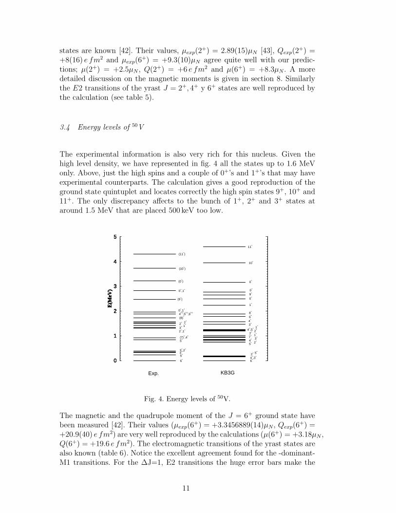
3.4 Energy levels of 50V
The experimental information is also very rich for this nucleus. Given thehigh level density, we have represented in fig. 4 all the states up to 1.6 MeVonly. Above, just the high spins and a couple of 0+’s and 1+’s that may haveexperimental counterparts. The calculation gives a good reproduction of theground state quintuplet and locates correctly the high spin states 9+, 10+ and11+. The only discrepancy affects to the bunch of 1+, 2+ and 3+ states ataround 1.5 MeV that are placed 500 keV too low.
0
1
2
3
4
5
E(M
eV)
0
1
2
3
4
5
E(M
eV)
0
1
2
3
4
5
E(M
eV)
0
1
2
3
4
5
E(M
eV)
Exp. KB3G
6+
5+4
+3+,2
+
0+,1
+
5+
(7)+,4
+
2+,1
+3
+ 1+2
+ 2+
(8)+
4(+)
,5(+)
,6(+)
(9+)
6+
0+,1
+
4+,3
+2
+ 5+
2+
3+
1+
5+
2+
4+
7+
2+
1+
6+
8+
(0+)
(10+)
(11+)
1+
0+
4+
9+
0+
0+
10+
11+
3+
4+,5
+
Fig. 4. Energy levels of 50V.
The magnetic and the quadrupole moment of the J = 6+ ground state havebeen measured [42]. Their values (µexp(6
+) = +3.3456889(14)µN , Qexp(6+) =
+20.9(40) e fm2) are very well reproduced by the calculations (µ(6+) = +3.18µN ,Q(6+) = +19.6 e fm2). The electromagnetic transitions of the yrast states arealso known (table 6). Notice the excellent agreement found for the -dominant-M1 transitions. For the ∆J=1, E2 transitions the huge error bars make the
11
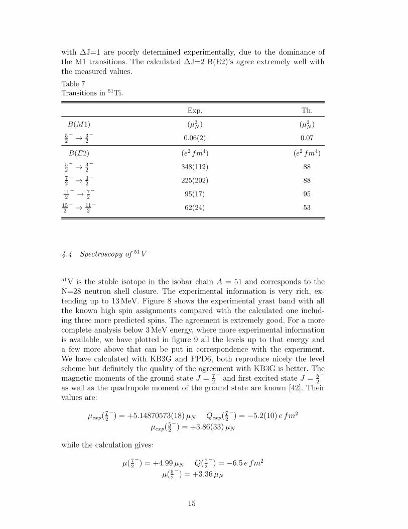
comparison meaningless. On the contrary, for the only ∆J=2 transition mea-sured, the agreement is very good.
Table 6Transitions in 50V.
Exp. Th.
B(M1) (µ2N ) (µ2
N )
7+ → 6+ 1.2(2) 1.0
8+ → 7+ 0.3(1) 0.2
11+ → 10+ 0.9(3) 1.1
B(E2) (e2 fm4) (e2 fm4)
7+ → 6+ 875+1313−875 108
8+ → 6+ 98(44) 74
8+ → 7+ 219+438−219 10
11+ → 10+ 109+328−109 29
4 The isobars A=51
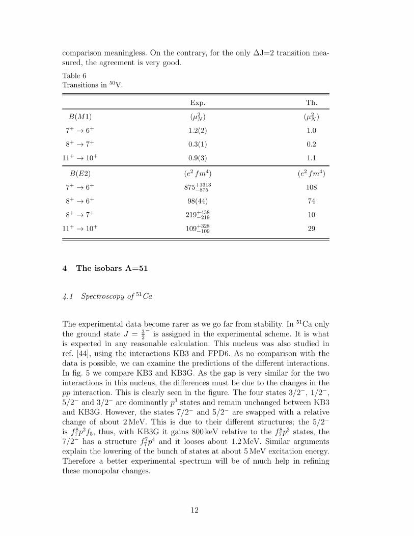
4.1 Spectroscopy of 51Ca
The experimental data become rarer as we go far from stability. In 51Ca onlythe ground state J = 3
2
−is assigned in the experimental scheme. It is what
is expected in any reasonable calculation. This nucleus was also studied inref. [44], using the interactions KB3 and FPD6. As no comparison with thedata is possible, we can examine the predictions of the different interactions.In fig. 5 we compare KB3 and KB3G. As the gap is very similar for the twointeractions in this nucleus, the differences must be due to the changes in thepp interaction. This is clearly seen in the figure. The four states 3/2−, 1/2−,5/2− and 3/2− are dominantly p3 states and remain unchanged between KB3and KB3G. However, the states 7/2− and 5/2− are swapped with a relativechange of about 2MeV. This is due to their different structures; the 5/2−
is f 87 p
2f5, thus, with KB3G it gains 800 keV relative to the f 87 p
3 states, the7/2− has a structure f 7
7 p4 and it looses about 1.2MeV. Similar arguments
explain the lowering of the bunch of states at about 5MeV excitation energy.Therefore a better experimental spectrum will be of much help in refiningthese monopolar changes.
12
0
1
2
3
4
5
6
7
8
E(M
eV)
0
1
2
3
4
5
6
7
8
E(M
eV)
0
1
2
3
4
5
6
7
8
E(M
eV)
Exp. KB3 KB3G
(3/2−)
(1/2,3/2,5/2)
(1/2,3/2,5/2)
3/2−
1/2−
5/2−
7/2−
3/2−
5/2−
3/2−
9/2−
1/2−
7/2− 11/2
−9/2−
1/2−
11/2−
3/2−
1/2−
5/2−
3/2−
5/2−
7/2−
9/2−
1/2−
3/2−
5/2−
11/2−
1/2−
11/2−
9/2−
7/2−
5/2−
Fig. 5. Energy levels of 51Ca.
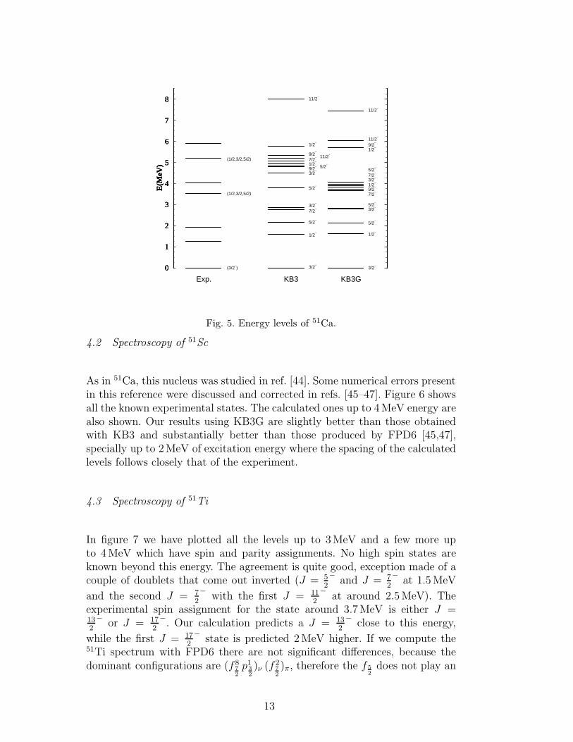
4.2 Spectroscopy of 51Sc
As in 51Ca, this nucleus was studied in ref. [44]. Some numerical errors presentin this reference were discussed and corrected in refs. [45–47]. Figure 6 showsall the known experimental states. The calculated ones up to 4MeV energy arealso shown. Our results using KB3G are slightly better than those obtainedwith KB3 and substantially better than those produced by FPD6 [45,47],specially up to 2MeV of excitation energy where the spacing of the calculatedlevels follows closely that of the experiment.
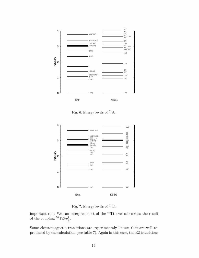
4.3 Spectroscopy of 51Ti
In figure 7 we have plotted all the levels up to 3MeV and a few more upto 4MeV which have spin and parity assignments. No high spin states areknown beyond this energy. The agreement is quite good, exception made of acouple of doublets that come out inverted (J = 5
2
−and J = 7
2
−at 1.5MeV
and the second J = 72
−with the first J = 11
2
−at around 2.5MeV). The
experimental spin assignment for the state around 3.7MeV is either J =132
−or J = 17
2
−. Our calculation predicts a J = 13
2
−close to this energy,
while the first J = 172
−state is predicted 2MeV higher. If we compute the
51Ti spectrum with FPD6 there are not significant differences, because thedominant configurations are (f 8
7
2
p132
)ν (f27
2
)π, therefore the f 5
2
does not play an
13
0
1
2
3
4
E(M
eV)
0
1
2
3
4
E(M
eV)
Exp. KB3G
(7/2)−
(3/2)−
(11/2)−
(3/2,5/2,7/2+)
(3/2,5/2)
(1/2−)
(3/2−)
(3/2−,5/2
−)
(3/2−,5/2
−)
(1/2,3/2,5/2)
(3/2−,5/2
−)
7/2−
3/2−
11/2−
9/2−
5/2−
7/2−
1/2−
11/2−,3/2
−
9/2−
5/2−
7/2−
5/2−
3/2−
5/2−
3/2−
5/2−
7/2−
1/2−
9/2−
Fig. 6. Energy levels of 51Sc.
0
1
2
3
4
E(M
eV)
0
1
2
3
4
E(M
eV)
Exp. KB3G
3/2−
1/2−
7/2−
(5/2)−
5/2−
3/2−
(11/2−)
3/2−
1/2−
5/2−
7/2−
3/2−
5/2−
7/2−
(7/2,9/2)−
(15/2−)
1/2−(5/2,7/2)
−
7/2−
11/2−
9/2−
5/2−15/2
−(7/2,9/2)−3/2
−(5/2,7/2,9/2)
(13/2,17/2)
1/2−
9/2−
7/2−
3/2−
13/2−
Fig. 7. Energy levels of 51Ti.
important role. We can interpret most of the 51Ti level scheme as the resultof the coupling 50Ti⊗p13
2
.
Some electromagnetic transitions are experimentaly known that are well re-produced by the calculation (see table 7). Again in this case, the E2 transitions
14
with ∆J=1 are poorly determined experimentally, due to the dominance ofthe M1 transitions. The calculated ∆J=2 B(E2)’s agree extremely well withthe measured values.
Table 7Transitions in 51Ti.
Exp. Th.
B(M1) (µ2N ) (µ2
N )
52
− → 32
−0.06(2) 0.07
B(E2) (e2 fm4) (e2 fm4)
52
− → 32
−348(112) 88
72
− → 32
−225(202) 88
112
− → 72
−95(17) 95
152
− → 112
−62(24) 53
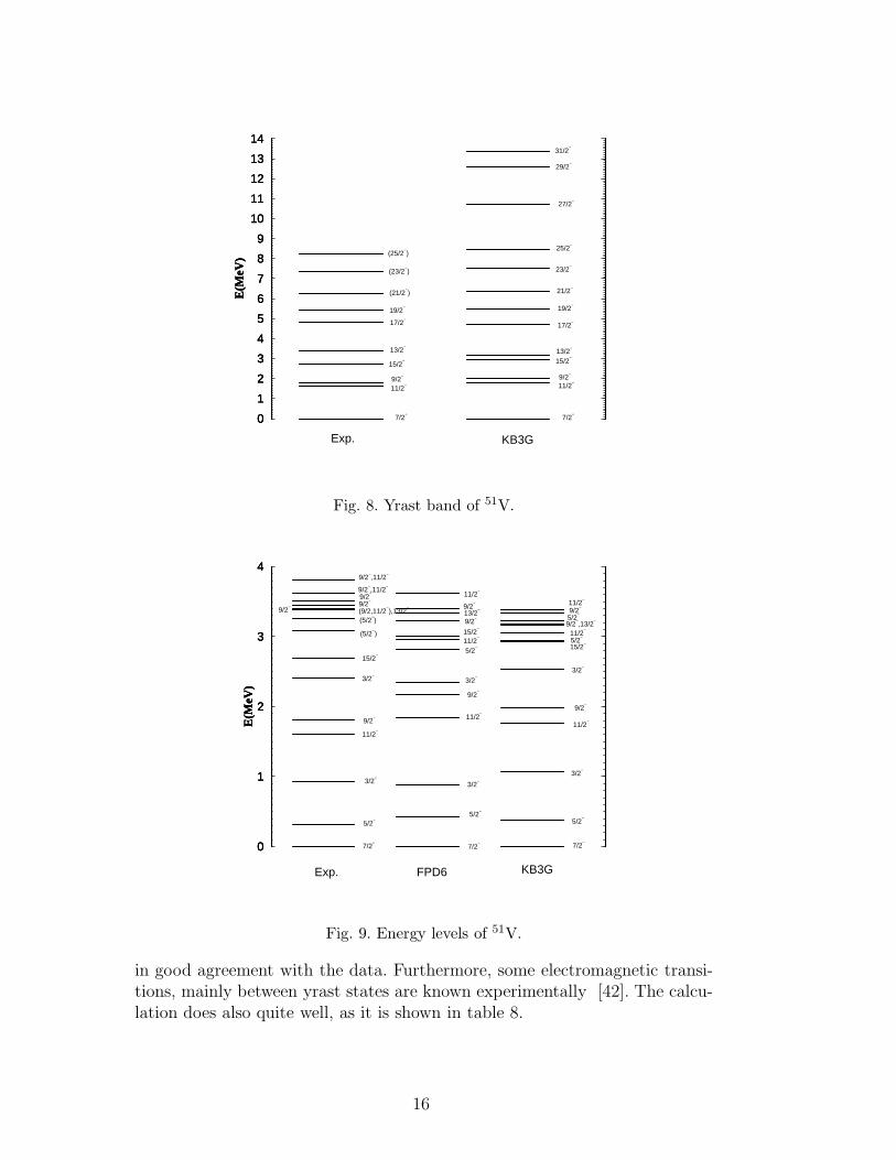
4.4 Spectroscopy of 51V
51V is the stable isotope in the isobar chain A = 51 and corresponds to theN=28 neutron shell closure. The experimental information is very rich, ex-tending up to 13MeV. Figure 8 shows the experimental yrast band with allthe known high spin assignments compared with the calculated one includ-ing three more predicted spins. The agreement is extremely good. For a morecomplete analysis below 3MeV energy, where more experimental informationis available, we have plotted in figure 9 all the levels up to that energy anda few more above that can be put in correspondence with the experiment.We have calculated with KB3G and FPD6, both reproduce nicely the levelscheme but definitely the quality of the agreement with KB3G is better. Themagnetic moments of the ground state J = 7
2
−and first excited state J = 5
2
−
as well as the quadrupole moment of the ground state are known [42]. Theirvalues are:
µexp(72
−) = +5.14870573(18)µN Qexp(
72
−) = −5.2(10) e fm2
µexp(52
−) = +3.86(33)µN
while the calculation gives:
µ(72
−) = +4.99µN Q(7
2
−) = −6.5 e fm2
µ(52
−) = +3.36µN
15
0
1
2
3
4
5
6
7
8
9
10
11
12
13
14
E(M
eV)
0
1
2
3
4
5
6
7
8
9
10
11
12
13
14
E(M
eV)
0
1
2
3
4
5
6
7
8
9
10
11
12
13
14
E(M
eV)
Exp. KB3G
7/2−
17/2−
19/2−
9/2−
(21/2−)
11/2−
13/2−
15/2−
(25/2−)
15/2−
29/2−
31/2−
13/2−
21/2−
23/2−
(23/2−)
25/2−
27/2−
7/2−
9/2−
11/2−
17/2−
19/2−
Fig. 8. Yrast band of 51V.
0
1
2
3
4
E(M
eV)
0
1
2
3
4
E(M
eV)
0
1
2
3
4
E(M
eV)
Exp. FPD6
7/2−
5/2−
3/2−
11/2−
9/2−
3/2−
15/2−
7/2−
5/2−
3/2−
11/2−
9/2−
3/2−
(5/2−)
5/2−
(5/2−)
9/2−
(9/2,11/2−),13/2
−
15/2−
7/2−
5/2−
3/2−
11/2−
9/2−
3/2−
KB3G
9/2−
9/2−
9/2−,11/2
−
9/2−,11/2
−
15/2−
5/2−
11/2−
9/2−
13/2−9/2
−
11/2−
11/2−
9/2−,13/2
−5/2−
9/2−
11/2−
Fig. 9. Energy levels of 51V.
in good agreement with the data. Furthermore, some electromagnetic transi-tions, mainly between yrast states are known experimentally [42]. The calcu-lation does also quite well, as it is shown in table 8.
16

Table 8Transitions in 51V.
Exp. Th.
B(M1) (µ2N ) (µ2
N )
92
− → 72
−0.0006(2) 0.2·10−6
132
− → 112
−<0.0077 0.014
B(E2) (e2 fm4) (e2 fm4)
92
− → 72
−35(6) 32
112
− → 72
−95(8) 103
132
− → 112
−<34.8 0.01
152
− → 112
−66(6) 78
4.5 Spectroscopy of 51Cr
We present in fig. 10 the results for the yrast band of 51Cr in a t = 5 trunca-tion and in the full space using KB3G. We have also included the low-lyingJ = 1
2
−, 32
−and 5
2
−states, and a second state of each spin from J = 19
2
−
on. The figure shows that the full calculation do not modify substantially theresults obtained at t = 5. The agreement with the experimental data is very
0
1
2
3
4
5
6
7
8
9
10
E(M
eV)
0
1
2
3
4
5
6
7
8
9
10
E(M
eV)
0
1
2
3
4
5
6
7
8
9
10
E(M
eV)
Exp. KB3G
7/2−
3/2−
1/2−
9/2− 5/2
−11/2−
13/2−
15/2−
(21/2−)
15/2−
(23/2−)
(21/2, 23/2−)
13/2−
(23/2, 25/2−)
(25/2, 27/2−)
19/2−
21/2−
23/2−
(17/2)−
21/2−
(19/2−)
23/2−
25/2−
25/2−
27/2−
27/2−
19/2−
7/2−
3/2−
1/2−
5/2−
21/2−
9/2−11/2
−
7/2−
3/2−
23/2−
21/2−
17/2−
23/2−
KB3G
25/2−
1/2−
25/2−
5/2−
9/2−
19/2−
27/2−
27/2−
11/2−
(t=5)
15/2−
13/2−
17/2−
19/2−
(full)
Fig. 10. Yrast band of 51Cr; experiment, t = 5 and full calculation.
17
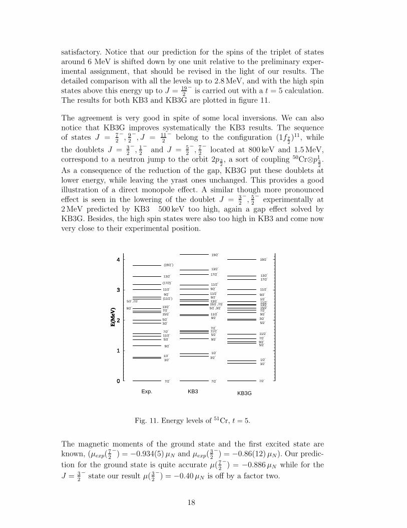
satisfactory. Notice that our prediction for the spins of the triplet of statesaround 6 MeV is shifted down by one unit relative to the preliminary exper-imental assignment, that should be revised in the light of our results. Thedetailed comparison with all the levels up to 2.8MeV, and with the high spinstates above this energy up to J = 19
2
−is carried out with a t = 5 calculation.
The results for both KB3 and KB3G are plotted in figure 11.
The agreement is very good in spite of some local inversions. We can alsonotice that KB3G improves systematically the KB3 results. The sequenceof states J = 7
2
−, 92
−, J = 11
2
−belong to the configuration (1f 7
2
)11, while
the doublets J = 32
−, 12
−and J = 5
2
−, 72
−located at 800 keV and 1.5MeV,
correspond to a neutron jump to the orbit 2p 3
2
, a sort of coupling 50Cr⊗p132
.
As a consequence of the reduction of the gap, KB3G put these doublets atlower energy, while leaving the yrast ones unchanged. This provides a goodillustration of a direct monopole effect. A similar though more pronouncedeffect is seen in the lowering of the doublet J = 3
2
−, 52
−experimentally at
2MeV predicted by KB3 500 keV too high, again a gap effect solved byKB3G. Besides, the high spin states were also too high in KB3 and come nowvery close to their experimental position.
0
1
2
3
4
E(M
eV)
0
1
2
3
4
E(M
eV)
0
1
2
3
4
E(M
eV)
Exp. KB3
7/2−
3/2−
1/2−
9/2−
5/2−
11/2−
7/2−
3/2−
5/2−
15/2−
7/2−9/2
− 13/2−
(11/2−)
9/2−
11/2−
9/2−
11/2−
(17/2)−
13/2−
(19/2−)
5/2−,3/2
−
9/2−
15/2−,7/2
−
11/2−
7/2−
3/2−
1/2−
5/2−
7/2−
9/2−
11/2−
7/2−
3/2−
9/2−
11/2−
17/2−
13/2−
KB3G
13/2−
1/2−
5/2−9/2−
19/2−
7/2−
7/2−
11/2−
5/2−
3/2−
9/2−
5/2−,7/2
−
15/2−13/2−11/2−
1/2−
9/2−
11/2−
17/2−
13/2−
19/2−
Fig. 11. Energy levels of 51Cr, t = 5.
The magnetic moments of the ground state and the first excited state areknown, (µexp(
72
−) = −0.934(5)µN and µexp(
32
−) = −0.86(12)µN). Our predic-
tion for the ground state is quite accurate µ(72
−) = −0.886µN while for the
J = 32
−state our result µ(3
2
−) = −0.40µN is off by a factor two.
18
In table 9 we compare the experimental and calculated transition probabilities.The B(M1)’s and the ∆J=2 B(E2)’s are well reproduced . However this is notthe case for the ∆J=1 B(E2)’s, in particular the discrepancies are huge for
the transitions 112
− → 92
−and 13
2
− → 112
−. We have carried out a consistency
test using the experimental M1/E2 branchings, δ, and we have found thatthe experimental δ values are inconsistent with the experimental B(E2)’s butconsistent with the calculated values. This is not surprising, because of thecomplete dominance of the M1 transition, that may cause large errors in theextraction of the B(E2) value. In order to discard any other origin of thediscrepancy we have repeated the calculation with FPD6 and the situation isthe same or even worse.Table 9Transitions in 51Cr.
Exp. Th.
B(M1) (µ2N ) (µ2
N )
92
− → 72
−0.31683(3043) 0.439
112
− → 92
−1.253(537) 1.295
132
− → 112
−0.8950(1969) 1.356
B(E2) (e2 fm4) (e2 fm4)
92
− → 72
−124(56) 213
112
− → 72
−67(34) 72
112
− → 92
−8(3) 180
132
− → 112
−6(1) 151
152
− → 112
−44(1) 53
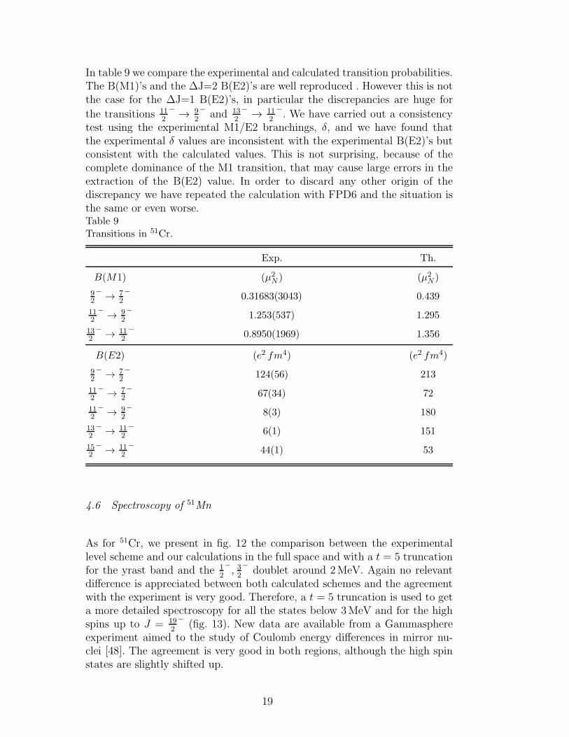
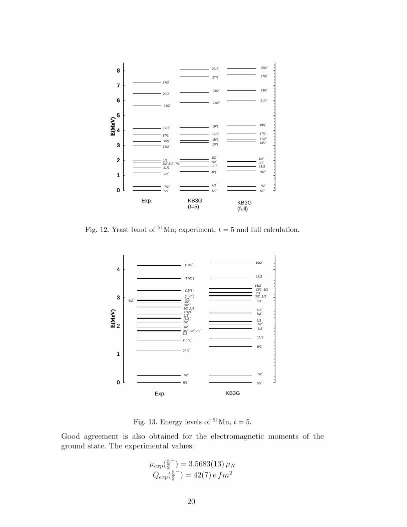
4.6 Spectroscopy of 51Mn
As for 51Cr, we present in fig. 12 the comparison between the experimentallevel scheme and our calculations in the full space and with a t = 5 truncationfor the yrast band and the 1
2
−, 32
−doublet around 2MeV. Again no relevant
difference is appreciated between both calculated schemes and the agreementwith the experiment is very good. Therefore, a t = 5 truncation is used to geta more detailed spectroscopy for all the states below 3MeV and for the highspins up to J = 19
2
−(fig. 13). New data are available from a Gammasphere
experiment aimed to the study of Coulomb energy differences in mirror nu-clei [48]. The agreement is very good in both regions, although the high spinstates are slightly shifted up.
19
0
1
2
3
4
5
6
7
8
E(M
eV)
0
1
2
3
4
5
6
7
8
E(M
eV)
0
1
2
3
4
5
6
7
8
E(M
eV)
Exp. KB3G
7/2−
17/2−
19/2−
9/2−
5/2−
11/2−
21/2−
23/2−
27/2−
15/2−
5/2−
7/2−
13/2−
9/2−
11/2−
13/2−
15/2−
17/2−
19/2−
21/2−
23/2−
27/2−
25/2−
5/2−
7/2−
9/2−
11/2−
13/2−
15/2−
17/2−
19/2−
21/2−
23/2−
27/2−
25/2−
3/2−,5/2
−,7/2
−1/2
−
3/2−
1/2−
3/2−
KB3G
1/2−
(t=5) (full)
Fig. 12. Yrast band of 51Mn; experiment, t = 5 and full calculation.
0
1
2
3
4
E(M
eV)
0
1
2
3
4
E(M
eV)
Exp. KB3G
5/2−
7/2−
(9/2)−
(11/2)−
3/23/2
−,5/2
−,7/2
−1/2
−
3/2−
(5/2−)
5/2(−)
(7/2)−
1/2−,3/2
−3/2
(−)1/2
−5/2(−) 3/2
−(13/2
−)
(15/2−)
(17/2−)
(19/2−)
5/2−
7/2−
9/2−
11/2−
3/2−
1/2−
3/2−
5/2−
7/2−
5/2−,1/2
−
13/2−,9/2
−15/2
−
17/2−
19/2−
3/2−
7/2−
Fig. 13. Energy levels of 51Mn, t = 5.
Good agreement is also obtained for the electromagnetic moments of theground state. The experimental values:
µexp(52
−) = 3.5683(13)µN
Qexp(52
−) = 42(7) e fm2
20
are very well reproduced by the KB3G calculation:
µ(52
−) = 3.40µN
Q(52
−) = 35 e fm2
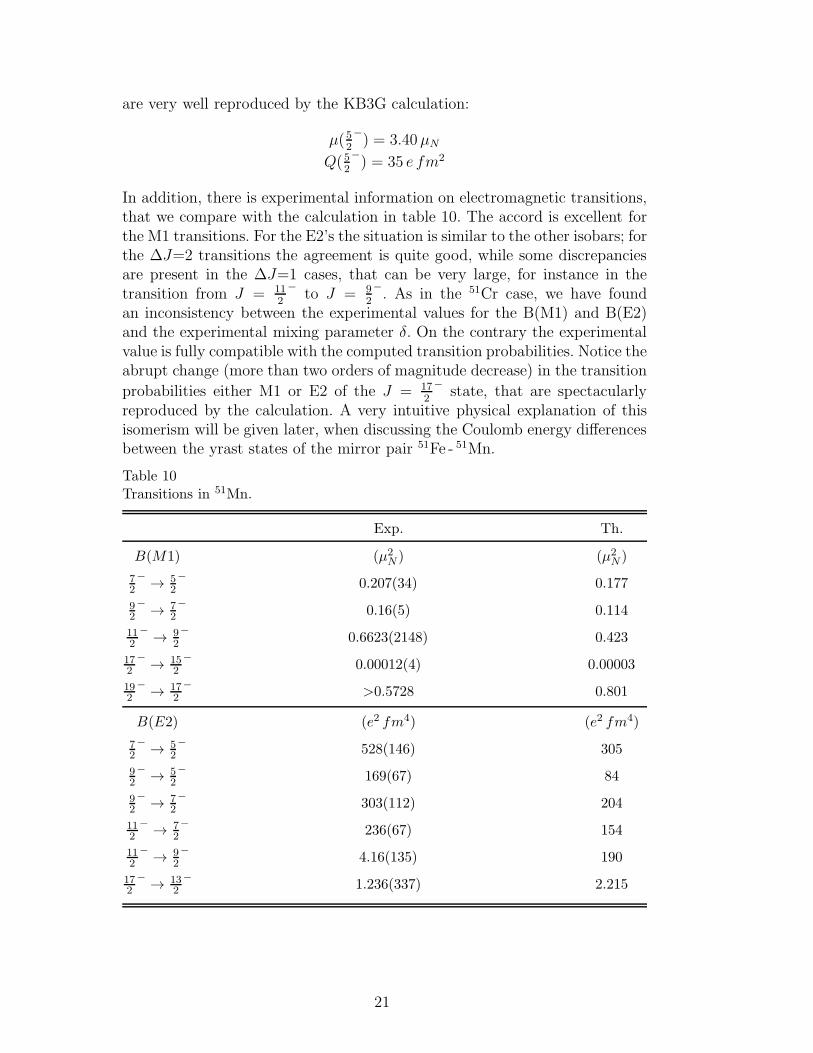
In addition, there is experimental information on electromagnetic transitions,that we compare with the calculation in table 10. The accord is excellent forthe M1 transitions. For the E2’s the situation is similar to the other isobars; forthe ∆J=2 transitions the agreement is quite good, while some discrepanciesare present in the ∆J=1 cases, that can be very large, for instance in thetransition from J = 11
2
−to J = 9
2
−. As in the 51Cr case, we have found
an inconsistency between the experimental values for the B(M1) and B(E2)and the experimental mixing parameter δ. On the contrary the experimentalvalue is fully compatible with the computed transition probabilities. Notice theabrupt change (more than two orders of magnitude decrease) in the transition
probabilities either M1 or E2 of the J = 172
−state, that are spectacularly
reproduced by the calculation. A very intuitive physical explanation of thisisomerism will be given later, when discussing the Coulomb energy differencesbetween the yrast states of the mirror pair 51Fe - 51Mn.
Table 10Transitions in 51Mn.
Exp. Th.
B(M1) (µ2N ) (µ2
N )
72
− → 52
−0.207(34) 0.177
92
− → 72
−0.16(5) 0.114
112
− → 92
−0.6623(2148) 0.423
172
− → 152
−0.00012(4) 0.00003
192
− → 172
−>0.5728 0.801
B(E2) (e2 fm4) (e2 fm4)
72
− → 52
−528(146) 305
92
− → 52
−169(67) 84
92
− → 72
−303(112) 204
112
− → 72
−236(67) 154
112
− → 92
−4.16(135) 190
172
− → 132
−1.236(337) 2.215
21
5 The isobars A=52
As in the A = 51 isobaric multiplet we have performed full 0hω calculationsfor all the isotopes in 52Cr and 52Mn the full calculation is limited to the yrastlevels. More detailed spectroscopy is carried out with a t=5 truncation. Theresults of the full pf -shell calculation for 52Fe have been already publishedin [5]. The experimental values are taken from ref. [32].
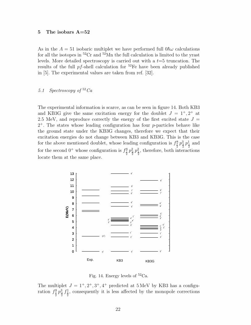
5.1 Spectroscopy of 52Ca
The experimental information is scarce, as can be seen in figure 14. Both KB3and KB3G give the same excitation energy for the doublet J = 1+, 2+ at2.5 MeV, and reproduce correctly the energy of the first excited state J =2+. The states whose leading configuration has four p-particles behave likethe ground state under the KB3G changes, therefore we expect that theirexcitation energies do not change between KB3 and KB3G. This is the casefor the above mentioned doublet, whose leading configuration is f 8
7
2
p332
p112
and
for the second 0+ whose configuration is f 87
2
p232
p212
, therefore, both interactions
locate them at the same place.
0
1
2
3
4
5
6
7
8
9
10
11
12
13
E(M
eV)
0
1
2
3
4
5
6
7
8
9
10
11
12
13
E(M
eV)
Exp. KB3 KB3G
0+
(2+)
0+
2+
0+
2+4
+4
+
6+
6+
8+
1+
0+
2+
4+ 2
+0
+
4+
6+
6+
8+
3+
3+
1+
5+
7+
9+
1+
3+
1+
3+
5+
7+
9+
Fig. 14. Energy levels of 52Ca.
The multiplet J = 1+, 2+, 3+, 4+ predicted at 5MeV by KB3 has a configu-ration f 8
7
2
p332
f 15
2
, consequently it is less affected by the monopole corrections
22
(∆Vpp) made in KB3G than the ground state, and moves down 1MeV in ex-citation energy. The states J = 5+, J = 6+2 , J = 7+, J = 8+ and J = 9+ arealso lowered by KB3G, due to the occupation of the 1f 1
5
2
orbit.
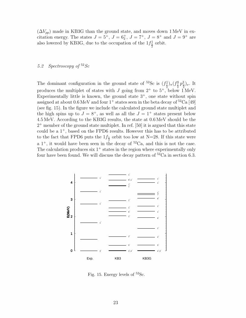
5.2 Spectroscopy of 52Sc
The dominant configuration in the ground state of 52Sc is (f 17
2
)π(f87
2
p332
)ν . It
produces the multiplet of states with J going from 2+ to 5+, below 1MeV.Experimentally little is known, the ground state 3+, one state without spinassigned at about 0.6MeV and four 1+ states seen in the beta decay of 52Ca [49](see fig. 15). In the figure we include the calculated ground state multiplet andthe high spins up to J = 8+, as well as all the J = 1+ states present below4.5MeV. According to the KB3G results, the state at 0.6MeV should be the2+ member of the ground state multiplet. In ref. [50] it is argued that this statecould be a 1+, based on the FPD6 results. However this has to be attributedto the fact that FPD6 puts the 1f 5
2
orbit too low at N=28. If this state were
a 1+, it would have been seen in the decay of 52Ca, and this is not the case.The calculation produces six 1+ states in the region where experimentally onlyfour have been found. We will discuss the decay pattern of 52Ca in section 6.3.
0
1
2
3
4
E(M
eV)
0
1
2
3
4
E(M
eV)
0
1
2
3
4
E(M
eV)
Exp. KB3 KB3G
3+
1+
1+
1+
1+
3+,4
+
5+
2+
1+
6+
1+
1+
1+
7+
8+,1
+
4+,3
+
5+
2+
1+
6+
1+
1+
8+
1+
7+
1+
1+
1+
Fig. 15. Energy levels of 52Sc.
23
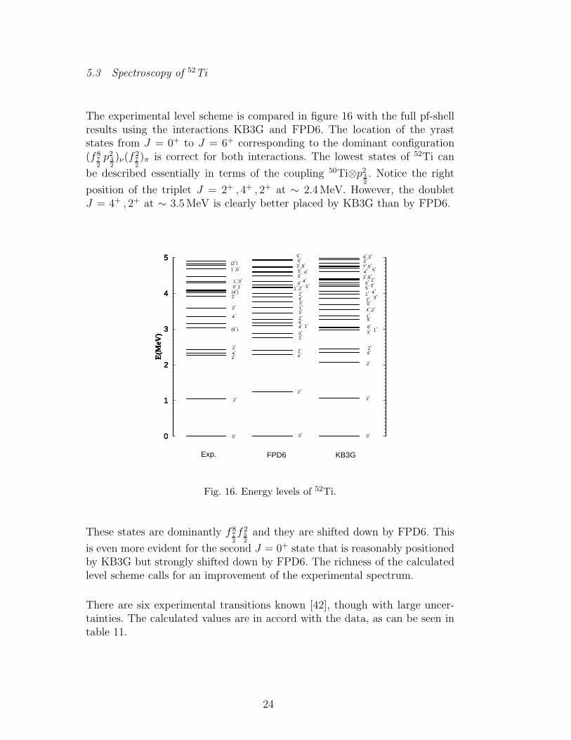
5.3 Spectroscopy of 52Ti
The experimental level scheme is compared in figure 16 with the full pf-shellresults using the interactions KB3G and FPD6. The location of the yraststates from J = 0+ to J = 6+ corresponding to the dominant configuration(f 8
7
2
p232
)ν(f27
2
)π is correct for both interactions. The lowest states of 52Ti can
be described essentially in terms of the coupling 50Ti⊗p232
. Notice the right
position of the triplet J = 2+ , 4+ , 2+ at ∼ 2.4MeV. However, the doubletJ = 4+ , 2+ at ∼ 3.5MeV is clearly better placed by KB3G than by FPD6.
0
1
2
3
4
5
E(M
eV)
0
1
2
3
4
5
E(M
eV)
0
1
2
3
4
5
E(M
eV)
Exp. FPD6 KB3G
0+
2+
2+4+
2+
(6+)
4+
2+
2+
(4+)
0+,1
−1
−,0
+
1−,0
+(2
+)
0+
2+
2+
4+
2+
6+
4+
2+
4+
0+
2+
0+
1+,2
+
0+
0+
2+
2+
4+
2+
6+
4+
4+,2
+
1+
0+
7+,0
+
2+
2+
0+
3+
1+
3+
4+
5+
3+ 4
+5+
3+,8
+
5+
3+ 1
+
1+
3+1
+ 4+5
+6
+3
+,8
+4
+ 5+
3+
6+,5
+
Fig. 16. Energy levels of 52Ti.
These states are dominantly f 87
2
f 25
2
and they are shifted down by FPD6. This
is even more evident for the second J = 0+ state that is reasonably positionedby KB3G but strongly shifted down by FPD6. The richness of the calculatedlevel scheme calls for an improvement of the experimental spectrum.
There are six experimental transitions known [42], though with large uncer-tainties. The calculated values are in accord with the data, as can be seen intable 11.
24
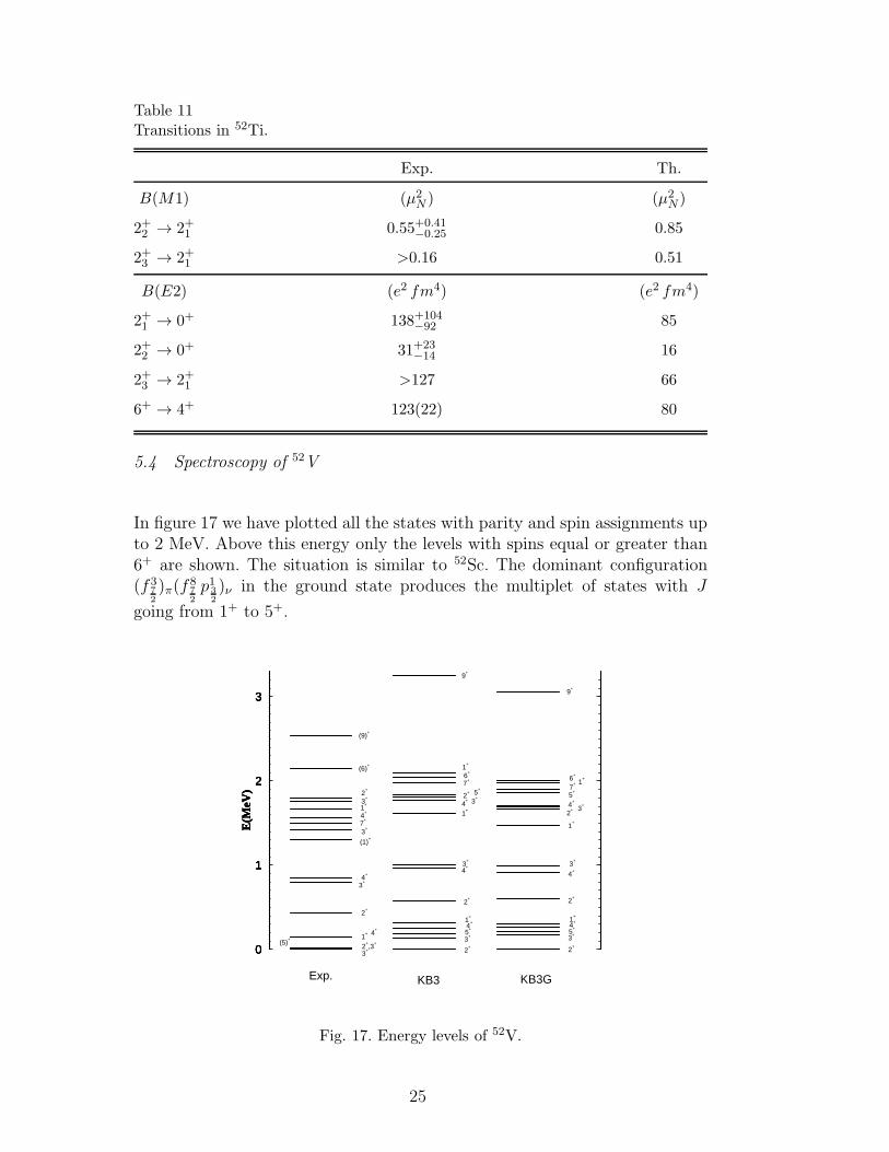
Table 11Transitions in 52Ti.
Exp. Th.
B(M1) (µ2N ) (µ2
N )
2+2 → 2+1 0.55+0.41−0.25 0.85
2+3 → 2+1 >0.16 0.51
B(E2) (e2 fm4) (e2 fm4)
2+1 → 0+ 138+104−92 85
2+2 → 0+ 31+23−14 16
2+3 → 2+1 >127 66
6+ → 4+ 123(22) 80
5.4 Spectroscopy of 52V
In figure 17 we have plotted all the states with parity and spin assignments upto 2 MeV. Above this energy only the levels with spins equal or greater than6+ are shown. The situation is similar to 52Sc. The dominant configuration(f 3
7
2
)π(f87
2
p132
)ν in the ground state produces the multiplet of states with J
going from 1+ to 5+.
0
1
2
3
E(M
eV)
0
1
2
3
E(M
eV)
0
1
2
3
E(M
eV)
0
1
2
3
E(M
eV)
Exp. KB3 KB3G
3+
2+,3
+(5)+ 1
+ 4+
2+
3+4
+
(1)+
3+
7+
4+
1+3+
2+
2+
3+
5+4+1
+
2+
4+3+
1+
4+ 3
+2+
7+
2+
3+5+4+1+
2+
4+
3+
1+
2+ 3
+4+
6+
7+
6+
1+
(6)+
(9)+
1+
9+
9+
5+
5+
Fig. 17. Energy levels of 52V.
25
The calculated ground state multiplet is more dilated that its experimentalcounterpart. Although the more relevant features are well accounted for wedo not predict the correct ground state spin. The J = 3+, 4+ doublet around850 keV comes out inverted. These states can be described as the result of thecoupling 51V⊗p13
2
. The high spin states J = 7+ and J = 9+ are shifted up,
making the agreement with experiment worse than in the other nuclei studiedin this work.
Only two electromagnetic transitions are experimentally known [42]: the E2connecting the states J = 9+ and J = 7+ (B(E2) = 81(6) e2 fm4) andthe M1 conecting the first excited J = 2+ state and the J = 3+ groundstate (B(M1) = 1.7(4)µ2
N). For the first one the calculation produces a valueB(E2) = 87 e2 fm4 and for the second B(M1, 2+ → 3+) = 1.7µ2
N , a ratherimpresive agreement.
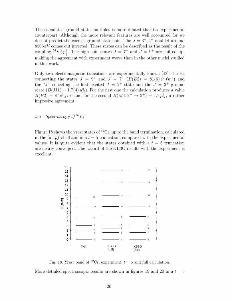
5.5 Spectroscopy of 52Cr
Figure 18 shows the yrast states of 52Cr, up to the band termination, calculatedin the full pf -shell and in a t = 5 truncation, compared with the experimentalvalues. It is quite evident that the states obtained with a t = 5 truncationare nearly converged. The accord of the KB3G results with the experiment isexcellent.
0
1
2
3
4
5
6
7
8
9
10
11
12
13
14
15
16
E(M
eV)
0
1
2
3
4
5
6
7
8
9
10
11
12
13
14
15
16
E(M
eV)
0
1
2
3
4
5
6
7
8
9
10
11
12
13
14
15
16
E(M
eV)
Exp. KB3G
0+
2+
4+
8+
10+
12+
6+
8+
10+
12+
8+
10+
12+
0+
2+
14+
4+
16+
14+
16+
6+
KB3G
0+
2+
4+
6+
(t=5) (full)
Fig. 18. Yrast band of 52Cr; experiment, t = 5 and full calculation.
More detailed spectroscopic results are shown in figures 19 and 20 in a t = 5
26
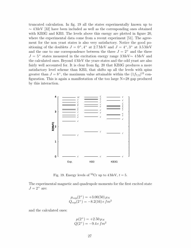
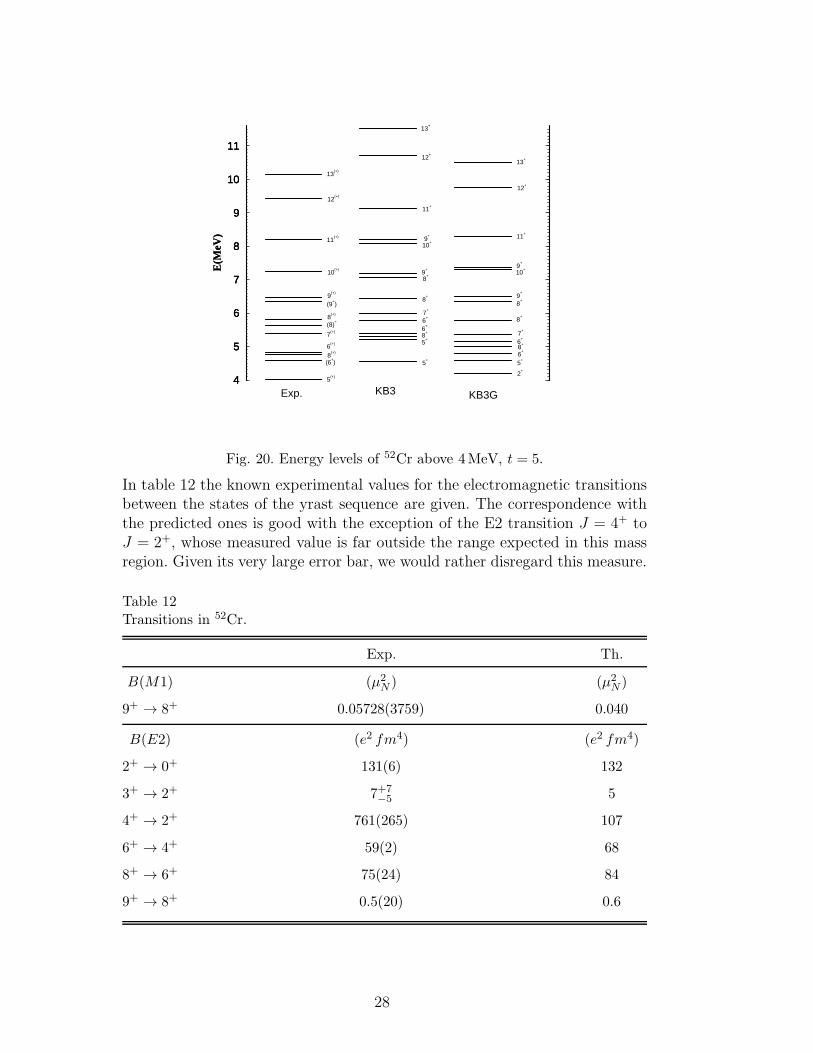
truncated calculation. In fig. 19 all the states experimentally known up to∼ 4MeV [32] have been included as well as the corresponding ones obtainedwith KB3G and KB3. The levels above this energy are plotted in figure 20,where the experimental data come from a recent experiment [51]. The agree-ment for the non yrast states is also very satisfactory. Notice the good po-sitioning of the doublets J = 0+, 4+ at 2.7MeV and J = 4+, 3+ at 3.5MeVand the one to one correspondence between the three J = 2+ and the threeJ = 5+ states measured in the excitation energy range 3MeV∼ 4MeV andthe calculated ones. Beyond 4MeV the yrare states and the odd yrast are alsofairly well accounted for. It is clear from fig. 20 that KB3G produces a moresatisfactory level scheme than KB3, that shifts up all the levels with spinsgreater than J = 8+, the maximum value attainable within the (1f7/2)
12 con-figuration. This is again a manifestation of the too large N=28 gap producedby this interaction.
0
1
2
3
4
E(M
eV)
0
1
2
3
4
E(M
eV)
0
1
2
3
4
E(M
eV)
Exp. KB3
0+
2+
4+
0+
4+
2+
6+
2+
4+3+
5+
2+
(5)+
0+
2+
0+
4+
2+
4+
3+
4+
6+
2+
5+
5+
KB3G
0+
2+
4+
4+
0+
2+
6+
4+3+
2+
5+
Fig. 19. Energy levels of 52Cr up to 4MeV, t = 5.
The experimental magnetic and quadrupole moments for the first excited stateJ = 2+ are:
µexp(2+) = +3.00(50)µN
Qexp(2+) = −8.2(16) e fm2
and the calculated ones:
µ(2+) = +2.50µN
Q(2+) = −9.4 e fm2
27
4
5
6
7
8
9
10
11
E(M
eV)
4
5
6
7
8
9
10
11
E(M
eV)
4
5
6
7
8
9
10
11
Exp. KB35
(+)
8+
(6+)
8(+)
(8)+
13(+)
(9+)
12+
13+
6(+)
9(+)
5+
6+
6+
7(+)
8(+)
10(+)
11(+)
12(+)
13+
8+
11+
8+
7+
9+
10+
9+
KB3G
5+
6+
2+
8+5
+ 6+
7+
8+
8+
9+
10+
9+
11+
12+
Fig. 20. Energy levels of 52Cr above 4MeV, t = 5.
In table 12 the known experimental values for the electromagnetic transitionsbetween the states of the yrast sequence are given. The correspondence withthe predicted ones is good with the exception of the E2 transition J = 4+ toJ = 2+, whose measured value is far outside the range expected in this massregion. Given its very large error bar, we would rather disregard this measure.
Table 12Transitions in 52Cr.
Exp. Th.
B(M1) (µ2N ) (µ2
N )
9+ → 8+ 0.05728(3759) 0.040
B(E2) (e2 fm4) (e2 fm4)
2+ → 0+ 131(6) 132
3+ → 2+ 7+7−5 5
4+ → 2+ 761(265) 107
6+ → 4+ 59(2) 68
8+ → 6+ 75(24) 84
9+ → 8+ 0.5(20) 0.6
28
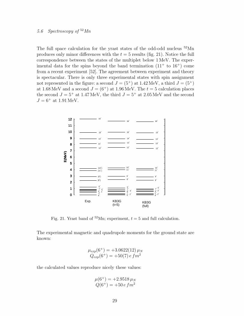
5.6 Spectroscopy of 52Mn
The full space calculation for the yrast states of the odd-odd nucleus 52Mnproduces only minor differences with the t = 5 results (fig. 21). Notice the fullcorrespondence between the states of the multiplet below 1MeV. The exper-imental data for the spins beyond the band termination (11+ to 16+) comefrom a recent experiment [52]. The agreement between experiment and theoryis spectacular. There is only three experimental states with spin assignmentnot represented in the figure: a second J = (5+) at 1.42MeV, a third J = (5+)at 1.68MeV and a second J = (6+) at 1.96MeV. The t = 5 calculation placesthe second J = 5+ at 1.47MeV, the third J = 5+ at 2.05MeV and the secondJ = 6+ at 1.91MeV.
0
1
2
3
4
5
6
7
8
9
10
11
12
E(M
eV)
0
1
2
3
4
5
6
7
8
9
10
11
12
E(M
eV)
0
1
2
3
4
5
6
7
8
9
10
11
12
E(M
eV)
Exp. KB3G
6+
2+ 1
+4+ 3
+7+
5+
(8+)
(9+)
(11+)
(10+)
6+ 2
+1+4+ 3
+7+
5+
8+
9+
11+
10+
6+ 2
+1+
4+ 3
+7+ 5
+
8+
9+
11+
10+
12+
13+
14+
15+
16+
12+
13+
KB3G
14+
15+
16+
12+
13+
14+
15+
16+
(t=5) (full)
Fig. 21. Yrast band of 52Mn; experiment, t = 5 and full calculation.
The experimental magnetic and quadrupole moments for the ground state areknown:
µexp(6+) = +3.0622(12)µN
Qexp(6+) = +50(7) e fm2
the calculated values reproduce nicely these values:
µ(6+) = +2.9518µN
Q(6+) = +50 e fm2
29
Some electromagnetic transitions along the yrast sequence have been mea-sured. The calculations are in fair agreement with them (see table 13).
Table 13Transitions in 52Mn.
Exp. Th.
B(M1) (µ2N ) (µ2
N )
7+ → 6+ 0.5012(2506) 0.667
8+ → 7+ >0.015931 0.405
9+ → 8+ 1.074+3.043−0.537 0.759
B(E2) (e2 fm4) (e2 fm4)
7+ → 6+ 92+484−81 126
8+ → 6+ >1.15 33
8+ → 7+ >4.15 126
9+ → 7+ 104+300−46 66
11+ → 9+ 54(6) 53
6 Half-lives and other β-decay properties
Once the level schemes have been analysed, we study the β− decays of thesenuclei, to complete the description of this mass region. We present the resultswith the same ordering used for the level schemes. Because of the increasingsizes of the calculations we have limited this study to the isotopes of Calcium,Scandium, Titanium and Vanadium. The calculated values for KB3 and KB3Ggathered in the tables correspond to full 0hw calculation unless otherwise indi-cated. The Qβ− values are also included. The errors attached to the calculatedvalues proceed from the errors in the experimental Qβ− values. We computethe half-lives by making the convolution of the strength function producedby the Lanczos method with the Fermi function, increasing the number ofiterations until convergence is achieved.
6.1 β− decays in the isobar chain A = 50
The experimental and calculated half-lives in the isobar chain A = 50 aregiven in table 14. The agreement is quite satisfactory.
30
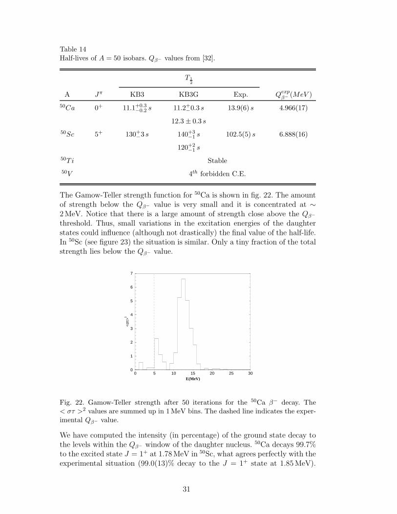
Table 14Half-lives of A = 50 isobars. Qβ− values from [32].
T 1
2
A Jπ KB3 KB3G Exp. Qexpβ−
(MeV )
50Ca 0+ 11.1+0.3−0.2 s 11.2+−0.3 s 13.9(6) s 4.966(17)
12.3 ± 0.3 s
50Sc 5+ 130+−3 s 140+3−1 s 102.5(5) s 6.888(16)
120+2−1 s
50T i Stable
50V 4th forbidden C.E.
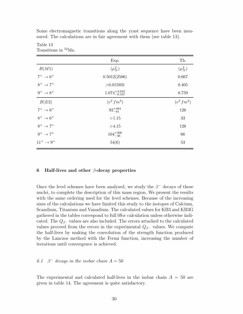
The Gamow-Teller strength function for 50Ca is shown in fig. 22. The amountof strength below the Qβ− value is very small and it is concentrated at ∼2MeV. Notice that there is a large amount of strength close above the Qβ−
threshold. Thus, small variations in the excitation energies of the daughterstates could influence (although not drastically) the final value of the half-life.In 50Sc (see figure 23) the situation is similar. Only a tiny fraction of the totalstrength lies below the Qβ− value.
0 5 10 15 20 25 30E(MeV)
0
1
2
3
4
5
6
7
<στ>
2
Fig. 22. Gamow-Teller strength after 50 iterations for the 50Ca β− decay. The< στ >2 values are summed up in 1MeV bins. The dashed line indicates the exper-imental Qβ− value.
We have computed the intensity (in percentage) of the ground state decay tothe levels within the Qβ− window of the daughter nucleus. 50Ca decays 99.7%to the excited state J = 1+ at 1.78MeV in 50Sc, what agrees perfectly with theexperimental situation (99.0(13)% decay to the J = 1+ state at 1.85MeV).
31
0 5 10 15 20 25 30 35 40E(MeV)
0
1
2
3
4
5
6
<στ>
2
Fig. 23. Gamow-Teller strength after 50 iterations for the 50Sc β− decay. The< στ >2 values are summed up in 1MeV bins. The dashed line indicates the exper-imental Qβ− value.
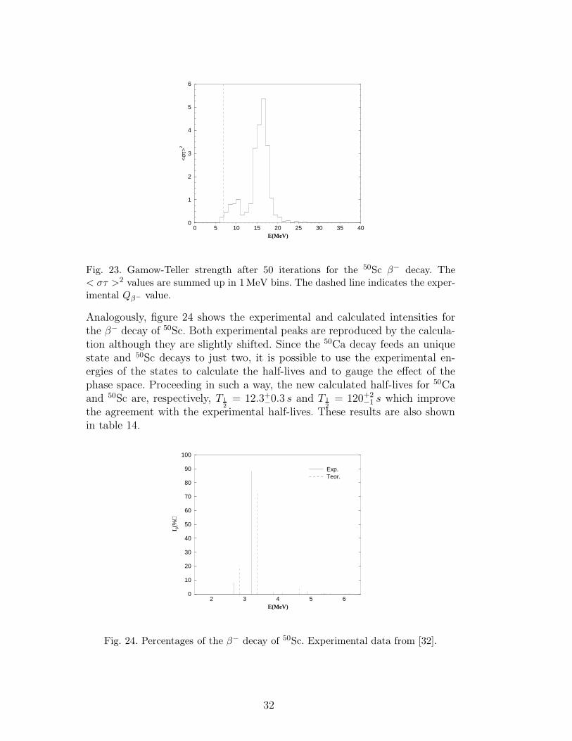
Analogously, figure 24 shows the experimental and calculated intensities forthe β− decay of 50Sc. Both experimental peaks are reproduced by the calcula-tion although they are slightly shifted. Since the 50Ca decay feeds an uniquestate and 50Sc decays to just two, it is possible to use the experimental en-ergies of the states to calculate the half-lives and to gauge the effect of thephase space. Proceeding in such a way, the new calculated half-lives for 50Caand 50Sc are, respectively, T 1
2
= 12.3+−0.3 s and T 1
2
= 120+2−1 s which improve
the agreement with the experimental half-lives. These results are also shownin table 14.
2 3 4 5 6E(MeV)
0
10
20
30
40
50
60
70
80
90
100
I β(%
)
Exp.Teor.
Fig. 24. Percentages of the β− decay of 50Sc. Experimental data from [32].
32
6.2 β− decays in the isobar chain A = 51
Table 15 gathers the experimental and calculated half-lives for the isobar chainA = 51. The calculated values are quite close to the experimental ones.
Table 15Half-lives of A = 51 isobars. Qβ− values from [32].
T 1
2
A Jπ KB3 KB3G Exp. Qexpβ−
(MeV )
51Ca 32
−8.9+1.0
−0.9 s 7.6+0.8−0.7 s 10.0(8) s 7.332(93)
51Sc 72
−14.1+−0.3 s 10.4+−0.2 s 12.4(1) s 6.508(20)
12.3 ± 0.3 s
51T i 32
−6.94+−0.02min 8.04+−0.02min 5.76(1)min 2.4706(15)
6.97 ± 0.02min
51V Stable
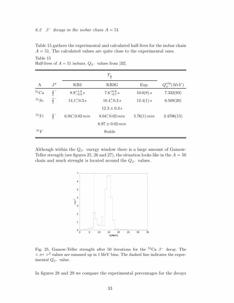
Although within the Qβ− energy window there is a large amount of Gamow-Teller strength (see figures 25, 26 and 27), the situation looks like in the A = 50chain and much strenght is located around the Qβ− values.
0 5 10 15 20 25 30 35E(MeV)
0
1
2
3
4
5
6
7
<στ>
2
Fig. 25. Gamow-Teller strength after 50 iterations for the 51Ca β− decay. The< στ >2 values are summed up in 1MeV bins. The dashed line indicates the exper-imental Qβ− value.
In figures 28 and 29 we compare the experimental percentages for the decays
33
0 5 10 15 20 25 30 35 40E(MeV)
0
1
2
3
4
5
6
7
8
9
<στ>
2
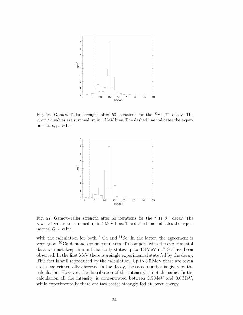
Fig. 26. Gamow-Teller strength after 50 iterations for the 51Sc β− decay. The< στ >2 values are summed up in 1MeV bins. The dashed line indicates the exper-imental Qβ− value.
0 5 10 15 20 25 30 35E(MeV)
0
1
2
3
4
5
6
7
8
<στ>
2
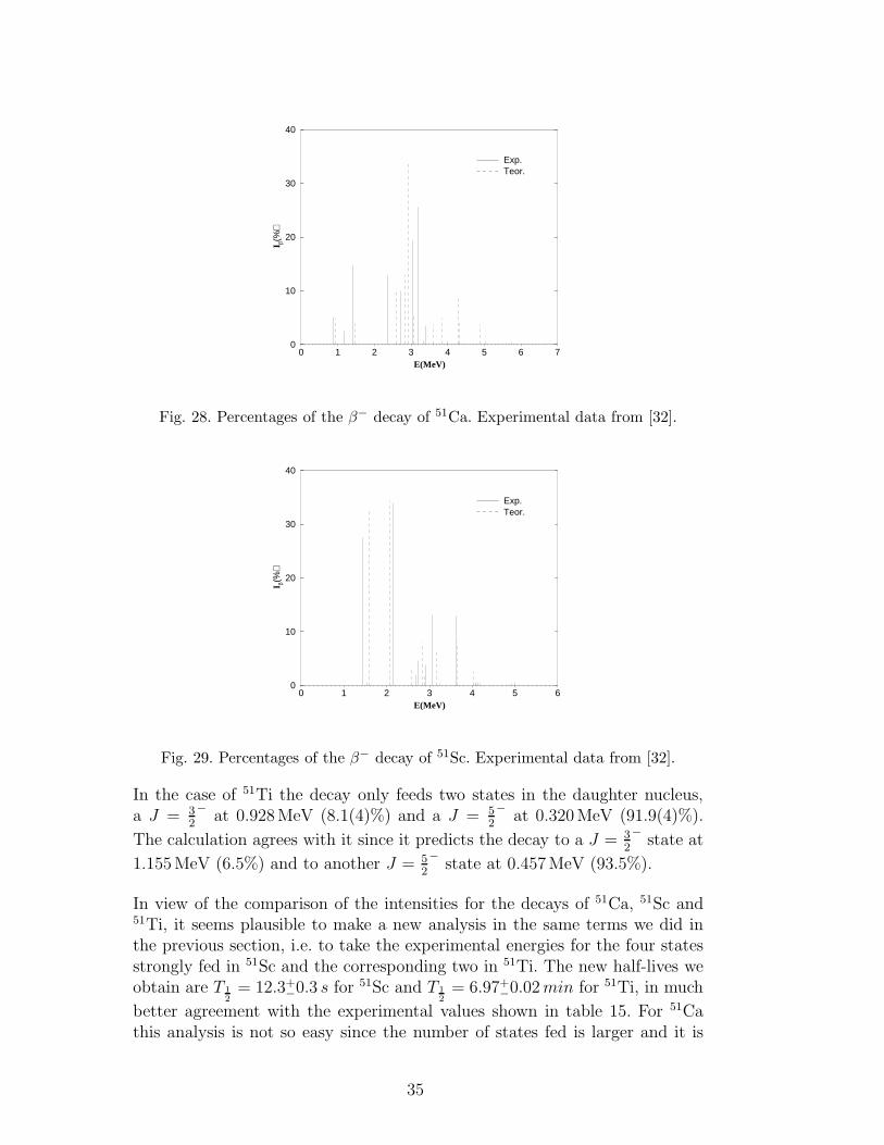
Fig. 27. Gamow-Teller strength after 50 iterations for the 51Ti β− decay. The< στ >2 values are summed up in 1MeV bins. The dashed line indicates the exper-imental Qβ− value.
with the calculation for both 51Ca and 51Sc. In the latter, the agreement isvery good. 51Ca demands some comments. To compare with the experimentaldata we must keep in mind that only states up to 3.8MeV in 51Sc have beenobserved. In the first MeV there is a single experimental state fed by the decay.This fact is well reproduced by the calculation. Up to 3.5MeV there are sevenstates experimentally observed in the decay, the same number is given by thecalculation. However, the distribution of the intensity is not the same. In thecalculation all the intensity is concentrated between 2.5MeV and 3.0MeV,while experimentally there are two states strongly fed at lower energy.
34
0 1 2 3 4 5 6 7E(MeV)
0
10
20
30
40
I β(%
)
Exp.Teor.
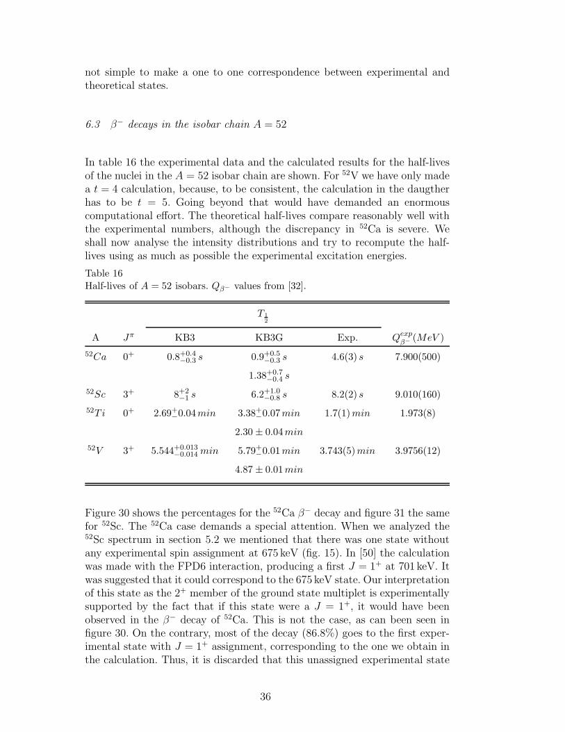
Fig. 28. Percentages of the β− decay of 51Ca. Experimental data from [32].
0 1 2 3 4 5 6E(MeV)
0
10
20
30
40
I β(%
)
Exp.Teor.
Fig. 29. Percentages of the β− decay of 51Sc. Experimental data from [32].
In the case of 51Ti the decay only feeds two states in the daughter nucleus,a J = 3
2
−at 0.928MeV (8.1(4)%) and a J = 5
2
−at 0.320MeV (91.9(4)%).
The calculation agrees with it since it predicts the decay to a J = 32
−state at
1.155MeV (6.5%) and to another J = 52
−state at 0.457MeV (93.5%).
In view of the comparison of the intensities for the decays of 51Ca, 51Sc and51Ti, it seems plausible to make a new analysis in the same terms we did inthe previous section, i.e. to take the experimental energies for the four statesstrongly fed in 51Sc and the corresponding two in 51Ti. The new half-lives weobtain are T 1
2
= 12.3+−0.3 s for 51Sc and T 1
2
= 6.97+−0.02min for 51Ti, in much
better agreement with the experimental values shown in table 15. For 51Cathis analysis is not so easy since the number of states fed is larger and it is
35
not simple to make a one to one correspondence between experimental andtheoretical states.
6.3 β− decays in the isobar chain A = 52
In table 16 the experimental data and the calculated results for the half-livesof the nuclei in the A = 52 isobar chain are shown. For 52V we have only madea t = 4 calculation, because, to be consistent, the calculation in the daugtherhas to be t = 5. Going beyond that would have demanded an enormouscomputational effort. The theoretical half-lives compare reasonably well withthe experimental numbers, although the discrepancy in 52Ca is severe. Weshall now analyse the intensity distributions and try to recompute the half-lives using as much as possible the experimental excitation energies.
Table 16Half-lives of A = 52 isobars. Qβ− values from [32].
T 1
2
A Jπ KB3 KB3G Exp. Qexpβ−
(MeV )
52Ca 0+ 0.8+0.4−0.3 s 0.9+0.5
−0.3 s 4.6(3) s 7.900(500)
1.38+0.7−0.4 s
52Sc 3+ 8+2−1 s 6.2+1.0
−0.8 s 8.2(2) s 9.010(160)
52T i 0+ 2.69+−0.04min 3.38+−0.07min 1.7(1)min 1.973(8)
2.30 ± 0.04min
52V 3+ 5.544+0.013−0.014 min 5.79+−0.01min 3.743(5)min 3.9756(12)
4.87 ± 0.01min
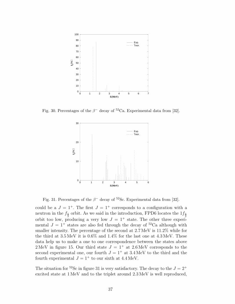
Figure 30 shows the percentages for the 52Ca β− decay and figure 31 the samefor 52Sc. The 52Ca case demands a special attention. When we analyzed the52Sc spectrum in section 5.2 we mentioned that there was one state withoutany experimental spin assignment at 675 keV (fig. 15). In [50] the calculationwas made with the FPD6 interaction, producing a first J = 1+ at 701 keV. Itwas suggested that it could correspond to the 675 keV state. Our interpretationof this state as the 2+ member of the ground state multiplet is experimentallysupported by the fact that if this state were a J = 1+, it would have beenobserved in the β− decay of 52Ca. This is not the case, as can been seen infigure 30. On the contrary, most of the decay (86.8%) goes to the first exper-imental state with J = 1+ assignment, corresponding to the one we obtain inthe calculation. Thus, it is discarded that this unassigned experimental state
36
0 1 2 3 4 5 6 7E(MeV)
0
10
20
30
40
50
60
70
80
90
100
I β(%
)
Exp.Teor.
Fig. 30. Percentages of the β− decay of 52Ca. Experimental data from [32].
0 1 2 3 4 5 6E(MeV)
0
10
20
30
I β(%
)
Exp.Teor.
Fig. 31. Percentages of the β− decay of 52Sc. Experimental data from [32].
could be a J = 1+. The first J = 1+ corresponds to a configuration with aneutron in the f 5
2
orbit. As we said in the introduction, FPD6 locates the 1f 5
2
orbit too low, producing a very low J = 1+ state. The other three experi-mental J = 1+ states are also fed through the decay of 52Ca although withsmaller intensity. The percentage of the second at 2.7MeV is 11.2% while forthe third at 3.5MeV it is 0.6% and 1.4% for the last one at 4.3MeV. Thesedata help us to make a one to one correspondence between the states above2MeV in figure 15. Our third state J = 1+ at 2.6MeV corresponds to thesecond experimental one, our fourth J = 1+ at 3.4MeV to the third and thefourth experimental J = 1+ to our sixth at 4.4MeV.
The situation for 52Sc in figure 31 is very satisfactory. The decay to the J = 2+
excited state at 1MeV and to the triplet around 2.3MeV is well reproduced,
37
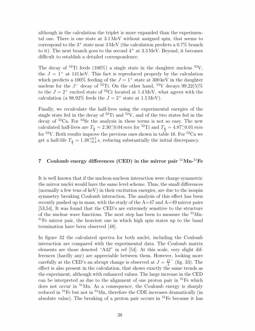
although in the calculation the triplet is more expanded than the experimen-tal one. There is one state at 3.1MeV without assigned spin, that seems tocorrespond to the 3+ state near 3MeV (the calculation predicts a 0.7% branchto it). The next branch goes to the second 4+ at 3.3MeV. Beyond, it becomesdifficult to establish a detailed correspondence.
The decay of 52Ti feeds (100%) a single state in the daughter nucleus 52V,the J = 1+ at 141 keV. This fact is reproduced properly by the calculationwhich predicts a 100% feeding of the J = 1+ state at 300 keV in the daughternucleus for the β− decay of 52Ti. On the other hand, 52V decays 99.22(5)%to the J = 2+ excited state of 52Cr located at 1.4MeV, what agrees with thecalculation (a 98.92% feeds the J = 2+ state at 1.5MeV).
Finally, we recalculate the half-lives using the experimental energies of thesingle state fed in the decay of 52Ti and 52V, and of the two states fed in thedecay of 52Ca. For 52Sc the analysis in these terms is not so easy. The newcalculated half-lives are T 1
2
= 2.30+−0.04min for 52Ti and T 1
2
= 4.87+−0.01min
for 52V. Both results improve the previous ones shown in table 16. For 52Ca weget a half-life T 1
2
= 1.38+0.7−0.4 s, reducing substantially the initial discrepancy.
7 Coulomb energy differences (CED) in the mirror pair 51Mn-51Fe
It is well known that if the nucleon-nucleon interaction were charge symmetricthe mirror nuclei would have the same level scheme. Thus, the small differences(normally a few tens of keV) in their excitation energies, are due to the isospinsymmetry breaking Coulomb interaction. The analysis of this effect has beenrecently pushed up in mass, with the study of the A=47 and A=49 mirror pairs[53,54]. It was found that the CED’s are extremely sensitive to the structureof the nuclear wave functions. The next step has been to measure the 51Mn-51Fe mirror pair, the heaviest one in which high spin states up to the bandtermination have been observed [48].
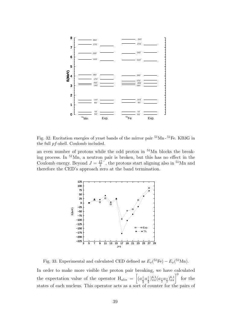
In figure 32 the calculated spectra for both nuclei, including the Coulombinteraction are compared with the experimental data. The Coulomb matrixelements are those denoted “A42” in ref [54]. At this scale, very slight dif-ferences (hardly any) are appreciable between them. However, looking more
carefully at the CED’s an abrupt change is observed at J = 172
−(fig. 33). The
effect is also present in the calculation, that shows exactly the same trends asthe experiment, although with enhanced values. The large increase in the CEDcan be interpreted as due to the alignment of one proton pair in 51Fe whichdoes not occur in 51Mn. As a consequence, the Coulomb energy is sharplyreduced in 51Fe but not in 51Mn, therefore the CDE increases dramatically (inabsolute value). The breaking of a proton pair occurs in 51Fe because it has
38
0
1
2
3
4
5
6
7
8
E(M
eV)
0
1
2
3
4
5
6
7
8
E(M
eV)
0
1
2
3
4
5
6
7
8
E(M
eV)
0
1
2
3
4
5
6
7
8
E(M
eV)
51Mn Exp.
51Fe
5/2−
7/2−
9/2−
11/2−
13/2−
15/2−
17/2−
19/2−
21/2−
23/2−
25/2−
27/2−
5/2−
7/2−
9/2−
11/2−
13/2−
15/2−
17/2−
19/2−
21/2−
23/2−
27/2−
25/2−
Exp.
Fig. 32. Excitation energies of yrast bands of the mirror pair 51Mn - 51Fe. KB3G inthe full pf -shell. Coulomb included.
an even number of protons while the odd proton in 51Mn blocks the break-ing process. In 51Mn, a neutron pair is broken, but this has no effect in theCoulomb energy. Beyond J = 17
2
−, the protons start aligning also in 51Mn and
therefore the CED’s approach zero at the band termination.
3 5 7 9 11 13 15 17 19 21 23 25 27 292*J
−225
−200
−175
−150
−125
−100
−75
−50
−25
0
25
50
75
100
125
E(k
eV)
Th.
3 5 7 9 11 13 15 17 19 21 23 25 27 29−225
−200
−175
−150
−125
−100
−75
−50
−25
0
25
50
75
100
125
Exp.
Fig. 33. Experimental and calculated CED defined as Ex(51Fe)− Ex(
51Mn).
In order to make more visible the proton pair breaking, we have calculated
the expectation value of the operator Halin =[
(a+72
a+72
)6,1ππ(a 7
2
a 7
2
)6,1ππ
]0
for the
states of each nucleus. This operator acts as a sort of counter for the pairs of
39
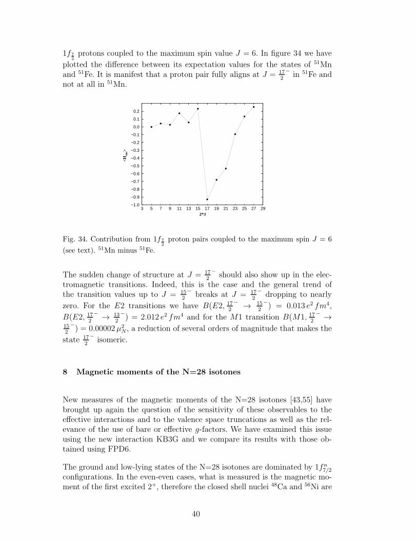
1f 7
2
protons coupled to the maximum spin value J = 6. In figure 34 we have
plotted the difference between its expectation values for the states of 51Mnand 51Fe. It is manifest that a proton pair fully aligns at J = 17
2
−in 51Fe and
not at all in 51Mn.
3 5 7 9 11 13 15 17 19 21 23 25 27 292*J
−1.0
−0.9
−0.8
−0.7
−0.6
−0.5
−0.4
−0.3
−0.2
−0.1
0.0
0.1
0.2
<H
alin>
Fig. 34. Contribution from 1f 7
2
proton pairs coupled to the maximum spin J = 6
(see text). 51Mn minus 51Fe.
The sudden change of structure at J = 172
−should also show up in the elec-
tromagnetic transitions. Indeed, this is the case and the general trend ofthe transition values up to J = 15
2
−breaks at J = 17
2
−dropping to nearly
zero. For the E2 transitions we have B(E2, 172
− → 152
−) = 0.013 e2 fm4,
B(E2, 172
− → 132
−) = 2.012 e2 fm4 and for the M1 transition B(M1, 17
2
− →152
−) = 0.00002µ2
N , a reduction of several orders of magnitude that makes the
state 172
−isomeric.
8 Magnetic moments of the N=28 isotones
New measures of the magnetic moments of the N=28 isotones [43,55] havebrought up again the question of the sensitivity of these observables to theeffective interactions and to the valence space truncations as well as the rel-evance of the use of bare or effective g-factors. We have examined this issueusing the new interaction KB3G and we compare its results with those ob-tained using FPD6.
The ground and low-lying states of the N=28 isotones are dominated by 1fn7/2
configurations. In the even-even cases, what is measured is the magnetic mo-ment of the first excited 2+, therefore the closed shell nuclei 48Ca and 56Ni are
40
excluded from this systematics. In the 1fn7/2 limit, the value of the 2+ mag-
netic moment, which is the same for 50Ti, 52Cr and 54Fe, is 3.31 µN , using bareg-factors. The usual choice of effective g-factors, gseff=0.75 gsbare, g
lπ=1.1 µN
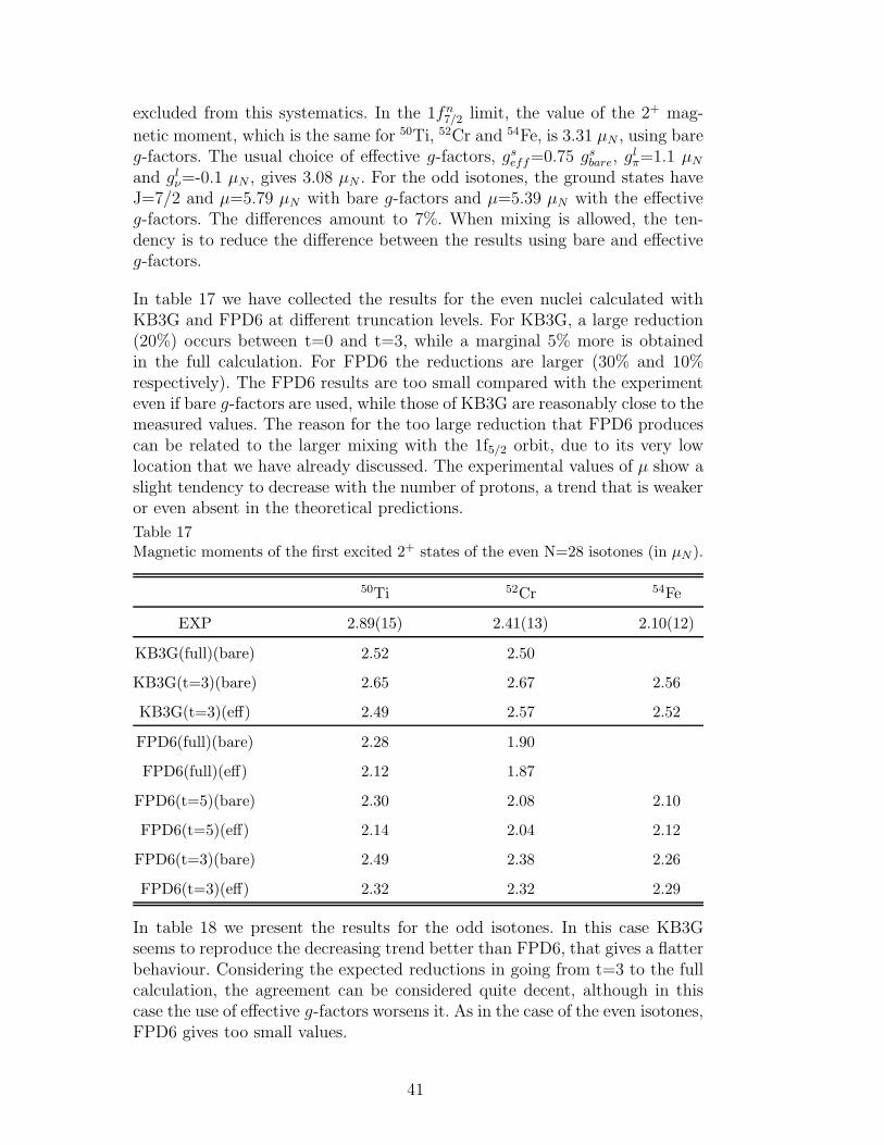
and glν=-0.1 µN , gives 3.08 µN . For the odd isotones, the ground states haveJ=7/2 and µ=5.79 µN with bare g-factors and µ=5.39 µN with the effectiveg-factors. The differences amount to 7%. When mixing is allowed, the ten-dency is to reduce the difference between the results using bare and effectiveg-factors.
In table 17 we have collected the results for the even nuclei calculated withKB3G and FPD6 at different truncation levels. For KB3G, a large reduction(20%) occurs between t=0 and t=3, while a marginal 5% more is obtainedin the full calculation. For FPD6 the reductions are larger (30% and 10%respectively). The FPD6 results are too small compared with the experimenteven if bare g-factors are used, while those of KB3G are reasonably close to themeasured values. The reason for the too large reduction that FPD6 producescan be related to the larger mixing with the 1f5/2 orbit, due to its very lowlocation that we have already discussed. The experimental values of µ show aslight tendency to decrease with the number of protons, a trend that is weakeror even absent in the theoretical predictions.
Table 17Magnetic moments of the first excited 2+ states of the even N=28 isotones (in µN ).
50Ti 52Cr 54Fe
EXP 2.89(15) 2.41(13) 2.10(12)
KB3G(full)(bare) 2.52 2.50
KB3G(t=3)(bare) 2.65 2.67 2.56
KB3G(t=3)(eff) 2.49 2.57 2.52
FPD6(full)(bare) 2.28 1.90
FPD6(full)(eff) 2.12 1.87
FPD6(t=5)(bare) 2.30 2.08 2.10
FPD6(t=5)(eff) 2.14 2.04 2.12
FPD6(t=3)(bare) 2.49 2.38 2.26
FPD6(t=3)(eff) 2.32 2.32 2.29
In table 18 we present the results for the odd isotones. In this case KB3Gseems to reproduce the decreasing trend better than FPD6, that gives a flatterbehaviour. Considering the expected reductions in going from t=3 to the fullcalculation, the agreement can be considered quite decent, although in thiscase the use of effective g-factors worsens it. As in the case of the even isotones,FPD6 gives too small values.
41
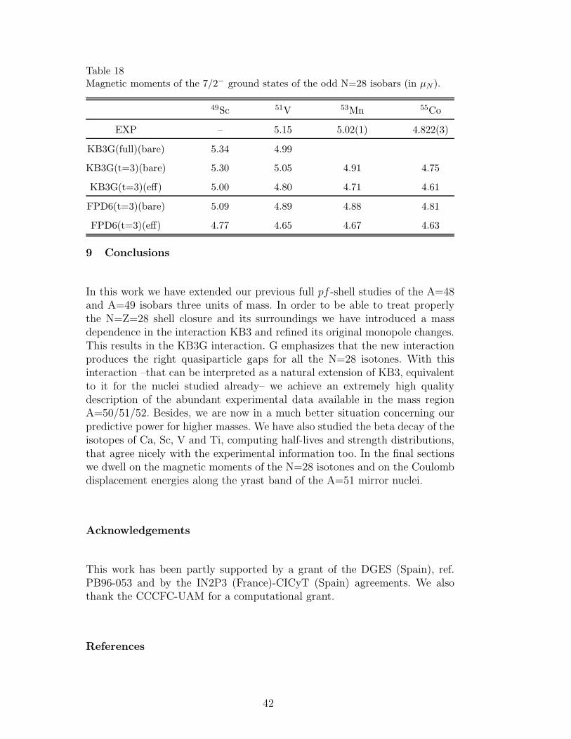
Table 18Magnetic moments of the 7/2− ground states of the odd N=28 isobars (in µN ).
49Sc 51V 53Mn 55Co
EXP – 5.15 5.02(1) 4.822(3)
KB3G(full)(bare) 5.34 4.99
KB3G(t=3)(bare) 5.30 5.05 4.91 4.75
KB3G(t=3)(eff) 5.00 4.80 4.71 4.61
FPD6(t=3)(bare) 5.09 4.89 4.88 4.81
FPD6(t=3)(eff) 4.77 4.65 4.67 4.63
9 Conclusions
In this work we have extended our previous full pf -shell studies of the A=48and A=49 isobars three units of mass. In order to be able to treat properlythe N=Z=28 shell closure and its surroundings we have introduced a massdependence in the interaction KB3 and refined its original monopole changes.This results in the KB3G interaction. G emphasizes that the new interactionproduces the right quasiparticle gaps for all the N=28 isotones. With thisinteraction –that can be interpreted as a natural extension of KB3, equivalentto it for the nuclei studied already– we achieve an extremely high qualitydescription of the abundant experimental data available in the mass regionA=50/51/52. Besides, we are now in a much better situation concerning ourpredictive power for higher masses. We have also studied the beta decay of theisotopes of Ca, Sc, V and Ti, computing half-lives and strength distributions,that agree nicely with the experimental information too. In the final sectionswe dwell on the magnetic moments of the N=28 isotones and on the Coulombdisplacement energies along the yrast band of the A=51 mirror nuclei.
Acknowledgements
This work has been partly supported by a grant of the DGES (Spain), ref.PB96-053 and by the IN2P3 (France)-CICyT (Spain) agreements. We alsothank the CCCFC-UAM for a computational grant.
References
42
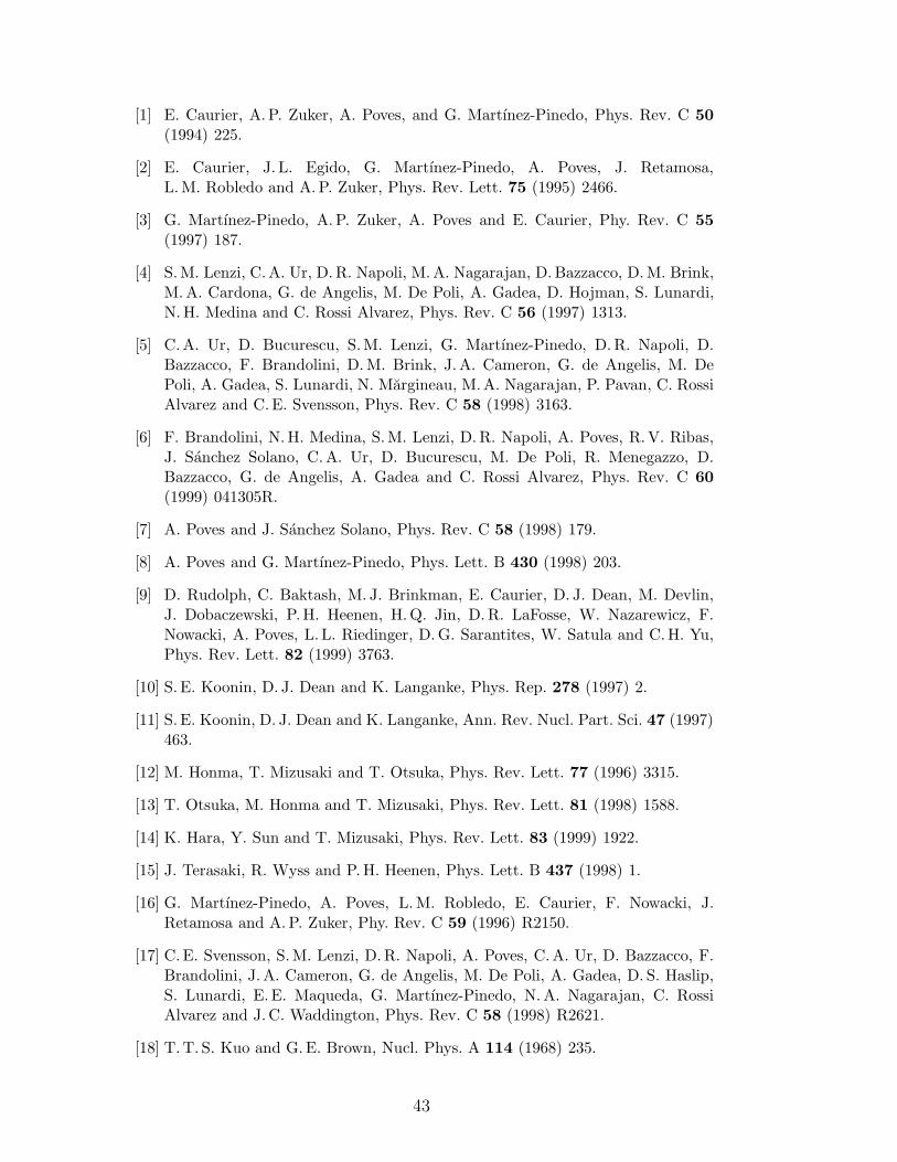
[1] E. Caurier, A.P. Zuker, A. Poves, and G. Martınez-Pinedo, Phys. Rev. C 50
(1994) 225.
[2] E. Caurier, J. L. Egido, G. Martınez-Pinedo, A. Poves, J. Retamosa,L.M. Robledo and A. P. Zuker, Phys. Rev. Lett. 75 (1995) 2466.
[3] G. Martınez-Pinedo, A.P. Zuker, A. Poves and E. Caurier, Phy. Rev. C 55
(1997) 187.
[4] S.M. Lenzi, C.A. Ur, D.R. Napoli, M.A. Nagarajan, D. Bazzacco, D.M. Brink,M.A. Cardona, G. de Angelis, M. De Poli, A. Gadea, D. Hojman, S. Lunardi,N. H. Medina and C. Rossi Alvarez, Phys. Rev. C 56 (1997) 1313.
[5] C.A. Ur, D. Bucurescu, S.M. Lenzi, G. Martınez-Pinedo, D.R. Napoli, D.Bazzacco, F. Brandolini, D.M. Brink, J.A. Cameron, G. de Angelis, M. DePoli, A. Gadea, S. Lunardi, N. Margineau, M.A. Nagarajan, P. Pavan, C. RossiAlvarez and C.E. Svensson, Phys. Rev. C 58 (1998) 3163.
[6] F. Brandolini, N. H. Medina, S.M. Lenzi, D. R. Napoli, A. Poves, R.V. Ribas,J. Sanchez Solano, C.A. Ur, D. Bucurescu, M. De Poli, R. Menegazzo, D.Bazzacco, G. de Angelis, A. Gadea and C. Rossi Alvarez, Phys. Rev. C 60
(1999) 041305R.
[7] A. Poves and J. Sanchez Solano, Phys. Rev. C 58 (1998) 179.
[8] A. Poves and G. Martınez-Pinedo, Phys. Lett. B 430 (1998) 203.
[9] D. Rudolph, C. Baktash, M. J. Brinkman, E. Caurier, D. J. Dean, M. Devlin,J. Dobaczewski, P.H. Heenen, H.Q. Jin, D. R. LaFosse, W. Nazarewicz, F.Nowacki, A. Poves, L. L. Riedinger, D.G. Sarantites, W. Satula and C.H. Yu,Phys. Rev. Lett. 82 (1999) 3763.
[10] S. E. Koonin, D. J. Dean and K. Langanke, Phys. Rep. 278 (1997) 2.
[11] S. E. Koonin, D. J. Dean and K. Langanke, Ann. Rev. Nucl. Part. Sci. 47 (1997)463.
[12] M. Honma, T. Mizusaki and T. Otsuka, Phys. Rev. Lett. 77 (1996) 3315.
[13] T. Otsuka, M. Honma and T. Mizusaki, Phys. Rev. Lett. 81 (1998) 1588.
[14] K. Hara, Y. Sun and T. Mizusaki, Phys. Rev. Lett. 83 (1999) 1922.
[15] J. Terasaki, R. Wyss and P.H. Heenen, Phys. Lett. B 437 (1998) 1.
[16] G. Martınez-Pinedo, A. Poves, L.M. Robledo, E. Caurier, F. Nowacki, J.Retamosa and A. P. Zuker, Phy. Rev. C 59 (1996) R2150.
[17] C.E. Svensson, S.M. Lenzi, D. R. Napoli, A. Poves, C.A. Ur, D. Bazzacco, F.Brandolini, J.A. Cameron, G. de Angelis, M. De Poli, A. Gadea, D. S. Haslip,S. Lunardi, E. E. Maqueda, G. Martınez-Pinedo, N.A. Nagarajan, C. RossiAlvarez and J.C. Waddington, Phys. Rev. C 58 (1998) R2621.
[18] T.T. S. Kuo and G. E. Brown, Nucl. Phys. A 114 (1968) 235.
43
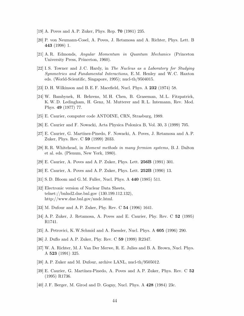
[19] A. Poves and A. P. Zuker, Phys. Rep. 70 (1981) 235.
[20] P. von Neumann-Cosel, A. Poves, J. Retamosa and A. Richter, Phys. Lett. B443 (1998) 1.
[21] A. R. Edmonds, Angular Momentum in Quantum Mechanics (PrincetonUniversity Press, Princeton, 1960).
[22] I. S. Towner and J.C. Hardy, in The Nucleus as a Laboratory for Studying
Symmetries and Fundamental Interactions, E.M. Henley and W.C. Haxtoneds. (World-Scientific, Singapore, 1995); nucl-th/9504015.
[23] D.H. Wilkinson and B.E. F. Macefield, Nucl. Phys. A 232 (1974) 58.
[24] W. Bambynek, H. Behrens, M.H. Chen, B. Graseman, M. L. Fitzpatrick,K.W.D. Ledingham, H. Genz, M. Mutterer and R. L. Intemann, Rev. Mod.Phys. 49 (1977) 77.
[25] E. Caurier, computer code ANTOINE, CRN, Strasburg, 1989.
[26] E. Caurier and F. Nowacki, Acta Physica Polonica B, Vol. 30, 3 (1999) 705.
[27] E. Caurier, G. Martınez-Pinedo, F. Nowacki, A. Poves, J. Retamosa and A.P.Zuker, Phys. Rev. C 59 (1999) 2033.
[28] R. R. Whitehead, in Moment methods in many fermion systems, B. J. Daltonet al. eds. (Plenum, New York, 1980).
[29] E. Caurier, A. Poves and A.P. Zuker, Phys. Lett. 256B (1991) 301.
[30] E. Caurier, A. Poves and A.P. Zuker, Phys. Lett. 252B (1990) 13.
[31] S.D. Bloom and G.M. Fuller, Nucl. Phys. A 440 (1985) 511.
[32] Electronic version of Nuclear Data Sheets,telnet://bnlnd2.dne.bnl.gov (130.199.112.132),http://www.dne.bnl.gov/nndc.html.
[33] M. Dufour and A.P. Zuker, Phy. Rev. C 54 (1996) 1641.
[34] A. P. Zuker, J. Retamosa, A. Poves and E. Caurier, Phy. Rev. C 52 (1995)R1741.
[35] A. Petrovici, K.W.Schmid and A. Faessler, Nucl. Phys. A 605 (1996) 290.
[36] J. Duflo and A.P. Zuker, Phy. Rev. C 59 (1999) R2347.
[37] W.A. Richter, M. J. Van Der Merwe, R. E. Julies and B.A. Brown, Nucl. Phys.A 523 (1991) 325.
[38] A. P. Zuker and M. Dufour, archive LANL, nucl-th/9505012.
[39] E. Caurier, G. Martınez-Pinedo, A. Poves and A. P. Zuker, Phys. Rev. C 52
(1995) R1736.
[40] J. F. Berger, M. Girod and D. Gogny, Nucl. Phys. A 428 (1984) 23c.
44
[41] T. Gonzalez Llarena, Ph.D. Thesis, UAM Madrid, 1999.
[42] R. B. Firestone, Table of Isotopes Vol. I and II, edited by V. S. Shirley (Wiley-Interscience, New York, 1996).
[43] K.-H. Speidel, R. Ernst, O. Kenn, J. Gerber, P. Maier-Komor, N. Benczer-Koller, G. Kumbartzki, L. Zamick, M. S. Fayache, and Y.Y. Sharon, Phy. Rev.C 62 (2000) 031301R.
[44] A. Novoselsky, M. Vallieres and O. La’adan, Phys. Rev. Lett. 79 (1997) 4341.
[45] Y. Utsuno, T. Sebe, T. Otsuka and T. Mizusaki, Phys. Rev. Lett. 81 (1998)5948.
[46] A. Novoselsky, M. Vallieres and O. La’adan, Phys. Rev. Lett. 81 (1998) 5949.
[47] A. Novoselsky, M. Vallieres and O. La’adan, Phys. Rev. Lett. 81 (1998) 5955.
[48] M.A. Bentley, S. J. Williams, D. T. Joss, C.D. O’Leary, A.M. Bruce, J.A.Cameron, P. Fallon, L. Frankland, W. Gelletly, C. J. Lister, G. Martınez-Pinedo, A. Poves, P. H. Regan, P. Reiter, B. Rubio, J. Sanchez Solano, D.Seweryniak, C.E. Svensson, S.M. Vicent and D.D. Warner, Phys. Rev. C, 62(2000) 051303R.
[49] A. Huck, G. Klotz, A. Knipper, C. Miehe, C. Richard-Serre, G. Walter, A.Poves, H. L. Ravn and G. Marguier, Phys. Rev. C 31 (1985) 2226.
[50] A. Novoselsky and M. Vallieres, Phys. Rev. C 57 (1998) R19.
[51] D. E. Appelbe, J. Sanchez Solano, J.A. Cameron, J. Chenkin, T.E. Drake,B. Djerroud, S. Filibotte, A. Poves, J. C. Waddington and D. Ward, to bepublished.
[52] M. Axiotis et al., to be published.
[53] C.D. O’Leary, M.A. Bentley, D. E. Appelbe, D.M. Cullen, S. Erturk, R.A.Bark, A. Maj and T. Saitoh, Phys. Rev. Lett. 79 (1997) 4349.
[54] M.A. Bentley, C.D. O’Leary, A. Poves, G. Martınez-Pinedo, D. E. Appelbe,R.A. Bark, D.M. Cullen, S. Erturk and A. Maj, Phys. Lett. B 437 (1998) 243;erratum in Phys. Lett. B 451 (1999) 445.
[55] R. Ernst, K.-H. Speidel, O. Kenn, U. Nachum, J. Gerber, P. Maier-Komor, N.Benczer-Koller, G. Jakob, G. Kumbartzki, L. Zamick and F. Nowacki, Phys.Rev. Lett. 84 (2000) 416.
45


![],f& J, e [, JfAÍËÍÌ](https://img.pdfslide.fr/doc/110x75/6252ea542a6e68297a2f2bcd/famp-j-e-jfa.jpg)