Embed Size (px)
Citation preview
ÉCOLE DE TECHNOLOGIE SUPÉRIEURE UNIVERSITÉ DU QUÉBEC
THÈSE PAR ARTICLES PRÉSENTÉE À L’ÉCOLE DE TECHNOLOGIE SUPÉRIEURE
COMME EXIGENCE PARTIELLE À L’OBTENTION DU
DOCTORAT EN GÉNIE Ph.D.
PAR Ahmed JOUBAIR
CONTRIBUTION À L’AMÉLIORATION DE LA PRÉCISION ABSOLUE DES ROBOTS PARALLÈLES
MONTRÉAL, LE 1er AOÛT 2012
©Tous droits réservés, Ahmed Joubair, 2012
©Tous droits réservés
Cette licence signifie qu’il est interdit de reproduire, d’enregistrer ou de diffuser en tout ou en partie, le
présent document. Le lecteur qui désire imprimer ou conserver sur un autre media une partie importante de
ce document, doit obligatoirement en demander l’autorisation à l’auteur.
PRÉSENTATION DU JURY
CETTE THÈSE A ÉTÉ ÉVALUÉE
PAR UN JURY COMPOSÉ DE : M. Ilian A. Bonev, directeur de thèse Département de génie de la production automatisée à l’École de technologie supérieure M. Antoine S. Tahan, président du jury Département de génie mécanique à l’École de technologie supérieure M. Pascal Bigras, membre du jury Département de génie de la production automatisée à l’École de technologie supérieure M. René Mayer, examinateur externe Département de génie mécanique à l’école polytechnique de Montréal
ELLE A FAIT L’OBJET D’UNE SOUTENANCE DEVANT JURY ET PUBLIC
LE 25 JUILLET 2012
À L’ÉCOLE DE TECHNOLOGIE SUPÉRIEURE

REMERCIEMENTS
En premier lieu, j’exprime ma vive gratitude à mon directeur de recherche le Pr Ilian Bonev
pour son soutien, sa disponibilité et pour m’avoir offert d’excellentes conditions de travail
tout au long de ce projet de recherche. Je tiens à présenter mes sincères remerciements au
Pr Antoine Tahan d’avoir accepté de présider le jury et pour ses conseils en ce qui a trait au
domaine de la métrologie. Mes chaleureux remerciements s’adressent aussi au Pr Pascal
Bigras pour avoir accepté d’être un membre du jury et pour avoir eu la gentillesse de
répondre à mes questions, notamment concernant la commande robotique. J’adresse mes
sincères remerciements au Pr René Mayer d’avoir accepté d’être un examinateur externe.
Mes vifs remerciements s’adressent aussi au Dr Mohamed Slamani pour son aide et toutes les
discussions enrichissantes que nous avons souvent eues, tout au long de la réalisation de ce
projet.
Je tiens à remercier les organismes suivants, pour leur financement :
- le programme des Chaires de recherche du Canada;
- la Fondation canadienne pour l’innovation (FCI);
- le Fonds québécois de la recherche sur la nature et les technologies (FQRNT).
Un grand merci à MM. Antonio Pexiero et Randy Aucoin, respectivement président et vice-
président de la compagnie Artypac Automation, où j’étais employé durant les deux premières
années de mon projet doctoral. Merci pour la flexibilité des horaires que vous m’avez offerts!
Merci à M. Hugo Landry, le sympathique technicien du laboratoire de métrologie, qui a été
toujours disponible pour m’aider à prendre des mesures en utilisant la MMT. Merci aussi à
MM. Francis Bourbonnais, François Vadnais et Alexandre Vigneault pour leurs aides
techniques. Je tiens aussi à saluer tous les membres du laboratoire CoRo avec qui j’ai passé
cinq agréables années. Merci Moncef pour ton sens de l’humour et ta permanente bonne
humeur qui ont été à l’origine de plusieurs agréables discussions!
VI
Merci Ann, Bertille et Jean-Marc, pour vos encouragements très appréciés! Merci à tous ceux
et celles qui ont contribué de près ou de loin à la réalisation de ce projet.
Finalement, et avec un très grand plaisir, je tiens à dédier cette thèse à ceux qui me sont les
plus chers : mes respectueux parents, mes frères et sœurs, ma femme et mes adorables
enfants, Soumaya et Ibrahim. Merci pour votre soutien et vos encouragements indéfectibles!
Un remerciement spécial à mon grand frère Mohammed qui m’a montré le chemin de
l’université et m’a encouragé tout au long de mon cursus universitaire. Quant à Soumaya et
Ibrahim, ils ont contribué agréablement avec leurs propres manières!
CONTRIBUTION À L’AMÉLIORATION DE LA PRÉCISION ABSOLUE DES ROBOTS PARALLÈLES
Ahmed JOUBAIR
RÉSUMÉ
Le but de la présente étude est de contribuer à l’amélioration de la précision absolue des robots parallèles, en ayant recours aux méthodes d’étalonnage géométrique. Ces méthodes consistent à identifier les valeurs des paramètres géométriques du robot, en vue d’améliorer la correspondance entre le robot réel et le modèle mathématique utilisé par son contrôleur. En plus de la compensation des erreurs géométriques, les opérations d’étalonnage proposées permettent d’identifier précisément le référentiel de base de chaque robot étudié. Les méthodes développées sont appliquées à deux robots parallèles à moins de six degrés de liberté (ddl) : une table de positionnement précis à trois ddl (PreXYT) et un robot plan cinq-barres (DexTAR) à deux ddl. Pour le premier robot, l’étalonnage est effectué en utilisant d’abord une méthode d’identification directe. Le deuxième travail destinée à améliorer la précision absolue du PreXYT résulte de la méthode géométrique directe d’étalonnage. En ce qui concerne le robot DexTAR, sa précision est améliorée en utilisant une approche d’auto-étalonnage qui exploite les modes de fonctionnement et les modes d’assemblage, pour réduire le nombre de positions d’étalonnage. Cette approche est particulièrement intéressante pour sa simplicité : à chaque position d’étalonnage une sphère de précision est installée en permanence pour servir de cible de mesure. Les positions de ces billes, placées sur une plateforme amovible, n’est mesurée qu’une seule fois, en utilisant une machine de mesure tridimensionnel (MMT). Après la réinstallation de la plateforme sur la base du robot, l’étalonnage peut se faire n’importe quand en n’utilisant que les informations provenant des encodeurs des actionneurs. Les données d’étalonnage et de validation des résultats sont récoltées en utilisant deux appareils mesurant par palpage. Le premier appareil est un bras articulé de mesure de coordonnées, de la compagnie FARO Technologies ; le second est une MMT de la compagnie Mitutoyo. Les incertitudes de mesures de ces machines sont respectivement ±18 µm et ±2,7 µm (niveau de confiance de 95%). Sachant que la qualité de l’étalonnage est inversement proportionnelle aux incertitudes de mesures, l’utilisation d’instruments précis avec des modèles géométriques d’étalonnage quasi-complet nous a permis d’atteindre ces résultats : les erreurs maximales en position et en orientation ont été réduites respectivement à 0,044 mm et 0,009° pour le PreXYT, à l’intérieur d’un cercle de 170 mm de diamètre. Pour le robot DexTAR, l’erreur maximale de position a été réduite à 0,080 mm dans l’ensemble de son espace de travail, soit une zone d’environ 600 mm × 600 mm. Améliorer la précision des robots au-delà de ces valeurs, en utilisant juste les approches géométriques, pourrait s’avérer peu probable. En ce sens, l’ajout de la modélisation et la compensation des erreurs non géométriques serait utile pour obtenir des résultats meilleurs. Mots clés : robots parallèles, robots planaires, étalonnage géométrique, précision absolue.

CONTRIBUTION TO IMPROVING THE ABSOLUTE ACCURACY OF PARALLEL ROBOTS
Ahmed JOUBAIR
ABSTRACT
The purpose of the present study is to improve the absolute accuracy of parallel robots, using geometric calibration methods. These methods identify the values of the robot’s geometric parameters, to improve the correspondence between the real robot and the mathematical model used in its controller. In addition to the compensation of geometric errors, the proposed calibration approaches allow to identify accurately the base frame of each of the studied robots. The developed methods are applied using two parallel robots with less than six degrees of freedom (DOFs): a precision positioning table with three DOFs (PreXYT) and a planar five-bar robot (DexTAR) with two DOFs. For the first robot, the calibration is performed by first using a direct identification method. The second work to improve the absolute accuracy of PreXYT is based on the direct kinematic calibration method. The accuracy of the five-bar robot is improved by using a self-calibration approach that exploits the working modes and assembly modes, to reduce the number of calibration positions. Therefore, all possible robot configurations for each calibration position are retained. This approach is particularly attractive in its simplicity: at each calibration position, a precision ball is permanently installed as a target for measurements. The positions of these balls, placed on a removable platform, is measured only once, using a coordinate measuring machine (CMM). After reinstalling the platform of the robot, the calibration can be done anytime using only the information from the actuator encoders. Calibration and validation data are collected using two measuring devices. The first device is an articulated arm coordinate measurement, from FARO Technologies, the second is a Mitutoyo CMM. The measurement uncertainties of these machines are respectively ±18 μm and ±2.7 μm. Knowing that the quality of calibration is inversely proportional to the measurements uncertainties, using accurate instruments with near-complete geometric models allowed us to achieve these results: the maximum errors in position and orientation were reduced respectively to 0.044 mm and 0.009° for the PreXYT, within a circle of 170 mm in diameter. For the robot DexTAR, the maximum error of position was reduced to 0.077 mm throughout its workspace, i.e. 600 mm × 600 mm. Improve the accuracy of robots beyond these values, using only kinematic approaches, may be unlikely. In this sense, the addition of modeling and compensation of non-kinematic errors would be useful to obtain better results. Keywords: parallel robots, planar robots, kinematic calibration, absolute accuracy.

TABLE DES MATIÈRES
Page
INTRODUCTION .....................................................................................................................1
CHAPITRE 1 GÉNÉRALITÉS ET REVUE DE LITTÉRATURE ........................................5 1.1 Généralités .....................................................................................................................5
1.1.1 Robots industriels........................................................................................ 5 1.1.1.1 Robots sériels ............................................................................... 5 1.1.1.2 Robots parallèles .......................................................................... 6 1.1.1.3 Comparaison des robots parallèles et sériels ............................. 12
1.1.2 Modes de programmation des robots et intérêt de l’étalonnage ............... 12 1.1.2.1 Programmation par enseignement (en ligne) ............................. 13 1.1.2.2 Programmation hors ligne .......................................................... 13
1.1.3 Critères de performance des robots industriels ......................................... 14 1.1.3.1 Espace de travail ........................................................................ 14 1.1.3.2 Répétabilité de pose ................................................................... 14 1.1.3.3 Précision absolue de pose .......................................................... 17
1.1.4 Domaines nécessitant une bonne précision absolue ................................. 19 1.2 Revue de littérature ......................................................................................................20
1.2.1 Causes de manque de précision des robots industriels et approches d’étalonnage appropriées .......................................................................... 20 1.2.1.1 Facteurs articulaires ................................................................... 21 1.2.1.2 Facteurs géométriques ............................................................... 21 1.2.1.3 Facteurs non géométriques ........................................................ 22
1.2.2 Catégories d’étalonnage ............................................................................ 23 1.2.2.1 Étalonnage géométrique (niveau 2) ........................................... 23 1.2.2.2 Étalonnage non géométrique (niveau 3) .................................... 23 1.2.2.3 Étalonnage articulaire (niveau 1) ............................................... 24
1.2.3 Méthodes d’étalonnage géométrique ........................................................ 25 1.2.3.1 Étalonnage par la méthode directe ............................................. 25 1.2.3.2 Étalonnage par la méthode inverse ............................................ 26 1.2.3.3 Étalonnage sous contraintes ....................................................... 28 1.2.3.4 Autres méthodes d’étalonnage ................................................... 29
1.2.4 Procédure d’étalonnage ............................................................................. 30 1.2.4.1 Modélisation .............................................................................. 30 1.2.4.2 Mesures ...................................................................................... 32 1.2.4.3 Identification .............................................................................. 33 1.2.4.4 Compensation ............................................................................ 35
1.2.5 Difficultés de l’étalonnage ........................................................................ 35 1.2.5.1 Choix des poses d’étalonnage et de leur nombre ....................... 35 1.2.5.2 Détection de sources majeures d’imprécision des robots .......... 42
1.3 Conclusion ...................................................................................................................42
XII
CHAPITRE 2 ARTICLE1: A NOVEL XY-THETA PRECISION TABLE AND A GEOMETRIC PROCEDURE FOR ITS KINEMATIC CALIBRATION 43
2.1 Introduction ..................................................................................................................44 2.2 Kinematic analyses ......................................................................................................47
2.2.1 Direct and inverse kinematic analysis ....................................................... 47 2.2.2 Workspace analysis ................................................................................... 49
2.3 Prototype ......................................................................................................................50 2.4 Assessment of the position repeatability ......................................................................52 2.5 Determination of lead errors ........................................................................................57 2.6 Kinematic calibration ...................................................................................................58
2.6.1 Determination of the base reference frame ............................................... 61 2.6.2 Determination of mobile reference frame ................................................. 62 2.6.3 Determination of the distance s ................................................................. 63 2.6.4 Determination of the offsets d1 and d3 ...................................................... 64
2.7 Experimental validation ...............................................................................................65 2.8 Conclusions ..................................................................................................................68 2.9 Acknowledgements ......................................................................................................68
CHAPITRE 3 ARTICLE 2: KINEMATIC CALIBRATION OF A 3-DOF PLANAR PARALLEL ROBOT.................................................................................69
3.1 Introduction ..................................................................................................................70 3.2 Nominal kinematic model ............................................................................................72 3.3 Prototype ......................................................................................................................75 3.4 Calibration model.........................................................................................................77
3.4.1 World frame .............................................................................................. 80 3.4.2 Base and mobile reference frames ............................................................ 81 3.4.3 Orientation measurement error ................................................................. 83
3.5 Calibration method.......................................................................................................83 3.6 Calibration poses ..........................................................................................................85 3.7 Simulated calibration ...................................................................................................86 3.8 Actual calibration and validation .................................................................................89 3.9 Conclusions ..................................................................................................................94
CHAPITRE 4 ARTICLE 3: KINEMATIC CALIBRATION OF A FIVE-BAR PLANAR PARALLEL ROBOT USING ALL WORKING MODES .......................97
4.1 Introduction ..................................................................................................................98 4.2 Description of the robot prototype and the magnetic tooling balls ............................101 4.3 Calibration model.......................................................................................................105
4.3.1 World and base reference frames ............................................................ 110 4.4 Calibration method.....................................................................................................112 4.5 Observability analysis ................................................................................................116 4.6 Simulated calibration .................................................................................................121 4.7 Actual calibration and validation ...............................................................................126 4.8 Conclusions ................................................................................................................131 4.9 Acknowledgments......................................................................................................132
XIII
CONCLUSION GÉNÉRALE ................................................................................................133
LISTE DE RÉFÉRENCES BIBLIOGRAPHIQUES.............................................................135

LISTE DES TABLEAUX
Page Tableau 1.1 Comparaison entre les robots parallèles et sériels ...............................................12 Table 2.1 Positioning repeatability (in micrometers) ............................................................55 Table 2.2 Table 2. Pose accuracy at the orientation θ = 0° ...................................................66 Table 2.3 Pose accuracy at the orientation θ = 10° ...............................................................67 Table 2.4 Pose accuracy at the position {201.000 mm 137.500 mm} .................................67 Table 3.1 Results of simulations for parameter identification ..............................................87 Table 3.2 Position and orientation error after calibration .....................................................89 Table 3.3 Experimental results for parameter identification using the
FaroArm and the CMM.........................................................................................91 Table 3.4 Position and orientation errors before and after calibration,
as measured on a CMM ........................................................................................92 Table 4.1 Simulated results for the 12 parameters identified ................................................123 Table 4.2 Position errors after simulated calibration .............................................................125 Table 4. 3 Position errors after simulated and experimental calibration by increasing the
number of calibration positions. ..........................................................................126 Table 4.4 Experimental results for the 12 parameters identified ...........................................128 Table 4.5 Maximum and RMS position errors before and after calibration ..........................131

LISTE DES FIGURES
Page
Figure 1. 1 Robots sériels (a) ABB IRB 2400 (b) KUKA KR 30 jet (c) Stäubli
TS80 SCARA ..........................................................................................................6 Figure 1.2 Deux différents modes d’assemblage pour les mêmes valeurs articulaires ρ1 et ρ2
d’un robot plan à deux ddl ......................................................................................8 Figure 1.3 Deux configurations de la jambe gauche pour la même position commandée
(x1, y1) pour un robot plan à deux ddl ......................................................................8 Figure 1.4 Robot Delta (a) ABB IRB 340 (trois ddl) (b) Fanuc M-3iA (six ddl) ....................9 Figure 1.5 Robots (a) RP-1AH de Mitsubishi Electric (b) M833 de PI ................................10 Figure 1.6 Utilisation de la plateforme de Stewart pour (a) un manipulateur d’antenne (Tirée
de PI: Piezo Nano Positioning, 2012) et (b) un simulateur de vol CAE ...............10 Figure 1.7 Robot parallèle à trois ddl (HERMES de FATRONIK) utilisé ............................11 Figure 1.8 Robots parallèles (a) sous forme d’interface haptique à trois ddl (de Quanser)
(b) à six ddl destiné au positionnement de précision (SpaceFAB SF-2500 LS de MICOS) .................................................................................................................11
Figure 1.9 Illustration 2D (a) d’une mauvaise et (b) une bonne valeur de répétabilité de
position ..................................................................................................................17 Figure 1.10 Illustration 2D (a) d’une mauvaise et (b) une bonne valeur de précision de
position ..................................................................................................................18 Figure 1.11 Sources de manque de précision des robots et approches d’étalonnage
correspondantes .....................................................................................................21 Figure 1.12 Représentation géométrique de la relation entre les erreurs des poses et des
paramètres. Tirée de Nahvi et Hollerbach (1996) .................................................38
Figure 2.1 A serial XY-Theta positioning table (courtesy of Newport Corp.) .......................46 Figure 2.2 NAF3 alignment stage (courtesy of Hephaist Seiko Co., Ltd.) ............................46 Figure 2.3 Schematic diagram of the PreXYT .......................................................................47
XVIII
Figure 2.4 Constant-orientation workspace of the PreXYT ...................................................50 Figure 2.5 Experimental setup for measuring the repeatability of the PreXYT with
a CMM ..................................................................................................................52 Figure 2.6 Sequence for measuring position repeatability (not to scale) ...............................53 Figure 2.7 Projections in the xy plane of the thirty position measurements at poses
(a) P1; and (b) P2 ...................................................................................................56 Figure 2.8 Experimental setup for calibrating the PreXYT with a FaroArm .........................59 Figure 2.9 Procedure for determining the base reference frame ............................................62 Figure 2.10 Procedure for determining the distance s .............................................................64 Figure 2.11 Procedure for determining the offsets d1 and d3 ...................................................65 Figure 3.1 Schematic diagram of the nominal PreXYT model ..............................................73 Figure 3.2 Experimental setup for calibrating the PreXYT with a CMM ..............................76 Figure 3.3 Schematic diagram of the calibration model .........................................................78 Figure 3.4 PreXYT’s reference frames ..................................................................................81 Figure 3.5 Sets of calibration poses ........................................................................................86 Figure 3.6 Parameter identification errors ..............................................................................88 Figure 3.7 Experimental setup for calibrating PreXYT with a FaroArm Platinum ...............90 Figure 3.8 Position accuracy before calibration .....................................................................93 Figure 3.9 Position accuracy after calibration (FaroArm Platinum) ......................................93 Figure 3.10 Position accuracy after calibration (CMM) ..........................................................94 Figure 4.1 Photos of the DexTAR prototype during calibration ...........................................104 Figure 4.2 DexTAR’s working grid positions and the corresponding number......................105 Figure 4.3 Schematic of DexTAR’s calibration model .........................................................106
XIX
Figure 4.4 The world and base reference frames in DexTAR ...............................................112 Figure 4.5 Candidate positions for the set of calibration configurations ...............................120 Figure 4.6 Observability index and condition number using (a) our method and (b) the
conventional method ...........................................................................................121 Figure 4.7 Calibration positions obtained using (a) our method and (b) the conventional
method .................................................................................................................121 Figure 4.8 Parameter identification errors after simulated calibration using our method .....124 Figure 4.9 Position accuracy after simulated calibration using (a) our method and (b) the
conventional method ...........................................................................................125 Figure 4.10 Measuring the positions of the seven calibration ...............................................127 Figure 4.11 The seven calibration and fourteen validation positions ....................................128 Figure 4.12 Maximum position error for each validation position (among all the possible
configurations): (a) before calibration and after calibration, using (b) seven and (c) five precision balls .........................................................................................130

LISTE DES ABRÉVIATIONS, SIGLES ET ACRONYMES ASME American Society of Mechanical Engineering BF Base reference frame CAO Conception assistée par ordinateur CCD Charge Coupled Device CFI Canada Foundation for Innovation CMM Coordinate Measuring Machine CoRo Laboratoire de commande et de robotique ddl degré de liberté DOF Degree of freedom ÉG Étalonnage géométrique FEM Finite Element Method FQRNT Fonds québécois de la recherche sur la nature et les technologies HMI Interface homme-machine ISO International Organization for Standardization KL_F KL Frame, référentiel défini par K, L (axe des x) et le plan xy du PreXYT MGD Modèle géométrique direct MGI Modèle géométrique inverse MMT Machine de mesure tridimensionnelle RMS Root Mean Square RMSE Root Mean Square Error SCARA Selective Compliant Articulated Robot Arm SVD Décomposition en Valeurs Singulières
XXII
TCP Tool-Center Point WF World reference frame
LISTE DES SYMBOLES ET UNITÉS DE MESURE a, b, c Orientations angulaires de l’effecteur d’un robot
A1, A2 Articulations actives du DexTAR
AP Précision de positionnement de l’effecteur d’un robot
APa, APb, APc éléments de la précision d’orientation de l’effecteur d’un robot
B1, B2, C Articulations passives du DexTAR
C Origine du référentiel de la plateforme du PreXYT
Cx’y’ Référentiel de la plateforme du PreXYT
d Paramètre géométrique du PreXYT
d Distance entres les axes des deux articulations actives du DexTAR
D Matrice diagonale de l’analyse SVD
d1, d3 Offsets des actionneurs 1 et 3 du PreXYT
dX Erreurs des poses d’étalonnage
E Point correspondant à l’élément terminal du DexTAR
h Paramètre du PreXYT, sous forme d’une distance
in inch
J Matrice Jacobienne d’indentification
Jnorm Matrice Jacobienne normalisée d’identification
K, L Billes de références placées sur la plateforme du PreXYT
li,j Longueur du lien j de la jambe i du DexTAR
mm millimètre
m/s mètre par seconde
Nm Newton-mètre
O Origine du référentiel de la base du robot
Oi ième indice d’observabilité
Oxy Référentiel de la base du PreXYT
° degré
°C degré Celsius
Pi Position i du robot
R Origine du référentiel de la cellule (world frame) du robot
XXIV
r Moyenne des erreurs composées de position
rj Erreur composée d’une position à la jème reprise
s Distance entre l’axe des y et l’axe de rotation de l’actionneur 3 du PreXYT
vnom Vecteur des valeurs nominales des paramètres géométriques
vreal Vecteur des valeurs réelles (identifiées) des paramètres géométriques
, ,x y z Moyennes des coordonnées cartésiennes x, y et z
xest,j, yest,j Coordonnées xy de la position j estimée en fonction des paramètres
xmeas,j, ymeas,j Coordonnées xy de la position j mesurée
xc, yc, zc Coordonnées xyz d’une position commandée
XC Pose commandée
pXC Pseudo-pose commandée
vXC Vraie pose commandée
Xd Pose désirée
xK,j, yK,j Coordonnées mesurées par rapport au WF de la bille K à la position j
xL,j, yL,j Coordonnées mesurées par rapport au WF de la bille L à la position j
XM Pose mesurée
xO, yO Translation du référentiel BF par rapport au WF
Xo Pose obtenue
XR Pose de référence
xw, yw axes du référentiel d’atelier (world frame)
α, β, γ Paramètres du robot PreXYT, sous forme d’angles
δi Coefficient de correction de l’erreur de l’actionneur i du PreXYT
δj Offset de l’articulation active j du DexTAR
Δ Vecteur des erreurs des paramètres
Δnorm Vecteur des erreurs normalisées des paramètres
ε Répétabilité de position
εa, εb, εc éléments de la répitabilité d’orientation de l’effecteur d’un robot
εθ Rotation du KL_F par rapport au référentiel de la plateforme du PreXYT
ζi Coefficient pour déterminer la configuration de la jambe i du DexTAR
θ Angle d’orientation de la plateforme du PreXYT
XXV
θ1, θ2 Variables articulaires du DexTAR
θ,est,j Orientation estimée en fonction des paramètres du PreXYT à identifier
θm Valeur maximale de l’ angle d’orientation de la plateforme du PreXYT
θ,meas,j Orientation mesurée de la pose j de la plateforme du PreXYT
λ Orientation du référentiel KL_F par rapport au WF du PreXYT
μm micromètre
ξ Coefficient pour définir le mode d’assemblage du DexTAR
ρi Position articulaire de l’articulation i
Ciρ Coordonnée commandée de l’articulation i
ρi,j Coordonnée commandée de l’articulation i à la position j
Riρ Coordonnée réelle de l’articulation i
σ Écart type
σ1, σmax Valeur singulière maximale de l’analyse SVD
σi Valeur singulière i de l’analyse SVD
σn, σmin Valeur singulière minimale de l’analyse SVD
σr Écart type de l’erreur composée de position
ϕ Orientation du référentiel de la base du DexTAR par rapport à son WF

INTRODUCTION
De nos jours, de plus en plus d’industries ont recours aux robots industriels pour accomplir
diverses opérations, notamment parce que ces machines peuvent opérer dans des
environnements rudes et parfois difficiles d'accès pour les humains. Les robots peuvent aussi
exécuter de multiples tâches à répétition sur de longues durées. La répétition de tâches étant
l'une de leurs principales caractéristiques, on retrouve couramment les valeurs de répétabilité
sur les fiches techniques des robots, ce qui n’est toutefois pas le cas pour la précision. Ce
phénomène est justifié principalement par le mode de programmation des robots le plus
utilisé dans l’industrie : la programmation par enseignement (section 1.1.2.1). Un autre mode
appelé programmation hors ligne est aussi disponible (section 1.1.2.2). Ce dernier mode offre
davantage de flexibilité et peut permettre de gagner du temps. Le robot programmé hors ligne
peut reproduire les mouvements avec précision à condition que le modèle mathématique
programmé dans son contrôleur soit le plus proche possible de la réalité.
Les équations des modèles cinématiques sont basées sur la géométrie du robot et utilisent les
valeurs des paramètres (valeurs fixes) qui caractérisent cette géométrie. Ces modèles sont
classés en deux catégories, soit le modèle géométrique direct (MGD) et le modèle
géométrique inverse (MGI). Le MGI permet de calculer la position articulaire ρi de chacune
des articulations motorisées en se basant sur la pose (position et orientation) commandée de
l’organe terminal (l’effecteur). En connaissant les variables articulaires ρi, le MGD permet de
déterminer la position et l’orientation de l’effecteur.
Le programme du contrôleur du robot utilise les équations du MGI. Ainsi, pour déplacer
l’effecteur à une pose désirée Xd, le contrôleur doit calculer le mouvement ρi pour chacune
des articulations motorisées en utilisant les valeurs de la position et de l’orientation de Xd
ainsi que les valeurs des paramètres géométriques. Par la suite, le robot effectue les
mouvements de ses articulations, ce qui amène l’effecteur à une pose Xo, appelée pose
obtenue. Idéalement, Xo doit correspondre exactement à Xd. Mais dans les faits, il y’a
toujours des différences (erreurs de pose) entre ces valeurs. Ces erreurs sont dues aux
2
différences entre les modèles théorique et réel du robot. En fait, les équations du MGI, qui
calculent les mouvements articulaires du robot, utilisent les valeurs nominales des paramètres
qui sont différentes de leurs valeurs réelles; principales conséquences des tolérances
d’usinage et d’assemblage des composantes de la structure mécanique du robot. Pour
améliorer la précision (c.-à-d. réduire les erreurs de pose), il s’avère nécessaire d’évaluer les
« vraies » valeurs des paramètres géométriques du robot et de les instaurer, par la suite, dans
les équations de son MGI. Cette opération est appelée l’étalonnage géométrique (ÉG) des
robots. Étant donnée, qu’il n’est pas toujours possible d’effectuer des mesures directes pour
obtenir les valeurs réelles des paramètres, les approches d’étalonnage proposées dans la
littérature sont basées principalement sur des modèles d’optimisation. Les valeurs des
paramètres identifiés par ces méthodes d’étalonnage ne correspondent pas nécessairement
aux vraies valeurs des paramètres du robot. Elles représentent plutôt les valeurs qui
permettent de satisfaire les fonctions objectives des modèles d’optimisation utilisés dans la
procédure d’étalonnage. Ces fonctions consistent généralement à minimiser les erreurs
résiduelles des poses ou des mouvements articulaires.
Comme nous le verrons dans notre revue de littérature, l’étalonnage des robots manipulateurs
est un sujet traité par un grand nombre de travaux de recherche. Les robots sériels sont les
plus étudiés, suivis des robots parallèles à six degrés de liberté (ddl) et, notamment, le
mécanisme appelé plateforme de Stewart (aussi appelé hexapode). L’étalonnage des
manipulateurs parallèles à moins de six ddl est beaucoup moins étudié, malgré que leur
utilisation dans l’industrie soit de plus en plus populaire. Ceci étant dit, l’objectif de la
présente thèse est de contribuer à l’amélioration de la précision absolue des robots parallèles
à moins de six ddl, en utilisant des approches d’ÉG. Les méthodes proposées dans notre
travail de recherche consistent à améliorer la précision tout en respectant les balises
suivantes :
• améliorer la précision absolue de toute la cellule robotisée, en déterminant le
positionnement du référentiel de la base du robot par rapport à celui de la cellule, tout en
identifiant le reste des paramètres géométriques;
3
• apporter une attention particulière à la clarté et à la simplicité des méthodes proposées,
l’objectif étant d’améliorer le plus possible la précision absolue et de réduire la complexité
des approche proposées;
• proposer des méthodes adaptées à l’industrie, en proposant des approches axées sur la
pratique et en utilisant des instruments de mesure modernes, de haute précision et
largement disponible sur le marché.
Les approches d’étalonnage proposées dans le présent travail sont testées par simulations et
appliquées sur deux robots parallèles. Conçus au Laboratoire de commande et de robotique
(CoRo) de l’ÉTS, le premier robot est une table de positionnement précis (PreXYT) à trois
ddl, tandis que le deuxième est un robot plan de transfert rapide (DexTAR) à deux ddl.
Notons que ces méthodes d’étalonnage peuvent être utilisées pour d’autres robots parallèles.
Les opérations d’étalonnage de chaque robot sont effectuées après notre évaluation de sa
répétabilité. Ceci nous donne une idée de la précision que nous pourrions espérer atteindre
après l’étalonnage. La collection des données destinées à l’étalonnage et à la validation est
effectuée en utilisant une machine de mesure tridimensionnelle (MMT) avec une incertitude
de ±2,7 μm (95%) et un bras articulé de mesure dont la précision volumétrique est
±18 μm (95%). Ainsi, la précision de ces équipements nous permet d’effectuer un étalonnage
fiable et d’évaluer les résultats avec un minimum d’incertitude.
La présente thèse est élaborée de la façon suivante : une mise en contexte, dans le présent
chapitre, suivie de la problématique de recherche, des objectifs de cette thèse et d’une brève
description de la méthodologie. Le chapitre 1 présentera des généralités sur la robotique
industrielle, puis une revue de littérature qui couvrira l’étalonnage des robots industriels en se
référant à des travaux de recherches relatifs aux manipulateurs parallèles. Les chapitres 2, 3
et 4 porteront sur les travaux de recherche effectués dans le cadre de notre étude, présentés
sous forme d’articles scientifiques. Ainsi, le chapitre 2 traitera de l’amélioration de la
précision d’un robot parallèle à trois ddl, en adoptant une méthode d’étalonnage basée sur
une analyse géométrique. Au chapitre 3 sont présentés les résultats de l'étalonnage de ce
même robot, obtenus par une extension de la méthode directe d’ÉG, présentée à la
4
section 1.2.3.1. Cette étude est effectuée en utilisant séparément deux outils de mesure dont
les résultats sont comparés et discutés. Finalement, le chapitre 4 couvrira l’étalonnage d’un
robot parallèle à deux ddl. L’approche utilisée est basée sur la réduction du nombre de
positions d’étalonnage, tout en garantissant une amélioration significative de la précision
absolue. Cet objectif est atteint par l’exploitation des notions des modes d’assemblage et des
modes de travail du robot qui sont expliquées à la section 1.1.1.2.
CHAPITRE 1
GÉNÉRALITÉS ET REVUE DE LITTÉRATURE
1.1 Généralités
1.1.1 Robots industriels
Un robot industriel est constitué d’une ou plusieurs chaînes cinématiques, composées d’une
multitude de liens rigides, reliés par des articulations rotatives (rotoïdes) ou linéaires
(prismatique). Selon la structure des chaînes cinématiques, ces mécanismes sont classés en
deux principales catégories : les robots sériels et les robots parallèles (sections 1.1.1.1 et
1.1.1.2).
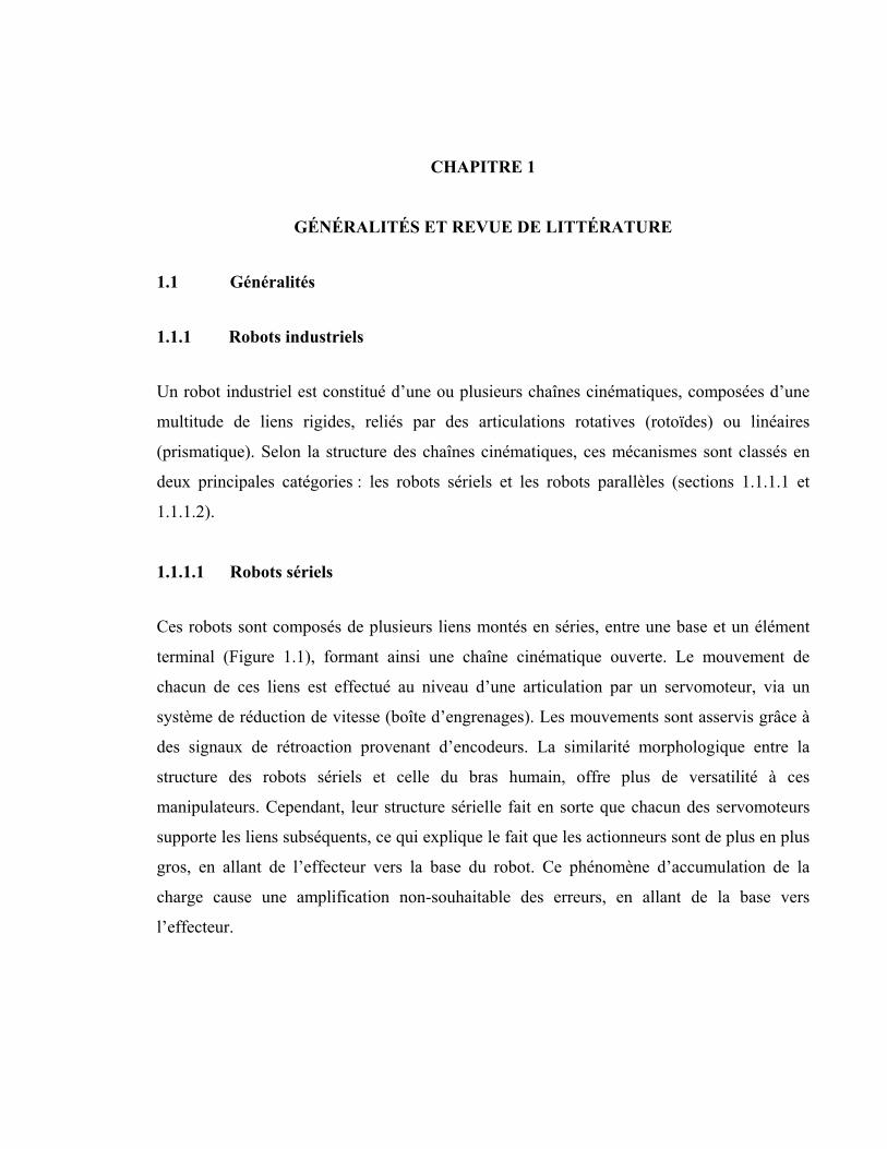
1.1.1.1 Robots sériels
Ces robots sont composés de plusieurs liens montés en séries, entre une base et un élément
terminal (Figure 1.1), formant ainsi une chaîne cinématique ouverte. Le mouvement de
chacun de ces liens est effectué au niveau d’une articulation par un servomoteur, via un
système de réduction de vitesse (boîte d’engrenages). Les mouvements sont asservis grâce à
des signaux de rétroaction provenant d’encodeurs. La similarité morphologique entre la
structure des robots sériels et celle du bras humain, offre plus de versatilité à ces
manipulateurs. Cependant, leur structure sérielle fait en sorte que chacun des servomoteurs
supporte les liens subséquents, ce qui explique le fait que les actionneurs sont de plus en plus
gros, en allant de l’effecteur vers la base du robot. Ce phénomène d’accumulation de la
charge cause une amplification non-souhaitable des erreurs, en allant de la base vers
l’effecteur.
6
(a) (b)
(c)
Figure 1. 1 Robots sériels (a) ABB IRB 2400 (b) KUKA KR 30 jet (c) Stäubli TS80 SCARA
1.1.1.2 Robots parallèles
Ces robots sont composés de plusieurs chaînes cinématiques indépendantes (jambes ou
segments) montées en parallèle. Celles-ci lient la base du manipulateur à son organe
7
terminal, formant par conséquent une chaine cinématique fermée. Cette structure fermée
permet une meilleure répartition des charges du robot sur ses différentes composantes et lui
donne plus de rigidité, tout en restreignant son espace de travail. En outre, la morphologie de
cette catégorie de robots offre une excellente répétabilité et éventuellement, une meilleure
précision, suite à leur étalonnage. Notons ici que le facteur de répétabilité influence
directement la précision après étalonnage.
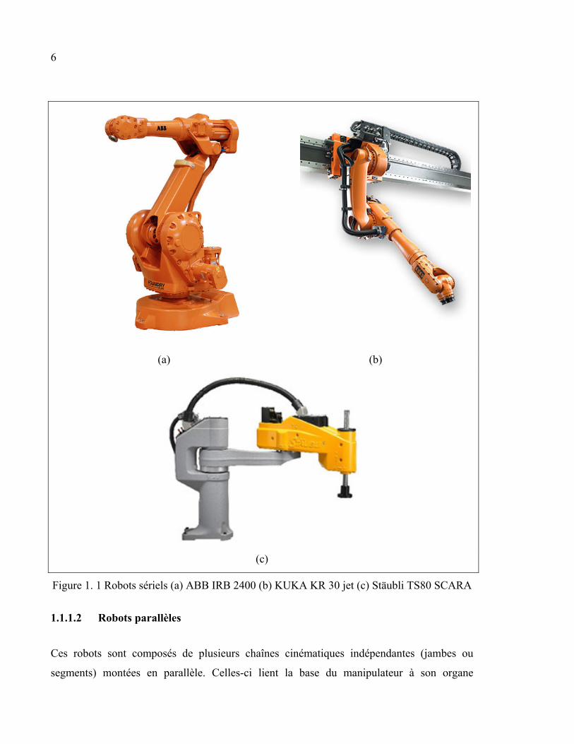
Contrairement aux robots sériels, les articulations des robots parallèles ne sont pas toutes
motorisées (actives); certaines d’entre elles sont passives. Ainsi, pour les mêmes
mouvements commandés aux articulations actives, l’effecteur du robot peut se trouver dans
des positions différentes. La position atteinte varie selon un élément introduit aux équations
du robot : on parle ici du mode d’assemblage. La Figure 1.2 illustre deux modes
d’assemblage pour un robot parallèle à deux ddl dont les articulations actives et passives sont
respectivement (A1, A2) et (B1, B2), alors que l’organe terminal est représenté par C. Le mode
d’assemblage est un coefficient utilisé dans les équations du MGD pour déterminer la
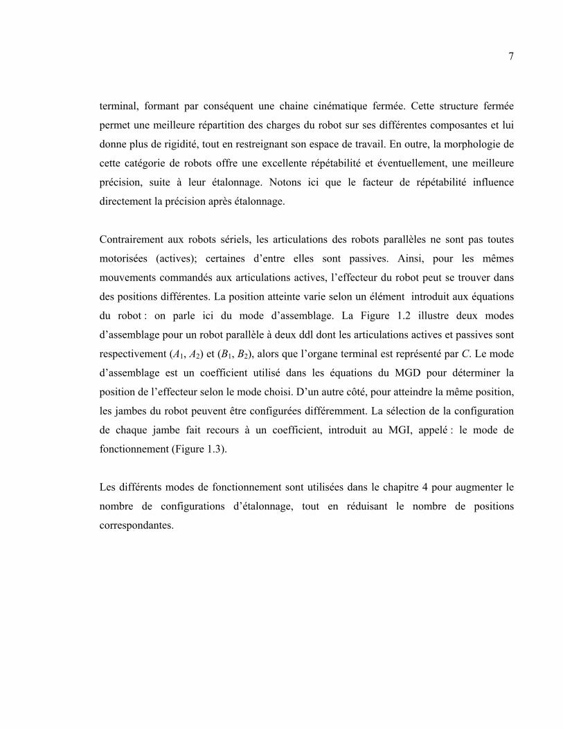
position de l’effecteur selon le mode choisi. D’un autre côté, pour atteindre la même position,
les jambes du robot peuvent être configurées différemment. La sélection de la configuration
de chaque jambe fait recours à un coefficient, introduit au MGI, appelé : le mode de
fonctionnement (Figure 1.3).
Les différents modes de fonctionnement sont utilisées dans le chapitre 4 pour augmenter le
nombre de configurations d’étalonnage, tout en réduisant le nombre de positions
correspondantes.
8
Figure 1.2 Deux différents modes d’assemblage pour les mêmes valeurs articulaires ρ1 et ρ2 d’un robot plan à deux ddl
Figure 1.3 Deux configurations de la jambe gauche pour la même position commandée (x1, y1) pour un robot plan à deux ddl
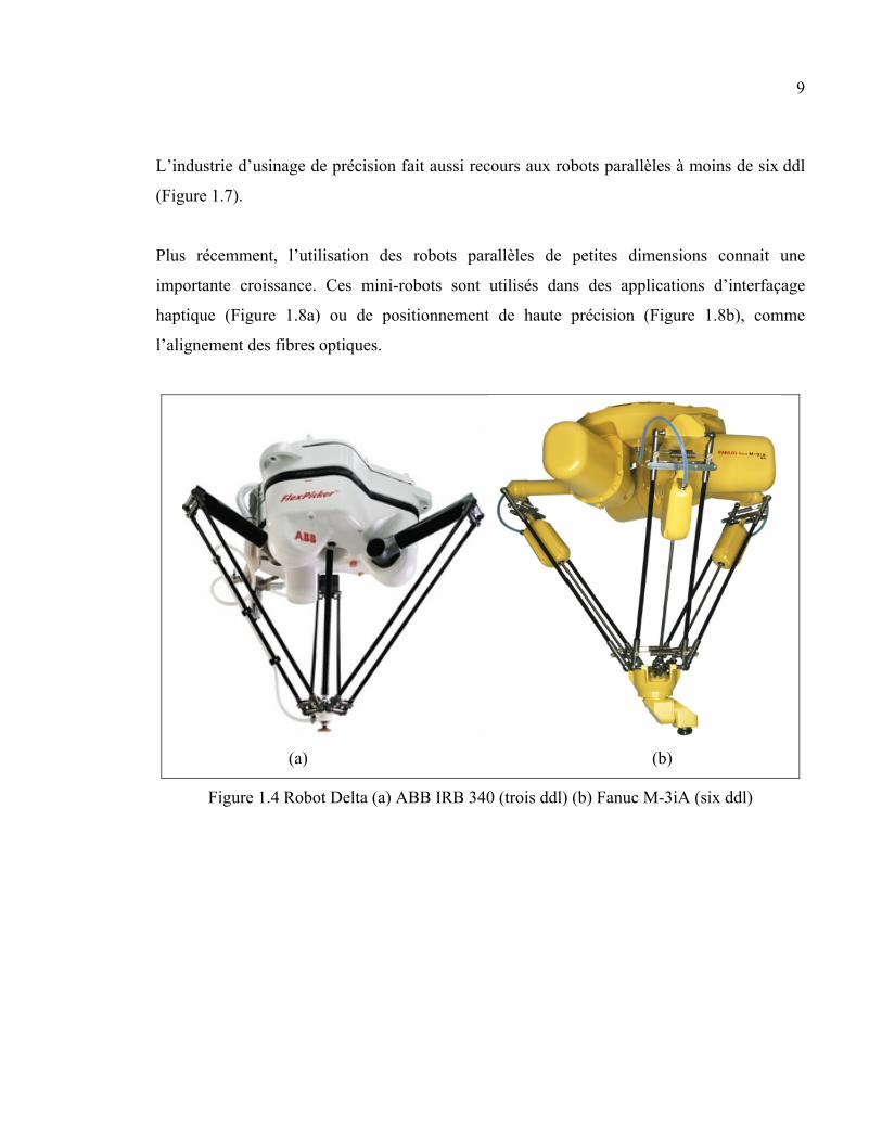
Bien que les robots sériels soient les plus utilisés dans l’industrie, ces dernières années, les
robots parallèles deviennent de plus en plus convoités. Cette croissance d’utilisation se
manifeste surtout dans les domaines qui nécessitent une rapidité élevée d’exécution des
tâches avec le maximum de précision absolue. Citons l’utilisation des robots Delta
(Figure 1.4) pour des applications de pick-and-place (transfert) à très grande vitesse,
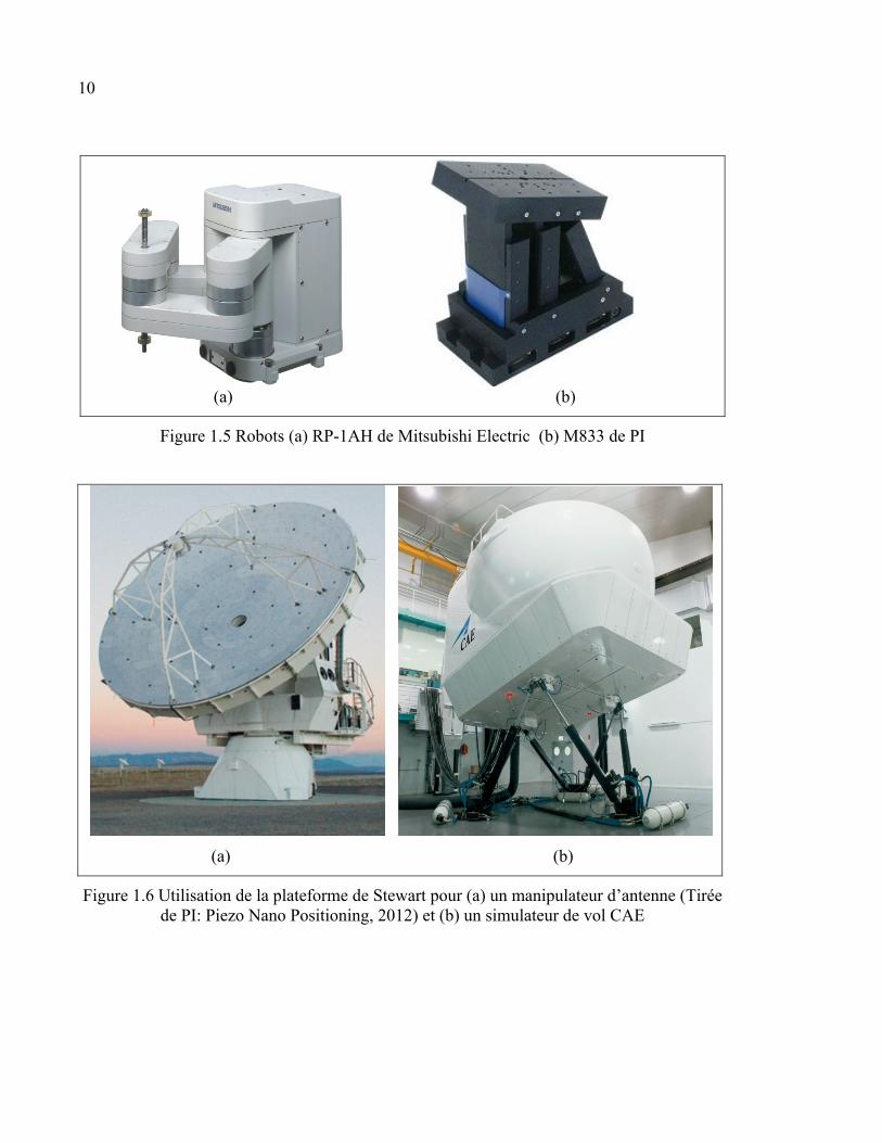
notamment dans les domaines agroalimentaire et pharmaceutique. Les robots plans
(Figure 1.5) sont généralement utilisés pour des opérations de manipulation de très haute
précision, notamment dans le domaine électronique. Les plateformes de Stewart, quant à
elles, sont très populaires, dans les domaines d’orientation de précision des antennes
paraboliques de télécommunication (Figure 1.6a) et des simulateurs de vol (Figure 1.6b).
9
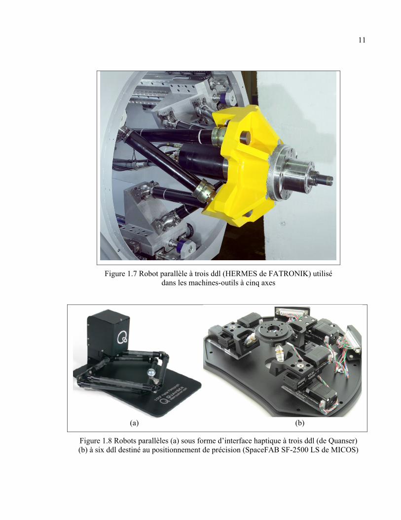
L’industrie d’usinage de précision fait aussi recours aux robots parallèles à moins de six ddl
(Figure 1.7).
Plus récemment, l’utilisation des robots parallèles de petites dimensions connait une
importante croissance. Ces mini-robots sont utilisés dans des applications d’interfaçage
haptique (Figure 1.8a) ou de positionnement de haute précision (Figure 1.8b), comme
l’alignement des fibres optiques.
(a) (b)
Figure 1.4 Robot Delta (a) ABB IRB 340 (trois ddl) (b) Fanuc M-3iA (six ddl)
10
(a) (b)
Figure 1.5 Robots (a) RP-1AH de Mitsubishi Electric (b) M833 de PI
(a) (b)
Figure 1.6 Utilisation de la plateforme de Stewart pour (a) un manipulateur d’antenne (Tirée de PI: Piezo Nano Positioning, 2012) et (b) un simulateur de vol CAE
11
Figure 1.7 Robot parallèle à trois ddl (HERMES de FATRONIK) utilisé dans les machines-outils à cinq axes
(a) (b)
Figure 1.8 Robots parallèles (a) sous forme d’interface haptique à trois ddl (de Quanser) (b) à six ddl destiné au positionnement de précision (SpaceFAB SF-2500 LS de MICOS)
12
1.1.1.3 Comparaison des robots parallèles et sériels
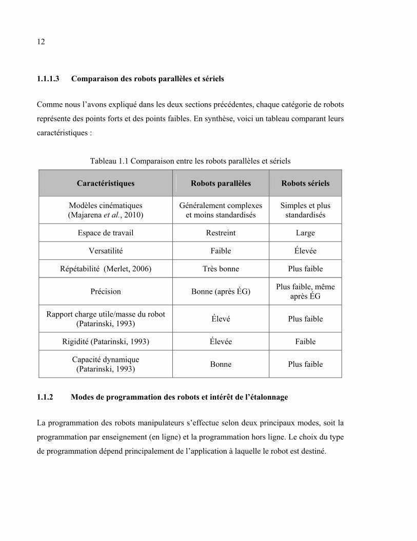
Comme nous l’avons expliqué dans les deux sections précédentes, chaque catégorie de robots
représente des points forts et des points faibles. En synthèse, voici un tableau comparant leurs
caractéristiques :
Tableau 1.1 Comparaison entre les robots parallèles et sériels
Caractéristiques Robots parallèles Robots sériels
Modèles cinématiques (Majarena et al., 2010)
Généralement complexes et moins standardisés
Simples et plus standardisés
Espace de travail Restreint Large
Versatilité Faible Élevée
Répétabilité (Merlet, 2006) Très bonne Plus faible
Précision Bonne (après ÉG) Plus faible, même
après ÉG
Rapport charge utile/masse du robot (Patarinski, 1993)
Élevé Plus faible
Rigidité (Patarinski, 1993) Élevée Faible
Capacité dynamique (Patarinski, 1993)
Bonne Plus faible
1.1.2 Modes de programmation des robots et intérêt de l’étalonnage
La programmation des robots manipulateurs s’effectue selon deux principaux modes, soit la
programmation par enseignement (en ligne) et la programmation hors ligne. Le choix du type
de programmation dépend principalement de l’application à laquelle le robot est destiné.
13
1.1.2.1 Programmation par enseignement (en ligne)
Une des principales raisons qui pourrait expliquer le peu d’intérêt accordé à la précision des
robots, par certaines industries, est l’approche de programmation adoptée. En effet, plusieurs
utilisateurs de robots industriels ne font recours qu’à la méthode de programmation par
enseignement. Cette méthode, appelée communément teach-in, consiste à déplacer
l’effecteur du robot sur plusieurs poses et de les enregistrer au fur et à mesure. Par la suite,
cet ensemble de poses devient la trajectoire du mouvement du robot. Ainsi, les adeptes de
cette méthode sont satisfaits des résultats, à condition que le robot ait une assez bonne
répétabilité pour effectuer ces trajectoires sans trop de variations. Bien que ce type
programmation soit facile, et ne requiert que peu de connaissances en robotique, il n’est
approprié que pour les opérations qui n’exigent pas une précision élevée, comme la soudure
ou la peinture. Par ailleurs, cette approche représente un inconvénient majeur : pendant
l’enseignement des poses de la trajectoire, le robot n’est pas disponible pour la production, ce
qui occasionne des coûts élevés pour les entreprises. En outre, l’utilisation des commandes
manuelles rend la programmation des mouvements de haute précision presqu'impossible.
1.1.2.2 Programmation hors ligne
Pour contrer les désavantages de la programmation par enseignement, il existe une
alternative appelée méthode de programmation hors ligne. Celle-ci consiste à programmer le
robot et simuler ses mouvements en utilisant des logiciels de conception assistée par
ordinateur (CAO) dédiés. Le robot n’est pas physiquement utilisé lors de la programmation,
ne causant aucun arrêt de production. Cette méthode bien qu’avantageuse, particulièrement
dans la phase de conception des cellules robotisées, présente un inconvénient non
négligeable : les résultats obtenus par simulation sont difficiles à reproduire sans erreurs en
pratique. Ce désavantage est attribué principalement au fait que les modèles nominaux des
robots, utilisés dans la simulation, ne correspondent pas parfaitement à leurs modèles réels.
Les différences entre les résultats de la simulation et ceux obtenus affectent la précision des
robots. Pour y remédier, un ÉG est nécessaire. Cette opération permet de rapprocher le
modèle mathématique du modèle réel du robot et d'améliorer ainsi sa précision absolue.
14
En résumé, pour profiter des avantages de la programmation hors ligne, il est nécessaire que
le robot soit doté d’une bonne précision absolue. Ce qui nous amène à définir certains critères
de performance, à la section suivante.
1.1.3 Critères de performance des robots industriels
Les robots industriels ont de multiples caractéristiques. Cependant, ce document ne traite que
de celles qui affectent notre sujet de recherche : l’espace de travail, la répétabilité et la
précision absolue.
1.1.3.1 Espace de travail
D’une manière générale, l’espace de travail d’un robot peut être définit comme étant
l’ensemble des positions pouvant être atteintes par son effecteur, sans passer par des
configurations de singularité. Comme nous l’avons mentionné précédemment, les robots
sériels ont des volumes de travail plus larges que leurs pairs parallèles. La structure sérielle
de ces robots leur permet de couvrir plus d’espace, avec moins de singularités. Toutefois, un
grand espace de travail présente une difficulté : la précision des robots n’est pas uniforme
dans tout cet espace, ce qui rend la tâche d’étalonnage assez complexe. En fait, un étalonnage
destiné à améliorer la précision absolue, ne peut être complètement efficace que s’il couvre
tout l’espace de travail. Dans ce contexte, une comparaison entre trois robots sériels à six ddl
(Romat 310, ABB IRB 6400S et KUKA KR 125) effectuée par Young et al. (2000) a
permis de démontrer que la précision de chacun de ces robots présente des anomalies qui se
manifestent par des irrégularités dans les enveloppes d’essai.
1.1.3.2 Répétabilité de pose
La répétabilité représente l’étroitesse de l’accord entre plusieurs valeurs atteintes pour la
même variable commandée, répétée plusieurs fois dans les mêmes conditions. La répétabilité
de pose est décomposée en deux valeurs, soit la répétabilité de position et celle d’orientation.
15
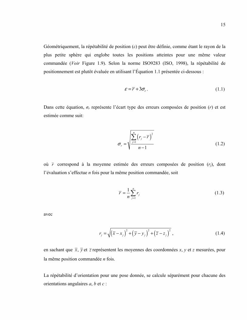
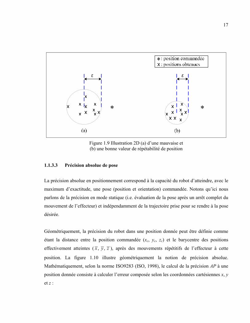
Géométriquement, la répétabilité de position (ε) peut être définie, comme étant le rayon de la
plus petite sphère qui englobe toutes les positions atteintes pour une même valeur
commandée (Voir Figure 1.9). Selon la norme ISO9283 (ISO, 1998), la répétabilité de
positionnement est plutôt évaluée en utilisant l’Équation 1.1 présentée ci-dessous :
3 rrε σ= + . (1.1)
Dans cette équation, σr représente l’écart type des erreurs composées de position (r) et est
estimée comme suit:
( )2
1
1
n
jj
r
r r
nσ =
−=
−
(1.2)
où r correspond à la moyenne estimée des erreurs composées de position (rj), dont
l’évaluation s’effectue n fois pour la même position commandée, soit
1
1 n
jj
r rn =
=
(1.3)
avec
( ) ( ) ( )2 2 2
j j j jr x x y y z z= − + − + − , (1.4)
en sachant que ,x y et z représentent les moyennes des coordonnées x, y et z mesurées, pour
la même position commandée n fois.
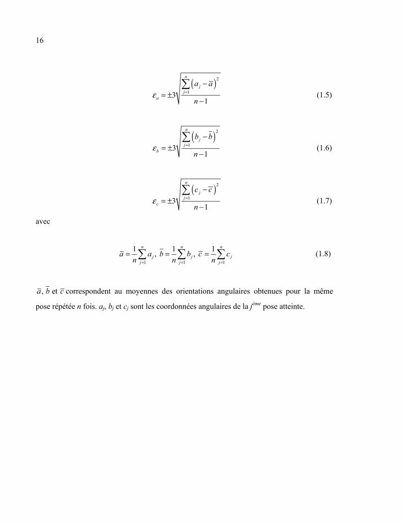
La répétabilité d’orientation pour une pose donnée, se calcule séparément pour chacune des
orientations angulaires a, b et c :
16
( )2
131
n
jj
a
a a
nε =
−= ±
−
(1.5)
( )2
131
n
jj
b
b b
nε =
−= ±
−
(1.6)
( )2
131
n
jj
c
c c
nε =
−= ±
−
(1.7)
avec
1 1 1
1 1 1, ,
n n n
j j jj j j
a a b b c cn n n= = =
= = =
(1.8)
, eta b c correspondent au moyennes des orientations angulaires obtenues pour la même
pose répétée n fois. aj, bj et cj sont les coordonnées angulaires de la jème pose atteinte.
17
Figure 1.9 Illustration 2D (a) d’une mauvaise et (b) une bonne valeur de répétabilité de position
1.1.3.3 Précision absolue de pose
La précision absolue en positionnement correspond à la capacité du robot d’atteindre, avec le
maximum d’exactitude, une pose (position et orientation) commandée. Notons qu’ici nous
parlons de la précision en mode statique (i.e. évaluation de la pose après un arrêt complet du
mouvement de l’effecteur) et indépendamment de la trajectoire prise pour se rendre à la pose
désirée.
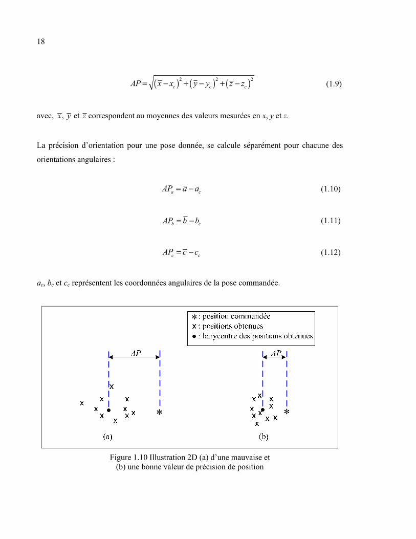
Géométriquement, la précision du robot dans une position donnée peut être définie comme
étant la distance entre la position commandée (xc, yc, zc) et le barycentre des positions
effectivement atteintes ( , ,x y z ), après des mouvements répétitifs de l’effecteur à cette
position. La figure 1.10 illustre géométriquement la notion de précision absolue.
Mathématiquement, selon la norme ISO9283 (ISO, 1998), le calcul de la précision AP à une
position donnée consiste à calculer l’erreur composée selon les coordonnées cartésiennes x, y
et z :
18
( ) ( ) ( )2 2 2
c c cAP x x y y z z= − + − + −
(1.9)
avec,
, etx y z correspondent au moyennes des valeurs mesurées en x, y et z.
La précision d’orientation pour une pose donnée, se calcule séparément pour chacune des
orientations angulaires :
a cAP a a= −
(1.10)
b cAP b b= −
(1.11)
c cAP c c= −
(1.12)
ac, bc et cc représentent les coordonnées angulaires de la pose commandée.
Figure 1.10 Illustration 2D (a) d’une mauvaise et (b) une bonne valeur de précision de position
19
La qualité de précision des robots est un critère important pour plusieurs applications (le
domaine médical, l’usinage de précision…etc.). Toutefois, selon une recherche que nous
avons effectuée auprès de 13 des plus populaires fabricants des robots, ceux-ci insistent sur la
répétabilité dans leurs documents techniques, sans mentionner les valeurs de la précision. En
fait, c’est considéré qu’avec une bonne répétabilité des robots, le manque de précision
pourrait être compensé par l’étalonnage.
Notons que depuis quelques années, certains fabricants de robots manipulateurs développent
et proposent au marché industriel des options préprogrammées destinées à l’étalonnage de
leurs robots. À notre connaissance, et sans vouloir mettre en doute l’efficacité de ces options,
il n’y a pas encore de travaux de recherche qui aient fait état des résultats obtenus. Les
fabricants des instruments de métrologie commencent, eux aussi, à démontrer une attention
particulière à l’amélioration de la précision des robots, en proposant des outils de plus en plus
adaptés aux processus d’étalonnage. Cet intérêt croissant pour l’étalonnage va de pair avec
l’augmentation de la demande pour des robots offrant une précision de qualité. La
section 1.1.4 met en lumière les cas et les applications qui exigent une bonne précision des
robots et évidement là où recourir à l’étalonnage devient un prérequis.
1.1.4 Domaines nécessitant une bonne précision absolue
Un robot doté d’une bonne répétabilité n’est pas nécessairement efficace dans toutes les
tâches qu’on lui demande d’exécuter, s’il n’a pas une bonne précision. En fait, les robots
industriels, par rapport à leur répétabilité, ont une précision faible (Young et al., 2000). Une
telle situation ne cause pas d’inconvénients pour les cas où la programmation est effectuée
selon la méthode traditionnelle, basée sur l’enseignement des poses. Par ailleurs, il existe une
multitude d’applications (Greenway, 2000; THÉSAME, 2012) où la précision des robots a
autant d’importance que leur répétabilité :
• la programmation hors ligne;
• l’interchangeabilité des robots sans devoir refaire l’enseignement des positions;
• l’utilisation d’un robot comme machine à mesurer;
20
• l’utilisation des robots dans les interventions chirurgicales;
• l’utilisation des robots dans l’usinage de précision;
• l’utilisation des robots dans des manipulations de haute précision ;
• la production cellulaire, où plusieurs robots se trouvent dans le même espace de travail.
Une bonne précision permet d’éviter les collisions et de rendre l’ensemble des robots plus
efficace.
1.2 Revue de littérature
Cette section présente un résumé des principaux aspects de l’étalonnage des robots
industriels, de manière générale, et plus spécifiquement des robots parallèles. Les principales
causes de manque de précision seront définies, puis pour y remédier, une présentation des
familles d'étalonnage. Les différentes méthodes d’étalonnage seront expliquées avec une
énumération des étapes de ce processus. Finalement, les difficultés de l’étalonnage sont
présentées en mettant en lumière, notamment, l’analyse d’observabilité des paramètres.
1.2.1 Causes de manque de précision des robots industriels et approches d’étalonnage appropriées
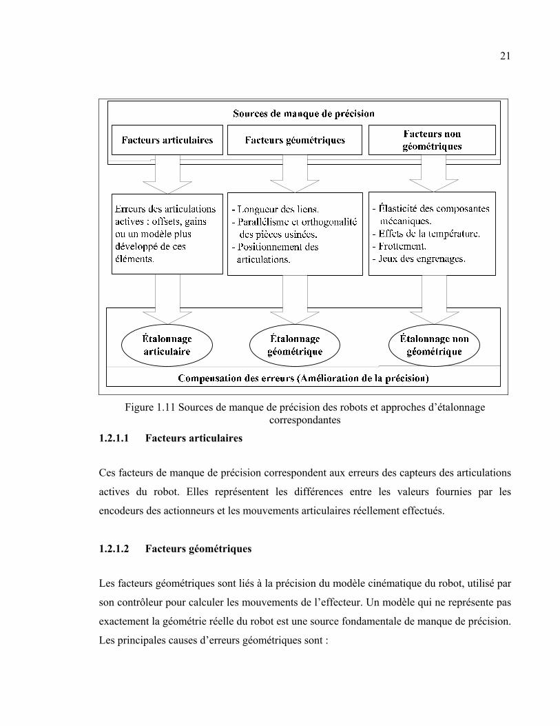
Plusieurs travaux de recherche ont discuté de l’origine des erreurs de poses des robots
industriels (Schroer, 1994; Greenway, 2000). Celles-ci sont attribuées aux erreurs des
articulations actives, à la précision des modèles cinématiques et aux erreurs occasionnées par
les aspects mécaniques des robots. Ces sources d’erreurs, présentées à la Figure 1.11, sont
appelées respectivement, les facteurs articulaires, les facteurs géométriques et les facteurs
non géométriques.
21
Figure 1.11 Sources de manque de précision des robots et approches d’étalonnage correspondantes
1.2.1.1 Facteurs articulaires
Ces facteurs de manque de précision correspondent aux erreurs des capteurs des articulations
actives du robot. Elles représentent les différences entre les valeurs fournies par les
encodeurs des actionneurs et les mouvements articulaires réellement effectués.
1.2.1.2 Facteurs géométriques
Les facteurs géométriques sont liés à la précision du modèle cinématique du robot, utilisé par
son contrôleur pour calculer les mouvements de l’effecteur. Un modèle qui ne représente pas
exactement la géométrie réelle du robot est une source fondamentale de manque de précision.
Les principales causes d’erreurs géométriques sont :
22
• les longueurs nominales des liens différentes des longueurs réelles. Ceci est causé
principalement par les tolérances de fabrication et d’assemblage;
• les caractéristiques géométriques des pièces usinées (parallélisme, orthogonalité, planéité,
etc.);
• le positionnement des articulations liées à la base et à l’élément terminal du robot;
• les erreurs de localisation du référentiel de la base du robot par rapport à celui de la
cellule;
• les erreurs de localisation du référentiel de l’outil sur l’organe terminal.
1.2.1.3 Facteurs non géométriques
Les facteurs non géométriques sont attribués à la qualité des composantes mécaniques du
robot. Ils comptent plusieurs éléments dont voici les principaux :
• l’élasticité des composantes mécaniques;
• les jeux mécaniques, notamment ceux des engrenages;
• les effets de la température.
Bien que tous ces éléments (articulaires, géométriques et non géométriques) contribuent à
dégrader la qualité de la précision des robots, leurs degrés d’impact varient. Plusieurs
recherches démontrent que ce sont les erreurs articulaires et celles d’origine géométrique qui
affectent le plus la précision des robots. Ainsi, selon Judd et Knasinski (1990) et Damak
(1996), les sources de manque de précision sont classées par ordre d’importance comme
suit :
1. les erreurs articulaires (offsets de la position zéro et gains);
2. les erreurs causées par les tolérances d’usinage et d’assemblages (erreurs géométriques);
3. les erreurs non géométriques.
Notons que l’impact des erreurs non géométriques peut augmenter selon les caractéristiques
mécaniques, l’environnement et les conditions d’utilisation du robot en question. Parmi ces
facteurs influents, on peut citer : l’état mécanique des réducteurs de vitesse, les charges
23
manipulées et leur emplacement dans l’espace de travail, la vitesse de fonctionnement et les
configurations adoptées par le robot pour atteindre les poses commandées.
1.2.2 Catégories d’étalonnage
Selon les sources d’imprécision à compenser, Elatta et al. (2004) présentent deux grandes
familles d’étalonnage des robots, soit l’ÉG, destiné à améliorer le modèle cinématique du
robot et l’étalonnage non géométrique qui vise à traiter les erreurs d’origine non
géométrique. Quant aux erreurs articulaires, elles sont généralement incluses dans l’ÉG.
1.2.2.1 Étalonnage géométrique (niveau 2)
Cette approche appelée aussi étalonnage cinématique considère que les liens du robot sont
parfaitement rigides et que celui-ci n’est pas en mode dynamique, c.-à-d. sans considérer
l’impact des mouvements du robot sur sa précision. Par conséquent, l’opération d’étalonnage
consiste à introduire des corrections uniquement sur le modèle cinématique du robot, en
identifiant les valeurs de ses paramètres.
Cette méthode apporte une meilleure amélioration de la précision pour les robots parallèles,
car leurs erreurs non géométriques sont assez faibles, vu la rigidité élevé de leurs structures.
Ceci justifie le fait que la majorité des travaux de recherche destinés à l’étalonnage de cette
catégorie de robots se base sur des approches géométriques, par exemple : Wu et al. (1988),
Oliviers et al. (1995), Masory et al. (1997), Zhuang et al. (1998) et Gatla et al. (2007).
1.2.2.2 Étalonnage non géométrique (niveau 3)
Ce type d’étalonnage, aussi appelé étalonnage non cinématique, est utilisé pour compenser
les erreurs non géométriques. Il consiste à développer des modèles mathématiques pour
compenser ces erreurs. Ces modèles sont souvent très complexes et selon Judd et Knasinski
(1990) et Damak (1996), ils apportent peu d’amélioration à la précision, comparativement à
l’ÉG. Ceci pourrait expliquer la rareté des travaux de recherche effectués dans ce domaine.
24
Néanmoins, effectuer un étalonnage non géométrique après avoir effectué un étalonnage
cinématique pourrait permettre d’atteindre des précisions élevées chez les robots sériels,
notamment (ces derniers étant davantage affectés par les erreurs non géométriques).
Parmi les études disponibles, citons le modèle proposé par Everett (1993), qui se base sur la
modélisation globale des erreurs non géométriques en utilisant les séries de Fourier. D’autres
travaux sont effectués pour modéliser des erreurs spécifiques, comme celles des systèmes
d’engrenage (Judd et Knasinski, 1990) ou encore les erreurs de torsion des liens (Damak,
1996). Gong et al. (2000) présentent une compensation des effets de la température sur la
précision d’un robot sériel à six ddl, en utilisant un modèle empirique d’erreurs thermiques.
Dans d’autres travaux, Oiwa (2002, 2005) procède à la compensation des effets de
déformation causés par la température et par des forces externes sur les liens et la base d’un
robot parallèle.
Mentionnons ici que notre travail de recherche traite exclusivement de l’ÉG et ne couvre pas
les erreurs non géométriques. Ainsi, pour simplifier le texte, le terme étalonnage fera
dorénavant référence à l’étalonnage géométrique et le terme paramètres, aux paramètres
géométriques.
1.2.2.3 Étalonnage articulaire (niveau 1)
Selon Roth et al. (1987), aux deux catégories d’étalonnage citées précédemment, s’ajoute
l’étalonnage dit de niveau 1. Celui-ci consiste à compenser les erreurs des articulations
actives du robot, i.e. modéliser la relation entre les valeurs affichées par les capteurs
(théoriquement les consignes) et les déplacements réels des articulations correspondantes par
rapport à leurs positions zéro (home position). Cependant, dans la majorité des travaux de
recherche, ces erreurs sont traitées dans l’ÉG (niveau 2). À titre d’exemple, Durango et al.
(2010) proposent une méthode d’ÉG d’un robot parallèle cinq-barres qui compense aussi les
erreurs articulaires. Celles-ci ont été, modélisées par l’introduction, dans le modèle
cinématique, d’un gain et un offset à leurs valeurs théoriques.
25
Comme nous l’avons mentionné à la section 1.2.1.3, les erreurs articulaires, et surtout les
offsets de la position zéro, représentent la première source des erreurs de poses. Par
conséquent, certains travaux de recherche procèdent uniquement à l’étalonnage de niveau 1.
Plusieurs d’entre eux n’identifient que les positions zéro des actionneurs (home positions),
plus fréquemment si les actionneurs du robot sont de haute précision : i.e. n’utilisent pas de
réducteurs de vitesse et sont dotés d'encodeurs de très bonne résolution. Dans ce contexte,
Ding et al. (2005) présentent l’étalonnage d’un robot planaire à deux ddl, utilisant des
servomoteurs sans boîtes d’engrenages, en corrigeant uniquement les erreurs des positions
zéro des articulations. Ces mêmes erreurs faisaient l’objet du travail d’étalonnage de
niveau 1 de Zhang et al. (2007) mené sur un robot parallèle redondant à deux ddl. Plus
récemment, l’identification de la position zéro des articulations a été effectuée par Chen et al.
(2008) pour améliorer la précision d’un robot sérial à six ddl. Soulignons que les deux robots
utilisés dans nos études sont dotés de servomoteurs précis, ce qui explique notre choix de
limiter les erreurs des actionneurs uniquement à des offsets.
1.2.3 Méthodes d’étalonnage géométrique
1.2.3.1 Étalonnage par la méthode directe
Cette méthode appelée aussi dans la littérature: méthode en boucle ouverte, consiste à
identifier les paramètres du robot en utilisant les équations du MGD. Cette méthode s’énonce
ainsi :
On commence par commander des mouvements articulaires ρi aux actionneurs du robot, pour
déplacer l’effecteur à une pose commandée XC. Après l’exécution du mouvement, la position
et l’orientation de l’effecteur sont mesurées (pose mesurée XM). En ne tenant pas compte des
erreurs de mesure, idéalement XM et XC doivent être identiques. Cependant, il y’a des
différences qui se manifestent entre ces deux valeurs. Ces erreurs, sont dues au fait que le
MGD utilise les valeurs nominales des paramètres qui sont différentes des valeurs réelles de
ceux-ci. L’objectif est alors de trouver le vecteur vreal des valeurs des paramètres qui
26
minimisent les erreurs de poses (Équation 1.13). Cette opération consiste à minimiser la
sommation des carrés des composantes des erreurs de poses.
Erreurdepose M CX X= −
(1.13)
Notons que XC est exprimée en fonction des ρi (valeurs connues) et des paramètres dont les
valeurs sont à identifier :
real( , )C
iX fct ρ= v
(1.14)
Les seules inconnues de l’équation 1.13 sont donc les paramètres du robot. Par ailleurs, le
nombre de poses nécessaires pour faire l’identification (poses d’étalonnage) est proportionnel
au nombre des paramètres. Le choix de ces poses et de leur nombre n’est pas évident et
nécessite une analyse supplémentaire, appelée étude d’observabilité. Ce volet de
l’étalonnage, largement abordé par les travaux de recherche (Borm et Manq, 1991; Bai et
Teo, 2003; Cong et al., 2006; Majarena et al., 2011), est présenté en détail dans la
section 1.2.5.1.
Comme nous l’avons mentionné précédemment, la méthode directe d’étalonnage nécessite
des informations sur les poses atteintes, après l’exécution des mouvements commandés aux
articulations. Ces données sont obtenues par des mesures effectuées directement sur
l’effecteur, soit d’une manière complète (Cong et al., 2006) ou partielle (Rauf et al., 2004;
Tang et al., 2005). La première méthode consiste à mesurer les positions et les orientations
de l’effecteur du robot, tandis que pour la méthode partielle, uniquement les positions ou les
orientations sont mesurées.
1.2.3.2 Étalonnage par la méthode inverse
Bien que la méthode directe permette d’effectuer un bon étalonnage des robots parallèles,
l'utilisation du MGD rend le processus d’identification des paramètres plus difficile. Cela est
27
dû à la grande complexité des équations du MGD des robots parallèles (Majarena et al.,
2010), notamment ceux dont le nombre de ddl est élevé (Yang et al., 2004). Une deuxième
méthode faisant recours à l’utilisation des équations du MGI est aussi proposée dans la
littérature. Contrairement à la méthode directe, basée sur l’identification des paramètres en
minimisant les erreurs résiduelles de poses, la méthode inverse vise à minimiser les erreurs
des mouvements des articulations. Ainsi, en utilisant une pose de référence connue (évaluée
apriori) XR, les coordonnées articulaires dites commandées Ciρ sont calculées en fonction de
XR (valeurs connues) et des paramètres vreal (valeurs inconnues, à identifier) en utilisant les
équations du MGI :
real( , )C R
i fct Xρ = v
(1.15)
L’identification consiste alors à trouver les valeurs des paramètres qui minimisent la
sommation des carrées des différences entre les Ciρ et les coordonnées articulaires réelles
Riρ , généralement collectés aux près des encodeurs du robot. La réduction de ces erreurs
implique une réduction des erreurs de pose du robot et par le fait même, l’amélioration de sa
précision.
La méthode inverse d’étalonnage est abondamment utilisée, notamment pour les robots
parallèles à six ddl (Zhuang et al., 1998; Daney, 2000; Ting et al., 2007; Agheli et Nategh,
2009). Dans plusieurs travaux de recherche, les valeurs Riρ sont mesurées par les encodeurs
internes du robot, sans faire recours à aucun instrument de mesure externe, d’où l’appellation
auto-étalonnage attribuée à cette approche. On divise l’auto-étalonnage en deux catégories :
• utiliser uniquement les encodeurs des articulations actives et les poses de référence et/ou
appliquer des contraintes géométriques au robot, soit sur l’effecteur ou sur les ddl.
L’étalonnage sous contraintes est détaillé à la section 1.2.3.3;
• utiliser les encodeurs des articulations actives et ajouter des capteurs redondants. Ceux-ci
sont généralement destinés à mesurer les mouvements des articulations passives
28
(Wampler et al., 1995; Zhuang, 1997; Yang et al., 2002). Ces capteurs additionnels sont
utilisés différemment par Patel et Ehmann (2000), en les plaçant sur des jambes
redondantes ajoutées pour étalonner un hexapode.
Daney et Emiris (2001) considèrent que l’étalonnage des robots parallèles par la méthode
inverse est plus robuste que celui en boucle ouverte, car il offre la possibilité de faire des
corrections séparément, pour chacune des jambes. D’un autre côté, la méthode directe est
techniquement plus facile à réaliser, puisque les mesures s’effectuent uniquement au niveau
de l’effecteur. Cependant, en étant basée sur des analyses numériques du MGD, souvent très
complexes pour les robots parallèles, cette méthode représente des faiblesses au niveau de
son efficacité. En fait, les résultats numériques peuvent être divergeant, en présence de bruits
élevés dans les valeurs mesurées. Ainsi, choisir les poses d’étalonnage adéquates (en faisant
recours à une analyse d’observabilité, par exemple) devient indispensable pour éviter ce
problème d’instabilité et avoir des solutions convergentes (Daney et Emiris, 2001).
1.2.3.3 Étalonnage sous contraintes
La résolution des systèmes mathématiques d’étalonnage nécessite un certain nombre de
poses qui doivent être choisies minutieusement, pour réduire l’impact des bruits de mesure et
offrir une meilleure identification des paramètres. En augmentant le nombre de poses
d’étalonnage, le processus d’identification peut être amélioré, à condition que cette opération
ne soit pas aléatoire (voir section 1.2.5.1). Cependant, cette solution accroit le temps de
mesure, ce qui mène à une augmentation des coûts. Pour pallier ce problème, une autre
approche est proposée : enrichir le modèle d’étalonnage avec plus d’informations sur l’état
du robot à chaque pose d’étalonnage. Ainsi, pour le même nombre de poses, on obtient des
équations supplémentaires. Par exemple, pour la même position d’étalonnage, différentes
configurations des articulations peuvent être utilisées. En fait, il s’agit d’appliquer des
contraintes physiques pour ramener l’effecteur exactement à la même position, après le
changement du mode de travail du robot. Cette idée est mise en pratique au chapitre 4.
29
De manière générale, l’étalonnage sous contraintes consiste à ajouter des contraintes
géométriques au robot pour limiter certains de ses mouvements pendant l’opération
d’étalonnage. Ceci peut être réalisé, entre autres, en fixant la position (Daney, 2000; Rauf et
Ryu, 2001; Abtahi et al., 2009) ou l’orientation (Ren et al., 2008; Ren et al., 2009a; Ren et
al., 2009b) de l’effecteur à des valeurs connues, ou en l’obligeant à faire un mouvement
linéaire ou à se déplacer selon un plan prédéfini (Ikits et Hollerbach, 1997; Kim et al., 2006).
Appliquer des contraintes sur les articulations, par exemple, en fixant l’orientation d’un
segment (Khalil et Dombre, 1999) est une autre possibilité.
Dans cette catégorie d’étalonnage, les mesures peuvent être prélevées soit sur l’organe
terminal ou sur les articulations du robot. Selon le type de contraintes appliquées et
l’approche d’étalonnage.
1.2.3.4 Autres méthodes d’étalonnage
Les méthodes classiques d’étalonnage, présentées dans les sections 1.2.3.1, 1.2.3.2 et 1.2.3.3,
sont basées principalement sur des algorithmes d’optimisation dont l’objectif et de minimiser
les erreurs de poses ou des mouvements articulaires. Ces méthodes nécessitent généralement
une analyse d’observabilité pour faire un choix approprié des poses d’étalonnage (voir
section 1.2.5.1). D’autres approches qui ne requièrent pas nécessairement des modèles
d’optimisation et/ou des études d’observabilité sont proposées dans la littérature. Parmi
celles-ci, on trouve des méthodes basées sur l’observation et l’analyse des mouvements des
liens du robot pour effectuer une estimation directe des valeurs des paramètres : Renaud et al.
(2005, 2006) procèdent à l’identification des paramètres en se basant sur l’observation par
caméra des jambes d’un hexapode. Un autre travail effectué par Blaise et al. (2010) consiste
à estimer les paramètres d’une plateforme de Stewart : chacune des articulations effectue des
mouvements rotatifs indépendants et la mesure se prend sur un même point sur le lien
subséquent. Il en résulte une sphère et son centre est identifié. Cette opération est répétée
pour toutes les articulations. Les distances entre les centres correspondent aux paramètres
30
géométriques du robot (longueurs des segments et distances entre les points d’ancrage de la
base ou de la plateforme).
Les méthodes présentées ci-dessus ont recours à des instruments de mesures externes aux
robots. Plus récemment, une méthode basée sur l’exploitation des propriétés géométriques
des robots parallèles a été proposée par Last et Hesselbach (2006) et Last et al. (2007).
Approche innovatrice, elle permet d’identifier les paramètres en exploitant les
caractéristiques des configurations de singularité, sans avoir recours à des mesures externes.
Cependant, elle reste difficile à appliquer dans l’industrie, compte tenu des risques de
l’utilisation des singularités de type 2 (singularités parallèles). Pour éviter ce désavantage,
Last et al. (2008) proposent d’utiliser les singularités de type 1 (singularités sérielles), moins
dommageables pour le robot. Cette méthode est basée sur le changement du mode de travail
de chaque jambe et l’observation des couples des actionneurs, au moment de la manifestation
d’une singularité du type 1 (un couple maximum correspond alors à la configuration de
singularité).
1.2.4 Procédure d’étalonnage
L’étalonnage des robots industriels s’effectue en suivant quatre principales étapes (Roth et al.
1987; Elatta et al., 2004), soit la modélisation, la prise des mesures, l’identification des
paramètres et finalement, la compensation des erreurs. Ces étapes sont présentées en détail
dans les sections subséquentes.
1.2.4.1 Modélisation
La modélisation consiste à créer un modèle mathématique qui doit être le plus proche
possible du modèle réel du robot. Dans plusieurs cas, de nouveaux paramètres (initialement
négligés) sont ajoutés au modèle nominal du robot. Cette opération est l’élément clé de l’ÉG,
puisque celui-ci vise à améliorer le modèle géométrique du robot. Les modèles les plus
abordés dans la littérature sont ceux des robots sériels : modèle de Denavit-Hartenberg (D-
H). Ce dernier est utilisé par Veitschegger et al. (1987) dans une méthode d’étalonnage qui
31
présente la précision absolue sous forme d’un modèle mathématique linéaire destiné à
compenser les erreurs de poses. D’autres chercheurs introduisent un (Chen et al., 2001) ou
deux (Stone, 1987; Zhuang et Roth, 1992) nouveaux paramètres à ce modèle pour contourner
ses singularités et améliorer le processus d’étalonnage. Le modèle D-H est aussi utilisé par
certains auteurs pour étalonner des robots parallèles. Parmis d’autres, Yang et al. (2009) et
Feng et al. (2011) ont utilisé les paramètres D-H pour étalonner deux robots parallèles
distincts, soit un mécanisme 6-PRRS et un 6-PPPS (voir la note à la fin de cette section).
Les modèles cinématiques des robots parallèles les plus populaires sont ceux de la plateforme
de Stewart, appelée aussi plateforme de Gough, (Oliviers et al., 1995; Masory et al., 1997;
Zhuang et al., 1998; Cong et al., 2006; Kim et al., 2006; Ting et al., 2007). Il s’agit d’un
hexapode couramment intégré dans les simulateurs de vol et les machines-outils à commande
numérique (catégorie des fraiseuses), comme celle étalonnée par Kim et al., (2006). Les
robots parallèles à moins de six ddl font l’objet de certains travaux (Wang et Fan, 2004; Ding
et al., 2005; Durango et al., 2010; Majarena et al., 2011), quoique moins nombreux que ceux
à six ddl. Ceux-ci ont des structures géométriques, et par le fait même, des modèles
mathématiques très diversifiés (Majarena et al., 2010). Dans ce contexte, une classification
des types des robots parallèles par nombre de ddl est élaborée par Nielsen et Roth (1999) et
Merlet (2006).
Note : Dans le domaine de la robotique parallèle, la description de la géométrie d’un robot
est souvent représentée par un chiffre suivi d’une série de lettres. Le chiffre correspond au
nombre de ddl, alors que les lettres symbolisent la succession des types d’articulations d’une
jambe, en partant de la base vers la plateforme. Ces lettres sont P, R, S et U qui
correspondent respectivement à des articulations prismatiques, rotoïdes, sphériques et
cardans (universal joint). Finalement, certaines notations distinguent les articulations actives
par un souligné.
32
1.2.4.2 Mesures
Cette étape consiste à collecter les données qui serviront à l’identification des valeurs des
paramètres du robot à étalonner. Pour ce faire, deux approches de mesures sont utilisées :
• Mesures internes : cette approche utilise les capteurs internes du robot, qui sont destinés
habituellement à son fonctionnement normal. Ces capteurs, principalement des encodeurs,
sont installés sur les articulations actives du robot. Des capteurs additionnels (redondants)
peuvent être utilisés, pour des fins d’étalonnage. Dans la majorité des cas, les capteurs
redondants sont installés sur les articulations passives (Wampler et al., 1995; Zhuang, H.
1997; Yang et al., 2002) pour obtenir des données suffisantes pour l’étalonnage. Selon
Hollerbach et Wampler (1996), pour que l’identification des paramètres soit possible, il
faut que le nombre total des capteurs des articulations (incluant les capteurs redondants)
soient plus élevé que le nombre des ddl du robot à étalonner. Deux principaux types de
capteurs sont utilisés, soit les capteurs angulaires (Wampler et al., 1995; Zhuang, 1997) et
linéaires. Ceux-ci sont destinés respectivement à la mesure des angles, pour les
articulations rotoïdes, et des distances, pour les articulations prismatiques. Reste à noter
que la résolution de ces capteurs affecte la qualité d’étalonnage. Dans ce contexte,
Hesselbach et al. (2005) proposent un algorithme pour déterminer la résolution nécessaire
des capteurs en fonction de la précision ciblée par le processus d’étalonnage.
• Mesures externes : des appareils de mesures externes au robot sont utilisées. Les
informations fournies par ces instruments sont sous formes de coordonnées cartésiennes.
Ces mesures permettent d’obtenir la position et l’orientation de l’effecteur du robot, dans
chaque configuration d’étalonnage. L’utilisation de cette approche nécessite de choisir
judicieusement l’instrument de mesure. Idéalement, l’incertitude de mesure de
l’instrument en question doit être quatre fois1 meilleure que la répétabilité du robot à
1 Selon la norme ISO9283 (ISO, 1998), l’incertitude de mesure totale doit être quatre fois meilleure que la caractéristique à vérifier (représentée, dans notre cas, par la répétabilité du robot).
33
étalonner; en procédant à l’étalonnage d’un robot, la meilleure précision qu’on puisse
obtenir est la valeur de sa répétabilité.
Les instruments des mesures externes fournissent des informations absolues (coordonnées
cartésiennes) ou relatives (des distances ou des angles). Pour la méthode la plus courante,
soit la mesure des coordonnées cartésiennes, on retrouve les appareils de poursuite laser
(Gong et al., 2000; Meng et al., 2003, Corbel et al., 2006; Blaise et al., 2010; Feng et al.,
2011), les caméra CCD (Motta et al., 2001; Watanabe et al., 2006), les capteurs optiques
de mesure de position ( Bai et Teo, 2003) et les CMM (Borm et Manq, 1991; Cong et al.,
2006; Majarena et al., 2011). Pour les mesures relatives, on retrouve l’interféromètre laser
(Majarena et al., 2011), les télémètres laser (Liu et al., 2010), les gauges de distance
(Abtahi et al., 2010), les barres à billes (Ota et al., 2000; Kim, 2005) les inclinomètres
(Besnard et Wisama, 1999; Ren et al., 2009a; Ren et al., 2009b) et les théodolites (Berg,
1992; Schroer, 1994). Notons qu’une combinaison de deux théodolites peut permettre des
mesures absolues (Berg, 1992; Schroer, 1994).
1.2.4.3 Identification
Les paramètres utilisés dans les équations cinématiques du robot sont affectés par des erreurs
qui rendent leurs valeurs réelles différentes des valeurs théoriques (nominales). L’étape
d’identification consiste à déterminer les valeurs « réelles » de ces paramètres. Étant donné
que les modèles d’étalonnage sont souvent non linéaires, la résolution de ces problèmes (i.e.
l’identification) est effectuée en utilisant des algorithmes d’optimisation dédiés, dont les plus
connus sont les suivants :
• méthode de Levenberg-Marquardt;
• méthode de Newton-Gauss;
• méthode du gradient;
• méthode des directions conjuguées.
34
Plus récemment, certaines études utilisent des approches de résolution basées sur
l’intelligence artificielle, utilisant des méthodes métaheuristiques stochastiques
d'optimisation. Parmi celles les plus utilisées, citons les algorithmes génétiques (Liu et al.,
2007), les réseaux neurones (Zhang, 2011; Zhang et al., 2011) et les algorithmes à évolution
différentielle (Liu et al., 2010). Notons que ces méthodes requièrent d’excellentes
connaissances en optimisation avancée, ce que très peu d’ingénieurs en robotique maitrisent.
De notre point de vue, cela défavorise leur implantation à grande échelle dans l’industrie. Par
ailleurs, l’utilisation de ces approches n’est vraiment justifiée que si le modèle d’étalonnage
est très complexe, hautement non linéaire et/ou discontinu. Ceci peut être éventuellement
causé par l’introduction de plusieurs erreurs non géométriques à un modèle déjà complexe,
comme dans le cas de l’étude effectuée par Zhang (2011).
Au lieu de résoudre le problème d’identification en utilisant des modèles non linéaires, il est
aussi d’usage de procéder à la linéarisation de ceux-ci avant de les résoudre numériquement,
comme le travail effectué par Cheng et al. (2011). Cette approche (linéarisation puis
résolution numérique) est utilisée dans le chapitre 4 de la présente recherche, pour
l’étalonnage d’un robot planaire à deux ddl.
Selon l’approche d’étalonnage utilisée, le processus d’identification consiste à trouver les
valeurs des paramètres qui minimisent les erreurs de poses ou des mouvements articulaires.
Ces deux approches sont utilisées respectivement pour la méthode directe d’étalonnage et la
méthode inverse. L’utilisation des valeurs identifiées des paramètres n’implique pas que les
erreurs de pose après étalonnage soient nulles (même si les erreurs non géométriques sont
nulles). En fait, l’incertitude de l’instrument de mesure affecte la précision d’identification
des paramètres. Cet impact est analysé par Jokiel Jr. et al. (2001) en utilisant la méthode de
Monte-Carlo, pour évaluer l’incertitude de la précision après étalonnage d’une plateforme de
Stewart à partir des incertitudes des paramètres identifiés, causées principalement par les
erreurs de mesure lors de l’étalonnage.
35
1.2.4.4 Compensation
Cette dernière étape consiste à instaurer le modèle corrigé du robot dans son contrôleur, en
utilisant les paramètres évalués par le processus d’identification. Ce modèle est considéré
comme étant le plus représentatif et le plus près du modèle réel du robot à étalonner. Son
utilisation permettra de compenser les erreurs et améliorer, par conséquent, la précision du
robot. Savoure et al. (2006) proposent une méthode de compensation qui utilise les poses
commandées et les valeurs estimées des paramètres pour faire une approximation linéaire des
erreurs articulaires. Ces erreurs sont, par la suite, introduites aux valeurs articulaires
calculées par le modèle nominal du robot, pour compenser les erreurs de pose.
Dans plusieurs cas le code source du contrôleur du robot n’est pas libre (open source), pour
qu’on puisse y apporter les modifications nécessaires suite à l’étape d’identification. La
solution qui s’offre est d’utiliser un système intermédiaire qui permet de calculer une pseudo-
pose commandée pXC (fake pose) qui va être commandée au contrôleur du robot pour que
l’effecteur atteigne la vraie pose commandée vXC. Ce système fonctionne comme suit :
(1) calculer les valeurs articulaires, en utilisant vXC et les valeurs identifiées des paramètres;
(2) calculer pXC, en utilisant les valeurs articulaires et les valeurs nominales des paramètres.
Finalement les valeurs de pXC sont commandées au robot.
1.2.5 Difficultés de l’étalonnage
Bien que l’étalonnage des robots soit traité par un grand nombre de chercheurs, cette
opération présente encore certaines difficultés. Les sections suivantes présentent les
principaux défis rencontrés dans ce domaine.
1.2.5.1 Choix des poses d’étalonnage et de leur nombre
Comme nous l’avons expliqué antérieurement, l’identification des paramètres par les
méthodes classiques nécessitent un certain nombre de poses d’étalonnage. La localisation de
ces poses doit être choisie de manière à rendre les paramètres plus identifiables et à réduire
36
l’impact des bruits de mesure sur le processus d’identification. Pour ce faire, une étude
d’observabilité s’avère nécessaire. Cette analyse consiste à répondre aux principales
questions suivantes :
• Où les poses d’étalonnage (qui seront choisies) se localisent-elles ?
• Quel est le nombre juste nécessaire de poses d’étalonnage, pour une identification efficace
des paramètres ?
Pour répondre à ces deux objectifs, des indices d’observabilité sont utilisés. Ainsi, les poses
d’étalonnage sont choisies dans l’espace du travail du robot, en vue d’améliorer l’indice (ou
les indices) d’observabilité. Cette amélioration implique que les paramètres soient mieux
identifiés (c.-à-d. mieux observables). Puisque le nombre de poses requis est proportionnel au
nombre de paramètres à identifier, il s’agit de déterminer le nombre optimal. Pour se faire, il
faut trouver la valeur à partir de laquelle l'indice d'observabilité tend vers la stabilité. Pour
visualiser ce phénomène, des graphiques d’indices d’observabilité sont utilisés (Figure 4.6).
Ces courbes présentent l’indice d’observabilité en fonction du nombre de poses d’étalonnage.
Le nombre optimal de poses est celui à partir duquel l’amélioration de l’indice
d’observabilité devient négligeable. Une augmentation supplémentaire du nombre des poses
ne fait qu’allonger la durée du processus de prise de mesures et de traitement des données,
sans amélioration significative dans l’exactitude d’identification des paramètres (c.-à-d. sans
amélioration considérable de la précision du robot).
Cinq indices d’observabilité (O1 … O5) sont présentés dans la littérature. Ils sont issus de
l’analyse de la décomposition en valeurs singulières (SVD) de la matrice Jacobienne
d’indentification J. Cette dernière représente les dérivées des équations de la cinématique
(équations utilisées dans le processus d’étalonnage) par rapport au vecteur des paramètres à
identifier au voisinage des poses d’étalonnage. La matrice J représente le lien entre les
erreurs dX des poses d’étalonnage et les erreurs des paramètres Δ :
Δd =X J
(1.16)
37
Dans cette section, nous considérons que tous les paramètres sont identifiables et
indépendants, c.-à-d. la matrice D de l’analyse SVD génère un nombre n des valeurs
singulières σi non nulles (rang = n) égal au nombre des paramètres à identifier :
1
2
0 0 0
0 0 0
0 0 0
0 0 0
0 0 0 0
0 0 0 0
n
σσ
σ
=
D
(1.17)
Le nombre de lignes de D correspond au nombre d’équations utilisées pour l’étalonnage et le
nombre de colonnes représente le nombre de paramètres à identifier. Par exemple, dans le cas
d’un robot à trois ddl, la dimension de D sera3m n× , où m correspond au nombre de poses
d’étalonnage.
Les σi nous fournissent de l’information sur la capacité du système mathématique à identifier
les paramètres. Le fait que les σi changent de valeurs selon les poses d’étalonnage explique
l’importance de bien choisir ces poses. Ainsi, les indices d’observabilité nous permettent de
faire des liens quantifiables entre les poses d’étalonnages, et par le fait même les valeurs des
σi, d’un côté et l’efficacité d’identification des paramètres de l’autre. Les formules
mathématiques de calcul des indices d’observabilité sont présentées dans les paragraphes qui
suivent. Pour donner plus de sens à ces calculs, nous présentons leurs significations
géométriques.
Selon Menq et al. (1989), si toutes les valeurs singulières σi sont différentes de zéro (c’est
notre hypothèse, citée ci-haut), les erreurs des paramètres Δ sont observables à partir des
erreurs mesurées dX des poses d’étalonnage. Géométriquement, en considérant que le
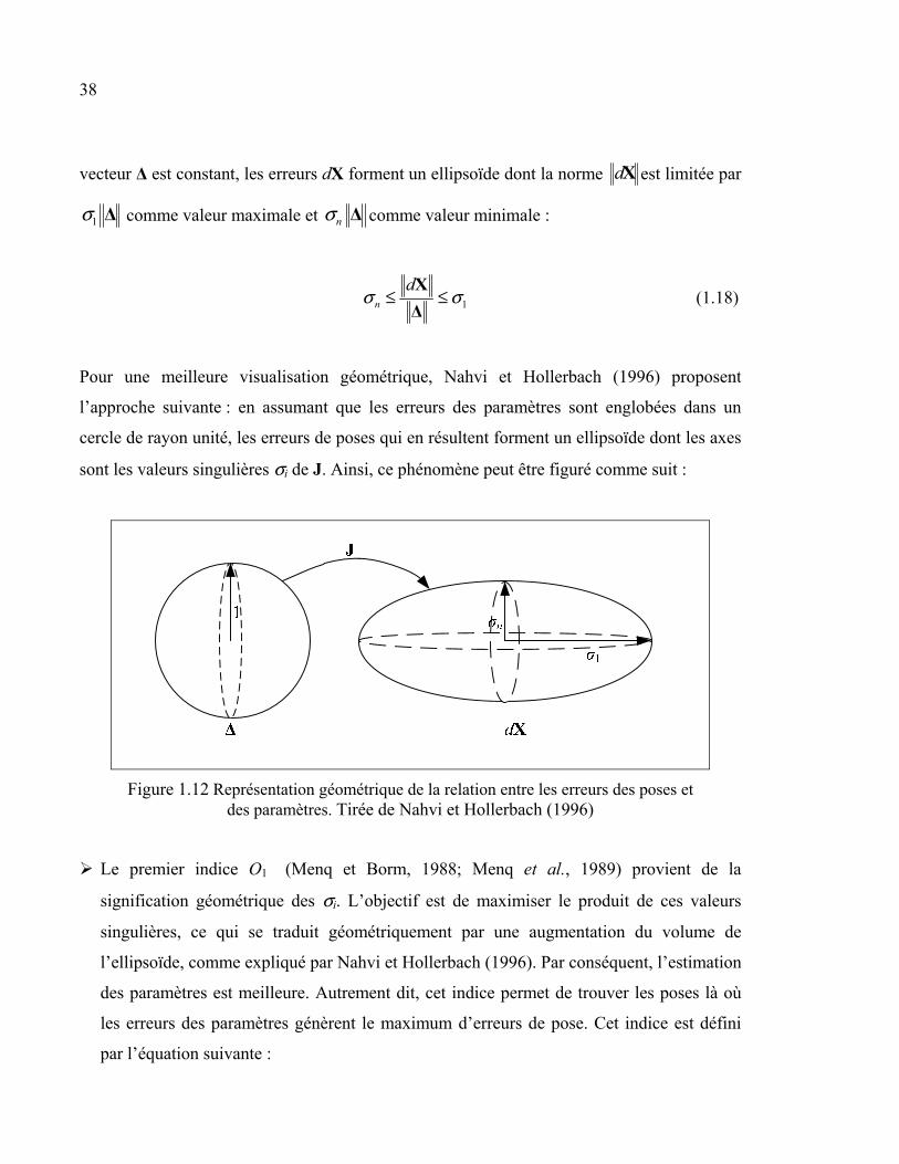
38
vecteur Δ est constant, les erreurs dX forment un ellipsoïde dont la norme dX est limitée par
1σ Δ comme valeur maximale et nσ Δ comme valeur minimale :
1n
dσ σ≤ ≤
X
Δ (1.18)
Pour une meilleure visualisation géométrique, Nahvi et Hollerbach (1996) proposent
l’approche suivante : en assumant que les erreurs des paramètres sont englobées dans un
cercle de rayon unité, les erreurs de poses qui en résultent forment un ellipsoïde dont les axes
sont les valeurs singulières σi de J. Ainsi, ce phénomène peut être figuré comme suit :
Figure 1.12 Représentation géométrique de la relation entre les erreurs des poses et des paramètres. Tirée de Nahvi et Hollerbach (1996)
Le premier indice O1 (Menq et Borm, 1988; Menq et al., 1989) provient de la
signification géométrique des σi. L’objectif est de maximiser le produit de ces valeurs
singulières, ce qui se traduit géométriquement par une augmentation du volume de
l’ellipsoïde, comme expliqué par Nahvi et Hollerbach (1996). Par conséquent, l’estimation
des paramètres est meilleure. Autrement dit, cet indice permet de trouver les poses là où
les erreurs des paramètres génèrent le maximum d’erreurs de pose. Cet indice est défini
par l’équation suivante :
39
( )1
1 21
... mmO
n
σ σ σ=
(1.19)
Avec, m et n représentent respectivement le nombre des poses d’étalonnage et le nombre
des paramètres à identifier.
Le deuxième indice proposé par Driels et Pathre (1990) représente l’inverse du nombre de
conditionnement de J. La maximisation de cet indice consiste à uniformiser les valeurs
des σi. Ce qui signifie géométriquement une amélioration de l’excentricité de l’ellipsoïde.
Par ailleurs, maximiser cet indice entraîne une minimisation du nombre de
conditionnement, ce qui implique une réduction de l’impact des bruits de mesures sur
l’identification des paramètres. Cet indice est défini par l’équation suivante :
min2
max
Oσσ
=
(1.20)
Le troisième indice est introduit par Nahvi et Hollerbach (1996). Il correspond tout
simplement à la valeur singulière minimale. Cette idée est issue de l’analyse de
l’Équation 1.18 dont la première inégalité permet d’écrire :
n dσ ≤Δ X
(1.21)
En sachant que Δ est un vecteur de constantes, une analyse rapide de l’Équation 1.21
permet de constater que plus la valeur singulière minimale (σn ≡ σmin) de J est grande,
plus les erreurs de poses deviennent importantes. L’objectif est alors de maximiser cet
indice. Ceci revient à dire géométriquement que nous cherchons à élargir le plus petit axes
de l’ellipsoïde des erreurs de poses. Gardons à l’idée que l’élargissement du volume de
l’ellipsoïde implique que les poses choisies soient plus sensibles aux erreurs des
paramètres. Ce troisième indice est défini par l’équation suivante :
40
3 min nO σ σ= =
(1.22)
Nahvi et Hollerbach (1996) ont démontré que dans certains cas, l’utilisation séparée des
trois premiers indices d’observabilité peut porter à confusion, en donnant des résultats
contradictoires dans le choix du set optimal des poses d’étalonnage. Pour pallier cet
inconvénient, ces auteurs proposent le quatrième indice, issu d’une multiplication des
indices O2 et O3. Par conséquent, géométriquement, l’axe minimal de l’ellipsoïde des
erreurs de poses sera plus grand et l’axe maximal sera plus petit (i.e. une meilleure
excentricité). Cet indice est défini par l’équation suivante :
2min
4max
Oσσ
=
(1.23)
Ce quatrième indice est aussi appelé indice d’amplification du bruit; sa valeur nous donne
des indications sur l’amplification des bruits de mesures et des erreurs non modélisées.
Selon les auteurs qui l’ont proposé, une augmentation de la valeur de cet indice mène à
une meilleure précision du processus d’identification.
Le cinquième indice est proposé par Sun et Hollerbach (2008), en se basant sur la
minimisation de la somme des inverses des σi :
1
1min
n
i iσ=
(1.24)
Cette minimisation se traduit par une maximisation de l’inverse de cette sommation.
L’objectif est alors de maximiser O5 :
41
5
1 2
11 1 1
m
O
σ σ σ
=+ + +
(1.25)
En résumé, cet indice représente la moyenne harmonique de toutes les valeurs singulières
divisée par le nombre de paramètres à identifier. L’objectif géométrique de cet indice est
similaire à celui de O1 qui consiste à élargir le volume de l’ellipsoïde, ce qui se traduit par
une augmentation de la sensibilité des poses d’étalonnage aux erreurs des paramètres.
Pour plus de détails sur chacun de ces indices, le lecteur est référé aux travaux qui les ont
proposées, citées antérieurement. Ces cinq indices sont analysés en détail et comparés
mathématiquement par Sun et Hollerbach (2008); une autre comparaison, des mêmes indices,
a été produite par Horne et Notash (2009) en utilisant des simulations appliquées sur un robot
à deux ddl.
Suivant la présentation et l’explication des différents indices d’observabilité des paramètres,
voici un survol du processus de sélection des poses d’étalonnage où ces indices sont utilisés.
Sommairement, ce processus consiste à choisir une pose à la fois parmi un ensemble de poses
potentielles (candidats), en utilisant des algorithmes de sélection. À chaque itération,
l’algorithme de sélection ajoute une pose qui améliore au mieux l’indice d’observabilité
utilisé. L’algorithme cesse les opérations de sélection après un certain nombre d’itérations
prédéfinies ou après avoir atteint un nombre de poses après les quelles l’indice
d’observabilité tend vers la stabilité. Les algorithmes de sélection peuvent être basés sur
l’utilisation d’un ou plusieurs indices. À titre d’exemple, Daney et al. (2005) proposent une
procédure de sélection basée sur la recherche tabou, en maximisant conjointement les quatre
premiers indices d’observabilité. Cette approche est validée en utilisant une plateforme de
Stewart. Les mêmes indices sont utilisés ultérieurement par Li et al. (2011) pour trouver les
meilleures configurations d’étalonnage d’un robot serial à six ddl.
42
1.2.5.2 Détection de sources majeures d’imprécision des robots
L’amélioration de la précision des robots, en se basant sur leurs modèles géométriques,
rencontre une difficulté considérée importante par certains auteurs. Ce problème
d’étalonnage cinématique, est caractérisé par la difficulté de détecter les sources majeures de
l’imprécision du robot, pour ainsi se concentrer sur leur modélisation. En fait, dans plusieurs
cas, on risque d’utiliser plusieurs sources d’imprécision à la fois, ce qui présente une certaine
redondance des paramètres et une éventuelle complexité inutile du modèle (Mooring et
Padavala, 1989). Notons que des modèles cinématiques plus complexes peuvent améliorer la
précision, malgré que les paramètres utilisés n’aient pas tous un impact significatif sur cette
amélioration, ou certains d’entre eux sont redondants.
1.3 Conclusion
Dans ce chapitre, nous avons d’abord présenté des notions de bases de la robotique
industrielle liées avec le sujet de notre travail de recherche. En second lieu, une revue de
littérature sur l’étalonnage des robots a été élaborée. En raison du grand nombre de travaux
publiés à ce sujet, il s’avère très difficile de couvrir tout les aspects traités dans ces
publications. Par conséquent, notre revue de littérature se veut une synthèse des aspects les
plus importants : les sources de manque de précision, les principales méthodes d’étalonnage
pour y remédier et l’analyse d’observabilité des paramètres, destinée à améliorer la qualité du
processus d’identification. En se basant sur ce résumé de la littérature existante, on peut
constater que la majorité des publications traitent des robots sériels. En seconde place, on
trouve les robots parallèles à six ddl (les hexapodes). Les travaux dédiés aux robots parallèles
à moins de six ddl sont plutôt rares, malgré qu’ils soient de plus en plus utilisés dans
plusieurs domaines. C’est justement cette catégorie des robots qui représente la cible de notre
travail de recherche.
CHAPITRE 2
ARTICLE1: A NOVEL XY-THETA PRECISION TABLE AND A GEOMETRIC PROCEDURE FOR ITS KINEMATIC CALIBRATION
Ahmed Joubair, Mohamed Slamani and Ilian A. Bonev
École de technologie supérieure, 1100, Notre-Dame Street West, Montreal, QC, H3C 1K3,
Canada
This chapter has been published as an article in
Robotics and Computer-Integrated Manufacturing: vol. 28, n° 1 (2012) p. 57-65
Résumé
Les dispositifs de positionnement de précision dans l’espace sont souvent basés sur les robots
parallèles, mais quand il s’agit du positionnement planaire, l’architecture sérielle est
pratiquement l’unique solution disponible dans l’industrie. Le problème avec les robots
parallèles est que plus ils sont couplés, plus il est difficile de les contrôler et ils ont un espace
de travail assez restreint, comparativement aux robots sériels. Cet article présente un nouvel
robot partiellement découplé, capable d’exécuter des mouvements de précision et ayant un
espace de travail relativement large. La nouveauté de ce robot parallèle réside dans son
habilité à atteindre l'état découplé en utilisant les jambes d'une structure cinématique
différente. La répétabilité du robot est évaluée en utilisant une CMM et elle est équivalente
aux erreurs des vis sans fin de ses actionneurs. Une simple méthode géométrique est
proposée pour identifier directement les référentiels de la base et de la plateforme du robot,
deux offsets des actionneurs et un paramètre sous forme d’une distance. Ceci en utilisant un
bras articulé de mesure de la compagnie FARO Technologies. Bien que cette méthode n’est
pas la plus efficace, elle donne une amélioration satisfaisante de la précision du robot, sans la
nécessité d’avoir des connaissances dans le domaine de l’étalonnage des robots. Une
validation expérimentale montre que la précision de position obtenue après calibration est
meilleure que 0,339 mm à l’intérieur d’un espace de travail d'environ 150 mm × 200 mm.
44
Abstract
Spatial precision positioning devices are often based on parallel robots, but when it comes to
planar positioning, the well-known serial architecture is virtually the only solution available
to industry. Problems with parallel robots are that most are coupled, more difficult to control
than serial robots, and have a small workspace. In this paper, new parallel robot is proposed
which can deliver accurate movements, is partially decoupled and has a relatively large
workspace. The novelty of this parallel robot lies in its ability to achieve the decoupled state
by employing legs of a different kinematic structure. The robot repeatability is evaluated
using a CMM and so are the actual lead errors of its actuators. A simple geometric method is
proposed for directly identifying the actual base and mobile reference frames, two actuator’s
offsets and one distance parameter, using a measurement arm from FARO Technologies.
While this method is certainly not the most efficient one, it yields a satisfactory improvement
of the robot accuracy without the need for any background in robot calibration. An
experimental validation shows that the position accuracy achieved after calibration is better
than 0.339 mm within a workspace of approximately 150 mm × 200 mm.
2.1 Introduction
Parallel robots are often said to be more precise than serial robots because they do not suffer
from error accumulation. While this might be true in theory (Briot and Bonev, 2007), the real
reason is that parallel robots can be built to be stiffer without being bulkier.
Spatial precision positioning devices are often based on hexapods (e.g., those manufactured
by PI and ALIO Industries) or tripods (e.g., the SpaceFAB manufactured by MICOS).
However, when it comes to planar three-degree-of-freedom (3-DOF) positioning, virtually all
commercial so-called XY-Theta positioning tables are based on the well-known sandwich
setup illustrated in Figure 2.1. This serial configuration has the advantage of simple motion
control. However, being “serial” means that the first actuator has to support the weight of all
the other actuators. As a result, the device would have to be large enough not only to support
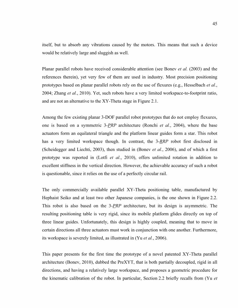
45
itself, but to absorb any vibrations caused by the motors. This means that such a device
would be relatively large and sluggish as well.
Planar parallel robots have received considerable attention (see Bonev et al. (2003) and the
references therein), yet very few of them are used in industry. Most precision positioning
prototypes based on planar parallel robots rely on the use of flexures (e.g., Hesselbach et al.,
2004; Zhang et al., 2010). Yet, such robots have a very limited workspace-to-footprint ratio,
and are not an alternative to the XY-Theta stage in Figure 2.1.
Among the few existing planar 3-DOF parallel robot prototypes that do not employ flexures,
one is based on a symmetric 3-PRP architecture (Ronchi et al., 2004), where the base
actuators form an equilateral triangle and the platform linear guides form a star. This robot
has a very limited workspace though. In contrast, the 3-RRP robot first disclosed in
(Scheidegger and Liechti, 2003), then studied in (Bonev et al., 2006), and of which a first
prototype was reported in (Lotfi et al., 2010), offers unlimited rotation in addition to
excellent stiffness in the vertical direction. However, the achievable accuracy of such a robot
is questionable, since it relies on the use of a perfectly circular rail.
The only commercially available parallel XY-Theta positioning table, manufactured by
Hephaist Seiko and at least two other Japanese companies, is the one shown in Figure 2.2.
This robot is also based on the 3-PRP architecture, but its design is asymmetric. The
resulting positioning table is very rigid, since its mobile platform glides directly on top of
three linear guides. Unfortunately, this design is highly coupled, meaning that to move in
certain directions all three actuators must work in conjunction with one another. Furthermore,
its workspace is severely limited, as illustrated in (Yu et al., 2006).
This paper presents for the first time the prototype of a novel patented XY-Theta parallel
architecture (Bonev, 2010), dubbed the PreXYT, that is both partially decoupled, rigid in all
directions, and having a relatively large workspace, and proposes a geometric procedure for
the kinematic calibration of the robot. In particular, Section 2.2 briefly recalls from (Yu et
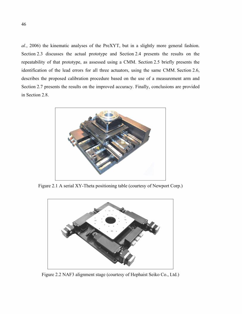
46
al., 2006) the kinematic analyses of the PreXYT, but in a slightly more general fashion.
Section 2.3 discusses the actual prototype and Section 2.4 presents the results on the
repeatability of that prototype, as assessed using a CMM. Section 2.5 briefly presents the
identification of the lead errors for all three actuators, using the same CMM. Section 2.6,
describes the proposed calibration procedure based on the use of a measurement arm and
Section 2.7 presents the results on the improved accuracy. Finally, conclusions are provided
in Section 2.8.
Figure 2.1 A serial XY-Theta positioning table (courtesy of Newport Corp.)
Figure 2.2 NAF3 alignment stage (courtesy of Hephaist Seiko Co., Ltd.)
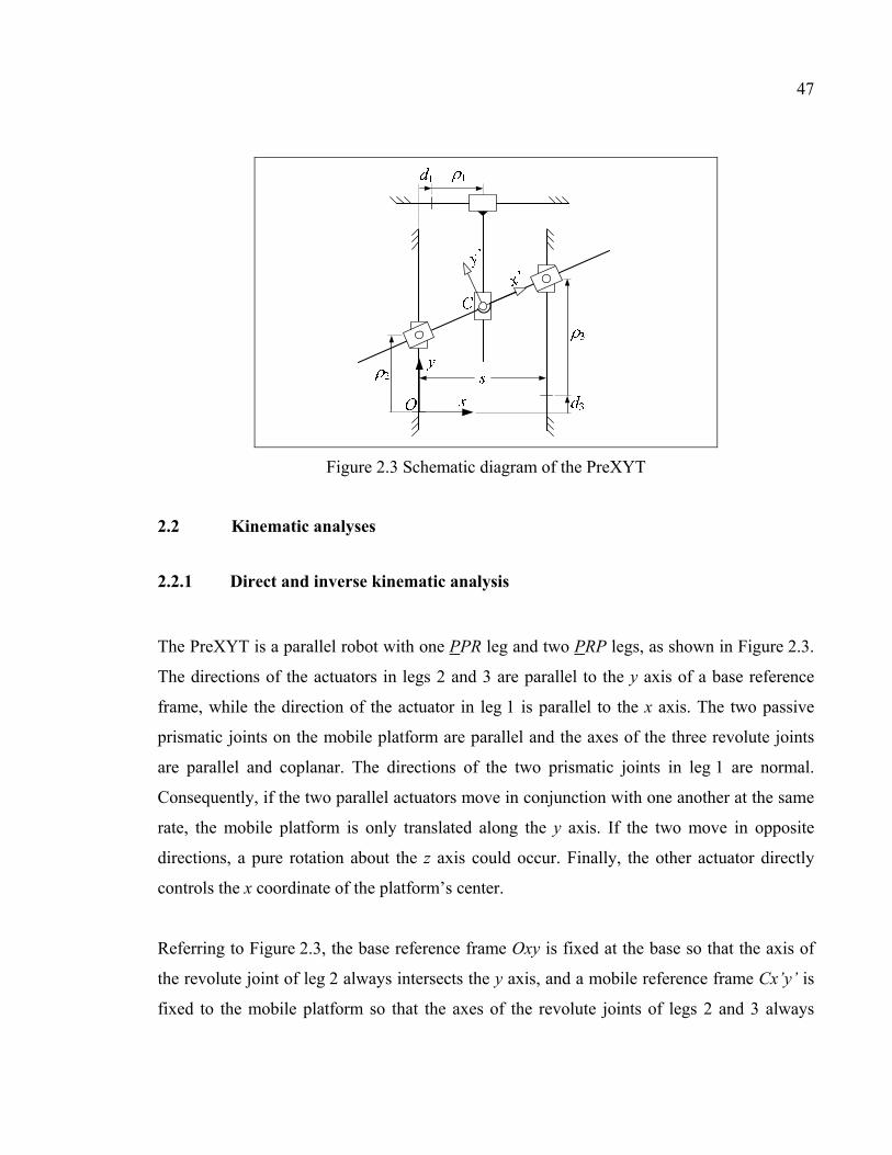
47
Figure 2.3 Schematic diagram of the PreXYT
2.2 Kinematic analyses
2.2.1 Direct and inverse kinematic analysis
The PreXYT is a parallel robot with one PPR leg and two PRP legs, as shown in Figure 2.3.
The directions of the actuators in legs 2 and 3 are parallel to the y axis of a base reference
frame, while the direction of the actuator in leg 1 is parallel to the x axis. The two passive
prismatic joints on the mobile platform are parallel and the axes of the three revolute joints
are parallel and coplanar. The directions of the two prismatic joints in leg 1 are normal.
Consequently, if the two parallel actuators move in conjunction with one another at the same
rate, the mobile platform is only translated along the y axis. If the two move in opposite
directions, a pure rotation about the z axis could occur. Finally, the other actuator directly
controls the x coordinate of the platform’s center.
Referring to Figure 2.3, the base reference frame Oxy is fixed at the base so that the axis of
the revolute joint of leg 2 always intersects the y axis, and a mobile reference frame Cx’y’ is
fixed to the mobile platform so that the axes of the revolute joints of legs 2 and 3 always
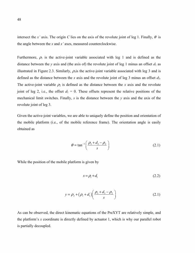
48
intersect the x’ axis. The origin C lies on the axis of the revolute joint of leg 1. Finally, θ is
the angle between the x and x’ axes, measured counterclockwise.
Furthermore, ρ1 is the active-joint variable associated with leg 1 and is defined as the
distance between the y axis and (the axis of) the revolute joint of leg 1 minus an offset d1 as
illustrated in Figure 2.3. Similarly, ρ3is the active-joint variable associated with leg 3 and is
defined as the distance between the x axis and the revolute joint of leg 3 minus an offset d3.
The active-joint variable ρ2 is defined as the distance between the x axis and the revolute
joint of leg 2, i.e., the offset d1 = 0. These offsets represent the relative positions of the
mechanical limit switches. Finally, s is the distance between the y axis and the axis of the
revolute joint of leg 3.
Given the active-joint variables, we are able to uniquely define the position and orientation of
the mobile platform (i.e., of the mobile reference frame). The orientation angle is easily
obtained as
1 3 3 2tand
s
ρ ρθ − + − =
(2.1)
While the position of the mobile platform is given by
1 1x dρ= + (2.2)
( ) 3 3 2
2 1 1
dy d
s
ρ ρρ ρ + − = + +
(2.1)
As can be observed, the direct kinematic equations of the PreXYT are relatively simple, and
the platform’s x coordinate is directly defined by actuator 1, which is why our parallel robot
is partially decoupled.
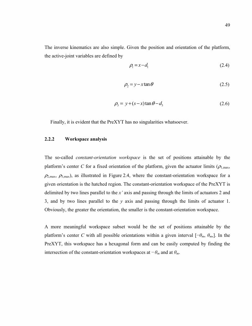
49
The inverse kinematics are also simple. Given the position and orientation of the platform,
the active-joint variables are defined by
1 1x dρ = −
(2.4)
2 tany xρ θ= −
(2.5)
3 3 ( ) tany s x dρ θ= + − −
(2.6)
Finally, it is evident that the PreXYT has no singularities whatsoever.
2.2.2 Workspace analysis
The so-called constant-orientation workspace is the set of positions attainable by the
platform’s center C for a fixed orientation of the platform, given the actuator limits (ρ1,max,
ρ2,max, ρ3,max), as illustrated in Figure 2.4, where the constant-orientation workspace for a
given orientation is the hatched region. The constant-orientation workspace of the PreXYT is
delimited by two lines parallel to the x’ axis and passing through the limits of actuators 2 and
3, and by two lines parallel to the y axis and passing through the limits of actuator 1.
Obviously, the greater the orientation, the smaller is the constant-orientation workspace.
A more meaningful workspace subset would be the set of positions attainable by the
platform’s center C with all possible orientations within a given interval [−θm, θm,]. In the
PreXYT, this workspace has a hexagonal form and can be easily computed by finding the
intersection of the constant-orientation workspaces at −θm and at θm.
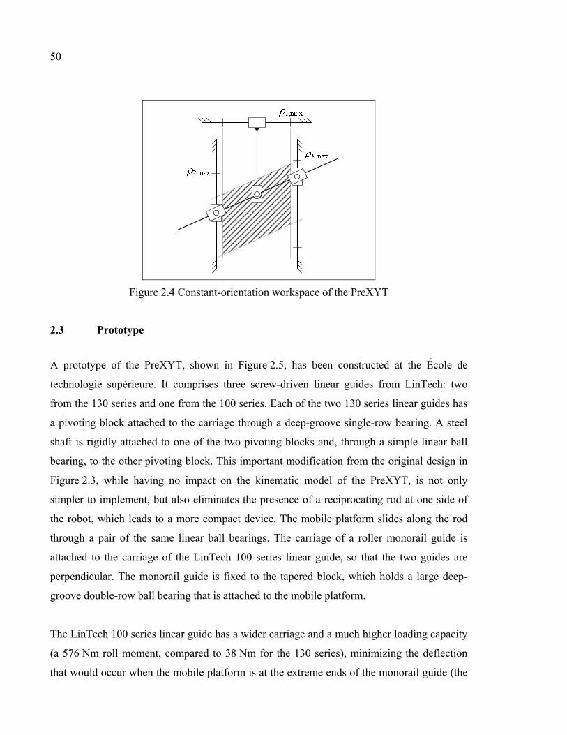
50
Figure 2.4 Constant-orientation workspace of the PreXYT
2.3 Prototype
A prototype of the PreXYT, shown in Figure 2.5, has been constructed at the École de
technologie supérieure. It comprises three screw-driven linear guides from LinTech: two
from the 130 series and one from the 100 series. Each of the two 130 series linear guides has
a pivoting block attached to the carriage through a deep-groove single-row bearing. A steel
shaft is rigidly attached to one of the two pivoting blocks and, through a simple linear ball
bearing, to the other pivoting block. This important modification from the original design in
Figure 2.3, while having no impact on the kinematic model of the PreXYT, is not only
simpler to implement, but also eliminates the presence of a reciprocating rod at one side of
the robot, which leads to a more compact device. The mobile platform slides along the rod
through a pair of the same linear ball bearings. The carriage of a roller monorail guide is
attached to the carriage of the LinTech 100 series linear guide, so that the two guides are
perpendicular. The monorail guide is fixed to the tapered block, which holds a large deep-
groove double-row ball bearing that is attached to the mobile platform.
The LinTech 100 series linear guide has a wider carriage and a much higher loading capacity
(a 576 Nm roll moment, compared to 38 Nm for the 130 series), minimizing the deflection
that would occur when the mobile platform is at the extreme ends of the monorail guide (the
51
passive prismatic joint in leg 1). Overall, this mechanical design provides high rigidity in all
directions, and particularly in the z direction, which yields a large payload capacity.
The 100 series and the two 130 series linear guides have travel lengths limited through
mechanical limit switches to about 170 mm and 300 mm respectively. The distance s
(Figure 2.3) is about 394 mm. As a result, the mobile platform can rotate up to ±35º and
translate inside a rectangle 170×300 mm, when at 0º. Or, referring to the more practical
workspace subset defined in the previous section, the set of positions attainable with any
orientation between −17° and 17° is at least a disk of diameter 170 mm. For comparison, the
mobile platform is about 160×160 mm and the base plate is 470×510 mm.
The motors of the linear guides are CMC BNL 2310 brushless servo motors, yielding a
maximum continuous torque of less than 0.7 Nm. No gear boxes are used, since the linear
guides use Acme precision ball screws of 5.080 mm (0.2 in) lead, with a specified maximum
lead error of 50 µm per 300 mm, zero backlash, and bidirectional repeatability of 5 µm.
We use no linear absolute encoders but only incremental encoders integrated into the motors.
Their resolution is 8000 pulses per revolution, which translates to about 0.6 μm of linear
resolution. Obviously, this is more than sufficient, since the repeatability of the linear guides
is 5 μm. Furthermore, when homing each actuator, we use both the mechanical limit switch
and the index pulse.
Finally, we used an AMP-20540 four-axis drive module and a DMC-2133 four-axis
controller from Galil. We interfaced these with a UniOp HMI device with a touch screen and
put all these components in the table top rack cabinet (not shown in Figure 2.5).
The cost of the off-the-shelf components was about $15 000. The cost of machining,
assembly, cabling, and programming, all carried out in-house, cannot be estimated.
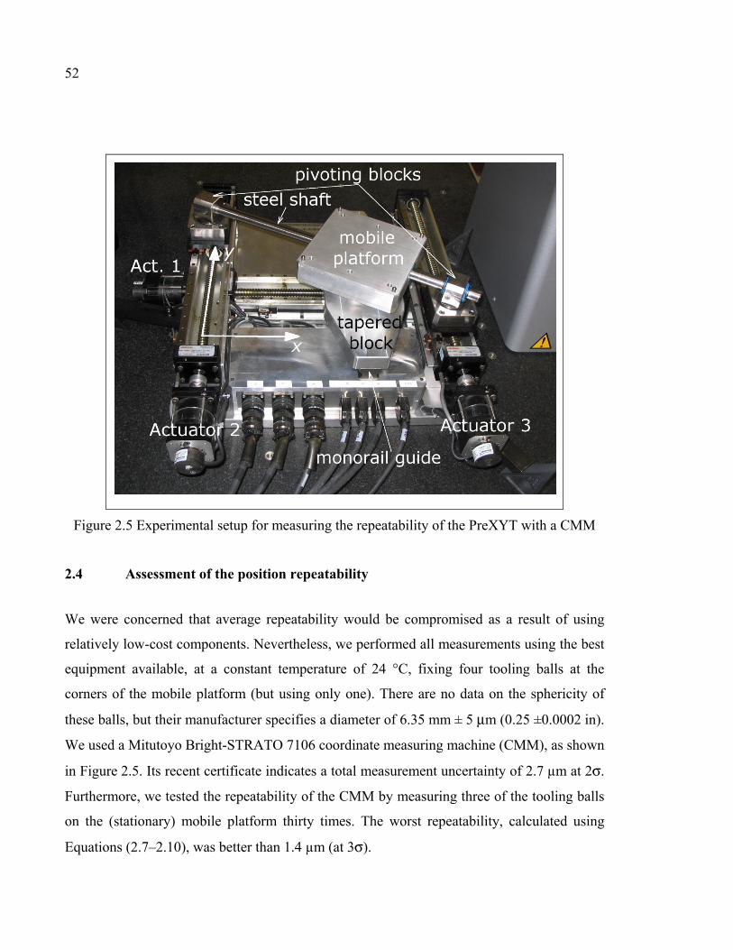
52
Figure 2.5 Experimental setup for measuring the repeatability of the PreXYT with a CMM
2.4 Assessment of the position repeatability
We were concerned that average repeatability would be compromised as a result of using
relatively low-cost components. Nevertheless, we performed all measurements using the best
equipment available, at a constant temperature of 24 °C, fixing four tooling balls at the
corners of the mobile platform (but using only one). There are no data on the sphericity of
these balls, but their manufacturer specifies a diameter of 6.35 mm ± 5 μm (0.25 ±0.0002 in).
We used a Mitutoyo Bright-STRATO 7106 coordinate measuring machine (CMM), as shown
in Figure 2.5. Its recent certificate indicates a total measurement uncertainty of 2.7 µm at 2σ.
Furthermore, we tested the repeatability of the CMM by measuring three of the tooling balls
on the (stationary) mobile platform thirty times. The worst repeatability, calculated using
Equations (2.7–2.10), was better than 1.4 µm (at 3σ).
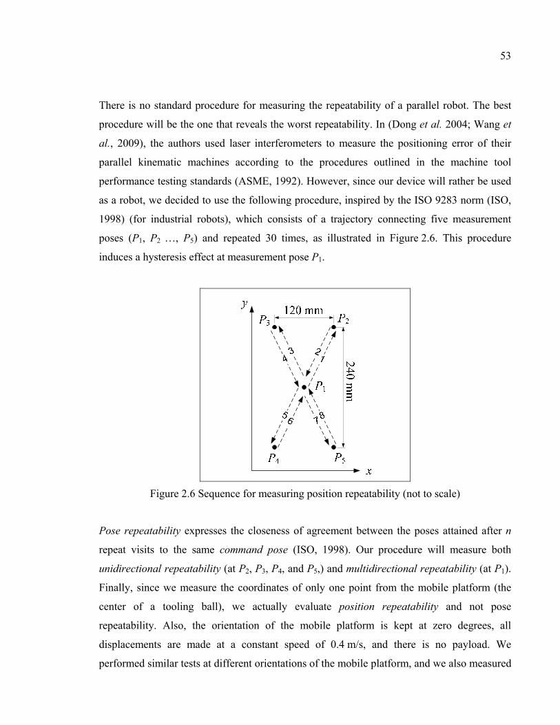
53
There is no standard procedure for measuring the repeatability of a parallel robot. The best
procedure will be the one that reveals the worst repeatability. In (Dong et al. 2004; Wang et
al., 2009), the authors used laser interferometers to measure the positioning error of their
parallel kinematic machines according to the procedures outlined in the machine tool
performance testing standards (ASME, 1992). However, since our device will rather be used
as a robot, we decided to use the following procedure, inspired by the ISO 9283 norm (ISO,
1998) (for industrial robots), which consists of a trajectory connecting five measurement
poses (P1, P2 …, P5) and repeated 30 times, as illustrated in Figure 2.6. This procedure
induces a hysteresis effect at measurement pose P1.
Figure 2.6 Sequence for measuring position repeatability (not to scale)
Pose repeatability expresses the closeness of agreement between the poses attained after n
repeat visits to the same command pose (ISO, 1998). Our procedure will measure both
unidirectional repeatability (at P2, P3, P4, and P5,) and multidirectional repeatability (at P1).
Finally, since we measure the coordinates of only one point from the mobile platform (the
center of a tooling ball), we actually evaluate position repeatability and not pose
repeatability. Also, the orientation of the mobile platform is kept at zero degrees, all
displacements are made at a constant speed of 0.4 m/s, and there is no payload. We
performed similar tests at different orientations of the mobile platform, and we also measured
54
the orientation repeatability at several positions. However, the analyses of the results from
these measurements did not reveal any further insights and will not be presented in this
paper.
There are two approaches for evaluating position repeatability, ε, from a set of n points. The
most natural one is to find the radius of the smallest sphere (or, in the planar case, circle) that
encloses all points. The other measure for evaluating position repeatability is to calculate the
mean position error with respect to the barycentre ( , , x y z ) of the cluster of n points
( , y , )i i ix z and add three times the standard deviation (ISO, 1998):
3 rrε σ= +
(2.7)
where
1ir r
n=
(2.8)
2
1
( )
1
n
ii
r
r r
nσ =
−=
−
(2.9)
2 2 2( ) ( ) ( )i i i ir x x y y z z= − + − + −
(2.10)
Table 2.1 shows the final results. Note that, even though we have measured the position at P1
120 times, we only consider the first 30 measurements. Considering all 120 measurements
yields nearly identical results.
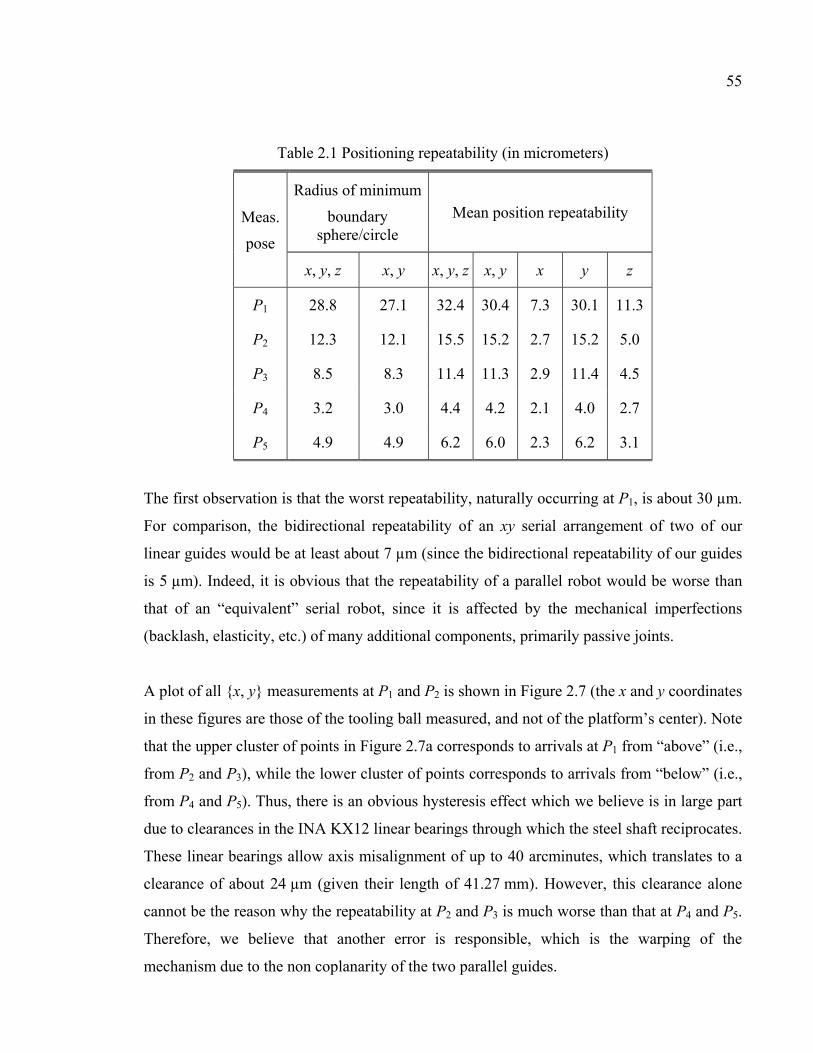
55
Table 2.1 Positioning repeatability (in micrometers)
Meas.
pose
Radius of minimum
boundary sphere/circle
Mean position repeatability
x, y, z x, y x, y, z x, y x y z
P1 28.8 27.1 32.4 30.4 7.3 30.1 11.3
P2 12.3 12.1 15.5 15.2 2.7 15.2 5.0
P3 8.5 8.3 11.4 11.3 2.9 11.4 4.5
P4 3.2 3.0 4.4 4.2 2.1 4.0 2.7
P5 4.9 4.9 6.2 6.0 2.3 6.2 3.1
The first observation is that the worst repeatability, naturally occurring at P1, is about 30 µm.
For comparison, the bidirectional repeatability of an xy serial arrangement of two of our
linear guides would be at least about 7 µm (since the bidirectional repeatability of our guides
is 5 µm). Indeed, it is obvious that the repeatability of a parallel robot would be worse than
that of an “equivalent” serial robot, since it is affected by the mechanical imperfections
(backlash, elasticity, etc.) of many additional components, primarily passive joints.
A plot of all {x, y} measurements at P1 and P2 is shown in Figure 2.7 (the x and y coordinates
in these figures are those of the tooling ball measured, and not of the platform’s center). Note
that the upper cluster of points in Figure 2.7a corresponds to arrivals at P1 from “above” (i.e.,
from P2 and P3), while the lower cluster of points corresponds to arrivals from “below” (i.e.,
from P4 and P5). Thus, there is an obvious hysteresis effect which we believe is in large part
due to clearances in the INA KX12 linear bearings through which the steel shaft reciprocates.
These linear bearings allow axis misalignment of up to 40 arcminutes, which translates to a
clearance of about 24 µm (given their length of 41.27 mm). However, this clearance alone
cannot be the reason why the repeatability at P2 and P3 is much worse than that at P4 and P5.
Therefore, we believe that another error is responsible, which is the warping of the
mechanism due to the non coplanarity of the two parallel guides.
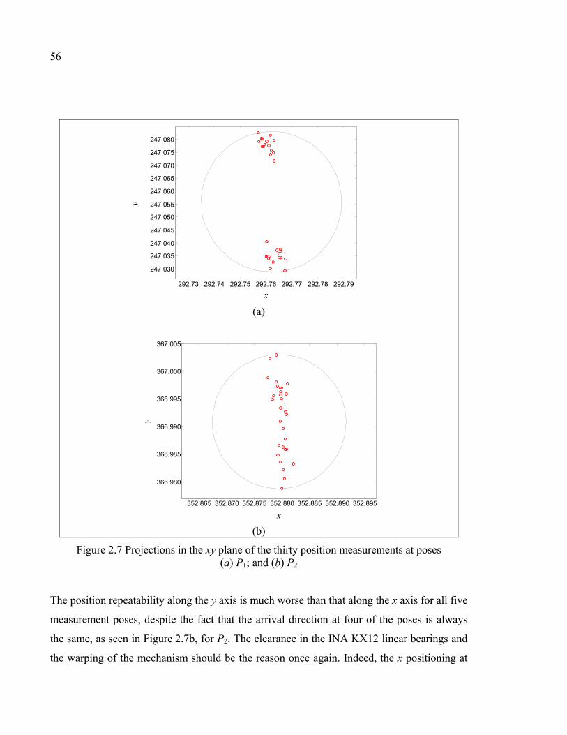
56
(a)
(b)
Figure 2.7 Projections in the xy plane of the thirty position measurements at poses (a) P1; and (b) P2
The position repeatability along the y axis is much worse than that along the x axis for all five
measurement poses, despite the fact that the arrival direction at four of the poses is always
the same, as seen in Figure 2.7b, for P2. The clearance in the INA KX12 linear bearings and
the warping of the mechanism should be the reason once again. Indeed, the x positioning at
292.73 292.74 292.75 292.76 292.77 292.78 292.79
247.030
247.035
247.040
247.045
247.050
247.055
247.060
247.065
247.070
247.075
247.080
x
y
352.865 352.870 352.875 352.880 352.885 352.890 352.895
366.980
366.985
366.990
366.995
367.000
367.005
x
y
57
the zero orientation is influenced almost exclusively by leg 1. Since both the passive linear
guide and the bearing of leg 1 are very stiff, the x positioning is very repeatable.
The mechanism does indeed undergo slight warping, which can be seen from analyzing the
coplanarity of the positions in P2, P3, P4, and P5. If we take the centers of the bounding
spheres for the measurements at these four poses, then we can calculate that the distance
from any of these centers to the plane formed by the other three centers is 52 µm.
Finally, note that the measurements shown in Table 2.1 were performed after a single
homing. However, we also tested the repeatability of our homing procedure by measuring the
position of our tooling ball after ten successive homing sequences, at the home position. This
repeatability is better than 2 µm (at 3σ).
2.5 Determination of lead errors
As already mentioned, the maximum lead error of our linear guides is 50 µm per 300 mm
and we do not use absolute linear encoders. Therefore, to improve the accuracy of the
PreXYT, we measured the actual lead error on the CMM using the following procedure. A
precision ball of diameter 9.525 mm (3/8 in) was solidly attached to the carriage of each of
the three linear guides using magnetic nests and hot glue. The range of motion of each
actuator was divided into six segments, i.e., seven consecutive positions at which
measurements were taken. Each first position corresponded to when the actuator is homed
and was considered at the reference position. Each actuator is then moved to each of the
subsequent six positions, and at each position the precision ball is measured using the CMM.
The measurement sequence for each actuator is repeated ten times (i.e., measurements are
done at positions 1→2→3→4→5→6→1→2…). A linear regression is then applied for each
actuator and the actual lead is determined. The actual screw errors were thus determined to
be −0.690×10⁻³ρ1, −0.454×10⁻³ρ2, and −0.358×10⁻³ρ3 (i.e., the actual lead for actuator 1 is
5.0764948 mm instead of 5.080 mm, etc.) or as much as 200 µm per 300 mm.
58
2.6 Kinematic calibration
While the repeatability of the PreXYT was assessed using a CMM and so were the actual
lead errors, we decided to use our own FaroArm Platinum measurement arm for the robot
calibration. This choice was made mainly because our FaroArm is accessible to us at all
times and much easier to use, but also because the FaroArm has a volumetric accuracy that is
sufficiently good for the calibration of the PreXYT. Indeed, the 3D point-to-point accuracy
of our 4 ft FaroArm Platinum is specified at ±18 µm. Of course, unlike the CMM where
triggering is automatic, the accuracy of measurements with the FaroArm is highly dependent
on the experience of the operator and on the rigid mounting of the FaroArm.
Figure 2.8 shows the setup used for calibrating the PreXYT and for assessing the point-to-
point accuracy of the FaroArm. Both the PreXYT and the FaroArm are solidly attached to a
heavy steel table. The FaroArm is equipped with its standard 3 mm probe and is used by
probing the same tooling balls (attached to the mobile platform) described in Section 2.4 and
the same precision balls described in Section 2.5.
We assessed the point-to-point accuracy of our FaroArm using a 300 mm scale bar (actually,
the calibration kit of our Renishaw telescoping ballbar). The scale bar was positioned in two
configurations: the one shown in Figure 2.8 and another one obtained by rotating the bar at
90°. At each configuration, each of the two high precision balls of the scale bar was
measured ten times using the PolyWorks software. In the scale-bar configuration shown in
Figure 2.8, the mean distance error was −6 µm and the standard deviation was 4 µm, while in
the second configuration, the mean distance error was 12 µm and the standard deviation was
5 µm. We also measured ten times the center of one of the tooling balls on the mobile
platform (while the robot controller was turned off) and repeatability, calculated using
Equations (2.7–2.10), was better than 7.3 µm (at 3σ). Therefore, we believe that the FaroArm
can be used for calibrating the PreXYT, since the multidirectional repeatability of our robot
is more than 30 µm and the volumetric accuracy that we aim at is certainly not less than
100 µm.
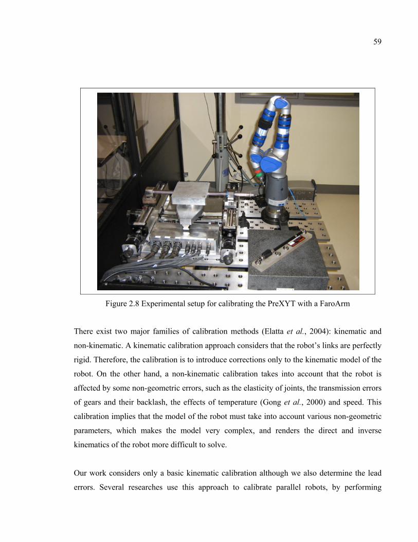
59
Figure 2.8 Experimental setup for calibrating the PreXYT with a FaroArm
There exist two major families of calibration methods (Elatta et al., 2004): kinematic and
non-kinematic. A kinematic calibration approach considers that the robot’s links are perfectly
rigid. Therefore, the calibration is to introduce corrections only to the kinematic model of the
robot. On the other hand, a non-kinematic calibration takes into account that the robot is
affected by some non-geometric errors, such as the elasticity of joints, the transmission errors
of gears and their backlash, the effects of temperature (Gong et al., 2000) and speed. This
calibration implies that the model of the robot must take into account various non-geometric
parameters, which makes the model very complex, and renders the direct and inverse
kinematics of the robot more difficult to solve.
Our work considers only a basic kinematic calibration although we also determine the lead
errors. Several researches use this approach to calibrate parallel robots, by performing
60
measurements on the actuators ( Zhuang et al., 1998) or on the end-effector (Wu et al., 1988;
Oliviers and Mayer, 1995; Masory et al., 1997; Gatla et al. 2007). Both approaches are used
to find the parameters that minimize the residuals of either the inverse or direct kinematic
model. Some methods add mechanical constraints to the robot, to limit some of its
movements during the calibration procedure. This can be achieved by blocking the position
or orientation of the end-effector to a known value (Daney, 2000), or by forcing it to make a
specific movement such as linear trajectory or to move along a predefined plan (Ikits and
Hollerbach, 1997). For more details about parallel robot calibration methods, the reader is
referred to (Last et al., 2011).
A calibration approach can use position data from the internal sensors of a robot (Ikits and
Hollerbach, 1997)and, possibly, from an external 3D measurement device such as a CMM
(Verner et al., 2005), a CCD camera (Motta et al., 2001; Watanabe et al., 2006), a laser
tracker (Gong et al., 2000), or other 2D or even 1D measurement devices such as an
inclinometer (Besnard and Wisama, 1999), a theodolite (Berg, 1992; Schroer, 1994), a triad
of dial gages (Abtahi et al., 2010) or a telescopic ballbar (Ota et al., 2000). In most cases, the
calibration is based on an optimization method that finds the parameters improving the
robot’s accuracy. While it is generally accepted that such approaches yield better results than
when trying to directly measure the robot geometry (an approach known as screw-axis
measurement in the case of serial robots (Abderrahim and Whittaker, 2000)), there are
virtually no reported works on such direct methods in the case of parallel robots. The only
exceptions are references (Blaise et al., 2010; Renaud et al., 2005), both describing direct
geometric methods for calibrating spatial parallel robots with cylindrical legs. In comparison
to the present work, the first work (Blaise et al., 2010) was too superficial, while the second
work (Renaud et al., 2005) used a single CCD camera. However, none of the methods
proposed in these two works is directly applicable to the PreXYT.
In this paper, we will use a geometric approach for obtaining the actual robot kinematic
parameters. Furthermore, we will determine only those kinematic parameters that do not
render the kinematic equations of the PreXYT more coupled. In other words, we will
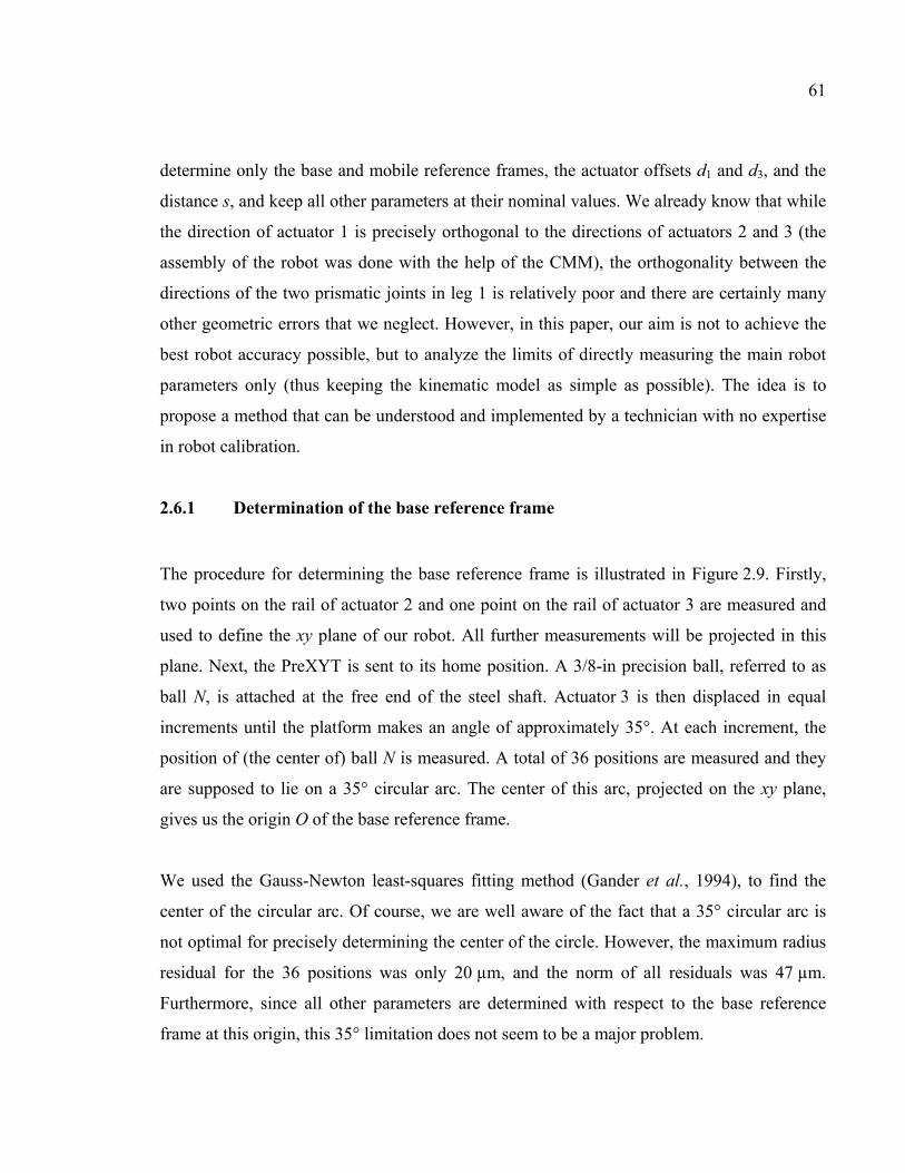
61
determine only the base and mobile reference frames, the actuator offsets d1 and d3, and the
distance s, and keep all other parameters at their nominal values. We already know that while
the direction of actuator 1 is precisely orthogonal to the directions of actuators 2 and 3 (the
assembly of the robot was done with the help of the CMM), the orthogonality between the
directions of the two prismatic joints in leg 1 is relatively poor and there are certainly many
other geometric errors that we neglect. However, in this paper, our aim is not to achieve the
best robot accuracy possible, but to analyze the limits of directly measuring the main robot
parameters only (thus keeping the kinematic model as simple as possible). The idea is to
propose a method that can be understood and implemented by a technician with no expertise
in robot calibration.
2.6.1 Determination of the base reference frame
The procedure for determining the base reference frame is illustrated in Figure 2.9. Firstly,
two points on the rail of actuator 2 and one point on the rail of actuator 3 are measured and
used to define the xy plane of our robot. All further measurements will be projected in this
plane. Next, the PreXYT is sent to its home position. A 3/8-in precision ball, referred to as
ball N, is attached at the free end of the steel shaft. Actuator 3 is then displaced in equal
increments until the platform makes an angle of approximately 35°. At each increment, the
position of (the center of) ball N is measured. A total of 36 positions are measured and they
are supposed to lie on a 35° circular arc. The center of this arc, projected on the xy plane,
gives us the origin O of the base reference frame.
We used the Gauss-Newton least-squares fitting method (Gander et al., 1994), to find the
center of the circular arc. Of course, we are well aware of the fact that a 35° circular arc is
not optimal for precisely determining the center of the circle. However, the maximum radius
residual for the 36 positions was only 20 µm, and the norm of all residuals was 47 µm.
Furthermore, since all other parameters are determined with respect to the base reference
frame at this origin, this 35° limitation does not seem to be a major problem.
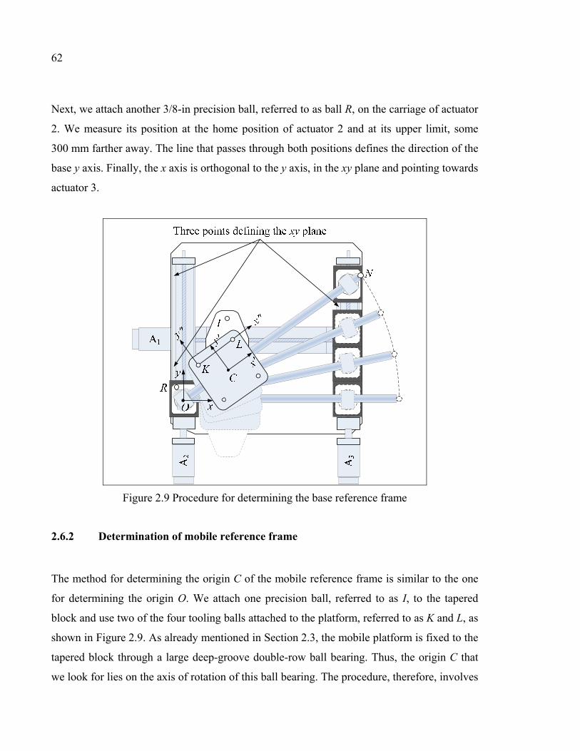
62
Next, we attach another 3/8-in precision ball, referred to as ball R, on the carriage of actuator
2. We measure its position at the home position of actuator 2 and at its upper limit, some
300 mm farther away. The line that passes through both positions defines the direction of the
base y axis. Finally, the x axis is orthogonal to the y axis, in the xy plane and pointing towards
actuator 3.
Figure 2.9 Procedure for determining the base reference frame
2.6.2 Determination of mobile reference frame
The method for determining the origin C of the mobile reference frame is similar to the one
for determining the origin O. We attach one precision ball, referred to as I, to the tapered
block and use two of the four tooling balls attached to the platform, referred to as K and L, as
shown in Figure 2.9. As already mentioned in Section 2.3, the mobile platform is fixed to the
tapered block through a large deep-groove double-row ball bearing. Thus, the origin C that
we look for lies on the axis of rotation of this ball bearing. The procedure, therefore, involves
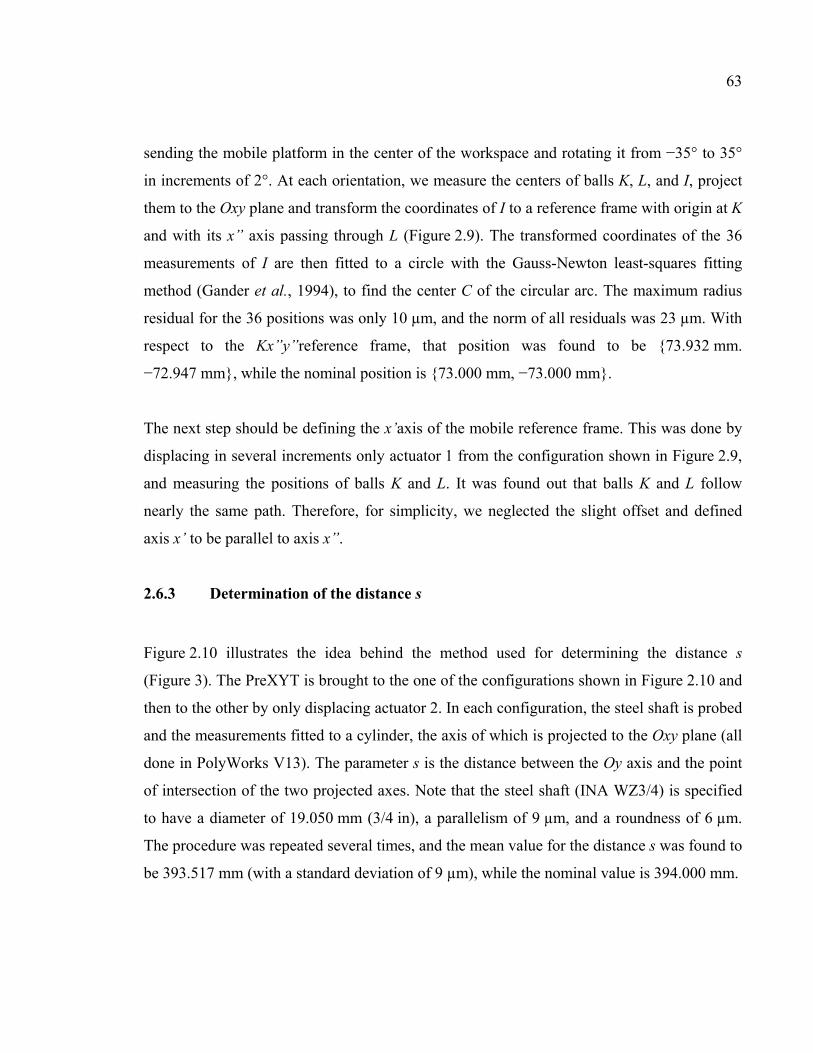
63
sending the mobile platform in the center of the workspace and rotating it from −35° to 35°
in increments of 2°. At each orientation, we measure the centers of balls K, L, and I, project
them to the Oxy plane and transform the coordinates of I to a reference frame with origin at K
and with its x” axis passing through L (Figure 2.9). The transformed coordinates of the 36
measurements of I are then fitted to a circle with the Gauss-Newton least-squares fitting
method (Gander et al., 1994), to find the center C of the circular arc. The maximum radius
residual for the 36 positions was only 10 µm, and the norm of all residuals was 23 µm. With
respect to the Kx”y”reference frame, that position was found to be {73.932 mm.
−72.947 mm}, while the nominal position is {73.000 mm, −73.000 mm}.
The next step should be defining the x’axis of the mobile reference frame. This was done by
displacing in several increments only actuator 1 from the configuration shown in Figure 2.9,
and measuring the positions of balls K and L. It was found out that balls K and L follow
nearly the same path. Therefore, for simplicity, we neglected the slight offset and defined
axis x’ to be parallel to axis x”.
2.6.3 Determination of the distance s
Figure 2.10 illustrates the idea behind the method used for determining the distance s
(Figure 3). The PreXYT is brought to the one of the configurations shown in Figure 2.10 and
then to the other by only displacing actuator 2. In each configuration, the steel shaft is probed
and the measurements fitted to a cylinder, the axis of which is projected to the Oxy plane (all
done in PolyWorks V13). The parameter s is the distance between the Oy axis and the point
of intersection of the two projected axes. Note that the steel shaft (INA WZ3/4) is specified
to have a diameter of 19.050 mm (3/4 in), a parallelism of 9 µm, and a roundness of 6 µm.
The procedure was repeated several times, and the mean value for the distance s was found to
be 393.517 mm (with a standard deviation of 9 µm), while the nominal value is 394.000 mm.
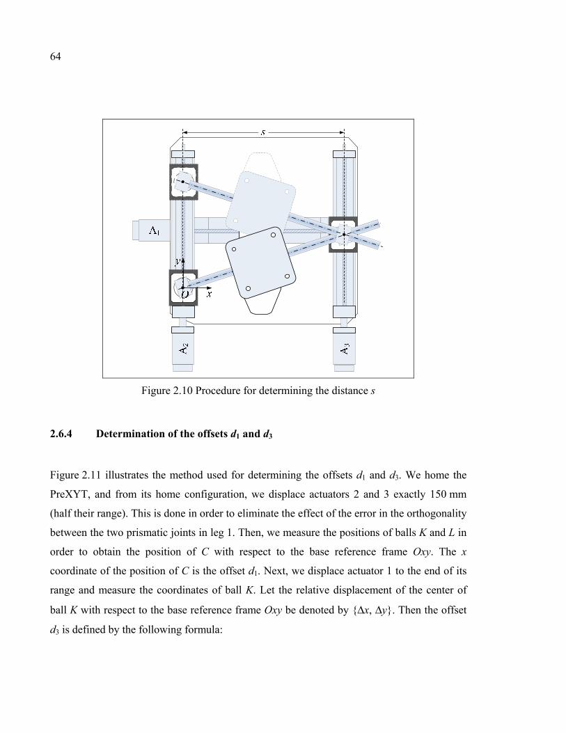
64
Figure 2.10 Procedure for determining the distance s
2.6.4 Determination of the offsets d1 and d3
Figure 2.11 illustrates the method used for determining the offsets d1 and d3. We home the
PreXYT, and from its home configuration, we displace actuators 2 and 3 exactly 150 mm
(half their range). This is done in order to eliminate the effect of the error in the orthogonality
between the two prismatic joints in leg 1. Then, we measure the positions of balls K and L in
order to obtain the position of C with respect to the base reference frame Oxy. The x
coordinate of the position of C is the offset d1. Next, we displace actuator 1 to the end of its
range and measure the coordinates of ball K. Let the relative displacement of the center of
ball K with respect to the base reference frame Oxy be denoted by {Δx, Δy}. Then the offset
d3 is defined by the following formula:
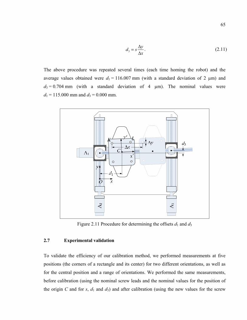
65
3
yd s
x
Δ=Δ
. (2.11)
The above procedure was repeated several times (each time homing the robot) and the
average values obtained were d1 = 116.007 mm (with a standard deviation of 2 µm) and
d3 = 0.704 mm (with a standard deviation of 4 µm). The nominal values were
d1 = 115.000 mm and d3 = 0.000 mm.
Figure 2.11 Procedure for determining the offsets d1 and d3
2.7 Experimental validation
To validate the efficiency of our calibration method, we performed measurements at five
positions (the corners of a rectangle and its center) for two different orientations, as well as
for the central position and a range of orientations. We performed the same measurements,
before calibration (using the nominal screw leads and the nominal values for the position of
the origin C and for s, d1 and d3) and after calibration (using the new values for the screw
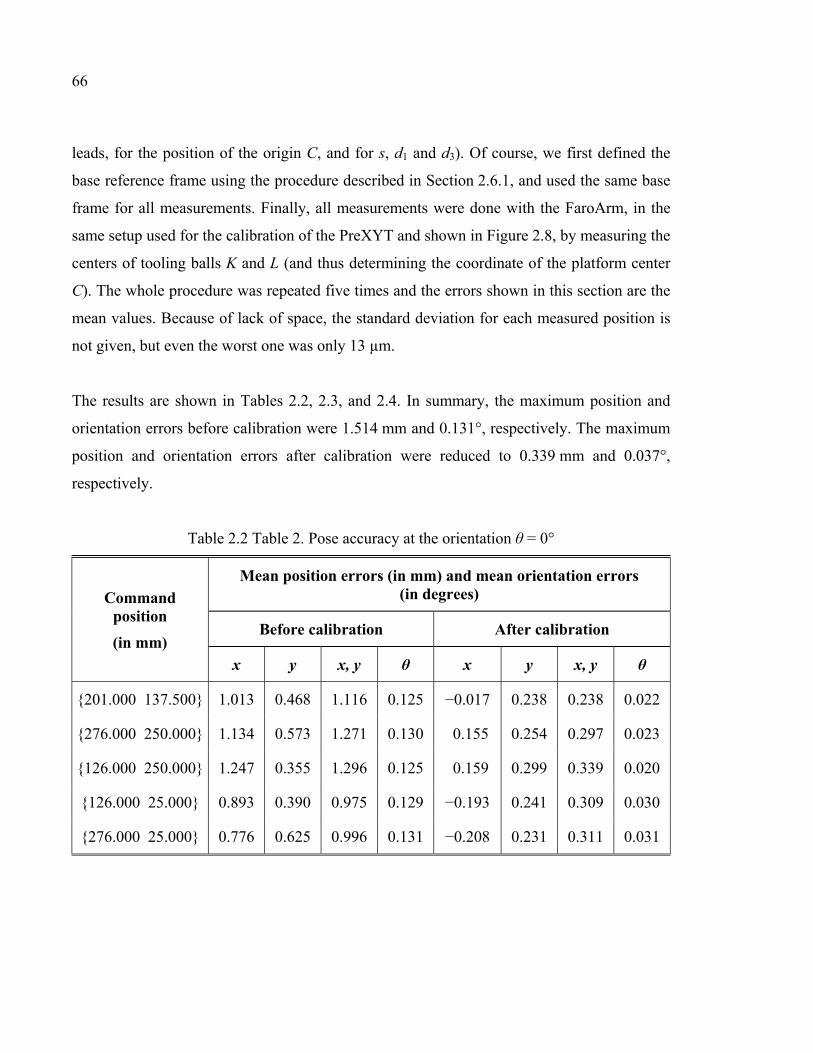
66
leads, for the position of the origin C, and for s, d1 and d3). Of course, we first defined the
base reference frame using the procedure described in Section 2.6.1, and used the same base
frame for all measurements. Finally, all measurements were done with the FaroArm, in the
same setup used for the calibration of the PreXYT and shown in Figure 2.8, by measuring the
centers of tooling balls K and L (and thus determining the coordinate of the platform center
C). The whole procedure was repeated five times and the errors shown in this section are the
mean values. Because of lack of space, the standard deviation for each measured position is
not given, but even the worst one was only 13 µm.
The results are shown in Tables 2.2, 2.3, and 2.4. In summary, the maximum position and
orientation errors before calibration were 1.514 mm and 0.131°, respectively. The maximum
position and orientation errors after calibration were reduced to 0.339 mm and 0.037°,
respectively.
Table 2.2 Table 2. Pose accuracy at the orientation θ = 0°
Command position
(in mm)
Mean position errors (in mm) and mean orientation errors (in degrees)
Before calibration After calibration
x y x, y θ x y x, y θ
{201.000 137.500} 1.013 0.468 1.116 0.125 −0.017 0.238 0.238 0.022
{276.000 250.000} 1.134 0.573 1.271 0.130 0.155 0.254 0.297 0.023
{126.000 250.000} 1.247 0.355 1.296 0.125 0.159 0.299 0.339 0.020
{126.000 25.000} 0.893 0.390 0.975 0.129 −0.193 0.241 0.309 0.030
{276.000 25.000} 0.776 0.625 0.996 0.131 −0.208 0.231 0.311 0.031
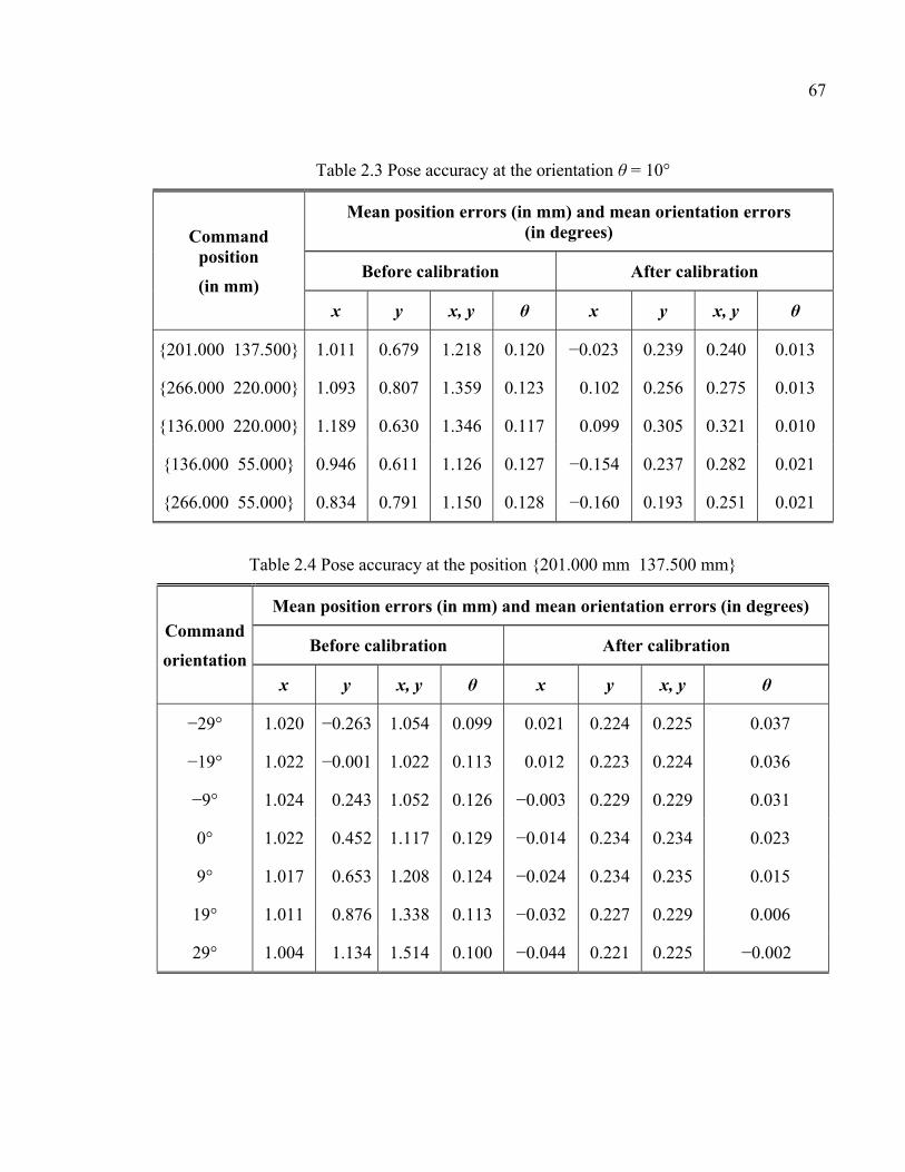
67
Table 2.3 Pose accuracy at the orientation θ = 10°
Command position
(in mm)
Mean position errors (in mm) and mean orientation errors (in degrees)
Before calibration After calibration
x y x, y θ x y x, y θ
{201.000 137.500} 1.011 0.679 1.218 0.120 −0.023 0.239 0.240 0.013
{266.000 220.000} 1.093 0.807 1.359 0.123 0.102 0.256 0.275 0.013
{136.000 220.000} 1.189 0.630 1.346 0.117 0.099 0.305 0.321 0.010
{136.000 55.000} 0.946 0.611 1.126 0.127 −0.154 0.237 0.282 0.021
{266.000 55.000} 0.834 0.791 1.150 0.128 −0.160 0.193 0.251 0.021
Table 2.4 Pose accuracy at the position {201.000 mm 137.500 mm}
Command
orientation
Mean position errors (in mm) and mean orientation errors (in degrees)
Before calibration After calibration
x y x, y θ x y x, y θ
−29° 1.020 −0.263 1.054 0.099 0.021 0.224 0.225 0.037
−19° 1.022 −0.001 1.022 0.113 0.012 0.223 0.224 0.036
−9° 1.024 0.243 1.052 0.126 −0.003 0.229 0.229 0.031
0° 1.022 0.452 1.117 0.129 −0.014 0.234 0.234 0.023
9° 1.017 0.653 1.208 0.124 −0.024 0.234 0.235 0.015
19° 1.011 0.876 1.338 0.113 −0.032 0.227 0.229 0.006
29° 1.004 1.134 1.514 0.100 −0.044 0.221 0.225 −0.002
68
2.8 Conclusions
Despite the low-cost off-the-shelf components, we were able to build a first prototype of a
novel 3-DOF planar parallel robot, dubbed PreXYT, with good positioning repeatability and
pose accuracy. Videos of the PreXYT are available at http://www.youtube.com/CoRoETS.
We also proposed a calibration method that is simple to understand and perform, and that
relies on the same trivial kinematic model as the nominal one. It was clearly demonstrated
that such a calibration method can lead to greatly improving the accuracy of the robot (by a
factor of almost five). To further improve the accuracy of the robot, we need to identify
additional design parameters, the most important being the angle between the two passive
joints in leg 1. While this could have been easily done using our geometric approach, taking
this error into consideration would have inevitably led to more complex kinematic equations,
which is why we deliberately ignored it.
2.9 Acknowledgements
We would like to thank the Fonds québécois de la recherche sur la nature et les technologies
(FQRNT) and the Canada Research Chair program for financing this work.
CHAPITRE 3
ARTICLE 2: KINEMATIC CALIBRATION OF A 3-DOF PLANAR PARALLEL ROBOT
Ahmed Joubair, Mohamed Slamani, and Ilian A. Bonev École de technologie supérieure, Montreal, QC, Canada
This chapter has been published as an article in
Industrial Robot: An International Journal: vol. 39, n° 4 (2012)
Résumé
Le but de cet article est de décrire une méthode d'étalonnage développée pour améliorer la
précision absolue d'un nouveau robot parallèle planaire à trois ddl. Le robot est conçu pour
des applications de positionnement précis en matière de manipulation des semi-conducteurs,
ce qui signifie que l'analyse de la précision est effectuée dans un espace de travail circulaire
d’un diamètre de170 mm. La méthode d'étalonnage utilise un modèle d'optimisation unique,
basé sur la méthode directe d’ÉG, tandis que les données expérimentales sont recueillies à
l’aide de deux sources. La première source de données est un bras articulé de mesure de
coordonnées, provenant de la compagnie FARO Technologies et la seconde est une CMM
Mitutoyo. Les deux séries de résultats d'étalonnage sont comparées. La simulation a confirmé
que notre modèle n'est pas sensible aux bruits de mesure. En outre, une validation
expérimentale montre que la précision absolue de la position et de l'orientation a été
améliorée, passant des erreurs maximales de 1,432 mm et 0,107° respectivement, avant
étalonnage, à 0,044 mm et 0,009° après étalonnage. L’originalité de cet article réside au fait
que la méthode d’étalonnage proposée permet d’identifier précisément le référentiel de la
base du robot en même temps que l’identification et la compensation des erreurs
géométriques, des offsets des actionneurs et des erreurs de leurs vis sans fins. La méthode
d’étalonnage proposée a été testée sur un nouveau robot planaire dont la précision absolue a
été améliorée pour atteindre la valeur de 0,044 mm.
70
Abstract
Purpose – The purpose of this paper is to describe a calibration method developed to
improve the absolute accuracy of a novel three degrees-of-freedom planar parallel robot. The
robot is designed for precise positioning applications in semiconductor handling, which
means that the accuracy analysis is performed within a circular workspace 170 mm in
diameter.
Design/methodology/approach – The calibration method makes use of a single optimization
model, based on the forward kinematic calibration approach, while the experimental data are
collected from two sources. The first data source is a measurement arm device from FARO
Technologies, and the second is a Mitutoyo coordinate measurement machine. The two sets
of calibration results are compared.
Findings – Simulation confirmed that our model is not sensitive to measurement noise.
Furthermore, an experimental validation shows that the absolute accuracy of position and
orientation was improved, from maximum errors of 1.432 mm and 0.107°respectively before
calibration to 0.044 mm and 0.009° after calibration.
Originality/value –This paper presents a calibration method which makes it possible to
accurately identify the actual robot’s base frame (base frame calibration),at the same time as
identifying and compensating for geometric errors, actuator offsets, and lead errors. The
proposed calibration method is tested on a novel planar robot, and its absolute accuracy was
found to improve to 0.044 mm.
Keywords Kinematic calibration, Robots, Absolute accuracy
Paper type Research paper
3.1 Introduction
It is often claimed that parallel robots are more precise than serial robots, because they do not
suffer from error accumulation. While this might be true in theory (Briot and Bonev, 2007),
the real reason is that parallel robots can be built to be more rigid without being bulkier. No
71
matter how rigid they are, parallel robots, too, should be calibrated in order to improve their
accuracy. Depending on the sources of inaccuracy (geometric vs. non geometric errors),robot
calibration is classified in two main categories: kinematic and non kinematic (Elatta et al.,
2004; Greenway, 2000; Schroer, 1994). Some researchers refer to them as level 2 and level
3calibration respectively, while level 1calibration represents the actuator lead error or offset
compensation (Roth et al., 1987). A kinematic calibration, which is the subject of this paper,
considers that the robot’s links are perfectly rigid and that the robot is not in dynamic mode.
This calibration is more appropriate for parallel robots since they present good rigidity,
which implies that their non geometric errors are generally small.
The kinematic approach to calibrating parallel robots has been used by many authors (such as
Oliviers and Mayer, 1995; Masory et al., 1997; Zhuang et al., 1998; Ren et al., 2009), mainly
for the6 degrees-of-freedom (DOF)Gough-Stewart platform. However, few works involve
the calibration of parallel robots with less than 6 DOFs, especially planar ones. Some of these
identify only actuator offsets (Pashkevich et al., 2009), or only the standard geometric
parameters (e.g. link lengths), like (Last et al., 2006), who present a calibration of a 5-bar
robot using singularity configurations. For the same type of robot, Durango et al. (2010)
propose a divide-and-conquer strategy to identify both geometric parameters and joint
offsets. Also, Kim (2005) presents a geometric calibration of a Cartesian parallel manipulator
using a ball bar to identify geometric parameters and offsets.
Calibration of parallel robots with less than 6 DOFs is generally undertaken without
identifying the actual robot’s base frame with respect to the world frame, simultaneously
with the robot’s other geometric parameters. Consequently, relative accuracy can be
improved and evaluated, but not absolute accuracy, because the actual base frame location is
not identified exactly (i.e. not identified by the calibration model).
This paper presents a contribution to the kinematic calibration of parallel robots by
developing a method based on the forward approach using full-pose measurement (position
and orientation of the end-effector) applied to a novel prototype of a planar parallel robot.
72
The measurements were processed using two probing machines: a FaroArm Platinum
measurement arm, and a Mitutoyo coordinate measurement machine (CMM). The aim of
using both machines is to determine how far each of the two instruments is capable of
improving the robot’s absolute accuracy. Identification is achieved using a single non linear
model based on the minimization of thesquare residuals of the platform’s position and
orientation.
With respect to the traditional calibration method, our approach makes it possible to identify
and compensate for geometric errors at the same time as identifying actuator offsets and lead
errors. Also, it makes possible the accurate determination of the actual mobile reference
frame and the base frame with respect to the world frame. This in turn makes it possible to
identify the end-effector’s position and orientation with respect to the actual base frame. As a
result, our method improves the absolute accuracy of the robot and not only its relative
accuracy. Furthermore, knowing the precise location of the base frame with respect to the
world frame permits the accurate interaction between the robot and other devices located in
the same work area, such as a vision system or other robots. Moreover, the proposed method
offers the following advantages: (1) it can be applied to other types of parallel robots; (2) it
can be applied with a minimum time lapse (with only eight calibration poses and two poses
to identify the world reference frame); and (3) measurements can be performed using any
coordinate measurement instrument.
This paper is organized as follows: the next section provides a description of the nominal
kinematic model, followed by presentation of the robot prototype. Then, the calibration
model and method are explained. Finally, the simulation study and experimentation results
are given, and conclusions are drawn.
3.2 Nominal kinematic model
The PreXYT (for Precision XY-Theta table), shown in Figure 3.1, is a planar parallel robot
with two PRP legs and one PPR leg (Bonev, 2010). Referring to Figure 3.1, the directions of
the actuators in the PRP legs are parallel to the y axis of a base reference frame, while the
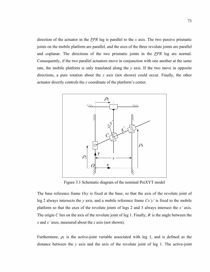
73
direction of the actuator in the PPR leg is parallel to the x axis. The two passive prismatic
joints on the mobile platform are parallel, and the axes of the three revolute joints are parallel
and coplanar. The directions of the two prismatic joints in the PPR leg are normal.
Consequently, if the two parallel actuators move in conjunction with one another at the same
rate, the mobile platform is only translated along the y axis. If the two move in opposite
directions, a pure rotation about the z axis (not shown) could occur. Finally, the other
actuator directly controls the x coordinate of the platform’s center.
Figure 3.1 Schematic diagram of the nominal PreXYT model
The base reference frame Oxy is fixed at the base, so that the axis of the revolute joint of
leg 2 always intersects the y axis, and a mobile reference frame Cx’y’ is fixed to the mobile
platform so that the axes of the revolute joints of legs 2 and 3 always intersect the x’ axis.
The origin C lies on the axis of the revolute joint of leg 1. Finally, θ is the angle between the
x and x’ axes, measured about the z axis (not shown).
Furthermore, ρ1 is the active-joint variable associated with leg 1, and is defined as the
distance between the y axis and the axis of the revolute joint of leg 1. The active-joint
74
variable ρ2 is defined as the distance between the x axis and the axis of the revolute joint of
leg 2 (i.e. O is chosen in such a way that it lies on the axis of the revolute joint of leg 2, when
ρ2 = 0). Similarly, ρ3is the active-joint variable associated with leg 3, and is defined as the
distance between the x axis and the axis of the revolute joint of leg 3. Finally, s is the
distance between the planes of motion of the axes of the revolute joints of legs 2 and 3.
Given the active-joint variables, we are able to define the position and orientation of the
mobile platform (i.e. of the mobile reference frame). The orientation angle is easily obtained,
as
1 3 2tans
ρ ρθ − − =
(3.1)
while the position of the mobile platform is given by
1x ρ=
(3.2)
3 22 1y
s
ρ ρρ ρ − = +
(3.3)
As can be observed, the direct kinematic equations of the PreXYT are relatively simple, and
the platform’sx coordinate is directly defined by actuator 1, which is why our parallel robot is
partially decoupled (in theory).
The inverse kinematics problem is also simple. Given the position and orientation of the
platform, the active-joint variables are
1 xρ =
(3.4)
75
2 tany xρ θ= −
(3.5)
3 ( ) tany s xρ θ= + −
(3.6)
It is evident that the PreXYT has no singularities.
3.3 Prototype
A prototype of the PreXYT, shown in Figure 3.2, has been constructed at the École de
technologie supérieure. It comprises three screw-driven linear guides from LinTech: two
from the 130 series, and one from the 100 series. Both the 130 series linear guides have a
pivoting block attached to the carriage through a deep-groove single-row bearing (revolute
joints 2 and 3). A steel shaft is rigidly attached to one of the two pivoting blocks and, through
a simple linear ball bearing, to the other pivoting block. The mobile platform slides along the
rod through a pair of the same linear ball bearings. The carriage of a roller monorail guide is
attached to the carriage of the LinTech 100 series linear guide, so that the two guides are
perpendicular. The monorail guide is fixed to the tapered block, which holds a large deep-
groove double-row ball bearing (revolute joint 1) that is attached to the mobile platform.
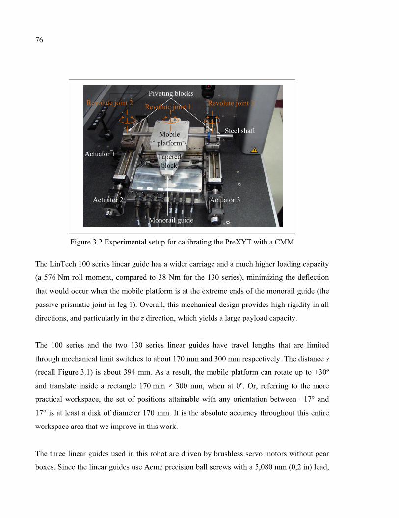
76
Monorail guide
Actuator 1
Actuator 2 Actuator 3
Tapered block
Pivoting blocks
Steel shaftMobileplatform
Revolute joint 3Revolute joint 2Revolute joint 1
Figure 3.2 Experimental setup for calibrating the PreXYT with a CMM
The LinTech 100 series linear guide has a wider carriage and a much higher loading capacity
(a 576 Nm roll moment, compared to 38 Nm for the 130 series), minimizing the deflection
that would occur when the mobile platform is at the extreme ends of the monorail guide (the
passive prismatic joint in leg 1). Overall, this mechanical design provides high rigidity in all
directions, and particularly in the z direction, which yields a large payload capacity.
The 100 series and the two 130 series linear guides have travel lengths that are limited
through mechanical limit switches to about 170 mm and 300 mm respectively. The distance s
(recall Figure 3.1) is about 394 mm. As a result, the mobile platform can rotate up to ±30º
and translate inside a rectangle 170 mm × 300 mm, when at 0º. Or, referring to the more
practical workspace, the set of positions attainable with any orientation between −17° and
17° is at least a disk of diameter 170 mm. It is the absolute accuracy throughout this entire
workspace area that we improve in this work.
The three linear guides used in this robot are driven by brushless servo motors without gear
boxes. Since the linear guides use Acme precision ball screws with a 5,080 mm (0,2 in) lead,
77
a specified maximum lead error of 50 µm per 300 mm, and bidirectional repeatability of
5 µm. In addition, only incremental encoders are used (8000 pulses per revolution). The
actuator homing is processed using the mechanical limit switch and the encoder index pulse,
and its repeatability was measured using a CMM at around 6 µm. Finally, note that the lead
errors are not considered in the nominal model described in the previous section.
3.4 Calibration model
The nominal kinematic model previously presented assumes that the machining and
assembly of all robot components is perfect, which is clearly not the case. Various errors
should therefore be taken into account, and a more realistic, so-called calibration model
should be developed. The purpose of the calibration process will then be to identify these
errors, so that the calibration model will more closely represent the actual robot.
In this work, as well as the distance s, several additional parameters are considered. Referring
to Figure 3.3, let H0 be a point in the Oxy plane such that C coincides with H0 when the first
actuator is homed (i.e. when ρ1 = 0) and actuators 2 and 3 are at their mid-travel lengths.
With this definition in mind, the additional parameters are:
• d1 (offset of actuator 1): distance between H0 and the y axis;
• d3 (offset of actuator 3): distance between the x axis and the axis of the revolute joint of
leg 3 when actuator 3 is homed (i.e. when ρ3 = 0);
• h: distance between H0 and the x axis;
• α: angle between the x axis and the positive direction of actuator 1, measured
counterclockwise (for example, in Figure 3.3, this angle is positive);
• β: angle between the y axis and the positive direction of actuator 3, measured
counterclockwise (for example, in Figure 3.3, this angle is positive);
• γ: angle between the y axis and the direction of the passive joint of leg 1, measured
counterclockwise, and being close to zero (for example, in Figure 3.3, this angle is
negative).
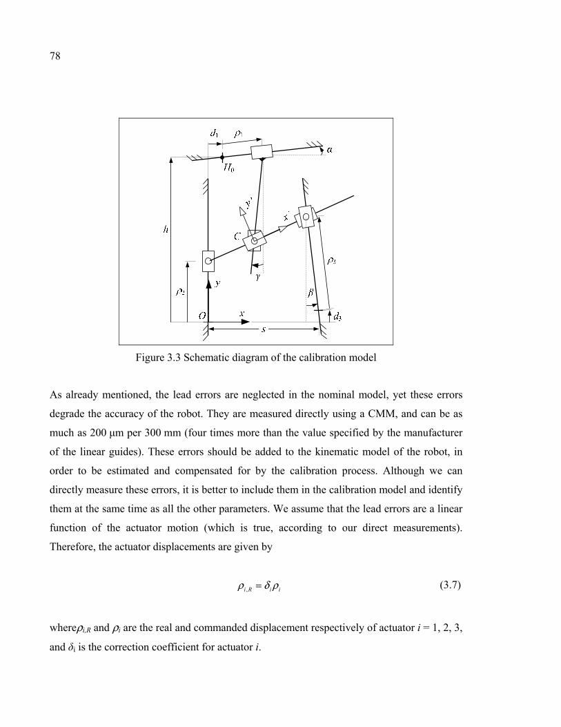
78
Figure 3.3 Schematic diagram of the calibration model
As already mentioned, the lead errors are neglected in the nominal model, yet these errors
degrade the accuracy of the robot. They are measured directly using a CMM, and can be as
much as 200 μm per 300 mm (four times more than the value specified by the manufacturer
of the linear guides). These errors should be added to the kinematic model of the robot, in
order to be estimated and compensated for by the calibration process. Although we can
directly measure these errors, it is better to include them in the calibration model and identify
them at the same time as all the other parameters. We assume that the lead errors are a linear
function of the actuator motion (which is true, according to our direct measurements).
Therefore, the actuator displacements are given by
,i R i iρ δ ρ=
(3.7)
whereρi,R and ρi are the real and commanded displacement respectively of actuator i = 1, 2, 3,
and δi is the correction coefficient for actuator i.
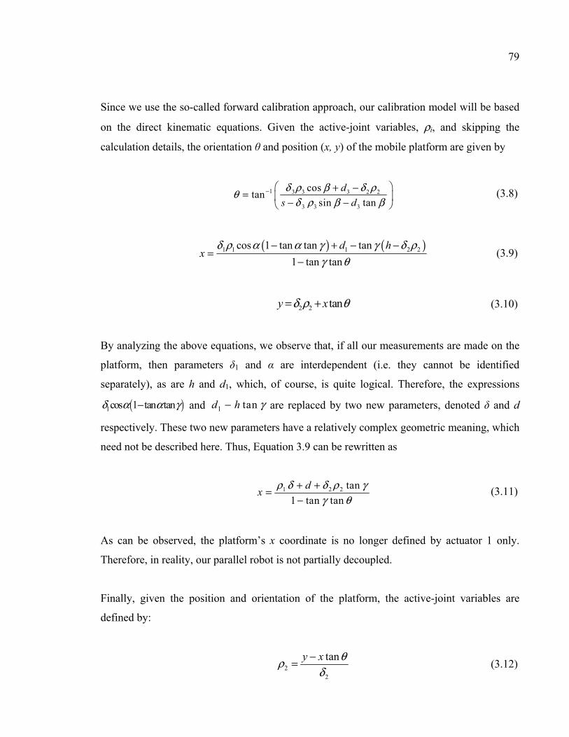
79
Since we use the so-called forward calibration approach, our calibration model will be based
on the direct kinematic equations. Given the active-joint variables, ρi, and skipping the
calculation details, the orientation θ and position (x, y) of the mobile platform are given by
1 3 3 3 2 2
3 3 3
costan
sin tan
d
s d
δ ρ β δ ρθδ ρ β β
− + −= − − (3.8)
( ) ( )1 1 1 2 2cos 1 tan tan tan
1 tan tan
d hx
δ ρ α α γ γ δ ργ θ
− + − −=
− (3.9)
2 2 tany xδ ρ θ= +
(3.10)
By analyzing the above equations, we observe that, if all our measurements are made on the
platform, then parameters δ1 and α are interdependent (i.e. they cannot be identified
separately), as are h and d1, which, of course, is quite logical. Therefore, the expressions
( )1cos 1 tan tanδ α α γ− and 1 tand h γ− are replaced by two new parameters, denoted δ and d
respectively. These two new parameters have a relatively complex geometric meaning, which
need not be described here. Thus, Equation 3.9 can be rewritten as
1 2 2 tan
1 tan tan
dx
ρ δ δ ρ γγ θ
+ +=−
(3.11)
As can be observed, the platform’s x coordinate is no longer defined by actuator 1 only.
Therefore, in reality, our parallel robot is not partially decoupled.
Finally, given the position and orientation of the platform, the active-joint variables are
defined by:
2
2
tany x θρδ
−=
(3.12)
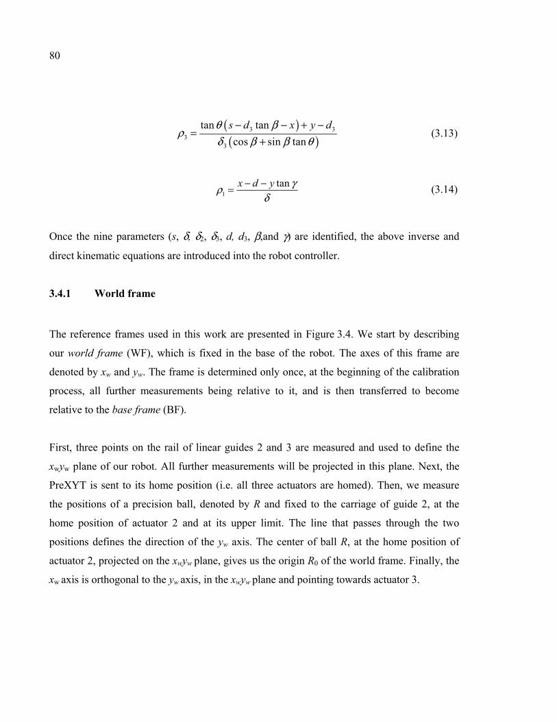
80
( )( )
3 33
3
tan tan
cos sin tan
s d x y dθ βρ
δ β β θ− − + −
=+
(3.13)
1
tanx d y γρδ
− −=
(3.14)
Once the nine parameters (s, δ, δ2, δ3, d, d3, β,and γ) are identified, the above inverse and
direct kinematic equations are introduced into the robot controller.
3.4.1 World frame
The reference frames used in this work are presented in Figure 3.4. We start by describing
our world frame (WF), which is fixed in the base of the robot. The axes of this frame are
denoted by xw and yw. The frame is determined only once, at the beginning of the calibration
process, all further measurements being relative to it, and is then transferred to become
relative to the base frame (BF).
First, three points on the rail of linear guides 2 and 3 are measured and used to define the
xwyw plane of our robot. All further measurements will be projected in this plane. Next, the
PreXYT is sent to its home position (i.e. all three actuators are homed). Then, we measure
the positions of a precision ball, denoted by R and fixed to the carriage of guide 2, at the
home position of actuator 2 and at its upper limit. The line that passes through the two
positions defines the direction of the yw axis. The center of ball R, at the home position of
actuator 2, projected on the xwyw plane, gives us the origin R0 of the world frame. Finally, the
xw axis is orthogonal to the yw axis, in the xwyw plane and pointing towards actuator 3.
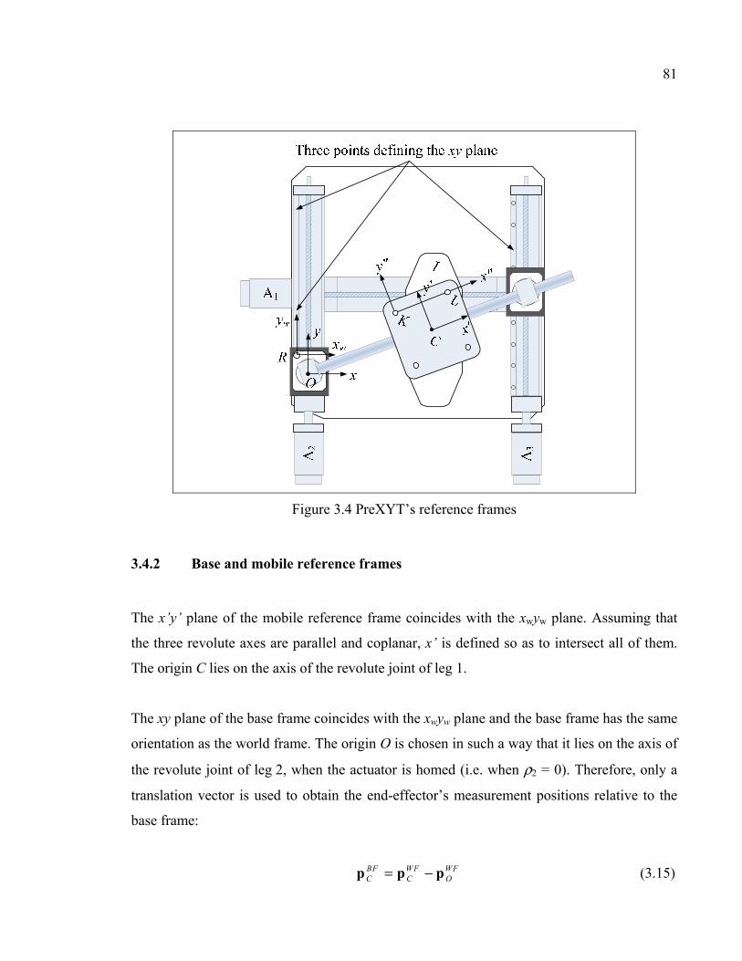
81
Figure 3.4 PreXYT’s reference frames
3.4.2 Base and mobile reference frames
The x’y’ plane of the mobile reference frame coincides with the xwyw plane. Assuming that
the three revolute axes are parallel and coplanar, x’ is defined so as to intersect all of them.
The origin C lies on the axis of the revolute joint of leg 1.
The xy plane of the base frame coincides with the xwyw plane and the base frame has the same
orientation as the world frame. The origin O is chosen in such a way that it lies on the axis of
the revolute joint of leg 2, when the actuator is homed (i.e. when ρ2 = 0). Therefore, only a
translation vector is used to obtain the end-effector’s measurement positions relative to the
base frame:
BF WF WFC C O= −p p p
(3.15)
82
where [ , ]BF TC x y=p and
WFCp represent the platform position relative to the base frame and to
the world frame respectively, and [ , ]WF TO O Ox y=p is the position of the base frame’s origin
with respect to the world frame. The offset coordinates xO and yO are obtained by the
calibration process, because we cannot measure them directly.
Similarly,WFCp cannot be obtained by direct measurement because there is no measurement
target (e.g. a tooling ball) placed exactly at (or above) the platform’s center C. Thus, two
tooling balls are attached to the platform, referred to as K and L, as shown in Figure 3.4.
These balls are used to define a reference frame denoted by KL_F with its origin at the
projection of K in the xwyw plane and its x” axis passing through the projection of L in the
xwyw plane. Note that the position of C with respect to KL_F is a constant vector _ [ , ]KL F T
C C Cx y=p . Then, to measure the pose of the mobile platform, we measure the centers
of balls K and L with respect to the world frame, namely the coordinates xK, yK, xL, and yL.
Finally, we obtain the platform position with respect to the base frame using the equation:
_ _ [ , ]BF WF WF WF WF T WF
C C O KL F KL F C C Ox y= − = + −p p p p R p
(3.16)
where _WFKL FR is the rotation matrix representing the orientation of KL_F with respect to the
world frame. Knowing that the orientation angle of KL_F with respect to the world frame is
λ, Equation 3.16 can be rewritten as follows:
cos sin
sin cosK C C OBF
CK C C O
x x y xx
y x y yy
λ λλ λ
+ − − = = + + −
p
(3.17)
where
83
( )atan 2 ,L K L Ky y x xλ = − −
(3.18)
3.4.3 Orientation measurement error
Ideally, the orientation λ of KL_F with respect to the base frame should be equal to the
measured platform orientation, θmeas. However, the x” axis is not perfectly parallel to the x’
axis, and there is an offset between θmeas and λ. This offset, εθ, is evaluated by the calibration
process. To do so, the platform orientation error is introduced at every position measured:
meas θθ λ ε= −
(3.19)
To summarize, in our calibration process, we have to identify a total of thirteen independent
parameters: xO and yO (the base frame translation with respect to the world frame), xC and yC
(the mobile frame translation with respect to KL_F), s, d, d3, δ, β, γ, the correction coefficient
for the lead errors δ2 andδ3, and, finally, the orientation measurement offset, εθ. Reference our
assumption that the axes of the three revolute joints are parallel, coplanar, and normal to the
directions of all the prismatic joints.
3.5 Calibration method
As mentioned previously, the aim of our calibration process is to reduce the end-effector’s
position and orientation absolute errors by accurately identifying the geometric parameters,
the lead error parameters, and the frame locations. The process is based on the direct method,
which compares the end-effector’s estimated and measured poses. For calibration pose j, the
measured position xmeas,j, ymeas,j and orientation θmeas,j are based on measurements of the K
and L precision balls, while the estimated poses xest,j, yest,j, θest,j are obtained from the direct
kinematic Equations 3.8, 3.10, and 3.11, which can also be represented as
, 1, 2, 3, 2 3 3( , , , , , , , , , , )est j x j j jx f s d dρ ρ ρ δ δ δ β γ=
(3.20)
84
, 1, 2, 3, 2 3 3( , , , , , , , , , , )est j y j j jy f s d dρ ρ ρ δ δ δ β γ=
(3.21)
, 1, 2, 3, 2 3 3( , , , , , , , , , , )est j j j jf s d dθθ ρ ρ ρ δ δ δ β γ=
(3.22)
where ρ1,j, ρ2,j, and ρ3,jare the actuator values commanded at the jth calibration pose.
The equations of the measured position and orientation can be rewritten based on Equations
3.17 and 3.19, as
, , , , ,( , , , , , , , )meas j x O O C C K j K j L j L jx f x y x y x y x y=
(3.23)
, , , , ,( , , , , , , , )meas j y O O C C K j K j L j L jy f x y x y x y x y=
(3.24)
, , , , ,( , , , , , , , , )meas j O O C C K j K j L j L jf x y x y x y x yθ θθ ε=
(3.25)
where xK,j, yK,j, xL,j, and yL,j, represent the measured coordinate for precision balls K and L
with respect to the world frame, at the jth calibration pose.
All the parameters are identified using the least squares minimization method:
( ) ( ) ( )( )2 2 2
, , , , , ,1
n
est j meas j est j meas j est j meas jj
minimize x x y y θ θ=
− + − + −
(3.26)
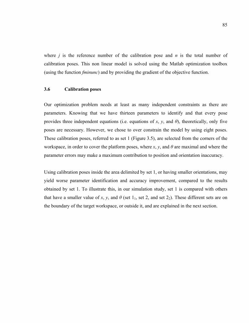
85
where j is the reference number of the calibration pose and n is the total number of
calibration poses. This non linear model is solved using the Matlab optimization toolbox
(using the function fminunc) and by providing the gradient of the objective function.
3.6 Calibration poses
Our optimization problem needs at least as many independent constraints as there are
parameters. Knowing that we have thirteen parameters to identify and that every pose
provides three independent equations (i.e. equations of x, y, and θ), theoretically, only five
poses are necessary. However, we chose to over constrain the model by using eight poses.
These calibration poses, referred to as set 1 (Figure 3.5), are selected from the corners of the
workspace, in order to cover the platform poses, where x, y, and θ are maximal and where the
parameter errors may make a maximum contribution to position and orientation inaccuracy.
Using calibration poses inside the area delimited by set 1, or having smaller orientations, may
yield worse parameter identification and accuracy improvement, compared to the results
obtained by set 1. To illustrate this, in our simulation study, set 1 is compared with others
that have a smaller value of x, y, and θ (set 11, set 2, and set 22). These different sets are on
the boundary of the target workspace, or outside it, and are explained in the next section.
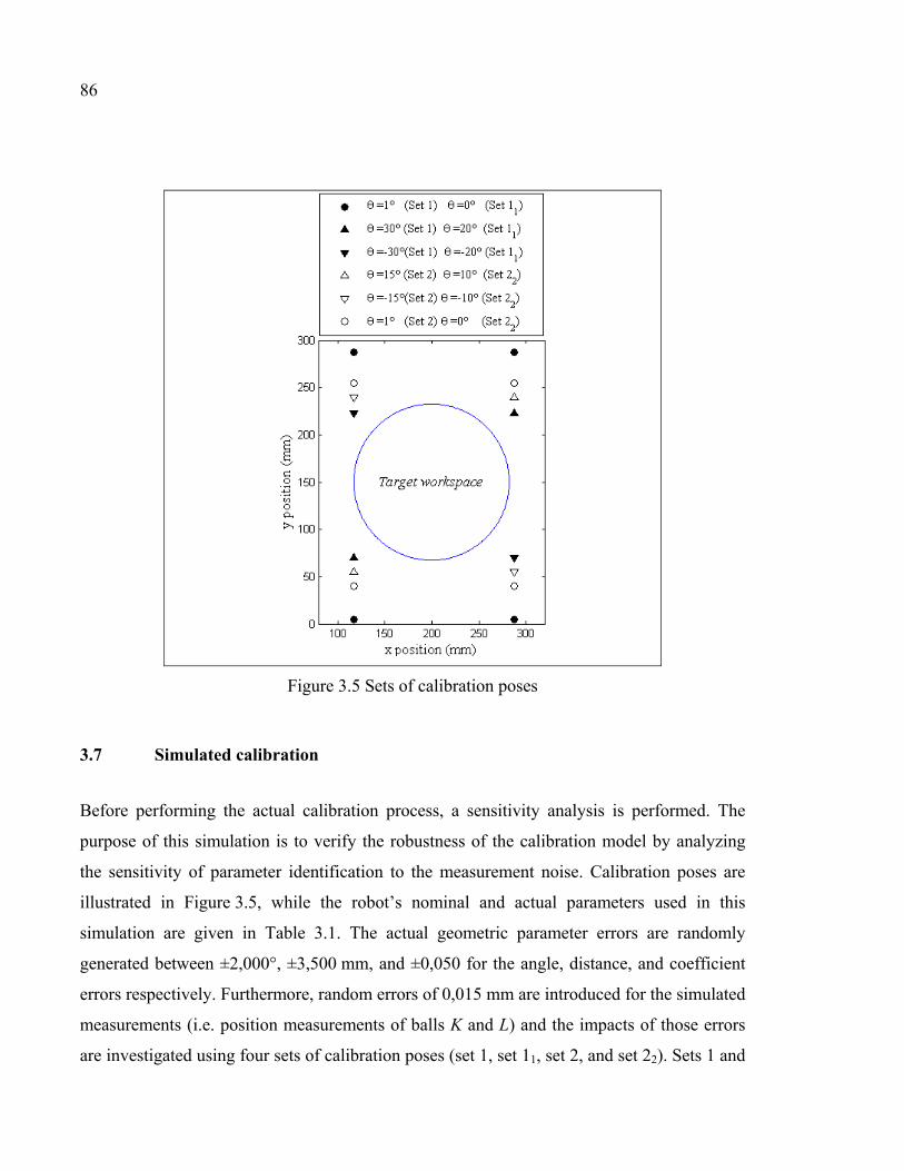
86
Figure 3.5 Sets of calibration poses
3.7 Simulated calibration
Before performing the actual calibration process, a sensitivity analysis is performed. The
purpose of this simulation is to verify the robustness of the calibration model by analyzing
the sensitivity of parameter identification to the measurement noise. Calibration poses are
illustrated in Figure 3.5, while the robot’s nominal and actual parameters used in this
simulation are given in Table 3.1. The actual geometric parameter errors are randomly
generated between ±2,000°, ±3,500 mm, and ±0,050 for the angle, distance, and coefficient
errors respectively. Furthermore, random errors of 0,015 mm are introduced for the simulated
measurements (i.e. position measurements of balls K and L) and the impacts of those errors
are investigated using four sets of calibration poses (set 1, set 11, set 2, and set 22). Sets 1 and
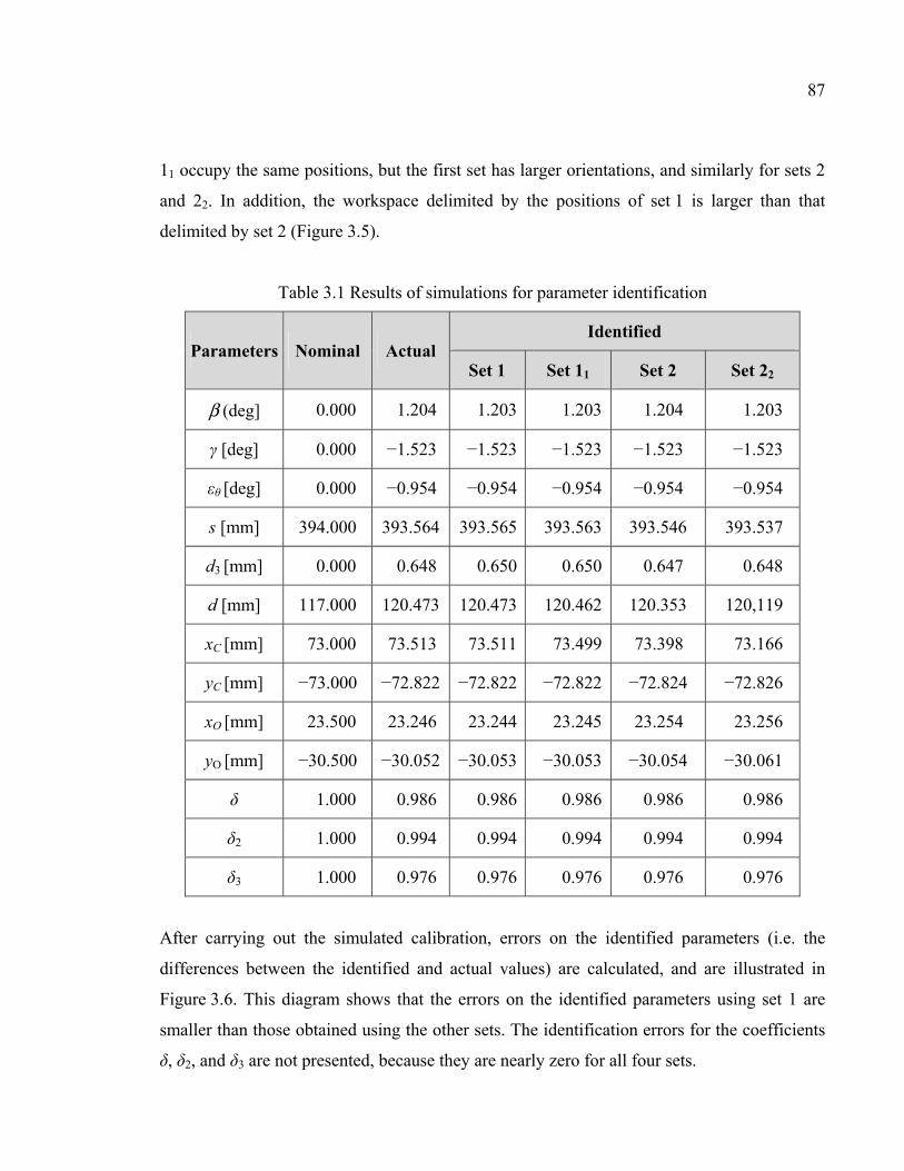
87
11 occupy the same positions, but the first set has larger orientations, and similarly for sets 2
and 22. In addition, the workspace delimited by the positions of set 1 is larger than that
delimited by set 2 (Figure 3.5).
Table 3.1 Results of simulations for parameter identification
Parameters Nominal Actual Identified
Set 1 Set 11 Set 2 Set 22
β (deg] 0.000 1.204 1.203 1.203 1.204 1.203
γ [deg] 0.000 −1.523 −1.523 −1.523 −1.523 −1.523
εθ [deg] 0.000 −0.954 −0.954 −0.954 −0.954 −0.954
s [mm] 394.000 393.564 393.565 393.563 393.546 393.537
d3 [mm] 0.000 0.648 0.650 0.650 0.647 0.648
d [mm] 117.000 120.473 120.473 120.462 120.353 120,119
xC [mm] 73.000 73.513 73.511 73.499 73.398 73.166
yC [mm] −73.000 −72.822 −72.822 −72.822 −72.824 −72.826
xO [mm] 23.500 23.246 23.244 23.245 23.254 23.256
yO [mm] −30.500 −30.052 −30.053 −30.053 −30.054 −30.061
δ 1.000 0.986 0.986 0.986 0.986 0.986
δ2 1.000 0.994 0.994 0.994 0.994 0.994
δ3 1.000 0.976 0.976 0.976 0.976 0.976
After carrying out the simulated calibration, errors on the identified parameters (i.e. the
differences between the identified and actual values) are calculated, and are illustrated in
Figure 3.6. This diagram shows that the errors on the identified parameters using set 1 are
smaller than those obtained using the other sets. The identification errors for the coefficients
δ, δ2, and δ3 are not presented, because they are nearly zero for all four sets.
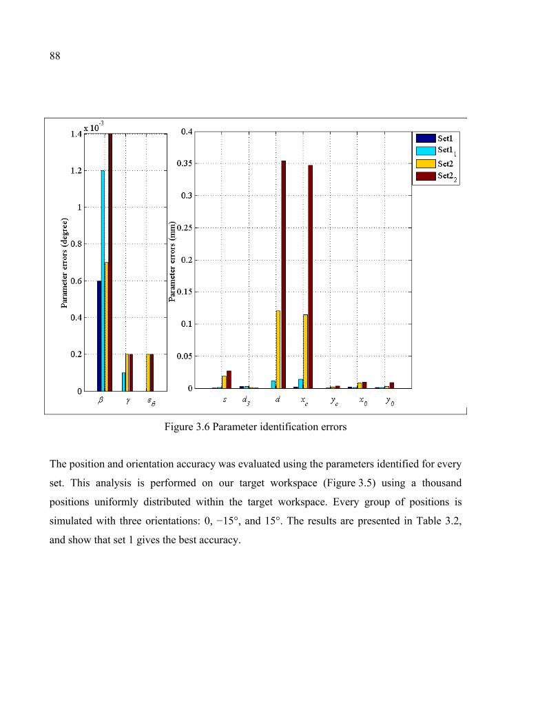
88
Figure 3.6 Parameter identification errors
The position and orientation accuracy was evaluated using the parameters identified for every
set. This analysis is performed on our target workspace (Figure 3.5) using a thousand
positions uniformly distributed within the target workspace. Every group of positions is
simulated with three orientations: 0, −15°, and 15°. The results are presented in Table 3.2,
and show that set 1 gives the best accuracy.
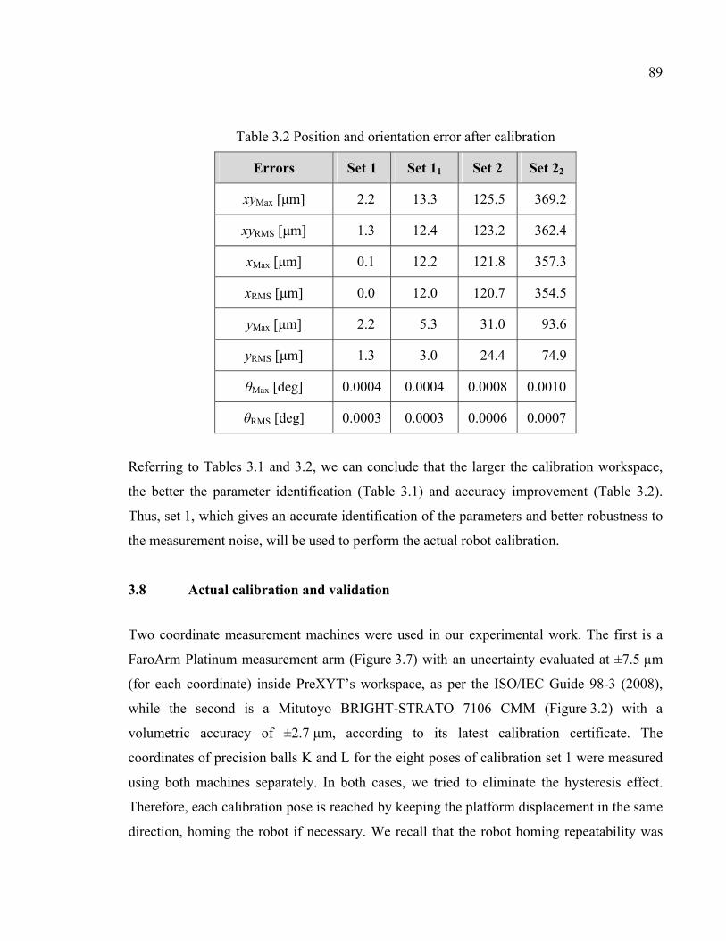
89
Table 3.2 Position and orientation error after calibration
Errors Set 1 Set 11 Set 2 Set 22
xyMax [μm] 2.2 13.3 125.5 369.2
xyRMS [μm] 1.3 12.4 123.2 362.4
xMax [μm] 0.1 12.2 121.8 357.3
xRMS [μm] 0.0 12.0 120.7 354.5
yMax [μm] 2.2 5.3 31.0 93.6
yRMS [μm] 1.3 3.0 24.4 74.9
θMax [deg] 0.0004 0.0004 0.0008 0.0010
θRMS [deg] 0.0003 0.0003 0.0006 0.0007
Referring to Tables 3.1 and 3.2, we can conclude that the larger the calibration workspace,
the better the parameter identification (Table 3.1) and accuracy improvement (Table 3.2).
Thus, set 1, which gives an accurate identification of the parameters and better robustness to
the measurement noise, will be used to perform the actual robot calibration.
3.8 Actual calibration and validation
Two coordinate measurement machines were used in our experimental work. The first is a
FaroArm Platinum measurement arm (Figure 3.7) with an uncertainty evaluated at ±7.5 µm
(for each coordinate) inside PreXYT’s workspace, as per the ISO/IEC Guide 98-3 (2008),
while the second is a Mitutoyo BRIGHT-STRATO 7106 CMM (Figure 3.2) with a
volumetric accuracy of ±2.7 µm, according to its latest calibration certificate. The
coordinates of precision balls K and L for the eight poses of calibration set 1 were measured
using both machines separately. In both cases, we tried to eliminate the hysteresis effect.
Therefore, each calibration pose is reached by keeping the platform displacement in the same
direction, homing the robot if necessary. We recall that the robot homing repeatability was
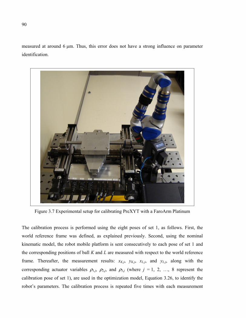
90
measured at around 6 µm. Thus, this error does not have a strong influence on parameter
identification.
Figure 3.7 Experimental setup for calibrating PreXYT with a FaroArm Platinum
The calibration process is performed using the eight poses of set 1, as follows. First, the
world reference frame was defined, as explained previously. Second, using the nominal
kinematic model, the robot mobile platform is sent consecutively to each pose of set 1 and
the corresponding positions of ball K and L are measured with respect to the world reference
frame. Thereafter, the measurement results: xK,j, yK,j, xL,j, and yL,j, along with the
corresponding actuator variables ρ1,j, ρ2,j, and ρ3,j (where j = 1, 2, …, 8 represent the
calibration pose of set 1), are used in the optimization model, Equation 3.26, to identify the
robot’s parameters. The calibration process is repeated five times with each measurement
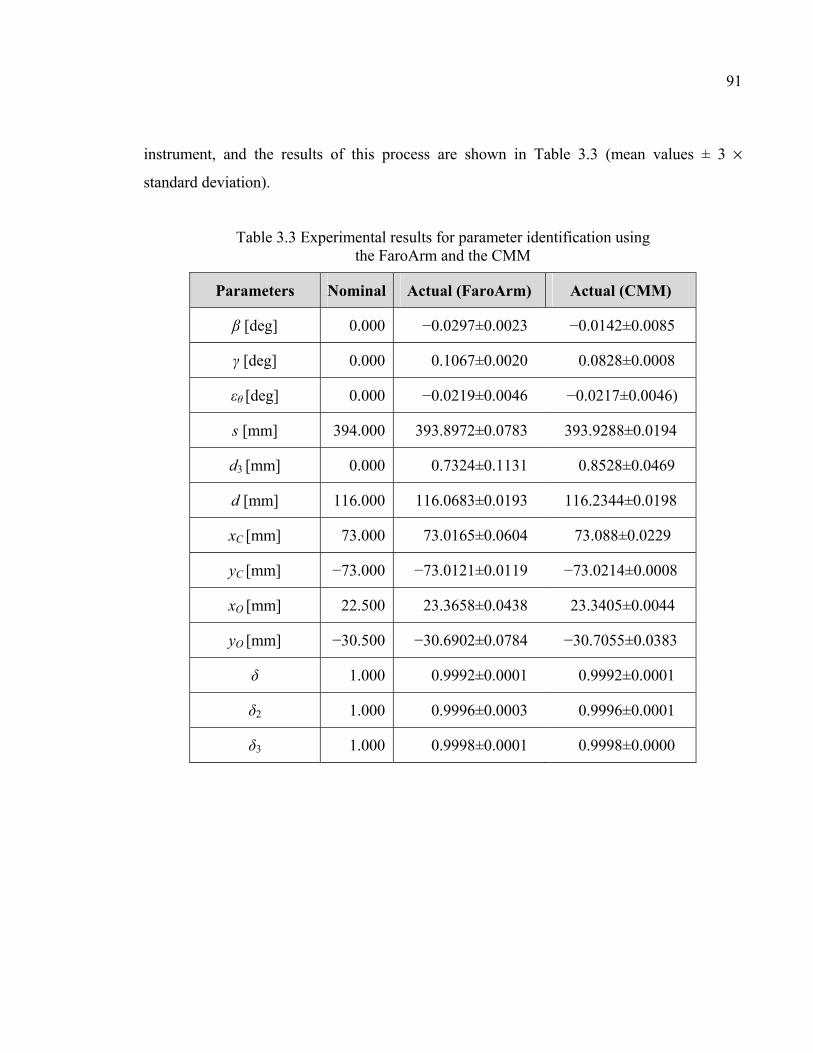
91
instrument, and the results of this process are shown in Table 3.3 (mean values ± 3 ×
standard deviation).
Table 3.3 Experimental results for parameter identification using the FaroArm and the CMM
Parameters Nominal Actual (FaroArm) Actual (CMM)
β [deg] 0.000 −0.0297±0.0023 −0.0142±0.0085
γ [deg] 0.000 0.1067±0.0020 0.0828±0.0008
εθ [deg] 0.000 −0.0219±0.0046 −0.0217±0.0046)
s [mm] 394.000 393.8972±0.0783 393.9288±0.0194
d3 [mm] 0.000 0.7324±0.1131 0.8528±0.0469
d [mm] 116.000 116.0683±0.0193 116.2344±0.0198
xC [mm] 73.000 73.0165±0.0604 73.088±0.0229
yC [mm] −73.000 −73.0121±0.0119 −73.0214±0.0008
xO [mm] 22.500 23.3658±0.0438 23.3405±0.0044
yO [mm] −30.500 −30.6902±0.0784 −30.7055±0.0383
δ 1.000 0.9992±0.0001 0.9992±0.0001
δ2 1.000 0.9996±0.0003 0.9996±0.0001
δ3 1.000 0.9998±0.0001 0.9998±0.0000
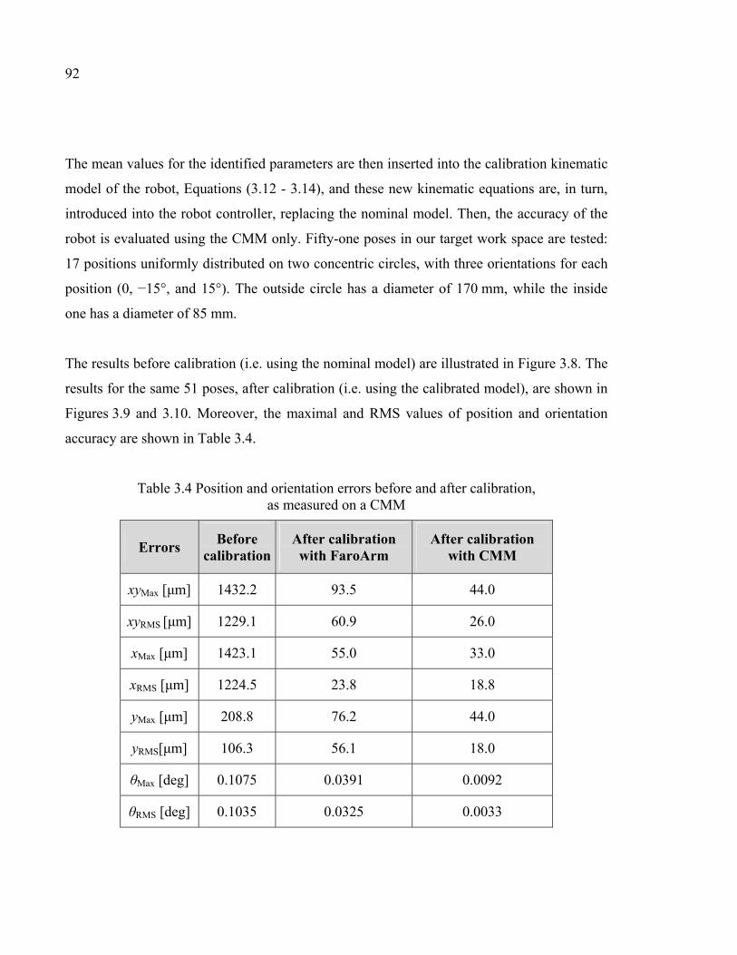
92
The mean values for the identified parameters are then inserted into the calibration kinematic
model of the robot, Equations (3.12 - 3.14), and these new kinematic equations are, in turn,
introduced into the robot controller, replacing the nominal model. Then, the accuracy of the
robot is evaluated using the CMM only. Fifty-one poses in our target work space are tested:
17 positions uniformly distributed on two concentric circles, with three orientations for each
position (0, −15°, and 15°). The outside circle has a diameter of 170 mm, while the inside
one has a diameter of 85 mm.
The results before calibration (i.e. using the nominal model) are illustrated in Figure 3.8. The
results for the same 51 poses, after calibration (i.e. using the calibrated model), are shown in
Figures 3.9 and 3.10. Moreover, the maximal and RMS values of position and orientation
accuracy are shown in Table 3.4.
Table 3.4 Position and orientation errors before and after calibration, as measured on a CMM
Errors Before
calibration After calibration with FaroArm
After calibration with CMM
xyMax [μm] 1432.2 93.5 44.0
xyRMS [μm] 1229.1 60.9 26.0
xMax [μm] 1423.1 55.0 33.0
xRMS [μm] 1224.5 23.8 18.8
yMax [μm] 208.8 76.2 44.0
yRMS[μm] 106.3 56.1 18.0
θMax [deg] 0.1075 0.0391 0.0092
θRMS [deg] 0.1035 0.0325 0.0033
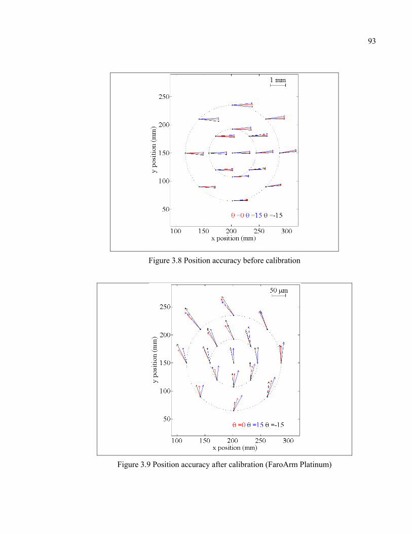
93
Figure 3.8 Position accuracy before calibration
Figure 3.9 Position accuracy after calibration (FaroArm Platinum)
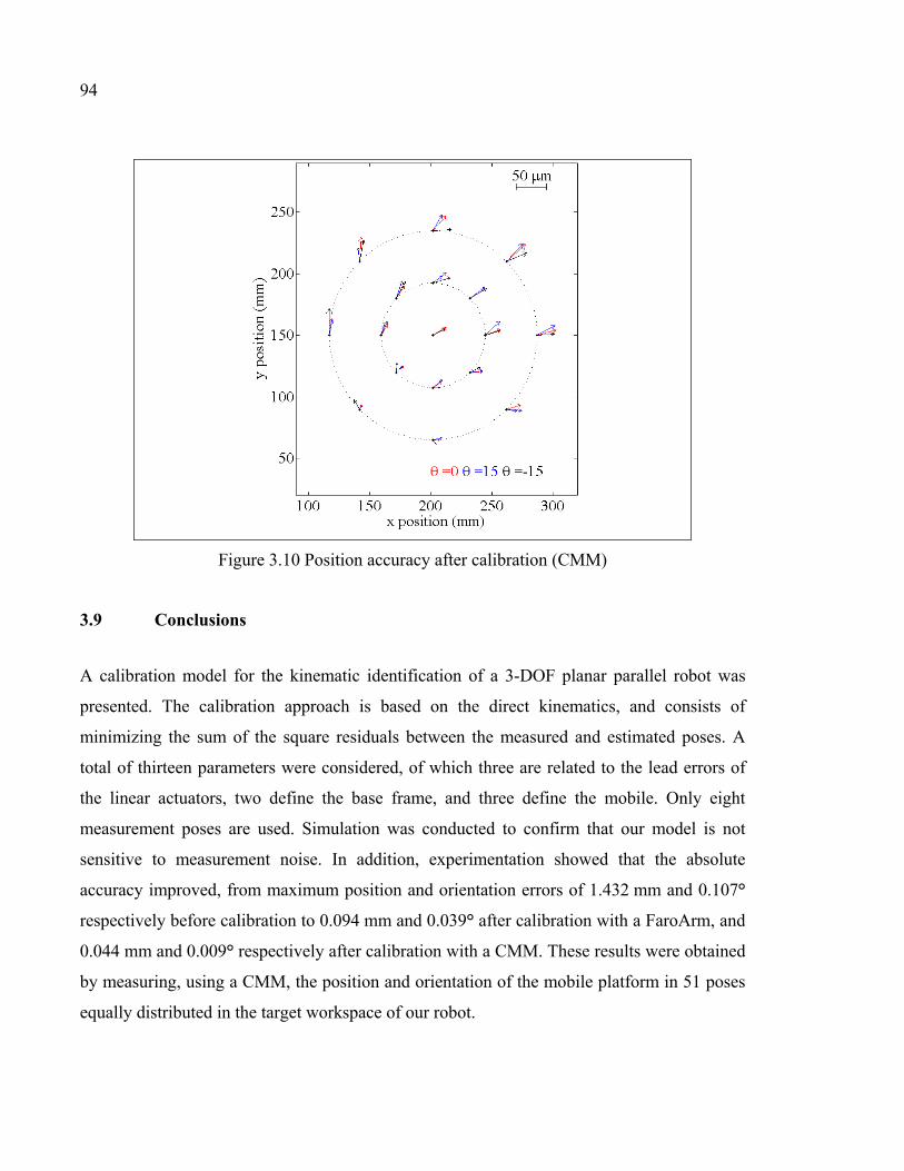
94
Figure 3.10 Position accuracy after calibration (CMM)
3.9 Conclusions
A calibration model for the kinematic identification of a 3-DOF planar parallel robot was
presented. The calibration approach is based on the direct kinematics, and consists of
minimizing the sum of the square residuals between the measured and estimated poses. A
total of thirteen parameters were considered, of which three are related to the lead errors of
the linear actuators, two define the base frame, and three define the mobile. Only eight
measurement poses are used. Simulation was conducted to confirm that our model is not
sensitive to measurement noise. In addition, experimentation showed that the absolute
accuracy improved, from maximum position and orientation errors of 1.432 mm and 0.107°
respectively before calibration to 0.094 mm and 0.039° after calibration with a FaroArm, and
0.044 mm and 0.009° respectively after calibration with a CMM. These results were obtained
by measuring, using a CMM, the position and orientation of the mobile platform in 51 poses
equally distributed in the target workspace of our robot.
95
The calibration was performed using two coordinate measurement devices. Results show that
identification using the CMM leads to better robot accuracy, because the parameter
uncertainty (±3σ) is smaller than that obtained by the FaroArm. Nevertheless, the results
obtained using the FaroArm are very satisfactory, and demonstrate that a small range
measurement arm can be used to calibrate a parallel robot and bring its positioning accuracy
to 0.094 mm or better.

CHAPITRE 4
ARTICLE 3: KINEMATIC CALIBRATION OF A FIVE-BAR PLANAR PARALLEL ROBOT USING ALL WORKING MODES
Ahmed Joubair, Mohamed Slamani and Ilian A. Bonev
École de technologie supérieure, 1100, Notre-Dame Street West, Montreal, QC, H3C 1K3,
Canada
This chapter has been submitted as an article in
Robotics and Computer-Integrated Manufacturing
Résumé
Dans cet article, nous présentons une procédure d’étalonnage simple et peu coûteuse, qui
améliore la précision de positionnement planaire d'un robot SCARA à double bras à des
niveaux difficiles ou impossibles à atteindre en utilisant un robot sériel équivalent. Les
mesures sont basées sur l'utilisation de sept billes magnétiques de précision, conçues par
nous-même. Ces billes sont fixées à la périphérie d'une plaque de travail amovible. Trois de
ces billes de précision servent à définir le référentiel de la cellule (World frame), alors que les
positions des centres de toutes les billes sont mesurées sur une CMM. L’effecteur a une
caractéristique spéciale, étant magnétisé et ayant la forme d’un verre (i.e. une forme conique
creuse). Les mesures sont effectuées par le positionnement manuel de l'effecteur sur chacune
des billes de précision, chacune avec la possibilité d’un maximum de quatre configurations
du robot. Chacune de ces mesures est répétable à ±0,015 mm. Le modèle d'étalonnage du
robot inclut tous les 12 paramètres géométriques, et la méthode d'étalonnage utilisée est
basée sur la linéarisation du modèle cinématique directe dans chaque configuration
d'étalonnage. Le nombre et l'emplacement optimaux des billes de précision sont obtenues par
une analyse d’observabilité. Finalement, une validation expérimentale dans 14 positions
supplémentaires indique que l'erreur de position maximale par rapport au référentiel de la
cellule est réduite à 0,080 mm dans l’ensemble de l'espace de travail du robot qui représente
600 mm × 600 mm.
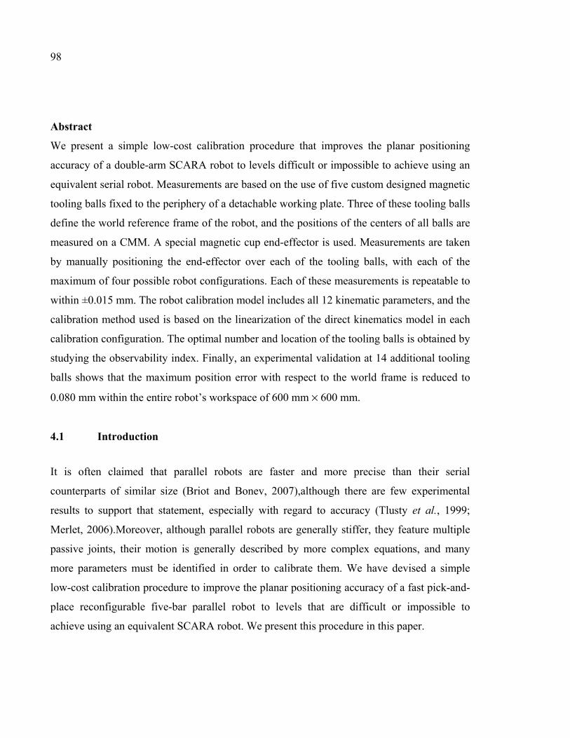
98
Abstract
We present a simple low-cost calibration procedure that improves the planar positioning
accuracy of a double-arm SCARA robot to levels difficult or impossible to achieve using an
equivalent serial robot. Measurements are based on the use of five custom designed magnetic
tooling balls fixed to the periphery of a detachable working plate. Three of these tooling balls
define the world reference frame of the robot, and the positions of the centers of all balls are
measured on a CMM. A special magnetic cup end-effector is used. Measurements are taken
by manually positioning the end-effector over each of the tooling balls, with each of the
maximum of four possible robot configurations. Each of these measurements is repeatable to
within ±0.015 mm. The robot calibration model includes all 12 kinematic parameters, and the
calibration method used is based on the linearization of the direct kinematics model in each
calibration configuration. The optimal number and location of the tooling balls is obtained by
studying the observability index. Finally, an experimental validation at 14 additional tooling
balls shows that the maximum position error with respect to the world frame is reduced to
0.080 mm within the entire robot’s workspace of 600 mm × 600 mm.
4.1 Introduction
It is often claimed that parallel robots are faster and more precise than their serial
counterparts of similar size (Briot and Bonev, 2007),although there are few experimental
results to support that statement, especially with regard to accuracy (Tlusty et al., 1999;
Merlet, 2006).Moreover, although parallel robots are generally stiffer, they feature multiple
passive joints, their motion is generally described by more complex equations, and many
more parameters must be identified in order to calibrate them. We have devised a simple
low-cost calibration procedure to improve the planar positioning accuracy of a fast pick-and-
place reconfigurable five-bar parallel robot to levels that are difficult or impossible to
achieve using an equivalent SCARA robot. We present this procedure in this paper.
99
Several publications describe the calibration of five-bar parallel robots. Everett and Lin
(1988) and Everett (1989) propose a calibration method based on the forward kinematics
approach, while method proposed in (Durango et al., 2010) is based on inverse kinematics.
However, validation of these methods is based only on simulations. For example, the results
of the simulation presented in (Durango et al., 2010) show that, after calibration, the position
accuracy is between 0.006 mm and 0.600 mm within a disk 1 m in diameter. Ding et al.
(2005) present a calibration procedure for a five-bar robot, with experimental validation,
based mainly on home position identification. In this case, the workspace of the robot is very
small (80 mm × 80 mm) compared to that of our robot (600 mm × 600 mm), and the
accuracy obtained after calibration is 0.084 mm and 0.292 mm for average and maximum
values respectively.
Our five-bar robot has a unique design, featuring four links of equal length (230 mm),
precision bearings, and direct drive motors (Campos et al., 2010). To make full use of the
robot’s workspace and without having to cross so-called parallel singularities, the robot can
switch between four different configurations (i.e. the four solutions of the inverse
kinematics). As a result, it can position its end-effector anywhere within an enclosed area of
about 600 mm × 600 mm. Furthermore, its bidirectional repeatability was found to be no
more than 0.010 mm.
The problem with calibrating such a relatively large and precise parallel robot is to find
adequate measurement equipment for doing so, and, ideally, another one for measuring 2D
coordinates for the validation phase. Fortunately, we have most of the devices used for robot
calibration, including a large Mitotoyo CMM, a Faro laser tracker, a Faro measurement arm,
a Renishaw telescoping ballbar, and a Renishaw laser interferometer system, as well as
various reference artifacts. Regrettably, a laser tracker is not sufficiently accurate for this
application (Slamani et al., 2012). Tests that we performed in conjunction with our CMM
showed that our laser tracker’s position error inside our robot’s workspace can be as much as
±0.030 mm. Moreover, our robot (rigidly fixed to a mobile table) is too big to be placed on a
CMM, as we had done with another parallel robot in (Joubair et al., 2012), and the optics of
100
the laser interferometer system are too bulky to be attached to the end-effector of our robot
(Slamani et al., 2012). A telescoping ballbar (also called a double-ball bar) could certainly be
used for calibration, as in (Ota et al., 2002; Takeda et al., 2002; Kim, 2005), but this is a
relatively expensive option (about $10,000) and difficult for potential users of our pick-and-
place robot to handle. Furthermore, its limited measurement range of ±1 mm might not be
sufficient for the uncalibrated robot.
Our robot is actuated by direct drive motors. When these motors are not energized, a force of
only 1 N or less need to be applied to the end-effector to move it in any direction, for any
robot configuration. Therefore, instead of using an expensive external measurement system,
we chose the well-known approach of constraining some or all the degrees-of-freedom
(DOFs) of the end-effector to a precisely known geometry (Mooring and Tang, 1984;
Veitschegger and Wu, 1987; Zhong and Lewis, 1995) as the best option. The ingenious
method for calibrating a parallel robot by crossing parallel singularities (Last and
Hesselbach, 2006) was discarded, as it cannot be used for absolute calibration.
One of the possibilities for the constraining geometry is to use a mechanical artifact, such as
a master square (a precision parallelepiped made of granite). We have one of these, but its
dimensions are not appropriate for our robot. Besides, we are looking for an absolute
calibration, and this requires that we define a world frame with some mechanical references
(locating pins, tooling balls, etc.). What seems to be the best approach, based on all the
criteria, is to use tooling balls. Not only can they define a world frame, but they can be used
for both calibration and validation. Furthermore, the small number of tooling balls needed for
calibration can be permanently fixed, so that recalibration can be performed at any time.
Therefore, we have designed a special type of magnetic tooling ball, along with a magnetic
cup end-effector, that guarantees a measurement noise of no more than ±0.015 mm
(according to extensive repeatability tests). These tooling balls are fixed to a detachable
working plate and their relative position can be measured easily on a CMM.
101
Calibrating a robot by constraining the position of its end-effector is not new. In the case of a
single point constraint, this approach was proposed for the calibration of 6-DOF serial robots
in (Bennett and Hollerbach, 1991; Edwards II and Galloway Jr, 1994), later further
developed in (Meggiolaro et al., 2000), and now widely used for the onsite recalibration of
measurement arms. The originality of our extension of this approach lies in the following: (1)
our tooling balls are magnetic; (2) we use only seven of them and they are permanently fixed
on the periphery of the robot’s working plate; (3) three of them are used to define the world
frame of the robot; and (4) we use up to four different robot configurations at each tooling
ball. The result is a low-cost, yet highly effective absolute calibration procedure that can be
performed by the user at any time.
This paper is organized as follows. In the next section, we present the prototype of our robot,
as well as the design of the tooling balls and end-effector. In section 4.3, we present the
calibration model of our 2-DOF five-bar robot, which consists of the 12 geometric
parameters that are to be identified (including the robot’s base frame). In section 4.4, we
present the calibration method used, which is based on the linearization of the direct
kinematics model in each calibration configuration. In section 4.5, we study the observability
index in order to obtain the optimal number and location of the calibration positions (i.e. the
seven tooling balls). In section 4.6, we present some simulation results on the effect of
measurement noise (no more than ±0.015 mm). In section 4.7, we present our validation
results, which show that the maximum position error in any of the 14 validation positions
within the working plate of 600 mm × 600 mm is no more than 0.077 mm with respect to the
world reference frame defined by three of the seven calibration tooling balls. We provide our
conclusions in section 4.8.
4.2 Description of the robot prototype and the magnetic tooling balls
The parallel robot used in this work is a five-bar planar robot, which we call DexTAR
(Dexterous Twin-Arm Robot). DexTAR (Figure 4.1) is based on a special five-bar design in
which all four links are of equal length (230 mm), and the distance between the axes of the
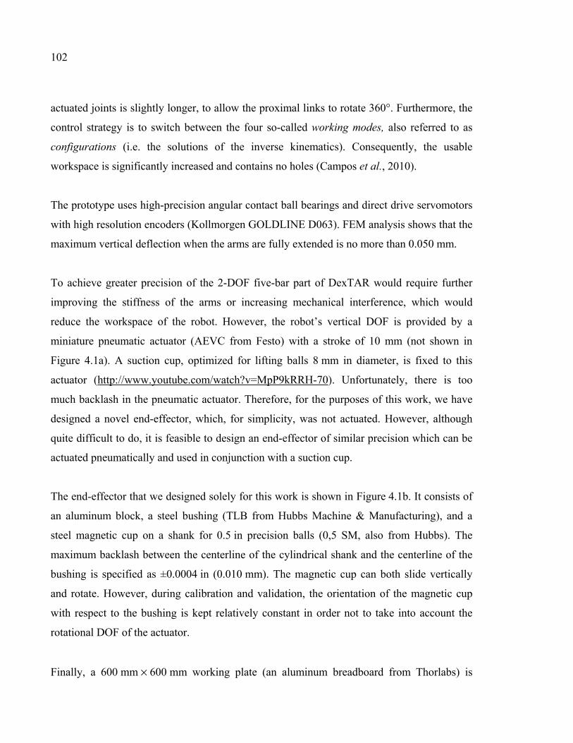
102
actuated joints is slightly longer, to allow the proximal links to rotate 360°. Furthermore, the
control strategy is to switch between the four so-called working modes, also referred to as
configurations (i.e. the solutions of the inverse kinematics). Consequently, the usable
workspace is significantly increased and contains no holes (Campos et al., 2010).
The prototype uses high-precision angular contact ball bearings and direct drive servomotors
with high resolution encoders (Kollmorgen GOLDLINE D063). FEM analysis shows that the
maximum vertical deflection when the arms are fully extended is no more than 0.050 mm.
To achieve greater precision of the 2-DOF five-bar part of DexTAR would require further
improving the stiffness of the arms or increasing mechanical interference, which would
reduce the workspace of the robot. However, the robot’s vertical DOF is provided by a
miniature pneumatic actuator (AEVC from Festo) with a stroke of 10 mm (not shown in
Figure 4.1a). A suction cup, optimized for lifting balls 8 mm in diameter, is fixed to this
actuator (http://www.youtube.com/watch?v=MpP9kRRH-70). Unfortunately, there is too
much backlash in the pneumatic actuator. Therefore, for the purposes of this work, we have
designed a novel end-effector, which, for simplicity, was not actuated. However, although
quite difficult to do, it is feasible to design an end-effector of similar precision which can be
actuated pneumatically and used in conjunction with a suction cup.
The end-effector that we designed solely for this work is shown in Figure 4.1b. It consists of
an aluminum block, a steel bushing (TLB from Hubbs Machine & Manufacturing), and a
steel magnetic cup on a shank for 0.5 in precision balls (0,5 SM, also from Hubbs). The
maximum backlash between the centerline of the cylindrical shank and the centerline of the
bushing is specified as ±0.0004 in (0.010 mm). The magnetic cup can both slide vertically
and rotate. However, during calibration and validation, the orientation of the magnetic cup
with respect to the bushing is kept relatively constant in order not to take into account the
rotational DOF of the actuator.
Finally, a 600 mm × 600 mm working plate (an aluminum breadboard from Thorlabs) is
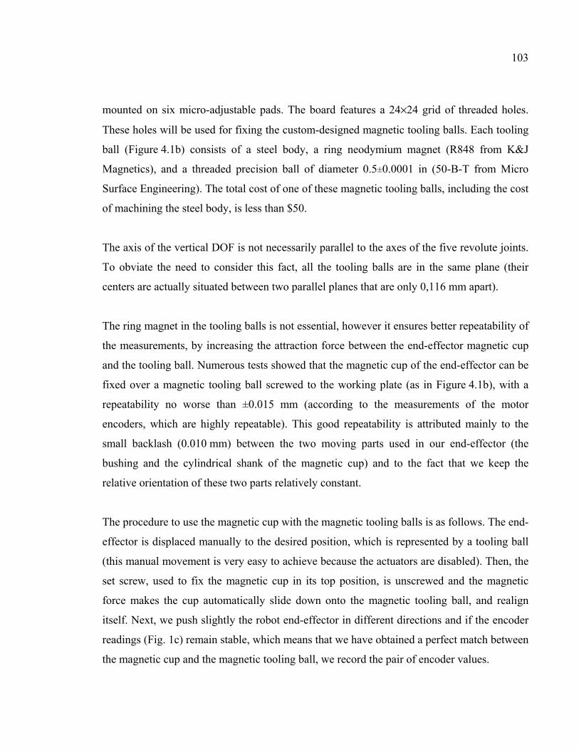
103
mounted on six micro-adjustable pads. The board features a 24×24 grid of threaded holes.
These holes will be used for fixing the custom-designed magnetic tooling balls. Each tooling
ball (Figure 4.1b) consists of a steel body, a ring neodymium magnet (R848 from K&J
Magnetics), and a threaded precision ball of diameter 0.5±0.0001 in (50-B-T from Micro
Surface Engineering). The total cost of one of these magnetic tooling balls, including the cost
of machining the steel body, is less than $50.
The axis of the vertical DOF is not necessarily parallel to the axes of the five revolute joints.
To obviate the need to consider this fact, all the tooling balls are in the same plane (their
centers are actually situated between two parallel planes that are only 0,116 mm apart).
The ring magnet in the tooling balls is not essential, however it ensures better repeatability of
the measurements, by increasing the attraction force between the end-effector magnetic cup
and the tooling ball. Numerous tests showed that the magnetic cup of the end-effector can be
fixed over a magnetic tooling ball screwed to the working plate (as in Figure 4.1b), with a
repeatability no worse than ±0.015 mm (according to the measurements of the motor
encoders, which are highly repeatable). This good repeatability is attributed mainly to the
small backlash (0.010 mm) between the two moving parts used in our end-effector (the
bushing and the cylindrical shank of the magnetic cup) and to the fact that we keep the
relative orientation of these two parts relatively constant.
The procedure to use the magnetic cup with the magnetic tooling balls is as follows. The end-
effector is displaced manually to the desired position, which is represented by a tooling ball
(this manual movement is very easy to achieve because the actuators are disabled). Then, the
set screw, used to fix the magnetic cup in its top position, is unscrewed and the magnetic
force makes the cup automatically slide down onto the magnetic tooling ball, and realign
itself. Next, we push slightly the robot end-effector in different directions and if the encoder
readings (Fig. 1c) remain stable, which means that we have obtained a perfect match between
the magnetic cup and the magnetic tooling ball, we record the pair of encoder values.
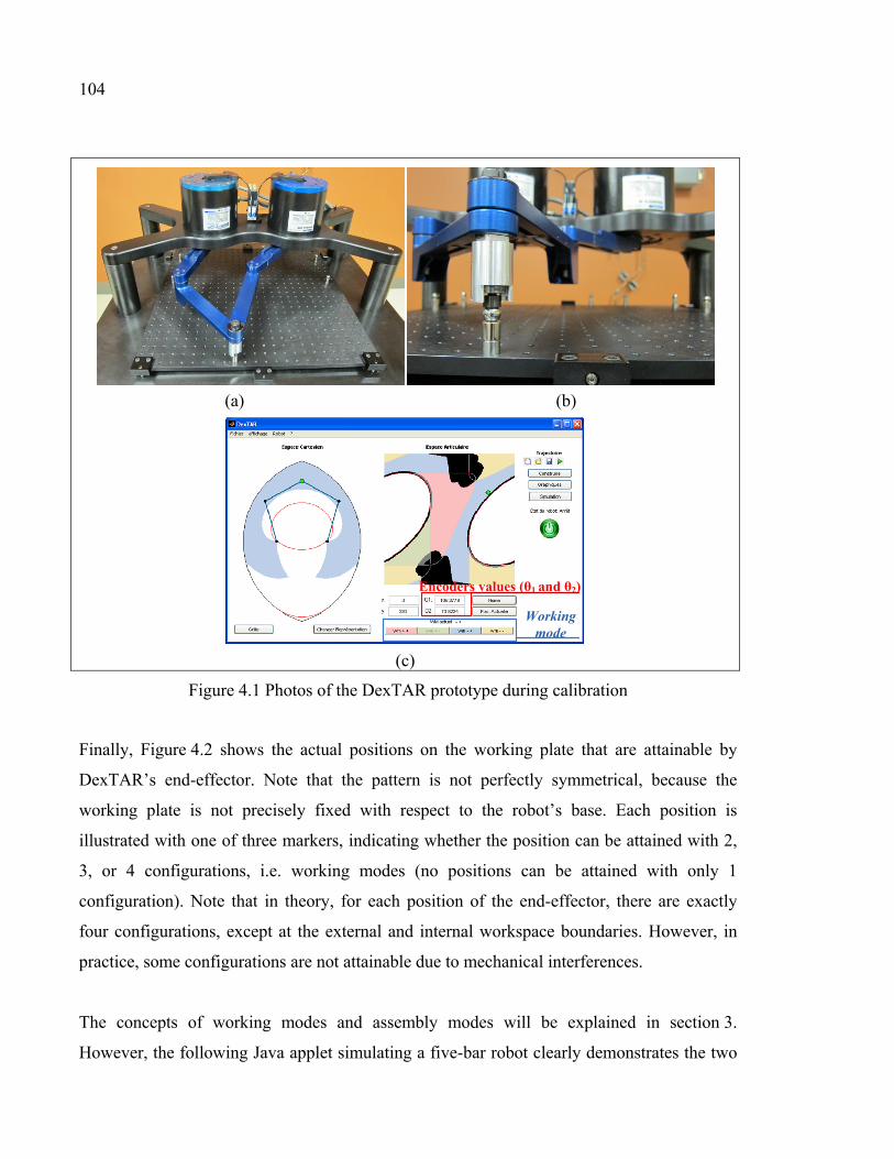
104
(a) (b)
Encoders values (θ1 and θ2)
Working mode
(c)
Figure 4.1 Photos of the DexTAR prototype during calibration
Finally, Figure 4.2 shows the actual positions on the working plate that are attainable by
DexTAR’s end-effector. Note that the pattern is not perfectly symmetrical, because the
working plate is not precisely fixed with respect to the robot’s base. Each position is
illustrated with one of three markers, indicating whether the position can be attained with 2,
3, or 4 configurations, i.e. working modes (no positions can be attained with only 1
configuration). Note that in theory, for each position of the end-effector, there are exactly
four configurations, except at the external and internal workspace boundaries. However, in
practice, some configurations are not attainable due to mechanical interferences.
The concepts of working modes and assembly modes will be explained in section 3.
However, the following Java applet simulating a five-bar robot clearly demonstrates the two
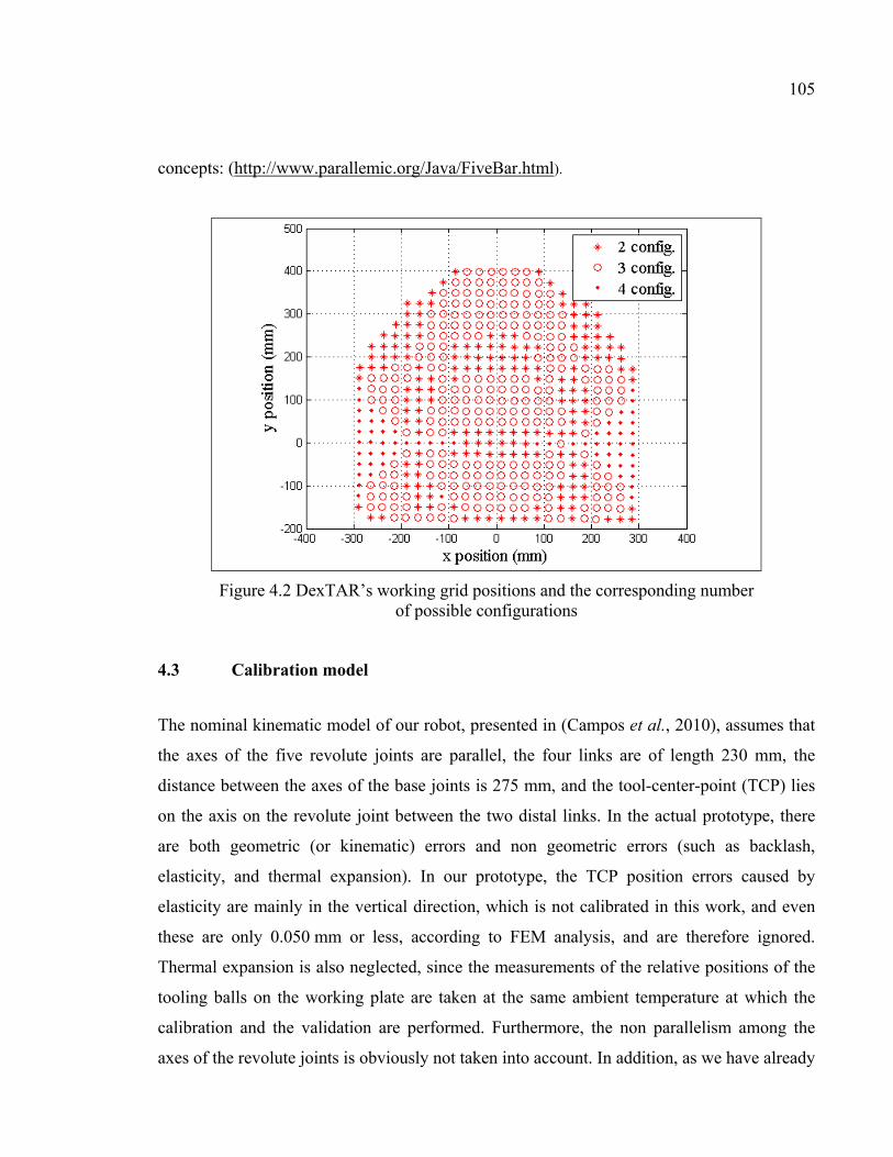
105
concepts: (http://www.parallemic.org/Java/FiveBar.html).
Figure 4.2 DexTAR’s working grid positions and the corresponding number of possible configurations
4.3 Calibration model
The nominal kinematic model of our robot, presented in (Campos et al., 2010), assumes that
the axes of the five revolute joints are parallel, the four links are of length 230 mm, the
distance between the axes of the base joints is 275 mm, and the tool-center-point (TCP) lies
on the axis on the revolute joint between the two distal links. In the actual prototype, there
are both geometric (or kinematic) errors and non geometric errors (such as backlash,
elasticity, and thermal expansion). In our prototype, the TCP position errors caused by
elasticity are mainly in the vertical direction, which is not calibrated in this work, and even
these are only 0.050 mm or less, according to FEM analysis, and are therefore ignored.
Thermal expansion is also neglected, since the measurements of the relative positions of the
tooling balls on the working plate are taken at the same ambient temperature at which the
calibration and the validation are performed. Furthermore, the non parallelism among the
axes of the revolute joints is obviously not taken into account. In addition, as we have already
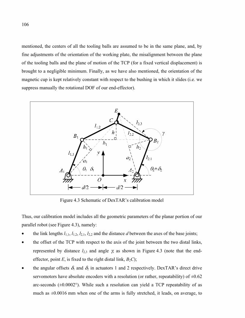
106
mentioned, the centers of all the tooling balls are assumed to be in the same plane, and, by
fine adjustments of the orientation of the working plate, the misalignment between the plane
of the tooling balls and the plane of motion of the TCP (for a fixed vertical displacement) is
brought to a negligible minimum. Finally, as we have also mentioned, the orientation of the
magnetic cup is kept relatively constant with respect to the bushing in which it slides (i.e. we
suppress manually the rotational DOF of our end-effector).
Figure 4.3 Schematic of DexTAR’s calibration model
Thus, our calibration model includes all the geometric parameters of the planar portion of our
parallel robot (see Figure 4.3), namely:
• the link lengths l1,1, l1,2, l2,1, l2,2 and the distance d between the axes of the base joints;
• the offset of the TCP with respect to the axis of the joint between the two distal links,
represented by distance l2,3 and angle γ, as shown in Figure 4.3 (note that the end-
effector, point E, is fixed to the right distal link, B2C);
• the angular offsets δ1 and δ2 in actuators 1 and 2 respectively. DexTAR’s direct drive
servomotors have absolute encoders with a resolution (or rather, repeatability) of ±0.62
arc-seconds (±0.0002°). While such a resolution can yield a TCP repeatability of as
much as ±0.0016 mm when one of the arms is fully stretched, it leads, on average, to
107
much smaller position errors, and we can therefore ignore the encoder errors. Note, too,
that our calibration procedure is not affected by control errors, since the robot is not
controlled. However, if the robot were to be controlled and in stationary mode, the
control errors would be virtually zero;
• the pose of the base frame, O-xy, with respect to the world frame (not shown in
Figure 4.3), which is defined by three of the tooling balls (explained at the end of this
section).
Since we use the linearization of the forward kinematics model, our calibration model is
based on the so-called identification Jacobian matrix, which, throughout this paper, refers to
the Jacobian matrix composed by the derivatives of the end-effector position vector with
respect to all the robot’s parameters.
Therefore, we will need the direct kinematics of the calibration model. Given the active-joint
variables θ1 and θ2, the position [ , ]TE OE x y= =p r of the TCP, point E, is calculated as
follows:
( )
2 2
2,3
2,2
cos sin
sin cosOE OB OC OB
l
l
γ γγ γ
− = + −
r r r r
(4.1)
where
2 2,1 2 2,1 2cos , sin
2
T
OB
dl lθ θ = +
r
(4.2)
1 1 2 1 2
1 2 1 2
10 1
1 0OC OB B B B BB B B B
b h
d dξ
− = + +
r r r r
(4.3)
1 1,1 1 1,1 1cos , sin
2
T
OB
dl lθ θ = −
r
(4.4)
108
with ξ= ±1 being the index that defines the robot’s assembly mode, and
2 21,2 1h l b= − ,
1 2
1 2
2 2 21,2 2.2
1 2B B
B B
l l db
d
− +=
(4.5)
1 2 1 2 1 2
TB B B B B Bd = r r
(4.6)
1 2 2 1B B OB OB= −r r r
(4.7)
As for the inverse kinematics, given the TCP’s position [ , ]TE OE x y= =p r , the active-joint
variables θ1 and θ2 are calculated as follows:
( )
1 1 1 11 atan2 ,A B A By xθ =
(4.8)
where 1 1ABx and
1 1ABy are the components of vector 1 1A Br :
1 1 1 1 1 1 1 1
1 1
1 11
0 1,
1 0
T
A B A B A B A C A CA C A C
a hx y
d dζ = = + −
r r r
(4.9)
with ζ1 being the so-called branch index that defines the configuration of arm 1, and
2 21 1,1 1h l a= − , 1
1
2 2 21,1 1,2
1 2A C
A C
l l da
d
− +=
(4.10)
1 1 1
TA C A C A Cd = r r
(4.11)
109
1 1
,02
T
A C OC OA OC
d = − = − − r r r r
(4.12)
The coordinates of point C are calculated in a similar fashion, by calculating the inverse
kinematics of arm 2:
( )
2 2
2,2
2,3
cos sin
sin cosOC OB OE OB
l
l
γ γγ γ
= + − −
r r r r
(4.13)
where
2 2 2 2 2 2
, 02
T
OB OA A B A B
d = + = + r r r r
(4.14)
2 2 2 2 2 2 2 2
2 2
2 22
0 1,
1 0
T
A B A B A B A E A EA E A E
a hx y
d dζ = = + −
r r r
(4.15)
with ζ2 being the branch index that defines the configuration of arm 2, and
2 22 2,1 2h l a= − , 2
2
2 2 22,1 2,3
2 2A E
A E
l l da
d
− +=
(4.16)
2 2 2
TA E A E A Ed r r=
(4.17)
2
,2
T
A E
dx y = −
r
(4.18)
Finally, the second active-joint variable is calculated as:
110
( )
2 2 2 22 atan2 ,A B A By xθ =
(4.19)
Note that a working mode (also referred to as robot configuration) is defined as the
combination of the two branch indices, ζ1 and ζ2. For a given position of the end-effector, not
lying on the workspace boundaries, there are four robot configurations (if mechanical
interferences are ignored). These four configurations are not necessarily corresponding to the
same assembly mode.
4.3.1 World and base reference frames
The two reference frames used in this work are shown in Figure 4.4. The first is the WF, and
is fixed in the working plate (the aluminum breadboard). The axes of this frame are denoted
by xw and yw. All further measurements are projected in the xwyw plane and represented with
respect to WF.
The world frame is defined by three of the precision balls, the centers of which are denoted
as (calibration) points P2, P4, and P5 (Figure 4.4). Point P2 is the origin R of the world frame,
and the axis xw is defined such that point P4 lies on the positive part of the axis. Finally, the
axis yw is defined such that point P5 lies in the first quadrant of the plane xwyw.
The second reference frame is the BF, O-xy, introduced in Figure 4.3 and also shown in
Figure 4.4. The xy plane of the base frame coincides with the xwyw plane, and the axes of the
robot’s revolute joints are perpendicular to that plane. The origin O of the base frame is
defined as being midway between points A1 and A2 (the intersection points between the axis
of the actuated joints and the plane xy). The vector that passes from A1 to A2 defines the
direction of the x axis. Finally, the yaxis points towards the front of the robot.
111
The position and orientation of the base frame with respect to the world frame are denoted by
vector [ , ]WF TO O Ox y=p and ϕ respectively. Therefore, the end-effector position with respect to
the world frame is defined as:
WF WF WF BFE O BF E= +p p R p
(4.20)
where [ , ]BF TE x y=p represents the position of the end-effector obtained from the equations of
the forward kinematics. By developing the rotation matrix WFBFR and substituting
BFEp ,
Equation 4.20 can be rewritten as follows:
cos sin
sin cosWF OWF
EWF O
x x x y
y y x y
ϕ ϕϕ ϕ
+ − = = + +
p
(4.21)
where WFEp is obtained by direct measurement, while the position coordinates xO and yO and
the angle ϕ are identified through the calibration process.
In summary, in our calibration process, we have to identify a total of 12 independent
parameters: the lengths of the “five bars”, l1,1, l1,2, l2,1, l2,2, and d, the end-effector offset
parameters, l2,3 and γ, the active-joint offsets , δ1 and δ2, and the pose of the base frame with
respect to the world frame, xO, yO, and ϕ.
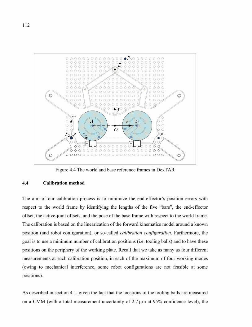
112
Figure 4.4 The world and base reference frames in DexTAR
4.4 Calibration method
The aim of our calibration process is to minimize the end-effector’s position errors with
respect to the world frame by identifying the lengths of the five “bars”, the end-effector
offset, the active-joint offsets, and the pose of the base frame with respect to the world frame.
The calibration is based on the linearization of the forward kinematics model around a known
position (and robot configuration), or so-called calibration configuration. Furthermore, the
goal is to use a minimum number of calibration positions (i.e. tooling balls) and to have these
positions on the periphery of the working plate. Recall that we take as many as four different
measurements at each calibration position, in each of the maximum of four working modes
(owing to mechanical interference, some robot configurations are not feasible at some
positions).
As described in section 4.1, given the fact that the locations of the tooling balls are measured
on a CMM (with a total measurement uncertainty of 2.7 μm at 95% confidence level), the
113
accuracy of our position measurements, when the working plate is put back on the robot, is
approximately equal to the repeatability of our magnetic cup end-effector measurements,
which is better than ±15 μm.
Therefore, the following calibration protocol is proposed:
Step 1. Using the identification Jacobian matrix, denoted J, an observability analysis is
performed to select the best calibration positions. Details of this analysis are
provided in the following section.
Step 2. Given the n calibration configurations obtained in the observability analysis, the
tooling balls are fixed to the corresponding positions on the working plate.
Step 3. The working plate is placed on the CMM. The world frame is identified, as
explained previously, and the centers xmeas,j, ymeas,j of all the tooling balls are
measured (j = 1…n). These data will be used for the identification process in
Eqs. 27 and 30. Next, the working plate is repositioned on the robot’s base. Recall
that the CMM and the robot are kept in rooms having the same ambient temperature.
Without going into the detail here, the plane of the tooling balls is aligned with the
plane of motion of the end-effector (as the vertical DOF of the robot has been
temporarily blocked).
Step 4. The control system of robot is turned on, but the actuators are disabled. This allows
the servomotors to move freely (movement achieved manually by the operator to
reach different calibration tooling balls), but be able to read their encoders.
Step 5. The end-effector is placed at calibration position Pj, using the first of a maximum of
four possible robot configurations. Then, by using the robot’s interface which
displays the information about the actual configuration of robot (see Figure 4.1c),
the encoder values θ1,meas and θ2,meas are recorded. The corresponding TCP position,
estimated with respect to world frames xest,j and yest,j, is obtained from the direct
kinematic equations, using the nominal values of the 12 parameters (vnom). These
values can also be represented as follows:
est , 1,meas, 2,meas, nom( , , )j x j jx f θ θ= v
(4.22)
114
est , 1,meas, 2,meas, nom( , , )j y j jy f θ θ= v
(4.23)
where
[ ]nom 1,1 1,2 2,1 2,2 2,3 1 2, , , , , , , , , , ,
230, 230, 230, 230, 275, 230, 0 , 0 ,0 , , ,0
T
O O
T
O O
l l l l d l x y
x y
γ δ δ α =
= ° ° ° °
v
(4.24)
with the length units being in millimeters.
Step 6. The end-effector is detached from the tooling ball, by lifting the magnetic cup (Fig.
1b) and displacing the end-effector away from its initial position, and put back on it
once the robot configuration has been changed. The configuration is changed
manually, by modifying the branch index of one or both robot arms. Then, the new
values of θ1,meas and θ2,meas are recorded from the robot’s interface. This step is
repeated until all feasible configurations for position Pj have been measured.
Step 7. Steps 5 and 6 are repeated for all calibration positions, i.e. for every calibration
position, we measure the active joint variables (θ1,meas and θ2,meas) and we calculate
the corresponding estimated TCP positions (xest,j and yest,j), for all possible
configurations. These estimated positions are recalculated each iteration in the
parameters identification process, by changing vnom by the latest values of the
identified parameters.
The above procedure can be seen at http://www.youtube.com/watch?v=Ypf8dtHOjZI. After
these steps have been completed, the parameter values are estimated as follows:
(a) An identification Jacobian matrix relating the position errors to the 12 unknown
parameter values is built by linearizing the forward kinematics model around each
calibration configuration. Using the nominal values of the 12 parameters given in
Equation 4.24, the identification Jacobian matrix is calculated as follows:
115
1
n
=
J
J
J
(4.25)
,
nom
,
nom
WF k
k
WF k
x
y
∂ ∂ = ∂
∂
vJ
v
(4.26)
where Jk is the 2×m Jacobian matrix at the kth calibration configuration, n is the number of
calibration configurations, and m is the number of parameters (m = 12 in our case).
(b) A system of linear equations is formed by the position errors measured, the robot’s
parameter errors, and the Jacobian matrix J. In order to maintain acceptable variance
of each parameter and obtain proper convergence in the linear system, parameter
scaling is implemented to improve the condition number of J. Matrix J is scaled
using the column scaling approach, which is a type of parameter scaling proposed in
(Sun and Hollerbach, 2008). The scaled (normalized) matrix obtained is denoted by
Jnorm, and it is used to identify the robot’s scaled parameter errors (Δnorm):
( )
,1 ,1
,1 ,11
, ,
, ,
meas est
meas est
T Tnorm norm norm norm
meas n est n
meas n est n
x x
y y
x x
y y
−
− − = − −
Δ J J J
(4.27)
(c) The parameter errors, which represent the difference between the real values and the
nominal values of the parameters, are denoted by Δ, and calculated as follows:
116
( )1,1 1,2 2,1 2,2 2,3 1 2
1
1 2
, , , , , , , , , , ,
diag , , ,
O O
T
l l l l d l x y
m normD D D
γ δ δ αε ε ε ε ε ε ε ε ε ε ε ε−
=
=
Δ
Δ (4.28)
where Dj, (j = 1, 2, …, m) are the scaling coefficients, defined as follows:
22,
1
n
j i ji
D J=
= .
(d) Finally, the vector of the real parameter values is
real nom= +v v Δ
(4.29)
To converge towards a solution for the unknown coefficient and parameter values, an
iterative Newton-based procedure was used. After vreal has been calculated, the vnom vector is
replaced by the last vreal vector obtained, and the estimation process is restarted from step (a).
The convergence criterion is the difference between two successive iterations of the root
mean square error (RMSE) between the measurement error and the predicted error,
( )2 2 2meas, est, meas, est ,1
( ) ( )
2
n
i i i iix x y y
RMSEn
=− + −
=
(4.30)
The convergence criterion is set to 10−16. The system converges towards a solution after six
iterations.
4.5 Observability analysis
Our identification problem needs at least as many independent constraints as there are
unknown parameters. Knowing that we have 12 parameters to identify and that every
measurement configuration provides two independent equations (one for xWF and another for
yWF), theoretically, only six measurement configurations are necessary to solve the linear
system in Equation 4.27. However, to obtain an accurate identification of the parameters, the
117
number of calibration configurations should be increased. Therefore, an observability
analysis is achieved to determine the measurement configurations where the parameter errors
are more easily distinguished and the measurement errors have minimum impact on the
identification process.
Five observability indices are presented in the literature, and are referred to as O1, O2,…, O5.
These five indices are discussed in(Horne and Notash, 2009). Further details are available in
(Sun and Hollerbach, 2008; Borm and Menq, 1989; Driels and Pathre, 1990; Nahvi and
Hollerbach, 1996). Moreover, many algorithms have been proposed to identify the
calibration configurations by optimizing these observability indices. Daney et al. (2005), for
example, propose an approach using a local convergence and tabu search, which makes it
possible to maximize the first four observability indices. This approach was tested
experimentally using a Stewart platform. More recently, Li et al. (2011)have proposed an
algorithm for selecting calibration poses based on maximizing the same indices as (Daney et
al., 2005), and adapted for a 6-DOF serial robot. In our analysis, the selection of calibration
configurations is achieved using the O1 index. The reason for this choice is that the index O1
makes the attribution of the position errors to the error parameters dominant, which means
that the effects of unmodeled errors and measurement noise are less significant. As a result,
better parameter estimation is achieved (Borm and Menq, 1991). Indeed, this index is the
best choice when the objective is to minimize the variance of the parameters (Sun and
Hollerbach, 2008), which is our objective.
As mentioned earlier in this paper, our calibration approach is based on measuring up to four
possible robot configurations for each end-effector position. This approach minimizes the
number of tooling balls necessary. It is clear that some of these robot configurations may not
improve observability, but we justify this approach because otherwise it would be too
complicated for the user to have to exclude configurations for a given tooling ball. We
maintain, therefore, that if a calibration position is selected (i.e. a tooling ball is present),
measurements should be performed with all possible robot configurations.
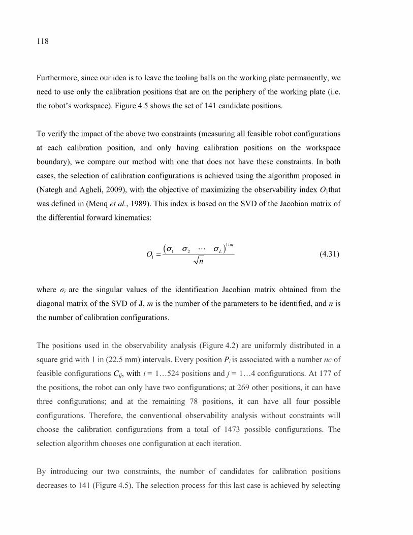
118
Furthermore, since our idea is to leave the tooling balls on the working plate permanently, we
need to use only the calibration positions that are on the periphery of the working plate (i.e.
the robot’s workspace). Figure 4.5 shows the set of 141 candidate positions.
To verify the impact of the above two constraints (measuring all feasible robot configurations
at each calibration position, and only having calibration positions on the workspace
boundary), we compare our method with one that does not have these constraints. In both
cases, the selection of calibration configurations is achieved using the algorithm proposed in
(Nategh and Agheli, 2009), with the objective of maximizing the observability index O1that
was defined in (Menq et al., 1989). This index is based on the SVD of the Jacobian matrix of
the differential forward kinematics:
( )1/
1 21
m
LOn
σ σ σ=
(4.31)
where σi are the singular values of the identification Jacobian matrix obtained from the
diagonal matrix of the SVD of J, m is the number of the parameters to be identified, and n is
the number of calibration configurations.
The positions used in the observability analysis (Figure 4.2) are uniformly distributed in a
square grid with 1 in (22.5 mm) intervals. Every position Pi is associated with a number nc of
feasible configurations Cij, with i = 1…524 positions and j = 1…4 configurations. At 177 of
the positions, the robot can only have two configurations; at 269 other positions, it can have
three configurations; and at the remaining 78 positions, it can have all four possible
configurations. Therefore, the conventional observability analysis without constraints will
choose the calibration configurations from a total of 1473 possible configurations. The
selection algorithm chooses one configuration at each iteration.
By introducing our two constraints, the number of candidates for calibration positions
decreases to 141 (Figure 4.5). The selection process for this last case is achieved by selecting
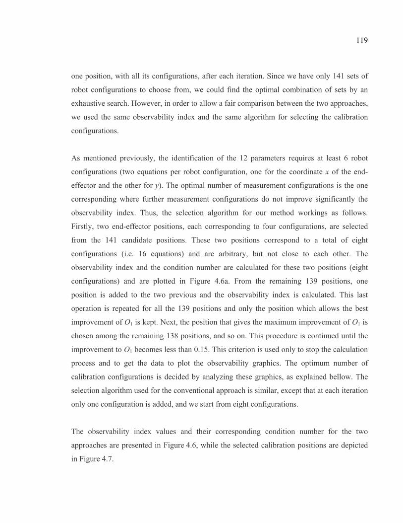
119
one position, with all its configurations, after each iteration. Since we have only 141 sets of
robot configurations to choose from, we could find the optimal combination of sets by an
exhaustive search. However, in order to allow a fair comparison between the two approaches,
we used the same observability index and the same algorithm for selecting the calibration
configurations.
As mentioned previously, the identification of the 12 parameters requires at least 6 robot
configurations (two equations per robot configuration, one for the coordinate x of the end-
effector and the other for y). The optimal number of measurement configurations is the one
corresponding where further measurement configurations do not improve significantly the
observability index. Thus, the selection algorithm for our method workings as follows.
Firstly, two end-effector positions, each corresponding to four configurations, are selected
from the 141 candidate positions. These two positions correspond to a total of eight
configurations (i.e. 16 equations) and are arbitrary, but not close to each other. The
observability index and the condition number are calculated for these two positions (eight
configurations) and are plotted in Figure 4.6a. From the remaining 139 positions, one
position is added to the two previous and the observability index is calculated. This last
operation is repeated for all the 139 positions and only the position which allows the best
improvement of O1 is kept. Next, the position that gives the maximum improvement of O1 is
chosen among the remaining 138 positions, and so on. This procedure is continued until the
improvement to O1 becomes less than 0.15. This criterion is used only to stop the calculation
process and to get the data to plot the observability graphics. The optimum number of
calibration configurations is decided by analyzing these graphics, as explained bellow. The
selection algorithm used for the conventional approach is similar, except that at each iteration
only one configuration is added, and we start from eight configurations.
The observability index values and their corresponding condition number for the two
approaches are presented in Figure 4.6, while the selected calibration positions are depicted
in Figure 4.7.
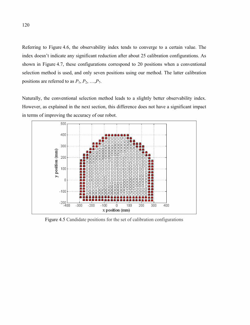
120
Referring to Figure 4.6, the observability index tends to converge to a certain value. The
index doesn’t indicate any significant reduction after about 25 calibration configurations. As
shown in Figure 4.7, these configurations correspond to 20 positions when a conventional
selection method is used, and only seven positions using our method. The latter calibration
positions are referred to as P1, P2, …,P7.
Naturally, the conventional selection method leads to a slightly better observability index.
However, as explained in the next section, this difference does not have a significant impact
in terms of improving the accuracy of our robot.
Figure 4.5 Candidate positions for the set of calibration configurations
121
(a) (b)
Figure 4.6 Observability index and condition number using (a) our method and (b) the conventional method
(a) (b)
Figure 4.7 Calibration positions obtained using (a) our method and (b) the conventional method
4.6 Simulated calibration
Before carrying out the actual calibration process, a sensitivity analysis is performed using
the calibration configurations selected by the observability analysis. The purpose of this
simulation is to analyze the sensitivity of parameter identification to measurement noise. In
addition, this section presents a comparison between the two sets of calibration
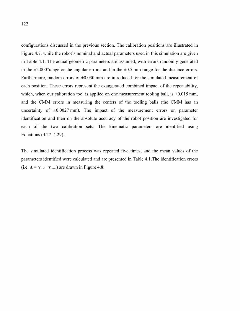
122
configurations discussed in the previous section. The calibration positions are illustrated in
Figure 4.7, while the robot’s nominal and actual parameters used in this simulation are given
in Table 4.1. The actual geometric parameters are assumed, with errors randomly generated
in the ±2.000°rangefor the angular errors, and in the ±0.5 mm range for the distance errors.
Furthermore, random errors of ±0,030 mm are introduced for the simulated measurement of
each position. These errors represent the exaggerated combined impact of the repeatability,
which, when our calibration tool is applied on one measurement tooling ball, is ±0.015 mm,
and the CMM errors in measuring the centers of the tooling balls (the CMM has an
uncertainty of ±0.0027 mm). The impact of the measurement errors on parameter
identification and then on the absolute accuracy of the robot position are investigated for
each of the two calibration sets. The kinematic parameters are identified using
Equations (4.27–4.29).
The simulated identification process was repeated five times, and the mean values of the
parameters identified were calculated and are presented in Table 4.1.The identification errors
(i.e. Δ = vreal−vnom) are drawn in Figure 4.8.
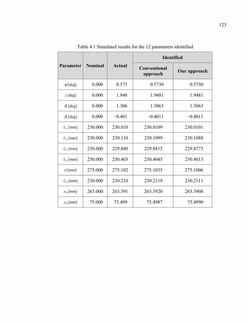
123
Table 4.1 Simulated results for the 12 parameters identified
Parameter Nominal Actual
Identified
Conventional approach
Our approach
ϕ [deg] 0.000 0.573 0.5730 0.5730
γ [deg] 0.000 1.948 1.9481 1.9481
δ1 [deg] 0.000 1.306 1.3063 1.3063
δ2 [deg] 0.000 −0.401 −0.4011 −0.4011
l1,1 [mm] 230.000 230.010 230.0109 230.0101
l1,2 [mm] 230.000 230.110 230.1099 230.1088
l2,1 [mm] 230.000 229.880 229.8812 229.8773
l2,2 [mm] 230.000 230.403 230.4045 230.4013
d [mm] 275.000 275.102 275.1035 275.1006
l2,3 [mm] 230.000 230.210 230.2119 230.2111
xO [mm] 263.000 263.391 263.3920 263.3908
yO [mm] 75.000 75.499 75.4987 75.4990
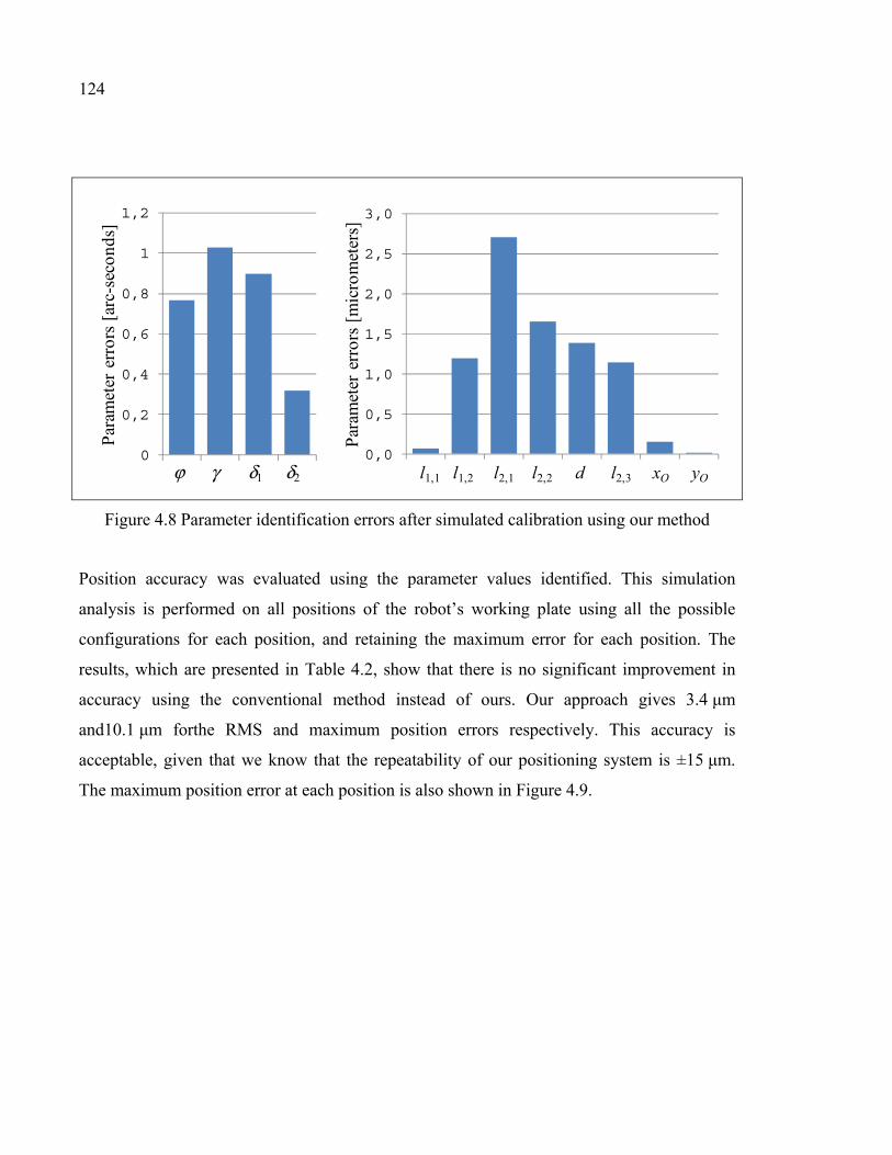
124
0
0,2
0,4
0,6
0,8
1
1,2
Par
amet
er e
rror
s [a
rc-s
econ
ds]
ϕ γ δ1 δ2
0,0
0,5
1,0
1,5
2,0
2,5
3,0
Par
amet
er e
rror
s [m
icro
met
ers]
l1,1 l1,2 l2,1 l2,2 d l2,3 xO yO
Figure 4.8 Parameter identification errors after simulated calibration using our method
Position accuracy was evaluated using the parameter values identified. This simulation
analysis is performed on all positions of the robot’s working plate using all the possible
configurations for each position, and retaining the maximum error for each position. The
results, which are presented in Table 4.2, show that there is no significant improvement in
accuracy using the conventional method instead of ours. Our approach gives 3.4 μm
and10.1 μm forthe RMS and maximum position errors respectively. This accuracy is
acceptable, given that we know that the repeatability of our positioning system is ±15 μm.
The maximum position error at each position is also shown in Figure 4.9.
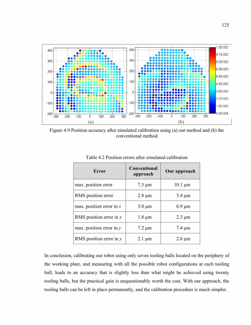
125
(a) (b)
Figure 4.9 Position accuracy after simulated calibration using (a) our method and (b) the conventional method
Table 4.2 Position errors after simulated calibration
Error Conventional
approach Our approach
max. position error 7.3 μm 10.1 μm
RMS position error 2.8 μm 3.4 μm
max. position error in x 5.0 μm 6.9 μm
RMS position error in x 1.8 μm 2.3 μm
max. position error in y 7.2 μm 7.4 μm
RMS position error in y 2.1 μm 2.6 μm
In conclusion, calibrating our robot using only seven tooling balls located on the periphery of
the working plate, and measuring with all the possible robot configurations at each tooling
ball, leads to an accuracy that is slightly less than what might be achieved using twenty
tooling balls, but the practical gain is unquestionably worth the cost. With our approach, the
tooling balls can be left in place permanently, and the calibration procedure is much simpler.
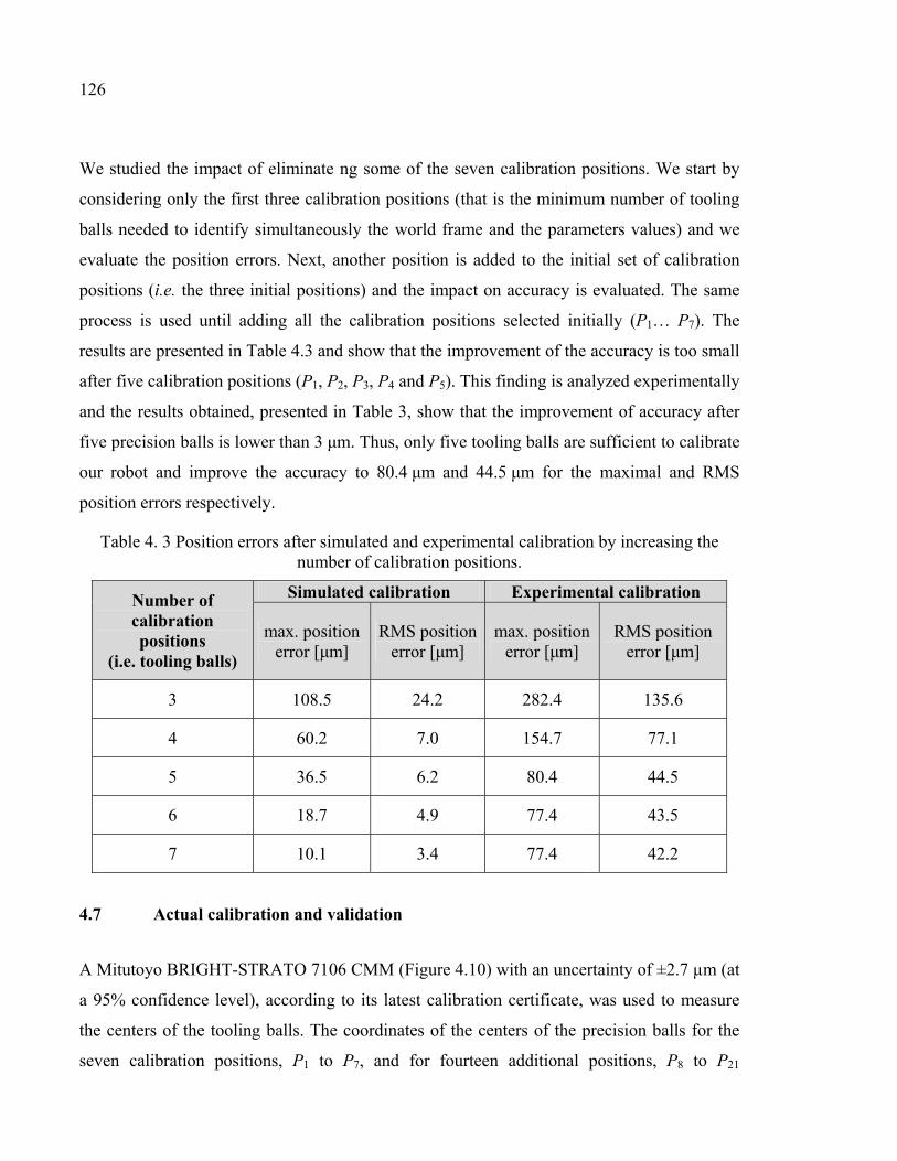
126
We studied the impact of eliminate ng some of the seven calibration positions. We start by
considering only the first three calibration positions (that is the minimum number of tooling
balls needed to identify simultaneously the world frame and the parameters values) and we
evaluate the position errors. Next, another position is added to the initial set of calibration
positions (i.e. the three initial positions) and the impact on accuracy is evaluated. The same
process is used until adding all the calibration positions selected initially (P1… P7). The
results are presented in Table 4.3 and show that the improvement of the accuracy is too small
after five calibration positions (P1, P2, P3, P4 and P5). This finding is analyzed experimentally
and the results obtained, presented in Table 3, show that the improvement of accuracy after
five precision balls is lower than 3 μm. Thus, only five tooling balls are sufficient to calibrate
our robot and improve the accuracy to 80.4 μm and 44.5 μm for the maximal and RMS
position errors respectively.
Table 4. 3 Position errors after simulated and experimental calibration by increasing the number of calibration positions.
Number of calibration positions
(i.e. tooling balls)
Simulated calibration Experimental calibration
max. position error [μm]
RMS position error [μm]
max. position error [μm]
RMS position error [μm]
3 108.5 24.2 282.4 135.6
4 60.2 7.0 154.7 77.1
5 36.5 6.2 80.4 44.5
6 18.7 4.9 77.4 43.5
7 10.1 3.4 77.4 42.2
4.7 Actual calibration and validation
A Mitutoyo BRIGHT-STRATO 7106 CMM (Figure 4.10) with an uncertainty of ±2.7 µm (at
a 95% confidence level), according to its latest calibration certificate, was used to measure
the centers of the tooling balls. The coordinates of the centers of the precision balls for the
seven calibration positions, P1 to P7, and for fourteen additional positions, P8 to P21
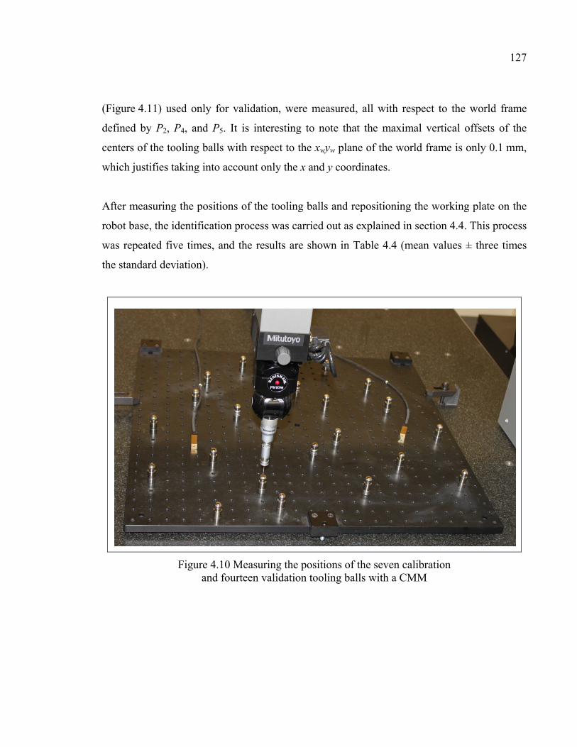
127
(Figure 4.11) used only for validation, were measured, all with respect to the world frame
defined by P2, P4, and P5. It is interesting to note that the maximal vertical offsets of the
centers of the tooling balls with respect to the xwyw plane of the world frame is only 0.1 mm,
which justifies taking into account only the x and y coordinates.
After measuring the positions of the tooling balls and repositioning the working plate on the
robot base, the identification process was carried out as explained in section 4.4. This process
was repeated five times, and the results are shown in Table 4.4 (mean values ± three times
the standard deviation).
Figure 4.10 Measuring the positions of the seven calibration and fourteen validation tooling balls with a CMM
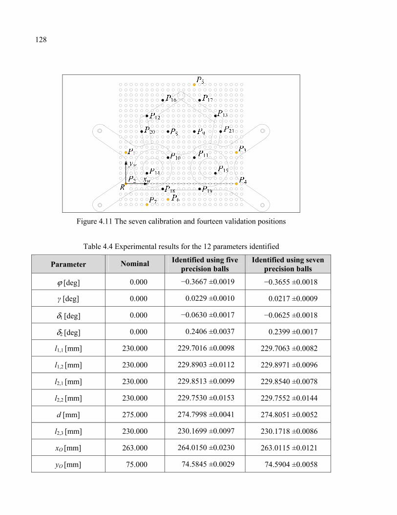
128
Figure 4.11 The seven calibration and fourteen validation positions
Table 4.4 Experimental results for the 12 parameters identified
Parameter Nominal Identified using five precision balls
Identified using seven precision balls
ϕ [deg] 0.000 −0.3667 ±0.0019 −0.3655 ±0.0018
γ [deg] 0.000 0.0229 ±0.0010 0.0217 ±0.0009
δ1 [deg] 0.000 −0.0630 ±0.0017 −0.0625 ±0.0018
δ2 [deg] 0.000 0.2406 ±0.0037 0.2399 ±0.0017
l1,1 [mm] 230.000 229.7016 ±0.0098 229.7063 ±0.0082
l1,2 [mm] 230.000 229.8903 ±0.0112 229.8971 ±0.0096
l2,1 [mm] 230.000 229.8513 ±0.0099 229.8540 ±0.0078
l2,2 [mm] 230.000 229.7530 ±0.0153 229.7552 ±0.0144
d [mm] 275.000 274.7998 ±0.0041 274.8051 ±0.0052
l2,3 [mm] 230.000 230.1699 ±0.0097 230.1718 ±0.0086
xO [mm] 263.000 264.0150 ±0.0230 263.0115 ±0.0121
yO [mm] 75.000 74.5845 ±0.0029 74.5904 ±0.0058
129
To evaluate robot accuracy after calibration, measurements at each of the fourteen validation
tooling balls were taken, with every possible robot configuration. This makes a total of 36
robot configurations. Each of the 36 validation measurements was repeated five times, and
only the mean value was retained. The position errors for all the configurations of each
position were sorted, and only the maximum value were kept (Figure 4.12). The maximum
position errors and RMS errors were reduced from 3.288 mm and 1.467 mm respectively
(when using the nominal values for the 12 parameters) to only 77.4 μm and 42.2 μm
respectively when using 7 tooling balls and to 80.4 μm and 44.5 μm respectively when using
5 balls. Further results are shown in Table 4.5.
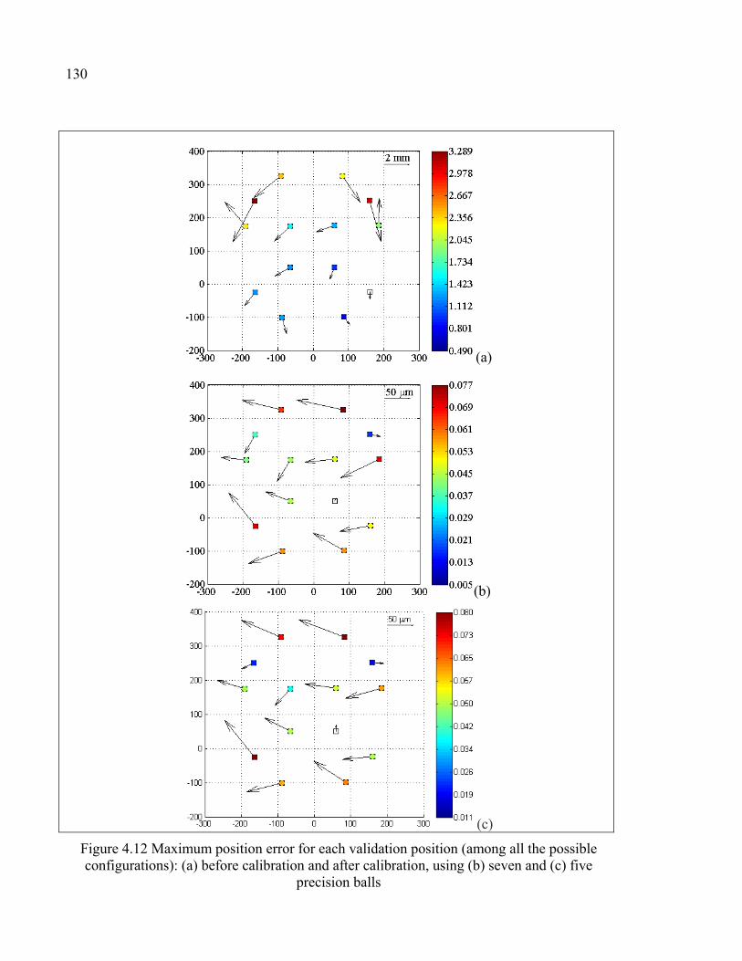
130
(a)
(b)
(c)
Figure 4.12 Maximum position error for each validation position (among all the possible configurations): (a) before calibration and after calibration, using (b) seven and (c) five
precision balls
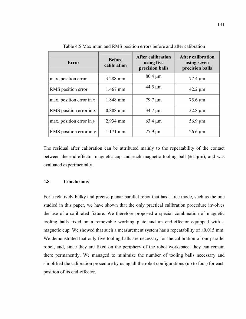
131
Table 4.5 Maximum and RMS position errors before and after calibration
Error Before
calibration
After calibration using five
precision balls
After calibration using seven
precision balls
max. position error 3.288 mm 80.4 μm 77.4 μm
RMS position error 1.467 mm 44.5 μm 42.2 μm
max. position error in x 1.848 mm 79.7 μm 75.6 μm
RMS position error in x 0.888 mm 34.7 μm 32.8 μm
max. position error in y 2.934 mm 63.4 μm 56.9 μm
RMS position error in y 1.171 mm 27.9 μm 26.6 μm
The residual after calibration can be attributed mainly to the repeatability of the contact
between the end-effector magnetic cup and each magnetic tooling ball (±15µm), and was
evaluated experimentally.
4.8 Conclusions
For a relatively bulky and precise planar parallel robot that has a free mode, such as the one
studied in this paper, we have shown that the only practical calibration procedure involves
the use of a calibrated fixture. We therefore proposed a special combination of magnetic
tooling balls fixed on a removable working plate and an end-effector equipped with a
magnetic cup. We showed that such a measurement system has a repeatability of ±0.015 mm.
We demonstrated that only five tooling balls are necessary for the calibration of our parallel
robot, and, since they are fixed on the periphery of the robot workspace, they can remain
there permanently. We managed to minimize the number of tooling balls necessary and
simplified the calibration procedure by using all the robot configurations (up to four) for each
position of its end-effector.
132
Using the above procedure and a calibration model based on 12 geometric parameters, 2 of
which are related to the actuator offset and 3of them defining the base frame with respect to
the world frame, we managed to improve the position accuracy of the robot to an RMS value
of 0.044 mm.
The proposed calibration method is therefore of great practical interest for parallel robots that
have multiple solutions to their inverse kinematics. Our method allows to minimize the
number of calibration fixtures and to simplify the calibration procedure (at each calibration
fixture, the user should measure all possible robot configurations). Furthermore, note that in
our method we can measure configurations which correspond to different assembly modes.
In contrast, if the robot motors are active, only configurations corresponding to a single
assembly mode can be measured.
4.9 Acknowledgments
This work was made possible through the support of the Canada Research Chairs program,
the Canada Foundation for Innovation (CFI), and the Fonds de recherche du Québec
(FQRNT). The authors would also like to thank the anonymous reviewers for their valuable
comments.
CONCLUSION GÉNÉRALE
La présente thèse avait pour objectif de proposer des méthodes d’étalonnage géométriques
destinées à améliorer la précision absolue des robots parallèles et plus particulièrement ceux
à moins de six degrés de liberté. En plus de la compensation des erreurs géométriques, les
opérations d’étalonnages proposées dans ce travail de recherche permettent d’identifier les
référentiels des bases et des plateformes des robots avec précision.
Les robots étudiés et étalonnés dans le cadre de ce travail sont deux robots plans : une table
de positionnement précis (PreXYT) et un robot plan cinq-barres (DexTAR). Le PreXYT a été
étalonné en utilisant deux approches distinctes : la première consiste en une méthode
d’identification basée sur l’analyse de la géométrie du robot, la deuxième est basée sur
l’utilisation de la méthode géométrique directe d’étalonnage. La précision du robot DexTAR
a été améliorée en utilisant une approche d’auto-étalonnage où le nombre de positions
d’étalonnage est minimisé alors que toutes les configurations possibles pour chacune des
positions sont retenues. En simplifiant ainsi la collecte de données pour l’étalonnage,
l'utilisateur n’a plus à sélectionner les configurations des positions d’étalonnage.
Comme nous l’avons présenté dans les chapitres 3 et 4, les résultats des simulations sont
toujours meilleurs que ceux obtenus lors des essais pratiques. Bien qu’il nous semble que ces
différences soient attribuées en partie aux erreurs du processus de mesure, les erreurs non
modélisées sont tout aussi significatives. Ainsi, malgré l’utilisation d’un modèle géométrique
complet (c.-à-d. qui prend en considération tous les paramètres géométriques), l’impact des
erreurs non géométriques (non modélisées dans la présente étude), vient dégrader les valeurs
de la précision. Pour cette catégorie d’erreurs, une compensation peut s’avérer nécessaire
pour améliorer d’avantage la précision des robots, advenant que les résultats obtenus, en
n’utilisant que l’approche géométrique, ne soient pas satisfaisants.
Dans notre travail de recherche, nous avons réussi à atteindre des précisions dans les mêmes
ordres de grandeurs que les valeurs de répétabilité des robots, principalement parce que les
134
modèles mathématiques utilisés tiennent compte de la quasi-totalité des paramètres
géométriques, tout en sachant que les erreurs non géométriques sont très faibles grâce à la
qualité supérieure des composantes mécaniques des robots utilisés. Un autre facteur réduit
l’impact des erreurs non géométriques : les robots sont destinés à manipuler des objets de
petite masse, d’où leur étalonnage à vide (c.-à-d. sans charge utile). La température ambiante
peut influencer la fiabilité des données ; les opérations d'étalonnage se sont donc déroulées
dans des conditions thermiques stables. En outre, l'utilisation d'appareils de mesure dont les
incertitudes de mesures sont très faibles, a permis d'augmenter la précision des résultats.
Rappelons que nous avons procédé à l’étalonnage du robot PreXYT en utilisant deux types
d’appareils de mesure : une MMT avec une incertitude de mesure de ±2,7 μm et un bras
articulé de mesure avec une incertitude de ±18 μm. En comparant les résultats de
l'étalonnage, le rapport suivant a pu être établi : plus l'incertitude de l'instrument de mesure
est faible, meilleure est la précision obtenue. Cependant, cette relation n’est pas directement
proportionnelle. En fait, comme nous l’avons démontré au chapitre 3, l’incertitude de mesure
du bras articulé est presque six fois supérieure que celle de la MMT, alors que la précision
obtenue en utilisant la MMT n’est que deux fois meilleure que la précision obtenue par le
bras articulé. Ainsi, une bonne analyse du rapport qualité/prix, selon les objectifs ciblés en
matière de précision après étalonnage, est très conseillée ; les prix des machines de mesures
grimpent exponentiellement à mesure qu’augmentent leurs précisions. À titre d’exemple, le
prix de la MMT que nous avons utilisée est environ dix fois plus élevé que celui du bras
articulé de mesure.
LISTE DE RÉFÉRENCES BIBLIOGRAPHIQUES
Abderrahim, M. et A.R. Whittaker. 2000. « Kinematic model identification of industrial manipulators ». Robotics and Computer-Integrated Manufacturing, vol. 16, n° 1, p. 1-8.
Abtahi, M., H. Pendar, A. Alasty et Gh.R. Vossoughi. 2009. « Calibration of parallel
kinematic machine tools using mobility constraint on the tool center point ». International Journal of Advanced Manufacturing Technology, vol. 45, n° 5-6, p. 531-539.
Abtahi, M., H. Pendar, A. Alasty et G. Vossoughi. 2010. « Experimental kinematic
calibration of parallel manipulators using a relative position error measurement system ». Robotics and Computer-Integrated Manufacturing, vol. 26, n° 6, p. 799-804.
Agheli, M.M. et M.J. Nategh. 2009. « Identifying the Kinematic Parameters of Hexapod
Machine Tool ». International Journal of Mechanical Systems Science and Engineering, vol. 1, n° 3, p. 149-154.
ASME: American Society of Mechanical Engineering. 1992. Methods for Performance
Evaluation of Computer Numerically Controlled Machine Centers, ASME B5.54, 154 p. Majarena, A.C., J. Santolaria, D. Samper et J. J. Aguilar. 2010. « An Overview of Kinematic
and Calibration Models Using Internal/External Sensors or Constraints to Improve the Behavior of Spatial Parallel Mechanisms ». Sensors Journal, vol. 10, n° 11, p. 10256-10297.
Bai, S. et M.Y. Teo. 2003. « Kinematic calibration and pose measurement of a medical
parallel manipulator by optical position sensors ». Journal of Robotic Systems, vol. 20, n° 4, p. 201-209.
Bennett, D.J. et J.M. Hollerbach. 1991. « Autonomous calibration of single-loop closed
kinematic chains formed by manipulators with passive endpoint constraints », IEEE Transactions on Robotics & Automation, vol. 7, n° 5, p. 597-606.
Berg, J.O. 1992. « Robot Accuracy: A Matter of Programming ». International Journal of
Advanced Manufacturing Technology, vol. l7, n° 4, p. 193-197. Besnard, S. et K. Wisama. 1999. « Calibration of Parallel Robots Using Two Inclinometers ».
In Proceedings of the IEEE International Conference on Robotics and Automation. (Detroit, USA, May 10-15 1999), vol. 3, p. 1758-1763.
Blaise, J., I.A. Bonev, B. Monsarrat, S. Briot, J.M. Lambert et C. Perron. 2010. « Kinematic
characterisation of hexapods for industry ». Industrial Robot: An International Journal, vol. 37, n° 1, p. 79-88.
136
Bonev, I.A., D. Zlatanov et C.M. Gosselin. 2003. « Singularity analysis of 3-DOF planar parallel mechanisms via screw theory ». Journal of Mechanical Design, vol. 125, n° 3, p. 573-581.
Bonev, I.A., A. Yu et P. Zsombor-Murray. 2006. « XY-Theta positioning table with parallel
kinematics and unlimited Theta rotation ». In Proceedings of the IEEE International Symposium on Industrial Electronics. (Montreal, Canada, July 9-13 2006), vol. 4, p. 3113-3117.
Bonev, I.A. May 4 2010. Planar parallel mechanism and method. US Patent No. 7,707,907. Borm, J.-H et C.-H. Menq. 1991. « Determination of Optimal Measurement Configurations
for Robot Calibration Based on Observability Measure ». The International Journal of Robotics Research, vol. 10, n° 1, p. 51-63.
Borm, J.H. et C.H. Menq. 1989. « Experimental study of observability of parameter errors in
robot calibration ». In Proceedings of the IEEE International Conference on Robotics and Automation. (Scottsdale, USA, May 14-19 1989) vol. 1, p. 587-592.
Briot, S. et I.A. Bonev. 2007. « Are parallel robots more accurate than serial robots ».
Transactions of the Canadian Society for Mechanical Engineering, vol. 31, n° 4, p. 445-455.
Campos, L., F. Bourbonnais, I.A. Bonev et P. Bigras. 2010. « Development of a five-bar
parallel robot with large workspace ». In Proceedings of the ASME 2010, International Design Engineering Technical Conferences (IDETC 2010). (Montreal, Canada, Aug. 15-18 2010), vol. 2, p. 917-922.
Chen, I.-M., G. Yang, C.T. Tan et S.H. Yeo. 2001. « Local POE model for robot kinematic
calibration ». Mechanism and Machine Theory, vol. 36, n° 11, p. 1215-1239. Chen, H., T. Fuhlbrigge, S. Choi, J. Wang et X. Li. 2008. « Practical Industrial Robot Zero
Offset Calibration ». 4th IEEE Conference on Automation Science and Engineering. (Arlington, USA, Aug. 23-26 2008), p. 516-521.
Cheng, G., S.-R. Ge et J.-L. Yu. 2011. « Sensitivity analysis and kinematic calibration of 3-
UCR symmetrical parallel robot leg ». Journal of Mechanical Science and Technology, vol. 25, n° 7, p. 1647-1655.
Cong, D., D.Yu et J. Han. 2006. « Kinematic calibration of parallel robots using CMM ». In
Proceedings of the 6th World Congress on Intelligent Control and Automation. (Dalian, China, June 21-23 2006), p. 8514-8518.
Corbel, D., O. Company, V. Nabat et P. Maurine. 2006. « Geometrical Calibration of the
High Speed Robot Par4 Using a Laser Tracker ». In Proceedings of the 12th IEEE
137
International Conference on Methods and Models in Automation and Robotics (MMAR 2006). (Miedzyzdroje, Poland, Aug. 28-31 2006), p. 687-692.
Damak, M. 1996. « Théorie et instrumentation pour l’étalonnage statique des robots : vers
une programmation hors-ligne industriellement plus efficace ». Thèse de Doctorat, Lille, École Nationale Supérieure d’Arts et Métiers (ENSAM) de Lille, 160 p.
Daney, D. 2000. « Étalonnage géométrique des robots parallèles ». Thèse de doctorat en
Robotique, Nice, Université de Nice - Sophia Antipolis, 161 p. Daney, D. et I.Z. Emiris. 2001. « Robust parallel robot calibration with partial information ».
In Proceedings of the IEEE International Conference on Robotics and Automation, (Seoul, May 21-26 2001), vol. 4, p. 3262-3267.
Daney, D., Y. Papegay et B. Madeline. 2005. « Choosing measurement poses for robot
calibration with the local convergence method and tabu search ». The International Journal of Robotics Research, vol. 24, n° 6, p. 501-518.
Daney, D., I.Z. Emiris, Y. Papegay, E. Tsigaridas et J.P. Merlet. 2006. « Calibration of
parallel robots : on the Elimination of Pose-Dependent parameters ». In Proceedings of EUCOMES, the first European Conference on Mechanism Science. (Obergurgl, Austria, Feb. 21-26 2006).
Ding, Q., L. Sun, J. Ji et L. Zhang. 2005. « Calibration of a 2-DOF planar parallel robot:
Home position identification and experimental verification ». In Proceedings of the IEEE International Conference on Mechatronics and Automation. (Niagara Falls, Canada, July 29-Aug. 1 2005), p. 510-515.
Dong, J., C. Yuan, J.A. Stori et P.M. Ferreira. 2004. « Development of a high-speed 3-axis
machine tool using a novel parallel-kinematics X-Y table ». International Journal of Machine Tools & Manufacture, vol. 44, n° 12-13, p. 1355-1371.
Driels, M.R. et U.S. Pathre. 1990. « Significance of observation strategy on the design of
robot calibration experiments ». Journal of Robotic Systems, vol. 7, n° 2, p. 197-223. Durango, S., D. Restrepo, O. Ruiz, J. Restrepo-Giraldo et A. Achiche. 2010. « Kinematic
identification of parallel mechanisms by a divide and conquer strategy ». In The 7th International Conference on Informatics in Control, Automation and Robotics (ICINCO 2010). (Funchal, Portugal, June 15-18 2010), p. 167-173.
Edwards II, C.A. et R.L. Galloway Jr. 1994. « A single-point calibration technique for a six
degree-of-freedom articulated arm ». The International Journal of Robotics Research, vol. 13, n° 3, p. 189-198.
138
Elatta, A.Y., L. P. Gen, F.L. Zhi, Y. Daoyuan et L. Fei. 2004. « An overview of Robotic calibration ». Information Technology Journal, vol. 3, n° 1, p. 74-78.
Everett, L.J. et C.Y. Lin. 1988. « Kinematic calibration of manipulators with closed loop
actuated joints ». In Proceedings IEEE International Conference on Robotics and Automation. (Philadelphia, USA, Apr. 24-29 1988), p. 792-797.
Everett, L.J. 1989. « Forward calibration of closed-loop jointed manipulators ». The
International Journal of Robotics Research, vol. 8, n° 4, p. 85-91. Everett, L.J. 1993. « Models for diagnosing robot error sources ». In Proceedings of the IEEE
International Conference on Robotics and Automation. (Atlanta, USA, May 2-3 1993), vol. 2, p. 155-159.
Feng, J., F. Gao et X. Zhao. 2011. « Calibration of a six-DOF parallel manipulator for
chromosome dissection ». Journal of Mechanical Engineering Science. Gander, W., G.H. Golub et R. Strebel. 1994. « Least-squares fitting of circles and ellipses ».
BIT Numerical Mathematics, vol. 34, n° 4, p. 558-578. Gatla, C. S., R. Lumia, J. Wood et G. Starr. 2007. « An Automated Method to Calibrate
Industrial Robots Using a Virtual Closed Kinematic Chain ». IEEE Transactions on Robotics, vol. 23, n° 6, p.1105-1116.
Gong, C., J. Yuan et J. NI. 2000. « Nongeometric error identification and compensation for
robotic system by inverse calibration International ». Journal of Machine Tools and Manufacture, vol. 40, n° 14, p. 2119-2137.
Greenway, B. 2000. « Robot accuracy ». Industrial Robot: An International Journal, vol. 27,
n° 4, p. 257-265. Hesselbach, J., J. Wrege, A. Raatz et O. Becker. 2004. « Aspects on design of high precision
parallel robots ». Assembly Automation, vol. 24, n° 1, p. 49-57. Hesselbach, J., C. Bier, I. Pietsch, N. Plitea, S. Büttgenbach, A. Wogersien et J. Güttler.
2005. « Passive-Joint Sensors for Parallel Robots ». Mechatronics, vol. 15, n° 1, p. 43-65. Hollerbach, J.M. et C.W. Wampler. 1996. « The calibration index and taxonomy for robot
kinematic calibration methods ». International Journal of Robotics Research, vol. 15, n° 6, p. 573-591.
Horne, A. et L. Notash. 2009. « Comparison of pose selection criteria for kinematic
calibration through simulation ». Computational Kinematics, Springer 2009, p. 291-298.
139
Ikits, M. and Hollerbach, J. 1997. « Kinematic Calibration Using a Plane Constraint ». In
Proceedings of the IEEE International Conference on Robotics and Automation. (Albuquerque, USA, Apr. 20-25 1997), vol. 4, p. 3191-3196.
ISO: International Organization for Standardization. 1998. Manipulating industrial robots –
Performance criteria and related test methods, NF EN ISO9283. ISO: International Organization for Standardization ISO/IEC Guide 98-3. 2008. Uncertainty
of measurement — Part 3: Guide to the expression of uncertainty in measurement (GUM:1995) Norme internationale.
Jokiel Jr, B., J.C. Ziegert et L. Bieg. 2001. « Uncertainty propagation in calibration of
parallel kinematics machines ». Precision Engineering, vol. 25, n° 1, p. 48-55. Joubair, A., M. Slamani et I.A. Bonev. 2012. « Kinematic calibration of a 3-DOF planar
parallel Jokiel Jr., robot ». Industrial Robot: An International Journal, vol. 39, n° 4. Judd, R. et A. Knasinski. 1990. « A technique to calibrate industrial robots with experimental
verification ». IEEE Transactions on Robotics and Automation, vol.6, n° 1, p. 20-30. Khalil, W. et E. Dombre. 1999. Modélisation identification et commande des robots, 2e
édition, Paris (France) : Hermès-Lavoisier Publications, 503 p. Kim, H.S. 2005. « Kinematic Calibration of a Cartesian Parallel Manipulator ». International
Journal of Control, Automation, and Systems, vol. 3, n° 3, p. 453-460. Kim, T.S., K.W Park et M.K. Lee. 2006. « Study on Observability of Paralleltyped
Machining Centre Using a Single Planar Table and Digital Indicators ». Mechanism and Machine Theory, vol. 41, n° 10, p. 1147-1156.
Last, P. et J. Hesselbach. 2006. « A new calibration strategy for a class of parallel
mechanisms ». Advances in Robot Kinematics, Springer Dordrecht (2006), p. 331-338. Last, P., D. Schütz, A. Raatz et J. Hesselbach, J. 2007. « Singularity based calibration of 3-
dof fully parallel planar manipulators ». In proceedings of the 12th IFToMM World Congress in Mechanism and Machine Science. (Besancon, France, June 18-21 2007).
Last, P., C. Budde, D. Schutz, J. Hesselbach et A. Raatz. 2008. « Parallel Robot Calibration
by Working Mode Change ». Advances in Robot Kinematics: Analysis and Design, vol. 6, p. 371-380.
Last, P., A. Raatz et J. Hesselbach. 2011. « Calibration of parallel kinematic structures –
Overview, classification and comparison ». Robotic Systems for Handling and Assembly, vol. 67, p. 93-106.
140
Li, T., K. Sun, Y. Jin et H. Liu. 2011. « A novel optimal calibration algorithm on a dexterous
6 DOF serial robot-with the optimization of measurement poses number ». In Proceedings of the IEEE International Conference on Robotics and Automation. (Shanghai, China, May 9-13 2011), p. 975-981.
Liu, Y., B. Liang, C. Li, L. Xue, S. Hu et Y. Jiang. 2007. « Calibration of a Steward Parallel
Robot Using Genetic Algorithm ». In Proceedings of the IEEE International Conference on Mechatronics and Automation. (Harbin, China, Aug. 5-8 2007). P. 2495-2500.
Liu, Y., H. Liu, F. Ni, W. Xu et F. Han. 2010. « Self-calibration of a Stewart Parallel Robot
with a Laser ranger ». Intelligent Robotics and Applications, Lecture Notes in Computer Science, vol. 6424, p. 570-581.
Lotfi, B., Z.W. Zhong et L.P. Khoo. 2010. « A novel algorithm to generate backlash-free
motions ». Mechanism and Machine Theory, vol. 45, n° 8, p. 1171-1184. Majarena, A.C., J. Santolaria, D. Samper et J.J. Aguilar. 2011. « Modelling and calibration
of parallel mechanisms using linear optical sensors and a coordinate measuring machine ». Measurament Science and Technology, vol. 22, n° 10.
Masory, O., J. Wang et H. Zhuang.1997. « Kinematic Modeling and Calibration of a Stewart
Platform ». Advanced Robotics, vol. 11, n° 5, p. 519-539. Meggiolaro, M.A., G. Scriffignano et S. Dubowsky. 2000. « Manipulator calibration using a
single endpoint contact constraint ». In Proceedings of the 26th Biennial Mechanisms and Robotics Conference of the 2000 ASME Design Engineering Technical Conferences. (Baltimore, USA, Sep. 2000).
Meng, G., L. Tiemin et Y. Wensheng. 2003. « Calibration Method and Experiment of
Stewart Platform using a Laser Tracker ». In Proceedings of the IEEE International Conference on Systems, Man and Cybernetics. (Virginia, USA, Oct. 5-8 2003), p. 2797-2802.
Menq, C.-H. et J.H. Borm. 1988. « Estimation and Observability Measure of Parameter
Errors in A Robot Kinematic Model ». In Proceedings of U.S.A-Japan Symposium on Flexible Automation. (Minneapolis, USA, July 18-20 1988), p. 65-70.
Menq, C.H., J.H. Borm et J.Z. Lai. 1989. « Identification and observability measure of a
basis set of error parameters in robot calibration ». Journal of Mechanisms, Transmissions and Automation in Design, vol. 111, n° 4, p. 513-518.
Merlet J.-P. 2006 Parallel Robots 2nd edition, Dordrecht (The Netherlands):
Dordrecht:Springer, 394 p.
141
Mooring, B.W. et G.-R. Tang. 1984. « An improved method for identifying the kinematic parameters in a six axis robot». In Proceedings of the ASME 1984 International Computers in Engineering Conference. (Las Vegas, USA, Aug. 12-16 1984) p. 79-84.
Mooring, B. W. et S.S. Padavala. 1989. « The Effect of Kinematic Model Complexity on
Manipulator Accuracy ». In Proceedings of the IEEE International Conference on Robotics and Automation. (Scottsdale, USA, May 14-19 1989), vol. 1, p. 593-598.
Motta, J.M.S.T., G.C. de Carvalho et R.S. Mcmaster. 2001. « Robot calibration using a 3D
vision-based measurement system with a single camera ». Robotics and Computer Integrated Manufacturing, vol. 17, n°6, p. 487-497.
Nahvi, A. et J.M. Hollerbach. 1996. « The noise amplification index for optimal pose
selection in robot calibration ». In Proceedings of the IEEE International Conference on Robotics and Automation. (Minneapolis, USA, Apr. 22-28 1996), p. 647-653.
Nategh, M.J. et M.M. Agheli. 2009. « A total solution to kinematic calibration of hexapod
machine tools with a minimum number of measurement configurations and superior accuracies ». International Journal of Machine Tools and Manufacture, vol. 49, n° 15, p. 1155-1164.
Nielsen, J. et B. Roth. 1999. « On the Kinematic Analysis of Robotic Mechanisms ». The
International Journal of Robotics Research, vol. 18, n° 12, p. 1147-1160. Oiwa, T. 2002. « Study on Accuracy Improvement of Parallel Kinematics Machine-
Compensation Methods for Thermal Expansion of Link and Machine Frame ». In Proceedings of the 1st Korea-Japan Conference on Positioning Technology. (Daejeon, South Korea, Oct. 2002) p. 189-194.
Oiwa, T. 2005. « Error Compensation System for Joints, Links and Machine Frame of
Parallel Kinematics Machines ». The International Journal of Robotics Research, vol. 24, n° 12, p. 1087-1102,
Oliviers, M.P. et J.R.R. Mayer. 1995. « Global kinematic calibration of a Stewart platform ».
In Proceedings of the ASME Dynamic Systems and Control Division, vol. 57, p. 129-136. Ota, H., T. Shibukawa et M. Uchiyama. 2000. « Forward kinematic calibration method for
parallel mechanism using pose data measured by a double ball bar system ». In Proceedings of the Year 2000 Parallel Kinematic Machines International Conference. (Ann Arbor, Michigan, USA, Sep. 13-15 2000), p. 57-62.
Ota, H., T. Shibukawa, T. Tooyama et M. Uchiyama. 2002. « Forward kinematic calibration
and gravity compensation for parallel-mechanism-based machine tools ». Journal of Multi-body Dynamics, vol. 216, n° 1, p. 39-49.
142
Pashkevich, A., D. Chablat et P. Wenger P. 2009. « Kinematic calibration of Orthoglide-type mechanisms from observation of parallel leg motions ». Mechatronics, vol. 19, n° 4, p. 478-488.
Patarinski, S.P. 1993. « Parallel robots: a review ». Technical Report Dept. Mechatronics and
Precision Eng., 1993, p. 1-30. Patel, A.J. et K.F. Ehmann. 2000. « Calibration of a hexapod machine tool using a redundant
leg ». International Journal of Machine Tools & Manufacture, vol. 40, n° 4, p. 489-512. PI :Piezo Nano Positionin. « Parallel Kinematics Positioning Systems: Controlling Motion in
up to 6 Axes with Sub-Micron Precision ». In Le site des produits : Hexapods et Tripods de PI. En ligne. <http://www.physikinstrumente.com/en/products/hexapod_tripod/ hexapod_introduction.php>. Consulté le 20 Mars 2012.
Rauf, A. et J. Ryu. 2001. « Fully autonomous calibration of parallel manipulators by
imposing position constraint ». In Proceedings of the IEEE International Conference on Robotics and Automation. (Seoul, South Korea, May 21-26 May 2001), p. 2389-2394.
Rauf, A., S.-G. Kim et J. Ryu. 2004. « Complete parameter identification of parallel
manipulators with partial pose information using a new measurement device ». Robotica, vol. 22, n° 6, p. 689-695.
Ren, X., Z. Feng et C. Su. 2008. « Kinematic Calibration of Parallel Robots using Orientation
Constraint ». In Proceedings of the IEEE International Symposium on Industrial Electronics. (Cambridge, UK, June 30-July 2 2008), p. 1435-1440.
Ren, X.-D., Z.-R. Feng et C.-P. Su .2009a. « Self-calibration of Parallel Manipulators Using
An Orientation Constraint ». In 4th IEEE Conference on Industrial Electronics and Applications, ( ICIEA 2009). (Xi'an, China, May 25-27 2009), p. 2841-2844.
Ren, X.-D., Z.-R. Feng et Su, C.-P. 2009b. « A new calibration method for parallel
kinematics machine tools using orientation constraint ». International Journal of Machine Tools and Manufacturing, vol. 49, n° 9, p. 708-721.
Renaud, P., N. Andreff, P. Martinet et G. Gogu. 2005. « Kinematic calibration of parallel
mechanisms: A novel approach using legs observation ». IEEE Transactions on Robotics, vol.21, n° 4, p. 529-538.
Renaud, P., N. Andreff, J.-M. Lavest et M. Dhome. 2006. « Simplifying the kinematic
calibration of parallel mechanisms using vision-based metrology ». IEEE Transactions on Robotics, vol. 22, n° 1, p. 12-22.
Ronchi, S., O. Company, F. Pierrot et A. Fournier. 2004. « PRP planar parallel mechanism in
configurations improving displacement resolution ». In Proceedings of the 1st
143
International Conference on Positioning Technology. (Hamamatsu, Japan, June 9-11 2004).
Roth, Z., B. Mooring et B. Ravani. 1987. « An Overview of Robot Calibration ». IEEE
Journal of Robotics and automation, vol.3, n° 5, p. 377-385. Savoure, L., P. Maurine, D. Corbel et S. Krut. 2006. « An improved method for the
geometrical calibration of parallelogram-based parallel robots ». In Proceedings of the IEEE International Conference on Robotics and Automation. (Orlando, USA, May 15-19 2006), p. 769 - 776.
Scheidegger, A. et R. Liechti. September 23 2003. Positioning device. US Patent
No. 6,622,586. Schroer, K. 1994. « Robocal-the IPK robot calibration package ». Industrial Robot: An
International Journal, vol. 21, n° 6. P. 35-39. Slamani, M., A. Nubiola et I.A. Bonev. 2012. « Assessment of the positioning performance
of an industrial robot ». Industrial Robot: An International Journal, vol. 39, n° 1, p. 57-68.
Stone, H .W. 1987. Kinematic Modeling, Identification, and control of robotic manipulators,
Boston Mass. (USA) : Kluwer Academic Puplishers, 224 p. Sun, Y. et J.M. Hollerbach. 2008. « Observability index selection for robot calibration ». In
Proceedings of the IEEE International Conference on Robotics and Automation. (Pasadena, USA, May 19-23 2008). p. 831-836.
Takeda, Y., G. Shen et H. Fanabashi. 2002. « A DBB-based kinematic calibration method for
in-parallel actuated mechanisms using a Fourier series ». In Proceedings of the ASME 2002 International Design Engineering Technical Conferences (IDETC 2002). (Montreal, Canada, Sep. 29-Oct. 2 2002). Vol. 5, P. 1201-1210.
Tang, X., J. Wang et M. Gao. 2005. « Kinematic calibration of gantry hybrid machine tool
based on estimation error and local measurement information ». International Journal of Advanced Manufacturing Technology, vol. 26, n°4, p.382-390.
THÉSAME : Mécatronique & Innovation. « Amélioration de la précision des robots
Stäubli ». In Le site des actualités de THÉSAME. En ligne. <http://www.thesame-innovation.com/Jitec/Jitec.php?Id=16>. Consulté le 6 Mars 2012.
Ting, Y., H.-C. Jar et C.-C. Li. 2007. « Measurement and calibration for Stewart
micromanipulation system ». Precision Engineering, vol.31, n° 3, p. 226-233.
144
Tlusty, J., J.C. Ziegert et S. Ridgeway. 1999. « Fundamental comparison of the use of serial and parallel kinematics for machine tools ». CIRP Annals - Manufacturing Technology, vol. 48, n° 1, p. 351-356.
Veitschegger, W.K., et C.-H. Wu. 1987. « A Method for Calibrating and Compensating
Robot Kinematic Errors ». In Proceedings of the IEEE International Conference on Robotics and Automation. (Mar 1987), vol.4, p. 39-44.
Verner, M., F. Xi et C. Mechefske. 2005. « Optimal calibration of parallel kinematic
machines ». Journal of Mechanical Design, vol. 127, n° 1, p. 62-69. Wampler, C.W., J.M. Hollerbach et T. Arai. 1995. « An implicit loop method for kinematic
calibration and its application to closed-chain mechanisms ». IEEE Transactions on Robotics and Automation, vol. 11, n° 5, p. 710-724.
Wang, H. et K.-C. Fan. 2004. « Identification of strut and assembly errors of a 3- PRS serial–
parallel machine tool ». International Journal of Machine Tools & Manufacture, vol. 44, n° 11, pp. 1171-1178.
Wang, L., J. Wu, J. Wang et Z. You. 2009. « An experimental study of a redundantly
actuated parallel manipulator for a 5-DOF hybrid machine tool » IEEE/ASME Transactions on Mechatronics, vol. 14, n° 1, p. 72-81.
Watanabe, A., S. Sakakibara, K. Ban, M. Yamada, G. Shen et T. Arai. 2006. « Kinematic
Calibration Method for Industrial Robots Using Autonomous Visual Measurement ». CIRP Annals - Manufacturing Technology, vol. 55, n° 1, p. 1-6.
Wu., C.-H., J. Ho et K.-Y. Young. 1988. « Design of robot accuracy compensator after
calibration ». In Proceedings of the IEEE International Conference on Robotics and Automation. (Philadelphia, Apr 24-29 1988), vol. 2, p. 780-785.
Yang, G., I.M. Chen, S.H. Yeo et W.K. Lim. 2002. « Simultaneous Base and Tool
Calibration for Self-Calibrated Parallel Robots ». Robotica, vol. 20, n° 4, p. 367-374. Yang, G., I.-M. Chen, W. Chen et W. Lin. 2004. « Kinematic design of a six-DOF parallel-
kinematics machine with decoupled-motion architecture ». IEEE Transactions on Robotics and Automation, vol. 20, n° 5, p. 876-884.
Yang, Y., Y. Liu, J. Pi, Y. Shi et W. Li. 2009. « Calibration of a 6 -PRRS Parallel
Manipulator Using D-H Method Combined with Vector Chain ». Mechatronics and Automation, 2009 (ICMA 2009) International Conference. (Changchun, China, 9-12 Aug. 2009), p.3944-3948.
Young, K. et C.G. Pickin. 2000. « Accuracy assessment of the modern industrial robot ».
Industrial Robot: An International Journal, vol. 27, n° 6, p. 427-436.
145
Yu, A., I.A. Bonev et P. Zsombor-Murray. 2006. « New XY-Theta positioning table with
partially decoupled parallel kinematics ». In Proceedings of the IEEE International Symposium on Industrial Electronics. (Montreal, Canada, July 9-13 2006), vol. 4, p. 3108 - 3112.
Zhang, Y., S. Cong, Z. Li et S. Jiang. 2007. « Auto-calibration of a redundant parallel
manipulator based on the projected tracking error ». Archive of Applied Mechanics, vol. 77, n° 10, p. 697-706.
Zhang, Z., J.K. Mills et W.L. Cleghorn. 2010. « Multi-mode vibration control and position
error analysis of parallel manipulator with multiple flexible links ». Transactions of the Canadian Society for Mechanical Engineering, vol. 34, n° 2, p. 197-213.
Zhang, D. 2011. « Optimal Kinematic Calibration of Parallel Manipulators with Pseudo-error
Theory and Cooperative Coevolutionary Network », Industrial Electronics, IEEE Transaction, vol. PP, n° 99, doi: 10.1109/TIE.2011.2166229.
Zhang, D., Z. Gao et P. Jiang. 2011. « A novel calibration method of parallel kinematic
manipulators based on multi-population coevolutionary neural network ». In IEEE Symposium on Computational Intelligence in Multicriteria Decision-Making (MDCM 2011). (Paris, France, 11-15 Apr. 2011), p. 205-211.
Zhong, X.L. et J.M. Lewis. 1995. « A new method for autonomous robot calibration ». In
Proceedings of the IEEE International Conference on Robotics and Automation. (Nagoya, Japan, May 21-27 1995), vol. 2 p. 1790-1795.
Zhuang, H. et Z.S. Roth. 1992. « Robot calibration using the CPC error model ». Journal of
Robotics and computer integrated manufacturing, vol. 9, n° 3, p. 227-237. Zhuang, H. 1997. « Self calibration of parallel mechanisms with a case study on Stewart
platforms ». IEEE Transactions on Robotics and Automation, vol. 13, n° 3, p. 387-397. Zhuang, H., Y. Jiahua et O. Masory. 1998. « Calibration of Stewart Platforms and Other
Parallel Manipulators by Minimizing Inverse Kinematic Residuals ». Journal of Robotic Systems, vo1. 15, n° 7, p. 395-405.