Elevation­dependent motion compensation for frequency­domain bistatic SAR image synthesis

Hubert M.J. CantalloubeDépartement Électro­Magnétisme et Radar 

Office National d'Études et Recherche AérospatialesPalaiseau, France

Gerhard KriegerDeutsches Zentrum für Luft­  und Raumfahrt 

(Germany)

Abstract—While  numerically   more  efficient,   frequency   domain SAR image synthesis is less easily adaptable to the irregular real airborne   trajectories   than   time­domain   image   synthesis. Trajectory nonlinearities have another consequence: The image focusing   depends   on   the   terrain   elevation,   hence   motion compensation   for   irregular   trajectories   on   mountainous   areas must take into account terrain elevation data.

Bistatic   SAR   processing   is   elevation­dependent   even   if   the trajectory   are   perfectly   linear   (with   the   exception   of   the   case where   both   aircrafts   follow   the   same   flight   line).     Terrain elevation can only be ignored at distance very large with respect to the elevation fluctuations, which is only the case in airborne bistatic SAR imaging when the area flown over is extremely flat.

We describe here how the monostatic elevation­dependent motion compensation   for  ­k   algorithm   is   adapted   to   bistatic  ­k synthesis algorithm.

Keywords­component; SAR image synthesis; multistatic radar;  motion­compensation

I. INTRODUCTION

Motion   compensation  of  monostatic  SAR   frequency­domain processing described in [1] may either take into account terrain elevation (DEM input data) or model ground as an horizontal plane. This processing, however, used the local tangent plane to the   terrain   surface   while   performing   the   critical   “azimuth migration” step (which corrects the first order motion effects under wide­band assumptions). The method described in [1] is routinely   used   at   the   French   Aerospace   Labs   (ONERA)   in processing high (10 cm) resolution SAR images acquired with the RAMSES experimental airborne radar. 

Processing   of   high   resolution   SAR   images   acquired   in mountainous   areas,   in   which   the   aircraft   trajectory   is significantly   distorted   due   to   the   important   air   turbulence conditions when flying close (and sometimes below) the crest line, required an improvement of the algorithms. Indeed, due to the high resolution, the angle of  integration is  large, but the approximation of the terrain surface by its tangent plane is not valid on such an angular sector.

The solution implemented was to use the aperture spanning test points   used   in   compensating   the   second   and   higher   order motion   compensation   terms,   in  order   to   evaluate   a   residual linear   component   of   the   phase.   The   basic   principle   of   our motion compensation is that this linear component should have been canceled by the prior azimuth migration (which is a wide band   process).   The   new   approach   is   to   feed   this   linear component residual into a control loop (similar to the one used in the ­ control loop described in [1]) thus constraining the linear phase residual (that will, at this point in the algorithm, be processed under narrow­band assumption) to be marginal. This processing yields images as the example in [2].

Since our lab is involved in bistatic SAR experimentation since the 2001 first joint experiment with DLR, and future bistatic acquisition   campaigns   are   planned   to   focus   on   higher resolution (at X and Ku­band) or lower frequencies (at L, P and VHF bands) in which the relative bandwidth is important, it was   important   to   adapt   our   frequency­domain   processor   to bistatic case [3]. Hence the better elevation­dependent focusing developed for mountainous areas should be adapted to bistatic processing either.

II.MONOSTATIC FREQUENCY DOMAIN ELEVATION­DEPENDENT MOCOMP

A. Frequency­domain processing principle

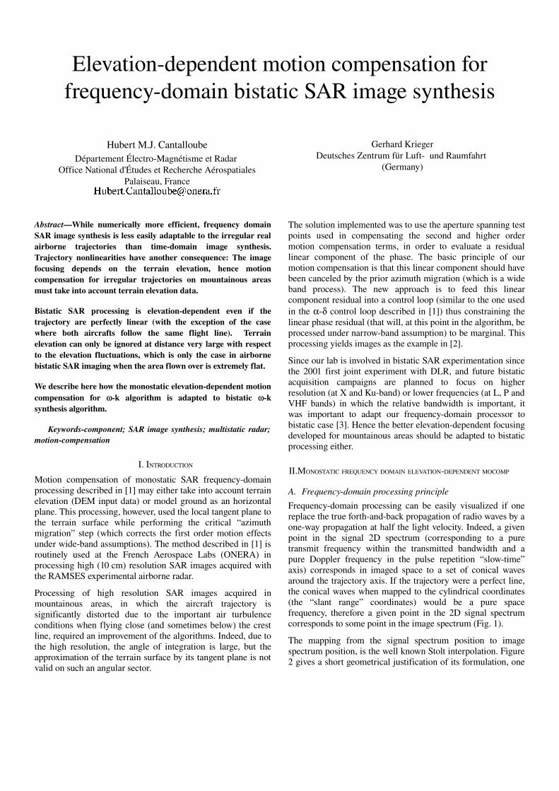
Frequency­domain processing can be easily visualized if one replace the true forth­and­back propagation of radio waves by a one­way propagation at half the light velocity. Indeed, a given point   in   the   signal   2D   spectrum   (corresponding   to   a   pure transmit   frequency   within   the   transmitted   bandwidth   and   a pure   Doppler   frequency   in   the   pulse   repetition   “slow­time” axis) corresponds in imaged space to a set of conical waves around the trajectory axis. If the trajectory were a perfect line, the conical waves when mapped to the cylindrical coordinates (the   “slant   range”   coordinates)   would   be   a   pure   space frequency, therefore a given point in the 2D signal spectrum corresponds to some point in the image spectrum (Fig. 1).

The   mapping   from   the   signal   spectrum   position   to   image spectrum position, is the well known Stolt interpolation. Figure 2 gives a short geometrical justification of its formulation, one 

of the crucial point for processor design is that the along­track dimension is unchanged.

Figure 1. Conical wave corresponding to a point in the 2D signal spectrum.

Figure 2. Stolt interpolation graphical justification: The along­track wavelengths of the signal (u) and the image (y) are identical, and the relation between the signal wavelength () and the image across­track wavelength (x) 

are easily derived from the construct.

Under the perfect linear trajectory assumption, SAR processing is “simply” taking the 2D Fourier transform of the signal, re­sampling it in the across­track dimension, apply a phase and amplitude  correction  (the   image space  wave phase  origin   is shifted   with   respect   to   signal   phase   origin,   it   can   also   be geometrically derived, see [4] for this derivation) and take the inverse 2D Fourier transform. Real trajectories indeed are not perfect lines, hence this simple scheme must be adapted.

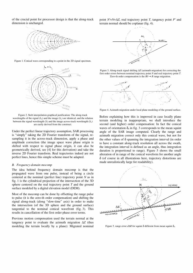
B. Frequency­domain mocompThe   idea   behind   frequency   domain   mocomp   is   that   the propagated   wave   from   one   pulse,   instead   of   being   a   circle centered at the nominal (perfect line) trajectory point  N  as in fig. 1 is the cylindrical projection of the intersection of the 3D sphere centered on the real trajectory point  T  and the ground surface modeled by a digital elevation model (DEM).

Most of the mocomp can be done by offsetting the range pulse to pulse (it is the zero­th order compensation) and shifting the signal along­track (along “slow­time” axis)  in order  to make the   intersection   (of   the   3D  sphere   and   the  ground   surface) tangential   to   the   nominal   conical   wavefront   (fig. 3).   This results in cancellation of the first order phase error terms.

Previous motion compensation used the terrain normal at the tangency   point   to   evaluate   the   azimuth   migration  Z  (thus modeling   the   terrain   locally  by  a  plane):  Migrated  nominal 

point  N'=N+Z, real trajectory point  T, tangency point  P'  and terrain normal should be coplanar (fig. 4).  

 

Figure 3. Along­track signal shifting Z (azimuth migration) for correcting the first order errors between nominal trajectory point N and real trajectory point T. 

Zero­th order compensation is the R0 → R range migration.

Figure 4. Azimuth migration under local plane modeling of the ground surface.

Before explaining how this is improved in case locally plane terrain   modeling   in   inappropriate,   we   shall   introduce   the second (and higher)  order compensation:  In  fact   the conical waves of orientation 0 in fig. 3 corresponds to the mean squint angle   of   the   SAR   image   computed.   Clearly   the   range   and azimuth migration correct only this conical wave, but not for the other values of  spanning the integration interval (in order to have a constant along­track resolution all across the swath, the integration interval is defined as an angle, thus integration duration is  proportional  to range).  Figure 5 shows the small alteration of in range of the conical waveform for another angle   (of course in all illustrations here, trajectory distortions are made unrealistically large for readability).

Figure 5. range error dR for squint  different from mean squint 0.

Unlike range and azimuth migrations  that  can be performed pulse per pulse (thus coping perfectly to the non stationarity of the trajectory deviations),  and being done by re sampling in time­domain   deals   well   with   wide   band   signals,   the compensation   of   the   second   and   higher   terms   are   done   by phase corrections in the range×Doppler (R×ku) domain (there is an  obvious   relation  between    and  ku).  This  has   two major drawbacks:  First,  correcting a  range error  by a  phase offset assumes  the range correction is  small  and  that   the signal  is narrow­band. Next, the Doppler (ku) domain is not resolved in (slow)  time hence   the  correction should be averaged on  the processing bloc.

In practice, we may split the second order compensation along several overlapping sub­blocs, and split the bandwidth into sub­bands in order to enforce narrow­band hypothesis. But this has a negative impact on the computation performance. Note that, as we use frequency agile waveforms, processing each agility separately saves memory usage and elegantly solves the range­processing/radial­velocity coupling problem, thus the negative impact of sub­band processing is controversial. We also have the possibility to split the Doppler aperture in case the second order   compensation   is   too   strong,   but   it   is   generally   less efficient.

The phase correction for varying ku is computed by evaluating dR  for   a   set   of   squint   angles  ­N,...,0,...+N  spanning   the integration interval and interpolating the values with a 2N­th degree polynomials.

The reason why this works is that the second and higher order terms   depends   of   the   distance   between   nominal   and   real trajectory,  which obviously evolves slowly, while  the zero­th order compensation is sensitive to very small variations across­track which require a pulse­to­pulse processing.

The improved motion compensation use the 2N+1  test points computed   for   the   second   order   correction   and  use   them  to model in 3D space the intersection of  the  T­centered sphere with the ground surface on fig. 4. Next, the azimuth migration Z is computed by canceling the mean slope of dR (instead of canceling its derivative at the 0 point as the previous method did).   In   order   to   save   computing   power   requirements,   this cancellation is done iteratively along “slow­time” by a control­loop similar to that used in computing the ­  relationship of fig. 3. Parameter    is an important input of the preprocessing of  the signal because it   is   the true looking direction, and is involved   in   range   compression   (which   may   depend   on Doppler), pre­integration, azimut re­sampling  etc.

The important point is that both  and the mean slope of dR do not need an extreme accuracy (as long as the zero­th order compensation is done for this very value) which justifies the use of slow numerical feedback loop.

III.BISTATIC FREQUENCY DOMAIN ELEVATION­DEPENDENT MOCOMP

Frequency­domain   processing   for   bistatic   SAR   follows   the same   principles   with   one   major   complication:   Image corresponding to a point of the 2D signal spectrum does not 

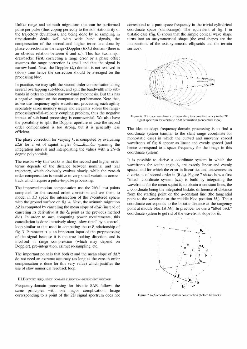
correspond to a pure space frequency in the trivial cylindrical coordinate   space   (slant×range).   The   equivalent   of   fig. 1   in bistatic case (fig. 6) shows that the simple conical wave shape turns   into  an  unsymmetrical   shape   (the  oval   shapes  are   the intersections of  the axis­symmetric ellipsoids and the terrain surface).

Figure 6. 3D space wavefront corresponding to a pure frequency in the 2D signal spectrum for a bistatic SAR acquisition (conceptual view).

The  idea  to  adapt   frequency­domain  processing   is   to   find  a coordinate   system  (similar   to   the   slant   range  coordinate   for monostatic   case)   in   which   the   curved   and   unevenly   spaced wavefronts of fig. 6 appear as linear and evenly spaced (and hence correspond to a space frequency for the image in this coordinate system).

It   is   possible   to   derive   a   coordinate   system   in   which   the wavefronts   for   squint  angle  0  are  exactly   linear  and  evenly spaced and for which the error in linearities and unevenness as  varies is of second order in (­0). Figure 7 shows how a first “tilted”   coordinate   system   (a,b)   is   build   by   integrating   the wavefronts for the mean squint 0 to obtain a­constant lines, the b coordinate being the integrated bistatic difference of distance from the starting point on the  a­constant line (the tangential point to the wavefront at the middle bloc position  M0). The a coordinate corresponds to the bistatic distance at the tangency point at middle bloc (at M0). In practice, we use a “tilted back” coordinate system to get rid of the wavefront slope for 0.

Figure 7. (a,b) coordinate system construction (before tilt back).

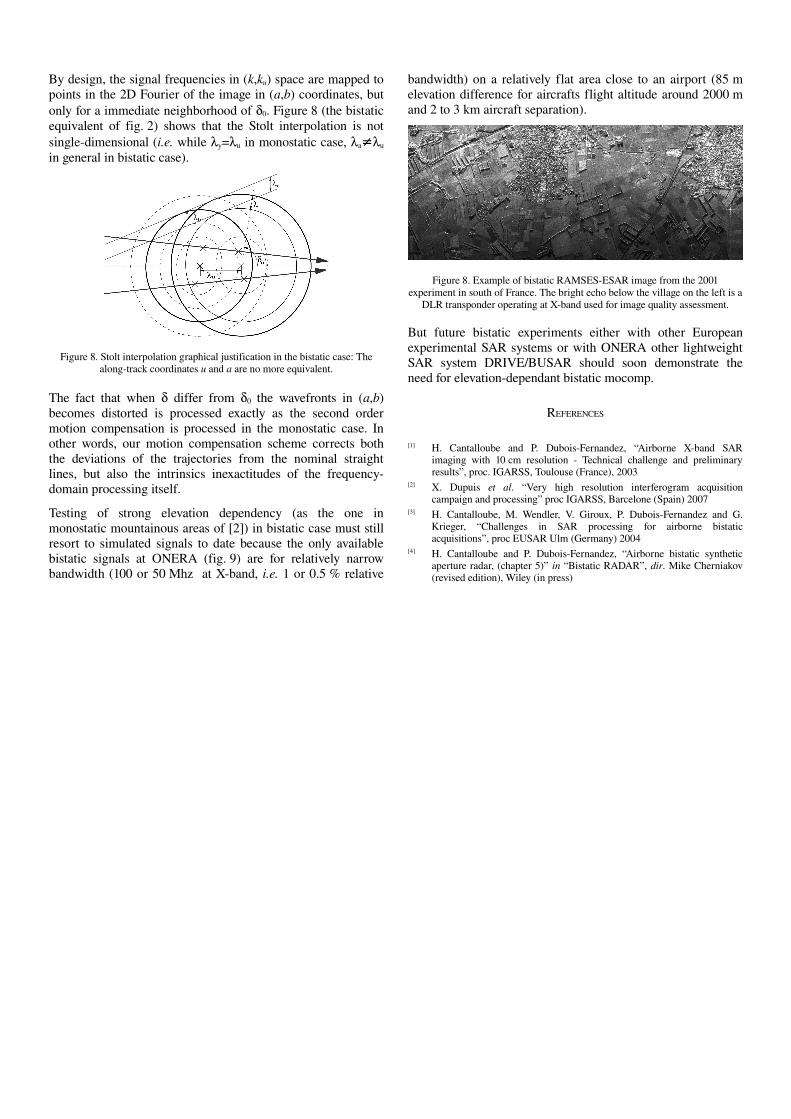
By design, the signal frequencies in (k,ku) space are mapped to points in the 2D Fourier of the image in (a,b) coordinates, but only for a immediate neighborhood of 0. Figure 8 (the bistatic equivalent of fig. 2) shows that  the Stolt  interpolation is not single­dimensional (i.e. while y=u in monostatic case, a≠u 

in general in bistatic case).

Figure 8. Stolt interpolation graphical justification in the bistatic case: The along­track coordinates u and a are no more equivalent.

The fact   that  when    differ   from  0  the wavefronts   in   (a,b) becomes   distorted   is  processed   exactly   as   the   second  order motion compensation is processed in the monostatic case. In other words,  our motion compensation scheme corrects both the   deviations   of   the   trajectories   from   the   nominal   straight lines,   but   also   the   intrinsics   inexactitudes  of   the   frequency­domain processing itself.

Testing   of   strong   elevation   dependency   (as   the   one   in monostatic mountainous areas of [2]) in bistatic case must still resort to simulated signals to date because the only available bistatic   signals  at  ONERA  (fig. 9)  are   for   relatively  narrow bandwidth (100 or 50 Mhz  at X­band, i.e. 1 or 0.5 % relative 

bandwidth) on a relatively flat area close to an airport (85 m elevation difference for aircrafts flight altitude around 2000 m and 2 to 3 km aircraft separation).

Figure 8. Example of bistatic RAMSES­ESAR image from the 2001 experiment in south of France. The bright echo below the village on the left is a 

DLR transponder operating at X­band used for image quality assessment.

But   future   bistatic   experiments   either   with   other   European experimental SAR systems or with ONERA other lightweight SAR   system   DRIVE/BUSAR   should   soon   demonstrate   the need for elevation­dependant bistatic mocomp. 

REFERENCES

[1] H.   Cantalloube   and   P.   Dubois­Fernandez,   “Airborne   X­band   SAR imaging  with  10 cm resolution   ­  Technical   challenge   and  preliminary results”, proc. IGARSS, Toulouse (France), 2003

[2] X.   Dupuis  et   al.   “Very   high   resolution   interferogram   acquisition campaign and processing” proc IGARSS, Barcelone (Spain) 2007

[3] H.  Cantalloube,  M.  Wendler,  V.  Giroux,  P.  Dubois­Fernandez  and  G. Krieger,   “Challenges   in   SAR   processing   for   airborne   bistatic acquisitions”, proc EUSAR Ulm (Germany) 2004

[4] H.  Cantalloube   and  P.  Dubois­Fernandez,   “Airborne  bistatic   synthetic aperture radar, (chapter 5)” in “Bistatic RADAR”, dir. Mike Cherniakov (revised edition), Wiley (in press)