Embed Size (px)
Citation preview
UNIVERSITE DE LIMOGES ECOLE DOCTORALE Gay Lussac – Sciences pour l’Environnement
Groupe de Recherche Eau Sol Environnement (GRESE)
Irstea de Bordeaux (Equipe CARMA)
Thèse
pour obtenir le grade de
DOCTEUR DE L’UNIVERSITÉ DE LIMOGES Discipline / Spécialité : Chimie environnementale
présentée et soutenue par
Gaëlle POULIER
le 5 Novembre 2014
Etude de l’échantillonnage intégratif passif pour l’évaluation
réglementaire de la qualité des milieux aquatiques : application à la
contamination en pesticides et en éléments trace métalliques des
bassins versants du Trec et de l’Auvézère
Thèse dirigée par Gilles GUIBAUD et Nicolas MAZZELLA
JURY : Michel Baudu – HDR, Université de Limoges (Président du jury)
Jean-Marie Mouchel – HDR, Université Pierre and Marie Curie (Rapporteur)
Patrick Mazellier – HDR, Université de Bordeaux (Rapporteur)
Ian J. Allan, Chercheur Sénior, Norwegian Institute for Water Research (NIVA) ((Examinateur)
Jean-Pierre Rebillard (Agence de l’Eau Adour-Garonne) (Examinateur)
Gilles Guibaud, HDR, Université de Limoges (Co-directeur de thèse)
Nicolas Mazzella, HDR, Irstea de Bordeaux (Co-directeur de thèse)
Adeline Charriau, Maître de Conférences, Université de Limoges (Co-directrice de thèse)
Sophie Lissalde, Ingénieure de recherche, Université de Limoges (Co-directrice de thèse)
Rémy Buzier, Maître de Conférences, Université de Limoges (Co-directeur de thèse)
Thès
e de
doc
tora
t

POULIER Gaëlle | Thèse de doctorat | Chimie Environnementale | Université de Limoges | 2014 2
Remerciements Mes remerciements vont en premier lieu à Gilles Guibaud, Nicolas Mazzella, Sophie Lissalde,
Adeline Charriau et Rémy Buzier pour avoir accepté de me confier ce travail de thèse. Gilles, merci
pour ta confiance, pour le partage de ton expérience, pour tes recadrages. Sophie, merci pour ta
patience, grâce à toi la petite agronome que j’étais a pu bénéficier d’une formation accélérée et de
haut niveau en chimie analytique. Adeline, merci pour ta rigueur, tes conseils avisés, ta disponibilité
sans faille. Nicolas, je n’ai pas de mots pour dire tout ce que tu m’as apporté au cours de trois ans en
termes d’expérience, de savoir, de…. la liste est bien trop longue. Merci. Rémy, merci d’avoir partagé
avec moi ton expérience sur les DGTs, et pour tes précieux conseils au cours de nombreux échanges
scientifiques. A vous tous, merci. Cette thèse n’aurait pas été ce qu’elle est sans votre soutien
constant. Votre complémentarité a fait la force de l’encadrement dont j’ai bénéficié.
Je tiens à remercier Michel Baudu et Daniel Poulain pour avoir accepté de m’accueillir au sein
de leurs équipes respectives, GRESE et CARMA.
Merci à Patrick Mazellier et Jean-Marie Mouchel pour avoir accepté d’être rapporteurs de ce
travail. Je remercie également Ian Allan et Jean-Pierre Rebillard pour avoir examiné ce manuscrit.
Je dois également remercier la Région Limousin et l’Agence de l’Eau Adour Garonne, qui ont
financé ce travail.
J’adresse aussi mes sincères remerciements à Dominique Lagorce et Bruno Moine pour avoir
partagé leurs connaissances et leur expérience du bassin versant limousin.
Un grand merci à l’équipe CARMA et au GRESE, pour m’avoir accueillie et intégrée à la vie du
laboratoire.
Au GRESE je remercie, Patrice Fondanèche et Karine Clériès pour leur soutien technique et
humain. Je n’aurais pu mener ce projet à terme sans votre aide. Je remercie aussi mes camarades
thésard, Alex, Loïc, Sonda, Isabelle et Nejma pour les pauses café/déjeuner.
A l’Irstea, il serait impensable de ne pas remercier « les filles du labo » : Brigitte, Mélissa,
Aurélie, Karine, ainsi que Sylvia, Sandra, Nathalie, Nina, Julie. Merci pour votre bonne humeur, vos
encouragements, les discussions, les sorties, les fou rires, les stages de danse… Ces années n’auraient
pas eu la même saveur sans vous. Merci à mon binôme de bureau Vincent pour ses conseils de
« grand frère de thèse ». Merci à Kewin pour avoir été un super stagiaire. Merci à Seb pour les stats,
POULIER Gaëlle | Thèse de doctorat | Chimie Environnementale | Université de Limoges | 2014 3
les Kinder et les pauses déjeuner. Merci aussi à Thibault. Merci à Guilherm pour son efficacité sur le
terrain.
Un grand merci à mes parents, ma mère Francette, mon père Jacky et mon beau-père Edgard,
à mon frère Stanley et à mon « double », ma sœur Wyllène. Même à 700 ou 9000 km de distance,
vos encouragements et votre confiance en moi ont été précieux. Ils m’ont permis de me remotiver
lors des petits « coups de mou ». Merci d’avoir fait de moi ce que je suis. Cette thèse, c’est aussi à
vous que je la dois.
Enfin, merci à toi Jo. Pour avoir partagé les moments de joie (et y avoir contribué souvent) et
les moments d’infortune. Pour avoir supporté le stress, la fatigue, la distance et mon caractère
« difficile » sans une seule plainte. Ce titre de docteur, tu le mérites autant que moi. Du fond du
cœur, merci !
POULIER Gaëlle | Thèse de doctorat | Chimie Environnementale | Université de Limoges | 2014 4
Résumé Parce qu’ils sont peu coûteux, faciles d’utilisation, et surtout très efficaces, les pesticides sont
devenus une composante majeure de l’agriculture moderne et se sont imposés dans de nombreuses
activités urbaines et domestiques. Ces molécules se retrouvent aujourd’hui dans tous les
compartiments de l’environnement notamment dans les milieux aquatiques. Le suivi resserré des
substances actives et de leurs résidus, présents dans l’environnement à des concentrations
potentiellement dommageables pour les écosystèmes, apparaît aujourd’hui comme une nécessité.
L’application de la Directive cadre sur l’eau, l’une des principales réglementations européenne
ciblant les eaux, requiert des techniques d’échantillonnage et d’analyse performantes, alliant haute
sensibilité, facilité de mise œuvre, coûts abordables, et surtout précision et fiabilité. Actuellement, la
méthodologie employée consiste en des prélèvements ponctuels d’eau à pas de temps lâche (une
fois par mois en général) suivi de l’analyse en laboratoire. Cette approche souffre d’un manque de
représentativité temporelle, couplée à une sensibilité analytique souvent peu satisfaisante. Les
techniques d’échantillonnage passif développées au cours des 20 dernières années pourraient être
intégrées dans les réseaux de surveillance réglementaires afin de pallier ces manques, mais des
questions subsistent encore quant à leur opérationnalité. Ces travaux de thèse visent à développer
puis tester les échantillonneurs passifs sur le terrain afin de déterminer leur adéquation avec les
exigences de la Directive cadre sur l’Eau, et le cas échéant, mettre en évidence les principaux verrous
scientifiques résiduels. L’originalité de ce travail réside dans:
- la variété des outils évalués : trois échantillonneurs différents ont été étudiés (Le Polar
Organic Chemical Integrative Sampler (POCIS), le Chemcatcher et le Diffusive Gradient in Thin film
(DGT). Les méthodes classiques de prélèvement ponctuels ont également été mise en œuvre.
- la variété des environnements étudiés : deux bassins versant très différents ont été
considérés, l’un présentant une contamination en pesticides forte, l’autre une contamination
modérée.
- La mise en en œuvre des échantillonneurs passifs dans un réel contexte réglementaire, les
cours d’eau choisis faisant l’objet d’un contrôle opérationnel. Les données acquises avec les
échantillonneurs passifs ont ainsi pu être comparées avec les suivis de l’Agence de l’Eau.
POULIER Gaëlle | Thèse de doctorat | Chimie Environnementale | Université de Limoges | 2014 5
Abstract The intensive use of pesticides in agriculture and urban activities since the 1950s has led to
diffuse contamination of environmental compartments (air, soil, water). The presence of these
molecules can lead to toxic effects for biota. The implementation of the Water Framework Directive
(WFD) requires the use of an efficient monitoring network, based on reliable sampling and analytical
techniques. Nowadays, grab sampling followed by extraction of analytes and chromatographic
analysis is the most widespread strategy because of its simplicity of implementation but it also has
numerous drawbacks. The crux of the issue lies in the lack of temporal representativeness and the
low analytical sensibility. An alternative strategy to overcome some of these problems could be the
use of passive samplers. This contribution aims at discuss about the possible application of passive
samplers in regulatory monitoring programs. The originality of this work lies in :
The variety of tested devices: three different samplers was studied (The Polar Organic
Chemical Integrative Sampler (POCIS), the Chemcatcher and the Diffusive Gradient in Thin Film
(DGT). Conventional grab sampling strategies were also evaluated.
The variety of studied environments: two very different watersheds were selected. The first
one presented a high level of contamination; the second had a low contamination in pesticides.
The implementation of passive samplers in a real regulatory context, as the selected streams
were monitored by the Water Agency for operational control. Data from the Water Agency could
therefore be compared with passive sampler data.
POULIER Gaëlle | Thèse de doctorat | Chimie Environnementale | Université de Limoges | 2014 6
Sommaire
POULIER Gaëlle | Thèse de doctorat | Chimie Environnementale | Université de Limoges | 2014 7

POULIER Gaëlle | Thèse de doctorat | Chimie Environnementale | Université de Limoges | 2014 8
INTRODUCTION ................................................................................................................................... 17
OBJECTIFS DES TRAVAUX ..................................................................................................................... 23
CHAPITRE 1 : GENERALITES .............................................................................................................. 25
1.1 LES PESTICIDES DANS L’ENVIRONNEMENT .............................................................................................. 27
1.1.1 Familles, modes d’action et usages .................................................................................... 27
1.1.2 Les phénomènes de dispersion ........................................................................................... 31
1.1.3 Impact des pesticides sur les écosystèmes et évaluation du risque ................................... 35
1.1.4 Etat des lieux de la contamination des eaux douces .......................................................... 38
1.2 LA REGLEMENTATION : DIRECTIVE CADRE SUR L’EAU (EU, 2000) ............................................................. 40
1.2.1 Les contrôles de surveillance .............................................................................................. 41
1.2.2 Les contrôles opérationnels ................................................................................................ 41
1.2.3 Les contrôles d’enquête ...................................................................................................... 42
1.3 L’ECHANTILLONNAGE ACTIF (OU CONVENTIONNEL) ................................................................................. 42
1.4 L’ECHANTILLONNAGE PASSIF .............................................................................................................. 43
1.4.1 Histoire et Théorie .............................................................................................................. 43
1.4.2 Caractéristiques du POCIS .................................................................................................. 47
1.4.3 Caractéristiques du Chemcatcher....................................................................................... 47
1.4.4 Caractéristiques du DGT ..................................................................................................... 48
1.4.5 Fraction échantillonnée ...................................................................................................... 49
1.4.6 Influence des facteurs environnementaux sur l’échantillonnage ....................................... 51
1.4.7 Méthodes de correction du biais lié à la variation des facteurs environnementaux .......... 53
CHAPITRE 2 : MATERIEL ET METHODES ............................................................................................ 57
2.1 SITES ETUDIES ................................................................................................................................. 59
2.1.1 Le PAT du Trec-Canaule ...................................................................................................... 60
2.1.2 Le PAT de l’Auvézère .......................................................................................................... 63
2.2 SELECTION DES MOLECULES ETUDIEES .................................................................................................. 64
2.3 PREPARATION DES ECHANTILLONNEURS PASSIFS ..................................................................................... 67
2.3.1 POCIS .................................................................................................................................. 67
2.3.2 Chemcatcher ...................................................................................................................... 68
2.3.3 DGT ..................................................................................................................................... 71
2.4 ETALONNAGE DES ECHANTILLONNEURS PASSIFS ...................................................................................... 73
2.4.1 Détermination des constances cinétiques d’accumulation et de désorption : POCIS et
Chemcatcher 73
2.4.2 Détermination des coefficients de diffusion : DGT ............................................................. 75
2.5 EXPOSITION DES ECHANTILLONNEURS PASSIFS SUR LE TERRAIN ET PRELEVEMENTS PONCTUELS D’EAU ................ 76
2.5.1 Conditions de déploiement ................................................................................................. 76
POULIER Gaëlle | Thèse de doctorat | Chimie Environnementale | Université de Limoges | 2014 9
2.5.2 Plan d’échantillonnage ....................................................................................................... 77
2.6 TECHNIQUES ANALYTIQUES ................................................................................................................ 81
2.6.1 Principes généraux ............................................................................................................. 81
2.6.2 Méthode instrumentale HPLC-ESI-MS/MS ......................................................................... 81
2.6.3 Méthode instrumentale GC-MS/MS ................................................................................... 84
2.6.4 Méthodes instrumentales ICP-MS et SAA-FG ..................................................................... 86
2.6.5 Extraction en phase solide (cartouche Chromabond HR-X) des pesticides polaires neutres
dans les eaux et analyse LC-ESI-MS/MS ....................................................................................................... 86
2.6.6 Validation selon la norme AFNOR NF T90 210 (2009) d’une méthode d’analyse des
pesticides hydrophobes dans les eaux par extraction sur Empore disque C18 et analyse GC-MS MS ........... 89
2.6.7 Validation selon la norme AFNOR NF T90 210 (2009) d’une méthode d’analyse des
pesticides dans les matières en suspension par ASE et analyse LC-ESI-MS/MS ........................................... 93
2.7 CONCLUSION PARTIELLE .................................................................................................................... 97
CHAPITRE 3 : ETALONNAGE DES ECHANTILLONNEURS PASSIFS EN LABORATOIRE ........................... 99
3.1 AVANT-PROPOS ............................................................................................................................. 101
3.2 CALIBRATION DU POCIS EN LABORATOIRE ET DETERMINATION DES RS ...................................................... 103
3.3 PUBLICATION 1 “CALIBRATION OF THE CHEMCATCHER PASSIVE SAMPLER AND PROPOSITION OF A NOVEL MODEL
FOR ESTIMATING SAMPLING RATES OF HYDROPHOBIC PESTICIDES” ................................................................................. 107
3.4 CONCLUSION PARTIELLE .................................................................................................................. 125
CHAPITRE 4 : VALIDATION DES ECHANTILLONNEURS PASSIFS SUR LE TERRAIN .............................. 127
4.1 AVANT-PROPOS ............................................................................................................................. 129
4.2 CORRECTION DU BIAIS ENVIRONNEMENTAL : EVALUATION DES DEMARCHES PRC ET ETALONNAGE IN SITU POUR LE
POCIS 131
4.2.1 Evaluation de la démarche PRC ........................................................................................ 131
4.2.2 Evaluation de la démarche « étalonnage in situ » ........................................................... 137
4.3 PUBLICATION 2 “CAN POCIS BE USED IN WATER FRAMEWORK DIRECTIVE (2000/60/EC) MONITORING
NETWORKS?” A STUDY FOCUSING ON PESTICIDES IN A FRENCH AGRICULTURAL WATERSHED................................................ 141
4.4 PUBLICATION 3 “DGT-LABILE AS, CD, CU AND NI MONITORING IN FRESHWATER: TOWARD A FRAMEWORK FOR
INTERPRETATION OF IN SITU DEPLOYMENT” ............................................................................................................... 169
4.5 CONCLUSION PARTIELLE .................................................................................................................. 187
CHAPITRE 5 : MISE EN ŒUVRE DU POCIS POUR LE SUIVI DE LA CONTAMINATION EN PESTICIDES DES
BASSINS VERSANTS DU TREC ET DE L’AUVEZERE .......................................................................................... 189
5.1 ETUDE D’UN ENVIRONNEMENT PRESENTANT UN FORT NIVEAU DE CONTAMINATION : PAT DU TREC-CANAULE . 191
5.1.1 Aspect quantitatif : Evolution des concentrations en pesticides estimées par le POCIS ... 192
5.1.2 Aspect qualitatif : fréquence d’apparition des molécules détectées avec les POCIS ........ 195
POULIER Gaëlle | Thèse de doctorat | Chimie Environnementale | Université de Limoges | 2014 10
5.2 PUBLICATION 4 “ESTIMATES OF PESTICIDE CONCENTRATIONS AND FLUXES IN TWO RIVERS OF AN EXTENSIVE FRENCH
MULTI-AGRICULTURAL WATERSHED: APPLICATION OF THE PASSIVE SAMPLING STRATEGY” ................................................... 201
5.3 CONCLUSION PARTIELLE .................................................................................................................. 223
CONCLUSION GENERALE ET PERSPECTIVES ........................................................................................ 225
REFERENCES ...................................................................................................................................... 233
ANNEXES ........................................................................................................................................... 243
ANNEXE 1. PUBLICATION N°5: OVERVIEW OF THE CHEMCATCHER FOR THE PASSIVE SAMPLING OF VARIOUS POLLUTANTS
IN AQUATIC ENVIRONMENTS. PART A- PRINCIPLES, CALIBRATION, PREPARATION AND ANALYSIS OF THE SAMPLER .................... 245
ANNEXE 2. PUBLICATION N°6: OVERVIEW OF THE CHEMCATCHER FOR THE PASSIVE SAMPLING OF VARIOUS POLLUTANTS
IN AQUATIC ENVIRONMENTS. PART B – FIELD HANDLING AND ENVIRONMENTAL APPLICATIONS FOR THE MONITORING OF
POLLUTANTS AND THEIR BIOLOGICAL EFFECTS ............................................................................................................ 275
ANNEXE 3. PHOTOGRAPHIES DES SITES ETUDIES .......................................................................................... 297
ANNEXE 4. VALORISATIONS .................................................................................................................... 301
POULIER Gaëlle | Thèse de doctorat | Chimie Environnementale | Université de Limoges | 2014 11
Liste des figures FIGURE 1 CHRONOLOGIE D'APPARITION DES DIFFERENTES FAMILLES DE PESTICIDES (EN GRIS, SUBSTANCE ACTIVE REPRESENTATIVE DE LA
FAMILLE) ......................................................................................................................................................... 29
FIGURE 2 EVOLUTION DE LA CONSOMMATION EN PRODUITS PHYTOSANITAIRES OU BIOCIDES EN FRANCE (UIPP, 2012) ................ 31
FIGURE 3 MODES DE PROPAGATION ET DEVENIR DES PESTICIDES DANS L'ENVIRONNEMENT (LISSALDE, 2010) .............................. 33
FIGURE 4 LES PESTICIDES LES PLUS QUANTIFIES DANS LES COURS D'EAU EN FRANCE METROPOLITAINE EN 2011 (SOES, 2013) ....... 39
FIGURE 5 LES PESTICIDES LES PLUS QUANTIFIES DANS LES EAUX SOUTERRAINES DE FRANCE METROPOLITAINE EN 2011 (SOES, 2013)
...................................................................................................................................................................... 40
FIGURE 6 VISUALISATION DES DIFFERENTS MODES D'ECHANTILLONNAGE. L’AXE DES ABSCISSES CORRESPOND AU TEMPS, Q REPRESENTE
LE DEBIT ET VECH EST LE VOLUME ECHANTILLONNE (ADAPTE DEORT ET AL. (2010A)). ...................................................... 43
FIGURE 7 DOMAINES D'APPLICATION DES PRINCIPAUX ECHANTILLONNEURS PASSIFS (EN BLEU) ET GAMME DE POLARITE DE QUELQUES
FAMILLES DE CONTAMINANTS ORGANIQUES (EN GRIS). HAP : HYDROCARBURES AROMATIQUES POLYCYCLIQUES, PPCP :
PHARMACEUTICAL AND PERSONNAL CARE PRODUCTS, PCB : POLYCCHLOROBYPHENYLS. APPLICABILITE DU DIFFUSIVE GRADIENT
IN THIN FILM (DGT) SPECIFIEE. ............................................................................................................................ 44
FIGURE 8 DIFFUSION DANS LES DIFFERENTS COMPARTIMENTS D’UN ECHANTILLONNEUR PASSIF (MAZZELLA ET AL., 2011) .............. 45
FIGURE 9 CINETIQUE D'ACCUMULATION DES CONTAMINANTS DANS UN ECHANTILLONNEUR PASSIF (VRANA ET AL., 2005B)............ 46
FIGURE 10 SCHEMA ET PHOTO D'UN POCIS.................................................................................................................... 47
FIGURE 11 PHOTO ET SCHEMA D'UN CHEMCATCHER ........................................................................................................ 48
FIGURE 12 SCHEMA ET PHOTO D'UN DGT ...................................................................................................................... 49
FIGURE 13 SEUIL DE COUPURE DE DIFFERENTS ECHANTILLONNEURS INTEGRATIFS. LE SCHEMA PRESENTE LES SEUILS DE COUPURE
THEORIQUES DE DIFFERENTS OUTILS D'ECHANTILLONNAGE PASSIF (NM) AINSI QUE LES SEUILS DE FRACTIONNEMENT (DIAMETRE
DE PORES DE LA MEMBRANE QUI ENGLOBE LA PHASE ADSORBANTE) DES DIFFERENTS COMPARTIMENTS DE L'ENVIRONNEMENT
(DISSOUS, COLLOÏDES ET MATIERES EN SUSPENSION) (VRANA ET AL., 2005B; ALLAN ET AL., 2006; LARDY-FONTAN. ET LALERE.,
2010). ........................................................................................................................................................... 50
FIGURE 14 LOCALISATION GEOGRAPHIQUE DU PAT DU TREC-CANAULE ET DES SITES ETUDIES (ETOILES JAUNES), ET OCCUPATION DES
SOLS (CHAMBRE D’AGRICULTURE DU LOT ET GARONNE, 2009) .................................................................................. 60
FIGURE 15 LOCALISATION GEOGRAPHIQUE DU PAT DE L'AUVEZERE ET DES SITES ETUDIES (ETOILES JAUNES), ET OCCUPATION DES SOLS
(CHAMBRE D'AGRICULTURE DE LA CORREZE, 2006) ................................................................................................. 63
FIGURE 16 DOPAGE DE DISQUE EMPORE C18 MAINTENUS PAR « HOLDERS » SUR UN DISPOSITIF VISIPREP ................................... 68
FIGURE 17 RENDEMENTS DE DOPAGE DU DISQUE EMPORE C18 (VOLUME 250 ML) ................................................................. 69
FIGURE 18 RENDEMENTS DE DOPAGE DU DISQUE EMPORE C18 (VOLUME 100 ML) ................................................................. 70
FIGURE 19 MONTAGE D'UN CHEMCATCHER .................................................................................................................... 70
FIGURE 20 SCHEMA DU DISPOSITIF UTILISE POUR LA CALIBRATION DES ECHANTILLONNEURS PASSIFS ........................................... 74
FIGURE 21 SCHEMA DU DISPOSITIF UTILISE POUR LA DETERMINATION DES COEFFICIENTS DE DIFFUSION DES ELEMENTS TRACE DANS LE
DGT ............................................................................................................................................................... 76
POULIER Gaëlle | Thèse de doctorat | Chimie Environnementale | Université de Limoges | 2014 12
FIGURE 22 CAGETTES PRETES A ETRE POSEES SUR LE TERRAIN. LES POCIS SONT POSITIONNES FACE AU COURANT TANDIS QUE LES
DGTS (SUR LE COTE DE LA CAGETTE) SONT PLACES DANS LE SENS PARRALLELE AU COURANT. LES CHEMCATCHER SONT A
L’INTERIEUR DE LA CAGETTE ................................................................................................................................. 77
FIGURE 23 DROITE D'ETALONNAGE DE LA METHODE DE MESURE ......................................................................................... 90
FIGURE 24 DETERMINATION THEORIQUE DE LA SPECIFICITE D'UNE METHODE D'ANALYSE .......................................................... 92
FIGURE 25 CINETIQUES D'ACCUMULATION DE LA DIA, DU METHOMYL ET DE L'IMIDACLOPRIDE OBTENUES LORS DE LA CALIBRATION AU
LABORATOIRE DU POCIS .................................................................................................................................. 103
FIGURE 26 CINETIQUE DE DESORPTION DE LA DIA D5 OBTENUE LORS DE LA CALIBRATION AU LABORATOIRE DU POCIS ................ 105
FIGURE 27 CONSTANTES CINETIQUES D'ACCUMULATION OBTENUES POUR LE POCIS PAR LISSALDE ET AL (2011) ET AU COURS DE LA
PRESENTE ETUDE APRES APPLICATION D'UN FACTEUR DE CORRECTION (KU CORRIGE) ...................................................... 105
FIGURE 28 COMPARAISON ENTRE LES CONCENTRATIONS MESUREES DANS L’EAU DU PRELEVEUR AUTOMATIQUE ET DANS LES
PRELEVEMENTS PONCTUELS HEBDOMADAIRES (CONCENTRATIONS DE REFERENCE) ET LES CONCENTRATIONS MESUREES GRACE AU
POCIS ET CALCULEES AVEC LES KU LABO (C POCIS), LES KU CORRIGES AVEC LE PRC (C POCIS) OU LES KU MESURES IN SITU. 135
FIGURE 29 COMPARAISON DES CONSTANTES CINETIQUES D'ACCUMULATION OBTENUES POUR LE POCIS LORS DE LA CALIBRATION EN
LABORATOIRE (KU LABO) NET LORS DE L'ETALONNAGE IN SITU (KU IN SITU) .................................................................. 138
FIGURE 30 PRECIPITATIONS, DEBIT ET CONCENTRATIONS EN PESTICIDES (POCIS) MESUREES SUR LE PAT DU TREC EN 2012 ........ 192
FIGURE 31 FREQUENCES DE DETECTION (%), CONCENTRATIONS MAXIMALES (µG/L) ET CONCENTRATIONS MOYENNES EN PESTICIDES
MESUREES SUR LE TREC (A), LE MANET (B) ET LA CANAULE (C) EN 2012 (LIMITE DE QUANTIFICATION COMPRISE ENTRE 2 ET 6
µG L-1) .......................................................................................................................................................... 196
FIGURE 32 EVOLUTION DES CONCENTRATIONS INTEGREES (A) ET DES RAPPORTS DEA/ATRAZINE ET DIA/ATRAZINE (B) MESURES SUR LE
TREC EN 2012 ................................................................................................................................................ 198
Liste des Tableaux
TABLEAU 1 LISTE ET PROPRIETES DES PESTICIDES ORGANIQUES ETUDIES (SUBSTANCES PRIORITAIRES DCE EN BLEU) ....................... 66
TABLEAU 2 PARAMETRES FIXES LORS DE LA CALIBRATION AU LABORATOIRE DU POCIS ............................................................. 74
TABLEAU 3 PARAMETRES ENREGISTRES LORS DE LA CALIBRATION IN SITU DU POCIS EN 2013 ................................................... 75
TABLEAU 4 PARAMETRES UTILISES LORS DE LA CALIBRATION AU LABORATOIRE DES CHEMCATCHERS............................................ 75
TABLEAU 5 PLAN D'ECHANTILLONNAGE REALISE SUR LE BASSIN VERSANT DU TREC-CANAULE EN 2012, 2013 ET 2014 ................ 79
TABLEAU 6 PLAN D'ECHANTILLONNAGE REALISE SUR LE BASSIN VERSANT DE L'AUVEZERE EN 2012 ET 2013 ................................ 80
TABLEAU 7 CONDITIONS DE GRADIENT UTILISEES EN CHROMATOGRAPHIE LIQUIDE .................................................................. 82
TABLEAU 8 PARAMETRES DE DETECTION DES PESTICIDES EN CHROMATOGRAPHIE LIQUIDE (DP, DECLUSTERING POTENTIAL ; EC,
ENERGIE DE COLLISION, CXP, CELL EXIT POTENTIAL). ETALONS INTERNES EN GRIS, TRACEURS EN BLEU ET PRC EN VERT. ......... 83
TABLEAU 9 RAMPE DE TEMPERATURE POUR L'ANALYSE DES PESTICIDES EN CHROMATOGRAPHIE GAZEUSE ................................... 84
TABLEAU 10 PARAMETRES DE MASSE DES PESTICIDES ET HAP ANALYSES EN CHROMATOGRAPHIE GAZEUSE (PRCS EN VERT, ETALONS
INTERNES EN GRIS) ............................................................................................................................................. 85
TABLEAU 11 RENDEMENTS D'EXTRACTION MOYENS ET COEFFICIENTS DE VARIATION (% CV) OBTENUS AVEC UNE CARTOUCHE
CHROMABOND HR-X POUR LES PESTICIDES POLAIRES NEUTRES .................................................................................. 88
POULIER Gaëlle | Thèse de doctorat | Chimie Environnementale | Université de Limoges | 2014 13
TABLEAU 12 PARAMETRES DE VALIDATION DE LA METHODE D'ANALYSE DES PESTICIDES HYDROPHOBES DANS LES EAUX (EN GRISE,
MOLECULES NON VALIDEES ET PARAMETRES DECLASSANTS) ........................................................................................ 91
TABLEAU 13 PARAMETRES DE LA METHODE ASE DES PESTICIDES DANS LES MES ................................................................... 94
TABLEAU 14 PARAMETRES DE VALIDATION DE LA METHODE D’ANALYSE DES PESTICIDES POLAIRES NEUTRES DANS LES MATIERES EN
SUSPENSION PAR HPLC-ESI/MS/MS (EN GRISE, MOLECULES NON VALIDEES OU EXCLUES ET PARAMETRES DECLASSANTS) .... 96
TABLEAU 15 CONSTANTES CINETIQUES D'ACCUMULATION (KU) ET TAUX D’ECHANTILLONNAGE (RS) OBTENUS POUR LES PESTICIDES DANS
LE POCIS SUITE A LA CALIBRATION AU LABORATOIRE .............................................................................................. 104
TABLEAU 16 POURCENTAGES D’EQUIVALENCE ENTRE LES CONCENTRATIONS MESUREES DANS L’EAU DU PRELEVEUR AUTOMATIQUE
(CONCENTRATION DE REFERENCE) ET LES CONCENTRATIONS MESUREES GRACE AU POCIS ET CALCULEES AVEC LES KU LABO (C
POCIS), OU LES KU CORRIGES AVEC LE PRC (C POCIS PRC) EN 2012. ...................................................................... 132
TABLEAU 17 POURCENTAGES D’EQUIVALENCE ENTRE LES CONCENTRATIONS MESUREES DANS L’EAU DU PRELEVEUR AUTOMATIQUE
(CONCENTRATION DE REFERENCE) ET LES CONCENTRATIONS MESUREES GRACE AU POCIS ET CALCULEES AVEC LES KU LABO (C
POCIS), OU LES KU CORRIGES AVEC LE PRC (C POCIS PRC) EN 2013. ...................................................................... 134
TABLEAU 18 POURCENTAGES D’EQUIVALENCE ENTRE LES CONCENTRATIONS MESUREES DANS L’EAU DU PRELEVEUR AUTOMATIQUE
(CONCENTRATION DE REFERENCE) ET LES CONCENTRATIONS MESUREES GRACE AU POCIS ET CALCULEES AVEC LES KU IN SITU (C
POCIS IN SITU) EN 2013 .................................................................................................................................. 138
POULIER Gaëlle | Thèse de doctorat | Chimie Environnementale | Université de Limoges | 2014 14
Liste des abréviations AEAG : Agence de l’Eau Adour Garonne
AFNOR : Agence Française de Normalisation
AMPA: Acide aminométhylphosphonique
ASE: Accelerated pressurized Solvent Extraction
CE : Energie de Collision
CT : Contrat Territorial
CV : Coeffcient de Variation
CXP : Cell Exit Potential
D : Coefficient de Diffusion
DAR : Rapport DEA/Atrazine
DCE : Directive Cadre sur l’Eau
DCPMU: 1-(3,4-dichlorophenyl)-3-methyl urea
DCPU: 3,4 Dichlorophényl-méthyl-urée
DDT: Dichlorodiphényltrichloroéthane
DEA: Déséthylatrazine
DEDIA : Déisopropyl-déséthyl-atrazine
DET: Déséthylterbuthylazine
DGT : Gradient de Diffusion en couche mince
DIA: Déisoprpopylatrazine
DIREN : Direction régionale de l'Environnement
DOM: Département d’Outre-Mer
DP: Decleusteuring Potential
DT50: Temps de demie-vie
EFSA: European Food Safety Authority
GC-MS/MS: Gas Chromatography / Tandem Mass Spectrometry
HAP: Hydrocarbure Aromatique Polycyclique
HPLC ESI-MS/MS: High Performance Liquid Chromatography / Electrospray Source Interface / Tandem Mass Spectrometry
ICP-MS : Inductive Coupled Plasma / Mass Spectrometry
IFEN : Institut Français de l’Environnement
IPPMU: 1-(4-isopropylphenyl)-3-methyl urée
IPPU: 1-(4-isopropyl phenyl) urea
IUPAC: International Union of Pure and Applied Chemistry
LDPE: Low Density Polyethylene
POULIER Gaëlle | Thèse de doctorat | Chimie Environnementale | Université de Limoges | 2014 15
LQ: Limite de Quantification
MAEt: Mesure Agro-Environnementale territorialisée
MES : Matières en Suspension
MESCO : Membrane-Enclosed Sorptive Coating sampler
NQE : Norme de Qualité Environnementale
NQE-CMA : Norme de Qualité Environnementale – Concentration Maximale Admissible
NQE-MA : Norme de Qualité Environnementale – Moyenne Annuelle
PAT: Plan d’Action Territorial
PCB: Polychlorobiphényle
PEC: Predicted Exposure Concentration
PNEC: Predicted No Effect Concentration
POCIS: Polar Organic Chemical Integrative Sampler
PPCP: Pharmaceutical and Personal Care Product
PRC: Composé de Performance et de Référence
PTFE: Polytetrafluoroéthylène
PVE: Plan Végétal Environnement
RCS: Réseau de Contrôle et de Surveillance
Rs: Taux d’échantillonnage
SAA-FG : Spectrométrie d'Absorption Atomique à Four en Graphite
SAU : Surface Agricole Utile
SOeS: Service de l’Observatoire et des Statistiques
SPE: Solid Phase Extraction
SPMD: Semi Permeable Membrane Device
SR: Silicone Rubber
SRM : Selective Reaction Monitoring
Sw: Solubilité dans l’eau
TEMED: Tétraméthyléthylènediamine
TWAC : Time Weighted Average Concentration
UE : Union Européenne
UIPP : Union des Industriels de la Protection des Plantes
POULIER Gaëlle | Thèse de doctorat | Chimie Environnementale | Université de Limoges | 2014 16

Introduction
POULIER Gaëlle | Thèse de doctorat | Chimie Environnementale | Université de Limoges | 2014 17

Introduction
POULIER Gaëlle | Thèse de doctorat | Chimie Environnementale | Université de Limoges | 2014 18
Introduction
Au lendemain de la seconde guerre mondiale, la France peinait à assurer son autosuffisance
alimentaire. Soixante-dix ans plus tard, elle est le premier producteur européen de produits agricoles
et représente 18 % de la production de l’Union Européenne (UE) à vingt-sept (Ministère de
l'agriculture de l'agroalimentaire et de la forêt, 2012). Cette évolution majeure a pu être réalisée
grâce à la généralisation de pratiques culturales qui ont profondément transformé le monde agricole.
Les propriétés antifongiques et insecticides des composés minéraux comme le soufre, le cuivre
et l’arsenic sont connues depuis longtemps (Calvet et al., 2005) et ont été utilisées depuis l'antiquité
par les Grecs, puis les Romains pour lutter contre les ravageurs des cultures. Mais les recherches sur
les armes chimiques réalisées au cours de la Première, puis de la Seconde Guerre Mondiale ont fait
grandement progresser les connaissances dans le domaine de la chimie organique de synthèse.
Tirant profit de ces avancées, de nouveaux composés organiques tels que les organochlorés et les
organophosphorés ont été mis au point, et ont peu à peu remplacé les pesticides minéraux. Parce
qu’ils sont souvent peu coûteux, faciles d’utilisation, et surtout très efficaces, les pesticides se sont
imposés dans la plupart des pratiques agricoles et sont devenus une composante majeure de
l’agriculture moderne. Ainsi, de 1945 à 1985 la consommation mondiale de pesticides a doublé tous
les dix ans (Gatignol et Etienne, 2010), et s’est accompagnée d’une hausse continue des rendements
agricoles. Bien que la lutte contre les ravageurs des cultures soit l’usage le plus connu des pesticides,
il faut noter que cette pratique s’est généralisée dans bien d’autres domaines. Sur les aspects
sanitaires, certains insecticides ont par exemple été largement utilisés pour lutter contre le
moustique, vecteur de maladies telles que la malaria ou la dengue. Dans les habitations, les
campagnes de dératisation et de désinsectisation font également appel à des produits
phytosanitaires, de même que l’usage ponctuel par les particuliers, dans les jardins ou en intérieur.
D’autre part, l’urbanisation croissante des villes appelle à un entretien régulier d’espaces tels que les
voies routières, les voies ferrées, les aérodromes, etc., impliquant l’emploi d’herbicides (Gatignol et
Etienne, 2010).
Toutefois, l’utilisation des produits phytosanitaires est de plus en plus remise en question.
Pendant cinquante ans, les conséquences de leur usage sur l’environnement ont été largement
ignorées ou sous-évaluées, mais l’apparition de phénomènes de résistance chez les organismes
ciblés, et la mise en évidence de perturbations des systèmes endocrinien et nerveux chez l’animal
sont autant de signaux d’alarme quant à l’usage systématique et répété des pesticides (Caquet et
Ramade, 1995). A la fin des années 1980, les gouvernements prennent conscience que la dispersion
des pesticides dans différents compartiments de l’environnement (eaux, sols, air …) peut devenir
préoccupante pour la qualité des milieux et la santé humaine. À la demande du ministère chargé de
l’environnement, le Service de l’Observatoire et des Statistiques (SOeS, anciennement IFEN Institut
POULIER Gaëlle | Thèse de doctorat | Chimie Environnementale | Université de Limoges | 2014 19
Introduction
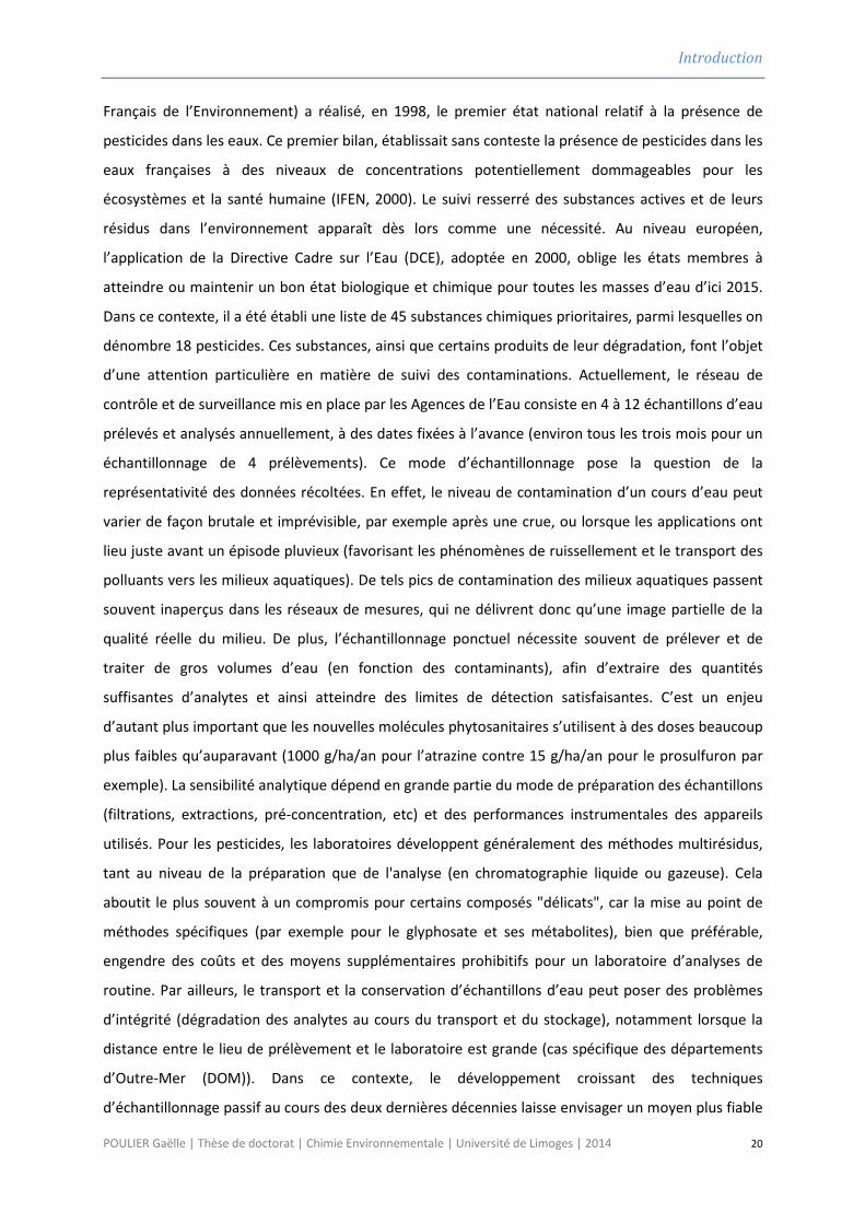
Français de l’Environnement) a réalisé, en 1998, le premier état national relatif à la présence de
pesticides dans les eaux. Ce premier bilan, établissait sans conteste la présence de pesticides dans les
eaux françaises à des niveaux de concentrations potentiellement dommageables pour les
écosystèmes et la santé humaine (IFEN, 2000). Le suivi resserré des substances actives et de leurs
résidus dans l’environnement apparaît dès lors comme une nécessité. Au niveau européen,
l’application de la Directive Cadre sur l’Eau (DCE), adoptée en 2000, oblige les états membres à
atteindre ou maintenir un bon état biologique et chimique pour toutes les masses d’eau d’ici 2015.
Dans ce contexte, il a été établi une liste de 45 substances chimiques prioritaires, parmi lesquelles on
dénombre 18 pesticides. Ces substances, ainsi que certains produits de leur dégradation, font l’objet
d’une attention particulière en matière de suivi des contaminations. Actuellement, le réseau de
contrôle et de surveillance mis en place par les Agences de l’Eau consiste en 4 à 12 échantillons d’eau
prélevés et analysés annuellement, à des dates fixées à l’avance (environ tous les trois mois pour un
échantillonnage de 4 prélèvements). Ce mode d’échantillonnage pose la question de la
représentativité des données récoltées. En effet, le niveau de contamination d’un cours d’eau peut
varier de façon brutale et imprévisible, par exemple après une crue, ou lorsque les applications ont
lieu juste avant un épisode pluvieux (favorisant les phénomènes de ruissellement et le transport des
polluants vers les milieux aquatiques). De tels pics de contamination des milieux aquatiques passent
souvent inaperçus dans les réseaux de mesures, qui ne délivrent donc qu’une image partielle de la
qualité réelle du milieu. De plus, l’échantillonnage ponctuel nécessite souvent de prélever et de
traiter de gros volumes d’eau (en fonction des contaminants), afin d’extraire des quantités
suffisantes d’analytes et ainsi atteindre des limites de détection satisfaisantes. C’est un enjeu
d’autant plus important que les nouvelles molécules phytosanitaires s’utilisent à des doses beaucoup
plus faibles qu’auparavant (1000 g/ha/an pour l’atrazine contre 15 g/ha/an pour le prosulfuron par
exemple). La sensibilité analytique dépend en grande partie du mode de préparation des échantillons
(filtrations, extractions, pré-concentration, etc) et des performances instrumentales des appareils
utilisés. Pour les pesticides, les laboratoires développent généralement des méthodes multirésidus,
tant au niveau de la préparation que de l'analyse (en chromatographie liquide ou gazeuse). Cela
aboutit le plus souvent à un compromis pour certains composés "délicats", car la mise au point de
méthodes spécifiques (par exemple pour le glyphosate et ses métabolites), bien que préférable,
engendre des coûts et des moyens supplémentaires prohibitifs pour un laboratoire d’analyses de
routine. Par ailleurs, le transport et la conservation d’échantillons d’eau peut poser des problèmes
d’intégrité (dégradation des analytes au cours du transport et du stockage), notamment lorsque la
distance entre le lieu de prélèvement et le laboratoire est grande (cas spécifique des départements
d’Outre-Mer (DOM)). Dans ce contexte, le développement croissant des techniques
d’échantillonnage passif au cours des deux dernières décennies laisse envisager un moyen plus fiable
POULIER Gaëlle | Thèse de doctorat | Chimie Environnementale | Université de Limoges | 2014 20
Introduction
et plus efficace pour le suivi de la qualité des milieux aquatiques, pour un coût et des moyens
logistiques équivalents.
Les principes théoriques et les modèles descriptifs de l’échantillonnage intégratif passif ont été
largement développés dans la littérature (Huckins et al, 1993; Alvarez et al, 2004; Stuer - Lauridsen,
2005; Vrana et al, 2005). Pour simplifier, un échantillonneur passif est généralement constitué d’une
phase réceptrice (solide ou liquide) présentant une grande affinité pour les molécules d’intérêt, et
séparée du milieu par une membrane. Les échantillonneurs passifs peuvent être exposés dans le
milieu étudié de plusieurs heures à plusieurs semaines, permettant ainsi l'accumulation et la pré-
concentration des analytes à l'intérieur de la phase réceptrice. L'analyse de la quantité d'analytes
piégée dans l’échantillonneur permet de calculer une concentration moyenne pondérée dans le
temps (TWAC) pour la molécule considérée, à condition que les constantes cinétiques
d'échantillonnage (taux d’échantillonnage (Rs) ou coefficient de diffusion (D)) des analytes soient
connues.
Plusieurs échantillonneurs passifs ont été développés au cours des vingt dernières années. On
peut citer par exemple les membranes semi-perméables (SPMD) ou Chemcatcher® pour les
composés hydrophobes, ou le Gradient de Diffusion en couche mince (DGT) pour les métaux et
métalloïdes (Huckins et al., 1993; Davison et Zhang, 1994; Zhang et Davison, 1995; Kingston et al.,
2000). Le Polar Organic Chemical Integrative Sampler (POCIS), dédié aux composés neutres
moyennement polaires a été développé plus récemment (Alvarez et al., 2004). Les caractéristiques
des échantillonneurs passifs (pré-concentration des analytes in situ et obtention d’une TWAC
permettent de détecter des composés à des concentrations plus faibles que dans les échantillons
ponctuels, et de réduire le risque de manquer des pics possibles de contaminants. Ces
caractéristiques pourraient être très utiles dans les réseaux de surveillance de la DCE, pour améliorer
la fiabilité des données recueillies.
POULIER Gaëlle | Thèse de doctorat | Chimie Environnementale | Université de Limoges | 2014 21

Introduction
POULIER Gaëlle | Thèse de doctorat | Chimie Environnementale | Université de Limoges | 2014 22
Introduction
Objectifs des travaux
Au cours des dernières décennies, les échantillonneurs passifs sont apparus comme un moyen de
résoudre certaines des contraintes liées à l’échantillonnage ponctuel. Leurs performances en termes
de sensibilité (baisse des limites de détection) et de représentativité temporelle (obtention d’une
concentration moyenne pondérée dans le temps) en font un outil de choix pour l’analyse des
contaminants en général, et des pesticides en particulier, dans les milieux aquatiques. Toutefois, leur
utilisation n’est toujours pas autorisée dans les réseaux réglementaires, notamment dans le cadre de
la DCE, l’une des principales réglementations ciblant les eaux. Ce paradoxe s’explique en partie par la
méconnaissance de certaines caractéristiques et processus entourant l’échantillonnage passif.
L’objectif principal de cette thèse est donc de définir le domaine d’application des
échantillonneurs passifs POCIS, Chemcatchers et DGT, et de vérifier leur validité pour la surveillance
réglementaire de la qualité de l’eau.
De cet objectif principal découlent plusieurs questions :
Quel est le degré de fiabilité des échantillonneurs passifs ? Quelle incertitude associer aux
données ? L’une des principales limitations des échantillonneurs passifs réside dans l’influence des
conditions environnementales sur la mesure. Les méthodologies couramment employées pour
corriger ce biais (approche PRC et étalonnage in situ) permettent-elles d’améliorer la justesse des
concentrations obtenues ?
Les Normes de Qualité Environnementales (NQEs) définies dans la DCE pour les substances
prioritaires sont établies pour la fraction totale (particulaire et dissoute) des contaminants. Quelle
est exactement la fraction échantillonnée par les échantillonneurs passifs ? La comparaison des
concentrations obtenues avec ces échantillonneurs avec les NQEs est-elle possible (contrôle de
surveillance) ?
Les échantillonneurs passifs sont-ils adaptés à une grande diversité d’environnements (cours
d’eau faiblement ou fortement contaminé, petits ou grands bassins versants, ….) ?
Pour les gestionnaires de milieux aquatiques, qu'apportent les échantillonneurs passifs comme
informations supplémentaires sur la connaissance des bassins versants ?
POULIER Gaëlle | Thèse de doctorat | Chimie Environnementale | Université de Limoges | 2014 23

Introduction
Pour répondre à ces questions, le manuscrit a été découpé en cinq grandes parties :
Le chapitre 1 consiste en une bibliographie générale, apportant des éléments de contexte
nécessaires à la compréhension des travaux réalisés dans le cadre cette thèse. Les problématiques
environnementales liées à l’utilisation des pesticides et à leur dispersion y sont abordées, ainsi que
les aspects réglementaires de la surveillance des cours d’eau. Enfin, les différentes techniques
d’échantillonnages sont présentées, avec un focus sur l’échantillonnage passif et les caractéristiques
des outils spécifiquement étudiés au cours de ces travaux.
Le chapitre 2 est consacré à la description des développements analytiques réalisés pour le
dosage des pesticides, sur une grande variété de matrices (eau filtrée, matières en suspension et
sédiments, extraits d’échantillonneurs passifs). Les dispositifs utilisés pour l’étalonnage des
échantillonneurs POCIS, Chemcatcher et DGT y sont également décrits.
Le chapitre 3 présente les résultats obtenus suite à la calibration du POCIS et du Chemcatcher.
Pour ce dernier, les résultats sont présentés sous la forme d’une publication.
Le Chapitre 4 est consacré aux résultats issus de la validation des échantillonneurs passifs sur
le terrain. La question de l’influence des conditions environnementales sur la justesse des données
délivrées y est abordée, ainsi que celle de la fraction échantillonnée. Les principaux résultats
concernant les outils DGT et POCIS sont présentés sous la forme de deux publications scientifiques.
Enfin, le Chapitre 5 concerne la mise en œuvre du POCIS sur le terrain, pour le suivi de la
contamination en pesticides de deux bassins versants ruraux très différents en termes de contexte
agricole: le Trec-Canaule (Lot-et-Garonne) et l’Auvézère (Corrèze).
POULIER Gaëlle | Thèse de doctorat | Chimie Environnementale | Université de Limoges | 2014 24
Chapitre 1 :Généralités
POULIER Gaëlle | Thèse de doctorat | Chimie Environnementale | Université de Limoges | 2014 25

Chapitre 1 : Généralités
POULIER Gaëlle | Thèse de doctorat | Chimie Environnementale | Université de Limoges | 2014 26
Chapitre 1 : Généralités
1.1 Les pesticides dans l’environnement Le mot « pesticide » est un terme générique qui englobe les produits phytopharmaceutiques
(ou phytosanitaires) et les produits biocides. Les produits phytosanitaires sont régis par le règlement
d’exécution (CE) n° 1107/2009 de l’Union Européenne (EU, 2009), qui en donne la définition
suivante : il s’agit des produits destinés à :
• protéger les végétaux ou les produits végétaux contre tous les organismes nuisibles ou
prévenir l’action de ceux-ci,
• exercer une action sur les processus vitaux des végétaux, assurer la conservation des
produits végétaux,
• détruire les végétaux ou les parties de végétaux indésirables,
• freiner ou prévenir une croissance indésirable des végétaux.
Les produits biocides sont régis par la directive européenne 98/8/CE (EU, 1998), qui les définit
comme l’ensemble des substances destinées « à détruire, repousser ou rendre inoffensifs les
organismes nuisibles, à en prévenir l'action ou à les combattre de toute autre manière, par une
action chimique ou biologique ». Cette directive a été instituée pour pallier l’absence de
réglementation vis-à-vis des pesticides à usage non agricole.
Le terme pesticide regroupe donc les substances chimiques destinées à repousser, détruire ou
combattre les ravageurs et les espèces indésirables de plantes ou d'animaux causant des dommages
aux denrées alimentaires, aux produits agricoles, au bois et aux produits ligneux. Les pesticides sont
utilisés aussi bien en agriculture que dans d’autres secteurs tels que le milieu hospitalier, la gestion
des espaces urbains, l’entretien des voies ferrées, ou dans les jardins domestiques. Il faut distinguer
les substances actives (responsables de l’effet létal ou protecteur du pesticide), des adjuvants ajoutés
dans les formulations commerciales pour améliorer l’efficacité du produit, par exemple en facilitant
l’accroche sur les surfaces foliaires (adhésif), ou la pénétration dans les tissus végétaux. Les
formulations commerciales peuvent ainsi combiner une ou plusieurs matières actives en association
avec différents adjuvants. Une fois appliquées, la plupart des substances actives (et des adjuvants)
subissent des phénomènes de dégradation qui aboutissent à la formation de molécules appelées
métabolites. Dans la suite du chapitre, le terme pesticide désignera indifféremment les substances
actives et leurs produits de dégradation.
1.1.1 Familles, modes d’action et usages
Les pesticides présentent une très grande diversité de caractéristiques chimiques, structurales
et fonctionnelles, qui rend toute tentative de classification particulièrement complexe. On peut
néanmoins les distinguer en fonction du type d’organisme ciblé. On parle ainsi d’herbicide, de
POULIER Gaëlle | Thèse de doctorat | Chimie Environnementale | Université de Limoges | 2014 27
Chapitre 1 : Généralités
fongicide ou d’insecticide, qui sont les familles les plus représentées. Certains pesticides sont
spécifiquement acaricides, nématicides ou algicides par exemple, mais font l’objet d’un usage
beaucoup plus restreint que les trois groupes précédemment cités. Une autre nomenclature très
répandue inspirée de l’IUPAC (Union internationale de chimie pure et appliquée) est basée sur la
structure chimique des molécules. Quelques familles parmi les plus connues sont listées ci-dessous,
suivant l’ordre chronologique d’apparition :
Les organochlorés : ce sont des composés incluant un atome de chlore (chlordane, aldrine,
endosulfan). Ce sont les pesticides de synthèse les plus anciens (Figure 1), les propriétés insecticides
du dichlorodiphényltrichloroéthane (DDT) et du lindane (les organochlorés les plus connus) ayant été
découverts avant 1950. Les organochlorés sont des insecticides de contact, dont le mode d’action
repose sur une altération du fonctionnement des canaux sodium, indispensables à la transmission de
l’influx nerveux. Leur action biocide est extrêmement efficace mais ces composés sont aujourd’hui
interdits en Europe et dans de nombreux autres pays en raison de leur grande stabilité dans
l’environnement, qui leur confère une rémanence excessive. Leur caractère lipophile les rend
bioaccumulables et fait craindre une contamination généralisée des chaînes alimentaires.
Les urées substituées : Les premiers brevets décrivant l’activité herbicide des urées substituées
sont parus à la fin des années 40, mais c’est à partir de 1951 avec la création du monuron, que leur
utilisation se généralise. Ces substances sont bâties autour du motif urée (NH2-CO-NH2), substitué sur
les atomes d’azote. Leur mode d’action est identique à celui des triazines, ce sont donc des
herbicides. Le diuron, l’isoproturon ou le chlortoluron font partie de cette famille. Ils sont utilisés
aussi bien en agriculture que dans les secteurs non agricoles.
Les carbamates : Depuis l'introduction du carbaryl en 1956 (Figure 1), plus de 50 matières
actives appartenant au groupe des carbamates ont été synthétisées. Ces derniers sont dérivés de
l'acide méthyl-ou diméthyl-carbamique et peuvent être dotés de propriétés insecticides (carbofuran,
pyrimicarbe), fongicides (propamocarbe) ou herbicides (asulame).
Les triazines : Les triazines doivent leur nom à la présence de trois atomes d’azote dans un
cycle aromatique. Ce sont des herbicides dont le mode d’action repose sur une inhibition de la
photosynthèse, par blocage du photosystème II. L’atrazine en est le représentant le plus connu, mais
on peut aussi citer la simazine ou la terbuthylazine. Ces molécules ont été massivement utilisées
(essentiellement pour le traitement des cultures de maïs) sur de très grandes surfaces jusqu’en 2003,
entrainant une contamination généralisée des sols et des cours d’eau. Bien que les composés de
cette famille soient aujourd’hui tous interdits, le caractère persistant de certaines molécules telles
que l’atrazine fait qu’il est encore possible de les quantifier dans la plupart des régions où elles ont
POULIER Gaëlle | Thèse de doctorat | Chimie Environnementale | Université de Limoges | 2014 28
Chapitre 1 : Généralités
été appliquées. Ainsi en 2011, l’atrazine était encore détectée dans plus de 10 % des eaux de surface,
alors qu’elle est interdite d’usage depuis 2003 (SOeS, 2013).
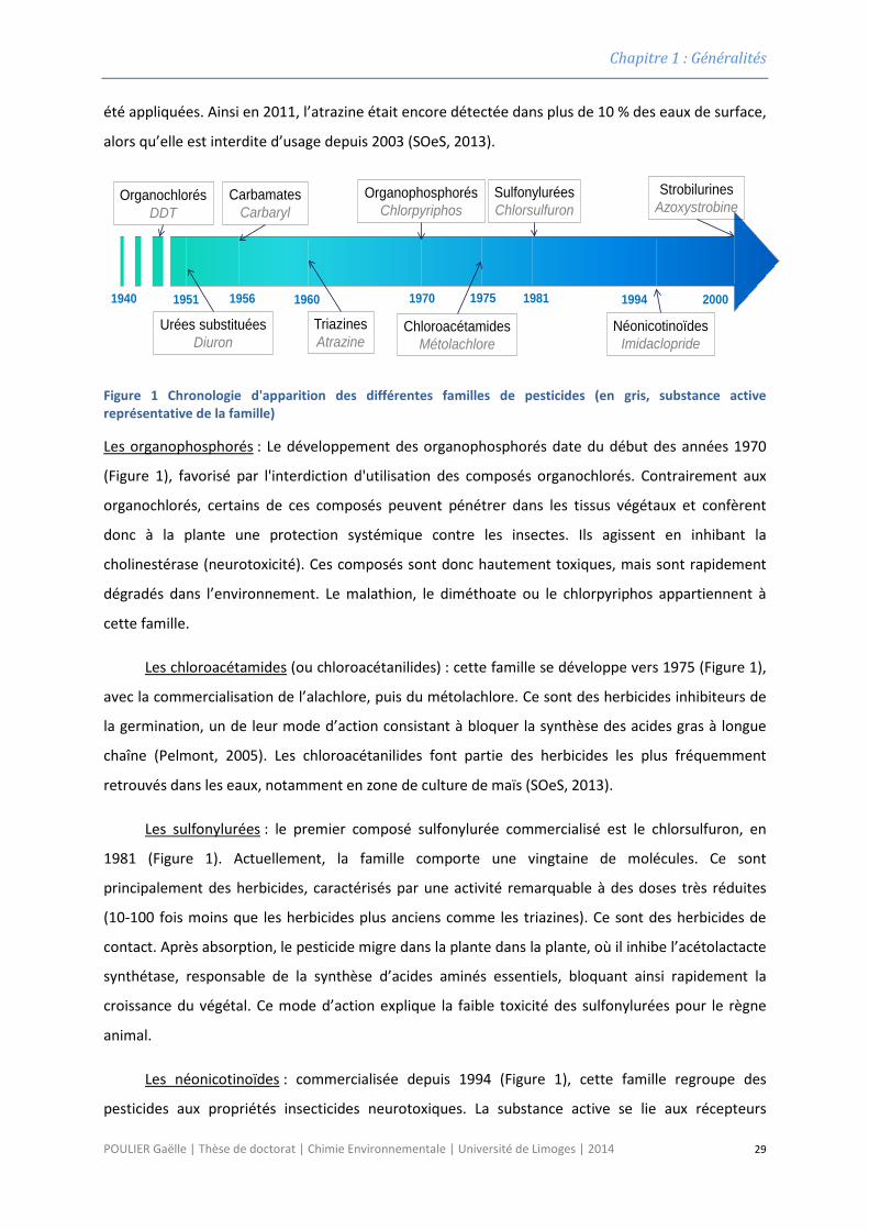
Figure 1 Chronologie d'apparition des différentes familles de pesticides (en gris, substance active représentative de la famille)
Les organophosphorés : Le développement des organophosphorés date du début des années 1970
(Figure 1), favorisé par l'interdiction d'utilisation des composés organochlorés. Contrairement aux
organochlorés, certains de ces composés peuvent pénétrer dans les tissus végétaux et confèrent
donc à la plante une protection systémique contre les insectes. Ils agissent en inhibant la
cholinestérase (neurotoxicité). Ces composés sont donc hautement toxiques, mais sont rapidement
dégradés dans l’environnement. Le malathion, le diméthoate ou le chlorpyriphos appartiennent à
cette famille.
Les chloroacétamides (ou chloroacétanilides) : cette famille se développe vers 1975 (Figure 1),
avec la commercialisation de l’alachlore, puis du métolachlore. Ce sont des herbicides inhibiteurs de
la germination, un de leur mode d’action consistant à bloquer la synthèse des acides gras à longue
chaîne (Pelmont, 2005). Les chloroacétanilides font partie des herbicides les plus fréquemment
retrouvés dans les eaux, notamment en zone de culture de maïs (SOeS, 2013).
Les sulfonylurées : le premier composé sulfonylurée commercialisé est le chlorsulfuron, en
1981 (Figure 1). Actuellement, la famille comporte une vingtaine de molécules. Ce sont
principalement des herbicides, caractérisés par une activité remarquable à des doses très réduites
(10-100 fois moins que les herbicides plus anciens comme les triazines). Ce sont des herbicides de
contact. Après absorption, le pesticide migre dans la plante dans la plante, où il inhibe l’acétolactacte
synthétase, responsable de la synthèse d’acides aminés essentiels, bloquant ainsi rapidement la
croissance du végétal. Ce mode d’action explique la faible toxicité des sulfonylurées pour le règne
animal.
Les néonicotinoïdes : commercialisée depuis 1994 (Figure 1), cette famille regroupe des
pesticides aux propriétés insecticides neurotoxiques. La substance active se lie aux récepteurs
1951
OrganochlorésDDT
1970
OrganophosphorésChlorpyriphos
1960
TriazinesAtrazine
Urées substituéesDiuron
CarbamatesCarbaryl
1981 1994
ChloroacétamidesMétolachlore
SulfonyluréesChlorsulfuron
NéonicotinoïdesImidaclopride
2000
StrobilurinesAzoxystrobine
19561940 1975
POULIER Gaëlle | Thèse de doctorat | Chimie Environnementale | Université de Limoges | 2014 29
Chapitre 1 : Généralités
nicotiniques de certains neurones du système nerveux central de l’insecte, aboutissant à une
paralysie totale puis à la mort. De par leur activité systémique, les néonicotinoïdes offrent une
protection prolongée, du stade de semence au stade adulte de la plante, car ils peuvent être utilisés
à la fois pour le traitement du sol, l’enrobage des semences, ou la protection des parties aériennes.
Le plus connu est l’imidaclopride, composant principal du Gaucho, récemment suspecté d’être à
l’origine du déclin des populations d’abeilles en milieu agricole par l’Autorité Européenne de Sécurité
des Aliments (EFSA).
Les strobilurines : ce sont des fongicides à large spectres, dérivés des strobilurines naturelles
produites par certains champignons lignicoles forestiers. La première strobilurine de synthèse,
l’azoxystrobine, a été commercialisée en 2000 (Figure 1). Leur mode d’action consiste en une
inhibition de la respiration, et confère à la plante une protection systémique et préventive contre les
champignons. Le kresoxim-méthyl fait également partie de cette famille. Leur efficacité à faible dose,
associée à la leur large spectre, a très vite favorisé le succès de ces substances. Toutefois, la récente
apparition de phénomènes de résistance (Leroux et al., 2004) a entraîné un net déclin de leur usage.
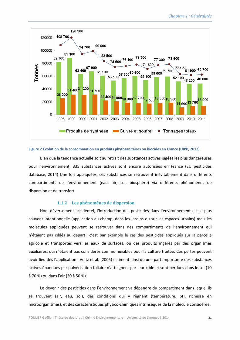
Avec plus de 62 000 tonnes de produits phytosanitaires vendus en 2011, la France est le 4ème
consommateur mondial de pesticides derrière les Etats-Unis, le Brésil et le Japon, et le 1er en Europe
(UIPP, 2012). Environ 90 % des pesticides commercialisés sont destinés à l’agriculture, le reste se
partage équitablement entre les usages domestiques et les usages collectifs (ANSES, 2010). L’analyse
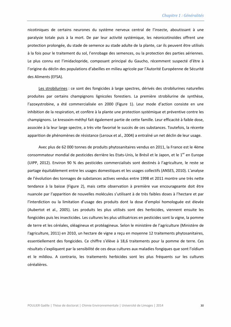
de l’évolution des tonnages de substances actives vendus entre 1998 et 2011 montre une très nette
tendance à la baisse (Figure 2), mais cette observation à première vue encourageante doit être
nuancée par l’apparition de nouvelles molécules s’utilisant à de très faibles doses à l’hectare et par
l’interdiction ou la limitation d’usage des produits dont la dose d’emploi homologuée est élevée
(Aubertot et al., 2005). Les produits les plus utilisés sont des herbicides, viennent ensuite les
fongicides puis les insecticides. Les cultures les plus utilisatrices en pesticides sont la vigne, la pomme
de terre et les céréales, oléagineux et protéagineux. Selon le ministère de l’agriculture (Ministère de
l'agriculture, 2011) en 2010, un hectare de vigne a reçu en moyenne 12 traitements phytosanitaires,
essentiellement des fongicides. Ce chiffre s’élève à 18,6 traitements pour la pomme de terre. Ces
résultats s’expliquent par la sensibilité de ces deux cultures aux maladies fongiques que sont l’oïdium
et le mildiou. A contrario, les traitements herbicides sont les plus fréquents sur les cultures
céréalières.
POULIER Gaëlle | Thèse de doctorat | Chimie Environnementale | Université de Limoges | 2014 30
Chapitre 1 : Généralités
Figure 2 Evolution de la consommation en produits phytosanitaires ou biocides en France (UIPP, 2012)
Bien que la tendance actuelle soit au retrait des substances actives jugées les plus dangereuses
pour l’environnement, 335 substances actives sont encore autorisées en France (EU pesticides
database, 2014) Une fois appliquées, ces substances se retrouvent inévitablement dans différents
compartiments de l’environnement (eau, air, sol, biosphère) via différents phénomènes de
dispersion et de transfert.
1.1.2 Les phénomènes de dispersion
Hors déversement accidentel, l’introduction des pesticides dans l’environnement est le plus
souvent intentionnelle (application au champ, dans les jardins ou sur les espaces urbains) mais les
molécules appliquées peuvent se retrouver dans des compartiments de l’environnement qui
n’étaient pas ciblés au départ : c’est par exemple le cas des pesticides appliqués sur la parcelle
agricole et transportés vers les eaux de surfaces, ou des produits ingérés par des organismes
auxiliaires, qui n’étaient pas considérés comme nuisibles pour la culture traitée. Ces pertes peuvent
avoir lieu dès l’application : Voltz et al. (2005) estiment ainsi qu’une part importante des substances
actives épandues par pulvérisation foliaire n’atteignent par leur cible et sont perdues dans le sol (10
à 70 %) ou dans l’air (30 à 50 %).
Le devenir des pesticides dans l’environnement va dépendre du compartiment dans lequel ils
se trouvent (air, eau, sol), des conditions qui y règnent (température, pH, richesse en
microorganismes), et des caractéristiques physico-chimiques intrinsèques de la molécule considérée.
POULIER Gaëlle | Thèse de doctorat | Chimie Environnementale | Université de Limoges | 2014 31
Chapitre 1 : Généralités
a) Compartiment atmosphérique
Après application, les pesticides peuvent se retrouver dans le compartiment atmosphérique
par volatilisation, depuis le sol nu ou depuis le couvert végétal. Lorsque la volatilisation a lieu
spécifiquement pendant l’application, on parle de « dérive » (Figure 3). Les principaux facteurs
influençant le flux de volatilisation sont la nature physico-chimique du composé (tension de vapeur,
constante de Henry), les conditions pédoclimatiques locales (vent, température, humidité, etc…) et le
mode de pulvérisation (Voltz et al., 2005). L’érosion éolienne (entrainement des particules de sol et
des molécules qui y sont adsorbées sous l’effet du vent) peut également contribuer à la présence de
pesticides dans l’atmosphère. Une fois dans l’air, les pesticides peuvent être transportés sur de très
longues distances, puis retourner au sol par dépôt ou lessivage par les pluies. C’est ainsi qu’il a été
possible de détecter du DDT ou du chlordane dans des régions telles que l’Arctique ou l’Antarctique,
où ces molécules n’ont jamais été utilisées (Oehme, 1991).
b) Compartiment sol
Hormis les phénomènes de dérive, la plupart des mécanismes de transport des molécules
concernent le sol (Figure 3). Une partie des pesticides présents sur les feuilles va ainsi retomber au
sol à la faveur d’une pluie. Le lessivage foliaire est un phénomène très variable, qui dépend de la
nature chimique du pesticide, du temps passé entre le traitement et l’occurrence de la pluie, de
l’intensité et de la durée de la pluie (Voltz et al., 2005). Les pertes par lessivage foliaire sont
maximales lorsque l’épisode pluvieux survient peu de temps après le traitement, et peuvent
atteindre 70 à 80 % des quantités appliquées pour les molécules polaires (Leonard, 1990).
POULIER Gaëlle | Thèse de doctorat | Chimie Environnementale | Université de Limoges | 2014 32
Chapitre 1 : Généralités
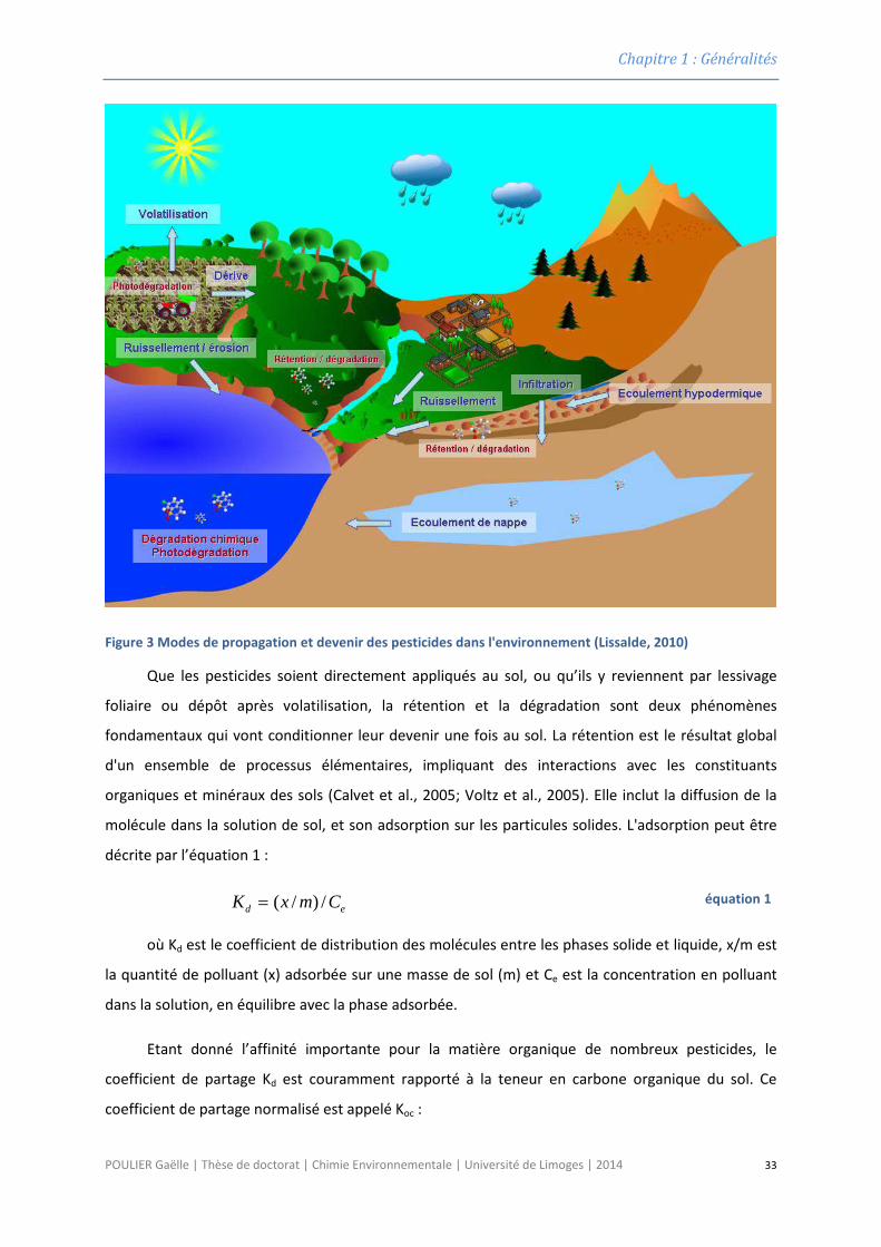
Figure 3 Modes de propagation et devenir des pesticides dans l'environnement (Lissalde, 2010)
Que les pesticides soient directement appliqués au sol, ou qu’ils y reviennent par lessivage
foliaire ou dépôt après volatilisation, la rétention et la dégradation sont deux phénomènes
fondamentaux qui vont conditionner leur devenir une fois au sol. La rétention est le résultat global
d'un ensemble de processus élémentaires, impliquant des interactions avec les constituants
organiques et minéraux des sols (Calvet et al., 2005; Voltz et al., 2005). Elle inclut la diffusion de la
molécule dans la solution de sol, et son adsorption sur les particules solides. L'adsorption peut être
décrite par l’équation 1 :
ed CmxK /)/(= équation 1
où Kd est le coefficient de distribution des molécules entre les phases solide et liquide, x/m est
la quantité de polluant (x) adsorbée sur une masse de sol (m) et Ce est la concentration en polluant
dans la solution, en équilibre avec la phase adsorbée.
Etant donné l’affinité importante pour la matière organique de nombreux pesticides, le
coefficient de partage Kd est couramment rapporté à la teneur en carbone organique du sol. Ce
coefficient de partage normalisé est appelé Koc :
POULIER Gaëlle | Thèse de doctorat | Chimie Environnementale | Université de Limoges | 2014 33
Chapitre 1 : Généralités
)/(%100 CKK doc ×= équation 2
où %C est le pourcentage de la masse de C organique par masse de terre sèche.
D’une manière générale, l’affinité des molécules pour les particules de sol augmente avec le
Koc, et diminue lorsque la solubilité (Sw) de la molécule augmente (Calvet et al., 2005). Autrement dit,
l’augmentation de l’affinité des molécules pour la matière organique s'accompagne de la diminution
de leur solubilité dans l'eau et d'une façon générale de l'augmentation de leur adsorption par les
sols. Pour les composés ionisables, compte tenu de ces phénomènes, le facteur principal
conditionnant la rétention est le pH.
La rétention des pesticides diminue leur mobilité dans le sol, et les rend moins sujets aux
processus de dégradation. La dégradation aboutit à l’apparition de métabolites, sous l’influence de
phénomènes biologiques ou abiotiques (Voltz et al., 2005). La dégradation peut conduire à la
minéralisation totale du pesticide, via des réactions d’oxydation, de réduction, d’hydrolyse, de
déhalogénation, etc… initiées par les constituants organiques et minéraux du sol, ou par la panoplie
enzymatique des organismes du sol. Les mécanismes prépondérants (biologiques ou abiotiques)
diffèrent en fonction des caractéristiques du sol et de la molécule (Barriuso et al., 2004). En général,
la transformation par l’action de la microflore du sol est le processus dominant, mais des exceptions
existent. Ainsi, il semble que les composés comportant de nombreux substituants halogénés soient
particulièrement récalcitrants à la dégradation biologique (Voltz et al., 2005). Un exemple très
illustratif est celui du chlordécone, un pesticide organochloré largement utilisé aux Antilles pour
lutter contre le charançon du bananier. A ce jour, on ne connaît pas de produit de dégradation de
cette molécule (dans les conditions naturelles), qui reste donc très stable dans les sols et pourrait s’y
maintenir pendant plusieurs décennies (Cabidoche et al., 2009).
Les cinétiques de dissipation des pesticides dans les sols sont souvent caractérisées par la
notion de temps de demi-vie (DT50), qui correspond au temps nécessaire pour diminuer de moitié la
quantité initiale de pesticide. Généralement, le DT50 diminue lorsque la température et l’humidité
augmentent (accélérant les réactions de dégradation) (Barriuso et al., 2004).
En pratique, c’est le couple rétention-dégradation qui détermine la mobilité des substances
dans le sol (Voltz et al., 2005). Cette mobilité n’est pas figée, et peut évoluer lorsque les conditions
physico-chimiques régnant dans le sol sont modifiées. Une partie de la fraction adsorbée d’un
pesticide peut alors être progressivement remise en solution, ce qui explique que des molécules
interdites d’usage depuis de nombreuses années soient encore détectées dans les cours d’eau ou les
nappes phréatiques.
POULIER Gaëlle | Thèse de doctorat | Chimie Environnementale | Université de Limoges | 2014 34
Chapitre 1 : Généralités
c) Compartiment eau
Le transport des pesticides présents dans le sol vers les milieux aquatiques a lieu par des
mécanismes de ruissellement et de percolation (Figure 3).
Le ruissellement de surface des eaux de pluie survient lorsqu’une pluie est suffisamment forte
ou d’une durée suffisamment longue pour que la couche superficielle du sol soit complètement
saturée. La pluie supplémentaire qui ne peut pénétrer dans le sol s’écoule alors en surface jusqu’à
rejoindre les cours d’eau. Le ruissellement est influencé par le type de sol, l’intensité de la pluie, la
pente du terrain, la nature du couvert végétal et son importance, les techniques culturales, les
caractéristiques physico-chimiques de chaque pesticide et le délai entre l’application du pesticide et
la pluie qui suit cette application. En France, en milieu agricole, les concentrations maximales dans
les eaux de ruissellement sont observées en avril, mai et juin (Miquel, 2003), période qui associe
souvent des quantités appliquées élevées (par rapport au reste de l’année) et des épisodes pluvieux
intenses et fréquents. En milieu urbain, la plus forte présence de surfaces imperméables, ainsi que
l'importance du drainage direct sans infiltration dans le sol accroît le risque de ruissellement des
pesticides qui peut atteindre 95 % sur du bitume non fissuré (Miquel, 2003). Ainsi, la quantité de
produit phytosanitaire entrainée par ruissellement est estimée à 1 % pour les usages agricoles, et à
50 % en moyenne pour les usages non agricoles (Amalric et al., 2003). Le transport des pesticides
dans les eaux de ruissellement se fait généralement sous forme dissoute, mais sur les sols sensibles à
l’érosion une partie de la fraction adsorbée sur les particules solides peut également être entraînée.
Cela est particulièrement vrai pour les composés hydrophobes les plus fortement retenus.
La contamination des nappes souterraines se fait suite à l’infiltration (ou percolation) des eaux
de pluie contaminées, qui se sont chargées en pesticides en surface. La rapidité d’infiltration de l’eau
dépend de la porosité du sol. Plus le sol est poreux (graviers, sables), plus l’eau s’infiltre rapidement
et peut rejoindre la nappe d’eau souterraine. Dans ce cas, les pesticides sont soustraits à l’action des
microorganismes et aux processus de rétention, ce qui rend la nappe particulièrement vulnérable à la
contamination. À l’inverse, un sol à texture fine, comme l’argile, est moins perméable à la
contamination, car l’eau s’y infiltre plus lentement (Amalric et al., 2003).
1.1.3 Impact des pesticides sur les écosystèmes et évaluation du risque
a) Effets sur les organismes vivants
Après épandage et dispersion dans l’environnement, les pesticides, même partiellement
dégradés et/ou dissociés des adjuvants présents dans les formulations commerciales, peuvent
affecter négativement des organismes vivants qui n’étaient pas ciblés au départ. Ces effets
POULIER Gaëlle | Thèse de doctorat | Chimie Environnementale | Université de Limoges | 2014 35
Chapitre 1 : Généralités
concernent tous les compartiments du vivant, des microorganismes aux mammifères, quel que soit
leur habitat (terrestre ou aquatique).
Organismes terrestres
Quel que soit le mode d’application (traitement sur sol nu ou application foliaire), l’exposition
des organismes du sol aux pesticides est inévitable. Des espèces non cibles peuvent ainsi recevoir,
selon les cas, la totalité ou une fraction (celle non retenue par le couvert végétal) de la dose
appliquée. Des suivis de 10 ans en vergers ont montré des impacts de sulfonylurées sur la diversité
bactérienne du sol. Les insectes volants sont exposés aux pesticides au moment de l’épandage, par
contact avec les surfaces traitées, par ingestions d’aliments contaminés ou par inhalation (Voltz et
al., 2005). Pour ces organismes, l’impact direct des pesticides provient généralement des propriétés
neurotoxiques de certaines molécules (pyréthrinoïdes notamment) (Sommer et al., 2001). Le déclin
des populations d’abeilles, plus connu sous le nom de syndrome d’effondrement, observé partout
dans le monde a été lié à l’utilisation de néonicotinoïdes (van der Sluijs et al., 2013; Laycock et al.,
2014) bien que les causes de ce déclin semblent être multifactorielles (EFSA, 2014). L’ingestion
d’aliments contaminés constitue souvent la voie principale d’exposition des vertébrés terrestres, du
fait de la tendance des animaux à quitter les parcelles lors des traitements (Voltz et al., 2005). La
raréfaction des sources de nourriture, et l’aversion gustative induite par la présence du pesticide sur
des aliments qui sont ensuite délaissés (dégoût qui se maintient même longtemps après que le
pesticide a disparu), sont des causes avancées pour expliquer le déclin des populations d’oiseaux
insectivores dans les zones traitées avec des organochlorés, des carbamates ou des
organophosphorés (Nicolaus et Lee, 1999; Genghini et al., 2006; Nocera et al., 2012).
Organismes aquatiques
Bien que généralement non intentionnelle, la contamination des milieux aquatiques peut avoir
des effets notables sur les organismes qui y vivent. Ces effets peuvent être directs, ou indirects, voire
les deux à la fois. Du fait de leurs propriétés physico-chimiques (solubilité et polarité), les pesticides
les plus fréquemment détectés dans les cours d’eau sont des herbicides. Les conséquences directes
de cette présence concernent la raréfaction des producteurs primaires photosynthétiques que sont
le phytoplancton, les microalgues, le biofilm ou les macrophytes (Solomon et al., 1996; Fairchild et
al., 1998; Ricart et al., 2009; Chang et al., 2011), beaucoup d’herbicides agissant par inhibition de la
photosynthèse. Les effets indirects peuvent se traduire par une réorganisation des communautés, les
espèces sensibles étant remplacées par des espèces plus tolérantes, mais potentiellement
indésirables (exemple des cyanobactéries sécrétant des toxines), qui se mettent à proliférer (Voltz et
al., 2005). Bien que les herbicides soient les pesticides majoritairement détectés dans les cours
POULIER Gaëlle | Thèse de doctorat | Chimie Environnementale | Université de Limoges | 2014 36
Chapitre 1 : Généralités
d’eau, certaines molécules insecticides peuvent également être quantifiées, leur présence (le plus
souvent fugace) résultant de pics de concnetration d’après traitement. Il a été démontré in situ que
certains insecticides (lindane, parathion, fenvalerate) peuvent avoir des effets extrêmement toxiques
(disparition de certaines espèces pendant plus d’un an après exposition à un pic de concentration de
6 µg L-1 pendant 1h) sur les invertébrés aquatiques (Liess et Schulz, 1999; Schulz et Liess, 1999), et ce
même à des concentrations inférieures au ng L-1 (Schulz et Liess, 1995). Concernant les vertébrés, les
poissons sont affectés par des perturbations du système endocrinien (inversion de sexe,
malformations des organes sexuels et altérations des fonctions reproductrices) occasionnées
généralement par les molécules de la famille des organochlorés (DDT, endosulfan) (Baatrup et Junge,
2001; Hemmer et al., 2001) et certaines triazines (Hayes et al., 2011). Par ailleurs, les amphibiens
subissent également les effets des pesticides perturbateurs endocriniens (Hayes et al., 2006).
b) Evaluation réglementaire du risque environnemental
La méthodologie utilisée dans le cadre réglementaire pour l’évaluation du risque
environnemental consiste à mettre en relation l'évaluation de la contamination du milieu, exprimée
en concentration prévisible, baptisée PEC ("Predicted Environmental Concentration") et l'évaluation
des effets, exprimée en termes de concentration prévisible sans effets, baptisée PNEC ("Predicted
No-Effect Concentration"). La PEC caractérise donc l’exposition des populations à la substance
considérée, tandis que la PNEC évalue la toxicité de cette substance pour les organismes testés. Le
risque environnemental est ensuite estimé au travers du rapport PEC/PNEC (la PNEC retenue étant
celle de l’organisme le plus sensible). Si ce rapport est inférieur à 1 alors le risque et considéré
comme acceptable. Ce système d’évaluation, dont la mise en œuvre est relativement simple,
présente toutefois plusieurs lacunes, résidant justement dans son approche simplifiée : le risque est
évalué pour une substance donnée, sur un organisme donné. Or dans, l’environnement, les êtres
vivants sont exposés non pas à une substance, mais à des « cocktails » de contaminants, dont les
effets peuvent s’annuler, s’additionner, ou s’amplifier (Lewis et al., 2012). En plus de la diversité des
polluants, s’ajoute la complexité des écosystèmes, avec toutes les interactions possibles entre les
individus, les espèces et les communautés (Foit et al., 2012). La question des effets « cocktails »
commence tout juste à être abordée. Des études récentes ont montré que des concentrations de
pesticides supposées sans effets quand on considère la substance individuelle, peuvent s’avérer
toxiques en cas de mélange (Hayes et al., 2006; Relyea, 2009; Norgaard et Cedergreen, 2010). Dans
ce cadre, de nouvelles approches sont proposées, consistant à évaluer l’effet des mélanges de
contaminants par couplage d’extraits d’échantillonneurs passifs avec les tests de d‘écotoxicité (Pesce
et al., 2011; Morin et al., 2012c; Kim Tiam et al., 2014). Les extraits d’échantillonneur offrent ainsi la
POULIER Gaëlle | Thèse de doctorat | Chimie Environnementale | Université de Limoges | 2014 37
Chapitre 1 : Généralités
possibilité d’obtenir des mélanges de contaminants « réalistes », représentatifs de ceux existant dans
le milieu naturel.
Dans tous les cas, l’évaluation du risque nécessite de caractériser au mieux l’exposition des
organismes. Pour cela, la réalisation d’un état des lieux régulier de la contamination est
indispensable.
1.1.4 Etat des lieux de la contamination des eaux douces
a) Eaux de surface
Au niveau Européen, Loos et al. (2009) ont, au cours d’une étude de grande ampleur portant
sur plus de 100 rivières dans 27 pays différents, récemment mis en évidence une contamination
généralisée des principaux cours d’eau d’Europe par les pesticides, du Portugal à la Turquie. Les
pesticides les plus fréquemment détectés étaient l’isproturon et le diuron.
Au niveau national, en 2011, des pesticides ont été décelés sur 93 % des points de mesure
(cours d’eau) en France métropolitaine et sur 85 % des points en Guadeloupe, Martinique et à La
Réunion. Ces résultats montrent la présence quasi-généralisée des pesticides dans les eaux de
surface (SOeS, 2013).
Les 15 molécules de pesticides les plus quantifiées dans les cours d’eau de France
métropolitaine en 2011 sont en majorité des herbicides ou leurs métabolites (Figure 4). Sur ces 15
molécules, 2 sont des métabolites (déséthylatrazine (DEA), acide aminométhylphosphonique
(AMPA)) et 3 sont des substances interdites d’utilisation (atrazine, diuron, métolachlore) (Figure 4).
Les zones géographiques les plus impactées correspondent aux zones de grande culture céréalière,
maraîchère ou viticole : nord de la France, bassin parisien, Sud-Ouest, amont du Rhône, ainsi que la
Martinique (SOeS, 2013).
POULIER Gaëlle | Thèse de doctorat | Chimie Environnementale | Université de Limoges | 2014 38
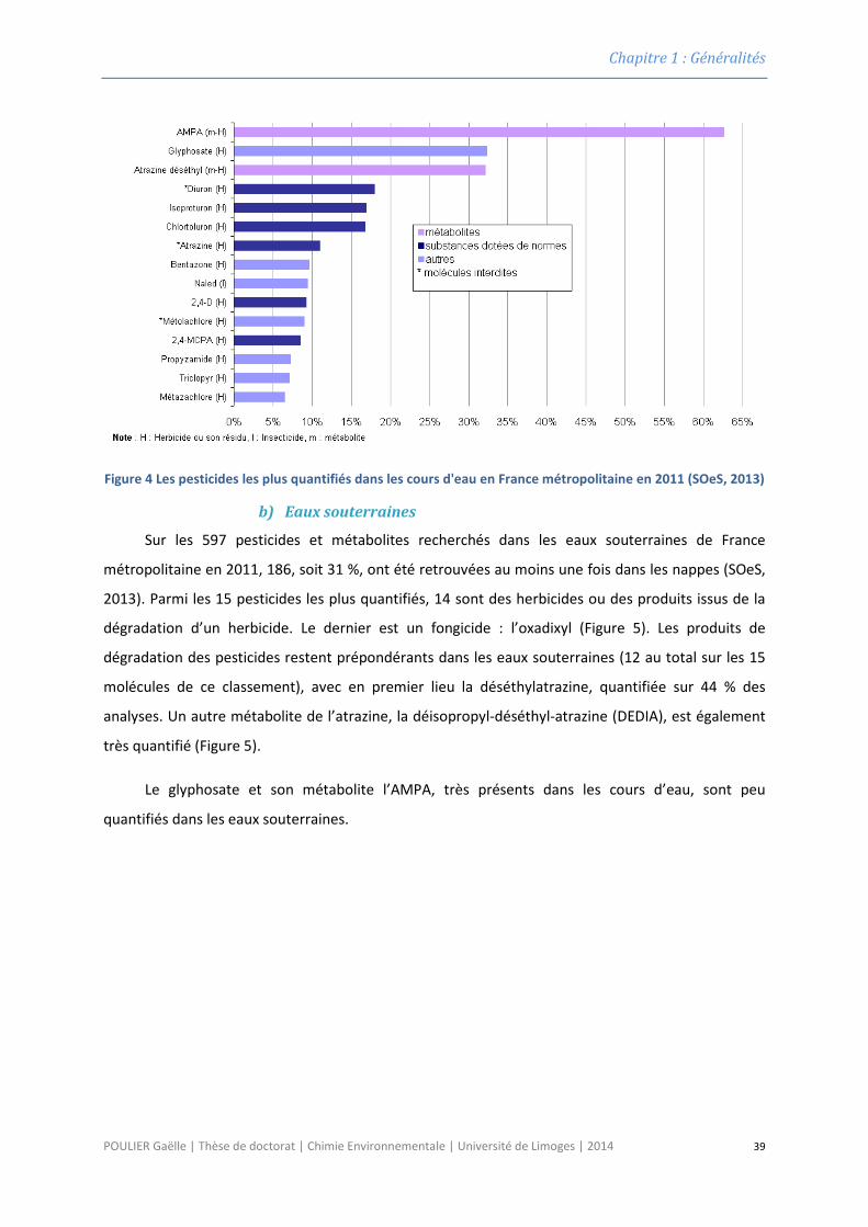
Chapitre 1 : Généralités
Figure 4 Les pesticides les plus quantifiés dans les cours d'eau en France métropolitaine en 2011 (SOeS, 2013)
b) Eaux souterraines
Sur les 597 pesticides et métabolites recherchés dans les eaux souterraines de France
métropolitaine en 2011, 186, soit 31 %, ont été retrouvées au moins une fois dans les nappes (SOeS,
2013). Parmi les 15 pesticides les plus quantifiés, 14 sont des herbicides ou des produits issus de la
dégradation d’un herbicide. Le dernier est un fongicide : l’oxadixyl (Figure 5). Les produits de
dégradation des pesticides restent prépondérants dans les eaux souterraines (12 au total sur les 15
molécules de ce classement), avec en premier lieu la déséthylatrazine, quantifiée sur 44 % des
analyses. Un autre métabolite de l’atrazine, la déisopropyl-déséthyl-atrazine (DEDIA), est également
très quantifié (Figure 5).
Le glyphosate et son métabolite l’AMPA, très présents dans les cours d’eau, sont peu
quantifiés dans les eaux souterraines.
POULIER Gaëlle | Thèse de doctorat | Chimie Environnementale | Université de Limoges | 2014 39
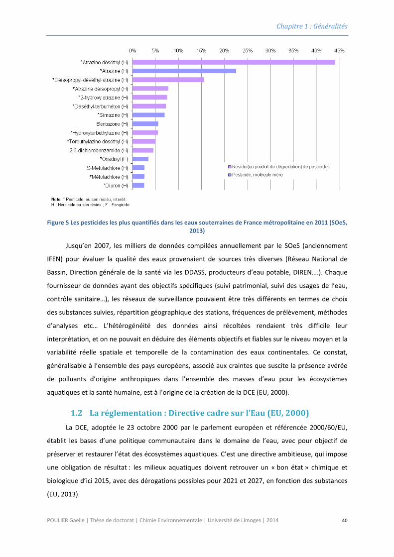
Chapitre 1 : Généralités
Figure 5 Les pesticides les plus quantifiés dans les eaux souterraines de France métropolitaine en 2011 (SOeS, 2013)
Jusqu’en 2007, les milliers de données compilées annuellement par le SOeS (anciennement
IFEN) pour évaluer la qualité des eaux provenaient de sources très diverses (Réseau National de
Bassin, Direction générale de la santé via les DDASS, producteurs d’eau potable, DIREN….). Chaque
fournisseur de données ayant des objectifs spécifiques (suivi patrimonial, suivi des usages de l’eau,
contrôle sanitaire…), les réseaux de surveillance pouvaient être très différents en termes de choix
des substances suivies, répartition géographique des stations, fréquences de prélèvement, méthodes
d’analyses etc… L’hétérogénéité des données ainsi récoltées rendaient très difficile leur
interprétation, et on ne pouvait en déduire des éléments objectifs et fiables sur le niveau moyen et la
variabilité réelle spatiale et temporelle de la contamination des eaux continentales. Ce constat,
généralisable à l’ensemble des pays européens, associé aux craintes que suscite la présence avérée
de polluants d’origine anthropiques dans l’ensemble des masses d’eau pour les écosystèmes
aquatiques et la santé humaine, est à l’origine de la création de la DCE (EU, 2000).
1.2 La réglementation : Directive cadre sur l’Eau (EU, 2000) La DCE, adoptée le 23 octobre 2000 par le parlement européen et référencée 2000/60/EU,
établit les bases d’une politique communautaire dans le domaine de l’eau, avec pour objectif de
préserver et restaurer l’état des écosystèmes aquatiques. C’est une directive ambitieuse, qui impose
une obligation de résultat : les milieux aquatiques doivent retrouver un « bon état » chimique et
biologique d’ici 2015, avec des dérogations possibles pour 2021 et 2027, en fonction des substances
(EU, 2013).
POULIER Gaëlle | Thèse de doctorat | Chimie Environnementale | Université de Limoges | 2014 40
Chapitre 1 : Généralités
Dans le cadre de la mise en œuvre de cette directive, un programme de surveillance a été
établi pour suivre l’état écologique (ou le potentiel écologique) et l’état chimique des eaux douces de
surface (entre autres) et permettre la classification de l’état des masses d’eau. Ce programme
comprend plusieurs volets : les contrôles de surveillance, les contrôles opérationnels, les contrôles
d’enquête et les contrôles additionnels.
1.2.1 Les contrôles de surveillance
Les contrôles de surveillance sont destinés à donner l’image de l’état général des eaux. Ils
suivent une logique de « suivi des milieux aquatiques » et non pas une logique de « suivi de flux
polluants » ou de « suivi d’impacts d’altérations ». Ce suivi est réalisé au sein du RCS (Réseau de
Contrôle et de Surveillance), mis en place par les Agences de l’Eau et constitué d’environ 1500 sites
de prélèvements répartis sur tout le territoire français. L’état chimique est évalué à l’échelle des
masses d’eau, par comparaison avec les normes de qualité environnementales (moyenne annuelle
(NQE-MA), et concentration maximale admissible (NQE-CMA)) définies pour les 45 substances
prioritaires de la directive 2013/39/EU (EU, 2013). Ces NQEs sont établies sur la base des PNEC. A ces
45 substances s’ajoutent les 9 polluants spécifiques de l’état écologique définis dans l’arrêté du 25
Juillet (2010), ce qui porte à 53 le nombre total de substance suivies pour le contrôle de l’état
chimique. La fréquence minimale de suivi, précisée dans l’Arrêté du 29 juillet (2011), est de 12 fois
par an pour les substances prioritaires, à raison de 2 fois par plan de gestion soit tous les trois ans.
1.2.2 Les contrôles opérationnels
Les contrôles opérationnels sont destinés à évaluer l’état de toutes les masses d’eau
identifiées comme risquant de ne pas atteindre les objectifs environnementaux de la DCE et/ou dans
lesquelles sont rejetées des substances prioritaires. Ces contrôles visent à suivre l’évolution de l’état
de ces masses d’eau (toujours selon une logique de suivi de milieu aquatique), suite aux actions
mises en place dans le cadre des programmes de mesures tels que les mesures agro-
environnementales (MAE) ou plan d’action à l'échelle de territoire (plan d’action territorialisé (PAT)
en Adour-Garonne ou Contrat Territoriaux (CT) en Loire-Bretagne). Ce type de contrôle, réalisé au
sein du RCO (Réseau de Contrôle Opérationnel) consiste à suivre les paramètres les plus
problématiques (identifiés comme responsables du risque de non atteinte du bon état écologique), à
une fréquence inférieure à celle du contrôle de surveillance, soit 4 fois par an. Les contrôles
opérationnels sont régulièrement mis à jour (au plus tard fin 2014 et ensuite tous les 6 ans) et ont
pour vocation à disparaître lorsque la masse d’eau aura retrouvé un bon état.
POULIER Gaëlle | Thèse de doctorat | Chimie Environnementale | Université de Limoges | 2014 41
Chapitre 1 : Généralités
1.2.3 Les contrôles d’enquête
Les contrôles d’enquête sont destinés à apporter des informations pour identifier les mesures
nécessaires à la réalisation des objectifs environnementaux et les mesures pour remédier aux effets
de pollutions accidentelles. Ils sont mis en place lorsque les raisons de tout excédent sont inconnues,
pour déterminer les causes pour lesquelles une masse d’eau n’atteint pas les objectifs
environnementaux (lorsqu’un contrôle opérationnel n’a pas encore été mis en place) et pour suivre
les pollutions accidentelles.
Il est évident que la mise en œuvre de la DCE nécessite un réseau de surveillance efficace et
adapté à ses objectifs ambitieux. Cela implique non seulement des techniques analytiques
performantes, capables de détecter et de quantifier les substances prioritaires à des concentrations
au moins inférieures aux NQE, mais aussi des méthodes et des fréquences d’échantillonnage
adaptées. En effet, l’échantillonnage est souvent la principale source de dispersion des résultats
d’une analyse (Fournier, 1995; Ort et al., 2010b). Cette erreur, difficile à estimer et souvent négligée
peut mener à des écarts de mesure de plus de 100 % (Ort et al., 2010b). L’étape d’échantillonnage
est donc essentielle pour garantir la fiabilité des résultats obtenus. Plusieurs techniques existent, qui
correspondent à des prélèvements actifs ou passifs (Figure 6).
1.3 L’échantillonnage actif (ou conventionnel) L’échantillonnage actif ponctuel (Figure 6) est actuellement la méthode la plus largement
utilisée pour le suivi de la qualité des milieux, principalement en raison de sa simplicité de mise en
œuvre. C’est aussi le seul mode d’échantillonnage autorisé dans le cadre de la DCE. Une simple
bouteille d’eau suffit à réaliser un prélèvement, qui est ensuite analysé en laboratoire. Toutefois, ce
type d’échantillonnage donne une « image » à un instant donné de la qualité de l’eau (Figure 6), et
plus l’intervalle de temps entre deux prélèvements sera grand, plus « l’image » sera éloignée de la
réalité. Ceci est particulièrement vrai sur les petits bassins versants, pour lesquels la contamination
varie à l’échelle de quelques heures. Pour être certain de ne pas manquer des pics de contamination
éventuellement très fugaces, et ainsi améliorer la fiabilité de « l’image » obtenue, il faut augmenter
la fréquence et le nombre d’échantillons. Dans ce cas, on peut utiliser un préleveur automatique
asservi au temps (un échantillon de volume V toutes les heures par exemple), au volume passé
(l’intervalle entre chaque prélèvement est ajusté en fonction du débit afin de maintenir un volume
échantillonné fixe), ou au débit (le volume échantillonné est ajusté au débit, mais l’intervalle de
temps entre chaque prélèvement est fixe) (Figure 6). Cependant, dès lors que l’on multiplie le
nombre d’échantillons, on augmente d’autant le nombre d’analyses et les coûts associés, qui
peuvent rapidement devenir limitants. De ce fait, même s’il offre une meilleure estimation de la
qualité du milieu, l’échantillonnage actif à pas de temps resserré est impossible à mettre en œuvre
POULIER Gaëlle | Thèse de doctorat | Chimie Environnementale | Université de Limoges | 2014 42
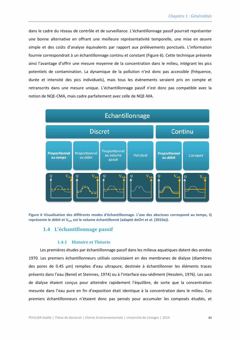
Chapitre 1 : Généralités
dans le cadre du réseau de contrôle et de surveillance. L’échantillonnage passif pourrait représenter
une bonne alternative en offrant une meilleure représentativité temporelle, une mise en œuvre
simple et des coûts d’analyse équivalents par rapport aux prélèvements ponctuels. L’information
fournie correspondrait à un échantillonnage continu et constant (Figure 6). Cette technique présente
ainsi l’avantage d’offrir une mesure moyenne de la concentration dans le milieu, intégrant les pics
potentiels de contamination. La dynamique de la pollution n’est donc pas accessible (fréquence,
durée et intensité des pics individuels), mais tous les évènements seraient pris en compte et
retranscrits dans une mesure unique. L’échantillonnage passif n’est donc pas compatible avec la
notion de NQE-CMA, mais cadre parfaitement avec celle de NQE-MA.
Figure 6 Visualisation des différents modes d'échantillonnage. L’axe des abscisses correspond au temps, Q représente le débit et Véch est le volume échantillonné (adapté deOrt et al. (2010a)).
1.4 L’échantillonnage passif
1.4.1 Histoire et Théorie
Les premières études par échantillonnage passif dans les milieux aquatiques datent des années
1970. Les premiers échantillonneurs utilisés consistaient en des membranes de dialyse (diamètres
des pores de 0.45 µm) remplies d’eau ultrapure, destinée à échantillonner les éléments traces
présents dans l’eau (Beneš et Steinnes, 1974) ou à l’interface eau-sédiment (Hesslein, 1976). Les sacs
de dialyse étaient conçus pour atteindre rapidement l’équilibre, de sorte que la concentration
mesurée dans l’eau pure en fin d’exposition était identique à la concentration dans le milieu. Ces
premiers échantillonneurs n’étaient donc pas pensés pour accumuler les composés étudiés, et
POULIER Gaëlle | Thèse de doctorat | Chimie Environnementale | Université de Limoges | 2014 43
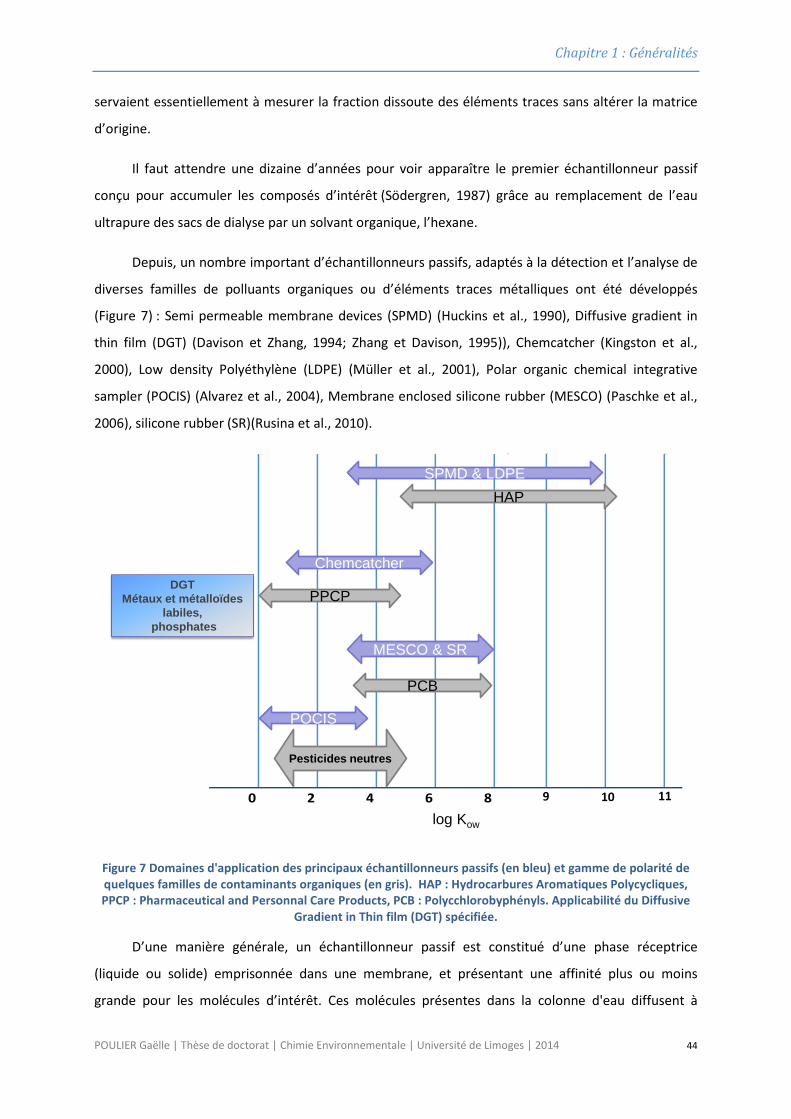
Chapitre 1 : Généralités
servaient essentiellement à mesurer la fraction dissoute des éléments traces sans altérer la matrice
d’origine.
Il faut attendre une dizaine d’années pour voir apparaître le premier échantillonneur passif
conçu pour accumuler les composés d’intérêt (Södergren, 1987) grâce au remplacement de l’eau
ultrapure des sacs de dialyse par un solvant organique, l’hexane.
Depuis, un nombre important d’échantillonneurs passifs, adaptés à la détection et l’analyse de
diverses familles de polluants organiques ou d’éléments traces métalliques ont été développés
(Figure 7) : Semi permeable membrane devices (SPMD) (Huckins et al., 1990), Diffusive gradient in
thin film (DGT) (Davison et Zhang, 1994; Zhang et Davison, 1995)), Chemcatcher (Kingston et al.,
2000), Low density Polyéthylène (LDPE) (Müller et al., 2001), Polar organic chemical integrative
sampler (POCIS) (Alvarez et al., 2004), Membrane enclosed silicone rubber (MESCO) (Paschke et al.,
2006), silicone rubber (SR)(Rusina et al., 2010).
Figure 7 Domaines d'application des principaux échantillonneurs passifs (en bleu) et gamme de polarité de quelques familles de contaminants organiques (en gris). HAP : Hydrocarbures Aromatiques Polycycliques, PPCP : Pharmaceutical and Personnal Care Products, PCB : Polycchlorobyphényls. Applicabilité du Diffusive
Gradient in Thin film (DGT) spécifiée.
D’une manière générale, un échantillonneur passif est constitué d’une phase réceptrice
(liquide ou solide) emprisonnée dans une membrane, et présentant une affinité plus ou moins
grande pour les molécules d’intérêt. Ces molécules présentes dans la colonne d'eau diffusent à
0 2 4 6 8
SPMD & LDPE
MESCO & SR
Chemcatcher
POCIS
HAP
PCB
PPCP
Pesticides neutres
DGTMétaux et métalloïdes
labiles,phosphates
log Kow
9 10 11
POULIER Gaëlle | Thèse de doctorat | Chimie Environnementale | Université de Limoges | 2014 44
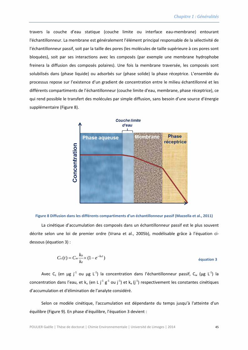
Chapitre 1 : Généralités
travers la couche d’eau statique (couche limite ou interface eau-membrane) entourant
l'échantillonneur. La membrane est généralement l’élément principal responsable de la sélectivité de
l’échantillonneur passif, soit par la taille des pores (les molécules de taille supérieure à ces pores sont
bloquées), soit par ses interactions avec les composés (par exemple une membrane hydrophobe
freinera la diffusion des composés polaires). Une fois la membrane traversée, les composés sont
solubilisés dans (phase liquide) ou adsorbés sur (phase solide) la phase réceptrice. L’ensemble du
processus repose sur l’existence d’un gradient de concentration entre le milieu échantillonné et les
différents compartiments de l’échantillonneur (couche limite d'eau, membrane, phase réceptrice), ce
qui rend possible le transfert des molécules par simple diffusion, sans besoin d’une source d’énergie
supplémentaire (Figure 8).
Figure 8 Diffusion dans les différents compartiments d’un échantillonneur passif (Mazzella et al., 2011)
La cinétique d’accumulation des composés dans un échantillonneur passif est le plus souvent
décrite selon une loi de premier ordre (Vrana et al., 2005b), modélisable grâce à l’équation ci-
dessous (équation 3) :
)1()( tk
e
uws
eekkCtC −−×=
équation 3
Avec Cs (en µg j-1 ou µg L-1) la concentration dans l’échantillonneur passif, Cw (µg L-1) la
concentration dans l’eau, et ku (en L j-1 g-1 ou j-1) et ke (j-1) respectivement les constantes cinétiques
d’accumulation et d'élimination de l’analyte considéré.
Selon ce modèle cinétique, l'accumulation est dépendante du temps jusqu’à l'atteinte d'un
équilibre (Figure 9). En phase d’équilibre, l’équation 3 devient :
POULIER Gaëlle | Thèse de doctorat | Chimie Environnementale | Université de Limoges | 2014 45
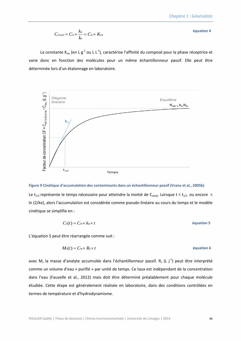
Chapitre 1 : Généralités
swwe
uweqs KC
kkCC ×=×=)(
équation 4
La constante Ksw (en L g-1 ou L L-1), caractérise l’affinité du composé pour la phase réceptrice et
varie donc en fonction des molécules pour un même échantillonneur passif. Elle peut être
déterminée lors d'un étalonnage en laboratoire.
Figure 9 Cinétique d'accumulation des contaminants dans un échantillonneur passif (Vrana et al., 2005b)
Le t1/2 représente le temps nécessaire pour atteindre la moitié de Cs(eq). Lorsque t < t1/2 ou encore <
ln (2/ke), alors l’accumulation est considérée comme pseudo-linéaire au cours du temps et le modèle
cinétique se simplifie en :
tkCtC uws ××=)( équation 5
L’équation 5 peut être réarrangée comme suit :
tRCtM sws ××=)( équation 6
avec Ms la masse d’analyte accumulée dans l’échantillonneur passif. Rs (L j-1) peut être interprété
comme un volume d’eau « purifié » par unité de temps. Ce taux est indépendant de la concentration
dans l’eau (Fauvelle et al., 2012) mais doit être déterminé préalablement pour chaque molécule
étudiée. Cette étape est généralement réalisée en laboratoire, dans des conditions contrôlées en
termes de température et d'hydrodynamisme.
POULIER Gaëlle | Thèse de doctorat | Chimie Environnementale | Université de Limoges | 2014 46
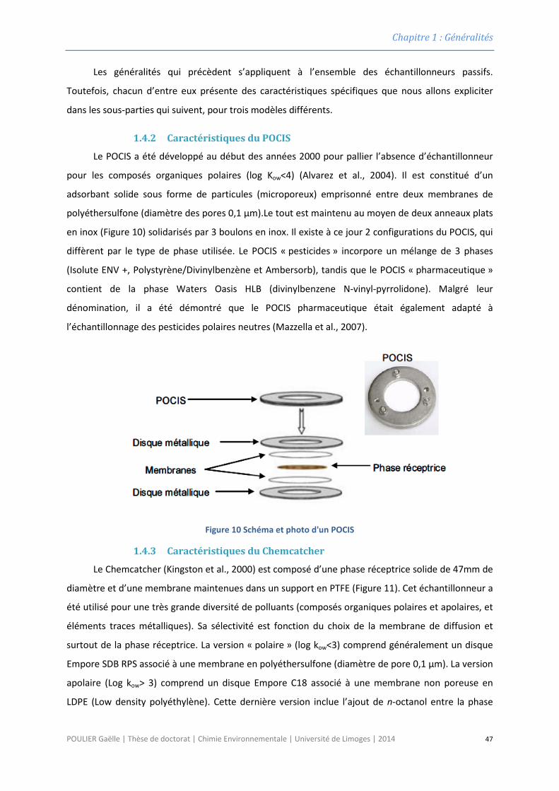
Chapitre 1 : Généralités
Les généralités qui précèdent s’appliquent à l’ensemble des échantillonneurs passifs.
Toutefois, chacun d’entre eux présente des caractéristiques spécifiques que nous allons expliciter
dans les sous-parties qui suivent, pour trois modèles différents.
1.4.2 Caractéristiques du POCIS
Le POCIS a été développé au début des années 2000 pour pallier l’absence d’échantillonneur
pour les composés organiques polaires (log Kow<4) (Alvarez et al., 2004). Il est constitué d’un
adsorbant solide sous forme de particules (microporeux) emprisonné entre deux membranes de
polyéthersulfone (diamètre des pores 0,1 µm).Le tout est maintenu au moyen de deux anneaux plats
en inox (Figure 10) solidarisés par 3 boulons en inox. Il existe à ce jour 2 configurations du POCIS, qui
diffèrent par le type de phase utilisée. Le POCIS « pesticides » incorpore un mélange de 3 phases
(Isolute ENV +, Polystyrène/Divinylbenzène et Ambersorb), tandis que le POCIS « pharmaceutique »
contient de la phase Waters Oasis HLB (divinylbenzene N-vinyl-pyrrolidone). Malgré leur
dénomination, il a été démontré que le POCIS pharmaceutique était également adapté à
l’échantillonnage des pesticides polaires neutres (Mazzella et al., 2007).
Figure 10 Schéma et photo d'un POCIS
1.4.3 Caractéristiques du Chemcatcher
Le Chemcatcher (Kingston et al., 2000) est composé d’une phase réceptrice solide de 47mm de
diamètre et d’une membrane maintenues dans un support en PTFE (Figure 11). Cet échantillonneur a
été utilisé pour une très grande diversité de polluants (composés organiques polaires et apolaires, et
éléments traces métalliques). Sa sélectivité est fonction du choix de la membrane de diffusion et
surtout de la phase réceptrice. La version « polaire » (log kow<3) comprend généralement un disque
Empore SDB RPS associé à une membrane en polyéthersulfone (diamètre de pore 0,1 µm). La version
apolaire (Log kow> 3) comprend un disque Empore C18 associé à une membrane non poreuse en
LDPE (Low density polyéthylène). Cette dernière version inclue l’ajout de n-octanol entre la phase
POULIER Gaëlle | Thèse de doctorat | Chimie Environnementale | Université de Limoges | 2014 47
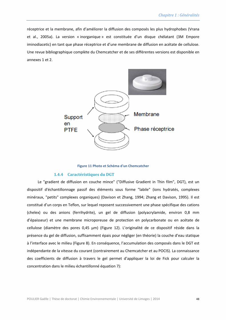
Chapitre 1 : Généralités
réceptrice et la membrane, afin d’améliorer la diffusion des composés les plus hydrophobes (Vrana
et al., 2005a). La version « inorganique » est constituée d’un disque chélatant (3M Empore
iminodiacetic) en tant que phase réceptrice et d’une membrane de diffusion en acétate de cellulose.
Une revue bibliographique complète du Chemcatcher et de ses différentes versions est disponible en
annexes 1 et 2.
Figure 11 Photo et Schéma d'un Chemcatcher
1.4.4 Caractéristiques du DGT
Le "gradient de diffusion en couche mince" ("Diffusive Gradient in Thin film", DGT), est un
dispositif d'échantillonnage passif des éléments sous forme "labile" (ions hydratés, complexes
minéraux, "petits" complexes organiques) (Davison et Zhang, 1994; Zhang et Davison, 1995). Il est
constitué d’un corps en Teflon, sur lequel reposent successivement une phase spécifique des cations
(chelex) ou des anions (ferrihydrite), un gel de diffusion (polyacrylamide, environ 0,8 mm
d’épaisseur) et une membrane microporeuse de protection en polycarbonate ou en acétate de
cellulose (diamètre des pores 0,45 µm) (Figure 12). L’originalité de ce dispositif réside dans la
présence du gel de diffusion, suffisamment épais pour négliger (en théorie) la couche d’eau statique
à l’interface avec le milieu (Figure 8). En conséquence, l’accumulation des composés dans le DGT est
indépendante de la vitesse du courant (contrairement au Chemcatcher et au POCIS). La connaissance
des coefficients de diffusion à travers le gel permet d’appliquer la loi de Fick pour calculer la
concentration dans le milieu échantillonné équation 7):
POULIER Gaëlle | Thèse de doctorat | Chimie Environnementale | Université de Limoges | 2014 48
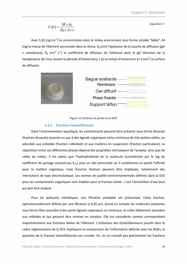
Chapitre 1 : Généralités
tSDMtCg
ge
×××
=δ)(
équation 7
Avec Ce(t) (ng cm-3) la concentration dans le milieu environnant sous forme soluble "labile", M
(ng) la masse de l'élément accumulée dans la résine, δg (cm) l’épaisseur de la couche de diffusion (gel
+ membrane), Dg (cm2 s-1) le coefficient de diffusion de l’élément dans le gel (fonction de la
température de l'eau durant la période d'immersion), t (s) le temps d'immersion et S (cm2) la surface
de diffusion.
Figure 12 Schéma et photo d'un DGT
1.4.5 Fraction échantillonnée
Dans l’environnement aquatique, les contaminants peuvent être présents sous forme dissoute
(fraction dissoute) associés ou pas à des ligands organiques et/ou minéraux de très petites tailles, ou
adsorbés aux colloïdes (fraction colloïdale) et aux matières en suspension (fraction particulaire). La
répartition entre ces différentes phases dépend des propriétés intrinsèques de l’analyte, ainsi que de
celles du milieu. Il est admis que l’hydrophobicité de la molécule (caractérisée par le log du
coefficient de partage octanol-eau Kow) joue un rôle primordial car il conditionne en partie l’affinité
pour la matière organique, mais d’autres facteurs peuvent être impliqués, notamment des
interactions de type électrostatique. Les normes de qualité environnementales définies dans la DCE
pour les contaminants organiques sont établies pour la fraction totale : c’est l’échantillon d’eau brut
qui doit être analysé.
Pour les polluants métalliques, une filtration préalable est préconisée. Cette fraction,
opérationnellement définie par une filtration à 0,45 µm, prend en compte les molécules présentes
sous forme libre associées à des petits ligands organiques ou minéraux, et celles faiblement associées
aux colloïdes et qui peuvent être remises en solution. Elle est considérée comme correspondant
majoritairement aux fractions labiles de l'élément. L’utilisation des échantillonneurs passifs dans le
cadre réglementaire de la DCE impliquant la comparaison de l’information délivrée avec les NQEs, la
question de la fraction échantillonnée est cruciale. Or, on ne connaît pas précisément les fractions
POULIER Gaëlle | Thèse de doctorat | Chimie Environnementale | Université de Limoges | 2014 49
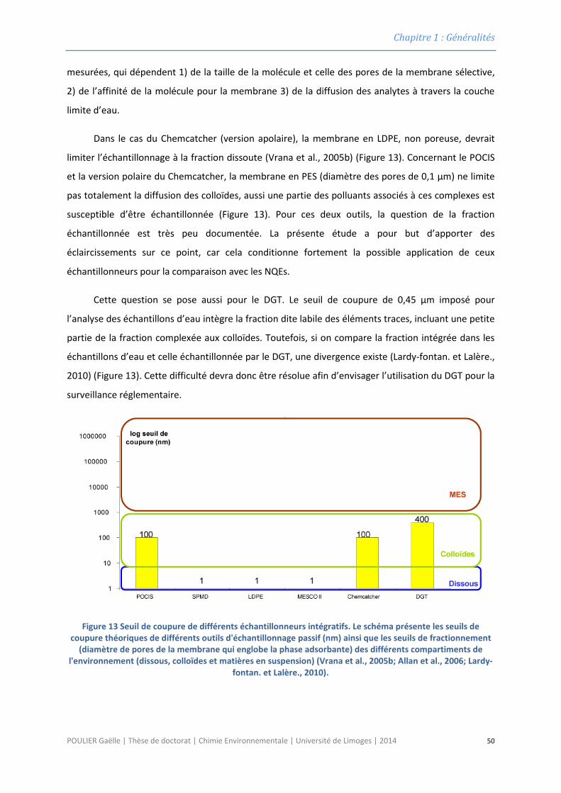
Chapitre 1 : Généralités
mesurées, qui dépendent 1) de la taille de la molécule et celle des pores de la membrane sélective,
2) de l’affinité de la molécule pour la membrane 3) de la diffusion des analytes à travers la couche
limite d’eau.
Dans le cas du Chemcatcher (version apolaire), la membrane en LDPE, non poreuse, devrait
limiter l’échantillonnage à la fraction dissoute (Vrana et al., 2005b) (Figure 13). Concernant le POCIS
et la version polaire du Chemcatcher, la membrane en PES (diamètre des pores de 0,1 µm) ne limite
pas totalement la diffusion des colloïdes, aussi une partie des polluants associés à ces complexes est
susceptible d’être échantillonnée (Figure 13). Pour ces deux outils, la question de la fraction
échantillonnée est très peu documentée. La présente étude a pour but d’apporter des
éclaircissements sur ce point, car cela conditionne fortement la possible application de ceux
échantillonneurs pour la comparaison avec les NQEs.
Cette question se pose aussi pour le DGT. Le seuil de coupure de 0,45 µm imposé pour
l’analyse des échantillons d’eau intègre la fraction dite labile des éléments traces, incluant une petite
partie de la fraction complexée aux colloïdes. Toutefois, si on compare la fraction intégrée dans les
échantillons d’eau et celle échantillonnée par le DGT, une divergence existe (Lardy-fontan. et Lalère.,
2010) (Figure 13). Cette difficulté devra donc être résolue afin d’envisager l’utilisation du DGT pour la
surveillance réglementaire.
Figure 13 Seuil de coupure de différents échantillonneurs intégratifs. Le schéma présente les seuils de coupure théoriques de différents outils d'échantillonnage passif (nm) ainsi que les seuils de fractionnement
(diamètre de pores de la membrane qui englobe la phase adsorbante) des différents compartiments de l'environnement (dissous, colloïdes et matières en suspension) (Vrana et al., 2005b; Allan et al., 2006; Lardy-
fontan. et Lalère., 2010).
POULIER Gaëlle | Thèse de doctorat | Chimie Environnementale | Université de Limoges | 2014 50
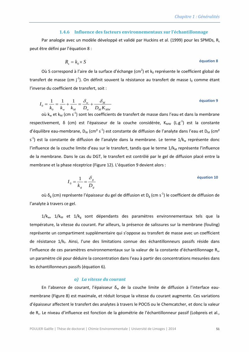
Chapitre 1 : Généralités
1.4.6 Influence des facteurs environnementaux sur l’échantillonnage
Par analogie avec un modèle développé et validé par Huckins et al. (1999) pour les SPMDs, Rs
peut être défini par l’équation 8 :
SkRs ×= 0 équation 8
Où S correspond à l’aire de la surface d’échange (cm2) et k0 représente le coefficient global de
transfert de masse (cm j-1). On définit souvent la résistance au transfert de masse I0 comme étant
l’inverse du coefficient de transfert, soit :
MWM
M
w
w
Mw KDDkkkI δδ
+=+==111
00
équation 9
où kw et kM (cm s-1) sont les coefficients de transfert de masse dans l’eau et dans la membrane
respectivement, δ (cm) est l’épaisseur de la couche considérée, KMW (L.g-1) est la constante
d’équilibre eau-membrane, DW (cm² s-1) est constante de diffusion de l’analyte dans l’eau et DM (cm²
s-1) est la constante de diffusion de l’analyte dans la membrane. Le terme 1/kw représente donc
l’influence de la couche limite d’eau sur le transfert, tandis que le terme 1/kM représente l’influence
de la membrane. Dans le cas du DGT, le transfert est contrôlé par le gel de diffusion placé entre la
membrane et la phase réceptrice (Figure 12). L’équation 9 devient alors :
g
g
g DkI
δ==
10
équation 10
où δg (cm) représente l’épaisseur du gel de diffusion et Dg (cm s-1) le coefficient de diffusion de
l’analyte à travers ce gel.
1/kw, 1/kM et 1/kg sont dépendants des paramètres environnementaux tels que la
température, la vitesse du courant. Par ailleurs, la présence de salissures sur la membrane (fouling)
représente un compartiment supplémentaire qui s’oppose au transfert de masse avec un coefficient
de résistance 1/kf. Ainsi, l’une des limitations connue des échantillonneurs passifs réside dans
l’influence de ces paramètres environnementaux sur la valeur de la constante d’échantillonnage Rs,
un paramètre clé pour déduire la concentration dans l’eau à partir des concentrations mesurées dans
les échantillonneurs passifs (équation 6).
a) La vitesse du courant
En l’absence de courant, l’épaisseur δw de la couche limite de diffusion à l’interface eau-
membrane (Figure 8) est maximale, et réduit lorsque la vitesse du courant augmente. Ces variations
d’épaisseur affectent le transfert des analytes à travers le POCIS ou le Chemcatcher, et donc la valeur
de Rs. Le niveau d’influence est fonction de la géométrie de l’échantillonneur passif (Lobpreis et al.,
POULIER Gaëlle | Thèse de doctorat | Chimie Environnementale | Université de Limoges | 2014 51
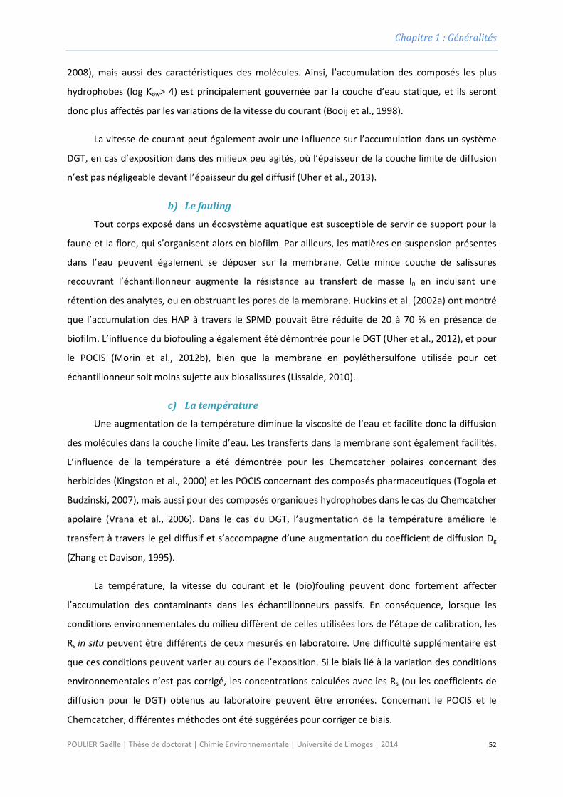
Chapitre 1 : Généralités
2008), mais aussi des caractéristiques des molécules. Ainsi, l’accumulation des composés les plus
hydrophobes (log Kow> 4) est principalement gouvernée par la couche d’eau statique, et ils seront
donc plus affectés par les variations de la vitesse du courant (Booij et al., 1998).
La vitesse de courant peut également avoir une influence sur l’accumulation dans un système
DGT, en cas d’exposition dans des milieux peu agités, où l’épaisseur de la couche limite de diffusion
n’est pas négligeable devant l’épaisseur du gel diffusif (Uher et al., 2013).
b) Le fouling
Tout corps exposé dans un écosystème aquatique est susceptible de servir de support pour la
faune et la flore, qui s’organisent alors en biofilm. Par ailleurs, les matières en suspension présentes
dans l’eau peuvent également se déposer sur la membrane. Cette mince couche de salissures
recouvrant l’échantillonneur augmente la résistance au transfert de masse I0 en induisant une
rétention des analytes, ou en obstruant les pores de la membrane. Huckins et al. (2002a) ont montré
que l’accumulation des HAP à travers le SPMD pouvait être réduite de 20 à 70 % en présence de
biofilm. L’influence du biofouling a également été démontrée pour le DGT (Uher et al., 2012), et pour
le POCIS (Morin et al., 2012b), bien que la membrane en poyléthersulfone utilisée pour cet
échantillonneur soit moins sujette aux biosalissures (Lissalde, 2010).
c) La température
Une augmentation de la température diminue la viscosité de l’eau et facilite donc la diffusion
des molécules dans la couche limite d’eau. Les transferts dans la membrane sont également facilités.
L’influence de la température a été démontrée pour les Chemcatcher polaires concernant des
herbicides (Kingston et al., 2000) et les POCIS concernant des composés pharmaceutiques (Togola et
Budzinski, 2007), mais aussi pour des composés organiques hydrophobes dans le cas du Chemcatcher
apolaire (Vrana et al., 2006). Dans le cas du DGT, l’augmentation de la température améliore le
transfert à travers le gel diffusif et s’accompagne d’une augmentation du coefficient de diffusion Dg
(Zhang et Davison, 1995).
La température, la vitesse du courant et le (bio)fouling peuvent donc fortement affecter
l’accumulation des contaminants dans les échantillonneurs passifs. En conséquence, lorsque les
conditions environnementales du milieu diffèrent de celles utilisées lors de l’étape de calibration, les
Rs in situ peuvent être différents de ceux mesurés en laboratoire. Une difficulté supplémentaire est
que ces conditions peuvent varier au cours de l’exposition. Si le biais lié à la variation des conditions
environnementales n’est pas corrigé, les concentrations calculées avec les Rs (ou les coefficients de
diffusion pour le DGT) obtenus au laboratoire peuvent être erronées. Concernant le POCIS et le
Chemcatcher, différentes méthodes ont été suggérées pour corriger ce biais.
POULIER Gaëlle | Thèse de doctorat | Chimie Environnementale | Université de Limoges | 2014 52
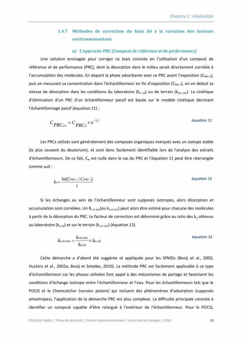
Chapitre 1 : Généralités
1.4.7 Méthodes de correction du biais lié à la variation des facteurs
environnementaux
a) L’approche PRC (Composé de référence et de performance)
Une solution envisagée pour corriger ce biais consiste en l’utilisation d’un composé de
référence et de performance (PRC), dont la désorption dans le milieu serait directement corrélée à
l’accumulation des molécules. En dopant la phase adsorbante avec ce PRC avant l’exposition (CPRC 0),
puis en mesurant sa concentration dans l’échantillonneur en fin d’exposition (CPRC f), on en déduit sa
vitesse de désorption dans les conditions du laboratoire (ke cal) ou de terrain (kein situ). La cinétique
d’élimination d’un PRC d’un échantillonneur passif est basée sur le modèle cinétique décrivant
l’échantillonnage passif (équation 11) :
tek
tePRCCPRCC −×=
0)( équation 11
Les PRCs utilisés sont généralement des composés organiques marqués avec un isotope stable
(le plus souvent du deuterium), et sont donc facilement identifiable lors de l'analyse des extraits
d'échantillonneurs. De ce fait, Cw est nulle dans le cas du PRC et l’équation 11 peut être réarrangée
comme suit :
tCCk fPRCPRC
e)/ln( /0
=
équation 12
Si les échanges au sein de l’échantillonneur sont supposés isotropes, alors désorption et
accumulation sont corrélées. Un Rs in situ(ou ku in situ) peut alors être estimé pour chacune des molécules
à partir de la désorption du PRC. Le facteur de correction est déterminé grâce au ratio des ke obtenus
au laboratoire (ke cal) et sur le terrain (ke in situ) (équation 13).
calcal
situin situin u
e
eu k
kkk ×=
équation 13
Cette démarche a d’abord été suggérée et appliquée pour les SPMDs (Booij et al., 2002;
Huckins et al., 2002a; Booij et Smedes, 2010). La méthode PRC est facilement applicable à ce type
d’échantillonneur car les phases utilisées font appel à des mécanismes de partage et favorisent les
conditions d’échange isotrope entre l’échantillonneur et l’eau. Pour les échantillonneurs tels que le
POCIS et le Chemcatcher (version polaire) qui incluent des phénomènes d’adsorption (supposés
anisotropes), l’application de la démarche PRC est plus complexe. La difficulté principale consiste à
identifier un composé capable d’être relargué à l’extérieur de l’échantillonneur. Pour le POCIS,
POULIER Gaëlle | Thèse de doctorat | Chimie Environnementale | Université de Limoges | 2014 53
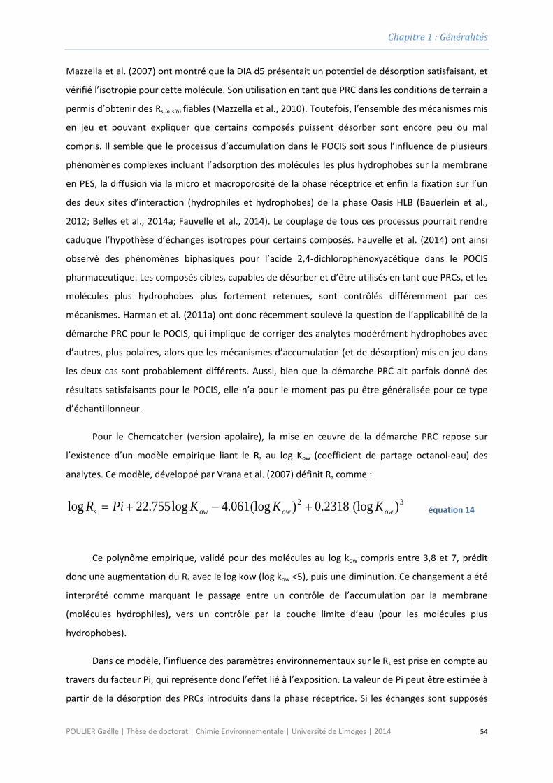
Chapitre 1 : Généralités
Mazzella et al. (2007) ont montré que la DIA d5 présentait un potentiel de désorption satisfaisant, et
vérifié l’isotropie pour cette molécule. Son utilisation en tant que PRC dans les conditions de terrain a
permis d’obtenir des Rs in situ fiables (Mazzella et al., 2010). Toutefois, l’ensemble des mécanismes mis
en jeu et pouvant expliquer que certains composés puissent désorber sont encore peu ou mal
compris. Il semble que le processus d’accumulation dans le POCIS soit sous l’influence de plusieurs
phénomènes complexes incluant l’adsorption des molécules les plus hydrophobes sur la membrane
en PES, la diffusion via la micro et macroporosité de la phase réceptrice et enfin la fixation sur l’un
des deux sites d’interaction (hydrophiles et hydrophobes) de la phase Oasis HLB (Bauerlein et al.,
2012; Belles et al., 2014a; Fauvelle et al., 2014). Le couplage de tous ces processus pourrait rendre
caduque l’hypothèse d’échanges isotropes pour certains composés. Fauvelle et al. (2014) ont ainsi
observé des phénomènes biphasiques pour l’acide 2,4-dichlorophénoxyacétique dans le POCIS
pharmaceutique. Les composés cibles, capables de désorber et d’être utilisés en tant que PRCs, et les
molécules plus hydrophobes plus fortement retenues, sont contrôlés différemment par ces
mécanismes. Harman et al. (2011a) ont donc récemment soulevé la question de l’applicabilité de la
démarche PRC pour le POCIS, qui implique de corriger des analytes modérément hydrophobes avec
d’autres, plus polaires, alors que les mécanismes d’accumulation (et de désorption) mis en jeu dans
les deux cas sont probablement différents. Aussi, bien que la démarche PRC ait parfois donné des
résultats satisfaisants pour le POCIS, elle n’a pour le moment pas pu être généralisée pour ce type
d’échantillonneur.
Pour le Chemcatcher (version apolaire), la mise en œuvre de la démarche PRC repose sur
l’existence d’un modèle empirique liant le Rs au log Kow (coefficient de partage octanol-eau) des
analytes. Ce modèle, développé par Vrana et al. (2007) définit Rs comme :
32 )(log2318.0)(log061.4log755.22log owowows KKKPiR +−+= équation 14
Ce polynôme empirique, validé pour des molécules au log kow compris entre 3,8 et 7, prédit
donc une augmentation du Rs avec le log kow (log kow <5), puis une diminution. Ce changement a été
interprété comme marquant le passage entre un contrôle de l’accumulation par la membrane
(molécules hydrophiles), vers un contrôle par la couche limite d’eau (pour les molécules plus
hydrophobes).
Dans ce modèle, l’influence des paramètres environnementaux sur le Rs est prise en compte au
travers du facteur Pi, qui représente donc l’effet lié à l’exposition. La valeur de Pi peut être estimée à
partir de la désorption des PRCs introduits dans la phase réceptrice. Si les échanges sont supposés
POULIER Gaëlle | Thèse de doctorat | Chimie Environnementale | Université de Limoges | 2014 54
Chapitre 1 : Généralités
isotropes, alors l’équation 4 est applicable, et l’équation 15 est obtenue en remplaçant la
concentration par la masse :
VKmm
VKkR swPRC
tPRC
swsituinesituinst
)ln(0
−=
équation 15
avec V (L) le volume de l’échantillonneur. Selon Vrana et al. (2006) la constante d’équilibre Ksw
peut également être liée à l’hydrophobicité des analytes d’après le modèle empirique :
77.1log382.1log −= owsw KK équation 16
Ainsi, tous les termes de l’équation 15 sont connus et le Rs in situ obtenu peut être reporté
dans l’équation 6 pour revenir à la concentration dans l’eau.
Vrana et al. (2006) ont suggéré le phenanthrène d10 et l’acenaphtène d10 comme PRCs
possibles. Et, après vérification de l’isotropie des échanges, les ont appliqués sur le terrain avec
succès pour améliorer la justesse du Chemcatcher (Vrana et al., 2007; Vrana et al., 2010). Toutefois,
le modèle empirique (équation 14) sur lequel repose la démarche explicitée ci-dessus a été
développé et validé sur un ensemble de molécules incluant principalement des HAPs. Seuls trois
pesticides ont été étudiés. Par conséquent, l’applicabilité de ce modèle pour des composés très
différents des HAPs en termes de propriétés physico-chimiques doit encore être vérifiée.
b) L’étalonnage in situ
Une autre méthode utilisée pour s’affranchir de l’influence des paramètres environnementaux
sur la vitesse d’accumulation des composés consiste à réaliser l’étalonnage des échantillonneurs
directement dans le milieu étudié (in situ). Les Rs in situ sont alors obtenus directement, et n’ont pas
besoin d’être corrigés si les conditions d’étude ne changent pas. Cette méthode permet d’améliorer
la justesse de l’échantillonneur (Meadows et al., 1998; Lissalde, 2010; Harman et al., 2011b).
Malheureusement, les coûts associés à sa mise en œuvre sont très élevés (important nombre
d’échantillonneurs exposés dans différents milieux, pour différentes molécules et dans différentes
conditions). Par ailleurs, il est possible que les conditions environnementales caractérisant le site
étudié changent en cours d’année (en raison des changements de saison par exemple), nécessitant
un nouvel étalonnage des outils. Par conséquent, cette méthode n’est pas adaptée pour la
surveillance de routine.
POULIER Gaëlle | Thèse de doctorat | Chimie Environnementale | Université de Limoges | 2014 55

Chapitre 1 : Généralités
POULIER Gaëlle | Thèse de doctorat | Chimie Environnementale | Université de Limoges | 2014 56
Chapitre 2 :Matériel et Méthodes
POULIER Gaëlle | Thèse de doctorat | Chimie Environnementale | Université de Limoges | 2014 57

Chapitre 2 : Matériel et Méthodes
POULIER Gaëlle | Thèse de doctorat | Chimie Environnementale | Université de Limoges | 2014 58
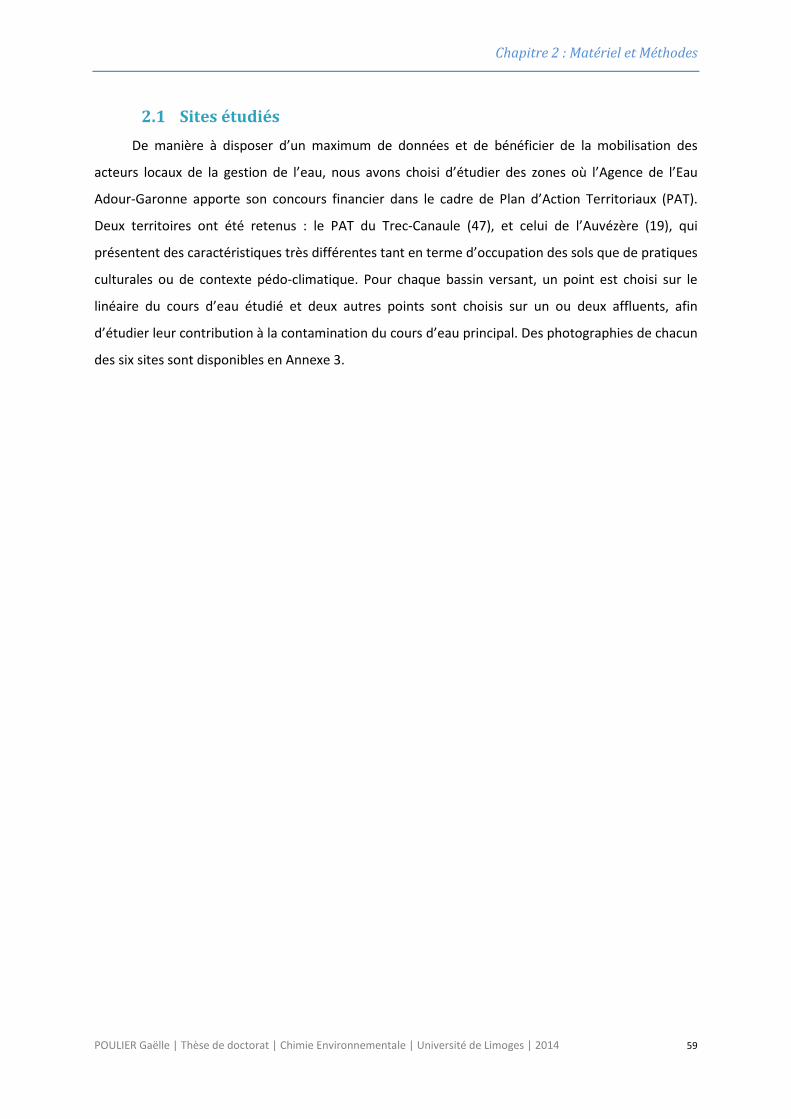
Chapitre 2 : Matériel et Méthodes
2.1 Sites étudiés De manière à disposer d’un maximum de données et de bénéficier de la mobilisation des
acteurs locaux de la gestion de l’eau, nous avons choisi d’étudier des zones où l’Agence de l’Eau
Adour-Garonne apporte son concours financier dans le cadre de Plan d’Action Territoriaux (PAT).
Deux territoires ont été retenus : le PAT du Trec-Canaule (47), et celui de l’Auvézère (19), qui
présentent des caractéristiques très différentes tant en terme d’occupation des sols que de pratiques
culturales ou de contexte pédo-climatique. Pour chaque bassin versant, un point est choisi sur le
linéaire du cours d’eau étudié et deux autres points sont choisis sur un ou deux affluents, afin
d’étudier leur contribution à la contamination du cours d’eau principal. Des photographies de chacun
des six sites sont disponibles en Annexe 3.
POULIER Gaëlle | Thèse de doctorat | Chimie Environnementale | Université de Limoges | 2014 59
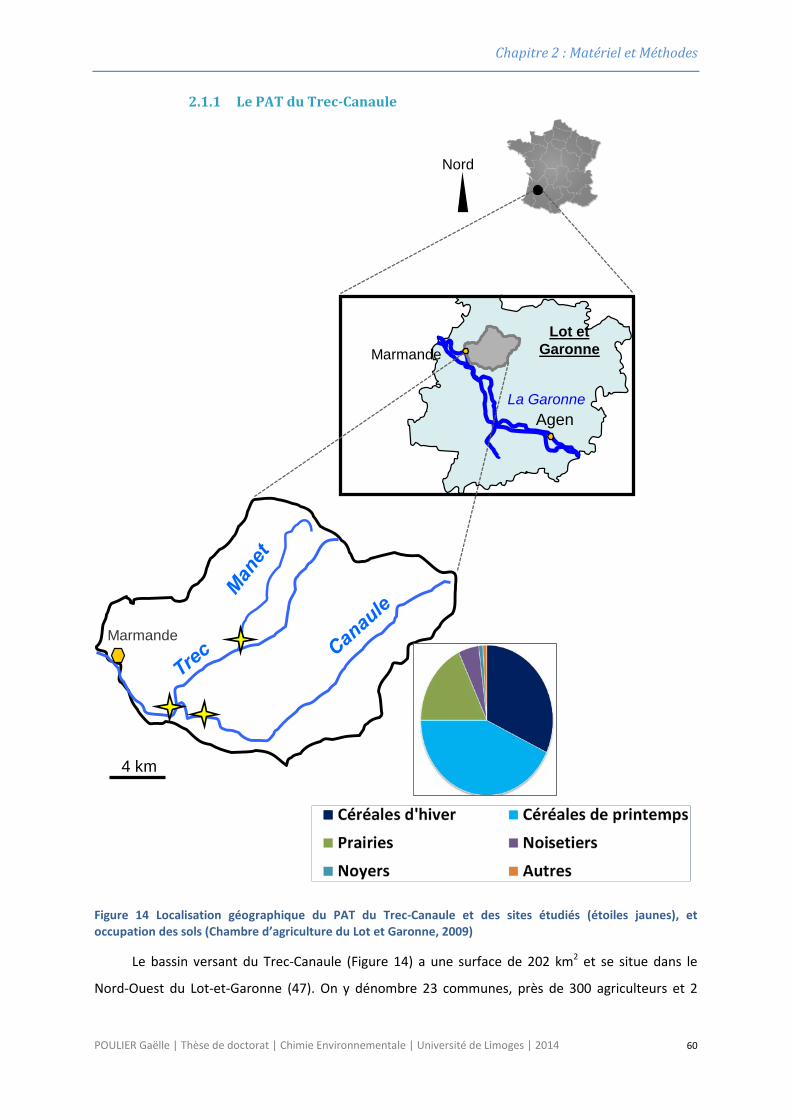
Chapitre 2 : Matériel et Méthodes
2.1.1 Le PAT du Trec-Canaule
Figure 14 Localisation géographique du PAT du Trec-Canaule et des sites étudiés (étoiles jaunes), et occupation des sols (Chambre d’agriculture du Lot et Garonne, 2009)
Le bassin versant du Trec-Canaule (Figure 14) a une surface de 202 km2 et se situe dans le
Nord-Ouest du Lot-et-Garonne (47). On y dénombre 23 communes, près de 300 agriculteurs et 2
Nord
Agen
MarmandeLot et
Garonne
La Garonne
Marmande
4 km
POULIER Gaëlle | Thèse de doctorat | Chimie Environnementale | Université de Limoges | 2014 60
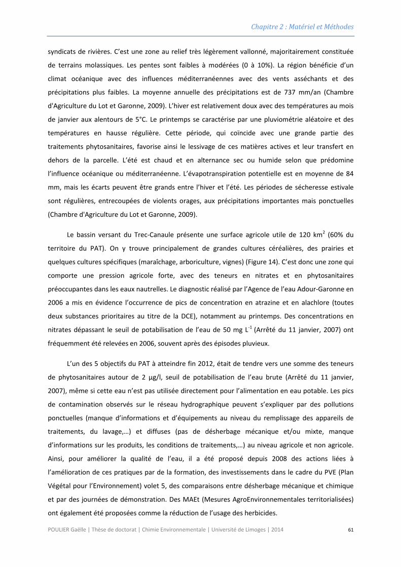
Chapitre 2 : Matériel et Méthodes
syndicats de rivières. C’est une zone au relief très légèrement vallonné, majoritairement constituée
de terrains molassiques. Les pentes sont faibles à modérées (0 à 10%). La région bénéficie d’un
climat océanique avec des influences méditerranéennes avec des vents asséchants et des
précipitations plus faibles. La moyenne annuelle des précipitations est de 737 mm/an (Chambre
d'Agriculture du Lot et Garonne, 2009). L’hiver est relativement doux avec des températures au mois
de janvier aux alentours de 5°C. Le printemps se caractérise par une pluviométrie aléatoire et des
températures en hausse régulière. Cette période, qui coïncide avec une grande partie des
traitements phytosanitaires, favorise ainsi le lessivage de ces matières actives et leur transfert en
dehors de la parcelle. L’été est chaud et en alternance sec ou humide selon que prédomine
l’influence océanique ou méditerranéenne. L’évapotranspiration potentielle est en moyenne de 84
mm, mais les écarts peuvent être grands entre l’hiver et l’été. Les périodes de sécheresse estivale
sont régulières, entrecoupées de violents orages, aux précipitations importantes mais ponctuelles
(Chambre d'Agriculture du Lot et Garonne, 2009).
Le bassin versant du Trec-Canaule présente une surface agricole utile de 120 km2 (60% du
territoire du PAT). On y trouve principalement de grandes cultures céréalières, des prairies et
quelques cultures spécifiques (maraîchage, arboriculture, vignes) (Figure 14). C’est donc une zone qui
comporte une pression agricole forte, avec des teneurs en nitrates et en phytosanitaires
préoccupantes dans les eaux nautrelles. Le diagnostic réalisé par l’Agence de l’eau Adour-Garonne en
2006 a mis en évidence l’occurrence de pics de concentration en atrazine et en alachlore (toutes
deux substances prioritaires au titre de la DCE), notamment au printemps. Des concentrations en
nitrates dépassant le seuil de potabilisation de l’eau de 50 mg L-1 (Arrêté du 11 janvier, 2007) ont
fréquemment été relevées en 2006, souvent après des épisodes pluvieux.
L’un des 5 objectifs du PAT à atteindre fin 2012, était de tendre vers une somme des teneurs
de phytosanitaires autour de 2 µg/l, seuil de potabilisation de l’eau brute (Arrêté du 11 janvier,
2007), même si cette eau n’est pas utilisée directement pour l’alimentation en eau potable. Les pics
de contamination observés sur le réseau hydrographique peuvent s’expliquer par des pollutions
ponctuelles (manque d’informations et d’équipements au niveau du remplissage des appareils de
traitements, du lavage,…) et diffuses (pas de désherbage mécanique et/ou mixte, manque
d’informations sur les produits, les conditions de traitements,…) au niveau agricole et non agricole.
Ainsi, pour améliorer la qualité de l’eau, il a été proposé depuis 2008 des actions liées à
l’amélioration de ces pratiques par de la formation, des investissements dans le cadre du PVE (Plan
Végétal pour l’Environnement) volet 5, des comparaisons entre désherbage mécanique et chimique
et par des journées de démonstration. Des MAEt (Mesures AgroEnvironnementales territorialisées)
ont également été proposées comme la réduction de l’usage des herbicides.
POULIER Gaëlle | Thèse de doctorat | Chimie Environnementale | Université de Limoges | 2014 61

Chapitre 2 : Matériel et Méthodes
Sur le PAT du Trec, les affluents étudiés sont la Canaule et le Manet (Figure 14). Les points de
prélèvements sont placés juste avant la confluence avec le Trec, afin d’évaluer la contribution de ces
deux cours d’eau à la contamination en pesticides. Ces deux stations sont également suivies dans le
réseau de mesures de l’Agence de l’Eau Adour-Garonne.
POULIER Gaëlle | Thèse de doctorat | Chimie Environnementale | Université de Limoges | 2014 62
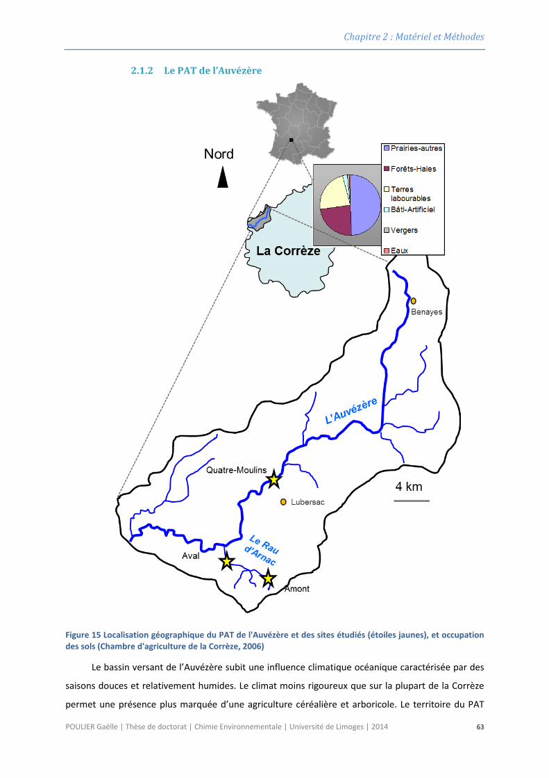
Chapitre 2 : Matériel et Méthodes
2.1.2 Le PAT de l’Auvézère
Figure 15 Localisation géographique du PAT de l'Auvézère et des sites étudiés (étoiles jaunes), et occupation des sols (Chambre d'agriculture de la Corrèze, 2006)
Le bassin versant de l’Auvézère subit une influence climatique océanique caractérisée par des
saisons douces et relativement humides. Le climat moins rigoureux que sur la plupart de la Corrèze
permet une présence plus marquée d’une agriculture céréalière et arboricole. Le territoire du PAT
POULIER Gaëlle | Thèse de doctorat | Chimie Environnementale | Université de Limoges | 2014 63
Chapitre 2 : Matériel et Méthodes
Auvezère, situé sur le bassin versant Limousin de cette rivière (Figure 15), a une surface de 180 km2
environ et est essentiellement rural. En plus des 40 premiers kilomètres de l’Auvezère, le périmètre
du PAT englobe de nombreux affluents, représentant 138 km de réseaux permanents et 187 km de
non permanents, définissant ainsi de nombreux petits sous-bassins versants. On y retrouve de
l’élevage bovin extensif (50 % du territoire du PAT en prairie), des grandes cultures, essentiellement
pour l’alimentation du bétail (23% du territoire du PAT en terre labourable) et de la pomiculture (1 %
du territoire du PAT en vergers pour la production de pommes Golden).
D’après les documents du PAT (Chambre d'Agriculture de la Corrèze, 2006) : « Les pratiques
phytosanitaires de la zone restent à améliorer, tant pour la protection de l’environnement
(manipulations à risques, matériel non adapté ou obsolète) que pour la protection de l’applicateur et
des tiers ». Les utilisateurs de produits phytosanitaires sont multiples sur le territoire du PAT :
agriculteurs, particuliers, SNCF (une ligne ferroviaire traverse le bassin versant), collectivités, haras
nationaux de Pompadour, service départemental de la voirie. Globalement, les concentrations en
pesticides retrouvées sont faibles mais de fortes valeurs peuvent être relevées ponctuellement pour
certaines substances (2,4-MCPA 1,9 µg/L ; glyphosate 3,4 µg/L en 2007).
En conclusion, sur le territoire du PAT Auvézère, l’emploi des produits phytosanitaires est
multi-utilisateurs et un bruit de fond est présent dans les eaux avec parfois des valeurs qui posent
problème dans le cadre de l’alimentation en eau potable ou pour le milieu naturel.
La station des Quatre-Moulins (Figure 15) est un point de captage pour l’alimentation en eau
potable des villes environnantes. La contamination en pesticides se devrait donc d’y être la plus
faible possible. Le choix du Rau d’Arnac est motivé par la taille relativement petite (10,5 km2) du
bassin versant drainé par ce cours d’eau, ce qui devrait faciliter l’étude des transferts de pesticides,
de la parcelle vers le ruisseau.
2.2 Sélection des molécules étudiées La famille des pesticides inclut plusieurs centaines de molécules. En France, plus de 300
substances actives sont aujourd’hui utilisées et peuvent potentiellement être retrouvées dans les
eaux de surface. A ces centaines de molécules s’ajoutent celles qui ont été utilisées par le passé et
qui sont depuis interdites (mais qui sont encore présentes dans les sols et les eaux), ainsi que leurs
produits de dégradation.
Les PAT du Trec-Canaule et de l’Auvézère sont suivis depuis au moins trois ans par l’Agence de
l’eau Adour-Garonne ainsi que les Chambre d’Agriculture du Lot-et-Garonne et de la Corrèze. L’étude
des chroniques de suivis des années précédentes nous a permis de sélectionner, dans un premier
POULIER Gaëlle | Thèse de doctorat | Chimie Environnementale | Université de Limoges | 2014 64
Chapitre 2 : Matériel et Méthodes
temps, les molécules les plus fréquemment retrouvées sur chacun des bassins versants, en lien avec
les pratiques culturales des agriculteurs. Sur le PAT du Trec, les herbicides associés à la culture du
maïs et des céréales, étaient essentiellement des chloroacétanilides : parmi les plus détectées, on
peut citer le métolachlore, l’acétochlore et le diméthénamide. Sur le PAT de l’Auvézère, les
molécules détectées appartenaient à des familles très diverses, conséquence directe de la
multiplicité des utilisateurs : herbicides de cultures d’hiver (chlortoluron, métazachlore), insecticides
associés aux vergers (pyrimicarbe, carbofuran) et fongicides (tébuconazole). Dans un second temps,
la liste a été adaptée aux caractéristiques des trois échantillonneurs passifs choisis. Le POCIS, le
Chemcatcher et le DGT échantillonnent respectivement les molécules polaires neutres (log Kow < 4),
les composés modérément hydrophobes (2 < log Kow < 6), et les métaux et métalloïdes (Figure 7).
Bien qu’elles soient parfois détectées à des concentrations élevées sur certains sites, les molécules
très polaires et ionisées (comme le glyphosate, son métabolite l’AMPA ou le dicamba ; log Kow < 0)
ont dû être exclues car aucun des trois échantillonneurs étudiés n’est adapté à ce type de composé.
Certaines molécules choisies étaient déjà intégrées dans les méthodes d’analyses du laboratoire de
Chimie de l’Irstea de Bordeaux, tandis que d’autres ont fait l’objet de développements analytiques
que nous décrirons ultérieurement. C’est le cas de la plupart des molécules hydrophobes analysées
en GC (Chromatographie Gazeuse), et de quelques herbicides ajoutés à la méthode HPLC
(Chromatographie Liquide Haute Performance). La liste définitive est disponible dans le Tableau 1.
Concernant les métaux et métalloïdes, le DGT étant capable d’échantillonner quasiment tous
les éléments (à condition d’adapter la phase réceptrice), le choix s’est porté sur quelques éléments
d’intérêt : Le Cu et l’As pour être ou avoir été utilisés comme produit phytosanitaire ; le Cd comme
micropolluant faisant l’objet de suivi sur la qualité des eaux dans la DCE ; et le Ni comme élément
pouvant se retrouver dans le bruit de fond géologique. Le choix du cuivre est bien sûr également
motivé par son utilisation fréquente dans certaines préparations à action fongicide (bouillie
bordelaise), essentiellement sur vignes et dans les vergers. Avec l’ICP-MS (Inductively Coupled
Plasma-Mass Spectrometry) le cuivre, le cadmium et le nickel, pourront être quantifiés à très faibles
concentrations.
POULIER Gaëlle | Thèse de doctorat | Chimie Environnementale | Université de Limoges | 2014 65
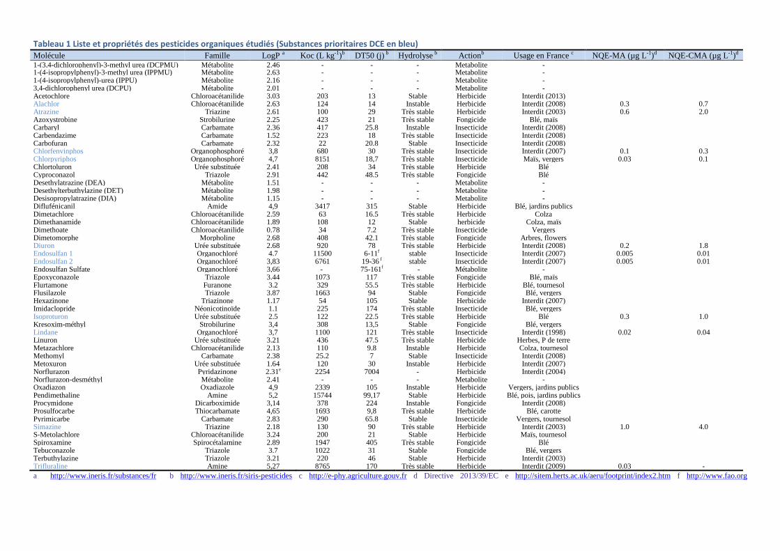
Tableau 1 Liste et propriétés des pesticides organiques étudiés (Substances prioritaires DCE en bleu) Molécule Famille LogP a Koc (L kg-1)b DT50 (j) b Hydrolyse b Actionb Usage en France c NQE-MA (µg L-1)d NQE-CMA (µg L-1)d 1-(3,4-dichlorophenyl)-3-methyl urea (DCPMU) Métabolite 2.46 - - - Metabolite - 1-(4-isopropylphenyl)-3-methyl urea (IPPMU) Métabolite 2.63 - - - Metabolite - 1-(4-isopropylphenyl)-urea (IPPU) Métabolite 2.16 - - - Metabolite - 3,4-dichlorophenyl urea (DCPU) Métabolite 2.01 - - - Metabolite - Acetochlore Chloroacétanilide 3.03 203 13 Stable Herbicide Interdit (2013) Alachlor Chloroacétanilide 2.63 124 14 Instable Herbicide Interdit (2008) 0.3 0.7 Atrazine Triazine 2.61 100 29 Très stable Herbicide Interdit (2003) 0.6 2.0 Azoxystrobine Strobilurine 2.25 423 21 Très stable Fongicide Blé, maïs Carbaryl Carbamate 2.36 417 25.8 Instable Insecticide Interdit (2008) Carbendazime Carbamate 1.52 223 18 Très stable Insecticide Interdit (2008) Carbofuran Carbamate 2.32 22 20.8 Stable Insecticide Interdit (2008) Chlorfenvinphos Organophosphoré 3,8 680 30 Très stable Insecticide Interdit (2007) 0.1 0.3 Chlorpyriphos Organophosphoré 4,7 8151 18,7 Très stable Insecticide Maïs, vergers 0.03 0.1 Chlortoluron Urée substituée 2.41 208 34 Très stable Herbicide Blé Cyproconazol Triazole 2.91 442 48.5 Très stable Fongicide Blé Desethylatrazine (DEA) Métabolite 1.51 - - - Metabolite - Desethylterbuthylazine (DET) Métabolite 1.98 - - - Metabolite - Desisopropylatrazine (DIA) Métabolite 1.15 - - - Metabolite - Diflufénicanil Amide 4,9 3417 315 Stable Herbicide Blé, jardins publics Dimetachlore Chloroacétanilide 2.59 63 16.5 Très stable Herbicide Colza Dimethanamide Chloroacétanilide 1.89 108 12 Stable herbicide Colza, maïs Dimethoate Chloroacétanilide 0.78 34 7.2 Très stable Insecticide Vergers Dimetomorphe Morpholine 2.68 408 42.1 Très stable Fongicide Arbres, flowers Diuron Urée substituée 2.68 920 78 Très stable Herbicide Interdit (2008) 0.2 1.8 Endosulfan 1 Organochloré 4.7 11500 6-11f stable Insecticide Interdit (2007) 0.005 0.01 Endosulfan 2 Organochloré 3,83 6761 19-36 f stable Insecticide Interdit (2007) 0.005 0.01 Endosulfan Sulfate Organochloré 3,66 - 75-161f - Métabolite - Epoxyconazole Triazole 3.44 1073 117 Très stable Fongicide Blé, maïs Flurtamone Furanone 3.2 329 55.5 Très stable Herbicide Blé, tournesol Flusilazole Triazole 3.87 1663 94 Stable Fongicide Blé, vergers Hexazinone Triazinone 1.17 54 105 Stable Herbicide Interdit (2007) Imidaclopride Néonicotinoïde 1.1 225 174 Très stable Insecticide Blé, vergers Isoproturon Urée substituée 2.5 122 22.5 Très stable Herbicide Blé 0.3 1.0 Kresoxim-méthyl Strobilurine 3,4 308 13,5 Stable Fongicide Blé, vergers Lindane Organochloré 3,7 1100 121 Très stable Insecticide Interdit (1998) 0.02 0.04 Linuron Urée substituée 3.21 436 47.5 Très stable Herbicide Herbes, P de terre Metazachlore Chloroacétanilide 2.13 110 9.8 Instable Herbicide Colza, tournesol Methomyl Carbamate 2.38 25.2 7 Stable Insecticide Interdit (2008) Metoxuron Urée substituée 1.64 120 30 Instable Herbicide Interdit (2007) Norflurazon Pyridazinone 2.31e 2254 7004 - Herbicide Interdit (2004) Norflurazon-desméthyl Métabolite 2.41 - - - Metabolite - Oxadiazon Oxadiazole 4,9 2339 105 Instable Herbicide Vergers, jardins publics Pendimethaline Amine 5,2 15744 99,17 Stable Herbicide Blé, pois, jardins publics Procymidone Dicarboximide 3,14 378 224 Instable Fongicide Interdit (2008) Prosulfocarbe Thiocarbamate 4,65 1693 9,8 Très stable Herbicide Blé, carotte Pyrimicarbe Carbamate 2.83 290 65.8 Stable Insecticide Vergers, tournesol Simazine Triazine 2.18 130 90 Très stable Herbicide Interdit (2003) 1.0 4.0 S-Metolachlore Chloroacétanilide 3.24 200 21 Stable Herbicide Maïs, tournesol Spiroxamine Spirocétalamine 2.89 1947 405 Très stable Fongicide Blé Tebuconazole Triazole 3.7 1022 31 Stable Fongicide Blé, vergers Terbuthylazine Triazole 3.21 220 46 Stable Herbicide Interdit (2003) Trifluraline Amine 5,27 8765 170 Très stable Herbicide Interdit (2009) 0.03 - a http://www.ineris.fr/substances/fr b http://www.ineris.fr/siris-pesticides c http://e-phy.agriculture.gouv.fr d Directive 2013/39/EC e http://sitem.herts.ac.uk/aeru/footprint/index2.htm f http://www.fao.org
Chapitre 2 : Matériel et Méthodes
2.3 Préparation des échantillonneurs passifs
2.3.1 POCIS
Les POCIS utilisés dans cette étude sont de type « pharmaceutique », c’est-à-dire comprenant
une phase réceptrice Oasis HLB (taille des particules de 30 µm, surface spécifique 810 m2 g-1, Waters
France). Cette phase est préalablement dopée en DIA d5 (Dr Ehrenstorfer GmbH, Augsburg,
Allemagne), utilisée comme PRC (Mazzella et al., 2010; Lissalde et al., 2011).
a) Dopage de l’adsorbant
La phase Oasis HLB est rincée avec 20 ml de méthanol (grade HPLC, Atlantic Labo Bruges,
France) puis séchée sous flux d’azote pendant 30 min. Après quoi, la phase sèche est extraite de la
cartouche et 5 g sont transférés dans un ballon et dopés en PRC par ajout de 35 ml de méthanol
contenant 200 µl de DIA-d5 à 100 ppm. Le mélange est placé 15 min aux ultrasons (Modèle B3210E-
DTH, 47 kHz, 335 watt, Branson, Connecticut, USA) afin d’assurer un dopage homogène, puis le
méthanol est évaporé lentement au rotavapor (Hei-VAP value 560-01100-00, Heidolph Instruments,
Schwabach, Allemagne) à 50°C. Enfin, la phase est séchée à l’étuve pendant 2 à 3h à 70°C et stockée
au réfrigérateur. Afin de déterminer la quantité exacte de PRC ajoutée, des cartouches de référence
sont préparées, éluées et analysées pour chaque lot de fabrication.
b) Montage des POCIS
Les POCIS sont préparés au laboratoire quelques jours avant l’exposition, avec 200 mg de
phase Oasis HLB dopée en DIA-d5, emprisonnée entre deux membranes en polyéthersulfone (0,1
µm, PALL Holtzheim, France). Le tout est maintenu au moyen de deux anneaux plats en inox et de 3
boulons en inox (Figure 10). Ces dispositifs sont ensuite stockés au réfrigérateur et transportés sur le
terrain dans des glacières à 4°C.
c) Démontage des POCIS et récupération de la phase Oasis HLB
Après exposition la phase Oasis HLB est récupérée dans un bécher avec 10 ml d’eau ultrapure
(18,2 MΩ, Système Synergy UV Millipore, Billerica, USA) puis transféré dans une cartouche SPE vide
préalablement pesée. Le bécher est rincé avec 5 ml d’eau ultrapure, également transférés sur la
cartouche SPE. L’ensemble de ces étapes est réalisé sous vide partiel (environ 53,33 kPa) à l’aide d’un
visiprep (Supelco, France). La cartouche est séchée sous flux d’azote pendant environ 30 min, puis de
nouveau pesée afin de s’assurer de la quantité de phase récupérée. Enfin, la cartouche est stockée
au congélateur jusqu’à l’élution.
POULIER Gaëlle | Thèse de doctorat | Chimie Environnementale | Université de Limoges | 2014 67
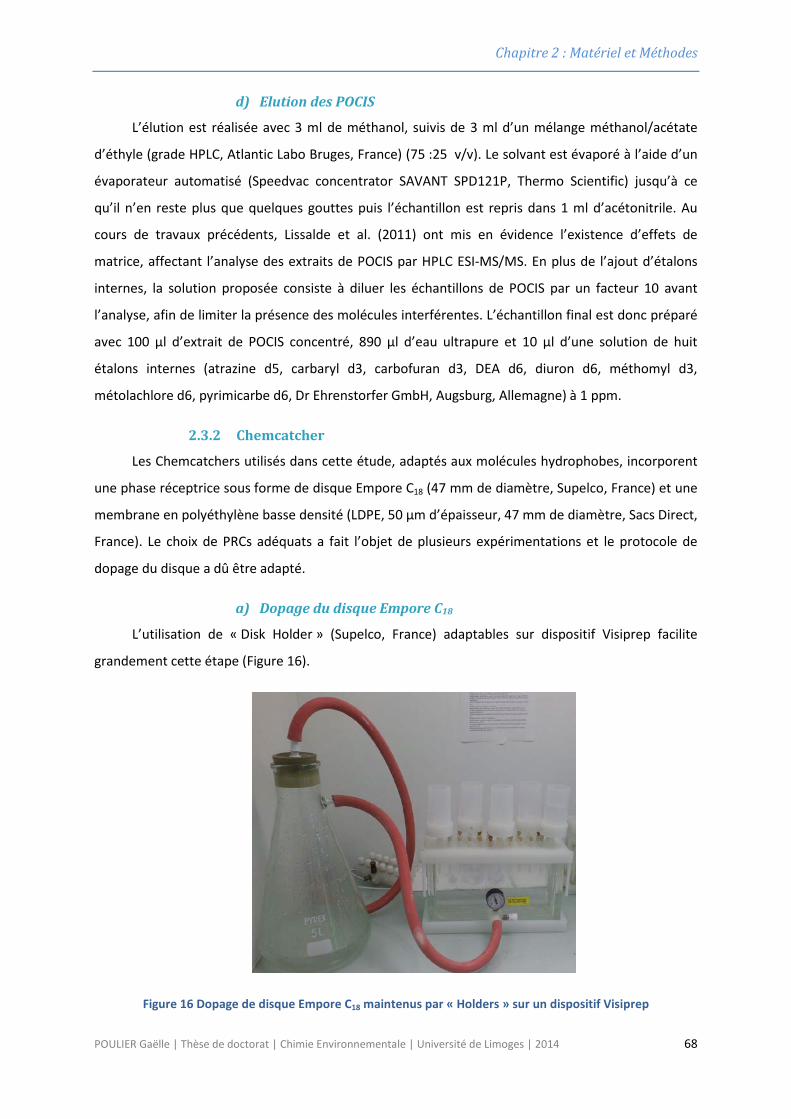
Chapitre 2 : Matériel et Méthodes
d) Elution des POCIS
L’élution est réalisée avec 3 ml de méthanol, suivis de 3 ml d’un mélange méthanol/acétate
d’éthyle (grade HPLC, Atlantic Labo Bruges, France) (75 :25 v/v). Le solvant est évaporé à l’aide d’un
évaporateur automatisé (Speedvac concentrator SAVANT SPD121P, Thermo Scientific) jusqu’à ce
qu’il n’en reste plus que quelques gouttes puis l’échantillon est repris dans 1 ml d’acétonitrile. Au
cours de travaux précédents, Lissalde et al. (2011) ont mis en évidence l’existence d’effets de
matrice, affectant l’analyse des extraits de POCIS par HPLC ESI-MS/MS. En plus de l’ajout d’étalons
internes, la solution proposée consiste à diluer les échantillons de POCIS par un facteur 10 avant
l’analyse, afin de limiter la présence des molécules interférentes. L’échantillon final est donc préparé
avec 100 µl d’extrait de POCIS concentré, 890 µl d’eau ultrapure et 10 µl d’une solution de huit
étalons internes (atrazine d5, carbaryl d3, carbofuran d3, DEA d6, diuron d6, méthomyl d3,
métolachlore d6, pyrimicarbe d6, Dr Ehrenstorfer GmbH, Augsburg, Allemagne) à 1 ppm.
2.3.2 Chemcatcher
Les Chemcatchers utilisés dans cette étude, adaptés aux molécules hydrophobes, incorporent
une phase réceptrice sous forme de disque Empore C18 (47 mm de diamètre, Supelco, France) et une
membrane en polyéthylène basse densité (LDPE, 50 µm d’épaisseur, 47 mm de diamètre, Sacs Direct,
France). Le choix de PRCs adéquats a fait l’objet de plusieurs expérimentations et le protocole de
dopage du disque a dû être adapté.
a) Dopage du disque Empore C18
L’utilisation de « Disk Holder » (Supelco, France) adaptables sur dispositif Visiprep facilite
grandement cette étape (Figure 16).
Figure 16 Dopage de disque Empore C18 maintenus par « Holders » sur un dispositif Visiprep
POULIER Gaëlle | Thèse de doctorat | Chimie Environnementale | Université de Limoges | 2014 68
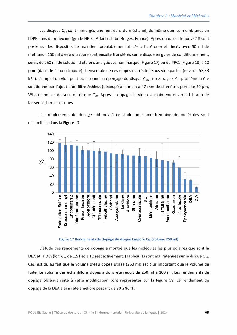
Chapitre 2 : Matériel et Méthodes
Les disques C18 sont immergés une nuit dans du méthanol, de même que les membranes en
LDPE dans du n-hexane (grade HPLC, Atlantic Labo Bruges, France). Après quoi, les disques C18 sont
posés sur les dispositifs de maintien (préalablement rincés à l’acétone) et rincés avec 50 ml de
méthanol. 150 ml d’eau ultrapure sont ensuite transférés sur le disque en guise de conditionnement,
suivis de 250 ml de solution d’étalons analytiques non marqué (Figure 17) ou de PRCs (Figure 18) à 10
ppm (dans de l’eau ultrapure). L’ensemble de ces étapes est réalisé sous vide partiel (environ 53,33
kPa). L’emploi du vide peut occasionner un perçage du disque C18, assez fragile. Ce problème a été
solutionné par l’ajout d’un filtre Ashless (découpé à la main à 47 mm de diamètre, porosité 20 µm,
Whatmann) en-dessous du disque C18. Après le dopage, le vide est maintenu environ 1 h afin de
laisser sécher les disques.
Les rendements de dopage obtenus à ce stade pour une trentaine de molécules sont
disponibles dans la Figure 17.
Figure 17 Rendements de dopage du disque Empore C18 (volume 250 ml)
L’étude des rendements de dopage a montré que les molécules les plus polaires que sont la
DEA et la DIA (log Kow de 1,51 et 1,12 respectivement, (Tableau 1) sont mal retenues sur le disque C18.
Ceci est dû au fait que le volume d’eau dopée utilisé (250 ml) est plus important que le volume de
fuite. Le volume des échantillons dopés a donc été réduit de 250 ml à 100 ml. Les rendements de
dopage obtenus suite à cette modification sont représentés sur la Figure 18. Le rendement de
dopage de la DEA a ainsi été amélioré passant de 30 à 86 %.
POULIER Gaëlle | Thèse de doctorat | Chimie Environnementale | Université de Limoges | 2014 69
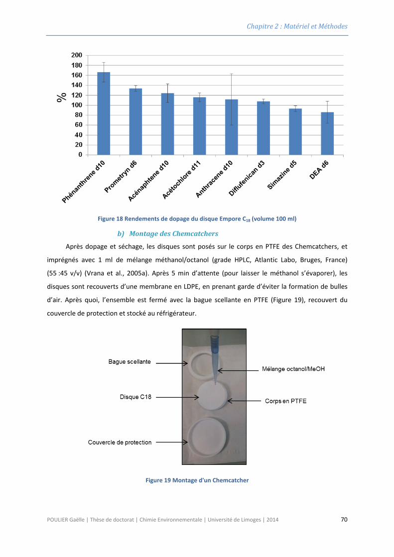
Chapitre 2 : Matériel et Méthodes
Figure 18 Rendements de dopage du disque Empore C18 (volume 100 ml)
b) Montage des Chemcatchers
Après dopage et séchage, les disques sont posés sur le corps en PTFE des Chemcatchers, et
imprégnés avec 1 ml de mélange méthanol/octanol (grade HPLC, Atlantic Labo, Bruges, France)
(55 :45 v/v) (Vrana et al., 2005a). Après 5 min d’attente (pour laisser le méthanol s’évaporer), les
disques sont recouverts d’une membrane en LDPE, en prenant garde d’éviter la formation de bulles
d’air. Après quoi, l’ensemble est fermé avec la bague scellante en PTFE (Figure 19), recouvert du
couvercle de protection et stocké au réfrigérateur.
Figure 19 Montage d'un Chemcatcher
POULIER Gaëlle | Thèse de doctorat | Chimie Environnementale | Université de Limoges | 2014 70
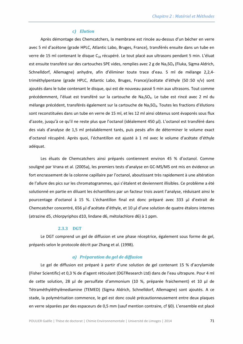
Chapitre 2 : Matériel et Méthodes
c) Elution
Après démontage des Chemcatchers, la membrane est rincée au-dessus d’un bécher en verre
avec 5 ml d’acétone (grade HPLC, Atlantic Labo, Bruges, France), transférés ensuite dans un tube en
verre de 15 ml contenant le disque C18 récupéré. Le tout placé aux ultrasons pendant 5 min. L’éluat
est ensuite transféré sur des cartouches SPE vides, remplies avec 2 g de Na2SO4 (Fluka, Sigma Aldrich,
Schnelldorf, Allemagne) anhydre, afin d’éliminer toute trace d’eau. 5 ml de mélange 2,2,4-
triméthylpentane (grade HPLC, Atlantic Labo, Bruges, France)/acétate d’éthyle (50 :50 v/v) sont
ajoutés dans le tube contenant le disque, qui est de nouveau passé 5 min aux ultrasons. Tout comme
précédemment, l’éluat est transféré sur la cartouche de Na2SO4. Le tube est rincé avec 2 ml du
mélange précédent, transférés également sur la cartouche de Na2SO4. Toutes les fractions d’élutions
sont reconstituées dans un tube en verre de 15 ml, et les 12 ml ainsi obtenus sont évaporés sous flux
d’azote, jusqu’à ce qu’il ne reste plus que l’octanol (idéalement 450 µl). L’octanol est transféré dans
des vials d’analyse de 1,5 ml préalablement tarés, puis pesés afin de déterminer le volume exact
d’octanol récupéré. Après quoi, l’échantillon est ajusté à 1 ml avec le volume d’acétate d’éthyle
adéquat.
Les éluats de Chemcatchers ainsi préparés contiennent environ 45 % d’octanol. Comme
souligné par Vrana et al. (2005a), les premiers tests d’analyse en GC-MS/MS ont mis en évidence un
fort encrassement de la colonne capillaire par l’octanol, aboutissant très rapidement à une altération
de l’allure des pics sur les chromatogrammes, qui s’étalent et deviennent illisibles. Ce problème a été
solutionné en partie en diluant les échantillons par un facteur trois avant l’analyse, réduisant ainsi le
pourcentage d’octanol à 15 %. L’échantillon final est donc préparé avec 333 µl d’extrait de
Chemcatcher concentré, 656 µl d’acétate d’éthyle, et 10 µl d’une solution de quatre étalons internes
(atrazine d5, chlorpyriphos d10, lindane d6, métolachlore d6) à 1 ppm.
2.3.3 DGT
Le DGT comprend un gel de diffusion et une phase réceptrice, également sous forme de gel,
préparés selon le protocole décrit par Zhang et al. (1998).
a) Préparation du gel de diffusion
Le gel de diffusion est préparé à partir d’une solution de gel contenant 15 % d’acrylamide
(Fisher Scientific) et 0,3 % de d’agent réticulant (DGTResearch Ltd) dans de l’eau ultrapure. Pour 4 ml
de cette solution, 28 µl de persulfate d’ammonium (10 %, préparée fraichement) et 10 µl de
Tétraméthyléthylènediamine (TEMED) (Sigma Aldrich, Schnelldorf, Allemagne) sont ajoutés. A ce
stade, la polymérisation commence, le gel est donc coulé précautionneusement entre deux plaques
en verre séparées par des espaceurs de 0,5 mm (sauf mention contraire, cf §0). L’ensemble est placé
POULIER Gaëlle | Thèse de doctorat | Chimie Environnementale | Université de Limoges | 2014 71
Chapitre 2 : Matériel et Méthodes
à l’étuve environ 45 min à 45°C, puis le gel est démoulé et réhydraté dans 500 ml d’eau ultrapure
(renouvelée quatre fois minimum) pendant 24 h. L’épaisseur du gel ainsi réhydraté est de 0,77 (±
0,02) mm. Le gel est stocké au réfrigérateur dans une solution de NaNO3 (0,01 M) jusqu’à utilisation.
b) Préparation des phases réceptrices Chelex et ferrihydrite
Les phases réceptrices Chelex, adaptées à l’échantillonnage des cations métalliques, sont
préparées à partir de 2 ml de solution de gel (voir ci-dessus) auxquels sont ajoutés 0,400 g de résine
Chelex-100 (forme sodique, 200-400 mesh, Bio-rad), 12 µl de persulfate d’ammonium (10 %) et 3,2 µl
de TEMED (Zhang et al., 1998). La solution est ensuite coulée entre deux plaques en verre séparées
par des espaceurs de 0,25 mm, puis mise à l’étuve 45 min à 45 °C (en position horizontale pour que
les particules de Chelex se déposent sur l’une des faces du gel). Après démoulage, la phase est
réhydratée dans 500 ml d’eau ultrapure (renouvelée quatre fois) pendant 24 h, puis découpée en
disques de surface 4,9 cm2, et stockée au réfrigérateur dans de l’eau ultrapure. L’épaisseur des
phases réhydratées est de 0,40 (± 0,03) mm.
Les phases réceptrices ferrihydrite, adaptées à l’échantillonnage des anions, sont préparées
selon le protocole décrit par Luo et al. (2010). Un gel de diffusion d’épaisseur 0,40 mm est immergé
dans une solution de 4,04 g de Fe(NO3)3, 9H2O dissous dans environ 40 ml d'eau ultrapure, puis le
volume est complété à 100 ml. Les gels sont immergés pendant au moins 2 h afin de permettre une
distribution uniforme des ions Fe3+. Une fois l’équilibre atteint, chaque gel est rincé avec de l'eau
ultrapure pendant quelques secondes, puis immergé dans 100 ml de solution tampon de MES (acide
2-(N-morpholino)ethanesulfonic (Sigma Aldrich, Schnelldorf, Allemagne) à 0,05 M ajustée à pH = 6,7
avec 4 ml de solution de NaOH (1M, Sigma Aldrich, Schnelldorf, Allemagne). La précipitation de la
ferrihydrite est visible après 1 min d'immersion. La solution tampon contenant les gels est agitée
pendant environ 40 min afin de permettre le développement complet de la ferrihydrite. Les gels sont
ensuite rincés plusieurs fois pour éliminer l'excès de réactifs (500 ml d’eau ultrapure renouvelée
quatre fois pendant 24 h, puis découpés (surface 4,9 cm2) et stockés au réfrigérateur (dans de l’eau
ultrapure).
c) Montage des DGT
Quelques jours avant exposition, les DGTs sont montés avec une phase réceptrice (Chelex ou
ferrihydrite), surmontée d’un gel de diffusion, puis d’un filtre en acétate de cellulose (0,12 mm
d’épaisseur, porosité 0,45 µm, Sartorius, France) (Figure 12). Les systèmes sont stockés avant
utilisation à 4°C dans un sachet hermétique en polyéthylène contenant quelques gouttes d’eau
ultrapure.
POULIER Gaëlle | Thèse de doctorat | Chimie Environnementale | Université de Limoges | 2014 72
Chapitre 2 : Matériel et Méthodes
d) Elution
L’élution est réalisée dès le retour de terrain ou le lendemain. Après démontage des DGTs, Les
résines sont récupérées et placées dans des tubes en plastique contenant 2 ml d’acide nitrique
suprapur (HNO3, 1 M) pendant au moins 24 h. Le coefficient d’élution des cations dans la résine
Chelex est de 92 % pour le cadmium, 85 % pour le cuivre et 89 % pour le nickel. Pour la résine
ferrihydrite, le coefficient d’élution est de 100 % pour l’arsenic.
2.4 Etalonnage des échantillonneurs passifs
2.4.1 Détermination des constances cinétiques d’accumulation et de
désorption : POCIS et Chemcatcher
Le calcul de la concentration moyenne dans l’eau, à partir de la masse d’analyte mesurée dans
les échantillonneurs de type POCIS et Chemcatcher (équation 6), nécessite de connaître les
constantes cinétiques d’accumulation de chacune des molécules cibles, pour chaque dispositif. En
cas d’utilisation de PRC, les constantes cinétiques de désorption des molécules choisies doivent
également être connues.
Dans un premier temps, cette étape a été réalisée au laboratoire, à l’aide d’un dispositif en
microcosme précédemment décrit par Fauvelle et al. (2012). L’aquarium a une contenance d’environ
80 L. Une pompe immergée associée à une rampe de diffusion maintient un courant constant en face
de chaque échantillonneur, tandis qu’une pompe péristaltique et un pousse-seringue alimentent le
dispositif en continu en eau de ville et en solution de pesticides concentrée (Figure 20). La pompe
péristaltique évacue également le surplus d’eau (surverse). Le taux de renouvellement de l’eau est
fixé à 25 % par jour. Les échantillonneurs passifs sont récupérés en triplicats, à intervalles de temps
réguliers.
Ce dispositif a été utilisé pour la calibration en laboratoire des POCIS, puis des Chemcatchers,
en ajustant certains paramètres tels que la concentration dans l’eau, la vitesse du courant, la
température, et le temps d’exposition.
POULIER Gaëlle | Thèse de doctorat | Chimie Environnementale | Université de Limoges | 2014 73
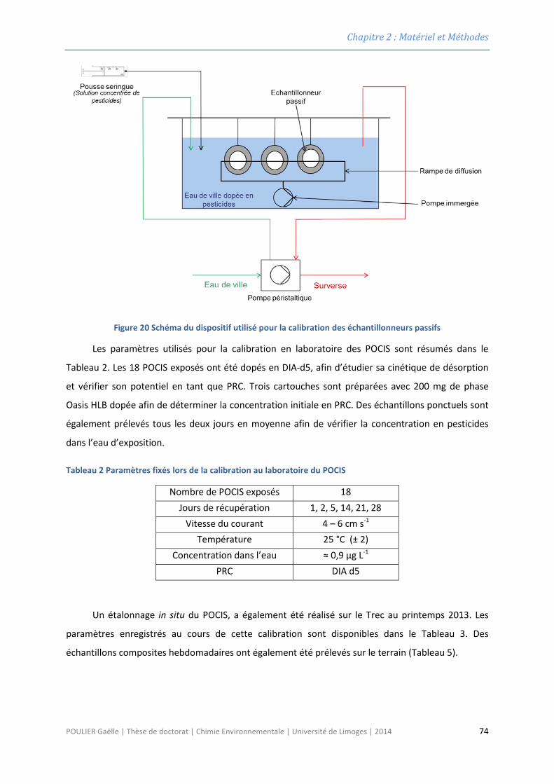
Chapitre 2 : Matériel et Méthodes
Figure 20 Schéma du dispositif utilisé pour la calibration des échantillonneurs passifs
Les paramètres utilisés pour la calibration en laboratoire des POCIS sont résumés dans le
Tableau 2. Les 18 POCIS exposés ont été dopés en DIA-d5, afin d’étudier sa cinétique de désorption
et vérifier son potentiel en tant que PRC. Trois cartouches sont préparées avec 200 mg de phase
Oasis HLB dopée afin de déterminer la concentration initiale en PRC. Des échantillons ponctuels sont
également prélevés tous les deux jours en moyenne afin de vérifier la concentration en pesticides
dans l’eau d’exposition.
Tableau 2 Paramètres fixés lors de la calibration au laboratoire du POCIS
Nombre de POCIS exposés 18 Jours de récupération 1, 2, 5, 14, 21, 28
Vitesse du courant 4 – 6 cm s-1 Température 25 °C (± 2)
Concentration dans l’eau ≈ 0,9 µg L-1 PRC DIA d5
Un étalonnage in situ du POCIS, a également été réalisé sur le Trec au printemps 2013. Les
paramètres enregistrés au cours de cette calibration sont disponibles dans le Tableau 3. Des
échantillons composites hebdomadaires ont également été prélevés sur le terrain (Tableau 5).
POULIER Gaëlle | Thèse de doctorat | Chimie Environnementale | Université de Limoges | 2014 74
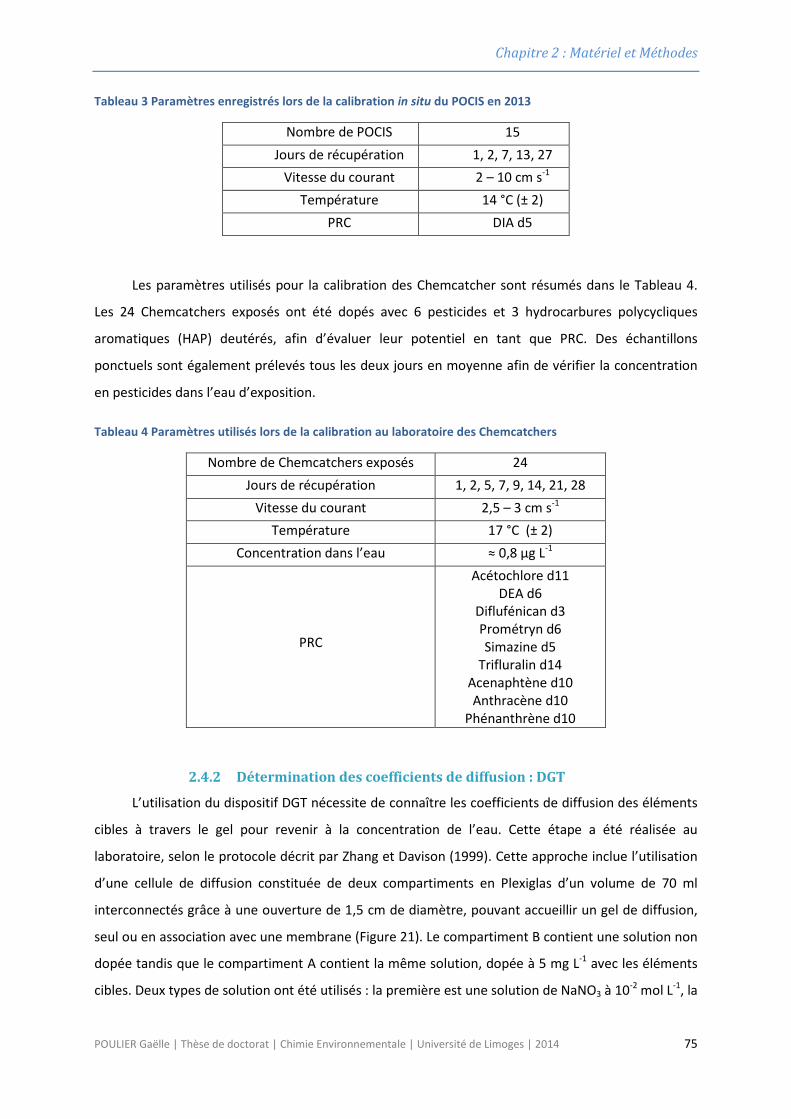
Chapitre 2 : Matériel et Méthodes
Tableau 3 Paramètres enregistrés lors de la calibration in situ du POCIS en 2013
Nombre de POCIS
15 Jours de récupération 1, 2, 7, 13, 27
Vitesse du courant 2 – 10 cm s-1 Température 14 °C (± 2)
PRC DIA d5
Les paramètres utilisés pour la calibration des Chemcatcher sont résumés dans le Tableau 4.
Les 24 Chemcatchers exposés ont été dopés avec 6 pesticides et 3 hydrocarbures polycycliques
aromatiques (HAP) deutérés, afin d’évaluer leur potentiel en tant que PRC. Des échantillons
ponctuels sont également prélevés tous les deux jours en moyenne afin de vérifier la concentration
en pesticides dans l’eau d’exposition.
Tableau 4 Paramètres utilisés lors de la calibration au laboratoire des Chemcatchers
Nombre de Chemcatchers exposés 24 Jours de récupération 1, 2, 5, 7, 9, 14, 21, 28
Vitesse du courant 2,5 – 3 cm s-1 Température 17 °C (± 2)
Concentration dans l’eau ≈ 0,8 µg L-1
PRC
Acétochlore d11 DEA d6
Diflufénican d3 Prométryn d6 Simazine d5
Trifluralin d14 Acenaphtène d10 Anthracène d10
Phénanthrène d10
2.4.2 Détermination des coefficients de diffusion : DGT
L’utilisation du dispositif DGT nécessite de connaître les coefficients de diffusion des éléments
cibles à travers le gel pour revenir à la concentration de l’eau. Cette étape a été réalisée au
laboratoire, selon le protocole décrit par Zhang et Davison (1999). Cette approche inclue l’utilisation
d’une cellule de diffusion constituée de deux compartiments en Plexiglas d’un volume de 70 ml
interconnectés grâce à une ouverture de 1,5 cm de diamètre, pouvant accueillir un gel de diffusion,
seul ou en association avec une membrane (Figure 21). Le compartiment B contient une solution non
dopée tandis que le compartiment A contient la même solution, dopée à 5 mg L-1 avec les éléments
cibles. Deux types de solution ont été utilisés : la première est une solution de NaNO3 à 10-2 mol L-1, la
POULIER Gaëlle | Thèse de doctorat | Chimie Environnementale | Université de Limoges | 2014 75
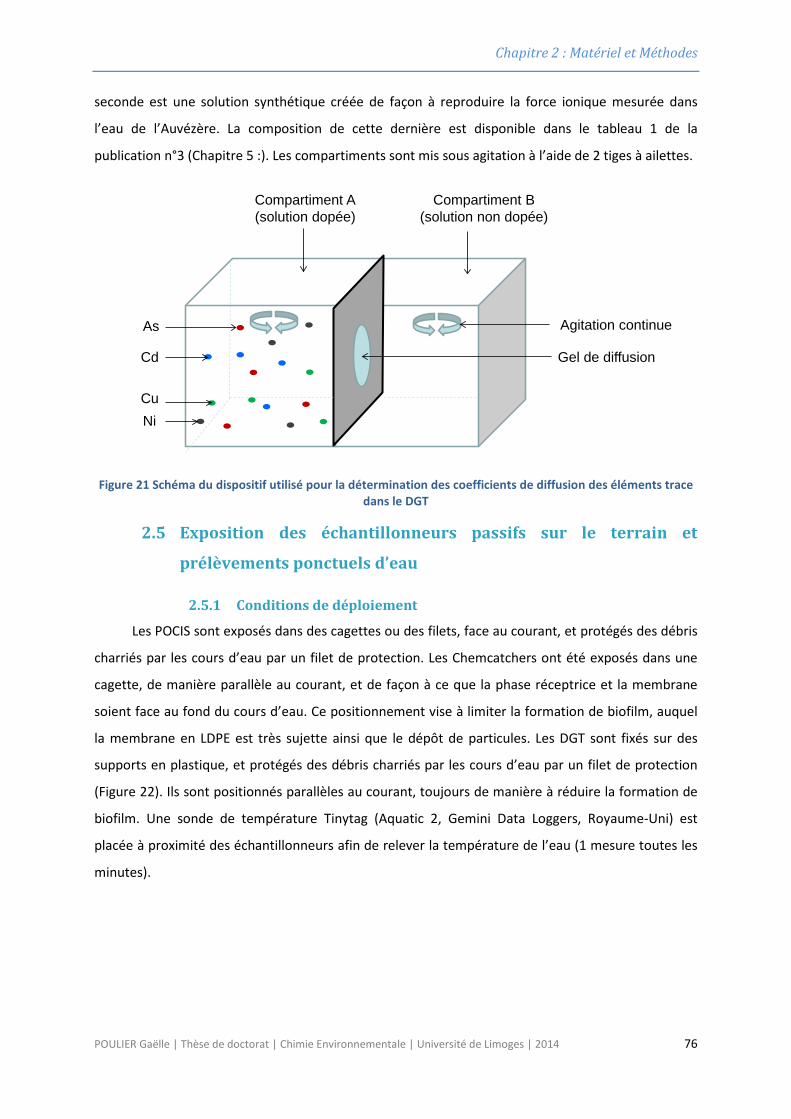
Chapitre 2 : Matériel et Méthodes
seconde est une solution synthétique créée de façon à reproduire la force ionique mesurée dans
l’eau de l’Auvézère. La composition de cette dernière est disponible dans le tableau 1 de la
publication n°3 (Chapitre 5 :). Les compartiments sont mis sous agitation à l’aide de 2 tiges à ailettes.
Figure 21 Schéma du dispositif utilisé pour la détermination des coefficients de diffusion des éléments trace dans le DGT
2.5 Exposition des échantillonneurs passifs sur le terrain et
prélèvements ponctuels d’eau
2.5.1 Conditions de déploiement
Les POCIS sont exposés dans des cagettes ou des filets, face au courant, et protégés des débris
charriés par les cours d’eau par un filet de protection. Les Chemcatchers ont été exposés dans une
cagette, de manière parallèle au courant, et de façon à ce que la phase réceptrice et la membrane
soient face au fond du cours d’eau. Ce positionnement vise à limiter la formation de biofilm, auquel
la membrane en LDPE est très sujette ainsi que le dépôt de particules. Les DGT sont fixés sur des
supports en plastique, et protégés des débris charriés par les cours d’eau par un filet de protection
(Figure 22). Ils sont positionnés parallèles au courant, toujours de manière à réduire la formation de
biofilm. Une sonde de température Tinytag (Aquatic 2, Gemini Data Loggers, Royaume-Uni) est
placée à proximité des échantillonneurs afin de relever la température de l’eau (1 mesure toutes les
minutes).
Compartiment A(solution dopée)
Compartiment B(solution non dopée)
Gel de diffusion
Agitation continueAs
Cd
CuNi
POULIER Gaëlle | Thèse de doctorat | Chimie Environnementale | Université de Limoges | 2014 76
Chapitre 2 : Matériel et Méthodes
Figure 22 Cagettes prêtes à être posées sur le terrain. Les POCIS sont positionnés face au courant tandis que les DGTs (sur le côté de la cagette) sont placés dans le sens parrallèle au courant. Les Chemcatcher sont à
l’intérieur de la cagette
Le temps d’exposition est généralement de 14 jours. Les échantillonneurs sont exposés en
exemplaire unique, en triplicats, ou en quintuplicats (Tableau 5 et Tableau 6) en fonction de l’objectif
des expérimentations. Après exposition, les échantillonneurs sont transportés au laboratoire dans
des glacières à 4°C puis démontés.
Pour chaque campagne, des blancs terrains correspondant à chaque type d’échantillonneur
sont préparés. Ces blancs sont préparés et transportés sur le terrain dans les mêmes conditions que
les systèmes exposés, puis ramenés au laboratoire et placés au réfrigérateur à 4 °C jusqu’à l’élution
(en même temps que les dispositifs exposés).
2.5.2 Plan d’échantillonnage
Les plans d’échantillonnage réalisés sur les bassins versants du Trec-Canaule et de l’Auvézère
sont résumés dans les Tableau 5 et Tableau 6.
En 2012, des POCIS ont été exposés sur chacun des sites (pour rappel, trois sur chaque bassin
versant, voir Figure 14 et Figure 15), de façon continue et le plus souvent en exemplaire unique. Sur
le bassin versant de l’Auvézère, des échantillons ponctuels d’eau ont également été prélevés toute
l’année. Au cours du printemps, les POCIS ont été exposés en triplicats sur le Trec et à la station des
Quatre-Moulins, sur l’Auvézère, afin de pouvoir comparer les concentrations obtenues avec celles
mesurées dans l’eau à l’aide du préleveur automatique (prélèvements de 50 ml d'eau toutes les
heures et récupération d'un échantillon composite hebdomadaire) installé à la même période. Enfin,
des DGT ont été exposés à la station des Quatre-Moulins (de janvier à mai) afin de réaliser un
premier screening. Cela nous a permis de constater la pureté insuffisante des blancs terrains, et nous
a conduits à déterminer la limite de quantification associée à cet échantillonneur, pour cet
environnement très peu contaminé (cf §4.4).
POULIER Gaëlle | Thèse de doctorat | Chimie Environnementale | Université de Limoges | 2014 77
Chapitre 2 : Matériel et Méthodes
En 2013, le suivi réalisé sur le bassin versant de l’Auvézère a été très peu modifié par rapport à
l’année précédente. Les DGT exposés cette année-là ont permis d’étudier l’influence de la
méthodologie de déploiement et d’exploitation des résultats sur la mesure DGT. Sur le Trec, des
POCIS et des Chemcatchers ont été exposés en mars, mai, juin, septembre et novembre afin de
comparer les concentrations obtenues avec celles du réseau de surveillance de l’Agence de l’eau
Adour-Garonne. Au printemps, les triplicats de POCIS et de Chemcatchers, associés au préleveur
automatique ont servi à la réalisation d’une calibration in situ, tandis que les quintuplicats de POCIS
associés aux échantillons ponctuels hebdomadaires ont permis d’étudier la fraction de pesticides
échantillonnée (l’eau a été filtrée et les matières en suspension ont été récupérées et analysées).
En 2014, l’étude de la fraction de contaminants échantillonnée a été de nouveau réalisée sur le
Trec, mais cette fois pour le Chemcatcher.
POULIER Gaëlle | Thèse de doctorat | Chimie Environnementale | Université de Limoges | 2014 78
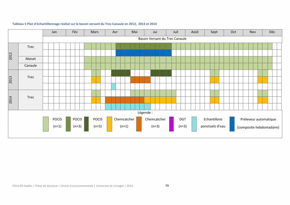
Tableau 5 Plan d'échantillonnage réalisé sur le bassin versant du Trec-Canaule en 2012, 2013 et 2014
Jan Fév Mars Avr Mai Jui Juil Août Sept Oct Nov Déc
Bassin Versant du Trec Canaule
2012
Trec
Manet
Canaule
2013
Trec
2014
Trec
Légende :
POCIS
(n=1) POCIS
(n=3) POCIS
(n=5) Chemcatcher
(n=1) Chemcatcher
(n=3) DGT
(n=3) Echantillons
ponctuels d’eau Préleveur automatique
(composite hebdomadaire)
POULIER Gaëlle | Thèse de doctorat | Chimie Environnementale | Université de Limoges | 2014 79
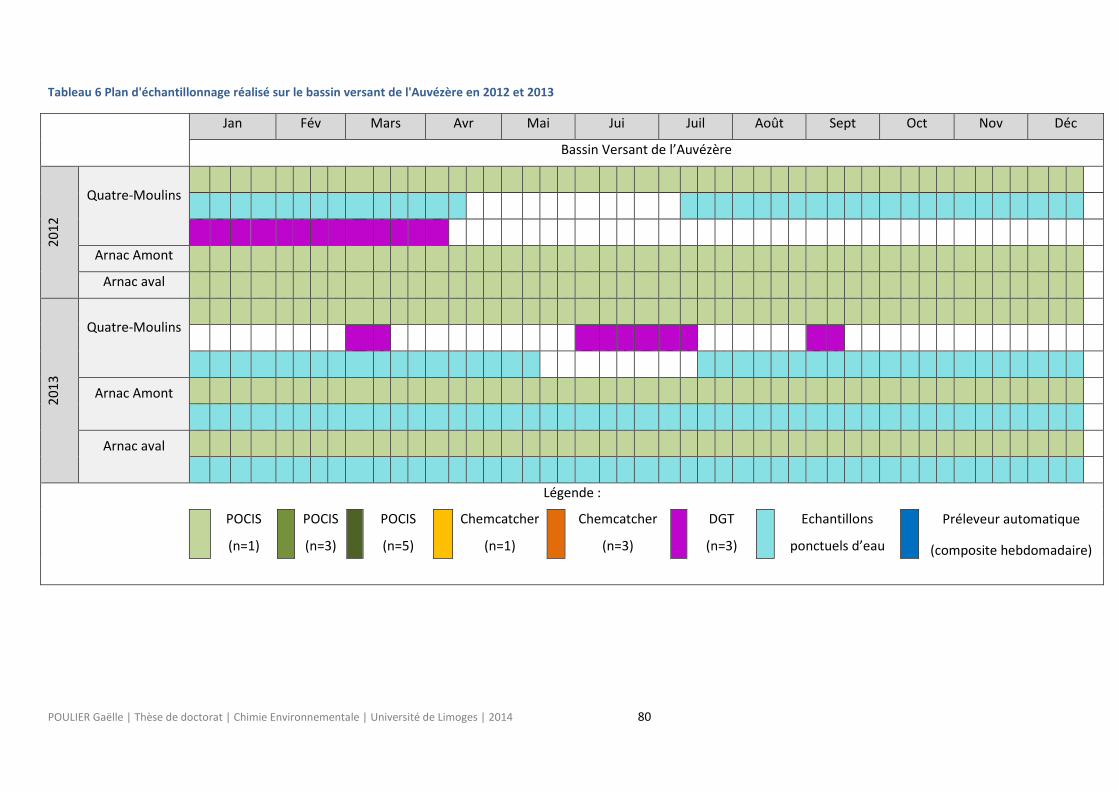
Tableau 6 Plan d'échantillonnage réalisé sur le bassin versant de l'Auvézère en 2012 et 2013
Jan Fév Mars Avr Mai Jui Juil Août Sept Oct Nov Déc
Bassin Versant de l’Auvézère
2012
Quatre-Moulins
Arnac Amont
Arnac aval
2013
Quatre-Moulins
Arnac Amont
Arnac aval
Légende :
POCIS
(n=1) POCIS
(n=3) POCIS
(n=5) Chemcatcher
(n=1) Chemcatcher
(n=3) DGT
(n=3) Echantillons
ponctuels d’eau Préleveur automatique
(composite hebdomadaire)
POULIER Gaëlle | Thèse de doctorat | Chimie Environnementale | Université de Limoges | 2014 80
Chapitre 2 : Matériel et Méthodes
2.6 Techniques analytiques
2.6.1 Principes généraux
Sauf en cas de rejet accidentel, les teneurs en pesticides sont souvent infimes dans
l’environnement en général, et dans l’eau en particulier. Pour les identifier et mesurer leur
concentration, il faut disposer de méthodes analytiques sensibles, sélectives, et capables de recouvrir
le plus large éventail possible de molécules. Le développement d’une méthode d’analyse d’une
matière active donnée, sur une matrice donnée, constitue donc véritablement un thème de
recherche, de même que l’adaptation d’une méthode existante à l’analyse de nouveaux composés,
et/ou de nouvelles matrices. En effet, un protocole satisfaisant pour un couple pesticide-matrice ne
convient pas à toutes les matrices, ni à tous les produits de la même famille, ni à tous les métabolites
de la matière active (Fournier, 1995). Il est donc primordial de développer la méthode d’analyse sur
l’ensemble des molécules et des matrices pour lesquelles elle sera utilisée. Si de nouveaux composés,
ou de nouvelles matrices sont ajoutés à la méthode initiale, celle-ci doit faire l’objet d’une nouvelle
validation. C’est le sujet de cette sous-partie, qui vise à décrire l’ensemble des développements
analytiques réalisés dans le cadre de cette thèse, ainsi que leur validation.
L’analyse des polluants dans les cours d’eau comporte généralement plusieurs étapes, incluant
l’extraction, la purification et la re-concentration des analytes de la matrice. Dans le cas des
échantillonneurs passifs, ces étapes sont réalisées (dans une certaine mesure) in situ, directement
dans le cours d’eau ce qui est l’un des avantages majeurs de cette technique. Par la suite, les
échantillons concentrés et purifiés sont analysés, le plus souvent par chromatographie liquide ou
gazeuse (pour séparer les différents constituants du mélange), associée à un détecteur (qui permet
d’identifier et de quantifier les composés).
2.6.2 Méthode instrumentale HPLC-ESI-MS/MS
Cette technique est adaptée aux molécules thermolabiles et non volatiles. Elle a été utilisée
dans cette étude pour l’analyse des pesticides les plus polaires.
L’appareillage est une HPLC Ultimate 3000 de Dionex, comprenant un dégazeur SRD-3600 à six
canaux, une pompe DGP-3600 M, un passeur automatique WPS-3000 TSL et un four thermostaté (40
°C) TCC-3100 HP 1xRH 2P-6P. La colonne chromatographique est une Gemini-NX C18 3 µm, 110 Å,
100 x 2 mm avec une colonne de garde Gemini-NX C18 4 x 2 mm (Phenomenex). La phase mobile est
un mélange d’acétonitrile et de solution d’acétate d’ammonium (5 mM, dans de l’eau ultrapure),
dont les conditions de gradient sont indiquées dans le Tableau 7. Le volume d’injection est de 40 µl.
POULIER Gaëlle | Thèse de doctorat | Chimie Environnementale | Université de Limoges | 2014 81
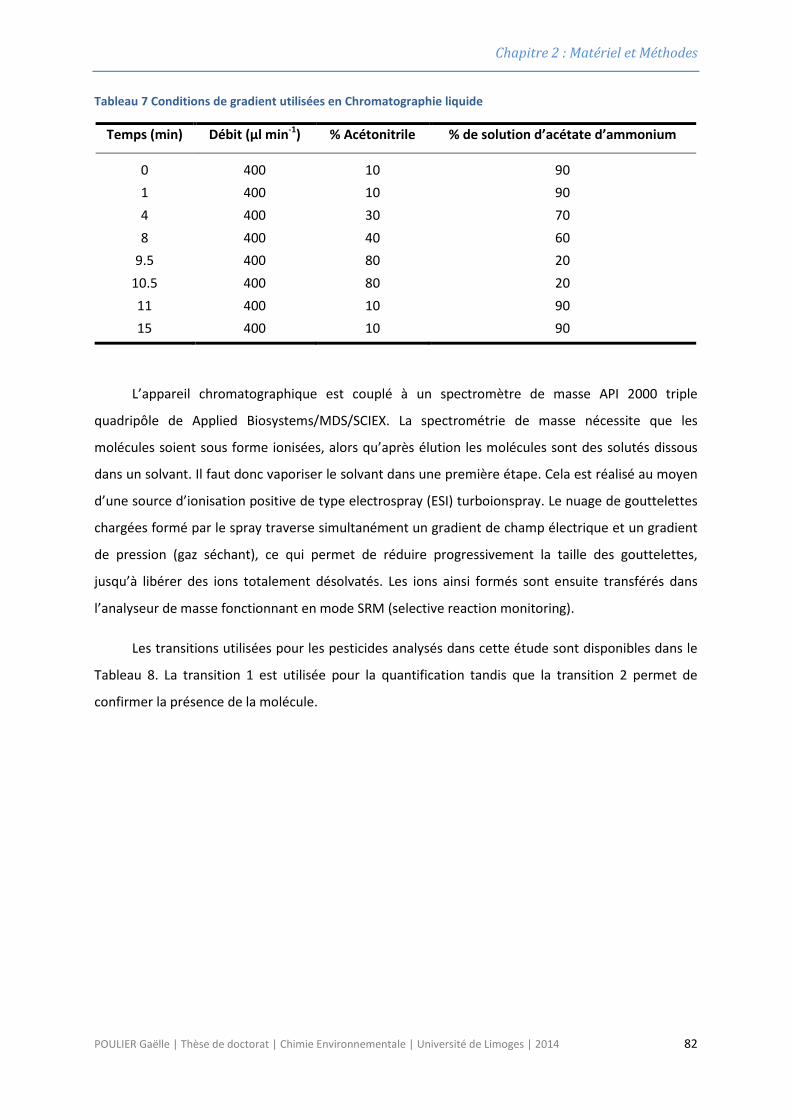
Chapitre 2 : Matériel et Méthodes
Tableau 7 Conditions de gradient utilisées en Chromatographie liquide
Temps (min) Débit (µl min-1) % Acétonitrile % de solution d’acétate d’ammonium
0 400 10 90 1 400 10 90 4 400 30 70 8 400 40 60
9.5 400 80 20 10.5 400 80 20 11 400 10 90 15 400 10 90
L’appareil chromatographique est couplé à un spectromètre de masse API 2000 triple
quadripôle de Applied Biosystems/MDS/SCIEX. La spectrométrie de masse nécessite que les
molécules soient sous forme ionisées, alors qu’après élution les molécules sont des solutés dissous
dans un solvant. Il faut donc vaporiser le solvant dans une première étape. Cela est réalisé au moyen
d’une source d’ionisation positive de type electrospray (ESI) turboionspray. Le nuage de gouttelettes
chargées formé par le spray traverse simultanément un gradient de champ électrique et un gradient
de pression (gaz séchant), ce qui permet de réduire progressivement la taille des gouttelettes,
jusqu’à libérer des ions totalement désolvatés. Les ions ainsi formés sont ensuite transférés dans
l’analyseur de masse fonctionnant en mode SRM (selective reaction monitoring).
Les transitions utilisées pour les pesticides analysés dans cette étude sont disponibles dans le
Tableau 8. La transition 1 est utilisée pour la quantification tandis que la transition 2 permet de
confirmer la présence de la molécule.
POULIER Gaëlle | Thèse de doctorat | Chimie Environnementale | Université de Limoges | 2014 82
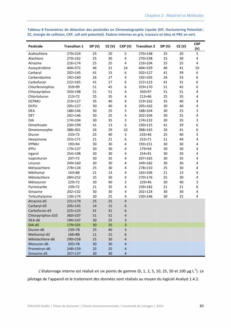
Chapitre 2 : Matériel et Méthodes
Tableau 8 Paramètres de détection des pesticides en Chromatographie Liquide (DP, Declustering Potential ; EC, énergie de collision, CXP, cell exit potential). Etalons internes en gris, traceurs en bleu et PRC en vert.
Pesticide Transition 1 DP (V) CE (V) CXP (V) Transition 2 DP (V) CE (V) CXP (V)
Acétochlore 270>224 25 20 5 270>148 25 20 5 Alachlore 270>162 25 30 4 270>238 25 30 4 Atrazine 216>174 25 25 4 216>104 25 25 4 Azoxystrobine 404>372 46 21 14 404>329 46 41 10 Carbaryl 202>145 41 15 6 202>127 41 39 6 Carbendazime 192>160 26 27 4 192>105 26 53 6 Carbofuran 222>165 41 17 6 222>123 41 31 6 Chlorfenvinphos 359>99 51 45 6 359>170 51 45 6 Chlorpyriphos 350>198 51 51 4 350>97 51 51 4 Chlortoluron 213>72 25 35 4 213>46 25 35 4 DCPMU 219>127 35 40 4 219>162 35 40 4 DCPU 205>127 30 40 4 205>162 30 40 4 DEA 188>146 30 25 3 188>104 30 25 3 DET 202>146 30 25 4 202>104 30 25 4 DIA 174>104 30 35 3 174>132 30 35 3 Dimethoate 230>199 41 13 6 230>125 41 29 6 Dimetomorphe 388>301 26 29 10 388>165 26 41 6 Diuron 233>72 25 40 3 233>46 25 40 3 Hexazinone 253>171 21 21 6 253>71 21 49 4 IPPMU 193>94 30 30 4 193>151 30 30 4 IPPU 179>137 30 30 4 179>94 30 30 4 Irgarol 254>198 30 30 4 254>91 30 30 4 Isoproturon 207>72 30 35 4 207>165 30 35 4 Linuron 249>160 30 30 4 249>182 30 30 4 Métazachlore 278>134 25 30 4 278>210 25 30 4 Méthomyl 163>88 21 13 4 163>106 21 13 4 Métolachlore 284>252 25 30 4 270>176 25 30 4 Métoxuron 229>72 30 40 3 229>46 30 40 3 Pyrimicarbe 239>72 21 35 4 239>182 21 21 6 Simazine 202>132 30 30 4 202>124 30 30 4 Terbuthylazine 130>174 30 25 4 230>146 30 25 4 Atrazine-d5 221>179 25 25 4 Carbaryl-d3 205>145 14 15 6 Carbofuran-d3 225>123 41 31 6 Chlorpyriphos-d10 360>107 51 51 4 DEA-d6 194>147 30 25 3 DIA-d5 179>101 30 35 3 Diuron-d6 239>78 25 40 3 Methomyl-d3 166>88 11 15 6 Métolachlore-d6 290>258 25 30 4 Monuron-d6 205>78 30 30 4 Prometryn-d6 248>159 25 25 4 Simazine-d5 207>137 30 30 4
L’étalonnage interne est réalisé en six points de gamme (0, 1, 2, 5, 10, 25, 50 et 100 µg L-1). Le
pilotage de l’appareil et le traitement des données sont réalisés au moyen du logiciel Analyst 1.4.2.
POULIER Gaëlle | Thèse de doctorat | Chimie Environnementale | Université de Limoges | 2014 83
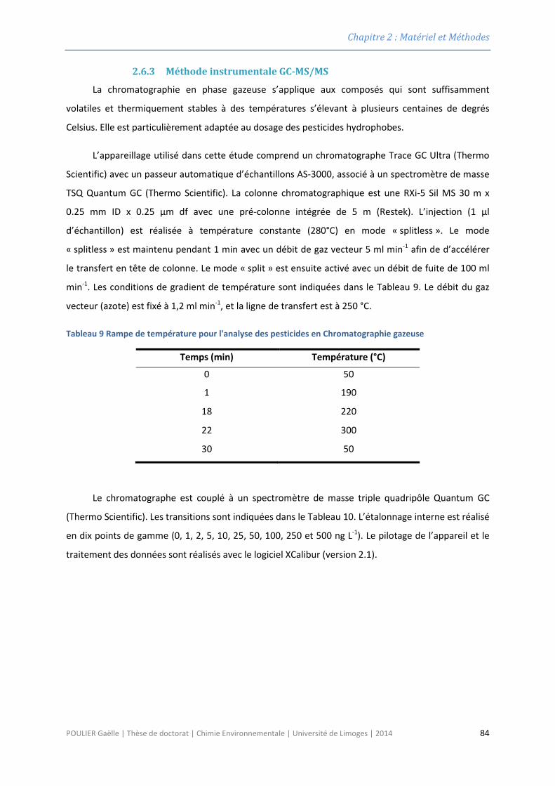
Chapitre 2 : Matériel et Méthodes
2.6.3 Méthode instrumentale GC-MS/MS
La chromatographie en phase gazeuse s’applique aux composés qui sont suffisamment
volatiles et thermiquement stables à des températures s’élevant à plusieurs centaines de degrés
Celsius. Elle est particulièrement adaptée au dosage des pesticides hydrophobes.
L’appareillage utilisé dans cette étude comprend un chromatographe Trace GC Ultra (Thermo
Scientific) avec un passeur automatique d’échantillons AS-3000, associé à un spectromètre de masse
TSQ Quantum GC (Thermo Scientific). La colonne chromatographique est une RXi-5 Sil MS 30 m x
0.25 mm ID x 0.25 µm df avec une pré-colonne intégrée de 5 m (Restek). L’injection (1 µl
d’échantillon) est réalisée à température constante (280°C) en mode « splitless ». Le mode
« splitless » est maintenu pendant 1 min avec un débit de gaz vecteur 5 ml min-1 afin de d’accélérer
le transfert en tête de colonne. Le mode « split » est ensuite activé avec un débit de fuite de 100 ml
min-1. Les conditions de gradient de température sont indiquées dans le Tableau 9. Le débit du gaz
vecteur (azote) est fixé à 1,2 ml min-1, et la ligne de transfert est à 250 °C.
Tableau 9 Rampe de température pour l'analyse des pesticides en Chromatographie gazeuse
Temps (min) Température (°C)
0 50
1 190
18 220
22 300
30 50
Le chromatographe est couplé à un spectromètre de masse triple quadripôle Quantum GC
(Thermo Scientific). Les transitions sont indiquées dans le Tableau 10. L’étalonnage interne est réalisé
en dix points de gamme (0, 1, 2, 5, 10, 25, 50, 100, 250 et 500 ng L-1). Le pilotage de l’appareil et le
traitement des données sont réalisés avec le logiciel XCalibur (version 2.1).
POULIER Gaëlle | Thèse de doctorat | Chimie Environnementale | Université de Limoges | 2014 84
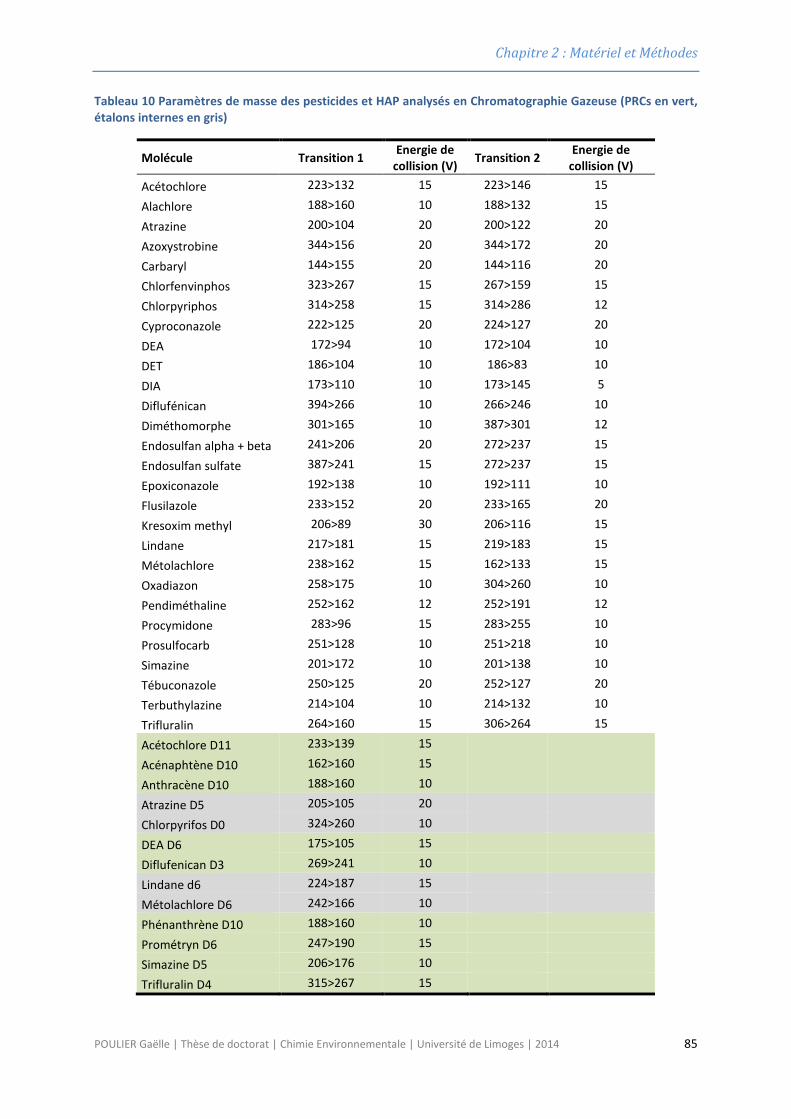
Chapitre 2 : Matériel et Méthodes
Tableau 10 Paramètres de masse des pesticides et HAP analysés en Chromatographie Gazeuse (PRCs en vert, étalons internes en gris)
Molécule Transition 1 Energie de collision (V) Transition 2 Energie de
collision (V) Acétochlore 223>132 15 223>146 15
Alachlore 188>160 10 188>132 15
Atrazine 200>104 20 200>122 20
Azoxystrobine 344>156 20 344>172 20
Carbaryl 144>155 20 144>116 20
Chlorfenvinphos 323>267 15 267>159 15
Chlorpyriphos 314>258 15 314>286 12
Cyproconazole 222>125 20 224>127 20
DEA 172>94 10 172>104 10
DET 186>104 10 186>83 10
DIA 173>110 10 173>145 5
Diflufénican 394>266 10 266>246 10
Diméthomorphe 301>165 10 387>301 12
Endosulfan alpha + beta 241>206 20 272>237 15
Endosulfan sulfate 387>241 15 272>237 15
Epoxiconazole 192>138 10 192>111 10
Flusilazole 233>152 20 233>165 20
Kresoxim methyl 206>89 30 206>116 15
Lindane 217>181 15 219>183 15
Métolachlore 238>162 15 162>133 15
Oxadiazon 258>175 10 304>260 10
Pendiméthaline 252>162 12 252>191 12
Procymidone 283>96 15 283>255 10
Prosulfocarb 251>128 10 251>218 10
Simazine 201>172 10 201>138 10
Tébuconazole 250>125 20 252>127 20
Terbuthylazine 214>104 10 214>132 10
Trifluralin 264>160 15 306>264 15
Acétochlore D11 233>139 15 Acénaphtène D10 162>160 15
Anthracène D10 188>160 10
Atrazine D5 205>105 20 Chlorpyrifos D0 324>260 10 DEA D6 175>105 15
Diflufenican D3 269>241 10 Lindane d6 224>187 15 Métolachlore D6 242>166 10 Phénanthrène D10 188>160 10
Prométryn D6 247>190 15 Simazine D5 206>176 10 Trifluralin D4 315>267 15
POULIER Gaëlle | Thèse de doctorat | Chimie Environnementale | Université de Limoges | 2014 85
Chapitre 2 : Matériel et Méthodes
2.6.4 Méthodes instrumentales ICP-MS et SAA-FG
L’ICP-MS est une technique de spectrométrie de masse dans laquelle la source d’ionisation est
une torche à plasma à couplage inductif (ICP). Cette technique permet d’atteindre des limites de
détection basses et se prête donc particulièrement bien à l’analyse des éléments traces. L’ICP-MS a
été utilisé dans cette étude pour le dosage du cuivre (Cu), du cadmium (Cd) et du nickel (Ni).
L’appareillage utilisé est un Agilent 7700X. L’étalonnage interne est réalisé avec 45Sc pour 63Cu et 60Ni,
et 115In pour 75As et 111Cd.
Le dosage de l’As dans les éluats des DGT contenant une phase réceptrice de type ferrihydrite
n’a pas été réalisé en ICP-MS pour ne pas prendre le risque de contaminer l’appareil avec le fer.
L’analyse a été réalisée par spectrométrie d’absorption atomique four graphite (SAA-FG), sur un
appareil Varian 880Z, équipé d’un module UltrAA, avec correction par effet Zeeman.
2.6.5 Extraction en phase solide (cartouche Chromabond HR-X) des
pesticides polaires neutres dans les eaux et analyse LC-ESI-MS/MS
Les pesticides étant le plus souvent présents dans l’eau à de très faibles concentrations (de
l’ordre du ng L-1, voire moins), il est très difficile, voire impossible de disposer d’appareils de mesure
suffisamment sensibles pour les quantifier directement dans l’échantillon prélevé sur le terrain. Il est
donc nécessaire de concentrer les analytes, en les solubilisant dans le plus petit volume de solvant
possible. Par ailleurs, dans le milieu naturel les pesticides coexistent avec un grand nombre de
molécules organiques présentant des caractéristiques proches (molécules médicamenteuses, résidus
de produits cosmétiques, etc.), qui peuvent interférer au moment de l’analyse, et qu’il convient donc
d’éliminer. Ces étapes peuvent être réalisées par extraction en phase solide. Le protocole comprend
quatre étapes : le conditionnement de la cartouche, le passage de l’échantillon, le rinçage (permet
d’éliminer certaines impuretés faiblement adsorbées) et enfin l’élution, qui permet de récupérer les
analytes retenus sur l’adsorbant. L’efficacité de l’extraction et de la purification dépend du choix de
l’adsorbant et des solvants de rinçage et d’élution.
Le protocole utilisé dans cette thèse est adapté de (Lissalde et al., 2011). Il a été optimisé pour
l’analyse des nouveaux composés intégrés dans cette étude.
Les cartouches (Chromabond HR-X) sont conditionnées avec 5 ml de méthanol (MeOH) suivis
de 5 ml d’eau ultrapure (EUP). Les échantillons d’eau (100 ml) filtrés sur filtres GF-F (Whatman, 0,7
µm) et ajustés à pH=7 avec HCl, NaOH ou H3PO4 (0,1 N) sont transférés sur la cartouche, qui est
ensuite rincée avec 5 ml d’EUP contenant 15 % de MeOH. Ces trois étapes (conditionnement,
percolation de l’échantillon et rinçage) sont réalisées sous vide partiel (environ 53,33 kPa). Après
séchage sous flux d’azote (30 minutes), l’élution est réalisée par 3 ml de MeOH suivis de 3 ml d’un
POULIER Gaëlle | Thèse de doctorat | Chimie Environnementale | Université de Limoges | 2014 86
Chapitre 2 : Matériel et Méthodes
mélange MeOH / Acétate d’éthyle (75 :25 v/v). L’ensemble du processus, est réalisé à l’aide d’un
dispositif Visiprep 12-ports (Supelco).
Après l’élution, l’échantillon est évaporé sous flux d’azote, ou à l’aide d’un évaporateur
automatisé, puis reconstitué dans 1 ml d’EUP contenant 10 % d’acétonitrile. Afin de vérifier que
l’extraction s’est bien déroulée, 10 µl d’un mélange à 10 mg L-1 de trois molécules deutérées
(prometryn d6, simazine d5 et monuron d6) appelées « surrogates » ont été ajoutés aux échantillons
d’eau, avant l’extraction. La concentration dans l’échantillon final doit être de 10 µg L-1. Dans le cas
contraire, un problème au cours de l’extraction doit être soupçonné, et les concentrations mesurées
dans les échantillons pour les pesticides sont corrigées avec celles des surrogates pour en tenir
compte.
La performance générale d’un protocole d’extraction peut être évaluée au moyen de l’étude
des rendements. Pour cela, des échantillons d’eau sont dopés à 0,04 µg L-1 et 0,2 µg L-1 avec une
solution à 1 mg L-1 contenant 41 pesticides polaires neutres (4 µl et 20 µl respectivement) et extraits
selon le protocole décrit ci-dessus. Les concentrations attendues dans l’échantillon final sont de 20 et
40 µg L-1. Les concentrations initiales en pesticides (avant dopage) sont déterminées grâce à l’analyse
de l’échantillon non dopé. Un rendement est considéré comme satisfaisant si le pourcentage de
récupération de l’analyte est supérieur à 70 %. Dans le cas contraire, les concentrations obtenues à
l’analyse pour les échantillons prélevés sur le terrain devront être corrigées pour tenir compte du
biais lié à un rendement trop faible. En cas de rendements inférieurs à 20 %, c’est toute la procédure
d’extraction et de purification qui doit être modifiée. L’étude des rendements a été réalisée sur les
échantillons ponctuels d’eau prélevés sur le Trec au cours de la campagne 2012, ainsi que dans l’eau
d’Evian. Les résultats obtenus sont listés dans le Tableau 11.
POULIER Gaëlle | Thèse de doctorat | Chimie Environnementale | Université de Limoges | 2014 87
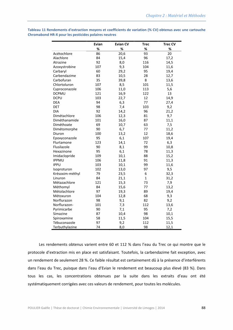
Chapitre 2 : Matériel et Méthodes
Tableau 11 Rendements d'extraction moyens et coefficients de variation (% CV) obtenus avec une cartouche Chromabond HR-X pour les pesticides polaires neutres
Evian %
Evian CV %
Trec %
Trec CV %
Acétochlore 86 20,6 93 20 Alachlore 84 15,4 96 17,2 Atrazine 92 8,0 116 14,5 Azoxystrobine 107 9,3 104 11,6 Carbaryl 60 29,2 95 19,4 Carbendazime 83 10,5 28 12,7 Carbofuran 35 39,8 8 13,6 Chlortoluron 107 8,5 101 11,5 Cyproconazole 106 11,0 113 5,6 DCPMU 121 16,9 122 13 DCPU 103 22,7 12 14,9 DEA 94 6,3 77 27,4 DET 98 7,4 103 9,2 DIA 92 14,2 96 21,2 Dimétachlore 106 12,3 81 9,7 Diméthanamide 101 16,0 87 11,1 Diméthoate 69 10,7 63 7,5 Dimétomorphe 90 6,7 77 11,2 Diuron 100 13,2 12 18,6 Epoxyconazole 95 6,1 107 19,4 Flurtamone 123 14,1 72 6,3 Flusilazole 90 8,1 99 10,8 Hexazinone 95 6,1 78 11,3 Imidaclopride 109 10,1 88 15,2 IPPMU 106 11,8 91 11,3 IPPU 103 10,1 99 11,6 Isoproturon 102 13,0 97 9,5 Krésoxim-méthyl 79 23,5 6 32,3 Linuron 84 21,1 1 31,2 Métazachlore 121 15,3 73 7,9 Méthomyl 84 15,6 77 13,2 Métolachlore 97 19,3 89 19,4 Métoxuron 104 12,8 68 9,3 Norflurazon 98 9,1 82 9,2 Norflurazon-
101 7,3 112 13,6 Pyrimicarbe 90 7,1 95 7,2 Simazine 87 10,4 98 10,1 Spiroxamine 58 11,5 104 15,5 Tébuconazole 97 9,2 112 11,5 Terbuthylazine 74 8,0 98 12,1
Les rendements obtenus varient entre 60 et 112 % dans l’eau du Trec ce qui montre que le
protocole d’extraction mis en place est satisfaisant. Toutefois, la carbendazime fait exception, avec
un rendement de seulement 28 %. Ce faible résultat est certainement dû à la présence d’interférents
dans l’eau du Trec, puisque dans l’eau d’Evian le rendement est beaucoup plus élevé (83 %). Dans
tous les cas, les concentrations obtenues par la suite dans les extraits d’eau ont été
systématiquement corrigées avec ces valeurs de rendement, pour toutes les molécules.
POULIER Gaëlle | Thèse de doctorat | Chimie Environnementale | Université de Limoges | 2014 88
Chapitre 2 : Matériel et Méthodes
2.6.6 Validation selon la norme AFNOR NF T90 210 (2009) d’une méthode
d’analyse des pesticides hydrophobes dans les eaux par extraction
sur Empore disque C18 et analyse GC-MS MS
Le protocole d’analyse des pesticides hydrophobes dans les eaux comprend les étapes
d’extraction et d’élution, puis l’analyse par GC-MS/MS.
a) Protocole d’extraction sur disque Empore C18
Les pesticides hydrophobes ont généralement très peu d’affinité avec l’eau, et ont plutôt
tendance à s’adsorber sur les matières en suspension. Par conséquent, il est très difficile de
quantifier ces molécules dans la phase dissoute, car les concentrations y sont faibles, souvent
inférieures au ng L-1. Pour y parvenir, il faut donc extraire (et reconcentrer) de grands volumes d’eau.
L’utilisation d’un adsorbant conditionné sous forme de disque, plutôt que sous forme de cartouche,
permet de traiter ces grands volumes.
Le protocole d’extraction mis au point pour les pesticides hydrophobes comprend donc un
adsorbant sous forme de disque Empore C18 (47 mm de diamètre, Supelco). La préparation des
échantillons, le volume de la prise d’essai, ainsi que des solvants de rinçage et d’élution ont été
optimisés grâce à un plan d’expérience.
Au retour de terrain, 500 ml d’eau sont filtrés sur filtre GF-F (0,7 µm, Whatmann) et ajustés à
pH=7 avec HClsuprapur (10 %) (Sigma Aldrich, Schnelldorf, Allemagne). L’échantillon est ensuite
transféré dans une fiole jaugée de 500 ml contenant 50 ml de méthanol (l’échantillon final contient
donc 10 % de méthanol). L’extraction est réalisée au moyen de « Holder disk » (Restek), adaptables
sur dispositif Visiprep (Figure 16). Tout comme précédemment pour les Chemcatcher, un filtre
Ashless (Whatmann, taille des pores 20 µm, découpé à la main à 47 mm de diamètre) est disposé en-
dessous du disque afin d’éviter qu’il ne se perce sous l’effet du vide. Le disque est tout d’abord rincé
avec 10 ml de dichlorométhane (grade HPLC, Atlantic Labo, Bruges France) puis conditionné avec 2 ×
5 ml de méthanol (avec temps d’imprégnation d’1 minute entre chaque fraction) et 10 ml d’eau
ultrapure. Après ce conditionnement, il est important de noter que le disque ne doit jamais être
laissé à sec, ce qui affecterait les performances de l’extraction. Les 500 ml d’échantillon sont ensuite
transférés, une attention particulière étant portée sur l’intensité du vide tout au long de l’extraction.
Après percolation des échantillons, le vide est maintenu pendant une heure afin de laisser sécher les
disques.
Le disque est ensuite imprégné avec 1 ml d’acétone puis l’élution est réalisée avec 3 × 5 ml de
dichlorométhane. Chaque fraction de 5 ml est versée dans la fiole ayant contenu l’échantillon, puis
transférée sur le disque en deux fois (avec temps d’imprégnation d’une minute). Là encore, le disque
POULIER Gaëlle | Thèse de doctorat | Chimie Environnementale | Université de Limoges | 2014 89
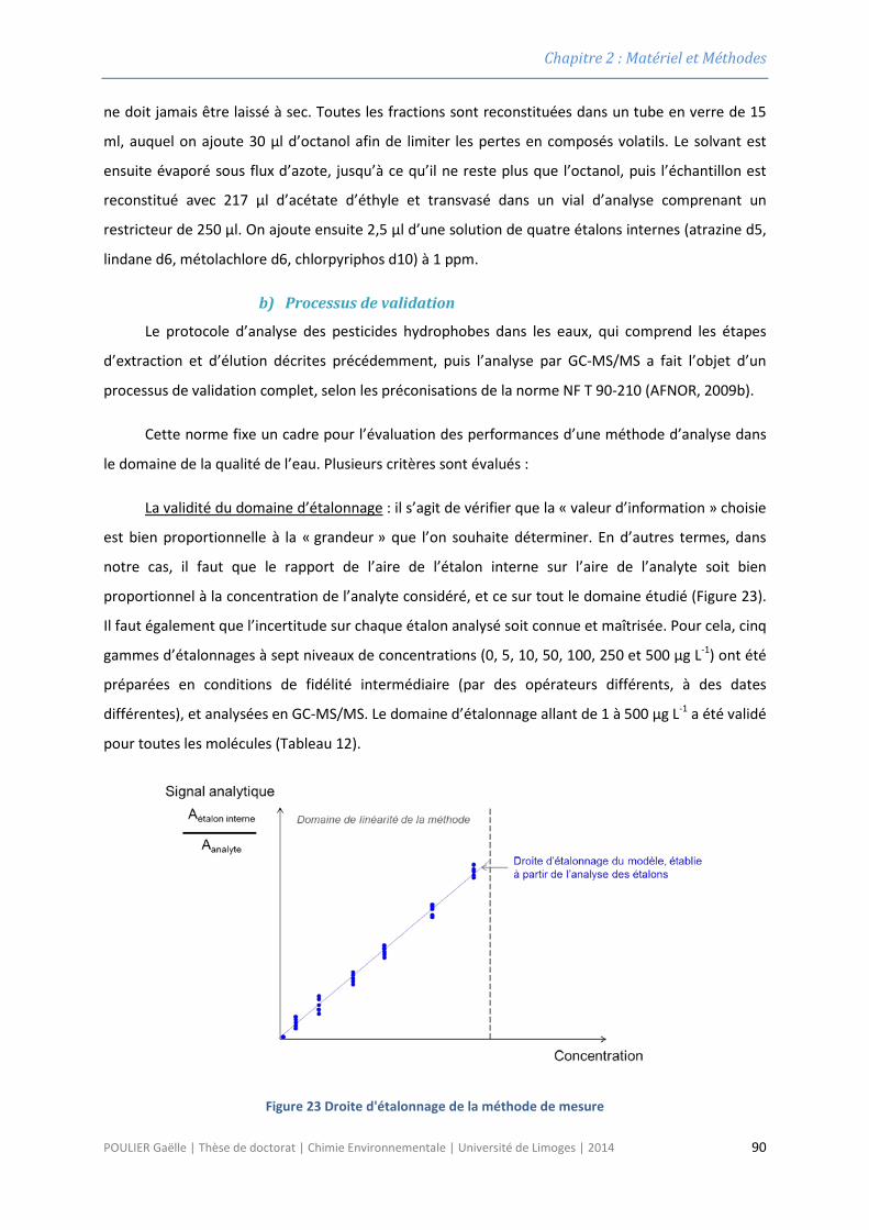
Chapitre 2 : Matériel et Méthodes
ne doit jamais être laissé à sec. Toutes les fractions sont reconstituées dans un tube en verre de 15
ml, auquel on ajoute 30 µl d’octanol afin de limiter les pertes en composés volatils. Le solvant est
ensuite évaporé sous flux d’azote, jusqu’à ce qu’il ne reste plus que l’octanol, puis l’échantillon est
reconstitué avec 217 µl d’acétate d’éthyle et transvasé dans un vial d’analyse comprenant un
restricteur de 250 µl. On ajoute ensuite 2,5 µl d’une solution de quatre étalons internes (atrazine d5,
lindane d6, métolachlore d6, chlorpyriphos d10) à 1 ppm.
b) Processus de validation
Le protocole d’analyse des pesticides hydrophobes dans les eaux, qui comprend les étapes
d’extraction et d’élution décrites précédemment, puis l’analyse par GC-MS/MS a fait l’objet d’un
processus de validation complet, selon les préconisations de la norme NF T 90-210 (AFNOR, 2009b).
Cette norme fixe un cadre pour l’évaluation des performances d’une méthode d’analyse dans
le domaine de la qualité de l’eau. Plusieurs critères sont évalués :
La validité du domaine d’étalonnage : il s’agit de vérifier que la « valeur d’information » choisie
est bien proportionnelle à la « grandeur » que l’on souhaite déterminer. En d’autres termes, dans
notre cas, il faut que le rapport de l’aire de l’étalon interne sur l’aire de l’analyte soit bien
proportionnel à la concentration de l’analyte considéré, et ce sur tout le domaine étudié (Figure 23).
Il faut également que l’incertitude sur chaque étalon analysé soit connue et maîtrisée. Pour cela, cinq
gammes d’étalonnages à sept niveaux de concentrations (0, 5, 10, 50, 100, 250 et 500 µg L-1) ont été
préparées en conditions de fidélité intermédiaire (par des opérateurs différents, à des dates
différentes), et analysées en GC-MS/MS. Le domaine d’étalonnage allant de 1 à 500 µg L-1 a été validé
pour toutes les molécules (Tableau 12).
Figure 23 Droite d'étalonnage de la méthode de mesure
POULIER Gaëlle | Thèse de doctorat | Chimie Environnementale | Université de Limoges | 2014 90
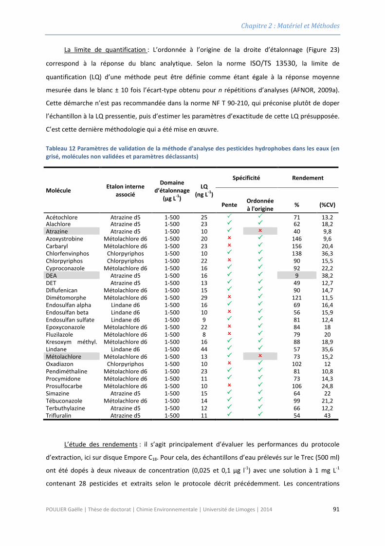
Chapitre 2 : Matériel et Méthodes
La limite de quantification : L’ordonnée à l’origine de la droite d’étalonnage (Figure 23)
correspond à la réponse du blanc analytique. Selon la norme ISO/TS 13530, la limite de
quantification (LQ) d’une méthode peut être définie comme étant égale à la réponse moyenne
mesurée dans le blanc ± 10 fois l’écart-type obtenu pour n répétitions d’analyses (AFNOR, 2009a).
Cette démarche n’est pas recommandée dans la norme NF T 90-210, qui préconise plutôt de doper
l’échantillon à la LQ pressentie, puis d’estimer les paramètres d’exactitude de cette LQ présupposée.
C’est cette dernière méthodologie qui a été mise en œuvre.
Tableau 12 Paramètres de validation de la méthode d'analyse des pesticides hydrophobes dans les eaux (en grisé, molécules non validées et paramètres déclassants)
Molécule Etalon interne associé
Domaine d’étalonnage
(µg L-1)
LQ (ng L-1)
Spécificité Rendement
Pente Ordonnée à l'origine % (%CV)
Acétochlore Atrazine d5 1-500 25 71 13,2 Alachlore Atrazine d5 1-500 23 62 18,2 Atrazine Atrazine d5 1-500 10 40 9,8 Azoxystrobine Métolachlore d6 1-500 20 146 9,6 Carbaryl Métolachlore d6 1-500 23 156 20,4 Chlorfenvinphos Chlorpyriphos
1-500 10 138 36,3 Chlorpyriphos Chlorpyriphos
1-500 22 90 15,5 Cyproconazole Métolachlore d6 1-500 16 92 22,2 DEA Atrazine d5 1-500 16 9 38,2 DET Atrazine d5 1-500 13 49 12,7 Diflufenican Métolachlore d6 1-500 15 90 14,7 Dimétomorphe Métolachlore d6 1-500 29 121 11,5 Endosulfan alpha Lindane d6 1-500 16 69 16,4 Endosulfan beta Lindane d6 1-500 10 56 15,9 Endosulfan sulfate Lindane d6 1-500 9 81 12,4 Epoxyconazole Métolachlore d6 1-500 22 84 18 Fluzilazole Métolachlore d6 1-500 8 79 20 Kresoxym méthyl.
Métolachlore d6 1-500 16 88 18,9 Lindane Lindane d6 1-500 44 57 35,6 Métolachlore Métolachlore d6 1-500 13 73 15,2 Oxadiazon Chlorpyriphos
1-500 10 102 12 Pendiméthaline Métolachlore d6 1-500 23 81 10,8 Procymidone Métolachlore d6 1-500 11 73 14,3 Prosulfocarbe Métolachlore d6 1-500 10 106 24,8 Simazine Atrazine d5 1-500 15 64 22 Tébuconazole Métolachlore d6 1-500 14 99 21,2 Terbuthylazine Atrazine d5 1-500 12 66 12,2 Trifluralin Atrazine d5 1-500 11 54 43
L’étude des rendements : il s’agit principalement d’évaluer les performances du protocole
d’extraction, ici sur disque Empore C18. Pour cela, des échantillons d’eau prélevés sur le Trec (500 ml)
ont été dopés à deux niveaux de concentration (0,025 et 0,1 µg l-1) avec une solution à 1 mg L-1
contenant 28 pesticides et extraits selon le protocole décrit précédemment. Les concentrations
POULIER Gaëlle | Thèse de doctorat | Chimie Environnementale | Université de Limoges | 2014 91
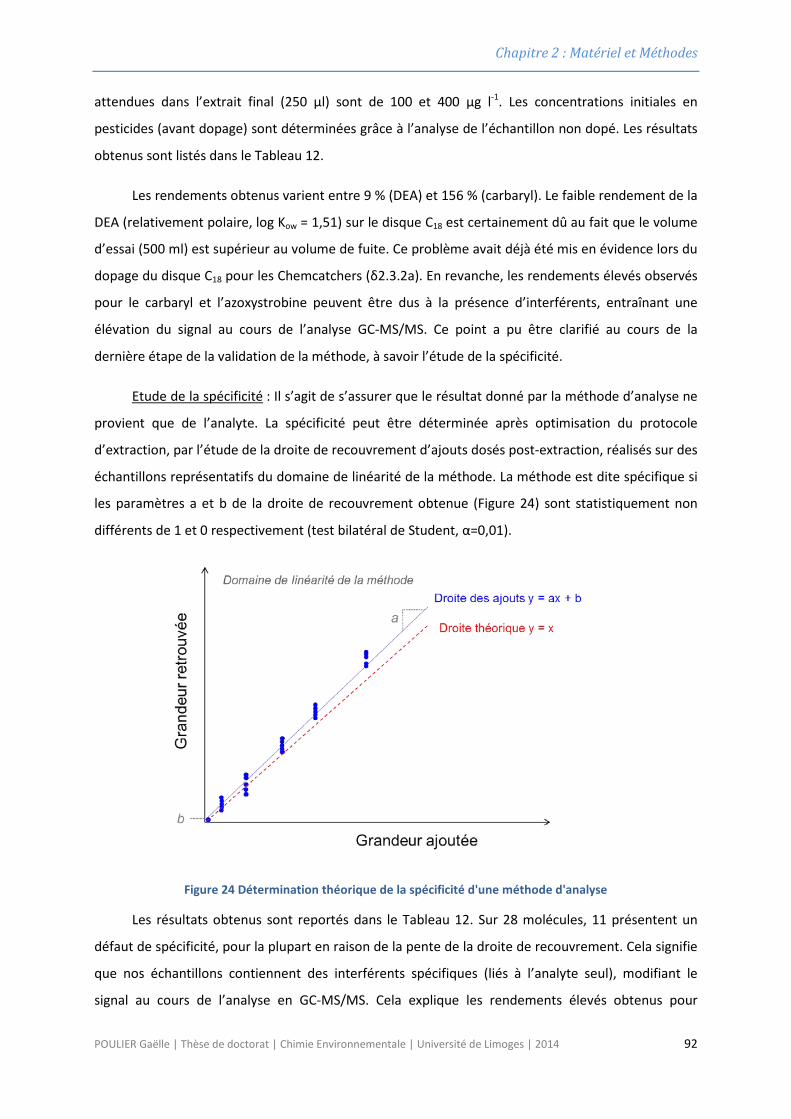
Chapitre 2 : Matériel et Méthodes
attendues dans l’extrait final (250 µl) sont de 100 et 400 µg l-1. Les concentrations initiales en
pesticides (avant dopage) sont déterminées grâce à l’analyse de l’échantillon non dopé. Les résultats
obtenus sont listés dans le Tableau 12.
Les rendements obtenus varient entre 9 % (DEA) et 156 % (carbaryl). Le faible rendement de la
DEA (relativement polaire, log Kow = 1,51) sur le disque C18 est certainement dû au fait que le volume
d’essai (500 ml) est supérieur au volume de fuite. Ce problème avait déjà été mis en évidence lors du
dopage du disque C18 pour les Chemcatchers (δ2.3.2a). En revanche, les rendements élevés observés
pour le carbaryl et l’azoxystrobine peuvent être dus à la présence d’interférents, entraînant une
élévation du signal au cours de l’analyse GC-MS/MS. Ce point a pu être clarifié au cours de la
dernière étape de la validation de la méthode, à savoir l’étude de la spécificité.
Etude de la spécificité : Il s’agit de s’assurer que le résultat donné par la méthode d’analyse ne
provient que de l’analyte. La spécificité peut être déterminée après optimisation du protocole
d’extraction, par l’étude de la droite de recouvrement d’ajouts dosés post-extraction, réalisés sur des
échantillons représentatifs du domaine de linéarité de la méthode. La méthode est dite spécifique si
les paramètres a et b de la droite de recouvrement obtenue (Figure 24) sont statistiquement non
différents de 1 et 0 respectivement (test bilatéral de Student, α=0,01).
Figure 24 Détermination théorique de la spécificité d'une méthode d'analyse
Les résultats obtenus sont reportés dans le Tableau 12. Sur 28 molécules, 11 présentent un
défaut de spécificité, pour la plupart en raison de la pente de la droite de recouvrement. Cela signifie
que nos échantillons contiennent des interférents spécifiques (liés à l’analyte seul), modifiant le
signal au cours de l’analyse en GC-MS/MS. Cela explique les rendements élevés obtenus pour
POULIER Gaëlle | Thèse de doctorat | Chimie Environnementale | Université de Limoges | 2014 92
Chapitre 2 : Matériel et Méthodes
l’azoxystrobine et le carbaryl. Un défaut de spécificité lié à la pente de la droite de recouvrement de
la méthode peut être ignoré si les concentrations obtenues dans les échantillons sont
systématiquement corrigées par les valeurs de rendements, ou en effectuant des ajouts dosés pour
chaque échantillon. En revanche, les cas de l’atrazine et du métolachlore sont plus problématiques
car pour ces molécules, le défaut de spécificité est lié à l’ordonnée à l’origine de la droite de
recouvrement de la méthode. Dans ce cas, les interférences sont non spécifiques et sont liées à la
présence d’un composé qui produit un signal, y compris en absence de l’analyte. Ces interférences ne
peuvent être corrigées par la méthode des ajouts dosés ou par les rendements. Par conséquent, ces
deux molécules ont été supprimées de la méthode d’analyse SPE disk-GC-MS/MS. Cette suppression
n’aura pas beaucoup d’influence car l’atrazine et le métolachlore sont déjà analysés en LC-MS/MS.
2.6.7 Validation selon la norme AFNOR NF T90 210 (2009) d’une méthode
d’analyse des pesticides dans les matières en suspension par ASE et
analyse LC-ESI-MS/MS
Les pesticides les plus hydrophobes ont une grande tendance à être adsorbés sur les matières
en suspension et les sédiments. Il est donc important de disposer d’une méthode d’analyse
spécifique pour ces compartiments, si l’on veut avoir une vision complète de la qualité d’un cours
d’eau. La méthode a été développée à la fois pour les pesticides polaires neutres et les pesticides
hydrophobes, et comprend l’extraction des analytes des matières en suspension (MES) par solvant
sous pression (Extraction Accélérée par Solvant, ASE) et l’analyse par GC-MS/MS ou LC-ESI-MS/MS.
a) Protocole d’extraction par ASE
Préparation des échantillons
Les échantillons d’eau prélevés sur le terrain sont filtrés sur filtre Ashless (taille des pores 20
µm) et/ou sur filtre GF-F (0,7 µm Whatmann) préalablement pesés. Le volume filtré varie en fonction
de la charge en MES. Les filtres sont ensuite congelés jusqu’à l’étape de lyophilisation.
Extraction des pesticides dans les matières en suspension par ASE
Le principe de l’ASE repose sur la mise en contact du solide à extraire avec un solvant (ou un
mélange de solvants) dans des conditions de température et de pression élevées. Les paramètres qui
peuvent être optimisés sont principalement la nature du solvant d’extraction et la température. Dans
cette étude, l’appareil utilisé est un ASE 200 DIONEX. Les cellules ont un volume de 22 ml. Le volume
mort est complété avec un matériau inerte (sable de Fontainebleau). Les paramètres de la méthode
sont disponibles dans le Tableau 13.
POULIER Gaëlle | Thèse de doctorat | Chimie Environnementale | Université de Limoges | 2014 93
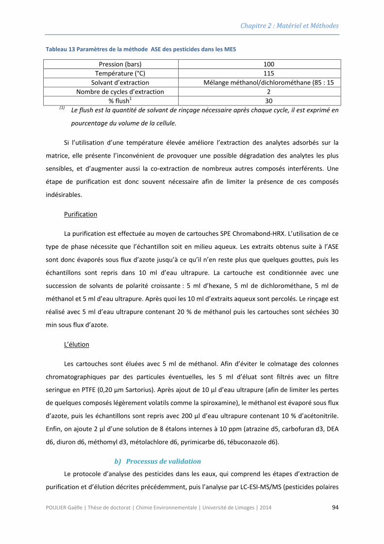
Chapitre 2 : Matériel et Méthodes
Tableau 13 Paramètres de la méthode ASE des pesticides dans les MES
Pression (bars) 100 Température (°C) 115
Solvant d’extraction Mélange méthanol/dichlorométhane (85 : 15
Nombre de cycles d’extraction 2 % flush1 30
(1) Le flush est la quantité de solvant de rinçage nécessaire après chaque cycle, il est exprimé en
pourcentage du volume de la cellule.
Si l’utilisation d’une température élevée améliore l’extraction des analytes adsorbés sur la
matrice, elle présente l’inconvénient de provoquer une possible dégradation des analytes les plus
sensibles, et d’augmenter aussi la co-extraction de nombreux autres composés interférents. Une
étape de purification est donc souvent nécessaire afin de limiter la présence de ces composés
indésirables.
Purification
La purification est effectuée au moyen de cartouches SPE Chromabond-HRX. L’utilisation de ce
type de phase nécessite que l’échantillon soit en milieu aqueux. Les extraits obtenus suite à l’ASE
sont donc évaporés sous flux d’azote jusqu’à ce qu’il n’en reste plus que quelques gouttes, puis les
échantillons sont repris dans 10 ml d’eau ultrapure. La cartouche est conditionnée avec une
succession de solvants de polarité croissante : 5 ml d’hexane, 5 ml de dichlorométhane, 5 ml de
méthanol et 5 ml d’eau ultrapure. Après quoi les 10 ml d’extraits aqueux sont percolés. Le rinçage est
réalisé avec 5 ml d’eau ultrapure contenant 20 % de méthanol puis les cartouches sont séchées 30
min sous flux d’azote.
L’élution
Les cartouches sont éluées avec 5 ml de méthanol. Afin d’éviter le colmatage des colonnes
chromatographiques par des particules éventuelles, les 5 ml d’éluat sont filtrés avec un filtre
seringue en PTFE (0,20 µm Sartorius). Après ajout de 10 µl d’eau ultrapure (afin de limiter les pertes
de quelques composés légèrement volatils comme la spiroxamine), le méthanol est évaporé sous flux
d’azote, puis les échantillons sont repris avec 200 µl d’eau ultrapure contenant 10 % d’acétonitrile.
Enfin, on ajoute 2 µl d’une solution de 8 étalons internes à 10 ppm (atrazine d5, carbofuran d3, DEA
d6, diuron d6, méthomyl d3, métolachlore d6, pyrimicarbe d6, tébuconazole d6).
b) Processus de validation
Le protocole d’analyse des pesticides dans les eaux, qui comprend les étapes d’extraction de
purification et d’élution décrites précédemment, puis l’analyse par LC-ESI-MS/MS (pesticides polaires
POULIER Gaëlle | Thèse de doctorat | Chimie Environnementale | Université de Limoges | 2014 94
Chapitre 2 : Matériel et Méthodes
neutres) a fait l’objet d’un processus de validation complet, selon les préconisations de la norme NF T
90-210 (AFNOR, 2009b). Le domaine d’étalonnage ayant déjà été effectuée par le laboratoire, les
critères restant à évaluer sont la limite de quantification, les rendements et la spécificité. L’ensemble
de ces paramètres ont été étudiés sur des sédiments prélevés au niveau du Trec et de l’Auvézère en
2012 (couche superficielle).
Validation pour l’analyse par LC-ESI/MS/MS
La spécificité a été déterminée par étude de la droite de recouvrement d’ajouts dosés post-
extraction, à quatre niveaux de concentration différents (5, 20, 30, 40 µg L-1) (n=2 ou n=3). Les
résultats sont visibles dans le Tableau 14. La méthode est spécifique pour toutes les molécules,
exceptées la flurtamone, la simazine et la terbuthylazine.
Les rendements ont été évalués à deux niveaux de dopage (40 et 80 ng g-1). Pour cela, 3 g de
sédiments sont dopés avec 5 ml d’eau ultrapure contenant 120 ou 240 ng de chaque pesticide.
L’ensemble est homogénéisé par agitation continue pendant 1h et placé au congélateur une nuit
(Northcott et Jones, 2000), avant lyophilisation et extraction selon le protocole décrit
précédemment. Les rendements obtenus (Tableau 14) varient de 47 % (carbendazime) à 129 %
(kresoxim méthyl). Le protocole d’extraction ASE est donc bien adapté aux molécules polaires
neutres. Le diuron, le méthomyl et la simazine, qui présentent tous trois un rendement nul, ont été
exclus de la méthode d’analyse.
POULIER Gaëlle | Thèse de doctorat | Chimie Environnementale | Université de Limoges | 2014 95
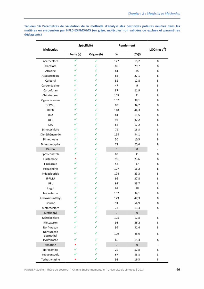
Chapitre 2 : Matériel et Méthodes
Tableau 14 Paramètres de validation de la méthode d’analyse des pesticides polaires neutres dans les matières en suspension par HPLC-ESI/MS/MS (en grisé, molécules non validées ou exclues et paramètres déclassants)
Molécules Spécificité Rendement
LOQ (ng g-1) Pente (a) Origine (b) % (CV)%
Acétochlore 127 15,2 8
Alachlore 85 29,7 8 Atrazine 81 25 8
Azoxystrobine 86 27,1 8
Carbaryl 85 12,8 8
Carbendazime 47 9 8 Carbofuran 87 21,9 8
Chlortoluron 109 41 8
Cyproconazole 107 38,1 8
DCPMU 83 34,2 8 DCPU 118 44,3 8
DEA 81 11,5 8
DET 94 42,2 8
DIA 62 17,2 8 Dimétachlore 79 15,3 8
Diméthénamide 118 34,1 8
Diméthoate 50 10,5 8
Dimétomorphe 71 25,6 8 Diuron 0 0 -
Epoxiconazole 83 41 8
Flurtamone 96 23,6 8
Flusilazole 53 17 8 Hexazinone 107 16,2 8
Imidaclopride 124 23,3 8
IPPMU 99 37,8 8
IPPU 99 33,7 8 Iragol 69 18 8
Isoproturon 102 34,1 8
Kresoxim-méthyl 129 47,3 8
Linuron 91 54,9 8 Métazachlore 73 13,4 8
Methomyl 0 0 -
Métolachlore 105 12,8 8
Métoxuron 93 26,2 8 Norflurazon 99 31,4 8 Norflurazon desmethyl 109 46,6 8
Pyrimicarbe 66 15,3 8
Simazine 0 0 -
Spiroxamine 29 52,8 8 Tebuconazole 67 33,8 8
Terbuthylazine 91 16,3 8
POULIER Gaëlle | Thèse de doctorat | Chimie Environnementale | Université de Limoges | 2014 96
Chapitre 2 : Matériel et Méthodes
Les rendements étant satisfaisants, il a été possible de valider une LQ selon les recommandations de
la norme NF T 90-210. Pour cela, les sédiments ont été dopés à 8 ng g-1 (LQ pressentie) puis extraits,
purifiés et analysés selon le protocole décrit précédemment. La LQ est validée si la concentration
obtenue dans les échantillons (XLQ) vérifie :
- XLQ - 2σLQ > LQ – 0,6 × LQ
- XLQ + 2σLQ < LQ + 0,6 × LQ
- avec σ l’écart-type mesuré pour 10 répétitions d’analyse.
La LQ de 8 ng g-1 a été validée pour toutes les molécules (Tableau 14).
2.7 Conclusion partielle Les développements analytiques réalisés au cours de cette étude et décrits dans ce chapitre
ont permis de mettre au point des méthodes d’analyse sur deux matrices différentes (eau naturelle
et sédiments), et ce pour une large gamme de molécules (composés polaires neutres, pesticides
hydrophobes, éléments trace métalliques). Les étapes de préparation et d’analyse des
échantillonneurs passifs ont également été optimisées.
Ces développements, indispensables à la réalisation de notre étude, nous ont permis
d’acquérir les résultats qui font l’objet du chapitre suivant.
POULIER Gaëlle | Thèse de doctorat | Chimie Environnementale | Université de Limoges | 2014 97

Chapitre 2 : Matériel et Méthodes
POULIER Gaëlle | Thèse de doctorat | Chimie Environnementale | Université de Limoges | 2014 98
Chapitre 3 :Etalonnage des échantillonneurs passifs en
laboratoire
POULIER Gaëlle | Thèse de doctorat | Chimie Environnementale | Université de Limoges | 2014 99

Chapitre 3 : Etalonnage des échantillonneurs passifs en laboratoire
POULIER Gaëlle | Thèse de doctorat | Chimie Environnementale | Université de Limoges | 2014 100
Chapitre 3 : Etalonnage des échantillonneurs passifs en laboratoire
3.1 Avant-propos Le calcul de la concentration moyenne dans l’eau, à partir de la masse d’analyte mesurée dans
les échantillonneurs de type POCIS et Chemcatcher (équation 6), nécessite de connaître les
constantes cinétiques d’accumulation de chacune des molécules cibles, pour chaque dispositif. En
cas d’utilisation de PRCs, les constantes cinétiques de désorption des molécules choisies doivent
également être connues. Cette étape est généralement réalisée en laboratoire, en microcosmes
permettant de contrôler la température, la vitesse du courant et la concentration dans l’eau.
Toutefois, ces expérimentations sons longues et coûteuses, et doivent être répétées pour chaque
nouvelle molécule d’intérêt. Aussi, de nombreux auteurs ont tenté de lier les constantes cinétiques
d’accumulation aux propriétés physico-chimiques des composés, notamment le log Kow.
Concernant le POCIS, toutes les tentatives de modélisation sont restées vaines, il n’est donc
pas possible, en l’état actuel des connaissances, de prédire le Rs des molécules cibles à partir de leurs
caractéristiques structurales ou chimiques. Par conséquent, l’étape de calibration en laboratoire
reste indispensable pour une utilisation quantitative ou semi-quantitative de l’outil. L’un des
premiers buts de ce travail de thèse était donc de réaliser la calibration du POCIS pour les molécules
sélectionnées avec pour objectifs de :
• vérifier l’applicabilité du POCIS pour les molécules ciblées. En d’autres termes, les Rs obtenus
doivent être assez élevés pour que la masse d’analytes accumulée au cours de l’exposition
puisse être quantifiée,
• déterminer le temps d’exposition adéquat, garantissant le maintien du régime intégratif pour
toutes les molécules,
• vérifier le potentiel de la DIA en tant que PRC.
Ces questions sont abordées dans la sous-partie 2 de cette section.
Concernant le Chemcatcher, un modèle empirique prédisant le Rs des analytes à partir du Log
de Kow a été développé par Vrana et al. (2007). Toutefois, ce modèle a été validé sur un ensemble de
molécules incluant principalement des HAPs. Seuls trois pesticides ont été étudiés. Par conséquent,
l’applicabilité de ce modèle pour des composés très différents des HAPs en termes de propriétés
physico-chimiques doit encore être vérifiée. Un travail a donc été engagé dans ce sens, avec pour
objectifs de :
•vérifier l’applicabilité du Chemcatcher pour les 17 pesticides sélectionnés,
POULIER Gaëlle | Thèse de doctorat | Chimie Environnementale | Université de Limoges | 2014 101
Chapitre 3 : Etalonnage des échantillonneurs passifs en laboratoire
•identifier des PRCs potentiels. Vrana et al. (2006) ont montré que la phénanthrène et
l’acénaphtène pouvaient être utilisées en tant que PRCs mais il serait souhaitable d’identifier
également des PRCs de la famille des pesticides, l’outil devant être utilisé ultérieurement pour cette
famille de composés,
•vérifier si le modèle développé par Vrana et al. (2007) pour les HAPs est valide pour les
pesticides, et le cas échéant, proposer un modèle adéquat
Ces questions sont détaillées dans la publication n°1, disponible dans la sous-partie 3 de cette
section.
POULIER Gaëlle | Thèse de doctorat | Chimie Environnementale | Université de Limoges | 2014 102
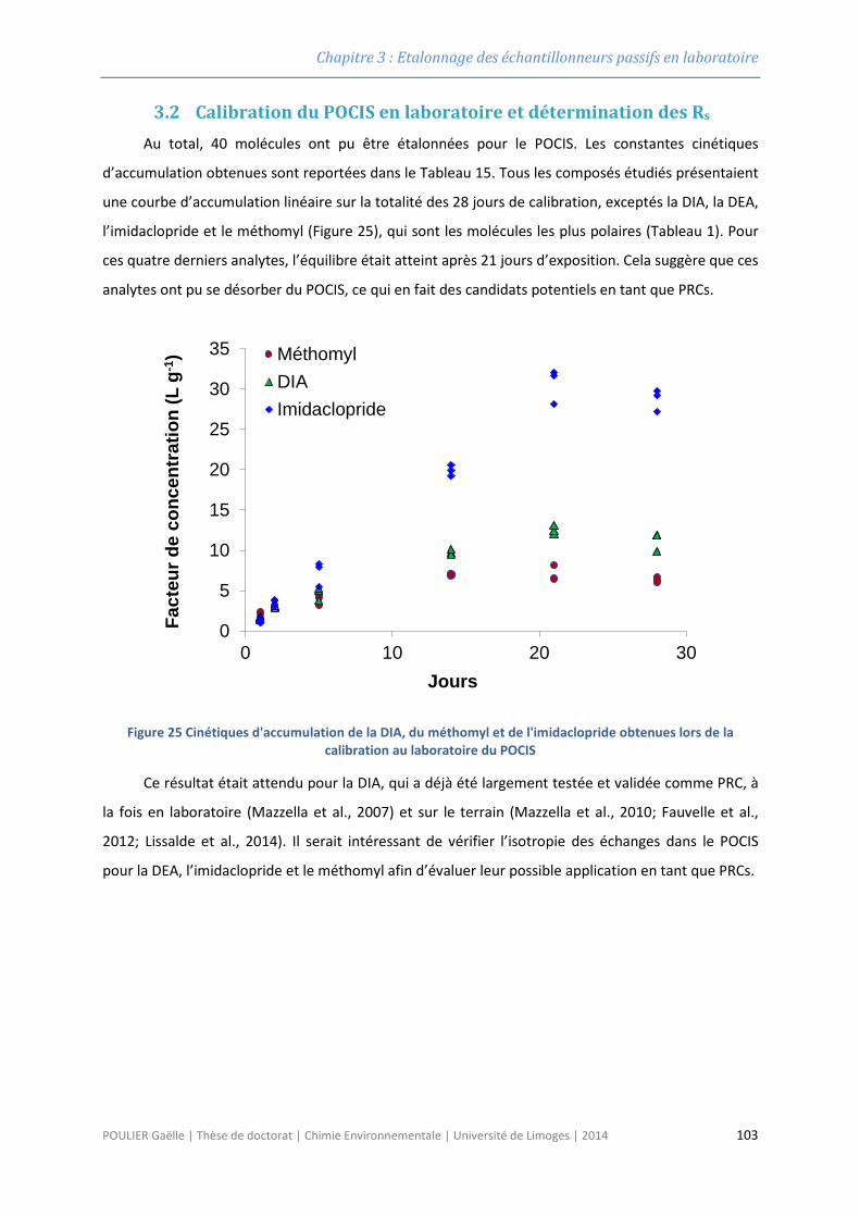
Chapitre 3 : Etalonnage des échantillonneurs passifs en laboratoire
3.2 Calibration du POCIS en laboratoire et détermination des Rs Au total, 40 molécules ont pu être étalonnées pour le POCIS. Les constantes cinétiques
d’accumulation obtenues sont reportées dans le Tableau 15. Tous les composés étudiés présentaient
une courbe d’accumulation linéaire sur la totalité des 28 jours de calibration, exceptés la DIA, la DEA,
l’imidaclopride et le méthomyl (Figure 25), qui sont les molécules les plus polaires (Tableau 1). Pour
ces quatre derniers analytes, l’équilibre était atteint après 21 jours d’exposition. Cela suggère que ces
analytes ont pu se désorber du POCIS, ce qui en fait des candidats potentiels en tant que PRCs.
Figure 25 Cinétiques d'accumulation de la DIA, du méthomyl et de l'imidaclopride obtenues lors de la calibration au laboratoire du POCIS
Ce résultat était attendu pour la DIA, qui a déjà été largement testée et validée comme PRC, à
la fois en laboratoire (Mazzella et al., 2007) et sur le terrain (Mazzella et al., 2010; Fauvelle et al.,
2012; Lissalde et al., 2014). Il serait intéressant de vérifier l’isotropie des échanges dans le POCIS
pour la DEA, l’imidaclopride et le méthomyl afin d’évaluer leur possible application en tant que PRCs.
0
5
10
15
20
25
30
35
0 10 20 30
Fact
eurd
e co
ncen
trat
ion
(L g
-1)
Jours
MéthomylDIAImidaclopride
POULIER Gaëlle | Thèse de doctorat | Chimie Environnementale | Université de Limoges | 2014 103
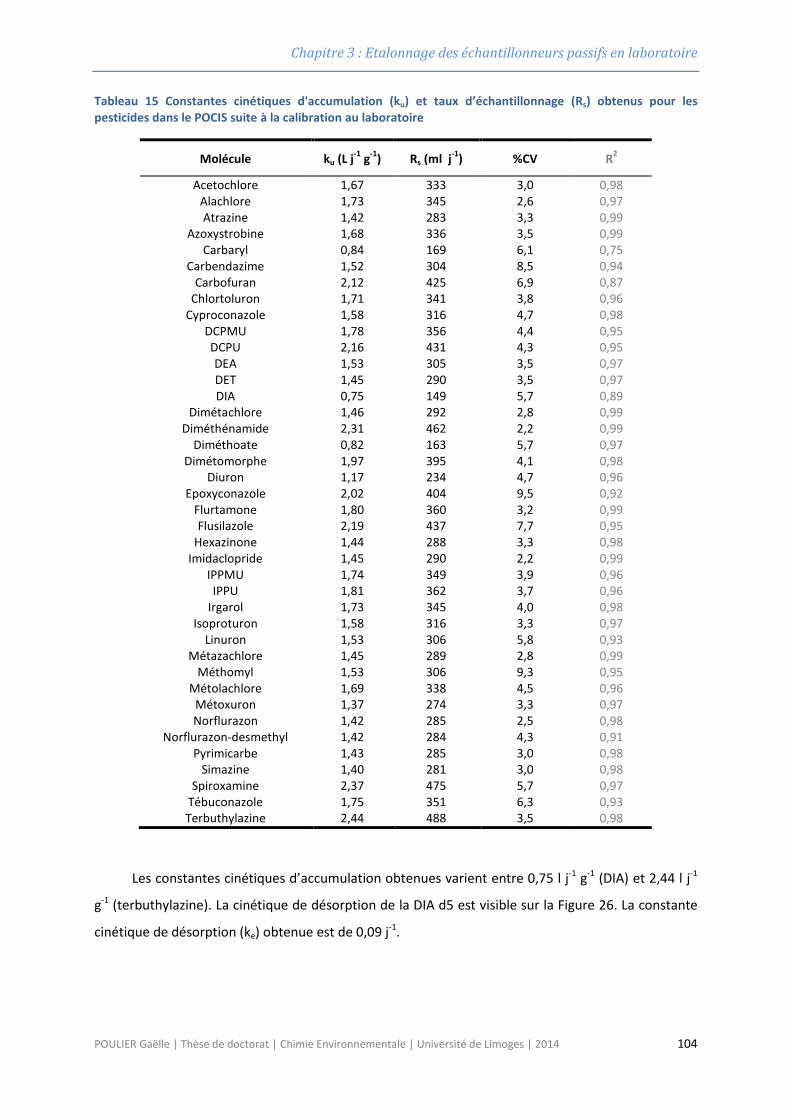
Chapitre 3 : Etalonnage des échantillonneurs passifs en laboratoire
Tableau 15 Constantes cinétiques d'accumulation (ku) et taux d’échantillonnage (Rs) obtenus pour les pesticides dans le POCIS suite à la calibration au laboratoire
Molécule ku (L j-1 g-1) Rs (ml j-1) %CV R2
Acetochlore 1,67 333 3,0 0,98 Alachlore 1,73 345 2,6 0,97 Atrazine 1,42 283 3,3 0,99
Azoxystrobine 1,68 336 3,5 0,99 Carbaryl 0,84 169 6,1 0,75
Carbendazime 1,52 304 8,5 0,94 Carbofuran 2,12 425 6,9 0,87
Chlortoluron 1,71 341 3,8 0,96 Cyproconazole 1,58 316 4,7 0,98
DCPMU 1,78 356 4,4 0,95 DCPU 2,16 431 4,3 0,95 DEA 1,53 305 3,5 0,97 DET 1,45 290 3,5 0,97 DIA 0,75 149 5,7 0,89
Dimétachlore 1,46 292 2,8 0,99 Diméthénamide 2,31 462 2,2 0,99
Diméthoate 0,82 163 5,7 0,97 Dimétomorphe 1,97 395 4,1 0,98
Diuron 1,17 234 4,7 0,96 Epoxyconazole 2,02 404 9,5 0,92
Flurtamone 1,80 360 3,2 0,99 Flusilazole 2,19 437 7,7 0,95
Hexazinone 1,44 288 3,3 0,98 Imidaclopride 1,45 290 2,2 0,99
IPPMU 1,74 349 3,9 0,96 IPPU 1,81 362 3,7 0,96
Irgarol 1,73 345 4,0 0,98 Isoproturon 1,58 316 3,3 0,97
Linuron 1,53 306 5,8 0,93 Métazachlore 1,45 289 2,8 0,99
Méthomyl 1,53 306 9,3 0,95 Métolachlore 1,69 338 4,5 0,96
Métoxuron 1,37 274 3,3 0,97 Norflurazon 1,42 285 2,5 0,98
Norflurazon-desmethyl 1,42 284 4,3 0,91 Pyrimicarbe 1,43 285 3,0 0,98
Simazine 1,40 281 3,0 0,98 Spiroxamine 2,37 475 5,7 0,97
Tébuconazole 1,75 351 6,3 0,93 Terbuthylazine 2,44 488 3,5 0,98
Les constantes cinétiques d’accumulation obtenues varient entre 0,75 l j-1 g-1 (DIA) et 2,44 l j-1
g-1 (terbuthylazine). La cinétique de désorption de la DIA d5 est visible sur la Figure 26. La constante
cinétique de désorption (ke) obtenue est de 0,09 j-1.
POULIER Gaëlle | Thèse de doctorat | Chimie Environnementale | Université de Limoges | 2014 104
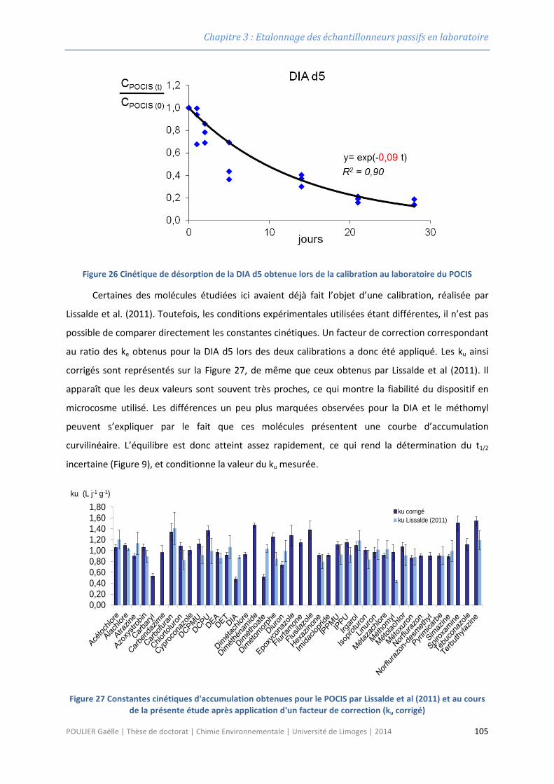
Chapitre 3 : Etalonnage des échantillonneurs passifs en laboratoire
Figure 26 Cinétique de désorption de la DIA d5 obtenue lors de la calibration au laboratoire du POCIS
Certaines des molécules étudiées ici avaient déjà fait l’objet d’une calibration, réalisée par
Lissalde et al. (2011). Toutefois, les conditions expérimentales utilisées étant différentes, il n’est pas
possible de comparer directement les constantes cinétiques. Un facteur de correction correspondant
au ratio des ke obtenus pour la DIA d5 lors des deux calibrations a donc été appliqué. Les ku ainsi
corrigés sont représentés sur la Figure 27, de même que ceux obtenus par Lissalde et al (2011). Il
apparaît que les deux valeurs sont souvent très proches, ce qui montre la fiabilité du dispositif en
microcosme utilisé. Les différences un peu plus marquées observées pour la DIA et le méthomyl
peuvent s’expliquer par le fait que ces molécules présentent une courbe d’accumulation
curvilinéaire. L’équilibre est donc atteint assez rapidement, ce qui rend la détermination du t1/2
incertaine (Figure 9), et conditionne la valeur du ku mesurée.
Figure 27 Constantes cinétiques d'accumulation obtenues pour le POCIS par Lissalde et al (2011) et au cours de la présente étude après application d'un facteur de correction (ku corrigé)
0,000,200,400,600,801,001,201,401,601,80 ku corrigé
ku Lissalde (2011)
ku (L j-1 g-1)
POULIER Gaëlle | Thèse de doctorat | Chimie Environnementale | Université de Limoges | 2014 105
Chapitre 3 : Etalonnage des échantillonneurs passifs en laboratoire
La calibration en laboratoire de l’échantillonneur passif Chemcatcher, dédié aux composés
hydrophobes, a également été réalisée. Les résultats sont détaillés dans la Publication n°1.
POULIER Gaëlle | Thèse de doctorat | Chimie Environnementale | Université de Limoges | 2014 106
Chapitre 3 : Etalonnage des échantillonneurs passifs en laboratoire
3.3 Publication 1 “Calibration of the Chemcatcher passive sampler
and proposition of a novel model for estimating sampling rates
of hydrophobic pesticides”
POULIER Gaëlle | Thèse de doctorat | Chimie Environnementale | Université de Limoges | 2014 107

Chapitre 3 : Etalonnage des échantillonneurs passifs en laboratoire
POULIER Gaëlle | Thèse de doctorat | Chimie Environnementale | Université de Limoges | 2014 108
Chapitre 3 : Etalonnage des échantillonneurs passifs en laboratoire
Calibration of the Chemcatcher passive sampler and proposition of a novel
model for estimating sampling rates of hydrophobic pesticides
Gaëlle Pouliera, b, Adeline Charriaub , Sophie Lissaldeb, Rémy Buzier b, François Delmasa, Patrice
Fondanèchea, Gilles Guibaud b, Nicolas Mazzellaa
a Unité de recherche REBX ; Groupement Irstea de Bordeaux, 50 avenue de Verdun, Gazinet, 33612 Cestas
cedex, France b Université de Limoges Groupement de Recherche Eau Sol Environnement (GRESE), 123 Avenue Albert
Thomas 87060 Limoges Cedex, France Corresponding authors: [email protected], [email protected]
Abstract The non-polar version of the Chemcatcher passive sampler has been used in numerous studies for the
monitoring of different hydrophobic compounds including polycyclic aromatic hydrocarbons (PAHs), polybrominated diphenyl ethers (PBDEs) and pesticides. Sampling rates of compounds, a key parameter to calculate water concentrations from amounts caught in the sampler, have been shown to be mainly influenced by hydrophobicity for PAHs. However little is known regarding pesticides. In this study, sampling rates of 17 pesticides were measured during a laboratory calibration experiment. Performance and reference compounds offload was also studied. After testing different empirical models for describing sampling rates of pesticides, we concluded that the unique criterion of hydrophobicity is insufficient to well predict sampling rates. The best relationship was obtained with a model including multiple additional variables such as density, molar volume, molecular weight and solvent access surface area. This model, developed specifically for pesticides, was not suitable for other types of compounds like PCBs and PBDEs so we concluded that sampling rates of compounds should always been determined during laboratory calibrations, and that the use of inadequate empirical relationship could lead to highly biased data.
Keywords: Chemcatcher, pesticides, passive sampling, modelling, sampling rates, calibration, water
1- Introduction The intensive use of pesticides for several decades since 1950s has led to a diffuse contamination of water
systems worldwide and quality monitoring is now mandatory by the Water Framework Directive in all Member States (EU, 2000). For now, grab sampling followed by chromatographic analysis is the most widespread strategy implemented in regulatory monitoring programs. However, this approach suffers from a lack of temporal representativeness since the sampling frequency is at best about 12 grab samples a year. Moreover the most hydrophobic compounds tends to adsorb on particles in water or accumulate in biota; hence freely dissolved concentrations of such compounds are often very low, typically in the pg L-1 to ng L-1 range. Measuring these low concentrations in grab samples requires either sampling huge volume of water, or highly sophisticated analytical technics. The development of several passive samplers dedicated to hydrophobic compounds in the last decades may help overcoming this issue. These include the semi-permeable membrane device (SPMD; Huckins et al. (1993)), the membrane enclosed sportive coating (MESCO; Vrana et al. (2001)) or silicone rubber Rusina et al. (2007).
The Chemcatcher passive sampler was developed by Portsmouth University (Kingston et al., 2000). Depending on the receiving phase and the covering diffusion limiting membrane, the Chemcatcher can be
POULIER Gaëlle | Thèse de doctorat | Chimie Environnementale | Université de Limoges | 2014 109
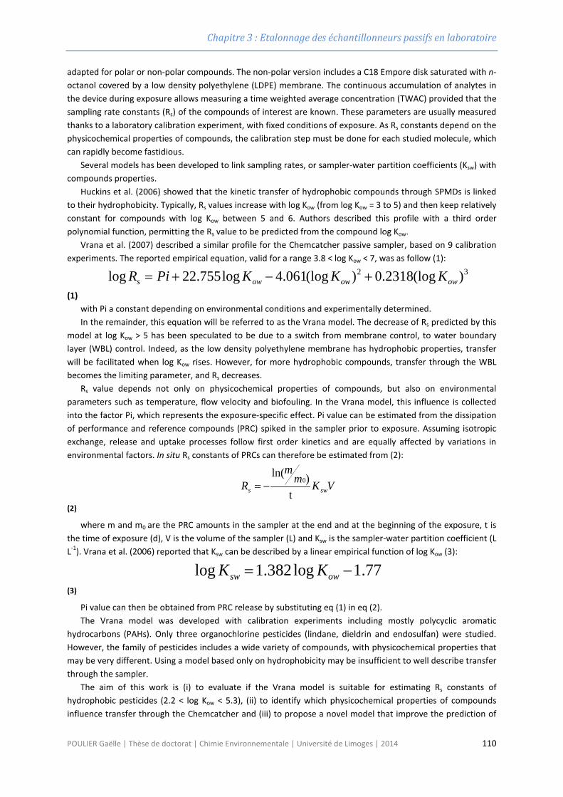
Chapitre 3 : Etalonnage des échantillonneurs passifs en laboratoire
adapted for polar or non-polar compounds. The non-polar version includes a C18 Empore disk saturated with n-octanol covered by a low density polyethylene (LDPE) membrane. The continuous accumulation of analytes in the device during exposure allows measuring a time weighted average concentration (TWAC) provided that the sampling rate constants (Rs) of the compounds of interest are known. These parameters are usually measured thanks to a laboratory calibration experiment, with fixed conditions of exposure. As Rs constants depend on the physicochemical properties of compounds, the calibration step must be done for each studied molecule, which can rapidly become fastidious.
Several models has been developed to link sampling rates, or sampler-water partition coefficients (Ksw) with compounds properties.
Huckins et al. (2006) showed that the kinetic transfer of hydrophobic compounds through SPMDs is linked to their hydrophobicity. Typically, Rs values increase with log Kow (from log Kow = 3 to 5) and then keep relatively constant for compounds with log Kow between 5 and 6. Authors described this profile with a third order polynomial function, permitting the Rs value to be predicted from the compound log Kow.
Vrana et al. (2007) described a similar profile for the Chemcatcher passive sampler, based on 9 calibration experiments. The reported empirical equation, valid for a range 3.8 < log Kow < 7, was as follow (1):
32 )(log2318.0)(log061.4log755.22log owowows KKKPiR +−+=
(1) with Pi a constant depending on environmental conditions and experimentally determined. In the remainder, this equation will be referred to as the Vrana model. The decrease of Rs predicted by this
model at log Kow > 5 has been speculated to be due to a switch from membrane control, to water boundary layer (WBL) control. Indeed, as the low density polyethylene membrane has hydrophobic properties, transfer will be facilitated when log Kow rises. However, for more hydrophobic compounds, transfer through the WBL becomes the limiting parameter, and Rs decreases.
Rs value depends not only on physicochemical properties of compounds, but also on environmental parameters such as temperature, flow velocity and biofouling. In the Vrana model, this influence is collected into the factor Pi, which represents the exposure-specific effect. Pi value can be estimated from the dissipation of performance and reference compounds (PRC) spiked in the sampler prior to exposure. Assuming isotropic exchange, release and uptake processes follow first order kinetics and are equally affected by variations in environmental factors. In situ Rs constants of PRCs can therefore be estimated from (2):
VKmm
R sws t)ln(
0−=
(2)
where m and m0 are the PRC amounts in the sampler at the end and at the beginning of the exposure, t is the time of exposure (d), V is the volume of the sampler (L) and Ksw is the sampler-water partition coefficient (L L-1). Vrana et al. (2006) reported that Ksw can be described by a linear empirical function of log Kow (3):
77.1log382.1log −= owsw KK
(3)
Pi value can then be obtained from PRC release by substituting eq (1) in eq (2). The Vrana model was developed with calibration experiments including mostly polycyclic aromatic
hydrocarbons (PAHs). Only three organochlorine pesticides (lindane, dieldrin and endosulfan) were studied. However, the family of pesticides includes a wide variety of compounds, with physicochemical properties that may be very different. Using a model based only on hydrophobicity may be insufficient to well describe transfer through the sampler.
The aim of this work is (i) to evaluate if the Vrana model is suitable for estimating Rs constants of hydrophobic pesticides (2.2 < log Kow < 5.3), (ii) to identify which physicochemical properties of compounds influence transfer through the Chemcatcher and (iii) to propose a novel model that improve the prediction of
POULIER Gaëlle | Thèse de doctorat | Chimie Environnementale | Université de Limoges | 2014 110
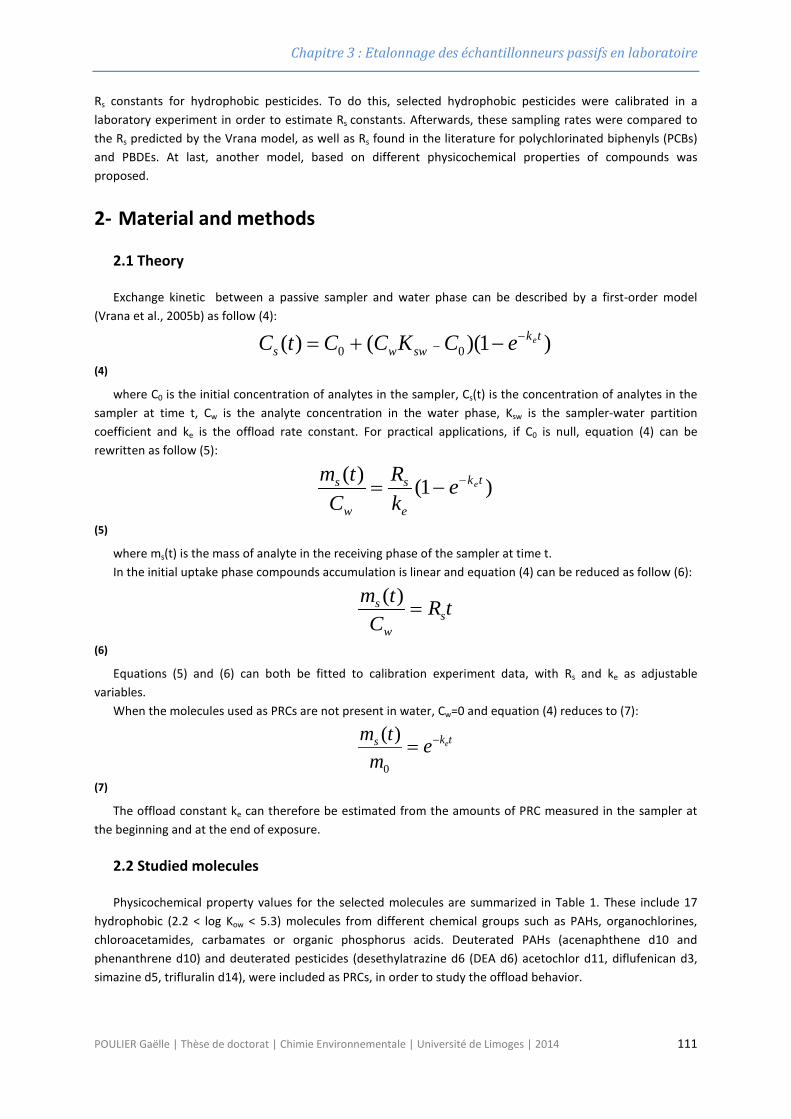
Chapitre 3 : Etalonnage des échantillonneurs passifs en laboratoire
Rs constants for hydrophobic pesticides. To do this, selected hydrophobic pesticides were calibrated in a laboratory experiment in order to estimate Rs constants. Afterwards, these sampling rates were compared to the Rs predicted by the Vrana model, as well as Rs found in the literature for polychlorinated biphenyls (PCBs) and PBDEs. At last, another model, based on different physicochemical properties of compounds was proposed.
2- Material and methods
2.1 Theory
Exchange kinetic between a passive sampler and water phase can be described by a first-order model (Vrana et al., 2005b) as follow (4):
)1)(()( 00tk
swwseeCKCCtC −
− −+=
(4)
where C0 is the initial concentration of analytes in the sampler, Cs(t) is the concentration of analytes in the sampler at time t, Cw is the analyte concentration in the water phase, Ksw is the sampler-water partition coefficient and ke is the offload rate constant. For practical applications, if C0 is null, equation (4) can be rewritten as follow (5):
)1()( tk
e
s
w
s eekR
Ctm −−=
(5)
where ms(t) is the mass of analyte in the receiving phase of the sampler at time t. In the initial uptake phase compounds accumulation is linear and equation (4) can be reduced as follow (6):
tRC
tms
w
s =)(
(6)
Equations (5) and (6) can both be fitted to calibration experiment data, with Rs and ke as adjustable variables.
When the molecules used as PRCs are not present in water, Cw=0 and equation (4) reduces to (7):
tks eem
tm −=0
)(
(7)
The offload constant ke can therefore be estimated from the amounts of PRC measured in the sampler at the beginning and at the end of exposure.
2.2 Studied molecules
Physicochemical property values for the selected molecules are summarized in Table 1. These include 17 hydrophobic (2.2 < log Kow < 5.3) molecules from different chemical groups such as PAHs, organochlorines, chloroacetamides, carbamates or organic phosphorus acids. Deuterated PAHs (acenaphthene d10 and phenanthrene d10) and deuterated pesticides (desethylatrazine d6 (DEA d6) acetochlor d11, diflufenican d3, simazine d5, trifluralin d14), were included as PRCs, in order to study the offload behavior.
POULIER Gaëlle | Thèse de doctorat | Chimie Environnementale | Université de Limoges | 2014 111
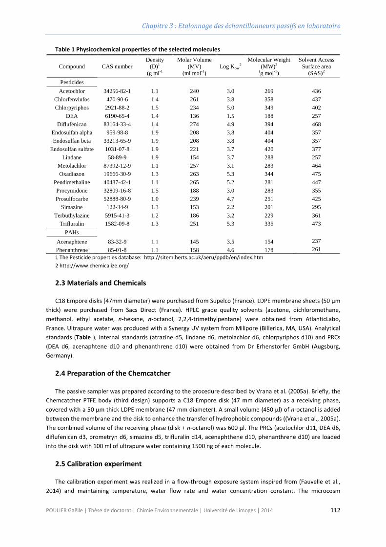
Chapitre 3 : Etalonnage des échantillonneurs passifs en laboratoire
Table 1 Physicochemical properties of the selected molecules
Compound CAS number Density
(D)1 (g ml-1
Molar Volume (MV)
(ml mol-1) Log Kow
2 Molecular Weight
(MW)2
(g mol-1)
Solvent Access Surface area
(SAS)2 Pesticides Acetochlor 34256-82-1 1.1 240 3.0 269 436
Chlorfenvinfos 470-90-6 1.4 261 3.8 358 437 Chlorpyriphos 2921-88-2 1.5 234 5.0 349 402
DEA 6190-65-4 1.4 136 1.5 188 257 Diflufenican 83164-33-4 1.4 274 4.9 394 468
Endosulfan alpha 959-98-8 1.9 208 3.8 404 357 Endosulfan beta 33213-65-9 1.9 208 3.8 404 357
Endosulfan sulfate 1031-07-8 1.9 221 3.7 420 377 Lindane 58-89-9 1.9 154 3.7 288 257
Metolachlor 87392-12-9 1.1 257 3.1 283 464 Oxadiazon 19666-30-9 1.3 263 5.3 344 475
Pendimethaline 40487-42-1 1.1 265 5.2 281 447 Procymidone 32809-16-8 1.5 188 3.0 283 355 Prosulfocarbe 52888-80-9 1.0 239 4.7 251 425
Simazine 122-34-9 1.3 153 2.2 201 295 Terbuthylazine 5915-41-3 1.2 186 3.2 229 361
Trifluralin 1582-09-8 1.3 251 5.3 335 473 PAHs
Acenaphtene 83-32-9 1.1 145 3.5 154 237 Phenanthrene 85-01-8 1.1 158 4.6 178 261 1 The Pesticide properties database: http://sitem.herts.ac.uk/aeru/ppdb/en/index.htm 2 http://www.chemicalize.org/
2.3 Materials and Chemicals
C18 Empore disks (47mm diameter) were purchased from Supelco (France). LDPE membrane sheets (50 µm thick) were purchased from Sacs Direct (France). HPLC grade quality solvents (acetone, dichloromethane, methanol, ethyl acetate, n-hexane, n-octanol, 2,2,4-trimethylpentane) were obtained from AtlanticLabo, France. Ultrapure water was produced with a Synergy UV system from Milipore (Billerica, MA, USA). Analytical standards (Table ), internal standards (atrazine d5, lindane d6, metolachlor d6, chlorpyriphos d10) and PRCs (DEA d6, acenaphtene d10 and phenanthrene d10) were obtained from Dr Erhenstorfer GmbH (Augsburg, Germany).
2.4 Preparation of the Chemcatcher
The passive sampler was prepared according to the procedure described by Vrana et al. (2005a). Briefly, the Chemcatcher PTFE body (third design) supports a C18 Empore disk (47 mm diameter) as a receiving phase, covered with a 50 µm thick LDPE membrane (47 mm diameter). A small volume (450 µl) of n-octanol is added between the membrane and the disk to enhance the transfer of hydrophobic compounds ((Vrana et al., 2005a). The combined volume of the receiving phase (disk + n-octanol) was 600 µl. The PRCs (acetochlor d11, DEA d6, diflufenican d3, prometryn d6, simazine d5, trifluralin d14, acenaphthene d10, phenanthrene d10) are loaded into the disk with 100 ml of ultrapure water containing 1500 ng of each molecule.
2.5 Calibration experiment
The calibration experiment was realized in a flow-through exposure system inspired from (Fauvelle et al., 2014) and maintaining temperature, water flow rate and water concentration constant. The microcosm
POULIER Gaëlle | Thèse de doctorat | Chimie Environnementale | Université de Limoges | 2014 112
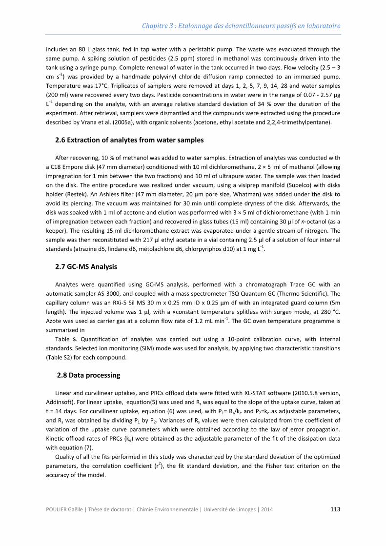
Chapitre 3 : Etalonnage des échantillonneurs passifs en laboratoire
includes an 80 L glass tank, fed in tap water with a peristaltic pump. The waste was evacuated through the same pump. A spiking solution of pesticides (2.5 ppm) stored in methanol was continuously driven into the tank using a syringe pump. Complete renewal of water in the tank occurred in two days. Flow velocity (2.5 – 3 cm s-1) was provided by a handmade polyvinyl chloride diffusion ramp connected to an immersed pump. Temperature was 17°C. Triplicates of samplers were removed at days 1, 2, 5, 7, 9, 14, 28 and water samples (200 ml) were recovered every two days. Pesticide concentrations in water were in the range of 0.07 - 2.57 μg L−1 depending on the analyte, with an average relative standard deviation of 34 % over the duration of the experiment. After retrieval, samplers were dismantled and the compounds were extracted using the procedure described by Vrana et al. (2005a), with organic solvents (acetone, ethyl acetate and 2,2,4-trimethylpentane).
2.6 Extraction of analytes from water samples
After recovering, 10 % of methanol was added to water samples. Extraction of analytes was conducted with a C18 Empore disk (47 mm diameter) conditioned with 10 ml dichloromethane, 2 × 5 ml of methanol (allowing impregnation for 1 min between the two fractions) and 10 ml of ultrapure water. The sample was then loaded on the disk. The entire procedure was realized under vacuum, using a visiprep manifold (Supelco) with disks holder (Restek). An Ashless filter (47 mm diameter, 20 µm pore size, Whatman) was added under the disk to avoid its piercing. The vacuum was maintained for 30 min until complete dryness of the disk. Afterwards, the disk was soaked with 1 ml of acetone and elution was performed with 3 × 5 ml of dichloromethane (with 1 min of impregnation between each fraction) and recovered in glass tubes (15 ml) containing 30 µl of n-octanol (as a keeper). The resulting 15 ml dichloromethane extract was evaporated under a gentle stream of nitrogen. The sample was then reconstituted with 217 µl ethyl acetate in a vial containing 2.5 µl of a solution of four internal standards (atrazine d5, lindane d6, métolachlore d6, chlorpyriphos d10) at 1 mg L-1.
2.7 GC-MS Analysis
Analytes were quantified using GC-MS analysis, performed with a chromatograph Trace GC with an automatic sampler AS-3000, and coupled with a mass spectrometer TSQ Quantum GC (Thermo Scientific). The capillary column was an RXi-5 Sil MS 30 m x 0.25 mm ID x 0.25 µm df with an integrated guard column (5m length). The injected volume was 1 µl, with a «constant temperature splitless with surge» mode, at 280 °C. Azote was used as carrier gas at a column flow rate of 1.2 mL min-1. The GC oven temperature programme is summarized in
Table S. Quantification of analytes was carried out using a 10-point calibration curve, with internal standards. Selected ion monitoring (SIM) mode was used for analysis, by applying two characteristic transitions (Table S2) for each compound.
2.8 Data processing
Linear and curvilinear uptakes, and PRCs offload data were fitted with XL-STAT software (2010.5.8 version, Addinsoft). For linear uptake, equation(5) was used and Rs was equal to the slope of the uptake curve, taken at t = 14 days. For curvilinear uptake, equation (6) was used, with P1= Rs/ke and P2=ke as adjustable parameters, and Rs was obtained by dividing P1 by P2. Variances of Rs values were then calculated from the coefficient of variation of the uptake curve parameters which were obtained according to the law of error propagation. Kinetic offload rates of PRCs (ke) were obtained as the adjustable parameter of the fit of the dissipation data with equation (7).
Quality of all the fits performed in this study was characterized by the standard deviation of the optimized parameters, the correlation coefficient (r2), the fit standard deviation, and the Fisher test criterion on the accuracy of the model.
POULIER Gaëlle | Thèse de doctorat | Chimie Environnementale | Université de Limoges | 2014 113
Chapitre 3 : Etalonnage des échantillonneurs passifs en laboratoire
3- Results and discussion
3.1 Accumulation of analytes and sampling rate constants
For DEA, acetochlor, metolachlor, simazine and terbuthylazine, uptake was very low (m/Cw values below 0.02 L after 28 days). Results of the first order model fits were poor and thus Rs values were not determined for these pesticides. Due to their low to moderate hydrophobicity (log kow < 3.2), the polar version of the Chemcatcher (SDB-RPS or SDB-XC disks with polyethersulfone membrane) may be more suitable for these pesticides (Schäfer et al., 2008; Vermeirssen et al., 2012). Typical uptake curves obtained for the other selected compounds after 28 days of Chemcatcher exposure are shown in Figure 1. Two different behaviors were observed. Compounds with log Kow < 3.8 such as oxadiazon and lindane exhibited linear uptake over the 28 days of exposure (Figure 1a). For these molecules, the calculated Rs constants were low and ranged from 1.4 ml d-1(chlorfenvinphos) to 44 ml d-1 (Endosulfan beta) (Table 2). In contrast, endosulfan alpha (log Kow = 3.8) and more hydrophobic compounds showed curvilinear accumulation in the sampler after 14 days of exposure (Figure 1b) and the obtained Rs were higher, ranging from 38.7 (oxadiazon) to 906.3 ml d-1 (chlorpyriphos).
Regression models were statistically validated (p < 0.005) for all of these pesticides, and the correlation coefficients were good, with values ranging from 0.98 (oxadiazon) to 0.80 (diflufenican) (Table 2).
Figure 1 Typical linear (a) and curvilinear (b) uptake curves of selected pesticides in the Chemcatcher
passive sampler. The draw lines show the fits of the data using Eq.() or Eq.().
012345678
0 10 20 30
m /
Cw
Exposure (day)
PendimethalineTrifluralin
0.0
0.2
0.4
0.6
0.8
1.0
1.2
0 10 20 30
m /
Cw
Exposure (day)
Endosulfan betaLindane
a
b
POULIER Gaëlle | Thèse de doctorat | Chimie Environnementale | Université de Limoges | 2014 114
Chapitre 3 : Etalonnage des échantillonneurs passifs en laboratoire
Table 2 Sampling rates (Rs) obtained for selected pesticides in the Chemcatcher passive sampler
Pesticide Log Kow Rs (ml d-1) %CV a r2 b Behaviour
Procymidone 3.0 1.9 6.0 0.86 Linear Lindane 3.7 12.7 3.0 0.94 Linear Endosulfan sulfate 3.7 10.6 5.0 0.92 Linear Endosulfan alpha 3.8 265.4 12.6 0.94 Curvilinear Endosulfan beta 3.8 44.0 4.0 0.94 Linear Chlorfenvinfos 3.8 1.4 6.7 0.83 Linear Prosulfocarbe 4.7 203.5 10.9 0.93 Curvilinear Diflufenican 4.9 61.9 20.3 0.80 Curvilinear Chlorpyriphos 5.0 906.3 16.6 0.93 Curvilinear Pendimethaline 5.2 555.7 13.7 0.92 Curvilinear Oxadiazon 5.3 38.7 34.3 0.98 Curvilinear Trifluraline 5.3 217.9 16.1 0.96 Curvilinear
a Coefficient of variation b Correlation coefficient of the linear or non-linear regression fitted with Eq.(6) and Eq.(5) respectively.
3.2 PRCs desorption
Chemcatcher were spiked with 8 deuterated coumpounds (acetochlore d11, DEA d6, diflufenican d3, prometryn d6, simazine d5, trifluralin d14, acenaphthene d10, phenanthrene d10), in order to study the offload behavior. Significant release could be observed only for DEA d6, acenaphtene d10 and phenanthrene d10 (Figure 2). The exchange rate constants ke for each compounds were obtained by fitting the data with Eq.(7). Values were 0.028 d-1 for DEA d6 (r2 =0.67, p < 0.05), 0.031 d-1 for acenaphthene d10 (r2=0.63, p < 0.05) and 0.042 d-1 for phenanthrene d10 (r2=0.89, p < 0.05). According to Vrana et al. (2007), ke should decrease when hydrophobicity rises. But here, the ke values obtained for the three compounds are very similar even though their hydrophobicity is very different (Table 1). This will be further discussed in part 3.3.
In general, it is recommended that the amount of retained PRC is larger than 20 % and smaller than 80 % of the initial amount in order to avoid inaccuracies due to insignificant dissipation or quantification near the quantification limit. After 15 days of exposure (which correspond to the typical exposure period of passive samplers in the field) the percentage of offload was about 40 % of the initial amount for the three compounds. Moreover, as isotropic behavior was demonstrated by Vrana et al. (2006) for acenaphtene and phenanthrene, this led to the conclusion that these compounds have good potential as PRC. For DEA, isotropic behavior could not be verified in this study because the molecule did not accumulate in the sampler.
Figure 2 Release of DEA d6, Phenanthrene d10 and Acenaphtene d10 from the Chemcatcher passive sampler.
Concentrations Ct are plotted relative to the dosing concentration C0
0,0
0,2
0,4
0,6
0,8
1,0
1,2
0 5 10 15 20 25 30
Ct/ C
0
days
DEA d6Acenaphtene d10Phenanthrene d10
POULIER Gaëlle | Thèse de doctorat | Chimie Environnementale | Université de Limoges | 2014 115
Chapitre 3 : Etalonnage des échantillonneurs passifs en laboratoire
3.3 Comparison with the Vrana Log Kow Model
According to the Vrana model, uptake of analytes in the Chemcatcher passive sampler only depends on their hydrophobicity and can be described with eq.(1). To verify this, Rs constants of PRCs (DEA d6, acenaphthene d10 and phenanthrene d10) were calculated from their ke value and their log Kow value by combining Eq.(2) and Eq.(3). Results are reported in Table 3.
Table 3 Summary of PRCs exchange kinetic parameters obtained from 29-day exposure in a laboratory experiment.
Log Kow % PRC ke (d-1) Calculated Rs a (L d-1) Pi b
DEA d6 1.5 51 0.028 3.83.10-5 -37,25 Acenaphtene d10 3.5 51 0.031 0.083 -40,59 Phenanthrene d10 4.6 35 0.042 0.885 -41,62
a Rs is calculated from the ke and the log kow values using Eq.(2) and Eq.(3) b Pi represents the exposure specific effect factor and is calculated using Eq.(1). The calculated Rs values for PRCs were in good agreement with the values predicted by the Vrana model
(Figure 3) for phenanthrene d10 and acenaphtene d10 but not for DEA d6. However, this result is not surprising since this model has been validated only for compounds with log Kow between 3.8 and 7. This confirms the fact that it is not suitable for more polar molecules such as DEA.
The calculated Rs values were transferred into Eq.(1) in order to obtain the exposure-specific factor Pi value
(Table 3). Since the Vrana model was shown to be not suitable for DEA, the average Pi value was calculated only using acenaphtene and phenanthrene. The obtained average Pi was then transferred into Eq.(1) to calculate the Rs predicted by the Vrana model for selected pesticides. Comparison with experimental Rs is provided in Figure 3. The Log Rs vs. Log Kow plot (Figure 3a) shows that experimental pesticide Rs does not fit in an acceptable way to the curve of the predicted Rs based on the Vrana model, since discrepancies of more than one log unit can be observed. As the log-log representation tends to minimize differences, these discrepancies are more visible in the plot of experimental Rs values vs. predicted Rs (without log-transformation) (Figure 3b). The Vrana model was developed with the old design of the Chemcatcher, which includes a 20mm deep depression in front of the sampler. As in this study, the new design of the Chemcatcher was used, with a reduced depth of cavity (7mm), discrepancies between predicted and experimental Rs values might be due to this design modification. However, Lobpreis et al. (2008) showed that the sampler modification generally results in a two fold increase of Rs. This is not what it is observed here. For example, the experimental sampling rate is 7 fold lower than expected for diflufenican and 9 fold higher for procymidone. For chlorfenvinfos, the multiplying factor is up to 58.
POULIER Gaëlle | Thèse de doctorat | Chimie Environnementale | Université de Limoges | 2014 116
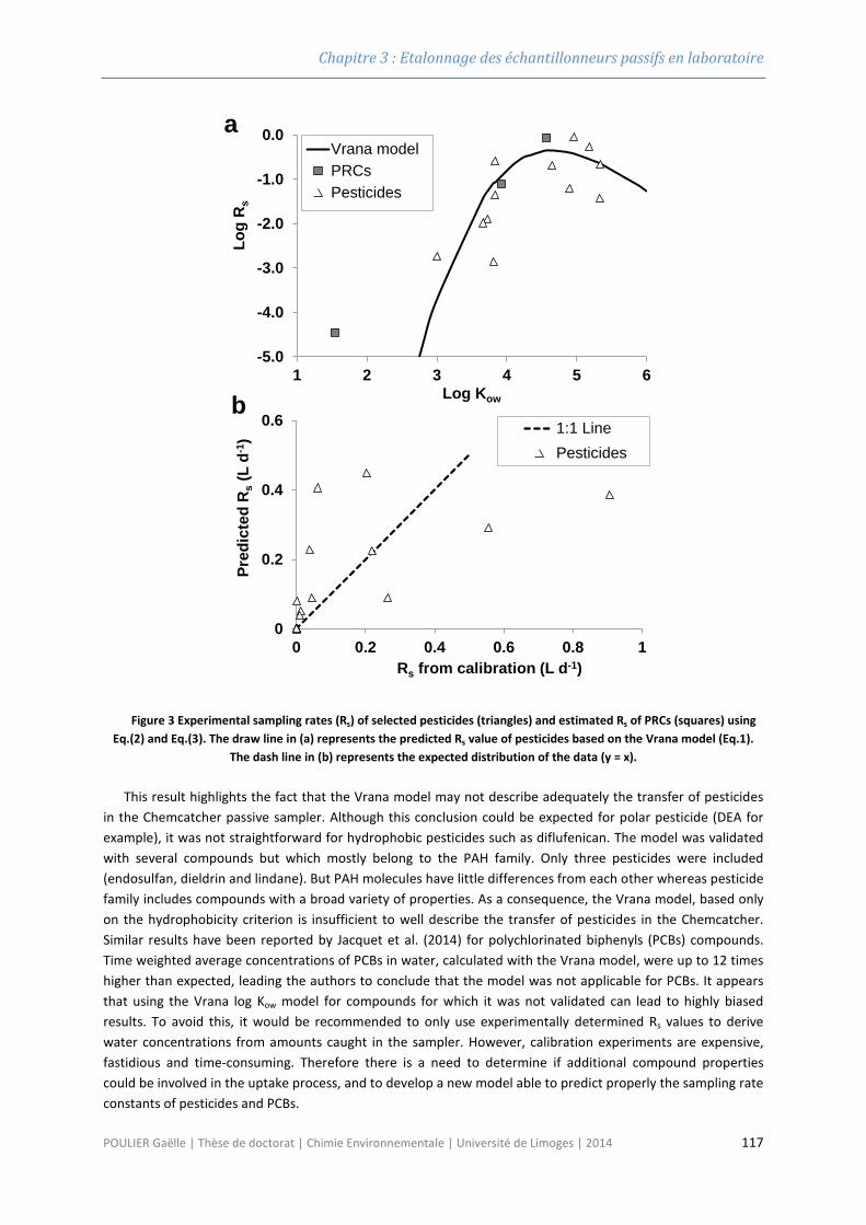
Chapitre 3 : Etalonnage des échantillonneurs passifs en laboratoire
Figure 3 Experimental sampling rates (Rs) of selected pesticides (triangles) and estimated Rs of PRCs (squares) using Eq.(2) and Eq.(3). The draw line in (a) represents the predicted Rs value of pesticides based on the Vrana model (Eq.1).
The dash line in (b) represents the expected distribution of the data (y = x). This result highlights the fact that the Vrana model may not describe adequately the transfer of pesticides
in the Chemcatcher passive sampler. Although this conclusion could be expected for polar pesticide (DEA for example), it was not straightforward for hydrophobic pesticides such as diflufenican. The model was validated with several compounds but which mostly belong to the PAH family. Only three pesticides were included (endosulfan, dieldrin and lindane). But PAH molecules have little differences from each other whereas pesticide family includes compounds with a broad variety of properties. As a consequence, the Vrana model, based only on the hydrophobicity criterion is insufficient to well describe the transfer of pesticides in the Chemcatcher. Similar results have been reported by Jacquet et al. (2014) for polychlorinated biphenyls (PCBs) compounds. Time weighted average concentrations of PCBs in water, calculated with the Vrana model, were up to 12 times higher than expected, leading the authors to conclude that the model was not applicable for PCBs. It appears that using the Vrana log Kow model for compounds for which it was not validated can lead to highly biased results. To avoid this, it would be recommended to only use experimentally determined Rs values to derive water concentrations from amounts caught in the sampler. However, calibration experiments are expensive, fastidious and time-consuming. Therefore there is a need to determine if additional compound properties could be involved in the uptake process, and to develop a new model able to predict properly the sampling rate constants of pesticides and PCBs.
-5.0
-4.0
-3.0
-2.0
-1.0
0.0
1 2 3 4 5 6
Log
Rs
Log Kow
Vrana modelPRCsPesticides
0
0.2
0.4
0.6
0 0.2 0.4 0.6 0.8 1
Pred
icte
d R
s(L
d-1
)
Rs from calibration (L d-1)
1:1 LinePesticides
a
b
POULIER Gaëlle | Thèse de doctorat | Chimie Environnementale | Université de Limoges | 2014 117
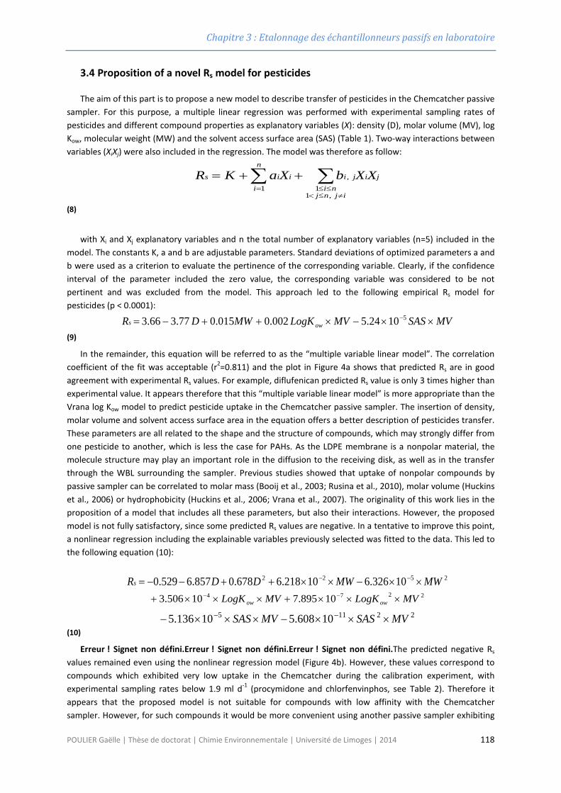
Chapitre 3 : Etalonnage des échantillonneurs passifs en laboratoire
3.4 Proposition of a novel Rs model for pesticides
The aim of this part is to propose a new model to describe transfer of pesticides in the Chemcatcher passive sampler. For this purpose, a multiple linear regression was performed with experimental sampling rates of pesticides and different compound properties as explanatory variables (X): density (D), molar volume (MV), log Kow, molecular weight (MW) and the solvent access surface area (SAS) (Table 1). Two-way interactions between variables (XiXj) were also included in the regression. The model was therefore as follow:
∑∑≠≤<
≤≤=
++=
ijnjni
jiji
n
iiis XXbXaKR
,11
,1
(8)
with Xi and Xj explanatory variables and n the total number of explanatory variables (n=5) included in the
model. The constants K, a and b are adjustable parameters. Standard deviations of optimized parameters a and b were used as a criterion to evaluate the pertinence of the corresponding variable. Clearly, if the confidence interval of the parameter included the zero value, the corresponding variable was considered to be not pertinent and was excluded from the model. This approach led to the following empirical Rs model for pesticides (p < 0.0001):
MVSASMVLogKMWDR ows ××−×++−= −51024.5002.0015.077.366.3
(9)
In the remainder, this equation will be referred to as the “multiple variable linear model”. The correlation coefficient of the fit was acceptable (r2=0.811) and the plot in Figure 4a shows that predicted Rs are in good agreement with experimental Rs values. For example, diflufenican predicted Rs value is only 3 times higher than experimental value. It appears therefore that this “multiple variable linear model” is more appropriate than the Vrana log Kow model to predict pesticide uptake in the Chemcatcher passive sampler. The insertion of density, molar volume and solvent access surface area in the equation offers a better description of pesticides transfer. These parameters are all related to the shape and the structure of compounds, which may strongly differ from one pesticide to another, which is less the case for PAHs. As the LDPE membrane is a nonpolar material, the molecule structure may play an important role in the diffusion to the receiving disk, as well as in the transfer through the WBL surrounding the sampler. Previous studies showed that uptake of nonpolar compounds by passive sampler can be correlated to molar mass (Booij et al., 2003; Rusina et al., 2010), molar volume (Huckins et al., 2006) or hydrophobicity (Huckins et al., 2006; Vrana et al., 2007). The originality of this work lies in the proposition of a model that includes all these parameters, but also their interactions. However, the proposed model is not fully satisfactory, since some predicted Rs values are negative. In a tentative to improve this point, a nonlinear regression including the explainable variables previously selected was fitted to the data. This led to the following equation (10):
2522 10326.610218.6678.0857.6529.0 MWMWDDRs ××−××++−−= −−
2274 10895.710506.3 MVLogKMVLogK owow ×××+×××+ −−
22115 10608.510136.5 MVSASMVSAS ×××−×××− −− (10)
Erreur ! Signet non défini.Erreur ! Signet non défini.Erreur ! Signet non défini.The predicted negative Rs values remained even using the nonlinear regression model (Figure 4b). However, these values correspond to compounds which exhibited very low uptake in the Chemcatcher during the calibration experiment, with experimental sampling rates below 1.9 ml d-1 (procymidone and chlorfenvinphos, see Table 2). Therefore it appears that the proposed model is not suitable for compounds with low affinity with the Chemcatcher sampler. However, for such compounds it would be more convenient using another passive sampler exhibiting
POULIER Gaëlle | Thèse de doctorat | Chimie Environnementale | Université de Limoges | 2014 118
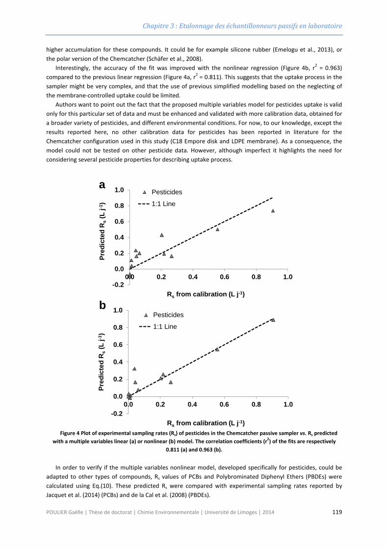
Chapitre 3 : Etalonnage des échantillonneurs passifs en laboratoire
higher accumulation for these compounds. It could be for example silicone rubber (Emelogu et al., 2013), or the polar version of the Chemcatcher (Schäfer et al., 2008).
Interestingly, the accuracy of the fit was improved with the nonlinear regression (Figure 4b, r2 = 0.963) compared to the previous linear regression (Figure 4a, r2 = 0.811). This suggests that the uptake process in the sampler might be very complex, and that the use of previous simplified modelling based on the neglecting of the membrane-controlled uptake could be limited.
Authors want to point out the fact that the proposed multiple variables model for pesticides uptake is valid only for this particular set of data and must be enhanced and validated with more calibration data, obtained for a broader variety of pesticides, and different environmental conditions. For now, to our knowledge, except the results reported here, no other calibration data for pesticides has been reported in literature for the Chemcatcher configuration used in this study (C18 Empore disk and LDPE membrane). As a consequence, the model could not be tested on other pesticide data. However, although imperfect it highlights the need for considering several pesticide properties for describing uptake process.
Figure 4 Plot of experimental sampling rates (Rs) of pesticides in the Chemcatcher passive sampler vs. Rs predicted
with a multiple variables linear (a) or nonlinear (b) model. The correlation coefficients (r2) of the fits are respectively 0.811 (a) and 0.963 (b).
In order to verify if the multiple variables nonlinear model, developed specifically for pesticides, could be
adapted to other types of compounds, Rs values of PCBs and Polybrominated Diphenyl Ethers (PBDEs) were calculated using Eq.(10). These predicted Rs were compared with experimental sampling rates reported by Jacquet et al. (2014) (PCBs) and de la Cal et al. (2008) (PBDEs).
-0.2
0.0
0.2
0.4
0.6
0.8
1.0
0.0 0.2 0.4 0.6 0.8 1.0
Pred
icte
d R
s(L
j-1 )
Rs from calibration (L j-1)
Pesticides
1:1 Line
-0.2
0.0
0.2
0.4
0.6
0.8
1.0
0.0 0.2 0.4 0.6 0.8 1.0
Pred
icte
d R
s(L
j-1 )
Rs from calibration (L j-1)
Pesticides
1:1 Line
a
b
POULIER Gaëlle | Thèse de doctorat | Chimie Environnementale | Université de Limoges | 2014 119
Chapitre 3 : Etalonnage des échantillonneurs passifs en laboratoire
Figure 5 Plot of experimental sampling rates (Rs) of pesticides (triangles), PBDEs (diamonds) and PCBs( circles) in the
Chemcatcher passive sampler vs. Rs predicted with the multiple variables nonlinear model using Eq.(10). Results (Figure 5) showed that the model proposed for pesticides is not well suited for PCBs and PBDEs. This
suggests that additional physicochemical properties may be involved in the uptake process. It appears that the use of a unique empirical model for predicting sampling rates of compounds belonging to different families is not possible. Therefore, there is a need for developing models for each family of compounds. An example is given in the supplementary material for the PCB family. Until these models are available we recommend using only sampling rates obtained from calibration experiments to go back to TWA concentrations from amounts caught in the Chemcatcher.
4- References
Booij K, Hofmans HE, Fischer CV, Van Weerlee EM (2003) Temperature-dependent uptake rates of nonpolar organic compounds by semipermeable membrane devices and low-density polyethylene membranes. Environmental Science & Technology 37: 361-366
de la Cal A, Kuster M, de Alda ML, Eljarrat E, Barcelo D (2008) Evaluation of the aquatic passive sampler Chemcatcher for the monitoring of highly hydrophobic compounds in water. Talanta 76: 327-332
Emelogu ES, Pollard P, Robinson CD, Smedes F, Webster L, Oliver IW, McKenzie C, Seiler TB, Hollert H, Moffat CF (2013) Investigating the significance of dissolved organic contaminants in aquatic environments: Coupling passive sampling with in vitro bioassays. Chemosphere 90: 210-219
Fauvelle V, Mazzella N, Belles A, Moreira A, Allan IJ, Budzinski H (2014) Optimization of the polar organic chemical integrative sampler for the sampling of acidic and polar herbicides. Analytical and Bioanalytical Chemistry 406: 3191-3199
Huckins JN, Manuweera GK, Petty JD, Mackay D, Lebo JA (1993) lipid-containing semipermeable-membrane devices for monitoring organic contaminants in water. Environmental Science & Technology 27: 2489-2496
Huckins JN, Petty JD, Booij K (2006) Monitors of Organic Chemicals in the Environment - semi permeable membrane devices. Springer, New-York
Jacquet R, Miege C, Smedes F, Tixier C, Tronczynski J, Togola A, Berho C, Valor I, Llorca J, Barillon B, Marchand P, Coquery M (2014) Comparison of five integrative samplers in laboratory for the monitoring of indicator and dioxin-like polychlorinated biphenyls in water. Chemosphere 98: 18-27
Kingston JK, Greenwood R, Mills GA, Morrison GM, Persson LB (2000) Development of a novel passive sampling system for the time-averaged measurement of a range of organic pollutants in aquatic environments. Journal of Environmental Monitoring 2: 487-495
-2.0
-1.0
0.0
1.0
2.0
3.0
4.0
0.0 0.2 0.4 0.6 0.8 1.0
Pred
icte
d R
s(L
j-1 )
Rs from calibration (L j-1)
1:1 LinePesticidesPBDEsPCBsHAPs
POULIER Gaëlle | Thèse de doctorat | Chimie Environnementale | Université de Limoges | 2014 120
Chapitre 3 : Etalonnage des échantillonneurs passifs en laboratoire
Lobpreis T, Vrana B, Dominiak E, Dercová K, Mills GA, Greenwood R (2008) Effect of housing geometry on the performance of Chemcatcher™ passive sampler for the monitoring of hydrophobic organic pollutants in water. Environmental Pollution 153: 706-710
Rusina TP, Smedes F, Klanova J, Booij K, Holoubek I (2007) Polymer selection for passive sampling: A comparison of critical properties. Chemosphere 68: 1344-1351
Rusina TP, Smedes F, Koblizkova M, Klanova J (2010) Calibration of silicone rubber passive samplers: Experimental and modeled relations between sampling rate and compound properties. Environmental Science and Technology 44: 362-367
Schäfer RB, Paschke A, Vrana B, Mueller R, Liess M (2008) Performance of the Chemcatcher® passive sampler when used to monitor 10 polar and semi-polar pesticides in 16 Central European streams, and comparison with two other sampling methods. Water Research 42: 2707-2717
Vermeirssen ELM, Dietschweiler C, Escher BI, van der Voet J, Hollender J (2012) Transfer Kinetics of Polar Organic Compounds over Polyethersulfone Membranes in the Passive Samplers Pocis and Chemcatcher. Environmental Science & Technology 46: 6759-6766
Vrana B, Mills G, Greenwood R, Knutsson J, Svensson K, Morrison G (2005a) Performance optimisation of a passive sampler for monitoring hydrophobic organic pollutants in water. Journal of Environmental Monitoring 7: 612-620
Vrana B, Mills GA, Allan IJ, Dominiak E, Svensson K, Knutsson J, Morrison G, Greenwood R (2005b) Passive sampling techniques for monitoring pollutants in water. Trac-Trends in Analytical Chemistry 24: 845-868
Vrana B, Mills GA, Dominiak E, Greenwood R (2006) Calibration of the Chemcatcher passive sampler for the monitoring of priority organic pollutants in water. Environmental Pollution 142: 333-343
Vrana B, Mills GA, Kotterman M, Leonards P, Booij K, Greenwood R (2007) Modelling and field application of the Chemcatcher passive sampler calibration data for the monitoring of hydrophobic organic pollutants in water. Environmental Pollution 145: 895-904
Vrana B, Popp P, Paschke A, Schuurmann G (2001) Membrane-enclosed sorptive coating. An integrative passive sampler for monitoring organic contaminants in water. Analytical Chemistry 73: 5191-5200
POULIER Gaëlle | Thèse de doctorat | Chimie Environnementale | Université de Limoges | 2014 121
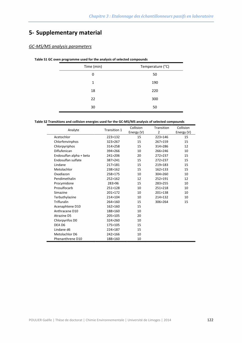
Chapitre 3 : Etalonnage des échantillonneurs passifs en laboratoire
5- Supplementary material
GC-MS/MS analysis parameters
Table S1 GC oven programme used for the analysis of selected compounds
Time (min) Temperature (°C)
0 50
1 190
18 220
22 300
30 50
Table S2 Transitions and collision energies used for the GC-MS/MS analysis of selected compounds
Analyte Transition 1 Collision Energy (V)
Transition 2
Collision Energy (V)
Acetochlor 223>132 15 223>146 15 Chlorfenvinphos 323>267 15 267>159 15 Chlorpyriphos 314>258 15 314>286 12 Diflufenican 394>266 10 266>246 10 Endosulfan alpha + beta 241>206 20 272>237 15 Endosulfan sulfate 387>241 15 272>237 15 Lindane 217>181 15 219>183 15 Metolachlor 238>162 15 162>133 15 Oxadiazon 258>175 10 304>260 10 Pendimethalin 252>162 12 252>191 12 Procymidone 283>96 15 283>255 10 Prosulfocarb 251>128 10 251>218 10 Simazine 201>172 10 201>138 10 Terbuthylazine 214>104 10 214>132 10 Trifluralin 264>160 15 306>264 15 Acenaphtene D10 162>160 15 Anthracene D10 188>160 10 Atrazine D5 205>105 20
Chlorpyrifos D0 324>260 10 DEA D6 175>105 15
Lindane d6 224>187 15 Metolachlor D6 242>166 10 Phenanthrene D10 188>160 10
POULIER Gaëlle | Thèse de doctorat | Chimie Environnementale | Université de Limoges | 2014 122
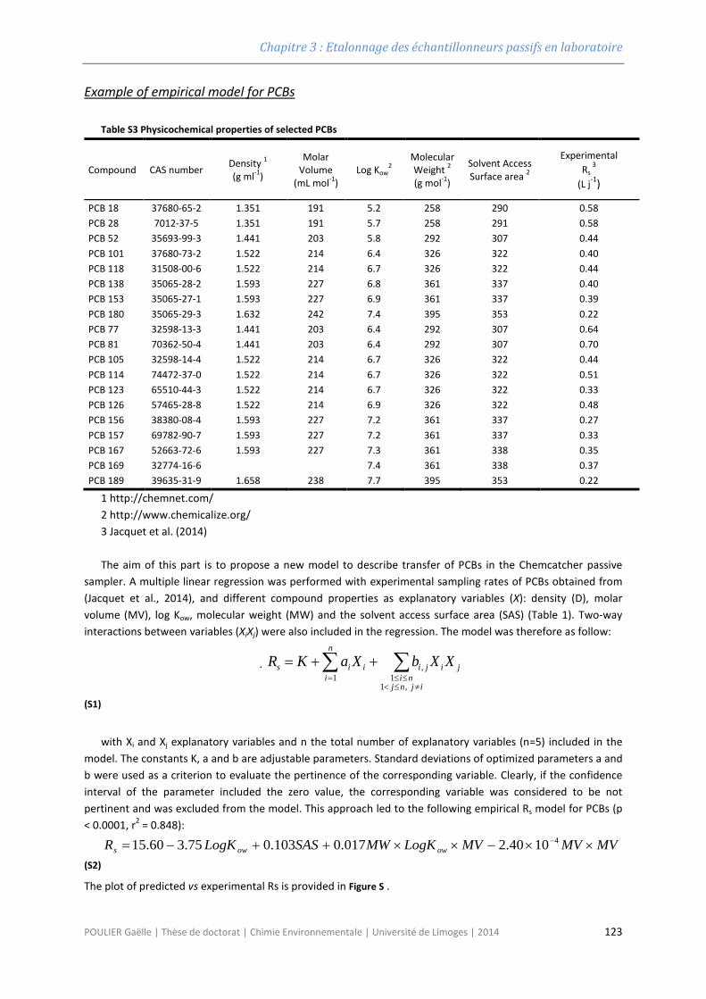
Chapitre 3 : Etalonnage des échantillonneurs passifs en laboratoire
Example of empirical model for PCBs
Table S3 Physicochemical properties of selected PCBs
Compound CAS number Density 1
(g ml-1)
Molar Volume
(mL mol-1) Log Kow
2 Molecular Weight 2 (g mol-1)
Solvent Access Surface area 2
Experimental Rs
3 (L j-1)
PCB 18 37680-65-2 1.351 191 5.2 258 290 0.58 PCB 28 7012-37-5 1.351 191 5.7 258 291 0.58 PCB 52 35693-99-3 1.441 203 5.8 292 307 0.44 PCB 101 37680-73-2 1.522 214 6.4 326 322 0.40 PCB 118 31508-00-6 1.522 214 6.7 326 322 0.44 PCB 138 35065-28-2 1.593 227 6.8 361 337 0.40 PCB 153 35065-27-1 1.593 227 6.9 361 337 0.39 PCB 180 35065-29-3 1.632 242 7.4 395 353 0.22 PCB 77 32598-13-3 1.441 203 6.4 292 307 0.64 PCB 81 70362-50-4 1.441 203 6.4 292 307 0.70 PCB 105 32598-14-4 1.522 214 6.7 326 322 0.44 PCB 114 74472-37-0 1.522 214 6.7 326 322 0.51 PCB 123 65510-44-3 1.522 214 6.7 326 322 0.33 PCB 126 57465-28-8 1.522 214 6.9 326 322 0.48 PCB 156 38380-08-4 1.593 227 7.2 361 337 0.27 PCB 157 69782-90-7 1.593 227 7.2 361 337 0.33 PCB 167 52663-72-6 1.593 227 7.3 361 338 0.35 PCB 169 32774-16-6 7.4 361 338 0.37 PCB 189 39635-31-9 1.658 238 7.7 395 353 0.22
1 http://chemnet.com/ 2 http://www.chemicalize.org/ 3 Jacquet et al. (2014) The aim of this part is to propose a new model to describe transfer of PCBs in the Chemcatcher passive
sampler. A multiple linear regression was performed with experimental sampling rates of PCBs obtained from (Jacquet et al., 2014), and different compound properties as explanatory variables (X): density (D), molar volume (MV), log Kow, molecular weight (MW) and the solvent access surface area (SAS) (Table 1). Two-way interactions between variables (XiXj) were also included in the regression. The model was therefore as follow:
. ∑∑≠≤<
≤≤=
++=
ijnjni
jiji
n
iiis XXbXaKR
,11
,1
(S1)
with Xi and Xj explanatory variables and n the total number of explanatory variables (n=5) included in the
model. The constants K, a and b are adjustable parameters. Standard deviations of optimized parameters a and b were used as a criterion to evaluate the pertinence of the corresponding variable. Clearly, if the confidence interval of the parameter included the zero value, the corresponding variable was considered to be not pertinent and was excluded from the model. This approach led to the following empirical Rs model for PCBs (p < 0.0001, r2 = 0.848):
MVMVMVLogKMWSASLogKR owows ××−××++−= −41040.2017.0103.075.360.15
(S2)
The plot of predicted vs experimental Rs is provided in Figure S .
POULIER Gaëlle | Thèse de doctorat | Chimie Environnementale | Université de Limoges | 2014 123
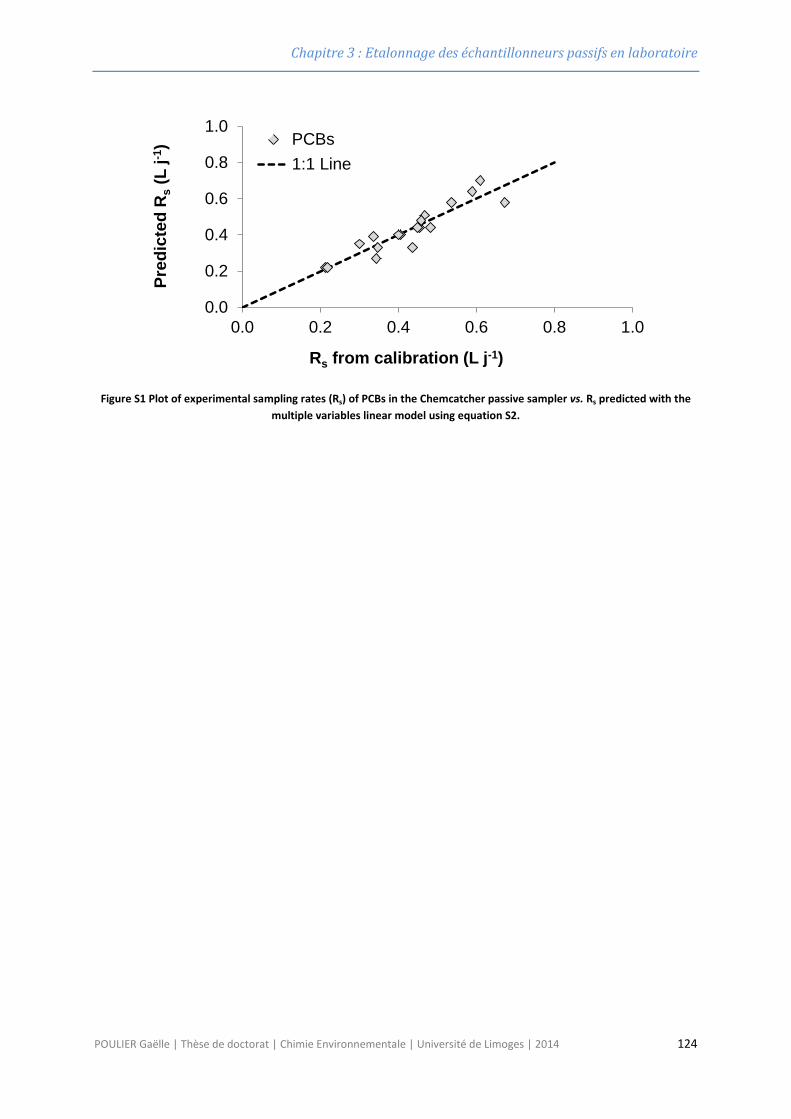
Chapitre 3 : Etalonnage des échantillonneurs passifs en laboratoire
Figure S1 Plot of experimental sampling rates (Rs) of PCBs in the Chemcatcher passive sampler vs. Rs predicted with the multiple variables linear model using equation S2.
0.0
0.2
0.4
0.6
0.8
1.0
0.0 0.2 0.4 0.6 0.8 1.0
Pred
icte
d R
s(L
j-1 )
Rs from calibration (L j-1)
PCBs1:1 Line
POULIER Gaëlle | Thèse de doctorat | Chimie Environnementale | Université de Limoges | 2014 124
Chapitre 3 : Etalonnage des échantillonneurs passifs en laboratoire
3.4 Conclusion partielle La validation et l’étalonnage des échantillonneurs passifs POCIS et Chemcatcher était une
étape clé, nécessaire à leur utilisation ultérieure sur le terrain. Dans le cas du POCIS, l’analyse des
cinétiques d’accumulation a montré que le dispositif peut être exposé sur le terrain au moins 14
jours sans risque de sortir du régime intégratif. L’applicabilité de la DIA d5 en tant que PRC a
également été démontrée. Dans le cas du Chemcatcher, il a été démontré que les relations
empiriques existantes, utilisées pour prédire les constantes cinétiques d’accumulation à partir des
propriétés physico-chimique des composés sont perfectibles .En effet, le modèle développé par
Vrana et al. (2007) pour les HAPs et basé uniquement sur l’hydrophobicité n’est pas valide pour
d’autres familles de molécules tels que les pesticides et les PCBs. De même, le modèle proposé au
terme de ce travail de thèse, qui prend en compte de multiples paramètres tels que le volume
molaire, la densité ou la surface des molécules, n’a été validé que pour des pesticides. Ces résultats
ont mis en lumière l’influence de certains paramètres, jusqu’ici négligés, dans le processus
d’accumulation. Les mécanismes d’accumulation des pesticides dans l’échantillonneur pourraient
donc s’avérer beaucoup plus complexes qu’attendu. Par conséquent, l’étape de calibration reste le
meilleur moyen d’obtenir des valeurs de Rs non biaisées.
L’ensemble des développements réalisés en laboratoire pour le POCIS et le Chemcatcher, ont
été mis en application sur le terrain. C’est l’objet du chapitre suivant.
POULIER Gaëlle | Thèse de doctorat | Chimie Environnementale | Université de Limoges | 2014 125

Chapitre 3 : Etalonnage des échantillonneurs passifs en laboratoire
POULIER Gaëlle | Thèse de doctorat | Chimie Environnementale | Université de Limoges | 2014 126
Chapitre 4 :Validation des échantillonneurs passifs sur le
terrain
POULIER Gaëlle | Thèse de doctorat | Chimie Environnementale | Université de Limoges | 2014 127

Chapitre 4 : Validation des échantillonneurs passifs sur le terrain
128
Chapitre 4 : Validation des échantillonneurs passifs sur le terrain
4.1 Avant-propos Dans le chapitre précédent, le domaine d’application (en termes de molécules accumulables)
des échantillonneurs POCIS et Chemcatcher a été identifié et les constantes cinétiques
d’accumulation, indispensables à l’utilisation des outils sur le terrain, ont été déterminées. Toutefois,
l’influence de certains paramètres environnementaux tels que la vitesse du courant, la température
ou le biofouling sur le Rs peut occasionner un biais sur la concentration mesurée si celle-ci n’est pas
corrigée pour tenir compte de la variation des conditions d’exposition. Deux approches ont été
proposées pour corriger ce biais. La plus couramment utilisée consiste à doper la phase réceptrice
avec des PRCs, dont la désorption dans le milieu varie en fonction des facteurs environnementaux,
de la même façon que l’accumulation des composés cibles. Toutefois, la méconnaissance de
l’ensemble des mécanismes mis en jeu dans le cas du POCIS (adsorption puis diffusion à travers la
membrane, diffusion à travers la macro et microporosité de la phase réceptrice et enfin adsoprtion
sur les sites hydrophobe ou hydrophile de la phase Oasis HLB), et incluant potentiellement des
phénomènes anisotropes, rend cette démarche incertaine. Il en résulte que de plus en plus d’auteurs
remettent aujourd’hui en question l’applicabilité de la démarche PRC pour le POCIS (Harman et al.,
2011a; Fauvelle et al., 2012). L’un des objectifs de ce travail de thèse a donc consisté à vérifier la
validité de cette approche pour le POCIS. Les résultats cette étude sont détaillés dans la sous-partie 2
de ce chapitre.
La deuxième méthode proposée pour limiter l’influence des conditions environnementales sur
la mesure délivrée par le POCIS consiste à réaliser l’étape d’étalonnage in situ. Le Rs mesuré est alors
représentatif du milieu d’exposition, et les concentrations calculées n’ont pas besoin d’être corrigées
si les conditions d’exposition ne changent pas. L’intérêt de cette démarche a été évalué dans la sous-
partie 2 de ce chapitre.
L’influence des conditions environnementales sur les données délivrées par les
échantillonneurs passifs représente un frein à leur future utilisation dans le cadre réglementaire, car
elle conditionne en grande partie leur degré de fiabilité. Si le biais qui en résulte ne peut pas être
corrigé par les deux approches citées précédemment, alors il est au moins nécessaire d’en connaître
l’amplitude afin de définir un intervalle de confiance qui pourra être associé aux données récoltées.
Cette question est abordée pour le POCIS dans la publication n°2 de ce chapitre.
Le deuxième verrou limitant l’utilisation des échantillonneurs passifs dans les réseaux de
surveillance réglementaires est la méconnaissance de la fraction échantillonnée. En effet, les NQEs
sont établies pour l’échantillon d’eau brute (pour les composés organiques), alors qu’il est admis que
129
Chapitre 4 : Validation des échantillonneurs passifs sur le terrain
la plupart des échantillonneurs passifs échantillonne la fraction dissoute, ou labile des contaminants.
Un travail a donc été engagé afin, d’une part, d’identifier la fraction échantillonnée par le POCIS, et
d’autre part, proposer une démarche permettant la comparaison avec les NQEs.
Dans le cas du DGT, la question de l’influence des conditions environnementales se pose
différemment car cette influence est limitée par l’insertion d’un gel de diffusion entre la membrane
et la phase réceptrice. Il est ainsi admis que l’effet de la vitesse du courant (et donc de la couche
limite d’eau) sur l’accumulation peut être négligée dans les milieux faiblement agités. Toutefois,
cette assertion doit être vérifiée. Par ailleurs, le coefficient de diffusion est un paramètre clé
indispensable au calcul de la concentration moyenne dans l’eau. La plupart des auteurs utilisent des
valeurs de coefficients de diffusion extraites de la littérature. Ce choix peut avoir une influence sur
les concentrations calculées, dans la mesure où ces valeurs extraites de la littérature ne tiennent pas
compte de la composition du milieu d’exposition, ni de la formation possible de biofilm à la surface
de la membrane. Le caractère négligeable ou non de ces paramètres conditionne donc la justesse des
données délivrées par le dispositif. Ces questions ont été abordées dans la publication n°3 en fin de
chapitre.
130
Chapitre 4 : Validation des échantillonneurs passifs sur le terrain
4.2 Correction du biais environnemental : évaluation des démarches
PRC et étalonnage in situ pour le POCIS
4.2.1 Evaluation de la démarche PRC
Pour rappel cette technique consiste à doper la phase adsorbante avec un PRC avant
l’exposition (CPRC 0), puis à mesurer sa concentration dans l’échantillonneur en fin d’exposition (CPRC f).
On en déduit sa vitesse de désorption dans les conditions du laboratoire (ke cal) ou de terrain (kein situ),
grâce à l’équation 12.
Cette démarche a été évaluée grâce aux POCIS exposés sur le Trec au printemps 2012 et 2013
(Tableau 5).
Une des conditions nécessaires à l’application de la correction est que le taux de désorption du
PRC (Ct/C0) doit être compris entre 20 et 80 %. Au-delà de ces bornes, la correction n’est pas fiable
(Huckins et al., 2002b). Le seul composé actuellement connu pour satisfaire ces exigences est la DIA.
Sa capacité à désorber du POCIS a été mise en évidence par Mazzella et al. (2010), et confirmée lors
de la calibration en laboratoire (Figure 26). La DIA a donc été utilisée pour cette étude en tant que
PRC. La molécule est marquée au deutérium (DIA-d5) afin de la distinguer de celle présente dans le
milieu naturel.
Tous les POCIS ont été dopés avec le PRC, exposés en triplicats ou en quintuplicats (Tableau 5)
et renouvelés tous les 14 jours. L’évaluation de l’approche PRC n’a pu être réalisée que sur le Trec. En
effet, le bassin versant de l’Auvézère étant très peu contaminé sur la période de mesure, le nombre
de molécules quantifiables était trop faible pour réaliser la comparaison entre les teneurs en
pesticides obtenus à partir des échantillons d’eau du préleveur automatique et le POCIS de façon
statistique.
Après récupération des POCIS et analyse de la phase réceptrice les concentrations moyennes
dans l’eau ont été calculées, en appliquant la correction PRC (C-POCIS PRC) (équation 13), ou sans
appliquer la correction (C-POCIS) lorsque le taux de désorption du PRC n’était pas satisfaisant
(équation 5).
Parallèlement, les échantillons d’eau récoltés par le préleveur automatique ont été récupérés,
regroupés sur 14 jours, filtrés et analysés. Les concentrations en pesticides mesurées dans ces
échantillons sont notées C-Préleveur et sont considérées comme valeurs de référence.
131
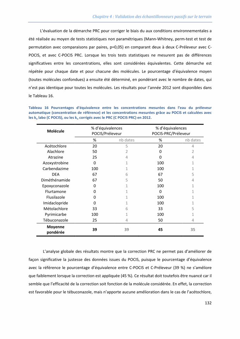
Chapitre 4 : Validation des échantillonneurs passifs sur le terrain
L’évaluation de la démarche PRC pour corriger le biais du aux conditions environnementales a
été réalisée au moyen de tests statistiques non paramétriques (Mann-Whitney, perm-test et test de
permutation avec comparaisons par paires, p=0,05) en comparant deux à deux C-Préleveur avec C-
POCIS, et avec C-POCIS PRC. Lorsque les trois tests statistiques ne mesurent pas de différences
significatives entre les concentrations, elles sont considérées équivalentes. Cette démarche est
répétée pour chaque date et pour chacune des molécules. Le pourcentage d’équivalence moyen
(toutes molécules confondues) a ensuite été déterminé, en pondérant avec le nombre de dates, qui
n’est pas identique pour toutes les molécules. Les résultats pour l’année 2012 sont disponibles dans
le Tableau 16.
Tableau 16 Pourcentages d’équivalence entre les concentrations mesurées dans l’eau du préleveur automatique (concentration de référence) et les concentrations mesurées grâce au POCIS et calculées avec les ku labo (C POCIS), ou les ku corrigés avec le PRC (C POCIS PRC) en 2012.
Molécule % d’équivalences POCIS/Préleveur
% d’équivalences POCIS-PRC/Préleveur
% nb dates % nb dates Acétochlore 20 5 20 4
Alachlore 50 2 0 2 Atrazine 25 4 0 4
Azoxystrobine 0 1 100 1 Carbendazime 100 1 100 1
DEA 67 6 67 5 Diméthénamide 67 5 50 4 Epoxyconazole 0 1 100 1
Flurtamone 0 1 0 1 Flusilazole 0 1 100 1
Imidaclopride 0 1 100 1 Métolachlore 33 6 33 5 Pyrimicarbe 100 1 100 1
Tébuconazole 25 4 50 4 Moyenne pondérée 39 39 45 35
L’analyse globale des résultats montre que la correction PRC ne permet pas d’améliorer de
façon significative la justesse des données issues du POCIS, puisque le pourcentage d’équivalence
avec la référence le pourcentage d’équivalence entre C-POCIS et C-Préleveur (39 %) ne s’améliore
que faiblement lorsque la correction est appliquée (45 %). Ce résultat doit toutefois être nuancé car il
semble que l’efficacité de la correction soit fonction de la molécule considérée. En effet, la correction
est favorable pour le tébuconazole, mais n’apporte aucune amélioration dans le cas de l’acétochlore,
132
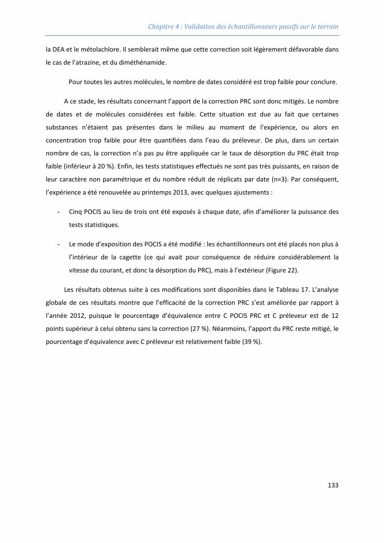
Chapitre 4 : Validation des échantillonneurs passifs sur le terrain
la DEA et le métolachlore. Il semblerait même que cette correction soit légèrement défavorable dans
le cas de l’atrazine, et du diméthénamide.
Pour toutes les autres molécules, le nombre de dates considéré est trop faible pour conclure.
A ce stade, les résultats concernant l’apport de la correction PRC sont donc mitigés. Le nombre
de dates et de molécules considérées est faible. Cette situation est due au fait que certaines
substances n’étaient pas présentes dans le milieu au moment de l’expérience, ou alors en
concentration trop faible pour être quantifiées dans l’eau du préleveur. De plus, dans un certain
nombre de cas, la correction n’a pas pu être appliquée car le taux de désorption du PRC était trop
faible (inférieur à 20 %). Enfin, les tests statistiques effectués ne sont pas très puissants, en raison de
leur caractère non paramétrique et du nombre réduit de réplicats par date (n=3). Par conséquent,
l’expérience a été renouvelée au printemps 2013, avec quelques ajustements :
- Cinq POCIS au lieu de trois ont été exposés à chaque date, afin d’améliorer la puissance des
tests statistiques.
- Le mode d’exposition des POCIS a été modifié : les échantillonneurs ont été placés non plus à
l’intérieur de la cagette (ce qui avait pour conséquence de réduire considérablement la
vitesse du courant, et donc la désorption du PRC), mais à l’extérieur (Figure 22).
Les résultats obtenus suite à ces modifications sont disponibles dans le Tableau 17. L’analyse
globale de ces résultats montre que l’efficacité de la correction PRC s’est améliorée par rapport à
l’année 2012, puisque le pourcentage d’équivalence entre C POCIS PRC et C préleveur est de 12
points supérieur à celui obtenu sans la correction (27 %). Néanmoins, l’apport du PRC reste mitigé, le
pourcentage d’équivalence avec C préleveur est relativement faible (39 %).
133
Chapitre 4 : Validation des échantillonneurs passifs sur le terrain
Tableau 17 Pourcentages d’équivalence entre les concentrations mesurées dans l’eau du préleveur automatique (concentration de référence) et les concentrations mesurées grâce au POCIS et calculées avec les ku labo (C POCIS), ou les ku corrigés avec le PRC (C POCIS PRC) en 2013.
Molécules % d’équivalences POCIS/Préleveur
% d’équivalences POCIS-PRC/Préleveur
% nb dates % nb dates Acétochlore 100 1 100 1
Atrazine 25 4 50 4 Carbendazime 0 2 0 2
Carbofuran 50 2 50 2 DEA 50 2 50 2
Diméthénamide 0 3 67 3 Dimétomorphe 0 0 0 2
Flurtamone 0 2 0 2 Imidaclopride 0 1 0 1 Métolachlore 20 5 40 5 Pyrimicarbe 0 2 50 2
Tébuconazole 100 2 50 2 Moyenne pondérée 27 26 39 28
La concentration mesurée dans le préleveur est considérée comme référence pour calculer le
pourcentage d’équivalence. Une erreur sur cette mesure peut grandement affecter nos résultats.
Afin de vérifier que ces résultats inattendus ne sont pas dus à une erreur de ce type, la comparaison
des données POCIS a également été effectuée avec les concentrations mesurées dans les
prélèvements ponctuels hebdomadaires (Figure 28). Les résultats obtenus sont très similaires, la
correction PRC n’améliore pas la justesse du POCIS.
134
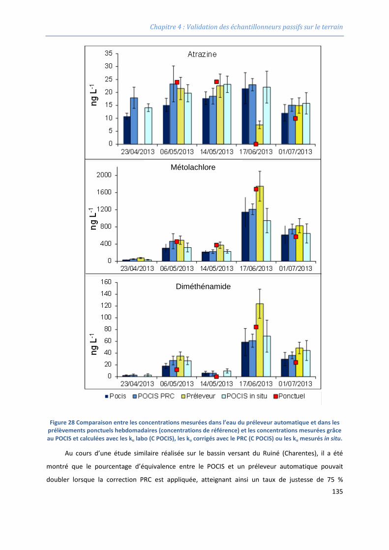
Chapitre 4 : Validation des échantillonneurs passifs sur le terrain
Figure 28 Comparaison entre les concentrations mesurées dans l’eau du préleveur automatique et dans les prélèvements ponctuels hebdomadaires (concentrations de référence) et les concentrations mesurées grâce au POCIS et calculées avec les ku labo (C POCIS), les ku corrigés avec le PRC (C POCIS) ou les ku mesurés in situ.
Au cours d’une étude similaire réalisée sur le bassin versant du Ruiné (Charentes), il a été
montré que le pourcentage d’équivalence entre le POCIS et un préleveur automatique pouvait
doubler lorsque la correction PRC est appliquée, atteignant ainsi un taux de justesse de 75 %
Métolachlore
Diméthénamide
135
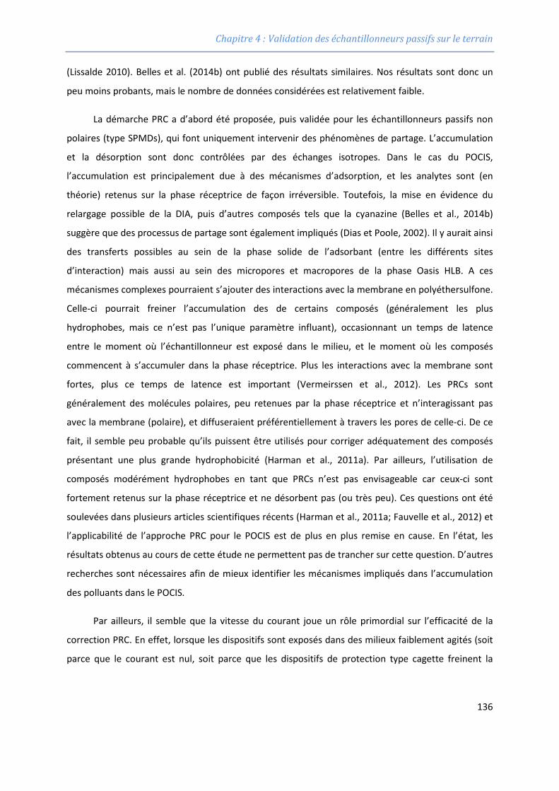
Chapitre 4 : Validation des échantillonneurs passifs sur le terrain
(Lissalde 2010). Belles et al. (2014b) ont publié des résultats similaires. Nos résultats sont donc un
peu moins probants, mais le nombre de données considérées est relativement faible.
La démarche PRC a d’abord été proposée, puis validée pour les échantillonneurs passifs non
polaires (type SPMDs), qui font uniquement intervenir des phénomènes de partage. L’accumulation
et la désorption sont donc contrôlées par des échanges isotropes. Dans le cas du POCIS,
l’accumulation est principalement due à des mécanismes d’adsorption, et les analytes sont (en
théorie) retenus sur la phase réceptrice de façon irréversible. Toutefois, la mise en évidence du
relargage possible de la DIA, puis d’autres composés tels que la cyanazine (Belles et al., 2014b)
suggère que des processus de partage sont également impliqués (Dias et Poole, 2002). Il y aurait ainsi
des transferts possibles au sein de la phase solide de l’adsorbant (entre les différents sites
d’interaction) mais aussi au sein des micropores et macropores de la phase Oasis HLB. A ces
mécanismes complexes pourraient s’ajouter des interactions avec la membrane en polyéthersulfone.
Celle-ci pourrait freiner l’accumulation des de certains composés (généralement les plus
hydrophobes, mais ce n’est pas l’unique paramètre influant), occasionnant un temps de latence
entre le moment où l’échantillonneur est exposé dans le milieu, et le moment où les composés
commencent à s’accumuler dans la phase réceptrice. Plus les interactions avec la membrane sont
fortes, plus ce temps de latence est important (Vermeirssen et al., 2012). Les PRCs sont
généralement des molécules polaires, peu retenues par la phase réceptrice et n’interagissant pas
avec la membrane (polaire), et diffuseraient préférentiellement à travers les pores de celle-ci. De ce
fait, il semble peu probable qu’ils puissent être utilisés pour corriger adéquatement des composés
présentant une plus grande hydrophobicité (Harman et al., 2011a). Par ailleurs, l’utilisation de
composés modérément hydrophobes en tant que PRCs n’est pas envisageable car ceux-ci sont
fortement retenus sur la phase réceptrice et ne désorbent pas (ou très peu). Ces questions ont été
soulevées dans plusieurs articles scientifiques récents (Harman et al., 2011a; Fauvelle et al., 2012) et
l’applicabilité de l’approche PRC pour le POCIS est de plus en plus remise en cause. En l’état, les
résultats obtenus au cours de cette étude ne permettent pas de trancher sur cette question. D’autres
recherches sont nécessaires afin de mieux identifier les mécanismes impliqués dans l’accumulation
des polluants dans le POCIS.
Par ailleurs, il semble que la vitesse du courant joue un rôle primordial sur l’efficacité de la
correction PRC. En effet, lorsque les dispositifs sont exposés dans des milieux faiblement agités (soit
parce que le courant est nul, soit parce que les dispositifs de protection type cagette freinent la
136
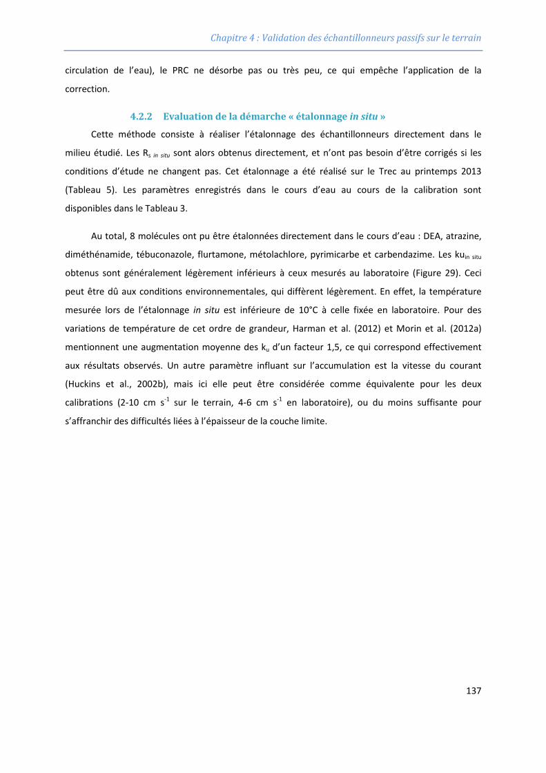
Chapitre 4 : Validation des échantillonneurs passifs sur le terrain
circulation de l’eau), le PRC ne désorbe pas ou très peu, ce qui empêche l’application de la
correction.
4.2.2 Evaluation de la démarche « étalonnage in situ »
Cette méthode consiste à réaliser l’étalonnage des échantillonneurs directement dans le
milieu étudié. Les Rs in situ sont alors obtenus directement, et n’ont pas besoin d’être corrigés si les
conditions d’étude ne changent pas. Cet étalonnage a été réalisé sur le Trec au printemps 2013
(Tableau 5). Les paramètres enregistrés dans le cours d’eau au cours de la calibration sont
disponibles dans le Tableau 3.
Au total, 8 molécules ont pu être étalonnées directement dans le cours d’eau : DEA, atrazine,
diméthénamide, tébuconazole, flurtamone, métolachlore, pyrimicarbe et carbendazime. Les kuin situ
obtenus sont généralement légèrement inférieurs à ceux mesurés au laboratoire (Figure 29). Ceci
peut être dû aux conditions environnementales, qui diffèrent légèrement. En effet, la température
mesurée lors de l’étalonnage in situ est inférieure de 10°C à celle fixée en laboratoire. Pour des
variations de température de cet ordre de grandeur, Harman et al. (2012) et Morin et al. (2012a)
mentionnent une augmentation moyenne des ku d’un facteur 1,5, ce qui correspond effectivement
aux résultats observés. Un autre paramètre influant sur l’accumulation est la vitesse du courant
(Huckins et al., 2002b), mais ici elle peut être considérée comme équivalente pour les deux
calibrations (2-10 cm s-1 sur le terrain, 4-6 cm s-1 en laboratoire), ou du moins suffisante pour
s’affranchir des difficultés liées à l’épaisseur de la couche limite.
137
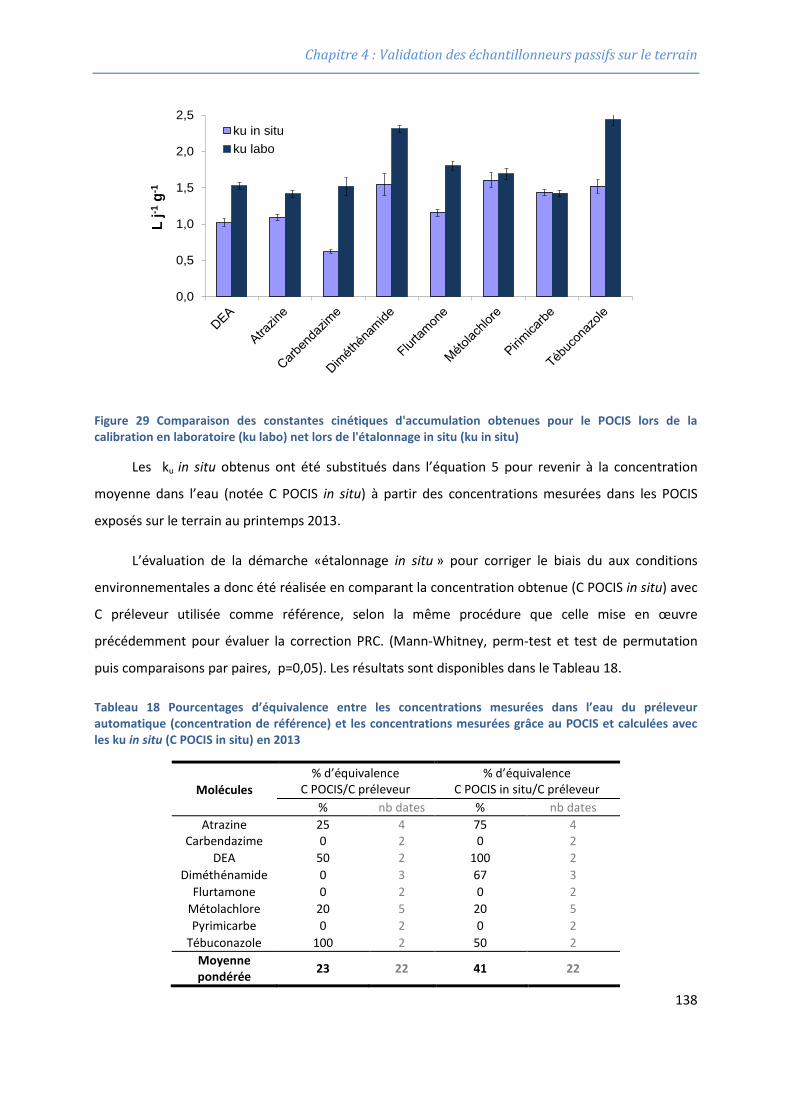
Chapitre 4 : Validation des échantillonneurs passifs sur le terrain
Figure 29 Comparaison des constantes cinétiques d'accumulation obtenues pour le POCIS lors de la calibration en laboratoire (ku labo) net lors de l'étalonnage in situ (ku in situ)
Les ku in situ obtenus ont été substitués dans l’équation 5 pour revenir à la concentration
moyenne dans l’eau (notée C POCIS in situ) à partir des concentrations mesurées dans les POCIS
exposés sur le terrain au printemps 2013.
L’évaluation de la démarche «étalonnage in situ » pour corriger le biais du aux conditions
environnementales a donc été réalisée en comparant la concentration obtenue (C POCIS in situ) avec
C préleveur utilisée comme référence, selon la même procédure que celle mise en œuvre
précédemment pour évaluer la correction PRC. (Mann-Whitney, perm-test et test de permutation
puis comparaisons par paires, p=0,05). Les résultats sont disponibles dans le Tableau 18.
Tableau 18 Pourcentages d’équivalence entre les concentrations mesurées dans l’eau du préleveur automatique (concentration de référence) et les concentrations mesurées grâce au POCIS et calculées avec les ku in situ (C POCIS in situ) en 2013
Molécules % d’équivalence
C POCIS/C préleveur % d’équivalence
C POCIS in situ/C préleveur % nb dates % nb dates
Atrazine 25 4 75 4 Carbendazime 0 2 0 2
DEA 50 2 100 2 Diméthénamide 0 3 67 3
Flurtamone 0 2 0 2 Métolachlore 20 5 20 5 Pyrimicarbe 0 2 0 2
Tébuconazole 100 2 50 2 Moyenne pondérée 23 22 41 22
0,0
0,5
1,0
1,5
2,0
2,5
L j-1
g-1
ku in situku labo
138
Chapitre 4 : Validation des échantillonneurs passifs sur le terrain
L’analyse globale des résultats montre que l’étalonnage in situ permet d’améliorer de façon
significative la précision du POCIS, puisque le pourcentage d’équivalence avec la référence est deux
fois supérieur à celui obtenu en utilisant les constantes cinétiques mesurées en laboratoire. Au cours
d’une étude similaire réalisée sur le Rhône, Ibrahim et al. (2013) ont rapporté une nette amélioration
de la justesse du POCIS lorsque l’étalonnage est réalisé in situ. Cependant, les constantes cinétiques
mesurées dans le milieu étaient 3 à 7 fois supérieures à celles obtenues en laboratoire, ce qui
suggère que les conditions régnant dans le milieu d’exposition étaient très différentes de celles fixées
au laboratoire. Dans ce cas de figure, l’apport de l’étalonnage in situ, qui permet d’obtenir des
constantes cinétiques réellement représentatives du milieu étudié apparaît clairement. Ici, les
conditions environnementales enregistrées sur le Trec sont proches de celles utilisées au laboratoire
en termes de vitesse de courant et de température, mais l’apport de l’étalonnage in situ par rapport
à un étalonnage en microcosme a quand même été mis en évidence. Ce résultat suggère que le biais
lié à l’utilisation de ku obtenus en laboratoire, et non corrigés, pourrait être négligeable.
Compte tenu du fait qu’en raison d’un taux de désorption insuffisant, la correction PRC n’a
souvent pas pu être appliquée sur les concentration obtenues avec le POCIS en 2012, et parfois en
2013, Il a été décidé, par la suite, de na pas corriger les données avec le PRC et d’utiliser les les ku
déterminés lors de l’étalonnage en laboratoire. Cela permet de traiter toutes les données 2012 et
2013 de façon homogène. A cela s’ajoute le fait que l’étalonnage in situ ne portait pas sur toutes les
substances retrouvées durant l’ensemble des deux campagnes, puisque cette approche dépend
inévitablement des composés quantifiés simultanément dans les eaux, au moment de l’étalonnage.
Ce choix implique que le biais lié aux variations des conditions environnementales ne sera pas
corrigé. Il est néanmoins possible de tenir compte des incertitudes globales (incluant le biais et la
dispersion potentiels des mesures) liées aux conditions environnementales, en appliquant un
intervalle de confiance qui intègre les variations maximales attendues pour les températures et les
vitesses de courant rencontrées dans le milieu naturel. Les résultats de l’étude de cet intervalle de
confiance, indispensable à une future utilisation du POCIS dans les réseaux de surveillance
réglementaires, sont détaillés dans la publication n°2.
139

Chapitre 4 : Validation des échantillonneurs passifs sur le terrain
140
Chapitre 4 : Validation des échantillonneurs passifs sur le terrain
4.3 Publication 2 “Can POCIS be used in Water Framework Directive (2000/60/EC) monitoring networks?” A study focusing on pesticides in a French agricultural watershed
Gaëlle Pouliera, b, Sophie Lissaldeb, Adeline Charriaub , Rémy Buzierb, François Delmasa, Kéwin
Gerya, Aurélie Moreiraa, Gilles Guibaudb, Nicolas Mazzellaa
Science of The Total Environment, volume 497-498, p 282-292, 2014, http://dx.doi.org/10.1016/j.scitotenv.2014.08.001
a Unité de recherche REBX ; Groupement Irstea de Bordeaux, 50 avenue de Verdun, Gazinet,
33612 Cestas cedex, France
b Université de Limoges Groupement de Recherche Eau Sol Environnement (GRESE), 123
Avenue Albert Thomas 87060 Limoges Cedex, France
Corresponding authors: [email protected], [email protected]
141

Chapitre 4 : Validation des échantillonneurs passifs sur le terrain
142
Chapitre 4 : Validation des échantillonneurs passifs sur le terrain
Can POCIS be used in Water Framework Directive (2000/60/EC) monitoring networks?
A study focusing on pesticides in a French agricultural watershed
Gaëlle Pouliera, b, Sophie Lissaldeb, Adeline Charriaub , Rémy Buzier b, François Delmasa, Kéwin Gerya, Aurélie Moreiraa, Gilles Guibaud b, Nicolas Mazzellaa
Science of The Total Environment, volume 497-498, p 282-292, 2014, http://dx.doi.org/10.1016/j.scitotenv.2014.08.001
a Unité de recherche REBX ; Groupement Irstea de Bordeaux, 50 avenue de Verdun, Gazinet, 33612 Cestas cedex, France
b Université de Limoges Groupement de Recherche Eau Sol Environnement (GRESE), 123 Avenue Albert Thomas 87060 Limoges Cedex, France
Corresponding authors: [email protected], [email protected]
Abstract In this study, the main current limitations in the application of the Polar Organic Chemical Integrative
Sampler (POCIS) in regulatory monitoring programmes were evaluated. POCIS were exposed from March to December by successive periods of 14 days in the River Trec (Lot et Garonne, France) and analysed for 34 pesticides. The study of the uncertainty related to the POCIS data was performed and we concluded that it might be up to 138 %, which is higher than European Union requirements but this issue was adequately counterbalanced by the gain of temporal representativeness. Comparison with data from the official monitoring program from the French Water Agency showed that the POCIS is already suitable for both operational and investigative monitoring. The sampled fraction issue, and then compliance with Environmental Quality Standards, was also addressed. It was confirmed that POCIS samples only the dissolved fraction of dimethenamid and showed that for compounds like atrazine, desethylatrazine and metolachor, the POCIS concentration is equivalent to the whole water concentration. For dimethenamid, which exhibited a tendency to adsorb on suspended matter, a method was suggested to assess the raw water concentration from the POCIS measure. Finally, an innovative procedure for using passive sampler data for compliance checks in the framework of surveillance monitoring is proposed.
Keywords: POCIS, Water Framework Directive, pesticides, uncertainty, sampled fraction, water monitoring
1. Introduction The Water Framework Directive (WFD) 2000/60/EC implemented in 2000 by the European Union (EU)
established a common framework for monitoring water quality and obliged member states to reach good ecological and chemical status for all water bodies by 2015 (EU, 2000), with extended deadlines set for 2021 and 2027. In this context, 45 molecules including 20 pesticides were listed as priority compounds and environmental quality standards (EQS) were determined (EU, 2013). The WFD specifies three types of controls, all of which may be part of monitoring programmes implemented at the river catchment scale (for continental surface waters), depending on water quality status. Surveillance monitoring is designed to assess long-term changes in water quality and provide information for the implementation of other monitoring programmes. This type of control includes at least twelve water samples per year (taken once a month) and analysed for priority compounds and river-catchment specific compounds (discharged in significant quantities into the water body). The concentrations measured are compared with EQS to determine the chemical status of the water body. If good status is not achieved, then operational monitoring must be implemented, with the major objective of providing an overview of water quality and evaluating the effectiveness of remediation strategies. The operational programme requires at least four water samples per year (taken every three months), analysed for the chemicals responsible for the deterioration of water quality. Investigative monitoring is established
143
Chapitre 4 : Validation des échantillonneurs passifs sur le terrain
prior to operational monitoring in order to identify contamination sources and select the most relevant parameters to analyse. It can also be implemented to assess the magnitude and impact of accidental pollution.
The implementation of the WFD requires an efficient monitoring network, based on reliable sampling and analytical techniques. Nowadays, grab sampling followed by extraction of analytes and chromatographic analysis (Herrero-Hernandez et al., 2013; Masia et al., 2013) is the most widespread strategy because (i) of its simplicity of implementation and (ii) it is the only method authorised for the three types of controls (surveillance, operational, investigative). However, grab sampling has numerous drawbacks which have been highlighted in the literature for several years (Allan et al., 2006a). The crux of the issue lies in the lack of temporal representativeness of this method. Indeed, very seasonal compounds such as pesticides may show high concentration peaks within short-term periods, and may therefore be completely missed with grab samples taken once a month. In such cases, Guidance Document No. 19 of the European Commission (2008) advises increasing the sampling frequency, especially during spring when the risk of contamination rises because of heavy rainfalls occurring just after pesticide applications. However, increasing the sampling frequency implies additional costs so this recommendation is scarcely applied. Another point of the grab sampling strategy subjected to criticism is the analytical performance, especially sensitivity. Some hydrophobic compounds that tend to accumulate in biota have a very low EQS. For example, trifluralin and endosulfan have EQSs of about 0.03 and 0.005 µg L-1, respectively (expressed as annual average concentration (AA-EQS)). These low concentrations are sometimes difficult to reach with the usual sampling and analytical methods.
To overcome some of the problems associated with grab sampling, an alternative strategy could be the use of passive samplers. Theory and modelling about passive samplers have been largely described elsewhere (Alvarez et al., 2004; Huckins et al., 1993; Stuer-Lauridsen, 2005; Vrana et al., 2005). Passive samplers can be exposed for several hours to several weeks in the studied aquatic environment, resulting in the accumulation and pre-concentration of analytes inside the receiving phase. Analysis of analyte amount trapped in the receiving phase allows calculation of the time-weighted average concentration (TWAC) in the aquatic environment of exposure if the sampling rate constants (Rs) of the analytes are known. Several passive samplers have been developed over the past twenty years, including, for example, Semi-permeable Membrane Devices (SPMD) or Chemcatcher® for hydrophobic compounds or Diffusive Gradient in Thin Films (DGT) for trace metals and metalloids (Davison and Zhang, 1994; Huckins et al., 1993; Kingston et al., 2000; Zhang and Davison, 1995). The Polar Organic Chemical Integrative sampler (POCIS), dedicated to polar neutral compounds was developed more recently (Alvarez et al., 2004). The characteristics of passive samplers (in situ pre-concentration step and TWAC) offer the possibility of detecting compounds at lower concentrations than in grab samples, and reduce the risk of missing potential contamination peaks. These features could be very useful in improving the reliability of data collected in WFD monitoring networks. However, some drawbacks restrain the extended use of passive samplers in regulatory programmes. The main difficulty is the influence of environmental conditions on the Rs value, a key parameter in calculating the TWAC. As the extent of this influence is not clearly known, it is difficult to determine the uncertainty associated with passive sampler data, as required in the European Directive 2009/90/EC (2009). The second major difficulty concerns the measured fraction of contaminant. Indeed, EQS values are established for the whole water sample analysis, which includes both the dissolved and suspended particulate matter-adsorbed parts of molecules. It is admitted that passive samplers measure only the truly dissolved (or labile for DGT) part of compounds, which implies that data obtained from such samplers cannot be used for compliance checks. However, to our knowledge, this assumption has never been verified, at least for the POCIS. Moreover, Allan et al. (2009) recently proposed a novel approach permitting estimation of the whole water concentration from the TWAC obtained with samplers, thanks to a correction factor including organic carbon- and dissolved organic carbon-water partition coefficients (KOC and KDOC, respectively). This manipulation could make it possible to compare passive sampler data with EQS.
This contribution discusses the possible application of POCIS data in the regulatory monitoring programme for pesticides. It focuses on one of the main requirements of the WFD, i.e. determination of uncertainty, a key factor for all monitoring programmes. It is assumed that if this parameter is known, POCIS data could be used to complement or replace grab water samples in the context of operational and investigative monitoring. This is evaluated by comparing POCIS and institutional data collected in a French agricultural watershed. Since surveillance monitoring involves comparison with EQS established for raw water,
144
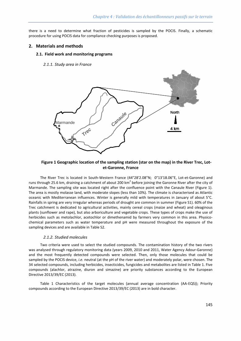
Chapitre 4 : Validation des échantillonneurs passifs sur le terrain
there is a need to determine what fraction of pesticides is sampled by the POCIS. Finally, a schematic procedure for using POCIS data for compliance checking purposes is proposed.
2. Materials and methods
2.1. Field work and monitoring programs
2.1.1. Study area in France
Figure 1 Geographic location of the sampling station (star on the map) in the River Trec, Lot-et-Garonne, France
The River Trec is located in South-Western France (44°28'2.08"N; 0°13'18.06"E, Lot-et-Garonne) and runs through 25.6 km, draining a catchment of about 200 km2 before joining the Garonne River after the city of Marmande. The sampling site was located right after the confluence point with the Canaule River (Figure 1). The area is mostly molasse land, with moderate slopes (less than 10%). The climate is characterised as Atlantic oceanic with Mediterranean influences. Winter is generally mild with temperatures in January of about 5°C. Rainfalls in spring are very irregular whereas periods of drought are common in summer (Figure S1). 60% of the Trec catchment is dedicated to agricultural activities, mainly cereal crops (maize and wheat) and oleaginous plants (sunflower and rape), but also arboriculture and vegetable crops. These types of crops make the use of herbicides such as metolachlor, acetochlor or dimethenamid by farmers very common in this area. Physico-chemical parameters such as water temperature and pH were measured throughout the exposure of the sampling devices and are available in Table S2.
2.1.2. Studied molecules
Two criteria were used to select the studied compounds. The contamination history of the two rivers was analysed through regulatory monitoring data (years 2009, 2010 and 2011, Water Agency Adour-Garonne) and the most frequently detected compounds were selected. Then, only those molecules that could be sampled by the POCIS device, i.e. neutral (at the pH of the river water) and moderately polar, were chosen. The 34 selected compounds, including herbicides, insecticides, fungicides and metabolites are listed in Table 1. Five compounds (alachlor, atrazine, diuron and simazine) are priority substances according to the European Directive 2013/39/EC (2013).
Table 1 Characteristics of the target molecules (annual average concentration (AA-EQS)); Priority compounds according to the European Directive 2013/39/EC (2013) are in bold character.
Marmande
TrecCan
aule
4 km
North
Marmande
TrecCan
aule
Marmande
TrecCan
aule
4 km
North
4 km4 km
North
145
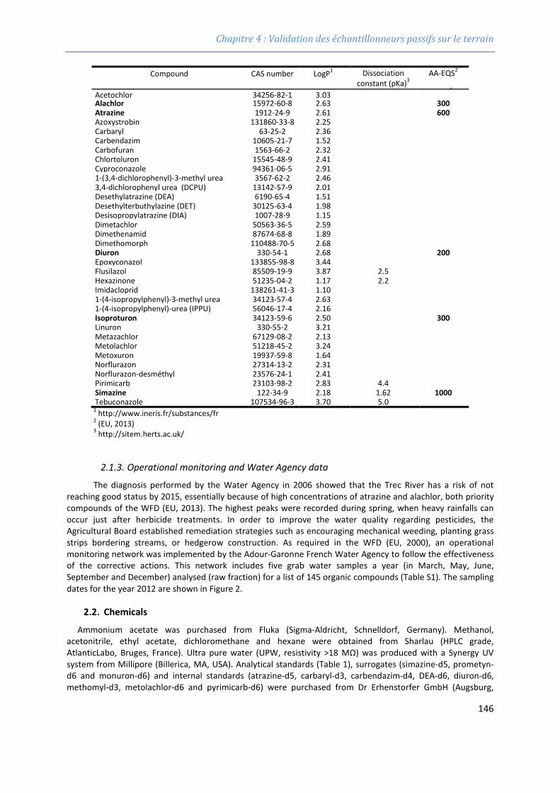
Chapitre 4 : Validation des échantillonneurs passifs sur le terrain
Compound CAS number LogP1 Dissociation constant (pKa)3
AA-EQS2
1 Acetochlor 34256-82-1 3.03 Alachlor 15972-60-8 2.63 300 Atrazine 1912-24-9 2.61 600 Azoxystrobin 131860-33-8 2.25 Carbaryl 63-25-2 2.36 Carbendazim 10605-21-7 1.52 Carbofuran 1563-66-2 2.32 Chlortoluron 15545-48-9 2.41 Cyproconazole 94361-06-5 2.91 1-(3,4-dichlorophenyl)-3-methyl urea
3567-62-2 2.46
3,4-dichlorophenyl urea (DCPU) 13142-57-9 2.01 Desethylatrazine (DEA) 6190-65-4 1.51 Desethylterbuthylazine (DET) 30125-63-4 1.98 Desisopropylatrazine (DIA) 1007-28-9 1.15 Dimetachlor 50563-36-5 2.59 Dimethenamid 87674-68-8 1.89 Dimethomorph 110488-70-5 2.68 Diuron 330-54-1 2.68 200 Epoxyconazol 133855-98-8 3.44 Flusilazol 85509-19-9 3.87 2.5 Hexazinone 51235-04-2 1.17 2.2 Imidacloprid 138261-41-3 1.10 1-(4-isopropylphenyl)-3-methyl urea
34123-57-4 2.63
1-(4-isopropylphenyl)-urea (IPPU) 56046-17-4 2.16 Isoproturon 34123-59-6 2.50 300 Linuron 330-55-2 3.21 Metazachlor 67129-08-2 2.13 Metolachlor 51218-45-2 3.24 Metoxuron 19937-59-8 1.64 Norflurazon 27314-13-2 2.31 Norflurazon-desméthyl 23576-24-1 2.41 Pirimicarb 23103-98-2 2.83 4.4 Simazine 122-34-9 2.18 1.62 1000 Tebuconazole 107534-96-3 3.70 5.0
1 http://www.ineris.fr/substances/fr 2 (EU, 2013) 3 http://sitem.herts.ac.uk/
2.1.3. Operational monitoring and Water Agency data
The diagnosis performed by the Water Agency in 2006 showed that the Trec River has a risk of not reaching good status by 2015, essentially because of high concentrations of atrazine and alachlor, both priority compounds of the WFD (EU, 2013). The highest peaks were recorded during spring, when heavy rainfalls can occur just after herbicide treatments. In order to improve the water quality regarding pesticides, the Agricultural Board established remediation strategies such as encouraging mechanical weeding, planting grass strips bordering streams, or hedgerow construction. As required in the WFD (EU, 2000), an operational monitoring network was implemented by the Adour-Garonne French Water Agency to follow the effectiveness of the corrective actions. This network includes five grab water samples a year (in March, May, June, September and December) analysed (raw fraction) for a list of 145 organic compounds (Table S1). The sampling dates for the year 2012 are shown in Figure 2.
2.2. Chemicals
Ammonium acetate was purchased from Fluka (Sigma-Aldricht, Schnelldorf, Germany). Methanol, acetonitrile, ethyl acetate, dichloromethane and hexane were obtained from Sharlau (HPLC grade, AtlanticLabo, Bruges, France). Ultra pure water (UPW, resistivity >18 MΩ) was produced with a Synergy UV system from Millipore (Billerica, MA, USA). Analytical standards (Table 1), surrogates (simazine-d5, prometyn-d6 and monuron-d6) and internal standards (atrazine-d5, carbaryl-d3, carbendazim-d4, DEA-d6, diuron-d6, methomyl-d3, metolachlor-d6 and pyrimicarb-d6) were purchased from Dr Erhenstorfer GmbH (Augsburg,
146
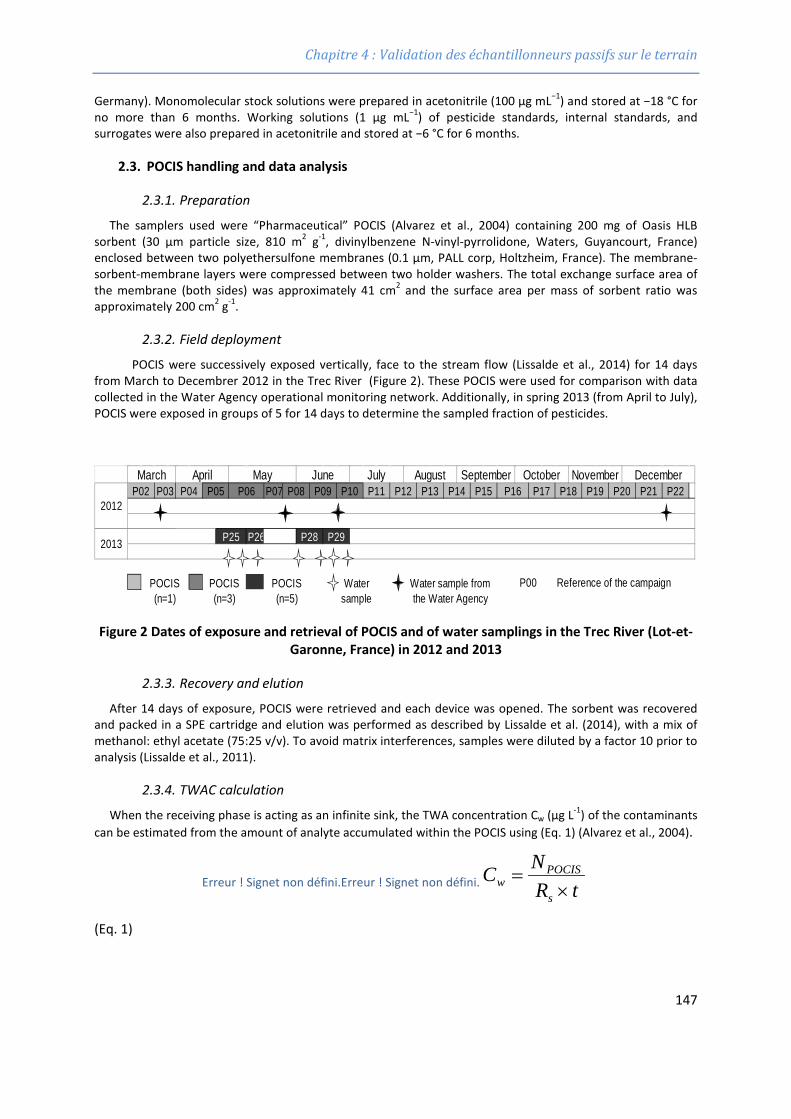
Chapitre 4 : Validation des échantillonneurs passifs sur le terrain
Germany). Monomolecular stock solutions were prepared in acetonitrile (100 μg mL−1) and stored at −18 °C for no more than 6 months. Working solutions (1 μg mL−1) of pesticide standards, internal standards, and surrogates were also prepared in acetonitrile and stored at −6 °C for 6 months.
2.3. POCIS handling and data analysis
2.3.1. Preparation
The samplers used were “Pharmaceutical” POCIS (Alvarez et al., 2004) containing 200 mg of Oasis HLB sorbent (30 µm particle size, 810 m2 g-1, divinylbenzene N-vinyl-pyrrolidone, Waters, Guyancourt, France) enclosed between two polyethersulfone membranes (0.1 µm, PALL corp, Holtzheim, France). The membrane-sorbent-membrane layers were compressed between two holder washers. The total exchange surface area of the membrane (both sides) was approximately 41 cm2 and the surface area per mass of sorbent ratio was approximately 200 cm2 g-1.
2.3.2. Field deployment
POCIS were successively exposed vertically, face to the stream flow (Lissalde et al., 2014) for 14 days from March to Decembrer 2012 in the Trec River (Figure 2). These POCIS were used for comparison with data collected in the Water Agency operational monitoring network. Additionally, in spring 2013 (from April to July), POCIS were exposed in groups of 5 for 14 days to determine the sampled fraction of pesticides.
Figure 2 Dates of exposure and retrieval of POCIS and of water samplings in the Trec River (Lot-et-Garonne, France) in 2012 and 2013
2.3.3. Recovery and elution
After 14 days of exposure, POCIS were retrieved and each device was opened. The sorbent was recovered and packed in a SPE cartridge and elution was performed as described by Lissalde et al. (2014), with a mix of methanol: ethyl acetate (75:25 v/v). To avoid matrix interferences, samples were diluted by a factor 10 prior to analysis (Lissalde et al., 2011).
2.3.4. TWAC calculation
When the receiving phase is acting as an infinite sink, the TWA concentration Cw (µg L-1) of the contaminants can be estimated from the amount of analyte accumulated within the POCIS using (Eq. 1) (Alvarez et al., 2004).
Erreur ! Signet non défini.Erreur ! Signet non défini. tRNC
s
POCISw ×=
(Eq. 1)
P07
P26
Reference of the campaign
P21 P22P17 P18March April May June July August
P19 P20P13 P14 P15 P16P06 P08 P09 P10 P11 P122012
2013
P02 P03 P04 P05September October November December
P25 P28 P29
Water sample from the Water Agency
P00POCIS (n=1)
POCIS (n=3)
POCIS (n=5)
Water sample
147
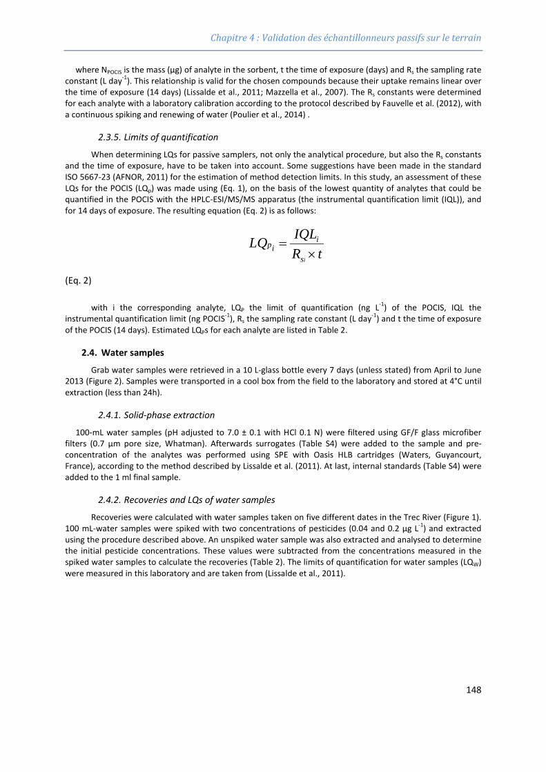
Chapitre 4 : Validation des échantillonneurs passifs sur le terrain
where NPOCIS is the mass (µg) of analyte in the sorbent, t the time of exposure (days) and Rs the sampling rate constant (L day-1). This relationship is valid for the chosen compounds because their uptake remains linear over the time of exposure (14 days) (Lissalde et al., 2011; Mazzella et al., 2007). The Rs constants were determined for each analyte with a laboratory calibration according to the protocol described by Fauvelle et al. (2012), with a continuous spiking and renewing of water (Poulier et al., 2014) .
2.3.5. Limits of quantification
When determining LQs for passive samplers, not only the analytical procedure, but also the Rs constants and the time of exposure, have to be taken into account. Some suggestions have been made in the standard ISO 5667-23 (AFNOR, 2011) for the estimation of method detection limits. In this study, an assessment of these LQs for the POCIS (LQp) was made using (Eq. 1), on the basis of the lowest quantity of analytes that could be quantified in the POCIS with the HPLC-ESI/MS/MS apparatus (the instrumental quantification limit (IQL)), and for 14 days of exposure. The resulting equation (Eq. 2) is as follows:
tRIQLLQ
is
iip
×=
(Eq. 2)
with i the corresponding analyte, LQP the limit of quantification (ng L-1) of the POCIS, IQL the instrumental quantification limit (ng POCIS-1), Rs the sampling rate constant (L day-1) and t the time of exposure of the POCIS (14 days). Estimated LQPs for each analyte are listed in Table 2.
2.4. Water samples
Grab water samples were retrieved in a 10 L-glass bottle every 7 days (unless stated) from April to June 2013 (Figure 2). Samples were transported in a cool box from the field to the laboratory and stored at 4°C until extraction (less than 24h).
2.4.1. Solid-phase extraction
100-mL water samples (pH adjusted to 7.0 ± 0.1 with HCl 0.1 N) were filtered using GF/F glass microfiber filters (0.7 µm pore size, Whatman). Afterwards surrogates (Table S4) were added to the sample and pre-concentration of the analytes was performed using SPE with Oasis HLB cartridges (Waters, Guyancourt, France), according to the method described by Lissalde et al. (2011). At last, internal standards (Table S4) were added to the 1 ml final sample.
2.4.2. Recoveries and LQs of water samples
Recoveries were calculated with water samples taken on five different dates in the Trec River (Figure 1). 100 mL-water samples were spiked with two concentrations of pesticides (0.04 and 0.2 µg L-1) and extracted using the procedure described above. An unspiked water sample was also extracted and analysed to determine the initial pesticide concentrations. These values were subtracted from the concentrations measured in the spiked water samples to calculate the recoveries (Table 2). The limits of quantification for water samples (LQW) were measured in this laboratory and are taken from (Lissalde et al., 2011).
148
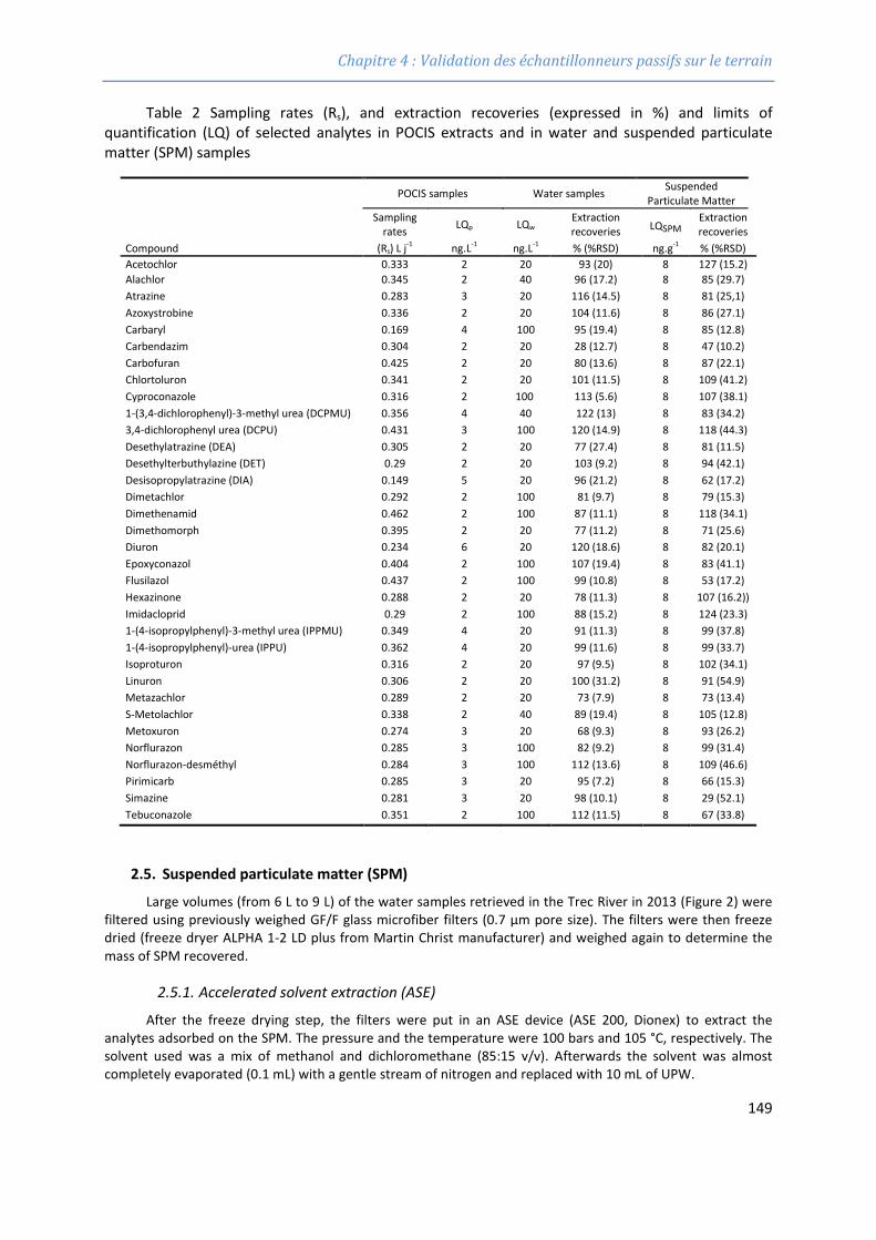
Chapitre 4 : Validation des échantillonneurs passifs sur le terrain
Table 2 Sampling rates (Rs), and extraction recoveries (expressed in %) and limits of quantification (LQ) of selected analytes in POCIS extracts and in water and suspended particulate matter (SPM) samples
Compound
POCIS samples Water samples Suspended Particulate Matter
Sampling rates LQp LQw Extraction
recoveries LQSPM Extraction recoveries
(Rs) L j-1 ng.L-1 ng.L-1 % (%RSD) ng.g-1 % (%RSD) Acetochlor 0.333 2 20 93 (20) 8 127 (15.2) Alachlor 0.345 2 40 96 (17.2) 8 85 (29.7) Atrazine 0.283 3 20 116 (14.5) 8 81 (25,1) Azoxystrobine 0.336 2 20 104 (11.6) 8 86 (27.1) Carbaryl 0.169 4 100 95 (19.4) 8 85 (12.8) Carbendazim 0.304 2 20 28 (12.7) 8 47 (10.2) Carbofuran 0.425 2 20 80 (13.6) 8 87 (22.1) Chlortoluron 0.341 2 20 101 (11.5) 8 109 (41.2) Cyproconazole 0.316 2 100 113 (5.6) 8 107 (38.1) 1-(3,4-dichlorophenyl)-3-methyl urea (DCPMU) 0.356 4 40 122 (13) 8 83 (34.2) 3,4-dichlorophenyl urea (DCPU) 0.431 3 100 120 (14.9) 8 118 (44.3) Desethylatrazine (DEA) 0.305 2 20 77 (27.4) 8 81 (11.5) Desethylterbuthylazine (DET) 0.29 2 20 103 (9.2) 8 94 (42.1) Desisopropylatrazine (DIA) 0.149 5 20 96 (21.2) 8 62 (17.2) Dimetachlor 0.292 2 100 81 (9.7) 8 79 (15.3) Dimethenamid 0.462 2 100 87 (11.1) 8 118 (34.1) Dimethomorph 0.395 2 20 77 (11.2) 8 71 (25.6) Diuron 0.234 6 20 120 (18.6) 8 82 (20.1) Epoxyconazol 0.404 2 100 107 (19.4) 8 83 (41.1) Flusilazol 0.437 2 100 99 (10.8) 8 53 (17.2) Hexazinone 0.288 2 20 78 (11.3) 8 107 (16.2)) Imidacloprid 0.29 2 100 88 (15.2) 8 124 (23.3) 1-(4-isopropylphenyl)-3-methyl urea (IPPMU) 0.349 4 20 91 (11.3) 8 99 (37.8) 1-(4-isopropylphenyl)-urea (IPPU) 0.362 4 20 99 (11.6) 8 99 (33.7) Isoproturon 0.316 2 20 97 (9.5) 8 102 (34.1) Linuron 0.306 2 20 100 (31.2) 8 91 (54.9) Metazachlor 0.289 2 20 73 (7.9) 8 73 (13.4) S-Metolachlor 0.338 2 40 89 (19.4) 8 105 (12.8) Metoxuron 0.274 3 20 68 (9.3) 8 93 (26.2) Norflurazon 0.285 3 100 82 (9.2) 8 99 (31.4) Norflurazon-desméthyl 0.284 3 100 112 (13.6) 8 109 (46.6) Pirimicarb 0.285 3 20 95 (7.2) 8 66 (15.3) Simazine 0.281 3 20 98 (10.1) 8 29 (52.1) Tebuconazole 0.351 2 100 112 (11.5) 8 67 (33.8)
2.5. Suspended particulate matter (SPM)
Large volumes (from 6 L to 9 L) of the water samples retrieved in the Trec River in 2013 (Figure 2) were filtered using previously weighed GF/F glass microfiber filters (0.7 µm pore size). The filters were then freeze dried (freeze dryer ALPHA 1-2 LD plus from Martin Christ manufacturer) and weighed again to determine the mass of SPM recovered.
2.5.1. Accelerated solvent extraction (ASE)
After the freeze drying step, the filters were put in an ASE device (ASE 200, Dionex) to extract the analytes adsorbed on the SPM. The pressure and the temperature were 100 bars and 105 °C, respectively. The solvent used was a mix of methanol and dichloromethane (85:15 v/v). Afterwards the solvent was almost completely evaporated (0.1 mL) with a gentle stream of nitrogen and replaced with 10 mL of UPW.
149
Chapitre 4 : Validation des échantillonneurs passifs sur le terrain
2.5.2. Purification
The 10 mL-UPW extracts were purified using Chromabond HRX cartridges (60 mg) (polystyrene divinylbenzene, Machery-Nagel, Hoerdt, France) with a Visiprep 12-port manifold from Supelco (Saint-Quentin-Fallavier, France). The conditioning, extraction and rinsing steps were carried out under a 53.33 kPa vacuum. The HRX cartridges were successively washed with 5 mL of hexane, acetonitrile, methanol and UPW, loaded with the 10 mL-UPW sample extract, rinsed with 5 mL of a mix of UPW/methanol (80:20 v/v) and dried under a stream of nitrogen. Analytes were eluted with 5 mL of methanol. The resulting sample was filtered with polytetrafluorethylene syringe filters of 0.20 µm pore size (Minisart SRP 25, Sartorius) to remove any traces of the HRX phase. Methanol was then evaporated with a stream of nitrogen before addition of 2 µl of a solution of 8 internal standards (atrazine-d5, carbaryl-d3, carbendazim-d4, DEA-d6, diuron-d6, methomyld3, metolachlor-d6 and pirimicarb-d6) (10 ng µL-1) and 198 µL of a mix of UPW and acetonitrile (90:10 v/v).
2.5.3. Recoveries and LQs of SPM samples
Recoveries and LQs were studied according to the French standard NF T 90-210 (AFNOR, 2009). Recoveries were determined with surface sediments (first 2-3 cm) sampled in the Trec River. The organic fraction of these sediments was about 4 %. 3 g of these sediments were spiked with 5 mL UPW containing either 120 ng or 240 ng of each pesticide, shaken for 45 min and then freeze-dried, resulting in 40 ng g-1 and 80 ng g-1 (dry weight) spiking levels. Afterwards, 5×100 mg sediment samples for each level of spiking were extracted and purified according to the procedure described above. An unspiked sediment sample was also extracted and analysed to determine the initial concentration of pesticides. Recovery data are listed in Table 2.
LQSPMs were determined with the same protocol, by the spiking of sediments at 8 ng g-1. Data are summarized in Table 2.
2.6. HPLC-ESI-MS/MS analysis
Pesticide analyses were performed by HPLC (HPLC Ultimate 3000 apparatus from Dionex) and ESI-MS/MS detection (API 2000 triple quadrupole apparatus from AB SCIEX). The procedures used are fully described (Lissalde et al., 2011) and can be found in the “Supporting information” section (Table S3 and Table S4) . IQL associated with the apparatus was about 500 fg injected onto the column for all analytes except for diuron and its metabolites (IQL = 1 pg on column). These IQLs correspond to 20 ng POCIS-1 for diuron and its metabolites and 10 ng POCIS-1 for other analytes. For water samples, these IQLs are 0.002 µg L-1 and 0.001 µg L-
1, respectively
The entire analytical procedure (matrix interferences, calibration function, recoveries and LQw and LQSPM) was validated according to the French standard NF T90-210 (AFNOR, 2009) for water samples (Lissalde et al., 2011) and SPM samples.
3. Results and discussion
3.1. Estimation of uncertainty associated with the POCIS data
Random and systematic errors are key parameters in determining the uncertainty of an analytical method (JCGM 100:2008, 2008). This determination must include all stages of the procedure, from sampling to chemical analysis. In general, uncertainty related to the analysis step of passive samplers or water extracts is quite well described, with indications of repeatability and percentage recoveries. In contrast, uncertainty due to the sampling step is rarely taken into account although it can be a substantial source of error (Allan et al., 2006b; Ort et al., 2010). To date, uncertainty associated with POCIS data has never been clearly determined, which restrains the use of this passive sampler in regulatory monitoring programmes. For this sampler, the major issue lies in the influence of environmental conditions on the Rs constant. As the extent of this influence was not clearly known, it has been difficult to determine the uncertainty associated with POCIS data, as required in the European Directive 2009/90/EC (2009). The aim of this part of the study is to determine the range of POCIS uncertainty, and the level of confidence of the data.
150
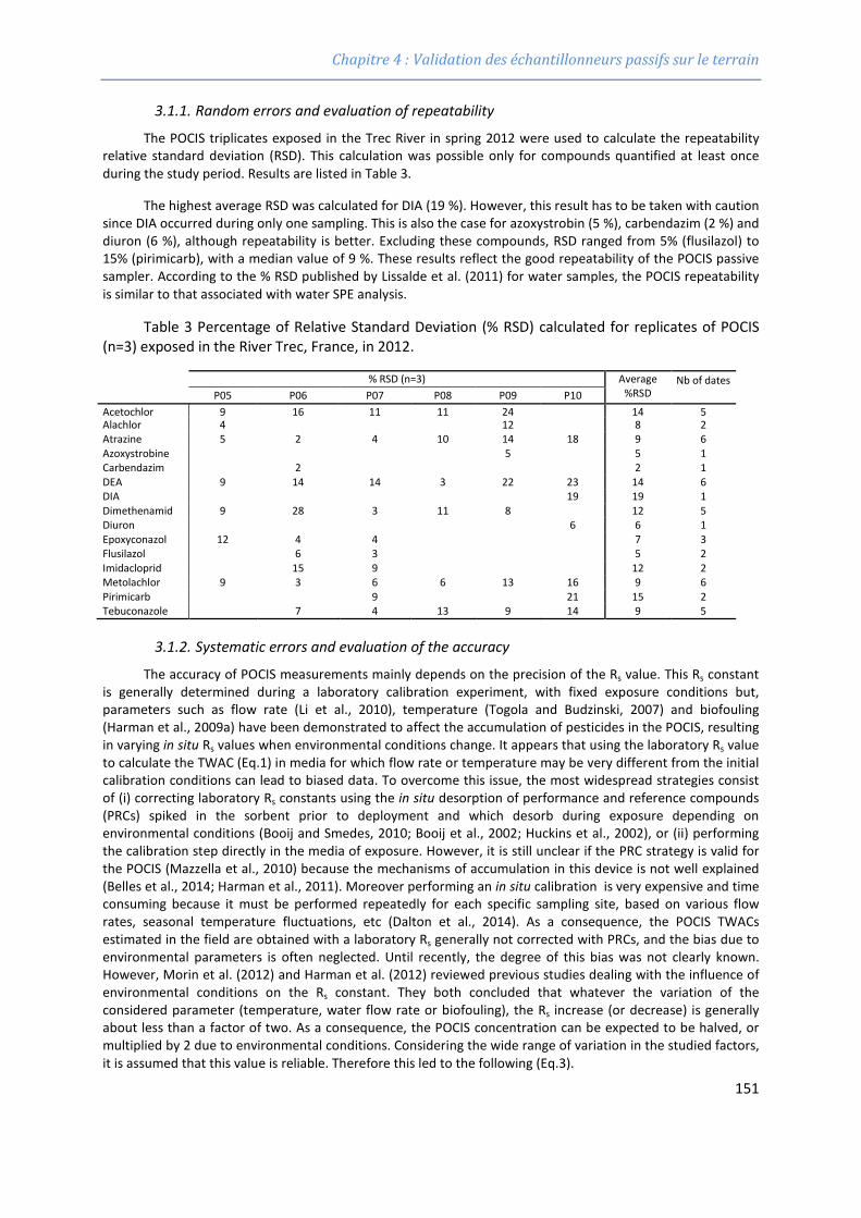
Chapitre 4 : Validation des échantillonneurs passifs sur le terrain
3.1.1. Random errors and evaluation of repeatability
The POCIS triplicates exposed in the Trec River in spring 2012 were used to calculate the repeatability relative standard deviation (RSD). This calculation was possible only for compounds quantified at least once during the study period. Results are listed in Table 3.
The highest average RSD was calculated for DIA (19 %). However, this result has to be taken with caution since DIA occurred during only one sampling. This is also the case for azoxystrobin (5 %), carbendazim (2 %) and diuron (6 %), although repeatability is better. Excluding these compounds, RSD ranged from 5% (flusilazol) to 15% (pirimicarb), with a median value of 9 %. These results reflect the good repeatability of the POCIS passive sampler. According to the % RSD published by Lissalde et al. (2011) for water samples, the POCIS repeatability is similar to that associated with water SPE analysis.
Table 3 Percentage of Relative Standard Deviation (% RSD) calculated for replicates of POCIS (n=3) exposed in the River Trec, France, in 2012.
% RSD (n=3) Average %RSD
Nb of dates P05 P06 P07 P08 P09 P10
Acetochlor 9 16 11 11 24 14 5 Alachlor 4 12 8 2 Atrazine 5 2 4 10 14 18 9 6 Azoxystrobine 5 5 1 Carbendazim 2 2 1 DEA 9 14 14 3 22 23 14 6 DIA 19 19 1 Dimethenamid 9 28 3 11 8 12 5 Diuron 6 6 1 Epoxyconazol 12 4 4 7 3 Flusilazol 6 3 5 2 Imidacloprid 15 9 12 2 Metolachlor 9 3 6 6 13 16 9 6 Pirimicarb 9 21 15 2 Tebuconazole 7 4 13 9 14 9 5
3.1.2. Systematic errors and evaluation of the accuracy
The accuracy of POCIS measurements mainly depends on the precision of the Rs value. This Rs constant is generally determined during a laboratory calibration experiment, with fixed exposure conditions but, parameters such as flow rate (Li et al., 2010), temperature (Togola and Budzinski, 2007) and biofouling (Harman et al., 2009a) have been demonstrated to affect the accumulation of pesticides in the POCIS, resulting in varying in situ Rs values when environmental conditions change. It appears that using the laboratory Rs value to calculate the TWAC (Eq.1) in media for which flow rate or temperature may be very different from the initial calibration conditions can lead to biased data. To overcome this issue, the most widespread strategies consist of (i) correcting laboratory Rs constants using the in situ desorption of performance and reference compounds (PRCs) spiked in the sorbent prior to deployment and which desorb during exposure depending on environmental conditions (Booij and Smedes, 2010; Booij et al., 2002; Huckins et al., 2002), or (ii) performing the calibration step directly in the media of exposure. However, it is still unclear if the PRC strategy is valid for the POCIS (Mazzella et al., 2010) because the mechanisms of accumulation in this device is not well explained (Belles et al., 2014; Harman et al., 2011). Moreover performing an in situ calibration is very expensive and time consuming because it must be performed repeatedly for each specific sampling site, based on various flow rates, seasonal temperature fluctuations, etc (Dalton et al., 2014). As a consequence, the POCIS TWACs estimated in the field are obtained with a laboratory Rs generally not corrected with PRCs, and the bias due to environmental parameters is often neglected. Until recently, the degree of this bias was not clearly known. However, Morin et al. (2012) and Harman et al. (2012) reviewed previous studies dealing with the influence of environmental conditions on the Rs constant. They both concluded that whatever the variation of the considered parameter (temperature, water flow rate or biofouling), the Rs increase (or decrease) is generally about less than a factor of two. As a consequence, the POCIS concentration can be expected to be halved, or multiplied by 2 due to environmental conditions. Considering the wide range of variation in the studied factors, it is assumed that this value is reliable. Therefore this led to the following (Eq.3).
151
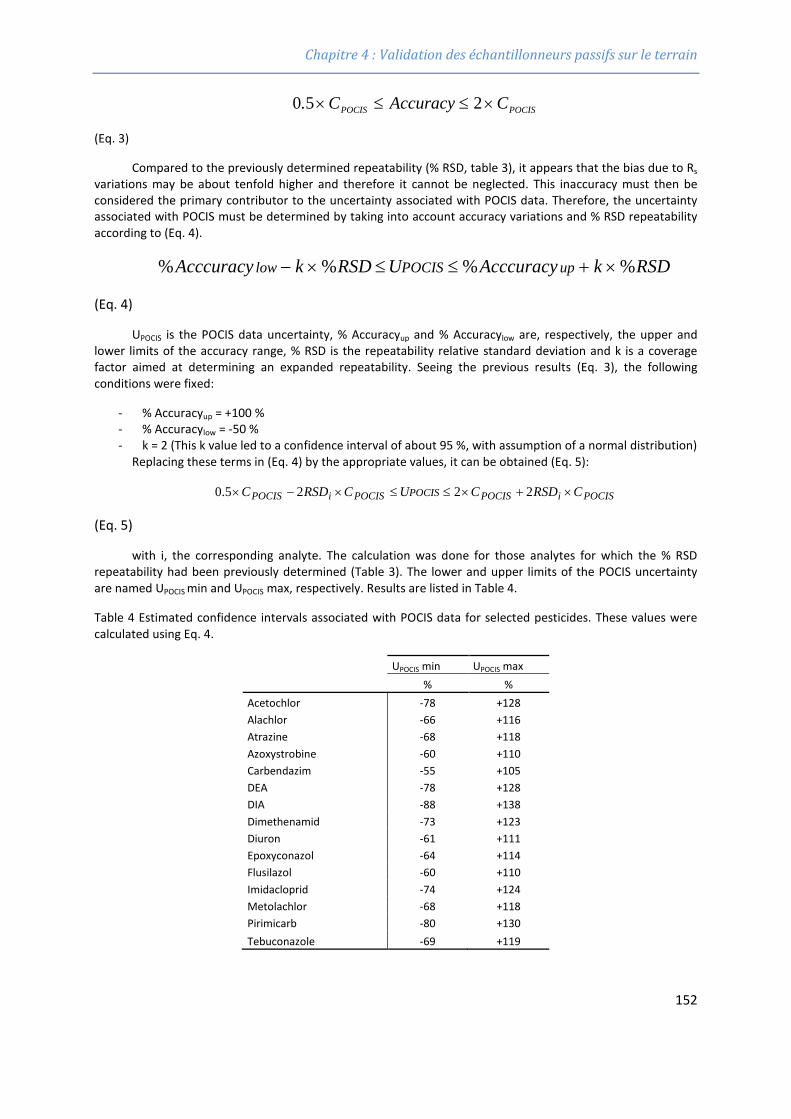
Chapitre 4 : Validation des échantillonneurs passifs sur le terrain
POCISPOCIS CAccuracyC. ×≤≤× 250
(Eq. 3)
Compared to the previously determined repeatability (% RSD, table 3), it appears that the bias due to Rs variations may be about tenfold higher and therefore it cannot be neglected. This inaccuracy must then be considered the primary contributor to the uncertainty associated with POCIS data. Therefore, the uncertainty associated with POCIS must be determined by taking into account accuracy variations and % RSD repeatability according to (Eq. 4).
RSDkAcccuracyURSDkAcccuracy upPOCISlow %%%% ×+≤≤×−
(Eq. 4)
UPOCIS is the POCIS data uncertainty, % Accuracyup and % Accuracylow are, respectively, the upper and lower limits of the accuracy range, % RSD is the repeatability relative standard deviation and k is a coverage factor aimed at determining an expanded repeatability. Seeing the previous results (Eq. 3), the following conditions were fixed:
- % Accuracyup = +100 % - % Accuracylow = -50 % - k = 2 (This k value led to a confidence interval of about 95 %, with assumption of a normal distribution)
Replacing these terms in (Eq. 4) by the appropriate values, it can be obtained (Eq. 5):
POCISiPOCISPOCISPOCISiPOCIS CRSDCUCRSDC ×+×≤≤×−× 2225.0
(Eq. 5)
with i, the corresponding analyte. The calculation was done for those analytes for which the % RSD repeatability had been previously determined (Table 3). The lower and upper limits of the POCIS uncertainty are named UPOCIS min and UPOCIS max, respectively. Results are listed in Table 4.
Table 4 Estimated confidence intervals associated with POCIS data for selected pesticides. These values were calculated using Eq. 4.
UPOCIS min UPOCIS max
% % Acetochlor -78 +128 Alachlor -66 +116 Atrazine -68 +118 Azoxystrobine -60 +110 Carbendazim -55 +105 DEA -78 +128 DIA -88 +138 Dimethenamid -73 +123 Diuron -61 +111 Epoxyconazol -64 +114 Flusilazol -60 +110 Imidacloprid -74 +124 Metolachlor -68 +118 Pirimicarb -80 +130 Tebuconazole -69 +119
152
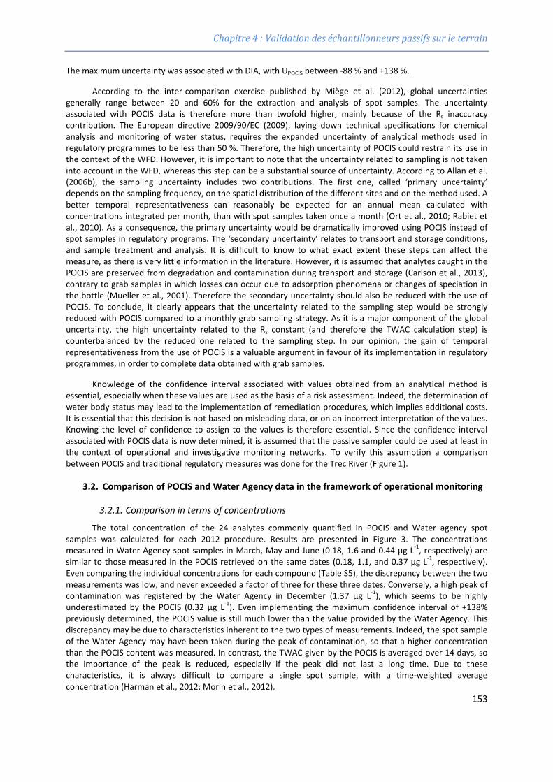
Chapitre 4 : Validation des échantillonneurs passifs sur le terrain
The maximum uncertainty was associated with DIA, with UPOCIS between -88 % and +138 %.
According to the inter-comparison exercise published by Miège et al. (2012), global uncertainties generally range between 20 and 60% for the extraction and analysis of spot samples. The uncertainty associated with POCIS data is therefore more than twofold higher, mainly because of the Rs inaccuracy contribution. The European directive 2009/90/EC (2009), laying down technical specifications for chemical analysis and monitoring of water status, requires the expanded uncertainty of analytical methods used in regulatory programmes to be less than 50 %. Therefore, the high uncertainty of POCIS could restrain its use in the context of the WFD. However, it is important to note that the uncertainty related to sampling is not taken into account in the WFD, whereas this step can be a substantial source of uncertainty. According to Allan et al. (2006b), the sampling uncertainty includes two contributions. The first one, called ‘primary uncertainty’ depends on the sampling frequency, on the spatial distribution of the different sites and on the method used. A better temporal representativeness can reasonably be expected for an annual mean calculated with concentrations integrated per month, than with spot samples taken once a month (Ort et al., 2010; Rabiet et al., 2010). As a consequence, the primary uncertainty would be dramatically improved using POCIS instead of spot samples in regulatory programs. The ‘secondary uncertainty’ relates to transport and storage conditions, and sample treatment and analysis. It is difficult to know to what exact extent these steps can affect the measure, as there is very little information in the literature. However, it is assumed that analytes caught in the POCIS are preserved from degradation and contamination during transport and storage (Carlson et al., 2013), contrary to grab samples in which losses can occur due to adsorption phenomena or changes of speciation in the bottle (Mueller et al., 2001). Therefore the secondary uncertainty should also be reduced with the use of POCIS. To conclude, it clearly appears that the uncertainty related to the sampling step would be strongly reduced with POCIS compared to a monthly grab sampling strategy. As it is a major component of the global uncertainty, the high uncertainty related to the Rs constant (and therefore the TWAC calculation step) is counterbalanced by the reduced one related to the sampling step. In our opinion, the gain of temporal representativeness from the use of POCIS is a valuable argument in favour of its implementation in regulatory programmes, in order to complete data obtained with grab samples.
Knowledge of the confidence interval associated with values obtained from an analytical method is essential, especially when these values are used as the basis of a risk assessment. Indeed, the determination of water body status may lead to the implementation of remediation procedures, which implies additional costs. It is essential that this decision is not based on misleading data, or on an incorrect interpretation of the values. Knowing the level of confidence to assign to the values is therefore essential. Since the confidence interval associated with POCIS data is now determined, it is assumed that the passive sampler could be used at least in the context of operational and investigative monitoring networks. To verify this assumption a comparison between POCIS and traditional regulatory measures was done for the Trec River (Figure 1).
3.2. Comparison of POCIS and Water Agency data in the framework of operational monitoring
3.2.1. Comparison in terms of concentrations
The total concentration of the 24 analytes commonly quantified in POCIS and Water agency spot samples was calculated for each 2012 procedure. Results are presented in Figure 3. The concentrations measured in Water Agency spot samples in March, May and June (0.18, 1.6 and 0.44 µg L-1, respectively) are similar to those measured in the POCIS retrieved on the same dates (0.18, 1.1, and 0.37 µg L-1, respectively). Even comparing the individual concentrations for each compound (Table S5), the discrepancy between the two measurements was low, and never exceeded a factor of three for these three dates. Conversely, a high peak of contamination was registered by the Water Agency in December (1.37 µg L-1), which seems to be highly underestimated by the POCIS (0.32 µg L-1). Even implementing the maximum confidence interval of +138% previously determined, the POCIS value is still much lower than the value provided by the Water Agency. This discrepancy may be due to characteristics inherent to the two types of measurements. Indeed, the spot sample of the Water Agency may have been taken during the peak of contamination, so that a higher concentration than the POCIS content was measured. In contrast, the TWAC given by the POCIS is averaged over 14 days, so the importance of the peak is reduced, especially if the peak did not last a long time. Due to these characteristics, it is always difficult to compare a single spot sample, with a time-weighted average concentration (Harman et al., 2012; Morin et al., 2012).
153
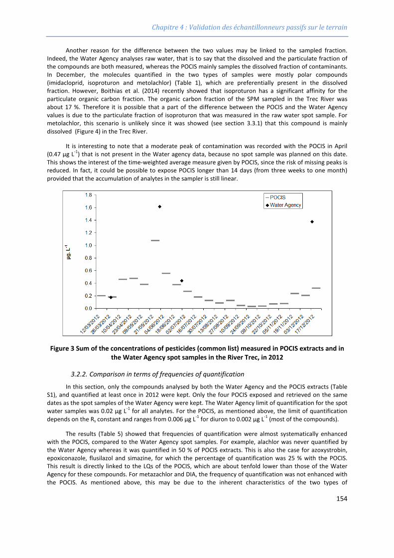
Chapitre 4 : Validation des échantillonneurs passifs sur le terrain
Another reason for the difference between the two values may be linked to the sampled fraction. Indeed, the Water Agency analyses raw water, that is to say that the dissolved and the particulate fraction of the compounds are both measured, whereas the POCIS mainly samples the dissolved fraction of contaminants. In December, the molecules quantified in the two types of samples were mostly polar compounds (imidacloprid, isoproturon and metolachlor) (Table 1), which are preferentially present in the dissolved fraction. However, Boithias et al. (2014) recently showed that isoproturon has a significant affinity for the particulate organic carbon fraction. The organic carbon fraction of the SPM sampled in the Trec River was about 17 %. Therefore it is possible that a part of the difference between the POCIS and the Water Agency values is due to the particulate fraction of isoproturon that was measured in the raw water spot sample. For metolachlor, this scenario is unlikely since it was showed (see section 3.3.1) that this compound is mainly dissolved (Figure 4) in the Trec River.
It is interesting to note that a moderate peak of contamination was recorded with the POCIS in April (0.47 µg L-1) that is not present in the Water agency data, because no spot sample was planned on this date. This shows the interest of the time-weighted average measure given by POCIS, since the risk of missing peaks is reduced. In fact, it could be possible to expose POCIS longer than 14 days (from three weeks to one month) provided that the accumulation of analytes in the sampler is still linear.
Figure 3 Sum of the concentrations of pesticides (common list) measured in POCIS extracts and in the Water Agency spot samples in the River Trec, in 2012
3.2.2. Comparison in terms of frequencies of quantification
In this section, only the compounds analysed by both the Water Agency and the POCIS extracts (Table S1), and quantified at least once in 2012 were kept. Only the four POCIS exposed and retrieved on the same dates as the spot samples of the Water Agency were kept. The Water Agency limit of quantification for the spot water samples was 0.02 µg L-1 for all analytes. For the POCIS, as mentioned above, the limit of quantification depends on the Rs constant and ranges from 0.006 µg L-1 for diuron to 0.002 µg L-1 (most of the compounds).
The results (Table 5) showed that frequencies of quantification were almost systematically enhanced with the POCIS, compared to the Water Agency spot samples. For example, alachlor was never quantified by the Water Agency whereas it was quantified in 50 % of POCIS extracts. This is also the case for azoxystrobin, epoxiconazole, flusilazol and simazine, for which the percentage of quantification was 25 % with the POCIS. This result is directly linked to the LQs of the POCIS, which are about tenfold lower than those of the Water Agency for these compounds. For metazachlor and DIA, the frequency of quantification was not enhanced with the POCIS. As mentioned above, this may be due to the inherent characteristics of the two types of
154
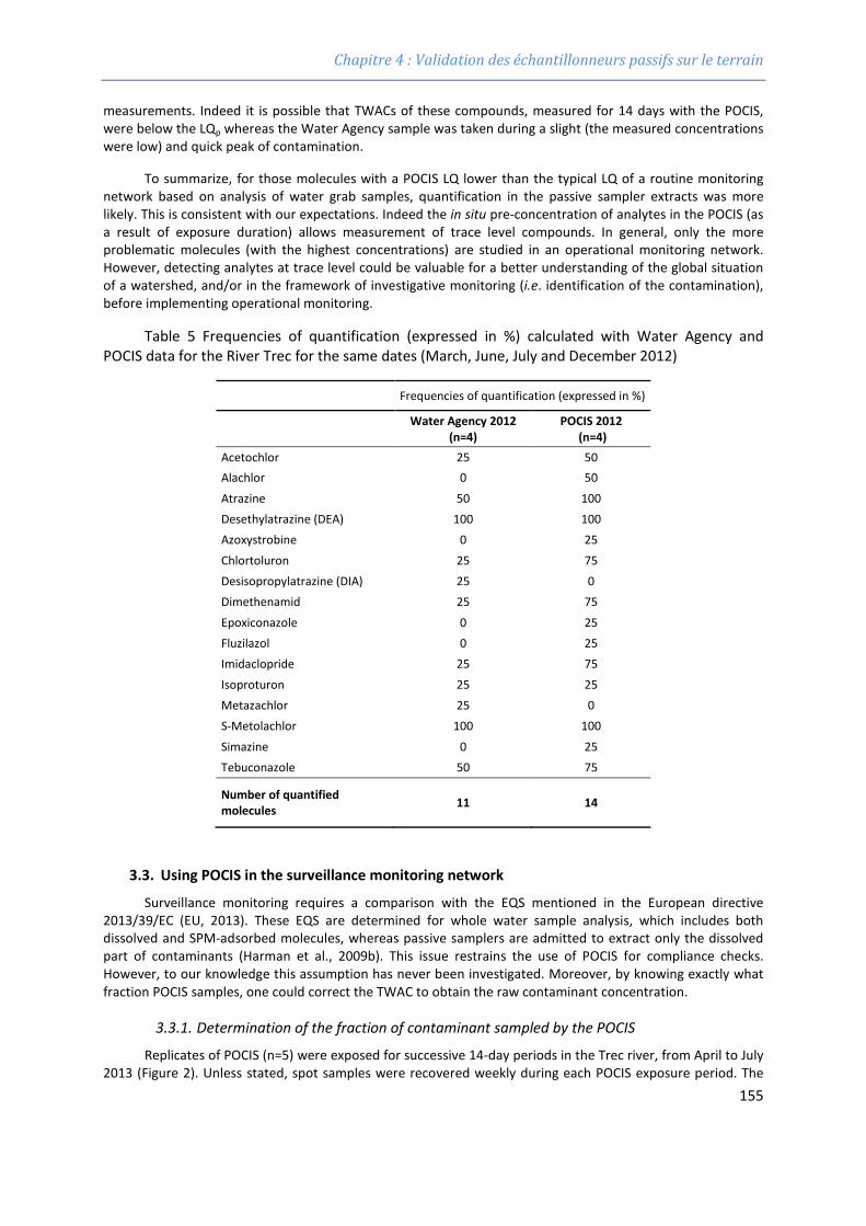
Chapitre 4 : Validation des échantillonneurs passifs sur le terrain
measurements. Indeed it is possible that TWACs of these compounds, measured for 14 days with the POCIS, were below the LQp whereas the Water Agency sample was taken during a slight (the measured concentrations were low) and quick peak of contamination.
To summarize, for those molecules with a POCIS LQ lower than the typical LQ of a routine monitoring network based on analysis of water grab samples, quantification in the passive sampler extracts was more likely. This is consistent with our expectations. Indeed the in situ pre-concentration of analytes in the POCIS (as a result of exposure duration) allows measurement of trace level compounds. In general, only the more problematic molecules (with the highest concentrations) are studied in an operational monitoring network. However, detecting analytes at trace level could be valuable for a better understanding of the global situation of a watershed, and/or in the framework of investigative monitoring (i.e. identification of the contamination), before implementing operational monitoring.
Table 5 Frequencies of quantification (expressed in %) calculated with Water Agency and POCIS data for the River Trec for the same dates (March, June, July and December 2012)
Frequencies of quantification (expressed in %)
Water Agency 2012 (n=4)
POCIS 2012 (n=4)
Acetochlor 25 50 Alachlor 0 50
Atrazine 50 100 Desethylatrazine (DEA) 100 100 Azoxystrobine 0 25
Chlortoluron 25 75 Desisopropylatrazine (DIA) 25 0 Dimethenamid 25 75
Epoxiconazole 0 25 Fluzilazol 0 25 Imidaclopride 25 75
Isoproturon 25 25 Metazachlor 25 0 S-Metolachlor 100 100
Simazine 0 25 Tebuconazole 50 75
Number of quantified molecules 11 14
3.3. Using POCIS in the surveillance monitoring network
Surveillance monitoring requires a comparison with the EQS mentioned in the European directive 2013/39/EC (EU, 2013). These EQS are determined for whole water sample analysis, which includes both dissolved and SPM-adsorbed molecules, whereas passive samplers are admitted to extract only the dissolved part of contaminants (Harman et al., 2009b). This issue restrains the use of POCIS for compliance checks. However, to our knowledge this assumption has never been investigated. Moreover, by knowing exactly what fraction POCIS samples, one could correct the TWAC to obtain the raw contaminant concentration.
3.3.1. Determination of the fraction of contaminant sampled by the POCIS
Replicates of POCIS (n=5) were exposed for successive 14-day periods in the Trec river, from April to July 2013 (Figure 2). Unless stated, spot samples were recovered weekly during each POCIS exposure period. The
155
Chapitre 4 : Validation des échantillonneurs passifs sur le terrain
average TWAC obtained with the passive samplers was compared to the average concentrations measured in both dissolved and raw fractions of the spot samples recovered during the same exposure period (Figure 2). Values below the LQ were settled to half the LQ in the average calculation. The raw concentration was obtained by adding the concentrations measured in the suspended matter (see section 2.5) to those measured in the filtered spot samples. The comparison was possible only for the compounds which could be quantified both in the water samples and in the POCIS extracts (atrazine, dimethenamid, DEA and metolachlor). Results are presented in Figure 4.
There were no significant differences between filtered and raw water concentrations for atrazine, DEA and metolachlor, which indicates that these molecules are not sorbed on SPM. This result is consistent with the low hydrophobicity of these compounds (logP < 3.24, Table 1) and their low soil organic carbon-water partition coefficients (< 200 L kg-1, www.ineris.fr/siris-pesticides). In contrast, dimethenamid exhibits an ability to sorb on suspended matter. Indeed, for the two samples recovered in May the concentration of this compound in raw water is almost 5 fold higher than the concentration in the dissolved fraction. This result is quite surprising since dimethenamid is polar (logP = 1.89, Table 1) and is not expected to sorb on particulate matter according to its organic carbon-water partition coefficient value (108 L kg-1, www.ineris.fr/siris-pesticides). Further research, beyond the scope of this study, would be needed to explain the behaviour of this compound.
The concentrations measured in the dissolved fraction and in the POCIS extracts are very similar for all compounds, especially when taking into account the confidence interval previously determined for the POCIS data. The assumption that the POCIS samples only the dissolved part of contaminants could therefore be verified, at least for dimethenamid. However for atrazine, DEA and metolachlor, it is difficult to conclude since their concentrations in the particulate fraction were close to zero. As a consequence, it is still unknown if part of this particulate fraction could be sampled by the POCIS. It is clear that more reliable data would be obtained by improving the accuracy of the POCIS measurement, as the large errors bars associated with current POCIS values make conclusions difficult. It could be possible, for example, to repeat the experiment using TWACs obtained with in situ Rs, or corrected with PRC desorption.
156
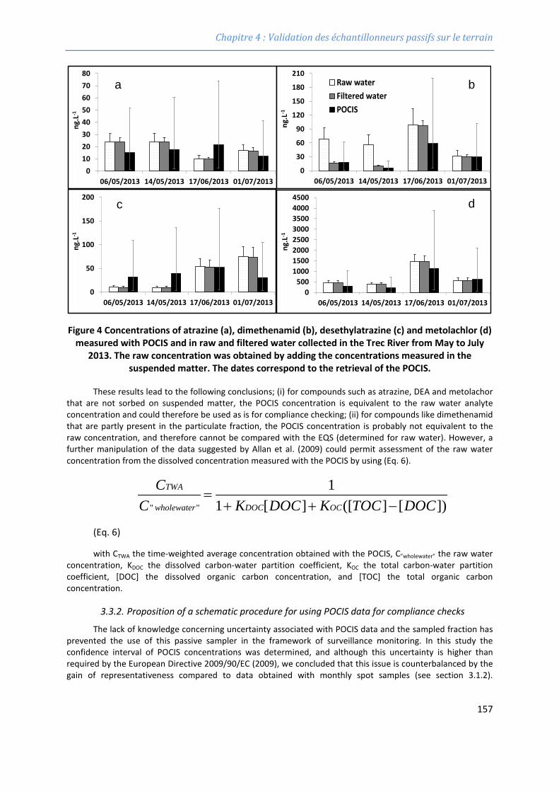
Chapitre 4 : Validation des échantillonneurs passifs sur le terrain
Figure 4 Concentrations of atrazine (a), dimethenamid (b), desethylatrazine (c) and metolachlor (d) measured with POCIS and in raw and filtered water collected in the Trec River from May to July
2013. The raw concentration was obtained by adding the concentrations measured in the suspended matter. The dates correspond to the retrieval of the POCIS.
These results lead to the following conclusions; (i) for compounds such as atrazine, DEA and metolachor that are not sorbed on suspended matter, the POCIS concentration is equivalent to the raw water analyte concentration and could therefore be used as is for compliance checking; (ii) for compounds like dimethenamid that are partly present in the particulate fraction, the POCIS concentration is probably not equivalent to the raw concentration, and therefore cannot be compared with the EQS (determined for raw water). However, a further manipulation of the data suggested by Allan et al. (2009) could permit assessment of the raw water concentration from the dissolved concentration measured with the POCIS by using (Eq. 6).
])[]([][11
"" DOCTOCKDOCKCC
OCDOCwholewater
TWA
−++=
(Eq. 6)
with CTWA the time-weighted average concentration obtained with the POCIS, C”wholewater” the raw water concentration, KDOC the dissolved carbon-water partition coefficient, KOC the total carbon-water partition coefficient, [DOC] the dissolved organic carbon concentration, and [TOC] the total organic carbon concentration.
3.3.2. Proposition of a schematic procedure for using POCIS data for compliance checks
The lack of knowledge concerning uncertainty associated with POCIS data and the sampled fraction has prevented the use of this passive sampler in the framework of surveillance monitoring. In this study the confidence interval of POCIS concentrations was determined, and although this uncertainty is higher than required by the European Directive 2009/90/EC (2009), we concluded that this issue is counterbalanced by the gain of representativeness compared to data obtained with monthly spot samples (see section 3.1.2).
01020304050607080
06/05/2013 14/05/2013 17/06/2013 01/07/2013
ng.L
-1
0
50
100
150
200
06/05/2013 14/05/2013 17/06/2013 01/07/2013
ng.L
-1
0
30
60
90
120
150
180
210
06/05/2013 14/05/2013 17/06/2013 01/07/2013
ng.L
-1
Raw waterFiltered waterPOCIS
0500
10001500200025003000350040004500
06/05/2013 14/05/2013 17/06/2013 01/07/2013
ng.L
-1
a b
c d
Raw waterFiltered waterPOCIS
157
Chapitre 4 : Validation des échantillonneurs passifs sur le terrain
Therefore, it is now possible to propose a procedure for using POCIS data for compliance checking purposes (Figure 5).
Step 1: Surveillance monitoring includes 12 concentration measurements a year, on a monthly basis. These spot samples would be replaced by POCIS exposed in the water body for 14 days (or more) and analysed for priority compounds.
Step 2: The TWACs obtained with the POCIS (CPOCIS) are corrected by the appropriate factors to account for the lower and upper limits of uncertainty previously determined for the POCIS data using (Eq. 5). The TWACs obtained this way are noted CPOCISmin and CPOCISmax. For atrazine for example, UPOCIS was between -68 % and + 118 % (Table 4). Consequently, for this compound, CPOCISmin = 0.32 × CPOCIS, and CPOCISmax = 2.18 × CPOCIS.
Step 3: The CPOCIS obtained in step 2 are used to calculate the annual average concentration. In France, it is recommended to determine a confidence interval associated with this average concentration by calculating a lower limit (MIN), and a upper limit (MAX). For this purpose, MIN is calculated with the CPOCISmin and values below LQ are replaced by 0. MAX is calculated with the CPOCISmax and values below LQ are replaced by LQ.
Step 4: The annual average concentrations MIN and MAX are compared to the AA-EQS. Good status is achieved if MAX is inferior to the AA-EQS. Good status is not achieved if MIN is superior to the AA-EQS. In all other cases, water diagnosis is not possible. This implies that the higher the LQ, the larger the discrepancy between MIN and MAX, and the more frequent the situation when diagnosis cannot be completed.
In step 3, the advantage of low LQ offered by POCIS instead of spot samples becomes clear. Indeed, it was previously showed (Table 2) that POCIS LQs can be tenfold lower than those associated with spot analysis of water samples. Therefore, the use of POCIS could lead to a significant reduction of “no water diagnosis possible” situations, where the risk of not achieving good status cannot be eliminated.
For compounds like dimethenamid, for which a significant fraction is sorbed on suspended particles, an additional step should be performed after step 1. The whole water concentration could be assessed using equation (Eq. 6), as proposed by Allan et al. (2009), from the POCIS concentrations and then corrected by the appropriate factors in step 2, as for other compounds. According to Allan et al. (2009), despite the high uncertainty of KOC and KDOC, the use of conservative values will result in an overestimation of “whole water” concentration. Good status should therefore be achieved if MAX averages calculated this way are still below the EQS.
158
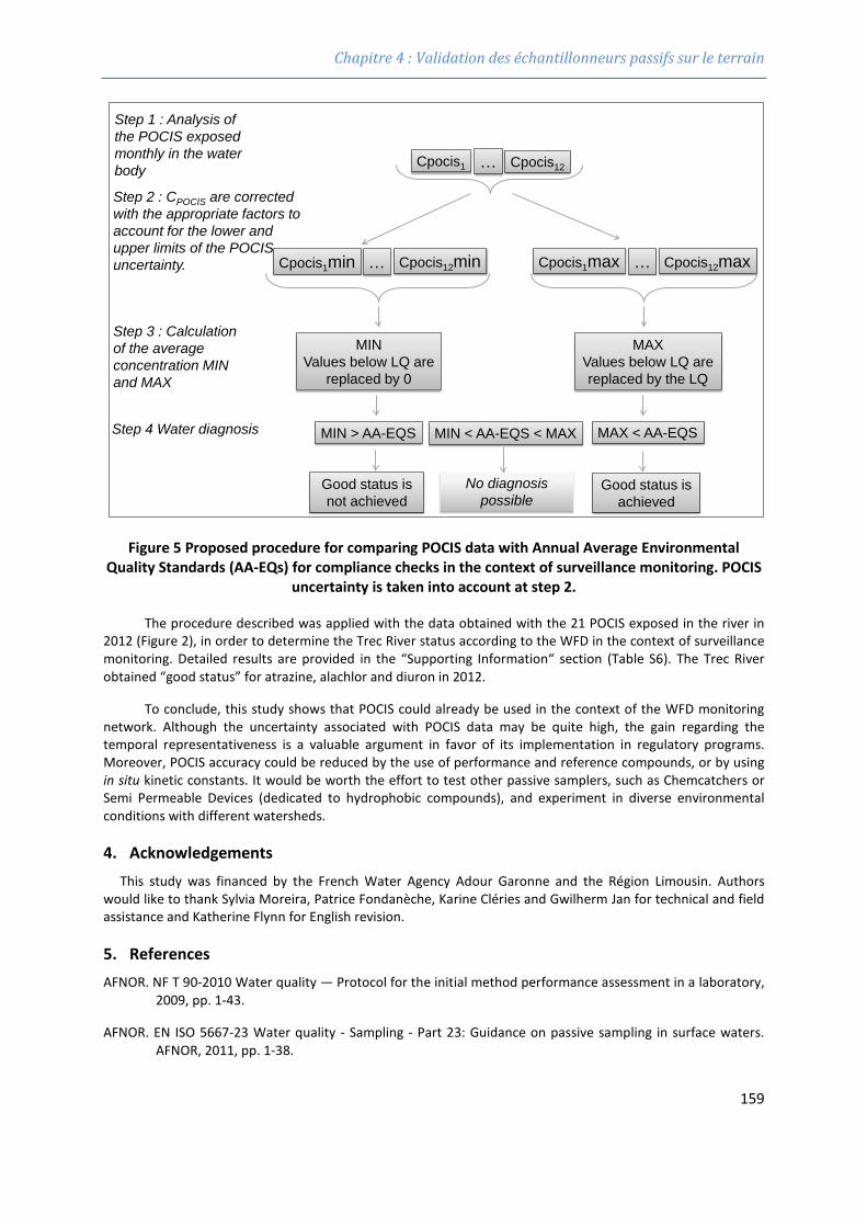
Chapitre 4 : Validation des échantillonneurs passifs sur le terrain
Figure 5 Proposed procedure for comparing POCIS data with Annual Average Environmental Quality Standards (AA-EQs) for compliance checks in the context of surveillance monitoring. POCIS
uncertainty is taken into account at step 2.
The procedure described was applied with the data obtained with the 21 POCIS exposed in the river in 2012 (Figure 2), in order to determine the Trec River status according to the WFD in the context of surveillance monitoring. Detailed results are provided in the “Supporting Information“ section (Table S6). The Trec River obtained “good status” for atrazine, alachlor and diuron in 2012.
To conclude, this study shows that POCIS could already be used in the context of the WFD monitoring network. Although the uncertainty associated with POCIS data may be quite high, the gain regarding the temporal representativeness is a valuable argument in favor of its implementation in regulatory programs. Moreover, POCIS accuracy could be reduced by the use of performance and reference compounds, or by using in situ kinetic constants. It would be worth the effort to test other passive samplers, such as Chemcatchers or Semi Permeable Devices (dedicated to hydrophobic compounds), and experiment in diverse environmental conditions with different watersheds.
4. Acknowledgements This study was financed by the French Water Agency Adour Garonne and the Région Limousin. Authors
would like to thank Sylvia Moreira, Patrice Fondanèche, Karine Cléries and Gwilherm Jan for technical and field assistance and Katherine Flynn for English revision.
5. References AFNOR. NF T 90-2010 Water quality — Protocol for the initial method performance assessment in a laboratory,
2009, pp. 1-43.
AFNOR. EN ISO 5667-23 Water quality - Sampling - Part 23: Guidance on passive sampling in surface waters. AFNOR, 2011, pp. 1-38.
Step 1 : Analysis of the POCIS exposed monthly in the water body Cpocis1 Cpocis12…
Cpocis1min Cpocis12maxCpocis1maxCpocis12min… …
MINValues below LQ are
replaced by 0
MAX Values below LQ are replaced by the LQ
Step 4 Water diagnosis MAX < AA-EQSMIN > AA-EQS
Good status isnot achieved
Good status isachieved
No diagnosispossible
MIN < AA-EQS < MAX
Step 2 : CPOCIS are corrected with the appropriate factors to account for the lower and upper limits of the POCIS uncertainty.
Step 3 : Calculation of the average concentration MIN and MAX
159
Chapitre 4 : Validation des échantillonneurs passifs sur le terrain
Allan IJ, Booij K, Paschke A, Vrana B, Mills GA, Greenwood R. Field Performance of Seven Passive Sampling Devices for Monitoring of Hydrophobic Substances. Environmental Science & Technology 2009; 43: 5383-5390.
Allan IJ, Vrana B, Greenwood R, Mills GA, Knutsson J, Holmberg A, et al. Strategic monitoring for the European Water Framework Directive. TrAC - Trends in Analytical Chemistry 2006b; 25: 704-715.
Allan IJ, Vrana B, Greenwood R, Mills GA, Roig B, Gonzalez C. A "toolbox" for biological and chemical monitoring requirements for the European Union's Water Framework Directive. Talanta 2006a; 69: 302-322.
Alvarez DA, Petty JD, Huckins JN, Jones-Lepp TL, Getting DT, Goddard JP, et al. Development of a passive, in situ, integrative sampler for hydrophilic organic contaminants in aquatic environments. Environmental Toxicology and Chemistry 2004; 23: 1640-1648.
Belles A, Pardon P, Budzinski H. Development of an adapted version of polar organic chemical integrative samplers (POCIS-Nylon). Analytical and Bioanalytical Chemistry 2014; 406: 1099-1110.
Boithias L, Sauvage S, Merlina G, Jean S, Probst J-L, Sánchez Pérez JM. New insight into pesticide partition coefficient Kd for modelling pesticide fluvial transport: Application to an agricultural catchment in south-western France. Chemosphere 2014; 99: 134-142.
Booij K, Smedes F. An Improved Method for Estimating in Situ Sampling Rates of Nonpolar Passive Samplers. Environmental Science & Technology 2010; 44: 6789-6794.
Booij K, Smedes F, van Weerlee EM. Spiking of performance reference compounds in low density polyethylene and silicone passive water samplers. Chemosphere 2002; 46: 1157-1161.
Carlson JC, Challis JK, Hanson ML, Wong CS. Stability of pharmaceuticals and other polar organic compounds stored on polar organic chemical integrative samplers and solid-phase extraction cartridges. Environmental Toxicology and Chemistry 2013; 32: 337-344.
Dalton RL, Pick FR, Boutin C, Saleem A. Atrazine contamination at the watershed scale and environmental factors affecting sampling rates of the polar organic chemical integrative sampler (POCIS). Environmental Pollution 2014; 189: 134-142.
Davison W, Zhang H. In situ speciation measurements of trace components in natural-waters using thin film gels. Nature 1994; 367: 546-548.
EU. Directive 2000/60/EC of The European Parliament and of the Council of 23 October 2000 establishing a framework for Community action in the field of water policy. . OJ L 327, . 22.12.2000, 2000, pp. 1-73.
EU. Directive 2009/60/EC of the Parliament and of the Council of 31 July 2009 laying down, pursuant to Directive 2000/60/EC, technical specifications for chemical analysis and monitoring of water status. OJ L 201 2009; 01.08.2009: 36-38.
EU. Directive 2013/39/EC of the European Parliament and of the Council of 12 August 2013 amending Directives 2000/60/EC and 2008/105/EC as regards priority substances in the field of water policy Text with EEA relevance OJ L 226 2013; 24.8.2013: 1-17.
European Commission. Guidance document No.19 'Chemical monitoring under the Water Framework directive'. Common Implementation Strategy for the Water Framework Directive (2000/60/EC) - 2008.
Fauvelle V, Mazzella N, Delmas F, Madarassou K, Eon M, Budzinski H. Use of Mixed-Mode Ion Exchange Sorbent for the Passive Sampling of Organic Acids by Polar Organic Chemical Integrative Sampler (POCIS). Environmental Science & Technology 2012; 46: 13344-13353.
Harman C, Allan IJ, Bäuerlein PS. The challenge of exposure correction for polar passive samplers the PRC and the POCIS. Environmental Science and Technology 2011; 45: 9120-9121.
160
Chapitre 4 : Validation des échantillonneurs passifs sur le terrain
Harman C, Allan IJ, Vermeirssen ELM. Calibration and use of the polar organic chemical integrative sampler-a critical review. Environmental Toxicology and Chemistry 2012; 31: 2724-2738.
Harman C, Boyum O, Thomas KV, Grung M. Small but different effect of fouling on the uptake rates of semipermeable membrane devices and polar organic chemical integrative samplers. Environmental Toxicology and Chemistry 2009a; 28: 2324-2332.
Harman C, Thomas KV, Tollefsen KE, Meier S, Boyum O, Grung M. Monitoring the freely dissolved concentrations of polycyclic aromatic hydrocarbons (PAH) and alkylphenols (AP) around a Norwegian oil platform by holistic passive sampling. Marine Pollution Bulletin 2009b; 58: 1671-1679.
Herrero-Hernandez E, Andrades MS, Alvarez-Martin A, Pose-Juan E, Rodriguez-Cruz MS, Sanchez-Martin MJ. Occurrence of pesticides and some of their degradation products in waters in a Spanish wine region. Journal of Hydrology 2013; 486: 234-245.
Huckins JN, Manuweera GK, Petty JD, Mackay D, Lebo JA. lipid-containing semipermeable-membrane devices for monitoring organic contaminants in water. Environmental Science & Technology 1993; 27: 2489-2496.
Huckins JN, Petty JD, Lebo JA, Almeida FV, Booij K, Alvarez DA, et al. Development of the permeability/performance reference compound approach for in situ calibration of semipermeable membrane devices. Environmental Science & Technology 2002; 36: 85-91.
JCGM 100:2008. Evaluation of measurement data — Guide to the expression of uncertainty in measurement, http://www.bipm.org/utils/common/documents/jcgm/JCGM_100_2008_E.pdf, 2008.
Kingston JK, Greenwood R, Mills GA, Morrison GM, Persson LB. Development of a novel passive sampling system for the time-averaged measurement of a range of organic pollutants in aquatic environments. Journal of Environmental Monitoring 2000; 2: 487-495.
Li H, Vermeirssen EL, Helm PA, Metcalfe CD. Controlled field evaluation of water flow rate effects on sampling polar organic compounds using polar organic chemical integrative samplers. Environmental Toxicology and Chemistry 2010; 29: 2461-2469.
Lissalde S, Mazzella N, Fauvelle V, Delmas F, Mazellier P, Legube B. Liquid chromatography coupled with tandem mass spectrometry method for thirty-three pesticides in natural water and comparison of performance between classical solid phase extraction and passive sampling approaches. Journal of Chromatography A 2011; 1218: 1492-1502.
Lissalde S, Mazzella N, Mazellier P. Polar organic chemical integrative samplers for pesticides monitoring: impacts of field exposure conditions. The Science of the total environment 2014; 488-489: 188-96.
Masia A, Campo J, Vazquez-Roig P, Blasco C, Pico Y. Screening of currently used pesticides in water, sediments and biota of the Guadalquivir River Basin (Spain). Journal of Hazardous Materials 2013; 263: 95-104.
Mazzella N, Dubernet JF, Delmas F. Determination of kinetic and equilibrium regimes in the operation of polar organic chemical integrative samplers - Application to the passive sampling of the polar herbicides in aquatic environments. Journal of Chromatography A. 1154, 2007, pp. 42-51.
Mazzella N, Lissalde S, Moreira S, Delmas F, Mazellier P, Huckins JN. Evaluation of the use of performance reference compounds in an oasis-HLB adsorbent based passive sampler for improving water concentration estimates of polar herbicides in freshwater. Environmental Science and Technology 2010; 44: 1713-1719.
Miège C, Schiavone S, Dabrin A, Coquery M, Mazzella N, Berho C, et al. An in situ intercomparison exercise on passive samplers for monitoring metals, polycyclic aromatic hydrocarbons and pesticides in surface waters. TrAC Trends in Analytical Chemistry 2012; 36: 128-143.
161
Chapitre 4 : Validation des échantillonneurs passifs sur le terrain
Morin N, Miège C, Coquery M, Randon J. Chemical calibration, performance, validation and applications of the polar organic chemical integrative sampler (POCIS) in aquatic environments. TrAC Trends in Analytical Chemistry 2012.
Mueller TC, Senseman SA, Carson KH, Sciumbato AS. Stability and recovery of triazine and chloroacetamide herbicides from pH adjusted water samples by using empore solid-phase extraction disks and gas chromatography with ion trap mass spectrometry. Journal of Aoac International 2001; 84: 1070-1073.
Ort C, Lawrence MG, Reungoat J, Mueller JF. Sampling for PPCPs in Wastewater Systems: Comparison of Different Sampling Modes and Optimization Strategies. Environmental Science & Technology 2010; 44: 6289-6296.
Poulier G, Lissalde S, Charriau A, Buzier R, Cleries K, Delmas F, et al. Estimates of pesticide concentrations and fluxes in two rivers of an extensive French multi-agricultural watershed: application of the passive sampling strategy. Environmental Science and Pollution Research 2014: 1-14.
Rabiet M, Margoum C, Gouy V, Carluer N, Coquery M. Assessing pesticide concentrations and fluxes in the stream of a small vineyard catchment – Effect of sampling frequency. Environmental Pollution 2010; 158: 737-748.
Stuer-Lauridsen F. Review of passive accumulation devices for monitoring organic micropollutants in the aquatic environment. Environmental Pollution 2005; 136: 503-524.
Togola A, Budzinski H. Development of polar organic integrative samplers for analysis of pharmaceuticals in aquatic systems. Analytical Chemistry 2007; 79: 6734-6741.
Vrana B, Mills GA, Allan IJ, Dominiak E, Svensson K, Knutsson J, et al. Passive sampling techniques for monitoring pollutants in water. Trac-Trends in Analytical Chemistry 2005; 24: 845-868.
Zhang H, Davison W. Performance characteristics of diffusion gradients in thin-films for the in-situ measurement of trace-metals in aqueous-solution. Analytical Chemistry 1995; 67: 3391-3400.
162
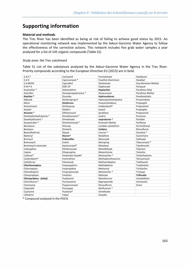
Chapitre 4 : Validation des échantillonneurs passifs sur le terrain
Supporting information Material and methods The Trec River has been identified as being at risk of failing to achieve good status by 2015. An operational monitoring network was implemented by the Adour-Garonne Water Agency to follow the effectiveness of the corrective actions. This network includes five grab water samples a year analysed for a list of 145 organic compounds (Table S1) Study area: the Trec catchment
Table S1 List of the substances analyzed by the Adour-Garonne Water Agency in the Trec River. Priority compounds according to the European Directive EU (2013) are in bold. 2,4,5 T Cymoxanil Formetenate Oxadiazon 2,4-D Cyproconazol * Fosethyl-Aluminium Oxadixyl 2,4-MCPA Cyprodinil Glufosinate Oxy-Demeton-Methyl A M P A DDD 24' Glyphosate Paraquat Acetochlor * Deltamethrin Heptachlor Parathion Ethyl Aclonifen Desisopropylatrazine * Hexaconazol Parathion Methyl Alachlor * Dicamba Hydrocarbures Pendimethalin Aldicarb Dichloroprop-P Hydroxyterbuthylazine Procymidone Aldrin Dichlorvos Imazamethabenz Propargite Aminotriazol Dichlorprop Imidacloprid* Propyzamid Asulam Dieldrin Ioxynil Propargite Atrazine * Diflufenicanil Iprodione Propyzamid Desethylterbuthylazine * Dimethanamid * Isodrin Pyrazone Desethylatrazine * Dimethoate Isoproturon * Pyridate Azoxystrobin * Dimethomorph * Kresoxim Methyl Pyrifenox Benoxacor Dinocap Lambda-cyhalothrin Pyrimethanyl Bentazon Dinoterb Lindane Rimsulfuron Betacyfluthrine Diquat Linuron * Simazine * Biphenyl Diuron* Malathion Sulcotrione Bromacil Endosulfan Mancozeb Sulfosate Bromoxynil Endrin Mecoprop Tebuconazol * Bromoxynil octanoate Epoxiconazol* Metalaxyl Tebufenozid Cadusaphos Ethofumesate Metaldehyde Tebutam Captan Ethoprophos Metamitrone Terbufos Carbaryl* Fenbutatin Oxydef Metazachlor * Terbuthylazine Carbendazim* Fenitrothion Methabenzthiazuron Tetraconazol Carbofuran Fénoxicarb Methamidophos Tolyfluanid Chlorfenvinphos Fenpropathrin Methidathion Triadimefon Chlormephos Fenpropidine Methomyl Trichlorfon Chlorothalonil Fenpropimorph Metolachlor * Triclopyr Chlorpropham Fenthion Molinate Trifluralin Chlorpyriphos - (ethyl) Fludioxonil Monolinuron Vamidothion Chlortoluron * Flumioxazine Napropamide Vinclozolin Clomazone Fluquinconazol Nicosulfuron Ziram Clopyralid Fluroxypyr Norflurazon *
Cyanazine Fluzilazol* Omethoate Cyfluthrin Folpel Oryzalin * Compound analyzed in the POCIS
163
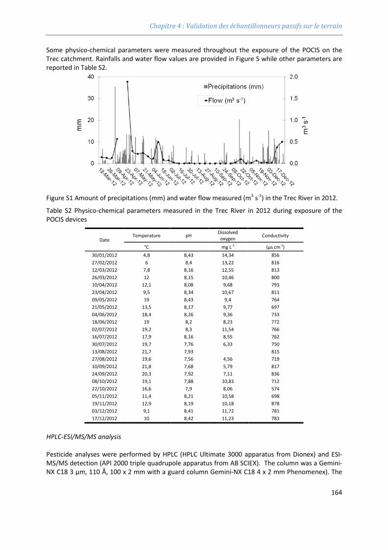
Chapitre 4 : Validation des échantillonneurs passifs sur le terrain
Some physico-chemical parameters were measured throughout the exposure of the POCIS on the Trec catchment. Rainfalls and water flow values are provided in Figure S while other parameters are reported in Table S2.
Figure S1 Amount of precipitations (mm) and water flow measured (m3 s-1) in the Trec River in 2012.
Table S2 Physico-chemical parameters measured in the Trec River in 2012 during exposure of the POCIS devices
Date Temperature pH Dissolved
oxygen Conductivity
°C mg L-1 (µs cm-1) 30/01/2012 4,8 8,43 14,34 856 27/02/2012 6 8,4 13,22 816 12/03/2012 7,8 8,16 12,55 813 26/03/2012 12 8,15 10,46 800 10/04/2012 12,1 8,08 9,68 793 23/04/2012 9,5 8,34 10,67 811 09/05/2012 19 8,43 9,4 764 21/05/2012 13,5 8,17 9,77 697 04/06/2012 18,4 8,26 9,36 733 18/06/2012 19 8,2 8,23 772 02/07/2012 19,2 8,3 11,54 766 16/07/2012 17,9 8,16 8,55 762 30/07/2012 19,7 7,76 6,33 750 13/08/2012 21,7 7,93 815 27/08/2012 19,6 7,56 4,56 719 10/09/2012 21,8 7,68 5,79 817 24/09/2012 20,3 7,92 7,11 836 08/10/2012 19,1 7,88 10,83 712 22/10/2012 16,6 7,9 8,06 574 05/11/2012 11,4 8,21 10,58 698 19/11/2012 12,9 8,19 10,18 878 03/12/2012 9,1 8,41 11,72 781 17/12/2012 10 8,42 11,23 783
HPLC-ESI/MS/MS analysis Pesticide analyses were performed by HPLC (HPLC Ultimate 3000 apparatus from Dionex) and ESI-MS/MS detection (API 2000 triple quadrupole apparatus from AB SCIEX). The column was a Gemini-NX C18 3 µm, 110 Å, 100 x 2 mm with a guard column Gemini-NX C18 4 x 2 mm Phenomenex). The
164
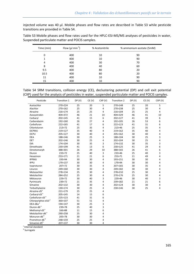
Chapitre 4 : Validation des échantillonneurs passifs sur le terrain
injected volume was 40 µl. Mobile phases and flow rates are described in Table S3 while pesticide transitions are provided in Table S4.
Table S3 Mobile phases and flow rates used for the HPLC-ESI-MS/MS analyses of pesticides in water, Suspended particulate matter and POCIS samples.
Time (min) Flow (µl min-1) % Acetonitrile % ammonium acetate (5mM)
0 400 10 90 1 400 10 90 4 400 30 70 8 400 40 60
9.5 400 80 20 10.5 400 80 20 11 400 10 90 15 400 10 90
Table S4 SRM transitions, collision energy (CE), declustering potential (DP) and cell exit potential (CXP) used for the analysis of pesticides in water, suspended particulate matter and POCIS samples.
Pesticide Transition 1 DP (V) CE (V) CXP (V) Transition 2 DP (V) CE (V) CXP (V)
Acetochlor 270>224 25 20 5 270>148 25 20 5 Alachlor 270>162 25 30 4 270>238 25 30 4 Atrazine 216>174 25 25 4 216>104 25 25 4 Azoxystrobin 404>372 46 21 14 404>329 46 41 10 Carbaryl 202>145 41 15 6 202>127 41 39 6 Carbendazim 192>160 26 27 4 192>105 26 53 6 Carbofuran 222>165 41 17 6 222>123 41 31 6 Chlortoluron 213>72 25 35 4 213>46 25 35 4 DCPMU 219>127 35 40 4 219>162 35 40 4 DCPU 205>127 30 40 4 205>162 30 40 4 DEA 188>146 30 25 3 188>104 30 25 3 DET 202>146 30 25 4 202>104 30 25 4 DIA 174>104 30 35 3 174>132 30 35 3 Dimethoate 230>199 41 13 6 230>125 41 29 6 Dimetomorph 388>301 26 29 10 388>165 26 41 6 Diuron 233>72 25 40 3 233>46 25 40 3 Hexazinon 253>171 21 21 6 253>71 21 49 4 IPPMU 193>94 30 30 4 193>151 30 30 4 IPPU 179>137 30 30 4 179>94 30 30 4 Isoproturon 207>72 30 35 4 207>165 30 35 4 Linuron 249>160 30 30 4 249>182 30 30 4 Metazachlor 278>134 25 30 4 278>210 25 30 4 Metolachlor 284>252 25 30 4 270>176 25 30 4 Métoxuron 229>72 30 40 3 229>46 30 40 3 Pyrimicarb 239>72 21 35 4 239>182 21 21 6 Simazine 202>132 30 30 4 202>124 30 30 4 Terbuthylazine 130>174 30 25 4 230>146 30 25 4 Atrazine-d5a 221>179 25 25 4 Carbaryl-d3 a 205>145 14 15 6 Carbofuran-d3 a 225>123 41 31 6 Chlorpyriphos-d10 a 360>107 51 51 4 DEA-d6a a 194>147 30 25 3 Diuron-d6 a 239>78 25 40 3 Methomyl-d3 a 166>88 11 15 6 Metolachlor-d6 a 290>258 25 30 4 Monuron-d6 b 205>78 30 30 4 Prometryn-d6 b 248>159 25 25 4 Simazine-d5b 207>137 30 30 4
a Internal standard b Surrogate
165
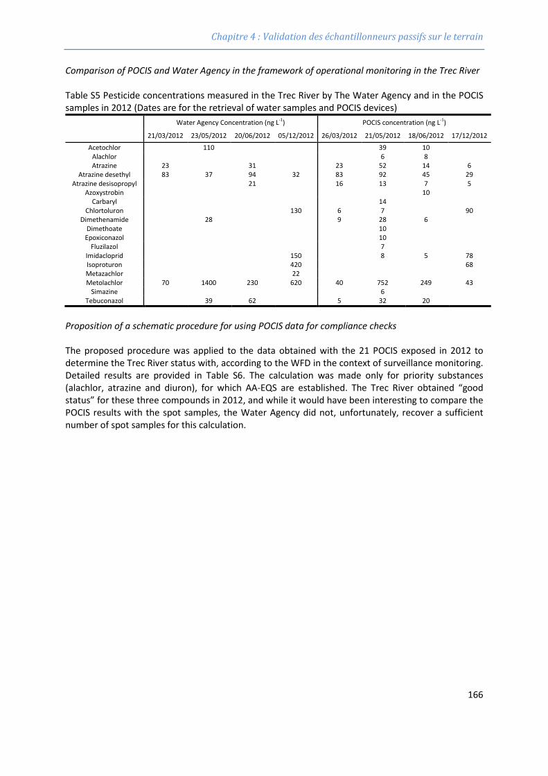
Chapitre 4 : Validation des échantillonneurs passifs sur le terrain
Comparison of POCIS and Water Agency in the framework of operational monitoring in the Trec River Table S5 Pesticide concentrations measured in the Trec River by The Water Agency and in the POCIS samples in 2012 (Dates are for the retrieval of water samples and POCIS devices)
Water Agency Concentration (ng L-1) POCIS concentration (ng L-1)
21/03/2012 23/05/2012 20/06/2012 05/12/2012 26/03/2012 21/05/2012 18/06/2012 17/12/2012
Acetochlor
110
39 10 Alachlor
6 8
Atrazine 23
31
23 52 14 6 Atrazine desethyl 83 37 94 32 83 92 45 29
Atrazine desisopropyl
21
16 13 7 5 Azoxystrobin
10
Carbaryl
14 Chlortoluron
130 6 7
90
Dimethenamide
28
9 28 6 Dimethoate
10
Epoxiconazol
10 Fluzilazol
7
Imidacloprid
150
8 5 78 Isoproturon
420
68
Metazachlor
22 Metolachlor 70 1400 230 620 40 752 249 43
Simazine
6 Tebuconazol
39 62
5 32 20
Proposition of a schematic procedure for using POCIS data for compliance checks The proposed procedure was applied to the data obtained with the 21 POCIS exposed in 2012 to determine the Trec River status with, according to the WFD in the context of surveillance monitoring. Detailed results are provided in Table S6. The calculation was made only for priority substances (alachlor, atrazine and diuron), for which AA-EQS are established. The Trec River obtained “good status” for these three compounds in 2012, and while it would have been interesting to compare the POCIS results with the spot samples, the Water Agency did not, unfortunately, recover a sufficient number of spot samples for this calculation.
166
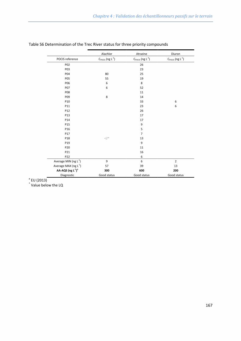
Chapitre 4 : Validation des échantillonneurs passifs sur le terrain
Table S6 Determination of the Trec River status for three priority compounds
Alachlor Atrazine Diuron
POCIS reference CPOCIS (ng L-1) CPOCIS (ng L-1) CPOCIS (ng L-1)
P02
26 P03
23
P04 80 25 P05 55 19 P06 6 8 P07 6 52 P08
11
P09 8 14 P10
33 6
P11
23 6 P12
26
P13
17 P14
17
P15
9 P16
5
P17
7 P18 <2* 13 P19
9
P20
11 P21
16
P22 6 Average MIN (ng L-1) 9 6 2 Average MAX (ng L-1) 57 39 13
AA-AQS (ng L-1)a 300 600 200 Diagnostic Good status Good status Good status
a EU (2013) * Value below the LQ
167

Chapitre 4 : Validation des échantillonneurs passifs sur le terrain
168
Chapitre 4 : Validation des échantillonneurs passifs sur le terrain
4.4 Publication 3 “DGT-labile As, Cd, Cu and Ni monitoring in
freshwater: Toward a framework for interpretation of in situ
deployment”
Rémy Buziera*, Adeline Charriaua, David Coronaa, Jean-François Lenaina, Patrice Fondanèchea,
Emmanuel Jousseina, Gaëlle Pouliera,b, Sophie Lissaldea, Nicolas Mazzella b, Gilles Guibauda
Environmental Pollution, 192 :52-58, 2014, http://dx.doi.org/10.1016/j.envpol.2014.05.017
a Université de Limoges, Groupement de Recherche Eau, Sol, Environnement (GRESE), 123
avenue Albert Thomas, 87060 LIMOGES, FRANCE
b IRSTEA, REBX Unit, 50 avenue de Verdun, 33612 CESTAS, FRANCE
* Corresponding author: [email protected]
169

Chapitre 4 : Validation des échantillonneurs passifs sur le terrain
170
Chapitre 4 : Validation des échantillonneurs passifs sur le terrain
DGT-labile As, Cd, Cu and Ni monitoring in freshwater: Toward a framework for in situ deployments interpretation
Rémy Buzier1*, Adeline Charriau1, David Corona1, Jean-François Lenain1, Patrice Fondanèche1, Emmanuel Joussein1, Gaëlle Poulier1,2, Sophie Lissalde1, Nicolas Mazzella2, Gilles Guibaud1
Environmental Pollution, 192 :52-58, 2014, http://dx.doi.org/10.1016/j.envpol.2014.05.017
1 Université de Limoges, Groupement de Recherche Eau, Sol, Environnement (GRESE), 123 avenue Albert Thomas, 87060 LIMOGES, France
2 IRSTEA, REBX Unit, 50 avenue de Verdun, 33612 CESTAS, FRANCE
* Corresponding author: [email protected]
Abstract
The Diffusive Gradient in Thin Film sampler (DGT) is evaluated nowadays as a tool for regulatory programs. In this context, the impact of procedures commonly followed on the accuracy of DGT-labile As, Cd, Cu, and Ni quantification was studied. Initial contamination of the samplers yields to define quantification limits instead of using blank subtraction in order to avoid artifact concentrations. Not considering the alteration of element diffusion within the filter membrane leads to significant underestimation. However, diffusion coefficients determined on a non-fouled membrane were suitable for the studied site, making thus possible to use data from literature. When the diffusive boundary layer formation is neglected, no loss of accuracy is recorded provided a layer thinner than 0.5 mm. Moreover, the exploration of the potential biases allows to initiate a framework that might help limit some of the inaccuracies in DGT-labile concentration estimation and interpretation, especially in a low contaminated context.
Capsule
“Toward a framework for limiting inaccuracies in DGT-labile concentration estimation and interpretation based on in situ deployments”.
Keywords: Diffusive Gradient in Thin film (DGT); metals; metalloids; diffusion coefficient; passive sampling.
1. Introduction
The Diffusive Gradient in Thin film technique (DGT) was first proposed 20 years ago by Davison and Zhang (1994) as an in situ speciation technique. DGT fixes the elements of interest on a binding layer and relies on controlling the mass transfer by a diffusive gel; this gel allows for a speciation approach by distinguishing colloidal and strongly bound complexes (Scally et al., 2006). The technique samples both free and weakly bound elements that make reference to the so-called DGT-labile fraction. This passive sampler has been implemented in various media, including natural waters (Tusseau-Vuillemin et al., 2007), wastewaters (Buzier et al., 2006), soils (Garrido and Mendoza, 2013) and sediments (Roulier et al., 2010). As a passive sampler, DGT makes it possible to perform in situ pre-concentration and to determine time-weighted average concentrations. Thanks to these characteristics, DGT is now considered as a potential monitoring tool for regulatory programs (Allan et al., 2008; Miège et al., 2012). The basics of this technique are now well known and mastered (Davison and Zhang, 2012); however, quantification of the DGT-labile fraction is not a straightforward process for in situ applications as a number of biases can occur.
Should the devices display an initial contamination, the level of this contamination must be negligible compared to the amount of elements accumulated during deployment so as to ensure an accurate DGT-labile fraction quantification. This point is rarely addressed in field studies, even though the contamination is not
171
Chapitre 4 : Validation des échantillonneurs passifs sur le terrain
necessarily negligible when deployment takes place in low contaminated systems. Some authors have subtracted the estimated initial system contamination (Dunn et al., 2007), whereas others have defined a detection limit in order to identify suspicious samples (Leermakers et al., 2005). However, no specific procedure is routinely used; Miège et al. (2012) recently concluded that the initial system contamination is partly responsible for measurement uncertainty and that more detailed protocols were needed.
Quantification can also be biased when the accumulated mass (m) is converted to a DGT-labile concentration (CDGT). In most studies, this conversion step is performed through the model proposed by Zhang and Davison (1995) (Eq. 1):
𝐶𝐶𝐷𝐷𝐷𝐷𝐷𝐷 = 𝑚𝑚∆𝑀𝑀𝑀𝑀𝑀𝑀𝑡𝑡𝐷𝐷𝑔𝑔𝐴𝐴𝑔𝑔
(1)
where ΔMDL is the material diffusion layer thickness (diffusive gel + membrane filter), Dg the diffusion coefficient in the diffusive gel, Ag the geometric exposure area and t the deployment time. This model implies the two following assumptions: 1) diffusive boundary layer (DBL) formation is negligible; and 2) no lateral diffusion occurs within the gel. Warnken et al. (2006) showed that these assumptions are invalid and moreover that both errors compensate for standard devices as long as DBL thickness remains limited. Davison and Zhang (2012) then Uher et al. (2013) therefore concluded that errors committed when simultaneously adopting both assumptions lie within the range of method uncertainty, and their use is in fact suitable for monitoring programs. A more sophisticated model that avoid assumptions (1) and (2) can still be used (Garmo et al., 2006) but requires an estimation of DBL thickness. This estimation phase is costly as well as time consuming; hence, it is not adapted to a monitoring context. When DBL is quite thick, a reliable CDGT cannot be determined by applying Eq. 1.
Bias can also be induced by the data selected as model inputs, especially the diffusion coefficient. Indeed, the Dg value introduced in Eq. 1 is most commonly the diffusion coefficient in the diffusive gel alone given that diffusion in the diffusive gel and membrane filter are usually assumed to be identical. The validity of this assumption, however, has only been minimally discussed in the literature. Scally et al. (2006) demonstrated its validity for Cd and Cu with polysulfone membranes, yet results from Uher et al. (2012) subsequently invalidated this assumption for 11 elements with polycarbonate membranes. Moreover, the membrane can become fouled during an in situ deployment and thereby alter elements diffusion (Uher et al., 2012). The systematic use of a diffusion coefficient in the diffusive gel alone is thus not necessarily relevant for in situ deployment and may bias the DGT-labile concentration estimation. In addition, the diffusion coefficient for cationic species in diffusive gels was shown to have been modified for deployment in water with an ionic strength (I) of less than 0.01 M (Fatin-Rouge et al., 2003) or less than 0.001 M (Warnken et al., 2005). When deployment takes place in poorly mineralized water (i.e. with a low ionic strength), a diffusion coefficient measurement in synthetic water with a similar composition is advised (Sangi et al., 2002; Fatin-Rouge et al., 2003).
The aim of this work is to discuss the quantification of DGT-labile arsenic (As), cadmium (Cd), copper (Cu), and nickel (Ni) based on in situ DGT deployment in a regulatory context. The potential biases stated above will be studied for a conventional in situ deployment. The DGT-labile concentration quantification will be discussed in terms of validity domain (i.e. limit of quantification) and in terms of accuracy. Finally, a procedure will be proposed to provide a framework for interpreting DGT-labile concentrations and to target complementary experiments capable of limiting biases.
2. Materials and methods
2.1. DGT preparation
Diffusive gels and binding gels were prepared according to the procedure given in Zhang et al. (1998). An agarose polyacrylamide hydrogel, containing 15% acrylamide (Fisher Scientific) and 0.3% agarose derived cross-linker (DGTResearch Ltd.), was used as a diffusive gel. According to the spacers used, the measured diffusive gel thicknesses were: 0.45, 0.77, 1.12 and 1.50 mm.
Ion exchange resin Chelex-100 (Na-form, 200-400 mesh, Bio-rad) was introduced as a binding phase for Cd, Cu, and Ni, whereas ferrihydrite served as the binding phase for As. Binding gels were prepared in a
172
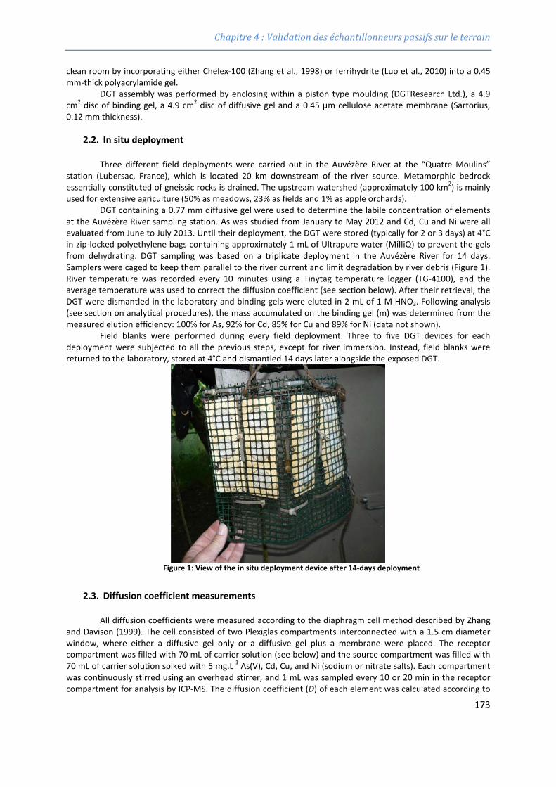
Chapitre 4 : Validation des échantillonneurs passifs sur le terrain
clean room by incorporating either Chelex-100 (Zhang et al., 1998) or ferrihydrite (Luo et al., 2010) into a 0.45 mm-thick polyacrylamide gel.
DGT assembly was performed by enclosing within a piston type moulding (DGTResearch Ltd.), a 4.9 cm2 disc of binding gel, a 4.9 cm2 disc of diffusive gel and a 0.45 µm cellulose acetate membrane (Sartorius, 0.12 mm thickness).
2.2. In situ deployment
Three different field deployments were carried out in the Auvézère River at the “Quatre Moulins” station (Lubersac, France), which is located 20 km downstream of the river source. Metamorphic bedrock essentially constituted of gneissic rocks is drained. The upstream watershed (approximately 100 km2) is mainly used for extensive agriculture (50% as meadows, 23% as fields and 1% as apple orchards).
DGT containing a 0.77 mm diffusive gel were used to determine the labile concentration of elements at the Auvézère River sampling station. As was studied from January to May 2012 and Cd, Cu and Ni were all evaluated from June to July 2013. Until their deployment, the DGT were stored (typically for 2 or 3 days) at 4°C in zip-locked polyethylene bags containing approximately 1 mL of Ultrapure water (MilliQ) to prevent the gels from dehydrating. DGT sampling was based on a triplicate deployment in the Auvézère River for 14 days. Samplers were caged to keep them parallel to the river current and limit degradation by river debris (Figure 1). River temperature was recorded every 10 minutes using a Tinytag temperature logger (TG-4100), and the average temperature was used to correct the diffusion coefficient (see section below). After their retrieval, the DGT were dismantled in the laboratory and binding gels were eluted in 2 mL of 1 M HNO3. Following analysis (see section on analytical procedures), the mass accumulated on the binding gel (m) was determined from the measured elution efficiency: 100% for As, 92% for Cd, 85% for Cu and 89% for Ni (data not shown).
Field blanks were performed during every field deployment. Three to five DGT devices for each deployment were subjected to all the previous steps, except for river immersion. Instead, field blanks were returned to the laboratory, stored at 4°C and dismantled 14 days later alongside the exposed DGT.
Figure 1: View of the in situ deployment device after 14-days deployment
2.3. Diffusion coefficient measurements
All diffusion coefficients were measured according to the diaphragm cell method described by Zhang and Davison (1999). The cell consisted of two Plexiglas compartments interconnected with a 1.5 cm diameter window, where either a diffusive gel only or a diffusive gel plus a membrane were placed. The receptor compartment was filled with 70 mL of carrier solution (see below) and the source compartment was filled with 70 mL of carrier solution spiked with 5 mg.L-1 As(V), Cd, Cu, and Ni (sodium or nitrate salts). Each compartment was continuously stirred using an overhead stirrer, and 1 mL was sampled every 10 or 20 min in the receptor compartment for analysis by ICP-MS. The diffusion coefficient (D) of each element was calculated according to
173
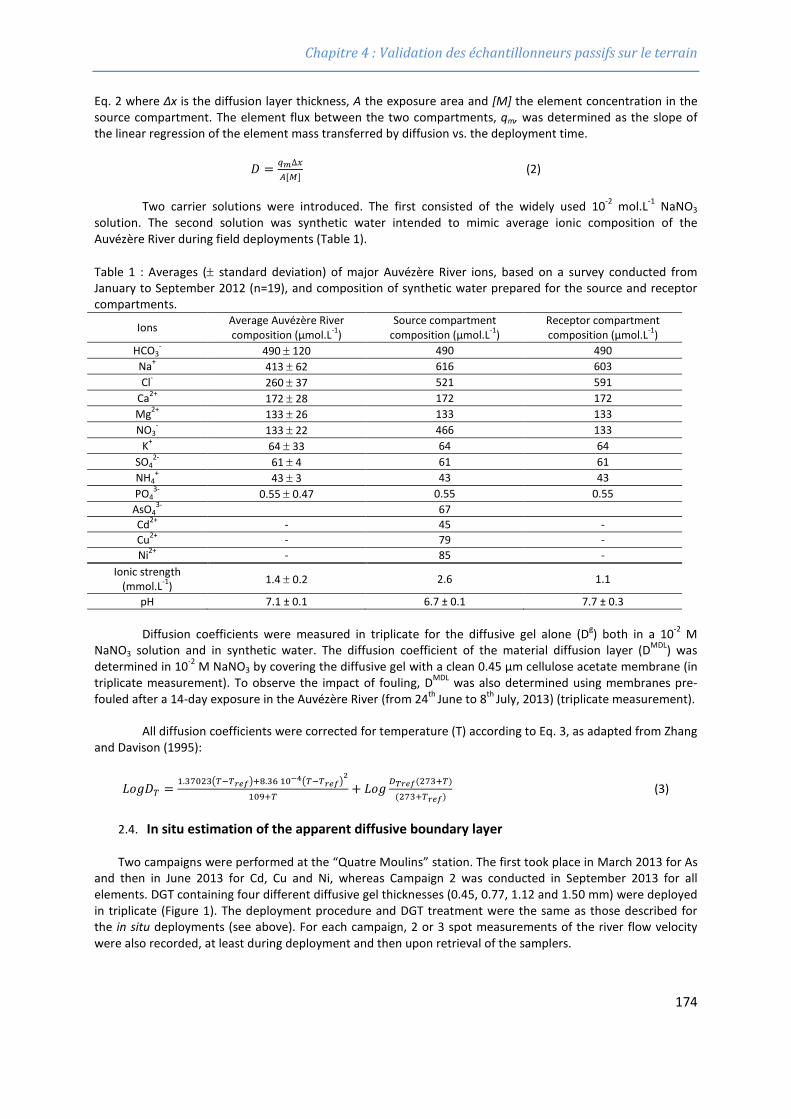
Chapitre 4 : Validation des échantillonneurs passifs sur le terrain
Eq. 2 where Δx is the diffusion layer thickness, A the exposure area and [M] the element concentration in the source compartment. The element flux between the two compartments, qm, was determined as the slope of the linear regression of the element mass transferred by diffusion vs. the deployment time.
𝐷𝐷 = 𝑞𝑞𝑚𝑚∆𝑥𝑥𝐴𝐴[𝑀𝑀]
(2)
Two carrier solutions were introduced. The first consisted of the widely used 10-2 mol.L-1 NaNO3 solution. The second solution was synthetic water intended to mimic average ionic composition of the Auvézère River during field deployments (Table 1).
Table 1 : Averages (± standard deviation) of major Auvézère River ions, based on a survey conducted from January to September 2012 (n=19), and composition of synthetic water prepared for the source and receptor compartments.
Ions Average Auvézère River composition (µmol.L-1)
Source compartment composition (µmol.L-1)
Receptor compartment composition (µmol.L-1)
HCO3- 490 ± 120 490 490
Na+ 413 ± 62 616 603 Cl- 260 ± 37 521 591
Ca2+ 172 ± 28 172 172 Mg2+ 133 ± 26 133 133 NO3
- 133 ± 22 466 133 K+ 64 ± 33 64 64
SO42- 61 ± 4 61 61
NH4+ 43 ± 3 43 43
PO43- 0.55 ± 0.47 0.55 0.55
AsO43- 67
Cd2+ - 45 - Cu2+ - 79 - Ni2+ - 85 -
Ionic strength (mmol.L-1) 1.4 ± 0.2 2.6 1.1
pH 7.1 ± 0.1 6.7 ± 0.1 7.7 ± 0.3 Diffusion coefficients were measured in triplicate for the diffusive gel alone (Dg) both in a 10-2 M
NaNO3 solution and in synthetic water. The diffusion coefficient of the material diffusion layer (DMDL) was determined in 10-2 M NaNO3 by covering the diffusive gel with a clean 0.45 µm cellulose acetate membrane (in triplicate measurement). To observe the impact of fouling, DMDL was also determined using membranes pre-fouled after a 14-day exposure in the Auvézère River (from 24th June to 8th July, 2013) (triplicate measurement).
All diffusion coefficients were corrected for temperature (T) according to Eq. 3, as adapted from Zhang and Davison (1995):
𝐿𝐿𝐿𝐿𝐿𝐿𝐷𝐷𝐷𝐷 = 1.37023𝐷𝐷−𝐷𝐷𝑟𝑟𝑟𝑟𝑟𝑟+8.36 10−4𝐷𝐷−𝐷𝐷𝑟𝑟𝑟𝑟𝑟𝑟2
109+𝐷𝐷+ 𝐿𝐿𝐿𝐿𝐿𝐿 𝐷𝐷𝑇𝑇𝑟𝑟𝑟𝑟𝑟𝑟(273+𝐷𝐷)
(273+𝐷𝐷𝑟𝑟𝑟𝑟𝑟𝑟) (3)
2.4. In situ estimation of the apparent diffusive boundary layer
Two campaigns were performed at the “Quatre Moulins” station. The first took place in March 2013 for As and then in June 2013 for Cd, Cu and Ni, whereas Campaign 2 was conducted in September 2013 for all elements. DGT containing four different diffusive gel thicknesses (0.45, 0.77, 1.12 and 1.50 mm) were deployed in triplicate (Figure 1). The deployment procedure and DGT treatment were the same as those described for the in situ deployments (see above). For each campaign, 2 or 3 spot measurements of the river flow velocity were also recorded, at least during deployment and then upon retrieval of the samplers.
174
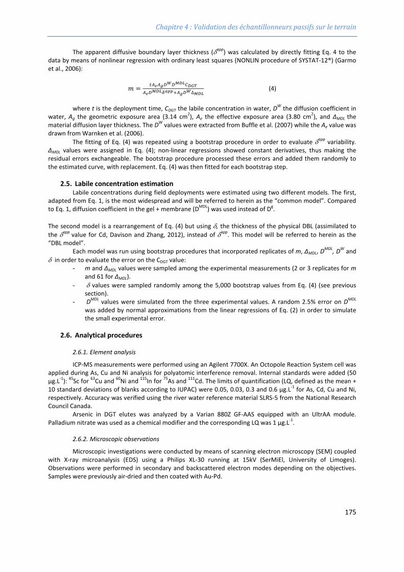
Chapitre 4 : Validation des échantillonneurs passifs sur le terrain
The apparent diffusive boundary layer thickness (δapp) was calculated by directly fitting Eq. 4 to the data by means of nonlinear regression with ordinary least squares (NONLIN procedure of SYSTAT-12®) (Garmo et al., 2006):
𝑚𝑚 = 𝑡𝑡𝐴𝐴𝑟𝑟𝐴𝐴𝑔𝑔𝐷𝐷𝑊𝑊𝐷𝐷𝑀𝑀𝑀𝑀𝑀𝑀𝐶𝐶𝑀𝑀𝐷𝐷𝑇𝑇𝐴𝐴𝑟𝑟𝐷𝐷𝑀𝑀𝑀𝑀𝑀𝑀𝛿𝛿𝑎𝑎𝑎𝑎𝑎𝑎+𝐴𝐴𝑔𝑔𝐷𝐷𝑊𝑊∆𝑀𝑀𝑀𝑀𝑀𝑀
(4)
where t is the deployment time, CDGT the labile concentration in water, DW the diffusion coefficient in water, Ag the geometric exposure area (3.14 cm2), Ae the effective exposure area (3.80 cm2), and ΔMDL the material diffusion layer thickness. The DW values were extracted from Buffle et al. (2007) while the Ae value was drawn from Warnken et al. (2006).
The fitting of Eq. (4) was repeated using a bootstrap procedure in order to evaluate δapp variability. ΔMDL values were assigned in Eq. (4); non-linear regressions showed constant derivatives, thus making the residual errors exchangeable. The bootstrap procedure processed these errors and added them randomly to the estimated curve, with replacement. Eq. (4) was then fitted for each bootstrap step.
2.5. Labile concentration estimation Labile concentrations during field deployments were estimated using two different models. The first,
adapted from Eq. 1, is the most widespread and will be referred to herein as the “common model”. Compared to Eq. 1, diffusion coefficient in the gel + membrane (DMDL) was used instead of Dg. The second model is a rearrangement of Eq. (4) but using δ, the thickness of the physical DBL (assimilated to the δapp value for Cd, Davison and Zhang, 2012), instead of δapp. This model will be referred to herein as the “DBL model”.
Each model was run using bootstrap procedures that incorporated replicates of m, ΔMDL, DMDL, DW and
δ in order to evaluate the error on the CDGT value: - m and ΔMDL values were sampled among the experimental measurements (2 or 3 replicates for m
and 61 for ΔMDL). - δ values were sampled randomly among the 5,000 bootstrap values from Eq. (4) (see previous
section). - DMDL values were simulated from the three experimental values. A random 2.5% error on DMDL
was added by normal approximations from the linear regressions of Eq. (2) in order to simulate the small experimental error.
2.6. Analytical procedures
2.6.1. Element analysis
ICP-MS measurements were performed using an Agilent 7700X. An Octopole Reaction System cell was applied during As, Cu and Ni analysis for polyatomic interference removal. Internal standards were added (50 µg.L-1): 45Sc for 63Cu and 60Ni and 115In for 75As and 111Cd. The limits of quantification (LQ, defined as the mean + 10 standard deviations of blanks according to IUPAC) were 0.05, 0.03, 0.3 and 0.6 µg.L-1 for As, Cd, Cu and Ni, respectively. Accuracy was verified using the river water reference material SLRS-5 from the National Research Council Canada.
Arsenic in DGT elutes was analyzed by a Varian 880Z GF-AAS equipped with an UltrAA module. Palladium nitrate was used as a chemical modifier and the corresponding LQ was 1 µg.L-1.
2.6.2. Microscopic observations
Microscopic investigations were conducted by means of scanning electron microscopy (SEM) coupled with X-ray microanalysis (EDS) using a Philips XL-30 running at 15kV (SerMiEl, University of Limoges). Observations were performed in secondary and backscattered electron modes depending on the objectives. Samples were previously air-dried and then coated with Au-Pd.
175
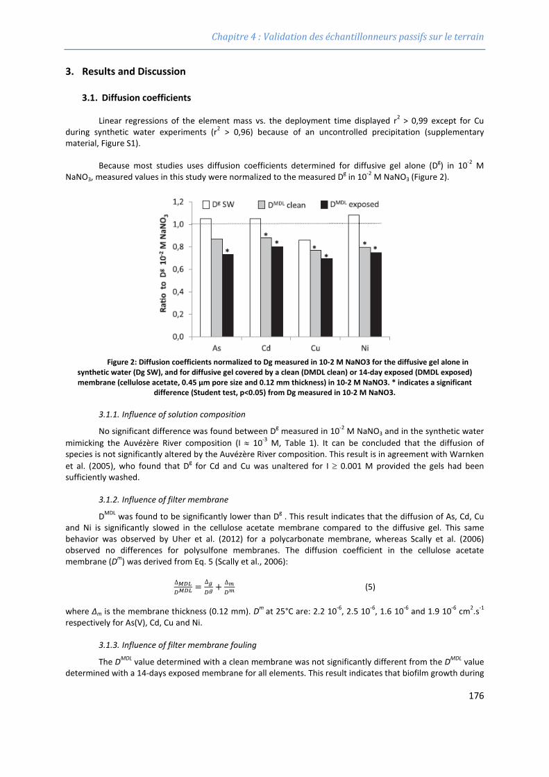
Chapitre 4 : Validation des échantillonneurs passifs sur le terrain
3. Results and Discussion
3.1. Diffusion coefficients
Linear regressions of the element mass vs. the deployment time displayed r2 > 0,99 except for Cu during synthetic water experiments (r2 > 0,96) because of an uncontrolled precipitation (supplementary material, Figure S1).
Because most studies uses diffusion coefficients determined for diffusive gel alone (Dg) in 10-2 M NaNO3, measured values in this study were normalized to the measured Dg in 10-2 M NaNO3 (Figure 2).
Figure 2: Diffusion coefficients normalized to Dg measured in 10-2 M NaNO3 for the diffusive gel alone in
synthetic water (Dg SW), and for diffusive gel covered by a clean (DMDL clean) or 14-day exposed (DMDL exposed) membrane (cellulose acetate, 0.45 µm pore size and 0.12 mm thickness) in 10-2 M NaNO3. * indicates a significant
difference (Student test, p<0.05) from Dg measured in 10-2 M NaNO3.
3.1.1. Influence of solution composition
No significant difference was found between Dg measured in 10-2 M NaNO3 and in the synthetic water mimicking the Auvézère River composition (I ≈ 10-3 M, Table 1). It can be concluded that the diffusion of species is not significantly altered by the Auvézère River composition. This result is in agreement with Warnken et al. (2005), who found that Dg for Cd and Cu was unaltered for I ≥ 0.001 M provided the gels had been sufficiently washed.
3.1.2. Influence of filter membrane
DMDL was found to be significantly lower than Dg . This result indicates that the diffusion of As, Cd, Cu and Ni is significantly slowed in the cellulose acetate membrane compared to the diffusive gel. This same behavior was observed by Uher et al. (2012) for a polycarbonate membrane, whereas Scally et al. (2006) observed no differences for polysulfone membranes. The diffusion coefficient in the cellulose acetate membrane (Dm) was derived from Eq. 5 (Scally et al., 2006):
∆𝑀𝑀𝑀𝑀𝑀𝑀𝐷𝐷𝑀𝑀𝑀𝑀𝑀𝑀 = ∆𝑔𝑔
𝐷𝐷𝑔𝑔+ ∆𝑚𝑚
𝐷𝐷𝑚𝑚 (5)
where Δm is the membrane thickness (0.12 mm). Dm at 25°C are: 2.2 10-6, 2.5 10-6, 1.6 10-6 and 1.9 10-6 cm2.s-1 respectively for As(V), Cd, Cu and Ni.
3.1.3. Influence of filter membrane fouling
The DMDL value determined with a clean membrane was not significantly different from the DMDL value determined with a 14-days exposed membrane for all elements. This result indicates that biofilm growth during
176
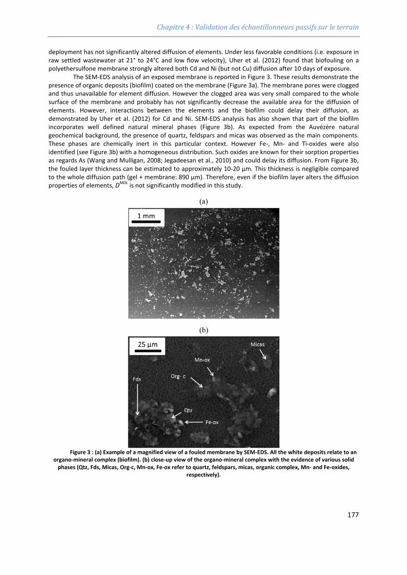
Chapitre 4 : Validation des échantillonneurs passifs sur le terrain
deployment has not significantly altered diffusion of elements. Under less favorable conditions (i.e. exposure in raw settled wastewater at 21° to 24°C and low flow velocity), Uher et al. (2012) found that biofouling on a polyethersulfone membrane strongly altered both Cd and Ni (but not Cu) diffusion after 10 days of exposure.
The SEM-EDS analysis of an exposed membrane is reported in Figure 3. These results demonstrate the presence of organic deposits (biofilm) coated on the membrane (Figure 3a). The membrane pores were clogged and thus unavailable for element diffusion. However the clogged area was very small compared to the whole surface of the membrane and probably has not significantly decrease the available area for the diffusion of elements. However, interactions between the elements and the biofilm could delay their diffusion, as demonstrated by Uher et al. (2012) for Cd and Ni. SEM-EDS analysis has also shown that part of the biofilm incorporates well defined natural mineral phases (Figure 3b). As expected from the Auvézère natural geochemical background, the presence of quartz, feldspars and micas was observed as the main components. These phases are chemically inert in this particular context. However Fe-, Mn- and Ti-oxides were also identified (see Figure 3b) with a homogeneous distribution. Such oxides are known for their sorption properties as regards As (Wang and Mulligan, 2008; Jegadeesan et al., 2010) and could delay its diffusion. From Figure 3b, the fouled layer thickness can be estimated to approximately 10-20 µm. This thickness is negligible compared to the whole diffusion path (gel + membrane: 890 µm). Therefore, even if the biofilm layer alters the diffusion properties of elements, DMDL is not significantly modified in this study.
Figure 3 : (a) Example of a magnified view of a fouled membrane by SEM-EDS. All the white deposits relate to an
organo-mineral complex (biofilm). (b) close-up view of the organo-mineral complex with the evidence of various solid phases (Qtz, Fds, Micas, Org-c, Mn-ox, Fe-ox refer to quartz, feldspars, micas, organic complex, Mn- and Fe-oxides,
respectively).
177
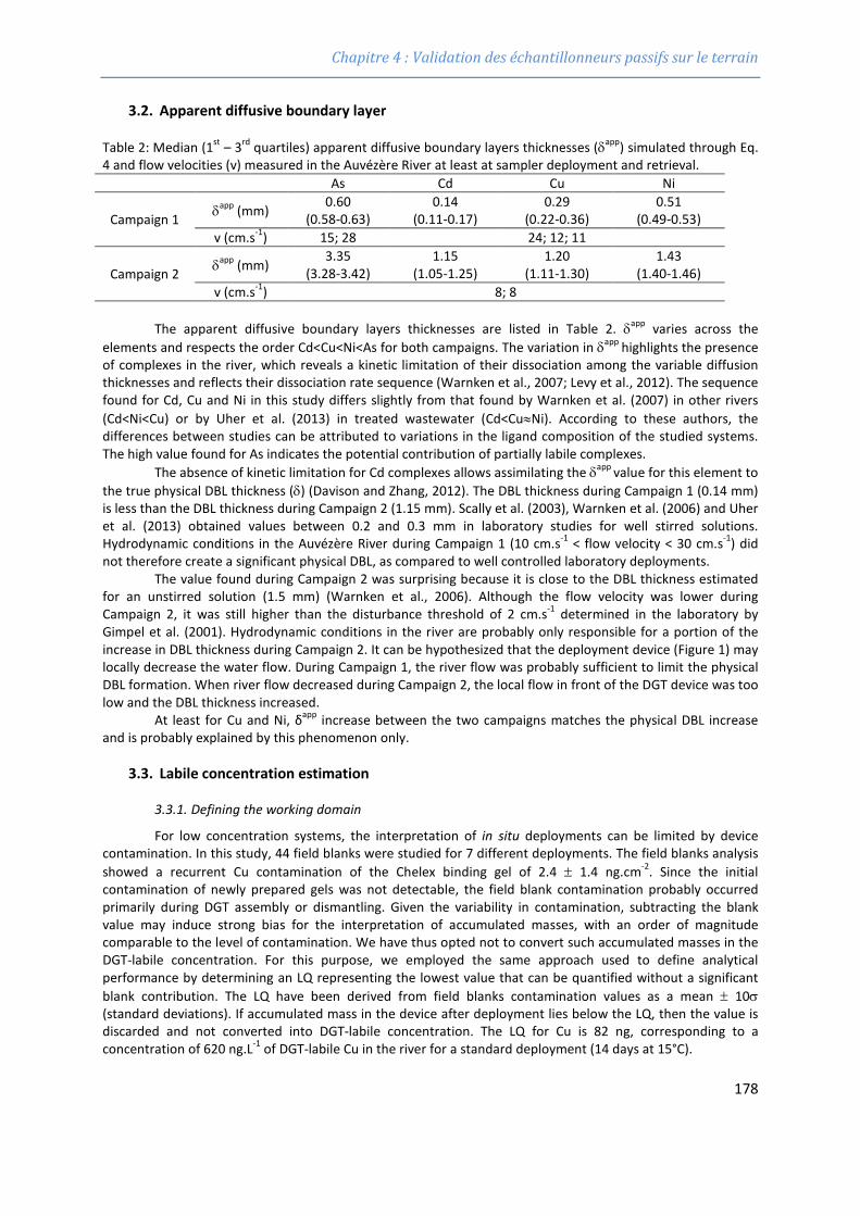
Chapitre 4 : Validation des échantillonneurs passifs sur le terrain
3.2. Apparent diffusive boundary layer
Table 2: Median (1st – 3rd quartiles) apparent diffusive boundary layers thicknesses (δapp) simulated through Eq. 4 and flow velocities (v) measured in the Auvézère River at least at sampler deployment and retrieval.
As Cd Cu Ni
Campaign 1 δapp (mm) 0.60
(0.58-0.63) 0.14
(0.11-0.17) 0.29
(0.22-0.36) 0.51
(0.49-0.53) v (cm.s-1) 15; 28 24; 12; 11
Campaign 2 δapp (mm) 3.35
(3.28-3.42) 1.15
(1.05-1.25) 1.20
(1.11-1.30) 1.43
(1.40-1.46) v (cm.s-1) 8; 8
The apparent diffusive boundary layers thicknesses are listed in Table 2. δapp varies across the
elements and respects the order Cd<Cu<Ni<As for both campaigns. The variation in δapp highlights the presence of complexes in the river, which reveals a kinetic limitation of their dissociation among the variable diffusion thicknesses and reflects their dissociation rate sequence (Warnken et al., 2007; Levy et al., 2012). The sequence found for Cd, Cu and Ni in this study differs slightly from that found by Warnken et al. (2007) in other rivers (Cd<Ni<Cu) or by Uher et al. (2013) in treated wastewater (Cd<Cu≈Ni). According to these authors, the differences between studies can be attributed to variations in the ligand composition of the studied systems. The high value found for As indicates the potential contribution of partially labile complexes.
The absence of kinetic limitation for Cd complexes allows assimilating the δapp value for this element to the true physical DBL thickness (δ) (Davison and Zhang, 2012). The DBL thickness during Campaign 1 (0.14 mm) is less than the DBL thickness during Campaign 2 (1.15 mm). Scally et al. (2003), Warnken et al. (2006) and Uher et al. (2013) obtained values between 0.2 and 0.3 mm in laboratory studies for well stirred solutions. Hydrodynamic conditions in the Auvézère River during Campaign 1 (10 cm.s-1 < flow velocity < 30 cm.s-1) did not therefore create a significant physical DBL, as compared to well controlled laboratory deployments.
The value found during Campaign 2 was surprising because it is close to the DBL thickness estimated for an unstirred solution (1.5 mm) (Warnken et al., 2006). Although the flow velocity was lower during Campaign 2, it was still higher than the disturbance threshold of 2 cm.s-1 determined in the laboratory by Gimpel et al. (2001). Hydrodynamic conditions in the river are probably only responsible for a portion of the increase in DBL thickness during Campaign 2. It can be hypothesized that the deployment device (Figure 1) may locally decrease the water flow. During Campaign 1, the river flow was probably sufficient to limit the physical DBL formation. When river flow decreased during Campaign 2, the local flow in front of the DGT device was too low and the DBL thickness increased.
At least for Cu and Ni, δapp increase between the two campaigns matches the physical DBL increase and is probably explained by this phenomenon only.
3.3. Labile concentration estimation
3.3.1. Defining the working domain
For low concentration systems, the interpretation of in situ deployments can be limited by device contamination. In this study, 44 field blanks were studied for 7 different deployments. The field blanks analysis showed a recurrent Cu contamination of the Chelex binding gel of 2.4 ± 1.4 ng.cm-2. Since the initial contamination of newly prepared gels was not detectable, the field blank contamination probably occurred primarily during DGT assembly or dismantling. Given the variability in contamination, subtracting the blank value may induce strong bias for the interpretation of accumulated masses, with an order of magnitude comparable to the level of contamination. We have thus opted not to convert such accumulated masses in the DGT-labile concentration. For this purpose, we employed the same approach used to define analytical performance by determining an LQ representing the lowest value that can be quantified without a significant blank contribution. The LQ have been derived from field blanks contamination values as a mean ± 10σ (standard deviations). If accumulated mass in the device after deployment lies below the LQ, then the value is discarded and not converted into DGT-labile concentration. The LQ for Cu is 82 ng, corresponding to a concentration of 620 ng.L-1 of DGT-labile Cu in the river for a standard deployment (14 days at 15°C).
178
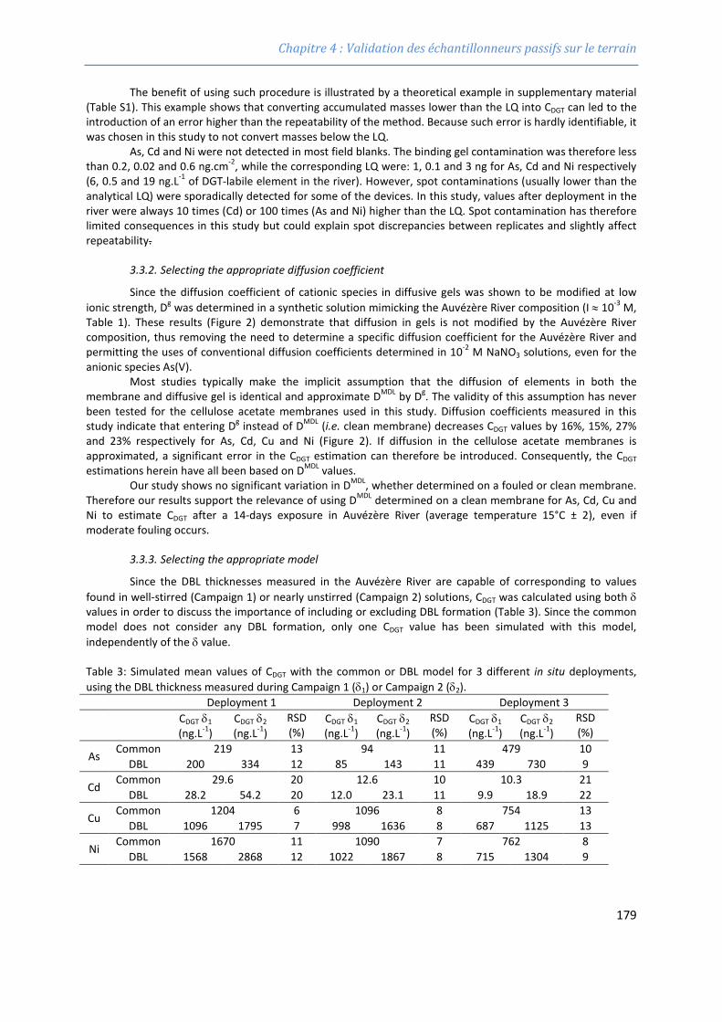
Chapitre 4 : Validation des échantillonneurs passifs sur le terrain
The benefit of using such procedure is illustrated by a theoretical example in supplementary material (Table S1). This example shows that converting accumulated masses lower than the LQ into CDGT can led to the introduction of an error higher than the repeatability of the method. Because such error is hardly identifiable, it was chosen in this study to not convert masses below the LQ.
As, Cd and Ni were not detected in most field blanks. The binding gel contamination was therefore less than 0.2, 0.02 and 0.6 ng.cm-2, while the corresponding LQ were: 1, 0.1 and 3 ng for As, Cd and Ni respectively (6, 0.5 and 19 ng.L-1 of DGT-labile element in the river). However, spot contaminations (usually lower than the analytical LQ) were sporadically detected for some of the devices. In this study, values after deployment in the river were always 10 times (Cd) or 100 times (As and Ni) higher than the LQ. Spot contamination has therefore limited consequences in this study but could explain spot discrepancies between replicates and slightly affect repeatability.
3.3.2. Selecting the appropriate diffusion coefficient
Since the diffusion coefficient of cationic species in diffusive gels was shown to be modified at low ionic strength, Dg was determined in a synthetic solution mimicking the Auvézère River composition (I ≈ 10-3 M, Table 1). These results (Figure 2) demonstrate that diffusion in gels is not modified by the Auvézère River composition, thus removing the need to determine a specific diffusion coefficient for the Auvézère River and permitting the uses of conventional diffusion coefficients determined in 10-2 M NaNO3 solutions, even for the anionic species As(V).
Most studies typically make the implicit assumption that the diffusion of elements in both the membrane and diffusive gel is identical and approximate DMDL by Dg. The validity of this assumption has never been tested for the cellulose acetate membranes used in this study. Diffusion coefficients measured in this study indicate that entering Dg instead of DMDL (i.e. clean membrane) decreases CDGT values by 16%, 15%, 27% and 23% respectively for As, Cd, Cu and Ni (Figure 2). If diffusion in the cellulose acetate membranes is approximated, a significant error in the CDGT estimation can therefore be introduced. Consequently, the CDGT estimations herein have all been based on DMDL values.
Our study shows no significant variation in DMDL, whether determined on a fouled or clean membrane. Therefore our results support the relevance of using DMDL determined on a clean membrane for As, Cd, Cu and Ni to estimate CDGT after a 14-days exposure in Auvézère River (average temperature 15°C ± 2), even if moderate fouling occurs.
3.3.3. Selecting the appropriate model
Since the DBL thicknesses measured in the Auvézère River are capable of corresponding to values found in well-stirred (Campaign 1) or nearly unstirred (Campaign 2) solutions, CDGT was calculated using both δ values in order to discuss the importance of including or excluding DBL formation (Table 3). Since the common model does not consider any DBL formation, only one CDGT value has been simulated with this model, independently of the δ value.
Table 3: Simulated mean values of CDGT with the common or DBL model for 3 different in situ deployments, using the DBL thickness measured during Campaign 1 (δ1) or Campaign 2 (δ2).
Deployment 1 Deployment 2 Deployment 3
CDGT δ1
(ng.L-1) CDGT δ2 (ng.L-1)
RSD (%)
CDGT δ1 (ng.L-1)
CDGT δ2 (ng.L-1)
RSD (%)
CDGT δ1 (ng.L-1)
CDGT δ2 (ng.L-1)
RSD (%)
As Common 219 13 94 11 479 10 DBL 200 334 12 85 143 11 439 730 9
Cd Common 29.6 20 12.6 10 10.3 21
DBL 28.2 54.2 20 12.0 23.1 11 9.9 18.9 22
Cu Common 1204 6 1096 8 754 13
DBL 1096 1795 7 998 1636 8 687 1125 13
Ni Common 1670 11 1090 7 762 8
DBL 1568 2868 12 1022 1867 8 715 1304 9
179
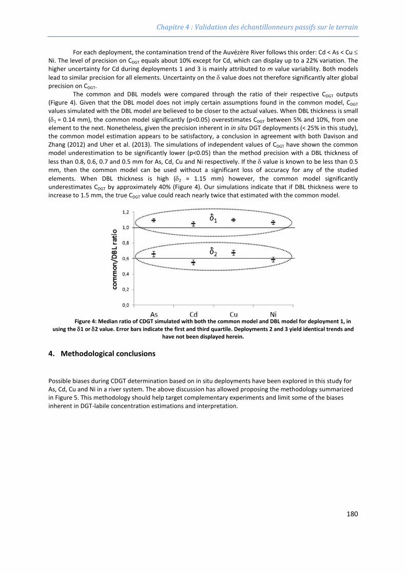
Chapitre 4 : Validation des échantillonneurs passifs sur le terrain
For each deployment, the contamination trend of the Auvézère River follows this order: Cd < As < Cu ≤ Ni. The level of precision on CDGT equals about 10% except for Cd, which can display up to a 22% variation. The higher uncertainty for Cd during deployments 1 and 3 is mainly attributed to m value variability. Both models lead to similar precision for all elements. Uncertainty on the δ value does not therefore significantly alter global precision on CDGT.
The common and DBL models were compared through the ratio of their respective CDGT outputs (Figure 4). Given that the DBL model does not imply certain assumptions found in the common model, CDGT values simulated with the DBL model are believed to be closer to the actual values. When DBL thickness is small (δ1 = 0.14 mm), the common model significantly (p<0.05) overestimates CDGT between 5% and 10%, from one element to the next. Nonetheless, given the precision inherent in in situ DGT deployments (< 25% in this study), the common model estimation appears to be satisfactory, a conclusion in agreement with both Davison and Zhang (2012) and Uher et al. (2013). The simulations of independent values of CDGT have shown the common model underestimation to be significantly lower (p<0.05) than the method precision with a DBL thickness of less than 0.8, 0.6, 0.7 and 0.5 mm for As, Cd, Cu and Ni respectively. If the δ value is known to be less than 0.5 mm, then the common model can be used without a significant loss of accuracy for any of the studied elements. When DBL thickness is high (δ2 = 1.15 mm) however, the common model significantly underestimates CDGT by approximately 40% (Figure 4). Our simulations indicate that if DBL thickness were to increase to 1.5 mm, the true CDGT value could reach nearly twice that estimated with the common model.
Figure 4: Median ratio of CDGT simulated with both the common model and DBL model for deployment 1, in
using the δ1 or δ2 value. Error bars indicate the first and third quartile. Deployments 2 and 3 yield identical trends and have not been displayed herein.
4. Methodological conclusions
Possible biases during CDGT determination based on in situ deployments have been explored in this study for As, Cd, Cu and Ni in a river system. The above discussion has allowed proposing the methodology summarized in Figure 5. This methodology should help target complementary experiments and limit some of the biases inherent in DGT-labile concentration estimations and interpretation.
180
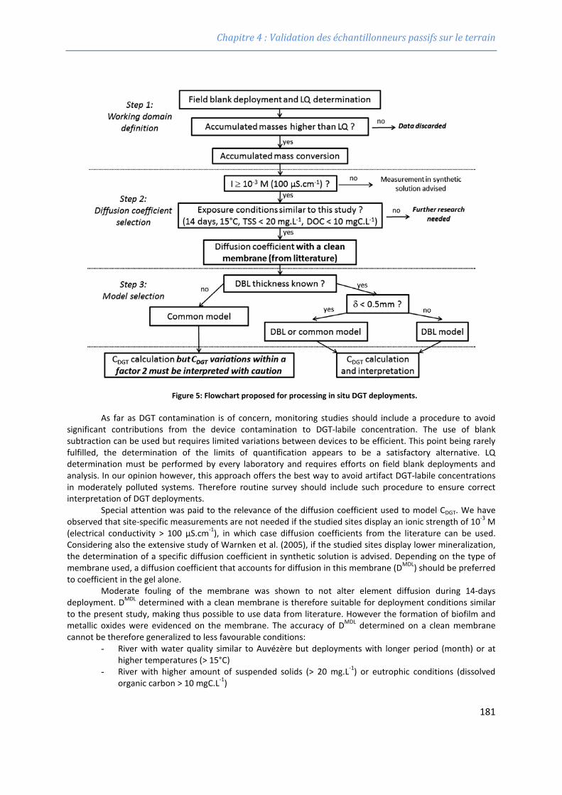
Chapitre 4 : Validation des échantillonneurs passifs sur le terrain
Figure 5: Flowchart proposed for processing in situ DGT deployments.
As far as DGT contamination is of concern, monitoring studies should include a procedure to avoid significant contributions from the device contamination to DGT-labile concentration. The use of blank subtraction can be used but requires limited variations between devices to be efficient. This point being rarely fulfilled, the determination of the limits of quantification appears to be a satisfactory alternative. LQ determination must be performed by every laboratory and requires efforts on field blank deployments and analysis. In our opinion however, this approach offers the best way to avoid artifact DGT-labile concentrations in moderately polluted systems. Therefore routine survey should include such procedure to ensure correct interpretation of DGT deployments.
Special attention was paid to the relevance of the diffusion coefficient used to model CDGT. We have observed that site-specific measurements are not needed if the studied sites display an ionic strength of 10-3 M (electrical conductivity > 100 µS.cm-1), in which case diffusion coefficients from the literature can be used. Considering also the extensive study of Warnken et al. (2005), if the studied sites display lower mineralization, the determination of a specific diffusion coefficient in synthetic solution is advised. Depending on the type of membrane used, a diffusion coefficient that accounts for diffusion in this membrane (DMDL) should be preferred to coefficient in the gel alone.
Moderate fouling of the membrane was shown to not alter element diffusion during 14-days deployment. DMDL determined with a clean membrane is therefore suitable for deployment conditions similar to the present study, making thus possible to use data from literature. However the formation of biofilm and metallic oxides were evidenced on the membrane. The accuracy of DMDL determined on a clean membrane cannot be therefore generalized to less favourable conditions:
- River with water quality similar to Auvézère but deployments with longer period (month) or at higher temperatures (> 15°C)
- River with higher amount of suspended solids (> 20 mg.L-1) or eutrophic conditions (dissolved organic carbon > 10 mgC.L-1)
181
Chapitre 4 : Validation des échantillonneurs passifs sur le terrain
For such conditions, using DMDL determined on both a clean and a fouled membrane can bias CDGT determination. If DMDL has been significantly altered by fouling during deployments, an average diffusion coefficient should be used. However, to ensure an accurate CDGT determination, this coefficient should integrate the time needed for fouling to limit the diffusion of elements. Therefore, further researches are needed to define a methodology to correct diffusion coefficients in a relevant way for such systems. In addition, regulatory programs will require simple correction factors. Such factors could be determined only after the study of numerous systems (water quality) at different seasons (temperature) and for different DGT deployment durations.
Given that regulatory programs require simple methodologies, the measurement of DBL thickness is not feasible in this context, and the common model will be chosen. The CDGT calculation by the common model was shown to be satisfactory provided the DBL is thinner than 0.5 mm. However, a greater thickness was measured even under moderate flow condition, which in turn was shown to reduce in half CDGT output from the common model. The deployment device may be partly responsible for the DBL thickness increase. This point is usually overlooked in most in situ studies and the deployment methodology is never addressed. A methodology that conciliates devices protection and flow velocity preservation needs to be developed to guarantee DBL thickness thinner than 0.5 mm in flowing waters. Until such methodology is developed, if DBL thickness remains unknown, then CDGT variations of less than a factor of 2 must be interpreted with caution.
5. Acknowledgments
The valuable assistance provided by Emeline Renaudie and Karine Cleries during field deployments is gratefully acknowledged. The authors would also like to thank the “Adour Garonne” Water Management Agency and the “Limousin” Regional Council for their financial support of this research.
6. References Allan, I. J., Knutsson, J., Guigues, N., Mills, G. A., Fouillac, A.-M. and Greenwood, R. (2008). "Chemcatcher and
DGT passive sampling devices for regulatory monitoring of trace metals in surface water." Journal of Environmental Monitoring 10(7): 821-829. DOI: 10.1039/b802581a
Buffle, J., Zhang, Z. and Startchev, K. (2007). "Metal Flux and Dynamic Speciation at (Bio)interfaces. Part I:
Critical Evaluation and Compilation of Physicochemical Parameters for Complexes with Simple Ligands and Fulvic/Humic Substances." Environmental Science & Technology 41(22): 7609-7620. DOI: 10.1021/es070702p
Buzier, R., Tusseau-Vuillemin, M.-H. and Mouchel, J.-M. (2006). "Evaluation of DGT as a metal speciation tool in
wastewater." Science of The Total Environment 358(1-3): 277-285. DOI: 10.1016/j.scitotenv.2005.09.051
Davison, W. and Zhang, H. (1994). "In situ speciation measurements of trace components in natural waters
using thin-films gels." Nature 367: 546-548. DOI: 10.1038/367546a0 Davison, W. and Zhang, H. (2012). "Progress in understanding the use of diffusive gradients in thin films (DGT) -
“ back to basics." Environmental Chemistry 9(1): 1-13. DOI: 10.1071/EN11084 Dunn, R. J. K., Teasdale, P. R., Warnken, J., Jordan, M. A. and Arthur, J. M. (2007). "Evaluation of the in situ,
time-integrated DGT technique by monitoring changes in heavy metal concentrations in estuarine waters." Environmental Pollution 148(1): 213-220. DOI: 10.1016/j.envpol.2006.10.027
Fatin-Rouge, N., Milon, A., Buffle, J., Goulet, R. R. and Tessier, A. (2003). "Diffusion and partitioning of solutes in
agarose hydrogels: The relative influence of electrostatic and specific interactions." Journal of Physical Chemistry B 107(44): 12126-12137. DOI: 10.1021/jp0303164
182
Chapitre 4 : Validation des échantillonneurs passifs sur le terrain
Garmo, O. A., Naqvi, K. R., Royset, O. and Steinnes, E. (2006). "Estimation of diffusive boundary layer thickness in studies involving diffusive gradients in thin films (DGT)." Analytical and Bioanalytical Chemistry 386(7-8): 2233-2237. DOI: 10.1007/s00216-006-0885-4
Garrido, T. and Mendoza, J. (2013). "Application of Diffusive Gradient in Thin Film to Estimate Available Copper
in Soil Solution." Soil and Sediment Contamination: An International Journal 22(6): 654-666. DOI: 10.1080/15320383.2013.756447
Gimpel, J., Zhang, H., Hutchinson, W. and Davison, W. (2001). "Effect of solution composition, flow and
deployment time on the measurement of trace metals by the diffusive gradient in thin films technique." Analytica Chimica Acta 448(1-2): 93-103. DOI: 10.1016/S0003-2670(01)01323-X
Jegadeesan, G., Al-Abed, S. R., Sundaram, V., Choi, H., Scheckel, K. G. and Dionysiou, D. D. (2010). "Arsenic
sorption on TiO2 nanoparticles: Size and crystallinity effects." Water Research 44(3): 965-973. DOI: 10.1016/j.watres.2009.10.047
Leermakers, M., Gao, Y., Gabelle, C., Lojen, S., Ouddane, B., Wartel, M. and Baeyens, W. (2005). "Determination
of High Resolution Pore Water Profiles of Trace Metals in Sediments of the Rupel River (Belgium) using Det (Diffusive Equilibrium in Thin Films) and DGT (Diffusive Gradients in Thin Films) Techniques." Water, Air, and Soil Pollution 166(1-4): 265-286. DOI: 10.1007/s11270-005-6671-7
Levy, J. L., Zhang, H., Davison, W., Galceran, J. and Puy, J. (2012). "Kinetic Signatures of Metals in the Presence
of Suwannee River Fulvic Acid." Environmental Science & Technology 46(6): 3335-3342. DOI: 10.1021/es2043068
Luo, J., Zhang, H., Santner, J. and Davison, W. (2010). "Performance Characteristics of Diffusive Gradients in
Thin Films Equipped with a Binding Gel Layer Containing Precipitated Ferrihydrite for Measuring Arsenic(V), Selenium(VI), Vanadium(V), and Antimony(V)." Analytical Chemistry 82(21): 8903-8909. DOI: 10.1021/ac101676w
Miège, C., Schiavone, S., Dabrin, A., Coquery, M., Mazzella, N., Berho, C., Ghestem, J. P., Togola, A., Gonzalez,
C., Gonzalez, J. L., Lalere, B., Lardy-Fontan, S., Lepot, B., Munaron, D. and Tixier, C. (2012). "An in situ intercomparison exercise on passive samplers for monitoring metals, polycyclic aromatic hydrocarbons and pesticides in surface waters." TrAC Trends in Analytical Chemistry 36(0): 128-143. DOI: 10.1016/j.trac.2012.01.009
Roulier, J.-L., Belaud, S. and Coquery, M. (2010). "Comparison of dynamic mobilization of Co, Cd and Pb in
sediments using DGT and metal mobility assessed by sequential extraction." Chemosphere 79(8): 839-843. DOI: 10.1016/j.chemosphere.2010.02.056
Sangi, M. R., Halstead, M. J. and Hunter, K. A. (2002). "Use of the diffusion gradient thin film method to
measure trace metals in fresh waters at low ionic strength." Analytica Chimica Acta 456(2): 241-251. DOI: 10.1016/S0003-2670(02)00012-0
Scally, S., Davison, W. and Zhang, H. (2003). "In situ measurements of dissociation kinetics and labilities of
metal complexes in solution using DGT." Environmental Science & Technology 37(7): 1379-1384. 10.1021/es0202006
Scally, S., Davison, W. and Zhang, H. (2006). "Diffusion coefficients of metals and metal complexes in hydrogels
used in diffusive gradients in thin films." Analytica Chimica Acta 558(1-2): 222-229. DOI: 10.1016/j.aca.2005.11.020
Tusseau-Vuillemin, M.-H., Gourlay, C., Lorgeoux, C., Mouchel, J.-M., Buzier, R., Gilbin, R., Seidel, J.-L. and Elbaz-
Poulichet, F. (2007). "Dissolved and bioavailable contaminants in the Seine river basin." Science of The Total Environment 375(1-3): 244-256. DOI: 10.1016/j.scitotenv.2006.12.018
183
Chapitre 4 : Validation des échantillonneurs passifs sur le terrain
Uher, E., Tusseau-Vuillemin, M.-H. and Gourlay-France, C. (2013). "DGT measurement in low flow conditions:
diffusive boundary layer and lability considerations." Environmental Science: Processes & Impacts 15(7): 1351-1358. DOI: 10.1039/c3em00151b
Uher, E., Zhang, H., Santos, S., Tusseau-Vuillemin, M.-H. l. n. and Gourlay-Francé, C. (2012). "Impact of
Biofouling on Diffusive Gradient in Thin Film Measurements in Water." Analytical Chemistry 84(7): 3111-3118. DOI: 10.1021/ac2028535
Wang, S. and Mulligan, C. N. (2008). "Speciation and surface structure of inorganic arsenic in solid phases: A
review." Environment International 34(6): 867-879. DOI: 10.1016/j.envint.2007.11.005 Warnken, K. W., Davison, W., Zhang, H., Galceran, J. and Puy, J. (2007). "In Situ Measurements of Metal
Complex Exchange Kinetics in Freshwater." Environmental Science & Technology 41(9): 3179-3185. DOI: 10.1021/es062474p
Warnken, K. W., Zhang, H. and Davison, W. (2005). "Trace Metal Measurements in Low Ionic Strength Synthetic
Solutions by Diffusive Gradients in Thin Films." Analytical Chemistry 77(17): 5440-5446. DOI: 10.1021/ac050045o
Warnken, K. W., Zhang, H. and Davison, W. (2006). "Accuracy of the Diffusive Gradients in Thin-Films
Technique: Diffusive Boundary Layer and Effective Sampling Area Considerations." Anal. Chem. 78(11): 3780-3787. DOI: 10.1021/ac060139d
Zhang, H. and Davison, W. (1995). "Performance characteristics of Diffusion Gradients in Thin films for the in
situ measurement of trace metals in aqueous solution." Analytical Chemistry 67(19): 3391-3400. DOI: 10.1021/ac00115a005
Zhang, H. and Davison, W. (1999). "Diffusional characteristics of hydrogels used in DGT and DET techniques."
Analytica Chimica Acta 398(2-3): 329-340. DOI: 10.1016/S0003-2670(99)00458-4 Zhang, H., Davison, W., Knight, B. and McGrath, S. (1998). "In Situ Measurements of Solution Concentrations
and Fluxes of Trace Metals in Soils Using DGT." Environ. Sci. Technol. 32(5): 704-710. DOI: 10.1021/es9704388
184
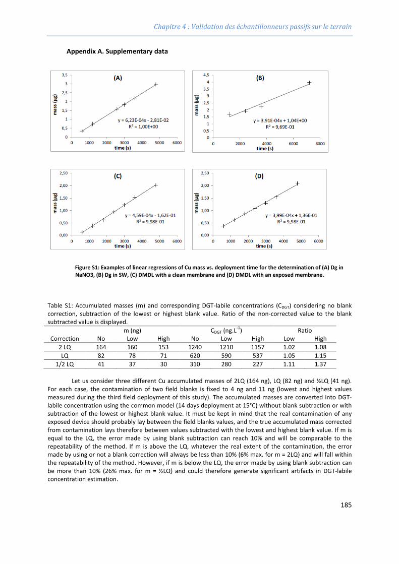
Chapitre 4 : Validation des échantillonneurs passifs sur le terrain
Appendix A. Supplementary data
Figure S1: Examples of linear regressions of Cu mass vs. deployment time for the determination of (A) Dg in NaNO3, (B) Dg in SW, (C) DMDL with a clean membrane and (D) DMDL with an exposed membrane.
Table S1: Accumulated masses (m) and corresponding DGT-labile concentrations (CDGT) considering no blank correction, subtraction of the lowest or highest blank value. Ratio of the non-corrected value to the blank subtracted value is displayed.
m (ng) CDGT (ng.L-1) Ratio Correction No Low High No Low High Low High
2 LQ 164 160 153 1240 1210 1157 1.02 1.08 LQ 82 78 71 620 590 537 1.05 1.15
1/2 LQ 41 37 30 310 280 227 1.11 1.37 Let us consider three different Cu accumulated masses of 2LQ (164 ng), LQ (82 ng) and ½LQ (41 ng).
For each case, the contamination of two field blanks is fixed to 4 ng and 11 ng (lowest and highest values measured during the third field deployment of this study). The accumulated masses are converted into DGT-labile concentration using the common model (14 days deployment at 15°C) without blank subtraction or with subtraction of the lowest or highest blank value. It must be kept in mind that the real contamination of any exposed device should probably lay between the field blanks values, and the true accumulated mass corrected from contamination lays therefore between values subtracted with the lowest and highest blank value. If m is equal to the LQ, the error made by using blank subtraction can reach 10% and will be comparable to the repeatability of the method. If m is above the LQ, whatever the real extent of the contamination, the error made by using or not a blank correction will always be less than 10% (6% max. for m = 2LQ) and will fall within the repeatability of the method. However, if m is below the LQ, the error made by using blank subtraction can be more than 10% (26% max. for m = ½LQ) and could therefore generate significant artifacts in DGT-labile concentration estimation.
185

Chapitre 4 : Validation des échantillonneurs passifs sur le terrain
186
Chapitre 4 : Validation des échantillonneurs passifs sur le terrain
4.5 Conclusion partielle Les expérimentations menées dans ce chapitre visaient à évaluer l’applicabilité et les limites
des échantillonneurs passifs POCIS et DGT dans les conditions de terrain. Une attention particulière a
été portée sur la question de la justesse et la fiabilité des données récoltées.
Dans le cas du POCIS, les principales sources d’incertitudes résidaient dans l’influence des
conditions environnementales sur la mesure, et la méconnaissance de la fraction échantillonnée.
Bien que les résultats concernant la méthode classique de correction du biais environnemental
(correction PRC) ne nous aient pas permis de conclure sur la réelle efficacité de cette approche, il a
été possible de définir un intervalle de confiance qui prend en compte ce biais. Cette solution permet
de donner à la mesure POCIS un caractère semi-quantitatif utilisable dans un contexte opérationnel
et réglementaire. Par ailleurs, l’incertitude associée à la mesure délivrée par le POCIS prend en
compte à la fois l’étape d’échantillonnage, et l’analyse en laboratoire, ce qui n’est pas le cas pour les
échantillons ponctuels d’eau, pour lesquels seule l’incertitude analytique est renseignée. Ceci,
associé à la mise en évidence que le POCIS échantillonne uniquement la fraction dissoute des
contaminants, nous permet de conclure que le dispositif pourrait être appliqué de façon fiable pour
la surveillance des milieux aquatiques dans le cadre de la DCE. Une procédure standard a été
proposée dans ce sens.
Dans le cas du DGT, les principales sources d’imprécisions résidaient dans la détermination
d’une limite de quantification appropriée, le choix du coefficient de diffusion (extrait de la littérature
ou déterminé expérimentalement), l’influence du biofouling et le caractère négligeable (ou non) de
la couche limite de diffusion entourant l’échantillonneur. Il a été conclu que le choix de paramètres
standards pouvait faciliter l’utilisation du DGT dans un contexte réglementaire. Ainsi, la couche limite
de diffusion peut être négligée, mais dans ce cas, des variations de concentrations inférieure à un
facteur deux devaient être interprétées avec précaution. De plus, l’utilisation de coefficients de
diffusion issus de la littérature et ne tenant pas compte du biofouling est valable pour des cas
favorables (biofouling limité). Néanmoins, il reste à déterminer la limite des cas pour lesquels cette
procédure reste valable. Une procédure standard d’interprétation des données a également été
proposée.
La dernière étape de cette étude a ensuite consisté à mettre en pratique les développements
et les connaissances précédemment acquises pour la mise en œuvre de l’échantillonneur POCIS sur
le terrain, et l’étude de la contamination en pesticides des bassins versants du Trec et de l’Auvézère.
187

Chapitre 4 : Validation des échantillonneurs passifs sur le terrain
Ces deux bassins présentent des contextes pédoclimatiques très différents. De même, les pressions
de contamination diffèrent : très élevée sur le Trec, elle est plus modérée sur l’Auvézère.
188
Chapitre 5 :Mise en œuvre du POCIS pour le suivi de la contamination en pesticides des bassins versants
du Trec et de l’Auvézère
POULIER Gaëlle | Thèse de doctorat | Chimie Environnementale | Université de Limoges | 2014 189

Chapitre 5 : Mise en œuvre du POCIS pour le suivi de la contamination en pesticides des bassins
versants du Trec et de l’Auvézère
190
Chapitre 5 : Mise en œuvre du POCIS pour le suivi de la contamination en pesticides des bassins
versants du Trec et de l’Auvézère
5.1 Etude d’un environnement présentant un fort niveau de
contamination : PAT du Trec-Canaule Le bassin versant du Trec-Canaule présente une surface agricole utile de 120 km2 (60% du
territoire du PAT). On y trouve principalement de grandes cultures céréalières, des prairies et
quelques cultures spéciales (maraîchage, arboriculture, vignes) (Figure 14). C’est donc une zone qui
comporte une pression agricole forte, avec des teneurs en nitrates et en phytosanitaires
préoccupantes dans le milieu aquatique. La présente étude, financée par l’Agence de l’Eau Adour
Garonne (AEAG) visait à 1) renforcer le réseau de surveillance mis en place par l’AEAG, notamment
en augmentant la fréquence des prélèvements ; 2) mettre en évidence s’il y a lieu la variabilité
saisonnière de la contamination en pesticides et identifier les périodes les plus à risque, 3) identifier
les zones où le risque toxique est le plus élevé et les principaux cours d’eau contribuant à la
contamination globale du Trec.
Des POCIS ont donc été exposés en continu sur le Trec, le Manet et la Canaule (Figure 14) de
mars à décembre 2012 selon le plan d’échantillonnage décrit précédemment (Tableau 5). Les
résultats sont présentés sur la Figure 30.
191
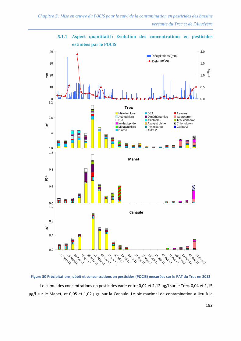
Chapitre 5 : Mise en œuvre du POCIS pour le suivi de la contamination en pesticides des bassins
versants du Trec et de l’Auvézère
5.1.1 Aspect quantitatif : Evolution des concentrations en pesticides
estimées par le POCIS
Figure 30 Précipitations, débit et concentrations en pesticides (POCIS) mesurées sur le PAT du Trec en 2012
Le cumul des concentrations en pesticides varie entre 0,02 et 1,12 µg/l sur le Trec, 0,04 et 1,15
µg/l sur le Manet, et 0,05 et 1,02 µg/l sur la Canaule. Le pic maximal de contamination a lieu à la
Manet
0.0
0.4
0.8
1.2
µg/L
Trec
0.0
0.4
0.8
1.2
µg/L
Métolachlore DEA AtrazineAcétochlore Diméthénamide IsoproturonDIA Alachlore TébuconazoleImidaclopride Azoxystrobine ChlortoluronMétazachlore Pyrimicarbe CarbarylDiuron Autres*
Canaule
0.0
0.4
0.8
1.2
12-Mar-12
26-Mar-12
10-Apr-12
23-Apr-12
09-May-12
21-May-12
04-Jun-12
18-Jun-12
02-Jul-12
16-Jul-12
30-Jul-12
13-Aug-12
27-Aug-12
10-Sep-12
24-Sep-12
08-Oct-12
22-Oct-12
05-Nov-12
19-Nov-12
03-Dec-12
17-Dec-12
µg/L
0
10
20
30
40m
m
0.0
0.5
1.0
1.5
2.0Précipitations (mm)Débit (m3/s)
m3 /s
(m3/s)
Débit (
Précipitations (mm)
192
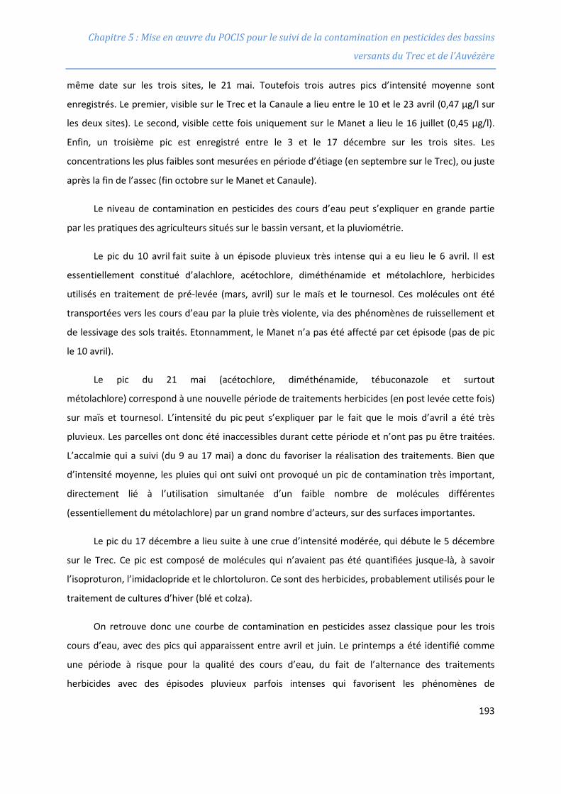
Chapitre 5 : Mise en œuvre du POCIS pour le suivi de la contamination en pesticides des bassins
versants du Trec et de l’Auvézère
même date sur les trois sites, le 21 mai. Toutefois trois autres pics d’intensité moyenne sont
enregistrés. Le premier, visible sur le Trec et la Canaule a lieu entre le 10 et le 23 avril (0,47 µg/l sur
les deux sites). Le second, visible cette fois uniquement sur le Manet a lieu le 16 juillet (0,45 µg/l).
Enfin, un troisième pic est enregistré entre le 3 et le 17 décembre sur les trois sites. Les
concentrations les plus faibles sont mesurées en période d’étiage (en septembre sur le Trec), ou juste
après la fin de l’assec (fin octobre sur le Manet et Canaule).
Le niveau de contamination en pesticides des cours d’eau peut s’expliquer en grande partie
par les pratiques des agriculteurs situés sur le bassin versant, et la pluviométrie.
Le pic du 10 avril fait suite à un épisode pluvieux très intense qui a eu lieu le 6 avril. Il est
essentiellement constitué d’alachlore, acétochlore, diméthénamide et métolachlore, herbicides
utilisés en traitement de pré-levée (mars, avril) sur le maïs et le tournesol. Ces molécules ont été
transportées vers les cours d’eau par la pluie très violente, via des phénomènes de ruissellement et
de lessivage des sols traités. Etonnamment, le Manet n’a pas été affecté par cet épisode (pas de pic
le 10 avril).
Le pic du 21 mai (acétochlore, diméthénamide, tébuconazole et surtout
métolachlore) correspond à une nouvelle période de traitements herbicides (en post levée cette fois)
sur maïs et tournesol. L’intensité du pic peut s’expliquer par le fait que le mois d’avril a été très
pluvieux. Les parcelles ont donc été inaccessibles durant cette période et n’ont pas pu être traitées.
L’accalmie qui a suivi (du 9 au 17 mai) a donc du favoriser la réalisation des traitements. Bien que
d’intensité moyenne, les pluies qui ont suivi ont provoqué un pic de contamination très important,
directement lié à l’utilisation simultanée d’un faible nombre de molécules différentes
(essentiellement du métolachlore) par un grand nombre d’acteurs, sur des surfaces importantes.
Le pic du 17 décembre a lieu suite à une crue d’intensité modérée, qui débute le 5 décembre
sur le Trec. Ce pic est composé de molécules qui n’avaient pas été quantifiées jusque-là, à savoir
l’isoproturon, l’imidaclopride et le chlortoluron. Ce sont des herbicides, probablement utilisés pour le
traitement de cultures d’hiver (blé et colza).
On retrouve donc une courbe de contamination en pesticides assez classique pour les trois
cours d’eau, avec des pics qui apparaissent entre avril et juin. Le printemps a été identifié comme
une période à risque pour la qualité des cours d’eau, du fait de l’alternance des traitements
herbicides avec des épisodes pluvieux parfois intenses qui favorisent les phénomènes de
193
Chapitre 5 : Mise en œuvre du POCIS pour le suivi de la contamination en pesticides des bassins
versants du Trec et de l’Auvézère
ruissellement et de lessivage. Toutefois, l’importance des surfaces dédiées aux cultures d’hiver
(environ 30% de la SAU du bassin versant) (Figure 14) rend possible l’apparition de pics de
contamination en automne. Nous n’avons pas mis en évidence de gradient de contamination amont-
aval sur le bassin versant mais le fait que les concentrations mesurées sur le Trec soient équivalentes
voire supérieures à celles retrouvées sur la Canaule juste avant le point de confluence montre qu’il
n’y a pas d’effet de dilution à cet endroit. Cela laisse supposer que le niveau de contamination du
Trec est plus élevé en amont de ce point.
194
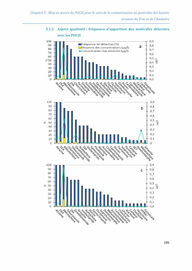
Chapitre 5 : Mise en œuvre du POCIS pour le suivi de la contamination en pesticides des bassins
versants du Trec et de l’Auvézère
5.1.2 Aspect qualitatif : fréquence d’apparition des molécules détectées
avec les POCIS
195
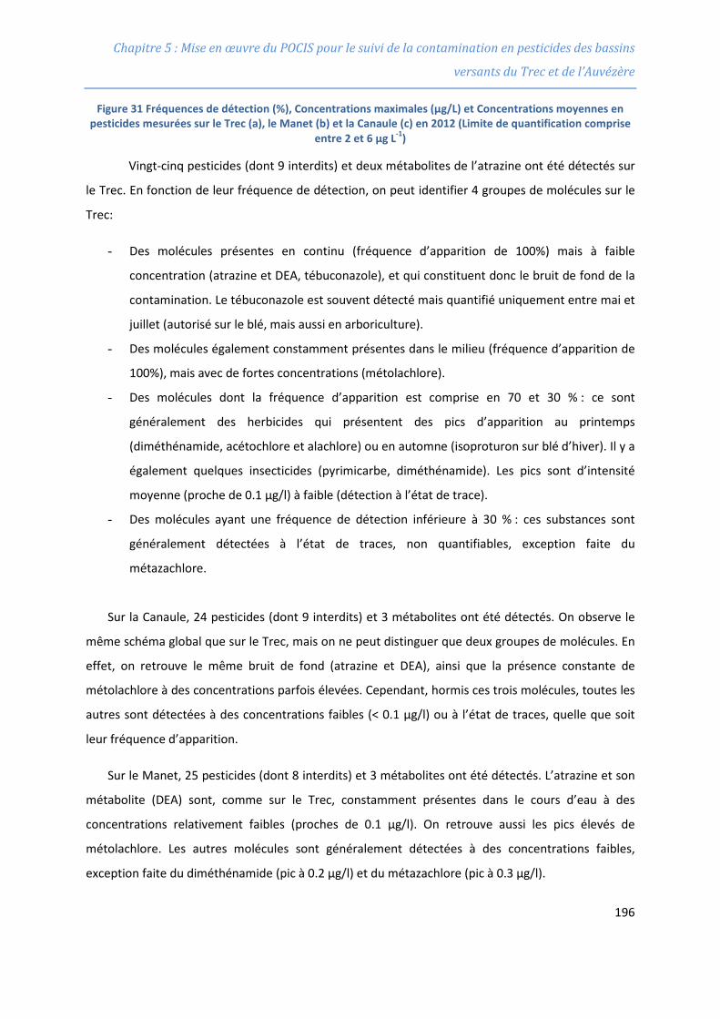
Chapitre 5 : Mise en œuvre du POCIS pour le suivi de la contamination en pesticides des bassins
versants du Trec et de l’Auvézère
Figure 31 Fréquences de détection (%), Concentrations maximales (µg/L) et Concentrations moyennes en pesticides mesurées sur le Trec (a), le Manet (b) et la Canaule (c) en 2012 (Limite de quantification comprise
entre 2 et 6 µg L-1)
Vingt-cinq pesticides (dont 9 interdits) et deux métabolites de l’atrazine ont été détectés sur
le Trec. En fonction de leur fréquence de détection, on peut identifier 4 groupes de molécules sur le
Trec:
- Des molécules présentes en continu (fréquence d’apparition de 100%) mais à faible
concentration (atrazine et DEA, tébuconazole), et qui constituent donc le bruit de fond de la
contamination. Le tébuconazole est souvent détecté mais quantifié uniquement entre mai et
juillet (autorisé sur le blé, mais aussi en arboriculture).
- Des molécules également constamment présentes dans le milieu (fréquence d’apparition de
100%), mais avec de fortes concentrations (métolachlore).
- Des molécules dont la fréquence d’apparition est comprise en 70 et 30 % : ce sont
généralement des herbicides qui présentent des pics d’apparition au printemps
(diméthénamide, acétochlore et alachlore) ou en automne (isoproturon sur blé d’hiver). Il y a
également quelques insecticides (pyrimicarbe, diméthénamide). Les pics sont d’intensité
moyenne (proche de 0.1 µg/l) à faible (détection à l’état de trace).
- Des molécules ayant une fréquence de détection inférieure à 30 % : ces substances sont
généralement détectées à l’état de traces, non quantifiables, exception faite du
métazachlore.
Sur la Canaule, 24 pesticides (dont 9 interdits) et 3 métabolites ont été détectés. On observe le
même schéma global que sur le Trec, mais on ne peut distinguer que deux groupes de molécules. En
effet, on retrouve le même bruit de fond (atrazine et DEA), ainsi que la présence constante de
métolachlore à des concentrations parfois élevées. Cependant, hormis ces trois molécules, toutes les
autres sont détectées à des concentrations faibles (< 0.1 µg/l) ou à l’état de traces, quelle que soit
leur fréquence d’apparition.
Sur le Manet, 25 pesticides (dont 8 interdits) et 3 métabolites ont été détectés. L’atrazine et son
métabolite (DEA) sont, comme sur le Trec, constamment présentes dans le cours d’eau à des
concentrations relativement faibles (proches de 0.1 µg/l). On retrouve aussi les pics élevés de
métolachlore. Les autres molécules sont généralement détectées à des concentrations faibles,
exception faite du diméthénamide (pic à 0.2 µg/l) et du métazachlore (pic à 0.3 µg/l).
196
Chapitre 5 : Mise en œuvre du POCIS pour le suivi de la contamination en pesticides des bassins
versants du Trec et de l’Auvézère
En conclusion, beaucoup de molécules différentes sont détectées sur le PAT du Trec-Canaule,
mais certaines uniquement à l’état de traces.
Le Trec paraît un peu plus contaminé que les deux autres cours d’eau car les herbicides y
sont détectés en plus grand nombre, plus fréquemment et à des concentrations un peu plus élevées
que sur le Manet et la Canaule (ex : acétochlore, alachlore, azoxystrobine, isoproturon). La présence
de ces molécules dans le cours d’eau est problématique car certaines sont interdites. Il est possible
que l’alachlore et le diméthénamide soient toujours utilisés, car ces molécules sont détectées aux
mêmes périodes qu’avant leur interdiction, c'est-à-dire au printemps. Les pics d’après traitements
observés sont typiques de molécules toujours en usage.
En revanche, il est peu probable que l’atrazine (interdite depuis 2003) soit encore utilisée.
Les concentrations mesurées sont faibles, presque constantes, et semblent surtout influencées par le
débit. Une façon de le vérifier consiste à calculer le rapport DEA/Atrazine (DAR). Un rapport inférieur
à 1 indique un apport récent de la molécule mère dans le milieu (Thurman et al., 1992). Ici, le DAR est
largement supérieur à 1 (Figure 32) ce qui laisse supposer qu’il n’y a pas eu d’apport récent
d’atrazine dans le milieu. La présence de la molécule et de son métabolite serait plutôt dûe à un
relargage par les nappes souterraines, ou à une remobilisation du stock présent dans le sol. Le fait
qu’on en retrouve près de 10 ans après son interdiction montre la persistance de l’atrazine dans les
sols et dans les eaux.
197
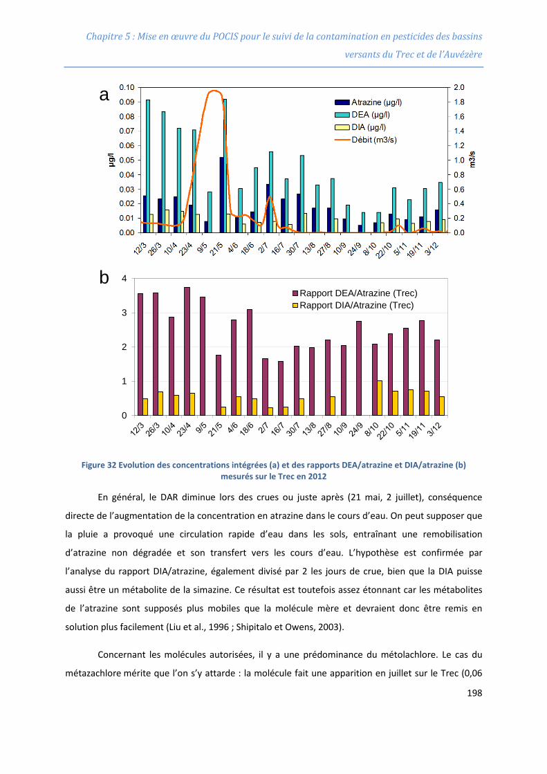
Chapitre 5 : Mise en œuvre du POCIS pour le suivi de la contamination en pesticides des bassins
versants du Trec et de l’Auvézère
Figure 32 Evolution des concentrations intégrées (a) et des rapports DEA/atrazine et DIA/atrazine (b) mesurés sur le Trec en 2012
En général, le DAR diminue lors des crues ou juste après (21 mai, 2 juillet), conséquence
directe de l’augmentation de la concentration en atrazine dans le cours d’eau. On peut supposer que
la pluie a provoqué une circulation rapide d’eau dans les sols, entraînant une remobilisation
d’atrazine non dégradée et son transfert vers les cours d’eau. L’hypothèse est confirmée par
l’analyse du rapport DIA/atrazine, également divisé par 2 les jours de crue, bien que la DIA puisse
aussi être un métabolite de la simazine. Ce résultat est toutefois assez étonnant car les métabolites
de l’atrazine sont supposés plus mobiles que la molécule mère et devraient donc être remis en
solution plus facilement (Liu et al., 1996 ; Shipitalo et Owens, 2003).
Concernant les molécules autorisées, il y a une prédominance du métolachlore. Le cas du
métazachlore mérite que l’on s’y attarde : la molécule fait une apparition en juillet sur le Trec (0,06
a
0
1
2
3
4Rapport DEA/Atrazine (Trec)Rapport DIA/Atrazine (Trec)
b
198

Chapitre 5 : Mise en œuvre du POCIS pour le suivi de la contamination en pesticides des bassins
versants du Trec et de l’Auvézère
µg/l) et le Manet (0,29µg/l) (Figure 30). Cc’est un herbicide généralement utilisé en hiver sur colza,
mais il peut aussi être utilisé pour le désherbage du tournesol. Les concentrations mesurées sont
significatives, et les niveaux mesurés permettent d’en situer l’origine sur le bassin versant du Manet.
199

Chapitre 5 : Mise en œuvre du POCIS pour le suivi de la contamination en pesticides des bassins
versants du Trec et de l’Auvézère
200
Chapitre 5 : Mise en œuvre du POCIS pour le suivi de la contamination en pesticides des bassins
versants du Trec et de l’Auvézère
5.2 Publication 4 “Estimates of pesticide concentrations and fluxes in
two rivers of an extensive French multi-agricultural watershed:
application of the passive sampling strategy”
Gaëlle Pouliera,b, Sophie Lissaldeb, Adeline Charriaub, Rémy Buzierb, Karine Cleriesb, François
Delmasa, Nicolas Mazzellaa, Gilles Guibaudb
Environmental Science and Pollution Research, 1-14, 2014, DOI 10.1007/s11356-014-2814-y
a Unité de Recherche REBX ; Groupement Irstea de Bordeaux, 50 Avenue de Verdun, Gazinet,
33612 Cestas cedex, France
b Université de Limoges, Groupe de Recherche Eau Sol Environnement (GRESE), 123 Avenue
Albert Thomas, 87060 Limoges cedex, France
Corresponding authors : [email protected]; [email protected]
201

Chapitre 5 : Mise en œuvre du POCIS pour le suivi de la contamination en pesticides des bassins
versants du Trec et de l’Auvézère
202
Chapitre 5 : Mise en œuvre du POCIS pour le suivi de la contamination en pesticides des bassins
versants du Trec et de l’Auvézère
Estimates of pesticide concentrations and fluxes in two rivers of an extensive French multi-agricultural watershed:
application of the passive sampling strategy Gaëlle Pouliera, b, Sophie Lissaldeb, Adeline Charriaub, Rémy Buzier b, Karine Cleriesb, François
Delmasa, Nicolas Mazzellaa, Gilles Guibaud b
Environmental Science and Pollution Research, 1-14, 2014, DOI 10.1007/s11356-014-2814-y
a Unité de recherche REBX ; Groupement Irstea de Bordeaux, 50 avenue de Verdun, Gazinet, 33612 Cestas cedex, France
b Université de Limoges Groupement de Recherche Eau Sol Environnement (GRESE), 123 Avenue Albert Thomas 87060 Limoges Cedex, France
Corresponding authors: [email protected], [email protected]
Abstract In this study, the passive sampling strategy was evaluated for its ability to improve water quality
monitoring in terms of concentrations and frequencies of quantification of pesticides, with a focus on flux calculation. Polar Organic Chemical Integrative Samplers (POCIS) were successively exposed and renewed at three sampling sites of an extensive French multi-agricultural watershed from January to September 2012. Grab water samples were recovered every 14 days during the same period and an automated sampler collected composite water samples from April to July 2012. 39 compounds (pesticides and metabolites) were analysed. Desethylatrazine, diuron and atrazine (banned in France for many years) likely arrived via groundwater whereas dimethanamid, imidacloprid and acetochlor (all still in use) were probably transported via leaching. The comparison of the three sampling strategies showed that the POCIS offers lower detection limits, resulting in the quantification of trace levels of compounds (acetochlor, diuron and desethylatrazine) that could not be measured in grab and composite water samples. As a consequence, the frequencies of occurrence were dramatically enhanced with the POCIS compared to spot sample data. Moreover, the integration of flood events led to a better temporal representation of the fluxes when calculated with the POCIS compared to the bimonthly grab sampling strategy. We concluded that the POCIS could be an advantageous alternative to spot sampling, offering better performance in terms of quantification limits, and more representative data.
Keywords: POCIS, passive sampling, pesticides, fluxes, water monitoring
1. Introduction
The intensive use of pesticides in agriculture and urban activities since the 1950’s has led to diffuse contamination of environmental compartments (air, soil, water) (Loos et al. 2009; Jaward et al. 2004). Pesticides are driven from the application area to water bodies via different hydrological processes including runoff, leaching, and transport with soil particles (Lennartz et al. 1997; Louchart et al. 2001). The presence of these molecules in natural water can lead to toxic effects for biota (Mason et al. 2003; Solomon et al. 1996; DeLorenzo et al. 2001), but can also have effects on humans, as pesticides are sometimes quantified in drinking water. In the past decades, European governments realized the necessity of controlling water quality. The Water Framework Directive (WFD), implemented in 2000 by the European Union (2000/60/EC 2000), requires
203
Chapitre 5 : Mise en œuvre du POCIS pour le suivi de la contamination en pesticides des bassins
versants du Trec et de l’Auvézère
Member States to reach good chemical and ecological status for all water bodies by 2015. In this context, Environmental Quality Standards (EQS) have been determined for 41 priority compounds, including 14 pesticides (2008/105/EC 2008). Water quality must be monitored at least once a month and compared to the EQS in order to determine the water body’s chemical quality status. Today, the only sampling strategy authorized is grab sampling. However, despite the simplicity of this strategy, numerous limitations have been noted.
The first is the sampling frequency. Indeed, pesticide concentrations can rapidly increase after rainfall, or during a flood event (Taghavi et al. 2011). In a recent study conducted in the stream of a small vineyard catchment, Rabiet et al. (2010) observed that the dissolved diuron concentration could be multiplied by a factor of 50 in only 5 days. This high reactivity was related to the rapid transfer of pesticides via runoff after a storm event. Moreover, this transfer can be strongly enhanced when rainfall occurs just after pesticide application. These examples show that the sampling frequency must be adapted to the temporal variation of pesticide concentrations, which is not the case with grab samples taken once a month on planned dates in regulatory monitoring programmes. Another disadvantage of the grab sampling strategy is its high limit of quantification. Indeed, some hydrophobic compounds have very low EQS (e.g., 0.01 µg L-1 for endosulfan) because they can accumulate in biota, leading to toxic effects even at low water concentrations. Such a low EQS may be difficult to identify with conventional analytical methods and sample preparation procedures.
When a water body fails to achieve “good status”, remediation actions may be implemented. The reduction of pesticide use is encouraged, and landscape design can be modified to reduce transfer (e.g., grass strips bordering streams, hedgerow construction). The best way to evaluate the efficiency of these remediation strategies required by the WFD is to monitor pesticide fluxes. However, depending on the water flow, high fluxes can be related to very low concentrations of pesticides because of a dilution effect. When these low concentrations are below the limit of detection, fluxes cannot be calculated although they can be high. But flux information could benefit regulatory investigative and operational monitoring network, resulting in better understanding of the global contamination of a watershed, and in the implementation of more accurate remediation strategies.
The passive sampling strategy developed over the past 20 years could overcome some of the problems related to grab sampling. Passive sampling theory and modelling are well described elsewhere (Huckins et al. 1993; Vrana et al. 2005; Stuer-Lauridsen 2005; Alvarez et al. 2004). Briefly, the strategy consists of an integrating device composed of a receiving phase (liquid or solid), exposed in the water body for a defined period (from a few hours to several weeks) that continuously accumulates contaminants. After retrieval and analysis of the receiving phase, a time-weighted average concentration (TWAC) can be calculated for the period of exposure. Passive sampling offers significant benefits compared to grab sampling. On one hand, the in situ accumulation of pesticides in the device allows quantification at lower limits of detection without an additional sample pre-concentration step (Lissalde et al. 2011). On the other hand, and as a consequence of sampling duration, potential pesticide peaks occurring after flood events are integrated (Allan et al. 2007), and the representativeness of the data collected is enhanced, especially regarding chronic exposures. Considering these points, it appears that the monitoring of pesticide concentrations in water, and the calculation of pesticide fluxes could be improved using a passive sampling strategy.
The main objective of this study was to verify the application of passive sampling compared to grab sampling to measure pesticide concentrations in a context of low contamination levels. The Auvézère catchment (France) was specifically selected due to its low level contamination with a wide range of pesticides. Polar Organic Chemical Integrative Samplers (POCIS) were exposed from January to September 2012 in the Auvèzère River and one of its small tributaries, the Arnac River. TWACs were then used to calculate fluxes in both rivers and to determine the contribution of the Arnac tributary to the contamination of the Auvézère River.
204
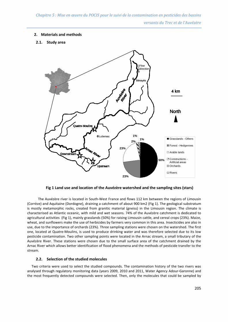
Chapitre 5 : Mise en œuvre du POCIS pour le suivi de la contamination en pesticides des bassins
versants du Trec et de l’Auvézère
2. Materials and methods
2.1. Study area
Fig 1 Land use and location of the Auvézère watershed and the sampling sites (stars)
The Auvézère river is located in South-West France and flows 112 km between the regions of Limousin (Corrèze) and Aquitaine (Dordogne), draining a catchment of about 900 km2 (Fig 1). The geological substratum is mostly metamorphic rocks, created from granitic material (gneiss) in the Limousin region. The climate is characterised as Atlantic oceanic, with mild and wet seasons. 74% of the Auvézère catchment is dedicated to agricultural activities (Fig 1), mainly grasslands (50%) for raising Limousin cattle, and cereal crops (23%). Maize, wheat, and sunflowers make the use of herbicides by farmers very common in this area. Insecticides are also in use, due to the importance of orchards (23%). Three sampling stations were chosen on the watershed. The first one, located at Quatre-Moulins, is used to produce drinking water and was therefore selected due to its low pesticide contamination. Two other sampling points were located in the Arnac stream, a small tributary of the Auvézère River. These stations were chosen due to the small surface area of the catchment drained by the Arnac River which allows better identification of flood phenomena and the methods of pesticide transfer to the stream.
2.2. Selection of the studied molecules
Two criteria were used to select the studied compounds. The contamination history of the two rivers was analysed through regulatory monitoring data (years 2009, 2010 and 2011, Water Agency Adour-Garonne) and the most frequently detected compounds were selected. Then, only the molecules that could be sampled by
4 km
Auvé
zère
Rive
rQuatre-Moulins
Arnac River
Upstream
Downstream
North
50%
23%
23%
2%
1%1% Grasslands - Others
Forest - Hedgerows
Arable lands
Constructions -Artificial areasOrchards
Rivers
Lubersac
Bénayès
Flow direction
4 km
Auvé
zère
Rive
rQuatre-Moulins
Arnac River
Upstream
Downstream
North
50%
23%
23%
2%
1%1% Grasslands - Others
Forest - Hedgerows
Arable lands
Constructions -Artificial areasOrchards
Rivers
Lubersac
Bénayès
4 km
Auvé
zère
Rive
rQuatre-Moulins
Arnac River
Upstream
Downstream
North
50%
23%
23%
2%
1%1% Grasslands - Others
Forest - Hedgerows
Arable lands
Constructions -Artificial areasOrchards
Rivers
4 km4 km
Auvé
zère
Rive
rQuatre-Moulins
Arnac River
Upstream
Downstream
North
50%
23%
23%
2%
1%1% Grasslands - Others
Forest - Hedgerows
Arable lands
Constructions -Artificial areasOrchards
Rivers
Auvé
zère
Rive
rQuatre-Moulins
Arnac River
Upstream
Downstream
Auvé
zère
Rive
rQuatre-Moulins
Arnac River
Upstream
Downstream
North
50%
23%
23%
2%
1%1% Grasslands - Others
Forest - Hedgerows
Arable lands
Constructions -Artificial areasOrchards
Rivers
NorthNorth
50%
23%
23%
2%
1%1% Grasslands - Others
Forest - Hedgerows
Arable lands
Constructions -Artificial areasOrchards
Rivers
Lubersac
Bénayès
Flow direction
205
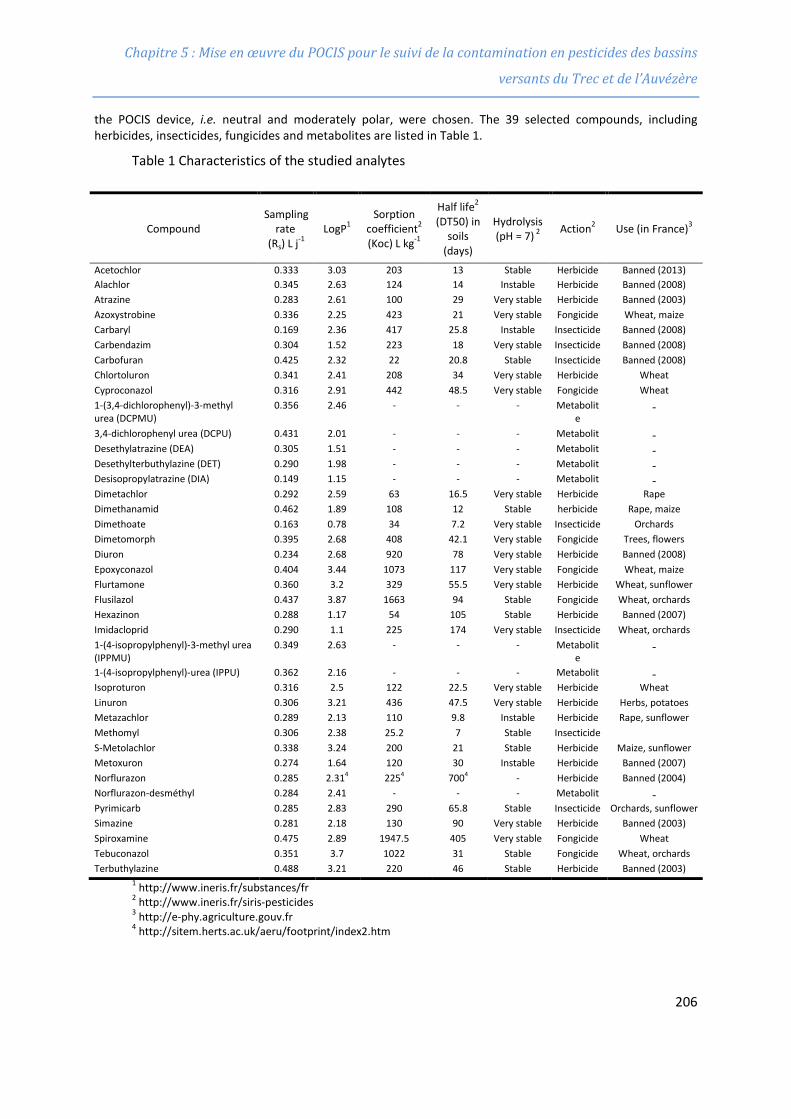
Chapitre 5 : Mise en œuvre du POCIS pour le suivi de la contamination en pesticides des bassins
versants du Trec et de l’Auvézère
the POCIS device, i.e. neutral and moderately polar, were chosen. The 39 selected compounds, including herbicides, insecticides, fungicides and metabolites are listed in Table 1.
Table 1 Characteristics of the studied analytes
Compound Sampling
rate (Rs) L j-1
LogP1 Sorption
coefficient2
(Koc) L kg-1
Half life2
(DT50) in soils
(days)
Hydrolysis (pH = 7) 2 Action2 Use (in France)3
Acetochlor 0.333 3.03 203 13 Stable Herbicide Banned (2013) Alachlor 0.345 2.63 124 14 Instable Herbicide Banned (2008) Atrazine 0.283 2.61 100 29 Very stable Herbicide Banned (2003) Azoxystrobine 0.336 2.25 423 21 Very stable Fongicide Wheat, maize Carbaryl 0.169 2.36 417 25.8 Instable Insecticide Banned (2008) Carbendazim 0.304 1.52 223 18 Very stable Insecticide Banned (2008) Carbofuran 0.425 2.32 22 20.8 Stable Insecticide Banned (2008) Chlortoluron 0.341 2.41 208 34 Very stable Herbicide Wheat Cyproconazol 0.316 2.91 442 48.5 Very stable Fongicide Wheat 1-(3,4-dichlorophenyl)-3-methyl urea (DCPMU)
0.356 2.46 - - - Metabolite
-
3,4-dichlorophenyl urea (DCPU) 0.431 2.01 - - - Metabolit
- Desethylatrazine (DEA) 0.305 1.51 - - - Metabolit
-
Desethylterbuthylazine (DET) 0.290 1.98 - - - Metabolit
- Desisopropylatrazine (DIA) 0.149 1.15 - - - Metabolit
-
Dimetachlor 0.292 2.59 63 16.5 Very stable Herbicide Rape Dimethanamid 0.462 1.89 108 12 Stable herbicide Rape, maize Dimethoate 0.163 0.78 34 7.2 Very stable Insecticide Orchards Dimetomorph 0.395 2.68 408 42.1 Very stable Fongicide Trees, flowers Diuron 0.234 2.68 920 78 Very stable Herbicide Banned (2008) Epoxyconazol 0.404 3.44 1073 117 Very stable Fongicide Wheat, maize Flurtamone 0.360 3.2 329 55.5 Very stable Herbicide Wheat, sunflower Flusilazol 0.437 3.87 1663 94 Stable Fongicide Wheat, orchards Hexazinon 0.288 1.17 54 105 Stable Herbicide Banned (2007) Imidacloprid 0.290 1.1 225 174 Very stable Insecticide Wheat, orchards 1-(4-isopropylphenyl)-3-methyl urea (IPPMU)
0.349 2.63 - - - Metabolite
-
1-(4-isopropylphenyl)-urea (IPPU) 0.362 2.16 - - - Metabolit
- Isoproturon 0.316 2.5 122 22.5 Very stable Herbicide Wheat Linuron 0.306 3.21 436 47.5 Very stable Herbicide Herbs, potatoes Metazachlor 0.289 2.13 110 9.8 Instable Herbicide Rape, sunflower Methomyl 0.306 2.38 25.2 7 Stable Insecticide S-Metolachlor 0.338 3.24 200 21 Stable Herbicide Maize, sunflower Metoxuron 0.274 1.64 120 30 Instable Herbicide Banned (2007) Norflurazon 0.285 2.314 2254 7004 - Herbicide Banned (2004) Norflurazon-desméthyl 0.284 2.41 - - - Metabolit
-
Pyrimicarb 0.285 2.83 290 65.8 Stable Insecticide Orchards, sunflower Simazine 0.281 2.18 130 90 Very stable Herbicide Banned (2003) Spiroxamine 0.475 2.89 1947.5 405 Very stable Fongicide Wheat Tebuconazol 0.351 3.7 1022 31 Stable Fongicide Wheat, orchards Terbuthylazine 0.488 3.21 220 46 Stable Herbicide Banned (2003)
1 http://www.ineris.fr/substances/fr 2 http://www.ineris.fr/siris-pesticides 3 http://e-phy.agriculture.gouv.fr 4 http://sitem.herts.ac.uk/aeru/footprint/index2.htm
206
Chapitre 5 : Mise en œuvre du POCIS pour le suivi de la contamination en pesticides des bassins
versants du Trec et de l’Auvézère
2.3. Chemicals
Ammonium acetate was purchased from Fluka (Sigma-Aldricht, Schnelldorf, Germany). Methanol, acetonitrile, and ethyl acetate were obtained from Sharlau (HPLC grade, AtlanticLabo, Bruges, France). Ultra pure water (UPW, resistivity >18 MΩ) was produced with a Synergy UV system from Millipore (Billerica, MA, USA). Analytical standards (Table 1), surrogates (simazine-d5, prometyn-d6 and monuron-d6) and internal standards (atrazine-d5, carbaryl-d3, carbendazim-d4, DEA-d6, diuron-d6, methomyl-d3, metolachlor-d6 and pyrimicarb-d6) were purchased from Dr Erhenstorfer GmbH (Augsburg, Germany). Monomolecular stock solutions were prepared in acetonitrile (100 μg mL−1) and stored at −18 °C for no more than 6 months. Working solutions (1 μg mL−1) of pesticide standards, internal standards, and surrogates were also prepared in acetonitrile and stored at −6 °C for 6 months.
2.4. Water samples
Grab water samples were retrieved every 14 days (unless stated) from January 16th to September 17th 2012. An automated sampler 6712 (Teledyne ISCO, USA), collected a 50 mL water sample every hour, was installed for three months (from April to July 2012) at the Quatre-Moulins station. 50 mL-water samples were transferred and mixed in a glass bottle (10 L) recovered once a week. Automated and grab water samples were transported in a cool box from the field to the laboratory and stored at 4°C until extraction (less than 24h).
Before analysis, pre-concentration of the analytes was performed using Solid-phase extraction (SPE) with Oasis HLB cartridges (Waters), according to the method described by Lissalde et al. (2011). Prior to SPE, 100-mL water samples (pH adjusted to 7.0 ± 0.1 with NaOH or H3PO4 0.1 N) were filtered using GF/F glass microfiber filters (0.7 µm pore size). Afterwards, 10 µL of a stock solution (acetonitrile) containing 20, 1 and 10 ng µL-1 of simazine-d5, prometyn-d6 and monuron-d6 (surrogates), respectively, was added to the water samples, resulting in a fortification level of 100 ng L-1. SPE was conducted using a Visiprep 12-port manifold (Supelco, France). The conditioning, extraction and rinsing steps were carried out under a 53.33 kPa vaccum. The SPE cartridges were successively washed with 5 mL of methanol, conditioned with 5 mL of UPW, loaded with 100 mL water samples, then rinsed with 5 mL of UPW containing 15% HPLC grade methanol. Cartridges were then dried under a nitrogen stream for 30 min. Elutions were achieved with 3 mL of methanol, followed by 3 mL of a mix of methanol: ethyl acetate (75:25 v/v). The 6-mL extracts were blown under a gentle stream of nitrogen and dissolved in 990 µL of UPW containing 10 % HPLC grade acetonitrile. 10 µL of a solution of 8 internal standards (10 ng µL-1) was then added to the sample, prior to analysis. The final concentrations of the internal standards were about 100 µg L-1 in the final sample.
2.5. POCIS
2.5.1. Preparation
The samplers used were handmade “Pharmaceutical” POCIS (Alvarez et al. 2004) containing 200 mg of Oasis HLB sorbent enclosed between two polyethersulfone membranes (0.1 µm pore size). The membrane-sorbent-membrane layers were compressed between two holder washers. The total exchange surface area of the membrane (both sides) was approximately 41 cm2 and the surface area per mass of sorbent ratio was approximately 200 cm2 g-1.
2.5.2. Field deployment and elution
POCIS (one per sampling station) were successively exposed in the rivers from January 16th to September 17th 2012. Moreover, in spring (from April to July 2012) POCIS were exposed in triplicates at the Quatre-Moulins station. Since the position of the POCIS can affect the sampling rate (Rs) value, passive samplers were systematically exposed vertically, face to the stream flow (they were also exposed this way during the calibration step). After 14 days of exposure, POCIS were retrieved and each device was opened. The Oasis HLB sorbent was recovered with 2x5 mL of UPW, directly transferred into a 1 mL empty SPE cartridge with a polyethylene frit and packed under vacuum using a Visiprep SPE manifold. Lissalde et al. (2011) published tap water extraction recoveries in Oasis HLB higher than 70% for our compounds. So we assume that important losses of analytes do not occur during the POCIS sorbent recovery with UPW. Afterwards, another polyethylene frit was added to the top of the SPE tube and all cartridges were dried under a nitrogen stream for 30 min. Afterwards, cartridges were weighed to measure the exact mass of adsorbent recovered. Elutions were
207
Chapitre 5 : Mise en œuvre du POCIS pour le suivi de la contamination en pesticides des bassins
versants du Trec et de l’Auvézère
achieved with 3 mL of methanol followed by 3 mL of a mix of methanol: ethyl acetate (75:25 v/v). The 6-mL extracts were blown under a gentle stream of nitrogen and dissolved in 1 mL of acetonitrile. To avoid matrix interferences, samples were diluted by a factor 10 prior to analysis (Lissalde et al. 2011).
2.6. Calculation of the TWAC
When the receiving phase is acting as an infinite sink, and assuming the accumulation of analytes is linear with time, the TWA concentrations Cw (µg L-1) of the contaminants can be estimated from the amount of these analytes within the POCIS using (Eq. 1) (Alvarez et al. 2004; Huckins et al. 1993).
Erreur ! Signet non défini.Erreur ! Signet non défini. tRNC
s
POCISw ×=
(Eq 1)
where NPOCIS is the mass (µg) of the analyte in the sorbent, t the time of exposure (days) and Rs the sampling rate constant (L day-1). This relationship is valid for the chosen compounds because their uptake remains linear over the time of exposure (14 days) (Mazzella et al. 2007; Lissalde et al. 2011). The Rs constants (Table 1) were determined for each analyte with a laboratory calibration according to the protocol described by Fauvelle et al. (2012), with a continuous spiking and renewing of water.
Rs constants depend on environmental conditions, particularly temperature, water flow rate and biofouling (Harman et al. 2008; Li et al. 2010; Togola and Budzinski 2007; Mazzella et al. 2008; Alvarez et al. 2004). As a consequence, the Rs constants determined during laboratory calibration can be different from the field uptake rates, resulting in semi-quantitative data for the POCIS. However, previous studies showed that the variation of Rs constants with environmental conditions are generally less than two fold (Harman et al. 2012; Morin et al. 2012) which is quite moderate and really acceptable for our applications such as studying frequencies of detection or occurrence.
2.7. Analysis
2.7.1. High Performance Liquid Chromatography (HPLC) and electrospray tandem mass spectrometry (ESI-MS/MS) analysis
Pesticide analyses were performed by HPLC (HPLC Ultimate 3000 apparatus from Dionex) and ESI-MS/MS detection (API 2000 triple quadrupole apparatus from AB SCIEX). The procedures used are fully described by Lissalde et al. (2011).The limit of quantification (LQ) associated with water samples was 0.020 µg L-1. For passive samplers, LQs depend on the analytical procedure, but also on the Rs constants and the time of exposure. For the studied compounds, and for an exposure of the POCIS of 14 days, estimated LQs ranged from 0.024 (DIA) to 0.001 µg L-1 (terbuthylazine) with a median value of 0.002 µg L-1. To simplify data interpretation while maintaining a safety factor on the basis of the median value, we decided to fix a threshold value of 0.005 µg L-1 for the POCIS.
The instrumental quantification limit (IQL) associated with the apparatus was about 500 fg injected onto the column for all analytes except for diuron and its metabolites (IQL = 1 pg on column). These IQLs correspond to 20 ng POCIS-1 for diuron and its metabolites and 10 ng POCIS-1 for other analytes. For water samples, these IQLs are 0.002 µg L-1 and 0.001 µg L-1 respectively.
2.8. Flux calculation
2.8.1. Auvézère’s water flow
Auvézère’s daily water flow was taken from the national database “Banque Hydro” at Bénayès and Lubersac (Fig 1). However, as the sampling point Quatre-Moulins is located at several kilometres from these two cities, the river discharge measurements taken from the database could not be used as is. The data were therefore combined to calculate Auvézère’s water flow rate (L s-1) at the Quatre-Moulins station (QQM) using (Eq.2), based on the assumption that the water flow rate is proportional to the surface of the catchment drained.
208
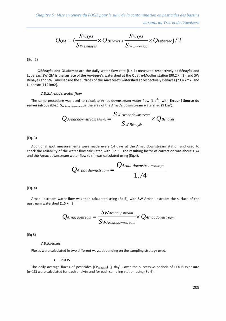
Chapitre 5 : Mise en œuvre du POCIS pour le suivi de la contamination en pesticides des bassins
versants du Trec et de l’Auvézère
2/)( LubersacLubersacW
QMWBénayès
BénayèsW
QMWQM Q
SSQ
SSQ ××= +
(Eq. 2)
QBénayès and QLubersac are the daily water flow rate (L s-1) measured respectively at Bénayès and Lubersac, SW QM is the surface of the Auvézère’s watershed at the Quatre-Moulins station (90.2 km2), and SW Bénayès and SW Lubersac are the surfaces of the Auvézère’s watershed at respectively Bénayès (23.4 km2) and Lubersac (112 km2).
2.8.2. Arnac’s water flow
The same procedure was used to calculate Arnac downstream water flow (L s-1), with Erreur ! Source du renvoi introuvable.). SW Arnac downstream is the area of the Arnac’s downstream watershed (9 km2).
BénayèsBénayèsW
downstreamArnacWdownstreamArnac Q
SSQ Bénayès ×=
(Eq. 3)
Additional spot measurements were made every 14 days at the Arnac downstream station and used to check the reliability of the water flow calculated with (Eq.3). The resulting factor of correction was about 1.74 and the Arnac downstream water flow (L s-1) was calculated using (Eq.4).
74.1BénayèsdownstreamArnac
downstreamArnacQQ =
(Eq. 4)
Arnac upstream water flow was then calculated using (Eq.5), with SW Arnac upstream the surface of the upstream watershed (1.5 km2).
downstreamArnacdownstreamArnac
upstreamArnacupstreamArnac Q
SwSwQ ×=
(Eq 5)
2.8.3. Fluxes
Fluxes were calculated in two different ways, depending on the sampling strategy used.
• POCIS
The daily average fluxes of pesticides (FPpesticide) (g day-1) over the successive periods of POCIS exposure (n=18) were calculated for each analyte and for each sampling station using (Eq.6).
209
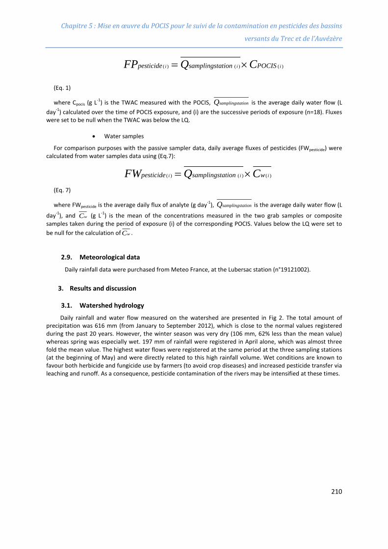
Chapitre 5 : Mise en œuvre du POCIS pour le suivi de la contamination en pesticides des bassins
versants du Trec et de l’Auvézère
)()()( iii POCISationsamplingstpesticide CQFP ×=
(Eq. 1)
where Cpocis (g L-1) is the TWAC measured with the POCIS, ationsamplingstQ is the average daily water flow (L day-1) calculated over the time of POCIS exposure, and (i) are the successive periods of exposure (n=18). Fluxes were set to be null when the TWAC was below the LQ.
• Water samples
For comparison purposes with the passive sampler data, daily average fluxes of pesticides (FWpesticide) were calculated from water samples data using (Eq.7):
)()()( iii wationsamplingstpesticide CQFW ×=
(Eq. 7)
where FWpesticide is the average daily flux of analyte (g day-1), ationsamplingstQ is the average daily water flow (L
day-1), and wC (g L-1) is the mean of the concentrations measured in the two grab samples or composite samples taken during the period of exposure (i) of the corresponding POCIS. Values below the LQ were set to be null for the calculation of wC .
2.9. Meteorological data
Daily rainfall data were purchased from Meteo France, at the Lubersac station (n°19121002).
3. Results and discussion
3.1. Watershed hydrology
Daily rainfall and water flow measured on the watershed are presented in Fig 2. The total amount of precipitation was 616 mm (from January to September 2012), which is close to the normal values registered during the past 20 years. However, the winter season was very dry (106 mm, 62% less than the mean value) whereas spring was especially wet. 197 mm of rainfall were registered in April alone, which was almost three fold the mean value. The highest water flows were registered at the same period at the three sampling stations (at the beginning of May) and were directly related to this high rainfall volume. Wet conditions are known to favour both herbicide and fungicide use by farmers (to avoid crop diseases) and increased pesticide transfer via leaching and runoff. As a consequence, pesticide contamination of the rivers may be intensified at these times.
210
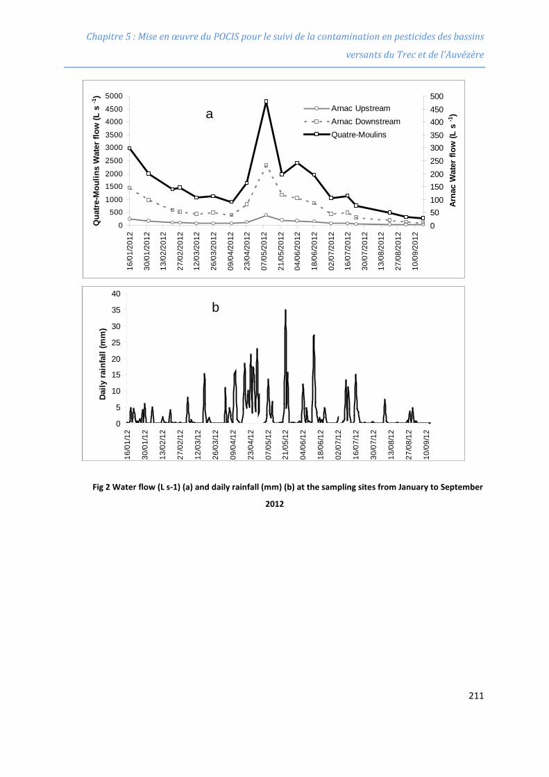
Chapitre 5 : Mise en œuvre du POCIS pour le suivi de la contamination en pesticides des bassins
versants du Trec et de l’Auvézère
Fig 2 Water flow (L s-1) (a) and daily rainfall (mm) (b) at the sampling sites from January to September
2012
0
5001000
15002000
2500
30003500
40004500
5000
16/0
1/20
12
30/0
1/20
12
13/0
2/20
12
27/0
2/20
12
12/0
3/20
12
26/0
3/20
12
09/0
4/20
12
23/0
4/20
12
07/0
5/20
12
21/0
5/20
12
04/0
6/20
12
18/0
6/20
12
02/0
7/20
12
16/0
7/20
12
30/0
7/20
12
13/0
8/20
12
27/0
8/20
12
10/0
9/20
12
Qua
tre-M
oulin
s W
ater
flow
(L s
-1)
050100150200250300350400450500
Arna
c W
ater
flow
(L s
-1)Arnac Upstream
Arnac DownstreamQuatre-Moulins
0
5
10
15
20
25
30
35
40
16/0
1/12
30/0
1/12
13/0
2/12
27/0
2/12
12/0
3/12
26/0
3/12
09/0
4/12
23/0
4/12
07/0
5/12
21/0
5/12
04/0
6/12
18/0
6/12
02/0
7/12
16/0
7/12
30/0
7/12
13/0
8/12
27/0
8/12
10/0
9/12
Daily
rain
fall
(mm
)a
b
0
5001000
15002000
2500
30003500
40004500
5000
16/0
1/20
12
30/0
1/20
12
13/0
2/20
12
27/0
2/20
12
12/0
3/20
12
26/0
3/20
12
09/0
4/20
12
23/0
4/20
12
07/0
5/20
12
21/0
5/20
12
04/0
6/20
12
18/0
6/20
12
02/0
7/20
12
16/0
7/20
12
30/0
7/20
12
13/0
8/20
12
27/0
8/20
12
10/0
9/20
12
Qua
tre-M
oulin
s W
ater
flow
(L s
-1)
050100150200250300350400450500
Arna
c W
ater
flow
(L s
-1)Arnac Upstream
Arnac DownstreamQuatre-Moulins
0
5
10
15
20
25
30
35
40
16/0
1/12
30/0
1/12
13/0
2/12
27/0
2/12
12/0
3/12
26/0
3/12
09/0
4/12
23/0
4/12
07/0
5/12
21/0
5/12
04/0
6/12
18/0
6/12
02/0
7/12
16/0
7/12
30/0
7/12
13/0
8/12
27/0
8/12
10/0
9/12
Daily
rain
fall
(mm
)a
b
211
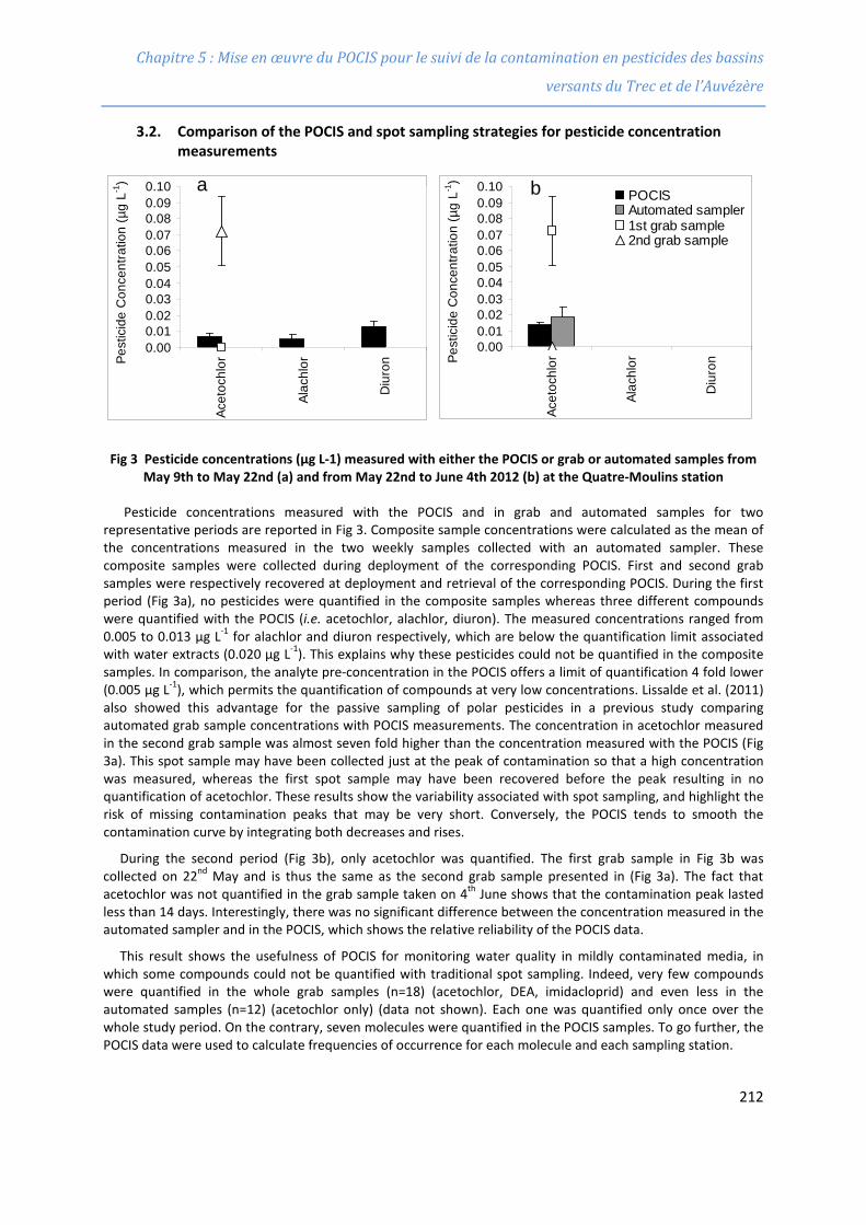
Chapitre 5 : Mise en œuvre du POCIS pour le suivi de la contamination en pesticides des bassins
versants du Trec et de l’Auvézère
3.2. Comparison of the POCIS and spot sampling strategies for pesticide concentration measurements
Fig 3 Pesticide concentrations (µg L-1) measured with either the POCIS or grab or automated samples from May 9th to May 22nd (a) and from May 22nd to June 4th 2012 (b) at the Quatre-Moulins station
Pesticide concentrations measured with the POCIS and in grab and automated samples for two representative periods are reported in Fig 3. Composite sample concentrations were calculated as the mean of the concentrations measured in the two weekly samples collected with an automated sampler. These composite samples were collected during deployment of the corresponding POCIS. First and second grab samples were respectively recovered at deployment and retrieval of the corresponding POCIS. During the first period (Fig 3a), no pesticides were quantified in the composite samples whereas three different compounds were quantified with the POCIS (i.e. acetochlor, alachlor, diuron). The measured concentrations ranged from 0.005 to 0.013 µg L-1 for alachlor and diuron respectively, which are below the quantification limit associated with water extracts (0.020 µg L-1). This explains why these pesticides could not be quantified in the composite samples. In comparison, the analyte pre-concentration in the POCIS offers a limit of quantification 4 fold lower (0.005 µg L-1), which permits the quantification of compounds at very low concentrations. Lissalde et al. (2011) also showed this advantage for the passive sampling of polar pesticides in a previous study comparing automated grab sample concentrations with POCIS measurements. The concentration in acetochlor measured in the second grab sample was almost seven fold higher than the concentration measured with the POCIS (Fig 3a). This spot sample may have been collected just at the peak of contamination so that a high concentration was measured, whereas the first spot sample may have been recovered before the peak resulting in no quantification of acetochlor. These results show the variability associated with spot sampling, and highlight the risk of missing contamination peaks that may be very short. Conversely, the POCIS tends to smooth the contamination curve by integrating both decreases and rises.
During the second period (Fig 3b), only acetochlor was quantified. The first grab sample in Fig 3b was collected on 22nd May and is thus the same as the second grab sample presented in (Fig 3a). The fact that acetochlor was not quantified in the grab sample taken on 4th June shows that the contamination peak lasted less than 14 days. Interestingly, there was no significant difference between the concentration measured in the automated sampler and in the POCIS, which shows the relative reliability of the POCIS data.
This result shows the usefulness of POCIS for monitoring water quality in mildly contaminated media, in which some compounds could not be quantified with traditional spot sampling. Indeed, very few compounds were quantified in the whole grab samples (n=18) (acetochlor, DEA, imidacloprid) and even less in the automated samples (n=12) (acetochlor only) (data not shown). Each one was quantified only once over the whole study period. On the contrary, seven molecules were quantified in the POCIS samples. To go further, the POCIS data were used to calculate frequencies of occurrence for each molecule and each sampling station.
0.000.010.020.030.040.050.060.070.080.090.10
Acet
ochl
or
Alac
hlor
Diu
ronPe
stic
ide
Con
cent
ratio
n (µ
g L-1
)
0.000.010.020.030.040.050.060.070.080.090.10
Acet
ochl
or
Alac
hlor
Diu
ronPe
stic
ide
Con
cent
ratio
n (µ
g L-1
)
POCISAutomated sampler1st grab sample2nd grab sample
a b
212
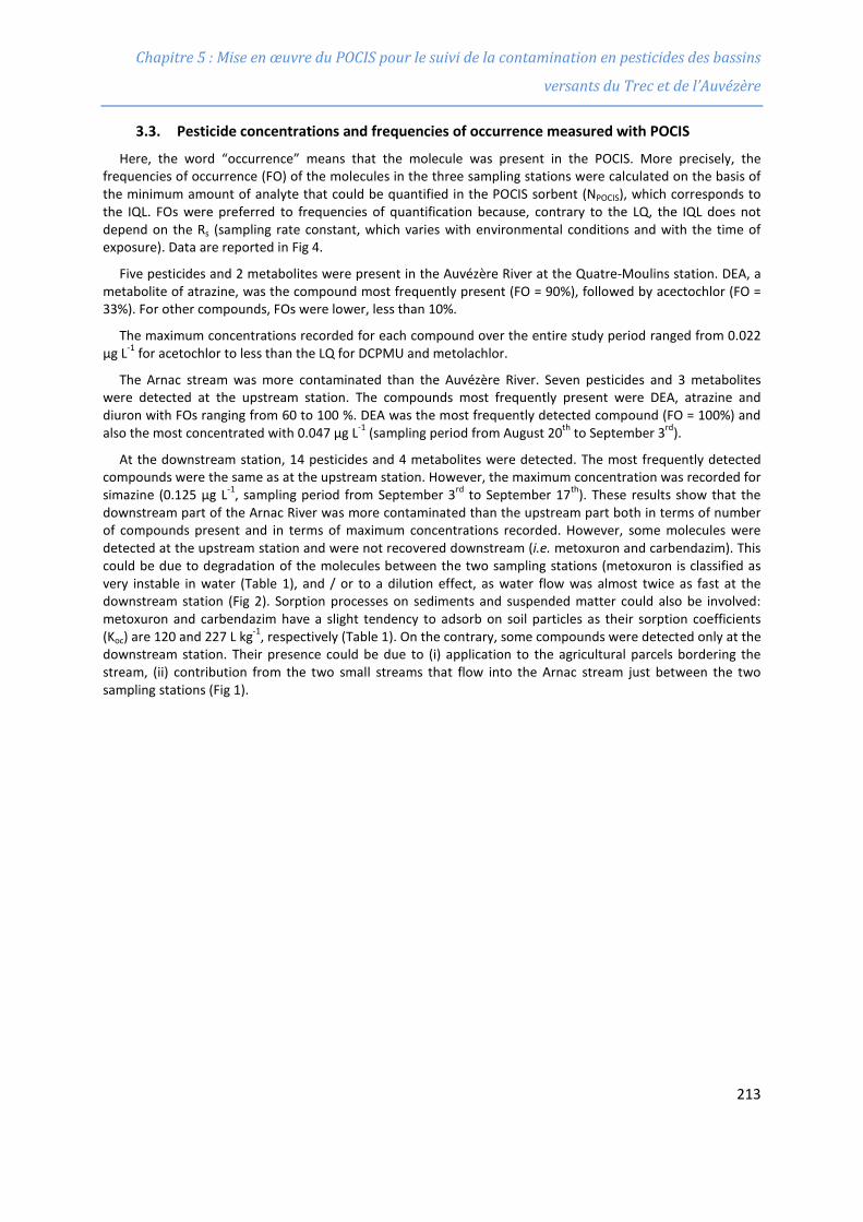
Chapitre 5 : Mise en œuvre du POCIS pour le suivi de la contamination en pesticides des bassins
versants du Trec et de l’Auvézère
3.3. Pesticide concentrations and frequencies of occurrence measured with POCIS
Here, the word “occurrence” means that the molecule was present in the POCIS. More precisely, the frequencies of occurrence (FO) of the molecules in the three sampling stations were calculated on the basis of the minimum amount of analyte that could be quantified in the POCIS sorbent (NPOCIS), which corresponds to the IQL. FOs were preferred to frequencies of quantification because, contrary to the LQ, the IQL does not depend on the Rs (sampling rate constant, which varies with environmental conditions and with the time of exposure). Data are reported in Fig 4.
Five pesticides and 2 metabolites were present in the Auvézère River at the Quatre-Moulins station. DEA, a metabolite of atrazine, was the compound most frequently present (FO = 90%), followed by acectochlor (FO = 33%). For other compounds, FOs were lower, less than 10%.
The maximum concentrations recorded for each compound over the entire study period ranged from 0.022 µg L-1 for acetochlor to less than the LQ for DCPMU and metolachlor.
The Arnac stream was more contaminated than the Auvézère River. Seven pesticides and 3 metabolites were detected at the upstream station. The compounds most frequently present were DEA, atrazine and diuron with FOs ranging from 60 to 100 %. DEA was the most frequently detected compound (FO = 100%) and also the most concentrated with 0.047 µg L-1 (sampling period from August 20th to September 3rd).
At the downstream station, 14 pesticides and 4 metabolites were detected. The most frequently detected compounds were the same as at the upstream station. However, the maximum concentration was recorded for simazine (0.125 µg L-1, sampling period from September 3rd to September 17th). These results show that the downstream part of the Arnac River was more contaminated than the upstream part both in terms of number of compounds present and in terms of maximum concentrations recorded. However, some molecules were detected at the upstream station and were not recovered downstream (i.e. metoxuron and carbendazim). This could be due to degradation of the molecules between the two sampling stations (metoxuron is classified as very instable in water (Table 1), and / or to a dilution effect, as water flow was almost twice as fast at the downstream station (Fig 2). Sorption processes on sediments and suspended matter could also be involved: metoxuron and carbendazim have a slight tendency to adsorb on soil particles as their sorption coefficients (Koc) are 120 and 227 L kg-1, respectively (Table 1). On the contrary, some compounds were detected only at the downstream station. Their presence could be due to (i) application to the agricultural parcels bordering the stream, (ii) contribution from the two small streams that flow into the Arnac stream just between the two sampling stations (Fig 1).
213
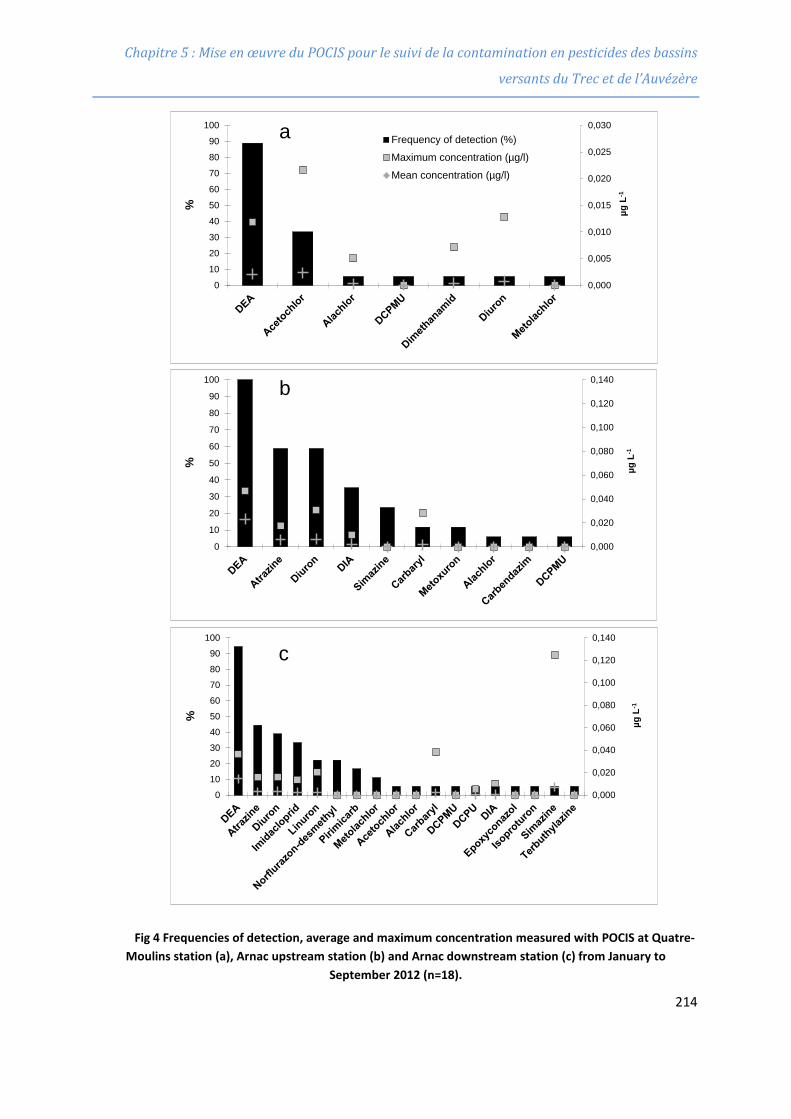
Chapitre 5 : Mise en œuvre du POCIS pour le suivi de la contamination en pesticides des bassins
versants du Trec et de l’Auvézère
Fig 4 Frequencies of detection, average and maximum concentration measured with POCIS at Quatre-Moulins station (a), Arnac upstream station (b) and Arnac downstream station (c) from January to
September 2012 (n=18).
0,000
0,005
0,010
0,015
0,020
0,025
0,030
0
10
20
30
40
50
60
70
80
90
100
µg L
-1
%
Frequency of detection (%)Maximum concentration (µg/l)Mean concentration (µg/l)
0,000
0,020
0,040
0,060
0,080
0,100
0,120
0,140
0
10
20
30
40
50
60
70
80
90
100
µg L
-1
%
0,000
0,020
0,040
0,060
0,080
0,100
0,120
0,140
0102030405060708090
100µg
L-1
%
a
b
c
214
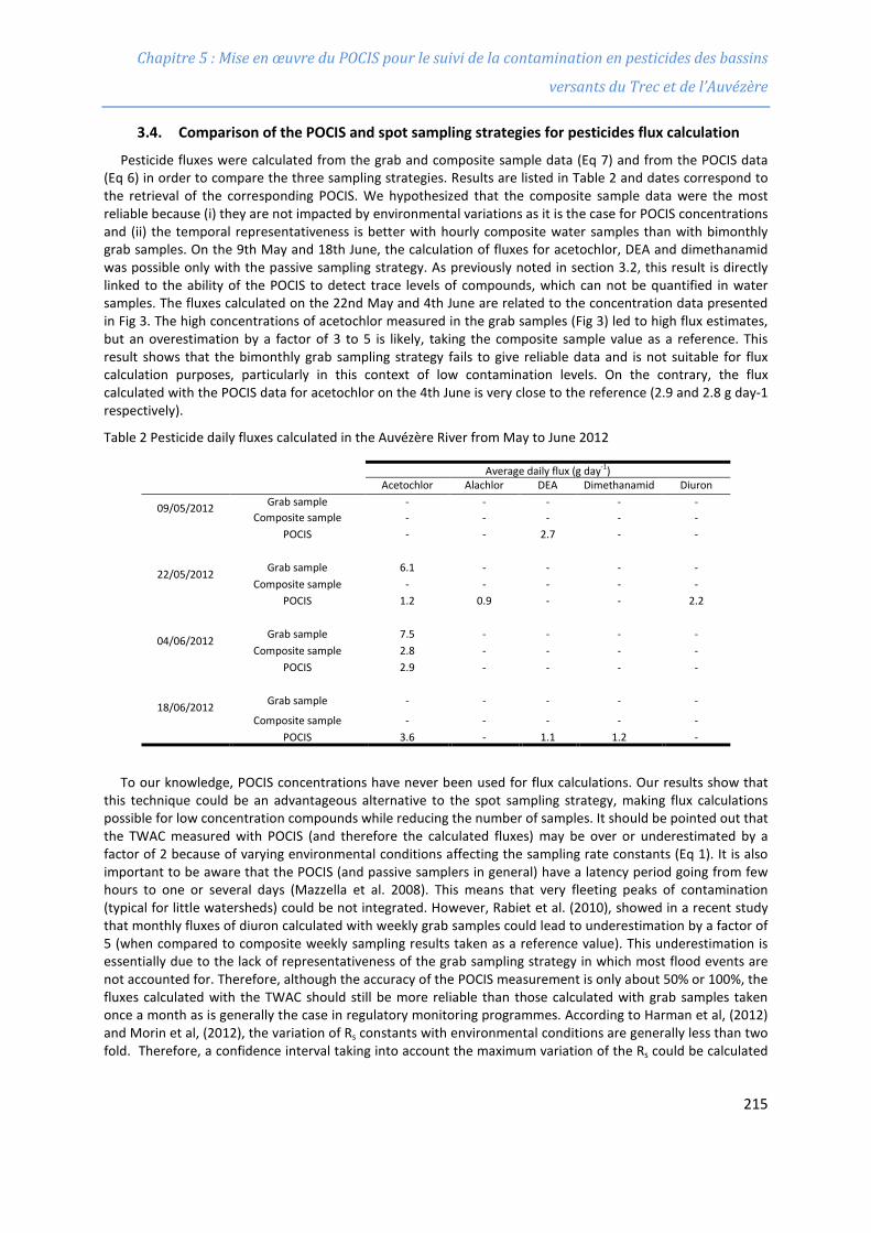
Chapitre 5 : Mise en œuvre du POCIS pour le suivi de la contamination en pesticides des bassins
versants du Trec et de l’Auvézère
3.4. Comparison of the POCIS and spot sampling strategies for pesticides flux calculation
Pesticide fluxes were calculated from the grab and composite sample data (Eq 7) and from the POCIS data (Eq 6) in order to compare the three sampling strategies. Results are listed in Table 2 and dates correspond to the retrieval of the corresponding POCIS. We hypothesized that the composite sample data were the most reliable because (i) they are not impacted by environmental variations as it is the case for POCIS concentrations and (ii) the temporal representativeness is better with hourly composite water samples than with bimonthly grab samples. On the 9th May and 18th June, the calculation of fluxes for acetochlor, DEA and dimethanamid was possible only with the passive sampling strategy. As previously noted in section 3.2, this result is directly linked to the ability of the POCIS to detect trace levels of compounds, which can not be quantified in water samples. The fluxes calculated on the 22nd May and 4th June are related to the concentration data presented in Fig 3. The high concentrations of acetochlor measured in the grab samples (Fig 3) led to high flux estimates, but an overestimation by a factor of 3 to 5 is likely, taking the composite sample value as a reference. This result shows that the bimonthly grab sampling strategy fails to give reliable data and is not suitable for flux calculation purposes, particularly in this context of low contamination levels. On the contrary, the flux calculated with the POCIS data for acetochlor on the 4th June is very close to the reference (2.9 and 2.8 g day-1 respectively).
Table 2 Pesticide daily fluxes calculated in the Auvézère River from May to June 2012
Average daily flux (g day-1) Acetochlor Alachlor DEA Dimethanamid Diuron
09/05/2012 Grab sample - - - - - Composite sample - - - - -
POCIS - - 2.7 - -
22/05/2012 Grab sample 6.1 - - - - Composite sample - - - - -
POCIS 1.2 0.9 - - 2.2
04/06/2012 Grab sample 7.5 - - - - Composite sample 2.8 - - - -
POCIS 2.9 - - - -
18/06/2012 Grab sample - - - - -
Composite sample - - - - - POCIS 3.6 - 1.1 1.2 -
To our knowledge, POCIS concentrations have never been used for flux calculations. Our results show that this technique could be an advantageous alternative to the spot sampling strategy, making flux calculations possible for low concentration compounds while reducing the number of samples. It should be pointed out that the TWAC measured with POCIS (and therefore the calculated fluxes) may be over or underestimated by a factor of 2 because of varying environmental conditions affecting the sampling rate constants (Eq 1). It is also important to be aware that the POCIS (and passive samplers in general) have a latency period going from few hours to one or several days (Mazzella et al. 2008). This means that very fleeting peaks of contamination (typical for little watersheds) could be not integrated. However, Rabiet et al. (2010), showed in a recent study that monthly fluxes of diuron calculated with weekly grab samples could lead to underestimation by a factor of 5 (when compared to composite weekly sampling results taken as a reference value). This underestimation is essentially due to the lack of representativeness of the grab sampling strategy in which most flood events are not accounted for. Therefore, although the accuracy of the POCIS measurement is only about 50% or 100%, the fluxes calculated with the TWAC should still be more reliable than those calculated with grab samples taken once a month as is generally the case in regulatory monitoring programmes. According to Harman et al, (2012) and Morin et al, (2012), the variation of Rs constants with environmental conditions are generally less than two fold. Therefore, a confidence interval taking into account the maximum variation of the Rs could be calculated
215
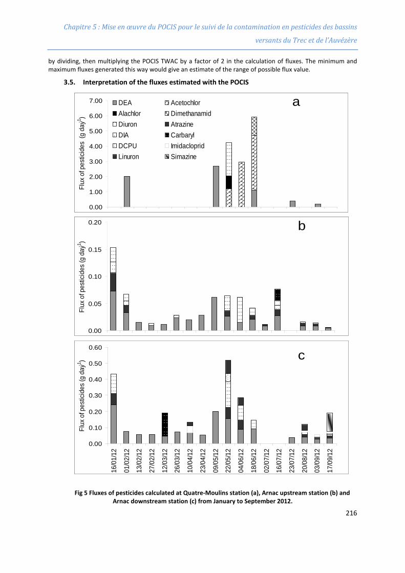
Chapitre 5 : Mise en œuvre du POCIS pour le suivi de la contamination en pesticides des bassins
versants du Trec et de l’Auvézère
by dividing, then multiplying the POCIS TWAC by a factor of 2 in the calculation of fluxes. The minimum and maximum fluxes generated this way would give an estimate of the range of possible flux value.
3.5. Interpretation of the fluxes estimated with the POCIS
Fig 5 Fluxes of pesticides calculated at Quatre-Moulins station (a), Arnac upstream station (b) and Arnac downstream station (c) from January to September 2012.
0.00
0.10
0.20
0.30
0.40
0.50
0.60
16/0
1/12
01/0
2/12
13/0
2/12
27/0
2/12
12/0
3/12
26/0
3/12
10/0
4/12
23/0
4/12
09/0
5/12
22/0
5/12
04/0
6/12
18/0
6/12
02/0
7/12
16/0
7/12
23/0
7/12
20/0
8/12
03/0
9/12
17/0
9/12
Flux
of p
estic
ides
(g d
ay-1
)
0.00
0.05
0.10
0.15
0.20
Flux
of p
estic
ides
(g d
ay-1
)
0.00
1.00
2.00
3.00
4.00
5.00
6.00
7.00
Flux
of p
estic
ides
(g
day-1
)
a
b
c
DEA AcetochlorAlachlor DimethanamidDiuron AtrazineDIA CarbarylDCPU ImidaclopridLinuron Simazine
0.00
0.10
0.20
0.30
0.40
0.50
0.60
16/0
1/12
01/0
2/12
13/0
2/12
27/0
2/12
12/0
3/12
26/0
3/12
10/0
4/12
23/0
4/12
09/0
5/12
22/0
5/12
04/0
6/12
18/0
6/12
02/0
7/12
16/0
7/12
23/0
7/12
20/0
8/12
03/0
9/12
17/0
9/12
Flux
of p
estic
ides
(g d
ay-1
)
0.00
0.05
0.10
0.15
0.20
Flux
of p
estic
ides
(g d
ay-1
)
0.00
1.00
2.00
3.00
4.00
5.00
6.00
7.00
Flux
of p
estic
ides
(g
day-1
)
a
b
c
DEA AcetochlorAlachlor DimethanamidDiuron AtrazineDIA CarbarylDCPU ImidaclopridLinuron Simazine
216
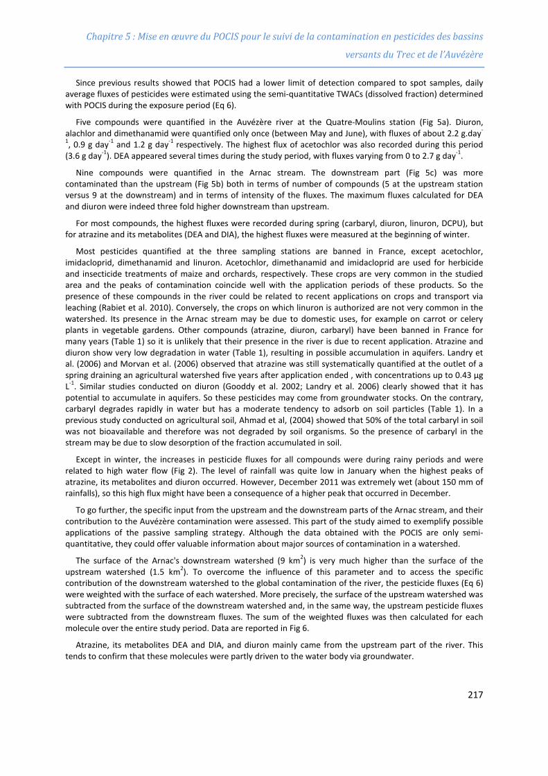
Chapitre 5 : Mise en œuvre du POCIS pour le suivi de la contamination en pesticides des bassins
versants du Trec et de l’Auvézère
Since previous results showed that POCIS had a lower limit of detection compared to spot samples, daily average fluxes of pesticides were estimated using the semi-quantitative TWACs (dissolved fraction) determined with POCIS during the exposure period (Eq 6).
Five compounds were quantified in the Auvézère river at the Quatre-Moulins station (Fig 5a). Diuron, alachlor and dimethanamid were quantified only once (between May and June), with fluxes of about 2.2 g.day-
1, 0.9 g day-1 and 1.2 g day-1 respectively. The highest flux of acetochlor was also recorded during this period (3.6 g day-1). DEA appeared several times during the study period, with fluxes varying from 0 to 2.7 g day-1.
Nine compounds were quantified in the Arnac stream. The downstream part (Fig 5c) was more contaminated than the upstream (Fig 5b) both in terms of number of compounds (5 at the upstream station versus 9 at the downstream) and in terms of intensity of the fluxes. The maximum fluxes calculated for DEA and diuron were indeed three fold higher downstream than upstream.
For most compounds, the highest fluxes were recorded during spring (carbaryl, diuron, linuron, DCPU), but for atrazine and its metabolites (DEA and DIA), the highest fluxes were measured at the beginning of winter.
Most pesticides quantified at the three sampling stations are banned in France, except acetochlor, imidacloprid, dimethanamid and linuron. Acetochlor, dimethanamid and imidacloprid are used for herbicide and insecticide treatments of maize and orchards, respectively. These crops are very common in the studied area and the peaks of contamination coincide well with the application periods of these products. So the presence of these compounds in the river could be related to recent applications on crops and transport via leaching (Rabiet et al. 2010). Conversely, the crops on which linuron is authorized are not very common in the watershed. Its presence in the Arnac stream may be due to domestic uses, for example on carrot or celery plants in vegetable gardens. Other compounds (atrazine, diuron, carbaryl) have been banned in France for many years (Table 1) so it is unlikely that their presence in the river is due to recent application. Atrazine and diuron show very low degradation in water (Table 1), resulting in possible accumulation in aquifers. Landry et al. (2006) and Morvan et al. (2006) observed that atrazine was still systematically quantified at the outlet of a spring draining an agricultural watershed five years after application ended , with concentrations up to 0.43 µg L-1. Similar studies conducted on diuron (Gooddy et al. 2002; Landry et al. 2006) clearly showed that it has potential to accumulate in aquifers. So these pesticides may come from groundwater stocks. On the contrary, carbaryl degrades rapidly in water but has a moderate tendency to adsorb on soil particles (Table 1). In a previous study conducted on agricultural soil, Ahmad et al, (2004) showed that 50% of the total carbaryl in soil was not bioavailable and therefore was not degraded by soil organisms. So the presence of carbaryl in the stream may be due to slow desorption of the fraction accumulated in soil.
Except in winter, the increases in pesticide fluxes for all compounds were during rainy periods and were related to high water flow (Fig 2). The level of rainfall was quite low in January when the highest peaks of atrazine, its metabolites and diuron occurred. However, December 2011 was extremely wet (about 150 mm of rainfalls), so this high flux might have been a consequence of a higher peak that occurred in December.
To go further, the specific input from the upstream and the downstream parts of the Arnac stream, and their contribution to the Auvézère contamination were assessed. This part of the study aimed to exemplify possible applications of the passive sampling strategy. Although the data obtained with the POCIS are only semi-quantitative, they could offer valuable information about major sources of contamination in a watershed.
The surface of the Arnac's downstream watershed (9 km2) is very much higher than the surface of the upstream watershed (1.5 km2). To overcome the influence of this parameter and to access the specific contribution of the downstream watershed to the global contamination of the river, the pesticide fluxes (Eq 6) were weighted with the surface of each watershed. More precisely, the surface of the upstream watershed was subtracted from the surface of the downstream watershed and, in the same way, the upstream pesticide fluxes were subtracted from the downstream fluxes. The sum of the weighted fluxes was then calculated for each molecule over the entire study period. Data are reported in Fig 6.
Atrazine, its metabolites DEA and DIA, and diuron mainly came from the upstream part of the river. This tends to confirm that these molecules were partly driven to the water body via groundwater.
217
Chapitre 5 : Mise en œuvre du POCIS pour le suivi de la contamination en pesticides des bassins
versants du Trec et de l’Auvézère
Fig 6 Total masses of pesticides loaded in the Arnac River (from January to September 2012) divided
by the watershed (downstream and upstream) surface areas.
The main objective of the Arnac River monitoring was to assess its contribution to the Auvézère contamination. To do this, total masses of pesticides flowing in the two rivers (Auvézère at the Quatre-Moulins station and the Arnac at the downstream station) were calculated by adding the fluxes recorded during the entire study period. For this purpose, fluxes were not weighted with the watershed surface areas. DEA and diuron were the only compounds quantified both in the Auvézère and Arnac Rivers, so the percentage contribution could be calculated only for these two molecules. We hypothesized that there was no degradation and no addition of the molecules between the Quatre-Moulins sampling station and the Arnac downstream sampling station. Data are reported in Table 3.
Table 3 Contribution of the Arnac River to the total pesticide contamination of the Auvézère River.
Auvézère (Quatre-Moulins
station) Arnac (downstream
station) Watershed surface area (km2)
90.2 9.0 Contribution of the Arnac River(%) Total mass of pesticides (g)
DEA 96 18 16 Diuron 28 6 18
The contribution of the Arnac River to the Auvézère's contamination was very similar for DEA and diuron (16 and 18 %, respectively). Taking into account the fact that the Arnac’s watershed represents less than 10 % of the surface of the Auvézère watershed, we can say that the Arnac contribution was more than 1.5 fold higher than expected. This result may indicate that the sources of pesticide contamination were not homogeneously distributed on the watershed.
4. Conclusion
The main conclusion of this study is that passive sampling is an efficient way to improve the representativeness of pesticide monitoring data. POCIS was shown to be a very useful tool to monitor pesticide concentrations in low contamination contexts. Indeed, the passive sampler gave better results in terms of limits of quantification and frequencies of occurrence compared to spot sampling. In the Quatre-Moulins station, three pesticides were quantified with POCIS during spring, whereas only acetochlor was measured in grab samples. DEA was the most frequently measured compound in the studied watershed with almost 100% occurrence. Although the data are semi-quantitative, the ability of POCIS to detect many compounds at trace levels made the calculation of pesticide fluxes in the Auvézère River possible even when concentrations were
-0.5
0.0
0.5
1.0
1.5
2.0
2.5
3.0
3.5
4.0
Atrazine Carbaryl DEA DIA Diuron
g km
-2
Contribution of the upstream watershedContribution of the downstream watershed
Input from the upstream watershed
Input from the downstream watershed
-0.5
0.0
0.5
1.0
1.5
2.0
2.5
3.0
3.5
4.0
Atrazine Carbaryl DEA DIA Diuron
g km
-2
Contribution of the upstream watershedContribution of the downstream watershed
Input from the upstream watershed
Input from the downstream watershed
218
Chapitre 5 : Mise en œuvre du POCIS pour le suivi de la contamination en pesticides des bassins
versants du Trec et de l’Auvézère
too low to be quantified in composite water samples. Additionally, the technical constraints associated with automated sampler maintenance (necessity for electricity, protection against potential vandalism, possible degradation of analytes in the bottle…) can be easily avoided with the use of POCIS. This feature can be useful for the monitoring of several sampling stations in the same or different watersheds, especially in remote areas, etc. Using passive sampler data to assess the specific input from small watersheds and determine their contribution to the contamination of the main river is very original and has never before been implemented. Used with several passive samplers dedicated to different types of compounds, such as semi-permeable membrane devices or Chemcatcher® for hydrophobic molecules, this strategy could permit targeting areas with higher contamination contributions. Flux information could benefit regulatory investigative and operational monitoring network, resulting in better understanding of the global contamination of a watershed, and in the implementation of more accurate remediation strategies.
5. Acknowledgments
This study was financed by the French Water Agency Adour Garonne and the Région Limousin. Authors would like to thank Aurélie Moreira, Patrice Fondanèche, Julie Bonafos, Emma Bourjas and Chloé Nicolas for technical and field assistance and Katherine Flynn for english revision.
6. References
2000/60/EC (2000) Directive 2000/60/EC of The European Parliament and of the Council of 23 October 2000 establishing a framework for Community action in the field of water policy. . OJ L 327, 22.12.2000:1-73
2008/105/EC (2008) 2008/105/EC of the European Parliament and of the Council of 16 December 2008 on environmental quality standards in the field of water policy. OJ L 348 24.12.2008:84-97
Ahmad R, Kookana RS, Megharaj M, Alston AM (2004) Aging reduces the bioavailability of even a weakly sorbed pesticide (carbaryl) in soil. Environmental Toxicology and Chemistry 23 (9):2084-2089. doi:10.1897/03-569
Allan IJ, Knutsson J, Guigues N, Mills GA, Fouillac AM, Greenwood R (2007) Evaluation of the Chemcatcher and DGT passive samplers for monitoring metals with highly fluctuating water concentrations. Journal of Environmental Monitoring 9 (7):672-681. doi:10.1039/b701616f
Alvarez DA, Petty JD, Huckins JN, Jones-Lepp TL, Getting DT, Goddard JP, Manahan SE (2004) Development of a passive, in situ, integrative sampler for hydrophilic organic contaminants in aquatic environments. Environmental Toxicology and Chemistry 23 (7):1640-1648. doi:10.1897/03-603
DeLorenzo ME, Scott GI, Ross PE (2001) Toxicity of pesticides to aquatic microorganisms: A review. Environmental Toxicology and Chemistry 20 (1):84-98. doi:10.1002/etc.5620200108
Fauvelle V, Mazzella N, Delmas F, Madarassou K, Eon M, Budzinski H (2012) Use of Mixed-Mode Ion Exchange Sorbent for the Passive Sampling of Organic Acids by Polar Organic Chemical Integrative Sampler (POCIS). Environmental Science & Technology 46 (24):13344-13353. doi:10.1021/es3035279
Gooddy DC, Chilton PJ, Harrison I (2002) A field study to assess the degradation and transport of diuron and its metabolites in a calcareous soil. Science of the Total Environment 297 (1-3):67-83. doi:10.1016/s0048-9697(02)00079-7
Harman C, Allan IJ, Vermeirssen ELM (2012) Calibration and use of the polar organic chemical integrative sampler-a critical review. Environmental Toxicology and Chemistry 31 (12):2724-2738
Harman C, Tollefsen KE, Bøyum O, Thomas K, Grung M (2008) Uptake rates of alkylphenols, PAHs and carbazoles in semipermeable membrane devices (SPMDs) and polar organic chemical integrative samplers (POCIS). Chemosphere 72 (10):1510-1516
Huckins JN, Manuweera GK, Petty JD, Mackay D, Lebo JA (1993) LIPID-CONTAINING SEMIPERMEABLE-MEMBRANE DEVICES FOR MONITORING ORGANIC CONTAMINANTS IN WATER. Environmental Science & Technology 27 (12):2489-2496. doi:10.1021/es00048a028
219
Chapitre 5 : Mise en œuvre du POCIS pour le suivi de la contamination en pesticides des bassins
versants du Trec et de l’Auvézère
Jaward FM, Farrar NJ, Harner T, Sweetman AJ, Jones KC (2004) Passive air sampling of PCBs, PBDEs, and organochlorine pesticides across Europe. Environmental Science & Technology 38 (1):34-41. doi:10.1021/es034705n
Landry D, Dousset S, Andreux F (2006) Leaching of oryzalin and diuron through undisturbed vineyard soil columns under outdoor conditions. Chemosphere 62 (10):1736-1747. doi:10.1016/j.chemosphere.2005.06.024
Lennartz B, Louchart X, Voltz M, Andrieux P (1997) Diuron and simazine losses to runoff water in Mediterranean vineyards. Journal of Environmental Quality 26 (6):1493-1502
Li H, Vermeirssen EL, Helm PA, Metcalfe CD (2010) Controlled field evaluation of water flow rate effects on sampling polar organic compounds using polar organic chemical integrative samplers. Environmental Toxicology and Chemistry 29 (11):2461-2469
Lissalde S, Mazzella N, Fauvelle V, Delmas F, Mazellier P, Legube B (2011) Liquid chromatography coupled with tandem mass spectrometry method for thirty-three pesticides in natural water and comparison of performance between classical solid phase extraction and passive sampling approaches. Journal of Chromatography A 1218 (11):1492-1502. doi:10.1016/j.chroma.2011.01.040
Loos R, Gawlik BM, Locoro G, Rimaviciute E, Contini S, Bidoglio G (2009) EU-wide survey of polar organic persistent pollutants in European river waters. Environmental Pollution 157 (2):561-568. doi:10.1016/j.envpol.2008.09.020
Louchart X, Voltz M, Andrieux P, Moussa R (2001) Herbicide transport to surface waters at field and watershed scales in a Mediterranean vineyard area. Journal of Environmental Quality 30 (3):982-991
Mason CF, Underwood GJC, Baker NR, Davey PA, Davidson I, Hanlon G, Long SP, Oxborough K, Paterson DM, Watson A (2003) The role of herbicides in the erosion of salt marshes in eastern England. Environmental Pollution 122 (1):41-49. doi:10.1016/s0269-7491(02)00284-1
Mazzella N, Debenest T, Delmas F (2008) Comparison between the polar organic chemical integrative sampler and the solid-phase extraction for estimating herbicide time-weighted average concentrations during a microcosm experiment. Chemosphere 73 (4):545-550. doi:10.1016/j.chemosphere.2008.06.009
Mazzella N, Dubernet JF, Delmas F (2007) Determination of kinetic and equilibrium regimes in the operation of polar organic chemical integrative samplers - Application to the passive sampling of the polar herbicides in aquatic environments.
Morin N, Miège C, Coquery M, Randon J (2012) Chemical calibration, performance, validation and applications of the polar organic chemical integrative sampler (POCIS) in aquatic environments. TrAC Trends in Analytical Chemistry (0)
Morvan X, Mouvet C, Baran N, Gutierrez A (2006) Pesticides in the groundwater of a spring draining a sandy aquifer: Temporal variability of concentrations and fluxes. Journal of Contaminant Hydrology 87 (3–4):176-190. doi:http://dx.doi.org/10.1016/j.jconhyd.2006.05.003
Rabiet M, Margoum C, Gouy V, Carluer N, Coquery M (2010) Assessing pesticide concentrations and fluxes in the stream of a small vineyard catchment – Effect of sampling frequency. Environmental Pollution 158 (3):737-748. doi:http://dx.doi.org/10.1016/j.envpol.2009.10.014
Solomon KR, Baker DB, Richards RP, Dixon DR, Klaine SJ, LaPoint TW, Kendall RJ, Weisskopf CP, Giddings JM, Giesy JP, Hall LW, Williams WM (1996) Ecological risk assessment of atrazine in North American surface waters. Environmental Toxicology and Chemistry 15 (1):31-74. doi:10.1897/1551-5028(1996)015<0031:eraoai>2.3.co;2
Stuer-Lauridsen F (2005) Review of passive accumulation devices for monitoring organic micropollutants in the aquatic environment. Environmental Pollution 136 (3):503-524. doi:10.1016/j.envpol.2005.12.004
Taghavi L, Merlina G, Probst JL (2011) The role of storm flows in concentration of pesticides associated with particulate and dissolved fractions as a threat to aquatic ecosystems Case study: the agricultural
220
Chapitre 5 : Mise en œuvre du POCIS pour le suivi de la contamination en pesticides des bassins
versants du Trec et de l’Auvézère
watershed of Save river (Southwest of France). Knowledge and Management of Aquatic Ecosystems (400). doi:06
10.1051/kmae/2011002
Togola A, Budzinski H (2007) Development of polar organic integrative samplers for analysis of pharmaceuticals in aquatic systems. Analytical Chemistry 79 (17):6734-6741
Vrana B, Mills GA, Allan IJ, Dominiak E, Svensson K, Knutsson J, Morrison G, Greenwood R (2005) Passive sampling techniques for monitoring pollutants in water. Trac-Trends in Analytical Chemistry 24 (10):845-868. doi:10.1016/j.trac.2005.06.006
221

Chapitre 5 : Mise en œuvre du POCIS pour le suivi de la contamination en pesticides des bassins
versants du Trec et de l’Auvézère
222
Chapitre 5 : Mise en œuvre du POCIS pour le suivi de la contamination en pesticides des bassins
versants du Trec et de l’Auvézère
5.3 Conclusion partielle La mise en œuvre du POCIS dans un environnement présentant une forte contamination en
pesticides a permis de mettre en évidence l’utilité du dispositif pour la détection de pics
imprévisibles survenant lors d’épisodes de crue, l’identification des périodes les plus à risques et la
détermination géographique des zones les plus impactées par la pollution. Les avantages du POCIS
par rapport aux prélèvements ponctuels pourraient également s’avérer utiles pour l’étude
d’environnement moins contaminés. La Directive Cadre sur l’Eau impose que des mesures
correctives (bandes enherbées, incitations au désherbage manuel, etc.) soient mises en œuvre
lorsque des substances prioritaires sont présentes dans les cours d’eau. Le meilleur moyen de
mesurer l’efficacité de ces actions consiste à étudier les flux, qui prennent en compte non seulement
la concentration, mais aussi le débit du cours d’eau. Or, dans le cas d’environnement peu contaminés
présentant un fort débit, il peut être difficile de quantifier certains polluants faiblement concentrés,
alors même que les flux peuvent être très élevés. L’applicabilité du POCIS pour la surveillance des flux
de pesticides a été évaluée sur le bassin versant de l’Auvézère. Les résultats de cette étude ont
montré que l’outil offre non seulement une meilleure sensibilité (les composés présents en très
faible concentration sont détectés et quantifiés plus souvent), mais également un gain de
représentativité temporelle, par rapport aux mesures classiques reposant sur un échantillonnage
ponctuel. Ces caractéristiques ont permis l’estimation de flux pour des composés qui n’étaient pas
détectés dans les échantillons d’eau.
Ainsi, la mise en œuvre du POCIS en conditions réelles, sur des bassins versants très
différents a livré des résultats qui laissent envisager une possible utilisation de l’outil pour le contrôle
de la qualité des cours d’eau. Il a été démontré que le POCIS peut être adapté aux trois volets de la
DCE, à savoir le contrôle de surveillance, le contrôle opérationnel et le contrôle d’enquête.
223

Chapitre 5 : Mise en œuvre du POCIS pour le suivi de la contamination en pesticides des bassins
versants du Trec et de l’Auvézère
224
Conclusion générale et perspectives
POULIER Gaëlle | Thèse de doctorat | Chimie Environnementale | Université de Limoges | 2014 225

POULIER Gaëlle | Thèse de doctorat | Chimie Environnementale | Université de Limoges | 2014 226
Conclusion générale et perspectives
Au cours des dernières décennies, les échantillonneurs passifs sont apparus comme un moyen
de résoudre certaines des contraintes liées à l’échantillonnage ponctuel. Leurs performances en
termes de sensibilité (baisse des limites de détection) et de représentativité temporelle (obtention
d’une concentration moyenne pondérée dans le temps) en font un outil de choix pour l’analyse des
contaminants en général, et des pesticides en particulier, dans les milieux aquatiques. Toutefois, la
méconnaissance de certaines caractéristiques et processus entourant l’échantillonnage passif
restreint aujourd’hui l’utilisation de tels outils dans les réseaux de surveillance réglementaires.
L’objectif principal de cette thèse était donc de définir le domaine d’application des
échantillonneurs passifs POCIS, Chemcatchers et DGT, et de vérifier leur validité pour la surveillance
réglementaire de la qualité de l’eau. Pour cela, les principaux verrous scientifiques et techniques
empêchant l’utilisation à large échelle de ces outils ont été étudiés.
L’une des grandes questions attachée à l’échantillonnage passif est celle de la calibration des
outils. Cette étape, souvent longue et coûteuse ne peut être réalisée systématiquement dans un
contexte d’analyses de routine. Il serait donc nécessaire d’établir des tables de Rs, contenant des
valeurs de référence pour chaque molécule, en précisant à la fois les conditions dans lesquelles ces
valeurs ont été acquises, et les conditions environnementales pour lesquelles elles s’appliquent. Les
laboratoires prestataires pourraient alors sélectionner dans ces tables des valeurs de Rs
représentatives du milieu étudié, en tenant compte de l’incertitude associée. Par ailleurs, la
construction de ces tables nécessite d’harmoniser au niveau européen les conditions d’étalonnage
des échantillonneurs passifs. En effet, les données de calibration actuellement disponibles, bien que
nombreuses, ont été acquises dans des conditions différentes et sont donc très hétérogènes.
Néanmoins, en l’état actuel de nos connaissances, une nouvelles calibration des outils
demeurera indispensable lorsque de nouvelles molécules devront être ajoutées au réseau de
surveillance. En effet, les résultats acquis au cours de ces travaux montrent que l’étalonnage en
laboratoire des échantillonneurs passifs POCIS et Chemcatcher reste une étape clé, nécessaire à leur
utilisation ultérieure sur le terrain, car il n’est pour le moment pas possible de prédire le Rs d’une
molécule à partir de ses propriétés physico-chimiques, ou à partir des Rs obtenus pour des molécules
appartenant à la même famille. La question de la modélisation des Rs a été très peu abordée dans le
cas du POCIS. Ibrahim et al. (2013) ont montré que 13 pesticides appartenant à différentes familles
mais possédant un log Kow compris entre 2 et 4 présentaient des Rs très similaires, le pourcentage du
coefficient de variation de la moyenne étant inférieur à 20 %. Ils ont alors suggéré d’utiliser une
unique valeur moyenne de Rs pour tous les composés correspondant à cette gamme
227
Conclusion générale et perspectives
d’hydrophobicité. Toutefois, des résultats contraires ont été reportés par d’autres auteurs, Li et al.
(2010) ayant obtenu une relation linéaire entre le Rs et le log Kow, tandis que MacLeod et al. (2007)
ont signalé une absence de relation entre ces deux paramètres.
Dans le cas du Chemcatcher, il a été démontré au cours de ces travaux que les relations
empiriques existantes, utilisées pour prédire les constantes cinétiques d’accumulation à partir des
propriétés physico-chimiques des composés sont perfectibles. En effet, le modèle développé par
Vrana et al. (2007) pour les HAP et basé uniquement sur l’hydrophobicité n’est pas valide pour
d’autres familles de molécules tels que les pesticides et les PCB. De même, le modèle proposé au
terme de ce travail de thèse, qui prend en compte de multiples paramètres tels que le volume
molaire, la densité ou la surface des molécules, n’a été ajusté que pour des pesticides. Ces résultats
ont mis en lumière l’influence de certains paramètres, jusqu’ici négligés, dans les échanges
cinétiques. Les mécanismes d’accumulation des pesticides dans l’échantillonneur pourraient donc
s’avérer beaucoup plus complexes qu’attendu.
Un effort particulier avait été engagé afin de définir l’influence des conditions
environnementales sur les données délivrées par les systèmes passifs. Cette question était cruciale
car elle conditionne en grande partie la fiabilité et la justesse des concentrations mesurées.
Dans le cas du POCIS, deux méthodes de correction du biais lié à la variation des conditions
d’exposition ont été évaluées. Les résultats concernant l’approche PRC sont mitigés car le nombre de
données disponibles est relativement faible. Par conséquent de nombreuses questions subsistent
encore sur le caractère opérationnel de cette méthode de correction. La démarche consistant à
étalonner l’outil directement dans le cours d’eau (in situ), a démontré une bonne efficacité pour
améliorer la justesse du POCIS. Nos résultats suggèrent qu’une calibration en microcosme et en
conditions contrôlées ne peut suffire à obtenir des constantes cinétiques suffisamment
représentatives du milieu étudié, même si les paramètres fixés (vitesse du courant et température
notamment) sont proches de ceux de l’environnement étudié. Ce résultat implique que l’utilisation
de tables de référence évoquée précédemment, nécessitera de disposer d’un jeu de données
suffisamment large pour pouvoir sélectionner le Rs le plus adéquat pour le milieu étudié, mais aussi
que l’incertitude globale associée à l’emploi de de ces valeurs ne sera probablement pas négligeable
et devra être renseignée.
L’approche PRC n’ayant pas donné de résultats totalement satisfaisants, et l’étalonnage in situ
étant impossible à mettre en œuvre dans le cadre de la surveillance de routine, la question de
228
Conclusion générale et perspectives
l’incertitude globale associée à la mesure des échantillonneurs passifs devenait primordiale. Cette
difficulté a pu être résolue grâce à la définition d’un intervalle de confiance qui prend en compte le
biais lié aux conditions environnementales, et qui intègre les variations maximales attendues pour les
températures et les vitesses de courant rencontrées dans le milieu naturel. Cette solution permet de
donner à la mesure POCIS un caractère semi-quantitatif utilisable dans un contexte opérationnel et
réglementaire. De plus, il a été démontré que le POCIS échantillonne uniquement la fraction dissoute
des contaminants, nous permet de conclure que le dispositif pourrait être appliqué de façon fiable
pour la surveillance des milieux aquatiques dans le cadre de la DCE. Une procédure standard a été
proposée dans ce sens.
Dans le cas du DGT, les principales sources d’imprécisions résidaient en premier lieu dans la
détermination d’une limite de quantification appropriée, qui dépend en grande partie de la pureté
des blancs analytiques. En second lieu, l’influence du choix du coefficient de diffusion (extrait de la
littérature ou déterminé expérimentalement), l’effet du (bio)fouling et le caractère négligeable (ou
non) de la couche limite de diffusion entourant l’échantillonneur ont été abordés. Il a été conclu que
le choix de paramètres standards pouvait faciliter l’utilisation du DGT dans un contexte
réglementaire. Ainsi, l’utilisation de coefficients de diffusion issus de la littérature et ne tenant pas
compte du (bio)fouling est valable pour des cas favorables (biofouling limité). Par ailleurs, la couche
limite de diffusion pourrait être négligée, mais dans ce cas, des variations de concentrations
inférieure à un facteur deux devraient être interprétées avec précaution.
La dernière étape de cette étude a consisté à mettre en pratique les développements et les
connaissances précédemment acquises pour la mise en œuvre de l’échantillonneur POCIS sur le
terrain, et l’étude de la contamination en pesticides des bassins versants du Trec et de l’Auvézère.
Ces deux bassins présentaient des contextes pédoclimatiques et des niveaux de pression très
différents.
La mise en œuvre du POCIS dans un environnement présentant une forte contamination en
pesticides a permis de mettre en évidence l’utilité du dispositif pour la détection de pics de
contamination survenant lors d’épisodes de crue par exemple, l’identification des périodes les plus à
risques et la détermination géographique des zones les plus impactées par la pollution. Les
performances du POCIS en termes de limites de quantification pourraient également s’avérer utiles
pour l’étude d’environnements moins contaminés. L’applicabilité du POCIS pour la surveillance des
flux de pesticides a été évaluée sur le bassin versant de l’Auvézère. Les résultats de cette étude ont
montré que l’outil offre non seulement une meilleure sensibilité (les composés présents en très
229
Conclusion générale et perspectives
faible concentration sont détectés et quantifiés plus souvent), mais également un gain de
représentativité temporelle, par rapport aux mesures classiques reposant sur un échantillonnage
ponctuel.
Au terme de ce travail de thèse, il a été démontré que le POCIS peut être adapté aux trois
volets de la DCE, à savoir le contrôle de surveillance, le contrôle opérationnel et le contrôle
d’enquête. Les concentrations moyennes obtenues cadrent parfaitement avec la notion de NQE-MA,
contrairement aux moyennes calculées sur la base de prélèvements ponctuels mensuels ou
trimestriels. Toutefois, l’association des échantillonneurs passifs et des prélèvements ponctuels
classiques reste nécessaire pour la comparaison avec les NQE exprimées en « concentration
maximale admissible », puisque le caractère intégratif de ces outils ne permet pas d’avoir accès à la
dynamique des contaminants dans l’eau (fréquence, durée et intensité des pics individuels).
Le Chemcatcher devra être testé plus largement et en conditions réelles afin de conclure sur
son applicabilité dans les réseaux de surveillance.
Enfin l’outil DGT semble être l’échantillonneur le plus abouti. L’influence des conditions
environnementale sur la mesure est réelle, mais limitée, et la question de la fraction échantillonnée
est aujourd’hui bien documentée. Le DGT est donc aujourd’hui l échantillonneur passif le plus
opérationnel pour une utilisation en routine.
Perspectives Dans l’avenir, un effort particulier devra être engagé afin de mieux comprendre les
mécanismes à l’œuvre dans le fonctionnement du POCIS. Les interactions entre les analytes et la
phase réceptrice, ainsi qu’avec la membrane devront être analysées dans le détail, afin de
comprendre pourquoi certaines molécules peuvent désorber, tandis que d’autres sont retenues de
façon irréversible. Tant que ces questions ne seront pas résolues, l’usage de la démarche PRC sera
limité dans le cas du POCIS. Les phénomènes d’accumulation biphasique ont été attribués en partie à
la diffusion différenciée des analytes, d’abord via la macroporosité (transfert rapide), puis la
microporosité (transfert plus lent) de la phase Oasis HLB, conditionnée sous forme de poudre. Cet
adsorbant existant aussi sous forme de disque, il pourrait s’avérer intéressant de modifier la
configuration du POCIS dans ce sens, afin de limiter l’influence de la taille des pores sur
l’accumulation. Par ailleurs, l’utilisation d’un adsorbant sous forme de disque, plutôt que sous forme
de particules permettrait de s’affranchir de la présence de la membrane. Ainsi, il pourrait être
envisagé d’exposer simultanément des POCIS « nus » et des POCIS avec membrane afin de mieux
230
Conclusion générale et perspectives
évaluer le rôle de celle-ci sur l’accumulation. Ceci n’a pu être fait que pour des Chemcatcher polaires
(Vermeirssen et al., 2012), tous les autres échantillonneurs passifs incluant une phase réceptrice sous
forme de particules, ou sous forme liquide, ce qui rend la membrane indispensable.
Ces questions se posent aussi dans le cas du Chemcatcher apolaire. Les modèles
d’accumulation fondés uniquement sur l’hydrophobicité des composés s’étant révélés incomplets, il
s’avère aujourd’hui nécessaire d’identifier l’ensemble des paramètres impliqués dans les échanges
cinétiques au sein de l’outil. Quelques pistes ont été avancées au terme de ces travaux (volume
molaire, densité, surface) mais des recherches supplémentaires sont nécessaires. Par ailleurs, il serait
intéressant de vérifier la validité du modèle proposé pour les pesticides sur le terrain.
La question de la correction du biais lié aux variations des conditions environnementales reste
posée. Réduire l’incertitude associée aux données issues de l’échantillonnage passif est un enjeu
majeur car un intervalle de confiance réduit permettrait de suivre plus finement les variations de
tendance (et donc de conclure de manière plus fiable sur l’efficacité des plans de gestion), et
limiterait le nombre de situations d’indécision, pour lesquelles le statut « bon » ou « mauvais » état
de la masse d’eau ne peut pas être défini. La question de la réduction de l’incertitude globale
pourrait être en partie solutionnée en exposant simultanément les POCIS ou les Chemcatcher avec
des échantillonneurs pour lesquels la démarche PRC a été validée (SPMDs par exemple) (Shaw et al.,
2009; Harman et al., 2011a). Cette approche mériterait d’être plus largement testée sur le terrain.
O’Brien et al., (2012) ont proposé de coupler le déploiement d’échantillonneurs passifs de type SPMD
avec des contrôleurs de débit passifs (« passive flow monitor » ou PFM). Une relation liant les Rs au
débit est alors obtenue, ce qui permet de déduire la valeur du Rs in situ à partir des conditions
hydrodynamiques régnant dans le milieu. Pour le moment, cette approche a été très peu appliquée.
Une autre piste étudiée consiste à s’inspirer de l’échantillonneur DGT, en insérant un gel de
diffusion entre la membrane et la phase réceptrice (Fauvelle, 2012), limitant ainsi l’influence de la
vitesse du courant (au moins dans les milieux faiblement agités). Toutefois, comme fait au cours de
ces travaux pour le DGT, il sera nécessaire d’étudier en détail l’incidence de la température et du
biofouling sur la mesure.
231

Conclusion générale et perspectives
232

Références
233

234
Références
AFNOR (2009a) ISO/TS 13530:2009 Qualité de l'eau - Lignes directrices pour le contrôle de qualité analytique pour l'analyse chimique et physicochimique de l'eau 1-39
AFNOR (2009b) NF T 90-210 Protocole d'évaluation initiale des performances d'une méthode dans un laboratoire. In, pp 1-43
Allan IJ, Vrana B, Greenwood R, Mills GA, Roig B, Gonzalez C (2006) A "toolbox" for biological and chemical monitoring requirements for the European Union's Water Framework Directive. Talanta 69: 302-322
Alvarez DA, Petty JD, Huckins JN, Jones-Lepp TL, Getting DT, Goddard JP, Manahan SE (2004) Development of a passive, in situ, integrative sampler for hydrophilic organic contaminants in aquatic environments. Environmental Toxicology and Chemistry 23: 1640-1648
Amalric L, Baran N, Jeannot R, Martin J-C, Mouvet C (2003) Les mécanismes de transfert des produits phytosanitaires du sol vers les nappes et les méthodes d'analyse des produits phytosanitaires dans les eaux. BRGM: 116 p
ANSES (2010) Exposition de la population générale aux résidus de pesticides en France : Synthèse et recommandations du comité d’orientation et de prospective scientifique de l’observatoire des résidus de pesticides (ORP). Rapport scientifique. 365p
Arrêté du 11 janvier (2007) relatif aux limites et références de qualité des eaux brutes et des eaux destinées à la consommation humaine mentionnées aux articles R. 1321-2, R. 1321-3,R. 1321-7 et R. 1321-38 du code de la santé publique. JORF n°36: pages 2180-2187
Arrêté du 25 Juillet (2010) relatif aux méthodes et critères d’évaluation de l’état écologique, de l’état chimique et du potentiel écologique des eaux de surface pris en application des articles R. 212-10, R. 212-11 et R. 212-18 du code de l’environnement. JORF n° 46: page 3429
Arrêté du 29 juillet (2011) modifiant l’arrêté du 25 janvier 2010 établissant le programme de surveillance de l’état des eaux en application de l’article R. 212-22 du code de l’environnement. JORF N°0217: 15627-15655
Aubertot JN, J.M. Barbier., A. Carpentier., J.J. Gril, L. Guichard., P. Lucas., S. Savary., I. Savini., (éditeurs). MV (2005) Pesticides, agriculture et environnement. Réduire l'utilisation des pesticides et limiter leurs impacts environnementaux. Rapport d'Expertise scientifique collective, INRA et Cemagref (France).
Baatrup E, Junge M (2001) Antiandrogenic pesticides disrupt sexual characteristics in the adult male guppy (Poecilia reticulata). Environmental Health Perspectives 109: 1063-1070
Barriuso E, Aurousseau P, Bedos C, Bockstaller C, Calvet R, Dubus I, Gaillardon P, Malterre F, Benoît R (2004) Estimation des risques environnementaux des pesticides. INRA Editions, France
Bauerlein PS, Mansell JE, ter Laak TL, de Voogt P (2012) Sorption Behavior of Charged and Neutral Polar Organic Compounds on Solid Phase Extraction Materials: Which Functional Group Governs Sorption? Environmental Science & Technology 46: 954-961
Belles A, Pardon P, Budzinski H (2014a) Development of an adapted version of polar organic chemical integrative samplers (POCIS-Nylon). Analytical and Bioanalytical Chemistry 406: 1099-1110
Belles A, Tapie N, Pardon P, Budzinski H (2014b) Development of the performance reference compound approach for the calibration of "polar organic chemical integrative sampler" (POCIS). Analytical and Bioanalytical Chemistry 406: 1131-1140
Beneš P, Steinnes E (1974) In situ dialysis for the determination of the state of trace elements in natural waters. Water Research 8: 947-953
Booij K, Sleiderink HM, Smedes F (1998) Calibrating the uptake kinetics of semipermeable membrane devices using exposure standards. Environmental Toxicology and Chemistry 17: 1236-1245
Booij K, Smedes F (2010) An Improved Method for Estimating in Situ Sampling Rates of Nonpolar Passive Samplers. Environmental Science & Technology 44: 6789-6794
235
Références
Booij K, Smedes F, van Weerlee EM (2002) Spiking of performance reference compounds in low density polyethylene and silicone passive water samplers. Chemosphere 46: 1157-1161
Cabidoche YM, Achard R, Cattan P, Clermont-Dauphin C, Massat F, Sansoulet J (2009) Long-term pollution by chlordecone of tropical volcanic soils in the French West Indies: A simple leaching model accounts for current residue. Environmental Pollution 157: 1697-1705
Calvet R, Barriuso E, Bedos C, Benoît P, Charnay M-P, Coquet Y (2005) Les pesticides dans le sol : Conséquences agronomiques et environnementales. Editions France Agricole
Caquet T, Ramade F (1995) La place des pesticides dans la pollution globale de l'environnement. In Impacts des pesticides sur la faune et la flore sauvages, Vol 76 p. INRA, France, pp 5-9
Chambre d'Agriculture de la Corrèze (2006) La gestion des phytosanitaires : une préoccupation d'aujourd'hui pour préserver demain. Phytobul (Bulletin d’informations élaboré par la Chambre d’Agriculture de la Corrèze dans le cadre de l’Action Test Auvézère) n°1: 4 p
Chambre d'Agriculture du Lot et Garonne (2009) PAT Trec Canaule en Lot et Garonne : Suivi de la qualité des rivières. Bilan 2009. In, pp p1-35
Chang KH, Sakamoto M, Ha JY, Miyabara Y, Nakano S, Doi H, Hanazato T (2011) Response of the plankton community to herbicide application (triazine herbicide, simetryn) in a eutrophicated system: short-term exposure experiment using microcosms. Limnology 12: 11-16
Davison W, Zhang H (1994) In situ speciation measurements of trace components in natural-waters using thin film gels. Nature 367: 546-548
Dias NC, Poole CF (2002) Mechanistic study of the sorption properties of OASIS((R)) HLB and its use in solid-phase extraction. Chromatographia 56: 269-275
EFSA (2014) Towards an integrated environmental risk assessment of multiple stressors on bees: review of research projects in Europe, knowledge gaps and recommendations EFSA Journal [En ligne] 12 (3) 102p http://www.efsa.europa.eu/en/efsajournal/pub/3594.htm
EU (1998) Directive 98/8/CE du parlement européen et du conseil du 16 février 1998 concernant la mise sur le marché des produits biocides. JO L 123 24.4.1998: 1
EU (2000) Directive 2000/60/EC of The European Parliament and of the Council of 23 October 2000 establishing a framework for Community action in the field of water policy. . In OJ L 327, , Vol 22.12.2000, pp 1-73
EU (2009) Règlement (CE) N° 1107/2009 du Parlement européen et du Conseil du 21 octobre 2009 concernant la mise sur le marché des produits phytopharmaceutiques et abrogeant les directives 79/117/CEE et 91/414/CEE du Conseil OJ L 309 24.11.2009: 1–50
EU (2013) Directive 2013/39/EC of the European Parliament and of the Council of 12 August 2013 amending Directives 2000/60/EC and 2008/105/EC as regards priority substances in the field of water policy Text with EEA relevance OJ L 226 24.8.2013: 1-17
EU pesticides database (2014) Active substances approved in the EU [En ligne] Consulté le 16 mai 2014
Fairchild JF, Ruessler DS, Carlson AR (1998) Comparative sensitivity of five species of macrophytes and six species of algae to atrazine, metribuzin, alachlor, and metolachlor. Environmental Toxicology and Chemistry 17: 1830-1834
Fauvelle V (2012) Evaluation de la contamination en pesticides des tributaires du bassin d'Arcachon et développement d'un échantillonneur passif spécifique des herbicides anioniques. Thèse de doctorat. Université de Bordeaux
Fauvelle V, Mazzella N, Belles A, Moreira A, Allan IJ, Budzinski H (2014) Optimization of the polar organic chemical integrative sampler for the sampling of acidic and polar herbicides. Analytical and Bioanalytical Chemistry 406: 3191-3199
Fauvelle V, Mazzella N, Delmas F, Madarassou K, Eon M, Budzinski H (2012) Use of Mixed-Mode Ion Exchange Sorbent for the Passive Sampling of Organic Acids by Polar Organic Chemical Integrative Sampler (POCIS). Environmental Science & Technology 46: 13344-13353
236
Références
Foit K, Kaske O, Liess M (2012) Competition increases toxicant sensitivity and delays the recovery of two interacting populations. Aquatic Toxicology 106: 25-31
Fournier J (1995) Méthodes de mesure de la contamination de la faune et la flore. In Impact des pesticides sur la faune et la flore sauvages. Ministère de l'Environnement, France, p 76 p
Gatignol MC, Etienne JC (2010) Rapport de l'Office Parlementaire des d'Evaluation des Choix Scientifiques et Technologiques sur les pesticides et la santé. N°421: 1-262
Genghini M, Gellini S, Gustin M (2006) Organic and integrated agriculture: the effects on bird communities in orchard farms in northern Italy. Biodiversity and Conservation 15: 3077-3094
Harman C, Allan IJ, Bäuerlein PS (2011a) The challenge of exposure correction for polar passive samplers the PRC and the POCIS. Environmental Science and Technology 45: 9120-9121
Harman C, Allan IJ, Vermeirssen ELM (2012) Calibration and use of the polar organic chemical integrative sampler-a critical review. Environmental Toxicology and Chemistry 31: 2724-2738
Harman C, Reid M, Thomas KV (2011b) In Situ Calibration of a Passive Sampling Device for Selected Illicit Drugs and Their Metabolites in Wastewater, And Subsequent Year-Long Assessment of Community Drug Usage. Environmental Science & Technology 45: 5676-5682
Hayes TB, Anderson LL, Beasley VR, de Solla SR, Iguchi T, Ingraham H, Kestemont P, Kniewald J, Kniewald Z, Langlois VS, Luque EH, McCoy KA, Munoz-de-Toro M, Oka T, Oliveira CA, Orton F, Ruby S, Suzawa M, Tavera-Mendoza LE, Trudeau VL, Victor-Costa AB, Willingham E (2011) Demasculinization and feminization of male gonads by atrazine: Consistent effects across vertebrate classes. Journal of Steroid Biochemistry and Molecular Biology 127: 64-73
Hayes TB, Case P, Chui S, Chung D, Haeffele C, Haston K, Lee M, Mai VP, Marjuoa Y, Parker J, Tsui M (2006) Pesticide mixtures, endocrine disruption, and amphibian declines: Are we underestimating the impact? Environmental Health Perspectives 114: 40-50
Hemmer MJ, Hemmer BL, Bowman CJ, Kroll KJ, Folmar LC, Marcovich D, Hoglund MD, Denslow ND (2001) Effects of p-nonylphenol, methoxychlor, and endosulfan on vitellogenin induction and expression in sheepshead minnow (Cyprinodon variegatus). Environmental Toxicology and Chemistry 20: 336-343
Hesslein R (1976) An in situ sampler for close interval pore water studies. Limnology and Oceanography 21: 912-914
Huckins JN, Manuweera GK, Petty JD, Mackay D, Lebo JA (1993) lipid-containing semipermeable-membrane devices for monitoring organic contaminants in water. Environmental Science & Technology 27: 2489-2496
Huckins JN, Petty JD, Lebo JA, Almeida FV, Booij K, Alvarez DA, Clark RC, Mogensen BB (2002a) Development of the permeability/performance reference compound approach for in situ calibration of semipermeable membrane devices. Environmental Science & Technology 36: 85-91
Huckins JN, Petty JD, Orazio CE, Lebo JA, Clark RC, Gibson VL, Gala WR, Echols KR (1999) Determination of uptake kinetics (Sampling rates) by lipid-containing semipermeable membrane devices (SPMDs) for polycyclic aromatic hydrocarbons (PAHs) in water. Environmental Science & Technology 33: 3918-3923
Huckins JN, Petty JD, Prest HF, Clark RC, Alvarez DA, Orazio CE, Lebo JA, Cranor WL, Johnson BT (2002b) A guide for the use of Semipermeable Membrane Devices (SPMDs) as sampler for waterborne hydrophobic organic contaminants. API publication 4690; American Petrolatum InstituteWashington, DC
Huckins JN, Tubergen MW, Manuweera GK (1990) Semipermeable membrane devices containing model lipid: A new approach to monitoring the bioavailability of lipophilic contaminants and estimating their bioconcentration potential. Chemosphere 20: 533-552
237
Références
Ibrahim I, Togola A, Gonzalez C (2013) In-situ calibration of POCIS for the sampling of polar pesticides and metabolites in surface water. Talanta 116: 495-500
IFEN (2000) Les pesticides dans les eaux - Bilan des données 1998 et 1999 Etudes et travaux N°34 Kim Tiam S, Morin S, Pesce S, Feurtet-Mazel A, Moreira A, Gonzalez P, Mazzella N (2014)
Environmental effects of realistic pesticide mixtures on natural biofilm communities with different exposure histories. The Science of the total environment 473-474: 496-506
Kingston JK, Greenwood R, Mills GA, Morrison GM, Persson LB (2000) Development of a novel passive sampling system for the time-averaged measurement of a range of organic pollutants in aquatic environments. Journal of Environmental Monitoring 2: 487-495
Lardy-fontan. S, Lalère. B (2010) Une vision metrologique sur les approches integratives de suivi de l'environnement : Etat de l'art et perspectives Programme Aquaref 2009. Convention ONEMA· LNE n01187/09 · Document DMSI/1 [En Ligne] 20p
Laycock I, Cotterell KC, O’Shea-Wheller TA, Cresswell JE (2014) Effects of the neonicotinoid pesticide thiamethoxam at field-realistic levels on microcolonies of Bombus terrestris worker bumble bees. Ecotoxicology and Environmental Safety 100: 153-158
Leonard RA (1990) Movement of pesticides into surface waters. In Cheng H. H., ed, Pesticides in the soil environment: processes, impacts, and modeling, Ed Soil Science Society of America, USA, Vol Vol 2
Leroux P, Gredt M, Walker A-S, Caron D, Moinard J (2004) La septoriose du blé. Caractéristiques et distribution des souches de Septoria tritici résistantes aux fongicides. Phytoma la Défense des Végétaux 574: 8-13
Lewis SE, Schaffelke B, Shaw M, Bainbridge ZT, Rohde KW, Kennedy K, Davis AM, Masters BL, Devlin MJ, Mueller JF, Brodie JE (2012) Assessing the additive risks of PSII herbicide exposure to the Great Barrier Reef. Marine Pollution Bulletin 65: 280-291
Li H, Helm PA, Metcalfe CD (2010) Sampling in the great lakes for pharmaceuticals, personal care products, and endocrine-disrupting substances using the passive polar organic chemichal integrative sampler. Environmental Toxicology and chemistry 29: 751-762
Liess M, Schulz R (1999) Linking insecticide contamination and population response in an agricultural stream. Environmental Toxicology and Chemistry 18: 1948-1955
Lissalde S (2010) Application et validation des échantillonneurs passifs de type POCIS pour l'échantillonnage intégré des pesticides dans les eaux du bassin versant charentais. Université de Poitiers, Poitiers
Lissalde S, Mazzella N, Fauvelle V, Delmas F, Mazellier P, Legube B (2011) Liquid chromatography coupled with tandem mass spectrometry method for thirty-three pesticides in natural water and comparison of performance between classical solid phase extraction and passive sampling approaches. Journal of Chromatography A 1218: 1492-1502
Lissalde S, Mazzella N, Mazellier P (2014) Polar organic chemical integrative samplers for pesticides monitoring: impacts of field exposure conditions. The Science of the total environment 488-489: 188-196
Liu SP, Yen ST, Kolpin DW (1996) Pesticides in ground water: Do atrazine metabolites matter? Water Ressources Bulletin 32: 845-853
Lobpreis T, Vrana B, Dominiak E, Dercová K, Mills GA, Greenwood R (2008) Effect of housing geometry on the performance of Chemcatcher™ passive sampler for the monitoring of hydrophobic organic pollutants in water. Environmental Pollution 153: 706-710
Loos R, Gawlik BM, Locoro G, Rimaviciute E, Contini S, Bidoglio G (2009) EU-wide survey of polar organic persistent pollutants in European river waters. Environmental Pollution 157: 561-568
Luo J, Zhang H, Santner J, Davison W (2010) Performance Characteristics of Diffusive Gradients in Thin Films Equipped with a Binding Gel Layer Containing Precipitated Ferrihydrite for Measuring Arsenic(V), Selenium(VI), Vanadium(V), and Antimony(V). Analytical Chemistry 82: 8903-8909
238
Références
MacLeod SL, McClure EL, Wong CS (2007) Laboratory calibration and field deployment of the polar organic chemical integrative sampler for pharmaceuticals and personal care products in wastewater and surface water. Environmental Toxicology and Chemistry 26: 2517-2529
Mazzella N, Coquery M, Miège C, Berho C, Ghestem JP, Togola A, Gonzalez C, Tixier C, Lardy-Fontan S (2011) Applicabilité des échantillonneurs passifs dans le cadre de la DCE. In. Irstea, France
Mazzella N, Dubernet JF, Delmas F (2007) Determination of kinetic and equilibrium regimes in the operation of polar organic chemical integrative samplers - Application to the passive sampling of the polar herbicides in aquatic environments.
Mazzella N, Lissalde S, Moreira S, Delmas F, Mazellier P, Huckins JN (2010) Evaluation of the use of performance reference compounds in an oasis-HLB adsorbent based passive sampler for improving water concentration estimates of polar herbicides in freshwater. Environmental Science and Technology 44: 1713-1719
Meadows JC, Echols KR, Huckins JN, Borsuk FA, Carline RF, Tillitt DE (1998) Estimation of uptake rate constants for PCB congeners accumulated by semipermeable membrane devices and brown trout (Salmo trutta). Environmental Science & Technology 32: 1847-1852
Ministère de l'agriculture (2011) Les traitements phytosanitaires en 2011. Agreste Les Dossiers N°17: 8p
Ministère de l'agriculture de l'agroalimentaire et de la forêt (2012) GraphAgri France 2012. GraphAgri
Miquel G (2003) La qualité de l'eau et de l'assainissement en France. Rapport de l'Office parlementaire d'évaluation des choix scientifiques et techniques. In, Vol N°215. OPECST, www.senat.fr, p Annexe 49 "Les pesticides dans les eaux de ruissellement"
Morin N, Miège C, Coquery M, Randon J (2012) Chemical calibration, performance, validation and applications of the polar organic chemical integrative sampler (POCIS) in aquatic environments. TrAC Trends in Analytical Chemistry 36: 144-175
Morin S, Pesce S, Kim-Tiam S, Libert X, Coquery M, Mazzella N (2012) Use of polar organic chemical integrative samplers to assess the effects of chronic pesticide exposure on biofilms. Ecotoxicology 21: 1570-1580
Müller JF, Manomanii K, Mortimer MR, McLachlan MS (2001) Partitioning of polycyclic aromatic hydrocarbons in the polyethylene/water system. Analytical and Bioanalytical Chemistry 371: 816-822
Nicolaus LK, Lee HS (1999) Low acute exposure to organophosphate produces long-term changes in bird feeding behavior. Ecological Applications 9: 1039-1049
Nocera JJ, Blais JM, Beresford DV, Finity LK, Grooms C, Kimpe LE, Kyser K, Michelutti N, Reudink MW, Smol JP (2012) Historical pesticide applications coincided with an altered diet of aerially foraging insectivorous chimney swifts. Proceedings of the Royal Society B-Biological Sciences 279: 3114-3120
Norgaard KB, Cedergreen N (2010) Pesticide cocktails can interact synergistically on aquatic crustaceans. Environmental Science and Pollution Research 17: 957-967
Northcott GL, Jones KC (2000) Spiking hydrophobic organic compounds into soil and sediment: A review and critique of adopted procedures. Environmental Toxicology and Chemistry 19: 2418-2430
O'Brien D, Komarova T, Mueller JF (2012) Determination of deployment specific chemical uptake rates for SPMD and PDMS using a passive flow monitor. Marine Pollution Bulletin 64: 1005-1011
Oehme M (1991) Dispersion and transport paths of toxic persistent organochlorines to the Arctic—levels and consequences. Science of The Total Environment 106: 43-53
Ort C, Lawrence MG, Reungoat J, Mueller JF (2010) Sampling for PPCPs in Wastewater systems : Comparison of different Sampling modes and optimization strategies. Environmental Science and Technology 44: 6289-6296
239
Références
Paschke A, Schwab K, Brummer J, Schuurmann G, Paschke H, Popp P (2006) Rapid semi-continuous calibration and field test of membrane-enclosed silicone collector as passive water sampler. Journal of Chromatography A 1124: 187-195
Pelmont J (2005) Biodégradations et métabolismes. EDP Sciences, France Pesce S, Morin S, Lissalde S, Montuelle B, Mazzella N (2011) Combining polar organic chemical
integrative samplers (POCIS) with toxicity testing to evaluate pesticide mixture effects on natural phototrophic biofilms. Environmental Pollution 159: 735-741
Relyea RA (2009) A cocktail of contaminants: how mixtures of pesticides at low concentrations affect aquatic communities. Oecologia 159: 363-376
Ricart M, Barcelo D, Geiszinger A, Guasch H, Lopez de Alda M, Romani AM, Vidal G, Villagrasa M, Sabater S (2009) Effects of low concentrations of the phenylurea herbicide diuron on biofilm algae and bacteria. Chemosphere 76: 1392-1401
Rusina TP, Smedes F, Koblizkova M, Klanova J (2010) Calibration of silicone rubber passive samplers: Experimental and modeled relations between sampling rate and compound properties. Environmental Science and Technology 44: 362-367
Schulz R, Liess M (1995) Chronic effects of low insecticide concentrations on fresh-water caddisfly larvae. Hydrobiologia 299: 103-113
Schulz R, Liess M (1999) A field study of the effects of agriculturally derived insecticide input on stream macroinvertebrate dynamics. Aquatic Toxicology 46: 155-176
Shaw M, Eaglesham G, Mueller JF (2009) Uptake and release of polar compounds in SDB-RPS Empore™ disks; implications for their use as passive samplers. Chemosphere 75: 1-7
Shipitalo MJ, Owens LB (2003) Atrazine, deethylatrazine and deisopropylatrazine in surface runoff from conservation tilled watersheds. Environmental Science & Technology 37: 944-950
Södergren A (1987) Solvent-filled dialysis membranes simulate uptake of pollutants by aquatic organisms. Environmental Science and Technology 21: 855-859
SOeS (2013) Contamination des cours d'eau par les pesticides en 2011 Chiffres & statistiques N°436 (Juillet 2013)
Solomon KR, Baker DB, Richards RP, Dixon DR, Klaine SJ, LaPoint TW, Kendall RJ, Weisskopf CP, Giddings JM, Giesy JP, Hall LW, Williams WM (1996) Ecological risk assessment of atrazine in North American surface waters. Environmental Toxicology and Chemistry 15: 31-74
Sommer C, Jensen KMV, Jespersen JB (2001) Topical treatment of calves with synthetic pyrethroids: effects on the non-target dung fly Neomyia cornicina (Diptera : Muscidae). Bulletin of Entomological Research 91: 131-137
Thurman EM, Goolsby DA, Meyer MT, Mills MS, Pomes ML, Kolpin DW (1992) A reconnaissance study of herbicides and their metabolites in surface water of the Midwestern Unites States using immunoassay and gas chromatography/mass spectrometry. Environmental Science and Technology 26: 2440-2447
Togola A, Budzinski H (2007) Development of polar organic integrative samplers for analysis of pharmaceuticals in aquatic systems. Analytical Chemistry 79: 6734-6741
Uher E, Tusseau-Vuillemin M-H, Gourlay-France C (2013) DGT measurement in low flow conditions: diffusive boundary layer and lability considerations. Environmental Science-Processes & Impacts 15: 1351-1358
Uher E, Zhang H, Santos S, Tusseau-Vuillemin M-H, Gourlay-France C (2012) Impact of Biofouling on Diffusive Gradient in Thin Film Measurements in Water. Analytical Chemistry 84: 3111-3118
UIPP (2012) Rapport d'activité annuel 2011-2012. In, p 43 pages Van der Sluijs JP, Simon-Delso N, Goulson D, Maxim L, Bonmatin J-M, Belzunces LP (2013)
Neonicotinoids, bee disorders and the sustainability of pollinator services. Current Opinion in Environmental Sustainability 5: 293-305
240
Références
Vermeirssen ELM, Dietschweiler C, Escher BI, van der Voet J, Hollender J (2012) Transfer Kinetics of Polar Organic Compounds over Polyethersulfone Membranes in the Passive Samplers Pocis and Chemcatcher. Environmental Science & Technology 46: 6759-6766
Voltz M, Alix A, Barriuso Benito E, Bedos C, Bonicelli B, Caquet T, Dubus I, Gascuel C, Gril J-J (2005) Devenir et transfert des pesticides dans l'environnement et impacts biologiques Pesticides, agriculture et environnement. Réduire l'utilisation des pesticides et en limiter les impacts environnementaux 219pp
Vrana B, Mills G, Greenwood R, Knutsson J, Svensson K, Morrison G (2005a) Performance optimisation of a passive sampler for monitoring hydrophobic organic pollutants in water. Journal of Environmental Monitoring 7: 612-620
Vrana B, Mills GA, Allan IJ, Dominiak E, Svensson K, Knutsson J, Morrison G, Greenwood R (2005b) Passive sampling techniques for monitoring pollutants in water. Trac-Trends in Analytical Chemistry 24: 845-868
Vrana B, Mills GA, Dominiak E, Greenwood R (2006) Calibration of the Chemcatcher passive sampler for the monitoring of priority organic pollutants in water. Environmental Pollution 142: 333-343
Vrana B, Mills GA, Kotterman M, Leonards P, Booij K, Greenwood R (2007) Modelling and field application of the Chemcatcher passive sampler calibration data for the monitoring of hydrophobic organic pollutants in water. Environmental Pollution 145: 895-904
Vrana B, Mills GA, Leonards PEG, Kotterman M, Weideborg M, Hajlová J, Kocourek V, Tomaniová M, Pulkrabová J, Suchanová M, Hájková K, Herve S, Ahkola H, Greenwood R (2010) Field performance of the Chemcatcher passive sampler for monitoring hydrophobic organic pollutants in surface water. Journal of Environmental Monitoring 12: 863-872
Zhang H, Davison W (1995) Performance characteristics of diffusion gradients in thin-films for the in-situ measurement of trace-metals in aqueous-solution. Analytical Chemistry 67: 3391-3400
Zhang H, Davison W (1999) Diffusional characteristics of hydrogels used in DGT and DET techniques. Analytica Chimica Acta 398: 329-340
Zhang H, Davison W, Knight B, McGrath S (1998) In situ measurements of solution concentrations and fluxes of trace metals in soils using DGT. Environmental Science & Technology 32: 704-710
241

Références
242

Annexes
243

Annexes
244
Annexes
Annexe 1.Publication n°5: Overview of the Chemcatcher for
the passive sampling of various pollutants in aquatic
environments. Part A- Principles, calibration, preparation
and analysis of the sampler
Adeline Charriaua, Sophie Lissaldea, Gaëlle Pouliera,b, Nicolas Mazzellab, Rémy
Buziera, Gilles Guibauda
a Groupement de Recherche Eau Sol Environnement (GRESE), Faculté des Sciences et
Techniques-Université de Limogzq, 123 avenue Albert Thomas 87060 Limoges Cedex, France
b Unité recherche EABX, Equipe CARMA, Irstea, Groupement de Bordeaux, 50 avenue de
Verdun, Gazinet, 33612 Cestas Cedex, France
245

Annexes
246
Overview of the Chemcatcher® for the passive sampling of various pollutants in aquatic environments
Part A: Principles, calibration, preparation and analysis of the sampler
Adeline Charriaua*, Sophie Lissaldea*, Gaëlle Pouliera,b, Nicolas Mazzellab, Rémy Buziera, Gilles Guibauda
a Groupement de Recherche Eau Sol Environnement (GRESE), Faculté des Sciences et
Techniques - Université de Limoges, 123 Avenue Albert Thomas 87060 Limoges Cedex, France b Unité de recherche EABX; Groupement Irstea de Bordeaux, 50 avenue de Verdun, Gazinet,
33612 Cestas cedex, France
* Corresponding author: [email protected] - [email protected]
Abstract The passive sampler Chemcatcher®, which was developed in 2000, can be adapted for various
types of water contaminants (e.g., trace metals, polycyclic aromatic hydrocarbons, pesticides and pharmaceutical residues) depending on the materials chosen for the receiving phase and the membrane. The Chemcatcher® has been used in numerous research articles in both laboratory experiments and field exposures, and here we review the state-of-the-art in applying this passive sampler. Part A of this review covers (1) the theory upon which the sampler is based (i.e., brief theory, calculation of water concentration, Performance and Reference compounds), (2) the preparation of the device (i.e., sampler design, choice of the membrane and disk, mounting of the tool), and (3) calibration procedures (i.e., design of the calibration tank, tested parameters, sampling rates).
Keywords: Natural waters; trace metals; organic contaminants; environmental monitoring; passive sampling; Chemcatcher®; calibration
247
Abbreviations
AMPA: AminoMethylPhosphonic Acid
CA: Cellulose Acetate
DGT: Diffusive Gradient in Thin films
GC: Gas Chromatography
HPLC: High Performance Liquid Chromatography
ICP-MS: Inductively Coupled Plasma Mass Spectrometry
LA-ICP-MS: Laser Ablation Inductively Coupled Plasma Mass Spectrometry
LDPE: Low Density PolyEthylene
MESCO: Membrane-Enclosed Sorptive Coating
MS: Mass Spectrometry
PAH: Polycyclic Aromatic Hydrocarbons
PBDE: PolyBromoDiphenylEthers
PC: Poly Carbonate
PCB: PolyChloroBiphenyls
PDB: Polyethylene Diffusion Bag
PE: PolyEthylene
PES: PolyEtherSulfone
POCIS: Polar Organic Chemical Integrative Sampler
POM: PolyOxyMethylene
PRC: Performance Reference Compound
PS: PolySulfone
PTFE: PolyTetraFluoroEthylene
PVC: PolyVinynilChloride
PVDF: PolyVinyliDeneFluoride
Rs: Sampling Rate
SDB-RPS: polyStyreneDivinylBenzene-Reverse Phase Sulfonated
SDB-XC: polyStyreneDivinylBenzene -exchange
ToF: Time of Flight
SPMD: Semi Permeable Membrane Device
TWAC: Time Weighted Average Concentration
UPW: Ultra-Pure Water
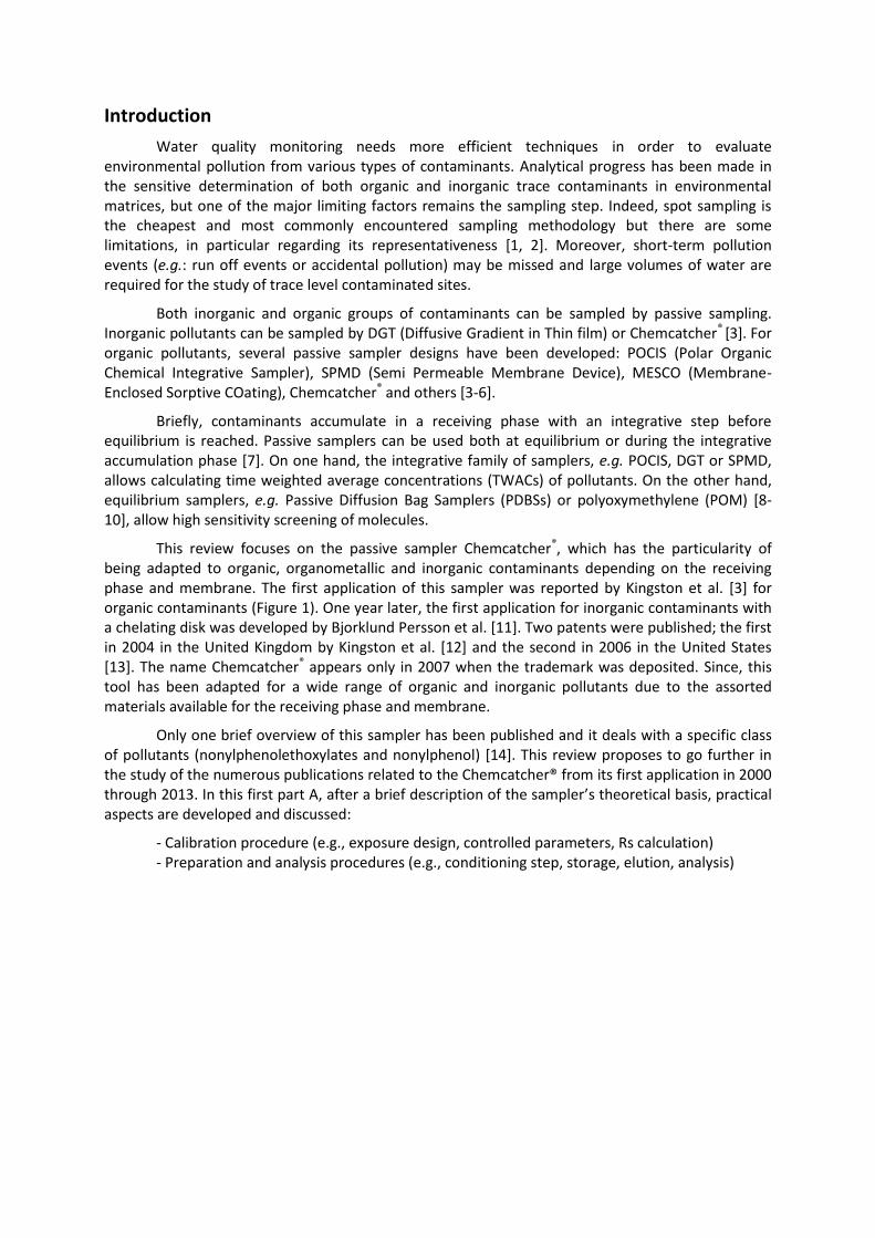
Introduction
Water quality monitoring needs more efficient techniques in order to evaluate environmental pollution from various types of contaminants. Analytical progress has been made in the sensitive determination of both organic and inorganic trace contaminants in environmental matrices, but one of the major limiting factors remains the sampling step. Indeed, spot sampling is the cheapest and most commonly encountered sampling methodology but there are some limitations, in particular regarding its representativeness [1, 2]. Moreover, short-term pollution events (e.g.: run off events or accidental pollution) may be missed and large volumes of water are required for the study of trace level contaminated sites.
Both inorganic and organic groups of contaminants can be sampled by passive sampling. Inorganic pollutants can be sampled by DGT (Diffusive Gradient in Thin film) or Chemcatcher® [3]. For organic pollutants, several passive sampler designs have been developed: POCIS (Polar Organic Chemical Integrative Sampler), SPMD (Semi Permeable Membrane Device), MESCO (Membrane-Enclosed Sorptive COating), Chemcatcher® and others [3-6].
Briefly, contaminants accumulate in a receiving phase with an integrative step before equilibrium is reached. Passive samplers can be used both at equilibrium or during the integrative accumulation phase [7]. On one hand, the integrative family of samplers, e.g. POCIS, DGT or SPMD, allows calculating time weighted average concentrations (TWACs) of pollutants. On the other hand, equilibrium samplers, e.g. Passive Diffusion Bag Samplers (PDBSs) or polyoxymethylene (POM) [8-10], allow high sensitivity screening of molecules.
This review focuses on the passive sampler Chemcatcher®, which has the particularity of being adapted to organic, organometallic and inorganic contaminants depending on the receiving phase and membrane. The first application of this sampler was reported by Kingston et al. [3] for organic contaminants (Figure 1). One year later, the first application for inorganic contaminants with a chelating disk was developed by Bjorklund Persson et al. [11]. Two patents were published; the first in 2004 in the United Kingdom by Kingston et al. [12] and the second in 2006 in the United States [13]. The name Chemcatcher® appears only in 2007 when the trademark was deposited. Since, this tool has been adapted for a wide range of organic and inorganic pollutants due to the assorted materials available for the receiving phase and membrane.
Only one brief overview of this sampler has been published and it deals with a specific class of pollutants (nonylphenolethoxylates and nonylphenol) [14]. This review proposes to go further in the study of the numerous publications related to the Chemcatcher® from its first application in 2000 through 2013. In this first part A, after a brief description of the sampler’s theoretical basis, practical aspects are developed and discussed:
- Calibration procedure (e.g., exposure design, controlled parameters, Rs calculation) - Preparation and analysis procedures (e.g., conditioning step, storage, elution, analysis)
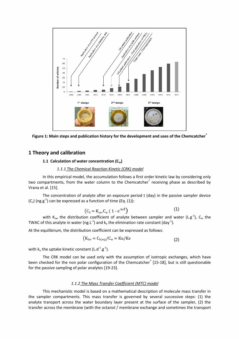
Figure 1: Main steps and publication history for the development and uses of the Chemcatcher®
1 Theory and calibration
1.1 Calculation of water concentration (Cw)
1.1.1 The Chemical Reaction Kinetic (CRK) model
In this empirical model, the accumulation follows a first order kinetic law by considering only two compartments, from the water column to the Chemcatcher® receiving phase as described by Vrana et al. [15].
The concentration of analyte after an exposure period t (day) in the passive sampler device (Cs) (ng.g-1) can be expressed as a function of time (Eq. (1)):
(CS = Ksw.Cw ( 1 - e-Ket) (1)
with Ksw the distribution coefficient of analyte between sampler and water (L.g-1), Cw the TWAC of this analyte in water (ng.L-1) and ke the elimination rate constant (day-1).
At the equilibrium, the distribution coefficient can be expressed as follows:
(2)
with ku the uptake kinetic constant (L.d-1.g-1).
The CRK model can be used only with the assumption of isotropic exchanges, which have been checked for the non polar configuration of the Chemcatcher® [15-18], but is still questionable for the passive sampling of polar analytes [19-23].
1.1.2 The Mass Transfer Coefficient (MTC) model
This mechanistic model is based on a mathematical description of molecule mass transfer in the sampler compartments. This mass transfer is governed by several successive steps: (1) the analyte transport across the water boundary layer present at the surface of the sampler, (2) the transfer across the membrane (with the octanol / membrane exchange and sometimes the transport
(KSw = CS(eq)/Cw = Ku/Ke
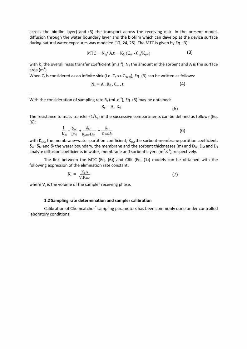
across the biofilm layer) and (3) the transport across the receiving disk. In the present model, diffusion through the water boundary layer and the biofilm which can develop at the device surface during natural water exposures was modeled [17, 24, 25]. The MTC is given by Eq. (3):
MTC = Ns/ A.t = K0 (Cw - Cs/Ksw) (3)
with ko the overall mass transfer coefficient (m.s-1), NS the amount in the sorbent and A is the surface area (m2)
When Cs is considered as an infinite sink (i.e. Cs << Cs(eq)), Eq. (3) can be written as follows:
(4)
.
With the consideration of sampling rate Rs (mL.d-1), Eq. (5) may be obtained:
(5)
The resistance to mass transfer (1/ko) in the successive compartments can be defined as follows (Eq. (6):
(6)
with KMW the membrane–water partition coefficient, KSM the sorbent-membrane partition coefficient, δW, δM and δS the water boundary, the membrane and the sorbent thicknesses (m) and DW, DM and DS
analyte diffusion coefficients in water, membrane and sorbent layers (m2.s-1), respectively.
The link between the MTC (Eq. (6)) and CRK (Eq. (1)) models can be obtained with the following expression of the elimination rate constant:
(7)
where Vs is the volume of the sampler receiving phase.
1.2 Sampling rate determination and sampler calibration
Calibration of Chemcatcher® sampling parameters has been commonly done under controlled laboratory conditions.
Ns = A . K0 . Cw . t
Rs = A . K0
1K0
δW δM δS
Dw KMWDM KSMDS
Ke =
= + +
K0AVsKSW
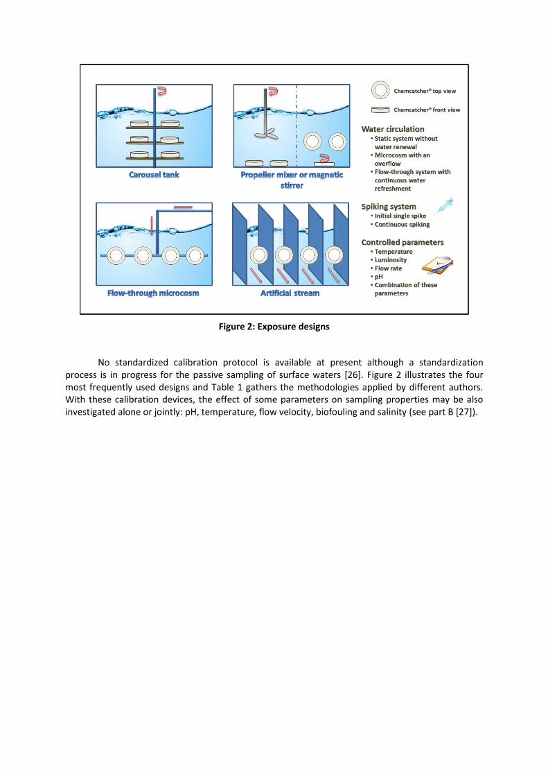
Figure 2: Exposure designs
No standardized calibration protocol is available at present although a standardization process is in progress for the passive sampling of surface waters [26]. Figure 2 illustrates the four most frequently used designs and Table 1 gathers the methodologies applied by different authors. With these calibration devices, the effect of some parameters on sampling properties may be also investigated alone or jointly: pH, temperature, flow velocity, biofouling and salinity (see part B [27]).

Tab 1: Calibration methodology (design, timing, tested parameters, matrix) (greenchecks indicate applied and red crosses unused parameters)
Conditions Design
Rs or k calculation
Other tested parameters
Ref
Type of tank Type of stirring Spiking
Compounds Matrix Duration Temperature Equilibration
time Stirring Container
Artificial stream
Carousel
Magnetic or
mechanic stirrer
Frontal pumping
Spike Flow
through Water
analysis Corrected by [water]
Ino
rgan
ics
Metals Low saline tap water
14 days - 48 hours 24 L, glass
tank - -
Temperature Flow velocity
[29]
Metals River water 3 days - - 220 L PET
30rpm No Rs calculation - [62]
Metals River water 28 days 18°C -
70cm/s - - - - [41]
Metals Natural water
10 days Various 2-3 days 1 L beaker
sampler rotate
400rpm
on sampler
- - pH, temperature,
concentration [11]
Metals - 5 hours Various - 1 L beaker - - - - Metal
concentration [42]
Org
ano
tin
s Organotin compounds
Tap water, artificial
seawater 14 days 11°C 48 hours
24L glass tank
- - pH, salinity, biofouling
[40]
Organotin compounds
Tap water 14 days - 48 hours 24 L glass
tank - -
Temperature Flow velocity
[53]
Org
anic
s
PAH 7 days 18°C 48 hours 20 L glass
tank
40rpm
Sampler geometry
[37]
PAH Distilled water
14 days 11°C 48 hours 20 L glass
tank -
Gap filling fluid between
membrane and disk
[27]
Pesticides, PAH, PCB
River water 5 days - -
200L stainless-
steel
30rpm No Rs calculation - [16]
Pesticides, PAH
- 14 days Various 48 hours 20 L glass
tank
Temperature, flow velocity
[15]
Pesticides PCB, PAH
- 14 days 15°C 48 hours 20 L glass
tank
30 rpm Membranes [54]
PCB, other Tap water 56 days 22.6°C 4 days 200 L tank
33 rpm [65]
Pesticides Other
Distilled water
14 days 11°C 48 hours 25 L stainless
steel tank
20 rpm - [22]
Pesticides Distilled water
7 days 13 °C - - 4.5 L
reservoir - - -
pH, time, membranes,
photolysis [67]
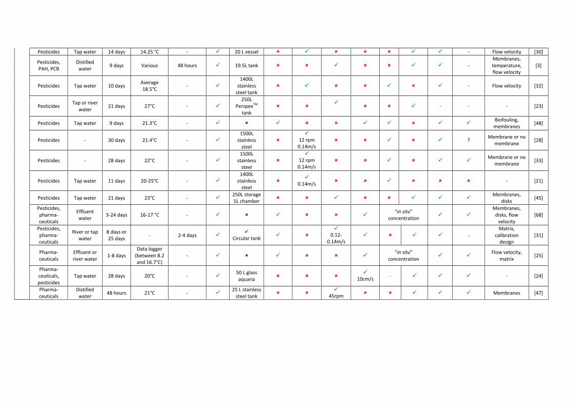
Pesticides Tap water 14 days 14.25 °C - 20 L vessel - Flow velocity [30]
Pesticides, PAH, PCB
Distilled water
9 days Various 48 hours 19.5L tank - Membranes, temperature, flow velocity
[3]
Pesticides Tap water 10 days Average 18.5°C
-
1400L stainless
steel tank - Flow velocity [32]
Pesticides Tap or river
water 21 days 27°C -
250L PerspexTM
tank
- - - [23]
Pesticides Tap water 9 days 21.3°C - Biofouling,
membranes [48]
Pesticides - 30 days 21.4°C -
1500L stainless
steel
12 rpm 0.14m/s
? Membrane or no
membrane [28]
Pesticides - 28 days 22°C -
1500L stainless
steel
12 rpm 0.14m/s
Membrane or no
membrane [33]
Pesticides Tap water 11 days 20-25°C -
1400L stainless
steel
0.14m/s - [21]
Pesticides Tap water 21 days 23°C - 250L storage 5L chamber
Membranes,
disks [45]
Pesticides, pharma-ceuticals
Effluent water
3-24 days 16-17 °C - “in situ”
concentration
Membranes, disks, flow
velocity [68]
Pesticides, pharma-ceuticals
River or tap water
8 days or 25 days
- 2-4 days
Circular tank
0.12-0.14m/s
- Matrix,
calibration design
[31]
Pharma-ceuticals
Effluent or river water
1-8 days Data logger
(between 8.2 and 16.7°C)
- “in situ”
concentration
Flow velocity, matrix
[25]
Pharma-ceuticals, pesticides
Tap water 28 days 20°C - 50 L glass aquaria
10cm/s - - [24]
Pharma-ceuticals
Distilled water
48 hours 21°C - 25 L stainless
steel tank
45rpm Membranes [47]
Design 1: Carousel tank
In this design, samplers are deployed in the water on tables which turn at a constant speed (see for instance [24], [28] and [15]). A major limitation could arise from the rotation speed and, as a consequence, the control of flow velocity on the samplers. Indeed, it is possible that, with time, water in the tank will also turn and thus the relative flow velocity at the surface of the sampler will decrease. Furthermore, only an estimate of the flow velocity can be achieved, on the basis of rpm.
Design 2: Propeller mixer or magnetic stirrer
In this simple design, samplers are arranged at the bottom of a beaker and water is stirred by a propeller mixer or a magnetic stirrer [29, 30]. This design allows a low flow rate at the vicinity of the created turbulences, rather than a controlled flow velocity in front of the samplers.
Design 3: Flow-through microcosm
This consists of an aquarium where samplers are positioned in front of nozzles of water. The flow rate is maintained by means of an aquarium pump [31]. This design is larger than the previous ones and thus may take up a lot of space and require higher volumes of water and spiking solution.
Design 4: Artificial stream
This exposure system was first designed by Vermeirssen et al. [32]. Several channels are fed with spiked water, sewage treatment effluents or naturally contaminated water from a stream or river. Compared to the other designs, it has the advantage of approximating real field conditions but it is also the largest in terms of size.
In a previous review on POCIS calibration, Harman et al. [33] summarized the main characteristics, advantages and limitations of the different available calibration devices. Practically, it must be noted that precautions should be taken when applying calibration devices. Indeed, Vrana et al. [15, 16] and Shaw at al. [19] noticed a decrease of dissolved analyte concentrations as a result of sampler uptake, vaporization, degradation or adsorption on tubing, tank walls and sampler body. An equilibration period is thus recommended before each experiment; Vrana et al. [15] and Aguilar-Martinez et al. [34] specified 48-hours. An additional continuous spiking system can be adapted to all the designs in order to maintain a constant contamination level. In addition, spot water samples were generally collected at regular time intervals and analyzed to check for variations in exposure concentrations. Due to the impact of water turbulence on analyte accumulation, it is essential to monitor flow velocity near the sampler. Stephens et al. [28] performed dye spikes above the sampler in a stirred tank and used photographic measurements to calculate the linear velocity relative to the sampler. More simply, a water velocity meter could be used to take spot measurements of the flow velocity at the sampler surface. Moreover, Gunold et al. [35] and Vrana et al. [15] replaced the removed samplers by empty Chemcatcher® bodies in order to maintain constant hydrodynamic conditions in the tank. Temperature and pH, should be kept constant [36] or at least monitored during exposure.
Sampling rates (approximately 600 Rs values) obtained for 113 compounds and various sampler configurations are available in a database (Excel file) in the supplementary material S1. As for the POCIS sampler [33], sampling rates reported in the literature for the Chemcatcher® device are affected by differences in exposure conditions during calibration experiments (see the various conditions in Table 1). These considerations hamper a direct comparison of published sampling rates. For instance, Rs values obtained for the pesticide atrazine, and the only SDB-RPS-PES configuration,
range between 0.013 0.003 L.day-1 (stagnant conditions at 16.2°C for [37]) and 0.170 L.day-1 (0.14
m.s-1 flow velocity at 22°C for [21]). A similar Rs value of 0.124 0.021 L.day-1 was also determined byO’Brien et al. [37] at 19.3°C and a 0.161 m.s-1 flow velocity. Only one study is, at present time, available for a direct comparison of Rs values obtained by means of different exposure systems (carousel tank and channel system) [36]. Sampling rates were almost systematically (20 compounds out of 22) higher in the tank laboratory study. According to the authors, this accelerated sorption
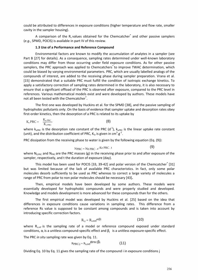
could be attributed to differences in exposure conditions (higher temperature and flow rate, smaller cavity in the sampler housing).
A comparison of the Rs values obtained for the Chemcatcher® and other passive samplers (e.g., SPMD, POCIS) is available in part IV of this review.
1.3 Use of a Performance and Reference Compound
Environmental factors are known to modify the accumulation of analytes in a sampler (see Part B [27] for details). As a consequence, sampling rates determined under well-known laboratory conditions may differ from those occurring under field exposure conditions. As for other passive samplers, the PRC approach was applied to Chemcatchers® to improve TWAC determination, which could be biased by varying environmental parameters. PRC, which are usually labelled analogs of the compounds of interest, are added to the receiving phase during sampler preparation. Vrana et al. [15] demonstrated that a suitable PRC must fulfill the condition of isotropic exchange kinetics. To apply a satisfactory correction of sampling rates determined in the laboratory, it is also necessary to ensure that a significant offload of the PRC is observed after exposure, compared to the PRC level in references. Various mathematical models exist and were developed by authors. These models have not all been tested with the Chemcatcher®.
The first one was developed by Huckins et al. for the SPMD [38], and the passive sampling of hydrophobic pollutants only. On the basis of evidence that sampler uptake and desorption rates obey first-order kinetics, then the desorption of a PRC is related to its uptake by
(8)
where kePRC is the desorption rate constant of the PRC (d-1), kuPRC is the linear uptake rate constant (unit), and the distribution coefficient of PRC, KS, is given in cm3.g-1.
PRC dissipation from the receiving phase to water is given by the following equation (Eq. (9)):
(9)
where N0,PRC and NPRC are the PRC masses (g) in the receiving phase prior to and after exposure of the sampler, respectively, and t the duration of exposure (day).
This model has been used for POCIS [33, 39-42] and polar version of the Chemcatcher® [31] but was limited because of the lack of available PRC characteristics. In fact, only some polar molecules desorb sufficiently to be used as PRC whereas to correct a large variety of molecules a range of PRC from polar to non polar molecules should be necessary [43].
Then, empirical models have been developed by some authors. These models were essentially developed for hydrophobic compounds and were properly studied and developed. Knowledge and models development is more advanced for these compounds than for the others.
The first empirical model was developed by Huckins et al. [25] based on the idea that differences in exposure conditions cause variations in sampling rates. This difference from a reference Rs value is supposed to be constant among compounds and is taken into account by introducing specific correction factors.
(10)
where Rs,ref is the sampling rate of a model or reference compound exposed under standard conditions, αi is a unitless compound-specific effect and βj is a unitless exposure-specific effect.
The PRC in situ sampling rate was given by Eq. 11.
RPRC,j = Rs,refαPRCβj (11)
Dividing Eq. 10 by Eq. 11 gives the sampling rate of the compound i in exposure conditions j
256
Ke PRC = Ku PRC
Ks PRC
NPRC = N0 PRC . e-Ke PRC . t
Ri,j = Rs,refαiβj
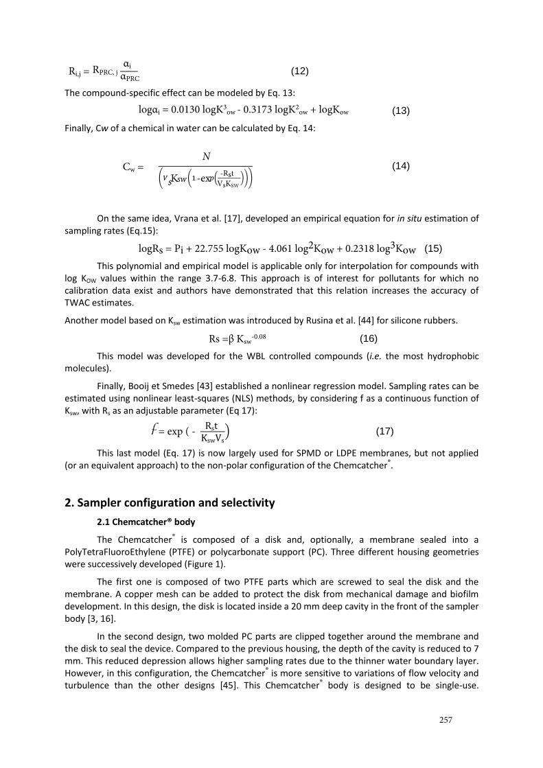
(12)
The compound-specific effect can be modeled by Eq. 13:
(13)
Finally, Cw of a chemical in water can be calculated by Eq. 14:
( ( ( )))
(14)
On the same idea, Vrana et al. [17], developed an empirical equation for in situ estimation of sampling rates (Eq.15):
(15)
This polynomial and empirical model is applicable only for interpolation for compounds with log KOW values within the range 3.7-6.8. This approach is of interest for pollutants for which no calibration data exist and authors have demonstrated that this relation increases the accuracy of TWAC estimates.
Another model based on Ksw estimation was introduced by Rusina et al. [44] for silicone rubbers.
(16)
This model was developed for the WBL controlled compounds (i.e. the most hydrophobic molecules).
Finally, Booij et Smedes [43] established a nonlinear regression model. Sampling rates can be estimated using nonlinear least-squares (NLS) methods, by considering f as a continuous function of Ksw, with Rs as an adjustable parameter (Eq 17):
) (17)
This last model (Eq. 17) is now largely used for SPMD or LDPE membranes, but not applied (or an equivalent approach) to the non-polar configuration of the Chemcatcher®.
2. Sampler configuration and selectivity
2.1 Chemcatcher® body
The Chemcatcher® is composed of a disk and, optionally, a membrane sealed into a PolyTetraFluoroEthylene (PTFE) or polycarbonate support (PC). Three different housing geometries were successively developed (Figure 1).
The first one is composed of two PTFE parts which are screwed to seal the disk and the membrane. A copper mesh can be added to protect the disk from mechanical damage and biofilm development. In this design, the disk is located inside a 20 mm deep cavity in the front of the sampler body [3, 16].
In the second design, two molded PC parts are clipped together around the membrane and the disk to seal the device. Compared to the previous housing, the depth of the cavity is reduced to 7 mm. This reduced depression allows higher sampling rates due to the thinner water boundary layer. However, in this configuration, the Chemcatcher® is more sensitive to variations of flow velocity and turbulence than the other designs [45]. This Chemcatcher® body is designed to be single-use.
257
Ri,j = RPRC, j αPRC
αi
logαi = 0.0130 logK3ow - 0.3173 logK2
ow + logKow
Cw =N
sK -ex -RstVsKSW
logRs = Pi + 22.755 logKow - 4.061 log2Kow + 0.2318 log3Kow
Rs =β Ksw-0.08
f = exp ( - RstKswVs
Disposability, which makes cleaning unnecessary, may be seen as an advantage [45]. However, for cost considerations, it must be balanced with the large number of samplers needed during field deployments and calibration experiments.
The third design is composed of two PTFE parts which screw together to seal the membrane and the disk. The depression of this design is approximately 2 mm and thus results in increased sampling rates, as for the second design.
During transport prior to deployment, a cap can be used to protect the disk and the membrane. All Chemcatcher® designs are also equipped at the back with a fastening lug which allows its suspension, facing downward, during field exposure. The sampling area is comprised between 14.5 and 17.5 cm².
2.2- Available materials for the receiving phase and diffusion-limiting membrane
Four types of Empore disks are used as receiving phases: C18, SDB-RPS, SDB-XC and chelating disks. C18, a silica sorbent bonded with octadecyl groups, is more appropriate for low polarity to nonpolar compounds. SDB-RPS (styrenedivinylbenzene-reverse phase sulfonated) is a poly(styrenedivinylbenzene) copolymer modified with sulfonic acid groups to make it hydrophilic and SDB-XC (styrenedivinylbenzene-exchange) is a poly(styrenedivinylbenzene) copolymer used as a reversed phase sorbent. These last two phases consist of 100% copolymeric particles that are spherical, porous and cross-linked and are suitable for polar and low polarity compounds. Chelating disks are made up of a polystyrene–divinylbenzene copolymer that has been modified with iminodiacetic acid groups and are suitable for metals.
The previously described receiving phases can be overlaid with different types of membranes or applied in a “naked” version [46]. The most commonly used membranes are cellulose acetate (CA, 0.45 µm pore size, 135-152 µm thickness), low-density polyethylene (LDPE, 10 Å pore size, 40 µm thickness), polysulfone (PS, 0.2 µm pore size, 152 µm thickness) and polyethersulfone (PES, 0.1-0.2 µm pore size, 40-146 µm thickness), although other materials were also tested [3].
2.3- Disks and membranes: assorted mountings according to the targeted pollutants
One of the advantages of the Chemcatcher® design is its potential application to a variety of both organic and inorganic contaminants by the use of a suitable combination of receiving phase and membrane.
For inorganic compounds, the most commonly used receiving phase is the iminodiacetate functionalized chelating disk. The chelating disk is associated to a cellulose acetate (CA) membrane for trace metals such as Cd, Cu, Ni, Pb and Zn [11, 34, 47-51]. In the case of inorganic mercury, the chelating disk was used by Aguilar-Martinez et al. [47] in combination with a polyethersulfone (PES) membrane. Aguilar-Martinez et al. [47] also evaluated a C18-CA configuration for the sampling of organotin compounds.
258
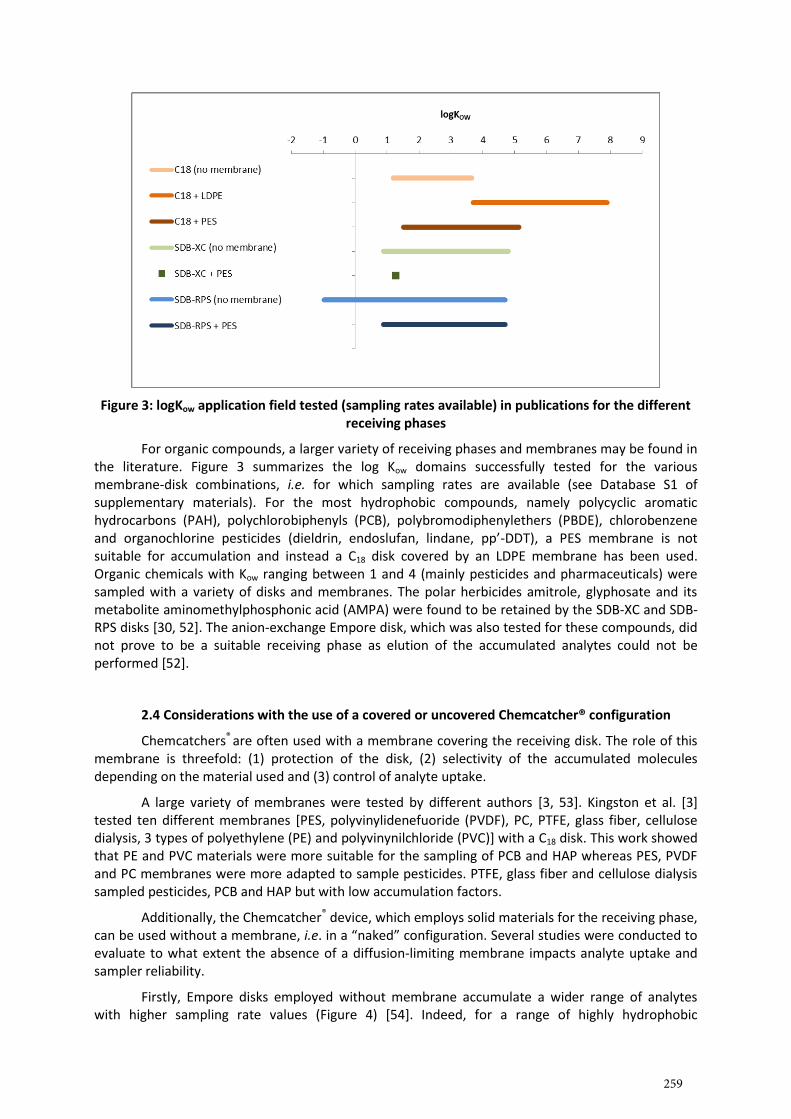
Figure 3: logKow application field tested (sampling rates available) in publications for the different receiving phases
For organic compounds, a larger variety of receiving phases and membranes may be found in the literature. Figure 3 summarizes the log Kow domains successfully tested for the various membrane-disk combinations, i.e. for which sampling rates are available (see Database S1 of supplementary materials). For the most hydrophobic compounds, namely polycyclic aromatic hydrocarbons (PAH), polychlorobiphenyls (PCB), polybromodiphenylethers (PBDE), chlorobenzene and organochlorine pesticides (dieldrin, endoslufan, lindane, pp’-DDT), a PES membrane is not suitable for accumulation and instead a C18 disk covered by an LDPE membrane has been used. Organic chemicals with Kow ranging between 1 and 4 (mainly pesticides and pharmaceuticals) were sampled with a variety of disks and membranes. The polar herbicides amitrole, glyphosate and its metabolite aminomethylphosphonic acid (AMPA) were found to be retained by the SDB-XC and SDB-RPS disks [30, 52]. The anion-exchange Empore disk, which was also tested for these compounds, did not prove to be a suitable receiving phase as elution of the accumulated analytes could not be performed [52].
2.4 Considerations with the use of a covered or uncovered Chemcatcher® configuration
Chemcatchers® are often used with a membrane covering the receiving disk. The role of this membrane is threefold: (1) protection of the disk, (2) selectivity of the accumulated molecules depending on the material used and (3) control of analyte uptake.
A large variety of membranes were tested by different authors [3, 53]. Kingston et al. [3] tested ten different membranes [PES, polyvinylidenefuoride (PVDF), PC, PTFE, glass fiber, cellulose dialysis, 3 types of polyethylene (PE) and polyvinynilchloride (PVC)] with a C18 disk. This work showed that PE and PVC materials were more suitable for the sampling of PCB and HAP whereas PES, PVDF and PC membranes were more adapted to sample pesticides. PTFE, glass fiber and cellulose dialysis sampled pesticides, PCB and HAP but with low accumulation factors.
Additionally, the Chemcatcher® device, which employs solid materials for the receiving phase, can be used without a membrane, i.e. in a “naked” configuration. Several studies were conducted to evaluate to what extent the absence of a diffusion-limiting membrane impacts analyte uptake and sampler reliability.
Firstly, Empore disks employed without membrane accumulate a wider range of analytes with higher sampling rate values (Figure 4) [54]. Indeed, for a range of highly hydrophobic
259
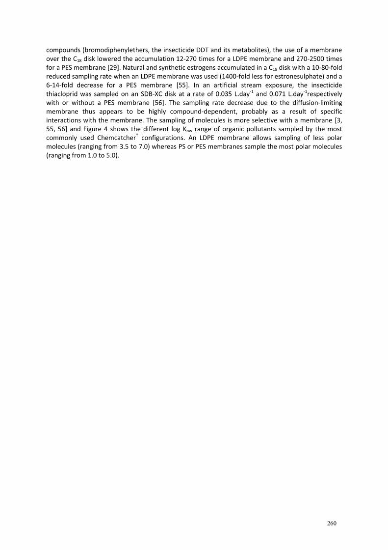
compounds (bromodiphenylethers, the insecticide DDT and its metabolites), the use of a membrane over the C18 disk lowered the accumulation 12-270 times for a LDPE membrane and 270-2500 times for a PES membrane [29]. Natural and synthetic estrogens accumulated in a C18 disk with a 10-80-fold reduced sampling rate when an LDPE membrane was used (1400-fold less for estronesulphate) and a 6-14-fold decrease for a PES membrane [55]. In an artificial stream exposure, the insecticide thiacloprid was sampled on an SDB-XC disk at a rate of 0.035 L.day-1 and 0.071 L.day-1respectively with or without a PES membrane [56]. The sampling rate decrease due to the diffusion-limiting membrane thus appears to be highly compound-dependent, probably as a result of specific interactions with the membrane. The sampling of molecules is more selective with a membrane [3, 55, 56] and Figure 4 shows the different log Kow range of organic pollutants sampled by the most commonly used Chemcatcher® configurations. An LDPE membrane allows sampling of less polar molecules (ranging from 3.5 to 7.0) whereas PS or PES membranes sample the most polar molecules (ranging from 1.0 to 5.0).
260
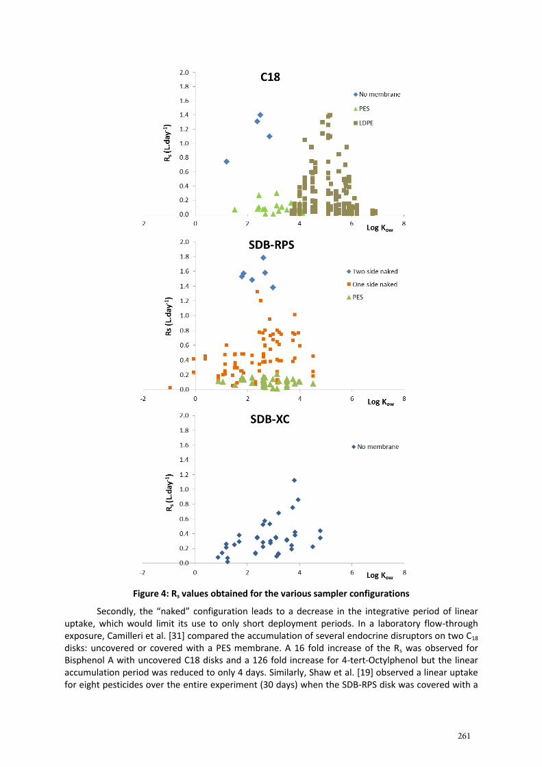
Figure 4: Rs values obtained for the various sampler configurations
Secondly, the “naked” configuration leads to a decrease in the integrative period of linear uptake, which would limit its use to only short deployment periods. In a laboratory flow-through exposure, Camilleri et al. [31] compared the accumulation of several endocrine disruptors on two C18 disks: uncovered or covered with a PES membrane. A 16 fold increase of the Rs was observed for Bisphenol A with uncovered C18 disks and a 126 fold increase for 4-tert-Octylphenol but the linear accumulation period was reduced to only 4 days. Similarly, Shaw et al. [19] observed a linear uptake for eight pesticides over the entire experiment (30 days) when the SDB-RPS disk was covered with a
261
PES membrane. For the uncovered disk, sampling rates were increased by a factor 2.5-3.5 but analyte uptake was no longer linear after 10 days of exposure. In two studies, Stephens et al. [28, 46] estimated that the linear accumulation for some pesticides in rivers was 5-7 days. Tran et al. [53] compared accumulation of five non-ionized pesticides with the use of two different membranes (PS and PES) and showed that PES was more suitable for all compounds except diuron. Tran et al. [53] extracted the membrane and the disk separately to study the partition between compartments and observed that diuron was highly accumulated in the membrane compared to the other tested pesticides. After 6 days, the ratio of diuron accumulated in the PES membrane compared to the Empore disk was 3.3:1 whereas this ratio was in the range of 1:1.2 and 1:1.5 for four other pesticides. From these results, the authors concluded that analytes first adsorbed onto the membrane, then diffused through the membrane and finally accumulated on the disk. These results were in accordance with other observations showing that the use of a diffusion-limiting membrane induces a lag-time between sampler deployment and the beginning of accumulation [54, 56]. Vermeirssen et al. [54] observed a lag phase for compounds with log Kow higher than 2.0 (diuron and diazinon). Two experiments were conducted for 6 and 32 days and the estimated lag phases were slightly different, probably as a result of a temperature variation between the experiments (20.5°C and 13.8°C, respectively). For instance, diazinon had a lag phase of 2.7 days for the 6-day trial and of 11 days for the 32-day trial. This lag-phase could be problematic for the quantification of these compounds in case of short-term fluctuating concentrations. All these considerations could be explained by the Eq. 7 (see I.1.2). With an uncovered mounting of the Chemcatcher® the middle term related to the transfer across the membrane is removed (Eq. 18).
(18)
This leads to an increase of the sampling rate Rs and eliminating rate ke. Therefore the naked configuration is more responsive and more relevant for short-term fluctuating concentrations.
The third constraint encountered when applying uncovered Empore disks is the higher extent of biofouling and the risk of deterioration during field deployment. Passive samplers are highly prone to biofilm development at their surface. This biofilm, whose development essentially depends on the material in contact with water, is known to potentially affect sampling rates by reducing the permeability of the diffusion-limiting membranes [56, 57] (see Part B [27] for details). PES membranes exhibited a higher resistance to biofouling compared to other commonly employed membranes for the POCIS or the Chemcatcher® in an organic polar configuration. However, depending on environmental conditions and sampled media, biofouling can occur on passive samplers even if a PES membrane is used [57] (see Part B [27] (part III-1)) for the influence of biofouling on sampling). Harman et al. [57] and Schafer et al. [56], who performed a 10-day deployment in an artificial stream, observed a biofilm layer on the uncovered disk while no biofouling occurred on samplers equipped with a PES membrane. Schafer et al. [56] reported that biofouling on the naked disk drastically decreased the sampling rates and became a source of error for the TWAC calculation.
As a consequence of the smaller range of linear uptake and the higher risk of biofouling, it is recommended that uncovered Chemcatchers® are deployed in the field only during reduced exposure periods. Taking advantage of the accelerated uptake kinetics of this “naked” sampler, this configuration has been suggested for the integration of short-term variations in environmental concentrations [56].
2.5 Role of interstitial n-octanol
For highly hydrophobic compounds, a high sampling rate is needed because of their very low concentration in water. Rs values are however limited by the additional internal resistance to mass transfer caused by water or air, which are present in C18 pores and as a thin layer between the surface of the LDPE membrane and the receiving phase [16]. In order to optimize the non-polar
262
1k0 Dw KswDs
δW δS
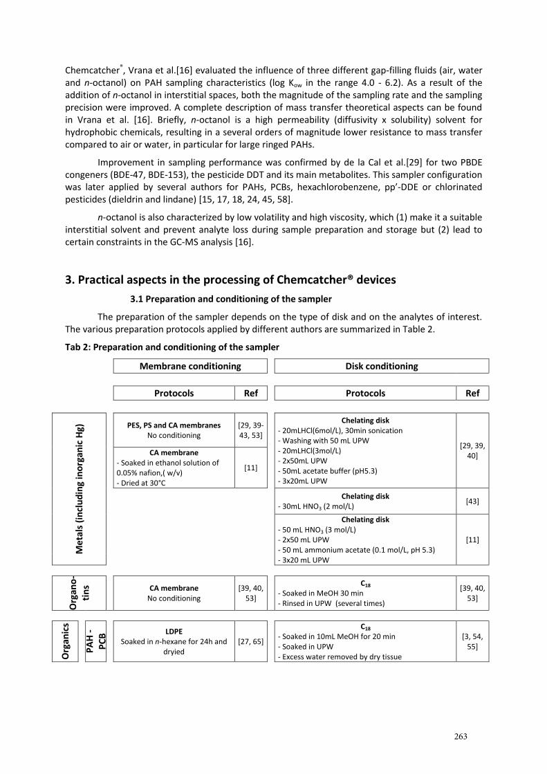
Chemcatcher®, Vrana et al.[16] evaluated the influence of three different gap-filling fluids (air, water and n-octanol) on PAH sampling characteristics (log Kow in the range 4.0 - 6.2). As a result of the addition of n-octanol in interstitial spaces, both the magnitude of the sampling rate and the sampling precision were improved. A complete description of mass transfer theoretical aspects can be found in Vrana et al. [16]. Briefly, n-octanol is a high permeability (diffusivity x solubility) solvent for hydrophobic chemicals, resulting in a several orders of magnitude lower resistance to mass transfer compared to air or water, in particular for large ringed PAHs.
Improvement in sampling performance was confirmed by de la Cal et al.[29] for two PBDE congeners (BDE-47, BDE-153), the pesticide DDT and its main metabolites. This sampler configuration was later applied by several authors for PAHs, PCBs, hexachlorobenzene, pp’-DDE or chlorinated pesticides (dieldrin and lindane) [15, 17, 18, 24, 45, 58].
n-octanol is also characterized by low volatility and high viscosity, which (1) make it a suitable interstitial solvent and prevent analyte loss during sample preparation and storage but (2) lead to certain constraints in the GC-MS analysis [16].
3. Practical aspects in the processing of Chemcatcher® devices
3.1 Preparation and conditioning of the sampler
The preparation of the sampler depends on the type of disk and on the analytes of interest. The various preparation protocols applied by different authors are summarized in Table 2.
Tab 2: Preparation and conditioning of the sampler
Membrane conditioning Disk conditioning
Protocols Ref Protocols Ref
Met
als
(in
clu
din
g in
org
anic
Hg)
PES, PS and CA membranes No conditioning
[29, 39-43, 53]
Chelating disk - 20mLHCl(6mol/L), 30min sonication - Washing with 50 mL UPW - 20mLHCl(3mol/L) - 2x50mL UPW - 50mL acetate buffer (pH5.3) - 3x20mL UPW
[29, 39, 40] CA membrane
- Soaked in ethanol solution of 0.05% nafion,( w/v) - Dried at 30°C
[11]
Chelating disk - 30mL HNO3 (2 mol/L)
[43]
Chelating disk - 50 mL HNO3 (3 mol/L) - 2x50 mL UPW - 50 mL ammonium acetate (0.1 mol/L, pH 5.3) - 3x20 mL UPW
[11]
Org
ano
-
tin
s CA membrane No conditioning
[39, 40, 53]
C18 - Soaked in MeOH 30 min - Rinsed in UPW (several times)
[39, 40, 53]
Org
anic
s
PA
H -
P
CB
LDPE Soaked in n-hexane for 24h and
dryied [27, 65]
C18 - Soaked in 10mL MeOH for 20 min - Soaked in UPW - Excess water removed by dry tissue
[3, 54, 55]
263
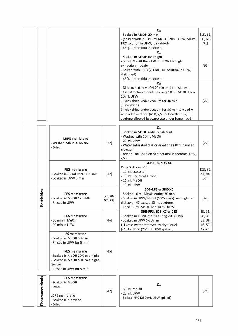
C18 - Soaked in MeOH 20 min - (Spiked with PRCs:10mLMeOH, 20mL UPW, 500mL PRC solution in UPW, disk dried) - 450µL interstitial n-octanol
[15, 16, 50, 69-
71]
C18 - Soaked in MeOH overnight - 50 mL MeOH then 150 mL UPW through extraction module - Spiked with PRCs (250mL PRC solution in UPW, disk dried) - 450µL interstitial n-octanol
[65]
C18 - Disk soaked in MeOH 20min until translucent - On extraction module, passing 10 mL MeOH then 20 mL UPW 1 : disk dried under vacuum for 30 min 2 : no drying 3 : disk dried under vacuum for 30 min, 1 mL of n-octanol in acetone (45%, v/v) put on the disk, acetone allowed to evaporate under fume hood
[27]
Pe
stic
ide
s
LDPE membrane - Washed 24h in n-hexane - Dried
[22]
C18 - Soaked in MeOH until translucent - Washed with 10mL MeOH - 20 mL UPW - Water saturated disk or dried one (30 min under nitrogen) - Added 1mL solution of n-octanol in acetone (45%, v/v)
[22]
PES membrane - Soaked in 20 mL MeOH 20 min - Soaked in UPW 5 min
[32]
SDB-RPS, SDB-XC On a Diskcover-47 - 10 mL acetone - 10 mL isopropyl alcohol - 10 mL MeOH - 10 mL UPW
[23, 30, 44, 48,
56 ]
PES membrane - Soaked in MeOH 12h-24h - Rinsed in UPW
[28, 48, 57, 72]
SDB-RPS or SDB-XC - Soaked 10 mL MeOH during 30 min - Soaked in UPW/MeOH (50/50, v/v) overnight on diskcover-47 passed 10 mL acetone, - Then 10 mL MeOH and 10 mL UPW
[45]
PES membrane - 30 min in MeOH - 30 min in UPW
[46]
SDB-RPS, SDB-XC or C18 - Soaked in 10 mL MeOH during 20-30 min - Soaked in UPW 5-30 min (- Excess water removed by dry tissue) (- Spiked PRC (250 mL UPW spiked))
[3, 21, 28, 31-33, 38, 46, 57, 67-76]
PS membrane - Soaked in MeOH 30 min - Rinsed in UPW for 5 min
PES membrane - Soaked in MeOH 20% overnight - Soaked in MeOH 50% overnight (twice) - Rinsed in UPW for 5 min
[45]
Ph
arm
ace
uti
cals
PES membrane - Soaked in MeOH - Dried
LDPE membrane - Soaked in n-hexane - Dried
[47]
C18 - 50 mL MeOH - 25 mL UPW - Spiked PRC (250 mL UPW spiked)
[24]
264
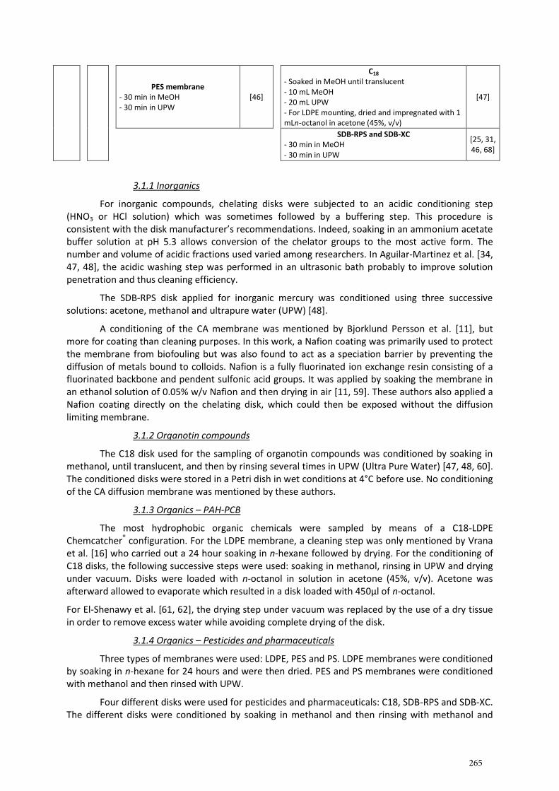
PES membrane - 30 min in MeOH - 30 min in UPW
[46]
C18 - Soaked in MeOH until translucent - 10 mL MeOH - 20 mL UPW - For LDPE mounting, dried and impregnated with 1 mLn-octanol in acetone (45%, v/v)
[47]
SDB-RPS and SDB-XC - 30 min in MeOH - 30 min in UPW
[25, 31, 46, 68]
3.1.1 Inorganics
For inorganic compounds, chelating disks were subjected to an acidic conditioning step (HNO3 or HCl solution) which was sometimes followed by a buffering step. This procedure is consistent with the disk manufacturer’s recommendations. Indeed, soaking in an ammonium acetate buffer solution at pH 5.3 allows conversion of the chelator groups to the most active form. The number and volume of acidic fractions used varied among researchers. In Aguilar-Martinez et al. [34, 47, 48], the acidic washing step was performed in an ultrasonic bath probably to improve solution penetration and thus cleaning efficiency.
The SDB-RPS disk applied for inorganic mercury was conditioned using three successive solutions: acetone, methanol and ultrapure water (UPW) [48].
A conditioning of the CA membrane was mentioned by Bjorklund Persson et al. [11], but more for coating than cleaning purposes. In this work, a Nafion coating was primarily used to protect the membrane from biofouling but was also found to act as a speciation barrier by preventing the diffusion of metals bound to colloids. Nafion is a fully fluorinated ion exchange resin consisting of a fluorinated backbone and pendent sulfonic acid groups. It was applied by soaking the membrane in an ethanol solution of 0.05% w/v Nafion and then drying in air [11, 59]. These authors also applied a Nafion coating directly on the chelating disk, which could then be exposed without the diffusion limiting membrane.
3.1.2 Organotin compounds
The C18 disk used for the sampling of organotin compounds was conditioned by soaking in methanol, until translucent, and then by rinsing several times in UPW (Ultra Pure Water) [47, 48, 60]. The conditioned disks were stored in a Petri dish in wet conditions at 4°C before use. No conditioning of the CA diffusion membrane was mentioned by these authors.
3.1.3 Organics – PAH-PCB
The most hydrophobic organic chemicals were sampled by means of a C18-LDPE Chemcatcher® configuration. For the LDPE membrane, a cleaning step was only mentioned by Vrana et al. [16] who carried out a 24 hour soaking in n-hexane followed by drying. For the conditioning of C18 disks, the following successive steps were used: soaking in methanol, rinsing in UPW and drying under vacuum. Disks were loaded with n-octanol in solution in acetone (45%, v/v). Acetone was afterward allowed to evaporate which resulted in a disk loaded with 450µl of n-octanol.
For El-Shenawy et al. [61, 62], the drying step under vacuum was replaced by the use of a dry tissue in order to remove excess water while avoiding complete drying of the disk.
3.1.4 Organics – Pesticides and pharmaceuticals
Three types of membranes were used: LDPE, PES and PS. LDPE membranes were conditioned by soaking in n-hexane for 24 hours and were then dried. PES and PS membranes were conditioned with methanol and then rinsed with UPW.
Four different disks were used for pesticides and pharmaceuticals: C18, SDB-RPS and SDB-XC. The different disks were conditioned by soaking in methanol and then rinsing with methanol and
265
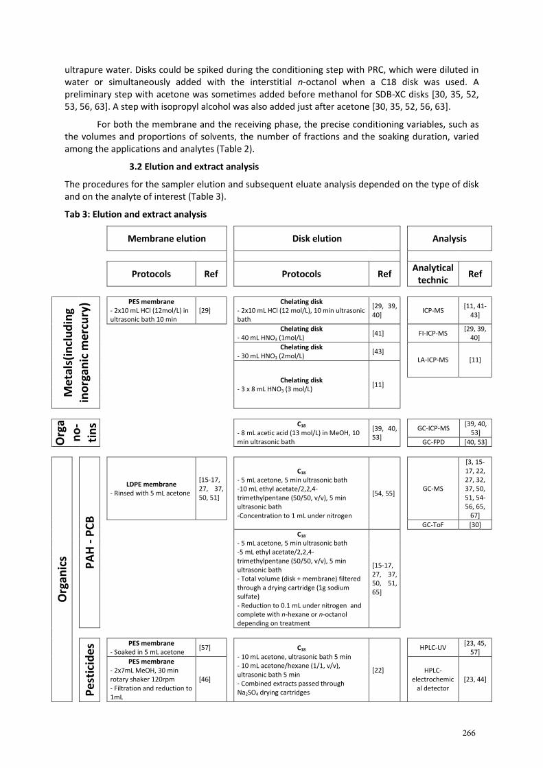
ultrapure water. Disks could be spiked during the conditioning step with PRC, which were diluted in water or simultaneously added with the interstitial n-octanol when a C18 disk was used. A preliminary step with acetone was sometimes added before methanol for SDB-XC disks [30, 35, 52, 53, 56, 63]. A step with isopropyl alcohol was also added just after acetone [30, 35, 52, 56, 63].
For both the membrane and the receiving phase, the precise conditioning variables, such as the volumes and proportions of solvents, the number of fractions and the soaking duration, varied among the applications and analytes (Table 2).
3.2 Elution and extract analysis
The procedures for the sampler elution and subsequent eluate analysis depended on the type of disk and on the analyte of interest (Table 3).
Tab 3: Elution and extract analysis
Membrane elution Disk elution Analysis
Protocols Ref Protocols Ref Analytical
technic Ref
Me
tals
(in
clu
din
g in
org
anic
me
rcu
ry) PES membrane
- 2x10 mL HCl (12mol/L) in ultrasonic bath 10 min
[29] Chelating disk
- 2x10 mL HCl (12 mol/L), 10 min ultrasonic bath
[29, 39, 40]
ICP-MS [11, 41-
43]
Chelating disk - 40 mL HNO3 (1mol/L)
[41] FI-ICP-MS [29, 39,
40]
Chelating disk - 30 mL HNO3 (2mol/L)
[43] LA-ICP-MS [11]
Chelating disk - 3 x 8 mL HNO3 (3 mol/L)
[11]
Org
an
o-
tin
s C18 - 8 mL acetic acid (13 mol/L) in MeOH, 10 min ultrasonic bath
[39, 40, 53]
GC-ICP-MS [39, 40,
53]
GC-FPD [40, 53]
Org
anic
s
PA
H -
PC
B
LDPE membrane - Rinsed with 5 mL acetone
[15-17, 27, 37, 50, 51]
C18 - 5 mL acetone, 5 min ultrasonic bath -10 mL ethyl acetate/2,2,4-trimethylpentane (50/50, v/v), 5 min ultrasonic bath -Concentration to 1 mL under nitrogen
[54, 55] GC-MS
[3, 15-17, 22, 27, 32, 37, 50, 51, 54-56, 65,
67]
GC-ToF [30]
C18 - 5 mL acetone, 5 min ultrasonic bath -5 mL ethyl acetate/2,2,4-trimethylpentane (50/50, v/v), 5 min ultrasonic bath - Total volume (disk + membrane) filtered through a drying cartridge (1g sodium sulfate) - Reduction to 0.1 mL under nitrogen and complete with n-hexane or n-octanol depending on treatment
[15-17, 27, 37, 50, 51, 65]
Pe
stic
ide
s PES membrane - Soaked in 5 mL acetone
[57] C18 - 10 mL acetone, ultrasonic bath 5 min - 10 mL acetone/hexane (1/1, v/v), ultrasonic bath 5 min - Combined extracts passed through Na2SO4 drying cartridges
[22]
HPLC-UV [23, 45,
57]
PES membrane - 2x7mL MeOH, 30 min rotary shaker 120rpm - Filtration and reduction to 1mL
[46] HPLC-
electrochemical detector
[23, 44]
266
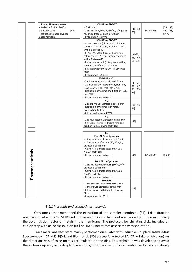
PS and PES membranes - Soaked in 2x4 mL MeOH ultrasonic bath - Reduction to near dryness under nitrogen
[45]
SDB-RPS or SDB-XC - Disk dried - 2x10 mL ACN/MeOH, (50/50, v/v) (or 15 mL and ultrasonic bath for 10 min) - Evaporation to dryness
[30, 48, 56]
LC-MS-MS [28, 33, 46, 48, 67-76]
SDB-RPS or SDB-XC - 5-8 mL acetone (ultrasonic bath 5min, rotary shaker 120 rpm, orbital shaker or with a Diskover-47) - 5-7 mL MeOH (ultrasonic bath 5min, rotary shaker 120 rpm, orbital shaker or with a Diskover-47) - Reduction to 1 mL (rotary evaporation, vacuum centrifuge or nitrogen) - Filtration with a 0.45 µm PTFE syringe filter - Evaporation to 500 µL
[31-33, 45, 46, 68 , 72]
SDB-RPS or C18 - 5 mL acetone, ultrasonic bath 5 min - 10 mL ethyl acetate/trimethylpentane, (50/50, v/v), ultrasonic bath 5 min - Reduction of volume and filtration (0.45 µm, PTFE) - Reduction under nitrogen
[3, 21, 28, 67, 71, 73-75]
C18 - 2x 5 mL MeOH, ultrasonic bath 5 min - Reduction of volume with rotary evaporation to 1 mL - Filtration (0.45 µm, PTFE)
[69, 70, 76]
C18 - 2x5 mL acetone, ultrasonic bath 5 min - Filtration of extracts (membrane and disk) on Na2SO4 drying cartridges
[57]
Ph
arm
aceu
tica
ls
C18 For LDPE configuration
- 15 mL acetone, ultrasonic bath 5 min - 10 mL acetone/hexane (50/50, v/v), ultrasonic bath 5 min - Combined extracts passed through Na2SO4 cartridges - Reduction under nitrogen
For PES configuration - 2x10 mL acetone/MeOH, (50/50, v/v) ultrasonic bath 5 min - Combined extracts passed through Na2SO4 cartridges - Reduction under nitrogen
[47] LC-MS-MS [25, 47]
SDB-RPS - 7 mL acetone, ultrasonic bath 5 min - 7 mL MeOH, ultrasonic bath 5 min - Filtration with a 0.45µm PTFE syringe filter - Evaporation to 100 µL
[25]
3.2.1 Inorganic and organotin compounds
Only one author mentioned the extraction of the sampler membrane [34]. This extraction was performed with a 12 M HCl solution in an ultrasonic bath and was carried out in order to study the accumulation factor of metals in the membrane. The protocols for chelating disks included an elution step with an acidic solution (HCl or HNO3) sometimes associated with sonication.
Trace metal analyses were mainly performed on eluates with Inductive Coupled Plasma-Mass Spectrometry (ICP-MS). Björklund Blom et al. [50] successfully tested LA-ICP-MS (Laser Ablation) for the direct analysis of trace metals accumulated on the disk. This technique was developed to avoid the elution step and, according to the authors, limit the risks of contamination and alteration during
267
sample handling and reduce the problem of oxide interference during analysis. Despite these advantages, the calibration had to be performed using samplers exposed to known concentrations under laboratory conditions and afterward analyzed by LA-ICP-MS. For organotin compounds the ICP-MS was coupled with a Gas Chromatography (GC) separation or a Gas Chromatography-Flame Photometric Detector (GC-FPD) was used.
3.2.2 Organics – PAH-PCB
For these contaminants, the membrane elution was performed by an organic solvent: acetone for Allan et al., [24, 58] Lobpreis et al. [45] and Vrana et al. [15-18] and methanol for Tran et al. [53]. Tran et al. [53] analyzed this fraction separately from the disk eluates whereas Allan et al. [24, 58], Lobpreis et al. [45] and Vrana et al. [15-18] combined the two fractions.
The disks were eluted in three stages: acetone in an ultrasonic bath, followed by ethylacetate/2,2,4-trimethylpentane (50/50, v/v) in an ultrasonic bath and finally, reduction under nitrogen. Allan et al. [24, 58], Lobpreis et al. [45] and Vrana et al. [15-18] added an extract drying stage by passing through a sodium sulfate cartridge. For these compounds, analyses were performed by GC/MS or GC/ToF (Time of Flight).
3.2.3 Organics – Pesticides and pharmaceuticals
The membranes were eluted by acetone or methanol. Vermeirssen et al. [54] analysed this extract separately from the receiving phase whereas Nyoni et al.[64] combined both extracts.
For the disks, various protocols were reported using organic solvents (Table 3).
For these compounds, analyses were performed using High Performance Liquid Chromatography with an Ultraviolet Detector (HPLC-UV) or with a tandem Mass Spectrometer detector (HPLC-MS/MS). A special application for glyphosate, its metabolite AMPA and amitrole, used an HPLC coupled with an ElectroChemical Detector [30, 52].
4 Comparison with other passive samplers
For organotin compounds, the Chemcatcher® [47, 48, 60] and SPMD [65, 66] are the only two used passive samplers. Performance of the Chemcatcher® and SPMD can be compared using several criteria (for instance, limit of quantification, extraction procedure, matrix effect and ease of analysis) but data are still scarce and these samplers have never been used jointly during laboratory or field studies. For the Chemcatcher®, Aguilar-Martinez et al. [60] evaluated method quantification limits (MQL) of 3.3-19.0, 0.8-3.5, 0.8-7.0 and 4.6-25.0 ng.L-1 for monobutyltin, dibutyltin, tributyltin and triphenyltin, respectively. MQL were determined as the minimum water concentration detectable after a 14-day exposure and were found to be suitable for the monitoring of slightly contaminated waters. However, the authors noted that the Environmental Quality Standards imposed by the Water Framework Directive [67] are not easily reached by either spot water or Chemcatcher® samplings. For SPMD, results were only expressed in ng.g-1 of triolein as no sampling rates were available [65]. Extraction and analytical procedures differed between samplers. Chemcatcher® extraction was performed with 8mL of acetic acid in methanol (13 mol.L-1) in an ultrasonic bath for 10 min. Recoveries were in the range 70-80 % for monobutyltin and 90-100 % for dibutyltin, tributyltin and triphenyltin [48, 60]. The extraction procedure for SPMD was performed with much higher volumes of solvent (200 mL aliquots of cyclohexane-dichloromethane) and for a longer time (3 times 24h). SPMD extracts were subsequently concentrated and cleaned-up. The presence of triolein in SPMD extracts, which results in background emission in GC-AED (atomic emission detector) analysis, required that the authors adapt the procedure with an improved clean-up. Organotin compounds from Chemcatcher® extracts were analysed directly after derivation by GC-ICP-MS for monobutyltin, dibutyltin and tributyltin, and GC-FPD (flame photometric detector) for triphenyltin [48, 60].
For trace metals, the most commonly used passive sampler is DGT, developed by Davison and Zhang [68] and now considered a robust monitoring device for the determination of labile
268
concentrations. DGT and Chemcatcher® were used jointly in several studies [49, 69-71] thus allowing for a direct comparison of devices. After exposure, DGT and Chemcatcher® undergo a similar procedure, i.e. a nitric acid elution and a subsequent ICP-MS analysis. DGT and Chemcatcher® can both be used to provide TWAC even if accumulation of trace metals in the receiving phase is based on different mechanisms. Indeed, accumulation in the DGT receiving phase (generally Chelex-100) is controlled by diffusion through the diffusive gel. Models derived from Fick’s first law and laboratory-measured diffusion coefficients are used to calculate TWAC [68]. For the metallic configuration of the Chemcatcher®, a preliminary calibration procedure is needed in order to determine the sampling rate of each trace metal [49, 69]. As noted by Allan et al. [49, 69], uncertainties in the determination of TWAC were increased by a bias in the selection of suitable Rs and the presence of a water boundary layer. Another critical issue in the interpretation of Chemcatcher® and DGT data is that the fractions sampled by these devices correspond to (1) freely dissolved metals and (2) inorganic and organic complexes able to dissociate during diffusion. Allan et al. [49, 69] compared TWACs to unfiltered, filtered (0.45µm) and ultra-filtered (5 kDa) spot water samples. These authors concluded that Chemcatcher® and DGT (open pore) data were generally consistent with the filtered and ultra-filtered fractions of spot water samples. Allan et al. [69] also observed the ability of both samplers to respond to highly fluctuating metal concentrations. In Roig et al. [71], a fairly good agreement was found between both passive samplers, except for lead because of a high uncertainty in calibration for this element. During an intercomparison exercise, DGT and Chemcatcher® data were not easy to compare as Chemcatchers® were deployed by only one participant at one site [70].
Depending on the polarity of organic compounds, Chemcatcher® could be compared to more commonly used devices: POCIS (for the SDB-XC or SDB-RPS with PES membrane) and SPMD (for the C18 with LDPE membrane).Only a few studies [29, 54, 58, 72] were conducted with the objective of comparing the performances of these passive samplers, in particular to investigate the various uptake kinetics and sampling rates [54, 72]. Indeed, Rs values will differ because of the intrinsic characteristics of each device (materials for the receiving phase and membrane, diffusion and accumulation mechanisms and sampling area). But this comparison is made difficult by the variety of calibration procedures that are applied, mainly different hydrodynamic, matrix and temperature conditions.
The major practical issues that arose from the comparison of SPMD and Chemcatcher® concern the standard deviation between replicates and the quantification limits of the different passive samplers. Chemcatcher® results appeared more reproducible than SPMD, as Allan et al. [58] showed lower standard deviations for the Chemcatcher®. Allan et al. [58] also highlighted the lower sampling rates obtained with Chemcatcher® compared to SPMD; explaining that this was essentially due to the higher sampling area of the SPMD (460 cm2 vs 17 cm2 for the Chemcatcher®). De la Cal et al. [29] indicated that the Chemcatcher® was not as efficient as SPMD for sampling low levels of contaminants. They also specified that the new Chemcatcher® design would probably give higher sampling rates due to the decreased water boundary layer (see section II-1). Jacquet et al. [72] compared the uptake kinetics of 19 PCBs for five devices: SPMD, LDPE strips, Chemcatcher®, SR (Silicone Rubber) sheets and the CFIS (Continuous Flow Integrative Sampler). Rs values were normalized to a sampling area of 100 cm² (NA). Authors attributed the generally lower NA values for the Chemcatcher® to the shape of the first design. Higher NA values would be expected with the later Chemcatcher® designs. Uptake curves were fairly linear for most PCBs and passive samplers throughout the exposure (91 days). Moreover, as stressed by the authors, a similar evolution of Rs values with PCBs was obtained for SPMD, LDPE strips, Chemcatcher® and SR sheets, despite the differences among sampler materials. Jacquet et al. [72] have also highlighted the problem of the models applied to calculate the Chemcatcher® TWACs.
For polar compounds, Chemcatcher® and POCIS, which are prepared with similar membrane material (PES) but different receiving phases, can be compared. Full reviews of Rs values obtained during POCIS calibrations are available in Morin et al. [73] and Harman et al. [33]. It appears, from
269
these reviews and the present work, that approximately 40 compounds (mainly pharmaceutical and pesticide residues) have been calibrated for both samplers. At present, as noted by Vermeirssen et al. [54], the sampling rate database includes more organic compounds for POCIS than Chemcatcher®. For polar compounds, only one study clearly compared Chemcatcher® and POCIS [54]. During 6-day and 32-day sorption experiments, Vermeirssen et al. [54] noted very similar uptake kinetics between the Chemcatcher® (SDB-RPS) and POCIS (« pesticide » configuration) for a selection of 22 compounds. They showed that the POCIS Rs values were 3.6-fold higher than those from Chemcatcher® but demonstrated that it was due to the difference between the sampling areas of these devices.The authors obtained a good correlation between both samplers with a factor of 2 between the Rs of 18 compounds (22 tested). The four other compounds had a Chemcatcher® Rs significantly higher or lower than the POCIS Rs. Diclofenac, mecoprop and sulcotrione had a 3- to 4-fold higher Rs for Chemcatcher® compared to POCIS, and diuron had a 2-fold higher Rs for POCIS compared to Chemcatcher®. Results were normalized to account for the higher POCIS sampling area (45.8 cm2). The authors explained the differences by the different properties of the sorbent materials (DVB-RPS vs C18), particularly in terms of extraction efficiency of molecules. Further investigations should be made to evaluate the uptake capacity of each sampler and the reversibility of sorption mechanisms (isotropic exchange) [54]. Comparing both samplers, Vermeirssen et al. [54] found that the Chemcatcher® was easier to handle and gave consistently more accurate replicates during experiments. Nonetheless, it is difficult to conclude that one sampler is superior to the other. Indeed, authors stressed that the POCIS is more versatile than the Chemcatcher® because the amount of sorbent can be easily increased to enhance the capacity of the sampler. Moreover, currently there is a larger diversity of materials that can be used as solid sorbents compared to disks.
5 Conclusion
Part A of this review investigated the various available Chemcatcher® designs and the following points were discussed in detail:
- Principle and calculation of Cw - Available disks and membranes - Preparation of the samplers - Elution of the disks and analysis
The Chemcatcher® device is presently the only universal passive sampler for the monitoring of inorganic, organometallic and organic pollutants in environmental water bodies. This versatility of the Chemcatcher® can be seen as an advantage but may also pose several difficulties for the user.
Firstly, a wide range of disks and membranes is available and the choice of the sampler configuration (design, materials and presence of a membrane) has to be guided by the targeted analytes and the constraints of the study. The variety of available mountings also points out the necessity of harmonized preparation and analysis procedures. Secondly, the Chemcatcher® is one among a variety of other passive samplers which are generally adapted to a more limited application domain.
Part B of this review [27] deals with the various environmental applications of the Chemcatcher® and focuses on (1) in-situ calibration procedures, (2) monitoring and (3) ecotoxicological applications of the device.
270
References
[1] D.A. Alvarez, P.E. Stackelberg, J.D. Petty, J.N. Huckins, E.T. Furlong, S.D. Zaugg, M.T. Meyer, Chemosphere 61 (2005) 610.
[2] N. Mazzella, T. Debenest, F. Delmas, Chemosphere 73 (2008) 545.
[3] J.K. Kingston, R. Greenwood, G.A. Mills, G.M. Morrison, L.B. Persson, Journal of Environmental Monitoring 2 (2000) 487.
[4] D.A. Alvarez, J.D. Petty, J.N. Huckins, T.L. Jones-Lepp, D.T. Getting, J.P. Goddard, S.E. Manahan, Environ. Toxicol. Chem. 23 (2004) 1640.
[5] J.N. Huckins, M.W. Tubergen, G.K. Manuweera, Chemosphere 20 (1990) 533.
[6] A. Paschke, K. Schwab, J. Brümmer, G. Schüürmann, H. Paschke, P. Popp, Journal of Chromatography A 1124 (2006) 187.
[7] B. Vrana, I.J. Allan, R. Greenwood, G.A. Mills, E. Dominiak, K. Svensson, J. Knutsson, G. Morrison, TrAC, Trends Anal. Chem. 24 (2005) 845.
[8] G. Cornelissen, G. Okkenhaug, G.D. Breedveld, J.-E. Srlie, Journal of Hydrology 369 (2009) 253.
[9] A. Jahnke, P. Mayer, D. Broman, M.S. McLachlan, Chemosphere 77 (2009) 764.
[10] P. Mayer, J. Tolls, J.L.M. Hermens, D. Mackay, Environmental Science & Technology 37 (2003) 184A.
[11] L. Björklund Persson, G.M. Morrison, J.U. Friemann, J. Kingston, G. Mills, R. Greenwood, Journal of Environmental Monitoring 3 (2001) 639.
[12] J. Kingston, UK. 2004.
[13] J. Kingston, US. 2006.
[14] H. Ahkola, S. Herve, J. Knuutinen, Environmental Science and Pollution Research 20 (2013) 1207.
[15] B. Vrana, G.A. Mills, E. Dominiak, R. Greenwood, Environmental Pollution 142 (2006) 333.
[16] B. Vrana, G. Mills, R. Greenwood, J. Knutsson, K. Svensson, G. Morrison, Journal of Environmental Monitoring 7 (2005) 612.
[17] B. Vrana, G.A. Mills, M. Kotterman, P. Leonards, K. Booij, R. Greenwood, Environmental Pollution 145 (2007) 895.
[18] B. Vrana, G.A. Mills, P.E.G. Leonards, M. Kotterman, M. Weideborg, J. Hajlova, V. Kocourek, M. Tomaniova, J. Pulkrabova, M. Suchanova, K. Hajkova, S. Herve, H. Ahkola, R. Greenwood, Journal of Environmental Monitoring 12 (2010) 863.
[19] M. Shaw, G. Eaglesham, J.F. Mueller, Chemosphere 75 (2009) 1.
[20] M. Shaw, M.J. Furnas, K. Fabricius, D. Haynes, S. Carter, G. Eaglesham, J.F. Mueller, Marine Pollution Bulletin 60 (2010) 113.
[21] M. Shaw, J.F. Mueller, Environmental Science & Technology 43 (2009) 1443.
[22] M. Shaw, J.F. Müller, Marine Pollution Bulletin 51 (2005) 876.
[23] M. Shaw, A. Negri, K. Fabricius, J.F. Mueller, Aquatic Toxicology 95 (2009) 108.
271
[24] I.J. Allan, K. Booij, A. Paschke, B. Vrana, G.A. Mills, R. Greenwood, Journal of Environmental Monitoring 12 (2010) 696.
[25] J.N. Huckins, J.D. Petty, K. Booij, Monitors of Organic Chemicals in the Environment, Springer, 2006.
[26] N.E.I. 5667-23, in: AFNOR (Ed.), Water quality — Sampling — Part 23: Guidance on passive sampling in surface waters, AFNOR. 2011, p. 38.
[27] S. Lissalde, A. Charriau, G. Poulier, N. Mazzella, R. Buzier, G. Guibaud, TrAC - Trends in Analytical Chemistry (Submitted).
[28] B.S. Stephens, A. Kapernick, G. Eaglesham, J. Mueller, Environmental Science and Technology 39 (2005) 8891.
[29] A. de la Cal, M. Kuster, M.L. de Alda, E. Eljarrat, D. Barceló, Talanta 76 (2008) 327.
[30] F. Sánchez-Bayo, R.V. Hyne, G. Kibria, P. Doble, Bulletin of Environmental Contamination and Toxicology (2013) 1.
[31] J. Camilleri, N. Morin, C. Miège, M. Coquery, C. Cren-Olivé, Journal of Chromatography A 1237 (2012) 37.
[32] E.L.M. Vermeirssen, J. Asmin, B.I. Escher, J.H. Kwon, I. Steimen, J. Hollender, Journal of Environmental Monitoring 10 (2008) 119.
[33] C. Harman, I.J. Allan, E.L.M. Vermeirssen, Environmental Toxicology and Chemistry 31 (2012) 2724.
[34] R. Aguilar-Martínez, M.M. Gómez-Gómez, R. Greenwood, G.A. Mills, B. Vrana, M.A. Palacios-Corvillo, Talanta 77 (2009) 1483.
[35] R. Gunold, R.B. Schafer, A. Paschke, G. Scharmann, M. Liess, Environmental Pollution 155 (2008) 52.
[36] E.L.M. Vermeirssen, C. Dietschweiler, B. Escher, J. Voet, J. Hollender, Analytical and Bioanalytical Chemistry (2013) 1.
[37] D. O'Brien, M. Bartkow, J.F. Mueller, Chemosphere 83 (2011) 1290.
[38] J.N. Huckins, J.D. Petty, J.A. Lebo, F.V. Almeida, K. Booij, D.A. Alvarez, W.L. Cranor, R.C. Clark, B.B. Mogensen, Environ. Sci. Technol. 36 (2002) 85.
[39] S. Lissalde, N. Mazzella, V. Fauvelle, F. Delmas, P. Mazellier, B. Legube, Journal of Chromatography A 1218 (2011) 1492.
[40] N. Mazzella, S. Lissalde, S. Moreira, F. Delmas, P. Mazellier, J.N. Huckins, Environmental Science & Technology 44 (2010) 1713.
[41] C. Harman, I.J. Allan, P.S. Bauerlein, Environmental Science and Technology 45 (2011) 9120.
[42] R.L. Dalton, F.R. Pick, C. Boutin, A. Saleem, Environmental Pollution 189 (2014) 134.
[43] K. Booij, F. Smedes, Environmental Science and Technology 44 (2010) 6789.
[44] T.P. Rusina, F. Smedes, M. Koblizkova, J. Klanova, Environmental Science & Technology 44 (2009) 362.
[45] T. Lobpreis, B. Vrana, E. Dominiak, K. Dercova, G.A. Mills, R. Greenwood, Environmental Pollution 153 (2008) 706.
[46] B.S. Stephens, A.P. Kapernick, G. Eaglesham, J.F. Mueller, Marine Pollution Bulletin 58 (2009) 1116.
272
[47] R. Aguilar-Martínez, M.M. Gómez-Gómez, M.A. Palacios-Corvillo, International Journal of Environmental Analytical Chemistry 91 (2011) 1100.
[48] R. Aguilar-Martínez, R. Greenwood, G.A. Mills, B. Vrana, M.A. Palacios-Corvillo, M.M. Gómez-Gómez, International Journal of Environmental Analytical Chemistry 88 (2008) 75.
[49] I.J. Allan, J. Knutsson, N. Guigues, G.A. Mills, A.M. Fouillac, R. Greenwood, Journal of Environmental Monitoring 10 (2008) 821.
[50] L. Björklund Blom, G.M. Morrison, J. Kingston, G.A. Mills, R. Greenwood, T.J.R. Pettersson, S. Rauch, Journal of Environmental Monitoring 4 (2002) 258.
[51] A. Neziri, P. Lazo, J. Brummer, A. Paschke, Journal of Environmental Protection and Ecology 12 (2011) 2218.
[52] F. Sánchez-Bayo, R.V. Hyne, K.L. Desseille, Analytica Chimica Acta 675 (2010) 125.
[53] A.T.K. Tran, R.V. Hyne, P. Doble, Environmental Toxicology and Chemistry 26 (2007) 435.
[54] E.L.M. Vermeirssen, C. Dietschweiler, B.I. Escher, J. Van Der Voet, J. Hollender, Environmental Science and Technology 46 (2012) 6759.
[55] M. Kuster, A. De La Cal, E. Eljarrat, M.J. Lopez De Alda, D. Barcelo, Talanta 83 (2010) 493.
[56] R.B. Schafer, A. Paschke, M. Liess, Journal of Chromatography A 1203 (2008) 1.
[57] C. Harman, O. Boyum, K.V. Thomas, M. Grung, Environmental Toxicology and Chemistry 28 (2009) 2324.
[58] I.J. Allan, K. Booij, A. Paschke, B. Vrana, G.A. Mills, R. Greenwood, Environmental Science and Technology 43 (2009) 5383.
[59] L. Björklund Blom, G.M. Morrison, M. Segura Roux, G. Mills, R. Greenwood, Journal of Environmental Monitoring 5 (2003) 404.
[60] R. Aguilar-Martínez, M.A. Palacios-Corvillo, R. Greenwood, G.A. Mills, B. Vrana, M.M. Gómez-Gómez, Analytica Chimica Acta 618 (2008) 157.
[61] N.S. El-Shenawy, R. Greenwood, I.M. Abdel-Nabi, Z.I. Nabil, Ocean Science Journal 44 (2009) 69.
[62] N.S. El-Shenawy, Z.I. Nabil, I.M. Abdel-Nabi, R. Greenwood, Journal of Environmental Science and Technology 3 (2010) 1.
[63] R.B. Schafer, A. Paschke, B. Vrana, R. Mueller, M. Liess, Water Research 42 (2008) 2707.
[64] H. Nyoni, L. Chimuka, B. Vrana, E. Cukrowska, Analytica Chimica Acta 694 (2011) 75.
[65] N. Folsvik, E.M. Brevik, J.A. Berge, Journal of Environmental Monitoring 2 (2000) 281.
[66] N. Folsvik, E.M. Brevik, J.A. Berge, Journal of Environmental Monitoring 4 (2002) 280.
[67] 2000/60/EC, Directive 2000/60/EC of the European Parliament and of the Council of 23 October 2000 establishing a framework for Community action in the field of water policy, OJ L 327, 22.12.2000, 1-73., 2000.
[68] W. Davison, H. Zhang, Environmental Chemistry 9 (2012) 1.
[69] I.J. Allan, J. Knutsson, N. Guigues, G.A. Mills, A.M. Fouillac, R. Greenwood, Journal of Environmental Monitoring 9 (2007) 672.
[70] C. Miège, S. Schiavone, A. Dabrin, M. Coquery, N. Mazzella, C. Berho, J.P. Ghestem, A. Togola, C. Gonzalez, J.L. Gonzalez, B. Lalere, S. Lardy-Fontan, B. Lepot, D. Munaron, C. Tixier, Trends in Analytical Chemistry 36 (2012) 128.
273
[71] B. Roig, C. Valat, I.J. Allan, R. Greenwood, C. Berho, N. Guigues, G.A. Mills, N. Ulitzur, TrAC Trends in Analytical Chemistry 26 (2007) 274.
[72] R. Jacquet, C. Miège, F. Smedes, C. Tixier, J. Tronczynski, A. Togola, C. Berho, I. Valor, J. Llorca, B. Barillon, P. Marchand, M. Coquery, Chemosphere (2013).
[73] N. Morin, C. Miège, M. Coquery, J. Randon, TrAC - Trends in Analytical Chemistry 36 (2012) 144.
[74] M. Bernal-González, C. Durán-Domínguez-de-Bazúa, Water, Air, & Soil Pollution 223 (2012) 5071.
[75] E.L.M. Vermeirssen, N. Bramaz, J. Hollender, H. Singer, B.I. Escher, Water Research 43 (2009) 903.
[76] K. Kennedy, M. Devlin, C. Bentley, K. Lee-Chue, C. Paxman, S. Carter, S.E. Lewis, J. Brodie, E. Guy, S. Vardy, K.C. Martin, A. Jones, R. Packett, J.F. Mueller, Marine Pollution Bulletin 64 (2012) 1495.
[77] K. Kennedy, T. Schroeder, M. Shaw, D. Haynes, S. Lewis, C. Bentley, C. Paxman, S. Carter, V.E. Brando, M. Bartkow, L. Hearn, J.F. Mueller, Marine Pollution Bulletin 65 (2012) 292.
[78] D. Page, P. Dillon, J. Mueller, M. Bartkow, Chemosphere 81 (2010) 394.
[79] B.I. Escher, P. Quayle, R. Muller, U. Schreiber, J.F. Mueller, Journal of Environmental Monitoring 8 (2006) 456.
[80] S.E. Lewis, B. Schaffelke, M. Shaw, Z.T. Bainbridge, K.W. Rohde, K. Kennedy, A.M. Davis, B.L. Masters, M.J. Devlin, J.F. Mueller, J.E. Brodie, Marine Pollution Bulletin 65 (2012) 280.
274
Annexe 2
POULIER Gaëlle | Thèse de doctorat | Chimie Environnementale | Université de Limoges | 2014 275
Annexe 2. Publication n°6: Overview of the Chemcatcher
for the passive sampling of various pollutants in aquatic
environments. Part B – Field handling and environmental
applications for the monitoring of pollutants and their
biological effects
Sophie Lissaldea, Adeline Charriaua, Gaëlle Pouliera,b, Nicolas Mazzellab, Rémy
Buziera, Gilles Guibauda
a Groupement de Recherche Eau Sol Environnement (GRESE), Faculté des Sciences et
Techniques-Université de Limogzq, 123 avenue Albert Thomas 87060 Limoges Cedex, France
b Unité recherche EABX, Equipe CARMA, Irstea, Groupement de Bordeaux, 50 avenue de
Verdun, Gazinet, 33612 Cestas Cedex, France

Annexe 2
POULIER Gaëlle | Thèse de doctorat | Chimie Environnementale | Université de Limoges | 2014 276
Overview of the Chemcatcher® for the passive sampling of various pollutants in aquatic environments
Part B: Field handling and environmental applications for the monitoring of pollutants and their biological effects.
Sophie Lissaldea*, Adeline Charriaua*, Gaëlle Pouliera,b, Nicolas Mazzellab, Rémy Buziera, Gilles Guibauda
aGroupement de Recherche Eau Sol Environnement (GRESE), Faculté des Sciences et Techniques - Université de Limoges, 123 Avenue Albert Thomas 87060 Limoges Cedex, France
b Unité de recherche EABX; Groupement Irstea de Bordeaux, 50 avenue de Verdun, Gazinet, 33612 Cestas cedex, France
* Corresponding author: [email protected]–[email protected]
Abstract
The Chemcatcher® has been used for a wide range of environmental applications in various media
(river water, seawater, sewage water, treated wastewater). The aim of part B of this review is to
compile and discuss the results obtained during these applications, from a screening or quantitative
monitoring of water contamination, to a comparison with biomonitoring and bioassays. Special
attention will also be paid to, firstly, the influence of environmental factors on analyte uptake and,
secondly, the use of Performance and Reference Compounds for the in situ correction of sampling
rates.
Keywords: Natural waters, wastewater, trace metals, organic contaminants, environmental monitoring, passive sampling, Chemcatcher®, bioassay
277
Abbreviations
2,4 MCPA: 2-Methyl-4-chlorophenoxyacetic acid
AMPA: AminoMethylPhosphonic Acid
CA: Cellulose Acetate
DGT: Diffusive Gradient in Thin films
GBR: Great Barrier Reef
LDPE: Low Density PolyEthylene
PAH: Polycyclic Aromatic Hydrocarbons
PAM: Pulse Amplitude Modulation
PCB: PolyChloroBiphenyls
PDMS: PolyDiMethylSiloxane
PES: PolyEtherSulfone
PFM: Passive Flow Monitor
POCIS: Polar Organic Chemical Integrative Sampler
PRC: Performance and Reference Compound
PS: PolySulfone
QA/QC: Quality Assurance/Quality Control
Rs: Sampling Rate
SDB-RPS: polyStyreneDivinylBenzene-Reverse Phase Sulfonated
SDB-XC: polyStyreneDivinylBenzene -exchange
SPMD: Semi-permeable membrane device
STP: Sewage Treatment Plant
TWAC: Time Weighted Average Concentration
UPW: Ultra Pure Water
WBL: Water Boundary Layer
WWTP: Waste Water Treatment Plant
278
Introduction
The implementation of the Water Framework Directive [1] requires permanent surveillance
monitoring of water bodies in the European Union. A lot of research has been done to develop and
apply more reliable and sensitive monitoring procedures. In the past twenty years, passive sampling
has been put forward as a promising tool to avoid the limitations of grab water sampling. Indeed, the
passive accumulation of contaminants in the receiving phase present the following advantages: (1)
time- and material-consuming procedures are reduced, (2) a lower limit of quantification can be
reached thanks to pre-concentration and (3) the continuous exposure to water contaminants
(generally 15 to 30 days) allows the assessment of overall contamination level without missing short-
term pollution events. At present, various samplers are adapted to different needs (e.g.: screening,
quantitation, ecotoxicological tests) of environmental analysis for trace pollutants [2, 3].
This review focuses on the Chemcatcher® passive sampler and proposes to study the
numerous publications related to this sampler since its first application in 2000 to the present, 2013.
In part A [4], we covered all the preparation, and analysis procedures, including the wide range of
contaminants which could be sampled with the Chemcatcher®. We also detailed the large variety of
available materials (membranes and disks) for the various sampler configurations. The calibration
procedure was also described as it is an essential preliminary step for determining Time Weighted
Average Concentrations (TWACs) of contaminants. In this second part B, the various application
domains of this passive sampler are covered. Indeed, the Chemcatcher® can be used as a quantitative
tool, as a screening tool and for biological aspects such as biomonitoring or bioassays with a specific
cocktail of contaminants.
The following points are detailed in this part and drawbacks are discussed.
- Quality assurance/Quality controls (QA/QC) for field deployment of the Chemcatcher®
- Screening and quantitation studies (i.e., quantitative application, monitoring, various
matrices)
- Biomonitoring and bioassay applications (i.e., Chemcatcher® extracts for bioassays,
ecotoxicological studies, comparison with biomonitoring)
I. QA/QC for the deployment of Chemcatcher® in natural waters
I-1- Exposure conditions
Chemcatchers® were exposed with the diffusion membrane facing downward to minimize the
settlement of particles and the colonization by biofilm. No different exposure position was
mentioned in the publications studied for the present review. Some precautions should be taken
when submerging the device in order to avoid trapped air bubbles on the surface of the sampler [5-
7]. To protect the sampler and facilitate its handling in the field, Chemcatchers® can be deployed in
cages made of stainless-steel (see for instance [8], [9], [10] and [11]) or in nylon-mesh baskets [12].
These types of exposure devices can disrupt water movement, therefore requiring a measurement of
water velocity in the immediate vicinity of the sampler.
Chemcatchers® were generally deployed in triplicate at each sampling site, with up to 6
replicates [13-15]. Exposure depth in the water column, which depends on site and deployment
constraints, is mentioned by seven of the authors ([8, 9, 16] and following ones). Depths were
between 15 cm [6, 11, 17] and 1.5 m [18] below the surface.
279
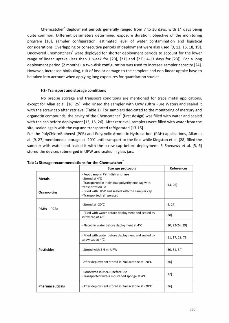
Chemcatcher® deployment periods generally ranged from 7 to 30 days, with 14 days being
quite common. Different parameters determined exposure duration: objective of the monitoring
program [16], sampler configuration, estimated level of water contamination and logistical
considerations. Overlapping or consecutive periods of deployment were also used [9, 12, 16, 18, 19].
Uncovered Chemcatchers® were deployed for shorter deployment periods to account for the lower
range of linear uptake (less than 1 week for [20], [21] and [22]; 4-13 days for [23]). For a long
deployment period (2 months), a two-disk configuration was used to increase sampler capacity [24].
However, increased biofouling, risk of loss or damage to the samplers and non-linear uptake have to
be taken into account when applying long exposures for quantitation studies.
I-2- Transport and storage conditions
No precise storage and transport conditions are mentioned for trace metal applications,
except for Allan et al. [16, 25], who rinsed the sampler with UPW (Ultra Pure Water) and sealed it
with the screw cap after retrieval (Table 1). For samplers dedicated to the monitoring of mercury and
organotin compounds, the cavity of the Chemcatcher® (first design) was filled with water and sealed
with the cap before deployment [13, 15, 26]. After retrieval, samplers were filled with water from the
site, sealed again with the cap and transported refrigerated [13-15].
For the PolyChloroBiphenyl (PCB) and Polycyclic Aromatic Hydrocarbon (PAH) applications, Allan et
al. [9, 27] mentioned a storage at -20°C until transport to the field while Kingston et al. [28] filled the
sampler with water and sealed it with the screw cap before deployment. El-Shenawy et al. [5, 6]
stored the devices submerged in UPW and sealed in glass jars.
Tab 1: Storage recommendations for the Chemcatcher®
Storage protocols References
Metals - Kept damp in Petri dish until use - Stored at 4°C - Transported in individual polyethylene bag with transportation lid - Filled with UPW and sealed with the sampler cap - Transported refrigerated
[14, 26]
Organo-tins
PAHs – PCBs - Stored at -20°C [9, 27]
- Filled with water before deployment and sealed by screw cap at 4°C
[28]
Pesticides
- Placed in water before deployment at 4°C [10, 22-24, 29]
- Filled with water before deployment and sealed by screw cap at 4°C
[11, 17, 28, 75]
- Stored with 3-6 ml UPW [30, 31, 34]
- After deployment stored in 7ml acetone at -20°C [36]
- Conserved in MeOH before use - Transported with a moistened sponge at 4°C
[12]
Pharmaceuticals - After deployment stored in 7ml acetone at -20°C [36]
280
For the pesticide and pharmaceutical organic Chemcatcher® version, some authors
recommended that users store and transport the sampler filled with UPW [10, 11, 17, 18, 22-24, 28-
31] or with a moist sponge [12] at 4°C to prevent sorbent drying. Gunold et al. [32] filled the
Chemcatchers® with tap water. For transport after exposure, some authors recommended storing the
devices filled with water. More precisely, Stephens et al. and Tan et al. [18, 33] filled the samplers
with UPW whereas Schafer et al. [17] used water from the sampling site.
For the storage of samples after retrieval and before analysis, two different procedures are
possible. The first one is to store the disks directly at 4°C or at -20°C after exposure, and to perform
elution just before analysis (see for instance [5, 13, 32, 34]). In that case, careful attention must be
paid to the preservation of analytes in the disk during storage. Gunold et al. [32] reported results
from the evaluation of analyte recoveries and degradations after a 14 and 21 day storage at 4°C. No
degradation in the disk during storage was noticed for the tested pesticides, except for carbofuran
and linuron. For these two molecules, the recoveries after an elution without storage were 78% and
81% respectively, whereas the recoveries decreased to 64% and 49% after 14 days. Finally, after 21
days, carbofuran and linuron were only recovered at 47% and 27%, respectively. The second way to
process samples is to perform the elution immediately after sampler retrieval and to store the
eluates at 4°C [12, 33] or at -20°C until analysis. Vermeirssen et al. [35, 36] performed the first
elution step directly in the field after sampler retrieval. The Chemcatcher® was dismantled and the
disk rolled and put into an acetone-filled tube. These tubes were transported refrigerated to the
laboratory where the elution was completed, immediately or after storage at -20°C [36]. In this latter
case, disks were allowed to reach room temperature before performing the end of the elution
procedure.
I-3- Field or preparation blanks
All of the following steps can contribute, in various proportions, to the overall contamination
of the Chemcatcher® devices: (1) initial contamination of reagents and sampler components, (2)
sampler assembly, (3) laboratory storage, (4) analytical procedures, (5) transport to and from the
field, (6) deployment and retrieval of the sampler [37]. Aguilar-Martìnez et al. [13] suggested the use
of blanks in order to control possible contamination from these different preparation and exposure
steps. Authors used two types of blanks: procedural blanks to estimate the contamination arising
from steps (1) to (4), and field blanks to account for additional contamination during steps (5) and
(6). Procedural blanks were also used to determine the initial concentrations of PRCs (Performance
and Reference Compounds) [8, 19].
Both types of blanks were constructed like field-exposed samplers, preferentially in the same
batch. Procedural blanks were filled with deionized water [38] and kept refrigerated during the entire
sampling period. Field blanks were transported to the field and exposed to ambient air during both
deployment and retrieval [8, 11, 38]. During the sampling period, they were filled with deionized
water and stored at 4°C [34] or -20°C [9]. For organic contaminants, Shaw et al. [23] kept the
procedural blanks at -20°C during exposure periods. Blanks were then extracted and analysed
alongside field samplers. For large-scale monitoring studies, like the one conducted by Kennedy et al.
[24], blank samples can be randomly analysed (10% for these authors). When blank values were
discussed, unexposed samplers generally did not contain detectable amounts of analytes [23, 38].
This was the case for pesticides, pharmaceuticals and PCBs [23, 38, 39]. For instance, during an
intercomparison exercise [40], various samplers were exposed and no detectable amounts of
281
pesticide were observed in field blanks. For some PAHs however (phenanthrene, naphthalene,
pyrene, and benzo[a]pyrene), there was a contamination depending on the sampling site and the
laboratory, but with no clear explanation.
Problems with procedural or field blanks occurred more commonly for trace metal and
mercury applications. Indeed, Aguilar-Martìnez et al. [13, 26] indicated that chelating disks were
contaminated with significant levels of Hg when received from the manufacturer. The authors
advised a rigorous cleaning of the disks before use (6M HCl solution for 30 min in an ultrasonic bath)
and employed low affinity materials for preparation and analysis procedures. A contamination of the
Chelating disks by trace metals was also noted by Allan et al. [16, 25] and Miège et al.[40]. In Allan et
al. [25], the masses of cadmium, copper, nickel, lead and zinc in field blanks were 0.2, 14.0, 2.0, 10.0
and 1.4% of those measured in field samplers, respectively. Copper and lead were also the most
problematic elements in Allan et al. [16], with masses in unexposed disks that ranged between 10
and 100% of those measured in field samplers. Miège et al. [40] also noted critical field blank
concentrations for cadmium, lead and zinc and recommended further work to improve the
robustness of TWAC determination, i.e. to reduce blank values and variability. It is however
important to note that variable metallic contamination of field blanks can also be found in DGT
(Diffusive Gradient in Thin films) devices depending on the element and laboratory [16, 25].
II. Influence of environmental factors on sampling rates
It is worth noting that all passive samplers are influenced by environmental parameters, to a
greater or lesser degree depending on their configuration (in particular the type of membrane,
porous or semi-permeable for either polar or hydrophobic chemicals), targeted analyte
characteristics (polar or hydrophobic) and variability of the studied parameters in each exposure case
[41].
In a previous review on SPMD (semi-permeable membrane device), Esteve-Turrillas et al. [42]
reported the effects of fouling, pH, salinity, temperature and flow velocities on analyte uptake.
Water flow velocity [43] and temperature were shown to strongly influence sampling rates because
of, respectively, a WBL (water boundary layer) or a membrane control of analyte uptake. Fouling of
the sampler surface induced a sampling rate reduction [42][44]..
For the POCIS device, the main factors affecting sampling rates have been reviewed by Harman et al.
[45]. The major studied parameter is water flow rate since a control by the WBL can be assumed [45].
In Li et al. [46], a small influence of flow rate was observed with an increase of only two-fold within
the flow rate range of 2.6 to 37 cm.s-1, but this effect was larger for more hydrophobic compounds. Li
et al. [47] also observed the effect of dissolved organic matter (DOM) and pH on the POCIS sampling
rate for pharmaceuticals, personal care products and endocrine disrupting substances. While there
was no observed effect for DOM, pH had an effect on sampling rate of ionic compounds. The effect
of fouling on POCIS appeared to be compound-dependent [44] but still needs more investigation
[45].
For DGT, the influence of environmental parameters on metal uptake was studied in
particular by Turner et al. [48], Uher et al. [49, 50] and Gimpel et al. [41]. Accumulation in the DGT
device, which is controlled by diffusion through the diffusive gel, may be impacted to various extents
by temperature and the formation of a water boundary layer [51]. Turner et al. [48] noted the
presence of a WBL even under fast flowing conditions and thus an underestimation of uranium
TWAC if WBL was not included in the calculation. On the contrary, Uher et al. [49] estimated that the
282
error made by neglecting WBL formation was lower than the analytical error, even under low flow
conditions. The effect of water temperature on diffusion coefficients can be taken into account using
a dedicated correcting formula [52]. Gimpel et al. [41] also evaluated the influence of water
composition and turbulence on DGT performance. pH and calcium concentration were found to have
no significant influence in an environmentally relevant range. An important effect of biofilm
formation was reported by Uher et al. [50] but under extreme conditions (wastewater).
Several environmental factors are also likely to affect Chemcatcher® sampling rates (Rs):
temperature, water flow rate, fouling, pH and salinity. As will be further described below, the
influence of these parameters depend on compound properties, sampler configuration (design, type
of disk and membrane) and site- and exposure-specific conditions. A supplementary difficulty is met
during field exposures since these parameters may be highly variable and fluctuate with time.
II-1- Hydrodynamic conditions)
There can be several types of resistance to analyte mass transfer (see [4] section I.2). Among
them, uptake may be limited by diffusion through the unstirred WBL at the interface with the
sampler, suggesting that an increased water flow velocity would imply a higher sampling rate, until
no more reduction of the WBL could be obtained. In the laboratory, the influence of hydrodynamic
conditions has been examined by several authors for different compounds and Chemcatcher®
configurations. However, this parameter is expressed in the literature either as a flow velocity (cm.s-
1) or as a rotation speed (rpm), which hampers a direct comparison of calibration data. Moreover, the
impact of hydrodynamic conditions differ depending on the Chemcatcher® design, as demonstrated
by Lobpreis et al. [53]. The second Chemcatcher® design, characterized by a smaller cavity, was found
to be more sensitive but also more affected by flow velocity. The authors suggested that a
compromise be made by users between a higher sensitivity and a reduced impact of water
turbulence. Moreover, it should be considered that, at high flow rates and particularly for low
hydrophobic compounds [35, 38], the period of integrative sampling can be reduced. Sampling rates
obtained in the laboratory under controlled flow velocities may not be relevant in lakes or rivers
under natural flow conditions. During field exposure, water turbulence can affect uptake
characteristics in an irregular and unpredictable way and are, moreover, difficult to monitor [28].
Hydrophobic configuration of the Chemcatcher®
Kingston et al. [28] noted an increase of sampling rates (pesticides, PCBs and phenanthrene)
with a higher flow velocity (overhead stirrer at 75, 140 and 250 rpm). For the C18 disk covered with a
polyethylene membrane, a 2-fold gain in accumulated amounts was observed for phenanthrene and
PCB 52 with an increase from 75 rpm to 250 rpm. A lower increase was noted for dieldrin and PCB
153; the authors suggested that the rate of diffusion was also controlled by the membrane for these
larger molecules. For a C18 disk covered with a PS membrane, accumulation factors were less
affected by changes in stirring rates. These results were attributed to the properties of the
polysulfone membrane (which is thicker and diffusion-limiting).
In Vrana et al. [54], a significant increase of sampling rates at higher rotation speeds was observed
for most compounds (PAHs, chlorobenzenes and organochlorine pesticides), with for instance,
phenanthrene Rs values of 0.145 L.day-1, 0.514 L.day-1 and 0.740 L.day-1 at rotation speeds of 0, 40
rpm and 70 rpm respectively.
283
A significant effect of water turbulence on organotin compounds was noted by Aguilar-
Martínez et al. [15]; sampling rates increased with stirring level (from static conditions to 40 rpm and
70 rpm). The limitation to analyte uptake was thus assigned to diffusion in the WBL rather than
diffusion in the cellulose acetate membrane.
Polar configuration of the Chemcatcher®
Gunold et al. [32] studied the influence of flow velocity (0.135 m.s-1 and 0.4 m.s-1) on the
uptake of 12 polar and semi polar pesticides (log Kow in the range 1.20 – 4.80). The authors suggested
that the differences among sampling rates were due to variability in analyte concentrations and
recommended more studies to assess the influence of flow velocity on hydrophilic compounds.
Vermeirssen et al. [35, 38] evaluated the influence of hydrodynamic conditions on Rs values
in a flow-through channel system fed by river water or treated sewage effluent and operating at 4
flow rate levels (0.026-0.03 m.s-1, 0.055-0.06 m.s-1, 0.15 m.s-1 and 0.37 m.s-1). A range of pesticides
and pharmaceuticals were sampled by 3 different Chemcatcher® configurations (SDB-RPS covered
with a PES membrane and naked SDB-XC and SDB-RPS disks). For both uncovered disks, accumulated
amounts were shown to increase at higher flow velocities. For the covered disk configuration, the
shape of the curve (accumulated amounts as a function of flow velocity) was flatter than that for
uncovered disks. In the lower velocity range (from 0.026 m.s-1 to around 0.2 m.s-1), the increase of
flow rate led to a decrease of the aqueous boundary layer and consequently an increase of analyte
uptake. From approximately 0.2 m.s-1, further decrease of the water boundary layer only slightly
influenced the uptake over the PES membrane, indicating that the membrane became the diffusion
limiting compartment. This effect, apparent at higher flow velocities, was larger for hydrophobic
compounds. In these studies, data fit the following empirical model well (Eq 1):
mSDB = a ( - ebv ) Eq (1)
where mSDB is the accumulated amount per SDB disk (in ng), ν the flow velocity (in m.s-1) and a, b and
c fit parameters.
Similar results were obtained by O’Brien et al. [55] for atrazine and prometryn on an SDB-
RPD disk covered with a PES membrane. An increase of sampling rate was observed for both
compounds between 0 and 16 cm.s-1 flow velocity. From 16 to 24 cm.s-1 flow velocity, sampling rates
did not increase at the same order of magnitude, leading to a plateau. In accordance with
Vermeirssen et al. [35, 38], this phenomenon was attributed to a change in the resistance to mass
transfer from the water boundary layer (at low flow rates) to the diffusion through the membrane
(which is independent on flow conditions).
The same conclusions were obtained by Aguilar-Martìnez et al. [13] for mercury with a PES
(PolyEtherSulfone) membrane and by Björklund Persson et al. [56] for trace metals with a CA
(Cellulose Acetate) membrane (5 rotation levels from static to 400 rpm).
II-2- Temperature
Theoretically, a higher temperature leads to an increased rate of diffusion in both water
boundary and membrane layers (if present), and an increased uptake rate in the receiving phase. As
noticed by Kingston et al. [28], the overall effect of temperature variations on analyte uptake is,
however, not easy to appreciate considering that on the one hand the properties of the polymeric
284
c
material of the diffusion-limiting membrane change with temperature and on the other hand the
equilibrium constant for the partition of the analyte decreases with higher temperature, while the
rate constant increases.
Hydrophobic configuration of the Chemcatcher®
For 6 hydrophobic organic compounds (pesticides, PCBs and phenanthrene), Kingston et al.
[28] noted an increase of sampling rates with a higher temperature (range 4 – 20°C).
Vrana et al. [54] studied the effect of temperature on the uptake of 19 hydrophobic compounds
(PAHs, chlorobenzenes and pesticides). The effect of water temperature (range 6 – 18°C) on the
receiving phase – water distribution coefficient was not found to be significant for four PAHs. The
authors thus suggested that temperature changes may have a higher impact on the kinetic aspect of
analyte uptake. Indeed, a higher temperature was found to significantly increase both compound
sampling rates and first order offload rate constants for selected perdeuterated PAHs under
turbulent flow conditions (40 and 70 rpm rotation speeds).
For organotin compounds on a C18-CA (cellulose acetate) configuration [15], a significant increase of
the sampling rate was only noted in the temperature range 4 – 11°C at the flow velocity of 40 cm.s-1.
No significant differences were observed in the temperature range 11 – 18 °C.
Polar configuration of the Chemcatcher®
For the Chelating disk configuration, no significant difference was found by Aguilar-Martìnez
et al. [13, 14] in the uptake of inorganic mercuryat 4 and 11°C. Indeed, at an estimated linear velocity
of 40 cm.s-1, Rs values were 0.080 0.018 L.day-1 (at 4°C) and 0.084 0.019 L.day-1 (at 11°C).
Similarly, for an estimated linear velocity of 70 cm.s-1, Rs values were 0.070 0.016 L.day-1 (at 4°C)
and 0.091 0.020 L.day-1 (at 11°C). Aguilar-Martìnez et al. [13] also suggested that the lag-time effect
on mercury uptake was higher at 4°C compared to 11°C. For trace metals, Björklund-Persson et
al.[56] recommended measuring at least the initial and final water temperatures as this parameter
influences the diffusion coefficient in the membrane.
II-3- Physico-chemical parameters (pH, water hardness and ionic strength)
pH could affect sampling rates through both interactions with sampler materials and
modification of analyte speciation or partition between protonated and deprotonated forms. For the
Chemcatcher® sampler, only a few studies have been carried out to evaluate the influence of this
parameter. In a comparison between Chemcatcher® and Diffusive Gradient in Thin film (DGT) devices,
Allan et al. [16] specified that the effect of water hardness should be evaluated for the metallic
configuration of the Chemcatcher®. The influence of ionic strength or salinity has rarely been
evaluated although several Chemcatcher® studies have been conducted in highly saline or brackish
media (see the list in section III).
Aguilar-Martìnez et al. [26] evaluated the influence of pH and salinity on the accumulation of
inorganic mercury (Chelating disk with PES membrane) and organotin compounds (Chelating disk
with CA membrane). For inorganic mercury, significantly lower accumulation, 20% lower, was
obtained with a 1-unit pH increase (from 6.7-7 to 8). The authors attributed this to the formation of
hydroxylated complexes (HgOH+, Hg(OH)2), which accumulated in the disk to a lesser extent than
Hg2+.The influence of pH on organotin accumulation factors was not found to be significant, taking
285
into account uptake variability. The authors also indicated that no significant effect of salinity was
observed for organotin compounds (tested media: tap water and artificial seawater).
The uptake of copper, cadmium and lead on a chelating disk covered with a Nafion-coated CA
membrane was studied by BjörklundPersson et al. [56]. Increased accumulation was noted at pH
values varying from 4 or 5 to 8 and, according to the authors, was due to reduced adsorption of
analytes in the receiving phase at low pH. Allan et al. [16] recommended further investigation on the
potential effect of water hardness.
Tran et al. [7] evaluated the performance of SDB-XC and SDB-RPS disks for sampling polar
non-ionized herbicides (simazine, atrazine, diuron, clomazone and metolachlor) and phenoxy acid
herbicides (dicamba, 2,4-D, 2,4-MCPA (2-Methyl-4-chlorophenoxyacetic acid) and triclopyr). Low
sampling rates (and even no detectable accumulation for dicamba) were obtained with both disks for
the phenoxy acid herbicides. Indeed, these compounds, which would be more retained in their
neutral form by the polystyrenedivynilbenzene polymer disk, are predominantly ionized at neutral
pH (pKa range 2-4). Tran et al. [7] suggested the use of an Anion Exchange SR disk to improve
sampling performance, but this receiving phase was later shown to induce elution difficulties for
glyphosate, its metabolite AMPA (AminoMethylPhosphonic Acid) and amitrole [57].
Bernal-Gonzalez et al. [58] constructed an experimental design to evaluate the influence of pH on
uptake of 15 pesticides (log Kow 1.70 – 3.65) with three different sampler configurations (C18 disk
covered with a PES or PC membrane or uncovered). For the investigated pH values (4 and 7), the
tested pesticides were present in a neutral form, with the exception of carbaryl, prometryn and
terbutryn. The authors noted maximum Rs values at pH 7 for all 3 sampler configurations.
II-4- Fouling of the sampler surface
The development of a biofilm layer at the sampler surface is a common problem during
environmental deployment of passive samplers, especially for media such as sewage effluents [33]
and for long deployment periods. A copper mesh can be mounted on the first Chemcatcher® design
to limit biofilm development and to prevent mechanical damage to the disk. However in some cases,
this was not enough to completely prevent biofilm formation [17]. Indeed, Gunold et al. [32] and
Schafer et al. [17] noticed a visibly developed biofilm (respectively after 14-21 days of exposure in
tap water and a 10-14 day field deployment in small streams in an agricultural watershed) even in
the presence of a copper mesh. Some authors suggested that PES membranes are less prone to
biofouling because of their hydrophilic nature [15, 59, 60]. The accumulation of suspended matter on
the sampler surface may impair the uptake of analytes. It is therefore recommended to install the
sampler facing downward during field deployment to limit the settlement of particles, and also to
carefully examine the disk at sampler retrieval in order to estimate the level of biofouling.
The presence of a biofilm is likely to affect sampling rates by increasing the resistance to
mass transfer (see section I.2). Since calibrations are generally performed in the laboratory without
significant fouling, this can induce an underestimation of TWAC. The effect of a biofilm may also be
compound-dependent, as previously noted for the Polar Organic Chemical Integrative Sampler
(POCIS) by Harman et al. [45]. Indeed, Harman et al. [45] suggested that the impact of a biofilm layer
may be more significant for less polar analytes. Several authors also suggested that enhanced
microbial degradation of analyte in the biofilm may explain the apparent lower uptake [9, 33, 60].
The consequence of a biofilm on analyte uptake needs further investigation but, in a first
quantitative approach, it can be evaluated though the comparison of data obtained with pre-fouled
or unfouled membranes.
286
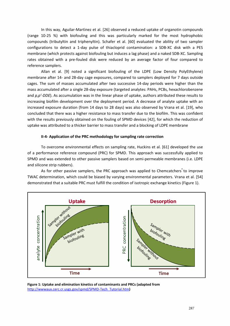
In this way, Aguilar-Martìnez et al. [26] observed a reduced uptake of organotin compounds
(range 10-25 %) with biofouling and this was particularly marked for the most hydrophobic
compounds (tributyltin and triphenyltin). Schafer et al. [60] evaluated the ability of two sampler
configurations to detect a 1-day pulse of thiacloprid contamination: a SDB-XC disk with a PES
membrane (which protects against biofouling but induces a lag phase) and a naked SDB-XC. Sampling
rates obtained with a pre-fouled disk were reduced by an average factor of four compared to
reference samplers.
Allan et al. [9] noted a significant biofouling of the LDPE (Low Density PolyEthylene)
membrane after 14- and 28-day cage exposures, compared to samplers deployed for 7 days outside
cages. The sum of masses accumulated after two successive 14-day periods were higher than the
mass accumulated after a single 28-day exposure (targeted analytes: PAHs, PCBs, hexachlorobenzene
and p,p’-DDE). As accumulation was in the linear phase of uptake, authors attributed these results to
increasing biofilm development over the deployment period. A decrease of analyte uptake with an
increased exposure duration (from 14 days to 28 days) was also observed by Vrana et al. [19], who
concluded that there was a higher resistance to mass transfer due to the biofilm. This was confident
with the results previously obtained on the fouling of SPMD devices [42], for which the reduction of
uptake was attributed to a thicker barrier to mass transfer and a blocking of LDPE membrane
II-4- Application of the PRC methodology for sampling rate correction
To overcome environmental effects on sampling rate, Huckins et al. [61] developed the use
of a performance reference compound (PRC) for SPMD. This approach was successfully applied to
SPMD and was extended to other passive samplers based on semi-permeable membranes (i.e. LDPE
and silicone strip rubbers).
As for other passive samplers, the PRC approach was applied to Chemcatchers® to improve
TWAC determination, which could be biased by varying environmental parameters. Vrana et al. [54]
demonstrated that a suitable PRC must fulfill the condition of isotropic exchange kinetics (Figure 1).
Figure 1: Uptake and elimination kinetics of contaminants and PRCs (adapted from http://wwwaux.cerc.cr.usgs.gov/spmd/SPMD-Tech_Tutorial.htm)
287
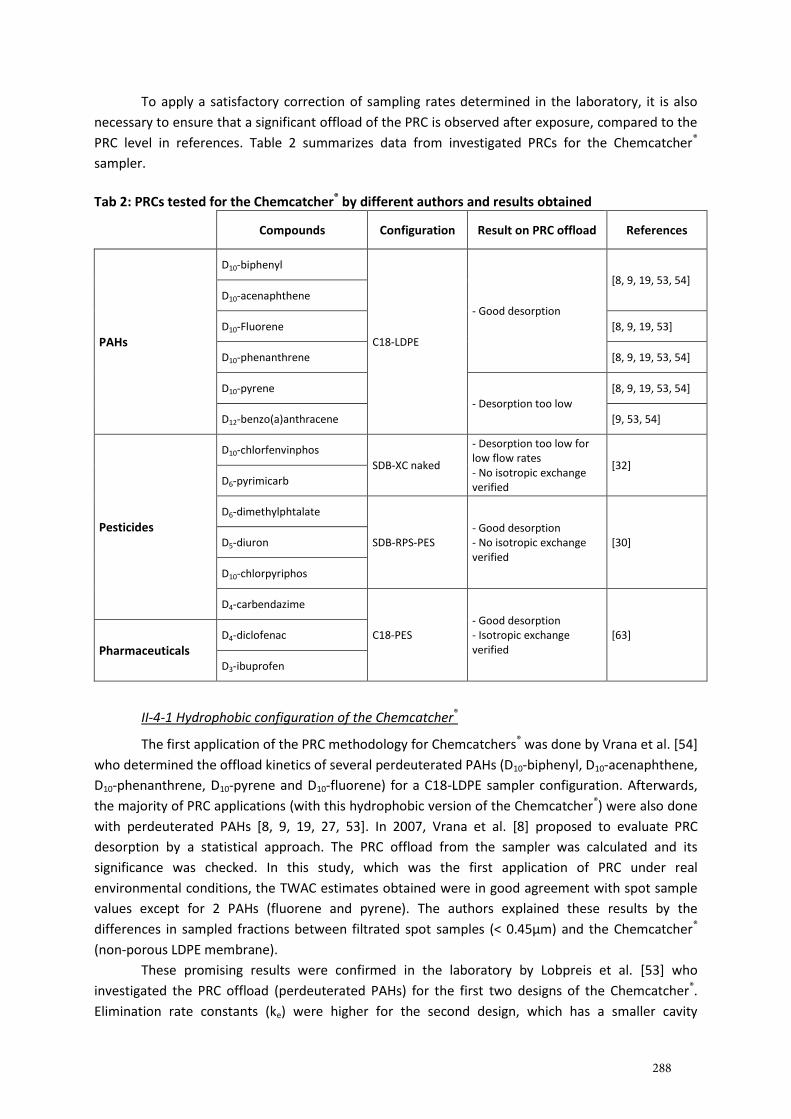
To apply a satisfactory correction of sampling rates determined in the laboratory, it is also
necessary to ensure that a significant offload of the PRC is observed after exposure, compared to the
PRC level in references. Table 2 summarizes data from investigated PRCs for the Chemcatcher®
sampler.
Tab 2: PRCs tested for the Chemcatcher® by different authors and results obtained
Compounds Configuration Result on PRC offload References
PAHs
D10-biphenyl
C18-LDPE
- Good desorption
[8, 9, 19, 53, 54]
D10-acenaphthene
D10-Fluorene [8, 9, 19, 53]
D10-phenanthrene [8, 9, 19, 53, 54]
D10-pyrene
- Desorption too low
[8, 9, 19, 53, 54]
D12-benzo(a)anthracene [9, 53, 54]
Pesticides
D10-chlorfenvinphos
SDB-XC naked
- Desorption too low for low flow rates - No isotropic exchange verified
[32]
D6-pyrimicarb
D6-dimethylphtalate
SDB-RPS-PES - Good desorption - No isotropic exchange verified
[30] D5-diuron
D10-chlorpyriphos
D4-carbendazime
C18-PES - Good desorption - Isotropic exchange verified
[63]
Pharmaceuticals D4-diclofenac
D3-ibuprofen
II-4-1 Hydrophobic configuration of the Chemcatcher®
The first application of the PRC methodology for Chemcatchers® was done by Vrana et al. [54]
who determined the offload kinetics of several perdeuterated PAHs (D10-biphenyl, D10-acenaphthene,
D10-phenanthrene, D10-pyrene and D10-fluorene) for a C18-LDPE sampler configuration. Afterwards,
the majority of PRC applications (with this hydrophobic version of the Chemcatcher®) were also done
with perdeuterated PAHs [8, 9, 19, 27, 53]. In 2007, Vrana et al. [8] proposed to evaluate PRC
desorption by a statistical approach. The PRC offload from the sampler was calculated and its
significance was checked. In this study, which was the first application of PRC under real
environmental conditions, the TWAC estimates obtained were in good agreement with spot sample
values except for 2 PAHs (fluorene and pyrene). The authors explained these results by the
differences in sampled fractions between filtrated spot samples (< 0.45µm) and the Chemcatcher®
(non-porous LDPE membrane).
These promising results were confirmed in the laboratory by Lobpreis et al. [53] who
investigated the PRC offload (perdeuterated PAHs) for the first two designs of the Chemcatcher®.
Elimination rate constants (ke) were higher for the second design, which has a smaller cavity
288
compared to the first design. For these non-polar compounds, the PRC was also shown to give an
acceptable correction of the variability in the water boundary layer due the different housing
geometries.
Still on a C18-LDPE configuration, Vrana et al. [19] evaluated the applicability of the PRC
approach during six field trials with variable exposure conditions (temperature, flow, biofouling
extent). The in-situ corrected TWACs were close to spot sample concentrations during the spring
trials for PAHs with log Kow higher than 4.5. For the autumn trials, several difficulties arose from: (1)
differences in analytical methods between laboratories, (2) concentration levels close to the method
quantification limits, and (3) differences in sampled fractions between spot and passive sampling.
Allan et al. [9] used PRC dissipation data to observe the transition between membrane and
boundary layer-controlled uptake with the Chemcatcher®. For example, analytes for which the
concentration in the sampler was near equilibrium, were characterized by a complete elimination of
PRC with similar log KOW. On the contrary, little PRC dissipation indicated molecules in the linear
phase of uptake.
For hydrophobic contaminants, the Chemcatcher® can be compared to SPMD, for which
potential PRCs (mainly labeled PAHs and PCBs) have been tested. Seethapathy et al. [62] reported
some authors’ observations on the effectiveness of the PRC application to SPMD. Depending on the
molecules, the use of PRCs could be a very effective solution to correct TWACs estimated by SPMD.
Finally, for hydrophobic compounds, the PRC approach seems to be efficient for both the
Chemcatcher® and SPMD.
II-4-2 Polar configuration of the Chemcatcher®
Application of the PRC approach has been evaluated for the polar configuration of the
Chemcatcher®, but only six studies [7, 30, 32, 36, 63, 64] mentioned pesticide or pharmaceutical
PRCs.
The first study on pesticides is from Tran et al. [7]. Authors did not investigate the use of PRC
but verified isotropic exchanges of triclopyr on SDB-XC sorbent. The demonstration of isotropic
behavior predicts successful use of triclopyr as a PRC.
Then, Gunold et al. [32] investigated an application of D10-chlorfenvinphos and D6-
pyrimicarb as PRCs on a naked SDB-XC disk. Results were not convincing, with a bad nonlinear
regression fit of the offload curves. The study [32] concluded that the PRC approach does not seem
to be applicable for polar receiving phases without membranes. The authors explained that an
inhomogeneity of PRC loading on the sorbent disk could result in important desorption variation in
the uncovered design. Alternatively, as previously suggested by Mills et al. [64], accumulation on the
disk for polar compounds is determined by adsorption rather than by partitioning, resulting in
different uptake and offload kinetics which are indeed governed by different mass transfer laws.
In the same way, Shaw et al. [30] investigated perdeuterated polar pesticides as PRCs (D6-
dimethylphtalate, D5-diuron and D10-chlorpyriphos) on an SDB-RPS disk covered by a PES membrane
or uncovered. No release of D6-dimethylphtalate or D10-chlorpyriphos was noted for the covered
configuration. Only D5-diuron was released from the disk in both configurations. However, even if
this molecule seemed to be a promising potential PRC, anisotropic exchanges were observed as 50 %
equilibrium was obtained at 4 days for the release of D5-diuron and at 30 days for the uptake of
diuron in the naked version. The same explanation as Mills et al. [64] was given; molecules were
associated to the disk material by adsorption rather than by partitioning.
289
Camilleri et al. [63] and Vermeirssen et al. [36] evaluated the ability of several pesticides or
pharmaceuticals as potential PRCs, respectively on a C18-PES configuration in a flow-through
microcosm, and a naked SDB-RPS configuration in a channel system and a circular tank. Of the 20
perdeuterated molecules tested by Camilleri et al. [63], only three showed first order kinetics with a
good fit and almost isotropic behavior (one pesticide: D4-carbendazime and two pharmaceuticals: D4-
diclofenac and D3-ibuprofen), whereas in Vermeirssen et al. [36], who investigated 22 non-
deuterated compounds, no exchanges were isotropic. However, Vermeirssen et al [36] specified that
release and accumulation experiments were not performed at the same time, which could have
impacted results. For the circular tank experiment, an excellent fit was obtained between desorption
data and a two-phase model, which includes an initial rapid desorption from the SDB disk followed by
a slower desorption phase. As PRCs were loaded by passing through the disk, authors attributed this
second phase to the fraction of analytes adsorbed deeper in the disk material.
For polar compounds, the Chemcatcher® can be compared to the POCIS passive sampler.
However, the application of PRC methodology to Rs correction of polar compounds still needs further
research. Indeed, for the POCIS sampler, Alvarez et al. [65] suggested that the PRC correction is not
directly applicable because uptake by SBE sorbent involves two different mechanisms: adsorption
and partitioning of the molecule. Mazzella et al. [66] successfully tested the PRC correction for the
POCIS but this approach is not as efficient as expected for some other authors and, in a previous
review, Harman et al. [45] pointed out some difficulties (e.g. sufficiently fugace molecules for PRC
candidates, lack of knowledge concerning adsorption and desorption processes).
Finally, the use of a PRC correction seems to be as difficult for this polar version of
Chemcatcher® as for the POCIS and, as a consequence, needs further research before concluding on
its applicability.
II-4-3 Other in situ Rs corrections
Alternative methodologies were proposed by some authors. Shaw et al. [30], who noted the
anisotropic behavior of polar PRCs on a SDB-RPS disk, evaluated the ability of surrogate PDMS
(polydimethylsiloxane) disks for deriving in situ sampling rates. Positively, the release of PRCs, which
were previously loaded on PDMS disks, was shown to be reproducible and linear. O’Brien et al. [55]
proposed an adaptation of the passive flow monitor (PFM), composed of a container opened on one-
side and filled with gypsum. The mass loss of gypsum proved to be linear over the deployment time
at a constant flow velocity, and also to increase with increased flow velocity (range 3.4 – 24 cm.s-1).
The uptake of atrazine and prometryn into a SDB-RPS disk was later corrected by the mass of gypsum
lost during sampler exposure.
III. Screening and quantitation studies
A majority of the articles involving the Chemcatcher® deal with environmental application
such as the screening or quantitation of pollutants in various aquatic systems from rivers to sewage
treatment plant effluents. The screening capacity of this tool was demonstrated by all the authors
and related to the high extraction capacity of the Chemcatcher® (e.g. [67]).
Despite its almost “universal” capacity, the Chemcatcher® was used for quantitation
applications rather than for screening studies. In order to use this sampler as a quantitative tool, a
calibration step is needed to determine sampling rates. Rs are calculated as shown in Charriau et
al.[4] (section I-2) and are then used to determine TWACs for Chemcatcher® field applications.
290
The majority of the quantitation studies took place in river waters [8, 9, 13, 14, 16, 17, 19, 34,
40, 55, 68]. Applications were also conducted in high salinity media such as seawater [10, 22-24, 26,
28], harbor sites [6, 14, 15, 26, 28] or estuarine and brackish waters [14, 34]. Some other
environments were also studied, such as storm water constructed wetlands [20, 21, 69 ], lakes and
reservoirs [11, 14] and agricultural irrigation channels [12, 70].
Concerning the quantitation of pollutants, wastewater treatment plant (WWTP) effluents
received less attention [14, 35, 38, 71]. Tan et al. [33] compared the Chemcatcher® to grab sampling
for monitoring endocrine disrupting compounds at various stages during treatment. The results were
not as strong as could be because samplers were impacted by drastic conditions of biofouling and by
a very low water flow velocity compared to laboratory calibration conditions. These combined
factors resulted in an important difference between passive sampling results and grab sampling. The
authors indicated that the PRC correction could not be used as extracts were afterwards employed
for bioassays. They stressed the necessity to adapt a PRC approach and to enhance knowledge on
Chemcatcher® behavior in such difficult matrices.
Miege et al. [40] reported the results of an inter-comparison of several passive samplers
including the Chemcatcher® (for polar and hydrophobic organic analytes and also for trace metals).
For two PAHs (fluoranthene and benzo(a)pyrene), C18-Chemcatcher® results were similar to the
robust mean of all participants and other passive samplers (SPMD, LDPE, MESCO). For two pesticides
that were also sampled by the POCIS (atrazine and metolachlor), the Chemcatcher® (SDB-XC) showed
systematically lower results compared to the robust mean reference. For atrazine, the Chemcatcher®
(SDB-RPS) had higher results (3 fold) than the robust mean. For two metals (cadmium and lead),
Chemcatcher® estimates were 4-fold higher than the robust mean. However, a comparison of DGT
and Chemcatcher® samplers was made difficult by the small amount of data, as Chemcatchers® were
only deployed by one participant.
Jacquet et al. [39] recently compared five passive samplers for the monitoring of PCBs in
water: SPMD, SR (silicone rubber), continuous-flow integrative sampler (CFIS), LDPE strip and
Chemcatcher®. TWACs estimated with Chemcatchers® were repeatable (ranging from 12 to 22%) but
were approximately 12-fold higher than those obtained with the other passive samplers. The authors
attributed this difference to the empirical Rs model used for TWAC calculation which was proposed
by Vrana et al. [8] for hydrophobic compounds but which may not be applicable to PCBs.
IV. Comparison with biomonitoring and use for ecotoxicological studies
Passive samplers have two major interesting characteristics: (1) their concentration ability,
which allows the extraction of large quantities of pollutants from water to the sorbent and (2) their
ability to sample only the dissolved fraction. Thanks to these qualities, passive samplers have been
used more and more for comparisons with biomonitoring and to prepare representative cocktails for
ecotoxicological tests. These aspects have been discussed in recent reviews of the POCIS sampler
[72] and the SPMD [42]. Bayen et al. [73] wrote a critical review on the use of passive samplers to
mimic dynamic exposure of aquatic organisms. As stressed by the authors, a preliminary study should
be performed to adjust field exposure duration to the time necessary to achieve equilibrium, mainly
for the most hydrophobic compounds. Zabiegala et al. [74] displayed the advantages and drawbacks
of passive samplers versus organisms for biomonitoring. These authors pointed out that passive
samplers (1) are immortal and less sensitive to water composition compared to organisms, (2) mimic
bioconcentration and do not metabolise compounds and (3) give access to an estimated water
291
concentration. Nevertheless, passive samplers accumulate only the dissolved fraction while some
organisms are also exposed to particle-bound molecules.
El-Shenawy et al. [5, 6] reported the use of Chemcatchers® for biomonitoring studies. The
passive sampler extracts were compared to mussel (Mytilusedulis) extracts first in a laboratory study
and then in the field (Portsmouth harbor, UK). Authors indicated that both approaches, passive
sampling and organism exposure, were complementary because the Chemcatcher® samples the
dissolved fraction of contaminants whereas organisms sample both dissolved and particulate-bound
fractions. This result will likely be dependent on organism type; indeed, the feeding behavior of e.g.,
fish, which swallow minimal amounts of water and suspended particles, is very different from that of
bivalves, which filter water.
Bioassay applications of passive samplers are now more documented. For the Chemcatcher®,
six applications for bioassays were reported by different authors [29, 33, 34, 38, 71, 75] for various
herbicides.
Escher et al. [34] used the Maxi-Imaging-Pulse Amplitude Modulation (PAM) method to
measure concentration-effect curves of Chemcatcher® extracts on two algal species (Desmodesmus
subspicatus and Phaeodactylum tricornutum).The same procedure was applied on SPE extracts of
water samples in order to compare biological effects. Excellent agreement was obtained between
chemical analysis of the extracts and the Maxi-Imaging-PAM bioassay. The herbicides diuron and
simazine, which were analytically detected, proved to contribute the most to the overall
phytotoxicity of the extracts.
Muller et al. [71] used three different bioassays: Maxi-Imaging-PAM (phytotoxicity),
MicrotoxTM (bacterial toxicity) and umuC assay (genotoxicity) to evaluate the toxicity of effluent from
sewage treatment plants (STP). All bioassays showed an effect of STP effluents. The results allowed
determination of the toxicity of STP effluents at different treatment steps and thus endpoints of
concern. This provides a powerful method for assessing effects of specific mixtures of organic
pollutants resulting from various biota compartments.
Tan et al. [33] studied the estrogenic effect of grab samples and passive sampler extracts of
different matrices of a WWTP (influent, aerobic and anaerobic bioreactors, return activated sludge,
clarifier, effluent, river water at the point of discharge and 1 km downstream). These authors used
the E-Screen assay, based on increased growth of MCF-7 cells in the presence of estrogenic
substances. The estrogenic activity obtained with passive sampler extracts was lower than that
obtained with grab samples. As explained in II-3, biofouling (particularly in the influent and
bioreactor compartments) and the impossibility of using the PRC strategy were probably the major
explanations for these results. The authors [33] stressed the necessity of doing more calibration
studies and of identifying PRC that do not interfere with the E-screen assay.
Shaw et al. [29] investigated four different bioassays to evaluate the sensitivity of coral reef
biota to mixtures of organic pollutants sequestered in passive samplers deployed in the Great Barrier
Reef (GBR, Australia). The four bioassays were: coral larval settlement (on Acropora millepora), sea
urchin larval development (on Heliocidaris tuberculata), bacterial luminescence (on Vibrio fischeri)
and microalgal photosynthesis with Maxi-Imaging-PAM (on Phaeodactylum tricornutum). As for
Muller et al. [71], the four tests showed that the passive sampler mixture impacted the tested
populations. The combination of tests on indigenous populations and passive sampler extracts of
GBR water allowed an understanding (under relevant conditions) of the local impacts of pollution.
Vermeirssen at al. [38] used a bioassay that assessed photosynthetic yield in the green algae
Pseudokirchneriella subcapitata by the saturation pulse method using Maxi-Imaging-PAM. This is a
292
measure of the toxicity of herbicides that target Photosystem II (PS II) in algae. Strong correlations
were obtained between the biological responses and the six analytically quantified herbicides in the
passive sampler extract. Expressed as diuron equivalent amounts, the biological responses were
always higher than the chemical responses, indicating that some effects could be attributed to
unidentified and unquantified PS II herbicides. This study demonstrated the interest of using passive
sampler extracts to study the effect of pertinent contaminant mixtures.
Lewis et al. [75] proposed an additive PS-II normalization of herbicide data from passive
sampler results and aquatic organism exposures. Then, a contour-map of the GBR was proposed to
compare pesticide concentrations with various Water Quality Guidelines from the Great Barrier Reef
Marine Park (Normalized Herbicide index Value relative to the GBR guideline and Normalized
Herbicide index Value relative to PSII inhibition thresholds). The authors concluded that this
approach, using a normalization index method, allowed toxicity assessment of herbicide mixtures
and provided a better understanding of pesticide risk in the GBR lagoon.
IV- Conclusions With the same housing, Chemcatcher® device is at present the only universal passive sampler
for either monitoring inorganic, organometallic or organic pollutants in environmental water bodies.
Part B of this review has summarized the various application fields of the passive sampler
Chemcatcher®. The following points have been discussed in detail:
- QA/QC for the transport, exposure and recovery of passive samplers
- Screening studies
- Quantitation studies and the problems/impacts of environmental parameters on the
calculated values of TWACs
- Proposed solutions and critical discussion of the PRC correction procedure
- Comparison of Chemcatcher® sampled fractions and biomonitoring analyses
- Use of Chemcatcher® extracts for bioassays
For all of these aspects, Chemcatcher® was positioned relative to other corresponding passive
samplers depending on the molecules of interest. This state-of-the-art also revealed some knowledge
gaps. Firstly, the effects of environmental parameters on pollutant accumulation (especially pH, ionic
strength and salinity) are still not well documented. These parameters should be studied in more
detail in order to (1) take precautions with the in situ application of the device and (2) try to evaluate
the most influential parameters. Secondly, the influence of flow rate and biofouling, mostly
documented in publications, showed that a correction is necessary in order to use the samplers as
quantitative tools. A solution is the use of PRC for organic chemical sampling, but this procedure has
been shown in some articles to be less efficient than expected, in particular for less hydrophobic
compounds. Thus, it is very important to work on this point to find some improvements for the
evaluation of TWAC with the Chemcatcher®. At present, this lack of knowledge also seems to be a
critical issue for other passive samplers, especially for the POCIS. Finally, as for all passive samplers,
standardization procedures are needed to give this tool a framework for the monitoring of pollutants
in water bodies. Some intercomparison works have been done to simultaneously test various passive
samplers and a recent publication shows rapid progress in this field [76].
Despite these points of concern, the Chemcatcher® is an interesting and promising tool for
the monitoring of various pollutants in aquatic environments. Table 3 summarizes the application
domains and the QA/QC recommendations for each use of the sampler.
293
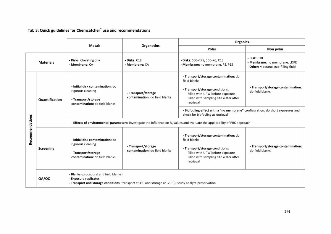
Tab 3: Quick guidelines for Chemcatcher® use and recommendations
Metals Organotins Organics
Polar Non polar
Materials - Disks: Chelating disk - Membrane: CA
- Disks: C18 - Membrane: CA
- Disks: SDB-RPS, SDB-XC, C18 - Membrane: no membrane, PS, PES
- Disk: C18 - Membrane: no membrane, LDPE - Other: n-octanol gap-filling fluid
Re
com
me
nd
atio
ns
Quantification
- Initial disk contamination: do rigorous cleaning
- Transport/storage contamination: do field blanks
- Transport/storage contamination: do field blanks
- Transport/storage contamination: do field blanks
- Transport/storage conditions: Filled with UPW before exposure Filled with sampling site water after retrieval
- Transport/storage contamination: do field blanks
- Biofouling effect with a “no membrane” configuration: do short exposures and check for biofouling at retrieval
- Effects of environmental parameters: investigate the influence on Rs values and evaluate the applicability of PRC approach
Screening
- Initial disk contamination: do rigorous cleaning
- Transport/storage contamination: do field blanks
- Transport/storage contamination: do field blanks
- Transport/storage contamination: do field blanks
- Transport/storage conditions: Filled with UPW before exposure Filled with sampling site water after retrieval
- Transport/storage contamination: do field blanks
QA/QC - Blanks (procedural and field blanks) - Exposure replicates - Transport and storage conditions (transport at 4°C and storage at -20°C): study analyte preservation
294
References
[1] 2000/60/EC, Directive 2000/60/EC of the European Parliament and of the Council of 23 October 2000 establishing a framework for Community action in the field of water policy, OJ L 327, 22.12.2000, 1-73., 2000. [2] F. Stuer-Lauridsen, Environmental Pollution 136 (2005) 503. [3] B. Vrana, I.J. Allan, R. Greenwood, G.A. Mills, E. Dominiak, K. Svensson, J. Knutsson, G. Morrison, TrAC, Trends Anal. Chem. 24 (2005) 845. [4] A. Charriau, S. Lissalde, G. Poulier, N. Mazzella, R. Buzier, G. Guibaud, TrAC - Trends in Analytical Chemistry Submitted (Submitted). [5] N.S. El-Shenawy, R. Greenwood, I.M. Abdel-Nabi, Z.I. Nabil, Ocean Science Journal 44 (2009) 69. [6] N.S. El-Shenawy, Z.I. Nabil, I.M. Abdel-Nabi, R. Greenwood, Journal of Environmental Science and Technology 3 (2010) 1. [7] A.T.K. Tran, R.V. Hyne, P. Doble, Environmental Toxicology and Chemistry 26 (2007) 435. [8] B. Vrana, G.A. Mills, M. Kotterman, P. Leonards, K. Booij, R. Greenwood, Environmental Pollution 145 (2007) 895. [9] I.J. Allan, K. Booij, A. Paschke, B. Vrana, G.A. Mills, R. Greenwood, Environmental Science and Technology 43 (2009) 5383. [10] M. Shaw, J.F. Müller, Marine Pollution Bulletin 51 (2005) 876. [11] H. Nyoni, L. Chimuka, B. Vrana, E. Cukrowska, Analytica Chimica Acta 694 (2011) 75. [12] F. Sánchez-Bayo, R.V. Hyne, G. Kibria, P. Doble, Bulletin of Environmental Contamination and Toxicology (2013) 1. [13] R. Aguilar-Martínez, M.M. Gómez-Gómez, R. Greenwood, G.A. Mills, B. Vrana, M.A. Palacios-Corvillo, Talanta 77 (2009) 1483. [14] R. Aguilar-Martínez, M.M. Gómez-Gómez, M.A. Palacios-Corvillo, International Journal of Environmental Analytical Chemistry 91 (2011) 1100. [15] R. Aguilar-Martínez, M.A. Palacios-Corvillo, R. Greenwood, G.A. Mills, B. Vrana, M.M. Gómez-Gómez, Analytica Chimica Acta 618 (2008) 157. [16] I.J. Allan, J. Knutsson, N. Guigues, G.A. Mills, A.M. Fouillac, R. Greenwood, Journal of Environmental Monitoring 10 (2008) 821. [17] R.B. Schafer, A. Paschke, B. Vrana, R. Mueller, M. Liess, Water Research 42 (2008) 2707. [18] B.S. Stephens, A.P. Kapernick, G. Eaglesham, J.F. Mueller, Marine Pollution Bulletin 58 (2009) 1116. [19] B. Vrana, G.A. Mills, P.E.G. Leonards, M. Kotterman, M. Weideborg, J. Hajlova, V. Kocourek, M. Tomaniova, J. Pulkrabova, M. Suchanova, K. Hajkova, S. Herve, H. Ahkola, R. Greenwood, Journal of Environmental Monitoring 12 (2010) 863. [20] D. Page, P. Dillon, J. Mueller, M. Bartkow, Chemosphere 81 (2010) 394. [21] D.W. Page, S.J. Khan, K. Miotlinski, Journal of Water Reuse and Desalination 1 (2011) 11. [22] K. Kennedy, M. Devlin, C. Bentley, K. Lee-Chue, C. Paxman, S. Carter, S.E. Lewis, J. Brodie, E. Guy, S. Vardy, K.C. Martin, A. Jones, R. Packett, J.F. Mueller, Marine Pollution Bulletin 64 (2012) 1495. [23] M. Shaw, M.J. Furnas, K. Fabricius, D. Haynes, S. Carter, G. Eaglesham, J.F. Mueller, Marine Pollution Bulletin 60 (2010) 113. [24] K. Kennedy, T. Schroeder, M. Shaw, D. Haynes, S. Lewis, C. Bentley, C. Paxman, S. Carter, V.E. Brando, M. Bartkow, L. Hearn, J.F. Mueller, Marine Pollution Bulletin 65 (2012) 292. [25] I.J. Allan, J. Knutsson, N. Guigues, G.A. Mills, A.M. Fouillac, R. Greenwood, Journal of Environmental Monitoring 9 (2007) 672. [26] R. Aguilar-Martínez, R. Greenwood, G.A. Mills, B. Vrana, M.A. Palacios-Corvillo, M.M. Gómez-Gómez, International Journal of Environmental Analytical Chemistry 88 (2008) 75. [27] I.J. Allan, K. Booij, A. Paschke, B. Vrana, G.A. Mills, R. Greenwood, Journal of Environmental Monitoring 12 (2010) 696.
295
[28] J.K. Kingston, R. Greenwood, G.A. Mills, G.M. Morrison, L.B. Persson, Journal of Environmental Monitoring 2 (2000) 487. [29] M. Shaw, A. Negri, K. Fabricius, J.F. Mueller, Aquatic Toxicology 95 (2009) 108. [30] M. Shaw, G. Eaglesham, J.F. Mueller, Chemosphere 75 (2009) 1. [31] B.S. Stephens, A. Kapernick, G. Eaglesham, J. Mueller, Environmental Science and Technology 39 (2005) 8891. [32] R. Gunold, R.B. Schafer, A. Paschke, G. Scharmann, M. Liess, Environmental Pollution 155 (2008) 52. [33] B.L.L. Tan, D.W. Hawker, J.F. Müller, F.D.L. Leusch, L.A. Tremblay, H.F. Chapman, Environment International 33 (2007) 654. [34] B.I. Escher, P. Quayle, R. Muller, U. Schreiber, J.F. Mueller, Journal of Environmental Monitoring 8 (2006) 456. [35] E.L.M. Vermeirssen, J. Asmin, B.I. Escher, J.H. Kwon, I. Steimen, J. Hollender, Journal of Environmental Monitoring 10 (2008) 119. [36] E.L.M. Vermeirssen, C. Dietschweiler, B. Escher, J. Voet, J. Hollender, Analytical and Bioanalytical Chemistry (2013) 1. [37] N.E.I. 5667-23, in: AFNOR (Ed.), Water quality — Sampling — Part 23: Guidance on passive sampling in surface waters, AFNOR. 2011, p. 38. [38] E.L.M. Vermeirssen, N. Bramaz, J. Hollender, H. Singer, B.I. Escher, Water Research 43 (2009) 903. [39] R. Jacquet, C. Miège, F. Smedes, C. Tixier, J. Tronczynski, A. Togola, C. Berho, I. Valor, J. Llorca, B. Barillon, P. Marchand, M. Coquery, Chemosphere (2013). [40] C. Miège, S. Schiavone, A. Dabrin, M. Coquery, N. Mazzella, C. Berho, J.P. Ghestem, A. Togola, C. Gonzalez, J.L. Gonzalez, B. Lalere, S. Lardy-Fontan, B. Lepot, D. Munaron, C. Tixier, Trends in Analytical Chemistry 36 (2012) 128. [41] J. Gimpel, H. Zhang, W. Hutchinson, W. Davison, Analytica Chimica Acta 448 (2001) 93. [42] F.A. Esteve-Turrillas, V. Yusà , A. Pastor, M. de la Guardia, Talanta 74 (2008) 443. [43] K. Booij, H.M. Sleiderink, F. Smedes, Environmental Toxicology and Chemistry 17 (1998) 1236. [44] C. Harman, O. Boyum, K.V. Thomas, M. Grung, Environmental Toxicology and Chemistry 28 (2009) 2324. [45] C. Harman, I.J. Allan, E.L.M. Vermeirssen, Environmental Toxicology and Chemistry 31 (2012) 2724. [46] H. Li, E.L. Vermeirssen, P.A. Helm, C.D. Metcalfe, Environmental Toxicology and Chemistry 29 (2010) 2461. [47] H. Li, P.A. Helm, G. Paterson, C.D. Metcalfe, Chemosphere In Press, Corrected Proof (2011). [48] G.S.C. Turner, G.A. Mills, P.R. Teasdale, J.L. Burnett, S. Amos, G.R. Fones, Analytica Chimica Acta 739 (2012) 37. [49] E. Uher, M.-H. Tusseau-Vuillemin, C. Gourlay-France, Environmental Science: Processes & Impacts 15 (2013) 1351. [50] E. Uher, H. Zhang, S. Santos, M.-H. Tusseau-Vuillemin, C. Gourlay-Francé, Analytical Chemistry 84 (2012) 3111. [51] Ø.A. Garmo, K.R. Naqvi, O. RØyset, E. Steinnes, Analytical and Bioanalytical Chemistry 386 (2006) 2233. [52] H. Zhang, W. Davison, Analytical Chemistry 67 (1995) 3391. [53] T. Lobpreis, B. Vrana, E. Dominiak, K. Dercova, G.A. Mills, R. Greenwood, Environmental Pollution 153 (2008) 706. [54] B. Vrana, G.A. Mills, E. Dominiak, R. Greenwood, Environmental Pollution 142 (2006) 333. [55] D. O'Brien, M. Bartkow, J.F. Mueller, Chemosphere 83 (2011) 1290. [56] L. Björklund Persson, G.M. Morrison, J.U. Friemann, J. Kingston, G. Mills, R. Greenwood, Journal of Environmental Monitoring 3 (2001) 639. [57] F. Sánchez-Bayo, R.V. Hyne, K.L. Desseille, Analytica Chimica Acta 675 (2010) 125.
296
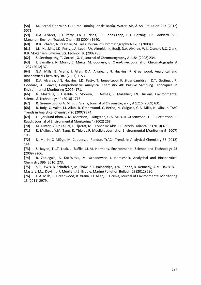
[58] M. Bernal-González, C. Durán-Domínguez-de-Bazúa, Water, Air, & Soil Pollution 223 (2012) 5071. [59] D.A. Alvarez, J.D. Petty, J.N. Huckins, T.L. Jones-Lepp, D.T. Getting, J.P. Goddard, S.E. Manahan, Environ. Toxicol. Chem. 23 (2004) 1640. [60] R.B. Schafer, A. Paschke, M. Liess, Journal of Chromatography A 1203 (2008) 1. [61] J.N. Huckins, J.D. Petty, J.A. Lebo, F.V. Almeida, K. Booij, D.A. Alvarez, W.L. Cranor, R.C. Clark, B.B. Mogensen, Environ. Sci. Technol. 36 (2002) 85. [62] S. Seethapathy, T. Gorecki, X. Li, Journal of Chromatography A 1184 (2008) 234. [63] J. Camilleri, N. Morin, C. Miège, M. Coquery, C. Cren-Olivé, Journal of Chromatography A 1237 (2012) 37. [64] G.A. Mills, B. Vrana, I. Allan, D.A. Alvarez, J.N. Huckins, R. Greenwood, Analytical and Bioanalytical Chemistry 387 (2007) 1153. [65] D.A. Alvarez, J.N. Huckins, J.D. Petty, T. Jones-Lepp, F. Stuer-Lauridsen, D.T. Getting, J.P. Goddard, A. Gravell, Comprehensive Analytical Chemistry 48: Passive Sampling Techniques in Environmental Monitoring (2007) 171. [66] N. Mazzella, S. Lissalde, S. Moreira, F. Delmas, P. Mazellier, J.N. Huckins, Environmental Science & Technology 44 (2010) 1713. [67] R. Greenwood, G.A. Mills, B. Vrana, Journal of Chromatography A 1216 (2009) 631. [68] B. Roig, C. Valat, I.J. Allan, R. Greenwood, C. Berho, N. Guigues, G.A. Mills, N. Ulitzur, TrAC Trends in Analytical Chemistry 26 (2007) 274. [69] L. Björklund Blom, G.M. Morrison, J. Kingston, G.A. Mills, R. Greenwood, T.J.R. Pettersson, S. Rauch, Journal of Environmental Monitoring 4 (2002) 258. [70] M. Kuster, A. De La Cal, E. Eljarrat, M.J. Lopez De Alda, D. Barcelo, Talanta 83 (2010) 493. [71] R. Muller, J.Y.M. Tang, R. Thier, J.F. Mueller, Journal of Environmental Monitoring 9 (2007) 105. [72] N. Morin, C. Miège, M. Coquery, J. Randon, TrAC - Trends in Analytical Chemistry 36 (2012) 144. [73] S. Bayen, T.L.T. Laak, J. Buffle, J.L.M. Hermens, Environmental Science and Technology 43 (2009) 2206. [74] B. Zabiegala, A. Kot-Wasik, M. Urbanowicz, J. Namieśnik, Analytical and Bioanalytical Chemistry 396 (2010) 273. [75] S.E. Lewis, B. Schaffelke, M. Shaw, Z.T. Bainbridge, K.W. Rohde, K. Kennedy, A.M. Davis, B.L. Masters, M.J. Devlin, J.F. Mueller, J.E. Brodie, Marine Pollution Bulletin 65 (2012) 280. [76] G.A. Mills, R. Greenwood, B. Vrana, I.J. Allan, T. Ocelka, Journal of Environmental Monitoring 13 (2011) 2979.
297

Annexes
298
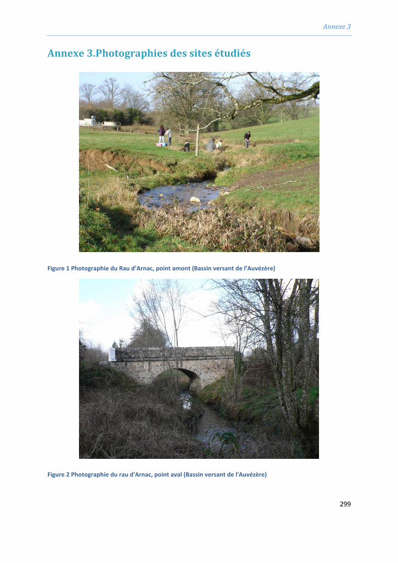
Annexe 3
Annexe 3.Photographies des sites étudiés
Figure 1 Photographie du Rau d’Arnac, point amont (Bassin versant de l’Auvézère)
Figure 2 Photographie du rau d'Arnac, point aval (Bassin versant de l'Auvézère)
299
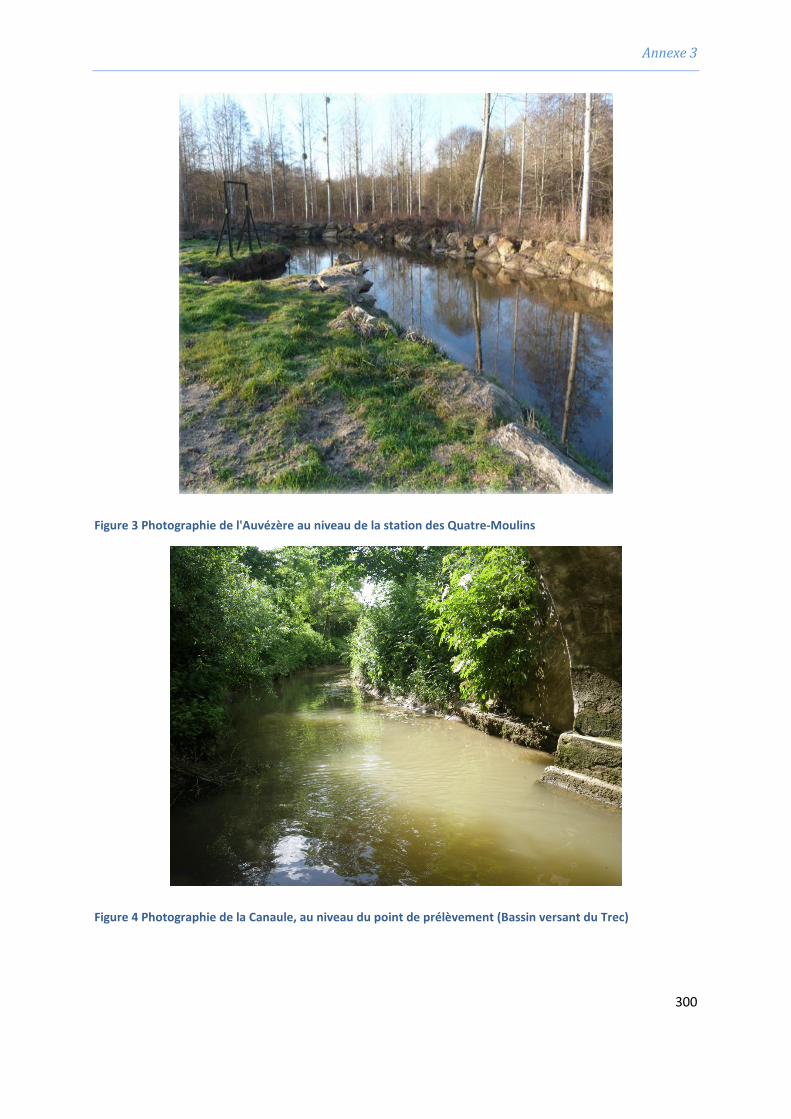
Annexe 3
Figure 3 Photographie de l'Auvézère au niveau de la station des Quatre-Moulins
Figure 4 Photographie de la Canaule, au niveau du point de prélèvement (Bassin versant du Trec)
300
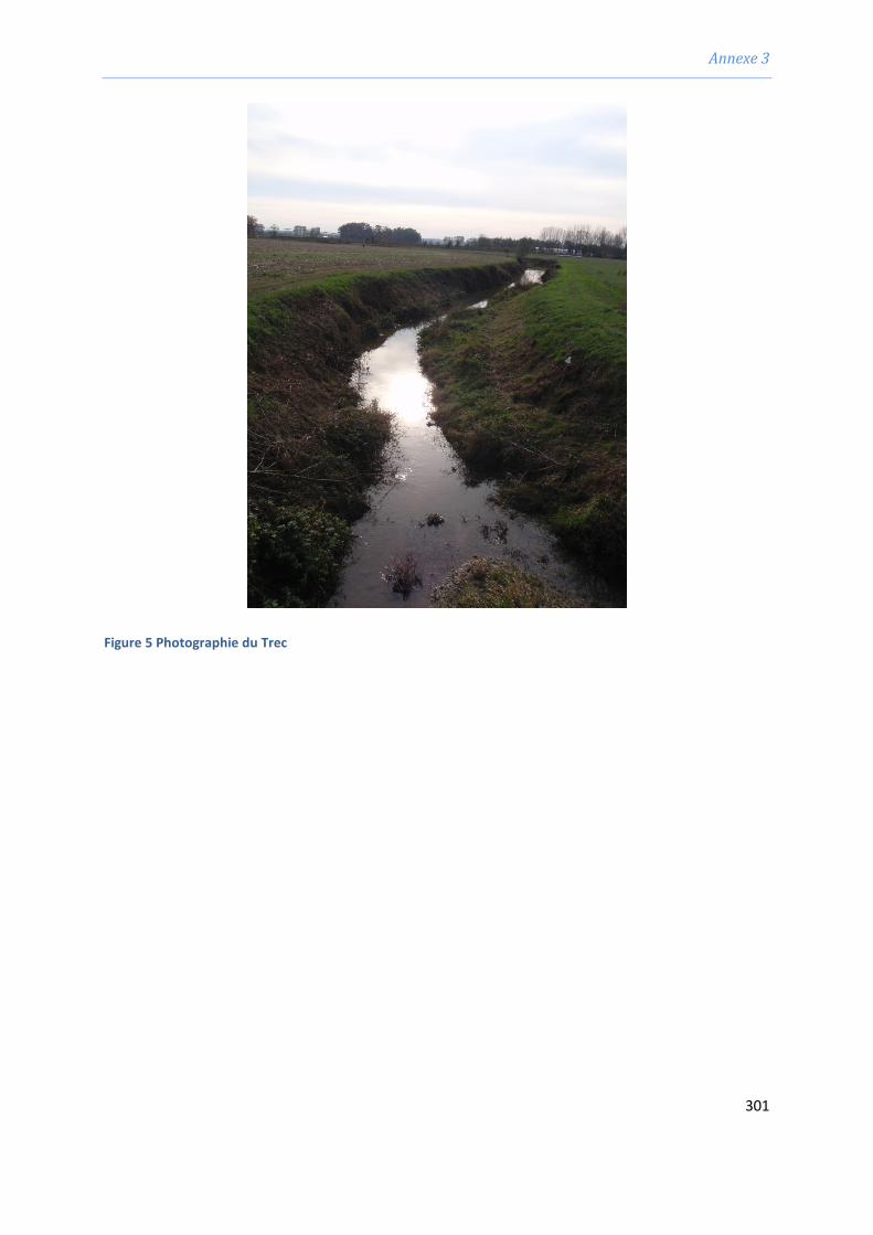
Annexe 3
Figure 5 Photographie du Trec
301
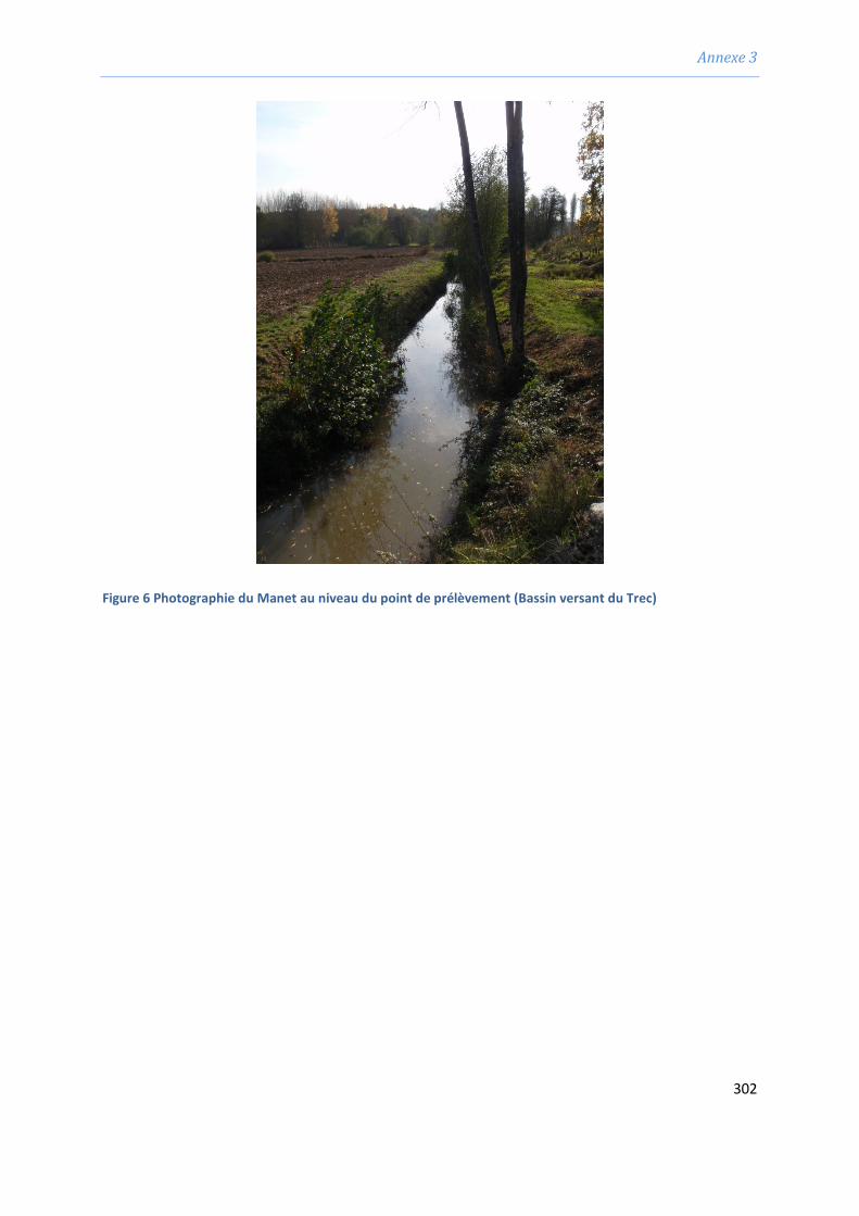
Annexe 3
Figure 6 Photographie du Manet au niveau du point de prélèvement (Bassin versant du Trec)
302
Annexe 4
Annexe 4.Valorisations
Rapport
« Etude de la contamination en pesticides des bassins versants du Trec (47) et de l’Auvézère (19) :
application de l’échantillonnage passif intégratif. Rapport intermédiaire (campagne 2012) »
Gaëlle Poulier, Nicolas Mazzella, Sophie Lissalde, Adeline Charriau, François Delmas, Rémy Buzier,
Gilles Guibaud.
Colloques (* orateur)
23rd Annual Meeting of the Society of Environmental Toxicology and Chemistry (SETAC) Europe.
“Laboratory calibration of the POCIS and application to the passive sampling of 40 polar pesticides
and metabolites in rivers of an agricultural watershed in south west of France”.
Gaëlle Poulier*, Adeline Charriau, Sophie Lissalde, Rémy Buzier, Patrice Fondanèche , Emeline
Renaudie, Nicolas Mazzella, Gilles Guibaud, François Delmas, Brigitte Delest, Aurélie Moreira,
Gwilherm Jan, Sylvia Moreira.
Poster scientifique, Glasgow, Mai 2013
43ème Congrès du Groupe Français des Pesticides (GFP). « Echantillonnage passif des pesticides dans
les cours d’eau : application dans le cadre des plans d’actions locaux de réduction des pollutions ».
Gaëlle Poulier*, Nicolas Mazzella, Gilles Guibaud, Sophie Lissalde, Adeline Charriau, Remi Buzier,
François Delmas, Brigitte Delest, Aurélie Moreira, Sylvia Moreira, Gwilherm Jan, Patrice Fondanèche,
Emeline Renaudie.
Communication orale, Albi, Mai 2013
6th international passive sampling workshop and symposium (IPSW). ”Interest of passive sampling to
improve Water Framework Directive monitoring network: Example of 40 polar pesticides monitoring
by POCIS on an agricultural watershed in France”.
Gaëlle Poulier*, Sophie Lissalde, Adeline Charriau , Rémy Buzier, Patrice Fondanèche , Karine Cléries ,
Nicolas Mazzella, François Delmas, Gilles Guibaud.
Communication orale, Bordeaux, Juin 2013
303
Annexe 4
Journées scientifiques de la Société Chimique de France (SCF). « Estimation des flux de pesticides
d’un bassin versant agricole : intérêt de la stratégie d’échantillonnage passif ».
Gaëlle Poulier, Sophie Lissalde*, Adeline Charriau, Rémy Buzier, Karine Cléries , François Delmas,
Nicolas Mazzella, Gilles Guibaud.
Communication orale, Limoges, Janvier 2014
Articles publiés
“Can POCIS be used in Water Framework Directive (2000/60/EC) monitoring networks?
A study focusing on pesticides in a French agricultural watershed”.
Gaëlle Poulier, Sophie Lissalde, Adeline Charriau , Rémy Buzier, François Delmas, Kéwin Gery, Aurélie
Moreira, Gilles Guibaud , Nicolas Mazzella.
Science of the Total Environment, volume 497-498, pages 282-292, 2014
“Estimates of pesticide concentrations and fluxes in two rivers of an extensive French multi-
agricultural watershed: application of the passive sampling strategy”.
Gaëlle Poulier, Sophie Lissalde, Adeline Charriau , Rémy Buzier, Karine Cleries, François Delmas,
Nicolas Mazzella, Gilles Guibaud
Environmental Science and Pollution Research, pages 1-14, 2014
“DGT-labile As, Cd, Cu and Ni monitoring in freshwater: Toward a framework for interpretation of in
situ deployment”.
Rémy Buzier, Adeline Charriau, David Corona, Jean-François Lenain, Patrice Fondanèche, Emmanuel
Joussein, Gaëlle Poulier, Sophie Lissalde, Nicolas Mazzella, Gilles Guibaud
Environmental Pollution 192: 52-58, 2014
Articles en préparation
“Calibration of the Chemcatcher passive sampler and proposition of a novel model for estimating
sampling rates of hydrophobic pesticides”.
Gaëlle Poulier, Adeline Charriau, Sophie Lissalde, Rémy Buzier, François Delmas, Patrice Fondanèche,
Gilles Guibaud, Nicolas Mazzella
304

Annexe 4
“Overview of the Chemcatcher for the passive sampling of various pollutants in aquatic environments.
Part A - Principles, calibration, preparation and analysis of the sampler”
Adeline Charriau, Sophie Lissalde, Gaëlle Poulier, Nicolas Mazzella, Rémy Buzier, Gilles Guibaud
“Overview of the Chemcatcher for the passive sampling of various pollutants in aquatic environments.
Part B – Field handling and environmental applications for the monitoring of pollutants and their
biological effects”
Sophie Lissalde, Adeline Charriau, Gaëlle Poulier, Nicolas Mazzella, Rémy Buzier, Gilles Guibaud
305