GarciaDiaz_MorenoMonroy(2012)

This article appeared in a journal published by Elsevier. The attached

copy is furnished to the author for internal non-commercial research

and education use, including for instruction at the authors institution

and sharing with colleagues.

Other uses, including reproduction and distribution, or selling or

licensing copies, or posting to personal, institutional or third party

websites are prohibited.

In most cases authors are permitted to post their version of the

article (e.g. in Word or Tex form) to their personal website or

institutional repository. Authors requiring further information

regarding Elsevier’s archiving and manuscript policies are

encouraged to visit:

http://www.elsevier.com/copyright

http://www.elsevier.com/copyright

Author's personal copy

Physica A 391 (2012) 1563–1574

Contents lists available at SciVerse ScienceDirect

Physica A

journal homepage: www.elsevier.com/locate/physa

Social influence, agent heterogeneity and the emergence of the urbaninformal sectorCésar García-Díaz a,b,∗, Ana I. Moreno-Monroy c

a Department of Management (ACED), University of Antwerp, Prinsstraat 13, BE-2000 Antwerp, Belgiumb Department of Industrial Engineering, Universidad de los Andes, Cra. 1 Este No. 19A-40 Bogotá, Colombiac Global Economics and Management Department, University of Groningen, Nettelbosje 2, 9747 AE Groningen, The Netherlands

a r t i c l e i n f o

Article history:Received 31 March 2011Received in revised form 24 August 2011Available online 6 September 2011

Keywords:Agent-based modelingRural–urban migrationAdaptation and self-organizing systemsPhysics and society

a b s t r a c t

We develop an agent-based computational model in which the urban informal sectoracts as a buffer where rural migrants can earn some income while queuing for higherpaying modern-sector jobs. In the model, the informal sector emerges as a result ofrural–urban migration decisions of heterogeneous agents subject to social influence in theform of neighboring effects of varying strengths. Besides using a multinomial logit choicemodel that allows for agent idiosyncrasy, explicit agent heterogeneity is introduced inthe form of socio-demographic characteristics preferred by modern-sector employers. Wefind that different combinations of the strength of social influence and the socio-economiccomposition of theworkforce lead to very different urbanization and urban informal sectorshares. In particular, moderate levels of social influence and a large proportion of ruralinhabitants with preferred socio-demographic characteristics are conducive to a higherurbanization rate and a larger informal sector.

© 2011 Elsevier B.V. All rights reserved.

1. Introduction

Developing countries experiencing the transition from a rural, agricultural society to a modern, urban one arecharacterized by a significantly large informal sector. In fact, the informal sector accounts on average for over 40% ofemployment in developing countries [1]. A substantial part of the informal sector is composed by traditional informalfirms, which can be found in sectors such as petty trading, domestic and repair services, and small-scale manufacturing [2].Such firms are characterized, among other things, by their small size, restrictions in accessing capital and other productiveresources, highly labor intensive technologies and very low productivity.1

The probabilistic job-searchmodel of Fields [3], an extension of the Harris–Todaro (HT) rural–urbanmigrationmodel [4],offers an explanation of the existence of the informal sector. The HT model assumes that migration decisions are based onexpected income differentials between rural and urban areas, net ofmigration costs, and that there is an institutionally fixedurbanminimumwage. Under these assumptions, rural to urbanmigration causes overcrowding and unemployment in cities

∗ Corresponding author at: Department of Management (ACED), University of Antwerp, Prinsstraat 13, BE-2000 Antwerp, Belgium. Tel.: +32 3 265 5064;fax: +32 3 265 4799.

E-mail address: [email protected] (C. García-Díaz).1 Dualistic models of the informal sector make a distinction between the traditional or low-end and the modern or high-end segments of the informal

sector (see Ref. [2]). The modern segment, as opposed to the traditional segment, is not always seen as a ‘last resort’ option by migrants because incomesin this segment are not necessarily low, and it can actually offer advantages such as flexible working hours. Even though throughout the paper we use theterms ‘traditional informal firm’ and ‘informal firm’ interchangeably, the reader should bear inmind that ourmodel is more compatible with the traditionalsegment of the informal sector.

0378-4371/$ – see front matter© 2011 Elsevier B.V. All rights reserved.doi:10.1016/j.physa.2011.08.057


1564 C. García-Díaz, A.I. Moreno-Monroy / Physica A 391 (2012) 1563–1574

asmigration rates exceed urban job creation rates. The HTmodel, however, tends to overestimate the urban unemploymentrate by ignoring the role of the informal sector. In the model by Fields, the informal sector acts as an economic buffer. Whenrural workers have no chances of finding a job in the higher paying urban modern sector, the urban informal sector acts asa ‘waiting’ sector: migrants are willing to accept some sort of income in the urban informal sector as long as they can live inurban areas and thus increase their chances to enter the modern sector.

The HT and Fields partial equilibrium models provide a rationale for the study of migration decisions. However, thesemodels assume that agents are homogeneous and that they act independently of each other. Extensive empirical literatureon rural–urbanmigration has shown that the effects of social influence and agent heterogeneity are by nomeans negligible,and can in fact be as important in migration decisions as income differentials [3,5,6].

Our rural–urban migration approach is completely dynamic. The innovativeness of it lies on explaining the emergenceof the informal sector by taking into account both the role of social influence and the socio-demographic characteristics ofagents that, embedded in an employment market, adaptively consider the decision to migrate. It is our aim to explore howthe strength of social influence effects may facilitate or hamper the evolutionary migration process. For such a purpose, webuild an agent-based computational model (ABM). ABMs have also been used in studies of informal settlement growth (e.g.Refs. [7,8]), which is partly determined by increasing rural–urban migration. This line of research is different in naturefrom ours, since its interest lies on the spatial properties of urban growth [9,10] and does not necessarily emphasizeeither the representation of labor-related economic incentives to migrate or the economic implications of migrationdecisions.

In the model to be presented here, the probabilistic job-search elements of Fields’ model are incorporated explicitly.Urbanization and the urban informal sector arise endogenously from migration decisions of heterogeneous agents that aresubject to social influence through neighboring effects. Agent heterogeneity is introduced firstly by modeling migrationdecisions according to a multinomial logit choice model that allows for agent idiosyncrasy in the decision-making process.A more explicit form of heterogeneity is introduced in the form of certain socio-demographic characteristics, which areassumed to be preferred bymodern-sector employers (i.e., predilection for young workers, or those of a specific gender. SeeRef. [11]). Social influence, in turn, is introduced by making migration decisions dependent on the location of the agent’scontacts (i.e., agent’s social network). We explore the effect of social influence on urbanization and the size of the urbaninformal sector by having neighboring effects of varying strengths.

Our model makes explicit the adaptive, backward-looking fashion of agents in rural–urban migration dynamics, incontrast to the sophisticated forward-looking fashion of optimizing agents [12,13]. In particular, a related paper [14] definesrural–urbanmigration as a binary discrete choice problem subject to neighboring effects of the Ising-like type. The outcomesof the model by Silveira et al. [14] constitute a locus of successive equilibrium points calculated under the assumptionthat agents are utility maximizers, and recomputed after the stochastic disturbances generated by neighboring effects.2Furthermore, themodel of Ref. [14] offers only a partial representation of urbanization in developing countries, as it assumesconstant urban unemployment rates while ignoring the existence of the informal sector.

In our model, adaptive agents such as modern firms and workers do their best according to past (immediate time step)information in order to decide both the required labor force and location in the next time step [15,16]. Past availableinformation in our model refers to (i) public information regarding the manufacturing good’s price, the rural, urbanmodernand informal-sector wages, and the agent composition in the urban sector (employed in the modern sector, unemployed,and employed in the informal sector), and (ii) the fact that each individual is aware of the immediate past location of his/herneighbors.

2. The model

We consider an economy with a total population NT distributed across a lattice that represents agent contacts. Thereare three sectors: an agricultural sector, a modern sector, and an informal sector. At time t , each sector has a populationdenoted by Nr,t , Nm,t and Ns,t , respectively. The agricultural sector operates exclusively in rural areas and employs all theavailable rural population (i.e., there is no rural unemployment). The modern and informal sectors operate in urban areasexclusively. Rural residents have no chance of obtaining modern-sector jobs, but once they migrate their chances increase.Thus, a resident of an urban area may be either (i) employed in the modern sector, (ii) unemployed with no income whileengaged in full-time job seeking, or (iii) engaged in the informal sector, receiving some income at the expense of a reducedjob search [3].

2.1. The agricultural sector

Empirical evidence on the nature of scale returns in agriculture ismixed, at best [17–20]. However, core economicmodels(e.g., geographical economics) use constant returns to scale in agriculture as a standard assumption [21]. Therefore, for the

2 Technically speaking, the model of Ref. [14] assumes that the system can re-compute its equilibrium point just before the next stochastic disturbanceof a migration decision takes place.


C. García-Díaz, A.I. Moreno-Monroy / Physica A 391 (2012) 1563–1574 1565

sake of convenience, we assume that agriculture exhibits constant returns to scale.3 The output of any farm at time t , yr,t , ischaracterized by:

yr,t = ArCr,t . (1)

Coefficient Ar is a scale parameter, and Cr,t represents the number of farm workers. We assume that the agricultural sectoris perfectly competitive. Therefore, the rural wage is equal to the marginal product, wr,t = pr,tAr , for all t . The agriculturalgood price pr,t is set equal to 1, so that agriculture is the ‘numéraire’ [14]. The price of the modern-sector good, pm,t , isdetermined in terms of agricultural good units.

2.2. The modern sector

The output of any modern firm at time t , ym,t , is:

ym,t = AmCαmm,t . (2)

Coefficient Am is a scale parameter, and 0 < αm < 1. Cm,t represents the number of workers [4,14]. At the beginningof time t , the firm has to decide on the amount of labor to hire based on the last observed wage value wm,t−1. The firmcomputes profits according to:

πm,t = pm,t−1ym,t − wm,t−1Cm,t . (3)

Assuming pm,t−1 and wm,t−1 constant for the firm’s profit optimization problem in period t , the first-order conditionyields:

Cm,t =

αmAmpm,t−1

wm,t−1

11−αm

. (4)

The price is calculated assuming that the relative scarcity between the modern-sector and the agricultural goods definesthe modern-sector good price (see Refs. [4,14]):

pm,t = λ1

Yr,t

Ym,t

λ2

, (5)

where Ym,t = i=Zmi=1 yim,t , Yr,t = i=Zr

i=1 yir,t , Zm is the number of modern firms, Zr is the number of farms, and λ1 and λ2are scale parameters. The determination of wage at time t , wm,t depends on a standard labor supply curve, a function of theamount of people employed at time t , Fm,t :

wm,t = βmFγmm,t , (6)

whereβm is a scale parameter andγm is thewage–labor elasticity.4 It is important to note that Fm,t = mini=Zm

i=1 Cim,t ,Nu,t

,

where Nu,t = Nm,t + Ns,t is the total urban population.

2.3. The informal sector

Following the ideas of Fields [3], taking an informal job will consume some search time and thereby reduce the chancesof finding a modern-sector job by a factor η, 0 < η < 1. We establish that people in the informal sector receive an incomeequal to ws,t that is highly volatile. This volatility is justified by at least three reasons. First, given their lack of access tocredit, low productivity and low returns, informal firms offer little possibilities for capitalization, which is a key ingredientfor productivity and output growth [22]. Second, informal firms are constantly threatened to be shut down or punishedby authorities. And third, informal firms are subject to fierce competition due to the very low entry requirements in theinformal sector.

Furthermore, since informal firms are assumed to be less efficient than modern firms, we place an upper limit on theirwage, implying that it can never be higher than the wage in the modern sector. This is in line with empirical evidence on

3 What would the implications of using non-constant returns be? On the one hand, under decreasing returns to scale farms would compute optimallabor requirements, which in turn would give rise to rural unemployment, and a consequent increase in the incentives for rural–urban migration. On theother hand, the assumption of increasing returns at the farm level is incompatible with the assumption of perfect competition in the agricultural sector.Assuming imperfect competition in the agricultural sector does not seem to be a suitable assumption for the case of the agricultural sector in an economyin the first stages of industrialization.4 Notice that, unlike the rural sector, we are not using the equilibrium-related marginal product concept for the modern sector, due to the adaptive way

in which the firms’ number of workers is computed. Instead, we model how the ‘demand’ (Eq. (4)) and ‘supply’ (Eq. (6)) adjust dynamically.



the existence of a persistent wage gap between the modern and the (traditional) informal sector.5 Furthermore, if informalfirms supply a different consumer base (e.g., low incomepeople) thanmodern firms [24], the production decisions ofmodernfirms are independent of informal-sector prices. Thus, we assume:

ws,t = τws,t−1 + (1 − τ )wm,t−1t , (7)

where τ is a constant, 0 < τ < 1, and t is a probabilistic term, uniformly distributed in [0, 1]. Coefficient τ is usedto compute a moving average between the historical value and a (stochastic) fraction of the modern-sector wage. Thisexpression captures the idea that income in the informal sector is highly volatile and may be either lower or higher thanrural income at any point in time [25]. The initial condition is ws,0 = 0.

2.4. Migration dynamics

Ref. [26] outlines two important reasonswhy social networks influencemigration decisions. First,migrants that belong tothe same social network may help each other reduce migration costs and identify job opportunities at the destination, themore so if they belong to the same community of origin. In our model, this translates into a direct effect of the agent’sneighborhood in his/her decision to migrate. Second, if migrating is seen as a positive sign of ability, a person whoseneighbors have migrated is more likely to migrate in order not to feel ‘inferior’. This peer pressure at the origin mightbe stronger for migrants with similar age, gender and education, and could lead to a snowball effect: a small initiationof migration could lead to a large wave of migration in the future, especially of migrants with similar profiles.6,7 We capturethis effect by introducing agent heterogeneity in the formof demographic traits (age, gender, et cétera) thatmake oneworkerpreferable over another one with different characteristics in the eyes of a modern-sector employer.

Thus, in the model at every time step, a share Act of the total population is enabled to migrate. Every agent inthe resulting group of potential migrants then decides where to migrate by taking into consideration the difference inexpected earnings [4], and the location of her/his neighboring contacts (the eight surrounding neighbors, known as MooreNeighborhood). The compound preferential effect toward sector x, x ∈ m, s, r for individual i is accounted by:

uix,t = κ1E(Wx,t) + κ2

j∈Ωi,t−1

ωj,t−1/Ωi,t−1

, (8)

where E(Wx,t) is the expectedwage value,Ωi,t is the set of neighbors of i at time t , |·| is the cardinality of a set, andωj,t = 1 if jshares the same locationwith i-at time t-,ωj,t = 0 otherwise. Coefficients κ1 and κ2 areweight parameters of the importanceof expected wage values and the location of the agent’s neighbors on the agent’s utility, respectively. In the remainder ofthe paper we refer to coefficient κ2 as ‘social influence’. A value of κ2 = 0 implies that agents base their migration decisionssolely on expected income differentials. The larger the value of κ2, the stronger the relative impact of social influence on theagent’s migration decisions. We refer to κ2 = 1 as ‘moderate social influence’, κ2 = 2 as ‘strong social influence’ and κ2 = 3as ‘very strong social influence’.

The decision-making process is realized through a logit choice model (e.g., Refs. [27,28]). The probability px,t of choosingx as a new location is:

px,t = exp(φuix,t)

k∈r,m,sexp(φui

k,t), (9)

where φ is a parameter that indicates how sensitive an individual is to utility variations.8Vacancies are filled first with available preferred individuals who have priority over non-preferred ones.9 Let us denote

Nm/e,t , Nm/ne,t , Ns/e,t and Ns/ne,t as the preferred and non-preferred agent populations of the modern and informal sectors,

5 Modeling the reasons why such a segmentation exists is not germane to this paper. It is still worthwhile mentioning some of the common explanationsof why modern-sector wages do not diminish in the presence of an excess of labor supply: first, modern-sector workers are paid an ‘efficiency premium’that diminishes the cost of monitoring; second, trade unions successfully set wages at a higher level in the modern sector than those prevailing in theinformal sector; and finally, existing labor market regulations set a minimum wage or other forms of obligatory worker compensation which result inhigher wages in the modern sector [23].6 It is important to note that peer pressure at the origin can act in the opposite direction if migration has a negative connotation.7 A third factor mentioned by Chen et al. [26] is the opportunity cost of migrating: More people migrating out of the village leads to more agricultural

resources and opportunities left for those who stay. In our model, this is captured by the effect of migration on relative prices (Eq. (5)).8 The value of φ was calibrated assuming that, under the baseline values of the model, and setting ws,t = 0∀t , Ns,t/NT should be insignificant or

close to zero. That is, (almost) nobody would be willing to move to the informal sector if chances for getting a modern-sector job are reduced, and atthe same time the agent perceives a (certain) zero income. On the contrary, high values of φ force Ns,t to be zero, but at the expense of eliminatingagent heterogeneity (idiosyncrasy) in the migration decision. We use φ = 5, which allows keeping agent heterogeneity while making Ns,t/NT very small(approximately 1.5%).9 We assume that in the case of downsizing, every employee would have the same probability of being fired.



Table 1Constants.

Parameter Description Value

Zm Number of modern firms 10Zr Number of farms 10Am Scale parameter modern sector 10Ar Scale parameter agriculture 1Act Migration prob. 0.15PrMn Prob. of being in modern sector (t = 0) 0.15PrEmp In modern sector, prob. of employment(t = 0) 1PrEd Prob. of being preferred 0.5κ1 Expected wage scale parameter 1η Probability-reducing parameter 0.5φ Logit function parameter 5τ Informal-sector income parameter 0.5

Table 2Parameter value ranges.

Parameter Description Baseline Range

NT Population size 752 502, 752,1002

αm Modern-sector labor-to-output elasticity 0.3 0.2, 0.3, 0.4λ1 Price scale parameter 15 10, 15, 20λ2 Price scale parameter 0.3 0.2, 0.3, 0.4βm Labor supply scale parameter 1 0.5, 1, 2γm Labor supply elasticity 0.1 0.05, 0.1, 0.3κ2 Social influence 0 0, 1, 2, 3

accordingly. Also, E(Wx/e,t) and E(Wx/ne,t), x ∈ r,m, s are the expected wage values for the preferred and non-preferredagents respectively. The computation of expected earnings in the rural sector is:

E(Wr/e,t) = E(Wr/ne,t) = wr . (10)

Let us also denote the preferred, modern-sector employed population as Fm/e,t . It is important to note that Fm/e,t ≤ Nm/e,t ,since the total preferred hired population cannot exceed the total available preferred population. Likewise, Fm,t − Fm/e,t ≤Nm/ne,t . The remaining expected wages take into account both the factor η and the agent type:

E(Wm/e,t) = wm,t−1

Fm/e,t−1

Nm/e,t−1 + ηNs/e,t−1

, (11)

E(Wm/ne,t) = wm,t−1

Fm,t−1 − Fm/e,t−1

Nm/ne,t−1 + ηNs/ne,t−1

. (12)

E(Ws/e,t) = wm,t−1θe,t + ws,t−1(1 − θe,t), (13)

E(Ws/ne,t) = wm,t−1θne,t + ws,t−1(1 − θne,t). (14)

Coefficients θe,t and θne,t are the probabilities of finding a job in the modern sector by an agent located in the informalsector, given that the agent is either preferred or non-preferred, respectively [3]:

θe,t = ηFm/e,t−1

Nm/e,t−1 + ηNs/e,t−1, (15)

θne,t = ηFm,t−1 − Fm/e,t−1

Nm/ne,t−1 + ηNs/ne,t−1. (16)

As initial conditions, the model assumes (i) a percentage of the total population in the modern sector (defined by theprobability PrMn), out of which a percentage is employed (defined by PrEmp), (ii) Ns,0 = 0. Tables 1 and 2 present a summaryof the constant and parameter values used in the model.

3. Results

3.1. Baseline model

The baseline values of the model are shown in Table 2. Under no neighbor influence (κ2 = 0), we explore the variationeffects of the remaining six parameters using regression (meta) models [29] with the percentage of population employed in



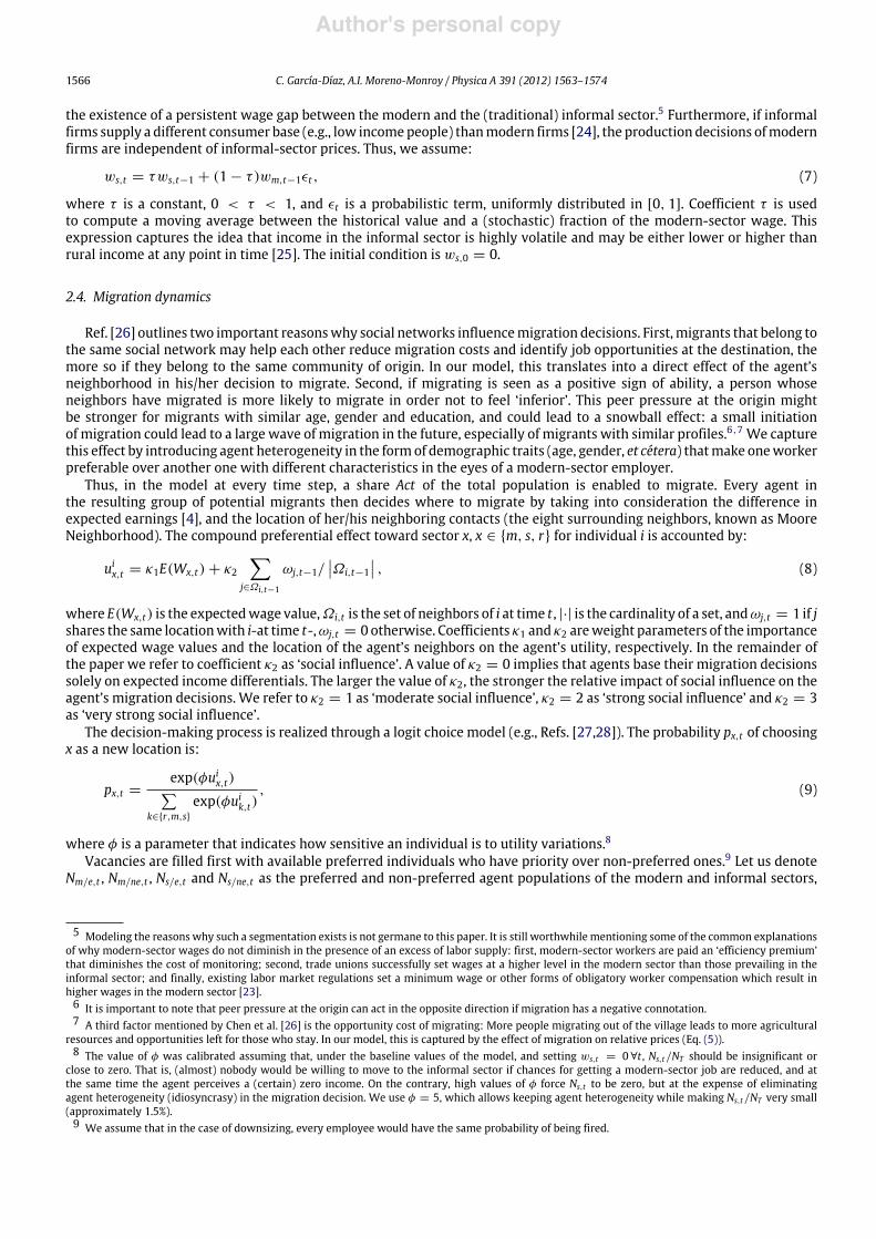
Fig. 1. A sample simulation run with baseline model values. The population employed in the informal sector Ns starts to rise and then oscillatesapproximately between 1000 and 4000 agents, according to perceived values of the informal sector wageWs .

Table 3OLSwith robust standard errorswith the percentage of population employed in the informal sector as a dependent variable (modelwith no social influence).Errors are in parenthesis.

Ind. variable OLS estimates√NT 0.632(0.009)

αm −25.952(2.072)λ1 −0.279(0.041)λ2 4.798(2.098)βm 24.782(0.311)γm 168.343(1.790)Constant −52.965(1.275)F6,7283 4197.32Number Obs. 7290R2 0.7827

the informal sector as dependent variable. 150 time steps were enough to observe convergence. A typical run that depictsthe behavior of the informal-sector population and corresponding wages is illustrated in Fig. 1. The six parameters gave atotal of 36 combination values. Running each combination 10 times, we obtain a sample size of 7290 simulation runs. Wetook data points for the dependent variable as the average value over the last 50 time steps.We ran an ordinary least-squares(OLS) regression with robust standard errors.10

Coefficient estimates are presented in Table 3. The percentage of population employed in the informal sector, Ns/NT , ispositively correlated to changes in lattice size. Results also reveal that Ns/NT is sensitive – and negatively correlated – tochanges in αm. An increase in αm results in a higher production capacity in the modern sector, which increases its laborforce demand. Some of these vacancies are filled with informal-sector workers which consequently reduces the size of theinformal sector.

A similar line of reasoning can be applied with respect to changes in the price scale parameter λ1, since the dependentvariable is negatively correlated to it. Coefficient λ2 is positive but has a non-significant effect with the tested sample size,which indicates that its effect is low.Moreover, themodel’s outcome is also highly sensitive to changes in bothβm and γm. Asexpected, increases in both βm and γm lead to a reduction in the hired modern-sector labor force, which redirects migrationtoward the informal sector and consequently inflates its population.

3.2. Social influence effects

Next, we take the baseline model (Table 2) and add social influence (κ2 > 0). For each scenario with a different κ2 valuewe collected 300 runs. We observed that an increase in social influence delays convergence. Moderate values of κ2 tend

10 Robust standard errors are used since diagnosis tests reveal the presence of heteroscedasticity. Alternatively, using weighted-least squares yieldedsimilar results. Residuals also appear to be non-normal, but this is overcome by using a very large sample size.



Fig. 2. Average population employed in the informal sector under different values of social influence. Continuous lines indicate confidence intervals ofthe mean at significance = 99%.

Fig. 3. Percentages over the total population ofmodern-sector job seekers (‘m+s’) and unemployment (‘m only’) under different values of social influence.

to boost the size of the informal sector. The independent effect of moderate social influence is considerable, as it almostdoubles the size of the informal sector (compare the values of Ns for the ‘k2 = 0’ and ‘k2 = 1’ lines in Fig. 2).

Interestingly, higher values of the social influence coefficient lead to the opposite effect, namely, a reduction of the sizeof the informal sector when compared to the baseline scenario. Stronger social influence makes it more difficult for agentsto overcome the inertia of staying in the original location. In this case, even in the presence of positive expected rural–urbanincome differentials, agents are inclined to stay in rural areas given that most of their neighbors share the same location.This inertia is very persistent over time, as can be seen from the rightward shift of the κ2 = 2 curve in Fig. 2.

For an additional inspection of results we use two definitions: (i) modern-sector job seekers, i.e., agents in the urbaninformal sector together with the urban unemployed population (‘m + s’), and (ii) the (urban) unemployed population, ‘monly’. The size of the informal sector is thus the difference between the ‘m + s’ and the ‘m only’ lines. Fig. 3 illustrates thatmoderate social influence reduces unemployment while increasing employment in the informal sector. However, undervery strong social influence (κ2 = 3) this result is partially reversed because employment in the informal sector is loweredas a result of more people being engaged in full-time modern-sector job search.



t = 0 t = 10

t = 20 t = 150

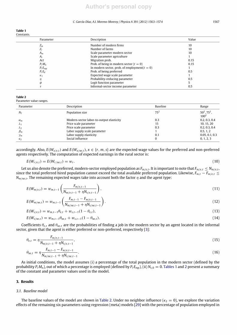
Fig. 4. Spatial effects of moderate social influence (κ2 = 1). White = rural, gray = informal, black = modern-sector.

t = 0 t = 1000

t = 5000 t = 7500

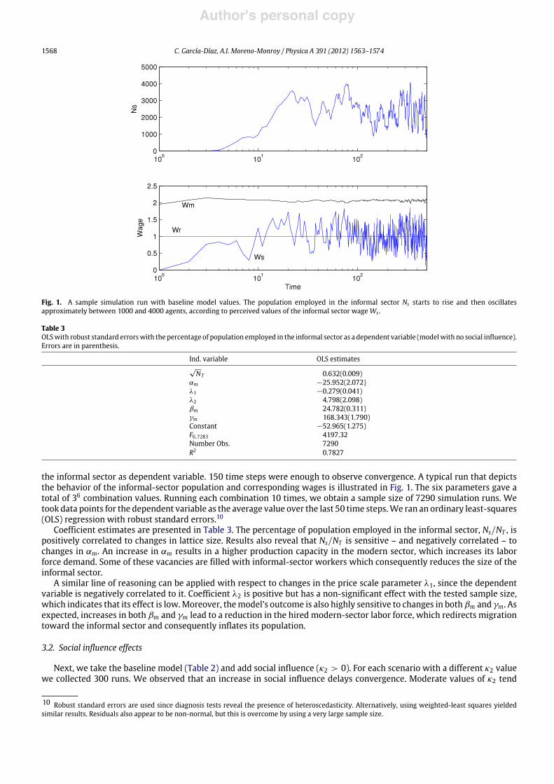
Fig. 5. Spatial effects of strong social influence (κ2 = 2). White = rural, gray = informal, black = modern-sector.

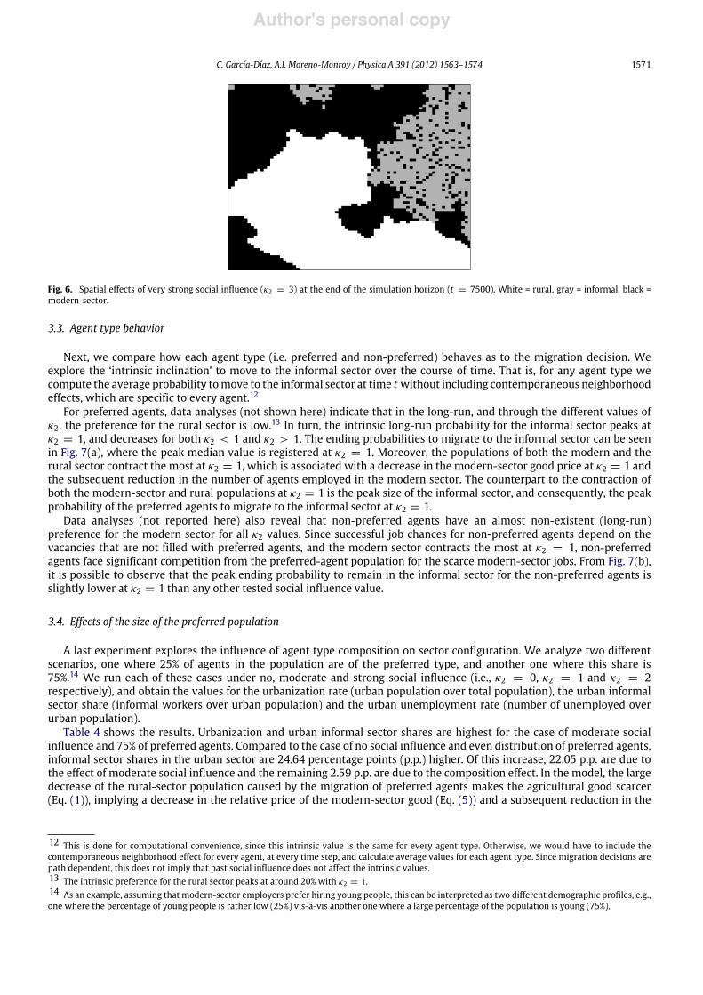
As can be seen in Fig. 4 for the case of moderate social influence, once the inertia of the initial (rural) location is broken,agents and their neighbors are fairly distributed in different sectors (e.g., rural, modern and informal) across the lattice, sothat only loose clustering is observed. For the case of strong social influence, however, clusters of agents in the rural sectorpersist (see the white patches in Fig. 5), and act as an attraction force for agents that either migrate back from urban to ruralareas or stay in rural areas. The extreme case of this spatial segregation is clearly visible in Fig. 6.

The interesting results under the case of very strong social influence deserve a deeper examination. Since the effect ofvery strong social influence (κ2 = 3) on the size of the informal sector might be influenced by changes in the potentialoutflow of migrants, we ran two additional tests: the first one was related to variations in the Act coefficient (0.15, 0.30,0.50, 0.75) in order to inspect if the strength of network ties effect is maintained when more agents are allowed to checkwhether they want to migrate or not. The second test checks the model’s sensitivity to variations in the multinomial logitequation parameter φ (3, 5, 15, 25). Neither tests revealed significant changes with respect to the results reported here.11

11 These results are available upon request.



Fig. 6. Spatial effects of very strong social influence (κ2 = 3) at the end of the simulation horizon (t = 7500). White = rural, gray = informal, black =modern-sector.

3.3. Agent type behavior

Next, we compare how each agent type (i.e. preferred and non-preferred) behaves as to the migration decision. Weexplore the ‘intrinsic inclination’ to move to the informal sector over the course of time. That is, for any agent type wecompute the average probability tomove to the informal sector at time t without including contemporaneous neighborhoodeffects, which are specific to every agent.12

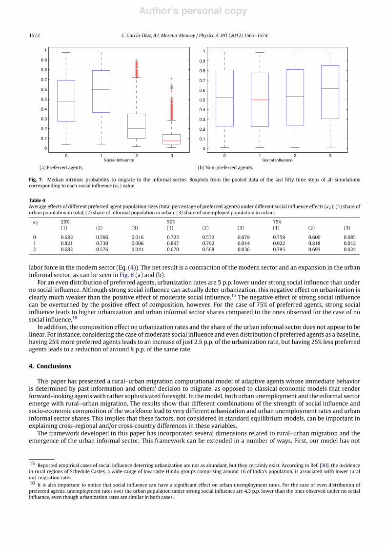
For preferred agents, data analyses (not shown here) indicate that in the long-run, and through the different values ofκ2, the preference for the rural sector is low.13 In turn, the intrinsic long-run probability for the informal sector peaks atκ2 = 1, and decreases for both κ2 < 1 and κ2 > 1. The ending probabilities to migrate to the informal sector can be seenin Fig. 7(a), where the peak median value is registered at κ2 = 1. Moreover, the populations of both the modern and therural sector contract the most at κ2 = 1, which is associated with a decrease in the modern-sector good price at κ2 = 1 andthe subsequent reduction in the number of agents employed in the modern sector. The counterpart to the contraction ofboth the modern-sector and rural populations at κ2 = 1 is the peak size of the informal sector, and consequently, the peakprobability of the preferred agents to migrate to the informal sector at κ2 = 1.

Data analyses (not reported here) also reveal that non-preferred agents have an almost non-existent (long-run)preference for the modern sector for all κ2 values. Since successful job chances for non-preferred agents depend on thevacancies that are not filled with preferred agents, and the modern sector contracts the most at κ2 = 1, non-preferredagents face significant competition from the preferred-agent population for the scarce modern-sector jobs. From Fig. 7(b),it is possible to observe that the peak ending probability to remain in the informal sector for the non-preferred agents isslightly lower at κ2 = 1 than any other tested social influence value.

3.4. Effects of the size of the preferred population

A last experiment explores the influence of agent type composition on sector configuration. We analyze two differentscenarios, one where 25% of agents in the population are of the preferred type, and another one where this share is75%.14 We run each of these cases under no, moderate and strong social influence (i.e., κ2 = 0, κ2 = 1 and κ2 = 2respectively), and obtain the values for the urbanization rate (urban population over total population), the urban informalsector share (informal workers over urban population) and the urban unemployment rate (number of unemployed overurban population).

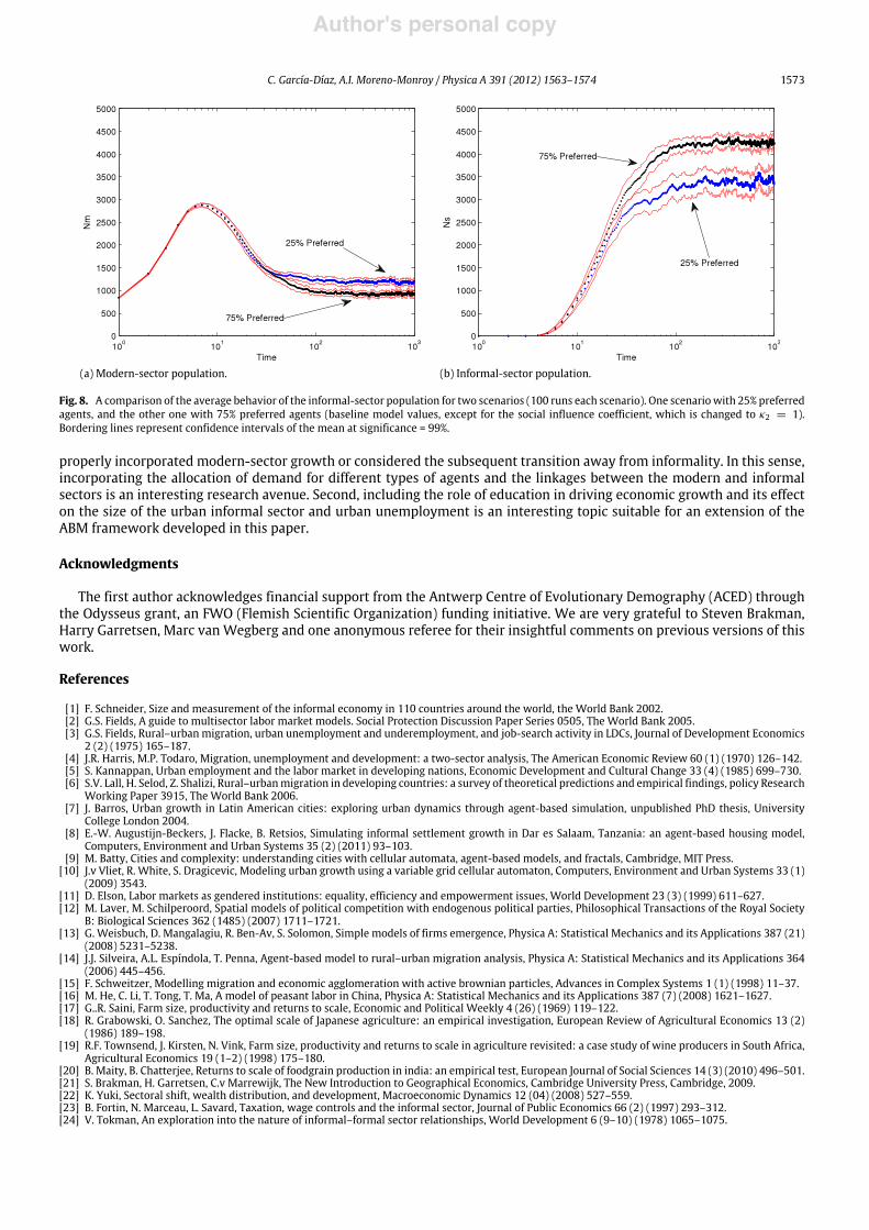
Table 4 shows the results. Urbanization and urban informal sector shares are highest for the case of moderate socialinfluence and 75% of preferred agents. Compared to the case of no social influence and even distribution of preferred agents,informal sector shares in the urban sector are 24.64 percentage points (p.p.) higher. Of this increase, 22.05 p.p. are due tothe effect of moderate social influence and the remaining 2.59 p.p. are due to the composition effect. In the model, the largedecrease of the rural-sector population caused by the migration of preferred agents makes the agricultural good scarcer(Eq. (1)), implying a decrease in the relative price of the modern-sector good (Eq. (5)) and a subsequent reduction in the

12 This is done for computational convenience, since this intrinsic value is the same for every agent type. Otherwise, we would have to include thecontemporaneous neighborhood effect for every agent, at every time step, and calculate average values for each agent type. Since migration decisions arepath dependent, this does not imply that past social influence does not affect the intrinsic values.13 The intrinsic preference for the rural sector peaks at around 20% with κ2 = 1.14 As an example, assuming that modern-sector employers prefer hiring young people, this can be interpreted as two different demographic profiles, e.g.,one where the percentage of young people is rather low (25%) vis-á-vis another one where a large percentage of the population is young (75%).



(a) Preferred agents. (b) Non-preferred agents.

Fig. 7. Median intrinsic probability to migrate to the informal sector. Boxplots from the pooled data of the last fifty time steps of all simulationscorresponding to each social influence (κ2) value.

Table 4Average effects of different preferred agent population sizes (total percentage of preferred agents) under different social influence effects (κ2); (1) share ofurban population in total, (2) share of informal population in urban, (3) share of unemployed population in urban.

κ2 25% 50% 75%(1) (2) (3) (1) (2) (3) (1) (2) (3)

0 0.683 0.596 0.016 0.722 0.572 0.079 0.759 0.600 0.0851 0.821 0.730 0.006 0.897 0.792 0.014 0.922 0.818 0.0122 0.682 0.576 0.041 0.670 0.568 0.036 0.795 0.693 0.024

labor force in the modern sector (Eq. (4)). The net result is a contraction of the modern sector and an expansion in the urbaninformal sector, as can be seen in Fig. 8 (a) and (b).

For an even distribution of preferred agents, urbanization rates are 5 p.p. lower under strong social influence than underno social influence. Although strong social influence can actually deter urbanization, this negative effect on urbanization isclearly much weaker than the positive effect of moderate social influence.15 The negative effect of strong social influencecan be overturned by the positive effect of composition, however. For the case of 75% of preferred agents, strong socialinfluence leads to higher urbanization and urban informal sector shares compared to the ones observed for the case of nosocial influence.16

In addition, the composition effect on urbanization rates and the share of the urban informal sector does not appear to belinear. For instance, considering the case ofmoderate social influence and even distribution of preferred agents as a baseline,having 25% more preferred agents leads to an increase of just 2.5 p.p. of the urbanization rate, but having 25% less preferredagents leads to a reduction of around 8 p.p. of the same rate.

4. Conclusions

This paper has presented a rural–urban migration computational model of adaptive agents whose immediate behavioris determined by past information and others’ decision to migrate, as opposed to classical economic models that renderforward-looking agentswith rather sophisticated foresight. In themodel, both urban unemployment and the informal sectoremerge with rural–urban migration. The results show that different combinations of the strength of social influence andsocio-economic composition of the workforce lead to very different urbanization and urban unemployment rates and urbaninformal sector shares. This implies that these factors, not considered in standard equilibrium models, can be important inexplaining cross-regional and/or cross-country differences in these variables.

The framework developed in this paper has incorporated several dimensions related to rural–urban migration and theemergence of the urban informal sector. This framework can be extended in a number of ways. First, our model has not

15 Reported empirical cases of social influence deterring urbanization are not as abundant, but they certainly exist. According to Ref. [30], the incidencein rural regions of Schedule Castes, a wide-range of low caste Hindu groups comprising around 16 of India’s population, is associated with lower ruralout-migration rates.16 It is also important to notice that social influence can have a significant effect on urban unemployment rates. For the case of even distribution ofpreferred agents, unemployment rates over the urban population under strong social influence are 4.3 p.p. lower than the ones observed under no socialinfluence, even though urbanization rates are similar in both cases.



(a) Modern-sector population. (b) Informal-sector population.

Fig. 8. A comparison of the average behavior of the informal-sector population for two scenarios (100 runs each scenario). One scenariowith 25% preferredagents, and the other one with 75% preferred agents (baseline model values, except for the social influence coefficient, which is changed to κ2 = 1).Bordering lines represent confidence intervals of the mean at significance = 99%.

properly incorporated modern-sector growth or considered the subsequent transition away from informality. In this sense,incorporating the allocation of demand for different types of agents and the linkages between the modern and informalsectors is an interesting research avenue. Second, including the role of education in driving economic growth and its effecton the size of the urban informal sector and urban unemployment is an interesting topic suitable for an extension of theABM framework developed in this paper.

Acknowledgments

The first author acknowledges financial support from the Antwerp Centre of Evolutionary Demography (ACED) throughthe Odysseus grant, an FWO (Flemish Scientific Organization) funding initiative. We are very grateful to Steven Brakman,Harry Garretsen, Marc van Wegberg and one anonymous referee for their insightful comments on previous versions of thiswork.

References

[1] F. Schneider, Size and measurement of the informal economy in 110 countries around the world, the World Bank 2002.[2] G.S. Fields, A guide to multisector labor market models. Social Protection Discussion Paper Series 0505, The World Bank 2005.[3] G.S. Fields, Rural–urban migration, urban unemployment and underemployment, and job-search activity in LDCs, Journal of Development Economics

2 (2) (1975) 165–187.[4] J.R. Harris, M.P. Todaro, Migration, unemployment and development: a two-sector analysis, The American Economic Review 60 (1) (1970) 126–142.[5] S. Kannappan, Urban employment and the labor market in developing nations, Economic Development and Cultural Change 33 (4) (1985) 699–730.[6] S.V. Lall, H. Selod, Z. Shalizi, Rural–urbanmigration in developing countries: a survey of theoretical predictions and empirical findings, policy Research

Working Paper 3915, The World Bank 2006.[7] J. Barros, Urban growth in Latin American cities: exploring urban dynamics through agent-based simulation, unpublished PhD thesis, University

College London 2004.[8] E.-W. Augustijn-Beckers, J. Flacke, B. Retsios, Simulating informal settlement growth in Dar es Salaam, Tanzania: an agent-based housing model,

Computers, Environment and Urban Systems 35 (2) (2011) 93–103.[9] M. Batty, Cities and complexity: understanding cities with cellular automata, agent-based models, and fractals, Cambridge, MIT Press.

[10] J.v Vliet, R. White, S. Dragicevic, Modeling urban growth using a variable grid cellular automaton, Computers, Environment and Urban Systems 33 (1)(2009) 3543.

[11] D. Elson, Labor markets as gendered institutions: equality, efficiency and empowerment issues, World Development 23 (3) (1999) 611–627.[12] M. Laver, M. Schilperoord, Spatial models of political competition with endogenous political parties, Philosophical Transactions of the Royal Society

B: Biological Sciences 362 (1485) (2007) 1711–1721.[13] G. Weisbuch, D. Mangalagiu, R. Ben-Av, S. Solomon, Simple models of firms emergence, Physica A: Statistical Mechanics and its Applications 387 (21)

(2008) 5231–5238.[14] J.J. Silveira, A.L. Espíndola, T. Penna, Agent-based model to rural–urban migration analysis, Physica A: Statistical Mechanics and its Applications 364

(2006) 445–456.[15] F. Schweitzer, Modelling migration and economic agglomeration with active brownian particles, Advances in Complex Systems 1 (1) (1998) 11–37.[16] M. He, C. Li, T. Tong, T. Ma, A model of peasant labor in China, Physica A: Statistical Mechanics and its Applications 387 (7) (2008) 1621–1627.[17] G..R. Saini, Farm size, productivity and returns to scale, Economic and Political Weekly 4 (26) (1969) 119–122.[18] R. Grabowski, O. Sanchez, The optimal scale of Japanese agriculture: an empirical investigation, European Review of Agricultural Economics 13 (2)

(1986) 189–198.[19] R.F. Townsend, J. Kirsten, N. Vink, Farm size, productivity and returns to scale in agriculture revisited: a case study of wine producers in South Africa,

Agricultural Economics 19 (1–2) (1998) 175–180.[20] B. Maity, B. Chatterjee, Returns to scale of foodgrain production in india: an empirical test, European Journal of Social Sciences 14 (3) (2010) 496–501.[21] S. Brakman, H. Garretsen, C.v Marrewijk, The New Introduction to Geographical Economics, Cambridge University Press, Cambridge, 2009.[22] K. Yuki, Sectoral shift, wealth distribution, and development, Macroeconomic Dynamics 12 (04) (2008) 527–559.[23] B. Fortin, N. Marceau, L. Savard, Taxation, wage controls and the informal sector, Journal of Public Economics 66 (2) (1997) 293–312.[24] V. Tokman, An exploration into the nature of informal–formal sector relationships, World Development 6 (9–10) (1978) 1065–1075.



[25] V. Jamal, J. Weeks, The vanishing rural–urban gap in sub-Saharan Africa, International Labor Review 127 (3) (1988) 271–292.[26] Y. Chen, G.Z. Jin, Y. Yang, Peer Migration in China. NBER Working Paper Series, Vol. w15671 2010.[27] J.D. Sterman, R. Henderson, E.D. Beinhocker, L.I. Newman, Getting big too fast: strategic dynamics with increasing returns and bounded rationality,

Management Science 53 (4) (2007) 683–696.[28] C. Fang, D. Levinthal, Near-term liability of exploitation: exploration and exploitation in multistage problems, Organization Science 20 (3) (2009)

538–551.[29] A.M. Law, D.M. Kelton, Simulation Modeling and Analysis, third ed. McGraw-Hill Higher Education, 2000.[30] P. Bhattacharya, Rural-to-urban migration in LDCs: a test of two rival models, Journal of International Development 14 (7) (2002) 951–972.

Documents

GarciaDiaz_MorenoMonroy(2012)