Embed Size (px)
Citation preview
JHEP08(2013)092
Published for SISSA by Springer
Received: July 3, 2013
Accepted: July 25, 2013
Published: August 19, 2013
Holographic entanglement plateaux
Veronika E. Hubeny,a Henry Maxfield,a Mukund Rangamania and Erik Tonnib
aCentre for Particle Theory & Department of Mathematical Sciences,
Science Laboratories, South Road, Durham DH1 3LE, U.K.bSISSA and INFN,
via Bonomea 265, 34136, Trieste, Italy
E-mail: [email protected], [email protected],
[email protected], [email protected]
Abstract: We consider the entanglement entropy for holographic field theories in finite
volume. We show that the Araki-Lieb inequality is saturated for large enough subregions,
implying that the thermal entropy can be recovered from the knowledge of the region and
its complement. We observe that this actually is forced upon us in holographic settings due
to non-trivial features of the causal wedges associated with a given boundary region. In
the process, we present an infinite set of extremal surfaces in Schwarzschild-AdS geometry
anchored on a given entangling surface. We also offer some speculations regarding the
homology constraint required for computing holographic entanglement entropy.
Keywords: Gauge-gravity correspondence, AdS-CFT Correspondence, Holography and
condensed matter physics (AdS/CMT)
ArXiv ePrint: 1306.4004
c© SISSA 2013 doi:10.1007/JHEP08(2013)092
JHEP08(2013)092
Contents
1 Introduction 1
2 Generic behaviour of holographic SA(α) 4
3 Entanglement entropy in 1 + 1 dimensional CFTs 6
4 Entanglement entropy in higher dimensional field theories 10
4.1 Entanglement plateaux in d > 2 11
4.2 Sub-dominant saddles: folds in minimal surfaces 14
5 Causality and holographic entanglement 16
6 Minimal versus extremal surfaces and the homology constraint 19
7 Discussion 24
A Mean curvature flow 27
A.1 Some geometry 27
A.2 The algorithm 29
B Near-horizon behaviour of minimal surfaces 30
B.1 The linear regime 31
B.2 Near-pole flat space regime 31
B.3 Matching asymptotics 32
B.4 Validity 33
B.5 Relation to θ∞ 33
1 Introduction
Entanglement is one of the most non-classical features of quantum mechanics and much
effort has been expended in trying to figure out a quantitative measure for the amount of
entanglement inherent in a quantum state. In local quantum field theories one such measure
is provided by the entanglement entropy SA associated with a specified (spacelike) region
A located on a Cauchy slice Σ. This quantity is defined to be the von Neumann entropy of
the reduced density matrix ρA obtained by integrating out the degrees of freedom in the
complementary region Ac. Famously the entanglement entropy is UV divergent, with the
leading divergence being given by the area of the entangling surface ∂A (the boundary of
A). However, the finite part of the entanglement entropy contains non-trivial information
about the quantum state and in certain cases serves as a novel order parameter. As usual,
it is this finite part which we shall consider.
– 1 –
JHEP08(2013)092
Our interest is in understanding the behaviour of entanglement entropy for field the-
ories defined on compact spatial geometries; so we take Σ to be a compact Riemannian
manifold (typically Sd−1). One of the questions which we wish to address is whether the
entanglement entropy for a fixed state of the field on Σ is a smooth function of the (geo-
metrical attributes of the) region A. We envisage considering a family of smooth regions
Aα characterized by some parameter α, which is a proxy for the relative size of A ⊂ Σ.
The main question we want to ask is whether SA(α) is smooth under changing α.
For finite systems, analogy with statistical mechanics suggests that this would indeed
be true. There should be no room for any discontinuity in SA(α) since the reduced density
matrix will change analytically with α. The place where this is expected to break down is
when we attain some analog of the thermodynamic limit, i.e., when the number of degrees
of freedom involved gets large. So a natural place to look for non-smooth behaviour is in
the dynamics of large N field theories on compact spacetimes in the planar limit. This
naturally motivates the study of field theories which can be captured holographically by
gravitational dynamics using the gauge/gravity correspondence. We will refer to these
holographic field theories as large c (central charge) theories; for conventional non-abelian
gauge theories c ∼ N2.
In past few years much progress has been made in understanding entanglement en-
tropy in large N field theories (at strong coupling) thanks to the seminal work of Ryu
& Takayanagi [RT] [1, 2], who gave a very simple geometric prescription for computing
SA for static states in terms of the area of a bulk minimal surface anchored on ∂A. This
prescription was extended by Hubeny, Rangamani, and Takayanagi [HRT] to arbitrary
time-dependent states in [3] where one considers extremal surfaces, which can also be re-
lated to light-sheets discussed in covariant entropy bound context [4]. There have been
many attempts to derive the prescription from first principles; the first was made in [5]
which was critically examined in [6]. More recently, [7] gave a nice argument deriving the
prescription for a special class of states (conformally invariant vacuum) and spherically
symmetric regions, by converting the reduced density matrix ρA to a thermal density ma-
trix. A local version of this argument has been made recently in [8] and together with
the results of [9, 10] goes quite a way in establishing the holographic prescription of [1] for
static states. Given these developments, it is apposite to take stock of the implications of
the holographic entanglement entropy prescription for the question we have in mind.
Let us first record some basic facts about SA which we will use to investigate the
behaviour of SA(α). It is a well known fact that when the total state of the field theory
is pure, the entanglement entropy of a given region and its complement are the same:
SA = SAc . This however ceases to be true when the entire system is itself in a density
matrix ρΣ. To measure the deviation from purity of the system we could monitor the
difference δSA = SA−SAc . From our perspective this quantity has some useful advantages.
Firstly, it is finite since the divergent contributions which are given in terms of intrinsic
and extrinsic geometry of the entangling surface ∂A cancel. Secondly, it is bounded from
above by the von Neumann entropy of the entire density matrix ρΣ, by the Araki-Lieb
inequality [11]:
| δSA | ≡ | SA − SAc | ≤ SA∪Ac = SρΣ . (1.1)
– 2 –
JHEP08(2013)092
So one way to phrase our original question is to ask whether δSA(α) is a smooth
function of α ∈ [0, 1] which we take to be a suitable function of the ratio of Vol(A)/Vol(Σ)
such that δSA is an odd-function around α = 12 and becomes the total entropy ±SρΣ at
α = 0, 1. The issue we want to focus on is whether there is any discontinuity either in SA(α)
or its derivatives as we vary α. We will argue here that for large c field theories SA(α)
(given by the RT prescription) has to be continuous for time-independent (static) density
matrices ρΣ. However, there can be non-trivial behaviour in ∂αSA(α): we will exhibit
explicit examples where the function SA(α) is continuous but fails to be differentiable.1 It
is important to distinguish this from situations where the total density matrix itself varies;
one can certainly have entanglement entropy of a fixed-size region which is discontinuous
e.g. as a function of temperature [13, 14], as is quite familiar from the simpler example
of Hawking-Page transition. Here we fix the total density matrix (which has the bulk
equivalent of fixing the spacetime) and consider the entanglement entropy as function of
the region.2
To understand the potential issues, we need to explain one key feature of the holo-
graphic prescription of [1, 3]. To compute SA, we find extremal surfaces3 EA in the bulk
spacetime M which are anchored on ∂A; in the asymptotically AdS spacetimes we con-
sider, we demand that ∂EA = ∂A. However, there can be multiple such surfaces in a
given spacetime. We are instructed to restrict attention to extremal surfaces EA which are
homologous to the boundary region A under consideration [16] and from the set of such
surfaces pick the one with smallest area. To wit,
SA = minX
Area(EA)
4GN, X = E :
∂EA ≡ EA
∣∣∂M = ∂A
∃ R ⊂M : ∂R = EA ∪ A(1.2)
where the region R is a bulk co-dimension one smooth surface (in the d + 1 dimen-
sional spacetime M) which is bounded by the extremal surface EA and the region Aon the boundary.
It was appreciated already in [16] that the homology constraint is crucial for the Araki-
Lieb inequality to be satisfied. The issue was further elaborated in [17] where 1+1 dimen-
sional CFTs on a torus were considered (see also [18] for a recent discussion). In particular,
its effects are most acutely felt when ρΣ is a density matrix, for then we anticipate the
bulk spacetime to have a horizon [19]. In static spacetimes this implies a non-trivial topol-
ogy in the bulk when restricted to a constant time slice, which can be easily intuited by
considering the Euclidean section of the geometry.
The homology constraint, being non-local from the boundary perspective, allows non-
trivial behaviour in the nature of the extremal surfaces that are admissible for the problem.
Indeed as we will show explicitly, there are many simple examples where one has multiple
1In fact, as we indicate in section 7, in time dependent examples the situation may be much more
intricate and will be discussed elsewhere [12].2Explicit examples of discontinuities in ∂αS(α) for field theories on a plane were recently noticed in [15],
which arises as a result of the minimal surface changing topology (even in causally trivial spacetimes).3We use the notation EA for generic extremal surfaces and indicate minimal surfaces relevant for static
geometries by MA. While we review the various assertions in terms of extremal surfaces we will for the
most part (until section 6) only consider minimal surfaces in this paper.
– 3 –
JHEP08(2013)092
extremal surfaces and only some of them are homologous to the boundary region in ques-
tion. In fact, the most bizarre aspect of our analysis is that for certain choices of boundary
regions there are no connected minimal surfaces satisfying the homology constraint: one
is forced into considering disconnected surfaces.4 Multiply connected extremal surfaces in
turn imply that one can have novel behaviour in SA or equivalently in δSA; we go on to
show that in static spacetimes these indicate that δSA(α) is continuous but not differen-
tiable, exhibiting explicit examples involving global AdS black hole geometries. We argue
that the lack of differentiability is the worst it gets for δSA in static spacetimes, proving
that δSA has to be a continuous function of α. Furthermore, when we are forced onto the
branch of disconnected extremal surfaces, it is easy to establish that δSA = SρΣ , i.e., the
Araki-Lieb inequality is saturated; we refer to this phenomenon as entanglement plateau.5
While in simple examples one can establish entanglement plateaux by explicit construc-
tion, it is interesting to examine when it should happen on general grounds. Curiously, it
is easy to provide a bound, though in a somewhat roundabout manner using machinery
outside the extremal surface technology. The necessary concept is geometric and has to
do with the behaviour of the causal wedge associated with A. These objects were studied
in the context of ‘causal holographic information’ in [22] from a very different perspective
(the motivation being to characterize the minimal amount of holographic information in
the reduced density matrix). Using the topology of the causal wedge one can establish
criteria for when the extremal surfaces EA become disconnected. The precise statement
and its proof will appear elsewhere [23], but we will flesh out the physical aspects of the
argument in what follows. Suffice to say for now that we find the interplay between causal-
ity and extremal surfaces extremely intriguing and believe that it points to some yet to be
fathomed facet of holography.
The outline of the paper is as follows: we begin in section 2 with a discussion of the
general behaviour of the entanglement entropy SA as function of the size parameter α and
argue that in the holographic context, SA(α) and consequentially δSA(α) should be contin-
uous functions. We then proceed to see the explicit behaviour of entanglement entropy in
1+1 dimensional CFTs on a torus in section 3 and in higher dimensional CFTs in section 4.
After displaying explicit examples of the entanglement plateaux, we outline the connection
with causal wedges in section 5. We then step back to compare the prescriptions involv-
ing minimal (RT) versus extremal (HRT) surfaces and relatedly the role of the homology
requirement in section 6 and conclude with a discussion of open issues in section 7. Some
technical aspects of finding the minimal surfaces are relegated to the appendices.
2 Generic behaviour of holographic SA(α)
We begin our discussion by explaining the continuity of SA(α). Importantly, we focus on
the RT prescription for static configurations, where the entire problem can be formulated
4The exchange of dominance between connected and disconnected surfaces in confining backgrounds for
field theories on non-compact geometries R1,d−2 × S1 has been well studied in the context of holographic
entanglement entropy, cf., [20, 21] for initial work. We will be however be considering field theories on
compact spatial volumes.5 This phenomenon like many others encountered in holographic duals is a feature of large c theories. At
finite central charge we cannot have any sharp plateaux; we thank Hong Liu for discussions on this issue.
– 4 –
JHEP08(2013)092
on a d dimensional Riemannian bulk geometry with (d− 1)-dimensional boundary (in the
conformal class of) Σ. Consider a family of boundary regions Aα ⊆ Σ specified by a real
number α. For example, we can fix the shape of A and let α denote the overall size; in
the simplest case of (d − 2)-spherically symmetric A on a spatial slice of ESUd boundary
spacetime, we take α ∈ [0, 1] to be the fractional volume of the system.6
Now, consider the function S(α) defined by a minimization of area over all smooth
bulk surfaces homologous to Aα. Starting from any surface homologous to Aα, we may
allow it to relax, continuously decreasing the area, such as by the mean curvature flow
described in appendix A. Since the area is bounded from below, it must tend to a limit, of
which one quarter in Planck units is given by Sk(α). This may take several values, labeled
by k, depending on the initial surface chosen, corresponding to different local minima of
the area functional. Generically, the surface itself will also converge to an endpoint,7 which
will be a corresponding minimal surface Mkα. As α is varied, we expect these minima to
come in a discrete set of families depending smoothly on some parameter (since Aα and
the spacetime are smooth), giving a set of curves in the plane of α and area. This means
we have a set of functions Sk(α), defined on some interval of α, continuous, and smooth
away from critical points of α, with S(α) = mink Sk(α).
We now wish to consider the behaviour of S(α) ≡ mink Sk(α). In simple spacetimes,
such as pure AdS and small deformations thereof, there is only a single family k = 1
which covers the full range of α, so in such cases S(α) is manifestly smooth. However,
it may happen at some point that two families, k = 1, 2, exchange dominance such that
S(α) = S1(α) < S2(α) for α smaller than some critical value αX , and S(α) = S2(α) < S1(α)
for α > αX . At α = αX , S1 = S2 = S, so S(α) is necessarily continuous. However, there
will generically be a discontinuity in ∂αS(α), so S(α) has a kink.
We argue that this discontinuity of the derivative is as bad as it can get, and S(α)
itself can never be discontinuous. For suppose S(α) has a jump discontinuity at some value
α = αm, so S(α) has different limits S− < S+ from the left and right respectively. Then
by taking some surface with α less than, but sufficiently close to, αm, and area sufficiently
close to S−, and deforming slightly, we expect to be able to find a surface with α > αm, but
area still less than S+: the variation in α may be taken as small as desired to temper the
change in area. This is in contradiction with Sα being the minimum of the area functional.
If desired, this deformed surface can be considered as the initial surface of a mean curvature
flow. This argument precludes, for example, a discontinuity when new families of minimal
surfaces appear at α = αm, and do not exist for α < αm. This creation can happen,
and typically such families appear at αm in pairs (we shall present an example in figure 8
below), but when this happens the area of the new family must exceed the area of some
existing family.
The above argument indicates that within the RT prescription, the entanglement en-
tropy of a given region A should vary continuously with the parameters specifying the
6With the standard SO(d−1) symmetric metric on spatial sections of ESUd, i.e., ds2Σ = dθ2+sin2 θ dΩ2
d−2,
we have α =∫ θ∞
0(sin θ)d−2dθ/
∫ π0
(sin θ)d−2dθ = 12− Γ( d
2)
√π Γ( d−1
2)
cos θ∞ 2F1
(12, 3−d
2, 3
2, cos2 θ∞
)for a polar
cap characterized by co-latitude θ∞.7For some special spacetimes, such as extremal black holes with an infinite throat, this need not be
strictly true, though it does not materially affect the argument.
– 5 –
JHEP08(2013)092
geometrical attributes of A. In the following two sections, we will see this behaviour real-
ized manifestly, even in situations where new families of minimal surfaces get nucleated at
some intermediate α. By examining these families more closely, we will identify examples
with large multiplicities of minimal surfaces.
3 Entanglement entropy in 1 + 1 dimensional CFTs
In the previous section we have argued that for the holographic entanglement entropy given
by a minimization procedure, SA(α) must be continuous but need not be differentiable.
The lack of differentiability is typically associated with two families of minimal surfaces
exchanging dominance. Such an occurrence is not new, and good examples already exist in
the literature. The simplest one occurs for the bulk spacetime being the BTZ black hole,
where this point was appreciated already in the early days [1, 16, 17] and fleshed out a
bit more explicitly in [18]. We quickly review this story to illustrate the contrast with our
other examples in higher dimensions.
The metric for the BTZ black hole is given by8
ds2 = −f(r) dt2 +dr2
f(r)+ r2 dθ2 , f(r) = r2 − r2
+ . (3.1)
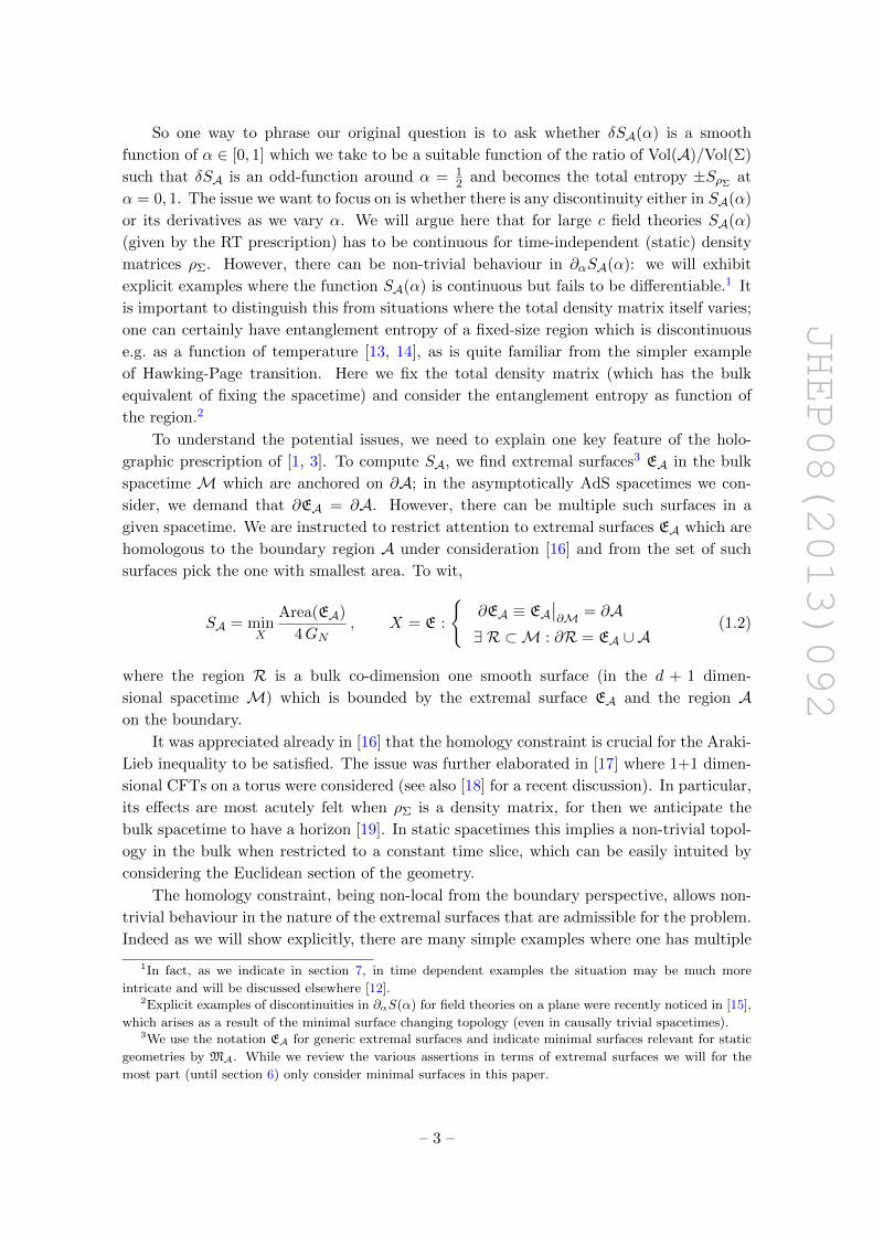
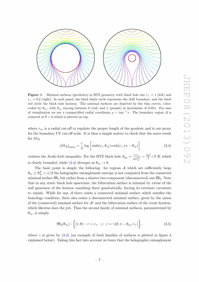
It is a simple matter to find the minimal surfaces for regions A = θ : |θ| ≤ θ∞ since these
are given by spacelike geodesics. The result is best described by writing down the spatial
projection of the surfaces [22]
M1(θ∞) :
(r, θ) : r = γ(θ, θ∞, r+) ≡ r+
(1− cosh2(r+ θ)
cosh2(r+ θ∞)
)− 12
(3.2)
and is plotted in figure 1 for large and small black holes, for a set of θ∞ ∈ [0, π].
As can be easily seen in figure 1, connected spacelike geodesics (satisfying the homology
constraint) always exist for any θ∞ and r+. This makes sense, since there is no reason for
the geodesics to break up (in fact, spacelike geodesics can orbit the black hole arbitrarily
many times before returning to the boundary, albeit at the expense of greater length). As
we will see in section 4, this is in stark contrast to the behaviour of co-dimension 2 surfaces
in higher dimensional black hole spacetimes. Also note that in the BTZ case, another effect
of the low dimensionality is that arbitrarily small black hole (r+ → 0 in (3.1)) always looks
effectively large in terms of the effect it has on geodesics.
Let us now consider the proper length along these geodesics and compute the entan-
glement entropy. As is well known, this computation reproduces the CFT computation of
Cardy-Calabrese [24] for thermal CFT on the infinite line. Naive application of the RT
result for the CFT on a cylinder leads to9
(SA)naive =c
3log
(2 r∞r+
sinh(r+ θ∞)
), ∀ θ∞ ∈ [0, π] (3.3)
8We work in units where the AdS length `AdS = 1 and also set the radius of the boundary circle R
parameterized by θ ∈ [0, 2π] to unity. It is easy to restore dimensions when necessary as we illustrate later.9We use CFT central charge determined by the Brown-Henneaux analysis c = 3 `AdS
2G(3)N
and note that
T =r+
2π `AdS Ris the temperature of the thermal density matrix ρΣ.
– 6 –
JHEP08(2013)092
Figure 1. Minimal surfaces (geodesics) in BTZ geometry with black hole size r+ = 1 (left) and
r+ = 0.2 (right). In each panel, the thick black circle represents the AdS boundary, and the thick
red circle the black hole horizon. The minimal surfaces are depicted by the thin curves, color-
coded by θ∞, with θ∞ varying between 0 (red) and π (purple) in increments of 0.05π. For ease
of visualization we use a compactified radial coordinate ρ = tan−1 r. The boundary region A is
centered at θ = 0 which is plotted on top.
where r∞ is a radial cut-off to regulate the proper length of the geodesic and is our proxy
for the boundary UV cut-off scale. It is then a simple matter to check that the naive result
for δSA
(δSA)naive =c
3log
[sinh(r+ θ∞) csch(r+ (π − θ∞)
](3.4)
violates the Araki-Lieb inequality. For the BTZ black hole SρΣ = π r+
2G(3)N
= 2π2
3 c T R, which
is clearly bounded, while (3.4) diverges as θ∞ → 0.
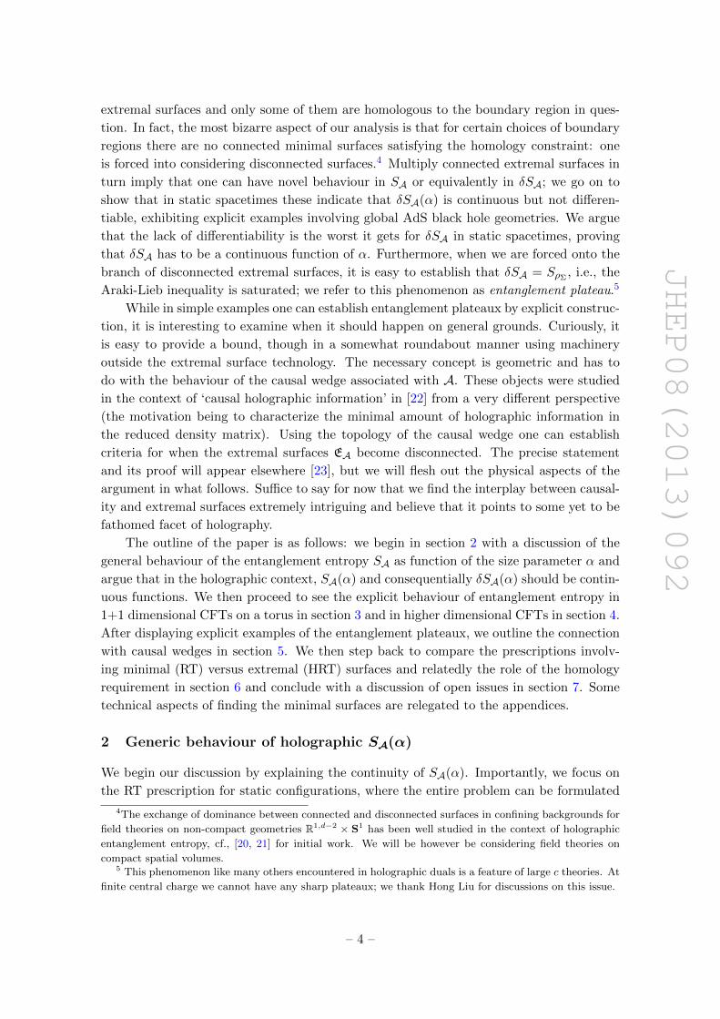
The basic point is simply the following: for regions A which are sufficiently large
θ∞ ≥ θX∞ > π/2 the holographic entanglement entropy is not computed from the connected
minimal surface M1 but rather from a shorter two-component (disconnected) one M2. Note
that in any static black hole spacetime, the bifurcation surface is minimal by virtue of the
null generator of the horizon vanishing there quadratically, forcing its extrinsic curvature
to vanish. While for any A there exists a connected minimal surface which satisfies the
homology condition, there also exists a disconnected minimal surface, given by the union
of the (connected) minimal surface for Ac and the bifurcation surface of the event horizon,
which likewise does the job. Thus the second family of minimal surfaces, parameterized by
θ∞, is simply
M2(θ∞) :
(r, θ) : r = r+ ∪ r = γ(θ, π − θ∞, r+)
, (3.5)
where γ is given by (3.2) (an example of both families of surfaces is plotted in figure 2
explained below). Taking this fact into account we learn that the holographic entanglement
– 7 –
JHEP08(2013)092
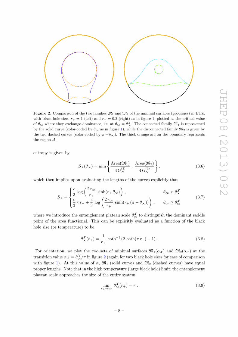
Figure 2. Comparison of the two families M1 and M2 of the minimal surfaces (geodesics) in BTZ,
with black hole sizes r+ = 1 (left) and r+ = 0.2 (right) as in figure 1, plotted at the critical value
of θ∞ where they exchange dominance, i.e. at θ∞ = θX∞. The connected family M1 is represented
by the solid curve (color-coded by θ∞ as in figure 1), while the disconnected family M2 is given by
the two dashed curves (color-coded by π − θ∞). The thick orange arc on the boundary represents
the region A.
entropy is given by
SA(θ∞) = min
Area(M1)
4G(3)N
,Area(M2)
4G(3)N
, (3.6)
which then implies upon evaluating the lengths of the curves explicitly that
SA =
c
3log
(2 r∞r+
sinh(r+ θ∞)
), θ∞ < θX∞
c
3π r+ +
c
3log
(2 r∞r+
sinh(r+ (π − θ∞))
), θ∞ ≥ θX∞
(3.7)
where we introduce the entanglement plateau scale θX∞ to distinguish the dominant saddle
point of the area functional. This can be explicitly evaluated as a function of the black
hole size (or temperature) to be
θX∞(r+) =1
r+coth−1 (2 coth(π r+)− 1) . (3.8)
For orientation, we plot the two sets of minimal surfaces M1(αX ) and M2(αX ) at the
transition value αX = θX∞/π in figure 2 (again for two black hole sizes for ease of comparison
with figure 1). At this value of α, M1 (solid curve) and M2 (dashed curves) have equal
proper lengths. Note that in the high temperature (large black hole) limit, the entanglement
plateau scale approaches the size of the entire system:
limr+→∞
θX∞(r+) = π . (3.9)
– 8 –
JHEP08(2013)092
Translating this into field theory quantities and using α = θ∞π to parameterize the
fraction of the system we consider, we have
αX =1
2π2 T Rcoth−1
(2 coth
(2π2 T R
)− 1)
(3.10)
where R is the radius of the boundary CFT cylinder. The main feature we want to illustrate
is that for α > αX
δSA = SρΣ =2π2
3c T R =⇒ SA = SAc + SρΣ (3.11)
as anticipated. Essentially for large enough boundary regions we can read off the thermal
entropy by comparing directly the entanglement entropy of a region and its complement.
The behaviour of δSA for 1+1 dimensional CFTs is shown explicitly later in figure 5 (where
we also demonstrate a similar feature in higher dimensional holographic field theories).
In deriving the relations (3.11), we have implicitly assumed r+ ≥ 1 (equivalently
TR ≥ 12π ), which is where the BTZ black hole is dual to the thermal density matrix for
the CFT. For lower temperatures the density matrix is dual to thermal AdS geometry and
the holographic computation described above should be modified. Geodesics in thermal
AdS will actually give a result which says SA = SAc at leading order in the c→∞ limit.10
The thermal result will only be recovered by considering 1/c corrections. This makes sense
since for TR < 12π one is in the ‘confined’ phase of the CFT (the terminology is inherited
from higher dimensions where one has an honest confinement/deconfinement transition in
the large N planar gauge theory).
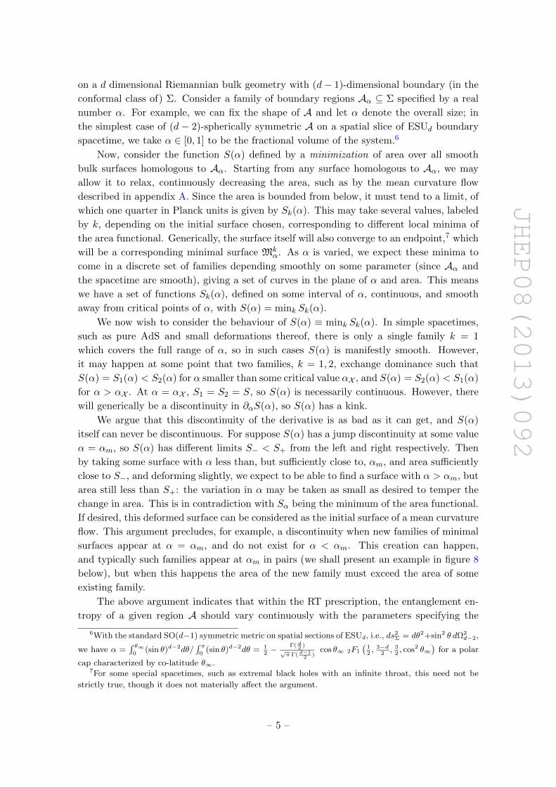
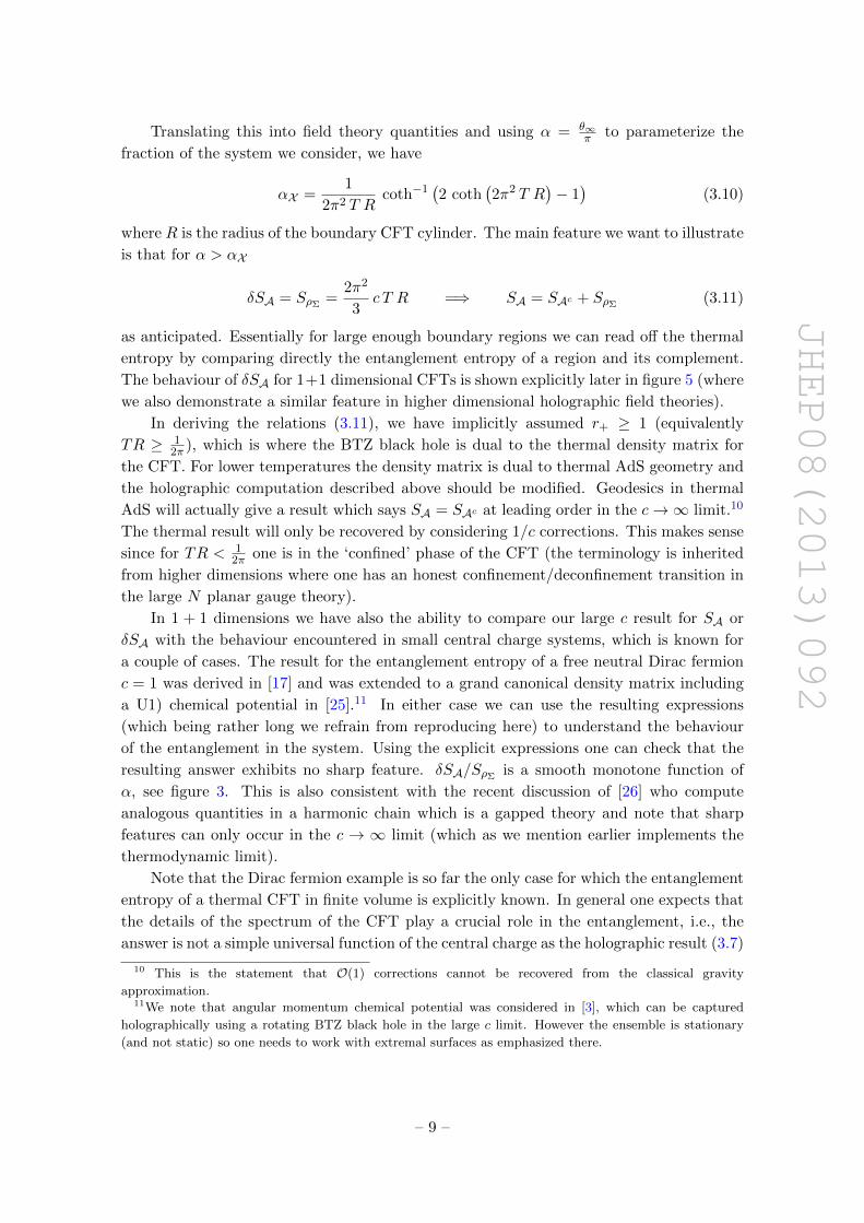
In 1 + 1 dimensions we have also the ability to compare our large c result for SA or
δSA with the behaviour encountered in small central charge systems, which is known for
a couple of cases. The result for the entanglement entropy of a free neutral Dirac fermion
c = 1 was derived in [17] and was extended to a grand canonical density matrix including
a U1) chemical potential in [25].11 In either case we can use the resulting expressions
(which being rather long we refrain from reproducing here) to understand the behaviour
of the entanglement in the system. Using the explicit expressions one can check that the
resulting answer exhibits no sharp feature. δSA/SρΣ is a smooth monotone function of
α, see figure 3. This is also consistent with the recent discussion of [26] who compute
analogous quantities in a harmonic chain which is a gapped theory and note that sharp
features can only occur in the c → ∞ limit (which as we mention earlier implements the
thermodynamic limit).
Note that the Dirac fermion example is so far the only case for which the entanglement
entropy of a thermal CFT in finite volume is explicitly known. In general one expects that
the details of the spectrum of the CFT play a crucial role in the entanglement, i.e., the
answer is not a simple universal function of the central charge as the holographic result (3.7)
10 This is the statement that O(1) corrections cannot be recovered from the classical gravity
approximation.11We note that angular momentum chemical potential was considered in [3], which can be captured
holographically using a rotating BTZ black hole in the large c limit. However the ensemble is stationary
(and not static) so one needs to work with extremal surfaces as emphasized there.
– 9 –
JHEP08(2013)092
è
è
è
è
è
è
è
è
è
è
è
è
è
è
è
è
è
è
è
è
è
è
è
è
è
è
è
è
è
è
è
è
è
è
è
è
è
è
è
è
è
è
è
è
è
è
è
è
è
è
è
è
è
è
è
è
è
è
è
è
è
è
è
è
è
è
è
è
ò
ò
ò
ò
ò
ò
ò
ò
ò
ò
ò
ò
ò
ò
ò
ò
ò
ò
ò
ò
ò
ò
ò
ò
ò
ò
ò
ò
ò
ò
ò
ò
ò
ò
ò
ò
ò
ò
ò
ò
ò
ò
ò
ò
ò
ò
ò
ò
ò
ò
ò
0.1 0.2 0.3 0.4 0.5
0.2
0.4
0.6
0.8
1.0δSA/SρΣ
α
Figure 3. Plot of the curves δSA/SρΣfor a Dirac fermion in 1 + 1 dimensions in the canonical
(T 6= 0) [17] and grand canonical (T, µ 6= 0) [25]. We examine the behaviour for a range of
temperatures and chemical potential. The solid curves from bottom are β = 4 (red), β = 2 (blue),
β = 1 (magenta) and β = 0.1 (black). The situation with the chemical potential turned on is
indicated with the same colour coding with µ = 0.1 represented by circles and µ = 0.5 by triangles.
The symmetry µ↔ 1−µ is used to restrict µ ∈ [0, 1/2] and we see that for µ = 0.5 the normalized
δSA is essentially the same at any temperature. This behaviour should be contrasted against the
large c holographic result displayed in figure 5 for d ≥ 2 thermal CFTs.
suggests. It would be interesting to see if one can use the technology of [9] to argue directly
from a CFT analysis for an entanglement plateau relation like (3.11) in the asymptotic large
c limit.
The behaviour of SA(α), not surprisingly, is in fact rather similar to the behaviour of
the entropy or free energy in the thermal ensemble (a point we will revisit in section 7). In
both cases there are multiple saddle points, which exchange dominance. For the thermal
density matrix the saddles are the thermal AdS geometry and the BTZ black hole both of
which exist for the entire range of the dimensionless parameter TR. For the holographic
entanglement entropy SA we have again two distinct saddles available for the entire range
of parameters: the connected and disconnected surfaces M1 and M2 exist for all values of
α ∈ [0, 1]. For a sufficiently large region α ≥ αX , however, it is the disconnected surface
that dominates and results in the entanglement plateau. We will soon see that existence
of both families over the entire range of α is peculiar to three dimensions and the situation
is much more intricate in higher dimensions.
4 Entanglement entropy in higher dimensional field theories
In the previous section we saw that already in the 3-dimensional bulk spacetime corre-
sponding to a thermal state in the dual CFT, we have multiple families of minimal surfaces
Mi anchored at the boundary entangling surface ∂A, for arbitrary A. Let us now examine
the analogous situation in higher dimensions. We will consider the Schwarzschild-AdSd+1
– 10 –
JHEP08(2013)092
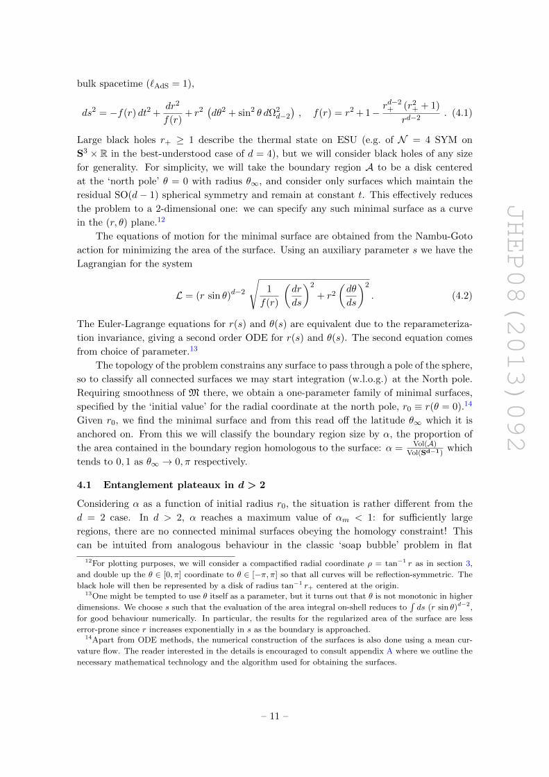
bulk spacetime (`AdS = 1),
ds2 = −f(r) dt2 +dr2
f(r)+ r2
(dθ2 + sin2 θ dΩ2
d−2
), f(r) = r2 + 1−
rd−2+ (r2
+ + 1)
rd−2. (4.1)
Large black holes r+ ≥ 1 describe the thermal state on ESU (e.g. of N = 4 SYM on
S3 × R in the best-understood case of d = 4), but we will consider black holes of any size
for generality. For simplicity, we will take the boundary region A to be a disk centered
at the ‘north pole’ θ = 0 with radius θ∞, and consider only surfaces which maintain the
residual SO(d− 1) spherical symmetry and remain at constant t. This effectively reduces
the problem to a 2-dimensional one: we can specify any such minimal surface as a curve
in the (r, θ) plane.12
The equations of motion for the minimal surface are obtained from the Nambu-Goto
action for minimizing the area of the surface. Using an auxiliary parameter s we have the
Lagrangian for the system
L = (r sin θ)d−2
√1
f(r)
(dr
ds
)2
+ r2
(dθ
ds
)2
. (4.2)
The Euler-Lagrange equations for r(s) and θ(s) are equivalent due to the reparameteriza-
tion invariance, giving a second order ODE for r(s) and θ(s). The second equation comes
from choice of parameter.13
The topology of the problem constrains any surface to pass through a pole of the sphere,
so to classify all connected surfaces we may start integration (w.l.o.g.) at the North pole.
Requiring smoothness of M there, we obtain a one-parameter family of minimal surfaces,
specified by the ‘initial value’ for the radial coordinate at the north pole, r0 ≡ r(θ = 0).14
Given r0, we find the minimal surface and from this read off the latitude θ∞ which it is
anchored on. From this we will classify the boundary region size by α, the proportion of
the area contained in the boundary region homologous to the surface: α = Vol(A)Vol(Sd−1)
which
tends to 0, 1 as θ∞ → 0, π respectively.
4.1 Entanglement plateaux in d > 2
Considering α as a function of initial radius r0, the situation is rather different from the
d = 2 case. In d > 2, α reaches a maximum value of αm < 1: for sufficiently large
regions, there are no connected minimal surfaces obeying the homology constraint! This
can be intuited from analogous behaviour in the classic ‘soap bubble’ problem in flat
12For plotting purposes, we will consider a compactified radial coordinate ρ = tan−1 r as in section 3,
and double up the θ ∈ [0, π] coordinate to θ ∈ [−π, π] so that all curves will be reflection-symmetric. The
black hole will then be represented by a disk of radius tan−1 r+ centered at the origin.13One might be tempted to use θ itself as a parameter, but it turns out that θ is not monotonic in higher
dimensions. We choose s such that the evaluation of the area integral on-shell reduces to∫ds (r sin θ)d−2,
for good behaviour numerically. In particular, the results for the regularized area of the surface are less
error-prone since r increases exponentially in s as the boundary is approached.14Apart from ODE methods, the numerical construction of the surfaces is also done using a mean cur-
vature flow. The reader interested in the details is encouraged to consult appendix A where we outline the
necessary mathematical technology and the algorithm used for obtaining the surfaces.
– 11 –
JHEP08(2013)092
space, of finding a minimal surface between two circular rings. To reduce the area, there
is a tendency to shrink the radius of the tube, counteracted by the constraint of ending
on the rings. But when the ratio of ring radius to separation is sufficiently small, the
rings do not hold the surface up enough to prevent the tube radius from shrinking to zero,
and the surface separates into two disconnected parts. This reasoning carries over directly
to our set-up, and the process of surfaces splitting into disconnected pieces can be seen
explicitly in the animations of our numerical simulations of mean curvature flow, to be
found on the arXiv as ancillary files for the submission. The area cost of having a wide
tube is greater in higher dimensions, which leads one to expect that αm should be smaller,
reflecting the greater tendency of the surfaces to split up.15 The physical point is that this
leaves no option but to consider the disconnected surfaces, to which we now turn. In the
next section, we offer a very different geometrical justification of why connected extremal
surfaces homologous to A cannot exist beyond a certain θ∞, which is based on causality
in the full Lorentzian geometry.
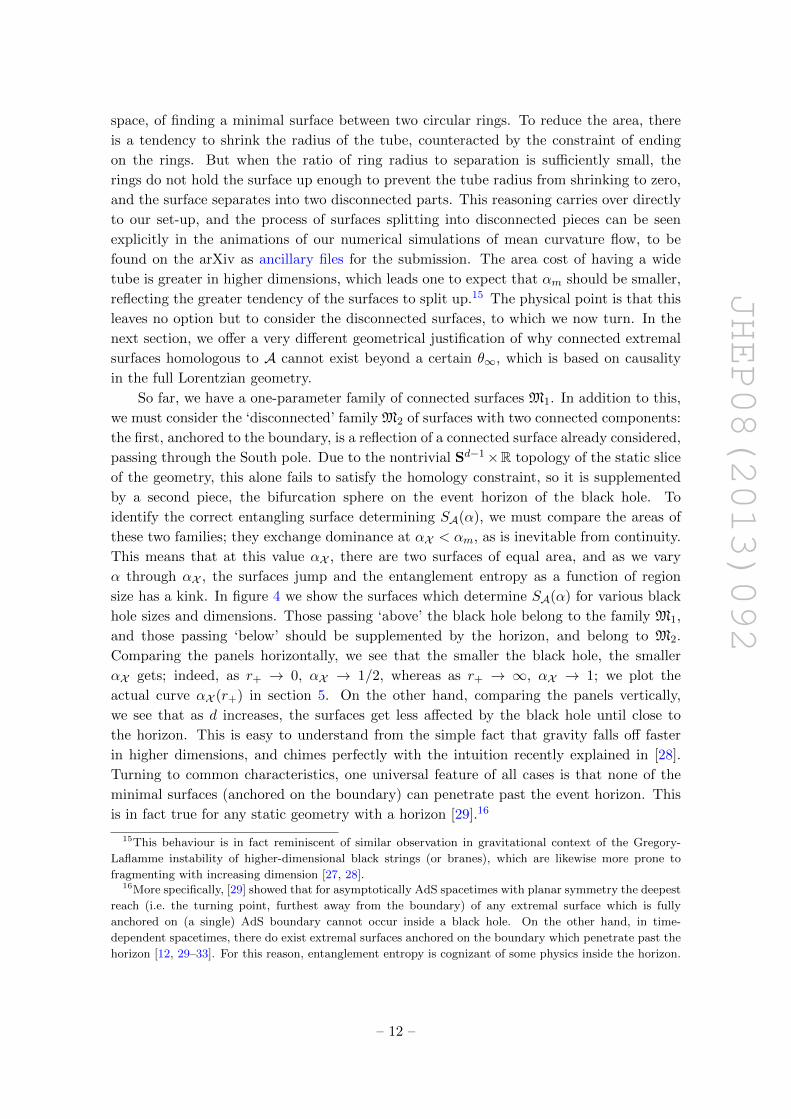
So far, we have a one-parameter family of connected surfaces M1. In addition to this,
we must consider the ‘disconnected’ family M2 of surfaces with two connected components:
the first, anchored to the boundary, is a reflection of a connected surface already considered,
passing through the South pole. Due to the nontrivial Sd−1×R topology of the static slice
of the geometry, this alone fails to satisfy the homology constraint, so it is supplemented
by a second piece, the bifurcation sphere on the event horizon of the black hole. To
identify the correct entangling surface determining SA(α), we must compare the areas of
these two families; they exchange dominance at αX < αm, as is inevitable from continuity.
This means that at this value αX , there are two surfaces of equal area, and as we vary
α through αX , the surfaces jump and the entanglement entropy as a function of region
size has a kink. In figure 4 we show the surfaces which determine SA(α) for various black
hole sizes and dimensions. Those passing ‘above’ the black hole belong to the family M1,
and those passing ‘below’ should be supplemented by the horizon, and belong to M2.
Comparing the panels horizontally, we see that the smaller the black hole, the smaller
αX gets; indeed, as r+ → 0, αX → 1/2, whereas as r+ → ∞, αX → 1; we plot the
actual curve αX (r+) in section 5. On the other hand, comparing the panels vertically,
we see that as d increases, the surfaces get less affected by the black hole until close to
the horizon. This is easy to understand from the simple fact that gravity falls off faster
in higher dimensions, and chimes perfectly with the intuition recently explained in [28].
Turning to common characteristics, one universal feature of all cases is that none of the
minimal surfaces (anchored on the boundary) can penetrate past the event horizon. This
is in fact true for any static geometry with a horizon [29].16
15This behaviour is in fact reminiscent of similar observation in gravitational context of the Gregory-
Laflamme instability of higher-dimensional black strings (or branes), which are likewise more prone to
fragmenting with increasing dimension [27, 28].16More specifically, [29] showed that for asymptotically AdS spacetimes with planar symmetry the deepest
reach (i.e. the turning point, furthest away from the boundary) of any extremal surface which is fully
anchored on (a single) AdS boundary cannot occur inside a black hole. On the other hand, in time-
dependent spacetimes, there do exist extremal surfaces anchored on the boundary which penetrate past the
horizon [12, 29–33]. For this reason, entanglement entropy is cognizant of some physics inside the horizon.
– 12 –
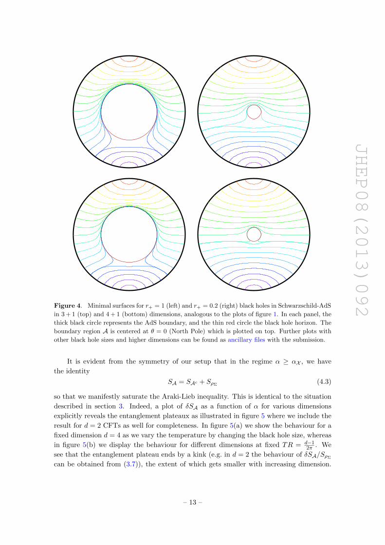
JHEP08(2013)092Figure 4. Minimal surfaces for r+ = 1 (left) and r+ = 0.2 (right) black holes in Schwarzschild-AdS
in 3 + 1 (top) and 4 + 1 (bottom) dimensions, analogous to the plots of figure 1. In each panel, the
thick black circle represents the AdS boundary, and the thin red circle the black hole horizon. The
boundary region A is centered at θ = 0 (North Pole) which is plotted on top. Further plots with
other black hole sizes and higher dimensions can be found as ancillary files with the submission.
It is evident from the symmetry of our setup that in the regime α ≥ αX , we have
the identity
SA = SAc + SρΣ (4.3)
so that we manifestly saturate the Araki-Lieb inequality. This is identical to the situation
described in section 3. Indeed, a plot of δSA as a function of α for various dimensions
explicitly reveals the entanglement plateaux as illustrated in figure 5 where we include the
result for d = 2 CFTs as well for completeness. In figure 5(a) we show the behaviour for a
fixed dimension d = 4 as we vary the temperature by changing the black hole size, whereas
in figure 5(b) we display the behaviour for different dimensions at fixed TR = d−12π . We
see that the entanglement plateau ends by a kink (e.g. in d = 2 the behaviour of δSA/SρΣ
can be obtained from (3.7)), the extent of which gets smaller with increasing dimension.
– 13 –
JHEP08(2013)092
0.1 0.2 0.3 0.4 0.5
0.2
0.4
0.6
0.8
1.0
0.1 0.2 0.3 0.4 0.5
0.2
0.4
0.6
0.8
1.0δSASρΣ
δSASρΣ
αα(b)(a)
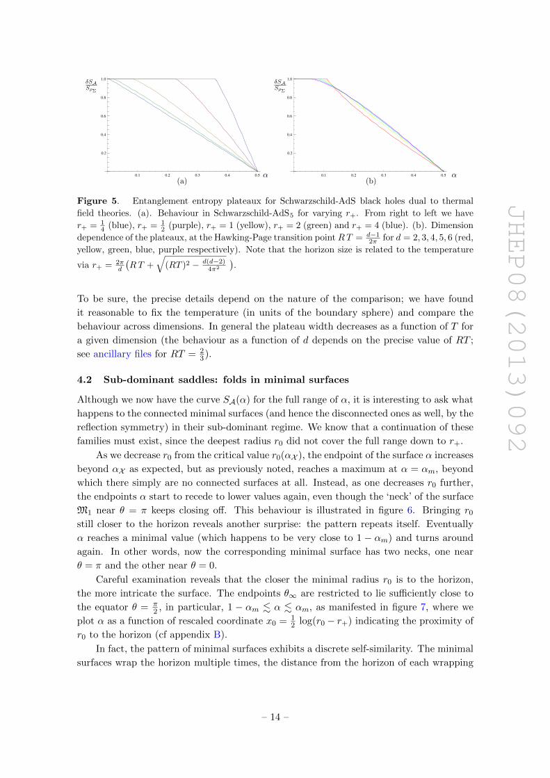
Figure 5. Entanglement entropy plateaux for Schwarzschild-AdS black holes dual to thermal
field theories. (a). Behaviour in Schwarzschild-AdS5 for varying r+. From right to left we have
r+ = 14 (blue), r+ = 1
2 (purple), r+ = 1 (yellow), r+ = 2 (green) and r+ = 4 (blue). (b). Dimension
dependence of the plateaux, at the Hawking-Page transition pointRT = d−12π for d = 2, 3, 4, 5, 6 (red,
yellow, green, blue, purple respectively). Note that the horizon size is related to the temperature
via r+ = 2πd
(RT +
√(RT )2 − d(d−2)
4π2
).
To be sure, the precise details depend on the nature of the comparison; we have found
it reasonable to fix the temperature (in units of the boundary sphere) and compare the
behaviour across dimensions. In general the plateau width decreases as a function of T for
a given dimension (the behaviour as a function of d depends on the precise value of RT ;
see ancillary files for RT = 23).
4.2 Sub-dominant saddles: folds in minimal surfaces
Although we now have the curve SA(α) for the full range of α, it is interesting to ask what
happens to the connected minimal surfaces (and hence the disconnected ones as well, by the
reflection symmetry) in their sub-dominant regime. We know that a continuation of these
families must exist, since the deepest radius r0 did not cover the full range down to r+.
As we decrease r0 from the critical value r0(αX ), the endpoint of the surface α increases
beyond αX as expected, but as previously noted, reaches a maximum at α = αm, beyond
which there simply are no connected surfaces at all. Instead, as one decreases r0 further,
the endpoints α start to recede to lower values again, even though the ‘neck’ of the surface
M1 near θ = π keeps closing off. This behaviour is illustrated in figure 6. Bringing r0
still closer to the horizon reveals another surprise: the pattern repeats itself. Eventually
α reaches a minimal value (which happens to be very close to 1 − αm) and turns around
again. In other words, now the corresponding minimal surface has two necks, one near
θ = π and the other near θ = 0.
Careful examination reveals that the closer the minimal radius r0 is to the horizon,
the more intricate the surface. The endpoints θ∞ are restricted to lie sufficiently close to
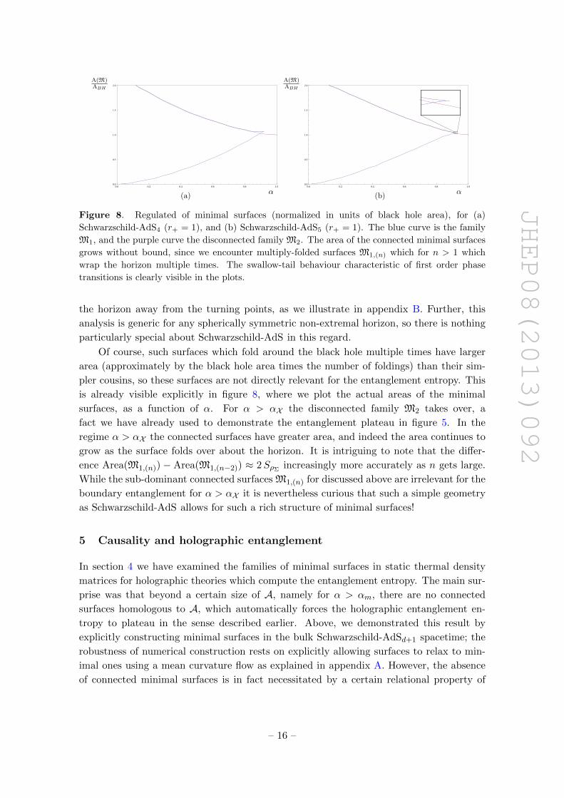
the equator θ = π2 , in particular, 1 − αm . α . αm, as manifested in figure 7, where we
plot α as a function of rescaled coordinate x0 = 12 log(r0 − r+) indicating the proximity of
r0 to the horizon (cf appendix B).
In fact, the pattern of minimal surfaces exhibits a discrete self-similarity. The minimal
surfaces wrap the horizon multiple times, the distance from the horizon of each wrapping
– 14 –
JHEP08(2013)092
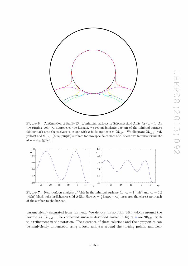
Figure 6. Continuation of family M1 of minimal surfaces in Schwarzschild-AdS5 for r+ = 1. As
the turning point r0 approaches the horizon, we see an intricate pattern of the minimal surfaces
folding back onto themselves; solutions with n-folds are denoted M1,(n). We illustrate M1,(0) (red,
yellow) and M1,(1) (blue, purple) surfaces for two specific choices of α; these two families terminate
at α = αm (green).
- 25 - 20 -15 -10 -5 00.0
0.2
0.4
0.6
0.8
1.0
- 20 -15 -10 -5 00.0
0.2
0.4
0.6
0.8
1.0
x0
α
x0
α
Figure 7. Near-horizon analysis of folds in the minimal surfaces for r+ = 1 (left) and r+ = 0.2
(right) black holes in Schwarzschild-AdS4. Here x0 = 12 log(r0 − r+) measures the closest approach
of the surface to the horizon.
parametrically separated from the next. We denote the solution with n-folds around the
horizon as M1,(n). The connected surfaces described earlier in figure 4 are M1,(0) with
this refinement in the notation. The existence of these solutions and their properties can
be analytically understood using a local analysis around the turning points, and near
– 15 –
JHEP08(2013)092
0.0 0.2 0.4 0.6 0.8 1.00.0
0.5
1.0
1.5
2.0
0.0 0.2 0.4 0.6 0.8 1.00.0
0.5
1.0
1.5
2.0
(b)α
A(M)ABH
(a)α
A(M)ABH
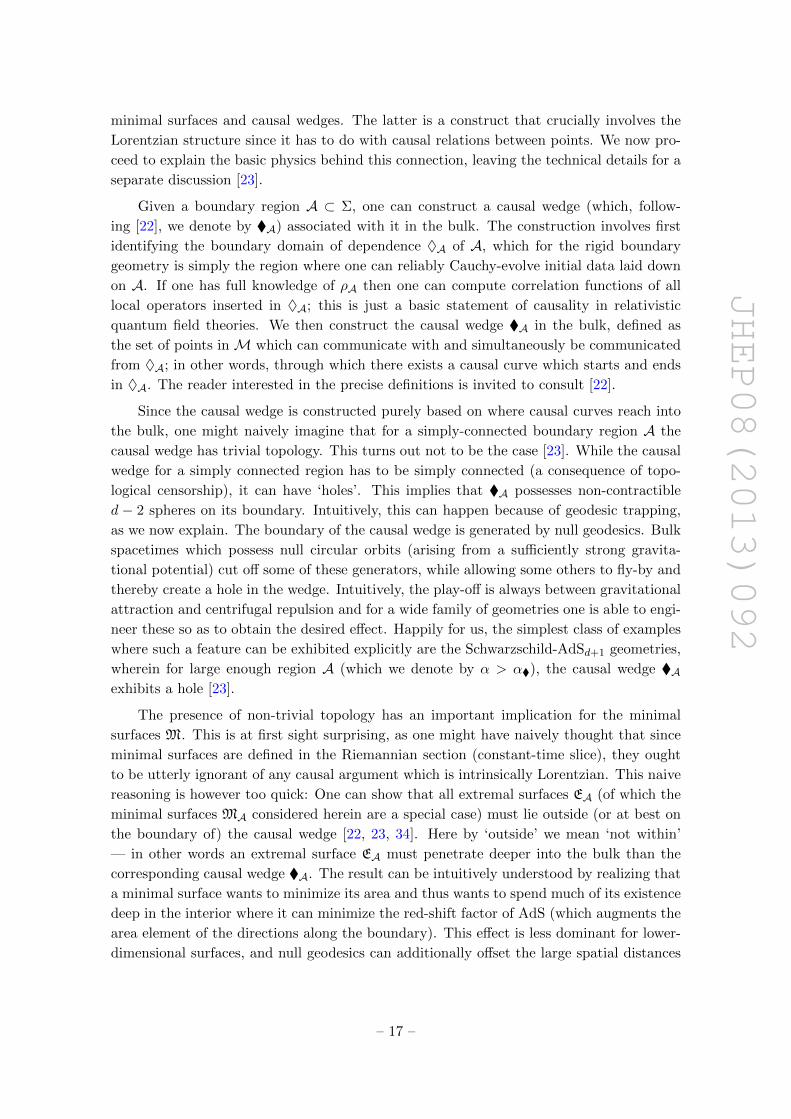
Figure 8. Regulated of minimal surfaces (normalized in units of black hole area), for (a)
Schwarzschild-AdS4 (r+ = 1), and (b) Schwarzschild-AdS5 (r+ = 1). The blue curve is the family
M1, and the purple curve the disconnected family M2. The area of the connected minimal surfaces
grows without bound, since we encounter multiply-folded surfaces M1,(n) which for n > 1 which
wrap the horizon multiple times. The swallow-tail behaviour characteristic of first order phase
transitions is clearly visible in the plots.
the horizon away from the turning points, as we illustrate in appendix B. Further, this
analysis is generic for any spherically symmetric non-extremal horizon, so there is nothing
particularly special about Schwarzschild-AdS in this regard.
Of course, such surfaces which fold around the black hole multiple times have larger
area (approximately by the black hole area times the number of foldings) than their sim-
pler cousins, so these surfaces are not directly relevant for the entanglement entropy. This
is already visible explicitly in figure 8, where we plot the actual areas of the minimal
surfaces, as a function of α. For α > αX the disconnected family M2 takes over, a
fact we have already used to demonstrate the entanglement plateau in figure 5. In the
regime α > αX the connected surfaces have greater area, and indeed the area continues to
grow as the surface folds over about the horizon. It is intriguing to note that the differ-
ence Area(M1,(n)) − Area(M1,(n−2)) ≈ 2SρΣ increasingly more accurately as n gets large.
While the sub-dominant connected surfaces M1,(n) for discussed above are irrelevant for the
boundary entanglement for α > αX it is nevertheless curious that such a simple geometry
as Schwarzschild-AdS allows for such a rich structure of minimal surfaces!
5 Causality and holographic entanglement
In section 4 we have examined the families of minimal surfaces in static thermal density
matrices for holographic theories which compute the entanglement entropy. The main sur-
prise was that beyond a certain size of A, namely for α > αm, there are no connected
surfaces homologous to A, which automatically forces the holographic entanglement en-
tropy to plateau in the sense described earlier. Above, we demonstrated this result by
explicitly constructing minimal surfaces in the bulk Schwarzschild-AdSd+1 spacetime; the
robustness of numerical construction rests on explicitly allowing surfaces to relax to min-
imal ones using a mean curvature flow as explained in appendix A. However, the absence
of connected minimal surfaces is in fact necessitated by a certain relational property of
– 16 –
JHEP08(2013)092
minimal surfaces and causal wedges. The latter is a construct that crucially involves the
Lorentzian structure since it has to do with causal relations between points. We now pro-
ceed to explain the basic physics behind this connection, leaving the technical details for a
separate discussion [23].
Given a boundary region A ⊂ Σ, one can construct a causal wedge (which, follow-
ing [22], we denote by A) associated with it in the bulk. The construction involves first
identifying the boundary domain of dependence ♦A of A, which for the rigid boundary
geometry is simply the region where one can reliably Cauchy-evolve initial data laid down
on A. If one has full knowledge of ρA then one can compute correlation functions of all
local operators inserted in ♦A; this is just a basic statement of causality in relativistic
quantum field theories. We then construct the causal wedge A in the bulk, defined as
the set of points inM which can communicate with and simultaneously be communicated
from ♦A; in other words, through which there exists a causal curve which starts and ends
in ♦A. The reader interested in the precise definitions is invited to consult [22].
Since the causal wedge is constructed purely based on where causal curves reach into
the bulk, one might naively imagine that for a simply-connected boundary region A the
causal wedge has trivial topology. This turns out not to be the case [23]. While the causal
wedge for a simply connected region has to be simply connected (a consequence of topo-
logical censorship), it can have ‘holes’. This implies that A possesses non-contractible
d − 2 spheres on its boundary. Intuitively, this can happen because of geodesic trapping,
as we now explain. The boundary of the causal wedge is generated by null geodesics. Bulk
spacetimes which possess null circular orbits (arising from a sufficiently strong gravita-
tional potential) cut off some of these generators, while allowing some others to fly-by and
thereby create a hole in the wedge. Intuitively, the play-off is always between gravitational
attraction and centrifugal repulsion and for a wide family of geometries one is able to engi-
neer these so as to obtain the desired effect. Happily for us, the simplest class of examples
where such a feature can be exhibited explicitly are the Schwarzschild-AdSd+1 geometries,
wherein for large enough region A (which we denote by α > α), the causal wedge Aexhibits a hole [23].
The presence of non-trivial topology has an important implication for the minimal
surfaces M. This is at first sight surprising, as one might have naively thought that since
minimal surfaces are defined in the Riemannian section (constant-time slice), they ought
to be utterly ignorant of any causal argument which is intrinsically Lorentzian. This naive
reasoning is however too quick: One can show that all extremal surfaces EA (of which the
minimal surfaces MA considered herein are a special case) must lie outside (or at best on
the boundary of) the causal wedge [22, 23, 34]. Here by ‘outside’ we mean ‘not within’
— in other words an extremal surface EA must penetrate deeper into the bulk than the
corresponding causal wedge A. The result can be intuitively understood by realizing that
a minimal surface wants to minimize its area and thus wants to spend much of its existence
deep in the interior where it can minimize the red-shift factor of AdS (which augments the
area element of the directions along the boundary). This effect is less dominant for lower-
dimensional surfaces, and null geodesics can additionally offset the large spatial distances
– 17 –
JHEP08(2013)092
by large temporal ones.17 Hence generically the causal wedge boundary is nestled between
the extremal surface and the AdS boundary. As an aside, this statement forms a crucial
ingredient in the arguments of [35] who argue that the holographic dual of the reduced
density matrix ρA must comprise of a bulk region that is larger than the casual wedge A.18
We are now in a position to explain the behaviour found in section 4. For α >
α the ability of the causal wedge to develop holes implies that we should anticipate a
corresponding change in the minimal surface. Indeed MA cannot pass into the hole in
A while remaining connected to the boundary, because of the nesting property: in order
to do so, it would have to pass through the causal wedge. This means that it either lies
completely outside the causal wedge or is contained entirely within the hole! One fact
which is somewhat obvious by causality is that the hole in the causal wedge must lie
outside the black hole event horizon. For static black hole spacetimes we have argued that
the bifurcation surface is a candidate extremal surface in section 3. So in the presence of
the hole in the wedge we can have a minimal surface component on the far side of the black
hole (hence outside A) and another component being simply the bifurcation surface. In
fact, as in the BTZ discussion, the homology constraint imposed upon the RT prescription
by the Araki-Lieb inequality necessitates both components. Hence the only surfaces that
are both minimal and homologous to A are the disconnected surfaces M2 described in
section 4.
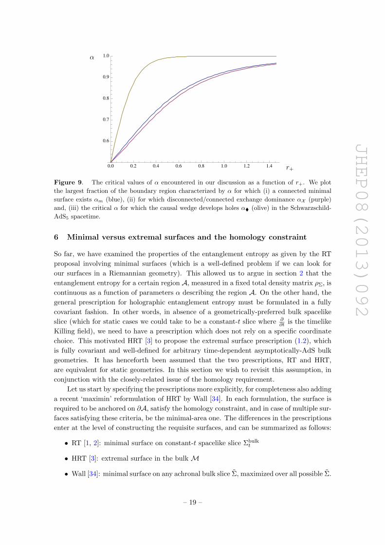
We demonstrate explicitly that αX ≤ αm ≤ α as one anticipates for first order
transitions for Schwarzschild-AdS5 in figure 9. As the figure indicates, the causal wedge
pinch off happens at α = α which is significantly larger than the bound αm on existence
of corresponding extremal surfaces. In other words, the connected minimal surface ceases
to exist long before this is necessitated by the topology of the causal wedge. While this
may seem to somewhat weaken our arguments regarding the utility of the causal wedge, we
should note that the pinch-off value α = α is a rather weak bound from the causal wedge
standpoint as well: already before the causal wedge pinches off, its geometry precludes the
requisite minimal surface. This is because prior to the pinch-off the opening becomes too
long and narrow to admit any extremal surface. To support the latter, the neck would have
to accommodate a sufficient ‘flare-out’ shape, as explained in section 4.1, which occurs for
θ∞ smaller by ∼ O(ρ0−ρ+), where ρ0 is the ρ-radius of null circular orbit and ρ+ gives the
horizon size. Hence a more sophisticated analysis which takes into account the shape of
the causal wedge apart from its topology would provide a much stronger bound on αm. It
would interesting to examine in detail precisely how close we can get to αm, but we leave
this for future exploration.
17Note that in comparison to pure AdS geometry, both null geodesics and extremal surfaces are neverthe-
less pushed towards the boundary by the gravitational potential well of a deformed bulk spacetime. This in
effect means that both entanglement entropy and causal holographic information defined in [22] grow with
positive mass deformations of the spacetime.18Caveat: The statements made above should be viewed with suitable caution, as they require some work
to be established rigorously. For further discussion and a proof of the nesting property of causal wedges
and extremal surfaces (modulo some technical assumptions), we refer the reader to [23] (see also [34] for a
related discussion in causally trivial spacetimes).
– 18 –
JHEP08(2013)092
0.0 0.2 0.4 0.6 0.8 1.0 1.2 1.4
0.6
0.7
0.8
0.9
1.0α
r+
Figure 9. The critical values of α encountered in our discussion as a function of r+. We plot
the largest fraction of the boundary region characterized by α for which (i) a connected minimal
surface exists αm (blue), (ii) for which disconnected/connected exchange dominance αX (purple)
and, (iii) the critical α for which the causal wedge develops holes α (olive) in the Schwarzschild-
AdS5 spacetime.
6 Minimal versus extremal surfaces and the homology constraint
So far, we have examined the properties of the entanglement entropy as given by the RT
proposal involving minimal surfaces (which is a well-defined problem if we can look for
our surfaces in a Riemannian geometry). This allowed us to argue in section 2 that the
entanglement entropy for a certain region A, measured in a fixed total density matrix ρΣ, is
continuous as a function of parameters α describing the region A. On the other hand, the
general prescription for holographic entanglement entropy must be formulated in a fully
covariant fashion. In other words, in absence of a geometrically-preferred bulk spacelike
slice (which for static cases we could take to be a constant-t slice where ∂∂t is the timelike
Killing field), we need to have a prescription which does not rely on a specific coordinate
choice. This motivated HRT [3] to propose the extremal surface prescription (1.2), which
is fully covariant and well-defined for arbitrary time-dependent asymptotically-AdS bulk
geometries. It has henceforth been assumed that the two prescriptions, RT and HRT,
are equivalent for static geometries. In this section we wish to revisit this assumption, in
conjunction with the closely-related issue of the homology requirement.
Let us start by specifying the prescriptions more explicitly, for completeness also adding
a recent ‘maximin’ reformulation of HRT by Wall [34]. In each formulation, the surface is
required to be anchored on ∂A, satisfy the homology constraint, and in case of multiple sur-
faces satisfying these criteria, be the minimal-area one. The differences in the prescriptions
enter at the level of constructing the requisite surfaces, and can be summarized as follows:
• RT [1, 2]: minimal surface on constant-t spacelike slice Σbulkt
• HRT [3]: extremal surface in the bulk M
• Wall [34]: minimal surface on any achronal bulk slice Σ, maximized over all possible Σ.
– 19 –
JHEP08(2013)092
While RT is restricted to static spacetimes, Wall’s prescription is formulated in causally
trivial bulk geometries. In this context, [34] proves equivalence between the maximin and
HRT prescriptions assuming the null energy condition. Although the maximin construction
is useful for some purposes (for example, it allows [34] to argue the existence of such
surfaces and prove strong subadditivity in the time-dependent context), it is conceptually
more complicated since the requisite surface is obtained by a two-step procedure of first
minimizing the area on some achronal slice Σ, and then maximizing the area with respect
to varying Σ. Moreover, here we wish to consider causally non-trivial spacetimes, so we
will henceforth restrict attention to the RT and HRT proposals.
In a globally static geometry, RT and HRT proposals are indeed equivalent, since any
extremal surface anchored at constant t on the boundary must coincide with the minimal
surface on Σbulkt , cf. [3].19 However, in a static but not globally static geometry (i.e.
when there is a global Killing field which is timelike near the AdS boundary but does not
necessarily remain timelike everywhere in the bulk), the situation can appear more subtle.
To illustrate the point, let us consider the eternal non-extremal Reissner-Nordstrom-
AdS geometry, corresponding to a static charged black hole. It has a metric of the
form (4.1), but with f(r) having two positive real roots at r = r± with r+ corresponding
to the outer (or event) horizon and r− the inner (or Cauchy) horizon with 0 < r− < r+.20
The causal structure is indicated in the Penrose diagram in figure 10. Apart from the
bifurcation surface of the event horizon at r = r+ which has zero extrinsic curvature (and
therefore is a compact extremal surface), there is an analogous compact extremal surface
at the inner horizon r = r−. At both surfaces the ∂∂t Killing field vanishes (and its norm
decreases in spacelike directions and increases in timelike directions), but whereas the area
of the surface is minimized to spatial deformations and maximized to temporal ones in the
case of event horizon, it is the other way around for the inner horizon.
Outside the black hole, the geometry is qualitatively similar to that of Schwarzschild-
AdS, in the sense that e.g. causal wedges for large enough boundary regions A will have
holes. This will in turn preclude the existence of connected extremal surfaces anchored on
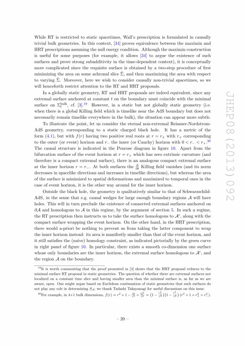
∂A and homologous to A in this regime, by the argument of section 5. In such a regime,
the RT prescription then instructs us to take the surface homologous to Ac, along with the
compact surface wrapping the event horizon. On the other hand, in the HRT prescription,
there would a-priori be nothing to prevent us from taking the latter component to wrap
the inner horizon instead: its area is manifestly smaller than that of the event horizon, and
it still satisfies the (naive) homology constraint, as indicated pictorially by the green curve
in right panel of figure 10. In particular, there exists a smooth co-dimension one surface
whose only boundaries are the inner horizon, the extremal surface homologous to Ac, and
the region A on the boundary.
19It is worth commenting that the proof presented in [3] shows that the HRT proposal reduces to the
minimal surface RT proposal in static geometries. The question of whether there are extremal surfaces not
localized on a constant time slice and having smaller area than the minimal surface is, as far as we are
aware, open. One might argue based on Euclidean continuation of static geometries that such surfaces do
not play any role in determining SA; we thank Tadashi Takayanagi for useful discussions on this issue.20For example, in 4+1 bulk dimensions, f(r) = r2 + 1− M
r2+ Q2
r4=(1− r2+
r2
)(1− r2−
r2
)(r2 + 1 + r2
+ + r2−).
– 20 –
JHEP08(2013)092
......
......
r = 0
r =∞r = r+
r = r−
Figure 10. A sketch of the Penrose diagram for non-extremal Reissner-Nordstrom-AdS black
hole (the figure repeats in the vertical direction, indicated by the ellipsis). The AdS boundaries are
indicated by the black vertical lines, the curvature singularities by purple vertical wiggly curves, the
horizons by blue diagonal dashed line, the projection of the boundary region A by the orange dot,
and the projection of the extremal surface by the blue horizontal line. The two panels distinguish
the RT (left) and naive HRT (right) prescriptions in case of disconnected surfaces: in the former the
disconnected surface lies at the event horizon (red dot) with the homology region R indicated by
the red dotted line. In the HRT case, the disconnected surface is at the Cauchy horizon (green dot),
and corresponding R then interpolates between this surface and its other boundaries as indicated
by the green dotted curve.
Note that if this were indeed the correct prescription, then we would find that, instead
of saturating the Araki-Lieb inequality as in (4.3), we would only satisfy it: δSA would still
plateau as a function of θ∞, but at a value which is lower21 than the expected value SρΣ :
δSA(θ∞ ≥ θX∞) =Ωd−1 r
d−1−
4G(d+1)N
=
(r−r+
)d−1
SρΣ . (6.1)
Although this result is consistent with the Araki-Lieb inequality, it is nevertheless at odds
with the CFT expectation: for nearly-neutral black holes where r− r+ we should be
close to the thermal value rather than parametrically separated from it!
This observation suggests that we need some modification to the homology constraint
specification in (1.2): the mere presence of some smooth surface R with the requisite
boundaries does not seem to suffice. One natural restriction, which indeed has already
been employed in [34], is to require that R be everywhere spacelike.22 With this additional
21The special case of extremal RN-AdS black hole with r− = r+ is somewhat more subtle, since there is
no bifurcation surface (instead the spacial geometry exhibits an infinite throat). We think this is a feature
rather than a bug, indicative of being at strictly zero temperature; however the HRT prescription can be
applied in the same limiting fashion as is commonly done with e.g. the Wald entropy of extremal black holes.22We thank Matt Headrick for useful discussions on this point.
– 21 –
JHEP08(2013)092
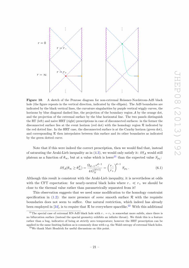
Figure 11. Sketch of the Schwarzschild-AdS ‘bag of gold’ embedding diagram (left) and Penrose
diagram (right). Here the right asymptotic boundary of eternal Schwarzschild-AdS geometry is cut-
off by a static shell (brown dotted curve), beyond which the spacetime caps off through a smooth
origin as indicated. The embedding diagram depicts event horizon bifurcation surface (red curve)
and the boundary region A (orange curve), at the endpoints of which is anchored the connected
part of the extremal surface (blue curve). The Penrose diagram has the same conventions as in
figure 10, but now the homology surface R (dotted green line) goes all the way around the tip.
restriction, the above example would be safely invalidated, since R cannot reach from the
Cauchy horizon bifurcation surface r = r− to the AdS boundary r = ∞ while remaining
spacelike everywhere, as evident from figure 10. The only other compact extremal surface
which is spacelike-separated from the boundary region A and the extremal surface homolo-
gous to Ac is the event horizon bifurcation surface, which recovers the thermal answer (4.3),
consistently with our expectations.
However, while the spacelike restriction on the homology constraint recovers the ther-
mal answer for the global eternal charged black hole, there are other geometries where
this does not suffice. As our second exhibit, consider a Schwarzschild-AdS ‘bag of gold’
geometry, discussed in e.g. [19, 36]. This has causal structure and a spatial embedding
geometry as sketched in figure 11. The right asymptotic region, as well as interior of the
black hole and white hole, are the same as in the eternal Schwarzschild-AdS geometry, but
the left asymptotic region is modified by a presence of a shell whose interior has a smooth
origin. Moreover, one can fine-tune the shell’s trajectory such that it remains static —
so the entire spacetime admits a Killing field ∂∂t . In the CFT dual, such static geometry
describes some equilibrium mixed (though not precisely thermal) density matrix.
Let us once again examine the entanglement entropy of a sufficiently large region A, for
which the causal wedge has a hole, so that no connected extremal surface anchored on ∂Acan pass on A’s side of the black hole. In the global eternal Schwarzschild-AdS spacetime,
the homology constraint would then have forced us to take the connected surface on Ac’sside of the black hole, along with the bifurcation surface on the event horizon. In the
present case however, while the bifurcation surface is still an extremal surface (cf. the red
curve in figure 11), its inclusion in the entanglement entropy computation is no longer
required by the homology constraint (even including the spacelike restriction): there exists
– 22 –
JHEP08(2013)092
· · ·· · ·
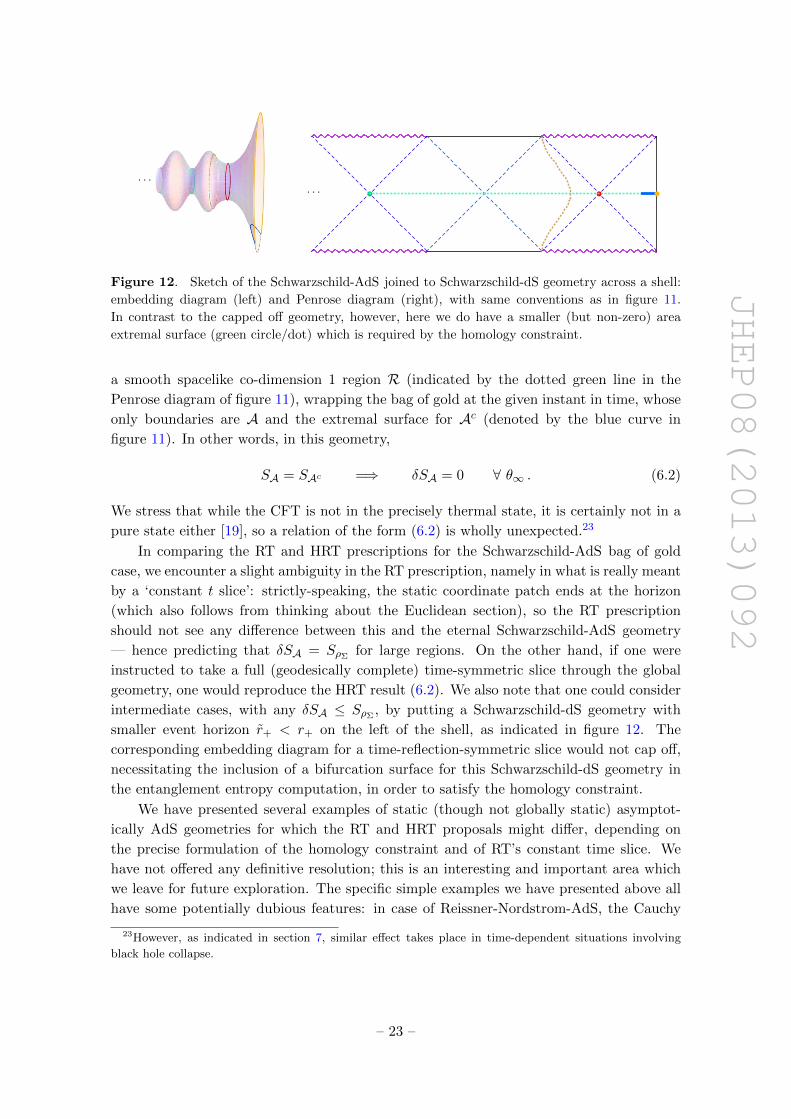
Figure 12. Sketch of the Schwarzschild-AdS joined to Schwarzschild-dS geometry across a shell:
embedding diagram (left) and Penrose diagram (right), with same conventions as in figure 11.
In contrast to the capped off geometry, however, here we do have a smaller (but non-zero) area
extremal surface (green circle/dot) which is required by the homology constraint.
a smooth spacelike co-dimension 1 region R (indicated by the dotted green line in the
Penrose diagram of figure 11), wrapping the bag of gold at the given instant in time, whose
only boundaries are A and the extremal surface for Ac (denoted by the blue curve in
figure 11). In other words, in this geometry,
SA = SAc =⇒ δSA = 0 ∀ θ∞ . (6.2)
We stress that while the CFT is not in the precisely thermal state, it is certainly not in a
pure state either [19], so a relation of the form (6.2) is wholly unexpected.23
In comparing the RT and HRT prescriptions for the Schwarzschild-AdS bag of gold
case, we encounter a slight ambiguity in the RT prescription, namely in what is really meant
by a ‘constant t slice’: strictly-speaking, the static coordinate patch ends at the horizon
(which also follows from thinking about the Euclidean section), so the RT prescription
should not see any difference between this and the eternal Schwarzschild-AdS geometry
— hence predicting that δSA = SρΣ for large regions. On the other hand, if one were
instructed to take a full (geodesically complete) time-symmetric slice through the global
geometry, one would reproduce the HRT result (6.2). We also note that one could consider
intermediate cases, with any δSA ≤ SρΣ , by putting a Schwarzschild-dS geometry with
smaller event horizon r+ < r+ on the left of the shell, as indicated in figure 12. The
corresponding embedding diagram for a time-reflection-symmetric slice would not cap off,
necessitating the inclusion of a bifurcation surface for this Schwarzschild-dS geometry in
the entanglement entropy computation, in order to satisfy the homology constraint.
We have presented several examples of static (though not globally static) asymptot-
ically AdS geometries for which the RT and HRT proposals might differ, depending on
the precise formulation of the homology constraint and of RT’s constant time slice. We
have not offered any definitive resolution; this is an interesting and important area which
we leave for future exploration. The specific simple examples we have presented above all
have some potentially dubious features: in case of Reissner-Nordstrom-AdS, the Cauchy
23However, as indicated in section 7, similar effect takes place in time-dependent situations involving
black hole collapse.
– 23 –
JHEP08(2013)092
horizon is unstable, while in the other two cases, the shell is unstable. Moreover, in all
cases, the difference between the prescriptions occurs due to a part of the geometry which
is beyond the horizon and thus causally inaccessible to an asymptotic observer. While this
feature might therefore seem rather unappealing, we stress that in general we would be
forced into such situation in any case, as long as the entanglement entropy is related to
some locally-defined geometric construct, due to the teleological nature of the event hori-
zon. The examples mentioned above merely illustrate the issues we have yet to confront
to fully understand the holographic entanglement entropy prescription.
7 Discussion
We have focused on exploring the behaviour of entanglement entropy SA under smooth
deformations of the entangling region A in finite systems. Of particular interest to us is
the distinction between the behaviour of holographic field theories, which in the large c
(planar limit) and strong coupling limit can be mapped onto the dynamics of classical
gravity, versus field theories away from the planar limit. Sharp features in observables are
possible in the latter since the planar limit allows one to enter a ‘thermodynamic regime’,
as evidenced for example by the thermal phase transitions in finite volume [37–39].
We focused in particular on the Araki-Lieb inequality which gives a useful measure of
the relative entanglement of a region A and its complement Ac. While this would vanish
if the entire system were in a pure state, it carries non-trivial information about the total
density matrix in general. We indeed encounter an interesting phenomenon of entanglement
plateaux: the Araki-Lieb inequality is saturated for finite system sizes, owing to some non-
trivial features of minimal surfaces which compute the holographic entanglement entropy.
Focusing on thermal density matrices in CFTs we find that in 1 + 1 dimensional
field theory the Araki-Lieb inequality forces us to modify the expression of entanglement
entropy for a large enough region (a point previously noted in [17, 18]) and provide an
analytic prediction of when the plateau is attained. We also contrast this behaviour of
large c theories against low central charge theories. There being very few exact results on
the entanglement entropy of thermal CFTs in finite volume, we focused on the available
expressions for Dirac fermion (with and without chemical potential). In the c = 1 case
we note the absence of any plateau and the Araki-Lieb inequality is only saturated when
the region under consideration (or its complement) is maximal. In higher dimensional
holographic examples this no longer is the case, δSA is forced by virtue of the features of
the holographic construction to plateau (see below).
For the main part of this work, we have considered the RT prescription for calculating
the holographic entanglement entropy, which is valid for static equilibrium situations. In
this context, one is instructed to work at a given instant in time, and the entanglement
entropy computation then involves finding the area of a requisite minimal surface in the
corresponding Riemannian geometry. Though innocuously simple-sounding, there is a rich
set of features associated with what precisely is meant by ‘requisite’. For a specified
boundary region A, the boundary of the relevant surface MA must coincide with the
– 24 –
JHEP08(2013)092
entangling surface ∂A, it must be homologous to A, and in case of multiple such surfaces,
it must be the one with smallest area.
It has already been observed previously that the last restriction can cause the entan-
glement entropy to have a kink (i.e., its first derivative with respect to the parameter α
characterizing the region A can be discontinuous). This is because there can exist multiple
families of minimal surfaces which can exchange dominance. Here we have explored this
multiplicity further, and discovered that even in the most simple case of global eternal
Schwarzschild-AdSd+1 geometry with d ≥ 3, in a certain regime of α there is actually an
infinite tower of minimal surfaces anchored on the same entangling surface (though only
the lowest two have a regime of dominance), seemingly approaching self-similar behaviour.
This curious feature can arise thanks to the dimensionality of the surfaces and compact-
ness of the horizon. On the other hand, in other regimes of α (namely for sufficiently large
region A), there is only a single, disconnected minimal surface satisfying the homology
requirement — unlike in the 2 + 1 dimensional case, a connected minimal surface homolo-
gous to A simply does not exist. This novel feature may be understood as a consequence
of certain properties of causal wedges discussed in [23].
We note in passing that the distinction between the AdS3 and higher dimensional
examples is quite reminiscent of the Hagedorn behaviour encountered in the dual field
theories. In AdS3 the BTZ black hole saddle point exists for all values of temperature (as
does the thermal AdS one), but it becomes sub-dominant at low temperatures. In higher
dimensions, the Schwarzschild-AdS saddles only exist above a minimum temperature Tmin;
they however take over from the thermal AdS saddle at a slightly higher temperature
TH > Tmin (when the horizon size is comparable to AdS length scale). So at low enough
temperatures we are always forced into the confining state. In the context of entanglement
entropy the analogous observation is about the existence of connected minimal surfaces in
the black hole geometry (we should emphasize that we are always in the deconfined phase
to be able to use the black hole saddle). In three dimensions, connected surfaces always
exist but fail to be dominant past some critical region size; in higher dimensions they cease
to exist past a critical region size given the homology constraint.
Our discussion was primarily focussed on entanglement entropy and in particular on
δSA. One could equally have focussed on the mutual information, I(A,B) = SA + SB −SA∪B, for two disjoint regions A and B. Holographic studies of mutual information also
reveal an interesting behaviour: for sufficiently separated regions I(A;B) = 0. This is due
to the fact that the extremal surface EA∪B breaks up into a disconnected surface anchored
on A and B to avoid thin necks. This has been extensively discussed in the literature
cf., [6] and [31, 33, 40] for implications of this construct in the context of probing black hole
interiors. For the regions we have considered A and Ac are not strictly disjoint, so we have
to be a bit more careful; naively the mutual information involves the sum of the entropies of
two regions (which we take to be A and Ac) while the Araki-Lieb inequality constrains their
difference, giving I(A;Ac) = 2SA which is UV divergent.24 One can however constrain
24We thank the referee for spotting an error in our original statement and for suggesting use of the
auxiliary purifying system.
– 25 –
JHEP08(2013)092
the mutual information between the smaller of A or Ac and the auxiliary system ρΣ which
purifies the global density matrix ρΣ (thus SρΣ = SA∪Ac = SρΣ) to vanish when Araki-Lieb
inequality is saturated. For example one has
I(A; ρΣ) = SA + SρΣ− SA∪ρΣ
= SA + SρΣ − SAc =
0, for α < 1
2
2SρΣ , for α > 12
(7.1)
In deriving this we used the fact that SA∪Ac∪ρΣ= 0 by definition of the purifying degrees
of freedom. In the case of the global thermal density matrix ρΣ is the thermofield double
which lives on the second asymptotic region of the eternal black hole Penrose diagram.
While these causal wedge considerations already by themselves guarantee that the en-
tanglement entropy SA(α) cannot be a smooth function for thermal states in higher dimen-
sions, we have argued that, if defined by a minimization procedure as in the RT prescription,
the entanglement entropy must nevertheless be continuous. Our argument crucially used
minimality. In particular, in the HRT prescription of computing entanglement entropy
via a smallest area extremal surface, the continuity argument given in section 2 does not
apply. It would be interesting to explore whether sufficient time-dependence can provide
counter-examples to continuity or whether the one can generalize the proof of continuity
to the Lorentzian context; we leave further investigation of this issue for the future [12].
Note that in this collapsed black hole context, the homology requirement is satisfied
automatically, though as explained in [12], that itself leads to very curious feature of
entanglement entropy: it can distinguish between an eternal black hole and a collapsed
one, arbitrarily long after the collapse had taken place [41]. In this sense, while in the
AdS/CFT context we are used to classical bulk surfaces providing at best only some coarse-
grained CFT information, the homology requirement induces a fine-grained aspect to the
entanglement entropy observable.
While in the time-dependent setting mentioned above, the RT prescription is mean-
ingless and therefore cannot be compared to the extremal surface generalization of HRT,
we have seen that there are subtle differences between the RT and HRT proposals even is
static situations. Indeed, a similar ‘fine-grained’ quality as mentioned above is manifested
in the entanglement entropy for e.g. the Schwarzschild-AdS bag of gold geometry discussed
in section 6: there the entanglement entropy (as given by the HRT prescription) can easily
distinguish the differences in the geometry behind the horizon, on the other side of the
Einstein-Rosen bridge. Other known diagnostics of the CFT density matrix not being pre-
cisely thermal typically require rather sophisticated machinery, such as detecting lack of
periodicity on the Euclidean time circle of the analytically continued solution. We find it
remarkable that entanglement entropy does the job so easily. This observation of course
crucially hinges on the precise formulation of the homology constraint, which deserves to
be understood better.
Acknowledgments
It is a pleasure to thank Jan de Boer, Juan Jottar, Hong Liu, Tadashi Takayanagi and
especially Matt Headrick for various illuminating discussions. We would also like to thank
– 26 –
JHEP08(2013)092
Hong Liu and Tadashi Takayanagi for their detailed comments on a draft of this manuscript.
VH and MR would like to thank CERN, ITF, Amsterdam and ICTP for hospitality during
the early stages of this project. In addition MR would like to acknowledge the hospitality
of Technion, Israel during the “Relativistic fluid dynamics and the gauge gravity duality”
workshop as well as the organizers of the “2nd Mediterranean Conference on Classical And
Quantum Gravity” Veli Losinj, Croatia for their hospitality during the concluding stages
of this project. HM is supported by a STFC studentship. VH and MR are supported in
part by the STFC Consolidated Grant ST/J000426/1.
A Mean curvature flow
In this appendix we summarize the algorithm we used to construct the minimal surfaces
in Schwarzschild-AdSd+1 for d ≥ 3. While one can directly numerically solve the Euler-
Lagrange equations of (4.2) directly, it is especially useful to consider alternate strategies
to ensure that we have obtained all the surfaces of interest.
For conceptual and computational purposes, it is useful to view minimal surfaces as
the endpoint of a flow of surfaces of decreasing area. This is analogous to a gradient descent
algorithm for finding a local minimum of a function, for which one considers a point moving
with velocity equal to minus the gradient of the function. This gives a curve along which the
function monotonically decreases, and exponentially decays to the minimum as a function
of flow time tflow ≡ t→∞.
In the analogous process for minimal submanifolds, the function to be minimized be-
comes the area functional, and the flow velocity vector becomes a vector field (which may
be taken to be normal) defined on the submanifold. The appropriate vector field is given
by the mean curvature of the submanifold, and the evolutionary process is known as mean
curvature flow.
We review the required differential geometric technology, and outline an algorithm for
computing the process in the case of codimension-one minimal surfaces.25
A.1 Some geometry
Let n be a smooth n-dimensional Riemannian manifold (e.g., n for situations of interest is a
constant time surface in the bulk spacetimeM), with metric g and Levi-Civita connection
∇. Further, let m ⊂ n be a smooth m-dimensional submanifold (with m < n), defined by
embedding ψ : m→ n. The induced metric on m is inherited from n as γ = ψ∗g given this
embedding. Vectors at a point on the submanifold can be decomposed into components
tangent and normal to m: U = U> + U⊥.
The natural structures associated with m ⊂ n are in terms of the intrinsic and extrinsic
geometry of the embedding, characterized by the induced metric γ (the first fundamental
form) and the extrinsic curvature K (the second fundamental form). Formally, given vector
25The minimal surfaces relevant for computing entanglement entropy using the prescription of [1] are
co-dimension two in the bulk. In static spacetimes however we can localize on a constant time bulk
hypersurface, leading thus to a search of co-dimension one surfaces on the slice.
– 27 –
JHEP08(2013)092
fields, say U and V , tangent to m, one can decompose the covariant derivative:
∇UV = (∇UV )> + (∇UV )⊥ = DUV +K(U, V ) , (A.1)
which effectively defines D and K. The former is the Levi-Civita connection of the induced
metric on m, while the latter is a normal-valued symmetric bi-linear form. It is worth
emphasizing that the second fundamental form depends only on the vectors at the point,
so it is a tensor on m. A particularly important object is obtained by taking its trace k,
giving a normal vector field on m: this is the mean curvature field.26 In components, using
coordinates xa intrinsic to m, and Xα on n, we have γab = gαβ ∂aXα ∂bX
β, and
hαβ = γab ∂aXα ∂bX
β , K γαβ = h µ
α h νβ ∇ν h γ
µ , kα = hµν K αµν .
Here h is the projection onto vectors tangent to m. Note that the extrinsic curvature
tensor K γαβ is symmetric in its lower indices which lie tangent to m, while the upper index
is transverse.
We are now in a position to make precise the geometric interpretation of the mean
curvature field alluded to above, that it is minus the gradient of the area functional on the
space of submanifolds.
Let us consider a smooth family of embeddings Ψ : I×m→ n, where I is some interval
parameterized by a flow time t. For each t ∈ I, ψt = Ψ(t, ·) : m → n is an embedding.
Let A be the area of the embedded submanifold:
A(t) =
∫mωt, (A.2)
where ωt is the induced volume form on m at time t.
Let V be the vector field given by the local velocity of the surface in this deformation,
so V = Ψ∗∂∂t . One should think of Ψ, or ψt, as defining a curve through the space of
embeddings, an infinite-dimensional manifold whose tangent space at ψ is given by the set
of Tn-valued vector fields on ψ. Then V is naturally the tangent vector to the curve.
We now have enough state our key result:
dA
dt= −
∫mg(k, V )ωt. (A.3)
In the space of embeddings, this is the natural inner product between V and −k, which
makes precise the analogy with a gradient. Note that, as is to be expected, only the normal
component of V contributes, since the tangent component is ‘pure gauge’, describing how
parameterization of the embedding evolves, and not the shape of the submanifold itself.
Proof. The method of proof is to compute ∂∂t of the induced volume form on m, and we
will show it is equal to (−g(k, V ) + D · V >)ωt. Since the last term is a total derivative,
the result will follow, provided that the variation is constrained to a compact region, or
26This definition of the mean curvature is not entirely universal: in some conventions the sign differs,
while in others the trace is divided by a factor of m, so that k is genuinely the mean of the eigenvalues of
K (which incidentally define the principal curvatures of the submanifold).
– 28 –
JHEP08(2013)092
we restrict the variation to be normal (so V > = 0). For ease of computation, we work in
a chart of normal coordinates xi on m at the point p, with respect to the induced metric
at time t = 0: γ(∂i, ∂j) = δij , and D∂i∂j = 0. Let ei = Ψ∗∂i. For later use, we note that
since Lie brackets commute with push-forward, [ei, V ] = 0, so ∇V ei = ∇eiV .
The induced volume form is given by ωt =√
det(g(ei, ej)) dx1 ∧ · · · ∧ dxm, so its
derivative at the point p and t = 0 is
1
2
∂
∂t(g(ei, ei)) ω0, (A.4)
where we have used the fact that the derivative of detA is detA tr(A−1A), and that dx1 ∧· · · ∧ dxm = ω0 at p in our normal coordinates. Now, again computing at the point p
and t = 0,
1
2
∂
∂tg(ei, ei) =
1
2V (g(ei, ei))
= g(∇V ei, ei)= g(∇eiV, ei)= ei(g(V, ei))− g(V,∇eiei)= ∂iV
>i − g(V,Deiei +K(ei, ei))
= D · V > − g(V, k).
In the final line we have used the fact that we have normal coordinates, so ∂i = Di, and
the sum over i reduces to the trace.
A.2 The algorithm
With the necessary mathematical formalism in hand, we now describe an algorithm for im-
plementing the mean curvature flow, specializing for simplicity to the case of codimension-
one surfaces. In this case, having chosen a direction for a normal, the mean curvature
vector field reduces to a scalar field, since the normal space is one-dimensional.
The method used is based on a level-set approach: the surfaces are described by the sets
m = x ∈ n| Φ(x) = c (A.5)
for some function Φ and some constant c, and the evolution of the function Φ is what we
shall model. This has several advantages:
• There is no requirement to pick a parameterization of the surface, so no problem with
‘gauge fixing’.
• A whole family of surfaces can be modeled at once, by computing the evolution for
Φ and picking different level sets.
• The algorithm elegantly allows for changes in topology: under mean curvature
flow, surfaces can split into several parts, and this causes no trouble for the level
set method.
– 29 –
JHEP08(2013)092
The definition of the flow gives the normal speed of a point on the surface as it evolves:
n(dxdt ) = k, with n being the normal to m. Provided that dΦ 6= 0, we also have a simple
way of computing a unit normal, n = dΦ‖dΦ‖ . To deduce the evolution of Φ, differentiate the
definition (A.5) of a surface m:
0 =∂Φ
∂t+ dΦ
(dx
dt
)=∂Φ
∂t+ ‖dΦ‖n
(dx
dt
)=∂Φ
∂t+ ‖dΦ‖ k .
The only ingredient which remains is to compute k using only information from Φ. Luckily,
this is given by a simple formula in terms of the normal k = −∇ · n. To see this, take n to
be the unit one-form, normal to the surface, but also defined, and unit, off it. Extend to
an orthonormal basis27 ei, n#. Then:
k = n(∇eiei) = ei(n(ei))− (∇ein)(ei)
= −∇ · n+ (∇n#n)(n#)
= −∇ · n+ g(n,∇n#n)
= −∇ · n+1
2n#(g(n, n)) = −∇ · n.
The term ei(n(ei)) in the first line vanishes because n(ei) = 0 everywhere, and the last
equality follows because g(n, n) = 1 everywhere.
This gives us our final evolution equation for Φ:
∂Φ
∂t= ‖dΦ‖ ∇ ·
(dΦ
‖dΦ‖
)=√gγδ ∂γΦ ∂δΦ
1√g∂α
( √g gαβ ∂βΦ√gγδ ∂γΦ∂δΦ
). (A.6)
This is a quasilinear parabolic PDE in Φ, which can be solved numerically by stan-
dard methods.
For the computations in this paper, only spherically symmetric surfaces were consid-
ered, so Φ was a function of two spatial coordinates θ and r (or another suitably redefined
radial coordinate). The PDE was solved with difference methods, with Neumann bound-
ary conditions at the poles of the sphere (θ = 0, π) to keep the surfaces regular there, and
mixed boundary conditions at radial boundaries set by the desired asymptotics.
B Near-horizon behaviour of minimal surfaces
An analytic solution of the equations of motion in a near-horizon approximation explains
the existence of an infinite self-similar family of minimal surfaces, wrapping the horizon
multiple times. We find that this is generic near any minimum of the radius of the Sd−1,
such as the Einstein-Rosen bridge of a non-extremal black hole, and is characterized entirely
by the number of dimensions,28 and a single parameter ξ ≡ r+ κ, where κ is the surface
gravity (which is related to the black hole temperature as T = 14π κ).
27We denote the ‘raised index’ normal vector by n#, so that g(n#, U) = n(U)28Here we will keep to spatial codimension-one surfaces, but the argument carries over essentially un-
changed for surfaces of any dimension m, wrapping a Sm−1 in an SO(d) symmetric space.
– 30 –
JHEP08(2013)092
For the analysis we use a modified radial coordinate z, regular at the event horizon,
defined by r = r+ + 12 r+ ξ z
2, and parametrize the surface by θ throughout. Dots will
denote differentiation with respect to θ.
We invoke two approximation schemes. The naive linearization holds away from the
poles, but breaks down close the θ = 0, π where z grows without bound. Near the poles,
we use a different approximation, reducing the problem locally to flat Euclidean space. We
will find that these two approximation schemes have overlapping domains of validity, so the
complete behaviour can be described by matching the asymptotics in each regime. This
predicts a tower of arbitrarily many branches of the surface wrapping the horizon, with a
known relationship between the distances from the horizon of successive surfaces.
Schematically: we start at the North pole θ = 0, and solve in the linear regime towards
the South pole θ = π. There we change to the near-pole regime, in which there will be a
turning point at a minimum angle ∆ away from the pole, at z = z0. These constants are
both computed from matching to the linearized solution. We then match up to another
branch moving back towards the North pole, where there will be a turning point given by
new, parametrically larger, ∆ and z0. The matching process will allow us to produce a
recurrence relation for the sequences ∆n, zn of turning points. We can obtain an entirely
analytic expression for these values, which, sufficiently close to the horizon, match precisely
with the values obtained from numerically integrated surfaces.
B.1 The linear regime
We start with the linear approximation, valid for z, z 1. In this case, the minimal surface
equation obtained from (4.2) reduces to
z + (d− 2) cot θ z − (d− 1) ξ z = 0 , ξ ≡ r+ κ. (B.1)
This equation has regular singular points at θ = 0, π, where the solutions have asymptotics
z ∼ θσ for σ = 0, 3 − d (or constant and z ∼ log θ asymptotics in d = 3). For ξ > 0 it is
easy to show that a solution regular at θ = 0 cannot be regular at θ = π, so the general
solution can be written
z(θ) = A zr(θ) +B zr(π − θ) (B.2)
using the symmetry under θ 7→ π− θ. Here zr is chosen by demanding zr(θ)→ 1 as θ → 0,
and the asymptotics are characterized by a parameter λ, by zr(θ) ∼ λ (π− θ)3−d as θ → π.
In fact, the solutions can be found explicitly in terms of associated Legendre functions, and
λ(d, ξ) can be found analytically.
B.2 Near-pole flat space regime
For the second approximation scheme, we assume z 1, z z, θ 1, in which case the
problem reduces to that of a spherically symmetric “soap bubble” in flat d-dimensional
Euclidean space, where (θ, z) are the radial and longitudinal coordinates respectively in a
cylindrical polar system. This has the solution
z = z0 ±∆
∫ θ∆
1
dx√x2d−4 − 1
. (B.3)
– 31 –
JHEP08(2013)092
The constants z0 and ∆ will be small values, describing the distance from horizon and pole
respectively of the turning point of the surface. Note that taking the limit θ → ∞, the
integral converges, so z tends to a fixed value when d > 3: the upper and lower branches
of the surface remain at bounded separation, characterized by the value of
Id =
∫ ∞1
dx√x2d−4 − 1
= −√π
Γ(
d−32(d−2)
)Γ(−1
2(d−2)
) . (B.4)
The asymptotics are given by
z ∼ z0 ± Id ∆ ∓ 1
d− 3∆d−2 θ3−d as
θ
∆→∞ . (B.5)
B.3 Matching asymptotics
With solutions in the two approximation schemes in hand, it now remains only to fix
constants of integration by matching the asymptotics. For definiteness, consider starting
from a known (∆n, zn) close to the North pole, computing the coefficients of the linear
solution, and finally extracting the values of (∆n+1, zn+1) close to the South pole.
The case d = 3 is a little different from d > 3, because of the logarithmic asymptotics,
so we will stick to d > 3 here. A very similar analysis holds in this case, for which we will
omit the details, and present only the results.
Recall the form of the linear solution z(θ) = Azr(θ)+B zr(π−θ), with the terms regular
at θ = 0, π respectively. Consistency imposes that the coefficients have parametrically
different sizes, with A B. Towards the South pole, the B-mode is also suppressed
relative to the A-mode by the growth of the latter, which renders B essentially irrelevant,
and the turning points can be characterized by a single parameter. Indeed, by matching
the asymptotics near the South pole, for consistency we need zn+1 = Id ∆n+1. Finally, we
match A with the relevant coefficients at each end,
zn + Id ∆n = A =∆d−2n+1
λ (d− 3), (B.6)
which finally gives us our recurrence relation
∆n+1 = [2λ (d− 3) ∆n]1d−2 , (B.7)
demonstrating a parametric growth in ∆, z at each step. This can be conveniently solved
by changing to the coordinate x, defined by r = r+ + e2x, (or 12 r+ ξ z
2 = e2x) from which
we get
xn =x0 − ν
(d− 2)n+ ν, ∆n =
√2
κ
exn
r+ Id(B.8)
with the constant ν given by
ν =1
2log
(r+ ξ
2
)+
log[2 (d− 2)λ Id−2d ]
d− 3. (B.9)
– 32 –
JHEP08(2013)092
It should be noted that the initial value of x where the surface smoothly crosses the pole
θ = 0, closest to the horizon, is not at x0, but rather at x = x0+log 2, since the solution here
is not given by (B.3), but by that obtained in the linear regime: constant x to leading order.
For completeness, we record the computed values of λ here:
λ =cosh(π )
(d− 3)π
2d−2((
d−32
)!)2
[(12)2 + 2][(3
2)2 + 2] · · · [(d−42 )2 + 2]
, d odd
λ = (d− 3)sinh(π )
(1
12 + 2
)(3
22 + 2
)(5
32 + 2
)· · ·
(d− 5(
d−42
)2+ 2
), d even
(B.10)
where in both cases, is defined by
2 = (d− 1) ξ − (d− 2)2
4. (B.11)
In d = 3, we have slightly altered formulae:
∆n+1 = −2λ∆n log
(∆n
2
)(B.12)
xn =1
2log
(r+ ξ
2
)+ log
[−∆n log
(∆n
2
)](B.13)
λ =2 cosh(π )
π. (B.14)
B.4 Validity
Having done this calculation, it is worth checking to see that we have done something sen-
sible: there must be some overlap between the domains of validity of each approximation.
It is straightforward to confirm this a posteriori, looking at overlaps near the North pole
for definiteness. Firstly, the linear approximation is valid when z, z 1, which requires
θ2−d to be much smaller than the coefficient of the growing mode. This holds for θ ∆.
Secondly, the near-pole approximation is valid when z z, which requires θd−2 ∆d−3
(as well as θ 1). This means that as long as ∆ remain small, both approximations are
simultaneously valid for
∆ θ ∆d−3d−2 . (B.15)
For d = 3, we have a similar result, with overlap region
e−1∆ θ −1
log ∆. (B.16)
B.5 Relation to θ∞
We can straightforwardly use this analysis to show that for θ∞ sufficiently close to π/2
there will be an infinite tower of minimal surfaces. This is because each branch of a surface
is characterized by a single parameter. All surfaces with a particular turning point will
match closely outside that turning point. To obtain a surface on later branches of this
– 33 –
JHEP08(2013)092
tower requires the initial value of −x to be exponentially large, so the distance from the
horizon will be suppressed by an exponential of an exponential.
Incidentally, this gives an indirect demonstration of non-existence of connected minimal
surfaces for sufficiently large θ∞. The connected surfaces form a one-parameter family,
parameterized by the maximum depth reached into the bulk, or equivalently the location
x0 of the surface at θ = 0. Considering θ∞ as a function of x0, continuity implies that there
are only two ways for θ∞ to reach arbitrarily close to π. The first is for θ∞ = π for some
x0, but this is precluded from happening by behaviour near the boundary. The other way
is for a sequence xm to exist such that θ∞(xm) tends to π, but the self-similarity properties
of surfaces indicated here will prevent this option also.
References
[1] S. Ryu and T. Takayanagi, Holographic derivation of entanglement entropy from AdS/CFT,
Phys. Rev. Lett. 96 (2006) 181602 [hep-th/0603001] [INSPIRE].
[2] S. Ryu and T. Takayanagi, Aspects of Holographic Entanglement Entropy, JHEP 08 (2006)
045 [hep-th/0605073] [INSPIRE].
[3] V.E. Hubeny, M. Rangamani and T. Takayanagi, A covariant holographic entanglement
entropy proposal, JHEP 07 (2007) 062 [arXiv:0705.0016] [INSPIRE].
[4] R. Bousso, The holographic principle, Rev. Mod. Phys. 74 (2002) 825 [hep-th/0203101]
[INSPIRE].
[5] D.V. Fursaev, Proof of the holographic formula for entanglement entropy, JHEP 09 (2006)
018 [hep-th/0606184] [INSPIRE].
[6] M. Headrick, Entanglement Renyi entropies in holographic theories, Phys. Rev. D 82 (2010)
126010 [arXiv:1006.0047] [INSPIRE].
[7] H. Casini, M. Huerta and R.C. Myers, Towards a derivation of holographic entanglement
entropy, JHEP 05 (2011) 036 [arXiv:1102.0440] [INSPIRE].
[8] A. Lewkowycz and J. Maldacena, Generalized gravitational entropy, arXiv:1304.4926
[INSPIRE].
[9] T. Hartman, Entanglement entropy at large central charge, arXiv:1303.6955 [INSPIRE].
[10] T. Faulkner, The entanglement Renyi entropies of disjoint intervals in AdS/CFT,
arXiv:1303.7221 [INSPIRE].
[11] H. Araki and E. Lieb, Entropy inequalities, Commun. Math. Phys. 18 (1970) 160.
[12] V.E. Hubeny and H. Maxfield, work in progress.
[13] T. Albash and C.V. Johnson, Holographic studies of entanglement entropy in
superconductors, JHEP 05 (2012) 079 [arXiv:1202.2605] [INSPIRE].
[14] A. Belin, A. Maloney and S. Matsuura, Holographic phases of Renyi entropies,
arXiv:1306.2640 [INSPIRE].
[15] H. Liu and M. Mezei, A refinement of entanglement entropy and the number of degrees of
freedom, arXiv:1202.2070 [INSPIRE].
[16] M. Headrick and T. Takayanagi, A holographic proof of the strong subadditivity of
entanglement entropy, Phys. Rev. D 76 (2007) 106013 [arXiv:0704.3719] [INSPIRE].
– 34 –
JHEP08(2013)092
[17] T. Azeyanagi, T. Nishioka and T. Takayanagi, Near extremal black hole entropy as
entanglement entropy via AdS2/CFT1, Phys. Rev. D 77 (2008) 064005 [arXiv:0710.2956]
[INSPIRE].
[18] D.D. Blanco, H. Casini, L.-Y. Hung and R.C. Myers, Relative entropy and holography,
arXiv:1305.3182 [INSPIRE].
[19] B. Freivogel et al., Inflation in AdS/CFT, JHEP 03 (2006) 007 [hep-th/0510046] [INSPIRE].
[20] T. Nishioka and T. Takayanagi, AdS bubbles, entropy and closed string tachyons, JHEP 01
(2007) 090 [hep-th/0611035] [INSPIRE].
[21] I.R. Klebanov, D. Kutasov and A. Murugan, Entanglement as a probe of confinement, Nucl.
Phys. B 796 (2008) 274 [arXiv:0709.2140] [INSPIRE].
[22] V.E. Hubeny and M. Rangamani, Causal holographic information, JHEP 06 (2012) 114
[arXiv:1204.1698] [INSPIRE].
[23] V.E. Hubeny, M. Rangamani and E. Tonni, Global properties of causal wedges in
asymptotically AdS spacetimes, arXiv:1306.4324 [INSPIRE].
[24] P. Calabrese and J.L. Cardy, Entanglement entropy and quantum field theory, J. Stat. Mech.
0406 (2004) P06002 [hep-th/0405152] [INSPIRE].
[25] N. Ogawa, T. Takayanagi and T. Ugajin, Holographic Fermi surfaces and entanglement
entropy, JHEP 01 (2012) 125 [arXiv:1111.1023] [INSPIRE].
[26] C.P. Herzog and M. Spillane, Tracing through scalar entanglement, Phys. Rev. D 87 (2013)
025012 [arXiv:1209.6368] [INSPIRE].
[27] M.M. Caldarelli, O.J. Dias, R. Emparan and D. Klemm, Black holes as lumps of fluid, JHEP
04 (2009) 024 [arXiv:0811.2381] [INSPIRE].
[28] R. Emparan, R. Suzuki and K. Tanabe, The large D limit of general relativity, JHEP 06
(2013) 009 [arXiv:1302.6382] [INSPIRE].
[29] V.E. Hubeny, Extremal surfaces as bulk probes in AdS/CFT, JHEP 07 (2012) 093
[arXiv:1203.1044] [INSPIRE].
[30] J. Abajo-Arrastia, J. Aparicio and E. Lopez, Holographic evolution of entanglement entropy,
JHEP 11 (2010) 149 [arXiv:1006.4090] [INSPIRE].
[31] T. Hartman and J. Maldacena, Time evolution of entanglement entropy from black hole
interiors, JHEP 05 (2013) 014 [arXiv:1303.1080] [INSPIRE].
[32] H. Liu and S.J. Suh, Entanglement tsunami: universal scaling in holographic thermalization,
arXiv:1305.7244 [INSPIRE].
[33] S.H. Shenker and D. Stanford, Black holes and the butterfly effect, arXiv:1306.0622
[INSPIRE].
[34] A.C. Wall, Maximin surfaces and the strong subadditivity of the covariant holographic
entanglement entropy, arXiv:1211.3494 [INSPIRE].
[35] B. Czech, J.L. Karczmarek, F. Nogueira and M. Van Raamsdonk, The gravity dual of a
density matrix, Class. Quant. Grav. 29 (2012) 155009 [arXiv:1204.1330] [INSPIRE].
[36] D. Marolf, Black holes, AdS and CFTs, Gen. Rel. Grav. 41 (2009) 903 [arXiv:0810.4886]
[INSPIRE].
– 35 –
JHEP08(2013)092
[37] E. Witten, Anti-de Sitter space, thermal phase transition and confinement in gauge theories,
Adv. Theor. Math. Phys. 2 (1998) 505 [hep-th/9803131] [INSPIRE].
[38] B. Sundborg, The Hagedorn transition, deconfinement and N = 4 SYM theory, Nucl. Phys.
B 573 (2000) 349 [hep-th/9908001] [INSPIRE].
[39] O. Aharony, J. Marsano, S. Minwalla, K. Papadodimas and M. Van Raamsdonk, The
Hagedorn-deconfinement phase transition in weakly coupled large-N gauge theories, Adv.
Theor. Math. Phys. 8 (2004) 603 [hep-th/0310285] [INSPIRE].
[40] I.A. Morrison and M.M. Roberts, Mutual information between thermo-field doubles and
disconnected holographic boundaries, arXiv:1211.2887 [INSPIRE].
[41] T. Takayanagi and T. Ugajin, Measuring black hole formations by entanglement entropy via
coarse-graining, JHEP 11 (2010) 054 [arXiv:1008.3439] [INSPIRE].
– 36 –