INSTITUT NATIONAL DE LA STATISTIQUE ET DES ETUDES ECONOMIQUES Série des Documents de Travail du CREST

(Centre de Recherche en Economie et Statistique)

n° 2008-10

Does Fertility Respond to Financial Incentives ?

G. LAROQUE1 B. SALANIÉ2

Les documents de travail ne reflètent pas la position de l'INSEE et n'engagent que leurs auteurs. Working papers do not reflect the position of INSEE but only the views of the authors.

1 CREST-INSEE and University College London. 2 Columbia University and CEPR. This research benefited from the financial support of the Alliance program during a visit of Guy Laroque at Columbia University. We are grateful to Gary Becker, Didier Blanchet, Pierre-André Chiappori, Olivia Ekert-Jaffé, Philippe Février, Dominique Goux, James Heckman, Mark Killingsworth, Anne Laferrère, Steve Levitt, Annalisa Luporini, Thierry Magnac, Kevin Murphy, Laurent Toulemon, Alain Trannoy, Daniel Verger and James Walker for their comments.

Does Fertility Respond

to Financial Incentives?

Guy Laroque1 Bernard Salanie2

July 9, 2008

1CREST-INSEE and University College London.2Columbia University and CEPR. This research benefited from the financial

support of the Alliance program during a visit of Guy Laroque at ColumbiaUniversity. We are grateful to Gary Becker, Didier Blanchet, Pierre-Andre Chi-appori, Olivia Ekert-Jaffe, Philippe Fevrier, Dominique Goux, James Heckman,Mark Killingsworth, Anne Laferrere, Steve Levitt, Annalisa Luporini, ThierryMagnac, Kevin Murphy, Laurent Toulemon, Alain Trannoy, Daniel Verger andJames Walker for their comments.

Abstract

There has been little empirical work evaluating the sensitivity of fertility to

financial incentives at the household level. We put forward an identification

strategy that relies on the fact that variation of wages induces variation in

benefits and tax credits among “comparable” households. We implement this

approach by estimating a discrete choice model of female participation and

fertility, using individual data from the French Labor Force Survey and a

fairly detailed representation of the French tax-benefit system. Our results

suggest that financial incentives play a notable role in determining fertility

decisions in France, both for the first and for the third child. As an example,

an unconditional child benefit with a direct cost of 0.3% of GDP might raise

total fertility by about 0.3 point.

Il y a peu d’etudes empiriques qui mesurent la sensibilite de la fecondite

aux incitations financieres. Nous presentons une strategie d’identification qui

repose sur le fait que des variations (exogenes) de salaires induisent des dif-

ferences de prestations et impots entre des menages qui sont par ailleurs ‘com-

parables’. Nous appliquons cette idee en estimant un modele de fecondite et

participation feminine en France, sur donnees individuelles de l’Enquete Em-

ploi, en utilisant une descrition detaillee des impots et transferts en France.

Nos resultats indiquent un impact notable des incitations financieres sur la

fecondite en France, pour les premier et troisieme enfants. Ainsi une presta-

tion familiale sans condition de ressources de cout direct egal a 0.3% du PIB

augmenterait la fecondite d’environ 0.3 point.

JEL codes: J13, J22, H53

Keywords: population, fertility, incentives, benefits.

Who can behold the male and female of each species, the corre-

spondence of their parts and instincts, their passions, and whole

course of life before and after generation, but must be sensible,

that the propagation of the species is intended by Nature?

(Hume (1776 (2005)), Part III).

1 Introduction

It is natural for economists raised on the New Home Economics to presume

the existence of a link between family transfers and fertility. The standard

model of Becker (1960, 1991) and Willis (1973) implies that the demand for

children depends on their cost, which in turn depends on family transfers

(see for instance Cigno (1986) for a theoretical study of the impact of taxes

on fertility). Yet in many countries (see Gauthier (1996)), family benefits

are mostly designed as a way to ensure a minimum standard of living to

families and children. There are notable exceptions: the policies towards

families implemented in France at the end of the 1930s were in part based on

the belief that family benefits increase fertility, and a 2004 reform explicitly

mentions fertility as a concern. Sweden and Quebec have also implemented

pronatalist policies in the past; more recently, other countries with much

more dire fertility issues such as Germany and Russia have enacted policy

measures designed to bring them closer to the replacement rate.

How can we quantify the effects of financial incentives on fertility? Several

approaches have been used so far (see for instance the survey of Hotz, Kler-

man, and Willis (1997)). A first group of studies uses panel data on countries;

then the unit of observation is a given (country, year) pair.1 This line of work

relies on the reasonable assumption that there is variation in family policies

over time and space that is not entirely explained by the other explanatory

variables. On the other hand, it suffers from the usual glaring problems of

panel country regressions: arbitrary functional form assumptions and a huge

1Thus the work of Ekert-Jaffe (1986), Blanchet and Ekert-Jaffe (1994) and Gauthierand Hatzius (1997) suggests that the French family benefit system may increase totalfertility by 0.1 to 0.2 child per woman.

1

number of omitted variables whose variation must be heroically assumed to

be orthogonal to the variation in policy parameters. These are compounded

by the fact that these studies sum up very complex tax-benefit systems in

a couple of variables only2. Thus the results obtained in these papers seem

fragile.

More recent work has used individual data, which alone can provide the

analyst with a large number of observations and with enough information to

measure precisely financial incentives to fertility. A few recent studies have

used the natural experiments approach to evaluate the fertility impact of a

given family benefit. Thus Milligan (2004) studies the effect of a cash benefit

given on the birth of a child in Quebec in the 1990s; by comparing fertility

of similar women residing in Quebec and in other Canadian states over this

period, it finds that this benefit strongly stimulated fertility. However, his

approach cannot yield an estimate of a “price elasticity”. Similar remarks

apply to Kearney (2004), who estimates the fertility effect of the introduc-

tion of family caps in many US states following the 1996 reform of welfare.3

A number of papers also studied the effects of the American welfare system

on fertility (see Moffitt (1998)); the results of Rosenzweig (1999) thus sug-

gest that in the 70s, social transfers like the AFDC had a large effect on the

probability that a young lower-class woman would become a single mother.

Keane and Wolpin (2007b, 2007a) estimate a dynamic programming model

of the decisions of young women. Their simulations suggest that the EITC,

whose amount is very low for single-child families, has increased the fertility

of high school dropouts by about 0.2 child per woman. Finally, Cohen, De-

hejia, and Romanov (2007) exploit a drastic reduction of child allowances in

Israel that affected mostly large families in 2003; their results suggest a large

2Ideally, one should also control for the endogeneity of policy variables, as argued byHeckman (1976) and more recently by Besley and Case (2000).

3 There is a small body of econometric literature that aims at estimating the effect offemale and male wages on fertility. Papers by Rosenzweig and Schultz (1985), Hotz andMiller (1988), Heckman and Walker (1989, 1990a, 1990b) confirm that as predicted bytheory, fertility decreases with the woman’s potential wage and increases with the otherincome of the household. The estimated effects are small; but as these papers make noattempt to use the form of the tax-benefit system, it is not quite clear what the estimatedcoefficients of wages represent in any case.

2

negative impact on the fertility of poorer households and new immigrants.

This brief literature review shows that it is difficult to find reliable sources

of variation and credible exclusion restrictions to identify the sensitivity of

fertility to the cost of children, both for theoretical and for practical reasons.4

Section 2 presents and justifies our empirical strategy, which is based on

comparing the fertility outcomes of women who have similar characteristics

except for their wage and the wage of their partner. As family benefits depend

on the two parents’ primary incomes, this provides variation in incentives that

we use to identify the relevant elasticity. We explain in Section 2 the pros

and cons of such an approach to this particular problem.

We apply this idea to the case of France. We focus on French data not

only because we know it well, but also because France has a rather generous

and diverse family benefit system. Its cost (including tax credits) is evaluated

at about 0.8% of GDP, and it comprises some unconditional, some means-

tested, and some employment-tested benefits.

We set up a discrete choice model of fertility and participation decisions on

the French Labor Force Surveys of 1997, 1998 and 1999. A crucial identifying

tool is a fairly detailed representation of the relevant taxes and benefits. We

have to account for women’s participation decisions, given that they are

so closely linked to their fertility choices5. In our model, every woman is

characterized by her productivity, her disutility for work and her net utility

for a new child. If her productivity is smaller than the minimum wage,

the woman cannot take a job. Otherwise, she can take a job paid at her

productivity if she wishes to do so. She then jointly decides on participation

and fertility, depending on her individual characteristics.

We have had to make simplifying assumptions. Thus we reduce the com-

plex dynamic decision process of couples to a static reduced form. We ignore

4Our previous work (Laroque and Salanie (2004a, 2004b)) in fact illustrates it. Inour first attempts at studying fertility behavior, we did not give center stage to issues ofidentification; these earlier papers also included older women, which tended to contaminateour estimates.

5A paper by Lefebvre, Brouillette, and Felteau (1994) estimated a nested logit of fertilityand participation on individual Canadian data; their results suggest that family benefitshave a non-negligible impact on fertility. However, we devote much more attention toidentification issues.

3

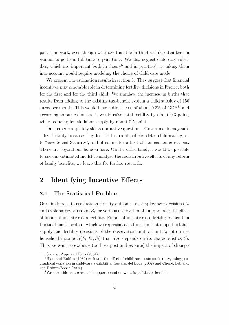
part-time work, even though we know that the birth of a child often leads a

woman to go from full-time to part-time. We also neglect child-care subsi-

dies, which are important both in theory6 and in practice7, as taking them

into account would require modeling the choice of child care mode.

We present our estimation results in section 3. They suggest that financial

incentives play a notable role in determining fertility decisions in France, both

for the first and for the third child. We simulate the increase in births that

results from adding to the existing tax-benefit system a child subsidy of 150

euros per month. This would have a direct cost of about 0.3% of GDP8; and

according to our estimates, it would raise total fertility by about 0.3 point,

while reducing female labor supply by about 0.5 point.

Our paper completely skirts normative questions. Governments may sub-

sidize fertility because they feel that current policies deter childbearing, or

to “save Social Security”, and of course for a host of non-economic reasons.

These are beyond our horizon here. On the other hand, it would be possible

to use our estimated model to analyze the redistributive effects of any reform

of family benefits; we leave this for further research.

2 Identifying Incentive Effects

2.1 The Statistical Problem

Our aim here is to use data on fertility outcomes Fi, employment decisions Li

and explanatory variables Zi for various observational units to infer the effect

of financial incentives on fertility. Financial incentives to fertility depend on

the tax-benefit-system, which we represent as a function that maps the labor

supply and fertility decisions of the observation unit Fi and Li into a net

household income R(Fi, Li, Zi) that also depends on its characteristics Zi.

Thus we want to evaluate (both ex post and ex ante) the impact of changes

6See e.g. Apps and Rees (2004).7Blau and Robins (1989) estimate the effect of child-care costs on fertility, using geo-

graphical variation in child-care availability. See also del Boca (2002) and Chone, Leblanc,and Robert-Bobee (2004).

8We take this as a reasonable upper bound on what is politically feasible.

4

in the function R on fertility outcomes. In France, the function R is very

complicated, highly nonlinear and not even differentiable; but at least it is

public information and it can be evaluated for all values of its arguments.

It is hard to discuss identification at this level of generality; let us therefore

focus on the simple setup we actually use in our application, in which an

observational unit is a household at a given date, the decision variable Li =

0, 1 is the woman’s extensive margin decision of working or not, and the

fertility outcome Fi = 0, 1 is the occurrence of a birth.

The vector of explanatory variables Zi may comprise several classes of

variables. Since a woman at a given period is our observational unit, Zi may

contain:

socio-demographic variables xi such as education, region, past fertility,

marriage status, and so on, which may impact current fertility directly

or because they contribute to determining taxes and benefits;

the market wage of this woman wi, which we take to be her earning

potential if she does not actually work;

the actual wage income of her partner (if any), which we denote wmi .

Several of these variables are clearly not strongly exogenous: the unobserved

“taste for children”, for instance, probably reduces human capital investment

and therefore education; and past fertility can only be weakly exogenous. We

abstract from endogeneity concerns in this section since we want to focus on

identification: we will assume that Z = (x,w,wm) is strongly exogenous. We

will also assume for now that w is observed for all women, whereas of course

it has to be imputed for non-working women.

If a woman’s labor supply decision is L, then her wage income wL enters

the R function; but so does L itself since some benefits are employment-

tested. Thus the tax-benefit system can be described in our application by

four functions which correspond to the four alternatives L = 0, 1;F = 0, 1:

net household income when the woman does not work and no birth

occurred R00(Z);

5

net household income when the woman does not work and a birth

occurred R01(Z);

net household income when the woman works and no birth occurred

R10(Z);

net household income when the woman works and a birth occurred

R11(Z).

Note that when the woman does not work, her market wage w does not enter

the net household income; thus R00(Z) and R01(Z) do not depend on w, but

only on X = (x,wm).

Given this notation, let Q be the distribution of the endogenous variables

L and F ; we can write it in all generality as

Q(L, F |R00(X), R01(X), R10(Z), R11(Z), Z)

and our aim is to evaluate changes in the distribution of F when any of the

four functions Rij shifts.

In this setup, we can only identify nonparametrically from the data the

distribution of L and F conditional on Z, which we denote P (L, F |Z). Under

our exogeneity assumptions, this allows us to answer questions such as:

what is the effect of more education on fertility?

what is the effect of higher male or female wages on fertility?

On the other hand, it does not allow us to evaluate policy-induced changes

in R without further non-testable restrictions.

2.2 Identifying Assumptions

The basic problem we face is that since there are four alternatives, we can

identify nonparametrically only three functions of Z from the data. But

knowing Q requires identifying three functions of both Z and four other

arguments (the Rij’s.) Before we discuss possible sources of exclusion re-

strictions, we introduce our approach to identification on the simple labor

supply model.

6

2.2.1 Identifying Labor Supply Behavior

As in our application, we focus here on the extensive margin9. In this case

we observe a probability of working P (Z); and our aim is “only” to recover a

probability Q(R0(X), R1(Z), Z), where R1 (resp. R0) is household net dispos-

able income when the woman works (resp. does not work.) Here one simple

way to achieve identification is to assume that

Assumption 1 The woman’s market wage w only enters Q through its effect

on R1 (net household income when the woman works).

Assumption 2 The wage income of her partner (if any) wm only enters Q

through its effect on R1 and on R0 (net household income when the woman

does not work).

Recall our notation: X = (x,wm) and Z = (X,w). Given assumptions 1

and 2, we can write P (Z) as Q(R0(X), R1(Z), x). Then changes in w identify

the effect of R1 on labor supply Q; and changes in wm, compensated by

changes in w so as to leave R1 constant, identify the effect of R0 on labor

supply.

More formally, fix x and let W2(x) be the support of the observed distri-

bution of (w,wm) given x. Then the effect of a change of the tax schedule

(R0, R1) into (R′0, R′1) is identified as follows.

Take any (w,wm) such that:

(w,wm) ∈ W2(x);

there exists a solution (w, wm) ∈ W2(x) toR′0(w

m, x) = R0(wm, x)

R′1(w,wm, x) = R1(w, w

m, x).

Then the effect of such a policy change on the labour supply of an indi-

vidual with characteristics (w,wm) is just

P (w, wm, x)− P (w,wm, x).

9The identification problem is similar on the intensive margin, unless of course (oftenimplicit) assumptions are made to constrain the possible causes of variation in hours.

7

(and under assumptions 1 and 2, it clearly does not depend on the choice of

the solution (w, wm)).

When the range of W2(x) is too small, identification may be sought

through further restrictions, which often involve x. E.g. let there be a vari-

able s that only enters Q through its effect on (R0, R1), and denote x = (s, t);

then for given Z = (w,wm, s, t), we only need to find a solution (w, wm, s) toR′0(w

m, s, t) = R0(wm, s, t)

R′1(w,wm, s, t) = R1(w, w

m, s, t)

in the support of the distribution of (w,wm, s) given t, and the effect of the

change then is

P (w, wm, s, t)− P (w,wm, s, t).

While this is enough to identify the effects of changes in taxes and benefits,

we need more if we want to identify the underlying utility functions. From

now on, the whole analysis is done conditional on x, which we drop from

the notation. Let us set up a standard binomial model. Labor supply is the

outcome of a utility maximization where

Assumption 3

the utility of the woman is U1(R1)−d when she works and her household

has disposable income R1;

it is U0(R0) when she does not work and her household has disposable

income R0,

where d measures the random disutility of labor, unobserved by the econo-

metrician, which has a distribution G that does not depend on w or wm.

Similarly, U0 and U1 only depend on (w,wm) through R0 and R1.

Then we can reparameterize the probability of working as Q(R0, R1).

Identification of the binomial choice model has been studied by Matzkin

8

(1992); but for our purposes, the following result in the line of Manski

(1985,1988) is more convenient:

Theorem 1 Assume the true model satisfies Assumptions 1, 2 and 3. More-

over assume that

1. G, U0 and U1 are differentiable, with positive derivatives;

2. denote R2 the image of W2 by the pair of functions (R0, R1); then R2

has a non-empty interior in IR2;

3. there exists a point (r0, r1) in R2 such that Q(r0, r1) = 0.5;

4. G(0) = 0.5.

Take any triple of functions (u0, u1, g) that is consistent with the data gen-

erated by (U0, U1, G). Then under these assumptions, there exist numbers a

(positive) and b such that for all (r0, r1) in the interior of R2,

u0(r0) = aU0(r0) + b and u1(r1) = aU1(r1) + b;

and defining the function δ(r0, r1) = u1(r1)− u0(r0) over R2,

g(y) = Q(r0, r1) if y = δ(r0, r1).

Proof: Take (r0, r1) inside R2. Since G′ > 0, simple differentiation inthe interior of R2 yields

−∂Q∂R0

∂Q∂R1

(r0, r1) =U ′0(r0)

U ′1(r1). (D)

It follows that any possible (u0, u1) must satisfy

U ′0(r0)

u′0(r0)=U ′1(r1)

u′1(r1)= a,

where a is constant, since it cannot depend on r1 by the first equality, noron r0 by the second equality (and a is positive since utilities are increasing.)

9

Integrating gives u0(r0) = aU0(r0) + b0u1(r1) = aU1(r1) + b1.

Moreover, G(0) = 0.5 by assumption, so that

U1(r1) ≡ U0(r0).

This equality must also hold for u0 and u1; but G(U1(r1)−U0(r0)) = 0.5 canalso be rewritten as

G

(u1(r1)− u0(r0)

a− b1 − b0

a

)= 0.5,

which implies

G

(−b1 − b0

a

)= 0.5

and so b0 = b1 = b. QED.

Note that this model has testable “nonparametric” implications:

1. Q must increase in R0 and decrease in R1;

2. log(−Q′0/Q′1) must have a zero cross derivative.

While the first one is fairly weak, the second one may provide an informative

check on the model. Recall Assumption 3: conditional on x, the distribution

of the disutility of labor d does not depend on (w,wm), that is, on (R0, R1).

If for instance the conditional variance of d depends on R0 and R1 in any way,

then the second restriction above will not hold. If the conditional mean of d

depends on (R0, R1), tests based on the second restriction will also detect it

unless this conditional mean is separably additive in R0 and R1.

2.2.2 Missing Wages

To be complete, we should recall that wages w are only observed for working

women. Selection may come from preference shocks or be linked to the

minimum wage. The issue is akin to the treatment effect problem: to achieve

nonparametric identification, we need one variable in the selection equation

10

(into employment) that only enters the outcome equation (the wage equation)

through its effect on the propensity score. The partner’s wage wm (if present)

can play such a role; in our specification we also use family composition

variables to that effect: they figure in the disutility of work—here in U1−U0—

but not in the wage equation.

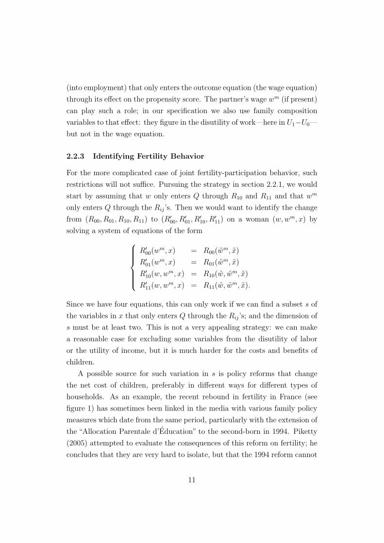
2.2.3 Identifying Fertility Behavior

For the more complicated case of joint fertility-participation behavior, such

restrictions will not suffice. Pursuing the strategy in section 2.2.1, we would

start by assuming that w only enters Q through R10 and R11 and that wm

only enters Q through the Rij’s. Then we would want to identify the change

from (R00, R01, R10, R11) to (R′00, R′01, R

′10, R

′11) on a woman (w,wm, x) by

solving a system of equations of the formR′00(w

m, x) = R00(wm, x)

R′01(wm, x) = R01(w

m, x)

R′10(w,wm, x) = R10(w, w

m, x)

R′11(w,wm, x) = R11(w, w

m, x).

Since we have four equations, this can only work if we can find a subset s of

the variables in x that only enters Q through the Rij’s; and the dimension of

s must be at least two. This is not a very appealing strategy: we can make

a reasonable case for excluding some variables from the disutility of labor

or the utility of income, but it is much harder for the costs and benefits of

children.

A possible source for such variation in s is policy reforms that change

the net cost of children, preferably in different ways for different types of

households. As an example, the recent rebound in fertility in France (see

figure 1) has sometimes been linked in the media with various family policy

measures which date from the same period, particularly with the extension of

the “Allocation Parentale d’Education” to the second-born in 1994. Piketty

(2005) attempted to evaluate the consequences of this reform on fertility; he

concludes that they are very hard to isolate, but that the 1994 reform cannot

11

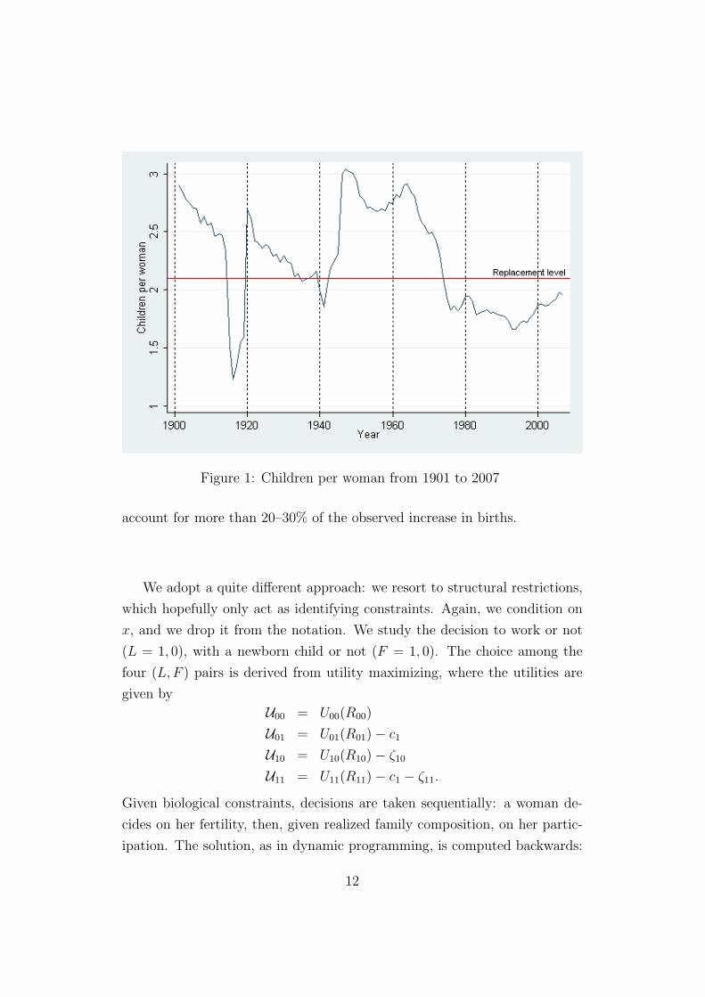
Figure 1: Children per woman from 1901 to 2007

account for more than 20–30% of the observed increase in births.

We adopt a quite different approach: we resort to structural restrictions,

which hopefully only act as identifying constraints. Again, we condition on

x, and we drop it from the notation. We study the decision to work or not

(L = 1, 0), with a newborn child or not (F = 1, 0). The choice among the

four (L, F ) pairs is derived from utility maximizing, where the utilities are

given by

U00 = U00(R00)

U01 = U01(R01)− c1U10 = U10(R10)− ζ10

U11 = U11(R11)− c1 − ζ11.

Given biological constraints, decisions are taken sequentially: a woman de-

cides on her fertility, then, given realized family composition, on her partic-

ipation. The solution, as in dynamic programming, is computed backwards:

12

first one compares U0F and U1F for a given value of F = 0, 1, then the ex-

pected values of max(U0F ,U1F ) to choose the optimal F .

The utility indices ULF are deterministic functions of household incomes,

which are assumed to be perfectly anticipated. Without loss of generality,

we take 00 to be the reference situation for which the disturbance is normal-

ized to zero. The other random terms are written in such a way that ζ10

and ζ11 represent the labor supply disturbances in the second stage, given

realized fertility, while c1 represents a shock on the cost of a newborn child.

It is convenient to assume that the three terms (ζ10, ζ11, c1) are mutually

independent.10

Assumption 4

the women anticipate perfectly their own wage as well as the wage of

their partner;

the shocks on the disutilities of labor given the presence of a newborn or

not, ζ10 and ζ11, and the shock on the cost of a child c1 are independently

distributed.

We denote G0 (resp. G1) the unknown distribution of ζ10 (resp. ζ11),

and K the unknown distribution of c1. It turns out that these assumptions

are (almost) enough to identify the true utility functions U00, U01, U10 and

U11 and the distributions G0, G1 and K up to the usual scale and location

normalization.

First consider labour supply decisions given the realization of the “new-

born”variable F for a woman of characteristics (w,wm). Given the realization

of F , the woman decides to work iff U1F > U0F . So she works with probability

PF (w,wm) = GF (U1F (R1F (w,wm))− U0F (R0F (wm))) .

This is of course the same problem as in section 2.2.1: a nice simplification

from our choice of stochastic specification is that c1 cancels out in the labour

10In fact we only need to assume that the couple (ζ11, c1) is independent of ζ10. But itwould be messier since then we have to use the distribution of ζ11 conditional on c1 whendescribing the labor supply decision after a birth.

13

supply decision problem. Reparameterize PF (w,wm) as QF (R0F , R1F ) as

before. Then we can apply Theorem 1, adapted to the new notation, for

given F = 0, 1.

Theorem 2 Assume that the true model satisfies assumptions 1 to 4, and

in addition:

1. GF , U0F and U1F are strictly increasing and differentiable;

2. GF (0) = 0.5;

3. the support R2F of the distribution of (R0F (wm), R1F (w,wm)) has a

non-empty interior;

4. it contains a (r0F , r1F ) such that U1F (r1F ) = U0F (r0F );

then the utility functions are identified up to scale and location. More pre-

cisely, for any representation (gF , uLF ) consistent with the data, there exist

numbers aF (positive) and bF such that for all (r0, r1) ∈ R2F ,

u0F (r0) = aFU0F (r0) + bF and u1F (r1) = aFU1F (r1) + bF ;

and defining the functions δF (r0F , r1F ) = u1(r1F ) − u0(r0F ) over R2F , we

have

gF (y) = QF (r0F , r1F ) if y = δF (r0F , r1F ).

Note that this implies that on the range of δF , gF (y) = GF (y/aF ).

Thus labor supply decisions in themselves give us some information about

utility functions; but this is not enough to allow us to identify incentive effects

of the R functions on fertility: changes in the ratio a1/a0 and in the cdf of

the cost of children c1, on which we know nothing as yet, can give totally

different estimates of the effect of fertility incentives.

To identify these remaining parameters, we of course need to study fer-

tility decisions. Nature comes to our help, in that fertility decisions must be

made in advance. The true indirect utility of a fertility decision F = 0, 1 is

Emax(U0F (R0F (wm)), U1F (R1F (w,wm))− ζ1F )− cF

14

where the expectation is only taken over the true cdf GF of the shock ζ1F ,

whose value is known to the woman at the time she takes her fertility decision

(and we normalized c0 = 0.) Denote VF the expectation term in this formula.

Now for any variable ξ with cdf S, denote

H(S, α, β) = Eξ max(α− ξ, β).

Then we can write

VF = H (GF , U1F (R1F ), U0F (R0F )) .

Therefore the probability of a newborn F = 1 is

P = Pr(V1 − c1 > V0) = K(V1 − V0) ≡ K(Ω), (K)

with

Ω(w,wm) = H (G1, U11(R11(w,wm)), U01(R01(w)))

−H (G0, U10(R10(w,wm)), U00(R00(w))) . (1)

Labour supply data yield a representation (gF , uLF ) equal to the true one

(GF , ULF ) up to an intercept bF and a scale factor aF :uLF (y) ≡ aFULF (y) + bF

gF (aFy) ≡ GF (y).

Any such choice of (a0, a1, b0, b1) generates its own representation of Ω, call

it ω. The data gives us the probability P (w,wm) that a woman has a baby,

conditional on her wage and her partner’s. We must still solve the functional

equation

P (w,wm) ≡ k(ω(w,wm))

with unknowns k, (a0, a1), and (b0, b1).

To go further, we need some regularity assumptions. We first need to

15

define an “expected marginal rate of substitution” for F = 0, 1:

MF (w,wm) =∂VF

∂w∂VF

∂wm

(w,wm);

We now state

Assumption 5 There exists (w, wm) in the interior ofW2 such that M0(w, wm) 6=

M1(w, wm).

Assumption 5 is very weak. It only requires that in expected terms (over

the shocks on the disutility of labor ζ10 and ζ11), the birth of a child changes

the utility value of an increase in the woman’s potential wage, relative to

an increase in her partner’s wage. There are several reasons why we expect

this to hold, with M0 < M1 in fact for most values of (w,wm). Let us just

mention two:

since women spend more time with young children than men, an in-

crease in their wage-earning potential is (relatively) less valuable if

F = 1 since a birth reduces participation;

some very significant family benefits, such as the APE in France, are

much more attractive for low earners.

Note that this assumption is testable: in fact, given utility functions uLF

obtained after estimating labor supply, and estimates PF (Z) of the proba-

bility of working after fertility outcome F = 0, 1, the marginal utility of a

wage increase is just the average of the marginal utilities when working and

when not working, weighted by the corresponding probabilities11 which can

be directly estimated from the data. Thus for t = w or t = wm, we can write:

∂vF∂t

= PF∂u1F

∂t+ (1− PF )

∂u0F

∂t; (V )

and this is enough to estimate MF since the derivatives of ULF are equal to

those of uLF , known up to a scale factor aF which cancels out in the ratio.

We will present estimates of M0 and M1 later on.

11Given our assumptions, no woman is ever at the margin of participation.

16

We can now state

Theorem 3 Let all assumptions of Theorem 2 hold, along with Assump-

tion 5. Avvvssume in addition that :

1. K is differentiable and strictly increasing at A(w, wm);

2. the RLF functions are differentiable at (w, wm).

Then

1. the marginal utilities are identified locally up to a common scale para-

meter. More precisely, any representation uLF consistent with the data

must satisfy

u′LF (RLF (w,wm)) = λU ′LF (RLF (w,wm))

over W2 for some λ > 0.

2. the cdfs of ζ10, ζ11 and c1 are also identified up to the choice of λ: any

representation (G0, G1, K) consistent with the data must satisfy locallygF (y) = GF (y/λ) for F = 0, 1;

k(y) = K(y/λ).

3. as a consequence, fertility effects of the tax-benefit system are exactly

identified at every point of W2.

Proof: under these assumptions, let (uLF ), (aF ), (bF ), (gF ) be a represen-tation compatible with the labour supply data. Now use (V) to define forZ = (w,wm) ∈ W2, and denoting again t = w or t = wm:

∂vF∂t

(Z) = PF (Z)∂u1F

∂t+ (1− PF (Z))

∂u0F

∂t;

Clearly,∂vF∂t

= aF∂VF∂t

.

17

Now we can write

∂P

∂t= K ′(K−1(P ))

(∂V1

∂t− ∂V0

∂t

)(Q).

It follows that∂P∂w∂P∂wm

=∂V1

∂w− ∂V0

∂w∂V1

∂wm − ∂V0

∂wm

,

or, with the alternative representation of the indirect utilities,

∂P∂w∂P∂wm

=∂v1∂w− a1

a0

∂v0∂w

∂v1∂wm − a1

a0

∂v0∂wm

.

This can be rearranged into

a1

a0

(∂v0

∂wm∂P

∂w− ∂v0

∂w

∂P

∂wm

)=∂v1

∂w

∂P

∂wm− ∂v1

∂wm∂P

∂w.

Everything in this equation is known at this stage, except for the ratio a1/a0.So it determines this ratio uniquely, provided that the term that multipliesit is not zero in some t. But if this term were zero, then so would the termon the right-hand side; and simple algebra shows that then both M0 and M1

would be equal to the marginal rate of substitution of P . Taking Z = (w, wm)shows that a1

a0is identified since by assumption 5, M0 6= M1 in this point at

least.Now fix a0 = λ > 0, which determines a1 and fixes v0 and v1; and take

any Z ∈ W2. Equation (Q) directly gives the density of k at k−1(P (t)) =v1(t) − v0(t). Now suppose we change the tax-benefit system so that RLF

becomes RLF + dRLF ; then the probability of a birth changes by

dP = k′(k−1(P ))

(∂v1

∂R01

dR01 +∂v1

∂R11

dR11

− ∂v0

∂R00

dR00 −∂v0

∂R10

dR10

); (2)

but everything in this formula is identified since, e.g.,

∂v1

∂R01

= (1− PF )∂u01

∂R01

.

It is easy to see that a different choice of λ would just rescale k′ and theuLF ’s in opposite directions, QED.

18

2.3 Implementing our Approach

In our application, we use as endogenous variables in the survey of year t:

for F = 0, 1, the occurrence of a birth between surveys (t− 1) and t

for L = 0, 1, employment in the current month in survey t.

We assume that when making her fertility decision at date (t−1), the woman

anticipates her (potential) market wage wt perfectly, as well as the employ-

ment and wage of the partner wmt and the other characteristics of her house-

hold xt.

We found that we needed a large number of covariates x to control for

fertility decisions, with parity-specific fertility equations, age of the woman,

ages of existing children. . . This makes it infeasible to go beyond parametric

methods given the available data, even though the structure of our model

and the continuous nature of the key variables RLF , w, wm naturally suggests

using an average derivative estimation method. ADE would seem more prac-

tical for labor supply decisions conditional on fertility, since we need fewer

covariates there. But

we also want to use observations for which wm = 0, which would require

adapting the ADE method;

more importantly, we also need to account both for the minimum wage

and for missing wages.

On the other hand, we can validate the assumptions that underlie our

identification of fertility responses. We shall use the uLF obtained at the

first stage to estimate VF up to the scale factors aF . This allows us first

to compute the expected marginal rates of substitution M0 and M1 and to

check that they differ from each other. Moreover, formula (K) implies that

ln

−∂Q

∂V1

∂Q

∂V0

has a zero cross-derivative in (V0, V1).

19

Our specification amounts to writing

Q = L(α1V1 − α0V0 − β),

where L is a given cdf and αF and β are linear functions of coefficients and

covariates. This satisfies the zero cross-derivative property by construction.

To test it, we extend the specification by including quadratic terms. Denote

T the argument of L above; we estimate

Q = L(γ1T + γ2T2 + γ3V

21 + γ4V0V1)

and we test that γ3 = γ4 = 0. This is similar to the test of the index

assumption in Ichimura and Taber (2002).

3 Specification and estimation results

3.1 Data and specification

The model is estimated on data from the French labor force surveys of 1997,

1998 and 1999. We discard women who are civil servants, who are over forty

years old, or who finished their studies less than two years before they were

surveyed12.

We decided to only keep women who were born French. Immigrant women

(defined by being born non-French and outside of France) represent about

9% of fertile-age women in France, but 13% of births each year are to an

immigrant mother. This higher fertility is partly due to a different age profile

of immigrant women, and also to births being delayed until the wife of an

immigrant worker comes to live in France. Women who immigrated to France

before puberty in fact have very similar fertility to French-born women. Thus

the fertility of immigrant women has quite different determinants than that

of French-born women.

Furthermore, in the results that are shown below, we only consider births

12The latter is to avoid modeling the decision of pursuing studies or going into the laborforce.

20

EmploymentFertility 0 1 Total

0 6,844 1,751 8,595

1 7,430 866 8,296

Total 14,274 2,617 16,891

Table 1: The sample structure

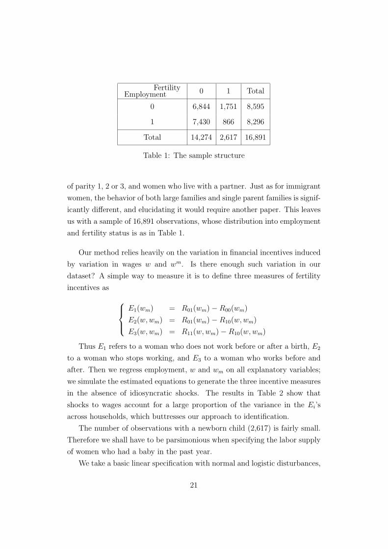
of parity 1, 2 or 3, and women who live with a partner. Just as for immigrant

women, the behavior of both large families and single parent families is signif-

icantly different, and elucidating it would require another paper. This leaves

us with a sample of 16,891 observations, whose distribution into employment

and fertility status is as in Table 1.

Our method relies heavily on the variation in financial incentives induced

by variation in wages w and wm. Is there enough such variation in our

dataset? A simple way to measure it is to define three measures of fertility

incentives as E1(wm) = R01(wm)−R00(wm)

E2(w,wm) = R01(wm)−R10(w,wm)

E3(w,wm) = R11(w,wm)−R10(w,wm)

Thus E1 refers to a woman who does not work before or after a birth, E2

to a woman who stops working, and E3 to a woman who works before and

after. Then we regress employment, w and wm on all explanatory variables;

we simulate the estimated equations to generate the three incentive measures

in the absence of idiosyncratic shocks. The results in Table 2 show that

shocks to wages account for a large proportion of the variance in the Ei’s

across households, which buttresses our approach to identification.

The number of observations with a newborn child (2,617) is fairly small.

Therefore we shall have to be parsimonious when specifying the labor supply

of women who had a baby in the past year.

We take a basic linear specification with normal and logistic disturbances,

21

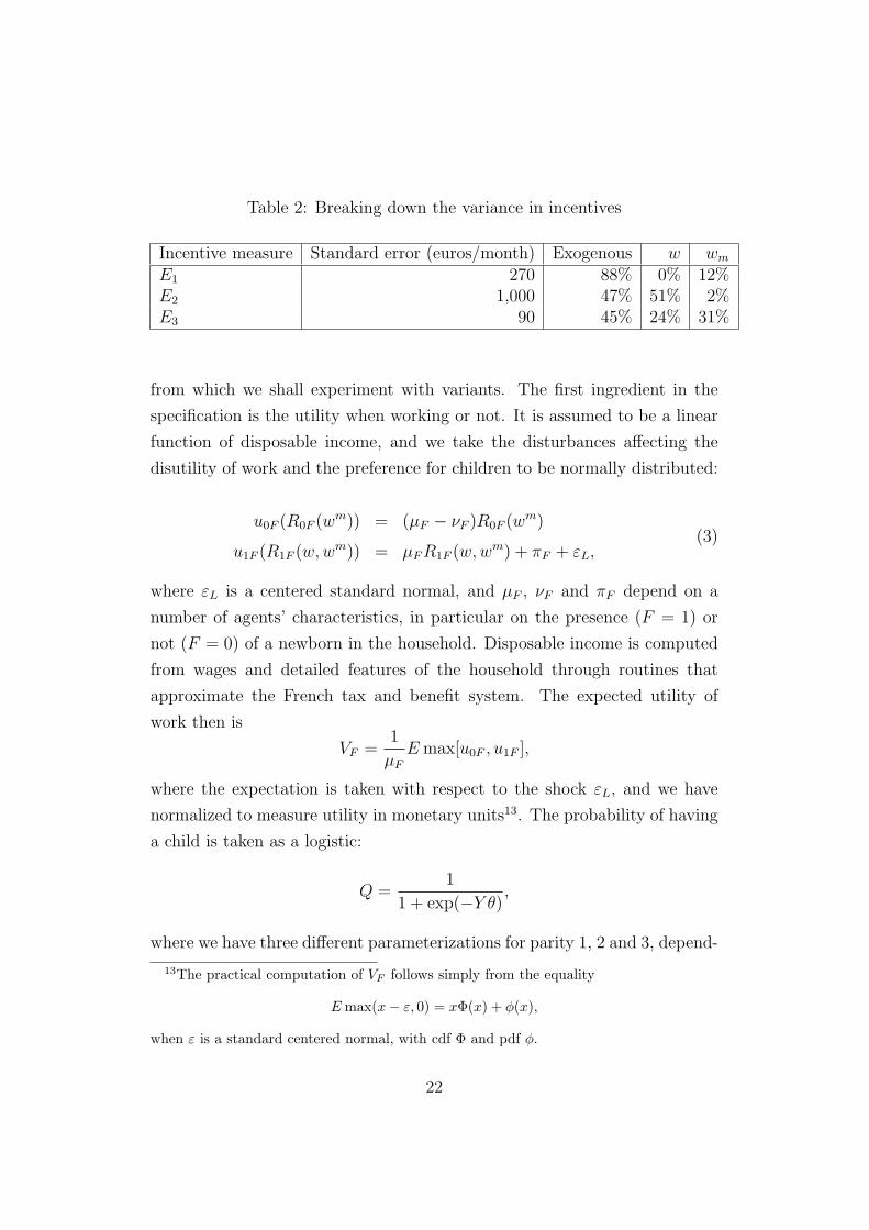
Table 2: Breaking down the variance in incentives

Incentive measure Standard error (euros/month) Exogenous w wmE1 270 88% 0% 12%E2 1,000 47% 51% 2%E3 90 45% 24% 31%

from which we shall experiment with variants. The first ingredient in the

specification is the utility when working or not. It is assumed to be a linear

function of disposable income, and we take the disturbances affecting the

disutility of work and the preference for children to be normally distributed:

u0F (R0F (wm)) = (µF − νF )R0F (wm)

u1F (R1F (w,wm)) = µFR1F (w,wm) + πF + εL,(3)

where εL is a centered standard normal, and µF , νF and πF depend on a

number of agents’ characteristics, in particular on the presence (F = 1) or

not (F = 0) of a newborn in the household. Disposable income is computed

from wages and detailed features of the household through routines that

approximate the French tax and benefit system. The expected utility of

work then is

VF =1

µFEmax[u0F , u1F ],

where the expectation is taken with respect to the shock εL, and we have

normalized to measure utility in monetary units13. The probability of having

a child is taken as a logistic:

Q =1

1 + exp(−Y θ),

where we have three different parameterizations for parity 1, 2 and 3, depend-

13The practical computation of VF follows simply from the equality

Emax(x− ε, 0) = xΦ(x) + φ(x),

when ε is a standard centered normal, with cdf Φ and pdf φ.

22

ing on age in a flexible way. The variables in Y include the difference V1−V0

between the labor market utility indices with and without a newborn, as well

as the level V0, both interacted with age and diploma. On top of these finan-

cial incentives variables, we have age, by itself and interacted with diploma

and being legally married. For parity two and three, the composition of the

family enters and is also interacted with the financial variables.

All parameters are estimated by maximum likelihood, with the endoge-

nous variable being the couple (L, F ). In the basic version of the model,

there are 136 parameters to estimate. The estimation program is written in

R and the optimization takes a couple of hours.

Remark: A complication comes from the fact that the value of the

woman labor cost w is only observed by the econometrician for those women

who participate. We handle this issue as follows. We maintain the assump-

tion that every woman knows her potential wage w, and chooses her decisions

accordingly. But the econometrician does not know w for the non participat-

ing women. Then the econometrician postulates and estimates a model for

wages, and uses it to take the expectation of the likelihood of the woman’s

decision. Following standard practice, we posit a Mincer equation for the

employer wage cost w:

logw = Xβ + σεw,

where X includes age at end of studies, time spent since end of studies and

their squares, as well as highest diploma obtained in five categories. We

estimate the Mincer equation in a first stage. To do this, we estimate a

participation model with exogenous fertility; we follow a procedure close to

Laroque and Salanie (2002) to take into account the existence of a (high)

minimum wage which bars a number of low skilled women from employment.

The results presented below take the Mincer equation as given, and in par-

ticular do not correct standard errors for the pre-estimation stage.

23

3.2 Estimation results

All the tables are gathered at the end of the paper. Incomes are measured

in hundreds of euros. To fix ideas, the median monthly household income in

our sample (as measured by the observed value of RLF ) is 1,950 euros.

3.2.1 Labor supply

We specify and estimate in a flexible way the utilities of working from (3),

which are identified through the choice of a standard normal disturbance.

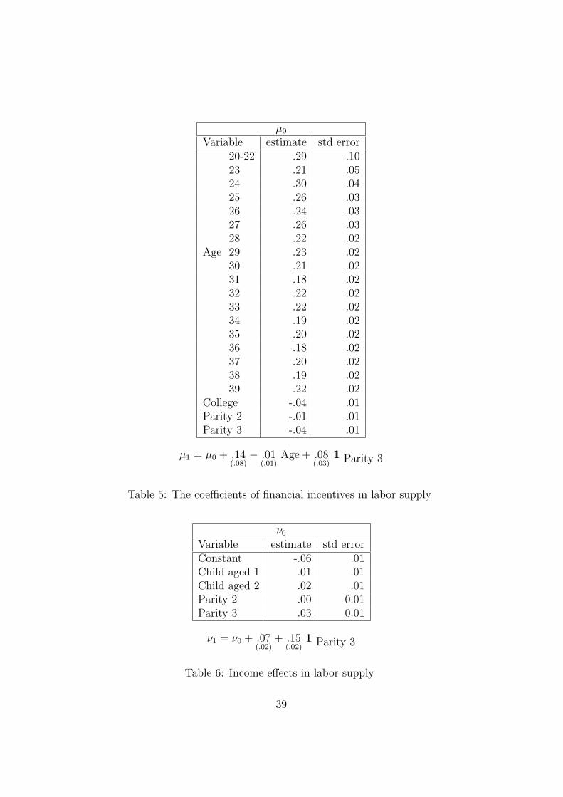
The coefficients of µF , which measures the sensitivity of the labor supply

of women to financial incentives to work (R1F −R0F ), are shown in Table 5.

For women without babies, who are in relatively larger number, µ0 is repre-

sented as the sum of indicator functions, of annual age, of college education

and of the size of the family (parity 2 or 3). To interpret the magnitude of

the coefficients, one must bear in mind the fact that on average half of the

women of the sample work: the shape of the normal distribution implies that

at the average point a change of 0.1 in the deterministic utility u1F − u0F

corresponds to a change of 4 points in the probability of working.

The sensitivity to financial incentives seems to be slightly decreasing with

age, from around 0.27 to 0.20 for a low skilled woman without children (Ta-

ble 5). An increase of 100 euros in the monthly income of such a household

would increases the woman’s probability of working by approximately 10

points. The sensitivity to incentives is slightly lower for educated women

and/or for women with two children, as a0 is reduced by .04 in both cases.

Given that only 15% of women in our sample have a baby in a given year,

we specify µ1 as the sum of µ0, a linear function of age, and an indicator

of a family with two children. The age term is insignificant, but the mean

estimate of these additional terms is negative; this suggests that the labor

supply of women with a newborn is less sensitive to financial incentives. On

the other hand, having two children increases µ1 − µ0 by 0.08: so after the

birth of a third child women are more sensitive to financial incentives.

The coefficient νF measures the income effects on labor supply and is

presented in Table 6. Leisure is a normal good for women without children:

24

an increase of 100 euros per month of other income (i.e. of her husband

income) reduces their probability of working by 4 points on average. The

effect is reversed for women with a baby, as already seen in Laroque and

Salanie (2002): one interpretation is that having a husband with a larger

income allows the woman to hire child care and continue with her professional

career. Indeed for a second born, an increase of other income of 100 euros

per month increases the probability of getting a job by 7 points on average.

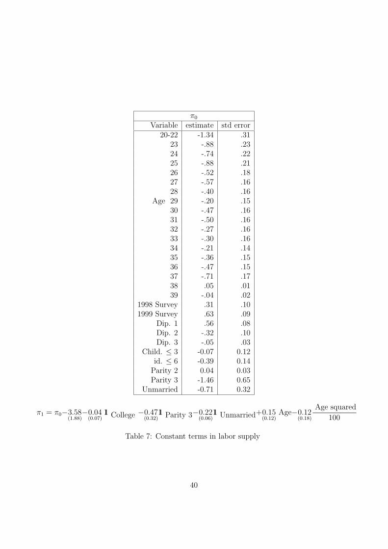
Finally the coefficient πF describes the constant term. For flexibility, π0

is represented as the sum of indicator functions, of age dummies, of diplomas

and of household structure (see Table 7). The constant is modified for women

with a young baby, by adding a quadratic polynomial in age, with three

indicators of education and family structure. The results are by and large

unsurprising:14 high diplomas make women more likely to work, having two

children and/or a baby deters from work.

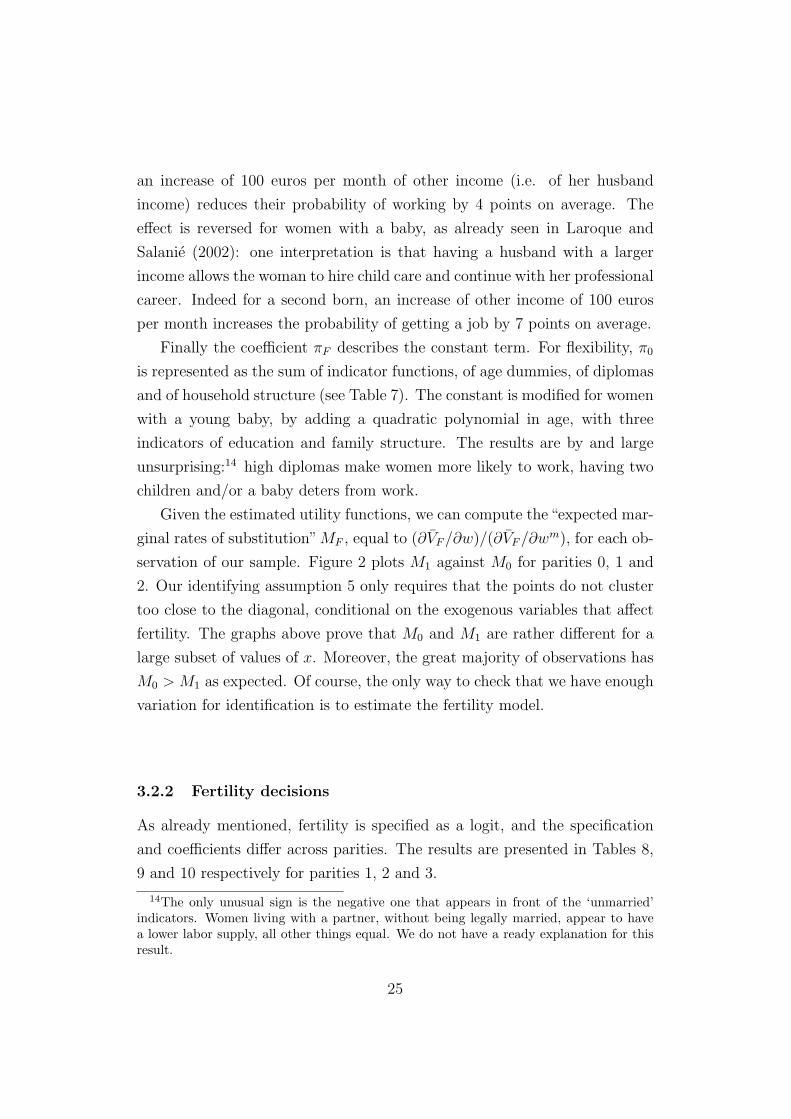
Given the estimated utility functions, we can compute the“expected mar-

ginal rates of substitution”MF , equal to (∂VF/∂w)/(∂VF/∂wm), for each ob-

servation of our sample. Figure 2 plots M1 against M0 for parities 0, 1 and

2. Our identifying assumption 5 only requires that the points do not cluster

too close to the diagonal, conditional on the exogenous variables that affect

fertility. The graphs above prove that M0 and M1 are rather different for a

large subset of values of x. Moreover, the great majority of observations has

M0 > M1 as expected. Of course, the only way to check that we have enough

variation for identification is to estimate the fertility model.

3.2.2 Fertility decisions

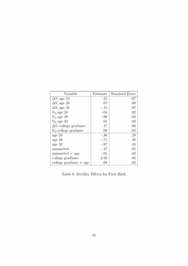
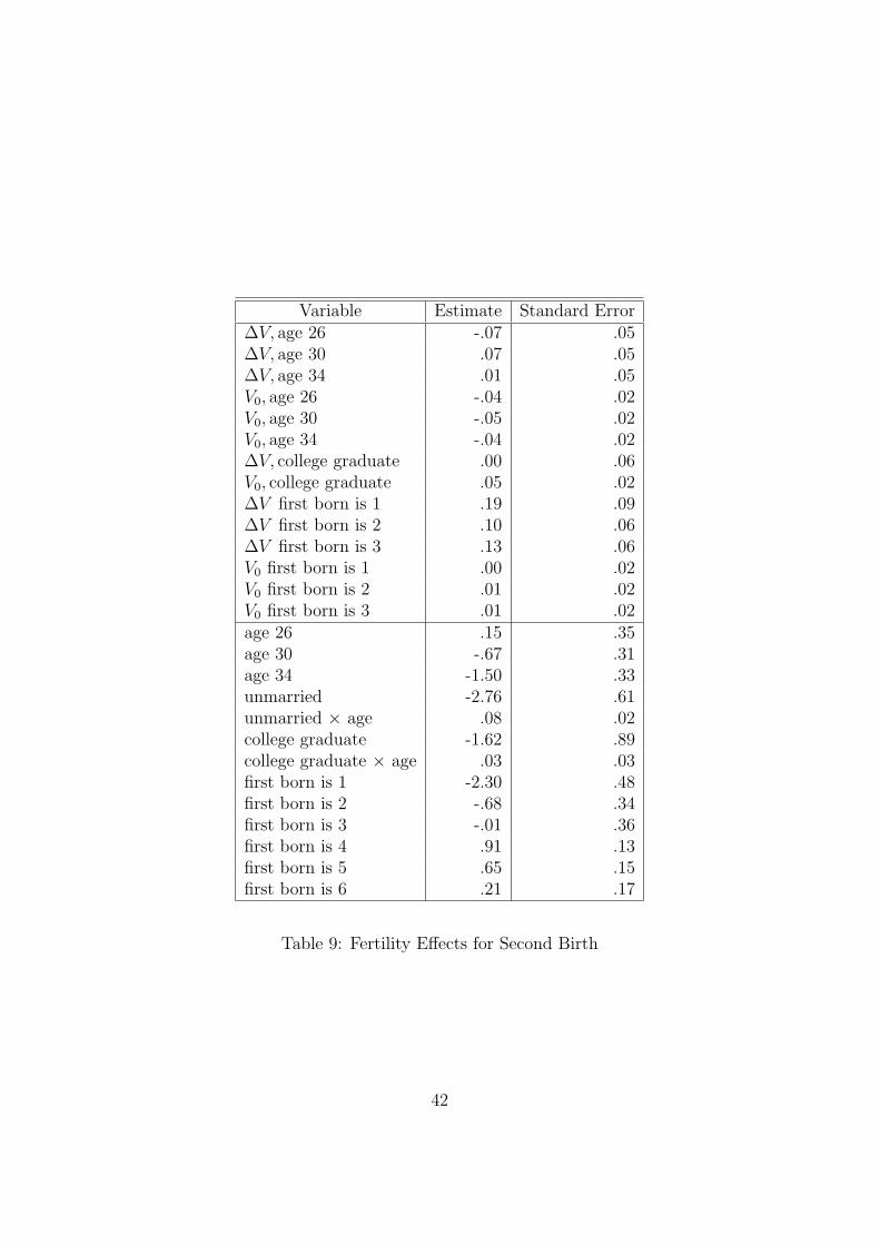
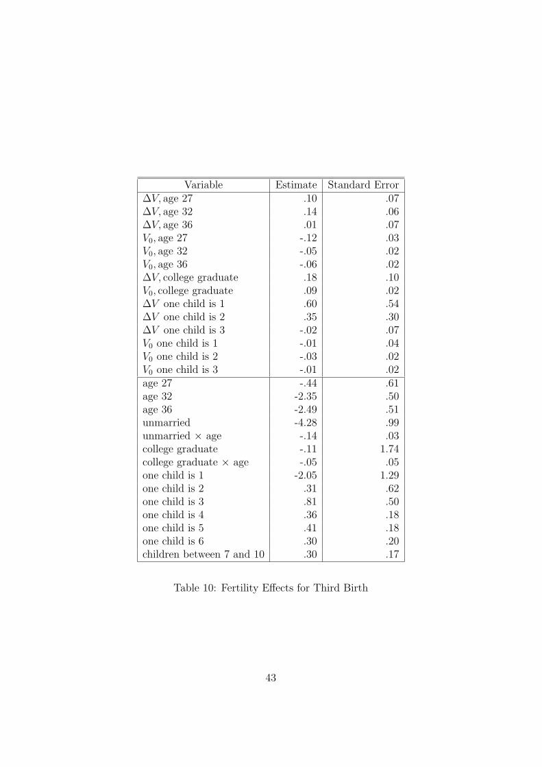
As already mentioned, fertility is specified as a logit, and the specification

and coefficients differ across parities. The results are presented in Tables 8,

9 and 10 respectively for parities 1, 2 and 3.

14The only unusual sign is the negative one that appears in front of the ‘unmarried’indicators. Women living with a partner, without being legally married, appear to havea lower labor supply, all other things equal. We do not have a ready explanation for thisresult.

25

M0

M1

0.05

0.10

0.15

0.20

0.25

0.1 0.2 0.3 0.4

Parity 1

0.1 0.2 0.3 0.4

Parity 2

0.1 0.2 0.3 0.4

Parity 3

Figure 2: Scatter plots of M1 against M0

The main variable of interest is the difference of the expected utilities

when having a baby or not, (V1 − V0). This variable is interacted with age

education and family composition, but since 15% of the women in the sample

have a baby, we do not have enough degrees of freedom to use a full set of age

dummies. Instead we posit a spline function of age, with three knots located

at the 15%, 50% and 85% quantiles of the age distribution of the sample for

each parity.

We renormalized the estimated utility indices VF so that they can be

interpreted in hundreds of euros per month. Thus given the functional form of

the logit, a change of 100 euros per month in (V1−V0) changes the probability

Q of fertility by Q(1 − Q)θ, where θ is the coefficient of ∆V that appears

in the tables. Take for example the change in Q for an average 24 year old

woman without children associated with an increase of financial incentives of

100 euros. Since Q is equal to 0.17 on average for these women, the increase

in the probability of a birth is 0.17 × 0.83 × 0.21 = 0.030; these 3.0 points

represent a 17% increase in the fertility rate. Another way to phrase is that

this 0.17 figure measures the average semi-elasticity of fertility with respect

26

Semi−elasticity in V1 −− V0

Dens

ity

0

1

2

3

4

5

−0.5 0.0 0.5 1.0

Parity 1

−0.5 0.0 0.5 1.0

Parity 2

−0.5 0.0 0.5 1.0

Parity 3

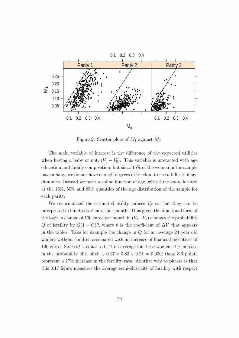
Figure 3: Semi elasticity of the probability of fertility with respect to V1−V0

to financial incentives for this group of women:

∂ lnQ

∂(V1 − V0)= 0.17.

Given the very diverse household compositions and incomes, the semi-

elasticities vary a lot in the population. This appears clearly in figure 3,

which plots the distribution of the estimated semi-elasticity with respect to

(V1 − V0) in our sample15. The first striking fact is perhaps that for second

births (the middle panel), the estimated semi-elasticities cluster around zero:

only 30% are larger than 0.1, and 20% are in fact negative (albeit small).

Thus financial incentives seem to play little role in the decision to have a

second child.

On the other hand, almost all estimated semi-elasticities are positive for

15Figures 3, 6, 4 and 5 focus on women of ages 24 to 36. Only 15% of first births occurbefore age 24, and 15% of third births occur after age 36.

27

the third birth, and half of them are larger than 0.3. These are large effects:

according to our estimates, an increase of 100 euros per month would bring

the probability of a third birth from 0.08 to 0.11 for a woman with two

children at age 32 (which is the median age for a third birth.)

The picture is more mixed for first births, as shown in the left panel of

figure 3. At the median age of 28 for a first birth, almost all semi-elasticities

are positive, and half of them are above 0.16. The effect is twice larger on

average for younger women; on the other hand, it becomes negative for the

majority of women of age 30 and older. On the whole population of childless

women, 80% of estimated semi-elasticities are positive; and the median is

0.11, which is much smaller than for third births.

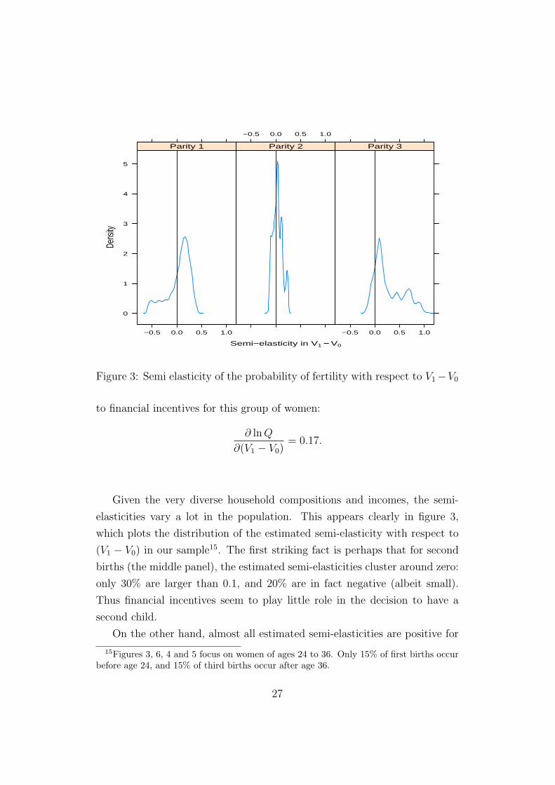
As the discussion above makes clear, the estimated effects are quite sen-

sitive to age. The profile of the estimated coefficients of financial incentives

(V1 − V0) for each age is represented on Figure 4, along with the 95% con-

fidence band. Other factors also play an important role. Note for instance

from Table 8 that childless college graduates seem to be more sensitive to

financial incentives than women without a college education. This is partly

compensated by the fact that college graduates of course have children later,

when the baseline effect turns negative; still, they tend to have a slightly

larger semi-elasticity than other women. This is somewhat surprising; and

Table 10 confirms it for the third birth.

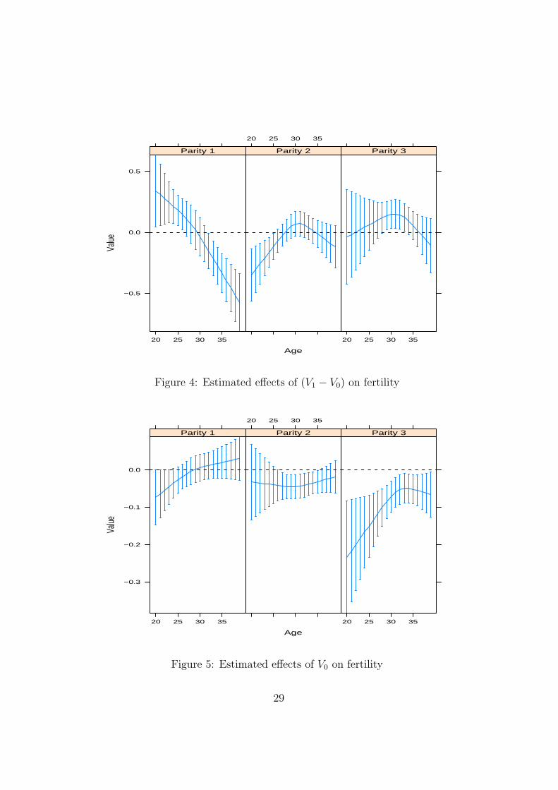
Our specification also allows for income effects, through the interactions of

V0 with age, education and family composition. The age profile, keeping fixed

education and family composition, is represented on Figure 5. The overall

effect on fertility is negative for women with lower education, and close to

zero for those with a college education. Figure 6 shows a striking symmetry

to Figure 3: for each parity, the estimated densities are close mirror images

with respect to the zero vertical line.

28

Age

Value

−0.5

0.0

0.5

20 25 30 35

Parity 1

20 25 30 35

Parity 2

20 25 30 35

Parity 3

Figure 4: Estimated effects of (V1 − V0) on fertility

Age

Value

−0.3

−0.2

−0.1

0.0

20 25 30 35

Parity 1

20 25 30 35

Parity 2

20 25 30 35

Parity 3

Figure 5: Estimated effects of V0 on fertility

29

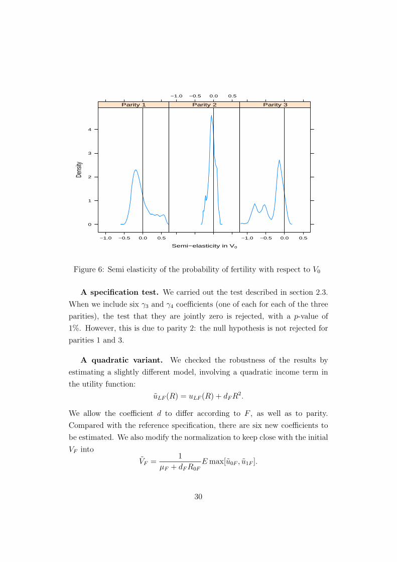
Semi−elasticity in V0

Dens

ity

0

1

2

3

4

−1.0 −0.5 0.0 0.5

Parity 1

−1.0 −0.5 0.0 0.5

Parity 2

−1.0 −0.5 0.0 0.5

Parity 3

Figure 6: Semi elasticity of the probability of fertility with respect to V0

A specification test. We carried out the test described in section 2.3.

When we include six γ3 and γ4 coefficients (one of each for each of the three

parities), the test that they are jointly zero is rejected, with a p-value of

1%. However, this is due to parity 2: the null hypothesis is not rejected for

parities 1 and 3.

A quadratic variant. We checked the robustness of the results by

estimating a slightly different model, involving a quadratic income term in

the utility function:

uLF (R) = uLF (R) + dFR2.

We allow the coefficient d to differ according to F , as well as to parity.

Compared with the reference specification, there are six new coefficients to

be estimated. We also modify the normalization to keep close with the initial

VF into

VF =1

µF + dFR0F

Emax[u0F , u1F ].

30

The point estimates of all the coefficients are positive, pointing towards a

convex utility function. The coefficients are largest for parity 1, smaller

for parity 0, and close to zero for parity 2. While the sum µF + dFR0F

stays positive, some of the µF coefficients become negative. A likelihood

test indicates that the quadratic terms are highly significant: the difference

between the two values of the log-likelihood is 19.6, for six degrees of freedom.

However we have not pursued this specification as the improvement of the

fit concerns labor supply, while the adjustment of fertility deteriorates.

The importance of financial incentives. We estimated the reference

model, constraining all the thirty-six coefficients of the value functions VF

in the fertility equation to be zero. The log-likelihood is reduced by 86.9

points, which is significant at any level. Thus in statistical terms, financial

incentives are highly significant in the fertility decision.

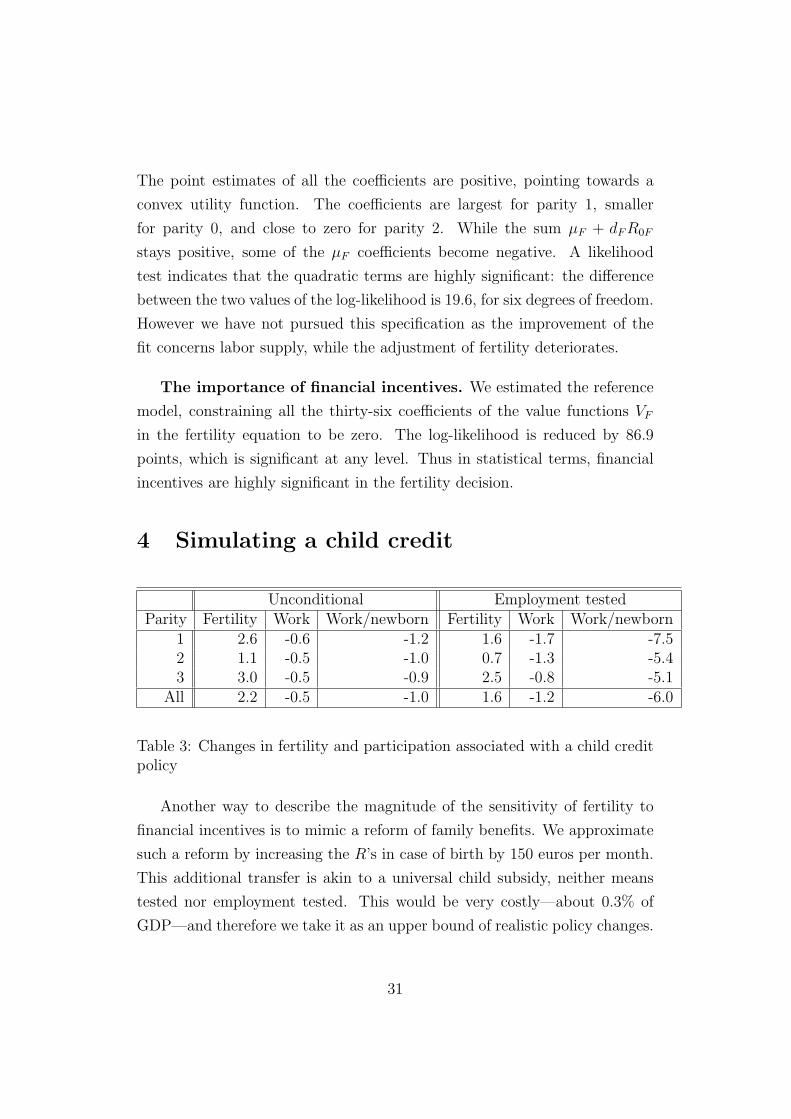
4 Simulating a child credit

Unconditional Employment testedParity Fertility Work Work/newborn Fertility Work Work/newborn

1 2.6 -0.6 -1.2 1.6 -1.7 -7.52 1.1 -0.5 -1.0 0.7 -1.3 -5.43 3.0 -0.5 -0.9 2.5 -0.8 -5.1

All 2.2 -0.5 -1.0 1.6 -1.2 -6.0

Table 3: Changes in fertility and participation associated with a child creditpolicy

Another way to describe the magnitude of the sensitivity of fertility to

financial incentives is to mimic a reform of family benefits. We approximate

such a reform by increasing the R’s in case of birth by 150 euros per month.

This additional transfer is akin to a universal child subsidy, neither means

tested nor employment tested. This would be very costly—about 0.3% of

GDP—and therefore we take it as an upper bound of realistic policy changes.

31

We can evaluate the effects of such a reform by adding it to our tax-benefit

computation module, simulating its effects on labor supply, recomputing V0

and V1, and simulating fertility according to the above model. We contrast

the situations where the transfer is conditional on stopping work (R01 is

increased by 150 euros, not R11) or unconditional (both R01 and R11 are

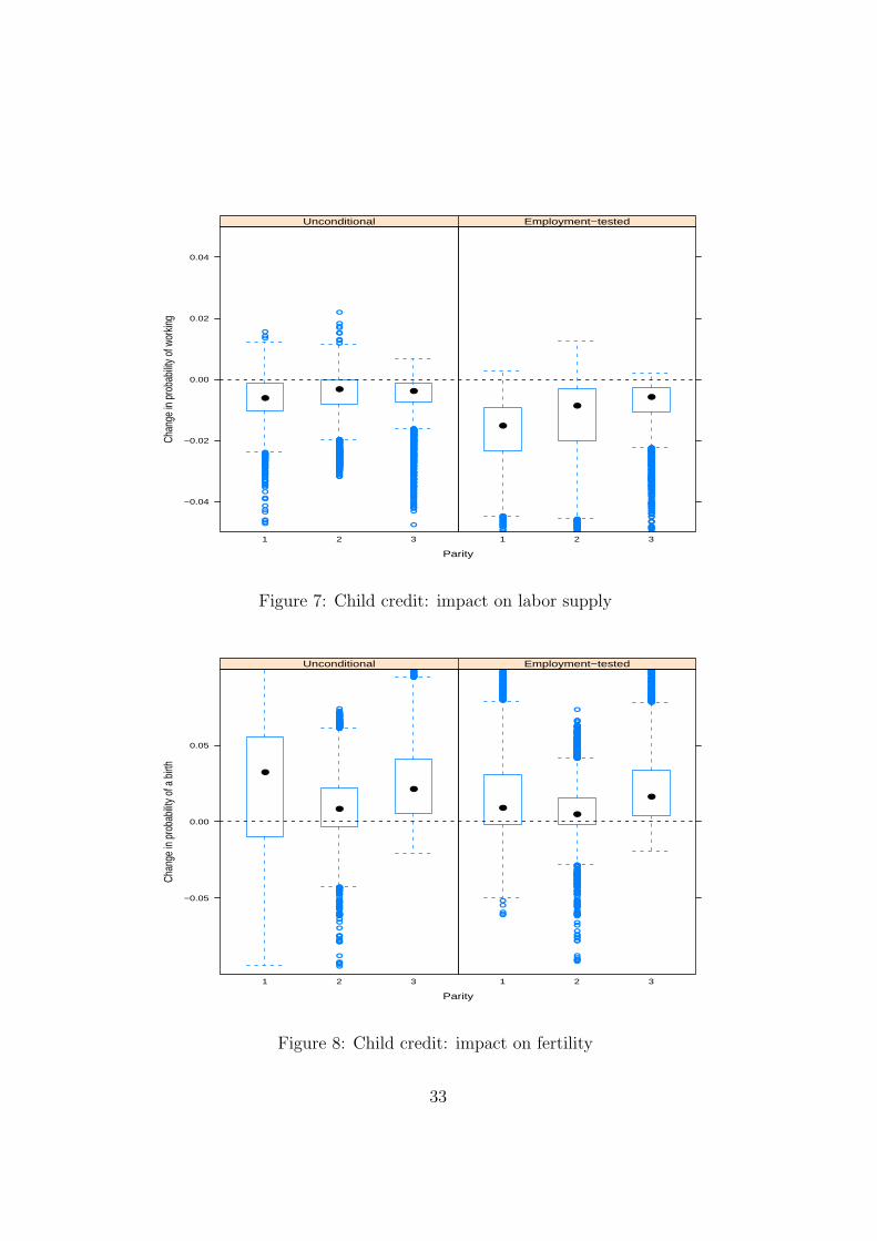
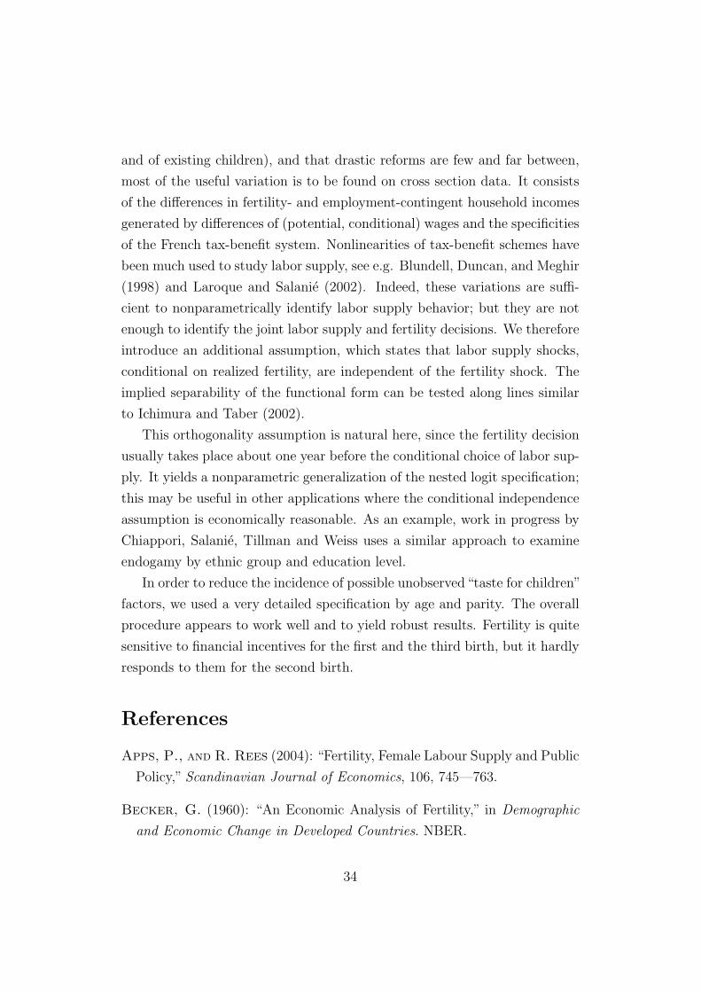
changed). The aggregate results, shown in points of fertility and labor force

participation, appear in Table 3, with box-plot graphs of the impacts on

Figures 7 and 8.

The exercise confirms that the effects of financial incentives on fertility

are sizeable. The unconditional child credit increases the fertility rate in

the sample by 2.2 points, from 15.5% to 17.7%. The increase is pronounced

for the first and third children, smaller for parity 2. It is associated with a

modest decrease of .5 point in labor participation, from 49.1% to 48.6%.

When the child credit is conditioned on not working, the increase in fer-

tility is only 1.6 points, which is still large. The brunt of the reduction bears

on first births: indeed women without children have the largest participa-

tion rate, 63.1%, to be compared with 47.8% for women with one child and

37.3% for women with two children. Unsurprisingly, the overall reduction

in participation is larger than when the child credit is unconditional, -1.2

point instead of -0.5. This effect is of course concentrated on women with a

newborn, for which it is huge: their participation goes down by 6.0 points16.

Conclusion

Our paper adopts an approach that differs from much of the literature on

evaluation. This choice is driven by the specific features of the problem we

study. Given that fertility behavior depends so crucially on ages (of parents

16This is in line with the results found in France after the extension of the Allocationparentale d’education to the second born in 1994: its value amounted to 450 euros, and itmay have reduced participation of this group by 15 points.

32

Parity

Chan

ge in

pro

babi

lity o

f wor

king

−0.04

−0.02

0.00

0.02

0.04

1 2 3

Unconditional

1 2 3

Employment−tested

Figure 7: Child credit: impact on labor supply

Parity

Chan

ge in

pro

babi

lity o

f a b

irth

−0.05

0.00

0.05

1 2 3

Unconditional

1 2 3

Employment−tested

Figure 8: Child credit: impact on fertility

33

and of existing children), and that drastic reforms are few and far between,

most of the useful variation is to be found on cross section data. It consists

of the differences in fertility- and employment-contingent household incomes

generated by differences of (potential, conditional) wages and the specificities

of the French tax-benefit system. Nonlinearities of tax-benefit schemes have

been much used to study labor supply, see e.g. Blundell, Duncan, and Meghir

(1998) and Laroque and Salanie (2002). Indeed, these variations are suffi-

cient to nonparametrically identify labor supply behavior; but they are not

enough to identify the joint labor supply and fertility decisions. We therefore

introduce an additional assumption, which states that labor supply shocks,

conditional on realized fertility, are independent of the fertility shock. The

implied separability of the functional form can be tested along lines similar

to Ichimura and Taber (2002).

This orthogonality assumption is natural here, since the fertility decision

usually takes place about one year before the conditional choice of labor sup-

ply. It yields a nonparametric generalization of the nested logit specification;

this may be useful in other applications where the conditional independence

assumption is economically reasonable. As an example, work in progress by

Chiappori, Salanie, Tillman and Weiss uses a similar approach to examine

endogamy by ethnic group and education level.

In order to reduce the incidence of possible unobserved“taste for children”

factors, we used a very detailed specification by age and parity. The overall

procedure appears to work well and to yield robust results. Fertility is quite

sensitive to financial incentives for the first and the third birth, but it hardly

responds to them for the second birth.

References

Apps, P., and R. Rees (2004): “Fertility, Female Labour Supply and Public

Policy,” Scandinavian Journal of Economics, 106, 745—763.

Becker, G. (1960): “An Economic Analysis of Fertility,” in Demographic

and Economic Change in Developed Countries. NBER.

34

(1991): A Treatise on the Family. Harvard University Press.

Besley, T., and A. Case (2000): “Unnatural Experiments? Estimating

the Incidence of Endogenous Policies,”Economic Journal, 110, F672–F694.

Blanchet, D., and O. Ekert-Jaffe (1994): “The Demographic Impact

of Family Benefits: Evidence from a Micromodel and from Macrodata,” in

The Family, the Market and the State in Ageing Societies, ed. by J. Er-

misch, and N. Ogawa. Clarendon Press.

Blau, D., and P. Robins (1989): “Fertility, Employment, and Child-care

Costs,” Demography, 26, 287–299.

Blundell, R., A. Duncan, and C. Meghir (1998): “Estimating Labor

Supply Responses Using Tax Reforms,” Econometrica, 66, 827–861.

Chone, P., D. Leblanc, and I. Robert-Bobee (2004): “Offre de travail

feminine et garde des enfants,” Economie et prevision, 162.

Cigno, A. (1986): “Fertility and the Tax-Benefit System: A Reconsideration

of the Theory of Family Taxation,” Economic Journal, 96, 1035–1051.

Cohen, A., R. Dehejia, and D. Romanov (2007): “Do Financial Incen-

tives Affect Fertility?,” Discussion Paper 13700, NBER.

del Boca, D. (2002): “The Effect of Child Care and Part-time Opportuni-

ties on Participation and Fertility Decisions in Italy,”Journal of Population

Economics, 15, 549–573.

Ekert-Jaffe, O. (1986): “Effets et limites des aides financieres aux

familles : une experience, un modele,” Population, 2, 327–348.

Gauthier, A. (1996): The State and the Family. Oxford University Press.

Gauthier, A., and J. Hatzius (1997): “Family Benefits and Fertility: An

Econometric Model,” Population Studies, 51, 295–346.

35

Heckman, J. (1976): “Simultaneous Equation Models with Continuous and

Discrete Endogenous Variables and Structural Shifts,” in Studies in Non-

linear Estimation, ed. by S. Goldfeld, and R. Quandt. North Holland.

Heckman, J., and J. Walker (1989): “Using Goodness of Fit and Other

Criteria to Choose among Competing Duration Models: A Case Study of

Hutterite Data,” in Sociological Methodology, ed. by C. Clogg. American

Sociological Association.

(1990a): “The Relationship between Wages and Income and the

Timing and Spacing of Births: Evidence from Swedish Longitudinal Data,”

Econometrica, 58, 1411–1441.

(1990b): “The Third Birth in Sweden,” Journal of Population Eco-

nomics, 3, 235–275.

Hotz, J., R. Klerman, and R. Willis (1997): “The Economics of Fer-

tility in Developed Countries,” in Handbook of Population Economics, ed.

by M. Rosenzweig, and O. Stark. North Holland.

Hotz, J., and R. Miller (1988): “An Empirical Model of Lifecycle Fertility

and Female Labour Supply,” Econometrica, 56, 91–118.

Hume, D. (1776 (2005)): Dialogues Concerning Natural Religion. Barnes

and Noble.

Ichimura, H., and C. Taber (2002): “Semiparametric Reduced-Form Es-

timation of Tuition Subsidies,” American Economic Review, 92, 286–292.

Keane, M., and K. Wolpin (2007a): “Exploring the Usefulness of a Non-

random Holdout Sample for Model Validation: Welfare Effects on Female

Behavior,” International Economic Review, 48, 1351–1378.

(2007b): “The Role of Labor and Marriage Markets, Preference Het-

erogeneity and the Welfare System on the Life Cycle Decisions of Black,

Hispanic and White Women,” Discussion paper, University of Pennsylva-

nia.

36

Kearney, M. S. (2004): “Is There an Effect of Incremental Welfare Benefits

on Fertility Behavior? A Look at the Family Cap,” Journal of Human

Resources, 39, 295–325.

Laroque, G., and B. Salanie (2002): “Labor Market Institutions and

Employment in France,” Journal of Applied Econometrics, 17, 25–48.

(2004a): “Fecondite et offre de travail des femmes en France,”

Economie publique, 13(2), 61–94.

(2004b): “Fertility and Financial Incentives in France,” CESIfo

Economic Studies, 50, 423–450.

Lefebvre, P., L. Brouillette, and C. Felteau (1994): “Les effets

des impots et des allocations familiales sur les comportements de fecondite

et de travail des canadiennes : resultat d’un modele de choix discrets,”

Population, 2, 415–456.

Milligan, K. (2004): “Subsidizing the Stork: New Evidence on Tax Incen-

tives and Fertility,” Review of Economics and Statistics, forthcoming.

Moffitt, R. (1998): “The Effect of Welfare on Marriage and Fertility,” in

Welfare, the Family, and Reproductive Behavior: Research Perspectives,

ed. by R. Moffitt. National Academy Press.

Piketty, T. (2005): “L’impact de l’allocation parentale d’education sur

l’activite feminine et la fecondite en France, 1982-2002,” in Histoires de

familles, histoires familiales, ed. by C. Lefevre. INED.

Rosenzweig, M. (1999): “Welfare, Marital Prospects, and Nonmarital

Childbearing,” Journal of Political Economy, 107, S3–S32.

Rosenzweig, M., and T. P. Schultz (1985): “The Demand for and Sup-

ply of Births: Fertility and its Lifecycle Consequences,” American Eco-

nomic Review, 75, 992–1015.

Willis, R. (1973): “A New Approach to the Economic Theory of Fertility

Behavior,” Journal of Political Economy, 81, S14–S64.

37

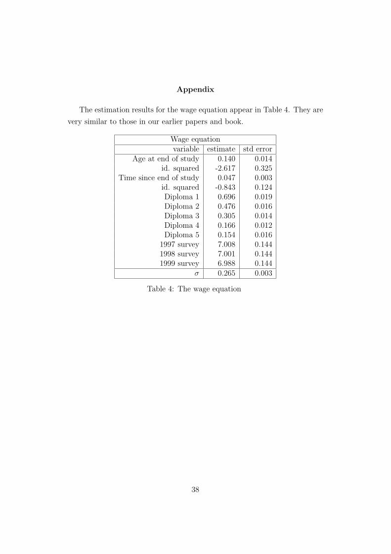
Appendix

The estimation results for the wage equation appear in Table 4. They are

very similar to those in our earlier papers and book.

Wage equationvariable estimate std error

Age at end of study 0.140 0.014id. squared -2.617 0.325

Time since end of study 0.047 0.003id. squared -0.843 0.124Diploma 1 0.696 0.019Diploma 2 0.476 0.016Diploma 3 0.305 0.014Diploma 4 0.166 0.012Diploma 5 0.154 0.016

1997 survey 7.008 0.1441998 survey 7.001 0.1441999 survey 6.988 0.144

σ 0.265 0.003

Table 4: The wage equation

38

µ0

Variable estimate std error20-22 .29 .1023 .21 .0524 .30 .0425 .26 .0326 .24 .0327 .26 .0328 .22 .02

Age 29 .23 .0230 .21 .0231 .18 .0232 .22 .0233 .22 .0234 .19 .0235 .20 .0236 .18 .0237 .20 .0238 .19 .0239 .22 .02

College -.04 .01Parity 2 -.01 .01Parity 3 -.04 .01

µ1 = µ0 + .14(.08)− .01

(.01)Age + .08

(.03)11 Parity 3

Table 5: The coefficients of financial incentives in labor supply

ν0

Variable estimate std errorConstant -.06 .01Child aged 1 .01 .01Child aged 2 .02 .01Parity 2 .00 0.01Parity 3 .03 0.01

ν1 = ν0 + .07(.02)

+ .15(.02)

11 Parity 3

Table 6: Income effects in labor supply

39

π0

Variable estimate std error20-22 -1.34 .31

23 -.88 .2324 -.74 .2225 -.88 .2126 -.52 .1827 -.57 .1628 -.40 .16

Age 29 -.20 .1530 -.47 .1631 -.50 .1632 -.27 .1633 -.30 .1634 -.21 .1435 -.36 .1536 -.47 .1537 -.71 .1738 .05 .0139 -.04 .02

1998 Survey .31 .101999 Survey .63 .09

Dip. 1 .56 .08Dip. 2 -.32 .10Dip. 3 -.05 .03

Child. ≤ 3 -0.07 0.12id. ≤ 6 -0.39 0.14

Parity 2 0.04 0.03Parity 3 -1.46 0.65

Unmarried -0.71 0.32

π1 = π0−3.58(1.88)−0.04

(0.07)11 College −0.47

(0.32)11 Parity 3−0.22

(0.06)11 Unmarried+0.15

(0.12)Age−0.12

(0.18)

Age squared

100

Table 7: Constant terms in labor supply

40

Variable Estimate Standard Error∆V, age 24 .21 .07∆V, age 28 .07 .08∆V, age 32 -.15 .07V0, age 24 -.04 .02V0, age 28 -.00 .02V0, age 32 .01 .02∆V, college graduate .17 .08V0, college graduate .00 .02age 24 -.36 .28age 28 -.71 .30age 32 -.97 .34unmarried -.47 .65unmarried × age -.01 .02college graduate -2.50 .86college graduate × age .08 .03

Table 8: Fertility Effects for First Birth

41

Variable Estimate Standard Error∆V, age 26 -.07 .05∆V, age 30 .07 .05∆V, age 34 .01 .05V0, age 26 -.04 .02V0, age 30 -.05 .02V0, age 34 -.04 .02∆V, college graduate .00 .06V0, college graduate .05 .02∆V first born is 1 .19 .09∆V first born is 2 .10 .06∆V first born is 3 .13 .06V0 first born is 1 .00 .02V0 first born is 2 .01 .02V0 first born is 3 .01 .02age 26 .15 .35age 30 -.67 .31age 34 -1.50 .33unmarried -2.76 .61unmarried × age .08 .02college graduate -1.62 .89college graduate × age .03 .03first born is 1 -2.30 .48first born is 2 -.68 .34first born is 3 -.01 .36first born is 4 .91 .13first born is 5 .65 .15first born is 6 .21 .17

Table 9: Fertility Effects for Second Birth

42

Variable Estimate Standard Error∆V, age 27 .10 .07∆V, age 32 .14 .06∆V, age 36 .01 .07V0, age 27 -.12 .03V0, age 32 -.05 .02V0, age 36 -.06 .02∆V, college graduate .18 .10V0, college graduate .09 .02∆V one child is 1 .60 .54∆V one child is 2 .35 .30∆V one child is 3 -.02 .07V0 one child is 1 -.01 .04V0 one child is 2 -.03 .02V0 one child is 3 -.01 .02age 27 -.44 .61age 32 -2.35 .50age 36 -2.49 .51unmarried -4.28 .99unmarried × age -.14 .03college graduate -.11 1.74college graduate × age -.05 .05one child is 1 -2.05 1.29one child is 2 .31 .62one child is 3 .81 .50one child is 4 .36 .18one child is 5 .41 .18one child is 6 .30 .20children between 7 and 10 .30 .17

Table 10: Fertility Effects for Third Birth

43