Embed Size (px)
Citation preview
Université de Liège - Faculté des Sciences Appliquées
Punching shear of deep pile caps
Travail de �n d'études réalisé en vue de l'obtention du grade deMaster Ingénieur Civil des Constructions par Jeunehomme Denis
Année académique 2014-1015
Composition du jury :
MIHAYLOV BoyanFRANSSEN Jean-MarcCOLLIN FrédéricCERFONTAINE Frédéric
Lundi 1er juin 2015
First of all, I would like to thank Mr. Boyan Mihaylov, the promoter of this thesis, for thecontinuous help he brought to both the development of the model and the writing of my thesis.His advice were always useful and I have tried to follow them as much as I could. Then, Iwould to thank the other members of my jury for the interest they brought to my work andfor the comments they formulated which were really helpful. I also would like to express mygratitude to my two o�ce coworkers, namely Mrs. Jian Liu and Mr. Nikola Tatar for theirpatience and their permanent good mood which brought motivation when I had none and tomy parents without whom no word of this thesis would have been written. I will �nish theacknowledgment by thanking Mrs. Anaïs De Cuyper for kicking my ass when I needed it towork e�ciently and for her unconditional support.
Thesis statement
Reinforced concrete pile caps belong to the family of deep elements which work predominantlyin shear. As such, they are characterized by complex deformation patterns and cannot bemodeled based on the classical assumption that plane sections remain plane. In this context,it is necessary to develop a new approach which captures better their ultimate shear behavior.
This thesis consists of the development and the analysis of a model for the shear strength ofcaps joining four piles. To do so, it is planned to use the two-parameters kinematic theory(2PKT) previously developed for deep beams by Mihaylov et al. (2013), and extend it topile caps. The basic idea is to evolve this 2D model into a 3D one. Thus, the same basicphenomena explaining the behavior of deep beams should be taken into account, but thedi�erent terms which compose the 2PKT approach have to be adapted in order to capturethe speci�cs of pile caps.
The �rst step consists of �nding in the literature tests performed on four-pile caps andbuild a database with the properties of each test specimen. The interest is double: on theone hand, it will allow to observe the behavior of as many specimens as possible to identifythe common failure modes and more speci�cally to try to �nd a reoccurring crack pattern.On the other hand, these tests will serve to evaluate the accuracy of the model.
The �nal goal of this thesis is to determine the reliability of this model and more precisely tostudy its behavior in its �eld of use. So, it will be necessary to vary some key parameters ofpile caps and study the results produced by the model. Using the database, it will be possi-ble to determine how accurate the model is in capturing the e�ect of di�erent experimentalvariables.
In parallel, a strut-and-tie model will be used to illustrate one way the pile caps are di-mensioned nowadays. In that way, comparisons between this approach, the test specimens,and the 2PKT model could be provided.
Signature of the members of the Jury:
MIHAYLOV Boyan (promoter): FRANSSEN Jean-Marc:
COLLIN Frédéric: CERFONTAINE Frédéric:
Abstract
Punching shear of deep pile caps
Jeunehomme DenisSecond year of the Master's degree in Civil EngineeringAcademic year 2014-2015
The purpose of this Master's thesis is to develop a model predicting the shear strengthof deep pile caps and especially in the case of four-piles specimens. The considered approachconsisted of starting from the 2PKT model realized by B. Mihaylov et al. in 2013 [1], whichis initially used to predict the shear strength of deep beams, and extending it for deep pilecaps. To do so, the di�erent components of the model had to be adapted accordingly tothis new con�guration. Then, to evaluate both the e�ciency and the utility of this model,two veri�cations were performed. The �rst one is based one the series of tests realizedon such elements in order to experimentally determine their ultimate strength. Thereby,using all data collected during these tests, the model was able to predict the theoreticalstrength of the di�erent considered elements. As such, these values were then compared tothe experimental strengths in order to determine the accuracy it could reach. Besides, theresults were hopeful considering the model o�ers the possibility to approach reality in a safeway while keeping a good e�ciency. Then, the utility of the model was evaluated dependingon the improvements it can bring compared to the classical design methods. In particular,the pile caps are generally designed using some strut-and-tie models. at this occasion, therealized model should keep it simple and follow reasonable assumptions in order to correspondas well as possible with what is done in practice. Unfortunately, the results of the comparisonbetween the strut-and-tie model and the 2PKT model extended for pile caps showed somemitigated improvements of the predicted values which thus seems to question the use of thismodel.
Résumé
Résistance au cisaillement des semelles sur pieux
JEUNEHOMME DenisDeuxième année du grade de master en ingénieur civil des constructions (�nalité approfondie)Année académique 2014-2015
Le but de ce travail de �n d'étude était de développer un modèle permettant d'évaluerla résistance au cisaillement des semelles sur pieux et en particulier dans le cas d'élémentsà quatre pieux. L'approche considérée a consisté à partir du modèle 2PKT réalisé par B.Mihaylov et al. en 2013 [1], permettant initialement de prédire la résistance au cisaillementdes poutres hautes, et de l'étendre aux éléments de types semelles sur pieux. Pour ce faire,les di�érents éléments composant ce modèle ont dû être adapté de manière à correspondre àleur nouvelle con�guration. De manière à évaluer tant l'e�cacité que l'utilité de ce modèle,deux véri�cations ont été envisagées. La première se base sur les séries de tests réalisés surce type d'éléments pour déterminer expérimentalement leur résistance ultime. Ainsi, en util-isant l'ensemble des données récoltées lors de ces tests, le modèle a pu prédire la résistancethéorique des di�érents éléments considérés. A ce titre, ces valeurs ont ensuite été comparéesaux résistances expérimentales de manière à déterminer la précision qu'il pouvait atteindre.Les résultats sont d'ailleurs encourageant dans le sens où le modèle permet d'approcher laréalité de manière sécuritaire tout conservant une bonne e�cacité. L'utilité du modèle aensuite été évaluée en fonction des améliorations qu'il apporte vis-à-vis des méthodes dedimensionnement classique. En l'occurrence, les semelles sur pieux sont généralement di-mensionnées à l'aide de modèles bielle-tirant. Le modèle réalisé à cette occasion devait restersimple et suivre des hypothèses raisonnable de manière à correspondre au mieux à ce quiest fait en pratique en bureau d'études. Malheureusement, les résultats de la comparaisonentre le modèle bielle-tirant et le modèle 2PKT étendu aux semelles sur pieux n'a permisque d'illustrer une amélioration mittigées des prédictions, ce qui semble rendre discutablel'utilisation de ce modèle.
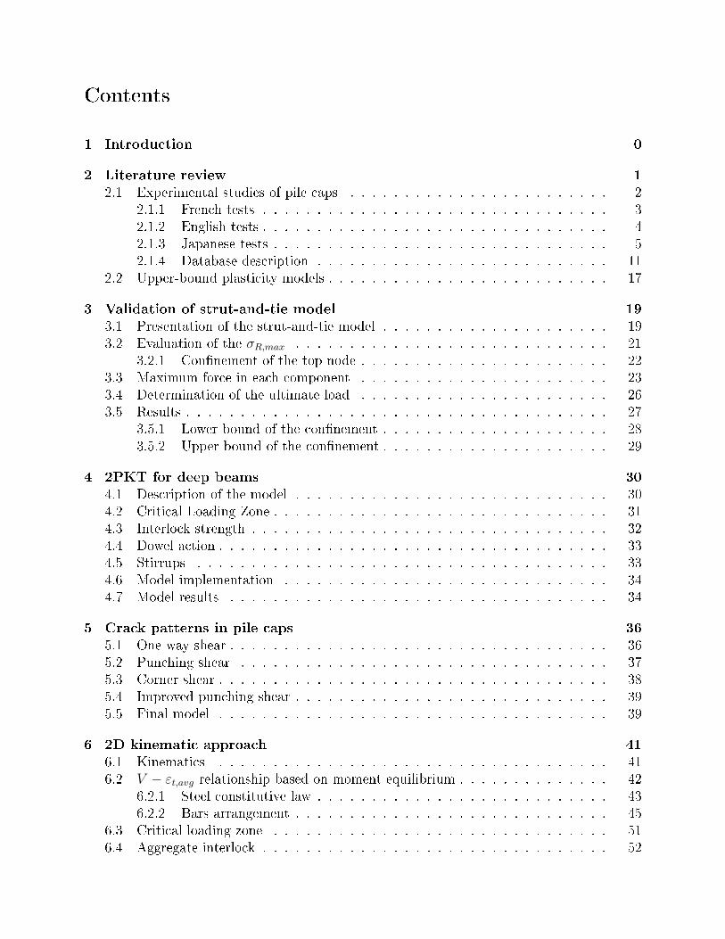
Contents
1 Introduction 0
2 Literature review 1
2.1 Experimental studies of pile caps . . . . . . . . . . . . . . . . . . . . . . . . 22.1.1 French tests . . . . . . . . . . . . . . . . . . . . . . . . . . . . . . . . 32.1.2 English tests . . . . . . . . . . . . . . . . . . . . . . . . . . . . . . . . 42.1.3 Japanese tests . . . . . . . . . . . . . . . . . . . . . . . . . . . . . . . 52.1.4 Database description . . . . . . . . . . . . . . . . . . . . . . . . . . . 11
2.2 Upper-bound plasticity models . . . . . . . . . . . . . . . . . . . . . . . . . . 17
3 Validation of strut-and-tie model 19
3.1 Presentation of the strut-and-tie model . . . . . . . . . . . . . . . . . . . . . 193.2 Evaluation of the σR,max . . . . . . . . . . . . . . . . . . . . . . . . . . . . . 21
3.2.1 Con�nement of the top node . . . . . . . . . . . . . . . . . . . . . . . 223.3 Maximum force in each component . . . . . . . . . . . . . . . . . . . . . . . 233.4 Determination of the ultimate load . . . . . . . . . . . . . . . . . . . . . . . 263.5 Results . . . . . . . . . . . . . . . . . . . . . . . . . . . . . . . . . . . . . . . 27
3.5.1 Lower bound of the con�nement . . . . . . . . . . . . . . . . . . . . . 283.5.2 Upper bound of the con�nement . . . . . . . . . . . . . . . . . . . . . 29
4 2PKT for deep beams 30
4.1 Description of the model . . . . . . . . . . . . . . . . . . . . . . . . . . . . . 304.2 Critical Loading Zone . . . . . . . . . . . . . . . . . . . . . . . . . . . . . . . 314.3 Interlock strength . . . . . . . . . . . . . . . . . . . . . . . . . . . . . . . . . 324.4 Dowel action . . . . . . . . . . . . . . . . . . . . . . . . . . . . . . . . . . . . 334.5 Stirrups . . . . . . . . . . . . . . . . . . . . . . . . . . . . . . . . . . . . . . 334.6 Model implementation . . . . . . . . . . . . . . . . . . . . . . . . . . . . . . 344.7 Model results . . . . . . . . . . . . . . . . . . . . . . . . . . . . . . . . . . . 34
5 Crack patterns in pile caps 36
5.1 One way shear . . . . . . . . . . . . . . . . . . . . . . . . . . . . . . . . . . . 365.2 Punching shear . . . . . . . . . . . . . . . . . . . . . . . . . . . . . . . . . . 375.3 Corner shear . . . . . . . . . . . . . . . . . . . . . . . . . . . . . . . . . . . . 385.4 Improved punching shear . . . . . . . . . . . . . . . . . . . . . . . . . . . . . 395.5 Final model . . . . . . . . . . . . . . . . . . . . . . . . . . . . . . . . . . . . 39
6 2D kinematic approach 41
6.1 Kinematics . . . . . . . . . . . . . . . . . . . . . . . . . . . . . . . . . . . . 416.2 V − εt,avg relationship based on moment equilibrium . . . . . . . . . . . . . . 42
6.2.1 Steel constitutive law . . . . . . . . . . . . . . . . . . . . . . . . . . . 436.2.2 Bars arrangement . . . . . . . . . . . . . . . . . . . . . . . . . . . . . 45
6.3 Critical loading zone . . . . . . . . . . . . . . . . . . . . . . . . . . . . . . . 516.4 Aggregate interlock . . . . . . . . . . . . . . . . . . . . . . . . . . . . . . . . 52
6.5 Dowel action . . . . . . . . . . . . . . . . . . . . . . . . . . . . . . . . . . . . 536.6 Solution procedure . . . . . . . . . . . . . . . . . . . . . . . . . . . . . . . . 556.7 Results . . . . . . . . . . . . . . . . . . . . . . . . . . . . . . . . . . . . . . . 58
7 3D kinematic approach 60
7.1 Kinematics . . . . . . . . . . . . . . . . . . . . . . . . . . . . . . . . . . . . 607.2 V − εt,avg relationship based on moment equilibrium . . . . . . . . . . . . . . 627.3 Critical loading zone . . . . . . . . . . . . . . . . . . . . . . . . . . . . . . . 647.4 Aggregate interlock . . . . . . . . . . . . . . . . . . . . . . . . . . . . . . . . 677.5 Dowel action . . . . . . . . . . . . . . . . . . . . . . . . . . . . . . . . . . . . 697.6 Solution procedure . . . . . . . . . . . . . . . . . . . . . . . . . . . . . . . . 707.7 Results . . . . . . . . . . . . . . . . . . . . . . . . . . . . . . . . . . . . . . . 71
8 Comparison with tests 73
8.1 2D kinematic approach . . . . . . . . . . . . . . . . . . . . . . . . . . . . . . 738.1.1 In�nitely elastic reinforcement . . . . . . . . . . . . . . . . . . . . . . 748.1.2 Elastic-plastic reinforcement . . . . . . . . . . . . . . . . . . . . . . . 76
8.2 3D kinematic approach . . . . . . . . . . . . . . . . . . . . . . . . . . . . . . 788.2.1 In�nitely elastic reinforcement . . . . . . . . . . . . . . . . . . . . . . 798.2.2 Plastic softening . . . . . . . . . . . . . . . . . . . . . . . . . . . . . 80
8.3 Choice of the model . . . . . . . . . . . . . . . . . . . . . . . . . . . . . . . . 838.4 Comparison with the strut-and-tie model . . . . . . . . . . . . . . . . . . . . 84
9 Parametric studies 88
9.1 In�uence of the e�ective depth d . . . . . . . . . . . . . . . . . . . . . . . . . 909.2 In�uence of the reinforcement ratio ρl . . . . . . . . . . . . . . . . . . . . . . 92
10 Conclusion 95
1 Introduction
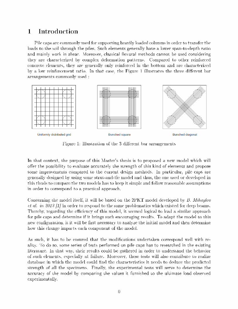
Pile caps are commonly used for supporting heavily loaded columns in order to transfer theloads to the soil through the piles. Such elements generally have a lower span-to-depth ratioand mainly work in shear. Moreover, classical �exural methods cannot be used consideringthey are characterized by complex deformation patterns. Compared to other reinforcedconcrete elements, they are generally only reinforced in the bottom and are characterizedby a low reinforcement ratio. In that case, the Figure 1 illustrates the three di�erent bararrangements commonly used :
Figure 1: Illustration of the 3 di�erent bar arrangements
In that context, the purpose of this Master's thesis is to proposed a new model which willo�er the possibility to evaluate accurately the strength of this kind of elements and proposesome improvements compared to the current design methods. In particular, pile caps aregenerally designed by using some strut-and-tie model and thus, the one used or developed inthis thesis to compare the two models has to keep it simple and follow reasonable assumptionsin order to correspond to a practical approach.
Concerning the model itself, it will be based on the 2PKT model developed by B. Mihaylovet al. in 2013 [1] in order to respond to the same problematics which existed for deep beams.Thereby, regarding the e�ciency of this model, it seemed logical to lead a similar approachfor pile caps and determine if it brings such encouraging results. To adapt the model to thisnew con�guration, it it will be �rst necessary to analyze the initial model and then determinehow this change impacts each component of the model.
As such, it has to be ensured that the modi�cations undertaken correspond well with re-ality. To do so, some series of tests performed on pile caps has to researched in the existingliterature. In that way, their results could be gathered in order to understand the behaviorof such elements, especially at failure. Moreover, these tests will also contribute to realizedatabase in which the model could �nd the characteristics it needs to deduce the predictedstrength of all the specimens. Finally, the experimental tests will serve to determine theaccuracy of the model by comparing the values it furnished to the ultimate load observedexperimentally.
0
2 Literature review
As it was already mentioned, several sources from the literature will be used all alongthis thesis. All of them have di�erent purpose but they can be synthesized into four di�erentcategories:
� Experimental studies of pile caps
This category try to centralize as much as possible tests which were made on pile caps andespecially on four-pile caps. By investigating the way the specimens failed, it will be possibleto try to draw some reoccurring failure modes and their corresponding crack patterns. Con-sidering the fact that these observations are really useful to understand properly the involvedphenomena when the failure occurs.
Moreover, it will permit to gather the di�erent characteristic parameters of the tested speci-mens. Therefore, they will form a database which could be used to put to test the new model.Indeed, the results it will produce can be compared to the corresponding experimental valueswhich will give information on its accuracy.
� Strut-and-tie model for pile caps
Before developing a new model, it is important to know exactly where the state of the arthas reached. To do so, it is necessary to evaluate the strength and more importantly theweaknesses of the current methods in order to identify the �elds where some improvementscan be made. In the case of deep pile caps, Eurocode 2 remains quite vague regarding theseelements. In fact, there is no speci�c calculation for them and only some recommendationsare indicated such as :
Reinforcement in a pile cap should be calculated either by using strut-and-tie or �exural meth-ods as appropriate, Eurocode 2
Knowing that, it will be useful to develop at least one method in order to compare it tothe experimental results. In particular, the strut-and-tie model appears to be the best alter-native to test the way pile caps are designed nowadays. Indeed, it permits to describe how theforces are �owing through the element �tting better with the phenomena the dimensioning issupposed to describe. Moreover, the �exural method is clearly not the best way to get intothe problem while one of the main hypothesis on which this method is based on, namely that"plane sections remain plane" cannot be applied to deep elements, to which most pile capsbelong.
The idea was initially to use a strut-and-tie model based on an existing one. However,it appeared that the information given were not su�cient to understand the assumptionsused and the geometry considered for the nodes. As such, it was decided to develop a newmodel which will be developped later in this work.
� 2PKT for deep beams
1
This is the model which will be extended from 2 dimensions into 3D. As such, it is im-portant to evaluate the quality of the initial model and the accuracy of its results. Indeed,it is useless to try to base this work on a model if this one did not lead to any interesting result.
Then, it is a necessity to understand precisely the phenomena involved in the beam fail-ure and handle them well enough to start the development of the new model. This requiresto be able to identify the di�erences and the similarities between pile caps and beams, butmore important, to understand how these changes impact the model and their consequenceson the di�erent parameters of the model.
� Upper-bound plasticity models
In the same idea of the 2PKT, a model was developed in the university of Southern, Den-mark, to describe the collapse mechanism of pile caps in order to predict their strength. Todo so, they identi�ed and parametrized one failure mode in particular. Then, they were ableto deduce the values of the di�erent components of the strength based on this particular mode.
Because this thesis tries to solve the same problem than their, it can be interesting to inves-tigate the reasons why they have chosen this particular pattern and not another one in orderto try to �nd new explanations of what happens at failure and also inspire of their picturesto develop some simpli�ed models which could be used through this thesis.
2.1 Experimental studies of pile caps
Six di�erent series of tests were found. They are extending over a period of time from1967 to 2001. They come from 3 di�erent countries:
� France� United Kingdom� Japan
The purpose of this section is to describe each of them in order to draw a fast picture oftheir content and understand how they will be useful to the development of the new model.Indeed, more than bringing some new data to this study, the observations and the develop-ments performed in parallel can give some precious informations, helping the understandingof the physical phenomena or giving interesting results of pile caps behavior.
Moreover, it is necessary to describe the tests procedures. In that way, it is possible toanalyze and interpret the results obtained both concerning the observed values and the con-clusions they could draw from them. Thus, the following criteria have to be detailed:
� Description of the specimens� Test setup� Main experimental observations
2
2.1.1 French tests
These are the oldest series of tests found in the literature. They were reported in a paperpublished by J. Blévot and R. Frémy in 1967 [2]. This article is organized around two dis-tinct topics. The �rst one concerns a proposed simpli�ed method for the dimensioning of pilecaps based on the "Struts method", while the second part simply gives a report of the testsmade on scaled or full size pile caps. The tests were realized to compare di�erent reinforcingbar arrangements in order to evaluate their respective e�ciency.
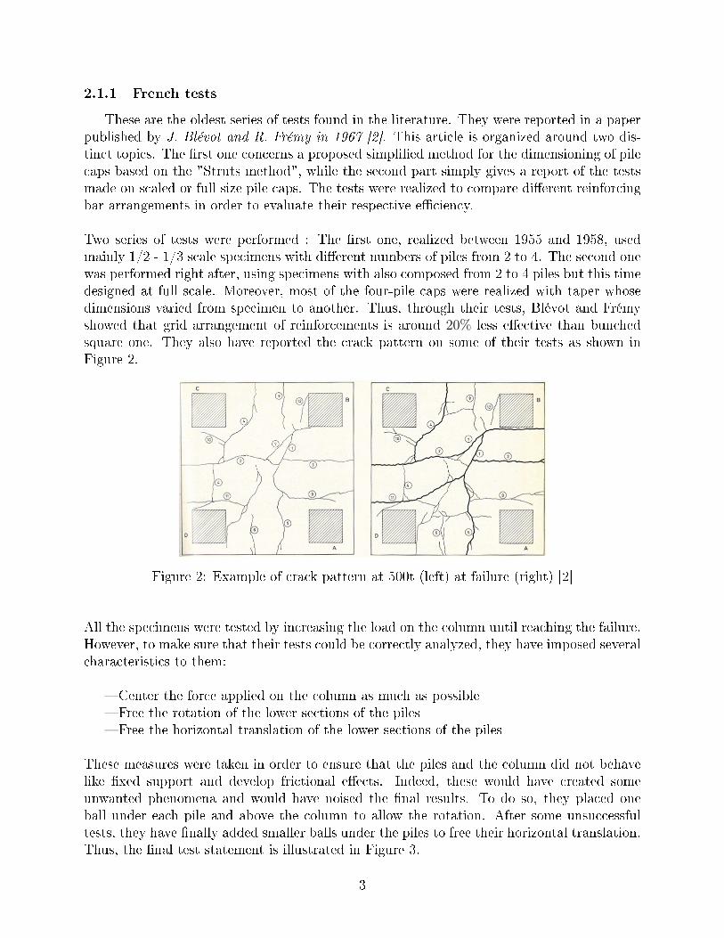
Two series of tests were performed : The �rst one, realized between 1955 and 1958, usedmainly 1/2 - 1/3 scale specimens with di�erent numbers of piles from 2 to 4. The second onewas performed right after, using specimens with also composed from 2 to 4 piles but this timedesigned at full scale. Moreover, most of the four-pile caps were realized with taper whosedimensions varied from specimen to another. Thus, through their tests, Blévot and Frémyshowed that grid arrangement of reinforcements is around 20% less e�ective than bunchedsquare one. They also have reported the crack pattern on some of their tests as shown inFigure 2.
Figure 2: Example of crack pattern at 500t (left) at failure (right) [2]
All the specimens were tested by increasing the load on the column until reaching the failure.However, to make sure that their tests could be correctly analyzed, they have imposed severalcharacteristics to them:
� Center the force applied on the column as much as possible� Free the rotation of the lower sections of the piles� Free the horizontal translation of the lower sections of the piles
These measures were taken in order to ensure that the piles and the column did not behavelike �xed support and develop frictional e�ects. Indeed, these would have created someunwanted phenomena and would have noised the �nal results. To do so, they placed oneball under each pile and above the column to allow the rotation. After some unsuccessfultests, they have �nally added smaller balls under the piles to free their horizontal translation.Thus, the �nal test statement is illustrated in Figure 3.
3
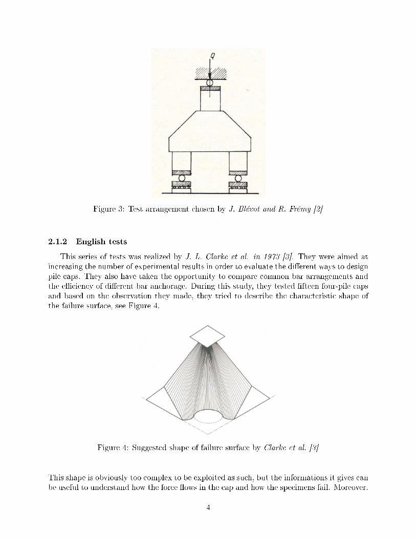
Figure 3: Test arrangement chosen by J. Blévot and R. Frémy [2]
2.1.2 English tests
This series of tests was realized by J. L. Clarke et al. in 1973 [3]. They were aimed atincreasing the number of experimental results in order to evaluate the di�erent ways to designpile caps. They also have taken the opportunity to compare common bar arrangements andthe e�ciency of di�erent bar anchorage. During this study, they tested �fteen four-pile capsand based on the observation they made, they tried to describe the characteristic shape ofthe failure surface, see Figure 4.
Figure 4: Suggested shape of failure surface by Clarke et al. [3]
This shape is obviously too complex to be exploited as such, but the informations it gives canbe useful to understand how the force �ows in the cap and how the specimens fail. Moreover,
4
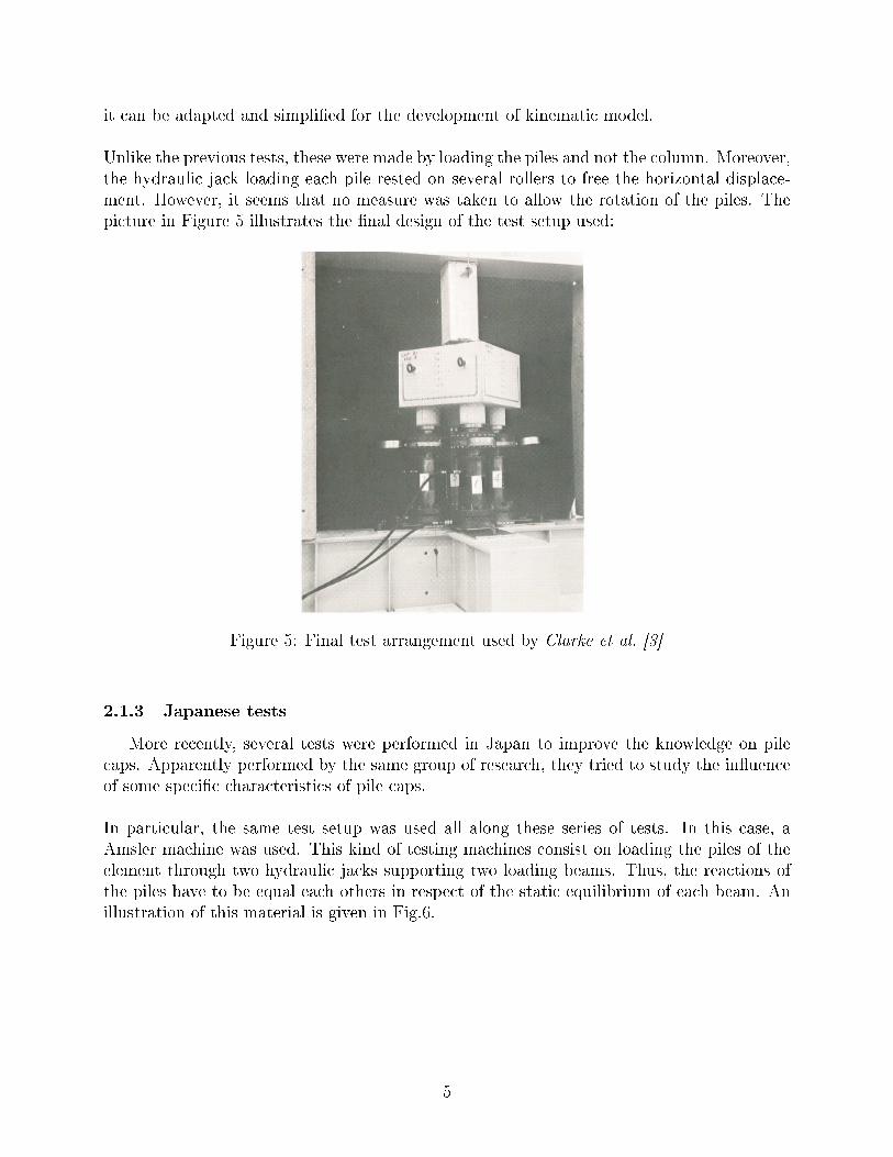
it can be adapted and simpli�ed for the development of kinematic model.
Unlike the previous tests, these were made by loading the piles and not the column. Moreover,the hydraulic jack loading each pile rested on several rollers to free the horizontal displace-ment. However, it seems that no measure was taken to allow the rotation of the piles. Thepicture in Figure 5 illustrates the �nal design of the test setup used:
Figure 5: Final test arrangement used by Clarke et al. [3]
2.1.3 Japanese tests
More recently, several tests were performed in Japan to improve the knowledge on pilecaps. Apparently performed by the same group of research, they tried to study the in�uenceof some speci�c characteristics of pile caps.
In particular, the same test setup was used all along these series of tests. In this case, aAmsler machine was used. This kind of testing machines consist on loading the piles of theelement through two hydraulic jacks supporting two loading beams. Thus, the reactions ofthe piles have to be equal each others in respect of the static equilibrium of each beam. Anillustration of this material is given in Fig.6.
5
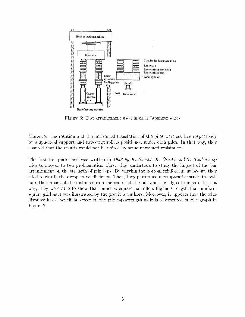
Figure 6: Test arrangement used in each Japanese series
Moreover, the rotation and the horizontal translation of the piles were set free respectivelyby a spherical support and two-stage rollers positioned under each piles. In that way, theyensured that the results would not be noised by some unwanted resistance.
The �rst test performed was written in 1998 by K. Suzuki, K. Otsuki and T. Tsubata [4]tries to answer to two problematics. First, they undertook to study the impact of the bararrangement on the strength of pile caps. By varying the bottom reinforcement layout, theytried to clarify their respective e�ciency. Then, they performed a comparative study to eval-uate the impact of the distance from the center of the pile and the edge of the cap. In thatway, they were able to show that bunched square bar o�ers higher strength than uniformsquare grid as it was illustrated by the previous authors. Moreover, it appears that the edgedistance has a bene�cial e�ect on the pile cap strength as it is represented on the graph inFigure 7.
6
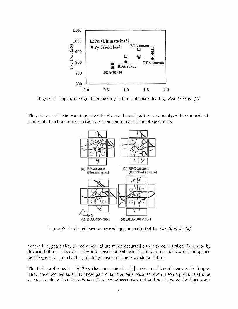
Figure 7: Impact of edge distance on yield and ultimate load by Suzuki et al. [4]
They also used their tests to gather the observed crack pattern and analyze them in order torepresent the characteristic crack distribution on each type of specimens.
Figure 8: Crack pattern on several specimens tested by Suzuki et al. [4]
Where it appears that the common failure mode occurred either by corner shear failure or by�exural failure. However, they also have noticed two others failure modes which happenedless frequently, namely the punching shear and one way shear failure.
The tests performed in 1999 by the same scientists [5] used some four-pile caps with tapper.They have decided to study these particular elements because, even if some previous studiesseemed to show that there is no di�erence between tapered and non tapered footings, some
7
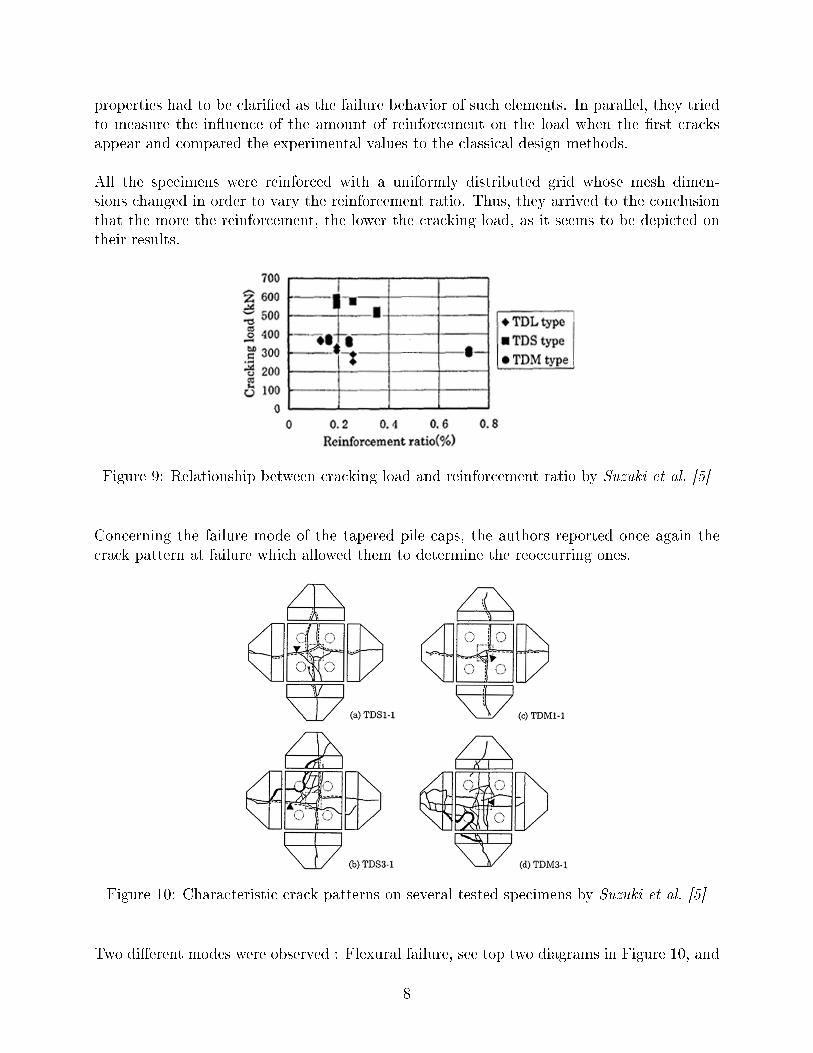
properties had to be clari�ed as the failure behavior of such elements. In parallel, they triedto measure the in�uence of the amount of reinforcement on the load when the �rst cracksappear and compared the experimental values to the classical design methods.
All the specimens were reinforced with a uniformly distributed grid whose mesh dimen-sions changed in order to vary the reinforcement ratio. Thus, they arrived to the conclusionthat the more the reinforcement, the lower the cracking load, as it seems to be depicted ontheir results.
Figure 9: Relationship between cracking load and reinforcement ratio by Suzuki et al. [5]
Concerning the failure mode of the tapered pile caps, the authors reported once again thecrack pattern at failure which allowed them to determine the reoccurring ones.
Figure 10: Characteristic crack patterns on several tested specimens by Suzuki et al. [5]
Two di�erent modes were observed : Flexural failure, see top two diagrams in Figure 10, and
8
corner shear failure, see bottom diagrams in Figure 10. However, regarding their detailedresults, it appears that most of the specimens failed by �exure instead of shear.
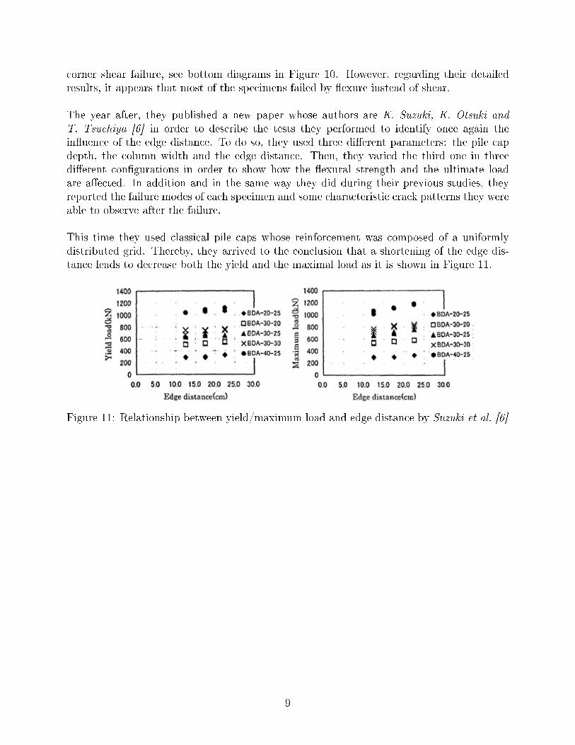
The year after, they published a new paper whose authors are K. Suzuki, K. Otsuki andT. Tsuchiya [6] in order to describe the tests they performed to identify once again thein�uence of the edge distance. To do so, they used three di�erent parameters: the pile capdepth, the column width and the edge distance. Then, they varied the third one in threedi�erent con�gurations in order to show how the �exural strength and the ultimate loadare a�ected. In addition and in the same way they did during their previous studies, theyreported the failure modes of each specimen and some characteristic crack patterns they wereable to observe after the failure.
This time they used classical pile caps whose reinforcement was composed of a uniformlydistributed grid. Thereby, they arrived to the conclusion that a shortening of the edge dis-tance leads to decrease both the yield and the maximal load as it is shown in Figure 11.
Figure 11: Relationship between yield/maximum load and edge distance by Suzuki et al. [6]
9
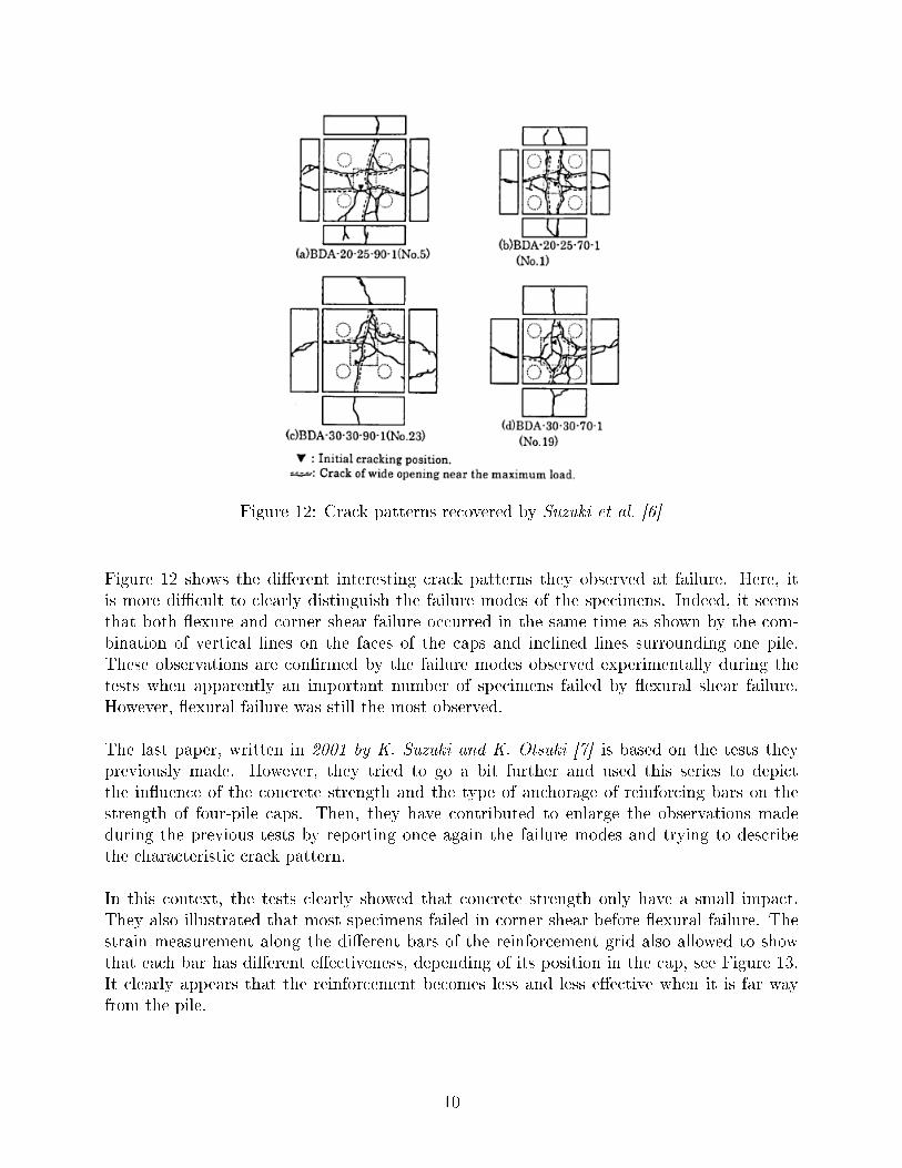
Figure 12: Crack patterns recovered by Suzuki et al. [6]
Figure 12 shows the di�erent interesting crack patterns they observed at failure. Here, itis more di�cult to clearly distinguish the failure modes of the specimens. Indeed, it seemsthat both �exure and corner shear failure occurred in the same time as shown by the com-bination of vertical lines on the faces of the caps and inclined lines surrounding one pile.These observations are con�rmed by the failure modes observed experimentally during thetests when apparently an important number of specimens failed by �exural shear failure.However, �exural failure was still the most observed.
The last paper, written in 2001 by K. Suzuki and K. Otsuki [7] is based on the tests theypreviously made. However, they tried to go a bit further and used this series to depictthe in�uence of the concrete strength and the type of anchorage of reinforcing bars on thestrength of four-pile caps. Then, they have contributed to enlarge the observations madeduring the previous tests by reporting once again the failure modes and trying to describethe characteristic crack pattern.
In this context, the tests clearly showed that concrete strength only have a small impact.They also illustrated that most specimens failed in corner shear before �exural failure. Thestrain measurement along the di�erent bars of the reinforcement grid also allowed to showthat each bar has di�erent e�ectiveness, depending of its position in the cap, see Figure 13.It clearly appears that the reinforcement becomes less and less e�ective when it is far wayfrom the pile.
10
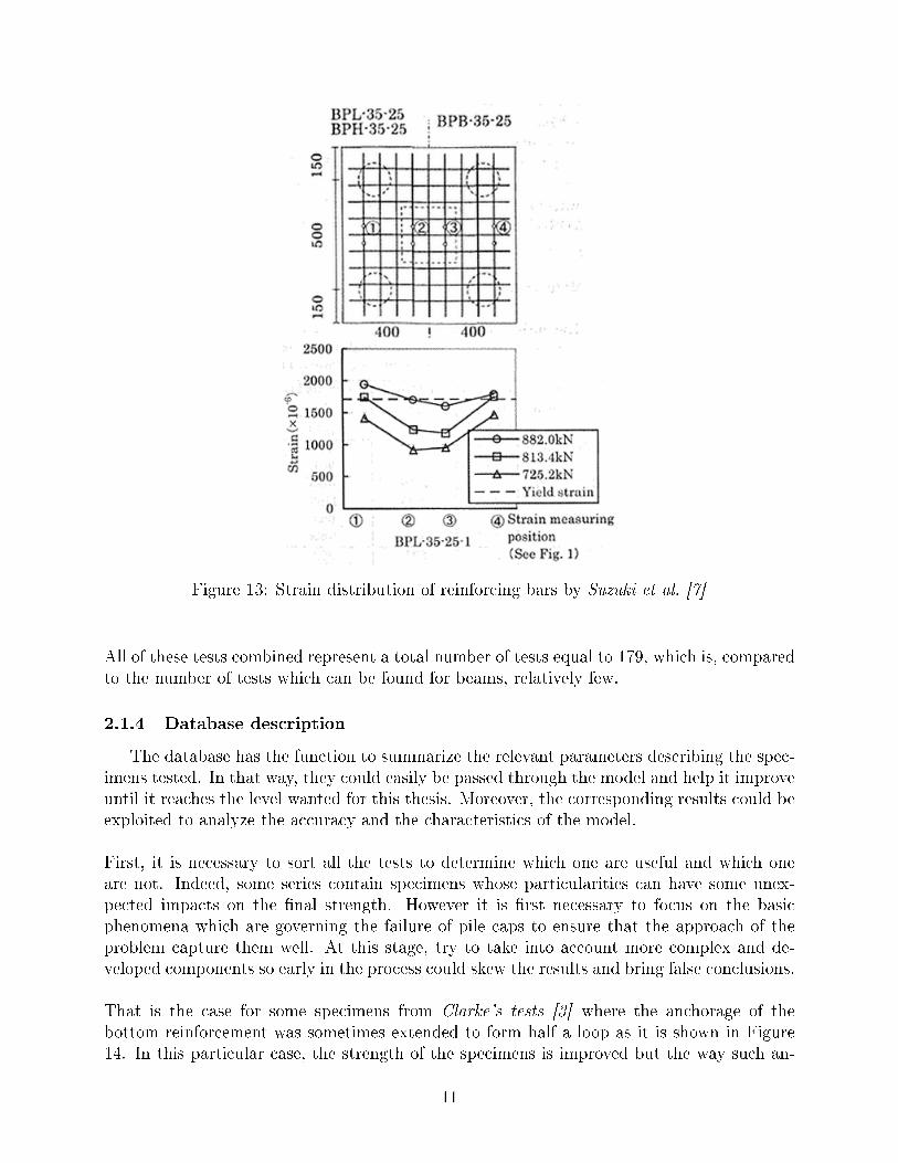
Figure 13: Strain distribution of reinforcing bars by Suzuki et al. [7]
All of these tests combined represent a total number of tests equal to 179, which is, comparedto the number of tests which can be found for beams, relatively few.
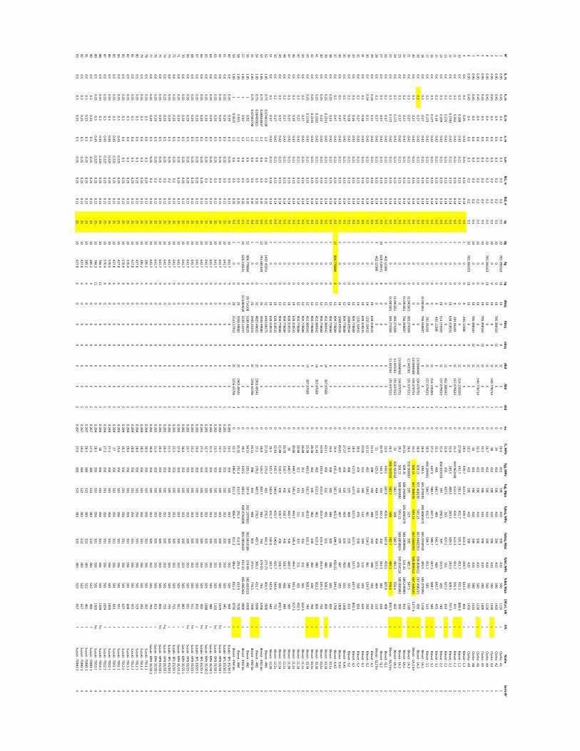
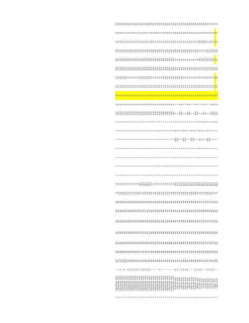
2.1.4 Database description
The database has the function to summarize the relevant parameters describing the spec-imens tested. In that way, they could easily be passed through the model and help it improveuntil it reaches the level wanted for this thesis. Moreover, the corresponding results could beexploited to analyze the accuracy and the characteristics of the model.
First, it is necessary to sort all the tests to determine which one are useful and which oneare not. Indeed, some series contain specimens whose particularities can have some unex-pected impacts on the �nal strength. However it is �rst necessary to focus on the basicphenomena which are governing the failure of pile caps to ensure that the approach of theproblem capture them well. At this stage, try to take into account more complex and de-veloped components so early in the process could skew the results and bring false conclusions.
That is the case for some specimens from Clarke's tests [3] where the anchorage of thebottom reinforcement was sometimes extended to form half a loop as it is shown in Figure14. In this particular case, the strength of the specimens is improved but the way such an-
11
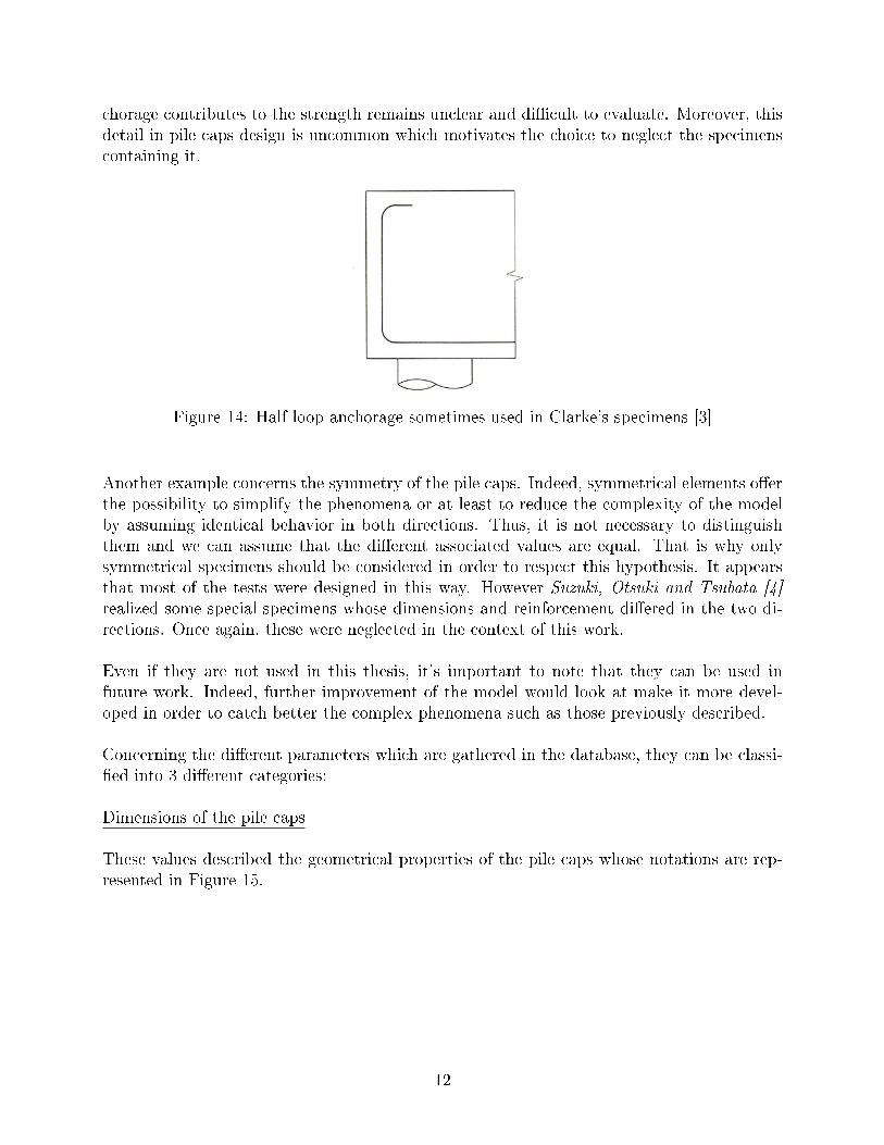
chorage contributes to the strength remains unclear and di�cult to evaluate. Moreover, thisdetail in pile caps design is uncommon which motivates the choice to neglect the specimenscontaining it.
Figure 14: Half loop anchorage sometimes used in Clarke's specimens [3]
Another example concerns the symmetry of the pile caps. Indeed, symmetrical elements o�erthe possibility to simplify the phenomena or at least to reduce the complexity of the modelby assuming identical behavior in both directions. Thus, it is not necessary to distinguishthem and we can assume that the di�erent associated values are equal. That is why onlysymmetrical specimens should be considered in order to respect this hypothesis. It appearsthat most of the tests were designed in this way. However Suzuki, Otsuki and Tsubata [4]realized some special specimens whose dimensions and reinforcement di�ered in the two di-rections. Once again, these were neglected in the context of this work.
Even if they are not used in this thesis, it's important to note that they can be used infuture work. Indeed, further improvement of the model would look at make it more devel-oped in order to catch better the complex phenomena such as those previously described.
Concerning the di�erent parameters which are gathered in the database, they can be classi-�ed into 3 di�erent categories:
Dimensions of the pile caps
These values described the geometrical properties of the pile caps whose notations are rep-resented in Figure 15.
12
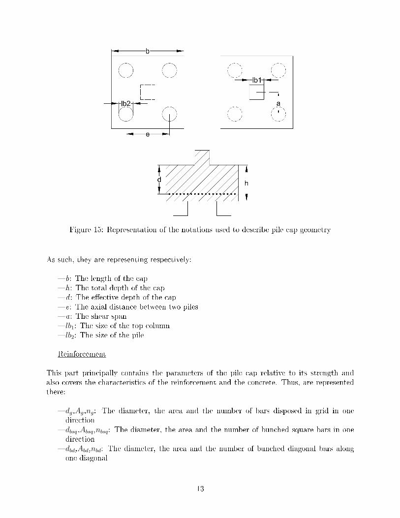
Figure 15: Representation of the notations used to describe pile cap geometry
As such, they are representing respectively:
� b: The length of the cap� h: The total depth of the cap� d : The e�ective depth of the cap� e: The axial distance between two piles� a: The shear span� lb1: The size of the top column� lb2: The size of the pile
Reinforcement
This part principally contains the parameters of the pile cap relative to its strength andalso covers the characteristics of the reinforcement and the concrete. Thus, are representedthere:
� dg,Ag,ng: The diameter, the area and the number of bars disposed in grid in onedirection
� dbsq,Absq,nbsq: The diameter, the area and the number of bunched square bars in onedirection
� dbd,Abd,nbd: The diameter, the area and the number of bunched diagonal bars alongone diagonal
13
Material properties
� ag: The size of the coarse aggregates� fc: The compressive strength of the concrete� fy,g,fy,bsq,fy,bd: The yielding strength of the bottom reinforcement. Respectively ingrid, bunched square and bunched diagonal
� fu,g,fu,bsq,fu,bd: The ultimate strength of the bottom reinforcement. Respectively ingrid, bunched square and bunched diagonal
� εu,g,εu,bsq,εu,bd: The ultimate strain of the bottom reinforcement. Respectively in grid,bunched square and bunched diagonal
Test results
� Name: Permits to identify the origin of the current specimen and to distinguish thetests made during the same series.
� Series N�: It is a pointer I used to separate the di�erent series each other to make easierthe graph drawings.• 1 = J. Clarke [3]• 2 = J. Blévot and R. Frémy [2]• 3 = K. Suzuki, K. Otsuki (2001) [7]• 4 = K. Suzuki, K. Otsuki, T. Tsubata (1999) [5]• 5 = K. Suzuki, K.Otsuki, T. Tsubata (1998) [4]• 6 = K. Suzuki, K. Otsuki, T. Tsuchiya(2000) [6]
� Nu,e: The ultimate load observed at failure during the test.� EFL: Describe the failure mode of the specimen.• "c" = Corner shear failure• "f" = Flexural failure• "p" = Punching shear failure• "f+c" = Combination of �exural and corner shear failure• "f+p" = Combination of �exural and punching shear failure
Most of these parameters were given for the di�erent tests. If they were not, it was necessaryto make a reasonable assumption. In particular, this was the case for the ag and εu valuesfor which only the Japanese authors indicated both while [3] reported only the size of thecoarse aggregates. For the missing ones, the following values were used:
� ag = 9.5mm� εu = 10%
Finally, from the 174 initial specimens,145 remain. Unfortunately, most of the specimen weresmall (d ≤ 400mm) which generally decreases the reliability of the test results. The smallerthe element, the greater the impact of imperfections. Thus, we can fear some noisy resultsfor the smallest values of d and an increase of accuracy for higher ones.
14
N°
b, m
h, m
d, m
e, m
a,m
lb1
, mlb
2, m
ag
dg
Ag
ng
db
sqA
bsq
nb
sqd
bd
Ab
dn
bd
eu
fc, MP
afy
g, M
Pa
fug
, Mp
afy
bsq
, MP
afu
bsq
, Mp
afy
bd
, MP
afu
bd
, Mp
a|
Nf,e
|, k
NE
FL
Na
me
Se
rie N
°
10
.95
0.4
50
.40
.60
.30
.20
.29
.51
07
85
.39
81
63
10
10
00
10
00
02
6.6
41
05
90
41
05
90
41
05
90
11
10
cC
lark
e - A
11
20
.95
0.4
50
.40
.60
.30
.20
.29
.51
00
01
07
85
.39
81
63
10
10
00
03
44
10
59
04
10
59
04
10
59
01
42
0c
Cla
rke
- A2
1
30
.95
0.4
50
.40
.60
.30
.20
.29
.51
00
01
00
01
05
49
.77
87
14
70
38
41
05
90
41
05
90
41
05
90
13
40
cC
lark
e - A
31
40
.95
0.4
50
.40
.60
.30
.20
.29
.51
07
85
.39
81
63
10
10
00
10
00
02
6.7
41
05
90
41
05
90
41
05
90
12
30
cC
lark
e - A
41
50
.95
0.4
50
.40
.60
.30
.20
.29
.51
00
01
07
85
.39
81
63
10
10
00
03
3.2
41
05
90
41
05
90
41
05
90
14
00
cC
lark
e - A
51
60
.95
0.4
50
.40
.60
.30
.20
.29
.51
00
01
00
01
05
49
.77
87
14
70
32
.34
10
59
04
10
59
04
10
59
01
23
0c
Cla
rke
- A6
1
70
.95
0.4
50
.40
.60
.30
.20
.29
.51
00
01
07
85
.39
81
63
10
10
00
03
44
10
59
04
10
59
04
10
59
01
51
0c
Cla
rke
- A8
1
80
.95
0.4
50
.40
.60
.30
.20
.29
.51
07
85
.39
81
63
10
10
00
10
00
03
3.2
41
05
90
41
05
90
41
05
90
14
50
cC
lark
e - A
91
90
.60
.30
.25
0.4
20
.21
0.1
50
.14
9.5
00
08
40
2.1
23
86
80
00
02
9.1
43
9.7
61
3.3
43
9.7
61
3.3
43
9.7
61
3.3
85
0c
Ble
vo
t - 1,1
2
10
0.6
0.3
0.2
68
0.4
20
.21
0.1
50
.14
9.5
00
00
00
10
31
4.1
59
26
54
02
7.8
54
51
.75
91
.34
51
.75
91
.34
51
.75
91
.38
80
.4c
Ble
vo
t - 1,2
2
11
0.6
0.3
0.2
62
0.4
20
.21
0.1
50
.14
9.5
00
08
20
1.0
61
93
41
01
57
.07
96
33
20
31
.34
44
.96
31
58
61
3.3
43
9.7
61
3.3
45
1.7
59
1.3
87
1c
Ble
vo
t - 1,3
2
12
0.6
0.3
0.2
78
10
.42
0.2
10
.15
0.1
49
.50
00
10
62
8.3
18
53
18
00
00
32
.62
83
.54
09
.52
83
.54
09
.52
83
.54
09
.57
47
.5c
Ble
vo
t - 2,1
2
13
0.6
0.3
0.2
76
0.4
20
.21
0.1
50
.14
9.5
00
00
00
12
45
2.3
89
34
24
03
2.8
35
54
27
.53
55
42
7.5
35
54
27
.58
10
cB
levo
t - 2,2
2
14
0.6
0.3
0.2
69
0.4
20
.21
0.1
50
.14
9.5
00
01
03
14
.15
92
65
41
01
57
.07
96
33
20
31
.63
04
.83
33
33
39
72
90
.53
97
33
3.5
42
07
40
cB
levo
t - 2,3
2
15
0.6
0.2
0.1
80
.42
0.2
10
.15
0.1
49
.50
00
84
02
.12
38
68
00
00
32
.14
69
64
2.7
46
96
42
.74
69
64
2.7
47
5c
Ble
vo
t - 3,1
2
16
0.6
0.3
0.1
77
0.4
20
.21
0.1
50
.14
9.5
00
00
00
10
31
4.1
59
26
54
03
7.2
44
7.3
58
8.7
44
7.3
58
8.7
44
7.3
58
8.7
54
0c
Ble
vo
t - 3,2
2
17
0.6
0.3
0.1
73
0.4
20
.21
0.1
50
.14
9.5
00
08
20
1.0
61
93
41
01
57
.07
96
33
20
30
.94
40
.29
64
91
59
4.7
43
1.7
59
4.7
45
1.3
58
55
10
cB
levo
t - 3,3
2
18
0.6
0.3
0.2
70
.42
0.2
10
.15
0.1
49
.50
00
11
.04
53
61
76
6.5
48
60
78
00
00
26
.64
94
.55
81
.07
04
92
49
2.6
06
55
74
58
1.0
70
49
18
49
4.5
58
1.0
70
49
21
15
0c
Ble
vo
t - 1A
,12
19
0.6
0.3
0.2
70
.42
0.2
10
.15
0.1
49
.50
00
00
01
3.0
38
40
48
53
4.0
70
75
14
03
6.8
50
3.1
55
67
.46
82
35
50
3.1
55
67
.46
82
35
35
04
.80
94
12
56
7.4
68
23
59
00
cB
levo
t - 1A
,22
20
0.6
0.3
0.2
70
.42
0.2
10
.15
0.1
49
.50
00
00
01
3.0
38
40
48
53
4.0
70
75
14
03
3.2
50
3.1
55
67
.46
82
35
50
3.1
55
67
.46
82
35
35
04
.80
94
12
56
7.4
68
23
51
17
7.5
cB
levo
t - 1A
,2 b
is2
21
0.6
0.3
0.2
70
.42
0.2
10
.15
0.1
49
.50
00
11
.04
53
61
38
3.2
74
30
44
11
.04
53
61
19
1.6
37
15
22
03
6.6
51
0.5
66
66
75
95
52
35
95
48
5.7
54
7.5
11
85
cB
levo
t - 1A
,32
22
0.6
0.2
0.1
70
.42
0.2
10
.15
0.1
49
.50
00
11
.04
53
61
76
6.5
48
60
78
00
00
29
.15
50
9.3
55
80
.24
09
84
50
5.6
80
32
79
58
0.2
40
98
36
51
1.3
55
80
.24
09
84
81
5c
Ble
vo
t - 3A
,12
23
0.6
0.3
0.1
70
.42
0.2
10
.15
0.1
49
.50
00
00
01
3.0
38
40
48
53
4.0
70
75
14
03
9.2
50
3.1
55
80
.88
58
82
50
3.1
55
80
.88
58
82
45
05
.05
41
18
58
0.8
85
88
29
00
cB
levo
t - 3A
,22
24
0.6
0.2
0.1
72
0.4
20
.21
0.1
50
.14
9.5
00
01
1.0
45
36
13
83
.27
43
04
41
1.0
45
36
11
91
.63
71
52
20
32
50
0.4
33
33
35
82
.75
08
58
2.7
48
5.3
55
6.6
66
5c
Ble
vo
t - 3A
,32
25
0.6
0.3
0.1
72
0.4
20
.21
0.1
50
.14
9.5
00
01
1.0
45
36
13
83
.27
43
04
41
1.0
45
36
11
91
.63
71
52
20
46
.15
00
.43
33
33
58
2.7
50
85
82
.74
85
.35
56
.68
42
.5c
Ble
vo
t - 3A
,3 b
is2
26
0.6
0.2
0.1
70
.42
0.2
10
.15
0.1
49
.58
40
2.1
23
86
80
00
00
00
33
.94
59
.56
07
.84
59
.56
07
.84
59
.56
07
.84
08
cB
levo
t - Q,1
2
27
0.6
0.3
0.2
70
.42
0.2
10
.15
0.1
49
.51
06
28
.31
85
31
80
00
00
00
30
.75
34
2.3
44
23
42
.34
42
34
2.3
44
26
50
cB
levo
t - Q,2
2
28
0.6
0.3
0.2
70
.42
0.2
10
.15
0.1
49
.58
40
2.1
23
86
80
00
00
00
21
32
5.3
46
43
25
.34
64
32
5.3
46
45
10
cB
levo
t - Q,2
bis
2
29
0.6
0.1
40
.11
0.4
20
.21
0.1
50
.14
9.5
00
01
06
28
.31
85
31
80
00
01
3.1
54
98
59
24
98
59
24
98
59
22
50
cB
levo
t - 6,1
2
30
0.6
0.1
40
.11
0.4
20
.21
0.1
50
.14
9.5
00
01
41
23
1.5
04
32
80
00
01
3.1
54
61
53
4.5
46
15
34
.54
61
53
4.5
29
0c
Ble
vo
t - 6,2
2
31
0.6
0.2
0.1
80
.42
0.2
10
.15
0.1
49
.50
00
10
62
8.3
18
53
18
00
00
22
.05
51
25
93
51
25
93
51
25
93
65
0c
Ble
vo
t - 6,3
2
32
0.6
0.2
0.1
70
.42
0.2
10
.15
0.1
49
.50
00
14
12
31
.50
43
28
00
00
30
.64
76
55
84
76
55
84
76
55
88
50
cB
levo
t - 6,4
2
33
0.6
0.3
0.2
60
.42
0.2
10
.15
0.1
49
.50
00
12
90
4.7
78
68
48
00
00
18
.45
17
.56
17
.55
17
.56
17
.55
17
.56
17
.58
42
.5c
Ble
vo
t - 6,5
2
34
0.6
0.3
0.2
80
.42
0.2
10
.15
0.1
49
.50
00
16
16
08
.49
54
48
00
00
18
.44
68
55
54
68
55
54
68
55
58
10
cB
levo
t - 6,6
2
35
0.6
0.5
0.4
70
.42
0.2
10
.15
0.1
49
.50
00
12
90
4.7
78
68
48
00
00
27
.27
45
96
35
45
96
35
45
96
35
12
00
cB
levo
t - 9,A
12
36
0.6
0.5
0.4
70
.42
0.2
10
.15
0.1
49
.50
00
16
16
08
.49
54
48
00
00
40
.81
46
75
95
46
75
95
46
75
95
19
00
cB
levo
t - 9,A
22
37
0.6
0.5
0.4
70
.42
0.2
10
.15
0.1
49
.51
29
04
.77
86
84
81
29
04
.77
86
84
80
00
03
4.4
43
5.2
58
7.2
46
5.3
64
4.2
45
0.2
56
44
.21
70
0c
Ble
vo
t - 9,A
32
38
0.6
0.2
50
.23
0.4
20
.21
0.1
50
.14
9.5
00
01
29
04
.77
86
84
80
00
03
4.6
44
66
05
44
66
05
44
66
05
85
0c
Ble
vo
t - 10
,1a
2
39
0.6
0.2
50
.22
11
0.4
20
.21
0.1
50
.14
9.5
00
01
24
52
.38
93
42
41
43
07
.87
60
82
04
3.1
14
56
61
64
56
61
64
80
56
8.2
80
0c
Ble
vo
t - 10
,1b
2
40
0.6
0.2
50
.22
0.4
20
.21
0.1
50
.14
9.5
00
01
29
04
.77
86
84
80
00
03
3.9
34
53
.36
15
.34
53
.36
15
.34
53
.36
15
.37
50
cB
levo
t - 10
,2a
2
41
0.6
0.2
50
.22
02
0.4
20
.21
0.1
50
.14
9.5
00
01
24
52
.38
93
42
41
43
07
.87
60
82
03
1.4
34
62
61
5.3
46
26
15
.34
80
56
2.2
80
0c
Ble
vo
t - 10
,2b
2
42
0.6
0.2
50
.22
31
0.4
20
.21
0.1
50
.14
9.5
00
01
29
04
.77
86
84
80
00
02
8.3
84
62
63
04
62
63
04
62
63
07
60
cB
levo
t - 10
,3a
2
43
0.6
0.2
50
.21
54
0.4
20
.21
0.1
50
.14
9.5
00
01
24
52
.38
93
42
41
43
07
.87
60
82
03
3.3
84
63
.56
31
.54
63
.56
31
.54
80
56
8.2
74
0c
Ble
vo
t - 10
,3b
2
44
0.6
0.3
0.2
70
.42
0.2
10
.15
0.1
49
.50
00
12
90
4.7
78
68
48
00
00
26
.88
31
14
31
31
14
31
31
14
31
56
2.5
cB
levo
t - 11
,1a
2
45
0.6
0.3
0.2
70
.42
0.2
10
.15
0.1
49
.50
00
12
90
4.7
78
68
48
00
00
19
.48
31
14
31
31
14
31
31
14
31
49
2.5
cB
levo
t - 11
,1b
2
46
0.6
0.3
0.2
90
.42
0.2
10
.15
0.1
49
.50
00
10
62
8.3
18
53
18
00
00
30
.86
44
4.7
54
5.3
44
4.7
54
5.3
44
4.7
54
5.3
55
7.5
cB
levo
t - 11
,2a
2
47
0.6
0.3
0.2
70
.42
0.2
10
.15
0.1
49
.50
00
10
62
8.3
18
53
18
00
00
30
44
0.7
54
64
40
.75
46
44
0.7
54
65
85
cB
levo
t - 11
,2b
2
48
0.6
0.2
0.1
70
.42
0.2
10
.15
0.1
49
.50
00
12
90
4.7
78
68
48
00
00
20
.78
31
8.7
43
63
18
.74
36
31
8.7
43
68
40
cB
levo
t - 12
,1a
2
49
0.6
0.2
0.1
70
.42
0.2
10
.15
0.1
49
.50
00
12
90
4.7
78
68
48
00
00
21
.88
31
8.7
43
63
18
.74
36
31
8.7
43
66
92
.5c
Ble
vo
t - 12
,1b
2
50
0.6
0.2
0.1
70
.42
0.2
10
.15
0.1
49
.50
00
10
62
8.3
18
53
18
00
00
32
.43
43
5.7
54
0.6
43
5.7
54
0.6
43
5.7
54
0.6
75
0c
Ble
vo
t - 12
,2a
2
51
0.6
0.2
0.1
70
.42
0.2
10
.15
0.1
49
.50
00
10
62
8.3
18
53
18
00
00
26
.14
31
.75
42
.64
31
.75
42
.64
31
.75
42
.66
40
cB
levo
t - 12
,2b
2
52
1.8
50
.75
0.6
74
61
53
81
.20
.60
.50
.35
9.5
16
14
07
.43
35
17
32
64
33
.98
17
58
00
00
37
.25
27
9.3
40
12
76
.24
01
.52
77
.75
40
1.5
70
00
cB
levo
t - 4N
12
53
1.8
50
.75
0.6
81
64
44
71
.20
.60
.50
.35
9.5
12
79
1.6
81
34
97
25
39
26
.99
08
28
00
00
40
.85
16
.78
22
.74
43
76
44
79
.55
76
46
70
0c
Ble
vo
t - 4N
1 b
is2
54
1.8
50
.75
0.6
64
09
30
11
.20
.60
.50
.35
9.5
00
03
24
82
5.4
86
32
62
51
96
3.4
95
41
40
37
.12
78
.54
07
.52
78
.54
07
.53
00
.34
31
.76
58
0c
Ble
vo
t - 4N
22
55
1.8
50
.75
0.6
73
03
73
81
.20
.60
.50
.35
9.5
00
02
52
94
5.2
43
11
62
01
25
6.6
37
06
40
34
.15
49
88
19
49
88
19
47
4.5
77
6.5
73
90
cB
levo
t - 4N
2 b
is2
56
1.8
51
0.9
21
.20
.60
.50
.35
9.5
12
90
4.7
78
68
48
28
.71
41
08
51
80
.48
62
98
00
00
34
.15
29
3.1
39
7.4
26
2.1
97
93
81
38
2.6
81
01
88
27
4.9
63
82
.68
10
19
65
00
cB
levo
t - 4N
32
57
1.8
51
0.9
21
.20
.60
.50
.35
9.5
10
62
8.3
18
53
18
22
.63
84
62
83
22
0.1
32
47
80
00
04
9.3
42
9.5
68
3.5
46
9.4
75
60
98
80
5.0
85
36
59
45
3.3
38
05
.08
53
66
90
00
cB
levo
t - 4N
3 b
is2
58
1.8
51
0.9
15
1.2
0.6
0.5
0.3
59
.50
00
25
39
26
.99
08
28
25
19
63
.49
54
14
03
5.3
52
91
.44
12
.92
91
.44
12
.92
91
.44
12
.97
53
0c
Ble
vo
t - 4N
42
59
1.8
51
0.9
22
51
.20
.60
.50
.35
9.5
00
02
02
51
3.2
74
12
82
01
25
6.6
37
06
40
42
.34
86
.48
11
.34
86
.48
11
.34
86
.48
11
.38
75
0c
Ble
vo
t - 4N
4 b
is2
60
0.8
0.3
50
.29
0.5
0.2
50
.30
.15
25
10
64
1.7
90
00
00
00
.28
52
4.1
35
35
05
35
35
05
35
35
05
96
0c
Su
zuk
i - BP
L 35
/30
13
61
0.8
0.3
50
.29
0.5
0.2
50
.30
.15
25
10
64
1.7
90
00
00
00
.28
52
5.6
35
35
05
35
35
05
35
35
05
94
1c
Su
zuk
i - BP
L 35
/30
23
62
0.8
0.3
50
.29
0.5
0.2
50
.30
.15
25
10
64
1.7
90
00
00
00
.28
52
3.7
35
35
05
35
35
05
35
35
05
10
29
f+c
Su
zuk
i - BP
B 3
5/3
0 1
3
63
0.8
0.3
50
.29
0.5
0.2
50
.30
.15
25
10
64
1.7
90
00
00
00
.28
52
3.5
35
35
05
35
35
05
35
35
05
11
03
f+c
Su
zuk
i - BP
B 3
5/3
0 2
3
64
0.8
0.3
50
.29
0.5
0.2
50
.30
.15
25
10
64
1.7
90
00
00
00
.28
53
1.5
35
35
05
35
35
05
35
35
05
98
0c
Su
zuk
i - BP
H 3
5/3
0 1
3
65
0.8
0.3
50
.29
0.5
0.2
50
.30
.15
25
10
64
1.7
90
00
00
00
.28
53
2.7
35
35
05
35
35
05
35
35
05
10
88
f+c
Su
zuk
i - BP
H 3
5/3
0 2
3
66
0.8
0.3
50
.29
0.5
0.2
50
.25
0.1
52
51
06
41
.79
00
00
00
0.2
85
27
.13
53
50
53
53
50
53
53
50
59
02
f+c
Su
zuk
i - BP
L 35
/25
13
67
0.8
0.3
50
.29
0.5
0.2
50
.25
0.1
52
51
06
41
.79
00
00
00
0.2
85
25
.63
53
50
53
53
50
53
53
50
58
72
cS
uzu
ki - B
PL 3
5/2
5 2
3
68
0.8
0.3
50
.29
0.5
0.2
50
.25
0.1
52
51
06
41
.79
00
00
00
0.2
85
23
.23
53
50
53
53
50
53
53
50
59
11
f+c
Su
zuk
i - BP
B 3
5/2
5 1
3
69
0.8
0.3
50
.29
0.5
0.2
50
.25
0.1
52
51
06
41
.79
00
00
00
0.2
85
23
.73
53
50
53
53
50
53
53
50
59
21
f+c
Su
zuk
i - BP
B 3
5/2
5 2
3
70
0.8
0.3
50
.29
0.5
0.2
50
.25
0.1
52
51
06
41
.79
00
00
00
0.2
85
36
.63
53
50
53
53
50
53
53
50
58
82
cS
uzu
ki - B
PH
35
/25
13
71
0.8
0.3
50
.29
0.5
0.2
50
.25
0.1
52
51
06
41
.79
00
00
00
0.2
85
37
.93
53
50
53
53
50
53
53
50
59
51
cS
uzu
ki - B
PH
35
/25
23
72
0.8
0.3
50
.29
0.5
0.2
50
.20
.15
25
10
64
1.7
90
00
00
00
.28
52
2.5
35
35
05
35
35
05
35
35
05
75
5c
Su
zuk
i - BP
L 35
/20
13
73
0.8
0.3
50
.29
0.5
0.2
50
.20
.15
25
10
64
1.7
90
00
00
00
.28
52
1.5
35
35
05
35
35
05
35
35
05
73
5c
Su
zuk
i - BP
L 35
/20
23
74
0.8
0.3
50
.29
0.5
0.2
50
.20
.15
25
10
64
1.7
90
00
00
00
.28
52
0.4
35
35
05
35
35
05
35
35
05
75
5f+
pS
uzu
ki - B
PB
35
/20
13
75
0.8
0.3
50
.29
0.5
0.2
50
.20
.15
25
10
64
1.7
90
00
00
00
.28
52
0.2
35
35
05
35
35
05
35
35
05
80
4f+
cS
uzu
ki - B
PB
35
/20
23
76
0.8
0.3
50
.29
0.5
0.2
50
.20
.15
25
10
64
1.7
90
00
00
00
.28
53
1.4
35
35
05
35
35
05
35
35
05
81
3c
Su
zuk
i - BP
H 3
5/2
0 1
3
77
0.8
0.3
50
.29
0.5
0.2
50
.20
.15
25
10
64
1.7
90
00
00
00
.28
53
0.8
35
35
05
35
35
05
35
35
05
79
4c
Su
zuk
i - BP
H 3
5/2
0 2
3
78
0.9
0.3
50
.30
.60
.30
.25
0.1
52
51
02
85
.24
00
00
00
0.2
84
30
.93
56
50
13
56
50
13
56
50
13
92
fS
uzu
ki - T
DL1
14
79
0.9
0.3
50
.30
.60
.30
.25
0.1
52
51
02
85
.24
00
00
00
0.2
84
28
.23
56
50
13
56
50
13
56
50
13
92
fS
uzu
ki - T
DL1
24
80
0.9
0.3
50
.30
.60
.30
.25
0.1
52
51
04
27
.86
00
00
00
0.2
84
28
.63
56
50
13
56
50
13
56
50
15
19
fS
uzu
ki - T
DL2
14
81
0.9
0.3
50
.30
.60
.30
.25
0.1
52
51
04
27
.86
00
00
00
0.2
84
28
.83
56
50
13
56
50
13
56
50
14
72
fS
uzu
ki - T
DL2
24
82
0.9
0.3
50
.30
.60
.30
.25
0.1
52
51
05
70
.48
00
00
00
0.2
84
29
.63
56
50
13
56
50
13
56
50
16
08
fS
uzu
ki - T
DL3
14
83
0.9
0.3
50
.30
.60
.30
.25
0.1
52
51
05
70
.48
00
00
00
0.2
84
29
.33
56
50
13
56
50
13
56
50
16
27
fS
uzu
ki - T
DL3
24
84
0.9
0.3
50
.30
.45
0.2
25
0.2
50
.15
25
10
42
7.8
60
00
00
00
.28
42
5.6
35
65
01
35
65
01
35
65
01
92
1f
Su
zuk
i - TD
S1
14
85
0.9
0.3
50
.30
.45
0.2
25
0.2
50
.15
25
10
42
7.8
60
00
00
00
.28
42
73
56
50
13
56
50
13
56
50
18
33
fS
uzu
ki - T
DS
1 2
4
86
0.9
0.3
50
.30
.45
0.2
25
0.2
50
.15
25
10
57
0.4
80
00
00
00
.28
42
7.2
35
65
01
35
65
01
35
65
01
10
05
fS
uzu
ki - T
DS
2 1
4
87
0.9
0.3
50
.30
.45
0.2
25
0.2
50
.15
25
10
57
0.4
80
00
00
00
.28
42
7.3
35
65
01
35
65
01
35
65
01
10
54
fS
uzu
ki - T
DS
2 2
4
88
0.9
0.3
50
.30
.45
0.2
25
0.2
50
.15
25
10
78
4.3
11
00
00
00
0.2
84
28
35
65
01
35
65
01
35
65
01
12
99
f+c
Su
zuk
i - TD
S3
14
89
0.9
0.3
50
.30
.45
0.2
25
0.2
50
.15
25
10
78
4.3
11
00
00
00
0.2
84
28
.13
56
50
13
56
50
13
56
50
11
30
3f+
cS
uzu
ki - T
DS
3 2
4
90
0.9
0.3
0.2
50
.50
.25
0.2
50
.15
25
10
28
5.2
40
00
00
00
.26
72
7.5
38
35
22
38
35
22
38
35
22
49
0f
Su
zuk
i - TD
M1
14
91
0.9
0.3
0.2
50
.50
.25
0.2
50
.15
25
10
28
5.2
40
00
00
00
.26
72
6.3
38
35
22
38
35
22
38
35
22
46
1f
Su
zuk
i - TD
M1
24
92
0.9
0.3
0.2
50
.50
.25
0.2
50
.15
25
10
42
7.8
60
00
00
00
.26
72
9.6
38
35
22
38
35
22
38
35
22
65
7f
Su
zuk
i - TD
M2
14
93
0.9
0.3
0.2
50
.50
.25
0.2
50
.15
25
10
42
7.8
60
00
00
00
.26
72
7.6
38
35
22
38
35
22
38
35
22
65
7f
Su
zuk
i - TD
M2
24
94
0.9
0.3
0.2
50
.50
.25
0.2
50
.15
25
13
12
70
10
00
00
00
0.2
88
27
37
05
28
37
05
28
37
05
28
12
45
cS
uzu
ki - T
DM
3 1
4
95
0.9
0.3
0.2
50
.50
.25
0.2
50
.15
25
13
12
70
10
00
00
00
0.2
88
28
37
05
28
37
05
28
37
05
28
12
10
cS
uzu
ki - T
DM
3 2
4
96
0.9
0.2
0.1
50
.54
0.2
70
.30
.15
25
10
57
0.4
80
00
00
00
.25
62
1.3
41
36
06
41
36
06
41
36
06
51
9f+
cS
uzu
ki - B
P 2
0 1
5
97
0.9
0.2
0.1
50
.54
0.2
70
.30
.15
25
10
57
0.4
80
00
00
00
.25
62
0.4
41
36
06
41
36
06
41
36
06
48
0f+
cS
uzu
ki - B
P 2
0 2
5
98
0.9
0.2
0.1
50
.54
0.2
70
.30
.15
25
00
01
05
70
.48
00
00
.25
62
1.9
41
36
06
41
36
06
41
36
06
51
9f+
pS
uzu
ki - B
PC
20
15
99
0.9
0.2
0.1
50
.54
0.2
70
.30
.15
25
00
01
05
70
.48
00
00
.25
61
9.9
41
36
06
41
36
06
41
36
06
52
9f+
pS
uzu
ki - B
PC
20
25
10
00
.90
.25
0.2
0.5
40
.27
0.3
0.1
52
51
07
13
10
00
00
00
0.2
56
22
.64
13
60
64
13
60
64
13
60
67
35
cS
uzu
ki - B
P 2
5 1
5
10
10
.90
.25
0.2
0.5
40
.27
0.3
0.1
52
51
07
13
10
00
00
00
0.2
56
21
.54
13
60
64
13
60
64
13
60
67
55
cS
uzu
ki - B
P 2
5 2
5
10
20
.90
.25
0.2
0.5
40
.27
0.3
0.1
52
50
00
10
71
31
00
00
0.2
56
18
.94
13
60
64
13
60
64
13
60
68
18
f+c
Su
zuk
i - BP
C 2
5 1
5
10
30
.90
.25
0.2
0.5
40
.27
0.3
0.1
52
50
00
10
71
31
00
00
0.2
56
22
41
36
06
41
36
06
41
36
06
81
3f+
pS
uzu
ki - B
PC
25
25
10
40
.80
.20
.15
0.5
0.2
50
.30
.15
25
10
42
7.8
60
00
00
00
.27
22
9.1
40
55
92
40
55
92
40
55
92
48
5f+
cS
uzu
ki - B
P 2
0/3
0 1
5
10
50
.80
.20
.15
0.5
0.2
50
.30
.15
25
10
42
7.8
60
00
00
00
.27
22
9.8
40
55
92
40
55
92
40
55
92
48
0f+
cS
uzu
ki - B
P 2
0/3
0 2
5
10
60
.80
.20
.15
0.5
0.2
50
.30
.15
25
00
01
04
27
.86
00
00
.27
22
9.8
40
55
92
40
55
92
40
55
92
50
0f
Su
zuk
i - BP
C 2
0/3
0 1
5
10
70
.80
.20
.15
0.5
0.2
50
.30
.15
25
00
01
04
27
.86
00
00
.27
22
9.8
40
55
92
40
55
92
40
55
92
49
5f
Su
zuk
i - BP
C 2
0/3
0 2
5
10
80
.80
.30
.25
0.5
0.2
50
.30
.15
25
10
57
0.4
80
00
00
00
.27
22
7.3
40
55
92
40
55
92
40
55
92
91
6c
Su
zuk
i - BP
30
/30
15
10
90
.80
.30
.25
0.5
0.2
50
.30
.15
25
10
57
0.4
80
00
00
00
.27
22
8.5
40
55
92
40
55
92
40
55
92
90
7f+
cS
uzu
ki - B
P 3
0/3
0 2
5
11
00
.80
.30
.25
0.5
0.2
50
.30
.15
25
00
01
05
70
.48
00
00
.27
22
8.9
40
55
92
40
55
92
40
55
92
10
39
f+c
Su
zuk
i - BP
C 3
0/3
0 1
5
11
10
.80
.30
.25
0.5
0.2
50
.30
.15
25
00
01
05
70
.48
00
00
.27
23
0.9
40
55
92
40
55
92
40
55
92
10
29
f+c
Su
zuk
i - BP
C 3
0/3
0 2
5
11
20
.80
.30
.25
0.5
0.2
50
.25
0.1
52
51
05
70
.48
00
00
00
0.2
72
30
.94
05
59
24
05
59
24
05
59
27
94
f+c
Su
zuk
i - BP
30
/25
15
11
30
.80
.30
.25
0.5
0.2
50
.25
0.1
52
51
05
70
.48
00
00
00
0.2
72
26
.34
05
59
24
05
59
24
05
59
27
25
cS
uzu
ki - B
P 3
0/2
5 2
5
11
40
.80
.30
.25
0.5
0.2
50
.25
0.1
52
50
00
10
57
0.4
80
00
0.2
72
29
.14
05
59
24
05
59
24
05
59
28
53
f+c
Su
zuk
i - BP
C 3
0/2
5 1
5
11
50
.80
.30
.25
0.5
0.2
50
.25
0.1
52
50
00
10
57
0.4
80
00
0.2
72
29
.24
05
59
24
05
59
24
05
59
28
72
f+c
Su
zuk
i - BP
C 3
0/2
5 2
5
11
60
.70
.20
.15
0.4
50
.22
50
.25
0.1
52
51
02
85
.24
00
00
00
0.3
26
.13
58
49
63
58
49
63
58
49
62
94
fS
uzu
ki - B
DA
20
/25
/70
16
11
70
.70
.20
.15
0.4
50
.22
50
.25
0.1
52
51
02
85
.24
00
00
00
0.3
26
.13
58
49
63
58
49
63
58
49
63
04
fS
uzu
ki - B
DA
20
/25
/70
26
11
80
.80
.20
.15
0.4
50
.22
50
.25
0.1
52
51
02
85
.24
00
00
00
0.3
25
.43
58
49
63
58
49
63
58
49
63
04
fS
uzu
ki - B
DA
20
/25
/80
16
11
90
.80
.20
.15
0.4
50
.22
50
.25
0.1
52
51
02
85
.24
00
00
00
0.3
25
.43
58
49
63
58
49
63
58
49
63
04
fS
uzu
ki - B
DA
20
/25
/80
26
12
00
.90
.20
.15
0.4
50
.22
50
.25
0.1
52
51
02
85
.24
00
00
00
0.3
25
.83
58
49
63
58
49
63
58
49
63
33
fS
uzu
ki - B
DA
20
/25
/90
16
12
10
.90
.20
.15
0.4
50
.22
50
.25
0.1
52
51
02
85
.24
00
00
00
0.3
25
.83
58
49
63
58
49
63
58
49
63
33
fS
uzu
ki - B
DA
20
/25
/90
26
12
20
.70
.30
.25
0.4
50
.22
50
.20
.15
25
10
42
7.8
60
00
00
00
.32
5.2
35
84
96
35
84
96
35
84
96
53
4f
Su
zuk
i - BD
A 3
0/2
0/7
0 1
6
12
30
.70
.30
.25
0.4
50
.22
50
.20
.15
25
10
42
7.8
60
00
00
00
.32
4.6
35
84
96
35
84
96
35
84
96
54
9f+
cS
uzu
ki - B
DA
30
/20
/70
26
12
40
.80
.30
.25
0.4
50
.22
50
.20
.15
25
10
42
7.8
60
00
00
00
.32
5.2
35
84
96
35
84
96
35
84
96
56
8f
Su
zuk
i - BD
A 3
0/2
0/8
0 1
6
12
50
.80
.30
.25
0.4
50
.22
50
.20
.15
25
10
42
7.8
60
00
00
00
.32
6.6
35
84
96
35
84
96
35
84
96
56
4f
Su
zuk
i - BD
A 3
0/2
0/8
0 2
6
12
60
.90
.30
.25
0.4
50
.22
50
.20
.15
25
10
42
7.8
60
00
00
00
.32
63
58
49
63
58
49
63
58
49
65
83
fS
uzu
ki - B
DA
30
/20
/90
16
12
70
.90
.30
.25
0.4
50
.22
50
.20
.15
25
10
42
7.8
60
00
00
00
.32
6.1
35
84
96
35
84
96
35
84
96
58
8f
Su
zuk
i - BD
A 3
0/2
0/9
0 2
6
12
80
.70
.30
.25
0.4
50
.22
50
.25
0.1
52
51
04
27
.86
00
00
00
0.2
67
28
.83
83
52
23
83
52
23
83
52
26
62
f+c
Su
zuk
i - BD
A 3
0/2
5/7
0 1
6
12
90
.70
.30
.25
0.4
50
.22
50
.25
0.1
52
51
04
27
.86
00
00
00
0.2
67
26
.53
83
52
23
83
52
23
83
52
26
76
f+c
Su
zuk
i - BD
A 3
0/2
5/7
0 2
6
13
00
.80
.30
.25
0.4
50
.22
50
.25
0.1
52
51
04
27
.86
00
00
00
0.2
67
29
.43
83
52
23
83
52
23
83
52
26
96
f+c
Su
zuk
i - BD
A 3
0/2
5/8
0 1
6
13
10
.80
.30
.25
0.4
50
.22
50
.25
0.1
52
51
04
27
.86
00
00
00
0.2
67
27
.83
83
52
23
83
52
23
83
52
27
25
f+c
Su
zuk
i - BD
A 3
0/2
5/8
0 2
6
13
20
.90
.30
.25
0.4
50
.22
50
.25
0.1
52
51
04
27
.86
00
00
00
0.2
67
29
38
35
22
38
35
22
38
35
22
76
4f+
cS
uzu
ki - B
DA
30
/25
/90
16
13
30
.90
.30
.25
0.4
50
.22
50
.25
0.1
52
51
04
27
.86
00
00
00
0.2
67
26
.83
83
52
23
83
52
23
83
52
27
64
fS
uzu
ki - B
DA
30
/25
/90
26
13
40
.70
.30
.25
0.4
50
.22
50
.30
.15
25
10
42
7.8
60
00
00
00
.32
6.8
35
84
96
35
84
96
35
84
96
76
9f+
cS
uzu
ki - B
DA
30
/30
/70
16
13
50
.70
.30
.25
0.4
50
.22
50
.30
.15
25
10
42
7.8
60
00
00
00
.32
5.9
35
84
96
35
84
96
35
84
96
73
0f+
cS
uzu
ki - B
DA
30
/30
/70
26
13
60
.80
.30
.25
0.4
50
.22
50
.30
.15
25
10
42
7.8
60
00
00
00
.32
7.4
35
84
96
35
84
96
35
84
96
82
8f+
cS
uzu
ki - B
DA
30
/30
/80
16
13
70
.80
.30
.25
0.4
50
.22
50
.30
.15
25
10
42
7.8
60
00
00
00
.32
7.4
35
84
96
35
84
96
35
84
96
80
9f+
cS
uzu
ki - B
DA
30
/30
/80
26
13
80
.90
.30
.25
0.4
50
.22
50
.30
.15
25
10
42
7.8
60
00
00
00
.32
7.2
35
84
96
35
84
96
35
84
96
84
3f+
cS
uzu
ki - B
DA
30
/30
/90
16
13
90
.90
.30
.25
0.4
50
.22
50
.30
.15
25
10
42
7.8
60
00
00
00
.32
4.5
35
84
96
35
84
96
35
84
96
81
3f+
cS
uzu
ki - B
DA
30
/30
/90
26
14
00
.70
.40
.35
0.4
50
.22
50
.25
0.1
52
51
05
70
.48
00
00
00
0.3
25
.93
58
49
63
58
49
63
58
49
61
01
9c
Su
zuk
i - BD
A 4
0/2
5/7
0 1
6
14
10
.70
.40
.35
0.4
50
.22
50
.25
0.1
52
51
05
70
.48
00
00
00
0.3
24
.83
58
49
63
58
49
63
58
49
61
06
8f+
cS
uzu
ki - B
DA
40
/25
/70
26
14
20
.80
.40
.35
0.4
50
.22
50
.25
0.1
52
51
05
70
.48
00
00
00
0.3
26
.53
58
49
63
58
49
63
58
49
61
11
7f
Su
zuk
i - BD
A 4
0/2
5/8
0 1
6
14
30
.80
.40
.35
0.4
50
.22
50
.25
0.1
52
51
05
70
.48
00
00
00
0.3
25
.53
58
49
63
58
49
63
58
49
61
11
7f+
cS
uzu
ki - B
DA
40
/25
/80
26
14
40
.90
.40
.35
0.4
50
.22
50
.25
0.1
52
51
05
70
.48
00
00
00
0.3
25
.73
58
49
63
58
49
63
58
49
61
17
6f
Su
zuk
i - BD
A 4
0/2
5/9
0 1
6
14
50
.90
.40
.35
0.4
50
.22
50
.25
0.1
52
51
05
70
.48
00
00
00
0.3
26
35
84
96
35
84
96
35
84
96
11
81
fS
uzu
ki - B
DA
40
/25
/90
26
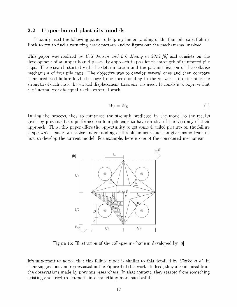
2.2 Upper-bound plasticity models
I mainly used the following paper to help my understanding of the four-pile caps failure.Both to try to �nd a recurring crack pattern and to �gure out the mechanisms involved.
This paper was realized by U.G Jensen and L.C Hoang in 2012 [8] and consists on thedevelopment of an upper bound plasticity approach to predict the strength of reinforced pilecaps. The research started with the determination and the parametrization of the collapsemechanism of four-pile caps. The objective was to develop several ones and then comparetheir predicted failure load, the lowest one corresponding to the answer. To determine thestrength of each case, the virtual displacement theorem was used. It consists to express thatthe internal work is equal to the external work.
WI = WE (1)
During the process, they to compared the strength predicted by the model to the resultsgiven by previous tests performed on four-pile caps to have an idea of the accuracy of theirapproach. Thus, this paper o�ers the opportunity to get some detailed pictures on the failureshape which makes an easier understanding of the phenomena and can gives some leads onhow to develop the current model. For example, here is one of the considered mechanism
Figure 16: Illustration of the collapse mechanism developed by [8]
It's important to notice that this failure mode is similar to this detailed by Clarke et al. intheir suggestions and represented in the Figure 4 of this work. Indeed, they also inspired fromthe observations made by previous researchers. In that context, they started from somethingexisting and tried to extend it into something more successful.
17
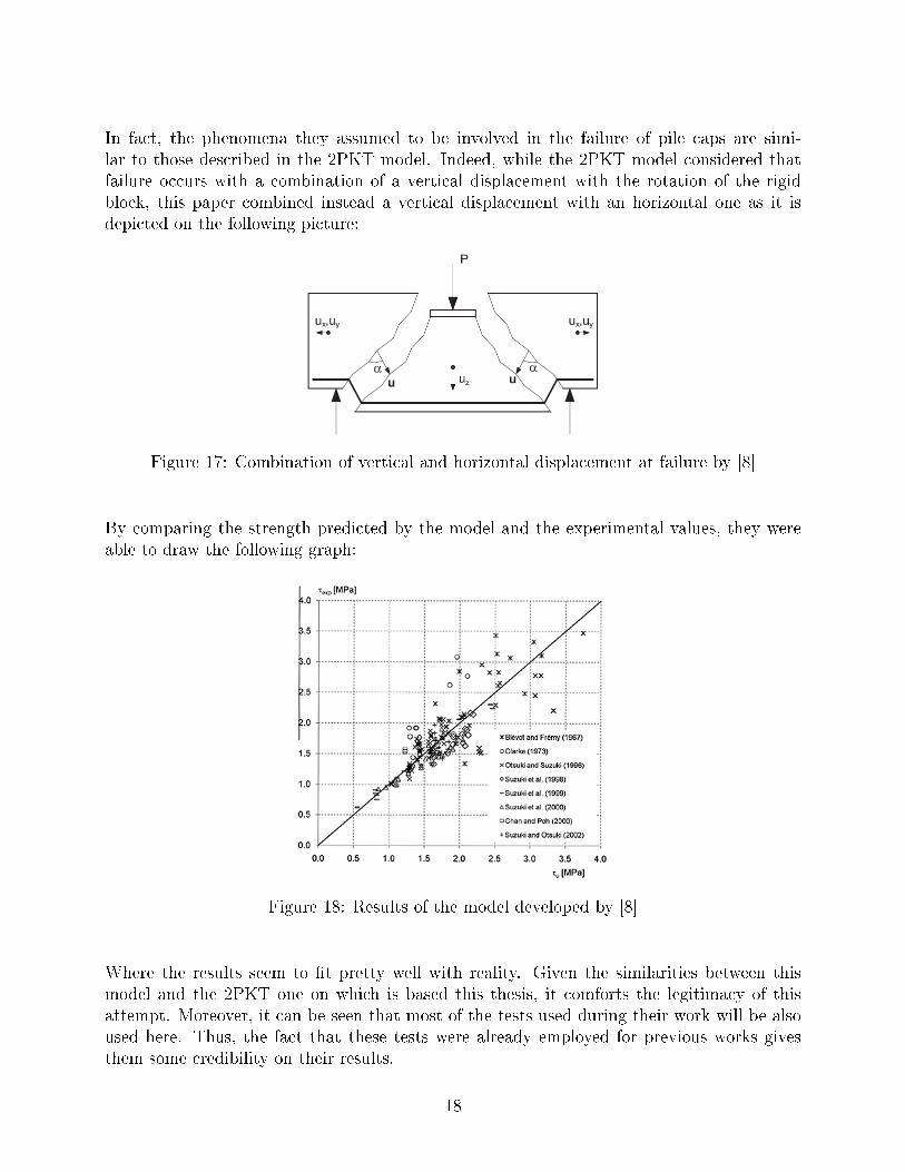
In fact, the phenomena they assumed to be involved in the failure of pile caps are simi-lar to those described in the 2PKT model. Indeed, while the 2PKT model considered thatfailure occurs with a combination of a vertical displacement with the rotation of the rigidblock, this paper combined instead a vertical displacement with an horizontal one as it isdepicted on the following picture:
Figure 17: Combination of vertical and horizontal displacement at failure by [8]
By comparing the strength predicted by the model and the experimental values, they wereable to draw the following graph:
Figure 18: Results of the model developed by [8]
Where the results seem to �t pretty well with reality. Given the similarities between thismodel and the 2PKT one on which is based this thesis, it comforts the legitimacy of thisattempt. Moreover, it can be seen that most of the tests used during their work will be alsoused here. Thus, the fact that these tests were already employed for previous works givesthem some credibility on their results.
18
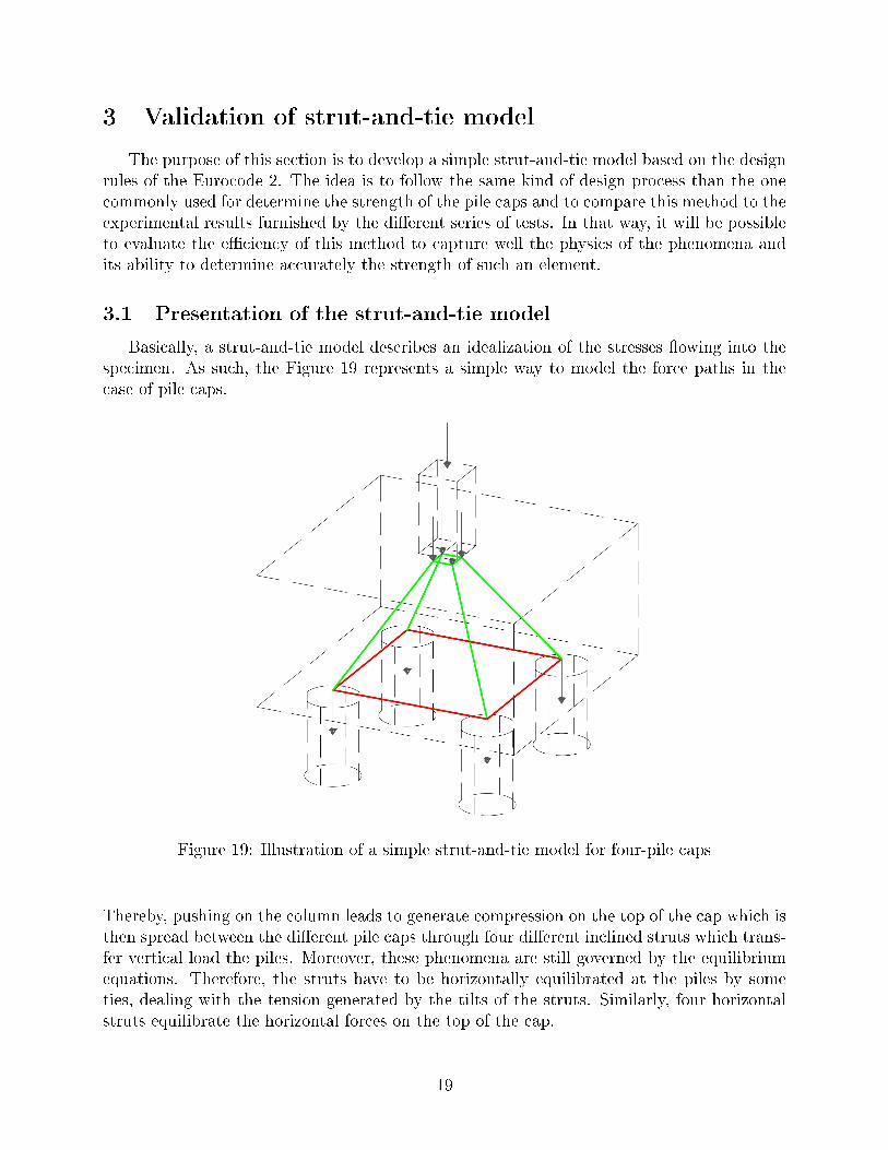
3 Validation of strut-and-tie model
The purpose of this section is to develop a simple strut-and-tie model based on the designrules of the Eurocode 2. The idea is to follow the same kind of design process than the onecommonly used for determine the strength of the pile caps and to compare this method to theexperimental results furnished by the di�erent series of tests. In that way, it will be possibleto evaluate the e�ciency of this method to capture well the physics of the phenomena andits ability to determine accurately the strength of such an element.
3.1 Presentation of the strut-and-tie model
Basically, a strut-and-tie model describes an idealization of the stresses �owing into thespecimen. As such, the Figure 19 represents a simple way to model the force paths in thecase of pile caps.
Figure 19: Illustration of a simple strut-and-tie model for four-pile caps
Thereby, pushing on the column leads to generate compression on the top of the cap which isthen spread between the di�erent pile caps through four di�erent inclined struts which trans-fer vertical load the piles. Moreover, these phenomena are still governed by the equilibriumequations. Therefore, the struts have to be horizontally equilibrated at the piles by someties, dealing with the tension generated by the tilts of the struts. Similarly, four horizontalstruts equilibrate the horizontal forces on the top of the cap.
19
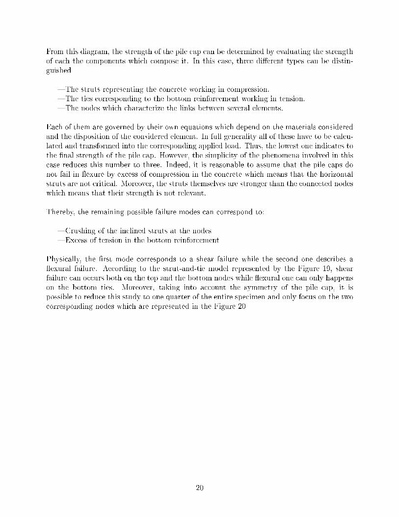
From this diagram, the strength of the pile cap can be determined by evaluating the strengthof each the components which compose it. In this case, three di�erent types can be distin-guished
� The struts representing the concrete working in compression.� The ties corresponding to the bottom reinforcement working in tension.� The nodes which characterize the links between several elements.
Each of them are governed by their own equations which depend on the materials consideredand the disposition of the considered element. In full generality all of these have to be calcu-lated and transformed into the corresponding applied load. Thus, the lowest one indicates tothe �nal strength of the pile cap. However, the simplicity of the phenomena involved in thiscase reduces this number to three. Indeed, it is reasonable to assume that the pile caps donot fail in �exure by excess of compression in the concrete which means that the horizontalstruts are not critical. Moreover, the struts themselves are stronger than the connected nodeswhich means that their strength is not relevant.
Thereby, the remaining possible failure modes can correspond to:
� Crushing of the inclined struts at the nodes� Excess of tension in the bottom reinforcement
Physically, the �rst mode corresponds to a shear failure while the second one describes a�exural failure. According to the strut-and-tie model represented by the Figure 19, shearfailure can occurs both on the top and the bottom nodes while �exural one can only happenson the bottom ties. Moreover, taking into account the symmetry of the pile cap, it ispossible to reduce this study to one quarter of the entire specimen and only focus on the twocorresponding nodes which are represented in the Figure 20
20
Figure 20: Identi�cation of the nodes to verify
3.2 Evaluation of the σR,max
Before expressing the equations of each components, it is necessary to remember that thisstudy it is not a matter of designing conservatively these element but rather to evaluate itsaccuracy against reality. As such, the di�erent terms will correspond to the basic propertiesthey described without taking into account the safety factors usually considered. The con-sequences of this concern especially the calculation strength of the materials which will nowcorrespond to
fc,k = fc,d (2)
fy,k = fy,d (3)
That being said, each con�guration has to be detailed in order to identify the correspondingexpression of the maximum stress. Thereby, the node 1 located on the top of the pile cap isonly submitted to compression. In such a case, the stress can reach the following value:
σnt,max = 0.85ν ′fc,d (4)
ν ′ = 1− fc,k250
(5)
In the bottom node, two veri�cations have to be led. The �rst one aims to determine thestrength on the inclined strut and the second one concerns the strength of the horizontal ties.
21
Concerning the node itself, it is submitted to both compression and traction. Moreover,two di�erent ties meet there. For these reasons, the maximum compression stress cannotexceed the following expression:
σnb,max = 0.75ν ′fc,d (6)
However, the expression corresponding to the strength of the tie is easier to determine consid-ering it simply expresses that failure occurs if the bottom reinforcement reaches its yieldingstrength. Thereby,
σt,max = fy (7)
3.2.1 Con�nement of the top node
It has to be mentioned that these stresses and more precisely the maximum stress onthe top node σnt,max will give really conservative results. Indeed, considering the top nodeis submitted to compression in all direction knowing that the external load acts verticallyand the horizontal struts bring compression in the horizontal plan. As such, this triaxialcon�nement tends to increase the maximum stress reachable in the node. In particular,Eurocode 2 speci�es that triaxially compressed nodes may be checked according:
σn,max = fc,k(1 + 5σ2/fc,k) for σ2 ≤ 0.05fc,kσn,max = fc,k(1.125 + 2.5σ2/fc,k) for σ2 > 0.05fc,k
(8)
Where σ2 represents the lowest main stress in the plan perpendicular to the strut. Moreover,Eurocode 2 imposes a maximal value by limiting the maximum stress to
σn,max ≤ 3ν ′fc,d (9)
In particular, that means that it would be necessary to use the Mohr circle of this plan toexpress the two corresponding main stresses and choose the lowest one. However, it seemsunrealistic to consider such an approach in a classic design. Therefore, some assumptionscan be expressed to evaluate the impact of the con�nement.
First of all, it is commonly recognized that the biaxial con�nement can reach at maximumthe value of 1.25fc,d. Extending this concept to the current case, it seems realistic to considerthat reaching this value for a triaxial con�nement constitute a conservative approach. Then,by coupling this assumption to the maximum value recommended by Eurocode 2, it appearsthat the con�nement is contained between two bounds:
σc,min = 1.25ν ′fc,d (10)
σc,max = 3ν ′fc,d (11)
In particular, these two expressions will serve to depict the extreme results of the strut-and-tiemodel
22
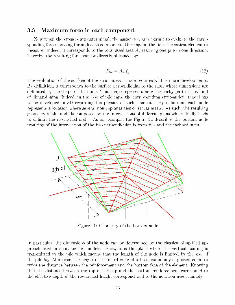
3.3 Maximum force in each component
Now when the stresses are determined, the associated area permit to evaluate the corre-sponding forces passing through each component. Once again, the tie is the easiest element tomeasure. Indeed, it corresponds to the total steel area As reaching one pile in one direction.Thereby, the resulting force can be directly obtained by:
Ftie = As.fy (12)
The evaluation of the surface of the strut at each node requires a little more developments.By de�nition, it corresponds to the surface perpendicular to the strut whose dimensions aredelimited by the shape of the node. This shape represents here the tricky part of this kindof dimensioning. Indeed, in the case of pile caps, the corresponding strut-and-tie model hasto be developed in 3D regarding the physics of such elements. By de�nition, each noderepresents a location where several non-coplanar ties or struts meets. As such, the resultinggeometry of the node is composed by the intersections of di�erent plans which �nally leadsto delimit the researched node. As an example, the Figure 21 describes the bottom noderesulting of the intersection of the two perpendicular bottom ties and the inclined strut:
Figure 21: Geometry of the bottom node
In particular, the dimensions of the node can be determined by the classical simpli�ed ap-proach used in strut-and-tie models. First, it is the place where the vertical loading istransmitted to the pile which means that the length of the node is limited by the size ofthe pile lb2. Moreover, the height of the e�ect zone of a tie is commonly supposed equal totwice the distance between the reinforcement and the bottom face of the element. Knowingthat the distance between the top of the cap and the bottom reinforcement correspond tothe e�ective depth d, the researched height correspond well to the notation used, namely:
23
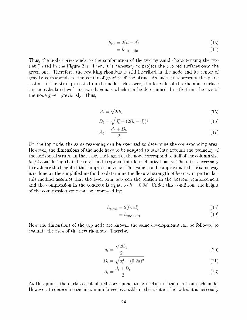
htie = 2(h− d) (13)
= hbot node (14)
Thus, the node corresponds to the combination of the two pyramid characterizing the twoties (in red in the Figure 21). Then, it is necessary to project the two red surfaces onto thegreen one. Therefore, the resulting rhombus is still inscribed in the node and its center ofgravity corresponds to the center of gravity of the strut. As such, it represents the planesection of the strut projected on the node. Moreover, the formula of the rhombus surfacecan be calculated with its two diagonals which can be determined directly from the size ofthe node given previously. Thus,
db =√
2lb2 (15)
Db =√d2b + (2(h− d))2 (16)
Ab =db +Db
2(17)
On the top node, the same reasoning can be executed to determine the corresponding area.However, the dimensions of the node have to be adapted to take into account the geometry ofthe horizontal struts. In that case, the length of the node correspond to half of the column sizelb1/2 considering that the total load is spread into four identical parts. Then, it is necessaryto evaluate the height of the compression zone. This value can be approximated the same wayit is done by the simpli�ed method to determine the �exural strength of beams. in particular,this method assumes that the lever arm between the tension in the bottom reinforcementand the compression in the concrete is equal to h = 0.9d. Under this condition, the heightof the compression zone can be expressed by:
hstrut = 2(0.1d) (18)
= htop node (19)
Now the dimensions of the top node are known, the same developments can be followed toevaluate the area of the new rhombus. Thereby,
dt =
√2lb1
2(20)
Dt =√d2t + (0.2d)2 (21)
At =dt +Dt
2(22)
At this point, the surfaces calculated correspond to projection of the strut on each node.However, to determine the maximum forces reachable in the strut at the nodes, it is necessary
24
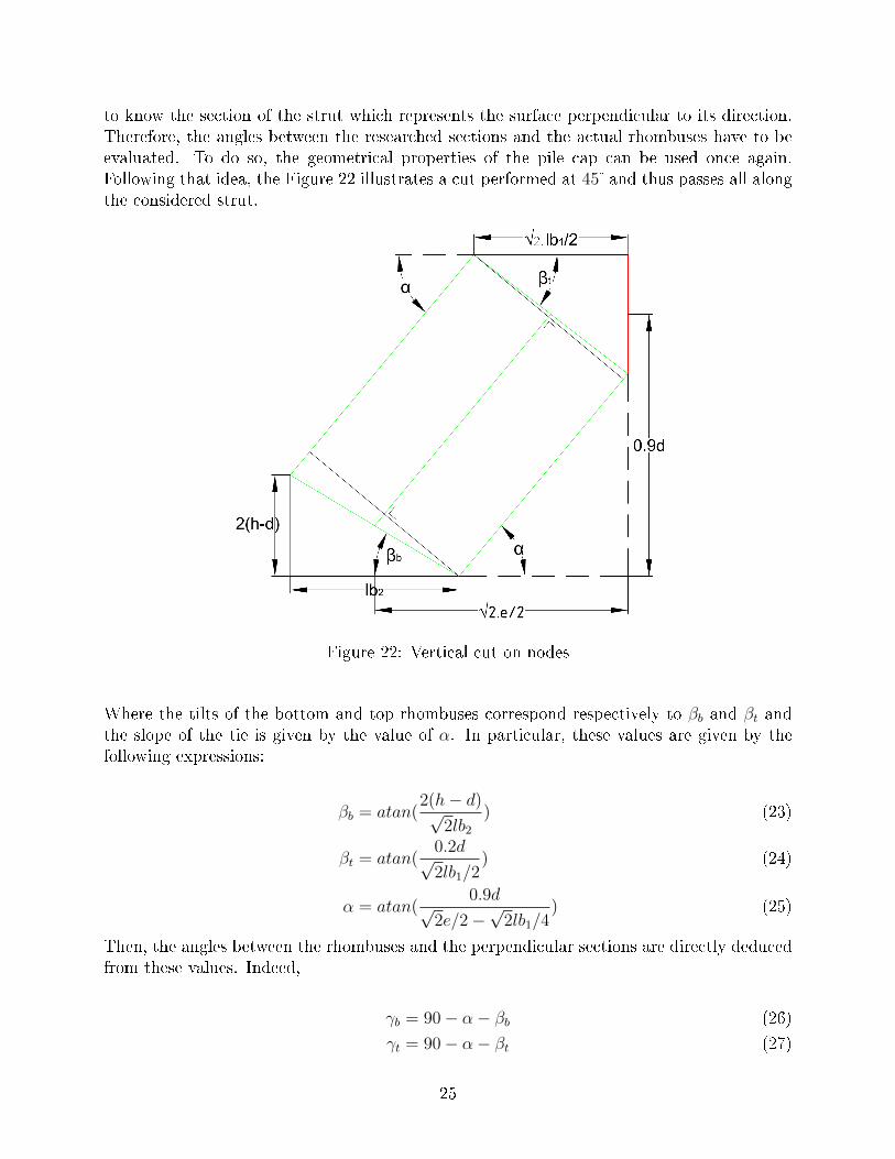
to know the section of the strut which represents the surface perpendicular to its direction.Therefore, the angles between the researched sections and the actual rhombuses have to beevaluated. To do so, the geometrical properties of the pile cap can be used once again.Following that idea, the Figure 22 illustrates a cut performed at 45�and thus passes all alongthe considered strut.
Figure 22: Vertical cut on nodes
Where the tilts of the bottom and top rhombuses correspond respectively to βb and βt andthe slope of the tie is given by the value of α. In particular, these values are given by thefollowing expressions:
βb = atan(2(h− d)√
2lb2
) (23)
βt = atan(0.2d√2lb1/2
) (24)
α = atan(0.9d√
2e/2−√
2lb1/4) (25)
Then, the angles between the rhombuses and the perpendicular sections are directly deducedfrom these values. Indeed,
γb = 90− α− βb (26)
γt = 90− α− βt (27)
25
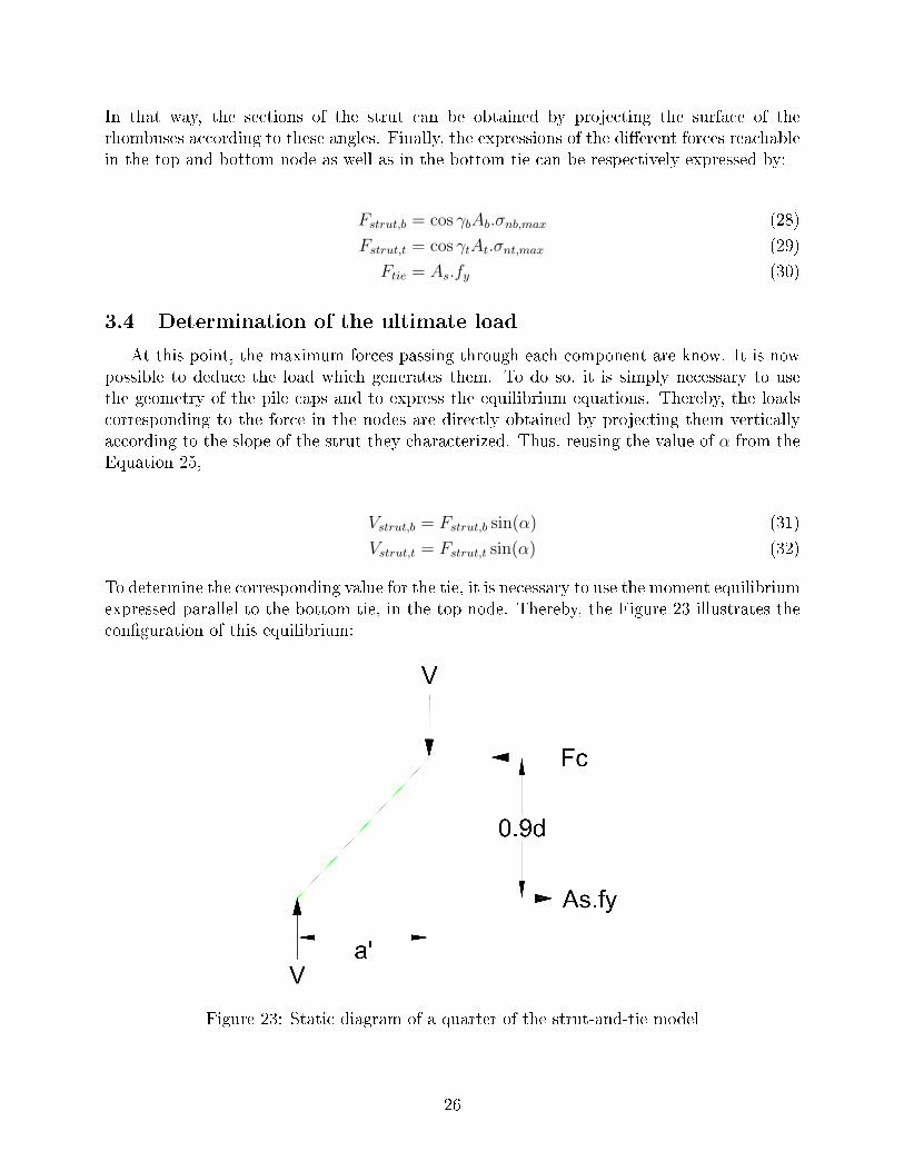
In that way, the sections of the strut can be obtained by projecting the surface of therhombuses according to these angles. Finally, the expressions of the di�erent forces reachablein the top and bottom node as well as in the bottom tie can be respectively expressed by:
Fstrut,b = cos γbAb.σnb,max (28)
Fstrut,t = cos γtAt.σnt,max (29)
Ftie = As.fy (30)
3.4 Determination of the ultimate load
At this point, the maximum forces passing through each component are know. It is nowpossible to deduce the load which generates them. To do so, it is simply necessary to usethe geometry of the pile caps and to express the equilibrium equations. Thereby, the loadscorresponding to the force in the nodes are directly obtained by projecting them verticallyaccording to the slope of the strut they characterized. Thus, reusing the value of α from theEquation 25,
Vstrut,b = Fstrut,b sin(α) (31)
Vstrut,t = Fstrut,t sin(α) (32)
To determine the corresponding value for the tie, it is necessary to use the moment equilibriumexpressed parallel to the bottom tie, in the top node. Thereby, the Figure 23 illustrates thecon�guration of this equilibrium:
Figure 23: Static diagram of a quarter of the strut-and-tie model
26
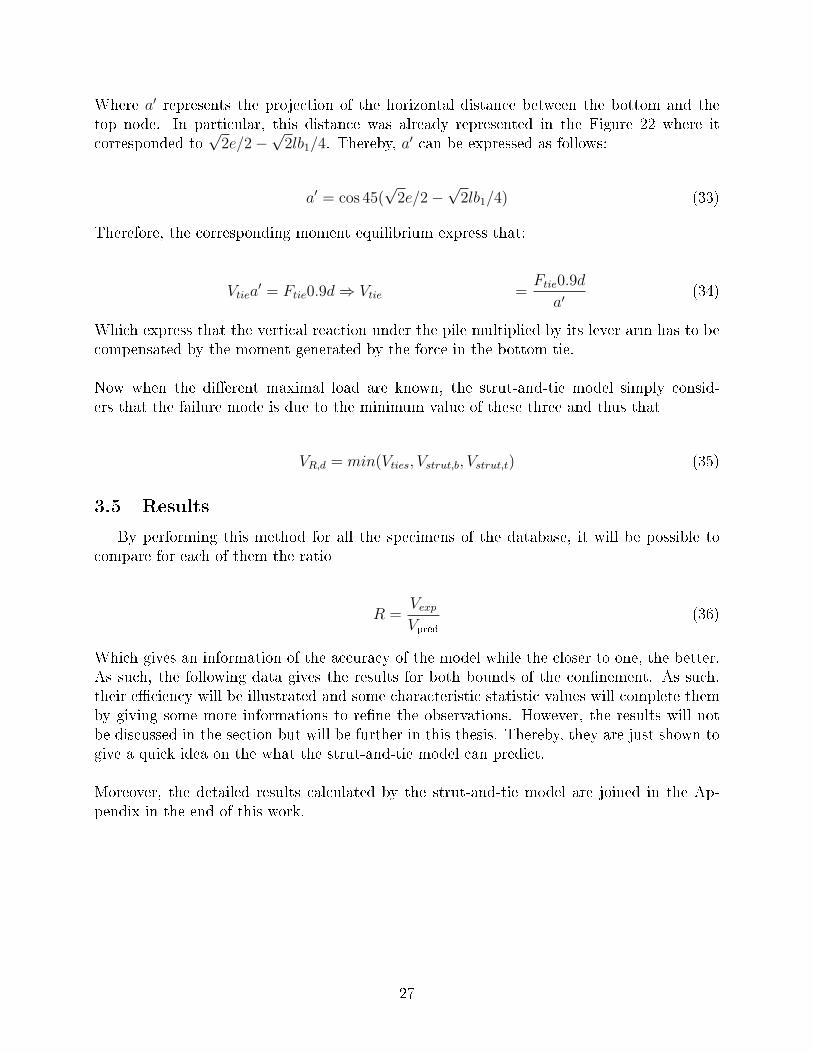
Where a′ represents the projection of the horizontal distance between the bottom and thetop node. In particular, this distance was already represented in the Figure 22 where itcorresponded to
√2e/2−
√2lb1/4. Thereby, a
′ can be expressed as follows:
a′ = cos 45(√
2e/2−√
2lb1/4) (33)
Therefore, the corresponding moment equilibrium express that:
Vtiea′ = Ftie0.9d⇒ Vtie =
Ftie0.9d
a′(34)
Which express that the vertical reaction under the pile multiplied by its lever arm has to becompensated by the moment generated by the force in the bottom tie.
Now when the di�erent maximal load are known, the strut-and-tie model simply consid-ers that the failure mode is due to the minimum value of these three and thus that
VR,d = min(Vties, Vstrut,b, Vstrut,t) (35)
3.5 Results
By performing this method for all the specimens of the database, it will be possible tocompare for each of them the ratio
R =VexpVpred
(36)
Which gives an information of the accuracy of the model while the closer to one, the better.As such, the following data gives the results for both bounds of the con�nement. As such,their e�ciency will be illustrated and some characteristic statistic values will complete themby giving some more informations to re�ne the observations. However, the results will notbe discussed in the section but will be further in this thesis. Thereby, they are just shown togive a quick idea on the what the strut-and-tie model can predict.
Moreover, the detailed results calculated by the strut-and-tie model are joined in the Ap-pendix in the end of this work.
27
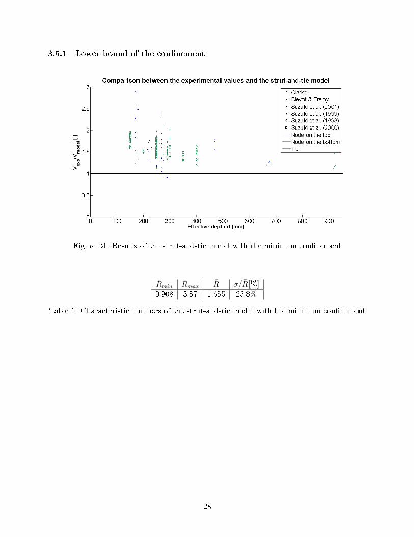
3.5.1 Lower bound of the con�nement
Figure 24: Results of the strut-and-tie model with the minimum con�nement
Rmin Rmax R̄ σ/R̄[%]0.908 3.87 1.655 25.8%
Table 1: Characteristic numbers of the strut-and-tie model with the minimum con�nement
28
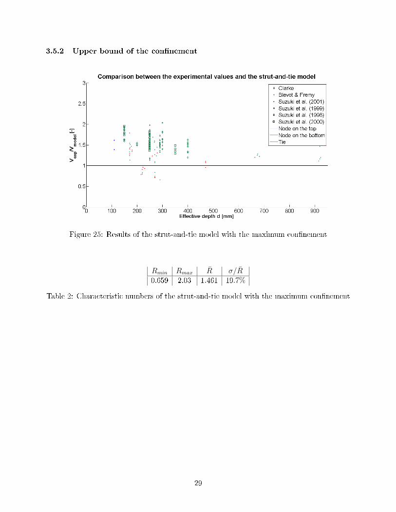
3.5.2 Upper bound of the con�nement
Figure 25: Results of the strut-and-tie model with the maximum con�nement
Rmin Rmax R̄ σ/R̄0.659 2.03 1.461 19.7%
Table 2: Characteristic numbers of the strut-and-tie model with the maximum con�nement
29
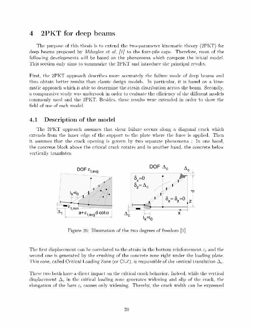
4 2PKT for deep beams
The purpose of this thesis is to extend the two-parameter kinematic theory (2PKT) fordeep beams proposed by Mihaylov et al. [1] to the four-pile caps. Therefore, most of thefollowing developments will be based on the phenomena which compose the initial model.This section only aims to summarize the 2PKT and introduce the principal results.
First, the 2PKT approach describes more accurately the failure mode of deep beams andthus obtain better results than classic design models. In particular, it is based on a kine-matic approach which is able to determine the strain distribution across the beam. Secondly,a comparative study was undertook in order to evaluate the e�ciency of the di�erent modelscommonly used and the 2PKT. Besides, these results were extended in order to show the�eld of use of each model.
4.1 Description of the model
The 2PKT approach assumes that shear failure occurs along a diagonal crack whichextends from the inner edge of the support to the plate where the force is applied. Thenit assumes that the crack opening is govern by two separate phenomena : In one hand,the concrete block above the critical crack rotates and in another hand, the concrete belowvertically translates.
Figure 26: Illustration of the two degrees of freedom [1]
The �rst displacement can be correlated to the strain in the bottom reinforcement εt and thesecond one is generated by the crushing of the concrete zone right under the loading plate.This zone, called Critical Loading Zone (or CLZ), is responsible of the vertical translation ∆c.
These two both have a direct impact on the critical crack behavior. Indeed, while the verticaldisplacement ∆c in the critical loading zone generates widening and slip of the crack, theelongation of the bars εt causes only widening. Thereby, the crack width can be expressed
30
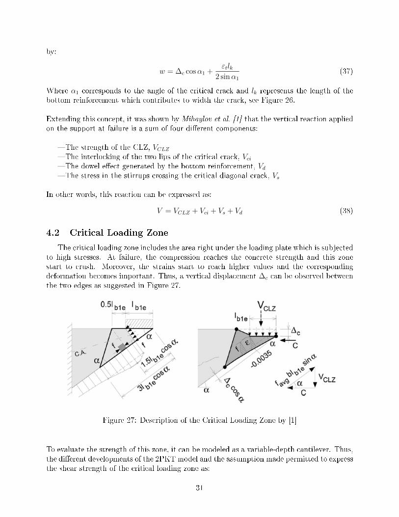
by:
w = ∆c cosα1 +εtlk
2 sinα1
(37)
Where α1 corresponds to the angle of the critical crack and lk represents the length of thebottom reinforcement which contributes to width the crack, see Figure 26.
Extending this concept, it was shown by Mihaylov et al. [1] that the vertical reaction appliedon the support at failure is a sum of four di�erent components:
� The strength of the CLZ, VCLZ� The interlocking of the two lips of the critical crack, Vci� The dowel e�ect generated by the bottom reinforcement, Vd� The stress in the stirrups crossing the critical diagonal crack, Vs
In other words, this reaction can be expressed as:
V = VCLZ + Vci + Vs + Vd (38)
4.2 Critical Loading Zone
The critical loading zone includes the area right under the loading plate which is subjectedto high stresses. At failure, the compression reaches the concrete strength and this zonestart to crush. Moreover, the strains start to reach higher values and the correspondingdeformation becomes important. Thus, a vertical displacement ∆c can be observed betweenthe two edges as suggested in Figure 27.
Figure 27: Description of the Critical Loading Zone by [1]
To evaluate the strength of this zone, it can be modeled as a variable-depth cantilever. Thus,the di�erent developments of the 2PKT model and the assumption made permitted to expressthe shear strength of the critical loading zone as:
31
VCLZ = k1.43f 0.8c blb1e sin2 α (39)
Where k represents the crack shape and lb1e the length of the critical loading zone.
The force in the CLZ is parallel to the diagonal crack, and VCLZ is the vertical of thiszone.
Moreover, the value of ∆c is only governed by the crushing of the critical loading zone.Thereby, it can simply be expressed as the de�ection of a cantilever on which is applied auniformly distributed force at its edge
∆c = 0.0105lb1e cotα (40)
Where lb1e corresponds to the e�ective width of the loading plate parallel to the longitudinaldimension of the beam. In particular, this value depends on the position of the loading plate.For example, when it lays in the middle of the member, the force is equally redistributedbetween the two supports and then:
lb1e = 0.5lb1 (41)
where lb1 is the width of the loading plate.
4.3 Interlock strength
The interlock strength takes into account the friction between the two sides of the crackand especially between the aggregates of each side and can be expressed by the followingequation:
Vci =0.18√fc
0.31 + 24wage+16
bd (42)
Here, w represents the crack width and illustrates that the wider the crack, the less the sidesof the crack are able to develop friction. It is the opposite for the aggregates size which hasa positive e�ect on the interlock strength because biggest aggregates o�er a higher resistanceto the translation.
Concerning the surface concerned, the friction develops from the top to the bottom rein-forcement all along the width of the section b. However, it is once again the vertical compo-nent which is interesting to determine the vertical reaction and in this particular case, theprojected length of the crack is equal to the e�ective height d.
32
4.4 Dowel action
When the failure occurs and the critical crack appears, the beam is separated onto twoparts. However, they are still connected by the critical loading zone, the stirrups and thebottom reinforcement. As such, the vertical translation of the concrete under the crack sub-jects this reinforcement to a double curvature as it is represented on the second picture ofFigure 26. Thus the bars will start to resist to this deformation in the same way the dowelsresist to the shear in composite �oors.
Thereby, the expression of the dowel action developed in that way is given by the followingequation:
Vd = nbfyed3b
3lk(43)
Of course, the total strength is a function of the characteristics of the bars knowing that themore they are, the higher the strength as it is depicted by the number of bars nb, the stressin the bars fye and the bars diameter db. It is also necessary to take into account lk whichalso represents the length of the reinforcement between the two kinks formed by the dowelaction. Thus, the larger it is, the lower the sti�ness of the portion of the bars involved in thedowel e�ect. Consequently, the corresponding strength will be diminished.
It is also important to note that the stress in the bars does not represent the yielding strengthof the bars. Indeed, it is described by the following expression:
fye = fy
[1−
(TminfyAs
)2]≤ 500MPa (44)
≥ 0 (45)
This equation describes the fact that the total stress in the bars cannot exceed the yieldstrength of the steel. Thereby, the remaining strain available to develop the dowel e�ectdepends on the di�erence between the yield strength and the tension in the bars. WhenThese two becomes equal, the reinforcement starts yielding and it is not any more able toresist the vertical displacement. In this case, the strength of the dowel e�ect falls to 0 andof course cannot reach negative values.
4.5 Stirrups
The critical crack develops through the stirrups which resists to its widening. The strengthof each stirrups is known by de�nition but it remains to determine the number of concernedstirrups. Thus, the maximum strength supported by the stirrups can be expressed as follows:
Vs = ρvb(d cotα1− l0 − 1.5lb1e)fv ≥ 0 (46)
33
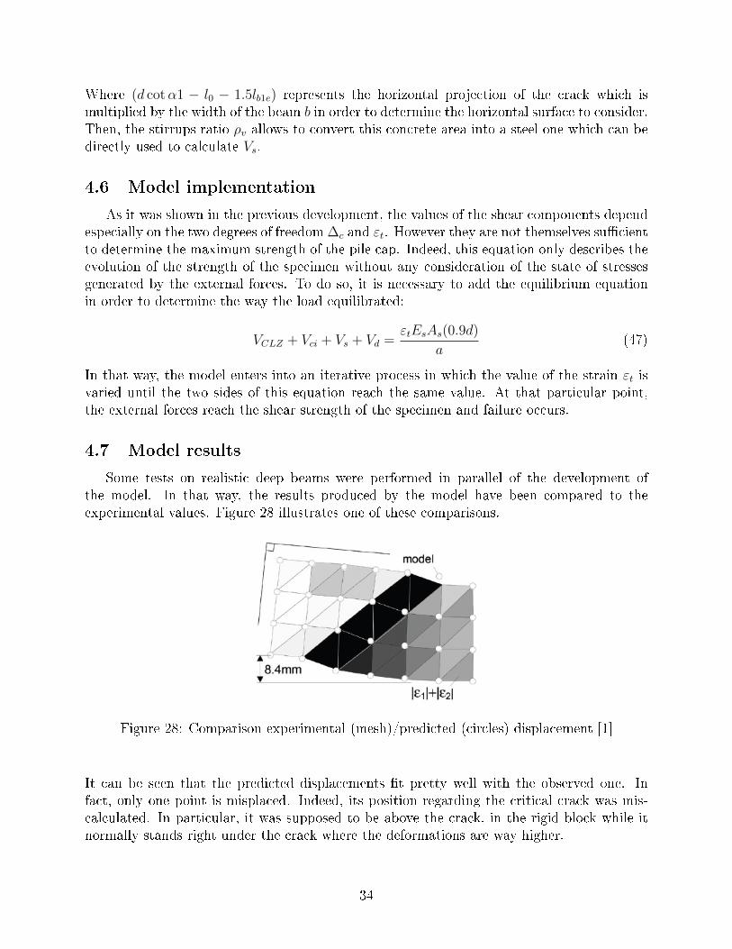
Where (d cotα1 − l0 − 1.5lb1e) represents the horizontal projection of the crack which ismultiplied by the width of the beam b in order to determine the horizontal surface to consider.Then, the stirrups ratio ρv allows to convert this concrete area into a steel one which can bedirectly used to calculate Vs.
4.6 Model implementation
As it was shown in the previous development, the values of the shear components dependespecially on the two degrees of freedom ∆c and εt. However they are not themselves su�cientto determine the maximum strength of the pile cap. Indeed, this equation only describes theevolution of the strength of the specimen without any consideration of the state of stressesgenerated by the external forces. To do so, it is necessary to add the equilibrium equationin order to determine the way the load equilibrated:
VCLZ + Vci + Vs + Vd =εtEsAs(0.9d)
a(47)
In that way, the model enters into an iterative process in which the value of the strain εt isvaried until the two sides of this equation reach the same value. At that particular point,the external forces reach the shear strength of the specimen and failure occurs.
4.7 Model results
Some tests on realistic deep beams were performed in parallel of the development ofthe model. In that way, the results produced by the model have been compared to theexperimental values. Figure 28 illustrates one of these comparisons.
Figure 28: Comparison experimental (mesh)/predicted (circles) displacement [1]
It can be seen that the predicted displacements �t pretty well with the observed one. Infact, only one point is misplaced. Indeed, its position regarding the critical crack was mis-calculated. In particular, it was supposed to be above the crack, in the rigid block while itnormally stands right under the crack where the deformations are way higher.
34
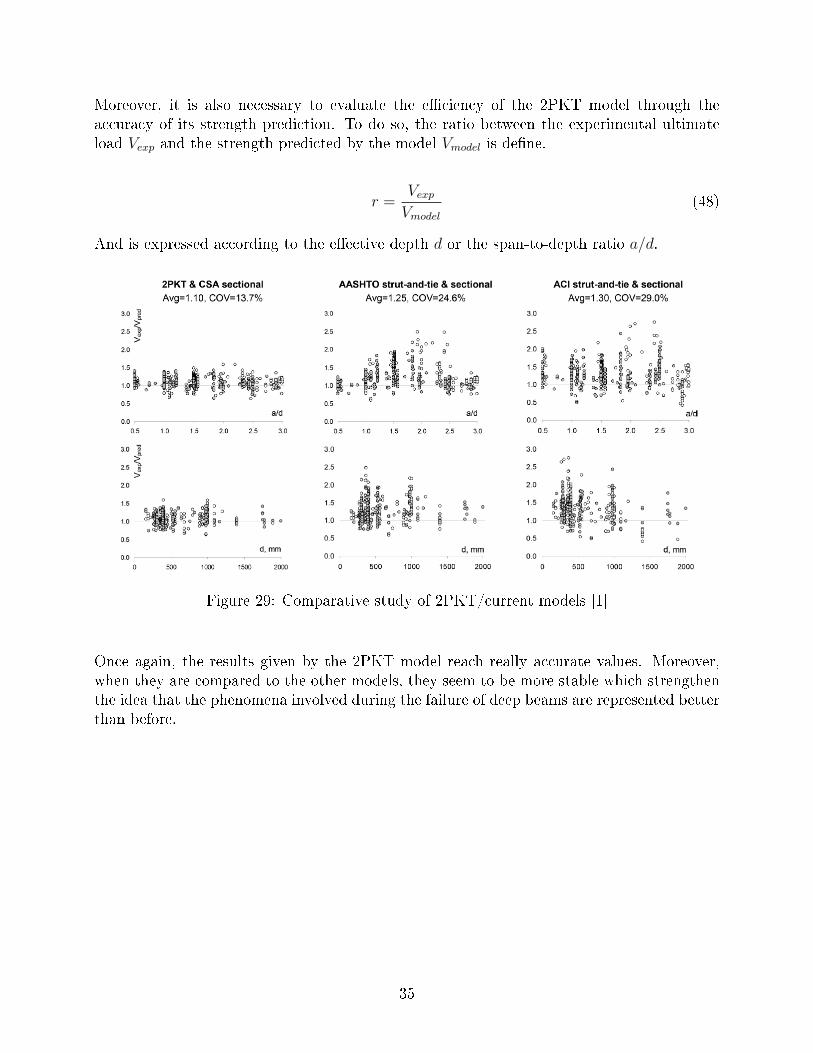
Moreover, it is also necessary to evaluate the e�ciency of the 2PKT model through theaccuracy of its strength prediction. To do so, the ratio between the experimental ultimateload Vexp and the strength predicted by the model Vmodel is de�ne.
r =VexpVmodel
(48)
And is expressed according to the e�ective depth d or the span-to-depth ratio a/d.
Figure 29: Comparative study of 2PKT/current models [1]
Once again, the results given by the 2PKT model reach really accurate values. Moreover,when they are compared to the other models, they seem to be more stable which strengthenthe idea that the phenomena involved during the failure of deep beams are represented betterthan before.
35
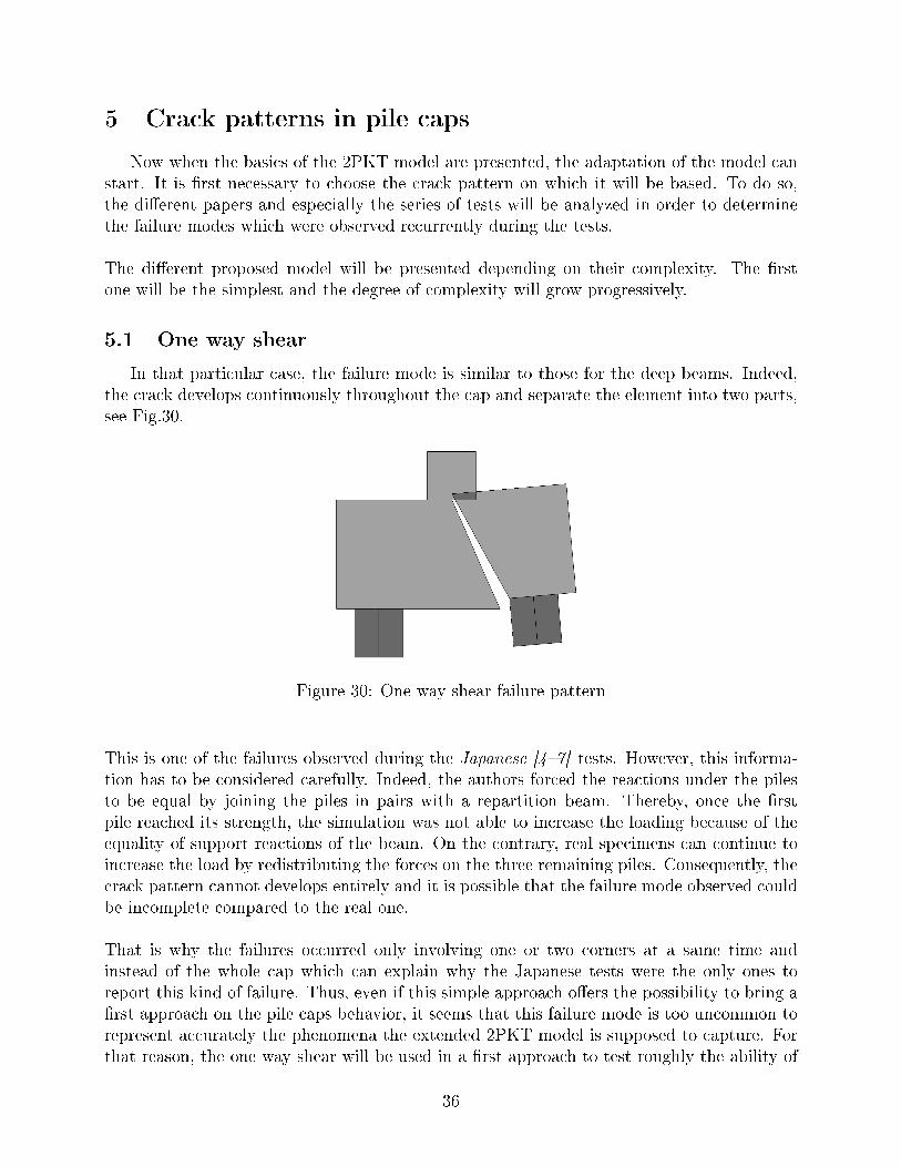
5 Crack patterns in pile caps
Now when the basics of the 2PKT model are presented, the adaptation of the model canstart. It is �rst necessary to choose the crack pattern on which it will be based. To do so,the di�erent papers and especially the series of tests will be analyzed in order to determinethe failure modes which were observed recurrently during the tests.
The di�erent proposed model will be presented depending on their complexity. The �rstone will be the simplest and the degree of complexity will grow progressively.
5.1 One way shear
In that particular case, the failure mode is similar to those for the deep beams. Indeed,the crack develops continuously throughout the cap and separate the element into two parts,see Fig.30.
Figure 30: One way shear failure pattern
This is one of the failures observed during the Japanese [4�7] tests. However, this informa-tion has to be considered carefully. Indeed, the authors forced the reactions under the pilesto be equal by joining the piles in pairs with a repartition beam. Thereby, once the �rstpile reached its strength, the simulation was not able to increase the loading because of theequality of support reactions of the beam. On the contrary, real specimens can continue toincrease the load by redistributing the forces on the three remaining piles. Consequently, thecrack pattern cannot develops entirely and it is possible that the failure mode observed couldbe incomplete compared to the real one.
That is why the failures occurred only involving one or two corners at a same time andinstead of the whole cap which can explain why the Japanese tests were the only ones toreport this kind of failure. Thus, even if this simple approach o�ers the possibility to bring a�rst approach on the pile caps behavior, it seems that this failure mode is too uncommon torepresent accurately the phenomena the extended 2PKT model is supposed to capture. Forthat reason, the one way shear will be used in a �rst approach to test roughly the ability of
36
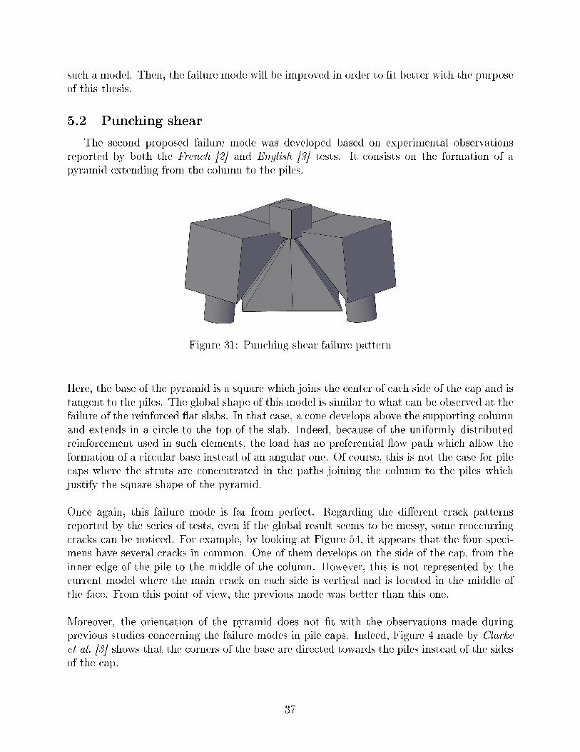
such a model. Then, the failure mode will be improved in order to �t better with the purposeof this thesis.
5.2 Punching shear
The second proposed failure mode was developed based on experimental observationsreported by both the French [2] and English [3] tests. It consists on the formation of apyramid extending from the column to the piles.
Figure 31: Punching shear failure pattern
Here, the base of the pyramid is a square which joins the center of each side of the cap and istangent to the piles. The global shape of this model is similar to what can be observed at thefailure of the reinforced �at slabs. In that case, a cone develops above the supporting columnand extends in a circle to the top of the slab. Indeed, because of the uniformly distributedreinforcement used in such elements, the load has no preferential �ow path which allow theformation of a circular base instead of an angular one. Of course, this is not the case for pilecaps where the struts are concentrated in the paths joining the column to the piles whichjustify the square shape of the pyramid.
Once again, this failure mode is far from perfect. Regarding the di�erent crack patternsreported by the series of tests, even if the global result seems to be messy, some reoccurringcracks can be noticed. For example, by looking at Figure 54, it appears that the four speci-mens have several cracks in common. One of them develops on the side of the cap, from theinner edge of the pile to the middle of the column. However, this is not represented by thecurrent model where the main crack on each side is vertical and is located in the middle ofthe face. From this point of view, the previous mode was better than this one.
Moreover, the orientation of the pyramid does not �t with the observations made duringprevious studies concerning the failure modes in pile caps. Indeed, Figure 4 made by Clarkeet al. [3] shows that the corners of the base are directed towards the piles instead of the sidesof the cap.
37
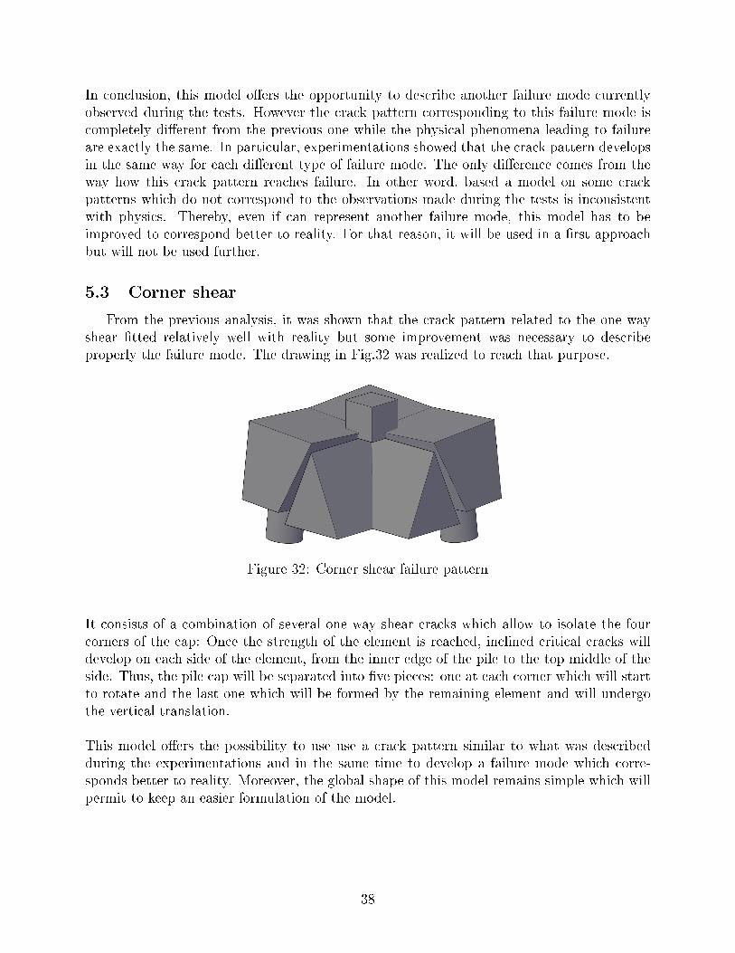
In conclusion, this model o�ers the opportunity to describe another failure mode currentlyobserved during the tests. However the crack pattern corresponding to this failure mode iscompletely di�erent from the previous one while the physical phenomena leading to failureare exactly the same. In particular, experimentations showed that the crack pattern developsin the same way for each di�erent type of failure mode. The only di�erence comes from theway how this crack pattern reaches failure. In other word, based a model on some crackpatterns which do not correspond to the observations made during the tests is inconsistentwith physics. Thereby, even if can represent another failure mode, this model has to beimproved to correspond better to reality. For that reason, it will be used in a �rst approachbut will not be used further.
5.3 Corner shear
From the previous analysis, it was shown that the crack pattern related to the one wayshear �tted relatively well with reality but some improvement was necessary to describeproperly the failure mode. The drawing in Fig.32 was realized to reach that purpose.
Figure 32: Corner shear failure pattern
It consists of a combination of several one way shear cracks which allow to isolate the fourcorners of the cap: Once the strength of the element is reached, inclined critical cracks willdevelop on each side of the element, from the inner edge of the pile to the top middle of theside. Thus, the pile cap will be separated into �ve pieces: one at each corner which will startto rotate and the last one which will be formed by the remaining element and will undergothe vertical translation.
This model o�ers the possibility to use use a crack pattern similar to what was describedduring the experimentations and in the same time to develop a failure mode which corre-sponds better to reality. Moreover, the global shape of this model remains simple which willpermit to keep an easier formulation of the model.
38
5.4 Improved punching shear
A similar approach can be led in order to develop a new punching shear failure. Indeed, ifseveral one way shear cracks are once again combined but this time not to isolate the cornerbut to cut the cap through its whole length, the resulting failure mode includes a pyramidforms at failure, see Figure 33. Its base still corresponds to a square whose orientation isnow correctly represented. Thereby, this failure mode permits to conciliate both a reasonablecrack pattern and a punching shear model which �t better with experimental observations.
Figure 33: Punching failure pattern with a combination of one way shear
Concerning the behavior of this model, it can be seen that the shape of the corners areconserved: Inclined cracks still develop in the same way as previously mentioned whichisolates the four corners from the rest of the pile cap. The main di�erence comes from thecentral part of the cap: While it remained in only one block in the corner shear model, it isnow cut into �ve di�erent pieces where the pyramid represents the central element. In thatcon�guration, most of the elements rotate and only the pyramid moves downward.
5.5 Final model
The advantage of the two models presented in 5.3 and 5.4 is that they are based on thesame scheme. Thereby it is possible to combine them in order to obtain a new one which isable to represent the two expected failure modes into only one model.
This model reuses the previous model considering the fact the central part is cut in sev-eral elements. However, the pyramid does not undergo any more the vertical displacementalone. Indeed, the total displacement ∆c is now divided equally between the pyramid andthe four lateral elements. Moreover, the corners become again the only parts to rotate as itwas the case for the corner shear model. Thus, following this model, the failure of the pilecap can be shown in Fig.34.
39
Figure 34: Final model combining punching and corner shear
This model describes the interactions which exist between these two failure modes and thefact that the two are the result of the same phenomena which develop di�erently. Thereby,the model evaluates the corner shear failure by considering displacement ∆c
2between the
corners and the lateral elements. Similarly, the punching shear failure occurs with the dis-placement ∆c
2between the lateral elements and the central pyramid.
Obviously, the model remains very simple in comparison with the real failures and espe-cially when the two crack patterns are compared. However, it is not the purpose of thisthesis which rather tries to develop a new approach to evaluate the strength of pile caps bystaying simple enough in order to describe distinctly the phenomena it attempts to represent.
In this particular context, it responds well to the current problematic considering what waspreviously discussed. Indeed, the 2PKT model and especially the components involved inthe strength of the pile cap can easily be applied to this model. Moreover, its simple shapecontributes to ease the writing of the equations describing the di�erent phenomena and thussimpli�es the calculation process. At last but surely most importantly, the failures it de-scribes corresponds to the observations reported during the series of tests, both regardingthe crack pattern and the failure mode. For that reasons, this model will be the �nal oneused in this thesis.
40
6 2D kinematic approach
All the tools required to build the 2PKT model for pile caps are now presented. It is nowpossible to start from the failure modes previously described and adapt the equations of the2PKT for deep beams in a way they describe the chosen mode. Thereby, this section willconsist of establishing and describing the model based on the one way shear failure.
To do so, the kinematics of the model will be presented in more details than what wasdone in the previous section. In that way, each component involved in the strength of thepile cap will be clearly identi�ed in order to associate them with the right term.
Then, each term will be developed in order to detail how the initial expressions of the 2PKTfor deep beams have to be adapted to correspond to this new con�guration.This includesthe description of the evolution of the equation characterizing these di�erent terms but itwill be also necessary to detail how each parameter which composes them is impacted bythis change. Moreover, a variability study for the parameter εt will be performed for each ofthem in order to predict their evolution during the iterative process and more important dounderstand their behavior when the applied force increases.
Finally, all this information will be regrouped and assembled to form the complete model. Inparallel, some explanation will be given concerning some speci�cities of the computer codeused for the calculations, especially concerning the iterative process and the choice whetherto consider or not the yielding of the �exural reinforcement.
6.1 Kinematics
When the applied force increases, the concrete zone right under the column plate becomesmore and more loaded and the compression �owing to the supports increases. At failure, acrack develop from the column plate to the piles where the slip is avoid by the interlock of thetwo faces of the crack and by the dowel e�ect brought by the bottom reinforcement. More-over, the critical loading zone starts crushing and creates a vertical displacement betweenthe parts on either side of the crack.
Figure 35 shows another picture of the current failure mode which is now represented in3D in order to illustrate better how the di�erent parts move with respect to each other:
41
Figure 35: Description of the one way shear failure
Under this con�guration, the failure mode is similar to which observed for deep beams andthe components contributing to the strength of the element are almost the same. The �rstdi�erence comes from the absence of stirrups. Indeed, pile caps are typically designed with-out any stirrup which means that the shear component Vs is 0. Moreover, it appears thatthe critical loading zone is concentrated under the column and does not extend trough theentire width of the pile cap as it was the case for deep beams.
Concerning the aggregate interlock area, it can at maximum develop all along the failurecrack which corresponds to the whole length and the whole height of the cap. Finally, thedowel action which represent the last component involved in the strength of pile caps remainsunchanged compared to what is done for deep beams. Of course, the ratio of reinforcement,its location and its arrangement have an impact on the �nal value but the basic principlesremain the same.
All the di�erent parts are now identi�ed and it is now possible to analyze them separatelyin order to adapt their expression to the current con�guration.
6.2 V − εt,avg relationship based on moment equilibrium
As it was previously mentioned, the strength of the pile caps will be calculated by deter-mining the value of the strain on the bottom reinforcement εt under which the shear forcetransfered through the critical crack
V = VCLZ + Vci + Vs + Vd (49)
is in equilibrium with the shear force derived from moment equilibrium
V =σtAs(0.9d)
a(50)
42
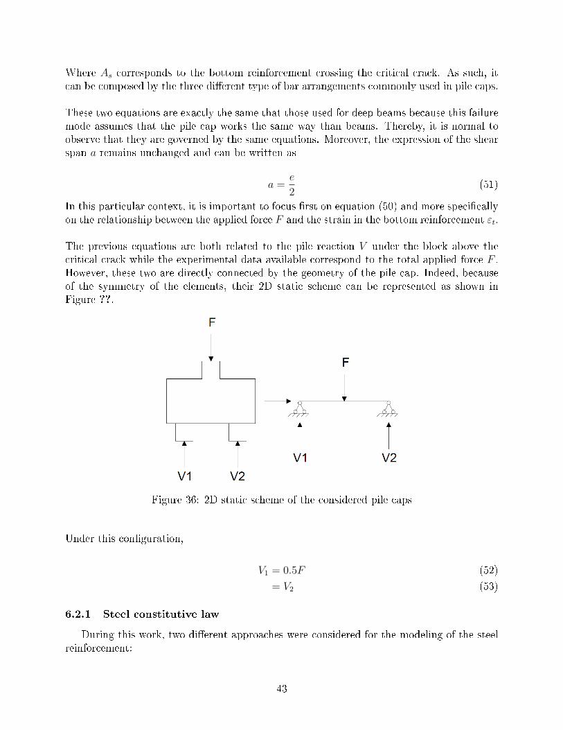
Where As corresponds to the bottom reinforcement crossing the critical crack. As such, itcan be composed by the three di�erent type of bar arrangements commonly used in pile caps.
These two equations are exactly the same that those used for deep beams because this failuremode assumes that the pile cap works the same way than beams. Thereby, it is normal toobserve that they are governed by the same equations. Moreover, the expression of the shearspan a remains unchanged and can be written as
a =e
2(51)
In this particular context, it is important to focus �rst on equation (50) and more speci�callyon the relationship between the applied force F and the strain in the bottom reinforcement εt.
The previous equations are both related to the pile reaction V under the block above thecritical crack while the experimental data available correspond to the total applied force F .However, these two are directly connected by the geometry of the pile cap. Indeed, becauseof the symmetry of the elements, their 2D static scheme can be represented as shown inFigure ??.
Figure 36: 2D static scheme of the considered pile caps
Under this con�guration,
V1 = 0.5F (52)
= V2 (53)
6.2.1 Steel constitutive law
During this work, two di�erent approaches were considered for the modeling of the steelreinforcement:
43
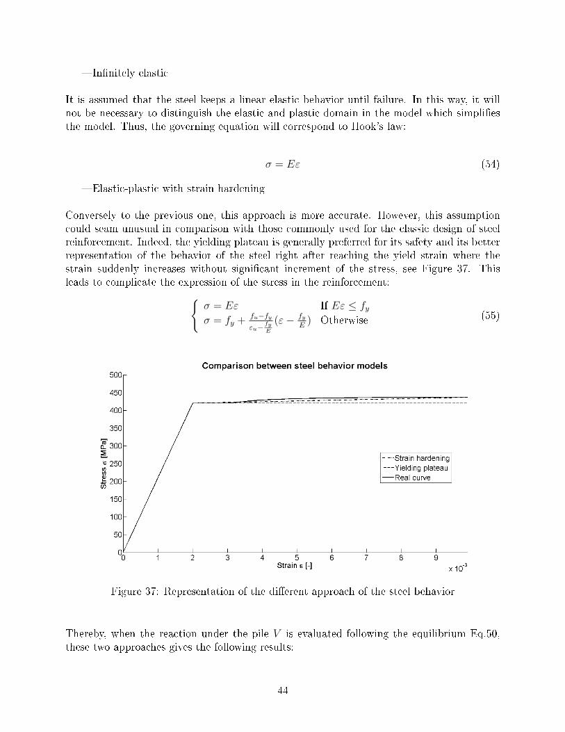
� In�nitely elastic
It is assumed that the steel keeps a linear elastic behavior until failure. In this way, it willnot be necessary to distinguish the elastic and plastic domain in the model which simpli�esthe model. Thus, the governing equation will correspond to Hook's law:
σ = Eε (54)
� Elastic-plastic with strain hardening
Conversely to the previous one, this approach is more accurate. However, this assumptioncould seam unusual in comparison with those commonly used for the classic design of steelreinforcement. Indeed, the yielding plateau is generally preferred for its safety and its betterrepresentation of the behavior of the steel right after reaching the yield strain where thestrain suddenly increases without signi�cant increment of the stress, see Figure 37. Thisleads to complicate the expression of the stress in the reinforcement:{
σ = Eε If Eε ≤ fyσ = fy + fu−fy
εu−fyE
(ε− fyE
) Otherwise (55)
Figure 37: Representation of the di�erent approach of the steel behavior
Thereby, when the reaction under the pile V is evaluated following the equilibrium Eq.50,these two approaches gives the following results:
44
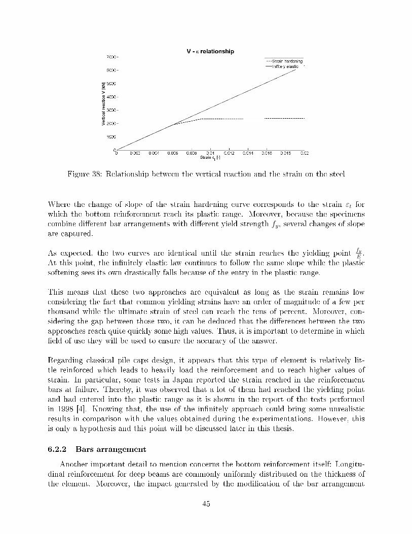
Figure 38: Relationship between the vertical reaction and the strain on the steel
Where the change of slope of the strain hardening curve corresponds to the strain εt forwhich the bottom reinforcement reach its plastic range. Moreover, because the specimenscombine di�erent bar arrangements with di�erent yield strength fy, several changes of slopeare captured.
As expected, the two curves are identical until the strain reaches the yielding point fyE.
At this point, the in�nitely elastic law continues to follow the same slope while the plasticsoftening sees its own drastically falls because of the entry in the plastic range.
This means that these two approaches are equivalent as long as the strain remains lowconsidering the fact that common yielding strains have an order of magnitude of a few perthousand while the ultimate strain of steel can reach the tens of percent. Moreover, con-sidering the gap between those two, it can be deduced that the di�erences between the twoapproaches reach quite quickly some high values. Thus, it is important to determine in which�eld of use they will be used to ensure the accuracy of the answer.
Regarding classical pile caps design, it appears that this type of element is relatively lit-tle reinforced which leads to heavily load the reinforcement and to reach higher values ofstrain. In particular, some tests in Japan reported the strain reached in the reinforcementbars at failure. Thereby, it was observed that a lot of them had reached the yielding pointand had entered into the plastic range as it is shown in the report of the tests performedin 1998 [4]. Knowing that, the use of the in�nitely approach could bring some unrealisticresults in comparison with the values obtained during the experimentations. However, thisis only a hypothesis and this point will be discussed later in this thesis.
6.2.2 Bars arrangement
Another important detail to mention concerns the bottom reinforcement itself: Longitu-dinal reinforcement for deep beams are commonly uniformly distributed on the thickness ofthe element. Moreover, the impact generated by the modi�cation of the bar arrangement
45
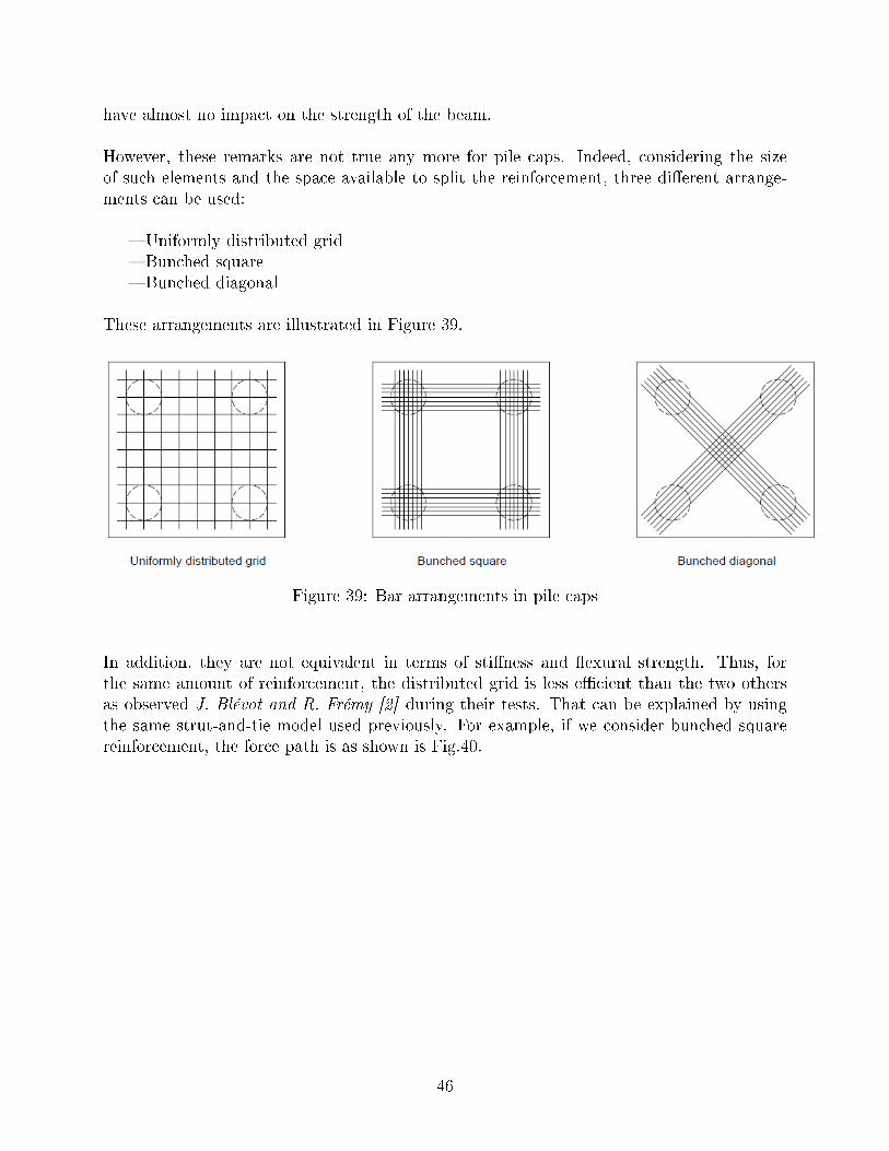
have almost no impact on the strength of the beam.
However, these remarks are not true any more for pile caps. Indeed, considering the sizeof such elements and the space available to split the reinforcement, three di�erent arrange-ments can be used:
� Uniformly distributed grid� Bunched square� Bunched diagonal
These arrangements are illustrated in Figure 39.
Figure 39: Bar arrangements in pile caps
In addition, they are not equivalent in terms of sti�ness and �exural strength. Thus, forthe same amount of reinforcement, the distributed grid is less e�cient than the two othersas observed J. Blévot and R. Frémy [2] during their tests. That can be explained by usingthe same strut-and-tie model used previously. For example, if we consider bunched squarereinforcement, the force path is as shown is Fig.40.
46
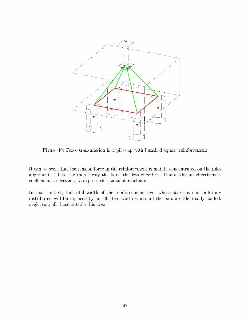
Figure 40: Force transmission in a pile cap with bunched square reinforcement
It can be seen that the tension force in the reinforcement is mainly concentrated on the pilesalignment. Thus, the more away the bars, the less e�ective. That's why an e�ectivenesscoe�cient is necessary to express this particular behavior.
In that context, the total width of the reinforcement layer whose stress is not uniformlydistributed will be replaced by an e�ective width where all the bars are identically loaded,neglecting all those outside this area.
47
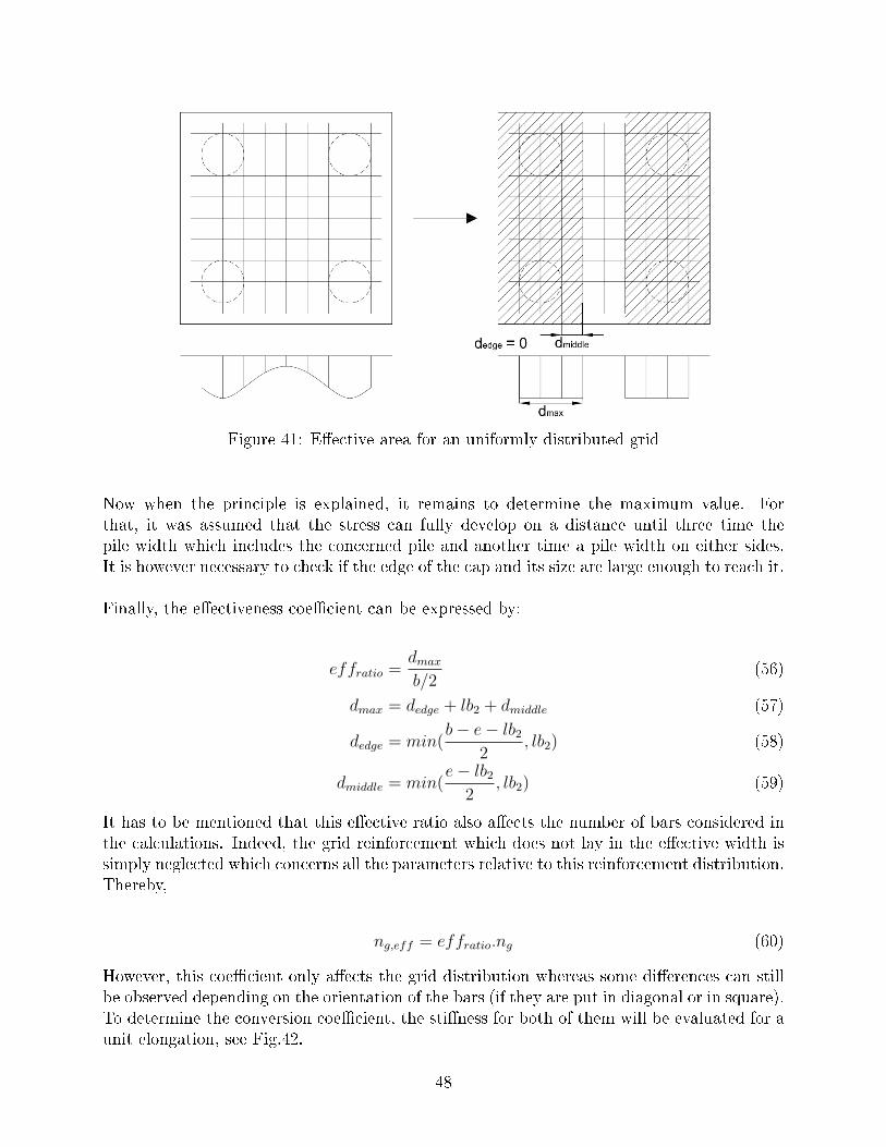
Figure 41: E�ective area for an uniformly distributed grid
Now when the principle is explained, it remains to determine the maximum value. Forthat, it was assumed that the stress can fully develop on a distance until three time thepile width which includes the concerned pile and another time a pile width on either sides.It is however necessary to check if the edge of the cap and its size are large enough to reach it.
Finally, the e�ectiveness coe�cient can be expressed by:
effratio =dmaxb/2
(56)
dmax = dedge + lb2 + dmiddle (57)
dedge = min(b− e− lb2
2, lb2) (58)
dmiddle = min(e− lb2
2, lb2) (59)
It has to be mentioned that this e�ective ratio also a�ects the number of bars considered inthe calculations. Indeed, the grid reinforcement which does not lay in the e�ective width issimply neglected which concerns all the parameters relative to this reinforcement distribution.Thereby,
ng,eff = effratio.ng (60)
However, this coe�cient only a�ects the grid distribution whereas some di�erences can stillbe observed depending on the orientation of the bars (if they are put in diagonal or in square).To determine the conversion coe�cient, the sti�ness for both of them will be evaluated for aunit elongation, see Fig.42.
48
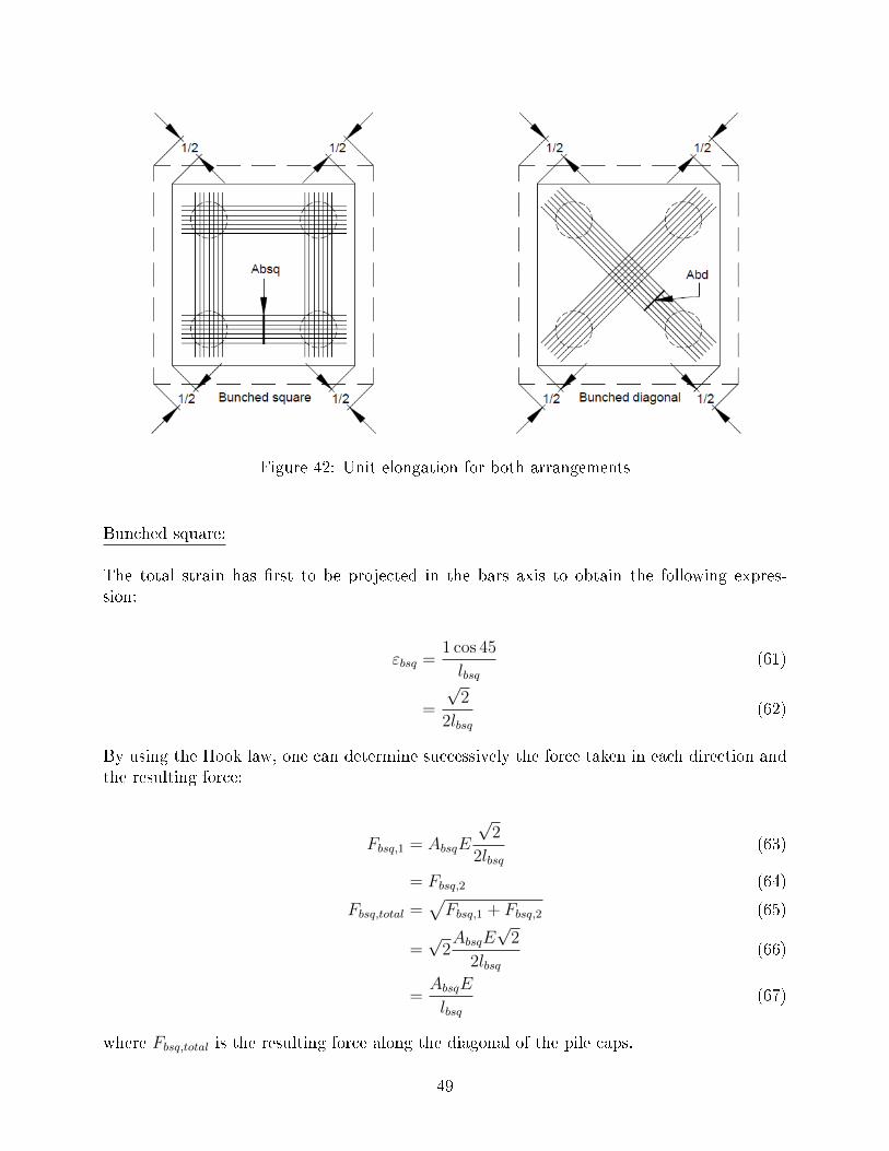
Figure 42: Unit elongation for both arrangements
Bunched square:
The total strain has �rst to be projected in the bars axis to obtain the following expres-sion:
εbsq =1 cos 45
lbsq(61)
=
√2
2lbsq(62)
By using the Hook law, one can determine successively the force taken in each direction andthe resulting force:
Fbsq,1 = AbsqE
√2
2lbsq(63)
= Fbsq,2 (64)
Fbsq,total =√Fbsq,1 + Fbsq,2 (65)
=√
2AbsqE
√2
2lbsq(66)
=AbsqE
lbsq(67)
where Fbsq,total is the resulting force along the diagonal of the pile caps.
49
Bunched diagonal:
In that case, and using the same principle, the following equation is obtained:
Fbd =AbdE
lbd(68)
To determine the conversion coe�cient, it remains to express the fact that Fbsq,total = Fbd inorder to determine the area of steel required in each case. Moreover, it is necessary to takeinto account that the length of the bunched diagonal reinforcement are longer than bunchedsquare one:
√2lbsq = lbd (69)
Thus,
AbsqE
lbsq=AbdE
lbd(70)
⇒√
2Absq = Abd (71)
Which means that for an equivalent result, it is necessary to place√
2 time more reinforce-ment if the bars are positioned in diagonal rather than in square.
However, the reinforcement is generally expressed direction by direction. So, Absq includesall the bars in one direction instead of considering only one path between two piles (as it wasde�ned in Figure 42).
As such, the previous coe�cient has to be adapted to correspond to this convention. Thus,
⇒√
2Absq2
= Abd (72)
Which gives the �nal expression allowing to convert one type of bar arrangement into another.For example, if it is necessary to convert the di�erent reinforcement onto an equivalentbunched square area, each types of bar can be expressed as follows:
Ag→bsq = effratioAg (73)
Absq→bsq = Absq (74)
Abd→bsq =2Abd√
2(75)
Which �nally gives the total amount of steel to consider for the calculation of the bottomreinforcement crossing the critical crack (as required for example in the Equation 50 for thecalculation of the moment equilibrium).
As = Ag→bsq + Absq→bsq + Abd→bsq (76)
50
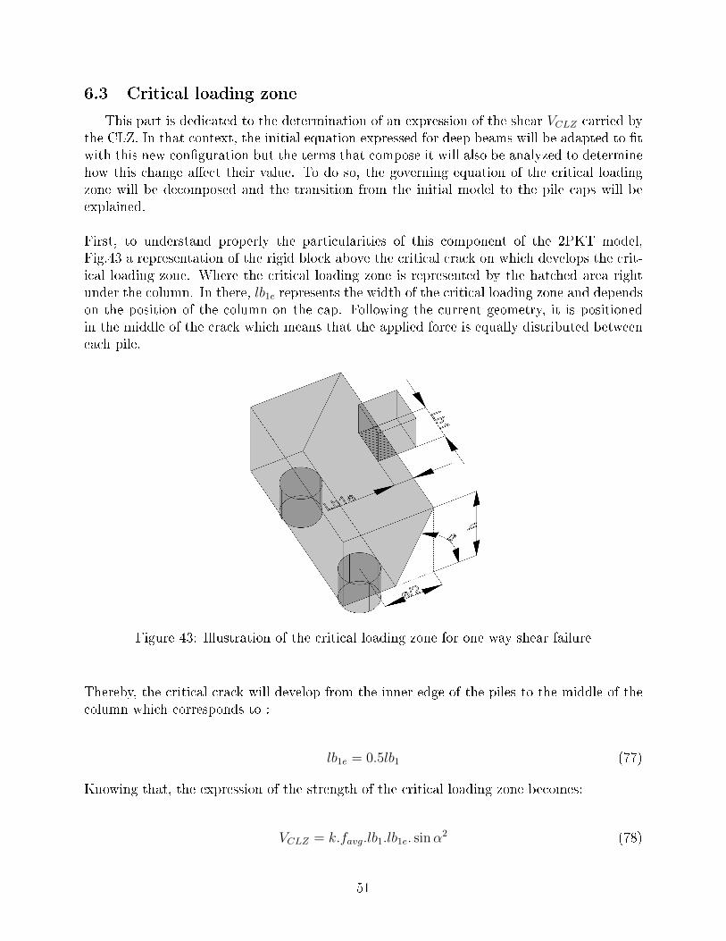
6.3 Critical loading zone
This part is dedicated to the determination of an expression of the shear VCLZ carried bythe CLZ. In that context, the initial equation expressed for deep beams will be adapted to �twith this new con�guration but the terms that compose it will also be analyzed to determinehow this change a�ect their value. To do so, the governing equation of the critical loadingzone will be decomposed and the transition from the initial model to the pile caps will beexplained.
First, to understand properly the particularities of this component of the 2PKT model,Fig.43 a representation of the rigid block above the critical crack on which develops the crit-ical loading zone. Where the critical loading zone is represented by the hatched area rightunder the column. In there, lb1e represents the width of the critical loading zone and dependson the position of the column on the cap. Following the current geometry, it is positionedin the middle of the crack which means that the applied force is equally distributed betweeneach pile.
Figure 43: Illustration of the critical loading zone for one way shear failure
Thereby, the critical crack will develop from the inner edge of the piles to the middle of thecolumn which corresponds to :
lb1e = 0.5lb1 (77)
Knowing that, the expression of the strength of the critical loading zone becomes:
VCLZ = k.favg.lb1.lb1e. sinα2 (78)
51
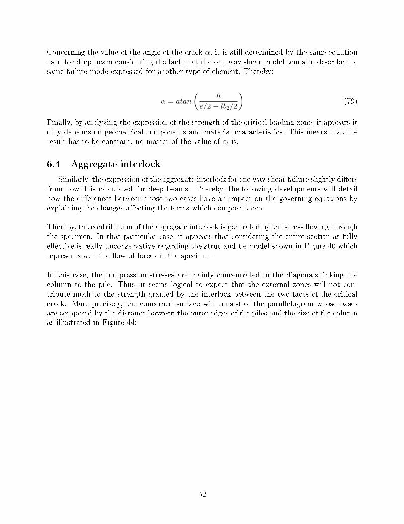
Concerning the value of the angle of the crack α, it is still determined by the same equationused for deep beam considering the fact that the one way shear model tends to describe thesame failure mode expressed for another type of element. Thereby:
α = atan
(h
e/2− lb2/2
)(79)
Finally, by analyzing the expression of the strength of the critical loading zone, it appears itonly depends on geometrical components and material characteristics. This means that theresult has to be constant, no matter of the value of εt is.
6.4 Aggregate interlock
Similarly, the expression of the aggregate interlock for one way shear failure slightly di�ersfrom how it is calculated for deep beams. Thereby, the following developments will detailhow the di�erences between those two cases have an impact on the governing equations byexplaining the changes a�ecting the terms which compose them.
Thereby, the contribution of the aggregate interlock is generated by the stress �owing throughthe specimen. In that particular case, it appears that considering the entire section as fullye�ective is really unconservative regarding the strut-and-tie model shown in Figure 40 whichrepresents well the �ow of forces in the specimen.
In this case, the compression stresses are mainly concentrated in the diagonals linking thecolumn to the pile. Thus, it seems logical to expect that the external zones will not con-tribute much to the strength granted by the interlock between the two faces of the criticalcrack. More precisely, the concerned surface will consist of the parallelogram whose basesare composed by the distance between the outer edges of the piles and the size of the columnas illustrated in Figure 44:
52
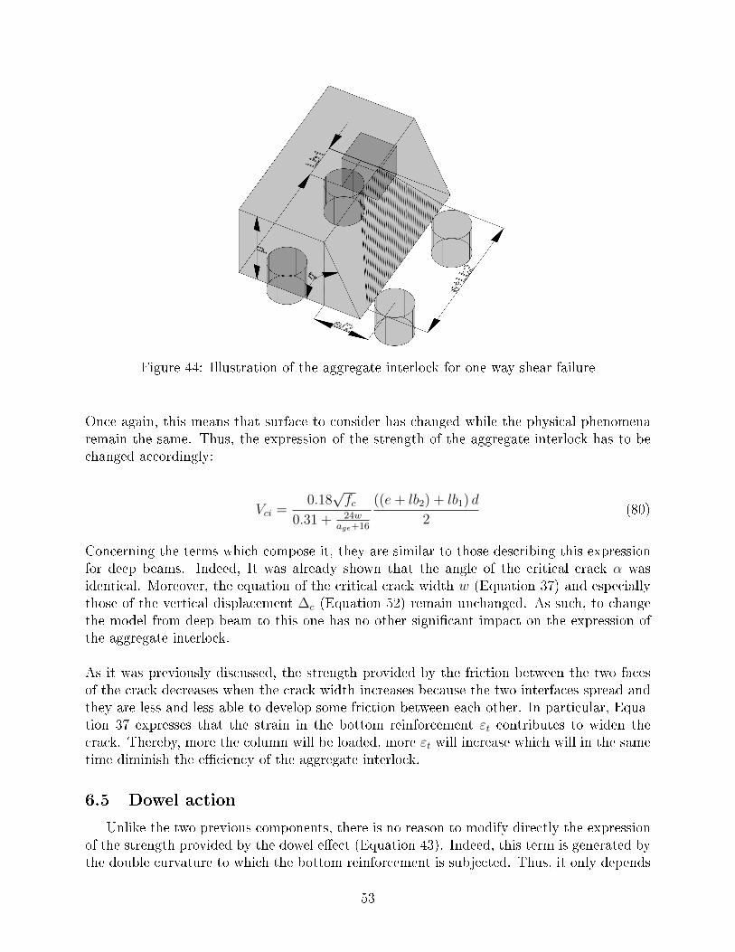
Figure 44: Illustration of the aggregate interlock for one way shear failure
Once again, this means that surface to consider has changed while the physical phenomenaremain the same. Thus, the expression of the strength of the aggregate interlock has to bechanged accordingly:
Vci =0.18√fc
0.31 + 24wage+16
((e+ lb2) + lb1) d
2(80)
Concerning the terms which compose it, they are similar to those describing this expressionfor deep beams. Indeed, It was already shown that the angle of the critical crack α wasidentical. Moreover, the equation of the critical crack width w (Equation 37) and especiallythose of the vertical displacement ∆c (Equation 52) remain unchanged. As such, to changethe model from deep beam to this one has no other signi�cant impact on the expression ofthe aggregate interlock.
As it was previously discussed, the strength provided by the friction between the two facesof the crack decreases when the crack width increases because the two interfaces spread andthey are less and less able to develop some friction between each other. In particular, Equa-tion 37 expresses that the strain in the bottom reinforcement εt contributes to widen thecrack. Thereby, more the column will be loaded, more εt will increase which will in the sametime diminish the e�ciency of the aggregate interlock.
6.5 Dowel action
Unlike the two previous components, there is no reason to modify directly the expressionof the strength provided by the dowel e�ect (Equation 43). Indeed, this term is generated bythe double curvature to which the bottom reinforcement is subjected. Thus, it only depends
53
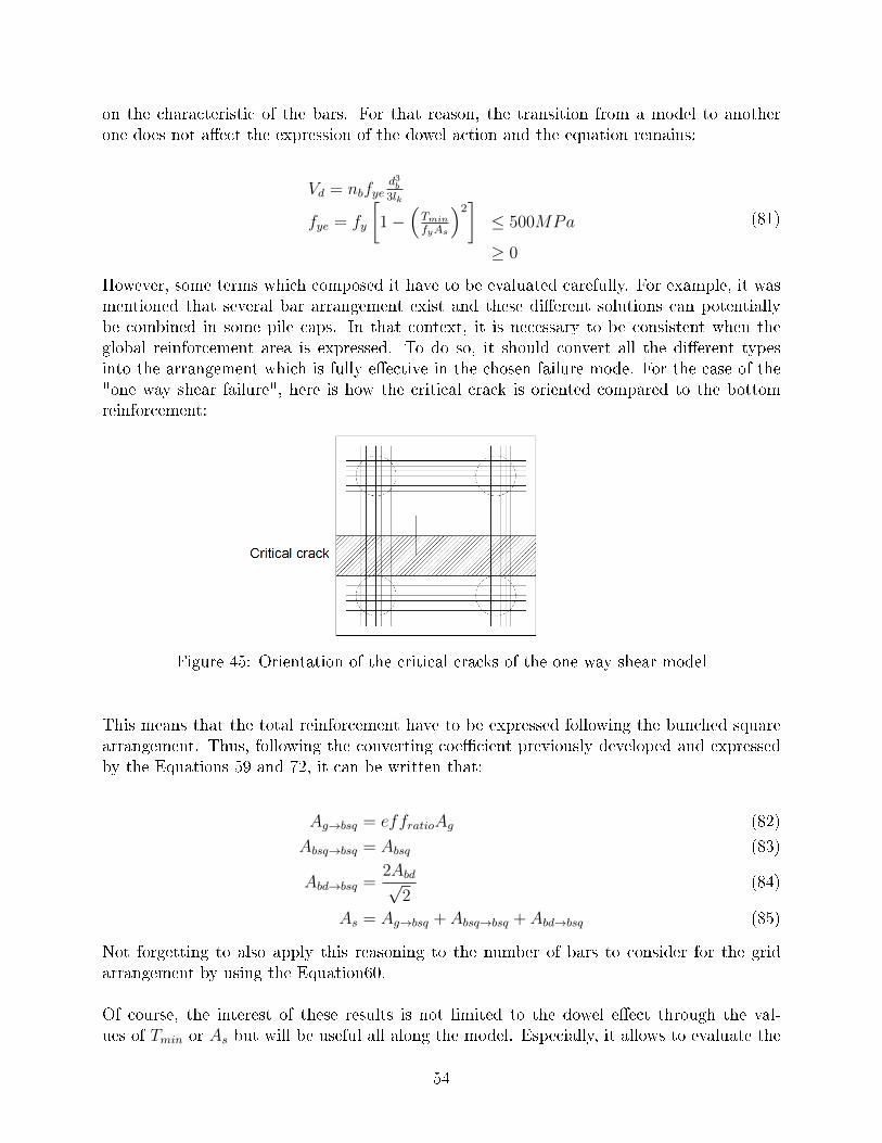
on the characteristic of the bars. For that reason, the transition from a model to anotherone does not a�ect the expression of the dowel action and the equation remains:
Vd = nbfyed3b3lk
fye = fy
[1−
(Tmin
fyAs
)2]≤ 500MPa
≥ 0
(81)
However, some terms which composed it have to be evaluated carefully. For example, it wasmentioned that several bar arrangement exist and these di�erent solutions can potentiallybe combined in some pile caps. In that context, it is necessary to be consistent when theglobal reinforcement area is expressed. To do so, it should convert all the di�erent typesinto the arrangement which is fully e�ective in the chosen failure mode. For the case of the"one way shear failure", here is how the critical crack is oriented compared to the bottomreinforcement:
Figure 45: Orientation of the critical cracks of the one way shear model
This means that the total reinforcement have to be expressed following the bunched squarearrangement. Thus, following the converting coe�cient previously developed and expressedby the Equations 59 and 72, it can be written that:
Ag→bsq = effratioAg (82)
Absq→bsq = Absq (83)
Abd→bsq =2Abd√
2(84)
As = Ag→bsq + Absq→bsq + Abd→bsq (85)
Not forgetting to also apply this reasoning to the number of bars to consider for the gridarrangement by using the Equation60.
Of course, the interest of these results is not limited to the dowel e�ect through the val-ues of Tmin or As but will be useful all along the model. Especially, it allows to evaluate the
54
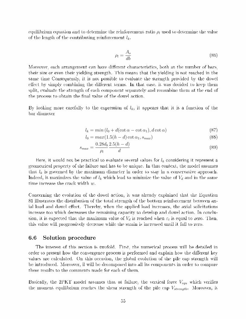
equilibrium equation and to determine the reinforcement ratio ρl used to determine the valueof the length of the contributing reinforcement lk.
ρl =Asdb
(86)
Moreover, each arrangement can have di�erent characteristics, both at the number of bars,their size or even their yielding strength. This means that the yielding is not reached in thesame time Consequently, it is not possible to evaluate the strength provided by the dowele�ect by simply combining the di�erent terms. In that case, it was decided to keep themsplit, evaluate the strength of each component separately and recombine them at the end ofthe process to obtain the �nal value of the dowel action.
By looking more carefully to the expression of lk, it appears that it is a function of thebar diameter
lk = min (l0 + d(cotα− cotα1), d cotα) (87)
l0 = max(1.5(h− d) cotα1, smax) (88)
smax =0.28dbρl
2.5(h− d)
d(89)
Here, it would not be practical to evaluate several values for lk considering it represent ageometrical property of the failure and has to be unique. In that context, the model assumesthat lk is governed by the maximum diameter in order to stay in a conservative approach.Indeed, it maximizes the value of lk which lead to minimize the value of Vd and in the sametime increase the crack width w.
Concerning the evolution of the dowel action, it was already explained that the Equation81 illustrates the distribution of the total strength of the bottom reinforcement between ax-ial load and dowel e�ect. Thereby, when the applied load increases, the axial solicitationsincrease too which decreases the remaining capacity to develop and dowel action. In conclu-sion, it is expected that the maximum value of Vd is reached when εt is equal to zero. Then,this value will progressively decrease while the strain is increased until it fall to zero.
6.6 Solution procedure
The interest of this section is twofold. First, the numerical process will be detailed inorder to present how the convergence process is performed and explain how the di�erent keyvalues are calculated. On this occasion, the global evolution of the pile cap strength willbe introduced. Moreover, il will be decomposed into all its components in order to comparethese results to the comments made for each of them.
Basically, the 2PKT model assumes that at failure, the vertical force Vequ which veri�esthe moment equilibrium reaches the shear strength of the pile cap Vstrength. Moreover, it
55
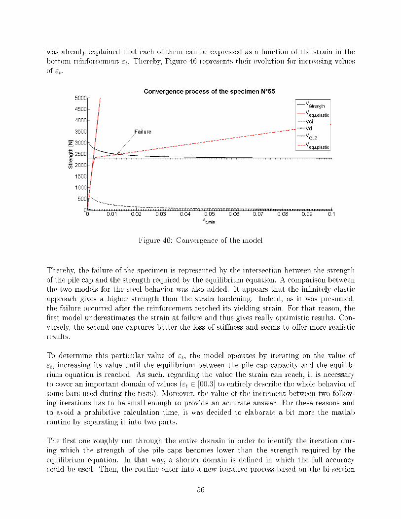
was already explained that each of them can be expressed as a function of the strain in thebottom reinforcement εt. Thereby, Figure 46 represents their evolution for increasing valuesof εt.
Figure 46: Convergence of the model
Thereby, the failure of the specimen is represented by the intersection between the strengthof the pile cap and the strength required by the equilibrium equation. A comparison betweenthe two models for the steel behavior was also added. It appears that the in�nitely elasticapproach gives a higher strength than the strain hardening. Indeed, as it was presumed,the failure occurred after the reinforcement reached its yielding strain. For that reason, the�rst model underestimates the strain at failure and thus gives really optimistic results. Con-versely, the second one captures better the loss of sti�ness and seems to o�er more realisticresults.
To determine this particular value of εt, the model operates by iterating on the value ofεt, increasing its value until the equilibrium between the pile cap capacity and the equilib-rium equation is reached. As such, regarding the value the strain can reach, it is necessaryto cover an important domain of values (εt ∈ [00.3] to entirely describe the whole behavior ofsome bars used during the tests). Moreover, the value of the increment between two follow-ing iterations has to be small enough to provide an accurate answer. For these reasons andto avoid a prohibitive calculation time, it was decided to elaborate a bit more the matlabroutine by separating it into two parts.
The �rst one roughly run through the entire domain in order to identify the iteration dur-ing which the strength of the pile caps becomes lower than the strength required by theequilibrium equation. In that way, a shorter domain is de�ned in which the full accuracycould be used. Then, the routine enter into a new iterative process based on the bi-section
56
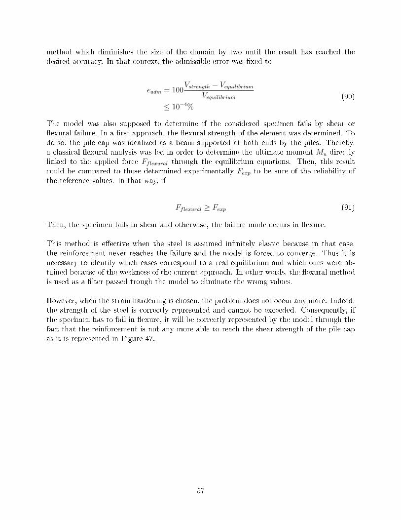
method which diminishes the size of the domain by two until the result has reached thedesired accuracy. In that context, the admissible error was �xed to
eadm = 100Vstrength − Vequilibrium
Vequilibrium
≤ 10−4%
(90)
The model was also supposed to determine if the considered specimen fails by shear or�exural failure. In a �rst approach, the �exural strength of the element was determined. Todo so, the pile cap was idealized as a beam supported at both ends by the piles. Thereby,a classical �exural analysis was led in order to determine the ultimate moment Mu directlylinked to the applied force Fflexural through the equilibrium equations. Then, this resultcould be compared to those determined experimentally Fexp to be sure of the reliability ofthe reference values. In that way, if
Fflexural ≥ Fexp (91)
Then, the specimen fails in shear and otherwise, the failure mode occurs in �exure.
This method is e�ective when the steel is assumed in�nitely elastic because in that case,the reinforcement never reaches the failure and the model is forced to converge. Thus it isnecessary to identify which cases correspond to a real equilibrium and which ones were ob-tained because of the weakness of the current approach. In other words, the �exural methodis used as a �lter passed trough the model to eliminate the wrong values.
However, when the strain hardening is chosen, the problem does not occur any more. Indeed,the strength of the steel is correctly represented and cannot be exceeded. Consequently, ifthe specimen has to fail in �exure, it will be correctly represented by the model through thefact that the reinforcement is not any more able to reach the shear strength of the pile capas it is represented in Figure 47.
57
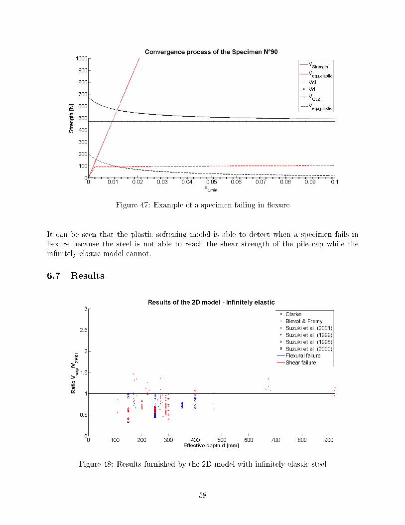
Figure 47: Example of a specimen failing in �exure
It can be seen that the plastic softening model is able to detect when a specimen fails in�exure because the steel is not able to reach the shear strength of the pile cap while thein�nitely elastic model cannot.
6.7 Results
Figure 48: Results furnished by the 2D model with in�nitely elastic steel
58
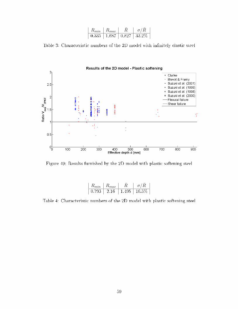
Rmin Rmax R̄ σ/R̄0.335 1.687 0.827 33.2%
Table 3: Characteristic numbers of the 2D model with in�nitely elastic steel
Figure 49: Results furnished by the 2D model with plastic softening steel
Rmin Rmax R̄ σ/R̄0.793 2.16 1.495 16.5%
Table 4: Characteristic numbers of the 2D model with plastic softening steel
59
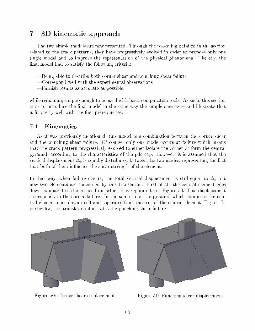
7 3D kinematic approach
The two simple models are now presented. Through the reasoning detailed in the sectionrelated to the crack patterns, they have progressively evolved in order to propose only onesingle model and to improve the representation of the physical phenomena. Thereby, the�nal model had to satisfy the following criteria:
� Being able to describe both corner shear and punching shear failure� Correspond well with the experimental observations� Furnish results as accurate as possible.
while remaining simple enough to be used with basic computation tools. As such, this sectionaims to introduce the �nal model in the same way the simple ones were and illustrate thatit �t pretty well with the �rst prerequisites.
7.1 Kinematics
As it was previously mentioned, this model is a combination between the corner shearand the punching shear failure. Of course, only one mode occurs at failure which meansthat the crack pattern progressively evolved to either isolate the corner or form the centralpyramid, according to the characteristics of the pile cap. However, it is assumed that thevertical displacement ∆c is equally distributed between the two modes, representing the factthat both of them in�uence the shear strength of the element.
In that way, when failure occurs, the total vertical displacement is still equal to ∆c butnow two elements are concerned by this translation. First of all, the central element goesdown compared to the corner from which it is separated, see Figure 50. This displacementcorresponds to the corner failure. In the same time, the pyramid which composes the cen-tral element goes down itself and separates from the rest of the central element, Fig.51. Inparticular, this translation illustrates the punching shear failure.
Figure 50: Corner shear displacement Figure 51: Punching shear displacement
60
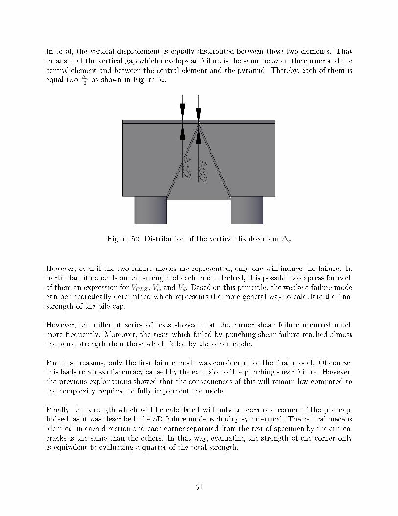
In total, the vertical displacement is equally distributed between these two elements. Thatmeans that the vertical gap which develops at failure is the same between the corner and thecentral element and between the central element and the pyramid. Thereby, each of them isequal two ∆c
2as shown in Figure 52.
Figure 52: Distribution of the vertical displacement ∆c
However, even if the two failure modes are represented, only one will induce the failure. Inparticular, it depends on the strength of each mode. Indeed, it is possible to express for eachof them an expression for VCLZ , Vci and Vd. Based on this principle, the weakest failure modecan be theoretically determined which represents the more general way to calculate the �nalstrength of the pile cap.
However, the di�erent series of tests showed that the corner shear failure occurred muchmore frequently. Moreover, the tests which failed by punching shear failure reached almostthe same strength than those which failed by the other mode.
For these reasons, only the �rst failure mode was considered for the �nal model. Of course,this leads to a loss of accuracy caused by the exclusion of the punching shear failure. However,the previous explanations showed that the consequences of this will remain low compared tothe complexity required to fully implement the model.
Finally, the strength which will be calculated will only concern one corner of the pile cap.Indeed, as it was described, the 3D failure mode is doubly symmetrical: The central piece isidentical in each direction and each corner separated from the rest of specimen by the criticalcracks is the same than the others. In that way, evaluating the strength of one corner onlyis equivalent to evaluating a quarter of the total strength.
61
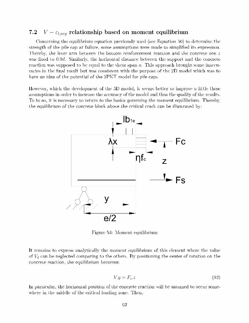
7.2 V − εt,avg relationship based on moment equilibrium
Concerning the equilibrium equation previously used (see Equation 50) to determine thestrength of the pile cap at failure, some assumptions were made to simpli�ed its expression.Thereby, the lever arm between the bottom reinforcement reaction and the concrete one zwas �xed to 0.9d. Similarly, the horizontal distance between the support and the concretereaction was supposed to be equal to the shear span a. This approach brought some inaccu-racies in the �nal result but was consistent with the purpose of the 2D model which was tohave an idea of the potential of the 2PKT model for pile caps.
However, which the development of the 3D model, it seems better to improve a little theseassumptions in order to increase the accuracy of the model and thus the quality of the results.To to so, it is necessary to return to the basics governing the moment equilibrium. Thereby,the equilibrium of the concrete block above the critical crack can be illustrated by:
Figure 53: Moment equilibrium
It remains to express analytically the moment equilibrium of this element where the valueof Vd can be neglected comparing to the others. By positioning the center of rotation on theconcrete reaction, the equilibrium becomes:
V.y = Fs.z (92)
In particular, the horizontal position of the concrete reaction will be assumed to occur some-where in the middle of the critical loading zone. Then,
62
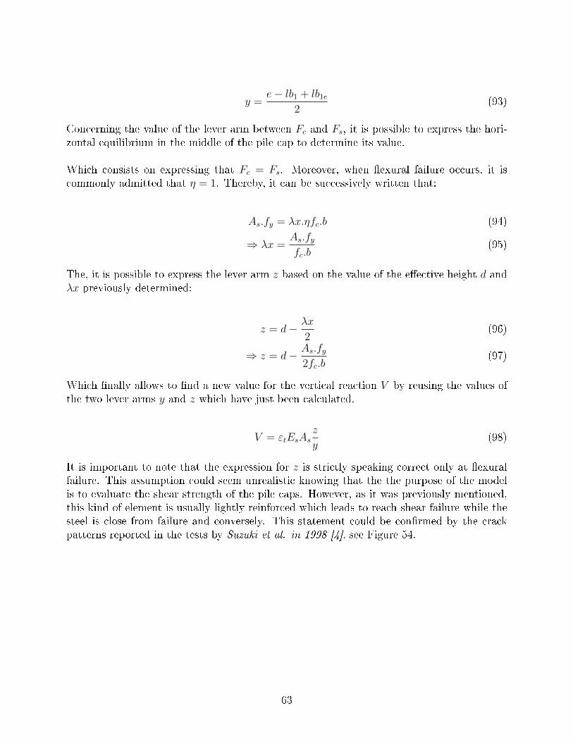
y =e− lb1 + lb1e
2(93)
Concerning the value of the lever arm between Fc and Fs, it is possible to express the hori-zontal equilibrium in the middle of the pile cap to determine its value.
Which consists on expressing that Fc = Fs. Moreover, when �exural failure occurs, it iscommonly admitted that η = 1. Thereby, it can be successively written that:
As.fy = λx.ηfc.b (94)
⇒ λx =As.fyfc.b
(95)
The, it is possible to express the lever arm z based on the value of the e�ective height d andλx previously determined:
z = d− λx
2(96)
⇒ z = d− As.fy2fc.b
(97)
Which �nally allows to �nd a new value for the vertical reaction V by reusing the values ofthe two lever arms y and z which have just been calculated.
V = εtEsAsz
y(98)
It is important to note that the expression for z is strictly speaking correct only at �exuralfailure. This assumption could seem unrealistic knowing that the the purpose of the modelis to evaluate the shear strength of the pile caps. However, as it was previously mentioned,this kind of element is usually lightly reinforced which leads to reach shear failure while thesteel is close from failure and conversely. This statement could be con�rmed by the crackpatterns reported in the tests by Suzuki et al. in 1998 [4], see Figure 54.
63
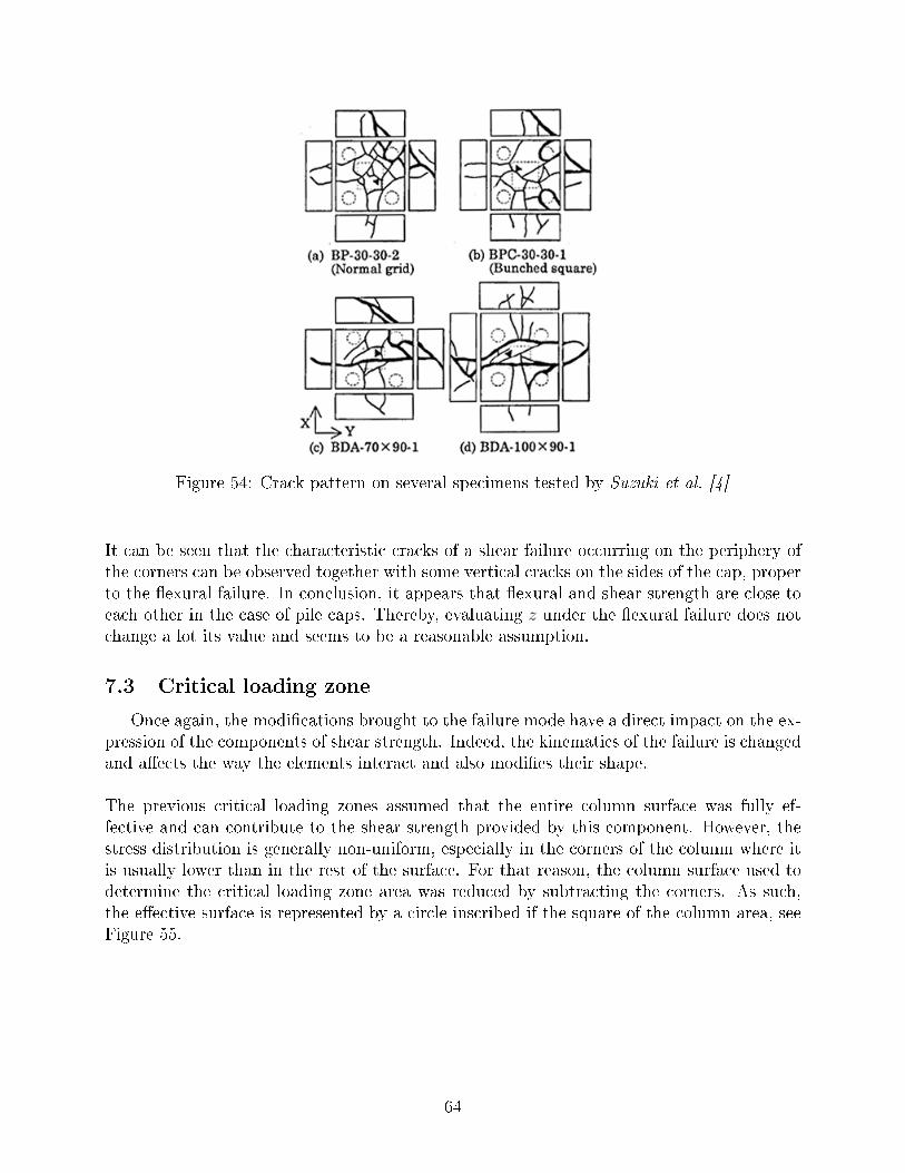
Figure 54: Crack pattern on several specimens tested by Suzuki et al. [4]
It can be seen that the characteristic cracks of a shear failure occurring on the periphery ofthe corners can be observed together with some vertical cracks on the sides of the cap, properto the �exural failure. In conclusion, it appears that �exural and shear strength are close toeach other in the case of pile caps. Thereby, evaluating z under the �exural failure does notchange a lot its value and seems to be a reasonable assumption.
7.3 Critical loading zone
Once again, the modi�cations brought to the failure mode have a direct impact on the ex-pression of the components of shear strength. Indeed, the kinematics of the failure is changedand a�ects the way the elements interact and also modi�es their shape.
The previous critical loading zones assumed that the entire column surface was fully ef-fective and can contribute to the shear strength provided by this component. However, thestress distribution is generally non-uniform, especially in the corners of the column where itis usually lower than in the rest of the surface. For that reason, the column surface used todetermine the critical loading zone area was reduced by subtracting the corners. As such,the e�ective surface is represented by a circle inscribed if the square of the column area, seeFigure 55.
64
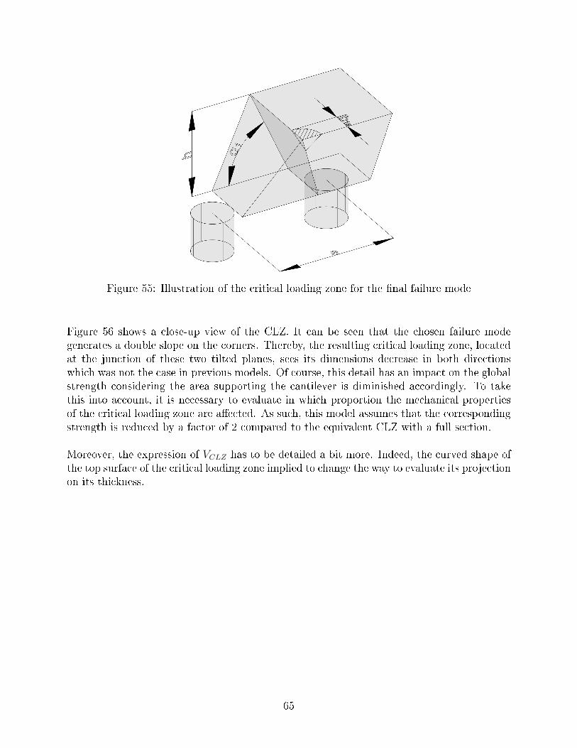
Figure 55: Illustration of the critical loading zone for the �nal failure mode
Figure 56 shows a close-up view of the CLZ. It can be seen that the chosen failure modegenerates a double slope on the corners. Thereby, the resulting critical loading zone, locatedat the junction of these two tilted planes, sees its dimensions decrease in both directionswhich was not the case in previous models. Of course, this detail has an impact on the globalstrength considering the area supporting the cantilever is diminished accordingly. To takethis into account, it is necessary to evaluate in which proportion the mechanical propertiesof the critical loading zone are a�ected. As such, this model assumes that the correspondingstrength is reduced by a factor of 2 compared to the equivalent CLZ with a full section.
Moreover, the expression of VCLZ has to be detailed a bit more. Indeed, the curved shape ofthe top surface of the critical loading zone implied to change the way to evaluate its projectionon its thickness.
65
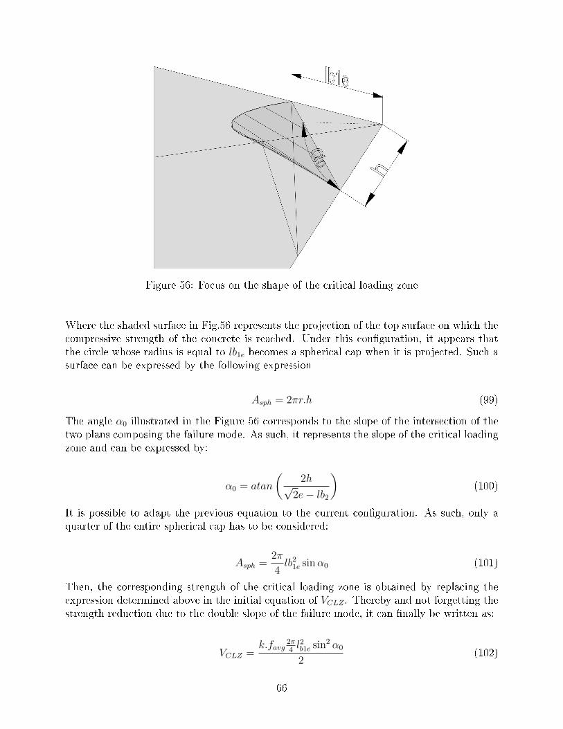
Figure 56: Focus on the shape of the critical loading zone
Where the shaded surface in Fig.56 represents the projection of the top surface on which thecompressive strength of the concrete is reached. Under this con�guration, it appears thatthe circle whose radius is equal to lb1e becomes a spherical cap when it is projected. Such asurface can be expressed by the following expression
Asph = 2πr.h (99)
The angle α0 illustrated in the Figure 56 corresponds to the slope of the intersection of thetwo plans composing the failure mode. As such, it represents the slope of the critical loadingzone and can be expressed by:
α0 = atan
(2h√
2e− lb2
)(100)
It is possible to adapt the previous equation to the current con�guration. As such, only aquarter of the entire spherical cap has to be considered:
Asph =2π
4lb2
1e sinα0 (101)
Then, the corresponding strength of the critical loading zone is obtained by replacing theexpression determined above in the initial equation of VCLZ . Thereby and not forgetting thestrength reduction due to the double slope of the failure mode, it can �nally be written as:
VCLZ =k.favg
2π4l2b1e sin2 α0
2(102)
66
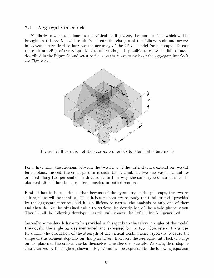
7.4 Aggregate interlock
Similarly to what was done for the critical loading zone, the modi�cations which will bebrought in this section will result from both the changes of the failure mode and severalimprovements realized to increase the accuracy of the 2PKT model for pile caps. To easethe understanding of the adaptations to undertake, it is possible to reuse the failure modedescribed in the Figure 34 and set it to focus on the characteristics of the aggregate interlock,see Figure 57.
Figure 57: Illustration of the aggregate interlock for the �nal failure mode
For a �rst time, the frictions between the two faces of the critical crack extend on two dif-ferent plans. Indeed, the crack pattern is such that it combines two one way shear failuresoriented along two perpendicular directions. In that way, the same type of surfaces can beobserved after failure but are interconnected in both directions.
First, it has to be mentioned that because of the symmetry of the pile caps, the two re-sulting plans will be identical. Thus it is not necessary to study the total strength providedby the aggregate interlock and it is su�cient to narrow the analysis to only one of themand then double the obtained value to retrieve the description of the whole phenomenon.Thereby, all the following developments will only concern half of the friction generated.
Secondly, some details have to be provided with regards to the relevant angles of the model.Previously, the angle α0 was mentioned and expressed by Eq.100. Concretely it was use-ful during the evaluation of the strength of the critical loading zone especially because theshape of this element depends on this parameter. However, the aggregate interlock developson the planes of the critical cracks themselves considered separately. As such, their slope ischaracterized by the angle α1 shown in Fig.57 and can be expressed by the following equation:
67
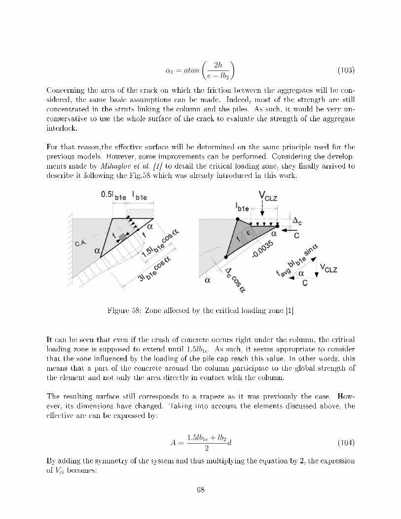
α1 = atan
(2h
e− lb2
)(103)
Concerning the area of the crack on which the friction between the aggregates will be con-sidered, the same basic assumptions can be made. Indeed, most of the strength are stillconcentrated in the struts linking the column and the piles. As such, it would be very un-conservative to use the whole surface of the crack to evaluate the strength of the aggregateinterlock.
For that reason,the e�ective surface will be determined on the same principle used for theprevious models. However, some improvements can be performed. Considering the develop-ments made by Mihaylov et al. [1] to detail the critical loading zone, they �nally arrived todescribe it following the Fig.58 which was already introduced in this work.
Figure 58: Zone a�ected by the critical loading zone [1]
It can be seen that even if the crush of concrete occurs right under the column, the criticalloading zone is supposed to extend until 1.5lb1e. As such, it seems appropriate to considerthat the zone in�uenced by the loading of the pile cap reach this value. In other words, thismeans that a part of the concrete around the column participate to the global strength ofthe element and not only the area directly in contact with the column.
The resulting surface still corresponds to a trapeze as it was previously the case. How-ever, its dimensions have changed. Taking into account the elements discussed above, thee�ective are can be expressed by:
A =1.5lb1e + lb2
2d (104)
By adding the symmetry of the system and thus multiplying the equation by 2, the expressionof Vci becomes:
68
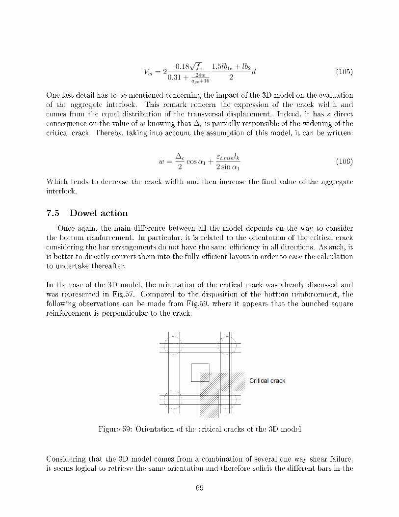
Vci = 20.18√fc
0.31 + 24wage+16
1.5lb1e + lb2
2d (105)
One last detail has to be mentioned concerning the impact of the 3D model on the evaluationof the aggregate interlock. This remark concern the expression of the crack width andcomes from the equal distribution of the transversal displacement. Indeed, it has a directconsequence on the value of w knowing that ∆c is partially responsible of the widening of thecritical crack. Thereby, taking into account the assumption of this model, it can be written:
w =∆c
2cosα1 +
εt,minlk2 sinα1
(106)
Which tends to decrease the crack width and then increase the �nal value of the aggregateinterlock.
7.5 Dowel action
Once again, the main di�erence between all the model depends on the way to considerthe bottom reinforcement. In particular, it is related to the orientation of the critical crackconsidering the bar arrangements do not have the same e�ciency in all directions. As such, itis better to directly convert them into the fully e�cient layout in order to ease the calculationto undertake thereafter.
In the case of the 3D model, the orientation of the critical crack was already discussed andwas represented in Fig.57. Compared to the disposition of the bottom reinforcement, thefollowing observations can be made from Fig.59, where it appears that the bunched squarereinforcement is perpendicular to the crack.
Figure 59: Orientation of the critical cracks of the 3D model
Considering that the 3D model comes from a combination of several one way shear failure,it seems logical to retrieve the same orientation and therefore solicit the di�erent bars in the
69
same way. Thereby all the steel reinforcement will be converted into the bunched squarearrangement in order to express them in the fully e�ective con�guration.
Moreover, it is shown in Fig.59 that the useful steel surface is spread over the two plansof the critical crack. Once again, it is equally distributed considering the symmetry of thepile cap and especially of the bottom reinforcement. It is also illustrated that only half ofthe reinforcement has to be considered in each direction. Following that, each reinforcementarrangement can be expressed by:
Ag→bsq =effratioAg
2(107)
Absq→bsq =Absq
2(108)
Abd→bsq =Abd√
2(109)
(110)
Which represents the steel area in only one direction. From this, it is possible to evaluatethe strength provided by the dowel action in this particular case and then double it to takeinto account the same e�ect occurring in the other direction. This �nally leads to determinethe total value of Vd in this way:
Vd = 2nbfyed3b
3lk(111)
fye = fy
[1−
(TminfyAs
)2]≤ 500MPa
≥ 0
(112)
7.6 Solution procedure
The total strength of the pile caps is still evaluated through an iterative process duringwhich the external force is compared to the current strength of the pile cap. The failure isreached when the value of the strain of the bottom reinforcement εt leads to an equilibriumbetween these two. Except the di�erences discussed above, the solution procedure remainsunchanged compared to the matlab routine described for the 2D model.
70
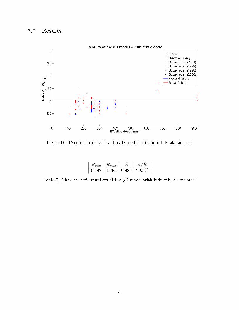
7.7 Results
Figure 60: Results furnished by the 3D model with in�nitely elastic steel
Rmin Rmax R̄ σ/R̄0.482 1.788 0.889 29.3%
Table 5: Characteristic numbers of the 3D model with in�nitely elastic steel
71
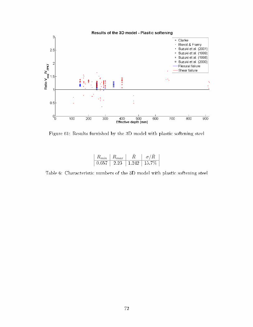
Figure 61: Results furnished by the 3D model with plastic softening steel
Rmin Rmax R̄ σ/R̄0.657 2.23 1.242 15.7%
Table 6: Characteristic numbers of the 3D model with plastic softening steel
72
8 Comparison with tests
This chapter will be divided into two part. The �rst one will consist to introduce theresults furnished by the two main models previously described. It is �rst necessary to evaluatethe accuracy of each of them. To do so, the strength determined numerically can be comparedto the experimental results. Therefore, the following ratio is de�ned:
R =VexpVmodel
(113)
First of all the values given by the two models will indicate if they are accurate enough to beused into further developments. Indeed, it has to be remembered that the main purpose ofthis work is to determine if the 2PKT model can help to describe better the pile cap behavior.For that reason, it is necessary to check if the main objective is reached.
It is not the only characteristic this analysis could provide. Thus, reusing the ratio expressedabove, it is logical to conclude that the closer from one, the better the model. However, thiscriteria has to be nuanced. For example, the results showing that R < 1 correspond to thecases for which the model is more optimistic than reality. As such, the position of the resultscompared to one will show whether the model tends to be conservative or not.
Moreover, the disparity of the results is a good indicator of the reliability of the model.Indeed, if it calculates some really good results but the others are scattered while the di�er-ences between the tested pile caps are small, this mitigates the con�dence that can be placedin it because its accuracy is not constant and depends on the characteristics of the specimenunder consideration. In this context, it is generally better to use a model whose results willbe a bit less accurate on average but constant in a larger domain.
In that way, it will be possible to compare the two main models considered in this the-sis. In that context, the weaknesses of each of them will be discussed in order to evaluatewhich one corresponds better to the objectives of this work. The comparative study willnot be limited to the models themselves but will also concern the hypothesis on the steelbehavior assumed in each of them. Thereby, the impacts of this choice will be representedthrough the results determined in each case.
However, the ratio R will not be the only value to be considered in this part. Indeed, itis not su�cient to evaluate properly the failure load of the pile caps, it is also necessary tocorrectly identify the failure mode. As such, the mode identi�ed by the models will be com-pared to the experimental observations in order to evaluate the predicting power of the model.
8.1 2D kinematic approach
As discussed above, the results of the 2D model will be presented through the ratio de-�ned by Eq.113. On this occasion, it is possible to take the opportunity to express them in
73
an useful way. To do so, it is necessary to use a parameter which represents well the sizeof the pile cap and have a direct impact on its strength. As such, the e�ective depth d �twell with these two criteria. Thereby, besides the analysis of the results themselves, someproperties could be observed.
Moreover, some key values can be used to bring new informations about the characteris-tics of the model. In this case, this includes the extremal values of the model (namely Rmin
and Rmax) which provide its worst predictions and which could be directly compared withthe corresponding values for the other models. To these two values, it is also useful to addthe mean ratio in order to determine its average accuracy and discuss about its locationcompared to 1. The �nal characteristic value represents the relative disparity of the results.In that way, it will be possible to analyze how the model behaves overall. Initially, thisinformation is given by the standard deviation σ. However, it is better to adapt it a littlein order to get a value which can be compared from a model to another. Therefore, thecoe�cient of variation (COV) σ
R̄is preferred.
8.1.1 In�nitely elastic reinforcement
All the results will be sorted following the series of tests to which they belong. Indeed,each of them was performed with its own process and its own pile cap design. As such, itis important to be able to distinguish them in order to to analyze them separately. In thatway, it will be possible to expose the potential inconsistencies in the experimental results andadapt the conclusions accordingly. Thereby, the analysis of the models will not only consistof a discussion of the results themselves but also making sure that the data used are relevant.
As it was mentioned, the interest is here to focus on the shear results considering it isthe main purpose of this work. That said, �exural failure remains a signi�cant part of theobserved failures which means that it is also necessary to evaluate the accuracy of the modelto capture this phenomenon. Thereby, �exural and shear failures are also distinguished. Thisis the opportunity to combine this distinction to the di�erent representation of each seriesof tests which can give a quick idea if the failure mode observed experimentally are wellcaptured or not by the model.
Following the remarks expressed above and according to the procedure described in Sec-tion 6.6, the results obtained for the 2D model when steel is modeled as in�nitely elastic areshown in Fig.62.
74
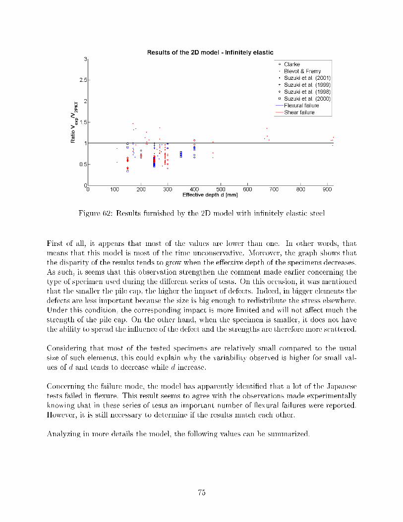
Figure 62: Results furnished by the 2D model with in�nitely elastic steel
First of all, it appears that most of the values are lower than one. In other words, thatmeans that this model is most of the time unconservative. Moreover, the graph shows thatthe disparity of the results tends to grow when the e�ective depth of the specimens decreases.As such, it seems that this observation strengthen the comment made earlier concerning thetype of specimen used during the di�erent series of tests. On this occasion, it was mentionedthat the smaller the pile cap, the higher the impact of defects. Indeed, in bigger elements thedefects are less important because the size is big enough to redistribute the stress elsewhere.Under this condition, the corresponding impact is more limited and will not a�ect much thestrength of the pile cap. On the other hand, when the specimen is smaller, it does not havethe ability to spread the in�uence of the defect and the strengths are therefore more scattered.
Considering that most of the tested specimens are relatively small compared to the usualsize of such elements, this could explain why the variability observed is higher for small val-ues of d and tends to decrease while d increase.
Concerning the failure mode, the model has apparently identi�ed that a lot of the Japanesetests failed in �exure. This result seems to agree with the observations made experimentallyknowing that in these series of tests an important number of �exural failures were reported.However, it is still necessary to determine if the results match each other.
Analyzing in more details the model, the following values can be summarized.
75
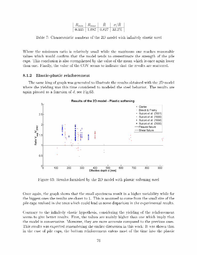
Rmin Rmax R̄ σ/R̄0.335 1.687 0.827 33.2%
Table 7: Characteristic numbers of the 2D model with in�nitely elastic steel
Where the minimum ratio is relatively small while the maximum one reaches reasonablevalues which would con�rm that the model tends to overestimate the strength of the pilecaps. This conclusion is also strengthened by the value of the mean which is once again lowerthan one. Finally, the value of the COV seems to indicate that the results are scattered.
8.1.2 Elastic-plastic reinforcement
The same king of graph was generated to illustrate the results obtained with the 2D modelwhere the yielding was this time considered to modeled the steel behavior. The results areagain plotted as a function of d, see Fig.63.
Figure 63: Results furnished by the 2D model with plastic softening steel
Once again, the graph shows that the small specimens result in a higher variability while forthe biggest ones the results are closer to 1. This is assumed to come from the small size of thepile caps realized in the tests which could lead to some disparities in the experimental results.
Contrary to the in�nitely elastic hypothesis, considering the yielding of the reinforcementseems to give better results. First, the values are mainly higher than one which imply thatthe model is conservative. Moreover, they are more accurate compared to the previous ones.This results was expected remembering the earlier discussion in this work: It was shown thatin the case of pile caps, the bottom reinforcement enters most of the time into the plastic
76
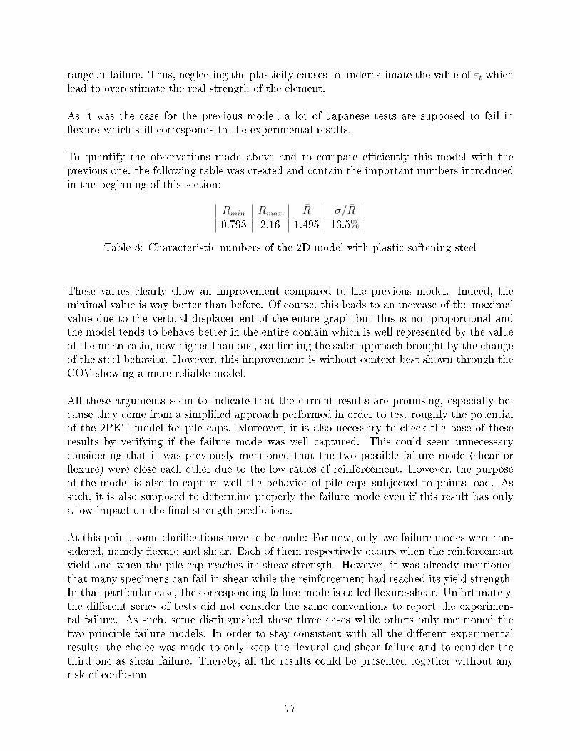
range at failure. Thus, neglecting the plasticity causes to underestimate the value of εt whichlead to overestimate the real strength of the element.
As it was the case for the previous model, a lot of Japanese tests are supposed to fail in�exure which still corresponds to the experimental results.
To quantify the observations made above and to compare e�ciently this model with theprevious one, the following table was created and contain the important numbers introducedin the beginning of this section:
Rmin Rmax R̄ σ/R̄0.793 2.16 1.495 16.5%
Table 8: Characteristic numbers of the 2D model with plastic softening steel
These values clearly show an improvement compared to the previous model. Indeed, theminimal value is way better than before. Of course, this leads to an increase of the maximalvalue due to the vertical displacement of the entire graph but this is not proportional andthe model tends to behave better in the entire domain which is well represented by the valueof the mean ratio, now higher than one, con�rming the safer approach brought by the changeof the steel behavior. However, this improvement is without context best shown through theCOV showing a more reliable model.
All these arguments seem to indicate that the current results are promising, especially be-cause they come from a simpli�ed approach performed in order to test roughly the potentialof the 2PKT model for pile caps. Moreover, it is also necessary to check the base of theseresults by verifying if the failure mode was well captured. This could seem unnecessaryconsidering that it was previously mentioned that the two possible failure mode (shear or�exure) were close each other due to the low ratios of reinforcement. However, the purposeof the model is also to capture well the behavior of pile caps subjected to points load. Assuch, it is also supposed to determine properly the failure mode even if this result has onlya low impact on the �nal strength predictions.
At this point, some clari�cations have to be made: For now, only two failure modes were con-sidered, namely �exure and shear. Each of them respectively occurs when the reinforcementyield and when the pile cap reaches its shear strength. However, it was already mentionedthat many specimens can fail in shear while the reinforcement had reached its yield strength.In that particular case, the corresponding failure mode is called �exure-shear. Unfortunately,the di�erent series of tests did not consider the same conventions to report the experimen-tal failure. As such, some distinguished these three cases while others only mentioned thetwo principle failure models. In order to stay consistent with all the di�erent experimentalresults, the choice was made to only keep the �exural and shear failure and to consider thethird one as shear failure. Thereby, all the results could be presented together without anyrisk of confusion.
77
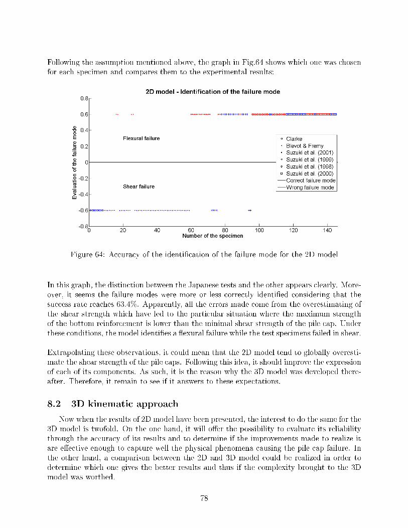
Following the assumption mentioned above, the graph in Fig.64 shows which one was chosenfor each specimen and compares them to the experimental results:
Figure 64: Accuracy of the identi�cation of the failure mode for the 2D model
In this graph, the distinction between the Japanese tests and the other appears clearly. More-over, it seems the failure modes were more or less correctly identi�ed considering that thesuccess rate reaches 63.4%. Apparently, all the errors made come from the overestimating ofthe shear strength which have led to the particular situation where the maximum strengthof the bottom reinforcement is lower than the minimal shear strength of the pile cap. Underthese conditions, the model identi�es a �exural failure while the test specimens failed in shear.
Extrapolating these observations, it could mean that the 2D model tend to globally overesti-mate the shear strength of the pile caps. Following this idea, it should improve the expressionof each of its components. As such, it is the reason why the 3D model was developed there-after. Therefore, it remain to see if it answers to these expectations.
8.2 3D kinematic approach
Now when the results of 2D model have been presented, the interest to do the same for the3D model is twofold. On the one hand, it will o�er the possibility to evaluate its reliabilitythrough the accuracy of its results and to determine if the improvements made to realize itare e�ective enough to capture well the physical phenomena causing the pile cap failure. Inthe other hand, a comparison between the 2D and 3D model could be realized in order todetermine which one gives the better results and thus if the complexity brought to the 3Dmodel was worthed.
78
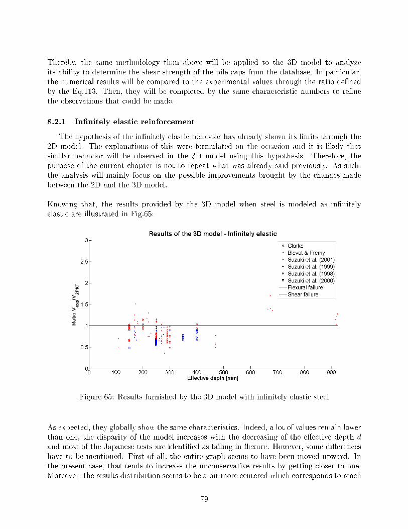
Thereby, the same methodology than above will be applied to the 3D model to analyzeits ability to determine the shear strength of the pile caps from the database. In particular,the numerical results will be compared to the experimental values through the ratio de�nedby the Eq.113. Then, they will be completed by the same characteristic numbers to re�nethe observations that could be made.
8.2.1 In�nitely elastic reinforcement
The hypothesis of the in�nitely elastic behavior has already shown its limits through the2D model. The explanations of this were formulated on the occasion and it is likely thatsimilar behavior will be observed in the 3D model using this hypothesis. Therefore, thepurpose of the current chapter is not to repeat what was already said previously. As such,the analysis will mainly focus on the possible improvements brought by the changes madebetween the 2D and the 3D model.
Knowing that, the results provided by the 3D model when steel is modeled as in�nitelyelastic are illustrated in Fig.65:
Figure 65: Results furnished by the 3D model with in�nitely elastic steel
As expected, they globally show the same characteristics. Indeed, a lot of values remain lowerthan one, the disparity of the model increases with the decreasing of the e�ective depth dand most of the Japanese tests are identi�ed as failing in �exure. However, some di�erenceshave to be mentioned. First of all, the entire graph seems to have been moved upward. Inthe present case, that tends to increase the unconservative results by getting closer to one.Moreover, the results distribution seems to be a bit more centered which corresponds to reach
79
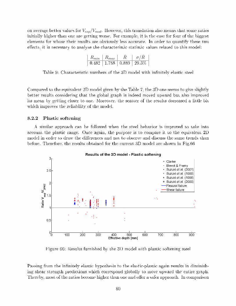
on average better values for Vexp/Vmod. However, this translation also means that some ratiosinitially higher than one are getting worse. For example, it is the case for four of the biggestelements for whose their results are obviously less accurate. In order to quantify these twoe�ects, it is necessary to analyze the characteristic statistic values related to this model:
Rmin Rmax R̄ σ/R̄0.482 1.788 0.889 29.3%
Table 9: Characteristic numbers of the 3D model with in�nitely elastic steel
Compared to the equivalent 2D model given by the Table 7, the 3D one seems to give slightlybetter results considering that the global graph is indeed moved upward but also improvedits mean by getting closer to one. Moreover, the scatter of the results decreased a little bitwhich improves the reliability of the model.
8.2.2 Plastic softening
A similar approach can be followed when the steel behavior is improved to take intoaccount the plastic range. Once again, the purpose is to compare it to the equivalent 2Dmodel in order to draw the di�erences and not to observe and discuss the same trends thanbefore. Therefore, the results obtained for the current 3D model are shown in Fig.66
Figure 66: Results furnished by the 3D model with plastic softening steel
Passing from the in�nitely elastic hypothesis to the elastic-plastic again results in diminish-ing shear strength predictions which correspond globally to move upward the entire graph.Thereby, most of the ratios become higher than one and o�er a safer approach. In comparison
80
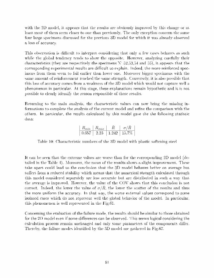
with the 2D model, it appears that the results are obviously improved by this change or atleast most of them seem closer to one than previously. The only exception concern the samefour large specimens discussed for the previous 3D model for which it was already observeda loss of accuracy.
This observation is di�cult to interpret considering that only a few cases behaves as suchwhile the global tendency tends to show the opposite. However, analyzing carefully theircharacteristics (they are respectively the specimens N�52,53,54 and 55), it appears that thecorresponding experimental results are di�cult to explain. Indeed, the more reinforced spec-imens from them seem to fail earlier than lower one. Moreover bigger specimens with thesame amount of reinforcement reached the same strength. Conversely, it is also possible thatthis loss of accuracy comes from a weakness of the 3D model which would not capture well aphenomenon in particular. At this stage, these explanations remain hypothetic and it is notpossible to clearly identify the reason responsible of these results.
Returning to the main analysis, the characteristic values can now bring the missing in-formations to complete the analysis of the current model and re�ne the comparison with theothers. In particular, the results calculated by this model gave the the following statisticdata:
Rmin Rmax R̄ σ/R̄0.657 2.23 1.242 15.7%
Table 10: Characteristic numbers of the 3D model with plastic softening steel
It can be seen that the extreme values are worse than for the corresponding 2D model (de-tailed in the Table 4). Moreover, the mean of the results shows a slight improvement. Thesetake apart could lead to the conclusion that the 3D model behaves better on average butsu�ers from a reduced stability which means that the numerical strength calculated throughthis model considered separately are less accurate but are distributed in such a way thatthe average is improved. However, the value of the COV shows that this conclusion is notcorrect. Indeed, the lower the value of σ/R̄, the lower the scatter of the results and thusthe more uniform the accuracy. In that way, the worse external values correspond to someisolated cases which do not represent well the global behavior of the model. In particular,this phenomenon is well represented in the Fig.61.
Concerning the evaluation of the failure mode, the results should be similar to those obtainedfor the 2D model even if some di�erences can be observed. This seems logical considering thecalculation process remain unchanged and only some parameters of the components di�er.Thereby, the failure modes identi�ed by the 3D model are gathered in Fig.67.
81
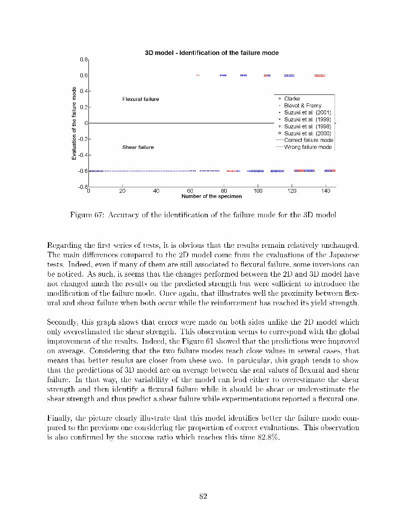
Figure 67: Accuracy of the identi�cation of the failure mode for the 3D model
Regarding the �rst series of tests, it is obvious that the results remain relatively unchanged.The main di�erences compared to the 2D model come from the evaluations of the Japanesetests. Indeed, even if many of them are still associated to �exural failure, some inversions canbe noticed. As such, it seems that the changes performed between the 2D and 3D model havenot changed much the results on the predicted strength but were su�cient to introduce themodi�cation of the failure mode. Once again, that illustrates well the proximity between �ex-ural and shear failure when both occur while the reinforcement has reached its yield strength.
Secondly, this graph shows that errors were made on both sides unlike the 2D model whichonly overestimated the shear strength. This observation seems to correspond with the globalimprovement of the results. Indeed, the Figure 61 showed that the predictions were improvedon average. Considering that the two failure modes reach close values in several cases, thatmeans that better results are closer from these two. In particular, this graph tends to showthat the predictions of 3D model are on average between the real values of �exural and shearfailure. In that way, the variability of the model can lead either to overestimate the shearstrength and then identify a �exural failure while it should be shear or underestimate theshear strength and thus predict a shear failure while experimentations reported a �exural one.
Finally, the picture clearly illustrate that this model identi�es better the failure mode com-pared to the previous one considering the proportion of correct evaluations. This observationis also con�rmed by the success ratio which reaches this time 82.8%.
82
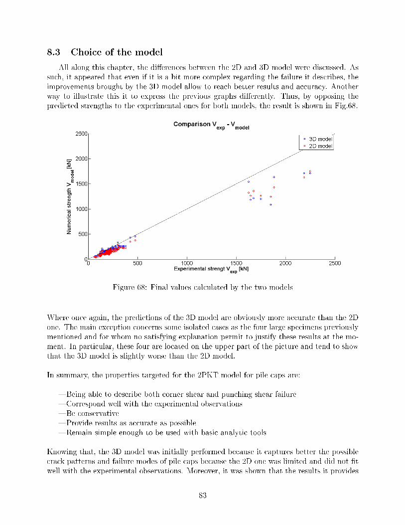
8.3 Choice of the model
All along this chapter, the di�erences between the 2D and 3D model were discussed. Assuch, it appeared that even if it is a bit more complex regarding the failure it describes, theimprovements brought by the 3D model allow to reach better results and accuracy. Anotherway to illustrate this it to express the previous graphs di�erently. Thus, by opposing thepredicted strengths to the experimental ones for both models, the result is shown in Fig.68.
Figure 68: Final values calculated by the two models
Where once again, the predictions of the 3D model are obviously more accurate than the 2Done. The main exception concerns some isolated cases as the four large specimens previouslymentioned and for whom no satisfying explanation permit to justify these results at the mo-ment. In particular, these four are located on the upper part of the picture and tend to showthat the 3D model is slightly worse than the 2D model.
In summary, the properties targeted for the 2PKT model for pile caps are:
� Being able to describe both corner shear and punching shear failure� Correspond well with the experimental observations� Be conservative� Provide results as accurate as possible� Remain simple enough to be used with basic analytic tools
Knowing that, the 3D model was initially performed because it captures better the possiblecrack patterns and failure modes of pile caps because the 2D one was limited and did not �twell with the experimental observations. Moreover, it was shown that the results it provides
83
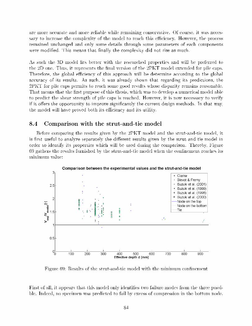
are more accurate and more reliable while remaining conservative. Of course, it was neces-sary to increase the complexity of the model to reach this e�ciency. However, the processremained unchanged and only some details through some parameters of each componentswere modi�ed. This means that �nally the complexity did not rise as much.
As such the 3D model �ts better with the researched properties and will be preferred tothe 2D one. Thus, it represents the �nal version of the 2PKT model extended for pile caps.Therefore, the global e�ciency of this approach will be determine according to the globalaccuracy of its results. As such, it was already shown that regarding its predictions, the2PKT for pile caps permits to reach some good results whose disparity remains reasonable.That means that the �rst purpose of this thesis, which was to develop a numerical model ableto predict the shear strength of pile caps is reached. However, it is now necessary to verifyif it o�ers the opportunity to improve signi�cantly the current design methods. In that way,the model will have proved both its e�ciency and its utility.
8.4 Comparison with the strut-and-tie model
Before comparing the results given by the 2PKT model and the strut-and-tie model, itis �rst useful to analyze separately the di�erent results given by the strut-and-tie model inorder to identify its properties which will be used during the comparison. Thereby, Figure69 gathers the results furnished by the strut-and-tie model when the con�nement reaches itsminimum value:
Figure 69: Results of the strut-and-tie model with the minimum con�nement
First of all, it appears that this model only identi�es two failure modes from the three possi-ble. Indeed, no specimen was predicted to fail by excess of compression in the bottom node.
84
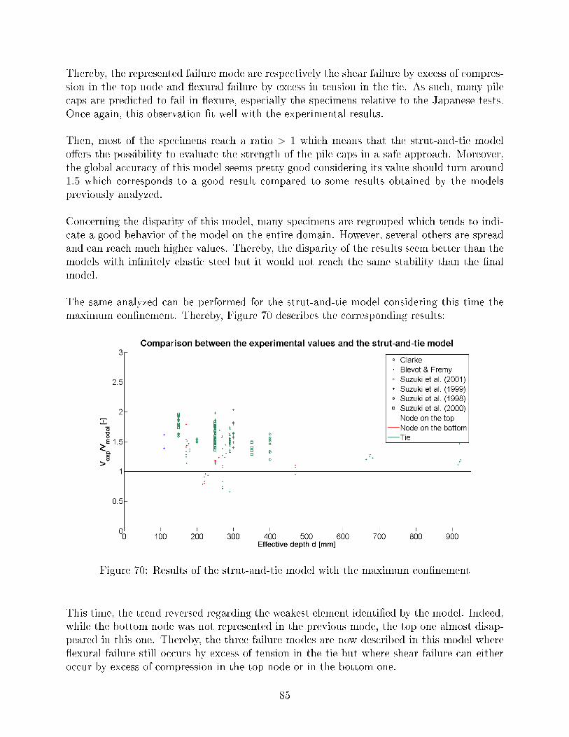
Thereby, the represented failure mode are respectively the shear failure by excess of compres-sion in the top node and �exural failure by excess in tension in the tie. As such, many pilecaps are predicted to fail in �exure, especially the specimens relative to the Japanese tests.Once again, this observation �t well with the experimental results.
Then, most of the specimens reach a ratio > 1 which means that the strut-and-tie modelo�ers the possibility to evaluate the strength of the pile caps in a safe approach. Moreover,the global accuracy of this model seems pretty good considering its value should turn around1.5 which corresponds to a good result compared to some results obtained by the modelspreviously analyzed.
Concerning the disparity of this model, many specimens are regrouped which tends to indi-cate a good behavior of the model on the entire domain. However, several others are spreadand can reach much higher values. Thereby, the disparity of the results seem better than themodels with in�nitely elastic steel but it would not reach the same stability than the �nalmodel.
The same analyzed can be performed for the strut-and-tie model considering this time themaximum con�nement. Thereby, Figure 70 describes the corresponding results:
Figure 70: Results of the strut-and-tie model with the maximum con�nement
This time, the trend reversed regarding the weakest element identi�ed by the model. Indeed,while the bottom node was not represented in the previous mode, the top one almost disap-peared in this one. Thereby, the three failure modes are now described in this model where�exural failure still occurs by excess of tension in the tie but where shear failure can eitheroccur by excess of compression in the top node or in the bottom one.
85
The change on the con�nement only a�ects the specimens which were identi�ed to fail inshear considering only the strength of the top node is increased. As such, these results aresimilar to the previous one knowing that a lot of specimens are supposed to fail in �exureand only some particular predictions has changed.
In particular, that led to lower signi�cantly the strength of some pile caps whose ratio coulddecrease even under one. Thereby it appears that the approach of this model is less safethan the previous one. However, this also led to improve a little the global accuracy of thestrut-and-tie model which seems to be a bit lower than previously. It �nally improved thestability of the model considering the isolated points are now closer to the general trendwhich corresponds to a lower the disparity of the results.
The general observations are now made for both models. It is now possible to start thecomparison strictly speaking. It will consist on opposing the 3D model with strain hardeningsteel to the two strut-and-tie model analyzed above. In order to bring more precise infor-mations, the statistic values of each of them will be used. As such, they are summarized inTable 11:
Strut-and-tie
Con�nement minRmin Rmax R̄ σ/R̄0.908 3.87 1.655 25.8%
Con�nement maxRmin Rmax R̄ σ/R̄0.659 2.03 1.461 19.7%
3D model
Strain hardeningRmin Rmax R̄ σ/R̄0.657 2.23 1.242 15.7%
Table 11: Comparison between the statistic values of each model
Globally, it can be observed that the extreme values of the 3D model seems worse than thoseof the strut-and-tie models. However, it was already mentioned that these only concernedisolated specimens and thus do not represent the global behavior of the model. Therefore, itis more usefull to concentrate on the two last values.
Concerning the average get by each model, it appears that the best one correspond to the3D model. More precisely, it shows an improvement of around 40% compared to the lowerbound of the con�nement and this improvement falls to 20% when compared to the upperbound. The same observation can be made for the coe�cient of variation, where the 3Dmodel can bring some improvements but which remain limited considering the increase ofcomplexity to implement this model. Indeed, the results of the strut-and-tie models were
86
already accurate. In that way, it is di�cult to improve further the predictions and the it willremain low compared to the initial model.
However, it is necessary to necessary to mitigate the results of the strut-and-tie modelsand especially those when the upper bound of the con�nement. Indeed, the assumptionsto consider the maximum value of the con�nement seems a bit unrealistic in the case of acurrent design method. In practical, it is more common to use the lowest value or if thecon�guration requires, something in between. In that way, the results brought by the 3Dmodel are even a bit more accurate which could justify to consider this approach in someparticular cases, for example when an extra precision is necessary. Otherwise, it seems thatthe 3D model would require too much e�ort.
87
9 Parametric studies
Now the 2PKT model for pile caps has proven its reliability, it can be used to evaluatesome properties of the pile caps and especially try to understand the impact of some keyparameters on the strength of the element. It is also the opportunity to check if the behav-iors announced by the model correspond well with reality by comparing the numerical curveswith some experimental results. Finally, it is the occasion to divide the total strength intoeach of its components and to study them separately in order to represent how changes theirrelative importance.
Ideally, such an approach require to consider several specimens whose characteristics areidentical except for the considered parameter. Thus, it is simply necessary to generate ele-ments based on these specimens and vary the component to study. In that way, experimentalresults correspond better with the evaluated situation which permits to easily compare themto the predictions and determine if the model capture well or not the corresponding behavior.
Unfortunately, non of the series of tests performed such an analysis which means that thespecimens have systematically at least two or more di�erent components. As such, it is di�-cult to evaluate the accuracy of the described phenomena considering that the others charac-teristics of the points of comparison do not match perfectly with the predictions. Moreover, itwas previously mentioned that most of the specimens were relatively small compared to realpile caps which increases the risk to obtain disturbed experimental results. Therefore, thesespecimens can potentially bring some more disturbances in the results which could pervertthe observations and thus bring to false conclusions.
However, it is possible to try to diminish these parasitic e�ects by trying to use the biggesttests available and to select those whose characteristics are as close as possible. In that way,the disturbances are limited and it is easier to evaluate the results. Under these conditions,it is also necessary to adapt accordingly the values of the numerical elements. Indeed, themodel has to remain consistent with all the experimental tests used to control the predictions.Thereby, only use the characteristics of one of them would lead to center the results on thisone in particular and would not represent them all. For that reason, the values used throughthe model will correspond to the average of all the tests used as comparatives.
By analyzing the di�erent specimens which constitute the database, it appears that eightof them meet these criteria. In particular, they correspond to the specimens N�52-N�59which represent the biggest pile caps realized by Blévot and Frémy [2]. Thereby, their char-acteristics are given in Figure 71.
88
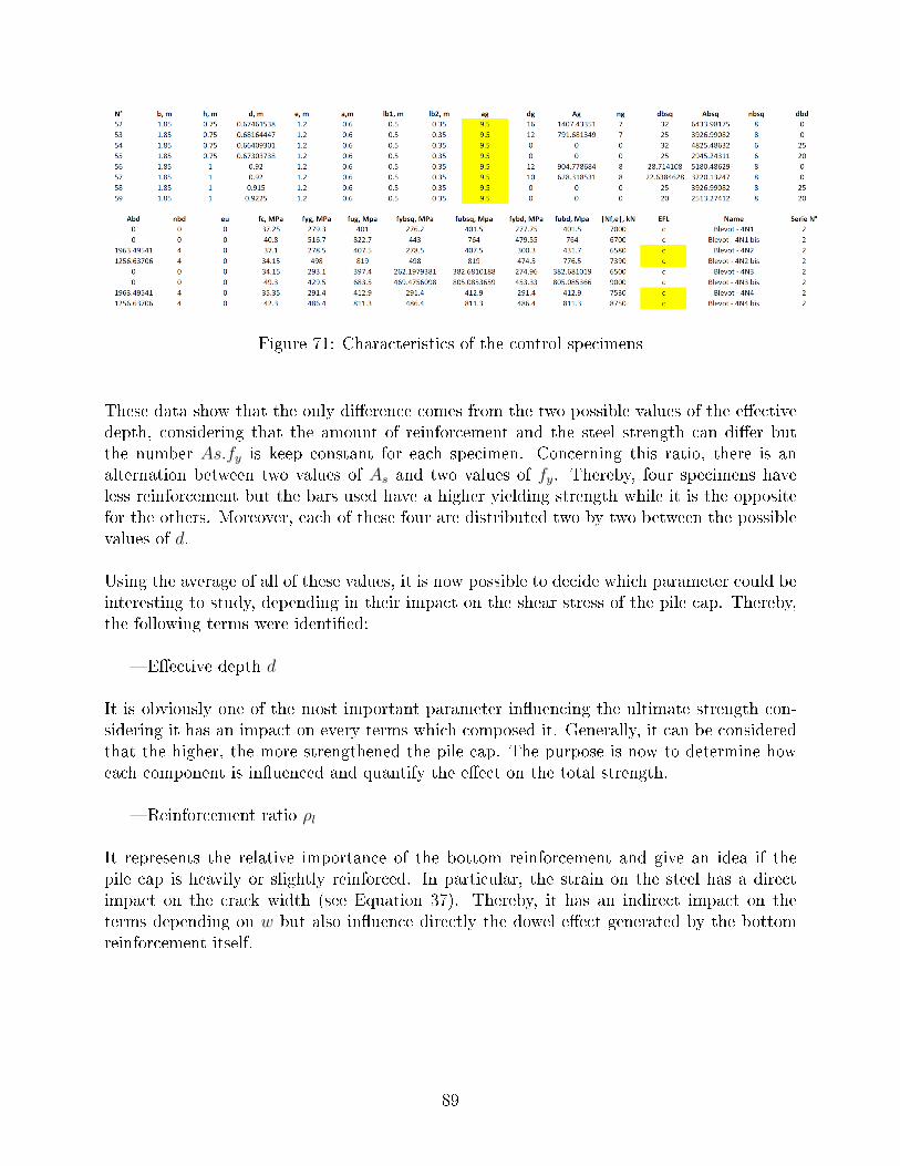
Figure 71: Characteristics of the control specimens
These data show that the only di�erence comes from the two possible values of the e�ectivedepth, considering that the amount of reinforcement and the steel strength can di�er butthe number As.fy is keep constant for each specimen. Concerning this ratio, there is analternation between two values of As and two values of fy. Thereby, four specimens haveless reinforcement but the bars used have a higher yielding strength while it is the oppositefor the others. Moreover, each of these four are distributed two by two between the possiblevalues of d.
Using the average of all of these values, it is now possible to decide which parameter could beinteresting to study, depending in their impact on the shear stress of the pile cap. Thereby,the following terms were identi�ed:
� E�ective depth d
It is obviously one of the most important parameter in�uencing the ultimate strength con-sidering it has an impact on every terms which composed it. Generally, it can be consideredthat the higher, the more strengthened the pile cap. The purpose is now to determine howeach component is in�uenced and quantify the e�ect on the total strength.
� Reinforcement ratio ρl
It represents the relative importance of the bottom reinforcement and give an idea if thepile cap is heavily or slightly reinforced. In particular, the strain on the steel has a directimpact on the crack width (see Equation 37). Thereby, it has an indirect impact on theterms depending on w but also in�uence directly the dowel e�ect generated by the bottomreinforcement itself.
89
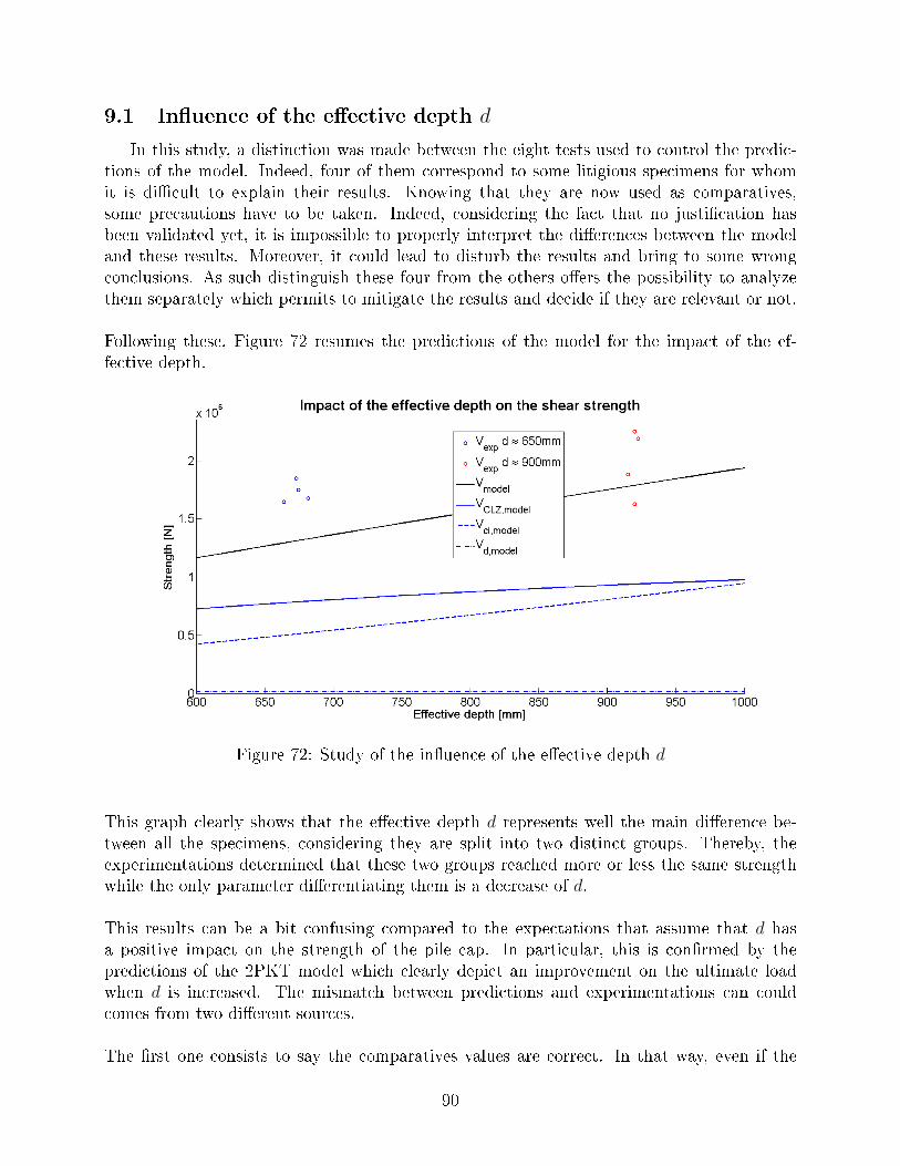
9.1 In�uence of the e�ective depth d
In this study, a distinction was made between the eight tests used to control the predic-tions of the model. Indeed, four of them correspond to some litigious specimens for whomit is di�cult to explain their results. Knowing that they are now used as comparatives,some precautions have to be taken. Indeed, considering the fact that no justi�cation hasbeen validated yet, it is impossible to properly interpret the di�erences between the modeland these results. Moreover, it could lead to disturb the results and bring to some wrongconclusions. As such distinguish these four from the others o�ers the possibility to analyzethem separately which permits to mitigate the results and decide if they are relevant or not.
Following these, Figure 72 resumes the predictions of the model for the impact of the ef-fective depth.
Figure 72: Study of the in�uence of the e�ective depth d
This graph clearly shows that the e�ective depth d represents well the main di�erence be-tween all the specimens, considering they are split into two distinct groups. Thereby, theexperimentations determined that these two groups reached more or less the same strengthwhile the only parameter di�erentiating them is a decrease of d.
This results can be a bit confusing compared to the expectations that assume that d hasa positive impact on the strength of the pile cap. In particular, this is con�rmed by thepredictions of the 2PKT model which clearly depict an improvement on the ultimate loadwhen d is increased. The mismatch between predictions and experimentations can couldcomes from two di�erent sources.
The �rst one consists to say the comparatives values are correct. In that way, even if the
90
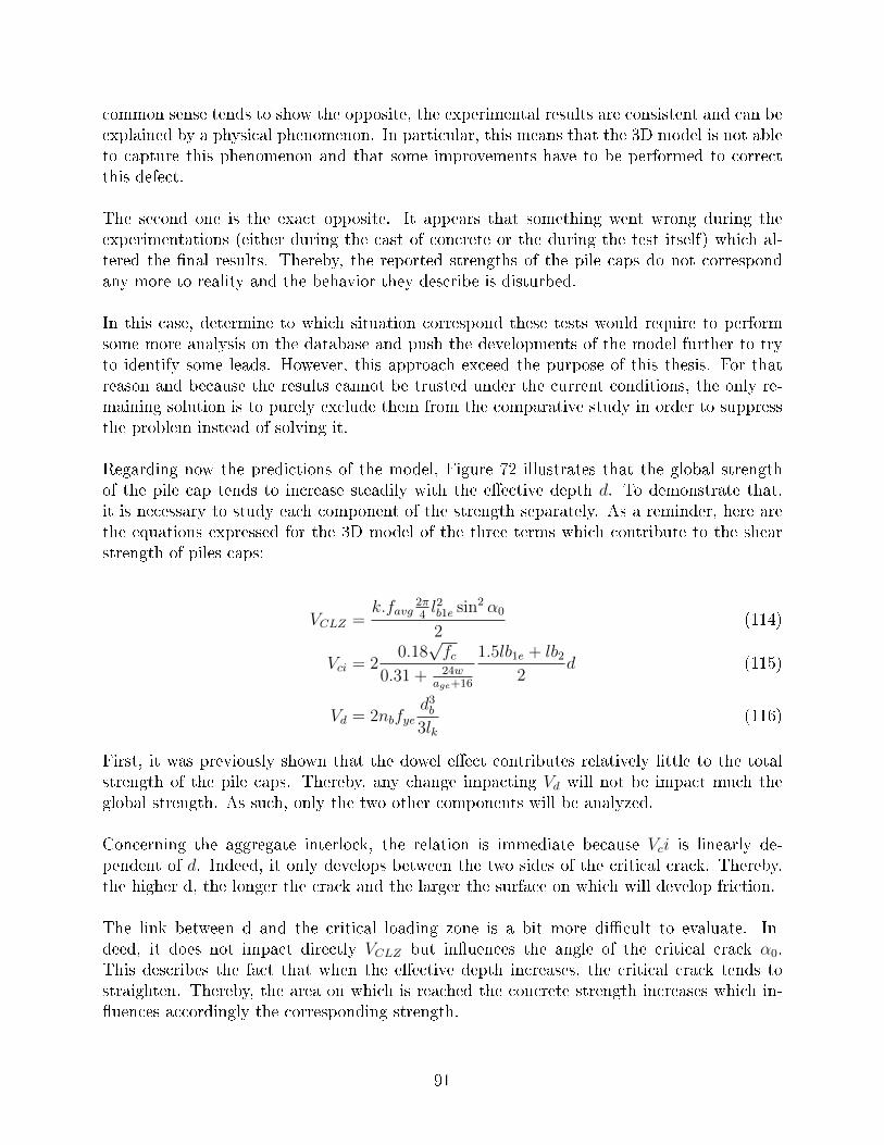
common sense tends to show the opposite, the experimental results are consistent and can beexplained by a physical phenomenon. In particular, this means that the 3D model is not ableto capture this phenomenon and that some improvements have to be performed to correctthis defect.
The second one is the exact opposite. It appears that something went wrong during theexperimentations (either during the cast of concrete or the during the test itself) which al-tered the �nal results. Thereby, the reported strengths of the pile caps do not correspondany more to reality and the behavior they describe is disturbed.
In this case, determine to which situation correspond these tests would require to performsome more analysis on the database and push the developments of the model further to tryto identify some leads. However, this approach exceed the purpose of this thesis. For thatreason and because the results cannot be trusted under the current conditions, the only re-maining solution is to purely exclude them from the comparative study in order to suppressthe problem instead of solving it.
Regarding now the predictions of the model, Figure 72 illustrates that the global strengthof the pile cap tends to increase steadily with the e�ective depth d. To demonstrate that,it is necessary to study each component of the strength separately. As a reminder, here arethe equations expressed for the 3D model of the three terms which contribute to the shearstrength of piles caps:
VCLZ =k.favg
2π4l2b1e sin2 α0
2(114)
Vci = 20.18√fc
0.31 + 24wage+16
1.5lb1e + lb2
2d (115)
Vd = 2nbfyed3b
3lk(116)
First, it was previously shown that the dowel e�ect contributes relatively little to the totalstrength of the pile caps. Thereby, any change impacting Vd will not be impact much theglobal strength. As such, only the two other components will be analyzed.
Concerning the aggregate interlock, the relation is immediate because Vci is linearly de-pendent of d. Indeed, it only develops between the two sides of the critical crack. Thereby,the higher d, the longer the crack and the larger the surface on which will develop friction.
The link between d and the critical loading zone is a bit more di�cult to evaluate. In-deed, it does not impact directly VCLZ but in�uences the angle of the critical crack α0.This describes the fact that when the e�ective depth increases, the critical crack tends tostraighten. Thereby, the area on which is reached the concrete strength increases which in-�uences accordingly the corresponding strength.
91
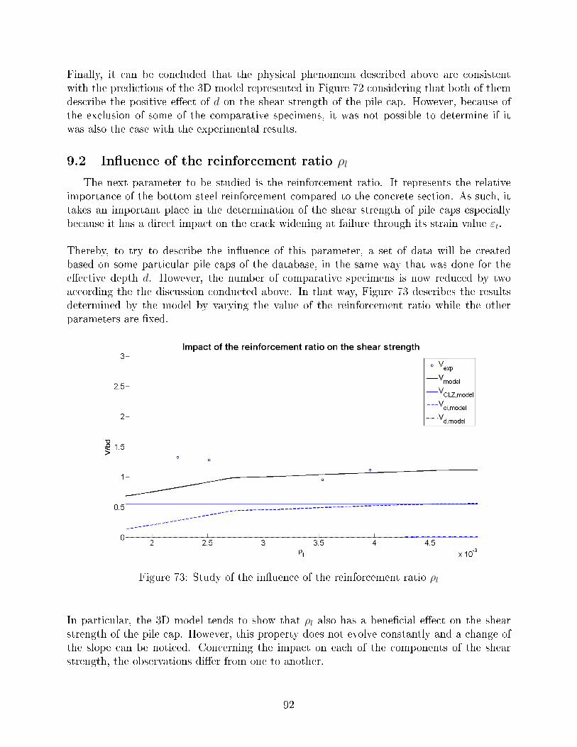
Finally, it can be concluded that the physical phenomena described above are consistentwith the predictions of the 3D model represented in Figure 72 considering that both of themdescribe the positive e�ect of d on the shear strength of the pile cap. However, because ofthe exclusion of some of the comparative specimens, it was not possible to determine if itwas also the case with the experimental results.
9.2 In�uence of the reinforcement ratio ρl
The next parameter to be studied is the reinforcement ratio. It represents the relativeimportance of the bottom steel reinforcement compared to the concrete section. As such, ittakes an important place in the determination of the shear strength of pile caps especiallybecause it has a direct impact on the crack widening at failure through its strain value εt.
Thereby, to try to describe the in�uence of this parameter, a set of data will be createdbased on some particular pile caps of the database, in the same way that was done for thee�ective depth d. However, the number of comparative specimens is now reduced by twoaccording the the discussion conducted above. In that way, Figure 73 describes the resultsdetermined by the model by varying the value of the reinforcement ratio while the otherparameters are �xed.
Figure 73: Study of the in�uence of the reinforcement ratio ρl
In particular, the 3D model tends to show that ρl also has a bene�cial e�ect on the shearstrength of the pile cap. However, this property does not evolve constantly and a change ofthe slope can be noticed. Concerning the impact on each of the components of the shearstrength, the observations di�er from one to another.
92
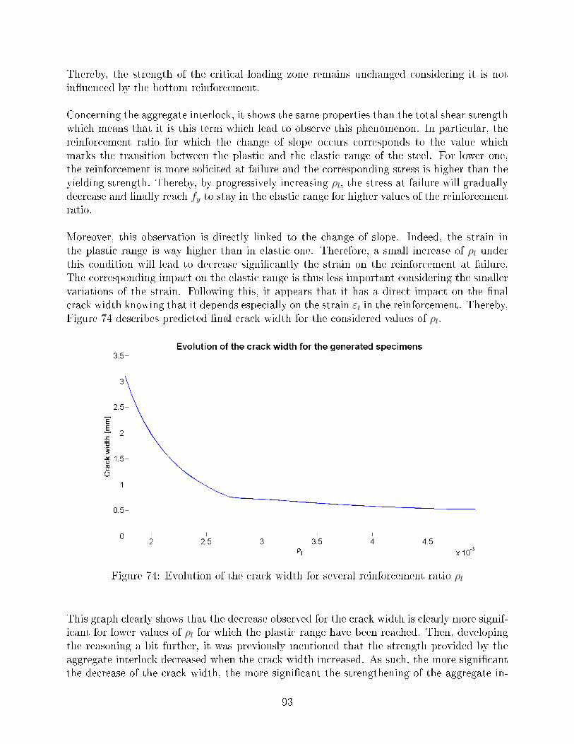
Thereby, the strength of the critical loading zone remains unchanged considering it is notin�uenced by the bottom reinforcement.
Concerning the aggregate interlock, it shows the same properties than the total shear strengthwhich means that it is this term which lead to observe this phenomenon. In particular, thereinforcement ratio for which the change of slope occurs corresponds to the value whichmarks the transition between the plastic and the elastic range of the steel. For lower one,the reinforcement is more solicited at failure and the corresponding stress is higher than theyielding strength. Thereby, by progressively increasing ρl, the stress at failure will graduallydecrease and �nally reach fy to stay in the elastic range for higher values of the reinforcementratio.
Moreover, this observation is directly linked to the change of slope. Indeed, the strain inthe plastic range is way higher than in elastic one. Therefore, a small increase of ρl underthis condition will lead to decrease signi�cantly the strain on the reinforcement at failure.The corresponding impact on the elastic range is thus less important considering the smallervariations of the strain. Following this, it appears that it has a direct impact on the �nalcrack width knowing that it depends especially on the strain εt in the reinforcement. Thereby,Figure 74 describes predicted �nal crack width for the considered values of ρl.
Figure 74: Evolution of the crack width for several reinforcement ratio ρl
This graph clearly shows that the decrease observed for the crack width is clearly more signif-icant for lower values of ρl for which the plastic range have been reached. Then, developingthe reasoning a bit further, it was previously mentioned that the strength provided by theaggregate interlock decreased when the crack width increased. As such, the more signi�cantthe decrease of the crack width, the more signi�cant the strengthening of the aggregate in-
93
terlock. This explains why the slope of Vci is bigger in the plastic range than in the elastic one.
A similar explanation can justify the behavior of the dowel e�ect which is equal to zerountil the reinforcement ratio reaches a su�ciently high value. This particular point corre-sponds once again to the transition between the plastic and the elastic range of the steel.Indeed, the bottom reinforcement is not able to develop a dowel e�ect if it has reached plas-ticity which means that Vd falls 0.
Even if it is not clear in Figure 73, the entrance into the plastic range occurs at the sametime for both the aggregate interlock and the dowel e�ect. However, the fact that Vd remainssmall compared to the other components tends to make di�cult the moment from when itdi�ers from 0
Now the predictions of the 3D model are explained, it is possible to compare them to theexperimental results. However they seem to represent that ρl has no impact on the ultimateload considering that the comparative specimens reaches more or less the same ultimate loadfor di�erent values of the reinforcement ratio. The reason for this is simple: These four pilecaps were designed in such a way that the number As.fy is more or less constant which meansthat the less the reinforcement, the higher the yielding strength. Therefore, these specimensget some extra strength due to this increase which is not represented through the generatedspecimen considering that As.fy progressively decreases with lower values of As.
In conclusion, the di�erences between the comparative specimens does not o�ers the possi-bility to represent experimentally the impact of only the amount of reinforcement. Thereby,this study will be once again limited to discuss the model predictions only without verifyingif it corresponds well to reality.
94
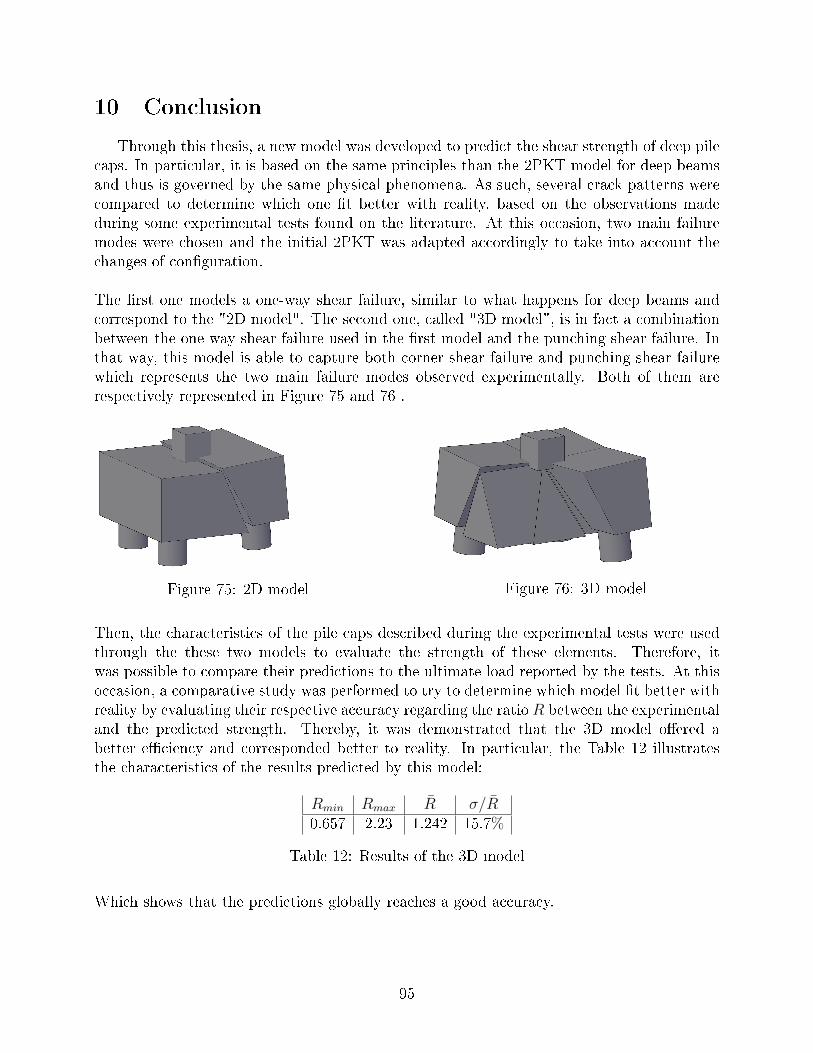
10 Conclusion
Through this thesis, a new model was developed to predict the shear strength of deep pilecaps. In particular, it is based on the same principles than the 2PKT model for deep beamsand thus is governed by the same physical phenomena. As such, several crack patterns werecompared to determine which one �t better with reality, based on the observations madeduring some experimental tests found on the literature. At this occasion, two main failuremodes were chosen and the initial 2PKT was adapted accordingly to take into account thechanges of con�guration.
The �rst one models a one-way shear failure, similar to what happens for deep beams andcorrespond to the "2D model". The second one, called "3D model", is in fact a combinationbetween the one way shear failure used in the �rst model and the punching shear failure. Inthat way, this model is able to capture both corner shear failure and punching shear failurewhich represents the two main failure modes observed experimentally. Both of them arerespectively represented in Figure 75 and 76 .
Figure 75: 2D model Figure 76: 3D model
Then, the characteristics of the pile caps described during the experimental tests were usedthrough the these two models to evaluate the strength of these elements. Therefore, itwas possible to compare their predictions to the ultimate load reported by the tests. At thisoccasion, a comparative study was performed to try to determine which model �t better withreality by evaluating their respective accuracy regarding the ratio R between the experimentaland the predicted strength. Thereby, it was demonstrated that the 3D model o�ered abetter e�ciency and corresponded better to reality. In particular, the Table 12 illustratesthe characteristics of the results predicted by this model:
Rmin Rmax R̄ σ/R̄0.657 2.23 1.242 15.7%
Table 12: Results of the 3D model
Which shows that the predictions globally reaches a good accuracy.
95
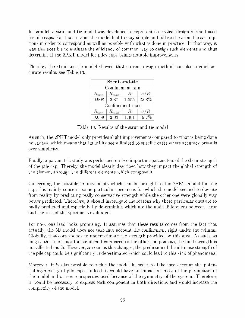
In parallel, a strut-and-tie model was developed to represent a classical design method usedfor pile caps. For that reason, the model had to stay simple and followed reasonable assump-tions in order to correspond as well as possible with what is done in practice. In that way, itwas also possible to evaluate the e�ciency of common way to design such elements and thusdetermine if the 2PKT model for piles caps brings notable improvements.
Thereby, the strut-and-tie model showed that current design method can also predict ac-curate results, see Table 13.
Strut-and-tie
Con�nement minRmin Rmax R̄ σ/R̄0.908 3.87 1.655 25.8%
Con�nement maxRmin Rmax R̄ σ/R̄0.659 2.03 1.461 19.7%
Table 13: Results of the strut-and-tie model
As such, the 2PKT model only provides slight improvements compared to what is being donenowadays, which means that its utility seem limited to speci�c cases where accuracy prevailsover simplicity.
Finally, a parametric study was performed on two important parameters of the shear strengthof the pile cap. Thereby, the model clearly described how they impact the global strength ofthe element through the di�erent elements which compose it.
Concerning the possible improvements which can be brought to the 2PKT model for pilecap, this mainly concerns some particular specimens for which the model seemed to deviatefrom reality by predicting really conservative strength while the other one were globally waybetter predicted. Therefore, it should investigate the reasons why these particular ones are sobadly predicted and especially by determining which are the main di�erences between theseand the rest of the specimens evaluated.
For now, one lead looks promising. It assumes that these results comes from the fact thatactually, the 3D model does not take into account the con�nement right under the column.Globally, that corresponds to underestimate the strength provided by this area. As such, aslong as this one is not too signi�cant compared to the other components, the �nal strength isnot a�ected much. However, as soon as this changes, the prediction of the ultimate strength ofthe pile cap could be signi�cantly underestimated which could lead to this kind of phenomena.
Moreover, it is also possible to re�ne the model in order to take into account the poten-tial asymmetry of pile caps. Indeed, it would have an impact on most of the parameters ofthe model and on some properties used because of the symmetry of the system. Therefore,it would be necessary to express each component in both directions and would increase thecomplexity of the model.
96
References
[1] B. Mihaylov, E. Bentz, and M. Collins, �Two-parameter kinematic theory for shear be-havior of deep beams,� ACI Structural Journal, vol. 110, no. 3, pp. 447�455, 2013. citedBy 1.
[2] J. Blévot and R. Frémy, �Semelles sur pieux,� Annales de l'Institut Technique du bâtimentet des Travaux Publics, vol. 20, pp. 223�279, February 1967.
[3] J. Clarke, �Behaviour and design of pile caps with four piles,� Technical report of theCement and Concrete Association, vol. 42, pp. 1�19, November 1973.
[4] K. Suzuki, K. Otsuki, and T. Tsubata, �In�uence of bar arrangement on ultimate strengthof four-pile caps,� Transactions of the Japan Concrete Institute, vol. 20, pp. 195�202, 1998.
[5] K. Suzuki, K. Otsuki, and T. Tsubata, �Experimental study on four-pile caps with taper,�Transactions of the Japan Concrete Institute, vol. 21, pp. 327�334, 1999.
[6] K. Suzuki, K. Otsuki, and T. Tsuchiya, �In�uence of edge distance on failure mechanismof pile caps,� Transactions of the Japan Concrete Institute, vol. 22, pp. 361�368, 2000.
[7] K. Suzuki and K. Otsuki, �Experimental study on corner shear failure of pile caps,�Transactions of the Japan Concrete Institute, vol. 23, pp. 303�310, 2001.
[8] U. b. Jensen and L. Hoang, �Collapse mechanisms and strength prediction of reinforcedconcrete pile caps,� Engineering Structures, vol. 35, pp. 203�214, 2012. cited By 1.

Appendix
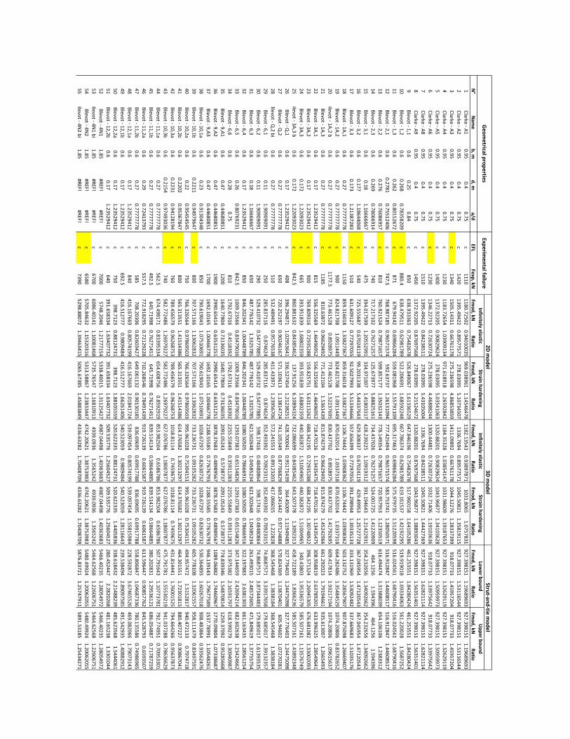
N°
Na
me
b, m
d, m
a/d
EF
LF
ex
p, k
NF
mo
d, k
NR
atio
Fm
od
, kN
Ra
tioF
mo
d, k
NR
atio
Fm
od
, kN
Ra
tioF
mo
d, k
NR
atio
Fm
od
, kN
Ra
tio
1C
lark
e - A
10
.95
0.4
0.7
5c
11
10
11
80
.72
50
20
.94
01
00
35
96
9.0
38
96
11
.14
54
64
78
11
82
.13
54
30
.93
89
78
71
10
31
.80
65
1.0
75
78
31
92
7.3
98
15
11
.19
68
96
93
92
7.3
98
15
11
.19
68
96
93
2C
lark
e - A
20
.95
0.4
0.7
5c
14
20
13
95
.49
42
20
.89
57
75
71
27
8.0
30
95
5.1
07
34
50
71
33
6.7
69
40
.89
57
75
71
10
45
.50
82
11
.35
81
91
15
92
7.3
98
15
11
.53
11
65
44
92
7.3
98
15
11
.53
11
65
44
3C
lark
e - A
30
.95
0.4
0.7
5c
13
40
15
05
.14
31
10
.66
76
11
78
27
5.2
36
59
84
.86
85
38
59
14
11
.09
89
20
.66
76
11
78
10
44
.12
27
61
.28
33
73
99
91
8.0
77
33
1.4
59
57
20
49
18
.07
73
31
.45
95
72
04
4C
lark
e - A
40
.95
0.4
0.7
5c
12
30
11
83
.72
65
41
.03
90
91
34
97
1.6
18
91
81
.26
59
28
42
11
84
.35
32
81
.03
85
41
47
10
31
.98
60
91
.19
18
76
53
92
7.3
98
15
11
.32
62
91
19
92
7.3
98
15
11
.32
62
91
19
5C
lark
e - A
50
.95
0.4
0.7
5c
14
00
13
72
.92
20
50
.90
82
96
24
27
8.0
30
95
5.0
35
41
06
31
32
0.8
82
01
0.9
08
29
62
41
04
3.9
68
77
1.3
41
03
62
89
27
.39
81
51
1.5
09
59
97
39
27
.39
81
51
1.5
09
59
97
3
6C
lark
e - A
60
.95
0.4
0.7
5c
12
30
13
46
.22
71
30
.72
63
07
24
27
5.2
36
59
84
.46
88
82
44
13
00
.44
48
10
.72
63
07
24
10
32
.71
40
61
.19
10
36
36
91
8.0
77
33
1.3
39
75
64
29
18
.07
73
31
.33
97
56
42
7C
lark
e - A
80
.95
0.4
0.7
5c
15
10
13
95
.49
42
20
.84
23
85
11
27
8.0
30
95
5.4
31
05
00
41
33
6.7
69
40
.84
23
85
11
10
45
.50
82
11
.44
42
73
69
92
7.3
98
15
11
.62
82
11
14
92
7.3
98
15
11
.62
82
11
14
8C
lark
e - A
90
.95
0.4
0.7
5c
14
50
13
72
.92
20
50
.87
69
75
68
27
8.0
30
95
5.2
15
24
67
21
32
0.8
82
01
0.8
76
97
56
81
04
3.9
68
77
1.3
88
93
04
39
27
.39
81
51
1.5
63
51
40
19
27
.39
81
51
1.5
63
51
40
1
9B
lev
ot - 1
,10
.60
.25
0.8
4c
85
06
38
.93
33
63
0.7
54
82
67
85
26
.84
90
67
1.6
13
36
52
96
47
.84
61
96
0.7
54
82
67
85
17
.96
01
58
1.6
41
05
28
64
61
.25
35
51
1.8
42
80
42
44
61
.25
35
51
1.8
42
80
42
4
10
Ble
vo
t - 1,2
0.6
0.2
68
0.7
83
58
20
9c
88
0.4
63
8.4
79
51
10
.62
98
17
89
52
2.2
06
69
11
.68
59
22
48
66
7.7
86
37
40
.62
98
17
89
61
9.1
61
53
71
.42
19
22
95
51
9.9
19
01
81
.69
33
40
63
56
1.2
20
02
81
.56
87
25
2
11
Ble
vo
t - 1,3
0.6
0.2
62
0.8
01
52
67
2c
87
16
79
.94
14
20
.69
86
62
84
55
9.0
81
96
81
.55
79
11
09
69
5.3
17
46
30
.69
86
62
84
57
5.9
79
73
51
.51
22
05
98
51
6.0
24
56
11
.68
79
04
16
51
6.0
24
56
11
.68
79
04
16
12
Ble
vo
t - 2,1
0.6
0.2
78
10
.75
51
24
06
c7
47
.57
68
.98
71
85
0.9
65
71
57
45
92
.63
73
71
.26
13
10
94
77
7.4
25
49
40
.96
57
15
74
58
3.7
53
74
11
.28
05
05
71
51
6.9
12
84
71
.44
60
85
17
51
6.9
12
84
71
.44
60
85
17
13
Ble
vo
t - 2,2
0.6
0.2
76
0.7
60
86
95
7c
81
07
60
.92
15
24
0.7
98
71
65
75
99
.85
71
77
1.3
50
32
14
37
78
.14
93
54
0.7
98
71
65
77
20
.95
79
53
1.1
23
50
51
96
16
.49
44
74
1.3
13
88
03
96
54
.10
61
06
1.2
38
33
12
14
Ble
vo
t - 2,3
0.6
0.2
69
0.7
80
66
91
4c
74
07
17
.21
71
02
0.7
62
71
25
71
25
.67
39
77
5.8
88
25
16
17
34
.43
70
26
0.7
62
71
25
75
24
.00
17
25
1.4
12
20
90
94
64
.12
56
1.5
94
39
64
64
.12
56
1.5
94
39
6
15
Ble
vo
t - 3,1
0.6
0.1
81
.16
66
66
67
c4
75
39
4.0
17
59
91
.20
55
29
91
33
4.9
71
00
71
.41
80
33
17
42
8.2
39
22
51
.10
91
93
12
39
1.1
94
64
31
.21
42
29
31
35
4.2
32
65
61
.34
09
26
62
35
4.2
32
65
61
.34
09
26
62
16
Ble
vo
t - 3,2
0.6
0.1
77
1.1
86
44
06
8c
54
07
25
.55
56
87
0.6
70
24
11
99
9.2
03
13
38
5.4
43
37
64
36
29
.30
83
37
0.6
70
24
11
94
29
.49
95
31
.25
72
77
28
36
7.0
45
95
41
.47
12
05
43
36
7.0
45
95
41
.47
12
05
43
17
Ble
vo
t - 3,3
0.6
0.1
73
1.2
13
87
28
3c
51
06
31
.60
91
27
0.7
72
97
05
59
2.5
02
79
93
5.5
13
34
66
65
57
.65
63
99
0.7
72
97
05
53
91
.29
89
44
1.3
03
35
13
33
33
.13
19
69
1.5
30
92
48
23
37
.66
96
83
1.5
10
35
17
6
18
Ble
vo
t - 1A
,10
.60
.27
0.7
77
77
77
8c
11
50
85
9.3
16
01
81
.33
82
73
67
85
9.3
16
01
81
.33
82
73
67
11
06
.74
44
21
.03
90
83
62
11
06
.74
44
21
.03
90
83
62
50
3.1
32
75
22
.28
56
79
07
90
7.8
75
09
81
.26
66
94
07
19
Ble
vo
t - 1A
,20
.60
.27
0.7
77
77
77
8c
90
08
24
.82
17
08
1.0
91
14
49
82
4.8
21
70
81
.09
11
44
98
70
.63
20
14
1.0
33
73
18
87
0.6
32
01
41
.03
37
31
86
64
.28
24
86
1.3
54
84
52
91
07
4.2
08
06
0.8
37
82
65
2
20
Ble
vo
t - 1A
,2 b
is0
.60
.27
0.7
77
77
77
8c
11
77
.57
73
.46
15
28
0.8
92
89
75
77
3.4
61
52
81
.52
23
76
95
83
0.4
37
70
20
.89
28
97
58
30
.43
77
02
1.4
17
92
69
56
09
.41
78
14
1.9
32
17
19
41
07
4.2
08
06
1.0
96
15
63
7
21
Ble
vo
t - 1A
,30
.60
.27
0.7
77
77
77
8c
11
85
81
0.6
38
72
0.9
66
29
49
27
71
.41
21
04
1.5
36
14
39
81
5.8
74
27
90
.96
62
94
92
81
5.8
74
27
91
.45
24
29
66
66
1.2
92
02
31
.79
19
46
61
93
5.6
13
00
71
.26
65
49
3
22
Ble
vo
t - 3A
,10
.60
.17
1.2
35
29
41
2c
81
55
56
.32
55
69
1.4
64
96
95
25
56
.32
55
69
1.4
64
96
95
27
18
.47
01
26
1.1
34
35
47
57
18
.47
01
26
1.1
34
35
47
53
08
.95
88
19
2.6
37
89
20
16
33
.99
63
25
1.2
85
49
64
1
23
Ble
vo
t - 3A
,20
.60
.17
1.2
35
29
41
2c
90
07
69
.80
93
16
0.7
29
35
28
81
59
.82
57
51
5.6
31
13
26
26
88
.34
21
95
0.7
29
35
28
86
88
.34
21
95
1.3
07
48
92
23
96
.57
13
24
2.2
69
45
30
56
76
.68
10
82
1.3
30
02
09
3
24
Ble
vo
t - 3A
,30
.60
.17
21
.22
09
30
23
c6
65
39
3.9
51
83
91
.68
80
23
59
39
3.9
51
83
91
.68
80
23
59
44
0.3
82
87
21
.51
00
49
65
44
0.3
82
87
21
.51
00
49
65
34
0.4
38
03
1.9
53
36
57
95
85
.50
71
61
1.1
35
76
74
9
25
Ble
vo
t - 3A
,3 b
is0
.60
.17
21
.22
09
30
23
c8
42
.58
60
.88
16
32
0.8
43
85
46
21
37
.91
25
66
.10
89
43
24
73
2.0
86
69
90
.84
38
54
62
64
3.5
07
37
81
.30
92
31
34
58
.72
21
89
1.8
36
62
36
58
5.5
07
16
11
.43
89
23
48
26
Ble
vo
t - Q,1
0.6
0.1
71
.23
52
94
12
c4
08
39
6.2
94
87
11
.02
95
36
41
33
6.5
27
45
41
.21
23
82
51
42
8.7
00
04
10
.95
17
14
39
36
4.4
50
09
1.1
19
49
48
53
27
.77
64
03
1.2
44
75
09
83
27
.77
64
03
1.2
44
75
09
8
27
Ble
vo
t - Q,2
0.6
0.2
70
.77
77
77
78
c6
50
72
0.2
52
19
70
.90
24
61
67
57
1.1
03
61
31
.13
81
47
24
74
1.1
05
34
90
.87
70
68
29
66
9.2
41
44
20
.97
12
48
88
57
0.8
24
36
91
.13
87
04
01
60
5.9
46
02
1.0
72
70
28
1
28
Ble
vo
t - Q,2
bis
0.6
0.2
70
.77
77
77
78
c5
10
53
2.4
89
49
10
.95
77
65
38
41
1.4
33
97
11
.23
95
67
06
57
2.2
41
55
30
.89
12
32
03
41
7.0
66
01
51
.22
28
28
36
8.5
45
46
81
.38
38
18
43
68
.54
54
68
1.3
83
81
84
29
Ble
vo
t - 6,1
0.6
0.1
11
.90
90
90
91
c2
50
28
5.8
37
11
60
.87
46
24
28
5.8
37
11
60
.87
46
24
35
2.4
93
39
20
.70
92
33
15
35
2.4
93
39
20
.70
92
33
15
74
.86
87
57
13
.33
91
76
58
17
9.6
85
01
71
.39
13
23
57
30
Ble
vo
t - 6,2
0.6
0.1
11
.90
90
90
91
c2
90
52
9.4
10
73
20
.54
77
78
85
52
9.4
10
73
20
.54
77
78
85
59
8.1
74
16
0.4
84
80
86
45
98
.17
41
60
.48
48
08
64
74
.86
87
57
13
.87
34
44
83
17
9.6
85
01
71
.61
39
35
35
31
Ble
vo
t - 6,3
0.6
0.1
81
.16
66
66
67
c6
50
48
7.7
76
14
21
.33
25
78
54
87
.77
61
42
1.3
32
57
85
62
1.5
02
64
81
.04
58
52
34
62
1.5
02
64
81
.04
58
52
34
26
1.4
93
01
52
.48
57
26
05
47
1.8
49
61
91
.37
75
57
54
32
Ble
vo
t - 6,4
0.6
0.1
71
.23
52
94
12
c8
50
84
6.2
02
34
11
.00
44
87
89
84
6.2
02
34
11
.00
44
87
89
10
80
.50
50
50
.78
66
69
16
10
80
.50
50
50
.78
66
69
16
32
2.1
97
88
32
.63
81
30
36
61
.16
34
35
1.2
85
61
25
4
33
Ble
vo
t - 6,5
0.6
0.2
60
.80
76
92
31
c8
42
.51
00
9.2
35
66
0.8
34
79
01
61
00
9.2
35
66
0.8
34
79
01
61
29
3.0
73
83
0.6
51
54
82
61
29
3.0
73
83
0.6
51
54
82
63
47
.14
46
59
2.4
26
94
21
46
82
.60
26
38
1.2
34
24
66
2
34
Ble
vo
t - 6,6
0.6
0.2
80
.75
c8
10
17
92
.67
31
60
.45
18
39
21
79
2.6
73
16
0.4
51
83
92
22
55
.55
84
90
.35
91
12
83
22
55
.55
84
90
.35
91
12
83
37
3.9
75
38
22
.16
59
17
97
61
8.5
99
27
91
.30
94
09
87
35
Ble
vo
t - 9,A
10
.60
.47
0.4
46
80
85
1c
12
00
16
40
.77
80
40
.73
13
60
35
16
40
.77
80
40
.73
13
60
35
20
91
.05
24
30
.57
38
73
72
09
1.0
52
43
0.5
73
87
37
77
4.8
39
34
61
.54
87
08
14
12
59
.37
09
20
.95
28
56
68
36
Ble
vo
t - 9,A
20
.60
.47
0.4
46
80
85
1c
19
00
29
90
.65
41
40
.63
53
12
51
29
90
.65
41
40
.63
53
12
51
38
78
.37
68
30
.48
98
95
67
38
78
.37
68
30
.48
98
95
67
10
89
.06
88
21
.74
46
09
67
17
70
.09
80
41
.07
33
86
87
37
Ble
vo
t - 9,A
30
.60
.47
0.4
46
80
85
1c
17
00
16
92
.10
16
51
.00
46
67
78
16
92
.10
16
51
.00
46
67
78
21
88
.55
58
50
.77
67
67
93
21
88
.55
58
50
.77
67
67
93
94
6.1
39
14
31
.79
67
75
89
15
37
.78
99
11
.10
54
82
61
38
Ble
vo
t - 10
,1a
0.6
0.2
30
.91
30
43
48
c8
50
79
0.6
19
04
31
.07
51
06
91
79
0.6
19
04
31
.07
51
06
91
10
28
.67
29
70
.82
63
07
32
10
28
.67
29
70
.82
63
07
32
53
0.3
64
89
31
.60
26
70
18
90
8.4
83
86
40
.93
56
24
76
39
Ble
vo
t - 10
,1b
0.6
0.2
21
10
.94
97
96
47
c8
00
70
7.5
71
16
61
.13
06
28
32
70
7.5
71
16
61
.13
06
28
32
73
3.2
36
73
11
.09
10
52
82
73
3.2
36
73
11
.09
10
52
82
60
5.7
78
10
81
.32
06
15
57
95
8.1
11
47
90
.83
49
75
91
40
Ble
vo
t - 10
,2a
0.6
0.2
20
.95
45
45
45
c7
50
76
6.3
26
56
40
.97
86
95
03
76
6.3
26
56
40
.97
86
95
03
99
5.9
61
02
80
.75
30
41
51
99
5.9
61
02
80
.75
30
41
51
49
4.9
57
47
21
.51
52
81
79
40
.47
21
33
0.7
97
47
18
41
Ble
vo
t - 10
,2b
0.6
0.2
20
20
.95
36
78
47
c8
00
56
5.3
13
55
11
.41
51
43
86
56
5.3
13
55
11
.41
51
43
86
61
4.3
76
58
21
.30
21
32
97
61
4.3
76
58
21
.30
21
32
97
46
4.3
01
55
11
.72
30
18
15
88
0.4
07
22
70
.90
86
70
41
42
Ble
vo
t - 10
,3a
0.6
0.2
23
10
.94
12
81
94
c7
60
78
9.4
56
57
90
.96
26
87
53
78
9.4
56
57
90
.96
26
87
53
10
18
.81
11
40
.74
59
67
51
01
8.8
11
14
0.7
45
96
75
43
1.8
14
44
11
.76
00
15
25
79
4.6
64
26
60
.95
63
78
73
43
Ble
vo
t - 10
,3b
0.6
0.2
15
40
.97
49
30
36
c7
40
58
2.7
72
48
61
.26
97
92
27
58
2.7
72
48
61
.26
97
92
27
62
7.0
76
78
61
.18
00
78
77
62
7.0
76
78
61
.18
00
78
77
47
5.7
91
78
11
.55
53
02
19
94
1.0
37
28
80
.78
63
66
29
44
Ble
vo
t - 11
,1a
0.6
0.2
70
.77
77
77
78
c5
62
.56
74
.49
81
71
0.8
33
95
33
46
54
.60
87
56
0.8
59
29
19
85
3.9
82
50
40
.65
86
78
68
53
.98
25
04
0.6
58
67
86
50
7.7
91
64
31
.10
77
37
81
79
2.7
74
95
10
.70
95
33
01
45
Ble
vo
t - 11
,1b
0.6
0.2
70
.77
77
77
78
c4
92
.56
45
.71
99
80
.76
27
14
51
64
5.7
19
98
0.7
62
71
45
18
39
.51
41
34
0.5
86
64
88
58
39
.51
41
34
0.5
86
64
88
53
80
.20
28
31
1.2
95
36
12
16
86
.05
48
87
0.7
17
87
25
9
46
Ble
vo
t - 11
,2a
0.6
0.2
90
.72
41
37
93
c5
57
.57
72
.91
82
95
0.7
21
29
22
87
10
.26
85
46
0.7
84
91
43
99
19
.72
61
39
0.6
06
15
87
91
9.7
26
13
90
.60
61
58
76
13
.59
64
47
0.9
08
57
76
28
45
.52
87
93
0.6
59
35
07
47
Ble
vo
t - 11
,2b
0.6
0.2
70
.77
77
77
78
c5
85
70
8.2
03
06
0.8
26
03
42
76
49
.06
11
32
0.9
01
30
18
58
36
.69
69
50
.69
91
77
88
83
6.6
96
95
0.6
99
17
78
85
58
.80
68
47
1.0
46
87
33
67
80
.13
55
86
0.7
49
86
96
5
48
Ble
vo
t - 12
,1a
0.6
0.1
71
.23
52
94
12
c8
40
41
6.1
67
66
90
.80
57
41
99
41
6.1
67
66
92
.01
84
17
24
53
9.0
97
45
40
.80
57
41
99
53
9.0
97
45
41
.55
81
59
84
22
8.5
92
87
23
.67
46
55
26
46
9.0
82
06
61
.79
07
31
43
49
Ble
vo
t - 12
,1b
0.6
0.1
71
.23
52
94
12
c6
92
.54
16
.51
27
77
0.9
80
94
84
41
6.5
12
77
71
.66
26
14
06
54
0.5
23
05
90
.98
09
48
45
40
.52
30
59
1.2
81
16
64
32
39
.53
84
94
2.8
90
97
58
54
91
.54
29
35
1.4
08
82
91
2
50
Ble
vo
t - 12
,2a
0.6
0.1
71
.23
52
94
12
c7
50
39
8.7
12
30
.88
12
47
31
39
8.7
12
31
.88
10
55
59
52
0.6
22
33
50
.88
12
47
31
52
0.6
22
33
51
.44
05
83
63
38
.61
84
32
2.2
14
88
23
94
85
.62
35
68
1.5
44
40
61
51
Ble
vo
t - 12
,2b
0.6
0.1
71
.23
52
94
12
c6
40
39
1.6
58
33
41
.63
40
77
32
39
1.6
58
33
41
.63
40
77
32
50
9.5
35
77
61
.25
60
45
27
50
9.5
35
77
61
.25
60
45
27
28
0.4
52
44
72
.28
20
26
84
81
.16
52
38
1.3
30
10
44
52
Ble
vo
t - 4N
11
.85
#R
EF
!#
RE
F!
c7
00
05
74
8.2
04
61
.21
77
71
54
53
38
.40
01
51
.31
12
54
27
49
87
.04
49
81
.40
36
36
83
49
87
.04
49
81
.40
36
36
83
54
66
.40
23
51
.28
05
49
72
54
66
.40
23
51
.28
05
49
72
53
Ble
vo
t - 4N
1 b
is1
.85
#R
EF
!#
RE
F!
c6
70
06
08
6.4
01
41
1.1
00
81
46
85
73
5.7
65
47
1.1
68
10
91
34
93
9.0
93
61
.35
65
24
24
93
9.0
93
61
.35
65
24
25
46
4.6
25
68
1.2
26
06
75
15
46
4.6
25
68
1.2
26
06
75
1
54
Ble
vo
t - 4N
21
.85
#R
EF
!#
RE
F!
c6
58
05
70
5.8
46
32
1.1
53
20
31
65
31
3.5
88
67
1.2
38
33
44
74
74
2.2
06
21
1.3
87
53
98
34
74
2.2
06
21
1.3
87
53
98
35
48
0.4
99
24
1.2
00
62
05
55
48
0.4
99
24
1.2
00
62
05
5
55
Ble
vo
t - 4N
2 b
is1
.85
#R
EF
!#
RE
F!
c7
39
05
29
8.8
80
72
1.3
94
63
41
55
06
5.6
73
85
1.4
58
83
84
94
33
6.6
32
82
1.7
04
08
70
94
33
6.6
32
82
1.7
04
08
70
95
87
6.8
37
21
1.2
57
47
91
15
89
1.5
31
85
1.2
54
34
27
1
Up
pe
r bo
un
dG
eo
me
trical p
rop
ertie
sE
xp
erim
en
tal fa
ilure
2D
mo
de
l3
D m
od
el
Stru
t-an
d-tie
mo
de
l
Infin
itely
ela
sticS
train
ha
rde
nin
gIn
finite
ly e
lastic
Stra
in h
ard
en
ing
Low
er b
ou
nd
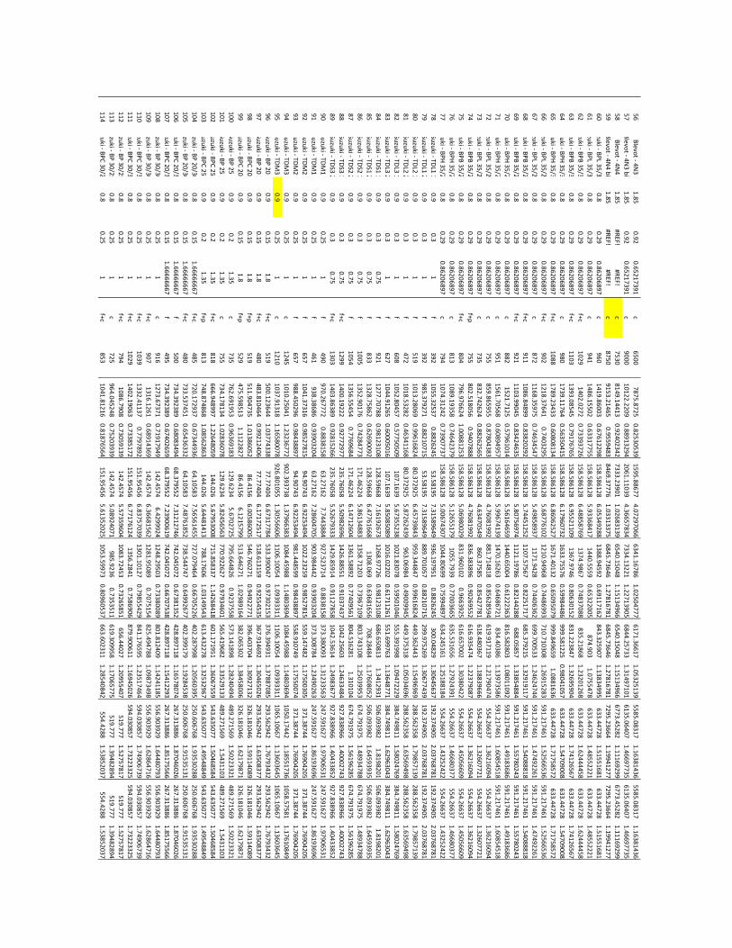
56
Ble
vo
t - 4N
31
.85
0.9
20
.65
21
73
91
c6
50
07
87
5.8
72
50
.82
53
05
39
15
95
.88
67
74
.07
29
70
66
63
41
.16
78
61
.02
50
47
77
61
71
.36
61
71
.05
32
51
39
55
85
.08
31
71
.16
38
14
36
55
85
.08
31
71
.16
38
14
36
57
Ble
vo
t - 4N
3 b
is1
.85
0.9
20
.65
21
73
91
c9
00
01
01
22
.22
09
0.8
89
13
29
42
06
1.1
10
39
4.3
66
57
83
47
33
4.1
32
21
1.2
27
13
90
56
84
4.2
57
33
1.3
14
97
10
16
13
5.0
64
07
1.4
66
97
73
56
13
5.0
64
07
1.4
66
97
73
5
58
Ble
vo
t - 4N
41
.85
#R
EF
!#
RE
F!
c7
53
08
14
9.1
44
13
0.9
24
02
34
27
33
3.2
39
01
1.0
26
83
13
96
54
0.1
50
48
1.1
51
34
96
66
54
0.1
50
48
1.1
51
34
96
66
77
3.4
52
82
1.1
11
69
29
96
77
3.4
52
82
1.1
11
69
29
9
59
Ble
vo
t - 4N
4 b
is1
.85
#R
EF
!#
RE
F!
c8
75
09
15
3.2
14
65
0.9
55
94
83
84
69
.37
77
61
.03
31
33
75
68
45
.73
64
61
.27
81
67
81
68
45
.73
64
61
.27
81
67
81
72
95
.23
66
41
.19
94
12
77
72
95
.23
66
41
.19
94
12
77
60
Su
zuk
i - BP
L 35
/30
10
.80
.29
0.8
62
06
89
7c
96
01
41
9.8
60
03
0.6
76
12
29
81
58
.58
61
28
6.0
53
49
28
81
38
8.9
45
92
0.6
91
17
16
28
43
.32
59
07
1.1
38
34
99
56
33
.44
72
81
.51
55
16
81
63
3.4
47
28
1.5
15
51
68
1
61
Su
zuk
i - BP
L 35
/30
20
.80
.29
0.8
62
06
89
7c
94
11
48
6.1
55
02
0.6
33
17
75
51
58
.58
61
28
5.9
33
68
41
71
44
0.5
55
90
.65
32
20
05
87
4.9
03
1.0
75
54
78
63
3.4
47
28
1.4
85
52
22
16
33
.44
72
81
.48
55
22
21
62
Su
zuk
i - BP
B 3
5/3
0 1
0.8
0.2
90
.86
20
68
97
f+c
10
29
14
02
.02
72
0.7
33
93
72
61
58
.58
61
28
6.4
88
58
76
91
37
4.9
86
70
.74
83
70
88
83
5.2
18
68
1.2
32
01
26
86
33
.44
72
81
.62
44
44
58
63
3.4
47
28
1.6
24
44
45
8
63
Su
zuk
i - BP
B 3
5/3
0 2
0.8
0.2
90
.86
20
68
97
f+c
11
03
13
93
.08
54
50
.79
17
67
65
15
8.5
86
12
86
.95
52
11
09
13
67
.97
46
0.8
06
30
15
28
31
.22
38
47
1.3
26
95
90
46
33
.44
72
81
.74
12
65
67
63
3.4
47
28
1.7
41
26
56
7
64
Su
zuk
i - BP
H 3
5/3
0 1
0.8
0.2
90
.86
20
68
97
c9
80
17
39
.11
76
40
.56
35
04
15
15
8.5
86
12
86
.17
96
07
32
16
33
.75
57
60
.59
98
44
86
99
9.5
81
22
50
.98
04
10
57
63
3.4
47
28
1.5
47
09
00
86
33
.44
72
81
.54
70
90
08
65
Su
zuk
i - BP
H 3
5/3
0 2
0.8
0.2
90
.86
20
68
97
f+c
10
88
17
89
.23
43
30
.60
80
81
34
15
8.5
86
12
86
.86
06
25
27
16
71
.40
13
20
.65
09
50
79
99
9.8
49
65
91
.08
81
63
66
33
.44
72
81
.71
75
85
72
63
3.4
47
28
1.7
17
58
57
2
66
Su
zuk
i - BP
L 35
/25
10
.80
.29
0.8
62
06
89
7f+
c9
02
12
18
.37
64
10
.74
03
29
51
58
.58
61
28
5.6
87
76
10
21
21
0.9
49
68
0.7
44
86
99
37
10
.71
03
08
1.2
69
15
28
35
91
.21
74
61
1.5
25
66
53
65
91
.21
74
61
1.5
25
66
53
6
67
Su
zuk
i - BP
L 35
/25
20
.80
.29
0.8
62
06
89
7c
87
21
16
8.3
59
75
0.7
46
34
54
71
58
.58
61
28
5.4
98
58
93
71
17
1.9
42
80
.74
40
63
62
69
9.7
00
53
31
.24
62
47
44
59
1.2
17
46
11
.47
49
22
61
59
1.2
17
46
11
.47
49
22
61
68
Su
zuk
i - BP
B 3
5/2
5 1
0.8
0.2
90
.86
20
68
97
f+c
91
11
08
6.8
48
99
0.8
38
20
29
21
58
.58
61
28
5.7
44
51
25
21
10
7.5
75
67
0.8
22
51
71
76
85
.37
92
15
1.3
29
19
11
75
91
.21
74
61
1.5
40
88
81
85
91
.21
74
61
1.5
40
88
81
8
69
Su
zuk
i - BP
B 3
5/2
5 2
0.8
0.2
90
.86
20
68
97
f+c
92
11
10
3.9
90
45
0.8
34
24
63
51
58
.58
61
28
5.8
07
56
97
41
12
1.1
97
86
0.8
21
44
28
86
88
.05
85
71
.33
85
48
84
59
1.2
17
46
11
.55
78
02
43
59
1.2
17
46
11
.55
78
02
43
70
Su
zuk
i - BP
H 3
5/2
5 1
0.8
0.2
90
.86
20
68
97
c8
82
15
21
.71
25
0.5
79
61
01
41
58
.58
61
28
5.5
61
64
65
91
44
0.6
50
04
0.6
12
22
36
38
16
.58
28
03
1.0
80
11
09
25
91
.21
74
61
1.4
91
83
68
65
91
.21
74
61
1.4
91
83
68
6
71
Su
zuk
i - BP
H 3
5/2
5 2
0.8
0.2
90
.86
20
68
97
c9
51
15
61
.70
56
80
.60
89
49
57
15
8.5
86
12
85
.99
67
41
39
14
70
.16
26
30
.64
68
67
21
83
4.4
03
86
1.1
39
73
58
65
91
.21
74
61
1.6
08
54
51
85
91
.21
74
61
1.6
08
54
51
8
72
Su
zuk
i - BP
L 35
/20
10
.80
.29
0.8
62
06
89
7c
75
58
59
.86
59
55
0.8
78
04
38
31
58
.58
61
28
4.7
60
81
99
28
81
.71
48
18
0.8
56
28
59
46
19
.91
71
19
1.2
17
90
47
45
54
.26
63
71
.36
21
60
94
55
4.2
66
37
1.3
62
16
09
4
73
Su
zuk
i - BP
L 35
/20
20
.80
.29
0.8
62
06
89
7c
73
58
32
.74
26
24
0.8
82
62
56
51
58
.58
61
28
4.6
34
70
54
98
60
.37
58
50
.85
42
77
81
61
8.4
80
36
71
.18
83
96
66
55
4.2
66
37
1.3
26
07
72
15
54
.26
63
71
.32
60
77
21
74
Su
zuk
i - BP
B 3
5/2
0 1
0.8
0.2
90
.86
20
68
97
f+p
75
58
02
.51
80
56
0.9
40
78
88
15
8.5
86
12
84
.76
08
19
92
83
6.3
83
89
60
.90
26
95
52
61
6.9
35
47
41
.22
37
90
87
55
4.2
66
37
1.3
62
16
09
45
54
.26
63
71
.36
21
60
94
75
Su
zuk
i - BP
B 3
5/2
0 2
0.8
0.2
90
.86
20
68
97
f+c
80
47
96
.97
66
24
1.0
08
81
25
31
58
.58
61
28
5.0
69
80
02
98
31
.96
01
02
0.9
66
39
25
61
6.6
57
00
21
.30
38
04
22
55
4.2
66
37
1.4
50
56
60
95
54
.26
63
71
.45
05
66
09
76
Su
zuk
i - BP
H 3
5/2
0 1
0.8
0.2
90
.86
20
68
97
c8
13
10
89
.19
35
80
.74
64
23
79
15
8.5
86
12
85
.12
65
51
79
10
55
.79
39
0.7
70
03
66
56
35
.53
16
56
1.2
79
24
39
15
54
.26
63
71
.46
68
03
77
55
4.2
66
37
1.4
66
80
37
7
77
Su
zuk
i - BP
H 3
5/2
0 2
0.8
0.2
90
.86
20
68
97
c7
94
10
74
.31
24
20
.73
90
77
37
15
8.5
86
12
85
.00
67
43
07
10
44
.80
69
90
.75
99
48
97
63
4.2
45
16
11
.25
18
81
84
55
4.2
66
37
1.4
32
52
42
25
54
.26
63
71
.43
25
24
22
78
Su
zuk
i - TD
L1 1
0.9
0.3
1f
39
21
05
5.3
25
37
0.8
82
62
45
53
.58
19
57
.31
58
96
49
93
6.1
97
95
10
.88
26
24
53
00
.04
82
91
.30
64
56
37
19
2.3
74
90
52
.03
76
87
81
19
2.3
74
90
52
.03
76
87
81
79
Su
zuk
i - TD
L1 2
0.9
0.3
1f
39
29
85
.37
92
71
0.8
82
10
71
55
3.5
81
95
7.3
15
89
64
98
89
.70
10
57
0.8
82
10
71
52
99
.97
52
69
1.3
06
77
43
91
92
.37
49
05
2.0
37
68
78
11
92
.37
49
05
2.0
37
68
78
1
80
Su
zuk
i - TD
L2 1
0.9
0.3
1f
51
91
01
3.2
80
69
0.9
96
16
82
48
0.3
72
92
56
.45
73
98
43
95
9.3
44
84
70
.99
61
68
24
44
9.3
62
44
31
.15
49
69
69
28
8.5
62
35
81
.79
85
71
39
28
8.5
62
35
81
.79
85
71
39
81
Su
zuk
i - TD
L2 2
0.9
0.3
1f
47
21
01
8.5
32
82
0.4
63
41
16
88
0.3
72
92
55
.87
26
24
39
96
3.0
69
84
0.4
90
09
94
54
49
.37
53
18
1.0
50
34
69
62
88
.56
23
58
1.6
35
69
49
82
88
.56
23
58
1.6
35
69
49
8
82
Su
zuk
i - TD
L3 1
0.9
0.3
1f
60
81
05
2.8
04
57
0.5
77
50
50
91
07
.16
39
5.6
73
55
23
81
02
1.8
30
78
0.5
95
01
04
65
55
.39
19
98
1.0
94
72
22
93
84
.74
98
11
1.5
80
24
76
93
84
.74
98
11
1.5
80
24
76
9
83
Su
zuk
i - TD
L3 2
0.9
0.3
1f
62
71
04
4.9
12
65
0.6
00
05
01
61
07
.16
39
5.8
50
85
08
91
01
6.0
22
02
0.6
17
11
26
15
51
.69
97
63
1.1
36
48
77
13
84
.74
98
11
1.6
29
63
04
33
84
.74
98
11
1.6
29
63
04
3
84
Su
zuk
i - TD
S1
10
.90
.30
.75
f9
21
12
77
.70
78
80
.98
12
31
08
12
8.5
96
68
7.1
61
92
67
31
26
8.9
77
26
0.9
81
23
10
86
86
.65
08
13
1.3
41
29
31
50
6.0
93
98
21
.81
98
20
15
06
.09
39
82
1.8
19
82
01
85
Su
zuk
i - TD
S1
20
.90
.30
.75
f8
33
13
28
.75
86
20
.62
69
00
92
12
8.5
96
68
6.4
77
61
66
81
30
8.0
69
0.6
36
81
65
67
08
.28
48
41
.17
60
80
52
50
6.0
93
98
21
.64
59
39
35
50
6.0
93
98
21
.64
59
39
35
86
Su
zuk
i - TD
S2
10
.90
.30
.75
f1
00
51
35
2.9
01
76
0.7
42
84
77
31
71
.46
22
45
.86
13
48
83
13
58
.71
20
30
.73
96
71
09
80
3.7
43
10
81
.25
03
99
53
67
4.7
91
97
51
.48
93
47
88
67
4.7
91
97
51
.48
93
47
88
87
Su
zuk
i - TD
S2
20
.90
.30
.75
f1
05
41
35
6.5
54
54
0.7
76
96
84
17
1.4
62
24
6.1
47
12
60
41
36
1.5
88
92
0.7
74
09
56
18
04
.51
62
81
1.3
10
10
46
74
.79
19
75
1.5
61
96
28
56
74
.79
19
75
1.5
61
96
28
5
88
Su
zuk
i - TD
S3
10
.90
.30
.75
f+c
12
99
14
00
.19
22
20
.92
77
29
77
23
5.7
60
58
5.5
09
82
69
61
42
6.8
85
51
0.9
10
37
43
71
04
2.2
56
03
1.2
46
33
48
49
27
.83
89
66
1.4
00
02
74
39
27
.83
89
66
1.4
00
02
74
3
89
Su
zuk
i - TD
S3
20
.90
.30
.75
f+c
13
03
14
03
.86
38
90
.92
81
52
66
23
5.7
60
58
5.5
26
79
33
31
42
9.8
59
14
0.9
11
27
85
81
04
2.5
36
14
1.2
49
83
67
79
27
.83
89
66
1.4
04
33
85
29
27
.83
89
66
1.4
04
33
85
2
90
Su
zuk
i - TD
M1
10
.90
.25
1f
49
09
70
.26
77
72
0.8
83
81
58
63
.27
16
27
.74
43
88
49
27
.52
37
14
0.8
83
81
58
37
3.3
80
09
31
.31
23
35
63
24
7.5
91
62
71
.97
90
65
31
24
7.5
91
62
71
.97
90
65
31
91
Su
zuk
i - TD
M1
20
.90
.25
1f
46
19
38
.38
68
60
.93
90
32
04
63
.27
16
27
.28
60
47
05
90
3.9
84
44
20
.93
90
32
04
37
3.3
08
78
41
.23
49
02
63
24
7.5
91
62
71
.86
19
36
96
24
7.5
91
62
71
.86
19
36
96
92
Su
zuk
i - TD
M2
10
.90
.25
1f
65
71
04
1.3
73
16
0.9
85
27
81
59
4.9
07
43
6.9
22
53
49
41
02
2.2
32
59
0.9
85
27
81
55
59
.14
74
82
1.1
75
00
30
53
71
.38
74
41
.76
90
42
05
37
1.3
87
44
1.7
69
04
20
5
93
Su
zuk
i - TD
M2
20
.90
.25
1f
65
79
88
.45
02
96
0.9
84
38
89
79
4.9
07
43
6.9
22
53
49
49
81
.44
85
99
0.9
84
38
89
75
58
.91
07
49
1.1
75
50
07
43
71
.38
74
41
.76
90
42
05
37
1.3
87
44
1.7
69
04
20
5
94
Su
zuk
i - TD
M3
10
.90
.25
1c
12
45
10
10
.25
04
11
.23
23
67
72
90
2.3
93
73
81
.37
96
63
83
10
84
.45
98
81
.14
80
36
94
10
84
.45
98
81
.14
80
36
94
10
50
.17
44
21
.18
55
17
36
10
58
.57
58
11
.17
61
08
49
95
Su
zuk
i - TD
M3
20
.90
.25
1c
12
10
10
37
.91
31
81
.16
58
00
78
92
6.8
01
05
51
.30
55
66
06
11
06
.10
05
41
.09
39
33
11
11
06
.10
05
41
.09
39
33
11
10
65
.10
66
71
.13
60
36
45
10
65
.10
66
71
.13
60
36
45
96
Su
zuk
i - BP
20
10
.90
.15
1.8
f+c
51
95
00
.12
36
44
1.0
37
74
33
87
7.7
74
04
6.6
73
17
78
45
33
.39
00
47
0.9
73
02
15
33
76
.39
49
31
1.3
78
87
08
52
93
.56
29
42
1.7
67
93
43
22
93
.56
29
42
1.7
67
93
43
2
97
Su
zuk
i - BP
20
20
.90
.15
1.8
f+c
48
04
83
.81
04
64
0.9
92
12
40
67
7.7
74
04
6.1
71
72
51
75
18
.61
31
59
0.9
25
54
53
53
67
.91
46
92
1.3
04
65
02
62
93
.56
29
42
1.6
35
08
37
72
93
.56
29
42
1.6
35
08
37
7
98
Su
zuk
i - BP
C 2
0 1
0.9
0.1
51
.8f+
p5
19
51
1.9
04
73
51
.01
38
60
52
86
.41
56
6.0
05
86
00
55
46
.76
02
71
0.9
49
22
77
13
96
.40
37
04
1.3
09
27
13
23
26
.18
10
46
1.5
91
14
08
93
26
.18
10
46
1.5
91
14
08
9
99
Su
zuk
i - BP
C 2
0 2
0.9
0.1
51
.8f+
p5
29
47
5.5
98
51
31
.11
22
82
78
6.4
15
66
.12
15
79
95
13
.64
62
71
1.0
29
89
16
43
82
.06
53
02
1.3
84
58
00
63
26
.18
10
46
1.6
21
79
87
13
26
.18
10
46
1.6
21
79
87
1
10
0S
uzu
ki - B
P 2
5 1
0.9
0.2
1.3
5c
73
57
62
.69
19
53
0.9
63
69
18
31
29
.62
34
5.6
70
27
25
79
5.6
64
82
60
.92
37
55
85
73
.14
18
98
1.2
82
40
49
44
89
.27
15
69
1.5
02
23
32
14
89
.27
15
69
1.5
02
23
32
1
10
1S
uzu
ki - B
P 2
5 2
0.9
0.2
1.3
5c
75
57
34
.17
81
34
1.0
28
36
07
81
29
.62
34
5.8
24
56
56
37
70
.92
26
27
0.9
79
34
60
15
65
.41
96
82
1.3
35
29
13
34
89
.27
15
69
1.5
43
11
03
48
9.2
71
56
91
.54
31
10
3
10
2S
uzu
ki - B
PC
25
10
.90
.21
.35
f+c
81
86
66
.94
89
97
1.2
26
48
05
91
44
.02
65
.67
95
30
08
71
5.8
58
33
71
.14
26
84
18
60
1.1
71
95
11
.36
06
75
59
54
3.6
35
07
71
.50
46
85
84
54
3.6
35
07
71
.50
46
85
84
10
3S
uzu
ki - B
PC
25
20
.90
.21
.35
f+p
81
37
48
.87
48
68
1.0
85
62
86
31
44
.02
65
.64
48
14
13
78
8.1
76
06
1.0
31
49
54
36
13
.43
22
78
1.3
25
32
96
75
43
.63
50
77
1.4
95
48
84
95
43
.63
50
77
1.4
95
48
84
9
10
4S
uzu
ki - B
P 2
0/3
0 1
0.8
0.1
51
.66
66
66
67
f+c
48
57
20
.17
29
37
0.6
73
44
93
66
4.1
05
83
7.5
65
61
45
57
27
.07
94
64
0.6
67
05
22
64
02
.28
79
98
1.2
05
60
39
52
50
.60
67
68
1.9
35
30
28
82
50
.60
67
68
1.9
35
30
28
8
10
5S
uzu
ki - B
P 2
0/3
0 2
0.8
0.1
51
.66
66
66
67
f+c
48
07
33
.53
74
51
0.6
54
36
33
26
4.1
05
83
7.4
87
61
85
27
38
.54
47
47
0.6
49
92
67
74
02
.39
91
79
1.1
92
84
53
82
50
.60
67
68
1.9
15
35
13
12
50
.60
67
68
1.9
15
35
13
1
10
6S
uzu
ki - B
PC
20
/30
10
.80
.15
1.6
66
66
66
7f
50
07
34
.39
23
89
0.6
80
83
49
46
8.3
79
55
27
.31
21
27
46
74
2.0
45
07
20
.67
38
13
52
42
8.8
97
11
81
.16
57
80
74
26
7.3
13
88
61
.87
04
60
26
26
7.3
13
88
61
.87
04
60
26
10
7S
uzu
ki - B
PC
20
/30
20
.80
.15
1.6
66
66
66
7f
49
57
34
.39
23
89
0.6
74
02
65
96
8.3
79
55
27
.23
90
06
19
74
2.0
45
07
20
.66
70
75
38
42
8.8
97
11
81
.15
41
22
93
26
7.3
13
88
61
.85
17
55
66
26
7.3
13
88
61
.85
17
55
66
10
8S
uzu
ki - B
P 3
0/3
0 1
0.8
0.2
51
c9
16
12
73
.67
37
10
.71
91
79
49
14
2.4
57
46
.42
99
92
41
24
8.2
95
03
0.7
33
80
08
98
01
.81
24
09
1.1
42
41
18
55
56
.90
39
29
1.6
44
80
79
35
56
.90
39
29
1.6
44
80
79
3
10
9S
uzu
ki - B
P 3
0/3
0 2
0.8
0.2
51
f+c
90
71
31
6.1
26
10
.68
91
43
69
14
2.4
57
46
.36
68
15
62
12
81
.95
08
90
.70
75
15
48
25
.49
47
88
1.0
98
73
49
85
56
.90
39
29
1.6
28
64
71
65
56
.90
39
29
1.6
28
64
71
6
11
0S
uzu
ki - B
PC
30
/30
10
.80
.25
1f+
c1
03
91
33
2.4
11
37
0.7
79
78
92
15
1.9
54
56
6.8
37
57
03
91
30
1.1
01
27
0.7
98
55
42
98
41
.17
65
95
1.2
35
17
46
45
94
.03
08
57
1.7
49
06
73
95
94
.03
08
57
1.7
49
06
73
9
11
1S
uzu
ki - B
PC
30
/30
20
.80
.25
1f+
c1
02
91
40
2.1
90
63
0.7
33
85
17
21
51
.95
45
66
.77
17
61
24
13
56
.28
41
0.7
58
69
06
87
9.9
00
61
11
.16
94
50
26
59
4.0
30
85
71
.73
22
33
25
59
4.0
30
85
71
.73
22
33
25
11
2S
uzu
ki - B
P 3
0/2
5 1
0.8
0.2
51
f+c
79
41
08
6.7
90
80
.73
05
91
39
14
2.4
57
45
.57
35
96
04
10
83
.72
45
30
.73
26
58
51
65
6.4
40
27
1.2
09
55
40
75
19
.77
71
.52
75
78
17
51
9.7
77
1.5
27
57
81
7
11
3S
uzu
ki - B
P 3
0/2
5 2
0.8
0.2
51
c7
25
96
4.0
45
24
80
.75
20
39
39
14
2.4
57
45
.08
92
40
71
98
5.9
23
60
.73
53
51
16
19
.30
99
58
1.1
70
65
77
55
19
.77
71
.39
48
28
94
51
9.7
77
1.3
94
82
89
4
11
4S
uzu
ki - B
PC
30
/25
10
.80
.25
1f+
c8
53
10
41
.81
21
60
.81
87
65
64
15
1.9
54
56
5.6
13
52
02
51
05
3.5
99
73
0.8
09
60
53
76
63
.60
23
11
1.2
85
40
84
25
54
.42
88
1.5
38
52
03
75
54
.42
88
1.5
38
52
03
7
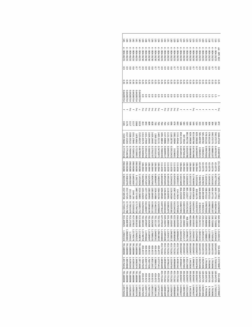
11
5S
uzu
ki - B
PC
30
/25
20
.80
.25
1f+
c8
72
10
44
.47
32
40
.83
48
70
61
51
.95
45
65
.73
85
57
63
10
55
.72
85
20
.82
59
69
92
66
4.2
84
12
41
.31
26
91
31
55
4.4
28
81
.57
27
89
87
55
4.4
28
81
.57
27
89
87
11
6S
uzu
ki - B
DA
20
/25
/70
10
.70
.15
1.5
f2
94
59
0.5
75
77
50
.49
78
19
27
42
.43
77
66
.92
77
92
61
60
9.1
47
73
10
.48
26
41
54
25
8.7
23
00
81
.13
63
50
43
16
9.6
45
73
51
.73
30
23
23
16
9.6
45
73
51
.73
30
23
23
11
7S
uzu
ki - B
DA
20
/25
/70
20
.70
.15
1.5
f3
04
59
0.5
75
77
50
.98
88
12
07
42
.43
77
67
.16
34
31
81
60
9.1
47
73
10
.98
88
12
07
25
8.7
23
00
81
.17
50
01
81
69
.64
57
35
1.7
91
96
96
16
9.6
45
73
51
.79
19
69
6
11
8S
uzu
ki - B
DA
20
/25
/80
10
.80
.15
1.5
f3
04
57
8.5
01
22
60
.99
07
05
65
42
.43
77
67
.16
34
31
81
59
8.9
73
22
20
.99
07
05
65
25
8.9
68
40
61
.17
38
88
37
16
9.6
45
73
51
.79
19
69
61
69
.64
57
35
1.7
91
96
96
11
9S
uzu
ki - B
DA
20
/25
/80
20
.80
.15
1.5
f3
04
57
8.5
01
22
60
.99
07
05
65
42
.43
77
67
.16
34
31
81
59
8.9
73
22
20
.99
07
05
65
25
8.9
68
40
61
.17
38
88
37
16
9.6
45
73
51
.79
19
69
61
69
.64
57
35
1.7
91
96
96
12
0S
uzu
ki - B
DA
20
/25
/90
10
.90
.15
1.5
f3
33
58
5.4
09
78
20
.90
63
52
14
2.4
37
76
7.8
46
78
55
60
4.8
91
90
90
.90
63
52
12
59
.24
15
51
1.2
84
51
63
11
69
.64
57
35
1.9
62
91
40
61
69
.64
57
35
1.9
62
91
40
6
12
1S
uzu
ki - B
DA
20
/25
/90
20
.90
.15
1.5
f3
33
58
5.4
09
78
20
.90
63
52
14
2.4
37
76
7.8
46
78
55
60
4.8
91
90
90
.90
63
52
12
59
.24
15
51
1.2
84
51
63
11
69
.64
57
35
1.9
62
91
40
61
69
.64
57
35
1.9
62
91
40
6
12
2S
uzu
ki - B
DA
30
/20
/70
10
.70
.25
0.9
f5
34
82
9.1
99
02
80
.64
39
94
97
10
6.0
94
45
.03
32
53
48
39
.66
17
60
.63
59
70
37
46
2.6
18
24
41
.15
42
99
48
39
3.8
20
45
71
.35
59
47
84
39
3.8
20
45
71
.35
59
47
84
12
3S
uzu
ki - B
DA
30
/20
/70
20
.70
.25
0.9
f+c
54
98
15
.00
57
68
0.6
73
61
48
61
06
.09
44
5.1
74
63
69
38
28
.61
08
16
0.6
62
55
47
14
60
.55
30
32
1.1
92
04
51
33
93
.82
04
57
1.3
94
03
62
73
93
.82
04
57
1.3
94
03
62
7
12
4S
uzu
ki - B
DA
30
/20
/80
10
.80
.25
0.9
f5
68
82
9.1
99
02
80
.68
49
98
39
10
6.0
94
45
.35
37
22
72
83
9.7
77
42
60
.67
63
69
69
46
2.9
96
09
11
.22
67
92
22
39
3.8
20
45
71
.44
22
81
63
93
.82
04
57
1.4
42
28
16
12
5S
uzu
ki - B
DA
30
/20
/80
20
.80
.25
0.9
f5
64
86
1.9
92
73
60
.65
42
97
86
10
6.0
94
45
.31
60
20
45
86
5.1
32
01
70
.65
19
23
62
46
8.2
58
95
1.2
04
46
17
63
93
.82
04
57
1.4
32
12
46
93
93
.82
04
57
1.4
32
12
46
9
12
6S
uzu
ki - B
DA
30
/20
/90
10
.90
.25
0.9
f5
83
84
7.9
92
40
.68
75
06
16
10
6.0
94
45
.49
51
06
25
85
4.4
26
54
20
.68
23
28
99
46
6.1
94
06
51
.25
05
52
17
39
3.8
20
45
71
.48
03
70
03
39
3.8
20
45
71
.48
03
70
03
12
7S
uzu
ki - B
DA
30
/20
/90
20
.90
.25
0.9
f5
88
85
0.3
31
37
60
.69
14
95
12
10
6.0
94
45
.54
22
34
09
85
6.2
32
93
90
.68
67
29
01
46
6.5
73
12
31
.26
02
52
62
39
3.8
20
45
71
.49
30
66
17
39
3.8
20
45
71
.49
30
66
17
12
8S
uzu
ki - B
DA
30
/25
/70
10
.70
.25
0.9
f+c
66
21
15
1.4
55
46
0.5
74
92
45
41
11
.65
58
5.9
28
93
51
71
14
1.9
62
40
.57
97
03
85
65
6.0
52
93
91
.00
90
64
91
45
3.7
31
26
21
.45
90
13
42
45
3.7
31
26
21
.45
90
13
42
12
9S
uzu
ki - B
DA
30
/25
/70
20
.70
.25
0.9
f+c
67
61
08
2.2
90
94
0.6
24
60
11
11
.65
58
6.0
54
32
05
11
08
7.4
42
19
0.6
21
64
22
46
22
.54
40
49
1.0
85
86
69
44
53
.73
12
62
1.4
89
86
86
94
53
.73
12
62
1.4
89
86
86
9
13
0S
uzu
ki - B
DA
30
/25
/80
10
.80
.25
0.9
f+c
69
61
16
9.2
87
56
0.5
95
23
42
51
11
.65
58
6.2
33
44
24
21
15
6.0
42
84
0.6
02
05
38
16
65
.15
02
45
1.0
46
38
01
34
53
.73
12
62
1.5
33
94
76
44
53
.73
12
62
1.5
33
94
76
4
13
1S
uzu
ki - B
DA
30
/25
/80
20
.80
.25
0.9
f+c
72
51
12
1.5
45
51
0.6
46
42
94
11
11
.65
58
6.4
93
16
91
91
11
8.6
04
91
0.6
48
12
87
56
41
.39
89
55
1.1
30
34
17
24
53
.73
12
62
1.5
97
86
21
34
53
.73
12
62
1.5
97
86
21
3
13
2S
uzu
ki - B
DA
30
/25
/90
10
.90
.25
0.9
f+c
76
41
15
7.4
08
86
0.6
60
09
51
71
11
.65
58
6.8
42
45
69
11
14
6.8
61
02
0.6
66
16
61
66
59
.23
64
75
1.1
58
91
64
64
53
.73
12
62
1.6
83
81
60
94
53
.73
12
62
1.6
83
81
60
9
13
3S
uzu
ki - B
DA
30
/25
/90
20
.90
.25
0.9
f7
64
10
91
.38
81
40
.70
00
25
93
11
1.6
55
86
.84
24
56
91
10
94
.89
58
50
.69
77
83
27
62
7.0
79
23
31
.21
83
46
84
45
3.7
31
26
21
.68
38
16
09
45
3.7
31
26
21
.68
38
16
09
13
4S
uzu
ki - B
DA
30
/30
/70
10
.70
.25
0.9
f+c
76
91
40
5.3
11
31
0.5
47
20
97
11
06
.09
44
7.2
48
26
19
31
36
4.9
31
94
0.5
63
39
80
67
01
.52
17
95
1.0
96
18
83
24
59
.45
72
1.6
73
71
41
14
59
.45
72
1.6
73
71
41
1
13
5S
uzu
ki - B
DA
30
/30
/70
20
.70
.25
0.9
f+c
73
01
36
9.1
91
80
.53
31
61
24
10
6.0
94
46
.88
06
64
77
13
36
.41
98
60
.54
62
35
52
70
1.3
21
14
71
.04
08
92
61
45
9.4
57
21
.58
88
31
34
45
9.4
57
21
.58
88
31
34
13
6S
uzu
ki - B
DA
30
/30
/80
10
.80
.25
0.9
f+c
82
81
42
9.2
44
45
0.5
79
32
70
71
06
.09
44
7.8
04
37
04
51
38
3.8
94
93
0.5
98
31
13
27
02
.35
42
08
1.1
78
89
23
54
59
.45
72
1.8
02
12
65
14
59
.45
72
1.8
02
12
65
1
13
7S
uzu
ki - B
DA
30
/30
/80
20
.80
.25
0.9
f+c
80
91
42
9.2
44
45
0.5
66
03
33
31
06
.09
44
7.6
25
28
46
51
38
3.8
94
93
0.5
84
58
19
57
02
.35
42
08
1.1
51
84
04
74
59
.45
72
1.7
60
77
33
64
59
.45
72
1.7
60
77
33
6
13
8S
uzu
ki - B
DA
30
/30
/90
10
.90
.25
0.9
f+c
84
31
42
1.2
79
49
0.5
93
12
75
41
06
.09
44
7.9
45
75
39
71
37
7.7
45
29
0.6
11
86
92
77
02
.87
09
97
1.1
99
36
66
45
9.4
57
21
.83
47
73
73
45
9.4
57
21
.83
47
73
73
13
9S
uzu
ki - B
DA
30
/30
/90
20
.90
.25
0.9
f+c
81
31
31
2.4
55
79
0.6
19
44
94
41
06
.09
44
7.6
62
98
69
21
29
1.6
26
03
0.6
29
43
91
67
02
.38
33
43
1.1
57
48
75
94
59
.45
72
1.7
69
47
92
94
59
.45
72
1.7
69
47
92
9
14
0S
uzu
ki - B
DA
40
/25
/70
10
.70
.35
0.6
42
85
71
4c
10
19
15
25
.69
25
20
.66
78
93
42
19
8.0
42
88
5.1
45
35
03
41
52
4.2
68
65
0.6
68
51
73
39
13
.56
64
48
1.1
15
40
87
47
91
.68
00
98
1.2
87
13
60
67
91
.68
00
98
1.2
87
13
60
6
14
1S
uzu
ki - B
DA
40
/25
/70
20
.70
.35
0.6
42
85
71
4f+
c1
06
81
47
8.4
06
20
.72
23
99
57
19
8.0
42
88
5.3
92
77
15
14
87
.57
43
90
.71
79
47
29
90
8.0
91
81
91
.17
60
92
52
79
1.6
80
09
81
.34
90
29
74
79
1.6
80
09
81
.34
90
29
74
14
2S
uzu
ki - B
DA
40
/25
/80
10
.80
.35
0.6
42
85
71
4f
11
17
15
51
.27
84
50
.72
00
51
26
19
8.0
42
88
5.6
40
19
26
71
54
4.1
93
0.7
23
35
51
89
17
.52
78
52
1.2
17
40
17
47
91
.68
00
98
1.4
10
92
34
37
91
.68
00
98
1.4
10
92
34
3
14
3S
uzu
ki - B
DA
40
/25
/80
20
.80
.35
0.6
42
85
71
4f+
c1
11
71
50
8.5
55
22
0.7
40
44
35
61
98
.04
28
85
.64
01
92
67
15
11
.18
55
0.7
39
15
47
99
12
.27
23
92
1.2
24
41
57
91
.68
00
98
1.4
10
92
34
37
91
.68
00
98
1.4
10
92
34
3
14
4S
uzu
ki - B
DA
40
/25
/90
10
.90
.35
0.6
42
85
71
4f
11
76
15
17
.13
20
30
.77
51
46
78
19
8.0
42
88
5.9
38
10
79
51
51
7.9
71
95
0.7
74
71
78
89
13
.86
87
89
1.2
86
83
68
17
91
.68
00
98
1.4
85
44
84
87
91
.68
00
98
1.4
85
44
84
8
14
5S
uzu
ki - B
DA
40
/25
/90
20
.90
.35
0.6
42
85
71
4f
11
81
15
29
.96
68
0.7
71
91
21
81
98
.04
28
85
.96
33
55
01
15
27
.89
72
80
.77
29
57
72
91
5.4
09
92
51
.29
01
32
47
91
.68
00
98
1.4
91
76
41
67
91
.68
00
98
1.4
91
76
41
6
![L’Écho des Caps l’écho caps › files › file › echopdf › 1352 ECHO _web.pdf · 2014-01-13 · 04] écho des caps n° 1352 • vendredi 10 janvier 2014 Dossier préparé](https://img.pdfslide.fr/doc/110x75/5f2459a9b07ccd548f3614fd/lacho-des-caps-lacho-a-files-a-file-a-echopdf-a-1352-echo-webpdf.jpg)