Cahiers du département d’économétrieFaculté des sciences économiques et sociales

Université de Genève

Novembre 2000

Département d’économétrieUniversité de Genève, 40 Boulevard du Pont-d’Arve, CH -1211 Genève 4

http://www.unige.ch/ses/metri/

Quality of capital goodsand investment demand:

a putty-clay modelTobias Müller

No 2000.09

Quality of capital goods and investment demand:a putty-clay model∗

Tobias Muller∗∗

October 2000

Abstract

This paper proposes a model where firms choose simultaneously the qualityand quantity of investment. The quality characteristics of capital goods (e.g.energy efficiency) can be chosen ex ante, but remain fixed ex post. As a result,Tobin’s average q is not a sufficient statistic for the explanation of investment;the improved quality of capital goods due to energy price increases providesanother, independent motive which can be characterized in a simple way inthis model. On the one hand, the model provides a tractable tool for theanalysis of investment demand, because of its recursive structure. On theother hand, the putty-clay structure provides a new explanation of the puzzlewhy conventional estimates of marginal adjustment costs are strongly biasedupwards. Simulations with a calibrated model suggest that, in the context ofenergy price shocks, “true” marginal adjustment costs might be overestimatedby a factor of five.

∗I thank Fabrizio Carlevaro, Joseph Doucet, Myriam Garbely, Jean-Marie Grether and PierreMohnen for helpful comments on an earlier draft.

∗∗Department of econometrics, University of Geneva, 40 bd du Pont-d’Arve, 1211 Geneva 4,Switzerland. Email: Tobias.Mueller@metri.unige.ch

1 Introduction

Neoclassical models of investment demand with convex adjustment costs have not

performed well in empirical studies.1 In the early literature, most econometric stud-

ies using the q-model of investment found parameter values that imply very high

marginal adjustment costs. If these results were taken literally, expected profitabil-

ity would have very little effect on investment. Recent research has corrected and

extended the earlier work in several respect. First, more sophisticated economet-

ric techniques have been employed in order to deal with problems of measurement

error; they have yielded more plausible estimates. Second, different assumptions

concerning the adjustment cost function have been explored. For example, increas-

ing returns in the adjustment technology lead to lumpiness of investment. Third,

the effects of irreversibility and uncertainty on firms’ investment decisions have been

modeled, explaining in particular why firms use high hurdle rates (Abel and Eberly,

1994; Dixit and Pindyck, 1994).

This paper takes a different direction. Instead of focusing on the issue of adjust-

ment costs, it extends the traditional model of investment with convex adjustment

costs by taking the putty-clay relation between capital and energy into account. This

assumption can be intuitively justified by the observation that energy efficiency is

part of the design of the capital good: it can be chosen ex ante, but there is not

much scope to change energy use ex post. Moreover, Atkeson and Kehoe (1999) have

shown recently that a putty-clay model of capital and energy reproduces quite well

the evolution of energy use and of the energy-capital ratio in aggregate US data.

It is well known that average and marginal q differ in putty-clay models (see

e.g., Abel, 1990). This property holds also in the present model, where Tobin’s

(1969) average q is not the only determinant of investment. The improved quality of

capital goods due to energy price increases provides another, independent motive,

for which an explicit expression is derived below. If this view of the investment

process is correct, conventional investment models are misspecified and give biased

results. This bias can be severe in the context of energy price shocks: simulation

analysis of the period 1974-1994 concludes that marginal adjustment costs might be

overestimated by a factor of five.

In the model, firms choose simultaneously the quantity and the quality of the

capital good. At each point in time, there is a continuum of different qualities

available. “Quality” can be interpreted here as the energy efficiency which char-

1For recent surveys of investment models, see Caballero (1999), Chirinko (1993) and Hassettand Hubbard (1997).

1

acterizes the capital good. Despite this general setup, the model turns out to be

highly tractable, for two reasons. First, the “curse of dimensionality”, from which

traditional putty-clay models suffer, is avoided here by assuming that all capital

vintages are fully utilized. Second, the analysis of investment demand is simplified

by the recursivity of the model, which is due to the specification of adjustment costs.

It is useful to consider these two aspects in turn.

Traditional putty-clay models suffer from the “curse of dimensionality”, since one

has to keep track of all past capital vintages. Indeed, these models are based on the

assumption that the relation between labor and capital is putty-clay and determine

endogenously whether a particular capital vintage is (fully) utilized or not (e.g.

Solow, 1962). By contrast, the situation is different if the capital is putty-clay in

terms of energy efficiency. Energy represents a small proportion of the total costs

of capital and energy; it is therefore highly unlikely that a given capital vintage is

removed from operation because of a change in energy prices. This idea is formalized

by Atkeson and Kehoe (1999) who use aggregate US data to show that in a putty-

clay model of energy and capital, the probability that some capital vintage is left idle

is vanishingly small. Thus the assumption that all capital vintages are fully utilized

has a firm justification. This assumption allows to simplify the model considerably:

two state variables are sufficient to describe the quantity and (energetic) quality of

the aggregate capital stock.

The analysis is simplified even further by the fact that the model is partly recur-

sive. First, the firm chooses the energetic quality of the capital equipment based on

discounted expected energy prices, independently of the investment quantity deci-

sion. Second, the firm decides upon the volume of investment, taking the previously

chosen energy efficiency into account. This particular recursive structure results

from the assumption that (convex) adjustment cost apply to the quantity of invest-

ment, and not to its quality. This assumption implies for example that a firm incurs

identical adjustment costs for two machines with identical production capacities,

even if their specific energy consumption differs. It does not mean, however, that

quality improvement has no cost. Indeed, a highly energy-efficient equipment entails

higher acquisition costs than a low-quality equipment.

How can the traditional assumption of convex adjustment costs lead to such a

large bias in conventional estimates of adjustment cost parameters, as the simulation

analysis in this paper suggests? There are two reasons. First, the quality-corrected

measure of investment (which is conventionally used in econometric studies) falls

less after an energy price shock than the unadjusted measure (which determines ad-

2

justment costs in the model of this paper), since the choice of more energy-efficient

equipment compensates in part the fall in the quantity of investment. As a conse-

quence, even if marginal q is used as independent variable in the regression, results

are biased. Second, the wedge between marginal and average q depends on energy

price shocks. In the case of an unexpected energy price increase, the variation of

average q tends to overstate the variation in investment incentives (i.e. in marginal

q). On the one hand, an unexpected shock leads to a sudden decrease in the market

value of the existing capital stock, and therefore to a fall in average q. On the other

hand, the second incentive to invest, which is rooted in the fact that investment

improves the energy efficiency of the capital stock, plays a greater role in periods

following energy price shocks.

The remainder of the paper is organized as follows. The next section presents

the investment model, which is set up in a deterministic framework. Section 3

establishes that the model can be solved recursively and discusses the choice of en-

ergy efficiency. Section 4 derives an equation of investment demand and gives an

interpretation of the wedge between marginal and average q. Section 5 analyzes

the dynamic properties of the model and examines the consequences of an energy

price shock. Section 6 describes the simulation exercise: a conventional q-model of

investment is estimated econometrically on data that is generated by simulating a

calibrated putty-clay investment model. Finally, the appendix discusses the neces-

sary and sufficient conditions for optimality in the investment model. This model

is an interesting example of an optimal control problem where sufficient conditions

can only be established through a change in state variables.

2 The model

Capital equipment can only produce services by using energy and other inputs, such

as operating and maintenance services, and by jointly producing other outputs,

such as emissions. Moreover, energy efficiency and other specific input requirements

(or specific emission coefficients) are embodied in the capital equipment. Thus

they can be considered as quality characteristics. To simplify the presentation, it is

assumed here that there is only one quality characteristic which differentiates capital

goods. This quality characteristic, η, can be thought of as being the specific energy

consumption of the capital good.2

2All variables are functions of time t. The time variable is omitted unless it is essential forunderstanding.

3

For a given productive capacity of the capital good, there is a continuum of

different qualities available. A high-quality good is more expensive than a low-

quality good; this price differential can be interpreted as a monetary measure of

embodied quality. A cost index of quality, θ, can thus be defined by comparing, for

a given productive capacity, the costs of capital goods characterized by different η,

to some base design. This relation can be described by the function θ = θ(η, t),

which has the following properties:

θ(η, t) > 0, θη(η, t) < 0, θt(η, t) < 0, θηη(η, t) > 0, (1)

where θη (θηη) denotes the first-order (second-order) partial derivative of θ with

respect to η. The influence of embodied technical change on the relation between η

and θ is captured by the time argument t.

Note that the function θ can be derived from an ex-ante constant-returns-to-

scale production function I = g[I , e, t], where I denotes investment (i.e. capital of

the latest vintage) measured in terms of productive capacity, I = θI is the neoclas-

sical measure of investment which accounts also for the energy-saving component

of capital, and e = ηI is energy required for the use of I. Dividing by I yields

g[θ, η, t] = 1, which defines implicitly the function θ, as an isoquant of the ex-ante

production function g.

Now turn to the determination of the capital stock, measured in units of pro-

duction capacity. The capital stock can be obtained by cumulating past investment.

Assume that capital goods deteriorate at a constant rate δ, so that the capital stock

at time t is given by:

K(t) =∫ t

−∞I(s)e−δ(t−s)ds,

where I(s) designates the stock of capital goods of vintage s (or gross investment

at time s), measured in units of production capacity. Deriving this expression with

respect to time yields the familiar equation of permanent inventory:

K = I − δK, (2)

where a dot over a variable denotes the derivative of that variable with respect to

time.

How is the average quality of the capital stock determined? Since specific energy

consumption is embodied in each capital vintage, the energy use of a given vintage

cannot be changed after it is installed. Moreover, the capital stock is assumed to be

4

fully utilized.3 Total energy demand E is given by the sum of energy demands linked

to all surviving capital vintages. Thus, it depends on past investment decisions and

in particular on the choices of capacity and energy efficiency:

E(t) =∫ t

−∞η(s)I(s)e−δ(t−s)ds.

The average specific energy consumption of the capital stock can then be defined as

follows:

η(t) =E(t)

K(t)=

∫ t

−∞η(s)

I(s)e−δ(t−s)

K(t)ds. (3)

Obviously, η is a weighted average of specific energy consumptions chosen in the

past. The weights reflect the importance of surviving vintages in the capital stock.

Deriving (3) with respect to time yields the following differential equation, describing

the evolution of average specific energy consumption:

˙η = (I/K)(η − η). (4)

This equation shows that the average quality is not adjusted immediately to the

desired level, since it can be changed only by replacing old inefficient vintages and

by adding new, more energy-efficient equipment to the existing capital stock. Note

that the model is greatly simplified by the fact that the evolution of η does not

depend on the entire vintage structure of the capital stock, which is due to the

assumption of a constant deterioration rate δ.

It is useful to define a neoclassical measure of the capital stock, which accounts

also for the energy-saving component of capital: K =∫ t−∞ I(s) exp[−δ(t − s)]ds.

On average, the energy-saving component of capital is given by θ = K/K, which

evolves according to:˙θ = (I/K)(θ − θ). (5)

Output Y is produced using the services of capital equipment and of other pro-

duction factors, among which only labor L will be considered for simplicity. As the

capital stock is fully utilized, capital services are proportional to the capital stock

3This assumption is much less restrictive than it may seem at first sight. Atkeson and Kehoe(1999) construct a putty-clay model whose structure is close to the present framework, but wherethe utilization of the different capital vintages is chosen endogenously. They establish a ruledetermining a cutoff level η∗: all capital vintages τ characterized by η(τ) < η∗ are fully utilized(all other vintages are not utilized at all). Atkeson and Kehoe (1999) then argue that in empiricalapplications all capital vintages are fully utilized with probability close to one. Indeed, because ofthe small share of energy in the total cost of capital services, extremely large variations in energyprices would be needed to make the cutoff rule binding.

5

K. The production function, assumed to exhibit constant returns to scale, can then

be written as follows:

Y = f(K,L) (6)

Energy does not appear in this production function because it is not directly pro-

ductive, but is only needed in order to operate the capital stock.4 As described

above in equation (3), energy demand is linked to the capital stock in a way that

can be interpreted as a bottom-up relationship: E = ηK.

It is assumed that there are convex adjustment costs, denoted by C, which are

internal to the firm. Following Abel and Blanchard (1983), they depend both on

the level and the rate of investment:

C(I,K) = I h(I/K), h′ > 0, 2h′ + (I/K)h′′ > 0, h(δ) = 0. (7)

Thus C is increasing and convex with respect to I and is zero if no net investment

is undertaken.

The firm is assumed to minimize its costs over an infinite horizon. This opti-

mization problem can be solved in two stages (Berndt et al., 1981). First, the firm

minimizes its short-run variable costs; then it minimizes total costs in the long run.

Since energy is linked to capital, it is not considered as a variable factor, and the

first stage amounts to minimizing labor costs. A variable cost function V can be

defined as follows: V (w,K, Y ) = minLwL | f(K,L) = Y , where w is the wage

rate. In the long run, the firm incurs, besides variable costs, the costs of energy and

of investment goods, and adjustment costs. Total instantaneous cost at a point in

time is therefore given by:

Γ = wL+ vE + pI + C(I,K) = V (w,K, Y ) + vηK + I [θ(η) + h(I/K)] (8)

where v is the price of energy. In the second stage, the firm solves the following

problem:

Ω(0) = min∫ ∞

0Γ(t)e−rtdt, s.t. (2), (4), K(0) = K0, η(0) = η0. (9)

4Note that the description of production given by equation (6) is equivalent with the followingputty-clay formulation, where capital and energy are substitutable ex ante, but not ex post:

Y (t) = f [K(t), L(t)], K(t) =∫ t

−∞g[I(s), e(s), s]e−δ(t−s)ds.

6

For the sake of simplicity and without loss of generality, the real interest rate r is

assumed to be constant.

The next two sections discuss the properties of the optimal choice of invest-

ment quality and quantity. The complete necessary and sufficient conditions for the

optimal control problem (9) are derived in the appendix.5

3 Choice of energy efficiency

In the model, the firm chooses simultaneously the quantity I and the quality η of

the capital equipment. It turns out that the specific energy consumption is chosen

independently from the quantity of investment. Indeed, equations (A4), (A6) and

(A7), given in the appendix, can be rewritten as:

ν = −v + ν(r + δ) (10)

ν = −θη(η, t) (11)

limt→∞ e−rtν(t) = 0 (12)

where ν is equal to the negative of the multiplier µE in the appendix. Thus νK0

measures the impact of a marginal increase in the initial average specific energy

consumption η0 on the present discounted value of future costs. Obviously, ν is

determined by (10) and (12), independently of the other endogenous variables of

the model. Furthermore, (11) shows that the quality of the latest vintage η depends

only on ν. This is sufficient to prove that the model is recursive. The choice of the

control variables can thus be seen as a three-stage process. First, the shadow price

ν is determined, then the specific energy consumption is chosen, and finally the firm

decides upon the volume of investment.

How is the energy efficiency of new investment goods chosen in the model? Using

the transversality condition (12), the differential equation (10) can be solved to yield:

ν(t) =∫ ∞

te−(r+δ)(s−t)v(s) ds (13)

Thus the shadow price ν at time t is equal to the present discounted value of fu-

5Note that the Hamiltonian associated with problem (9) is not jointly concave with respectto the control and state variables. The sufficiency conditions of the Mangasarian theorem cantherefore not be applied to this problem. The weaker conditions of the Arrow theorem are notsatisfied either. As shown in the appendix, there exists a canonical change in variables whichtransforms the original problem in such a way that the conditions of both theorems are fulfilled.The proposed change in variables consists in replacing the state variable η by energy demand,E = ηK.

7

ture energy prices. The optimal choice of energy efficiency is well described by the

combination of equations (11) and (13). Specific energy consumption of the invest-

ment good is chosen in such a way that, at the margin, the reduction in the cost

of the investment good that could be obtained by opting for a less energy-efficient

equipment is exactly offset by the increased future energy costs implied by such a

decision.

To simplify the following presentation, it is useful to introduce the inverse func-

tion of −θη, denoted by φ. Assumption (1) ensures its existence: since θ is convex,

−θη is a monotonically decreasing function of η. From equations (11) and (13), the

specific energy consumption is therefore given by:

η = φ(ν, t) (14)

Since θ(η) is convex by assumption, φν < 0 for all ν > 0. This implies that specific

energy consumption is strictly decreasing in expected energy prices and strictly

increasing in the expected real interest rate.

4 Investment demand

Having chosen the quality of the investment good, the firm determines the volume

of investment. As marginal and average q differ in this putty-clay model, the in-

vestment decision depends not only on average q, but also on embodied technical

change and on variations in the present value of expected energy prices.

To establish this result, it is useful to determine first the market value of capital.

In the neoclassical investment model, the market value of capital is equal to the

present value of expected marginal products of capital services. In the present model,

capital services can only be provided by incurring energy costs. This is reflected in

the expression of the shadow price of K, which is obtained from equations (A3) and

(A7) in the appendix:

λK = µK − νη, µK(t) = −∫ ∞

te−(r+δ)(s−t) [VK(w,K, Y ) + CK(I,K)] ds. (15)

Assuming perfect competition on the output market, the market value of total

capital stock at time t = 0 is equal to the present value of expected profits:

Π(0) =∫ ∞0 Y (t) exp(−rt)dt−Ω(0), (where the output price is normalized to unity).

Along the lines of Hayashi (1982), it can be shown that Π(0) = λK(0)K0, a result

that can be extended for any t.

8

Average q can now be determined as the ratio between the firm’s market value,

Π, and its replacement cost. As the average quality of the capital stock is η, its

replacement cost is given by θ(η, t)K, and average q becomes: qA = λK/θ(η, t).

Marginal q differs from average q because the quality of the latest capital vintage,

η, is different from the average quality of the stock. The market value of the latest

vintage is equal to λK + ν(η − η),6 and its replacement cost is θ(η, t). Therefore,

marginal q is given by qM = [λK + ν(η − η)]/θ(η, t).Turn now to the investment equation, which can be derived from the necessary

conditions of the cost minimization problem. Substituting equation (14) into (A5),

given in the appendix, yields:

CI = µK − νφ(ν, t) − θ[φ(ν, t), t].

Assumptions (7) imply that CI is a strictly increasing function of the investment

rate I/K, crossing the origin. Therefore, the inverse of this function exists and is

denoted by ψ. From (7), it is clear that ψ is increasing and that ψ(0) = δ. Using

(15), the investment equation can then be written as:

I/K = ψ λK + ν[η − φ(ν, t)] − θ[φ(ν, t), t] (16)

How does this equation relate to the q-theory of investment? In terms of marginal

q, investment demand is given by: I/K = ψ[θ(η, t)(qM − 1)]. To establish the link

with empirical work, it is useful to see how investment demand relates to average q.

Using (11) to rearrange equation (16) yields:

I

K= ψ

[θ(η, t)(qA − 1) + θ(η, t)X

], X =

θη(η, t)

θ(η, t)(η − η) −

[θ(η, t) − θ(η, t)

θ(η, t)

],

(17)

where η = φ(ν, t). Equation (17) illustrates the double role of gross investment.

On the one hand, investment increases production capacity. Thus, average q is a

determinant of the investment rate. On the other hand, gross investment improves

the average energy efficiency of the capital stock by adding equipment of the latest,

(supposedly) more energy-efficient, vintage to the existing stock. Because of this

quality-upgrading, the firm will be able to save on future energy costs. This second

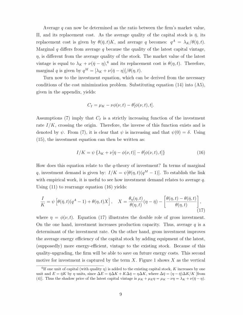
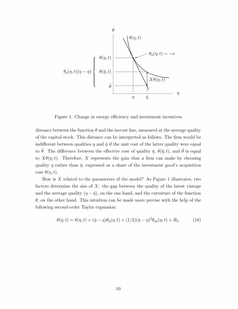
motive for investment is captured by the term X. Figure 1 shows X as the vertical

6If one unit of capital (with quality η) is added to the existing capital stock, K increases by oneunit and E = ηK by η units, since ∆E = η∆K + K∆η = η∆K, where ∆η = (η − η)∆K/K [from(4)]. Thus the shadow price of the latest capital vintage is µK + µEη = µK − νη = λK + ν(η − η).

9

θ(η, t)

θη(η, t)(η − η)

......................................................

θη(η, t) = −ν

.......θ

Xθ(η, t)

ηηη

θ

θ(η, t)

...............................θ(η, t)

.................................

Figure 1: Change in energy efficiency and investment incentives

distance between the function θ and the isocost line, measured at the average quality

of the capital stock. This distance can be interpreted as follows. The firm would be

indifferent between qualities η and η if the unit cost of the latter quality were equal

to θ. The difference between the effective cost of quality η, θ(η, t), and θ is equal

to Xθ(η, t). Therefore, X represents the gain that a firm can make by choosing

quality η rather than η, expressed as a share of the investment good’s acquisition

cost θ(η, t).

How is X related to the parameters of the model? As Figure 1 illustrates, two

factors determine the size of X: the gap between the quality of the latest vintage

and the average quality (η− η), on the one hand, and the curvature of the function

θ, on the other hand. This intuition can be made more precise with the help of the

following second-order Taylor expansion:

θ(η, t) = θ(η, t) + (η − η)θη(η, t) + (1/2)(η − η)2θηη(η, t) +R2. (18)

10

Neglecting the Lagrange remainder R2, equation (18) allows to rewriteX as follows:7

X (1/2)θηη(η, t)

θ(η, t)(η − η)2 =

1

2

(ses2kσ

) (η − ηη

)2

, (19)

where σ is the ex-ante elasticity of substitution between energy and capital, se is

the (expected) cost share of energy and sk(= 1− se) the cost share of capital in the

ex-ante composite I.

It is clear from (19) that most of the variability in X can be expected from the

variability of the term [(η − η)/η]2, since the structural parameters se, sk and σ

tend to be rather stable. On the one hand, such variability occurs during periods of

large (unexpected) changes in energy prices. On the other hand, investment-specific

technological shocks might also be responsible for the volatility of X. In the latter

case, the factor bias of those shocks is crucial: only energy-saving technical change

might lead to large changes in [(η− η)/η]2. As the information on the factor bias of

technological shocks is currently lacking, this issue is not pursued further here.8

5 Dynamic properties of the model

This section shows that the (local) dynamic behavior of the model can be analyzed

in a recursive way, using a suitable change in variables. Thus, the dynamic response

to exogenous shocks (e.g. a technological shock, discussed in the next section) can

be analyzed in a simple and transparent way.

The dynamics of firm behavior can be described by a system of four differential

equations governing the paths of the state variables K and η and of their shadow

prices, and by transversality conditions (12) and (A7). In the general case, it is

difficult to analyze a system of this order. In the present model, however, the

system can be simplified by a change in variables. Replacing λK by µK = λK + νη

7The (second) equality in (19) is obtained as follows. Note first that − ηθη/θ = νe/I can beinterpreted as the ratio between se and sk. Moreover, it can be shown that ηθηη/θη = 1/(skσ).Thus:

X =12

(ηθηη

θη

)(ηθη

θ

)(η − η

η

)2

=12

(se

s2kσ

)(η − η

η

)2

.

8Greenwood et al. (2000) analyze the role of investment-specific technological shocks in businesscycles. In their model, technological shocks affect the efficiency of (the latest vintage of) capital,without influencing the efficiency of other inputs.

11

leads to the following system of differential equations:9

ν = −v + ν(r + δ) (20)

µK = −Ψ2h′(Ψ) + VK(w,K, Y ) + µK(r + δ) (21)

K = (Ψ − δ)K (22)

˙η = (φ(ν, t) − η)Ψ (23)

where Ψ = ψ(µK − νφ(ν, t) − θ[φ(ν, t), t]) denotes the investment rate.

The properties close to equilibrium of this system can be analyzed by linearizing

the system of differential equations at the steady state equilibrium (where technical

change comes to a halt). As a first step, the equilibrium values of the endogenous

variables are determined, assuming that all exogenous variables remain constant

after a certain date. Setting derivatives with respect to time to zero yields η = η

and I = δK and the following equations:

ν∗ =v

r + δ(24)

−VK(w,K∗, Y ) + δ2h′(δ) = µ∗K(r + δ) (25)

µ∗K = θ[φ(ν∗)] + ν∗φ(ν∗) (26)

η∗ = φ(ν∗) (27)

where the equilibrium values of endogenous variables are denoted by a star (∗), and

η = η∗ and I = δK∗.

The linearized dynamic system is easier to analyze than the original system

because it is even more recursive, since the average specific energy consumption, η,

is determined independently of the investment rate. Therefore, the local dynamics of

energy efficiency can be studied independently of the local dynamics of investment.

The optimal path of the shadow price of energy can be determined as follows.

Combining equations (20) and (24) yields: ν = (r + δ)(ν − ν∗). Because of the

transversality condition (12), the unique solution of this equation is given by: ν(t) =

ν(0) = ν∗. This implies that the shadow price of energy immediately jumps to

its new equilibrium after a shock. Close to equilibrium, the evolution of average

specific energy consumption is governed by: ˙η = δφ′(ν∗)(ν − ν∗) − δ(η − η∗). Since

ν jumps instantaneously to its equilibrium value, this equation simplifies to: ˙η =

−δ(η − η∗). Consequently, η converges towards its equilibrium value at rate δ. The

9The system is obtained from equations (2), (4), (10) and (A3). In these equations, controlvariables I and η are replaced by their expressions in terms of the state variables.

12

η

ν

ν∗ ν = 0

˙η = 0

η∗

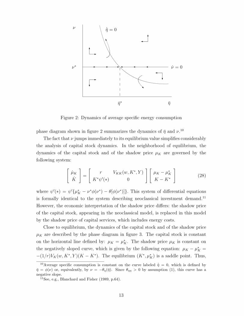
Figure 2: Dynamics of average specific energy consumption

phase diagram shown in figure 2 summarizes the dynamics of η and ν.10

The fact that ν jumps immediately to its equilibrium value simplifies considerably

the analysis of capital stock dynamics. In the neighborhood of equilibrium, the

dynamics of the capital stock and of the shadow price µK are governed by the

following system:

µK

K

=

r VKK(w,K∗, Y )

K∗ψ′(∗) 0

µK − µ∗KK −K∗

(28)

where ψ′(∗) = ψ′µ∗K − ν∗φ(ν∗) − θ[φ(ν∗)]. This system of differential equations

is formally identical to the system describing neoclassical investment demand.11

However, the economic interpretation of the shadow price differs: the shadow price

of the capital stock, appearing in the neoclassical model, is replaced in this model

by the shadow price of capital services, which includes energy costs.

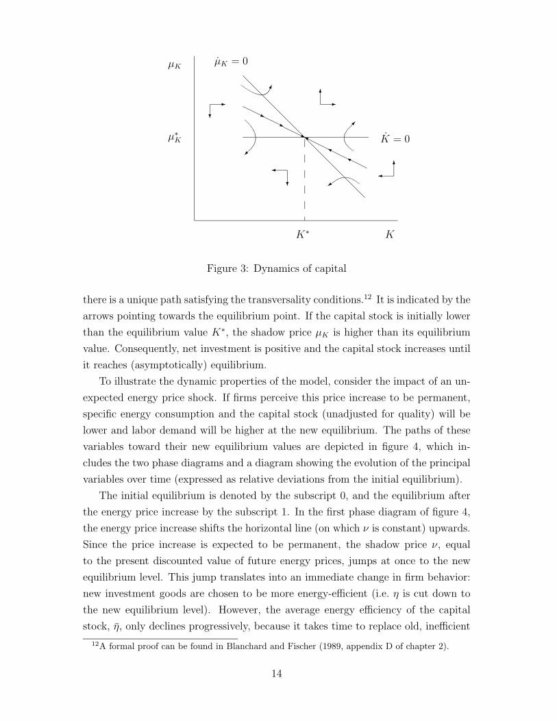
Close to equilibrium, the dynamics of the capital stock and of the shadow price

µK are described by the phase diagram in figure 3. The capital stock is constant

on the horizontal line defined by: µK = µ∗K . The shadow price µK is constant on

the negatively sloped curve, which is given by the following equation: µK − µ∗K =

−(1/r)VK(w,K∗, Y )(K −K∗). The equilibrium (K∗, µ∗K) is a saddle point. Thus,

10Average specific consumption is constant on the curve labeled ˙η = 0, which is defined byη = φ(ν) or, equivalently, by ν = −θη(η). Since θηη > 0 by assumption (1), this curve has anegative slope.

11See, e.g., Blanchard and Fisher (1989, p.64).

13

K∗ K

µK

µ∗K K = 0

µK = 0

Figure 3: Dynamics of capital

there is a unique path satisfying the transversality conditions.12 It is indicated by the

arrows pointing towards the equilibrium point. If the capital stock is initially lower

than the equilibrium value K∗, the shadow price µK is higher than its equilibrium

value. Consequently, net investment is positive and the capital stock increases until

it reaches (asymptotically) equilibrium.

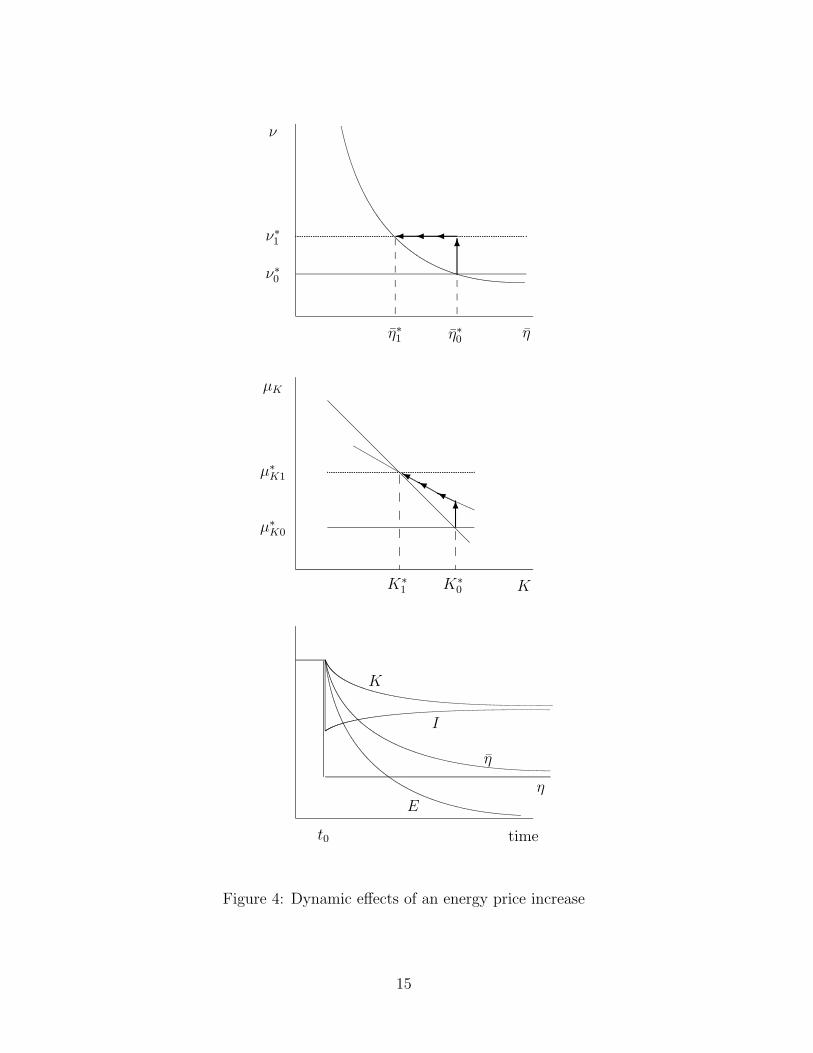
To illustrate the dynamic properties of the model, consider the impact of an un-

expected energy price shock. If firms perceive this price increase to be permanent,

specific energy consumption and the capital stock (unadjusted for quality) will be

lower and labor demand will be higher at the new equilibrium. The paths of these

variables toward their new equilibrium values are depicted in figure 4, which in-

cludes the two phase diagrams and a diagram showing the evolution of the principal

variables over time (expressed as relative deviations from the initial equilibrium).

The initial equilibrium is denoted by the subscript 0, and the equilibrium after

the energy price increase by the subscript 1. In the first phase diagram of figure 4,

the energy price increase shifts the horizontal line (on which ν is constant) upwards.

Since the price increase is expected to be permanent, the shadow price ν, equal

to the present discounted value of future energy prices, jumps at once to the new

equilibrium level. This jump translates into an immediate change in firm behavior:

new investment goods are chosen to be more energy-efficient (i.e. η is cut down to

the new equilibrium level). However, the average energy efficiency of the capital

stock, η, only declines progressively, because it takes time to replace old, inefficient

12A formal proof can be found in Blanchard and Fischer (1989, appendix D of chapter 2).

14

η

ν

ν∗1

η∗1

K∗1 K

µK

µ∗K1

η∗0

ν∗0

K∗0

µ∗K0

time

K

I

η

η

E

t0

Figure 4: Dynamic effects of an energy price increase

15

capital goods by new, more energy-efficient ones.

The behavior of the capital stock, K, can be read from the second phase diagram

of figure 4. The change in the shadow price of energy, ν, affects the equilibrium

value of the shadow price of capital services, µK , because the latter includes the

cost of energy. Since the equilibrium capital stock is lowered by the energy price

increase, the firm expects higher marginal productivity of capital in the future.

Consequently, the shadow price µK jumps immediately onto the saddle path and

subsequently converges towards the new equilibrium. At the same time, the capital

stock K diminishes slowly.

How does investment react to the energy price increase? It can be shown that

the negative impact of the shock (increasing energy costs and higher price of the in-

vestment good) prevails over the positive effect (higher future marginal productivity

of capital). Therefore, the investment volume drops at once and converges subse-

quently to the new equilibrium value13. If the measure of investment is adjusted for

improved energy efficiency (I), the results change. The energy price increase leads

to a quality improvement of investment goods which may (or may not) compensate

the drop in the volume of investment.

Finally, the evolution of derived energy demand, E, is conditioned by the evo-

lution of the capital stock and its average energy efficiency. As shown above, the

two latter variables adjust progressively to the new equilibrium. Therefore, energy

demand diminishes slowly over time and tends towards the new equilibrium.

As in the standard q-theory of investment, rational expectations of future events

influence present decisions in this model. For example, if an energy price increase

was preannounced (as might be the case for energy or carbon taxes), the choice of

energy efficiency and of investment volume would begin to change before the price

increase becomes effective.

6 Energy price shocks and adjustment costs

Turn now to the implications of this model for the estimation of adjustment cost

parameters. This section uses a simulation model, which is calibrated on aggregate

US data for the period following the two first energy price shocks, in order to generate

data on the evolution of the investment rate and average q. Then a “conventional”

q-model is estimated on the basis of this artificial data. The main result of this

13The initial impact may be bigger or smaller than the equilibrium impact. After the initial fall,the investment rate increases progressively. However, this does not imply that the investment levelincreases, since the capital stock diminishes over time.

16

exercise is that the “true” marginal adjustment costs are overestimated by a factor

of five.

There are two major differences between this model and conventional q-models of

investment (e.g. Summers, 1981, Hayashi, 1982). First, the investment rate, which

is explained by the investment function, is not defined in the same way. Equation

(17) of the model explains the investment rate I/K, whereas conventional models

explain the quality-adjusted investment rate I/K. The relation between the two

concepts can be expressed using equation (5), as follows:

I/K = θI/(θK) = (I/K) − ( ˙θ/θ) (29)

As a positive energy price shock leads both to a fall in average q and to the choice

of more energy-efficient equipment, ( ˙θ/θ) is likely to be negatively correlated with

average q. This correlation should also be observed with negative shocks.

Second, average q is not the only determinant of the investment rate in this

model, as equation (17) makes clear. Equation (19) suggests that the additional

term X might play an important role in periods with large energy price shocks,

since [(η−η)/η]2 can be expected to vary considerably. Because of this square term,

the correlation between qA and X can be expected to be negative in case of positive

energy price shocks, and positive in case of negative shocks.

The simulation model is set up in discrete time and has the same structure as

the theoretical model of this paper. Functional specifications and parameters which

describe the structure of production are taken from Atkeson and Kehoe (1999), who

use aggregate US data for the period 1960–1994. The two production functions f

and g (from which θ is derived) are assumed to be Cobb-Douglas, and the cost shares

are 0.57 for labor and 0.043 for energy (which are the average cost shares over the

period 1960–1994 in US non-energy sectors).

Adjustment costs (7) are specified as: h(I/K) = (b/2)[(I/K)− c]2/(I/K). As a

consequence, the investment function ψ in (17) is linear:

I/K = (1/b)[θ(η, t)(qA − 1) +X

]+ c (30)

What values should the adjustment cost parameters of the “true” model take? The

recent consensus seems to be that marginal adjustment costs are much lower than

what was found in the early literature (Caballero, 1999; Hassett and Hubbard, 1997).

However, conventional models still yields estimates of b which are closer to 20 than

to 1, even if firm-level data are used (Cummins et al., 1996). The parameter of the

17

1.0

1.2

1.4

1.6

1.8

2.0

2.2

2.4

2.6

0 5 10 15 20

Period

Ene

rgy

pric

e in

dex

Doubleshock

Singleshock

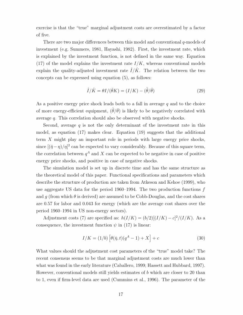
Figure 5: Simulated energy price shocks

“true” model is chosen such that the estimation of a conventional q-model on the

basis of the simulated data comes close to the conventional estimates (see table 1

below). As a result of this trial and error procedure, b is set to 4 in the simulation

model. The adjustment parameter c is assumed to be equal to the depreciation rate

δ, which is set to 0.1. The real interest rate is fixed at 0.05.

The evolution of the energy price is simulated such that it is consistent with

Atkeson and Kehoe’s (1999) data. Using the annual energy price data for the US

1960–1994, these authors estimate an ARMA(1,1) energy price process:

log vt+1 = (1 − ρ) log v + ρ log vt + γεt−1 + εt, εt ∼ N(0, σ2p), (31)

and obtain the following results: ρ = 0.9, γ = 0.35 and σp = 0.108. Here it is

assumed that firms form their expectations of energy prices on the basis of this

process. As the simulation model is deterministic, this assumption implies that,

after a shock, the energy price is expected to follow the trajectory defined by (31),

ignoring the possibility of future shocks.

Two types of energy price shocks are simulated (see figure 5). They are assumed

to be unexpected by firms and can be seen as a “stylized” representation of the

1974 and 1979 oil price shocks, as they appear in the aggregate data constructed

by Atkeson and Kehoe (1999) (assuming that t = 0 corresponds to the year 1974).

18

0.092

0.094

0.096

0.098

0.100

0.102

0 5 10 15 20

Period

Inve

stm

ent r

ate

-0.03

-0.02

-0.01

0.00

0.01

Tob

in's

q

Invest. rate

I/K

qM-1

qA-1

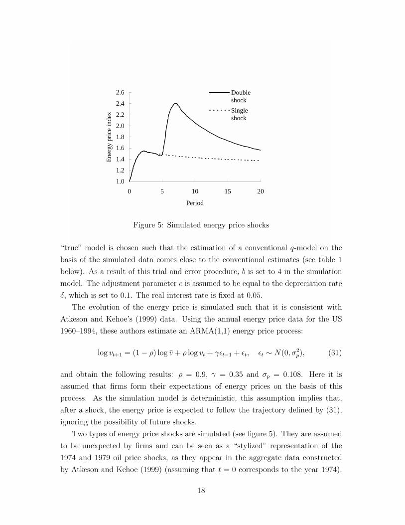
Figure 6: Impact of single energy price shock

First, a single shock is simulated by setting ε0 to 0.3. As a result, the energy price

reaches a maximum (54% higher than the initial level) at t = 2, then it falls back

slowly to the new equilibrium v, which is assumed to be 35% higher than the initial

energy price level v0.14 Second, a double shock is simulated by adding to the initial

impulse a second shock, by setting ε5 to 0.4. With this second shock, the energy

price reaches a second maximum, 141% percent higher than v0, at t = 7. The

simulated trajectory of the energy price which results from these two shocks reflects

approximately the actual evolution.15

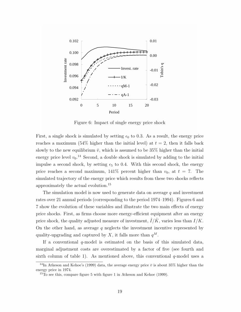
The simulation model is now used to generate data on average q and investment

rates over 21 annual periods (corresponding to the period 1974–1994). Figures 6 and

7 show the evolution of these variables and illustrate the two main effects of energy

price shocks. First, as firms choose more energy-efficient equipment after an energy

price shock, the quality adjusted measure of investment, I/K, varies less than I/K.

On the other hand, as average q neglects the investment incentive represented by

quality-upgrading and captured by X, it falls more than qM .

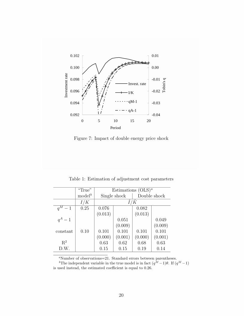
If a conventional q-model is estimated on the basis of this simulated data,

marginal adjustment costs are overestimated by a factor of five (see fourth and

sixth column of table 1). As mentioned above, this conventional q-model uses a

14In Atkeson and Kehoe’s (1999) data, the average energy price v is about 35% higher than theenergy price in 1974.

15To see this, compare figure 5 with figure 1 in Atkeson and Kehoe (1999).

19

0.092

0.094

0.096

0.098

0.100

0.102

0 5 10 15 20

Period

Inve

stm

ent r

ate

-0.04

-0.03

-0.02

-0.01

0.00

0.01

Tob

in's

q

Invest. rate

I/K

qM-1

qA-1

Figure 7: Impact of double energy price shock

Table 1: Estimation of adjustment cost parameters

“True” Estimations (OLS)a

modelb Single shock Double shock

I/K I/KqM − 1 0.25 0.076 0.082

(0.013) (0.013)qA − 1 0.051 0.049

(0.009) (0.009)constant 0.10 0.101 0.101 0.101 0.101

(0.000) (0.001) (0.000) (0.001)R2 0.63 0.62 0.68 0.63

D.W. 0.15 0.15 0.19 0.14

aNumber of observations=21. Standard errors between parentheses.bThe independent variable in the true model is in fact (qM −1)θ. If (qM −1)

is used instead, the estimated coefficient is equal to 0.26.

20

different definition of the investment rate than the “true” model and neglects the

influence of the term X. In order to identify the contribution of these two factors,

another version of the model is estimated, where the quality-adjusted investment

rate is regressed on marginal q (see third and fifth columns of table 1). It is clear

from these results that the strong negative correlation between ( ˙θ/θ) and qA (-0.96

over the estimation period) is responsible for an important part of the estimation

bias.

7 Conclusion

This paper presents a deterministic investment model where capital and energy

are linked by a putty-clay relationship. The model is tractable enough to allow a

simple and intuitive analysis of the behavior of investment demand in the presence of

energy price shocks. Moreover, the endogenous wedge between marginal and average

q, which is a result of the putty-clay structure, can be described as a function of

some key parameters and variables. If there are large energy price shocks, the model

exhibits dynamic behavior which suggests that marginal adjustment costs will be

overestimated by conventional q-models. Exploratory simulation analysis indicates

that this bias might be quite serious, suggesting therefore a new explanation of the

empirical failure of conventional q-models.

Several extensions and applications of this model seem promising. First, the

analysis of this paper is limited by the use of a deterministic set-up. Incorporating

explicitly the uncertainty of energy prices would thus represent an important step

forward. Second, the putty-clay framework is well suited for the analysis of embodied

technical change, an issue which has (again) become prominent as a consequence

of the empirical work by Gordon (1990). By contrast to the putty-putty model

employed by Greenwood et al. (2000), the putty-clay framework shifts the emphasis

towards the question of factor bias. Indeed, capital-saving technical progress leads

to the economic depreciation of existing capital goods; this effects works through

a fall in average q. By contrast, energy-saving technical progress favors the second

investment motive and thus increases the wedge between marginal and average q.

Third, the exploratory simulations carried out in this paper call for econometric

studies which would take the putty-clay structure of capital and energy (and possibly

other inputs) explicitly into account. The model proposed in this paper is not

only consistent, but also simpler than the theoretical framework used in previous

empirical work (see e.g. Berndt and Wood, 1984).

21

Appendix

Necessary and sufficient conditions for cost minimization

In the original cost minimization problem (9), the sufficient conditions provided by

the theorems of Mangasarian and Arrow do not apply. However, a canonical change

in variables (see Gelfand and Fomin, 1963, p.77) transforms the original problem

into a modified problem to which the theorems of Mangasarian and Arrow apply In

this appendix, the necessary and sufficient conditions of the modified problem are

described.

Recall that the state variables are K and η and the controls I and η. The

proposed change in variables is: replace η by E = ηK. For all K = 0, the function

defining the change in variables is a one-to-one correspondence.

The problem of the firm can now be restated, The firm minimizes the present

discounted value of future costs:

∫ ∞

0e−rt[V (w,K, Y ) + vE + θ(η)I + C(I,K)]dt

where the paths of state variables are constrained by the following differential equa-

tions:

K = I − δK (A1)

E = Iη − δE (A2)

The first of these differential equations is unchanged [see equation (2)]. The second

is obtained by differentiating E = ηK with respect to time and by using equations

(2) and (4) of the original model. The initial conditions are: K(0) = K0 and

E(0) = η0K0 = E0.

The current-value Hamiltonian is defined by:

H = −[V (w,K, Y ) + vE + θ(η)I + C(I,K)] + µK(I − δK) + µE(Iη − δE)

Pontryagin’s Maximum Principle provides the necessary conditions of this prob-

lem. Let I∗ and η∗ be a solution of the problem defined above and let K∗ and

E∗ be the optimal paths of the associated state variables. Necessary conditions for

optimality are given by the following equations:

µK = CK(I∗, K∗) + VK(w,K∗, Y ) + µK(r + δ) (A3)

µE = v + µE(r + δ) (A4)

22

where µK and µE are auxiliary variables associated with state variables K and E.

Moreover, the Maximum Principle includes the condition that the control vari-

ables maximize the Hamiltonian. First, setting the derivatives of the Hamiltonian

with respect to the control variables I and η to zero, yields:

µK + µEη∗ = θ(η∗, t) + CI(I∗, K∗) (A5)

µE = θη(η∗, t) (A6)

Second, it has to be established that the Hamiltonian is concave in (I, η). The

matrix of second derivatives of H with respect to I and η is negative defined since,

for all I,K, η = 0:

∂2H/∂I2 = −CII(I,K) < 0

∂2H/∂η2 = −θηη(η, t)I < 0

∂2H/∂I∂η = µE − θη(η, t) = 0

The signs of the two first expression follow from the convexity assumptions.

For the necessary transversality conditions, we refer to a theorem by Seierstad

(see Seierstad and Sydsaeter, 1987, p.244). Denote by:

g1(K,E, I, η) = I − δK and g2(K,E, I, η) = Iη − δE

the functions appearing in differential equations (A1) and (A2). The theorem es-

tablishes that if there exists a number k such that, for all t:

∣∣∣∣∣ ∂gi∂K

∣∣∣∣∣ ≤ k and

∣∣∣∣∣∂gi∂E∣∣∣∣∣ ≤ k i = 1, 2

then the auxiliary variables µK and µE, solutions of equations (A3) and (A4), satisfy:

limt→∞ e−rtµK(t) = 0 and lim

t→∞ e−rtµE(t) = 0. (A7)

The conditions of the theorem are obviously fulfilled since one can choose k ≥ δ.

Then:∂g1∂K

= δ,∂g1∂E

= 0,∂g2∂K

= 0 and∂g2∂E

= δ.

23

Following Mangasarian’s theorem16, the conditions of the Maximum Principle

are also sufficient if the Hamiltonian H is jointly concave in the state and control

variables (K,E, I, η) and if a transversality condition, given below, is satisfied.

The concavity of the Hamiltonian can be established by showing that the Hessian

matrix of H is semi-defined negative:

∂2H∂I2

∂2H∂I∂η

∂2H∂I∂K

∂2H∂I∂E

∂2H∂η∂I

∂2H∂η2

∂2H∂η∂K

∂2H∂η∂E

∂2H∂K∂I

∂2H∂K∂η

∂2H∂K2

∂2H∂K∂E

∂2H∂E∂I

∂2H∂E∂η

∂2H∂E∂K

∂2H∂E2

=

−CII 0 −CIK 0

0 −θηη(η, t)I 0 0

−CKKI 0 −VKK − CKK 0

0 0 0 0

The determinant of the complete matrix is zero. The principal minor with order

2 is the matrix of second derivatives of H with respect to (I, η), which is negative

definite as shown above. In order to establish the concavity of the Hamiltonian, it

remains thus to be shown that the determinant of the principal minor with order 3

is negative. This determinant is equal to:

−θηηI (CIICKK − CIK + CIIVKK) .

Since the adjustment cost function C(I,K) is assumed to be homogeneous of de-

gree 1, the Hessian matrix of C is singular. Consequently:

CIICKK − CIK = 0.

Because of the convexity assumptions on C(I,K) and θ(η) and since VKK > 0, the

determinant of the principal minor with order 3 is negative.

The sufficient transversality condition is:

limt→∞ e−rt[µK(t)(K(t) −K∗(t)) + µE(t)(E(t) − E∗(t))] ≥ 0

for all admissible K(t), E(t) [satisfying the initial conditions and differential equa-

tions (A1) and (A2)]. Obviously, the necessary transversality condition (A7) implies

the sufficient transversality condition (the expression above is zero).

16For a precise statement of this theorem in the context of infinite horizons, see Seierstad andSydsaeter (1987, p.234f). Note that if Mangasarian’s theorem applies, the sufficient conditions ofArrow’s theorem are also satisfied.

24

References

Abel, A.B., 1990. Consumption and Investment. In: Friedman, B.M. and Hahn,F.H. (eds.), Handbook of Monetary Economics, chapter 14, North Holland,Amsterdam.

Abel, A.B. and Blanchard, O., 1983. An Intertemporal Model of Saving and In-vestment. Econometrica, 51(3), 675–692.

Abel, A.B. and Eberly, J.C., 1994. A Unified Model of Investment Under Uncer-tainty. American Economic Review, 84(5), 1369–1384.

Atkeson, A. and Kehoe, P.J., 1999. Models of Energy Use: Putty-Putty VersusPutty-Clay. American Economic Review, 89(4), 1028–1043.

Berndt, E. R., Morrison, C. and Watkins, G. C. (1981). Dynamic Models of EnergyDemand: An Assessment and Comparison. In: Berndt, E. R. and Field, B. C.(eds.), Modeling and Measuring Natural Resource Substitution, pages 259–289,MIT Press, Cambridge, MA.

Berndt, E.R. and Wood, D.O., 1984. Energy Price Changes and the Induced Reval-uation of Durable Capital in U.S. Manufacturing During the OPEC Decade.MIT Energy Lab Report No 84-003.

Blanchard, O.J. and Fischer, S., 1989. Lectures on Macroeconomics. MIT Press,Cambridge, MA.

Caballero, R.J., 1999. Aggegate Investment. In: Taylor, J.B. and Woodford, M.(eds.), Handbook of Macroeconomics, Vol. 1B, North-Holland, Amsterdam.

Chirinko, R.S., 1993. Business Fixed Investment Spending: Modeling Strategies,Empirical Results, and Policy Implications. Journal of Economic Literature,31, 1875–1911.

Cummins, J.G., Hassett, K.A. and Hubbard, R.G., 1996. Tax Reforms and Invest-ment: A Cross-Country Comparison. Journal of Public Economics, 62(1-2),237–273.

Dixit, A.K and Pindyck, R.S., 1994. Investment under Uncertainty. PrincetonUniversity Press, Princeton.

Gelfand, I.M. and Fomin, S.V., 1963. Calculus of Variations. Prentice-Hall, Engle-wood Cliffs N.J.

Gordon, R.J., 1990. The Measurement of Durable Goods Prices. University ofChicago Press, Chicago.

Greenwood, J., Hercowitz, Z. and P. Krusell, 2000. The role of investment-specifictechnological change in the business cycle. European Economic Review, 44,91–115.

25

Hassett, K.A. and Hubbard, R.G., 1997. Tax Policy and Investment In: Auer-bach, A.J., ed. Fiscal policy: Lessons from economic research. MIT Press,Cambridge.

Hayashi, F., 1982. Tobin’s marginal q and average q : a neoclassical interpretation.Econometrica, 50(1), 213–224.

Seierstad, A. and Sydsaeter, K., 1987. Optimal Control Theory with EconomicApplications. North Holland, Amsterdam.

Solow, R., 1962. Substitution and Fixed Proportions in the Theory of Capital.Review of Economic Studies, 29(3), 207–218.

Summers, L.H., 1981. Taxation and Corporate Investment: A q-Theory Approach.Brookings Papers on Economic Activity, 1.

Tobin, J., 1969. A General Equilibrium Approach To Monetary Theory. Journal ofMoney, Credit, and Banking, 1, 15–29.

26