Embed Size (px)
Citation preview
Université Blaise Pascal - Clermont II
École Doctorale
Sciences Pour l'Ingénieur De Clermont-Ferrand
Thèse
Présentée par
Nabil MABROUK
Ingénieur en industries alimentaires
DEA en Modélisation en Hydraulique et Environnement
pour obtenir le grade de
Docteur d'Université
Spécialité: Informatique
Analyzing individual-basedmodels of microbial systems
Soutenue publiquement le 7 janvier 2010 devant le jury:
Président : Pr. David Hill
LIMOS, Clermont-Ferrand
Rapporteur : Pr. Cristian Picioreanu
Université Technique de Delft, Departement de biotechnologie, Pays-Bas
Pr. Jean-Daniel Zucker
IRD, Unité de recherche GEODES, Paris
Examinateur : Dr. Théodore Bouchez
Chercheur, Cemagref, unité HBAN, Antony
Directeurs de thèse : Dr. Guillaume Deffuant
Directeur de recherche, Cemagref, LISC, Clermont-Ferrand
Pr. Claude Lobry
Responsable de l'équipe MERE (INRIA/INRA), Montpellier

Abstract
There is a debate in ecology between those favoring simple aggregated mathe-
matical models containing only a few equations expressing a small number of gen-
eral principles and those preferring complex individual-based models that are more
structurally realistic with a more detailed representation of the basic processes and
interactions at the level of the individuals. In this thesis we attempt to bridge these
two approaches by deriving deterministic moment approximation models of micro-
bial individual-based models. We illustrate the approach on the example of bio�lm
growth with immotile and motile bacteria. We show that moment model can capture
the main features of spatial pattern that arise in simpli�ed bio�lm individual-based
models. Finally we assess the limitation of the moment models in capturing the
e�ect of local �uctuations of the individuals environment.

Contents
1 Introduction 1
1.1 Individual-based perspective of microbial systems . . . . . . . . . . . 1
1.2 Individual-based modeling of microbial systems . . . . . . . . . . . . 2
1.3 Aggregated mathematical modeling of microbial ecosystems . . . . . 3
1.4 Debate between IBM and mathematical modeling . . . . . . . . . . . 4
1.5 Thesis scope . . . . . . . . . . . . . . . . . . . . . . . . . . . . . . . . 5
1.5.1 Approximating spatially explicit IBMs with moment methods 6
1.6 Methods and tools . . . . . . . . . . . . . . . . . . . . . . . . . . . . 7
1.6.1 IBM description . . . . . . . . . . . . . . . . . . . . . . . . . 7
1.6.2 IBM implementation . . . . . . . . . . . . . . . . . . . . . . . 7
1.6.3 Exploring the IBMs using SimExplorer . . . . . . . . . . . . . 8
1.7 Report outline . . . . . . . . . . . . . . . . . . . . . . . . . . . . . . 8
2 Microbial colony growth: comparison of an individual-based model
and di�usion-reaction model 11
2.1 Modeling microbial spatial patterns . . . . . . . . . . . . . . . . . . . 12
2.2 Individual-based model . . . . . . . . . . . . . . . . . . . . . . . . . . 13
2.3 Model description . . . . . . . . . . . . . . . . . . . . . . . . . . . . . 14
2.3.1 Overview . . . . . . . . . . . . . . . . . . . . . . . . . . . . . 14
2.3.2 Design Concepts . . . . . . . . . . . . . . . . . . . . . . . . . 15
2.3.3 Details . . . . . . . . . . . . . . . . . . . . . . . . . . . . . . . 15
2.3.4 Model parameters . . . . . . . . . . . . . . . . . . . . . . . . 17
2.4 Individual-based model simulation . . . . . . . . . . . . . . . . . . . 17
2.5 Aggregated mathematical model . . . . . . . . . . . . . . . . . . . . 18
2.6 Comparing the IBM with the di�usion-reaction model . . . . . . . . 22
2.7 Discussion . . . . . . . . . . . . . . . . . . . . . . . . . . . . . . . . . 23
3 Moment approximation of a microbial IBM for colony growth 29
3.1 Description of the simpli�ed individual-based model . . . . . . . . . 30
3.1.1 Overview . . . . . . . . . . . . . . . . . . . . . . . . . . . . . 30
3.1.2 Design concepts . . . . . . . . . . . . . . . . . . . . . . . . . . 31
3.1.3 Details . . . . . . . . . . . . . . . . . . . . . . . . . . . . . . . 32
3.1.4 Parameters . . . . . . . . . . . . . . . . . . . . . . . . . . . . 32
3.1.5 Model outputs . . . . . . . . . . . . . . . . . . . . . . . . . . 33
3.1.6 Comparison of the simpli�ed IBM with the detailed IBM . . . 33
3.1.7 Moment approximation of the simpli�ed IBM . . . . . . . . . 34
3.1.8 Solving the moment approximation model . . . . . . . . . . . 43
3.2 Comparison of the moment model with the simpli�ed IBM . . . . . . 45
3.2.1 Density independent growth model (b′1 = 0) . . . . . . . . . . 45
3.2.2 Density dependant division model (b′1 > 0) . . . . . . . . . . . 48
iv Contents
3.3 Discussion . . . . . . . . . . . . . . . . . . . . . . . . . . . . . . . . . 49
3.4 Annexe A: expressing the moment model in radial coordinates . . . . 52
4 Moment approximation of a simpli�ed bio�lm IBM with detach-
ment 53
4.1 Introduction . . . . . . . . . . . . . . . . . . . . . . . . . . . . . . . . 53
4.2 A simpli�ed bio�lm IBM with detachment . . . . . . . . . . . . . . . 54
4.2.1 Individual-based model parameters . . . . . . . . . . . . . . . 56
4.3 IBM simulation results . . . . . . . . . . . . . . . . . . . . . . . . . . 56
4.4 Deriving the moment approximation model . . . . . . . . . . . . . . 57
4.5 Comparison of the moment model and the IBM . . . . . . . . . . . . 61
4.6 Discussion . . . . . . . . . . . . . . . . . . . . . . . . . . . . . . . . . 62
5 A detailed individual-based model of bio�lm formed with motile
bacteria 67
5.1 Background . . . . . . . . . . . . . . . . . . . . . . . . . . . . . . . . 68
5.2 Model description . . . . . . . . . . . . . . . . . . . . . . . . . . . . . 69
5.2.1 Purpose . . . . . . . . . . . . . . . . . . . . . . . . . . . . . . 70
5.2.2 State variables and scales . . . . . . . . . . . . . . . . . . . . 70
5.2.3 Scales . . . . . . . . . . . . . . . . . . . . . . . . . . . . . . . 70
5.2.4 Process overview and scheduling . . . . . . . . . . . . . . . . 70
5.2.5 Design Concepts . . . . . . . . . . . . . . . . . . . . . . . . . 72
5.2.6 Submodels . . . . . . . . . . . . . . . . . . . . . . . . . . . . . 72
5.3 Results . . . . . . . . . . . . . . . . . . . . . . . . . . . . . . . . . . . 77
5.4 Discussion . . . . . . . . . . . . . . . . . . . . . . . . . . . . . . . . . 79
6 Moment approximation of the motile bacteria IBM 87
6.1 Description of the simpli�ed IBM . . . . . . . . . . . . . . . . . . . . 88
6.1.1 Overview . . . . . . . . . . . . . . . . . . . . . . . . . . . . . 88
6.1.2 Details . . . . . . . . . . . . . . . . . . . . . . . . . . . . . . . 90
6.2 Moment approximation . . . . . . . . . . . . . . . . . . . . . . . . . 92
6.2.1 First moment dynamics . . . . . . . . . . . . . . . . . . . . . 92
6.2.2 Second moment dynamics . . . . . . . . . . . . . . . . . . . . 93
6.2.3 Closure of the moment hierarchy . . . . . . . . . . . . . . . . 100
6.2.4 Solving the moment model . . . . . . . . . . . . . . . . . . . 100
6.3 Results and discussion . . . . . . . . . . . . . . . . . . . . . . . . . . 100
6.4 Conclusion . . . . . . . . . . . . . . . . . . . . . . . . . . . . . . . . . 111
7 Exploring the labyrinth-like patterns in a simpli�ed IBM of a mi-
crobial bio�lm formed with motile bacteria 117
7.1 Simpli�ed IBM for bio�lm formed with density-dependent motile bac-
teria . . . . . . . . . . . . . . . . . . . . . . . . . . . . . . . . . . . . 117
7.2 Numerical exploration of the IBM . . . . . . . . . . . . . . . . . . . . 119
7.3 Deriving the moment approximation model . . . . . . . . . . . . . . 120
Contents v
7.4 Discussion and conclusion . . . . . . . . . . . . . . . . . . . . . . . . 129
8 Conclusion 131
8.1 Perspectives . . . . . . . . . . . . . . . . . . . . . . . . . . . . . . . . 133
Bibliography 135

Chapter 1
Introduction
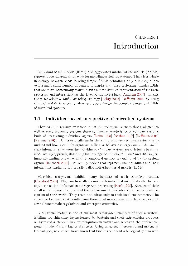
Individual-based models (IBMs) and aggregated mathematical models (AMMs)
represent two di�erent approaches for modeling ecological systems. There is a debate
in ecology between those favoring simple AMMs containing only a few equations
expressing a small number of general principles and those preferring complex IBMs
that are more �structurally realistic� with a more detailed representation of the basic
processes and interactions at the level of the individuals [Aumann 2007]. In this
thesis we adopt a double-modeling strategy [Lobry 2003] [De�uant 2004] by using
(simple) AMMs to check, analyze and approximate the complex dynamic of IBMs
of microbial systems.
1.1 Individual-based perspective of microbial systems
There is an increasing awareness in natural and social sciences that ecological as
well as socio-economic systems share common characteristics of complex systems
built of interacting individual agents [Levin 1998] [Arthur 1997] [De�uant 2005]
[Rammel 2007]. A major challenge in the study of these complex systems is to
understand how seemingly organized collective behavior emerges out of the small-
scale interactions between the individuals. Complex system research tends to adopt
a bottom-up approach, describing kinds of agents and environments and then exper-
imentally �nding out what kind of complex dynamics are exhibited by the system
agents [Railsback 2001]. Bottom-up models that represent the individuals and their
interactions explicitly are broadly called individual-based models (IBMs).
Microbial ecosystems exhibit many features of such complex systems
[Crawford 2005]. They are basically formed with individual microbial cells that en-
capsulate action, information storage and processing [Kreft 1998]. Because of their
small size compared to the size of their environment, microbial cells have a local per-
ception of their world. They react and adapt only to their local environment. The
collective behavior that results from these local interactions may, however, exhibit
several macroscale regularities and emergent properties.
A Microbial bio�lm is one of the most remarkable examples of such a system.
Bio�lms are thin slimy layers formed by bacteria and their extracellular products
on hydrated surfaces. They are ubiquitous in nature and represent the preferential
growth mode of many bacterial species. Using advanced microscopy and molecular
technologies, researchers have shown that bio�lms represent a biological system with
2 Chapter 1. Introduction
a high level of organization where bacteria form structured, coordinated, functional
communities [O'Toole 2000]. The formation of these organized �cities of microbes�
is however to a large part mediated by local interactions between the individual
cells and with their immediate surrounding environment. By viewing such systems
as complex systems formed with locally interacting individuals, microbial ecology
can take bene�t from tools and approaches (like the individual-based modeling ap-
proach) developed to study comparable systems in other �elds of science.
1.2 Individual-based modeling of microbial systems
The individual-based modeling approach attempts to capture the properties and
dynamic of a population by describing all the actions of its constitutive individuals
and their interaction with the environment and with each other. Since the indi-
viduals are represented explicitly in the model, the inherent heterogeneity of the
population can be readily accounted for by explicitly modeling local di�erences in
the environment and between the individuals [Murphy 2008] [Kreft 1999]. Grimm
[Grimm 1999] de�nes IBMs in the ecological context as � simulation models that
treat individuals as unique and discrete entities which have at least one property
in addition to age that changes during the life cycle�. Since microbe models do
not include age (rather size) the de�nition is usually relaxed to include at least
two independent properties (not counting position) [Hellweger 2009]. However, sev-
eral bottom-up models used in ecology that do not entirely satisfy this de�nition
are still referred to as IBM as long as they treat individuals as discrete entities
[Dieckmann 2000].
A survey of the literature on the use of IBMs in microbial ecology
shows that the approach is gaining a certain acceptance among microbiol-
ogists (see [Hellweger 2009] [Ferrer 2008] for a review). IBM approach has
been applied for modeling bacteria systems that arise in wastewater treatment
plants [Kreft 2001] [Gujer 2002][Picioreanu 2004][Picioreanu 2005] [Xavier 2005],
medical and industrial settings, bacteria in food and other environments
[Ginovart 2002][Dens 2005][Emonet 2005]. Hellweger and Bucci [Hellweger 2009] re-
viewed 46 published papers dealing with IBM application for microbial and phyto-
plankton systems. They noticed that the use of IBM approach is often motivated
by the importance of the population heterogeneity(46%), emergence of population
level patterns (24%), discreteness of the individuals (5%) and other reasons (26%)
[Hellweger 2009]. The rapidly growing interest in the individual-based modeling
approach is to a major part encouraged by the rapid increase in computing power
and advances in molecular biology, biochemistry and confocal microscopy during
the last 20 years. Powerful computers make it practical to simulate large num-
bers of individuals in virtual environments while the new experimental tools used
in microbiology provide a detailed observation of the individual-level dynamics and
raises new questions about the functioning and organization of microbial ecosys-
1.3. Aggregated mathematical modeling of microbial ecosystems 3
tems. Examples include the development of the complex structure of microbial
bio�lms as revealed by confocal microscopy observations and investigated using
IBMs [Kreft 2001][Picioreanu 2004] or the adaptative and collaborating strategies of
the individuals and their impact on the population level dynamics [Vlachos 2006].
Although IBMs enjoyed the claim of the latest generation models they face criti-
cism as well [Laspidou 2009]. Some of the drawbacks of the IBM approach are simply
due to the relatively young age of the approach which still misses a solid methodolog-
ical framework for developing, implementing and validating IBMs. These issues have
been addressed by several recent textbooks that proposed guidelines for building and
using individual-based [Grimm 2006][Treuil 2008]. Other limitations however are in-
herent to the nature of the IBMs as stochastic simulation models. IBMs used in
ecology often encompass the randomness of individual-level interactions and evolve
in a large state and parameter space that can only be sampled. The complexity
and limited generality are often quoted as the main limitations of individual-based
modeling [Uchmanski 1996]. Grimm noticed that IBMs usually make more realis-
tic assumptions than simple aggregated mathematical models, but it should not be
forgotten that the aim of individual-based modeling is not `realism' but modeling
and that modeling must be guided by a problem or question about a real system,
not just by the system itself [Grimm 2006].
1.3 Aggregated mathematical modeling of microbial
ecosystems
Traditionally, microbial systems are modeled using aggregated mathematical mod-
els. Aggregated mathematical models often take the form of a set of di�erential and
partial di�erential equations that describe the dynamic of aggregated system-level
state variables. The notion of aggregated state variable implies some averaging or
grouping of the microscale variables of a system. For instance a system formed with
N discrete individuals each characterized by a real-valued state variableXi, i = 1..N
is entirely described by the vector (Xi)i=1..N . An aggregated mathematical model
of this systems implies the reduction of the individual-based model to a smaller
system described with new (aggregated) variables Yj , j = 1..M with M << N .
The aggregated mathematical model is then formed with the set of di�erential (or
partial di�erential) equations of the variables Yj with the appropriate boundary and
initial conditions.
A generic example of aggregated mathematical models used in microbial ecology
can be derived for a simple system formed with N individuals each characterized
with a mass mi, i = 1..N . Rather than tracking the dynamics of each individual one
can de�ne a new aggregated variable Yj , j = 1 corresponding to the total mass of
the individuals and derive a di�erential equation that describe the dynamics of this
4 Chapter 1. Introduction
variable. The aggregated mathematical model then takes the form of a di�erential
equation:
dY
dt= Φ(Y )Y (1.1)
Where φ(Y ) is a function that describes the net growth rate of the population.
Equations of this kind still play such a central role in microbial ecology, that many
subsequent elaborations of theory have taken them as the starting point. Resource
dynamics and spatial variation can be introduced and the models are sometimes
interpreted as referring to individuals by assuming that the function Φ(Y ) also de-
scribes the interactions at the level of the individual [McKane 2004]. However in
most situations these models are generally derived without the need of a detailed
knowledge of the interactions between the individuals and rely instead on the as-
sumption that the terms which arise in the governing equations represent the net
e�ects of individual interactions in some generic way [McKane 2004].
The relative simplicity and genericity of aggregated mathematical models from
one side and the availability of a solid mathematical and numerical framework
to analyze them on the other side have contributed to their successful establish-
ment as a standard for modeling ecological systems. Additionally, for decades mi-
crobial ecology struggled as a scienti�c discipline because of the lack of reliable
experimental tools to observe the individual-level structure of microbial ecosys-
tems. Microbes were observed and quanti�ed mainly at the population level
[Hellweger 2009][Brehm-Stecher 2004]. For example the bacteria in a wastewater
treatment bioreactor were quanti�ed by measuring the volatile suspended solids.
Thus, simple aggregated mathematical models were su�cient to exploit such data.
1.4 Debate between IBM and mathematical modeling
There is still an ongoing debate in ecology between those favoring simple system-
level mathematical models containing only a few equations expressing a small num-
ber of general principles and those preferring complex simulation models that are
more �structurally realistic� with a more detailed representations of the basic pro-
cesses and interactions determining the system dynamic [Aumann 2007]. Grimm
[Grimm 2005] noticed that strengths and weakness of IBMs and system-level math-
ematical models are to a large degree inversely related. Mathematical models are
transparent and easy to communicate as they are by de�nition, formulated in the
universal and unambiguous language of mathematics. They can make predictions,
require less data for parameter estimation and model validation, may be less prone
to error propagation and since they embody only a few heuristic principles, may be
likely to lead to general causal understanding [Aumann 2007]. Mathematical mod-
els, however, have very limited ability to answer question about how system level
behavior emerge out of local interactions. On the other hand, IBMs are designed
1.5. Thesis scope 5
to answer such questions by explicitly representing the individuals and their inter-
actions. They often encompass the randomness of individual-level interactions and
thus yield realistic system-level patterns. However, one consequence of IBMs being
less simple than classical mathematical models is that IBMs are not easy to com-
municate, analyze and learn from [Grimm 2005]. IBMs evolve in a large parameter
state space which can only be sampled [Murrell 2000]. Consequently it is generally
not known to what extent the outcome obtained for a set of parameters holds for
other sets [Murrell 2000]. Furthermore, if the simulations are stochastic, the eco-
logical signal may only emerge after averaging over a series of realizations, even
with a particular parameter set, which may become computationally very expensive
[Murrell 2000]. IBM advocate however claims that the approach is more than a
new tool that adds to the toolbox of ecologists, but had a signi�cant implication on
the way we look to these complex system. By using IBMs the focus is shifted from
populations to individuals and several IBMs have demonstrated the potential signi�-
cance of individual characteristics to population dynamics and ecosystems processes
[Grimm 2005].
1.5 Thesis scope
In this thesis, we move beyond the debate of whether of mathematical models
or IBMs are more appropriate for representing microbial ecosystems, and concen-
trate on how the bene�ts of aggregated mathematical models can be combined with
strengths of IBMs. We adopt a �double-modeling� strategy [De�uant 2004] by using
mathematical models along with IBMs in modeling microbial systems. Such an ap-
proach can help bridging the perceived gap between individual-based and classical
approaches to microbial system modeling. We provide simple illustrations of how
mathematical models can be used to analyze and approximate the dynamic of IBMs
of microbial systems and assess their potential and limits in reproducing the rich
and complex dynamic of the IBM.
We consider an IBM as �a virtual experimental system� designed to encompass the
complexity of a microbial system by including features like the discreteness of the
individuals, the stochasticity of their interactions, the heterogeneity of their traits
and the heterogeneity of their local environment. Once constructed an IBM can be
sampled by running computer simulations and/or �modeled� (in the sens of approxi-
mated) using aggregated mathematical models. Grimm and Railsback [Grimm 2006]
noticed that the approximation of the IBM dynamic using aggregated mathematical
models attempts to bridge the perceived gap between individual-based and classical
approaches to ecological modeling and expands the ecologists' toolbox by deriv-
ing new aggregated mathematical models in which individual-level interaction are
acknowledged.
6 Chapter 1. Introduction
1.5.1 Approximating spatially explicit IBMs with moment meth-ods
We focus on approximating spatially explicit microbial IBM using moments ap-
proximation. Moment approximation has shown promise in deriving deterministic
aggregated mathematical models that links individual-traits and local interactions
to the population level dynamic [Dieckmann 2000][Murrell 2000] [Bolker 1997]. The
approach provides a general framework for building direct deterministic approxima-
tions of the dynamic of stochastic IBMs if the latter are adequately simpli�ed. There
are in the literature several good examples demonstrating that moment models can
accurately approximate the dynamic of many stochastic IBMs with the advantages
of being deterministic, evolve in a tractable state parameter space and are compu-
tationally less expensive than IBMs. One of the aims of this thesis is to investigate
whether this approach can also apply to spatially explicit IBMs used in microbiology
and assess the potential and limits of the moment approach in capturing the main
features of the IBM simulated microbial spatial patterns.
The essence of the moment approach is in deriving the dynamics of spatial mo-
ments by considering the processes a�ecting the spatial patterns and de�ned at the
level of the individuals. They provide an alternative (or extension) to the mean-�eld
approach as moment methods elegantly formalizes the notion of the �individual's-
eye view� of the spatial heterogeneity. Consider a population of N individuals each
characterized with a spatial location x in the space. The vector (xi)i=1..N de�nes
the spatial pattern of the population. If the individuals are not located at random
in the domain, we refer to the population as having a spatial structure. The spatial
pattern change through the individual-level stochastic events (birth, death, move-
ment, ..) and an individual-based model simulation basically provides a realization
of this pattern, whereas spatial moments provide a statistical description of the
spatial pattern and moment models approximate the dynamic of these statistical
quantities in time by considering the e�ect of the individual-level events.
Spatial moments are usually expressed in term correlation densities functions.
The spatial pattern formed by the individuals can be de�ned by the list of the
location of the individuals or in a continuous formulation using the density function
p(x) that is peaked at all locations occupied by individuals and is zero elsewhere.
For a given spatial pattern p the �rst spatial moment is de�ned as:
N(p) =1
A
∫p(x)dx (1.2)
where A is the area of the considered domain. This corresponds to the mean
density of individuals in the system. The second moment corresponds to the density
of pairs formed by individuals that are vectorial distance ξ apart and is de�ned as:
C(ξ, p) =1
A
∫p(x)p(x+ ξ)dx (1.3)
1.6. Methods and tools 7
The third moment, denoted T (ξ, ξ′, p) corresponds to the density of triplet of
individuals where the �rst pair in the triplet is separated with a vectorial distance
ξ and the second pair with a vectorial distance ξ′. We can also de�ne additional
higher order spatial moment, but usually the moment approximation is restricted
to the these three spatial moments.
The derivation of a tractable deterministic moment model from the stochastic
rules of the IBM requires some level of approximation which are veri�ed by con-
fronting the moment model to the IBM simulations. The main approximation
needed for in deriving the moment model is related to the cascade of hierarchy
of spatial moment which at some level need to be cut o� using a closure equa-
tion. Often moment models are limited to the �rst and second spatial moments
and neglect the triple correlation between the positions of three individuals. The
underlying assumption is that the probability of encountering a particular triplet
con�guration is fully given by pair densities [Van Baalen 2000]. Another important
approximation is that the moment equation are based on the average neighborhood
experienced by the individuals. Hence �uctuations experienced by the individuals
are not considered in moment approximation models.
1.6 Methods and tools
1.6.1 IBM description
IBM description is often a critical step. While mathematical models are fully
described with a set of equations, variable de�nitions and a parameter table, the
description of an IBM usually requires a combination of mathematical equations,
algorithmic rules (if .. then) and lengthy verbal description. This often makes the
reproduction of an IBM di�cult because of the ambiguity that may arise in the
description of the model. Recently a standard protocol for describing IBMs called
ODD (Overview, Design concepts and Details) has been proposed [Grimm 2006].
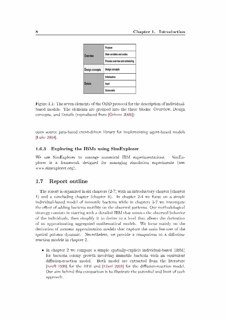
The protocol aims to structure the information about the IBM in a standard se-
quence (�gure 5.1). The logic behind ODD is to provide �rst the context and
general information (Overview), followed by more strategic considerations (Design
concepts) and �nally more technical details [Grimm 2006]. In this thesis we adopt
the ODD framework to describe the IBMs.
1.6.2 IBM implementation
There are several �exible modeling environments for implementing individual-based
models. Such environments include several utilities for storing the individuals, per-
forming neighbor search, creating a graphical user interface, analyzing the simulation
and tracking the state of the individuals. Agent-based modeling environment of this
kind include NetLogo, Repast and Mason. In this work we used Mason library, an
8 Chapter 1. Introduction
Figure 1.1: The seven elements of the ODD protocol for the description of individual-
based models. The elements are grouped into the three blocks: Overview, Design
concepts, and Details (reproduced from [Grimm 2006])
open source java-based event-driven library for implementing agent-based models
[Luke 2004].
1.6.3 Exploring the IBMs using SimExplorer
We use SimExplorer to manage numerical IBM experimentations. SimEx-
plorer is a framework designed for managing simulation experiments (see:
www.simexplorer.org).
1.7 Report outline
The report is organized in six chapters (2-7) with an introductory chapter (chapter
1) and a concluding chapter (chapter 8). In chapter 2-4 we focus on a simple
individual-based model of immotile bacteria while in chapters 5-7 we investigate
the e�ect of adding bacteria motility on the observed patterns. Our methodological
strategy consists in starting with a detailed IBM that mimics the observed behavior
of the individuals, then simplify it to derive to a level that allows the derivation
of an approximating aggregated mathematical models. We focus mainly on the
derivation of moment approximation models that capture the main features of the
spatial pattern dynamic. Nevertheless, we provide a comparison to a di�usion-
reaction models in chapter 2.
• In chapter 2 we compare a simple spatially-explicit individual-based (IBM)
for bacteria colony growth involving immotile bacteria with an equivalent
di�usion-reaction model. Both model are extracted from the literature
[Kreft 1998] for the IBM and [Eberl 2001] for the di�usion-reaction model.
Our aim behind this comparison is to illustrate the potential and limit of each
approach.
1.7. Report outline 9
• In chapter 3 we simplify the colony growth IBM and approximate the simpli�ed
IBM with an aggregated mathematical moment model.
• In chapter 4 we investigate the stationary patterns that arise in a system
with immotile bacteria and compare these patterns to those yielded by an
approximating moment model.
• In chapter 5 to 7 we focus on a new individual-based model that includes bac-
teria surface-associated motility. The originality of this model is in assuming
that the excretion of exopolymeric substances by the bacteria tend to reduces
their migration capacity yielding a rich variety of spatial patterns. In chapter
5 we present the detailed individual-based model
• In chapter 6 we provide a �rst simpli�cation of the detailed individual-based
model in which we keep the exopolymeric substance dynamic and approximate
the simpli�ed model using moment approximation techniques
• In chapter 7 we provide a further simpli�cation of the model that still allow
to reproduce the main patterns observed in the previous models. We compare
the simpli�ed IBM results to those obtain with an approximating moment
model.
• Finally, in chapter 8 we summarize the main results and propose some per-
spectives.

Chapter 2
Microbial colony growth:
comparison of an individual-based
model and di�usion-reaction
model
Contents
2.1 Modeling microbial spatial patterns . . . . . . . . . . . . . . 12
2.2 Individual-based model . . . . . . . . . . . . . . . . . . . . . . 13
2.3 Model description . . . . . . . . . . . . . . . . . . . . . . . . . 14
2.3.1 Overview . . . . . . . . . . . . . . . . . . . . . . . . . . . . . 14
2.3.2 Design Concepts . . . . . . . . . . . . . . . . . . . . . . . . . 15
2.3.3 Details . . . . . . . . . . . . . . . . . . . . . . . . . . . . . . . 15
2.3.4 Model parameters . . . . . . . . . . . . . . . . . . . . . . . . 17
2.4 Individual-based model simulation . . . . . . . . . . . . . . . 17
2.5 Aggregated mathematical model . . . . . . . . . . . . . . . . 18
2.6 Comparing the IBM with the di�usion-reaction model . . . 22
2.7 Discussion . . . . . . . . . . . . . . . . . . . . . . . . . . . . . . 23
Di�usion-reaction models (DRM) are traditionally used for simulating the for-
mation of spatial patterns in biological systems [Murray 2001]. A vast mathe-
matical theory for DRMs and a considerable body of literature of their applica-
tions in biology and microbial systems now exist. In this chapter we compare an
individual-based model (IBM) adapted from [Kreft 1998] and a di�usion-reaction
model described in [Eberl 2001]. Both models represent the core of several more
complex microbial bio�lm models involving multiple microbial groups and metabo-
lites [Kreft 2001][Eberl 2001][Picioreanu 2004][Xavier 2005]. We use both models to
simulate the growth of a microbial colony initiated with a single cell located at the
center of a squared two-dimensional domain. The cell grows by uptaking a di�usive
nutrient which concentration is imposed at the domain boundary. We propose to
compare the spatial patterns of the simulated colonies yielded by both models in
two di�erent growth regimes: the 'reaction-limited' regime where the growth of the
12
Chapter 2. Microbial colony growth: comparison of an
individual-based model and di�usion-reaction model
bacteria is limited by their nutriment uptake capacity and the 'di�usion-limited'
regime in which the bacteria growth is limited by the nutrient transport. Through
this comparison, we aim to illustrate the potential and limitation of each approach.
The chapter is organized in six sections. The �rst section introduces the problem
of modeling microbial spatial patterns using IBMs and DRMs. In the second section
we present the IBM using the ODD (Overview, Design Concepts and Details) pro-
tocol recommended in [Grimm 2006]. In the third section we simulate the growth of
a colony in the 'reaction-limited' and the 'di�usion-limited' regimes. In the fourth
section we present the aggregated di�usion-reaction model. In the �fth section we
compare the di�usion-reaction model pattern to the average pattern yielded by the
IBM. Finally we discuss the limitation and potential of each approach.
2.1 Modeling microbial spatial patterns
The problem of aggregation of microbial cells, in particular bacteria, is a cen-
tral one in microbial ecology. Depending on the bacterial species and the culture
conditions, individual cells can form colonies [Ben-Jacob 2000], �ocs [Schmid 2003],
granules [Morgenroth 1997] and bio�lms [Costerton 1995] that exhibit a great diver-
sity of forms. Such patterns are often observable at the level of the population but
are to a large extent mediated by the processes taking place at the level of the indi-
vidual cells. Much e�ort is dedicated to explore the linkage between these levels. In
particular how changes in individuals' responses to their environment translate into
changes in observable patterns and conversely how the emergence of these spatial
structures a�ect the dynamic of the individuals.
IBMs and aggregated mathematical models based on the di�usion-reaction equa-
tion framework have both been extensively used to investigate how these spatial
structures form and evolve in time [Grimson 1994] [Kreft 2001] [Picioreanu 2004]
[Lacasta 1999][Eberl 2001][Cogan 2004][Alpkvist 2007]. While IBMs attempt to
simulate the development of microbial patterns by specifying the behavioral and
interactions rules at the level of the discrete individuals, di�usion-reaction models
represent the pattern as an entity (a density �eld) and attempt to capture how this
entity evolve in time. The di�usion-reaction model is usually considered as the con-
tinuum limit of the IBM when the number of the individuals is large. This implies
that the di�usion-reaction model can be derived rigorously from the rules stated in
the IBM. However in practice, the derivation of the di�usion-reaction equation from
rigorous considerations of the individual-level rules is often complex and feasible
only for some ideal systems. Consequently, and as will be illustrated in this chapter
(section 3), assumptions and simpli�cations have to be made in the development of
the di�usion-reaction model and comparison of the di�usion-reaction model to the
IBM can be helpful to measure the impact of these simpli�cations.
2.2. Individual-based model 13
Kreft et al. [Kreft 1998] proposed an original IBM (called Bacsim) involving
discrete representation of the individual cells and an explicit description of their
processes (growth, division, shoving). The shoving process, a mechanisms by which
the individuals push each others to relax overlapping, is the main process responsible
of the colony expansion. In the di�usion-reaction mathematical model proposed in
[Eberl 2001] the bacteria spatial distribution is represented with a biomass concen-
tration �eld which dynamic is given by a di�usion-reaction mass balance equation.
The nutrient dynamic in both models is represented identically using a di�usion-
reaction mass balance equation. The models di�er essentially by the way they rep-
resent the biomass (discrete versus continuous) and the biomass-related processes,
especially biomass redistribution. The growth of the bacteria increases the local
density of the biomass which needs to be redistributed over space. In the IBM rules
are set to place the newborn cell close to the mother cell and the �nal distribution
of bacteria results from the self-organization of the individuals through a shoving
process. This mechanisms is described in the AMMs proposed in [Eberl 2001] as
a density-dependent di�usion. The biomass di�usion increases with the increase of
the local density of biomass.
We shall note that an alternative to the aggregated di�usion-reaction mathemat-
ical model proposed in [Eberl 2001] is to consider the biomass as a viscous �uid
as in the Dckery-Klapper model [Dockery 2001][Cogan 2004]. The biomass is then
described with a density and a pressure �elds. The growth of the biomass increases
the local pressure inducing an advective transport of the biomass. The biomass
advective vector u is linked to the local pressure gradient ∇p through the Darcy
law:
u = −λ∇p (2.1)
where λ is the Darcy constant. Compared to the DRM proposed by Eberl
[Eberl 2001], this model is much more accepted and has been extended to multiple
microbial types [Alpkvist 2007] The Dockery-Klapper model [Dockery 2001] however
involves an additional state variable (pressure p) and more complex boundaries
conditions at the bio�lm/bulk interface. For simplicity we consider the Eberl model
in this chapter.
2.2 Individual-based model
We describe an IBM for a system initially formed with a bacterial cell located in
the center a two dimensional squared domain. The model is a simpli�ed version of
Kreft's IBM Bacsim simulating the growth of a single Escherichia coli cell into a
colony[Kreft 1998].
14
Chapter 2. Microbial colony growth: comparison of an
individual-based model and di�usion-reaction model
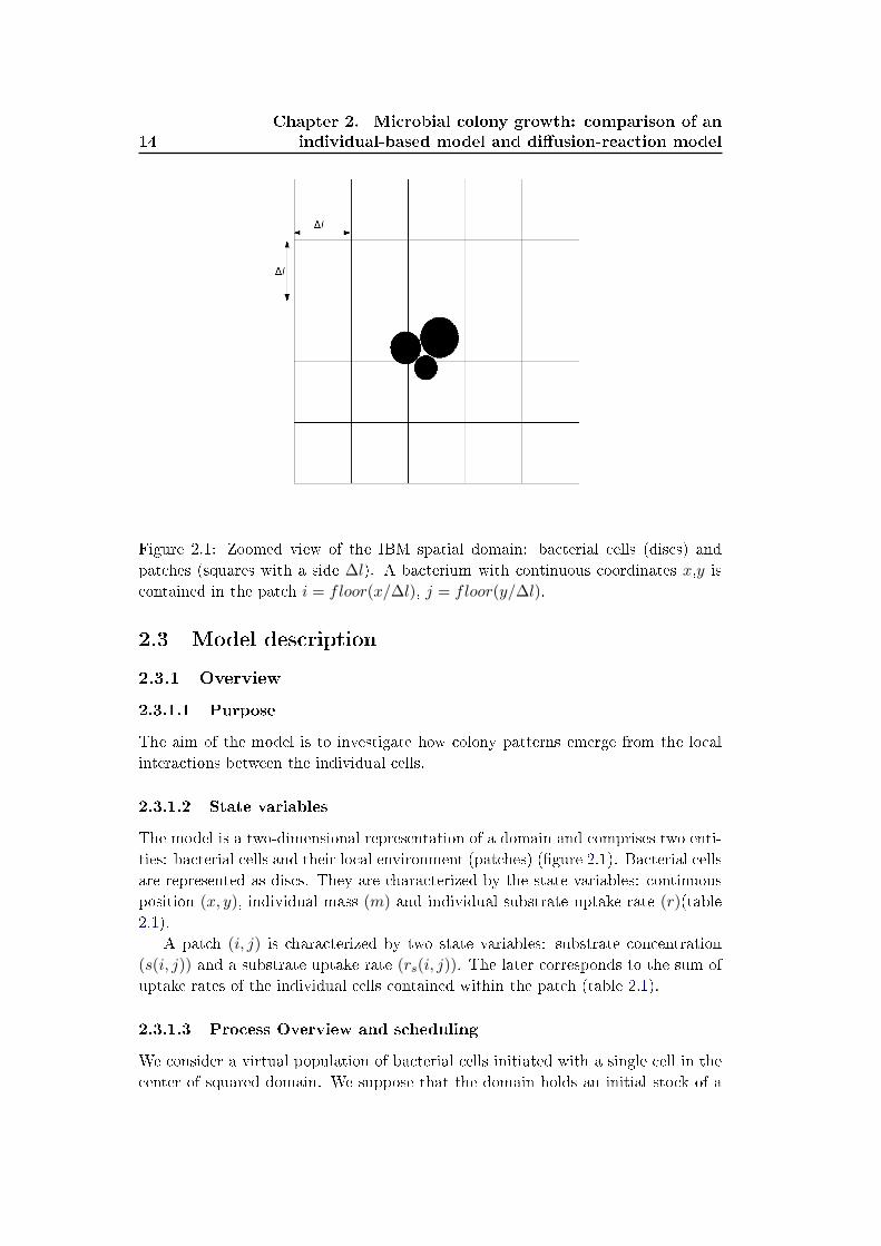
Figure 2.1: Zoomed view of the IBM spatial domain: bacterial cells (discs) and
patches (squares with a side ∆l). A bacterium with continuous coordinates x,y is
contained in the patch i = floor(x/∆l), j = floor(y/∆l).
2.3 Model description
2.3.1 Overview
2.3.1.1 Purpose
The aim of the model is to investigate how colony patterns emerge from the local
interactions between the individual cells.
2.3.1.2 State variables
The model is a two-dimensional representation of a domain and comprises two enti-
ties: bacterial cells and their local environment (patches) (�gure 2.1). Bacterial cells
are represented as discs. They are characterized by the state variables: continuous
position (x, y), individual mass (m) and individual substrate uptake rate (r)(table
2.1).
A patch (i, j) is characterized by two state variables: substrate concentration
(s(i, j)) and a substrate uptake rate (rs(i, j)). The later corresponds to the sum of
uptake rates of the individual cells contained within the patch (table 2.1).
2.3.1.3 Process Overview and scheduling
We consider a virtual population of bacterial cells initiated with a single cell in the
center of squared domain. We suppose that the domain holds an initial stock of a
2.3. Model description 15
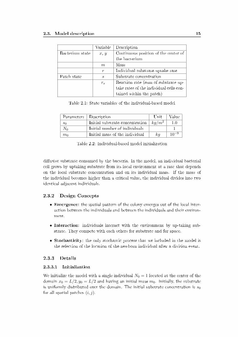
Variable Description
Bacterium state x, y Continuous position of the center of
the bacterium
m Mass
r Individual substrate uptake rate
Patch state s Substrate concentration
rs Reaction rate (sum of substrate up-
take rates of the individual cells con-
tained within the patch)
Table 2.1: State variables of the individual-based model
Parameters Description Unit Value
s0 Initial substrate concentration kg/m2 1.0
N0 Initial number of individuals 1
m0 Initial mass of the individual kg 10−9
Table 2.2: Individual-based model initialization
di�usive substrate consumed by the bacteria. In the model, an individual bacterial
cell grows by uptaking substrate from its local environment at a rate that depends
on the local substrate concentration and on its individual mass. If the mass of
the individual becomes higher than a critical value, the individual divides into two
identical adjacent individuals.
2.3.2 Design Concepts
• Emergence: the spatial pattern of the colony emerges out of the local inter-
action between the individuals and between the individuals and their environ-
ment.
• Interaction: individuals interact with the environment by up-taking sub-
strate. They compete with each others for substrate and for space.
• Stochasticity: the only stochastic process that we included in the model is
the selection of the location of the newborn individual after a division event.
2.3.3 Details
2.3.3.1 Initialization
We initialize the model with a single individual N0 = 1 located at the center of the
domain x0 = L/2, y0 = L/2 and having an initial mass m0. Initially, the substrate
is uniformly distributed over the domain. The initial substrate concentration is s0for all spatial patches (i, j).
16
Chapter 2. Microbial colony growth: comparison of an
individual-based model and di�usion-reaction model
2.3.3.2 Submodels
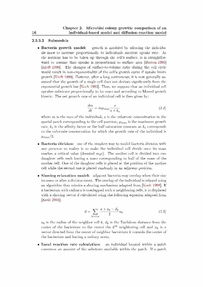
• Bacteria growth model: growth is modeled by allowing the individu-
als mass to increase proportionally to individuals nutrient uptake rate. As
the nutrient has to be taken up through the cell's surface, it is straightfor-
ward to assume that uptake is proportional to surface area [Button 1993]
[Kreft 1998]. The changes of surface-to-volume ratio during the cell cycle
would result in non-exponentiality of the cell's growth curve if uptake limits
growth [Kreft 1998]. However, after a long controversy, it is now generally as-
sumed that the growth of a single cell does not deviate signi�cantly from the
exponential growth law [Koch 1993]. Thus, we suppose that an individual cell
uptakes substrate proportionally to its mass and according to Monod growth
kinetic. The net growth rate of an individual cell is then given by:
dm
dt= mµmax
s
s+ ks(2.2)
where m is the mas of the individual, s is the substrate concentration in the
spatial patch corresponding to the cell position, µmax is the maximum growth
rate, ks is the a�nity factor or the half-saturation constant as ks corresponds
to the substrate concentration for which the growth rate of the individual is
µmax/2.
• Bacteria division: one of the simplest way to model bacteria division with
any pretense to reality is to make the individual cell divide once its mass
reaches a critical value (denoted mdc). The mother cell is divided into two
daughter cells each having a mass corresponding to half of the mass of the
mother cell. One of the daughter cells is placed at the position of the mother
cell while the second one is placed randomly in an adjacent position.
• Shoving relaxation model: adjacent bacteria may overlap when their size
increase or after a division event. The overlap of the individual is relaxed using
an algorithm that mimics a shoving mechanism adapted from [Kreft 1998]. If
a bacterium with radius a is overlapped with n neighboring cells, it is displaced
with a shoving vector d calculated using the following equation adapted from
[Kreft 2001]:
d =∑k=1:n
a+ ak − dk2
uk (2.3)
ak is the radius of the neighbor cell k, dk is the Euclidean distance from the
center of the bacterium to the center the kth neighboring cell and uk is a
vector directed from the center of neighbor bacterium k towards the center of
the bacterium and having a unitary norm.
• Local reaction rate calculation: an individual located within a patch
consumes an amount of the substrate available within the patch. If a patch
2.4. Individual-based model simulation 17
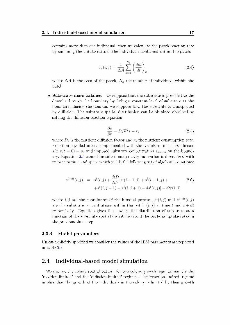
contains more than one individual, then we calculate the patch reaction rate
by summing the uptake rates of the individuals contained within the patch:
rs(i, j) =1
∆A
Nk∑k=1
(dm
dt
)k
(2.4)
where ∆A is the area of the patch, Nk the number of individuals within the
patch
• Substrate mass balance: we suppose that the substrate is provided to the
domain through the boundary by �xing a constant level of substrate at the
boundary. Inside the domain, we suppose that the substrate is transported
by di�usion. The substrate spatial distribution can be obtained obtained by
solving the di�usion-reaction equation:
∂s
∂t= Ds∇2s− rs (2.5)
where Ds is the nutrient di�usion factor and rs the nutrient consumption rate.
Equation eq:substrate is complemented with the a uniform initial conditions
s(x, t, t = 0) = s0 and imposed substrate concentration sbound on the bound-
ary. Equation 2.5 cannot be solved analytically but rather is discretized with
respect to time and space which yields the following set of algebraic equations:
st+dt(i, j) = st(i, j) +dtD
∆l2[st(i− 1, j) + st(i+ 1, j) + (2.6)
+st(i, j − 1) + st(i, j + 1)− 4st(i, j)]− dtr(i, j)
where i, j are the coordinates of the internal patches, st(i, j) and st+dt(i, j)
are the substrate concentrations within the patch (i, j) at time t and t + dt
respectively. Equation gives the new spatial distribution of substrate as a
function of the substrate spatial distribution and the bacteria uptake rates in
the previous time-step.
2.3.4 Model parameters
Unless explicitly speci�ed we consider the values of the IBM parameters are reported
in table 2.3
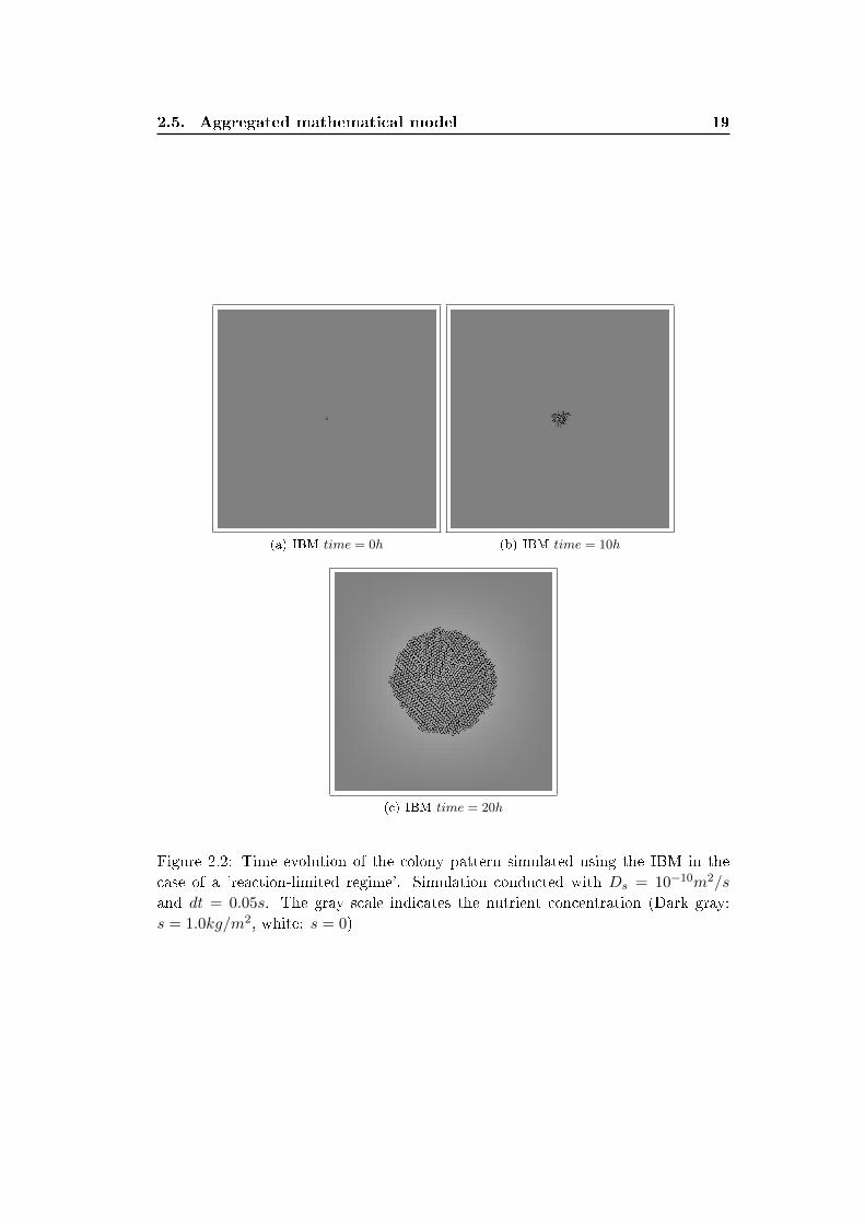
2.4 Individual-based model simulation
We explore the colony spatial pattern for two colony growth regimes, namely the
'reaction-limited' and the 'di�usion-limited' regimes. The 'reaction-limited' regime
implies that the growth of the individuals in the colony is limited by their growth
18
Chapter 2. Microbial colony growth: comparison of an
individual-based model and di�usion-reaction model
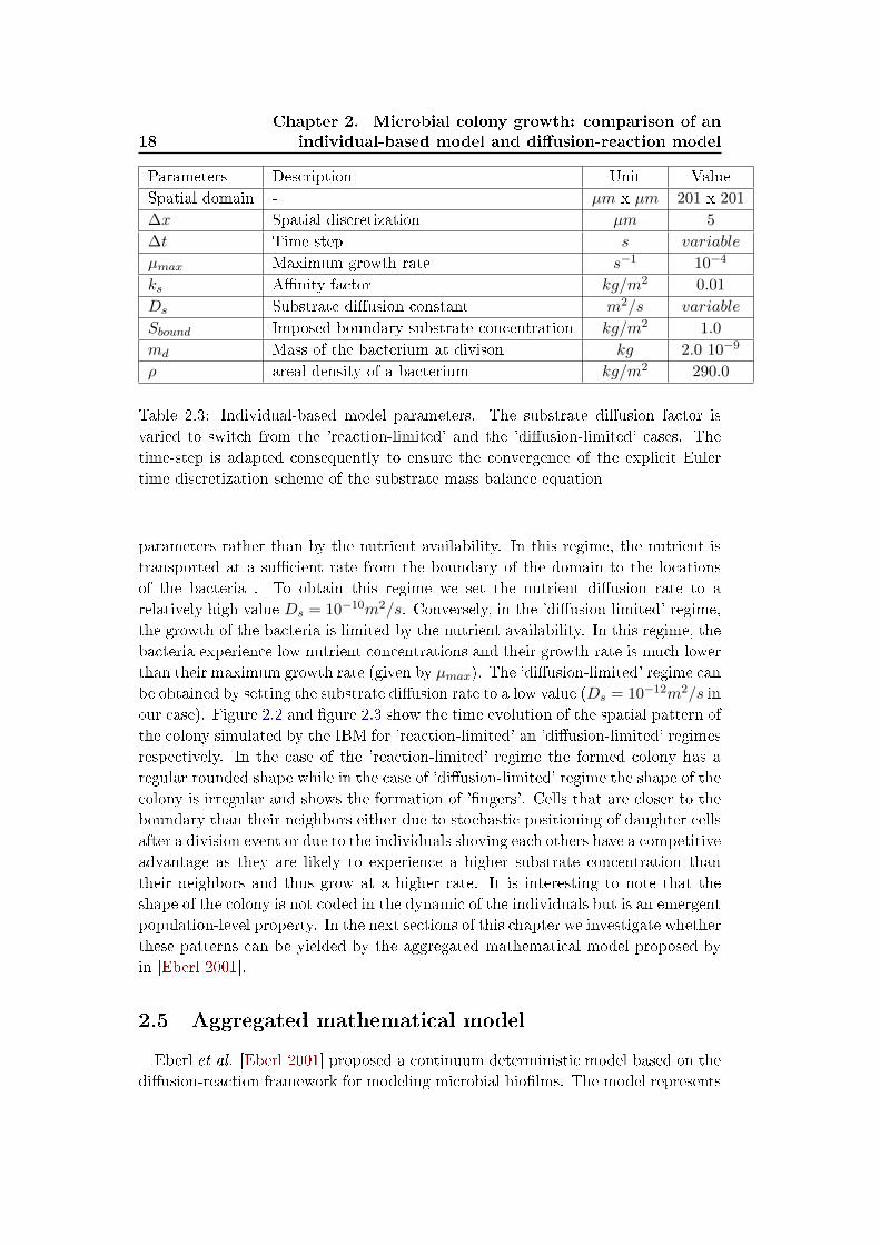
Parameters Description Unit Value
Spatial domain - µm x µm 201 x 201
∆x Spatial discretization µm 5
∆t Time step s variable
µmax Maximum growth rate s−1 10−4
ks A�nity factor kg/m2 0.01
Ds Substrate di�usion constant m2/s variable
Sbound Imposed boundary substrate concentration kg/m2 1.0
md Mass of the bacterium at divison kg 2.0 10−9
ρ areal density of a bacterium kg/m2 290.0
Table 2.3: Individual-based model parameters. The substrate di�usion factor is
varied to switch from the 'reaction-limited' and the 'di�usion-limited' cases. The
time-step is adapted consequently to ensure the convergence of the explicit Euler
time discretization scheme of the substrate mass balance equation
parameters rather than by the nutrient availability. In this regime, the nutrient is
transported at a su�cient rate from the boundary of the domain to the locations
of the bacteria . To obtain this regime we set the nutrient di�usion rate to a
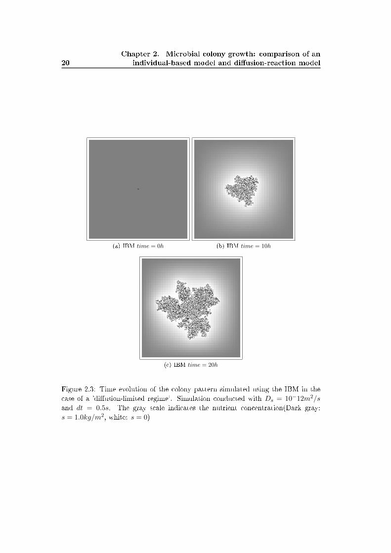
relatively high value Ds = 10−10m2/s. Conversely, in the 'di�usion-limited' regime,
the growth of the bacteria is limited by the nutrient availability. In this regime, the
bacteria experience low nutrient concentrations and their growth rate is much lower
than their maximum growth rate (given by µmax). The 'di�usion-limited' regime can
be obtained by setting the substrate di�usion rate to a low value (Ds = 10−12m2/s in
our case). Figure 2.2 and �gure 2.3 show the time evolution of the spatial pattern of
the colony simulated by the IBM for 'reaction-limited' an 'di�usion-limited' regimes
respectively. In the case of the 'reaction-limited' regime the formed colony has a
regular rounded shape while in the case of 'di�usion-limited' regime the shape of the
colony is irregular and shows the formation of '�ngers'. Cells that are closer to the
boundary than their neighbors either due to stochastic positioning of daughter cells
after a division event or due to the individuals shoving each others have a competitive
advantage as they are likely to experience a higher substrate concentration than
their neighbors and thus grow at a higher rate. It is interesting to note that the
shape of the colony is not coded in the dynamic of the individuals but is an emergent
population-level property. In the next sections of this chapter we investigate whether
these patterns can be yielded by the aggregated mathematical model proposed by
in [Eberl 2001].
2.5 Aggregated mathematical model
Eberl et al. [Eberl 2001] proposed a continuum deterministic model based on the
di�usion-reaction framework for modeling microbial bio�lms. The model represents
2.5. Aggregated mathematical model 19
(a) IBM time = 0h (b) IBM time = 10h
(c) IBM time = 20h
Figure 2.2: Time evolution of the colony pattern simulated using the IBM in the
case of a 'reaction-limited regime'. Simulation conducted with Ds = 10−10m2/s
and dt = 0.05s. The gray scale indicates the nutrient concentration (Dark gray:
s = 1.0kg/m2, white: s = 0)
20
Chapter 2. Microbial colony growth: comparison of an
individual-based model and di�usion-reaction model
(a) IBM time = 0h (b) IBM time = 10h
(c) IBM time = 20h
Figure 2.3: Time evolution of the colony pattern simulated using the IBM in the
case of a 'di�usion-limited regime'. Simulation conducted with Ds = 10−12m2/s
and dt = 0.5s. The gray scale indicates the nutrient concentration(Dark gray:
s = 1.0kg/m2, white: s = 0)
2.5. Aggregated mathematical model 21
the individuals and the substrate with two density �elds denoted respectively s(x, y)
and cb(x, y).
Compared to the IBM that we presented above, the di�usion-reaction model
that we describe in this section is an aggregated mathematical model. The no-
tion of aggregated model implies the use of aggregated state variables which provide
a macroscale description of the state of the bacteria. In a di�usion-reaction model
the aggregated state variable is biomass density �eld which determines the expected
mass density of bacteria in any location x, y of the domain.
The di�usion-reaction model for the bacteria has the following general form:
∂cb∂t
= ∇2(Dbcb) + rbcb (2.7)
The �rst term in the right-hand side accounts for the di�usion of the biomass and
the second term for the production of biomass. The �rst term expresses how the mass
of the bacteria is redistributed over neighboring patches. This term provides a rough
approximation at the macro-level of the shoving process described in the IBM. The
expansion of the colony depends on the local density of bacteria and takes place only
if the biomass density approaches a prescribed maximum value which establishes an
upper bound [Eberl 2001]. Elberl et al. [Eberl 2001] proposed a density-dependent
expression for the di�usion factor Db that satis�es this condition. The expression
takes the following generic form:
Db = D0cαb
(Cbmax − cb)β(2.8)
with α, β > 1 and D0 three parameters and Cbmax the maximum local density of
biomass. The physical interpretation of this equation is that the biomass di�usivity
vanishes as cb becomes small but increases as cb grows due to substrate uptake.
Equation 2.7 is coupled to the following di�usion-reaction equation of the substrate:
∂s
∂t= Ds∇2s− rb (2.9)
where s is the concentration of substrate, Ds the di�usion factor of the substrate
and rb the substrate uptake rate. Assuming a Monod kinetic as in the IBM, the
substrate uptake rate is given by:
rb = µmaxs
s+ kscb (2.10)
where µmax is the maximum growth rate of the bacteria and ks the half-
saturation Monod constant. Additionally, we consider the same boundary and initial
conditions for the substrate as those that we used in the IBM (�xed concentration of
substrate at the boundary and uniform initial distribution of the substrate). For the
biomass we consider periodic boundary conditions and we suppose that an initial

22
Chapter 2. Microbial colony growth: comparison of an
individual-based model and di�usion-reaction model
Parameters Description Unit Value
Spatial domain µm x µm 201 x 201
∆l µm 5
∆t s variable
µmax Maximum growth rate of the individuals s−1 10−4
ks A�nity factor kg/m2 0.01
Ds Substrate di�usion constant m2/s variable
Cbmax Maximum local density of biomass m2/s 10−12
α dimensionless 4.0
β dimensionless 4.0
D0 m2/s variable
Table 2.4: Di�usion-reaction model parameters
seed of biomass is located in the central patch of the domain. The model parameters
are reported in table 2.4.
2.6 Comparing the IBM with the di�usion-reaction
model
We compare the simulation results of both models for the two colony growth
regimes. The di�usion-reaction model proposed in [Eberl 2001] is not derived rig-
orously from the microscale dynamic that we considered in the IBM. It uses an
ad-hoc approximation of these microscale processes based on a density-dependent
expression of the biomass di�usion. This function requires four parameters α, β,
D0 and Cbmax and one of the di�culties that arises when we attempt to compare
the DRM with the IBM is to assign appropriate values to these parameters. The
parameter Cbmax (the maximum local density of biomass) can be deduced from the
IBM simulations by taking the maximum measured local density of biomass. For
the parameters α and β we use the values suggested by Eberl et al. [Eberl 2001].
The parameter D0, which is the maximum value of the biomass di�usion factor is
calibrated (manually) to obtain the best �t between the patterns yielded by both
models. A high value of D0 yields a simulated colony that expands faster than in
the IBM.
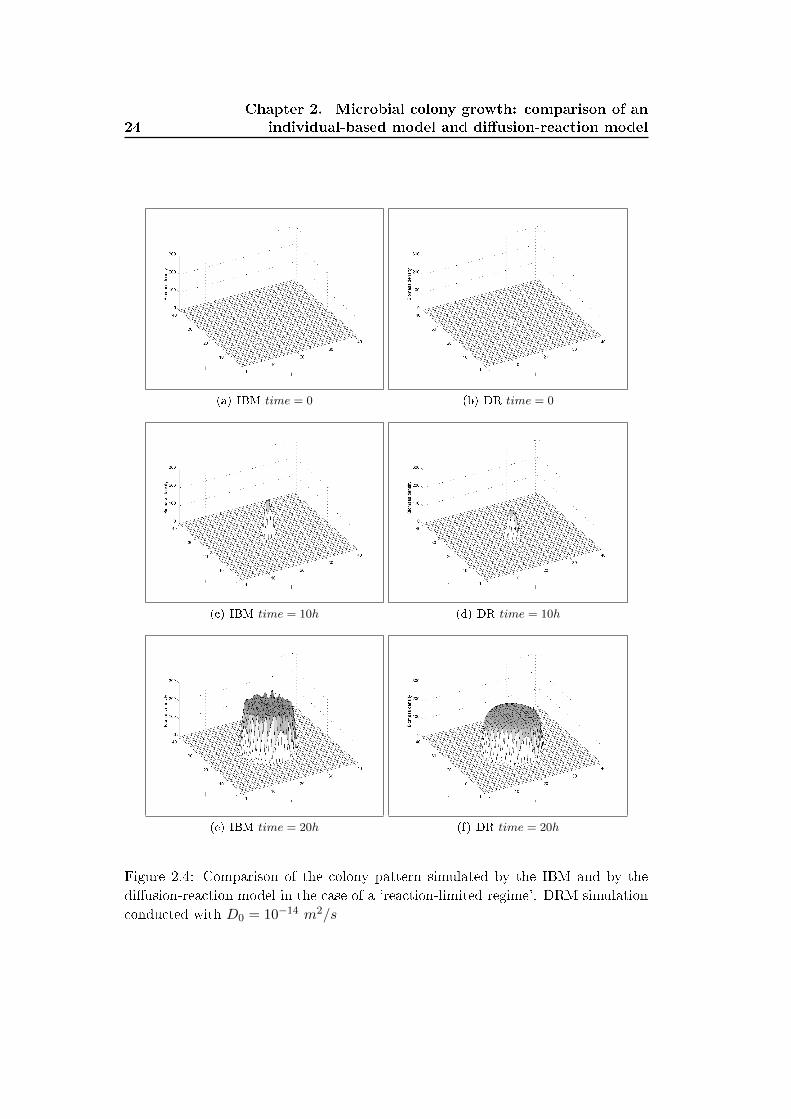
Figure 2.4 compares the snapshots of the colonies simulated with the IBM and the
di�usion-reaction model in the case of a 'reaction-limited' regime. Both models yield
rounded shaped colonies that expand equally in all directions. The �uctuations in
the colony simulated with the IBM are due to the stochastic positioning the newborn
individuals. The length scale of these �uctuations is relatively small compared to
the size of the colony, and a small number of simulations is su�cient to extract the
2.7. Discussion 23
deterministic limit yielded by the di�usion-reaction model.
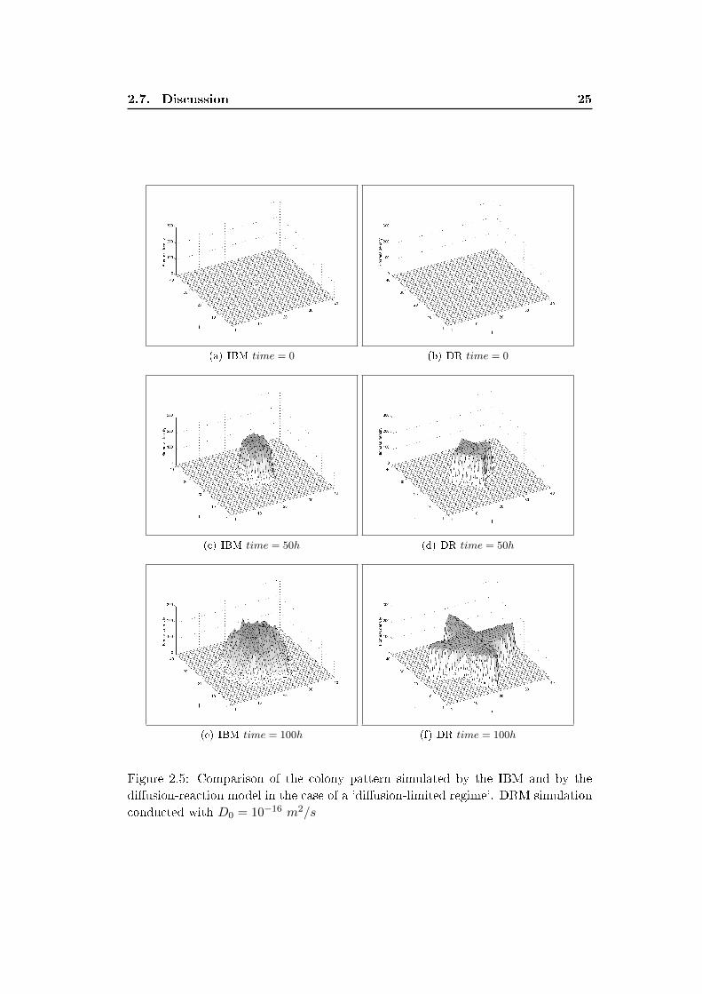
We compare the shape of the simulated colonies in the case of 'di�usion-limited'
regime. In this case, the individuals experience signi�cant heterogeneities in the
substrate concentration and consequently grow at di�erent rate depending on their
location in the colony. Individuals located at the edge of the colony tend to have
high growth rates in comparison to the individuals located at the center of the
colony. Figure 2.5 compares snapshots of the simulated colony patterns. The IBM
pattern is averaged over 20 IBM simulations run with with the same parameter and
di�erent seeds for the random number generator. In the di�usion-reaction model
the colony expands forming �ngers that are directed towards the closest distances to
the boundary of the domain where the substrate concentration is the highest. While
'�ngers' are also formed in each of the IBM simulations, they are not observed in the
average pattern and are not likely to be directed towards any preferential direction.
They seems to occur at random and the average pattern shows a round-shaped
colony. The closest distance to the boundary is not necessary the one with the
steepest nutrient gradient as the nutrient distribution is heterogeneous and can be
a�ected with the irregular shape of the colony.
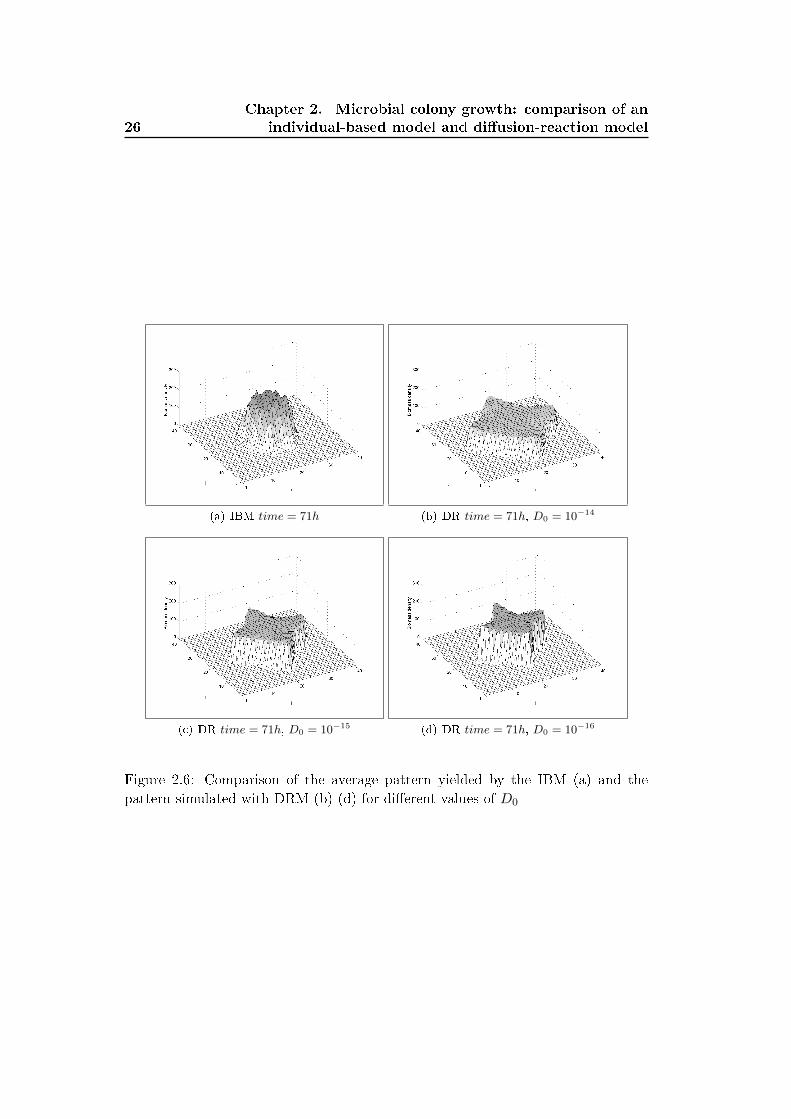
We assessed the sensitivity of the DRM pattern to the variation of the parameter
D0. Figure 2.6 shows the average pattern obtained with the IBM at an intermediate
time t = 71h and the pattern yielded by the DRM for three values of the parameter
D0. The increases of D0 increases the size of the colony and reduced it areal biomass
density (vertical axis). The shape of the colony however still have the star-like shape
with �ngers directed towards the closest boundary.
2.7 Discussion
IBM and DRM are two commonly used modeling approaches for simulating micro-
bial spatial patterns formation. In this chapter we compared these two approaches
by considering a simple case of the a mono-species colony growing on a di�usive sub-
strate. Both models yield comparable results for the case of 'reaction-limited' regime
but show signi�cant di�erences in the case of 'di�usion-limited' regime. While , int
he 'di�usion-limited' regime each realization of the IBM yields a pattern with an
irregular shape and '�nger-like' structure the average pattern yields a round shaped
colony suggesting the '�ngers' have no preferential direction. The direct averaging
of spatial patterns obtained through the replication of a simulation is often an in-
appropriate approach as some important features of the pattern (irregular shape,
�nger formation) that has an impact on the local environment of the individuals are
lost during the averaging exercise.
The DRM captures the formation of '�ngers' in the case of the 'di�usion-limited'
regime. The DRM pattern is symmetric and the �ngers directed towards the closest
24
Chapter 2. Microbial colony growth: comparison of an
individual-based model and di�usion-reaction model
(a) IBM time = 0 (b) DR time = 0
(c) IBM time = 10h (d) DR time = 10h
(e) IBM time = 20h (f) DR time = 20h
Figure 2.4: Comparison of the colony pattern simulated by the IBM and by the
di�usion-reaction model in the case of a 'reaction-limited regime'. DRM simulation
conducted with D0 = 10−14 m2/s
2.7. Discussion 25
(a) IBM time = 0 (b) DR time = 0
(c) IBM time = 50h (d) DR time = 50h
(e) IBM time = 100h (f) DR time = 100h
Figure 2.5: Comparison of the colony pattern simulated by the IBM and by the
di�usion-reaction model in the case of a 'di�usion-limited regime'. DRM simulation
conducted with D0 = 10−16 m2/s
26
Chapter 2. Microbial colony growth: comparison of an
individual-based model and di�usion-reaction model
(a) IBM time = 71h (b) DR time = 71h, D0 = 10−14
(c) DR time = 71h, D0 = 10−15 (d) DR time = 71h, D0 = 10−16
Figure 2.6: Comparison of the average pattern yielded by the IBM (a) and the
pattern simulated with DRM (b)-(d) for di�erent values of D0
2.7. Discussion 27
boundary. One of the limitations of the DRMs is the identi�ability of the model
parameters. As these models are rarely rigorously derived from the microscale dy-
namic of the individuals they imply the use of ad-hoc approximations involving
several parameters. These parameters encompass the complexity of the microscale
interaction and may lack physical meaning. Thus their values may be di�cult to
obtain from laboratory experiments.
Applying both approaches to a same problem may be very helpful. DRM provide
a deterministic reference to which the IBM simulations can be compared while the
IBM may help in assessing the quality of the approximations needed in the DRM
and in the identi�ability of the DRM parameters.

Chapter 3
Moment approximation of a
microbial IBM for colony growth
Contents
3.1 Description of the simpli�ed individual-based model . . . . 30
3.1.1 Overview . . . . . . . . . . . . . . . . . . . . . . . . . . . . . 30
3.1.2 Design concepts . . . . . . . . . . . . . . . . . . . . . . . . . . 31
3.1.3 Details . . . . . . . . . . . . . . . . . . . . . . . . . . . . . . . 32
3.1.4 Parameters . . . . . . . . . . . . . . . . . . . . . . . . . . . . 32
3.1.5 Model outputs . . . . . . . . . . . . . . . . . . . . . . . . . . 33
3.1.6 Comparison of the simpli�ed IBM with the detailed IBM . . 33
3.1.7 Moment approximation of the simpli�ed IBM . . . . . . . . . 34
3.1.8 Solving the moment approximation model . . . . . . . . . . . 43
3.2 Comparison of the moment model with the simpli�ed IBM 45
3.2.1 Density independent growth model (b′1 = 0) . . . . . . . . . . 45
3.2.2 Density dependant division model (b′1 > 0) . . . . . . . . . . 48
3.3 Discussion . . . . . . . . . . . . . . . . . . . . . . . . . . . . . . 49
3.4 Annexe A: expressing the moment model in radial coordi-
nates . . . . . . . . . . . . . . . . . . . . . . . . . . . . . . . . . 52
In the previous chapter (chapter 2) we investigated how a spatially explicit
individual-based model for simulating the growth of a microbial colony compares
to di�usion-reaction models. In this chapter we are concerned with another class
of aggregated mathematical models, namely spatial moment approximation models.
Spatial moments models were originally developed in statistical physics and have
been applied during the last decade to the approximation of individual-based models
that arise in several ecological systems of plants and animals [Dieckmann 2000]. In
this chapter we discuss the extension of the approach to modeling microbial systems
and illustrate with the example of microbial colony growth with a slight di�erence
compared to the previous chapter. Here we will consider systems initialized with
n0 > 1 individuals randomly distributed rather than with one individual located in
the center of the domain.
30
Chapter 3. Moment approximation of a microbial IBM for colony
growth
The derivation of the moment approximating model from the detailed IBM in-
cluding individuals with variable sizes and complex shoving process is quiet di�cult.
Thus our approach consist in �rst simplifying the detailed IBM than approximate
the simpli�ed IBM using moment techniques.
The chapter in organized in three parts: the �rst part is dedicated to the sim-
pli�cation of the colony growth IBM. In the second part we derive a moment ap-
proximation model of the simpli�ed IBM. In the third part we compare the moment
model and the simpli�ed model to assess the quality of the approximations consid-
ered in the moment model. We conclude this chapter by discussing the relevance
of the spatial moment method in approximating microbial IBMs and the possible
extensions of the approach.
3.1 Description of the simpli�ed individual-based model
We describe in Chapter 2 an IBM for the growth of a colony in which the in-
dividual cells are represented as discs with variable diameters. The individuals
grow and divide while uptaking a di�usive substrate. They shove each others mak-
ing the size of the colony to increase. The individuals compete for the nutrient
and the increase of their local density decreases the level of nutrient and reduces
their growth rate. This phenomena is somehow comparable to a density-dependent
growth process. When the local density of the bacteria increases their individual
growth rate decreases because of the decrease of the local substrate concentration
perceived by the bacteria. We propose to construct a simple IBM that captures
this density-dependant growth without considering the variability in individual size
and the explicit dynamic of the substrate. We also simplify the shoving process by
using instead a uniform dispersion kernel. We assess how this simpli�cation a�ect
the shape of the colony. In this section we propose to describe the simpli�ed IBM
using the ODD protocol.
3.1.1 Overview
3.1.1.1 State variables and scales
We consider a sessile community of individual bacterial cells living in a two-
dimensional space. The individual cells are considered as point particles entirely
characterized by their location x = (x1, x2) in this plane. The abiotic environment
is homogeneous in space.
3.1.1.2 Process overview
The community changes through two stochastic events acting on the individuals:
division and lysis (or death). We suppose that individuals divide with a probability
that decreases with the increase of the local density of individuals and die with
a constant probability. The local density is measured using an interaction kernel
3.1. Description of the simpli�ed individual-based model 31
specifying how neighboring individuals a�ect the division rate of a focal individual.
During a division event we suppose that the parent individual generates an o�spring
which position is randomly selected within a neighborhood of its parent.
3.1.1.3 Scheduling
The temporal behavior of the simpli�ed IBM is governed solely by the stochas-
tic division and death events. To simulate the temporal evolution of such system
we need to specify when the next event will occur, what kind of event it will be
and which individual will be concerned with the event. Gillespie [GIllespie 1976]
proposed a Monte Carlo procedure for simulating comparable stochastic processes
that arise in chemical reaction research. The procedure can easily be extended to
a stochastic birth-death model in which the individuals experience di�erent birth
and death probabilities [Dieckmann 1999]. The procedure iterate over the following
steps:
1. Set the time to t = 0
2. Calculate the division and death rates bi(p) and di of each individual i = 1..n
where p is the spatial pattern at time t
3. Calculate the sums rb =∑n
i=1 bi(p) and rd =∑n
i=1 di. The rate at which an
event (division or death) occurs is given by r(t) = rb(t) + rd(t)
4. Choose the waiting time τ for the next event to occur according to τ = −1r lnλ
where 0 < λ ≤ 1 is a uniformly distributed random number
5. Choose a division or death event with a probability rb/r and rd/r respectively
6. Choose an individual k with a probability bk/rb (if the event is division) or
dk/rd if the event is death, where bk and dk are the respectively the division
and death rates of the individual k
7. Perform the selected event on the individual k
8. Update time according to t = t+ τ
9. Continue from step 2 until t < tend
3.1.2 Design concepts
• Stochasticity: all the processes (division and death processes)are stochastic.
• Emergence: the spatial pattern emerges from the iteration of division and
death processes of the individuals.
32
Chapter 3. Moment approximation of a microbial IBM for colony
growth
3.1.3 Details
3.1.3.1 Initialization
The model is initialized with N0 = 100 cells distributed uniformly over the domain.
3.1.3.2 Submodels
• Division: we suppose that the probability per unit of time that an individual
i in position xi produces a new cell located in position x′ is given by:
B(xi, x′) = [b1 − b′1ploc(xi)]K
(||xi − x′||
wb
)(3.1)
The parameters b1 and b′1 are the density-independent and the density-
dependant division rates respectively. The term ploc(xi) is the local den-
sity (de�ned in more details below) perceived by the individual in xi.
K(||xi−x′||/wb) is a dispersion kernel (we call it also birth or division kernel).
The dispersion kernel gives the probability that the newly formed individ-
ual disperses instantaneously after the division event to the location x′. For
simplicity we use a uniform dispersion kernel. In some way, the dispersion
kernel translates the observation that daughter cells are located randomly in
the neighborhood of their mother cells.
• Calculation of the perceived local density: in a system containing N indi-
viduals, each individual has at maximum N − 1 neighbors. However, as we
suppose that individuals perceive only their local environment. They are likely
to be a�ected only by the neighbors located in their immediate surrounding
environment. In order to calculate this perceived local density of neighbors we
use a uniform interaction kernel, denoted K(||xi − xj ||/wd). The interactionkernel measures the contribution of the individual j in xj to the local den-
sity perceived by the individual i in xi. The perceived local density is then
calculated using the following expression:
ploc(x) =
j=n∑j=0,j 6=i
K
(||xi − xj ||
wd
)(3.2)
• Death process: we suppose that the individuals die at a constant rate d1.
The death probability of an individual per unit of time is supposed to be
independent from the local density of individuals.
3.1.4 Parameters
The model parameters are summarized in table 1.
3.1. Description of the simpli�ed individual-based model 33
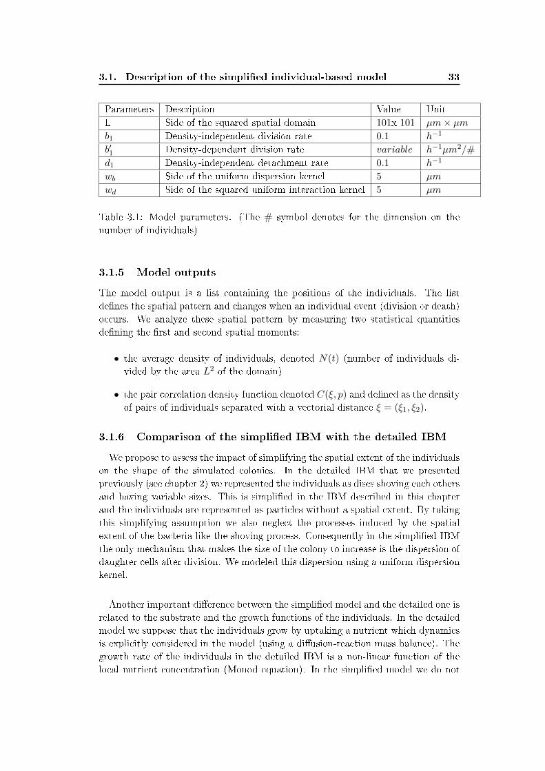
Parameters Description Value Unit
L Side of the squared spatial domain 101x 101 µm× µmb1 Density-independent division rate 0.1 h−1
b′1 Density-dependant division rate variable h−1µm2/#
d1 Density-independent detachment rate 0.1 h−1
wb Side of the uniform dispersion kernel 5 µm
wd Side of the squared uniform interaction kernel 5 µm
Table 3.1: Model parameters. (The # symbol denotes for the dimension on the
number of individuals)
3.1.5 Model outputs
The model output is a list containing the positions of the individuals. The list
de�nes the spatial pattern and changes when an individual event (division or death)
occurs. We analyze these spatial pattern by measuring two statistical quantities
de�ning the �rst and second spatial moments:
• the average density of individuals, denoted N(t) (number of individuals di-
vided by the area L2 of the domain)
• the pair correlation density function denoted C(ξ, p) and de�ned as the density
of pairs of individuals separated with a vectorial distance ξ = (ξ1, ξ2).
3.1.6 Comparison of the simpli�ed IBM with the detailed IBM
We propose to assess the impact of simplifying the spatial extent of the individuals
on the shape of the simulated colonies. In the detailed IBM that we presented
previously (see chapter 2) we represented the individuals as discs shoving each others
and having variable sizes. This is simpli�ed in the IBM described in this chapter
and the individuals are represented as particles without a spatial extent. By taking
this simplifying assumption we also neglect the processes induced by the spatial
extent of the bacteria like the shoving process. Consequently in the simpli�ed IBM
the only mechanism that makes the size of the colony to increase is the dispersion of
daughter cells after division. We modeled this dispersion using a uniform dispersion
kernel.
Another important di�erence between the simpli�ed model and the detailed one is
related to the substrate and the growth functions of the individuals. In the detailed
model we suppose that the individuals grow by uptaking a nutrient which dynamics
is explicitly considered in the model (using a di�usion-reaction mass balance). The
growth rate of the individuals in the detailed IBM is a non-linear function of the
local nutrient concentration (Monod equation). In the simpli�ed model we do not
34
Chapter 3. Moment approximation of a microbial IBM for colony
growth
account explicitly for the nutrient dynamic. The division rate of the individual is a
decreasing linear function of the local density of the individuals.
Figures 3.1 and 3.2 show colony patterns simulated with both models in the case
of a 'reaction-limited' and 'di�usion-limited' regimes. We switch from the 'reaction-
limited' regime to the 'di�usion-limited' regime by decreasing the nutrient di�usion
factor in the detailed model and by increasing the value of the density-dependent
growth parameter b′1 in the simpli�ed model. The patterns yielded by both models
shows similarities and di�erences. First the simpli�ed model reproduces quiet well
the circular and irregular shapes observed in the detailed model. The distribution
of the individuals within the colony are however di�erent in the pattern yielded
by both models. In the original model the individuals are tightly packed where as
in the simpli�ed model they are dispersed within the colony. This is due to the
simpli�cation of the mechanical pushing process (shoving process) considered in the
detailed model. Shoving process rearranges the position of the individual in the
colony simulated with the detailed IBM and relax overlapping of neighboring cells.
In the detailed IBM the cells continuously shove each others and their position in
slightly modi�ed after each time step while in the simpli�ed IBM the position of the
daughter cell is �xed after the division event and do not change in time. The e�ect
of shoving can be included in the simpli�ed IBM by adding a density-dependent
motility process where individuals become motile when the local density of neighbors
increases. However for simplicity we do not include this e�ect and consider that the
simpli�ed IBM already captures the main features of colony shape. Another form
of density-dependent motility will be studied in more detail in chapter 5 to 7.
Finally, substrate dynamic can also be included in the simpli�ed IBM by repre-
senting substrate as particles undergoing a Brownian motion. The division rate of
the bacteria can be expressed as a function of the local density of substrate par-
ticles, and substrate consumption can be modeled as predation process. However
this adds some complexity to the individual-based model and some algebra to the
moment approximation model. We consider that at least qualitatively the e�ect
of the substrate is implicitly included in the simpli�ed IBM through the use of
density-dependent growth function.
3.1.7 Moment approximation of the simpli�ed IBM
Now we propose to derive a deterministic mathematical model approximating
the dynamic of the simpli�ed IBM using moment approximation techniques. The
principle of the moment approximation technique is to derive the equations that
describe the dynamic of the �rst and second spatial moments. The �rst moment
is the average density and contains no spatial information about the pattern. The
second moment measure the variation of the density of individuals in space and is
represented by the density of pairs of individuals separated with vectorial distance
ξ. We �rst start by de�ning these moments for a set of n individuals that inhabit
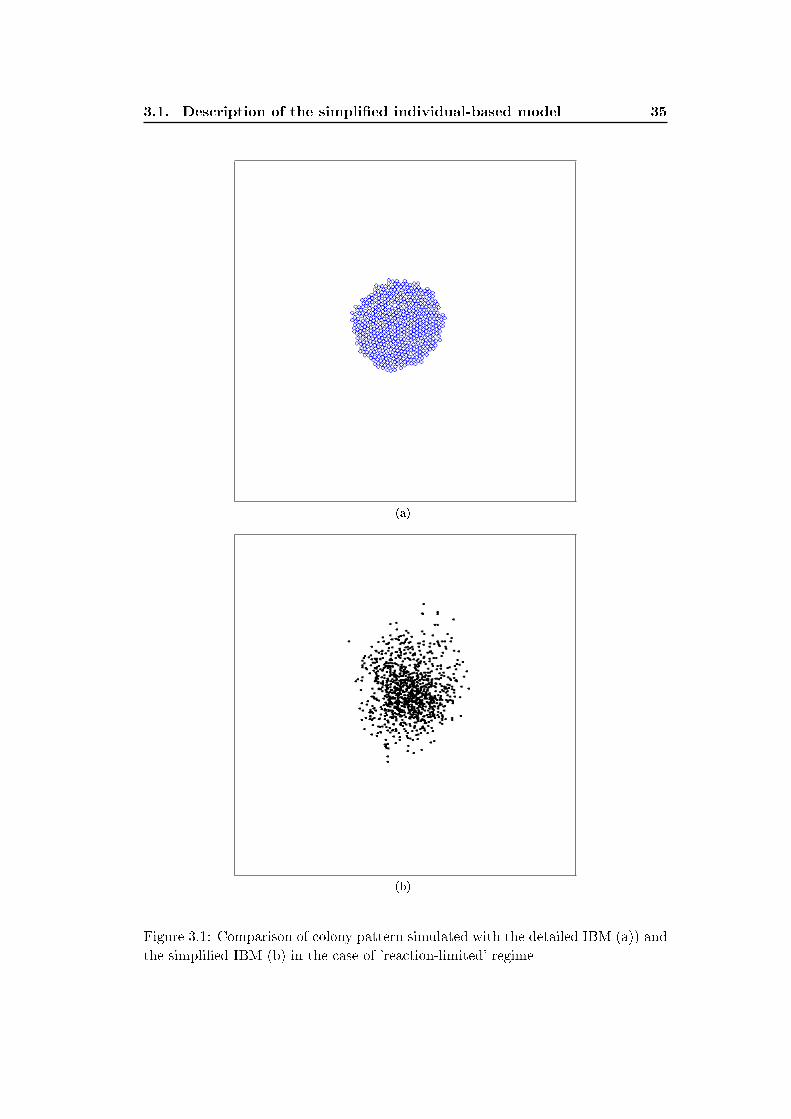
3.1. Description of the simpli�ed individual-based model 35
(a)
(b)
Figure 3.1: Comparison of colony pattern simulated with the detailed IBM (a)) and
the simpli�ed IBM (b) in the case of 'reaction-limited' regime
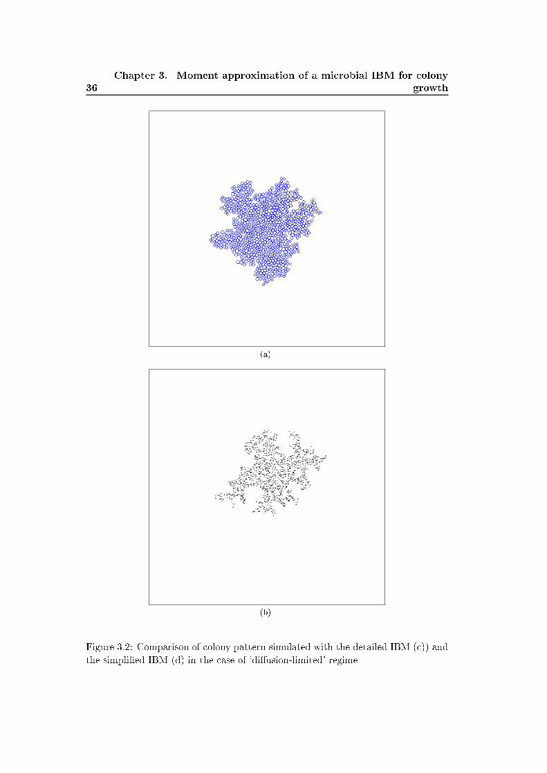
36
Chapter 3. Moment approximation of a microbial IBM for colony
growth
(a)
(b)
Figure 3.2: Comparison of colony pattern simulated with the detailed IBM (c)) and
the simpli�ed IBM (d) in the case of 'di�usion-limited' regime
3.1. Description of the simpli�ed individual-based model 37
a continuous space and occupying continuous positions xi, i = 1..n then we derive
their dynamical equations.
The �rst and second moments can be calculated on the pattern yielded by the
IBM and compared to those obtained by solving numerically the moment model
equations. The calculation of the �rst moment from the IBM simulation results
is performed simply by counting the number of individuals and dividing by the
domain area to get an average density over the domain. The second spatial moment
is measured through the pair correlation function. The pair correlation function
C(ξ) gives the average density of individuals located at a vectorial distance ξ from
a focal individual. We calculate the pair correlation density function for a given
pattern p formed with n individuals as in [Dieckmann 2000] by counting for a focal
individual at location x = (x1, x2), the number of paired individuals within the
square (x1 + ξ1, x1 + ξ1 + dξ1) × (x2 + ξ2, x2 + ξ2 + dξ2), using a su�ciently small
spatial resolution dξ = (dξ1, dξ2). We repeat this procedure for each individual in
turn being the focal one and dividing the total count by the domain area L2 and
by dξ1dξ2 yields the pair density at distance ξ. The result is a matrix. The central
value of the matrix corresponds to the average density of individuals experienced by
a focal individual at distances smaller than the spatial resolution dξ. The matrix can
be understood by imagining that a virtual focal individual is located in the center.
The matrix than correspond to the average `individuals'eye view' of its environment.
Figure 3.3 shows two snapshots of an IBM simulation of two colonies. The colonies
show di�erent shapes. The bacteria in the �rst seems distributed uniformly where
as they are organized in small groups in the second pattern. Figure 3.4 reports the
corresponding pair correlation functions (C(ξ) matrices plotted using Matlab). The
matrices should not be confused with the colony pattern itself. The matrices de-
scribes the average local environment experience by an individual within the colony
at di�erent distances. A peak in the center of the matrix indicates that the indi-
viduals experience a high density of neighbors at short distances. These densities
tend to vanish at higher distances. The matrices are normalized such that a value
of 1 corresponds to a Poisson-like patterns where the individuals are uniformly dis-
tributed over the domain. Values higher than one indicates an aggregated pattern
meaning that the density experienced by the individuals is higher than what would
be expected if the individuals were distributed uniformly. The comparison of the
pair correlation matrices con�rm that the individuals within the colonies in �gure
3.3 experience di�erent local conditions in term of neighbor densities. The pro�les
of the Cartesian pair correlation function plotted in �gure 3.4 that the pair cor-
relation function takes values close to 1 for the �rst colony indicating the absence
of any spatial structure, whereas the second function peaked at short distance and
vanished to one at large distances. The peak at short distances indicates that the
individuals are likely to experience higher densities of neighbors than what would
be experienced in the absence of any spatial structure. The pair correlation function
38
Chapter 3. Moment approximation of a microbial IBM for colony
growth
captures well the heterogeneities experienced by the individuals.
3.1.7.1 Deriving the dynamic equations of the �rst and second moment
The dynamic of the �rst moment (mean density of individuals) is given by the
following equation:
dN
dt= (b1 − d1)N − b′1
∫C(ξ)K
(||ξ||wd
)dξ (3.3)
The �rst term on the right-hand side is neighborhood-independent components
of divisions and death, and the second term is the neighborhood-dependent compo-
nents of divisions. The integral term involve the pair density function C(ξ) and the
interaction kernel K(||ξ||/wd). This term encompass the e�ect of the local environ-
ment on the mean density of individuals which is the result of the spatial structure,
as given by C(ξ), and on the extent the individuals experience the e�ect of this
structure as given by K(||ξ||/wd). Note that if the side of the uniform interaction
kernel, wd, is equal to the side L of the domain than equation 3.3 can be simpli�ed
to a simple non spatial Lotka-voltera equation [Law 2000]:
dN
dt= (b1 − d1)N − b′1N2 (3.4)
In this case the division rate of any individual is equally a�ected by all the
other individuals. However in most microbial system the individuals perceive only
their local environment. The dynamic of the second moment accounts for the pro-
cesses (division and death) that a�ect the density of pairs separated with a vectorial
distance ξ.
dC(ξ)
dt=
(dC(ξ)
dt
)division
+
(dC(ξ)
dt
)death
(3.5)
The terms in the right-hand side denote respectively the e�ect of division and
death events on the density of pairs C(ξ). The e�ect of the death is straightforward.
Consider a pair of individuals separated with a distance ξ. If one of these two
individual dies than we loose a pair of individuals separated with a distance ξ. The
rate at which we loose pairs of individual separated with a distance ξ is given by:
(dC(ξ)
dt
)death
= −2d1C(ξ) (3.6)
The e�ect of the individual division events on the density of pairs at distance ξ
is more complicated and is given by the following equation:
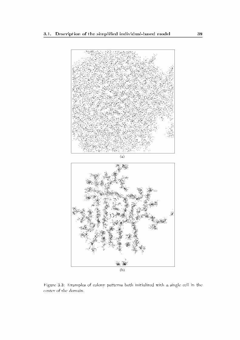
3.1. Description of the simpli�ed individual-based model 39
(a)
(b)
Figure 3.3: Examples of colony patterns both initialized with a single cell in the
center of the domain.
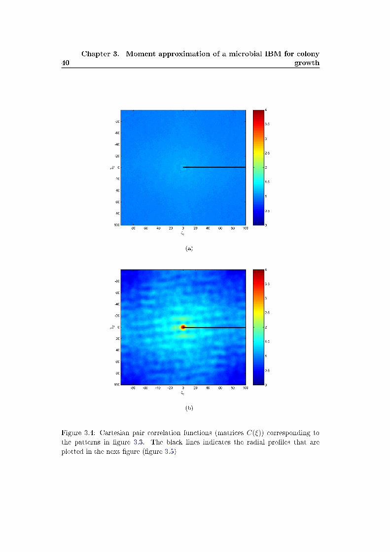
40
Chapter 3. Moment approximation of a microbial IBM for colony
growth
(a)
(b)
Figure 3.4: Cartesian pair correlation functions (matrices C(ξ)) corresponding to
the patterns in �gure 3.3. The black lines indicates the radial pro�les that are
plotted in the next �gure (�gure 3.5)
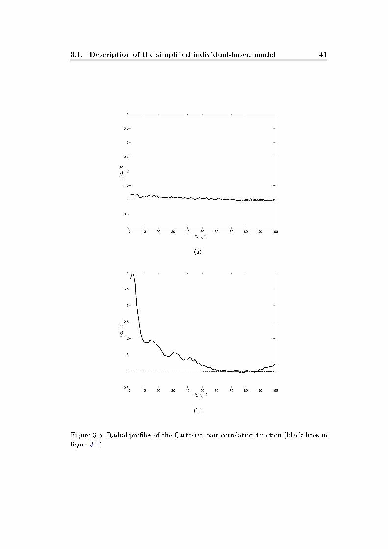
3.1. Description of the simpli�ed individual-based model 41
(a)
(b)
Figure 3.5: Radial pro�les of the Cartesian pair correlation function (black lines in
�gure 3.4)
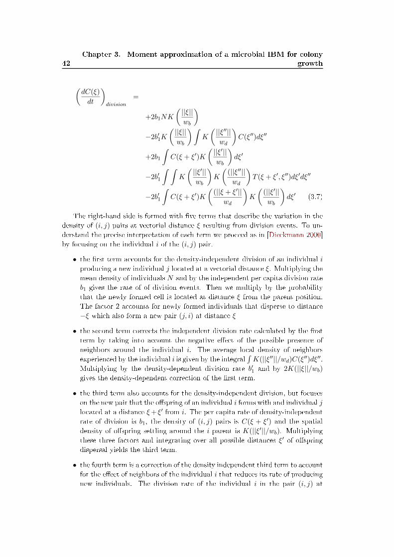
42
Chapter 3. Moment approximation of a microbial IBM for colony
growth
(dC(ξ)
dt
)division
=
+2b1NK
(||ξ||wb
)−2b′1K
(||ξ||wb
)∫K
(||ξ′′||wd
)C(ξ′′)dξ′′
+2b1
∫C(ξ + ξ′)K
(||ξ′||wb
)dξ′
−2b′1
∫ ∫K
(||ξ′||wb
)K
((||ξ′′||wd
)T (ξ + ξ′, ξ′′)dξ′dξ′′
−2b′1
∫C(ξ + ξ′)K
((||ξ + ξ′||
wd
)K
((||ξ′||wb
)dξ′ (3.7)
The right-hand side is formed with �ve terms that describe the variation in the
density of (i, j) pairs at vectorial distance ξ resulting from division events. To un-
derstand the precise interpretation of each term we proceed as in [Dieckmann 2000]
by focusing on the individual i of the (i, j) pair.
• the �rst term accounts for the density-independent division of an individual i
producing a new individual j located at a vectorial distance ξ. Multiplying the
mean density of individuals N and by the independent per capita division rate
b1 gives the rate of of division events. Then we multiply by the probability
that the newly formed cell is located at distance ξ from the parent position.
The factor 2 accounts for newly formed individuals that disperse to distance
−ξ which also form a new pair (j, i) at distance ξ
• the second term corrects the independent division rate calculated by the �rst
term by taking into account the negative e�ect of the possible presence of
neighbors around the individual i. The average local density of neighbors
experienced by the individual i is given by the integral∫K(||ξ′′||/wd)C(ξ′′)dξ′′.
Multiplying by the density-dependent division rate b′1 and by 2K(||ξ||/wb)gives the density-dependent correction of the �rst term.
• the third term also accounts for the density-independent division, but focuses
on the new pair that the o�spring of an individual i forms with and individual j
located at a distance ξ+ ξ′ from i. The per capita rate of density-independent
rate of division is b1, the density of (i, j) pairs is C(ξ + ξ′) and the spatial
density of o�spring settling around the i parent is K(||ξ′||/wb). Multiplying
these three factors and integrating over all possible distances ξ′ of o�spring
dispersal yields the third term.
• the fourth term is a correction of the density independent third term to account
for the e�ect of neighbors of the individual i that reduces its rate of producing
new individuals. The division rate of the individual i in the pair (i, j) at
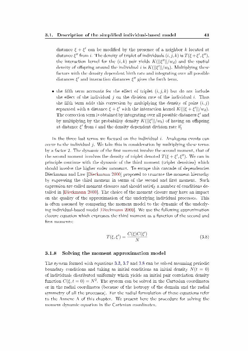
3.1. Description of the simpli�ed individual-based model 43
distance ξ + ξ′ can be modi�ed by the presence of a neighbor k located at
distance ξ′′ from i. The density of triplet of individuals (i, j, k) is T (ξ+ξ′, ξ′′),
the interaction kernel for the (i, k) pair yields K(||ξ′′||/wd) and the spatial
density of o�spring around the individual i is K(||ξ′||/wb). Multiplying these
factors with the density dependent birth rate and integrating over all possible
distances ξ′ and interaction distances ξ′′ gives the forth term.
• the �fth term accounts for the e�ect of triplet (i, j, k) but do not include
the e�ect of the individual j on the division rate of the individual i. Thus
the �fth term adds this correction by multiplying the density of pairs (i, j)
separated with a distance ξ + ξ′ with the interaction kernel K(||ξ + ξ′||/wd).The correction term is obtained by integrating over all possible distances ξ′ and
by multiplying by the probability density K(||ξ′||/wb) of having an o�spring
at distance ξ′ from i and the density dependent division rate b′1
In the three last terms we focused on the individual i. Analogous events can
occur to the individual j. We take this in consideration by multiplying these terms
by a factor 2. The dynamic of the �rst moment involve the second moment, that of
the second moment involves the density of triplet denoted T (ξ + ξ′, ξ′′). We can in
principle continue with the dynamic of the third moment (triplet densities) which
should involve the higher order moments. To escape this cascade of dependencies
Dieckmann and Law [Dieckmann 2000] proposed to truncate the moment hierarchy
by expressing the third moment in terms of the second and �rst moment. Such
expression are called moment closures and should satisfy a number of conditions de-
tailed in [Dieckmann 2000]. The choice of the moment closure may have an impact
on the quality of the approximation of the underlying individual processes. This
is often assessed by comparing the moment model to the dynamic of the underly-
ing individual-based model [Dieckmann 2000]. We use the following approximation
closure equation which expresses the third moment as a function of the second and
�rst moments:
T (ξ, ξ′) =C(ξ)C(ξ′)
N(3.8)
3.1.8 Solving the moment approximation model
The system formed with equations 3.3, 3.7 and 3.8 can be solved assuming periodic
boundary conditions and taking as initial conditions an initial density N(t = 0)
of individuals distributed uniformly which yields an initial pair correlation density
function C(ξ, t = 0) = N2. The system can be solved in the Cartesian coordinates
or in the radial coordinates (because of the isotropy of the domain and the radial
symmetry of all the processes). For the radial formulation of these equations refer
to the Annexe A of this chapter. We present here the procedure for solving the
moment dynamic equation in the Cartesian coordinates.
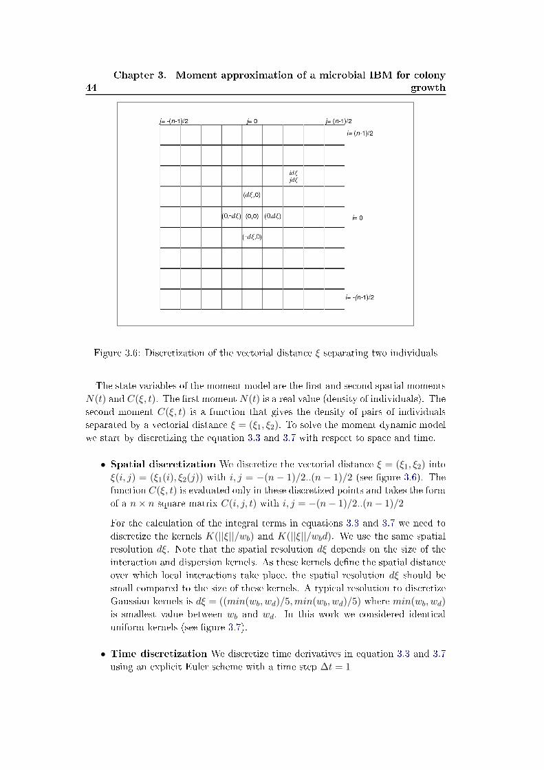
44
Chapter 3. Moment approximation of a microbial IBM for colony
growth
Figure 3.6: Discretization of the vectorial distance ξ separating two individuals
The state variables of the moment model are the �rst and second spatial moments
N(t) and C(ξ, t). The �rst moment N(t) is a real value (density of individuals). The
second moment C(ξ, t) is a function that gives the density of pairs of individuals
separated by a vectorial distance ξ = (ξ1, ξ2). To solve the moment dynamic model
we start by discretizing the equation 3.3 and 3.7 with respect to space and time.
• Spatial discretization We discretize the vectorial distance ξ = (ξ1, ξ2) into
ξ(i, j) = (ξ1(i), ξ2(j)) with i, j = −(n − 1)/2..(n − 1)/2 (see �gure 3.6). The
function C(ξ, t) is evaluated only in these discretized points and takes the form
of a n× n square matrix C(i, j, t) with i, j = −(n− 1)/2..(n− 1)/2
For the calculation of the integral terms in equations 3.3 and 3.7 we need to
discretize the kernels K(||ξ||/wb) and K(||ξ||/wbd). We use the same spatial
resolution dξ. Note that the spatial resolution dξ depends on the size of the
interaction and dispersion kernels. As these kernels de�ne the spatial distance
over which local interactions take place, the spatial resolution dξ should be
small compared to the size of these kernels. A typical resolution to discretize
Gaussian kernels is dξ = ((min(wb, wd)/5,min(wb, wd)/5) where min(wb, wd)
is smallest value between wb and wd. In this work we considered identical
uniform kernels (see �gure 3.7).
• Time discretization We discretize time derivatives in equation 3.3 and 3.7
using an explicit Euler scheme with a time step ∆t = 1
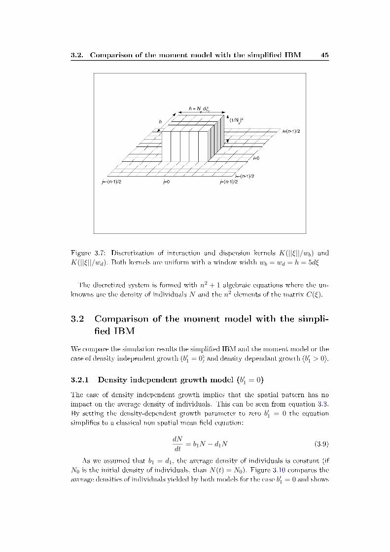
3.2. Comparison of the moment model with the simpli�ed IBM 45
Figure 3.7: Discretization of interaction and dispersion kernels K(||ξ||/wb) and
K(||ξ||/wd). Both kernels are uniform with a window width wb = wd = h = 5dξ
The discretized system is formed with n2 + 1 algebraic equations where the un-
knowns are the density of individuals N and the n2 elements of the matrix C(ξ).
3.2 Comparison of the moment model with the simpli-
�ed IBM
We compare the simulation results the simpli�ed IBM and the moment model or the
case of density-independent growth (b′1 = 0) and density-dependant growth (b′1 > 0).
3.2.1 Density independent growth model (b′1 = 0)
The case of density independent growth implies that the spatial pattern has no
impact on the average density of individuals. This can be seen from equation 3.3.
By setting the density-dependent growth parameter to zero b′1 = 0 the equation
simpli�es to a classical non spatial mean �eld equation:
dN
dt= b1N − d1N (3.9)
As we assumed that b1 = d1, the average density of individuals is constant (if
N0 is the initial density of individuals, than N(t) = N0). Figure 3.10 compares the
average densities of individuals yielded by both models for the case b′1 = 0 and shows
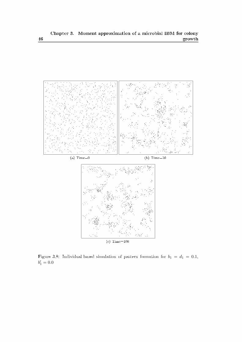
46
Chapter 3. Moment approximation of a microbial IBM for colony
growth
(a) Time=0 (b) Time=50
(c) Time=100
Figure 3.8: Individual-based simulation of pattern formation for b1 = d1 = 0.1,
b′1 = 0.0
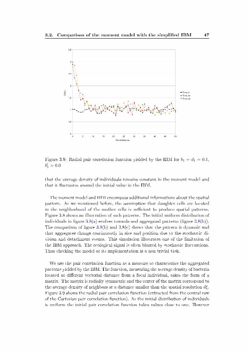
3.2. Comparison of the moment model with the simpli�ed IBM 47
Figure 3.9: Radial pair correlation function yielded by the IBM for b1 = d1 = 0.1,
b′1 = 0.0
that the average density of individuals remains constant in the moment model and
that it �uctuates around the initial value in the IBM.
The moment model and IBM encompass additional informations about the spatial
pattern. As we mentioned before, the assumption that daughter cells are located
in the neighborhood of the mother cells is su�cient to produce spatial patterns.
Figure 3.8 shows an illustration of such patterns. The initial uniform distribution of
individuals in �gure 3.8(a) evolves towards and aggregated patterns (�gure 3.8(b)).
The comparison of �gure 3.8(b) and 3.8(c) shows that the pattern is dynamic and
that aggregates change continuously in size and position due to the stochastic di-
vision and detachment events. This simulation illustrates one of the limitation of
the IBM approach. The ecological signal is often blurred by stochastic �uctuations.
Thus checking the model or its implementation is a non trivial task.
We use the pair correlation function as a measure to characterize the aggregated
patterns yielded by the IBM. The function, measuring the average density of bacteria
located at di�erent vectorial distance from a focal individual, takes the form of a
matrix. The matrix is radially symmetric and the center of the matrix correspond to
the average density of neighbors at a distance smaller than the spatial resolution dξ.
Figure 3.9 shows the radial pair correlation function (extracted from the central row
of the Cartesian pair correlation function). As the initial distribution of individuals
is uniform the initial pair correlation function takes values close to one. However
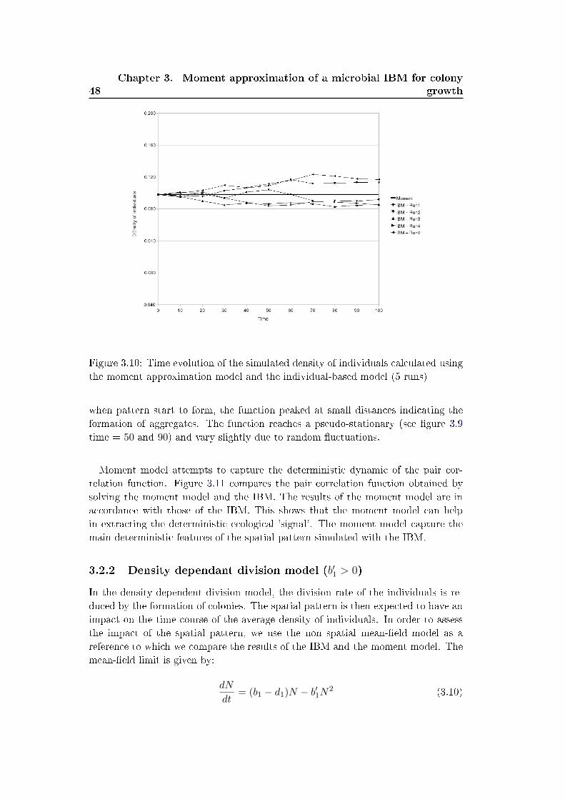
48
Chapter 3. Moment approximation of a microbial IBM for colony
growth
Figure 3.10: Time evolution of the simulated density of individuals calculated using
the moment approximation model and the individual-based model (5 runs)
when pattern start to form, the function peaked at small distances indicating the
formation of aggregates. The function reaches a pseudo-stationary (see �gure 3.9
time = 50 and 90) and vary slightly due to random �uctuations.
Moment model attempts to capture the deterministic dynamic of the pair cor-
relation function. Figure 3.11 compares the pair correlation function obtained by
solving the moment model and the IBM. The results of the moment model are in
accordance with those of the IBM. This shows that the moment model can help
in extracting the deterministic ecological 'signal'. The moment model capture the
main deterministic features of the spatial pattern simulated with the IBM.
3.2.2 Density dependant division model (b′1 > 0)
In the density-dependent division model, the division rate of the individuals is re-
duced by the formation of colonies. The spatial pattern is then expected to have an
impact on the time course of the average density of individuals. In order to assess
the impact of the spatial pattern, we use the non spatial mean-�eld model as a
reference to which we compare the results of the IBM and the moment model. The
mean-�eld limit is given by:
dN
dt= (b1 − d1)N − b′1N2 (3.10)
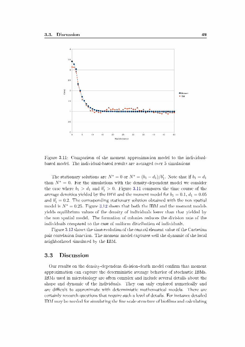
3.3. Discussion 49
Figure 3.11: Comparison of the moment approximation model to the individual-
based model. The individual-based results are averaged over 5 simulations
The stationary solutions are N∗ = 0 or N∗ = (b1 − d1)/b′1. Note that if b1 = d1than N∗ = 0. For the simulations with the density-dependent model we consider
the case where b1 > d1 and b′1 > 0. Figure 3.11 compares the time course of the
average densities yielded by the IBM and the moment model for b1 = 0.1, d1 = 0.05
and b′1 = 0.2. The corresponding stationary solution obtained with the non spatial
model is N∗ = 0.25. Figure 3.12 shows that both the IBM and the moment models
yields equilibrium values of the density of individuals lower than that yielded by
the non spatial model. The formation of colonies reduces the division rate of the
individuals compared to the case of uniform distribution of individuals.
Figure 3.13 shows the time evolution of the central element value of the Cartesian
pair correlation function. The moment model captures well the dynamic of the local
neighborhood simulated by the IBM.
3.3 Discussion
Our results on the density-dependent division-death model con�rm that moment
approximation can capture the deterministic average behavior of stochastic IBMs.
IBMs used in microbiology are often complex and include several details about the
shape and dynamic of the individuals. They can only explored numerically and
are di�cult to approximate with deterministic mathematical models. There are
certainly research questions that require such a level of details. For instance detailed
IBM may be needed for simulating the �ne scale structure of bio�lms and calculating
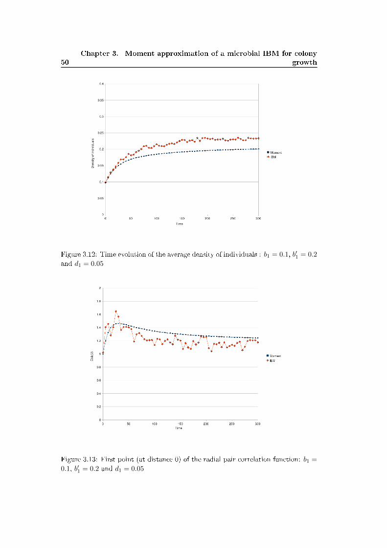
50
Chapter 3. Moment approximation of a microbial IBM for colony
growth
Figure 3.12: Time evolution of the average density of individuals : b1 = 0.1, b′1 = 0.2
and d1 = 0.05
Figure 3.13: First point (at distance 0) of the radial pair correlation function: b1 =
0.1, b′1 = 0.2 and d1 = 0.05
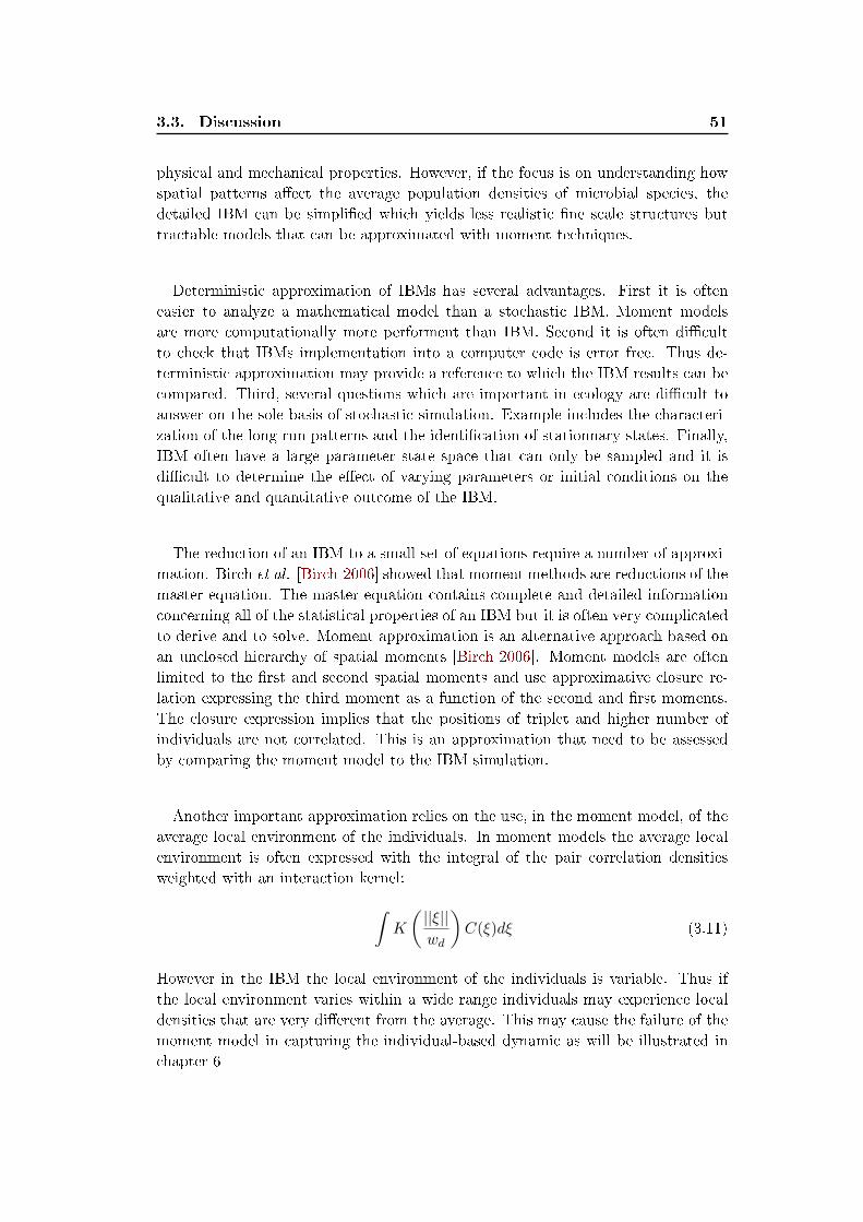
3.3. Discussion 51
physical and mechanical properties. However, if the focus is on understanding how
spatial patterns a�ect the average population densities of microbial species, the
detailed IBM can be simpli�ed which yields less realistic �ne scale structures but
tractable models that can be approximated with moment techniques.
Deterministic approximation of IBMs has several advantages. First it is often
easier to analyze a mathematical model than a stochastic IBM. Moment models
are more computationally more performent than IBM. Second it is often di�cult
to check that IBMs implementation into a computer code is error free. Thus de-
terministic approximation may provide a reference to which the IBM results can be
compared. Third, several questions which are important in ecology are di�cult to
answer on the sole basis of stochastic simulation. Example includes the characteri-
zation of the long-run patterns and the identi�cation of stationnary states. Finally,
IBM often have a large parameter state space that can only be sampled and it is
di�cult to determine the e�ect of varying parameters or initial conditions on the
qualitative and quantitative outcome of the IBM.
The reduction of an IBM to a small set of equations require a number of approxi-
mation. Birch et al. [Birch 2006] showed that moment methods are reductions of the
master equation. The master equation contains complete and detailed information
concerning all of the statistical properties of an IBM but it is often very complicated
to derive and to solve. Moment approximation is an alternative approach based on
an unclosed hierarchy of spatial moments [Birch 2006]. Moment models are often
limited to the �rst and second spatial moments and use approximative closure re-
lation expressing the third moment as a function of the second and �rst moments.
The closure expression implies that the positions of triplet and higher number of
individuals are not correlated. This is an approximation that need to be assessed
by comparing the moment model to the IBM simulation.
Another important approximation relies on the use, in the moment model, of the
average local environment of the individuals. In moment models the average local
environment is often expressed with the integral of the pair correlation densities
weighted with an interaction kernel:∫K
(||ξ||wd
)C(ξ)dξ (3.11)
However in the IBM the local environment of the individuals is variable. Thus if
the local environment varies within a wide range individuals may experience local
densities that are very di�erent from the average. This may cause the failure of the
moment model in capturing the individual-based dynamic as will be illustrated in
chapter 6
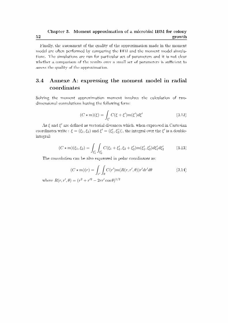
52
Chapter 3. Moment approximation of a microbial IBM for colony
growth
Finally, the assessment of the quality of the approximation made in the moment
model are often performed by comparing the IBM and the moment model simula-
tions. The simulations are run for particular set of parameters and it is not clear
whether a comparison of the results over a small set of parameters is su�cient to
assess the quality of the approximation.
3.4 Annexe A: expressing the moment model in radial
coordinates
Solving the moment approximation moment involves the calculation of two-
dimensional convolutions having the following form:
(C ?m)(ξ) =
∫ξ′C(ξ + ξ′)m(ξ′)dξ′ (3.12)
As ξ and ξ′ are de�ned as vectorial distances which, when expressed in Cartesian
coordinates write : ξ = (ξ1, ξ2) and ξ′ = (ξ′1, ξ
′2)), the integral over the ξ
′ is a double-
integral:
(C ?m)(ξ1, ξ2) =
∫ξ′1
∫ξ′2
C(ξ1 + ξ′1, ξ2 + ξ′2)m(ξ′1, ξ′2)dξ
′1dξ′2 (3.13)
The convolution can be also expressed in polar coordinates as:
(C ?m)(r) =
∫r′
∫θC(r′)m(R(r, r′, θ))r′dr′dθ (3.14)
where R(r, r′, θ) = (r2 + r′2 − 2rr′ cos θ)1/2
Chapter 4
Moment approximation of a
simpli�ed bio�lm IBM with
detachment
Contents
4.1 Introduction . . . . . . . . . . . . . . . . . . . . . . . . . . . . 53
4.2 A simpli�ed bio�lm IBM with detachment . . . . . . . . . . 54
4.2.1 Individual-based model parameters . . . . . . . . . . . . . . . 56
4.3 IBM simulation results . . . . . . . . . . . . . . . . . . . . . . 56
4.4 Deriving the moment approximation model . . . . . . . . . 57
4.5 Comparison of the moment model and the IBM . . . . . . . 61
4.6 Discussion . . . . . . . . . . . . . . . . . . . . . . . . . . . . . . 62
4.1 Introduction
In this chapter we propose to derive a moment model approximating a simpli�ed
individual-based model (IBM) of microbial bio�lms development. The IBM is basi-
cally an extension of the colony growth IBM presented in chapter 3 by considering a
multi-colonies system and including a bio�lm detachment process. Our aim is �rst
to explore the di�erent spatial patterns yielded by the IBM under di�erent divi-
sion and detachment conditions. We characterize these patterns using the �rst and
second spatial moments introduced in the previous chapter. Second, we propose to
approximate the dynamic of these aggregated descriptors using the moment approx-
imation approach and compare the result of the aggregated mathematical moment
model to the IBM simulations.
The chapter is organized in four sections. The �rst section is dedicated to the
description of the simpli�ed bio�lm individual-based model where the individuals
are subject to a density-dependent detachment process. In the second section we
propose to explore the spatial patterns yielded by the IBM when the spatial ranges of
the division and detachment kernels are varied. We derive a moment approximation
model in the third section of the chapter. Finally we compare the moment model
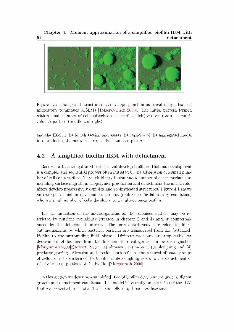
54
Chapter 4. Moment approximation of a simpli�ed bio�lm IBM with
detachment
Figure 4.1: The spatial structure in a developing bio�lm as revealed by advanced
microscopy techniques (CSLM) [Tolker-Nielsen 2000]. The initial pattern formed
with a small number of cells adsorbed on a surface (left) evolves toward a multi-
colonies pattern (middle and right)
and the IBM in the fourth section and assess the capacity of the aggregated model
in reproducing the main features of the simulated patterns.
4.2 A simpli�ed bio�lm IBM with detachment
Bacteria attach to hydrated surfaces and develop bio�lms. Bio�lms development
is a complex and sequential process often initiated by the adsorption of a small num-
ber of cells on a surface. Through binary �ssion and a number of other mechanisms
including surface migration, exopolymer production and detachment the initial colo-
nizers develop progressively complex and sophisticated structures. Figure 4.1 shows
an example of bio�lm development process (under speci�c laboratory conditions)
where a small number of cells develop into a multi-colonies bio�lm.
The accumulation of the microorganisms on the colonized surface may be re-
stricted by nutrient availability (treated in chapter 2 and 3) and/or counterbal-
anced by the detachment process. The term detachment here refers to di�er-
ent mechanisms by which bacterial particles are transported from the (attached)
bio�lm to the surrounding �uid phase. Di�erent processes are responsible for
detachment of biomass from bio�lms and four categories can be distinguished
[Morgenroth 2000][Stewart 1993]: (1) abrasion, (2) erosion, (3) sloughing and (4)
predator grazing. Abrasion and erosion both refer to the removal of small groups
of cells from the surface of the bio�lm while sloughing refers to the detachment of
relatively large portions of the bio�lm [Morgenroth 2000].
In this section we describe a simpli�ed IBM of bio�lm development under di�erent
growth and detachment conditions. The model is basically an extension of the IBM
that we presented in chapter 3 with the following three modi�cations:
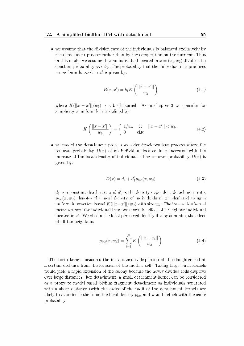
4.2. A simpli�ed bio�lm IBM with detachment 55
• we assume that the division rate of the individuals is balanced exclusively by
the detachment process rather than by the competition on the nutrient. Thus
in this model we assume that an individual located in x = (x1, x2) divides at a
constant probability rate b1. The probability that the individual in x produces
a new born located in x′ is given by:
B(x, x′) = b1K
(||x− x′||
wb
)(4.1)
where K(||x − x′||/wb) is a birth kernel. As in chapter 3 we consider for
simplicity a uniform kernel de�ned by:
K
(||x− x′||
wb
)=
{1/wb if ||x− x′|| < wb0 else
(4.2)
• we model the detachment process as a density-dependent process where the
removal probability D(x) of an individual located in x increases with the
increase of the local density of individuals. The removal probability D(x) is
given by:
D(x) = d1 + d′1ploc(x,wd) (4.3)
d1 is a constant death rate and d′1 is the density dependent detachment rate.
ploc(x,wd) denotes the local density of individuals in x calculated using a
uniform interaction kernelK(||x−x′||/wd) with size wd. The interaction kernelmeasures how the individual in x perceives the e�ect of a neighbor individual
located in x′. We obtain the local perceived density if x by summing the e�ect
of all the neighbors:
ploc(x,wd) =
N∑i=1
K
(||x− xi||
wd
)(4.4)
The birth kernel measures the instantaneous dispersion of the daughter cell at
a certain distance from the location of the mother cell. Taking large birth kernels
would yield a rapid extension of the colony because the newly divided cells disperse
over large distances. For detachment, a small detachment kernel can be considered
as a proxy to model small bio�lm fragment detachment as individuals separated
with a short distance (with the order of the radii of the detachment kernel) are
likely to experience the same the local density ploc and would detach with the same
probability.
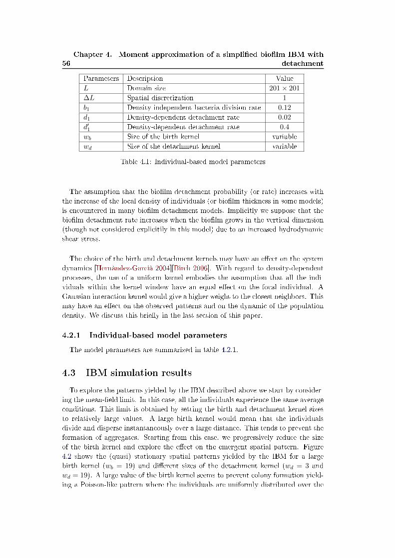
56
Chapter 4. Moment approximation of a simpli�ed bio�lm IBM with
detachment
Parameters Description Value
L Domain size 201× 201
∆L Spatial discretization 1
b1 Density-independent bacteria division rate 0.12
d1 Density-dependent detachment rate 0.02
d′1 Density-dependent detachment rate 0.4
wb Size of the birth kernel variable
wd Size of the detachment kernel variable
Table 4.1: Individual-based model parameters
The assumption that the bio�lm detachment probability (or rate) increases with
the increase of the local density of individuals (or bio�lm thickness in some models)
is encountered in many bio�lm detachment models. Implicitly we suppose that the
bio�lm detachment rate increases when the bio�lm grows in the vertical dimension
(though not considered explicitily in this model) due to an increased hydrodynamic
shear stress.
The choice of the birth and detachment kernels may have an e�ect on the system
dynamics [Hernàndez-Garcià 2004][Birch 2006]. With regard to density-dependent
processes, the use of a uniform kernel embodies the assumption that all the indi-
viduals within the kernel window have an equal e�ect on the focal individual. A
Gaussian interaction kernel would give a higher weight to the closest neighbors. This
may have an e�ect on the observed patterns and on the dynamic of the population
density. We discuss this brie�y in the last section of this paper.
4.2.1 Individual-based model parameters
The model parameters are summarized in table 4.2.1.
4.3 IBM simulation results
To explore the patterns yielded by the IBM described above we start by consider-
ing the mean-�eld limit. In this case, all the individuals experience the same average
conditions. This limit is obtained by setting the birth and detachment kernel sizes
to relatively large values. A large birth kernel would mean that the individuals
divide and disperse instantaneously over a large distance. This tends to prevent the
formation of aggregates. Starting from this case, we progressively reduce the size
of the birth kernel and explore the e�ect on the emergent spatial pattern. Figure
4.2 shows the (quasi) stationary spatial patterns yielded by the IBM for a large
birth kernel (wb = 19) and di�erent sizes of the detachment kernel (wd = 3 and
wd = 19). A large value of the birth kernel seems to prevent colony formation yield-
ing a Poisson-like pattern where the individuals are uniformly distributed over the
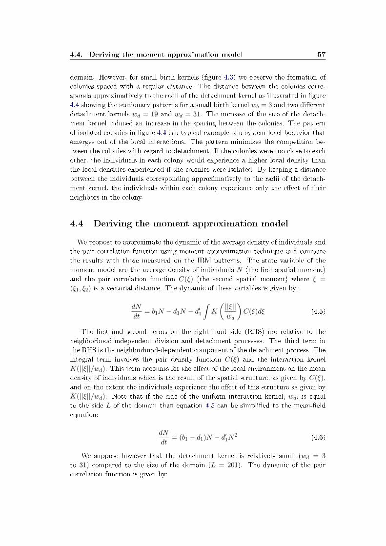
4.4. Deriving the moment approximation model 57
domain. However, for small birth kernels (�gure 4.3) we observe the formation of
colonies spaced with a regular distance. The distance between the colonies corre-
sponds approximatively to the radii of the detachment kernel as illustrated in �gure
4.4 showing the stationary patterns for a small birth kernel wb = 3 and two di�erent
detachment kernels wd = 19 and wd = 31. The increase of the size of the detach-
ment kernel induced an increase in the spacing between the colonies. The pattern
of isolated colonies in �gure 4.4 is a typical example of a system-level behavior that
emerges out of the local interactions. The pattern minimizes the competition be-
tween the colonies with regard to detachment. If the colonies were too close to each
other, the individuals in each colony would experience a higher local density than
the local densities experienced if the colonies were isolated. By keeping a distance
between the individuals corresponding approximatively to the radii of the detach-
ment kernel, the individuals within each colony experience only the e�ect of their
neighbors in the colony.
4.4 Deriving the moment approximation model
We propose to approximate the dynamic of the average density of individuals and
the pair correlation function using moment approximation technique and compare
the results with those measured on the IBM patterns. The state variable of the
moment model are the average density of individuals N (the �rst spatial moment)
and the pair correlation function C(ξ) (the second spatial moment) where ξ =
(ξ1, ξ2) is a vectorial distance. The dynamic of these variables is given by:
dN
dt= b1N − d1N − d′1
∫K
(||ξ||wd
)C(ξ)dξ (4.5)
The �rst and second terms on the right-hand side (RHS) are relative to the
neighborhood-independent division and detachment processes. The third term in
the RHS is the neighborhood-dependent component of the detachment process. The
integral term involves the pair density function C(ξ) and the interaction kernel
K(||ξ||/wd). This term accounts for the e�ect of the local environment on the mean
density of individuals which is the result of the spatial structure, as given by C(ξ),
and on the extent the individuals experience the e�ect of this structure as given by
K(||ξ||/wd). Note that if the side of the uniform interaction kernel, wd, is equal
to the side L of the domain than equation 4.5 can be simpli�ed to the mean-�eld
equation:
dN
dt= (b1 − d1)N − d′1N2 (4.6)
We suppose however that the detachment kernel is relatively small (wd = 3
to 31) compared to the size of the domain (L = 201). The dynamic of the pair
correlation function is given by:
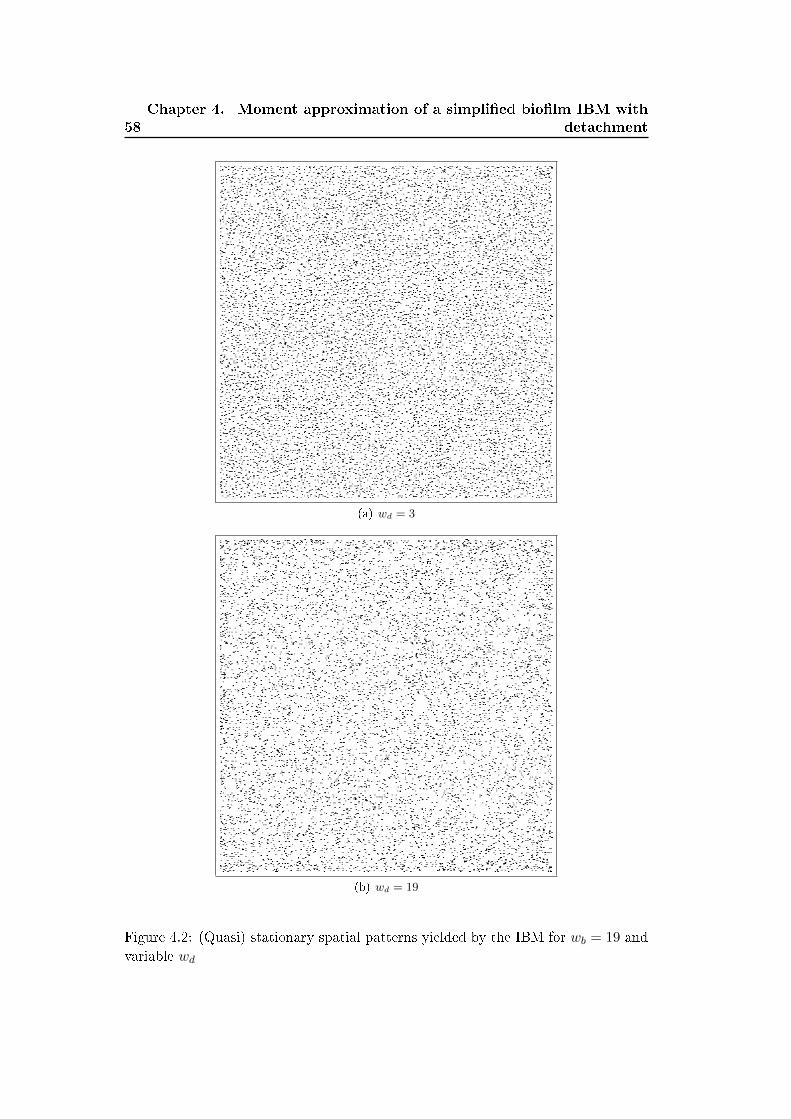
58
Chapter 4. Moment approximation of a simpli�ed bio�lm IBM with
detachment
(a) wd = 3
(b) wd = 19
Figure 4.2: (Quasi) stationary spatial patterns yielded by the IBM for wb = 19 and
variable wd
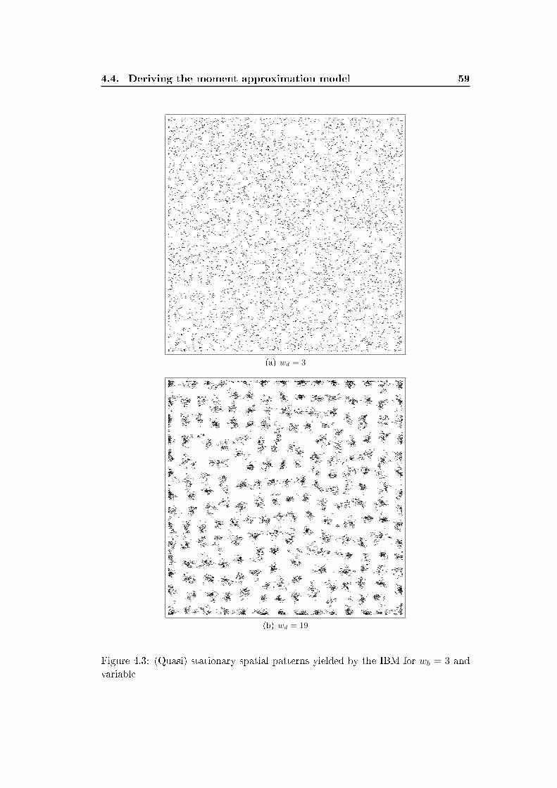
4.4. Deriving the moment approximation model 59
(a) wd = 3
(b) wd = 19
Figure 4.3: (Quasi) stationary spatial patterns yielded by the IBM for wb = 3 and
variable
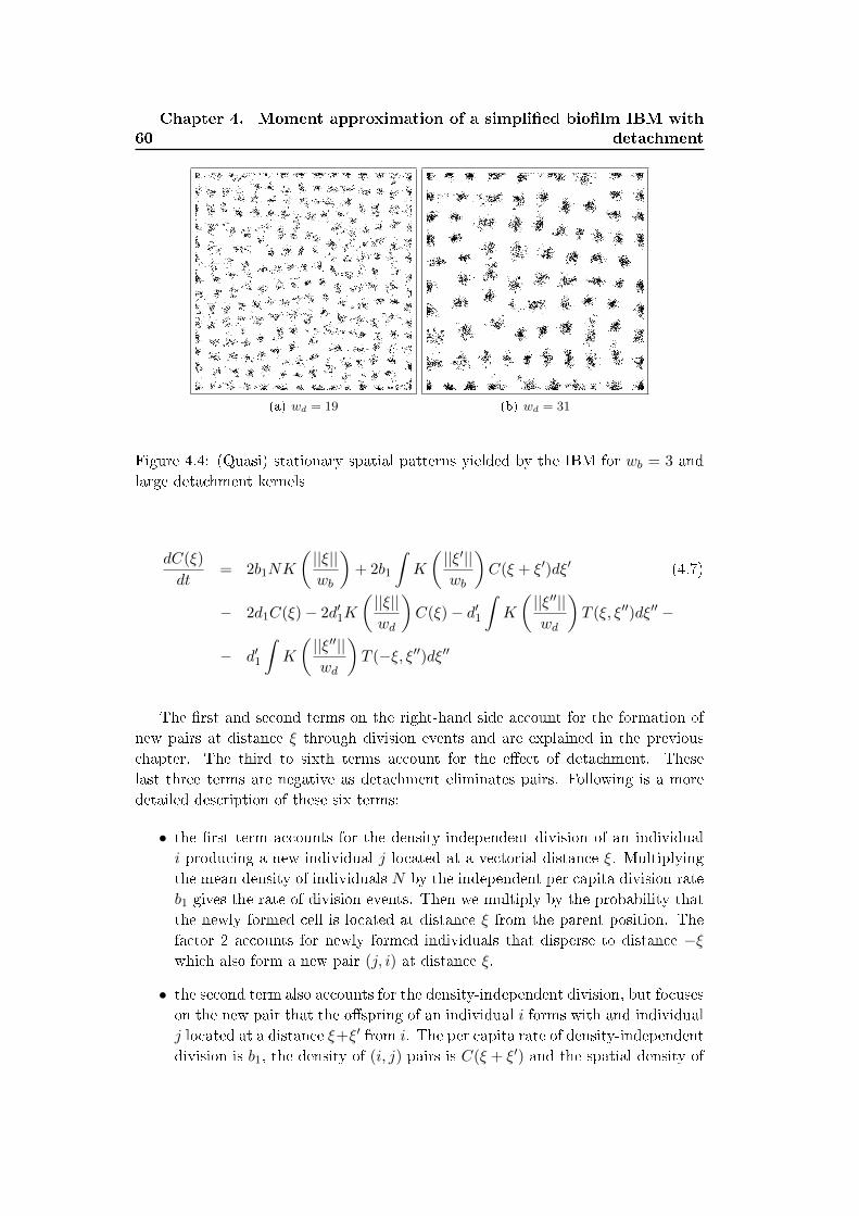
60
Chapter 4. Moment approximation of a simpli�ed bio�lm IBM with
detachment
(a) wd = 19 (b) wd = 31
Figure 4.4: (Quasi) stationary spatial patterns yielded by the IBM for wb = 3 and
large detachment kernels
dC(ξ)
dt= 2b1NK
(||ξ||wb
)+ 2b1
∫K
(||ξ′||wb
)C(ξ + ξ′)dξ′ (4.7)
− 2d1C(ξ)− 2d′1K
(||ξ||wd
)C(ξ)− d′1
∫K
(||ξ′′||wd
)T (ξ, ξ′′)dξ′′ −
− d′1
∫K
(||ξ′′||wd
)T (−ξ, ξ′′)dξ′′
The �rst and second terms on the right-hand side account for the formation of
new pairs at distance ξ through division events and are explained in the previous
chapter. The third to sixth terms account for the e�ect of detachment. These
last three terms are negative as detachment eliminates pairs. Following is a more
detailed description of these six terms:
• the �rst term accounts for the density-independent division of an individual
i producing a new individual j located at a vectorial distance ξ. Multiplying
the mean density of individuals N by the independent per capita division rate
b1 gives the rate of division events. Then we multiply by the probability that
the newly formed cell is located at distance ξ from the parent position. The
factor 2 accounts for newly formed individuals that disperse to distance −ξwhich also form a new pair (j, i) at distance ξ.
• the second term also accounts for the density-independent division, but focuses
on the new pair that the o�spring of an individual i forms with and individual
j located at a distance ξ+ξ′ from i. The per capita rate of density-independent
division is b1, the density of (i, j) pairs is C(ξ + ξ′) and the spatial density of
4.5. Comparison of the moment model and the IBM 61
o�spring settling around the i parent is K(||ξ′||/wb). Multiplying these three
factors and integrating over all possible distances ξ′ of o�spring dispersal yields
the second term.
• the third term accounts for ij pairs that are lost due to the density-independent
death of the individual i in the pair (respectively j).
• the fourth term corrects the death rate of the individual i in the pair ij by
adding the e�ect of the individual j on the death rate of the individual i.
• the �fth and sixth terms correct the death rate of the individual i in the pair ij
by adding the e�ect of neighbors (other than j) located at a distance ξ′′ from i.
The density of this triplet con�guration is given by the triple density function
T (ξ, ξ′′) and T (−ξ, ξ′′) We multiply by the detachment kernel calculated at
distance ξ′′ and integrate over all possible neighbors (or all distances ξ′′).
The system formed with equations 4.5 and 4.7 involves the third spatial moment
T (ξ, ξ′). To close this system we need to express the third moment as a function
of the �rst and the second moments. We use the following closure expressions
[Dieckmann 2000]:
T (ξ, ξ′) =C(ξ)C(ξ′)C(ξ′ − ξ)
N3(4.8)
As will be detailed in the next paragraph the choice of the closure expression
can have a signi�cant impact on the simulated pattern. This choice is guided by
the comparison of the moment and the individual-based model patterns. A good
closure is the one that allows the moment model to capture the main features of the
patterns and dynamics yielded by the individual-based model.
We solve the moment model formed with equations 4.5, 4.7, 4.8 and ??, as
detailed in the previous chapter, by discretizing the vectorial distances ξ with a
spatial resolution dξ = (dξ1, dξ2) and time with a constant time step ∆t. We use an
explicit Euler scheme for descritizing the time derivative. The resultant algebraic
system is formed with n2x + 1 equation (where nx is the size of discretized C(ξ)
expresses the density of individuals N and the pair correlation matrix C(ξ) at the
instant t+ ∆t as a function of N and C at the previous instant t.
4.5 Comparison of the moment model and the IBM
We compare the time course of the average density of individuals yielded by the
IBM and the moment model (�gure 4.5) and the stationary radial pair correlation
function (�gure 4.6). For a large birth kernel wb = 19, the IBM and the moment
models yields comparable results to those obtained with the mean-�eld limit (dashed
line in �gure 4.5(a)). In this case where the distribution of the individuals is uniform
as can be seen from the pair density correlation functions in �gure 4.6(a)which take
values close to 1 in both models indicating that the local density of pairs is almost
62
Chapter 4. Moment approximation of a simpli�ed bio�lm IBM with
detachment
equal to N2 (the average density of pairs in the system) For small birth kernels
however, the density of individuals increases in both models beyond the stationary
value yielded by the mean-�eld model. This is a counter intuitive result as one may
expect that the formation of aggregates would increase the detachment rate of the
individuals yielding lower equilibrium density than what would be obtained in the
case of a uniform distribution. The organization of the individuals with a regular
distance is likely to induce a lower average detachment rate as this arrangement
seems to minimize the competition with regard to detachment between the colonies.
The pattern of isolated colonies yields an oscillating radial pair correlation func-
tion. The �rst peak is due to the high density of neighbors within the colony (short
distance). the waves are due to the regular arrangement of the colonies. The peaks
in the IBM are lower than those yielded by the moment model and the wavy radial
pair correlation function seems to vanish to 1 in the IBM for large distances. This
is due to the �uctuations around the colonies simulated by the IBM. The individu-
als are in majority enclosed within the colonies but some of them are still between
the colonies due to the stochastic division and detachment process. This blurs the
deterministic ecological signal as revealed by the moment model.
4.6 Discussion
We approximated the dynamic of a simpli�ed IBM with a population of individuals
inhabiting a two-dimensional domain. The individuals are subject to division events
and a density-dependent detachment process. The numerical exploration of the
IBM shows for large birth kernels the newborn cells disperse over large distances
preventing the formation of colonies. In this case the average density yielded by the
IBM evolve as in the mean-�eld limits.
However when we reduce the size of the birth kernel, patterns with isolated
microcolonies may emerge and can be observed especially when the size of the de-
tachment kernel is higher than that of the birth kernel.
We approximated the IBM with a moment model. Moment model attempts to
capture how the local environment of the individuals evolve in time and how it a�ects
the average density of individuals. The derived moment model is globally in a good
agreement with the IBM. Moment model predicts a Poisson-like distribution in the
case of large birth kernels and an oscillating radial pair correlation function, in the
case of small dispersion and large detachment kernel, with a period approximatively
corresponding to the size of the detachment kernel. The peaks in the oscillating
pair correlation function however are high in the moment model than in the IBM.
This may be explained by the choice of the closure. The closure expresses the the
third moment in term of �rst and second moments. The moment model results can
be very sensitive to the choice of the closure expression. For instance the classical
second order closures (T (ξ, ξ′) = C(ξ′)C(ξ)/N) fails in predicting the wavy strcture
of the pair correlation while the third order closure overestimates the hight of the
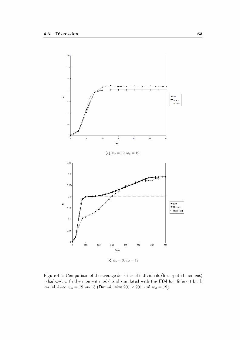
4.6. Discussion 63
(a) wb = 19, wd = 19
(b) wb = 3, wd = 19
Figure 4.5: Comparison of the average densities of individuals (�rst spatial moment)
calculated with the moment model and simulated with the IBM for di�erent birth
kernel sizes: wb = 19 and 3 (Domain size 201× 201 and wd = 19)
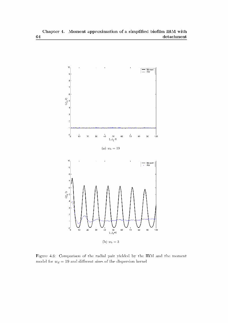
64
Chapter 4. Moment approximation of a simpli�ed bio�lm IBM with
detachment
(a) wb = 19
(b) wb = 3
Figure 4.6: Comparison of the radial pair yielded by the IBM and the moment
model for wd = 19 and di�erent sizes of the dispersion kernel
4.6. Discussion 65
peaks.
This is one of the limtations of moment models which provide deterministic ap-
proximations of the dynamic of the individual-based model. The quality of the ap-
proximation need to be assessed through comparison to the individual-based model
simulations and improved by selecting the best closure expression.

Chapter 5
A detailed individual-based model
of bio�lm formed with motile
bacteria
Published in Theory in Biosciences: Mabrouk, N., De�uant,G.,Tolker-Nielsen,T.,
Lobry,C.: Bacteria can form interconnected microcolonies when a self-excreted prod-
uct reduces their surface motility: evidence from individual-based model simulation.
DOI: 10.1007/s12064-009-0078-8
Contents
5.1 Background . . . . . . . . . . . . . . . . . . . . . . . . . . . . . 68
5.2 Model description . . . . . . . . . . . . . . . . . . . . . . . . . 69
5.2.1 Purpose . . . . . . . . . . . . . . . . . . . . . . . . . . . . . . 70
5.2.2 State variables and scales . . . . . . . . . . . . . . . . . . . . 70
5.2.3 Scales . . . . . . . . . . . . . . . . . . . . . . . . . . . . . . . 70
5.2.4 Process overview and scheduling . . . . . . . . . . . . . . . . 70
5.2.5 Design Concepts . . . . . . . . . . . . . . . . . . . . . . . . . 72
5.2.6 Submodels . . . . . . . . . . . . . . . . . . . . . . . . . . . . 72
5.3 Results . . . . . . . . . . . . . . . . . . . . . . . . . . . . . . . . 77
5.4 Discussion . . . . . . . . . . . . . . . . . . . . . . . . . . . . . . 79
We propose to analyze using numerical experimentations a new individual-based
model of a microbial system formed with surface-associated motile bacteria which
motility is reduced by a self-excreted substance. The model is inspired from re-
cent experimental observations of Pseudomonas aeruginosa, a model bacterium in
bio�lm research that have been shown to bind, under speci�c growth conditions, to
self-excreted DNA. These experimental observations also showed that Pseudomonas
aeruginosa forms interconnected microcolonies and presumed a possible involvement
of the extracellular DNA in the formation of these patterns. In this chapter, we use
an individual-based model to assess the involvement of bacteria motility and inter-
action with self-excreted extracellular substance in the formation of patterns with
interconnected microcolonies. Our analysis is based on numerical experimentations
using the IBM and starting with obvious cases than moving progressively to the
case of interest.
68
Chapter 5. A detailed individual-based model of bio�lm formed with
motile bacteria
5.1 Background
Many bacteria have an innate propensity to form bio�lms: they build struc-
tured multicellular communities attached to solid surfaces. Microscopic examina-
tion of bio�lms formed by Pseudomonas aeruginosa, a model bacterium in bio�lm
research [Costerton 1995][Davey 2000], reveals a wide diversity of spatial patterns
which, depending on the growth conditions, range from a �at thin layer of cells
to a patchy pattern with interconnected microcolonies having complex tower or
mushroom like shapes [Klausen 003b][Barken 2008]. At least some explanation for
the di�erent bio�lm patterns formed under di�erent conditions relates to surface
motility. Conditions that promote extensive surface motility can lead to the for-
mation of �at, homogeneous bio�lms, whereas bio�lms characterized by aggregates
result from at least a subpopulation of the community ceasing to move at an early
stage of bio�lm formation [Parsek 2008]. In P. aeruginosa bio�lms, formation of
initial microcolonies (stalks) that subsequently become colonized by cap-forming
bacteria is necessary for the formation of mushroom-shaped multicellular structures
[Klausen 003a][Klausen 003b]. These multicellular structures often provide impor-
tant bene�ts such as a higher tolerance to adverse conditions [Parsek 2008], and can
be crucial in industrial processes. Therefore, much experimental and theoretical
e�ort is currently devoted to understand their mechanisms of formation.
The formation of spatial patterns in P. aeruginosa bio�lms involves a com-
plex interplay between cell proliferation, surface-associated motility and the pro-
duction of extracellular macromolecules that form a structural matrix (for a re-
view see [Parsek 2008]). Evidence has been provided that arrest of type IV
pili-mediated motility (twitching motility) plays a role in the formation of the
initial microcolonies in P. aeruginosa bio�lms, whereas �agella- driven motility
(swarming motility) plays a role in the subsequent formation of the cap-portion of
the mushroom-shaped structures [Klausen 003a][Klausen 003b][Barken 2008]. The
early stages of bio�lm development by P. aeruginosa is dependent on extracellular
DNA [Whitchurch 2002], which is known to bind with high a�nity to type IV pili
[Aas 2002][Van Schaik 2005], a �mbrae extending from the cell body and mediat-
ing surface-associated twitching motility. Hence it may be assumed that initially
motile bacteria stop and form microcolonies in the regions of abundant extracellu-
lar DNA. Recently, Allesen- Holm et al. [Allesen-Holm 2006] visualized the spatial
distribution of extracellular DNA and bacteria in P. aeruginosa bio�lms, grown in
�ow chambers on minimal glucose medium. In 2-day-old bio�lms the extracellular
DNA was present inside the small microcolonies, but accumulated mainly in the
outer layer of the microcolonies and between the microcolonies forming a grid-like
structure. Zoomed views of the microcolonies revealed that they were often inter-
connected with thin strands of extracellular DNA covered with bacteria (see �gure
5.1). In 4-day-old bio�lms cap- like multicellular structures had formed on top of
the initial small microcolonies, and the highest concentration of extracellular DNA
was present between the stalk- portion and the cap-portion of the mushroom-shaped
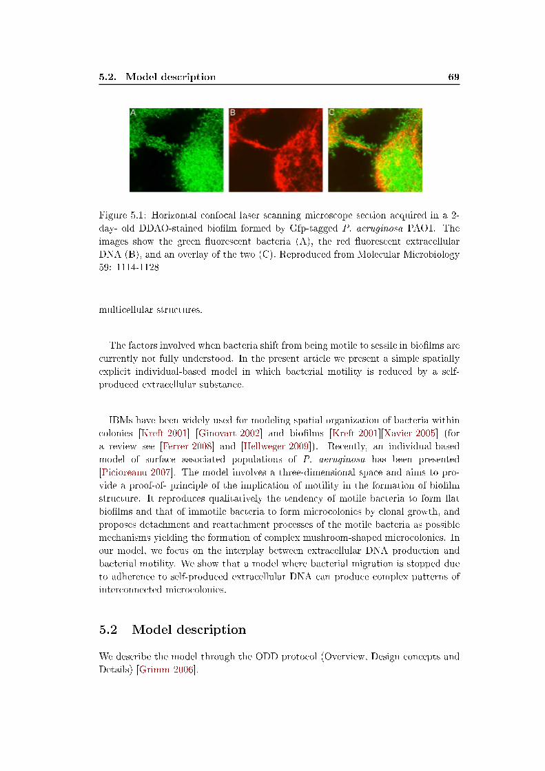
5.2. Model description 69
Figure 5.1: Horizontal confocal laser scanning microscope section acquired in a 2-
day- old DDAO-stained bio�lm formed by Gfp-tagged P. aeruginosa PAO1. The
images show the green �uorescent bacteria (A), the red �uorescent extracellular
DNA (B), and an overlay of the two (C). Reproduced from Molecular Microbiology
59: 1114-1128
multicellular structures.
The factors involved when bacteria shift from being motile to sessile in bio�lms are
currently not fully understood. In the present article we present a simple spatially
explicit individual-based model in which bacterial motility is reduced by a self-
produced extracellular substance.
IBMs have been widely used for modeling spatial organization of bacteria within
colonies [Kreft 2001] [Ginovart 2002] and bio�lms [Kreft 2001][Xavier 2005] (for
a review see [Ferrer 2008] and [Hellweger 2009]). Recently, an individual-based
model of surface associated populations of P. aeruginosa has been presented
[Picioreanu 2007]. The model involves a three-dimensional space and aims to pro-
vide a proof-of- principle of the implication of motility in the formation of bio�lm
structure. It reproduces qualitatively the tendency of motile bacteria to form �at
bio�lms and that of immotile bacteria to form microcolonies by clonal growth, and
proposes detachment and reattachment processes of the motile bacteria as possible
mechanisms yielding the formation of complex mushroom-shaped microcolonies. In
our model, we focus on the interplay between extracellular DNA production and
bacterial motility. We show that a model where bacterial migration is stopped due
to adherence to self-produced extracellular DNA can produce complex patterns of
interconnected microcolonies.
5.2 Model description
We describe the model through the ODD protocol (Overview, Design concepts and
Details) [Grimm 2006].

70
Chapter 5. A detailed individual-based model of bio�lm formed with
motile bacteria
Figure 5.2: Schematic representation of the model entities: bacterial cells (discs)
and patches (squares with a side ∆l). A bacterium with continuous coordinates x,y
is contained in the patch i = floor(x/∆l), j = floor(y/∆l).
5.2.1 Purpose
The model we propose is intended to qualitatively explore the role of surface-
motility reduction by self-produced macromolecules in bio�lm pattern formation.
We address this question at a rather abstract level, and the model results are not
compared to speci�c experimental results.
5.2.2 State variables and scales
The model is a two-dimensional representation of a bio�lm system and comprises
two entities: bacterial cells and their local environment (patches) (�gure 5.2). Bac-
terial cells are represented as discs. They are characterized by the state variables:
continuous position (x, y), individual mass (m), individual di�usion factor (Df ) and
individual substrate uptake rate (r)(table 5.1). A Patch (i, j) is characterized by the
state variables: substrate concentration (s), extracellular substance concentration
(p) and a substrate uptake rate (rs). The later corresponds to the sum of uptake
rates of the individual cells contained within the patch (table 5.1).
5.2.3 Scales
We simulated the �rst day of the bio�lm development. We discretized time with a
constant time step, denoted ∆t = 1s. A spatial patch has a size of 5 × 5 µm and
the whole domain contains 400 × 400 patches (spatial domain side l = 2000µm).
Bacterial cells have variable diameters (∼ 2µm) depending on their masses.
5.2.4 Process overview and scheduling
In the IBM, bacteria move stochastically along a 2-D surface while consuming
substrate, growing and reproducing by binary �ssion and excreting a product. Bac-
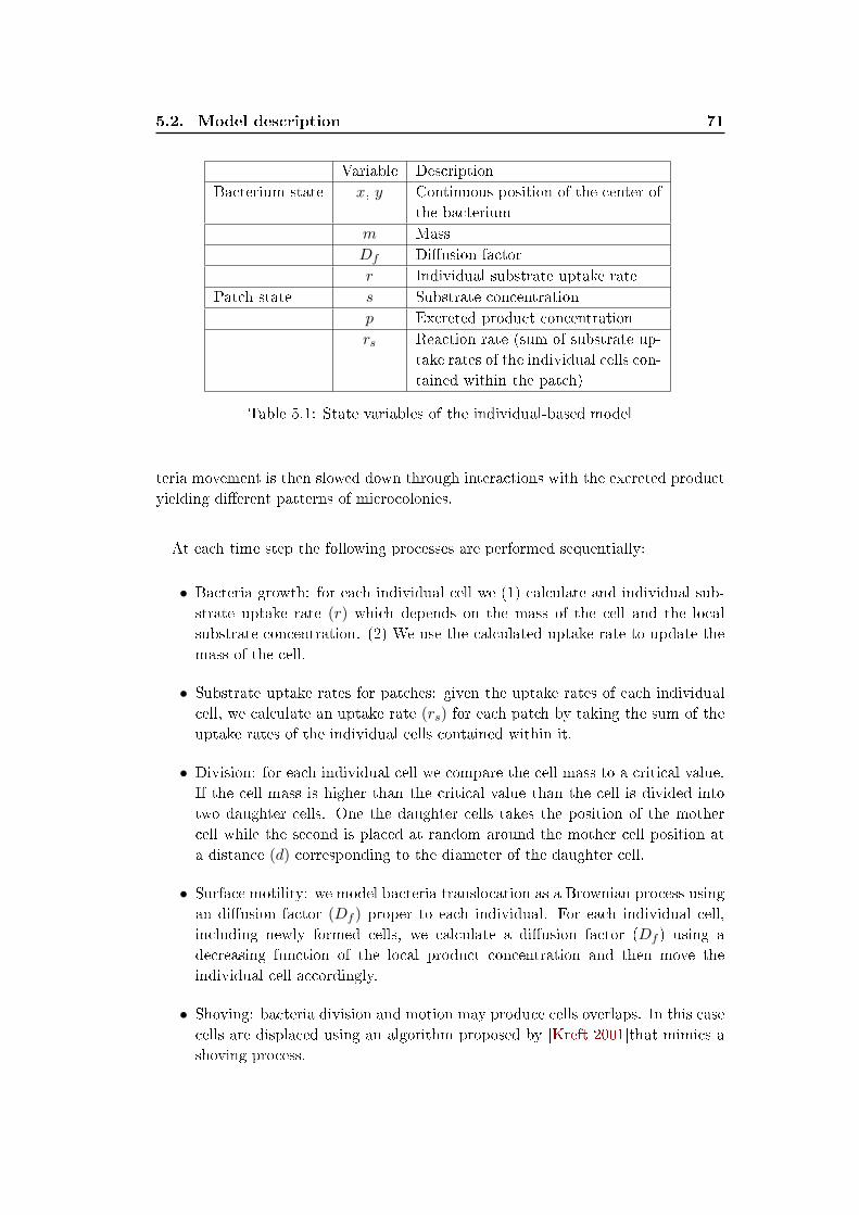
5.2. Model description 71
Variable Description
Bacterium state x, y Continuous position of the center of
the bacterium
m Mass
Df Di�usion factor
r Individual substrate uptake rate
Patch state s Substrate concentration
p Excreted product concentration
rs Reaction rate (sum of substrate up-
take rates of the individual cells con-
tained within the patch)
Table 5.1: State variables of the individual-based model
teria movement is then slowed down through interactions with the excreted product
yielding di�erent patterns of microcolonies.
At each time step the following processes are performed sequentially:
• Bacteria growth: for each individual cell we (1) calculate and individual sub-
strate uptake rate (r) which depends on the mass of the cell and the local
substrate concentration. (2) We use the calculated uptake rate to update the
mass of the cell.
• Substrate uptake rates for patches: given the uptake rates of each individual
cell, we calculate an uptake rate (rs) for each patch by taking the sum of the
uptake rates of the individual cells contained within it.
• Division: for each individual cell we compare the cell mass to a critical value.
If the cell mass is higher than the critical value than the cell is divided into
two daughter cells. One the daughter cells takes the position of the mother
cell while the second is placed at random around the mother cell position at
a distance (d) corresponding to the diameter of the daughter cell.
• Surface motility: we model bacteria translocation as a Brownian process using
an di�usion factor (Df ) proper to each individual. For each individual cell,
including newly formed cells, we calculate a di�usion factor (Df ) using a
decreasing function of the local product concentration and then move the
individual cell accordingly.
• Shoving: bacteria division and motion may produce cells overlaps. In this case
cells are displaced using an algorithm proposed by [Kreft 2001]that mimics a
shoving process.
72
Chapter 5. A detailed individual-based model of bio�lm formed with
motile bacteria
• Substrate and excreted product mass balances: we modeled the substrate
and the excreted product dynamics using two di�usion-reaction equations dis-
cretized on the lattice formed by the patches. The reaction terms in these
equations are calculated using the substrate uptake rate (rs) previously cal-
culated for each patch.
5.2.5 Design Concepts
• Emergence: the IBM is designed such that the spatial pattern of bacteria and
product distribution emerge from local interactions.
• Sensing: in our model, a bacterium senses the substrate and product concen-
tration within the patch corresponding to its position. The substrate concen-
tration a�ects the growth rate of the bacterium whereas the product concen-
tration a�ects the motility of the bacteria.
• Stochasticity: bacteria motility and the positioning of the daughter cells after
a division event are the only stochastic processes that we considered in the
IBM.
• Observation: at each time step the state variables for bacteria and patches are
recorded.
5.2.6 Submodels
5.2.6.1 Bacteria growth
We calculate the individual substrate uptake rate (r(t)) of a cell located in (x, y)
and having a mass m using the following Monod-like kinetic equation:
r(t) = µmaxms(i, j, t)
s(i, j, t) + ks(5.1)
Where s(i, j, t) is the substrate concentration at patch (i, j) with i = floor(x/∆l)
and j = floor(y/∆l) and µmax and ks are Monod kinetic parameters. The growth
rate of the bacterium is given by:
dm
dt= Ybr(t) (5.2)
Where Y b is the biomass yield (expressed in mass of bacteria per mass of con-
sumed substrate). The time derivative is discretized using an Euler explicit scheme
and the new mass of the cell is calculated by:
m(t+ ∆t) = m(t) + ∆tYbr(t) (5.3)
With ∆t the time step. The product excretion rate rp(t) of the considered
individual cell is given by:
rp(t) = Ypr(t) (5.4)
5.2. Model description 73
5.2.6.2 Substrate Uptake rates
For each patch we calculate a substrate uptake rate rs(t, i, j) by summing the indi-
vidual substrate uptake rates of the cells contained within the patch:
rs(t, i, j) =1
∆l2
∑k
rk(t) (5.5)
where k is the number of cells in patch i, j.
5.2.6.3 Bacteria division
If the mass of a focal individual (a mother cell) becomes greater than twice the initial
mass of an individual (2m0 ≤ m) it divides into two daughter cells each with a mass
m/2. The �rst daughter cell takes the position of the mother cell while the second
daughter cell is placed randomly at a distance d (distance between the centers of
both cells) corresponding to the diameter of the daughter cells (both daughter cells
have the same diameter).
5.2.6.4 Bacteria motility
The motility of the cells is modeled as a Brownian motion process with an apparent
di�usion factor (Df) which is speci�c to each individual cell. For a given bacterium
located at x, y at time t, the position of the bacterium at the instant t+ ∆t is given
by:
x(t+ ∆t) = x(t) +√
2Df (x, y)∆tN(0, 1) (5.6)
y(t+ ∆t) = y(t) +√
2Df (x, y)∆tN(0, 1)
where N(0, 1) draws a number from a centered normal distribution of standard
deviation 1 (generated using the Mersenne Twister pseudo-random number gener-
ator). As we assumed that bacteria motility was reduced by the excreted product,
we calculate di�usion factor (Df ) as a decreasing function of the excreted product
concentration in the corresponding patch (i, j). We use the following function:
Df = Dfmax1
1 + βp(i, j, t)(5.7)
Where Dfmax is the maximum di�usion factor of the bacterium, β is a binding
a�nity factor and p(i, j, t) is the product concentration at patch (i, j). The param-
eter β rules the sensitivity of Df to the variation of p(i, j, t) as shown by �gure
5.3.
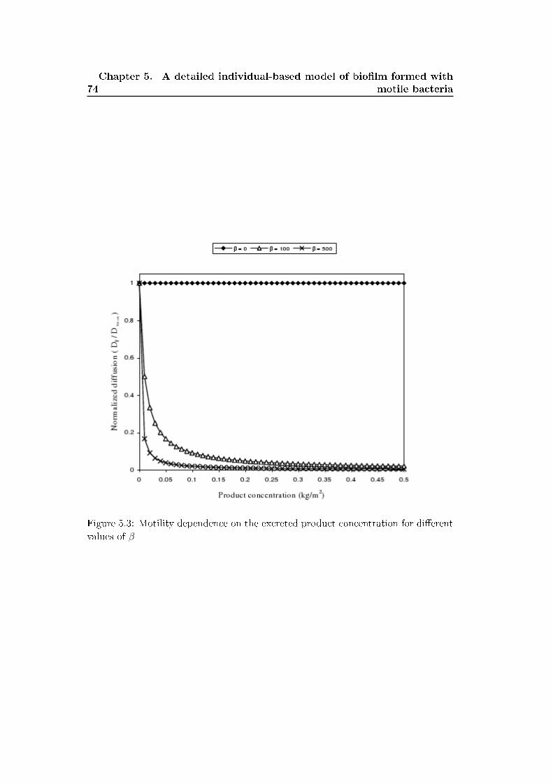
74
Chapter 5. A detailed individual-based model of bio�lm formed with
motile bacteria
Figure 5.3: Motility dependence on the excreted product concentration for di�erent
values of β
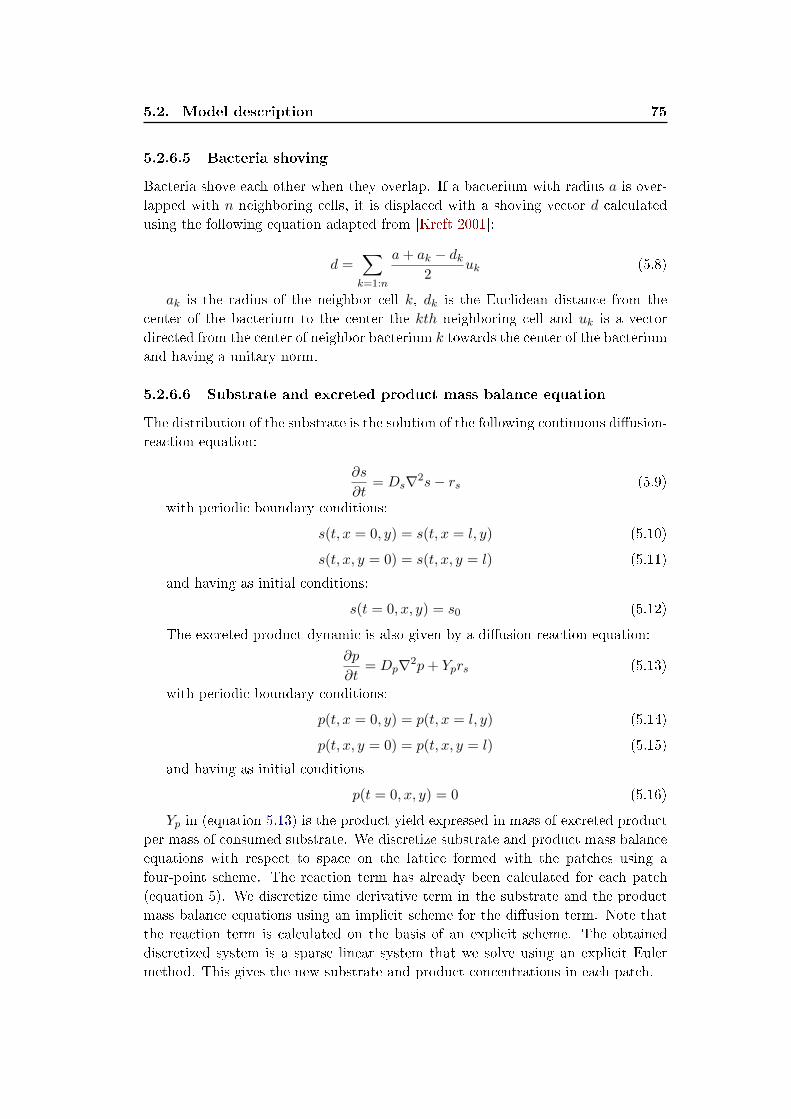
5.2. Model description 75
5.2.6.5 Bacteria shoving
Bacteria shove each other when they overlap. If a bacterium with radius a is over-
lapped with n neighboring cells, it is displaced with a shoving vector d calculated
using the following equation adapted from [Kreft 2001]:
d =∑k=1:n
a+ ak − dk2
uk (5.8)
ak is the radius of the neighbor cell k, dk is the Euclidean distance from the
center of the bacterium to the center the kth neighboring cell and uk is a vector
directed from the center of neighbor bacterium k towards the center of the bacterium
and having a unitary norm.
5.2.6.6 Substrate and excreted product mass balance equation
The distribution of the substrate is the solution of the following continuous di�usion-
reaction equation:
∂s
∂t= Ds∇2s− rs (5.9)
with periodic boundary conditions:
s(t, x = 0, y) = s(t, x = l, y) (5.10)
s(t, x, y = 0) = s(t, x, y = l) (5.11)
and having as initial conditions:
s(t = 0, x, y) = s0 (5.12)
The excreted product dynamic is also given by a di�usion-reaction equation:
∂p
∂t= Dp∇2p+ Yprs (5.13)
with periodic boundary conditions:
p(t, x = 0, y) = p(t, x = l, y) (5.14)
p(t, x, y = 0) = p(t, x, y = l) (5.15)
and having as initial conditions
p(t = 0, x, y) = 0 (5.16)
Yp in (equation 5.13) is the product yield expressed in mass of excreted product
per mass of consumed substrate. We discretize substrate and product mass balance
equations with respect to space on the lattice formed with the patches using a
four-point scheme. The reaction term has already been calculated for each patch
(equation 5). We discretize time derivative term in the substrate and the product
mass balance equations using an implicit scheme for the di�usion term. Note that
the reaction term is calculated on the basis of an explicit scheme. The obtained
discretized system is a sparse linear system that we solve using an explicit Euler
method. This gives the new substrate and product concentrations in each patch.
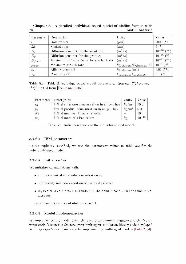
76
Chapter 5. A detailed individual-based model of bio�lm formed with
motile bacteria
Parameter Description Units Value
l Domain size (µm) 2000 (*)
∆l Spatial step (µm) 5 (*)
Ds Di�usion constant for the substrate (m2/s) 10−10 (**)
Dp Di�usion constant for the product (m2/s) 10−16 (*)
Dfmax Maximum di�usion factor for the bacteria (m2/s) 10−12 (**)
µmax Maximum growth rate kgsubstrate/(kgbiomass s) 10−4 (**)
ks A�nity constant kgsubstrate/m2) 0.01 (**)
Yp Product yield kgbiomass/kgsubstrate 0.1 (*)
Table 5.2: Table 2 Individual-based model parameters. Source: (*)Assumed -
(**)Adapted from [Picioreanu 2007]
Parameter Description Units Value
s0 Initial substrate concentration in all patches kg/m2 10.0
p0 Initial product concentration in all patches kg/m2 0.0
N0 Initial number of bacterial cells − 100
m0 Initial mass of a bacterium kg 10−15
Table 5.3: Initial conditions of the individual-based model
5.2.6.7 IBM parameters
Unless explicitly speci�ed, we use the parameters values in table 5.2 for the
individual-based model.
5.2.6.8 Initialization
We initialize all simulations with:
• a uniform initial substrate concentration s0
• a uniformly null concentration of excreted product
• N0 bacterial cells drawn at random in the domain each with the same initial
mass m0.
Initial conditions are detailed in table 5.3.
5.2.6.9 Model implementation
We implemented the model using the Java programming language and the Mason
framework. Mason is a discrete event multiagent simulation library code developed
at the George Mason University for implementing multi-agent models [Luke 2004].
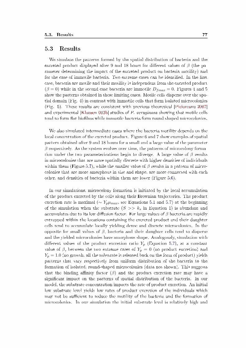
5.3. Results 77
5.3 Results
We simulate the patterns formed by the spatial distribution of bacteria and the
excreted product displayed after 9 and 18 hours for di�erent values of β (the pa-
rameter determining the impact of the excreted product on bacteria motility) and
for the case of immotile bacteria. Two extreme cases can be identi�ed. In the �rst
case, bacteria are motile and their motility is independent from the excreted product
(β = 0) while in the second case bacteria are immotile Dfmax = 0. Figures 4 and 5
show the patterns obtained in these limiting cases. Motile cells disperse over the spa-
tial domain (Fig. 4) in contrast with immotile cells that form isolated microcolonies
(Fig. 5). These results are consistent with previous theoretical [Picioreanu 2007]
and experimental [Klausen 003b] studies of P. aeruginosa showing that motile cells
tend to form �at bio�lms while immotile bacteria form round shaped microcolonies.
We also simulated intermediate cases where the bacteria motility depends on the
local concentration of the excreted product. Figure 6 and 7 show examples of spatial
pattern obtained after 9 and 18 hours for a small and a large value of the parameter
β respectively. As the system evolves over time, the patterns of microcolony forma-
tion under the two parameterizations begin to diverge. A large value of β results
in microcolonies that are more spatially discrete with higher densities of individuals
within them (Figure 5.7), while the smaller value of β results in a pattern of micro-
colonies that are more amorphous in size and shape, are more connected with each
other, and densities of bacteria within them are lower (Figure 5.6).
In our simulations, microcolony formation is initiated by the local accumulation
of the product excreted by the cells along their Brownian trajectories. The product
excretion rate is maximal (∼ Ypµmax, see Equations 5.1 and 5.7) at the beginning
of the simulation when the substrate (S >> ks in Equation 1) is abundant and
accumulates due to its low di�usion factor. For large values of β bacteria are rapidly
entrapped within the locations containing the excreted product and their daughter
cells tend to accumulate locally yielding dense and discrete microcolonies. In the
opposite for small values of β, bacteria and their daughter cells tend to disperse
and the yielded microcolonies have amorphous shape. Analogously, simulation with
di�erent values of the product excretion ratio Yp (Equation 5.7), at a constant
value of β, between the two extreme cases of Yp = 0 (no product excretion) and
Yp = 1.0 (no growth, all the substrate is released back on the form of product) yields
patterns that vary respectively from uniform distribution of the bacteria to the
formation of isolated, round-shaped microcolonies (data not shown). This suggests
that the binding a�nity factor (β) and the product excretion rate may have a
signi�cant impact on the patterns of spatial distribution of the bacteria. In our
model, the substrate concentration impacts the rate of product excretion. An initial
low substrate level yields low rates of product excretion of the individuals which
may not be su�cient to reduce the motility of the bacteria and the formation of
microcolonies. In our simulation the initial substrate level is relatively high and
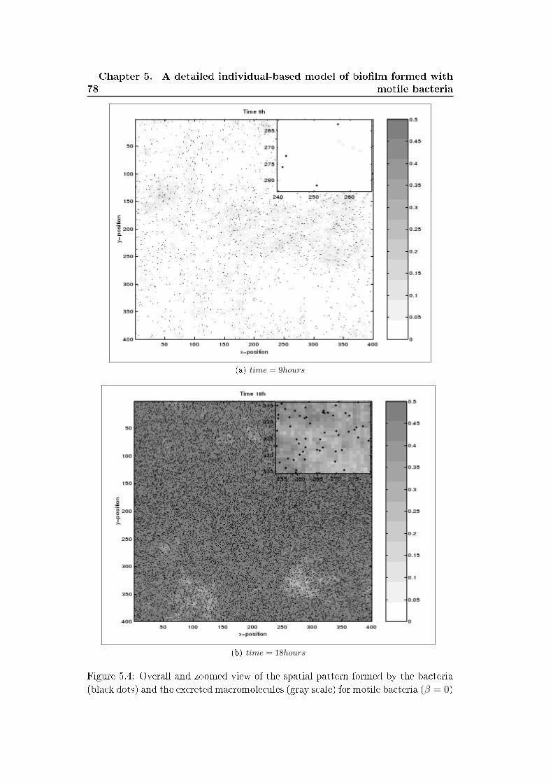
78
Chapter 5. A detailed individual-based model of bio�lm formed with
motile bacteria
(a) time = 9hours
(b) time = 18hours
Figure 5.4: Overall and zoomed view of the spatial pattern formed by the bacteria
(black dots) and the excreted macromolecules (gray scale) for motile bacteria (β = 0)
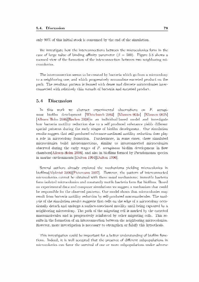
5.4. Discussion 79
only 90% of this initial stock is consumed by the end of the simulation.
We investigate how the interconnections between the microcolonies form in the
case of large value of binding a�nity parameter (β = 500). Figure 5.8 shows a
zoomed view of the formation of the interconnection between two neighboring mi-
crocolonies.
The interconnection seems to be created by bacteria which go from a microcolony
to a neighboring one, and which progressively accumulate excreted product on the
path. The resultant pattern is formed with dense and discrete microcolonies inter-
connected with relatively thin strands of bacteria and excreted product.
5.4 Discussion
In this work we abstract experimental observations on P. aerugi-
nosa bio�lm development [Whitchurch 2002] [Klausen 003a] [Klausen 003b]
[Allesen-Holm 2006][Barken 2008]in an individual-based model and investigate
how bacteria motility reduction due to a self-produced substance yields di�erent
spatial patterns during the early stages of bio�lm development. Our simulation
results suggest that self-produced substance-mediated motility reduction does play
a role in microcolony formation. Furthermore, in some cases, these simulated
microcolonies build interconnections, similar to interconnected microcolonies
observed during the early stages of P. aeruginosa bio�lm development in �ow
chambers[Allesen-Holm 2006], and also in bio�lms formed by Pseudomonas species
in marine environments [Dalton 1994][Dalton 1996].
Several authors already explored the mechanisms yielding microcolonies in
bio�lms[Alpkvist 2006][Picioreanu 2007]. However, the pattern of interconnected
microcolonies cannot be obtained with these usual mechanisms: immotile bacteria
form isolated microcolonies and constantly motile bacteria form �at bio�lms. Based
on experimental data and computer simulations we suggest a mechanism that could
be responsible for the observed patterns. Our model shows that microcolonies may
result from bacteria motility reduction by self-produced macromolecules. The anal-
ysis of the simulation results suggests that cells on the edge of a microcolony occa-
sionally detach and undergo a surface-associated motility until being captured by a
neighboring microcolony. The path of the migrating cell is marked by the excreted
macromolecules and is progressively reinforced by other migrating cells. This re-
sults in the formation of an interconnection between the neighboring microcolonies.
However, more investigation is necessary to strengthen or falsify this hypothesis.
This investigation could be important for a better understanding of bio�lm func-
tions. Indeed, it is well accepted that the presence of di�erent subpopulations in
microcolonies can favor the survival of one or more subpopulations under adverse
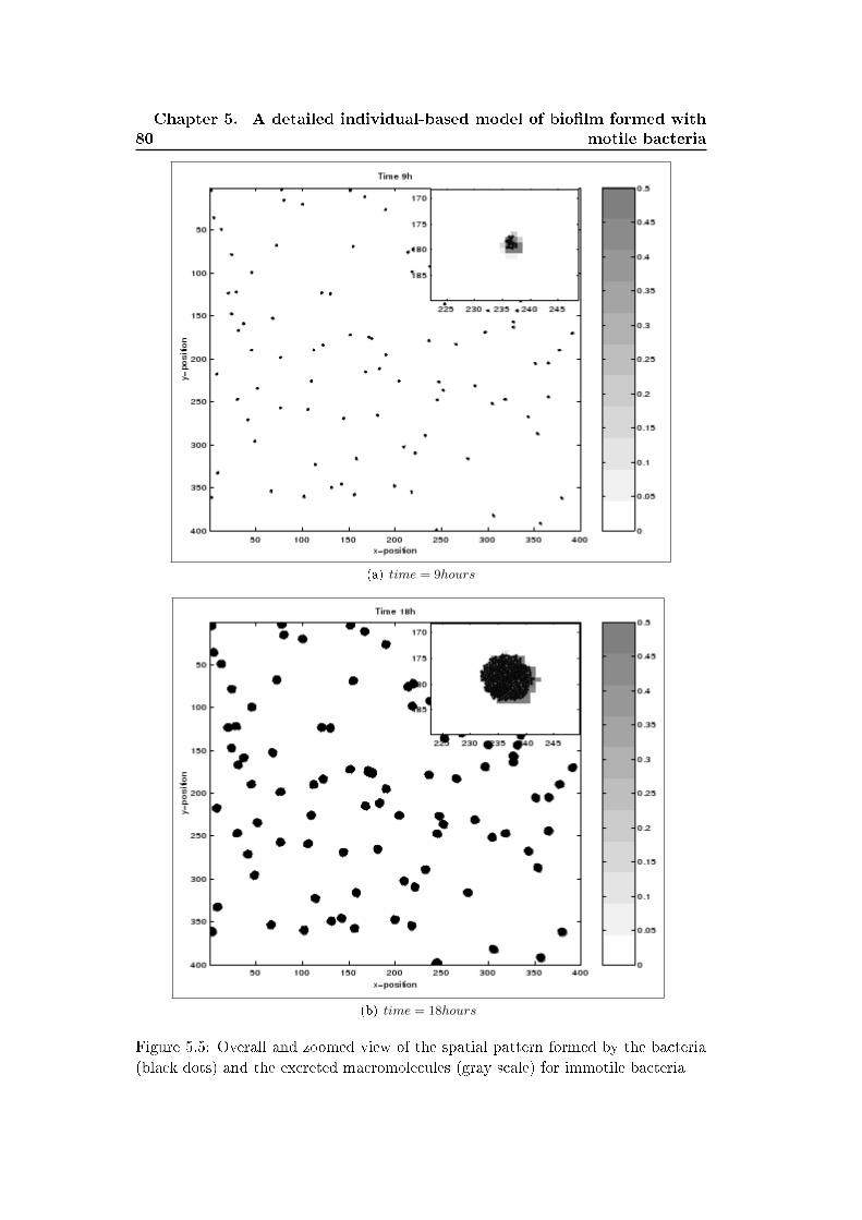
80
Chapter 5. A detailed individual-based model of bio�lm formed with
motile bacteria
(a) time = 9hours
(b) time = 18hours
Figure 5.5: Overall and zoomed view of the spatial pattern formed by the bacteria
(black dots) and the excreted macromolecules (gray scale) for immotile bacteria
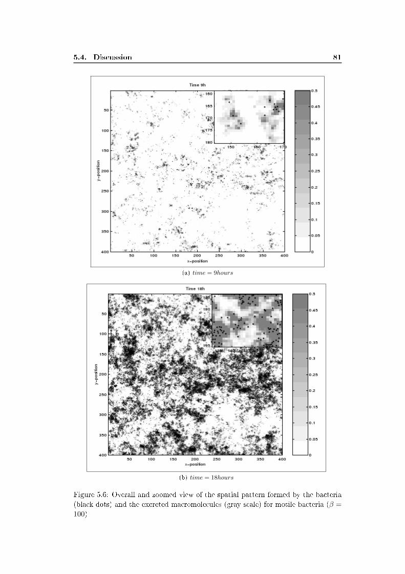
5.4. Discussion 81
(a) time = 9hours
(b) time = 18hours
Figure 5.6: Overall and zoomed view of the spatial pattern formed by the bacteria
(black dots) and the excreted macromolecules (gray scale) for motile bacteria (β =
100)
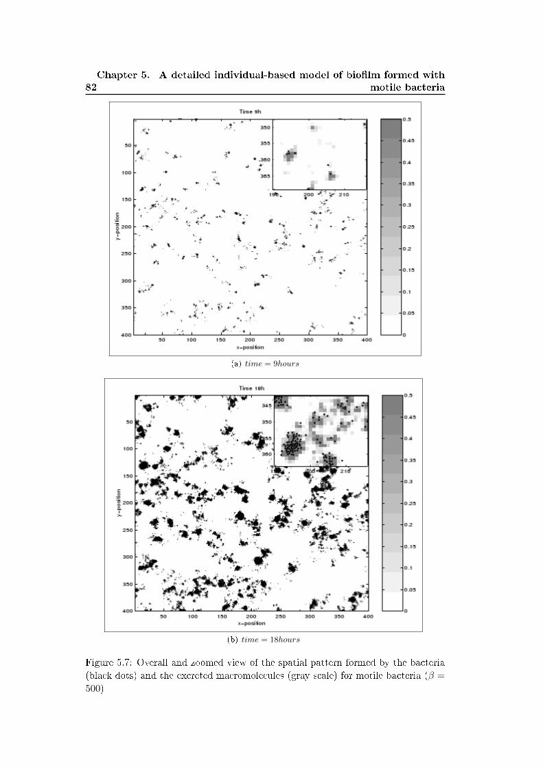
82
Chapter 5. A detailed individual-based model of bio�lm formed with
motile bacteria
(a) time = 9hours
(b) time = 18hours
Figure 5.7: Overall and zoomed view of the spatial pattern formed by the bacteria
(black dots) and the excreted macromolecules (gray scale) for motile bacteria (β =
500)
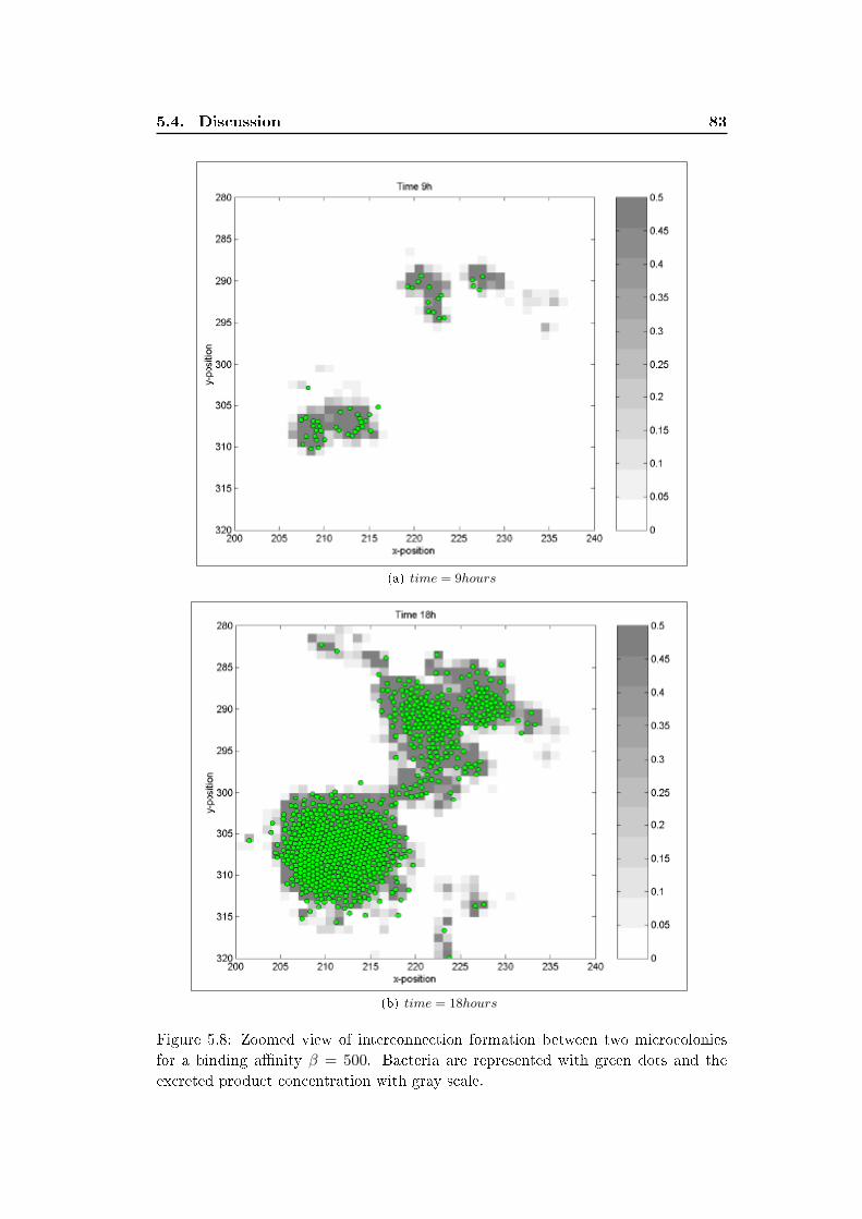
5.4. Discussion 83
(a) time = 9hours
(b) time = 18hours
Figure 5.8: Zoomed view of interconnection formation between two microcolonies
for a binding a�nity β = 500. Bacteria are represented with green dots and the
excreted product concentration with gray scale.
84
Chapter 5. A detailed individual-based model of bio�lm formed with
motile bacteria
conditions [Parsek 2008][Johnson 2008]. However, recent observations suggest that
in some cases the matrix of extracellular DNA (and possibly other products) may
guide migration of the cells between microcolonies [Lu 2005][Barken 2008] favoring a
type of collaboration between distinct subpopulations within a bio�lm. This may be
related to studies in landscape ecology where this pattern of interconnected habitats
is recognized as particularly important (Burel and Baudry, 2003) [Burel 2003].
Individual-based models are appealing to microbiologists because of the emphasis
on the individual cell as the fundamental unit and the richness of their dynamic.
However when they are too complex they often become di�cult to analyze which
limits their practical payo� [Grimm 2005]. Therefore, we have attempted to keep
our model as simple as possible and inspired by the phenomenological results men-
tioned in the introduction, but rich enough to produce patterns of interconnected
microcolonies. Johnson [Johnson 2008] proposed a model based on the assumption
of the �direct� interaction between individual cells through attractive (and repul-
sive) forces arguing that forces between cells can be a proxy for the behavior we
expect to see due to chemotaxis in response to chemicals released by other cells
[Johnson 2008]. The assumption simpli�es the model as the dynamic of the ex-
creted product is not considered explicitly. This is a reasonable assumption when
the dynamics of the chemical being produced is fast (high di�usion) compared to the
dynamic of the bacteria (motility and growth) [Lee 2001]. Our model is based on
the assumption that the excreted macromolecules like DNA and exopolymers di�use
at low rates and persist on the path of the motile bacteria. This seems to play a
role in the formation of the interconnected microcolonies as microcolonies yielded by
Johnson's model through attractive/repulsive forces seem not to be interconnected
[Johnson 2008]. Our study included, however, some limitations that should be ac-
knowledged for future research in this area. Examples, inherent to individual-based
modeling approach, include the question of how to measure the �goodness� of an
IBM. Grimm and Railsback [Grimm 2005] suggested that testing an IBM against
multiple observed patterns is a powerful way to assess the IBM capacity to capture
system's essential characteristics. In this work we assessed the �goodness� of our
IBM through comparison of an observed pattern (connected microcolonies in �g.1)
to a simulated one (�g.8). Despite the similarities between the experimental and
simulated patterns (thin path of bacteria and product connecting neighboring mi-
crocolonies) there are still di�erences. For example cells surrounded the thin path in
�gure 1 while they are contained in the area with high amount of product in �gure 8.
Therefore, additional patterns should be identi�ed and compared to the simulated
ones in order to strengthen or falsify the hypothetical implication of self-excreted
product in motility reduction and formation of interconnected microcolonies. An-
other limitation of our model is the determination of parameters like the binding
a�nity factor (β) and cell di�usion (Df ). These parameters may be di�cult to
obtain from experimental observations and their impact should be assessed through
sensitivity analysis.
5.4. Discussion 85
Finally, the model can be extended to investigate the e�ect of other macro-
molecules like exopolymers on the bacteria motility and microcolonies formation.
Another potential extension is to include additional processes like bacteria detach-
ment and substrate feeding which allow investigating the e�ect of the interactions
between cell motility and excreted macromolecules on the architecture of mature
bio�lms.

Chapter 6
Moment approximation of an
individual-based model of a
bio�lm formed with motile
bacteria
Contents
6.1 Description of the simpli�ed IBM . . . . . . . . . . . . . . . 88
6.1.1 Overview . . . . . . . . . . . . . . . . . . . . . . . . . . . . . 88
6.1.2 Details . . . . . . . . . . . . . . . . . . . . . . . . . . . . . . . 90
6.2 Moment approximation . . . . . . . . . . . . . . . . . . . . . . 92
6.2.1 First moment dynamics . . . . . . . . . . . . . . . . . . . . . 92
6.2.2 Second moment dynamics . . . . . . . . . . . . . . . . . . . . 93
6.2.3 Closure of the moment hierarchy . . . . . . . . . . . . . . . . 100
6.2.4 Solving the moment model . . . . . . . . . . . . . . . . . . . 100
6.3 Results and discussion . . . . . . . . . . . . . . . . . . . . . . 100
6.4 Conclusion . . . . . . . . . . . . . . . . . . . . . . . . . . . . . 111
In this chapter we derive a moment approximation model of an individual-based
model (IBM) describing the formation of microcolonies due to bacteria motility
reduction by a self-produced product. The direct derivation of moment models of
the IBM presented in chapter 5 is di�cult. thus we start by simplifying the IBM than
approximating the simpli�ed IBM with a moment model. The main simpli�cations
consist in representing the individuals (bacteria and product) as point particles.
The moment model aggregates the state variables of the simpli�ed IBM into two
type of quantities: the average density of individuals (bacteria and polymer) which
correspond to the �rst spatial moment and the average neighborhood of an individ-
ual at di�erent distances, measured by the self and cross pair density correlation
functions (second spatial moments). The �uctuation of the local density of indi-
viduals observed in the IBM are averaged in the moment model. We show in this
chapter that if the individual response to these �uctuations is non-linear or depends
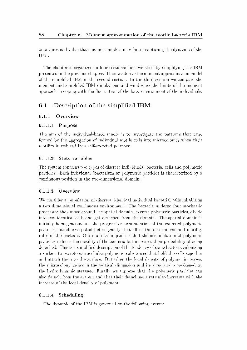
88 Chapter 6. Moment approximation of the motile bacteria IBM
on a threshold value than moment models may fail in capturing the dynamic of the
IBM.
The chapter is organized in four sections: �rst we start by simplifying the IBM
presented in the previous chapter. Than we derive the moment approximation model
of the simpli�ed IBM in the second section. In the third section we compare the
moment and simpli�ed IBM simulations and we discuss the limits of the moment
approach in coping with the �uctuation of the local environment of the individuals.
6.1 Description of the simpli�ed IBM
6.1.1 Overview
6.1.1.1 Purpose
The aim of the individual-based model is to investigate the patterns that arise
formed by the aggregation of individual motile cells into microcolonies when their
motility in reduced by a self-excreted polymer.
6.1.1.2 State variables
The system contains two types of discrete individuals: bacterial cells and polymeric
particles. Each individual (bacterium or polymeric particle) is characterized by a
continuous position in the two-dimensional domain.
6.1.1.3 Overview
We consider a population of discrete, identical individual bacterial cells inhabiting
a two dimensional continuous environment. The bacteria undergo four stochastic
processes: they move around the spatial domain, excrete polymeric particles, divide
into two identical cells and get detached from the domain. The spatial domain is
initially homogeneous but the progressive accumulation of the excreted polymeric
particles introduces spatial heterogeneity that a�ect the detachment and motility
rates of the bacteria. Our main assumption is that the accumulation of polymeric
particles reduces the motility of the bacteria but increases their probability of being
detached. This is a simpli�ed description of the tendency of some bacteria colonizing
a surface to excrete extracellular polymeric substances that hold the cells together
and attach them to the surface. But when the local density of polymer increases,
the microcolony grows in the vertical dimension and its structure is weakened by
the hydrodynamic stresses. Finally we suppose that the polymeric particles can
also detach from the system and that their detachment rate also increases with the
increase of the local density of polymers.
6.1.1.4 Scheduling
The dynamic of the IBM is governed by the following events:
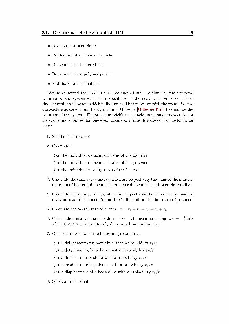
6.1. Description of the simpli�ed IBM 89
• Division of a bacterial cell
• Production of a polymer particle
• Detachment of bacterial cell
• Detachment of a polymer particle
• Motility of a bacterial cell
We implemented the IBM in the continuous time. To simulate the temporal
evolution of the system we need to specify when the next event will occur, what
kind of event it will be and which individual will be concerned with the event. We use
a procedure adapted from the algorithm of Gillespie [GIllespie 1976] to simulate the
evolution of the system. The procedure yields an asynchronous random execution of
the events and suppose that one event occurs at a time. It iterates over the following
steps:
1. Set the time to t = 0
2. Calculate:
(a) the individual detachment rates of the bacteria
(b) the individual detachment rates of the polymer
(c) the individual motility rates of the bacteria
3. Calculate the sums r1, r2 and r3 which are respectively the sums of the individ-
ual rates of bacteria detachment, polymer detachment and bacteria motility.
4. Calculate the sums r4 and r5 which are respectively the sum of the individual
division rates of the bacteria and the individual production rates of polymer
5. Calculate the overall rate of events : r = r1 + r2 + r3 + r4 + r5
6. Choose the waiting time τ for the next event to occur according to τ = −1r lnλ
where 0 < λ ≤ 1 is a uniformly distributed random number
7. Choose an event with the following probabilities:
(a) a detachment of a bacterium with a probability r1/r
(b) a detachment of a polymer with a probability r2/r
(c) a division of a bacteria with a probability r3/r
(d) a production of a polymer with a probability r4/r
(e) a displacement of a bacterium with a probability r5/r
8. Select an individual:
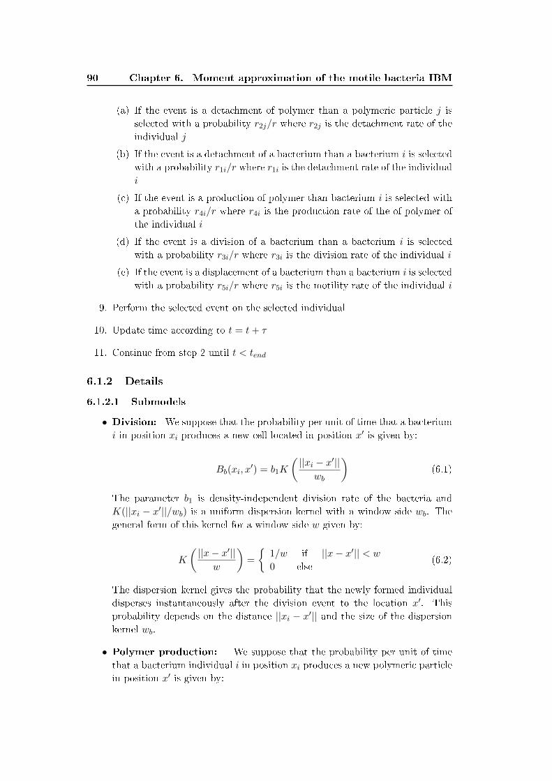
90 Chapter 6. Moment approximation of the motile bacteria IBM
(a) If the event is a detachment of polymer than a polymeric particle j is
selected with a probability r2j/r where r2j is the detachment rate of the
individual j
(b) If the event is a detachment of a bacterium than a bacterium i is selected
with a probability r1i/r where r1i is the detachment rate of the individual
i
(c) If the event is a production of polymer than bacterium i is selected with
a probability r4i/r where r4i is the production rate of the of polymer of
the individual i
(d) If the event is a division of a bacterium than a bacterium i is selected
with a probability r3i/r where r3i is the division rate of the individual i
(e) If the event is a displacement of a bacterium than a bacterium i is selected
with a probability r5i/r where r5i is the motility rate of the individual i
9. Perform the selected event on the selected individual
10. Update time according to t = t+ τ
11. Continue from step 2 until t < tend
6.1.2 Details
6.1.2.1 Submodels
• Division: We suppose that the probability per unit of time that a bacterium
i in position xi produces a new cell located in position x′ is given by:
Bb(xi, x′) = b1K
(||xi − x′||
wb
)(6.1)
The parameter b1 is density-independent division rate of the bacteria and
K(||xi − x′||/wb) is a uniform dispersion kernel with a window side wb. The
general form of this kernel for a window side w given by:
K
(||x− x′||
w
)=
{1/w if ||x− x′|| < w
0 else(6.2)
The dispersion kernel gives the probability that the newly formed individual
disperses instantaneously after the division event to the location x′. This
probability depends on the distance ||xi − x′|| and the size of the dispersion
kernel wb.
• Polymer production: We suppose that the probability per unit of time
that a bacterium individual i in position xi produces a new polymeric particle
in position x′ is given by:
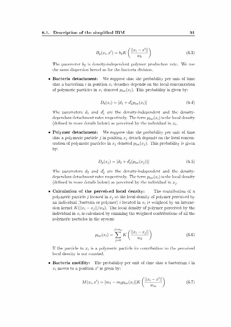
6.1. Description of the simpli�ed IBM 91
Bp(xi, x′) = b2K
(||xi − x′||
wb
)(6.3)
The parameter b2 is density-independent polymer production rate. We use
the same dispersion kernel as for the bacteria division.
• Bacteria detachment: We suppose that the probability per unit of time
that a bacterium i in position xi detaches depends on the local concentration
of polymeric particles in xi denoted ploc(xi). This probability is given by:
Db(xi) = [d1 + d′1ploc(xi)] (6.4)
The parameters d1 and d′1 are the density-independent and the density-
dependant detachment rates respectively. The term ploc(xi) is the local density
(de�ned in more details below) as perceived by the individual in xi.
• Polymer detachment: We suppose that the probability per unit of time
that a polymeric particle j in position xj detach depends on the local concen-
tration of polymeric particles in xj denoted ploc(xj). This probability is given
by:
Dp(xj) = [d2 + d′2(ploc(xj))] (6.5)
The parameters d2 and d′2 are the density-independent and the density-
dependant detachment rates respectively. The term ploc(xi) is the local density
(de�ned in more details below) as perceived by the individual in xj .
• Calculation of the perceived local density: The contribution of a
polymeric particle j located in xj to the local density of polymer perceived by
an individual (bacteria or polymer) i located in xi is weighted by an interac-
tion kernel K(||xi − xj ||/wd). The local density of polymer perceived by the
individual in xi is calculated by summing the weighted contributions of all the
polymeric particles in the system:
ploc(xi) =
j=np∑j=0
K
(||xi − xj ||
wd
)(6.6)
If the particle in xi is a polymeric particle its contribution to the perceived
local density is not counted.
• Bacteria motility: The probability per unit of time that a bacterium i in
xi moves to a position x′ is given by:
M(xi, x′) = [m1 −m2ploc(xi)]K
(||xi − x′||wm
)(6.7)
92 Chapter 6. Moment approximation of the motile bacteria IBM
Where m1 and m2 are respectively the density-independent and the density
dependent motility rates and K(||xi − x′||/wm) a uniform motility kernel.
6.1.2.2 Initialization
The model is initialized with nb(t = 0) = 1000 bacterial cells distributed uniformly
over the domain. Initially there are no polymer particles in the domain (np(t = 0) =
0)
6.1.2.3 Model parameters
The individual-based model parameters are summarized in table 6.3. Unless explic-
itly speci�ed, we use the default parameter values in table 6.3.
6.2 Moment approximation
We propose to develop a deterministic mathematical model that approximate the
dynamic of the individual-based model described in the previous section using mo-
ment approximation techniques.
6.2.1 First moment dynamics
The dynamic of the �rst moment (average densities of bacteria and polymer) is given
by the following equations:
dNb
dt= (b1 − d1)Nb − d′1
∫Cbp(ξ)K
(||ξ||wd
)dξ (6.8)
dNp
dt= b2Nb − d2Np − d′2
∫Cpp(ξ)K
(||ξ||wd
)dξ (6.9)
Equations 6.8 and 6.9 describe respectively the dynamic of the average density
of bacteria Nb and polymer Np. The integral terms in the right-hand side are the
neighborhood-dependent components of the detachment. They involve respectively
the pair densities Cbp(ξ) and Cpp(ξ) and an interaction kernel K(||ξ||/wd). These
terms encompass the e�ect of the local density of polymer in the neighborhood of
bacteria, as given by Cbp(ξ), and in the neighborhood of a polymeric particle, as
given by Cpp(ξ), weighted by the uniform interaction kernel K(||ξ||/wd). Note thatif the size wd of uniform interaction kernel is equal to the side of the domain than
a bacterium (respectively a polymeric particle) experiences equally the e�ect of all
the polymeric particle within the domain. This reduces equations 6.8 and 6.9 to the
following mean-�eld system:
dNb
dt= (b1 − d1)Nb − d′1NbNp (6.10)
dNp
dt= b2Nb − d2Np − d′2NpNp (6.11)
6.2. Moment approximation 93
The mean-�eld equations can also be obtained if the position of the bacterial
cells (respectively the polymeric cells) are not correlated with the position of the
polymeric particles. In this case the density of pairs formed with a focal bacterium
(respectively a focal polymeric particles) with a polymeric particle located at a
vectorial distance ξ from the focal particle is equal to the product of the average
densities NbNp (respectively NpNp). Spatial patterns formation and small interac-
tion kernel may cause a departure from the mean-�eld model. The system formed
with equations 6.8 and 6.9 is not closed and need to be coupled to the dynamic of
Cbp(ξ) and Cpp(ξ).
6.2.2 Second moment dynamics
The pair correlation functions Cbb(ξ), Cbp(ξ) and Cpp(ξ) characterize the spatial
pattern formed by the bacteria and the polymer. They measure respectively the
densities of pairs formed with two bacteria, a bacterium and a polymeric particle
or two polymeric particles at di�erent vectorial distance ξ. The dynamic of these
functions account for the �ve processes: bacteria division, production of polymeric
particles, bacteria detachment, polymer detachment and motility of the bacteria.
6.2.2.1 Dynamic of the bacteria-bacteria pair correlation function
The dynamic of the bacteria-bacteria pair correlation function Cbb(ξ) is given by:
dCbb(ξ)
dt=
(dCbb(ξ)
dt
)division
+
(dCbb(ξ)
dt
)detachment
+
(dCbb(ξ)
dt
)motility
(6.12)
The terms in the right hand side denotes for the e�ect of three processes that
may modify the bacteria pattern and which are the bacteria division, detachment
and motility events. The e�ect of division events on Cbb(ξ) is given by the following
equation:
(dCbb(ξ)
dt
)division
= +2b1NbK
(||ξ||wb
)+2b1
∫Cbb(ξ + ξ′)K
(||ξ′||wb
)dξ′ (6.13)
• The �rst term in the right-hand side accounts for the division of a bacterium
i producing a new cell j located at a vectorial distance ξ. This event yields a
new pair of bacteria separated with a vectorial distance ξ. The rate at which
such division events occur is obtained by multiplying the density of average
bacteria Nb by the division rate b1. Then we multiply by the probability
K(||ξ||/wb) that the newly formed cells are located at a distance ξ from the
parent cell. The factor 2 accounts for newly formed cells at a vectorial distance
−ξ which also form a new par (j, i) at distance ξ.
94 Chapter 6. Moment approximation of the motile bacteria IBM
• The second term focuses on the new pair that the daughter cell of a parent
bacterium i form with a bacterium j located at a distance ξ + ξ′ from i. The
density of (i, j) pairs is Cbb(ξ + ξ) and the division rate is b1. Multiplying
these two factors with the probability K(||ξ′||/wb) that the newly formed cells
is located at a distance ξ′ from i and integrating over all possible distances ξ′
gives the second term. We also take into consideration that analogous event
can occur to the individual j by multiplying the second term by a factor 2.
The contribution of the detachment events of bacteria to the dynamic of Cbb(ξ)
is given by:
(dCbb(ξ)
dt
)detachment
= −2d1Cbb(ξ)
−2d′1
∫K
(||ξ′′||wd
)Tbbp(ξ, ξ
′′)dξ′′ (6.14)
• The �rst term in the right hand side accounts for the detachment of the cell i
in the pair (i, j). Such events occur at a rate d1. Multiplying d1 by the density
Cbb(ξ) of (i, j) pairs at distance ξ gives the resulting decrease in that density.
The factor 2 accounts that analogous event can occur for the individual j.
• The second term is the density-dependent detachment term that accounts for
the presence of polymeric particles in the neighborhood of the bacteria. The
detachment of a bacterium i of the (i, j) pair can result from the presence of
polymer particle k at a distance ξ′′ from i. Such triplet con�guration occurs
at a density Tbbp(ξ, ξ′′). The cumulative e�ect of the polymeric particles k
situated at di�erent distances ξ′′ from the cell i is obtained by weighting the
triplet density with K(||ξ′′||/wd) and integrating over all interaction distances
ξ′′. Multiplying contribution of the local density of polymer with the density-
dependent detachment rate of the bacteria d′1 gives the second term. The
factor 2 accounts for the analogous event that can occur for the cell j in the
the pair (i, j).
The contribution of the motility to the dynamic of Cbb(ξ) is given by the following
equation:
(dCbb(ξ)
dt
)motility
= −2m1Cbb(ξ) (6.15)
+2m1
∫K
(||ξ′||wm
)Cbb(ξ + ξ′)dξ′
+2m2
∫K
(||ξ′′||wd
)Tbbp(ξ, ξ
′′)dξ′′
−2m2
∫ ∫K
(||ξ′||wm
)K
(||ξ′′||wd
)Tbbp(ξ + ξ′, ξ′′)dξ′dξ′′
6.2. Moment approximation 95
• When the individual i moves, the original pair (i, j) at distance ξ is destroyed.
The �rst term in the right hand side accounts for this process by multiplying
the density-independent motility rate of m1 by the density of pairs Cbb(ξ) of
the original pair con�guration.
• On the other hand a new (i, j) pair of bacteria is created at distance ξ when the
cell i at originally at a distance ξ+ ξ′ from the cell j moves a distance ξ′. This
e�ect is captured by the second term, which weights the density Cbb(ξ + ξ′)
of the original pair con�guration with the motility kernel UK(||ξ′||/wm) and
integrating over all possible motility distances ξ′.
• The third term corrects the �rst term by accounting for the possible presence
of polymeric particles in the neighborhood of the cell in the pair (i, j) originally
at a distance ξ. The motility of i in the pair (i, j) is reduced by the presence
of polymeric particle k located at a distance ξ′′ from i. The density triplet
formed with two cells separated with a distance ξ and a polymeric particle at
a distance ξ′′ from i is Tbbp(ξ, ξ′′). Weighting this density by the interaction
kernel K(||ξ′′||/wd) and integrating over all distances ξ′′ gives the third term.
The factor 2 accounts for the analogous event that can occur for the cell j.
• The last term corrects the second term by accounting for motility reduction of
the cell i originally at a distance ξ+ ξ′ from the cell j due to the presence of a
polymeric particle k at a distance ξ′′ from i. The cumulative e�ect of the poly-
meric particles k is obtained by multiplying the triplet density Tbbp(ξ + ξ′, ξ′′)
by the interaction kernel K(||ξ′′||/wd) and integrating over all distances ξ′′.
The result is then multiplied by the motility kernel K(||ξ′||/wm), integrated
over all distances ξ′ and multiplied by the density dependent motility rate m2.
the factor 2 accounts for analogous event that may be experienced by the cell
j in the pair (i, j).
6.2.2.2 Dynamic of the polymer-polymer pair correlation function
The dynamic of the density of pairs of polymeric particles separated with a distance
ξ is given buy the following equation:
dCpp(ξ)
dt=
(dCpp(ξ)
dt
)production
+
(dCpp(ξ)
dt
)detachment
(6.16)
The �rst term in the right-hand side accounts for the contribution of polymer
production events and the second term for polymer detachment events . Polymer
production events contribute to the creation positively to Cpp(ξ) according to the
following equation:
(dCpp(ξ)
dt
)production
= +2b2
∫K
(||ξ′||wb
)Cbp(ξ + ξ′)dξ′ (6.17)
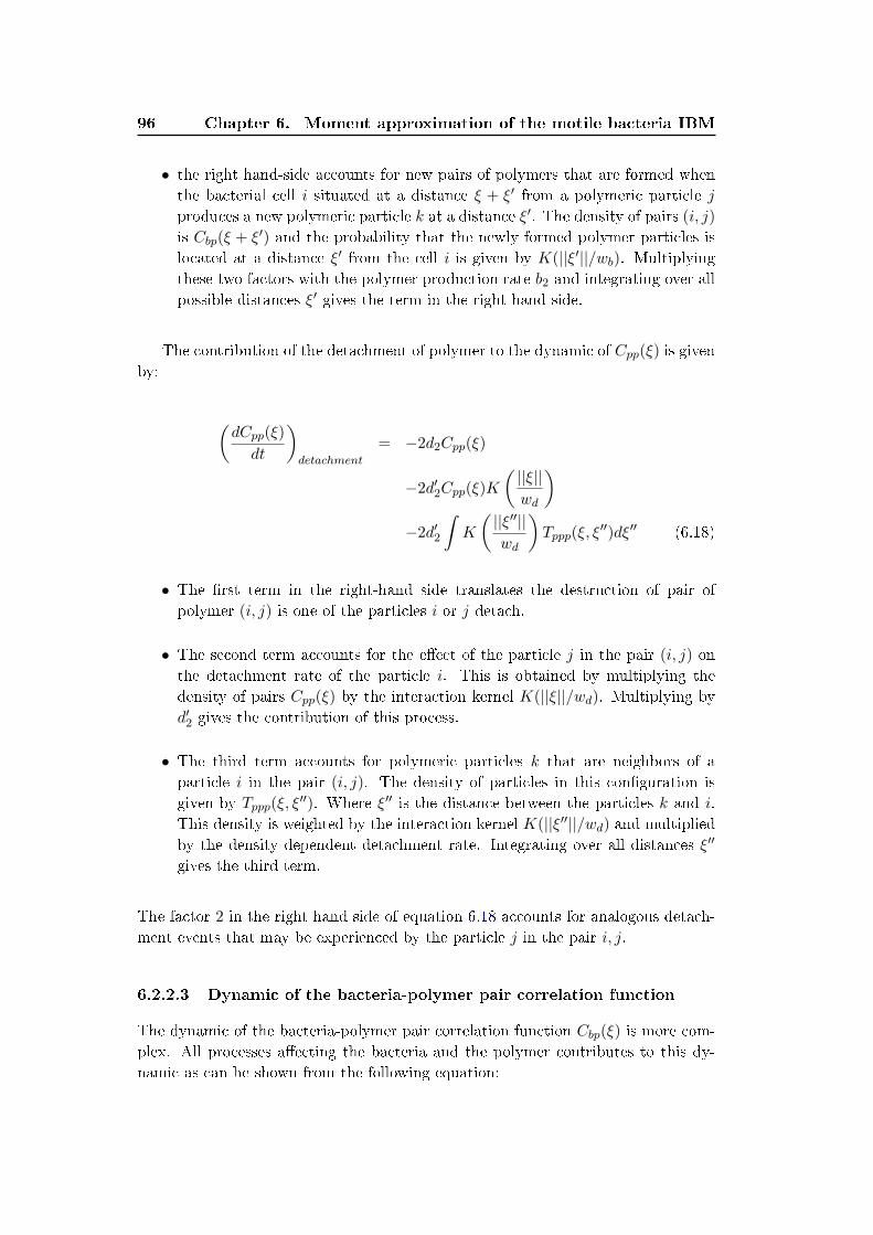
96 Chapter 6. Moment approximation of the motile bacteria IBM
• the right hand-side accounts for new pairs of polymers that are formed when
the bacterial cell i situated at a distance ξ + ξ′ from a polymeric particle j
produces a new polymeric particle k at a distance ξ′. The density of pairs (i, j)
is Cbp(ξ + ξ′) and the probability that the newly formed polymer particles is
located at a distance ξ′ from the cell i is given by K(||ξ′||/wb). Multiplying
these two factors with the polymer production rate b2 and integrating over all
possible distances ξ′ gives the term in the right-hand side.
The contribution of the detachment of polymer to the dynamic of Cpp(ξ) is given
by:
(dCpp(ξ)
dt
)detachment
= −2d2Cpp(ξ)
−2d′2Cpp(ξ)K
(||ξ||wd
)−2d′2
∫K
(||ξ′′||wd
)Tppp(ξ, ξ
′′)dξ′′ (6.18)
• The �rst term in the right-hand side translates the destruction of pair of
polymer (i, j) is one of the particles i or j detach.
• The second term accounts for the e�ect of the particle j in the pair (i, j) on
the detachment rate of the particle i. This is obtained by multiplying the
density of pairs Cpp(ξ) by the interaction kernel K(||ξ||/wd). Multiplying by
d′2 gives the contribution of this process.
• The third term accounts for polymeric particles k that are neighbors of a
particle i in the pair (i, j). The density of particles in this con�guration is
given by Tppp(ξ, ξ′′). Where ξ′′ is the distance between the particles k and i.
This density is weighted by the interaction kernel K(||ξ′′||/wd) and multiplied
by the density dependent detachment rate. Integrating over all distances ξ′′
gives the third term.
The factor 2 in the right hand side of equation 6.18 accounts for analogous detach-
ment events that may be experienced by the particle j in the pair i, j.
6.2.2.3 Dynamic of the bacteria-polymer pair correlation function
The dynamic of the bacteria-polymer pair correlation function Cbp(ξ) is more com-
plex. All processes a�ecting the bacteria and the polymer contributes to this dy-
namic as can be shown from the following equation:
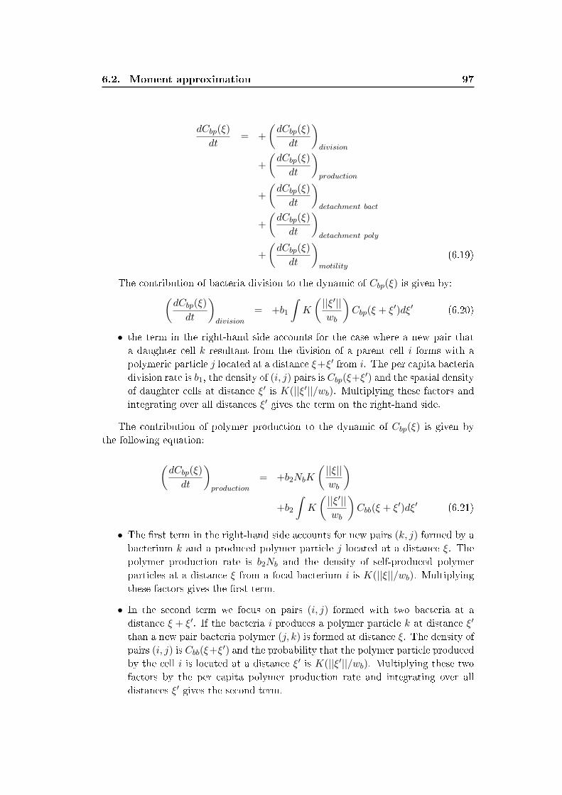
6.2. Moment approximation 97
dCbp(ξ)
dt= +
(dCbp(ξ)
dt
)division
+
(dCbp(ξ)
dt
)production
+
(dCbp(ξ)
dt
)detachment bact
+
(dCbp(ξ)
dt
)detachment poly
+
(dCbp(ξ)
dt
)motility
(6.19)
The contribution of bacteria division to the dynamic of Cbp(ξ) is given by:(dCbp(ξ)
dt
)division
= +b1
∫K
(||ξ′||wb
)Cbp(ξ + ξ′)dξ′ (6.20)
• the term in the right-hand side accounts for the case where a new pair that
a daughter cell k resultant from the division of a parent cell i forms with a
polymeric particle j located at a distance ξ+ξ′ from i. The per capita bacteria
division rate is b1, the density of (i, j) pairs is Cbp(ξ+ξ′) and the spatial density
of daughter cells at distance ξ′ is K(||ξ′||/wb). Multiplying these factors and
integrating over all distances ξ′ gives the term on the right-hand side.
The contribution of polymer production to the dynamic of Cbp(ξ) is given by
the following equation:
(dCbp(ξ)
dt
)production
= +b2NbK
(||ξ||wb
)+b2
∫K
(||ξ′||wb
)Cbb(ξ + ξ′)dξ′ (6.21)
• The �rst term in the right-hand side accounts for new pairs (k, j) formed by a
bacterium k and a produced polymer particle j located at a distance ξ. The
polymer production rate is b2Nb and the density of self-produced polymer
particles at a distance ξ from a focal bacterium i is K(||ξ||/wb). Multiplying
these factors gives the �rst term.
• In the second term we focus on pairs (i, j) formed with two bacteria at a
distance ξ + ξ′. If the bacteria i produces a polymer particle k at distance ξ′
than a new pair bacteria polymer (j, k) is formed at distance ξ. The density of
pairs (i, j) is Cbb(ξ+ξ′) and the probability that the polymer particle produced
by the cell i is located at a distance ξ′ is K(||ξ′||/wb). Multiplying these two
factors by the per capita polymer production rate and integrating over all
distances ξ′ gives the second term.
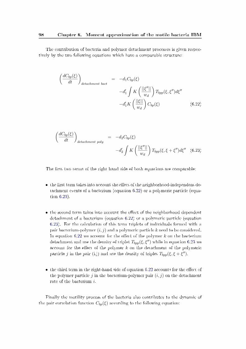
98 Chapter 6. Moment approximation of the motile bacteria IBM
The contribution of bacteria and polymer detachment processes is given respec-
tively by the two following equations which have a comparable structure:
(dCbp(ξ)
dt
)detachment bact
= −d1Cbp(ξ)
−d′1∫K
(||ξ′′||wd
)Tbpp(ξ, ξ
′′)dξ′′
−d′1K(||ξ||wd
)Cbp(ξ) (6.22)
(dCbp(ξ)
dt
)detachment poly
= −d2Cbp(ξ)
−d′2∫K
(||ξ′′||wd
)Tbpp(ξ, ξ + ξ′′)dξ′′ (6.23)
The �rst two terms of the right-hand side of both equations are comparable:
• the �rst term takes into account the e�ect of the neighborhood-independent de-
tachment events of a bacterium (equation 6.22) or a polymeric particle (equa-
tion 6.23).
• the second term takes into account the e�ect of the neighborhood dependent
detachment of a bacterium (equation 6.22) or a polymeric particle (equation
6.23). For the calculation of this term triplets of individuals formed with a
pair bacterium-polymer (i, j) and a polymeric particle k need to be considered.
In equation 6.22 we account for the e�ect of the polymer k on the bacterium
detachment and use the density of triplet Tbpp(ξ, ξ′′) while in equation 6.23 we
account for the e�ect of the polymer k on the detachment of the polymeric
particle j in the pair (i,j) and use the density of triplet Tbpp(ξ, ξ + ξ′′).
• the third term in the right-hand side of equation 6.22 accounts for the e�ect of
the polymer particle j in the bacterium-polymer pair (i, j) on the detachment
rate of the bacterium i.
Finally the motility process of the bacteria also contributes to the dynamic of
the pair correlation function Cbp(ξ) according to the following equation:
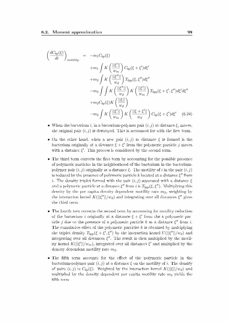
6.2. Moment approximation 99
(dCbp(ξ)
dt
)motility
= −m1Cbp(ξ)
+m1
∫K
(||ξ′||wm
)Cbp(ξ + ξ′)dξ′
+m2
∫K
(||ξ′′||wd
)Tbpp(ξ, ξ
′′)dξ′′
−m2
∫ ∫K
(||ξ′′||wd
)K
(||ξ′||wm
)Tbpp(ξ + ξ′, ξ′′)dξ′dξ′′
+m2Cbp(ξ)K
(||ξ||wd
)−m2
∫K
(||ξ′||wm
)K
(||ξ + ξ′||wd
)Cbp(ξ + ξ′)dξ′ (6.24)
• When the bacterium i, in a bacterium-polymer pair (i, j) at distance ξ, moves,
the original pair (i, j) is destroyed. This is accounted for with the �rst term.
• On the other hand, when a new pair (i, j) at distance ξ is formed is the
bacterium originally at a distance ξ + ξ′ from the polymeric particle j moves
with a distance ξ′. This process is considered by the second term.
• The third term corrects the �rst term by accounting for the possible presence
of polymeric particles in the neighborhood of the bacterium in the bacterium-
polymer pair (i, j) originally at a distance ξ. The motility of i in the pair (i, j)
is reduced by the presence of polymeric particle k located at a distance ξ′′ from
i. The density triplet formed with the pair (i, j) separated with a distance ξ
and a polymeric particle at a distance ξ′′ from i is Tbpp(ξ, ξ′′). Multiplying this
density by the per capita density dependent motility rate m2, weighting by
the interaction kernel K(||ξ′′||/wd) and integrating over all distances ξ′′ gives
the third term.
• The fourth tern corrects the second term by accounting for motility reduction
of the bacterium i originally at a distance ξ + ξ′ from the a polymeric par-
ticle j due to the presence of a polymeric particle k at a distance ξ′′ from i.
The cumulative e�ect of the polymeric particles k is obtained by multiplying
the triplet density Tbpp(ξ + ξ′, ξ′′) by the interaction kernel U(||ξ′′||/wd) and
integrating over all distances ξ′′. The result is then multiplied by the motil-
ity kernel K(||ξ′||/wm), integrated over all distances ξ′ and multiplied by the
density dependent motility rate m2.
• The �fth term accounts for the e�ect of the polymeric particle in the
bacterium-polymer pair (i, j) at a distance ξ on the motility of i. The density
of pairs (i, j) is Cbp(ξ). Weighted by the interaction kernel K(||ξ||/wd) and
multiplied by the density dependent per capita motility rate m2 yields the
�fth term

100 Chapter 6. Moment approximation of the motile bacteria IBM
• The sixth term corrects the second term in which a bacterium polymer pair
originally at a distance ξ + ξ′ yields a new pair at a distance ξ after the
bacterium has moved with a distance ξ′. The sixth term account for the e�ect
of the polymeric particle in this pair on the motility of the bacterium. The
density of the original pairs is Cbp(ξ + ξ) that we weight by the interaction
kernel K(||ξ + ξ′||/wd). Multiplying by K(||ξ′||/wm) which represents the
probability to move with a distance ξ′ and the per capita density dependent
motility rates than integrating over all distances ξ′ yields the sixth term.
6.2.3 Closure of the moment hierarchy
The dynamic of the �rst moment involves second moment terms and the dynamic
of the second moment involves the third moment terms. To truncate the hierarchy
of the moment we suppose that the position of triplet particles are not correlated
and can be expressed as the product of the second moment terms. This yields the
following closure expressions:
Tppp(ξ, ξ′′) =
Cpp(ξ)Cpp(ξ′′)
Np(6.25)
Tbpp(ξ, ξ′′) =
Cbp(ξ)Cbp(ξ′′)
Nb(6.26)
Tbbp(ξ, ξ′′) =
Cbb(ξ)Cbp(ξ′′)
Nb(6.27)
6.2.4 Solving the moment model
The state variables of the moment model are the average densities of bacteria (Nb)
and polymer (Np) and the three pair correlation functions Cbb(ξ), Cpp(ξ) and Cbp(ξ).
The pair correlation function are discretized with regards to space with spatial res-
olution dξ = (dξ1, dξ2) and they are transformed into three matrices. We discretize
time derivatives according to an Euler explicit scheme and we use a �xed time step
∆t = 0.1.
6.3 Results and discussion
In this section we compare the IBM and the moment model. All parameters take
the values listed in table 6.1 unless otherwise stated. In the �rst part we turn o�
all the density dependent processes and assess how density-independent motility
a�ects the spatial pattern. We show that motility promotes the dispersion of the
bacteria and prevents colony formation. In the second part we turn on the motility
dependence on the local polymer density and compare the pattern to the previously
obtained ones. We show that the reduction of motility due to the produced polymer
promotes colony formation. Finally, we turn on the density-dependent detachment
processes. The detachment rate increases with the increase of the local density
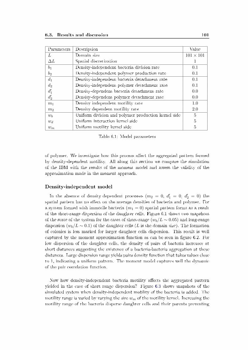
6.3. Results and discussion 101
Parameters Description Value
L Domain size 101× 101
∆L Spatial discretization 1
b1 Density-independent bacteria division rate 0.1
b2 Density-independent polymer production rate 0.1
d1 Density-independent bacteria detachment rate 0.1
d2 Density-independent polymer detachment rate 0.1
d′1 Density-dependent bacteria detachment rate 0.0
d′2 Density-dependent polymer detachment rate 0.0
m1 Density-independent motility rate 1.0
m2 Density-dependent motility rate 2.0
wb Uniform division and polymer production kernel side 5
wd Uniform Interaction kernel side 5
wm Uniform motility kernel side 5
Table 6.1: Model parameters
of polymer. We investigate how this process a�ect the aggregated pattern formed
by density-dependent motility. All along this section we compare the simulation
of the IBM with the results of the moment model and assess the validity of the
approximation made in the moment approach.
Density-independent model
In the absence of density-dependent processes (m2 = 0, d′1 = 0, d′2 = 0) the
spatial pattern has no e�ect on the average densities of bacteria and polymer. For
a system formed with immotile bacteria (m1 = 0) spatial pattern forms as a result
of the short-range dispersion of the daughter cells. Figure 6.1 shows two snapshots
of the state of the system for the cases of short-range (wb/L ∼ 0.05) and long-range
dispersion (wb/L ∼ 0.1) of the daughter cells (L is the domain size). The formation
of colonies is less marked for larger daughter cells dispersion. This result is well
captured by the moment approximation function as can be seen in �gure 6.2. For
low dispersion of the daughter cells, the density of pairs of bacteria increases at
short distances suggesting the existence of a bacteria-bacteria aggregation at these
distances. Large dispersion range yields pairs density function that takes values close
to 1, indicating a uniform pattern. The moment model captures well the dynamic
of the pair correlation function.
Now how density-independent bacteria motility a�ects the aggregated pattern
yielded in the case of short range dispersion? Figure 6.3 shows snapshots of the
simulated system when density-independent motility of the bacteria is added. The
motility range is varied by varying the size wm of the motility kernel. Increasing the
motility range of the bacteria disperse daughter cells and their parents preventing
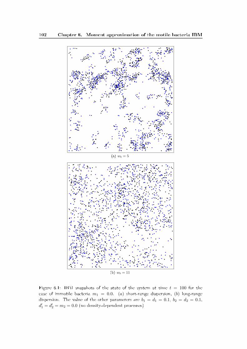
102 Chapter 6. Moment approximation of the motile bacteria IBM
(a) wb = 5
(b) wb = 11
Figure 6.1: IBM snapshots of the state of the system at time t = 100 for the
case of immotile bacteria m1 = 0.0. (a) short-range dispersion, (b) long-range
dispersion. The value of the other parameters are b1 = d1 = 0.1, b2 = d2 = 0.1,
d′1 = d′2 = m2 = 0.0 (no density-dependent processes)
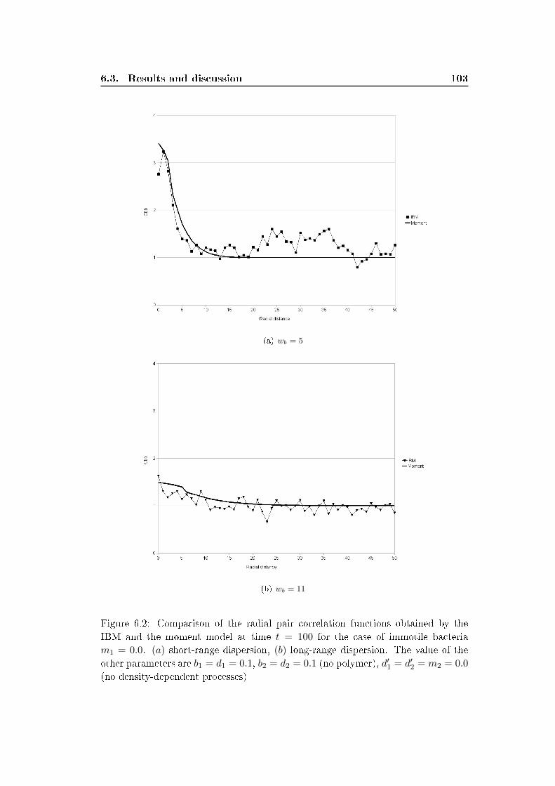
6.3. Results and discussion 103
(a) wb = 5
(b) wb = 11
Figure 6.2: Comparison of the radial pair correlation functions obtained by the
IBM and the moment model at time t = 100 for the case of immotile bacteria
m1 = 0.0. (a) short-range dispersion, (b) long-range dispersion. The value of the
other parameters are b1 = d1 = 0.1, b2 = d2 = 0.1 (no polymer), d′1 = d′2 = m2 = 0.0
(no density-dependent processes)
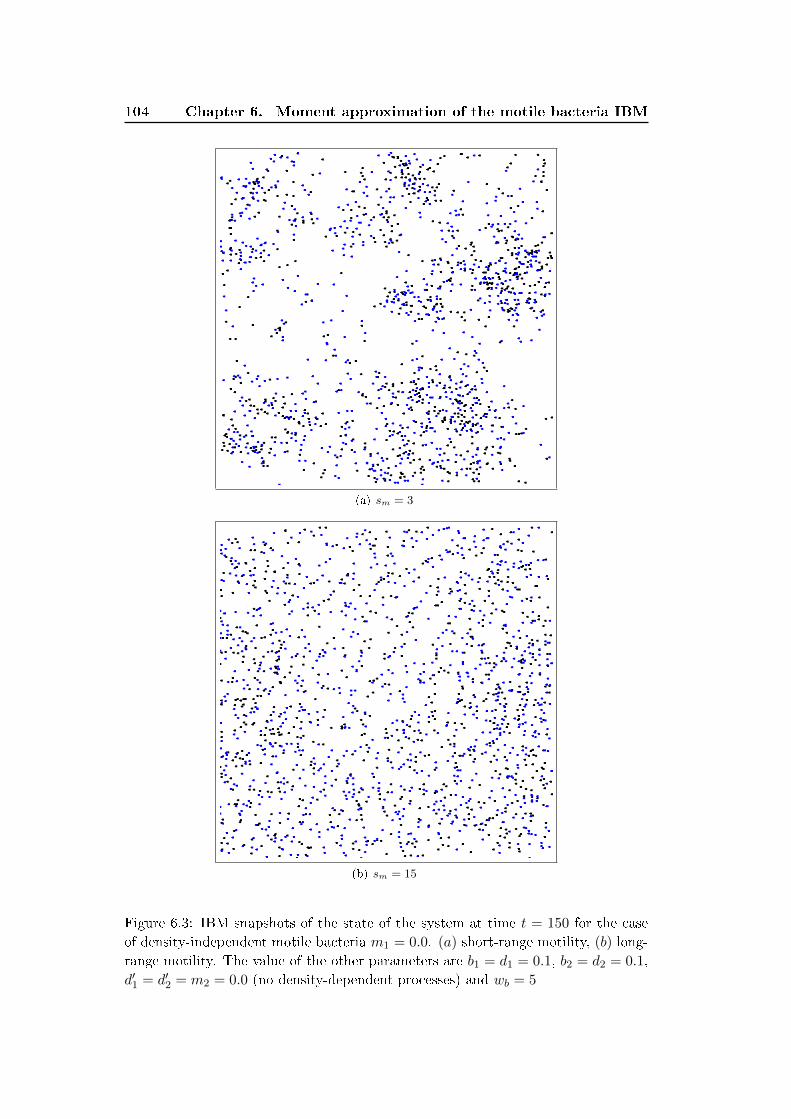
104 Chapter 6. Moment approximation of the motile bacteria IBM
(a) sm = 3
(b) sm = 15
Figure 6.3: IBM snapshots of the state of the system at time t = 150 for the case
of density-independent motile bacteria m1 = 0.0. (a) short-range motility, (b) long-
range motility. The value of the other parameters are b1 = d1 = 0.1, b2 = d2 = 0.1,
d′1 = d′2 = m2 = 0.0 (no density-dependent processes) and wb = 5
6.3. Results and discussion 105
the formation of colonies. In essence, the motility acts as the dispersal kernel and
tend to mix the bacteria yielding uniform patterns. This is also demonstrated by
the pair correlation function in �gure 6.4. The pair correlation function in the
IBM and moment models take values close to 1 for long-range motility indicating
a uniform spatial pattern. We show in the next section that long-range motility
plays the inverse role and promotes aggregated patterns formation in the case of
density-dependent motility
Density-dependent motility
In the IBM, the density-dependent motility process is described by equation 6.7.
The probability per unit of time that a bacterium moves to any other position
within the domain is given by m1 −m2ploc(x) where ploc(x) is the local density of
polymer perceived by the bacterium in location x. The value of the local density
of polymer is not bounded as a bacterium can hypothetically have any number of
neighboring polymeric particles. In order to avoid negative probabilities we �x a
threshold for the local densities of polymer above which the motility probability
is set to zero. The threshold value corresponds to m1/m2. While in the IBM the
local density of polymer perceived by an individual �uctuates due to the di�erent
stochastic processes, the dynamic of the moment model relies on the average value
of the local density of polymer which is, for the parameters used in this chapter,
always below the threshold value m1/m2.
Figure 6.5 shows snapshots of the state of the system for di�erent values of m2.
In the IBM, increasing the value of m2 promotes the formation of colonies due
to the decrease of the immobilization threshold. This can also be observed from
�gure 6.6 showing the radial pairs correlation function (at time t = 400) simulated
with the IBM and withe moment model. The pair correlation function peaked at
short distance with the increase of the value of m2. Surprisingly, comparison with
the moment model shows that the later fail in capturing the formation of colonies
(�gure 6.6(b)). The pair correlation function yielded by the moment model remains
close to 1 indicating a uniform pattern. To explain this di�erence we extracted the
time course of the local polymer densities experienced by the bacteria in the IBM
and the moment model. The local density experienced by the bacteria in the IBM
di�er from an individual to another depending on the location of the individual
and its neighborhood. At each time step we calculate the average local density
of polymer and the maximum value experienced by the bacteria. In the moment
model, only the average local polymeric density is considered in the model and is
given by:
ploc =
∫K
(||ξ||wd
)Cbp(ξ)dξ (6.28)
Figure 6.7 compares the average and maximum values of the local polymer den-
sity experienced by the individuals in the IBM with the average local density of
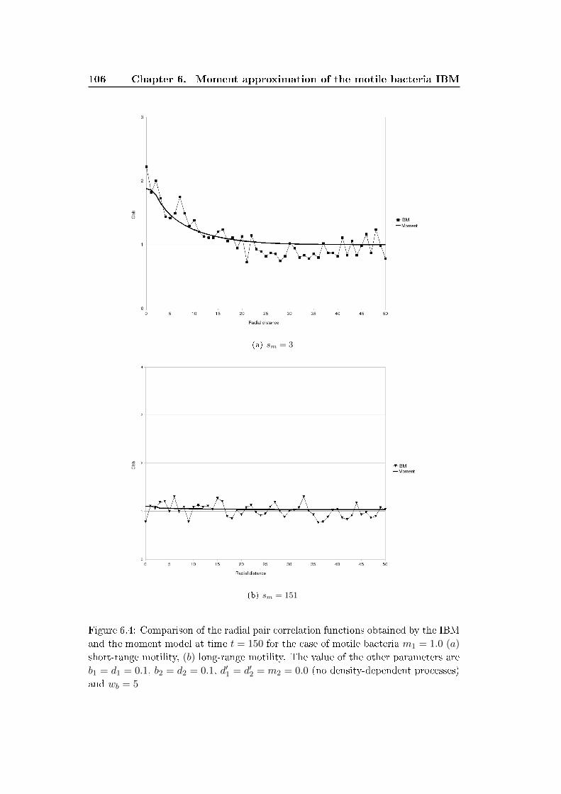
106 Chapter 6. Moment approximation of the motile bacteria IBM
(a) sm = 3
(b) sm = 151
Figure 6.4: Comparison of the radial pair correlation functions obtained by the IBM
and the moment model at time t = 150 for the case of motile bacteria m1 = 1.0 (a)
short-range motility, (b) long-range motility. The value of the other parameters are
b1 = d1 = 0.1, b2 = d2 = 0.1, d′1 = d′2 = m2 = 0.0 (no density-dependent processes)
and wb = 5
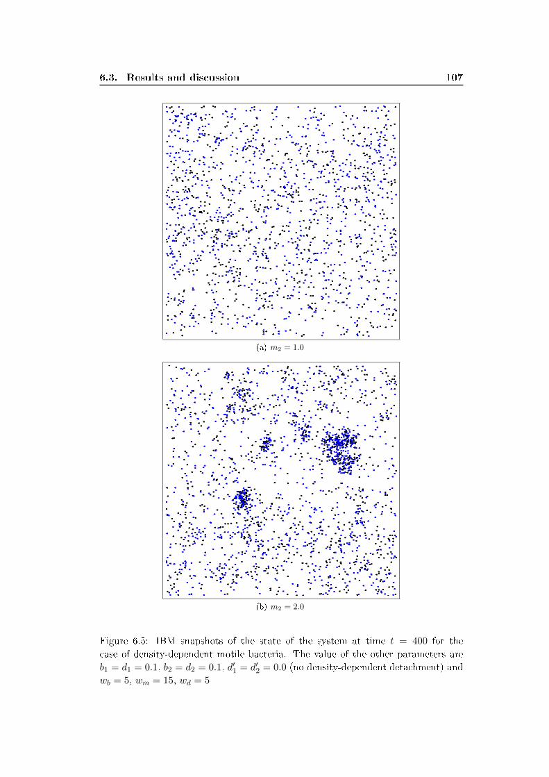
6.3. Results and discussion 107
(a) m2 = 1.0
(b) m2 = 2.0
Figure 6.5: IBM snapshots of the state of the system at time t = 400 for the
case of density-dependent motile bacteria. The value of the other parameters are
b1 = d1 = 0.1, b2 = d2 = 0.1, d′1 = d′2 = 0.0 (no density-dependent detachment) and
wb = 5, wm = 15, wd = 5
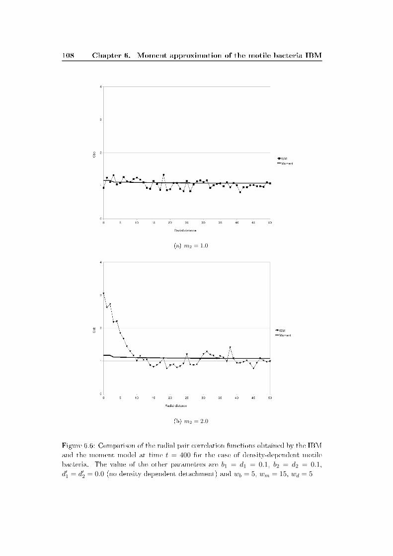
108 Chapter 6. Moment approximation of the motile bacteria IBM
(a) m2 = 1.0
(b) m2 = 2.0
Figure 6.6: Comparison of the radial pair correlation functions obtained by the IBM
and the moment model at time t = 400 for the case of density-dependent motile
bacteria. The value of the other parameters are b1 = d1 = 0.1, b2 = d2 = 0.1,
d′1 = d′2 = 0.0 (no density-dependent detachment) and wb = 5, wm = 15, wd = 5
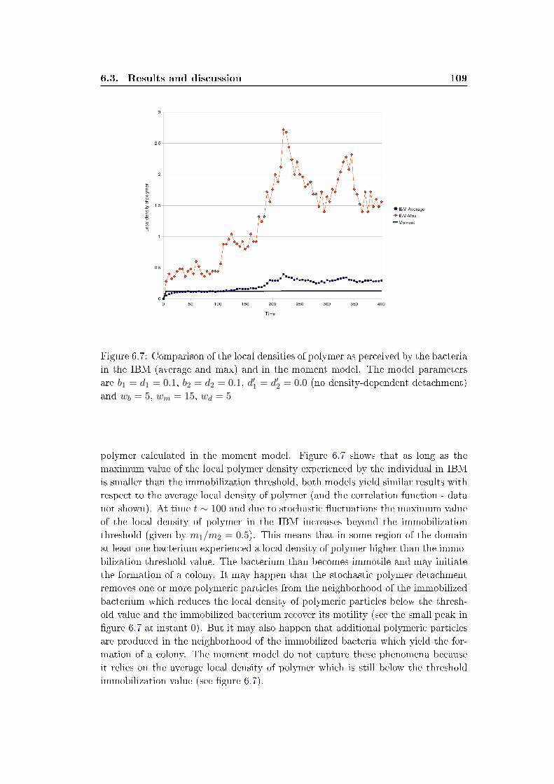
6.3. Results and discussion 109
Figure 6.7: Comparison of the local densities of polymer as perceived by the bacteria
in the IBM (average and max) and in the moment model. The model parameters
are b1 = d1 = 0.1, b2 = d2 = 0.1, d′1 = d′2 = 0.0 (no density-dependent detachment)
and wb = 5, wm = 15, wd = 5
polymer calculated in the moment model. Figure 6.7 shows that as long as the
maximum value of the local polymer density experienced by the individual in IBM
is smaller than the immobilization threshold, both models yield similar results with
respect to the average local density of polymer (and the correlation function - data
not shown). At time t ∼ 100 and due to stochastic �uctuations the maximum value
of the local density of polymer in the IBM increases beyond the immobilization
threshold (given by m1/m2 = 0.5). This means that in some region of the domain
at least one bacterium experienced a local density of polymer higher than the immo-
bilization threshold value. The bacterium than becomes immotile and may initiate
the formation of a colony. It may happen that the stochastic polymer detachment
removes one or more polymeric particles from the neighborhood of the immobilized
bacterium which reduces the local density of polymeric particles below the thresh-
old value and the immobilized bacterium recover its motility (see the small peak in
�gure 6.7 at instant 0). But it may also happen that additional polymeric particles
are produced in the neighborhood of the immobilized bacteria which yield the for-
mation of a colony. The moment model do not capture these phenomena because
it relies on the average local density of polymer which is still below the threshold
immobilization value (see �gure 6.7).
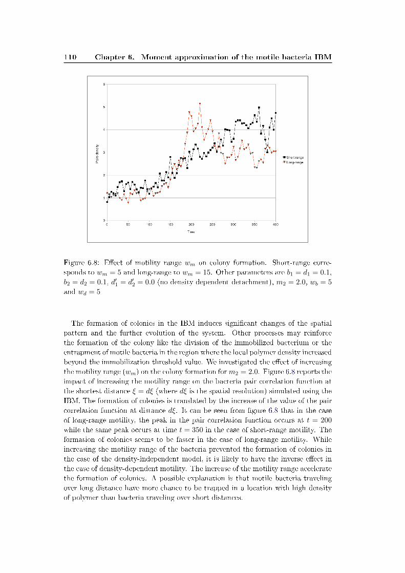
110 Chapter 6. Moment approximation of the motile bacteria IBM
Figure 6.8: E�ect of motility range wm on colony formation. Short-range corre-
sponds to wm = 5 and long-range to wm = 15. Other parameters are b1 = d1 = 0.1,
b2 = d2 = 0.1, d′1 = d′2 = 0.0 (no density-dependent detachment), m2 = 2.0, wb = 5
and wd = 5
The formation of colonies in the IBM induces signi�cant changes of the spatial
pattern and the further evolution of the system. Other processes may reinforce
the formation of the colony like the division of the immobilized bacterium or the
entrapment of motile bacteria in the region where the local polymer density increased
beyond the immobilization threshold value. We investigated the e�ect of increasing
the motility range (wm) on the colony formation form2 = 2.0. Figure 6.8 reports the
impact of increasing the motility range on the bacteria pair correlation function at
the shortest distance ξ = dξ (where dξ is the spatial resolution) simulated using the
IBM. The formation of colonies is translated by the increase of the value of the pair
correlation function at distance dξ. It can be seen from �gure 6.8 that in the case
of long-range motility, the peak in the pair correlation function occurs at t = 200
while the same peak occurs at time t = 350 in the case of short-range motility. The
formation of colonies seems to be faster in the case of long-range motility. While
increasing the motility range of the bacteria prevented the formation of colonies in
the case of the density-independent model, it is likely to have the inverse e�ect in
the case of density-dependent motility. The increase of the motility range accelerate
the formation of colonies. A possible explanation is that motile bacteria traveling
over long distance have more chance to be trapped in a location with high density
of polymer than bacteria traveling over short distances.
6.4. Conclusion 111
Density-dependent detachment
So far, we considered that detachment of the bacteria and polymer occurs at a
�xed density-independent rate (d1 = d2 = 0.1 and d′1 = d′2 = 0). Now we investigate
the case where the detachment rates of polymer and bacteria increase with the local
density of polymer. This means that bacteria and polymer enclosed within colonies
will experience higher detachment rates that their dispersed counterparts. Figure
6.9 shows IBM snapshots of the pattern for two di�erent values of density-dependent
detachment rates d′1 = d′2 = 0.05 and d′1 = d′2 = 0.1. Increasing the e�ect of the
density-dependent detachment prevents the formation of the colonies. This is con-
�rmed by the pair correlation functions in �gure 6.10 where the peak reached by the
pair correlation function is lower in the case of higher density-dependent detachment
rates, indicating a lower level of aggregation of the bacteria. The moment model
fails in capturing the colonies formation and the e�ect of the density-dependent
detachment is under-estimated in the moment model.
Density-dependent detachment has an impact on the average-density of the bac-
teria and polymer. Figure 6.11 shows the time course of the density of bacteria
and polymer calculated with the IBM and the moment model. For high density-
dependent detachment rates, the equilibrium densities yielded by the IBM are lower
than the densities that results from the moment model. The formation of colonies
increases the detachment rate experienced by the bacteria which yields lower equi-
librium densities. The di�erence between both models vanishes for higher density-
detachment rates because of the absence of colonies formation.
6.4 Conclusion
We derived a moment approximation equations of a simpli�ed IBM that describes
colonies formation due to to bacteria motility reduction by a self-produced polymer.
Both models account for �ve processes taking place at the level of the individuals. To
analyze these models we proceed progressively starting with a density independent
model obtained by setting the motility and detachment density dependent factors
to zero. We show that in the absence of motility, colonies form as a result of the
low dispersion of the daughter cells and that density-independent motility tend to
increase this dispersion range preventing the formation of colonies. Moment model
and the IBM compare very well in the case of density independent model. The
pair correlation function of the bacteria positions yielded by the IBM simulation
captured the main features of the simulated patterns and are in a good agreement
with those yielded by the moment model.
Starting from the case of bacteria with a long-motility range (no colonies for-
mation) we then introduced density-dependent motility. Our results showed that
colonies form due to the immobilization of bacteria in the location where the local
density of polymer increases above a threshold value. While in average, the local
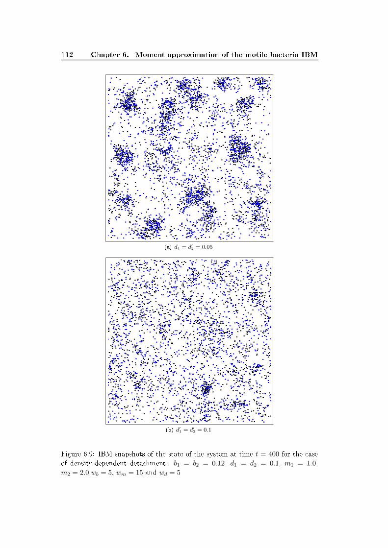
112 Chapter 6. Moment approximation of the motile bacteria IBM
(a) d1 = d′2 = 0.05
(b) d′1 = d′2 = 0.1
Figure 6.9: IBM snapshots of the state of the system at time t = 400 for the case
of density-dependent detachment. b1 = b2 = 0.12, d1 = d2 = 0.1, m1 = 1.0,
m2 = 2.0,wb = 5, wm = 15 and wd = 5
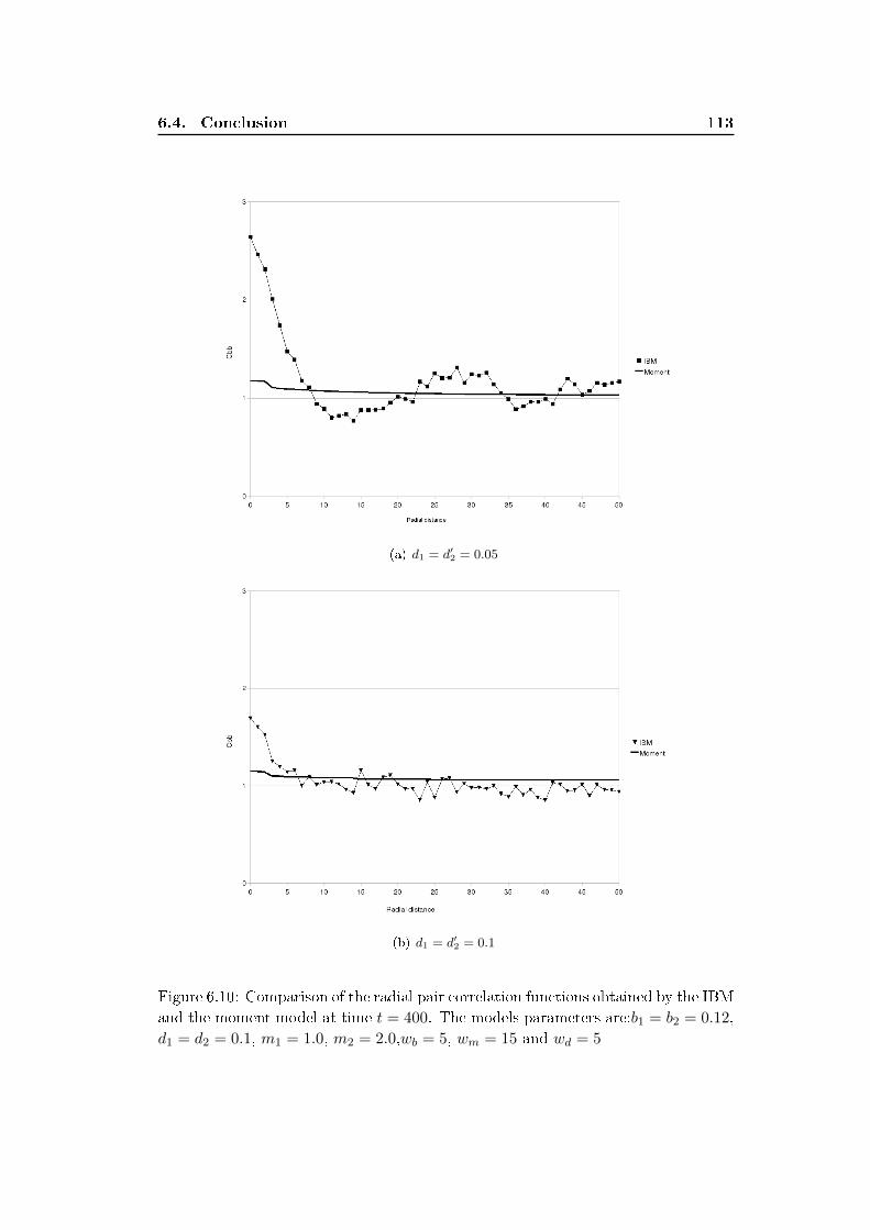
6.4. Conclusion 113
(a) d1 = d′2 = 0.05
(b) d1 = d′2 = 0.1
Figure 6.10: Comparison of the radial pair correlation functions obtained by the IBM
and the moment model at time t = 400. The models parameters are:b1 = b2 = 0.12,
d1 = d2 = 0.1, m1 = 1.0, m2 = 2.0,wb = 5, wm = 15 and wd = 5

114 Chapter 6. Moment approximation of the motile bacteria IBM
(a) d1 = d′2 = 0.05
(b) d1 = d′2 = 0.1
Figure 6.11: Comparison of the time course of the densities of bacteria Nb and
polymer Np yielded by the IBM and the moment model. The models parameters
are:b1 = b2 = 0.12, d1 = d2 = 0.1, m1 = 1.0, m2 = 2.0,wb = 5, wm = 15 and wd = 5
6.4. Conclusion 115
density experienced by the individuals remain below the immobilization threshold,
�uctuations in local polymer densities would have pushed the value of the local den-
sity above the immobilization threshold which initiated the formation of colonies.
The moment model do not capture this process, as the dynamics of the moments is
based on the average local density.
Furthermore, we investigated how the formation of colonies in the case of den-
sity dependent motility is a�ected by the size of the motility kernel sm. Surpris-
ingly increasing the motility range of the bacteria tend to promote the formation
of colonies. Long range motility, allowing motile bacteria to travel over longer dis-
tances, increases their chance to cross locations where the polymer density exceeds
the immobilization threshold value.
Finally, the in�uence of density-dependent detachment of polymer and bacteria
goes the other direction of density-dependent motility. Detachment is assumed to
increase with the local density of polymer experienced by the individuals. Thus
depending on the value of the density-dependent detachment parameters colonies
may or may not form.

Chapter 7
Exploring the labyrinth-like
patterns in a simpli�ed IBM of a
microbial bio�lm formed with
motile bacteria
Contents
7.1 Simpli�ed IBM for bio�lm formed with density-dependent
motile bacteria . . . . . . . . . . . . . . . . . . . . . . . . . . . 117
7.2 Numerical exploration of the IBM . . . . . . . . . . . . . . . 119
7.3 Deriving the moment approximation model . . . . . . . . . 120
7.4 Discussion and conclusion . . . . . . . . . . . . . . . . . . . . 129
We propose to further simplify the individual-based model (IBM) presented in the
previous chapter and discuss its approximation using moment models. The main
simpli�cation is that individuals motility and detachment depend now directly on
the local density of the individuals rather than on the excreted polymer. Hence we
do not consider polymer dynamic in this chapter.
The chapter is organized in four sections: in the �rst section we describe the
simpli�ed IBM. In the second section we explore the pattern yielded by the IBM
and compare these patterns qualitatively to experimental bio�lm patterns and to
the pattern obtained with the IBM including the polymer (chapter 6). Finally we
discuss the approximation of the IBM using moment approach assess the technical
di�culties in solving moment equations with motility.
7.1 Simpli�ed IBM for bio�lm formed with density-
dependent motile bacteria
The IBM that we describe in this section is an extension of the IBM presented in
chapter 4 that includes division and density dependent detachment. In addition to
these processes , we include a density-dependent motility process. The resultant
IBM considers the following three processes:
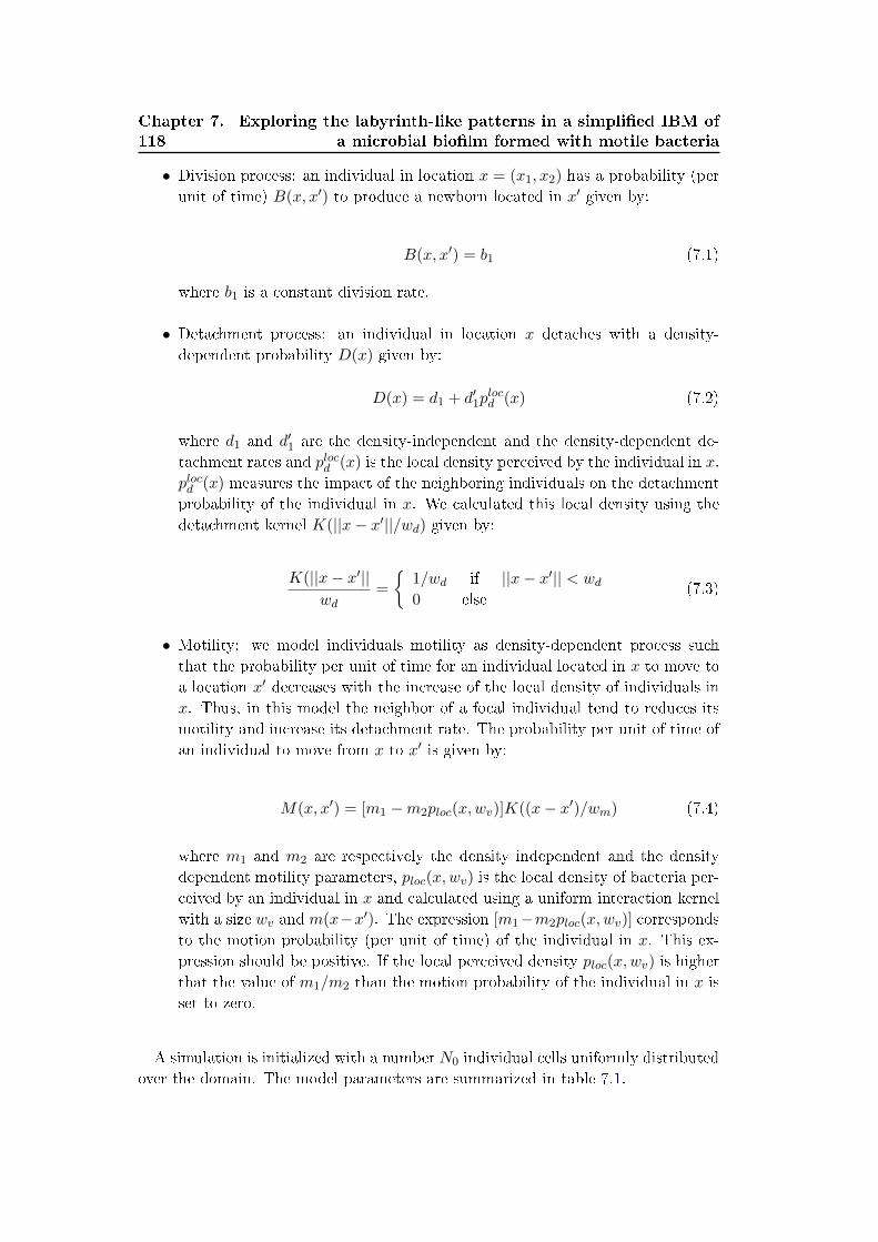
118
Chapter 7. Exploring the labyrinth-like patterns in a simpli�ed IBM of
a microbial bio�lm formed with motile bacteria
• Division process: an individual in location x = (x1, x2) has a probability (per
unit of time) B(x, x′) to produce a newborn located in x′ given by:
B(x, x′) = b1 (7.1)
where b1 is a constant division rate.
• Detachment process: an individual in location x detaches with a density-
dependent probability D(x) given by:
D(x) = d1 + d′1plocd (x) (7.2)
where d1 and d′1 are the density-independent and the density-dependent de-
tachment rates and plocd (x) is the local density perceived by the individual in x.
plocd (x) measures the impact of the neighboring individuals on the detachment
probability of the individual in x. We calculated this local density using the
detachment kernel K(||x− x′||/wd) given by:
K(||x− x′||wd
=
{1/wd if ||x− x′|| < wd0 else
(7.3)
• Motility: we model individuals motility as density-dependent process such
that the probability per unit of time for an individual located in x to move to
a location x′ decreases with the increase of the local density of individuals in
x. Thus, in this model the neighbor of a focal individual tend to reduces its
motility and increase its detachment rate. The probability per unit of time of
an individual to move from x to x′ is given by:
M(x, x′) = [m1 −m2ploc(x,wv)]K((x− x′)/wm) (7.4)
where m1 and m2 are respectively the density independent and the density
dependent motility parameters, ploc(x,wv) is the local density of bacteria per-
ceived by an individual in x and calculated using a uniform interaction kernel
with a size wv and m(x−x′). The expression [m1−m2ploc(x,wv)] corresponds
to the motion probability (per unit of time) of the individual in x. This ex-
pression should be positive. If the local perceived density ploc(x,wv) is higher
that the value of m1/m2 than the motion probability of the individual in x is
set to zero.
A simulation is initialized with a number N0 individual cells uniformly distributed
over the domain. The model parameters are summarized in table 7.1.
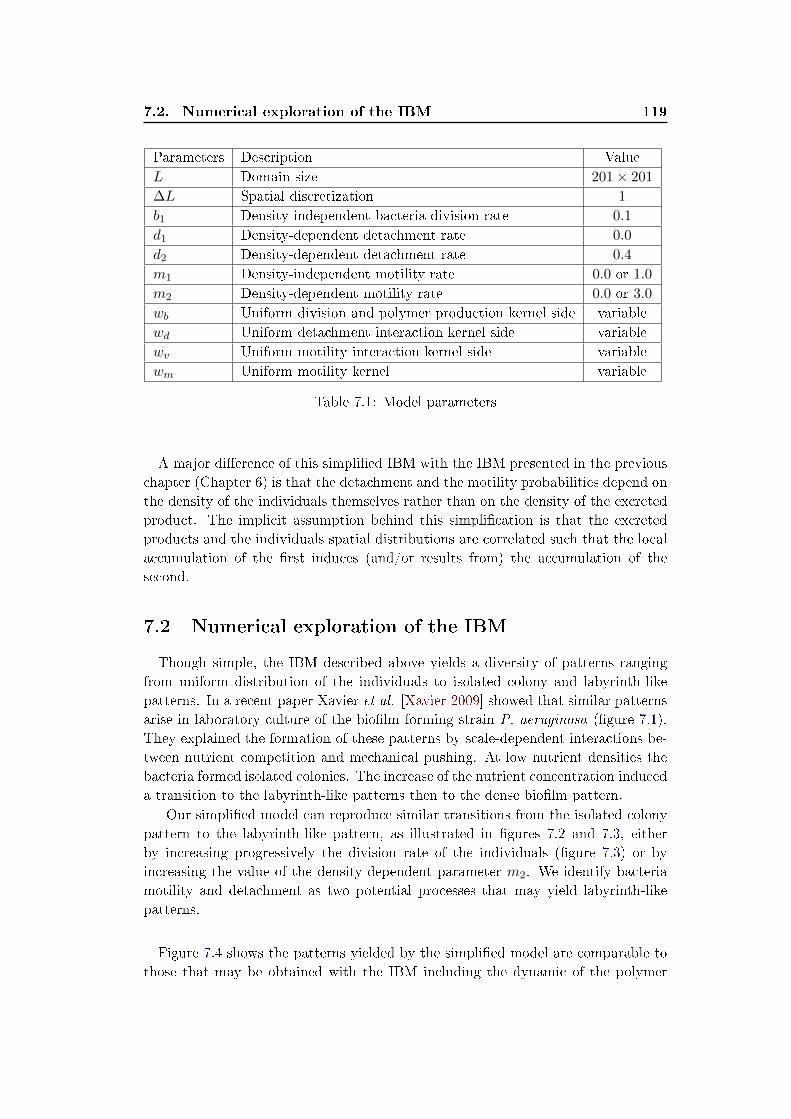
7.2. Numerical exploration of the IBM 119
Parameters Description Value
L Domain size 201× 201
∆L Spatial discretization 1
b1 Density-independent bacteria division rate 0.1
d1 Density-dependent detachment rate 0.0
d2 Density-dependent detachment rate 0.4
m1 Density-independent motility rate 0.0 or 1.0
m2 Density-dependent motility rate 0.0 or 3.0
wb Uniform division and polymer production kernel side variable
wd Uniform detachment interaction kernel side variable
wv Uniform motility interaction kernel side variable
wm Uniform motility kernel variable
Table 7.1: Model parameters
A major di�erence of this simpli�ed IBM with the IBM presented in the previous
chapter (Chapter 6) is that the detachment and the motility probabilities depend on
the density of the individuals themselves rather than on the density of the excreted
product. The implicit assumption behind this simpli�cation is that the excreted
products and the individuals spatial distributions are correlated such that the local
accumulation of the �rst induces (and/or results from) the accumulation of the
second.
7.2 Numerical exploration of the IBM
Though simple, the IBM described above yields a diversity of patterns ranging
from uniform distribution of the individuals to isolated colony and labyrinth-like
patterns. In a recent paper Xavier et al. [Xavier 2009] showed that similar patterns
arise in laboratory culture of the bio�lm forming strain P. aeruginosa (�gure 7.1).
They explained the formation of these patterns by scale-dependent interactions be-
tween nutrient competition and mechanical pushing. At low nutrient densities the
bacteria formed isolated colonies. The increase of the nutrient concentration induced
a transition to the labyrinth-like patterns then to the dense bio�lm pattern.
Our simpli�ed model can reproduce similar transitions from the isolated colony
pattern to the labyrinth-like pattern, as illustrated in �gures 7.2 and 7.3, either
by increasing progressively the division rate of the individuals (�gure 7.3) or by
increasing the value of the density-dependent parameter m2. We identify bacteria
motility and detachment as two potential processes that may yield labyrinth-like
patterns.
Figure 7.4 shows the patterns yielded by the simpli�ed model are comparable to
those that may be obtained with the IBM including the dynamic of the polymer
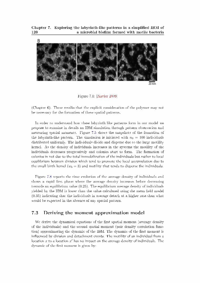
120
Chapter 7. Exploring the labyrinth-like patterns in a simpli�ed IBM of
a microbial bio�lm formed with motile bacteria
Figure 7.1: [Xavier 2009]
(Chapter 6). These results that the explicit consideration of the polymer may not
be necessary for the formation of these spatial patterns.
In order to understand how these labyrinth-like patterns form in our model we
propose to examine in details an IBM simulation through pattern observation and
measuring spatial moments. Figure 7.5 shows the snapshots of the formation of
the labyrinth-like pattern. The simulation is initiated with n0 = 100 individuals
distributed uniformly. The individuals divide and disperse due to the large motility
kernel. As the density of individuals increases in the systems the motility of the
individuals decreases progressively and colonies start to form. The formation of
colonies in not due to the total immobilization of the individuals but rather to local
equilibrium between division which tend to promote the local accumulation due to
the small birth kernel (wb = 3) and motility that tends to disperse the individuals.
Figure 7.8 reports the time evolution of the average density of individuals and
shows a rapid �rst phase where the average density increases before decreasing
towards an equilibrium value (0.25). The equilibrium average density of individuals
yielded by the IBM is lower than the value calculated using the mean-�eld model
(0.35) indicating that the individuals in average detach at a higher rate than what
would be expected in the absence of any spatial pattern.
7.3 Deriving the moment approximation model
We derive the dynamical equations of the �rst spatial moment (average density
of the individuals) and the second spatial moment (pair density correlation func-
tion) approximating the dynamic of the IBM. The dynamic of the �rst moment is
in�uenced by division and detachment events. The motility of an individual from a
location x to a location x′ has no impact on the average density of individuals. The
dynamic of the �rst moment is given by:

7.3. Deriving the moment approximation model 121
(a) b1 = 0.10 (b) b1 = 0.13
(c) b1 = 0.15
Figure 7.2: Examples of patterns yielded by the simpli�ed IBM and the IBM with
extracellular product
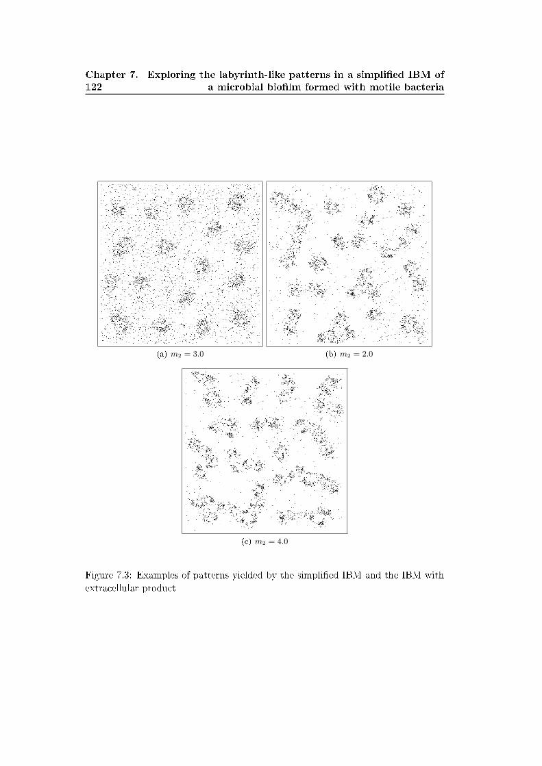
122
Chapter 7. Exploring the labyrinth-like patterns in a simpli�ed IBM of
a microbial bio�lm formed with motile bacteria
(a) m2 = 3.0 (b) m2 = 2.0
(c) m2 = 4.0
Figure 7.3: Examples of patterns yielded by the simpli�ed IBM and the IBM with
extracellular product
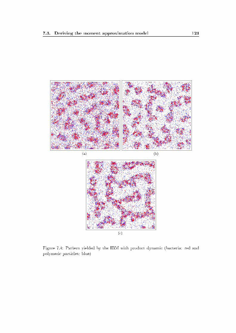
7.3. Deriving the moment approximation model 123
(a) (b)
(c)
Figure 7.4: Pattern yielded by the IBM with product dynamic (bacteria: red and
polymeric particles: blue)
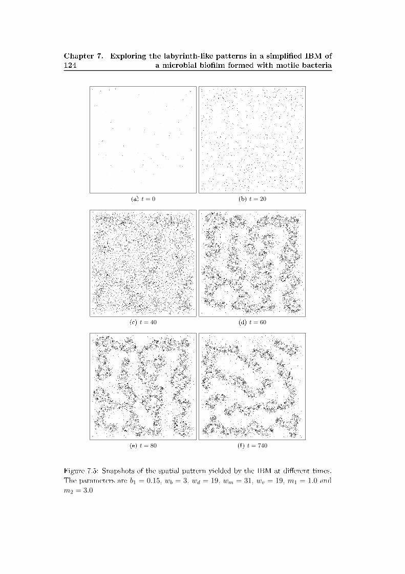
124
Chapter 7. Exploring the labyrinth-like patterns in a simpli�ed IBM of
a microbial bio�lm formed with motile bacteria
(a) t = 0 (b) t = 20
(c) t = 40 (d) t = 60
(e) t = 80 (f) t = 740
Figure 7.5: Snapshots of the spatial pattern yielded by the IBM at di�erent times.
The parameters are b1 = 0.15, wb = 3, wd = 19, wm = 31, wv = 19, m1 = 1.0 and
m2 = 3.0
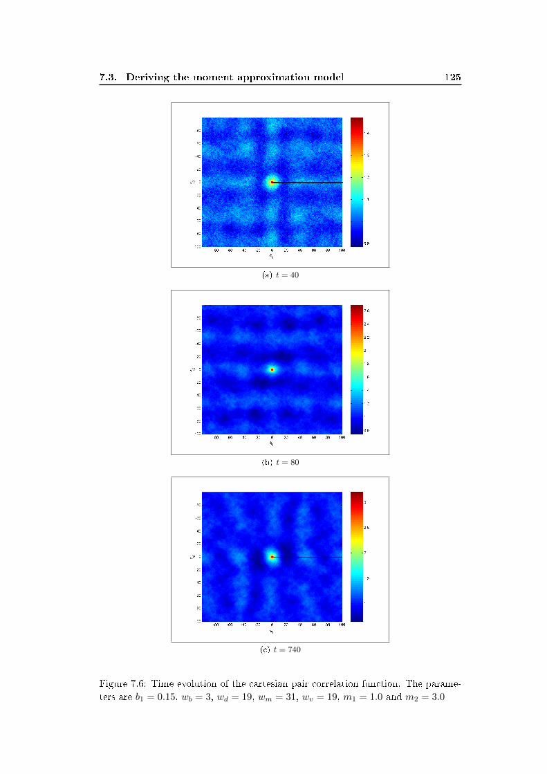
7.3. Deriving the moment approximation model 125
(a) t = 40
(b) t = 80
(c) t = 740
Figure 7.6: Time evolution of the cartesian pair correlation function. The parame-
ters are b1 = 0.15, wb = 3, wd = 19, wm = 31, wv = 19, m1 = 1.0 and m2 = 3.0
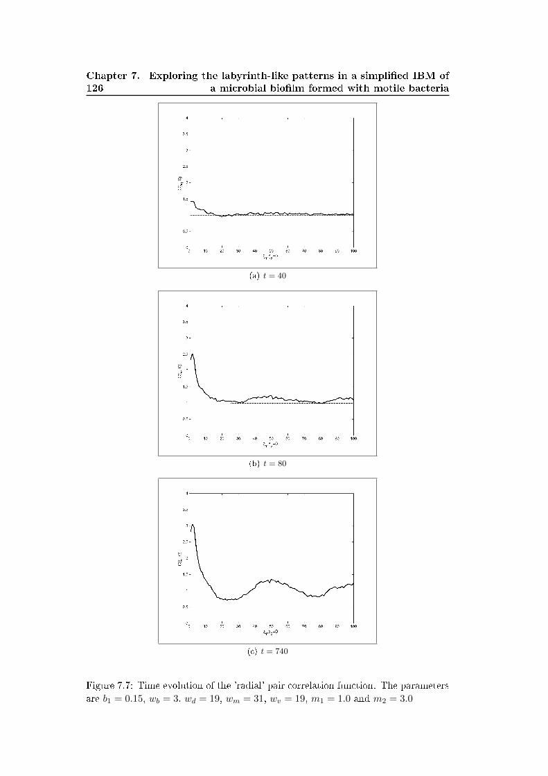
126
Chapter 7. Exploring the labyrinth-like patterns in a simpli�ed IBM of
a microbial bio�lm formed with motile bacteria
(a) t = 40
(b) t = 80
(c) t = 740
Figure 7.7: Time evolution of the 'radial' pair correlation function. The parameters
are b1 = 0.15, wb = 3, wd = 19, wm = 31, wv = 19, m1 = 1.0 and m2 = 3.0
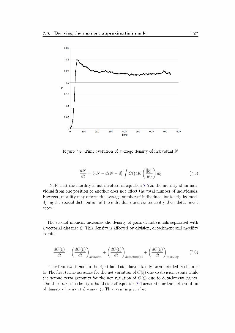
7.3. Deriving the moment approximation model 127
Figure 7.8: Time evolution of average density of individual N
dN
dt= b1N − d1N − d′1
∫C(ξ)K
(||ξ||wd
)dξ (7.5)
Note that the motility is not involved in equation 7.5 as the motility of an indi-
vidual from one position to another does not a�ect the total number of individuals.
However, motility may a�ects the average number of individuals indirectly by mod-
ifying the spatial distribution of the individuals and consequently their detachment
rates.
The second moment measures the density of pairs of individuals separated with
a vectorial distance ξ. This density is a�ected by division, detachment and motility
events:
dC(ξ)
dt=
(dC(ξ)
dt
)division
+
(dC(ξ)
dt
)detachment
+
(dC(ξ)
dt
)motility
(7.6)
The �rst two terms on the right hand side have already been detailed in chapter
4. The �rst terme accounts for the net variation of C(ξ) due to division events while
the second term accounts for the net variation of C(ξ) due to detachment events.
The third term in the right hand side of equation 7.6 accounts for the net variation
of density of pairs at distance ξ. This term is given by:
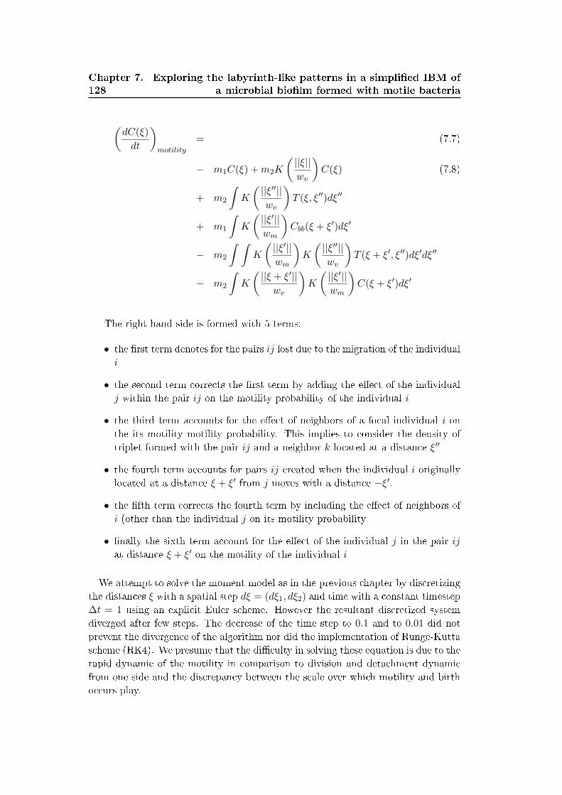
128
Chapter 7. Exploring the labyrinth-like patterns in a simpli�ed IBM of
a microbial bio�lm formed with motile bacteria
(dC(ξ)
dt
)motility
= (7.7)
− m1C(ξ) +m2K
(||ξ||wv
)C(ξ) (7.8)
+ m2
∫K
(||ξ′′||wv
)T (ξ, ξ′′)dξ′′
+ m1
∫K
(||ξ′||wm
)Cbb(ξ + ξ′)dξ′
− m2
∫ ∫K
(||ξ′||wm
)K
(||ξ′′||wv
)T (ξ + ξ′, ξ′′)dξ′dξ′′
− m2
∫K
(||ξ + ξ′||wv
)K
(||ξ′||wm
)C(ξ + ξ′)dξ′
The right-hand side is formed with 5 terms:
• the �rst term denotes for the pairs ij lost due to the migration of the individual
i
• the second term corrects the �rst term by adding the e�ect of the individual
j within the pair ij on the motility probability of the individual i
• the third term accounts for the e�ect of neighbors of a focal individual i on
the its motility motility probability. This implies to consider the density of
triplet formed with the pair ij and a neighbor k located at a distance ξ′′
• the fourth term accounts for pairs ij created when the individual i originally
located at a distance ξ + ξ′ from j moves with a distance −ξ′.
• the �fth term corrects the fourth term by including the e�ect of neighbors of
i (other than the individual j on its motility probability
• �nally the sixth term account for the e�ect of the individual j in the pair ij
at distance ξ + ξ′ on the motility of the individual i
We attempt to solve the moment model as in the previous chapter by discretizing
the distances ξ with a spatial step dξ = (dξ1, dξ2) and time with a constant timestep
∆t = 1 using an explicit Euler scheme. However the resultant discretized system
diverged after few steps. The decrease of the time step to 0.1 and to 0.01 did not
prevent the divergence of the algorithm nor did the implementation of Runge-Kutta
scheme (RK4). We presume that the di�culty in solving these equation is due to the
rapid dynamic of the motility in comparison to division and detachment dynamic
from one side and the discrepancy between the scale over which motility and birth
occurs play.
7.4. Discussion and conclusion 129
7.4 Discussion and conclusion
In this chapter we show that the simpli�cation of the polymer dynamic (IBM of
chapter 6) still allow the obtainment of diversity of patterns including the labyrinth-
like pattern that have been observed in laboratory bio�lm experiments. In a system
formed with a density-independent motile bacteria, the individuals tend to disperse
and produce no spatial structure. Our model suggest that the formation of colonies
in such system may result from density-dependent motility reduction process. The
spatial pattern of the colonies seems to be in�uenced by local equilibrium between
individuals 'entering' the colony through migration or division and individuals 'leav-
ing' the colony through migration and detachment. In the absence of motility the
yielded pattern is formed with isolated colony. However when density-dependent
motility is considered the colonies may connect yielding the labyrinth-like patterns.
The detachment kernel seems to play a role in maintaining the strips of the labyrinth
separated. This structure yielded a cartesian correlation matrix with a peak in the
center (indicating the tendency of the individual to aggregate due to the reduction
of their motility) and a wavy structure due to the labyrinth-like pattern.
There are few attempts in the literature of approximating individual-based mod-
els with density-dependent motility using moment models. Murrell and Law
[Murrell 2000] approximated an IBM of Beetles migration in a fragmented woodland.
They considered a �xed landscape pattern and assumed that beetles are attracted
by the locations corresponding to woodland. In their model, Murrell and Law con-
sidered only the motility process(no birth and death processes). In their paper, the
size of the migration kernel was relatively small compared to the size of the domain.
The interaction kernel (the equivalent of K(||ξ||/wv) in our work) is not speci�ed
explicitly in their work as they assumed that interaction occur exclusively when an
individual enters a woodland patch. Implicitly, they consider an interaction kernel
with a size corresponding to the size of a patch (equivalent to the spatial resolution
dξ in our work). Though simpler than our model, Murrell and Law highlighted
that there may be practical problems in the numerical integration of the dynamical
system due, in their work, to the discrepancy between the scale of movement and
the space scale of the woodland patterns.
In this work we meet comparable di�culties in the numerical integration of the
moment model. We presume that in part the instability of our numerical scheme is
due to the discrepancy between the spatial scales over which the di�erent processes
occur combined with the signi�cant di�erence in the motility rate and birth and
detachment rates. We hope to address these issues in a future work.


Chapter 8
Conclusion
Contents
8.1 Perspectives . . . . . . . . . . . . . . . . . . . . . . . . . . . . . 133
This thesis takes place in the context of the debate between complex individual
based models (IBMs) and more traditional di�erential equation models with a low
number of variables. The use of individual-based models (IBMs) in microbial ecol-
ogy has been growing rapidly during the last two decades, encouraged by the fast
increase in computing power and advances in laboratory observation techniques.
IBMs expand the toolbox of theoretical ecologists providing a valuable means to
investigate how system-level properties emerge out of local interactions. However
several reviews and textbooks on the use of IBMs in ecology (but also in other
�elds) pointed out some of the limitation of the approach. The complexity and
limited generality are often quoted as the main limitations of individual-based mod-
eling [Uchmanski 1996] [Grimm 1999]. IBMs evolve in a large state space as the
description of the system requires the description of the state of all the individuals.
A key question is whether all these state variables are necessary for the purpose of
an investigation. A smaller model with a small number of aggregated state variables
wouldn't be more appropriate ?
In this work, we try to reconcile these opposite points of view. Indeed, we investi-
gate how practical and productive it is to approximate the dynamic of IBMs used in
microbial ecology with aggregated mathematical models involving a small number
of state variables. In particular, we assess whether these 'simpler' models capture
successfully the spatio-temporal patterns yielded by the IBM. Several aggregated
models of the literature describe complex microbial systems without referring ex-
plicitly to individuals, and as a �rst approach we compare in chapter 2 one of these
models (a di�usion-reaction model) to an IBM of bacterial colony growth. The IBM
explicitly represents the individual microbial cells and their variability. Compar-
isons of this type can be helpful as the deterministic model can provide us with a
reference to which the IBM results can be compared. However, we show that the
comparison can be di�cult (even meaningless) when the aggregated model is de-
rived independently of the IBM. One of the main di�culties is to assign appropriate
values to the parameters of both models, especially when some of these parameters
132 Chapter 8. Conclusion
have no clear physical meaning. In our example, we had to tune the parameters of
the di�usion-reaction model empirically to obtain the best �t with the IBM.
Then we adopted a general approach involving two steps: (i) simplifying IBMs
to transform them into clearer mathematical objects and (ii) deriving determin-
istic mathematical models which approximate some aggregated dynamics of this
simpli�ed IBM. We focused on moment approximation techniques which provide a
valuable means to derive deterministic models on the middle ground between over-
simpli�ed mean-�eld models and intractable IBMs. In particular, this approach
allows one to capture some important aspects of spatial dynamics. Chapter 3 and
4 illustrated how such models are derived on the example of the colony growth and
planar bio�lm development. The moment approach captures the main features of
spatial pattern dynamics yielded by the IBM. The originality of the moment ap-
proach is in projecting the complexity of the IBM into a new state space where
the variables are the average number of individuals (�rst spatial moment) and the
average neighborhood of the individuals at di�erent distances (second spatial mo-
ment given by the pair correlation function). The heterogeneities of the individual
properties (mass and diameter) and their spatial extent are not considered by the
moment model. The nutrient dynamic is also simpli�ed and considered indirectly
through density-dependent growth function (chapter 3). These substantial simpli-
�cations of the original IBM that did not prevent the moment model to reproduce
the main statistical features of the IBM simulation.
In the second part of this thesis (chapter 5 to 7) we investigate how the full
approach applies to a new individual-based model of bio�lm formation involving
motile bacteria, which motility is reduced by a self-excreted product (exopolymeric
substances). The IBM attempts to explain the formation of patterns with inter-
connected microcolonies observed in recent bio�lm experiments. Chapter 5 gives a
detailed description of the IBM and qualitative comparison of the simulated patterns
with those observed in experimental laboratory setting of P. aeruginosa cultivation.,
a model bacterium in bio�lm research. In this part, the moment approach provided
some interesting insights on the studied dynamics, but we also encountered some of
its limitations and also some practical di�culties of implementation.
In chapter 6 we proposed a simpli�ed version of the IBM obtained by neglecting
the spatial extent of the bacteria and the dynamic of the nutrient. The excretion of
extracellular product is considered in this �rst simpli�ed model. We approximated
the resultant IBM using moment approach and compared the patterns dynamics
yielded by both models. The moment model captured the dynamic of the IBM in
the case of immotile bacteria but failed in capturing the formation of colonies and
the subsequent resultant transformation of the patterns. The detailed analysis of
the IBM patterns shows that the colonies form when the local density of polymer
reaches a threshold value causing the quasi immobilization of the individuals. This
8.1. Perspectives 133
may happens in few location within the domain due to the stochastic �uctuations
of the individuals neighborhood but not necessary in average. As the moment
model is based on the average neighborhood it misses this process. The example
illustrates well one of the major limitation of the moment approach in dealing with
the �uctuations especially if the individuals response to these �uctuations are non-
linear or ruled by threshold values. In such a situation the aggregation of the IBM
using �rst and second moment measures as state variable may not be appropriate.
Chapter 7 illustrates some of the technical limitations that may be encountered
when implementing and solving moment models. We simplify further the IBM
with motile bacteria by dropping the polymer dynamics and assuming that the
bacteria motility is reduced by the increase of their local density. The resultant
model is simpler to analyze though numerical experimentation and still reproduces
the rich patterns that can be observed with the polymer. We discretized the moment
model using either Euler scheme and RK4 but both time discretization schemes
are unstable for the parameters that we considered. The discrepancy between the
motility and birth kernel size and the signi�cant di�erence between the time scale
and mobility and the other processes are probably at the origin of these instabilities.
We shall note however that the moment equations still miss a solid mathematical
framework that allow the analysis of their properties.
8.1 Perspectives
The aggregation of individual-based models that arise in ecology, and microbial
ecology in particular, is still in its infancy as a research �eld. There are few attempts
in the microbial ecological literature to simplify the detailed IBMs and approximate
their dynamics using a small number of aggregated state variables. The approach
is more encountered in physics through the derivation of the master equation and
its further reduction to simpler models. The di�culty to extend this approach to
ecology lies in the richness and complexity of the ecological interactions. Living
organisms, unlike inert interacting particles, have the capacity to adapt and evolve
which may confer to the population new emergent properties. We believe that much
research e�ort are still needed to develop reliable techniques for the aggregation and
reduction of IBMs that arise in ecology.
Moment approximation can be useful in deriving new models where the local
neighborhood of the individuals is considered explicitly as a state variable. They
however have some limitations that may be overcome with an additional research
e�ort. In particular tools and methods to analyze moment models are needed.
There are other techniques for deriving aggregated mathematical models that can
be explored in future work. In particular, models of probability densities provide
some average behaviors which are interesting to compare with the di�erent runs of
134 Chapter 8. Conclusion
the IBM, and can be complementary with the moment approximation. It can also
be interesting to compute the second moment of these density models, and compare
it with the second moment approximation.
Finally IBM simpli�cation may yield �unrealistic� models but it seems to us nec-
essary if we would like to generalize the IBM results and elaborate new theories, and
explore how complex structures can emerge form interactions. Moreover, we hope
that our work brought some convincing evidences that di�erential equation models
approximating these IBMs can bring some insight about this process of emergence.
Bibliography
[Aas 2002] F. E. Aas, M. Wolfgang, S. Frye, S. Dunham, C. Lvold and M. Koomey.
Competence for natural transformation in Neisseria gonorrhoeae: compo-
nents of DNA binding and uptake linked to type IV pilus expression. Molec-
ular Microbiology, vol. 46, no. 3, pages 749�760, 2002. 68
[Allesen-Holm 2006] M. Allesen-Holm, K. B. Barken, L. Yang, M. Klausen, J. S.
Webb, S. Kjelleberg, S. Molin, M. Givskov and T. Tolker-Nielsen. A charac-
terization of DNA release in Pseudomonas aeruginosa cultures and bio�lms.
Molecular Microbiology, vol. 59, no. 4, pages 1114�1128, 2006. 68, 79
[Alpkvist 2006] E. Alpkvist, C. Picioreanu, M.C.M. Van Loosdrecht and A. Heyden.
Three-dimensional bio�lm model with individual cells and continuum EPS
matrix. Biotechnology and Bioengineering, vol. 94, pages 961�979, 2006. 79
[Alpkvist 2007] E. Alpkvist and I. Klapper. A multidimensional multispecies contin-
uum model for heterogenuous bio�lm development. Bulletin of Mathematical
Biology, vol. 69, pages 765�789, 2007. 12, 13
[Arthur 1997] B. Arthur W., N. Durlauf S. and A. Lane D., editeurs. The economy
as an evolving complex system ii. Santa Fe Institute Studies in the Science
of Complexity, Readings, MA: Addison-Wesley, 1997. 1
[Aumann 2007] Craig A. Aumann. A methodology for developing simulation models
of complex systems. Ecological Modelling, vol. 202, no. 3-4, pages 385�396,
April 2007. 1, 4
[Barken 2008] K. B. Barken, S. J. Pamp, L.g Yang, M. Gjermansen, J. J. Bertrand,
M. Klausen, M.l Givskov, C. B. Whitchurch, J. N. Engel and T. Tolker-
Nielsen. Roles of type IV pili, �agellum-mediated motility and extracellular
DNA in the formation of mature multicellular structures in Pseudomonas
aeruginosa bio�lms. Environmental Microbiology, vol. 10, no. 9, pages 2331�
2343, 2008. 68, 79, 84
[Ben-Jacob 2000] E. Ben-Jacob, I. Cohen and H. Levine. The Cooperative Self-
Organization of Microorganisms. Adv. Phys., vol. 49, pages 395�554, 2000.
12
[Birch 2006] A. Birch D. and R. Young W. A master eaquation for a spatial popu-
lation model with pair interactions. Theoretical Population Biology, vol. 70,
pages 26�42, 2006. 51, 56
[Bolker 1997] B. Bolker and S.W . Pacala. Using Moment Equations to Understand
Stochastically Driven Spatial Pattern Formation in Ecological Systems. The-
oretical Population Biology, vol. 52, no. 3, pages 179�197, December 1997.
6
136 Bibliography
[Brehm-Stecher 2004] B.F. Brehm-Stecher and E.A. Johnson. Single-cell micro-
biology: tools, technologies and applications. Microbial Molecular Biology
Review, vol. 68, pages 538�559, 2004. 4
[Burel 2003] F. Burel and J. Baudry. Landscape ecology. Science Publishers, 2003.
84
[Button 1993] D.K. Button. Nutrient-limited microbial growth kinetics: overview
and recent. Antonie van Leeuwenhoek, vol. 63, pages 225�235, 1993. 16
[Cogan 2004] N. Cogan and J.P. Keener. The role of the bio�lm matrix in structural
development. Math. Med. and Biol, vol. 21, pages 147�166, 2004. 12, 13
[Costerton 1995] JW Costerton, Z Lewandowski, DE Calcwell, DR Korber and
HM Lappin-Scott. Microbial bio�lms. Annu Rev Microbiol, vol. 49, pages
711�745, 1995. 12, 68
[Crawford 2005] W. Crawford J., K. Ritz Harris and M. Young I. Towards an
evolutionnary ecology of life in soil. Trends Ecol. Evol., vol. 20, pages 81�87,
2005. 1
[Dalton 1994] H.M. Dalton, L.K. Poulsen, P. Halaz, M.L. Angles and A.E. Good-
man. Substratum-induced morphological changes in a marine bacterium and
their relevance to bio�lm structure. Journal of Bacteriology, vol. 176, pages
6900�6906, 1994. 79
[Dalton 1996] H M Dalton, A E Goodman and K C Marshall. Diversity in surface
colonization behavior in marine bacteria. Journal of Industrial Microbiology
and Biotechnology, vol. 17, no. 3, pages 228�234, September 1996. 79
[Davey 2000] M.E. Davey and G.A. O'Toole. Microbial Bio�lms: from Ecology to
Molecular Genetics. Microbiology And Molecular Biology Reviews, vol. 12,
pages 847�867, 2000. 68
[De�uant 2004] G. De�uant. Modeliser la complexite: quelques pistes pour relever
le de�. Rapport technique, Memoire d'Habilitation a Diriger des Recherches.
Ecole Doctorale SPI. Universite Blaise Pascal de Clermont-Ferrand, 2004. 1,
5
[De�uant 2005] G. De�uant, S. Huet and F. Amblard. An individual-based model
of innovation di�usion mixing social value and individual bene�t. Ameri-
can Journal of Sociology 110-4, 1041-1069. American Journal of Sociology,
vol. 110, pages 1041�1069, 2005. 1
[Dens 2005] E.J. Dens, K. Bernaerts, A.R. Standaert, J.U. Kreft and J.F. Van Impe.
Cell division theory and individual-based modelling of microbial lag. Part II.
Modeling lag phenomena induced by temperature shifts. Journal of Food
Microbiology, vol. 101, pages 319�332, 2005. 2

Bibliography 137
[Dieckmann 1999] U. Dieckmann. From Individuals to Populations: Systematic
Model Reduction in Evolutionary Theory and Spatial Ecology. Rapport tech-
nique, Habilitation report - Wien University, 1999. 31
[Dieckmann 2000] U. Dieckmann, R. Law and J.A.J Metz. The geometry of eco-
logical interactions: simplifying spatial complexity. Cambridge University
Press, 2000. 2, 6, 29, 37, 42, 43, 61
[Dockery 2001] J. Dockery and I. Klapper. Finger formation in bio�lm layers. SIAM
J. APPL. Math., vol. 62, pages 853�869, 2001. 13
[Eberl 2001] J. Eberl H., D.F. Parker and M.C.M. Van Loosdrecht. A new deter-
ministic spatio-temporal continu mode for bio�lm development. Journal of
Theoretical Medicine, vol. 3, pages 161�175, 2001. 8, 11, 12, 13, 18, 21, 22
[Emonet 2005] T. Emonet, C.M. North, C.E. Wickersham and P. Cluzel. AgentCell:
a digital single-cell assay for bacterial chemotaxis. Bioinformatics, vol. 21,
pages 2714�27, 2005. 2
[Ferrer 2008] J. Ferrer, C. Prats and D. Lopez. Individual-based Modelling: An
Essential Tool for Microbiology. J Biol Phys, vol. 34, pages 19�37, 2008. 2,
69
[GIllespie 1976] T. GIllespie D. A general method for numerically simulating the
stochastic time evolution of coupled chemical reactions. Journal of Compu-
tational Physics, vol. 22, pages 403�434, 1976. 31, 89
[Ginovart 2002] Marta Ginovart, Daniel Lopez and Joaquim Valls. INDISIM,
An Individual-based Discrete Simulation Model to Study Bacterial Cultures.
Journal of Theoretical Biology, vol. 214, no. 2, pages 305�319, January 2002.
2, 69
[Grimm 1999] Volker Grimm, Tomasz Wyszomirski, David Aikman and Janusz Uch-
manski. Individual-based modelling and ecological theory: synthesis of a work-
shop. Ecological Modelling, vol. 115, no. 2-3, pages 275�282, February 1999.
2, 131
[Grimm 2005] Volker Grimm and Steven F. Railsback. Individual-based modeling
and ecology. Princeton University Press, 2005. 4, 5, 84
[Grimm 2006] Volker Grimm, Uta Berger, Finn Bastiansen, Sigrunn Eliassen, Vin-
cent Ginot, Jarl Giske, John Goss-Custard, Tamara Grand, Simone K. Heinz,
Geir Huse, Andreas Huth, Jane U. Jepsen, Christian Jorgensen, Wolf M.
Mooij, Birgit Muller, Guy Pe'er, Cyril Piou, Steven F. Railsback, Andrew M.
Robbins, Martha M. Robbins, Eva Rossmanith, Nadja Ruger, Espen Strand,
Sami Souissi, Richard A. Stillman, Rune Vabo, Ute Visser and Donald L.
138 Bibliography
DeAngelis. A standard protocol for describing individual-based and agent-
based models. Ecological Modelling, vol. 198, no. 1-2, pages 115�126, Septem-
ber 2006. 3, 5, 7, 8, 12, 69
[Grimson 1994] M. Grimson and G. Barker. Continuum model for the spatiotemporal
growth of bacterial colonies. Phys Rev E, vol. 49, pages 1680�1684, 1994. 12
[Gujer 2002] W. Gujer. Microscopic versus macroscopic biomass models in activated
sludge systems. Water Science and Technology, vol. 46, pages 1�11, 2002. 2
[Hellweger 2009] F.L. Hellweger and V. Bucci. A bunch of tiny individuals -
Individual-based modeling for microbes. Ecological Modelling, vol. 220, pages
8�22, 2009. 2, 4, 69
[Hernàndez-Garcià 2004] López C. Hernàndez-Garcià E. Clustering, advection and
patterns in a mode of population dynamics with neighborhood-dependent
rates. Phys Rev E, vol. 70, 2004. 56
[Johnson 2008] Leah R. Johnson. Microcolony and bio�lm formation as a survival
strategy for bacteria. Journal of Theoretical Biology, vol. 251, no. 1, pages
24�34, March 2008. 84
[Klausen 003a] M. Klausen, A. Heydorn, P. Ragas, L. Lambertsen, A. Aaes-
Jorgensen, S. Molin and T. Tolker-Nielsen. Bio�lm formation by Pseu-
domonas aeruginosa wild type, �agella and type IV pili mutants. Molecular
Microbiology, vol. 48, no. 6, pages 1511�1524, June 2003a. 68, 79
[Klausen 003b] M. Klausen, A. Aaes-Jorgensen, S. Molin and T. Tolker-Nielsen.
Involvement of bacterial migration in the development of complex multicellu-
lar structures in Pseudomonas Aeruginosa bio�lms. Molecular Microbiology,
vol. 50, no. 1, pages 61�68, October 2003b. 68, 77, 79
[Koch 1993] L. Koch A. Biomass growth rate during the prokaryote cell cycle. Crit
Rev Microbiol, vol. 19, pages 17�42, 1993. 16
[Kreft 1998] J.U. Kreft, G. Booth and Wimpenny J.W.T. Bacsim, a simulator for
individual-based modelling of bacterial colony growth. Microbiology, vol. 144,
pages 3275�3278, 1998. 1, 8, 11, 13, 16
[Kreft 1999] J U Kreft, G Booth and J W T Wimpenny. Applications of individual-
based modelling in microbial ecology. In Johnson Green Bell C R Brylin-
sky M, editeur, Microbial Biosystems: New Frontiers. Proceeding of the 8th
International Symposium on Microbial Ecology, 1999. 2
[Kreft 2001] Jan-Ulrich Kreft, Cristian Picioreanu, Julian W.T. Wimpenny and
Marck C.M. van Loosdrecht. Individual-based modelling of bio�lms. Mi-
crobiology, vol. 147, pages 2897�2912, 2001. 2, 3, 11, 12, 16, 69, 71, 75
Bibliography 139
[Lacasta 1999] A.M. Lacasta, I.R. Cantalapiedra, C.E. Auguet, A. Pearanda and
L. Ramirez-Piscina. Modelling of spatio-temporal patterns in bacterial
colonies. Phys. Rev. E, vol. 59, pages 7036 � 7041, 1999. 12
[Laspidou 2009] C.S. Laspidou, A. Kungolos and P. Samaras. Cellular-automata
and individual-based approaches for the model of bio�lm structure: Pros and
cons. Desalination, vol. Article in Press, 2009. 3
[Law 2000] R. Law and U. Dieckmann. Moment approximations of individual-based
models, chapitre 14, pages 252�270. Cambridge University Press, 2000. 38
[Lee 2001] C. Lee, M. Hoopes, J. Diehl, W. Gilliland, G. Huxel, E. Leaver, K. Mc-
Cann, J. Umbanhowar and A. Mogilner. Non-local concepts and models in
biology. Journal of Theoretical Biology, vol. 210, pages 201�219, 2001. 84
[Levin 1998] S. A. Levin. Ecosystems and the biosphere as complex adaptative sys-
tems. Ecosystems, vol. 1, pages 431�436, 1998. 1
[Lobry 2003] C. Lobry. Modèles mathématiques et modèles informatiques, sur la
théorie du modèle. Annales des Ponts et Chaussées, vol. 107-108, pages 10�
18, 2003. 1
[Lu 2005] Ann Lu, Kyunyung Cho, Wesley P. Black, Xue-yan Duan, Renate Lux,
Zhaomin Yang, Heidi B. Kaplan, David R. Zusman and Wenyuan Shi. Ex-
opolysaccharide biosynthesis genes required for social motility in Myxococcus
xanthus. Molecular Microbiology, vol. 55, no. 1, pages 206�220, 2005. 84
[Luke 2004] S. Luke, C. Cio�-Revilla, L. Panait and K. Sullivan. MASON : A
Java Multi-Agent Simulation Toolkit. Proceedings of the 2004 SwarmFest
Workshop, 2004. 8, 76
[McKane 2004] A. J. McKane and T. J. Newman. Stochastic models in population
biology and their deterministic = analogs, October 2004. 4
[Morgenroth 1997] E. Morgenroth, T. Sherdena, M. C. M. Van Loosdrecht M.C.M.,
J.J. Heijnen and P.A. Wilderer. Aerobic granular sludge in a sequencing
batch reactor. Water Research, vol. 31, pages 3191�3194, 1997. 12
[Morgenroth 2000] E. Morgenroth and P.A. Wilderer. In�uence of detachment
mechanisms on competition in bio�lms. Water Research, vol. 34, pages 417�
426, 2000. 54
[Murphy 2008] T. Murphy J., R. Walshe and M. Devocelle. An Agent Based Ap-
proach to Modelling Microbial Ecosystems. ERCIM News, vol. (april), 2008.
2
[Murray 2001] J.D. Murray. Mathematical biology: I. an introduction. Springer,
3rd ed. 2001. 11
140 Bibliography
[Murrell 2000] D.J. Murrell and R. Law. Beetles in fragmented woodlands: a formal
framework for dynamics of movement in ecological landscapes. Journal of
Animal Ecology, vol. 69, no. 3, pages 471�483, 2000. 5, 6, 129
[O'Toole 2000] G. O'Toole, H. Kaplan and R. Kolter. Bio�lm formation as microbial
development. Annu Rev Microbiol, vol. 54, pages 49�79, 2000. 2
[Parsek 2008] Matthew R Parsek and Tim Tolker-Nielsen. Pattern formation in
Pseudomonas aeruginosa bio�lms. Current Opinion in Microbiology, vol. 11,
no. 6, pages 560�566, December 2008. 68, 84
[Picioreanu 2004] Cristian Picioreanu, Jan-Ulrich Kreft and Mark C. M. van Loos-
drecht. Particle-Based Multidimensional Multispecies Bio�lm Model. Appl.
Environ. Microbiol., vol. 70, no. 5, pages 3024�3040, 2004. 2, 3, 11, 12
[Picioreanu 2005] C. Picioreanu, D.J. Batstone and M.C.M. Van Loosdrecht. Multi-
dimensional modelling of anaerobic granules. Water Science and Technology,
vol. 53, pages 501�507, 2005. 2
[Picioreanu 2007] C. Picioreanu, J-U Kreft, M. Klaussen, J.A.J. Haagensen,
T. Tolker-Nielsen and S. Molin. Microbial mobility involvement in bio�lm
structure formation - a 3D modelling study. Water Science & Technology,
vol. 55, pages 337�343, 2007. 69, 76, 77, 79
[Railsback 2001] F. Railsback Steven. Concepts from Complex Adaptative Sys-
tems as a Framework for Individual-based Modelling. Ecological Modelling,
vol. 139, pages 47�62, 2001. 1
[Rammel 2007] C. Rammel, S. Stagl and H. Wil�ng. Managing Complex Adaptive
systems: A Co-Evolutionary Perspective on Natural Resource Management.
Ecological Economics, vol. 63, pages 9�21, 2007. 1
[Schmid 2003] M. Schmid, A. Thill, U. Purkhold, M. Walcher, J.-Y. Bottero,
P. Ginestet, P.H. Per Halkjaer Nielsen, S. Wuertz and M. Wagner. Charac-
terization of activated sludge �ocs by confocal laser scanning microscopy and
image analysis. Water Research, vol. 37, pages 2043�2052, 2003. 12
[Stewart 1993] P. S. Stewart. A Model for Bio�lm Detachment. Biotech Bioeng,
vol. 41, pages 111�117, 1993. 54
[Tolker-Nielsen 2000] Tim Tolker-Nielsen, U. C. Brinch, P. C. Ragas, J. B. Ander-
sen, Carsten Suhr J. and S. Molin. Development and Dynamics of Pseu-
domonas sp. Bio�lms. J. Bacteriol., vol. 182, no. 22, pages 6482�6489,
November 2000. 54
[Treuil 2008] J.P. Treuil, D. Zucker and A. Drogoul. Modélisation et simulation à
base d'agents. 2008. 3

Bibliography 141
[Uchmanski 1996] Janusz Uchmanski and Volker Grimm. Individual-based modelling
in ecology: what makes the di�erence? Trends in Ecology & Evolution,
vol. 11, no. 10, pages 437�441, October 1996. 3, 131
[Van Baalen 2000] M. Van Baalen. The geometry of ecological interactions: Simpli-
fying spatial complexity� chapitre Pair approximations for di�erent spatial
geometries, pages 359�387. Cambridge University Press, 2000. 7
[Van Schaik 2005] E.J. Van Schaik, C.L. Giltner, G.F. Audette, D.W. Keizer, D.L.
Bautista, C.M. Slupsky, B.D. Sykes and R.T. Irvin. DNA Binding: a Novel
Function of Pseudomonas aeruginosa Type IV Pili. Journal of Bacteriology,
vol. 187, no. 4, pages 1455�1464, February 2005. 68
[Vlachos 2006] C. Vlachos, R.C. Paton, J.R. Saunders and Q.H. Wu. A rule-based
approach to the modelling of bacterial ecosystems. Biosystems, vol. 84, pages
49�72, 2006. 3
[Whitchurch 2002] C.B. Whitchurch, T. Tolker-Nielsen, Paula C. Ragas and John S.
Mattick. Extracellular DNA required for bacterial bio�lm formation. Science,
vol. 295, pages 1487�1487, 2002. 68, 79
[Xavier 2005] Joao B. Xavier, Cristian Picioreanu and Mark C. M. van Loosdrecht.
A framework for multidimensional modelling of activity and structure of mul-
tispecies bio�lms. Environmental Microbiology, vol. 7, pages 1085�1103,
2005. 2, 11, 69
[Xavier 2009] J.B. Xavier, E. Martinez-Garcia and K.R. Foster. Social Evolution
of Spatial Patterns in Bacterial Bio�lms: when con�ict drives disorder. The
American Naturalist, vol. 174, pages 1�12, 2009. 119, 120