Embed Size (px)
Citation preview
THÈSE
En vue de l'obtention du
DOCTORAT DE L’UNIVERSITÉ DE TOULOUSE
Délivré par l'Université Toulouse III - Paul Sabatier
Discipline ou spécialité :Hydrologie, hydrochimie, sols eau environnement
JURY
Jérôme Viers (Président)
Kazuyo Tachikawa (Rapporteur)
Márcio Martins Pimentel (Rapporteur)
Mathieu Roy Barman (examinateur)
Présentée et soutenue par ROUSSEAU TRISTAN Le 24 septembre 2013
Titre : Concentrations en terres rares (REE) et composition isotopique du Nd à
l’interface fleuve Amazone/océan Atlantique : traçage de processus et bilan.
Ecole doctorale : SDU2E
Unité de recherche : UMR 5563
Directeurs de Thèse : CATHERINE JEANDEL, JEROEN SONKE
ET GERALDO RESENDE BOAVENTURA


1
Résumé
En milieu aquatique les concentrations en éléments terres rares (REE) lorsqu’elles sont
normalisées forment un spectre dont l’aspect est fonction de celui du matériel source, il est
ensuite modifié par fractionnement lors des processus de dissolution, de transport et de
spéciation chimique. Parmi les REE, le Nd conserve l’empreinte de la composition isotopique
(CI) caractéristique du type de roche dont il provient, plus cette roche est récente plus le Nd
associé est « radiogénique ». Les REE et la CI du Nd sont ainsi en géochimie aquatique des
traceurs singuliers de source, de transport et de processus. La CI du Nd est hétérogène dans
l’océan. C’est cette propriété qui a d’abord incité l’étude des REE et de la CI du Nd car elle a
permis en milieu marins de tracer la circulation et le mélange de masses d’eau en complément
des traceurs classiques comme la salinité et la température avec des applications également en
paléo-océanographie.
Avec la base de données croissante de CI du Nd et de [REE] dans l’océan la communauté
s’est intéressée à leur cycle géochimique et a constaté l’évidence d’un terme source manquant
dans le bilan global pour expliquer les variations spatiales de ces éléments. Depuis une dizaine
d’années les études convergent et identifient les sédiments déposes sur les marges comme source
potentiellement importante de Nd par un processus d’échange aux marges (Boundary exchange
BE). Le BE, tracé donc par des bilans de masse à échelles globales et régionales motive des
études plus fines de processus par des expériences de mise en contact de sédiments avec de l’eau
de mer et par l’étude locale de marges océaniques et d’estuaires. En effet, si les marges sont une
source massive de Nd à l’océan elles le sont certainement aussi pour d’autres éléments et ce
terme n’a jusqu’ alors pas été pris en compte en géochimie marine (Jeandel et al. 2011).
Dans le cadre de ce doctorat, je me suis intéressé aux apports du fleuve Amazone en REE
en et Nd à l’océan. Contribuant à lui seul à ~20 %, ~10 %, et ~3% des apports fluviaux
mondiaux en eau, sédiments et éléments dissous il est incontournable dans l’étude des cycles
géochimiques océaniques il est de plus localisé dans une zone cruciale pour la circulation des
masses d’eau entre les deux hémisphères. Des campagnes d’échantillonnage ont ainsi été
réalisées dans le cadre du projet AMANDES sur le fleuve Amazone, dans l’estuaire, sur le
plateau continental et au large des côtes Brésiliennes et Guyanaises. Ce projet s’intègre dans la
thématique « étude de processus » du programme international GEOTRACES.
Les travaux pionniers réalisés dans l’estuaire du fleuve Amazone ont montré le
comportement non conservatif des REE dans l’estuaire ou près de 95 % de ces éléments sont
soustraits de la phase dissoute en début de gradient salin. Cette diminution a été attribuée aux
colloïdes qui coagulent et floculent sous d’effet de l’augmentation de la force ionique. Aux
salinités intermédiaires les concentrations en REE augmentent à nouveau (Sholkovitz, 1993). Le
manque d’informations sur l’endmember Amazonien, sur la nature et la cinétique de processus
estuariens rend difficile la quantification des apports effectifs en REE à l’océan (Barroux et al.
2006).
Une approche inédite a donc été utilisée dans le cadre de cette thèse : une étude d’estuaire
couplant les analyses classiques de concentrations en REE dans la phase dissoute avec des
données d’ultrafiltration et de compositions isotopiques du Nd. Une méthode très précise
d’analyse des concentrations en REE par dilution isotopique utilisant 10 spikes et une mesure par
ICP-MS de champ sectoriel a été développée dans le cadre de ce travail pour observer finement
2
d’évolution des spectres de terres rares dans cette zone d’interface cette méthode a donné lieu à
une publication dans JAAS et nous avons participé à un exercice d’intercalibration qui a donné
lieu à une publication dans Geostandards et Geoanalytical Research. Cette méthode qui a permis
un gain notable de précision, de sensibilité et une optimisation des protocoles de séparation et
préconcentration permet l’analyse de tout type d’échantillons d’eaux naturelles.
Nous observons dans le gradient de salinité 1) Une forte diminution des concentrations en
REE liées aux colloïdes avec l’augmentation de la salinité. En effet plus de 80% des REE
dissoutes sont présentes dans la phase colloïdale pour le pôle amazonien contre moins de 10%
pour le pôle marin. Les Données de CI du Nd suggèrent que près de 17% du Nd associé aux
colloïdes coagulés dans le gradient salin pourrait être redisponibilisé à la phase dissoute lors de
l’advection de la plume vers les côtes guyanaises. 2) Dans le gradient salin aux salinités
moyennes et hautes les mesures de composition isotopique du Nd suggèrent une origine
lithogénique pour le Nd apporté à la phase dissoute car il a une signature différente de celles des
endmembers fluvial et océanique. Ce processus a été quantifié par un bilan de masse prenant en
compte les εNd et les concentrations en REE et nous observons dans l’estuaire un transfert de
près de 1% du Nd des particules lithogéniques vers la phase dissoute. En confrontant nos
données aux données d’âge calculées par Pieter van Beck et Marc Souhaut utilisant les mesures
d’activité du Radium nous pouvons estimer l’échelle de temps de ce processus à une vingtaine de
jours ce qui est en accord avec des données obtenus expérimentalement. 3) Les eaux de fond du
plateau continental entre 40 et 90m qui n’ont pas été en contact avec le pôle Amazonien
présentent des concentrations élevées et la CI du Nd suggère un apport de REE par Boundary
Exchange provenant des sédiments déposés sur la marge.
L’eau Antarctique intermédiaire (AAIW) échantillonnée durant les campagnes Amandes
est caractérisée par des valeurs de εNd négatives ce qui est surprenant pour cette masse d’eau. En
effet au sud de 30°S elle est au contraire radiogénique (Jeandel 1993, Stitchel et al. 2012). Des
AAIW peu radiogéniques ont été récemment échantillonnées dans le bassin d’Angola et ont été
considérées locales (Rickli et al 2009). En nous appuyant sur un modèle de mélange révélant une
cohérence isotopique et hydrologique entre l’AAIW échantillonnée dans le cadre d’AMANDES
et celle échantillonnée dans le bassin de l’Angola nous suggérons que cette zone peu étudiée est
affectée par le Boundary Exchange au point de modifier les compositions isotopiques du Nd à
l’échelle du bassin océanique. En comparant les profils de température et salinité (Ө-S) mesurés
dans le cadre d’amandes avec ceux extraits de la base de donnée « World Ocean Circulation
Experiment » (WOCE) nous identifions une zone barrière ou des lentilles d’eau centrales
profondes nord atlantique (lower-NAW) cisaillent les eau centrales profondes sud atlantique
(‘lower-SAW’) et l’eau Antarctique intermédiaire (l’AAIW) et qui contribuerait à altérer sur une
courte distance ces les caractéristiques de ces eaux circulant vers le Nord.
L’information majeure apportée par mes travaux réside dans le fait que nous avons observé
et quantifié pour la première fois, à échelle locale et en milieu naturel, la contribution en Nd des
particules lithogéniques à la phase dissoute. Ce point apporte une évidence supplémentaire de
l’importance des sédiments en suspension et de ceux déposés sur les marges en termes de
transfert de Nd et REE à l’océan; terme qui jusqu’à récemment n’était pas pris en compte en
géochimie pour les REE, mais aussi pour d’autres éléments chimiques (Jeandel et al., 2011;
Jones et al., 2012a; Jones et al., 2012b; Pearce et al. 2013, Tréguer and De La Rocha, 2013).
3
Resumo
Em meios Aquáticos os teores em elementos terras raras (REE) quando normalizados
formam um espectro cujo o aspecto é função do material fonte, este é em seguida
modificado por fracionamento em processos de dissolução, transporte e especiação
química. Um dos REEs, o Nd conserva a marca da composição isotópica (CI) caraterística do
tipo de rocha de onde este provém, quanto mais esta rocha é recente mais o Nd associado é
«radiogénico». Os REES e a CI do Nd são assim em geoquímica traçadores singulares de
fonte, transporte e processos. A CI do Nd é conservada pelas massas de água, este é
heterogêneo no oceano. E esta propriedade que tem primeiramente iniciado os estudos de
REE e da CI do Nd pois permitiu em meio marinho o traçamento da circulação e da mistura
de massas de água em complemento de traçadores clássicos como a salinidade e a
temperatura com aplicações também em paleo-oceanografia.
Com a base de dados crescente em CI do Nd e [REE] no oceano a comunidade tem se
interessado no seu ciclo geoquímico e tem constatado a evidência de um termo de fonte
faltante no balanço global destes elementos para explicar a suas variações espaciais. Desde
cerca de dez anos, os estudos têm convergido e identificam os sedimentos nas margens
como potencial fonte importante de Nd por um processo de troca com as margens
continentais (BE). O BE traçados em escala global e regional tem motivado estudos mais
finos do processo por meio de experimentos de contato entre sedimentos e água marinha e
estudos locais das margens oceânicas e estuários. De fato se as margens são uma enorme
fonte de Nd para o oceano estas o são certamente também para outros elementos, e este
termo, até agora não foi levado em consideração em geoquímica marinha.
No quadro deste doutorado, eu me interessei na contribuição do rio Amazonas em REE
e Nd para o oceano. Contribuindo por 20%, 10%, e ~3% dos aportes mundiais em água,
sedimentos e elementos dissolvidos, é impossível contornar este no estudo dos ciclos
geoquímicos dos elementos, este é também localizado em uma zona crucial para troca de
água entre os dois hemisférios. Campanhas de amostragem foram, assim, realizadas no
âmbito do projeto AMANDES no rio Amazonas, na foz, na plataforma continental e ao largo
das costas brasileiras e guianesas. Este projeto está integrado da temática "estudo do
processo" do programa internacional GEOTRACES.
Trabalhos pioneiros realizados no estuário do rio Amazonas mostraram o
comportamento não conservativo dos REE no estuário, onde cerca de 95% desses elementos
são retirados da fase dissolvida no início do gradiente salino. Esta redução foi atribuída à
colóides que neste coagulam sob o efeito do aumento da força iônica. Em salinidades
intermediárias e mais altas as concentrações em REE reaumentam. A falta de informações
sobre o polo amazônico e sobre a natureza destes processos torna difícil a quantificação das
contribuições efetivas em REE para o oceano.
4
Uma abordagem inédita foi utilizada no âmbito desta tese : um estudo do estuário
acoplando análises clássicas de concentrações em REE na fase dissolvida com dados de ultra
filtração e de composições isotópicas de Nd. Um método preciso de Análise das
concentrações em REE por diluição isotópica utilizando 10 spikes e medição por ICP-MS de
campo magnético setorial foi desenvolvida no âmbito deste trabalho para observar de
maneira fina a evolução dos espectros de REE nesta zona de interface. Este método foi
publicado na revista JAAS e participamos em um exercício de intercalibração que foi
publicado na revista Geostandards e Geoanalytical Research.Este método tem permitido um
ganho notável em precisão, sensibilidade e uma optimização dos protocolos de separação e
reconcentração permitindo a análise de todos os tipos de águas naturais.
Observamos no gradiente de salinidade : 1) Uma forte redução nas concentrações em
REE ligados à colóides com o aumento da salinidade. De fato mais de 80% dos REEs
dissolvidos estão presentes na fase coloidal para o polo Amazônico contra menos de 10%
para o polo marinho. Os dados do IC de Nd sugerem que uma fração significativa do Nd
poderia ser redisponibilizada para a fase dissolvida durante a advecção da pluma para as
costas guianesas 2) No gradiente salino em salinidades médias e altas as medições da
composição isotópica do Nd sugerem uma origem lithogénica para o Nd transferido para a
fase dissolvida porque este tem uma assinatura diferente daquelas dos polos de mistura
fluvial e oceânico. Este processo foi quantificado aplicando um balanço de massa
considerando o εNd e os teores em REE, e observamos no estuário uma transferência de
quase 1% do Nd das partículas lithogenicas em suspensão para a fase dissolvida.
Confrontando nossos dados com os dados de idade de encontro água doce/água salina
calculados por Pieter van Beck e Marc Souhaut com medidas de atividade do Radium,
podemos estimar a escala de tempo deste processo à cerca de vinte dias. Esta escala de
tempo esta de acordo com dados obtidos experimentalmente. 3) Águas de fundo da
plataforma continental entre 40 e 90m, que não estiveram em contato com o pólo
Amazônico apresentam teores altos em Nd e a sua composição isotópica sugere uma
contribuição de REE proveniente de sedimentos depositados na margem pelo processo de
«troca com as margens» (Boundary Exchange-BE).
A Água Antártica intermédia (AAIW) amostrada durante as campanhas Amandes é
caracterizada por valores de εNd levemente radiogênicos o que é surpreendente para esta
massa de água, de fato, ao sul de 30 °S, esta épelo contrário radiogênica (Jeandel 1993,
Stitchel et al. 2012). AAIW levemente radiogenica foi encontrada anteriormente na bacia da
Angola e era considerado local (Rickli et al 2009). Baseando nos emum modelo de mistura
revelando uma coerência isotópica e hidrológica entre as AAIW amostradas ao largo da
costa guianesa e na bacia de Angola, sugerimos que esta zona pouco estudada é afetada por
troca com com margens a ponto de modificas a composição isotópica do Nd na escala da
bacia oceânica. Comparando os perfis de temperatura e salinidade (Θ-S) medidos Amandes e
aqueles extraídos da base de dados « World Ocean Circulation Experiment » (WOCE)
identificamos uma zona barreira onde Águas Centrais Norte Atlânticas Profunda («lower-
5
NAW») cisalham "As Águas Centrais Sul Atlânticas Profundas ("lower-SAW") e a AAIW e que
contribuiriam na alteração em uma curta distancia das características águas circulando em
direção do norte.
A informação principal trazida por meu trabalho é que foi observada e quantificada
pela primeira vez em escal local e em meio natural a contribuição em Nd das particulas
litogenicas para a fase dissolvida. Isto traz mais uma evidencia da importância dos
sedimentos em suspensão e daqueles depositados nas margem ens em termos de
transferência de Nd e REE para o oceano ; termo que era até recentemente não levado em
consideração em geoquímica marinha para não somente para os REES mas, tambem para
outros elementos químicos (Jeandel et al., 2011; Jones et al., 2012; Jones et al., 2012b;
Pearce e al. 2013, Tréguer e Rocha, 2013).

6
7
Je remercie Catherine, Jeroen et Geraldo, mes encadrants de thèse de m’avoir accordé leur
confiance pour réaliser ces travaux, de m’avoir formé à chaque étape de ce doctorat, que ce
soit sur le terrain, sur la paillasse, derrière les machines et dans la phase de rédaction. Je les
remercie pour les nombreuses discussions, et pour m’avoir poussé à cibler l’essentiel et à ne
pas me perdre dans des détails monopolisant souvent ma curiosité.
Je remercie les membres de mon jury, Kazuyo Tachikawa, Marcio Pimentel, Matthieu Roy
Barman et Jérôme Viers pour leurs nombreux commentaires et corrections qui m’ont permis
d’améliorer mon manuscrit.
Je remercie le CNRS et le CNPQ pour le soutien financier qui m’a permis de mener à bien
cette thèse. Je Remercie également l’ANA, la CPRM, l’IRD, l’INSU : des instituts sans
lesquels les collectes d’échantillons réalisées dans le cadre de ce doctorat auraient été
impossibles.
Je remercie les directeurs des laboratoires français et brésiliens pour leur accueil au sein des
locaux qui m’ont permis de travailler dans de bonnes conditions.
Je remercie les personnes avec qui j’ai eu plaisir d’échanger, de collaborer et de rire sur le
terrain et au laboratoire, Patrick Seyler, Frédérique Seyler, Rémy Chuchla, Kathy Pradoux,
Marc Souhaut, Peter van Beek, François Lacan, Marie Paule Bonnet, Jean Michel Martinez,
Stéphane Calmant, Franck Poitrasson, Pierre Brunet, Mélanie Grenier, Marie Labatut, Ester
Garcia, Vincent Fournier, Lars Heimburger, Jeremy Masbou, Ruoyu Sun, Maxime Enrico,
Laure Laffont, Jérôme Chmeleff, Fréderic Candaudap, Manu et Jonathan, Aude Coutaud,
Sophie Demouy, Fréderic Satgé, Aymen Saïd, Christelle Lagane, Aude Sturma, Alan Hally,
Nolwenn Lemaitre, Raul Espinoza, Alisson Akerman, Daniel Mulholand, Giana Pinheiro,
Cristina Arantes, Massimo Matteini, Bernhard Bühn, Karina Salcedo, Carmen Mendoza, Jean
Sébastien Moquet, et Leonardo Dardengo qui nous a quitté trop vite.
Je remercie ma famille pour son soutien.
Merci à mes innombrables « co-bureaux » et colocataires qui sont à présents mes amis. Merci
à Bárbara Heliodora Ribeiro.

8
9
…..Vous êtes le sel de la terre et la lumière du monde.
(Matthieu 5 ; Psaume 8)
…..Vós sois o sal da terra e a luz do mundo.
(Mateus 5 ; Salmo 8)
10
Préambule :
Les éléments terres rares (rare earth elements REE) sont une famille de quinze éléments
chimiques qui, bien qu’encore peu connus de la majorité de la population, sont ubiquistes
dans notre vie quotidienne. Leur usage s’est tant répandu qu’elles semblent devenues
difficilement remplaçables : En effet seules les industries cosmétiques et alimentaires
semblent leur échapper. Les REE sont employées dans la fabrication d’objets et d’appareils
d’usage courant (raffinage du pétrole, pots catalytiques, verres optiques, ampoules à
incandescence, tubes cathodiques et écrans plats, microphones et haut-parleurs, stockage
informatique etc.) mais aussi dans le domaine médical (céramiques dentaires, traitement de
cellules cancéreuses et rayons X) et enfin elles sont incontournables dans tous les
développements technologiques actuels d’énergie propres ou renouvelables et les dispositifs
permettant l’économie d’énergie (panneaux solaires, éoliennes et hydroliennes, piles à
combustible à ampoules basse consommation, batteries d’automobiles hybrides).
D’après le rapport du groupe de travail stratégique sur les approvisionnements en
minerais bruts dépêché par la commission européenne en 2010 les REE occupent de loin la
première place en terme de « risque d’approvisionnement » ainsi que de dégâts
environnementaux collatéraux engendrés par leur extraction
(http://ec.europa.eu/enterprise/policies/raw-materials/documents/index_en.htm). Les « risques
d’approvisionnement» sont de nature économique et géopolitique. En effet la Chine détient le
monopole de production et de commercialisation des REE, ce qui pousse les nations à
redéfinir les stratégies minières et à envisager l’exploitation d’autres gisements (Brésil, Japon
Etats-Unis, Russie...mais aussi fonds des mers). Les «dégâts environnementaux» sont liés à
l’énorme quantité de solvants acides et basiques entrant dans les procédés de séparation des
REE et aux hautes teneurs en éléments radioactifs (U Th) des résidus miniers engendrés. Si
des transferts de REE dans l’environnement à des doses toxiques pour les organismes vivants
n’ont pas encore été observés, des REE d’origine anthropique ont clairement été décelés dans
de nombreux cours d’eau européens (Kulaksiz and Bau, 2011a, b)
Les REE sont tout aussi imprescriptibles en sciences de la terre que dans l’industrie.En
effet depuis les années 1960, la géologie a bénéficié d’une forte tradition d’analyses
géochimiques des REE et du système isotopique Sm/Nd rendues possible grâce à l’invention
puis l’essor de la spectrométrie de masse. Ces analyses ont notamment mis en lumière des
processus de différentiation rhéologique dans le manteau, permis la datation de roches ou
encore aidé à la reconstitution des formations des bassins sédimentaires ainsi qu’à leur
évolution (Henderson 1984).
Les REE peuvent donc être considérées comme traceur et mémoire de l’histoire des
roches et sédiments. Il en est de même pour l’eau. En effet comme nous le détaillerons dans
ce manuscrit, les REE et la composition isotopique du Nd en milieu aquatique conservent
l’empreinte de leur source et des processus géochimiques auxquels ils ont été confrontés. Les
travaux réalisés dans le cadre de ce doctorat portent sur le cycle géochimique de ces éléments
en milieux aquatique et plus spécifiquement sur leur comportement à l’interface fleuve-
marge/océan.
11
Preâmbulo
Os elementosterras raras (Rare earth elements REE) compõem uma família de 15 elementos
químicos. Embora ainda pouco conhecidos pela maioria da população, são ubiquístas em nosso
quotidiano. Excluindo as industrias dos cosméticos e alimentícia, são utilizados em larga escala em
todos setores da economia nos parecendo, atualmente, insubstituíveis. Os REE são empregados
desde a fabricação de objetos e aparelhos de uso comum (refino do petróleo, catalisadores, lentes
ópticas, lâmpadas incandescentes, tubos catódicos, lcds, televisores plasma, microfones et alto-
falantes, no armazenamento de dados e etc.), na industria medical (Cerâmicas odontológicas,
tratamento de células cancerosase raios X) bem como no desenvolvimento de tecnologias de energia
limpa ou renovável e nos dispositivos que permitem esse tipo de economia (painéis solares, energia
eólica, pilhas combustíveis, lampadas de baixa consumação, baterias de veículos híbridos).
Segundo o relatório do grupo de trabalho estratégico sobre o abastecimento, a demanda em
minerais brutos mandado pela comissão européia em 2012 os REE ocupam de longe o primeiro lugar
em termos de riscos de “abastecimento” e de danos ambientais colaterais causados pela sua
extração (http://ec.europa.eu/enterprise/policies/raw-materials/documents/index_en.htm). Os
“riscos de abastecimento”são de natureza econômica e geopolítica. Do ponto de vista geopolítico,
encontra-se o monopólio chinés de produção e de comercialização dos REE, obrigando os outros
atores da cena mundial a redefinirem suas estratégias mineiras e a buscar a exploração de outras
jazidas (Brasil, Japão, Estados Unidos Russia e também o fundo dos oceanos). Já do ponto de vista
ambiental, conclui-se que os danos ambientais estão ligados a enorme quantidade de solventes
ácidos e básicos utilizados nos procedimentos de separação dos REE e principalmente nos altos
teores em elementos radioativos (U Th) dos resíduos mineiros. Os danos ao meio ambiente e aos
organismos vivos causados pela transferência de doses tóxicas dos REE ainda são desconhecidas,
ainda assim REE de origem antrópica foram observados em numerosos rios europeus. (Kulaksiz and
Bau 2011; Kulaksiz and Bau 2011).
Os REES são imprescindíveis tanto em geociência como na industria, assim, desde os anos 60, a
geologia vem se beneficiando de uma forte tradição de analises de geoquímica dos REE e do sistema
isotópico Sm/Nd possibilitados pela invenção e o aperfeiçoamento da espectrometria de massas.
Estas análises revelaram processos de diferenciação geológica no manto, permitiram a datação de
rochas, e contribuiram no entendimento da formação de bacias sedimentares.
Os REE podem assim serem considerados como traçadores e memória da historia das rochas e
sedimentos. Estes são tambem traçadores na água. De fato como será detalhado neste manuscrito
os REEs e a composição isotópica do Nd em meios aquáticos conservam a marca da sua fonte e dos
processos geoquímicos que os afetaram. O trabalho realisado no âmbito deste doutorado trata do
ciclo geoquímico destes elementos em meio aquático e mais especificamente na interface
rio/margem/oceano.
12
Sommaire
Liste des tableaux 16
Liste des figures 19
Chapitre 1 : Introduction 25
1.1Contexte et motivations 26
1.2 Contexte Géographique et hydrologique 32
1.2.1 Le Bassin Amazonien 34
1.2.2 Hydrologie du fleuve Amazone 33
1.2.3 Estuaire et marge 35
1.2.4 Courants marins et masses d’eau 36
1.3 Les éléments terres rares en milieux aquatiques 40
1.3.1 Géochimie des métaux traces en milieux aquatiques 40
a) Dissolution et complexation 40
b) Spéciation organique 41
c) Particules et Colloïdes 42
d) Synthèse 44
1.3.2 Eléments terres rares et εNd 45
a) Environnement marin 45
b) Environnement continental 50
c) Estuaires 55
1.4 Objectifs 60
/Objetivos 61
Chapitre 2 : Méthodologie 63
2.1 Campagnes d’échantillonnage 64
2.1.1 Campagnes AMANDES 64
2.1.2 Campagne CARBAMA 65
2.1.3 Campagnes cprm-foz. 66
2.1.4 Campagne ANA 66
13
2.2 Collecte et conditionnement des échantillons 68
2.2.1 Collecte et conditionnement 68
2.2.2 Echantillons “in situ” 69
2.2.3 Echantillons “in vitro” 70
2.3 Détermination des concentrations en éléments Terres rares 72
2.4 Détermination de la composition isotopique du Nd 73
2.4.1 Chimie de préconcentration et séparation 73
2.4.2 La mesure au TIMS Finnigan MAT 261 75
Chapitre 3 : Analyse de concentrations en REE par
Dilution isotopique sur un SF-ICPMS 77
3.1 Introduction 78
/ Introdução 83
3.2 Article publié : Rare earth element analysis in natural waters by
multiple isotope dilution-sector field ICP-MS. 86
1. Introduction 87
2. Materials and Methods 89
3 Results and discussion 102
4 Conclusions 112
Notes and references 114
Supplementary informations 115
Chapitre 4 : Les REE et le Nd dans l’estuaire du fleuve
Amazone et l’Atlantique équatorial. 127
4.1 Introduction 128
/ Introdução 132
4.2 Article en préparation : REE concentrations and
Nd isotope Dynamics in the Amazon River estuary 133
1. Introduction 134
2. Materials and Methods 136
3. Results and discussion 137
4. Conclusion 149
5. References 150
14
4.3 Article en préparation : REE concentrations and isotope
systematic in the Amazon River plume and nearby Atlantic 155
1. Introduction 156
2. Materials and Methods 157
3. Hydrological setting 158
4. Results 164
5. Discussion 168
6. Conclusion 174
7. References 175
5 : Conclusions et perspectives 179
5.1 Conclusions 180
/ Conclusões 184
5.2 Perspectives 188
/ Perspectivas 190
5.3 Références Bibliographiques 192
ANNEXE : A compilation of Silicon, Rare Earth Element and Twenty-one
other trace element concentrations in the Natural River Water Standard
SLRS-5 (NRC-CNRC) 205
15
Liste des tableaux 1.2 Tableau 1: ……………………………………………………………………………… 33
Affluents principaux du fleuve Amazone
Tableau 2 : ……………………………………………………………………………… 39
Caractéristiques de température, salinité et domaines de profondeurs des masses d’eau
principales de l’océan Atlantique (Libes, 1992).
Tableau 3: ………………………………………………………………………………. 54
Données de compositions isotopiques publiées pour le fleuve Amazone et ses affluents
2.1 Tableau 1: ………………………………………………………………………………. 65
Dates et nombre d’échantillons collectés durant les campagnes AMANDES
2.2 Tableau 2: ………………………………………………………………………………. 70
Récapitulatif des échantillons collectés
3.1 Tableau 1:……………………………………………………………….………….…… 79
Liste non exhaustive des différentes méthodologies employées pour la filtration le traitement
de l’échantillon et son analyse.
3.2 Table 1: …………………………………………………………………..…………….. 91
REE isotope abundances, ratios and atomic weights of natural and enriched isotope standard
solutions. Ab = abundance, Mn = atomic mass of the naturalREE element, Ms = atomic mass
of the spike REE. ‘nat’ and ‘spk’ refer to natural and spike respectively.
Table 2: …………………………………………………………………………………. 103
Efficiency of pre-concentration/separation protocols for Ba removal. ‘Cop.’ refers to co-
precipitation. AM3 803 and AM3 102 are seawater and river water endmember samples
(salinities 36.2 and 0) from the Amazon estuary collected on 4/10/2008 in the framework of
the AMANDES project.
Table 3: …………………………………………………………………………………. 105
REE sensitivity (Sens.), detection and quantification limits (LOD, LOQ), at instrumental
(0.32MHNO3) and procedural blank levels. ‘Mcps’ stands for 106 counts per second
Table 4: …………………………………………………………………..……………... 107
SLRS-4, SLRS-5 and CASS-5 REE analyses of his study, intercalibrated concentrations of
the SLRS-4 river water reference water (Yeghicheyan et al., 2001) *, published
concentrations of SLRS-5 (Heimburger et al., 2012)**. SLRS-4 and SLRS-5 were processed
with AG50W-X8 and CASS-5 with co-precipitation + AG1-X8 +AG50W-X8.
Table 5: …………………………………………………………………………………. 109
Definitions and values of REE anomalies discussed in the text for the CASS-5 coastal sea
water CRM. * refers to the background value of the anomalous REE. pn refers to PASS
normalized.
Table 6: ………………………………………………………………………………… 112
Intercalibrated REE concentrations of the 2000m and 15m (van de Flierdt et al., 2012) waters
from North East Atlantic BATS station, and corresponding GD41 and GS63 samples analyzed
of this study (samples were treated with Nobias + AG50W-X8).
Table S1: ……………………………………………………………………………….. 116
A total of five MC-ICP-MS cup configurations were used to calibrate the single REE enriched
spike mother solutions. Ratios used for exponential law mass bias correction and for reverse
isotope dilution are indicated in the last two columns. Interfered isotopes are marked with a
16
star, third isotopes used for isobaric corrections are marked with a circle note that 142Nd
could not be corrected for the minor isobaric interference 142Ce.
Table S2: ………………………………………………………………………………. 124
Comparison of standard deviation behavior on 5 replicate of single isotope analysis and
isotopic ratios analysis for two different acquisition methods of same duration (n=5).
Liste des Figures
Table S3: …………………………………………………………………………….… 125
Instrument parameters
Table S4: …………………………………………………………………………….… 125
Average and standard deviation of the measured/natural isotopic ratios of the mass bias
monitoring solution during one analytical session (n=7).
4.2 Table 1: …………………………………………………………………………………140
Suspended material Nd Isotopic composition measured in the Amazon and its affluents
(1)Allègre et al 1996 (2) Viers et al. 2008
Table 2: …………………………………………………………………………………146
Hydrological and geochemical data. Long., Lat., Temp., Sal., Cond. and Oxy. stands for
Longitude, latitude, Temperature, Salinity, conductivity and dissolved Oxygen.
Table 3: …………………………………………………………………………………148
Mass balance results for appointing dissolved Nd fractions in the Amazon River salinity
gradient based on Nd IC.
4.3 Table 1: ……………………………………………………………………………….…164
Endmembers water masses Endmembers characteristics (Bourles et al. 1999, Tsuchiya et al.
1994)
Table 2: ………………………………………………………………………………… 165
AMANDES 1 and 2 stations locations and sample hydrographic characteristics, εNd and [
REE](expressed in pmol.kg-1).
Table 3: ………………………………………………………………………………… 173
Ө and S of used in the system of equations X1, X2 and X3 and associated solutions α, β and
γ. Estimated εNd are calculated for each sample using Endmembers’ εNd and α, β and γ
mixing coefficients. Measured εNd are reported for comparison.
ANNEXE
Table 1: ………………………………………………………………………………... 209
Instrumentation and procedures of the participating laboratories.
Table 2: ………………………………………………………………………………... 212
Isotopes used for ICP-MS and wavelength used for ICP-OES by the participating laboratories.
Internal standard isotopes or spikes are in boldface.
Table 3: ………………………………………………………………………………… 214
Average concentration values (µg.l-1), uncertainty σR and relative uncertainty rσR for
certified elements in the river water standard SLRS-5.
Table 4: ………………………………………………………………………………… 217
Average concentration values (ng.l-1), uncertainty σR and relative uncertainty rσR of REEs in
the river water standard SLRS-5.
17
Table 5: ………………………………………………………………………………… 221
Proposed mean concentration values (µg.l-1), standard deviation (s), relative standard
deviation (RSD) from each laboratory, compilation meanwith expanded uncertainty U and
relative expanded uncertainty (rU) of uncertainty elements in the river water certified
reference materiel SLRS-5.
18
Liste des figures 1.1 Figure 1:………………………………………………………………………….………26
Normalisation de concentrations en éléments chimiques de l’Amazone par leur concentration
moyenne dans l’océan (Taylor and McLennan 1985).
Figure 2:…………………………………………………………………….…………… 27
Abondances relatives des REE pour une eau océanique échantillonnée à la station BATS
concentration moyenne dans l’océan (McLennan, 1989).
Figure 3: ………………………………………………………………………………… 30
Schéma du cycle géochimique océanique des REE. 1) apports de poussières continentales, 2)
apports de cendres volcaniques, 3) apports fluviaux, 4) coagulation des colloïdes
fluviaux/dissolution, 5) apports d’eaux souterraines, 6) échange avec les marges (boundary
exchange), 7) adsorption/désorption, 8) absorption/reminéralisation, 9) précipitation d’oxydes,
10) hydrothermalisme.
1.2 Figure 4: ……………………………………………………………………………….… 32
Bassin amazonien.
Figure 5: ………....……………………………………………………………………… 32
Unités géologiques principales du Bassin amazonien.
Figure6: ………….……………………………………………………………………… 34
Cartographie des zones d’inondation du Bassin amazonien à partir d’images SAR (Martinez
and Le Toan 2007)
Figure 7:…………….………………………………………………………………….… 35
(a): Carte représentant le fleuve amazone entre Manaus et l’estuaire. (b) detail de l’estuaire
du fleuve Amazone adapté de (Smoak et al., 2006).
Figure 8:…………….………………………………………………………………….… 36
Image Modis® montrant l’extension du panache sédimentaire de l’Amazone.
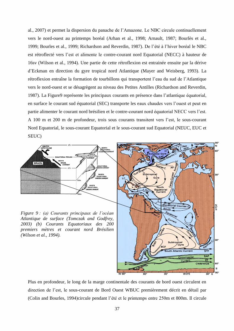
Figure 9:…………….………………………………………………………………….… 37
(a) Courants principaux de l’océan Atlantique de surface (Tomczak and Godfrey, 2003) (b)
Courants équatoriaux des 200 premiers mètres et Courant Nord Brésilien (Wilson et al.,
1994).
Figure 10: …………..…………………………………………………………………… 38
Sortie de modèle de vitesse de courant moyen en m.s-1
à 35°W entre 6°s et 6°N: (a) octobre-
novembre-décembre, (b) avril-mai-juin (Böning and Kröger 2005)
Figure 11: …………………………………………………………..…………………… 39
a),b) Principales masses d’eau de l’océan Atlantique le long d’un transect nord sud c) salinités
correspondantes (Transect WOCE reporté dans le software ODV). (Eau Antarctique de fond-
AABW; Eau Antarctique intermédiaire-AAIW; Eau nord Atlantique de fond-NADW; Eau
Arctique intermédiaire-AIW, Eau Arctique de Fond-ABW; Eau chaude de surface-WWS)
Modifié de (Piepgras and Wasserburg, 1987).
Figure 12: ………………………………………..……………………………………… 43
Distribution des colloïdes organiques et inorganiques en fonction de leurs tailles. Modifié de
Gaillardet et al. (2003).
Figure 13: ……………………………………………………………..………………… 44
19
Processus clés contrôlant la spéciation des métaux traces (M) dans les systèmes aquatiques. X
et L sont de ligands inorganiques, ‘Coll’. signifie colloïdes et ‘part.’signifie particules.
Modifié de Santschi, et al. (1997).
Figure 14: ………………………………………………………………………………… 46
Rapport Nd/Si dans l’océan modifié de (Bertram and Elderfield 1993)
Figure 15: ………………………………………………………………………………… 46
Caractéristiques typiques des spectres de REE marins. Modifié de (Lacan and Jeandel, 2004a)
Figure 16: ………………………………………………………………………………… 47
Deux échantillons présentant une différence due à une contribution lithogénique lors de la
campagne campagne Keops. (Zhang, Lacan et al. 2008)
Figure 17: ………………………………………………………………………………… 48
Compilation des mesures de compositions isotopiques existantes à ce jour (Lacan et al, 2012)
Figure 18 :………………………………………………………………………………… 48
Expérience de mise en contact de plusieurs types de sédiments avec de l’eau intermédiaire de
l’océan austral (Pierce et al. 2013)
Figure 19: ………………………………………………………………………………… 50
Relation entre la concentration en Nd et le pH des eaux continentales(Deberdt, Viers et al.
2002).
Figure 20: ………………………………………………………………………………… 51
Spectres de REE dissous analysés dans les principaux affluents du fleuve Amazone, modifié
de Barroux et al.(2006).
Figure 21: ………………………………………………………………………………… 53
a) Normalisation des concentrations en REE du matériel colloïdal par le matériel dissous total.
b) Modélisation de la spéciation des REE au sein des différentes classes de tailles observées.
(Deberdt, Viers et al. 2002).
Figure 22: ………………………………………………………………………………… 53
Spéciation du do lanthane pour le fleuve moyen mondial (Livingstone 1963) obtenue grâce au
modèle WHAM couplé au modules V et VId’ interactions avec les substances humiques.
Figure 23: ………………………………………………………………………………… 55
Provenance des sédiments du Solimões et du Madeira déterminée par la systématique Sr-
Nd(Viers, Roddaz et al. 2008).
Figure 24: ………………………………………………………………………………… 56
Mélange non conservatif du Nd dans l’embouchure du fleuve Amazone (Sholkovitz 1993)
2.1 Figure 1: …………………………………………………………………………………... 64
Stations d’échantillonnage des campagnes océanographiques AMANDES 1, 2 et 3
Figure 2: …………………………………………………………………………...……… 65
Stations d’échantillonnage de la campagne fluviale CARBAMA 3.
Figure 3: ………………………………………………………………...………………… 66
Stations d’échantillonnage de la campagne fluviale CPRM FOZ
Figure 4: …………………………………………………………………...……………… 67
Localisation des échantillons collectés le long des profils réalisés à Óbidos en avril 2008 lors
de la mesure du débit du fleuve par l’ANA
2.2 Figure 5: …………………………………………………………………………………… 69
20
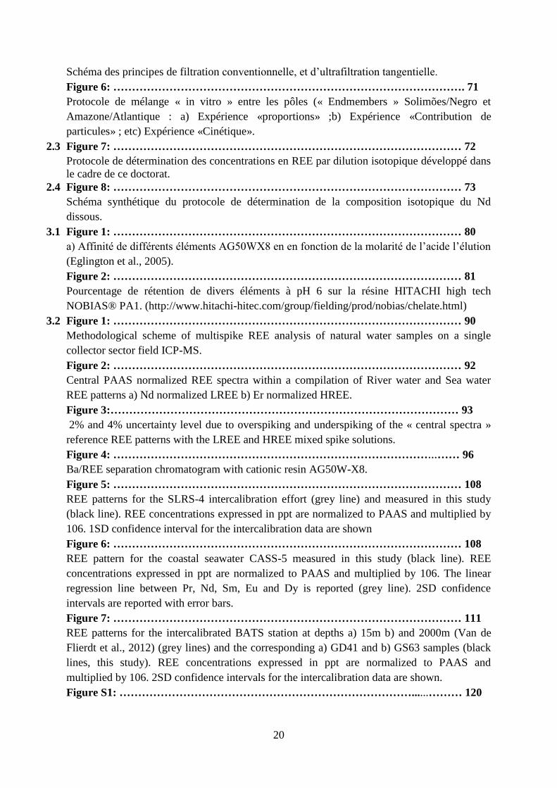
Schéma des principes de filtration conventionnelle, et d’ultrafiltration tangentielle.
Figure 6: …………………………………………………………………………………. 71
Protocole de mélange « in vitro » entre les pôles (« Endmembers » Solimões/Negro et
Amazone/Atlantique : a) Expérience «proportions» ;b) Expérience «Contribution de
particules» ; etc) Expérience «Cinétique».
2.3 Figure 7: ………………………………………………………………………………… 72
Protocole de détermination des concentrations en REE par dilution isotopique développé dans
le cadre de ce doctorat.
2.4 Figure 8: ………………………………………………………………………………… 73
Schéma synthétique du protocole de détermination de la composition isotopique du Nd
dissous.
3.1 Figure 1: ………………………………………………………………………………… 80
a) Affinité de différents éléments AG50WX8 en en fonction de la molarité de l’acide l’élution
(Eglington et al., 2005).
Figure 2: ………………………………………………………………………………… 81
Pourcentage de rétention de divers éléments à pH 6 sur la résine HITACHI high tech
NOBIAS® PA1. (http://www.hitachi-hitec.com/group/fielding/prod/nobias/chelate.html)
3.2 Figure 1: ………………………………………………………………………………… 90
Methodological scheme of multispike REE analysis of natural water samples on a single
collector sector field ICP-MS.
Figure 2: ………………………………………………………………………………… 92
Central PAAS normalized REE spectra within a compilation of River water and Sea water
REE patterns a) Nd normalized LREE b) Er normalized HREE.
Figure 3:………………………………………………………………………………… 93
2% and 4% uncertainty level due to overspiking and underspiking of the « central spectra »
reference REE patterns with the LREE and HREE mixed spike solutions.
Figure 4: ………………………………………………………………………………… 96
Ba/REE separation chromatogram with cationic resin AG50W-X8.
Figure 5: ………………………………………………………………………………… 108
REE patterns for the SLRS-4 intercalibration effort (grey line) and measured in this study
(black line). REE concentrations expressed in ppt are normalized to PAAS and multiplied by
106. 1SD confidence interval for the intercalibration data are shown
Figure 6: ………………………………………………………………………………… 108
REE pattern for the coastal seawater CASS-5 measured in this study (black line). REE
concentrations expressed in ppt are normalized to PAAS and multiplied by 106. The linear
regression line between Pr, Nd, Sm, Eu and Dy is reported (grey line). 2SD confidence
intervals are reported with error bars.
Figure 7: ………………………………………………………………………………… 111
REE patterns for the intercalibrated BATS station at depths a) 15m b) and 2000m (Van de
Flierdt et al., 2012) (grey lines) and the corresponding a) GD41 and b) GS63 samples (black
lines, this study). REE concentrations expressed in ppt are normalized to PAAS and
multiplied by 106. 2SD confidence intervals for the intercalibration data are shown.
Figure S1: ……………………………………………………………………...………… 120
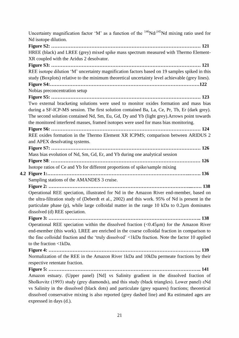
21
Uncertainty magnification factor ‘M’ as a function of the 146
Nd/145
Nd mixing ratio used for
Nd isotope dilution.
Figure S2: ………………………………………………………………………………… 121
HREE (black) and LREE (grey) mixed spike mass spectrum measured with Thermo Element-
XR coupled with the Aridus 2 desolvator.
Figure S3: ………………………………………………………………………………… 121
REE isotope dilution ‘M’ uncertainty magnification factors based on 19 samples spiked in this
study (Boxplots) relative to the minimum theoretical uncertainty level achievable (grey lines).
Figure S4:…………………………………………………………………………………122
Nobias preconcentration setup
Figure S5: ………………………………………………………………………………… 123
Two external bracketing solutions were used to monitor oxides formation and mass bias
during a SF-ICP-MS session. The first solution contained Ba, La, Ce, Pr, Tb, Er (dark grey).
The second solution contained Nd, Sm, Eu, Gd, Dy and Yb (light grey).Arrows point towards
the monitored interfered masses, framed isotopes were used for mass bias monitoring.
Figure S6: ………………………………………………………………………………… 124
REE oxides formation in the Thermo Element XR ICPMS; comparison between ARIDUS 2
and APEX desolvating systems.
Figure S7: ………………………………………………………………………………… 126
Mass bias evolution of Nd, Sm, Gd, Er, and Yb during one analytical session
Figure S8: ………………………………………………………………………………… 126
Isotope ratios of Ce and Yb for different proportions of spike/sample mixing
4.2 Figure 1:……………………………………………………………………………..……. 136
Sampling stations of the AMANDES 3 cruise.
Figure 2: ……………………………………………………………………………...…… 138
Operational REE speciation, illustrated for Nd in the Amazon River end-member, based on
the ultra-filtration study of (Deberdt et al., 2002) and this work. 95% of Nd is present in the
particulate phase (p), while large colloidal matter in the range 10 kDa to 0.2µm dominates
dissolved (d) REE speciation.
Figure 3: ………………………………………………………………………………….. 138
Operational REE speciation within the dissolved fraction (<0.45µm) for the Amazon River
end-member (this work). LREE are enriched in the coarse colloidal fraction in comparison to
the fine colloidal fraction and the ‘truly dissolved’ <1kDa fraction. Note the factor 10 applied
to the fraction <1kDa.
Figure 4: ………………………………………………………………………………….. 139
Normalization of the REE in the Amazon River 1kDa and 10kDa permeate fractions by their
respective retentate fraction.
Figure 5: ………………………………………………………………………………….. 141
Amazon estuary. (Upper panel) [Nd] vs Salinity gradient in the dissolved fraction of
Sholkovitz (1993) study (grey diamonds), and this study (black triangles). Lower panel) εNd
vs Salinity in the dissolved (black dots) and particulate (grey squares) fractions; theoretical
dissolved conservative mixing is also reported (grey dashed line) and Ra estimated ages are
expressed in days (d.).
22
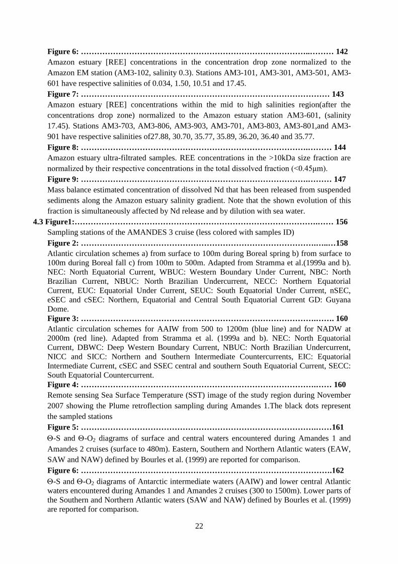
Figure 6: …………………………………………………………………………..……… 142
Amazon estuary [REE] concentrations in the concentration drop zone normalized to the
Amazon EM station (AM3-102, salinity 0.3). Stations AM3-101, AM3-301, AM3-501, AM3-
601 have respective salinities of 0.034, 1.50, 10.51 and 17.45.
Figure 7: ………………………………………………………………………………… 143
Amazon estuary [REE] concentrations within the mid to high salinities region(after the
concentrations drop zone) normalized to the Amazon estuary station AM3-601, (salinity
17.45). Stations AM3-703, AM3-806, AM3-903, AM3-701, AM3-803, AM3-801,and AM3-
901 have respective salinities of27.88, 30.70, 35.77, 35.89, 36.20, 36.40 and 35.77.
Figure 8: ………………………………………………………………………….……… 144
Amazon estuary ultra-filtrated samples. REE concentrations in the >10kDa size fraction are
normalized by their respective concentrations in the total dissolved fraction (<0.45μm).
Figure 9: ………………………………………………………………………….……… 147
Mass balance estimated concentration of dissolved Nd that has been released from suspended
sediments along the Amazon estuary salinity gradient. Note that the shown evolution of this
fraction is simultaneously affected by Nd release and by dilution with sea water.
4.3 Figure1:……………………………………………………………………………….…… 156
Sampling stations of the AMANDES 3 cruise (less colored with samples ID)
Figure 2: …………………………………………………………………………….…..…158
Atlantic circulation schemes a) from surface to 100m during Boreal spring b) from surface to
100m during Boreal fall c) from 100m to 500m. Adapted from Stramma et al.(1999a and b).
NEC: North Equatorial Current, WBUC: Western Boundary Under Current, NBC: North
Brazilian Current, NBUC: North Brazilian Undercurrent, NECC: Northern Equatorial
Current, EUC: Equatorial Under Current, SEUC: South Equatorial Under Current, nSEC,
eSEC and cSEC: Northern, Equatorial and Central South Equatorial Current GD: Guyana
Dome.
Figure 3: …………………………………………………………………………….……. 160
Atlantic circulation schemes for AAIW from 500 to 1200m (blue line) and for NADW at
2000m (red line). Adapted from Stramma et al. (1999a and b). NEC: North Equatorial
Current, DBWC: Deep Western Boundary Current, NBUC: North Brazilian Undercurrent,
NICC and SICC: Northern and Southern Intermediate Countercurrents, EIC: Equatorial
Intermediate Current, cSEC and SSEC central and southern South Equatorial Current, SECC:
South Equatorial Countercurrent.
Figure 4: …………………………………………………………………………….…… 160
Remote sensing Sea Surface Temperature (SST) image of the study region during November
2007 showing the Plume retroflection sampling during Amandes 1.The black dots represent
the sampled stations
Figure 5: …………………………………………………………………………….……161
-S and -O2 diagrams of surface and central waters encountered during Amandes 1 and
Amandes 2 cruises (surface to 480m). Eastern, Southern and Northern Atlantic waters (EAW,
SAW and NAW) defined by Bourles et al. (1999) are reported for comparison.
Figure 6: ………………………………………………………………………………….162
-S and -O2 diagrams of Antarctic intermediate waters (AAIW) and lower central Atlantic
waters encountered during Amandes 1 and Amandes 2 cruises (300 to 1500m). Lower parts of
the Southern and Northern Atlantic waters (SAW and NAW) defined by Bourles et al. (1999)
are reported for comparison.
23
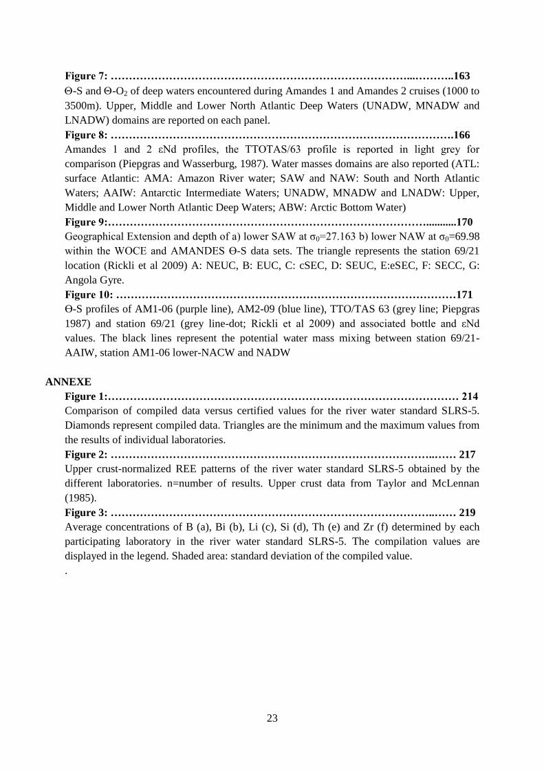
Figure 7: ………………………………………………………………………...………..163
-S and -O2 of deep waters encountered during Amandes 1 and Amandes 2 cruises (1000 to
3500m). Upper, Middle and Lower North Atlantic Deep Waters (UNADW, MNADW and
LNADW) domains are reported on each panel.
Figure 8: ………………………………………………………………………………….166
Amandes 1 and 2 εNd profiles, the TTOTAS/63 profile is reported in light grey for
comparison (Piepgras and Wasserburg, 1987). Water masses domains are also reported (ATL:
surface Atlantic: AMA: Amazon River water; SAW and NAW: South and North Atlantic
Waters; AAIW: Antarctic Intermediate Waters; UNADW, MNADW and LNADW: Upper,
Middle and Lower North Atlantic Deep Waters; ABW: Arctic Bottom Water)
Figure 9:……………………………………………………………………………...........170
Geographical Extension and depth of a) lower SAW at σ0=27.163 b) lower NAW at σ0=69.98
within the WOCE and AMANDES Ө-S data sets. The triangle represents the station 69/21
location (Rickli et al 2009) A: NEUC, B: EUC, C: cSEC, D: SEUC, E:eSEC, F: SECC, G:
Angola Gyre.
Figure 10: …………………………………………………………………………………171
Ө-S profiles of AM1-06 (purple line), AM2-09 (blue line), TTO/TAS 63 (grey line; Piepgras
1987) and station 69/21 (grey line-dot; Rickli et al 2009) and associated bottle and εNd
values. The black lines represent the potential water mass mixing between station 69/21-
AAIW, station AM1-06 lower-NACW and NADW
ANNEXE
Figure 1:…………………………………………………………………………………… 214
Comparison of compiled data versus certified values for the river water standard SLRS-5.
Diamonds represent compiled data. Triangles are the minimum and the maximum values from
the results of individual laboratories.
Figure 2: ……………………………………………………………………………..…… 217
Upper crust-normalized REE patterns of the river water standard SLRS-5 obtained by the
different laboratories. n=number of results. Upper crust data from Taylor and McLennan
(1985).
Figure 3: ……………………………………………………………………………..…… 219
Average concentrations of B (a), Bi (b), Li (c), Si (d), Th (e) and Zr (f) determined by each
participating laboratory in the river water standard SLRS-5. The compilation values are
displayed in the legend. Shaded area: standard deviation of the compiled value.
.

24
25
Chapitre 1 :
Introduction
Sommaire
1.1Contexte et motivations 26
1.2 Contexte géographique et hydrologique 32
1.2.1 Le Bassin amazonien 32
1.2.2 Hydrologie du fleuve amazone 33
1.2.3 Estuaire et marge 35
1.2.4 Courants marins et masses d’eau 36
1.3 Les éléments terres Rares en milieux aquatiques 40
1.3.1 Géochimie des métaux traces en milieux aquatiques 40
a) Dissolution et Complexation 40
b) Spéciation organique 41
c) Particules et Colloïdes 42
d) Synthèse 44
1.3.2 Eléments terres Rares et εNd 45
a) Environnement marin 45
b) Environnement continental 50
c) Estuaires 55
1.4 Objectifs 60
/Objetivos 61
26
1.1Contexte et motivations
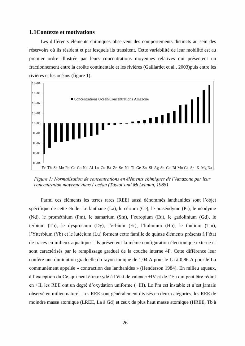
Les différents éléments chimiques observent des comportements distincts au sein des
réservoirs où ils résident et par lesquels ils transitent. Cette variabilité de leur mobilité est au
premier ordre illustrée par leurs concentrations moyennes relatives qui présentent un
fractionnement entre la croûte continentale et les rivières (Gaillardet et al., 2003)puis entre les
rivières et les océans (figure 1).
Parmi ces éléments les terres rares (REE) aussi dénommés lanthanides sont l’objet
spécifique de cette étude. Le lanthane (La), le cérium (Ce), le praséodyme (Pr), le néodyme
(Nd), le prométhium (Pm), le samarium (Sm), l’europium (Eu), le gadolinium (Gd), le
terbium (Tb), le dysprosium (Dy), l’erbium (Er), l’holmium (Ho), le thulium (Tm),
l’Ytterbium (Yb) et le lutécium (Lu) forment cette famille de quinze éléments présents à l’état
de traces en milieux aquatiques. Ils présentent la même configuration électronique externe et
sont caractérisés par le remplissage graduel de la couche interne 4F. Cette différence leur
confère une diminution graduelle du rayon ionique de 1,04 A pour le La à 0,86 A pour le Lu
communément appelée « contraction des lanthanides » (Henderson 1984). En milieu aqueux,
à l’exception du Ce, qui peut être oxydé à l’état de valence +IV et de l’Eu qui peut être réduit
en +II, les REE ont un degré d’oxydation uniforme (+III). Le Pm est instable et n’est jamais
observé en milieu naturel. Les REE sont généralement divisés en deux catégories, les REE de
moindre masse atomique (LREE, La à Gd) et ceux de plus haut masse atomique (HREE, Tb à
1E-04
1E-03
1E-02
1E-01
1E+00
1E+01
1E+02
1E+03
1E+04
Fe Th Sn Mn Pb Ce Co Nd Al Lu Cu Ba Zr Se Ni Tl Ge Zn Si Ag Sb Cd Bi Mo Ca Sr K Mg Na
Concentrations Ocean/Concentrations Amazone
Figure 1: Normalisation de concentrations en éléments chimiques de l’Amazone par leur
concentration moyenne dans l’océan (Taylor and McLennan, 1985)
27
Lu) ; cependant, un troisième groupe est souvent introduit, celui des REE de masses
intermédiaires (MREE, Sm à Dy).
Or, résultat de la nucléosynthèse, les REE de numéro atomique pair sont plus abondants
que ceux de numéro atomique impair (figure 2.a). Pour s’affranchir de ces variations
d’abondance relative « d’origine », on normalise les concentrations de ces éléments par un
matériel de référence comme le schiste australien post archéen (PAAS) (McLennan, 1989)ce
qui définit « un spectre de REE ». Les différences graduelles en masse et en rayon ionique des
REE font qu’ils se comportent de façon « presque » similaire au cours des processus
géochimiques. Ces légers fractionnements entre les différentes REE sont visualisables après
normalisation. Pour représenter les spectres de REE en milieux aquatiques, il est commun de
multiplier les abondances normalisées par 10^6
, car les REE sont présentes à des
concentrations de l’ordre du ppm (10-6
g/g) dans les roches et du ppt (10-12
g/g) dans les eaux
(figure 2b).
L’étude des REE en milieux aquatiques présente en conséquence un intérêt non
négligeable, en effet, leur présence dans l’eau est liée à l’érosion et l’altération chimique des
Figure 2: Abondances relatives des REE pour une eau océanique échantillonnée à
la station BATS concentration moyenne dans l’océan (McLennan 1989).
1.1Contexte et motivations
28
roches, sols et sédiments et à leur spéciation. La sorption et la complexation des REE avec les
ligands en solution ont des constantes de partage variées et peuvent présenter un gradient
d’affinité important le long de la série des lanthanides. Ces variations se reflètent dans les
spectres de REE qui sont fonction du matériel source et qui sont fractionnés par l’ensemble de
ces mécanismes de sorption et complexation.
Au sein des spectres certaines REE peuvent présenter une abondance normalisée
légèrement supérieure ou légèrement inférieure à celle de ces voisines, on parle alors
d’anomalie positive ou négative. Par exemple, les anomalies en Ce et Eu sont dues à la au
changement du degré d’oxydation de ces éléments comparés à leurs voisins trivalents (La, Pr
et Sm, Gd) ce qui entraine une différence dans leur réactivité. Ces anomalies peuvent
également provenir d’apports anthropiques, il a ainsi été observé des anomalies positives en
La et Gd dans des rivières (Kulaksiz and Bau, 2011a, b). Les anomalies sont observables
visuellement sur les spectres mais elles sont aussi quantifiables, on normalise alors la valeur
de la REE présentant l’anomalie par sa valeur théorique estimée grâce à celle des REE
voisines.
Par l’étude des variations des spectres de REE et de leurs possibles anomalies, les REE
sont donc des traceurs de sources et de processus.
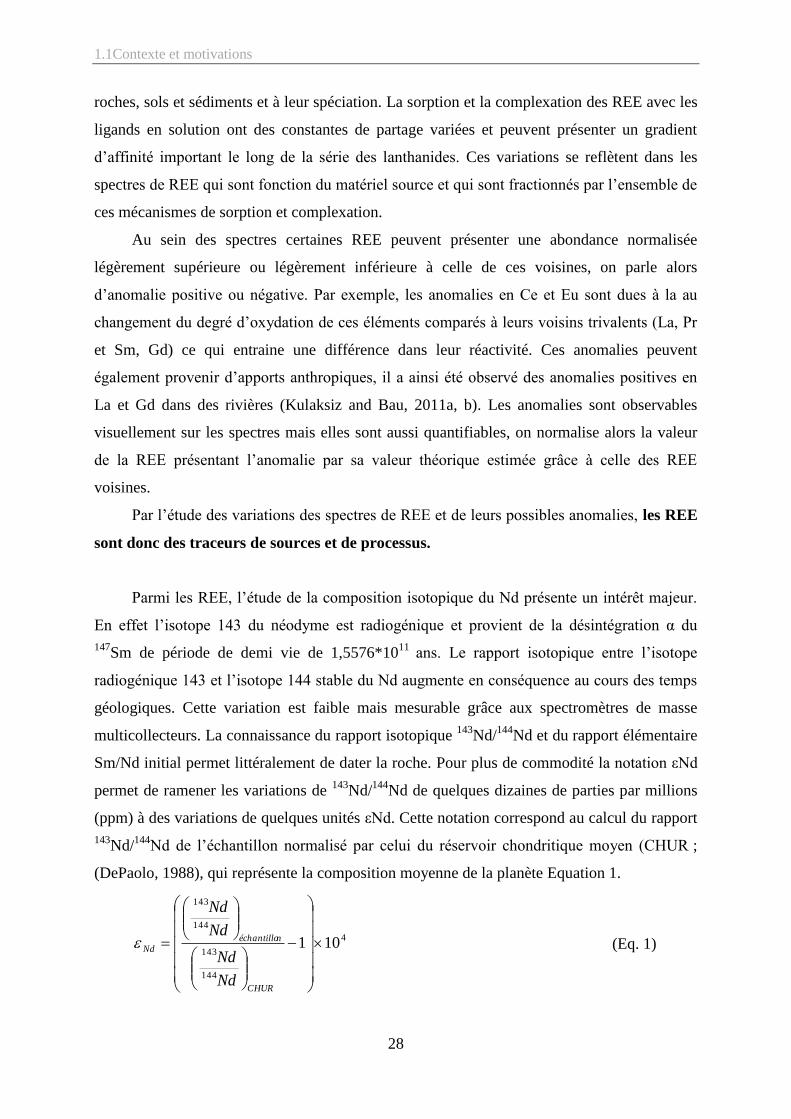
Parmi les REE, l’étude de la composition isotopique du Nd présente un intérêt majeur.
En effet l’isotope 143 du néodyme est radiogénique et provient de la désintégration α du
147Sm de période de demi vie de 1,5576*10
11 ans. Le rapport isotopique entre l’isotope
radiogénique 143 et l’isotope 144 stable du Nd augmente en conséquence au cours des temps
géologiques. Cette variation est faible mais mesurable grâce aux spectromètres de masse
multicollecteurs. La connaissance du rapport isotopique 143
Nd/144
Nd et du rapport élémentaire
Sm/Nd initial permet littéralement de dater la roche. Pour plus de commodité la notation εNd
permet de ramener les variations de 143
Nd/144
Nd de quelques dizaines de parties par millions
(ppm) à des variations de quelques unités εNd. Cette notation correspond au calcul du rapport
143Nd/
144Nd de l’échantillon normalisé par celui du réservoir chondritique moyen (CHUR ;
(DePaolo, 1988), qui représente la composition moyenne de la planète Equation 1.
4
144
143
144
143
101
CHUR
néchantillo
Nd
Nd
Nd
Nd
Nd
(Eq. 1)
29
Lors de son transfert des roches et sédiments vers le milieu aqueux, le Nd conserve sa
signature isotopique, c’est ainsi un traceur de source, ou d’origine pour une masse d’eau.
Les REE et le Nd intègrent la liste de plus en plus ample d’éléments en trace permettant
le traçage de source et processus en milieux aquatiques et présentent un intérêt majeur en
sciences de la terre et de l’environnement. Les milieux aquatiques sont le vecteur de transport
de ces éléments provenant de l’érosion et de l’altération de la croûte continentale. Les
éléments traces avant d’acquérir leur singularité de traceur auprès de la communauté
scientifique sont sujets dans un premier temps à des études exploratoires. Les travaux
pionniers consistent en la mesure des concentrations et des compositions isotopiques (CI) de
ces éléments dans l’eau et en l’étude de leurs variabilités spatio-temporelles. La suite logique
du raisonnement vient dans l’identification des processus physico-chimiques pouvant
expliquer les variations observées. Cette approche permet ainsi la reconstitution du cycle
géochimique de ces éléments. Les cycles géochimiques/biogéochimiques sont principalement
gouvernés par la solubilité et la réactivité des éléments et par leurs interactions avec les
organismes vivants. Comprendre les processus qui conduisent à une répartition donnée des
éléments en trace permet en retour d’utiliser leurs concentrations et compositions isotopiques
pour tracer qualitativement voire quantitativement leurs transports ou les processus auxquels
ils sont réactifs.
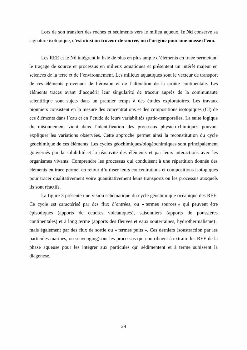
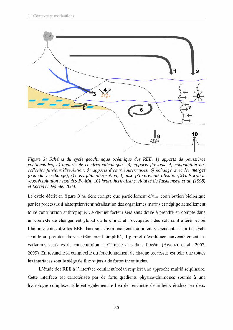
La figure 3 présente une vision schématique du cycle géochimique océanique des REE.
Ce cycle est caractérisé par des flux d’entrées, ou « termes sources » qui peuvent être
épisodiques (apports de cendres volcaniques), saisonniers (apports de poussières
continentales) et à long terme (apports des fleuves et eaux souterraines, hydrothermalisme) ;
mais également par des flux de sortie ou « termes puits ». Ces derniers (soustraction par les
particules marines, ou scavenging)sont les processus qui contribuent à extraire les REE de la
phase aqueuse pour les intégrer aux particules qui sédimentent et à terme subissent la
diagenèse.
1.1Contexte et motivations
30
Le cycle décrit en figure 3 ne tient compte que partiellement d’une contribution biologique
par les processus d’absorption/reminéralisation des organismes marins et néglige actuellement
toute contribution anthropique. Ce dernier facteur sera sans doute à prendre en compte dans
un contexte de changement global ou le climat et l’occupation des sols sont altérés et où
l’homme concentre les REE dans son environnement quotidien. Cependant, si un tel cycle
semble au premier abord extrêmement simplifié, il permet d’expliquer convenablement les
variations spatiales de concentration et CI observées dans l’océan (Arsouze et al., 2007,
2009). En revanche la complexité du fonctionnement de chaque processus est telle que toutes
les interfaces sont le siège de flux sujets à de fortes incertitudes.
L’étude des REE à l’interface continent/océan requiert une approche multidisciplinaire.
Cette interface est caractérisée par de forts gradients physico-chimiques soumis à une
hydrologie complexe. Elle est également le lieu de rencontre de milieux étudiés par deux
Figure 3: Schéma du cycle géochimique océanique des REE. 1) apports de poussières
continentales, 2) apports de cendres volcaniques, 3) apports fluviaux, 4) coagulation des
colloïdes fluviaux/dissolution, 5) apports d’eaux souterraines, 6) échange avec les marges
(boundary exchange), 7) adsorption/désorption, 8) absorption/reminéralisation, 9) adsorption
-coprécipitation / nodules Fe-Mn, 10) hydrothermalisme. Adapté de Rasmunsen et al. (1998)
et Lacan et Jeandel 2004.
31
communautés géochimiques différentes n’utilisant pas les mêmes approches : les
« continentalistes » et les océanographes.
Cette thèse de doctorat porte sur le comportement et le devenir des REE à l’interface
entre le fleuve Amazone et l’océan Atlantique. De par sa situation géographique reculée et
enclavée par la forêt amazonienne, le fleuve Amazone est au regard de ses dimensions peu
étudié et peu instrumenté en comparaison aux cours d’eau européens. L'observatoire de
recherche en environnement (ORE) HYBAM (Contrôles géodynamique, hydrologique et
biogéochimique de l’érosion/altération et des transferts de matière dans le bassin de
l’Amazone) opérationnel depuis 2003 et le projet ANR AMANDES (Amazone Andes) ont
permis la collecte des échantillons analysés au cours de ce doctorat. Ces projets
multidisciplinaires apportent également les données hydrologiques et géochimiques
essentielles à l’exploitation des résultats obtenus.
Nous allons dans un premier temps décrire le contexte géographique et hydrologique de
cette zone d’étude puis proposer un état de l’art de la compréhension des cycles des REE et de
la CI du Nd en environnement fluvial estuarien et océanique. Nous présenterons alors les
objectifs spécifiques de ce doctorat.
32
1.2 Contexte géographique et hydrologique
Le fleuve Amazone draine le plus
grand bassin hydrographique mondial
(6,15 106 km
2) (Figure 4)C’est au
monde le plus grand fleuve en terme de
longueur et de débit avec une décharge
annuelle moyenne de 209000 m3.s
-
1(Junk and Sioli, 1984; Molinier et al.,
1997)
Les eaux du fleuve Amazone
transportent annuellement entre
0,8*109
(Filizola and Guyot, 2004) et
1,2*109
(Milliman et al., 1985) tonnes
de matériel en Suspension (MES), et approximativement 2 à 3*108 tonnes d’éléments dissous
(Milliman and Meade, 1983). Le fleuve Amazone contribue en conséquence pour ~20 %, ~10
%, et~3% des apports fluviaux mondiaux en eau, sédiments et éléments dissous (Callede et
al., 2004; Gaillardet et al., 2003; Milliman and Syvitski, 1992).
1.2.1 Le Bassin amazonien
Le bassin hydrographique du
fleuve Amazone s’étend sur des faciès
géomorphologiques très diversifiés. Il
est bordé dans sa partie ouest et sud-
ouest par la cordillère des Andes
caractérisée par un haut relief, dans sa
partie nord par des sierras qui sont de
grandes plaines montagneuses (2500 à
3000 m) et dans la partie sud par des
plaines d’altitudes modérées (800 à
1000m). Les plaines centrales occupent
le reste du bassin (Junk and Sioli, 1984).
D’un point géologique, trois
Figure 4 : Bassin amazonien.
Figure 5 : Unités géologiques principales du
Bassin amazonien.
33
grandes unités structurelles occupent le bassin (Figure 5) :
Le bouclier central Brésilien au sud et le bouclier Guyanais au nord datent de l’Archéen et du
Protérozoïque le bassin sédimentaire est basé sur des formations du Pléistocène du Néogène et
du crétacé supérieur, et la cordillère des Andes d’une largeur de 100-200 km. Les
affleurements qui composent la cordillère sont majoritairement du neoproterozoique, toutefois
certaines formations ont des âges contrastés comme l’arche de Fitzgerald du Miocène ou la
Pastasa du Crétacé ainsi que des granites et sédiments remaniés du Paléozoïque (CPRM,
2009 ;Roddaz et al., 2005). Bien que la surrection des Andes ait débuté au Crétacé la majeure
partie de son relief et de son altitude s’est mise en place durant le Miocène Supérieur (Garzione et
al., 2008). Le bassin du fleuve Amazone est recouvert principalement par la plus grande forêt
humide mondiale âgée de près de 55Ma et qui abrite 1/10ieme
des espèces connues(Morley,
2000; WWF, 2008).
1.2.2 Hydrologie du fleuve amazone
Le Bassin amazonien, localisé dans une zone tropicale humide, est sujet à une
pluviométrie intense (2000 mm/an). Des études météorologiques complétées d’analyses de
composition isotopiques de l’eau de pluie ont permis de tracer la provenance de celle-ci.
L’eau évaporée de l’océan Atlantique parvient jusqu’au bassin en se recyclant dans celui-ci,
une partie significative des précipitations est également restituée par évapotranspiration. Le
bilan d’eau transporté par le fleuve Amazone correspond à moins de 50% du volume d’eau de
pluie (Junk and Sioli, 1984).
Les principaux tributaires du fleuve Amazone sont le rio Solimões, le rio Negro, le rio
Madeira, le rio Tapajós, et le rio Xingu (Figure 1).Le pic de crue est atteint en avril pour le
Madeira en juillet pour le Solimões et en août pour le Negro. L’Amazone dominé
principalement par ces trois
affluents atteint sa crue
maximum en juin et minimum
en octobre. La différence de
hauteur d’eau entre ces
extrêmes atteint 7 à 10m. Les
débits de ces affluents (Callede
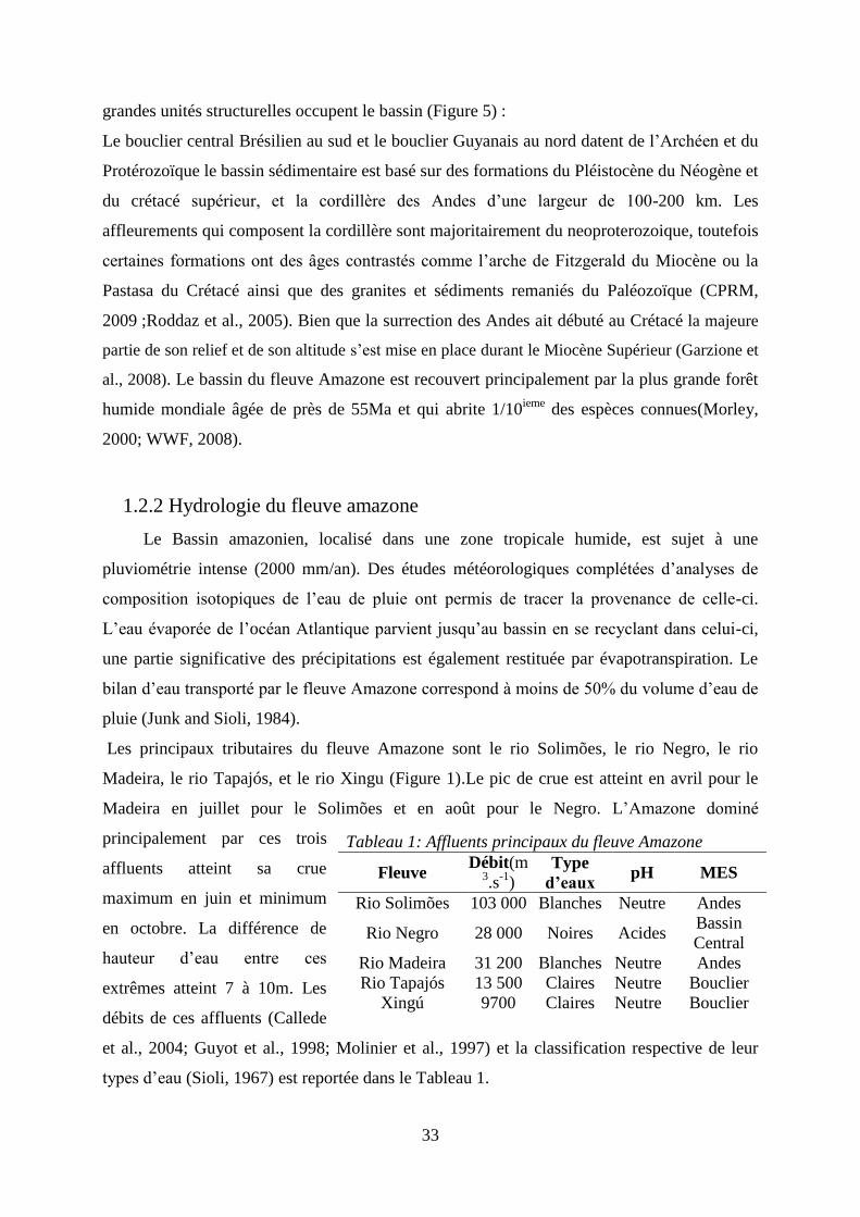
et al., 2004; Guyot et al., 1998; Molinier et al., 1997) et la classification respective de leur
types d’eau (Sioli, 1967) est reportée dans le Tableau 1.
Tableau 1: Affluents principaux du fleuve Amazone
Fleuve Débit(m
3.s
-1)
Type
d’eaux pH MES
Rio Solimões 103 000 Blanches Neutre Andes
Rio Negro 28 000 Noires Acides Bassin
Central
Rio Madeira 31 200 Blanches Neutre Andes
Rio Tapajós 13 500 Claires Neutre Bouclier
Xingú 9700 Claires Neutre Bouclier
1.2 Contexte Géographique et hydrologique
34
Selon cette classification, les eaux « Blanches » de pH quasi neutre ont un aspect visuel
jaune/marron dû aux fortes teneurs en MES composées principalement d’argiles, ces eaux
charrient le matériel érodé des Andes. Les « eaux Noires » de pH acide ont de fortes
concentrations en matière inorganique dissoute, de faibles teneurs en carbonates, leurs MES
proviennent du drainage du bassin central. Les « eaux Claires » de pH quasi neutre ont une
forte pénétration de lumière permettent la floraison de « blooms planctoniques », ces eaux
drainent les boucliers anciens et altérés.
La variabilité annuelle du débit du fleuve Amazone et de ses affluents a une influence
conséquente sur la dynamique hydrologique des plaines d’inondation. Ces plaines
d’inondation, aussi appelées várzeas, jouent un rôle important dans l’hydrologie la
biogéochimie et l’écologie du bassin, et représentent une surface de 300000 m3.s
-1 (Figure
6) ;(Junk, 1997; Martinez and Le Toan, 2007).
Richey et al.(1989) estiment que 30% du débit du fleuve Amazone transite par les
várzeas qui jouent un rôle de stockage du matériel dissous et particulaire, pouvant varier de
quelques mois (eau et matières dissoutes) à plusieurs centaines à quelques milliers d’années
(sédiments) (Meade, 1994; Viers et al., 2005). Dunne et al.(1998) ont estimé que 80% du
matériel en suspension transporté par le fleuve Amazone transite par les várzeas soit un flux
annuel de deux billions de tonnes. Durant le cycle hydrologique annuel, une dynamique
transverse s’installe entre le fleuve et les zones d’inondation interconnectées, contrôlant
Figure 6: Cartographie des zones d’inondation du Bassin
amazonien à partir d’images SAR (Martinez and Le Toan, 2007)
35
l’équilibre spatial et temporel des processus de transferts et sédimentation (Amoros and Petts,
1993). D’un point de vue biogéochimique les zones d’inondation font donc office de filtre et
réacteur chimique (Mertes et al., 1996).
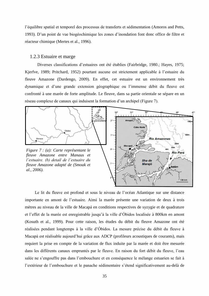
1.2.3 Estuaire et marge
Diverses classifications d’estuaires ont été établies (Fairbridge, 1980.; Hayes, 1975;
Kjerfve, 1989; Pritchard, 1952) pourtant aucune est strictement applicable à l’estuaire du
fleuve Amazone (Dardengo, 2009). En effet, cet estuaire est un environnement très
dynamique et d’une grande extension géographique ou l’immense débit du fleuve est
confronté à une marée de forte amplitude. Le fleuve, dans sa partie orientale se sépare en un
réseau complexe de canaux qui induisent la formation d’un archipel (Figure 7).
Le lit du fleuve est profond et sous le niveau de l’océan Atlantique sur une distance
importante en amont de l’estuaire. Ainsi la marée présente une variation de deux à trois
mètres au niveau de la ville de Macapá en conditions respectives de syzygie et de quadrature
et l’effet de la marée est enregistrable jusqu’à la ville d’Óbidos localisée à 800km en amont
(Kosuth et al., 1999). Pour cette raison, les études du débit du fleuve Amazone ont été
réalisées pendant longtemps à la ville d’Óbidos. La mesure précise du débit du fleuve à
Macapá est réalisable aujourd’hui grâce aux ADCP (profileurs acoustiques de courants), mais
requiert la prise en compte de la variation de flux induite par la marée et doit être mesurée
dans les différents canaux empruntés par le fleuve. En raison du fort débit du fleuve, l’eau
salée ne s’engouffre pas dans l’embouchure et en conséquence le mélange estuarien se fait à
l’extérieur de l’embouchure et le panache sédimentaire s’étend significativement au-delà de
Figure 7 : (a): Carte représentant le
fleuve Amazone entre Manaus et
l’estuaire. (b) detail de l’estuaire du
fleuve Amazone adapté de (Smoak et
al., 2006).
1.2 Contexte Géographique et hydrologique
36
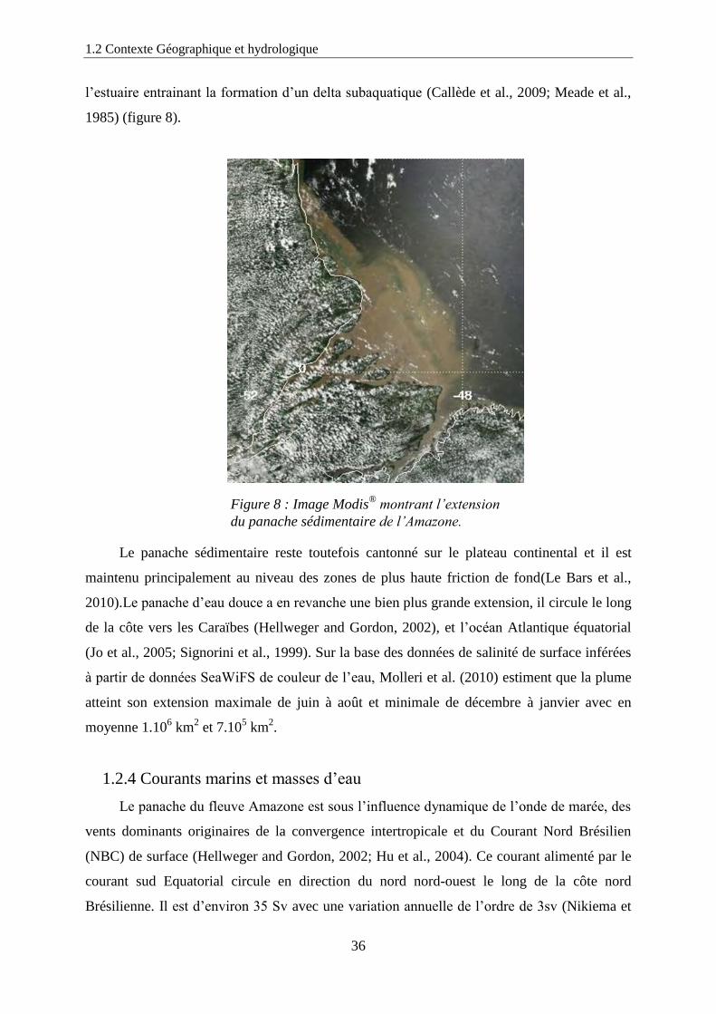
l’estuaire entrainant la formation d’un delta subaquatique (Callède et al., 2009; Meade et al.,
1985) (figure 8).
Le panache sédimentaire reste toutefois cantonné sur le plateau continental et il est
maintenu principalement au niveau des zones de plus haute friction de fond(Le Bars et al.,
2010).Le panache d’eau douce a en revanche une bien plus grande extension, il circule le long
de la côte vers les Caraïbes (Hellweger and Gordon, 2002), et l’océan Atlantique équatorial
(Jo et al., 2005; Signorini et al., 1999). Sur la base des données de salinité de surface inférées
à partir de données SeaWiFS de couleur de l’eau, Molleri et al. (2010) estiment que la plume
atteint son extension maximale de juin à août et minimale de décembre à janvier avec en
moyenne 1.106 km
2 et 7.10
5 km
2.
1.2.4 Courants marins et masses d’eau
Le panache du fleuve Amazone est sous l’influence dynamique de l’onde de marée, des
vents dominants originaires de la convergence intertropicale et du Courant Nord Brésilien
(NBC) de surface (Hellweger and Gordon, 2002; Hu et al., 2004). Ce courant alimenté par le
courant sud Equatorial circule en direction du nord nord-ouest le long de la côte nord
Brésilienne. Il est d’environ 35 Sv avec une variation annuelle de l’ordre de 3sv (Nikiema et
Figure 8 : Image Modis®
montrant l’extension
du panache sédimentaire de l’Amazone.
37
al., 2007) et permet la dispersion du panache de l’Amazone. Le NBC circule continuellement
vers le nord-ouest au printemps boréal (Arhan et al., 1998; Arnault, 1987; Bourlès et al.,
1999; Bourles et al., 1999; Richardson and Reverdin, 1987). De l’été à l’hiver boréal le NBC
est rétroflecté vers l’est et alimente le contre-courant nord Equatorial (NECC) à hauteur de
16sv (Wilson et al., 1994). Une partie de cette rétroflexion est entrainée ensuite par la dérive
d’Eckman en direction du gyre tropical nord Atlantique (Mayer and Weisberg, 1993). La
rétroflexion entraîne la formation de tourbillons qui transportent l’eau du sud de l’Atlantique
vers le nord-ouest et se désagrègent au niveau des Petites Antilles (Richardson and Reverdin,
1987). La Figure9 représente les principaux courants en présence dans l’atlantique équatorial,
en surface le courant sud équatorial (SEC) transporte les eaux chaudes vers l’ouest et peut en
partie alimenter le courant nord brésilien et le contre-courant nord équatorial NECC vers l’est.
A 100 m et 200 m de profondeur, trois sous courants transitent vers l’est, le sous-courant
Nord Equatorial, le sous-courant Equatorial et le sous-courant sud Equatorial (NEUC, EUC et
SEUC)
Plus en profondeur, le long de la marge continentale des courants de bord ouest circulent en
direction de l’est, le sous-courant de Bord Ouest WBUC premièrement décrit en détail par
(Colin and Bourles, 1994)circule pendant l’été et le printemps entre 250m et 800m. Il circule
Figure 9 : (a) Courants principaux de l’océan
Atlantique de surface (Tomczak and Godfrey,
2003) (b) Courants Equatoriaux des 200
premiers mètres et courant nord Brésilien
(Wilson et al., 1994).
1.2 Contexte Géographique et hydrologique
38
en juin mais en septembre sa circulation est nulle, il est en moyenne de 9sv à ces profondeurs.
Il a également été observé lors de la campagne AMANDES1 en octobre 2007 (Silva et al., In
prep.).
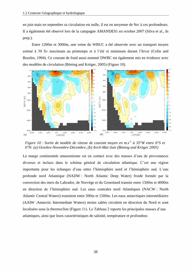
Entre 1200m et 3000m, une veine du WBUC a été observée avec un transport moyen
estimé à 30 Sv maximum au printemps et à l’été et minimum durant l’hiver (Colin and
Bourles, 1994). Ce courant de fond aussi nommé DWBC est également mis en évidence avec
des modèles de circulation (Böning and Kröger, 2005) (Figure 10).
La marge continentale amazonienne est en contact avec des masses d’eau de provenances
diverses et inclues dans le schéma général de circulation atlantique. C’est une région
importante pour les échanges d’eau entre l’hémisphère nord et l’hémisphère sud. L’eau
profonde nord Atlantique (NADW : North Atlantic Deep Water) froide formée par la
convection des mers du Labrador, de Norvège et du Groenland transite entre 1500m et 4000m
en direction de l’hémisphère sud. Les eaux centrales nord Atlantiques (NACW : North
Atlantic Central Waters) transitent entre 500m et 1500m. Les eaux antarctiques intermédiaires
(AAIW :Antarctic Intermediate Waters) moins salées circulent en direction du Nord et sont
localisées sous la thermocline (Figure 11). Le Tableau 2 reporte les principales masses d’eau
atlantiques, ainsi que leurs caractéristiques de salinité, température et profondeur.
Figure 10 : Sortie de modèle de vitesse de courant moyen en m.s-1
à 35°W entre 6°S et
6°N: (a) Octobre-Novembre-Décembre, (b) Avril-Mai-Juin (Böning and Kröger 2005)
39
Tableau 2 : Caractéristiques de température, salinité et domaines de profondeurs des masses
d’eau principales de l’océan Atlantique (Libes, 1992).
Masses d’eau Salinité Température Profondeurs
Eau Antarctique de
Fond
Antartic Bottom Water
(AABW) 34,66 -0,4 4000-fond
Eau Antarctique
Intermédiaire
Antarctic Intermediate Water
(AAIW) 34,2-34,4 0-2 500-1000
Eau Arctique
Intermédiaire
Arctic Intermediate Waters
(AIW) 34,8-34,9 3-4 200-1000
Eaux
Méditerranéennes Mediteranean Waters (MIW) 36,5 8-17 1400-1600
Eaux centrales nord
Atlantiques
North Atlantic central Waters
(NACW) 35,1-36,7 8-19 100-500
Eaux intermédiaires
nord Atlantiques
North Atlantic Intermediate
Waters (NAIW) 34,73 4-8 300-1000
Eaux nord Atlantiques
profondes e de fond
North Atlantic Deep and
Bottom water (NADW
NABW)
34,9 2,5-3,1 1300-fond
Figure 11: a),b) Principales masses d’eau de l’océan Atlantique le long d’un transectnord sud c) salinités
correspondantes (Transect WOCE reporté dans le software ODV). (Eau Antarctique de fond-AABW; Eau
Antarctique intermédiaire-AAIW; Eau nord atlantique de fond-NADW; Eau Arctique intermédiaire-AIW,
EauArctique de fond-ABW; Eau chaude de surface-WWS) Modifié de (Piepgras and Wasserburg, 1987).
40
1.3 Les éléments terres rares en Milieux Aquatiques
Dans cette partie nous aborderons des notions générales de géochimie de métaux en
milieu aquatique pour effectuer ensuite une revue des connaissances sur les REE et la
composition isotopique du Nd dans l’océan, l’Amazone et à l’interface entre ces deux
milieux.
1.3.1 Géochimie des métaux traces en milieux aquatiques
a) Dissolution et complexation
La complexation des ions métalliques par les molécules d’eau interfère avec la liaison
électrostatique entre les molécules d’eau. Si le soluté a une liaison forte avec la molécule
d’eau, il est thermodynamiquement stable et soluble. Ceci permet sa dissolution et son
transport dans la phase dissoute. Dans le cas contraire, sa réactivité le rend relativement
instable et il devient moins soluble.
A titre d’exemple, le rapport Sr/Nd dans la croûte Continentale moyenne est de 10
(McLennan, 1989), ces deux éléments voient leur cycle géochimique aquatique découplés lors
de l’altération des roches. Le Sr a une forte affinité avec l’eau et un temps de résidence dans
l’océan de 5*10^6
ans comparable à celui des sels majeurs, le rapport Sr/Nd augmente entre
les roches et rivières et entre les rivières et les océans, le Sr est donc bien plus soluble que le
Nd.
La majorité des métaux ayant une forte affinité avec l’oxygène des molécules d’eau sont
cerclés d’une sphère externe d’hydratation forte, et une sphère externe d’hydratation faible
(Benjamin and Honeyman, 2000). La force de cette complexation tend à augmenter avec la
charge de l’ion métallique et à diminuer avec sa taille. Cette interaction métal-eau est
typiquement illustrée par la notation Me(H2O)xn+
. Le cation est alors considéré comme libre
dans l’eau et pour plus de commodité exprimé par la notation Men+.
L’eau agit dans ce cas
comme un ligand inorganique.
Dans la sphère d’hydratation du cation, une molécule d’eau peut être substituée par un
autre ligand, le complexe ainsi obtenu est généralement plus stable que le complexe aqueux.
Dans le cas ou deux espèces se substituent aux molécules d'eau, le complexe formé avec le
ligand est qualifié de bidenté, et de manière générale, lorsque que plus d’un complexe non
aqueux est formé, il est qualifié de multidenté.
41
Jusqu’aux années 1980 la spéciation des métaux aux ligands inorganiques était
déterminée grâce à des modèles d’équilibre d’association thermodynamique utilisant des
constantes de stabilité pour les complexes majeurs (Millero, 1985; Turner et al., 1981). La
prise en compte des interactions entre métaux et ligands organiques a connu un essor à partir
des années 1990.
b) Spéciation organique
Santschi et al.(1990) ont décrit la complexation des métaux par la matière organique d’une
forme simple par l’équation suivante :
M1L1 +M2L2 = M1L2 + M2L1 (Eq.2)
Ou M1 représente le métal trace étudié, M2 un métal majeur ou proton, L1 l’eau ou un
ligand inorganique L2 un ligand organique.
Dans la phase dissoute, l’ion métallique peut donc se présenter sous la forme d’un ion hydraté
libre, ou sous forme de complexe organique ou inorganique. Sa spéciation est généralement
décrite expérimentalement et elle est dépendante de la constante de stabilité notée :
KML,M’=[ML]/[M’]+[L’]. (Eq.3)
Ou M’ et L’ représentent le métal et le ligand libre, et ML le complexe formé.
Bien que de nombreuses synthèses aient été publiées sur la spéciation des éléments traces
dans les eaux naturelles, la source et le détail des groupements fonctionnels des ligands
organiques restent peu renseignés.
–COOH, –OH, –NR2, e –SR2 (ou R est un méthyle ou un hydrogène) font partie des
groupements chimiques clés intervenant dans la spéciation organique des métaux. Les sources
naturelles de ces groupements chimiques sont phytochélatines, biopolímères, et les substances
humiques (SH). La difficulté de modélisation de la complexation des métaux par la matière
organique réside dans la forte diversité de celle-ci et en particulier des substances humiques
(SH) composées entre autres par les acides fulviques (AF) et les acides humiques (AH).
Les groupements fonctionnels qui les composent (carboxyliques, phénoliques...) ont des
affinités propres pour chaque métal et une affinité totale résultante variable due aux
concentrations et différentes proportions de ces groupements. Il y a deux manières de
déterminer les constantes d’équilibre des différents groupements fonctionnels de la matière
organique : soit en utilisant un modèle discret comportant un seul type de groupement
fonctionnel pour lequel une constante K est considérée, soit à partir d’un modèle multi-sites
permettant l’utilisation d’une constante K pour chaque groupement. Des études appliquent des
1.3 Les éléments Terres Rares en Milieux Aquatiques
42
modèles de spéciation à l’équilibre comme le WHAM (Windemere Humic Aqueous Model)
(Tipping, 1994), qui sont plus efficaces lorsque l’on considère que les complexes sont formés,
ou que les processus d’adsorption sont réversibles. Ces vingt dernières années, de nombreuses
études ont montré l’importance des ligands organiques dans la complexation des métaux
traces et ce particulièrement pour la phase colloïdale. Ces études montrent clairement le
comportement différentiel des métaux entre la phase dissoute et colloïdale (entre ~1nm et
0,2µm).
L’interaction métaux/organismes planctoniques est fondamentale en milieux aquatiques,
l’importance de ce compartiment organique “vivant” a entrainé l’agrégation de ces
interactions à une discipline indépendante ou la composante biologique est centrale : la
biogéochimie. Le cycle biogéochimique des éléments qui était traditionnellement limité à
l’étude des sels nutritifs et aux constituants majeurs des êtres vivants (C,H,O,N,P,Si) a inclut
les métaux traces qualifiés d’oligoéléments ou de micronutriments suites à la découverte de
l’importance de ceux-ci dans les métabolismes (Fe,Mn,Cu,Mo,Zn,B...). Les oligoéléments
sont sujets à des interactions avec les organismes par voie d’absorption ou d’assimilation.
L’assimilation de ceux-ci par les organismes peut être occasionnée par la substitution d’un
élément (limitant ou non) ou par l’assimilation involontaire par l’organisme se manifestant
par un simple transit ou par une bioaccumulation.
c) Particules et Colloïdes
La mobilité du métal est fonction de la nature de ses phases porteuses. En effet, plus
celles-ci sont légères et mobiles, plus le métal est susceptible d’être transporté par l’eau. Le
matériel particulaire se distingue du matériel dissous par la limite opérationnelle de filtration
des membranes de pores de 0.45µm. Il existe en pratique un continuum de tailles des
composés entre le dissous “vrai” défini opérationnellement comme étant inférieur à 1000Da
(on parle dans ce cas en termes de poids moléculaire) et le matériel particulaire. Cette classe
de taille est qualifiée de fraction colloïdale, et peut être séparée par des techniques
d’ultrafiltration ou de dialyse. Les colloïdes des eaux naturelles englobent une extrême
diversité et complexité de composés (organismes, détritus végétaux, macromolécules,
minéraux, argiles et oxydes), ils sont généralement en suspension dans la colonne d’eau car
leur vitesse de sédimentation est généralement inférieure à 10-2
cm.-1
(Stum, 1981). C’est
43
pourquoi ils sont traditionnellement considérés comme mobiles et assimilés à la phase
dissoute.
Une grande partie des composés intervenants dans la spéciation des métaux en milieu
aquatique est de nature colloïdale. Les métaux peuvent en effet s’adsorber à la surface des
particules et des colloïdes par voie de physisorption qui dépend des forces électrostatiques de
van der Waals ou de chemisorption où la liaison est alors de nature covalente(Reynolds and
Richards, 1996). Les coloides représentent de plus de larges surfaces, pour la fraction des
petits colloïdes (5-200nm) elle est superieure à 18m2 par m
3 d’eau en surface dans l’océan
Atlantique Nord (Wells and Goldberg, 1994). La phase colloïdale est en conséquence cruciale
dans le cycle géochimique des métaux. La Figure 12 représente les types et domaines de taille
du matériel dissous colloïdal et particulaire.
Les estuaires, sources hydrothermales, résurgences sous-marines sont des zones
d’interface qui présentent généralement de forts gradients physico chimiques (T°, potentiel
hydrogène, force ionique) pouvant affecter de manière critique la “stabilité” des colloïdes. La
surface de contact entre les colloïdes et l’eau représentant une importante énergie libre, des
électrolytes et des cations adsorbés altèrent leur charge de surface et des polymères peuvent
former des ponts entre colloïdes distincts entrainant la coagulation et la floculation du
colloïde. Les oxy-hydroxydes peuvent également précipiter lors de changements de conditions
de potentiels hydrogène et redox (pH et Eh).
Figure 12: Distribution des colloïdes organiques et inorganiques en fonction de leurs
tailles. Modifié de Gaillardet et al. (2003).
1.3 Les éléments Terres Rares en Milieux Aquatiques
44
Lorsque la masse des composés néoformés devient critique la composante verticale du
transport du colloïde domine en son mouvement horizontal lié à la circulation de la masse
d’eau. Ce découplage entraine la soustraction des colloïdes de la colonne d’eau et correspond
approximativement au gain de volume retenu par des filtres de 0,22 et 0,45µm.
La modélisation de la soustraction de colloïdes par voie de coagulation a été réalisée par
des études de distribution de taille de particules (Fillela and Buffle, 1993). Les modèles
physico chimiques de stabilité des colloïdes considèrent le bilan attraction/répulsion inter
colloïdes. La répulsion des particules est due aux interactions électrostatiques de Coulomb
ayant comme contrepartie l’attraction due aux forces électrostatiques de van der Waals.
L’énergie de répulsion dépend du potentiel de surface et de sa diminution dans la partie
diffuse de la couche double, la diminution du potentiel avec la distance est fonction de la
force ionique. L’attraction de van der Waals comme première approche est inversement
proportionnelle au carré de la distance intercolloïdale.
d) synthèse
La Figure 13 synthétise et schématise les processus présentés dans les sections
précédentes et qui contrôlent la spéciation des métaux traces. C’est un système complexe
d’interactions physico-chimiques aux constantes et cinétiques variées.
Figure 13: Processus clés contrôlant la spéciation des métaux traces (M) dans les
systèmes aquatiques. X et L sont de ligands inorganiques, ‘Coll’. signifie colloïdes
et ‘part.’signifie particules. Modifié de Santschi et al. (1997).
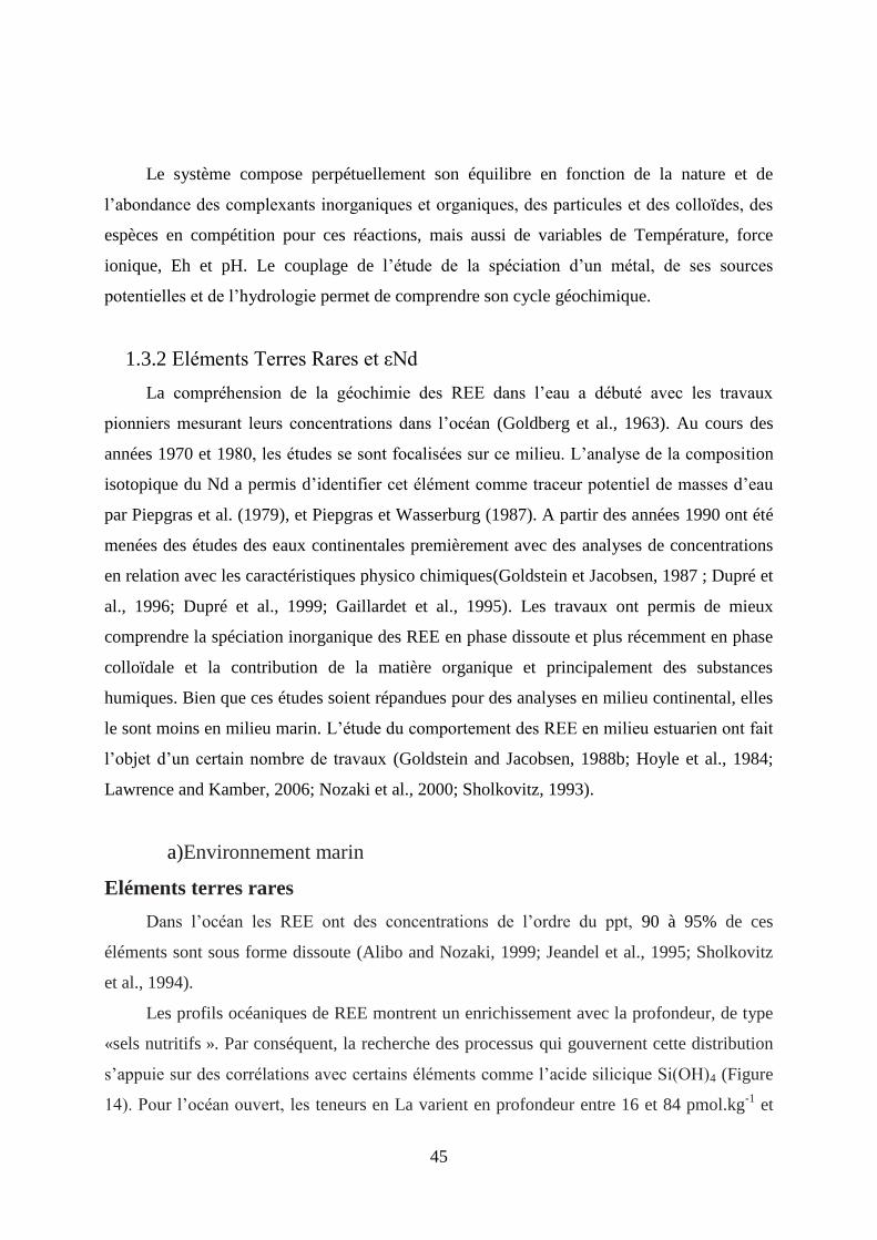
45
Le système compose perpétuellement son équilibre en fonction de la nature et de
l’abondance des complexants inorganiques et organiques, des particules et des colloïdes, des
espèces en compétition pour ces réactions, mais aussi de variables de Température, force
ionique, Eh et pH. Le couplage de l’étude de la spéciation d’un métal, de ses sources
potentielles et de l’hydrologie permet de comprendre son cycle géochimique.
1.3.2 Eléments Terres Rares et εNd
La compréhension de la géochimie des REE dans l’eau a débuté avec les travaux
pionniers mesurant leurs concentrations dans l’océan (Goldberg et al., 1963). Au cours des
années 1970 et 1980, les études se sont focalisées sur ce milieu. L’analyse de la composition
isotopique du Nd a permis d’identifier cet élément comme traceur potentiel de masses d’eau
par Piepgras et al. (1979), et Piepgras et Wasserburg (1987). A partir des années 1990 ont été
menées des études des eaux continentales premièrement avec des analyses de concentrations
en relation avec les caractéristiques physico chimiques(Goldstein et Jacobsen, 1987 ; Dupré et
al., 1996; Dupré et al., 1999; Gaillardet et al., 1995). Les travaux ont permis de mieux
comprendre la spéciation inorganique des REE en phase dissoute et plus récemment en phase
colloïdale et la contribution de la matière organique et principalement des substances
humiques. Bien que ces études soient répandues pour des analyses en milieu continental, elles
le sont moins en milieu marin. L’étude du comportement des REE en milieu estuarien ont fait
l’objet d’un certain nombre de travaux (Goldstein and Jacobsen, 1988b; Hoyle et al., 1984;
Lawrence and Kamber, 2006; Nozaki et al., 2000; Sholkovitz, 1993).
a)Environnement marin
Eléments terres rares
Dans l’océan les REE ont des concentrations de l’ordre du ppt, 90 à 95% de ces
éléments sont sous forme dissoute (Alibo and Nozaki, 1999; Jeandel et al., 1995; Sholkovitz
et al., 1994).
Les profils océaniques de REE montrent un enrichissement avec la profondeur, de type
«sels nutritifs ». Par conséquent, la recherche des processus qui gouvernent cette distribution
s’appuie sur des corrélations avec certains éléments comme l’acide silicique Si(OH)4 (Figure
14). Pour l’océan ouvert, les teneurs en La varient en profondeur entre 16 et 84 pmol.kg-1
et
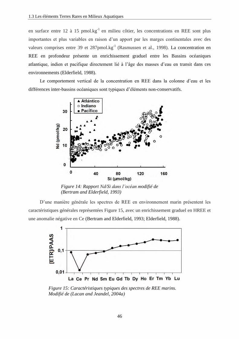
1.3 Les éléments Terres Rares en Milieux Aquatiques
46
en surface entre 12 à 15 pmol.kg-1
en milieu côtier, les concentrations en REE sont plus
importantes et plus variables en raison d’un apport par les marges continentales avec des
valeurs comprises entre 39 et 287pmol.kg-1
(Rasmussen et al., 1998). La concentration en
REE en profondeur présente un enrichissement graduel entre les Bassins océaniques
atlantique, indien et pacifique directement lié à l’âge des masses d’eau en transit dans ces
environnements (Elderfield, 1988).
Le comportement vertical de la concentration en REE dans la colonne d’eau et les
différences inter-bassins océaniques sont typiques d’éléments non-conservatifs.
D’une manière générale les spectres de REE en environnement marin présentent les
caractéristiques générales représentées Figure 15, avec un enrichissement graduel en HREE et
une anomalie négative en Ce (Bertram and Elderfield, 1993; Elderfield, 1988).
Figure 15: Caractéristiques typiques des spectres de REE marins.
Modifié de (Lacan and Jeandel, 2004a)
Figure 14: Rapport Nd/Si dans l’océan modifié de
(Bertram and Elderfield, 1993)
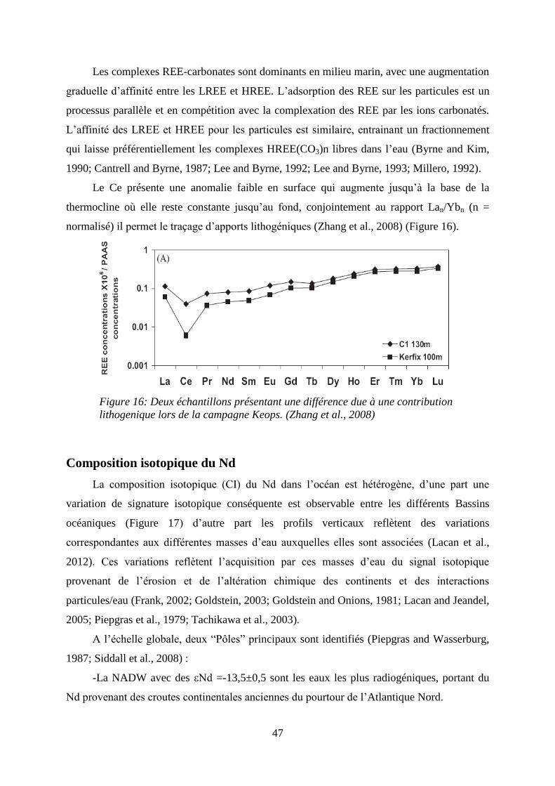
47
Les complexes REE-carbonates sont dominants en milieu marin, avec une augmentation
graduelle d’affinité entre les LREE et HREE. L’adsorption des REE sur les particules est un
processus parallèle et en compétition avec la complexation des REE par les ions carbonatés.
L’affinité des LREE et HREE pour les particules est similaire, entrainant un fractionnement
qui laisse préférentiellement les complexes HREE(CO3)n libres dans l’eau (Byrne and Kim,
1990; Cantrell and Byrne, 1987; Lee and Byrne, 1992; Lee and Byrne, 1993; Millero, 1992).
Le Ce présente une anomalie faible en surface qui augmente jusqu’à la base de la
thermocline où elle reste constante jusqu’au fond, conjointement au rapport Lan/Ybn (n =
normalisé) il permet le traçage d’apports lithogéniques (Zhang et al., 2008) (Figure 16).
Composition isotopique du Nd
La composition isotopique (CI) du Nd dans l’océan est hétérogène, d’une part une
variation de signature isotopique conséquente est observable entre les différents Bassins
océaniques (Figure 17) d’autre part les profils verticaux reflètent des variations
correspondantes aux différentes masses d’eau auxquelles elles sont associées (Lacan et al.,
2012). Ces variations reflètent l’acquisition par ces masses d’eau du signal isotopique
provenant de l’érosion et de l’altération chimique des continents et des interactions
particules/eau (Frank, 2002; Goldstein, 2003; Goldstein and Onions, 1981; Lacan and Jeandel,
2005; Piepgras et al., 1979; Tachikawa et al., 2003).
A l’échelle globale, deux “Pôles” principaux sont identifiés (Piepgras and Wasserburg,
1987; Siddall et al., 2008) :
-La NADW avec des εNd =-13,5±0,5 sont les eaux les plus radiogéniques, portant du
Nd provenant des croutes continentales anciennes du pourtour de l’Atlantique Nord.
Figure 16: Deux échantillons présentant une différence due à une contribution
lithogenique lors de la campagne Keops. (Zhang et al., 2008)
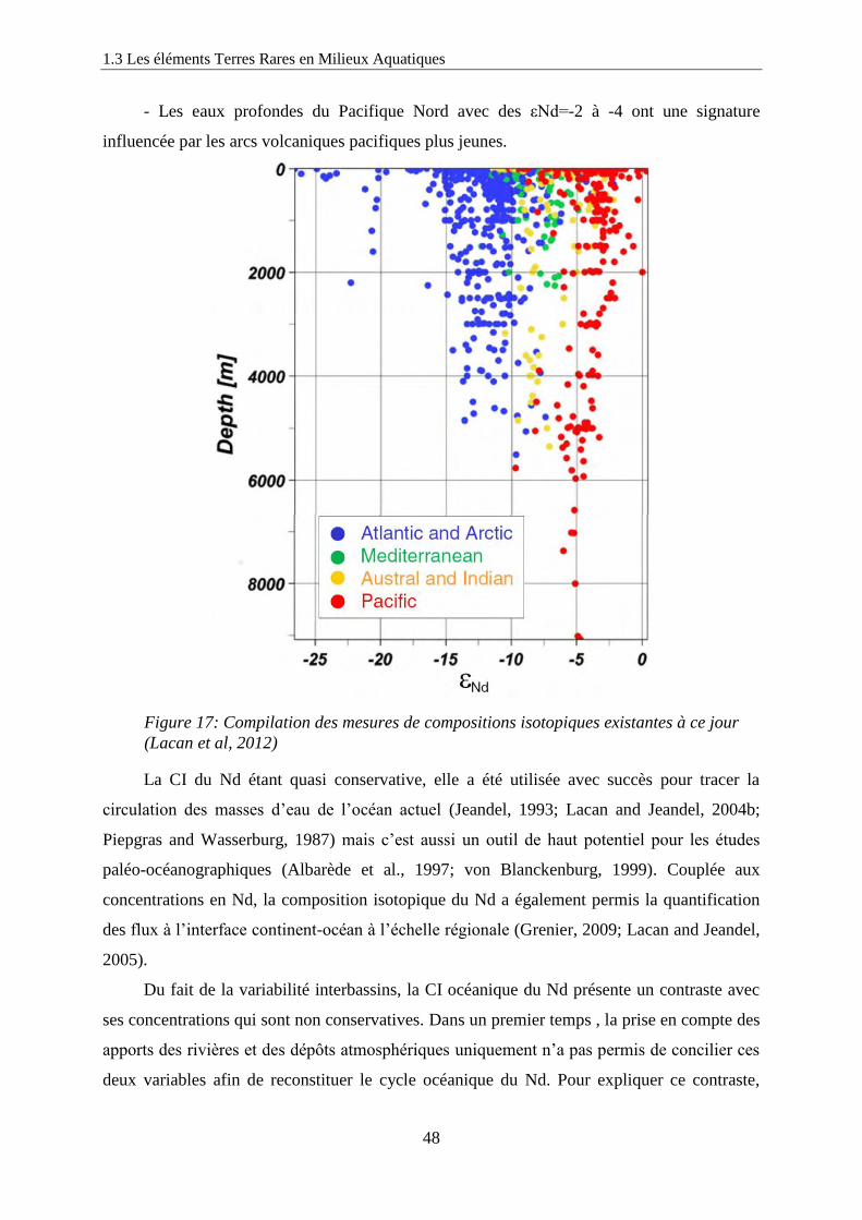
1.3 Les éléments Terres Rares en Milieux Aquatiques
48
- Les eaux profondes du Pacifique Nord avec des εNd=-2 à -4 ont une signature
influencée par les arcs volcaniques pacifiques plus jeunes.
La CI du Nd étant quasi conservative, elle a été utilisée avec succès pour tracer la
circulation des masses d’eau de l’océan actuel (Jeandel, 1993; Lacan and Jeandel, 2004b;
Piepgras and Wasserburg, 1987) mais c’est aussi un outil de haut potentiel pour les études
paléo-océanographiques (Albarède et al., 1997; von Blanckenburg, 1999). Couplée aux
concentrations en Nd, la composition isotopique du Nd a également permis la quantification
des flux à l’interface continent-océan à l’échelle régionale (Grenier, 2009; Lacan and Jeandel,
2005).
Du fait de la variabilité interbassins, la CI océanique du Nd présente un contraste avec
ses concentrations qui sont non conservatives. Dans un premier temps , la prise en compte des
apports des rivières et des dépôts atmosphériques uniquement n’a pas permis de concilier ces
deux variables afin de reconstituer le cycle océanique du Nd. Pour expliquer ce contraste,
Figure 17: Compilation des mesures de compositions isotopiques existantes à ce jour
(Lacan et al, 2012)
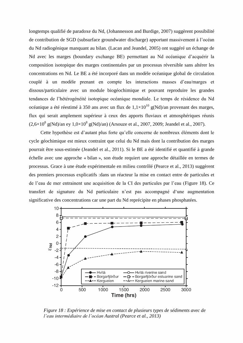
49
longtemps qualifié de paradoxe du Nd, (Johannesson and Burdige, 2007) suggèrent possibilité
de contribution de SGD (subsurface groundwater discharge) apportant massivement à l’océan
du Nd radiogénique manquant au bilan. (Lacan and Jeandel, 2005) ont suggéré un échange de
Nd avec les marges (boundary exchange BE) permettant au Nd océanique d’acquérir la
composition isotopique des marges continentales par un processus réversible sans altérer les
concentrations en Nd. Le BE a été incorporé dans un modèle océanique global de circulation
couplé à un modèle prenant en compte les interactions masses d’eau/marges et
dissous/particulaire avec un module biogéochimique et pouvant reproduire les grandes
tendances de l’hétérogénéité isotopique océanique mondiale. Le temps de résidence du Nd
océanique a été réestimé à 350 ans avec un flux de 1,1×10¹⁰
g(Nd)/an provenant des marges,
flux qui serait amplement supérieur à ceux des apports fluviaux et atmosphériques réunis
(2,6×10⁸ g(Nd)/an ey 1,0×10
8 g(Nd)/an) (Arsouze et al., 2007, 2009; Jeandel et al., 2007).
Cette hypothèse est d’autant plus forte qu’elle concerne de nombreux éléments dont le
cycle géochimique est mieux contraint que celui du Nd mais dont la contribution des marges
pourrait être sous-estimée (Jeandel et al., 2011). Si le BE a été identifié et quantifié à grande
échelle avec une approche « bilan », son étude requiert une approche détaillée en termes de
processus. Grace à une étude expérimentale en milieu contrôlé (Pearce et al., 2013) suggèrent
des premiers processus explicatifs :dans un réacteur la mise en contact entre de particules et
de l’eau de mer entrainent une acquisition de la CI des particules par l’eau (Figure 18). Ce
transfert de signature du Nd particulaire n’est pas accompagné d‘une augmentation
significative des concentrations car une part du Nd reprécipite en phases phosphatées.
Figure 18 : Expérience de mise en contact de plusieurs types de sédiments avec de
l’eau intermédiaire de l’océan Austral (Pearce et al., 2013)
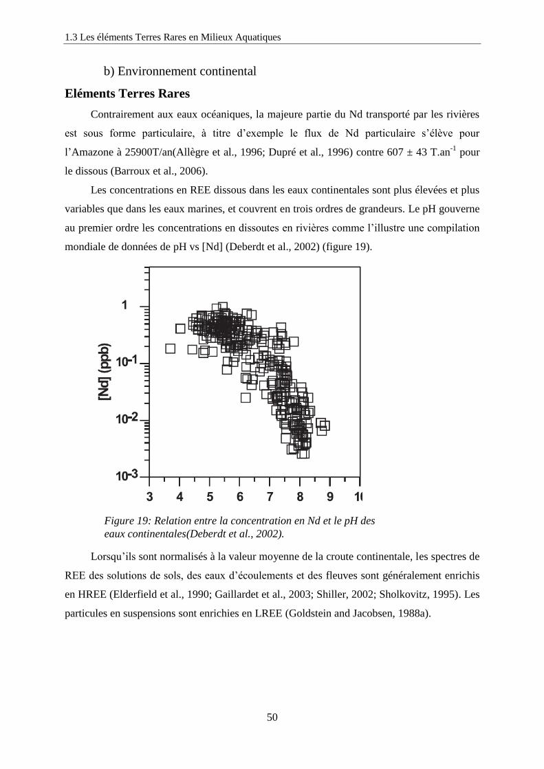
1.3 Les éléments Terres Rares en Milieux Aquatiques
50
b) Environnement continental
Eléments Terres Rares
Contrairement aux eaux océaniques, la majeure partie du Nd transporté par les rivières
est sous forme particulaire, à titre d’exemple le flux de Nd particulaire s’élève pour
l’Amazone à 25900T/an(Allègre et al., 1996; Dupré et al., 1996) contre 607 ± 43 T.an-1
pour
le dissous (Barroux et al., 2006).
Les concentrations en REE dissous dans les eaux continentales sont plus élevées et plus
variables que dans les eaux marines, et couvrent en trois ordres de grandeurs. Le pH gouverne
au premier ordre les concentrations en dissoutes en rivières comme l’illustre une compilation
mondiale de données de pH vs [Nd] (Deberdt et al., 2002) (figure 19).
Lorsqu’ils sont normalisés à la valeur moyenne de la croute continentale, les spectres de
REE des solutions de sols, des eaux d’écoulements et des fleuves sont généralement enrichis
en HREE (Elderfield et al., 1990; Gaillardet et al., 2003; Shiller, 2002; Sholkovitz, 1995). Les
particules en suspensions sont enrichies en LREE (Goldstein and Jacobsen, 1988a).
Figure 19: Relation entre la concentration en Nd et le pH des
eaux continentales(Deberdt et al., 2002).
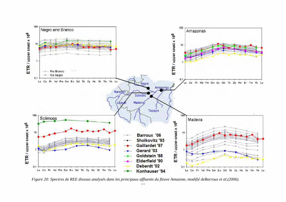
51
Figure 20: Spectres de REE dissous analysés dans les principaux affluents du fleuve Amazone, modifié deBarroux et al.(2006).
1.3 Les éléments Terres Rares en Milieux Aquatiques
52
Barroux et al. (2006) proposent une synthèse de leurs travaux réalisés dans le cadre du
projet Hybam et d’autres études menées sur le Bassin amazonien (Deberdt et al., 2002;
Elderfield et al., 1990; Gaillardet et al., 1997; Gerard et al., 2003; Goldstein and Jacobsen,
1988a; Konhauser et al., 1994; Sholkovitz, 1993)(Figure. 20). Malgré la faible précision (10-
20% RSD) des mesures de concentrations en REE réalisées certaines caractéristiques des
spectres obtenus permettent de différencier nettement la signature du fleuve amazone et de ses
différents affluents. A Óbidos, point d’échantillonnage représentatif du fleuve Amazone, un
spectre « concave» enrichit en MREE avec des teneurs normalisées maximales en Gd et un
enrichissement en HREE par rapport aux LREE. Des tendances similaires sont observées pour
le Madeira avec un fractionnement HREE/LREE plus ample résultant en des rapports Gd/Lu
et Lu/La plus importants. Pour le Negro, l’amplitude du spectre est moins marquée et présente
une légère concavité avec un maximum en Sm ou Gd mais sans enrichissement en HREE par
rapport aux LREE. Les spectres du Solimões ont des caractéristiques proches de celles du
Negro pour les HREE et MREE mais sont appauvris en LREE. Les REE présentent
systématiquement des concentrations plus élevées dans le Negro que dans le rio Solimões. Il y
a une variabilité saisonnière conséquente dans les concentrations en REE et particulièrement
pour le Madeira ainsi qu’une corrélation entre les concentrations de REE et le débit du fleuve.
(Smoak et al., 2006).
Deberdt et al.(2002), ont développé une approche pour étudier la spéciation des REE du
Bassin amazonien en combinant les techniques d’ultrafiltration avec des calculs de spéciation
afin de déterminer la nature des colloïdes et leur contribution dans la mobilité des REE. Le
package EQ3NR de modélisation chimique a été utilisé en prenant en compte les constantes
de complexation inorganiques des principaux ligands dissous, ainsi que les groupes
carboxyliques et phénoliques (R-(COO)22-
, R-(C6H4O2)2-
) comme première approximation
des ligands organiques. La phase colloïdale domine largement la spéciation des REE avec une
forte contribution des colloïdes minéraux comme les hydroxydes de fer pour les eaux
blanches et claires et une forte contribution des colloïdes organiques pour les eaux du Rio
Negro. A l’exception du Trombetas et du Tapajos les REE trivalents libres dans l’eau ne
représentent qu’une faible part du total des REE présents en solution (Figure 21 a et b).
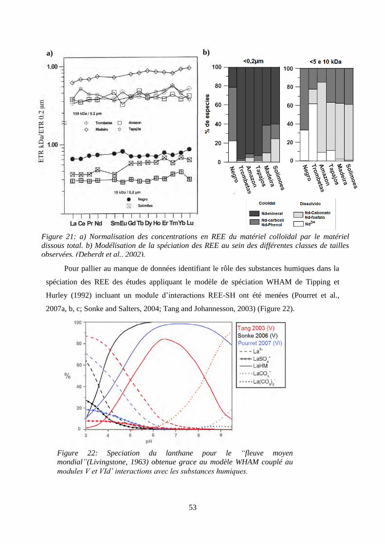
53
Pour pallier au manque de données identifiant le rôle des substances humiques dans la
spéciation des REE des études appliquant le modèle de spéciation WHAM de Tipping et
Hurley (1992) incluant un module d’interactions REE-SH ont été menées (Pourret et al.,
2007a, b, c; Sonke and Salters, 2004; Tang and Johannesson, 2003) (Figure 22).
Figure 21: a) Normalisation des concentrations en REE du matériel colloïdal par le matériel
dissous total. b) Modélisation de la spéciation des REE au sein des différentes classes de tailles
observées. (Deberdt et al., 2002).
a) b)
Figure 22: Speciation du lanthane pour le “fleuve moyen
mondial”(Livingstone, 1963) obtenue grace au modèle WHAM couplé au
modules V et VId’ interactions avec les substances humiques.
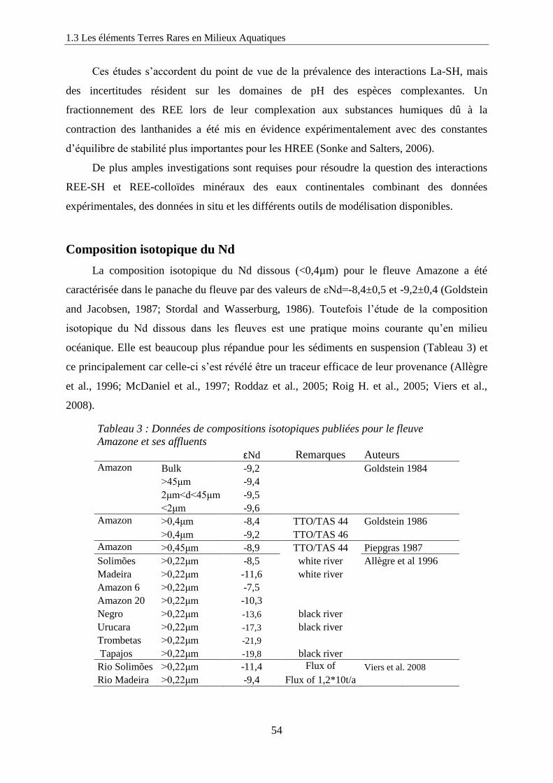
1.3 Les éléments Terres Rares en Milieux Aquatiques
54
Ces études s’accordent du point de vue de la prévalence des interactions La-SH, mais
des incertitudes résident sur les domaines de pH des espèces complexantes. Un
fractionnement des REE lors de leur complexation aux substances humiques dû à la
contraction des lanthanides a été mis en évidence expérimentalement avec des constantes
d’équilibre de stabilité plus importantes pour les HREE (Sonke and Salters, 2006).
De plus amples investigations sont requises pour résoudre la question des interactions
REE-SH et REE-colloïdes minéraux des eaux continentales combinant des données
expérimentales, des données in situ et les différents outils de modélisation disponibles.
Composition isotopique du Nd
La composition isotopique du Nd dissous (<0,4µm) pour le fleuve Amazone a été
caractérisée dans le panache du fleuve par des valeurs de εNd=-8,4±0,5 et -9,2±0,4 (Goldstein
and Jacobsen, 1987; Stordal and Wasserburg, 1986). Toutefois l’étude de la composition
isotopique du Nd dissous dans les fleuves est une pratique moins courante qu’en milieu
océanique. Elle est beaucoup plus répandue pour les sédiments en suspension (Tableau 3) et
ce principalement car celle-ci s’est révélé être un traceur efficace de leur provenance (Allègre
et al., 1996; McDaniel et al., 1997; Roddaz et al., 2005; Roig H. et al., 2005; Viers et al.,
2008).
Tableau 3 : Données de compositions isotopiques publiées pour le fleuve
Amazone et ses affluents
εNd Remarques Auteurs
Amazon
mouth Bulk -9,2 Goldstein 1984
>45μm -9,4
2μm<d<45μm -9,5
<2μm -9,6
Amazon
mouth >0,4μm -8,4 TTO/TAS 44 Goldstein 1986
>0,4μm -9,2 TTO/TAS 46
Amazon
mouth >0,45μm -8,9 TTO/TAS 44 Piepgras 1987
Solimões >0,22μm -8,5 white river Allègre et al 1996
Madeira >0,22μm -11,6 white river
Amazon 6 >0,22μm -7,5
Amazon 20 >0,22μm -10,3
Negro >0,22μm -13,6 black river
Urucara >0,22μm -17,3 black river
Trombetas >0,22μm -21,9
Tapajos >0,22μm -19,8 black river
Rio Solimões >0,22μm -11,4 Flux of
1,4*10^4t/a Viers et al. 2008
Rio Madeira >0,22μm -9,4 Flux of 1,2*10t/a
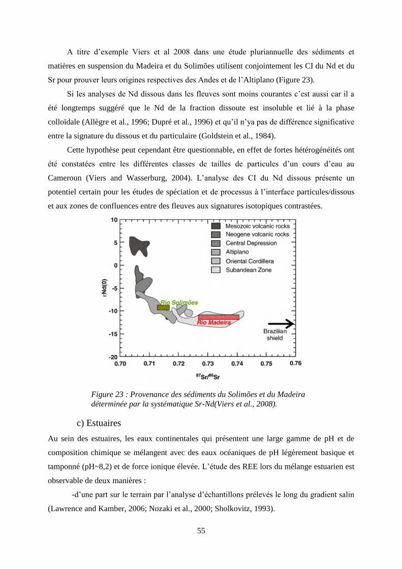
55
A titre d’exemple Viers et al 2008 dans une étude pluriannuelle des sédiments et
matières en suspension du Madeira et du Solimões utilisent conjointement les CI du Nd et du
Sr pour prouver leurs origines respectives des Andes et de l’Altiplano (Figure 23).
Si les analyses de Nd dissous dans les fleuves sont moins courantes c’est aussi car il a
été longtemps suggéré que le Nd de la fraction dissoute est insoluble et lié à la phase
colloïdale (Allègre et al., 1996; Dupré et al., 1996) et qu’il n’ya pas de différence significative
entre la signature du dissous et du particulaire (Goldstein et al., 1984).
Cette hypothèse peut cependant être questionnable, en effet de fortes hétérogénéités ont
été constatées entre les différentes classes de tailles de particules d’un cours d’eau au
Cameroun (Viers and Wasserburg, 2004). L’analyse des CI du Nd dissous présente un
potentiel certain pour les études de spéciation et de processus à l’interface particules/dissous
et aux zones de confluences entre des fleuves aux signatures isotopiques contrastées.
c) Estuaires
Au sein des estuaires, les eaux continentales qui présentent une large gamme de pH et de
composition chimique se mélangent avec des eaux océaniques de pH légèrement basique et
tamponné (pH~8,2) et de force ionique élevée. L’étude des REE lors du mélange estuarien est
observable de deux manières :
-d’une part sur le terrain par l’analyse d’échantillons prélevés le long du gradient salin
(Lawrence and Kamber, 2006; Nozaki et al., 2000; Sholkovitz, 1993).
Figure 23 : Provenance des sédiments du Solimões et du Madeira
déterminée par la systématique Sr-Nd(Viers et al., 2008).
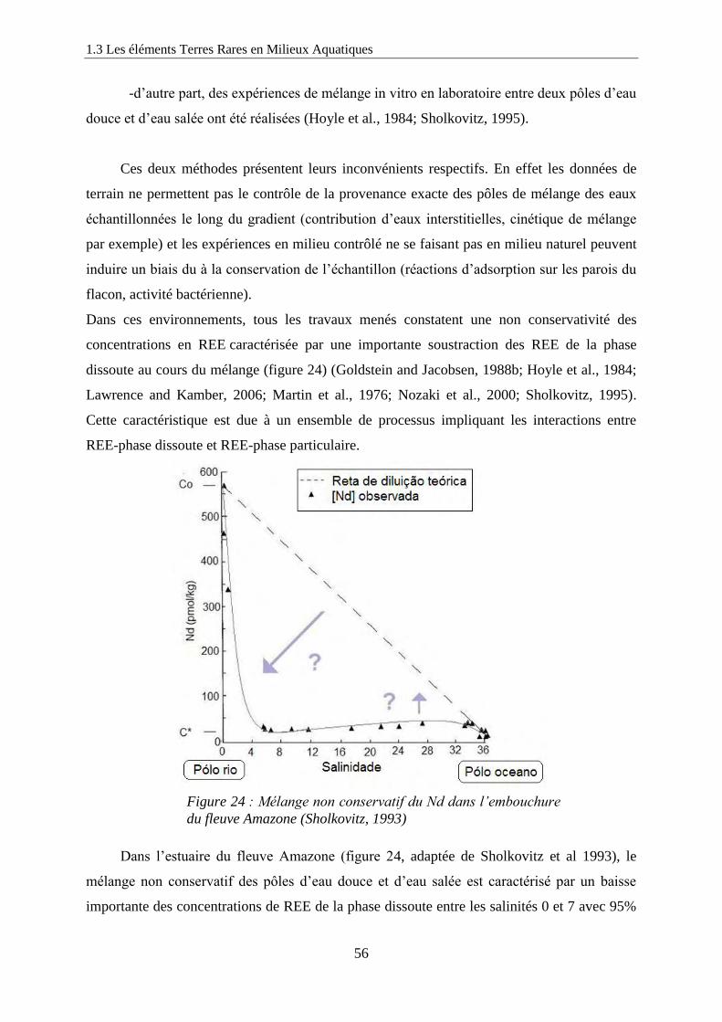
1.3 Les éléments Terres Rares en Milieux Aquatiques
56
-d’autre part, des expériences de mélange in vitro en laboratoire entre deux pôles d’eau
douce et d’eau salée ont été réalisées (Hoyle et al., 1984; Sholkovitz, 1995).
Ces deux méthodes présentent leurs inconvénients respectifs. En effet les données de
terrain ne permettent pas le contrôle de la provenance exacte des pôles de mélange des eaux
échantillonnées le long du gradient (contribution d’eaux interstitielles, cinétique de mélange
par exemple) et les expériences en milieu contrôlé ne se faisant pas en milieu naturel peuvent
induire un biais du à la conservation de l’échantillon (réactions d’adsorption sur les parois du
flacon, activité bactérienne).
Dans ces environnements, tous les travaux menés constatent une non conservativité des
concentrations en REE caractérisée par une importante soustraction des REE de la phase
dissoute au cours du mélange (figure 24) (Goldstein and Jacobsen, 1988b; Hoyle et al., 1984;
Lawrence and Kamber, 2006; Martin et al., 1976; Nozaki et al., 2000; Sholkovitz, 1995).
Cette caractéristique est due à un ensemble de processus impliquant les interactions entre
REE-phase dissoute et REE-phase particulaire.
Dans l’estuaire du fleuve Amazone (figure 24, adaptée de Sholkovitz et al 1993), le
mélange non conservatif des pôles d’eau douce et d’eau salée est caractérisé par un baisse
importante des concentrations de REE de la phase dissoute entre les salinités 0 et 7 avec 95%
Figure 24 : Mélange non conservatif du Nd dans l’embouchure
du fleuve Amazone (Sholkovitz, 1993)
57
des LREE, 90 à 95% des MREE et 85 à 90% des HREE présentes dans l’eau douce qui
disparaissent, puis entre les salinités 7 et 33 les concentrations de REE ré-augmentent, de 10%
pour les LREE, de 2 à 5% pour les MREE et HREE. Il reste à présent incertain si cette hausse
des teneurs en REE dissoutes aux salinités intermédiaires est due à une hétérogénéité de la
zone de mélange estuarienne ou dû à une désorption des REE particulaires (Sholkovitz 1993).
La hausse n’est pas observée pour le Ce, et les auteurs attribuent ce processus à une influence
biologique sur les conditions redox (Sholkovitz and Szymczak, 2000; Sholkovitz, 1993).
Une expérience de mélange in vitro entre un fleuve riche en matière organique avec des
eaux de l’océan adjacent (Hoyle et al., 1984) a conduit à une soustraction préférentielle des
HREE (95%) par rapport aux LREE (60%). En outre, la formation de l’anomalie de Ce
caractéristique du milieu marin n’a pas été observée. Les auteurs ont émis l’hypothèse d’une
association préférentielle des REE avec des colloïdes organo-ferreux. La même expérience fut
répétée avec les eaux d’une rivière présentant de faibles teneurs en matière organique et a
résulté en un mélange conservatif. Une étude de l’estuaire du fleuve Great Whale a montré
qu'en plus de la coagulation de colloïdes riches en fer d’autres processus doivent avoir lieu
dans la zone de mélange ou que la cinétique d’agrégation est plus complexe(Goldstein and
Jacobsen, 1988b). Une expérience de mélange in vitro avec plusieurs étapes d’ultrafiltrations
a été réalisée pour les eaux du Mississipi, Connecticut et Hudson (Sholkovitz, 1995).
L’objectif de cette expérience fut de déterminer précisément l’effet du pH dans l’adsorption
des REE sur les colloïdes de tailles différentes ainsi que les causes du transfert en REE vers la
phase dissoute aux salinités intermédiaires. Une tendance similaire à celle observée dans
l’estuaire du fleuve Amazone a été reproduite au cours de ces mélanges (diminution forte des
concentrations suivie d’une ré-augmentation plus faible en solution). Ces travaux montrent
que plus le pH est proche de la neutralité plus le LREE et MREE sont préférentiellement
associés à la phase colloïdale et que la phase dissoute est fractionnée. De plus, les REE sont
portées principalement par la phase colloïdale et présentent un fractionnement
HREE>MREE>LREE dans les petits colloïdes. Il semble donc que le transfert des REE vers
la phase dissoute aux salinités intermédiaires est préférentiel pour les LREE. Ceci expliquerait
les observations de Sholkovitz (1993) dans l’estuaire de l’Amazone.
Bien que la soustraction des REE de la phase dissoute et le fractionnement associé soit
bien identifiée pour les estuaires, leur spéciation au cours de ce processus et la quantification
du Nd provenant des particules aux salinités plus hautes demeurent incertaines. Ainsi l’apport
de REE par le fleuve Amazone ne peut être calculé en multipliant ses concentrations fluviales
REE par le débit du fleuve. Ce type de calcul repose sur des hypothèses telle que celle de la
1.3 Les éléments Terres Rares en Milieux Aquatiques
58
redissolution complète des colloïdes coagulés (Barroux et al., 2006; Tachikawa et al., 2003)
ou utilisant la concentration effective C* qui est l’extrapolation des teneurs en REE des
salinités les plus élevées vers la salinité 0 mais ne prend pas en compte le transfert particules
-> dissous ni le devenir à plus long terme des colloïdes coagulés porteurs de Nd.
L’utilisation conjointe d’outils tels que l’ultrafiltration, et de modèles de spéciation, et
des expériences de mélange in vitro aident donc à la compréhension des processus qui siègent
dans les zones d’interfaces estuariennes (Goldstein and Jacobsen, 1988b; Hoyle et al., 1984;
Lawrence and Kamber, 2006; Martin et al., 1976; Nozaki et al., 2000; Sholkovitz, 1995). La
confrontation de ces méthodes avec les analyses de composition isotopique lors du contact
particules/eau de mer(Jones et al., 2012; Pearce et al., 2013) doivent permettre de contraindre
avec plus de précision le rôle de estuaires et marges sur le cycle océanique de REE et du Nd et
requiert des méthodes précises de mesures de concentrations.

59
1.4 Objectifs
60
1.4 Objectifs
Les objectifs principaux de ce doctorat sont :
Evaluer la signature, l’origine et le devenir des REE en transit dans l’estuaire du fleuve
Amazone.
Quantifier les apports effectifs de ces éléments à l’océan résultant de l’ensemble des
processus.
Tracer la signature des REE amazoniennes dans les masses d’eau océaniques en contact avec
la marge brésilienne.
Afin atteindre les objectifs généraux, les objectifs spécifiques ont été :
Analyser la composition isotopique du Nd dissous du fleuve Amazone.
Déterminer avec une méthode haute précision les concentrations en REE le long du gradient
salin, ce au sein des différentes classes de taille de particules utilisant des techniques de
filtration et ultrafiltration.
Réaliser des expériences de mélange in vitro entre les eaux des différents pôles de mélange.
Les développements analytiques induits par ces objectifs ont été de :
Perfectionner les protocoles de préconcentration et séparation chimique pour les analyses de
concentrations en REE.
Développer un protocole de séparation chimique pour l’analyse de la composition isotopique
du Nd sur des échantillons d’eau continentale.
Développer une méthode de haute précision et sensibilité pour l’analyse des concentrations en
REE par multi-dilution isotopique (10 spikes REE encrichis) et ICP-MS a secteur magnétique.
61
Objectivos
Os objetivos principais deste doutorado são :
Avaliar a assinatura, a origem e o devir dos REE em trânsito do estuário do rio Amazonas.
Quantificar os aportes efetivos nestes elementos resultando dos processos envolvido no
estuário.
Traçar a assinatura dos REE amazônicos em massas de água oceânicas em contato com a
margem brasileira.
Para cumprir estes objetivos gerais, os objetivos específicos tem sido de :
Analisar a composição isotópica do Nd dissolvido do rio amazonas.
Determinar com um método de alta precisão os teores em REE ao longo do gradiente salino
em diferentes classes de tamanho de partículas usando técnicas de filtração e ultrafiltração.
Realizar experimentos de mistura in vitro entre os dois polos de mistura.
Os desenvolvimentos analíticos induzidos por estes objetivos tem sido de :
Aperfeiçoar os protocolos de reconcentração e separação química para análises de teores
em REE.
Desenvolver um protocolo de separação química para análises de composição isotópica do
Nd em amostras de águas continentais.
Desenvolver um método de alta precisão e sensibilidade para a análise de teores em REE por
multi-diluição isotópica (10 spikes de REE enriquecidos) e ICP-MS de campo magnético
setorial.

62
63
Chapitre 2 :
Méthodologie
Sommaire
2.1 Campagnes d’échantillonnage 64
2.1.1 Campagnes AMANDES 64
2.1.2 Campagne CARBAMA 65
2.1.3 Campagnes cprm-foz. 66
2.1.4 Campagne ANA 66
2.2 Collecte et conditionnement des échantillons 68
2.2.1 Collecte et conditionnement 68
2.2.2 Echantillons “in situ” 69
2.2.3 Echantillons “in vitro” 70
2.3 Détermination des concentrations en éléments Terres rares 72
2.4 Détermination de la composition isotopique du Nd 73
2.4.1 Chimie de préconcentration et séparation 73
2.4.2 La mesure au TIMS Finnigan MAT 261 75
64
2.1 Campagnes d’échantillonnage
La collecte d’échantillons analysés dans le cadre de cette thèse a été réalisée au cours
des campagnes AMANDES 1 2 et 3, CARBAMA 3, CRM-FOZ et ANA-Óbidos, qui
s’insèrent dans des projets multidisciplinaires de recherche en océanographie (AMANDES),
limnologie/hydrologie (CARBAMA) et suivi du débit du fleuve Amazone par le Service
géologique brésilien (Serviço Geológico do Brasil-CPRM) et l’Agence nationale de l’eau
(Agência Nacional das Aguas-ANA).
2.1.1 Campagnes AMANDES
Les campagnes AMANDES 1, AMANDES 2 et AMANDES 3 sont toutes les trois
intégrées au projet AMANDES (Amazon-Andes, IRD/CNRS/ANR). Ces campagnes ont été
réalisées dans l’estuaire, sur la marge, le talus et au large des côtes Guyanaise et Brésilienne à
bord du Navire Océanographique ANTEA (Figure 1).
Elles ont consisté en des déploiements de mouillages instrumentés (courantomètres
doppler de fond), la réalisation de profils de salinité, température et oxygène dissous à l’aide
d’une sonde CTD et la collecte d’échantillons pour analyses de sels nutritifs, concentrations
en éléments traces, mesures de concentrations et de compositions isotopiques de traceurs (Nd,
Ra, Pb, Be…). Le Tableau 1 liste les dates des campagnes et le nombre d’échantillons
prélevés pour les mesures de REE et CI de Nd.
Figure 1 : Stations d’échantillonnage des campagnes
océanographiquesAMANDES 1, 2 et 3.
65
Tableau 1: Dates et nombre d’échantillons collectés durant les campagnes AMANDES
Campagne Date Localisation Echantillons
collectés Profils
AMANDES 1 22/10/2007
04/11/2007 Talus plateforme et large de la côte
Guyanaise, estuaire du fleuve Oyapock. 31 3
AMANDES 2 08/01/2008
24/01/2008 Talus plateforme et large de la côte
Guyanaise, 15 3
AMANDES 3 06/04/2008
17/04/2008 Talus et plateforme de la cote Brésilienne,
estuaire du fleuve Amazone. 14 2
Au cours de la campagne AMANDES 3, le gradient salin a été échantillonné et une
expérience de mélange in vitro entre les pôles d’eau douce et d’eau salée a été réalisée à bord.
2.1.2 Campagne CARBAMA
La campagne d’échantillonnage CARBAMA est liée au projet CARBAMA
(CARBONE-AMAZONIA). Cette campagne a été réalisée à bord du MARGLEISSON II du
11 au 28 mai 2008 et a permis l’échantillonnage, la filtration et l’ultrafiltration des principaux
affluents du fleuve Amazone : le Rio Negro et une várzea (plaine d’inondation) adjacente, le
Rio Solimões, le Rio Madeira, le Rio Tapajós, et le Rio Amazone près de la ville d’Óbidos
(Figure 2).
Figure 2 : Stations d’échantillonage de la campagne
fluvialeCARBAMA 3
2.1 Campagnes d’échantillonnage
66
Un échantillonnage le long du gradient de conductivité de la confluence Rio Negro -
Rio Solimões et une expérience de mélange in vitro de ces deux affluents ont été réalisés
pendant cette campagne.
2.1.3 Campagnes CPRM-FOZ.
Les campagnes CPRM-FOZ sont régulièrement organisées par l’ANA (Agência
Nacional da Águas) et la CPRM (Serviço Geológico do Brasil) avec pour objectif la mesure
précise du débit du fleuve Amazone. Les mesures sont réalisées près de la ville de Macapa
dans le canal nord, le canal sud et le canal de Breves avec un profileur acoustique à effet
doppler (ADCP).Les échantillons des canaux nord et sud ont été collectés les 3 et 4 juin et 1
et 2 septembre 2008 (Figure 3).
2.1.4 Campagne ANA
Lors de la campagne de mesure de débits d’affluents du fleuve Amazone réalisée par
l’ANA en avril 2010, 4 profils ont pu être effectués à Óbidos au moment de la mesure du
débit du fleuve (Figure 4).
Figure 3 : Stations d’échantillonnage de la campagne fluviale CPRM FOZ.
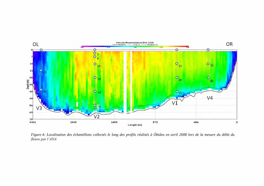
Figure 4: Localisation des échantillons collectés le long des profils réalisés à Óbidos en avril 2008 lors de la mesure du débit du
fleuve par l’ANA
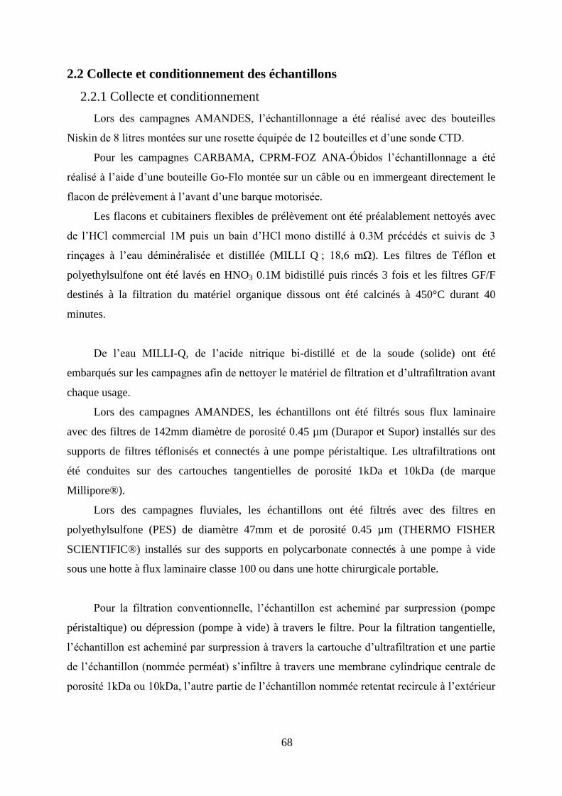
68
2.2 Collecte et conditionnement des échantillons
2.2.1 Collecte et conditionnement
Lors des campagnes AMANDES, l’échantillonnage a été réalisé avec des bouteilles
Niskin de 8 litres montées sur une rosette équipée de 12 bouteilles et d’une sonde CTD.
Pour les campagnes CARBAMA, CPRM-FOZ ANA-Óbidos l’échantillonnage a été
réalisé à l’aide d’une bouteille Go-Flo montée sur un câble ou en immergeant directement le
flacon de prélèvement à l’avant d’une barque motorisée.
Les flacons et cubitainers flexibles de prélèvement ont été préalablement nettoyés avec
de l’HCl commercial 1M puis un bain d’HCl mono distillé à 0.3M précédés et suivis de 3
rinçages à l’eau déminéralisée et distillée (MILLI Q ; 18,6 mΩ). Les filtres de Téflon et
polyethylsulfone ont été lavés en HNO3 0.1M bidistillé puis rincés 3 fois et les filtres GF/F
destinés à la filtration du matériel organique dissous ont été calcinés à 450°C durant 40
minutes.
De l’eau MILLI-Q, de l’acide nitrique bi-distillé et de la soude (solide) ont été
embarqués sur les campagnes afin de nettoyer le matériel de filtration et d’ultrafiltration avant
chaque usage.
Lors des campagnes AMANDES, les échantillons ont été filtrés sous flux laminaire
avec des filtres de 142mm diamètre de porosité 0.45 µm (Durapor et Supor) installés sur des
supports de filtres téflonisés et connectés à une pompe péristaltique. Les ultrafiltrations ont
été conduites sur des cartouches tangentielles de porosité 1kDa et 10kDa (de marque
Millipore®).
Lors des campagnes fluviales, les échantillons ont été filtrés avec des filtres en
polyethylsulfone (PES) de diamètre 47mm et de porosité 0.45 µm (THERMO FISHER
SCIENTIFIC®) installés sur des supports en polycarbonate connectés à une pompe à vide
sous une hotte à flux laminaire classe 100 ou dans une hotte chirurgicale portable.
Pour la filtration conventionnelle, l’échantillon est acheminé par surpression (pompe
péristaltique) ou dépression (pompe à vide) à travers le filtre. Pour la filtration tangentielle,
l’échantillon est acheminé par surpression à travers la cartouche d’ultrafiltration et une partie
de l’échantillon (nommée perméat) s’infiltre à travers une membrane cylindrique centrale de
porosité 1kDa ou 10kDa, l’autre partie de l’échantillon nommée retentat recircule à l’extérieur
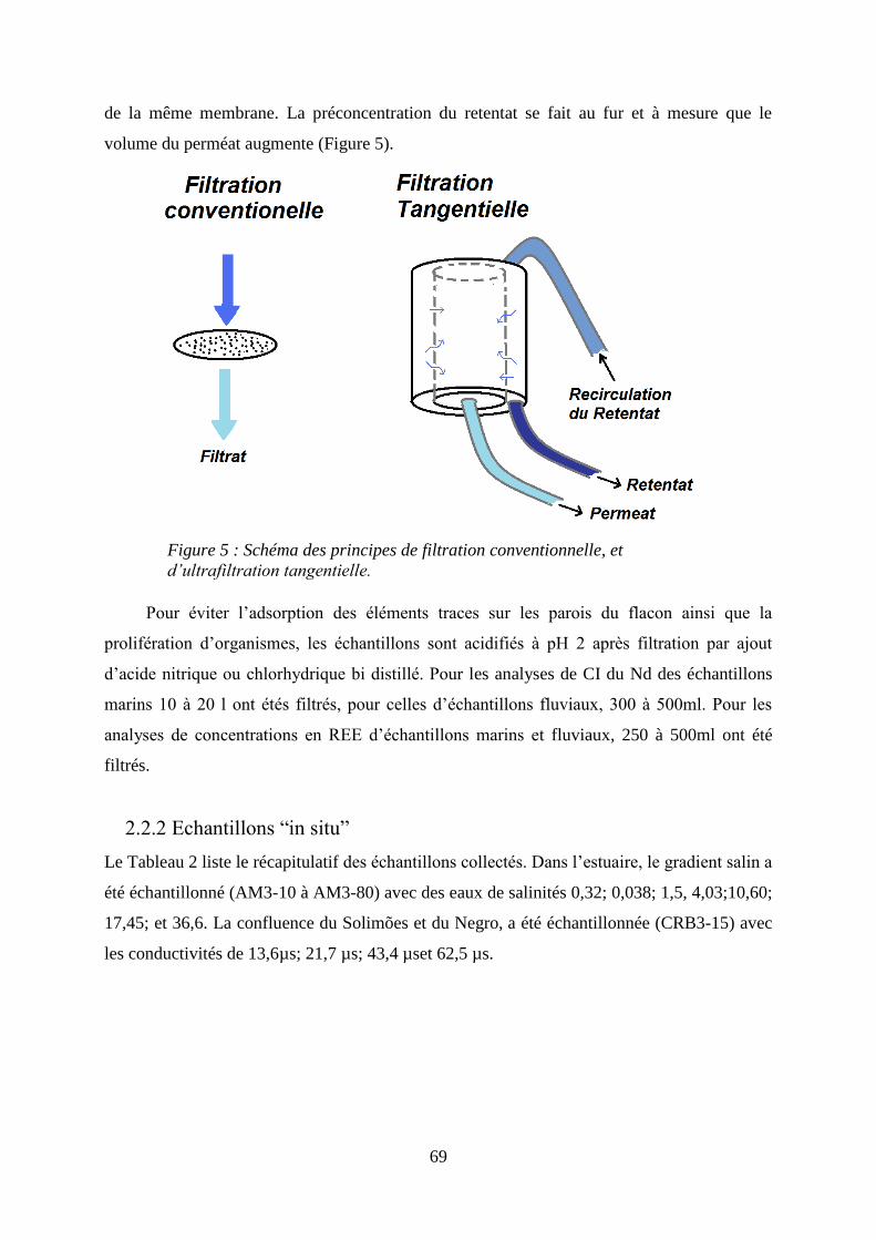
69
de la même membrane. La préconcentration du retentat se fait au fur et à mesure que le
volume du perméat augmente (Figure 5).
Pour éviter l’adsorption des éléments traces sur les parois du flacon ainsi que la
prolifération d’organismes, les échantillons sont acidifiés à pH 2 après filtration par ajout
d’acide nitrique ou chlorhydrique bi distillé. Pour les analyses de CI du Nd des échantillons
marins 10 à 20 l ont étés filtrés, pour celles d’échantillons fluviaux, 300 à 500ml. Pour les
analyses de concentrations en REE d’échantillons marins et fluviaux, 250 à 500ml ont été
filtrés.
2.2.2 Echantillons “in situ”
Le Tableau 2 liste le récapitulatif des échantillons collectés. Dans l’estuaire, le gradient salin a
été échantillonné (AM3-10 à AM3-80) avec des eaux de salinités 0,32; 0,038; 1,5, 4,03;10,60;
17,45; et 36,6. La confluence du Solimões et du Negro, a été échantillonnée (CRB3-15) avec
les conductivités de 13,6µs; 21,7 µs; 43,4 µset 62,5 µs.
Figure 5 : Schéma des principes de filtration conventionnelle, et
d’ultrafiltration tangentielle.
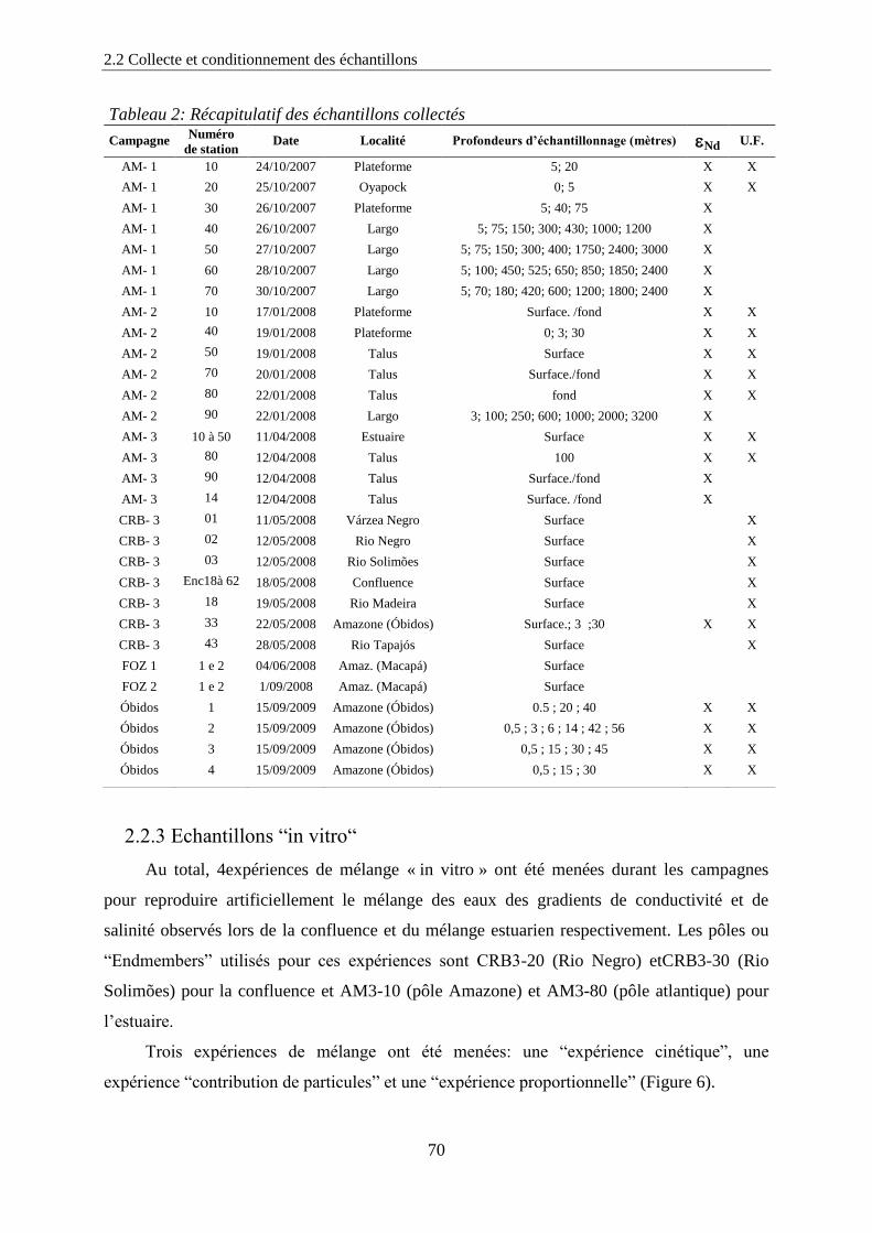
2.2 Collecte et conditionnement des échantillons
70
2.2.3 Echantillons “in vitro“
Au total, 4expériences de mélange « in vitro » ont été menées durant les campagnes
pour reproduire artificiellement le mélange des eaux des gradients de conductivité et de
salinité observés lors de la confluence et du mélange estuarien respectivement. Les pôles ou
“Endmembers” utilisés pour ces expériences sont CRB3-20 (Rio Negro) etCRB3-30 (Rio
Solimões) pour la confluence et AM3-10 (pôle Amazone) et AM3-80 (pôle atlantique) pour
l’estuaire.
Trois expériences de mélange ont été menées: une “expérience cinétique”, une
expérience “contribution de particules” et une “expérience proportionnelle” (Figure 6).
Tableau 2: Récapitulatif des échantillons collectés
Campagne Numéro
de station Date Localité Profondeurs d’échantillonnage (mètres) Nd U.F.
AM- 1 10 24/10/2007 Plateforme 5; 20 X X
AM- 1 20 25/10/2007 Oyapock 0; 5 X X
AM- 1 30 26/10/2007 Plateforme 5; 40; 75 X
AM- 1 40 26/10/2007 Largo 5; 75; 150; 300; 430; 1000; 1200 X
AM- 1 50 27/10/2007 Largo 5; 75; 150; 300; 400; 1750; 2400; 3000 X
AM- 1 60 28/10/2007 Largo 5; 100; 450; 525; 650; 850; 1850; 2400 X
AM- 1 70 30/10/2007 Largo 5; 70; 180; 420; 600; 1200; 1800; 2400 X
AM- 2 10 17/01/2008 Plateforme Surface. /fond X X
AM- 2 40
19/01/2008 Plateforme 0; 3; 30 X X
AM- 2 50
19/01/2008 Talus Surface X X
AM- 2 70
20/01/2008 Talus Surface./fond X X
AM- 2 80
22/01/2008 Talus fond X X
AM- 2 90
22/01/2008 Largo 3; 100; 250; 600; 1000; 2000; 3200 X
AM- 3 10 à 50 11/04/2008 Estuaire Surface X X
AM- 3 80
12/04/2008 Talus 100 X X
AM- 3 90
12/04/2008 Talus Surface./fond X
AM- 3 14
12/04/2008 Talus Surface. /fond X
CRB- 3 01
11/05/2008 Várzea Negro Surface X
CRB- 3 02
12/05/2008 Rio Negro Surface X
CRB- 3 03
12/05/2008 Rio Solimões Surface X
CRB- 3 Enc18à 62
18/05/2008 Confluence Surface X
CRB- 3 18
19/05/2008 Rio Madeira Surface X
CRB- 3 33
22/05/2008 Amazone (Óbidos) Surface.; 3 ;30 X X
CRB- 3 43
28/05/2008 Rio Tapajós Surface X
FOZ 1 1 e 2 04/06/2008 Amaz. (Macapá) Surface
FOZ 2 1 e 2 1/09/2008 Amaz. (Macapá) Surface
Óbidos 1 15/09/2009 Amazone (Óbidos) 0.5 ; 20 ; 40 X X
Óbidos 2 15/09/2009 Amazone (Óbidos) 0,5 ; 3 ; 6 ; 14 ; 42 ; 56 X X
Óbidos 3 15/09/2009 Amazone (Óbidos) 0,5 ; 15 ; 30 ; 45 X X
Óbidos 4 15/09/2009 Amazone (Óbidos) 0,5 ; 15 ; 30 X X
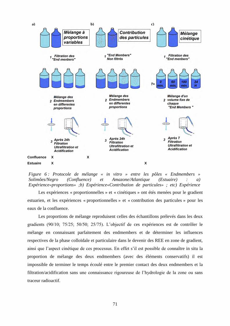
71
Confluence X X
Estuaire X X
Les expériences « proportionnelles » et « cinétiques » ont étés menées pour le gradient
estuarien, et les expériences « proportionnelles » et « contribution des particules » pour les
eaux de la confluence.
Les proportions de mélange reproduisent celles des échantillons prélevés dans les deux
gradients (90/10; 75/25; 50/50; 25/75). L’objectif de ces expériences est de contrôler le
mélange en connaissant parfaitement des endmembers et de déterminer les influences
respectives de la phase colloïdale et particulaire dans le devenir des REE en zone de gradient,
ainsi que l’aspect cinétique de ces processus. En effet s’il est possible de connaître in situ la
proportion de mélange des deux endmembers (avec des éléments conservatifs) il est
impossible de terminer le temps écoulé entre le premier contact des deux endmembers et la
filtration/acidification sans une connaissance rigoureuse de l’hydrologie de la zone ou sans
traceur radioactif.
Figure 6 : Protocole de mélange « in vitro » entre les pôles « Endmembers »
Solimões/Negro (Confluence) et Amazone/Atlantique (Estuaire) : a)
Expérience«proportions» ;b) Expérience«Contribution de particules» ; etc) Expérience
«Cinétique».
a) b) c)
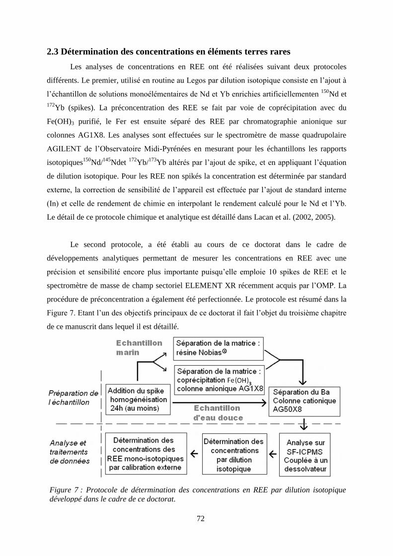
72
2.3 Détermination des concentrations en éléments terres rares
Les analyses de concentrations en REE ont été réalisées suivant deux protocoles
différents. Le premier, utilisé en routine au Legos par dilution isotopique consiste en l’ajout à
l’échantillon de solutions monoélémentaires de Nd et Yb enrichies artificiellementen 150
Nd et
172Yb (spikes). La préconcentration des REE se fait par voie de coprécipitation avec du
Fe(OH)3 purifié, le Fer est ensuite séparé des REE par chromatographie anionique sur
colonnes AG1X8. Les analyses sont effectuées sur le spectromètre de masse quadrupolaire
AGILENT de l’Observatoire Midi-Pyrénées en mesurant pour les échantillons les rapports
isotopiques150
Nd/145
Ndet 172
Yb/173
Yb altérés par l’ajout de spike, et en appliquant l’équation
de dilution isotopique. Pour les REE non spikés la concentration est déterminée par standard
externe, la correction de sensibilité de l’appareil est effectuée par l’ajout de standard interne
(In) et celle de rendement de chimie en interpolant le rendement calculé pour le Nd et l’Yb.
Le détail de ce protocole chimique et analytique est détaillé dans Lacan et al. (2002, 2005).
Le second protocole, a été établi au cours de ce doctorat dans le cadre de
développements analytiques permettant de mesurer les concentrations en REE avec une
précision et sensibilité encore plus importante puisqu’elle emploie 10 spikes de REE et le
spectromètre de masse de champ sectoriel ELEMENT XR récemment acquis par l’OMP. La
procédure de préconcentration a également été perfectionnée. Le protocole est résumé dans la
Figure 7. Etant l’un des objectifs principaux de ce doctorat il fait l’objet du troisième chapitre
de ce manuscrit dans lequel il est détaillé.
2.4 Détermination de la composition isotopique du Nd Figure 7 : Protocole de détermination des concentrations en REE par dilution isotopique
développé dans le cadre de ce doctorat.
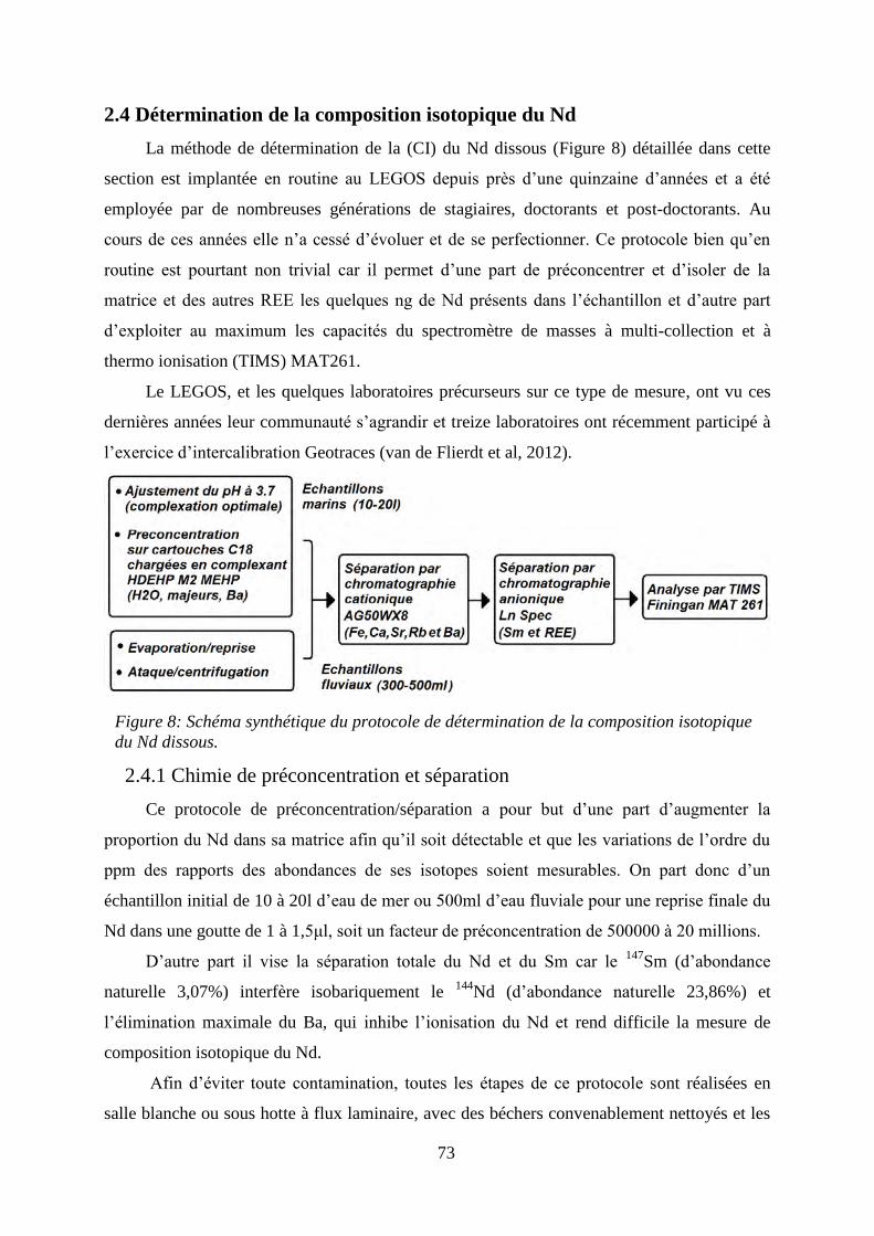
73
2.4 Détermination de la composition isotopique du Nd
La méthode de détermination de la (CI) du Nd dissous (Figure 8) détaillée dans cette
section est implantée en routine au LEGOS depuis près d’une quinzaine d’années et a été
employée par de nombreuses générations de stagiaires, doctorants et post-doctorants. Au
cours de ces années elle n’a cessé d’évoluer et de se perfectionner. Ce protocole bien qu’en
routine est pourtant non trivial car il permet d’une part de préconcentrer et d’isoler de la
matrice et des autres REE les quelques ng de Nd présents dans l’échantillon et d’autre part
d’exploiter au maximum les capacités du spectromètre de masses à multi-collection et à
thermo ionisation (TIMS) MAT261.
Le LEGOS, et les quelques laboratoires précurseurs sur ce type de mesure, ont vu ces
dernières années leur communauté s’agrandir et treize laboratoires ont récemment participé à
l’exercice d’intercalibration Geotraces (van de Flierdt et al, 2012).
2.4.1 Chimie de préconcentration et séparation
Ce protocole de préconcentration/séparation a pour but d’une part d’augmenter la
proportion du Nd dans sa matrice afin qu’il soit détectable et que les variations de l’ordre du
ppm des rapports des abondances de ses isotopes soient mesurables. On part donc d’un
échantillon initial de 10 à 20l d’eau de mer ou 500ml d’eau fluviale pour une reprise finale du
Nd dans une goutte de 1 à 1,5μl, soit un facteur de préconcentration de 500000 à 20 millions.
D’autre part il vise la séparation totale du Nd et du Sm car le 147
Sm (d’abondance
naturelle 3,07%) interfère isobariquement le 144
Nd (d’abondance naturelle 23,86%) et
l’élimination maximale du Ba, qui inhibe l’ionisation du Nd et rend difficile la mesure de
composition isotopique du Nd.
Afin d’éviter toute contamination, toutes les étapes de ce protocole sont réalisées en
salle blanche ou sous hotte à flux laminaire, avec des béchers convenablement nettoyés et les
Figure 8: Schéma synthétique du protocole de détermination de la composition isotopique
du Nd dissous.
74
réactifs utilisés sont ultra-purs ou purifiés en salle blanche. Les molarités des acides doivent
être scrupuleusement respectées, enfin, la réalisation de blanc et le suivi des rendements du
protocole sont nécessaires.
Préconcentration sur cartouches C18 (échantillons d’eau de mer)
Le pH des échantillons est porté à 3,7 +/- 0,2 par l’ajout de quelques gouttes de NH4OH
ultrapur. A l’aide d’une pompe péristaltique, l’échantillon est ensuite injecté au travers de 2 à
4 cartouches Sep Pak C18 préalablement chargées avec 14 gouttes d’un puissant chelatant
phosphaté le HDEHP M2 MEHP (acide phosphorique mono-(2bis-ethyhhexyl)). Chaque
cartouche pouvant traiter 5l d’eau de mer, l’échantillon ainsi préconcentré occupe un espace
réduit et est conservable longtemps, au réfrigérateur et dans le noir.
L’élution de l’échantillon concentré sur les cartouches est réalisée toujours avec une
pompe péristaltique avec laquelle on fait couler d’abord 5mlde HCl 0,01N à travers les
cartouches qui assurent la séparation d’une grande partie du Ba suivis de 35 ml d’ HCl 6N
dans lesquels les REE sont récupérées.
Evaporation et attaque (échantillons d’eau fluviale)
Les échantillons sont évaporés puis digérés dans un bain d’eau régale. Si le résidu de
matière organique reste important après ce traitement, l’échantillon peut être centrifugé ou
attaqué par ajout de quelques gouttes d’eau oxygénée.
Chromatographie Cationique AG50 W X8
Les éluats des cartouches C18 (eau de mer) ou les résidus d’attaque (eau fluviale) sont
évaporés et repris avec 2ml de HCl 2N puis chargés sur une colonne de 15cm de hauteur et
0,5cm de diamètre remplie de 1ml de résine cationique AG50WX8 100-200 mesh ; 13 ml de
HCL 2N sont premièrement élués, suivis de 4 ml de HNO3 2,5N Ces étapes permettent
l’élimination de Fe, Ca, Sr, Rb et Ba. Les REE sont enfin éluées dans une fraction de 6ml de
HCl 4N. Les colonnes sont ensuite nettoyées avec 4ml de HNO3 2,5n et 15ml HCl 6N prêts à
l’emploi pour une nouvelle série de chromatographie.
Chromatographie Anionique LN Spec
Les colonnes Ln mesurent 7cm et sont remplies de 385mg de résine Ln Spec. Elles
permettent une séparation fine entre le Nd et les REE voisines. Pour cette raison, chaque
colonne lors de sa préparation est calibrée indépendamment avec un indicateur coloré et
permettant de déterminer la fenêtre exacte d’élution du Nd, celle-ci pouvant varier
sensiblement d’une colonne à l’autre.
Les éluats des colonnes cationiques AG50W-X8 sont évaporés et repris avec 0,2ml de
HCl 0,2N puis chargés sur les colonnes. Des volumes spécifiques à chaque colonne de
75
HCl0,2N (Elution REE) puis de HCl 0,25N (élution Nd) sont ensuite déposés sur la colonne.
Après évaporation de l’éluat de cette dernière fraction, l’échantillon est prêt pour l’analyse.
2.4.2 La mesure au TIMS Finnigan MAT 261
La mesure de composition isotopique du Nd est réalisée à l’aide d’un spectromètre de
masse multi-collecteur à secteur magnétique à thermo ionisation (TIMS) Finningan MAT261.
L’échantillon, au terme du protocole chimique de séparation est repris dans 1,5μl
d’HCl 2N puis déposé sur un filament de Re positionné sur un barillet contenant treize
emplacements. Chaque emplacement comporte deux filaments de Re installés face à face et
parallèlement : le filament évaporant (sur lequel le Nd a été déposé) et un filament ionisant.
Une tension est dans un premier temps appliquée graduellement au filament évaporant et
provoque son réchauffement par effet Joule et l’évaporation progressive du dépôt, une tension
est ensuite appliquée au deuxième filament qui provoque l’ionisation du Nd évaporé.
Les ions sont accélérés par un champ magnétique formant un faisceau, ce faisceau est
ensuite dévié par un puissant aimant permettant leur séparation par masse atomique pour être
ensuite détectés dans des cages faraday. Le signal converti en volts est mesuré, et le calcul des
rapports isotopiques est ainsi possible. Les réglages (tuning) électromagnétiques de guidage et
focalisation des faisceaux ioniques varient d’un échantillon à l’autre et sont réalisés
manuellement au cours du réchauffement progressif des filaments. Une séquence
d’acquisition est lancée lorsque le signal détecté atteint une intensité et une stabilité
satisfaisantes. L’acquisition peut être menée en mode statique au cours duquel chaque
collecteur réceptionne une masse unique, ou bien en mode dynamique ou « jumping mode »
au cours duquel les collecteurs mesurent des cycles successifs de signaux de deux à trois
isotopes distincts. Les processus d’évaporation et de séparation fractionnent des ions en
favorisant premièrement la transmission des masses les plus légères et ensuite, par effet de
réservoir, des masses les plus lourdes. Ce biais de masse variable tout au long de
l’évaporation de l’échantillon peut être modélisé convenablement par une loi statistique
exponentielle qui en permet la correction mathématique après acquisition.

76
77
Chapitre 3 :
Analyse de concentrations en REE par
dilution isotopique sur un SF-ICPMS
Sommaire
3.1 Introduction 78
/ Introdução 83
3.2 Article publié :Rare earth element analysis in natural waters by
multiple isotope dilution-sector field ICP-MS. 86
1. Introduction 87
2. Materials and Methods 89
3 Results and discussion 102
4 Conclusions 112
Notes and references 114
Supplementary Informations 115
78
3.1Introduction
Afin d’observer des variations subtiles des spectres et anomalies de REE dans les
phases dissoutes et colloïdales au sein du gradient de salinité de l’estuaire du fleuve Amazone
et du gradient de conductivité de la confluence Rio Negro/Rio Solimões, mon travail de
doctorat s’est appuyé sur des objectifs analytiques ambitieux. Il s’agissait de mesurer les
concentrations des différentes REE dans ces matrices avec une précision analytique de
2SD%. Cette précision est comparable aux précisions atteintes par ID-TIMS (Dilution
isotopique et spectromètre de masse à thermo ionisation). Cette dernière méthode était
utilisée jusqu’au début de années 90 et permettait l’analyse très précise des REE possédant au
minimum 2 isotopes (10 de 14 REE). Les travaux pionniers des équipes d’Harry Elderfield en
Angleterre et d’Ed Sholkovitz aux USA sont tous basés sur cette méthode particulièrement
appropriée pour l’analyse du gradient salin. Cette méthode requiert toutefois une chimie de
séparation fastidieuse et un long temps d’analyse.
Au cours des années 90, l’utilisation des ICPMS quadrupolaires (spectromètres de
masses à source plasma) par standard externe s’est répandue permettant la mesure de la
totalité des REE (donc incluant les monoisotopiques, Pr, Tm, Tb, Ho) en un temps très réduit
d’analyse mais au détriment de la précision de la mesure (~3 à 12 RSD%). Un regain de
précision et de limite de détection a pu être atteint par la suite avec les générations de
spectromètres de masse à champ sectoriel SF-ICPMS et/ou utilisant des standards internes
(In, Re, Tm..). Les géochimistes marins du LEGOS ont ensuite proposé la combinaison de la
mesure par standard externe et de la dilution isotopique sur 2 REE, permettant une
amélioration significative de la précision et la possibilité de corriger convenablement les
rendements de préconcentration et séparation chimique mais sans toutefois égaler les mesures
par ID-TIMS. Une liste non exhaustive de méthodes d’analyses de REE en eaux naturelles est
reportée dans le tableau 5.
Le développement de la méthode qui fait l’objet de ce chapitre a été inspiré des travaux
de Baker et al. (2002), qui ont été les premiers à s’intéresser au transfert d’une méthode à dix
spikes sur ICPMS. Les auteurs ont récupéré des mélanges de spike utilisés par Matthew
Thirwall du temps des mesures ID TIMS et ont développé un protocole d’analyses de roches
sur un ICPMS multicollecteur (MC-ICPMS).
L’objectif de cette partie de la thèse fut de créer un protocole d’analyses de REE
dissous par dilution isotopique en étendant la méthode « LEGOS » de deux spikes à dix
spikes et mettant à profit une machine acquise récemment par la plateforme analytique de
l’OMP : l’ICP-MS de champ sectoriel ELEMENT-XR.
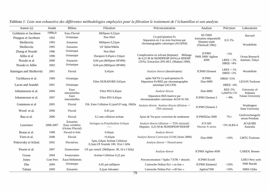
79
Tableau 1: Liste non exhaustive des différentes méthodologies employées pour la filtration le traitement de l’échantillon et son analyse.
Auteur (s) Année Milieu Filtration Préconcentration Analyse Précision Laboratoire
Goldstein et Jacobsen 1988a,b
Estu./Fluvial Millipore 0,22µm
Co-précipitation Fe
Séparation en 2 ou trois fractions par
chromatographie cationique (AG50X8)
ID-TIMS
Ionisation séquentielle
filament triple
(Thirlwall 1982)
0,5/ 2%.
Harvard Piepgras et Jacobsen 1992 Océanique
Non filtré
Sholkovitz 1993 Estuarien Millipore 0,22µm
WoodsHole Sholkovitz 1995 Estuarien UF 5kDa/50kDa
Zhang et Nozaki 1996 Océanique
Non filtré
Complexation en solvant (heptane): Mélange
de 0,25 M de M2HDPEHP (65%) et HDEHP
(35%). Extraction 20% HCl. (Shabani 1990)
ICPMS
PMS 2000/ Agilent
4500
<5% Ocean Research
Institute, Tokyo
Alibo et al 1999 Océanique
Durapore 0,45µm e 0,6µm
Nozaki et al 2000 Estuarien 0,04 µm (Millipore HF400) LREE < 2%
HREE <4% Nozaki et Alibo 2003 Océanique
0,04 µm (Millipore HF400)
Hannigan and Sholkovitz 2001 Fluvial 0,45µm Analyse directe (dessolvateur) ICPMS Element LREE < 1%
HREE <2% WoodsHole
Tachikawa et al. 1999 Océanique Filtre DURAPORE 0,65µm
spike Nd/Yb Co-précipitation Fe
Séparation Fe/REE par chromatographie
anionique (AG1X8)
ICPMS
Elan 6000
LREE < 5%
LEGOS Toulouse HREE<15%
Lacan and Jeandel 2001 Océanique LREE<0,9% HREE <4%
Johannesson et al. 2004 Eaux
interstitielles Filtre PES 0,45µm Analyse directe Elan 6000
REE<5%
LaNdYb<1%
Ce<10%
University of
Alabama
Johannesson et al. 2007 Eaux
interstitielles Filtre PES 0,45µm
Séparation REE/matrice par
chromatographie cationique AG50 W-X8 ICPMS Element 2 < 4%
Tulane University
Gammons et al 2005 Fluvial Filt. Ester Cellulose 0,1µm/UF tang. 10kDa Analyse directe Analyse directe (dilution ->
TDS minimal) ICPMS Element 2
Washington
State University Wood et al. 2006 Fluvial 0,45 µm
Bau et al. 2006 Fluvial 0,2 mm cellulose-acétate Ajout de Tm pour correction de rendement ICPMSElan 5000 7%< GeoForschungsZe
ntrum Potsdam
Lawrence 2006-2007
Estuarien
Eaux certifiées
(Océan./Fluvial)
Seringue en Polyéthylène 0,45µm
-----
Analyse directe (dilution -> TDS minimal)
Heptano: 0,25 M de M2HDPEHP/HDEHP
ICP-MS
Thermo X series <3% SLRS-4
ACQUIRE
Australia
Braun et al. 1998 Fluvial et Sols 0,45µm Analyse directe
Elan 6000 <10% LMTG Toulouse Viers et al. 2008 Fluvial >0,45µm Analyse directe Correction O/OH (Aries 2000)
Pokrovsky et Schott 2002 Fluvial/est. 5µm, 0,8µm Acétate Cellulose
0,2µm.UF frontale 100, 10,et 1 kDa Analyse directe + Dessolvateur
Pouret et al. 2007 Souterraines UF par centrif. (Millipore: 30, 10 e 5 kDa) Analyse directe ICPMS Agilent 4500 CAREN, Rennes
Gruau 2004 Souterraines Acétate Cellulose 0,22 µm
Jones Com Pers Eaux/Sédiments -
Preconcentration ? Spike 7 ETR + dessolv. ICPMS Excell LDEO New york
Zhu 2009 Océanique
0,45 µm millipore Cartouche Nobias Pa1 « on line » ICPMS Element2 <10% NMI Ibaraki
Takata 2009 Estuarien 0,2µm Advantec Cartouche Nobias Pa1 « off line » Agilent7500 <10% NIRS Chiba
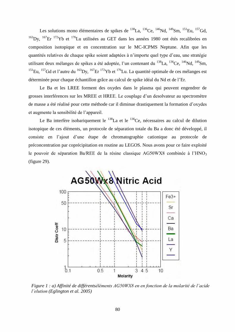
80
Les solutions mono élémentaires de spikes de 138
La, 136
Ce, 146
Nd, 149
Sm, 151
Eu, 157
Gd,
163Dy,
167Er
172Yb et
176Lu utilisées au GET dans les années 1980 ont étés recalibrées en
composition isotopique et en concentration sur le MC-ICPMS Neptune. Afin que les
quantités relatives de chaque spike soient adaptées à n’importe quel type d’eau, une stratégie
utilisant deux mélanges de spikes a été adoptée, l’un contenant du 138
La, 136
Ce, 146
Nd, 149
Sm,
151Eu,
157Gd et l’autre du
163Dy,
167Er
172Yb et
176Lu. La quantité optimale de ces mélanges est
déterminée pour chaque échantillon grâce au calcul de spike idéal du Nd et de l’Er.
Le Ba et les LREE forment des oxydes dans le plasma qui peuvent engendrer de
grosses interférences sur les MREE et HREE. Le couplage d’un desolvateur au spectromètre
de masse a été réalisé pour cette méthode car il diminue drastiquement la formation d’oxydes
et augmente la sensibilité de l’appareil.
Le Ba interfère isobariquement le 138
La et le 136
Ce, nécessaires au calcul de dilution
isotopique de ces éléments, un protocole de séparation totale du Ba a donc été développé, il
consiste en l’ajout d’une étape de chromatographie cationique au protocole de
préconcentration par coprécipitation en routine au LEGOS. Nous avons pour ce faire exploité
le pouvoir de séparation Ba/REE de la résine classique AG50WX8 combinée à l’HNO3
(figure 29).
Figure 1 : a) Affinité de différentséléments AG50WX8 en en fonction de la molarité de l’acide
l’elution (Eglington et al. 2005)
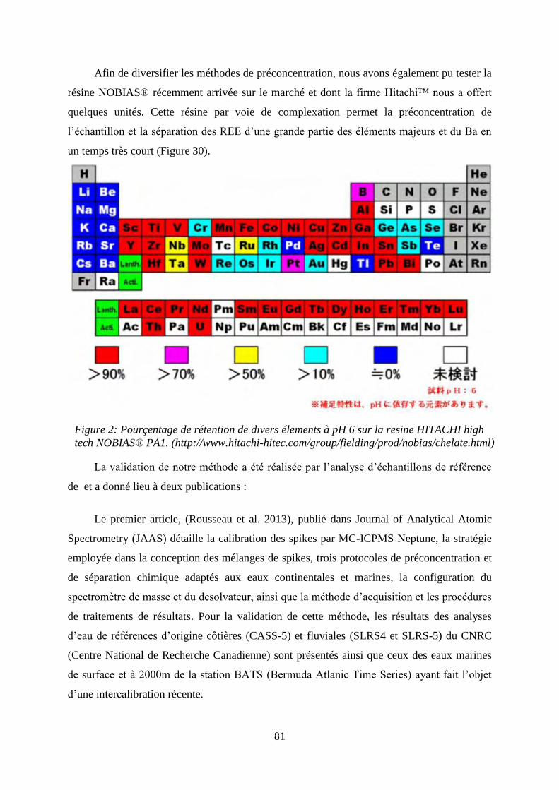
81
Afin de diversifier les méthodes de préconcentration, nous avons également pu tester la
résine NOBIAS® récemment arrivée sur le marché et dont la firme Hitachi™ nous a offert
quelques unités. Cette résine par voie de complexation permet la préconcentration de
l’échantillon et la séparation des REE d’une grande partie des éléments majeurs et du Ba en
un temps très court (Figure 30).
La validation de notre méthode a été réalisée par l’analyse d’échantillons de référence
de et a donné lieu à deux publications :
Le premier article, (Rousseau et al. 2013), publié dans Journal of Analytical Atomic
Spectrometry (JAAS) détaille la calibration des spikes par MC-ICPMS Neptune, la stratégie
employée dans la conception des mélanges de spikes, trois protocoles de préconcentration et
de séparation chimique adaptés aux eaux continentales et marines, la configuration du
spectromètre de masse et du desolvateur, ainsi que la méthode d’acquisition et les procédures
de traitements de résultats. Pour la validation de cette méthode, les résultats des analyses
d’eau de références d’origine côtières (CASS-5) et fluviales (SLRS4 et SLRS-5) du CNRC
(Centre National de Recherche Canadienne) sont présentés ainsi que ceux des eaux marines
de surface et à 2000m de la station BATS (Bermuda Atlanic Time Series) ayant fait l’objet
d’une intercalibration récente.
Figure 2: Pourçentage de rétention de divers élements à pH 6 sur la resine HITACHI high
tech NOBIAS® PA1. (http://www.hitachi-hitec.com/group/fielding/prod/nobias/chelate.html)
3.1 Introduction
82
Un second article publié dans Geostandards and Analytical Methods est un exercice
d’intercalibration de la mesure du standard SLRS 5 dans lequel nos résultats d’analyse de
SLRS 5 sont comparables à ceux obtenus avec 8 autres méthodes pratiquées en routine dans
des laboratoires français, il est reporté en annexe de ce manuscript.
La méthode Multispikes développée dans le cadre de ce doctorat est sans doute
actuellement la plus juste et la plus précise au monde pour des analyses de REE dissous en
eaux naturelles par ICPMS et se rapproche de la qualité des mesures ID-TIMS.
83
Introdução
Para observar as variações suteis dos espectros e das anomalias dos REE nas fases
dissolvidas e coloidais do gradiente de salinidade do estuário do rio Amazonas e do
gradiente de conductividade da confluência rio Negro/rio Solimões, meu trabalho de
doutorado teve objetivos analíticos ambiciosos, consistindo em medir os teores em REE
nestas matrizes com uma precisão analítica de 2SD%.
Esta precisão é comparável às atingidas por ID-TIMS (diluição isotópica com
espectrômetro de termo-ionização). Este método, usado até o começo dos anos 90,
permitia a análise muito precisa dos REE possuindo no mínimo 2 isótopos (10 dos 14 REE).
Os trabalhos pioneiros dos grupos de Harry Elderfield na Inglaterra e de Ed Sholkovitz nos
Estados Unidos, são baseados neste método particularmente apropriado para a análise do
gradiente salino. No entanto, este método requer uma química de separação fastidiosa e
um tempo de análise elevado.
Nos anos 90, o uso dos ICPMS quadruplares (Espectrômetros de massa com fonte de
plasma) por padrão externo se generalizaram permitindo a medida da totalidadedos REE
(incluindo os monoisotópicos, Pr, Tm, Tb, Ho) em um tempo de analise muito reduzido mas
ao padecer da precisão da medida (~3 à 12 RSD%). Um reganho na precisão e no limite de
detecção tem sido atingido posteriormente com as gerações de espectrômetros de massas
de campo setorial SF-ICPMS e /ou utilizando padrões internos (In, Re, Tm..). Os geoquímicos
oceanógrafos do LEGOS tem proposto posteriormentede combinar a medida do padrão
externo com a medida por diluição isotópica sobre 2 REE, permitindo uma melhoria
significativa na precisão e a possibilidadede corrigir convenientemente os rendimentos de
pré-concentração e separação química sem, no entanto, igualizar as medidas por ID-
TIMS.Uma lista não exaustiva dos métodos de análise dos REE em águas naturais é
reportada na Tabela 5.
O desenvolvimento do método apresentado neste capítulo foi inspirado no trabalho
de Baker (2002), que foi um dos primeiros a se interessar à transferência de um método de
10 spikes do TIMS para o ICPMS. Os autores utilizaram as misturas de spike usadas por
Mattew Thirwall no tempo das medidas ID-TIMS desenvolveram um protocolo de análises
3.1 Introdução
84
de rochas com um ICPMS multicoletor (MC-ICPMS).O objetivo deste artigo consistiu em
criar um protocolo de análises de REE dissolvidos por diluição isotópica ampliando o
« método Legos »de 2 spikes para 10 spikes aproveitando um aparelho adquirido
recentemente pela plataforma analítica do OMP : O ICPMS de campo setorial ELEMENT-XR.
As soluções monoelementarias de spikes de 138La, 136Ce, 146Nd, 149Sm, 151Eu, 157Gd,
163Dy, 167Er 172Yb e 176Lu, utilizadas no GET nos anos 1980, foram recalibradas em
composição isotópica e concentração com o MC-ICPMS Neptune. Para que as quantidades
relativas de cada spike estejam adaptadas a qualquer tipo de água, uma estratégia usando
duas misturas de spike foi adotada. Uma mistura contendo138La, 136Ce, 146Nd, 149Sm, 151Eu,
157Gd e a outra 163Dy, 167Er 172Yb et 176Lu. A quantidade optimal destas misturas é
determinada para cada amostra mediante o cálculo da quantidade de spike ideal de Nd e Er.
O Ba e os LREE formam óxidos no plasmaque podem levar a grandes interferências sobre os
MREE e LREE.A acoplagem de um dessolvatador ao espectrômetro de massas foi realizada
para este método porque desta forma diminui drasticamente a formação de óxidos e
aumenta a sensibilidade do aparelho.
O Ba interfere isobaricamente o 138La et le 136Ce necessários no calculo da diluição
isotópica destes elementos, assim um protocolo de separação total do Ba foi desenvolvido.
Este consiste na adição deuma etapa de chromatografia catiônica ao protocolo de pré-
concentração em rotina no LEGOS. Temos explorado o poder de separação Ba/REE da resina
clássica AG50WX8 combinada ao l’HNO3 (Figura 29).
Para diversificar os métodos de pré-concentração, testamos também a resinaNOBIAS®
recentemente chegada no mercado e cuja a firma HITACHI®nos ofertou algumas unidades.
Esta resina, por via de complexação, permite a pré-concentração da amostra e a separação
dos REE do Ba e de uma grande parte dos elementos maiores num tempo reduzido (Figura
30).
A validação do nosso método foi realizada com a análise de amostras de referência,
que consiste na adição deuma etapa de chromatografia catiônica ao protocolo de pré-
concentração e tem levado a redação de duas publicações :
85
O primeiro artigo, (Rousseau et al. 2013),publicado em Journal of Analytical Atomic
Spectrometry (JAAS) detalha a calibração dos spikes por MC-ICPMS Neptune, a estratégia
empregada na concepção das misturas de spikes, 3 protocolos de reconcentração e
separação química adaptados as águas continentais e marinhas, a configuração
doespectrômetro de massas e do dessolvator, bem como o método de aquisição e os
procedimentos no tratamento dos resultados. Para a validação deste método, os
resultadosde análises de águas de referências de origem costeira (CASS-5) e fluviais (SLRS4
et SLRS-5) do CNRC (Centro nacional de pesquisa do Canadá).São apresentados também os
de amostras águas marinhas de superfície e a 2000m da estação BATS (Bermuda Atlantic
Time Series)recentemente intercalibradas.
O segundo artigo publicado em Geostandards and Analytical Methods é um exercício
de intercalibração na medida da água de referência SLRS 5 no qual nossos resultados são
comparadoscom aqueles obtidos com 8 outros métodos praticados em rotinaem
laboratórios franceses, este é artigo esta reportado em annexo deste manuscrito.
O método multispike desenvolvido neste doutorado é, sem duvida, atualmente, o
mais justo e preciso no mundo para análises de REE dissolvidos em águas naturais por
ICPMS e se aproxima da qualidade de medidas obtidas ID-TIMS.
86
3.2 Article publié : Rare earth element analysis in natural waters by
multiple isotope dilution - sector field ICP-MS.
Tristan Rousseau,*a
Jeroen E. Sonke,a Jerome Chmeleff,
a Frederic Candaudap,
a François
Lacan,b Geraldo Boaventura
c, Patrick Seyler
a, Catherine Jeandel
b.
aGET, Université de Toulouse, CNRS, IRD, CNES, 14 Avenue Edouard Belin, F-31400
Toulouse, France. bLEGOS, Université de Toulouse, CNRS, IRD, CNES, 14 Avenue Edouard Belin, F-31400
Toulouse, France cUniversidade De Brasilia, UNB, LAGEQ, Campus universitario Darcy Ribeiro, 70.910-900 Brasilia,
DF, Brazil
Received 1st November 2012 /Accepted 4th February 2013
DOI: 10.1039/c3ja30332b
www.rsc.org/jaas
Abstract
The rare earth elements (REEs) are valuable tracers in the earth, ocean and
environmental sciences. Ten out of fourteen stable REEs have two or more isotopes, making
them suitable for quantification by isotope dilution. We present a plasma mass spectrometry
based multiple isotope dilution method for high precision REE concentration analysis in
aqueous media. Key aspects of the method are: (i) flexible spiking of ten REEs via two LREE
and HREE mixed spike solutions. (ii) Offline pre-concentration and matrix removal, by ion
chromatography for freshwater samples and by iron co-precipitation or ion chromatography
with the Nobias resin for seawater samples. (iii) High sensitivity detection by sector field-
inductively coupled plasma mass spectrometry (SF-ICP-MS). (vi) The use of a desolvation
micro-nebulization introduction system to lower polyatomic Ba and LREE-oxide
interferences on HREEs. The method is suitable for a range of freshwater to seawater type
samples, and was validated against SLRS-4, SLRS-5, and CASS-5 reference materials and
two GEOTRACES marine inter-comparison samples. Long-term external precision on all
REEs was <2% RSD, except La and Ce. Minimum sample volumes are 1 ml for freshwater
and 50 ml for seawater. The multispike SF-ICP-MS method should be of particular interest in
exploring subtle variations in aqueous REE fractionation patterns and anomalies in large
numbers of samples.
87
1. Introduction
Rare Earth Elements (REEs) in rocks and sediments are tracers of crustal differentiation
or palaeoproxies for seawater REE composition.1–4
In natural waters REEs – together with Nd
isotopes – are tracers of lithogenic inputs, solute–particle interactions, redox processes, and
water mass mixing and circulation.5–11
To first order, the aqueous geochemistry of the REE is governed by the lanthanide
contraction effect, i.e. the gradual decrease in ionic radii from La to Lu. Yet, both in
experimental and natural systems complex REE trends are observed that require different
explanations. Examples are middle REE (MREE) enrichment in Amazon River waters that
have been linked to preferential dissolution of MREE-enriched phosphate minerals,12
or the
so-called tetrad effect in seawater samples.13
In addition to redox related Ce anomalies in
most natural waters, observations of natural Gd and Tb anomalies in seawater14
and evidence
of anthropogenic La and Gd anomalies have been reported.15,16
Both the tetrad effect and the
seawater Gd and Tb anomalies have been questioned due to analytical limitations and
normalization issues.17
Detecting subtle changes in REE patterns and REE anomalies in these
fractions often requires final uncertainties better than 2% RSD.
There are several methods for REE concentration determination in natural waters.
Initially highly precise, yet time consuming analyses were made by isotope dilution (ID)
thermal ionization mass spectrometry.8,18
While ID avoids quantification problems due to
losses of REE during sample preparation, this method required laborious matrix and intra-
REE separations due to a limited Faraday cup configuration flexibility and the need to avoid
interferences.19–21
One could typically determine three REEs at the same time, and mono-
isotopic REEs were not measured by this method.
In the 1990s, the advent of inductively coupled plasma mass spectrometers (ICP-MS)
provided much faster yet less precise analyses. REE concentration determination by
quadrupole (Q-) ICP-MS using external calibration yields typical RSD's of 5–15%. Despite
relatively low detection limits, oxide interferences in REEs, and matrix effects, Q-ICP-MS
has been the key in exploring REE cycling in continental waters.22–25
The use of sample
aerosol desolvating devices as ICP-MS introduction systems has been shown to enhance
sensitivity and limit Ba and light REEs (LREEs) oxide interferences on heavy REEs
(HREEs).26
Finally, single and multi-collector sector field mass spectrometers (SF-ICP-MS)
have higher sensitivity than Q-ICP-MS, making them more suitable for ultra-trace REE
analysis. Following dilution of seawater in order to lower the matrix ion concentrations
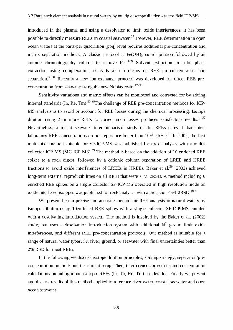
3.2 Rare earth element analysis in natural waters by multiple isotope dilution - sector field ICP-MS.
88
introduced in the plasma, and using a desolvator to limit oxide interferences, it has been
possible to directly measure REEs in coastal seawater.27
However, REE determination in open
ocean waters at the parts-per quadrillion (ppq) level requires additional pre-concentration and
matrix separation methods. A classic protocol is Fe(OH)3 coprecipitation followed by an
anionic chromatography column to remove Fe.28,29
Solvent extraction or solid phase
extraction using complexation resins is also a means of REE pre-concentration and
separation.30,31
Recently a new ion-exchange protocol was developed for direct REE pre-
concentration from seawater using the new Nobias resin.32–34
Sensitivity variations and matrix effects can be monitored and corrected for by adding
internal standards (In, Re, Tm).35,36
The challenge of REE pre-concentration methods for ICP-
MS analysis is to avoid or account for REE losses during the chemical processing. Isotope
dilution using 2 or more REEs to correct such losses produces satisfactory results.11,37
Nevertheless, a recent seawater intercomparison study of the REEs showed that inter-
laboratory REE concentrations do not reproduce better than 10% 2RSD.38
In 2002, the first
multispike method suitable for SF-ICP-MS was published for rock analyses with a multi-
collector ICP-MS (MC-ICP-MS).39
The method is based on the addition of 10 enriched REE
spikes to a rock digest, followed by a cationic column separation of LREE and HREE
fractions to avoid oxide interferences of LREEs in HREEs. Baker et al.39
(2002) achieved
long-term external reproducibilities on all REEs that were <1% 2RSD. A method including 6
enriched REE spikes on a single collector SF-ICP-MS operated in high resolution mode on
oxide interfered isotopes was published for rock analyses with a precision <5% 2RSD.40,41
We present here a precise and accurate method for REE analysis in natural waters by
isotope dilution using 10enriched REE spikes with a single collector SF-ICP-MS coupled
with a desolvating introduction system. The method is inspired by the Baker et al. (2002)
study, but uses a desolvation introduction system with additional N2 gas to limit oxide
interferences, and different REE pre-concentration protocols. Our method is suitable for a
range of natural water types, i.e. river, ground, or seawater with final uncertainties better than
2% RSD for most REEs.
In the following we discuss isotope dilution principles, spiking strategy, separation/pre-
concentration methods and instrument setup. Then, interference corrections and concentration
calculations including mono-isotopic REEs (Pr, Tb, Ho, Tm) are detailed. Finally we present
and discuss results of this method applied to reference river water, coastal seawater and open
ocean seawater.
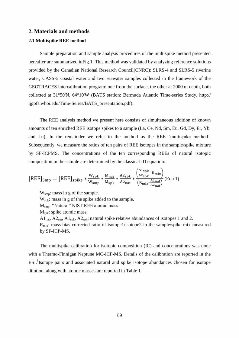
89
2. Materials and methods
2.1 Multispike REE method
Sample preparation and sample analysis procedures of the multispike method presented
hereafter are summarized inFig.1. This method was validated by analyzing reference solutions
provided by the Canadian National Research Council(CNRC): SLRS-4 and SLRS-5 riverine
water, CASS-5 coastal water and two seawater samples collected in the framework of the
GEOTRACES intercalibration program: one from the surface, the other at 2000 m depth, both
collected at 31°50'N, 64°10'W (BATS station: Bermuda Atlantic Time-series Study, http://
ijgofs.whoi.edu/Time-Series/BATS_presentation.pdf).
The REE analysis method we present here consists of simultaneous addition of known
amounts of ten enriched REE isotope spikes to a sample (La, Ce, Nd, Sm, Eu, Gd, Dy, Er, Yb,
and Lu). In the remainder we refer to the method as the REE ‘multispike method’.
Subsequently, we measure the ratios of ten pairs of REE isotopes in the sample/spike mixture
by SF-ICPMS. The concentrations of the ten corresponding REEs of natural isotopic
composition in the sample are determined by the classical ID equation:
–
(Equ.1)
Wsmp: mass in g of the sample.
Wspk: mass in g of the spike added to the sample.
Msmp: “Natural” NIST REE atomic mass.
Mspk: spike atomic mass.
A1nat, A2nat, A1spk, A2spk: natural spike relative abundances of isotopes 1 and 2.
Rmix: mass bias corrected ratio of isotope1/isotope2 in the sample/spike mix measured
by SF-ICP-MS.
The multispike calibration for isotopic composition (IC) and concentrations was done
with a Thermo-Finnigan Neptune MC-ICP-MS. Details of the calibration are reported in the
ESI.†Isotope pairs and associated natural and spike isotope abundances chosen for isotope
dilution, along with atomic masses are reported in Table 1.
Figure 1: Methodological scheme of multispike REE analysis of natural water samples on a single collector sector field ICP-MS.
91
Table 1: REE isotope abundances, ratios and atomic weights of natural and enriched isotope
standard solutions. Ab = abundance, Mn = atomic mass of the natural REE element, Ms =
atomic mass of the spike REE. ‘nat’ and ‘spk’ refer to natural and spike respectively.
The ideal amount of enriched spike to be added to a sample can be determined by
evaluating the uncertainty magnification factor, M:
(Equ.2)
This uncertainty level can be minimized as follows:
(Equ.3)
We obtain the ideal Rmix:
(Equ.4)
A discussion of the uncertainty magnification factor and ideal Rmix-ideal is reported in
the ESI.†
Finding the optimum spike concentration requires a good idea of the approximate REE
concentrations in an unknown sample. However, as discussed below, a certain amount of
overspiking or underspiking can be tolerated without much increase of the final uncertainty on
REE concentrations. Natural water samples display a variety of REE concentrations and
spectra. We therefore chose to add the enriched REE spikes to the samples by using two
mixed spike solutions. One containing the light to middle rare earth element spikes La, Ce,
Nd, Sm, Eu, Gd, hereafter called ‘mixed LREE spikes’ and one containing Dy, Er, Yb, Lu,
Isotope1 Isotope2 Ab.1nat Ab.2nat Ab.1spk Ab.2spk Mn Ms
La 138 139 0.09% 99.91% 6.76% 93.24% 138.91 138.84 0.0009 0.0725
Ce 136 140 0.19% 88.45% 24.342% 69.85% 140.12 139.01 0.0021 0.3485
Nd 146 145 17.18% 8.29% 97.35% 0.52% 144.24 145.88 2.0721 186.4034
Sm 149 147 13.82% 14.99% 96.72% 0.22% 150.37 148.94 0.9219 429.9969
Eu 151 153 47.81% 52.19% 97.70% 2.30% 151.96 150.97 0.9161 42.5030
Gd 157 155 15.65% 14.80% 91.66% 0.24% 157.25 156.97 1.0574 375.7594
Dy 163 161 24.90% 18.89% 95.60% 0.14% 162.50 162.90 1.3180 678.3316
Er 167 166 22.95% 33.60% 95.37% 1.27% 167.26 166.96 0.6830 75.0720
Yb 172 171 21.83% 14.28% 95.84% 1.31% 173.04 171.97 1.5287 73.3741
Lu 176 175 2.59% 97.41% 74.49% 25.51% 174.97 175.69 0.0266 2.9196
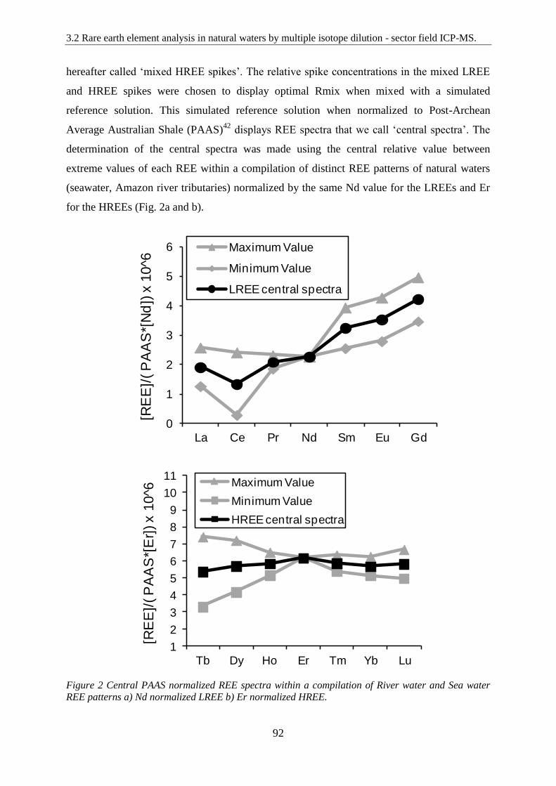
3.2 Rare earth element analysis in natural waters by multiple isotope dilution - sector field ICP-MS.
92
hereafter called ‘mixed HREE spikes’. The relative spike concentrations in the mixed LREE
and HREE spikes were chosen to display optimal Rmix when mixed with a simulated
reference solution. This simulated reference solution when normalized to Post-Archean
Average Australian Shale (PAAS)42
displays REE spectra that we call ‘central spectra’. The
determination of the central spectra was made using the central relative value between
extreme values of each REE within a compilation of distinct REE patterns of natural waters
(seawater, Amazon river tributaries) normalized by the same Nd value for the LREEs and Er
for the HREEs (Fig. 2a and b).
Figure 2 Central PAAS normalized REE spectra within a compilation of River water and Sea water
REE patterns a) Nd normalized LREE b) Er normalized HREE.
0
1
2
3
4
5
6
La Ce Pr Nd Sm Eu Gd
[RE
E]/
( P
AA
S*[
Nd
]) x
10^6
Maximum Value
Minimum Value
LREE central spectra
1
2
3
4
5
6
7
8
9
10
11
Tb Dy Ho Er Tm Yb Lu
[RE
E]/
( P
AA
S*[
Er]
) x 1
0^6
Maximum Value
Minimum Value
HREE central spectra
0
1
2
3
4
5
6
La Ce Pr Nd Sm Eu Gd
[RE
E]/
( P
AA
S*[
Nd
]) x
10^6
Maximum Value
Minimum Value
LREE central spectra
1
2
3
4
5
6
7
8
9
10
11
Tb Dy Ho Er Tm Yb Lu
[RE
E]/
( P
AA
S*[
Er]
) x 1
0^6
Maximum Value
Minimum Value
HREE central spectra
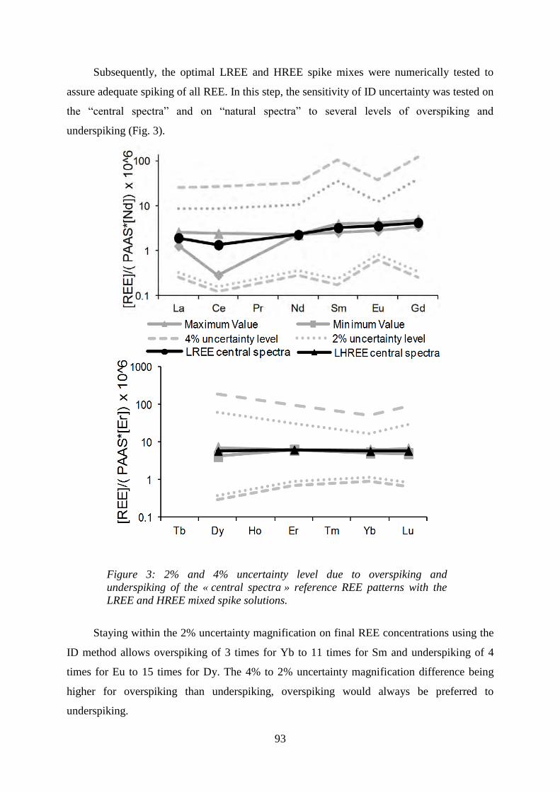
93
Subsequently, the optimal LREE and HREE spike mixes were numerically tested to
assure adequate spiking of all REE. In this step, the sensitivity of ID uncertainty was tested on
the “central spectra” and on “natural spectra” to several levels of overspiking and
underspiking (Fig. 3).
Figure 3: 2% and 4% uncertainty level due to overspiking and
underspiking of the « central spectra » reference REE patterns with the
LREE and HREE mixed spike solutions.
Staying within the 2% uncertainty magnification on final REE concentrations using the
ID method allows overspiking of 3 times for Yb to 11 times for Sm and underspiking of 4
times for Eu to 15 times for Dy. The 4% to 2% uncertainty magnification difference being
higher for overspiking than underspiking, overspiking would always be preferred to
underspiking.
3.2 Rare earth element analysis in natural waters by multiple isotope dilution - sector field ICP-MS.
94
The relative spike concentrations in mixed HREE and LREE spikes were also adjusted
to minimize the isobaric and oxide interferences induced by the spike addition. We also aimed
to obtain the same order of magnitude of signal within each pair of isotopes to assure that they
were measured in the same SF-ICP- MS counting mode, i.e. pulse or analogue mode.
Consequently, some REE spikes were slightly and voluntary under or overspiked. For
La and Lu, overspiking allowed us to minimize the isobaric interferences of Ba and Yb
respectively. Nd, Sm and Dy were slightly underspiked to lower the quantity of Nd and Sm
oxide interferences on HREEs and to reduce the difference of the signal between Dy isotopes.
For routine analyses, the amounts of LREE and HREE spike mixes added to the sample are
calculated by determining the optimal Nd and Er spiking. This requires a prior knowledge of
the approximate Nd and Er concentrations in the sample within a 300% confidence interval.
2.2 Preconcentration, matrix removal, and Ba separation
REE analyses by ICP-MS of freshwater and more specifically seawater samples can
require pre-concentration and matrix removal in order to increase detection limits, lower the
ionic charge in the plasma, or limit isobaric and oxide interferences(i.e.: Sn, Sb, Ba). The
presence of Ba in the sample is critical in the REE multispike method due to isobaric
interferences on La and Ce and BaO interferences on Nd, Sm and Gd. We used three different
separation protocols, one suitable for freshwater and two suitable for coastal and open ocean
seawaters. All sample preparations were performed under ISO 2 conditions in the LEGOS and
GET clean rooms. All acids used were in-house double distilled and deionized (DI) water was
<18 MU.
2.2.1 Freshwater samples.
For freshwater samples, we used a single offline chromatography column using the
AG50W-X8 (Dowex) cationic resin.43
A 200 mm height and 2.5 mm inner diameter quartz
column equipped with a 1 mm frit is filled with 100–200 mesh AG50W-X8 resin. The
exchange capacity of the column is approximately of 2.6 meq. The sample is aliquoted and
evaporated to dryness, and then dissolved in 2 ml of 2 M HCl, and loaded on the
preconditioned column. After a 3 time 200 ml rinse with 2 M HCl, 1.4 ml of 2 M HCl is
added to the column followed by 8.2 ml of 2.5 M HNO3 for Ba removal. The REEs are then
eluted in 15 ml of 6 M HCl. A chromatogram of this separation method is shown in Fig. 4.
After each sample elution, the column is washed and regenerated with 7 ml of 2.5 M
95
HNO3and 20 ml of 6 M HCl. The sample is evaporated to dryness and redissolved in 0.32 M
HNO3 for analysis by SF-ICP-MS. This separation protocol displays a more than 90%
recovery even for Lu which is the first REE eluted after Ba and La which is the last REE
eluted at the end of the 6 M HCl fraction.
2.2.2 Seawater samples.
For seawater samples two preconcentration protocols were used. The first is inspired by
the routine protocol used at the LEGOS laboratory and consists in REE Fe(OH)3 co-
precipitation followed by Fe removal with anionic chromatography.29
The second protocol
consists in the retention of REEs onto the Hitachi NobiasTM
resin. Both methods are followed
by a chromatographic separation step as described in the previous section to ensure a
complete removal of Ba.
(a)Fe oxide REE co-precipitation + AG50W-X8 cationic column.
REE pre-concentration by co-precipitation with Fe(OH)3 is achieved by adding 0.5 g of
purified and HCl dissolved Fe to 100–500 ml of the seawater sample. After 24 h (at
least)homogenization, the pH is increased to 7–8 by addition of ultrapure NH4OH leading to
the formation of an Fe(OH)3 precipitate. After 24 h sedimentation, the precipitate is rinsed
and centrifuged 3 times with DI water in order to remove a maximum of water soluble salts.
After the last centrifugation step, the sample is evaporated to dryness, the precipitate is
dissolved in 6 M HCl and the Fe is separated from the REEs by retention in a 100mmheight
and 2.5mminner diameter quartz column with a 1 mm frit that is filled with a 200–400 mesh
AG1-X8 (Biorad) resin. The REEs are eluted in 6 M HCl and Fe is finally eluted from the
column with 0.1 M HCl. This separation protocol usually displays recoveries of REEs
superior to 95%; further details can be found in ref. 29. The eluate containing REEs, traces of
Ba and other impurities is then evaporated to dryness, redissolved in 2 ml of 2 M HCl, and
loaded in the AG50W-X8 cationic column as described in the previous section for Ba
separation.
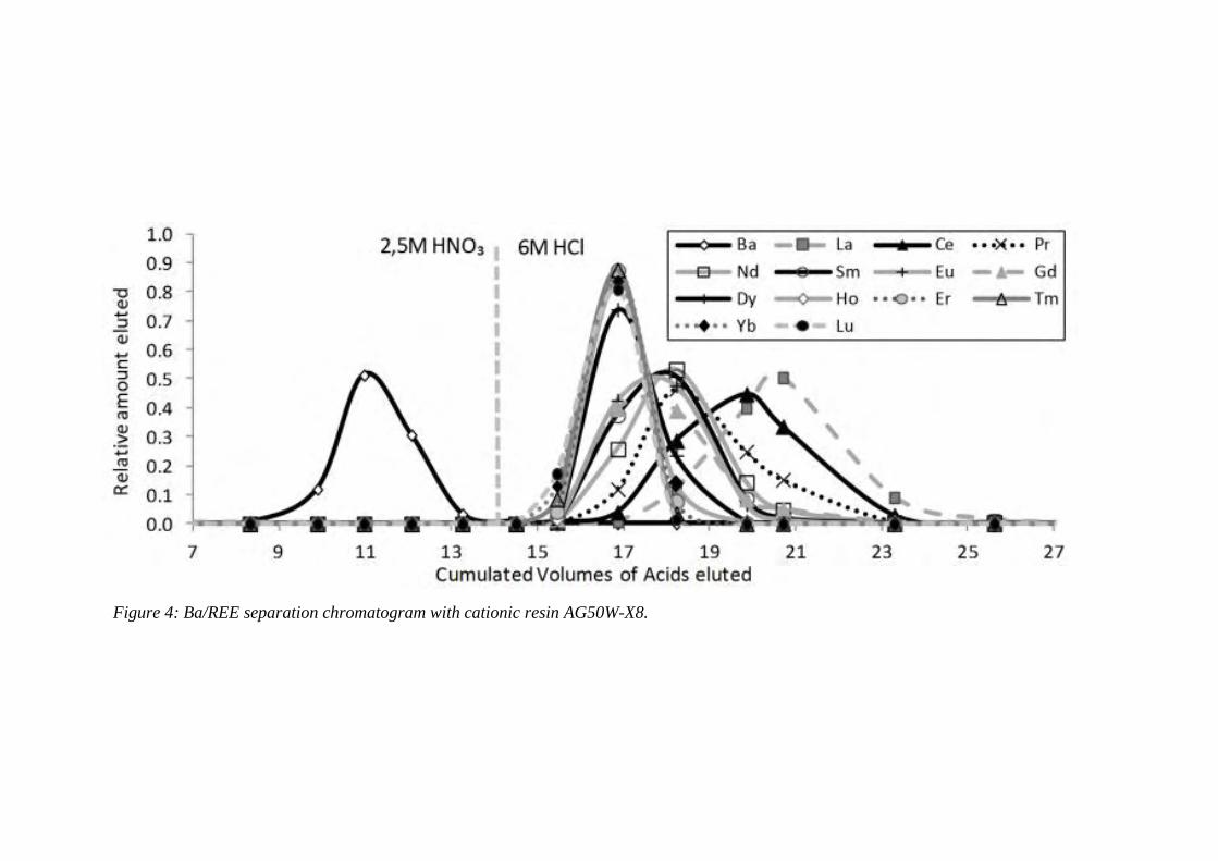
Figure 4: Ba/REE separation chromatogram with cationic resin AG50W-X8.
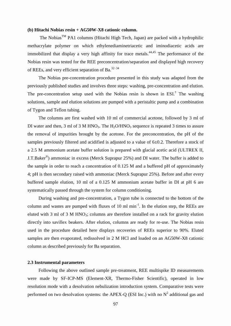
97
(b) Hitachi Nobias resin + AG50W-X8 cationic column.
The NobiasTM
PA1 columns (Hitachi High Tech, Japan) are packed with a hydrophilic
methacrylate polymer on which ethylenediaminetriacetic and iminodiacetic acids are
immobilized that display a very high affinity for trace metals.44,45
The performance of the
Nobias resin was tested for the REE preconcentration/separation and displayed high recovery
of REEs, and very efficient separation of Ba.32–34
The Nobias pre-concentration procedure presented in this study was adapted from the
previously published studies and involves three steps: washing, pre-concentration and elution.
The pre-concentration setup used with the Nobias resin is shown in ESI.† The washing
solutions, sample and elution solutions are pumped with a peristaltic pump and a combination
of Tygon and Teflon tubing.
The columns are first washed with 10 ml of commercial acetone, followed by 3 ml of
DI water and then, 3 ml of 3 M HNO3. The H2O/HNO3 sequence is repeated 3 times to assure
the removal of impurities brought by the acetone. For the preconcentration, the pH of the
samples previously filtered and acidified is adjusted to a value of 6±0.2. Therefore a stock of
a 2.5 M ammonium acetate buffer solution is prepared with glacial acetic acid (ULTREX II,
J.T.Baker®
) ammoniac in excess (Merck Suprapur 25%) and DI water. The buffer is added to
the sample in order to reach a concentration of 0.125 M and a buffered pH of approximately
4; pH is then secondary raised with ammoniac (Merck Suprapur 25%). Before and after every
buffered sample elution, 10 ml of a 0.125 M ammonium acetate buffer in DI at pH 6 are
systematically passed through the system for column conditioning.
During washing and pre-concentration, a Tygon tube is connected to the bottom of the
column and wastes are pumped with fluxes of 10 ml min-1
. In the elution step, the REEs are
eluted with 3 ml of 3 M HNO3; columns are therefore installed on a rack for gravity elution
directly into savillex beakers. After elution, columns are ready for re-use. The Nobias resin
used in the procedure detailed here displays recoveries of REEs superior to 90%. Eluted
samples are then evaporated, redissolved in 2 M HCl and loaded on an AG50W-X8 cationic
column as described previously for Ba separation.
2.3 Instrumental parameters
Following the above outlined sample pre-treatment, REE multispike ID measurements
were made by SF-ICP-MS (Element-XR, Thermo-Fisher Scientific), operated in low
resolution mode with a desolvation nebulization introduction system. Comparative tests were
performed on two desolvation systems: the APEX-Q (ESI Inc.) with no N2 additional gas and
3.2 Rare earth element analysis in natural waters by multiple isotope dilution - sector field ICP-MS.
98
the Aridus II (Cetac Inc.) with N2 as an additional gas. The Aridus II system was kept for this
method because it displayed lower oxide formation.
All atomic masses between 135 and 178 plus 129 and 131 were analyzed. This allowed
the measurement of all isotopes used for ID, oxide and isobaric interference corrections. For
isotopic ratio measuring purpose we opted like Willbold et al. (2005) for an acquisition
method consisting of repeated fast scan measurements of all isotopes instead of long
individual measurements for each isotope. This reduces the time interval between two
acquisitions and is less sensitive to small instabilities in the signal due to variation of the
sample flow in the introduction system. 60 consecutive sweeps were thus programmed with 4
short measurements per isotope mass made on flat peak tops in low resolution mode. The
dwell time per isotope lasted between 0.004 and 0.4 s according to the signal intensity of each
isotope in order to increase precision on the least abundant isotopes for a total acquisition time
of 6 min per sample.
Isotope measurements with the Element XR SF-ICP-MS are achieved by setting the
magnet to the first isotopic mass position. The isotopes to be measured above the magnet
mass are reached with electric scans until reaching a default value of 15% mass variation. The
magnetic field is then switched to the next mass position followed by a settling time of a few
tens of ms. For our method and starting from 129
Xe, a 15% mass variation leads to a first
magnet jump at mass 149 and a second at mass 171.The magnet jump leads to an unusual
instrumental mass bias for the 147
Sm/149
Sm and 171
Yb/172
Yb ratios of up to 10%. The default
mass scanning range was therefore modified to a value of 20%. All isotopes between masses
129 and 178 were then covered with a single “magnet jump” at mass 154 and two series of
electric scans (135 → 153, and 154 →178). Setting the “magnet jump” at mass 154 has the
advantage of affecting neither the pairs of isotopes used in ID calculation nor the isotopes
used for isobaric corrections. Instrument parameters are reported in the ESI.†
2.4 Data treatment
(a)Sequence.
A sequence is composed of spiked samples, procedural blanks and CRMs that are
regularly bracketed by HNO3 blanks, monitoring solutions and spike solutions for mass bias
and oxide formation corrections.
99
(b) Blank correction.
The first step in the data treatment is the blank correction. Signals on the chemistry
blanks (which include the instrumental 0.32 M HNO3 blank) are typically low (<1%) and
directly subtracted from sample signals for most isotope masses. For a better precision of
isobaric corrections on La, Ce and Lu (cf. paragraph d), Xe, Ba and Hf are not corrected for
blank contribution, and Ce and Yb blank corrections are made after their isobaric interference
corrections on La and Lu respectively.
(c) Oxide interference corrections.
In the multispike method oxide formation is monitored in two synthetic REE solutions
bracketing a series of 5 samples. The first solution contains Ba, La, Ce, Pr, Tb, Er and Yb of
natural isotopic composition and allows the monitoring of the following oxides:
%BaO=138
Ba16
O/138
Ba ; (Equ.5)
%LaO =139
La16
O/139
La; (Equ.6)
%CeO=140
Ce16
O/140
Ce; (Equ.7)
%PrO=141
Pr16
O/141
Pr; (Equ.8)
%TbO=159
Tb16
O /159
Tb. (Equ.9)
The second solution contains Nd, Sm, Eu, Gd, Dy, and allows the monitoring of:
%NdO=146
Nd16
O /146
Nd; (Equ.10)
%SmO=149
Sm16
O /149
Sm; (Equ.11)
%EuO=153
Eu16
O/153
Eu; (Equ.12)
%GdO=155
Gd16
O/155
Gd; (Equ.13)
%DyO=161
Dy16
O/161
Dy. (Equ.14)
An average value of each elemental oxide formation rate is calculated for the session;
the regular analysis of those oxide formation rates allows us to correct with more accuracy the
interfering oxides and to monitor their stability. Hydroxide formation was found to be below
the detection limit and is therefore not considered in this study.
(d) Isobaric interference corrections.
136Ce,
138La and
176Lu are required for the Ce, La and Yb isotope dilution calculation.
These isotopes are respectively interfered by 136
Xe and 136
Ba, 138
Ba and 138
Ce and 176
Yb and
176Hf. The interference correction of
136Ba and
136Xe on
136Ce is made using the interference
free 137
Ba and 134
Xe isotopes. The correction of 138
Ba and 176
Hfisobars (on 138
La and 176
Lu
3.2 Rare earth element analysis in natural waters by multiple isotope dilution - sector field ICP-MS.
100
respectively) follows the same logic. The interference correction is less trivial for 138
Ce and
176Yb on
138La and
176Lu, because
138Ce and
176Yb are naturally present in the sample and are
also added to the mixed spike solutions. The pairs of ratios 138
Ce/140
Ce vs. 136
Ce/140
Ce and
176Yb/
171Yb vs.
176Yb/
172Yb evolve linearly within the mixing between spike and sample
endmembers of contrasted isotopic compositions. These relations allow us to efficiently
unravel the combined spike and natural 138
Ce and 176
Yb contributions to the measured signals
on masses 138 and 176. The isobaric corrections are calculated as follows:
– (Eq.15)
– (Eq.16)
where Cps138
is the measured total ion count on mass 138, ‘A’ refers to natural
abundance, and coefficients ‘0.0305 and0.0028’ are the slope and intercepts of the mixing
diagrams (idem for Lu). Note that in addition mass bias corrections are made to Eq. (15) and
(16) (see next section).
(e) Mass bias correction.
Isotopic ratios used for isotope dilution and isobaric corrections are corrected for
instrumental mass bias, with a fractionation factor calculated as follows:
(Eq.17)
fx/y: fractionation factor between the M REE pair of isotopes
of x and y masses.
CpsxM: counts per second of the M REE isotope of x mass.
AxMnat: natural abundance of the M REE isotope of x mass.
Fractionation factors are calculated from the same analysis of the synthetic bracketing
solutions that are also used for determining oxide formation (Ba, La, Ce, Pr, Tb, Er, Yb and
Nd, Sm, Eu, Gd, Dy). A series of 5 samples are bracketed with monitoring solutions and
blanks. For each series, an average fractionation factor is calculated using the two bracketing
analyses. The factor is then applied to correct for mass bias on samples as follows.
101
(Eq.18)
The 131
Xe/136
Xe mass bias is also monitored in the 0.32 M HNO3 instrument blank
solution after corrections from minor 136
Ce and 136
Ba isobaric interferences. Due to low
signals and highly interfered natural 138
La, 136
Ce and 175
Lu in the bracketing monitoring
solutions, mass bias for 138
La/139
La, 136
La/140
La and 175
Lu/176
Lu is monitored in the ‘mixed
spike’ solutions which display sufficient 138
La, 136
Ce and 175
Lu signals.
(f) Mono-isotopic REEs.
The mono-isotopic REE (i.e.: Pr, Tb, Ho, Tm) concentrations are determined by
external calculation using a bracketing standard and are corrected for chemistry yields using
isotope diluted REEs as internal standards. This method readily integrates the dilution factor,
preparation chemistry yields and avoids the need of a third internal standard sometimes used
in concentration determination (i.e. Tm, In or Re) to correct the shift of sensitivity between
standard and sample. This shift of sensitivity is commonly due to the time elapsed between
the two measurements and differences of matrix compositions or little variation of the sample
flow in the introduction system. Ratios between sample concentrations obtained by isotope
dilution and externally calculated concentrations are monitored for 143
Nd, 145
Nd, 146
Nd, 147
Sm,
149Sm,
151Eu,
153Eu,
155Gd,
157Gd,
161Dy,
163Dy,
166Er,
167Er,
171Yb and
172Yb.
As illustrated for 151
Eu:
(Eq.19)
Abbreviations smp and bk stand for sample and beaker.
Abbreviations ID and EC stand for the isotope concentration
determined by “isotope dilution” and “calculated externally”.
Spk stands for the spike isotope concentration.
(Eq.20)
LREEspk: “mixed LREE spike”.
‘nat’ and ‘std’ stand for natural and standard.
3.2 Rare earth element analysis in natural waters by multiple isotope dilution - sector field ICP-MS.
102
An average Rsmp/bk is then calculated for each element, and a linear regression is then
fitted between individual elemental R and the corresponding atomic masses. The
Rsmp/bk are then inferred for Pr, Tb, Tm and Ho masses and multiplied by their
externally calculated concentrations.
3 Results and discussion
In this section we discuss: (1) the performance of the multispike SF-ICP-MS method,
and (2) results for certified reference materials SLRS-4 and SLRS-5 river water and CASS-5
coastal seawater. We also compare open ocean samples collected during a GEOTRACES
intercalibration cruise at the BATS (Bermuda Atlantic Time Series) station at depths of
15m(GS63) and 2000 m (GD41).
3.1 Separation chemistry
The most critical aspect of the separation chemistry is the removal of Ba. 136
Ba and
138Ba interfere with spike isotopes
136Ce and
138La respectively. We discuss here the case of
138Ba.
Due to the lower La concentration in seawater than in river water, the Ba/La ratio is
typically more elevated in seawater. The efficiency of Ba removal during the sample
processing was evaluated from the (138
Ba/138
La)nat and (138
Ba/(138
Lanat + 138
Laspk)) ratios for 7
different samples analyzed in this study and processed with different separation/pre-
concentration techniques (Table 2).
A co-precipitation step applied to river and seawater samples causes a 50- to 250-fold
reduction in the [Ba]/ [La] ratio for seawater but does not affect significantly the Ba/La ratio
of river water samples. Even with enriched 138
La spike addition to the sample, the 138
Ba/138
La
ratios are still too high to perform ID on river water La with a single co-precipitation step.
The ionic exchange capacity of AG50W-X8 is sufficient to process a river water sample and
remove most of the Ba. SLRS-4 and SLRS-5 show a 2000-fold drop in the Ba level, allowing
a La ID calculation with a 25% isobaric correction of 138
Ba on 138
La. However, this method is
not powerful enough for seawater samples.
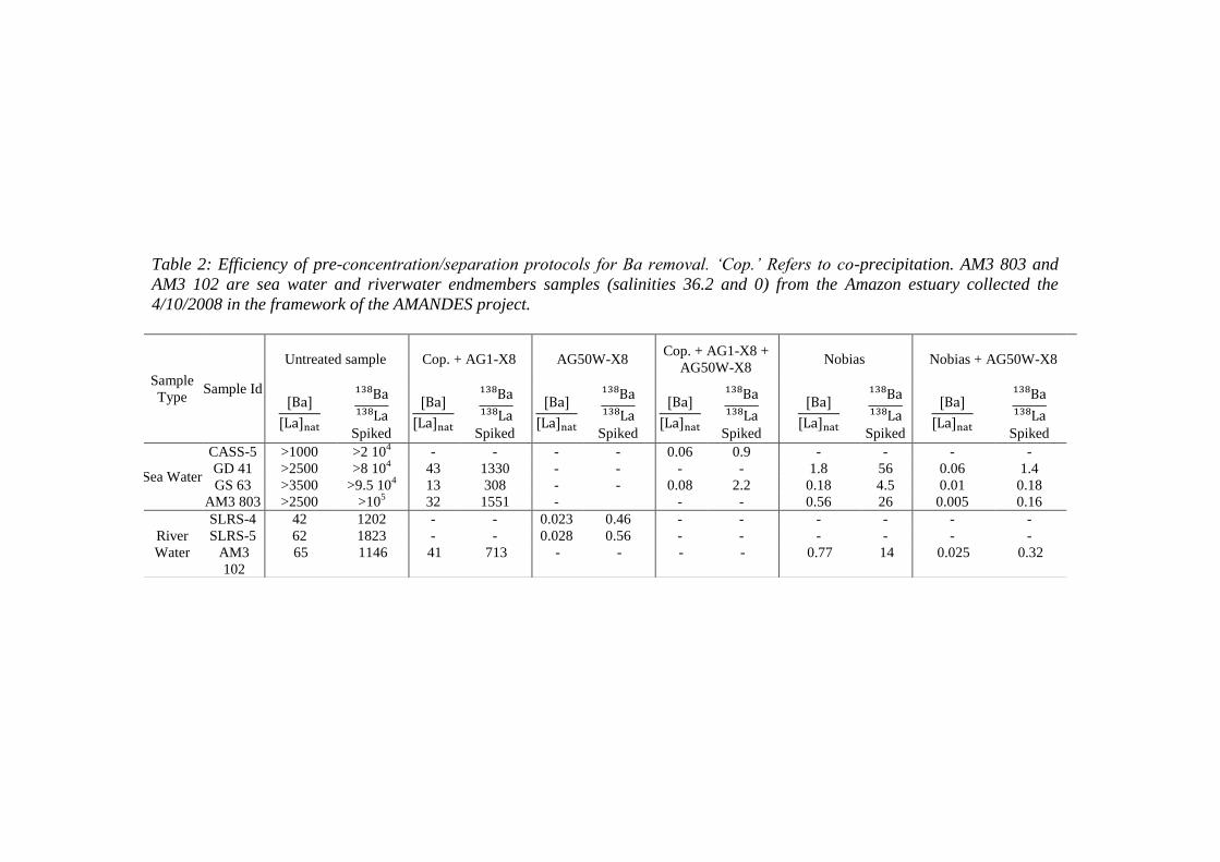
Table 2: Efficiency of pre-concentration/separation protocols for Ba removal. ‘Cop.’ Refers to co-precipitation. AM3 803 and
AM3 102 are sea water and riverwater endmembers samples (salinities 36.2 and 0) from the Amazon estuary collected the
4/10/2008 in the framework of the AMANDES project.
Sample
Type Sample Id
Untreated sample Cop. + AG1-X8 AG50W-X8 Cop. + AG1-X8 +
AG50W-X8 Nobias Nobias + AG50W-X8
Spiked
Spiked
Spiked
Spiked
Spiked
Spiked
Sea Water
CASS-5 >1000 >2 104 - - - - 0.06 0.9 - - - -
GD 41 >2500 >8 104 43 1330 - - - - 1.8 56 0.06 1.4
GS 63 >3500 >9.5 104 13 308 - - 0.08 2.2 0.18 4.5 0.01 0.18
AM3 803 >2500 >105 32 1551 - - - 0.56 26 0.005 0.16
River
Water
SLRS-4 42 1202 - - 0.023 0.46 - - - - - -
SLRS-5 62 1823 - - 0.028 0.56 - - - - - -
AM3
102
65 1146 41 713 - - - - 0.77 14 0.025 0.32
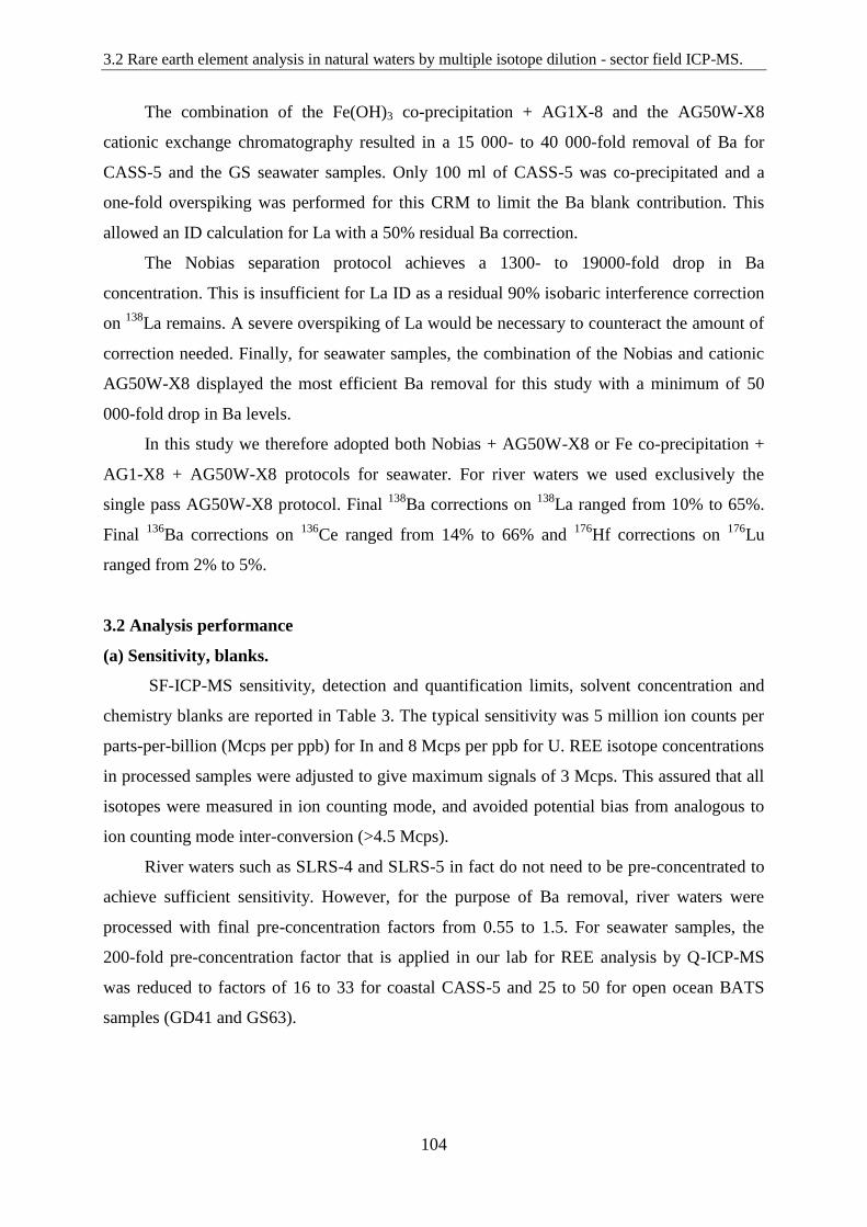
3.2 Rare earth element analysis in natural waters by multiple isotope dilution - sector field ICP-MS.
104
The combination of the Fe(OH)3 co-precipitation + AG1X-8 and the AG50W-X8
cationic exchange chromatography resulted in a 15 000- to 40 000-fold removal of Ba for
CASS-5 and the GS seawater samples. Only 100 ml of CASS-5 was co-precipitated and a
one-fold overspiking was performed for this CRM to limit the Ba blank contribution. This
allowed an ID calculation for La with a 50% residual Ba correction.
The Nobias separation protocol achieves a 1300- to 19000-fold drop in Ba
concentration. This is insufficient for La ID as a residual 90% isobaric interference correction
on 138
La remains. A severe overspiking of La would be necessary to counteract the amount of
correction needed. Finally, for seawater samples, the combination of the Nobias and cationic
AG50W-X8 displayed the most efficient Ba removal for this study with a minimum of 50
000-fold drop in Ba levels.
In this study we therefore adopted both Nobias + AG50W-X8 or Fe co-precipitation +
AG1-X8 + AG50W-X8 protocols for seawater. For river waters we used exclusively the
single pass AG50W-X8 protocol. Final 138
Ba corrections on 138
La ranged from 10% to 65%.
Final 136
Ba corrections on 136
Ce ranged from 14% to 66% and 176
Hf corrections on 176
Lu
ranged from 2% to 5%.
3.2 Analysis performance
(a) Sensitivity, blanks.
SF-ICP-MS sensitivity, detection and quantification limits, solvent concentration and
chemistry blanks are reported in Table 3. The typical sensitivity was 5 million ion counts per
parts-per-billion (Mcps per ppb) for In and 8 Mcps per ppb for U. REE isotope concentrations
in processed samples were adjusted to give maximum signals of 3 Mcps. This assured that all
isotopes were measured in ion counting mode, and avoided potential bias from analogous to
ion counting mode inter-conversion (>4.5 Mcps).
River waters such as SLRS-4 and SLRS-5 in fact do not need to be pre-concentrated to
achieve sufficient sensitivity. However, for the purpose of Ba removal, river waters were
processed with final pre-concentration factors from 0.55 to 1.5. For seawater samples, the
200-fold pre-concentration factor that is applied in our lab for REE analysis by Q-ICP-MS
was reduced to factors of 16 to 33 for coastal CASS-5 and 25 to 50 for open ocean BATS
samples (GD41 and GS63).
105
The multispike SF-ICP-MS method then permits a full REE analysis of a 50 ml
seawater sample. However as procedural blanks are a limiting factor, by precaution samples
volumes were kept higher with 100 ml for CASS-5, 250 ml for GD41, and 500 ml for GS63.
Instrumental blank signals in 0.32 M HNO3 were systematically more than 3 orders of
magnitude inferior to sample measurement signals. Instrumental detection limits for the REE
were in the range of 0.005 to 1 ppq. Overall REE chemistry blanks are <1 pg, except for La,
Ce and Nd with the coprecipitation + AG1-X8 + AG50W-X8 and Nobias + AG50W-X8
seawater protocols (<15 pg).
For 139
La, chemistry blank corrections were low with 0.08% for SLRS-4 and SLRS-5,
0.29% for CASS-5, 0.4% for GD41 and 0.15% for GS63. For 140
Ce blanks were less than
0.12% for SLRS- 4 and SLRS-5 processed with AG50W-X8 but reached up to 2% for CASS-
5 samples and up to 3% for GD41 and inferior to 0.8% for GS63. Relatively high blank
corrections were also observed for 155
Gd, 169
Tm and 159
Tb ranging from 0.6% to 1.7% for the
samples analyzed. All other isotopes analyzed had blank corrections <0.4%.
The excellent sensitivity and detection limits obtained with our protocol would allow
lowering substantially the initial sample volumes. However, this clearly requires further
efforts in order to reduce chemistry blank contributions. For CASS-5, using less than 100 ml
would yield significant blank corrections. For the co-precipitation protocol, the chemistry
Table 3: REE sensitivity (Sens.), detection and quantification limits (LOD, LOQ),
instrumental (0.32 M HNO3) and procedural blank levels. ‘Mcps’stands for 106 counts per
second
Sens.
(Mcps/
ppb)
LOD
(ppq)
LOQ
(ppq)
0.32 M
HNO3
(ppq)
Chemistry Blanks (pg)
AG50W-X8
Cop+
AG1-X8+
AG50W-X8
Nobias+AG5
0W-X8
Ba 4.3 30 99 1293 20 27 33
La 4.7 15 50 76 2.3 5 2.9
Ce 4.9 11 37 72 3.3 13 7
Pr 5.3 1 5 22 0.4 0.77 0.51
Nd 5.5 2 5 72 1.05 2.22 1.41
Sm 5.4 3 9 86 0.31 0.42 0.36
Eu 5.6 3 8 32 0.10 0.07 0.14
Gd 5.8 3 9 172 0.28 0.14 0.62
Tb 6.0 2 6 10 0.06 0.06 0.06
Dy 6.3 1 4 37 0.36 0.35 0.39
Ho 6.5 1 4 6 0.06 0.07 0.07
Er 6.6 1 3 24 0.15 0.22 0.19
Tm 6.6 1 4 6 0.07 0.06 0.07
Yb 6.5 1 2 53 0.25 0.37 0.55
Lu 6.6 1 4 12 0.05 0.05 0.08
3.2 Rare earth element analysis in natural waters by multiple isotope dilution - sector field ICP-MS.
106
blanks can potentially be reduced by lowering the amount of iron added to the sample and for
the Nobias protocol by improving the wash and rinse steps of the column and reducing the
amount of buffer added to the sample.
(b) Oxide production.
Oxide formation levels of the desolvation– SF-ICP-MS setup were described in the
Materials and methods section. The use of the CETAC Aridus II as the introduction system
reduces oxide formation down to values inferior to 0.001% for BaO/Ba, 0.0035% for LaO/La
and 0.002% for CeO/ Ce. At these levels, the corrections induced on interfered isotopes are
insignificant and comparable to instrumental 0.32 M HNO3 blank signals. Maximum
corrections of 1.6% and 0.25% were made for 139
LaO on 155
Gd and 149
SmO on 165
Ho
respectively.
The previously published multispike method for REE analysis in rock materials on a
MC-ICP-MS required chromatographic separation of LREEs and HREEs in order to avoid
oxide interferences due to enriched LREE patterns in rocks and the significantly higher oxide
production when operating the desolvator with no additional gas.39
It appears that the use of a
desolvating introduction system with additional nitrogen gas is an interesting alternative for
water samples usually depleted in HREEs.
(c) Isotope dilution.
Except for La and Lu, which were overspiked to avoid substantial isobaric interference
corrections of 138
Ba and 138
Ce on 138
La and 176
Yb and 176
Hf on 176
Lu, the long-term
uncertainty magnification factors of REE concentration analysis by the multispike method,
based on the 19 samples presented, were close to the ideal limit.
3.3 Reference solution analysis
(a) Canadian National Research Council reference solutions.
SLRS-4 and SLRS-5 river water reference solutions and CASS-5 seawater (CNRC)
were analyzed. 5 ml of SLRS-4 and SLRS-5 and 100 ml of CASS-5 were spiked. 5 spiked
replicates were prepared and each replicate was analyzed 2 or 3 times during 2 SF-ICP-MS
sessions. Details of the sample treatment procedures, concentrations expressed in parts-per-
trillion (ppt) and confidence intervals in 2 SD and 2 RSD are reported in Table 4.
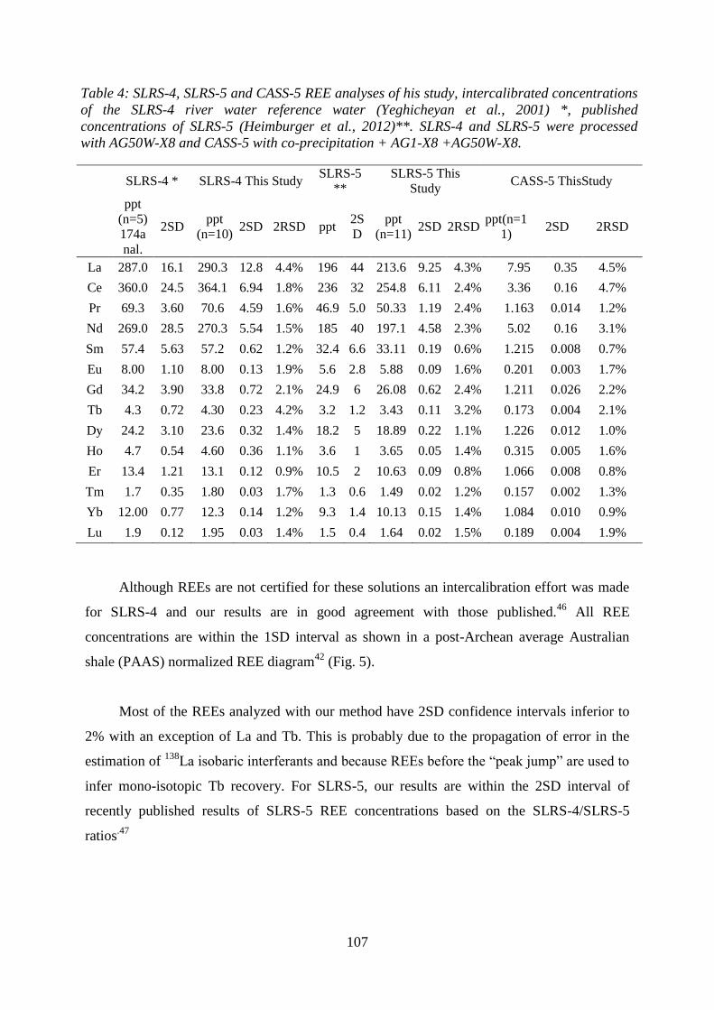
107
Although REEs are not certified for these solutions an intercalibration effort was made
for SLRS-4 and our results are in good agreement with those published.46
All REE
concentrations are within the 1SD interval as shown in a post-Archean average Australian
shale (PAAS) normalized REE diagram42
(Fig. 5).
Most of the REEs analyzed with our method have 2SD confidence intervals inferior to
2% with an exception of La and Tb. This is probably due to the propagation of error in the
estimation of 138
La isobaric interferants and because REEs before the “peak jump” are used to
infer mono-isotopic Tb recovery. For SLRS-5, our results are within the 2SD interval of
recently published results of SLRS-5 REE concentrations based on the SLRS-4/SLRS-5
ratios.47
Table 4: SLRS-4, SLRS-5 and CASS-5 REE analyses of his study, intercalibrated concentrations
of the SLRS-4 river water reference water (Yeghicheyan et al., 2001) *, published
concentrations of SLRS-5 (Heimburger et al., 2012)**. SLRS-4 and SLRS-5 were processed
with AG50W-X8 and CASS-5 with co-precipitation + AG1-X8 +AG50W-X8.
SLRS-4 * SLRS-4 This Study SLRS-5
**
SLRS-5 This
Study CASS-5 ThisStudy
ppt
(n=5)
174a
nal.
2SD ppt
(n=10) 2SD 2RSD ppt
2S
D
ppt
(n=11) 2SD 2RSD
ppt(n=1
1) 2SD 2RSD
La 287.0 16.1 290.3 12.8 4.4% 196 44 213.6 9.25 4.3% 7.95 0.35 4.5%
Ce 360.0 24.5 364.1 6.94 1.8% 236 32 254.8 6.11 2.4% 3.36 0.16 4.7%
Pr 69.3 3.60 70.6 4.59 1.6% 46.9 5.0 50.33 1.19 2.4% 1.163 0.014 1.2%
Nd 269.0 28.5 270.3 5.54 1.5% 185 40 197.1 4.58 2.3% 5.02 0.16 3.1%
Sm 57.4 5.63 57.2 0.62 1.2% 32.4 6.6 33.11 0.19 0.6% 1.215 0.008 0.7%
Eu 8.00 1.10 8.00 0.13 1.9% 5.6 2.8 5.88 0.09 1.6% 0.201 0.003 1.7%
Gd 34.2 3.90 33.8 0.72 2.1% 24.9 6 26.08 0.62 2.4% 1.211 0.026 2.2%
Tb 4.3 0.72 4.30 0.23 4.2% 3.2 1.2 3.43 0.11 3.2% 0.173 0.004 2.1%
Dy 24.2 3.10 23.6 0.32 1.4% 18.2 5 18.89 0.22 1.1% 1.226 0.012 1.0%
Ho 4.7 0.54 4.60 0.36 1.1% 3.6 1 3.65 0.05 1.4% 0.315 0.005 1.6%
Er 13.4 1.21 13.1 0.12 0.9% 10.5 2 10.63 0.09 0.8% 1.066 0.008 0.8%
Tm 1.7 0.35 1.80 0.03 1.7% 1.3 0.6 1.49 0.02 1.2% 0.157 0.002 1.3%
Yb 12.00 0.77 12.3 0.14 1.2% 9.3 1.4 10.13 0.15 1.4% 1.084 0.010 0.9%
Lu 1.9 0.12 1.95 0.03 1.4% 1.5 0.4 1.64 0.02 1.5% 0.189 0.004 1.9%
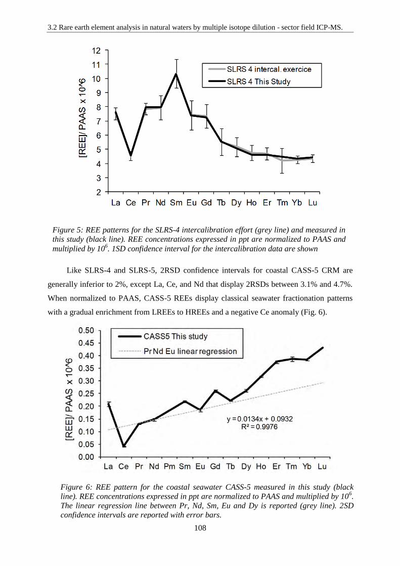
3.2 Rare earth element analysis in natural waters by multiple isotope dilution - sector field ICP-MS.
108
Like SLRS-4 and SLRS-5, 2RSD confidence intervals for coastal CASS-5 CRM are
generally inferior to 2%, except La, Ce, and Nd that display 2RSDs between 3.1% and 4.7%.
When normalized to PAAS, CASS-5 REEs display classical seawater fractionation patterns
with a gradual enrichment from LREEs to HREEs and a negative Ce anomaly (Fig. 6).
Figure 5: REE patterns for the SLRS-4 intercalibration effort (grey line) and measured in
this study (black line). REE concentrations expressed in ppt are normalized to PAAS and
multiplied by 106. 1SD confidence interval for the intercalibration data are shown
Figure 6: REE pattern for the coastal seawater CASS-5 measured in this study (black
line). REE concentrations expressed in ppt are normalized to PAAS and multiplied by 106.
The linear regression line between Pr, Nd, Sm, Eu and Dy is reported (grey line). 2SD
confidence intervals are reported with error bars.

109
Anomalies were calculated for Ce, Sm, and Gd, with methods described by several
authors (Table 5) and by linear regression inspired by Kulaksiz and Bau (2011).16,48
These
authors made a linear least square regression of coherent logarithmic values of PAAS
normalized REEs (log(REEPAAS)) (Pr, Nd, Sm) against their ranking amongst the lanthanide
series (i.e. from 1 to 15) for tap water samples in order to infer the Gd background value. We
used Pr, Nd and Eu PAAS normalized concentrations for the linear regression (without
logarithm) as illustrated in Fig. 6 (Pm was introduced in the lanthanide diagram to show the
coherent Pr, Nd and Eu normalized patterns as a function of their ranking).
REE anomalies were calculated for each replicate analysis in order to be able to
calculate average values and associated 2RSD. All anomalies calculated by alternative
equations show the same value within the associated confidence intervals. Besides the typical
seawater Ce anomaly in CASS-5, three major additional anomalies can be observed for La,
Sm and Gd.
The unusual Sm anomaly was also observed on other CNRC CRMs like SLRS-4 and
SLRS-5 (this study), CASS-4 and NASS-5 and has been attributed to Sm contamination
during CRM preparation. 49–51
With the exception of Ce, the anomalies calculated for CASS-5
replicates display low uncertainties of 1.7% 2RSD (Sm) and 2.2% 2RSD (Gd). Ce anomalies
present 2RSD uncertainties of 4.8% and 6.1% due to the higher uncertainties of La and Ce
concentrations. Nevertheless our uncertainty on the Ce anomaly is inferior to the typical 9–
21% 2RSD uncertainties calculated for the recent GEOTRACES seawater REE
intercomparison. 38
Table 5: Definitions and values of REE anomalies discussed in the text for
the CASS-5 coastal sea water CRM. * refers to the background value of the
anomalous REE. pn refers to PASS normalized.
Equation Reference Anomaly 2RSD
Cepn/Ce*=Cepn/(2Prpn- Ndpn) (Bolhar et al., 2004) 0.371 6.1%
Cepn/Ce*= Cepn/f(Prpn,Ndpn,Eupn) - 0.355 4.8%
Smpn/Sm =3Smpn/(Ndpn+2Eupn) (Alibo and Nozaki, 1999) 1.264 1.7%
Smpn/Sm*=Smpn/f(Prpn,Ndpn,Eupn) - 1.266 1.6%
Gdpn/Gd*=2Gdpn/(Eupn+Tbpn) (De Baar et al., 1985) 1.282 2.3%
Gdpn/Gd*=Gdpn/f(Prpn,Ndpn,Eupn) - 1.309 2.1%
Ybpn/Yb*= 2Ybpn/(Tmpn+Lupn) (De Baar et al., 1985) 0.941 1.3%

3.2 Rare earth element analysis in natural waters by multiple isotope dilution - sector field ICP-MS.
110
(b) BATS station GEOTRACES intercalibration.
Dedicated REE samples collected during a GEOTRACES intercalibration cruise were
completely consumed after the analysis by 9 laboratories.38,52
K. Bruland kindly provided us
with closely related samples from the same station and depths, yet preserved for other trace
metal intercalibration efforts. We received 500 ml aliquots of filtered (0.2 µm) acidified
seawater stored in HDPE bottles.
For the GD41 BATS 2000 m deep water sample two 250 ml sub-aliquots were made
and spiked independently. For the GS63 BATS 15 m surface water sample 500 ml was
spiked. In an initial attempt, the samples were passed through the Nobias column and
analyzed twice to determine all REE concentrations except La and Ce which had >90%
interferences from Ba isotopes. To lower Ba interferences, the remaining sample was passed
through the AG50W-X8 column, allowing more accurate and precise La and Ce concentration
determination in a third analysis session.
Table 6 reports REE concentrations published by the GEOTRACES intercalibration
effort and GD41 and GS63 REE concentrations determined in this study. Concentrations are
expressed in ppt, confidence intervals in 2SD and 2 RSD%. For both GD41 and GS63 all
REEs are within the 2SD confidence interval established during the intercalibration exercise
(Fig. 7a and b). The BATS surface and deep samples reveal numerous subtle REE features:
Ce anomalies calculated according to Bolhar et al. (2004)53
increase from 0.177 at 15 m to
0.518 at 2000 m depth. Well-developed Gd anomalies for Atlantic samples are present, and
are constant at both depths, in agreement with observations in the literature.11,14,38
HREEs Yb
and Lu are significantly fractionated between both depths. Finally, La also appears
fractionated between both depths with Lapn/Cepn ratios of 1.14 on the surface and 1.35 at 2000
m. All of these features reflect the interplay between input sources and elemental fractionation
processes related to REE speciation.
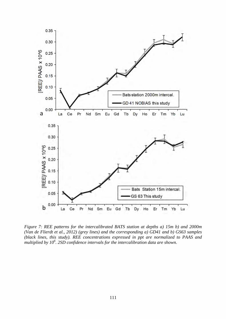
111
Figure 7: REE patterns for the intercalibrated BATS station at depths a) 15m b) and 2000m
(Van de Flierdt et al., 2012) (grey lines) and the corresponding a) GD41 and b) GS63 samples
(black lines, this study). REE concentrations expressed in ppt are normalized to PAAS and
multiplied by 106. 2SD confidence intervals for the intercalibration data are shown.
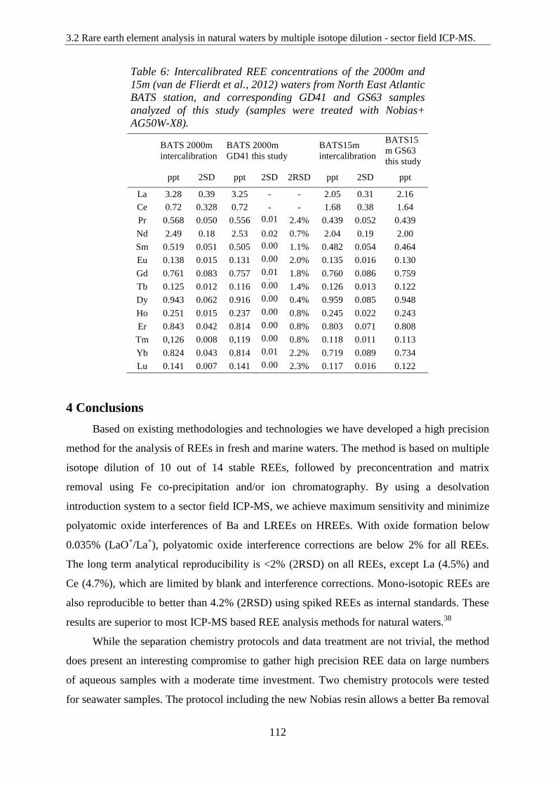
3.2 Rare earth element analysis in natural waters by multiple isotope dilution - sector field ICP-MS.
112
4 Conclusions
Based on existing methodologies and technologies we have developed a high precision
method for the analysis of REEs in fresh and marine waters. The method is based on multiple
isotope dilution of 10 out of 14 stable REEs, followed by preconcentration and matrix
removal using Fe co-precipitation and/or ion chromatography. By using a desolvation
introduction system to a sector field ICP-MS, we achieve maximum sensitivity and minimize
polyatomic oxide interferences of Ba and LREEs on HREEs. With oxide formation below
0.035% (LaO+/La
+), polyatomic oxide interference corrections are below 2% for all REEs.
The long term analytical reproducibility is <2% (2RSD) on all REEs, except La (4.5%) and
Ce (4.7%), which are limited by blank and interference corrections. Mono-isotopic REEs are
also reproducible to better than 4.2% (2RSD) using spiked REEs as internal standards. These
results are superior to most ICP-MS based REE analysis methods for natural waters.38
While the separation chemistry protocols and data treatment are not trivial, the method
does present an interesting compromise to gather high precision REE data on large numbers
of aqueous samples with a moderate time investment. Two chemistry protocols were tested
for seawater samples. The protocol including the new Nobias resin allows a better Ba removal
Table 6: Intercalibrated REE concentrations of the 2000m and
15m (van de Flierdt et al., 2012) waters from North East Atlantic
BATS station, and corresponding GD41 and GS63 samples
analyzed of this study (samples were treated with Nobias+
AG50W-X8).
BATS 2000m
intercalibration
BATS 2000m
GD41 this study
BATS15m
intercalibration
BATS15
m GS63
this study
ppt 2SD ppt 2SD 2RSD ppt 2SD ppt
La 3.28 0.39 3.25 - - 2.05 0.31 2.16
Ce 0.72 0.328 0.72 - - 1.68 0.38 1.64
Pr 0.568 0.050 0.556 0.01
1 2.4% 0.439 0.052 0.439
Nd 2.49 0.18 2.53 0.02 0.7% 2.04 0.19 2.00
Sm 0.519 0.051 0.505 0.00
5 1.1% 0.482 0.054 0.464
Eu 0.138 0.015 0.131 0.00
3 2.0% 0.135 0.016 0.130
Gd 0.761 0.083 0.757 0.01
3 1.8% 0.760 0.086 0.759
Tb 0.125 0.012 0.116 0.00
2 1.4% 0.126 0.013 0.122
Dy 0.943 0.062 0.916 0.00
4 0.4% 0.959 0.085 0.948
Ho 0.251 0.015 0.237 0.00
3 0.8% 0.245 0.022 0.243
Er 0.843 0.042 0.814 0.00
5 0.8% 0.803 0.071 0.808
Tm 0,126 0.008 0,119 0.00
1 0.8% 0.118 0.011 0.113
Yb 0.824 0.043 0.814 0.01
8 2.2% 0.719 0.089 0.734
Lu 0.141 0.007 0.141 0.00
4 2.3% 0.117 0.016 0.122
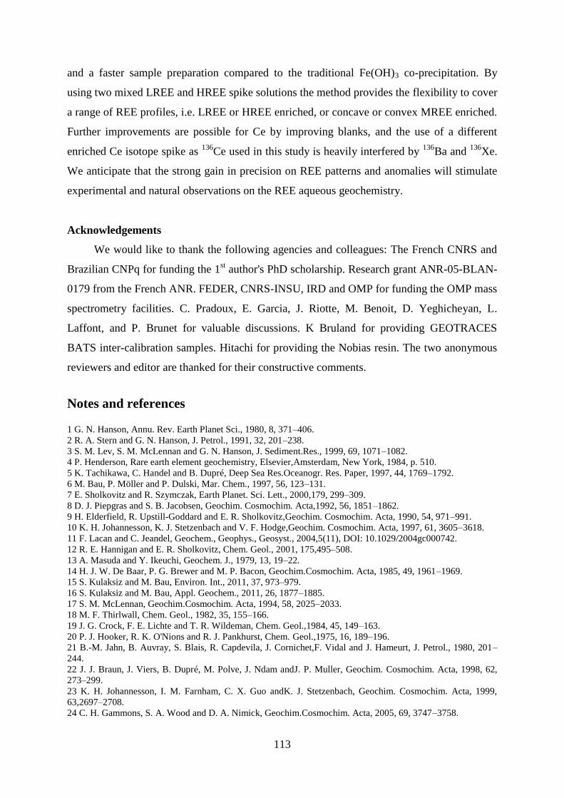
113
and a faster sample preparation compared to the traditional Fe(OH)3 co-precipitation. By
using two mixed LREE and HREE spike solutions the method provides the flexibility to cover
a range of REE profiles, i.e. LREE or HREE enriched, or concave or convex MREE enriched.
Further improvements are possible for Ce by improving blanks, and the use of a different
enriched Ce isotope spike as 136
Ce used in this study is heavily interfered by 136
Ba and 136
Xe.
We anticipate that the strong gain in precision on REE patterns and anomalies will stimulate
experimental and natural observations on the REE aqueous geochemistry.
Acknowledgements
We would like to thank the following agencies and colleagues: The French CNRS and
Brazilian CNPq for funding the 1st author's PhD scholarship. Research grant ANR-05-BLAN-
0179 from the French ANR. FEDER, CNRS-INSU, IRD and OMP for funding the OMP mass
spectrometry facilities. C. Pradoux, E. Garcia, J. Riotte, M. Benoit, D. Yeghicheyan, L.
Laffont, and P. Brunet for valuable discussions. K Bruland for providing GEOTRACES
BATS inter-calibration samples. Hitachi for providing the Nobias resin. The two anonymous
reviewers and editor are thanked for their constructive comments.
Notes and references
1 G. N. Hanson, Annu. Rev. Earth Planet Sci., 1980, 8, 371–406.
2 R. A. Stern and G. N. Hanson, J. Petrol., 1991, 32, 201–238.
3 S. M. Lev, S. M. McLennan and G. N. Hanson, J. Sediment.Res., 1999, 69, 1071–1082.
4 P. Henderson, Rare earth element geochemistry, Elsevier,Amsterdam, New York, 1984, p. 510.
5 K. Tachikawa, C. Handel and B. Dupré, Deep Sea Res.Oceanogr. Res. Paper, 1997, 44, 1769–1792.
6 M. Bau, P. Möller and P. Dulski, Mar. Chem., 1997, 56, 123–131.
7 E. Sholkovitz and R. Szymczak, Earth Planet. Sci. Lett., 2000,179, 299–309.
8 D. J. Piepgras and S. B. Jacobsen, Geochim. Cosmochim. Acta,1992, 56, 1851–1862.
9 H. Elderfield, R. Upstill-Goddard and E. R. Sholkovitz,Geochim. Cosmochim. Acta, 1990, 54, 971–991.
10 K. H. Johannesson, K. J. Stetzenbach and V. F. Hodge,Geochim. Cosmochim. Acta, 1997, 61, 3605–3618.
11 F. Lacan and C. Jeandel, Geochem., Geophys., Geosyst., 2004,5(11), DOI: 10.1029/2004gc000742.
12 R. E. Hannigan and E. R. Sholkovitz, Chem. Geol., 2001, 175,495–508.
13 A. Masuda and Y. Ikeuchi, Geochem. J., 1979, 13, 19–22.
14 H. J. W. De Baar, P. G. Brewer and M. P. Bacon, Geochim.Cosmochim. Acta, 1985, 49, 1961–1969.
15 S. Kulaksiz and M. Bau, Environ. Int., 2011, 37, 973–979.
16 S. Kulaksiz and M. Bau, Appl. Geochem., 2011, 26, 1877–1885.
17 S. M. McLennan, Geochim.Cosmochim. Acta, 1994, 58, 2025–2033.
18 M. F. Thirlwall, Chem. Geol., 1982, 35, 155–166.
19 J. G. Crock, F. E. Lichte and T. R. Wildeman, Chem. Geol.,1984, 45, 149–163.
20 P. J. Hooker, R. K. O'Nions and R. J. Pankhurst, Chem. Geol.,1975, 16, 189–196.
21 B.-M. Jahn, B. Auvray, S. Blais, R. Capdevila, J. Cornichet,F. Vidal and J. Hameurt, J. Petrol., 1980, 201–
244.
22 J. J. Braun, J. Viers, B. Dupré, M. Polve, J. Ndam andJ. P. Muller, Geochim. Cosmochim. Acta, 1998, 62,
273–299.
23 K. H. Johannesson, I. M. Farnham, C. X. Guo andK. J. Stetzenbach, Geochim. Cosmochim. Acta, 1999,
63,2697–2708.
24 C. H. Gammons, S. A. Wood and D. A. Nimick, Geochim.Cosmochim. Acta, 2005, 69, 3747–3758.
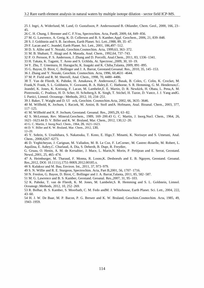
3.2 Rare earth element analysis in natural waters by multiple isotope dilution - sector field ICP-MS.
114
25 J. Ingri, A. Widerlund, M. Land, O. Gustafsson, P. Anderssonand B. Ohlander, Chem. Geol., 2000, 166, 23–
45.
26 C. H. Chung, I. Brenner and C. F.You, Spectrochim. Acta, PartB, 2009, 64, 849–856.
27 M. G. Lawrence, A. Greig, K. D. Collerson and B. S. Kamber,Appl. Geochem., 2006, 21, 839–848.
28 S. J. Goldstein and S. B. Jacobsen, Earth Planet. Sci. Lett.,1988, 89, 35–47.
29 F. Lacan and C. Jeandel, Earth Planet. Sci. Lett., 2001, 186,497–512.
30 D. S. Alibo and Y. Nozaki, Geochim.Cosmochim. Acta, 1999,63, 363–372.
31 M. B. Shabani, T. Akagi and A. Masuda, Anal. Chem., 1992,64, 737–743.
32 P. O. Persson, P. S. Andersson, J. Zhang and D. Porcelli, Anal.Chem., 2011, 83, 1336–1341.
33 H. Takata, K. Tagami, T. Aono and S. Uchlida, At. Spectrosc.,2009, 30, 10–19.
34 Y. Zhu, T. Umemura, H. Haraguchi, K. Inagaki and K. Chiba,Talanta, 2009, 891–895.
35 G. Bayon, D. Birot, C. Bollinger and J. A. Barrat, Geostand.Geoanal. Res., 2010, 35, 145–153.
36 J. Zhang and Y. Nozaki, Geochim. Cosmochim. Acta, 1996, 60,4631–4644.
37 M. P. Field and R. M. Sherrell, Anal. Chem., 1998, 70, 4480–4486.
38 T. Van de Flierdt, K. Pahnke, H. Amakawa, P. Andersson,C. Basak, B. Coles, C. Colin, K. Crocket, M.
Frank,N. Frank, S. L. Goldstein, V. Goswami, B. A. Haley,E. C. Hathorne, S. R. Hemming, G. M. Henderson,C.
Jeandel, K. Jones, K. Kreissig, F. Lacan, M. Lambelet,E. E. Martin, D. R. Newkirk, H. Obata, L. Pena,A. M.
Piotrowski, C. Pradoux, H. D. Scher, H. Schoberg,S. K. Singh, T. Stichel, H. Tazoe, D. Vance, J. J. Yang andG.
I. Partici, Limnol. Oceanogr.: Methods, 2012, 10, 234–251.
39 J. Baker, T. Waight and D. Ul eck, Geochim. Cosmochim.Acta, 2002, 66, 3635–3646.
40 M. Willbold, K. Jochum, I. Raczek, M. Amini, B. Stoll andA. Hofmann, Anal. Bioanal. Chem., 2003, 377,
117–125.
41 M. Willbold and K. P. Jochum, Geostand. Geoanal. Res., 2005,29, 63–82.
42 S. McLennan, Rev. Mineral.Geochem., 1989, 169–200.43 G. C. Martin, J. Inorg.Nucl. Chem., 1964, 26,
1621–1623.44 D. V. Biller and K. W. Bruland, Mar. Chem., 2012, 130,12–20. 43 G. C. Martin, J. Inorg.Nucl. Chem., 1964, 26, 1621–1623.
44 D. V. Biller and K. W. Bruland, Mar. Chem., 2012, 130,
12–20. 45 Y. Sohrin, S. Urushihara, S. Nakatsuka, T. Kono, E. Higo,T. Minami, K. Norisuye and S. Umetani, Anal.
Chem., 2008,6267–6273.
46 D. Yeghicheyan, J. Carignan, M. Valladon, M. B. Le Coz, F. LeCornec, M. Castrec-Rouelle, M. Robert, L.
Aquilina, E. Aubry,C. Churlaud, A. Dia, S. Deberdt, B. Dupr, R. Freydier,
G. Gruau, O. Henin, A. M. de Kersabiec, J. Mace, L. Marin,N. Morin, P. Petitjean and E. Serrat, Geostand.
Newsl.,2001, 25, 465–474.
47 A. Heimburger, M. Tharaud, F. Monna, R. Losno,K. Desboeufs and E. B. Nguyen, Geostand. Geoanal.
Res.,2012, DOI: 10.1111/j.1751-908X.2012.00185.x.
48 S. Kulaksız and M. Bau, Environ. Int., 2011, 37, 973–979.
49 S. N. Willie and R. E. Sturgeon, Spectrochim. Acta, Part B,2001, 56, 1707–1716.
50 N. Freslon, G. Bayon, D. Birot, C. Bollinger and J. A. Barrat,Talanta, 2011, 85, 582–587.
51 M. G. Lawrence and B. S. Kamber, Geostand. Geoanal. Res.,2007, 31, 95–103.
52 K. Pahnke, T. van de Flierdt, K. M. Jones, M. Lambelet,S. R. Hemming and S. L. Goldstein, Limnol.
Oceanogr.:Methods, 2012, 10, 252–269.
53 R. Bolhar, B. S. Kamber, S. Moorbath, C. M. Fedo andM. J. Whitehouse, Earth Planet. Sci. Lett., 2004, 222,
43–60.
54 H. J. W. De Baar, M. P. Bacon, P. G. Brewer and K. W. Bruland, Geochim.Cosmochim. Acta, 1985, 49,
1943–1959.
115
Supplementary Information
Contents:
1.Spike calibration on MC-ICPMS……………………………….…....p.1
2. Optimum Spike/Sample mixing……………………………………...p.5
3. Nobias pre-concentration protocol…………………………………..p.7
4. Oxides and mass bias monitoring solutions…………………………p.7
5. Desolvator-SF-ICPMS settings and performances…………………p.8
6. Isobaric corrections on 138
La and 176
Lu…………………………..p.10
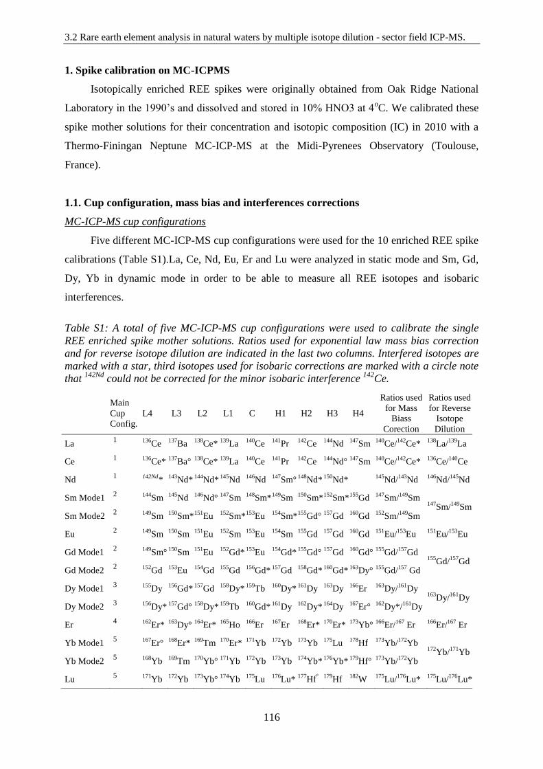
3.2 Rare earth element analysis in natural waters by multiple isotope dilution - sector field ICP-MS.
116
1. Spike calibration on MC-ICPMS
Isotopically enriched REE spikes were originally obtained from Oak Ridge National
Laboratory in the 1990’s and dissolved and stored in 10% HNO3 at 4oC. We calibrated these
spike mother solutions for their concentration and isotopic composition (IC) in 2010 with a
Thermo-Finingan Neptune MC-ICP-MS at the Midi-Pyrenees Observatory (Toulouse,
France).
1.1. Cup configuration, mass bias and interferences corrections
MC-ICP-MS cup configurations
Five different MC-ICP-MS cup configurations were used for the 10 enriched REE spike
calibrations (Table S1).La, Ce, Nd, Eu, Er and Lu were analyzed in static mode and Sm, Gd,
Dy, Yb in dynamic mode in order to be able to measure all REE isotopes and isobaric
interferences.
Table S1: A total of five MC-ICP-MS cup configurations were used to calibrate the single
REE enriched spike mother solutions. Ratios used for exponential law mass bias correction
and for reverse isotope dilution are indicated in the last two columns. Interfered isotopes are
marked with a star, third isotopes used for isobaric corrections are marked with a circle note
that 142Nd
could not be corrected for the minor isobaric interference 142
Ce.
Main
Cup
Config.
L4 L3 L2 L1 C H1 H2 H3 H4
Ratios used
for Mass
Biass
Corection
Ratios used
for Reverse
Isotope
Dilution
La 1 136
Ce 137
Ba 138
Ce* 139
La 140
Ce 141
Pr 142
Ce 144
Nd 147
Sm 140
Ce/142
Ce* 138
La/139
La
Ce 1 136
Ce* 137
Ba° 138
Ce* 139
La 140
Ce 141
Pr 142
Ce 144
Nd° 147
Sm 140
Ce/142
Ce* 136
Ce/140
Ce
Nd 1 142Nd
* 143
Nd* 144
Nd* 145
Nd 146
Nd 147
Sm° 148
Nd* 150
Nd* 145
Nd/143
Nd 146
Nd/145
Nd
Sm Mode1 2 144
Sm 145
Nd 146
Nd° 147
Sm 148
Sm* 149
Sm 150
Sm* 152
Sm* 155
Gd 147
Sm/149
Sm 147
Sm/149
Sm Sm Mode2
2 149Sm
150Sm*
151Eu
152Sm*
153Eu
154Sm*
155Gd°
157Gd
160Gd
152Sm/
149Sm
Eu 2 149
Sm 150
Sm 151
Eu 152
Sm 153
Eu 154
Sm 155
Gd 157
Gd 160
Gd 151
Eu/153
Eu 151
Eu/153
Eu
Gd Mode1 2 149
Sm° 150
Sm 151
Eu 152
Gd* 153
Eu 154
Gd* 155
Gd° 157
Gd 160
Gd° 155
Gd/157
Gd 155
Gd/157
Gd Gd Mode2
2 152Gd
153Eu
154Gd
155Gd
156Gd*
157Gd
158Gd*
160Gd*
163Dy°
155Gd/
157 Gd
Dy Mode1 3 155
Dy 156
Gd* 157
Gd 158
Dy* 159
Tb 160
Dy* 161
Dy 163
Dy 166
Er 163
Dy/161
Dy 163
Dy/161
Dy Dy Mode2
3 156Dy*
157Gd°
158Dy*
159Tb
160Gd*
161Dy
162Dy*
164Dy
167Er°
162Dy*/
161Dy
Er 4 162
Er* 163
Dy° 164
Er* 165
Ho 166
Er 167
Er 168
Er* 170
Er* 173
Yb° 166
Er/167
Er 166
Er/167
Er
Yb Mode1 5 167
Er° 168
Er* 169
Tm 170
Er* 171
Yb 172
Yb 173
Yb 175
Lu 178
Hf 173
Yb/172
Yb 172
Yb/171
Yb Yb Mode2
5 168Yb
169Tm
170Yb°
171Yb
172Yb
173Yb
174Yb*
176Yb*
179Hf°
173Yb/
172Yb
Lu 5 171
Yb 172
Yb 173
Yb° 174
Yb 175
Lu 176
Lu* 177
Hf°
179Hf
182W
175Lu/
176Lu*
175Lu/
176Lu*
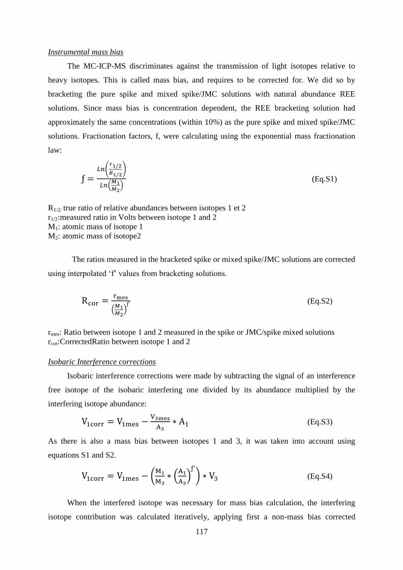
117
Instrumental mass bias
The MC-ICP-MS discriminates against the transmission of light isotopes relative to
heavy isotopes. This is called mass bias, and requires to be corrected for. We did so by
bracketing the pure spike and mixed spike/JMC solutions with natural abundance REE
solutions. Since mass bias is concentration dependent, the REE bracketing solution had
approximately the same concentrations (within 10%) as the pure spike and mixed spike/JMC
solutions. Fractionation factors, f, were calculating using the exponential mass fractionation
law:
(Eq.S1)
R1/2: true ratio of relative abundances between isotopes 1 et 2
r1/2:measured ratio in Volts between isotope 1 and 2
M1: atomic mass of isotope 1
M2: atomic mass of isotope2
The ratios measured in the bracketed spike or mixed spike/JMC solutions are corrected
using interpolated ‘f’ values from bracketing solutions.
(Eq.S2)
rmes: Ratio between isotope 1 and 2 measured in the spike or JMC/spike mixed solutions
rcor:CorrectedRatio between isotope 1 and 2
Isobaric Interference corrections
Isobaric interference corrections were made by subtracting the signal of an interference
free isotope of the isobaric interfering one divided by its abundance multiplied by the
interfering isotope abundance:
(Eq.S3)
As there is also a mass bias between isotopes 1 and 3, it was taken into account using
equations S1 and S2.
(Eq.S4)
When the interfered isotope was necessary for mass bias calculation, the interfering
isotope contribution was calculated iteratively, applying first a non-mass bias corrected
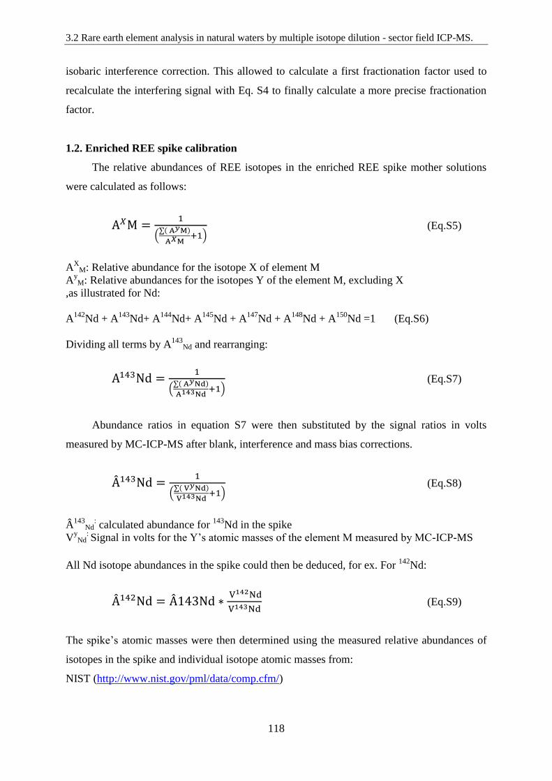
3.2 Rare earth element analysis in natural waters by multiple isotope dilution - sector field ICP-MS.
118
isobaric interference correction. This allowed to calculate a first fractionation factor used to
recalculate the interfering signal with Eq. S4 to finally calculate a more precise fractionation
factor.
1.2. Enriched REE spike calibration
The relative abundances of REE isotopes in the enriched REE spike mother solutions
were calculated as follows:
(Eq.S5)
AX
M: Relative abundance for the isotope X of element M
AyM: Relative abundances for the isotopes Y of the element M, excluding X
,as illustrated for Nd:
A142
Nd + A143
Nd+ A144
Nd+ A145
Nd + A147
Nd + A148
Nd + A150
Nd =1 (Eq.S6)
Dividing all terms by A143
Nd and rearranging:
(Eq.S7)
Abundance ratios in equation S7 were then substituted by the signal ratios in volts
measured by MC-ICP-MS after blank, interference and mass bias corrections.
(Eq.S8)
Â143
Nd: calculated abundance for
143Nd in the spike
VyNd
: Signal in volts for the Y’s atomic masses of the element M measured by MC-ICP-MS
All Nd isotope abundances in the spike could then be deduced, for ex. For 142
Nd:
(Eq.S9)
The spike’s atomic masses were then determined using the measured relative abundances of
isotopes in the spike and individual isotope atomic masses from:
NIST (http://www.nist.gov/pml/data/comp.cfm/)
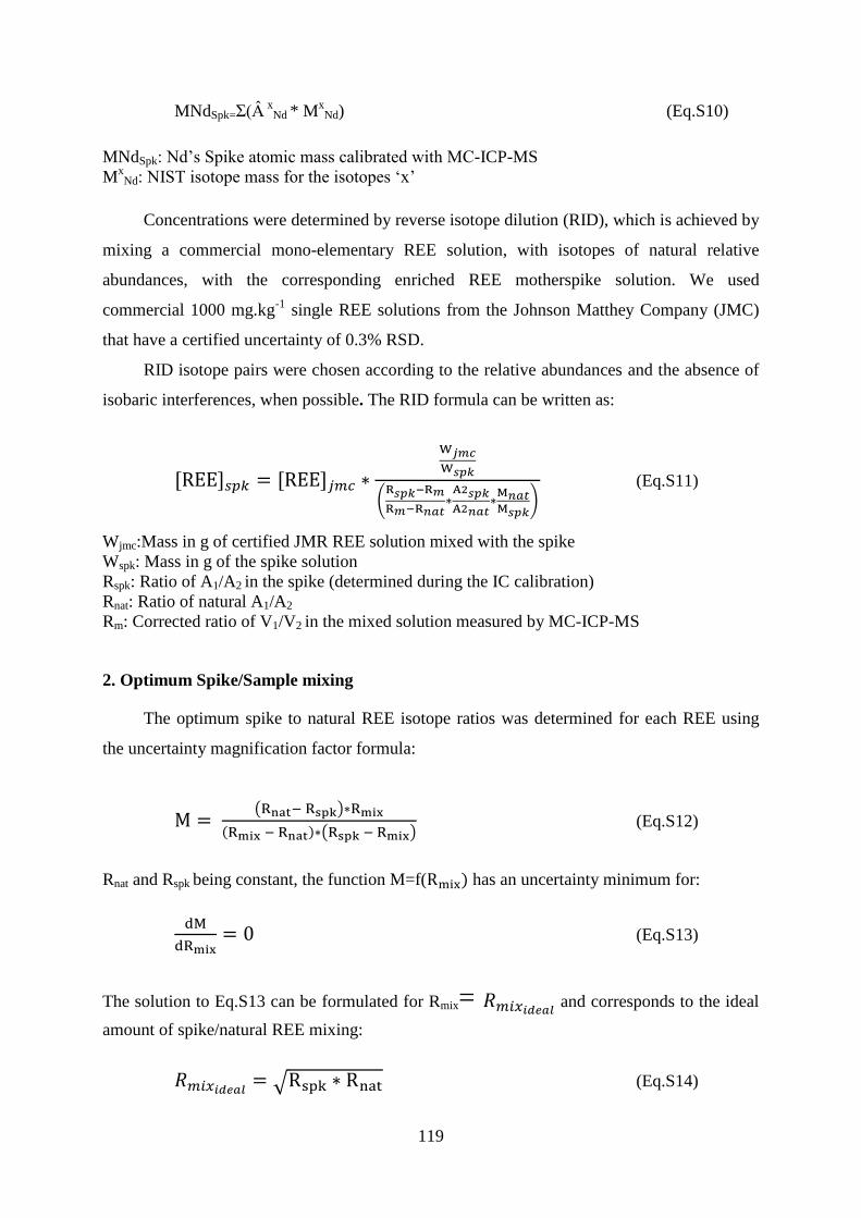
119
MNdSpk=Σ(Â x
Nd * MxNd) (Eq.S10)
MNdSpk: Nd’s Spike atomic mass calibrated with MC-ICP-MS
MxNd: NIST isotope mass for the isotopes ‘x’
Concentrations were determined by reverse isotope dilution (RID), which is achieved by
mixing a commercial mono-elementary REE solution, with isotopes of natural relative
abundances, with the corresponding enriched REE motherspike solution. We used
commercial 1000 mg.kg-1
single REE solutions from the Johnson Matthey Company (JMC)
that have a certified uncertainty of 0.3% RSD.
RID isotope pairs were chosen according to the relative abundances and the absence of
isobaric interferences, when possible. The RID formula can be written as:
(Eq.S11)
Wjmc:Mass in g of certified JMR REE solution mixed with the spike
Wspk: Mass in g of the spike solution
Rspk: Ratio of A1/A2 in the spike (determined during the IC calibration)
Rnat: Ratio of natural A1/A2
Rm: Corrected ratio of V1/V2 in the mixed solution measured by MC-ICP-MS
2. Optimum Spike/Sample mixing
The optimum spike to natural REE isotope ratios was determined for each REE using
the uncertainty magnification factor formula:
(Eq.S12)
Rnat and Rspk being constant, the function M=f( has an uncertainty minimum for:
(Eq.S13)
The solution to Eq.S13 can be formulated for Rmix= and corresponds to the ideal
amount of spike/natural REE mixing:
(Eq.S14)
3.2 Rare earth element analysis in natural waters by multiple isotope dilution - sector field ICP-MS.
120
Figure S1 illustrates the mixing between natural Nd and enriched 146
Nd spike for the ratio
146Nd/
145Nd. The value for M decreases between the Rnat (2.07) and the
(19.63)
corresponding to the underspiking zone and increases between and Rspk (186.4)
corresponding to the overspiking zone.
Figure S1: Uncertainty magnification factor ‘M’ as a function of the
146Nd/
145Nd mixing ratio
used for Nd isotope dilution.
In practice, the ideal amount of isotopic spikes were approximated using the reverse
isotope dilution equation (Eq.S11) for a given sample [REE] and replacing Rmby .
One difficulty is that added spike isotopes may themselves generate molecular and isobaric
interferences. Therefore, simulations of ideally spiked samples were made numerically
considering several plausible levels of plasma oxide and hydroxide formation in order to
evaluate the magnitude of oxi-hydroxide interferences (ie: Ba and LREE on MREE and
MREE on HREE) and isobaric interferences (ie: Ba, La, Ce and Yb, Lu, Hf).
After this optimization to limit isobaric and oxide interferences, a stock of mixedLREE
spike and mixedHREE spike solutions was prepared. These stock solutions contain
respectively 51ppb for La, 15ppb for Ce, 113 ppb for Nd, 48 ppb for Sm, 18 ppb forEu and 92
ppb for Gd (mixed spike LREE ) and 116 ppb for Dy, 65 ppb for Er, 41 ppb for Yb and 17
ppb for Lu (mixed spike HREE). Dilutions of those mother solutions were made to achieve
200µl to 1ml of spike aliquots when spiking samples. A SF-ICPMS mass spectrum of both
HREE and LREE mixed spike solutions is reported in Figure S2.
1
2
3
4
5
6
7
0 20 40 60 80 100 120 140 160 180
M
Rm
OverspikingUnderspikingRmideal
121
Figure S2: HREE (black) and LREE (grey) mixed spike mass spectrum measured with Thermo
Element-XR coupled with the Aridus 2 desolvator.
The average dispersion of the uncertainty magnification factor ‘M’ obtained on the 19
samples analyzed in this study are reported in Figure S3. The grey line represents for each
element the theoretical uncertainty magnification factor corresponding to an ideal proportion
of sample/spike mixing and the boxplots represent the observed uncertainty magnification
factor. Except for La and Lu which are overspiked on purpose all isotope/sample mixing
proportions were close to ideal.
Figure S3: REE isotope dilution ‘M’ uncertainty magnification factors based
on 19 samples spiked in this study (Boxplots) relative to the minimum
theoretical uncertainty level achievable (grey lines).
0.0E+00
5.0E+05
1.0E+06
1.5E+06
2.0E+06
2.5E+06
3.0E+06
3.5E+06
136
138
140
142
144
146
148
150
152
154
156
158
160
162
164
166
168
170
172
174
176
Co
un
ts.s
⁻¹
Atomic Mass Number
Spike LREE
Spike HREE
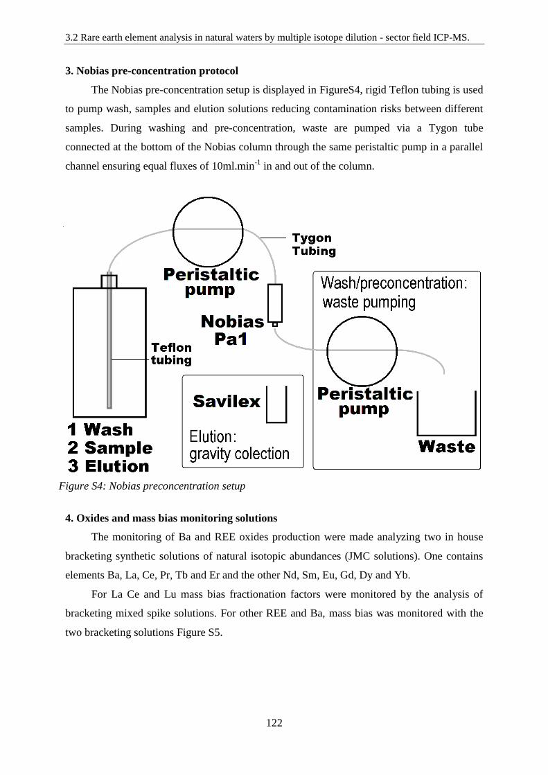
3.2 Rare earth element analysis in natural waters by multiple isotope dilution - sector field ICP-MS.
122
3. Nobias pre-concentration protocol
The Nobias pre-concentration setup is displayed in FigureS4, rigid Teflon tubing is used
to pump wash, samples and elution solutions reducing contamination risks between different
samples. During washing and pre-concentration, waste are pumped via a Tygon tube
connected at the bottom of the Nobias column through the same peristaltic pump in a parallel
channel ensuring equal fluxes of 10ml.min-1
in and out of the column.
Figure S4: Nobias preconcentration setup
4. Oxides and mass bias monitoring solutions
The monitoring of Ba and REE oxides production were made analyzing two in house
bracketing synthetic solutions of natural isotopic abundances (JMC solutions). One contains
elements Ba, La, Ce, Pr, Tb and Er and the other Nd, Sm, Eu, Gd, Dy and Yb.
For La Ce and Lu mass bias fractionation factors were monitored by the analysis of
bracketing mixed spike solutions. For other REE and Ba, mass bias was monitored with the
two bracketing solutions Figure S5.
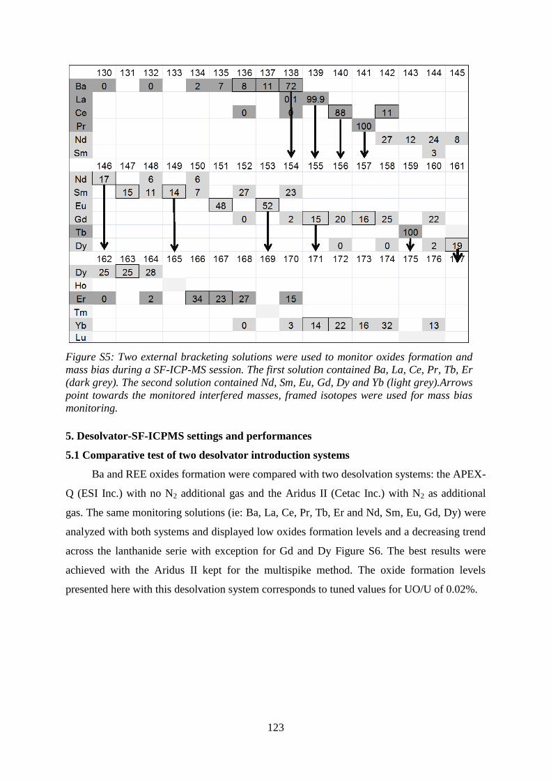
123
Figure S5: Two external bracketing solutions were used to monitor oxides formation and
mass bias during a SF-ICP-MS session. The first solution contained Ba, La, Ce, Pr, Tb, Er
(dark grey). The second solution contained Nd, Sm, Eu, Gd, Dy and Yb (light grey).Arrows
point towards the monitored interfered masses, framed isotopes were used for mass bias
monitoring.
5. Desolvator-SF-ICPMS settings and performances
5.1 Comparative test of two desolvator introduction systems
Ba and REE oxides formation were compared with two desolvation systems: the APEX-
Q (ESI Inc.) with no N2 additional gas and the Aridus II (Cetac Inc.) with N2 as additional
gas. The same monitoring solutions (ie: Ba, La, Ce, Pr, Tb, Er and Nd, Sm, Eu, Gd, Dy) were
analyzed with both systems and displayed low oxides formation levels and a decreasing trend
across the lanthanide serie with exception for Gd and Dy Figure S6. The best results were
achieved with the Aridus II kept for the multispike method. The oxide formation levels
presented here with this desolvation system corresponds to tuned values for UO/U of 0.02%.
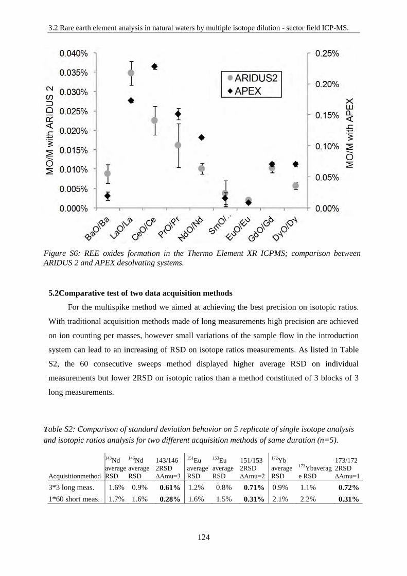
3.2 Rare earth element analysis in natural waters by multiple isotope dilution - sector field ICP-MS.
124
Figure S6: REE oxides formation in the Thermo Element XR ICPMS; comparison between
ARIDUS 2 and APEX desolvating systems.
5.2Comparative test of two data acquisition methods
For the multispike method we aimed at achieving the best precision on isotopic ratios.
With traditional acquisition methods made of long measurements high precision are achieved
on ion counting per masses, however small variations of the sample flow in the introduction
system can lead to an increasing of RSD on isotope ratios measurements. As listed in Table
S2, the 60 consecutive sweeps method displayed higher average RSD on individual
measurements but lower 2RSD on isotopic ratios than a method constituted of 3 blocks of 3
long measurements.
Table S2: Comparison of standard deviation behavior on 5 replicate of single isotope analysis
and isotopic ratios analysis for two different acquisition methods of same duration (n=5).
Acquisitionmethod
143Nd
average
RSD
146Nd
average
RSD
143/146
2RSD
∆Amu=3
151Eu
average
RSD
153Eu
average
RSD
151/153
2RSD
∆Amu=2
172Yb
average
RSD
173Ybaverag
e RSD
173/172
2RSD
∆Amu=1
3*3 long meas. 1.6% 0.9% 0.61% 1.2% 0.8% 0.71% 0.9% 1.1% 0.72%
1*60 short meas. 1.7% 1.6% 0.28% 1.6% 1.5% 0.31% 2.1% 2.2% 0.31%
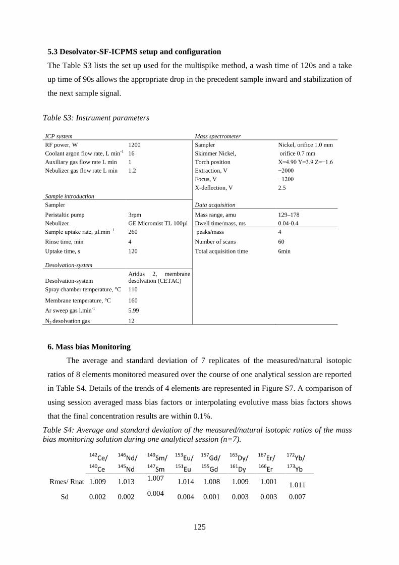
125
5.3 Desolvator-SF-ICPMS setup and configuration
The Table S3 lists the set up used for the multispike method, a wash time of 120s and a take
up time of 90s allows the appropriate drop in the precedent sample inward and stabilization of
the next sample signal.
Table S3: Instrument parameters
6. Mass bias Monitoring
The average and standard deviation of 7 replicates of the measured/natural isotopic
ratios of 8 elements monitored measured over the course of one analytical session are reported
in Table S4. Details of the trends of 4 elements are represented in Figure S7. A comparison of
using session averaged mass bias factors or interpolating evolutive mass bias factors shows
that the final concentration results are within 0.1%.
Table S4: Average and standard deviation of the measured/natural isotopic ratios of the mass
bias monitoring solution during one analytical session (n=7).
142Ce/ 140Ce
146Nd/ 145Nd
149Sm/ 147Sm
153Eu/ 151Eu
157Gd/ 155Gd
163Dy/ 161Dy
167Er/ 166Er
172Yb/ 173Yb
Rmes/ Rnat 1.009 1.013 1.007
1.014 1.008 1.009 1.001 1.011
Sd 0.002 0.002 0.004 0.004 0.001 0.003 0.003 0.007
ICP system Mass spectrometer
RF power, W 1200 Sampler Nickel, orifice 1.0 mm
Coolant argon flow rate, L min-1 16 Skimmer Nickel, orifice 0.7 mm
Auxiliary gas flow rate L min 1 Torch position X=4.90 Y=3.9 Z=−1.6
Nebulizer gas flow rate L min 1.2 Extraction, V −2000
Focus, V −1200
X-deflection, V 2.5
Sample introduction
Sampler Data acquisition
Peristaltic pump 3rpm Mass range, amu 129–178
Nebulizer GE Micromist TL 100µl Dwell time/mass, ms 0.04-0.4
Sample uptake rate, μl.min−1 260 peaks/mass 4
Rinse time, min 4 Number of scans 60
Uptake time, s 120 Total acquisition time 6min
Desolvation-system
Desolvation-system
Aridus 2, membrane
desolvation (CETAC)
Spray chamber temperature, °C 110
Membrane temperature, °C 160
Ar sweep gas l.min-1 5.99
N2 desolvation gas 12
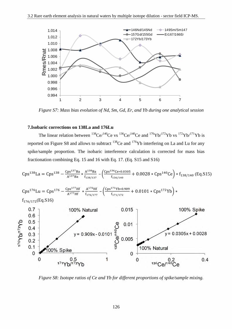
3.2 Rare earth element analysis in natural waters by multiple isotope dilution - sector field ICP-MS.
126
Figure S7: Mass bias evolution of Nd, Sm, Gd, Er, and Yb during one analytical session
7.Isobaric corrections on 138La and 176Lu
The linear relation between 138
Ce/140
Ce vs 136
Ce/140
Ce and 176
Yb/172
Yb vs 172
Yb/171
Yb is
reported on Figure S8 and allows to subtract 138
Ce and 176
Yb interfering on La and Lu for any
spike/sample proportion. The isobaric interference calculation is corrected for mass bias
fractionation combining Eq. 15 and 16 with Eq. 17. (Eq. S15 and S16)
–
(Eq.S15)
–
(Eq.S16)
Figure S8: Isotope ratios of Ce and Yb for different proportions of spike/sample mixing.
0.994
0.996
0.998
1.000
1.002
1.004
1.006
1.008
1.010
1.012
1.014
1 2 3 4 5 6 7
Rm
es/R
na
t
146Nd/145Nd 149Sm/Sm147
157Gd/155Gd Er167/166Er
172Yb/173Yb
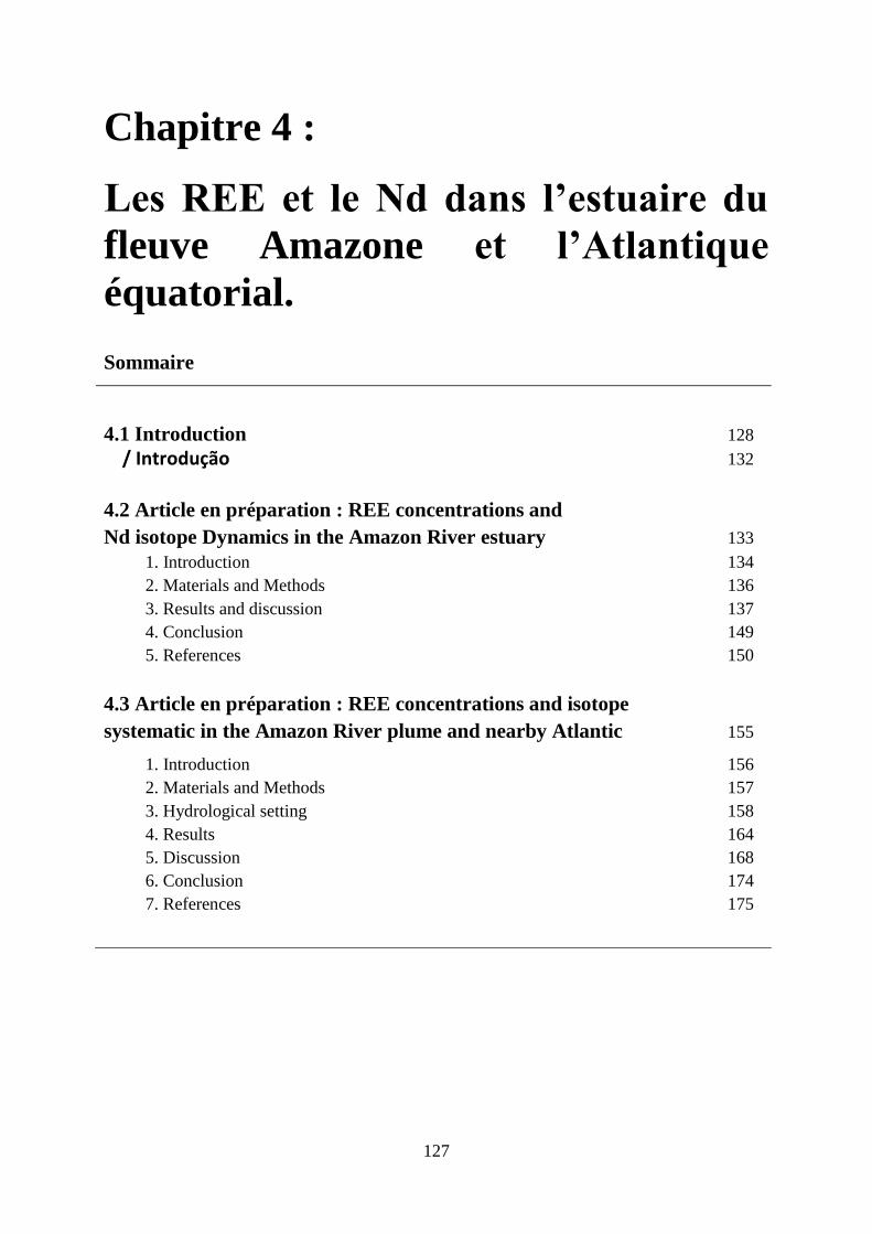
127
Chapitre 4 :
Les REE et le Nd dans l’estuaire du
fleuve Amazone et l’Atlantique
équatorial.
Sommaire
4.1 Introduction 128
/ Introdução 132
4.2 Article en préparation : REE concentrations and
Nd isotope Dynamics in the Amazon River estuary 133
1. Introduction 134
2. Materials and Methods 136
3. Results and discussion 137
4. Conclusion 149
5. References 150
4.3 Article en préparation : REE concentrations and isotope
systematic in the Amazon River plume and nearby Atlantic 155
1. Introduction 156
2. Materials and Methods 157
3. Hydrological setting 158
4. Results 164
5. Discussion 168
6. Conclusion 174
7. References 175
128
4.1 Introduction
Ce chapitre regroupe deux articles en préparation qui présentent et discutent les résultats
obtenus au cours des campagnes AMANDES :
Le premier article : “REE concentrations and Nd isotope dynamics in the Amazon River
estuary” est focalisé sur la campagne Amandes 3 réalisée en avril 2008 dans l’estuaire du
fleuve Amazone le long du gradient salin. Les compositions isotopiques du Nd dans les phases
dissoute et particulaire ainsi que les concentrations en REE dans les phases dissoutes et
colloïdales ont été mesurées. Cette approche est originale en milieu naturel pour l’estuaire
Amazonien. En effet les travaux pionniers ont consisté en la mesure de concentrations en REE
dans la phase dissoute dite totale (< 0,22µm), en des expériences de mélange et d’ultrafiltration
en laboratoire. Une seule mesure de la composition isotopique Nd pour le pôle (ou
« endmember, ci après EM) Amazonien était jusqu’alors disponible. Cette étude a permis de :
1) caractériser l’EM du fleuve Amazone, 2) Observer que la signature en REE observée à la
station de suivi du fleuve Amazone à Óbidos est représentative de celle trouvée à l’embouchure
du fleuve pour la salinité ’zero’, 3) confirmer le comportement variable des concentrations en
REE le long du gradient salin (forte diminution aux faibles salinités, ré-augmentation aux
salinités intermédiaires et hautes), 4)Lier la diminution de la part des concentrations en REE le
long du gradient salin à une baisse de la fraction des colloïdes auxquels ils sont associés, 5)
Identifier l’origine lithogénique des REE apportés en solution aux salinités moyennes et hautes
6) Proposer un bilan de masse annuel du transfert du Nd des particules vers la phase dissoute au
sein de l’estuaire.
Le deuxième article : “REE concentrations and isotope systematic in the Amazon River
plume and nearby Atlantic” présente et discute les profils de εNd mesurés au large des côtes
Guyanaise et sur la marge au cours d’Amandes 1 et 2 en Octobre 2007 et janvier 2008. Ces
profils ont permis d’enrichir la base donnée mondiale de compositions isotopiques du Nd
océanique dans cette zone jusqu’alors peu échantillonnée et qui est cruciale dans le transit
trans-équatorial de masses d’eau Atlantique venant du Nord et du Sud. Les observations
majeures se dégageant de ce jeu de données sont : 1) Le relargage d’une partie du Nd soustrait
par les colloïdes coagulés dans l’estuaire, 2) Une signature isotopique légèrement plus
radiogénique pour les eaux centrales nord Atlantiques que pour les eaux centrales sud
Atlantiques, 3) Un contraste isotopique important entre les eaux Antarctiques intermédiaires
129
provenant du sud (peu radiogéniques) et les eaux centrales profondes du nord plus
radiogéniques.
Des eaux faiblement radiogéniques ont étés récemment observées dans le Bassin de
l’Angola (Rickli et al 2009).Elles étaient considérées comme locales uniquement. A la lumière
des observations faites au cours d’Amandes, et qui couplent les paramètres hydrologiques et
isotopiques, nous suggérons que ces eaux non radiogéniques du sud s’étendent sur une plus
grande surface dans le nord du gyre sud-atlantique ; Nous identifions et quantifions aussi
l’intrusion des eaux centrales du nord dans les eaux intermédiaires du sud au passage de
l’équateur.
4.1 Introdução
130
Introdução
Este capítulo agrupa dois artigos em preparação os quais apresentam e discutem os
resultados obtidos durante as campanhas AMANDES :
O primeiro artigo : “REE concentrations and Nd isotope dynamic in the Amazon River
estuary” tem foco na campanha Amandes 3 realizada em abril de 2008 no estuário do rio
Amazonas ao longo do gradiente salino. As composições isotópicas do Nd nas fases do
material particulado e do dissolvido e os teores em REE nas fases do material dissolvido e
coloidal foram determinados.Esta abordagem é original em ambiente natural para o estuário
Amazônico. De fato trabalhos pioneiros tem consistido na medida de teores em REE na fase
dissolvida total (< 0.22オm) e em experimentos de mistura e ultrafiltração em laboratório. Até
agora, somente uma única medida da composição isotópica do Nd para o pólo (ou
Endmember, a seguir definido por EM) Amazônico eradisponível.Este estudo permitiu: 1) a
caracterização do EM do rio Amazonas; 2) Observar que a assinatura em REE observada em
Óbidos é representativa daquela encontrada na foz parasalinidade 0; 3) de confirmar o
comportamento variável dos teores em REE ao longo do gradiente salino (forte diminuição em
salinidades baixas, aumento em salinidades médias e altas); 4) ligar a diminuição da parte dos
teores em REE ao longo do gradiente salino à uma diminuição dos teores em colóides aos
quais estes são associados, 5) identificar a origem litogênica dos REE dissolvidos em salinidade
médias e altas 6) propor um balanço de massa anual da transferência do Nd das partículas
para a fase dissolvida nos estuários.
O Segundo artigo : “REE concentrations and isotope systematic in the Amazon River
plume and nearby Atlantic” apresenta e discute perfis verticais de εNd medidos ao largo da
costa guianesa e na margem durante Amandes 1 e 2 em outubro e janeiro de 2008.Estes
perfis permitiram o enriquecimento da base de dado mundial do Nd oceânico nesta zona
pouco amostrada e portanto crucial no trânsito equatorial de massas de água provenientesdo
norte e do sul. As observaçõesmaiores se destacando neste jogo de dados são: 1) a
relargagem de parte do Nd substraído pelos colóides coagulados no estuário, 2) uma
assinatura isotópica ligeiramente mais radiogênica para as águas centrais provenientes do
atlântico norte quando comparadas as águas centrais do atlântico sul; 3) um contraste
isotópico importante entre as Águas Antárticas Intermediárias (AAIW)proveniente do sul
131
(levemente radiogênicas) e as Águas Centrais Profundas (Lower-CAW) mais
radiogênicas.Águaslevemente radiogênicas foram recentementeobservadas na bacia oceânica
angolana (Rickli et al 2009) e eram consideradas unicamente locais. Na luz das observações
realizadas durante Amandes acoplando os parâmetros hidrológicos e isotópicos, sugerimos
que as águas não radiogênicas do sul têm uma extensão maior ao norte do giro sul-atlântico ;
identificamos e quantificamos também a intrusão lower-CAW em águas intermediárias do sul.
132
4.2 Article en préparation : REE concentrations Nd isotope dynamics in the
Amazon River estuary
T.C.C. Rousseaua, J.E. Sonke
a, G. Boaventura
c, P. Seyler
a C. Pradoux
b, P. van Beek
b M.
Souhautb& C. Jeandel
b
aGET, Université de Toulouse, CNRS, IRD, CNES, 14 Avenue Edouard Belin, F-31400
Toulouse, France. bLEGOS, Université de Toulouse, CNRS, IRD, CNES, 14 Avenue Edouard Belin, F-31400
Toulouse, France cUniversidade De Brasilia, UNB, LAGEQ, Campus universitario Darcy Ribeiro, 70.910-900 Brasilia,
DF, Brazil
In preparation for Marine Chemistry
Abstract
The first estuary study coupling traditional dissolved Rare Earth Element concentration [REE]
analysis with ultrafiltration and Nd isotopic composition (IC) analysis is proposed here.
Sampling was done in the framework of the AMANDES project within the Amazon estuary
salinity gradient and on the Brazilian shelf. Similar to published work, our results confirm the
sharp drop in [REE] in the low (0-17) salinity zone, followed by a minor increase in [REE] at
higher salinities. We observe a decrease of the coarse colloidal Nd fraction (>10kDa) from
more than 80% in the Amazon River to less than 10% for the seawater end member. The
distinct Nd IC of the Amazon suspended particles (>0.45µm, εNd= -10.6), dissolved Nd (εNd=
-8.9) and the seawater end member (εNd= -12) allowed us to attribute the Nd release at mid
salinities to the desorption and/or dissolution of suspended particulate Nd. The dynamics of
dissolved/particle IC homogenization were estimated to be about 19 days, based on radon age
dating of the Amazon River plume. Estuarine bottom waters at 40-90m depth which had not
been in contact with the Amazon River end member also showed elevated Nd concentrations
and slightly unradiogenic Nd IC. These results suggest that the Amazon River Nd (and REE)
flux to the Equatorial Atlantic Ocean is dominated by suspended and shelf sediments.
133
1. Introduction
Understanding Rare Earth Element (REE) speciation, dynamics, and mass balance in
natural waters is important because the REE and neodymium (Nd) isotopes are used as tracers
of water mass transport and mixing in the modern ocean (Jeandel, 1993; Lacan and Jeandel,
2004; Piepgras and Wasserburg, 1980; Shimizu et al., 1994), and as paleoproxies for past
oceanic circulation patterns (Frank et al., 2002; Gutjahr et al., 2008; Piotrowski et al., 2004,
2005; Rutberg et al., 2000). In river waters, REE speciation is mainly controlled by organic and
mineral colloids (Deberdt et al., 2002) whereas in seawater REE concentrations are lower and
their speciation is thought to be controlled by carbonates and phosphates (Luo and Byrne,
2001).
In the ocean, dissolved REE are of lithogenic origin. The Nd isotope signature, defined
as εNd (the ratio of radiogenic 143
Nd over stable 144
Nd, normalized to CHUR (DePaolo and
Wasserburg, 1976), on the parts per ten-thousand scale) reflects the geological age of the
lithogenic Nd source (Piepgras et al., 1979; Stordal and Wasserburg, 1986). Sources of REEs to
the oceans are direct river discharge, dissolution of a fraction of atmospheric dust (1-7%), but
mostly a large release of REE (including Nd isotopes) from estuarine and shelf sediments at the
continent-ocean boundary (Arsouze et al., 2007; Sholkovitz and Szymczak, 2000; Tachikawa et
al., 2003). The marine Nd cycle has been included in a general ocean circulation model
(Arsouze et al., 2009). It was estimated that 1 to 3 percent of the annual Nd flux by continental
weathering has to be released to seawater to explain the combined variations in Nd
concentrations and Nd isotopic composition. However, the processes yielding this release are
not understood yet. Hypotheses invoke estuarine processes transforming the river solid
discharge (Jones et al., 2012a; Pearce et al., 2013; Sholkovitz, 1995), boundary exchange
processes directly involving the sediments deposited on the margins and/or submarine
groundwater discharge (Johannesson and Burdige, 2007; Lacan and Jeandel, 2005; van de
Flierdt et al., 2007).
Estuaries are important biogeochemical reactors where river fluxes of inorganic and
organic matter from the continents influence the chemistry and biology of the coastal and
ultimately open ocean. It is well-known that the flocculation of river dissolved organic matter
by sea salt drives the non-conservative behavior of trace metals in estuaries (Boyle et al., 1977;
Eckert and Sholkovitz, 1976; Sholkovitz, 1976).
The margin off the Amazon River mouth is of particular interest: the immense discharge
of the Amazon River (representing 20% of the freshwater discharge to the ocean and 6% of the
global riverine sediment discharge, c.a. 1.2 x 10¹⁵
g.yr-1
) causes river/ocean mixing to take
4.2 REE concentrations and Nd isotope dynamics in the Amazon River estuary
134
place out on the continental shelf instead of within a drowned river valley. The water on the
shelf is characterized by estuarine-like processes (Gibbs, 1967; Gibbs and Konwar, 1986;
Warne et al., 2002), with freshwater lenses extending 120 km offshore (Gibbs, 1970). The tidal
influence is strong on the shelf, generating internal waves and re circulations that can be seen
up to ~100 km inland (Kosuth et al., 2009). Strong physical reworking and redox processes
within the Amazon basin are the main drivers behind the largest source of dissolved elements
to the Atlantic Ocean (DeMaster et al., 1996; Sullivan and Aller, 1996; Swarzenski et al.,
1995).Van Der Loeff et al.(1997) suggested that the Amazon riverine input could be the major
source of Cd, Zn and Cu to tropical Atlantic surface waters. The Amazon River was identified
as the most probable source of low salinity waters with elevated concentrations of nutrients,
particulate organic carbon, Cu and Cd in the mid-Atlantic Ocean as far as 5 to 9°N-28°W that
is off the African coast.
A landmark study on the REE dynamics in the Amazon estuary was published by
Sholkovitz, (1993) who showed that 0.22 µm filtered REE concentrations behave non-
conservatively in the salinity gradient. From 0 - 6.6‰ salinity >90% of REE are removed from
solution. This removal was attributed to coagulation of riverine colloids. Surprisingly, from 6.6
- 34.4‰ salinity, all REE concentrations increase and this was interpreted as due to the release
of REE from sediments and resuspended particles, without precising their nature. An
alternative, but unfavored explanation was the mixing with a previously discharged Amazon
River water mass with higher REE concentrations. Looking in detail, it was also noticed that
the REE concentration rebound in the 6.6 - 34.4 salinity zone was more pronounced for LREE
than HREE. A subsequent detailed study on the aquatic chemistry of the REE in estuaries made
abundant use of experimental mixing of river and sea water end-members and the ultrafiltration
technique observed that adsorption and coagulation processes affects predominantly LREE
over HREE (Sholkovitz, 1995).A second follow-up study on the REE dynamics in Indonesian
estuaries confirmed the potential role of estuarine and shelf sediments as sources of REE to the
oceans (Sholkovitz and Szymczak, 2000).More recently Pearce et al. (2013) performed
leaching experiments of riverine, estuarine and marine sediments with open ocean sea water.
The results showed that the εNd value of the dissolved phase rapidly changes from the initial
sea water value towards an εNd value similar to that of the sediments and that up to 9% of Nd
is released from the solid material within 4 months’ time. To our knowledge only a single
dissolved εNd measurement was made in the Amazon estuary (Piepgras and Wasserburg, 1987)
and no detailed characterization of εNd along an estuarine salinity gradient has been made.
135
In this study we revisit the REE dynamics and Nd isotopic composition of the Amazon
River estuary. The objectives are: i) to explore potential variations in dissolved and particulate
εNd in the salinity gradient in relation to the physicochemical REE transformations and ii) to
combine estuarine εNd and REE observations in order to refine our understanding of the
suggested scavenging, adsorption and desorption mechanisms that drive REE dynamics. In a
forthcoming paper will detail the impact of the Amazon discharge on the εNd of nearby marine
water masses in a still poorly documented area, yet crucial for inter-hemispheric water transfer
and characterized by complex circulation features.
Samples from the Amazon estuary were collected during one of the fourth sampling
cruises of the AMANDES project. We performed onboard 10kDa ultrafiltration in order to
observe in details the REE features of the coarse REE-colloidal (0.45µm>>10kDa) and fine
REE-colloidal and truly dissolved fractions (<10kDa). A newly developed ICP-MS method,
based on multi-spike isotope dilution, was used to generate high precision REE concentrations
over the entire river to sea water salinity continuum (Rousseau et al. 2013).
2. Materials and Methods
Sampling was done in the framework of the multidisciplinary AMANDES project,
during the oceanographic cruise on the NO/ANTEA in April 2008 (AMANDES 3). Figure 1
shows the sampling map. Samples were collected using 8 L Niskin bottles mounted on a 12
bottle rosette, equipped with a CTD (conductivity temperature density) gauge and dissolved
oxygen, chlorophyll and light attenuation sensors. For Nd IC analysis, 10 L were filtered on
board with 0.45µm polyethersulfone (PES) Supor®filters and immediately acidified to pH 3.5
using double distilled 6M HCl. Each 10 L sample was pre-concentrated using two C18 SepPak
cartridges loaded with a strong REE complexant (HDEHP/H2MEHP) (Shabani et al., 1992).
Back at the land-based LEGOS laboratory, the REE were eluted using 6M HCl, evaporated and
re-dissolved in 1.5 ml of 1M HCl. Nd separation was achieved by a two step chromatography
protocol using cationic AG50 X8 and Ln-SPEC resins: After evaporation to dryness and
dissolution again in 2M HCl,C18 eluate was loaded on a cation exchange column (0.6 cm in
diameter, 4.8 cm in height) packed with Biorad AG50W-X8 (200 to 400 mesh) resin to extract
the REE from the remaining matrix using HCl and HNO3. The REE were then eluted with 6ml
of 6M HCl. This solution was evaporated and re-dissolved in 0.3 ml of 0.2 M HCl for the final
extraction of Nd using an anionic exchange column (0.4 cm in diameter, 4 cm in height) packed
with 0.5 ml of Ln-Spec resin. A final elution using 2.5 ml of 0.2 M HCl allowed recovering the
neodymium. Details of the procedures used on the cationic and anionic columns are described
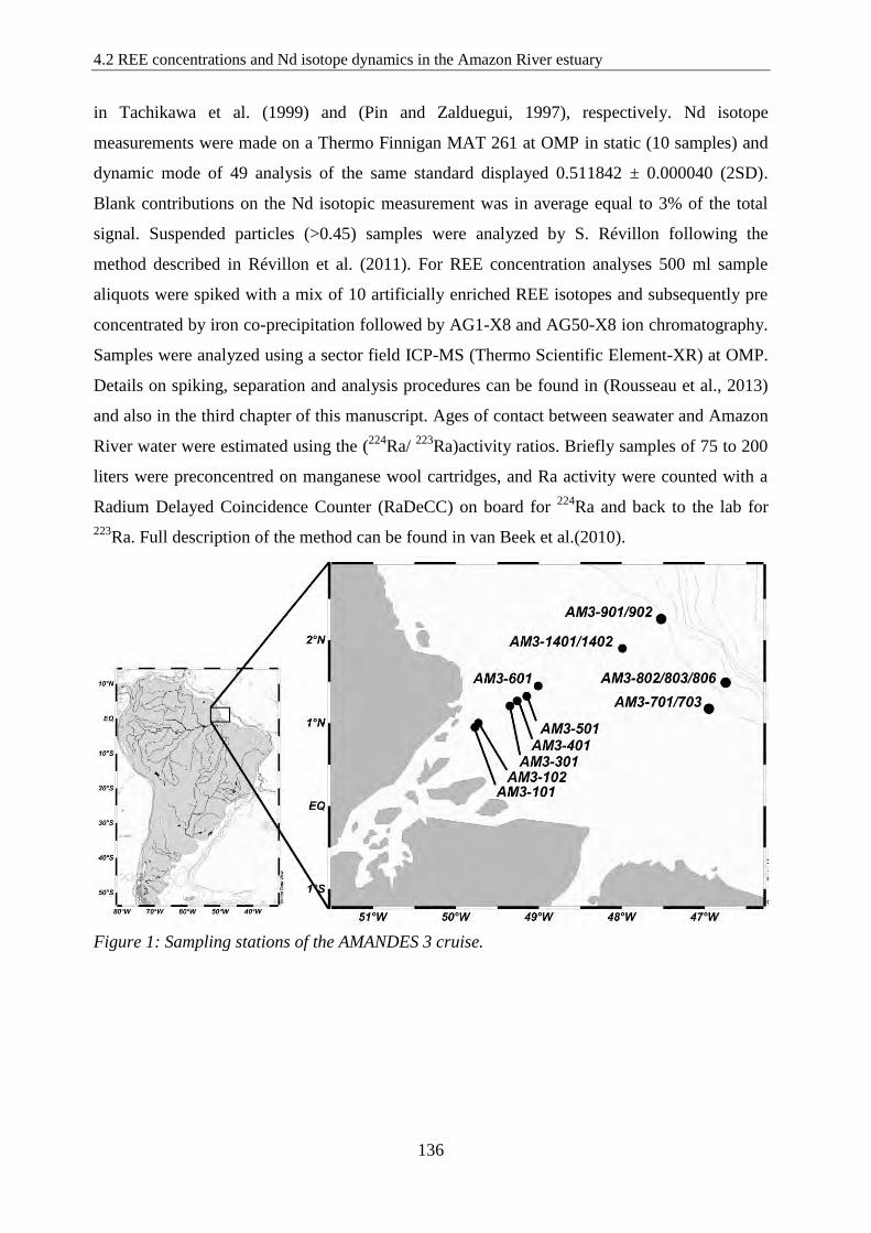
4.2 REE concentrations and Nd isotope dynamics in the Amazon River estuary
136
in Tachikawa et al. (1999) and (Pin and Zalduegui, 1997), respectively. Nd isotope
measurements were made on a Thermo Finnigan MAT 261 at OMP in static (10 samples) and
dynamic mode of 49 analysis of the same standard displayed 0.511842 ± 0.000040 (2SD).
Blank contributions on the Nd isotopic measurement was in average equal to 3% of the total
signal. Suspended particles (>0.45) samples were analyzed by S. Révillon following the
method described in Révillon et al. (2011). For REE concentration analyses 500 ml sample
aliquots were spiked with a mix of 10 artificially enriched REE isotopes and subsequently pre
concentrated by iron co-precipitation followed by AG1-X8 and AG50-X8 ion chromatography.
Samples were analyzed using a sector field ICP-MS (Thermo Scientific Element-XR) at OMP.
Details on spiking, separation and analysis procedures can be found in (Rousseau et al., 2013)
and also in the third chapter of this manuscript. Ages of contact between seawater and Amazon
River water were estimated using the (224
Ra/ 223
Ra)activity ratios. Briefly samples of 75 to 200
liters were preconcentred on manganese wool cartridges, and Ra activity were counted with a
Radium Delayed Coincidence Counter (RaDeCC) on board for 224
Ra and back to the lab for
223Ra. Full description of the method can be found in van Beek et al.(2010).
Figure 1: Sampling stations of the AMANDES 3 cruise.
137
3. Results and discussion
3.1 Amazon Endmenber (EM)
Barroux et al., (2006) studied the seasonal variations in dissolved (<0.2 µm) REE
concentrations at Obidos and reviewed all earlier published Amazon River REE data.
Dissolved [Nd]d,<0.2um varied between 47 ng.kg-1
to 178 ng.kg-1
(336 to 1234 pmol.kg-1
), during
the low to high water stages in 2003 to 2005. [Nd]d,<0.2µm was shown to correlate significantly
with discharge of the Amazon River (r2=0.64):
[Nd]d,<0.2um = 7x10⁻⁴
x D – 9.6 Eq. 1
where D represents the discharge in m3/sec.
During AMANDES 3, the [Nd]d,<0.45µm of the river EM measured in the upper estuary
was 123 ng.kg-1
(853 pmol.kg-1
)on April 10th
2008 (sample AM3-101, Table 2). The Amazon
discharge at this time 2008 was 234,300 m3/s using equation 1, we estimated Nd concentration
at Obidos of 154 ± 40 ng.L-1
(1068± 277 pmol.kg-1
)similar to our observation of 123 ng.kg-1
.
The TTO/TAS 44 Amazon river endmember samples 44 and 46 collected during the low water
stage in December 1982 displayed dissolved Nd concentrations of 53.9 and 48.5 ng.L-1
(374 and
336 pmol.kg-1
,Piepgras and Wasserburg, 1987),also consistent with the dissolved Nd seasonal
variation.
The particulate Nd concentration of the river end member, [Nd]p, is 33 mg.kg-1
and is
comparable to that of (Hannigan and Sholkovitz, 2001) who found 40 mg.kg-1
(277 µmol.kg-
1)as well as depth integrated average values at Obidos of 38 mg.kg
-1 and 34 mg.kg
-1 (263 and
236 µmol.kg-1
inJune 2005 and March 2006 respectively; (Bouchez et al., 2011). Using the
Suspended Particulate Matter (SPM) concentration observed upstream at Obidos in early April
2008, the resulting particulate [Nd]p of 1760 ng.kg-1
(12.2 µmol.kg-1
). This high [Nd]p value
underlines how the continental REE flux to the oceans is dominated by the particulate REE
fraction in rivers (Figure 2).
The REE distribution in the 5kDa and 100 kDa ultrafiltered fractions of the Amazon
River were determined once at Obidos during the low water stage (Deberdt et al., 2002). The
authors found a [Nd]d,<5kDa of 3.1 ng.kg-1
(21.5 pmol.kg-1
) and [Nd]d,<100kDa of 13.3 ng.kg-1
(92.2
pmol.kg-1
), representing7% and 32% of the total [Nd]d,<0.2µm of 42.1 ng.kg-1
(292 pmol.kg-1
),
respectively.
Figure 2 summarizes the Nd fractions in the dissolved, colloidal and particle phases of
the Amazon River. We observe for the intermediate 10kDa ultrafiltration cut-off a [Nd]d,<10kDa
of 40 ng.kg-1
for a total [Nd]d,<0.45µm of 123 ng.kg-1
(853 pmol.kg-1
), which amounts to a
[Nd]d,<10kDa fraction of 32%, in agreement with (Deberdt et al., 2002). For the smaller 1kDa
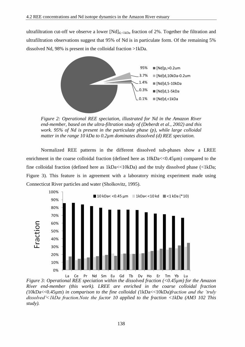
4.2 REE concentrations and Nd isotope dynamics in the Amazon River estuary
138
ultrafiltration cut-off we observe a lower [Nd]d,<1kDa fraction of 2%. Together the filtration and
ultrafiltration observations suggest that 95% of Nd is in particulate form. Of the remaining 5%
dissolved Nd, 98% is present in the colloidal fraction >1kDa.
Figure 2: Operational REE speciation, illustrated for Nd in the Amazon River
end-member, based on the ultra-filtration study of (Deberdt et al., 2002) and this
work. 95% of Nd is present in the particulate phase (p), while large colloidal
matter in the range 10 kDa to 0.2µm dominates dissolved (d) REE speciation.
Normalized REE patterns in the different dissolved sub-phases show a LREE
enrichment in the coarse colloidal fraction (defined here as 10kDa<<0.45µm) compared to the
fine colloidal fraction (defined here as 1kDa<<10kDa) and the truly dissolved phase (<1kDa;
Figure 3). This feature is in agreement with a laboratory mixing experiment made using
Connecticut River particles and water (Sholkovitz, 1995).
Figure 3: Operational REE speciation within the dissolved fraction (<0.45µm) for the Amazon
River end-member (this work). LREE are enriched in the coarse colloidal fraction
(10kDa<<0.45µm) in comparison to the fine colloidal (1kDa<<10kDa)fraction and the ‘truly
dissolved’<1kDa fraction.Note the factor 10 applied to the fraction <1kDa (AM3 102 This
study).
95%
3.7%
1.4%
0.3%
0.1%
[Nd]p,>0.2um
[Nd]d,10kDa-0.2um
[Nd]d,5-10kDa
[Nd]d,1-5kDa
[Nd]d,<1kDa
0%
10%
20%
30%
40%
50%
60%
70%
80%
90%
100%
La Ce Pr Nd Sm Eu Gd Tb Dy Ho Er Tm Yb Lu
10 kDa< <0.45 µm 1kDa< <10 kd <1 kDa (*10)
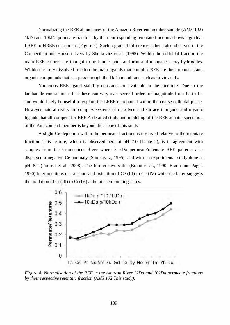
139
Normalizing the REE abundances of the Amazon River endmember sample (AM3-102)
1kDa and 10kDa permeate fractions by their corresponding retentate fractions shows a gradual
LREE to HREE enrichment (Figure 4). Such a gradual difference as been also observed in the
Connecticut and Hudson rivers by Sholkovitz et al. (1995). Within the colloidal fraction the
main REE carriers are thought to be humic acids and iron and manganese oxy-hydroxides.
Within the truly dissolved fraction the main ligands that complex REE are the carbonates and
organic compounds that can pass through the 1kDa membrane such as fulvic acids.
Numerous REE-ligand stability constants are available in the literature. Due to the
lanthanide contraction effect these can vary over several orders of magnitude from La to Lu
and would likely be useful to explain the LREE enrichment within the coarse colloidal phase.
However natural rivers are complex systems of dissolved and surface inorganic and organic
ligands that all compete for REE.A detailed study and modeling of the REE aquatic speciation
of the Amazon end member is beyond the scope of this study.
A slight Ce depletion within the permeate fractions is observed relative to the retentate
fraction. This feature, which is observed here at pH=7.0 (Table 2), is in agreement with
samples from the Connecticut River where 5 kDa permeate/retentate REE patterns also
displayed a negative Ce anomaly (Sholkovitz, 1995), and with an experimental study done at
pH=8.2 (Pourret et al., 2008). The former favors the (Braun et al., 1990; Braun and Pagel,
1990) interpretations of transport and oxidation of Ce (III) to Ce (IV) while the latter suggests
the oxidation of Ce(III) to Ce(IV) at humic acid bindings sites.
Figure 4: Normalisation of the REE in the Amazon River 1kDa and 10kDa permeate fractions
by their respective retentate fraction (AM3 102 This study).
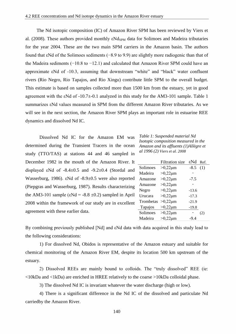
4.2 REE concentrations and Nd isotope dynamics in the Amazon River estuary
140
The Nd isotopic composition (IC) of Amazon River SPM has been reviewed by Viers et
al. (2008). These authors provided monthly εNdSPM data for Solimoes and Madeira tributaries
for the year 2004. These are the two main SPM carriers in the Amazon basin. The authors
found that εNd of the Solimoes sediments (−8.9 to 9.9) are slightly more radiogenic than that of
the Madeira sediments (−10.8 to −12.1) and calculated that Amazon River SPM could have an
approximate εNd of -10.3, assuming that downstream “white” and “black” water confluent
rivers (Rio Negro, Rio Tapajos, and Rio Xingu) contribute little SPM to the overall budget.
This estimate is based on samples collected more than 1500 km from the estuary, yet in good
agreement with the εNd of -10.7±-0.1 analyzed in this study for the AM3-101 sample. Table 1
summarizes εNd values measured in SPM from the different Amazon River tributaries. As we
will see in the next section, the Amazon River SPM plays an important role in estuarine REE
dynamics and dissolved Nd IC.
Dissolved Nd IC for the Amazon EM was
determined during the Transient Tracers in the ocean
study (TTO/TAS) at stations 44 and 46 sampled in
December 1982 in the mouth of the Amazon River. It
displayed εNd of -8.4±0.5 and -9.2±0.4 (Stordal and
Wasserburg, 1986). εNd of -8.9±0.5 were also reported
(Piepgras and Wasserburg, 1987). Results characterizing
the AM3-101 sample (εNd = -8.8 ±0.2) sampled in April
2008 within the framework of our study are in excellent
agreement with these earlier data.
By combining previously published [Nd] and εNd data with data acquired in this study lead to
the following considerations:
1) For dissolved Nd, Obidos is representative of the Amazon estuary and suitable for
chemical monitoring of the Amazon River EM, despite its location 500 km upstream of the
estuary.
2) Dissolved REEs are mainly bound to colloids. The “truly dissolved” REE (ie:
<10kDa and <1kDa) are enriched in HREE relatively to the coarse >10kDa colloidal phase.
3) The dissolved Nd IC is invariant whatever the water discharge (high or low).
4) There is a significant difference in the Nd IC of the dissolved and particulate Nd
carriedby the Amazon River.
Table 1: Suspended material Nd
Isotopic composition measured in the
Amazon and its affluents (1)Allègre et
al 1996 (2) Viers et al. 2008
Filtration size εNd Ref.
Solimoes >0,22μm -8.5 (1)
Madeira >0,22μm -
11.6 Amazone >0,22μm -7.5
(2)
Amazone >0,22μm -
10.3 Negro >0,22μm -13.6
Urucara >0,22μm -17.3
Trombetas >0,22μm -21.9
Tapajos >0,22μm -19.8
Solimoes >0,22μm -
11.4 Madeira >0,22μm -9.4
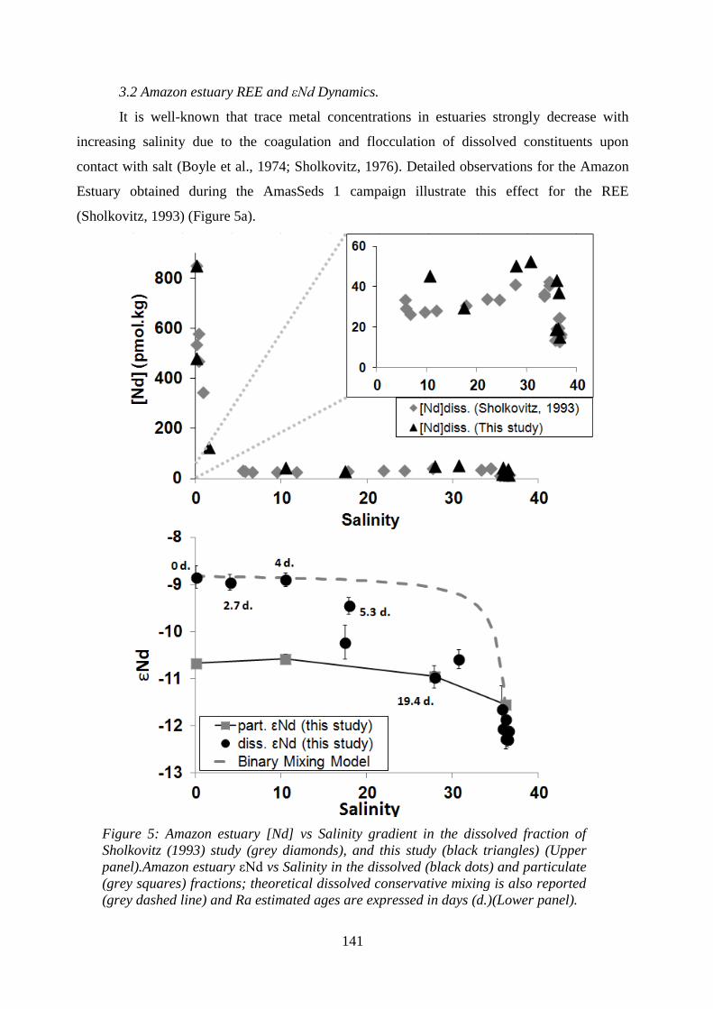
141
3.2 Amazon estuary REE and εNd Dynamics.
It is well-known that trace metal concentrations in estuaries strongly decrease with
increasing salinity due to the coagulation and flocculation of dissolved constituents upon
contact with salt (Boyle et al., 1974; Sholkovitz, 1976). Detailed observations for the Amazon
Estuary obtained during the AmasSeds 1 campaign illustrate this effect for the REE
(Sholkovitz, 1993) (Figure 5a).
Figure 5: Amazon estuary [Nd] vs Salinity gradient in the dissolved fraction of
Sholkovitz (1993) study (grey diamonds), and this study (black triangles) (Upper
panel).Amazon estuary εNd vs Salinity in the dissolved (black dots) and particulate
(grey squares) fractions; theoretical dissolved conservative mixing is also reported
(grey dashed line) and Ra estimated ages are expressed in days (d.)(Lower panel).
4.2 REE concentrations and Nd isotope dynamics in the Amazon River estuary
142
The fraction of REEs that are removed from the dissolved phase in the salinity gradient
must be calculated relative to the REE concentrations in the river end-member. Sholkovitz
(1993) noted that the lowest AmasSeds 1 salinity samples (0.3) taken on 4-10 August 1989, and
which have Nd concentrations of 83.5 and 67.9 ng.kg-1
(579 and 471 pmol.kg-1
), do not
represent the true river end-member. Using equation 1 and the Amazon discharge at this time in
1989 (237,814 m3.sec
-1) yields corresponding Nd concentration at Obidos of 157 ±40 ng.L
-1
(1.1±0.3 μmol.kg-1
). Figure 5a shows the Nd concentration gradient observed during both
Amaseds 1 and Amandes 3 campaign (Sholkovitz 1993, this study).
Similar to Sholkovitz’(1993) observations we find that total Nd concentrations rapidly
decrease in the low-salinity region (0-10‰) from 123 ng.kg-1
to a minimum of 4.3 ng.kg-1
(853
to a minimum of 29.8pmol.kg-1
). Using the estimated river end-member of 157 ng.kg-1
(1.1±0.3
μmol.kg-1
)and the observed Nd minima of 3.8 ng.kg-1
(26.3 pmol.kg-1
) for the AmasSeds I
campaign, both the Sholkovitz (1993) and this study show that more than 96% of dissolved Nd
was removed from solution in the Amazon Estuary. There is however one difference with this
previous study: The dissolved Nd removal by coagulation we observe reaches its maximum at a
higher salinity of 17.5 than the AmasSeds 1 study (6.6). This feature could be related to the fact
that different filter pore sizes were used between the two studies (ie: 0.45μm here vs 0.22μm
during AmasSed) but could also represent true natural variation.
In Figure 6 are reported REE patterns within the low salinity REE removal zone.
Concentrations of the 14 REE in each sample are normalized by the concentrations of the
Amazon end member (AM3-102).
Figure 6: Amazon estuary [REE] concentrations (<0.45µm) in the concentration drop zone
normalized to the AmazonEM station (AM3-102, salinity 0.3). Stations AM3-101, AM3-301,
AM3-501, AM3-601 have respective salinities of 0.034, 1.50, 10.51 and 17.45.
0.01
0.10
1.00
La Ce Pr Nd Sm Eu Gd Tb Dy Ho Er Tm Yb Lu[RE
E] /
[R
EE
]AM
3-1
02
101/102 301/102 501/102 601/102
Nd/Yb =0.87
Nd/Yb =0.54
Nd/Yb =0.57
Nd/Yb =0.41
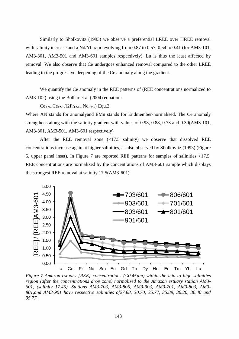
143
Similarly to Sholkovitz (1993) we observe a preferential LREE over HREE removal
with salinity increase and a Nd/Yb ratio evolving from 0.87 to 0.57, 0.54 to 0.41 (for AM3-101,
AM3-301, AM3-501 and AM3-601 samples respectively), Lu is thus the least affected by
removal. We also observe that Ce undergoes enhanced removal compared to the other LREE
leading to the progressive deepening of the Ce anomaly along the gradient.
We quantify the Ce anomaly in the REE patterns of (REE concentrations normalized to
AM3-102) using the Bolhar et al (2004) equation:
CeAN= CeEMn/(2PrEMn- NdEMn) Equ.2
Where AN stands for anomalyand EMn stands for Endmember-normalised. The Ce anomaly
strengthens along with the salinity gradient with values of 0.98, 0.88, 0.73 and 0.39(AM3-101,
AM3-301, AM3-501, AM3-601 respectively)
After the REE removal zone (<17.5 salinity) we observe that dissolved REE
concentrations increase again at higher salinities, as also observed by Sholkovitz (1993) (Figure
5, upper panel inset). In Figure 7 are reported REE patterns for samples of salinities >17.5.
REE concentrations are normalized by the concentrations of AM3-601 sample which displays
the strongest REE removal at salinity 17.5(AM3-601).
Figure 7:Amazon estuary [REE] concentrations (<0.45µm) within the mid to high salinities
region (after the concentrations drop zone) normalized to the Amazon estuary station AM3-
601, (salinity 17.45). Stations AM3-703, AM3-806, AM3-903, AM3-701, AM3-803, AM3-
801,and AM3-901 have respective salinities of27.88, 30.70, 35.77, 35.89, 36.20, 36.40 and
35.77.
0.00
0.50
1.00
1.50
2.00
2.50
3.00
3.50
4.00
4.50
5.00
La Ce Pr Nd Sm Eu Gd Tb Dy Ho Er Tm Yb Lu
[RE
E] /
[R
EE
]AM
3-6
01
703/601 806/601
903/601 701/601
803/601 801/601
901/601
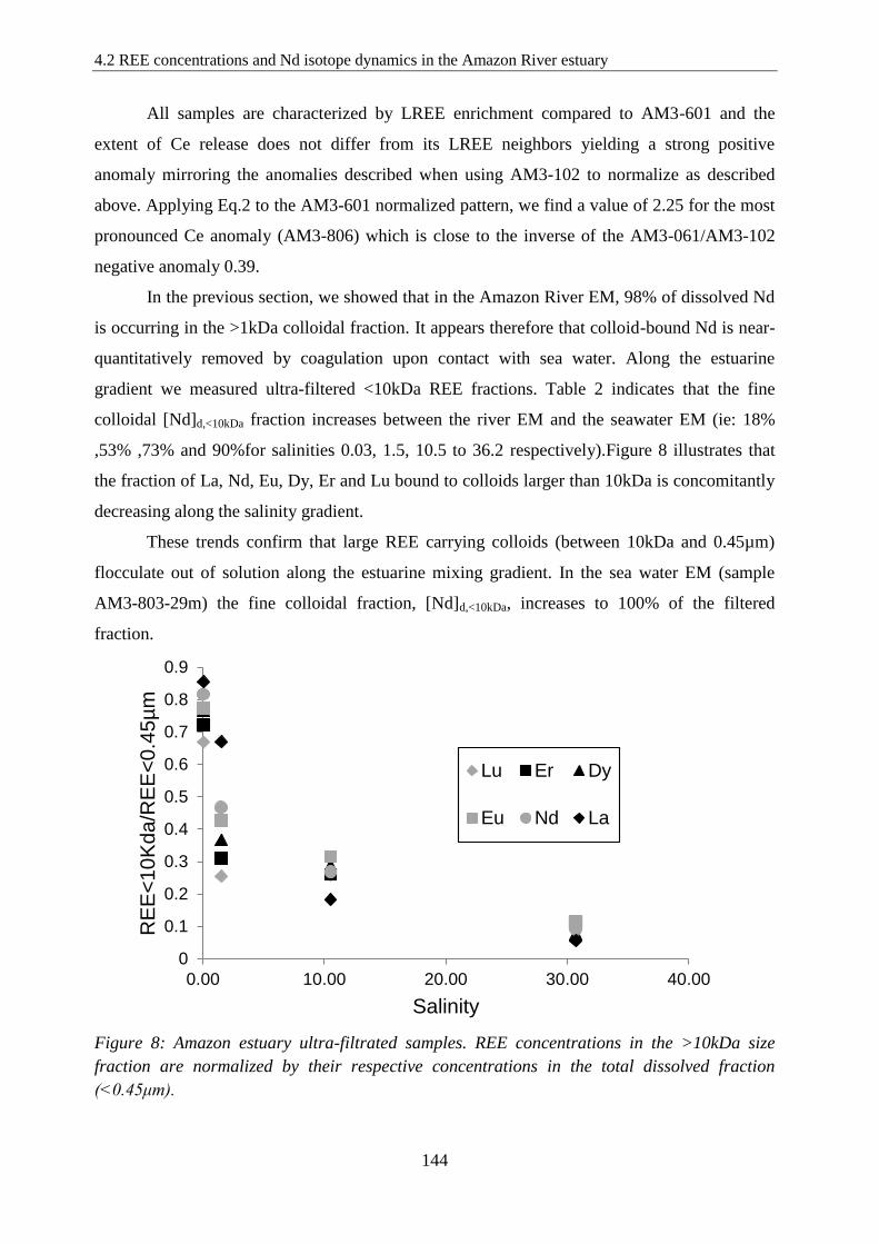
4.2 REE concentrations and Nd isotope dynamics in the Amazon River estuary
144
All samples are characterized by LREE enrichment compared to AM3-601 and the
extent of Ce release does not differ from its LREE neighbors yielding a strong positive
anomaly mirroring the anomalies described when using AM3-102 to normalize as described
above. Applying Eq.2 to the AM3-601 normalized pattern, we find a value of 2.25 for the most
pronounced Ce anomaly (AM3-806) which is close to the inverse of the AM3-061/AM3-102
negative anomaly 0.39.
In the previous section, we showed that in the Amazon River EM, 98% of dissolved Nd
is occurring in the >1kDa colloidal fraction. It appears therefore that colloid-bound Nd is near-
quantitatively removed by coagulation upon contact with sea water. Along the estuarine
gradient we measured ultra-filtered <10kDa REE fractions. Table 2 indicates that the fine
colloidal [Nd]d,<10kDa fraction increases between the river EM and the seawater EM (ie: 18%
,53% ,73% and 90%for salinities 0.03, 1.5, 10.5 to 36.2 respectively).Figure 8 illustrates that
the fraction of La, Nd, Eu, Dy, Er and Lu bound to colloids larger than 10kDa is concomitantly
decreasing along the salinity gradient.
These trends confirm that large REE carrying colloids (between 10kDa and 0.45µm)
flocculate out of solution along the estuarine mixing gradient. In the sea water EM (sample
AM3-803-29m) the fine colloidal fraction, [Nd]d,<10kDa, increases to 100% of the filtered
fraction.
Figure 8: Amazon estuary ultra-filtrated samples. REE concentrations in the >10kDa size
fraction are normalized by their respective concentrations in the total dissolved fraction
(<0.45μm).
0
0.1
0.2
0.3
0.4
0.5
0.6
0.7
0.8
0.9
0.00 10.00 20.00 30.00 40.00
RE
E<
10
Kd
a/R
EE
<0
.45
µm
Salinity
Lu Er Dy
Eu Nd La
145
Table 2: Hydrological and geochemical data. Long., Lat., Temp., Sal., Cond. and Oxy. stands for Longitude, latitude, Temperature, Salinity, conductivity and dissolved
Oxygen. REE concentration areexpressed in pmol.kg-1
.
Station Date Long. Latit. Depth Temp. Sal. pH Cond. (mS) Oxy.
ml/l εNd 2SE
La Ce Pr Nd Sm Eu Gd Tb Dy Ho Er Tm Yb Lu
AM3-0101 10/04/2008 -49.76 0.96 6.9 27.75 0.03 85,3 .10-3
1.89
<0.45 μm 350.1 870.5 117.4 535.5 128.4 28.6 147.4 21.1 121.0 23.7 64.7 8.7 52.6 8.0
-10.7 0.1 >0.45 μm
AM3-0102 10/04/2008 -49.74 0.98 6.9 27.75 0.03 7.035 49,6 .10
-3 2.13 -8.8 0.2 <0.45 μm 596.5 1480.5 191.3 850.2 199.7 43.8 217.1 30.6 174.5 32.9 88.4 11.9 72.7 10.5
10kdP 86 210 31 156 41 10 49 7 41 9 25 3 22 3
1kdP 10.3 21.2 3.04 15.1 3.84 0.81 4.59 0.63 3.73 0.8 2.41 0.34 2.29 0.37
AM3-03 10/04/2008 -49.36 1.21 7 27.85 1.5 7.29 3,41 2.37
<0.45 μm 85.2 164.1 26.2 126.1 33.5 8.7 41.1 6.0 35.3 7.3 21.0 2.9 18.8 2.9
10kdP 28 70 13 67 19 5 24 4 22 5 14 2 14 2
AM3-04 10/04/2008 -49.26 1.26 7.2 27.58 4.03 7.32 7,75 2.35 -9 0.2 <0.45 μm
10kdP 39 67 12 61 16 4 21 3 18 4 12 2 11 2
AM3-05 10/04/2008 -49.15 1.34 3.1 27.67 10.51 7.70 17,83 3.25 -8.9 0.1 <0.45 μm 40.4 52.4 9.7 45.5 11.2 2.9 14.5 2.1 12.5 2.7 8.0 1.1 7.1 1.1
-10.6 0.1 >0.45 μm
10kdP 33 40 7 33 8 2 10 1 9 2 6 1 5 1
AM3-06 10/04/2008 -49.02 1.45 4.3 27.6 17.45 7.889 - 3.16 -10.2 0.4 <0.45 μm 34.0 17.4 6.3 29.8 7.0 1.9 10.5 1.5 9.8 2.3 7.0 1.0 6.2 1.0
AM3-0701 11/04/2008 -46.97 1.17 43.1 27.61 35.89 - 3.1 -12.1 0.2 <0.45 μm 42.9 62.6 10.1 43.4 9.4 2.3 11.3 1.6 9.7 2.1 5.9 0.8 4.7 0.7
AM3-0703
5 28.29 27.88 - 3.72 -11 0.2 <0.45 μm 45.5 73.1 11.3 50.5 11.6 3.0 14.8 2.2 13.6 3.0 8.9 1.2 7.3 1.1
-10.9 0.1 >0.45 μm
AM3-0802 11/04/2008 -46.73 1.49 93.1 25.13 36.4 - 3.38 -12.3 0.2 <0.45 μm 41.2 52.1 8.8 37.4 7.2 1.7 8.4 1.2 7.9 1.9 5.6 0.7 4.4 0.7
AM3-0803
29 27.72 36.2 8.31 - 3.52 -12.3 0.2 <0.45 μm 29.2 40.1 5.7 24.6 5.1 1.3 6.5 1.0 6.1 1.4 4.0 0.5 3.2 0.5
-11.5 0.1 >0.45 μm
<0.45 μm 26 45 6 29 6 2 8 1 7 2 5 1 4 1
10kdP 21.1 25.8 4.6 19.5 3.8 0.9 4.7 0.7 4.9 1.2 3.5 0.5 2.7 0.4
AM3-0806
4 27.88 30.7 - 3.67 -10.6 0.2 <0.45 μm 48.4 80.2 12.0 52.5 11.8 2.9 14.2 2.1 12.8 2.8 7.9 1.1 6.5 1.0
AM3-09 12/04/2008 -47.50 2.26 9.2 27.98 35.77 - 3.5 -11.6 0.5 <0.45 μm 20.7 25.4 4.5 19.2 3.7 0.9 4.6 0.7 4.8 1.1 3.5 0.5 2.7 0.4
AM3-09
88.4 24.76 36.55 - 3.39 -12.1 0.2 <0.45 μm 16.6 16.3 3.4 15.2 2.8 0.6 3.7 0.6 4.2 1.0 3.2 0.4 2.5 0.4
AM3-14 12/04/2008 -48.00 1.91 51.4 27.01 36.16 - 3.07 -11.9 0.3 <0.45 μm
AM3-14
4 28.12 17.88 - 4.41 -9.5 0.2 <0.45 μm
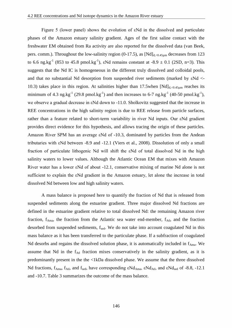
4.2 REE concentrations and Nd isotope dynamics in the Amazon River estuary
146
Figure 5 (lower panel) shows the evolution of εNd in the dissolved and particulate
phases of the Amazon estuary salinity gradient. Ages of the first saline contact with the
freshwater EM obtained from Ra activity are also reported for the dissolved data (van Beek,
pers. comm.). Throughout the low-salinity region (0-17.5), as [Nd]d,<0.45µm decreases from 123
to 6.6 ng.kg-1
(853 to 45.8 pmol.kg-1
), εNd remains constant at -8.9 ± 0.1 (2SD, n=3). This
suggests that the Nd IC is homogeneous in the different truly dissolved and colloidal pools,
and that no substantial Nd desorption from suspended river sediments (marked by εNd <-
10.3) takes place in this region. At salinities higher than 17.5when [Nd]d,<0.45µm reaches its
minimum of 4.3 ng.kg-1
(29.8 pmol.kg-1
) and then increases to 6-7 ng.kg-1
(40-50 pmol.kg-1
),
we observe a gradual decrease in εNd down to -11.0. Sholkovitz suggested that the increase in
REE concentrations in the high salinity region is due to REE release from particle surfaces,
rather than a feature related to short-term variability in river Nd inputs. Our εNd gradient
provides direct evidence for this hypothesis, and allows tracing the origin of these particles.
Amazon River SPM has an average εNd of -10.3, dominated by particles from the Andean
tributaries with εNd between -8.9 and -12.1 (Viers et al., 2008). Dissolution of only a small
fraction of particulate lithogenic Nd will shift the εNd of total dissolved Nd in the high
salinity waters to lower values. Although the Atlantic Ocean EM that mixes with Amazon
River water has a lower εNd of about -12.1, conservative mixing of marine Nd alone is not
sufficient to explain the εNd gradient in the Amazon estuary, let alone the increase in total
dissolved Nd between low and high salinity waters.
A mass balance is proposed here to quantify the fraction of Nd that is released from
suspended sediments along the estuarine gradient. Three major dissolved Nd fractions are
defined in the estuarine gradient relative to total dissolved Nd: the remaining Amazon river
fraction, fAma, the fraction from the Atlantic sea water end-member, fAtl, and the fraction
desorbed from suspended sediments, fsed. We do not take into account coagulated Nd in this
mass balance as it has been transferred to the particulate phase. If a subfraction of coagulated
Nd desorbs and regains the dissolved solution phase, it is automatically included in fAma. We
assume that Nd in the fAtl fraction mixes conservatively in the salinity gradient, as it is
predominantly present in the the <1kDa dissolved phase. We assume that the three dissolved
Nd fractions, fAma, fAtl, and fsed, have corresponding εNdAma, εNdAtl, and εNdsed of -8.8, -12.1
and -10.7. Table 3 summarizes the outcome of the mass balance.
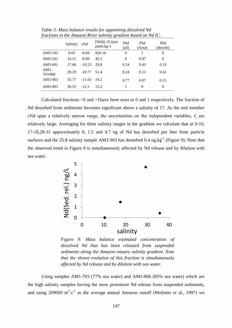
147
Table 3: Mass balance results for appointing dissolved Nd
fractions in the Amazon River salinity gradient based on Nd IC.
Salinity εNd
[Nd]d,<0.2μm
pmol.kg-1 fNd
(atl)
fNd
(Ama)
fNd
(desorb)
AM3-102 0.03 -8.84 850.16 0 1 0
AM3-501 10.51 -8.89 45.5 0 0.97 0
AM3-601 17.66 -10.23 29.8 0.24 0.43 0.33
AM3-
703/806 29.29 -10.77 51.4 0.24 0.13 0.63
AM3-903 35.77 -11.63 19.2 0.77 0.07 0.15
AM3-901 36.55 -12.1 15.2 1 0 0
Calculated fractions <0 and >1have been reset to 0 and 1 respectively. The fraction of
Nd desorbed from sediments becomes significant above a salinity of 17. As the end member
εNd span a relatively narrow range, the uncertainties on the independent variables, f, are
relatively large. Averaging for three salinity ranges in the gradient we calculate that at 0-10,
17-18,28-31 approximately 0, 1.5 and 4.7 ng of Nd has desorbed per liter from particle
surfaces and the 35.8 salinity sample AM3-903 has desorbed 0.4 ng.kg-1
(Figure 9). Note that
the observed trend in Figure 9 is simultaneously affected by Nd release and by dilution with
sea water.
Figure 9: Mass balance estimated concentration of
dissolved Nd that has been released from suspended
sediments along the Amazon estuary salinity gradient. Note
that the shown evolation of this fraction is simultaneously
affected by Nd release and by dilution with sea water.
Using samples AM1-703 (77% sea water) and AM1-806 (85% sea water) which are
the high salinity samples having the most prominent Nd release from suspended sediments,
and using 209000 m3.s
-1 as the average annual Amazon runoff (Molinier et al., 1997) we
0
1
2
3
4
5
0 10 20 30 40
Nd
(Sed
. rel
.) n
g/L
salinity
4.2 REE concentrations and Nd isotope dynamics in the Amazon River estuary
148
estimate that a total of 259 Tons of Nd per year is released from suspended sediments upon
mixing with sea water. This accounts for more than 1% of the Nd carried by suspended
sediments (Viers et al., 2008a). With Ra estimated ages we can further argue that this release
process occurs within approximately 19 days. The release of Nd from sediments observed
during AmasSed 1 (Sholkovitz, 1993) and this study is coherent with batch experiments
where lithogenic particles of diverse origins were incubated with seawater (Pearce et al.,
2013). The time scale for Nd release of 19 days that we observe is similar to the experimental
time scale of Nd release. In summary, our observations suggest that dissolved REE have little
influence on the REE composition of the Amazon plume and Atlantic Ocean. Rather, as
colloidal REE coagulate and sediment out of solution, the desorption of REE from suspended
sediments dominates REE concentrations and Nd IC of the Amazon River plume over the
north-east Brazilian shelf. More research is needed to determine the fate of REE bound to
coagulated and sedimented colloids. Possibly the slow mineralization of POC releases the
associated REE, that should still carry their Amazon River dissolved εNdAM of -8.9.
In the >35 salinity range there is also evidence for a contribution of sediment sourced
Nd, as Nd concentrations of 3.6 to 6.3 ng.kg-1
are elevated over those of the reference Atlantic
Ocean EM (2.2 ng.kg-1
). Samples AM1-701, AM1-802 and AM1-803 were collected near the
break of the continental slope at bottom depth (43, 29 and 93m) where the Amazon freshwater
has no influence. During the AmasSeds 1 study, Sholkovitz (1993) also observed deep
samples with elevated concentrations. The author attributed it to possible release from bottom
sediments and referred to McKee et al.(1987;) and Swarzenski et al.(1991) who had measured
elevated U concentrations within the Amazon estuary. We strongly suspect here that Nd
release from sediment is indeed occurring on the Brazilian shelf, as more broadly
hypothesized by (Arsouze et al, 2009). Together with the elevated dissolved Nd
concentrations observed at AM1-701, AM1-802 and AM1-803 stations, the slightly less
radiogenic signatures (-12.3) suggests that Atlantic surface waters upon contact with the
north-east Brazilian margin had their εNd modified by boundary exchange processes before
their arrival in the Amazon estuary.
4. Conclusions
We applied to the Amazon estuary the first REE study coupling traditional dissolved
[REE] analysis with ultrafiltration and Nd IC analysis. For the Amazon River EM our results
complete previous estimates of the total dissolved and colloid-bound REE concentrations.
Similarly, we observe dissolved and particulate Nd IC within the range of previous
149
observations (Barroux et al., 2006; Sholkovitz, 1993; Stordal and Wasserburg, 1986; Viers et
al., 2008b). In the Amazon estuary salinity gradient we observed the following: 1) Ultrafiltred
colloid-bound REE strongly drecreases with increasing salinity. Indeed more than 80% of
REE are present in the colloidal phase in the Amazon River EM and less than 10% are present
in the seawater EM. 2) Dissolved Nd IC measurements suggest a lithogenic origin for the Nd
released at mid to high salinities (εNd= -10.7) as it has a contrasted isotopic signature with
both dissolved Amazon and oceanic EM (εNdAM= -8.9 and εNdSW= -12.1). In addition, shelf
bottom waters at 40-90m depth which had not been in contact with the Amazon River EM
showed elevated Nd concentrations and slightly unradiogenic Nd IC. We suggest this
provides evidence for margin sourced Nd.
The oceanic REE and Nd geochemical cycle study requires a good estimation of
sources and sinks. The Amazon River supply of exportable (dissolved) Nd to the ocean was
previously estimated assuming a total release of Nd from coagulated colloids (Barroux et al.,
2006; Tachikawa et al., 2003). Earlier work on the global marine Nd cycle suggested that Nd
should be released from suspended and deposited sediments in order to explain the oceanic
εNd variations and budget (Arsouze et al., 2009; Tachikawa et al., 2003). The present study
allowed to observe for the first time in natural water on short scales of space and time the
release of Nd from lithogenic particles and confirms the importance of suspended and margin-
deposited sediments. Indeed, the large amount of Nd released from lithogenic Amazon River
suspended sediments over limited space and time scales, underlines that sediments deposited
on continental margins contribute significantly to the global marine Nd budget. Until recently
this term was neglected in the Nd oceanic geochemical cycle but also in those of other
chemical elements as mentioned in a growing number of experimental and modeling studies
(Homoky et al., 2013; Jeandel et al., 2011; Jones et al., 2012a; Jones et al., 2012b; Tréguer
and De La Rocha, 2013).
5. References
Arsouze, T., Dutay, J.C., Lacan, F., Jeandel, C., 2007. Modeling the neodymium isotopic composition
with a global ocean circulation model. Chemical Geology 239, 165-177.
Arsouze, T., Dutay, J.C., Lacan, F., Jeandel, C., 2009. Reconstructing the Nd oceanic cycle using a
coupled dynamical - biogeochemical model. Biogeosciences 6, 2829-2846.
Barroux, G.A., Seyler, P., Sonke, J., Viers, J., Boaventura, G., Sondag, F., Lagane, C., 2006.
Seasonality of dissolved element fluxes in the Amazon River Endmember. Geochimica et
Cosmochimica Acta 70, A38-A38.
Bouchez, J., Gaillardet, J., France-Lanord, C., Maurice, L., Dutra-Maia, P., 2011. Grain size control of
river suspended sediment geochemistry: Clues from Amazon River depth profiles.
Geochemistry, Geophysics, Geosystems 12, Q03008.
4.2 REE concentrations and Nd isotope dynamics in the Amazon River estuary
150
Boyle, E., Collier, R., Dengler, A.T., Edmond, J.M., Ng, A.C., Stallard, R.F., 1974. On the chemical
mass-balance in estuaries. Geochimica et Cosmochimica Acta 38, 1719-1728.
Boyle, E.A., Edmond, J.M., Sholkovitz, E.R., 1977. The mechanism of iron removal in estuaries.
Geochimica et Cosmochimica Acta 41, 1313-1324.
Braun, J.-J., Pagel, M., Muller, J.-P., Bilong, P., Michard, A., Guillet, B., 1990. Cerium anomalies in
lateritic profiles. Geochimica et Cosmochimica Acta 54, 781-795.
Braun, J.J., Pagel, M., 1990. U, Th and REE in the Akongo lateritic profile (SW Cameroon). Chemical
Geology 84, 357-359.
Deberdt, S., Viers, J., Dupre, B., 2002. New insights about the rare earth elements (REE) mobility in
river waters. Bulletin De La Societe Geologique De France 173, 147-160.
DeMaster, Ragueneau, O., Nittrouer, C.A., 1996. Preservation efficiencies and accumulation rates of
biogenic Si and organic C, N, and P in high-latitude sediments: the Ross Sea. J. Geophys. Res.
101, 501-518.
DePaolo, D.J., Wasserburg, G.J., 1976. Nd isotopic variations and petrogenetic models. Geophysical
Research Letters 3, 249-252.
Eckert, J.M., Sholkovitz, E.R., 1976. The flocculation of iron, aluminium and humates from river
water by electrolytes. Geochimica et Cosmochimica Acta 40, 847-848.
Frank, M., Whiteley, N., Kasten, S., Hein, J.R., O'Nions, K., 2002. North Atlantic deep water export to
the Southern Ocean over the past 14 Myr: Evidence from Nd and Pb isotopes in ferromanganese
crusts. Paleoceanography 17.
Gibbs, 1967. The Geochemistry of the Amazon River System: Part I. The Factors that Control the
Salinity and the Composition and Concentration of the Suspended Solids Geol. Soc. Amer.
Bull., 78, 1203-1232.
Gibbs, R.J., 1970. Circulation in the Amazon river estuary and adjacent Atlantic Ocean. . J. Mar. Res.,
28, 113-123.
Gibbs, R.J., Konwar, L., 1986. Coagulation and settling of Amazon River suspended sediment." In
C.A. Nittrouer and K.J. DeMaster (eds.), Sedimentary processes on the Amazon continental
shelf, Continental Shelf Research 6 (1/2): . 127-149.
Gutjahr, M., Frank, M., Stirling, C.H., Keigwin, L.D., Halliday, A.N., 2008. Tracing the Nd isotope
evolution of North Atlantic deep and intermediate waters in the Western North Atlantic since
the Last Glacial Maximum from Blake Ridge sediments. Earth and Planetary Science Letters
266, 61-77.
Hannigan, R.E., Sholkovitz, E.R., 2001. The development of middle rare earth element enrichments in
freshwaters: weathering of phosphate minerals. Chemical Geology 175, 495-508.
Homoky, W.B., John, S.G., Conway, T.M., Mills, R.A., 2013. Distinct iron isotopic signatures and
supply from marine sediment dissolution. Nat Commun 4.
Jeandel, C., 1993. Concentration and isotopic composition of Nd in the South Atlantic Ocean. Earth
and Planetary Science Letters 117, 581-591.
Jeandel, C., Peucker-Ehrenbrink, B., Jones, M.T., Pearce, C.R., Oelkers, E.H., Godderis, Y., Lacan, F.,
Aumont, O., Arsouze, T., 2011. Ocean margins: The missing term in oceanic element budgets?
Johannesson, K.H., Burdige, D.J., 2007. Balancing the global oceanic neodymium budget: Evaluating
the role of groundwater. Earth and Planetary Science Letters 253, 129-142.
Jones, M.T., Pearce, C.R., Jeandel, C., Gislason, S.R., Eiriksdottir, E.S., Mavromatis, V., Oelkers,
E.H., 2012a. Riverine particulate material dissolution as a significant flux of strontium to the
oceans. Earth and Planetary Science Letters 355–356, 51-59.
Jones, M.T., Pearce, C.R., Oelkers, E.H., 2012b. An experimental study of the interaction of basaltic
riverine particulate material and seawater. Geochimica et Cosmochimica Acta 77, 108-120.
Kosuth, P., Callede, J., Laraque, A., Filizola, N., Guyot, J.L., Seyler, P., Fritsch, J.M., Guimaraes, V.,
2009. Sea-tide effects on flows in the lower reaches of the Amazon River. Hydrological
Processes 23, 3141-3150.
Lacan, F., Jeandel, C., 2004. Denmark Strait water circulation traced by heterogeneity in neodymium
isotopic compositions. Deep Sea Research Part I: Oceanographic Research Papers 51, 71-82.
Lacan, F., Jeandel, C., 2005. Neodymium isotopes as a new tool for quantifying exchange fluxes at the
continent-ocean interface. Earth and Planetary Science Letters 232, 245-257.
151
Luo, Y.R., Byrne, R.H., 2001. Yttrium and rare earth element complexation by chloride ions at 25
degrees C. Journal of Solution Chemistry 30, 837-845.
McKee, B.A., DeMaster, D.J., Nittrouer, C.A., 1987. Uranium geochemistry on the Amazon shelf:
Evidence for uranium release from bottom sediments. Geochimica et Cosmochimica Acta 51,
2779-2786.
Molinier, M., Guyot, J.-L., Guimarães, V.E., Oliveira, E., Filizola, N., 1997. Hydrologie Du Bassin
Amazonien. Environnement Et Développement En Amazonie Brésilienne. H. Théry. Paris,
Belin, 400
Pearce, C.R., Jones, M.T., Oelkers, E.H., Pradoux, C., Jeandel, C., 2013. The effect of particulate
dissolution on the neodymium (Nd) isotope and Rare Earth Element (REE) composition of
seawater. Earth and Planetary Science Letters.
Piepgras, D.J., Wasserburg, G.J., 1980. Neodymium isotopic variations in seawater. Earth and
Planetary Science Letters 50, 128-138.
Piepgras, D.J., Wasserburg, G.J., 1987. Rare earth element transport in the western North Atlantic
inferred from Nd isotopic observations. Geochimica et Cosmochimica Acta 51, 1257-1271.
Piepgras, D.J., Wasserburg, G.J., Dasch, E.J., 1979. The isotopic composition of Nd in different ocean
masses. Earth and Planetary Science Letters 45, 223-236.
Pin, Zalduegui, 1997. Sequential separation of light rare-earth elements, thorium and.
Piotrowski, A.M., Goldstein, S.L., Hemming, S.R., Fairbanks, R.G., 2004. Intensification and
variability of ocean thermohaline circulation through the last deglaciation. Earth and Planetary
Science Letters 225, 205-220.
Piotrowski, A.M., Goldstein, S.L., Hemming, S.R., Fairbanks, R.G., 2005. Temporal relationships of
carbon cycling and ocean circulation at glacial boundaries. Science 307, 1933-1938.
Pourret, O., Davranche, M., Gruau, G., Dia, A., 2008. New insights into cerium anomalies in organic-
rich alkaline waters. Chemical Geology 251, 120-127.
Révillon, S., Jouet, G., Bayon, G., Rabineau, M., Dennielou, B., Hémond, C., Berné, S., 2011. The
provenance of sediments in the Gulf of Lions, western Mediterranean Sea. Geochemistry,
Geophysics, Geosystems 12, Q08006.
Rousseau, T.C.C., Sonke, J.E., Chmeleff, J., Candaudap, F., Lacan, F., Boaventura, G., Seyler, P.,
Jeandel, C., 2013. Rare earth element analysis in natural waters by multiple isotope dilution -
sector field ICP-MS. Journal of Analytical Atomic Spectrometry 28, 573-584.
Rutberg, R.L., Hemming, S.R., Goldstein, S.L., 2000. Reduced North Atlantic Deep Water flux to the
glacial Southern Ocean inferred from neodymium isotope ratios. Nature 405, 935-938.
Shabani, M.B., Akagi, T., Masuda, A., 1992. Preconcentration of trace rare-earth elements in seawater
by complexation with bis(2-ethylhexyl) hydrogen phosphate and 2-ethylhexyl dihydrogen
phosphate adsorbed on a c18 cartridge and determination by inductively coupled plasma mass-
spectrometry. Analytical Chemistry 64, 737-743.
Shimizu, H., Tachikawa, K., Masuda, A., Nozaki, Y., 1994. Cerium and neodymium isotope ratios and
REE patterns in seawater from the North Pacific Ocean. Geochimica et Cosmochimica Acta 58,
323-333.
Sholkovitz, E., Szymczak, R., 2000. The estuarine chemistry of rare earth elements: comparison of the
Amazon, Fly, Sepik and the Gulf of Papua systems. Earth and Planetary Science Letters 179,
299-309.
Sholkovitz, E.R., 1976. Flocculation of dissolved organic and inorganic matter during the mixing of
river water and seawater. Geochimica et Cosmochimica Acta 40, 831-845.
Sholkovitz, E.R., 1993. The geochemistry of rare earth elements in the Amazon River estuary.
Geochimica et Cosmochimica Acta 57, 2181-2190.
Sholkovitz, E.R., 1995. The Aquatic Geochemistry of Rare Earth Element in river and estuaries.
Aquatic Geochemistry, 1-34.
Stordal, M.C., Wasserburg, G.J., 1986. Neodymium isotopic study of Baffin Bay water: sources of
REE from very old terranes. Earth and Planetary Science Letters 77, 259-272.
Sullivan, K.A., Aller, R.C., 1996. Diagenetic cycling of arsenic in Amazon shelf sediments.
Geochimica et Cosmochimica Acta 60, 1465-1477.
4.2 REE concentrations and Nd isotope dynamics in the Amazon River estuary
152
Swarzenski, P.W., McKee, B.A., Booth, J.G., 1991. Uranium geochemistry on the Amazon shelf:
Seasonal differences in source functions and dissolved /colloidal partitioning of uranium
isotopes. Eos 72, 64.
Swarzenski, P.W., McKee, B.A., Booth, J.G., 1995. Uranium geochemistry on the Amazon shelf:
Chemical phase partitioning and cycling across a salinity gradient. Geochimica et
Cosmochimica Acta 59, 7-18.
Tachikawa, K., Athias, V., Jeandel, C., 2003. Neodymium budget in the modern ocean and paleo-
oceanographic implications. Journal of Geophysical Research-Oceans 108.
Tachikawa, K., Jeandel, C., Vangriesheim, A., Dupré, B., 1999. Distribution of rare earth elements
and neodymium isotopes in suspended particles of the tropical Atlantic Ocean (EUMELI site).
Deep Sea Research Part I: Oceanographic Research Papers 46, 733-755.
Tréguer, P.J., De La Rocha, C.L., 2013. The World Ocean Silica Cycle. Annual Review of Marine
Science 5, 477-501.
van Beek, P., Souhaut, M., Reyss, J.L., 2010. Measuring the radium quartet (228Ra, 226Ra, 224Ra,
223Ra) in seawater samples using gamma spectrometry. Journal of Environmental Radioactivity
101, 521-529.
van de Flierdt, T., Goldstein, S.L., Hemming, S.R., Roy, M., Frank, M., Halliday, A.N., 2007. Global
neodymium-hafnium isotope systematics -- revisited. Earth and Planetary Science Letters 259,
432-441.
van Der Loeff, M.R., Helmers, E., Kattner, G., 1997. Continuous transects of cadmium, copper, and
aluminium in surface waters of the Atlantic Ocean, 50°N to 50°S: correspondence and contrast
with nutrient-like behaviour. Geochimica et Cosmochimica Acta 61, 47-61.
Viers, J., Roddaz, M., Filizola, N., Guyot, J.-L., Sondag, F., Brunet, P., Zouiten, C., Boucayrand, C.,
Martin, F., Boaventura, G.R., 2008a. Seasonal and provenance controls on Nd-Sr isotopic
compositions of Amazon rivers suspended sediments and implications for Nd and Sr fluxes
exported to the Atlantic Ocean. Earth and Planetary Science Letters 274, 511-523.
Viers, J., Roddaz, M., Filizola, N., Guyot, J.L., Sondag, F., Brunet, P., Zouiten, C., Boucayrand, C.,
Martin, F., Boaventura, G.R., 2008b. Seasonal and provenance controls on Nd-Sr isotopic
compositions of Amazon rivers suspended sediments and implications for Nd and Sr fluxes
exported to the Atlantic Ocean. Earth and Planetary Science Letters 274, 511-523.
Warne, A.G., Meade, R., White, A.W., Guevara, E.H., Gibeaut, J., Smyth, R.C., Aslan, A., Tremblay,
T., 2002. Regional controls on geomorphology, hydrology, and ecosystem integrity in the
Orinoco Delta, Venezuela. Geomorphology 44, 273-307.

153
154
4.3 Article en préparation: REE concentrations and isotope systematic in
the Amazon River plume and nearby Atlantic
T.C.C, Rousseaua, C. Jeandel
b, J.E Sonke
a, G. Boaventura
c, P. Seyler
a, A. Costa
d, M.
Grenierb, P. van Beck
b and M. Souhaut
b
aGET, Université de Toulouse, CNRS, IRD, CNES, 14 Avenue Edouard Belin, F-31400
Toulouse, France. bLEGOS, Université de Toulouse, CNRS, IRD, CNES, 14 Avenue Edouard Belin, F-31400
Toulouse, France cUniversidade De Brasilia, UNB, LAGEQ, Campus universitario Darcy Ribeiro, 70.910-900 Brasilia,
DF, Brazil dLaboratório de Oceanografia Física, Departamento de Oceanografia da Universidade
Federal de Pernambuco, Av. Arquitetura s/n, 50740-550, Campus Universitário, Recife,
PE, Brazil
Abstract
We present here dissolved εNd data acquired during AMANDES 1 and AMANDES 2
cruises in the western Atlantic Ocean. This region is important for water masses transfer
between the two hemispheres. Sampling was made during 2007/2008 on the Guyana shelf
/slope an off the margin. In surface advected Amazon freshwater plume Nd Isotopic
Composition (IC) suggests that a significant fraction of Nd can be released from estuarine salt
induced coagulated colloids. This Nd supply raises fundamental questions on particle
chemical composition, reactivity, lability and transport. We identified a dynamic zone located
west of 40°W from 5° N to 7° N which may act as a barrier attenuating the Antaric
Intermediate Waters (AAIW) characteristics in a reduced space-scale. In this region
southwards lenses of radiogenic lower North Atlantic waters (NAW) sinks within more
radiogenic lower South Atlantic Waters (SAW) and AAIW. The AAIW Nd IC we observe is
5 εNd units lower than the one widely accepted and previously observed south of 30°S. A 3
endmembers mixing model reveals an hydrological and isotopic coherence between our
observations previous ones of at 7°N and in the Angola Basin. We suggest a broad extension
of these unradiogenic AAIW signatures acquired by Boundary Exchange processes (BE) with
south Atlantic margins.
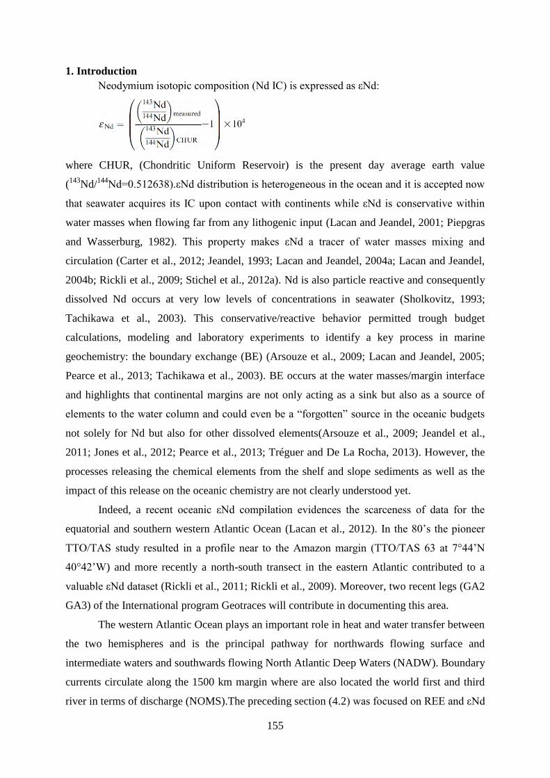
155
1. Introduction
Neodymium isotopic composition (Nd IC) is expressed as εNd:
where CHUR, (Chondritic Uniform Reservoir) is the present day average earth value
(143
Nd/144
Nd=0.512638).εNd distribution is heterogeneous in the ocean and it is accepted now
that seawater acquires its IC upon contact with continents while εNd is conservative within
water masses when flowing far from any lithogenic input (Lacan and Jeandel, 2001; Piepgras
and Wasserburg, 1982). This property makes εNd a tracer of water masses mixing and
circulation (Carter et al., 2012; Jeandel, 1993; Lacan and Jeandel, 2004a; Lacan and Jeandel,
2004b; Rickli et al., 2009; Stichel et al., 2012a). Nd is also particle reactive and consequently
dissolved Nd occurs at very low levels of concentrations in seawater (Sholkovitz, 1993;
Tachikawa et al., 2003). This conservative/reactive behavior permitted trough budget
calculations, modeling and laboratory experiments to identify a key process in marine
geochemistry: the boundary exchange (BE) (Arsouze et al., 2009; Lacan and Jeandel, 2005;
Pearce et al., 2013; Tachikawa et al., 2003). BE occurs at the water masses/margin interface
and highlights that continental margins are not only acting as a sink but also as a source of
elements to the water column and could even be a “forgotten” source in the oceanic budgets
not solely for Nd but also for other dissolved elements(Arsouze et al., 2009; Jeandel et al.,
2011; Jones et al., 2012; Pearce et al., 2013; Tréguer and De La Rocha, 2013). However, the
processes releasing the chemical elements from the shelf and slope sediments as well as the
impact of this release on the oceanic chemistry are not clearly understood yet.
Indeed, a recent oceanic εNd compilation evidences the scarceness of data for the
equatorial and southern western Atlantic Ocean (Lacan et al., 2012). In the 80’s the pioneer
TTO/TAS study resulted in a profile near to the Amazon margin (TTO/TAS 63 at 7°44’N
40°42’W) and more recently a north-south transect in the eastern Atlantic contributed to a
valuable εNd dataset (Rickli et al., 2011; Rickli et al., 2009). Moreover, two recent legs (GA2
GA3) of the International program Geotraces will contribute in documenting this area.
The western Atlantic Ocean plays an important role in heat and water transfer between
the two hemispheres and is the principal pathway for northwards flowing surface and
intermediate waters and southwards flowing North Atlantic Deep Waters (NADW). Boundary
currents circulate along the 1500 km margin where are also located the world first and third
river in terms of discharge (NOMS).The preceding section (4.2) was focused on REE and εNd
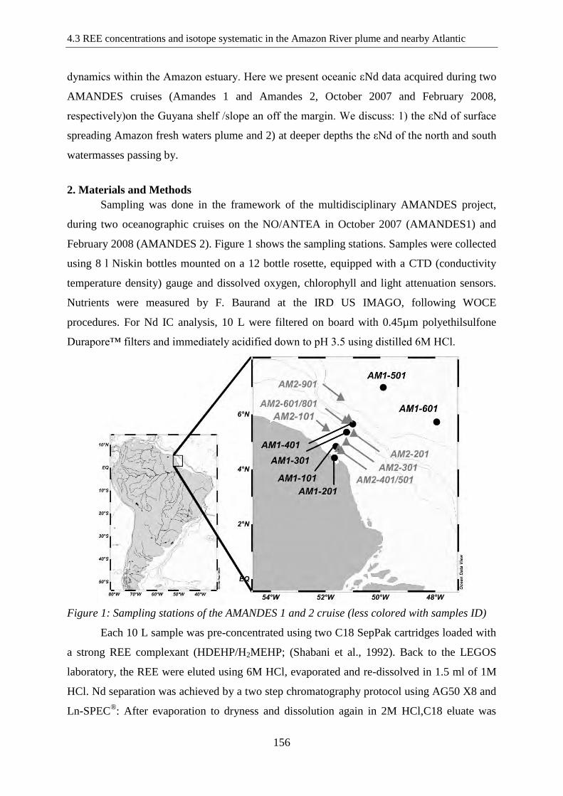
4.3 REE concentrations and isotope systematic in the Amazon River plume and nearby Atlantic
156
dynamics within the Amazon estuary. Here we present oceanic εNd data acquired during two
AMANDES cruises (Amandes 1 and Amandes 2, October 2007 and February 2008,
respectively)on the Guyana shelf /slope an off the margin. We discuss: 1) the εNd of surface
spreading Amazon fresh waters plume and 2) at deeper depths the εNd of the north and south
watermasses passing by.
2. Materials and Methods
Sampling was done in the framework of the multidisciplinary AMANDES project,
during two oceanographic cruises on the NO/ANTEA in October 2007 (AMANDES1) and
February 2008 (AMANDES 2). Figure 1 shows the sampling stations. Samples were collected
using 8 l Niskin bottles mounted on a 12 bottle rosette, equipped with a CTD (conductivity
temperature density) gauge and dissolved oxygen, chlorophyll and light attenuation sensors.
Nutrients were measured by F. Baurand at the IRD US IMAGO, following WOCE
procedures. For Nd IC analysis, 10 L were filtered on board with 0.45µm polyethilsulfone
Durapore™ filters and immediately acidified down to pH 3.5 using distilled 6M HCl.
Figure 1: Sampling stations of the AMANDES 1 and 2 cruise (less colored with samples ID)
Each 10 L sample was pre-concentrated using two C18 SepPak cartridges loaded with
a strong REE complexant (HDEHP/H2MEHP; (Shabani et al., 1992). Back to the LEGOS
laboratory, the REE were eluted using 6M HCl, evaporated and re-dissolved in 1.5 ml of 1M
HCl. Nd separation was achieved by a two step chromatography protocol using AG50 X8 and
Ln-SPEC®: After evaporation to dryness and dissolution again in 2M HCl,C18 eluate was
157
loaded on a cation exchange column (0.6 cm in diameter, 4.8 cm in height) packed with
Biorad AG50W-X8 (200 to 400 mesh) resin to extract the REE from the remaining matrix
using HCl and HNO3. The REE were then eluted with 6ml of 6M HCl. This solution was
evaporated and re-dissolved in 0.3 ml of 0.2 M HCl for the final extraction of Nd using an
anionic exchange column (0.4 cm in diameter, 4 cm in height) packed with 0.5 ml of Ln-Spec
resin. A final elution using 2.5 ml of 0.2 M HCl allowed recovering the neodymium. Details
of the procedures used on the cationic and anionic columns are described in Tachikawa et
al.(1999) and Pin and Zalduegui(1997), respectively. Nd isotope measurements were made on
a Thermo Finnigan MAT 261 at the Observatoire Midi Pyrennées (OMP) in static (10
samples) and dynamic mode (23 samples). For the static mode, 36 analyses of La Jolla
standard were performed with 0.511882 ± 0.000060 (2SD).The generally accepted value
being 0.511860 ± 0.000020, we corrected all these measurements from a machine bias
of0.000022. Dynamic mode of 49 analyses of the same standard displayed 0.511842 ±
0.000040 (2SD). Blank contribution on the Nd isotopic measurement was in average equal to
3% of the total signal. For REE concentration analyses 500 ml sample aliquots were spiked
with a mix of 10 artificially enriched REE isotopes and subsequently pre concentrated by iron
coprecipitation followed by AG1-X8 and AG50-X8 ion chromatography. Samples were
analyzed using a sector field ICP-MS (Thermo Scientific Element-XR) at OMP. Details on
spiking, separation and analysis procedures can be found in Rousseau et al.(2013) and also in
the third chapter of this manuscript.
3. Hydrological setting
Currents
Between 10°N and 10°S, the Atlantic western boundary is the main pathway for inter-
hemispheric seawater exchange for surface, intermediate and deep waters (Dengler et al.,
2004; Schmitz and McCartney, 1993). The north Brazilian current (NBC) and its deeper
component the north Brazilian under current (NBUC) flow along the Brazilian margin, down
to 250 m depth. The NBC/NBUC originates from the Brazilian Current and branches of the
South Equatorial Current SEC. During boreal spring these western boundary currents flows
mainly northwestwards. Part of the NBUC leaves the margin to feed the Equatorial Under
Current (EUC) and the NBC and is partly retroflected eastwards to feed the North Equatorial
Counter Current (NECC) from summer to winter (Figure 2 a, b c) (Arnault, 1987; Bourlès et
al., 1999; Bourles et al., 1999; Gordon, 1986; Richardson and Reverdin, 1987; Schott et al.,
2005; Wilson et al., 1994).
4.3 REE concentrations and isotope systematic in the Amazon River plume and nearby Atlantic
158
Figure 2: Atlantic circulation schemes a) from surface to 100m during Boreal spring b) from
surface to 100m during Boreal fall c) from 100m to 500m. Adapted from Stramma et al. (1999
a and b). NEC: North Equatorial Current, WBUC: Western Boundary Under Current, NBC:
North Brazilian Current, NBUC: North Brazilian Undercurrent, NECC: Northern Equatorial
Counter Current, EUC: Equatorial Under Current, SEUC: South Equatorial Under Current,
nSEC, eSEC and cSEC: Northern, Equatorial and Central South Equatorial Current GD:
Guyana Dome.
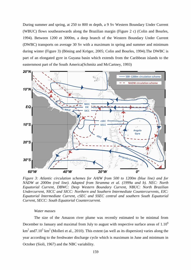
159
During summer and spring, at 250 to 800 m depth, a 9 Sv Western Boundary Under Current
(WBUC) flows southeastwards along the Brazilian margin (Figure 2 c) (Colin and Bourles,
1994). Between 1200 et 3000m, a deep branch of the Western Boundary Under Current
(DWBC) transports on average 30 Sv with a maximum in spring and summer and minimum
during winter (Figure 3) (Böning and Kröger, 2005; Colin and Bourles, 1994).The DWBC is
part of an elongated gyre in Guyana basin which extends from the Caribbean islands to the
easternmost part of the South America(Schmitz and McCartney, 1993)
Figure 3: Atlantic circulation schemes for AAIW from 500 to 1200m (blue line) and for
NADW at 2000m (red line). Adapted from Stramma et al. (1999a and b). NEC: North
Equatorial Current, DBWC: Deep Western Boundary Current, NBUC: North Brazilian
Undercurrent, NICC and SICC: Northern and Southern Intermediate Countercurrents, EIC:
Equatorial Intermediate Current, cSEC and SSEC central and southern South Equatorial
Current, SECC: South Equatorial Countercurrent.
Water masses
The size of the Amazon river plume was recently estimated to be minimal from
December to January and maximal from July to august with respective surface areas of 1.106
km2
and7.105 km
2 (Molleri et al., 2010). This extent (as well as its dispersion) varies along the
year according to the freshwater discharge cycle which is maximum in June and minimum in
October (Sioli, 1967) and the NBC variability.
Angola Gyre
SECC
cSEC
SICC
EICNICC
500–1200m circulation scheme
NADW circulation scheme
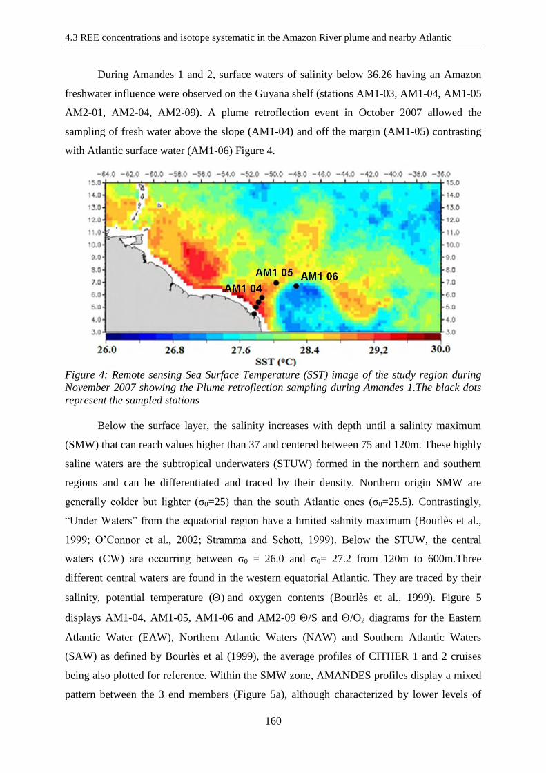
4.3 REE concentrations and isotope systematic in the Amazon River plume and nearby Atlantic
160
During Amandes 1 and 2, surface waters of salinity below 36.26 having an Amazon
freshwater influence were observed on the Guyana shelf (stations AM1-03, AM1-04, AM1-05
AM2-01, AM2-04, AM2-09). A plume retroflection event in October 2007 allowed the
sampling of fresh water above the slope (AM1-04) and off the margin (AM1-05) contrasting
with Atlantic surface water (AM1-06) Figure 4.
Figure 4: Remote sensing Sea Surface Temperature (SST) image of the study region during
November 2007 showing the Plume retroflection sampling during Amandes 1.The black dots
represent the sampled stations
Below the surface layer, the salinity increases with depth until a salinity maximum
(SMW) that can reach values higher than 37 and centered between 75 and 120m. These highly
saline waters are the subtropical underwaters (STUW) formed in the northern and southern
regions and can be differentiated and traced by their density. Northern origin SMW are
generally colder but lighter (σ0=25) than the south Atlantic ones (σ0=25.5). Contrastingly,
“Under Waters” from the equatorial region have a limited salinity maximum (Bourlès et al.,
1999; O’Connor et al., 2002; Stramma and Schott, 1999). Below the STUW, the central
waters (CW) are occurring between σ0 = 26.0 and σ0= 27.2 from 120m to 600m.Three
different central waters are found in the western equatorial Atlantic. They are traced by their
salinity, potential temperature (and oxygen contents (Bourlès et al., 1999). Figure 5
displays AM1-04, AM1-05, AM1-06 and AM2-09 /S and /O2 diagrams for the Eastern
Atlantic Water (EAW), Northern Atlantic Waters (NAW) and Southern Atlantic Waters
(SAW) as defined by Bourlès et al (1999), the average profiles of CITHER 1 and 2 cruises
being also plotted for reference. Within the SMW zone, AMANDES profiles display a mixed
pattern between the 3 end members (Figure 5a), although characterized by lower levels of
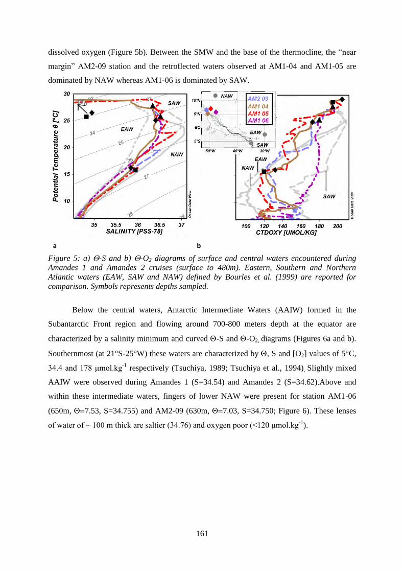
161
dissolved oxygen (Figure 5b). Between the SMW and the base of the thermocline, the “near
margin” AM2-09 station and the retroflected waters observed at AM1-04 and AM1-05 are
dominated by NAW whereas AM1-06 is dominated by SAW.
Figure 5: a) -S and b) -O2 diagrams of surface and central waters encountered during
Amandes 1 and Amandes 2 cruises (surface to 480m). Eastern, Southern and Northern
Atlantic waters (EAW, SAW and NAW) defined by Bourles et al. (1999) are reported for
comparison. Symbols represents depths sampled.
Below the central waters, Antarctic Intermediate Waters (AAIW) formed in the
Subantarctic Front region and flowing around 700-800 meters depth at the equator are
characterized by a salinity minimum and curved -S and -O2, diagrams (Figures 6a and b).
Southernmost (at 21°S-25°W) these waters are characterized by , S and [O2] values of 5°C,
34.4 and 178 μmol.kg-1
respectively (Tsuchiya, 1989; Tsuchiya et al., 1994). Slightly mixed
AAIW were observed during Amandes 1 (S=34.54) and Amandes 2 (S=34.62).Above and
within these intermediate waters, fingers of lower NAW were present for station AM1-06
(650m, 7.53, S=34.755) and AM2-09 (630m, 7.03, S=34.750; Figure 6). These lenses
of water of ~ 100 m thick are saltier (34.76) and oxygen poor (<120 μmol.kg-1
).
a b
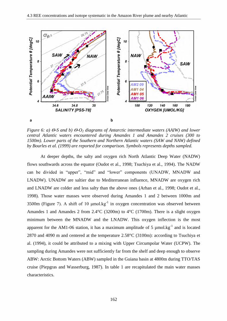
4.3 REE concentrations and isotope systematic in the Amazon River plume and nearby Atlantic
162
Figure 6: a) -S and b) -O2 diagrams of Antarctic intermediate waters (AAIW) and lower
central Atlantic waters encountered during Amandes 1 and Amandes 2 cruises (300 to
1500m). Lower parts of the Southern and Northern Atlantic waters (SAW and NAW) defined
by Bourles et al. (1999) are reported for comparison. Symbols represents depths sampled.
At deeper depths, the salty and oxygen rich North Atlantic Deep Water (NADW)
flows southwards across the equator (Oudot et al., 1998; Tsuchiya et al., 1994). The NADW
can be divided in “upper”, “mid” and “lower” components (UNADW, MNADW and
LNADW). UNADW are saltier due to Mediterranean influence, MNADW are oxygen rich
and LNADW are colder and less salty than the above ones (Arhan et al., 1998; Oudot et al.,
1998). Those water masses were observed during Amandes 1 and 2 between 1000m and
3500m (Figure 7). A shift of 10 μmol.kg-1
in oxygen concentration was observed between
Amandes 1 and Amandes 2 from 2.4°C (3200m) to 4°C (1700m). There is a slight oxygen
minimum between the MNADW and the LNADW. This oxygen inflection is the most
apparent for the AM1-06 station, it has a maximum amplitude of 5 µmol.kg-1
and is located
2870 and 4090 m and centered at the temperature 2.58°C (3100m): according to Tsuchiya et
al. (1994), it could be attributed to a mixing with Upper Circumpolar Water (UCPW). The
sampling during Amandes were not sufficiently far from the shelf and deep enough to observe
ABW: Arctic Bottom Waters (ABW) sampled in the Guiana basin at 4800m during TTO/TAS
cruise (Piepgras and Wasserburg, 1987). In table 1 are recapitulated the main water masses
characteristics.
a b
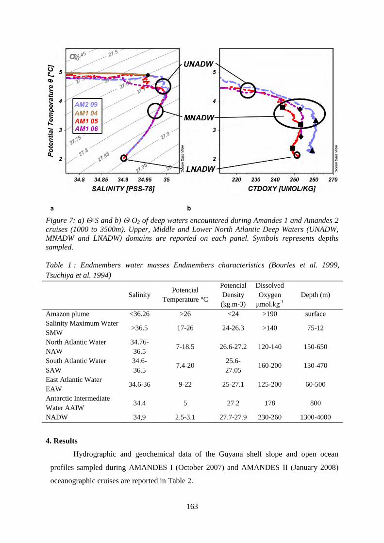
163
Figure 7: a) -S and b) -O2 of deep waters encountered during Amandes 1 and Amandes 2
cruises (1000 to 3500m). Upper, Middle and Lower North Atlantic Deep Waters (UNADW,
MNADW and LNADW) domains are reported on each panel. Symbols represents depths
sampled.
Table 1 : Endmembers water masses Endmembers characteristics (Bourles et al. 1999,
Tsuchiya et al. 1994)
Salinity Potencial
Temperature °C
Potencial
Density
(kg.m-3)
Dissolved
Oxygen
μmol.kg-1
Depth (m)
Amazon plume <36.26 >26 <24 >190 surface
Salinity Maximum Water
SMW >36.5 17-26 24-26.3 >140 75-12
North Atlantic Water
NAW
34.76-
36.5 7-18.5 26.6-27.2 120-140 150-650
South Atlantic Water
SAW
34.6-
36.5 7.4-20
25.6-
27.05 160-200 130-470
East Atlantic Water
EAW 34.6-36 9-22 25-27.1 125-200 60-500
Antarctic Intermediate
Water AAIW 34.4 5 27.2 178 800
NADW 34,9 2.5-3.1 27.7-27.9 230-260 1300-4000
4. Results
Hydrographic and geochemical data of the Guyana shelf slope and open ocean
profiles sampled during AMANDES I (October 2007) and AMANDES II (January 2008)
oceanographic cruises are reported in Table 2.
a b
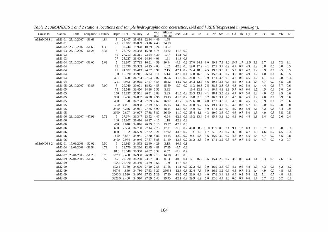
164
Table 2 : AMANDES 1 and 2 stations locations and sample hydrographic characteristics, εNd and [ REE](expressed in pmol.kg-1
).
Cruise Id Station Date Longitude Latitude Depth T °C salinity σ oxy ml/l
Silicate μmol/kg
εNd 2SE La Ce Pr Nd Sm Eu Gd Tb Dy Ho Er Tm Yb Lu
AMANDES 1 AM1-01 25/10/2007 -51.63 4.84 5 28.407 35.498 22.64 4.49 1.58
AM1-01 20 28.182 36.099 23.16 4.48 24.79
AM1-02 25/10/2007 -51.68 4.38 5 30.244 19.928 10.39 3.24 63.67
AM1-03 26/10/2007 -51.24 5.34 5 28.972 26.358 15.60 4.74 24.22 -11.5 0.2
AM1-03 40 27.213 36.311 23.64 4.39 1.47 -11.1 0.3
AM1-03 77 25.227 36.406 24.34 4.03 1.91 -11.8 0.3
AM1-04 27/10/2007 -51.00 5.63 5 28.997 27.712 16.61 4.59 20.94 -9.6 0.3 27.8 24.2 6.0 29.2 7.2 2.0 10.5 1.7 11.5 2.8 8.7 1.1 7.2 1.1
AM1-04 72 25.790 36.383 24.15 4.03 1.82 -12.3 0.3 19.0 17.2 4.1 17.9 3.7 0.9 4.7 0.7 4.9 1.2 3.8 0.5 3.0 0.5
AM1-04 75 24.672 36.413 24.52 3.97 2.15 -12.1 0.2 22.4 18.8 4.5 19.7 3.9 1.0 5.2 0.7 4.7 1.2 3.9 0.6 3.5 0.5
AM1-04 150 16.920 35.911 26.24 3.11 5.14 -12.2 0.4 12.8 16.3 3.5 15.3 3.0 0.7 3.7 0.8 4.9 1.2 4.0 0.6 3.6 0.5
AM1-04 451 8.498 34.784 27.04 3.02 16.56 -11.3 0.2 21.0 7.3 3.9 17.1 3.3 0.8 4.2 0.6 4.5 1.2 4.1 0.6 3.8 0.6
AM1-04 1251 4.983 34.965 27.67 4.54 18.42 -14.2 0.8 24.3 12.6 4.6 19.8 3.4 0.8 4.6 0.7 5.3 1.4 4.7 0.7 4.5 0.8
AM1-05 28/10/2007 -49.83 7.00 5 29.040 30.021 18.32 4.53 15.59 -9.7 0.2 11.3 10.3 2.5 38.5 2.8 0.8 4.3 0.9 5.9 1.4 4.4 0.6 3.7 0.6
AM1-05
75 25.548 36.450 24.28 3.53 3.22
16.4 12.2 4.1 18.9 4.1 1.1 5.7 0.9 6.0 1.5 4.5 0.6 3.8 0.6
AM1-05 150 15.897 35.951 26.51 2.83 5.33 -11.5 0.3 20.3 13.3 4.1 18.4 3.5 0.9 4.7 0.7 5.0 1.3 4.0 0.6 3.5 0.6
AM1-05 300 9.406 34.897 26.98 2.96 13.13 -11.5 0.2 16.8 7.9 3.7 16.3 3.1 0.8 4.3 0.6 4.5 1.2 4.0 0.6 3.9 0.6
AM1-05 400 8.178 34.784 27.09 2.67 16.97 -11.7 0.37 22.6 10.0 4.0 17.2 3.3 0.8 4.3 0.6 4.5 1.2 3.9 0.6 3.7 0.6
AM1-05 1750 4.051 34.988 27.79 5.68 15.05 -14.6 0.7 31.8 9.7 4.5 19.1 3.7 0.9 4.8 0.8 5.7 1.5 5.0 0.7 5.0 0.8
AM1-05 2400 3.276 34.961 27.85 5.90 18.44 -13.7 0.5 14.9 6.7 3.9 17.4 3.5 0.9 4.9 0.8 5.9 1.6 5.2 0.8 5.4 0.9
AM1-05 3000 2.697 34.927 27.88 5.82 26.90 -11.9 0.2 25.4 4.1 4.3 19.0 3.6 0.9 4.6 0.7 5.0 1.3 4.0 0.5 3.5 0.5
AM1-06 28/10/2007 -47.99 5.72 5 27.674 36.347 23.52 4.47 0.64 -12.9 0.3 16.2 13.4 3.4 15.4 3.1 1.0 4.1 0.6 4.4 1.1 3.4 0.5 2.6 0.4
AM1-06
100 25.807 36.416 24.17 4.15 1.18 -12.2 0.2
AM1-06 450 9.010 34.816 26.99 3.18 13.57 -12.9 0.3
AM1-06 650 7.564 34.730 27.14 2.75 17.81 -9.9 0.2 40.0 58.2 10.0 41.9 8.8 2.1 9.1 1.3 8.3 1.9 5.7 0.8 5.0 0.8
AM1-06 850 5.162 34.559 27.32 3.21 27.92 -13.3 0.2 1.3 1.0 0.7 5.6 2.2 0.7 3.8 0.6 4.7 1.3 4.6 0.7 4.5 0.8
AM1-06 1850 3.857 34.981 27.80 5.86 14.25 -12.9 0.2 9.2 5.8 3.6 15.9 3.0 0.7 4.5 0.7 5.5 1.4 4.7 0.7 4.5 0.8
AM1-06 2400 2.974 34.946 27.87 5.88 21.49 -13.3 0.2 21.2 3.8 3.9 17.1 3.2 0.8 4.7 0.7 5.5 1.4 4.7 0.7 4.3 0.7
AMANDES 2 AM2-01 17/01/2008 -52.02 5.50 5 26.983 34.573 22.40 4.29 3.15
-10.5 0.1
AM2-04 19/01/2008 -51.54 4.72 2 26.770 21.220 12.45 4.88 17.65 -9.7 0.2
AM2-04
18.8 26.040 36.380 24.07 3.32 6.57 -9.4 0.2
AM2-07 20/01/2008 -51.28 5.75 337.3 9.460 34.900 26.98 2.10 14.08 -11.6 0.3
AM2-09 22/01/2008 -51.47 6.57 2.2 27.320 36.260 23.57 3.83 0.83 -10.6 0.4 17.1 16.2 3.6 15.4 2.9 0.7 3.9 0.6 4.4 1.1 3.3 0.5 2.6 0.4
AM2-09
102.5 25.570 36.480 24.29 3.66 1.09 -11.8 0.4
AM2-09
602.1 6.780 34.670 27.20 2.58 21.68 -11.1 0.3 22.2 6.5 3.9 16.9 3.3 0.9 4.2 0.6 4.8 1.3 4.3 0.6 4.2 4.2
AM2-09
997.6 4.860 34.780 27.53 3.27 26038 -12.8 0.3 22.4 7.3 3.9 16.9 3.2 0.9 4.5 0.7 5.3 1.4 4.9 0.7 4.8 4.5
AM2-09 2000.3 3.530 34.970 27.83 5.29 17.20 -13.5 0.5 23.9 6.6 4.0 17.6 3.4 1.1 4.9 0.8 5.8 1.5 5.1 0.7 4.8 4.9
AM2-09 3228.9 2.460 34.910 27.89 5.43 29.45 -12.1 0.2 29.9 6.9 5.0 22.6 4.4 1.3 6.0 0.9 6.6 1.7 5.7 0.8 5.2 6.0
165
Surface waters
The Amazon plume is advected northwestward which allows it to reach the studied
area. It is characterized by surface sample of salinity <36, dissolved εNd values ranging from
-9.6 to -10.6 and Nd concentrations from 15.3 to 38.8 pmol.kg-1
. The AM1-04, AM1-05
surface samples collected in the plume but above and off the Guyana margin (salinities of
27.7, 30.7) show respective concentrations of 29.2 and 38.5 pmol.kg-1 and associated εNd
values of -9.6, and -9.7. These concentrations and isotopic compositions are different from the
ones observed at similar salinities within the Amazon estuary during the AMANDES 3
campaign. For example, AM3-0703 and AM3-0806 samples (salinities 27.88 and 30.7)
displayed higher Nd concentrations of 50.3 and 52.5 pmol.kg-1
respectively associated with
less radiogenic εNd values of-11 and -10.6 respectively (see the preceding section “REE
concentrations and Nd isotope dynamics in the Amazon River estuary”)
The AM1-06 surface sample collected outside of the plume displayed high salinity
(36.56) and an unradiogenic εNd value of -12.9 associated to a low Nd concentration of 15.3
pmol.kg-1
. This sample was the less radiogenic surface sample of the three Amandes cruises.
It is comparable to the unradiogenic TTO/TAS 63 surface sample (-14) attributed either to
atmospheric inputs or easterly water masses advected by the North Equatorial Current
(Piepgras and Wasserburg, 1987).
Central and intermediate waters
In Figure 8 are displayed vertical εNd profiles together with the associated water
masses collected during AMANDES 1 and 2. TTO/TAS 63 data are also reported for
comparison (Piepgras and Wasserburg, 1987). Within the salinity maximum and the upper
part of Central Waters, εNd are comprised between -11.3 and -12.5, although NAW seems
to be slightly more radiogenic than SAW. This isotopic shift is observable firstly by
difference between the AM1-04 150 m and AM1-05 150 m thermocline samples. They are
characterized by σ0 of 26.244 and 26.513 and εNd of -12.2± 0.4 and -11.5±0.3 respectively.
This north/south difference affecting the Central Waters is in agreement with earlier results
in the eastern Atlantic, with εNd =-11.16±0.3at 200m at the 22°N 69/11 station and εNd = -
12.49±0.3at the same depth at the equatorial 69/18 station (Rickli et al., 2009).
4.3 REE concentrations and isotope systematic in the Amazon River plume and nearby Atlantic
166
Another north/south isotopic shift for Central Waters is observed at deeper depths
at the AM1-06 station. Its lower-SAW sample (450 m, =9° and salinity 34.816) and the
lower-NAW intrusion (650m, =7.56° and salinity 34.730) have contrasted εNd signatures
of -12.9±0.3 and -9.9±0.2 respectively. Relatively radiogenic values for Central Waters in
the north Atlantic waters were only found in the western basin at station AII 109-1 (36.25°N
61.97°W; Piepgras and Wasserburg, 1987). Contrastingly, unradiogenic signatures for SAW
were also observed in the Angola basin at station 69/21 (εNd =-13.36 ±0.3 at 200m). This
signature was considered as local and attributed to reduction of Congo riverferromanganese
coatings (Rickli et al., 2009).The AAIW displaying the most pronounced S minimum (AM1-
0
500
1000
1500
2000
2500
3000
3500
4000
4500
-16 -14 -12 -10 -8
Dep
th
εNd
TTO TAS/63
AM1 04
AM1 05
AM1 06
AM2 09
LNADW
MNADW
UNADW
AAIW
AMA
NACW
ATL
SACW
ABW
Figure 8: Amandes 1 and 2 εNd profiles, the TTOTAS/63 profile is reported in light grey
for comparison (Piepgras and Wasserburg, 1987). Water masses domains are also
reported (ATL: surface Atlantic: AMA: Amazon River water; SAW and NAW: South and
North Atlantic Waters; AAIW: Antarctic Intermediate Waters; UNADW, MNADW and
LNADW: Upper, Middle and Lower North Atlantic Deep Waters; ABW: Arctic Bottom
Water)
167
06 850m) is also marked by an unradiogenic value of -13.3±0.2. As for the lower-SAW,
such negative values for AAIW have only been encountered in the Angola basin station
69/21 (Rickli et al., 2009). As it will be discussed below, these unradiogenic signatures may
cover a broader extension.
Deep waters
AM2-09 εNd profile is comparing closely with the TTO TAS 63 profile with values
of -13.5±0.5 at 2000m and -12.8±0.2 at 3220m. During Amandes 1 the samples AM1-04
1251m(very close to the slope) and AM1-05 1750 m (further offshore) show εNd values
clearly less radiogenic(-14.2 ± - 0.8 and -14.6 ± -0.7 respectively). Although the large error
bars affecting these 2 data invite us to interpret them thoroughly, such unradiogenic signatures
are surprisingly low for NADW, which signal εNd was never found below -13.7 so far (Lacan
et al., 2012; Pahnke et al., 2012; Piepgras and Wasserburg, 1980). The Oxygen minimum
sampled at AM1-05 3000m is slightly more radiogenic (εNd =-11.9) when compared to
MNADW and LNADW values (This study, Piepgras and Wasserburg, 1987).
5. Discussion
Surface
For the radiogenic surface sample AM1-06 located outside of the Amazon freshwater
plume could be explained by the atmospheric contribution hypothesis emitted by Piepgras and
Wasserbug (1987) to explain the surface radiogenic signature of TTO/TAS 63 surface sample.
This would be further supported by Nd isotopic compositions of dust collected from 26°W to
31°W and 0°N to 12°N and ranging from -12.7 to -14.5 (Goldstein et al., 1984; Grousset et
al., 1988; Grousset et al., 1998). However as no data are available for the central equatorial
Atlantic, unradiogenic easterlies waters contribution cannot be excluded (Lacan et al., 2012).
Surface dissolved samples collected during AMANDES 1 and 2 and located within
the plume are relatively more radiogenic than those of similar salinities analyzed in the
Amazon mouth during AMANDES 3. In the previous section) it was discussed that the mid to
high salinity part of the saline gradient were marked by the suspended sediments signature
(εNd= -10.7) whereas the more radiogenic coagulated colloids (εNd= -8.9) had left the
dissolved fraction in the low salinity zone. The difference we find here within the salinity
gradient located further north west off the Guyanese coast could reflect either: 1) a weaker
contribution of lithogenic suspended sediments release together with a larger supply of Nd
released from coagulated colloids 2) the influence of more radiogenic lithogenic material that
4.3 REE concentrations and isotope systematic in the Amazon River plume and nearby Atlantic
168
could have been added to the plume between the Amazon mouth and the Guyana coast. The
lack of εNd data for the sediments and rocks characterizing the shoreline prevents us to
conclude further on this second hypothesis.
Let us now assume that for any reason, the colloids –very abundant in the Amazon
river waters- have not been totally removed from the waters after their coagulation when the
salinity increases. The dissolved Amazonian colloids carry 100 ng of Nd per grams of river
water. Assuming that this river water has been diluted by seawater until higher salinities and
that the associated coagulated colloids lighter than suspended sediments have been advected
together with the river plume until the Guyana shelf there is a potential remaining pool of
coagulated colloids of 18 and 24 ng per litters at salinities 27.7 and 30.7 (AM1-04 and AM1-
05 surface samples salinities) in the particulate phase.
A mass balance can be formulated using the Nd IC from samples collected within the
estuary during the Amandes 3 campaign where AM3-01 and AM3-09 88m represent
respectively the Amazon (-8.8) and SW (-12.1) endmembers. The mass balance indicates that
for AM1-04 and AM1-05 surface samples respective contributions of Nd of “coagulated
colloids” origins where of 3.2 ng.kg-1
and 4.1 ng.kg-1
. Considering the colloid advection, this
would represent a release of at least 17% of the Nd carried by the coagulated colloid pool.
Note that this mass balance does not account for the Nd release from lithogenic particles.
Considering that lithogenic particles supply dominates the dissolved phase within
estuary, and estuarine formed organo-mineral particles may contribute to Nd release 1000km
away from the estuary: 1) Lateral advection may dominate vertical sinking for the coagulated
colloids transport contrastingly with lithogenic particles 2) The time lapse of Nd release
process from coagulated colloids is more important than the residence time within the estuary
3) There is a need to clarify whether this release process is due to desorption or if coagulated
colloids dissolve again after a certain time. This last point is important as it concerns the
particle lability and needs to be assessed for trace metals and organic carbon transport and
sink quantification. Ultrafiltration of river plume samples and batch experiments of
coagulated colloids degradation may give insights into these processes.
Central and intermediate waters
At station AM1-06 the lower-SAW (450 m, 9°C salinity 34.816 and εNd =-12.9) and
the lower-NAW intrusion (650m, 7.56°C, salinity 34.730 and εNd =-9.9) can be
geographically traced using the WOCE experiment database. The Figure 9 displays locations
169
and depths of their respective potential density values (σ0=26.98 for lower-SAW and 27.163
for lower-NAW), extracted from the WOCE CTD database applying their respective
temperatures (8.9 to 9.2) and (7.20 to 7.80) as sample selection criteria (http://.odv.awi.de/).
Because of the complexity of the equatorial current scheme, currents have been represented
by arrows and identified with letters (from A to G) in Figure 9. The lower-SAW extends from
19°S in the eastern Atlantic to 7°N in the western Atlantic with depth varying between 230
and 474 m. It is advected eastwards to the Angola gyre (G)by a vein coming from the
Equatorial Under Current(B: EUC),the South Equatorial Counter Current (F: SECC) at 10°S
and the South Equatorial Under Current (D:SEUC) at 5°S and westwards by the equatorial
branch of the South Equatorial current (E:eSEC) at 2.5°s and the central branch of the South
Equatorial Current (C: cSEC) at 7°S (Arhan et al., 1998; Bourlès et al., 1999; Oudot et al.,
1998; Stramma and Schott, 1999). The lower-NAW extends mainly along the 7°N on average
at 550m and flows eastwards within the north equatorial under current (A: NEUC). It was
observed along transects made during ETAMBOT and CITHER (Arhan et al., 1998; Stramma
and Schott, 1999). The zone of intrusion of lower-NAW lenses in lower-SAW waters is
located west of 40°W from 5°N to 7° N within the overlap of the two sections represented in
figure 9 a) and b). The AM1-06 (5.72N, -47.99W) illustrates those lenses intrusions and
sinking because the σ0=27.163 is located at 650m, it is one of the deepest depths observed for
this water mass (Figure 9b).
As presented in the results section, such radiogenic values for NAW where only
found in the western basin at station AII 109-1 (36.25°N; 61.97°W; Piepgras and Wasserburg,
1987). Although there is no potential hydrological link between the AM1-06 650m radiogenic
lower-NAW and the AII 109-1 station, we can speculate on a radiogenic endmember for
NAW that was sampled during AMANDES or on a local input having the Amazon signature.
The lower-SAW at 5°N displays isotopic and hydrological parameters very similar to
the unradiogenic Angola basin values observed at station 69/21 This supports the idea that
unradiogenic signatures for SAW have broader extension than the local one previously
thought (Rickli et al., 2009).
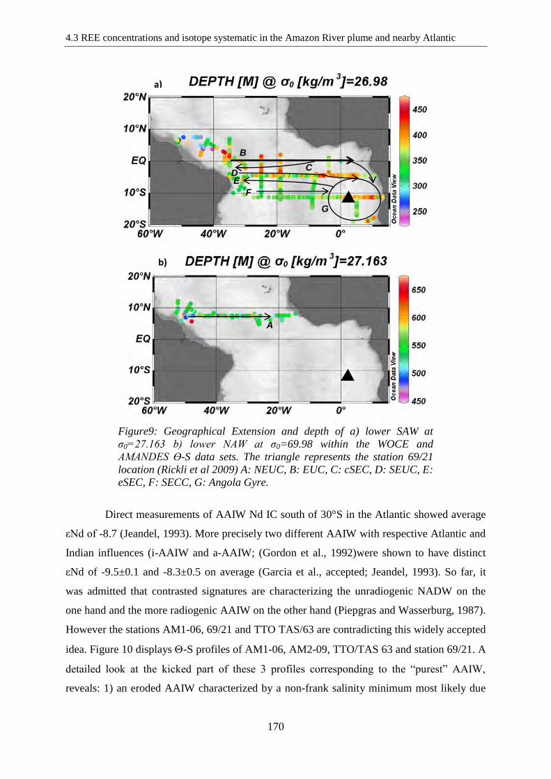
4.3 REE concentrations and isotope systematic in the Amazon River plume and nearby Atlantic
170
Figure9: Geographical Extension and depth of a) lower SAW at
σ0=27.163 b) lower NAW at σ0=69.98 within the WOCE and
AMANDES Ө-S data sets. The triangle represents the station 69/21
location (Rickli et al 2009) A: NEUC, B: EUC, C: cSEC, D: SEUC, E:
eSEC, F: SECC, G: Angola Gyre.
Direct measurements of AAIW Nd IC south of 30°S in the Atlantic showed average
εNd of -8.7 (Jeandel, 1993). More precisely two different AAIW with respective Atlantic and
Indian influences (i-AAIW and a-AAIW; (Gordon et al., 1992)were shown to have distinct
εNd of -9.5±0.1 and -8.3±0.5 on average (Garcia et al., accepted; Jeandel, 1993). So far, it
was admitted that contrasted signatures are characterizing the unradiogenic NADW on the
one hand and the more radiogenic AAIW on the other hand (Piepgras and Wasserburg, 1987).
However the stations AM1-06, 69/21 and TTO TAS/63 are contradicting this widely accepted
idea. Figure 10 displays -S profiles of AM1-06, AM2-09, TTO/TAS 63 and station 69/21. A
detailed look at the kicked part of these 3 profiles corresponding to the “purest” AAIW,
reveals: 1) an eroded AAIW characterized by a non-frank salinity minimum most likely due
A
B
C D E
G
F
a)
b)
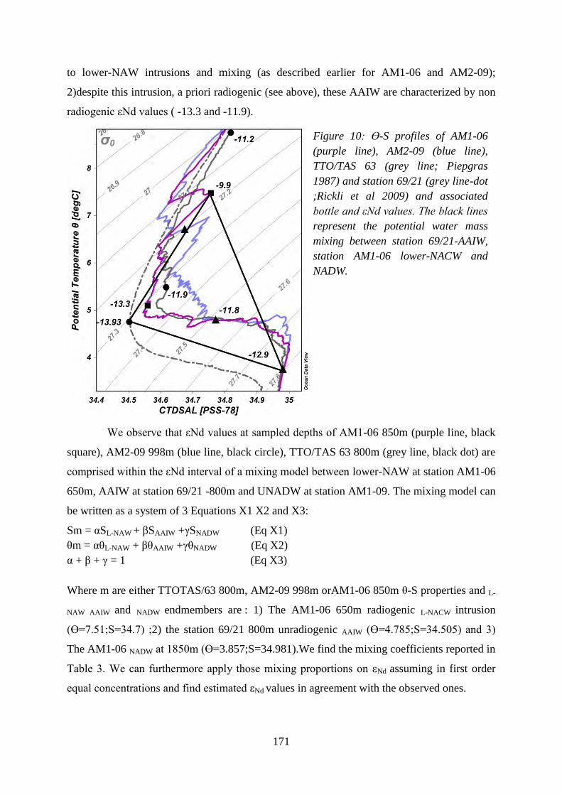
171
to lower-NAW intrusions and mixing (as described earlier for AM1-06 and AM2-09);
2)despite this intrusion, a priori radiogenic (see above), these AAIW are characterized by non
radiogenic εNd values ( -13.3 and -11.9).
We observe that εNd values at sampled depths of AM1-06 850m (purple line, black
square), AM2-09 998m (blue line, black circle), TTO/TAS 63 800m (grey line, black dot) are
comprised within the εNd interval of a mixing model between lower-NAW at station AM1-06
650m, AAIW at station 69/21 -800m and UNADW at station AM1-09. The mixing model can
be written as a system of 3 Equations X1 X2 and X3:
Sm = αSL-NAW + βSAAIW +γSNADW (Eq X1)
θm = αθL-NAW + βθAAIW +γθNADW (Eq X2)
α + β + γ = 1 (Eq X3)
Where m are either TTOTAS/63 800m, AM2-09 998m orAM1-06 850m θ-S properties and L-
NAW AAIW and NADW endmembers are : 1) The AM1-06 650m radiogenic L-NACW intrusion
(Ө=7.51;S=34.7) ;2) the station 69/21 800m unradiogenic AAIW (Ө=4.785;S=34.505) and 3)
The AM1-06 NADW at 1850m (Ө=3.857;S=34.981).We find the mixing coefficients reported in
Table 3. We can furthermore apply those mixing proportions on εNd assuming in first order
equal concentrations and find estimated εNd values in agreement with the observed ones.
Figure 10: Ө-S profiles of AM1-06
(purple line), AM2-09 (blue line),
TTO/TAS 63 (grey line; Piepgras
1987) and station 69/21 (grey line-dot
;Rickli et al 2009) and associated
bottle and εNd values. The black lines
represent the potential water mass
mixing between station 69/21-AAIW,
station AM1-06 lower-NACW and
NADW.
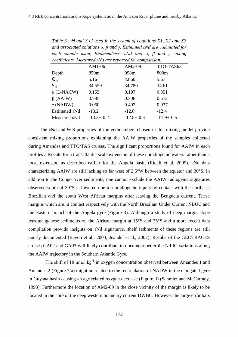
4.3 REE concentrations and isotope systematic in the Amazon River plume and nearby Atlantic
172
Table 3 : Ө and S of used in the system of equations X1, X2 and X3
and associated solutions α, β and γ. Estimated εNd are calculated for
each sample using Endmembers’ εNd and α, β and γ mixing
coefficients. Measured εNd are reported for comparison.
AM1-06 AM2-09 TTO-TAS63
Depth 850m 998m 800m
Өm 5.16 4.860 5.67
Sm 34.559 34.780 34.61
α (L-NACW) 0.155 0.197 0.351
β (AAIW) 0.795 0.306 0.572
γ (NADW) 0.050 0.497 0.077
Estimated εNd -13.2 -12.6 -12.4
Measured εNd -13.3+-0.2 -12.8+-0.3 -11.9+-0.5
The εNd and Ө-S properties of the endmembers chosen in this mixing model provide
consistent mixing proportions explaining the AAIW properties of the samples collected
during Amandes and TTO/TAS cruises. The significant proportions found for AAIW in each
profiles advocate for a transatlantic scale extension of these unradiogenic waters rather than a
local extension as described earlier for the Angola basin (Rickli et al, 2009). εNd data
characterizing AAIW are still lacking so far west of 2.5°W between the equator and 30°S. In
addition to the Congo river sediments, one cannot exclude the AAIW radiogenic signatures
observed south of 30°S is lowered due to unradiogenic inputs by contact with the northeast
Brazilian and the south West African margins after leaving the Benguela current. These
margins which are in contact respectively with the North Brazilian Under Current NBUC and
the Eastern branch of the Angola gyre (Figure 3). Although a study of deep margin slope
ferromanganese sediments on the African margin at 15°S and 25°S and a more recent data
compilation provide insights on εNd signatures, shelf sediments of these regions are still
poorly documented (Bayon et al., 2004; Jeandel et al., 2007). Results of the GEOTRACES
cruises GA02 and GA03 will likely contribute to document better the Nd IC variations along
the AAIW trajectory in the Southern Atlantic Gyre.
The shift of 10 μmol.kg-1
in oxygen concentration observed between Amandes 1 and
Amandes 2 (Figure 7 a) might be related to the recirculation of NADW in the elongated gyre
in Guyana basin causing an age related oxygen decrease (Figure 3) (Schmitz and McCartney,
1993). Furthermore the location of AM2-09 in the close vicinity of the margin is likely to be
located in the core of the deep western boundary current DWBC. However the large error bars
173
on εNd of the depleted NADW oxygen samples do not allow us to depict whether or not this
depletion is going together with a significant shift in isotopic compositions.
6. Conclusion
We presented here oceanic εNd data acquired in the framework of the
multidisciplinary AMANDES project on the Guyana shelf /slope an offshore in October 2007
and February 2008. We sampled and analyzed several water masses for Nd IC determination
in this poorly documented region crucial for heat and water exchange between the two
hemispheres.
In surface offshore non Amazon-influenced zone we found unradiogenic Nd signature
which combine with earlier observations of Piegras et Wasserburg (1987), Goldstein et al.
(1984) and Grousset et al. (1988, 1998). This strengthens the idea that cross-atlantic dust
transport may occur and contribute to Nd supply at sea surface. In the NBC advected Amazon
plume our results differs from observation made at similar salinities within the Amazon
estuary (section 4.2). The Nd IC suggests that a significant fraction of Nd can be released
from estuarine formed organo-mineral particules. These particles are not lithogenic, they are
formed by the salt induced coagulation/flocculation of colloids within the salinity gradient.
On a balance scale, this Nd supply is far less consequent than the amount of Nd released from
suspended and margin deposited particles of lithogenic origin. However this observation
raises fundamental questions on particle chemical composition, reactivity, lability and
transport. We compared the Amandes offshore Ө-S profiles with the WOCE database and
identified a dynamic zone located west of 40°W from 5°N to 7° N were southwards lenses of
radiogenic lower-NAW sinks within more radiogenic lower-SAW and AAIW waters leading
to eroded AAIW. This region is the main pathway for AAIW to reach the north hemisphere
and may act as a barrier attenuating the AAIW salinity minimum in a reduced space-scale.
The AAIW Nd Isotopic composition we observe is 5 εNd units lower than the one
previously observed south of 30°S (Carter et al., 2012; Garcia et al., accepted; Jeandel, 1993;
Piepgras and Wasserburg, 1982; Stichel et al., 2012a; Stichel et al., 2012b). However a 3
endmembers mixing model reveals an hydrological and isotopic coherence between our
observations the ones of Piepgras et Wasserburg (1987) and Rickli et al. (2009). This last
author argued for a local unradiogenic AAIW in the Angola Basin, we rather suggest a
transatlantic scale extension of these unradiogenic signatures adquired by Boundary Exchange
processes (BE) between water masses advected by the North Brazilian Under Current NBUC
on the western boundary and the Eastern branch of the Angola gyre on the eastern boundary.
4.3 REE concentrations and isotope systematic in the Amazon River plume and nearby Atlantic
174
However, the lack of data on sediments deposited on the concerned margins combined to the
gap in seawater εNd data in the studied area prevent us to draw more detailed conclusions.
7. References
Arhan, M., Mercier, H., Bourlès, B., Gouriou, Y., 1998. Hydrographic sections across the Atlantic at
7°30N and 4°30S. Deep Sea Research Part I: Oceanographic Research Papers 45, 829-872.
Arnault, S., 1987. Tropical Atlantic geostrophic currents and ship drifts. Journal of Geophysical
Research: Oceans (1978–2012) 92, 5076-5088.
Arsouze, T., Dutay, J.C., Lacan, F., Jeandel, C., 2009. Reconstructing the Nd oceanic cycle using a
coupled dynamical - biogeochemical model. Biogeosciences 6, 2829-2846.
Bayon, G., German, C.R., Burton, K.W., Nesbitt, R.W., Rogers, N., 2004. Sedimentary Fe–Mn
oxyhydroxides as paleoceanographic archives and the role of aeolian flux in regulating
oceanic dissolved REE. Earth and Planetary Science Letters 224, 477-492.
Böning, C.W., Kröger, J., 2005. Seasonal variability of deep currents in the equatorial Atlantic: a
model study. Deep Sea Research Part I: Oceanographic Research Papers 52, 99-121.
Bourlès, B., Gouriou, Y., Chuchla, R., 1999. On the circulation in the upper layer of the western
equatorial Atlantic. Journal of Geophysical Research 1042, 21151-21170.
Bourles, B., Molinari, R.L., Johns, E., Wilson, W.D., Leaman, K.D., 1999. Upper layer currents in the
western tropical North Atlantic (1989–1991). Journal of Geophysical Research: Oceans 104,
1361-1375.
Carter, P., Vance, D., Hillenbrand, C.D., Smith, J.A., Shoosmith, D.R., 2012. The neodymium isotopic
composition of waters masses in the eastern Pacific sector of the Southern Ocean. Geochimica
et Cosmochimica Acta 79, 41-59.
Colin, C., Bourles, B., 1994. Western boundary currents and transports off french-guiana as inferred
from pegasus observations. Oceanologica Acta 17, 143-157.
Dengler, M., Schott, F.A., Eden, C., Brandt, P., Fischer, J., Zantopp, R.J., 2004. Break-up of the
Atlantic deep western boundary current into eddies at 8° S. Nature 432, 1018-1020.
Garcia, E., Jeandel, C., Labatut, M., Lacan, F., Vance, D., Chavagnac, V., accepted. Rare Earth
Elements and Nd isotopes tracing water mass mixing and particle-seawater interactions in the
SE Atlantic. Geochimica et Cosmochimica Acta.
Goldstein, S.L., O'Nions, R.K., Hamilton, P.J., 1984. A Sm-Nd isotopic study of atmospheric dusts
and particulates from major river systems. Earth and Planetary Science Letters 70, 221-236.
Gordon, A.L., 1986. Interocean exchange of thermocline water. Journal of Geophysical Research:
Oceans 91, 5037-5046.
Gordon, A.L., Weiss, R.F., Smethie, W.M., Warner, M.J., 1992. Thermocline and intermediate water
communication between the South Atlantic and Indian Oceans. Journal of Geophysical
Research: Oceans (1978–2012) 97, 7223-7240.
Grousset, F.E., Biscaye, P.E., Zindler, A., Prospero, J., Chester, R., 1988. Neodymium isotopes as
tracers in marine sediments and aerosols: North Atlantic. Earth and Planetary Science Letters
87, 367-378.
Grousset, F.E., Parra, M., Bory, A., Martinez, P., Bertrand, P., Shimmield, G., Ellam, R.M., 1998.
Saharan wind regimes traced by the Sr–Nd isotopic composition of subtropical Atlantic
sediments: Last Glacial Maximum vs today. Quaternary Science Reviews 17, 395-409.
Jeandel, C., 1993. Concentration and isotopic composition of Nd in the South Atlantic Ocean. Earth
and Planetary Science Letters 117, 581-591.
Jeandel, C., Arsouze, T., Lacan, F., Téchiné, P., Dutay, J.C., 2007. Isotopic Nd compositions and
concentrations of the lithogenic inputs into the ocean: A compilation, with an emphasis on the
margins. Chemical Geology 239, 156-164.
Jeandel, C., Peucker-Ehrenbrink, B., Jones, M.T., Pearce, C.R., Oelkers, E.H., Godderis, Y., Lacan, F.,
Aumont, O., Arsouze, T., 2011. Ocean margins: The missing term in oceanic element
budgets?
175
Jones, M.T., Pearce, C.R., Jeandel, C., Gislason, S.R., Eiriksdottir, E.S., Mavromatis, V., Oelkers,
E.H., 2012. Riverine particulate material dissolution as a significant flux of strontium to the
oceans. Earth and Planetary Science Letters 355–356, 51-59.
Lacan, F., Jeandel, C., 2001. Tracing Papua New Guinea imprint on the central Equatorial Pacific
Ocean using neodymium isotopic compositions and Rare Earth Element patterns. Earth and
Planetary Science Letters 186, 497-512.
Lacan, F., Jeandel, C., 2004a. Denmark Strait water circulation traced by heterogeneity in neodymium
isotopic compositions. Deep Sea Research Part I: Oceanographic Research Papers 51, 71-82.
Lacan, F., Jeandel, C., 2004b. Subpolar Mode Water formation traced by neodymium isotopic
composition. Geochemistry Geophysics Geosystems.
Lacan, F., Jeandel, C., 2005. Neodymium isotopes as a new tool for quantifying exchange fluxes at the
continent-ocean interface. Earth and Planetary Science Letters 232, 245-257.
Lacan, F., Tachikawa, K., Jeandel, C., 2012. Neodymium isotopic composition of the oceans: A
compilation of seawater data. Chemical Geology 300–301, 177-184.
Molleri, G.S.F., Novo, E.M.L.d.M., Kampel, M., 2010. Space-time variability of the Amazon River
plume based on satellite ocean color. Continental Shelf Research 30, 342-352.
O’Connor, B.M., Fine, R.A., Maillet, K.A., Olson, D.B., 2002. Formation rates of subtropical
underwater in the Pacific Ocean. Deep Sea Research Part I: Oceanographic Research Papers
49, 1571-1590.
Oudot, C., Morin, P., Baurand, F., Wafar, M., Corre, P.L., 1998. Northern and southern water masses
in the equatorial Atlantic: distribution of nutrients on the WOCE A6 and A7 lines. Deep Sea
Research Part I: Oceanographic Research Papers 45, 873-902.
Pahnke, K., van de Flierdt, T., Jones, K.M., Lambelet, M., Hemming, S.R., Goldstein, S.L., 2012.
GEOTRACES intercalibration of neodymium isotopes and rare earth element concentrations
in seawater and suspended particles. Part 2: Systematic tests and baseline profiles. Limnol.
Oceanogr. Meth. 10, 252-269.
Pearce, C.R., Jones, M.T., Oelkers, E.H., Pradoux, C., Jeandel, C., 2013. The effect of particulate
dissolution on the neodymium (Nd) isotope and Rare Earth Element (REE) composition of
seawater. Earth and Planetary Science Letters.
Piepgras, D.J., Wasserburg, G.J., 1980. Neodymium isotopic variations in seawater. Earth and
Planetary Science Letters 50, 128-138.
Piepgras, D.J., Wasserburg, G.J., 1982. Isotopic composition of neodymium in waters from the drake
passage. Science 217, 207-214.
Piepgras, D.J., Wasserburg, G.J., 1987. Rare earth element transport in the western North Atlantic
inferred from Nd isotopic observations. Geochimica et Cosmochimica Acta 51, 1257-1271.
Pin, Zalduegui, 1997. Sequential separation of light rare-earth elements, thorium and.
Richardson, P.L., Reverdin, G., 1987. Seasonal cycle of velocity in the Atlantic North Equatorial
Countercurrent as measured by surface drifters, current meters, and ship drifts. Journal of
Geophysical Research: Oceans (1978–2012) 92, 3691-3708.
Rickli, J., Frank, M., Baker, A.R., Aciego, S., de Souza, G., Georg, R.B., Halliday, A.N., 2011.
Hafnium and neodymium isotopes in surface waters of the eastern Atlantic Ocean:
Implications for sources and inputs of trace metals to the ocean. Geochimica et Cosmochimica
Acta 74, 540-557.
Rickli, J., Frank, M., Halliday, A.N., 2009. The hafnium-neodymium isotopic composition of Atlantic
seawater. Earth and Planetary Science Letters 280, 118-127.
Rousseau, T.C.C., Sonke, J.E., Chmeleff, J., Candaudap, F., Lacan, F., Boaventura, G., Seyler, P.,
Jeandel, C., 2013. Rare earth element analysis in natural waters by multiple isotope dilution -
sector field ICP-MS. Journal of Analytical Atomic Spectrometry 28, 573-584.
Schmitz, W.J., McCartney, M.S., 1993. On the North Atlantic Circulation. Reviews of Geophysics 31,
29-49.
Schott, F.A., Dengler, M., Zantopp, R., Stramma, L., Fischer, J., Brandt, P., 2005. The Shallow and
Deep Western Boundary Circulation of the South Atlantic at 5°–11°S. Journal of Physical
Oceanography 35, 2031-2053.
Shabani, M.B., Akagi, T., Masuda, A., 1992. Preconcentration of trace rare-earth elements in seawater
by complexation with bis(2-ethylhexyl) hydrogen phosphate and 2-ethylhexyl dihydrogen
4.3 REE concentrations and isotope systematic in the Amazon River plume and nearby Atlantic
176
phosphate adsorbed on a c18 cartridge and determination by inductively coupled plasma mass-
spectrometry. Analytical Chemistry 64, 737-743.
Sholkovitz, E.R., 1993. The geochemistry of rare earth elements in the Amazon River estuary.
Geochimica et Cosmochimica Acta 57, 2181-2190.
Sioli, H., 1967. Studies in Amazonian Waters. Bel‚m.
Stichel, T., Frank, M., Rickli, J., Haley, B.A., 2012a. The hafnium and neodymium isotope
composition of seawater in the Atlantic sector of the Southern Ocean. Earth and Planetary
Science Letters 317–318, 282-294.
Stichel, T., Frank, M., Rickli, J., Hathorne, E.C., Haley, B.A., Jeandel, C., Pradoux, C., 2012b.
Sources and input mechanisms of hafnium and neodymium in surface waters of the Atlantic
sector of the Southern Ocean. Geochimica et Cosmochimica Acta 94, 22-37.
Stramma, L., Schott, F., 1999. The mean flow field of the tropical Atlantic Ocean. Deep Sea Research
Part II: Topical Studies in Oceanography 46, 279-303.
Tachikawa, K., Athias, V., Jeandel, C., 2003. Neodymium budget in the modern ocean and paleo-
oceanographic implications. Journal of Geophysical Research-Oceans 108.
Tachikawa, K., Jeandel, C., Vangriesheim, A., Dupré, B., 1999. Distribution of rare earth elements
and neodymium isotopes in suspended particles of the tropical Atlantic Ocean (EUMELI site).
Deep Sea Research Part I: Oceanographic Research Papers 46, 733-755.
Tréguer, P.J., De La Rocha, C.L., 2013. The World Ocean Silica Cycle. Annual Review of Marine
Science 5, 477-501.
Tsuchiya, M., 1989. Circulation of the Antarctic Intermediate Water in the North Atlantic Ocean.
Journal of Marine Research 47, 747-755.
Tsuchiya, M., Talley Lynne, D., McCartney Michael, S., 1994. Water-mass distributions in the
western South Atlantic; A section from South Georgia Island (54S) northward across the
equator. Journal of Marine Research 52, 55-81.
Wilson, W.D., Johns, E., Molinari, R.L., 1994. Upper layer circulation in the western tropical North
Atlantic Ocean during August 1989. Journal of Geophysical Research: Oceans (1978–2012)
99, 22513-22523.
177
5:Conclusions et perspectives
Sommaire
5.1 Conclusions 180
/ Conclusões 184
5.2 Perspectives 188
/ Perspectivas 190
5.3 Références bibliographiques 192
178
5.1 Conclusions
D’un point de vue personnel cette thèse de doctorat a été très formatrice et très
polyvalente. J’ai ainsi travaillé dans trois laboratoires et j’ai collaboré avec des géochimistes
marins et continentaux. Elle m’a permis de participer à des campagnes d’échantillonnage
océanographiques et fluviales, totalisant près de deux mois sur le fleuve Amazone, dans
l’estuaire, sur le plateau continental et au large des côtes Brésiliennes et Guyanaises. Des
échantillons d’eau provenant aussi bien du rio Negro à près de 3000 km de l’embouchure du
fleuve que de l’eau nord Atlantique de fond collectée à plus de 3000 m de profondeur dans
l’océan Atlantique équatorial ont ainsi été rapportés au laboratoire. J’ai pu me former à la
préparation et à l’analyse de ces échantillons en salle blanche puis sur de nombreuses
machines et particulièrement les spectromètres de masse de l’Observatoire Midi-Pyrénées
(OMP): l’ICMPS Agilent, l’ICPMS à haute résolution Element-XR, le MC-ICPMS Neptune
et le TIMS MAT 261.
Une partie de ce doctorat a notamment été consacrée à des développements analytiques.
Une méthode d’analyse des concentrations en REE dans les eaux naturelles par dilution
isotopique utilisant 10 spikes a été développée. Les spikes utilisés pour ce travail sont ceux
qui étaient utilisés au LMTG dans les années 1980 pour des analyses sur TIMS et délaissés
depuis avec l’avènement des ICPMS. La problématique générant le besoin de développer une
telle méthode étant la précision requise pour la détection de fractionnements entre les REE au
cours du transit estuarien, cette méthode permet la mesure de tout type de spectres de REE en
utilisant deux mélanges de spikes l’un composé de LREE et l’autre de HREE. Elle est ainsi
adaptée tant pour les géochimistes continentaux que pour les océanographes.
Cette méthode a mis à profit l’ICPMS à haute résolution, acquis récemment par la
plateforme analytique de l’OMP, que nous avons couplé à un système d’introduction de
désolvatation (ARIDUS). Un gain substantiel de sensibilité a été atteint en divisant par 5 les
limites de détections atteintes au laboratoire sur l’ICPMS quadruplolaire avant ce travail. La
précision de la mesure s’est également accrue avec une reproductibilité à long terme <2%
(2RSD) sur la plupart des REE grâce à la dilution isotopique. Le développement de cette
méthode a permis également une amélioration importante des interférences polyatomiques
d’oxydes de Ba et de LREEs sur les HREEs. Avec des taux de formation d’oxydes< 0,035%
(LaO+/La
+) soit une baisse d’un facteur 30 par rapport à ceux habituellement observés avant
ce développement. Cette méthode permet en conséquence d’obtenir des résultats de meilleure
qualité comparé à la plupart des méthodes d’analyses de concentrations en REE par ICP-MS.
179
En particulier, les précisions et justesses atteintes se rapprochent des mesures ID-TIMS avec
l’avantage de mesurer les 4 REE monoisotopiques. Nos résultats pour le matériel de référence
SLRS-5 ont pu être comparés à ceux obtenus par d’autres laboratoires et ils se trouvent très
proches de la moyenne de l’ensemble des données avec les plus petites erreurs standards
relatives (Yeghicheyan et al., 2013).
Nous avons optimisé les protocoles de préconcentration pour séparer au maximum les
REE de la matrice. Un premier protocole pour les échantillons d’eau de mer fait appel à la
nouvelle résine Nobias (Hitachi) dont nous sommes un des premiers laboratoires en France à
avoir testé les performances. Cette résine permet une meilleure séparation du Ba et un temps
de préparation plus court comparé au protocole traditionnel de préconcentration par co-
precipitation au Fe(OH)3. Le protocole de co-précipitationau Fe(OH)3 a été optimisé en
termes de temps de chimie, de blancs de préparation et d’efficacité de séparation du Ba.
Enfin, pour les eaux douces, un protocole simple de séparation du Ba utilisant la résine
cationique AG50-X8 a été développé.
Cette méthode permet de suivre finement les variations de spectres de REE et de
détecter de faibles anomalies de REE. Elle présente un potentiel certain pour mieux
comprendre le cycle géochimique des REE par des études en milieu naturel et des expériences
en laboratoire.
Nous avons réalisé la première étude d’estuaire couplant les analyses classiques de
concentrations en REE dans la phase dissoute avec des données d’ultrafiltration et des
compositions isotopiques du Nd. Pour le pôle d’eau douce du fleuve Amazone nos résultats
complètent les estimations précédentes pour les concentrations en REE dissoutes et associées
aux colloïdes. Nous observons également des compositions isotopiques du Nd dissous et
particulaire en accord avec celles de la littérature. La station d’observation Hybam à Óbidos,
plus facile d’accès que l’Amazone à son exutoire est donc représentative du ‘pôle’ amazonien.
Dans le gradient de salinité de l’estuaire du fleuve Amazone nous observons 1) Une
forte diminution des concentrations en REE liées aux colloïdes avec l’augmentation de la
salinité. En effet plus de 80% des REE dissoutes sont présentes dans la phase colloïdale pour
le pôle Amazonien contre moins de 10% pour le pôle marin 2) Les mesures de composition
isotopique du Nd suggèrent une origine lithogénique pour le Nd apporté à la phase dissoute
aux salinités moyennes et hautes (εNd= -10.7) car il a une signature différente de celles des
endmembers fluvial et océanique (εNdAM= -8.9 et εNdSW= -12.1). Ce Nd pourrait etre
transmis à la phase dissoute par voie de désorption ou dissolution. 3) Les données de Ra
5.1 Conclusions
180
permettent d’estimer l’échelle de temps de ce processus à une vingtaine de jours ce qui est en
accord avec des données obtenues expérimentalement. 4) Ce processus mis en évidence pour
la première fois en milieu naturel, a été quantifié par un bilan de masse prenant en compte les
εNd et les concentrations en REE et nous observons dans l’estuaire un transfert de près de 1%
du Nd des particules lithogéniques vers la phase dissoute. De plus, les eaux de fond du plateau
continental entre 40 et 90m qui n’ont pas été en contact avec le pôle Amazonien présentent
des concentrations élevées en Nd et moins radiogéniques que les sources citées
précédemment, nous suggérons donc un apport en Nd provenant des sédiments déposés sur la
marge.
En surface au large de la marge guyanaise, dans une zone non influencée par la plume
d’eau douce, nous avons observé une signature peu radiogénique qui corrobore les
observations de Piepgras et Wasserburg (1987), Goldstein et al. (1984) et Grousset et al
(1988, 1998).Ceci renforce l’idée que des poussières sahariennes puissent être transportées
d’un bout à l’autre de l’océan Atlantique et contribuent aux apports de Nd de l’océan de
surface.
Dans le panache d’eau douce de l’Amazone advecté en surface jusqu’aux Côtes
guyanaises, nos résultats diffèrent des observations réalisées à des salinités similaires au sein
de l’estuaire. Les données de composition isotopique du Nd suggèrent qu’une fraction
significative du Nd peut être relarguée des particules organo-minérales formées dans
l’estuaire. Ces particules non-lithogéniques se sont formées par la coagulation/floculation des
colloïdes Amazoniens au sein du gradient salin. Cette observation soulève des questions
fondamentales sur la composition chimique des particules, leur réactivité, leur labilité et leur
transport.
En comparant les profils Ө-S analysés en océan ouvert et extraits de la base de donnée
WOCE nous avons identifié une zone dynamique localisée à l’ouest de 40°W entre 5°S et 7°S
ou des lentilles de ‘lower-NAW’ radiogéniques circulent vers le sud et plongent dans la
‘lower-SAW’ et l’AAIW qui sont moins radiogéniques ce qui contribue à éroder le maximum
de salinité de l’AAIW. Cette région est le passage principal pour l’AAIW vers l’hémisphère
nord et pourrait représenter une barrière pour l’AAIW, altérant sont maximum de salinité sur
une courte distance.
L’AAIW échantillonnée durant les campagnes Amandes est caractérisée par des
valeurs de εNd de 5 unités inférieures à celles observées précédemment par les 5 études au
sud de 30°S par. Toutefois un modèle de mélange à 3 pôles révèle une cohérence isotopique
181
et hydrologique entre nos observations et celles de Piepgras et Wasserburg (1987) et Rickli et
al. (2009). Ces derniers ont argumenté une présence locale d’AAIW « peu radiogéniques »
dans le Bassin d’Angola. Nous proposons une extension plus large de ces signatures peu
radiogéniques à l’échelle du bassin océanique. Cette signature aurait été acquise par échange
aux marges, (boundary exchange) entre les masses d’eau advectées par le sous-courant nord
Brésilien (NBUC) à l’ouest, et la branche est du gire Angolais à l’est.
L’étude du cycle géochimique du Nd et des REE requiert une bonne estimation des
sources et des puits. Avant ce travail, les apports du fleuve Amazone en Nd exportable
(dissous) à l’océan étaient estimés en faisant l’hypothèse d’un relargage total du Nd associé
aux colloïdes coagulés (Tachikawa 2003, Barroux, 2006). Nos observations vérifient en partie
ce postulat mais ce mécanisme est encore peu clair et nécessite une étude plus approfondie.
Toutefois l’information majeure apportée par nos travaux réside dans l’importance des
sédiments déposés sur la marge et de ceux en suspension dans le transfert de Nd à l’océan. En
effet, la quantité importante de Nd provenant des particules lithogéniques en suspension sur
des échelles spatiale et temporelle si réduites souligne une contribution significative des
marges au budget global de cet élément. Ces observations confirment directement des
précédents travaux de modélisation portant sur le cycle global du Nd et qui ont suggérés que
du Nd dissous doit provenir des marges (Tachikawa et al. 2003, Arsouze et al. 2007, 2009) et
des travaux expérimentaux de mise en contact de sédiments lithogénique à des eaux marines
(Pearce et al. 2013).
Jusqu’à récemment ce terme était négligé dans le cycle géochimique du Nd mais
également dans celui d’autres éléments chimiques comme le montre un nombre croissant de
travaux d’expérimentaux et de modélisation(Jeandel et al., 2011; Jones et al., 2012a; Jones et
al., 2012b; Pearce et al. 2013, Tréguer and De La Rocha, 2013).
5.1 Conclusões
182
Conclusões
De um ponto de vista pessoal esta these de doutorado tem sido muito formadora e muito
polivalente. Tenho trabalhado em três laboratórios e tenho colaborado com geoquímicos marinho e
continentais. Esta me permitiu participar de campanhas de amostragem oceanográficas e fluviais,
totalizando cerca de dois meses no rio Amazonas, no estuário, na plataforma continental e ao largo
das costas brasileiras e guyanesas. Amostras de água proveniente tanto do rio negro a cerca de
3000km do estuario do rio quanto amostras de Águas Norte atlánticas profundas coletadas a mais de
3000m de profundidade no oceano atlántico equatorial foram assim levadas até o laboratório. Eu me
formei na preparação e na análise destas amostras em salas limpas e sobre numerosos aperelhos e
particularmente os espectrômetros de massas do Observatoire Midi Pyrrennées (OMP) : O ICPMS
Agilent, o ICPMS de alta resolução ELEMENT XR, O MC-ICPMS Neptune e o TIMS MAT 261.
Uma parte deste doutorado tem notavelmente sido dedicada à desenvolvimentos analíticos.
Um método de análise de teores em REE em águas naturais por dilução isotópica usando 10 spykes
tem sido desenvolvida. Os spikes usados para este trabalho são aqueles que eram utilisados
antigamente no LMTG nos anos 80 para análises com o TIMS e deixados de lado com o advento dos
ICPMS. A problemática generando a necessidade de desenvolver um tal método sendo a precisão
requerida para a deteção dos fracionamentos de REEs durante o trânsito estuarino, este método
permite a medida de todos os espectros de REE usando duas misturas de spike um composto de LREE
e o outro de HREE. Assim ele é adaptado para geoquímicos tanto continentais quanto oceanógrafos.
Este metodo tem aproveitado o ICPMS de alta resolução adquirido recentemente pela
plataforma analítica do OMP. Temos acoplado este aparelho a um sistema de introdução por
dessolvatação. Um ganho substancial em sensibilidade tem sido atingido dividindo por 5 os limites
de deteção atingidos no laboratorio com o ICPMS quadrupolar antes deste trabalho. A precisão da
medida tem também sido aumentada com uma reprodutibilidade de longo prazo <2% (2RSD) na
maior parte dos REE graças à dilução isotópica. O desenvolvimento deste método tem permitido
também uma melhoria importante das interferências poli-atômicas dos óxidos de Ba e LREE sobre os
HREE. Com teores de formação de óxidos < 0,035% (LaO+/La+) ou seja uma diminuição de um factor
30 quando comparado à aqueles habitualmente observados antes deste desenvolvimento. Este
método permite em consequëncia a obtenção de resultados de melhor qualidade em comparação à
maioria dos metodos analíticos de teores em REE por ICP-MS com a vantagem de medir os 4 REEs
monoisotópicos. Nossos resultados para o material de referênçia SLRS-5 tem tido a oportunidade de
ser comparado aos obtidos por outros laboratórios e estes se encontram muito próximos da media
do cada dado com os menores erros padrão relativos (Yeghicheyan et al., 2013).
183
Temos optimizado os protócolos de preconcentração para separar ao máximo os REE da
matriz. Um primeiro protócolo para as águas marinhas requer a nova résina Nobias (Hitachi) cuja
somos um dos primeiros laboratórios na frança a ter testado as perfórmances. Esta resina permite
uma melhor separação do Ba e um tempo de preparação mais curto em comparação ao protócolo
tradicional de preconcentração por co-precipitação com Fe(OH)3. O protócolo de co-precipitação
com Fe(OH)3 tem sido optimizado em termos de tempo de química, de brancos de preparação e de
eficiênçia na separação do Ba. Enfim para as águas continentais, um protócolo simples de separação
do Ba usando a resina catiônica AG50-X8 tem sido desenvolvido. Este método permite o
monitamento fino dos espectros de REE e de detectar leves anomalias de REE. Ele representa um
potencial para melhor entender o ciclo geoquímico dos REE por estudos em meios naturais e
experimentos em laboratório.
Temos realisado o primeiro estudo de estuário acoplando análises clássicas de concentração
em REE na fase dissolvida com dados de ultrafiltração e de composição isotópicas do Nd. Para o pôlo
de água doce do rio Amazonas os nossos resultados completam estimações precedentes dos teores
em REE dissolvidos associados a collóides . Observamos também composições isotópicas do Nd
dissolvido e particulado em acordo com a literatura. A estação de observação Hybam em Óbidos,
mais fácil de acesso que o Rio Amazonas na sua foz é em consequência representativa do « pólo »
amazônico.
No gradiente de salinidade do estuário do rio Amazonas observamos: 1) Uma forte
diminução dos teores em REE ligados a colóides com o aumento da salinidade.
De fato mais de 80% dos REES dissolvidos são presentes na fase colloidal para o pólo
amazónico contra menos de 10% para o pólo marinho 2) As medidas de composição isotópica do Nd
sugerem uma origem litogénica para o Nd transmetido à fase dissolvida em salinidades medias e
altas (εNd= -10.7) porque este tem uma assinatura differente da dos endmembers fluvial e oceânico
(εNdAM= -8.9 e εNdSW= -12.1). 3) Os dados de Radium permitem a estimação da escala de tempo
deste processus à aproximadamente 20 dias, um periodo de acordo com o dados obtídos
experimentalmente. 4) Este processos evidenciado pela primeira vez em meio natural tem sido
quantificado por um balanço de massas levando em conta os εNd e as concentrações em REE e
observamos no estuário uma transferência de cerca de 1% do Nd das particulas litogénicas para a
fase dissolvida. Enfim, as águas de fundo da plataforma continental entre 40m e 90m que não tem
sido em contato com o pólo amazónico presentando teores elevados em N dde menos radiogênicos
que as fontes citadas precedentemente, sugerimos uma contribuição de Nd proveniente dos
sedimentos depositados na margem.
Em superficie ao largo da margem guyanesa, em uma zona não influenciada pela pluma de
água doce do rio Amazonas, temos observado uma sinatura pouco radiogenica que corrobora as
5.1 Conclusões
184
observações de Piepgras et Wasserburg (1987), Goldstein et al. (1984) et Grousset et al (1988, 1998).
Isto renforça a idea que poeiras saharianas podem ser transportadas de um lado ao outro do oceano
e contribue aos aportes en Nd no oceano de superfície.
Na pluma do rio Amazonas advectada en superficie até as costas guyanesas, nossos
resultados diferem das observações realisadas em salinidades similares no estuário. Estes dados de
composição isotópica sugerem que uma fração significativa do Nd é relargada das partículas organo-
metalicas formadas no estuário. Estas particulas non-litogénicas foram formadas pela
coagulação/floculação dos colóides amazónicos dentro do gradiente de salinidade. Esta informação
levanta questões fundamentais sobre a composição quimica das partículas, a sua reatividade, a sua
labilidade e o seu transporte.
Comparando os perfis Ө-S analisados em oceano aberto e extraídos da base de dados WOCE
temos identificado uma zona dinâmica localisada oeste de 40°W entre 5°S e 70S onde lentes de
« lower-NAW » radiogenicas circulam em direção do sul e mergulham na « lower-SAW » et na
« AAIW » menos radiogénica. Esta região é o lugar de passagem principal da AAIW para o hemisferio
norte e poderia representar uma barreira para a AAIW, alterando o seu maximo de salinidade numa
curta distância.
A AAIW amostrada durante as campanhas Amandes é caraterisada por valores de εNd de 5
unidades inferiores à aquelas obervadas precedentemente em estudos ao sul de 30°S. Portanto um
modelo de mistura de 3 pôlos revela uma coherência isotópica e hidrológica entre nossas
observações e aquelas de Piepgras et Wasserburg (1987) e Rickli et al. (2009). Estes últimos
argumentarm por uma presença local das AAIW nãoradiogénicas na bacia da Angola. Propusemos
uma extensão mais larga destas assinaturas não radiogénicas na escala da baçia oceânica. Esta
assinatura teria sido adquirida por troca com margems (Boundary Exchange BE) entre massas de
água advectadas pela correnteza norte brasileira (NBUC) na parte oeste e pela componente oriental
do giro Angolano na parte leste.
O estudo do ciclo geoquímico do Nd e dos REE requer uma boa estimação das fontes e dos
poços . Antes deste trabalho os aportes do rio amazonas em Nd exportavel eram estimados com a
hypóthese de uma redisponibilisação total do Nd associado a colóides coagulados (Tachikawa et al
2003, Barroux et al, 2006). Nossas observações verificam em parte este postulado mais este
mecanismo permanece pouco claro e necessita um estudo mais aprofundado. No entanto a
informação maior aportada por nossos trabalhos resida na importância dos sedimentos depositados
na margem e naqueles em suspensão na transferância do N dao Oceano. De fato, a quantidade
importante de Nd proveniente das particulas litogénicas em suspensão em escalas espaciais e
temporais tão reduzidas resalta uma contribução significativa das margens no balango global deste
185
elemento. Estas observações confirmam diretamente trabalhos precedentes de modelagem do ciclo
global do Nd e que sugeriram que parte significativa do Nd dissolvido deve provenir das margens
(Tachikawa et al. 2003, Arsouze et al. 2007, 2009) e de trabalhos experimentais de contato entre
sedimentos litogénicos e águas marinhas (Pearce et al. 2013).
Até recentemente este termo era negligido no ciclo geoquímico do Nd mas também naquele
de outros elementos químicos como mostrado em um numero crescente de trabalhos experimentais
e de modelagem (Jeandel et al., 2011; Jones et al., 2012a; Jones et al., 2012b; Pearce et al. 2013,
Tréguer and De La Rocha, 2013).
186
5.2 Perspectives
Des questions restent non résolues et de nouvelles questions surviennent au terme de ce
doctorat. Pour le fleuve Amazone : Pourquoi la composition isotopique du Nd dissous dans
l’Amazone est-elle différente de celle des particules ? Y a-t-il un gradient vertical de
concentrations et compositions isotopiques du Nd dissous dans le lit du fleuve Amazone ? A
la lumière des progrès analytiques de mesures de concentration en REE, des améliorations des
techniques de modélisation de spéciation prenant en compte les substances humiques, d’un
échantillonnage des différentes fractions de colloïdes, quelle est la spéciation des REE dans la
zone de mélange entre le rio Negro et le rio Solimões et dans le cours principal du fleuve ?
Pour l’océan Atlantique : Quel est le devenir des colloïdes coagulés, porteurs des REE ?
Les marges continentales du nord et du nordeste Brésilien ont-elles des compositions
isotopiques très négatives et quel est le budget en Nd océanique échangé avec ces marges ?
Quelle est la contribution de l’Orénoque et de l’Oyapoque en Nd ? Quels éléments sont
également transférés des particules lithogéniques vers l’océan et ce processus est-il
congruent ?
Tous les échantillons prélevés au cours de ce doctorat n’ont pas pu être analysés. Leur
analyse permettra d’apporter des éléments de réponses à certaines de ces problématiques.
Comme indiqué dans la section « matériels et méthodes », le gradient de conductivité dans la
zone de mélange entre le rio Negro et le rio Solimões « encontro» a été échantillonné, de plus
des expériences de mélange in vitro ont été réalisées en reproduisant les rapports des
différents pôles échantillonnés au sein de l’« encontro» et de l’estuaire. Tous ces échantillons
ont été filtrés et ultrafiltrés et permettront de mieux comprendre la spéciation des REE dans le
fleuve Amazone mais aussi le rôle des particules et les cinétiques de réactions dans ces zones
de gradient. L’estuaire de la rivière Oyapoque a également été échantillonné au cours de la
campagne Amandes 1. Une section transversale de profils à Óbidos a été échantillonnée et
filtrée, et cette section a été réalisée conjointement à une mesure ADCP. L’analyse de ces
échantillons nous renseignera sur l’homogénéité du fleuve Amazone et permettra de calculer
les flux d’éléments avec plus de précision. L’analyse des concentrations dans des échantillons
ultrafiltrés d’eau de mer est inédite et prometteuse pour comprendre la spéciation des REEs en
milieu marin. Un profil océanique complet a été ultrafiltré à la station AM 2 09 ainsi que
quelques échantillons sur la marge Guyanaise.
187
L’étude d’estuaire et les études d’incubations in vitro récemment publiées ont permis de
mettre en évidence les processus qui avaient été suggérés par des bilans de masses globaux du
Nd. Il serait intéressant de coupler cette approche avec des observations en milieu naturel en
étendant cette étude à d’autres éléments chimiques tout en observant la nature et l’évolution
des particules. Le rôle de l’activité biologique est pour l’instant éludé dans ce processus, il est
pourtant important d’en faire le suivi afin de déterminer si celle-ci y prend part.
La quantification à l’échelle mondiale par extrapolation des études d’estuaires et
d’incubations in vitro est cependant délicate. Pour cette quantification l’approche
« modélisation couplée » reste a plus appropriée. Ainsi à l’échelle régionale la méthode
utilisée dans le cadre de la thèse de Mélanie Grenier (2013) qui consiste à un couplage entre
des modèles de circulation lagrangienne à des données de concentration et composition
isotopique du Nd semble la plus appropriée. A une échelle plus globale la méthode utilisée
dans le cadre de la thèse de Thomas Arsouze (2009) qui consiste au couplage de modèles de
circulation en trois dimensions à un modèle d’interaction particule-dissous alimenté par une
base de données mondiales du Nd est adéquate. Elle requiert toutefois l’alimentation des
bases de données avec les compositions isotopiques du Nd des marges continentales et des
masses d’eau et ce particulièrement dans de larges zones ou les données sont peu nombreuses
voir absentes.
5.2 Perspectivas
188
Perspectivas
Perguntas ficam não resolvidas e novas perguntas surgem ao termino deste
doutorado. Para o rio Amazonas : Porque a composição isotópica do Nd dissolvido é
differente daquela das partículas ? Há um gradiente vertical de concentrações e
composições isotópicas do Nd dissolvido no leito do rio Amazonas ? Na luz dos progressos
analíticos nas medidas de concentração em REE, da melhoria das technicas de modelagem
da especiação levando em consideração as substâncias húmicas, da amostragem das
differentes frações coloidais, qual é a especiação dos REEs na zona de encontro entre o rio
Negro e o rio Solimões e no curso principal do rio Amazonas ?
Para o oceano Atlântico : Qual é o devir dos colóides coagulados portadores dos REE ?
As margens continentais do norte e do Nordeste Brasileiro têm composição isotópica muito
negativas e qual é o balanço em Nd oceânico trocado com estas margens? Qual é a
contribuição do Orenoque em nd ? Quais elementos são da mesma forma transferidos das
particulas litogénicas para o oceano e será que este processus é congruente ?
Todas as amostras coletadas neste doutorado não puderam ser analisadas. A análise
destas trará elementos de respostas a algumas desta problemáticas. Como indicado na
seção « Materiais e métodos », o gradiente de condutividade na zona de encontro das aguas
do Rio Negro e o rio solimões foi amostrado, também experimentos de mistura in vitro
foram realisados reproduzindo as proporções dos differentes pôlos amostrados no encontro
e no estuário. Estas amostras foram filtradas e ultrafiltradas e a análise desta permitirá um
melhor entendimento da especiação dos REE no rio Amazonas, mas também, do papel das
partículas e das cinéticas de reações nestas zonas do gradiente. O estuário do rio Oyapoque
foi também amostrado durante a campanha Amandes 1. Uma seção transversal de perfis em
Óbidos foi amostrada e filtrada, e esta seção foi realisada em conjunto com uma medida de
ADCP. A análise destas amostras nós dará informações sobre a homogeneidade do rio
Amazonas e permitirá o calculo dos fluxos de elementos com mais precisão. A análise dos
teores em amostras ultrafiltradas de água marinha é inedita e promissora para entender a
especiação dos REE em meio oceânico. Um perfil completo foi ultrafiltrado na estação AM2
09 assim que algumas amostras na margem guyanesa.
O estudo do estuário e os estudos in vitro recentemente publicados tem permitido de
evidenciar os processos que tem sido sugeridos anteriormente com balanços de massas
globais em Nd. Seria interessante acoplar esta abordagem com observações em meio natural
extendindo este estudo a outros elementos químicos monitorando ao mesmo tempo a
natura e a evolução das particulas. O papel da atividade biológica esta no momento deixado
de lado neste processus, portanto é importante de monitorar esta para determinar se ela
participa dos processus.
A quantificação na escala munidal por extrapolação dos estudos de estuários e de
incubação in vitro e portanto delicada. Para esta quantificação, a abordagem de modelagem
189
acoplada fica a mais apropriada. Assim, em escalas regionais o metodo utilisado na tese de
doutorado de Melanie grenier (2013) consistindo na coplagem entre modelos de circulação
lagrangianos a dados de concentração e composição isotópica do Nd parece a mais
apropriada. A uma escala mais global, o método ultilisado no quadro da these de Thomas
Arsouze (2009) consistindo no acoplamento de modelos em 3 dimensões a um modelo de
interação particulas-dissolvido alimentado por uma base de dados mundiai em εNd é
adequado. Este requer no entanto a alimentação das bases de dados com composições
isotópicas do Nd das margens continentais e de massas de água e particularmente em largas
zonas onde os dados são raros e até ausentes.
190
5.3 Références bibliographiques Akagi, T., Fu, F.-f., Hongo, Y., Takahashi, K., 2011. Composition of rare earth elements in settling
particles collected in the highly productive North Pacific Ocean and Bering Sea: Implications
for siliceous-matter dissolution kinetics and formation of two REE-enriched phases.
Geochimica et Cosmochimica Acta 75, 4857-4876.
Albarède, F., Goldstein, S.L., Dautel, D., 1997. The neodymium isotopic composition of manganese
nodules from the Southern and Indian oceans, the global oceanic neodymium budget, and their
bearing on deep ocean circulation. Geochimica et Cosmochimica Acta 61, 1277-1291.
Alibo, D.S., Nozaki, Y., 1999. Rare earth elements in seawater: particle association, shale-
normalization, and Ce oxidation. Geochimica et Cosmochimica Acta 63, 363-372.
Allègre, C.J., Dupré, B., Négrel, P., Gaillardet, J., 1996. Sr---Nd---Pb isotope systematics in Amazon
and Congo River systems: constraints about erosion processes. Chemical Geology 131, 93-
112.
Amoros, C., Petts, G.E., 1993. Hydrosystemes Fluviaux. Masson, Paris.
Arhan, M., Mercier, H., Bourlès, B., Gouriou, Y., 1998. Hydrographic sections across the Atlantic at
7°30N and 4°30S. Deep Sea Research Part I: Oceanographic Research Papers 45, 829-872.
Arnault, S., 1987. Tropical Atlantic geostrophic currents and ship drifts. Journal of Geophysical
Research: Oceans (1978–2012) 92, 5076-5088.
Arsouze, T., Dutay, J.C., Lacan, F., Jeandel, C., 2007. Modeling the neodymium isotopic composition
with a global ocean circulation model. Chemical Geology 239, 165-177.
Arsouze, T., Dutay, J.C., Lacan, F., Jeandel, C., 2009. Reconstructing the Nd oceanic cycle using a
coupled dynamical - biogeochemical model. Biogeosciences 6, 2829-2846.
Baker, J., Waight, T., Ulfbeck, D., 2002. Rapid and highly reproducible analysis of rare earth elements
by multiple collector inductively coupled plasma mass spectrometry. Geochimica et
Cosmochimica Acta 66, 3635-3646.
Barroux, G.A., Seyler, P., Sonke, J., Viers, J., Boaventura, G., Sondag, F., Lagane, C., 2006.
Seasonality of dissolved element fluxes in the Amazon River Endmember. Geochimica et
Cosmochimica Acta 70, A38-A38.
Bau, M., Möller, P., Dulski, P., 1997. Yttrium and lanthanides in eastern Mediterranean seawater and
their fractionation during redox-cycling. Marine Chemistry 56, 123-131.
Bau, M., 1999. Scavenging of dissolved yttrium and rare earths by precipitating iron oxyhydroxide:
experimental evidence for Ce oxidation, Y-Ho fractionation, and lanthanide tetrad effect.
Geochimica et Cosmochimica Acta 63, 67-77.
Bau, M., Knappe, A., Dulski, P., 2006. Anthropogenic gadolinium as a micropollutant in river waters
in Pennsylvania and in Lake Erie, northeastern United States. Chemie der Erde -
Geochemistry 66, 143-152.
Bayon, G., Birot, D., Bollinger, C., Barrat, J.A., 2010. Multi-Element Determination of Trace
Elements in Natural Water Reference Materials by ICPSFMS after Tm Addition and Iron Co-
precipitation. . Geostandards and Geoanalytical Research 35, 145-153.
Bayon, G., German, C.R., Burton, K.W., Nesbitt, R.W., Rogers, N., 2004. Sedimentary Fe–Mn
oxyhydroxides as paleoceanographic archives and the role of aeolian flux in regulating
oceanic dissolved REE. Earth and Planetary Science Letters 224, 477-492.
Benjamin, M.M., Honeyman, B.D., 2000. Trace Metals. in Earth System Science- From
Biogeochemical Cycles to Global Change (Jacobsen, S. B. Charlson, R. J. Rodhe, H.
OriansnG.H, eds) Academic Press, 377-411.
Bertram, C.J., Elderfield, H., 1993. The geochemical balance of the rare earth elements and
neodymium isotopes in the oceans. Geochimica et Cosmochimica Acta 57, 1957-1986.
Biller, D.V., Bruland, K.W., 2012. Analysis of Mn, Fe, Co, Ni, Cu, Zn, Cd, and Pb in seawater using
the Nobias-chelate PA1 resin and magnetic sector inductively coupled plasma mass
spectrometry (ICP-MS). Marine Chemistry 130, 12-20.
Bolhar, R., Kamber, B.S., Moorbath, S., Fedo, C.M., Whitehouse, M.J., 2004. Characterisation of
early Archaean chemical sediments by trace element signatures. Earth and Planetary Science
Letters 222, 43-60.
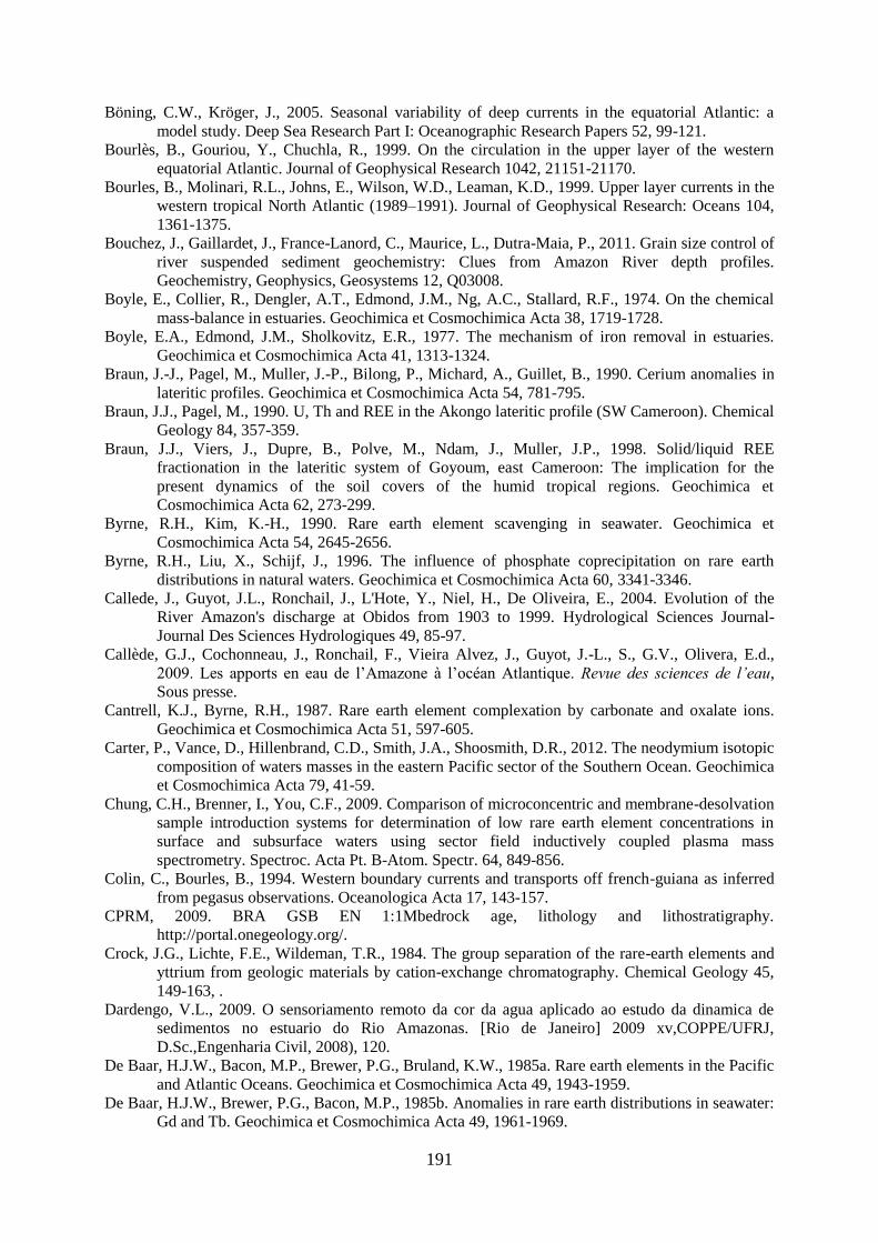
191
Böning, C.W., Kröger, J., 2005. Seasonal variability of deep currents in the equatorial Atlantic: a
model study. Deep Sea Research Part I: Oceanographic Research Papers 52, 99-121.
Bourlès, B., Gouriou, Y., Chuchla, R., 1999. On the circulation in the upper layer of the western
equatorial Atlantic. Journal of Geophysical Research 1042, 21151-21170.
Bourles, B., Molinari, R.L., Johns, E., Wilson, W.D., Leaman, K.D., 1999. Upper layer currents in the
western tropical North Atlantic (1989–1991). Journal of Geophysical Research: Oceans 104,
1361-1375.
Bouchez, J., Gaillardet, J., France-Lanord, C., Maurice, L., Dutra-Maia, P., 2011. Grain size control of
river suspended sediment geochemistry: Clues from Amazon River depth profiles.
Geochemistry, Geophysics, Geosystems 12, Q03008.
Boyle, E., Collier, R., Dengler, A.T., Edmond, J.M., Ng, A.C., Stallard, R.F., 1974. On the chemical
mass-balance in estuaries. Geochimica et Cosmochimica Acta 38, 1719-1728.
Boyle, E.A., Edmond, J.M., Sholkovitz, E.R., 1977. The mechanism of iron removal in estuaries.
Geochimica et Cosmochimica Acta 41, 1313-1324.
Braun, J.-J., Pagel, M., Muller, J.-P., Bilong, P., Michard, A., Guillet, B., 1990. Cerium anomalies in
lateritic profiles. Geochimica et Cosmochimica Acta 54, 781-795.
Braun, J.J., Pagel, M., 1990. U, Th and REE in the Akongo lateritic profile (SW Cameroon). Chemical
Geology 84, 357-359.
Braun, J.J., Viers, J., Dupre, B., Polve, M., Ndam, J., Muller, J.P., 1998. Solid/liquid REE
fractionation in the lateritic system of Goyoum, east Cameroon: The implication for the
present dynamics of the soil covers of the humid tropical regions. Geochimica et
Cosmochimica Acta 62, 273-299.
Byrne, R.H., Kim, K.-H., 1990. Rare earth element scavenging in seawater. Geochimica et
Cosmochimica Acta 54, 2645-2656.
Byrne, R.H., Liu, X., Schijf, J., 1996. The influence of phosphate coprecipitation on rare earth
distributions in natural waters. Geochimica et Cosmochimica Acta 60, 3341-3346.
Callede, J., Guyot, J.L., Ronchail, J., L'Hote, Y., Niel, H., De Oliveira, E., 2004. Evolution of the
River Amazon's discharge at Obidos from 1903 to 1999. Hydrological Sciences Journal-
Journal Des Sciences Hydrologiques 49, 85-97.
Callède, G.J., Cochonneau, J., Ronchail, F., Vieira Alvez, J., Guyot, J.-L., S., G.V., Olivera, E.d.,
2009. Les apports en eau de l’Amazone à l’océan Atlantique. Revue des sciences de l’eau,
Sous presse.
Cantrell, K.J., Byrne, R.H., 1987. Rare earth element complexation by carbonate and oxalate ions.
Geochimica et Cosmochimica Acta 51, 597-605.
Carter, P., Vance, D., Hillenbrand, C.D., Smith, J.A., Shoosmith, D.R., 2012. The neodymium isotopic
composition of waters masses in the eastern Pacific sector of the Southern Ocean. Geochimica
et Cosmochimica Acta 79, 41-59.
Chung, C.H., Brenner, I., You, C.F., 2009. Comparison of microconcentric and membrane-desolvation
sample introduction systems for determination of low rare earth element concentrations in
surface and subsurface waters using sector field inductively coupled plasma mass
spectrometry. Spectroc. Acta Pt. B-Atom. Spectr. 64, 849-856.
Colin, C., Bourles, B., 1994. Western boundary currents and transports off french-guiana as inferred
from pegasus observations. Oceanologica Acta 17, 143-157.
CPRM, 2009. BRA GSB EN 1:1Mbedrock age, lithology and lithostratigraphy.
http://portal.onegeology.org/.
Crock, J.G., Lichte, F.E., Wildeman, T.R., 1984. The group separation of the rare-earth elements and
yttrium from geologic materials by cation-exchange chromatography. Chemical Geology 45,
149-163, .
Dardengo, V.L., 2009. O sensoriamento remoto da cor da agua aplicado ao estudo da dinamica de
sedimentos no estuario do Rio Amazonas. [Rio de Janeiro] 2009 xv,COPPE/UFRJ,
D.Sc.,Engenharia Civil, 2008), 120.
De Baar, H.J.W., Bacon, M.P., Brewer, P.G., Bruland, K.W., 1985a. Rare earth elements in the Pacific
and Atlantic Oceans. Geochimica et Cosmochimica Acta 49, 1943-1959.
De Baar, H.J.W., Brewer, P.G., Bacon, M.P., 1985b. Anomalies in rare earth distributions in seawater:
Gd and Tb. Geochimica et Cosmochimica Acta 49, 1961-1969.
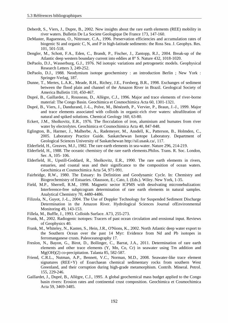
5.3 Références bibliographiques
192
Deberdt, S., Viers, J., Dupre, B., 2002. New insights about the rare earth elements (REE) mobility in
river waters. Bulletin De La Societe Geologique De France 173, 147-160.
DeMaster, Ragueneau, O., Nittrouer, C.A., 1996. Preservation efficiencies and accumulation rates of
biogenic Si and organic C, N, and P in high-latitude sediments: the Ross Sea. J. Geophys. Res.
101, 501-518.
Dengler, M., Schott, F.A., Eden, C., Brandt, P., Fischer, J., Zantopp, R.J., 2004. Break-up of the
Atlantic deep western boundary current into eddies at 8° S. Nature 432, 1018-1020.
DePaolo, D.J., Wasserburg, G.J., 1976. Nd isotopic variations and petrogenetic models. Geophysical
Research Letters 3, 249-252.
DePaolo, D.J., 1988. Neodymium isotope geochemistry : an introduction Berlin ; New York :
Springer-Verlag, 187.
Dunne, T., Mertes, L.A.K., Meade, R.H., Richey, J.E., Forsberg, B.R., 1998. Exchanges of sediment
between the flood plain and channel of the Amazon River in Brazil. Geological Society of
America Bulletin 110, 450-467.
Dupré, B., Gaillardet, J., Rousseau, D., Allègre, C.J., 1996. Major and trace elements of river-borne
material: The Congo Basin. Geochimica et Cosmochimica Acta 60, 1301-1321.
Dupré, B., Viers, J., Dandurand, J.-L., Polve, M., Bénézeth, P., Vervier, P., Braun, J.-J., 1999. Major
and trace elements associated with colloids in organic-rich river waters: ultrafiltration of
natural and spiked solutions. Chemical Geology 160, 63-80.
Eckert, J.M., Sholkovitz, E.R., 1976. The flocculation of iron, aluminium and humates from river
water by electrolytes. Geochimica et Cosmochimica Acta 40, 847-848.
Eglington, B., Harmer, J., Malherbe, A., Rademeyer, M., Ansdell, K., Patterson, B., Holmden, C.,
2005. Laboratory Practice Guide. Saskatchewan Isotope Laboratory. Department of
Geological Sciences University of Saskatchewan http://sil.usask.ca/, 117.
Elderfield, H., Greaves, M.J., 1982. The rare earth elements in sea-water. Nature 296, 214-219.
Elderfield, H., 1988. The oceanic chemistry of the rare earth elements.Philos. Trans. R. Soc. London,
Ser. A, 105- 106.
Elderfield, H., Upstill-Goddard, R., Sholkovitz, E.R., 1990. The rare earth elements in rivers,
estuaries, and coastal seas and their significance to the composition of ocean waters.
Geochimica et Cosmochimica Acta 54, 971-991.
Fairbridge, R.W., 1980. The Estuary: Its Definition and Geodynamic Cycle. In: Chemistry and
Biogeochemistry of Estuaries. Olausson, E.; Cato, I. (Eds.). Wiley. New York, 1-35.
Field, M.P., Sherrell, R.M., 1998. Magnetic sector ICPMS with desolvating micronebulization:
Interference-free subpicogram determination of rare earth elements in natural samples.
Analytical Chemistry 70, 4480-4486.
Filizola, N., Guyot, J.-L., 2004. The Use of Doppler Technology for Suspended Sediment Discharge
Determination in the Amazon River. Hydrological Sciences Journal ofEnvironmental
Monitoring 49, 143-153.
Fillela, M., Buffle, J., 1993. Colloids Surface. A73, 255-273.
Frank, M., 2002. Radiogenic isotopes: Tracers of past ocean circulation and erosional input. Reviews
of Geophysics 40.
Frank, M., Whiteley, N., Kasten, S., Hein, J.R., O'Nions, K., 2002. North Atlantic deep water export to
the Southern Ocean over the past 14 Myr: Evidence from Nd and Pb isotopes in
ferromanganese crusts. Paleoceanography 17.
Freslon, N., Bayon, G., Birot, D., Bollinger, C., Barrat, J.A., 2011. Determination of rare earth
elements and other trace elements (Y, Mn, Co, Cr) in seawater using Tm addition and
Mg(OH)(2) co-precipitation. Talanta 85, 582-587.
Friend, C.R.L., Nutman, A.P., Bennett, V.C., Norman, M.D., 2008. Seawater-like trace element
signatures (REE+Y) of Eoarchaean chemical sedimentary rocks from southern West
Greenland, and their corruption during high-grade metamorphism. Contrib. Mineral. Petrol.
155, 229-246.
Gaillardet, J., Dupré, B., Allègre, C.J., 1995. A global geochemical mass budget applied to the Congo
basin rivers: Erosion rates and continental crust composition. Geochimica et Cosmochimica
Acta 59, 3469-3485.
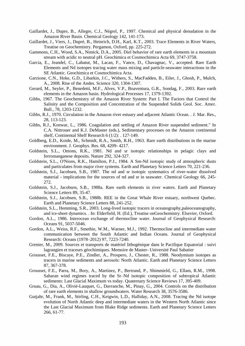
193
Gaillardet, J., Dupre, B., Allegre, C.J., Négrel, P., 1997. Chemical and physical denudation in the
Amazon River Basin. Chemical Geology 142, 141-173.
Gaillardet, J., Viers, J., Dupré, B., Heinrich, D.H., Karl, K.T., 2003. Trace Elements in River Waters,
Treatise on Geochemistry. Pergamon, Oxford, pp. 225-272.
Gammons, C.H., Wood, S.A., Nimick, D.A., 2005. Diel behavior of rare earth elements in a mountain
stream with acidic to neutral pH. Geochimica et Cosmochimica Acta 69, 3747-3758.
Garcia, E., Jeandel, C., Labatut, M., Lacan, F., Vance, D., Chavagnac, V., accepted. Rare Earth
Elements and Nd isotopes tracing water mass mixing and particle-seawater interactions in the
SE Atlantic. Geochimica et Cosmochimica Acta.
Garzione, C.N., Hoke, G.D., Libarkin, J.C., Withers, S., MacFadden, B., Eiler, J., Ghosh, P., Mulch,
A., 2008. Rise of the Andes. Science 320, 1304-1307.
Gerard, M., Seyler, P., Benedetti, M.F., Alves, V.P., Boaventura, G.R., Sondag, F., 2003. Rare earth
elements in the Amazon basin. Hydrological Processes 17, 1379-1392.
Gibbs, 1967. The Geochemistry of the Amazon River System: Part I. The Factors that Control the
Salinity and the Composition and Concentration of the Suspended Solids Geol. Soc. Amer.
Bull., 78, 1203-1232.
Gibbs, R.J., 1970. Circulation in the Amazon river estuary and adjacent Atlantic Ocean. . J. Mar. Res.,
28, 113-123.
Gibbs, R.J., Konwar, L., 1986. Coagulation and settling of Amazon River suspended sediment." In
C.A. Nittrouer and K.J. DeMaster (eds.), Sedimentary processes on the Amazon continental
shelf, Continental Shelf Research 6 (1/2): . 127-149.
Goldberg, E.D., Koide, M., Schmidt, R.A., Smith, R.H., 1963. Rare earth distributions in the marine
environment. J. Geophys. Res. 68, 4209- 4217.
Goldstein, S.L., Onions, R.K., 1981. Nd and sr isotopic relationships in pelagic clays and
ferromanganese deposits. Nature 292, 324-327.
Goldstein, S.L., O'Nions, R.K., Hamilton, P.J., 1984. A Sm-Nd isotopic study of atmospheric dusts
and particulates from major river systems. Earth and Planetary Science Letters 70, 221-236.
Goldstein, S.J., Jacobsen, S.B., 1987. The nd and sr isotopic systematics of river-water dissolved
material - implications for the sources of nd and sr in seawater. Chemical Geology 66, 245-
272.
Goldstein, S.J., Jacobsen, S.B., 1988a. Rare earth elements in river waters. Earth and Planetary
Science Letters 89, 35-47.
Goldstein, S.J., Jacobsen, S.B., 1988b. REE in the Great Whale River estuary, northwest Quebec.
Earth and Planetary Science Letters 88, 241-252.
Goldstein, S.L., Hemming, S.R., 2003. Long-lived isotopic tracers in oceanography,paleoceanography,
and ice-sheet dynamics. . In: Elderfield, H. (Ed.), Treatise onGeochemistry. Elsevier, Oxford.
Gordon, A.L., 1986. Interocean exchange of thermocline water. Journal of Geophysical Research:
Oceans 91, 5037-5046.
Gordon, A.L., Weiss, R.F., Smethie, W.M., Warner, M.J., 1992. Thermocline and intermediate water
communication between the South Atlantic and Indian Oceans. Journal of Geophysical
Research: Oceans (1978–2012) 97, 7223-7240.
Grenier, M., 2009. Sources et transports de matériel lithogénique dans le Pacifique Equatorial : suivi
lagrangien et traceurs géochimiques. Memoire de Master- Université Paul Sabatier
Grousset, F.E., Biscaye, P.E., Zindler, A., Prospero, J., Chester, R., 1988. Neodymium isotopes as
tracers in marine sediments and aerosols: North Atlantic. Earth and Planetary Science Letters
87, 367-378.
Grousset, F.E., Parra, M., Bory, A., Martinez, P., Bertrand, P., Shimmield, G., Ellam, R.M., 1998.
Saharan wind regimes traced by the Sr–Nd isotopic composition of subtropical Atlantic
sediments: Last Glacial Maximum vs today. Quaternary Science Reviews 17, 395-409.
Gruau, G., Dia, A., Olivié-Lauquet, G., Davranche, M., Pinay, G., 2004. Controls on the distribution
of rare earth elements in shallow groundwaters. Water Research 38, 3576-3586.
Gutjahr, M., Frank, M., Stirling, C.H., Keigwin, L.D., Halliday, A.N., 2008. Tracing the Nd isotope
evolution of North Atlantic deep and intermediate waters in the Western North Atlantic since
the Last Glacial Maximum from Blake Ridge sediments. Earth and Planetary Science Letters
266, 61-77.
5.3 Références bibliographiques
194
Guyot, J.-L., Callede, J., Molinier, M., Guimarães, V., Oliveira, E., 1998. La Variabilité Hydrologique
Actuelle Dans Le Bassin De L'amazone. Bull. Inst. Fr. études andines 27, 779-788.
Hannigan, R.E., Sholkovitz, E.R., 2001. The development of middle rare earth element enrichments in
freshwaters: weathering of phosphate minerals. Chemical Geology 175, 495-508.
Hanson, G.N., 1980. Rare earth elements in petrogenetic studies of igneous systems. Annual Review
in Earth and Planetary Sciences 8, 371-406.
Hayes, M.O., 1975. Morphology and sand accumulation in estuaries. In Estuarine Research, Vol.2,
Geology and Engineering.. 3-22.
Heimburger, A., Tharaud, M., Monna, F., Losno, R., Desboeufs, K., Nguyen, E.B., 2012. SLRS-5
elemental concentrations of thirty-three uncertified elements deduced from SLRS-5/SLRS-4
ratios. Geostandards Newsletter-the Journal of Geostandards and Geoanalysis??, ??
Hellweger, A.F., Gordon, A.L., 2002. Tracing Amazon River water into the Caribbean Sea. Journal of
Marine Research 60, 537-549.
Henderson , P., 1984. Rare earth element geochemistry. Amsterdam ; New York , Elsevier, 510.
Homoky, W.B., John, S.G., Conway, T.M., Mills, R.A., 2013. Distinct iron isotopic signatures and
supply from marine sediment dissolution. Nat Commun 4.
Hooker, P.J., O'Nions, R.K., Pankhurst, R.J., 1975. Determination of rare earth elements in U.S.G.S.
standard rocks by mixed solvent ion exchange and mass-spectrometric isotope dilution.
Chemical Geology 16 189-196.
Hoyle, J., Elderfield, H., Gledhill, A., Greaves, M., 1984. The behaviour of the rare earth elements
during mixing of river and sea waters. Geochimica et Cosmochimica Acta 48, 143-149.
Hu, C., Montgomery, E.T., Schmitt, R.W., Muller-Karger, F.E., 2004. The dispersal of the Amazon
and Orinoco River water in the tropical Atlantic and Caribbean Sea: Observation from space
and S-PALACE floats. Deep Sea Research Part II: Topical Studies in Oceanography 51, 1151-
1171.
Ingri, J., Widerlund, A., Land, M., Gustafsson, O., Andersson, P., Ohlander, B., 2000. Temporal
variations in the fractionation of the rare earth elements in a boreal river; the role of colloidal
particles. Chemical Geology 166, 23-45.
Jahn, B.-M., Auvray, B., Blais, S., Capdevila, R., Cornichet, J., Vidal, F., and Hameurt, J., 1980. .
Trace element geochemistry and petrogenesis of Finnish greenstone belts. Journal of
Petrology, 201-244.
Jeandel, C., 1993. Concentration and isotopic composition of Nd in the South Atlantic Ocean. Earth
and Planetary Science Letters 117, 581-591.
Jeandel, C., Bishop, J.K., Zindler, A., 1995. Exchange of neodymium and its isotopes between
seawater and small and large particles in the Sargasso Sea. Geochimica et Cosmochimica Acta
59, 535-547.
Jeandel, C., Arsouze, T., Lacan, F., Téchiné, P., Dutay, J.C., 2007. Isotopic Nd compositions and
concentrations of the lithogenic inputs into the ocean: A compilation, with an emphasis on the
margins. Chemical Geology 239, 156-164.
Jeandel, C., Peucker-Ehrenbrink, B., Jones, M.T., Pearce, C.R., Oelkers, E.H., Godderis, Y., Lacan, F.,
Aumont, O., Arsouze, T., 2011. Ocean margins: The missing term in oceanic element
budgets?
Jo, Y.-H., Yan, X.-H., Dzwonkowski, B., Liu, W.T., 2005. A study of the freshwater discharge from
the Amazon River into the tropical Atlantic using multi-sensor data. Geophysical Research
Letters 32, L02605.
Johannesson, K.H., Stetzenbach, K.J., Hodge, V.F., Berry Lyons, W., 1996. Rare earth element
complexation behavior in circumneutral pH groundwaters: Assessing the role of carbonate and
phosphate ions. Earth and Planetary Science Letters 139, 305-319.
Johannesson, K.H., Stetzenbach, K.J., Hodge, V.F., 1997. Rare earth elements as geochemical tracers
of regional groundwater mixing. Geochimica et Cosmochimica Acta 61, 3605-3618.
Johannesson, K.H., Farnham, I.M., Guo, C.X., Stetzenbach, K.J., 1999. Rare earth element
fractionation and concentration variations along a groundwater flow path within a shallow,
basin-fill aquifer, southern Nevada, USA. Geochimica et Cosmochimica Acta 63, 2697-2708.
195
Johannesson, K.H., Tang, J., Daniels, J.M., Bounds, W.J., Burdige, D.J., 2004. Rare earth element
concentrations and speciation in organic-rich blackwaters of the Great Dismal Swamp,
Virginia, USA. Chemical Geology 209, 271-294.
Johannesson, K.H., Burdige, D.J., 2007. Balancing the global oceanic neodymium budget: Evaluating
the role of groundwater. Earth and Planetary Science Letters 253, 129-142.
Johannesson, K.H., Tang, J., 2007. Comment on "Effects of organic ligands on fractionation of rare
earth elements (REEs) in hydroponic plants: An application to the determination of binding
capacities by humic acid for modelling" by Ding et al. [Chemosphere 65 (2006) 1942-1948].
Chemosphere 68, 1392-1393.
Jones, M.T., Pearce, C.R., Jeandel, C., Gislason, S.R., Eiriksdottir, E.S., Mavromatis, V., Oelkers,
E.H., 2012a. Riverine particulate material dissolution as a significant flux of strontium to the
oceans. Earth and Planetary Science Letters 355–356, 51-59.
Jones, M.T., Pearce, C.R., Oelkers, E.H., 2012b. An experimental study of the interaction of basaltic
riverine particulate material and seawater. Geochimica et Cosmochimica Acta 77, 108-120.
Junk, W., Sioli, H., 1984. The Amazon: Limnology and Landscape Ecology of a Mighty Tropical
River and its Basin 264.
Junk, W.J., 1997. The Central Amazon Floodplain: ecology of a pulsing system. Ecological Studies,
Springer, Amsterdam. 126, 525.
Kjerfve, B., 1989. Estuarine Characteristics, Circulation and Physical Processes. In: Estuarine
Ecology. Day Jr., J. W. (Eds.). John Wiley and Sons, New York, 47-78.
Konhauser, K.O., Fyfe, W.S., Kronberg, B.I., 1994. Multi-element chemistry of some Amazonian
waters and soils. Chemical Geology 111, 155-175.
Kosuth, P., Callède, J., Laraque, A., Filiozola, N., Guyot, J.-L., Seyler, P., 1999. Sea tide effects on
downstream Amazon river flow. . Symposium Manaus 99, novembre 1999.
Kosuth, P., Callede, J., Laraque, A., Filizola, N., Guyot, J.L., Seyler, P., Fritsch, J.M., Guimaraes, V.,
2009. Sea-tide effects on flows in the lower reaches of the Amazon River. Hydrological
Processes 23, 3141-3150.
Kulaksiz, S., Bau, M., 2011a. Anthropogenic gadolinium as a microcontaminant in tap water used as
drinking water in urban areas and megacities. Applied Geochemistry 26, 1877-1885.
Kulaksiz, S., Bau, M., 2011b. Rare earth elements in the Rhine River, Germany: First case of
anthropogenic lanthanum as a dissolved microcontaminant in the hydrosphere. Environment
International 37, 973-979.
Lacan, F., Jeandel, C., 2001. Tracing Papua New Guinea imprint on the central Equatorial Pacific
Ocean using neodymium isotopic compositions and Rare Earth Element patterns. Earth and
Planetary Science Letters 186, 497-512.
Lacan, F., Jeandel, C., 2004a. Denmark Strait water circulation traced by heterogeneity in neodymium
isotopic compositions. Deep Sea Research Part I: Oceanographic Research Papers 51, 71-82.
Lacan, F., Jeandel, C., 2004b. Neodymium isotopic composition and rare earth element concentrations
in the deep and intermediate Nordic Seas: Constraints on the Iceland Scotland Overflow Water
signature. Geochemistry Geophysics Geosystems 5.
Lacan, F., Jeandel, C., 2004c. Subpolar Mode Water formation traced by neodymium isotopic
composition. Geochemistry Geophysics Geosystems.
Lacan, F., Jeandel, C., 2005. Neodymium isotopes as a new tool for quantifying exchange fluxes at the
continent-ocean interface. Earth and Planetary Science Letters 232, 245-257.
Lacan, F., Tachikawa, K., Jeandel, C., 2012. Neodymium isotopic composition of the oceans: A
compilation of seawater data. Chemical Geology 300–301, 177-184.
Lawrence, M.G., Kamber, B.S., 2006. The behaviour of the rare earth elements during estuarine
mixing--revisited. Marine Chemistry 100, 147-161.
Lawrence, M.G., Greig, A., Collerson, K.D., Kamber, B.S., 2006. Direct quantification of rare earth
element concentrations in natural waters by ICP-MS. Applied Geochemistry 21, 839-848.
Lawrence, M.G., Kamber, B.S., 2007. Rare Earth Element Concentrations in the Natural Water
Reference Materials (NRCC) NASS-5, CASS-4 and SLEW-3. Geostandards and
Geoanalytical Research 31, 95-103.
5.3 Références bibliographiques
196
Le Bars, Y., Lyard, F., Jeandel, C., Dardengo, L., 2010. The AMANDES tidal model for the Amazon
estuary and shelf. Ocean Modelling 31, 132-149.
Lee, J.H., Byrne, R.H., 1992. Examination of comparative rare earth element complexation behavior
using linear free-energy relationships. Geochimica et Cosmochimica Acta 56, 1127-1137.
Lee, J.H., Byrne, R.H., 1993. Complexation of trivalent rare earth elements (Ce, Eu, Gd, Tb, Yb) by
carbonate ions. Geochimica et Cosmochimica Acta 57, 295-302.
Lev, S.M., McLennan, S.M., Hanson, G.N., 1999. Mineralogic controls on REE mobility during
black-shale diagenesis. Journal of Sedimentary Research 69, 1071-1082.
Libes, S.M., 1992. An introduction to marine biogeochemistry. Wiley. New York. US., 733.
Livingstone, D.A., 1963. The sodium cycle and the age of the ocean. Geochimica et Cosmochimica
Acta 27, 1055-1069.
Luo, Y.R., Byrne, R.H., 2001. Yttrium and rare earth element complexation by chloride ions at 25
degrees C. Journal of Solution Chemistry 30, 837-845.
Martin, G.C., 1964. Conditions for the separation of rare earth radioisotopes from salts of adjacent rare
earth by ion-exchange. Journal of Inorganic & Nuclear Chemistry 26, 1621-1623.
Martin, J.-M., Hogdahl, O.T., Philippot, J.C., 1976. Rare earth element supply to the ocean. . J.
Geophys. Res. 81, 3119-3124.
Martinez, J.M., Le Toan, T., 2007. Mapping of flood dynamics and spatial distribution of vegetation in
the Amazon floodplain using multitemporal SAR data. /Remote Sensing of Environment.108,
209-223, .
Masuda, A., Ikeuchi, Y., 1979. Lanthanide tetrad effect observed in marine-environment. Geochemical
Journal 13, 19-22.
Masuda, A., Kawakami, O., Dohmoto, Y., Takenaka, T., 1987. Lanthanide tetrad effects in nature - 2
mutually opposite types, W and M. Geochemical Journal 21, 119-124.
Mayer, D.A., Weisberg, R.H., 1993. A Description of COADS Surface Meteorological Fields and the
Implied Sverdrup Transports for the Atlantic Ocean from 30°S to 60°N. Journal of Physical
Oceanography 23, 2201-2221.
McDaniel, D.K., McLennan, S.M., Hanson, G.N., 1997. Provenance of Amazon fan muds: constraints
from Nd and Pb isotopes. In: Flood,R.D., Piper, D.J.W., Klaus, A., Peterson, L.C. (Eds.),
Proceedings of the Ocean Drilling Program, Scientific Results, pp. 169–176.
McKee, B.A., DeMaster, D.J., Nittrouer, C.A., 1987. Uranium geochemistry on the Amazon shelf:
Evidence for uranium release from bottom sediments. Geochimica et Cosmochimica Acta 51,
2779-2786.
McLennan, S., 1989. Rare earth elements in sedimentary rocks; influence of provenance and
sedimentary processes. . Reviews in Mineral Geochemistry, :169-200.
McLennan, S.M., 1994. Rare-eart element geochemistry and the tetrad effect. Geochimica et
Cosmochimica Acta 58, 2025-2033.
Meade, R.H., Dunne, T., Richey, J.E., Santos, U.D., Salati, E., 1985. Storage and remobilization of
suspended sediment in the lower amazon river of brazil. Science 228, 488-490.
Meade, R.H., 1994. Suspended sediments of the modern Amazon and Orinoco rivers. Quaternary
International 21, 29-39.
Mertes, L.A.K., Dunne, T., Martinelli, L.A., 1996. Channel-floodplain geomorphology along the
Solimoes-Amazon River, Brazil. Geological Society of America Bulletin 108, 1089-1107.
Millero, F.J., 1985. The effect of ionic interactions on the oxidation of metals in natural waters.
Geochimica et Cosmochimica Acta 49, 547-553.
Millero, F.J., 1992. Stability constants for the formation of rare earth-inorganic complexes as a
function of ionic strength. Geochimica et Cosmochimica Acta 56, 3123-3132.
Milliman, J.D., Meade, R.H., 1983. World-wide delivery of river sediment to the oceans. Journal of
Geology 91, 1-21.
Milliman, J.D., Shen, H.T., Yang, Z.S., Meade, R.H., 1985. Transport and deposition of river
dediment in the changjiang estuary and adjacent continental-shelf. Continental Shelf Research
4, 37-45.
Milliman, J.D., Syvitski, J.P.M., 1992. Geomorphic Tectonic Control of sediment disccahrge to the
ocean - The importance of small mountainous rivers. Journal of Geology 100, 525-544.
197
Molinier, M., Guyot, J.-L., Guimarães, V.E., Oliveira, E., Filizola, N., 1997. Hydrologie Du Bassin
Amazonien. Environnement Et Développement En Amazonie Brésilienne. H. Théry. Paris,
Belin, 400
Molleri, G.S.F., Novo, E.M.L.d.M., Kampel, M., 2010. Space-time variability of the Amazon River
plume based on satellite ocean color. Continental Shelf Research 30, 342-352.
Morley, R.J., 2000. Origin and Evolution of Tropical Rain Forests. Wiley. New York. US.
Nikiema, O., Devenon, J.-L., Baklouti, M., 2007. Numerical modelling of the Amazon River plume.
Continental Shelf Research 27 873-899.
Nozaki, Y., Lerche, D., Alibo, D.S., Snidvongs, A., 2000. The estuarine geochemistry of rare earth
elements and indium in the Chao Phraya River, Thailand. Geochimica et Cosmochimica Acta
64, 3983-3994.
Nozaki, K., Alibo, D.S., 2003. Dissolved rare earth elements in the Southern Ocean, southwest of
Australia: Unique patterns compared to the South Atlantic data. Geochemical Journal, 47-62.
O’Connor, B.M., Fine, R.A., Maillet, K.A., Olson, D.B., 2002. Formation rates of subtropical
underwater in the Pacific Ocean. Deep Sea Research Part I: Oceanographic Research Papers
49, 1571-1590.
Oudot, C., Morin, P., Baurand, F., Wafar, M., Corre, P.L., 1998. Northern and southern water masses
in the equatorial Atlantic: distribution of nutrients on the WOCE A6 and A7 lines. Deep Sea
Research Part I: Oceanographic Research Papers 45, 873-902.
Pahnke, K., van de Flierdt, T., Jones, K.M., Lambelet, M., Hemming, S.R., Goldstein, S.L., 2012.
GEOTRACES intercalibration of neodymium isotopes and rare earth element concentrations
in seawater and suspended particles. Part 2: Systematic tests and baseline profiles. Limnol.
Oceanogr. Meth. 10, 252-269.
Pearce, C.R., Jones, M.T., Oelkers, E.H., Pradoux, C., Jeandel, C., 2013. The effect of particulate
dissolution on the neodymium (Nd) isotope and Rare Earth Element (REE) composition of
seawater. Earth and Planetary Science Letters.
Persson, P.O., Andersson, P.S., Zhang, J., Porcelli, D., 2011. Determination of Nd Isotopes in Water:
A Chemical Separation Technique for Extracting Nd from Seawater Using a Chelating Resin.
Analytical Chemistry 83, 1336-1341.
Piepgras, D.J., Wasserburg, G.J., Dasch, E.J., 1979. The isotopic composition of Nd in different ocean
masses. Earth and Planetary Science Letters 45, 223-236.
Piepgras, D.J., Wasserburg, G.J., 1980. Neodymium isotopic variations in seawater. Earth and
Planetary Science Letters 50, 128-138.
Piepgras, D.J., Wasserburg, G.J., 1982. Isotopic composition of neodymium in waters from the drake
passage. Science 217, 207-214.
Piepgras, D.J., Wasserburg, G.J., 1987. Rare earth element transport in the western North Atlantic
inferred from Nd isotopic observations. Geochimica et Cosmochimica Acta 51, 1257-1271.
Piepgras, D.J., Jacobsen, S.B., 1992. The behavior of rare earth elements in seawater: Precise
determination of variations in the North Pacific water column. Geochimica et Cosmochimica
Acta 56, 1851-1862.
Pin C., Briot D., C., B., F., P., 1994. Concomitant separation of strontium and samarium-neodynium
for isotopic analysis in silicate samples, based on specific extraction chromatography. Acta,
298,. Analytica Chimica Acta 298, , 209–217.
Pin, C., Zalduegui, J.S., 1997. Sequential separation of light rare-earth elements, thorium and uranium
by miniaturized extraction chromatography: Application to isotopic analyses of silicate
Piotrowski, A.M., Goldstein, S.L., Hemming, S.R., Fairbanks, R.G., 2004. Intensification and
variability of ocean thermohaline circulation through the last deglaciation. Earth and Planetary
Science Letters 225, 205-220.
Pokrovsky, O.S., Schott, J., 2002. Iron colloids/organic matter associated transport of major and trace
elements in small boreal rivers and their estuaries (NW Russia). Chemical Geology 190, 141-
179.
Piotrowski, A.M., Goldstein, S.L., Hemming, S.R., Fairbanks, R.G., 2005. Temporal relationships of
carbon cycling and ocean circulation at glacial boundaries. Science 307, 1933-1938.
5.3 Références bibliographiques
198
Pourret, O., Davranche, M., Gruau, G., Dia, A., 2007a. Competition between humic acid and
carbonates for rare earth elements complexation. Journal of Colloid and Interface Science 305,
25-31.
Pourret, O., Davranche, M., Gruau, G., Dia, A., 2007b. Organic complexation of rare earth elements in
natural waters: Evaluating model calculations from ultrafiltration data. Geochimica et
Cosmochimica Acta 71, 2718-2735.
Pourret, O., Davranche, M., Gruau, G., Dia, A., 2007c. Rare earth elements complexation with humic
acid. Chemical Geology 243, 128-141.
Pourret, O., Davranche, M., Gruau, G., Dia, A., 2008. New insights into cerium anomalies in organic-
rich alkaline waters. Chemical Geology 251, 120-127.
Prichard, F.E., Crosby, N.T., Day, J.A., Hardcastle, W.A., Holcombe, D.G., Treble, R.D., 1995
Quality in the analytical chemistry laboratory., in: John Wiley and Sons Ed. (Ed.), Analytical
Chemistry by Open Learning., p. 307.
Pritchard, D.W., 1952. Estuarine hydrography. In: Advances in Geophysics, v.1, Academic Press,
New York, 243-288.
Rasmussen, B., Buick, R., Taylor, W.R., 1998. Removal of oceanic REE by authigenic precipitation of
phosphatic minerals. Earth and Planetary Science Letters 164, 135-149.
Révillon, S., Jouet, G., Bayon, G., Rabineau, M., Dennielou, B., Hémond, C., Berné, S., 2011. The
provenance of sediments in the Gulf of Lions, western Mediterranean Sea. Geochemistry,
Geophysics, Geosystems 12, Q08006.
Reynolds, T.D., Richards, P.A., 1996. Unit Operations and processes in Environmental Engineering, .
2nd, Boston, Massachusetts: PWS Publishing.
Richardson, P.L., Reverdin, G., 1987. Seasonal cycle of velocity in the Atlantic North Equatorial
Countercurrent as measured by surface drifters, current meters, and ship drifts. Journal of
Geophysical Research: Oceans (1978–2012) 92, 3691-3708.
Richey, J.E., Nobre, C., Deser, C., 1989. Amazon river discharge and climate variability - 1903 to
1985. Science 246, 101-103.
Rickli, J., Frank, M., Halliday, A.N., 2009. The hafnium-neodymium isotopic composition of Atlantic
seawater. Earth and Planetary Science Letters 280, 118-127.
Rickli, J., Frank, M., Baker, A.R., Aciego, S., de Souza, G., Georg, R.B., Halliday, A.N., 2011.
Hafnium and neodymium isotopes in surface waters of the eastern Atlantic Ocean:
Implications for sources and inputs of trace metals to the ocean. Geochimica et Cosmochimica
Acta 74, 540-557.
Roddaz, M., Viers, J., Brusset, S., Baby, P., Hérail, G., 2005. Sediment provenances and drainage
evolution of the Neogene Amazonian foreland basin. Earth and Planetary Science Letters 239,
57-78.
Roig H., L., Rego A, P., M, R, Dantas E, L., Meneses P, R., Walde, D., H, W, Goia M, L., C,, 2005.
Assinatura isotopica Sm-Nd de sedimentos em suspensão: implicações na caracterizaçõ da
proveniencia dos sedimentos do paraiba do sul. SP. Revista Brasileira de Geociencias 35, 503-
514.
Rousseau, T.C.C., Sonke, J.E., Chmeleff, J., Candaudap, F., Lacan, F., Boaventura, G., Seyler, P.,
Jeandel, C., 2013. Rare earth element analysis in natural waters by multiple isotope dilution -
sector field ICP-MS. Journal of Analytical Atomic Spectrometry 28, 573-584.
Rutberg, R.L., Hemming, S.R., Goldstein, S.L., 2000. Reduced North Atlantic Deep Water flux to the
glacial Southern Ocean inferred from neodymium isotope ratios. Nature 405, 935-938.
Santschi, P., Höhener, P., Benoit, G., Buchholtz-ten Brink, M., 1990. Chemical processes at the
sediment-water interface. Marine Chemistry 30, 269-315.
Santschi, P.H., Lenhart, J.J., Honeyman, B.D., 1997. Heterogeneous processes affecting trace
contaminant distribution in estuaries: The role of natural organic matter. Marine Chemistry 58,
99-125.
Schijf, J., De Baar, H.J.W., Millero, F.J., 1995. Vertical distributions and speciation of dissolved rare
earth elements in the anoxic brines of Bannock Basin, eastern Mediterranean Sea. Geochimica
et Cosmochimica Acta 59, 3285-3299.
Schmitz, W.J., McCartney, M.S., 1993. On the North Atlantic Circulation. Reviews of Geophysics 31,
29-49.
199
Schott, F.A., Dengler, M., Zantopp, R., Stramma, L., Fischer, J., Brandt, P., 2005. The Shallow and
Deep Western Boundary Circulation of the South Atlantic at 5°–11°S. Journal of Physical
Oceanography 35, 2031-2053.
Shabani, M.B., Akagi, T., Masuda, A., 1992. Preconcentration of trace rare-earth elements in seawater
by complexation with bis(2-ethylhexyl) hydrogen phosphate and 2-ethylhexyl dihydrogen
phosphate adsorbed on a c18 cartridge and determination by inductively coupled plasma mass-
spectrometry. Analytical Chemistry 64, 737-743.
Shiller, A.M., 2002. Seasonality of dissolved rare earth elements in the lower Mississippi River
Geochemistry Geophysics Geosystems 3.
Shimizu, H., Tachikawa, K., Masuda, A., Nozaki, Y., 1994. Cerium and neodymium isotope ratios and
REE patterns in seawater from the North Pacific Ocean. Geochimica et Cosmochimica Acta
58, 323-333.
Sholkovitz, E.R., 1976. Flocculation of dissolved organic and inorganic matter during the mixing of
river water and seawater. Geochimica et Cosmochimica Acta 40, 831-845.
Sholkovitz, E.R., 1993. The geochemistry of rare earth elements in the Amazon River estuary.
Geochimica et Cosmochimica Acta 57, 2181-2190.
Sholkovitz, E.R., Landing, W.M., Lewis, B.L., 1994. Ocean particle chemistry: The fractionation of
rare earth elements between suspended particles and seawater. Geochimica et Cosmochimica
Acta 58, 1567-1579.
Sholkovitz, E.R., 1995a. The aquatic chemistry of rare earth elements in rivers and estuaries. Aquatic
Geochemistry 1, 1-34.
Sholkovitz, E.R., 1995b. The Aquatic Geochemistry of Rare Earth Element in river and estuaries.
Aquatic Geochemistry, 1-34.
Sholkovitz, E., Szymczak, R., 2000. The estuarine chemistry of rare earth elements: comparison of the
Amazon, Fly, Sepik and the Gulf of Papua systems. Earth and Planetary Science Letters 179,
299-309.
Siddall, M., Khatiwala, S., van de Flierdt, T., Jones, K., Goldstein, S.L., Hemming, S., Anderson, R.F.,
2008. Towards explaining the Nd paradox using reversible scavenging in an ocean general
circulation model. Earth and Planetary Science Letters 274, 448-461.
Signorini, S.R., Murtugudde, R.G., McClain, C.R., Christian, J.R., Picaut, J., Busalacchi, A.J., 1999.
Biological and physical signatures in the tropical and subtropical Atlantic. Journal of
Geophysical Research-Oceans 104, 18367-18382.
Silva, A.C., Grenier, M., Chuchla, R., Grelet, J., Roubaud, F., Hamelin, B., Lyard, F., Jeandel, C., In
prep. Water Masses and Zonal Current in the Western Tropical Atlantic in October 2007 and
January 2008 (AMANDES project).
Sioli, H., 1967. Studies in Amazonian Waters. Bel‚m.
Smoak, J.M., Krest, J.M., Swarzenski, P.W., 2006. Geochemistry of the Amazon Estuary. Hdb Env
Chem 5, 71–90.
Sohrin, Y., Urushihara, S., Nakatsuka, S., Kono, T., Higo, E., Minami, T., Norisuye, K., Umetani, S.,
2008. Multielemental Determination of GEOTRACES Key Trace Metals in Seawater by
ICPMS after Preconcentration Using an Ethylenediaminetriacetic Acid Chelating Resin.
Analytical Chemistry, 6267-6273.
Sonke, J.E., Salters, V.J.M., 2004. Determination of neodymium–fulvic acid binding constants by
capillary electrophoresis inductively coupled plasma mass spectrometry (CE-ICP-MS).
Journal Of Analytical Spectrometry, 235-240.
Sonke, J.E., Salters, V.J.M., 2006. Lanthanide-humic substances complexation. I. Experimental
evidence for a lanthanide contraction effect. Geochimica et Cosmochimica Acta 70, 1495-
1506.
Stern, R.A., Hanson, G.N., 1991. Archean high-Mg granodiorite - a derivative of light rare-earth
element-enriched monzodiorite of mantle origin. Journal of Petrology 32, 201-238.
Stichel, T., Frank, M., Rickli, J., Haley, B.A., 2012a. The hafnium and neodymium isotope
composition of seawater in the Atlantic sector of the Southern Ocean. Earth and Planetary
Science Letters 317–318, 282-294.
5.3 Références bibliographiques
200
Stichel, T., Frank, M., Rickli, J., Hathorne, E.C., Haley, B.A., Jeandel, C., Pradoux, C., 2012b.
Sources and input mechanisms of hafnium and neodymium in surface waters of the Atlantic
sector of the Southern Ocean. Geochimica et Cosmochimica Acta 94, 22-37.
Stordal, M.C., Wasserburg, G.J., 1986. Neodymium isotopic study of Baffin Bay water: sources of
REE from very old terranes. Earth and Planetary Science Letters 77, 259-272.
Stramma, L., Schott, F., 1999. The mean flow field of the tropical Atlantic Ocean. Deep Sea Research
Part II: Topical Studies in Oceanography 46, 279-303.
Stum, W., Morgan, J.,, 1981. Aquatic chemistry. An introduction emphazing chemical equilibria in
natural waters. 2nd Edition. Wiley Intersciences.
Sullivan, K.A., Aller, R.C., 1996. Diagenetic cycling of arsenic in Amazon shelf sediments.
Geochimica et Cosmochimica Acta 60, 1465-1477.
Swarzenski, P.W., McKee, B.A., Booth, J.G., 1991. Uranium geochemistry on the Amazon shelf:
Seasonal differences in source functions and dissolved /colloidal partitioning of uranium
isotopes. Eos 72, 64.
Swarzenski, P.W., McKee, B.A., Booth, J.G., 1995. Uranium geochemistry on the Amazon shelf:
Chemical phase partitioning and cycling across a salinity gradient. Geochimica et
Cosmochimica Acta 59, 7-18.
Tachikawa, K., Athias, V., Jeandel, C., 2003. Neodymium budget in the modern ocean and paleo-
oceanographic implications. Journal of Geophysical Research-Oceans 108.
Tachikawa, K., Handel, C., Dupré, B., 1997. Distribution of rare earth elements and neodymium
isotopes in settling particulate material of the tropical Atlantic Ocean (EUMELI site). Deep
Sea Research Part I: Oceanographic Research Papers 44, 1769-1792.
Tachikawa, K., Jeandel, C., Vangriesheim, A., Dupré, B., 1999. Distribution of rare earth elements
and neodymium isotopes in suspended particles of the tropical Atlantic Ocean (EUMELI site).
Deep Sea Research Part I: Oceanographic Research Papers 46, 733-755.
Takata, H., Tagami, K., Aono, T., Uchlida, S., 2009. Determination of trace levels of Yttrium and
Arare Earth Elements in Estuarine and Coastal Waters by Inductively Coupled Mass
Spectrometry Following Preconcentration with NOBIAS-CHELATE Resin. Atomic
Apectroscopy 30, 10-19.
Tang, J., Johannesson, K.H., 2003. Speciation of rare earth elements in natural terrestrial waters:
assessing the role of dissolved organic matter from the modeling approach. Geochimica et
Cosmochimica Acta 67, 2321-2339.
Taylor, S.R., McLennan, S.M., 1985. The Continental Crust: Its Composition and Evolution.
Blackwell Scientific Publication, Carlton, , 312 p.
Thirlwall, M.F., 1982. A triple-filament method for rapid and precise analysis of rare-earth elements
by isotope dilution. Chemical Geology 35, 155-166.
Tipping, E., Hurley, M.A., 1992. A unifying model of cation binding by humic substances.
Geochimica et Cosmochimica Acta 56, 3627-3641.
Tipping, E., 1994. WHAMC--A chemical equilibrium model and computer code for waters,
sediments, and soils incorporating a discrete site/electrostatic model of ion-binding by humic
substances. Computers & Geosciences 20, 973-1023.
Tomczak, M., Godfrey, J.S., 2003. Regional Oceanography: an Introduction 2nd edn. edn (2003),
xi+390p., figs., tabls., ind., 25 cm.
Tréguer, P.J., De La Rocha, C.L., 2013. The World Ocean Silica Cycle. Annual Review of Marine
Science 5, 477-501.
Tsuchiya, M., 1989. Circulation of the Antarctic Intermediate Water in the North Atlantic Ocean.
Journal of Marine Research 47, 747-755.
Tsuchiya, M., Talley Lynne, D., McCartney Michael, S., 1994. Water-mass distributions in the
western South Atlantic; A section from South Georgia Island (54S) northward across the
equator. Journal of Marine Research 52, 55-81.
Turner, D.R., Whitfield, M., Dickson, A.G., 1981. The equilibrium speciation of dissolved
components in freshwater and sea water at 25°C and 1 atm pressure. Geochimica et
Cosmochimica Acta 45, 855-881.
201
van Beek, P., Souhaut, M., Reyss, J.L., 2010. Measuring the radium quartet (228Ra, 226Ra, 224Ra,
223Ra) in seawater samples using gamma spectrometry. Journal of Environmental
Radioactivity 101, 521-529.
van de Flierdt, T., Goldstein, S.L., Hemming, S.R., Roy, M., Frank, M., Halliday, A.N., 2007. Global
neodymium-hafnium isotope systematics -- revisited. Earth and Planetary Science Letters 259,
432-441.
Van de Flierdt, T., Pahnke, K., Amakawa, H., Andersson, P., Basak, C., Coles, B., Colin, C., Crocket,
K., Frank, M., Frank, N., Goldstein, S.L., Goswami, V., Haley, B.A., Hathorne, E.C.,
Hemming, S.R., Henderson, G.M., Jeandel, C., Jones, K., Kreissig, K., Lacan, F., Lambelet,
M., Martin, E.E., Newkirk, D.R., Obata, H., Pena, L., Piotrowski, A.M., Pradoux, C., Scher,
H.D., Schoberg, H., Singh, S.K., Stichel, T., Tazoe, H., Vance, D., Yang, J.J., Partici, G.I.,
2012. GEOTRACES intercalibration of neodymium isotopes and rare earth element
concentrations in seawater and suspended particles. Part 1: reproducibility of results for the
international intercomparison. Limnol. Oceanogr. Meth. 10, 234-251.
Van Der Loeff, M.R., Helmers, E., Kattner, G., 1997. Continuous transects of cadmium, copper, and
aluminium in surface waters of the Atlantic Ocean, 50°N to 50°S: correspondence and contrast
with nutrient-like behaviour. Geochimica et Cosmochimica Acta 61, 47-61.
Viers, J., Dupré, B., Polvé, M., Schott, J., Dandurand, J.-L., Braun, J.-J., 1997. Chemical weathering in
the drainage basin of a tropical watershed (Nsimi-Zoetele site, Cameroon) : comparison
between organic-poor and organic-rich waters. Chemical Geology 140, 181-206.
Viers, J., Wasserburg, G.J., 2004. Behavior of Sm and Nd in a lateritic soil profile. Geochimica et
Cosmochimica Acta 68, 2043-2054.
Viers, J., Barroux, G., Pinelli, M., Seyler, P., Oliva, P., Dupré, B., Boaventura, G.R., 2005. The
influence of the Amazonian floodplain ecosystems on the trace element dynamics of the
Amazon River mainstem (Brazil). Science of The Total Environment 339, 219-232.
Viers, J., Roddaz, M., Filizola, N., Guyot, J.L., Sondag, F., Brunet, P., Zouiten, C., Boucayrand, C.,
Martin, F., Boaventura, G.R., 2008. Seasonal and provenance controls on Nd-Sr isotopic
compositions of Amazon rivers suspended sediments and implications for Nd and Sr fluxes
exported to the Atlantic Ocean. Earth and Planetary Science Letters 274, 511-523.
von Blanckenburg, F., 1999. Perspectives: Paleoceanography - Tracing past ocean circulation? Science
286, 1862-1863.
Warne, A.G., Meade, R., White, A.W., Guevara, E.H., Gibeaut, J., Smyth, R.C., Aslan, A., Tremblay,
T., 2002. Regional controls on geomorphology, hydrology, and ecosystem integrity in the
Orinoco Delta, Venezuela. Geomorphology 44, 273-307.
Wells, M.L., Goldberg, E.D., 1994. The distribution of colloids in the North-Atlantic and Southern
Oceans. Limnology and Oceanography 39, 286-302.
Willbold, M., Jochum, K., Raczek, I., Amini, M., Stoll, B., Hofmann, A., 2003. Validation of multi-
element isotope dilution ICPMS for the analysis of basalts. Analytical and Bioanalytical
Chemistry 377, 117-125.
Willbold, M., Jochum, K.P., 2005. Multi-Element Isotope Dilution Sector Field ICP-MS: A Precise
Technique for the Analysis of Geological Materials and its Application to Geological
Reference Materials. Geostandards and Geoanalytical Research 29, 63-82.
Willie, S.N., Sturgeon, R.E., 2001. Determination of transition and rare earth elements in seawater by
flow injection inductively coupled plasma time-of-flight mass spectrometry. Spectroc. Acta Pt.
B-Atom. Spectr. 56, 1707-1716.
Wilson, W.D., Johns, E., Molinari, R.L., 1994. Upper layer circulation in the western tropical North
Atlantic Ocean during August 1989. Journal of Geophysical Research: Oceans (1978–2012)
99, 22513-22523.
Wood, S.A., 1990. The aqueous geochemistry of the rare-earth elements and yttrium: 1. Review of
available low-temperature data for inorganic complexes and the inorganic REE speciation of
natural waters. Chemical Geology 82, 159-186.
Wood, S.A., Gammons, C.H., Parker, S.R., 2006. The behavior of rare earth elements in naturally and
anthropogenically acidified waters. Journal of Alloys and Compounds 418, 161-165.
WWF, 2008. Amazon Rainforest, Amazon Plants, Amazon River Animals World Wide Fund for
Nature http://www.worldwildlife.org/wildplaces/amazon/index.cfm. Retrieved 2008-05-06. .
5.3 Références bibliographiques
202
Yeghicheyan, D., Carignan, J., Valladon, M., Le Coz, M.B., Le Cornec, F., Castrec-Rouelle, M.,
Robert, M., Aquilina, L., Aubry, E., Churlaud, C., Dia, A., Deberdt, S., Dupr, B., Freydier, R.,
Gruau, G., Henin, O., de Kersabiec, A.M., Mace, J., Marin, L., Morin, N., Petitjean, P., Serrat,
E., 2001. A compilation of silicon and thirty one trace elements measured in the natural river
water reference material SLRS-4 (NRC-CNRC). Geostandards Newsletter-the Journal of
Geostandards and Geoanalysis 25, 465-474.
Zhang, J., Nozaki, Y., 1996. Rare earth elements and yttrium in seawater: ICP-MS determinations in
the East Caroline, Coral Sea, and South Fiji basins of the western South Pacific Ocean.
Geochimica et Cosmochimica Acta 60, 4631-4644.
Zhang, Y., Lacan, F., Jeandel, C., 2008. Dissolved rare earth elements tracing lithogenic inputs over
the Kerguelen Plateau (Southern Ocean). Deep Sea Research Part II: Topical Studies in
Oceanography 55, 638-652.
Zhu, Y., Umemura, T., Haraguchi, H., Inagaki, K., Chiba, K., 2009. Determination of REEs in
seawater by ICP-MS after on-line preconcentration using a syringe-driven chelating column.
Talanta, 891-895.
203
ANNEXE :A compilation of Silicon, Rare Earth Element and Twenty-one
other trace element concentrations in the Natural River Water Standard
SLRS-5 (NRC-CNRC)
Delphine Yeghicheyan1, Cécile Bossy
2, Martine Bouhnik-Le Coz
3, Chantal Douchet
4,
Guy Granier5
, Alexie Heimburger6
, François Lacan7, Aurélie Lanzanova
8, TristanC.C.
Rousseau9, Jean-Luc Seidel
10, Mickaël Tharaud
11, Frédéric Cadaudap
8, Jerome
Chmeleff8, Christophe Cloquet
1, Sophie Delpoux
10, Marie Labatut
7 , Rémi Losno
6,
Catherine Pradoux5
, Yann Sivry9 andJeroen Sonke
8,9
Received Date: 17-Dec-2012/Accepted Date: 03-Apr-2013
DOI: 10.1111/j.1751-908X.2013.00232.x
(1) Service d’Analyse des Roches et des Minéraux (SARM), CNRS-CRPG, 15, rue Notre Dame des Pauvres, BP
20, 54501 Vandoeuvre-lès-Nancy, France
(2) Université de Bordeaux, EPOC UMR 5805, Avenue des facultés, 33405 Talence Cédex, France
(3) Géosciences Rennes, UMR 6118 CNRS – Université Rennes 1, Campus de Beaulieu, 35042 Rennes Cedex,
France
(4) Laboratoire Géosciences Montpellier, Laboratoire ICP-MS, Batiment 22cc060, Université Montpellier 2,
Place Eugène Bataillon, 34095 Montpellier Cédex 5, France
(5) CEA/MARCOULE, DEN/DRCP/CETAMA, B.P. 17171, 30207 Bagnols-sur-Cèze, France
(6) Laboratoire Inter-universitaire des Systèmes Atmosphériques, UMR 7583, CNRS-Université Paris Est-
Créteil-Université Paris Diderot, 61 av. Gal de Gaulle, F-94010 Créteil, France
(7) LEGOS (CNES/CNRS/IRD/University of Toulouse), Observatoire Midi-Pyrénées, 14 av. Edouard Belin,
31400 Toulouse, France
(8) Géosciences Environnement Toulouse, UMR 5563, Service ICP-MS Observatoire Midi-Pyrénées, CNRS,
Université Paul Sabatier, IRD, 14 av Edouard Belin, 31400 Toulouse, France
(9) Géosciences Environnement Toulouse, Observatoire Midi-Pyrénées, CNRS, Université Paul Sabatier,
IRD,14 av Edouard Belin, 31400 Toulouse, France
(10) Laboratoire HydroSciences Montpellier, UMR 5569, Université Montpellier 2, Case MSE, Place Eugène
Bataillon, 34095 Montpellier Cédex 5, France
(11) Laboratoire de Géochimie des Eaux, Université Paris Diderot, Sorbonne Paris Cité, Institut de Physique du
Globe de Paris, UMR 7154 CNRS, F-75205 Paris, France
* Corresponding author. e-mail: [email protected]
ANNEXE A compilation of Silicon, Rare Earth Element and Twenty-one other trace element
concentrations in the Natural River Water Standard SLRS-5 (NRC-CNRC)
204
Keywords : river water reference material, ICP-MS, rare earth elements, trace elements
The natural river water certified reference material SLRS-5 (NRC-CNRC) was routinely
analysed in this study for major and trace elements by ten French laboratories. Most of the
measurements were made using ICP-MS (inductively coupled plasma-mass spectrometry).
Because no certified values are assigned by NRC-CNRC for silicon and thirty-five trace
element concentrations (rare earth elements, Ag, B, Bi, Cs, Ga, Ge, Li, Nb, P, Rb, Rh, Re, S,
Sc, Sn, Th, Ti, Tl, W, Y and Zr), or for isotopic ratios, we provide a compilation of the
concentrations and related uncertainties obtained by the participating laboratories. Strontium
isotopic ratios are also given.
Mots-clés : standard d’eau de rivière, ICP-MS, terres rares, éléments en traces
Le matériel de référence certifiée d’eau de rivière naturelle SLRS-5 (NRC-CNRC) est analysé
régulièrement comme contrôle qualité par dix laboratoires français étudiant les éléments
majeurs et en trace dans les solutions naturelles. La plupart des mesures sont réalisées par
ICP-MS (inductively coupled plasma-mass spectrometry). Le silicium et 35 éléments en trace
(terres rares, Ag, B, Bi, Cs, Ga, Ge, Li, Nb, P, Rb, Rh, Re, S, Sc, Sn, Th, Ti, Tl, W, Y et Zr)
ne sont pas certifiés par NRC-CNRC. Aucun rapport isotopique n'est disponible. Nous
proposons, pour ces éléments, des valeurs moyennes et leurs incertitudes associées obtenues
par les différents laboratoires participants. Le rapport isotopique de Sr est aussi mesuré.
Mots-clés : matériau de référence d’eau de rivière, ICP-MS, terres rares, éléments en trace.
205
Natural river water reference materials are widely used in order to control routine
wateranalyses by geochemists and hydrogeologists (Tosiani et al. 2004, Lawrence et al.
2006,Birkeet al. 2010, Bayonet al. 2010). Among these reference materials, the Ottawa
riverwater SLRS, prepared by the National Research Council (NRC-CNRC Canada), has
beenused by ten French geoscience laboratories. This study is a follow-up to the SLRS-
4compilation performed by French laboratories within the framework of the CNRS
"Isotrace"network (Yeghicheyan et al. 2001): because the batch of SLRS-4 is now exhausted,
a newbatch referred to as SLRS-5 was made available and is currently used for trace
elementdeterminations, which are useful for tracing sources and studying geochemical
processes. The
ten participating French laboratories (the Service d’Analyse des Roches et des Minéraux
ofNancy, the Laboratoire d'Environnements et Paléoenvironnements Océaniques
etContinentaux of Bordeaux, the Geosciences Laboratory of Rennes, the
HydroSciencesLaboratory of Montpellier, the Geosciences Laboratory of Montpellier, the
Laboratoired'Etudes en Géophysique et Océanographie Spatiales of Toulouse, the Laboratoire
Interuniversitairedes Systèmes Atmosphériques of Paris, the Laboratoire de Géochimie des
Eauxof Paris, and the Geoscience Environnement of Toulouse (research team) and
theObservatoire Midi-Pyrénées (OMP) ICP-MS Facility group routinely analysed the SLRS-
5CRM by ICP-MS and to a lesser extent by ICP-AES. In addition to certified elements
anddepending on the aims of each laboratory, uncertified elements were also measured in
theSLRS reference water.
This present compilation includes two years of individual routine results and also
proposes a compilation mean for uncertified elements. Statistical treatmentswere performed
by each laboratory, which were responsible for eliminating their own outliersand for
providing average values and standard deviations. Additional statistical treatmentsbased on
ISO Guides (ISO 5725-2, 13528 and 21748), were carried out: (i) calculation of
thecompilation mean and its related uncertainty from all acquired data and, (ii) evaluation of
theperformance of the compilation calculation by comparing compilation results with
certifiedvalues when these are available. We stress the fact that our approach is experimental
andcompilation data do not contribute to determining reference values. We simply
indicateadditional, very useful, information for laboratories with random and systematic
biasesincluded in our calculations from all our results. Isotopic Sr values (87
Sr/86
Sr) are
alsoproposed by the Service d'Analyse des Roches et des Minéraux (Nancy). Compilation
resultswere then compared with the SLRS-4 batch and to results obtained by a standardization
procedure with SLRS-4 performed by Heimburger et al. (2012).
ANNEXE A compilation of Silicon, Rare Earth Element and Twenty-one other trace element
concentrations in the Natural River Water Standard SLRS-5 (NRC-CNRC)
206
I. Instrumentation and statistical treatment
Instruments
Equipment used by each laboratory is reported in Table 1. All the laboratories used
quadrupole or High Resolution ICP-MS. Instrumental operating parameters were similar for
all ICP-MS instruments, but sample introduction systems, subtracted blanks, acid molarity
ofanalysed solutions and calibration methods were specific to each laboratory. Oxides
anddoubly-charged ions were lower than 3% and the different laboratories applied oxide
andhydroxide interference corrections (Aries et al. 2000) both monitored with mono-
elementalsolutions, except for the LISA/LGE-IPGP, which worked under high resolution
conditions inorder to avoid these interferences (Heimburger et al. 2012). All of these
corrections arereported in Table 1. Furthermore, CCT (Collision Cell Technology) with He
gas was used tolimit or eliminate interference corrections (cf. Table 2). Since it is routine in
performance, thechoice to use CCT was left to each participant. Most used CCT for the same
element, mainlythe transition metals (e.g., Zn). This choice was made based on the
manufacturers'recommendations and on the individual experiments and internal tuning
(Tanner et al. 2002).
In addition, the SARM and LISA laboratories also used ICP-AES (iCap3500
ThermoFisherScientific and Arcos Spectro, respectively) for Si and S measurements using
wavelengthswithout spectral interferences. Even though the LEGOS laboratory used more
than onesample introduction system, they felt that their results were coherent enough to group
their measurements together.
Instrument calibrations were carried out using synthetic multi elemental solutions.
Instrumental drift was monitored and corrected if necessary by using one of two techniques:
(i) addition of an internal standard tosamples such as In (Geosciences, Rennes), In and Re
(OMP, Toulouse), In, Ge and Bi (HydroSciences, Montpellier) or (ii) measurement of a
standard solution every 4–5 samples (LISA, EPOC, Geosciences Rennes, SARM Nancy).
Two groups (GET and LEGOS, Toulouse) added spikes for REE isotope dilution
measurements. Subtracted blanks and acids are listed in Table 1. Blanks were acidified with
2% v/v HNO3 for all laboratories (Carignan et al. 2001). Geosciences Rennes, EPOC, the
Toulouse teams, HydroSciences and Geosciences Montpellier added 2% v/v HNO3 to samples
to reach pH 1 (instead of pH 1.6 reported by NRC-CNRC for SLRS-5) because a more stable
signal was observed for all the elements under this condition. Table 2 summarises the isotopes
taken into account, as well as spikes and internal standards measured by the different teams.
When several isotopes were measured, we chose that with the smallest standard deviation
after verifying the absence of interferences after verifying the absence of interferences.
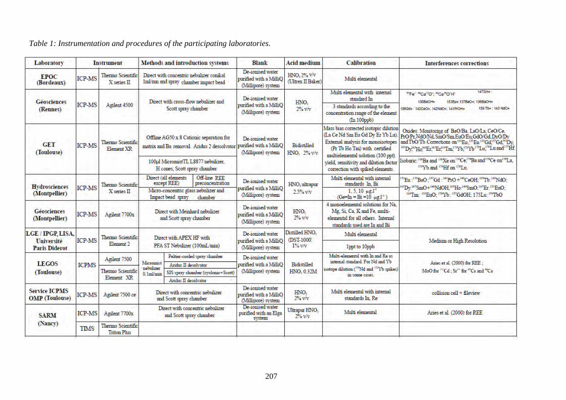
207
Table 1: Instrumentation and procedures of the participating laboratories.
ANNEXE A compilation of Silicon, Rare Earth Element and Twenty-one other trace element
concentrations in the Natural River Water Standard SLRS-5 (NRC-CNRC)
208
For Sr isotope determination, 30 ml of SLRS-5 was evaporated in triplicate.
Strontiumisolation from the rest of the matrix was then carried out following an analytical
protocolsimilar to that of Pin et al. (1994). Briefly, the samples were diluted with 2 ml of
HNO3 (2mol.l-1
) and loaded onto Sr Spec resin (Eichrom), which had been previously washed
andconditioned. Strontium was then isolated from Rb, Ba and REE using nitric acid solutions
atvarious values of molarity. The Sr fraction was then dried, ready for measurement by TIMS.
Strontium isotopes measurements were done using TIMS (Triton Plus from Thermo
Electron)at the CRPG in multi-collection mode using Re as the filament. Five Faraday cups
were usedto monitor Rb also. To correct for instrumental mass bias, internal normalisation
using a86
Sr/88
Sr ratio of 0.1194 and an exponential law were used. International Sr reference
materialNBS 987 was used to control the method accuracy. The blank processed and
measured alongwith the samples gave a value of less than 100 pg, which is negligible
compared with theamount of Sr from the sample (about 1.5 μg).
Statistical methods
All laboratories proposed their own average working values after outlier rejection by
theirown methods. The Dixon and Grubbs tests at the 95% confidence level (Miller and
Miller1993, Prichard 1995, Feinberg 1996) were applied by LEGOS and SARM (Nancy).
Detailedstatistical methods were not available for the others. The statistical tests classically
used tointerpret the results of a round-robin study assume a population meeting the criteria of
anormal distribution defined by the mean and the variance. Differences in data size (n = 2–
284)did not allow the certification of elemental concentrations in SLRS-5 because it did not
followany statistical law. Therefore, the aim of this paper is only to propose compilation
values foruncertified elements. Instead of using robust statistical methods for which no
hypothesis concerning the distribution is necessary, we chose the general approach based on
the ISO5725-2 procedural standard, in order to define the criteria of repeatability,
reproducibility andthe knowledge of compilation value, to reveal the possible existence of a
bias betweenlaboratories. Thus, compiled data were interpreted using a homogeneous
statistical model forboth certified and uncertified elements.
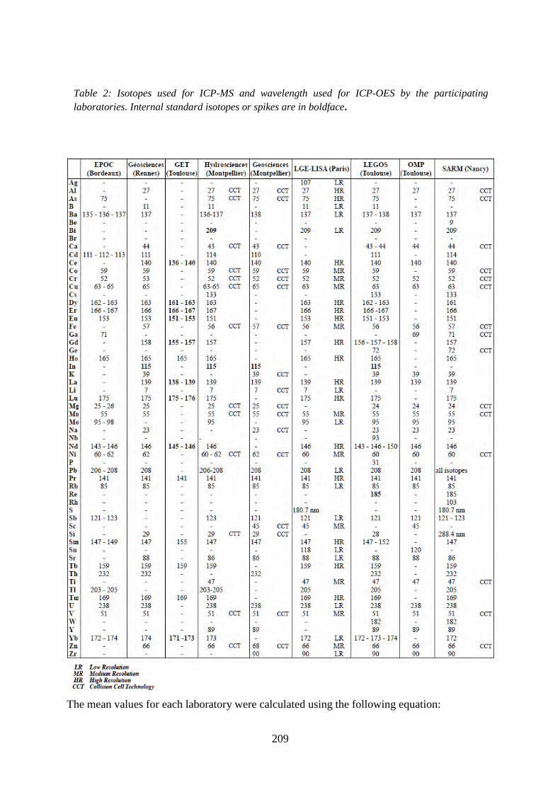
209
The mean values for each laboratory were calculated using the following equation:
Table 2: Isotopes used for ICP-MS and wavelength used for ICP-OES by the participating
laboratories. Internal standard isotopes or spikes are in boldface.
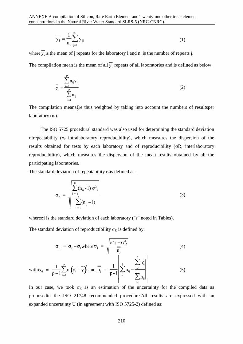
ANNEXE A compilation of Silicon, Rare Earth Element and Twenty-one other trace element
concentrations in the Natural River Water Standard SLRS-5 (NRC-CNRC)
210
(1)
where is the mean of j repeats for the laboratory i and ni is the number of repeats j.
The compilation mean is the mean of all repeats of all laboratories and is defined as below:
(2)
The compilation meansare thus weighted by taking into account the numbers of resultsper
laboratory (ni).
The ISO 5725 procedural standard was also used for determining the standard deviation
ofrepeatability (σr intralaboratory reproducibility), which measures the dispersion of the
results obtained for tests by each laboratory and of reproducibility (σR, interlaboratory
reproducibility), which measures the dispersion of the mean results obtained by all the
participating laboratories.
The standard deviation of repeatability σris defined as:
(3)
whereσi is the standard deviation of each laboratory ("s" noted in Tables).
The standard deviation of reproductibility σR is defined by:
where (4)
with and (5)
In our case, we took σR as an estimation of the uncertainty for the compiled data as
proposedin the ISO 21748 recommended procedure.All results are expressed with an
expanded uncertainty U (in agreement with ISO 5725-2) defined as:
yi 1
ni
yij
j1
n i
y i
y i
y
nijyij
i1
p
nij
i1
p
r
(nij -1) 2ij
i 1
p
(nij 1)i 1
p
R r l
l 2
d 2
r
n j
d 1
p 1ni
i1
p
yi y 2
n j 1
p -1nij
nij
2
i1
p
nij
i1
p
i1
p
y
nijyij
i1
p
nij
i1
p
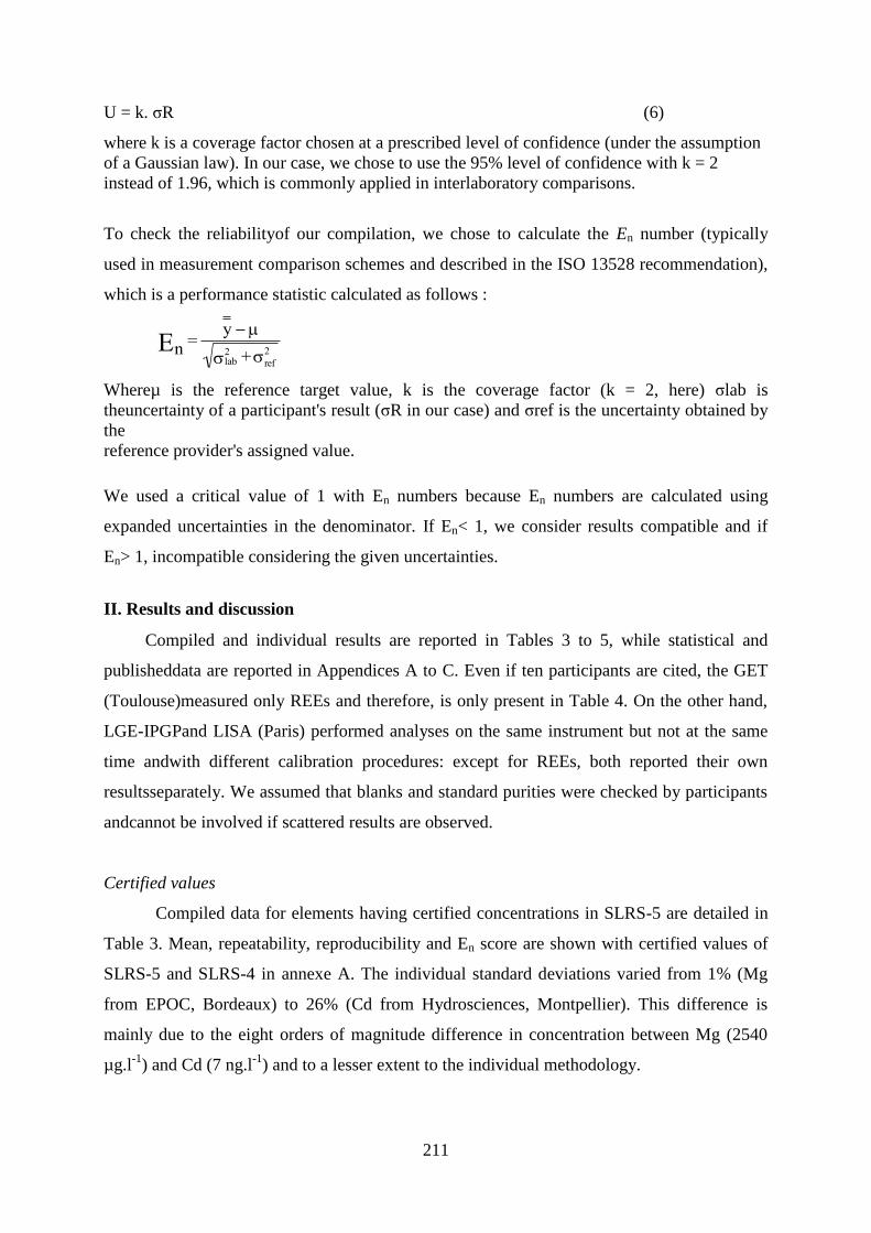
211
U = k. σR (6)
where k is a coverage factor chosen at a prescribed level of confidence (under the assumption
of a Gaussian law). In our case, we chose to use the 95% level of confidence with k = 2
instead of 1.96, which is commonly applied in interlaboratory comparisons.
To check the reliabilityof our compilation, we chose to calculate the En number (typically
used in measurement comparison schemes and described in the ISO 13528 recommendation),
which is a performance statistic calculated as follows :
Whereµ is the reference target value, k is the coverage factor (k = 2, here) σlab is
theuncertainty of a participant's result (σR in our case) and σref is the uncertainty obtained by
the
reference provider's assigned value.
We used a critical value of 1 with En numbers because En numbers are calculated using
expanded uncertainties in the denominator. If En< 1, we consider results compatible and if
En> 1, incompatible considering the given uncertainties.
II. Results and discussion
Compiled and individual results are reported in Tables 3 to 5, while statistical and
publisheddata are reported in Appendices A to C. Even if ten participants are cited, the GET
(Toulouse)measured only REEs and therefore, is only present in Table 4. On the other hand,
LGE-IPGPand LISA (Paris) performed analyses on the same instrument but not at the same
time andwith different calibration procedures: except for REEs, both reported their own
resultsseparately. We assumed that blanks and standard purities were checked by participants
andcannot be involved if scattered results are observed.
Certified values
Compiled data for elements having certified concentrations in SLRS-5 are detailed in
Table 3. Mean, repeatability, reproducibility and En score are shown with certified values of
SLRS-5 and SLRS-4 in annexe A. The individual standard deviations varied from 1% (Mg
from EPOC, Bordeaux) to 26% (Cd from Hydrosciences, Montpellier). This difference is
mainly due to the eight orders of magnitude difference in concentration between Mg (2540
µg.l-1
) and Cd (7 ng.l-1
) and to a lesser extent to the individual methodology.
nE =y
lab2
+ref
2
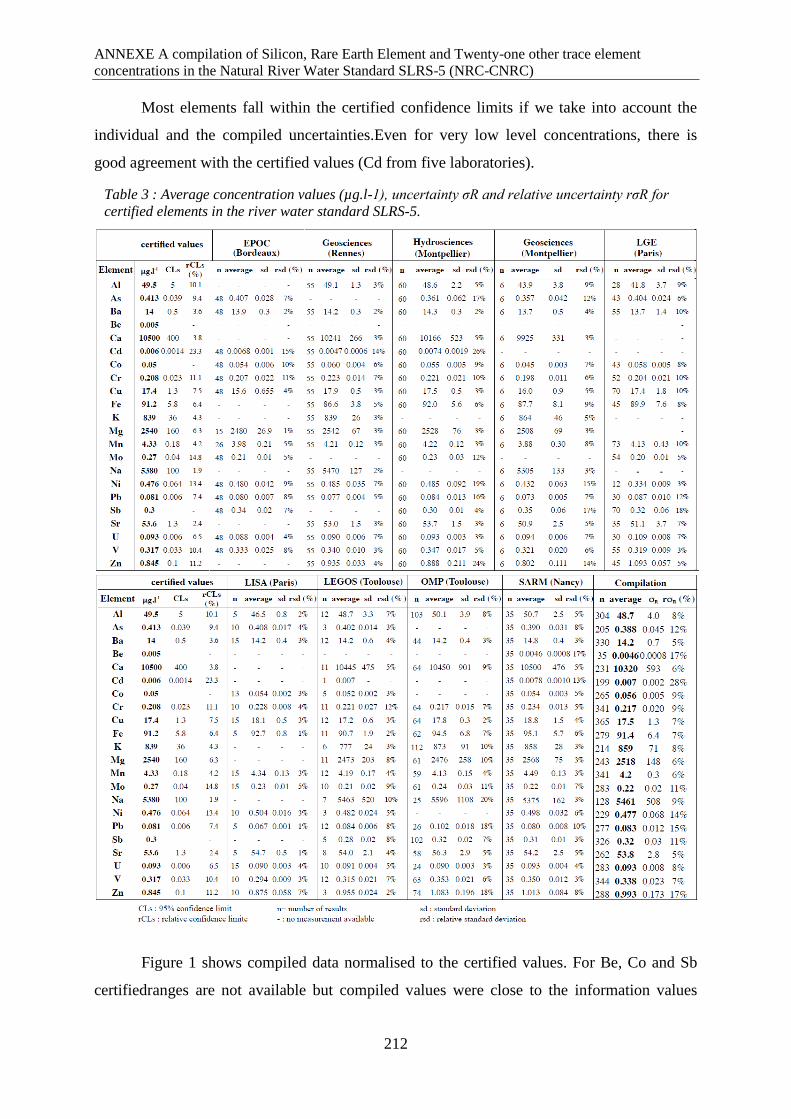
ANNEXE A compilation of Silicon, Rare Earth Element and Twenty-one other trace element
concentrations in the Natural River Water Standard SLRS-5 (NRC-CNRC)
212
Most elements fall within the certified confidence limits if we take into account the
individual and the compiled uncertainties.Even for very low level concentrations, there is
good agreement with the certified values (Cd from five laboratories).
Figure 1 shows compiled data normalised to the certified values. For Be, Co and Sb
certifiedranges are not available but compiled values were close to the information values
Table 3 : Average concentration values (µg.l-1), uncertainty σR and relative uncertainty rσR for
certified elements in the river water standard SLRS-5.
213
given byNCR-CNRC (difference of less than 10%). In all other cases, the compilation value
fell intothe certified range except for Mo and Zn where the compiled weighted average was
about20% lower and 20% higher than the certified value.
Standard deviations of repeatability and reproducibility are rather similar in Appendix
A,which may suggest no inter-laboratory bias. The En numbers calculated indicate
thatcompilation values were consistent with target values. Note that the certified value for
Mo,which was recently added to the certificate by the provider (0.27 ± 0.04 μg.l-1
), is
slightlyhigher than that of the compilation (0.22 ± 0.05 μg.l-1
) and of the proposed value
byHeimburger et al. (2012) (0.21 ± 0.04 μg.l-1
).
As reported, for example, by Date and Gray (1989) and May and Weidmeyer
(1998),uncorrected/corrected polyatomic interferences on K (ArH+), Zn (ArMg, sulfur
species) andNi (CaO) might explain most of the outliers and high standard deviations
observed for theseelements (Table 3). Furthermore, possible contamination on blanks or
Figure 1: Comparison of compiled data versus certified values for the river water standard
SLRS-5. Diamonds represent compiled data. Triangles are the minimum and the maximum
values from the results of individual laboratories.
ANNEXE A compilation of Silicon, Rare Earth Element and Twenty-one other trace element
concentrations in the Natural River Water Standard SLRS-5 (NRC-CNRC)
214
calibrationmethodologies for elements such as Cd, Co, Ni, Pb and Zn introduce noise in
measurements(Figure 1).
Therefore, individual laboratories obtained consistent values for certified elements
within theNRC-CNRC limits and all compiled data fell within these limits, except for Zn.
This indicatesthe proficiency of the participating laboratories and thus suggests that they also
producetrustworthy results. It also allows us to have confidence in our mode of calculation
foruncertified elements (mean values and expanded uncertainty).
Uncertified values
Tables 4 and 5 show compilation means obtained from laboratories with expanded uncertainty
U, while published data are reported in Appendices B and C.
Rare earth elements: Compiled and individual results for REEs are shown in Figure 2
andreported in Table 4. Their concentrations varied from 252 ng.l-1
(Ce) to 1.5 ng.l-1
(Tm)
andrelative expanded uncertainty (rU) varied from 6% (La) to 31% (Tm),
suggestinghomogeneous results between laboratories and techniques. Uncertainty values
correlatesomewhat with concentration.
Larger inter-laboratory variation for middle REEs may be partly explained by
noiseintroduced by isobaric interference corrections for oxides of low atomic number
REEs(LREEs) and Ba. Higher values for Eu and Gd reported by the LEGOS are difficult to
explain by insufficient interference correction: this laboratory used both a desolvating and a
classicsample introduction technique and did not observe any bias between the results
obtained, despite the fact that desolvation is known to generate very small amounts of oxides.
The highvalue of Lu given by EPOC is most likely explained by a calibration bias, because
none of theparticipants applied oxide corrections to the mass 175. The GET laboratory
applied an isotopedilution method using ten enriched REE spikes and achieved uncertainties
better than 2%RSD on all REEs. This high precision method yielded REE concentrations that
overlappednarrowly with the REE compilation concentrations based on all participating
laboratories(Table 4).
REE patterns normalised to upper crust concentrations (Taylor and McLennan 1985)
arereported in Figure 2a. Patterns display LREE enrichment relative to high atomic
numberREEs (HREEs) as well as a large negative Ce anomaly. The SLRS-5 compilation
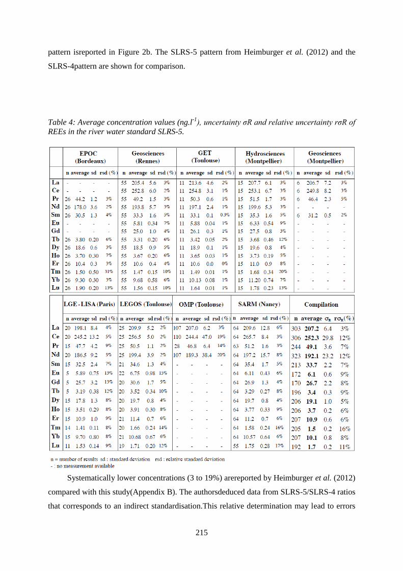
215
pattern isreported in Figure 2b. The SLRS-5 pattern from Heimburger et al. (2012) and the
SLRS-4pattern are shown for comparison.
Table 4: Average concentration values (ng.l-1
), uncertainty σR and relative uncertainty rσR of
REEs in the river water standard SLRS-5.
Systematically lower concentrations (3 to 19%) arereported by Heimburger et al. (2012)
compared with this study(Appendix B). The authorsdeduced data from SLRS-5/SLRS-4 ratios
that corresponds to an indirect standardisation.This relative determination may lead to errors
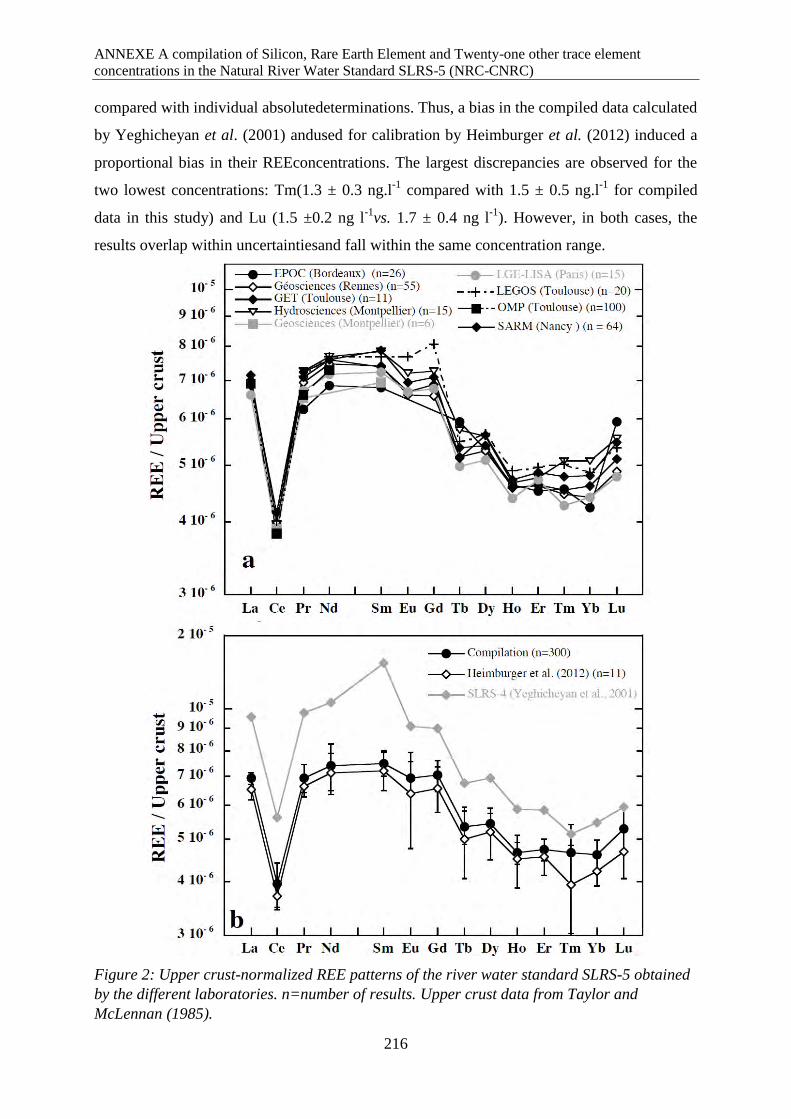
ANNEXE A compilation of Silicon, Rare Earth Element and Twenty-one other trace element
concentrations in the Natural River Water Standard SLRS-5 (NRC-CNRC)
216
compared with individual absolutedeterminations. Thus, a bias in the compiled data calculated
by Yeghicheyan et al. (2001) andused for calibration by Heimburger et al. (2012) induced a
proportional bias in their REEconcentrations. The largest discrepancies are observed for the
two lowest concentrations: Tm(1.3 ± 0.3 ng.l-1
compared with 1.5 ± 0.5 ng.l-1
for compiled
data in this study) and Lu (1.5 ±0.2 ng l-1
vs. 1.7 ± 0.4 ng l-1
). However, in both cases, the
results overlap within uncertaintiesand fall within the same concentration range.
Figure 2: Upper crust-normalized REE patterns of the river water standard SLRS-5 obtained
by the different laboratories. n=number of results. Upper crust data from Taylor and
McLennan (1985).
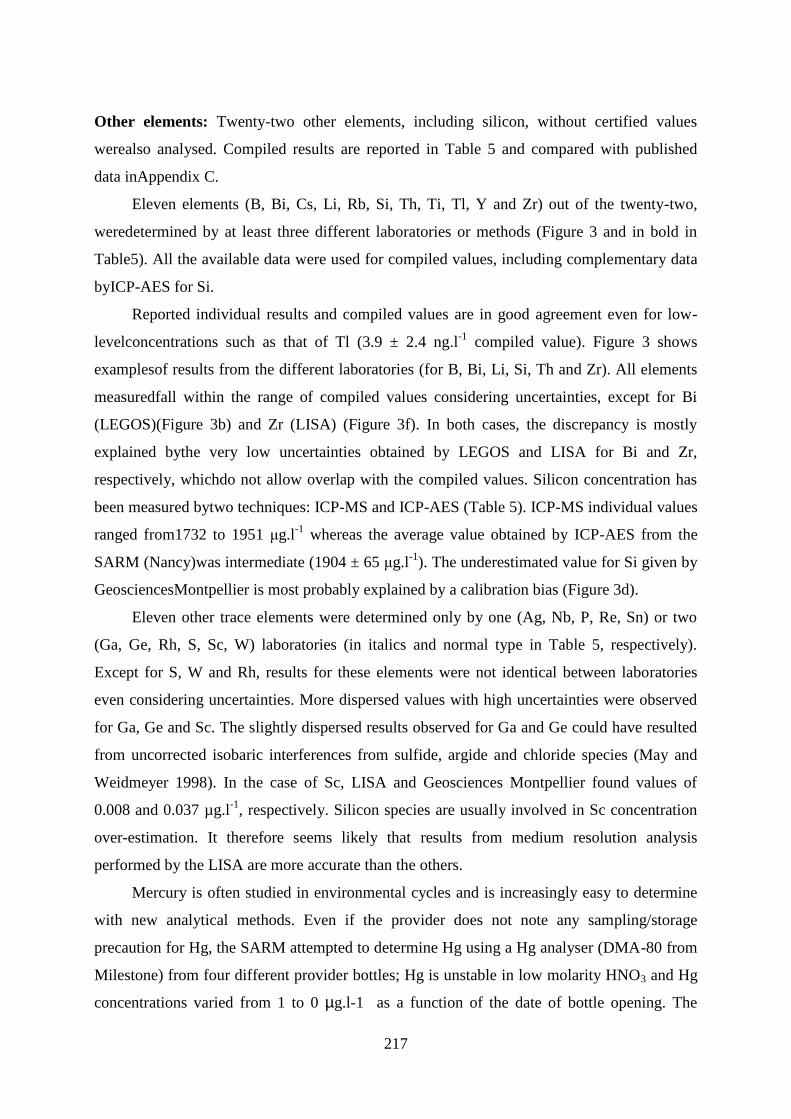
217
Other elements: Twenty-two other elements, including silicon, without certified values
werealso analysed. Compiled results are reported in Table 5 and compared with published
data inAppendix C.
Eleven elements (B, Bi, Cs, Li, Rb, Si, Th, Ti, Tl, Y and Zr) out of the twenty-two,
weredetermined by at least three different laboratories or methods (Figure 3 and in bold in
Table5). All the available data were used for compiled values, including complementary data
byICP-AES for Si.
Reported individual results and compiled values are in good agreement even for low-
levelconcentrations such as that of Tl (3.9 ± 2.4 ng.l-1
compiled value). Figure 3 shows
examplesof results from the different laboratories (for B, Bi, Li, Si, Th and Zr). All elements
measuredfall within the range of compiled values considering uncertainties, except for Bi
(LEGOS)(Figure 3b) and Zr (LISA) (Figure 3f). In both cases, the discrepancy is mostly
explained bythe very low uncertainties obtained by LEGOS and LISA for Bi and Zr,
respectively, whichdo not allow overlap with the compiled values. Silicon concentration has
been measured bytwo techniques: ICP-MS and ICP-AES (Table 5). ICP-MS individual values
ranged from1732 to 1951 μg.l-1
whereas the average value obtained by ICP-AES from the
SARM (Nancy)was intermediate (1904 ± 65 μg.l-1
). The underestimated value for Si given by
GeosciencesMontpellier is most probably explained by a calibration bias (Figure 3d).
Eleven other trace elements were determined only by one (Ag, Nb, P, Re, Sn) or two
(Ga, Ge, Rh, S, Sc, W) laboratories (in italics and normal type in Table 5, respectively).
Except for S, W and Rh, results for these elements were not identical between laboratories
even considering uncertainties. More dispersed values with high uncertainties were observed
for Ga, Ge and Sc. The slightly dispersed results observed for Ga and Ge could have resulted
from uncorrected isobaric interferences from sulfide, argide and chloride species (May and
Weidmeyer 1998). In the case of Sc, LISA and Geosciences Montpellier found values of
0.008 and 0.037 µg.l-1
, respectively. Silicon species are usually involved in Sc concentration
over-estimation. It therefore seems likely that results from medium resolution analysis
performed by the LISA are more accurate than the others.
Mercury is often studied in environmental cycles and is increasingly easy to determine
with new analytical methods. Even if the provider does not note any sampling/storage
precaution for Hg, the SARM attempted to determine Hg using a Hg analyser (DMA-80 from
Milestone) from four different provider bottles; Hg is unstable in low molarity HNO3 and Hg
concentrations varied from 1 to 0 µg.l-1 as a function of the date of bottle opening. The
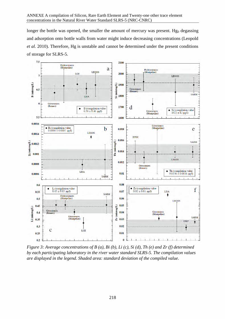
ANNEXE A compilation of Silicon, Rare Earth Element and Twenty-one other trace element
concentrations in the Natural River Water Standard SLRS-5 (NRC-CNRC)
218
longer the bottle was opened, the smaller the amount of mercury was present. Hg0 degassing
and adsorption onto bottle walls from water might induce decreasing concentrations (Leopold
et al. 2010). Therefore, Hg is unstable and cannot be determined under the present conditions
of storage for SLRS-5.
Figure 3: Average concentrations of B (a), Bi (b), Li (c), Si (d), Th (e) and Zr (f) determined
by each participating laboratory in the river water standard SLRS-5. The compilation values
are displayed in the legend. Shaded area: standard deviation of the compiled value.
219
Table 5: Proposed mean concentration values (µg.l-1), standard deviation (s), relative
standard deviation (RSD)from each laboratory, compilation meanwith expanded
uncertainty U and relative expanded uncertainty (rU) of uncertainty elements in the river
water certified reference materiel SLRS-5.
ANNEXE A compilation of Silicon, Rare Earth Element and Twenty-one other trace element
concentrations in the Natural River Water Standard SLRS-5 (NRC-CNRC)
220
Sr isotopic ratio: Strontium isotope measurements provided an average value of 0.711011
(Table 5) ranging between 0.710960 and 0.711075, each individual measurement having an
uncertainty less than 10 ppm. Such a value is consistent with the mixture of various
lithologies represented in the river basin.
SLRS-5 versus SLRS-4: SLRS-4 certified concentrations are also reported in Appendix A,as
well as data from Yeghicheyan et al. (2001) in Appendices B and C for comparisonpurposes.
As far as certified values are concerned, the two batches are different: Al, As, Be,Cd, Cr, Fe,
Ni, Pb, V and Zn are lower in the SLRS-5 than in the SLRS-4 batch. While Vdiffered only by
1%, Cd was a factor of two lower in SLRS-5. On the other hand, Ba, Ca, Co,Cu, K, Mg, Mn,
Mo, Na, Sb, Sr, U are more concentrated in SLRS-5. For Cu, the differencereached 861%
suggesting contamination during sampling rather than solid charge variationsin the reference
water. REE concentrations were depleted by about 30% for LREEs and 12%for HREEs in
SLRS-5 water relative to SLRS-4 (Appendix B). Moreover, the REEconcentration
comparison of both Heimburger et al. (2012) and this study with the SLRS-4compilation data
(Yeghicheyan et al. 2001) showed the same trend (Figure 2b). However Smconcentrations
showed the largest variation (33.2 ng.l-1
instead of 57.4 ng.l-1
) whereas HREEswere rather
similar. Such a difference may be explained by the inclusion of some uncorrectedvalues in the
compilation of the SLRS-4 paper (Yeghicheyan et al. 2001).
For other elements (Appendix C), variations between batches are more obvious: Ag,
Cs, Li, P,Rb, Th, Tl, Y and Zr were lower while B, Ga, Ge, Si, Ti and W were higher than in
SLRS-4.These variable proportions directly depend on sampling and lithological
contributions.
III. Conclusion
We report a compilation of concentrations for certified and uncertified elements in
the naturalriver water certified reference material SLRS-5 (NRC-CNRC) from two years of
routineanalysis in ten different French laboratories. The reported results show coherent values
forREE concentrations, with relative expanded uncertainties ranging from 6% to 31%.
Strontiumisotopic ratios were also determined.Seventeen elements (B, Bi, Cs, Ga, Ge, Li, Rb,
Rh, S, Sc, Si, Th, Ti, Tl, W, Y and Zr)determined by at least two laboratories yielded
compiled values having relative expandeduncertainties ranging from 8% to 241%. Five more
trace element (Ag, Nb, P Re andSn)concentrations were reported, but with a more restricted
number of results.
221
Aknowledgements
This study was supported by CNRS funds and the "Isotrace" network. It is dedicated to
JeanCarignan, SARM director from 1995 to 2011. We would like to thank P-Y. Martin
(SARM)who performed mercury analyses and Laurie Reisberg for initial corrections. Special
thanksare due to the three anonymous reviewers for their constructive comments.
References
NF/ISO 5725-2 (1994) Exactitude (justesse et fidélité) des résultats et méthodes de mesure. Méthode
de base pour la détermination de la répétabilité et de la reporductibilité d'une méthode de mesure
normalisée, 44p.
NF/ISO 21748 (2010) Lignes directrices relatives à l'utilisation d'estimations de la répétabilité, de la
reproductibilité et de la justesse dans l'évaluation de l'incertitude de mesure.
ISO/DIS 13528 (2005)Statistical methods for use in proficiency testing by interlaboratory
comparisons, 66p.
Aries S., Valladon M, Polvé M. and Dupré B. (2000) A routine method for oxide and hydroxide
interference corrections in ICP-MS chemical analysis of environmental and geological samples.
Geostandards Newsletter 24,1, 19-31.
Bayon G., Birot D., Bollinger C. and Barat J.A. (2010) Multi-element determination of race elements
in natural water reference materials by ICP-SFMS after Tm addition and Iron co-precipitation.
Geostandards Newsletter 35, 145-153.
Birke M., Reinman C., Demetriades A., Rauch U., Lorenz H., Harazim B., Glatte W.(2010)
Determination of major and trace elements in European bottled mineral water — Analytical
methods. J. Geochemical Exploration 107,3, 217-226.
Carignan J., Hild P., Mevelle G., Morel J. and Yeghicheyan D. (2001) Routine analysis of trace
elements in geological samples using flow-injection and low-pressure on-line liquid
chromatography ICP-MS: a study of geostandards BR, DR-N, UB-N, ANG and GH, Geostandards
Newsletter, in this issue.
Date A.R. and Gray A.L. (1989) Applications of inductively coupled plasma mass spectrometry.
Blackie Ed., New York, 254 pp.
Feinberg M. (1996) La validation des méthodes d’analyse : une approche chimiométrique de
l’assurance qualité au laboratoire. Masson, Paris, 397 pp.
HeimburgerA., Tharaud M., Monna F., LosnoR., DesboeufsK., Bon Nguyen E. (2012) SLRS-5
elemental concentrations deducted from SLRS-5/SLRS-4 ratios of thirty three uncertified elements.
Geostandards and Geoanalytical Research, in press.
Lawrence M.G., Greig A., Collerson K.D., Kamber B.S. (2006) Direct quantification of rare earth
element concentrations in natural waters by ICP-MS. Applied Geochemistry, 21, 839-848.
Leopold K., Foulkes M. and Worsfold P. (2010) Methods for the determination and speciation of
mercury in natural waters – A review.Analytica Chimica Acta, 663, 127–138.
May T.W. and Wiedmeyer R.H. (1998) A table of polyatomic interferences in ICP-MS. Atomic
Spectroscopy 19, 150-155.
Miller J.C. and Miller J.N. (1993) Statistics for analytical chemistry.3rd
ed., Ellis Horwood PTR
Prentice Hall, New York, 233 pp.
Pin C., Briot D., Bassin C. and Poitrasson F. (1994) Concomitant separation of strontium and
samarium-neodynium for isotopic analysis in silicate samples, based on specific extraction
chromatography. Analytica Chimica Acta, 298,209–217.
Prichard F.E., Crosby N.T., Day J.A., Hardcastle W.A., Holcombe D.G. and Treble R.D. (1995)
Quality in the analytical chemistry laboratory.In Analytical Chemistry by Open Learning.John
Wiley and Sons Ed., 307 pp.
ANNEXE A compilation of Silicon, Rare Earth Element and Twenty-one other trace element
concentrations in the Natural River Water Standard SLRS-5 (NRC-CNRC)
222
Tanner S.C., Baranov V.I. and Bandura D.R. (2002) Reaction cells and collision cells for ICP-MS: A
tutorial review. Spectrochimica Acta Part B, 57, 1361–1452.
Taylor S.R. and McLennan S.M. (1985) The continental crust : its composition and evolution.
Blackwell, Oxford, 460pp.
Tosiani T., Loubet M., Viers J., Valladon M., Tapia J., Marrero S., Yanes C., Ramirez A., Dupre B.
(2004) Major and trace elements in river-borne materials from the Cuyuni basin (southern
Venezuela): evidence for organo-colloidal control on the dissolved load and element redistribution
between the suspended and dissolved load. Chem. Geology 2011, 3, 305-334.
Yeghicheyan, D., Carignan J., Valladon M., Bouhnik Le Coz M., F. Le Cornec, Castrec-Rouelle M.,
Robert M., Aquilina L., Aubry E., Churlaud C., Dia A., Deberdt S., Dupré B., Freydier R., Gruau
G., Hénin O., De Kersabiec A-M., Macé J., Marin L., Morin N., Petitjean P., Serrat E. (2001) A
Compilation of Silicon and Thirty One Trace Elements Measured in the Natural River Water
Reference Material SLRS-R (NRC-CNRC). Geostandards newsletter, 25, 465-47

Résumé
L’estuaire du fleuve Amazone est le sièged’apports colossaux à l’océan en eau continentale, éléments dissous
et particules. Cet estuaire est localisé dans une régioncruciale dans la circulation des masses d’eau entre les
deux hémisphères. Un échantillonnage du fleuve Amazone et de son estuaire, du plateau continental et du
large des côtes brésiliennes et guyanaises a été réalisé dansle cadre du projet de recherche AMANDES
(ANR/IRD/INSU). Ce projet est intégré dans la catégorie « étude de processus » au programme international
GEOTRACES. Ce doctorat a consisté en l’étude des concentrations en terres rares (REE) et de la
composition isotopique (CI) du Nd qui sont des traceurs de source, de transport et de processus. Une méthode
inédite et très précise de détermination de concentrations en REE par dilution isotopique a été de ce fait
développée. Les données obtenues permettent 1)d’observer que la répartition du Nd entre phases dissoutes,
colloïdales et particulaires change radicalement entre l'eau de rivière et l'eau de mer 2) de tracer pour la
première fois à l’échelle locale et en milieu naturel des apports conséquents en Nd et REE à la phasedissoute
et provenant des particules lithogéniques en suspension et déposées sur la margecontinentale 3) de compléter
la base de données mondiale de ces traceur mettant en évidence pour les eaux antarctiques intermédiaires une
signature géochimique contrastant celle habituellement observée au sud de 30°S et qui pourrait être expliquée
par des apports provenant des marges continentales. Ces observations appuient des travaux récents
d’expérimentation et de modélisation concluant à la sous-estimation des sédiments marinscomme terme
source d’éléments dissous à l’océan, terme crucial pour l’étude les cycles géochimiques globaux.
Resumo
Oestuárioo do rio Amazonas é o sitio de apportes colossais Águas continentais, elementos dissolvidos e
material particulado. Esteestuárioé localizado em uma região crucial na circulação das massas de agua entre
os dois hemisférios. Uma amostragem do rio amazonas e do seuestuário, do platô continental e do largo das
costas Guyanesas e francesas foi realizado no âmbito do projeto de pesquisa AMANDES (ANR/IRD/INSU).
EsteProjeto esta integrado na categoria “estudos de processos“ do programa internacional GEOTRACES.
Este doutorado tem consistido no estudo dos teores em elementos terras raras (REE) e da composição
isotópica do Nd que são traçadores de fonte, de transporte e de processos. Um método inédito e muito preciso
na determinação de teores em REE por dilução isotópica foi emconsequência desenvolvido. Os dados obtidos
permitem 1) a observação da mudança radical na repartição do Nd entre as phases particuladas dissolvidas e
colloidais entre a Água do rio e a Água do oceano. 2) de traçar pela primeira vez na escala local e em meio
natural apportes consequentes em Nd e REE para a fase dissolvida e proveniente s das partículas litogênicas
em suspensão e depositadas na margem. 3) de completar a base de dados mundial destes traçadores revelando
para asÁguas antárcticas intermediarias uma assinatura geoquímica em contraste com aquela habitualmente
observada ao sul de 30°S e que poderia ser explicada por apportes provenientes das margens continentais.
Estas observações apoiam trabalhos recentes de experimentação e de modelagem concluindo a sob estimação
dos sedimentos marinhos como termo de fonte para o oceano, termo crucial para o estudo dos ciclos
geoquímicos globais.
Abstract
The Amazon estuary is a major source of continental waters, dissolved elements and particles. This estuary is
located in a crucial area for inter hemispheric water-mass transfers. A sampling of the Amazon and its
estuary, the Brazilian and Guyanese margin and offshore waters was made in the framework of the
AMANDES (ANR/IRD/INSU) research project. This Project is intregrated in the “process study” topic of the
international research program GEOTRACES. This doctorate consisted in the study of rare earth element
concentrations (REE) and Nd isotopic compositions both of these being tracers of source, transport and
processes. A precise isototopic dilution method for determining the REE concentrations was thus developed.
The obtained data allows to 1) observe a radical change in Nd repartition between dissolved particles and
colloids from the river water to the seawater; 2) trace for the first time at a local scale and in a natural
environment, consequent lithogenic sources of Nd and REE to the dissolved phase from suspended and
margin deposited sediments; complete the world database of these tracers thus revealing a contrasted
geoquemical signature for the Antarctic Intermediate Waters with that observed south of 30°S and which
could be explained by South Atlantic sourced contributions of margin sediment. Recent experimental and
modelling works conclude theunderestimation of marine sediments as a source term for the ocean, a term
which is crucial for global geoquemical cycles.