Embed Size (px)
Citation preview

Palestine Polytechnic University
College of Engineering
Electrical Engineering Department
Electronics and Communication Engineering
Bachelor Thesis
Graduation Project
Traffic Congestion Management at Road Intersections Using Wi-Fi Technology
Project Team
Abdulghafar Shabaneh
Abdulsalam Shabaneh
Ibrahim Zughayer
Supervisor: Dr. Murad AbuSubaih
Hebron-Palestine
May-2014
Palestine Polytechnic University
College of Engineering
Electrical Engineering Department
Traffic Congestion Management at Road Intersections Using Wi-Fi Technology
Project Team
Abdulghafar Shabaneh
Abdulsalam Shabaneh
Ibrahim Zughayer
By the guidance of our supervisor, and by the acceptance of all members in the testing committee, this project is delivered to department of electrical engineering in the college of engineering, to be as practical fulfillment of the requirement of the department for the degree of B.Sc.
Supervisor Signature
------------------------------
Testing committee signature
--------------------------- -----------------------------
The head of department signature
-------------------------------------------

جامعة بولیتكنك فلسطین
كلیة الھندسة
دائرة الھندسة الكھربائیة
Traffic Congestion Management at Road Intersections Using Wi-Fi Technology
فریق المشروع
ابراھیم الصغیر عبد الغفار شبانھ عبد السلام شبانھ
ة بناء على نظام كلیة الھندسة وإشراف ومتابعة المشرف المباشر على المشروع وموافقة أعضاء اللجنوذلك للوفاء بمتطلبات درجة البكالوریوس . لى دائرة الھندسة الكھربائیةالمناقشة، تم تقدیم ھذا العمل إ
.في ھندسة الاتصالات
توقیع المشرف
----------------------------
توقیع اللجنة المناقشة
--------------------------- -----------------------------
توقیع رئیس الدائرة
-------------------------------------------

الإهداء
..إلى الذین صنعوا من الأیام قضیة عمر
...له إلى من عجز قلمي عن وصف حبي وتقدیري....يدرب يإلى الشمعة التي أنارت ل
..الأشواك عن دربي لیمهد لي طریق العلمإلى من حصد
العزيز إلى والدي
..أرقى وأروع حب عرفته البشریة إلى
..إلى نبع الحنان الدائم الذي سهر كي أنام وأبقى
..إلى القلب الناصع بالبیاض
رضاك يا والدتي
..إلى من شاركوني أجمل الذكریات وكانوا معي كل اللحظات
أصدقـائي الأعزاء
..إلى الذین بذلوا كل جهدوعطاء لكي أصل إلى هذه اللحظة
أساتذتي الكرام
...إلى كل طلاب العلم والمعرفة في كل مكان
والى أبناء شعبي ووطني كافةفي كل مكان إلى كل أهلي وأقاربي
.أهدي إلیهم جمیعا باسمي هذا العمل

قدیركر والت الش
إلى الأستاذ الدكتور الفاضل مراد أبو صبیح صاحب الامتنان عظیمبجزیل الشكر و نتقدم
الفضل الكبیر في إرشاداته لنا واتمام واخراج هذا المشروع بصورته النهائیة من خلال
.إرشاداته ومساعدته القیمة
كل الذین ساعدونا ومدو لنا ید العون ولم یبخلوا ىلبجزیل الشكر والعرفان إ كذلك نتقدم
.نشكرهم جمیعا ... ن أساتذة أو طلاب أو أقاربعلینا بالعلم، سواء م
ولا یسعنا في هذا المقام إلا أن نتقدم أیضا بجزیل الشكر والعرفان إلى جمیع أعضاء
.على الجهد والعطاء الذي منحونا إیاهالهندسة الهیئة التدریسیة في كلیة
.أیضا نشكر أهلنا وجمیع زملائنا
.الجزیل لجمیع من ساهم بإنجاح هذا العملوفي النهایة نتقدم بالشكر
فریق العمل
I
Contents
Chapter 1: Introduction
1.1 Problem statement………………………………………………………...… 2
1.2 Motivation……………………………………………………………………. 3
1.3 Approach……………………………………………………………………... 4
1.4 Objectives…………………………………………………………………….. 4
1.5 Literature review ……………………………………………………………. 5
1.6 Project schedule ………………………………………….………………….. 8
Chapter 2: Components Background
2.1 Cameras……………………………………………………………..……… 12
2.1.1 Video cameras…………………………………………………………. 12
2.1.2 History…………………………………………………………….…… 12
2.1.3 Some types of cameras ………………………………….....….………. 13
2.1.4 Applications………………………………………………………….... 14
2.2 Image processing………………………………………………………….… 14
2.2.1 Purpose of Image processing…………………………………….….…. 15
2.2.2 Types of Image processing…………………………………….………. 15
2.2.3 Image processing applications…………………………………….….... 16
2.2.4 Image processing software…………………………………….………. 17
2.3 Microcontrollers…………………………………………………….……… 17
2.3.1 Applications…………………………………………………….……... 18
2.3.2 Classification of Microcontrollers……………………………..………. 18
2.3.3 Raspberry Pi microcontroller………………………………….…….… 19
2.3.4 Arduino Uno microcontroller……………………….....……….……… 21
2.3.4.1 Power ……………………………………………….………. 22
2.3.4.2 Memory ……………………………………………..……….. 22
2.3.4.3 Programming …………………………………………….…… 22
II
2.4 Digital signal processing…………………………………………...………. 23
2.4.1 Digital signal processors..……………………………………………....24
2.4.2 Advantages………………………………………………………..…… 24
2.4.3 Disadvantages…………………………………….................................. 25
2.4.4 Applications...…………………………………….................................. 25
2.5 Wi-Fi Technology…………………………………………………………... 26
2.5.1 Historical background……………………………………………...….. 27
2.5.2 Advantages and Limitations……………………………………...……. 27
2.5.3 Wi-Fi Standards………………………………………..……………… 28
2.6 Wireless Transceivers Technologies…………………..…………………... 29
2.6.1 ZigBee……………………………………………………….……….. 30
2.6.2 WiFly GSX transceiver……………………………………..…………. 31
2.6.2.1 Applications …………………………………………..……… 32
2.6.2.2 WiFly 4………………………………………………..……… 33
2.7 Solar Energy……………………………………………………..…………. 33
2.7.1 Principle of Operation…………………………………………..…….. 34
2.7.2 Photovoltaic Panels……………………………………………..…….. 35
2.7.3 Solar cells……………………………………………………...………. 36
2.7.4 Advantages and Disadvantages of Solar Energy…………………...…. 37
2.7.5 Applications………………………………………………………….... 38
Chapter 3: System Conceptual Design
3.1 Overview……………………………………………………………………. 40
3.2 General block diagram…………………………………………………….. 40
3.3 Main components……………………………………………………...…… 41
3.3.1 Solar System …………………………………………………………. 41
3.3.2 Congestion Detection System………………………………………… 42
3.3.3 Wi-Fi Transmitter…………………………………………………….. 44
3.3.4 Wi-Fi Receivers with built-in Alarm………………………………….. 44
3.4 System flowcharts………………………………………………….……….. 45
3.4.1 Transmitter side………………………………………….…………….. 45
3.4.2 Receiver side…………………………………………….…………….. 46
III
3.5 System functions ……………………………………………………..…….. 47
3.6 Software …………………………………………………………...……..… 48
3.6.1 Raspberry pi programming………………………………………….… 48
3.6.2 Wi-Fi module programming…………………………….…………….. 48
3.6.3 Image processing technique…………………………….……………... 48
Chapter 4: System Implementation
4.1 Overview…………………………………………………………….……… 51
4.2 Solar power parameters……………………………………….…….…….. 51
4.3 Microcontroller Specifications and Setup………………….…………….. 53
4.4 Network Configuration and Access points……………………………..… 54
4.5 Access the Raspberry pi GUI ……………………………….......…………56
4.6 Webcam Connection and configuration……………………………….…60
4.7 Image Processing Software (Octave)…………………………………….61
4.8 Receiver Implementation and Configuration ………...………..………… 65
4.8.1 Module Specifications and Features………………………………..… 65
4.8.2 Alarm Configuration and Circuit Design….....…………..…………… 67
4.8.3 Hardware Setup and Configuration…………………………..………. 67
4.9 Implementing the Image Processing Code…………………………………69
Chapter 5: Testing and System's Performance
5.1 Overview……………………………………………………………………. 74
5.2 Testing and Results…..…………………………………………………….. 74
5.2.1 Testing the Image Processing Code ……………………………….…. 74
5.2.2 Testing the Wifly Modules…………………………………………… 83
5.2.3 Testing the Wi-Fi Network……..…………………………………….. 83
5.2.4 Testing the Solar System….………………………………………….. 84
IV
5.3 Performance Evaluation.……………………………………………...…… 84
5.3.1 Response Time of the Raspberry Pi …….……………………………. 84
5.3.2 Response Time of the Wifly Modules…………...………………….…84
5.3.3 Evaluation Results………………………………………………...…... 85
Chapter 6: Learning Outcomes and Future Work
6.1 Introduction…………………….......……………………………………….. 87
6.2 Acquired Learning Outcomes ……..………………………………………. 87
6.3 Future Work…….……………………………………………………...…… 87
6.4 Conclusion …………………………………………………………….......…87
6.5 Problems ………………………………………………………………..……88
Bibliography ……………………………………………….....…….….. 89
Appendix……………………………………………………..….….……93
V
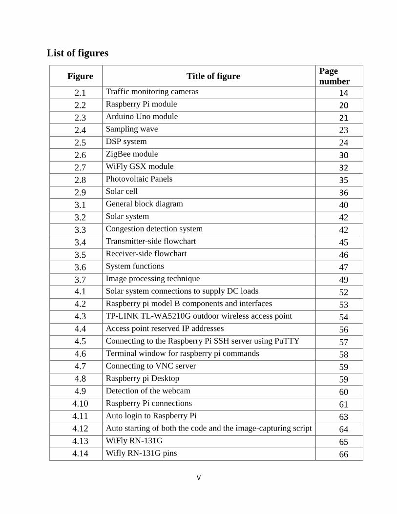
List of figures
Figure Title of figure Page
number
2.1 Traffic monitoring cameras 14
2.2 Raspberry Pi module 20
2.3 Arduino Uno module 21
2.4 Sampling wave 23
2.5 DSP system 24
2.6 ZigBee module 30
2.7 WiFly GSX module 32
2.8 Photovoltaic Panels 35
2.9 Solar cell 36
3.1 General block diagram 40
3.2 Solar system 42
3.3 Congestion detection system 42
3.4 Transmitter-side flowchart 45
3.5 Receiver-side flowchart 46
3.6 System functions 47
3.7 Image processing technique 49
4.1 Solar system connections to supply DC loads 52
4.2 Raspberry pi model B components and interfaces 53
4.3 TP-LINK TL-WA5210G outdoor wireless access point 54
4.4 Access point reserved IP addresses 56
4.5 Connecting to the Raspberry Pi SSH server using PuTTY 57
4.6 Terminal window for raspberry pi commands 58
4.7 Connecting to VNC server 59
4.8 Raspberry pi Desktop 59
4.9 Detection of the webcam 60
4.10 Raspberry Pi connections 61
4.11 Auto login to Raspberry Pi 63
4.12 Auto starting of both the code and the image-capturing script 64
4.13 WiFly RN-131G 65
4.14 Wifly RN-131G pins 66
VI
4.15 WiFly RN-131G connection with Buzzer 68
4.16 Wifly receiver modules 69
4.17 Reference image for the first lane in daytime 71
4.18 Reference image for the second lane in daytime 72
4.19 Reference image for the second lane in nighttime 72
5.1 First lane congested image 74
5.2-5.8 Image processing results for first lane congested image 75
5.9 First lane uncongested image 76
5.10-5.16 Image processing results for first lane uncongested image 77
5.17 Second lane uncongested image 78
5.18-5.24 Image processing results for second lane uncongested image 79
5.25 Second lane congested image 80
5.26 Image processing result for second lane congested image 81
5.27 Congested traffic at night 81
5.28-5.34 Image processing results for congested traffic at night 82
VII
List of tables
Table Title of table Page number
1.2 First semester project schedule 9
1.1 Second semester project schedule 10
2.1 Characteristics of 802.11 protocols 29
4.1 Specifications of TP-Link TL-WA5210G 55
4.2 Pin description 66
4.3 Sensors description 66
5.1 Evaluation results 85
VIII
Abstract
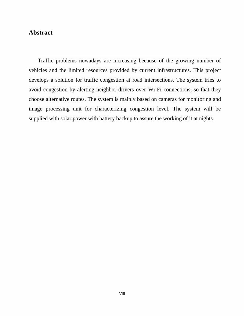
Traffic problems nowadays are increasing because of the growing number of
vehicles and the limited resources provided by current infrastructures. This project
develops a solution for traffic congestion at road intersections. The system tries to
avoid congestion by alerting neighbor drivers over Wi-Fi connections, so that they
choose alternative routes. The system is mainly based on cameras for monitoring and
image processing unit for characterizing congestion level. The system will be
supplied with solar power with battery backup to assure the working of it at nights.

IX
ملخص ال

1
Chapter 1
Introduction
1.1 Problem statement
1.2 Motivation
1.3 Approach
1.4 Objectives
1.5 Literature review
1.6 Project schedule
2
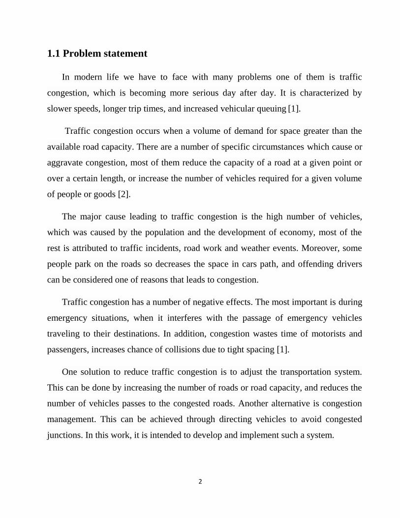
1.1 Problem statement
In modern life we have to face with many problems one of them is traffic
congestion, which is becoming more serious day after day. It is characterized by
slower speeds, longer trip times, and increased vehicular queuing [1].
Traffic congestion occurs when a volume of demand for space greater than the
available road capacity. There are a number of specific circumstances which cause or
aggravate congestion, most of them reduce the capacity of a road at a given point or
over a certain length, or increase the number of vehicles required for a given volume
of people or goods [2].
The major cause leading to traffic congestion is the high number of vehicles,
which was caused by the population and the development of economy, most of the
rest is attributed to traffic incidents, road work and weather events. Moreover, some
people park on the roads so decreases the space in cars path, and offending drivers
can be considered one of reasons that leads to congestion.
Traffic congestion has a number of negative effects. The most important is during
emergency situations, when it interferes with the passage of emergency vehicles
traveling to their destinations. In addition, congestion wastes time of motorists and
passengers, increases chance of collisions due to tight spacing [1].
One solution to reduce traffic congestion is to adjust the transportation system.
This can be done by increasing the number of roads or road capacity, and reduces the
number of vehicles passes to the congested roads. Another alternative is congestion
management. This can be achieved through directing vehicles to avoid congested
junctions. In this work, it is intended to develop and implement such a system.

3
1.2 Motivations
This project deals with a very important and vital aspect in human life that is the
traffic congestion on streets and roads.
The idea is not implemented in our country which really needs a planned and a
well-designed system that informs the drivers about congestion state before they
arrive tat congested intersections. Here are some points that motivate us to work on
this project:
Saving time and effort for drivers and passengers.
Saving the fuel.
Saving the roads from the heavy load that results from Conglomeration of the cars
especially in the bridges.
In general, the congestion causes noise in the city and bothers all people in the
area around.
Congestion increases the emitting of harmful gases in the middle of the city which
increases the air pollution.
Sometimes, congestion has negative effects on people, so that it may cause
nervous tension to some of them due to the delay.
Congestion causes failure in the job of the firemen, ambulance which could leads
to disastrous and terrible results.
We are reducing the consequences of congestion represented mainly by accidents.
Congestion is a cause to several accidents, especially at road intersections.
4
1.3 Approach
This project develops an automatic way for road congestion management. It uses
a monitoring system, digital image processing and wireless communication network.
A camera will be installed alongside the road. It will capture image sequences. Based
on image processing results, a transmitter device sends alarm signal via Wi-Fi to the
receiver devices installed in the cars around the area of this intersection, if congestion
is recognized.
This alarm helps drivers by providing pre-knowledge of traffic congestion at next
intersection and changes their routes before reaching this congested intersection. In
order to increase the reach ability of alarm to all cars, it is intended to display alarm
signals at LCD‟s installed at road sides before the intersection.
The system will be supplied with solar power with battery backup to assure the
working of it at nights.
1.4 Objectives
The project objectives can be summarized as:
Use image processing techniques on the snapshots of the camera for improving
congestion recognition.
Enable drivers to change their paths before reaching congested road intersections
by providing them with the current state of congestion.
Mounting, installing and testing the system practically on a chosen intersection at
different conditions.
To design a useful practical system using the new technologies in this era to
benefit our society.
5
Power the circuits and modules from a solar energy system with chargeable
batteries.
To contribute with such system design and implementation to overcome daily
problems of traffic congestion.
1.5 Literature review
Now let‟s talk briefly about some previous related literature that suggested and
used different solutions and systems to deal with this disturbing problem, traffic
congestion.
One of these literatures is based on exploiting the variation in wireless link
characteristics when line of sight conditions between a wireless sender and receiver
vary. This system comprises of a wireless sender-receiver pair across a road. The
sender continuously sends packets. The receiver measures metrics like signal
strength, link quality and packet reception. These metrics show a marked change in
values depending on whether the road in between has free-flowing or congested
traffic. The Wi-Fi Shield makes the Arduino Uno Wi-Fi compatible. The project plan
is to create a wireless sensor network that is capable of estimating the density of
traffic. The PIR Sensor will detect infrared movement. The sensor will send the
information to the Arduino Uno and the WiShield. The wireless router is used to
make the connection between the Arduino Uno and webpage. The sensor will detect
car movement by the change in infrared patterns. The data will then be transmitted to
the Arduino Uno, then the personal computer which will display the webpage and
binary numbers [3].
6
Another previous research is suggesting the single magnetic sensor to detect and
record the time of vehicles passing it, calculates the length of vehicle based on the
time assuming constant speed common to all vehicles. From a large number of
samples of time and vehicle length, they calculate median of the two metrics and
estimate median speed as (median length/ median time). If this median speed deviates
from expected median speed, congestion is reported [4].
Other researches proposed the use of audio-based techniques like Microwave
radars and ultrasonic sensors. Microwave radars use specially allocated radio
frequency for detecting vehicles. There are two types of microwave radar detectors.
The type of microwave radar uses the Doppler principle to detect vehicles. According
to the Doppler Principle the difference in frequency between the transmitted and
received signals is proportional to the speed of the vehicle. So this type of microwave
radar first transmits electromagnetic energy at a constant frequency. If the detector
senses any shift in the received frequency it deduces that vehicle has passed. On
major problem with this type of microwave radar is that it cannot detect stationary
vehicles. The second type of microwave radar detector transmits a frequency-
modulated continuous wave that varies the transmitted frequency continuously with
time. This enables the system to measure the range of the vehicle from the detector.
Hence, this type of microwave radar can detect stationary vehicles as well. Speed of
the vehicle can be calculated by measuring the time taken by a vehicle to move
between two internal markers separated by a known distance. However, even these
microwave radar systems have problems like over estimating speed and occupancy
values. But ultrasonic sensors use sound waves (above the audible range) to
determine the presence or distance of an object. Ultrasonic detectors transmit sound
at 25 KHz to 50 KHz. A part of the transmitted energy is reflected back from the road
or the vehicle to the receiver. By measuring the time taken for the sound echo to
7
return the distance of an object can be found. The ultrasonic Doppler detector that
also measures vehicle speed is much more expensive than the presence detector.
These technologies are sensitive to noise and environmental conditions. They are
commonly used for cops while chasing cars. Using these techniques for congestion
recognition may face many challenges on a road since radars require the sound beam
to be "aimed" at a specific vehicle and not to a whole bunch of congested vehicles of
various sizes that will cause multiple reflections and make it too hard to decide
whether or not the traffic is congested [5].
Other studies suggested using of probe-vehicles‟ GPS traces, they first classify
the road network into segments delimited by traffic signals. Temporal and spatial
speed traces within each segment are then analyzed, and a threshold technique is
developed to categorize traffic within the segment as congested versus free-flowing.
Such probe-based techniques are more applicable to developing regions due to the
lower cost, and lack of traffic orderliness assumptions [4].
Other project was developed in our university used fixed number of sensors of a
specific type will be distributed along the road. The distance between each two
consecutive sensors are known and specific. Each sensor will sense the part of the
road in front of it and check if a vehicle exists in this part or not. So, each sensor in
this road will get analog data refer to its part status and send them continuously by a
transmitter to a control module that will gather this data, make some analysis
depending on the assumptions and theories that we will use, then get the conclusions,
finally send the results to an interne website using wireless technologies
The last project is the ramp meter, it is a device, usually a basic traffic light or a
two-section signal (red and green only, no yellow) light together with a signal
controller that regulates the flow of traffic entering freeways according to current
8
traffic conditions. It is the use of traffic signals at freeway on-ramps to manage the
rate of automobiles entering the freeway. Ramp metering systems have proved to be
successful in decreasing traffic congestion and improving driver safety [6].
1.6 Project schedule
Now let us review the project schedule involving the main activities with which
the project will be developed by. The project schedule is divided in two schedules:
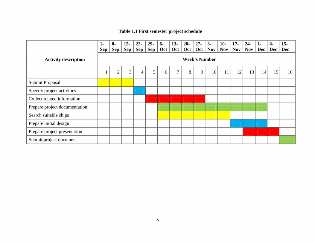
1) First semester project schedule: Schedule refers to the activities that should be
complete in the first semester. Table 1.1 shows first semester activities.
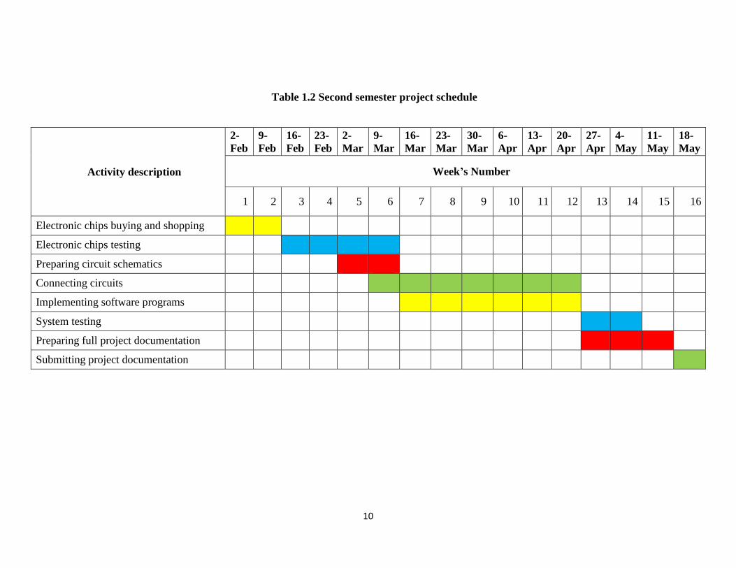
2) Second semester project schedule: Schedule refers to the activities should be
done in the second semester. Table 1.2 shows second semester activities.
9
Table 1.1 First semester project schedule
Activity description
1-
Sep
8-
Sep
15-
Sep
22-
Sep
29-
Sep
6-
Oct
13-
Oct
20-
Oct
27-
Oct
3-
Nov
10-
Nov
17-
Nov
24-
Nov
1-
Dec
8-
Dec
15-
Dec
Week’s Number
1 2 3 4 5 6 7 8 9 10 11 12 13 14 15 16
Submit Proposal
Specify project activities
Collect related information
Prepare project documentation
Search suitable chips
Prepare initial design
Prepare project presentation
Submit project document
10
Table 1.2 Second semester project schedule
Activity description
2-
Feb
9-
Feb
16-
Feb
23-
Feb
2-
Mar
9-
Mar
16-
Mar
23-
Mar
30-
Mar
6-
Apr
13-
Apr
20-
Apr
27-
Apr
4-
May
11-
May
18-
May
Week’s Number
1 2 3 4 5 6 7 8 9 10 11 12 13 14 15 16
Electronic chips buying and shopping
Electronic chips testing
Preparing circuit schematics
Connecting circuits
Implementing software programs
System testing
Preparing full project documentation
Submitting project documentation
11
Chapter 2
Components Background
2.1 Cameras
2.2 Image processing
2.3 Microcontrollers
2.4 Digital signal processing
2.5 Wi-Fi Technology
2.6 Wireless Transceivers Technologies
2.7 Solar Energy
12
2.1 Cameras
Closed-circuit television (CCTV) cameras can produce images or recordings
for surveillance purposes, and can be either video cameras, or digital stills cameras
[7].
It is most often applied for surveillance in areas that may need monitoring such as
banks, airports and convenience stores.
2.1.1 Video Cameras
Video cameras are either analog or digital.
Analog: Can record straight to a video tape recorder which is able to record
analogue signals as pictures.
Digital: These cameras do not require a video capture card because they work
using a digital signal which can be saved directly to a computer [7].
2.1.2 History
The first CCTV system was installed by Siemens AG in Germany at 1942. The
earliest systems required constant monitoring because there was no way to record and
store the information. Recording systems would be introduced later, when primitive
reel-to-reel media was used to preserve the data, where the magnetic tapes had to be
changed manually. It was a time consuming, expensive and unreliable process; the
operator had to manually thread the tape from the tape reel through the recorder onto
an empty take-up reel. Due to these efforts, video surveillance was rare. Only
when VCR technology became available in the 1970s, which made it easy to record
and erase information, did video surveillance start to become much more common.
13
During the 1990s digital multiplexing, which allowed for several cameras to
record at once, and introduced time lapse and motion only recording has increased
the use of CCTV across the country and increased the savings of time and money.
In recent decades, especially with general crime fears growing in the 1990s and
2000s, public space use of surveillance cameras has taken off [8].
2.1.3 Some Types of Cameras
Infrared/Night Vision: These night-vision cameras have the ability to see images
in pitch black conditions using IR LEDs. In some cases they are for mobile
applications.
Network/IP: These cameras, both hardwired and wireless, transmit images over
the Internet, often compressing the bandwidth so as not to overwhelm the web. IP
cameras are easier to install than analog cameras because they do not require a
separate cable run or power boost to send images over a longer distance.
Wireless: Not all wireless cameras are IP-based. Some wireless cameras can use
alternative modes of wireless transmission
Day/Night: Day/night cameras compensate for varying light conditions to allow
the camera to capture images. These are primarily used in outdoor applications
High-Definition Cameras :These give the operators the ability to zoom in with
extreme clarity
Board Cameras: These tiny cameras are well suited for desktop use [9].
14
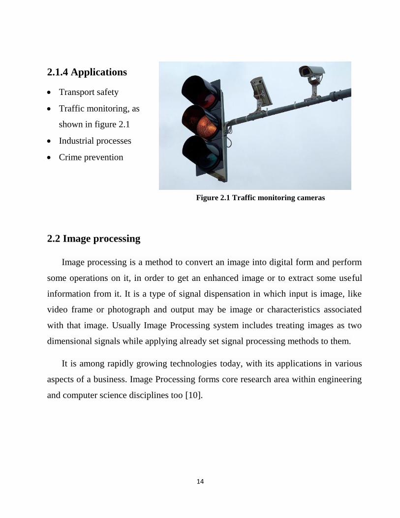
2.1.4 Applications
Transport safety
Traffic monitoring, as
shown in figure 2.1
Industrial processes
Crime prevention
Figure 2.1 Traffic monitoring cameras
2.2 Image processing
Image processing is a method to convert an image into digital form and perform
some operations on it, in order to get an enhanced image or to extract some useful
information from it. It is a type of signal dispensation in which input is image, like
video frame or photograph and output may be image or characteristics associated
with that image. Usually Image Processing system includes treating images as two
dimensional signals while applying already set signal processing methods to them.
It is among rapidly growing technologies today, with its applications in various
aspects of a business. Image Processing forms core research area within engineering
and computer science disciplines too [10].
15
Image processing basically includes the following three steps:
Importing the image with optical scanner or by digital photography
Analyzing and manipulating the image which includes data compression and
image enhancement and spotting patterns that are not to human eyes like satellite
photographs.
Output is the last stage in which result can be altered image or report that is based
on image analysis [10].
2.2.1 Purpose of Image processing
The purpose of image processing is divided into 5 groups [10]. They are:
1) Visualization - Observe the objects that are not visible.
2) Image sharpening and restoration - To create a better image.
3) Image retrieval - Seek for the image of interest.
4) Measurement of pattern – Measures various objects in an image.
5) Image Recognition – Distinguish the objects in an image.
2.2.2 Types of Image processing
The two types of methods used for Image Processing are Analog and Digital
Image Processing. Analog or visual techniques of image processing can be used for
the hard copies like printouts and photographs. Image analysts use various
fundamentals of interpretation while using these visual techniques. The image
processing is not just confined to area that has to be studied but on knowledge of
16
analyst. Association is another important tool in image processing through visual
techniques. So analysts apply a combination of personal knowledge and collateral
data to image processing.
Digital Processing techniques help in manipulation of the digital images by using
computers. As raw data from imaging sensors from satellite platform contains
deficiencies. To get over such flaws and to get originality of information, it has to
undergo various phases of processing. The three general phases that all types of data
have to undergo while using digital technique are Pre- processing, enhancement and
display, information extraction [10].
2.2.3 Image processing applications
Digital image processing, as a computer based technology, carries out automatic
processing, manipulation and interpretation of such visual information, and it plays
an increasingly important role in many aspects of our daily life, as well as in a wide
variety of disciplines and fields in science and technology, with applications such as
television, photography, robotics, remote sensing, medical diagnosis and industrial
inspection, and this list:
1) Intelligent transportation systems.
2) Remote sensing.
3) Moving object tracking.
5) Biomedical imaging techniques.
4) Defense surveillance.
6) Automatic visual inspection system [11].
17
2.2.4 Image Processing Software
GNU Octave is a free and open source alternative to Matlab. It was initially
conceived around 1988 as an accompaniment for a textbook on chemical reactor
design, at the University of Wisconsin . It was developed further in 1992, leading to a
full 1.0 release in 1994. It was licensed under the GPL, a free and open-source
software license, as part of the GNU Project1, hence the name "GNU Octave" [12].
GNU Octave is a high-level language, primarily intended for numerical
computations. It provides a convenient command line interface for solving linear and
nonlinear problems numerically, and for performing other numerical experiments using
a language that is mostly compatible with Matlab. It may also be used as a batch-
oriented language.
Octave has extensive tools for solving common numerical linear algebra
problems, finding the roots of nonlinear equations, integrating ordinary functions,
manipulating polynomials, and integrating ordinary differential and differential-
algebraic equations. It is easily extensible and customizable via user-defined functions
written in Octave's own language, or using dynamically loaded modules written in
C++, C, Fortran, or other languages [13].
2.3 Microcontrollers
A microcontroller is a small computer on a single integrated circuit containing a
processor core, memory, and programmable input/output peripherals. Program
memory in the form of NOR flash or OTP ROM is also often included on chip, as
well as a typically small amount of RAM. Microcontrollers are designed for
embedded applications, in contrast to the microprocessors used in personal computers
or other general purpose applications [14].

18
2.3.1 Applications
Microcontrollers are used in automatically controlled products and devices, such
as automobile engine control systems, implantable medical devices, remote controls,
office machines, appliances, power tools, toys and other embedded systems. By
reducing the size and cost compared to a design that uses a separate microprocessor,
memory, and input/output devices, microcontrollers make it economical to digitally
control even more devices and processes [14].
Some featured types of applications:
Alternative Energy
Automotive & Transportation
Consumer & Portable Electronics
Industrial
Medical
Smart Grid
2.3.2 Classification of Microcontrollers
Microcontrollers are classified on different aspects like architecture,
programming language used, bus width, memory, instruction set etc. There are a huge
variety of microcontrollers. The can be classified on following:
Internal bus width:
4 bit, 8 bit, 16 bit, 32 bit
Instruction set:
C.I.S.C
R.I.S.C
Architecture:
Harvard
Von Neumann (or Princeton)
19
Memory:
FLASH
EEPROM
SRAM
Embedded memory
External memory
Families:
ATMEL AVR - atmega, Xmega, Attinyâ
PIC - PIC16F, PIC18F
ARM - ARM7, ARM9, ARM11
8051 - AT89s52, p89v51rd2
Motorola - 68HC11
Integrated Peripherals:
Number of I/O ports.
Number and type of timers.
A.D.C
Other I/O interfaces like U.A.R.T, S.P.I [15].
2.3.3 Raspberry Pi Microcontroller
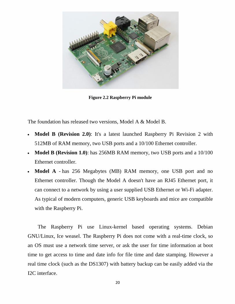
The Raspberry Pi shown in figure 2.2 is a single-board computer developed in
the UK by the Raspberry Pi Foundation. The Raspberry Pi is a credit-card sized
computer that plugs into the TV and a keyboard. It‟s a capable little PC which can be
used for many of the things that a desktop PC does, like spreadsheets, word-
processing and games. It also plays high-definition video. The design is based around
a Broadcom BCM2835 SoC, which includes an ARM1176JZF-S 800 MHz processor,
Video Core IV GPU, and 256 or 512 Megabytes of RAM. The design does not
include a built-in hard disk or solid-state drive, instead relying on an SD card for
booting and long-term storage. This board is intended to run Linux kernel based
operating systems [16].
20
Figure 2.2 Raspberry Pi module
The foundation has released two versions, Model A & Model B.
Model B (Revision 2.0): It's a latest launched Raspberry Pi Revision 2 with
512MB of RAM memory, two USB ports and a 10/100 Ethernet controller.
Model B (Revision 1.0): has 256MB RAM memory, two USB ports and a 10/100
Ethernet controller.
Model A - has 256 Megabytes (MB) RAM memory, one USB port and no
Ethernet controller. Though the Model A doesn't have an RJ45 Ethernet port, it
can connect to a network by using a user supplied USB Ethernet or Wi-Fi adapter.
As typical of modern computers, generic USB keyboards and mice are compatible
with the Raspberry Pi.
The Raspberry Pi use Linux-kernel based operating systems. Debian
GNU/Linux, Ice weasel. The Raspberry Pi does not come with a real-time clock, so
an OS must use a network time server, or ask the user for time information at boot
time to get access to time and date info for file time and date stamping. However a
real time clock (such as the DS1307) with battery backup can be easily added via the
I2C interface.
21
The Raspberry Pi Foundation has released various SD Card images that can be
loaded onto an SD Card to produce a preliminary operating system. The image is
based upon Linux version of Debian OS (Raspbian) with the LXDE desktop and the
Midori browser, plus various programming tools. The image can also run on QEMU
allowing the Raspberry Pi to be emulated on various other platforms [16].
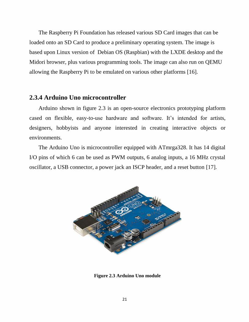
2.3.4 Arduino Uno microcontroller
Arduino shown in figure 2.3 is an open-source electronics prototyping platform
cased on flexible, easy-to-use hardware and software. It‟s intended for artists,
designers, hobbyists and anyone interested in creating interactive objects or
environments.
The Arduino Uno is microcontroller equipped with ATmrga328. It has 14 digital
I/O pins of which 6 can be used as PWM outputs, 6 analog inputs, a 16 MHz crystal
oscillator, a USB connector, a power jack an ISCP header, and a reset button [17].
Figure 2.3 Arduino Uno module
22
2.3.4.1 Power
The board can be powered via USB, DC adapter (wall-wart) or battery. The
power source is selected automatically. To use AC to DC adapter we need 2.1mm
center-positive plug power jack. Battery can be connected either to USB, power jack
or inserted in Gnd and Vin pin heads of the POWER connector. The recommended
range of supply is 7 to 12 volts despite limits of 6 to 20 volt due to the fact that
voltage lover than 7V makes 5V onboard pin unstable and voltage higher then 12V
can lead the voltage regulator to overheat and directly damage the board [17].
2.3.4.2 Memory
The ATmega328 has 32 KB (with 0.5 KB used for the boot loader). It also has 2
KB of SRAM and 1 KB of EEPROM [17].
2.3.4.3 Programming
As it comes to programming Arduino Uno can be programmed with provided
software. The board is pre burned with boot loader that allows to upload new code to
it directly via USB, no external hardware programmer needed [17].
The Arduino programming language is a simplified version of C/C++ [18].
It is intended to use Raspberry Pi rather than Arduino Uno microcontroller
because the project deals with cameras that are easier to be connected to Raspberry
Pi. Also microcontroller must perform the image processing that requires high
processing speed.
23
2.4 Digital signal processing
Signal processing is the action of changing one or more features (parameters) of a
digital signal according to a predetermined requirement. The parameters that are to be
changed may be amplitude, frequency, and phase.
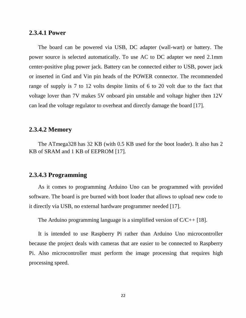
The signals that are to be processed are converted into numerical form before any
processing. This conversion is known as sampling, the sampling wave is shown in
figure 2.4, according to sampling theorem, an analog signal can be exactly
reconstructed from its samples if the sampling rate is at least twice the highest
frequency component present in the signal [19].
Figure 2.4 Sampling wave
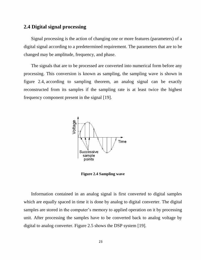
Information contained in an analog signal is first converted to digital samples
which are equally spaced in time it is done by analog to digital converter. The digital
samples are stored in the computer‟s memory to applied operation on it by processing
unit. After processing the samples have to be converted back to analog voltage by
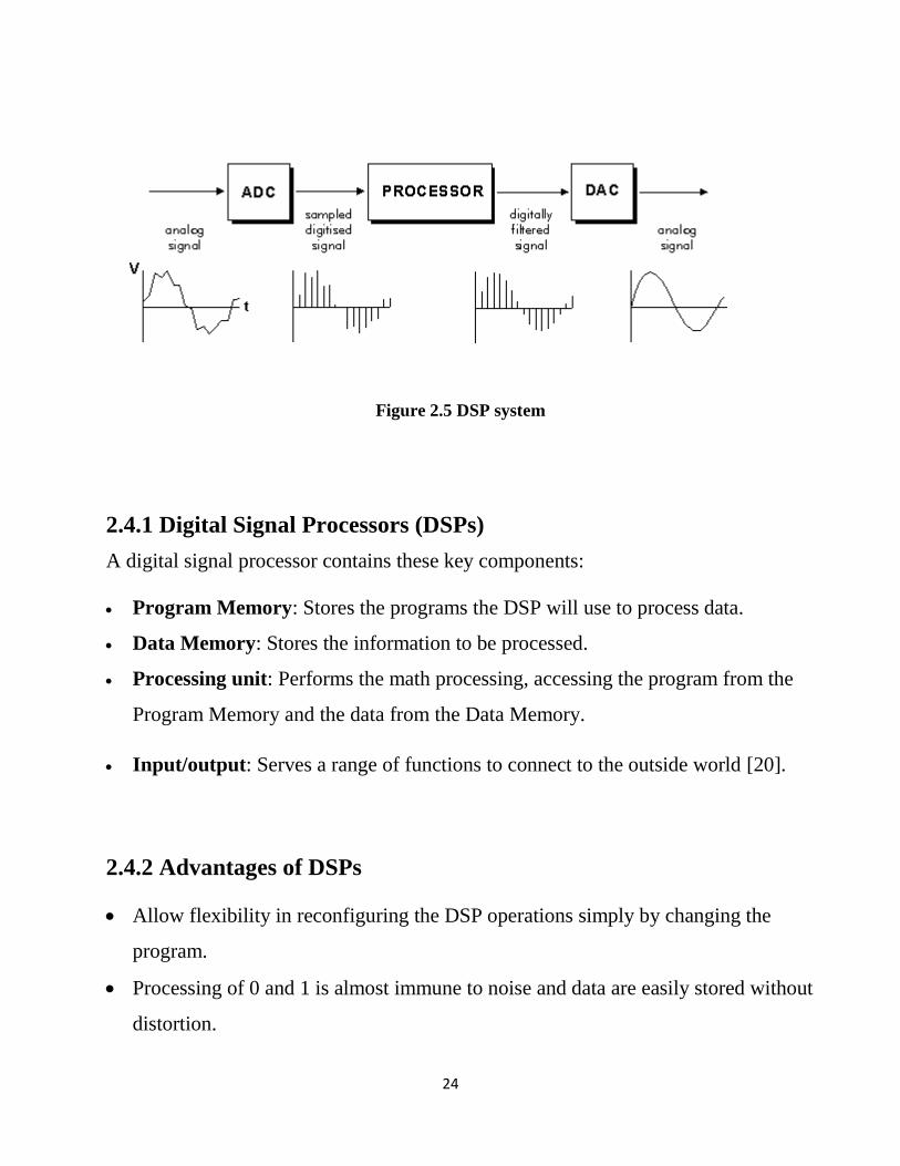
digital to analog converter. Figure 2.5 shows the DSP system [19].
24
Figure 2.5 DSP system
2.4.1 Digital Signal Processors (DSPs)
A digital signal processor contains these key components:
Program Memory: Stores the programs the DSP will use to process data.
Data Memory: Stores the information to be processed.
Processing unit: Performs the math processing, accessing the program from the
Program Memory and the data from the Data Memory.
Input/output: Serves a range of functions to connect to the outside world [20].
2.4.2 Advantages of DSPs
Allow flexibility in reconfiguring the DSP operations simply by changing the
program.
Processing of 0 and 1 is almost immune to noise and data are easily stored without
distortion.
25
Security can be introduced by encrypting [21].
Complex algorithms fit into a single chip.
Digital processing is insensitive to component tolerances, aging, environmental
conditions and electromagnetic interference.
Noise is easy to control after initial quantization [22].
Cheaper to implement.
Can be stored on disk [23].
2.4.3 Disadvantages of DSPs
Require significantly more power [22].
When the signal is weak, within a few tenths of millivolts, we cannot amplify the
signal after it is digitized.
Finite word length problems [23].
2.4.4 DSP Applications
Communication systems
Modulation/demodulation, channel equalization, echo cancellation.
Music
Synthetic instruments, audio effects, noise reduction.
Consumer electronics
Perceptual coding of audio and video on DVDs, speech synthesis, speech
recognition.
Experimental physics
Sensor-data evaluation.
26
Medical diagnostics
Magnetic-resonance and ultrasonic imaging, computer tomography, audiology.
Engineering
Control systems, feature extraction for pattern recognition.
Security
Surveillance system, signal intelligence [22].
Image processing
Filtering, edge effects, enhancement [23].
2.5 Wi-Fi Technology
Wi-Fi is an abbreviation of the phrase Wireless Fidelity. Wi-Fi is a popular
technology that allows an electronic device to exchange data or connect to the
internet wirelessly using radio waves. The Wi-Fi Alliance defines Wi-Fi as any
"wireless local area network (WLAN) products that are based on the Institute of
Electrical and Electronics Engineers' (IEEE) 802.11 standards". Wi-Fi technology in
recent years is growing rapidly and is widely used throughout the world.
Many devices can use Wi-Fi, e.g. personal computers, video-game consoles,
smart phones, some digital cameras, tablet computers and digital audio players. These
can connect to a network resource such as the Internet via a wireless network access
point. Such an access point (or hotspot) has a range of about 20 meters (65 feet)
indoors and a greater range outdoors. Hotspot coverage can comprise an area as small
as a single room with walls that block radio waves, or as large as many square miles
achieved by using multiple overlapping access points [24].
27
2.5.1 Historical Background
Wi-Fi technology has its origins in a 1985 ruling by the US Federal
Communications Commission that released the ISM band for unlicensed use. In
1991, NCR Corporation with AT&T Corporation invented the precursor to 802.11
intended for use in cashier systems.
A key patent used in Wi-Fi was developed by the Australian radio astronomer
John O'Sullivan as a by-product in a CSIRO research project, "a failed experiment to
detect exploding mini black holes the size of an atomic particle". In 1992 and 1996,
Australian organization CSIRO obtained patents for a method later used in Wi-Fi to
"unsmear" the signal.
In 1999, the Wi-Fi Alliance was formed as a trade association to hold the Wi-Fi
trademark under which most products are sold [25].
2.5.2 Advantages and Limitations
Advantages:
The main advantages of using Wi-Fi technology is the lack of wires. This is a
wireless connection that can merge together multiple devices. Wi-Fi network is
particularly useful in cases where the wiring is not possible or even unacceptable. For
example, it is often used in the halls of conferences and international exhibitions. It is
ideal for buildings that are considered architectural monuments of history, as it
excludes the wiring cables.
28
Wi-Fi allows cheaper deployment of local area networks (LANs). Also spaces
where cables cannot be run, such as outdoor areas and historical buildings, can host
wireless LANs.
Wi-Fi networks are widely used to connect a variety of devices, not only between
themselves but also to the Internet. And almost all modern laptops, tablets, and some
mobile phones have this feature. It is very convenient and allows to connect to the
internet almost anywhere, not just where the cables are laid [26].
Limitations:
Wi-Fi has a limited radius of action and it is suitable for home networking, which
is more dependent on the environment.
At high density Wi-Fi-points operating in the same or adjacent channels, they can
interfere with each other. This affects the quality of the connection [27].
2.5.3 Wi-Fi Standards
802.11 Protocols
The 802.11 family consist of a series of half-duplex over-the-air modulation
techniques that use the same basic protocol. The most popular are those defined by
the 802.11b and 802.11g protocols, which are amendments to the original standard.
802.11-1997 was the first wireless networking standard in the family, but
802.11b was the first widely accepted one, followed by 802.11a and 802.11g.
802.11n is a new multi-streaming modulation technique. Other standards in the
family (c–f, h, j) are service amendments and extensions or corrections to the
29
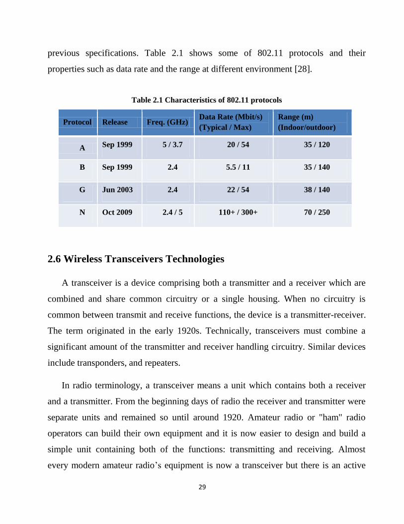
previous specifications. Table 2.1 shows some of 802.11 protocols and their
properties such as data rate and the range at different environment [28].
Table 2.1 Characteristics of 802.11 protocols
2.6 Wireless Transceivers Technologies
A transceiver is a device comprising both a transmitter and a receiver which are
combined and share common circuitry or a single housing. When no circuitry is
common between transmit and receive functions, the device is a transmitter-receiver.
The term originated in the early 1920s. Technically, transceivers must combine a
significant amount of the transmitter and receiver handling circuitry. Similar devices
include transponders, and repeaters.
In radio terminology, a transceiver means a unit which contains both a receiver
and a transmitter. From the beginning days of radio the receiver and transmitter were
separate units and remained so until around 1920. Amateur radio or "ham" radio
operators can build their own equipment and it is now easier to design and build a
simple unit containing both of the functions: transmitting and receiving. Almost
every modern amateur radio‟s equipment is now a transceiver but there is an active
Protocol Release Freq. (GHz) Data Rate (Mbit/s)
(Typical / Max)
Range (m)
(Indoor/outdoor)
A Sep 1999 5 / 3.7 20 / 54 35 / 120
B Sep 1999 2.4 5.5 / 11 35 / 140
G Jun 2003 2.4 22 / 54 38 / 140
N Oct 2009 2.4 / 5 110+ / 300+ 70 / 250
30
market for pure radio receivers, mainly for shortwave listening (SWL) operators. An
example of a transceiver would be a walkie-talkie, or a CB radio[29].
The RF Transceiver uses RF modules for high speed data transmission. The
microelectronic circuits in the digital-RF architecture work at speeds up to 100 GHz.
The objective in the design was to bring digital domain closer to the antenna, both at
the receiver and transmitter ends using software defined radio (SDR). The software-
programmable digital processors used in the circuits permit conversion between
digital baseband signals and analog RF [30].
2.6.1 ZigBee
ZigBee is a specification for a suite of high level communication protocols used
to create personal area networks built from small, low-power digital radios. ZigBee is
based on an IEEE 802.15 standard. Though low-powered, ZigBee devices often
transmit data over longer distances by passing data through intermediate devices to
reach more distant ones, creating a mesh network; i.e., a network with no centralized
control or high-power transmitter/receiver able to reach all of the networked devices.
The decentralized nature of such wireless ad hoc networks makes them suitable for
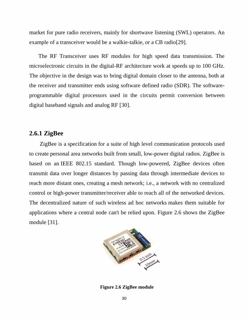
applications where a central node can't be relied upon. Figure 2.6 shows the ZigBee
module [31].
Figure 2.6 ZigBee module
31
ZigBee is used in applications that require a low data rate, long battery life, and
secure networking. ZigBee has a defined rate of 250 Kbit/s, best suited for periodic or
intermittent data or a single signal transmission from a sensor or input device.
Applications include wireless light switches, electrical meters with in-home-displays,
traffic management systems, and other consumer and industrial equipment that
requires short-range wireless transfer of data at relatively low rates. The technology
defined by the ZigBee specification is intended to be simpler and less expensive than
other WPANs, such as Bluetooth or Wi-Fi.
ZigBee networks are secured by 128 bit symmetric encryption keys. In home
automation applications, transmission distances range from 10 to 100 meters line-of-
sight, depending on power output and environmental characteristics [31].
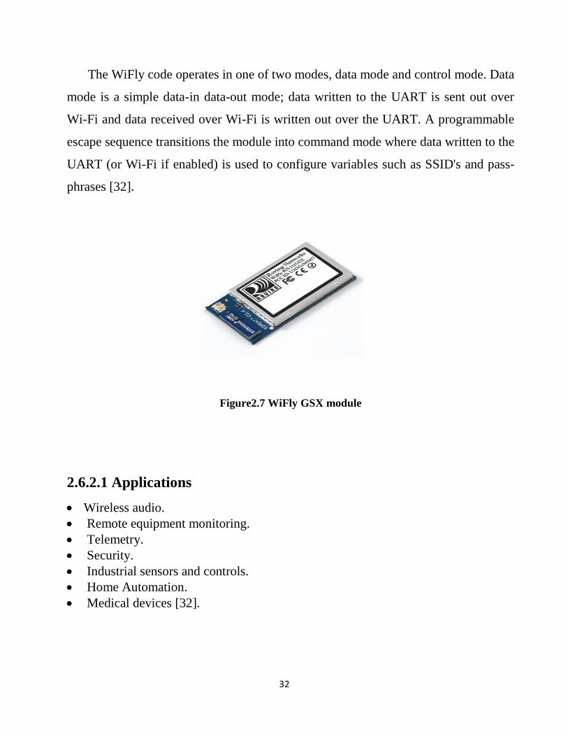
2.6.2 WiFly GSX transceiver
The WiFly GSX module shown in figure 2.7 is a standalone, embedded wireless
802.11 networking module. The module is fully qualified and Wi-Fi certified 2.4
GHz IEEE 802.11b/g transceiver.
Because of its small size and extremely low power consumption, the WiFly
module is perfect for mobile wireless applications such as asset monitoring, GPS
tracking and battery sensors.
In the simplest configuration the hardware only requires four connections (PWR,
TX, RX, GND) to create a wireless data connection. The WiFly GSX module is
programmed and controlled with a simple ASCII command language. Once the
WiFly GSX is setup it can scan to find an access point, associate, authenticate and
connect over any Wi-Fi network .
32
The WiFly code operates in one of two modes, data mode and control mode. Data
mode is a simple data-in data-out mode; data written to the UART is sent out over
Wi-Fi and data received over Wi-Fi is written out over the UART. A programmable
escape sequence transitions the module into command mode where data written to the
UART (or Wi-Fi if enabled) is used to configure variables such as SSID's and pass-
phrases [32].
Figure2.7 WiFly GSX module
2.6.2.1 Applications
Wireless audio.
Remote equipment monitoring.
Telemetry.
Security.
Industrial sensors and controls.
Home Automation.
Medical devices [32].
33
2.6.2.2 WiFly 4
WiFly 4.00 is the default firmware for all Wi-Fi modules, replacing all previous
WiFly versions. WiFly 4.00 provides a number of enhancements such as enterprise
security, AP Mode and secondary UDP broadcast [32].
It is intended to use a Wi-Fi transceiver rather than ZigBee transceiver since it is
planned to have a centralized network that sends the multicast alarm messages to
specific receivers. So the Ad-hoc network of ZigBee is not of high interest. Also
messages must be sent to far distances which are only possible by Wi-Fi.
2.7 Solar Energy
Solar energy is energy that comes from the sun. Every day the sun radiates an
enormous amount of energy. The sun radiates more energy in one second than
people have used since the beginning of time. All this energy comes from within the
sun itself. Like other stars, the sun is a big gas ball made up mostly of hydrogen and
helium. The sun generates energy in its core in a process called nuclear fusion.
During nuclear fusion, the sun‟s extremely high pressure and hot temperature
cause hydrogen atoms to come apart and their nuclei to fuse or combine. Some
matter is lost during nuclear fusion. The lost matter is emitted into space as radiant
energy.
It takes millions of years for the energy in the sun‟s core to make its way to the
solar surface, and then approximately eight minutes to travel the 93 million miles to
earth. The solar energy travels to the earth at a speed of 186,000 miles per second, the
speed of light.

34
Only a small portion of the energy radiated by the sun into space strikes the earth,
one part in two billion. Yet this amount of energy is enormous. Every day enough
energy strikes the United States to supply the nation‟s energy needs for one and a half
years! About 15 percent of the sun‟s energy that hits the earth is reflected back into
space. Another 30 percent is used to evaporate water, which, lifted into the
atmosphere, produces rainfall. Plants, the land, and the oceans also absorb solar
energy. The rest could be used to supply our needs [33].
2.7.1 Principle of Operation
Light (photons) striking certain compounds, in particular metals, causes the
surface of the material to emit electrons. Light striking other compounds causes the
material to accept electrons. It is the combination of these two compounds that can be
made use of to cause electrons to flow through a conductor, and thereby create
electricity. This phenomenon is called the photo-electric effect. Photovoltaic means
sunlight converted into a flow of electrons (electricity).
Solar power is a rapidly developing energy source in Australia and around the
world. The potential for using the sun to directly supply our power needs is huge,
Solar panels can generate electricity without any waste or pollution, or dependence
on the Earth‟s natural resources once they are constructed. Solar panels have no
moving parts so they are very reliable and have a long life span. Solar panels are
relatively easy to install and are very low maintenance .
35
A useful characteristic of solar photovoltaic power generation is that it can be
installed on any scale as opposed to conventional forms of power generation which
require large scale plant and maintenance. Solar panels can be installed to generate
power where it is needed which removes the need to transport and distribute power
over long distances to remote areas [34].
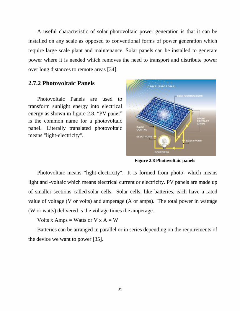
2.7.2 Photovoltaic Panels
Photovoltaic Panels are used to
transform sunlight energy into electrical
energy as shown in figure 2.8. “PV panel”
is the common name for a photovoltaic
panel. Literally translated photovoltaic
means "light-electricity".
Figure 2.8 Photovoltaic panels
Photovoltaic means "light-electricity". It is formed from photo- which means
light and -voltaic which means electrical current or electricity. PV panels are made up
of smaller sections called solar cells. Solar cells, like batteries, each have a rated
value of voltage (V or volts) and amperage (A or amps). The total power in wattage
(W or watts) delivered is the voltage times the amperage.
Volts x Amps = Watts or V x A = W
Batteries can be arranged in parallel or in series depending on the requirements of
the device we want to power [35].
36
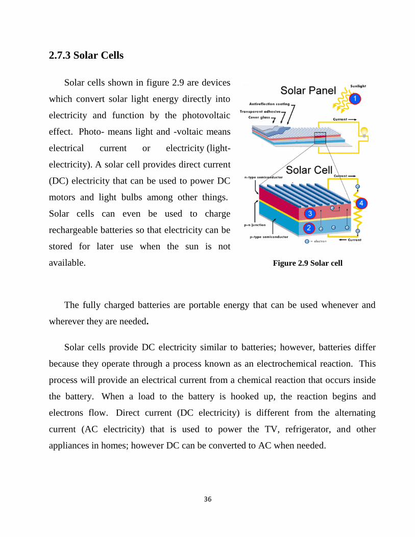
2.7.3 Solar Cells
Solar cells shown in figure 2.9 are devices
which convert solar light energy directly into
electricity and function by the photovoltaic
effect. Photo- means light and -voltaic means
electrical current or electricity (light-
electricity). A solar cell provides direct current
(DC) electricity that can be used to power DC
motors and light bulbs among other things.
Solar cells can even be used to charge
rechargeable batteries so that electricity can be
stored for later use when the sun is not
available. Figure 2.9 Solar cell
The fully charged batteries are portable energy that can be used whenever and
wherever they are needed.
Solar cells provide DC electricity similar to batteries; however, batteries differ
because they operate through a process known as an electrochemical reaction. This
process will provide an electrical current from a chemical reaction that occurs inside
the battery. When a load to the battery is hooked up, the reaction begins and
electrons flow. Direct current (DC electricity) is different from the alternating
current (AC electricity) that is used to power the TV, refrigerator, and other
appliances in homes; however DC can be converted to AC when needed.
37
Solar cells produce DC electricity from light. Sunlight contains packets of
energy called photons that can be converted directly into electrical energy. One can‟t
see the photons but they hit the cell and produce free electrons that move through the
wires and cause an electrical current as shown in figure 2.9. The electrical current is
the electricity that powers the load. Although the photons can't be seen, one can see
the light and assume that the amount of photons hitting the solar cell is related to the
amount of light hitting the solar cell. A greater amount of light available means a
greater amount of photons are hitting the solar cell and generating more power from
it [35].
2.7.4 Advantages and Disadvantages of Solar Energy
Advantages:
Solar energy makes use of a renewable natural resource that is readily available.
Solar power does not create carbon dioxide or other toxic emissions.
Use of solar thermal power to heat water or generate electricity will help reduce
the Territory‟s complete dependence on fossil fuels.
Solar water heaters are an established technology, readily available on the
commercial market, and simple enough to build, install and maintain.
The production of electricity by the photovoltaic process is quiet and produces no
toxic fumes.
PV cells generate direct-current electricity that can be stored in batteries and used
in a wide range of voltages depending on the configuration of the battery bank.
Although most electric appliances operate on alternating current, an increasing
number of appliances using direct current are now available. Where these are not
practical, PV-generated direct current can be changed into alternating current by
using inverters [36].

38
Disadvantages:
Solar thermal systems are not cost-effective in areas that have long periods of
cloudy weather or short daylight hours.
The arrays of collecting devices for large systems cover extensive land areas.
Solar thermal systems only work with sunshine and do not operate at night or in
inclement weather. Storage of hot water for domestic or commercial use is
simple, using insulated tanks, but storage of fluids at the higher temperatures
needed for electrical generation, or storage of electricity itself, needs further
technical development.
Photovoltaic-produced electricity is presently more expensive than power supplied
by utilities.
Batteries need periodic maintenance and replacement.
High voltage direct-current electricity can pose safety hazards to inadequately
trained home operators or utility personnel [36].
2.7.5 Applications
Indoor and outdoor Lighting
Water heating
Cooking using solar cookers
Water treatment using Solar Stills
Battery Charging
Electricity production
39
Chapter 3
System Conceptual Design
3.1 Overview
3.2 General block diagram
3.3 Main components
3.4 System flowcharts
3.5 System functions
3.6 Software
40
3.1 Overview
In this chapter we will describe the system main parts and the design concepts.
We will illustrate the general block diagram, system main components. Then describe
some details of the inner blocks or components and how it is related to other
components will be described.
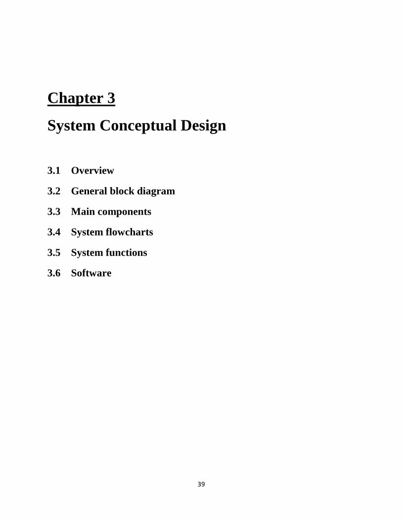
3.2 General block diagram
The main parts of the system as shown in general system block diagram figure
3.1 are: solar system as a power supply, congestion detection system to decide the
congestion occurrence, Wi-Fi transmitter, Wi-Fi receiver with alarm system to alert
the drivers if congestion occurs.
Solar system Congestion detection system Transmitter
Figure 3.1 General block diagram
Photovoltaic
cells
Charge
controller
Backup
batteries
Wi-Fi
transmitter
Digital signal
processing
Microcontroller Cameras
Wi-Fi
receivers
Alarm in the car
(sound or light)
On-screen message
outside the car (LCD)
41
3.3 Main components
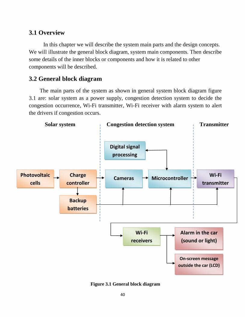
3.3.1 Solar System
Solar power systems provide a continuous, reliable power solution that's easily
deployed, cost-effective and require little maintenance. As shown in figure 3.2, the
main components of the solar system are:
a) Photovoltaic cells: Photovoltaic is the direct conversion of light into electricity at
the atomic level. Some materials exhibit a property known as the photoelectric
effect that causes them to absorb photons of light and release electrons. When
these free electrons are captured, resulting electric current can be used as
electricity. Silicon is a material known as a semiconductor as it conducts
electricity and it is the main material for photovoltaic cells. Impurities such as
boron or phosphorus are added to this base material. These impurities create the
environment for electrons to be freed when sunlight hits the photovoltaic panel.
The freeing of electrons leads to the production of electricity [37].
b) Charge controller (CC): is needed to prevent overcharging of the batteries.
Proper charging will prevent damage and increase the life and performance of the
batteries [38].
c) Backup batteries: Batteries are used to store energy for use at a later time, like
night time or on cloudy days. The number of batteries used by the system varies
with battery type and anticipated storage needs [39].
42
Figure 3.2 Solar system
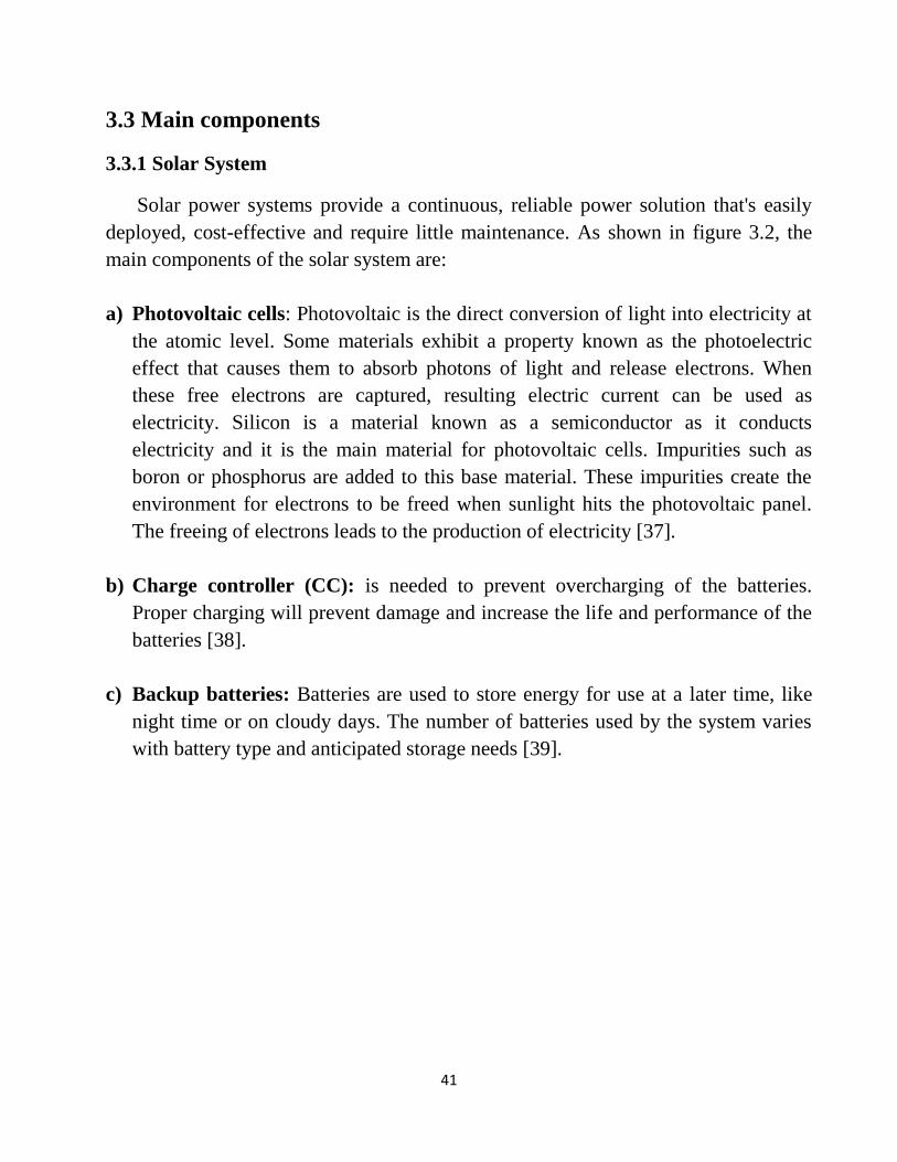
3.3.2 Congestion Detection System
Cameras are connected to the microcontroller. The MC takes and processes the
snapshots of the video camera. We will use two different ways for detecting the cars.
One is to compare the snapshots with previously saved images with congestion and
announce the intersection state to the transmitter. The other option is to process each
snapshot to count the number of vehicles. Figure 3.3 explains the connection of the
congestion detection system.
Figure 3.3 Congestion detection system
Digital signal
processing
Cameras
Microcontroller
I/O ADC
Memory
Tx
43
a) Cameras: It is planned to use a camera to communicate with the microcontroller
that has a camera interface. One camera may be not enough to observe all ways of
the intersection even with a wide angle range of view; so three to four cameras
will be used.
b) Microcontroller Unit: The image processing algorithm for traffic measurement is
realized by an image processing code written as Matlab commands that can be
run on the microcontroller.
1. A/D converter
The continuous analog signal of the camera is converted to digital to extract
the snapshots at different time intervals. This filter processing allows normalized
images to be obtained when there are variations in the lighting due to external
environmental conditions .
2. DSP algorithms
The image processing algorithm generated by Matlab software performs the
required analysis on the current frame of the video to decide the intersection state.
3. Memory in the microcontroller
The built in memory is used for storing images for later use and process by
the system. Snapshots are stored for reference comparing issues, or taken at
specified time intervals for direct processing .
44
4. I/O interfaces
The microcontroller Ethernet interface will be used for the microcontroller
to join the network. This will provide a continuous connection to the access point.
Also it will be used to communicate with the PC. Other built-in interfaces are
found as GPIO pins that will be used if needed .
3.3.3 Wi-Fi Transmitter
The microcontroller has an Ethernet port; it is easy to be connected to a Wi-Fi
access point. This access point will have an external directional antenna for the signal
to reach the far distances needed. Three or four external directional antennas will be
used to send to all the four lanes of the intersection.
3.3.4 Wi-Fi Receivers with built-in Alarm
The message from the antenna will reach the Wi-Fi devices since they are
connected to the access point. The devices are previously programmed to respond to
the message type as an alarm for the drivers to avoid the intersection, or as
permission for the drivers to continue their routes. The alarm is either a Buzzer sound
on the same receiver module.
45
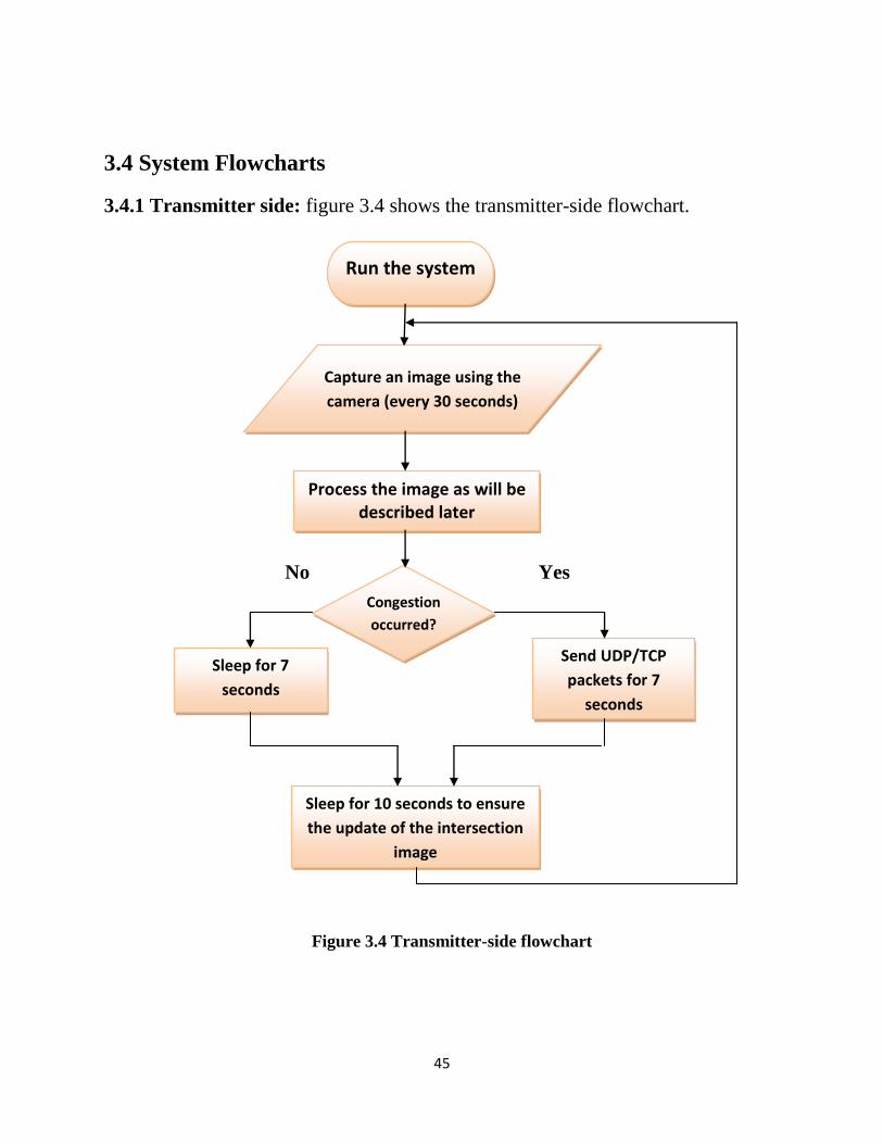
3.4 System Flowcharts
3.4.1 Transmitter side: figure 3.4 shows the transmitter-side flowchart.
No Yes
Figure 3.4 Transmitter-side flowchart
Run the system
Capture an image using the
camera (every 30 seconds)
Process the image as will be described later
Congestion
occurred?
Send UDP/TCP
packets for 7
seconds
Sleep for 7
seconds
Sleep for 10 seconds to ensure
the update of the intersection
image
46
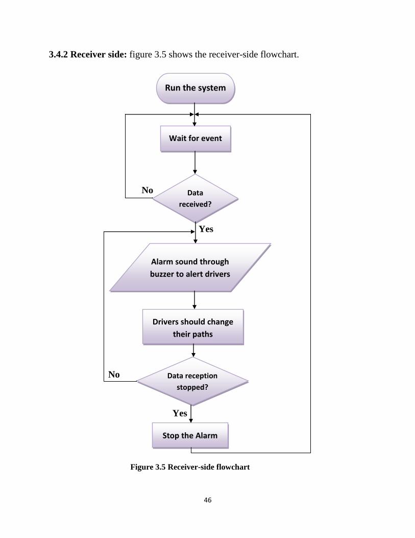
3.4.2 Receiver side: figure 3.5 shows the receiver-side flowchart.
No
Yes
No
Yes
Figure 3.5 Receiver-side flowchart
Run the system
Wait for event
Data
received?
Data reception
stopped?
Alarm sound through
buzzer to alert drivers
Stop the Alarm
Drivers should change
their paths

47
3.5 System Functions
In this section we show the functions at the intersection and at drivers‟ side. This
is illustrated in figure 3.6.
Intersection side
Drivers side
Figure 3.6 System functions
Take the images
at time intervals
Determine
congestion state
Receive the
signal
Send data to
drivers side
Analyze
received data
Process taken
images
Alarm sound through buzzer to alert drivers
Drivers should
decide the path
to go
48
3.6 Software
3.6.1 Raspberry Pi Programming
Raspberry pi is a miniature ARM based microcontroller that depends on Linux,
which is an incredibly robust and flexible operating system that can run on
everything from large supercomputers all the way down to small embedded devices.
To work with the Raspberry pi; It is required to put one of the supported Linux-based
OS images such as Raspbian , available on their official web site, to an SD card by
special disk imaging software, then install it on the microcontroller.
Raspberry pi supports a lot of programming languages. Some of them are:
Octave, Bare metal, C/C++, Java, Python, Scratch or any language that can be
compiled for the ARMv6 chip.
Model B of the raspberry pi that will be used supports a Matlab programmed
code. This code will be written within terminal in the Raspberry pi operating system
via the Ethernet interface [40].
3.6.2 Wi-Fi Module Programming
Programming the Wi-Fi module is just required at the receiver; because we are
using an access point at the transmitter. After this programming the Wi-Fi module
will be able to connect to the access point, receive the transmitted signal and translate
it to an alert for the drivers.
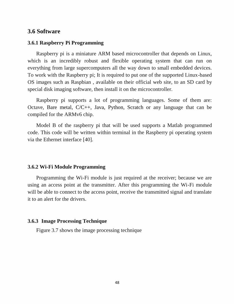
3.6.3 Image Processing Technique
Figure 3.7 shows the image processing technique
49
No Yes
No Yes
Figure 3.7 Image processing technique
Start
Load the saved reference image for the daytime from the SD card
Load the captured image from the previous
step in the "Transmitter flow chart"
Subtract background from the current image to obtain an
image with cars only and black background
Adjust the resulted image and remove the noise
Compute the number of connected components
based on their exterior boundaries
Median filtering then convert it to binary image
Find the area for both black and white pixels and
determine the ratio of black to white
Is (ratio<21&&
No. >8) ?
Pass "Congestion
occurred" to the
transmitter flow
chart
Time is Daytime?
Load the saved reference image for the nighttime from the SD card
Pass
"No congestion"
to the
transmitter flow
chart
50
Chapter 4
System Implementation
4.1 Overview
4.2 Solar power Parameters
4.3 Microcontroller Specifications and Setup
4.4 Network Configuration and Access points
4.5 Access the Raspberry pi GUI
4.6 Webcam Connection and Configuration
4.7 Image Processing Software (Octave)
4.8 Receiver Implementation and Configuration
4.9 Implementing the Image Processing Code
51
4.1 Overview
In this chapter we will explain the system design in details. We will calculate the
solar power system parameters, number of devices used and the software code to be
used for image processing.
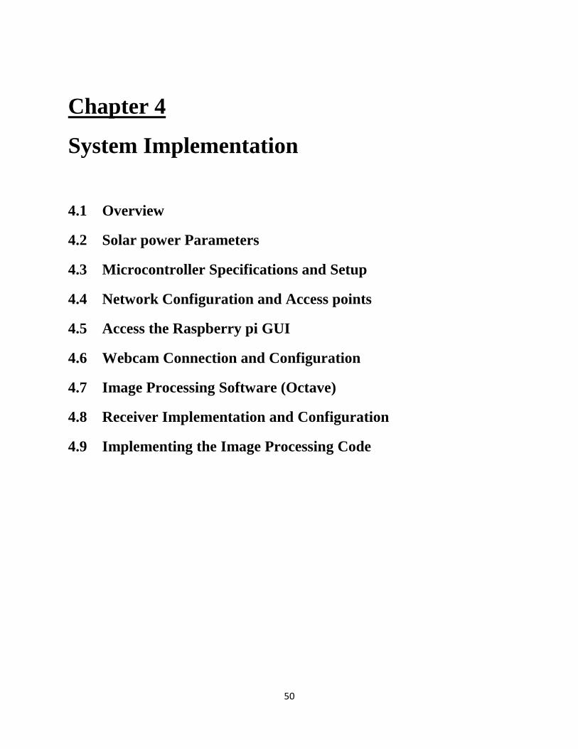
4.2 Solar power parameters
By examining the power dissipation of system appliances it is found that the
total wattage needed is 23 Watt. Here are the wattage values for them:
Considering the low power sleeping modes of devices and the time the system is
not working, we assume a working load of 16 hours in a day. Therefore total daily
watt-hours required is 23w*16hr = 368WH/day
= 12V, Battery charging efficiency = 87%
Watt-hours required for maximum depth of discharge of 87% is 368/0.87 = 423WH
Minimum Battery Capacity = 423/12v = 35.25 Ah
Average rate of solar radiation in Palestine is G = 5400 WH/ m^2 /day
PV area= wattage / (
* G)
PV area= 864 / (0.87 * 0.14 * 5400) = 0.56
Quantity Load Power usage for one Power
2 Wi-Fi access point 8 16
2 Raspberry pi and webcam 3.5 7
Total = 23 watt
52
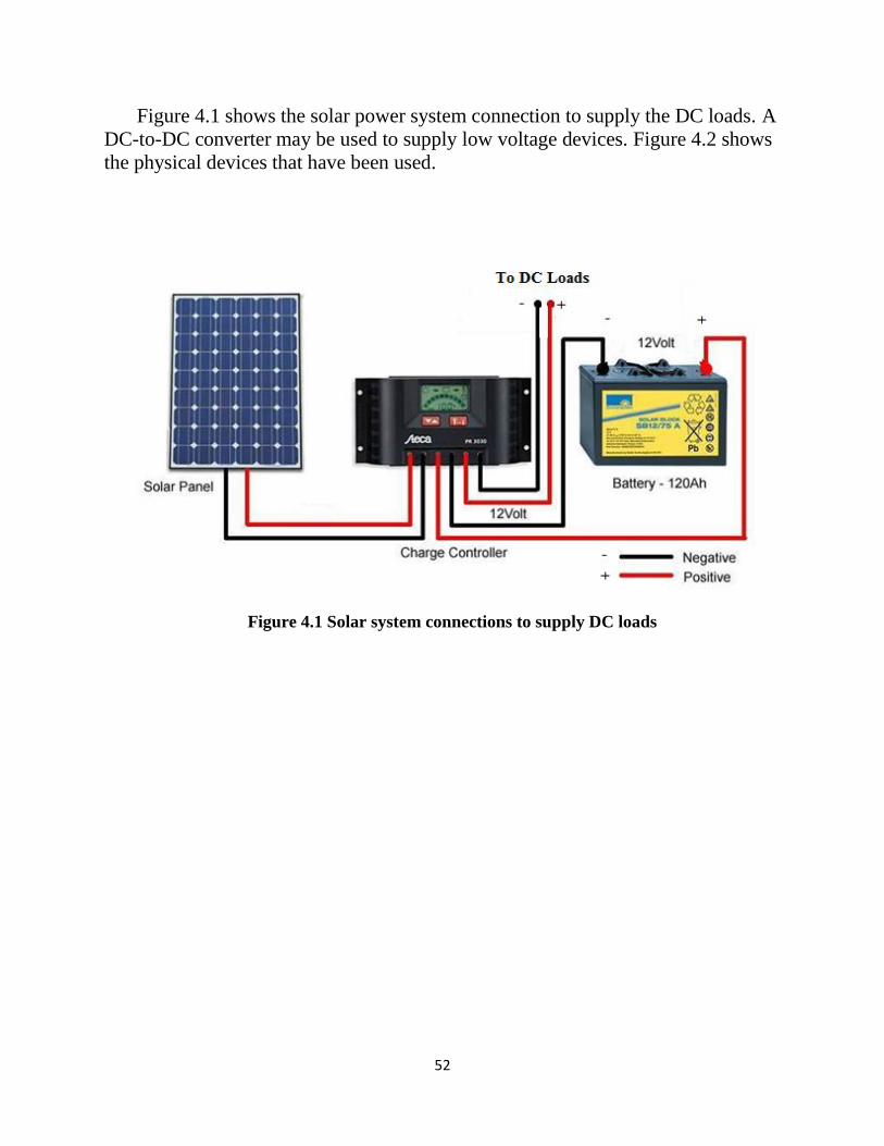
Figure 4.1 shows the solar power system connection to supply the DC loads. A
DC-to-DC converter may be used to supply low voltage devices. Figure 4.2 shows
the physical devices that have been used.
Figure 4.1 Solar system connections to supply DC loads
53
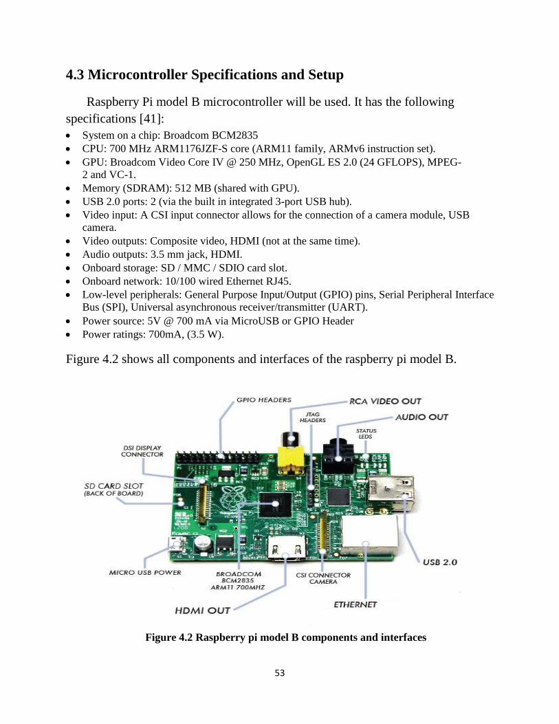
4.3 Microcontroller Specifications and Setup
Raspberry Pi model B microcontroller will be used. It has the following
specifications [41]:
System on a chip: Broadcom BCM2835
CPU: 700 MHz ARM1176JZF-S core (ARM11 family, ARMv6 instruction set).
GPU: Broadcom Video Core IV @ 250 MHz, OpenGL ES 2.0 (24 GFLOPS), MPEG-
2 and VC-1.
Memory (SDRAM): 512 MB (shared with GPU).
USB 2.0 ports: 2 (via the built in integrated 3-port USB hub).
Video input: A CSI input connector allows for the connection of a camera module, USB
camera.
Video outputs: Composite video, HDMI (not at the same time).
Audio outputs: 3.5 mm jack, HDMI.
Onboard storage: SD / MMC / SDIO card slot.
Onboard network: 10/100 wired Ethernet RJ45.
Low-level peripherals: General Purpose Input/Output (GPIO) pins, Serial Peripheral Interface
Bus (SPI), Universal asynchronous receiver/transmitter (UART).
Power source: 5V @ 700 mA via MicroUSB or GPIO Header
Power ratings: 700mA, (3.5 W).
Figure 4.2 shows all components and interfaces of the raspberry pi model B.
Figure 4.2 Raspberry pi model B components and interfaces
54
In order to use the Raspberry Pi, it is needed to install one of the images of the
Linux operating system onto an SD card. We chose to install Raspbian OS image as
follows [40]:
1) Insert an SD card that is 4GB or greater in size into a PC computer.
2) Format the SD card so that the Raspberry can read it.
3) Unzip the downloaded image file of Raspbian.
4) Copy the extracted files onto the SD card that we just formatted.
5) Insert the SD card into its place in Raspberry and connect the power supply.
6) Choose to install, a temporary display will be connected to show the status and
help us proceeding with the install.
Having done that, Raspberry will be able to interact and communicate with the
peripherals that we want to connect.
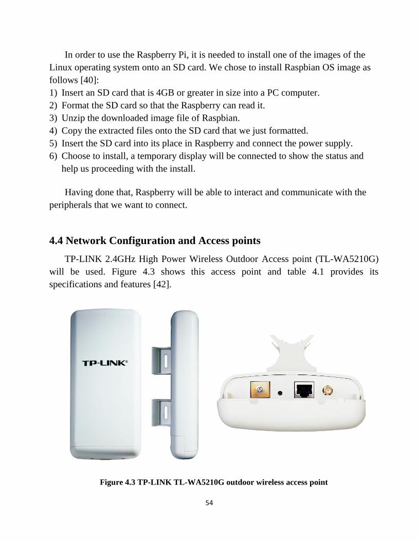
4.4 Network Configuration and Access points
TP-LINK 2.4GHz High Power Wireless Outdoor Access point (TL-WA5210G)
will be used. Figure 4.3 shows this access point and table 4.1 provides its
specifications and features [42].
Figure 4.3 TP-LINK TL-WA5210G outdoor wireless access point
55
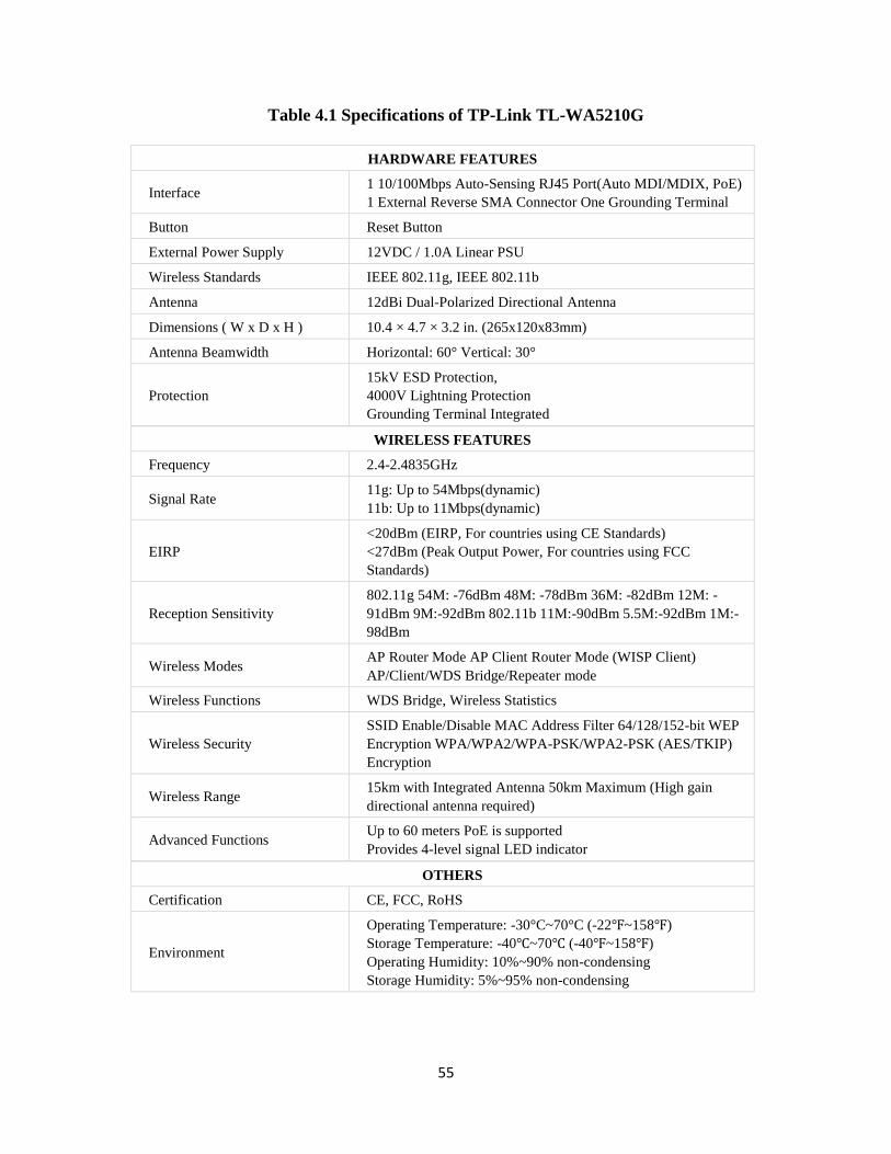
Table 4.1 Specifications of TP-Link TL-WA5210G
HARDWARE FEATURES
Interface 1 10/100Mbps Auto-Sensing RJ45 Port(Auto MDI/MDIX, PoE)
1 External Reverse SMA Connector One Grounding Terminal
Button Reset Button
External Power Supply 12VDC / 1.0A Linear PSU
Wireless Standards IEEE 802.11g, IEEE 802.11b
Antenna 12dBi Dual-Polarized Directional Antenna
Dimensions ( W x D x H ) 10.4 × 4.7 × 3.2 in. (265x120x83mm)
Antenna Beamwidth Horizontal: 60° Vertical: 30°
Protection
15kV ESD Protection,
4000V Lightning Protection
Grounding Terminal Integrated
WIRELESS FEATURES
Frequency 2.4-2.4835GHz
Signal Rate 11g: Up to 54Mbps(dynamic)
11b: Up to 11Mbps(dynamic)
EIRP
<20dBm (EIRP, For countries using CE Standards)
<27dBm (Peak Output Power, For countries using FCC
Standards)
Reception Sensitivity
802.11g 54M: -76dBm 48M: -78dBm 36M: -82dBm 12M: -
91dBm 9M:-92dBm 802.11b 11M:-90dBm 5.5M:-92dBm 1M:-
98dBm
Wireless Modes AP Router Mode AP Client Router Mode (WISP Client)
AP/Client/WDS Bridge/Repeater mode
Wireless Functions WDS Bridge, Wireless Statistics
Wireless Security
SSID Enable/Disable MAC Address Filter 64/128/152-bit WEP
Encryption WPA/WPA2/WPA-PSK/WPA2-PSK (AES/TKIP)
Encryption
Wireless Range 15km with Integrated Antenna 50km Maximum (High gain
directional antenna required)
Advanced Functions Up to 60 meters PoE is supported
Provides 4-level signal LED indicator
OTHERS
Certification CE, FCC, RoHS
Environment
Operating Temperature: -30°C~70°C (-22℉~158℉)
Storage Temperature: -40℃~70℃ (-40℉~158℉)
Operating Humidity: 10%~90% non-condensing
Storage Humidity: 5%~95% non-condensing
56
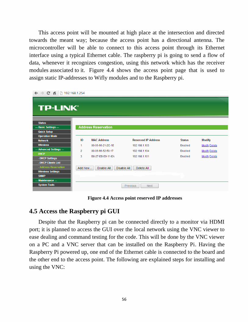
This access point will be mounted at high place at the intersection and directed
towards the meant way; because the access point has a directional antenna. The
microcontroller will be able to connect to this access point through its Ethernet
interface using a typical Ethernet cable. The raspberry pi is going to send a flow of
data, whenever it recognizes congestion, using this network which has the receiver
modules associated to it. Figure 4.4 shows the access point page that is used to
assign static IP-addresses to Wifly modules and to the Raspberry pi.
Figure 4.4 Access point reserved IP addresses
4.5 Access the Raspberry pi GUI
Despite that the Raspberry pi can be connected directly to a monitor via HDMI
port; it is planned to access the GUI over the local network using the VNC viewer to
ease dealing and command testing for the code. This will be done by the VNC viewer
on a PC and a VNC server that can be installed on the Raspberry Pi. Having the
Raspberry Pi powered up, one end of the Ethernet cable is connected to the board and
the other end to the access point. The following are explained steps for installing and
using the VNC:
57
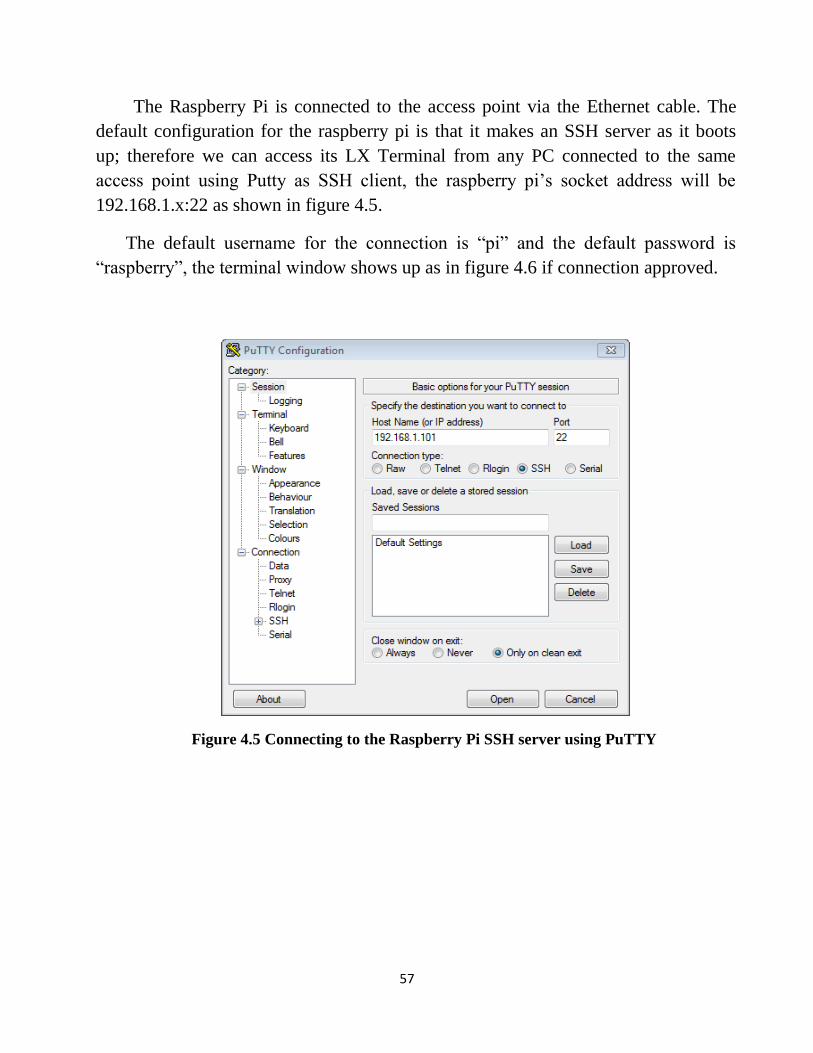
The Raspberry Pi is connected to the access point via the Ethernet cable. The
default configuration for the raspberry pi is that it makes an SSH server as it boots
up; therefore we can access its LX Terminal from any PC connected to the same
access point using Putty as SSH client, the raspberry pi‟s socket address will be
192.168.1.x:22 as shown in figure 4.5.
The default username for the connection is “pi” and the default password is
“raspberry”, the terminal window shows up as in figure 4.6 if connection approved.
Figure 4.5 Connecting to the Raspberry Pi SSH server using PuTTY
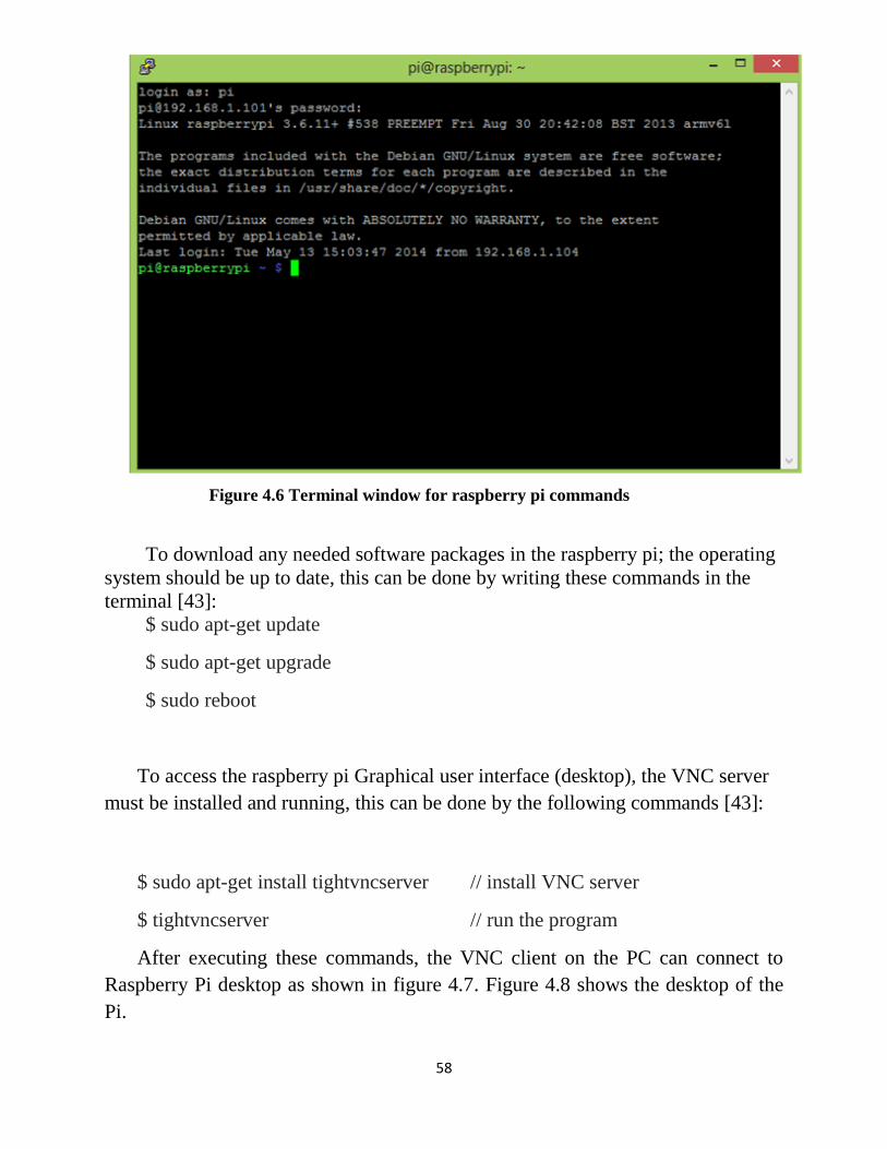
58
Figure 4.6 Terminal window for raspberry pi commands
To download any needed software packages in the raspberry pi; the operating
system should be up to date, this can be done by writing these commands in the
terminal [43]:
$ sudo apt-get update
$ sudo apt-get upgrade
$ sudo reboot
To access the raspberry pi Graphical user interface (desktop), the VNC server
must be installed and running, this can be done by the following commands [43]:
$ sudo apt-get install tightvncserver // install VNC server
$ tightvncserver // run the program
After executing these commands, the VNC client on the PC can connect to
Raspberry Pi desktop as shown in figure 4.7. Figure 4.8 shows the desktop of the
Pi.
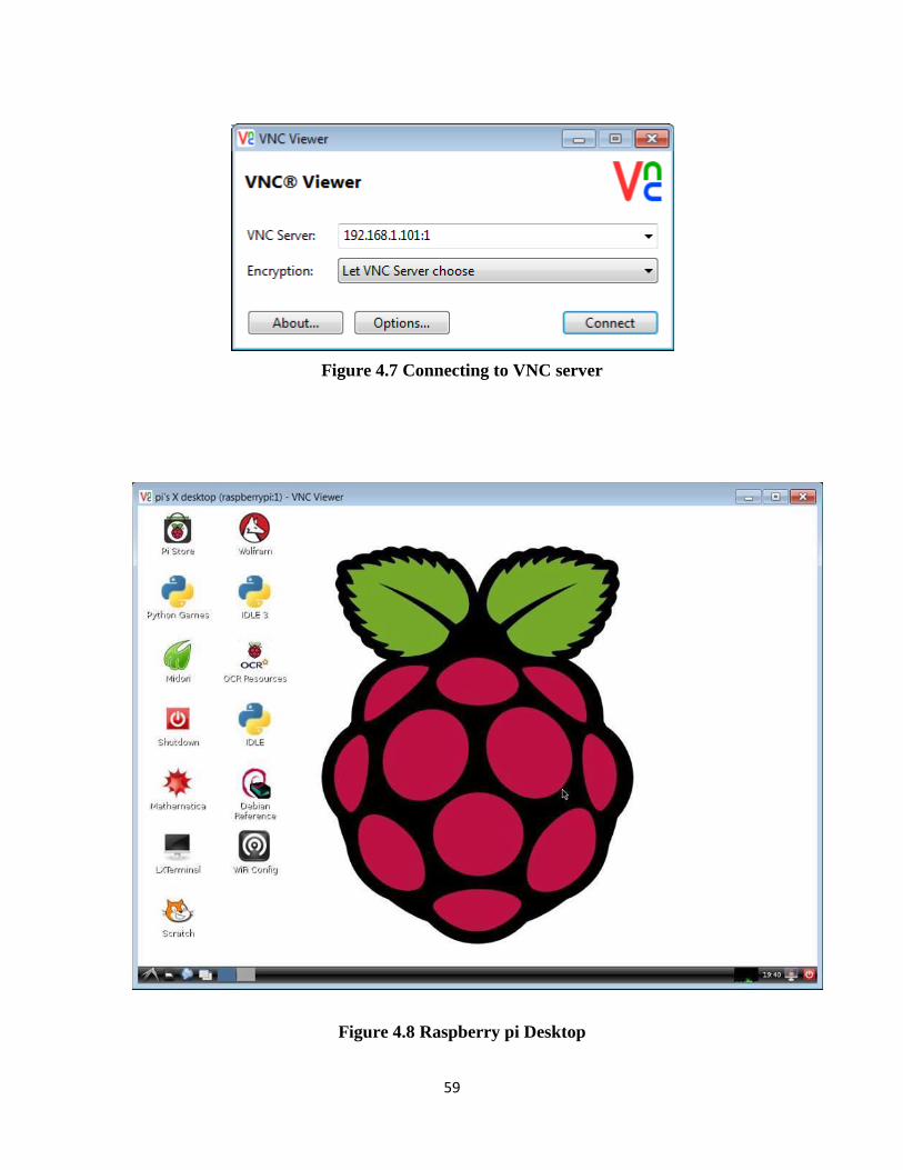
59
Figure 4.7 Connecting to VNC server
Figure 4.8 Raspberry pi Desktop
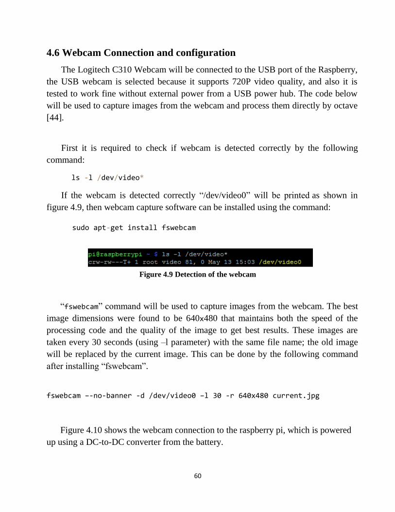
60
4.6 Webcam Connection and configuration
The Logitech C310 Webcam will be connected to the USB port of the Raspberry,
the USB webcam is selected because it supports 720P video quality, and also it is
tested to work fine without external power from a USB power hub. The code below
will be used to capture images from the webcam and process them directly by octave
[44].
First it is required to check if webcam is detected correctly by the following
command:
ls -l /dev/video*
If the webcam is detected correctly “/dev/video0” will be printed as shown in
figure 4.9, then webcam capture software can be installed using the command:
sudo apt-get install fswebcam
Figure 4.9 Detection of the webcam
“fswebcam” command will be used to capture images from the webcam. The best
image dimensions were found to be 640x480 that maintains both the speed of the
processing code and the quality of the image to get best results. These images are
taken every 30 seconds (using –l parameter) with the same file name; the old image
will be replaced by the current image. This can be done by the following command
after installing “fswebcam”.
fswebcam –-no-banner -d /dev/video0 –l 30 -r 640x480 current.jpg
Figure 4.10 shows the webcam connection to the raspberry pi, which is powered
up using a DC-to-DC converter from the battery.
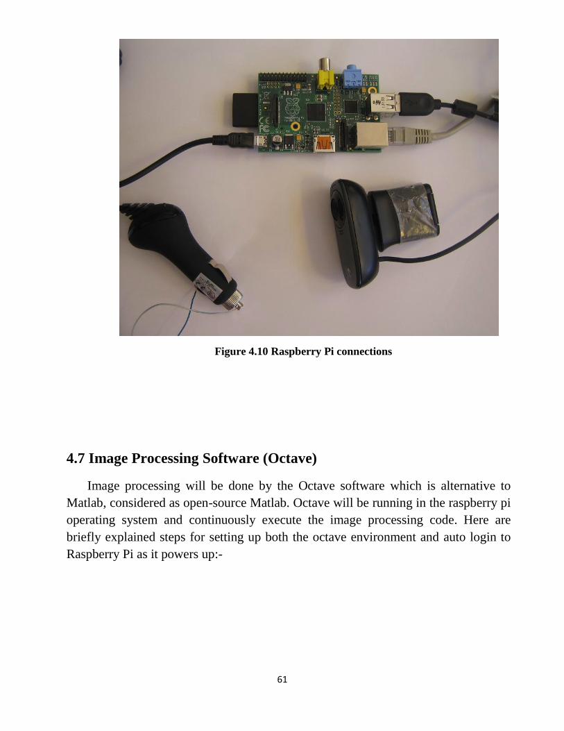
61
Figure 4.10 Raspberry Pi connections
4.7 Image Processing Software (Octave)
Image processing will be done by the Octave software which is alternative to
Matlab, considered as open-source Matlab. Octave will be running in the raspberry pi
operating system and continuously execute the image processing code. Here are
briefly explained steps for setting up both the octave environment and auto login to
Raspberry Pi as it powers up:-
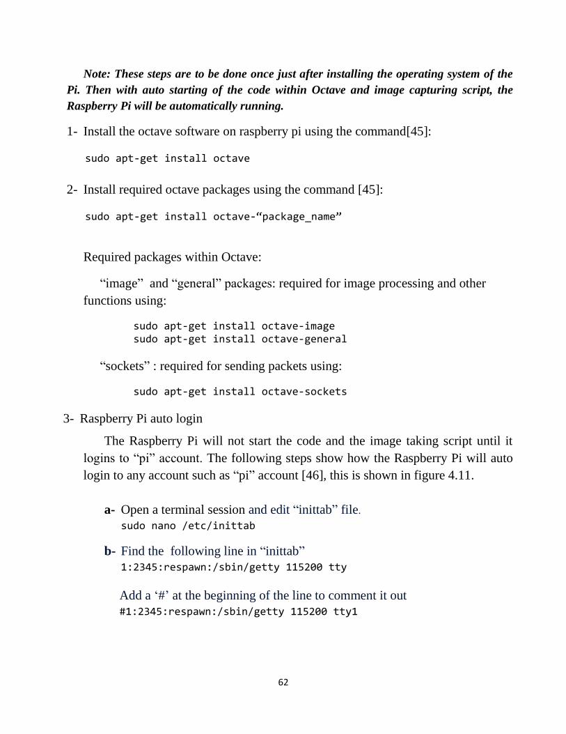
62
Note: These steps are to be done once just after installing the operating system of the
Pi. Then with auto starting of the code within Octave and image capturing script, the
Raspberry Pi will be automatically running.
1- Install the octave software on raspberry pi using the command[45]: sudo apt-get install octave
2- Install required octave packages using the command [45]: sudo apt-get install octave-“package_name”
Required packages within Octave:
“image” and “general” packages: required for image processing and other
functions using:
sudo apt-get install octave-image sudo apt-get install octave-general
“sockets” : required for sending packets using:
sudo apt-get install octave-sockets
3- Raspberry Pi auto login
The Raspberry Pi will not start the code and the image taking script until it
logins to “pi” account. The following steps show how the Raspberry Pi will auto
login to any account such as “pi” account [46], this is shown in figure 4.11.
a- Open a terminal session and edit “inittab” file.
sudo nano /etc/inittab
b- Find the following line in “inittab”
1:2345:respawn:/sbin/getty 115200 tty
Add a „#‟ at the beginning of the line to comment it out
#1:2345:respawn:/sbin/getty 115200 tty1
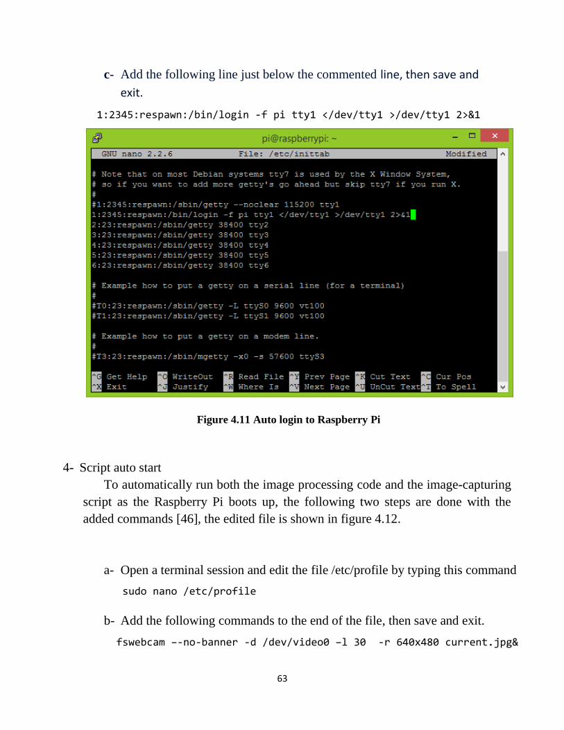
63
c- Add the following line just below the commented line, then save and
exit.
1:2345:respawn:/bin/login -f pi tty1 </dev/tty1 >/dev/tty1 2>&1
Figure 4.11 Auto login to Raspberry Pi
4- Script auto start
To automatically run both the image processing code and the image-capturing
script as the Raspberry Pi boots up, the following two steps are done with the
added commands [46], the edited file is shown in figure 4.12.
a- Open a terminal session and edit the file /etc/profile by typing this command
sudo nano /etc/profile
b- Add the following commands to the end of the file, then save and exit.
fswebcam –-no-banner -d /dev/video0 –l 30 -r 640x480 current.jpg&
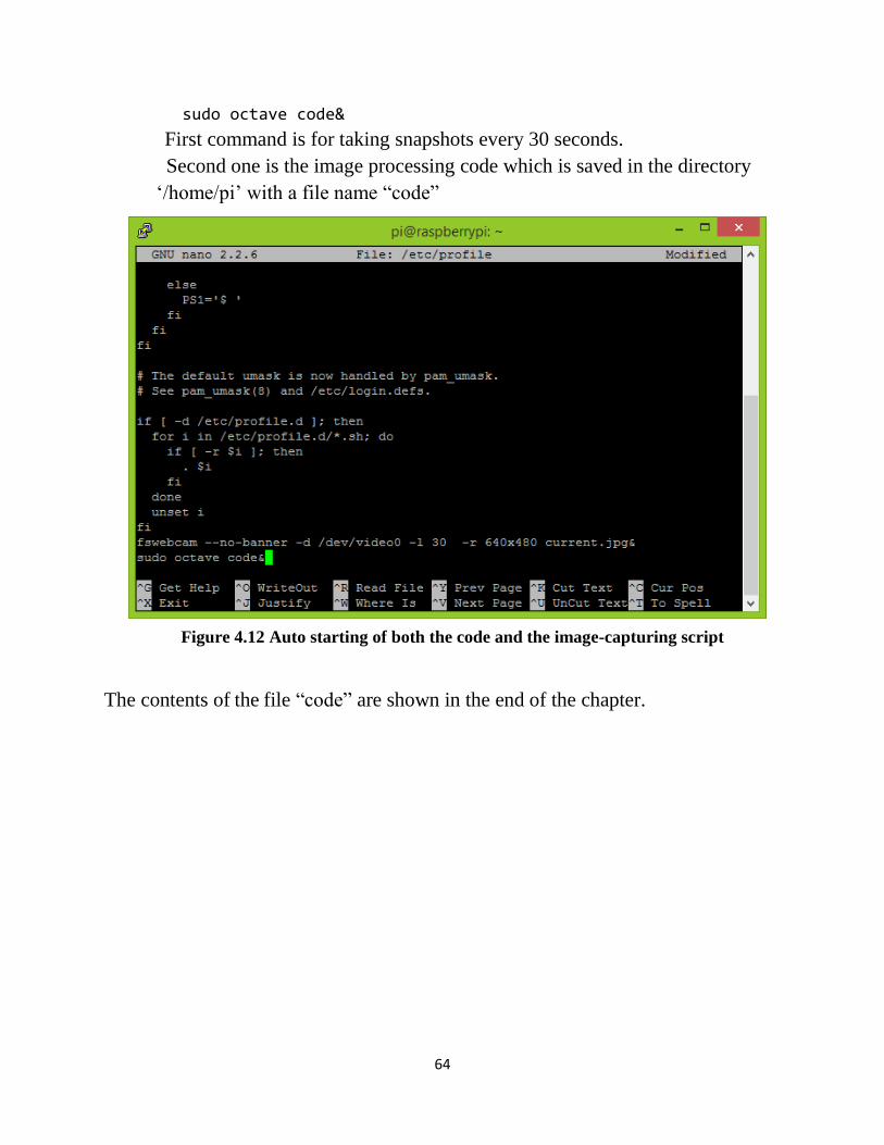
64
sudo octave code&
First command is for taking snapshots every 30 seconds.
Second one is the image processing code which is saved in the directory
„/home/pi‟ with a file name “code”
Figure 4.12 Auto starting of both the code and the image-capturing script
The contents of the file “code” are shown in the end of the chapter.
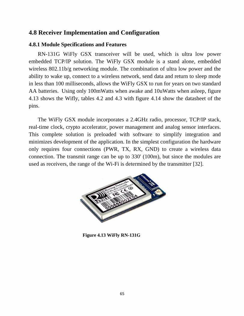
65
4.8 Receiver Implementation and Configuration
4.8.1 Module Specifications and Features
RN-131G WiFly GSX transceiver will be used, which is ultra low power
embedded TCP/IP solution. The WiFly GSX module is a stand alone, embedded
wireless 802.11b/g networking module. The combination of ultra low power and the
ability to wake up, connect to a wireless network, send data and return to sleep mode
in less than 100 milliseconds, allows the WiFly GSX to run for years on two standard
AA batteries. Using only 100mWatts when awake and 10uWatts when asleep, figure
4.13 shows the Wifly, tables 4.2 and 4.3 with figure 4.14 show the datasheet of the
pins.
The WiFly GSX module incorporates a 2.4GHz radio, processor, TCP/IP stack,
real-time clock, crypto accelerator, power management and analog sensor interfaces.
This complete solution is preloaded with software to simplify integration and
minimizes development of the application. In the simplest configuration the hardware
only requires four connections (PWR, TX, RX, GND) to create a wireless data
connection. The transmit range can be up to 330' (100m), but since the modules are
used as receivers, the range of the Wi-Fi is determined by the transmitter [32].
Figure 4.13 WiFly RN-131G
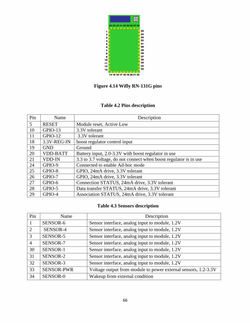
66
Figure 4.14 Wifly RN-131G pins
Table 4.2 Pins description
Pin Name Description
5 RESET Module reset, Active Low
10 GPIO-13 3.3V tolerant
11 GPIO-12 3.3V tolerant
18 3.3V-REG-IN boost regulator control input
19 GND Ground
20 VDD-BATT Battery input, 2.0-3.3V with boost regulator in use
21 VDD-IN 3.3 to 3.7 voltage, do not connect when boost regulator is in use
24 GPIO-9 Connected to enable Ad-hoc mode
25 GPIO-8 GPIO, 24mA drive, 3.3V tolerant
26 GPIO-7 GPIO, 24mA drive, 3.3V tolerant
27 GPIO-6 Connection STATUS, 24mA drive, 3.3V tolerant
28 GPIO-5 Data transfer STATUS, 24mA drive, 3.3V tolerant
29 GPIO-4 Association STATUS, 24mA drive, 3.3V tolerant
Table 4.3 Sensors description
Pin Name Description
1 SENSOR-6 Sensor interface, analog input to module, 1.2V
2 SENSOR-4 Sensor interface, analog input to module, 1.2V
3 SENSOR-5 Sensor interface, analog input to module, 1.2V
4 SENSOR-7 Sensor interface, analog input to module, 1.2V
30 SENSOR-1 Sensor interface, analog input to module, 1.2V
31 SENSOR-2 Sensor interface, analog input to module, 1.2V
32 SENSOR-3 Sensor interface, analog input to module, 1.2V
33 SENSOR-PWR Voltage output from module to power external sensors, 1.2-3.3V
34 SENSOR-0 Wakeup from external condition
67
Features:
Ultra low power 100mWatt active, 10uWatt sleep mode.
Host Data Rate Up to 100 Mbps for SDIO, 44 Mbps for SPI and 2.7 Mbps for
UART.
Throughput 4 Mbps with TCP/IP and WPA2.
UART hardware interfaces.
10 general purpose digital I/O.
8 analog sensor interfaces.
Real-time clock for wakeup and time stamping.
Accepts 3.3VDC regulated or 2-3VDC battery.
Supports Ad-hoc connection.
Real time clock for time stamping, auto-sleep and auto-wakeup modes.
Configuration over UART or wireless interfaces using simple ASCII commands.
Over the air firmware upgrade (FTP), and data file upload.
Secure Wi-Fi authentication WEP-128, WPA-PSK (TKIP), WPA2-PSK, EAP-
TLS for WPA1 & WPA2 Enterprise.
Built in networking applications DHCP, UDP, DNS, ARP and ICMP [32].
4.8.2 Alarm Configuration and Circuit Design
Data transfer pin in the module will be connected to a Buzzer. Buzzer will
continue running as long as the octave is sending data packets. Figure 4.15 shows the
circuit diagram. The following commands will be integrated with the image
processing code on octave auto-startup file. Sending data to the Wifly module will
take place whenever the processing code decides a congestion, data transfer will last
for 7 seconds until we check again [32].
4.8.3 Hardware Setup and Configuration
The implemented receiver modules are shown in figure 4.16, for the first run, the
Wifly is connected to make its own Ad-hoc network that will be used to send
commands for the module to associate with an access point, and save the
configuration.
To enter the command mode, „$$$‟ are typed. The module replies with „CMD‟ to
indicate it is in command mode. The module has to be associated with the secured
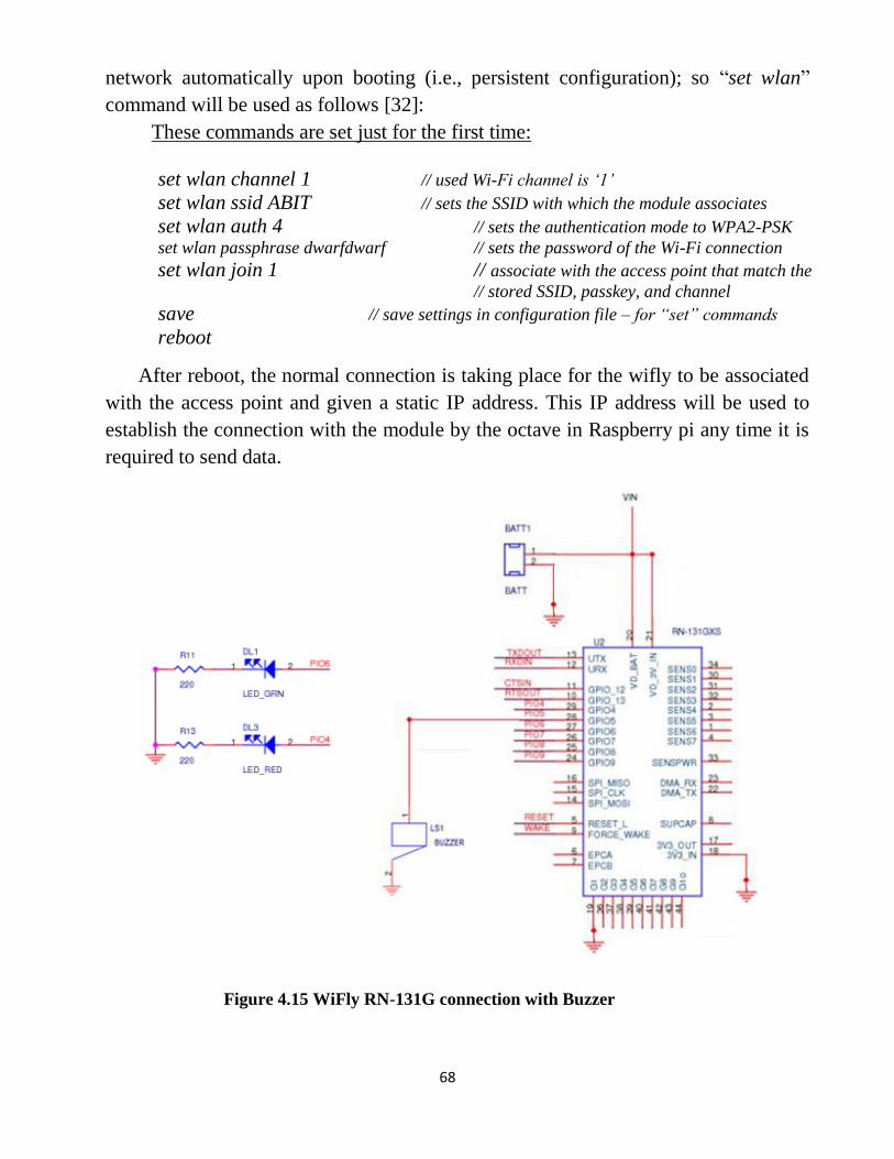
68
network automatically upon booting (i.e., persistent configuration); so “set wlan”
command will be used as follows [32]:
These commands are set just for the first time:
set wlan channel 1 // used Wi-Fi channel is „1‟
set wlan ssid ABIT // sets the SSID with which the module associates
set wlan auth 4 // sets the authentication mode to WPA2-PSK
set wlan passphrase dwarfdwarf // sets the password of the Wi-Fi connection
set wlan join 1 // associate with the access point that match the
// stored SSID, passkey, and channel
save // save settings in configuration file – for “set” commands
reboot
After reboot, the normal connection is taking place for the wifly to be associated
with the access point and given a static IP address. This IP address will be used to
establish the connection with the module by the octave in Raspberry pi any time it is
required to send data.
Figure 4.15 WiFly RN-131G connection with Buzzer
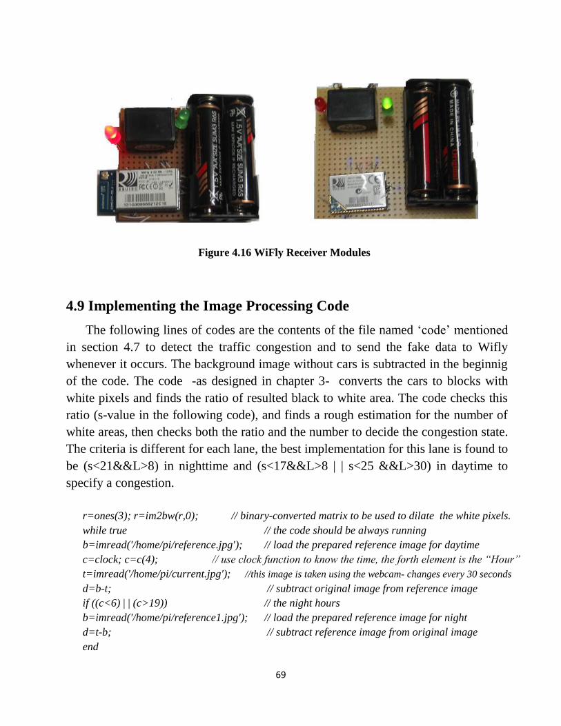
69
Figure 4.16 WiFly Receiver Modules
4.9 Implementing the Image Processing Code
The following lines of codes are the contents of the file named „code‟ mentioned
in section 4.7 to detect the traffic congestion and to send the fake data to Wifly
whenever it occurs. The background image without cars is subtracted in the beginnig
of the code. The code -as designed in chapter 3- converts the cars to blocks with
white pixels and finds the ratio of resulted black to white area. The code checks this
ratio (s-value in the following code), and finds a rough estimation for the number of
white areas, then checks both the ratio and the number to decide the congestion state.
The criteria is different for each lane, the best implementation for this lane is found to
be (s<21&&L>8) in nighttime and (s<17&&L>8 | | s<25 &&L>30) in daytime to
specify a congestion.
r=ones(3); r=im2bw(r,0); // binary-converted matrix to be used to dilate the white pixels.
while true // the code should be always running
b=imread('/home/pi/reference.jpg'); // load the prepared reference image for daytime
c=clock; c=c(4); // use clock function to know the time, the forth element is the “Hour”
t=imread('/home/pi/current.jpg'); //this image is taken using the webcam- changes every 30 seconds
d=b-t; // subtract original image from reference image
if ((c<6) | | (c>19)) // the night hours
b=imread('/home/pi/reference1.jpg'); // load the prepared reference image for night
d=t-b; // subtract reference image from original image
end
70
d=imcomplement(d); // each pixel value is subtracted from the max-pixel value (255)
d=d-100; // decrease the brightness of the image
d = imadjust(d,stretchlim(d),[0 .9]); // finding the lower and upper limits for contrast stretching
// of the image, imadjust to increase the contrast of the image
d=rgb2gray(d); // convert from RGB image to gray scale
d=imadjust(d); // adjusting image intensity
th=graythresh(d); // computes threshold for conversion from gray scale
if ((c<6) | | (c>19)) // check the night hours to apply the night threshold
th=.25; end // night threshold is fixed at 0.25
d=medfilt2(d); // to binary image right after the median filtering
d=im2bw(d,th); //black and white image, value of any pixel is either zero or one (binary)
d=imcomplement(d); // black and white are reversed
d=bwmorph(d,'majority',9); // morphological operation to remove tiny unwanted objects
d=imdilate(d,r); // dilate the white pixels using a 3×3 white matrix
blackcount = sum(sum(d==0)); // calculate the total area of black pixels of value „0‟
whitecount = sum(sum(d)); // calculate the total area of white pixels with value „1‟
s=blackcount/whitecount; // find the ratio of black to white
cc=bwboundaries(d,8,'noholes'); //compute exterior object boundaries using 8-connected objects
L=numel(cc); // compute the number of objects based on their exterior boundaries
if ((c<6) | | (c>19)) // check the night hours to apply a criteria
if (s<21&&L>8 ) transmitting // check the criteria in nighttime and transmit if true
else sleep(7) end // sleep 7 seconds if no congestion at night
else if (s<17&&L>8 | | s<25 &&L>30) // check the criteria if it detects a congestion – this criteria
// is different for the daytime
transmitting end // call the m-file that we built using socket for transmission
else sleep(7) // sleep 7 seconds if no congestion at daytime
end
sleep(10) // sleep10 seconds before checking again
end
The m-file of “transmitting.m” is copied to the Octave image-package directory
to be called from inside the previous code. The m-file contains the following
commands:
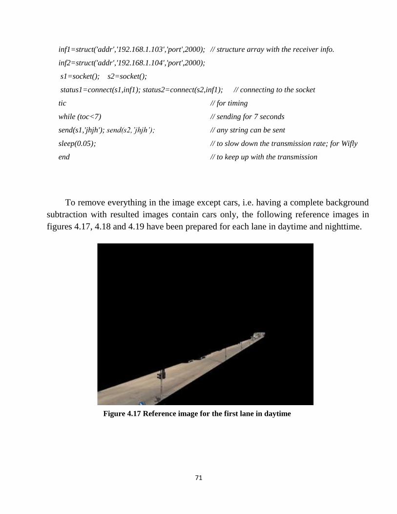
71
inf1=struct('addr','192.168.1.103','port',2000); // structure array with the receiver info.
inf2=struct('addr','192.168.1.104','port',2000);
s1=socket(); s2=socket();
status1=connect(s1,inf1); status2=connect(s2,inf1); // connecting to the socket
tic // for timing
while (toc<7) // sending for 7 seconds
send(s1,'jhjh'); send(s2,‟jhjh‟); // any string can be sent
sleep(0.05) ; // to slow down the transmission rate; for Wifly
end // to keep up with the transmission
To remove everything in the image except cars, i.e. having a complete background
subtraction with resulted images contain cars only, the following reference images in
figures 4.17, 4.18 and 4.19 have been prepared for each lane in daytime and nighttime.
Figure 4.17 Reference image for the first lane in daytime
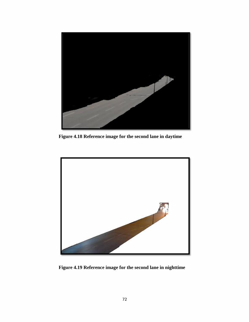
72
Figure 4.18 Reference image for the second lane in daytime
Figure 4.19 Reference image for the second lane in nighttime
73
Chapter 5
Testing and System’s Performance
5.1 Overview
5.2 Testing and Results
5.3 Performance Evaluation
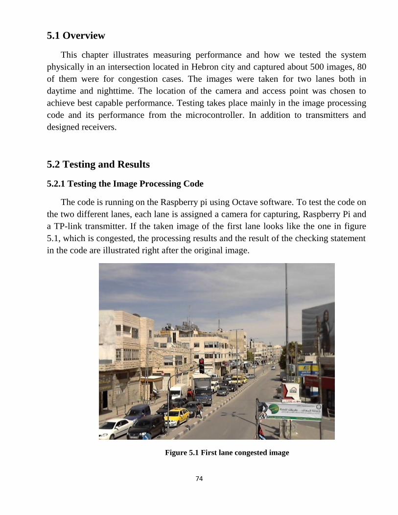
74
5.1 Overview
This chapter illustrates measuring performance and how we tested the system
physically in an intersection located in Hebron city and captured about 500 images, 80
of them were for congestion cases. The images were taken for two lanes both in
daytime and nighttime. The location of the camera and access point was chosen to
achieve best capable performance. Testing takes place mainly in the image processing
code and its performance from the microcontroller. In addition to transmitters and
designed receivers.
5.2 Testing and Results
5.2.1 Testing the Image Processing Code
The code is running on the Raspberry pi using Octave software. To test the code on
the two different lanes, each lane is assigned a camera for capturing, Raspberry Pi and
a TP-link transmitter. If the taken image of the first lane looks like the one in figure
5.1, which is congested, the processing results and the result of the checking statement
in the code are illustrated right after the original image.
Figure 5.1 First lane congested image
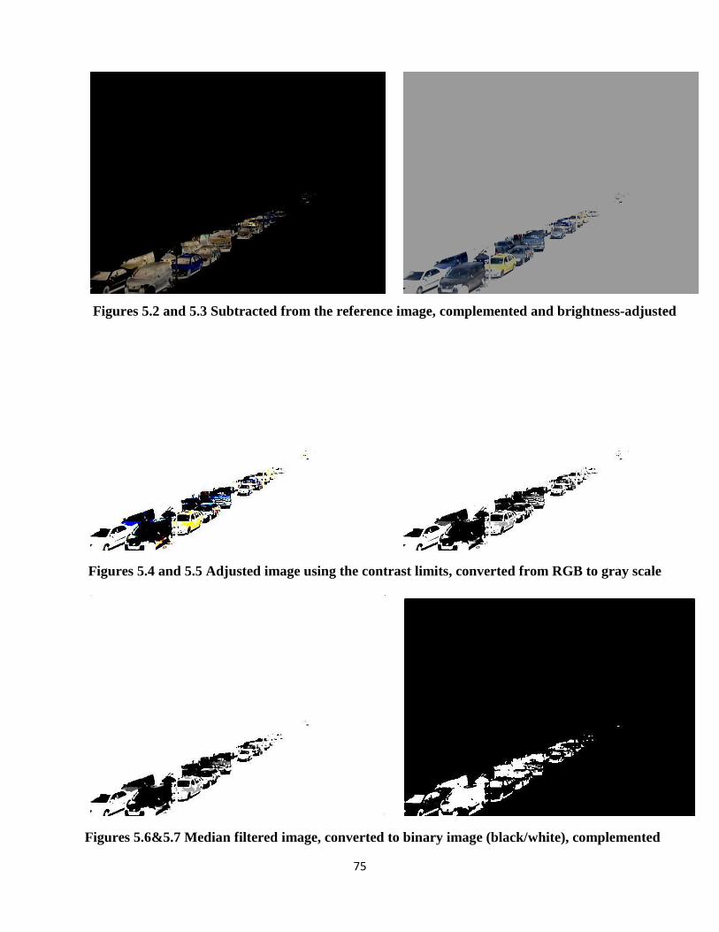
75
Figures 5.2 and 5.3 Subtracted from the reference image, complemented and brightness-adjusted
Figures 5.4 and 5.5 Adjusted image using the contrast limits, converted from RGB to gray scale
Figures 5.6&5.7 Median filtered image, converted to binary image (black/white), complemented
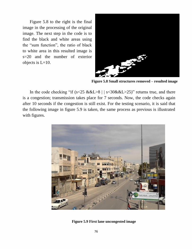
76
Figure 5.8 to the right is the final
image in the processing of the original
image. The next step in the code is to
find the black and white areas using
the “sum function”, the ratio of black
to white area in this resulted image is
s=20 and the number of exterior
objects is L=10.
Figure 5.8 Small structures removed – resulted image
In the code checking “if (s<25 &&L>8 | | s<30&&L>25)” returns true, and there
is a congestion; transmission takes place for 7 seconds. Now, the code checks again
after 10 seconds if the congestion is still exist. For the testing scenario, it is said that
the following image in figure 5.9 is taken, the same process as previous is illustrated
with figures.
Figure 5.9 First lane uncongested image
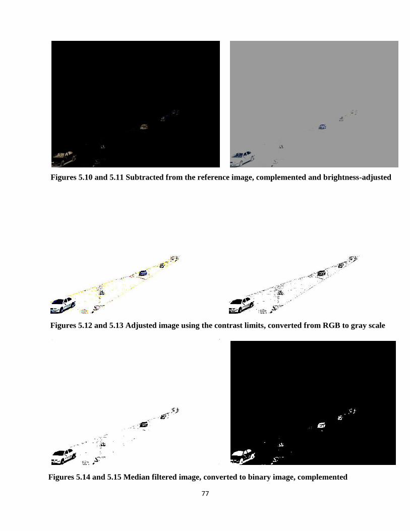
77
Figures 5.10 and 5.11 Subtracted from the reference image, complemented and brightness-adjusted
Figures 5.12 and 5.13 Adjusted image using the contrast limits, converted from RGB to gray scale
Figures 5.14 and 5.15 Median filtered image, converted to binary image, complemented
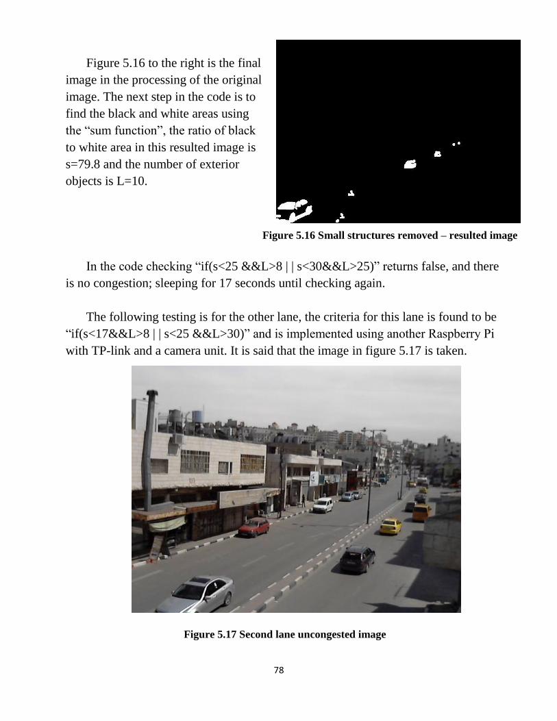
78
Figure 5.16 to the right is the final
image in the processing of the original
image. The next step in the code is to
find the black and white areas using
the “sum function”, the ratio of black
to white area in this resulted image is
s=79.8 and the number of exterior
objects is L=10.
Figure 5.16 Small structures removed – resulted image
In the code checking “if(s<25 &&L>8 | | s<30&&L>25)” returns false, and there
is no congestion; sleeping for 17 seconds until checking again.
The following testing is for the other lane, the criteria for this lane is found to be
“if(s<17&&L>8 | | s<25 &&L>30)” and is implemented using another Raspberry Pi
with TP-link and a camera unit. It is said that the image in figure 5.17 is taken.
Figure 5.17 Second lane uncongested image
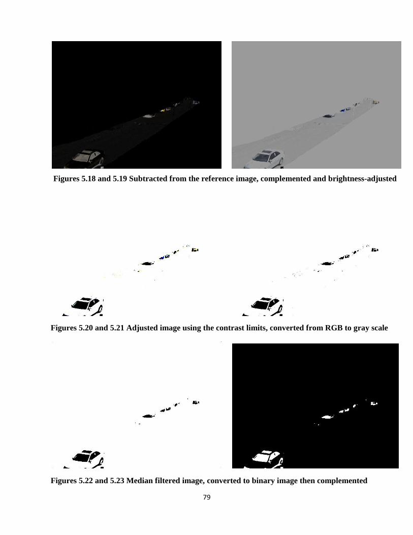
79
Figures 5.18 and 5.19 Subtracted from the reference image, complemented and brightness-adjusted
Figures 5.20 and 5.21 Adjusted image using the contrast limits, converted from RGB to gray scale
Figures 5.22 and 5.23 Median filtered image, converted to binary image then complemented
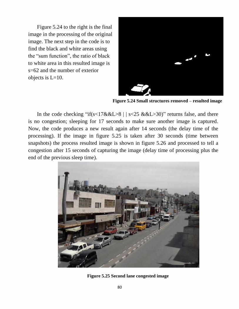
80
Figure 5.24 to the right is the final
image in the processing of the original
image. The next step in the code is to
find the black and white areas using
the “sum function”, the ratio of black
to white area in this resulted image is
s=62 and the number of exterior
objects is L=10.
Figure 5.24 Small structures removed – resulted image
In the code checking “if(s<17&&L>8 | | s<25 &&L>30)” returns false, and there
is no congestion; sleeping for 17 seconds to make sure another image is captured.
Now, the code produces a new result again after 14 seconds (the delay time of the
processing). If the image in figure 5.25 is taken after 30 seconds (time between
snapshots) the process resulted image is shown in figure 5.26 and processed to tell a
congestion after 15 seconds of capturing the image (delay time of processing plus the
end of the previous sleep time).
Figure 5.25 Second lane congested image
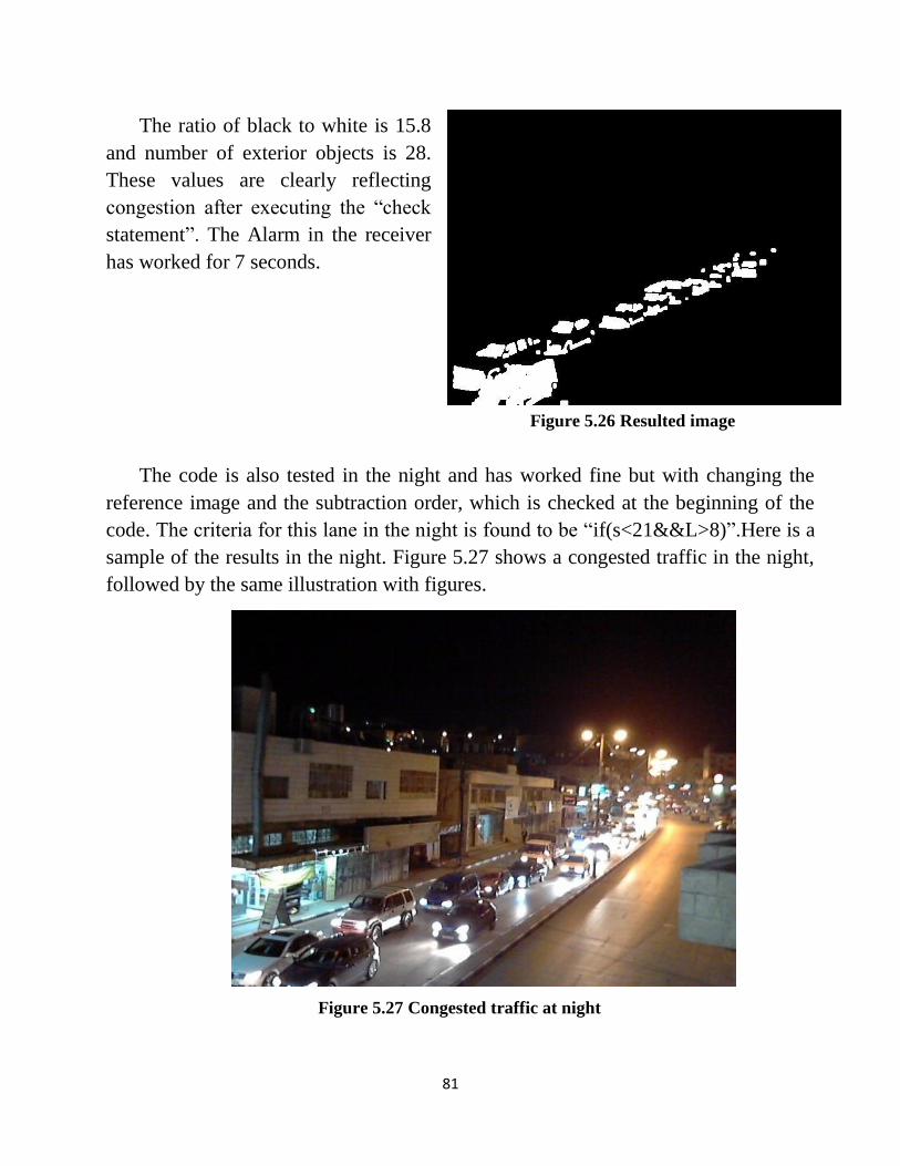
81
The ratio of black to white is 15.8
and number of exterior objects is 28.
These values are clearly reflecting
congestion after executing the “check
statement”. The Alarm in the receiver
has worked for 7 seconds.
Figure 5.26 Resulted image
The code is also tested in the night and has worked fine but with changing the
reference image and the subtraction order, which is checked at the beginning of the
code. The criteria for this lane in the night is found to be “if(s<21&&L>8)”.Here is a
sample of the results in the night. Figure 5.27 shows a congested traffic in the night,
followed by the same illustration with figures.
Figure 5.27 Congested traffic at night
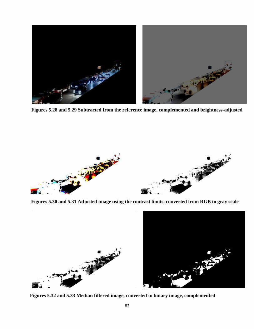
82
Figures 5.28 and 5.29 Subtracted from the reference image, complemented and brightness-adjusted
Figures 5.30 and 5.31 Adjusted image using the contrast limits, converted from RGB to gray scale
Figures 5.32 and 5.33 Median filtered image, converted to binary image, complemented
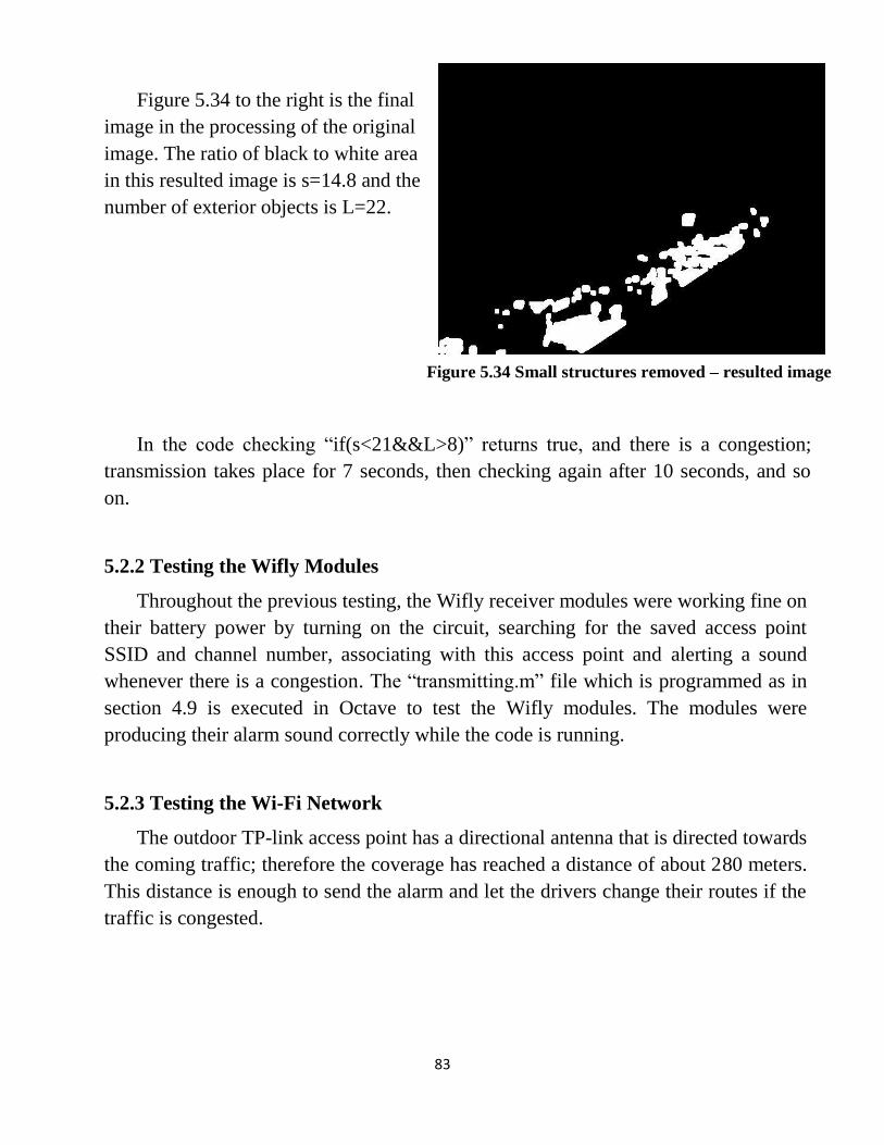
83
Figure 5.34 to the right is the final
image in the processing of the original
image. The ratio of black to white area
in this resulted image is s=14.8 and the
number of exterior objects is L=22.
Figure 5.34 Small structures removed – resulted image
In the code checking “if(s<21&&L>8)” returns true, and there is a congestion;
transmission takes place for 7 seconds, then checking again after 10 seconds, and so
on.
5.2.2 Testing the Wifly Modules
Throughout the previous testing, the Wifly receiver modules were working fine on
their battery power by turning on the circuit, searching for the saved access point
SSID and channel number, associating with this access point and alerting a sound
whenever there is a congestion. The “transmitting.m” file which is programmed as in
section 4.9 is executed in Octave to test the Wifly modules. The modules were
producing their alarm sound correctly while the code is running.
5.2.3 Testing the Wi-Fi Network
The outdoor TP-link access point has a directional antenna that is directed towards
the coming traffic; therefore the coverage has reached a distance of about 280 meters.
This distance is enough to send the alarm and let the drivers change their routes if the
traffic is congested.
84
5.2.4 Testing the Solar System
PV-panel and the charge controller with the battery were tested many times in
sunny days, the panel is producing about 55W of power at 19 volts, the charge
controller was charging the battery at 12V. The battery was supplying the two TP-
link access points and the two raspberries with the power, it worked for about 6 hours
in the night, which is enough for running the system in the possible congestion traffic
times after sunset.
5.3 Performance Evaluation
In this section, evaluation results of system components are presented. This
includes selection probability and response time.
5.3.1 Response Time of the Raspberry Pi
The main delay of the Raspberry Pi is in the processing time at the Raspberry Pi,
image capturing and storing to „/home/pi/current.jpg‟ requires 4 seconds with a
complexity of order 1 „O(n)‟, and the image processing code with complexity of order
2 „O(n2)‟ since it handles two while loops, it needs 10 seconds to be executed. This
total delay of 14 seconds can be reduced to 11 seconds by speeding up the Pi to
950MHz from the configuration, but this state decreases the life time of the Pi and
hence not implemented. This delay time does not exceed the traffic lights stopping
time of about 52 seconds in one lane and more than a minute in the other.
5.3.2 Response Time of Wifly Modules
The wifly modules takes about 1 second to be associated with the access point, but
after running for a long time on the same batteries, the supplied power for the wifly
decreases and causes a delay of about 3 seconds to be associated, to improve this
response time, batteries should be replaced.
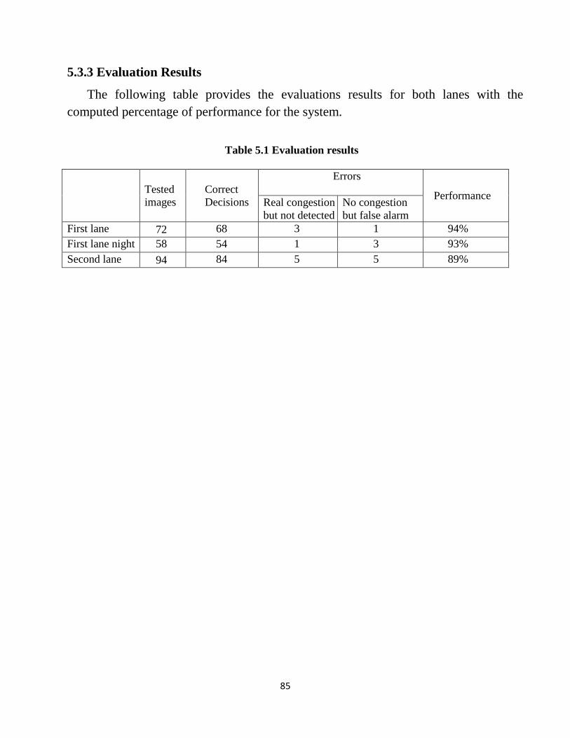
85
5.3.3 Evaluation Results
The following table provides the evaluations results for both lanes with the
computed percentage of performance for the system.
Table 5.1 Evaluation results
Tested
images
Correct
Decisions
Errors
Performance
Real congestion
but not detected
No congestion
but false alarm
First lane 72 68 3 1 94%
First lane night 58 54 1 3 93%
Second lane 94 84 5 5 89%

86
Chapter 6
Learning Outcomes and Future Work
6.1 Introduction
6.2 Acquired Learning Outcomes
6.3 Future Work
6.4 Conclusion
6.5 Problems
87
6.1 Introduction
This chapter describes the learning outcomes that have been acquired during the
work on the project, suggestions for future work and development. Problems that
raised during the work on the project are also mentioned.
6.2 Acquired Learning Outcomes
Upon accomplishing the project tasks many talents and abilities have been
acquired, such as:
1- Dealing with Raspberry Pi microcontroller.
2- Dealing with Wifly module.
3- Image processing using octave.
4- Learning and dealing with solar power systems.
5- Troubleshooting and problem solving.
6.3 Future Work
Different ideas have appeared while implementing the system, such as:
1- Linking this project with smart phone devices to spread the alarm system.
2- Keep sending packets during image processing.
3- Install the cameras on a fixed high place to capture better images and get a
better performance.
4- Integrate the project to detect the traffic congestion from any system with
traffic-monitoring video.

88
6.4 Conclusion
1. We designed and implemented an operational system for congestion
recognition and alerting.
2. Testing Results have shown acceptable performance over large number of
runs.
3. System adoption is very easy and direct.
4. Requirements are simple and in hands.
5. Drivers can be alerted over their smart phones or special units with Wi-Fi
Interface.
6. Our Next Step: Consult Hebron Municipality and other responsible parties in
the country and present the system for real deployment and use.
6.5 Problems
Many problems have been raised during the work on the project. Some of these
problems are:
1. The availability of the project‟s components.
2. Slow response in the system because the image processing steps.
3. Big time spent to choose the suitable location to take snapshots for the
intersection.
89
Bibliography:
[1] G.Bhaskar and Raghu BA, “WRTS: Wireless Sensor Based Real Time Traffic Information
System”, International Journal of Computer Applications Technology and Research, Vol. 2, Issue.
4, 2013, pp. 481- 486
[2] Akash Yadav, et al, “To Control the Traffic Congestion with the Help of Roof to Roof
Transportation System and Window Parking System”, International Journal of Innovative Research
in Science, Engineering and Technology, Vol. 3, Issue. 2, February 2014, p.2
[3] Brittany Crowell, “Wireless Sensor Utilizing Wi-Fi that is Capable of Estimating the
Density of Traffic”, Department of Computer Science Jackson State University, 2011, available
at http://143.132.8.23/cms/reu/2011/docs2011/Final-Reports-Slides/Final-Report-Brittany-Crowell.pdf
[4] Swaroop Roy, et al, “Wireless Across Road: RF based Road Traffic Congestion Detection”,
5th (2011) , pp.1-3, available at http://www.cse.iitb.ac.in/~riju/wisard.pdf .
[5] Ashish Dhar, “Traffic and Road Condition Monitoring System”, Indian Institute of Technology.
(2008), pp. 4-5, available at
http://www.cse.iitb.ac.in/synerg/lib/exe/fetch.php?id=public%3Astudents%3Aashish%3Astart&cac
he=cache&media=public:students:ashish:report2.pdf .MR 07305041
[6] Cambridge Systematics Inc, “Performance Measurement Framework and Congestion
Management Update Study”, 3(2010), p.35, available at
http://www.azmag.gov/Documents/TRANS_2010-11-02_MAG-CMP-Final-Baseline-Report.pdf
[7] CCTV cameras, overview, available at http://www.wsystems.com/news/cctv-camera.html
[8] T. NAGALAKSHMI, “A Study On Usage Of CCTV Surveillance System With Special
Reference To Business Outlets In Hyderabad”, Tactful Management Research Journal, Vol. 1 ,
Issue. 2, Nov 2012, pp.1-2
[9] Cameras‟ types, available at
http://www.cepro.com/article/print/12_common_types_of_security_cameras/
[10] I. A. Ansari and R. Y. Borse, “Image Processing and Analysis”, International Journal of
Engineering Research and Applications, Vol. 3, Issue 4, Jul-Aug 2013, pp.1655-1658
90
[11] S.S Tiwana and Sukhpreet Kaur, “Study on Various Glass Defect Using Glass Edge Detection
Methods”, International Journal of Computer Science and Mobile Computing, Vol. 2, Issue. 5, May
2013, pp.82-85
[12] Abhinay Mukunthan, "A Plotting Application For GNU Octave ", Bachelor of computer
engineering, University of Wollongong, 2007
[13] GNU octave, overview, available at www.gnu.org/software/octave
[14] R. R. Ambadas and R. P. Chaudhari, “PIC Microcontroller Universal Board”, International
Journal of Innovative Technology and Exploring Engineering, Vol. 3, Issue. 7, December 2013, p. 1
[15] Microcontroller, Classification, available at
http://www.zseries.in/classroom/courses/mm01/3.4.html
[16] Raspberry pi microcontroller, overview, types, software, available at
http://www.element14.com/community/docs/DOC-42993/l/raspberry-pi-single-board-computer
[17] Jakub Wójcik, “The conception and the implementation of control system for servomotor with
application of wireless network”, Master thesis in Computer Engineering and Electrical Systems,
AGH University of Science and Technology, 2011
[18] W. Durfee, “Arduino Microcontroller Guide”, University of Minnesota (2011), p. 2, available
at http://www.me.umn.edu/courses/me2011/arduino/arduinoGuide.pdf
[19] Rupinder Kaur, Manjit Thapa and Bhubneshwar Sharma, “Tow Major Tasks Done By
Digital Image Processing it's Steps Of Processing And Study Of Kinds Of Various Techniques For
Processing”, Journal of International Academic Research for Multidisciplinary, Vol. 1, Issue.12,
January 2014, pp.1-2 .
[20] Digital signal processing, components, available at
http://www.analog.com/en/content/beginners_guide_to_dsp/fca.html
[21] Hing Cheung, “Overview of Digital Signal Processing (DSP)”, Department of Electronic
Engineering in Hong Kong University ,2011, pp.11-15 available at
http://www.ee.cityu.edu.hk/~hcso/ee3202_1.pdf
[22] Markus Kuhn, “Digital Signal Processing ”,Michaelmas (2009 ) part 2, pp. 4-5,available at
http://www.cl.cam.ac.uk/teaching/0910/DSP/slides-2up.pdf

91
[23] Ch.Ganapathy Reddy, “DSP NOTES ” ,pp. 2-3,white paper, available at
http://www.gnits.ac.in/dsp.pdf
[24] ukpoma theo, “Wi-Fi”, June 2012, p.1, white paper, available at
http://www.studymode.com/essays/Wifi-1018293.html
[25] ukpoma theo, “uses of Wi-Fi”, white paper, available at
http://www.academia.edu/4290335/uses_of_WiFi
[26] Muhammad Khairi, “Advantages of Wi-Fi ”, white paper, available at
http://www.scribd.com/doc/128086923/Advantages-of-Wifi
[27] Wi-Fi, advantages, disadvantages, available at http://digitalwalt.com/wi-fi-advantages-
disadvantages/
[28] Sourangsu Banerji and R.S. Chowdhury, “RECENT DEVELOPMENTS IN IEEE 802.11:
WLAN TECHNOLOGY ”, International Journal of Mechatronics, Electrical and Computer
Technology, Vol. 3, Issue. 9, Oct 2013, pp. 1001-1013
[29] R.Barathi, K.Valarmathi and S.Amutha, “HIGHLY RECONFIGURABLE TRANSCEIVER
FOR CELLULAR ”, Journal of International Academic Research for Multidisciplinary, Vol. 1,
Issue. 4, MAY 2013, p. 1
[30] Ashwini Holakar ,et al, “Sensor Movement Based Sensor Switching for Data Acquisition”,
International Journal of Ethics in Engineering & Management Education, Vol.1, Issue.4, p. 61,
April 2014
[31] Chonggang Wang, Tao Jiang and Qian Zhang, “ ZigBee Network Protocols and
Applications”, Taylor & Francis Group, United States, 2014
[32] WiFly GSX (RN-131G) Module, overview, applications, features, software setup,
programming, types, available at http://www.microchip.com
[33] National Energy Education Development Project, “Energy From the Sun Student Guide”, p.
2, 2013-2014, available at
http://www.need.org/files/curriculum/guides/energyfromthesunstudentguide.pdf
[34] Solar panel, brief history, overview, available at
http://www.energymatters.com.au/renewable-energy/solar-power/solar-panels.php
[35] Solar energy, cells, panels, available at http://www.makeitsolar.com/solar-energy-information

92
[36] Solar energy, advantages, disadvantages, available at www.vienergy.org/solar.doc
[37] Ram Darash Patel and Priti Shukla, “MATLAB/ Simulink based model of photovoltaic cell and
their Experimental Verification”, BLB-International Journal of Science & Technology, Vol. 5,
Issue. 1, 2014, p. 1
[38] Vince Lombardi, “Solar Power 101 .A Practical Guide to Solar Power System Design for
Homeowners “, B.S. / M.S. Engineering Mechanics. Virginia Tech. Version 08.08.12 (1988/1990),
pp. 6-7
[39] Solar Power System, batteries, controller, available at http://www.cutes.com.tw/pdf/solar.pdf
[40] Raspberry Pi microcontroller, software, programming, install operating system, available at
http://www.raspberrypi.org
[41] Raspberry Pi microcontroller, specification, available at http://elinux.org/RPi_Hardware
[42] TP-LINK Outdoor Access point, specification, available at http://www.tp-link.com
[43] Raspberry Pi, update, install VNC-server, available at www.ubuntu.com
[44] Raspberry Pi microcontroller, camera software, available at
http://www.makeuseof.com/tag/how-to-capture-time-lapse-photography-with-your-raspberry-pi-
and-dslr-or-usb-webcam/
[45] Raspberry pi, install octave, available at http://wiki.octave.org/Octave_for_Debian_systems
[46] Raspberry pi, auto login, auto start, available at http://www.opentechguides.com/how-
to/article/raspberry-pi/5/raspberry-pi-auto-start.ht

93
Appendix Datasheets
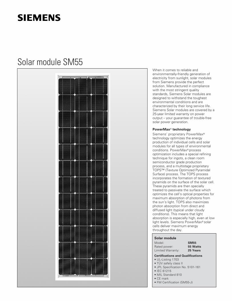
Solar module SM55 When it comes to reliable andenvironmentally-friendly generation ofelectricity from sunlight, solar modulesfrom Siemens provide the perfectsolution. Manufactured in compliancewith the most stringent qualitystandards, Siemens Solar modules aredesigned to withstand the toughestenvironmental conditions and arecharacterized by their long service life.Siemens Solar modules are covered by a25-year limited warranty on poweroutput – your guarantee of trouble-freesolar power generation.
PowerMax® technology
Siemens’ proprietary PowerMax®
technology optimizes the energyproduction of individual cells and solarmodules for all types of environmentalconditions. PowerMax® processoptimization includes a special refiningtechnique for ingots, a clean roomsemiconductor grade productionprocess, and a multistage proprietaryTOPS™ (Texture Optimized PyramidalSurface) process. The TOPS processincorporates the formation of texturedpyramids on the surface of the solar cell.These pyramids are then speciallytreated to passivate the surface whichoptimizes the cell’s optical properties formaximum absorption of photons fromthe sun’s light. TOPS also maximizesphoton absorption from direct anddiffused light (typical under cloudyconditions). This means that lightabsorption is especially high, even at lowlight levels. Siemens PowerMax® solarcells deliver maximum energythroughout the day.
Solar module
Model: SM55
Rated power: 55 Watts
Limited Warranty: 25 Years
Certifications and Qualifications
• UL-Listing 1703• TÜV safety class II• JPL Specification No. 5101-161• IEC 61215• MIL Standard 810• CE mark• FM Certification (SM55-J)
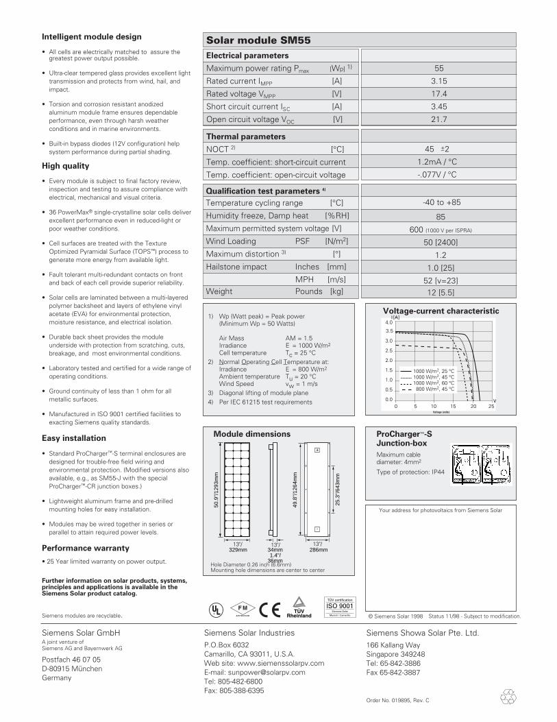
Intelligent module design
• All cells are electrically matched to assure thegreatest power output possible.
• Ultra-clear tempered glass provides excellent lighttransmission and protects from wind, hail, andimpact.
• Torsion and corrosion resistant anodizedaluminum module frame ensures dependableperformance, even through harsh weatherconditions and in marine environments.
• Built-in bypass diodes (12V configuration) helpsystem performance during partial shading.
High quality
• Every module is subject to final factory review,inspection and testing to assure compliance withelectrical, mechanical and visual criteria.
• 36 PowerMax® single-crystalline solar cells deliverexcellent performance even in reduced-light orpoor weather conditions.
• Cell surfaces are treated with the TextureOptimized Pyramidal Surface (TOPS™) process togenerate more energy from available light.
• Fault tolerant multi-redundant contacts on frontand back of each cell provide superior reliability.
• Solar cells are laminated between a multi-layeredpolymer backsheet and layers of ethylene vinylacetate (EVA) for environmental protection,moisture resistance, and electrical isolation.
• Durable back sheet provides the moduleunderside with protection from scratching, cuts,breakage, and most environmental conditions.
• Laboratory tested and certified for a wide range ofoperating conditions.
• Ground continuity of less than 1 ohm for allmetallic surfaces.
• Manufactured in ISO 9001 certified facilities toexacting Siemens quality standards.
Easy installation
• Standard ProCharger™-S terminal enclosures aredesigned for trouble-free field wiring andenvironmental protection. (Modified versions alsoavailable, e.g., as SM55-J with the specialProCharger™-CR junction boxes.)
• Lightweight aluminum frame and pre-drilledmounting holes for easy installation.
• Modules may be wired together in series orparallel to attain required power levels.
Performance warranty
• 25 Year limited warranty on power output.
Further information on solar products, systems,principles and applications is available in theSiemens Solar product catalog.
50.9
"/12
93m
m
25.3
"/64
3mm
49.8
"/12
64m
m
329mm 34mm1.4"/
36mm
286mm13"/ 13"/ 13"/
Module dimensions
Your address for photovoltaics from Siemens Solar
1) Wp (Watt peak) = Peak power(Minimum Wp = 50 Watts)
Air Mass AM = 1.5Irradiance E = 1000 W/m2
Cell temperature Tc = 25 °C2) Normal Operating Cell Temperature at:
Irradiance E = 800 W/m2
Ambient temperature Tu = 20 °CWind Speed vw = 1 m/s
3) Diagonal lifting of module plane4) Per IEC 61215 test requirements
Siemens Solar GmbHA joint venture ofSiemens AG and Bayernwerk AG
Postfach 46 07 05D-80915 MünchenGermany
Siemens modules are recyclable. Status 11/98 - Subject to modification.
Order No. 019895, Rev. C
Siemens Solar IndustriesP.O.Box 6032Camarillo, CA 93011, U.S.A.Web site: www.siemenssolarpv.comE-mail: [email protected]: 805-482-6800Fax: 805-388-6395
Siemens Showa Solar Pte. Ltd.166 Kallang WaySingapore 349248Tel: 65-842-3886Fax 65-842-3887
Voltage-current characteristic
ProCharger™-SJunction-box
Maximum cable diameter: 4mm2
Type of protection: IP44
Hole Diameter 0.26 inch (6.6mm)Mounting hole dimensions are center to center
Solar module SM55Electrical parameters
Maximum power rating Pmax [Wp] 1)
Rated current IMPP [A]
Rated voltage VMPP [V]
Short circuit current ISC [A]
Open circuit voltage VOC [V]
55
3.15
17.4
3.45
21.7
© Siemens Solar 1998
Thermal parameters
NOCT 2) [°C]
Temp. coefficient: short-circuit current
Temp. coefficient: open-circuit voltage
45 _+2
1.2mA / °C
-.077V / °C
Qualification test parameters 4)
Temperature cycling range [°C]
Humidity freeze, Damp heat [%RH]
Maximum permitted system voltage [V]
Wind Loading PSF [N/m2]
Maximum distortion 3) [°]
Hailstone impact Inches [mm]
MPH [m/s]Weight Pounds [kg]
-40 to +85
85
600 (1000 V per ISPRA)
50 [2400]
1.2
1.0 [25]
52 [v=23]12 [5.5]
Voltage (volts)
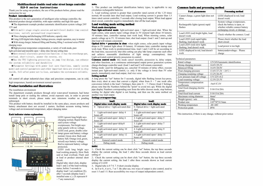
LED LEDLED
Settings button
MultifunctionalMultifunctionalMultifunctionalMultifunctional doubledoubledoubledouble roadroadroadroad solarsolarsolarsolar streetstreetstreetstreet lampslampslampslamps controllercontrollercontrollercontrollerSLD-D series instructions
Thank you for using our products, the use of the products before, please read theinstruction for useProduct introductionThis product is the new generation of intelligent solar recharge controller, theindustrial product design reliability, with super stability and high life-span★The department example product automatic identification system voltage 24V
12V and★With multi-stage single session and multilevel double time control
functions, satisfy personalized requirements
★Three charging and discharging LED indicator, capacity state★Using LED digital tube display Settings process, simple operation, easy to master★With strong charger, balanced filling and floating filling 3-sectional series PWM
charging ways★High precision temperature compensation, a variety of work mode, pure
light-activated and steerable open + delay shut, but any setting time★Have overall electronic protection function: it has the overcharge put,
overload, short-circuit, answer the reverse, etc
★Has the TVS lightning protection, no jump line design, can enhance
the system reliability and durability
★Parameter Settings with power lost save functions, namely system
model and control parameters and other important data are stored in chip
inside, fell after power not to lose, and makes the system more reliable.
★
All control all adopt industrial-class chips and precision components, can in cold,high temperature, humid environment normal operationProductProductProductProduct installationinstallationinstallationinstallation andandandand illustrationsillustrationsillustrationsillustrationsThe installation environmentThe department example products through strict water-proof treatment, had betterinstall lamp pole or sealing the cabinet, avoid exposure rain, in order to preventterminals in short circuit, please make sure rainstorm weather no pondingsubmerged.This product with battery should be installed in the same place, ensure products andbattery attachment does not exceed 1 meters, facilitate accurate testing batteryvoltage and environmental temperature, adjust charging status.EachEachEachEach indicatorindicatorindicatorindicator statusstatusstatusstatus explanation:explanation:explanation:explanation:
LED1 (green) long bright sayscharging normal, Rapid flashessaid system voltageoverpressure, Not bright sayssolar panels with no voltage.LED2 (red, green, double colorlamp) green said battery voltagenormal, Green slow flash saidbattery full; Orange (red, green,mixed) says battery voltage,Red to represent battery voltageprotection.LED3 (red) long bright says
load working properly, Slow flashsaid at load overload, Flash saidat load or product internal shortcircuit.Digital tube: short click, displayload 1 and 2 of the load workingstatus, before 3 seconds todisplay load 1 set condition (X),after 3 seconds (display load 2installed state x.). (X represent 0~ 7 any numerical)
notenotenotenote:1、This product can intelligent identification battery types, is applicable to anycirculation rechargeable batteries2、Load working current is greater than controller rated current of the 1.25 timesnormal, 60 seconds later shut load output, Load working current is greater than 1.5times rated current controller, 5 seconds after closing load output, When load appearshort circuit, controller negative immediately shut off the load output.LoadLoadLoadLoad workingworkingworkingworking modemodemodemode settingsettingsettingsetting methodmethodmethodmethodWorkWorkWorkWork modemodemodemode descriptionsdescriptionsdescriptionsdescriptionsPurePurePurePure light-activatedlight-activatedlight-activatedlight-activated modemodemodemode: light-activated open + light-activated shut. When thenight comes, solar panels input voltage drops to 5V (natural light about 10 lumen),10 minutes later, controller startup start work load, When morning comes, solarpanels voltage up to 5V, 10 minutes later, shut load output. (load 1 and 2 start-up andshut load will remain consistent)OpticalOpticalOpticalOptical drivedrivedrivedrive ++++ possessionpossessionpossessionpossession inininin closeclosecloseclose: when night comes, solar panels input voltagedrops to 5V (natural light about 10 lumen), 10 minutes later, controller startup startwork load, When work to predetermined time, load 1 and 2 will be set according tothe load time, successively shut (this setting can play b&t lamp cooperate each otherand achieve reasonable distribution of light energy consumption); timeLight-activated control priority possession in control.CommonCommonCommonCommon controlcontrolcontrolcontrol modemodemodemode: this mode cancel steerable, possession in, delay output,and other functions, as a continuous uninterrupted output power generation systemscharge-discharge controller used. (load 1 and load 2 will remain consistent)Debug mode: used for debugging use, canceled 10 minutes of delay effect, executeinstant pure light-activated control, i.e. only if the voltage is lower than 5V solarpanels, immediately start load output, And vice versa.SettingSettingSettingSetting methodmethodmethodmethodA long press the "set" button for 5 seconds, digital tube flashing loosen key-press,then every short at once that convert a digital, when from 0 ~ 7 one week afterconversion (which is the load 1 Settings), then enter 0. ~ 7. Choice (load 2 Settings,please note that the Numbers behind the "point" to avoid mix up). While the digitalpipe display Numbers corresponding user from the table chooses mode, stop buttons,waiting for digital tube digital is not beating, and then use the same method setanother way load output.SettingsSettingsSettingsSettings averageservingaverageservingaverageservingaverageserving:
note:note:note:note:1、Check the current setting can be short click "set" button, the top three secondsdisplay the current setting, the load 1 after three seconds shown as load currentsetting of2、Check the current setting can be short click "set" button, the top three secondsdisplay the current setting, the load 1 after three seconds shown as load currentsetting of 2.LED3、Digital tube is 0 7 0. 7. 0 short circular display.4、In 0 or 0., 6 or 6., 7 or 7. Be after use, two ways of output is also control, need toreset 1-5 and 1-5. Rear accessibility two ways of output independent control。
CommonCommonCommonCommon faultsfaultsfaultsfaults andandandand processingprocessingprocessingprocessing methodmethodmethodmethodFaultFaultFaultFault phenomenaphenomenaphenomenaphenomena ProcessingProcessingProcessingProcessing methodmethodmethodmethod
Cannot charge, a green light does notshine
LED2 displayed in red, loaddoesn't work
Rechargeable lights (green) rapidflashes
System voltage overpressure,check the battery is open, orwhether reliable connect batteryrecharging circuit, or damage
Load LED3 (red) bright lights, loaddoesn't work Check whether the connect. Load
Load LED3 (red) rapid lightsflashing, load doesn't work
Please check whether the loadshort circuit
Load LED3 (red) slow lightsflashing, load doesn't work Load power is too high
LED2 displayed in red, load doesn'twork
batteryundervoltage,Pleasecharge
Technical parameters
This instruction, if there is any change, without prior notice
load1load1load1load1 load2load2load2load2DigitalDigitalDigitalDigital tubestubestubestubes workworkworkwork displaydisplaydisplaydisplay modemodemodemode DigitalDigitalDigitalDigital tubestubestubestubes workworkworkwork displaydisplaydisplaydisplay modemodemodemode0 Optical drive + light-activated shut 0. Optical drive + light-activated
shut1 Light-activated open+ delay 4hours off
1. Light-activated open+ delay3hours off
2 Light-activated open+ delay 6hours off
2. Light-activated open+ delay 5hours off
3 Light-activated open+delay8hours off
3. Light-activated open+ delay 7hours off
4 Light-activated open+ delay 10hours off
4. Light-activated open+ delay 9hours off
5 Light-activated open+ delay 12hours off
5. Light-activated open+ delay 11hours off
6 General control mode 6. General control mode7 Debug mode 7. Debug mode
Rated voltage 12V24VAutomatic identificationStrong charging pressure 14.6V/29.2VBalanced filling 14.4V/28.8VFloat charging pressure 13.6V/27.2V(25℃)
Charging resuming voltage 13.2V/26.4VLow pressure load off voltage 11V/22V±0.2Load resuming voltage 12.5V/25.5VTemperature compensationcoefficients -5mV/Ċ/2V
Total fixed charging electriccurrent 5/10/15A/20A
Total fixed load current 5/10/15A/20AMaximum wiring diameter 4mm²Weight (gross) / sets 200gProduct size 118*78*32.5mmWorking temperature -40~60ĊProtection grade IP56
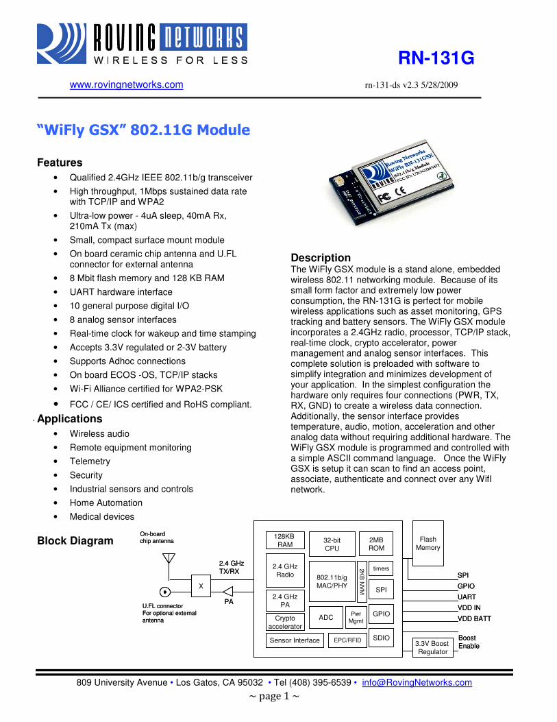
RN-131G
www.rovingnetworks.com rn-131-ds v2.3 5/28/2009
809 University Avenue • Los Gatos, CA 95032 • Tel (408) 395-6539 • [email protected]
~ page 1 ~
“WiFly GSX” 802.11G Module
Features
• Qualified 2.4GHz IEEE 802.11b/g transceiver
• High throughput, 1Mbps sustained data rate with TCP/IP and WPA2
• Ultra-low power - 4uA sleep, 40mA Rx, 210mA Tx (max)
• Small, compact surface mount module
• On board ceramic chip antenna and U.FL connector for external antenna
• 8 Mbit flash memory and 128 KB RAM
• UART hardware interface
• 10 general purpose digital I/O
• 8 analog sensor interfaces
• Real-time clock for wakeup and time stamping
• Accepts 3.3V regulated or 2-3V battery
• Supports Adhoc connections
• On board ECOS -OS, TCP/IP stacks
• Wi-Fi Alliance certified for WPA2-PSK
• FCC / CE/ ICS certified and RoHS compliant.
Applications
• Wireless audio
• Remote equipment monitoring
• Telemetry
• Security
• Industrial sensors and controls
• Home Automation
• Medical devices
Description The WiFly GSX module is a stand alone, embedded wireless 802.11 networking module. Because of its small form factor and extremely low power consumption, the RN-131G is perfect for mobile wireless applications such as asset monitoring, GPS tracking and battery sensors. The WiFly GSX module incorporates a 2.4GHz radio, processor, TCP/IP stack, real-time clock, crypto accelerator, power management and analog sensor interfaces. This complete solution is preloaded with software to simplify integration and minimizes development of your application. In the simplest configuration the hardware only requires four connections (PWR, TX, RX, GND) to create a wireless data connection. Additionally, the sensor interface provides temperature, audio, motion, acceleration and other analog data without requiring additional hardware. The WiFly GSX module is programmed and controlled with a simple ASCII command language. Once the WiFly GSX is setup it can scan to find an access point, associate, authenticate and connect over any WifI network.
Block Diagram
2.4 GHzRadio 802.11b/g
MAC/PHYSPI
GPIO
SDIO
2.4 GHzPA
32-bitCPU
ADC
128KB
RAM2MBROM
Crypto
accelerator
EPC/RFID
timers
Sensor Interface
Pwr
Mgmt
Flash
Memory
GPIO
UART
SPI
X
2.4 GHz TX/RX
PAU.FL connector
For optional external
antenna
On-board
chip antenna
Boost Enable3.3V Boost
Regulator
VDD IN
VDD BATT
2K
B N
VM
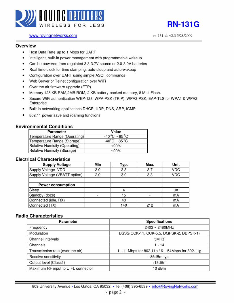
RN-131G
www.rovingnetworks.com rn-131-ds v2.3 5/28/2009
809 University Avenue • Los Gatos, CA 95032 • Tel (408) 395-6539 • [email protected]
~ page 2 ~
Overview
• Host Data Rate up to 1 Mbps for UART
• Intelligent, built-in power management with programmable wakeup
• Can be powered from regulated 3.3-3.7V source or 2.0-3.0V batteries
• Real time clock for time stamping, auto-sleep and auto-wakeup
• Configuration over UART using simple ASCII commands
• Web Server or Telnet configuration over WiFi
• Over the air firmware upgrade (FTP)
• Memory 128 KB RAM,2MB ROM, 2 KB battery-backed memory, 8 Mbit Flash.
• Secure WiFi authentication WEP-128, WPA-PSK (TKIP), WPA2-PSK, EAP-TLS for WPA1 & WPA2 Enterprise
• Built in networking applications DHCP, UDP, DNS, ARP, ICMP
• 802.11 power save and roaming functions
Environmental Conditions
Parameter Value
Temperature Range (Operating) -40 oC ~ 85
oC
Temperature Range (Storage) -40oC ~ 85
oC
Relative Humidity (Operating) ≤90% Relative Humidity (Storage) ≤90%
Electrical Characteristics Supply Voltage Min Typ. Max. Unit
Supply Voltage VDD 3.0 3.3 3.7 VDC
Supply Voltage (VBATT option) 2.0 3.0 3.3 VDC
Power consumption
Sleep 4 uA
Standby (doze) - 15 - mA
Connected (idle, RX) 40 mA
Connected (TX) 140 212 mA
Radio Characteristics
Parameter Specifications
Frequency 2402 ~ 2480MHz
Modulation DSSS(CCK-11, CCK-5.5, DQPSK-2, DBPSK-1)
Channel intervals 5MHz
Channels 1 - 14
Transmission rate (over the air) 1 – 11Mbps for 802.11b / 6 – 54Mbps for 802.11g
Receive sensitivity -85dBm typ.
Output level (Class1) +18dBm
Maximum RF input to U.FL connector 10 dBm
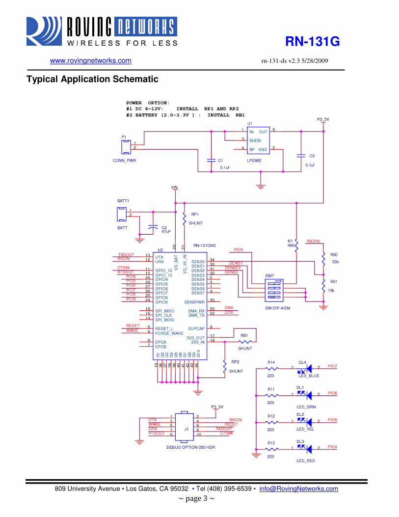
RN-131G
www.rovingnetworks.com rn-131-ds v2.3 5/28/2009
809 University Avenue • Los Gatos, CA 95032 • Tel (408) 395-6539 • [email protected]
~ page 3 ~
Typical Application Schematic
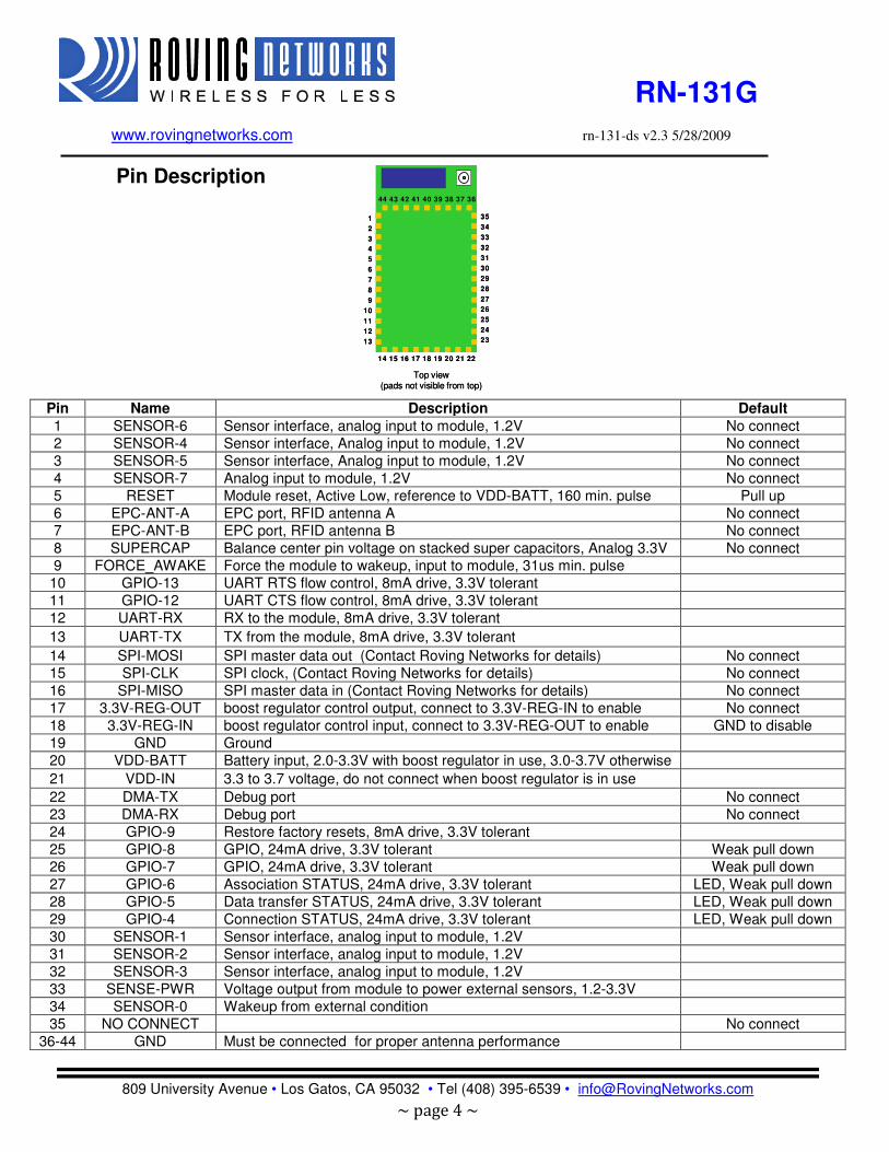
RN-131G
www.rovingnetworks.com rn-131-ds v2.3 5/28/2009
809 University Avenue • Los Gatos, CA 95032 • Tel (408) 395-6539 • [email protected]
~ page 4 ~
Pin Description
Pin Name Description Default
1 SENSOR-6 Sensor interface, analog input to module, 1.2V No connect
2 SENSOR-4 Sensor interface, Analog input to module, 1.2V No connect
3 SENSOR-5 Sensor interface, Analog input to module, 1.2V No connect
4 SENSOR-7 Analog input to module, 1.2V No connect
5 RESET Module reset, Active Low, reference to VDD-BATT, 160 min. pulse Pull up
6 EPC-ANT-A EPC port, RFID antenna A No connect
7 EPC-ANT-B EPC port, RFID antenna B No connect
8 SUPERCAP Balance center pin voltage on stacked super capacitors, Analog 3.3V No connect
9 FORCE_AWAKE Force the module to wakeup, input to module, 31us min. pulse
10 GPIO-13 UART RTS flow control, 8mA drive, 3.3V tolerant
11 GPIO-12 UART CTS flow control, 8mA drive, 3.3V tolerant
12 UART-RX RX to the module, 8mA drive, 3.3V tolerant
13 UART-TX TX from the module, 8mA drive, 3.3V tolerant
14 SPI-MOSI SPI master data out (Contact Roving Networks for details) No connect
15 SPI-CLK SPI clock, (Contact Roving Networks for details) No connect
16 SPI-MISO SPI master data in (Contact Roving Networks for details) No connect
17 3.3V-REG-OUT boost regulator control output, connect to 3.3V-REG-IN to enable No connect
18 3.3V-REG-IN boost regulator control input, connect to 3.3V-REG-OUT to enable GND to disable
19 GND Ground
20 VDD-BATT Battery input, 2.0-3.3V with boost regulator in use, 3.0-3.7V otherwise
21 VDD-IN 3.3 to 3.7 voltage, do not connect when boost regulator is in use
22 DMA-TX Debug port No connect
23 DMA-RX Debug port No connect
24 GPIO-9 Restore factory resets, 8mA drive, 3.3V tolerant
25 GPIO-8 GPIO, 24mA drive, 3.3V tolerant Weak pull down
26 GPIO-7 GPIO, 24mA drive, 3.3V tolerant Weak pull down
27 GPIO-6 Association STATUS, 24mA drive, 3.3V tolerant LED, Weak pull down
28 GPIO-5 Data transfer STATUS, 24mA drive, 3.3V tolerant LED, Weak pull down
29 GPIO-4 Connection STATUS, 24mA drive, 3.3V tolerant LED, Weak pull down
30 SENSOR-1 Sensor interface, analog input to module, 1.2V
31 SENSOR-2 Sensor interface, analog input to module, 1.2V
32 SENSOR-3 Sensor interface, analog input to module, 1.2V
33 SENSE-PWR Voltage output from module to power external sensors, 1.2-3.3V
34 SENSOR-0 Wakeup from external condition
35 NO CONNECT No connect
36-44 GND Must be connected for proper antenna performance
35
34
33
32
31
30
29
28
27
26
25
24
23
1
2
3
4
5
6
7
8
9
10
11
12
13
Top view(pads not visible from top)
14 15 16 17 18 19 20 21 22
44 43 42 41 40 39 38 37 36
35
34
33
32
31
30
29
28
27
26
25
24
23
1
2
3
4
5
6
7
8
9
10
11
12
13
Top view(pads not visible from top)
14 15 16 17 18 19 20 21 22
44 43 42 41 40 39 38 37 36
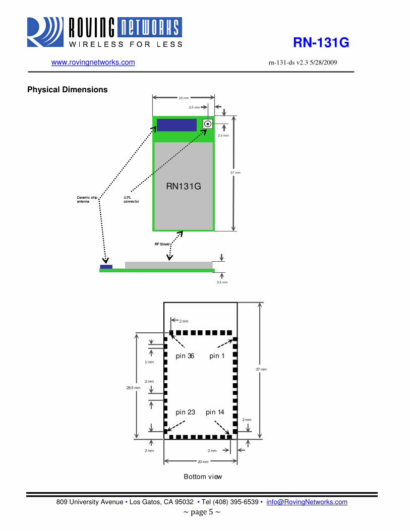
RN-131G
www.rovingnetworks.com rn-131-ds v2.3 5/28/2009
809 University Avenue • Los Gatos, CA 95032 • Tel (408) 395-6539 • [email protected]
~ page 5 ~
Physical Dimensions
RF Shield
Ceramic chipantenna
37 mm
20 mm
RN131G
2.5 mm
2.5 mm
3.5 mm
U.FLconnector
RF Shield
Ceramic chipantenna
37 mm
20 mm
RN131G
2.5 mm
2.5 mm
37 mm
20 mm
RN131G
2.5 mm
2.5 mm
3.5 mm
U.FLconnector
37 mm
2 mm
2 mm
2 mm
1 mm
2 mm
20 mm
Bottom view
2 mm
28.5 mm
pin 23 pin 14
pin 1pin 36
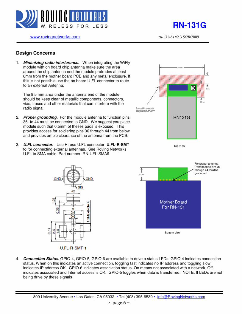
RN-131G
www.rovingnetworks.com rn-131-ds v2.3 5/28/2009
809 University Avenue • Los Gatos, CA 95032 • Tel (408) 395-6539 • [email protected]
~ page 6 ~
Design Concerns
1. Minimizing radio interference. When integrating the WiFly
module with on board chip antenna make sure the area around the chip antenna end the module protrudes at least 6mm from the mother board PCB and any metal enclosure. If this is not possible use the on board U.FL connector to route to an external Antenna.
The 8.5 mm area under the antenna end of the module should be keep clear of metallic components, connectors, vias, traces and other materials that can interfere with the radio signal.
2. Proper grounding. For the module antenna to function pins 36- to 44 must be connected to GND. We suggest you place module such that 0.5mm of theses pads is exposed. This provides access for soldiering pins 36 through 44 from below and provides ample clearance of the antenna from the PCB.
3. U.FL connector. Use Hirose U.FL connector U.FL-R-SMT to for connecting external antennas. See Roving Networks U.FL to SMA cable. Part number: RN-UFL-SMA6
4. Connection Status. GPIO-4, GPIO-5, GPIO-6 are available to drive a status LEDs. GPIO-4 indicates connection
status. When on this indicates an active connection, toggling fast indicates no IP address and toggling slow indicates IP address OK. GPIO-6 indicates association status. On means not associated with a network, Off indicates associated and Internet access is OK. GPIO-5 toggles when data is transferred. NOTE: If LEDs are not being drive by these signals
Bottom view
Mother BoardFor RN-131
8.5 mm
For proper antenna Performance pins 36 through 44 must be grounded
RN131G
8.5 mm
6 mm
30 mm
Keep metallic components,
connectors,,vias and traces,away from antenna area
Top view

RN-131G
www.rovingnetworks.com rn-131-ds v2.3 5/28/2009
809 University Avenue • Los Gatos, CA 95032 • Tel (408) 395-6539 • [email protected]
~ page 7 ~
5. Keep out areas. When designing your PCB avoid exposed trace and via beneath the module.
6. Powering the module. The WiFly module can be powered from either 3.0VDC batteries or 3.3VDC regulated power.
3.0VDC battery power
• Apply power to pin 20 (VDD-BATT)
• Short pin 17 (3.3V-REG-OUT) to pin 18 (3.3V-REG-IN)
3.3 VDC power
• Apply power to pin 20(VDD-BATT) and pin 21 (VDD-IN)
• Connect pin 18 (3.3V-REG-IN) to ground and leave pin 17 (3.3V-REG-OUT) un connected.
7. Sensor Interfaces. Inputs must not exceed 1.2V. Sensitivity saturates at 400 mV.
8. Adhoc mode and Restoring Factory Settings. Adhoc mode is controlled through GPIO-9. It is a good idea to
connect pin 24, GPIO-9 to a switch or jumper connected to a pull up. When GPIO-9 is driven high at power up the module will be in Adhoc mode. If GPIO-9 is then toggled low 5 times, the initial factory default configuration will be RESTORED. This is useful for cases where the module is mis-configured and is no long responding.
Compliance Information
• FCC Certified for us in the United States and CE approved for use in Europe and other countries.
• Environmentally friendly RoHS compliant
Ordering Information
Part Number Description
RN-131G With chip antenna
RN-131G-EVAL Development Kit for the RN-131G (Includes the RN-131G module)
RN-UFL-SMA6 6 inch cable with U.FL connector on one end and SMA on the other
For other configurations, contact Roving Networks directly.
Visit http://www.rovingnetworks.com for current pricing and a list of distributors carrying our products.
Copyright © 2009 Roving Networks. All rights reserved. Roving Networks reserves the right to make corrections, modifications, and other changes to its products, documentation and services at any time. Customers should obtain the latest relevant information before placing orders and should verify that such information is current and complete.
Bottom view
3 mm
Keep out areas: There are two 1 mm round test pads on thebottom of the module. Avoid placing any exposed tracesor vias in these areas
8.0 mm
6mm 5 mm

RN-131G
www.rovingnetworks.com rn-131-ds v2.3 5/28/2009
809 University Avenue • Los Gatos, CA 95032 • Tel (408) 395-6539 • [email protected]
~ page 8 ~
Roving Networks assumes no liability for applications assistance or customer product design. Customers are responsible for their products and applications using Roving Networks components. To minimize the risks associated with customer products and applications, customers should provide adequate design and operating safeguards. Roving Networks products are not authorized for use in safety-critical applications (such as life support) where a failure of the Roving Networks product would reasonably be expected to cause severe personal injury or death, unless officers of the parties have executed an agreement specifically governing such use. All other trademarks are property of their respective owners.


![[2015] Etude V-Traffic IDF - NEW](https://img.pdfslide.fr/doc/110x75/586e000d1a28abd7678b546c/2015-etude-v-traffic-idf-new.jpg)