Embed Size (px)
Citation preview

N
◦d'ordre: 4937
THÈSE
présentée à
L'UNIVERSITÉ BORDEAUX 1
É ole Do torale de Mathématiques et Informatique de Bordeaux
par
Gabriel Renault
pour obtenir le grade de
DOCTEUR
SPÉCIALITÉ : INFORMATIQUE
Jeux ombinatoires dans les graphes
Soutenue le 29 novembre 2013 au Laboratoire Bordelais de Re her he en Informatique (LaBRI)
Après avis des rapporteurs :
Mi hael Albert Professeur
Sylvain Gravier Dire teur de re her he
Brett Stevens Professeur
Devant la ommission d'examen omposée de :
Examinateurs
Tristan Cazenave Professeur
Éri Du hêne Maître de onféren e
Rapporteurs
Sylvain Gravier Dire teur de re her he
Brett Stevens Professeur
Dire teurs de thèse
Paul Dorbe Maître de onféren e
Éri Sopena Professeur

ii

Remer iements iii
Remer iements
Je voudrais d'abord remer ier les rapporteurs et membres de mon jury de
s'être intéressés à mes travaux, d'avoir lu ma thèse, assisté à ma soutenan e
et posé des questions évoquant de futurs axes de re her he sur le sujet. Mer i
beau oup à Mi hael Albert, Sylvain Gravier et Brett Stevens d'avoir pris le
temps de lire ma thèse en détail et exprimé des remarques pertinentes et
onstru tives sur leurs rapports. Mer i beau oup à Tristan Cazenave d'avoir
a epté de présider mon jury. Mer i beau oup à Éri Du hêne d'être venu
de Lyon pour ma soutenan e.
Je tiens à remer ier plus parti ulièrement mes dire teurs de thèse Paul
Dorbe et Éri Sopena. Travailler ave eux a toujours été un plaisir, ils ont un
don pour déterminer quels problèmes m'intéresseraient parti ulièrement. Ils
m'ont fait on�an e en a eptant de m'en adrer pour mon stage de M2, puis
pour ma thèse. Je les remer ie aussi pour toutes les opportunités qu'ils m'ont
apportées, que e soit des expérien es d'enseignement un peu di�érentes au
sein de Math en Jeans et Maths à Modeler, des séjours de re her he ou
des onféren es. L'é hange ave eux a aussi été très agréable sur le plan
humain, 'était sympathique de pouvoir aussi parler en dehors d'un ontexte
de travail.
Je voudrais également remer ier les personnes ave lesquelles j'ai eu
l'o asion de travailler, en parti ulier Bo²tjan, Éri , Ga²per, Julien, Re-
be a, Ri hard, Sandi et Simon. C'est toujours intéressant de se pen her sur
un problème ave quelqu'un qui peut avoir une vision un peu di�érente et
d'arriver à une solution grâ e à es deux points de vue.
J'ai aussi eu la han e de parti iper aux séminaires du groupe de tra-
vail Graphes et Appli ations. Je remer ie ses membres et plus parti ulière-
ment eux qui ont été do torants en même temps que moi, ave lesquels j'ai
eu le plus d'é hange, Adrien, Clément, Émilie Florent, Hervé, Noël, Petru,
Pierre, Quentin, Romari , Sagnik, Thomas et Tom. C'était aussi un plaisir
de otoyer les membres permanents, André, Arnaud, Cyril, David, Frantisek,
Frédéri , Mi kael, Ni olas, Ni olas, Olivier, Olivier, Philippe et Ralf.
Je remer ie aussi les her heurs en graphes et jeux que j'ai eu la han e
de ren ontrer en onféren e ou séjour de re her he, parmi lesquels Aline, An-
dré, Ararat, Benjamin, Guillem, Guillaume, Jean-Florent, Julien, Laetitia,
Laurent, Louis, Marthe, Neil, Ni olas, Paul, Reza, Théophile et Urban.
J'ai eu la han e d'enseigner à l'Université Bordeaux 1, et je voudrais re-
mer ier les enseignants qui m'ont a ompagné pour e par ours, notamment
Aurélien, Christian, David, Frédéri , Frédérique, Jean-Paul, Pas al, Pierre,
Pierre et Vin ent. Je tiens également à remer ier Marie-Line ave laquelle
j'ai pu en adrer l'a tivité Math en Jeans à l'université.
Je remer ie aussi toute l'équipe administrative du LaBRI pour leur e�-
a ité, leur amabilité et leur bonne humeur, en parti ulier eux ave lesquels

iv Remer iements
j'ai eu le plus d'o asions de dis uter, Brigitte, Cathy, Isabelle, Lebna, Maïté
et Philippe.
Je voudrais remer ier les do torants qui ont parti ipé à faire vivre le
bureau 123 via des débats et dis ussions, en parti ulier Amal, Benjamin,
Christian, Christopher, Edon, Eve, Florian, Jaime, Jér�me, Lorijn, Lu as,
Matthieu, Nesrine, Omar, Oualid, Pierre, Sinda, Tom, Tung, Van-Cuong,
Wafa et Yi.
La vie au labo aurait été di�érente sans les a tivités organisées par
l'AFoDIB, et les sorties entre do torants. Je remer ie leurs parti ipants
les plus fréquents, parmi eux qui n'ont pas en ore été ités, Abbas, Adrien,
Allyx, Anaïs, Anna, Carlos, Cedri , Cyril, David, Dominik, Etienne, Fouzi,
Jér�me, Lorenzo, Martin, Matthieu, Noémie-Fleur, Razanne, Rémi, Simon,
Srivathsan, Thomas, Vin ent et Xavier.
J'ai aussi eu des onta ts en dehors de la sphère de l'université. Je
voudrais remer ier mes amis ave lesquels mes sujets de dis ussions variaient
un peu en omparaison, ou qui m'ont permis de vulgariser mes travaux, en
parti ulier Alexandre, Amélie, Benjamin, Benoît, Cé ile, Clément, Emeri ,
Ena, Guilhem, Irène, Jonas, Kévin, Laure, Nolwenn, Ophélia, Pierre, Rémi
et Romain. Je iterai aussi les emails du RatonLaveur qui pouvaient
parti iper à me mettre de bonne humeur.
Je voudrais aussi remer ier ma famille pour des raisons similaires, ainsi
que pour m'avoir fait on�an e et en ouragé dans la voie que je voulais
suivre. Je remer ie mes parents, mes frères et s÷ur, mes grands-parents,
on les, tantes, ousins et ousines. Un remer iement spé ial à Xiaohan qui
a donné une autre dimension à la vulgarisation en me poussant à la réaliser
en anglais.
Résumé v
Jeux ombinatoires dans les graphes
Résumé : Dans ette thèse, nous étudions les jeux ombinatoires sous
di�érentes ontraintes. Un jeu ombinatoire est un jeu à deux joueurs, sans
hasard, ave information omplète et �ni a y lique. D'abord, nous regardons
les jeux impartiaux en version normale, en parti ulier les jeux VertexNim
et Timber. Puis nous onsidérons les jeux partisans en version normale, où
nous prouvons des résultats sur les jeux Timbush, Toppling Dominoes
et Col. Ensuite, nous examinons es jeux en version misère, et étudions
les jeux misères modulo l'univers des jeux di ots et modulo l'univers des
jeux dead-endings. En�n, nous parlons du jeu de domination qui, s'il n'est
pas ombinatoire, peut être étudié en utilisant des outils de théorie des jeux
ombinatoires.
Mots- lés : jeux ombinatoires, graphes, jeux impartiaux,
jeux partisans, version normale, version misère, jeu de domi-
nation
vi Abstra t
Combinatorial games on graphs
Abstra t: In this thesis, we study ombinatorial games under di�erent
onventions. A ombinatorial game is a �nite a y li two-player game with
omplete information and no han e. First, we look at impartial games
in normal play and in parti ular at the games VertexNim and Timber.
Then, we onsider partizan games in normal play, with results on the games
Timbush, Toppling Dominoes and Col. Next, we look at all these games
in misère play, and study misère games modulo the di ot universe and modulo
the dead-ending universe. Finally, we talk about the domination game whi h,
despite not being a ombinatorial game, may be studied with ombinatorial
games theory tools.
Keywords: ombinatorial games, graphs, impartial games,
partizan games, normal onvention, misère onvention, dom-
ination game
Contents vii
Contents
1 Introdu tion 1
1.1 De�nitions . . . . . . . . . . . . . . . . . . . . . . . . . . . . . 2
1.1.1 Combinatorial Games . . . . . . . . . . . . . . . . . . 2
1.1.2 Graphs . . . . . . . . . . . . . . . . . . . . . . . . . . 6
2 Impartial games 13
2.1 VertexNim . . . . . . . . . . . . . . . . . . . . . . . . . . . . 14
2.1.1 Dire ted graphs . . . . . . . . . . . . . . . . . . . . . . 16
2.1.2 Undire ted graphs . . . . . . . . . . . . . . . . . . . . 21
2.2 Timber . . . . . . . . . . . . . . . . . . . . . . . . . . . . . . 26
2.2.1 General results . . . . . . . . . . . . . . . . . . . . . . 27
2.2.2 Trees . . . . . . . . . . . . . . . . . . . . . . . . . . . . 32
2.2.2.1 Paths . . . . . . . . . . . . . . . . . . . . . . 39
2.3 Perspe tives . . . . . . . . . . . . . . . . . . . . . . . . . . . . 40
3 Partizan games 43
3.1 Timbush . . . . . . . . . . . . . . . . . . . . . . . . . . . . . 44
3.1.1 General results . . . . . . . . . . . . . . . . . . . . . . 45
3.1.2 Paths . . . . . . . . . . . . . . . . . . . . . . . . . . . 49
3.1.3 Bla k and white trees . . . . . . . . . . . . . . . . . . 54
3.2 Toppling Dominoes . . . . . . . . . . . . . . . . . . . . . . 61
3.2.1 Preliminary results . . . . . . . . . . . . . . . . . . . . 63
3.2.2 Proof of Theorem 3.27 . . . . . . . . . . . . . . . . . . 65
3.3 Col . . . . . . . . . . . . . . . . . . . . . . . . . . . . . . . . 72
3.3.1 General results . . . . . . . . . . . . . . . . . . . . . . 76
3.3.2 Known results . . . . . . . . . . . . . . . . . . . . . . . 80
3.3.3 Caterpillars . . . . . . . . . . . . . . . . . . . . . . . . 93
3.3.4 Cographs . . . . . . . . . . . . . . . . . . . . . . . . . 96
3.4 Perspe tives . . . . . . . . . . . . . . . . . . . . . . . . . . . . 98
4 Misère games 101
4.1 Spe i� games . . . . . . . . . . . . . . . . . . . . . . . . . . . 104
4.1.1 Geography . . . . . . . . . . . . . . . . . . . . . . . 105
4.1.2 VertexNim . . . . . . . . . . . . . . . . . . . . . . . 111
4.1.3 Timber . . . . . . . . . . . . . . . . . . . . . . . . . . 113
4.1.4 Timbush . . . . . . . . . . . . . . . . . . . . . . . . . 116
4.1.5 Toppling Dominoes . . . . . . . . . . . . . . . . . . 117
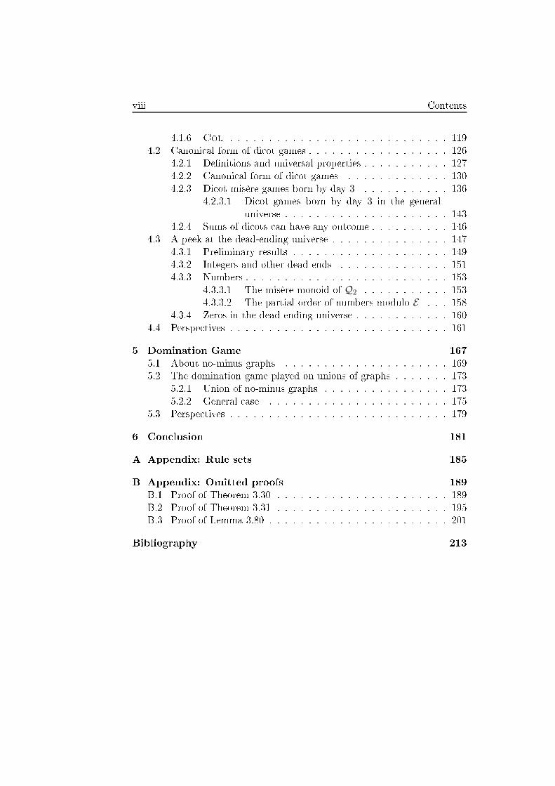
viii Contents
4.1.6 Col . . . . . . . . . . . . . . . . . . . . . . . . . . . . 119
4.2 Canoni al form of di ot games . . . . . . . . . . . . . . . . . . 126
4.2.1 De�nitions and universal properties . . . . . . . . . . . 127
4.2.2 Canoni al form of di ot games . . . . . . . . . . . . . 130
4.2.3 Di ot misère games born by day 3 . . . . . . . . . . . 136
4.2.3.1 Di ot games born by day 3 in the general
universe . . . . . . . . . . . . . . . . . . . . . 143
4.2.4 Sums of di ots an have any out ome . . . . . . . . . . 146
4.3 A peek at the dead-ending universe . . . . . . . . . . . . . . . 147
4.3.1 Preliminary results . . . . . . . . . . . . . . . . . . . . 149
4.3.2 Integers and other dead ends . . . . . . . . . . . . . . 151
4.3.3 Numbers . . . . . . . . . . . . . . . . . . . . . . . . . . 153
4.3.3.1 The misère monoid of Q2 . . . . . . . . . . . 153
4.3.3.2 The partial order of numbers modulo E . . . 158
4.3.4 Zeros in the dead-ending universe . . . . . . . . . . . . 160
4.4 Perspe tives . . . . . . . . . . . . . . . . . . . . . . . . . . . . 161
5 Domination Game 167
5.1 About no-minus graphs . . . . . . . . . . . . . . . . . . . . . 169
5.2 The domination game played on unions of graphs . . . . . . . 173
5.2.1 Union of no-minus graphs . . . . . . . . . . . . . . . . 173
5.2.2 General ase . . . . . . . . . . . . . . . . . . . . . . . 175
5.3 Perspe tives . . . . . . . . . . . . . . . . . . . . . . . . . . . . 179
6 Con lusion 181
A Appendix: Rule sets 185
B Appendix: Omitted proofs 189
B.1 Proof of Theorem 3.30 . . . . . . . . . . . . . . . . . . . . . . 189
B.2 Proof of Theorem 3.31 . . . . . . . . . . . . . . . . . . . . . . 195
B.3 Proof of Lemma 3.80 . . . . . . . . . . . . . . . . . . . . . . . 201
Bibliography 213
Chapter 1. Introdu tion 1
Chapter 1
Introdu tion
Combinatorial games are games of pure strategy, loser to Che kers,
Chess or Go than to Dominion, League of Legends, or Rugby. They are
games satisfying some onstraints insuring a player has a winning strategy.
Our goal here is to �nd whi h player it is, and even the strategy if possible.
There exist other game theories, su h as e onomi game theory, where
there might be several players, who are allowed to play their moves at the
same time. There, the players' `best' strategies are often probabilisti , that
is for example a player would de ide to play the move A with probability
0.3, the move B with probability 0.5, and the move C with probability 0.2,be ause they do not know what their opponent might do and ea h of these
moves might be better than the other depending on the opponent's move. In
ombinatorial game, this does not happen, the `winning' player always has
a deterministi winning strategy.
The �rst paper in ombinatorial game theory was published in 1902 by
Bouton [5℄, who solved the game of Nim, game that would be ome the ref-
eren e in impartial games thanks to the theory developed independently by
Grundy and Sprague in the 30s. For a few de ades, resear hers studied the
games where both players have the same moves and are only distinguished by
who plays �rst, games we all impartial. In the late 70s, Berlekamp, Conway
and Guy developed the theory of partizan games, where the two players may
have di�erent moves. These games introdu e many more possibilities, as for
example a player might have a winning strategy whoever starts playing. The
omplexity of determining the winner of a ombinatorial game was also on-
sidered, ranging from polynomial problems to exptime- omplete problems.
Another topi in ombinatorial game theory that has interested resear hers
is the misère version of a game, that is the game where the winning on-
dition is reversed. These games were not well understood, mainly be ause
when they de ompose, it is harder to put together the separate analysis of
the omponents, until Plambe k and Siegel proposed a way to make it sim-
pler in the beginning of the 21st entury. Referen es about the topi in ludethe books Winning Ways [4℄ and On Numbers and Games [10℄, and other
books that were published more re ently, su h as Lessons in Play [1℄, Games,
Puzzles, & Computation [11℄ and Combinatorial Game Theory [39℄.
Graph theory is more an ient, Euler was already looking at it in the 18th
entury. A graph is a mathemati al obje t that an be used to represent any
kind of network, su h as omputer networks, road networks, so ial networks,

2 1.1. De�nitions
or neural networks.
Natural questions that arise on these networks an be translated under a
graph formalism. Among lassi graph problems, one an mention olouring
and domination. These problems admit variants that are two-player games,
where the players may build an answer to the original problem.
In this thesis, we study ombinatorial games, mostly games played on
graphs. We �rst give some basi de�nitions on games and graphs, before
presenting our results on games. We start with impartial games before going
to partizan games and ontinuing with games in misère play. We end with
a game that is not ombinatorial but is more like a graph parameter.
1.1 De�nitions . . . . . . . . . . . . . . . . . . . . . . . 2
1.1.1 Combinatorial Games . . . . . . . . . . . . . . . . 2
1.1.2 Graphs . . . . . . . . . . . . . . . . . . . . . . . . 6
1.1 De�nitions
1.1.1 Combinatorial Games
A ombinatorial game is a �nite two-player game with perfe t information
and no han e. The players, alled Left and Right, alternate moves until one
player has no available move. Under the normal onvention, the last player
to move wins the game. Under the misère onvention, that same player loses
the game. By onvention, Left is a female player whereas Right is a male
player.
A position of a game an be de�ned re ursively by its sets of options
G = {GL|GR}, where GLis the set of positions rea hable in one move by
Left ( alled Left options), and GRthe set of positions rea hable in one move
by Right ( alled Right options). The word game an be used to refer to a
set of rules, as well as to a spe i� position as just des ribed. A follower of
a game is a game that an be rea hed after a su ession of (not ne essarily
alternating) Left and Right moves. The zero game 0 = {·|·}, is the game
with no option (the dot indi ates an empty set of options). The birthday of a
game is de�ned re ursively as one plus the maximum birthday of its options,
with 0 being the only game with birthday 0. We say a game G is born on
day n if its birthday is n and that it is born by day n if its birthday is at
most n. The games born on day 1 are {0|·} = 1, {·|0} = 1 and {0|0} = ∗.The games born by day 1 are the same with the addition of 0. A game G is

Chapter 1. Introdu tion 3
0 1 1 ∗
Figure 1.1: Game trees of games born by day 1.
said to be simpler than a game H if the birthday of G is smaller than the
birthday of H.
A game an also be depi ted by its game tree, where the game trees of
its options are linked to the root by downward edges, left-slanted for Left
options and right-slanted for Right options. For instan e, the game trees of
games born by day 1 are depi ted on Figure 1.1.
When the Left and Right options of a game are always the same and that
property is true for any follower of the game, we say the game is impartial.
Otherwise, we say it is partizan.
Given two games G = {GL|GR} and H = {HL|HR}, we re ursively
de�ne the (disjun tive) sum of G and H as G + H = {GL + H,G +HL|GR + H,G + HR} (where GL + H is the set of sums of H and an
element of GL), i.e. the game where ea h player hooses on their turn
whi h one of G and H to play on. We write {GL1 · · ·GLk |GR1 · · ·GRℓ} for
{{GL1 · · ·GLk}|{GR1 · · ·GRℓ}} to simplify the notation. We denote by GL
any Left option of G, and by GRany of its Right options. The onjugate G
of a game G is de�ned re ursively by G = {GR|GL} (where GRis the set of
onjugates of elements of GR), that is the game where Left and Right would
have swit hed their roles.
For both onventions, there are four possible out omes for a game. Games
for whi h Left has a winning strategy whatever Right does and whoever plays
�rst have out ome L (for left). Similarly, N , P and R (for next, previous and
right) denote respe tively the out omes of games for whi h the �rst player,
the se ond player, and Right has a winning strategy. We note o+(G) the
normal out ome of a game G i.e. its out ome under the normal onvention
and o−(G) the misère out ome ofG. We also say for any out ome O, G ∈ O+
or G is a (normal) O-position whenever o+(G) = O, and H ∈ O−or H is
a (misère) O-position when o−(H) = O. Out omes are partially ordered
a ording to Figure 1.2, with greater games being more advantageous for
Left. Note that there is no general relationship between the normal out ome
and the misère out ome of a game.
Given two games G and H, we say that G is greater than or equal to Hin normal play whenever Left prefers the game G rather than the game H in
any sum, that is G >+ H if for every game X, o+(G+X) > o+(H+X). We
say that G and H are equivalent in normal play, denoted G ≡+ H, when for
every game X, o+(G +X) = o+(H +X) (i.e. G >+ H and H >+ G). We
also say that G is (stri tly) greater than H in normal play if G is greater than

4 1.1. De�nitions
L
N P
R
Figure 1.2: Partial ordering of out omes
or equal to H but G and H are not equivalent, that is G >+ H if G >+ Hand G 6≡+ H. We say that G and H are in omparable in normal play if
none is greater than or equal to the other, that is G �
+ H if G �+ H and
H �+ G. Inequality, equivalen e and in omparability are de�ned similarly
under misère onvention, using supers ript − instead of +. We reserved the
symbol = for equality between game trees, when used between games.
For normal play, there exist other hara terisations for he king inequal-
ity:
G >+ H ⇔ G+H ∈ P+ ∪ L+
⇔ (∀GR ∈ GR, GR H) ∧ (∀HL ∈ HL, G HL).
The last hara terisation was a tually the original de�nition given by Conway
in [10℄. The se ond one tells us that for any games G and H, if G and H are
equivalent in normal play, then the sum of G and the onjugate of H is a
normal P-position and, as G is equivalent to itself, G+G is always a normal
P-position, whi h is a tually easy to prove by mimi king the �rst player's
move as the se ond player.
In normal play, �nding the out ome of a game is the same as �nding how
it is ompared to 0:
G is a P-position if G ≡+ 0 : G is zero
G is an L-position if G >+ 0 : G is positive
G is an R-position if G <+ 0 : G is negative
G is an N -position if G �
+ 0 : G is fuzzy
For example, 0 is zero, 1 is positive, 1 is negative, and ∗ is fuzzy.
As G +G ≡+ 0 for any game G, we all the onjugate of a game G the
negative of G and denote it −G in normal play.
We remind the reader that the order is only partial, in both onventions,
and many pairs of games are in omparable, su h as 0 and ∗.Siegel showed [38℄ that if two games are omparable in misère play, they
are omparable in normal play as well, in the same order, namely:
Theorem 1.1 (Siegel [38℄) If G >− H, then G >+ H.

Chapter 1. Introdu tion 5
However, the onverse in not true, as {∗|∗} ≡+ 0 and {∗|∗} �− 0.
Some options are onsidered irrelevant, either be ause there is a better
move or be ause the answer of the opponent is `predi table'. We give here
the de�nition of these options, omitting the supers ripts + and −, as theyare de�ned the same way for normal play and misère play.
De�nition 1.2 (dominated and reversible options)
Let G be a game.
(a) A Left option GLis dominated by some other Left option GL′
if
GL′
> GL.
(b) A Right option GRis dominated by some other Right option GR′
if
GR′
6 GR.
( ) A Left option GLis reversible through some Right option GLR
if
GLR 6 G.
(d) A Right option GRis reversible through some Left option GRL
if
GRL > G.
In both normal and misère play, a game is said to be in anoni al form
if none of its options is dominated or reversible and all its options are in
anoni al form, and every game is equivalent to a single game in anoni al
form [4, 10, 38℄. To get to this anoni al form, one may use two di�erent
operations orresponding to the status of the option they want to get rid of:
• Whenever GL1is dominated, removing GL1
leaves an equivalent game:
G ≡ {GL \ {GL1}|GR}• Whenever GR1
is dominated, removing GR1leaves an equivalent game:
G ≡ {GL|GR \ {GR1}}• Whenever GL1
is reversible through GL1R1, bypassing GL1
leaves an
equivalent game: G ≡ {(GL \ {GL1}) ∪GL1R1L|GR}• Whenever GR1
is reversible through GR1L1, bypassing GR1
leaves an
equivalent game: G ≡ {GL|(GR \ {GR1}) ∪GR1L1R}
Theorem 1.1 implies that if an option is dominated (resp. reversible) in
misère play, it is also dominated (resp. reversible) in normal play. Again,
the onverse is not true: in {{∗|∗}, 0|{∗|∗}, 0}, all options are dominated in
normal play, but none is dominated in misère play; in {∗|∗}, both options are
reversible in normal play, but none is reversible in misère play. This implies
that the normal anoni al form of a game and its misère anoni al form may
be di�erent: {∗|∗} is in misère anoni al form, whereas its normal anoni al
form is 0.

6 1.1. De�nitions
a bc
d e f
Figure 1.3: The undire ted graph with
vertex set {a, b, c, d, e, f} and edge set
{(a, d), (b, c), (b, e), (b, f), (e, f)}
a bc
d e f
Figure 1.4: The dire ted graph with
vertex set {a, b, c, d, e, f} and ar set
{(a, b), (c, b), (c, f), (e, d), (f, c)}
1.1.2 Graphs
A graph G onsists of a set of verti es V (G) and a multiset of edges E(G)representing a symmetri binary relation between the verti es. As the re-
lation is symmetri , the edge between two verti es u and v will be repre-
sented by (u, v) or (v, u) and the multipli ity of the edge between u and
v is the sum of the multipli ity of these edges in the multiset E(G). We
say a graph is simple if the relation represented by E(G) is irre�exive and
E(G) is a set, that is if no vertex is in relation with itself and the mul-
tipli ity of ea h edge is (0 or) 1. A dire ted graph G is a generalisation
of a graph, su h that the relation represented by E(G) no longer needs to
be symmetri . We sometimes note A(G) rather than E(G) when G is a
dire ted graph, and we all dire ted edges or ar s the elements of A(G).The underlying undire ted graph und(G) of a dire ted graph G is the graph
obtained by onsidering ar s as edges, that is V (und(G)) = V (G) and
E(und(G)) = {(u, v)|(u, v) ∈ A(G) or (v, u) ∈ A(G)}. An oriented graph
is a dire ted graph whose underlying undire ted graph is a simple graph.
An orientation
−→G of a graph G is a dire ted graph su h that the underly-
ing undire ted graph of
−→G is G. The number of verti es |V (G)| of a graph
G is alled the order of G. A subgraph H of a graph G is a graph whose
vertex set is a subset of V (G) and whose edge set is a subset of E(G). An
indu ed subgraph H of G is a subgraph of G su h that E(H) is the restri -tion of E(G) to elements of V (H). The graph indu ed by a set of verti es
{v1 · · · vk} of a graph G is the indu ed subgraph G[{v1 · · · vk}] of G with
vertex set {v1 · · · vk}.
Example 1.3 Figure 1.3 gives an example of a graph. The graph is simple
as the multipli ity of ea h edge is at most one. Figure 1.4 gives an example
of a dire ted graph. The dire ted graph is simple as the multipli ity of ea h
edge is at most one. Nevertheless, it is not an oriented graph as it ontains
both the ar (c, f) and the ar (f, c).

Chapter 1. Introdu tion 7
A path (v1 · · · vn) of a graph G is a list of verti es of G su h that for any
i in J2;nK, (vi−1, vi) is an edge of G. A dire ted path (v1 · · · vn) of a dire ted
graph G is a list of verti es of G su h that for any i in J2;nK, (vi−1, vi) is anar of G. We say that (n − 1) is the length of the path, and that the path
is from v1 to vn. A y le (v1 · · · vn) of a graph G is a path of G su h that
(vn, v1) ∈ E(G). A ir uit (v1 · · · vn) of a dire ted graph G is a dire ted path
of G su h that (vn, v1) ∈ A(G). We also say that n is the length of the y le.
A path or y le is said to be simple if all its verti es are pairwise distin t. A
graph is said to be onne ted if for any pair u, v of verti es, there exists a pathfrom u to v. A onne ted omponent of a graph G is a maximal onne ted
subgraph of G. A dire ted graph is said to be strongly onne ted if for any
pair u, v of verti es, there exists a dire ted path from u to v and a dire ted
path from v to u. A strongly onne ted omponent of a dire ted graph G is
a maximal strongly onne ted subgraph of G. A onne ted omponent of a
dire ted graph G is a onne ted omponent of und(G). The distan e d(u, v)between two verti es u and v in a graph G is the length of the shortest path
between u and v in G if su h a path exists, and in�nite otherwise.
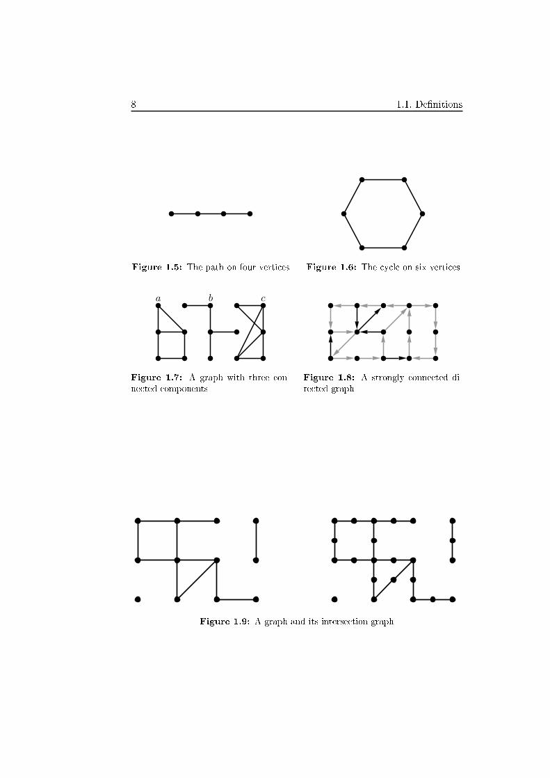
Example 1.4 Figure 1.5 gives an example of a path. Figure 1.6 gives an
example of a y le. We an see that both graphs are onne ted. Figure 1.7
is an example of a non- onne ted graph having three onne ted omponents:
there is no path from a to b or to c, and there is none either from b to c.Figure 1.8 is an example of a strongly- onne ted dire ted graph: given any
two verti es of the dire ted graph, one only needs to follow the grey ar s
from one to the other.
A subdivision of a graph G is a graph obtained from G by repla ing some
edges by paths of any length. The interse tion graph of a graph G is the
subdivision of G su h that ea h edge of G has been repla ed by a path with
two edges.
Example 1.5 Figure 1.9 gives an example of a graph (on the left) and its
interse tion graph (on the right). Every edge of the �rst graph has been
repla ed by a vertex in ident to both ends of that edge.
A neighbour u of a vertex v in a graph G is a vertex su h that
(u, v) ∈ E(G). When u is a neighbour of v, we say u and v are adja-
ent. The neighbourhood N(v) of a vertex v is the set of all neighbours of v.The losed neighbourhood N [v] of a vertex v is the set N(v)∪{v}. The degreedG(v) (or d(v)) of a vertex v in a graph G is the number of its neighbours.
An in-neighbour of a vertex v in a dire ted graph G is a vertex u su h that
(u, v) ∈ E(G). An out-neighbour of a vertex u in a dire ted graph G is a
vertex v su h that (u, v) ∈ E(G). We say (u, v) is an out-ar of u and an
in-ar of v. The in-degree d−G(v) (or d−(v)) of a vertex v in a dire ted graph
G is the number of its in-neighbours. The out-degree d+G(v) (or d+(v)) of
8 1.1. De�nitions
Figure 1.5: The path on four verti es Figure 1.6: The y le on six verti es
a b c
Figure 1.7: A graph with three on-
ne ted omponents
Figure 1.8: A strongly onne ted di-
re ted graph
Figure 1.9: A graph and its interse tion graph

Chapter 1. Introdu tion 9
Figure 1.10: An independent set of a
graph
Figure 1.11: A lique of a graph
a vertex v in a dire ted graph G is the number of its out-neighbours. The
degree dG(v) (or d(v)) of a vertex v in a dire ted graph G is the sum of its
in-degree and its out-degree.
An independent set is a set of verti es indu ing a graph with no edge.
A lique is a set of verti es indu ing a graph where any pair of verti es
forms an edge. A proper olouring of a graph G over a set S is a fun tion
c : V (G) → S su h that for any element i of S, c−1(i) is an independent set.
A partial proper olouring of a graph G is a proper olouring of an indu ed
subgraph of G. A bipartite graph is a graph admitting a proper olouring
over a set of size 2. A planar graph is a graph one an draw on the plane
without having edges rossing ea h other.
Example 1.6 In Figure 1.10, the grey verti es form an independent set of
the graph: they are pairwise not adja ent. In Figure 1.10, the grey verti es
form a lique of the graph: they are pairwise adja ent.
The omplement G of a simple graph G is the
graph with vertex set V (G) = V (G) and edge set
E(G) = {(u, v)|u, v ∈ V (G), u 6= v, (u, v) /∈ E(G)}. The disjoint union
G ∪ H of two graphs G and H (having disjoint sets of verti es, that is
V (G) ∩ V (H) = ∅) is the graph with vertex set V (G ∪H) = V (G) ∪ V (H)and edge set E(G ∪H) = E(G) ∪ E(H). The join G ∨ H of two graphs Gand H is the graph with vertex set V (G ∨H) = V (G) ∪ V (H) and edge
set E(G ∨H) = E(G) ∪E(H) ∪ {(u, v)|u ∈ V (G), v ∈ V (H)}. The disjointunion and the join operations are extended to more than two graphs,
iteratively, as the operation is both ommutative and asso iative. The
Cartesian produ t G�H of two graphs G and H is the graph with vertex
set V (G�H) = {(u, v)|u ∈ V (G), v ∈ V (H)} and edge set
E(G�H) = {((u1, v1), (u2, v2))|(u1 = u2 and (v1, v2) ∈ E(H))or (v1 = v2 and (u1, u2) ∈ E(G))}.

10 1.1. De�nitions
Figure 1.12: A forest of three trees
Example 1.7 The omplement of an independent set is a lique, and vi e
versa. The join of n verti es is a lique. The disjoint union of n verti es is
an independent set. The omplement of the join of k graphs is the disjoint
union of the omplements of these graphs. The Cartesian produ t of two
single edges is a y le on four verti es.
A tree is a onne ted graph with no y le. A forest is a graph with no
y le. A star is a tree where all verti es but one have degree 1. That vertexwith higher degree is alled the enter of the star. A subdivided star is any
subdivision of a star. A aterpillar is a tree su h that the set of verti es of
degree at least 2 forms a path. A rooted tree is a tree with a spe ial vertex,
alled the root of the tree. In a rooted tree, a vertex u is a hild of a vertex
v if u and v are adja ent and the distan e between u and the root is greater
than the distan e between v and the root; in this ase, we say v is a parent
of u. In a tree, a vertex of degree 1 is alled a leaf, and any other vertex is
alled an internal node.
Example 1.8 Figure 1.12 is an example of a forest. As in any forest, ea h
onne ted omponent is a tree. The middle one is a subdivided star, where
the grey vertex is the enter. The right one is a aterpillar, where the verti es
of degree at least two are ir led in grey, while the edges onne ting them
are grey too, highlighting the fa t they form a path.
A split graph is a graph whose vertex set an be partitioned into a lique
and an independent set. The adja en y relation between these two sets might
be anything.
Example 1.9 Figure 1.13 gives an example of a split graph. The white
verti es indu e a lique, and the bla k verti es indu e an independent set.

Chapter 1. Introdu tion 11
Figure 1.13: A split graph
The set of ographs is de�ned re ursively as follows: the graph with one
vertex and no edge is a ograph; if G and H are ographs, then G ∪H and
G ∨H are ographs.
Given a rooted tree with all internal nodes labelled D or J , going from the
leaves to the root, we an asso iate to ea h node of the tree a graph as follows:
a leaf is asso iated to a single vertex; a node labelled D is asso iated to the
disjoint union of its hildren; and a node labelled J is asso iated to the join
of its hildren.
A otree of a ograph is a labelled rooted tree su h that: the leaves orrespond
to the verti es of the ograph; the internal node are labelled D or J ; and the
graph asso iated to the root is the ograph.
Example 1.10 Figure 1.14 gives an example of a ograph, while Figure 1.15
gives a otree asso iated with the ograph of Figure 1.14. The root is the
J vertex on the top. The two verti es labelled J on the right of the otree
ould be merged (into the root), but this is not ne essary.

12 1.1. De�nitions
a b c d e
f g h
Figure 1.14: A ograph
a c b d e f h g
D
J
D
J
J
D
J
Figure 1.15: An asso iated otree

Chapter 2. Impartial games 13
Chapter 2
Impartial games
Impartial games are a subset of games in whi h the players are not distin-
guished, that is they both have the same set of moves through the whole
game. More formally, a game G is said to be impartial if GL = GRand all
its options are impartial.
As the players are not distinguished, the only possible out omes are Nand P (the only di�eren e between the players is who plays �rst). When we
deal with impartial games only, we refer to the �rst player as she and the
se ond player as he.
Sprague [41, 42℄ and Grundy [19℄ showed independently that any impar-
tial position is equivalent in normal play to a Nim position on a single heap.
The size of su h a heap is unique, whi h indu es a fun tion on positions
that is alled the Grundy-value and is noted g. An impartial game has out-
ome P if and only if its Grundy-value is 0. The Grundy-value of a game
is the minimum non-negative integer that is not the Grundy-value of any
option of this game. The purpose of the Grundy-value is to give additional
information ompared to the out ome. It is a tually su� ient to know the
Grundy-values of two games to determine the Grundy-value of their sum:
g(G+H) = g(G)⊕ g(H)
where ⊕ is the XOR of integers (sum of numbers in binary without arrying).
That operation is also alled the Nim-sum of two integers. It is known that
g(G) = g(H) ⇔ G ≡+ H when G and H are both impartial games (the
Grundy-value is not de�ned on partizan games), and two impartial games
having di�erent Grundy-values are in omparable.
The impartial games we will present in this hapter are alled Ver-
texNim and Timber. Both games are played on dire ted graphs, though
VertexNim is played on weighted dire ted graphs whereas having weights
would be irrelevant when playing Timber. In Se tion 2.1, we de�ne the game
VertexNim and give polynomial-time algorithms for �nding the normal
out ome of dire ted graphs with a self loop on every vertex and undire ted
graphs where the self-loops are optional. In Se tion 2.2, we de�ne the game
Timber, show how to redu e any position to a forest and give polynomial-
time algorithms for �nding the normal out ome of onne ted dire ted graphs
and oriented forests of paths.

14 2.1. VertexNim
The results presented in Se tion 2.1 are about to appear in [16℄ (joint
work with Éri Du hêne), and those presented in Se tion 2.2 appeared in [29℄
(joint work with Ri hard Nowakowski, Emily Lamoureux, Stephanie Mellon
and Timothy Miller).
2.1 VertexNim . . . . . . . . . . . . . . . . . . . . . 14
2.1.1 Dire ted graphs . . . . . . . . . . . . . . . . . . . . 16
2.1.2 Undire ted graphs . . . . . . . . . . . . . . . . . . 21
2.2 Timber . . . . . . . . . . . . . . . . . . . . . . . . 26
2.2.1 General results . . . . . . . . . . . . . . . . . . . . 27
2.2.2 Trees . . . . . . . . . . . . . . . . . . . . . . . . . . 32
2.3 Perspe tives . . . . . . . . . . . . . . . . . . . . . . 40
2.1 VertexNim
VertexNim is an impartial game played on a weighted strongly- onne ted
dire ted graph with a token on a vertex. On a move, a player de reases the
weight of the vertex where the token is and slides the token along a dire ted
edge. When the weight of a vertex v is set to 0, v is removed from the
graph and all the pairs of ar s (p, v) and (v, s) (with p and s not ne essarilydistin t) are repla ed by an ar (p, s).
A position is des ribed by a triple (G,w, u), where G is a dire ted graph,
w a fun tion from V (G) to positive integers and u a vertex of G.
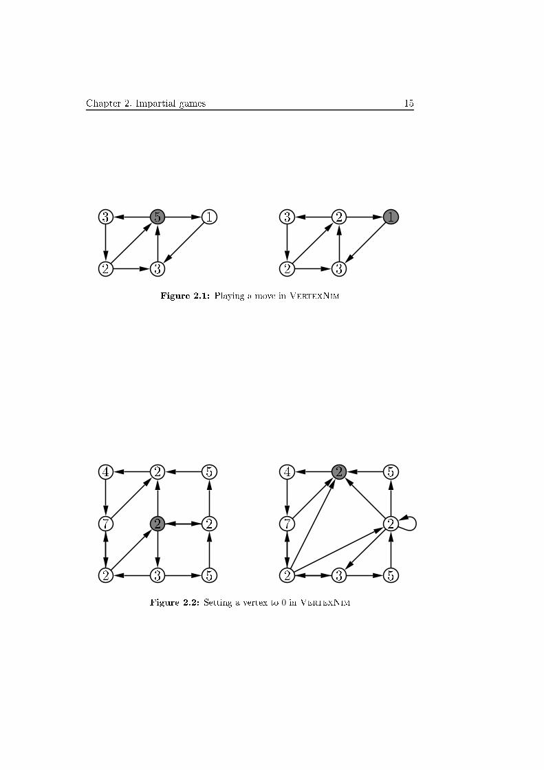
Example 2.1 Figure 2.1 gives an example of a move. The token is on the
grey vertex. The player whose turn it is hooses to de rease the weight of
this vertex from 5 to 2 and slide the token through the ar to the right. They
ould have slid it through the ar to the left, but through no other ar .
Example 2.2 Figure 2.2 is an example of a move whi h sets a vertex to
0. The token is on the grey vertex. The player whose turn it is hooses to
de rease the weight of this vertex from 2 to 0 and move the token through the
ar to the right. New ar s are added from the bottom left vertex and middle
right vertex to the bottom middle vertex, top middle vertex and middle right
vertex, reating a self loop on the middle right vertex.
VertexNim an also be played on a onne ted undire ted graph G by
seeing it as a symmetri dire ted graph where the vertex set remains the
same and the ar set is {(u, v), (v, u)|(u, v) ∈ E(G)}.
Chapter 2. Impartial games 15
2 3
3 5 1
2 3
3 2 1
Figure 2.1: Playing a move in VertexNim
2 3 5
7 2 2
4 2 5
2 3 5
7 2
4 2 5
Figure 2.2: Setting a vertex to 0 in VertexNim

16 2.1. VertexNim
VertexNim an be seen as a variant of the game Vertex NimG (see
[43℄), where the players annot put the token on a vertex with weight 0 and
instead ontinue to move it until it rea hes a vertex with positive weight,
though we only onsider the Remove then move version.
Multiple ar s are irrelevant, so we an onsider we are only dealing with
simple dire ted graphs.
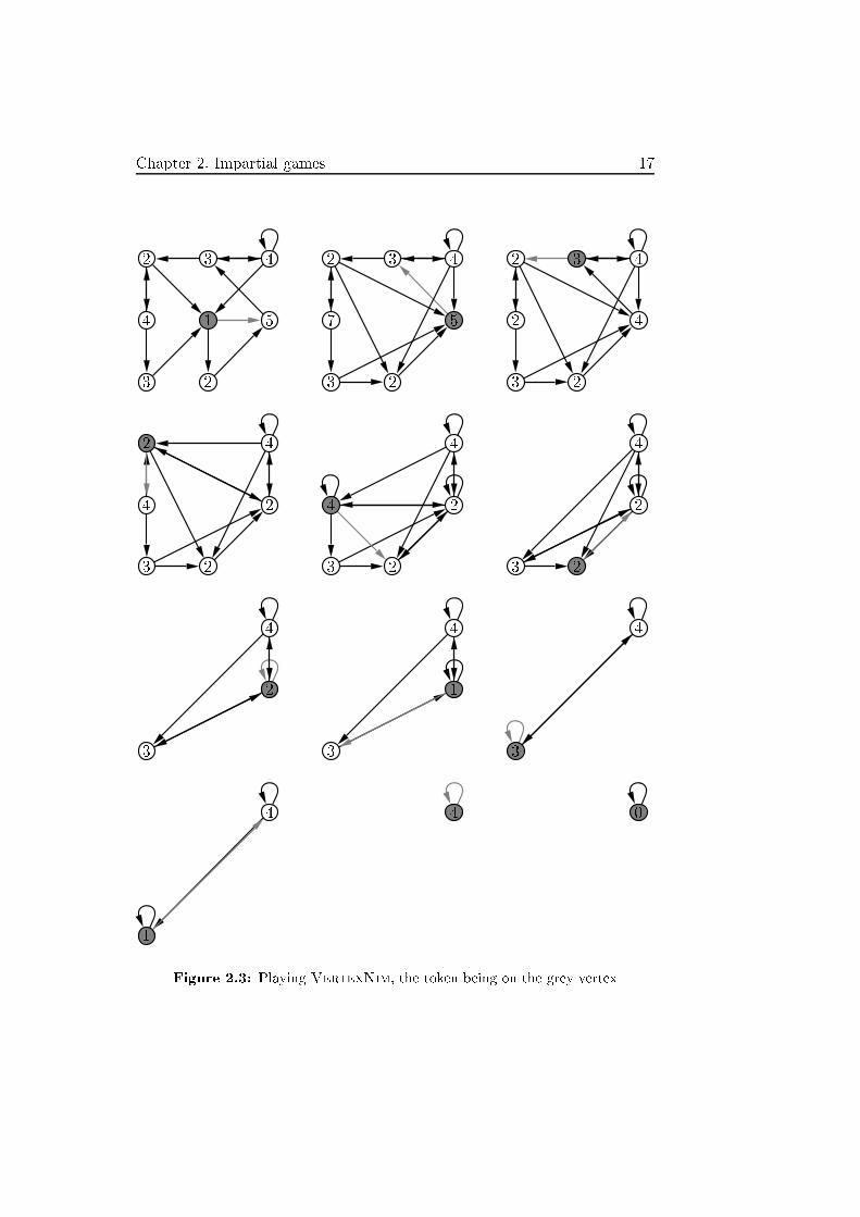
Example 2.3 Figure 2.3 shows an exe ution of the game. The token is on
the grey vertex and the player whose turn it is moves it through the grey ar .
After 11 moves, all weights are set to 0, so the player who started the game
wins. Be areful that it does not mean the starting position is an N -position,
as the se ond player might have better moves to hoose at some point in the
game.
In this se tion, we present algorithms to �nd the out ome of any dire ted
graph with a self loop on every vertex and the out ome of any undire ted
graph.
2.1.1 Dire ted graphs
On a ir uit, without any loop, the game is alled Adja ent Nim. We �rst
analyse the ase when the graph is a ir uit and no vertex has weight 1, thatis w−1(1) = ∅. If the length of the ir uit is odd, the �rst player an redu e
the weight of the �rst vertex to 1 then � opy� the moves of the se ond player
(redu ing the weight of the vertex to 0 if he just did the same, and redu ing
the weight to 1 otherwise) to for e him to play on the verti es she leaves him
in a way so that he is for ed to empty them (be ause she left the weight as
1), breaking the �symmetry� on the last vertex to save the last move for her.
When the length of the ir uit is even, a player who would empty a vertex
while no 1 has appeared would get themself in the position of a se ond player
on an odd ir uit, so it is never a good move and the two players will play on
distin t sets of verti es until a vertex is lowered to 1. A tually, we will see
that getting the weight of a vertex to 1 is not good either, so the minimum
weight of the verti es de ides the winner.
Theorem 2.4 Let (Cn, w, v1) : n > 3 be an instan e of VertexNim with
Cn the ir uit of length n and w : V → N>1.
• If n is odd, then (Cn, w, v1) is an N -position.
• If n is even, then (Cn, w, v1) is an N -position if and only if the smallest
index of a vertex of minimum weight, that is min{argmin16i6n
w(vi)}, is
even.
Note that when n is even, the above Theorem implies that the �rst player
who must play on a vertex of minimum weight will lose the game.
Proof.
Chapter 2. Impartial games 17
3 2
4 1 5
2 3 4
3 2
7 5
2 3 4
3 2
42
2 3 4
3 2
4 2
2 4
3 2
4 2
4
3 2
2
4
3
2
4
3
1
4
3
4
1
4 4 0
Figure 2.3: Playing VertexNim, the token being on the grey vertex

18 2.1. VertexNim
• Case (1) If n is odd, then the �rst player an apply the following
strategy to win: �rst, she plays w(v1) → 1. Then for all 1 6 i < n−12 :
if the se ond player empties v2i, then the �rst player also empties
the following vertex v2i+1. Otherwise, she sets w(v2i+1) to 1. The
strategy is di�erent for the last two verti es of Cn: if the se ond
player empties vn−1, then she plays w(vn) → 1, otherwise she plays
w(vn) → 0. As w(v1) = 1, the se ond player is now for ed to empty
v1. Sin e an even number of verti es have been deleted at this
point, we have an odd ir uit to play on. It now su� es for the
�rst player to empty all the verti es on the se ond run. Indeed, the
se ond player is also for ed to set ea h weight to 0 sin e he has to
play on verti es having their weight equal to 1. Sin e the ir uit is
odd, the �rst player is guaranteed to make the last move on vn or vn−1.
• Case (2) If n is even, we laim that who must play the �rst vertex of
minimum weight will lose the game. The winning strategy of the other
player onsists in de reasing by 1 the weight of ea h vertex at their
turn. First assume that min{argmin16i6n
w(vi)} is odd. If the strategy
of the se ond player always onsists in de reasing the weight of the
verti es he plays on by 1, then the �rst player will be the �rst to
set a weight to 0 or 1. If she sets a vertex to 0, then the se ond
player now fa es an instan e (C ′n−1, w
′, vi) with w′ : V ′ → N>1, whi h
is winning a ording to the previous item. If she sets a vertex to
1, then the se ond player will empty the following vertex, leaving to
the �rst player a position (C ′n−1 = (v′1, v
′2, . . . , v
′n−1), w
′, v′2) with w′ :V ′ → N>1 ex ept on w′(v′1) = 1. This position orresponds to the
one of the previous item after the �rst move, and is thus losing. A
similar argument shows that the �rst player has a winning strategy if
min{argmin16i6n
w(vi)} is even.
�
On a general strongly onne ted digraph, the problem seems harder.
Nevertheless, we manage to �nd the out ome of a strongly onne ted digraph
having the additional ondition that every vertex has a self loop.
When the token is on a vertex with weight at least 2 and a self loop, we
give a non- onstru tive argument that the game is an N -position (though
from the rest of the proof, we an dedu e a winning move in polynomial
time). Hen e, when the token is on a vertex of weight 1, the aim of both
players is to have the other player be the one that moves it to a vertex with
weight at least 2. This is why we de�ne a labelling of the verti es of the
dire ted graph that indi ates if the next player is on a good position to have
her opponent eventually move the token to a vertex with weight at least 2.
Chapter 2. Impartial games 19
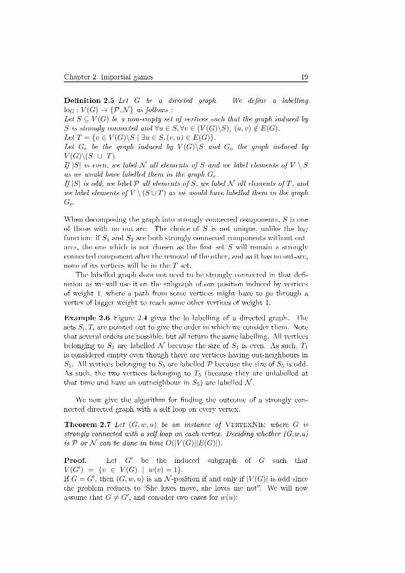
De�nition 2.5 Let G be a dire ted graph. We de�ne a labelling
loG : V (G) → {P,N} as follows :
Let S ⊆ V (G) be a non-empty set of verti es su h that the graph indu ed by
S is strongly onne ted and ∀u ∈ S,∀v ∈ (V (G)\S), (u, v) /∈ E(G).Let T = {v ∈ V (G)\S | ∃u ∈ S, (v, u) ∈ E(G)}.Let Ge be the graph indu ed by V (G)\S and Go the graph indu ed by
V (G)\(S ∪ T ).If |S| is even, we label N all elements of S and we label elements of V \ Sas we would have labelled them in the graph Ge.
If |S| is odd, we label P all elements of S, we label N all elements of T , andwe label elements of V \ (S ∪ T ) as we would have labelled them in the graph
Go.
When de omposing the graph into strongly onne ted omponents, S is one
of those with no out-ar . The hoi e of S is not unique, unlike the loGfun tion: if S1 and S2 are both strongly onne ted omponents without out-
ar s, the one whi h is not hosen as the �rst set S will remain a strongly
onne ted omponent after the removal of the other, and as it has no out-ar ,
none of its verti es will be in the T set.
The labelled graph does not need to be strongly onne ted in that de�-
nition as we will use it on the subgraph of our position indu ed by verti es
of weight 1, where a path from some verti es might have to go through a
vertex of bigger weight to rea h some other verti es of weight 1.
Example 2.6 Figure 2.4 gives the lo labelling of a dire ted graph. The
sets Si, Ti are pointed out to give the order in whi h we onsider them. Note
that several orders are possible, but all return the same labelling. All verti es
belonging to S1 are labelled N be ause the size of S1 is even. As su h, T1
is onsidered empty even though there are verti es having out-neighbours in
S1. All verti es belonging to S5 are labelled P be ause the size of S5 is odd.
As su h, the two verti es belonging to T5 (be ause they are unlabelled at
that time and have an outneighbour in S5) are labelled N .
We now give the algorithm for �nding the out ome of a strongly on-
ne ted dire ted graph with a self loop on every vertex.
Theorem 2.7 Let (G,w, u) be an instan e of VertexNim where G is
strongly onne ted with a self loop on ea h vertex. De iding whether (G,w,u)
is P or N an be done in time O(|V (G)||E(G)|).
Proof. Let G′be the indu ed subgraph of G su h that
V (G′) = {v ∈ V (G) | w(v) = 1}.If G = G′
, then (G,w, u) is an N -position if and only if |V (G)| is odd sin e
the problem redu es to �She loves move, she loves me not�. We will now
assume that G 6= G′, and onsider two ases for w(u):

20 2.1. VertexNim
N N N P N P
N N P N P N
P N P P N N
N P P P N P
S1 S2T2
S3
T3
S4
T4S5
T5 S6
S7T7
S8
Figure 2.4: lo-labelling of a dire ted graph
• Case (1) Assume w(u) > 2. If there is a winning move whi h redu es
the weight of u to 0, then we an play it and win. Otherwise, redu ing
the weight of u to 1 and staying on u is a winning move. Hen e
(G,w, u) is an N -position.
• Case (2) Assume now w(u) = 1, i.e., u ∈ G′. A ording to De�nition
2.5, omputing loG′yields a sequen e of ouples of sets (Si, Ti) (whi h
is not unique). Note that we do not onsider Ti when Si has an even
size. Thus the following assertions hold: if u ∈ Si for some i, then any
dire t su essor v of u is either in the same omponent Si (as there
are no out-ar ) or has been previously labelled (is in ∪j<i(Sj ∪ Tj)),and if u ∈ Ti 6= ∅ for some i, then there exists a dire t su essor v of
u in the set Si, with loG′(v) = P.Our goal is to show that (G,w, u) is an N -position if and only
if loG′(u) = N by indu tion on |V (G′)|. If |V (G′)| = 1, then
V (G′) = {u} and loG′(u) = P. Sin e w(u) = 1, we are for ed to
redu e u to 0 and go to a vertex v su h that w(v) > 2, whi h we
previously proved to be a losing move. Now assume |V (G′)| > 2.First, note that when one redu es the weight of a vertex v to 0, therepla ement of the ar s does not hange the strongly onne ted om-
ponents (ex ept for the omponent ontaining v of ourse, whi h loses

Chapter 2. Impartial games 21
one vertex). Consequently, if u ∈ Si for some i, then for any vertex
v ∈ ∪i−1l=1(Tl∪Sl), loG′\{u}(v) = loG′(v) and for any vertex w ∈ Si\{u},
loG′\{u}(w) 6= loG′(w) sin e parity of Si has hanged. If u ∈ Ti for some
i, then for any vertex v ∈ (∪i−1l=1(Tl ∪ Sl)) ∪ Si, loG′\{u}(v) = loG′(v).
We now onsider two ases for u: �rst assume that loG′(u) = P, withu ∈ Si for some i. We redu e the weight of u to 0 and we are for ed to
move to a dire t su essor v. If w(v) > 2, we previously proved this is
a losing move. If v ∈ ∪i−1l=1(Tl ∪ Sl), then loG′\{u}(v) = loG′(v) = N (if
loG′(v) = P , we would have v ∈ Sl, and so u ∈ Tl) and it is a losing
move by indu tion hypothesis. If v ∈ Si, then loG′\{u}(v) 6= loG′(v)and as loG′(v) = P , loG′\{u}(v) = N and the move to v is a losing
move by indu tion hypothesis.
Now assume that loG′(u) = N . If u ∈ Ti for some i, we an redu e
the weight of u to 0 and move to a vertex v ∈ Si, whi h is a winning
move by indu tion hypothesis. If u ∈ Si for some i, it means that
|Si| is even, we an redu e the weight of u to 0 and move to a vertex
v ∈ Si, with loG′\{u}(v) 6= loG′(v) = N . This is a winning move by
indu tion hypothesis. Hen e, (G,w, u) is an N -position if and only if
loG′(u) = N . Figure 2.5 illustrates the omputation of the lo fun tion.
Con erning the omplexity of the omputation, note that when w(u) > 2,the algorithm answers in onstant time. The omputation of loG′(u) whenw(u) = 1 needs to be analysed more arefully. De omposing a dire ted graph
H into strongly onne ted omponents to �nd the sets S and T an be done
in time O(|V (H)| + |E(H)|), and both |V (H)| and |E(H)| are less than or
equal to |E(G)| in our ase sin e H is a subgraph of G and G is strongly
onne ted. Moreover, the number of times we ompute S and T is learly
bounded by |V (G)|. These remarks lead to a global algorithm running in
O(|V (G)||E(G)|) time. �
The omplexity of the problem on a general digraph where some of the
verti es with weight at least 2 have no self loop is still open (remark that
having a self loop on a vertex of weight 1 does not a�e t the game).
2.1.2 Undire ted graphs
On undire ted graphs with a self loop on ea h vertex, the omputation of
the labelling is easier sin e any onne ted omponent is �strongly onne ted�.
Hen e, the same algorithm gives a better omplexity as the labelling of the
subgraph indu ed by the verti es of weight 1 be omes linear.
Proposition 2.8 Let (G,w, u) be a VertexNim position on an undire ted
graph su h that there is a self loop on ea h vertex of G. De iding whether
(G,w, u) is P or N an be done in time O(|V (G)|).

22 2.1. VertexNim
1N 5 1
P2
1N 7 1 N 3
3 1
P5 1
P
4 1
P1
P
4 1
P1 N
1
N1 N 1 N
1P 5 1 P
2 1
N1
N
Figure 2.5: lo-labelling fun tion of a subgraph indu ed by verti es of weight 1assuming every vertex has an undrawn self loop
Proof. Let G′be the indu ed subgraph of G su h that
V (G′) = {v ∈ V (G) | w(v) = 1}.If G = G′
, then (G,w, u) is an N -position if and only if |V (G)| is odd sin e
the problem redu es to �She loves move, she loves me not�. In the rest of
the proof, assume G 6= G′.
• Case (1) We �rst onsider the ase where w(u) > 2. If there is a
winning move whi h redu es the weight of u to 0, then we play it and
win. Otherwise, redu ing the weight of u to 1 and staying on u is a
winning move. Hen e (G,w, u) is an N -position.
• Case (2) Assume w(u) = 1. Let nu be the number of verti es of the
onne ted omponent of G′whi h ontains u. We show that (G,w, u)
is an N -position if and only if nu is even by indu tion on nu. If nu = 1,then we are for ed to redu e the weight of u to 0 and move to another
vertex v having w(v) > 2, whi h we previously proved to be a losing
move. Now assume nu > 2. If nu is even, we redu e the weight of
u to 0 and move to an adja ent vertex v with w(v) = 1, whi h is a
winning move by indu tion hypothesis. If nu is odd, then we redu e
the weight of u to 0 and we are for ed to move to an adja ent vertex v.If w(v) > 2, then we previously proved it is a losing move. If w(v) = 1,this is also a losing move by indu tion hypothesis. Therefore in that
ase, (G,w, u) is an N -position if and only if nu is even.

Chapter 2. Impartial games 23
Con erning the omplexity of the omputation, note that when w(u) > 2,the algorithm answers in onstant time. When w(u) = 1, we only need to
�nd the onne ted omponent of G′ ontaining u and its order, whi h an
be done in O(|V (G)|) time. Thus, the algorithm runs in O(|V (G)|) time. �
We now fo us on the general ase where the self loops are optional. A
vertex of weight at least 2 with a self loop is still a winning starting point
for the same reason as in the previous studied ases, and lowering the weight
of a vertex to 0 gives a self loop to all its neighbours be ause the graph is
undire ted, so the verti es of weight 1 are taken are of the same way as in
the above proposition. We show how to de ide the out ome of a position in
the following theorem.
Theorem 2.9 Let (G,w, u) be a Vertexnim position on an undire ted
graph. De iding whether (G,w, u) is P or N an be done in O(|V (G)||E(G)|)time.
The proof of this theorem requires several de�nitions that we present
here.
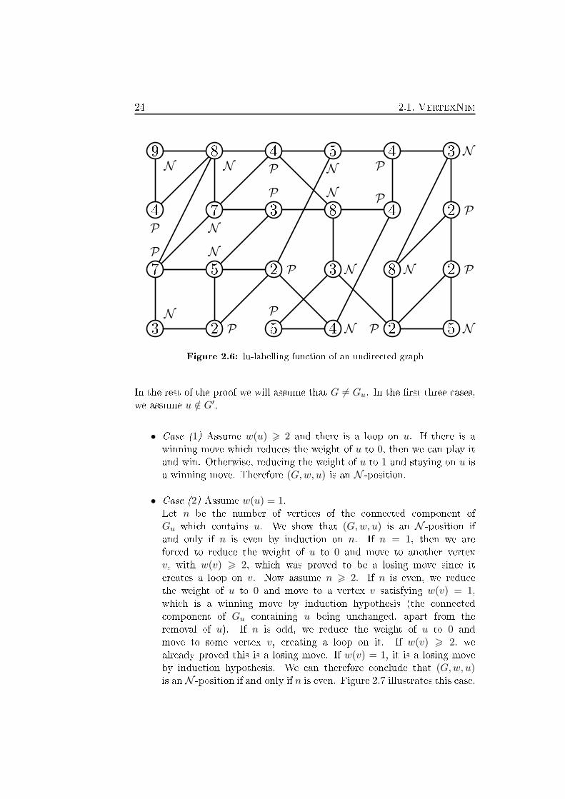
De�nition 2.10 Let G be an undire ted graph with a weight fun tion
w : V → N>0 de�ned on its verti es.
Let S = {u ∈ V (G) | ∀v ∈ V (G), w(u) 6 w(v)}.Let T = {v ∈ V (G)\S | ∃u ∈ S, (v, u) ∈ E(G)}.
Let G be the graph indu ed by V (G) \ (S ∪ T ).We de�ne a labelling luG,w of its verti es as follows :
• ∀u ∈ S, luG,w(u) = P, ∀v ∈ T , luG,w(v) = N• ∀t ∈ V (G)\(S ∪ T ), luG,w(t) = lu
G,w(t).
Example 2.11 Figure 2.6 gives the lu labelling of an undire ted weighted
graph. The lowest weight is 2, so all the verti es having weight 2 are labelledP. Then we know we an label all their unlabelled neighbours with N .
Proof. Let Gu be the indu ed subgraph of G su h that
V (Gu) = {v ∈ V (G) | w(v) = 1 or v = u}, and G′be the indu ed
subgraph of G su h that
V (G′) = {v ∈ V (G) |w(v) > 2(v, v) /∈ E(G)∀t ∈ V (G), (v, t) ∈ E(G) ⇒ w(t) > 2}.
If G = Gu and w(u) = 1, then (G,w, u) is an N -position if and only if
|V (G)| is odd sin e it redu es to �She loves move, she loves me not�.
If G = Gu and w(u) > 2, we redu e the weight of u to 0 and move to any
vertex if |V (G)| is odd, and we redu e the weight of u to 1 and move to
any vertex if |V (G)| is even; both are winning moves, hen e (G,w, u) is anN -position.
24 2.1. VertexNim
3
N2
P5
P
4
N2
P5
N
7
P
5
N
2
P3
N8
N2
P
4
P
7
N
3
P
8
N
4
P2
P
9
N8
N4
P
5
N
4
P3
N
Figure 2.6: lu-labelling fun tion of an undire ted graph
In the rest of the proof we will assume that G 6= Gu. In the �rst three ases,
we assume u /∈ G′.
• Case (1) Assume w(u) > 2 and there is a loop on u. If there is a
winning move whi h redu es the weight of u to 0, then we an play it
and win. Otherwise, redu ing the weight of u to 1 and staying on u is
a winning move. Therefore (G,w, u) is an N -position.
• Case (2) Assume w(u) = 1.Let n be the number of verti es of the onne ted omponent of
Gu whi h ontains u. We show that (G,w, u) is an N -position if
and only if n is even by indu tion on n. If n = 1, then we are
for ed to redu e the weight of u to 0 and move to another vertex
v, with w(v) > 2, whi h was proved to be a losing move sin e it
reates a loop on v. Now assume n > 2. If n is even, we redu e
the weight of u to 0 and move to a vertex v satisfying w(v) = 1,whi h is a winning move by indu tion hypothesis (the onne ted
omponent of Gu ontaining u being un hanged, apart from the
removal of u). If n is odd, we redu e the weight of u to 0 and
move to some vertex v, reating a loop on it. If w(v) > 2, we
already proved this is a losing move. If w(v) = 1, it is a losing move
by indu tion hypothesis. We an therefore on lude that (G,w, u)is an N -position if and only if n is even. Figure 2.7 illustrates this ase.
Chapter 2. Impartial games 25
3 2 3 3 5
3 5 1 7 1
1 1 1 1 4
1 1
u
2 1 1
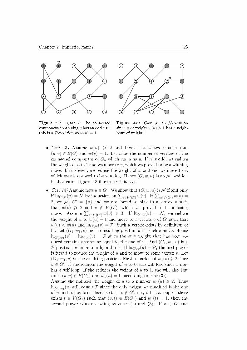
Figure 2.7: Case 2: the onne ted
omponent ontaining u has an odd size:
this is a P-position as w(u) = 1.
3 2 3 1 1
1 5 4 1 2
1 2 4 2
u1
7 3 1 1 2
Figure 2.8: Case 3: an N -position
sin e u of weight w(u) > 1 has a neigh-
bour of weight 1.
• Case (3) Assume w(u) > 2 and there is a vertex v su h that
(u, v) ∈ E(G) and w(v) = 1. Let n be the number of verti es of the
onne ted omponent of Gu whi h ontains u. If n is odd, we redu e
the weight of u to 1 and we move to v, whi h we proved to be a winning
move. If n is even, we redu e the weight of u to 0 and we move to v,whi h we also proved to be winning. Hen e (G,w, u) is an N -position
in that ase. Figure 2.8 illustrates this ase.
• Case (4) Assume now u ∈ G′. We show that (G,w, u) is N if and only
if luG′,w(u) = N by indu tion on
∑v∈V (G′) w(v). If
∑v∈V (G′)w(v) =
2, we get G′ = {u} and we are for ed to play to a vertex v su h
that w(v) > 2 and v /∈ V (G′), whi h we proved to be a losing
move. Assume
∑v∈V (G′)w(v) > 3. If luG′,w(u) = N , we redu e
the weight of u to w(u) − 1 and move to a vertex v of G′su h that
w(v) < w(u) and luG′,w(v) = P. Su h a vertex exists by de�nition of
lu. Let (G1, w1, v) be the resulting position after su h a move. Hen e
luG′
1,w1(v) = luG′,w(v) = P sin e the only weight that has been re-
du ed remains greater or equal to the one of v. And (G1, w1, v) is aP-position by indu tion hypothesis. If luG′,w(u) = P, the �rst playeris for ed to redu e the weight of u and to move to some vertex v. Let(G1, w1, v) be the resulting position. First remark that w1(v) > 2 sin eu ∈ G′
. If she redu es the weight of u to 0, she will lose sin e v now
has a self loop. If she redu es the weight of u to 1, she will also lose
sin e (u, v) ∈ E(G1) and w1(u) = 1 (a ording to ase (3)).
Assume she redu ed the weight of u to a number w1(u) > 2. Thus
luG′
1,w1(u) still equals P sin e the only weight we modi�ed is the one
of u and it has been de reased. If v /∈ G′, i.e., v has a loop or there
exists t ∈ V (G1) su h that (v, t) ∈ E(G1) and w1(t) = 1, then the
se ond player wins a ording to ases (1) and (3). If v ∈ G′and

26 2.2. Timber
5N 3P 1 4P 2 3 1 7
4P 3 7P 4 8 1 5 2P
4P 5N 8N 3N 5 4N 1 3N
5
N7
N8
P4 2
P5 1 2
Figure 2.9: Case 4: lu-labelling of the subgraph G′
luG′,w(v) = N , then luG′
1,w1(v) is still N sin e the only weight we
de reased is the one of a vertex labelled P being a neighbour of u.Consequently the resulting position makes the se ond player win by
indu tion hypothesis. If v ∈ G′and luG′,w(v) = P , then we ne essarily
have w(v) = w(u) in G′. As luG′
1,w1(u) = P and (u, v) ∈ E(G1), then
luG′
1,w1(v) be omes N , implying that the se ond player wins by indu -
tion hypothesis. Hen e (G,w, u) is N if and only if luG′,w(u) = N .
Figure 2.9 shows an example of the lu labelling.
Con erning the omplexity of the omputation, note that all the ases
ex ept (4) an be exe uted in O(|E(G)|) operations. Hen e the omputation
of luG′,w(u) to solve ase (4) be omes ru ial. We just need to ompute the
strongly onne ted omponent and the asso iated dire ted a y li graph to
ompute S and T , so in the worst ase, it an be done in O(|E(G)|) time.
And the number of times where S and T are omputed in the re ursive
de�nition of lu is learly bounded by |V (G)|. All of this leads to a global
algorithm running in O(|V (G)||E(G)|) time.
�
2.2 Timber
Timber is an impartial game played on a dire ted graph. On a move, a
player hooses an ar (x, y) of the graph and removes it along with all that is
still onne ted to the endpoint y in the underlying undire ted graph where
the ar (x, y) has already been removed. Another way of seeing it is to put a
verti al domino on every ar of the dire ted graph, and onsider that if one
domino is toppled, it topples the dominoes in the dire tion it was toppled
and reates a hain rea tion. The dire tion of the ar indi ates the dire tion

Chapter 2. Impartial games 27
x y
Figure 2.10: Playing a move in Timber
in whi h the domino an be initially toppled, but has no in iden e on the
dire tion it is toppled, or on the fa t that it is toppled, if a player has hosen
to topple a domino whi h will eventually topple it.
The des ription of a position onsists only of the dire ted graph on whi h
the two players are playing. Note that it does not need to be strongly
onne ted, or even onne ted.
Example 2.12 Figure 2.10 gives an example of a move. The player whose
move it is hooses to remove the ar (x, y). The whole onne ted omponent
ontaining y in the underlying undire ted graph without the ar (x, y) is
removed with it.
Example 2.13 Figure 2.11 shows an exe ution of the game. On a given
position, the player who is playing is hoosing the dark grey ar , and all
that will disappear along with it is oloured in lighter grey. The xi and yiindi ate the endpoints of the hosen ar . After the fourth move, the graph
is empty of ar s, so the game ends. Note that some games an end leaving
several isolated verti es, as well as no vertex at all.
In this se tion, we present algorithms to �nd the normal out ome of any
onne ted dire ted graph, and the Grundy-value of any orientation of paths.
2.2.1 General results
First, we see how to redu e the problem to orientations of forests: playing
in a y le removes the whole onne ted omponent, and playing on an ar
going out of a degree-1 vertex leaves only that vertex in the omponent. In
both ases there are no more move available in the omponent after they
have been played, so it is natural to aim at redu ing the former to the latter.
The only issue is how to deal with the ar s whi h were going in and out the
y le. This is what we present in Theorem 2.14. Note that the y le does
not need to be indu ed, nor even elementary.

28 2.2. Timber
y1
x1
x2
y2
y3
x3 x4
y4
Figure 2.11: Playing Timber

Chapter 2. Impartial games 29
Theorem 2.14 Let G be a dire ted graph seen as a Timber position su h
that there exists a set S of verti es that forms a 2-edge- onne ted omponent
of G, and x, y two verti es not belonging to V (G). Let G′be the dire ted
graph with vertex set
V (G′) = (V (G) \ S) ∪ {x, y}
and ar set
A(G′) = (A(G) \ {(u, v)|{u, v} ∩ S 6= ∅})∪ {(u, x)|u ∈ (V (G) \ S),∃v ∈ S, (u, v) ∈ A(G)}∪ {(x, u)|u ∈ (V (G) \ S),∃v ∈ S, (v, u) ∈ A(G)}∪ {(y, x)}.
Then G =+ G′.
Proof. Let H be any game su h that Left has a winning strategy on G+Hplaying �rst (or se ond). On G′+H, she an follow the same strategy unless
it re ommends to hoose an ar between elements of S or Right hooses the
ar (y, x). In the �rst ase, she an hoose the ar (y, x), whi h is still on
play sin e any move removing (y, x) in G′would remove all ar of S in G.
Both moves leave some H0 where Left has a winning strategy playing se ond
sin e the move in the �rst game was winning. In the se ond ase, she an
assume he hose any ar of S and ontinue to follow her strategy. For similar
reasons, it is possible and it is winning.
The proof that Right wins G′+H whenever he wins G+H is similar. �
Using this redu tion, the number of y les de reases stri tly, so after
repeating the pro ess as many times as possible (whi h is a �nite number of
times), we end up with a dire ted graph with no y le, namely an orientation
of a forest.
Corollary 2.15 For any dire ted graph G, there exists an orientation of a
forest FG su h that G =+ FG and su h an FG is omputable in quadrati
time.
In Corollary 2.15, the omplexity is important, as it is easy to produ e
an orientation of a forest (even an orientation of a path) with any Grundy-
value:
de�ne Pn the oriented graph with vertex set
V (Pn) = {vi}06i6n
and ar set
A(Pn) = {(vi−1, vi)}16i6n.
Then the Timber position Pn has Grundy-value n.

30 2.2. Timber
Example 2.16 Figure 2.12 shows an example of a dire ted graph (on top)
and a orresponding forest (on bottom), obtained after applying the redu -
tion from Theorem 2.14. The y les are oloured grey and redu ed to the
grey verti es of the forest. The white verti es denote the verti es of degree 1we add with an out-ar toward those grey verti es. There might be several
su h forests depending on the hoi e of the omponent used for the redu tion,
but they all share the same Grundy-value. Choosing maximal 2- onne ted
omponents when redu ing leads to a unique forest with least number of
verti es.
The next proposition allows us another redu tion. In parti ular, it gives
another proof that all forests that an be obtained from a graph G after the
redu tion of Theorem 2.14 are equivalent (set k and ℓ to 0).
Proposition 2.17 Let T be an orientation of a tree su h that there exist
three sets of verti es {ui}06i6k, {vi}06i6k, {wi}06i6ℓ ⊂ V (G) su h that:
1. ({(ui−1, ui)}16i6k ∪ {(vi−1, vi)}16i6k ∪ {(wi−1, wi)}16i6ℓ) ⊂ A(G)
2. (uk, w0), (vk, wℓ) ∈ A(G).
3. u0 and v0 have in-degree 0 and out-degree 1.
4. for all 1 6 i 6 k, uk and vk have in-degree 1 and out-degree 1.
Let T ′be the orientation of a tree with vertex set
V (T ′) = V (T ) \ {vi}06i6k
and ar set
A(T ′) = A(T ) \ ({(vi−1, vi)}16i6k ∪ {(vk, wℓ)}).
Then T =+ T ′.
Proof. The proof is similar to the one of Theorem 2.14: playing on (vi−1, vi)or (ui−1, ui) is similar (as well as (vk, wℓ) and (uk, w0)), and no move apart
from some (vj−1, vj) (and (vk, wℓ)) would remove the ar (ui−1, ui) withoutremoving the ar (vi−1, vi).
�
Note that we never used the fa t we were onsidering the normal version
of the game when we proved both the redu tions from Theorem 2.14 and
Proposition 2.17. That means they an be used in the misère version as
well.

Chapter 2. Impartial games 31
Figure 2.12: A Timber position and a orresponding orientation of a forest
32 2.2. Timber
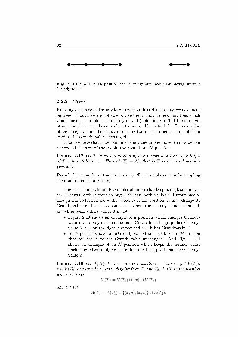
Figure 2.13: A Timber position and its image after redu tion having di�erent
Grundy-values
2.2.2 Trees
Knowing we an onsider only forests without loss of generality, we now fo us
on trees. Though we are not able to give the Grundy-value of any tree, whi h
would have the problem ompletely solved (being able to �nd the out ome
of any forest is a tually equivalent to being able to �nd the Grundy-value
of any tree), we �nd their out omes using two more redu tions, one of them
leaving the Grundy-value un hanged.
First, we note that if we an �nish the game in one move, that is we an
remove all the ar s of the graph, the game is an N -position.
Lemma 2.18 Let T be an orientation of a tree su h that there is a leaf vof T with out-degree 1. Then o+(T ) = N , that is T is a next-player win
position.
Proof. Let x be the out-neighbour of v. The �rst player wins by toppling
the domino on the ar (v, x). �
The next lemma eliminates ouples of moves that keep being losing moves
throughout the whole game as long as they are both available. Unfortunately,
though this redu tion keeps the out ome of the position, it may hange its
Grundy-value, and we know some ases where the Grundy-value is hanged,
as well as some others where it is not:
• Figure 2.13 shows an example of a position whi h hanges Grundy-
value after applying the redu tion. On the left, the graph has Grundy-
value 3, and on the right, the redu ed graph has Grundy-value 1.• All P-positions have same Grundy-value (namely 0), so any P-position
that redu es keeps the Grundy-value un hanged. And Figure 2.14
shows an example of an N -position whi h keeps the Grundy-value
un hanged after applying the redu tion: both positions have Grundy-
value 2.
Lemma 2.19 Let T1, T2 be two timber positions. Choose y ∈ V (T1),z ∈ V (T2) and let x be a vertex disjoint from T1 and T2. Let T be the position
with vertex set
V (T ) = V (T1) ∪ {x} ∪ V (T2)
and ar set
A(T ) = A(T1) ∪ {(x, y), (x, z)} ∪A(T2).

Chapter 2. Impartial games 33
Figure 2.14: A Timber N -position and its image after redu tion having the same
Grundy-value
Let T ′be the position with vertex set
V (T ′) = V (T1) ∪ V (T2)
where y and z are identi�ed, and ar set
A(T ′) = A(T1) ∪A(T2).
Then o+(T ) = o+(T ′).
Proof. We show it by indu tion on the number of verti es of T ′. If
V (T ′) = {y}, then there is no move in T ′and T onsists in two ar s
going out the same vertex. Hen e o+(T ) = P = o+(T ′). Assume now
|V (T ′)| > 1. Assume the �rst player has a winning move in T . If the hosenar removes x from the game, hoosing the same ar in T ′
leaves the same
position. Otherwise, hoosing the same ar in T ′leaves a position whi h has
the same out ome by indu tion. Hen e the �rst player has a winning move
in T ′. The proof that she has a winning move in T if she has one in T ′
is
similar. �
Example 2.20 The redu tion is from T to T ′. Figures 2.15 and 2.16 illus-
trate the redu tion by giving an example of an orientation of a tree and its
image after redu tion. The initial graph has no move that empties it, so we
try to �nd a smaller graph with the same out ome. The grey ar s are the
ones we ontra t, and the redu tion annot be applied anywhere else on the
�rst tree. However, the redu tion an again be applied on the grey ar s of
the se ond tree (and only them).
The next lemma presents a redu tion whi h preserves the Grundy-value.
When there are two orientations of paths dire ted toward a leaf from a
ommon vertex x, none of these paths a�e t the other, or the rest of the
tree. Hen e we an repla e them with just one path, whose length is the
Nim-sum of the lengths of the original paths.
Lemma 2.21 Let T0 be an orientation of a tree, w ∈ V (T0) a vertex, and
n,m ∈ N two integers. Let T be the position with vertex set
V (T ) = V (T0) ∪ {yi}16i6n ∪ {zi}16i6m

34 2.2. Timber
Figure 2.15: An orientation of a tree seen as a Timber position
Figure 2.16: Its image after redu tion, having the same out ome

Chapter 2. Impartial games 35
and ar set
A(T ) = A(T0) ∪{(yi, yi+1)}16i6n−1
∪{(zi, zi+1)}16i6m−1
∪{(w, y1), (w, z1)}.
Let T ′be the position with vertex set
V (T ′) = V (T0) ∪ {xi}16i6n⊕m
and ar set
A(T ′) = A(T0) ∪ {(xi, xi+1)}16i6(n⊕m)−1 ∪ {(w, x1)}.
Then o+(T + T ′) = P and o+(T ) = o+(T ′).
Proof. We prove it by indu tion on |V (T0)| + n + m and show
that o+(T + T ′) = P whi h means g(T ) = g(T ′) and thus implies that
o+(T ) = o+(T ′). If n+m = 0, T = T0 = T ′.
Assume now |V (T0)| + n +m > 0. Any ar of T0 is in both T and T ′,
thus if the �rst player hooses su h an edge in one of T or T ′then the se ond
player an hoose the orresponding ar in T ′or T , whi h leaves a P-position
(either by indu tion or be ause the two remaining positions are the same).
Assume the �rst player hooses the ar (yi, yi+1) (or (w, y1) = (y0, y1)). If
(i ⊕ m) < (n ⊕ m), the se ond player an hoose the ar (xi⊕m, x(i⊕m)+1)(or (w, x1) if i⊕m = 0) whi h leaves a P-position by indu tion. Otherwise,
there exists j < m su h that (i ⊕ j = n ⊕ m), and the se ond player an
hoose the ar (zj , zj+1) whi h leaves a P-position by indu tion. Similarly,
we an prove that the se ond player has a winning answer to any move of
the type (xi, xi+1) or (zi, zi+1). �
Example 2.22 Again, the redu tion is from T to T ′. Figures 2.17 and 2.18
illustrate the redu tion by giving an example of an orientation of a tree
and its image after redu tion. The initial graph has no move that empties
it, and the redu tion from Lemma 2.19 annot be applied, so we use the
other redu tion to get a smaller tree having the same out ome (even better,
having the same Grundy-value). The grey ar s of the �rst tree are the ones
of the paths we merge, and the redu tion annot be applied anywhere else
on the �rst tree. The grey ar s of the se ond tree are the ones of the paths
we reated by merging those of the �rst tree. The redu tion an again be
applied on the se ond tree, where it is even possible to apply the redu tion
from Lemma 2.19.
A position for whi h we annot apply the redu tion from Lemma 2.19 or
Lemma 2.21 is alled minimal. A leaf path is a path from a vertex x to a
leaf y, with x 6= y, onsisting only of verti es of degree 2, apart from y and
possibly x.

36 2.2. Timber
Figure 2.17: An orientation of a tree seen as a Timber position
Figure 2.18: Its image after redu tion, having the same out ome

Chapter 2. Impartial games 37
The oming lemma is important be ause it gives us the out ome of a
minimal position. Thus after having redu ed our initial position as mu h as
we ould, we get its out ome. Furthermore, if it is an N -position, it proposes
a winning move, that we an ba ktra k to get a winning move from the initial
position.
Lemma 2.23 A minimal position with out ome P an only be a graph with
no ar .
Proof. Let T be a minimal position with at least one ar . If it has exa tly
one ar , it is obviously in N , so we an assume T has at least two ar s.
Then there exists a vertex w at whi h there are two leaf paths {xi}06i6n
and {yi}06i6m (x0 = w = y0). If (xn, xn−1) or (ym, ym−1) is an ar , the �rst
player an hoose it and win. Now assume both (xn−1, xn) and (ym−1, ym)are ar s. As T is minimal, it annot be redu ed using Lemma 2.19, so all
(xi, xi+1), (yi, yi+1), (w, x1) and (w, y1) are ar s. But then we an apply the
redu tion from Lemma 2.21, whi h is a ontradi tion. �
Applying redu tions from Lemma 2.19 and Lemma 2.21 leads us to a
position where �nding the out ome is easy: either the graph has no ar left
and it is a P-position or there is a move that empties the graph and it is an
N -position. Note that the redu tion from Lemma 2.19 de reases the number
of verti es without in reasing the number of leaves, and the redu tion from
Lemma 2.21 de reases the number of leaves without in reasing the number
of verti es, so they an only be applied a linear number of times. As �nding
where to apply the redu tion an be done in linear time, this leads to a
quadrati time algorithm.
Theorem 2.24 We an ompute the out ome of any onne ted oriented
graph G in time O(|V (G)|2).
Note that for a tree, the number of edges is equal to the number of verti es
minus one, and a onne ted graph ontaining a y le is always an N -position.
Hen e, we an onsider O(|V (G)|) = O(|E(G)|) for the redu tion part of the
algorithm sin e �nding a y le is linear in the number of verti es.
Though this is enough to ompute the out ome of any orientation of
trees, it does not give us its Grundy-value, ex ept when we are onsidering a
P-position as they all have Grundy-value 0. The �rst redu tion we presented
in this subse tion may hange the Grundy-value of the position, but it is not
the ase of the se ond redu tion. Looking further on that dire tion, we tried
to �nd a more general redu tion that takes two leaf paths out of the same
vertex and repla e them with only one leaf path out of that vertex, leaving
the rest of the graph unmodi�ed, and keeping the Grundy-value un hanged.

38 2.2. Timber
With this, we would redu e the tree to a path, and as we an ompute
the Grundy-value of a path relatively e� iently (see Theorem 2.26 below),
we would get an algorithm to ompute the Grundy-value of any orientation
of trees, leading to an algorithm to ompute the out ome (and even the
Grundy-value) of any orientation of forests, and thus of any dire ted graph.
Unfortunately, doing this on general leaf paths is not possible, as shown in
Example 2.25.
Example 2.25 De�ne P1 and P2 two orientations of paths with vertex set
V (Pi) = {xi, yi, zi}
and ar set
A(Pi) = {(xi, yi), (zi, yi)}
for both i ∈ {1, 2}. Consider that the verti es identi�ed with a vertex of
the rest of the tree are x1 and x2. Assume there is an orientation of a path
P3 satisfying the above onditions. Identifying x1 and x2 without adding
anything leaves a path with Grundy-value 2, so P3 should have Grundy-
value 2. The moves that would remove the rest of the tree should ea h leave
the same value as one of the moves that would remove the rest of the tree in
our hoi e of P1 and P2, be ause we annot ensure that these values would
appear in the rest of the tree, so they all should have Grundy-value 0, andthere should be at least one for ea h value left by a move that would remove
the rest of the tree in our hoi e of P1 and P2 for the same reasons, so there
should be at least one move in P3 that would remove the rest of the tree
and leave a position with Grundy-value 0. Among all those potential ar s,
we look at the one losest to the leaf of that leaf path, and all it a. If
there are any ar s loser to the leaf, they are all pointing towards the leaf,
and the Grundy-value of those ar s, that are left alone after a player would
have moved on a, is equal to the number of ar s. Hen e there are no loser
ar . There annot be any other ar in P3 that would remove the rest of
the tree, be ause it would leave the ar a that still ould empty the graph,
whi h means it would leave a position with Grundy-value di�erent from 0.As the Grundy-value of P3 should be 2, the only possible P3 with the above
onditions is the graph with vertex set
V (P3) = {x3, y3, z3, t3}
and ar set
A(P3) = {(x3, y3), (y3, z3), (t3, z3)},
with the vertex we identify with a vertex of the rest of the tree being x3.Unfortunately, if the rest of the tree is an isolated ar in whi h we identify
the endpoint to a vertex of P1, P2 or P3, the two graphs do not have the
same Grundy-value: the one with P1 and P2 has Grundy-value 1 while the
one with P3 has Grundy-value 3.

Chapter 2. Impartial games 39
2.2.2.1 Paths
In the ase of paths, we an show additional results ompared to trees.
The same algorithm may be used, and we an even spare the redu tion of
Lemma 2.21.
Using CGSuite [37℄, we determined the number of P-positions on paths oflength 2n for small n's. Imputing them in the On-line En y lopedia of Integer
Sequen es [40℄ suggested that it orresponds to the nthCatalan number,
and pointed at a referen e [12℄, whi h led to the following representation. A
position an be represented visually on a 2-dimensional graph on a latti e:
wat h the path horizontally from left to right, start at (0, 0) and let an ar
dire ted leftward be a line joining the latti e points (x, y) and (x+ 1, y + 1)and an ar dire ted rightward be the line joining (x, y) and (x+ 1, y − 1).
We all that representation the peak representation of a Timber position
on an orientation of a path.
A Dy k path of length 2n is one of these paths that also ends at (2n, 0)and whi h never goes below the x-axis. More formally, a Dy k path of length
2n is a path on a latti e starting from (0, 0) and ending at (2n, 0) whi h steps
are of the form ((x, y), (x + 1, y + 1)) and ((x, y), (x + 1, y − 1)) where the
se ond oordinate is never negative.
We note that an orientation of a path is a P-position if and only if its
peak representation is a Dy k path. This gives us the number of P-positionsthat are paths of length 2k, the kth Catalan number ck = (2k)!
k!(k+1)! . And no
path of odd length is a P-position.This is interesting sin e there are few games where the number of
P-positions is known depending on the size of the data. Even for Nim whi h
was introdu ed a entury ago, no general formula is known yet.
We now look at the Grundy-values of paths. All followers of a position
of a Timber position are Timber positions whose graphs are indu ed sub-
graphs of the original one, where two verti es are in the same onne ted
omponent if and only if they were in the same onne ted omponent in the
original graph. When the graph is a path, the number of onne ted indu ed
subgraphs is quadrati in the length of the path (E(G) − i + 1 hoi es of
subgraphs with i edges, for any i). When you know the Grundy-values of
all the options of a game, the Grundy-value of this game an be omputed
in linear time. The number of options of a Timber position is the number
of its edges. It therefore su� es to ompute and store the Grundy-values of
all subpaths of an orientation of a path by length in reasing order to get the
Grundy-value of the original path in ubi time.
Theorem 2.26 We an ompute the Grundy-value of any orientation of
paths P in time O(|V (P )|3).

40 2.3. Perspe tives
1 1 1 1 1 1 1 1 1 1 1 1
2 1 0 2 1 2 0 2 1 0 2
2 2 3 2 2 3 3 2 2 3
3 3 3 2 3 0 3 3 3
4 3 3 3 1 1 2 4
4 3 2 4 1 0 5
4 4 5 4 4 6
5 5 5 5 6
6 6 6 6
6 7 7
7 8
8
Figure 2.19: Computing the Grundy-value of a path
Example 2.27 Figure 2.19 gives an example of a path and the Grundy-
value of all its subpaths, illustrating the algorithm: on the ith line are the
Grundy-values of subpaths of length i; on the jth olumn are the Grundy-
values of the subpaths whose leftmost ar is the jth of the original path. We
an onsider there is a 0th line whi h only ontains 0's, but this is not ne -essary as the �rst line always only ontains 1's. We underlined the Grundy-
value of the whole path.
To ompute the value in ase (i, j), that is the Grundy-value of the
subpath ontaining the kth ar for all k between i and i + j − 1, you look
at ea h of these edges and build the set of Grundy-values of the options of
the subpath: you start with an empty set of values; if the kth ar is dire ted
toward the right, you add the value in ase (i, k − i) to your set; if the kth
ar is dire ted toward the left, you add the value in ase (k+1, i+ j−k−1)to your set. The value you put in ase (i, j) is the minimum non-negative
integer that does not appear in the set you just built.
2.3 Perspe tives
In this hapter, we looked at the games VertexNim and Timber.
In the ase of VertexNim, we gave a polynomial-time algorithm to �nd
the normal out ome of any undire ted graph with a token on any vertex,
as well as the out ome of any strongly onne ted dire ted graph with a self
loop on every vertex, and a token on any vertex. Then, we have a natural
question.

Chapter 2. Impartial games 41
Question 2.28 What is the omplexity of VertexNim played on a general
dire ted graph?
Looking at another variant of Nim played on graphs, Vertex NimG
[9, 43℄, our results seem to apply to the variant where a vertex of weight 0is not removed (see [16℄), but they do not if it is removed. In parti ular, in
the latter ase, the problem is pspa e- omplete on graphs with a self loop
on ea h vertex, even if the weight of verti es is at most 2.
In the ase of Timber, we found the normal out ome of any orientation
of trees, whi h gives the normal out ome of any onne ted dire ted graph
in polynomial time, and gave an algorithm to �nd the Grundy-value of any
orientation of paths in polynomial time.
We are now left with the following problem.
Question 2.29 Is there a polynomial-time algorithm to �nd the Grundy-
value of any Timber position on orientations of trees?
Note that it would give the out ome of any Timber position on dire ted
graphs, as a dire ted graph redu es to an orientation of a forest having the
same Grundy-value by Theorem 2.14, and from that forest, we would be able
to ompute the Grundy-value of ea h onne ted omponents as they are all
trees and we just need to sum the values to �nd the Grundy-value of the
original position, whi h also gives its out ome.
The omplexity of the problem is the same as �nding the out ome of any
Timber position on dire ted graphs, as a position has Grundy-value n if and
only if the se ond player wins the game made of the sum of that position
with the orientation of a path with n ar s, all dire ted toward the same leaf,
and the Grundy-value of a Timber position is bounded by its number of
ar s.


Chapter 3. Partizan games 43
Chapter 3
Partizan games
Partizan games are the natural extension of impartial games where the
players may have di�erent sets of moves. We say that a game is partizan
whenever the moves are not ne essarily equal for the two players, but parti-
zan games ontain impartial games as well.
As with impartial games, there exists a fun tion that assigns a value
to any partizan game. Two games having the same value are equivalent
under normal play, and vi e versa. Hen e, we identify those values with the
anoni al forms of the games they represent. As an example, the anoni al
forms of numbers are re ursively de�ned as follows (with n, k being positive
integers and m any integer):
0 = {·|·}n = {n − 1|·}
−n = {·| − n+ 1}2m+12k
= {2m2k
|2m+22k
}
The order between games represented by numbers is the same as in Q2.
Unfortunately, many values are not numbers. For example, an impartial
game with Grundy-value n would be denoted as having value ∗n, ex eptwhen n is 0 or 1, respe tively denoted by 0 and ∗. Berlekamp, Conway and
Guy [4, 10℄ give a useful tool to prove some games are numbers:
Theorem 3.1 (Berlekamp et al. [4℄, Conway [10℄) [Simpli ity the-
orem℄ Suppose for x = {xL|xR} that some number z satis�es z xL and
z � xR for any Left option xL ∈ xL and any Right option xR ∈ xR, butthat no ( anoni al) option of z satis�es the same ondition (that is, for any
option z′ ∈ zL ∪ zR, there exists a Left option xL ∈ xL su h that z′ 6 xL or
there exists a Right option xR ∈ xR su h that z′ > xR). Then x = z.
In other words, if there is a number z satisfying z xL and z � xR for
any Left option xL ∈ xL and any Right option xR ∈ xR, then x is equivalent
to the number with smallest birthday satisfying this property.
To simplify proofs, we often do not state results on the opposite of games
on whi h we proved similar results. This an be justi�ed by the following
proposition.
Proposition 3.2 Let G and H be any two games. If G >+ H, then
−G 6+ −H. As a onsequen e, G ≡+ H ⇔ −G ≡+ −H.

44 3.1. Timbush
Proof. Assume G >+ H. Then Left wins G −H = (−H) − (−G) playingse ond. Hen e −H >+ −G. �
In this hapter, we onsider three partizan games: Timbush, Toppling
Dominoes and Col. Timbush is the natural partizan extension of Timber,
where some ar s an only be hosen by one player. In se tion 3.1, we de�ne
the game, prove that any position an be redu ed to a forest, as in Timber,
and give an algorithm to ompute the out ome of any orientation of paths
and any orientation of trees where no ar an be removed by both players.
Toppling Dominoes is a variant of Timbush, where the graph is a forest
of paths and all ar s are bidire tional. In se tion 3.2, we de�ne the game,
prove the existen e of some values appearing as onne ted paths, and give
a uni ity result about some of them. Col is a olouring game played on an
undire ted graph. In se tion 3.3, we de�ne the game and give the values of
graphs belonging to some in�nite lasses of graphs.
The results presented in Se tion 3.1 are a joint work with Ri hard
Nowakowski, while the results presented in Se tions 3.2 and 3.3 are a joint
work with Paul Dorbe and Éri Sopena [14℄.
3.1 Timbush . . . . . . . . . . . . . . . . . . . . . . . 44
3.1.1 General results . . . . . . . . . . . . . . . . . . . . 45
3.1.2 Paths . . . . . . . . . . . . . . . . . . . . . . . . . 49
3.1.3 Bla k and white trees . . . . . . . . . . . . . . . . 54
3.2 Toppling Dominoes . . . . . . . . . . . . . . . . 61
3.2.1 Preliminary results . . . . . . . . . . . . . . . . . . 63
3.2.2 Proof of Theorem 3.27 . . . . . . . . . . . . . . . . 65
3.3 Col . . . . . . . . . . . . . . . . . . . . . . . . . . . 72
3.3.1 General results . . . . . . . . . . . . . . . . . . . . 76
3.3.2 Known results . . . . . . . . . . . . . . . . . . . . 80
3.3.3 Caterpillars . . . . . . . . . . . . . . . . . . . . . . 93
3.3.4 Cographs . . . . . . . . . . . . . . . . . . . . . . . 96
3.4 Perspe tives . . . . . . . . . . . . . . . . . . . . . . 98
3.1 Timbush
Timbush is the natural partizan extension of Timber, played on a dire ted
graph with ar s oloured bla k, white, or grey. On her move, Left hooses

Chapter 3. Partizan games 45
x
y
t
z
x'
y'
Figure 3.1: Playing a move in Timbush
a bla k or grey ar (x, y) of the graph and removes it along with all that is
still onne ted to the endpoint y in the underlying undire ted graph. On his
move, Right does the same with a white or grey ar .
The des ription of a position onsists of the dire ted graph on whi h the
two players are playing, and a olouring fun tion from the set of ar s to the
set of olours {black,white, grey}. Note that the dire ted graph does not
need to be strongly onne ted, or even onne ted.
AllTimber positions areTimbush positions: just keep the same dire ted
graph and onsider all ar s are grey.
In all the �gures, white ar s are represented with dashed arrows, and
bla k ar s are thi ker, to avoid onfusion between the olours.
Example 3.3 Figure 3.1 gives an example of a Left move. Left hooses to
remove the bla k ar (x, y). The whole onne ted omponent ontaining yin the underlying undire ted graph without the ar (x, y) is removed with
it. She ould not have hosen the ar (z, t) be ause it is white, but the greyar (x′, y′) is allowed to her.
In this se tion, we present algorithms to �nd the normal out ome of
any oloured orientation of a path, and the normal out ome of any oloured
onne ted dire ted graph with no grey ar .
3.1.1 General results
First, we see how to adapt the results obtained on Timber to Timbush.
The redu tion to get an orientation of a forest from a dire ted graph without
hanging the value is the same, but we now have to take are of the olours
of the ar s too. We aim at keeping them the same, but we still need to �nd
the olour of the ar we add, and we hoose the olour that gives the same
possibilities as those given by the y le. The proof follows the same pattern
as the proof of Theorem 2.14.

46 3.1. Timbush
Theorem 3.4 Let G be a dire ted graph seen as a Timbush position su h
that there exist a set of verti es S that forms a 2-edge- onne ted omponent
of G, and x, y two verti es not belonging to G. Let G′be the dire ted graph
with vertex set
V (G′) = (V (G)\S) ∪ {x, y}
and ar set
A(G′) = (A(G) \ {(u, v)|{u, v} ∩ S 6= ∅})∪ {(u, x)|u ∈ (V (G) \ S),∃v ∈ S, (u, v) ∈ A(G)}∪ {(x, u)|u ∈ (V (G) \ S),∃v ∈ S, (v, u) ∈ A(G)}∪ {(y, x)}.
keeping the same olours, where the olour of (y, x) is grey if the ar s in Syield di�erent olours, and of the unique olour of ar s in S otherwise. Then
G ≡+ G′.
Proof. Let H be any game su h that Left has a winning strategy on G+Hplaying �rst (or se ond). On G′+H, she an follow the same strategy unless
it re ommends to hoose an ar between elements of S or Right hooses the
ar (y, x). In the �rst ase, she an hoose the ar (y, x), whi h is still in
play sin e any move removing (y, x) in G′would remove all ar s of S in G.
Both moves leave some H0 where Left has a winning strategy playing se ond
sin e the move in the �rst game was winning. In the se ond ase, she an
assume he hose any ar of S and ontinue to follow her strategy. For similar
reasons, it is possible and it is winning.
The proof that Right wins G′+H whenever he wins G+H is similar. �
Again, we get the orollary that leaves us with a forest.
Corollary 3.5 For any dire ted graph G, there exists an orientation of a
forest FG su h that G ≡+ FG and FG is omputable in quadrati time.
Example 3.6 Figure 3.2 shows an example of a dire ted graph (on top) and
a orresponding forest (on bottom), obtained after applying the redu tion
from Theorem 3.4. Light grey areas surround the y les, whi h are redu ed
to the grey verti es of the forest. The white verti es denote the verti es of
degree 1 we add with an out-ar toward those grey verti es. There might be
several su h forests depending on the hoi e of the omponent used for the
redu tion, but they all share the same value. Choosing maximal 2- onne ted
omponents when redu ing leads to a unique forest with least number of
verti es.
We an also adapt the proposition giving us a redu tion removing leaf-
paths with ar s dire ted from the leaf, but we also need to pay attention to
the olours, whi h gives extra onditions.

Chapter 3. Partizan games 47
Figure 3.2: A Timbush position and a orresponding orientation of a forest

48 3.1. Timbush
Proposition 3.7 Let T be an orientation of a tree su h that there exist three
sets of verti es {ui}06i6k,{vi}06i6k,{wi}06i6ℓ ⊂ V (G) su h that:
1. ({(ui−1, ui)}16i6k ∪ {(vi−1, vi)}16i6k ∪ {(wi−1, wi)}16i6ℓ ⊂ A(G).
2. {(uk, w0), (vk, wℓ)}) ⊂ A(G).
3. u0 and v0 have in-degree 0 and out-degree 1.
4. for all 1 6 i 6 k, ui and vi have in-degree 1 and out-degree 1.
5. for all 1 6 i 6 k, (ui−1, ui) and (vi−1, vi) have the same olour.
6. (uk, w0) and (vk, wℓ) have the same olour.
Let T ′be the orientation of a tree with vertex set
V (T ′) = V (T )\{vi}06i6k
and ar set
A(T ′) = A(T )\({(vi−1, vi)}16i6k ∪ {(vk, wℓ)})
keeping the same olours. Then T ≡+ T ′.
Proof. The proof is similar to the one of Theorem 3.4, playing on (vi−1, vi)or (ui−1, ui) is similar (as well as (vk, wℓ) and (uk, w1)), and no move apart
from some (vj−1, vj) (and (vk, wℓ)) would remove the ar (ui−1, ui) withoutremoving the ar (vi−1, vi). �
We now fo us on trees again. Before going to spe i� ases, we give the
analog of Lemma 2.19 in the partizan version. Note again that it sometimes
hanges the value of the game, and it sometimes does not, using the same
examples as in Figures 2.13 and 2.14 as all positions of Timber are positions
of Timbush.
Lemma 3.8 Let T1, T2 be two Timbush positions. Choose y ∈ V (T1),z ∈ V (T2) and let x be a vertex not belonging to V (T1) or V (T2). Let Tbe the position with vertex set
V (T ) = V (T1) ∪ {x} ∪ V (T2)
and ar set
E(T ) = E(T1) ∪ {(x, y), (x, z)} ∪E(T2)
where (x, y) and (x, z) are either both grey or of non-grey di�erent olours
and the other ar s keep the same olours. Let T ′be the position with vertex
set
V (T ′) = V (T1) ∪ V (T2)

Chapter 3. Partizan games 49
where y and z are identi�ed, and ar set
E(T ′) = E(T1) ∪ E(T2)
keeping the same olours for all ar s. Then o+(T ) = o+(T ′).
Proof. We show it by indu tion on the number of verti es of T ′. If
V (T ′) = {y}, then there is no move in T ′and T is either 1 + (−1) = 0 or
∗ + ∗ = 0. Hen e o+(T ) = P = o+(T ′). Assume now |V (T ′)| > 1. Assume
Left has a winning move in T . This winning move annot be by hoosing
(x, y) or (x, z) be ause Right would hoose the other move and win. If the
hosen ar removes x from the game, hoosing the same ar in T ′leaves
the same position. Otherwise, hoosing the same ar in T ′leaves a position
whi h has the same out ome by indu tion. Hen e Left has a winning move
in T ′. The proof that Left has a winning move in T if she has one in T ′
and that Right has a winning move in T if and only if he has one in T ′are
similar. �
Example 3.9 Again, the redu tion is from T to T ′. Figures 3.3 and 3.4
illustrate the redu tion by giving an example of an orientation of a tree and
its image after redu tion. Not even one player has a move that empties the
initial graph, so we try to �nd a smaller graph with the same out ome. The
ar s in light grey areas are the ones we ontra t, and the redu tion annot be
applied anywhere else on the �rst tree. The dark grey area indi ates a pair
of ar s going out a degree-2 vertex, whi h annot be ontra ted be ause its
olours do not mat h the statement of Lemma 3.8. However, the redu tion
an again be applied on the ar s in the light grey areas of the se ond tree
(and only on them).
3.1.2 Paths
Though �nding an e� ient algorithm whi h gives the normal out ome of any
orientation of trees has eluded us, we an determine the normal out ome of
any orientation of paths.
On paths, we an ode the problem with a word. The letter K (resp. C,Q) would represent a bla k (resp. grey, white) ar dire ted leftward, while
Y (resp. J , D) would represent a bla k (resp. grey, white) ar dire ted
rightward. Let w = w1w2 · · ·w|w|.
As in Se tion 2.2, we an see it as a row of dominoes, ea h oloured bla k,
grey or white, that would topple everything in one dire tion when hosen,
where hosen dominoes an only be toppled fa e up, with Left only being
allowed to hoose bla k or grey dominoes, and Right only being allowed to
hoose white or grey dominoes. The position is read from left to right.
Example 3.10 Figure 3.5 shows an orientation of a path, the row of domi-
noes and the word used for oding it.

50 3.1. Timbush
Figure 3.3: An orientation of a tree seen as a Timbush position
Figure 3.4: Its image after redu tion, having the same out ome

Chapter 3. Partizan games 51
KQYJYQKJCKDKDJ
Figure 3.5: A Timbush position, the orresponding row of dominoes and the
orresponding word
We say a domino is right-topplable if it orresponds to an ar dire ted
rightward, that is if it is represented by a Y , a J or a D. Likewise, a domino
represented by a K, a C or a Q is said to be left-topplable.
The next lemma is quite useful as it tells us that if we have a winning
move for one player, then the only possible winning move going in the same
dire tion for the other player is the exa t same move, if available. This is
natural as if they were di�erent winning moves, one player would be able to
play their move after the other player, and leave the same position as if they
had played it �rst. Nevertheless, it is still possible for one player to have
several winning moves going in the same dire tion when their opponent has
no winning move going in that dire tion. And it is also possible that the two
players have di�erent winning moves, if they topple in di�erent dire tions.
Lemma 3.11 If both players have a winning move toppling rightward, then
these moves are on the same domino.
Proof. Assume Left has a winning move toppling the right-topplable domino
wi and Right has a winning move toppling the right-topplable domino wj .
If i < j, after Right topples wj , Left an topple wi, leaving the game in
the same position as if she had toppled wi right in the beginning, whi h is
a winning move, and toppling wj was not winning for Right. The proof is
similar if i > j. �
We de�ne the following three sets of words:
L = {KY,KJ} ∪ {CY DnY,CY DnJ}n∈NR = {QD,QJ} ∪ {CDY nD,CDY nJ}n∈NE = {KD,CJ,QY }
The reader would have re ognised E as the set of subwords that an be
deleted without modifying the normal out ome of the path using Lemma 3.8.
In the following, we then often assume the position does not ontain any
element of E as a subword.
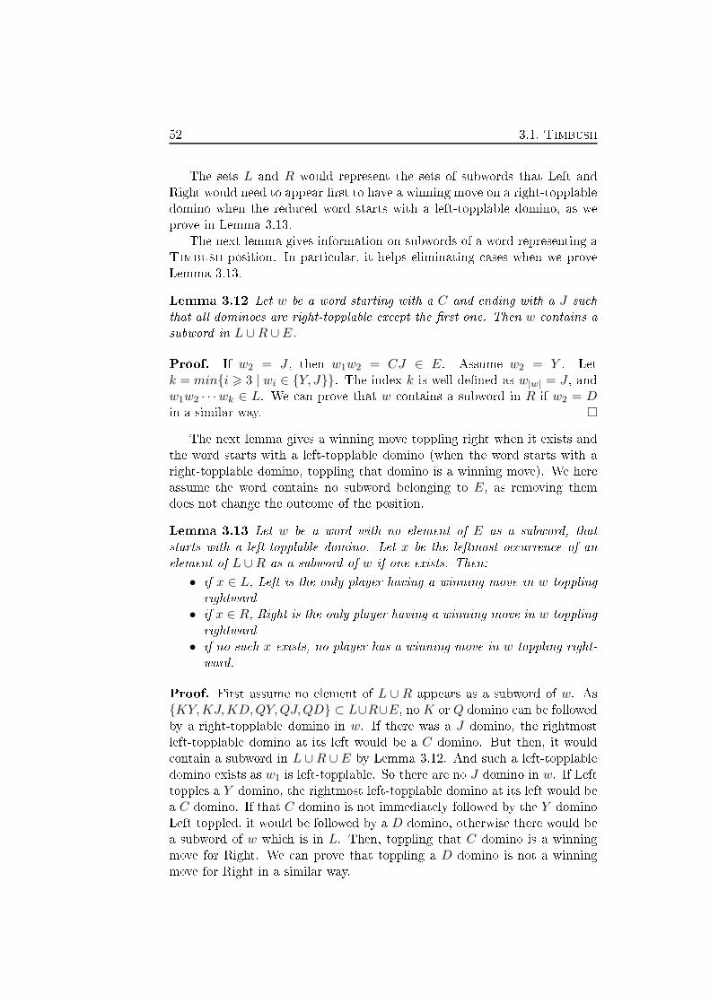
52 3.1. Timbush
The sets L and R would represent the sets of subwords that Left and
Right would need to appear �rst to have a winning move on a right-topplable
domino when the redu ed word starts with a left-topplable domino, as we
prove in Lemma 3.13.
The next lemma gives information on subwords of a word representing a
Timbush position. In parti ular, it helps eliminating ases when we prove
Lemma 3.13.
Lemma 3.12 Let w be a word starting with a C and ending with a J su h
that all dominoes are right-topplable ex ept the �rst one. Then w ontains a
subword in L ∪R ∪ E.
Proof. If w2 = J , then w1w2 = CJ ∈ E. Assume w2 = Y . Let
k = min{i > 3 | wi ∈ {Y, J}}. The index k is well-de�ned as w|w| = J , andw1w2 · · ·wk ∈ L. We an prove that w ontains a subword in R if w2 = Din a similar way. �
The next lemma gives a winning move toppling right when it exists and
the word starts with a left-topplable domino (when the word starts with a
right-topplable domino, toppling that domino is a winning move). We here
assume the word ontains no subword belonging to E, as removing them
does not hange the out ome of the position.
Lemma 3.13 Let w be a word with no element of E as a subword, that
starts with a left-topplable domino. Let x be the leftmost o urren e of an
element of L ∪R as a subword of w if one exists. Then:
• if x ∈ L, Left is the only player having a winning move in w toppling
rightward
• if x ∈ R, Right is the only player having a winning move in w toppling
rightward
• if no su h x exists, no player has a winning move in w toppling right-
ward.
Proof. First assume no element of L ∪ R appears as a subword of w. As
{KY,KJ,KD,QY,QJ,QD} ⊂ L∪R∪E, no K or Q domino an be followed
by a right-topplable domino in w. If there was a J domino, the rightmost
left-topplable domino at its left would be a C domino. But then, it would
ontain a subword in L ∪R ∪ E by Lemma 3.12. And su h a left-topplable
domino exists as w1 is left-topplable. So there are no J domino in w. If Lefttopples a Y domino, the rightmost left-topplable domino at its left would be
a C domino. If that C domino is not immediately followed by the Y domino
Left toppled, it would be followed by a D domino, otherwise there would be
a subword of w whi h is in L. Then, toppling that C domino is a winning
move for Right. We an prove that toppling a D domino is not a winning
move for Right in a similar way.

Chapter 3. Partizan games 53
Now assume x exists and is in L. We show that toppling the rightmost
domino of x is a winning move for Left. Let w′be the resulting position after
this move. The position w′ ontains no element of L∪R∪E as a subword and
starts with a left-topplable domino, so Right has no winning move toppling
rightward. Hen e, we an assume Right would topple a domino leftward.
If Right topples a domino whi h is not part of x, Left topples the leftmost
domino of x, whi h is a winning move. Otherwise, x = CY DiY or CYDiJfor some i and Right would have toppled the C domino, whi h leaves an
L-position. We now show that no Right's move toppling rightward in w is
winning. By Lemma 3.11, if Right has a winning move toppling rightward,
it would be by toppling the rightmost domino of x. But then, Left wins bytoppling the leftmost domino of x.
We an prove that Right is the only player having a winning move top-
pling rightward if x exists and is in L in a similar way. �
Example 3.14 Figure 3.6 gives three rows of dominoes, with the words
oding it, ea h of them starting with a left-topplable domino and having no
subword in E. On the �rst row, the leftmost apparition of a subword in L∪Ris KJ , so Left an win the game playing �rst by toppling that J domino. On
the se ond row, the leftmost apparition of a subword in L ∪R is CDY Y D,
so Right an win the game playing �rst by toppling that last D domino. On
the third row, the word ontains no subword of L ∪ R, so no player has a
winning move toppling rightward. On the �rst two rows, that winning move
is underlined, and the domino orresponding is pointed at. Note that there
might be other winning moves toppling rightward, the se ond J of the �rst
row for instan e.
When a word starts with a right-topplable domino, hoosing it is a win-
ning move. Using that with Lemmas 3.11 and 3.13, we an �nd whi h player
an win toppling a domino rightward. As the same observations an be made
about left-topplable winning moves, we get the out ome of any word in linear
time.
Theorem 3.15 We an ompute the out ome of any word w in time O(|w|).
We end this study on paths by giving a hara terisation of Timbush
P-positions on paths.
Theorem 3.16 Let w be a word representing a Timbush P-position, su hthat no subword of w is in E. Then w is the empty word.
Proof. Assume w is not the empty word. As it is a P-position, it startswith a left-topplable domino, and it has no word of L or R as a subword.
Therefore, we an prove, as in the proof of Lemma 3.13, that it ontains no
J domino. By symmetry, it does not ontain any C domino. But neither

54 3.1. Timbush
CCDDYKJJCQQDKQCY
QKCDYYDYCKYDJDCCKQJ
KCYQQCKCDYYYCKQKQ
Figure 3.6: Words representing Timbush positions with a winning move toppling
rightward underlined when it exists
a K domino nor a Q domino an be followed by a right-topplable domino
without w having a subword belonging to L∪R∪E. Hen e all dominoes are
left-topplable. But that would mean the last domino is left-topplable, and
whoever plays it wins the game, ontradi ting the fa t that w is a P-position.Hen e w has to be the empty word. �
We an therefore ount the number of Timbush path P-positions of
length 2n, given by the formula 3ncn, where cn is the nthCatalan number
(2n)!n!(n+1)! , as well as on lude there would be no Timbush path P-positionsof odd length.
3.1.3 Bla k and white trees
We now look at general orientations of trees again, but add a restri tion on
the olours used, by forbidding any ar to be oloured grey.
Note that dire ted graphs having no grey ar might have grey ar s that
appear when redu ed to orientations of forests using Theorem 3.4, if they
ontain a two- oloured y le, but for su h onne ted graphs, the out ome is
always N . It is also possible to get a bla k and white oloured orientation
of a forest equivalent to the original graph by dupli ating ea h grey ar with
the leaf from whi h it originates, leaving a bla k ar and a white ar .
Example 3.17 Figure 3.7 shows an example of a dire ted graph (on the
left) and a orresponding forest (on the right), obtained after applying the

Chapter 3. Partizan games 55
redu tion from Theorem 3.4 and repla ing ea h grey ar by a bla k ar
and a white ar . Light grey areas surround the y les, whi h are redu ed
to the grey verti es of the forest. The white verti es denote the verti es
of degree 1 we add with an out-ar toward those grey verti es. When the
2- onne ted omponent is mono hromati , we only add one of these white
verti es, whereas we add two if it ontains both bla k ar s and white ar s.
There might be several su h forests depending on the hoi e of the omponent
used for the redu tion, but they all share the same value. Choosing maximal
2- onne ted omponents when redu ing leads to a unique forest with least
number of verti es.
Lemma 3.8 a ts as Lemma 2.19, but we also need to �nd analogous of
Lemma 2.18 and 2.21 to �nd the out ome of a bla k and white tree.
We �rst re all the de�nition of a leaf-path: a leaf-path is a path from a
vertex x to a leaf y, with x 6= y, onsisting only of verti es of degree 2, apartfrom y and possibly x.
The next lemma is analogous to Lemma 2.18, that is a way to �nd a
winning move in a minimal position, though it may appear in non-minimal
positions as well. Nevertheless, in a non-minimal position, we would need to
�nd a winning move for ea h player to be able to stop the analysis without
redu ing any more.
Lemma 3.18 Let T be a bla k and white oloured orientation of a tree su h
that there is a leaf v of T with out-degree 1 or a vertex u with in-degree
0 and out-degree 2 from whi h there is a leaf-path in whi h all ar s are
dire ted toward the leaf. If all ar s in ident with v or u are bla k, then
T ∈ L+ ∪ N+, that is Left wins the game playing �rst. If they are all white,
then T ∈ R+ ∪ N+.
Proof. Assume we are in the �rst ase, with the ar in ident to v being
bla k. Let x be the out-neighbour of v. If Left starts, she wins by toppling
the domino on the ar (v, x), as that move empties the graph.
Assume now we are in the se ond ase, with the ar s in ident to u being
bla k. Let x be the out-neighbour of u further from the leaf onsidered in
the leaf-path. If Left starts, she wins by toppling the domino on the ar
(u, x), as Right will never be able to remove the other ar in ident to u and
Left empties the graph when she plays it.
The proof of the ases where the ar s in ident to v or u are white is
similar. �
The next lemma is an analogous of Lemma 2.21, that is a way to trans-
form two leaf-paths with all ar s dire ted towards the leaves into only one
leaf-path. As in Lemma 2.21, the game after redu tion is equivalent in nor-
mal play to the game before redu tion.

56 3.1. Timbush
Figure 3.7: A bla k and white Timbush position and a orresponding bla k and
white orientation of a forest

Chapter 3. Partizan games 57
Lemma 3.19 Let T0 be a bla k and white oloured orientation of a tree,
u ∈ V (T0) a vertex, and n,m, ℓ ∈ N three integers. Let P1 (resp. P2, P3) be
a bla k and white oloured orientation of a path with vertex set
{xi}06i6n(resp. {yi}06i6m, {zi}06i6ℓ)
and ar set
{(xi, xi+1)}06i6(n−1)(resp. {(yi, yi+1)}06i6m−1, {(zi, zi+1)}06i6ℓ−1).
Let T be the position with vertex set
V (T ) = V (T0) ∪ V (P2) ∪ V (P3)
where u, y0 and z0 are identi�ed and ar set
A(T ) = A(T0) ∪A(P2) ∪A(P3)
sharing the same olours as in T0, P2 or P3.
Let T ′be the position with vertex set
V (T ′) = V (T0) ∪ V (P1)
where u and x0 are identi�ed and ar set
E(T ′) = E(T ) ∪ E(P1)
sharing the same olours as in T0 or P1.
Then o+(T − T ′) = o+(P2 + P3 − P1).
Proof. We prove it by indu tion on |V (T0)|+ n+m+ ℓ. If n+m+ ℓ = 0,T = T0 = T ′
, P1 = P2 = P3 = {·|·} and o+(T −T ′) = P = o+(P2+P3−P1).
Assume now |V (T0)|+ n+m+ ℓ > 0. Assume Left has a winning move
in P2 +P3 −P1. She an play that move in T −T ′, whi h is a winning move
by indu tion hypothesis. Similarly, we an prove Right has a winning move
in T − T ′if he has one in P2 + P3 − P1. Assume now Left has no winning
move in P2 + P3 − P1, i.e. P2 + P3 − P1 6 0. Any dire ted edge of T0 is
both in T and T ′, thus if Left hooses su h an edge in one of T or −T ′
then
Right an hoose the orresponding ar in −T ′or T , whi h leaves either a
P-position if the move topples u or if P2 + P3 − P1 = 0 by indu tion, or an
R-position by indu tion otherwise. Assume Left hooses an ar of P2, P3 or
−P1 in the game T−T ′. As these paths are numbers that only have numbers
as options (by Berlekamp's rule [4℄), it an only de rease the value of the
remaining path, so it is a losing move by indu tion hypothesis. Similarly, we
an prove Right has no winning move in T − T ′if he has no winning move
in P2 + P3 − P1. �
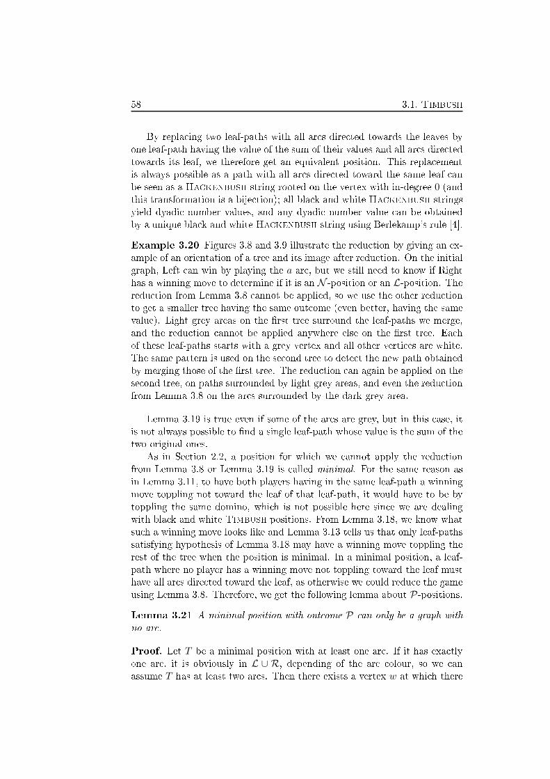
58 3.1. Timbush
By repla ing two leaf-paths with all ar s dire ted towards the leaves by
one leaf-path having the value of the sum of their values and all ar s dire ted
towards its leaf, we therefore get an equivalent position. This repla ement
is always possible as a path with all ar s dire ted toward the same leaf an
be seen as a Ha kenbush string rooted on the vertex with in-degree 0 (andthis transformation is a bije tion); all bla k and white Ha kenbush strings
yield dyadi number values, and any dyadi number value an be obtained
by a unique bla k and white Ha kenbush string using Berlekamp's rule [4℄.
Example 3.20 Figures 3.8 and 3.9 illustrate the redu tion by giving an ex-
ample of an orientation of a tree and its image after redu tion. On the initial
graph, Left an win by playing the a ar , but we still need to know if Right
has a winning move to determine if it is an N -position or an L-position. Theredu tion from Lemma 3.8 annot be applied, so we use the other redu tion
to get a smaller tree having the same out ome (even better, having the same
value). Light grey areas on the �rst tree surround the leaf-paths we merge,
and the redu tion annot be applied anywhere else on the �rst tree. Ea h
of these leaf-paths starts with a grey vertex and all other verti es are white.
The same pattern is used on the se ond tree to dete t the new path obtained
by merging those of the �rst tree. The redu tion an again be applied on the
se ond tree, on paths surrounded by light grey areas, and even the redu tion
from Lemma 3.8 on the ar s surrounded by the dark grey area.
Lemma 3.19 is true even if some of the ar s are grey, but in this ase, it
is not always possible to �nd a single leaf-path whose value is the sum of the
two original ones.
As in Se tion 2.2, a position for whi h we annot apply the redu tion
from Lemma 3.8 or Lemma 3.19 is alled minimal. For the same reason as
in Lemma 3.11, to have both players having in the same leaf-path a winning
move toppling not toward the leaf of that leaf-path, it would have to be by
toppling the same domino, whi h is not possible here sin e we are dealing
with bla k and white Timbush positions. From Lemma 3.18, we know what
su h a winning move looks like and Lemma 3.13 tells us that only leaf-paths
satisfying hypothesis of Lemma 3.18 may have a winning move toppling the
rest of the tree when the position is minimal. In a minimal position, a leaf-
path where no player has a winning move not toppling toward the leaf must
have all ar s dire ted toward the leaf, as otherwise we ould redu e the game
using Lemma 3.8. Therefore, we get the following lemma about P-positions.
Lemma 3.21 A minimal position with out ome P an only be a graph with
no ar .
Proof. Let T be a minimal position with at least one ar . If it has exa tly
one ar , it is obviously in L ∪ R, depending of the ar olour, so we an
assume T has at least two ar s. Then there exists a vertex w at whi h there

Chapter 3. Partizan games 59
a
Figure 3.8: An orientation of a tree seen as a Timbush position
Figure 3.9: Its image after redu tion, having the same out ome

60 3.1. Timbush
are two leaf-paths {xi}06i6n and {yi}06i6m (x0 = w = y0). If (xn, xn−1) or(ym, ym−1) is an ar , the player whi h an topple it an hoose it and win
playing �rst. Now assume both (xn−1, xn) and (ym−1, ym) are ar s. As Tis minimal, it annot be redu ed using Lemma 3.8, so if one of (xi+1, xi),(yi+1, yi), (x1, w) or (y1, w) is an ar , the one with verti es of greater index,
say (xi+1, xi), has to share the olour of the ar (xi+1, xi+2). Then the player
whi h an topple (xi+1, xi) an hoose it and win playing �rst. Assume now
all (xi, xi+1), (yi, yi+1), (w, x1) and (w, y1) are ar s. Then we an apply the
redu tion from Lemma 3.19, whi h is a ontradi tion. �
Finding the out ome of a minimal position now be omes a formality. If
there is no ar , we are dealing with a P-position. If there is just one ar , theout ome is L if the ar is bla k and R if it is white. When there are two ar s
or more, we he k in ea h leaf-path who has a winning move not toppling
the leaf of that leaf-path. If both players have su h a move, we are dealing
with an N -position. Otherwise, the only player who has su h a move, and
su h a player exists sin e there is a vertex at whi h there are two leaf-paths
and one of these paths has to yield su h a winning move for the same reason
as in the proof of Lemma 3.21 sin e the position is minimal, wins the game
whether they play �rst or se ond. Indeed, if the other player does not play
an ar of a leaf-path, it leaves a vertex at whi h there were two leaf-paths
whi h are still there and where the former player an win; if they play on an
ar of a leaf-path that topples toward the leaf of that leaf-path, the situation
is the same unless the tree was a path from the beginning and Lemma 3.13
(and its ounterpart on left-topplable winning moves) ould on lude even
before the move was played; if they play on an ar of a leaf-path that does
not topple toward the leaf of that leaf-path, it annot be a winning move by
assumption. Note that the redu tion from Lemma 3.8 de reases the number
of verti es without in reasing the number of leaves, and the redu tion from
Lemma 3.19 de reases the number of leaves without in reasing the number
of verti es, so they an only be applied a linear number of times. As �nding
where to apply the redu tion an be done in linear time, this leads to a
quadrati time algorithm.
Theorem 3.22 We an ompute the out ome of any bla k and white on-
ne ted oriented graph G in time O(|V (G)|2).
Note that for a tree, the number of edges is equal to the number of
verti es minus one, and the redu tion to get an orientation of a tree from a
onne ted oriented graph ontaining a y le an be done in time O(|V (G)|2).Hen e, we an onsider O(|V (G)|) = O(|E(G)|) for the se ond part of the
algorithm.

Chapter 3. Partizan games 61
LLRELER
Figure 3.10: A row of dominoes and the orresponding Timbush position
3.2 Toppling Dominoes
Toppling Dominoes is a partizan game, introdu ed by Albert
Nowakowski and Wolfe in [1℄, played on one or several rows of dominoes
oloured bla k, white, or grey. On her move, Left hooses a bla k or grey
domino and topples it with all dominoes (of the same row) at its left, or
with all dominoes (of the same row) at its right. On his turn, Right does
the same with a white or grey domino.
To des ribe a one row Toppling Dominoes game, we just give the
word formed by the olours of its dominoes read from left to right. The
bla k, white and grey dominoes are also symbolised respe tively by an L (for
Left or bLa k), an R (for Right ≈ white) and an E (for Either or grEy). For
example, LLERR represents a Toppling Dominoes game with two bla k
dominoes followed by a grey then two white dominoes.
A Toppling Dominoes position with n dominoes an be seenas a Tim-
bush position on a path with 2n ar s, ea h domino being represented by
two ar s sharing the same olour (as the domino) pointing toward the same
vertex. See Figure 3.10 for an example.
A �rst easy observation on Toppling Dominoes is that the only game
on one row that has out ome P is the empty row. Indeed, if there is at least
one domino, any player who an play a domino at one end of the line an
win playing �rst. So if both extremities of the game are bla k, the game
has out ome L, if both are white, the game has out ome R, otherwise the
game has out ome N . This uniqueness of the 0 game is rather unusual, and
a natural question that arises is the following :
Question 3.23 In the game Toppling Dominoes, are there many equiva-
len e lasses with a unique element onsisting of only one row? Or are there
many games with few representations in a single row?
Some initial study of this question was given by Fink, Nowakowski, Siegel
and Wolfe in [17℄. They gave mu h redit to this question with the following
result:
Theorem 3.24 (Fink et al. [17℄) All numbers appear uniquely in Top-
pling Dominoes, i.e. if two games G and G′have value a same number,
then they are identi al.
A ni e orollary of this result is that numbers in Toppling Dominoes
are ne essarily palindromes, sin e they equal their reversal. In the following,

62 3.2. Toppling Dominoes
for a given number x, we denote by x the unique Toppling Dominoes
game with value x.
Fink et al. on lude [17℄ with a series of onje tures, some of whi h
are inspired by Theorem 3.24. They reformulate Theorem 3.24 as follows,
expli itly des ribing for a number x the unique Toppling Dominoes games
with value x.
Theorem 3.25 (Fink et al. [17℄) If a game G has value a number in
anoni al form {a|b}, then G is the Toppling Dominoes game aLRb.
Their �rst onje ture was that a similar result is also true when a and bare numbers but not the resulting game:
Conje ture 3.26 (Fink et al. [17℄) Let a and b be numbers with a > b,the game {a|b} is given (uniquely) by the Toppling Dominoes game aLRb.
In the following, we settle this onje ture. We �rst prove that the game
aLRb is indeed the game {a|b}, but we then show that aEb also has value
{a|b}. However, we prove that there are no other Toppling Dominoes
game with that value, namely:
Theorem 3.27 Let a > b be numbers and G be a Toppling Dominoes
game. The value of G is {a|b} if and only if G is aLRb, aEb or one of their
reversals.
The proof of this result is given in Subse tion 3.2.2. Fink et al. proposed
two similar onje tures in [17℄, for the games
{a∣∣{b|c}
}and
{{a|b}
∣∣{c|d}}.
Conje ture 3.28 (Fink et al. [17℄) Let a, b and c be numbers with
a > b > c. The game
{a∣∣{b|c}
}is given (uniquely) by the Toppling Domi-
noes game aLRcRLb.
Conje ture 3.29 (Fink et al. [17℄) Let a, b, c and d be numbers with
a > b > c > d. The game
{{a|b}
∣∣{c|d}}is given (uniquely) by the Toppling
Dominoes game bRLaLRdRLc.
We propose the following results to settle the onje tures.
Theorem 3.30 If a > b > c are numbers, then aLRcRLb has value{a∣∣{b|c}
}. Moreover, if a > b, then aEcRLb also has value
{a∣∣{b|c}
}.
Theorem 3.31 If a > b > c > d are numbers, then both bRLaLRdRLcand bRLaEdRLc have value
{{a|b}
∣∣{c|d}}.
The proofs of these results are given respe tively in Appendi es B.1
and B.2, as they use the same kind of argument as the proof of Theorem 3.27.
Note also that Conje ture 3.29 is not true when b = c. Indeed, the
game
{{a|b}
∣∣{b|d}}has value b, and therefore has a unique representation
by Theorem 3.24.
In the following, we prove Theorem 3.27, but �rst we prove in Subse -
tion 3.2.1 some useful preliminary results.
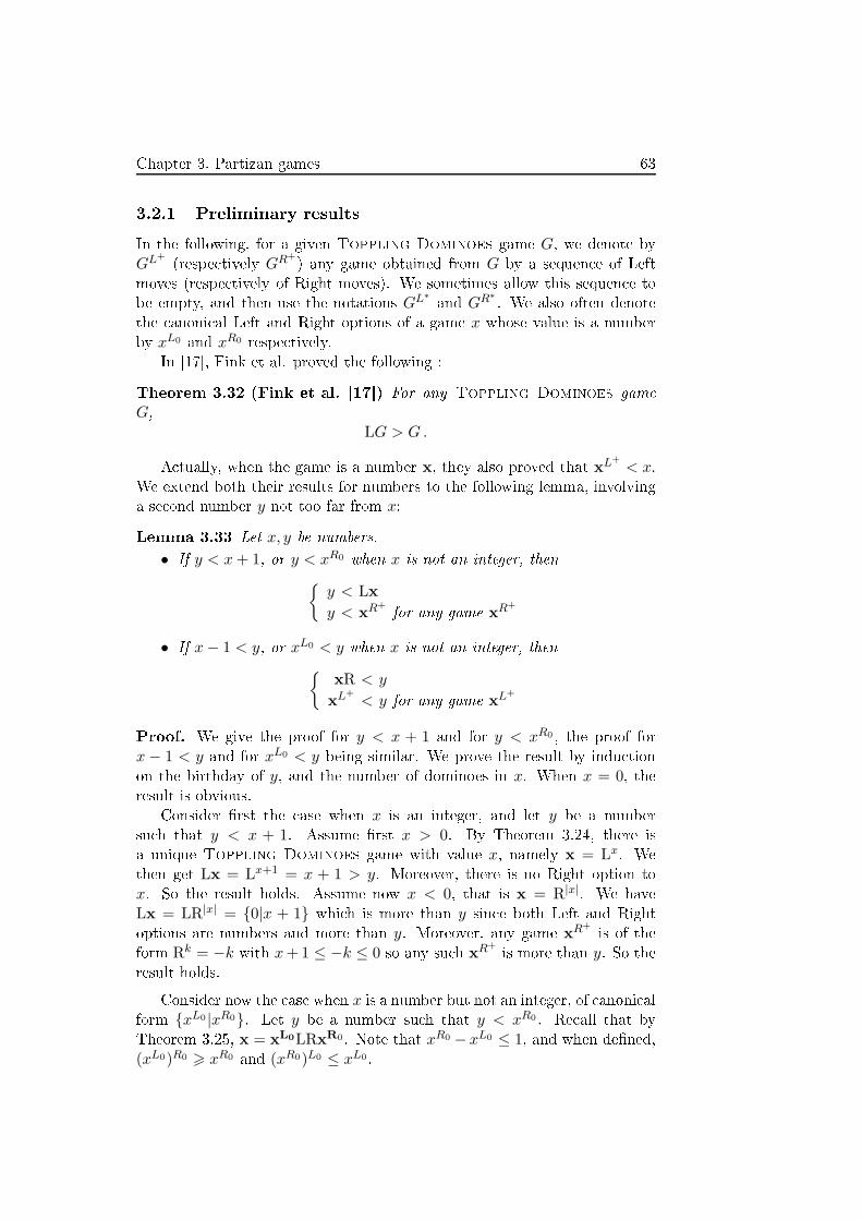
Chapter 3. Partizan games 63
3.2.1 Preliminary results
In the following, for a given Toppling Dominoes game G, we denote by
GL+
(respe tively GR+
) any game obtained from G by a sequen e of Left
moves (respe tively of Right moves). We sometimes allow this sequen e to
be empty, and then use the notations GL∗
and GR∗
. We also often denote
the anoni al Left and Right options of a game x whose value is a number
by xL0and xR0
respe tively.
In [17℄, Fink et al. proved the following :
Theorem 3.32 (Fink et al. [17℄) For any Toppling Dominoes game
G,LG > G .
A tually, when the game is a number x, they also proved that xL+
< x.We extend both their results for numbers to the following lemma, involving
a se ond number y not too far from x:
Lemma 3.33 Let x, y be numbers.
• If y < x+ 1, or y < xR0when x is not an integer, then
{y < Lx
y < xR+
for any game xR+
• If x− 1 < y, or xL0 < y when x is not an integer, then
{xR < y
xL+
< y for any game xL+
Proof. We give the proof for y < x + 1 and for y < xR0, the proof for
x− 1 < y and for xL0 < y being similar. We prove the result by indu tion
on the birthday of y, and the number of dominoes in x. When x = 0, theresult is obvious.
Consider �rst the ase when x is an integer, and let y be a number
su h that y < x + 1. Assume �rst x > 0. By Theorem 3.24, there is
a unique Toppling Dominoes game with value x, namely x = Lx. We
then get Lx = Lx+1 = x + 1 > y. Moreover, there is no Right option to
x. So the result holds. Assume now x < 0, that is x = R|x|. We have
Lx = LR|x| = {0|x + 1} whi h is more than y sin e both Left and Right
options are numbers and more than y. Moreover, any game xR+
is of the
form Rk = −k with x+1 ≤ −k ≤ 0 so any su h xR+
is more than y. So the
result holds.
Consider now the ase when x is a number but not an integer, of anoni al
form {xL0 |xR0}. Let y be a number su h that y < xR0. Re all that by
Theorem 3.25, x = xL0LRxR0. Note that xR0 − xL0 ≤ 1, and when de�ned,
(xL0)R0 > xR0and (xR0)L0 ≤ xL0
.

64 3.2. Toppling Dominoes
To prove Lx > y, we an just prove that whoever plays �rst, Left has a
winning strategy in Lx − y = LxL0LRxR0 − y. When Left starts, she an
move to LxL0 − y. Sin e xL0is born earlier than x and y < xR0 ≤ (xL0)R0
(or y < xR0 ≤ xL0 +1 if xL0is an integer), we an use indu tion and get y <
LxL0. Thus LxL0 − y is positive and Left wins. Now onsider the ase when
Right starts; we list all his possible moves from Lx − y = LxL0LRxR0 − y.If Right plays in −y, we get
• Lx + (−y)R0. We have (−y)R0 = −(yL0) and yL0 < y < xR0
. Thus
applying indu tion, we get Lx > yL0and thus Lx + (−y)R0 > 0, so
Left wins.
Suppose now Right moves in LxL0LRxR0. Toppling rightward, Right an
move to:
• L(xL0)R− y. By Theorem 3.32, L(xL0)R− y > (xL0)R− y. Moreover,
sin e y < xR0 ≤ (xL0)R0, we have by indu tion (xL0)R > y. Thus
L(xL0)R − y is positive and Left wins.
• LxL0L − y whi h is more that LxL0 − y by Theorem 3.32, whi h is
positive as proved earlier. Thus Left wins.
• LxL0LR(xR0)R − y. Then Left an answer to LxL0 − y whi h again
is positive as proved earlier, and win.
Toppling leftward, Right an move to:
• (xL0)RLRxR0−y. Then Left an answer to (xL0)R−y whi h is positiveas proved earlier.
• xR0 − y, positive by initial assumption.
• (xR0)R − y. We have (xR0)R0 > xR0 > y, so by indu tion (xR0)R > yand Left wins.
We now prove by indu tion that xR+
> y for any xR+
. A game
xR+
=(xL0LRxR0
)R+
may take seven di�erent forms, namely:
•(xL0
)R+
, larger than y by indu tion sin e
(xL0)R0
> xR0 > y.
•(xL0
)R+
L, whi h is larger than
(xL0
)R+
, thus also larger than y.
• xL0L, larger than y by indu tion sin e
(xL0)R0
> xR0 > y.
•(xR0
)R+
, larger than y by indu tion sin e
(xR0
)R0 > xR0 > y.• xR0
, larger than y by our initial assumption.
•(xL0
)R+
LR(xR0
)R∗
. In this ase, we show that Left has a win-
ning move in
(xL0
)R+
LR(xR0
)R∗
− y. When playing �rst, she
an move to
(xL0
)R+
− y that we already proved to be posi-
tive. When playing se ond, we may only onsider Right's move
to
(xL0
)R+
LR(xR0
)R∗
+ (−y)R0, to whi h she answers similarly to
(xL0
)R+
+ (−y)R0, also positive sin e (−y)R0 > −y.
• xL0LR(xR0
)R+
= x′. If y ≤ xL0
, then Left wins in x′ − y by playing
to xL0 − y or xL0 + (−y)R0. Otherwise, we pro eed by indu tion on

Chapter 3. Partizan games 65
the birthday of y and the number of dominoes in x′. If Right starts in
x′, we an use indu tion dire tly and get that Left wins. If he starts
in −y, sin e (−y)R0 > −y, we an also apply indu tion. Now if Left
annot win when starting, we have x′ − y is P, so x′ = y. Yet, y is
a number su h that xL0 < y < xR0, so y is not born earlier than x.
So by Theorem 3.25, x is a subword of y and as x′is a stri t subword
of x, x′ 6= y. By uni ity (Theorem 3.24), x′ 6≡+ y, whi h yields a
ontradi tion.
�
This gives us the following orollary.
Corollary 3.34 If a > b > c > d are numbers, then aR+
> {a|b},aR
+
>{a∣∣{b|c}
}, aR
+
>{{a|b}
∣∣c}and aR
+
>{{a|b}
∣∣{c|d}}.
Proof. By Lemma 3.33, we know that aR+
> a+aR0
2 whi h itself is a number
larger than a, b, c and d. The inequalities follow. �
3.2.2 Proof of Theorem 3.27
We now hara terise the positions on one row having value {a|b}, for anynumbers a > b. We start by proving that aLRb is among those positions,
and we �rst prove a preliminary lemma on options of aLRb.
Lemma 3.35 Let a, b be numbers su h that a > b. For any Right option bR
obtained from b toppling rightward, we have aLRbR > b.
Proof. To prove that aLRbR > b, we an just prove that Left has a winning
strategy in aLRbR − b whoever plays �rst. When Left starts, she an move
to a− b, and sin e a− b > 0, rea h a game whi h is P or L, thus win. Now onsider the ase when Right starts, and his possible moves from aLRbR−b.If Right plays in −b, we get
• aLRbR + (−b)R. Re all that sin e b is taken in its anoni al form, −bhas at most one Right option, namely (−b)R0
. Here Left an answer
to a+ (−b)R0whi h is positive sin e (−b)R0 > −b > −a. Therefore it
is a winning position for Left.
Consider now Right's possible moves in aLRbR. Toppling rightward, Right
an move to:
• aR − b. Using Lemma 3.33 with x = y = a, we get aR > a, and sin e
a > b, aR − b > 0.• aL− b. Again, by Lemma 3.33, aL− b > 0 and Left wins.
• aLR(bR)R − b. Then Left an answer to a− b, leaving a game in L or
in P sin e a− b > 0, thus win.
Toppling leftward, Right an move to:
66 3.2. Toppling Dominoes
• aRLRbR − b. Then Left an answer to aR − b whi h is positive as
proved above.
• bR − b whi h is positive by Lemma 3.33.
• (bR)R − b, again positive by Lemma 3.33.
�
We an now state the following laim.
Claim 3.36 Let a, b be numbers su h that a > b. We have aLRb = {a|b}.
Proof. To prove that aLRb = {a|b}, we prove that the se ond player has a
winning strategy in aLRb−{a|b}. Without loss of generality, we may assume
Right starts the game, and onsider his possible moves from aLRb− {a|b}.If Right plays in −{a|b}, we get
• aLRb− a. Then Left an answer to a− a whi h has value 0.
Consider now Right's possible moves in aLRb. Toppling rightward, Right
an move to:
• aR − {a|b}. Then Left an answer to aR − b, whi h is positive.
• aL− {a|b}, whi h is positive by Corollary 3.34.
• aLRbR−{a|b}. Then Left an answer to aLRbR−b, whi h is positive
by Lemma 3.35.
Toppling leftward, Right an move to:
• aRLRb−{a|b}. Then Left an answer to aR−{a|b}, whi h is positive
by Corollary 3.34.
• b− {a|b}. Then Left an answer to b− b whi h has value 0.• bR − {a|b}. Then Left an answer to bR − b whi h is positive.
�
As an example, here is a representation of {2|34}:
We now prove that aEb also has value {a|b}, and we again need to prove
�rst a preliminary lemma on options of aEb.
Lemma 3.37 Let a, b be numbers su h that a > b. For any Right option bR
obtained from b toppling rightward, we have aEbR > b.
Proof. We prove that Left has a winning strategy in aEbR − b whoever
plays �rst. When Left starts, she an move to a− b, rea hing a game that is
P or L, thus win. Now onsider the ase when Right starts, and his possible
moves from aEbR − b. If Right plays in −b, we get
• aEbR+(−b)R. Re all that sin e b is taken in its anoni al form, there
is only one Right option to −b, namely (−b)R0. Here Left an answer
to a+ (−b)R0whi h is positive sin e (−b)R0 > −b > −a. Therefore it
is a winning position for Left.

Chapter 3. Partizan games 67
Consider now Right's possible moves in aEbR. Toppling rightward, Right
an move to:
• aR − b, whi h is positive.
• a− b, whi h is positive.
• aE(bR)R−b. Then Left an answer to a−b whi h is positive and win.
Toppling leftward, Right an move to:
• aREbR − b. Then Left an answer to aR − b, whi h is positive.
• bR − b whi h is positive.
• (bR)R − b, again positive.
�
We an now state the following laim.
Claim 3.38 Let a, b be numbers su h that a > b. We have aEb = {a|b}.
Proof. To prove that aEb = {a|b}, we prove that the se ond player has a
winning strategy in aEb−{a|b}. Without loss of generality, we may assume
Right starts the game, and onsider his possible moves from aEb−{a|b}. IfRight plays in −{a|b}, we get
• aEb− a. Then Left an answer to a− a = 0.
Consider now Right's possible moves in aEb. Toppling leftward, Right an
move to:
• aREb− {a|b}. Then Left an answer to aR − {a|b}, whi h is positive
by Corollary 3.34.
• b− {a|b}. Then Left an answer to b− b, whi h has value 0.• bR − {a|b}. Then Left an answer to bR − b, whi h is positive.
Toppling rightward, Right an move to:
• aR − {a|b}. Then Left an answer to aR − b, whi h is positive.
• a− {a|b}. Then Left an answer to a− b, having value at least 0.• aEbR − {a|b}. Then if a > b Left an answer to aEbR − b, whi h is
positive by Lemma 3.37. Otherwise, a = b and Left an answer to
bR − {a|b}, whi h is positive by Corollary 3.34.
�
As an example, here is a representation of {12 | −
54}:
We now start proving these two rows of dominoes (and their reversals) are
the only rows having the value {a|b}. The next four lemmas are preliminary
lemmas, proving some options may not o ur for a player in a game having
value {a|b}.First we prove that some of Left's moves from aLRb annot be available
for Right in a game having value {a|b}.

68 3.2. Toppling Dominoes
Lemma 3.39 Let a, b be numbers su h that a > b. For any Left option bL
obtained from b toppling rightward, we have aLRbL < {a|b}.
Proof. We prove that Right has a winning strategy in aLRbL − {a|b}whoever plays �rst. When Right starts, he an move to bL −{a|b}, whi h is
negative by Corollary 3.34. Now onsider the ase when Left starts and her
possible moves to aLRbL − {a|b}. If Left plays in −{a|b}, we get
• aLRbL − b. Then Right an answer to bL − b, whi h is negative.
Consider now Left's possible moves in aLRbL. Toppling rightward, Left an
move to:
• aL − {a|b}. Then Right an answer to aL − a, whi h is negative.
• a− {a|b}. Then Right an answer to a− a whi h has value 0.• aLR(bL)L − {a|b}. Then Right an answer to aLR(bL)L − a, whi h
is negative by Lemma 3.35 sin e both moves in b were by toppling
rightward, allowing us to onsider aLR(bL)L as some aLRbL.
Toppling leftward, Left an move to:
• aLLRbL−{a|b}. Then Right an answer to bL−{a|b} whi h is negativeby Corollary 3.34.
• RbL − {a|b} whi h is negative as RbL < bLby Lemma 3.33 and
bL − {a|b} is negative by Corollary 3.34.
• (bL)L − {a|b} whi h is negative by Corollary 3.34.
�
Now we prove that some of Right's moves from aLRb annot be available
for Left in a game having value {a|b}. Note that these moves are not the
reversal of moves onsidered in the previous lemma.
Lemma 3.40 Let a, b be numbers su h that a > b. For any Right option bR
obtained from b toppling rightward, we have aLRbR > {a|b}.
Proof. We prove that Left has a winning strategy in aLRbR−{a|b} whoeverplays �rst. When Left starts, she an move to aLRbR − b, whi h is positive
by Lemma 3.35. Now onsider the ase where Right starts, and his possible
moves from aLRbR − {a|b}. If Right plays in {a|b}, we get
• aLRbR − a. Then Left an answer to a− a whi h has value 0.
Consider now Right's possible moves in aLRbR. Toppling rightward, Right
an move to:
• aR − {a|b}. Then Left an answer to aR − b, whi h is positive.
• aL− {a|b}, whi h is positive by Corollary 3.34.
• aLR(bR)R − {a|b}. Then Left an answer to aLR(bR)R − b, whi his positive by Lemma 3.35 sin e both moves in b were by toppling
rightward, allowing us to onsider aLR(bR)R as some aLRbR.
Toppling leftward, Right an move to:

Chapter 3. Partizan games 69
• aRLRbR−{a|b}. Then Left an answer to aR−{a|b}, whi h is positive
by Corollary 3.34.
• bR − {a|b}. Then Left an answer to bR − b, whi h is positive.
• (bR)R − {a|b}. Then Left an answer to (bR)R − b, whi h is positive.
�
Similarly, we prove that some of Left's moves from aEb annot be avail-
able for Right in a game having value {a|b}.
Lemma 3.41 Let a, b be numbers su h that a > b. For any Left option bL
obtained from b toppling rightward, we have aEbL < {a|b}.
Proof. We prove that Right has a winning strategy in aEbL−{a|b} whoeverplays �rst. When Right starts, he an move to bL−{a|b}, whi h is negative
by Corollary 3.34. Now onsider the ase when Left starts, and her possible
moves from aEbL − {a|b}. If Left plays in −{a|b}, we get
• aEbL − b. Then Right an answer to bL − b, whi h is negative.
Consider now Right's possible moves in aEbL. Toppling rightward, Left an
move to:
• aL − {a|b}. Then Right an answer to aL − a, whi h is negative.
• a− {a|b}. Then Right an answer to a− a whi h has value 0.• aE(bL)L − {a|b}. Then Right an answer to aE(bL)L − b, whi h is
negative by Corollary 3.34 sin e both moves in b were by toppling
rightward, allowing us to onsider aE(bL)L as some aEbL.
Toppling leftward, Left an move to:
• aLEbL−{a|b}. Then Right an answer to bL−{a|b}, whi h is negative
by Corollary 3.34.
• bL − {a|b}, negative by Corollary 3.34.
• (bL)L − {a|b}, negative by Corollary 3.34.
�
Finally we prove that some of Right's moves from aEb annot be available
for Left in a game having value {a|b}. Note that again these moves are not
the reversal of moves onsidered in the previous lemma.
Lemma 3.42 Let a, b be numbers su h that a > b. For any Right option bR
obtained from b toppling rightward, we have aEbR > {a|b}.
Proof. We prove that Left has a winning strategy in aEbR−{a|b} whoever
plays �rst. When Left starts, she an move to aEbR−b, whi h is positive by
Lemma 3.37 if a > b and to bR − {a|b}, whi h is positive by Corollary 3.34
if a = b. Now onsider the ase when Right starts, and his possible moves
from aEbR − {a|b}. If Right plays in −{a|b}, we get
• aEbR − a. Then Left an answer to a− a whi h has value 0.
70 3.2. Toppling Dominoes
Consider now Right's possible moves in aEbR. Toppling rightward, Right
an move to:
• aR − {a|b}. Then Left an answer to aR − b, whi h is positive.
• a− {a|b}. Then Left an answer to a− a whi h has value 0.• aE(bR)R−{a|b}. Then Left an answer to aE(bR)R−b, whi h is posi-
tive by Lemma 3.37 sin e both moves in b were by toppling rightward,
allowing us to onsider aE(bR)R as some aEbR.
Toppling leftward, Right an move to:
• aREbR−{a|b}. Then Left an answer to aR−{a|b}, whi h is positive
by Corollary 3.34.
• bR − {a|b}. Then Left an answer to bR − b, whi h is positive.
• (bR)R − {a|b}. Then Left an answer to (bR)R − b, whi h is positive.
�
Though we want to deal with a game having value {a|b}, it might not
be in anoni al form, that is its options and other proper followers might
not be numbers. As most known results in Toppling Dominoes are about
numbers, we get ba k there with the following lemma.
Lemma 3.43 Let a be a number and x be a game su h that x > a. Then
there exists a number b > a su h that b ∈ xL∗
.
Proof. We prove it by indu tion on the birthdays of x and a.If x = a, then a ∈ xL
∗
and a > a. Otherwise, x > a, so aR0 6 x or
a 6 xL for some xL. In both ases, we on lude by indu tion hypothesis,
sin e aR0 > a and (xL)L∗
⊆ xL∗
. �
To fully hara terise Toppling Dominoes rows having value {a|b}, weneed another lemma from [17℄:
Lemma 3.44 (Fink et al. [17℄) [Sandwi h Lemma℄ Let G be a Top-
pling Dominoes position with value α. From G − α, if the �rst player
topples dominoes toward the left (right) then the winning response is not to
topple a domino toward the left (right).
We now assume some Toppling Dominoes position x has value {a|b}to for e some properties on su h positions.
Lemma 3.45 If a > b are numbers and x is a Toppling dominoes posi-
tion with value {a|b}, then
• a ∈ xL ∪ xL2
,
• for any number a0 > a, a0 /∈ xL∗
,
• b ∈ xR ∪ xR2
,
• for any number b0 < b, b0 /∈ xR∗
.

Chapter 3. Partizan games 71
Proof. As x = {a|b}, x − {a|b} is a se ond-player win. From x − {a|b},Right an move to x − a, from whi h Left should have a winning move. It
annot be to x+ (−a)L0 = {a|b} − aR0as it is not winning sin e aR0
an be
written {r1|r2} with r1 > a and r2 > b. Hen e there is a Left move x0 of xsu h that x0 > a. By Lemma 3.43, there exists a number a0 > a su h that
a0 ∈ xL∗
0 ⊂ xL+
. If a0 ∈ xL, then a0 = a as otherwise Left's move from
x− {a|b} to a0 − {a|b} would be winning. As xL>3
⊂ xL2
, we do not need
onsider that ase. Thus we an assume a0 ∈ xL2
\xL. We an then write
x = w1δ1a0δ2w2 with δ1, δ2 ∈ {L,E}. In the following, we use the fa t that
Left has no winning �rst move in x−{a|b}. From x−{a|b}, Left an topple
δ2 rightward to w1δ1a0. If Right answers to w1δ1a0 − a, Left an topple
δ1 leftward to a0 − a and win. Hen e Right's winning answer has to be to
some (w1δ1a0)R − {a|b} and an only be a hieved by toppling leftward by
Lemma 3.44. If he moves to a0 or some aR0 , Left's move to a0 − b or aR0 − bis a winning move sin e aR0 > a0 > a > b. Hen e his winning move is to
some wR1 δ1a0 − {a|b}. But then Left an answer to a0 − {a|b} and we have
a0 = a or Right would have no winning strategy. This implies both that
a ∈ xL ∪ xL2
, and that for any number a0 > a, a0 /∈ xL∗
.
A similar reasoning would prove the last two stated items. �
Lemma 3.46 If a > b are numbers and x is a Toppling dominoes po-
sition with value {a|b}, then x has a Left option to a or a Right option to
b.
Proof. By Lemma 3.45, we know that a ∈ xL ∪ xL2
and b ∈ xR ∪ xR2
.
Assume that a only appears in xL2
\xLand b only appears in xR
2
\xR.
We an write x = w1δ1aδ2w2 su h that b /∈ wR+
1 and δ1, δ2 ∈ {L,E}, or
x = w1δ1bδ2w2 su h that a /∈ wL+
1 and δ1, δ2 ∈ {R,E}. Consider the one
with w1 having the smallest length. Without loss of generality, we an
assume it is w1δ1aδ2w2, and onsider Left's move from x − {a|b} to
w1δ1a− {a|b}. We saw in the proof of Lemma 3.45 that Right's win-
ning answer an only be to some wR1 δ1a− {a|b}. Now Left an move to
wR1 δ1a− b. If Right answers to wR
1 δ1a− bL0, Left an move to a− bL0
and
win. Hen e Right's winning answer has to be to some (wR1 δ1a)
R − b. For
this move to be winning, we have (wR1 δ1a)
R 6 b, so by Lemma 3.43 we have
b0 ∈ ((wR1 δ1a)
R)R∗
for some number b0 6 b. If b0 < b, by Lemma 3.45 we
have b0 /∈ xR∗
, so b0 has to be obtained from wR1 δ1a by only toppling left-
ward. We have b0 < b 6 a, hen e b0 annot be some aR > a, nor some
(wR1 )
Rδ1a sin e it would mean that a ∈ bL0 and then a < b0. Hen e b0 = b.
Again, b has to be obtained from wR1 δ1a by only toppling leftward sin e
b /∈ aR+
as b 6 a, and no b starts in x before w1 ends. In parti ular,
(wR1 δ1a)
Ris of the form wR
1 δ1a, a or aR. (wR1 δ1a)
R annot be of the form
aR, sin e aR > a > b. If (wR1 δ1a)
Ris of the form wR
1 δ1a, Left an move from
wR1 δ1a− b to a− b and win. Hen e (wR
1 δ1a)R = a, sin e (wR
1 δ1a)R 6 b 6 a,
72 3.3. Col
we have a = b and δ1 = E. w1 annot be greater than or equal to a sin e
otherwise we would �nd a number a0 > a su h that a0 ∈ wL∗
1 . Similarly,
w1 annot be less than or equal to b = a. As aL < a < aR, there exists a
Left move wL1 of w1 that is greater than or equal to a and so we an �nd
a number a0 > a su h that a0 ∈ (wL1 )
L∗
, whi h again is not possible. This
means there was no winning move for Right from wR1 δ1a− b, whi h means
there was no winning move for Right from w1δ1a− {a|b}, whi h ontradi ts
the fa t that x = {a|b}. Hen e we have that a ∈ xLor b ∈ xR
. �
We an now prove the following laim.
Claim 3.47 If a > b are numbers and x is a Toppling dominoes position
with value {a|b}, then x is either aLRb or aEb (or the reversal of one of
them).
Proof. By Lemma 3.46, we an assume without loss of generality that
x = aLx′or x = aEx′
for some x′.
First assume x = aLx′. If x is a stri t subword of aLRb, then x is an option
of aLRb, so they annot be equal. For the same reason, aLRb annot be
a stri t subword of x. Looking from left to right, we �nd the �rst domino
where x di�ers from aLRb. If it is a white or grey domino instead of a
bla k one, then Right has a move from x−{a|b} to aLRbL −{a|b} whi h is
winning by Lemma 3.39. If it is a bla k or grey domino instead of a white
one, then Left has a move from x−{a|b} to aL−{a|b} or to aLRbR−{a|b}whi h are winning by Corollary 3.34 and Lemma 3.40. So x annot di�er
from aLRb.Now assume x = aEx′
. If x is a stri t subword of aEb, then x is an option of
aEb, so they annot be equal. For the same reason, aEb annot be a stri t
subword of x. Looking from left to right, we �nd the �rst domino where
x di�ers from aEb. If it is a white or grey domino instead of a bla k one,
then Right has a move from x− {a|b} to aEbL − {a|b} whi h is winning by
Lemma 3.41. If it is a bla k or grey domino instead of a white one, then Left
has a move from x−{a|b} to aEbR−{a|b} whi h is winning by Lemma 3.42.
So x annot di�er from aEb.
�
3.3 Col
Col is a partizan game played on an undire ted graph with verti es either
un oloured or oloured bla k or white. A move of Left onsists in hoosing
an un oloured vertex and olouring it bla k, while a move of Right would be
to do the same with the olour white. An extra ondition is that the partial
olouring has to stay proper, that is no two adja ent verti es should have
the same olour.
Chapter 3. Partizan games 73
Un oloured verti es are represented grey.
When a player hooses a vertex, they thus be ome unable to play on any
of its neighbours for the rest of the game. Hen e, all these neighbours are
somehow reserved for the other player. Another way of seeing the game is
to play it on the graph of available moves: a position is an undire ted graph
with all verti es oloured bla k, white or grey; a move of Left is to hoose
a bla k or grey vertex, remove it from the game with all its bla k oloured
neighbours, and hange the olour of its other neighbours to white; a move
of Right is to hoose a white or grey vertex, remove it from the game with all
its white oloured neighbours, and hange the olour of its other neighbours
to bla k. This means that bla k verti es are reserved for Left, white verti es
for Right, and either player an hoose grey verti es. In the following, we
use that se ond representation.
The des ription of a position onsists of the graph on whi h the two
players are playing, and a reservation fun tion from the set of verti es to the
set of olours {black,white, grey}.
Example 3.48 Figure 3.11 shows an example of a Col position under the
two representations. On top is the �rst representation as in the original
de�nition of the game. On bottom is the se ond representation, that we use
in the following. Both represent the same game. To go from the original
representation to the se ond representation, we delete bla k verti es and
olour their neighbours white, delete verti es that were originally white and
olour their neighbours bla k, and delete verti es we gave both olours. We
an see the se ond representation seems simpler, and that is why we use it.
Example 3.49 Figure 3.12 gives an example of a Right move. Right hooses
the grey vertex x. That vertex is removed from the game. The white vertex
y also disappears. The grey vertex z be omes bla k. The bla k vertex t
stays bla k. The rest of the graph does not hange as no other verti es are
neighbours of x.
We represent some graphs using words: ea h letter used in this repre-
sentation orresponds to a subgraph with a spe i� vertex being in ident
with the edges onne ting that subgraph to the subgraphs orresponding to
the letters before and after this one. The spe i� verti es orresponding to
the �rst letter and the last letter are not neighbours, unless the words has
length 2. An o represents a grey vertex, a B a bla k vertex and a W a white
vertex, the only vertex being the spe i� vertex. An x represents a path
with two grey verti es, anyone of them being the spe i� vertex. All the
graphs that an be represented by words using these letters are aterpillars
with maximum degree 3. We also note Cn the y le on n grey verti es.
Example 3.50 Figure 3.13 shows a word and the unique graph that it en-
odes. You an see that for ea h x, there is a vertex whose degree remains
1.

74 3.3. Col
Figure 3.11: A Col position in its two representations

Chapter 3. Partizan games 75
y
x
z t
Figure 3.12: Playing a move in Col
xWooxxxoWoBxoWxooxWBoxBoxxo
Figure 3.13: Representation of a aterpillar by a word
We now introdu e a few notation that we use in the following. We note
ℓG(v) the label of a vertex v ∈ V (G), that is B if the vertex is oloured
bla k, W if it is oloured white and o if it is un oloured. Modifying the label
of a vertex is equivalent to modifying its olour. We say ℓG(u) = −ℓG(v)if both ℓG(u) and ℓG(v) are o or if one is B and the other is W . Given a
Col position G, we note −G the Col position su h that V (−G) = V (G),E(−G) = E(G) and ∀v ∈ G, ℓ−G(v) = −ℓG(v). The reader would have
re ognised that the game −G is the onjugate of the game G. Given two
Col positions G1, G2 and two verti es u1 ∈ V (G1), u2 ∈ V (G2) su h that
ℓG1(u1) = ℓG2
(u2), we note (G1, u1)⊙ (G2, u2) the Col position de�ned by:
V ((G1, u1)⊙ (G2, u2)) = V (G1) ∪ V (G2) \ {u2}E((G1, u1)⊙ (G2, u2)) = E(G1) ∪ E(G2[V (G2) \ {u2}])
∪{(u1, v) | (u2, v) ∈ E(G2)})
ℓ(G1,u1)⊙(G2,u2)(v) =
{ℓG1
(v) if v ∈ V (G1)ℓG2
(v) otherwise
Given a vertex u in a Col position G, we note by G+u (resp. G−
u ) the Col
position obtained from G by re-labelling B (resp. W ) the vertex u.We note PB
n (resp PBBn , PBW
n , PWBn , PWW
n ) the Col position (Bon, u) (resp(BonB,u), (BonW,u), (WonB,u), (WonW,u)) where the spe i� vertex u
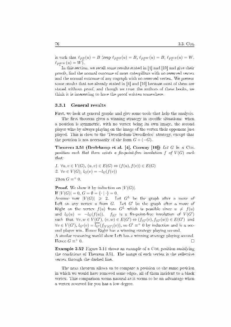
76 3.3. Col
is su h that ℓPBn(u) = B (resp ℓPBB
n(u) = B, ℓPBW
n(u) = B, ℓPWB
n(u) = W ,
ℓPWWn
(u) = W ).
In this se tion, we re all some results stated in [4℄ and [10℄ and give their
proofs, �nd the normal out ome of most aterpillars with no reserved vertex
and the normal out ome of any ograph with no reserved vertex. We present
some results that are already stated in [4℄ and [10℄ be ause most of them are
stated without proof, and though we trust the authors of these books, we
think it is interesting to have the proof written somewhere.
3.3.1 General results
First, we look at general graphs and give some tools that help the analysis.
The �rst theorem gives a winning strategy in spe i� situations: when
a position is symmetri , with no vertex being its own image, the se ond
player wins by always playing on the image of the vertex their opponent just
played. This is lose to the `Tweedledum-Tweedledee' strategy, ex ept that
the position is not ne essarily of the form G+ (−G).
Theorem 3.51 (Berlekamp et al. [4℄, Conway [10℄) Let G be a Col
position su h that there exists a �x-point-free involution f of V (G) su h
that:
1. ∀u, v ∈ V (G), (u, v) ∈ E(G) ⇔ (f(u), f(v)) ∈ E(G)
2. ∀v ∈ V (G), lG(v) = −lG(f(v))
Then G ≡+ 0.
Proof. We show it by indu tion on |V (G)|.If |V (G)| = 0, G = ∅ = {· | ·} = 0.Assume now |V (G)| > 2. Let GL
be the graph after a move of
Left on any vertex u from G. Let G′be the graph after a move of
Right on the vertex f(u) from GLwhi h is possible sin e u 6= f(u)
and lG(u) = −lG(f(u)). f|G′is a �x-point-free involution of V (G′)
su h that ∀v,w ∈ V (G′), (v,w) ∈ E(G′) ⇔ (f|G′(v), f|G′(w)) ∈ E(G′) and
∀v ∈ V (G′), lG′(v) = lG′(f|V (G′)(v)), so G′ ≡+ 0 by indu tion and is a se -
ond player win. Hen e Right has a winning strategy playing se ond.
A similar reasoning would show Left has a winning strategy playing se ond.
Hen e G ≡+ 0. �
Example 3.52 Figure 3.14 shows an example of a Col position satisfying
the onditions of Theorem 3.51. The image of ea h vertex is the re�e tive
vertex through the dashed line.
The next theorem allows us to ompare a position to the same position
in whi h we would have removed some edges, all of them in ident to a bla k
vertex. This omparison seems natural as it seems to be an advantage when
a vertex reserved for you has a low degree.
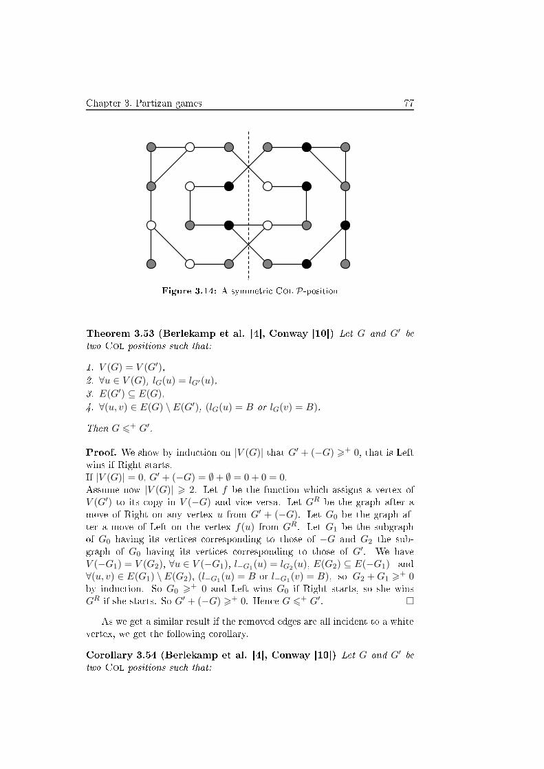
Chapter 3. Partizan games 77
Figure 3.14: A symmetri Col P-position
Theorem 3.53 (Berlekamp et al. [4℄, Conway [10℄) Let G and G′be
two Col positions su h that:
1. V (G) = V (G′),
2. ∀u ∈ V (G), lG(u) = lG′(u),
3. E(G′) ⊆ E(G),
4. ∀(u, v) ∈ E(G) \E(G′), (lG(u) = B or lG(v) = B).
Then G 6+ G′.
Proof. We show by indu tion on |V (G)| that G′ + (−G) >+ 0, that is Leftwins if Right starts.
If |V (G)| = 0, G′ + (−G) = ∅+ ∅ = 0 + 0 = 0.Assume now |V (G)| > 2. Let f be the fun tion whi h assigns a vertex of
V (G′) to its opy in V (−G) and vi e versa. Let GRbe the graph after a
move of Right on any vertex u from G′ + (−G). Let G0 be the graph af-
ter a move of Left on the vertex f(u) from GR. Let G1 be the subgraph
of G0 having its verti es orresponding to those of −G and G2 the sub-
graph of G0 having its verti es orresponding to those of G′. We have
V (−G1) = V (G2), ∀u ∈ V (−G1), l−G1(u) = lG2
(u), E(G2) ⊆ E(−G1) and
∀(u, v) ∈ E(G1) \ E(G2), (l−G1(u) = B or l−G1
(v) = B), so G2 +G1 >+ 0
by indu tion. So G0 >+ 0 and Left wins G0 if Right starts, so she wins
GRif she starts. So G′ + (−G) >+ 0. Hen e G 6+ G′
. �
As we get a similar result if the removed edges are all in ident to a white
vertex, we get the following orollary.
Corollary 3.54 (Berlekamp et al. [4℄, Conway [10℄) Let G and G′be
two Col positions su h that:

78 3.3. Col
1. V (G) = V (G′)
2. ∀u ∈ V (G), lG(u) = lG′(u)
3. E(G′) ⊆ E(G)
4. ∀(u, v) ∈ E(G) \ E(G′), ((lG(u) = B and lG(v) = W )) or vi e versa
Then G ≡+ G′.
Proof. We have G 6+ G′and −G 6+ −G′
, so G ≡+ G′. �
A tually, we even have G = G′in this ase.
Adding a bla k vertex or reserving a vertex for Left seems to be an
advantage for her. The next theorem shows that this intuition is orre t.
Theorem 3.55 (Berlekamp et al. [4℄, Conway [10℄) Let G be a Col
position and u a grey vertex of G. Then:
1. G+u >+ G >+ G−
u
2. G+u >+ G \ {u} >+ G−
u
Proof. We show by indu tion on |V (G)| that G+u + (−G \ {u}) >+ 0, that
is Left wins if Right starts.
If |V (G)| = 0, G+u + (−G \ {u}) = ∅+ ∅ = 0.
Assume now |V (G)| > 2. We de�ne f the fun tion whi h assigns a vertex
of V (G+u ) \ {u} to its opy in V (−G \ {u}) and vi e versa. Let GR
be the
graph after a move of Right on any vertex v from G+u + (−G \ {u}). Let G0
be the graph after a move of Left on the vertex f(v) from GR. Let G1 be
the subgraph of G0 having its verti es orresponding to those of G+u and G2
the subgraph of G0 having its verti es orresponding to those of −G \ {u}.If (u, f(v)) ∈ E(G+
u + (−G \ {u})), then G1 = −G2, so G0 = G1 +G2 = 0.Otherwise, G1 = G+
1u and G2 = −G1 \ {u}, so G0 = G1 + G2 >+ 0 by
indu tion. Hen e 0 6+ G0 and Left wins G0 if Right starts, so she wins GR
if she starts. So G+u + (−G \ {u}) >+ 0. Hen e G+
u >+ G \ {u}.We show by indu tion on |V (G)| that G+
u +(−G) >+ 0, that is Left winsit if Right starts.
If |V (G)| = 0, G+u + (−G) = ∅+ ∅ = 0.
Assume |V (G)| > 2. We de�ne f the fun tion whi h assigns a vertex of
V (G+u ) to its opy in V (−G) and vi e versa. Let GR
be the graph after
a move of Right on any vertex v from G+u + (−G). Let G0 be the graph
after a move of Left on the vertex f(v) from GR. Let G1 be the subgraph
of G0 having its verti es orresponding to those of G+u and G2 the subgraph
of G0 having its verti es orresponding to those of −G. If u = f(v) or
(u, v) ∈ E(G+u + (−G \ {u})), then G1 = −G2, so G0 = G1 + G2 = 0. If
(u, f(v)) ∈ E(G+u + (−G \ {u})), then G2 = G+
2u and G1 = G2 \ {u}, soG0 = G1 + G2 >+ 0. Otherwise, G1 = (−G2)
+u , so G0 = G1 +G2 >+ 0 by
Chapter 3. Partizan games 79
indu tion. Hen e 0 6+ G0 and Left wins G0 if Right starts, so she wins GR
if she starts. So G+u + (−G) >+ 0. Hen e G+
u >+ G.Finally, −(G−
u ) = (−G)+u , so −(G−u ) >
+ −G and −(G−u ) >
+ −G \ {u}.Hen e G >+ G−
u and G \ {u} >+ G−u . �
The next theorem says that any Col position is equivalent under normal
play to a number or to the game ∗ added to a number, whi h makes �nding
the out ome of a sum easier. In parti ular, it implies that the sum of two
Col N -positions is a P-position. Also, if we �nd a move to z for both
players, we know the value of the game is z + ∗ without having the need
to he k other options. It also implies that if G is a Col position where
G = −G, whi h is the ase when all verti es are grey, then G = 0 or G = ∗.See [4℄, vol.1, p.47-48 for the proof.
Theorem 3.56 (Berlekamp et al. [4℄, Conway [10℄) For any Col po-
sition G, there exists a number z su h that G = z or G = z + ∗.
In a Col position, if there is a vertex for whi h the position has the
same value when the olour of the vertex is swit hed to bla k and when the
olour of the vertex is swit hed to white, it seems no player wants to play
on that vertex, whether it is reserved or not. The intuition is orre t, and
the following theorem shows a result even stronger: even if you identify that
vertex to any vertex of another position, keeping the �rst position as it was,
with no other vertex adja ent to a vertex of the added position, no player
wants to play on that vertex, whether it is reserved or not.
Theorem 3.57 (Berlekamp et al. [4℄, Conway [10℄)
1. Let G be a Col position and u a grey vertex of G su h that G+u ≡+ G−
u ,
G′any Col position and v a grey vertex of G′
. Then
(G+u , u)⊙ (G′+
v , v) ≡+ (G,u) ⊙ (G′, v) ≡+ (G \ {u}) + (G′ \ {v}) ≡+ (G−u , u)⊙ (G′−
v , v).
2. Let G be a Col position and u a vertex of G su h that G+u ≡+ G \ {u},
G′any Col position and v a vertex of G′
sharing the olour of u. Then(G+
u , u)⊙ (G′+v , v) ≡+ (G \ {u}) + (G′ \ {v}).
Proof. 1. We have G+u ≡+ G−
u , so 0 ≡+ G+u + (−G−
u ) ≡+ G+u + (−G)+u .
Moreover,
0 ≡+ G \ {u}+ (−G \ {u}) +G′ \ {v}+ (−G′ \ {v})≡+ G \ {u}+G′ \ {v} + (−G) \ {u}+ (−G′) \ {v}6
+ (G+u , u)⊙ (G′+
v , v) + ((−G)+u , u)⊙ ((−G′)+v , v)6
+ G+u +G′ \ {v} + (−G)+u + (−G′) \ {v}
≡+ (G+u + (−G)+u ) + (G′ \ {v}+ (−G′ \ {v}))
≡+ 0
Hen e
0 ≡+ (G+u , u)⊙ (G′+
v , v) + ((−G)+u , u)⊙ ((−G′)+v , v)≡+ (G+
u , u)⊙ (G′+v , v) + (−((G−
u , u)⊙ (G′−v , v)))

80 3.3. Col
From Theorem 3.55, we get
(G+u , u)⊙ (G′+
v , v) ≡+ (G,u) ⊙ (G′, v)≡+ (G \ {u}) + (G′ \ {v}≡+ (G−
u , u)⊙ (G′−v , v)
2. We have G+u ≡+ G \ {u}, so 0 ≡+ G+
u + (−G \ {u}).
0 ≡+ G \ {u} +G′ \ {u}+ (−G \ {u}) + (−G′ \ {u})6+ (G+
u , u)⊙ (G′+v , v) + (−((G \ {u}) + (G′ \ {v})))
6+ G+u +G′ \ {v} + (−G \ {u}) + (−G′ \ {v})
≡+ 0
Hen e
0 ≡+ (G+u , u)⊙ (G′+
v , v) + (−((G \ {u}) + (G′ \ {v})))(G+
u , u)⊙ (G′+v , v) ≡+ (G \ {u}) + (G′ \ {v})
�
We immediately get the following orollary, that we use frequently in the
following of the se tion.
Corollary 3.58 (Berlekamp et al. [4℄, Conway [10℄) For any Col po-
sition G, and any vertex v of G su h that ℓG(v) = B, we have
(G, v) ⊙ PBB0 ≡+ (G \ {v}) +B.
Proof. We have B = {∅ | ·} = BB. �
3.3.2 Known results
We now fo us on some lasses of trees. Though we want to �nd the out omes
of Col positions where all verti es are grey, we need intermediate lemmas
where some verti es are bla k or white.
We �rst prove that y les and paths having only grey verti es all have
value 0, apart from the isolated vertex whi h has value ∗. We separate the
proof with two lemmas, overing all possible maximal onne ted subpositions
that may appear throughout su h a game, as the disjun tive sum of numbers
and ∗ is easy to determine, before Theorem 3.61 ends the proof.
The �rst lemma gives the values of all paths where ea h leaf is either
bla k or white, and all internal nodes are grey.
Lemma 3.59 (Berlekamp et al. [4℄, Conway [10℄)
1. ∀n > 0, B ≡+ BonB ≡+ 1.2. ∀n > 0, BonW ≡+ 0.

Chapter 3. Partizan games 81
Proof. We show the results simultaneously by indu tion on n.B = {∅ | ·} = {0 | ·} ≡+ 1. BB = {∅ | ·} = {0 | ·} ≡+ 1.BW = B +W ≡+ 0.Let n > 1 be an integer.
BonB = {Won−1B,Won−2B,
n−3
2⋃
i=0
(BoiW +Won−i−3B)
| (B +Bon−2B),
n−3⋃
i=0
(BoiB +Bon−i−3B)}
≡+ {0, 0, (0 + 0) | 2, (1 + 1)} by induction≡+ 1.
BonW = {Won−1W,Won−2W, (Bon−2W +W ),
n−3⋃
i=0
(BoiW +Won−i−3W )
| Bon−1B,Bon−2B, (B +Bon−2W ),n−3⋃
i=0
(BoiB +Bon−i−3W )}
≡+ {−1,−1, (0 + (−1)), (0 + (−1)) | 1, 1, (1 + 0), (1 + 0)}by induction
≡+ 0.
�
The following lemma gives the values of all paths where exa tly one leaf
is either bla k or white, and all other verti es, in luding the other leaf, are
grey.
Lemma 3.60 (Berlekamp et al. [4℄, Conway [10℄) ∀n > 1, Bon ≡+ 12 .
Proof. We show the result by indu tion on n.Bo = {W, ∅ | B} = {−1, 0 | 1} ≡+ 1
2 .
Boo = {Wo,W,BW | (B +B), BB} ≡+ {−12 ,−1, 0 | (1 + 1), 1} ≡+ 1
2 .
Let n > 3 be an integer.
Bon = {Won−1,Won−2,
n−4⋃
i=1
(BoiW +Won−i−3, (Bon−3W +W ), Bon−2W
| (B +Bon−2),n−4⋃
i=0
(BoiB +Bon−i−3), (Bon−3B +B), Bon−2B}
≡+ {−1
2,−
1
2, (0−
1
2), (0 + (−1)), 0 | (1 +
1
2), (1 +
1
2), (1 + 1), 1}
by induction
≡+ 1
2.
�
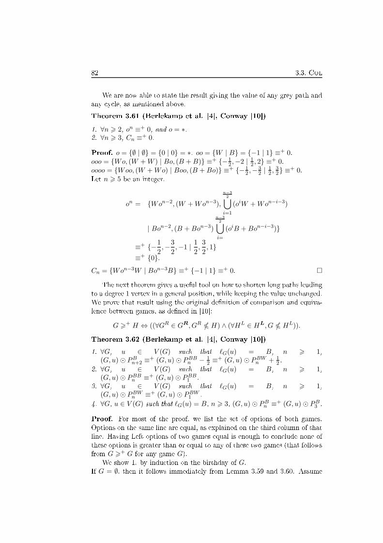
82 3.3. Col
We are now able to state the result giving the value of any grey path and
any y le, as mentioned above.
Theorem 3.61 (Berlekamp et al. [4℄, Conway [10℄)
1. ∀n > 2, on ≡+ 0, and o = ∗.2. ∀n > 3, Cn ≡+ 0.
Proof. o = {∅ | ∅} = {0 | 0} = ∗. oo = {W | B} = {−1 | 1} ≡+ 0.ooo = {Wo, (W +W ) | Bo, (B +B)} ≡+ {−1
2 ,−2 | 12 , 2} ≡+ 0.
oooo = {Woo, (W +Wo) | Boo, (B +Bo)} ≡+ {−12 ,−
32 | 1
2 ,32} ≡+ 0.
Let n > 5 be an integer.
on = {Won−2, (W +Won−3),
n−3
2⋃
i=1
(oiW +Won−i−3)
| Bon−2, (B +Bon−3)
n−3
2⋃
i=
(oiB +Bon−i−3)}
≡+ {−1
2,−
3
2,−1 |
1
2,3
2, 1}
≡+ {0}.
Cn = {Won−3W | Bon−3B} ≡+ {−1 | 1} ≡+ 0. �
The next theorem gives a useful tool on how to shorten long paths leading
to a degree 1 vertex in a general position, while keeping the value un hanged.
We prove that result using the original de�nition of omparison and equiva-
len e between games, as de�ned in [10℄:
G >+ H ⇔ ((∀GR ∈ GR, GR H) ∧ (∀HL ∈ HL, G HL)).
Theorem 3.62 (Berlekamp et al. [4℄, Conway [10℄)
1. ∀G, u ∈ V (G) su h that ℓG(u) = B, n > 1,(G,u) ⊙ PB
n+2 ≡+ (G,u) ⊙ PBB
n − 12 ≡+ (G,u) ⊙ PBW
n + 12 .
2. ∀G, u ∈ V (G) su h that ℓG(u) = B, n > 1,(G,u) ⊙ PBB
n ≡+ (G,u)⊙ PBB1 .
3. ∀G, u ∈ V (G) su h that ℓG(u) = B, n > 1,(G,u) ⊙ PBW
n ≡+ (G,u) ⊙ PBW1 .
4. ∀G, u ∈ V (G) su h that ℓG(u) = B, n > 3, (G,u) ⊙ PBn ≡+ (G,u) ⊙ PB
3 .
Proof. For most of the proof, we list the set of options of both games.
Options on the same line are equal, as explained on the third olumn of that
line. Having Left options of two games equal is enough to on lude none of
these options is greater than or equal to any of these two games (that follows
from G >+ G for any game G).We show 1. by indu tion on the birthday of G.
If G = ∅, then it follows immediately from Lemma 3.59 and 3.60. Assume
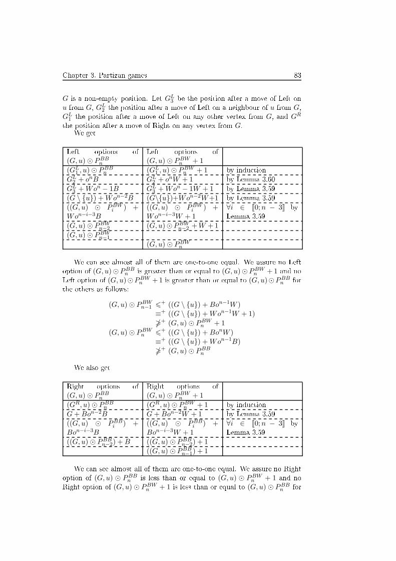
Chapter 3. Partizan games 83
G is a non-empty position. Let GL3 be the position after a move of Left on
u from G, GL2 the position after a move of Left on a neighbour of u from G,
GL1 the position after a move of Left on any other vertex from G, and GR
the position after a move of Right on any vertex from G.We get
Left options of
(G,u) ⊙ PBBn
Left options of
(G,u) ⊙ PBWn + 1
(GL1 , u)⊙ PBB
n (GL1 , u)⊙ PBW
n + 1 by indu tion
GL2 + onB GL
2 + onW + 1 by Lemma 3.60
GL3 +Won − 1B GL
3 +Won − 1W + 1 by Lemma 3.59
(G \ {u}) +Won−2B (G\{u})+Won−2W+1 by Lemma 3.59
((G,u) ⊙ PBWi ) +
Won−i−3B((G,u) ⊙ PBW
i ) +Won−i−3W + 1
∀i ∈ J0;n − 3K by
Lemma 3.59
(G,u) ⊙ PBWn−2 (G,u)⊙PBW
n−2 +W +1
(G,u) ⊙ PBWn−1
(G,u) ⊙ PBWn
We an see almost all of them are one-to-one equal. We assure no Left
option of (G,u)⊙PBBn is greater than or equal to (G,u)⊙PBW
n +1 and no
Left option of (G,u)⊙PBWn +1 is greater than or equal to (G,u)⊙PBB
n for
the others as follows:
(G,u) ⊙ PBWn−1 6+ ((G \ {u}) +Bon−1W )
≡+ ((G \ {u}) +Won−1W + 1)
�+ (G,u) ⊙ PBWn + 1
(G,u) ⊙ PBWn 6
+ ((G \ {u}) +BonW )
≡+ ((G \ {u}) +Won−1B)
�+ (G,u) ⊙ PBBn
We also get
Right options of
(G,u) ⊙ PBBn
Right options of
(G,u) ⊙ PBWn + 1
(GR, u)⊙ PBBn (GR, u)⊙ PBW
n + 1 by indu tion
G+Bon−2B G+Bon−2W + 1 by Lemma 3.59
((G,u) ⊙ PBBi ) +
Bon−i−3B((G,u) ⊙ PBB
i ) +Bon−i−3W + 1
∀i ∈ J0;n − 3K by
Lemma 3.59
((G,u) ⊙ PBBn−2) +B ((G,u) ⊙ PBB
n−2) + 1
((G,u) ⊙ PBBn−1) + 1
We an see almost all of them are one-to-one equal. We assure no Right
option of (G,u) ⊙ PBBn is less than or equal to (G,u) ⊙ PBW
n + 1 and no
Right option of (G,u) ⊙ PBWn + 1 is less than or equal to (G,u) ⊙ PBB
n for
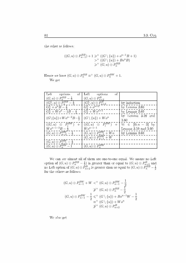
84 3.3. Col
the other as follows:
((G,u) ⊙ PBBn−1) + 1 >+ ((G \ {u}) + on−1B + 1)
>+ ((G \ {u}) +BonB)
>+ (G,u) ⊙ PBBn
Hen e we have (G,u) ⊙ PBBn ≡+ (G,u) ⊙ PBW
n + 1.
We get
Left options of
(G,u) ⊙ PBBn − 1
2
Left options of
(G,u) ⊙ PBn+2
(GL1 , u)⊙ PBB
n − 12 (GL
1 , u)⊙ PBn+2 by indu tion
GL2 + onB − 1
2 GL2 + on+2
by Lemma 3.60
GL3 +Won − 1B − 1
2 GL3 +Won+1
by Lemma 3.60
(G\{u})+Won−2B− 12 (G \ {u}) +Won
by Lemma 3.59 and
3.60
((G,u) ⊙ PBWi ) +
Won−i−3B − 12
((G,u) ⊙ PBWi ) +
Won−i−1∀i ∈ J0;n − 3K by
Lemma 3.59 and 3.60
(G,u) ⊙ PBWn−2 − 1
2 (G,u) ⊙ PBWn−2 +Wo by Lemma 3.60
(G,u) ⊙ PBWn−1 +W
(G,u) ⊙ PBWn−1 − 1
2
(G,u) ⊙ PBBn − 1 (G,u) ⊙ PBW
n
We an see almost all of them are one-to-one equal. We assure no Left
option of (G,u) ⊙ PBBn − 1
2 ) is greater than or equal to (G,u) ⊙ PBn+2 and
no Left option of (G,u)⊙PBn+2 is greater than or equal to (G,u)⊙PBB
n − 12
for the others as follows:
(G,u) ⊙ PBWn−1 +W <+ (G,u) ⊙ PBW
n−1 −1
2
�+ (G,u) ⊙ PBBn −
1
2
(G,u) ⊙ PBWn−1 −
1
26+ (G \ {u}) +Bon−1W −
1
2≡+ (G \ {u}) +Won
�+ (G,u) ⊙ PBn+2
We also get

Chapter 3. Partizan games 85
Right options of
(G,u) ⊙ PBBn − 1
2
Right options of
(G,u) ⊙ PBn+2
(GR, u)⊙ PBBn − 1
2 (GR, u)⊙ PBn+2 by indu tion
G+Bon−2B − 12 G+Bon
by Lemma 3.59 and
3.60
((G,u) ⊙ PBBi ) +
Bon−i−3B − 12
((G,u) ⊙ PBBi ) +
Bon−i−1∀i ∈ J0;n − 3K by
Lemma 3.59 and 3.60
((G,u)⊙PBBn−2)+B− 1
2 ((G,u) ⊙ PBBn−2) +Bo
by Lemma 3.59 and
3.60
((G,u) ⊙ PBBn−1) +B
(G,u) ⊙ PBBn + 0 (G,u) ⊙ PBB
n
We an see almost all of them are one-to-one equal. We assure no Right
option of (G,u) ⊙ PBBn − 1
2 is less than or equal to (G,u) ⊙ PBn+2 and no
Right option of (G,u) ⊙ PBn+2 is less than or equal to (G,u) ⊙ PBB
n − 12 for
the other as follows:
((G,u) ⊙ PBBn−1) +B >
+ (G \ {u}) + on−1B +B
>+ (G \ {u}) +BonB −1
2
>+ (G,u)⊙ PBB
n −1
2
Hen e we have (G,u) ⊙ PBBn ≡+ (G,u) ⊙ PB
n+2.
We show 2. by indu tion on the birthday of G and on n.If G = ∅, then it follows immediately from Lemma 3.59. If n = 1, there is
nothing to show.
Assume G is a non-empty graph and n > 2. Let GL3 be the graph after a
move of Left on u from G, GL2 the graph after a move of Left on a neighbour
of u from G, GL1 the graph after a move of Left on any other vertex from G,
and GRthe graph after a move of Right on any vertex from G.
We get
Left options of
(G,u) ⊙ PBBn
Left options of
(G,u) ⊙ PB1
(GL1 , u)⊙ PBB
n (GL1 , u)⊙ PBB
1 by indu tion
GL2 + onB GL
2 + oB by Lemma 3.60
GL3 +Won − 1B GL
3 +WB by Lemma 3.59
(G \ {u}) +Won−2B (G \ {u}) by Lemma 3.60
((G,u) ⊙ PBW0 ) +
Won−3B((G,u) ⊙ PBW
0 ) by Lemma 3.59
((G,u) ⊙ PBWi ) +
Won−i−3B∀i ∈ J0;n− 3K
(G,u) ⊙ PBWn−2
(G,u) ⊙ PBWn−1
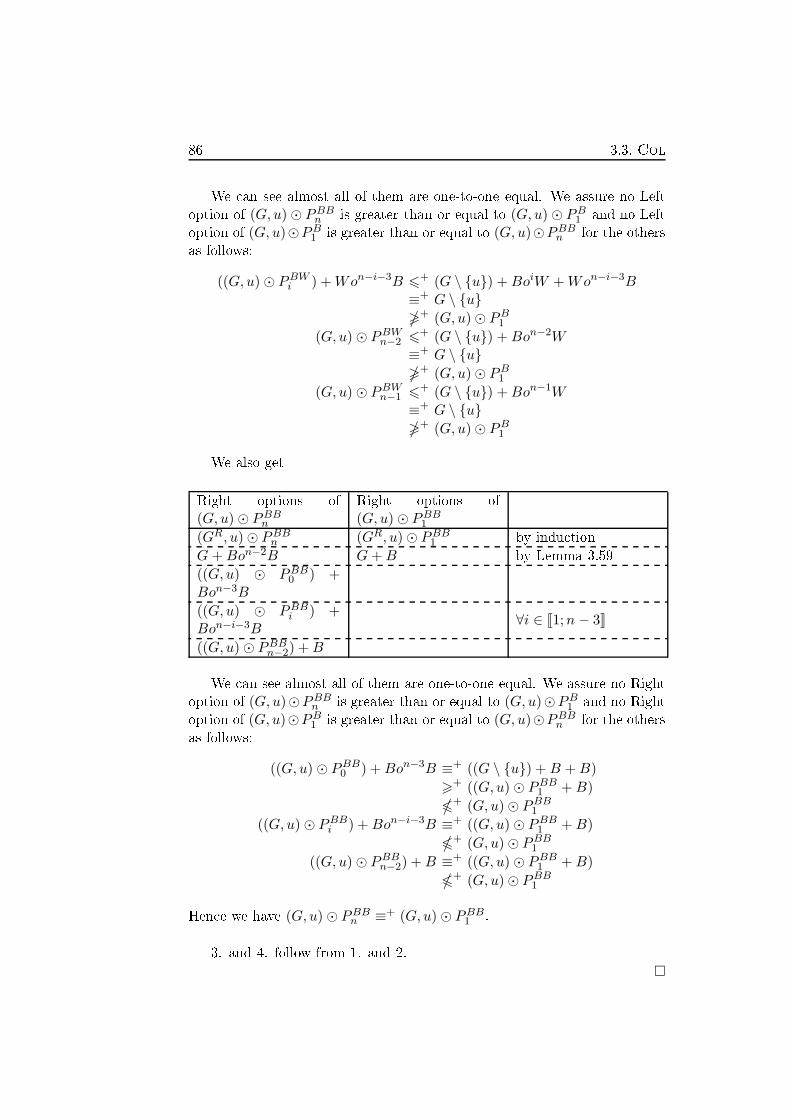
86 3.3. Col
We an see almost all of them are one-to-one equal. We assure no Left
option of (G,u) ⊙ PBBn is greater than or equal to (G,u) ⊙ PB
1 and no Left
option of (G,u)⊙PB1 is greater than or equal to (G,u)⊙PBB
n for the others
as follows:
((G,u) ⊙ PBWi ) +Won−i−3B 6
+ (G \ {u}) +BoiW +Won−i−3B≡+ G \ {u}�+ (G,u)⊙ PB
1
(G,u) ⊙ PBWn−2 6+ (G \ {u}) +Bon−2W
≡+ G \ {u}
�+ (G,u)⊙ PB1
(G,u) ⊙ PBWn−1 6
+ (G \ {u}) +Bon−1W≡+ G \ {u}�+ (G,u)⊙ PB
1
We also get
Right options of
(G,u) ⊙ PBBn
Right options of
(G,u) ⊙ PBB1
(GR, u)⊙ PBBn (GR, u)⊙ PBB
1 by indu tion
G+Bon−2B G+B by Lemma 3.59
((G,u) ⊙ PBB0 ) +
Bon−3B
((G,u) ⊙ PBBi ) +
Bon−i−3B∀i ∈ J1;n − 3K
((G,u) ⊙ PBBn−2) +B
We an see almost all of them are one-to-one equal. We assure no Right
option of (G,u)⊙PBBn is greater than or equal to (G,u)⊙PB
1 and no Right
option of (G,u)⊙PB1 is greater than or equal to (G,u)⊙PBB
n for the others
as follows:
((G,u) ⊙ PBB0 ) +Bon−3B ≡+ ((G \ {u}) +B +B)
>+ ((G,u) ⊙ PBB
1 +B)
+ (G,u)⊙ PBB1
((G,u) ⊙ PBBi ) +Bon−i−3B ≡+ ((G,u) ⊙ PBB
1 +B)
+ (G,u)⊙ PBB1
((G,u) ⊙ PBBn−2) +B ≡+ ((G,u) ⊙ PBB
1 +B)
+ (G,u)⊙ PBB1
Hen e we have (G,u) ⊙ PBBn ≡+ (G,u) ⊙ PBB
1 .
3. and 4. follow from 1. and 2.
�

Chapter 3. Partizan games 87
We now get ba k to smaller sets of positions, leading to an algorithm to
�nd the out ome of any grey tree with at most one vertex having degree at
least 3, that is Theorem 3.77.
We start with two simple positions for whi h we give the value.
Lemma 3.63 (Berlekamp et al. [4℄, Conway [10℄)
1. oBo ≡+ 0.2. ooBoo ≡+ 0.
Proof. oBo = {o, (W +W ) | Bo} = {∗,−1 + (−1)12} ≡+ 0.
ooBoo = {WBoo, (W + oo), (oW +Wo) | BBoo, (B +Boo)}
≡+ {−1
2,−1 + 0,−
1
2−
1
2| 1, 1 +
1
2}
≡+ 0
�
These two positions are now andidates for applying Theorem 3.57: on-
sidering the middle vertex as u, we now have ooo+u = 0 = −ooo+u = ooo−uand ooooo+u = 0 = −ooooo+u = ooooo−u .
A similar result on arbitrarily long path would help too, and that is
Lemma 3.66. To get there, we �nd the values of any maximal onne ted
subpositions of positions we an rea h from the original positions, whi h are
given in the two following lemmas, following the same pattern as for Lemmas
3.59, 3.60 and Theorem 3.61.
First, we see the values of paths whose leaves are reserved, having exa tly
one extra reserved vertex. If that extra reserved vertex was adja ent to a leaf
reserved for the same player, we ould use Corollary 3.58 and then on lude
with Lemma 3.60, to get a value whi h is a tually di�erent from the general
pattern. Hen e, we only onsider the other ases.
Lemma 3.64
1. ∀n > 1,m > 1, BonBomB ≡+ 1.2. ∀n > 0,m > 0, WonBomW ≡+ −1.3. ∀n > 0,m > 1, WonBomB ≡+ 0.
Proof.
1.
BoBoB = {WBoB, oB, (BW +WB) | (B +BoB)}
≡+ {0,1
2, (0 + 0) | (1 + 1)}
≡+ 1When n > 2 or m > 2, it follows from Theorem 3.62.
2.
WBW = (W +B +W ) = −1 + 1 + (−1) ≡+ −1.WBoW = (W +BoW ) ≡+ −1 + 0 = −1.WoBoW = {(W + oW ), (WW +WW ) | BBoW,BoW}
≡+ {−1−1
2,−1 + (−1) |
1
2, 0}
≡+ −1

88 3.3. Col
When n > 2 or m > 2, it follows from Theorem 3.62.
3.
WBoB = (W +BoB) ≡+ −1 + 1 ≡+ 0.WoBoB = {(W + oB), (WW +WB),Wo,WoBW
| BBoB,BoB, (WoB +B)}
≡+ {−1 +1
2,−1 + 0,−
1
2,−1 |
3
2, 1, 0 + 1}
≡+ 0When n > 2 or m > 2, it follows from Theorem 3.62. �
We now see the values of paths where exa tly one leaf is reserved, as
well as exa tly one extra vertex. Again, if that extra reserved vertex was
adja ent to a leaf reserved for the same player, we ould use Corollary 3.58
and on lude with Lemma 3.60, to get a value whi h is a tually di�erent
from the general pattern. Hen e, we again only onsider other ases.
Lemma 3.65
1. ∀n > 1,m > 3, BonBom = 12 .
2. ∀n > 0,m > 3, WonBom = −12 .
Proof. BonBom = (BonBoW +Bo) ≡+ 0 + 12 = 1
2 .
WonBom = (WonBoW +Bo) ≡+ −1 + 12 ≡+ −1
2 . �
Finally, we get the pattern on arbitrary long paths, where reserving ex-
a tly one vertex for a player does not give them an advantage, provided there
are at least three verti es on ea h side of this vertex.
Lemma 3.66 (Berlekamp et al. [4℄, Conway [10℄)
∀n > 3,m > 3, onBom ≡+ 0.
Proof.
onBom ≡+ (onBoW+Bo) ≡+ (WoBoW+Bo+Bo) ≡+ −1+ 12+
12 ≡+ 0
by Theorem 3.62. �
We now �nd the out ome of the set of positions we annot solve using
only Lemmas 3.63 and 3.66 before applying Theorem 3.57, that are stated
in Theorem 3.75: positions of the form onxoo with n at least 3. As before,we analyse the values of all maximal onne ted subpositions that players an
rea h from the initial position, whi h we are able to sum, but as there are
more kinds of these positions, we need more intermediate lemmas.
First, we look at positions where a player would have played on the non-
spe ial vertex of x, and a player, not ne essarily the other player, would have
played on the farther leaf from the spe ial vertex of x.
Lemma 3.67
1. ∀n > 0, BonBoo ≡+ 1.

Chapter 3. Partizan games 89
2. ∀n > 1, WonBoo ≡+ 0.
Proof. BBoo ≡+ B + oo ≡+ 1.BoBoo = {WBoo, oo, (B +Wo), (Bo+W ), BoBW
| (B +Boo), (BoB +B), BoBB}
≡+ {−1
2, 1 −
1
2,1
2+ (−1), 0 | 1 +
1
2, 1 + 1,
3
2}
≡+ 1
WoBoo = {(W + oo), (WW +Wo), (Wo+W ),WoBW| BBoo,Boo, (WoB +B),WoBB}
≡+ {−1 + 0,−1−1
2,−
1
2+ (−1),−1 | 1,
1
2, 0 + 1,
1
2}
≡+ 0When n > 2, it follows from Theorem 3.62. �
We now �nd the value of a game where a player would have played on
the non-spe ial vertex of x, using the result we just got from Lemma 3.67.
Lemma 3.68 ∀n > 3, onBoo ≡+ 12 .
Proof. onBoo ≡+ (WoBoo+Bo) ≡+ 0 + 12 = 1
2 by Theorem 3.62. �
We now onsider paths where exa tly two verti es are reserved, one being
a leaf and the other being the neighbour of the other leaf. If those two
verti es were neighbours, we ould either use Corollary 3.58 and on lude
with Theorem 3.61 or use Corollary 3.54 and on lude with Lemma 3.60,
both giving values di�erent from the general pattern. Hen e, again, we only
onsider other ases.
Lemma 3.69
1. ∀n > 1, BonBo ≡+ 34 .
2. ∀n > 1, WonBo ≡+ −14 .
Proof.
BoBo = {WBo, o, (BW +W ), Bo | (B +Bo), BoB}
≡+ {−1
2, ∗, 0 + (−1),
1
2| 1 +
1
2, 1}
≡+ 3
4WoBo = {(W + o), (WW +W ),Wo | BBo,Bo,WoB}
≡+ {−1 + ∗,−1 + (−1),−1
2| 1∗,
1
2, 0}
≡+ −1
4When n > 2, it follows from Theorem 3.62. �
We now use Lemma 3.69 to �nd the value of a path where exa tly one
vertex is reserved, provided one of its neighbours is a leaf and there are at
least two verti es in the other dire tion, the ases where there is one or none
having been solved earlier and yielding di�erent values.

90 3.3. Col
Lemma 3.70 ∀n > 2, oBon ≡+ 14 .
Proof.
oBoo = {oo, (W +Wo), (o+W ), oBW | Boo, (oB +B), oBB}
≡+ {0,−1 −1
2, ∗+ (−1),−
1
2|1
2,1
2+ 1, 1∗}
≡+ 1
4Let n > 3 be an integer.
oBon ≡+ (oBoW +Bo) ≡+ −14 +
12 ≡+ 1
4 by Theorem 3.62. �
The next lemma gives the value of two small positions: BxB and BxW ,
as they do not follow the rule we state in Lemma 3.72.
Lemma 3.71
1. BxB ≡+ 32 .
2. BxW ≡+ ∗.
Proof.
BxB = {oWB,W,BWB | (B +B +B), BBB}
≡+ {−1,1
2, 1 | 2, 3}
≡+ 3
2
BxW = {oWW, (W +W ), BWW | oBB, (B +B), BBW}≡+ {−2,−1∗, 0 | 0, 1∗, 2}≡+ ∗
�
We an use these results to �nd the value of the game after the players
have played from onxoo on the two leaves not in the x, where n is at least 3.
Lemma 3.72
1. ∀n > 1, BonxB ≡+ 54 .
2. ∀n > 1, BonxW ≡+ −14 .
Proof. We show the results simultaneously by indu tion on n.
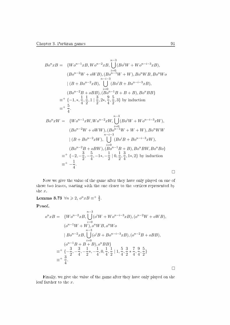
Chapter 3. Partizan games 91
BonxB = {Won−1xB,Won−2xB,
n−3⋃
i=0
(BoiW +Won−i−3xB),
(Bon−2W + oWB), (Bon−1W +W ), BonWB,BonWo
| (B +Bon−2xB),
n−i−3⋃
i=0
(BoiB +Bon−i−3xB),
(Bon−2B + oBB), (Bon−1B +B +B), BonBB}
≡+ {−1, ∗,1
4,1
2, 1 |
3
2, 2∗,
9
4,5
2, 3} by induction
≡+ 5
4.
BonxW = {Won−1xW,Won−2xW,n−3⋃
i=0
(BoiW +Won−i−3xW ),
(Bon−2W + oWW ), (Bon−1W +W +W ), BonWW
| (B +Bon−2xW ),n−i−3⋃
i=0
(BoiB +Bon−i−3xW ),
(Bon−2B + oBW ), (Bon−1B +B), BonBW,BonBo}
≡+ {−2,−3
2,−
5
4,−1∗,−
1
2| 0,
1
2,3
4, 1∗, 2} by induction
≡+ −1
4.
�
Now we give the value of the game after they have only played on one of
these two leaves, starting with the one loser to the verti es represented by
the x.
Lemma 3.73 ∀n > 2, onxB ≡+ 34 .
Proof.
onxB = {Won−2xB,
n−3⋃
i=0
(oiW +Won−i−3xB), (on−2W + oWB),
(on−1W +W ), onWB, onWo
| Bon−2xB,
n−3⋃
i=0
(oiB +Bon−i−3xB), (on−2B + oBB),
(on−1B +B +B), onBB}
≡+ {−3
2,−
3
4,−
1
2∗,−
1
4, 0,
1
4,1
2| 1,
5
4,3
2∗7
4,9
4,5
2}
≡+ 3
4.
�
Finally, we give the value of the game after they have only played on the
leaf farther to the x.
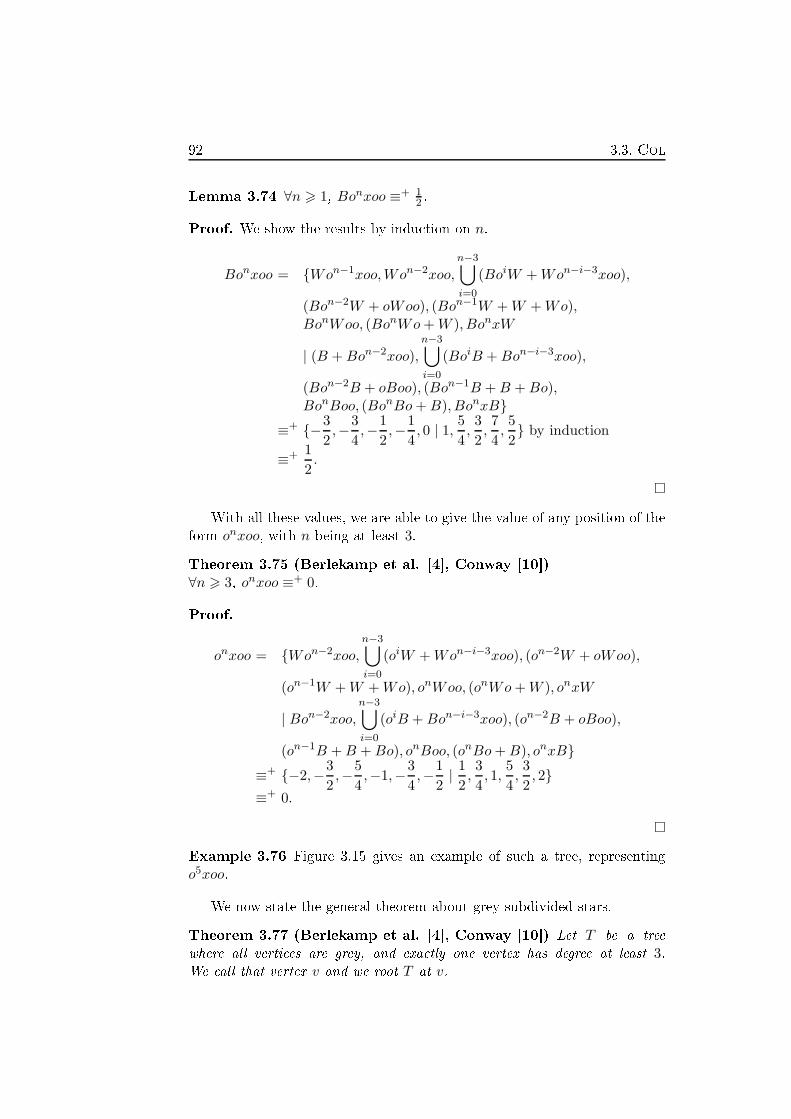
92 3.3. Col
Lemma 3.74 ∀n > 1, Bonxoo ≡+ 12 .
Proof. We show the results by indu tion on n.
Bonxoo = {Won−1xoo,Won−2xoo,
n−3⋃
i=0
(BoiW +Won−i−3xoo),
(Bon−2W + oWoo), (Bon−1W +W +Wo),BonWoo, (BonWo+W ), BonxW
| (B +Bon−2xoo),
n−3⋃
i=0
(BoiB +Bon−i−3xoo),
(Bon−2B + oBoo), (Bon−1B +B +Bo),BonBoo, (BonBo+B), BonxB}
≡+ {−3
2,−
3
4,−
1
2,−
1
4, 0 | 1,
5
4,3
2,7
4,5
2} by induction
≡+ 1
2.
�
With all these values, we are able to give the value of any position of the
form onxoo, with n being at least 3.
Theorem 3.75 (Berlekamp et al. [4℄, Conway [10℄)
∀n > 3, onxoo ≡+ 0.
Proof.
onxoo = {Won−2xoo,n−3⋃
i=0
(oiW +Won−i−3xoo), (on−2W + oWoo),
(on−1W +W +Wo), onWoo, (onWo+W ), onxW
| Bon−2xoo,n−3⋃
i=0
(oiB +Bon−i−3xoo), (on−2B + oBoo),
(on−1B +B +Bo), onBoo, (onBo+B), onxB}
≡+ {−2,−3
2,−
5
4,−1,−
3
4,−
1
2|1
2,3
4, 1,
5
4,3
2, 2}
≡+ 0.
�
Example 3.76 Figure 3.15 gives an example of su h a tree, representing
o5xoo.
We now state the general theorem about grey subdivided stars.
Theorem 3.77 (Berlekamp et al. [4℄, Conway [10℄) Let T be a tree
where all verti es are grey, and exa tly one vertex has degree at least 3.We all that vertex v and we root T at v.

Chapter 3. Partizan games 93
Figure 3.15: A subdivided star where removing the enter hanges the value
(i) If there are exa tly three leaves, one at depth 1, another at depth 2 and
the last at depth at least 3, or there are an odd number of leaves at
depth 1, then the game has value 0.
(ii) Otherwise, the game has value ∗.
Proof. The �rst ase stated, with three leaves, orresponds exa tly to posi-
tions of the form onxoo, that we proved have value 0 in Theorem 3.75. On
any other ase, we an use either Lemma 3.63 or 3.66 together with Theo-
rem 3.57 to remove the vertex v from the graph without hanging the value
of the position. As we only leave a disjun tive sum of paths, whi h all have
value 0 apart from isolated verti es, all we need to know is the parity of
the number of these isolated verti es to get the value of the position. These
isolated verti es were exa tly the leaves at depth 1, so if they are in odd
number, the value is ∗, and otherwise it is 0. �
Example 3.78 Figures 3.16 and 3.17 give examples of subdivided stars
where the entral vertex an be removed without hanging the value: one
an apply Theorem 3.57 together with Lemma 3.63 or 3.66 in both ases,
on paths ending on leaves of the same depth status, that is the number in-
di ated next to it. In Figure 3.16, the number of leaves at distan e 1 from
the entral vertex, that be ome isolated verti es after the entral vertex is
removed, is odd, so the position has value ∗. In Figure 3.17, that number is
even, so the position has value 0. There are 9 paths on Figure 3.16 and 8 on
Figure 3.17 where we an apply Theorem 3.57 to remove the entral vertex.
3.3.3 Caterpillars
We now work on �nding the out ome of grey aterpillars. Re all that a
aterpillar is a tree su h that the set of verti es of degree at least 2 forms a
path. Re all that sin e all verti es are grey, the position is its own opposite,
and has value 0 or ∗. We here fo us on aterpillars of the form xn.
First, when n is even, the position is symmetri , so it ful�ls the onditions
of Theorem 3.51.
Theorem 3.79 ∀n > 0, x2n ≡+ 0.

94 3.3. Col
3+
3+
3+ 1
3+ 1 1 2
Figure 3.16: A subdivided star with
value ∗
3+ 3+
3+
3+
1 2
1 2
Figure 3.17: A subdivided star with
value 0
When n is odd, any of the two involutions on the verti es keeping edges
between the images of adja ent verti es would have at least two �xed points:
the two entral verti es. This is why we need intermediate lemmas. Consid-
ering all maximal onne ted subpositions that players an rea h from su h a
aterpillar seems tedious as they do not seem to simplify as easily as before,
so we use a di�erent approa h: we �nd good enough answer for one player
and state the other player annot do better than some value to ensure some
bounds on the values of some positions leading to the value of the very �rst
game.
First, we �nd su h values and bounds on a few sets of positions, all stated
in a single lemma as the proofs are intertwined.
Lemma 3.80
1. ∀n > 1, x2nB ≡+ 34 and x2n−1B ≡+ 1
2 .
2. ∀n > 0, Bx2nB ≡+ 1 and Bx2n+1B ≡+ 32 .
3. ∀n > 0, Bx2nW ≡+ 0 and Bx2n+1W ≡+ ∗.
4. ∀n > 0,m > 0, x2nBx2mB >+ 1, x2n+1Bx2m+1B >+ 1,x2n+1Bx2mB >+ 3
4 and x2nBx2m+1B >+ 34 .
5. ∀n > 0,m > 0, x2nBx2mW >+ −14 , x
2n+1Bx2m+1W >+ −14 ,
x2n+1Bx2mW >+ −12 and x2nBx2m+1W >+ −1
2 .
6. ∀n > 0,m > 0, Bx2nBx2mB >+ 32 , Bx2n+1Bx2m+1B >+ 3
2 ,
Bx2n+1Bx2mB >+ 32 and Bx2nBx2m+1B >+ 3
2 .
7. ∀n > 0,m > 0, Bx2nBx2mW >+ 0, Bx2n+1Bx2m+1W >+ 0,Bx2n+1Bx2mW >+ 1
2 and Bx2nBx2m+1W >+ 12 .
The proof of this lemma an be found in Appendix B.3. The idea is to
list possible moves. Then, we use Theorems 3.53 and 3.55 and indu tion to
give a bound to the value of the position or to the value of a possible answer.

Chapter 3. Partizan games 95
We now show that the answer we propose for Left after some move of
Right is winning.
Lemma 3.81 ∀n > 0,m > 0, x2n+1Bx2m+1Wx >+ 0.
Proof. We prove Left has a winning strategy in x2n+1Bx2m+1Wx if Right
starts. Consider his possible moves from x2n+1Bx2m+1Wx. He an move to:
• B+oBx2n−1Bx2m+1Wx, having value at least B+x2nBx2m+1W +x,whi h has value at least
12 .
• xiBo+B + oBx2n−i−2Bx2m+1Wx, having value at least
12 or
12∗.
• x2n−1Bo+B +Bx2m+1Wx, having value at least 1 or 1∗.• x2n+1B +B + oBx2m−1Wx, having value at least
34 .
• x2n+1BxiBo+B + oBx2m−i−2Wx, having value at least
14 or
14∗.
• x2n+1Bx2m−1Bo+B + x, having value at least 1 or 1∗.• x2n+1Bx2mBo+Bo, having value at least
12 or
12∗.
• x2n+1Bx2m+1 +B, having value at least 1 or 1∗.• xiBx2n−iBx2m+1Wx. Then Left an answer to xiBx2n−iBWx2mWx,
whi h has value at least 0.• x2n+1BBx2mWx, having value at least x2n+1 + Bx2m + Wx, whi h
has value at least
14 or
14∗.
• x2n+1BxiBx2m−iWx. Then left an answer to
x2n+1BxiBWx2m−i−1Wx, whi h has value at least 0 when i is
odd, or to x2n+1Bxi−1WBx2m−iWx, whi h has value at least 0 when
i is even.• x2n+1Bx2mBWx, having value more than
34 .
• x2n+1Bx2m+1WB, having value at least
14 .
�
We now state the theorem, that almost all aterpillars of the form xn
have value 0.
Theorem 3.82 ∀n 6= 3, xn ≡+ 0, and xxx ≡+ ∗.
Proof. When n is even, it is true by Theorem 3.79. When n 6 3, it is trueby Theorem 3.77. Now assume n > 5 is odd. We prove the se ond player has
a winning strategy in xn. Without loss of generality, we may assume Right
starts the game and onsider his possible moves from xn. He an move to:
• B + oBxn−2, having value at least 1.
• xiBo+B + oBxn−i−3, having value at least 1 or 1∗.
• x2iBxn−2i−1. Without loss of generality, we may assume 2i > n−1
2 > 2.Then Left an answer to x2i−1WBxn−2i−1
, whi h has value
14 .
• x2i+1Bxn−2i−2. Without loss of generality, we may assume
2i+ 1 > n−12 > 2 . Then Left an answer to xWx2i−1Bxn−2i−2
, whi h
has value at least 0.
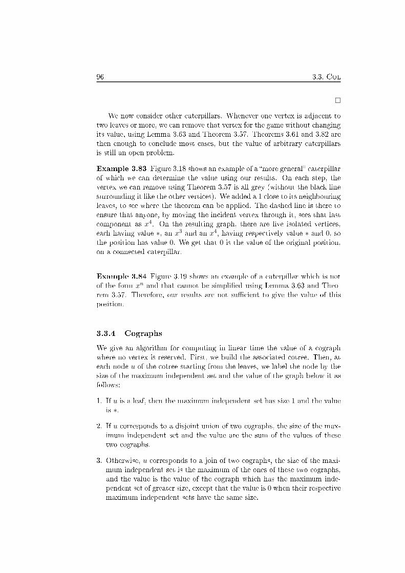
96 3.3. Col
�
We now onsider other aterpillars. Whenever one vertex is adja ent to
two leaves or more, we an remove that vertex for the game without hanging
its value, using Lemma 3.63 and Theorem 3.57. Theorems 3.61 and 3.82 are
then enough to on lude most ases, but the value of arbitrary aterpillars
is still an open problem.
Example 3.83 Figure 3.18 shows an example of a �more general� aterpillar
of whi h we an determine the value using our results. On ea h step, the
vertex we an remove using Theorem 3.57 is all grey (without the bla k line
surrounding it like the other verti es). We added a 1 lose to its neighbouringleaves, to see where the theorem an be applied. The dashed line is there to
ensure that anyone, by moving the in ident vertex through it, sees that last
omponent as x4. On the resulting graph, there are �ve isolated verti es,
ea h having value ∗, an x3 and an x4, having respe tively value ∗ and 0, sothe position has value 0. We get that 0 is the value of the original position,
on a onne ted aterpillar.
Example 3.84 Figure 3.19 shows an example of a aterpillar whi h is not
of the form xn and that annot be simpli�ed using Lemma 3.63 and Theo-
rem 3.57. Therefore, our results are not su� ient to give the value of this
position.
3.3.4 Cographs
We give an algorithm for omputing in linear time the value of a ograph
where no vertex is reserved. First, we build the asso iated otree. Then, at
ea h node u of the otree starting from the leaves, we label the node by the
size of the maximum independent set and the value of the graph below it as
follows:
1. If u is a leaf, then the maximum independent set has size 1 and the value
is ∗.
2. If u orresponds to a disjoint union of two ographs, the size of the max-
imum independent set and the value are the sum of the values of these
two ographs.
3. Otherwise, u orresponds to a join of two ographs, the size of the maxi-
mum independent set is the maximum of the ones of these two ographs,
and the value is the value of the ograph whi h has the maximum inde-
pendent set of greater size, ex ept that the value is 0 when their respe tive
maximum independent sets have the same size.

Chapter 3. Partizan games 97
1
1 1
1
1
Figure 3.18: Finding the value of a aterpillar by removing verti es a ording to
Lemma 3.63 and Theorem 3.57
Figure 3.19: A aterpillar where our results annot on lude alone

98 3.4. Perspe tives
Proof. We only need to ensure by indu tion that if the value of the graph is
∗, any player who starts the game has a winning strategy su h that their �rst
move is on a vertex ontained in a maximum independent set. When the
graph is a single vertex the result is true. When the graph is a disjoint union
of two ographs, the �rst player has a winning move only if one omponent
has value ∗ and the other omponent has value 0. A winning move is to move
the omponent of value ∗ to value 0, and there exists su h a move on a vertex
ontained in a maximum independent set of that omponent by indu tion.
That vertex is also ontained in a maximum independent set of the whole
graph, so the result is true. When the graph is a join of two ographs, the
�rst player has a winning move only if the omponent having the maximum
independent set of greater size has value ∗. A winning move is to move that
omponent of value ∗ to value 0, and there exists su h a move on a vertex
ontained in a maximum independent set of that omponent by indu tion.
That vertex is also ontained in a maximum independent set of the whole
graph, so the result is true. �
Example 3.85 Figures 3.20 and 3.21 illustrate the algorithm. Figure 3.20
is a ograph with all verti es grey. Figure 3.21 is the asso iated otree:
the leaves orrespond to the verti es of the ograph; the D internal nodes
indi ate when two ographs are gathered into one through disjoint union; the
J internal nodes indi ate when two ographs are gathered into one through
join. Next to ea h node, there is a ouple indi ating the value and the size of
a maximum independent set of the subgraph indu ed by the verti es below
that node.
3.4 Perspe tives
In this hapter, we onsidered the games Timbush, Toppling Dominoes
and Col.
In the ase of Timbush, we gave an algorithm to �nd the out ome of any
orientation of paths with oloured ar s and an algorithm to �nd the out ome
of any dire ted graph with ar s oloured bla k or white.
Note that if the onne ted dire ted graph we onsider ontains a 2-edge- onne ted omponent, any ar of that omponent is a winning move, but if
all these ar s are bla k, or they are all white, we do not know if the other
player have a winning move.
Hen e we ask the following questions.
Question 3.86 Can one �nd a polynomial-time algorithm whi h gives the
out ome of any Timbush position on dire ted graphs with oloured ar s?
Another di�eren e in result with Timber is that we do not give the value
of any orientation of paths. That problem is already non-trivial if we only
look at orientation of paths with ar s oloured bla k or white.
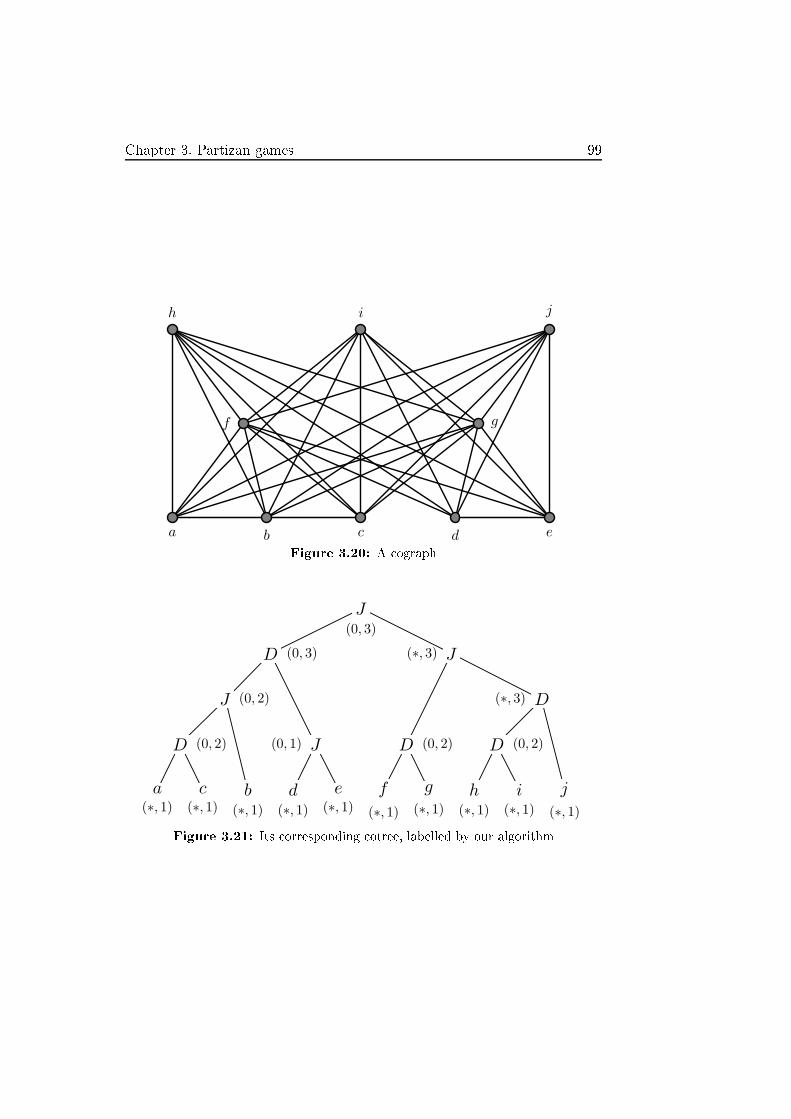
Chapter 3. Partizan games 99
a b c d e
f g
h i j
Figure 3.20: A ograph
a(∗, 1)
c(∗, 1)
b(∗, 1)
d(∗, 1)
e(∗, 1)
f
(∗, 1)
g(∗, 1)
h(∗, 1)
i(∗, 1)
j
(∗, 1)
D (0, 2)
J (0, 2)
D (0, 3)
J(0, 1)
J(0, 3)
D (0, 2)
J(∗, 3)
D (0, 2)
D(∗, 3)
Figure 3.21: Its orresponding otree, labelled by our algorithm

100 3.4. Perspe tives
Question 3.87 Is there a polynomial-time algorithm for �nding the value of
any Timbush position on dire ted paths with ar s oloured bla k or white?
In the ase of Toppling Dominoes, we proved that for any value of
the form {a|b} with a > b, {a||b|c} with a > b > c, and {a|b||c|d} with
a > b > c > d, there exists a Toppling Dominoes position on a single row
that have this value. We even found all representatives of positions of the
form {a|b}, whi h leads us to the following onje tures.
Conje ture 3.88 Let a > b > c be numbers and G a Toppling Dominoes
position with value {a|{b|c}}. Then G is aLRbRLc, aEbRLc or one of theirreversal. Furthermore, if a = b, then G is aLRbRLc or its reversal.
Conje ture 3.89 Let a > b > c > d be numbers and G a Toppling
Dominoes position with value {{a|b}|{c|d}}. Then G is bRLaLRdRLc,bRLaEdRLc or one of their reversal.
In the ase of Col, we restated some known results and went further in
�nding the values of most grey aterpillars and all grey ographs. Neverthe-
less, the problem on general trees is still open.
Question 3.90 What is the omplexity of �nding the out ome of any Col
position on a tree?

Chapter 4. Misère games 101
Chapter 4
Misère games
The misère version of a game is a game with the same game tree where the
vi tory ondition is reversed, that is the �rst player unable to move when it is
their turn wins. Under the misère onvention, the equivalen e of two games
is very limited, as proved by Mesdal and Ottaway [25℄ and Siegel in [38℄. In
parti ular, the equivalen e lass of 0 is restri ted to 0 itself, whi h shows a
serious ontrast with the normal onvention where any game having out ome
P is equivalent to 0. This is probably why Plambe k and Siegel de�ned in
[32, 34℄ an equivalen e relationship under restri ted universes, leading to a
breakthrough in the study of misère play games.
De�nition 4.1 (Plambe k and Siegel [32, 34℄) Let U be a universe of
games, G and H two games (not ne essarily in U). We say G is greater
than or equal to H modulo U in misère play and write G >− H (mod U)if o−(G +X) > o−(H +X) for every X ∈ U . We say G is equivalent to Hmodulo U in misère play and write G ≡− H (mod U) if G >− H (mod U)and H >− G (mod U).
For instan e, Plambe k and Siegel [32, 33, 34℄ onsidered the universe of
all positions of given games, espe ially o tal games. Other universes have
been onsidered, in luding the universes A of sums of alternating games [27℄,
I of impartial games [4, 10℄, D of di ot games [2, 26, 24℄, E of dead-ending
games [28℄, and G of all games [38℄. These lasses are ordered by in lusion
as follows:
I ⊂ D ⊂ E ⊂ G .
To simplify notation, we use from now on >−U and ≡−
U to denote superi-
ority and equivalen e modulo the universe U . Observe also that if U and U ′
are two universes with U ⊆ U ′, then for any two games G and H, G 6
−U H
whenever G 6−U ′ H.
Given a universe U , we an determine the equivalen e lasses under ≡−U
and form the quotient semi-group U/ ≡−U . This quotient, together with the
tetra-partition of elements into the sets L, N , P and R, is alled the misère
monoid of the set U , denoted MU . It is usually desirable to have the set of
games U losed under disjun tive sum, taking options and onjugates; when
a set of games is not already thus losed, we often onsider its losure under
these three operations, that we all the losure of the set.

102
A Left end is a game where Left has no move, and a Right end is a
game where Right has no move. In misère play, end positions are important
positions to see for a set of games if their onjugates are their opposites, that
is if G+G ≡−U 0.
Lemma 4.2 Let U be any game universe losed under onjugation and
followers, and let S be a set of games losed under followers. If
G+G+X ∈ L− ∪ N−for every game G ∈ S and every Left end X ∈ U ,
then G+G ≡−U 0 for every G ∈ S.
Proof. Let S be a set of games with the given onditions. Sin e U is losed
under onjugation, by symmetry we also have G + G + X ∈ R− ∪ N−for
every G ∈ S and every Right end X ∈ U . Let G be any game in S and
assume indu tively that H +H ≡−U 0 for every follower H of G. Let K be
any game in U , and suppose Left wins K. We must show that Left an win
G+G+K. Left should follow her usual strategy in K; if Right plays in Gor G to, say, GR +G +K ′
, with K ′ ∈ L− ∪ P−, then Left opies his move
and wins as the se ond player on GR+GL+K ′ = GR+GR+K ′ ≡−
U 0+K ′,
by indu tion. Otherwise, on e Left runs out of moves in K, say at a Left
end K ′′, she wins playing next on G+G+K ′′
by assumption. �
The universes we fo us on in this hapter are the di ot universe, denoted
D, and the dead-ending universe, denoted E . A game is said to be di ot
either if it is {·|·} or if it has both Left and Right options and all these
options are di ot. A Left (Right) end is a dead end if every follower is also
a Left (Right) end. A game is said to be dead-ending if all its end followers
are dead ends.
As with normal games, to simplify proofs, we often do not state results
on the onjugates of games on whi h we proved similar results. With the
following proposition, we justify this possibility and we observe that passing
by onjugates in the universe of onjugates, any result on the Left options
an be extended to the Right options, and vi e versa.
Proposition 4.3 Let G and H be any two games, and U a universe. Denote
by U the universe of the onjugates of the elements of U . If G >−U H, then
G 6−UH. As a onsequen e, G ≡−
U H ⇐⇒ G ≡−UH.
Proof. For a game X ∈ U , suppose Left an win G + X playing �rst
(respe tively se ond). We show that she also has a winning strategy on
H +X. Looking at onjugates, Right an win G+X = G+X. As X ∈ U
and G >−U H, Right an win H +X . Thus Left an win H +X = H +X
and G 6−UH. �
Relying on this proposition, we often give the results only on Left options
in the following, keeping in mind that they naturally extend to the Right

Chapter 4. Misère games 103
options provided the result holds on the universe of onjugate. This is always
the ase in the following sin e we either prove our results on all universes,
or on the universe D of di ots or E of dead-endings whi h are their own
onjugates.
Considering a game, it is quite natural to observe that adding an option
to a player who already has got some an only improve his position (hand-
tying prin iple). It was already proved in [25℄ in the universe G of all games.
As a onsequen e, this is true for any subuniverse U of G.
Proposition 4.4 Let G be a game with at least one Left option, S a set
of games and U a universe of games. Let H be the game de�ned by
HL = GL ∪ S and HR = GR. Then H >
−U G.
In this hapter, we frequently use the fa t that, when H has an additive
inverse H ′modulo U , G >
−U H if and only if G + H ′ >
−U 0 when all these
games are elements of U .
Proposition 4.5 Let U be a universe of game losed under disjun tive sum,
H,H ′ ∈ U be two games being inverses to ea h other modulo U . Then for
any game G ∈ U , we have G >−U H if and only if G+H ′ >
−U 0.
Proof. Assume �rst G >−U H. Let X ∈ U a game su h that Left wins X.
Then, as H+H ′ ≡−U 0, Left wins H+H ′+X. As H ′+X ∈ U and G >
−U H,
Left wins G+H ′ +X. Hen e G+H ′ >−U 0.
Assume now G+H ′ >−U 0. Let X ∈ U a game su h that Left wins H+X.
As H + X ∈ U and G + H ′ >−U 0, Left wins G + H ′ + H + X. Then, as
G+X ∈ U and H +H ′ ≡−U 0, Left wins G+X. Hen e G >
−U H. �
In this hapter, we �rst onsider the games we studied previously, now
under misère onvention, and study some misère universes. Se tion 4.1 is
dedi ated the spe i� games we mentioned, on whi h we give omplexity
results and ompare them with their normal version ounterparts. In Se -
tion 4.2, we study the universe of di ot games, de�ne a anoni al form for
them, and ount the number of di ot games in anoni al form born by day
3. In Se tion 4.3, we study the universe of dead-ending games, in parti ular
dead ends, normal anoni al-form numbers and a family of games that would
be equivalent to 0 modulo the dead-ending universe.
The results presented in Subse tion 4.1.1 are a joint work with Sylvain
Gravier and Simon S hmidt. The results presented in Se tion 4.1.2 are about
to appear in [16℄ (joint work with Éri Du hêne). The results presented
in Subse tion 4.1.3 appeared in [29℄ (joint work with Ri hard Nowakowski,
Emily Lamoureux, Stephanie Mellon and Timothy Miller). The results pre-
sented in Subse tion 4.1.6 are a joint work with Paul Dorbe and Éri Sopena.
The results presented in Se tion 4.2 are a joint work with Paul Dorbe , Aaron
Siegel and Éri Sopena [15℄. The results presented in Se tion 4.3 appeared
in [28℄ (joint work with Rebe a Milley).

104 4.1. Spe i� games
4.1 Spe i� games . . . . . . . . . . . . . . . . . . . . 104
4.1.1 Geography . . . . . . . . . . . . . . . . . . . . . 105
4.1.2 VertexNim . . . . . . . . . . . . . . . . . . . . . 111
4.1.3 Timber . . . . . . . . . . . . . . . . . . . . . . . . 113
4.1.4 Timbush . . . . . . . . . . . . . . . . . . . . . . . 116
4.1.5 Toppling Dominoes . . . . . . . . . . . . . . . . 117
4.1.6 Col . . . . . . . . . . . . . . . . . . . . . . . . . . 119
4.2 Canoni al form of di ot games . . . . . . . . . . 126
4.2.1 De�nitions and universal properties . . . . . . . . 127
4.2.2 Canoni al form of di ot games . . . . . . . . . . . 130
4.2.3 Di ot misère games born by day 3 . . . . . . . . . 136
4.2.4 Sums of di ots an have any out ome . . . . . . . 146
4.3 A peek at the dead-ending universe . . . . . . . 147
4.3.1 Preliminary results . . . . . . . . . . . . . . . . . . 149
4.3.2 Integers and other dead ends . . . . . . . . . . . . 151
4.3.3 Numbers . . . . . . . . . . . . . . . . . . . . . . . 153
4.3.4 Zeros in the dead-ending universe . . . . . . . . . . 160
4.4 Perspe tives . . . . . . . . . . . . . . . . . . . . . . 161
4.1 Spe i� games
We start by looking at the games we studied in the previous hapters, with
the addition of one game, Geography, and give some results about their
misère version. In parti ular, we see that some games, su h as VertexNim,
behave similarly in their misère and normal version, while others, su h as
Col, ask for a di�erent strategy from the players. The omplexity of �nding
the out ome of a position might also be di�erent in some games.
In this se tion, we de�ne the impartial game Geography and show the
pspa e- ompleteness of its variants under the misère onvention. We then
tra t our results on VertexNim from normal play to misère play, �nd the
misère out ome of Timber positions on oriented paths, redu e Timbush
positions to forests, give the misère out ome of any single row of Toppling
Dominoes and the misère monoid of Toppling Dominoes positions with-
out grey dominoes, and the misère out ome of any Col position on a grey
subdivided star.
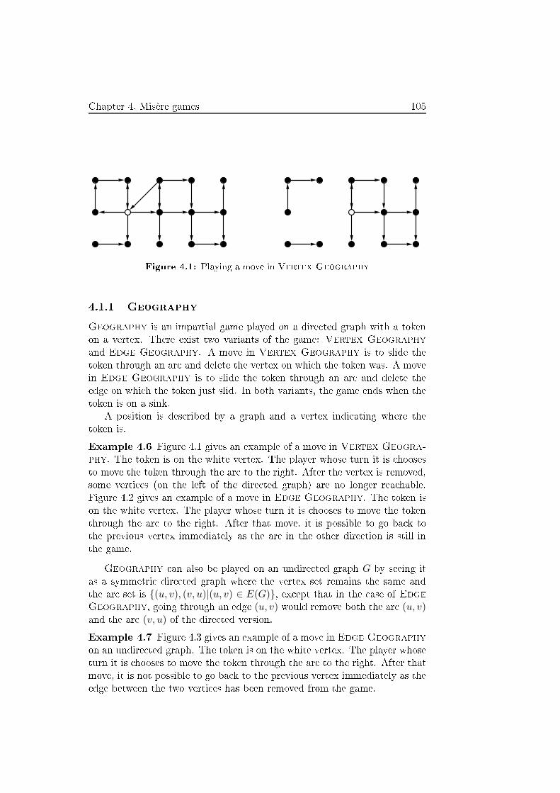
Chapter 4. Misère games 105
Figure 4.1: Playing a move in Vertex Geography
4.1.1 Geography
Geography is an impartial game played on a dire ted graph with a token
on a vertex. There exist two variants of the game: Vertex Geography
and Edge Geography. A move in Vertex Geography is to slide the
token through an ar and delete the vertex on whi h the token was. A move
in Edge Geography is to slide the token through an ar and delete the
edge on whi h the token just slid. In both variants, the game ends when the
token is on a sink.
A position is des ribed by a graph and a vertex indi ating where the
token is.
Example 4.6 Figure 4.1 gives an example of a move in Vertex Geogra-
phy. The token is on the white vertex. The player whose turn it is hooses
to move the token through the ar to the right. After the vertex is removed,
some verti es (on the left of the dire ted graph) are no longer rea hable.
Figure 4.2 gives an example of a move in Edge Geography. The token is
on the white vertex. The player whose turn it is hooses to move the token
through the ar to the right. After that move, it is possible to go ba k to
the previous vertex immediately as the ar in the other dire tion is still in
the game.
Geography an also be played on an undire ted graph G by seeing it
as a symmetri dire ted graph where the vertex set remains the same and
the ar set is {(u, v), (v, u)|(u, v) ∈ E(G)}, ex ept that in the ase of Edge
Geography, going through an edge (u, v) would remove both the ar (u, v)and the ar (v, u) of the dire ted version.
Example 4.7 Figure 4.3 gives an example of a move in Edge Geography
on an undire ted graph. The token is on the white vertex. The player whose
turn it is hooses to move the token through the ar to the right. After that
move, it is not possible to go ba k to the previous vertex immediately as the
edge between the two verti es has been removed from the game.
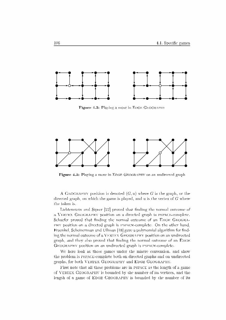
106 4.1. Spe i� games
Figure 4.2: Playing a move in Edge Geography
Figure 4.3: Playing a move in Edge Geography on an undire ted graph
A Geography position is denoted (G,u) where G is the graph, or the
dire ted graph, on whi h the game is played, and u is the vertex of G where
the token is.
Li htenstein and Sipser [22℄ proved that �nding the normal out ome of
a Vertex Geography position on a dire ted graph is pspa e- omplete.
S haefer proved that �nding the normal out ome of an Edge Geogra-
phy position on a dire ted graph is pspa e- omplete. On the other hand,
Fraenkel, S heinerman and Ullman [18℄ gave a polynomial algorithm for �nd-
ing the normal out ome of aVertex Geography position on an undire ted
graph, and they also proved that �nding the normal out ome of an Edge
Geography position on an undire ted graph is pspa e- omplete.
We here look at these games under the misère onvention, and show
the problem is pspa e- omplete both on dire ted graphs and on undire ted
graphs, for both Vertex Geography and Edge Geography.
First note that all these problems are in pspa e as the length of a game
of Vertex Geography is bounded by the number of its verti es, and the
length of a game of Edge Geography is bounded by the number of its

Chapter 4. Misère games 107
edges.
We start with Vertex Geography on dire ted graphs, where the re-
du tion is quite natural, we just add a losing move to every position of the
previous graph, move that the players will avoid until it be omes the only
available move, that is when the original game would have ended.
Theorem 4.8 Finding the misère out ome of a Vertex Geography po-
sition on a dire ted graph is pspa e- omplete.
Proof. We redu e the problem from normal Vertex Geography on di-
re ted graphs.
Let G be a dire ted graph. Let G′be the dire ted graph with vertex set
V (G′) = {u1, u2|u ∈ V (G)}
and ar set
A(G′) = {(u1, v1)|(u, v) ∈ A(G)} ∪ {(u1, u2)|u ∈ V (G)}
that is the graph where ea h vertex of G gets one extra out-neighbour that
was not originally in the graph. We laim that the normal out ome of (G, v)is the same as the misère out ome of (G′, v1) and show it by indu tion on
the number of verti es in G.If V (G) = {v}, then both (G, v) and (G′, v1) are P-positions. Assume
now |V (G)| > 2. Assume �rst (G, v) is an N -position. There is a winning
move in (G, v) to (G, u). We show that moving from (G′, v1) to (G′, u1) is awinning move. We have V (G′) = V (G′) ∪ {v2} and A(G′) = A(G′). As thevertex v2 is dis onne ted from the vertex u1 in G′
, the games (G′, u1) and(G′, u1) share the same game tree, and they both have out ome P by indu -
tion. Hen e (G′, v1) has out ome N . Now assume (G, v) is a P-position.For the same reason as above, moving from (G′, v1) to any (G′, u1) wouldleave a game whose misère out ome is the same as the normal out ome of a
game obtained after playing a move in (G, v), whi h is N . The only other
available move is from (G′, v1) to (G′, v2), whi h is a losing move as it ends
the game. Hen e (G′, v1) has out ome P. �
The proof in [22℄ a tually works even if we only onsider planar bipartite
dire ted graphs with maximum degree 3. As our redu tion keeps the pla-
narity and the bipartition, only adds verti es of degree 1 and in reases the
degree of verti es by 1, we get the following orollary.
Corollary 4.9 Finding the misère out ome of a Vertex Geography po-
sition on a planar bipartite dire ted graph with maximum degree 4 is pspa e- omplete.
For undire ted graphs, adding a new neighbour to ea h vertex would work
the same, but the normal version of Vertex Geography on undire ted

108 4.1. Spe i� games
u uv1
uv2
uv3
uv4
uv5
uv6 uv7
uv8
v
Figure 4.4: The ar gadget
graph is solvable in polynomial time, so we redu e from dire ted graphs, and
repla e ea h ar by an undire ted gadget. That gadget would need to a t
like an ar , that is a player who would want to take it in the wrong dire tion
would lose the game, as well as a player who would want to take it when the
vertex at the other end has already been played, and we want to for e that
a player who takes it is the player who moves the token to the other end, so
that it would be the other player's turn when the token rea h the end vertex
of the ar gadget, as in the original game.
Theorem 4.10 Finding the misère out ome of a Vertex Geography po-
sition on an undire ted graph is pspa e- omplete.
Proof. We redu e the problem from normal Vertex Geography on di-
re ted graphs.
We introdu e a gadget that will repla e any ar (u, v) of the original
dire ted graph, and add a neighbour to ea h vertex to have an undire ted
graph whose misère out ome is the normal out ome of the original dire ted
graph.
Let G be a dire ted graph. Let G′be the undire ted graph with vertex
set
V (G′) = {u, u′|u ∈ V (G)}∪ {uvi|(u, v) ∈ A(G), i ∈ J1; 8K}
and edge set
E(G′) = {(u, uv1), (uv1, uv2), (uv1, uv3), (uv1, uv6), (uv2, uv4), (uv3, uv5),(uv3, uv6), (uv4, uv5), (uv4, uv6), (uv5, uv6), (uv6, uv7), (uv7, uv8),(uv7, v)|(u, v) ∈ A(G)}
∪ {(u, u′)|u ∈ V (G)}
that is the graph where every ar (u, v) of G has been repla ed by the gadget
of Figure 4.4, identifying both u verti es and both v verti es, and ea h vertex

Chapter 4. Misère games 109
of G gets one extra neighbour that was not originally in the graph. We
laim that the normal out ome of (G,u) is the same as the misère out ome
of (G′, u) and show it by indu tion on the number of verti es in G.If V (G) = u, then (G,u) is a normal P-position. In (G′, u) the �rst
player an only move to (G′, u′) where the se ond player wins as he annot
move.
Now assume |V (G)| > 2.We �rst show that no player wants to move the token from v to any wv7,
whether w has been played or not. We will only prove it for moving the
token from v to some wv7 where w is still in the game, as the other ase is
similar. First note that if w is removed from the game in the sequen e of
move following that �rst move, as v is already removed, all verti es of the
form wvi would be dis onne ted from the token, and therefore unrea hable.
Hen e whether the move from wv1 to w is winning does not depend on the
set of verti es deleted in that sequen e, and it is possible to argue the two
ases. Assume the �rst player moved the token from v to any wv7. Then
the se ond player an move the token to wv6. From there, the �rst player
has four hoi es. If she goes to wv1, the se ond player answers to wv2, thenthe rest of the game is for ed and the se ond player wins. If she goes to
wv4, he answers to wv2 where she an only move to wv1, and let him go to
wv3 where she is for ed to play to wv5 and lose. The ase where she goes to
wv5 is similar. In the ase where she goes to wv3, we argue two ases: if the
move from wv1 to w is winning, he answers to wv5, where all is for ed until
he gets the move to w; if that move is losing, he answers to wv1, from where
she an either go to w, whi h is a losing move by assumption, or go to wv2where every move is for ed until she loses.
We now show that no player wants to move the token from v to any vw1
where w has already been played. Assume the �rst player just played that
move. Then the se ond player an move the token to vw3. From there, the
�rst player have two hoi es. If she plays to vw6, he answers to vw4, where
she an only end the game and lose. If she plays to vw5, he answers to vw4,
where the move to vw2 is immediately losing, and the move to vw6 for es
the token to go to vw7 and then vw8 where she loses.
Assume �rst that (G,u) is an N -position. There is a winning move in
(G,u) to some (G, v). We show that moving the token from u to uv1 in G′is
a winning move for the �rst player. From there, the se ond player has three
hoi es. If he moves the token to uv6, the �rst player answers to uv3, thenthe rest of the game is for ed and the �rst player wins. If he moves the token
to uv2, the �rst player answers to uv4, where the se ond player again has two
hoi es: either he goes to uv6, she answers to uv5 where he is for ed to lose
by going to uv3; or he goes to uv5, she answers to uv6 where the move to uv3is immediately losing and the move to uv7 is answered to a game (G′, v). Asu′ and all verti es of the form uvi are either played or dis onne ted from vin G′
, the only di�eren es in the possible moves in (followers of) the games

110 4.1. Spe i� games
(G′, v) and (G′, v) are moves from a vertex w to wu1 or to wu7, so they both
have out ome P by indu tion. The ase where he hooses to move the token
to uv3 is similar. Hen e (G′, u) is an N -position.
Now assume (G,u) is a P-position. Then any (G, v) that an be obtained
after a move from (G,u) is an N -position. Moving the token to u′ in G′is
immediately losing, so we may assume the �rst player moves it to some uv1,where the se ond player answers to uv3. From there the �rst player has two
hoi es. If she goes to uv6, the se ond player answers by going to uv4, whereboth available moves are immediately losing. If she goes to uv5, he answersto uv4, where the move to uv2 is immediately losing, and the move to uv6 isanswered to uv7, where again the move to uv8 is immediately losing, so we
may assume he moves the token to v. As u′ and all verti es of the form uviare either played or dis onne ted from v in G′
, the only di�eren es in the
possible moves in (followers of) the games (G′, v) and (G′, v) are moves from
a vertex w to wu1 or to wu7, so they both have out ome N by indu tion.
Hen e (G′, u) is a P-position. �
Again, using the fa t that the proof in [22℄ a tually works even if we
only onsider planar bipartite dire ted graphs with maximum degree 3, asour redu tion keeps the planarity sin e the gadget is planar with the verti es
we link to the rest of the graph being on the same fa e, only adds verti es
of degree at most 5 and in reases the degree of verti es by 1, we get the
following orollary.
Corollary 4.11 Finding the misère out ome of a Vertex Geography po-
sition on a planar undire ted graph with degree at most 5 is pspa e- omplete.
Though misère play is generally onsidered harder to solve than normal
play, the feature that makes it hard is the fa t that disjun tive sums do not
behave as ni ely as in normal play, and Geography is a game that does
not split into sums. Hen e the above result appears a bit surprising as it was
not expe ted.
We now look at Edge Geography where the redu tions are very similar
to the one for Vertex Geography on dire ted graphs.
We start with the undire ted version.
Theorem 4.12 Finding the misère out ome of an Edge Geography po-
sition on an undire ted graph is pspa e- omplete.
Proof. We redu e the problem from normal Edge Geography on undi-
re ted graphs.
Let G be an undire ted graph. Let G′be the undire ted graph with
vertex set
V (G′) = {u1, u2|u ∈ V (G)}
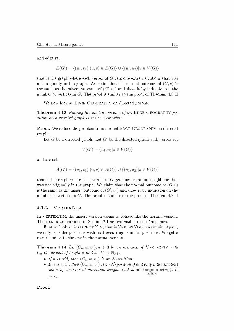
Chapter 4. Misère games 111
and edge set
E(G′) = {(u1, v1)|(u, v) ∈ E(G)} ∪ {(u1, u2)|u ∈ V (G)}
that is the graph where ea h vertex of G gets one extra neighbour that was
not originally in the graph. We laim that the normal out ome of (G, v) isthe same as the misère out ome of (G′, v1) and show it by indu tion on the
number of verti es in G. The proof is similar to the proof of Theorem 4.8 �
We now look at Edge Geography on dire ted graphs.
Theorem 4.13 Finding the misère out ome of an Edge Geography po-
sition on a dire ted graph is pspa e- omplete.
Proof. We redu e the problem from normal Edge Geography on dire ted
graphs.
Let G be a dire ted graph. Let G′be the dire ted graph with vertex set
V (G′) = {u1, u2|u ∈ V (G)}
and ar set
A(G′) = {(u1, v1)|(u, v) ∈ A(G)} ∪ {(u1, u2)|u ∈ V (G)}
that is the graph where ea h vertex of G gets one extra out-neighbour that
was not originally in the graph. We laim that the normal out ome of (G, v)is the same as the misère out ome of (G′, v1) and show it by indu tion on the
number of verti es in G. The proof is similar to the proof of Theorem 4.8 �
4.1.2 VertexNim
In VertexNim, the misère version seems to behave like the normal version.
The results we obtained in Se tion 2.1 are extensible to misère games.
First we look atAdja ent Nim, that isVertexNim on a ir uit. Again,
we only onsider positions with no 1 o urring as initial positions. We get a
result similar to the one in the normal version.
Theorem 4.14 Let (Cn, w, v1), n > 3 be an instan e of Vertexnim with
Cn the ir uit of length n and w : V → N>1.
• If n is odd, then (Cn, w, v1) is an N -position.
• If n is even, then (Cn, w, v1) is an N -position if and only if the smallest
index of a vertex of minimum weight, that is min{argmin16i6n
w(vi)}, is
even.
Proof.

112 4.1. Spe i� games
• Case (1) If n is odd, then the �rst player an apply the following
strategy to win: �rst, she plays w(v1) → 1. Then for all 1 6 i < n−12 :
if the se ond player empties v2i, then the �rst player also empties
the following vertex v2i+1. Otherwise, she plays w(v2i+1) → 1. This
time, the strategy is not di�erent for the last two verti es of Cn. As
w(v1) = 1, the se ond player is now for ed to empty v1. Sin e an
odd number of verti es was deleted sin e then, we now have an even
ir uit to play on. It now su� es for the �rst player to empty all the
verti es on the se ond run. Indeed, the se ond player is also for ed to
set ea h weight to 0 sin e he has to play on verti es satisfying w = 1.Sin e the ir uit is even, the �rst player is guaranteed to leave the
last move to the se ond player.
• Case (2) If n is even, we laim that who must play the �rst vertex
of minimum weight will lose the game. The winning strategy of the
other player onsists in de reasing by 1 the weight of ea h vertex at
their turn. Assume that min{argmin16i6n
w(vi)} is odd. If the strategy of
the se ond player always onsists in moving w(vi) → w(vi) − 1, thenthe �rst player will be the �rst to set a weight to 0 or 1. If she sets theweight of a vertex to 0, then the se ond player now fa es an instan e
(C ′n−1, w
′) with w′ : V ′ → N>1, whi h is winning a ording to the
previous item. If she sets the weight of a vertex to 1, then the se ond
player will empty the following vertex, leaving to the �rst player a
position (C ′n−1 = (v′1, v
′2, . . . , v
′N−1), w
′) with w′ : V ′ → N>1 ex ept on
w′(v′n−1) = 1. This position orresponds to the one of the previous
item after the �rst move, and is thus losing. A similar argument shows
that the �rst player has a winning strategy if min{argmin16i6n
w(vi)} is
even.
�
The reader would have seen the similarity between the proofs of normal
version and misère version. The following results are even more similar in
their proof, this is why we do not re all the proofs in their entirety.
We now state how to �nd the misère out ome of a VertexNim position
on any undire ted graph.
Theorem 4.15 Let (G,w, u) be an instan e of VertexNim, where G is an
undire ted graph. De iding whether the misère out ome of (G,w, u) is P or
N an be done in O(|V (G)||E(G)|) time.
Proof. If all verti es have weight 1, then (G,w, u) is an N -position if and
only if |V (G)| is even sin e it redu es to the misère version of �She loves
move, she loves me not�. Otherwise, we an use the same proof as the one

Chapter 4. Misère games 113
of Theorem 2.9 to see that (G,w, u) is N in the misère version if and only if
it is N in the normal version. �
Finally, we state how to �nd the misère out ome of a VertexNim posi-
tion on any dire ted graph with a self loop on ea h vertex.
Theorem 4.16 Let (G,w, u) be an instan e of VertexNim, where G is
strongly onne ted, with a loop on ea h vertex. De iding whether the misère
out ome of (G,w, u) is P or N an be done in time O(|V (G)||E(G)|).
Proof. If all verti es have weight 1, then (G,w, u) is an N position if and
only if |V (G)| is even sin e it redu es to the misère version of �She loves
move, she loves me not�. Otherwise, we an use the same proof as the one
of Theorem 2.7 to see that (G,w, u) is N in the misère version if and only if
it is N in the normal version. �
4.1.3 Timber
In Timber, going to misère is already harder. Though we an still redu e
the game to an oriented forest, whi h happens to be the same forest as for
normal play, we an only give a polynomial algorithm for �nding the misère
out ome of an oriented path.
Theorem 4.17 Let G be a dire ted graph seen as a Timber position su h
that there exist a set S of verti es that forms a 2-edge- onne ted omponent
of G, and x, y two verti es not belonging to G. Let G′be the dire ted graph
with vertex set
V (G′) = (V (G)\S) ∪ {x, y}
and ar set
A(G′) = (A(G) \ {(u, v)|{u, v} ∩ S 6= ∅})∪ {(u, x)|u ∈ (V (G) \ S),∃v ∈ S, (u, v) ∈ A(G)}∪ {(x, u)|u ∈ (V (G) \ S),∃v ∈ S, (v, u) ∈ A(G)}∪ {(y, x)}.
Then G =− G′.
Proof. The proof is identi al to the proof of Theorem 2.14 as we never used
the fa t we were under the normal onvention. �
As in normal play, we get the following orollary.
Corollary 4.18 For any dire ted graph G, there exists an oriented forest FG
su h that G =+ FG and G =− FG. Moreover, FG is omputable in quadrati
time.
The following proposition remains true as well for the same reason.

114 4.1. Spe i� games
Proposition 4.19 Let T be an oriented tree su h that there exist three sets
of verti es {ui}06i6k, {vi}06i6k, {wi}06i6ℓ ⊂ V (G) su h that:
1. ({(ui−1, ui)}16i6k ∪ {(vi−1, vi)}16i6k ∪ {(wi−1, wi)}16i6ℓ) ⊂ A(G),
2. (uk, w0), (vk, wℓ) ∈ A(G),
3. u0 and v0 have in-degree 0 and out-degree 1,
4. for all 1 6 i 6 k, uk and vk have in-degree 1 and out-degree 1.
Let T ′be the oriented tree with vertex set
V (T ′) = V (T ) \ {vi}06i6k
and ar set
A(T ′) = A(T ) \ ({(vi−1, vi)}16i6k ∪ {(vk, wℓ)}).
Then T =− T ′.
Proof. The proof is identi al to the proof of Proposition 2.17 as we never
used the fa t we were under the normal onvention. �
On paths, we an use the peak representation as de�ned in Se tion 2.2,
but we an also ode the problem with a word: L would represent an ar
dire ted leftward while R would represent an ar dire ted rightward. As in
Se tions 2.2 and 3.1, we an see it as a row of dominoes that would topple
everything in one dire tion when hosen, where hosen dominoes an only
be toppled fa e up. The position is read from left to right.
Given the alphabet {L,R}, for a word w, let |w|L be the num-
ber of L's in w, |w|R the number of R's in w and w[i,j] the subword
wiwi+1 · · ·wj . Let WP be the set of words w su h that for any i,|w[0,i]|L > |w[0,i]|R and |w|L = |w|R; and SWP be the set of words
w su h that w ∈ WP and ∀w1, w2 ∈ WP , w 6= w1LRw2. We de�ne
X = (SWP\{∅}) ∪ {Rw | w ∈ SWP} ∪ {wL | w ∈ SWP} ∪ {RwL | w ∈ SWP}.
We note w the word obtained from w after removing the �rst hara ter if it
is an R and the last one if it is an L.
The reader would have re ognised WP as the set of normal P-positionsof Timber on a path. We now prove that misère P-positions of Timber on
a path are those belonging to X, that is all words w su h that w ∈ SWPbut the empty word.
Theorem 4.20 In misère play, the P-positions of Timber on a path are
exa tly those whi h orrespond to words of X.

Chapter 4. Misère games 115
Proof. Let w ∈ X be a position. Assume w ∈ (SWP\{∅}). From the
normal play analysis, we know that the �rst player annot move to a position
in SWP ⊂ WP . Assume the �rst player an move to a position Rw0 with
w0 ∈ SWP . Then it follows that w = w1LRw0 for some w1. As w,w0 ∈ WPthen w1 ∈ WP , whi h is not possible sin e w ∈ SWP . Similarly, we an
prove the �rst player has no move to a position of the form w0L or Rw0Lwith w0 ∈ SWP . Similarly, we an prove the �rst player has no move to a
position in X from a position in X.
Let w /∈ X ∪ {∅}. Assume w ∈ WP . Then there exist w1, w2 ∈ WPsu h that w = w1LRw2, and we an hoose them su h that w2 ∈ SWP .From w, the �rst player an move to Rw2 ∈ X. Similarly, we an
prove the �rst player has a move to a position in X from a position in
({Rw | w ∈ WP} ∪ {wL | w ∈ WP} ∪ {RwL | w ∈ WP})\X .
Now assume w[0,1] = RR. The �rst player an move to R ∈ X.
Now assume w is none of the above forms. Thus w starts with an L and
ends with an R, and is not in WP , so the �rst player has a move from wto a position w0 ∈ WP\{∅}. Without loss of generality, we an assume it is
by toppling a domino leftward. If w0 ∈ SWP , the same move from w leaves
the position w0 ∈ X or w0L ∈ X. Otherwise, there exist w1, w2 ∈ WP su h
that w0 = w1LRw2 and we an hoose w2 ∈ SWP . The �rst player an
then move from w to Rw2 ∈ X or Rw2L ∈ X. �
SWP is the set of Timber positions whose peak representations are Dy k
paths without peaks at height 1. The number of su h Dy k paths of length
2n is the nthFine number Fn = 1
2
∑−2i=0(−1)icn−i
(12
)i, where ck = (2k)!
k!(k+1)!
is the kth Catalan number [31℄. This gives us the number of Timber misère
P-positions on paths of length n: there are no Timber misère P-positions
on paths of length 0; there are 2Fn =∑−2
i=0(−1)icn−i
(12
)iTimber misère
P-positions on paths of length 2n+ 1; there are Fn + Fn−1 Timber misère
P-positions on paths of length 2n.
That last number is also the number of Dy k paths of length 2n with no
peak at height 2 before the �rst time the path returns at height 0. We an
de�ne a bije tion between Timber misère P-positions on paths of length 2nand Dy k paths of length 2n with no peak at height 2 before the �rst time
the path returns at height 0 as follows (using their word representation): if
the word an be written w1Lw2R with both w1 and w2 representing Dy k
paths (note that w1 might be empty, but not w2), its image is Lw1Rw2.
otherwise, the word an be written RwL with w representing a Dy k path,
and its image is LwR. Figure 4.5 gives examples of the bije tion, using the
peak representation. The Timber misère P-positions are on the left, and at
their right are their images through the bije tion.

116 4.1. Spe i� games
→
→
→
Figure 4.5: Timber misère P-positions and their images, Dy k paths with no
peak at height 2 before the �rst return to 0
4.1.4 Timbush
For Timbush, we still redu e the dire ted graph to an oriented forest, but
our knowledge stops there. Even on an oriented path, �nding the misère
out ome seems hallenging.
Theorem 4.21 Let G be a dire ted graph seen as a Timbush position su h
that there exist a set S of verti es that forms a 2-edge- onne ted omponent
of G, and x, y two verti es not belonging to G. Let G′be the dire ted graph
with vertex set
V (G′) = (V (G)\S) ∪ {x, y}
and ar set
A(G′) = (A(G) \ {(u, v)|{u, v} ∩ S 6= ∅})∪ {(u, x)|u ∈ (V (G) \ S),∃v ∈ S, (u, v) ∈ A(G)}∪ {(x, u)|u ∈ (V (G) \ S),∃v ∈ S, (v, u) ∈ A(G)}∪ {(y, x)},
keeping the same olours, where the olour of (y, x) is grey if the ar s in
S yields di�erent olours, and of the unique olour of ar s in S otherwise.
Then G =− G′.
Proof. The proof is identi al to the proof of Theorem 3.4 as we never used
the fa t we were under the normal onvention. �
As in normal play, we get the following orollary.
Corollary 4.22 For any dire ted graph G, there exists an oriented forest
FG su h that G =+ FG and G =− FG and FG is omputable in quadrati
time.
The following proposition is true as well, for the same reason.
Chapter 4. Misère games 117
Proposition 4.23 Let T be an oriented tree su h that there exist three sets
of verti es {ui}06i6k,{vi}06i6k,{wi}06i6ℓ ⊂ V (G) su h that:
1. ({(ui−1, ui)}16i6k ∪ {(vi−1, vi)}16i6k ∪ {(wi−1, wi)}16i6ℓ ⊂ A(G),
2. {(uk, w0), (vk, wℓ)}) ⊂ A(G),
3. u0 and v0 have in-degree 0 and out-degree 1,
4. for all 1 6 i 6 k, uk and vk have in-degree 1 and out-degree 1,
5. for all 1 6 i 6 k, (uk−1, uk) and (vk−1, vk) have the same olour.
6. (uk, w0) and (vk, wℓ) have the same olour.
Let T ′be the oriented tree with vertex set
V (T ′) = V (T )\{vi}06i6k
and ar set
A(T ′) = A(T )\({(vi−1, vi)}16i6k ∪ {(vk, wℓ)}),
keeping the same olours, apart from (uk, w0) whi h be omes grey when
(uk, w0) and (vk, wℓ) had di�erent olours in T . Then T =− T ′.
Proof. The proof is identi al to the proof of Proposition 3.7 as we never
used the fa t we were under the normal onvention. �
4.1.5 Toppling Dominoes
In Toppling Dominoes, the misère out ome of a single row is easy to
determine, but �nding equivalen e lasses in the general ase has eluded us
for now.
Proposition 4.24 The misère out ome of a Toppling Dominoes position
on a single row is determined by its end dominoes and the dominoes right
next to them. For any string x,
• L,ERE,LxL,ERxL,LxRE,ERxRE ∈ R−,
• R,ELE,RxR,ELxR,RxLE,ELxLE ∈ L−,
• E ∈ P−,
• ∅, EL, LE, ER, RE, LxR, RxL, EEx, xEE, ELxL, LxLE, ERxR,RxRE, ELxRE, ERxLE ∈ N .
In parti ular, we note that there is only one Toppling Dominoes po-
sition on a single row that is a misère P-position.Nevertheless, when allowing a game on several rows, the set of Toppling
dominoes misère P-positions is in�nite, as all Nim positions are equal to a
Toppling dominoes position using only grey dominoes.

118 4.1. Spe i� games
However, if we restri t ourselves to bla k and white dominoes (ex luding
grey dominoes), we prove that no position is a misère P-position, no mat-
ter the number of rows of the position. We a tually fully hara terise the
out ome of any set of rows of bla k and white dominoes.
Before stating the theorem, we de�ne a pair of fun tions on sets of rows
of dominoes. For any set of rows G of bla k and white dominoes, we de�ne
ltd(G) the number of rows of dominoes in G that start and end with a bla k
domino. Similarly, we de�ne rtd(G) the number of rows of dominoes in Gthat start and end with a white domino.
Theorem 4.25 Let G be a set of rows of bla k and white dominoes. Then
o−(G) =
N−if ltd(G) = rtd(G)
L−if ltd(G) < rtd(G)
R−if ltd(G) > rtd(G)
Proof. We prove the result by indu tion on the number of dominoes in G.If there is no domino, the out ome is trivially N .
Assume now there is at least one domino. Assume �rst ltd(G) = rtd(G).If ltd(G) > 0, Left an play a domino on the edge of a row that starts and ends
with a bla k domino to remove it from the game, moving to a positionG′su h
that ltd(G′) = ltd(G)−1 = rtd(G)−1 = rtd(G
′)−1, whi h is an L-position by
indu tion. Otherwise, we may assume without loss of generality that there is
a row that starts with a bla k domino and ends with a white domino. Left an
hoose the rightmost bla k domino of that row and topple it leftward, moving
to a position G′su h that rtd(G
′) = rtd(G) + 1 = ltd(G) + 1 = ltd(G′) + 1,
whi h is an L-position by indu tion. A similar argument on Right moves
shows that G is an N -position. Assume now ltd(G) < rtd(G). Then
there exists a row that starts and ends with a white domino. If that
row ontains a bla k domino, Left an hoose the rightmost bla k domino
of that row and topple it leftward, moving to a position G′su h that
rtd(G′) = rtd(G) > ltd(G) = ltd(G
′), whi h is an L-position by indu tion.
Otherwise, that is if all rows that start and end with a white domino on-
tain no bla k domino, either she has no move and wins, or she an hoose a
bla k domino at an end of a row and topple it toward the other ends, mov-
ing to a position G′su h that rtd(G
′) = rtd(G) > ltd(G) > ltd(G′), whi h is
an L-position by indu tion. Whatever Right does, he an only hange the
status of one row, and only hange one of the end dominoes of this row or
empty it, moving to a position G′where rtd(G
′)− ltd(G′) = rtd(G)− l(tdG)
or rtd(G′)− ltd(G
′) = rtd(G)− ltd(G) − 1, whi h is either an L-position or
an N -position by indu tion. Hen e G is an L-position.The ase when ltd(G) > rtd(G) is similar. �
This implies that any row of bla k and white dominoes starting and end-
ing with a bla k domino is equivalent to a single bla k domino modulo the

Chapter 4. Misère games 119
universe of LR-Toppling Dominoes positions. Also any row of bla k and
white dominoes starting and ending with a white domino is equivalent to a
single white domino modulo the universe of LR-Toppling Dominoes po-
sitions and any row of bla k and white dominoes starting and ending with
dominoes of di�erent olours is equivalent to an empty row modulo the uni-
verse of LR-Toppling Dominoes positions. Note that this equivalen e is
not true in the universe of all Toppling Dominoes positions. For example,
the position LL and L are not equivalent in this universe: L + E + E is a
misère P-position, while LL+ E + E is a misère L-position.This equivalen e allows us to ompletely des ribe the misère monoid of
LR-Toppling Dominoes positions, whi h we present in Theorem 4.26.
Theorem 4.26 Under the mapping
G 7→ αltd(G)−rtd(G),
the misère monoid of LR-Toppling Dominoes positions is
MZ = 〈1, α, α−1 | α · α−1 = 1〉 ∼= (Z,+)
with out ome partition
N− = {1},L− = {α−n|n ∈ N∗},R− = {αn|n ∈ N∗}
and total ordering
αn > αm ⇔ n < m.
This result is quite surprising as in general, the misère version of a game
is harder than its normal version, and LR-Toppling Dominoes has not
been solved under normal onvention. From what we saw in Se tion 3.2 and
results from [17℄, the stru ture is ri her in normal play than in misère play.
4.1.6 Col
Noti e �rst that all Col positions are dead-ending.
On Col, we give the out ome of some lasses of graphs, and even equiv-
alen e lass modulo the dead-ending universe for some of them.
We use the same notation as in Se tion 3.3.
First, we present some features parti ipating in explaining why misère
play seems harder than normal play for the game of Col.
Adding a bla k vertex or reserving a vertex for Left would seem to be an
advantage for Right in misère play. Unfortunately, that intuition is false:
o−(o+ o) = N ; o−(oBo) = L
o−(ooo) = N ; o−(oBo) = L

120 4.1. Spe i� games
A theorem su h as Theorem 3.51 annot be stated: the se ond player
would never use su h strategy as they would be sure to lose this way, and
the �rst player annot for e su h a hoi e.
Now we are ba k with �nding misère out omes of positions.
We start with paths. The following lemma gives the equivalen e lass
modulo the dead-ending universe of paths whose end verti es are bla k or
white and all internal verti es are grey.
Lemma 4.27
1. for any non-negative integer n, BonB ≡−E B.
2. for any non-negative integer n, BonW ≡−E ∅.
Proof. We show simultaneously that G+B and G+BonB have the same
out ome, as well as G and G+BonW , by indu tion on n ∈ N and the order
of G ∈ E .By playing on any vertex of BonB, Left goes to a game whi h is equivalent
to ∅ modulo E , either by indu tion or be ause it is ∅. By playing on any
vertex of BonB, Right goes to a game whi h is equivalent to B +B modulo
E by indu tion or be ause it is B + B. By playing on any vertex of BonW ,
Left goes to a game whi h is equivalent to W modulo E by indu tion or
be ause it is W . By playing on any vertex of BonW , Right goes to a game
whi h is equivalent to B modulo E by indu tion or be ause it is B.
Let G be a dead-ending game su h that Left wins G + B playing �rst (or
se ond). On G + BonB, Left an follow her G + B strategy, unless Right
plays from some G′ + BonB to G′ + (BonB)R or the strategy re ommends
her to play from some G′+B to G′. In the former ase, Right has just moved
BonB to a game equivalent to B + B modulo E and she an put the game
on G′ + B whi h she wins a priori. In the latter ase, she an move from
G′ +BonB to a game equivalent to G′modulo E and ontinue as if she had
just moved from B to ∅.Let G be a dead-ending game su h that Right wins G + B playing �rst (or
se ond). On G + BonB, Right an follow his G + B strategy, unless Left
plays from some G′+BonB to G′+(BonB)L or he has no more move. In the
former ase, Left has just moved BonB to a game equivalent to ∅ modulo Eand he an assume she had just moved from B to ∅. In the latter ase, he
an move from G′ + BonB to a game equivalent to G′ + B + B modulo Ewhere he has no move and wins as he will never get any.
Hen e, BonB ≡−E B.
Let G be a dead-ending game su h that Left wins G playing �rst (or se ond).
On G+BonW , Left an follow her G strategy, unless Right plays from some
G′ +BonW to G′ + (BonW )R or she has no more move. In the former ase,
Right has just moved BonW to a game equivalent to B modulo E and she
an put the game on G′whi h she wins a priori. In the latter ase, she an
move from G′ +BonW to a game equivalent to G′ +W modulo E where he
Chapter 4. Misère games 121
has no move and wins as she will never get any.
A similar argument would show that when White has a winning strategy on
G, he has one on G+BonW .
Hen e, BonW ≡−E ∅. �
This implies the following result on y les, where all moves are equivalent,
leading to a position we just analysed.
Theorem 4.28 For any integer n greater than or equal to 3, we have
Cn ≡−E ∅.
Proof. The only Left option of Cn is Won−3W , whi h is equivalent to Wmodulo E and the only Right option of Cn is Bon−3B, whi h is equivalent
to B modulo E . Hen e Cn is equivalent to {W |B} = BW modulo E , and as
BW is equivalent to ∅ modulo E , Cn is as well. �
We now look at sums of paths as it gives us the misère out ome of any
grey path, and helps �nd the misère out ome of bigger positions.
Lemma 4.29
1. For any non-negative integer l, any non-negative integers ni (i ∈ J1; lK),we have Σl
i=1Woni ∈ N− ∪ L−, that is Left has a winning strategy if she
plays �rst.
2. For any non-negative integer l, any non-negative integers ni (i ∈ J1; lK),we have (W +Σl
i=1Woni) ∈ L−, that is Left has a winning strategy who-
ever plays �rst.
Proof. We show the results simultaneously by indu tion on n = Σli=1ni.
If n = 0, Left has no move on either Σli=1Woni
or (W +Σli=1Woni), and as
Right has at least one move on (W +Σli=1Woni), the results hold.
Assume n > 1. Without loss of generality, we may assume nl > 1. If Left
plays on the non-reserved leaf of Wonlin Σl
i=1Woni, it be omes equivalent
to W+Σl−1i=1Woni
modulo E , where Left has a winning strategy by indu tion.Hen e Left has a winning strategy on Σl
i=1Woniif she plays �rst.
We noti e (W + Σli=1Woni) = Σl
i=0Woniwith n0 = 0, so if Left is the
�rst player on (W + Σli=1Woni), then she has a winning strategy from 1.
Assume Right is the �rst player on (W +Σli=1Woni). If Right plays on W ,
then the game be omes (Σli=1Woni) where we just saw Left has a winning
strategy playing �rst. Otherwise, we may assume Right plays on a vertex
of Wonlwithout loss of generality. If this vertex is the non-reserved leaf,
then the game be omes equivalent to (W +Σl−1i=1Woni) modulo E where Left
has a winning strategy by indu tion. Otherwise, Left an answer on this
leaf, leaving a game equivalent to (W + Σl−1i=1Woni) modulo E where she
has a winning strategy by indu tion. Hen e Left has a winning strategy on
(W +Σli=1Woni). �
As expe ted, we an use this result to �nd the out ome of any grey path.

122 4.1. Spe i� games
Theorem 4.30 For any integer n greater than or equal to 2, we have
on ∈ N−that is the �rst player has a winning strategy.
Proof. o2 and BW have the same options, so are equivalent modulo E ,hen e o2 is equivalent to ∅ modulo E .Assume n > 3. Without loss of generality, we an assume that Left is the
�rst player. By playing on a vertex next to a leaf, Left leaves the game as
W +Won−3, where she has a winning strategy by Lemma 4.29. Hen e the
�rst player has a winning strategy on on. �
We now �nd the out ome of any tree with at most one vertex having
degree at least 3. Before that, we need to �nd the out ome of positions that
players might rea h from these trees. We do not onsider all su h positions
as we did in normal play, sin e we only need to onsider positions that o ur
under one player's winning strategy. We look again at sums of path, where
we re�ne the previous results. First, we add a path having exa tly one
bla k leaf and all other verti es being grey to a sum of paths onsidered in
Lemma 4.29, assuming there are at least two single white verti es.
Lemma 4.31 For any non-negative integer l, any non-negative integers ni
(i ∈ J1; l + 1K), we have (W +W +Bonl+1 +Σli=1Woni) ∈ L−
, that is Left
has a winning strategy whoever plays �rst.
Proof. We show the result by indu tion on Σl+1i=1ni. If Left is
the �rst player, she an play on the vertex reserved for her, leaving
(W +W +Wonl+1−1 +Σli=1Woni) where she has a winning strategy by
Lemma 4.29.
Assume now Right is the �rst player. If he plays on a W , then Left an play
on the vertex reserved for her, leaving (W +Wonl+1−1 + Σli=1Woni) where
she has a winning strategy by Lemma 4.29. If he plays on a vertex of Bonl+1,
Left an play on the vertex reserved for her, leaving a game equivalent to
(W +W +Bon′
l+1 +Σli=1Woni) modulo E , where she has a winning strategy
by indu tion. Otherwise, we an assume without loss of generality that Right
plays on a vertex of Wonland that nl > 1. If it is on the non-reserved leaf,
the game be omes equivalent to (W +W +Bonl+1 +Σl−1i=1Woni) modulo E ,
where Left has a winning strategy by indu tion. Otherwise, Left an answer
on this leaf, leaving a game equivalent to (W + W + Bonl+1 + Σl−1i=1Woni)
modulo E , where she has a winning strategy by indu tion.
Hen e Left has a winning strategy on (W +W +Bonl+1 +Σli=1Woni). �
We are now ba k to paths where exa tly one leaf is white and all other
verti es are grey, but we add the extra ondition that at least two of these
paths ea h ontain at least three verti es.
Lemma 4.32 For any non-negative integer k, any integer l greater than or
equal to 2, any integers ni greater than or equal to 2 (i ∈ J1; lK), we have
(Σkj=1Wo+Σl
i=1Woni) ∈ L−, that is Left has a winning strategy.
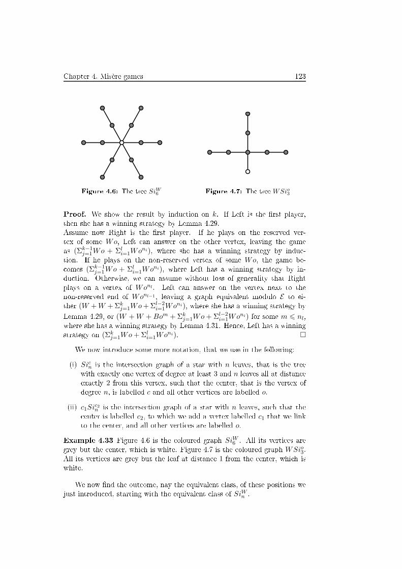
Chapter 4. Misère games 123
Figure 4.6: The tree SiW6 Figure 4.7: The tree WSio3
Proof. We show the result by indu tion on k. If Left is the �rst player,
then she has a winning strategy by Lemma 4.29.
Assume now Right is the �rst player. If he plays on the reserved ver-
tex of some Wo, Left an answer on the other vertex, leaving the game
as (Σk−1j=1Wo + Σl
i=1Woni), where she has a winning strategy by indu -
tion. If he plays on the non-reserved vertex of some Wo, the game be-
omes (Σk−1j=1Wo + Σl
i=1Woni), where Left has a winning strategy by in-
du tion. Otherwise, we an assume without loss of generality that Right
plays on a vertex of Wonl. Left an answer on the vertex next to the
non-reserved end of Wonl−1, leaving a graph equivalent modulo E to ei-
ther (W +W +Σkj=1Wo+Σl−2
i=1Woni), where she has a winning strategy by
Lemma 4.29, or (W +W +Bom +Σkj=1Wo+ Σl−2
i=1Woni) for some m 6 nl,
where she has a winning strategy by Lemma 4.31. Hen e, Left has a winning
strategy on (Σkj=1Wo+Σl
i=1Woni). �
We now introdu e some more notation, that we use in the following:
(i) Sicn is the interse tion graph of a star with n leaves, that is the tree
with exa tly one vertex of degree at least 3 and n leaves all at distan e
exa tly 2 from this vertex, su h that the enter, that is the vertex of
degree n, is labelled c and all other verti es are labelled o.
(ii) c1Sic2n is the interse tion graph of a star with n leaves, su h that the
enter is labelled c2, to whi h we add a vertex labelled c1 that we link
to the enter, and all other verti es are labelled o.
Example 4.33 Figure 4.6 is the oloured graph SiW6 . All its verti es are
grey but the enter, whi h is white. Figure 4.7 is the oloured graph WSio3.All its verti es are grey but the leaf at distan e 1 from the enter, whi h is
white.
We now �nd the out ome, nay the equivalent lass, of these positions we
just introdu ed, starting with the equivalent lass of SiWn .

124 4.1. Spe i� games
Lemma 4.34 For any integer n greater than or equal to 2, we have
SiWn ≡−E ∅.
Proof. Let G be a dead-ending game that Left wins playing �rst (or se ond).
On G + SiWn , Left an follow her G strategy, unless Right plays from some
G′ + SiWn to G′ + (SiWn )R or she has no more moves. In the former ase,
there are three ases. If Right plays on a leaf of SiWn , Left an answer on
the other leaf if n = 2, leaving a game equivalent to G modulo E , where shehas a winning strategy if she plays se ond, or on the vertex next to the one
Right just played on otherwise, leaving the game as G + SiWn−1 where she
has a winning strategy if she plays se ond by indu tion. If Right plays on a
non-leaf non-reserved vertex of SiWn , Left an answer on the leaf next to it,
leaving a game equivalent to G modulo E , where she has a winning strategy
if she plays se ond. If Right plays on the reserved vertex of SiWn , Left an
answer on a leaf, leaving the graph as G + Σn−1i=1 Bo >
−E G where she has a
winning strategy if she plays se ond. In the latter ase, she an move from
G′+SiWn to a game equivalent to G′+W modulo E by indu tion by playing
on a non-leaf of SiWn , where she has no move and wins as she will never get
any.
Let G be a dead-ending game that Right wins playing �rst (or se ond).
On G + SiWn , Right an follow his G strategy, unless Left plays from some
G′ + SiWn to G′ + (SiWn )L or he has no more moves. In the former ase,
there are two ases. If Left plays on a leaf of SiWn , Right an answer on the
vertex next to the one Left just played on, leaving a game equivalent to G′
modulo E , where he has a winning strategy if he plays se ond. If Left plays
on a non-leaf non-reserved vertex of SiWn , Right an answer on a non-leaf
non-reserved vertex of SiWn , leaving a game equivalent to G modulo E , wherehe has a winning strategy if he plays se ond. In the latter ase, he an move
from G′ + SiWn to a game equivalent to G′ + B modulo E by playing on a
non-leaf of SiWn , where he has no move and wins as he will never get any.
Hen e, SiWn ≡−E ∅. �
We now give the out ome of WSion, whi h orresponds to a position
where Left would have played on a leaf of Sion+1.
Lemma 4.35 For any integer n greater than or equal to 2, we have
WSion ∈ L−, that is Left has a winning strategy whoever plays �rst.
Proof. If Left is the �rst player, she an play on the entral vertex, leaving
the game as W +Σni=1Wo, where she has a winning strategy by Lemma 4.29.
Assume Right is the �rst player. If Right plays on the reserved vertex, the
game be omes equivalent to ∅ modulo E , where Left has a winning strategy
if she plays �rst. If Right plays on the entral vertex, the game be omes
Σni=1Bo >
−E ∅, where Left has a winning strategy if she plays �rst. If Right
plays on any non-reserved leaf, Left an answer on the entral vertex, leaving

Chapter 4. Misère games 125
the game as W+Σn−1i=1 Wo, where she has a winning strategy by Lemma 4.29.
If Right plays on any other vertex, the game be omes either equivalent to ∅modulo E , where Left has a winning strategy if she plays �rst, or, if n = 2,B+WBoo, where Left an play on the non-reserved non-leaf vertex, leaving
a game equivalent to W modulo E , where she has a winning strategy.
Hen e, Left has a winning strategy on WSion. �
Now we sum these positions with paths and �nd the out ome of su h
sums, as they appear in the strategy we propose.
Lemma 4.36 For any integer n greater than or equal to 2 and any non-
negative integer k, we have (Wok +WSion) ∈ L−, that is Left has a winning
strategy.
Proof. If Left is the �rst player, she an play on the entral vertex, leav-
ing the game as W +Wok +Σni=1Wo, where she has a winning strategy by
Lemma 4.29.
Assume now Right is the �rst player. If Right plays on the non-reserved
leaf on Wok, the game be omes equivalent to WSion modulo E , where Left
has a winning strategy by Lemma 4.35. If Right plays on any other ver-
tex of Wok, Left an answer on that leaf, leaving a game equivalent to
WSion modulo E , where she has a winning strategy by Lemma 4.35. If
Right plays on the reserved vertex of WSion, the game be omes equivalent
to Wok modulo E , where Left has a winning strategy if she plays �rst by
Lemma 4.29. If Right plays on the entral vertex ofWSion, the game be omes
Wok +Σni=1Bo >
−E Wok, where Left has a winning strategy if she plays �rst
by Lemma 4.29. If Right plays on any non-reserved leaf of WSion, Left ananswer on the entral vertex, leaving the game as W + Wok + Σn−1
i=1 Wo,where she has a winning strategy by Lemma 4.29. If Right plays on any
other vertex, the game be omes either equivalent to Wok modulo E , whereLeft has a winning strategy if she plays �rst by Lemma 4.29, or, if n = 2,Wok +B+WBoo, where Left an play on the non-reserved non-leaf vertex,
leaving a game equivalent to W +Wok modulo E , where she has a winning
strategy by Lemma 4.29.
Hen e, Left has a winning strategy on (Wok +WSion). �
We now state the theorem on the out ome of any grey subdivided star:
all these positions are misère N -positions.
Theorem 4.37 The �rst player has a winning strategy on any tree with
exa tly one vertex having degree at least three, with all verti es being oloured
grey.
Proof. We all v the vertex having degree l > 3, vi (1 6 i 6 l) the leaves
of the tree, ni (1 6 i 6 l) the distan e between v and vi. Without loss of
generality, we an assume that Left is the �rst player.

126 4.2. Canoni al form of di ot games
If at least one of the ni's is equal to 1, Left an play on v, leaving the graph
as Σli=1Woni−1
where she has a winning strategy by Lemma 4.29. Assume
su h ni does not exist. If at least two of the ni's are greater than or equal
to 3, Left an play on v, leaving the graph as Σli=1Woni−1
where she has a
winning strategy by Lemma 4.32. If all ni's are equal to 2, Left an play on
a leaf, leaving the graph as WSiol−1, where she has a winning strategy by
Lemma 4.35. If all but one ni are equal to 2, Left an play on the non-leaf
vertex at distan e 2 from v, leaving the graph as Womax16i6l(ni−3)+WSiol−1,
where she has a winning strategy by Lemma 4.36.
Hen e, the �rst player has a winning strategy on any tree with exa tly one
vertex having degree at least three. �
4.2 Canoni al form of di ot games
We now look at a more general universe of games, namely the universe of
di ot games. Re all that a game is said to be di ot either if it is {·|·} or if it
has both Left and Right options and all these options are di ot.
Example 4.38 Figure 4.8 gives three examples of games that are di ot. The
�rst game has both a Left option and a Right option, and both these options
are 0, so are di ot. One may re ognise the game ∗ = {0|0} introdu ed in the
introdu tion. The se ond game has two Left options and a Right option, and
all these options are 0 or ∗, so are di ot. The third game has a Left option
and two Right options, and we an see all these options are di ot. Figure 4.9
gives three examples of games that are not di ot. The �rst game has a Left
option but no Right option. The se ond game has both a Left option and a
Right option, but, though the Right option is di ot, the Left option is not
di ot as it has a Right option but no Left option. The third game has both
a Left option and a Right option, but none of these options is di ot as they
are numbers in normal anoni al form.
The universe of di ots ontains all impartial games as well as many par-
tizan games su h as all Clobber positions.
In normal play, di ot games are alled all-small, be ause if a player has
a signi� ant advantage in a game, adding any di ot position annot prevent
them from winning. In misère play, this is not the ase, as Siegel proved in
[38℄ that for any game G, there exists a di ot game G′su h that G + G′
is
a misère P-position.
In this se tion, we de�ne a redu ed form for di ot games, prove that it is
a tually a anoni al form, and ount the number of di ot games in anoni al
form born by day 3.
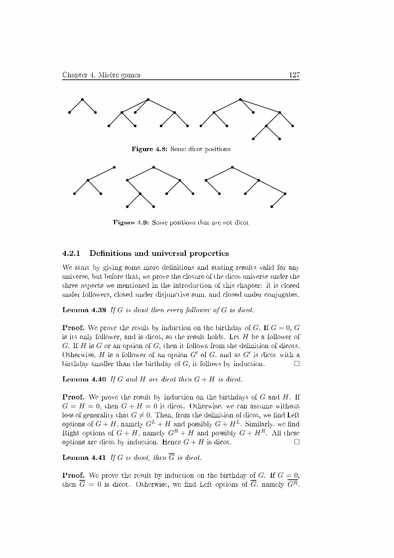
Chapter 4. Misère games 127
Figure 4.8: Some di ot positions
Figure 4.9: Some positions that are not di ot
4.2.1 De�nitions and universal properties
We start by giving some more de�nitions and stating results valid for any
universe, but before that, we prove the losure of the di ot universe under the
three aspe ts we mentioned in the introdu tion of this hapter: it is losed
under followers, losed under disjun tive sum, and losed under onjugates.
Lemma 4.39 If G is di ot then every follower of G is di ot.
Proof. We prove the result by indu tion on the birthday of G. If G = 0, Gis its only follower, and is di ot, so the result holds. Let H be a follower of
G. If H is G or an option of G, then it follows from the de�nition of di ots.
Otherwise, H is a follower of an option G′of G, and as G′
is di ot with a
birthday smaller than the birthday of G, it follows by indu tion. �
Lemma 4.40 If G and H are di ot then G+H is di ot.
Proof. We prove the result by indu tion on the birthdays of G and H. If
G = H = 0, then G + H = 0 is di ot. Otherwise, we an assume without
loss of generality that G 6= 0. Then, from the de�nition of di ot, we �nd Left
options of G+H, namely GL +H and possibly G+HL. Similarly, we �nd
Right options of G + H, namely GR + H and possibly G + HR. All these
options are di ot by indu tion. Hen e G+H is di ot. �
Lemma 4.41 If G is di ot, then G is di ot.
Proof. We prove the result by indu tion on the birthday of G. If G = 0,then G = 0 is di ot. Otherwise, we �nd Left options of G, namely GR
.
128 4.2. Canoni al form of di ot games
Similarly, we �nd Right options of G, namely GL. All these options are
di ot by indu tion. Hen e G is di ot. �
In [38℄, Siegel introdu ed the notion of the adjoint of a game. Re all that
a Left end is a game with no Left option, and a Right end is a game with no
Right option.
De�nition 4.42 (Siegel [38℄) The adjoint of G, denoted Go, is given by
Go =
∗ if G = 0 ,
{(GR)o|0} if G 6= 0 and G is a Left end,
{0|(GL)o} if G 6= 0 and G is a Right end,
{(GR)o|(GL)o} otherwise.
where (GR)o denotes the set of adjoints of elements of GR.
Observe that we an re ursively verify that the adjoint of any game is
di ot. In normal play, the onjugate of a game is onsidered as its opposite
and is thus denoted −G, sin e G+G ≡+ 0. The interest of the adjoint of agame is that it plays a similar role as the opposite of a game in normal play,
to for e a win for the se ond player re ursively, as the following proposition
suggests:
Proposition 4.43 (Siegel [38℄) For any game G, G + Gois a misère P-
position.
The following proposition was stated in [38℄ for the universe G of all
games. Mimi king the proof, we extend it to any universe.
Proposition 4.44 Let U be a universe of games, G and H two games (not
ne essarily in U). We have G >−U H if and only if the following two ondi-
tions hold:
(i) For all X ∈ U with o−(H +X) > P, we have o−(G+X) > P; and
(ii) For all X ∈ U with o−(H +X) > N , we have o−(G+X) > N .
Proof. The su� ien y follows from the de�nition of >. For the onverse,
we must show that o−(G+X) > o−(H +X) for all X ∈ U . Sin e we alwayshave o−(G+X) > R, if o−(H +X) = R, then there is nothing to prove. If
o−(H+X) = P or N , the result dire tly follows from (i) or (ii), respe tively.Finally, if o−(H+X) = L, then by (i) and (ii) we have both o−(G+X) > Pand o−(G+X) > N , hen e o−(G+X) = L. �
To obtain the anoni al form of a game, we generally remove or bypass
options that are not relevant. These options are of two types: dominated
options an be removed be ause another option is always a better move
Chapter 4. Misère games 129
for the player, and reversible options are bypassed sin e the answer of the
opponent is `predi table'. Under normal play, simply removing dominated
options and bypassing reversible options is su� ient to obtain a anoni al
form. Under misère play, Mesdal and Ottaway [25℄ proposed de�nitions of
dominated and reversible options under misère play in the universe G of all
games, proving that deleting dominated options and bypassing reversible
options does not hange the equivalen e lass of a game in general misère
play, then Siegel [38℄ proved that applying these operations a tually de�nes a
anoni al form in the universe G. Hen e the same method may be applied to
obtain a misère anoni al form. However, modulo smaller universes, games
with di�erent anoni al forms may be equivalent. In the following, we adapt
the de�nition of dominated and reversible options to restri ted universes
of games. We show in the next subse tion that a anoni al form modulo
the universe of di ots an be obtained by removing dominated options and
applying a slightly more ompli ated treatment to reversible options.
De�nition 4.45 (U-dominated and reversible options)
Let G be a game, U a universe of games.
(a) A Left option GLis U -dominated by some other Left option GL′
if
GL′
>−U GL
.
(b) A Right option GRis U -dominated by some other Right option GR′
if
GR′
6−U GR
.
( ) A Left option GLis U -reversible through some Right option GLR
if
GLR 6−U G.
(d) A Right option GRis U -reversible through some Left option GRL
if
GRL >−U G.
To obtain the known anoni al forms for the universe G of all games [38℄
but also for the universe I of impartial games [10℄, one may just remove dom-
inated and bypass reversible options as de�ned. The natural question that
arises is whether a similar pro ess gives anoni al forms in other universes.
Indeed, it is remarkable that in all universes losed by followers, dominated
options an be ignored, as shown by the following lemma.
Lemma 4.46 Let G be a game and let U be a universe of games losed by
taking option of games. Suppose GL1is U-dominated by GL2
, and let G′be
the game obtained by removing GL1from GL
. Then G ≡−U G′
.
Proof. By Proposition 4.4, we have G′ 6−U G. We thus only have to show
that G′ >−U G. For a game X ∈ U , suppose Left an win G + X playing
�rst (respe tively se ond), we show that she also has a winning strategy in
G′+X. A tually, she an simply follow the same strategy on G′+X, unless
she is eventually supposed to make a move from some G + Y to GL1 + Y .
In that ase, she is supposed to move to the game GL1 + Y and then win,
130 4.2. Canoni al form of di ot games
so o−(GL1 + Y ) > P. But GL2 >−U GL1
and Y ∈ U , thus o−(GL2 + Y ) > P.Therefore, Left an win by moving from G′ + Y to GL2 + Y , on luding the
proof. �
Note that in the ase that interest us here, that is when G is di ot, the
obtained game G′stays di ot.
Unfortunately, the ase involving reversible options is more omplex.
Nevertheless, we show in the next subse tion how we an deal with them
in the spe i� universe of di ot games. Beforehand, we adapt the de�nition
of downlinked or uplinked games from [38℄ to restri ted universes.
De�nition 4.47 Let G and H be any two games. If there exists some T ∈ Usu h that o−(G + T ) 6 P 6 o−(H + T ), we say that G is U -downlinked to
H (by T ). In that ase, we also say that H is U -uplinked to G by T .
Note that if two games are U -downlinked and U ⊆ U ′, then these two
games are also U ′-downlinked. Therefore, the smaller the universe U is, the
less `likely' it is that two games are U -downlinked.
Lemma 4.48 Let G and H be any two games and U be a universe of games.
If G >−U H, then G is U-downlinked to no HL
and no GRis U-downlinked
to H.
Proof. Let T ∈ U be any game su h that o−(G+T ) 6 P. Sin e G >−U H and
T ∈ U , o−(H +T ) 6 P as well. Hen e for any HL ∈ HL, o−(HL +T ) 6 N ,
and G is not U -downlinked to HLby T . Similarly, let T ′ ∈ U su h that
o−(H + T ′) > P. Then o−(G + T ′) > P and therefore, for any GR ∈ GR,
o−(GR + T ′) > N and GRis not U -downlinked to H by T ′
. �
4.2.2 Canoni al form of di ot games
In this subse tion, we onsider games within the universe D of di ots, and
show that we an de�ne pre isely a anoni al form in that ontext. In or-
der to do so, we �rst des ribe how to bypass the D-reversible options in
Lemmas 4.49 and 4.50.
Lemma 4.49 Let G be a di ot game. Suppose GL1is D-reversible through
GL1R1and either GL1R1 6= 0 or there exists another Left option GL2
of Gsu h that o−(GL2) > P. Let G′
be the game obtained by bypassing GL1:
G′ = {(GL1R1)L, GL \ {GL1}|GR} .
Then G′is a di ot game and G ≡−
D G′.
Proof. First observe that sin e G is di ot, all options of G′are di ot, and
under our assumptions, G′has both Left and Right options. Thus G′
is a
Chapter 4. Misère games 131
di ot game. We now prove that for any di ot game X, the games G+X and
G′ +X have the same misère out ome.
Suppose Left an win playing �rst (respe tively se ond) onG+X. Among
all the winning strategies for Left, onsider one that always re ommends a
move on X, unless the only winning move is on G. In the game G′ +X, let
Left follow the same strategy ex ept if the strategy re ommends pre isely
the move from G to GL1. In that ase, the position is of the form G′ + Y ,
with o−(GL1 + Y ) > P. Thus o−(GL1R1 + Y ) > N .
Suppose Left has a winning move in Y from GL1R1 + Y , i.e. there
exists some Y Lsu h that o−(GL1R1 + Y L) > P . But then by reversibil-
ity, o−(G+ Y L) > P, ontradi ting our hoi e of Left's strategy. So either
Left has a winning move of type GL1R1L + Y , whi h she an play dire tly
from G′ + Y , or she wins be ause she has no possible moves, meaning that
GL1R1 = 0 and Y = 0. In that ase, she an also win in G′ + Y = G′by
hoosing the winning move to GL2.
Now suppose Right an win playing �rst (respe tively se ond) on G+X.
Consider any winning strategy for Right, and let him follow exa tly the
same strategy on G′ + X unless Left moves from some position G′ + Y to
GL1R1L + Y . First note that by our assumption, G′is not a Left end, thus
if Right follows this strategy, Left an never run out of move prematurely.
Suppose now that Left made a move from some position G′ + Y to
GL1R1L + Y . Until that move, Right was following his winning strat-
egy, so o−(G + Y ) 6 P. Sin e GL1R1 6−D G and Y is a di ot, we have
o−(GL1R1 + Y ) 6 P. Thus GL1R1L + Y 6 N and Right an adapt his
strategy. �
With the previous lemma, we do not bypass reversible options through
0 when all other Left options have misère out ome at most N . Su h re-
versible options annot be treated similarly, as shows the example of the
game {0, ∗|∗}. Note that as shown in [2℄ and [3℄, {∗|∗} = ∗ + ∗ ≡−D 0 and
thus, by Proposition 4.4, {0, ∗|∗} >−D 0. Therefore, the Left option ∗ is
D-reversible through 0. However, {0, ∗|∗} 6≡−D {0|∗} sin e the �rst is an N -
position and the se ond is an R-position. Yet, we prove with the following
lemma that all reversible options ignored by Lemma 4.49 an be repla ed by
∗ without hanging the equivalen e lass of the game.
Lemma 4.50 Let G be a di ot game. Suppose GL1is D-reversible through
GL1R1 = 0. Let G′be the game obtained by repla ing GL1
by ∗:
G′ = {∗, GL \ {GL1}|GR} .
Then G′is a di ot game and G ≡−
D G′.
Proof. First observe that sin e G and ∗ are di ots, all options of G′are
di ots, and G′has both Left and Right options. Thus G′
is a di ot game.

132 4.2. Canoni al form of di ot games
We now prove that for any di ot game X, the games G+X and G′+X have
the same misère out ome.
Suppose Left an win playing �rst (respe tively se ond) onG+X. Among
all the winning strategies for Left, onsider one that always re ommends a
move on X, unless the only winning move is on G. In the game G′ +X, let
Left follow the same strategy ex ept if the strategy re ommends pre isely
the move from G to GL1. In that ase, the position is of the form G′ + Y ,
with o−(GL1 + Y ) > P. Thus o−(GL1R1 + Y ) > N .
Suppose Left has a winning move in GL1R1 + Y = 0 + Y = Y , i.e.
there exists some Y Lsu h that o−(Y L) > P. But then by reversibility,
o−(G + Y L) > P, ontradi ting our hoi e of Left's strategy. So Left has
no winning move in Y , and she wins be ause she has no possible moves, i.e.
Y = 0. In that ase, she an also win in G′+Y = G′by hoosing the winning
move to ∗.Now suppose Right an win playing �rst (respe tively se ond) on G+X.
Consider any winning strategy for Right, and let him follow exa tly the same
strategy on G′ +X unless Left moves from some position G′ + Y to ∗+ Y .
First note that by our assumption, G′is not a Left end, thus if Right follows
this strategy, Left an never run out of move prematurely.
Suppose now that Left made a move from some position G′ + Y to
∗ + Y . Until that move, Right was following his winning strategy, so
o−(G + Y ) 6 P. Sin e 0 = GL1R1 6−D G and Y is di ot, we have
o−(Y ) = o−(0 + Y ) 6 o−(G+ Y ) 6 P . So Right an move from ∗ + Y to
Y and win. �
Note that some reversible options may be dealt with using both Lem-
mas 4.49 and 4.50. Yet, it is still possible to apply Lemma 4.49 and remove
su h an option after having applied Lemma 4.50.
At this point, we want to de�ne a redu ed form for ea h game obtained
by applying the pre eding lemmas as long as we an. In addition, it was
proved by Allen in [2℄ and [3℄ that the game {∗|∗} is equivalent to 0 modulo
the universe of di ot games, and we thus redu e this game to 0. Therefore,we de�ne the redu ed form of a di ot game as follows:
De�nition 4.51 (Redu ed form) Let G be a di ot. We say G is in re-
du ed form if:
(i) it is not {∗|∗},
(ii) it ontains no dominated option,
(iii) if Left has a reversible option, it is ∗ and no other Left option has
out ome P or L,
(iv) if Right has a reversible option, it is ∗ and no other Right option has
out ome P or R,
(v) all its options are in redu ed form.

Chapter 4. Misère games 133
Observe �rst the following:
Theorem 4.52 Every game G is equivalent modulo the universe of di ots
to a game in redu ed form H whose birthday is no larger than the birthday
of G.
Proof. To obtain a game H equivalent to G in redu ed form, we an apply
iteratively Lemmas 4.46, 4.49 and 4.50. Applying these lemmas, we never
in rease the depth of the orresponding game tree, thus the birthday of the
redu ed game H is no larger than the birthday of G. �
We now prove that the redu ed form of a game an be seen as a anoni al
form. Before stating the main theorem, we need the two following lemmas.
Lemma 4.53 Let G and H be any games. If G �−D H, then:
(a) There exists some Y ∈ D su h that o−(G+Y ) 6 P and o−(H+Y ) > N ;
and
(b) There exists some Z ∈ D su h that o−(G+Z) 6 N and o−(H+Z) > P.
Proof. Negating the ondition of Proposition 4.44, we get that (a) or (b)
must hold. To prove the lemma, we show that (a) ⇒ (b) and (b) ⇒ (a).
Consider some Y ∈ D su h that o−(G + Y ) 6 P and o−(H + Y ) > N ,
and set
Z = {(HR)o, 0|Y } .
First note that sin e Z has both a Left and a Right option, and all its options
are di ots, Z is also di ot. We now show that Z satis�es o−(G + Z) 6 Nand o−(H +Z) > P, as required in (b). From the game G+Z, Right has awinning move to G+Y , so o−(G+Z) 6 N . We now prove that Right has no
winning move in the game H+Z. Observe �rst that H+Z is not a Right end
sin e Z is not. If Right moves to some HR +Z, Left has a winning response
to HR+(HR)o. If instead Right moves to H+Y then, sin e o−(H+Y ) > N ,
Left an win. Therefore o−(H + Z) > P, and (a) ⇒ (b).
To prove (b) ⇒ (a), for a given Z we set Y = {Z|0, (GL)o} and prove
similarly that Left wins if she plays �rst on H+Y and loses if she plays �rst
on G+ Y . �
Lemma 4.54 Let G and H be any games. The game G is D-downlinked to
H if and only if no GL >−D H and no HR 6
−D G.
Proof. Consider two games G and H su h that G is D-downlinked to Hby some third game T , i.e. o−(G + T ) 6 P 6 o−(H + T ). Then Left
has no winning move from G + T , thus o−(GL + T ) 6 N and similarly
o−(HR + T ) > N . Therefore, T witnesses both GL �−D H and G �−
D HR.
Conversely, suppose that no GL >−D H and no HR 6
−D G. Set
GL = {GL1 , . . . , G
Lk } and HR = {HR
1 , . . . ,HRℓ }. By Lemma 4.53, we an

134 4.2. Canoni al form of di ot games
asso iate to ea h GLi ∈ GL
a game Xi ∈ D su h that o−(GLi +Xi) 6 P and
o−(H +Xi) > N . Likewise, to ea h HRj ∈ HR
, we asso iate a game Yj ∈ D
su h that o−(G+Yj) 6 N and o−(HRj +Yj) > P. Let T be the game de�ned
by
TL =
{{0}(GR)o ∪ {Yj | 1 6 j 6 ℓ}
if both G and H are Right ends,
otherwise.
TR =
{{0}(HL)o ∪ {Xi | 1 6 i 6 k}
if both G and H are Left ends,
otherwise.
If HR(respe tively GR
) is non-empty, then so is {Yj | 1 6 j 6 ℓ}(respe tively (GR)o), and T has a Left option. If both GR
and HRare
empty, then TL = {0}, so T always has a Left option. Similarly, T also
always has a Right option. Moreover, all these options are di ots, so T is
di ot. We laim that G is D-downlinked to H by T .To show that o−(G + T ) 6 P, we just prove that Left loses if she plays
�rst in G+T . Sin e T has a Left option, G+T is not a Left end. If Left moves
to some GLi + T , then by our hoi e of Xi, Right has a winning response
to GLi +Xi. If Left moves to some G + (GR)o, then Right an respond to
GR+(GR)o and win (by Proposition 4.43). If Left moves to G+Yj, then by
our hoi e of Yj , o−(G + Yj) 6 N and Right an win. The only remaining
possibility is, when G and H are Right ends, that Left moves to G+0. Butthen Right annot move and wins.
Now, we show that o−(H + T ) > P by proving that Right loses playing
�rst in H + T . If Right moves to some HRj + T , then Left has a winning
response to HRj +Yj . If Right moves to H+(HL)o, then Left wins by playing
to HL + (HL)o, and if Right moves to H + Xi, then by our hoi e of Xi,
o−(H +Xi) > N and Left an win. Finally, the only remaining possibility,
when G and H are Left ends, is that Right moves to 0. But then Left annot
answer and wins. �
We now prove the main theorem of the se tion.
Theorem 4.55 Consider two di ot games G and H. If G ≡−D H and both
are in redu ed form, then G = H.
Proof. If G = H = 0, the result is lear. We pro eed by indu tion on the
birthdays of the games. Assume without loss of generality that G has an
option. Sin e G is di ot, it has both a Left and a Right option.
Consider a Left option GL. Suppose �rst that GL
is not D-reversible.
Sin e H ≡−D G, H >
−D G and Lemma 4.48 implies that H is not downlinked
to GL. Then by Lemma 4.54, either there exists some HL >
−D GL
, or there
exists some Right option GLRof GL
with GLR 6−D H. The latter would
imply that G >−D GLR
and thus that GLis D-reversible, ontradi ting our
assumption. So we must have some option HLsu h that HL >
−D GL
. A

Chapter 4. Misère games 135
similar argument for HLgives that there exists some Left option GL′
of Gsu h that GL′
>−D HL
. Therefore GL′
>−D HL >
−D GL
. If GL′
and GLare two
di�erent options, thenGLis dominated byGL′
, ontradi ting our assumption
that G is in redu ed form. Thus, GL′
and GLare the same option, and
GL ≡−D HL
. ButGLandHL
are in redu ed form, so by indu tion hypothesis,
GL = HL. The same argument applied to the Right options of G and to
the options of H shows the pairwise orresponden e of all non-D-reversible
options of G and H.
Assume now that GLis a D-reversible option. Then GL = ∗ and for all
other Left options GL′
, we have o−(GL′
) 6 N , and by reversibility, there
exists some Right option GLRof GL
su h that GLR 6−D G. Sin e the only
Right option of ∗ is 0, G >−D 0. Thus H >
−D 0, so either H = 0 or Left has a
winning move in H, namely a Left option HLsu h that o−(HL) > P. First
assume H = 0. Then by the pairwise orresponden e proved earlier, G has
no non-D-reversible options. Yet it is a di ot and must have both a Left and
a Right option, and sin e it is in redu ed form, both are ∗. Then G = {∗|∗}, a ontradi tion. Now assume H has a Left option HL
su h that o−(HL) > P.IfHL
is not D-reversible, then it is in orresponden e with a non-D-reversible
option GL′
, but then we should have o−(HL) = o−(GL′
) 6 N , a ontradi -
tion. So HLis D-reversible, and HL = GL = ∗. The same argument applied
to possible Right D-reversible options on ludes the proofs that G = H. �
This proves that the redu ed form of a game is unique, and that any two
D-equivalent games have the same redu ed form. Therefore, the redu ed
form as des ribed in De�nition 4.51 an be onsidered as the anoni al form
of the game modulo the universe of di ot games.
Siegel showed in [38℄ that for any games G and H, if G >− H, then
G >+ H also in normal play. This result an be strengthened as follows :
Theorem 4.56 Let G and H be any games. If G >−D H, then G >+ H.
Proof. Consider any two games G and H su h that G >−D H. We show that
G+H >+ 0, i.e. that Left an win G+H in normal play when Right moves
�rst [4℄, by indu tion on the birthdays of G and H. Suppose Right plays to
some GR +H. Sin e G >−D H, Lemma 4.48 implies GR
is not D-downlinked
to H. By Lemma 4.54, either there exists some Left option GRLof GR
with
GRL >−D H, or there exists some Right option HR
of H with GR >−D HR
.
In the �rst ase, we get by indu tion that GRL >+ H and Left an win
by moving to GRL + H. In the se ond ase, we get GR >+ HR, and Left
an win by moving to GR +HR. The argument when Right plays to some
G+HLis similar. �
Theorem 4.56 implies in parti ular that if two games are equivalent in
misère play modulo D, then they are also equivalent in normal play. It allows
us to use any normal play tools to prove in omparability or distinguishability

136 4.2. Canoni al form of di ot games
0 ∗ α α s s
z z ∗2
Figure 4.10: Game trees of the 9 di ot games born by day 2
(i.e. non equivalen e) to dedu e it modulo the universe of di ot games.
Moreover, a orollary of Theorem 4.56 is that its statement is also true for
any universe ontaining D, in parti ular for the universe G of all games
(implying the result of [38℄) and for the universe E of dead-ending games we
study in the next se tion.
Corollary 4.57 Let G and H be any games, U a universe ontaining all
di ot positions. If G >−U H, then G >+ H.
4.2.3 Di ot misère games born by day 3
We now use Theorem 4.55 to ount the di ot misère games born by day 3.Re all that the numbers of impartial misère games distinguishable modulo
the universe I of impartial games that are born by day 0, 1, 2, 3 and 4 are
respe tively 1, 2, 3, 5 and 22 (see [10℄). Siegel [38℄ proved that the numbers
of misère games distinguishable modulo the universe G of all games that are
born by day 0, 1 and 2 are respe tively 1, 4 and 256, while the number of
distinguishable misère games born by day 3 is less than 2183. Noti e that
sin e impartial games form a subset of di ot games, the number of di ot
games born by day 3 lies between 5 and 2183. Before showing that this
number is exa tly 1268, we state some properties of the di ot games born by
day 2.
Proposition 4.58 There are 9 di ot games born by day 2 distinguishable
modulo the universe D of di ot games, namely 0, ∗, α = {0|∗}, α = {∗|0},s = {0, ∗|0}, z = {0, ∗|∗}, s = {0|0, ∗}, z = {∗|0, ∗}, and ∗2 = {0, ∗|0, ∗} (see
Figure 4.10). They are partially ordered a ording to Figure 4.11. Moreover,
the out omes of their sums are given in Table 4.12.

Chapter 4. Misère games 137
s z
∗ α∗2
α 0
s zFigure 4.11: Partial ordering of di ot games born by day 2
0 ∗ α α s z s z ∗2
0 N P R L L N R N N∗ P N N N N L N R Nα R N P N N P R R Rα L N N P L L N P Ls L N N L L L N P L
z N L P L L L P N Ls R N R N N P R R Rz N R R P P N R R R∗2 N N R L L L R R P
Table 4.12: Out omes of sums of di ots born by day 2
Proof. There are 10 di ot games born by day 2, of whi h 0 and {∗|∗} are
equivalent. We now prove that these nine games are pairwise distinguishable
modulo the universe D of di ot games
1
. First note that these games are all
in redu ed form. Indeed, sin e all options are either 0 or ∗ whi h are not
omparable modulo D, there are no dominated options. Moreover, ∗ might
be reversible through 0, but sin e there are no other option at least P, it annot be redu ed. Thus, by Theorem 4.55, these games are pairwise non-
equivalent.
The proof of the out omes of sums of these games (given in Table 4.12)
is tedious but not di� ult, and omitted here.
We now show that these games are partially ordered a ording to Fig-
ure 4.11. Using the fa t that {∗|∗} ≡−D 0 and Proposition 4.4, we easily
infer the relations orresponding to edges in Figure 4.11. All other pairs are
in omparable: for ea h pair (X,Y ), there exist Z1, Z2 ∈ {0, ∗, α, α, s, s, z, z}su h that o−(X + Z1) 66 o−(Y + Z1) and o−(X + Z2) 6> o−(Y + Z2) (seeTable 4.13 for expli it su h Z1 and Z2). �
1
Milley gave an alternate proof of this fa t in [26℄.

138 4.2. Canoni al form of di ot games
X YZ1 su h that
o−(X + Z1) 66 o−(Y + Z1)Z2 su h that
o−(X + Z2) 6> o−(Y + Z2)
s z s ss α α αs 0 z zz ∗ 0 0z α α α∗ α α α∗ 0 0 0∗ ∗2 0 0α ∗2 0 αα 0 ∗ ∗α α α α∗2 0 ∗ ∗
Table 4.13: In omparability of di ots born by day 2
We now start ounting the di ot games born by day 3. Their Left and
Right options are ne essarily di ot games born by day 2. We an onsider
only games in their anoni al form, so with no D-dominated options.
Using Figure 4.11, we �nd the following 50 anti hains:
all 32 subsets of {0, ∗, α, α, ∗2},{s, z} and {s, z},4 ontaining s and any subset of {0, α}4 ontaining z and any subset of {∗, α}4 ontaining s and any subset of {0, α}4 ontaining z and any subset of {∗, α}
Therefore, hoosing GLand GR
among these anti hains, together with
the fa t that G is di ot, we get 492 + 1 = 2402 di ot games born by day 3with no D-dominated options.
To get only games in anoni al form, we still have to remove games with
D-reversible options. Note that an option from a di ot game born by day 3 an only be D-reversible through 0 or ∗ sin e these are the only di ot games
born by day 1. To deal with D-reversible options, we onsider separately the
games with di�erent out omes. If Left has a winning move from a game G,namely a move to ∗, α or s, or if she has no move from G, then o−(G) > N .
Otherwise, o−(G) 6 P. Likewise, if Right has a winning move from G,namely a move to ∗, α or s, or if he has no move from G, then o−(G) 6 N .
Otherwise, o−(G) > P. From this observation, we infer the out ome of any
di ot game born by day 3.
Chapter 4. Misère games 139
Consider �rst the games G with out ome P, i.e. GL ∩ {∗, α, s} = ∅and GR ∩ {∗, α, s} = ∅. Sin e o−(0) = N , G and 0 are D-in omparable,
so no option of G is D-reversible through 0. The following lemma allows to
hara terise di ot games born by day 3 whose out ome is P and that ontain
D-reversible options through ∗.
Lemma 4.59 Let G be a di ot game born by day 3 with misère out ome P.We have G >
−D ∗ if and only if GL ∩ {0, z} 6= ∅.
Proof. First suppose that GL∩{0, z} 6= ∅. Let X be a di ot game su h that
Left has a winning strategy on ∗+X when playing �rst (respe tively se ond).
Left an follow the same strategy on G+X, unless the strategy re ommends
that she plays from some ∗+Y to 0+Y , or Right eventually plays from some
G+Z to some GR +Z. In the �rst ase, we must have o−(0+Y ) > P. Left an move from G + Y either to 0 + Y or to z + Y , whi h are both winning
moves. Indeed, sin e z >−D 0, we have o−(z+Y ) > o−(0+Y ) > P. Suppose
now that Right just moved from G + Z to some GR + Z. By our hoi e
of strategy, we have o−(∗ + Z) > P. If GR = 0, then Left an ontinue
her strategy sin e 0 + Z is also a Right option of ∗ + Z. Otherwise, sin e
GR ∩ {∗, α, s} = ∅, GRis one of α, s, z, z, ∗2 and ∗ is a Left option of GR
.
Then Left an play from GR+Z to ∗+Z and win. Thus, if Left wins ∗+X,
she wins G+X as well and thus G >−D ∗.
Suppose now that GL ∩ {0, z} = ∅, that is GL ⊆ {α, s, z, ∗2}. Let
X = {s|0}. In ∗+X, Left wins playing to 0 +X and Right wins playing to
∗+ 0, hen e o−(∗ +X) = N . On the other hand, in G+X, Right wins by
playing to G + 0, but Left has no other option than α +X, s +X, z +X,
∗2 +X, G + s. In the last four, Right wins by playing to 0 +X or G + 0,both with out ome P. In α+X, Right wins by playing to α+ 0 whi h has
out ome R. So o−(G+X) = R, and sin e o−(∗+X) = N , we have G �−D ∗.�
We dedu e the following theorem:
Theorem 4.60 A di ot game G born by day 3 with out ome P is in anon-
i al form if and only if
{GL ∈
{{α}, {α, ∗2}, {∗2}, {s}, {s, z}, {z}, {α, z}, {0}
}, and
GR ∈{{α}, {α, ∗2}, {∗2}, {s}, {s, z}, {z}, {α, z}, {0}
}.
This yields 8 · 8 = 64 di ots non equivalent modulo D.
Proof. Let G be a di ot game born by day 3 with misère out ome
P, in anoni al form. By our earlier statement, GL ⊆ {0, α, s, z, z, ∗2}.By Lemma 4.59, options α, s, z, z, ∗2 are reversible through ∗ whenever
GL ∩ {0, z} 6= ∅. So z is not a Left option of G, and if 0 is, there
are no other Left options. Thus the only anti hains left for GLare
140 4.2. Canoni al form of di ot games
{{α}, {α, ∗2}, {∗2}, {s}, {s, z}, {z}, {α, z}, {0}
}. A similar argument with
onjugates gives all possibilities for GR. �
Now we onsider games G with out ome L, i.e. GL ∩ {∗, α, s} 6= ∅ and
GR ∩ {∗, α, s} = ∅. Sin e G 0 and G ∗, no Right option of G is
D-reversible. The two following lemmas allow us to hara terise di ot games
born by day 3 whose out ome is L and that ontain D-reversible Left options.
First, we hara terise positions that may ontain D-reversible Left options
through ∗.
Lemma 4.61 Let G be a di ot game born by day 3 with misère out ome L.We have G >
−D ∗ if and only if GL ∩ {0, z} 6= ∅.
Proof. The proof that if GL ∩ {0, z} 6= ∅, then Left wins G +X whenever
she wins ∗+X is the same as for Lemma 4.59.
Consider now the ase when GL ∩ {0, z} = ∅, that is
GL ⊆ {∗, α, s, α, s, z, ∗2}. Assume �rst that {0, z} ∩ GR 6= ∅ and let
X = {s|0}. Re all that in ∗+X, Left wins playing to 0+X and Right wins
playing to ∗+0, hen e o−(∗+X) = N . On the other hand, in G+X, Left has
no other option than α+X, ∗+X,α+X, s+X, s+X, z+X, ∗2+X,G+s. Inα+X, Right wins by playing to α+0, whose out ome is R. In G+s, by our
assumption, Right an play either to 0 + s or to z + s, with out ome R and
P respe tively, and thus wins. In all other ases, Right wins by playing to
0+X, whose out ome is P. Thus o−(G+X) 6 P, and sin e o−(∗+X) = N ,
we have G �−D ∗.
Now assume {0, z}∩GR = ∅, that is GR ⊆ {α, s, z, ∗2}. Let X ′ = {z|0}.In ∗ + X ′
, Left wins playing to 0 + X ′and Right wins playing to ∗ + 0,
hen e o−(∗ + X ′) = N . On the other hand, in G + X ′, Left has no other
option than G + z, α + X ′, ∗ + X ′, α + X ′, s + X ′, s + X ′, z + X ′, ∗2 + X ′.
In α +X ′, Right wins by playing to α + 0 whose out ome is R. In G + z,
Right wins by playing either to α+ z or s + z, both with out ome P, or toz + z or ∗2 + z, both with out ome R. In the remaining ases, Right wins
by playing to 0 +X ′whose out ome is P. Thus o−(G+X ′) 6 P, and sin e
o−(∗+X ′) = N , we have G �−D ∗. �
Now, we hara terise games that may ontain D-reversible Left options
through 0. The following lemma an a tually be proved for both games with
out ome L or N , and we also use it for the proof of Theorem 4.64.
Lemma 4.62 Let G be a di ot game born by day 3 with misère out ome Lor N . We have G >
−D 0 if and only if GR ∩ {0, α, z} = ∅.
Proof. Suppose �rst that GR ∩ {0, α, z} = ∅. Then every Right option of
G has 0 as a Left option. Let X be a di ot su h that Left has a winning
strategy on 0 +X when playing �rst (respe tively se ond). Left an follow
the same strategy on G + X until either Right plays on G or she has to
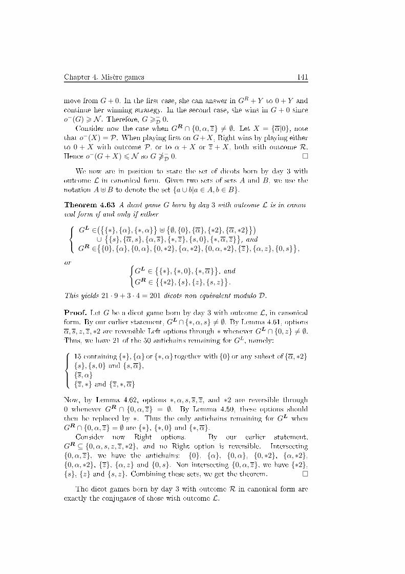
Chapter 4. Misère games 141
move from G+ 0. In the �rst ase, she an answer in GR + Y to 0 + Y and
ontinue her winning strategy. In the se ond ase, she wins in G + 0 sin e
o−(G) > N . Therefore, G >−D 0.
Consider now the ase when GR ∩ {0, α, z} 6= ∅. Let X = {α|0}, notethat o−(X) = P. When playing �rst on G+X, Right wins by playing either
to 0 + X with out ome P, or to α + X or z + X, both with out ome R.
Hen e o−(G+X) 6 N so G �−D 0. �
We now are in position to state the set of di ots born by day 3 with
out ome L in anoni al form. Given two sets of sets A and B, we use the
notation A ⊎B to denote the set {a ∪ b|a ∈ A, b ∈ B}.
Theorem 4.63 A di ot game G born by day 3 with out ome L is in anon-
i al form if and only if either
GL ∈({
{∗}, {α}, {∗, α}}⊎{∅, {0}, {α}, {∗2}, {α, ∗2}
})
∪{{s}, {α, s}, {α, s}, {∗, z}, {s, 0}, {∗, α, z}
}, and
GR ∈{{0}, {α}, {0, α}, {0, ∗2}, {α, ∗2}, {0, α, ∗2}, {z}, {α, z}, {0, s}
},
or {GL ∈
{{∗}, {∗, 0}, {∗, α}
}, and
GR ∈{{∗2}, {s}, {z}, {s, z}
}.
This yields 21 · 9 + 3 · 4 = 201 di ots non equivalent modulo D.
Proof. Let G be a di ot game born by day 3 with out ome L, in anoni al
form. By our earlier statement, GL ∩{∗, α, s} 6= ∅. By Lemma 4.61, options
α, s, z, z, ∗2 are reversible Left options through ∗ whenever GL ∩ {0, z} 6= ∅.Thus, we have 21 of the 50 anti hains remaining for GL
, namely:
15 ontaining {∗}, {α} or {∗, α} together with {0} or any subset of {α, ∗2}{s}, {s, 0} and {s, α},{s, α}{z, ∗} and {z, ∗, α}
Now, by Lemma 4.62, options ∗, α, s, s, z, and ∗2 are reversible through
0 whenever GR ∩ {0, α, z} = ∅. By Lemma 4.50, these options should
then be repla ed by ∗. Thus the only anti hains remaining for GLwhen
GR ∩ {0, α, z} = ∅ are {∗}, {∗, 0} and {∗, α}.Consider now Right options. By our earlier statement,
GR ⊆ {0, α, s, z, z, ∗2}, and no Right option is reversible. Interse ting
{0, α, z}, we have the anti hains: {0}, {α}, {0, α}, {0, ∗2}, {α, ∗2},{0, α, ∗2}, {z}, {α, z} and {0, s}. Non interse ting {0, α, z}, we have {∗2},{s}, {z} and {s, z}. Combining these sets, we get the theorem. �
The di ot games born by day 3 with out ome R in anoni al form are
exa tly the onjugates of those with out ome L.
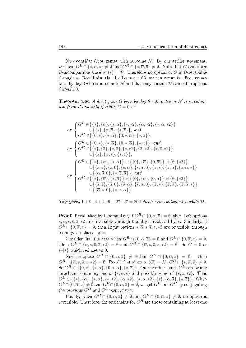
142 4.2. Canoni al form of di ot games
Now onsider di ot games with out ome N . By our earlier statement,
we have GL ∩ {∗, α, s} 6= ∅ and GR ∩ {∗, α, s} 6= ∅. Note that G and ∗ are
D-in omparable sin e o−(∗) = P. Therefore no option of G is D-reversible
through ∗. Re all also that by Lemma 4.62, we an re ognise di ot games
born by day 3 whose out ome isN and that may ontain D-reversible options
through 0.
Theorem 4.64 A di ot game G born by day 3 with out ome N is in anon-
i al form if and only if either G = 0 or
or
GL ∈{{∗}, {α}, {∗, α}, {∗, ∗2}, {α, ∗2}, {∗, α, ∗2}
}
∪{{s}, {α, s}, {∗, z}
}, and
GR ∈{{0, ∗}, {∗, α}, {0, ∗, α}, {∗, z}
},
or
GL ∈{{0, ∗}, {∗, α}, {0, ∗, α}, {∗, z}
}, and
GR ∈{{∗}, {z}, {∗, z}, {∗, ∗2}, {z, ∗2}, {∗, z, ∗2}
}
∪{{s}, {α, s}, {∗, z}
},
or
GL ∈{{∗}, {α}, {∗, α}
}⊎{{0}, {α}, {0, α}
}⊎{∅, {∗2}
}
∪{{s, z}, {s, 0}, {s, α}, {s, α, 0}, {z, ∗}, {z, α}, {z, α, ∗}
}
∪{{α, s, 0}, {∗, z, α}
}, and
GR ∈{{∗}, {α}, {∗, α}
}⊎{{0}, {α}, {0, α}
}⊎{∅, {∗2}
}
∪{{s, z}, {s, 0}, {s, α}, {s, α, 0}, {z, ∗}, {z, α}, {z, α, ∗}
}
∪{{α, s, 0}, {∗, z, α}
}.
This yields 1 + 9 · 4 + 4 · 9 + 27 · 27 = 802 di ots non equivalent modulo D.
Proof. Re all that by Lemma 4.62, if GR ∩ {0, α, z} = ∅, then Left options
∗, α, s, s, z, ∗2 are reversible through 0 and get repla ed by ∗. Similarly, if
GL ∩ {0, α, z} = ∅, then Right options ∗, α, s, s, z, ∗2 are reversible through
0 and get repla ed by ∗.
Consider �rst the ase when GR ∩ {0, α, z} = ∅ and GL ∩ {0, α, z} = ∅.Then GL ∩ {α, s, s, z, ∗2} = ∅ and GR ∩ {α, s, s, z, ∗2} = ∅. So G = 0 or
{∗|∗} whi h redu es to 0.
Now, suppose GR ∩ {0, α, z} 6= ∅ but GL ∩ {0, α, z} = ∅. Then
GR ∩ {α, s, s, z, ∗2} = ∅. Re all that sin e o−(G) = N , GR ∩ {∗, α, s} 6= ∅.So GR ∈ {{0, ∗}, {∗, α}, {0, ∗, α}, {∗, z}}. On the other hand, GL
an be any
anti hain ontaining one of {∗, α, s} and possibly some of {s, z, ∗2}. Thus
GL ∈ {{∗}, {α}, {∗, α}, {∗, ∗2}, {α, ∗2}, {∗, α, ∗2}, {s}, {α, s}, {∗, z}}. When
GL∩{0, α, z} 6= ∅ and GR∩{0, α, z} = ∅, we get GLand GR
by onjugating
the previous GRand GL
respe tively.
Finally, when GR ∩ {0, α, z} 6= ∅ and GL ∩ {0, α, z} 6= ∅, no option is
reversible. Therefore, the anti hains for GRare those ontaining at least one

Chapter 4. Misère games 143
s z
∗ α∗2
α∗+ ∗
s z
0
Figure 4.14: Partial ordering of di ot games born by day 2 in the general universe
of {0, α, z} and one of {∗, α, s}. There are 27 of them, namely:
18 ontaining some subset of {∗, α}, some subset of {0, α} and possibly {∗2}{s, z}{0, s}, {α, s} and {0, α, s},{∗, z}, {α, z} and {∗, α, z},{0, α, s}{∗, α, z}
The anti hains for GLare the onjugates of the anti hains for GR
. �
Adding the number of games with out ome P, L, R, and N , we get:
Theorem 4.65 There are 1268 di ots born by day 3 non equivalent modulo D.
4.2.3.1 Di ot games born by day 3 in the general universe
Comparing the number of di ot games born by day 3 in anoni al form to
the number of games born by day 3 in anoni al form is not that relevant,
as there are only 1046530 game trees of depth 3 representing di ot games,
whi h is far from the 21024 game trees representing all games born by day 3,or even the (slightly less than) 2183 with no dominated option. This is why
we ount the number of di ot games born by day 3 in their general anoni al
form modulo the universe of all games.
Re all that a game is in anoni al form if and only if all its options are
in anoni al form and it has no dominated option nor reversible option.
We �rst re all a result from [38℄.
Theorem 4.66 If H is a Left end and G is not, then G �− H.
This gives us the following orollary, when we only onsider di ot games.
Corollary 4.67 If G is a di ot game whi h is not 0, then G and 0 are
in omparable.

144 4.2. Canoni al form of di ot games
Proposition 4.68 There are 10 di ot games born by day 2 distinguishable
modulo the universe of all games, namely 0, ∗, ∗ + ∗ = {∗|∗} α = {0|∗},α = {∗|0}, s = {0, ∗|0}, z = {0, ∗|∗}, s = {0|0, ∗}, z = {∗|0, ∗}, and
∗2 = {0, ∗|0, ∗}. They are partially ordered a ording to Figure 4.14.
Proof. The proof is similar to the proof of Proposition 4.58. �
We now start ounting the di ot games born by day 3. Their Left and
Right options are ne essarily di ot games born by day 2. We an onsider
only games in their anoni al form, so with no dominated option.
Using Figure 4.14, we �nd the following 100 anti hains:
all 64 subsets of {0, ∗ + ∗, ∗, α, α, ∗2},{s, z}, {0, s, z}, {s, z} and {0, s, z},8 ontaining s and any subset of {0, ∗ + ∗, α}8 ontaining z and any subset of {0, ∗, α}8 ontaining s and any subset of {0, ∗ + ∗, α}8 ontaining z and any subset of {0, ∗, α}
Therefore, hoosing GLand GR
among these anti hains, together with
the fa t that G is di ot, we get 992 + 1 = 9802 di ot games born by day 3with no dominated option.
To get only games in anoni al form, we still have to remove games with
reversible options. Note that an option from a di ot game born by day 3 an only be reversible through 0 or ∗ sin e these are the only di ot games
born by day 1. As no di ot game is omparable with 0, no option an be
reversible through 0. Note that as o−(∗) = P, no game with out ome Nmay have a reversible option through ∗, and no game with out ome R may
have a Left option reversible through ∗. Again, if Left has a winning move
from a game G, namely a move to ∗, α or s, or if she has no move from G,then o−(G) > N . Otherwise, o−(G) 6 P. Likewise, if Right has a winning
move from G, namely a move to ∗, α or s, or if he has no move from G, theno−(G) 6 N . Otherwise, o−(G) > P.
We now hara terise di ot games having reversible options.
Lemma 4.69 Let G be a di ot game born by day 3 with misère out ome Por L. We have G >− ∗ if and only if 0 ∈ GL
.
Proof. First suppose 0 ∈ GL. Let X be a game su h that Left has a winning
strategy on ∗ +X when playing �rst (respe tively se ond). Left an follow
the same strategy on G+X, unless the strategy re ommends that she plays
from some ∗ + Y to 0 + Y , or Right eventually plays from some G + Z to
some GR + Z. In the �rst ase, she an just play from G + Y to 0 + Y .
Suppose now that Right just moved from G + Z to some GR + Z. By our
hoi e of strategy, we have o−(∗+Z) > P. If GR = 0, then Left an ontinue

Chapter 4. Misère games 145
her strategy sin e 0 + Z is also a Right option of ∗ + Z. Otherwise, sin e
GR ∩ {∗, α, s} = ∅, GRis one of ∗+ ∗, α, s, z, z, ∗2 and ∗ is a Left option of
GR. Then Left an play from GR + Z to ∗+ Z and win. Thus, if Left wins
∗+X, she wins G+X as well and thus G >− ∗.
Assume now 0 /∈ GL. Let X = {·|{·|3}}. In ∗+X, Left wins by moving
to X, so o−(∗ +X) > N . On the other hand, in G +X, Left has to move
to some GL + X, where GLis a non-zero di ot. Then Right an move to
GL + {·|3}, where Left has to play in GL, to GLL + {·|3}, where GLL
is a
di ot born by day 1. Right's move to GLL+3 is then a winning move. hen e
o−(G+X) 6 P, and we have G �− ∗. �
We now are in position to state the set of di ot games born by day 3 in
anoni al form (modulo the universe of all games) with any out ome.
Theorem 4.70 A di ot game G born by day 3 with out ome P is in anon-
i al form if and only if
GL ∈{{∗+ ∗}, {α}, {∗2}, {∗ + ∗, α}, {∗ + ∗, ∗2}, {α, ∗2}, {∗ + ∗, α, ∗2}
}
∪{{0}, {s, z}, {z}, {s}, {s, ∗ + ∗}, {z}, {z, α}
}
GR ∈{{∗+ ∗}, {α}, {∗2}, {∗ + ∗, α}, {∗ + ∗, ∗2}, {α, ∗2}, {∗ + ∗, α, ∗2}
}
∪{{0}, {s, z}, {z}, {s}, {s, ∗ + ∗}, {z}, {z, α}
}
This yields 14 · 14 = 196 non-equivalent di ot games.
Theorem 4.71 A di ot game G born by day 3 with out ome L is in anon-
i al form if and only if
GL ∈{{∗}, {α}, {∗, α}
}⊎{{∗+ ∗}, {α}, {∗ + ∗, α}
}⊎{∅, {∗2}
}
∪{{s, z}, {s, ∗ + ∗}, {s, α}, {s, α, ∗+ ∗}, {z, ∗}, {z, α}, {z, α, ∗}
}
∪{{α, s, ∗ + ∗}, {∗, z, α}, {s}, {α, s}, {∗, z}
}
∪{{∗}, {α}, {∗, α}, {∗, ∗2}, {α, ∗2}, {∗, α, ∗2}
}
∪{{0, ∗}, {0, α}, {0, ∗, α}, {0, s}
}, and
GR ∈{{∗+ ∗}, {α}, {∗2}, {∗ + ∗, α}, {∗ + ∗, ∗2}, {α, ∗2}, {∗ + ∗, α, ∗2}
}
∪{{s, z}, {z}, {s}, {s, ∗ + ∗}, {z}, {z, α}, {0}, {0, ∗ + ∗}, {0, α}
}
∪{{0, ∗2}, {0, ∗ + ∗, α}, {0, ∗ + ∗, ∗2}, {0, α, ∗2}, {0, ∗ + ∗, α, ∗2}
}
∪{{0, s, z}, {0, z}, {0, s}, {0, s, ∗ + ∗}, {0, z}, {0, z, α}
}
This yields 40 · 27 = 1080 non-equivalent di ot games.
The di ot games born by day 3 with out ome R in anoni al form are
exa tly the onjugates of those with out ome L.
Theorem 4.72 A di ot game G born by day 3 with out ome N is in anon-
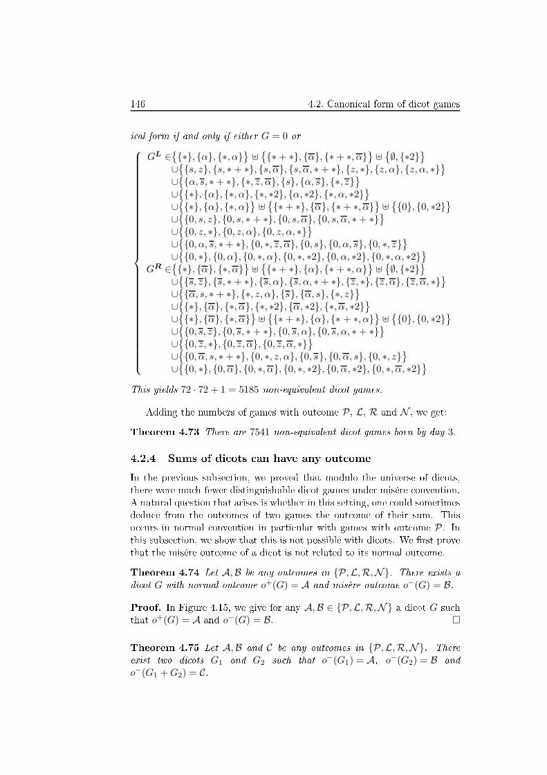
146 4.2. Canoni al form of di ot games
i al form if and only if either G = 0 or
GL ∈{{∗}, {α}, {∗, α}
}⊎{{∗+ ∗}, {α}, {∗ + ∗, α}
}⊎{∅, {∗2}
}
∪{{s, z}, {s, ∗ + ∗}, {s, α}, {s, α, ∗+ ∗}, {z, ∗}, {z, α}, {z, α, ∗}
}
∪{{α, s, ∗+ ∗}, {∗, z, α}, {s}, {α, s}, {∗, z}
}
∪{{∗}, {α}, {∗, α}, {∗, ∗2}, {α, ∗2}, {∗, α, ∗2}
}
∪{{∗}, {α}, {∗, α}
}⊎{{∗ + ∗}, {α}, {∗ + ∗, α}
}⊎{{0}, {0, ∗2}
}
∪{{0, s, z}, {0, s, ∗ + ∗}, {0, s, α}, {0, s, α, ∗+ ∗}
}
∪{{0, z, ∗}, {0, z, α}, {0, z, α, ∗}
}
∪{{0, α, s, ∗+ ∗}, {0, ∗, z, α}, {0, s}, {0, α, s}, {0, ∗, z}
}
∪{{0, ∗}, {0, α}, {0, ∗, α}, {0, ∗, ∗2}, {0, α, ∗2}, {0, ∗, α, ∗2}
}
GR ∈{{∗}, {α}, {∗, α}
}⊎{{∗+ ∗}, {α}, {∗ + ∗, α}
}⊎{∅, {∗2}
}
∪{{s, z}, {s, ∗+ ∗}, {s, α}, {s, α, ∗ + ∗}, {z, ∗}, {z, α}, {z, α, ∗}
}
∪{{α, s, ∗ + ∗}, {∗, z, α}, {s}, {α, s}, {∗, z}
}
∪{{∗}, {α}, {∗, α}, {∗, ∗2}, {α, ∗2}, {∗, α, ∗2}
}
∪{{∗}, {α}, {∗, α}
}⊎{{∗ + ∗}, {α}, {∗ + ∗, α}
}⊎{{0}, {0, ∗2}
}
∪{{0, s, z}, {0, s, ∗+ ∗}, {0, s, α}, {0, s, α, ∗ + ∗}
}
∪{{0, z, ∗}, {0, z, α}, {0, z, α, ∗}
}
∪{{0, α, s, ∗+ ∗}, {0, ∗, z, α}, {0, s}, {0, α, s}, {0, ∗, z}
}
∪{{0, ∗}, {0, α}, {0, ∗, α}, {0, ∗, ∗2}, {0, α, ∗2}, {0, ∗, α, ∗2}
}
This yields 72 · 72 + 1 = 5185 non-equivalent di ot games.
Adding the numbers of games with out ome P, L, R and N , we get:
Theorem 4.73 There are 7541 non-equivalent di ot games born by day 3.
4.2.4 Sums of di ots an have any out ome
In the previous subse tion, we proved that modulo the universe of di ots,
there were mu h fewer distinguishable di ot games under misère onvention.
A natural question that arises is whether in this setting, one ould sometimes
dedu e from the out omes of two games the out ome of their sum. This
o urs in normal onvention in parti ular with games with out ome P. In
this subse tion, we show that this is not possible with di ots. We �rst prove
that the misère out ome of a di ot is not related to its normal out ome.
Theorem 4.74 Let A,B be any out omes in {P,L,R,N}. There exists a
di ot G with normal out ome o+(G) = A and misère out ome o−(G) = B.
Proof. In Figure 4.15, we give for any A,B ∈ {P,L,R,N} a di ot G su h
that o+(G) = A and o−(G) = B. �
Theorem 4.75 Let A,B and C be any out omes in {P,L,R,N}. There
exist two di ots G1 and G2 su h that o−(G1) = A, o−(G2) = B and
o−(G1 +G2) = C.

Chapter 4. Misère games 147
Normal→Misère ↓
P L R N
P
L
R
N
Figure 4.15: Normal and misère out omes of some di ots
Proof. In Figure 4.16, we give for any A,B, C ∈ {P,L,R,N} two games
G1 and G2 su h that o−(G1) = A, o−(G2) = B and o−(G1 +G2) = C. �
4.3 A peek at the dead-ending universe
In many ombinatorial games, players pla e pie es on a board a ording to
some set of rules. Usually, these rules imply that the board spa e available
to a player at their turn are a subset of those available on the previous turn.
Among games �tting that des ription, we an mention Col, Domineering,
Hex, or Snort. One an also see it as a board where pie es are removed,
with rules implying that the set of pie es removable is de reasing after ea h
turn. Among games �tting that des ription, we an mention Ha kenbush,
Nim or any o tal game, or Timbush. A property all these games share in
ontrast with Partizan Peg Duotaire or Flip the oin is that no player
an `open up' moves for themself or for their opponent; in parti ular, a player
who has no available move at some position will not be able to play for the
rest of the game. This is the property we all dead-ending.
We re all the more formal de�nition of dead-ending: A Left (Right) end
is a dead end if every follower is also a Left (Right) end. A game is said to
be dead-ending if all its end followers are dead ends.
Note that di ot games, studied in Se tion 4.2, are all dead-ending, as the
only end follower of a di ot is 0, whi h is a dead end.
Example 4.76 Figure 4.17 gives three examples of games that are dead-
ending. The �rst game is a dead end. The se ond game is dead-ending as its
end followers are either 0 or 1, whi h are both dead ends. The third game is
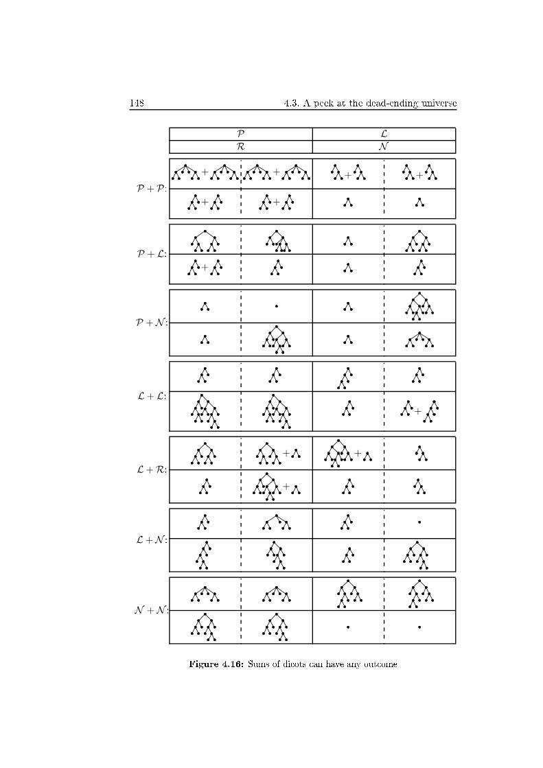
148 4.3. A peek at the dead-ending universe
P LR N
P + P:
+ + + +
+ +
P + L:
+
P +N :
L+ L:
+
L+R:
+ +
+
L+N :
N +N :
Figure 4.16: Sums of di ots an have any out ome

Chapter 4. Misère games 149
Figure 4.17: Some dead-ending positions
Figure 4.18: Some positions that are not dead-ending
a di ot game, hen e a dead-ending game. Figure 4.18 gives three examples
of games that are not dead-ending. The �rst game is a Right end that is not
a dead end as Right an move from one of Left's options. The se ond game
is not dead-ending be ause its Left option is a Left end that is not a dead
end. The third game is not dead-ending be ause both its Left option and its
Right option are ends that are not dead ends.
In the following, we look at numbers under their normal anoni al form.
Sin e, among other short omings, 1 ≮−E 2 or
1
2+ 1
26≡−
E 1 as games, to avoid
onfusion, we distinguish between the game a and the number a. For the
rest of this se tion, we use the notation 0 for the game {·|·} too.
In this se tion, we �nd the misère monoid of dead ends, the misère monoid
of normal-play anoni al form numbers, give their partial order modulo the
dead-ending universe and dis uss other dead-ending games, in the ontext
of equivalen y to zero modulo the universe of dead-ending games.
4.3.1 Preliminary results
We start by proving the losure of the dead-ending universe under the three
aspe ts we mentioned in the introdu tion of this hapter: it is losed under
followers, losed under disjun tive sum, and losed under onjugates.
Lemma 4.77 If G is dead-ending then every follower of G is dead-ending.

150 4.3. A peek at the dead-ending universe
Proof. If H is a follower of G, then every follower of H is also a follower of
G; thus if G satis�es the de�nition of dead-ending, then so does H. �
Lemma 4.78 If G and H are dead-ending then G+H is dead-ending.
Proof. Any follower of G+H is of the form G′ +H ′where G′
and H ′are
(not ne essarily proper) followers of G and H, respe tively. If G′ +H ′is a
Left end, then both G′and H ′
are Left ends, whi h must be dead, sin e Gand H are dead-ending. Thus, any followers G′′
and H ′′are Left ends, and
so all followers G′′ + H ′′of G′ + H ′
are Left ends. A symmetri argument
holds if G′ +H ′is a Right end, and so G+H is dead-ending. �
Lemma 4.79 If G is dead-ending, then G is dead-ending.
Proof. Any follower of G is the onjugate of a follower of G. If H is an end,
so is H, hen e assuming H is a follower of G, H is a dead end, and so is H.
�
Under misère play, Left wins any Left end playing �rst as she already has
no move. In a general ontext, she might lose playing se ond, for example
in the game {·|∗}, whi h is both a Left end and a misère N -position. In the
dead-ending universe, however, Left wins any non-zero Left end playing �rst
or se ond.
Lemma 4.80 If G 6= 0 is a dead Left end then G ∈ L−, and if G 6= 0 is a
dead Right end then G ∈ R−.
Proof. A Left end is always in L−or N−
. If G is a dead Left end then
any Right option GRis also a Left end, so Right has no good �rst move.
Similarly, a dead Right end is in R−. �
In the following of this se tion, we refer to two game fun tions de�ned
below, whi h are well-de�ned for our purpose, namely for numbers and ends.
De�nition 4.81 The left-length of a game G, denoted l(G), is the minimum
number of onse utive Left moves required for Left to rea h zero in G. Theright-length r(G) of G is the minimum number of onse utive Right moves
required for Right to rea h zero in G.
In general, the left- and right-length are well-de�ned if G has a non-
alternating path to zero for Left or Right, respe tively, and if the shortest
of su h paths is never dominated by another option. The latter ondition
ensures l(G) = l(G′) when G ≡− G′. As suggested above, both of these
onditions are met if G is a (normal-play) anoni al-form number or if G is
an end in E . If l(G) and l(H) are both well-de�ned then l(G+H) is de�nedand l(G+H) = l(G) + l(H). Similarly, when the right-length is de�ned for
G and H, we have r(G+H) = r(G) + r(H).
Chapter 4. Misère games 151
It would be possible to extend these fun tions to all games by repla ing
�zero� by �a Left end� for the left-length, and by �a Right end� for the right-
length, but we want to insist here that in the ases we use it, the end we
rea h is zero.
4.3.2 Integers and other dead ends
We �rst look at dead ends, with some fo us on integers.
Re all that n denote the game {n − 1|·} when n is positive, where 0 ={·|·}. Considering two positive integers n and m, their disjun tive sum has
the same game tree as the integer n + m. This is not true if n is negative
and m positive, and the two games (the disjun tive sum and the integer) are
not even equivalent in general misère play.
Any integer is an example of a dead end: if n > 0, then Right has no
move in n, and we indu tively see that he has no move in any follower of n;
similarly, if n < 0, then n is a dead Left end. Thus, the following results for
ends in the dead-ending universe are also true for all integers, modulo E .Our �rst result shows that when all games in a sum are dead ends, the
out ome is ompletely determined by the left- and right-lengths of the games.
As a sum of Left ends is a Left end and a sum of Right ends is a Right end,
we only onsider two games in a sum of ends, one being a Left end and the
other a Right end.
Lemma 4.82 If G is a dead Right end and H is a dead Left end then
o−(G+H) =
N−if l(G) = r(H)
L−if l(G) < r(H)
R−if l(G) > r(H)
Proof. Ea h player has no hoi e but to play in their own game, and so the
winner will be the player who an run out of moves �rst. �
We use Lemma 4.82 to prove the following theorem, whi h demonstrates
the invertibility of all ends modulo E , even giving the orresponding inverse.
Theorem 4.83 If G is a dead end, then G+G ≡−E 0.
Proof. Assume without loss of generality that G 6= 0 is a dead right
end. Sin e every follower of a dead end is also a dead end, Lemma 4.2
applies, with S the set of all dead Left and Right ends. It therefore suf-
� es to show G+G+X ∈ L− ∪ N−for any Left end X in E. We have
l(G) = r(G) and r(X) > 0, so l(G) 6 r(G) + r(X) = r(G+X), whi h gives
G+G+X ∈ L− ∪ N−by Lemma 4.82. �
We immediately get the following orollary by re alling that integers are
dead ends.

152 4.3. A peek at the dead-ending universe
Corollary 4.84 If n is an integer, then n+ n ≡−E 0.
This implies the following orollary about any sum of integers.
Corollary 4.85 If n and m are integers, then n+m ≡−E n+m.
Re all that equivalen y in E implies equivalen y in all subuniverse of E .Thus, in the universe of integers alone, every integer keeps its inverse.
Lemma 4.82 shows that when playing a sum of dead ends, both players
aim to exhaust their moves as fast as possible. This suggests that longer
paths to zero would be dominated by shorter paths; in parti ular, this would
give a total ordering of integers among dead ends, as established in Theo-
rem 4.86 below. Note that this ordering only holds in the subuniverse of the
losure of dead ends, that is the universe of sums of dead ends, and not in
the whole universe E . A tually, we show right in Theorem 4.87 that distin t
integers are in omparable modulo E , just as they are in the general misère
universe.
Theorem 4.86 If n < m ∈ Z, then n >−m modulo the losure of dead
ends.
Proof. By Corollary 4.84, it su� es to show n + m >− 0 (equivalently,
k > 0 for any negative integer k), modulo the losure of dead ends. Let Xbe any game in the losure of dead ends; then X = Y + Z where Y is a
dead Right end and Z is a dead Left end. Suppose Left wins X playing �rst;
then by Lemma 4.82, l(Y ) 6 r(Z). We need to show Left wins k + X, so
that o−(k +X) > o−(X). Sin e k is a negative integer, r(k) is de�ned and
r(k) = −k > 0. Thus l(Y ) 6 r(Z) < r(Z) + r(k) = r(Z + k), whi h gives
k + Y + Z = k+X ∈ L− ∪ N−, by Lemma 4.82. �
In general, an inequality under misère play between games implies the
same inequality under normal play between the same games [38℄. This is
also true for some spe i� universes, as we have seen with the di ot universe
in Se tion 4.2. Theorem 4.86 shows this is not always true for any universe.
We now show that integers, despite being totally ordered in the losure
of dead ends, are pairwise in omparable in the dead-ending universe.
Theorem 4.87 If n 6= m ∈ Z, then n ‖−E m.
Proof. Assume n > m.
De�ne two families of games αk and βk by
α1 = {0|0};αk = {0|αk−1};βk = {αk|αk}.
Note that o−(βk) = N and o−(k + βk) = P for all pos-
itive k. Thus m + m + βn−m ≡−E βn−m ∈ N−
and

Chapter 4. Misère games 153
n + m + βn−m ≡−E n−m + βn−m ∈ P−
, and m + βn−m witnesses
both n �−E m and n −
E m. �
As integers are pairwise in omparable, a dead end having several options
might have no E-dominated option. Thus, in the dead-ending universe, there
exists ends that are not integers. However, when restri ting ourselves to the
subuniverse of the losure of dead ends, the ordering given by theorem 4.86
implies that every end redu es to an integer. This fa t is presented in the
following lemma.
Lemma 4.88 If G is a dead end then G ≡−n modulo the losure of dead
ends, where n = l(G) if G is a Right end and n = −r(G) if G is a Left end.
Proof. Let G be a dead Right end (the argument for Left ends is sym-
metri ). Assume by indu tion that every option GLiof G (ne essarily a
dead Right end) is equivalent to the integer l(GLi). Modulo dead ends, by
Theorem 4.86, these Left options are totally ordered; thus G = {GL1 |·} for
GL1with smallest left-length. Then G is the anoni al form of the integer
l(GL1) + 1 = l(G). �
Lemma 4.88 shows that the losure of dead ends has pre isely the same
misère monoid as the losure of integers. The game of Domineering on
1 × n and n × 1 board is an instan e of these universes. We are now able
to ompletely des ribe the misère monoid of the losure of dead ends, whi h
we present in Theorem 4.89.
Theorem 4.89 Under the mapping
G 7→
{αl(G)
if G is a Right end
α−r(G)if G is a Left end
,
the misère monoid of the losure of dead ends is
MZ = 〈1, α, α−1 | α · α−1 = 1〉
with out ome partition
N− = {1},L− = {α−n|n ∈ N∗},R− = {αn|n ∈ N∗}
and total ordering
αn > αm ⇔ n < m.
4.3.3 Numbers
4.3.3.1 The misère monoid of Q2
We now look at all numbers under their normal anoni al form.

154 4.3. A peek at the dead-ending universe
We say a game a is a non-integer number if it is the normal-play anoni al
form of a (non-integer) dyadi rational, that is
a =2∗m+1
2k=
{2∗m
2k
∣∣2∗m+2
2k
},
with k > 0. The set of all integer and non-integer ( ombinatorial game)
numbers is thus the set of dyadi rationals, whi h we denote by Q2. As we
did for integers previously, we now determine the out ome of a general sum
of dyadi rationals and thereby des ribe the misère monoid of the losure of
numbers.
Note that the sum of two non-integer numbers (even if both are positive)
is not ne essarily another number. For example,
1
2+ 1
26= 1. We see in the
following that, unlike integers, the set of dyadi rationals is not losed under
disjun tive sum even when restri ted to the dead-ending universe; however,
losure does o ur when we restri t to numbers alone.
Lemma 4.92 below, analogous to Lemma 4.82 of the previous se tion,
shows that the out ome of a sum of numbers is determined by the left-
and right-lengths of the individual numbers. To prove this, we require
Lemma 4.91, whi h establishes a relationship between the left- or right-
lengths of numbers and their options; and to prove Lemma 4.91, we need
the following proposition.
Proposition 4.90 If a ∈ Q2\Z then at least one of aRLand aLR exists, and
either aL = a
RLor a
R = aLR
.
Proof. Let a = 2∗m+1
2kwith k > 0. If m ≡ 0( mod 2) then
aL =
2∗m
2k;aR =
2∗m+2
2k=
2∗m+2
2
2k−1=
{2∗m
2
2k−1
∣∣2∗m+4
2
2k−1
},
so aL = a
RL. Otherwise, m ≡ 1( mod 2) and then
aL =
2∗m
2k=
2∗m
2
2k−1=
{2∗m−2
2
2k−1
∣∣2∗m+2
2
2k−1
};aR =
2∗m+2
2k,
so aR = a
LR. �
Note that if a > 0 is a dyadi rational, then l(a) = 1 + l(aL), andif a < 0 is a dyadi rational, then r(a) = 1 + r(aR). We also have the
following inequalities for left-lengths of right options and right-lengths of
left options, when a is a non-integer dyadi rational.
Lemma 4.91 If a ∈ Q2\Z is positive, then l(aR) 6 l(a); if a is negative,
then r(aL) 6 r(a).
Chapter 4. Misère games 155
Proof. Assume a > 0 (the argument for a < 0 is symmetri ). Sin e a is in
anoni al form, both aLand a
Rare positive numbers. If a
L = aRL
, then
l(aR) = 1 + l(aRL) = 1 + l(aL) = l(a). Otherwise aR = a
LR, by Proposi-
tion 4.90; then aLis not an integer be ause a
LRexists, so by indu tion we
obtain l(aR) = l(aLR) 6 l(aL) = l(a)− 1 < l(a). �
We an now determine the out ome of a general sum of numbers, both
integer and non-integer.
Lemma 4.92 If {ai}16i6n and {bi}16i6m are sets of positive and negative
numbers, respe tively, with k =∑n
i=1 l(ai)−∑m
i=1 r(bi), then
o−
(n∑
i=1
ai +
m∑
i=1
bi
)=
L−if k < 0
N−if k = 0
R−if k > 0.
Proof. Let G =∑n
i=1 ai+∑m
i=1 bi. All followers of G are also of this form,
so assume the result holds for every proper follower of G. Suppose k < 0. Ifn = 0 then Left will run out of moves �rst be ause Left annot move last in
any negative number. So assume n > 0. Left moving �rst an move in an ai
to redu e k by one (sin e l(aiL) = l(ai) − 1), whi h is a Left-win position
by indu tion. If Right moves �rst in an ai then k does not in rease, sin e
l(aiR) 6 l(ai) by Lemma 4.91, so the position is a Left-win by indu tion; if
Right moves �rst in a bi then k does in rease by one, but Left an respond in
an ai (sin e n > 0) to bring k down again, leaving another Left-win position,
by indu tion. Thus G ∈ L−if k < 0.
The argument for k > 0 is symmetri . If k = 0 then either G = 0 is
trivially next-win, or both n and m are at least 1 and both players have a
good �rst move to hange k in their favour. �
Lemma 4.92 shows that in general misère play, the out ome of a sum of
numbers is ompletely determined by the left-lengths and right-lengths of the
positive and negative omponents, respe tively. From this we an on lude
that, modulo the losure of anoni al-form numbers, a positive number a is
equivalent to every other number with left-length l(a). In parti ular, every
positive number a is equivalent to the integer l(a). This is Corollary 4.93
below; together with Theorem 4.96, it will allow us to des ribe the misère
monoid of anoni al-form numbers.
Corollary 4.93 If a is a number, then
a ≡−Q2
{l(a) if a > 0
−r(a) if a < 0
As examples, the dyadi rational
3
4is equivalent to 2, and −11
8is equiv-
alent to −3, modulo Q2. Note that these equivalen ies do not hold in the

156 4.3. A peek at the dead-ending universe
larger universe E , as we see in the following that if a 6= b are numbers, thena 6≡−
E b.
We see then that the losure of numbers is isomorphi to the losure of
just integers; when restri ted to numbers alone, every non-integer is equiva-
lent to an integer. Thus the misère monoid of numbers, given below, is the
same monoid presented in Theorem 4.89.
Theorem 4.94 Under the mapping
a 7→
{αl(a)
if a is positive
α−r(a)if a is negative
,
the misère monoid of the losure of anoni al-form dyadi rationals is
MZ = 〈1, α, α−1 | α · α−1 = 1〉
with out ome partition
N− = {1},L− = {α−n|n ∈ N∗},R− = {αn|n ∈ N∗}.
As with integers, some of the stru ture found in the number universe is
also present in the larger universe E . We now give a proof that all numbers,
and not just integers, are invertible in the universe of dead-ending games,
having their onjugates as inverses. We require the following lemma, an
extension of Lemma 4.92.
Lemma 4.95 If {ai}16i6n and {bi}16i6m are sets of positive and negative
numbers, respe tively, and
∑ni=1 l(ai)−
∑mi=1 r(bi) < 0, then
o−
(n∑
i=1
ai +m∑
i=1
bi
)= L−
for any dead Left end X.
Proof. The argument from Lemma 4.92 works again, sin e if Right uses his
turn to play in X then Left responds with a move in a1 to de rease k by 1,whi h is a win for Left by indu tion. �
We an now apply Lemma 4.2 to on lude on the invertibility of all
numbers.
Theorem 4.96 If a ∈ Q2, then a+ a ≡−E 0.
Proof. Without loss of generality we an assume a is positive. Sin e every
follower of a number is also a number, we an use Lemma 4.2. That is, it suf-
� es to show a+ a+X ∈ L− ∪ N−for any Left end X ∈ E . IfX = 0, this is
true by Lemma 4.92. If X 6= 0, then we laim a+ a+X ∈ L−; assume this
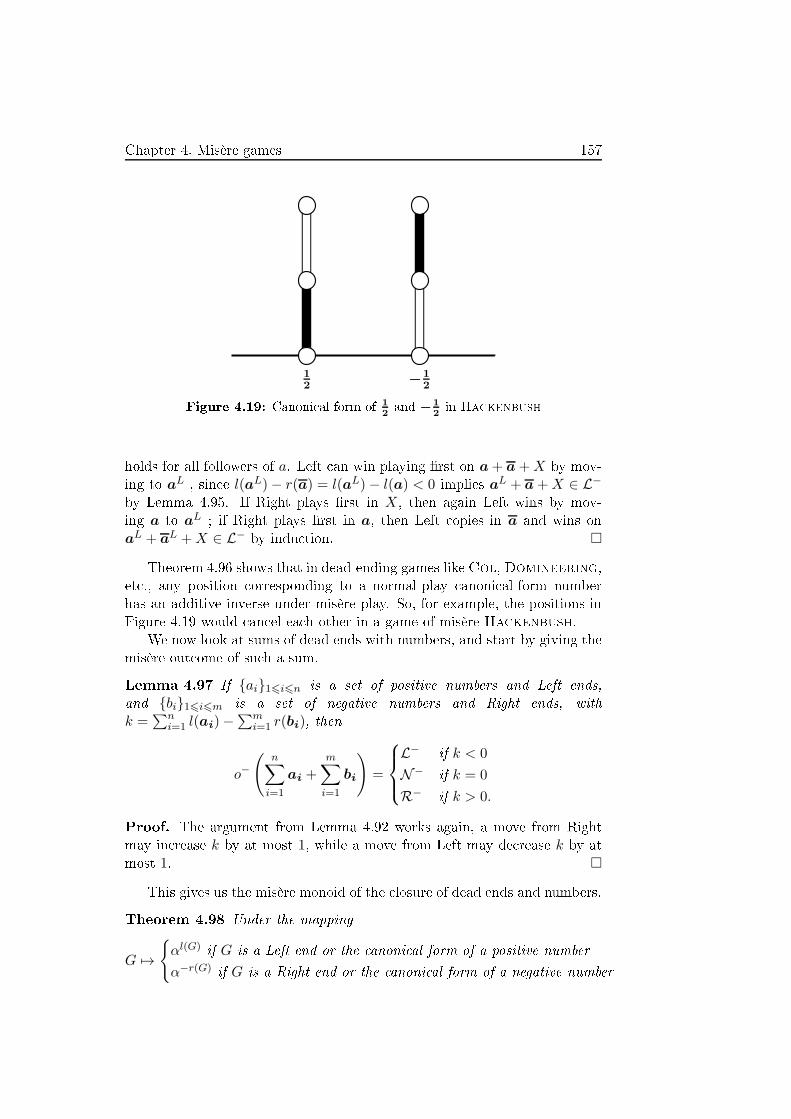
Chapter 4. Misère games 157
1
2−
1
2
Figure 4.19: Canoni al form of
1
2and −
1
2in Ha kenbush
holds for all followers of a. Left an win playing �rst on a+ a+X by mov-
ing to aL, sin e l(aL)− r(a) = l(aL)− l(a) < 0 implies a
L + a+X ∈ L−
by Lemma 4.95. If Right plays �rst in X, then again Left wins by mov-
ing a to aL; if Right plays �rst in a, then Left opies in a and wins on
aL + a
L +X ∈ L−by indu tion. �
Theorem 4.96 shows that in dead-ending games like Col, Domineering,
et ., any position orresponding to a normal-play anoni al-form number
has an additive inverse under misère play. So, for example, the positions in
Figure 4.19 would an el ea h other in a game of misère Ha kenbush.
We now look at sums of dead ends with numbers, and start by giving the
misère out ome of su h a sum.
Lemma 4.97 If {ai}16i6n is a set of positive numbers and Left ends,
and {bi}16i6m is a set of negative numbers and Right ends, with
k =∑n
i=1 l(ai)−∑m
i=1 r(bi), then
o−
(n∑
i=1
ai +
m∑
i=1
bi
)=
L−if k < 0
N−if k = 0
R−if k > 0.
Proof. The argument from Lemma 4.92 works again, a move from Right
may in rease k by at most 1, while a move from Left may de rease k by at
most 1. �
This gives us the misère monoid of the losure of dead ends and numbers.
Theorem 4.98 Under the mapping
G 7→
{αl(G)
if G is a Left end or the anoni al form of a positive number
α−r(G)if G is a Right end or the anoni al form of a negative number

158 4.3. A peek at the dead-ending universe
the misère monoid of the losure of dead ends and anoni al-form dyadi
rationals is
MZ = 〈1, α, α−1 | α · α−1 = 1〉
with out ome partition
N− = {1},L− = {α−n|n ∈ N∗},R− = {αn|n ∈ N∗}.
4.3.3.2 The partial order of numbers modulo E
Previously, we found that all integers were in omparable in the dead-ending
universe. We will see now that non-integer numbers are a bit more oop-
erative; although not totally ordered, we do have a ni e hara terisation of
the partial order of numbers in the universe E . First note that from Corol-
lary 4.57, we get the following result.
Theorem 4.99 If G >−E H, then G >+ H
This gives us the following orollary on numbers.
Corollary 4.100 If a, b ∈ Q2 and a > b, then a −E b.
Theorem 4.99 says that if a >−E b, then a > b as real numbers (or as
normal-play games). The onverse is learly not true for integers, by Theo-
rem 4.87; it is also not true for non-integers, sin e
1
2+ 1
2is a misèreN -position
while
3
4+ 1
2is a misère R-position, so that
1
2−
E3
4. Theorem 4.103 shows
that the additional stipulation l(a) 6 l(b) is su� ient for a >−E b. To prove
this result we need the following lemmas. As before, non-bold symbols rep-
resent a tual numbers, so that `a < b' indi ates inequality of a and b as
rational numbers, and aL means the rational number orresponding to the
left-option of the game a in anoni al form. Re all that if x = {xL|xR} is in(normal- play) anoni al form then x is the simplest number (i.e., the num-
ber with smallest birthday) su h that xL < x < xR. Thus, if xL < x, y < xR
and x 6= y, then x is simpler than y.
Lemma 4.101 If a and b are positive numbers su h that aL < b < a, thenl(aL) < l(b).
Proof. We have aL < b < a < aR, so a must be simpler than
b. Thus bL > aL, sin e otherwise bL < aL < b < bR would imply
that b is simpler than aL, whi h is simpler than a. Now, if bL = aL
then l(aL) = l(bL) = l(b)− 1 < l(b), and if bL > aL then by indu tion
aL < bL < b < a gives l(aL) < l(bL) = l(b)− 1 < l(b). �
Lemma 4.101 is now used to prove Lemma 4.102 below, whi h is needed
for the proof of Theorem 4.103. Note that in the following two arguments we
frequently use the fa t that, if a >−E b, then Left wins the position a+b+X
whenever she wins X ∈ E .

Chapter 4. Misère games 159
Lemma 4.102 If a and b are positive numbers su h that aL < b < a, thena >−
E b.
Proof. Note that b /∈ Z sin e there is no integer between aL and a if a is in
anoni al form. We must show that Left wins a+ b+X whenever she wins
X ∈ E .Case 1: bR = a.
Left an win a+b+X by playing her winning strategy on X. If Right moves
in a+ b to aR+ b+X ′
, then Left responds to aR + b
R+X ′ = aR+a+X ′
,
whi h she wins by indu tion sin e aRL 6 aL (see Proposition 4.90) gives
aRL < a < aR. If Right moves to a + bR+ X ′ = b
R + bR+ X ′
, with
X ′ ∈ L− ∪P−(sin e Left is playing her winning strategy in X), then Left's
response depends on whether bRL = bL or bLR = bR: in the former ase,
Left moves to bRL + b
R+X ′ = b
L + bL +X ′ ≡−
E X; in the latter ase, Left
moves to bR + b
LL+X ′ = b
R + bLR +X ′ = b
R + bR +X ′ ≡−
E X ′. In either
ase, Left wins as the previous player on X ′ ∈ L− ∪ P−.
When Left runs out of moves in X, she moves to aL + b + X ′′
. By
Lemma 4.101 we know l(aL) < l(b), and this gives o−(aL + b +X ′′) = L−
by Lemma 4.95.
Case 2: bR 6= a.Note that bR annot be greater than a, sin e aL < b < a < aR implies a is
simpler than b, while bL < b < a < bR would imply that b is simpler than
a. So bR < a, and together with aL < b < bR this gives aL < bR < a, whi hshows a >
−E b
Rby indu tion. Similarly bRL 6 bL < b < bR implies b
R >−E b,
by Case 1. Then by transitivity we have a >−E b. �
With lemma 4.102, we an now prove Theorem 4.103 below. The sym-
metri result for negative numbers holds as well.
Theorem 4.103 If a and b are positive numbers su h that a > b and
l(a) 6 l(b), then a >−E b.
Proof. By Corollary 4.100, we have a 6≡−E b, and so it su� es to show
a >−E b. Again we have b /∈ Z. Sin e a > b, if b > aL, then Lemma 4.102
gives a >−E b as required. So assume b 6 aL. Again, let X ∈ E be a game
whi h Left wins playing �rst; we must show Left wins a+b+X playing �rst.
Left should follow her winning strategy from X. If Right plays to a+bL+X ′
,
where X ′ ∈ L−∪P−, then Left responds with a
L+ bL+X ′
, whi h she wins
by indu tion: bL < b 6 aL and l(bL) = l(b) − 1 > l(a) − 1 = l(aL) implies
aL >−
E bL.
If Right plays to aR + b + X ′
(assuming this move exists), then
Left's response is aRL + b + X ′
if aRL > b, or aR + b
R + X ′if
aRL 6 b. In the �rst ase, Left wins by indu tion be ause aRL > b and
l(aRL) = l(aR)− 1 6 l(a)− 1 < l(b) implies aRL >−
E b. In the latter ase,

160 4.3. A peek at the dead-ending universe
note �rst that in fa t aRL 6= b, sin e we have already seen that as games
they have di�erent left-lengths. Then we see aRL < b < a < aR < aRR,
whi h shows aRmust be simpler than b. This gives bR 6 aR, as otherwise
bL < b < a < aR < bR would imply that b is simpler than aR. If bR = aR,
then bR = a
R, and if bR < aR, then we an apply Lemma 4.102 to on lude
that aR >−
E bR. In either ase, Left wins a
R + bR +X ′
with X ′ ∈ L− ∪ P−
as the se ond player.
Finally, if Left runs out of moves in X, then she moves to aL + b+X ′′
where X ′′is a dead Left end; then Left wins by Lemma 4.95 be ause
l(aL) < l(a) 6 l(b) = r(b). �
Corollary 4.104 For positive numbers a, b ∈ Q2, a >−E b if and only if
a > b and l(a) 6 l(b).
Proof. We need only prove the onverse of Theorem 4.103. Suppose a > band l(a) > l(b); then by Theorem 4.99, it annot be that a 6
−E b, so we need
only show a �−E b. We have o−(b+ b) = N , while o−(a + b) = R, sin e in
isolation the latter sum is equivalent to the positive integer l(a) − l(b), byTheorem 4.94. Thus a �−
E b. �
To ompletely des ribe the partial order of numbers within E , it remains
to onsider the omparability of a and b when a > 0 and b < 0 (or, sym-
metri ally, when a < 0 and b > 0). As before, by Corollary 4.100, we annot
have a 6−E b, and the same argument as above (b+b ∈ N−
and a+b ∈ R−)
shows a � b. The results on the order between numbers are summarised
below.
Theorem 4.105 The partial order of Q2, modulo E, is given by
a ≡−E b if a = b,
a >−E b if 0 < a < b and l(a) 6 l(b)
or b < a < 0 and r(b) 6 r(a),a ‖−E b otherwise.
4.3.4 Zeros in the dead-ending universe
We have found that integer and non-integer numbers, as well as all ends,
satisfy G+G ≡−E 0. It is not the ase that every game in E has its onjugate
as inverse; for example, ∗ + ∗ 6≡−E 0, although the equivalen e does hold in
the universe of di ot games. Milley [26℄ showed that no di ot game born on
day 2 is its onjugate inverse modulo the dead-ending universe, despite six
out of the seven of them being their onjugate inverses in the di ot universe.
The following lemma des ribes an in�nite family of games that are not
invertible in the universe of dead-ending games.
Lemma 4.106 If G = {n1, . . . ,nk|m1, . . . ,mℓ}, with ea h ni,mi ∈ N,then G+G 6≡−
E 0.
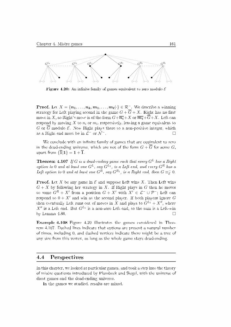
Chapter 4. Misère games 161
GLk GL2 GL1 GR1 GR2 GRℓ
Figure 4.20: An in�nite family of games equivalent to zero modulo E
Proof. Let X = {n1, . . . ,nk,m1, . . . ,mℓ|·} ∈ R−. We des ribe a winning
strategy for Left playing se ond in the game G+G+X. Right has no �rst
move in X, so Right's move is of the form G+ni+X ormi+G+X. Left an
respond by moving X to ni or mi, respe tively, leaving a game equivalent to
G or G modulo E . Now Right plays there to a non-positive integer, whi h
as a Right end must be in L−or N−
. �
We on lude with an in�nite family of games that are equivalent to zero
in the dead-ending universe, whi h are not of the form G + G for some G,apart from {1|1} = 1+ 1.
Theorem 4.107 If G is a dead-ending game su h that every GLhas a Right
option to 0 and at least one GL, say GL1
, is a Left end, and every GRhas a
Left option to 0 and at least one GR, say GR1
, is a Right end, then G ≡−E 0.
Proof. Let X be any game in E and suppose Left wins X. Then Left wins
G + X by following her strategy in X. If Right plays in G then he moves
to some GR + X ′from a position G + X ′
with X ′ ∈ L− ∪ P−; Left an
respond to 0 + X ′and win as the se ond player. If both players ignore G
then eventually Left runs out of moves in X and plays to GL1 +X ′′, where
X ′′is a Left end. But GL1
is a non-zero Left end, so the sum is a Left-win
by Lemma 4.80. �
Example 4.108 Figure 4.20 illustrates the games onsidered in Theo-
rem 4.107. Dashed lines indi ate that options are present a natural number
of times, in luding 0, and dashed verti es indi ate there might be a tree of
any size from this vertex, as long as the whole game stays dead-ending.
4.4 Perspe tives
In this hapter, we looked at parti ular games, and took a step into the theory
of misère quotients introdu ed by Plambe k and Siegel, with the universe of
di ot games and the dead-ending universe.
In the games we studied, results are mixed.
162 4.4. Perspe tives
The misère version of Geography is pspa e omplete even for some
`small' lass of graphs, but even if the problem Edge Geography on undi-
re ted graph is pspa e omplete in its normal version on general graphs,
there exists an algorithm that solves it in the restri ted ase of bipartite
undire ted graphs [18℄.
Question 4.109 What is the omplexity of �nding the misère out ome of
any Vertex Geography position on bipartite undire ted graphs?
In normal version, our results on VertexNim extended to Sto kman's
version of Vertex NimG, where a vertex of weight 0 is not removed. This
does not seem true in its misère version.
As all our results under the misère onvention are dire tly dedu ed from
our results under the normal onvention, we make the following onje ture.
Conje ture 4.110 The omplexity of �nding the misère out ome of any
VertexNim position on dire ted graphs with a token on a vertex is the same
as the omplexity of �nding the normal out ome of any VertexNim position
on dire ted graphs with a token on a vertex.
On Timber, we only redu ed the problem to oriented forests and found
the out ome of any oriented path. As Timber is not a game that separates
in several omponents, being able to �nd the out ome of any onne ted
omponent would already be interesting.
Question 4.111 Is there a polynomial-time algorithm that gives the misère
out ome of any Timber position on onne ted dire ted graphs?
On Timbush, we only redu ed the problem to oriented forests, but the
problem is an extension of Timber, on whi h we do not know mu h.
On Toppling Dominoes, we gave the misère out ome of a single row,
and found the misère monoid of Toppling Dominoes positions without
grey dominoes. Unexpe tedly, the problem seems easier than its normal
version. Hen e, we ask the following question.
Question 4.112 Can one �nd a polynomial-time algorithm that gives the
misère out ome of any Toppling Dominoes position (on several rows)?
On Col, we gave the misère out ome of any grey subdivided star.
In the ase of di ot games, we de�ned a redu ed form and proved it
was unique, before using this result to ount the number of di ot games in
anoni al form born by day 3.One problem of this anoni al form is that one needs �rst to dete t D-
dominated and D-reversible options to be able to delete or bypass them,
whi h we do not know whether it is solvable in polynomial time. Hen e, we
have the following question.

Chapter 4. Misère games 163
Question 4.113 What is the omplexity of omputing the anoni al form of
any di ot?
It would also be interesting to �nd a anoni al form for other universes.
Some of the proofs presented in that se tion were true for any universe, most
others would need the universe to be losed by adjoint, but the hard ase
to adapt seems to be the ase of reversible options through any end. The
universe of dead-ending games is losed by adjoint, and though we found
some way to deal with reversible options through dead ends, it was not
enough to give a unique form for ea h equivalent lass modulo the dead-
ending universe.
Question 4.114 Is there a natural way to de�ne a anoni al form for dead-
ending games?
We know we an still bypass most reversible options thanks to the fol-
lowing lemma.
Lemma 4.115 Let U be a universe and G be a game. Suppose GL1is
U-reversible through GL1R1, su h that GL1R1
is not a Left end. Let G′be
the game obtained by bypassing GL1:
G′ = {(GL1R1)L, GL \ {GL1}|GR} .
Then G ≡−U G′
.
The problem is to deal with options reversible through ends.
In the ase of dead-ending games, we found the misère monoid of ends
and numbers, and gave the partial order of numbers modulo the dead-ending
universe.
The original motivation of studying dead-ending games is to give a nat-
ural universe for the spe i� games we mentioned (Col, Domineering,
Ha kenbush. . . ), games where the players pla e pie es on a board never
to remove them, that we all pla ement games. A formal de�nition of a
pla ement game is the following.
De�nition 4.116 De�ne a game with a set M = ML ∪ MRof Left and
Right moves and a forbidding fun tion φ : 2M → 2M su h that we have for
any subset X of 2M,
⋃Y⊂X φ(Y ) ⊆ φ(X) and X ⊆ φ(X) as follows: a posi-
tion is a subset of M; from a position M , Left an move to M ∪ {m} for any
m ∈ ML\φ(M), and Right an move to M ∪ {m} for any m ∈ MR \ φ(M).Then a game G is a pla ement game if there exist a set M, a fun tion φ and
a subset M of M su h that G is the position obtained from M and φ on the
subset M as de�ned above, modulo the multipli ity of options.

164 4.4. Perspe tives
Figure 4.21: A dead-ending game whi h is not a pla ement game
Being a pla ement game is stronger than being a dead-ending game. For
example, the position on Figure 4.21 is a dead-ending game, and even a di ot
game, whi h is not a pla ement game. We an a tually prove that if you
de�ne re ursively the fun tion rb su h that rb(G) = 0 if G is a Right end
and rb(G) = 1+maxGR∈GR rb(GR), a pla ement game satis�es the ondition
rb(GL) 6 rb(G) for any Left option GLof G (whi h is not the ase for the
position on Figure 4.21).
Among properties we naturally onsider, the universe of pla ement games
is losed under followers, disjun tive sum and onjugates.
Question 4.117 What more an be said about pla ement games?
We an also look on a more general ontext of misère games.
In all examples of games we have seen having an inverse, the onjugate
of the game is an inverse. A natural question is: is this always true? Milley
[26℄ proved it is not, giving an example in a universe whi h is not losed
under onjugates. In [34℄, Plambe k and Siegel gives an example of an im-
partial universe, disproving even the ase where the universe is losed under
followers, disjun tive sum and onjugates. This example was not highlighted
in the paper as it is prior to the question. Having some answer for the above
question, we now ask the following question.
Question 4.118 For whi h universes U do we have G + H ≡−U 0 implies
H ≡−U G?
We know it is true for the universe G of all games, as the only way to
have G+G ≡−U 0 is to have G = 0, and we have examples of universes where
it is not, but even without asking for a hara terisation, it would be ni e to
know if universes su h as impartial games, di ot games, dead-ending games,
or even pla ement games have this property.
Another fa t one may noti e in this hapter is that in all universes we pre-
sented where there is no P-position, su h as the universe of LR-TopplingDominoes and the losure of dead-ends and numbers, all elements are in-
vertible, sometimes even in a bigger universe. This was onje tured by Milley.
Chapter 4. Misère games 165
Conje ture 4.119 (Milley (personal ommuni ation)) In any uni-
verse U losed under followers, disjun tive sum and onjugates, if U ontains
no P-position, then every element of U has an inverse modulo U in U .
For example, the out ome of a position in the losure of LR-TopplingDominoes, dead-ends and anoni al-form dyadi rationals is given by the
following proposition.
Proposition 4.120 If G is an LR-Toppling Dominoes posi-
tion, {ai}16i6n is a set of positive numbers and Left ends, and
{bi}16i6m is a set of negative numbers and Right ends, with
k = ltd(G) − rtd(G) +∑n
i=1 l(ai)−∑m
i=1 r(bi), then
o−
(G+
n∑
i=1
ai +
m∑
i=1
bi
)=
L−if k < 0
N−if k = 0
R−if k > 0.
This gives a misère monoid isomorphi to both the misère monoid of
LR-Toppling Dominoes positions, and to the monoid of the losure of
dead ends and anoni al-form dyadi rationals, whi h raises the following
onje ture.
Conje ture 4.121 If U and U ′are two universes losed under followers,
disjun tive sum and onjugates having misère monoids isomorphi to MZ,
then the misère monoid of the losure of positions of U and U ′is also iso-
morphi to MZ.
This might even be strengthened as follows.
Conje ture 4.122 If U and U ′are two universes losed under followers,
disjun tive sum and onjugates having isomorphi misère monoids, then the
misère monoid of the losure of positions of U and U ′is also isomorphi to
their ommon misère monoid.
In the last two onje tures, we onsider the out ome partition as part of
the misère monoid, that is we onsider they should be isomorphi as well.


Chapter 5. Domination Game 167
Chapter 5
Domination Game
The domination game is not a ombinatorial game. Nevertheless, some
tools used in its study are quite similar to some ombinatorial tools. For
example, the imagination strategy method proposed in [7℄ is similar to the
stealing strategy argument stating the player having a winning strategy in
Hex. We here show another parallel by onsidering the game on a non-
onne ted graph as a disjun tive sum.
Re all that a vertex is said to dominate itself and its neighbours, and that
a set of verti es is a dominating set if every vertex of the graph is dominated
by some vertex in the set.
The Domination game was introdu ed by Bre²ar, Klavºar and Rall in
[7℄. It is played on a �nite graph G by two players, Dominator and Staller.
They alternate turns in hoosing a vertex that dominates at least one new
vertex. The game ends when there is no possible move anymmore, that is
when the hosen verti es form a dominating set. Dominator's goal is that
the game �nishes in as few moves as possible while Staller tries to keep the
game going as long as she an. There are two possible variants of the game,
depending on who starts the game. In Game 1, Dominator starts, while in
Game 2, Staller starts. The game domination number, denoted by γg(G),is the total number of hosen verti es in Game 1 when both players play
optimally. Similarly, the Staller-start game domination number γ′g(G) is thetotal number of hosen verti es in Game 2 when both players play optimally.
Variants of the game where one player is allowed to pass a move on e
were already onsidered in [20℄ (and possibly elsewhere). In the Dominator-
pass game, Dominator is allowed to pass one move, while in the Staller-pass
game, Staller is. We denote respe tively by γgdp
and γ′gdp
the size of the set
of hosen verti es in game 1 and 2 where Dominator is allowed to pass one
move, and by γgsp
and γ′gsp
the size of the set of hosen verti es in game 1
and 2 where Staller is allowed to pass a move. Note that passing does not
ount as a move in the game domination number, as the value is the number
of hosen verti es.
We say that a graph G realises a pair (k, ℓ) ∈ N × N if γg(G) = k and
γ′g(G) = ℓ. For a graph G = (V,E) and a subset of verti es S ⊆ V , we
denote by G|S the partially dominated graph G where the verti es of S are
dominated. Kinnersley, West and Zamani [20℄ proved what is known as the
ontinuation prin iple:
168
Theorem 5.1 (Kinnersley et al[20℄) [Continuation Prin iple℄ Let Gbe a graph and A,B ⊆ V (G). If B ⊆ A, then γg(G|B) > γg(G|A) and
γ′g(G|B) 6 γ′g(G|A).
This very useful prin iple to prove inequalities involving γg and γ′g has
the following orollary, part of whi h was already proved in [7℄.
Theorem 5.2 (Bre²ar et al. [7℄, Kinnersley et al. [20℄) For any
graph G, |γg(G)− γ′g(G)| 6 1
As a onsequen e of this theorem, we have that realisable pairs are ne -
essarily of the form (k, k+1), (k, k) and (k, k−1). It is known that all these
pairs are indeed realisable, examples of graphs of ea h of these three types
are given in [7, 8, 20, 21℄. We say a partially dominated graph G is a (k,+)(resp. (k,=), (k,−)) if γg(G) = k and γ′g(G) = k + 1 (resp. γg(G) = k and
γ′g(G) = k, γg(G) = k and γ′g(G) = k−1). Additionally, we say that a graph
G is a plus (resp. equal, minus) if G is (k,+) (resp. (k,=), (k,−)) forsome k > 1.
Observation 5.3 If a partially dominated graph G|S is a (k,−), then for
any legal move u in G|S, the graph G|(S ∪N [u]) is a (k − 2,+).
Proof. Let G|S be a (k,−) and u be any legal move in G|S. By de�nition
of the game domination number, we have k = γg(G|S) 6 1+γ′g(G|S∪N [u]).Similarly, k − 1 = γ′g(G|S) > 1 + γg(G|S ∪ N [u]). By Theorem 5.2, we get
that
k − 1 6 γ′g(G|S ∪N [u]) 6 γg(G|S ∪N [u]) + 1 6 k − 1
and so equality holds throughout this inequality hain. Thus G|(S ∪N [u] isa (k − 2,+), as required. �
We say that a graph G is a no-minus graph if for any subset of verti es S,γg(G|S) 6 γ′g(G|S). Intuitively, it seems that no player getd any advantage
to pass in a no-minus graph.
In this hapter, we are interested in no-minus graphs and possible reali-
sations of unions of graphs. In Se tion 5.1, we prove that tri-split graphs and
dually hordal graphs are no-minus graphs. In Se tion 5.2, we give bounds
on the game domination number of the union of two graphs, given that we
know the game domination number of ea h omponent of the union, �rst
when both graphs are no-minus graphs, then in the general ase.
The results presented in this hapter are a joint work with Paul Dorbe
and Ga²per Ko²mrlj [13℄.
5.1 About no-minus graphs . . . . . . . . . . . . . . . 169

Chapter 5. Domination Game 169
5.2 The domination game played on unions of graphs 173
5.2.1 Union of no-minus graphs . . . . . . . . . . . . . . 173
5.2.2 General ase . . . . . . . . . . . . . . . . . . . . . 175
5.3 Perspe tives . . . . . . . . . . . . . . . . . . . . . . 179
5.1 About no-minus graphs
In this se tion, we onsider no-minus graphs.
To begin with no-minus graphs, we �rst need to prove what we laimed
was the intuitive de�nition of a no-minus, i.e. that it is not helpful to be
allowed to pass in su h games. In [7℄, Bre²ar et al. proved the following in
general:
Lemma 5.4 ([7℄) Let G be a graph. We have γg(G) ≤ γspg (G) ≤ γg(G) + 1
and γg(G)− 1 ≤ γdpg (G) ≤ γg(G).
Though the authors of [7℄ did not prove it, the exa t same proof te h-
nique (using the imagination strategy) an give the following inequalities,
for partially dominated graphs and for both games 1 and 2.
Lemma 5.5 Let G be a graph, S a subset of verti es of G. We have
γg(G|S) ≤ γspg (G|S) ≤ γg(G|S) + 1 ,
γ′g(G|S) ≤ γ′spg (G|S) ≤ γ′g(G|S) + 1 ,
γg(G|S) − 1 ≤ γdpg (G|S) ≤ γg(G|S) ,
γ′g(G|S) − 1 ≤ γ′dpg (G|S) ≤ γ′g(G|S) .
We now prove the following proposition on no-minus graphs, showing
that being allowed to pass is not helpful in su h graphs.
Proposition 5.6 If G is a no-minus graph, then
γgsp(G) = γg
dp(G) = γg(G) and γ′gsp(G) = γ′g
dp(G) = γ′g(G).
Proof. First, note that a player would pass a move only if it bene-
�ts them, so for any graph G (even if not a no-minus graph), we have
γgdp(G) 6 γg(G) 6 γg
sp(G) and γ′gdp(G) 6 γ′g(G) 6 γ′g
sp(G). Now, suppose
a no-minus graph G satis�es γgdp(G) < γg(G). We use the imagination strat-
egy to rea h a ontradi tion.
Consider a normal Dominator-start game played on G where Dominator
imagines he is playing a Dominator-pass game, while Staller plays optimally
in the normal game. Sin e γgdp(G) < γg(G), the strategy of Dominator
170 5.1. About no-minus graphs
in ludes passing a move at some point, say after x moves have been played.
Let S be the set of dominated verti es at that point. Sin e Dominator played
optimally the Dominator-pass domination game (but not ne essarily Staller),
if he was allowed to pass that move the game should end in no more than
γgdp(G). We thus have the following inequality:
x+ γ′g(G|S) 6 γgdp(G)
Now, remark that sin e Staller played optimally in the normal game, we have
that
x+ γg(G|S) > γg(G)
Adding the fa t that G is a no-minus, so that γg(G|S) 6 γ′g(G|S), we rea hthe following ontradi tion:
γg(G) 6 x+ γg(G|S) 6 x+ γ′g(G|S) 6 γgdp(G) < γg(G) .
Similar arguments omplete the proof for the Staller-pass and/or Staller-
start games. �
The next lemma also expresses an early property of no-minus graphs. It
is an extension of a result on forests from [20℄, the proof is about the same.
Lemma 5.7 Let G be a graph, S ⊆ V (G), su h that for any S′ ⊇ S,γg(G|S′) 6 γ′g(G|S′). Then we have γg(G ∪K1|S) > γg(G|S) + 1 and
γ′g(G ∪K1|S) > γ′g(G|S) + 1.
Proof. Given a graph G and a set S satisfying the hypothesis, we use
indu tion on the number of verti es in V (G) \S. If V (G) \ S = ∅, the laimis trivial. Suppose now that S V (G) and that the laim is true for every
G|S′with S S′
.
Consider �rst game 1. Let v be an optimal �rst move for
Dominator in the game G ∪ K1|S. If v is the added ver-
tex, then γg(G ∪K1|S) = γ′g(G|S) + 1 > γg(G|S) + 1 by our assumption
on G|S, and the inequality follows. Otherwise, let S′ = S ∪N [v].By the hoi e of the move and indu tion hypothesis, we have
γg(G ∪K1|S) = 1 + γ′g(G ∪K1|S′) > 1 + γ′g(G|S′) + 1. Sin e v is not ne -
essarily an optimal �rst move for Dominator in the game on G|S, we also
have that γg(G|S) 6 1 + γ′g(G|S′) and the result follows.
Consider now game 2. Let w be an optimal �rst move for Staller in
the game G|S, and let S′′ = S ∪N [w]. By optimality of this move, we
have γ′g(G|S) = 1 + γg(G|S′′). Playing also w in G ∪ K1|S, Staller gets
γ′g(G ∪K1|S) > 1 + γg(G ∪K1|S′′) > 2 + γg(G|S′′) by indu tion hypothe-
sis. The required inequality follows. �
It is known that forests are no-minus graphs [20℄. We now propose two
other families of graphs that are no-minus. The �rst is the family of tri-split

Chapter 5. Domination Game 171
graphs, a generalisation of split graphs and pseudo-split graph (ex ept it
does not ontain C5) inspired by [23℄. A graph is tri-split if its set of verti es
an be partitioned into three disjoint sets A 6= ∅, B and C with the following
properties:
∀u ∈ A, ∀v ∈ A ∪ C : uv ∈ E(G),
∀u ∈ B, ∀v ∈ B ∪ C : uv /∈ E(G).
We prove the following.
Theorem 5.8 Conne ted tri-split graphs are no-minus graphs.
Proof. Let G be a tri-split graph with the orresponding partition (A,B,C),let S ⊆ V (G) be a subset of dominated verti es, and onsider the game
played on G|S. If the game on G|S ends in at most two moves, then learly
γg(G|S) 6 γ′g(G|S). From now on, we assume that γg(G) > 3.Observe that Dominator has an optimal strategy playing only in A (in
both game 1 and game 2). Indeed, any vertex u in B dominates only itself
and some vertex in A (at least one by onne tivity). Any neighbour v of uin A dominates all of A and v, so is a better move than u for Dominator
by the ontinuation prin iple. Similarly, the neighbourhood of any vertex in
C is in luded in the neighbourhood of any vertex in A. So we now assume
Dominator only plays in A in the rest of the proof.
Suppose we know an optimal strategy on Game 2 for Dominator, we
propose an (imagination) strategy for Game 1 guaranteeing it will �nish no
later than Game 2. Let Dominator imagine a �rst move v0 ∈ B ∪ C from
Staller and play the game on G|S as if playing in G|(S ∪N [v0]). Staller playsoptimally on G|S not knowing about Dominator's imagined game. Note that
after Dominator's �rst move, the only di�eren e between the imagined game
and the real game is that v0 is dominated in the �rst but possibly not in the
se ond. Indeed, all the neighbours of v0 belong to A∪C, whi h are dominated
by Dominator's �rst move (in A by our assumption). Therefore, any move
played by Dominator in his imagined game is legal in the real game, though
Staller may eventually play a move in the real game that is illegal in the
imagined game, provided it newly dominates only v0. If she does so and the
game is not �nished yet, then Dominator imagines she played any legal move
v1 in B instead and ontinues. This may happen again, leading Dominator
to imagine a move v2 and so on. Denote by vi the last su h vertex before
the game ends, we thus have that vi is the only vertex possibly dominated
in the imagined game but not in the real game.
Assume now that the imagined game is just �nished. Denote by kI the
total number of moves in this imagined game. Note that the imagined game
looks like a Game 2 where Dominator played optimally but possibly not
Staller. We thus have that kI 6 γ′g(G|S). At that point, either the real
game is �nished or only vi is not yet dominated. So the real game �nishes

172 5.1. About no-minus graphs
at latest with the next move of any player, and the number of moves in the
real game kR satis�es kR 6 kI − 1 + 1. Moreover, in the real game, Staller
played optimally but possibly not Dominator, so kR > γg(G|S). We an
now on lude the proof bringing together all these inequalities into
γg(G|S) 6 kR 6 kI 6 γ′g(G|S) .
�
The se ond family of graphs we prove to be no-minus is the family of
dually hordal graphs, see [6℄. Let G be a graph, v one of its verti es. A
vertex u in N [v] is a maximum neighbour of v if for all w ∈ N [v], we have
N [w] ⊆ N [u]. A vertex ordering v1, . . . , vn is a maximum neighbourhood
ordering if for ea h i 6 n, vi has a maximum neighbour in G[{v1, . . . , vi}]. Agraph is dually hordal if it has a maximum neighbourhood ordering. Note
that forests and interval graphs are dually hordal [35℄.
Theorem 5.9 Dually hordal graphs are no-minus graphs.
Proof. We prove the result by indu tion on the number of non-dominated
verti es. Let G be a dually hordal graph with v1, . . . , vn a maximum neigh-
bourhood ordering of V (G). Let S ⊆ V (G) be a subset of dominated verti es
and denote by j the largest index su h that vj is not in S. We suppose by
way of ontradi tion that G|S is a (k,−), note that ne essarily k > 3. Let vibe a maximum neighbour of vj in G[{v1, . . . , vj}]. Let u be an optimal move
for Staller in G|(S∪N [vi]) and let S′ = S∪N [vi]∪N [u]. By Observation 5.3,
G|(S ∪N [u]) and G|(S ∪N [vi]) are both (k−2,+), so γg(G|S∪N [u]) = k−2and γ′g(G|S ∪N [vi]) = k − 1. By optimality of u, we get that
k − 1 = γ′g(G|S ∪N [vi]) = γg(G|S′) + 1 .
The vertex u is not a neighbour of vj , or its losed neighbourhood in
G[{v1, . . . , vj}] would be in luded in N [vi] and {vj+1, . . . , vn} ⊆ S, so playingu would not be legal in G|(S ∪N [vi]). Therefore, by ontinuation prin iple
(Theorem 5.1),
γg(G|S ∪N [u]) > γg(G|S′ \ {vj}) .
Moreover, be ause all verti es at distan e at most 2 from vj are dominated
in G|S′, we get that γg(G|S′ \ {vj}) = γg(G ∪K1|S
′). Now using indu tion
hypothesis to apply Lemma 5.7, we get
γg(G|S′ \ {vj}) > γg(G|S′) + 1 .
We thus on lude that
k − 2 = γg(G|S ∪N [u]) > γg(G|S′ \ {vj}) > γg(G|S′) + 1 = k − 1,
whi h leads to a ontradi tion. Therefore, G|S is not a minus and this
on ludes the proof. �

Chapter 5. Domination Game 173
5.2 The domination game played on unions of
graphs
5.2.1 Union of no-minus graphs
In this subse tion, we are interested in the possible values that the union of
two no-minus graphs may realise, a ording to the realisations of its om-
ponents. We in parti ular show that the union of two no-minus graphs is
always a no-minus graph.
We �rst prove a very general result that will allow us to ompute almost
all the bounds obtained later.
Theorem 5.10 Let G1|S and G2|S′be two partially dominated graphs and
x be any legal move in G1|S. We have
γg(G1 ∪G2|S ∪ S′) > min
(γg(G1|S) + γg
dp(G2|S′)
γgdp(G1|S) + γg(G2|S
′)
)(5.1)
γg(G1 ∪G2|S ∪ S′) 6 1 + max
(γ′g(G1|S ∪N [x]) + γ′g
sp(G2|S′)
γ′gsp(G1|S ∪N [x]) + γ′g(G2|S
′)
)(5.2)
γ′g(G1 ∪G2|S ∪ S′) 6 max
(γ′g(G1|S) + γ′g
sp(G2|S′)
γ′gsp(G1|S) + γ′g(G2|S
′)
)(5.3)
γ′g(G1 ∪G2|S ∪ S′) > 1 + min
(γg(G1|S ∪N [x]) + γg
dp(G2|S′)
γgdp(G1|S ∪N [x]) + γg(G2|S
′)
)(5.4)
Proof. To prove all these bounds, we simply des ribe what a player an do
by using a strategy of following, i.e. always answering to his opponent moves
in the same graph if possible.
Let us �rst onsider Game 1 in G1 ∪G2|S ∪ S′and what happens when
Staller adopts the strategy of following. Assume �rst that the game in G1
�nishes before the game in G2. Then Staller is sure with her strategy that
the number of moves in G1 is at least γg(G1|S). However, when G1 �n-
ishes, Staller may be for ed to play in G2 if Dominator played the �nal
move in G1. This situation somehow allows Dominator to pass on e in G2,
but no more. So we an ensure that the number of moves in G2 is no
less that γgdp(G2|S
′). Thus, in that ase, the total number of moves is no
less than γg(G1|S) + γgdp(G2|S
′). If on the other hand the game in G2 �n-
ishes �rst, we get similarly that the number of moves is then no less than
γgdp(G1|S) + γg(G2|S
′). Sin e she does not de ide whi h game �nishes �rst,
Staller an guarantee that
γg(G1∪G2|S ∪S′) > min(γg(G1|S)+γg
dp(G2|S′), γg
dp(G1|S)+γg(G2|S′)).
The same arguments in Game 2 with Dominator adopting the strategy of
following ensures that
γ′g(G1∪G2|S∪S′) 6 max(γ′g(G1|S)+γ′g
sp(G2|S
′), γ′gsp(G1|S)+γ′g(G2|S
′)).

174 5.2. The domination game played on unions of graphs
Let us ome ba k to Game 1. Suppose Dominator plays some vertex x in
V (G1) and then adopts the strategy of following. Then he an ensure that
γg(G1 ∪G2|S ∪ S′) 6 1 + γ′g(G1 ∪G2|S ∪ S′ ∪NG1[x]) and thus that
γg(G1 ∪G2|S ∪ S′) 6 1 + max
(γ′g(G1|S ∪N [x]) + γ′g
sp(G2|S′)
γ′gsp(G1|S ∪N [x]) + γ′g(G2|S
′)
).
The same is true for Staller in Game 2 to obtain Inequality (5.4). �
In the ase of the union of two no-minus graphs, these inequalities allow
us to give rather pre ise bounds on the possible values realised by the union.
The �rst ase is when one of the omponents is an equal.
Theorem 5.11 Let G1|S and G2|S′be partially dominated no-minus
graphs. If G1|S is a (k,=) and G2|S′is a (ℓ, ⋆) (with ⋆ ∈ {=,+}), then
the disjoint union G1 ∪G2|S ∪ S′is a (k + ℓ, ⋆).
Proof. We use inequalities from Theorem 5.10. Note that sin e G1 and G2
are no-minus graphs, we an apply Proposition 5.6 and get that the Staller-
pass and Dominator-pass games on any partially dominated G1 and G2 is
the same as the orresponding game.
For Game 1, let Dominator hoose an optimal move x in G2|S′, for
whi h we get γ′g(G2|S′ ∪N [x]) = ℓ− 1. Applying Inequalities (5.1) and (5.2)
inter hanging the role of G1 and G2, we then get that
k + ℓ 6 γg(G1 ∪G2|S ∪ S′) 6 1 + k + ℓ− 1 .
For Game 2, Staller an also hoose an optimal move x in G2|S′for whi h
γg(G2|S′ ∪N [x]) = γ′g(G2|S
′)− 1, and applying Inequalities (5.3) and (5.4),
we get that γ′g(G1 ∪G2|S ∪ S′) = γ′g(G1|S) + γ′g(G2|S′). �
We are now left with the ase where both omponents are plus.
Theorem 5.12 Let G1|S and G2|S′be partially dominated no-minus graphs
su h that G1|S is (k,+) and G2|S′is (ℓ,+). Then
k + ℓ 6 γg(G1 ∪G2|S ∪ S′) 6 k + ℓ+ 1,
k + ℓ+ 1 6 γ′g(G1 ∪G2|S ∪ S′) 6 k + ℓ+ 2.
In addition, all bounds are tight.
Proof. Similarly as in the proof before, taking x an optimal �rst move for
Dominator in G1|S and applying Inequalities (5.1) and (5.2), we get that
k + ℓ 6 γg(G1 ∪ G2|S ∪ S′) 6 k + ℓ+ 1. Also, taking for x an optimal �rst
move for Staller in G1|S and applying Inequalities (5.3) and (5.4), we get
that k + ℓ+ 1 6 γ′g(G1 ∪G2|S ∪ S′) 6 k + ℓ+ 2.
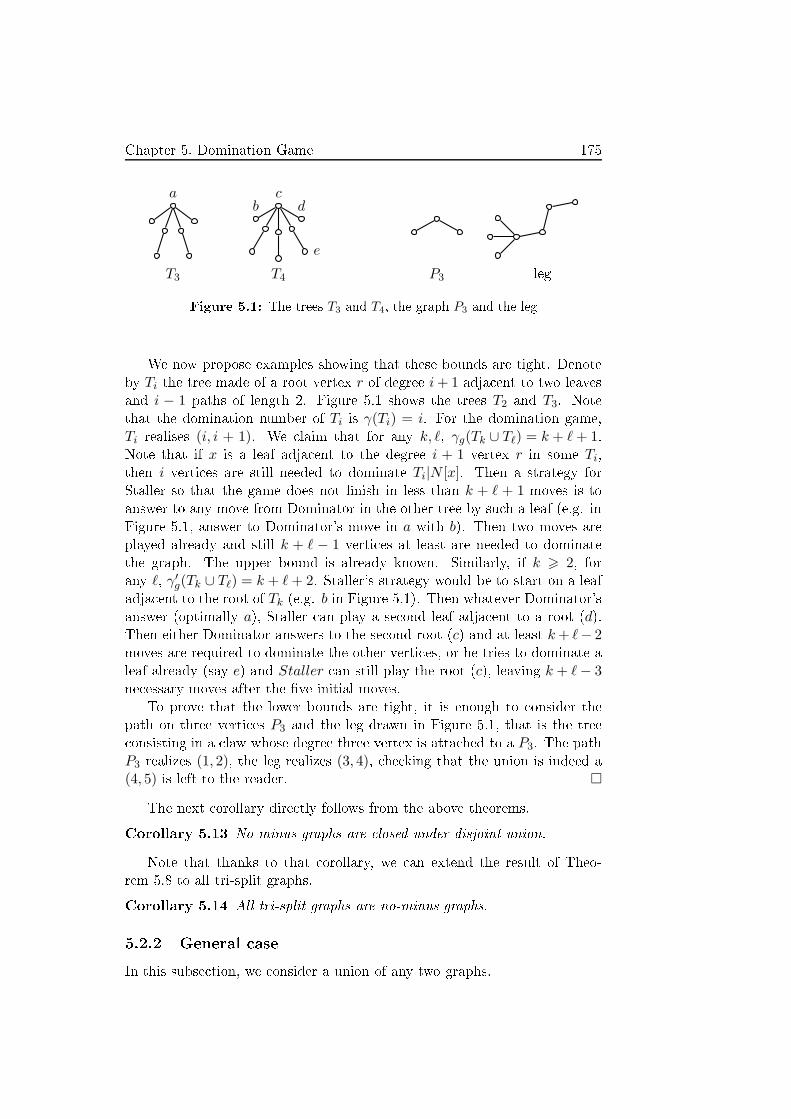
Chapter 5. Domination Game 175
a
T3
cd
e
b
T4 P3 leg
Figure 5.1: The trees T3 and T4, the graph P3 and the leg
We now propose examples showing that these bounds are tight. Denote
by Ti the tree made of a root vertex r of degree i+ 1 adja ent to two leaves
and i − 1 paths of length 2. Figure 5.1 shows the trees T2 and T3. Note
that the domination number of Ti is γ(Ti) = i. For the domination game,
Ti realises (i, i + 1). We laim that for any k, ℓ, γg(Tk ∪ Tℓ) = k + ℓ+ 1.Note that if x is a leaf adja ent to the degree i + 1 vertex r in some Ti,
then i verti es are still needed to dominate Ti|N [x]. Then a strategy for
Staller so that the game does not �nish in less than k + ℓ + 1 moves is to
answer to any move from Dominator in the other tree by su h a leaf (e.g. in
Figure 5.1, answer to Dominator's move in a with b). Then two moves are
played already and still k + ℓ − 1 verti es at least are needed to dominate
the graph. The upper bound is already known. Similarly, if k > 2, forany ℓ, γ′g(Tk ∪ Tℓ) = k + ℓ+ 2. Staller's strategy would be to start on a leaf
adja ent to the root of Tk (e.g. b in Figure 5.1). Then whatever Dominator's
answer (optimally a), Staller an play a se ond leaf adja ent to a root (d).Then either Dominator answers to the se ond root (c) and at least k+ ℓ− 2moves are required to dominate the other verti es, or he tries to dominate a
leaf already (say e) and Staller an still play the root (c), leaving k + ℓ− 3ne essary moves after the �ve initial moves.
To prove that the lower bounds are tight, it is enough to onsider the
path on three verti es P3 and the leg drawn in Figure 5.1, that is the tree
onsisting in a law whose degree three vertex is atta hed to a P3. The path
P3 realizes (1, 2), the leg realizes (3, 4), he king that the union is indeed a
(4, 5) is left to the reader. �
The next orollary dire tly follows from the above theorems.
Corollary 5.13 No-minus graphs are losed under disjoint union.
Note that thanks to that orollary, we an extend the result of Theo-
rem 5.8 to all tri-split graphs.
Corollary 5.14 All tri-split graphs are no-minus graphs.
5.2.2 General ase
In this subse tion, we onsider a union of any two graphs.

176 5.2. The domination game played on unions of graphs
Depending on the parity of the length of the game, we an re�ne Theo-
rem 5.10 as follows:
Theorem 5.15 Let G1|S1 and G2|S2 be partially dominated graphs.
• If γg(G1|S1) and γg(G2|S2) are both even, then
γg(G1 ∪G2|S1 ∪ S2) ≥ γg(G1|S1) + γg(G2|S2) (5.5)
• If γg(G1|S1) is odd and γ′g(G2|S2) is even, then
γg(G1 ∪G2|S1 ∪ S2) ≤ γg(G1|S1) + γ′g(G2|S2) (5.6)
• If γ′g(G1|S1) and γ′g(G2|S2) are both even, then
γ′g(G1 ∪G2|S1 ∪ S2) ≤ γ′g(G1|S1) + γ′g(G2|S2) (5.7)
• If γ′g(G1|S1) is odd and γg(G2|S2) is even, then
γ′g(G1 ∪G2|S1 ∪ S2) ≥ γ′g(G1|S1) + γg(G2|S2) (5.8)
Proof. The proof is similar to the proof of Theorem 5.10. For inequal-
ity (5.5), let Staller use the strategy of following, assume without loss of
generality that G1 is dominated before G2. If Dominator played opti-
mally in G1, by parity Staller played the last move there and Dominator
ould not pass a move in G2, thus he ould not manage less moves in G2
than γg(G2|S2). Yet Dominator may have played so that one more move
was ne essary in G1 in order to be able to pass in G2. Then the num-
ber of moves played in G2 may be only γgdp(G2|S2), but this is no less
than γg(G2|S2) − 1 and overall, the number of moves is the same. Hen e
we have γg(G1 ∪G2|S1 ∪ S2) ≥ γg(G1|S1) + γg(G2|S2). The same argument
with Dominator using the strategy of following gives inequality (5.7).
Similarly, for inequality (5.6), Let Dominator start with playing an op-
timal move x in G1|S1 and then apply the strategy of following. Then
Staller plays in G1 ∪ G2|(S1 ∪ N [x]) ∪ S2, where γ′g(G1|S1 ∪ N [x]) =γg(G1|S1)− 1 is even, as well as γ′g(G2|S2). Then by the previous argument,
γg(G1 ∪G2|S1 ∪ S2) ≤ γg(G1|S1) + γ′g(G2|S2). Inequality (5.8) is obtained
with a similar strategy for Staller. �
Using Theorem 5.10 and 5.15, we argue the 21 di�erent ases, a ording
to the type and the parity of ea h of the omponents of the union. To simplify
the omputation, we simply propose the following orollary of Theorem 5.10
Corollary 5.16 Let G1|S1 and G2|S2 be two partially dominated graphs.
We have
γg(G1 ∪G2|S1 ∪ S2) ≥ γg(G1|S1) + γg(G2|S2)− 1 , (5.9)
γg(G1 ∪G2|S1 ∪ S2) ≤ γg(G1|S1) + γ′g(G2|S2) + 1 , (5.10)
γ′g(G1 ∪G2|S1 ∪ S2) ≤ γ′g(G1|S1) + γ′g(G2|S2) + 1 , (5.11)
γ′g(G1 ∪G2|S1 ∪ S2) ≥ γ′g(G1|S1) + γg(G2|S2)− 1 . (5.12)

Chapter 5. Domination Game 177
Proof. To prove these inequalities, with simply apply inequalities of The-
orem 5.10 in a general ase. We hoose for the vertex x an optimal move,
getting for example that γ′g(G1|S1 ∪ N [x]) = γg(G1|S1) − 1. We also use
Lemma 5.5 and get for example γgdp(G2|S2) ≥ γg(G2|S2)− 1. �
We now present the general bounds in Table 5.2, whi h should be read as
follows. The �rst two olumns give the types and parities of the omponents
of the union, where e, e1 and e2 denote even numbers and o, o1, and o2 denoteodd numbers. The next two olumns give the bounds on the domination
game numbers of the union. In the last two olumns, we give the inequalities
we use to get these bounds. We add a ∗ to the inequality number when the
inequality is used ex hanging G1 and G2.
G1 G2 γg γ′g for γg for γ′g
(o1,−) (o2,+) γg = o1 + o2 − 1 γ′g = o1 + o2 (5.9),(5.6*) (5.12*),(5.7)
(e1,−) (e2,+) γg = e1 + e2 γ′g = e1 + e2 + 1 (5.5),(5.10*) (5.8*),(5.11)
(o1,−) (o2,−) γg = o1 + o2 − 1 γ′g = o1 + o2 − 2 (5.9),(5.6) (5.12),(5.7)
(e1,−) (e2,−) γg = e1 + e2 γ′g = e1 + e2 − 1 (5.5),(5.10) (5.8),(5.11)
(o1,=) (o2,−) γg = o1 + o2 − 1 o1 + o2 − 1 ≤ γ′g ≤ o1 + o2 (5.9),(5.6) (5.12*),(5.11)
(e1,=) (e2,−) γg = e1 + e2 e1 + e2 − 1 ≤ γ′g ≤ e1 + e2 (5.5),(5.10) (5.12),(5.11)
(e,=) (o,−) e+ o− 1 ≤ γg ≤ e+ o γ′g = e+ o− 1 (5.9),(5.10) (5.12),(5.7)
(o,=) (e,−) e+ o− 1 ≤ γg ≤ e+ o γ′g = e+ o (5.9),(5.10) (5.8),(5.11)
(e,=) (o,+) e+ o− 1 ≤ γg ≤ e+ o e+ o ≤ γ′g ≤ e+ o+ 1 (5.9),(5.6*) (5.12*),(5.11)
(o,−) (e,+) e+ o− 1 ≤ γg ≤ e+ o e+ o ≤ γ′g ≤ e+ o+ 1 (5.9),(5.10*) (5.12*),(5.11)
(e,−) (o,+) e+ o− 1 ≤ γg ≤ e+ o e+ o ≤ γ′g ≤ e+ o+ 1 (5.9),(5.10*) (5.12*),(5.11)
(e,=) (o,=) e+ o− 1 ≤ γg ≤ e+ o e+ o ≤ γ′g ≤ e+ o+ 1 (5.9),(5.6*) (5.8*),(5.11)
(o,−) (e,−) e+ o− 1 ≤ γg ≤ e+ o e+ o− 2 ≤ γ′g ≤ e+ o− 1 (5.9),(5.10) (5.12),(5.11)
(e1,=) (e2,=) e1 + e2 ≤ γg ≤ e1 + e2 + 1 e1 + e2 − 1 ≤ γ′g ≤ e1 + e2 (5.5),(5.10) (5.12),(5.7)
(e1,=) (e2,+) e1 + e2 ≤ γg ≤ e1 + e2 + 1 e1 + e2 + 1 ≤ γ′g ≤ e1 + e2 + 2 (5.5),(5.10*) (5.8*),(5.11)
(o,=) (e,+) e+ o− 1 ≤ γg ≤ e+ o+ 1 e+ o ≤ γ′g ≤ e+ o+ 2 (5.9),(5.10*) (5.8),(5.11)
(o1,+) (o2,+) o1 + o2 − 1 ≤ γg ≤ o1 + o2 + 1 o1 + o2 ≤ γ′g ≤ o1 + o2 + 2 (5.9),(5.6) (5.12),(5.7)
(e1,+) (e2,+) e1 + e2 ≤ γg ≤ e1 + e2 + 2 e1 + e2 + 1 ≤ γ′g ≤ e1 + e2 + 3 (5.5),(5.10) (5.8),(5.11)
(o1,=) (o2,=) o1 + o2 − 1 ≤ γg ≤ o1 + o2 + 1 o1 + o2 − 1 ≤ γ′g ≤ o1 + o2 + 1 (5.9),(5.10) (5.12),(5.11)
(o1,=) (o2,+) o1 + o2 − 1 ≤ γg ≤ o1 + o2 + 1 o1 + o2 ≤ γ′g ≤ o1 + o2 + 2 (5.9),(5.10*) (5.12*),(5.11)
(e,+) (o,+) e+ o− 1 ≤ γg ≤ e+ o+ 2 e+ o ≤ γ′g ≤ e+ o+ 3 (5.9),(5.10) (5.12),(5.11)
Table 5.2: Bounds for general graphs.
Using the inequalities of Theorems 5.10 and 5.15, we get the following
results.
Theorem 5.17 The bounds from Table 5.2 hold.
Note that only in the �rst four ases in Table 5.2 the exa t game dom-
ination number as well as the Staller-start game domination number are
determined, while in the next four ases this is the ase for exa tly one of
these two numbers. In all other ases, the di�eren e between the lower and
upper bound is at least one and at most three.
We managed to tighten all these bounds but �ve, on in�nite families of
graphs.
Re all that the Cartesian produ t G�H of two graphs G and H is the
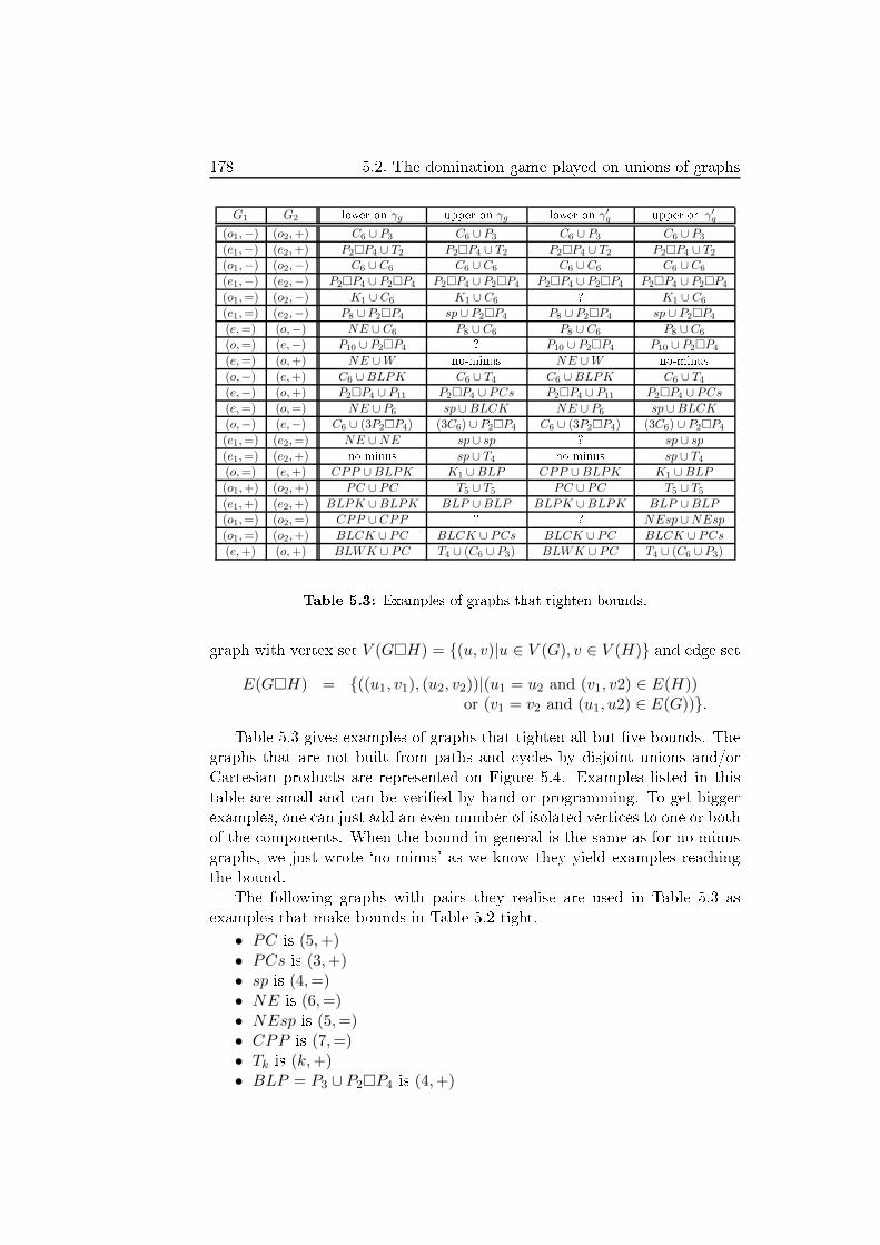
178 5.2. The domination game played on unions of graphs
G1 G2 lower on γg upper on γg lower on γ′g upper on γ′g
(o1,−) (o2,+) C6 ∪ P3 C6 ∪ P3 C6 ∪ P3 C6 ∪ P3
(e1,−) (e2,+) P2�P4 ∪ T2 P2�P4 ∪ T2 P2�P4 ∪ T2 P2�P4 ∪ T2
(o1,−) (o2,−) C6 ∪ C6 C6 ∪ C6 C6 ∪C6 C6 ∪ C6
(e1,−) (e2,−) P2�P4 ∪ P2�P4 P2�P4 ∪ P2�P4 P2�P4 ∪ P2�P4 P2�P4 ∪ P2�P4
(o1,=) (o2,−) K1 ∪ C6 K1 ∪ C6 ? K1 ∪ C6
(e1,=) (e2,−) P8 ∪ P2�P4 sp ∪ P2�P4 P8 ∪ P2�P4 sp ∪ P2�P4
(e,=) (o,−) NE ∪ C6 P8 ∪ C6 P8 ∪ C6 P8 ∪C6
(o,=) (e,−) P10 ∪ P2�P4 ? P10 ∪ P2�P4 P10 ∪ P2�P4
(e,=) (o,+) NE ∪W no-minus NE ∪W no-minus
(o,−) (e,+) C6 ∪BLPK C6 ∪ T4 C6 ∪BLPK C6 ∪ T4
(e,−) (o,+) P2�P4 ∪ P11 P2�P4 ∪ PCs P2�P4 ∪ P11 P2�P4 ∪ PCs
(e,=) (o,=) NE ∪ P6 sp ∪BLCK NE ∪ P6 sp ∪BLCK
(o,−) (e,−) C6 ∪ (3P2�P4) (3C6) ∪ P2�P4 C6 ∪ (3P2�P4) (3C6) ∪ P2�P4
(e1,=) (e2,=) NE ∪NE sp ∪ sp ? sp ∪ sp
(e1,=) (e2,+) no-minus sp ∪ T4 no-minus sp ∪ T4
(o,=) (e,+) CPP ∪BLPK K1 ∪BLP CPP ∪BLPK K1 ∪BLP
(o1,+) (o2,+) PC ∪ PC T5 ∪ T5 PC ∪ PC T5 ∪ T5
(e1,+) (e2,+) BLPK ∪BLPK BLP ∪BLP BLPK ∪BLPK BLP ∪BLP
(o1,=) (o2,=) CPP ∪ CPP ? ? NEsp ∪NEsp
(o1,=) (o2,+) BLCK ∪ PC BLCK ∪ PCs BLCK ∪ PC BLCK ∪ PCs
(e,+) (o,+) BLWK ∪ PC T4 ∪ (C6 ∪ P3) BLWK ∪ PC T4 ∪ (C6 ∪ P3)
Table 5.3: Examples of graphs that tighten bounds.
graph with vertex set V (G�H) = {(u, v)|u ∈ V (G), v ∈ V (H)} and edge set
E(G�H) = {((u1, v1), (u2, v2))|(u1 = u2 and (v1, v2) ∈ E(H))or (v1 = v2 and (u1, u2) ∈ E(G))}.
Table 5.3 gives examples of graphs that tighten all but �ve bounds. The
graphs that are not built from paths and y les by disjoint unions and/or
Cartesian produ ts are represented on Figure 5.4. Examples listed in this
table are small and an be veri�ed by hand or programming. To get bigger
examples, one an just add an even number of isolated verti es to one or both
of the omponents. When the bound in general is the same as for no-minus
graphs, we just wrote `no-minus' as we know they yield examples rea hing
the bound.
The following graphs with pairs they realise are used in Table 5.3 as
examples that make bounds in Table 5.2 tight.
• PC is (5,+)• PCs is (3,+)• sp is (4,=)• NE is (6,=)• NEsp is (5,=)• CPP is (7,=)• Tk is (k,+)• BLP = P3 ∪ P2�P4 is (4,+)

Chapter 5. Domination Game 179
k − 1
Figure 5.4: From top to bottom, left to right: PC, PCs, sp, NE, NEsp, CPP ,W , Tk
• BLC = P2�P4 ∪ C6 is (6,=)• BLCK = P2�P4 ∪ C6 ∪K1 is (7,=)• BLPK = P2�P4 ∪ P3 ∪K1 is (6,+)• BLWK = P2�P4 ∪W ∪K1 is (8,+)
5.3 Perspe tives
In this hapter, we looked at the domination game.
First, we took an interest in no-minus graphs, that are graphs in whi h
no player ever gets any advantage passing, no matter whi h set of verti es is
dominated. We proved that both tri-split graphs and dually hordal graphs
are no-minus graphs. Chordal graphs are another generalisation of split
graphs, interval graphs and forests, so we pose the following onje ture.
Conje ture 5.18 Partially dominated hordal graphs are no-minus graphs.
The lasses of graphs that we proved to be no-minus are re ognisable in
polynomial time. Hen e the following question is natural.
Question 5.19 Can no-minus graphs be re ognised in polynomial time?
Note that a naive algorithm that would onsist in he king the values of
γg and γ′g would not work. First be ause no polynomial algorithm is known

180 5.3. Perspe tives
to ompute γg or γ′g. And se ond be ause we would have to ompute these
values for all sets of initially-dominated verti es of the graph, and there are
an exponential number of su h sets.
Then we onsidered the game played on disjoint unions of graphs, where
we bounded the possible values of γg and γ′g. Noti e that our results hold
even when the graphs are not onne ted, so they an be applied re ursively,
though then the di�eren e between the lower bound and the upper bound
may in rease. Note that the strategy we propose is not always optimal,
however we think it gives the optimal bound in general.
Conje ture 5.20 All bounds from Table 5.2 are tight.
Chapter 6. Con lusion 181
Chapter 6
Con lusion
This thesis has examined games under both normal and misère onven-
tion, and even a graph parameter seen as a game.
In Chapter 2, we studied two impartial games under normal onvention.
The �rst is a generalisation of Adja ent Nim, lose to Vertex NimG, but
whi h for es the players to lower all the weights to 0. We found a polynomial-
time algorithm that gives the out ome of a large lass of positions, and as
our lass is losed under followers, this lets us �nd a strategy for the winning
player. Nevertheless, we did not solve the problem entirely. It would be
interesting to �nd an e� ient algorithm that would solve the general problem
on dire ted graphs where the self-loops are optional. The problem on dire ted
graphs with no self-loop is not losed under followers, so we do not think it
is the right problem to look at �rst.
The se ond impartial game we studied an be seen as a generalisation
of Nim, as there is a bije tion between Nim positions and orientations of
subdivided stars where all ar s are dire ted away from the enter, but was
a tually derived from Toppling Dominoes, through a version where only
paths were onsidered. We found the out ome of any position on a onne ted
dire ted graph, and the algorithm is a tually able to keep tra k of `equivalent'
ar s throughout the redu tion, so it is possible to ba ktra k any winning ar
from a minimal position to the original dire ted graph. As the game does
not split in di�erent omponents, we ould be satis�ed with this result, but
it still feels like the game is not solved yet until one �nd a way to give the
Grundy-value of any position. We partially answered this question by giving
a ubi -time algorithm that �nds the Grundy-value of any orientation of a
path. However, it would be interesting to have a more e� ient algorithm
that gives su h Grundy-values, even for orientations of paths only.
In Chapter 3, we studied three partizan games under normal onvention.
The �rst is a generalisation of Timber, that we studied in Chapter 2. We
gave polynomial-time algorithms to �nd the out ome of any orientation of
paths with oloured ar s, and of any onne ted dire ted graph with ar s
oloured bla k or white. Notwithstanding, the general problem is far from
solved. Even though the game does not split in di�erent omponents, we
do not know of an e� ient algorithm that would give the out ome of any
oloured onne ted dire ted graph. Finding the value of a position, even on
orientations of paths, seems like a hard problem, espe ially sin e there ould
be many di�erent values.

182
The se ond partizan game we studied is a oarsening of the �rst (though
it was de�ned earlier). The interest of our study was to hara terise positions
having some values, or prove the existen e of some values, on positions on a
single row. We ompletely hara terised the positions on a single row having
value {a|b} with a > b, and provided examples of positions on a single row
having value {a|{b|c}} for a > b > c or {{a|b}|{c|d}} for a > b > c > d. Itwould be interesting to omplete the hara terisation of these last two sets
of positions. Other interesting onje tures on the game an be found in [17℄.
The last partizan game we looked at is a olouring game. Though any
position on a grey graph has value 0 or ∗, and the value of other positions is
restri ted to numbers and sums of numbers and ∗, �nding the out ome of a
position is quite omplex. We gave the out omes of grey positions belonging
to some sub lasses of trees, and the out omes of grey ographs. It would be
interesting to �nd an algorithm that would give the out ome of any grey tree,
and maybe put it together with the algorithm we propose for grey ographs
to �nd the out ome of any distan e-hereditary graph.
In Chapter 4, we swit hed to the misère onvention. First, we des ribed
the misère version of the games we studied earlier. We provided results on
a omplexity level as well as on �nding algorithms that give the out ome of
position, and results on redu ing the problem to positions that seem simpler.
There are games on whi h we did not say mu h, but the misère version of
a game is in general harder to solve than its normal version, as highlighted
with Vertex Geography, where one an �nd the normal out ome of any
position on an undire ted graph G in time O(|E(G)|√
|V (G)|) whereas �nd-ing the misère out ome of a position, even on planar undire ted graphs of
maximum degree 5, is pspa e- omplete. In ontrast, we gave a solution
to �nd the misère out ome of any LR-Toppling Dominoes position in a
linear time. However, there is still a lot to sear h on the general version of
Toppling Dominoes under misère onvention, where we allow grey domi-
noes. The other games we studied are not ompletely solved either, and
ould be subje t to future resear h.
Then we looked at misère universes. The �rst we onsider is a well-
known set of games. Under the normal onvention, these games are alled
all-small be ause they all are in�nitesimal, that is they are smaller than any
positive number and greater than any negative number. Under the misère
onvention, we gave them a anoni al form. However, there is no e� ient
way to ompute this anoni al form as it requires to dete t dominated and
reversible options, and we do not know of an e� ient way of omparing any
two games. In pra ti e, though, there are situations where it is possible to
ompare games, and we hope our analysis of games born by day 3 an help
in the endgames of di ot positions.
Next, we looked at a se ond universe in misère play. Though this universe
is somehow new, it ontains many games that have been studied before. In
Chapter 6. Con lusion 183
parti ular, it ontains the universe of di ot games, studied in the previous
se tion. We analysed ends and numbers. Ends might appear quite often in
games, but numbers in normal anoni al form are less frequent. Nonetheless,
it is still interesting to know there are quite many games admitting an inverse
modulo the dead-ending universe, and that even some games not being of
this kind of sum are equivalent to 0 in this universe.
In Chapter 5, we left ombinatorial games to study the domination game.
We found some lasses of graphs where the analysis should be easier, and
looked at what value the parameter of the disjoint union of two graphs may
have onsidering the values of the parameter of these two graphs and the
pro ess an be repeated on more than two omponents. It is interesting
to see how this vision from ombinatorial games, seeing the game as a dis-
jun tive sum, helps highlighting how interesting no-minus graphs are for the
domination game. We also used the imagination strategy whi h, without
being de�ned as a ombinatorial games tool, may remind us of the stealing
strategy argument used to �nd the winning player in some ombinatorial
games. No-minus graphs are interesting be ause they are somewhat more
predi table, so it would be ni e to be able to hara terise them, or �nd other
lasses of graphs having this property.


Chapter A. Appendix: Rule sets 185
Appendix A
Appendix: Rule sets
• Clobber is a partizan game played on an undire ted graph with
verti es oloured bla k or white. At her turn, Left hooses a white
vertex she olours bla k and a bla k vertex she removes from the game
provided the two verti es were adja ent. At his turn, Right hooses a
bla k vertex he olours white and a white vertex he removes from the
game provided the two verti es were adja ent.
• Col is a partizan game played on an undire ted graph with verti es
either un oloured or oloured bla k or white. A move of Left onsists
in hoosing an un oloured vertex and olouring it bla k, while a move
of Right would be to do the same with the olour white. An extra
ondition is that the partial olouring has to stay proper, that is no
two adja ent verti es should have the same olour. Another way of
seeing the game is to play it on the graph of available moves: a position
is an undire ted graph with all verti es oloured bla k, white or grey;
a move of Left is to hoose a bla k or grey vertex, remove it from the
game with all its bla k oloured neighbours, and hange the olour of
its other neighbours to white; a move of Right is to hoose a white
or grey vertex, remove it from the game with all its white oloured
neighbours, and hange the olour of its other neighbours to bla k.
• Domineering is a partizan game played on a square grid, where
some verti es might be missing. A move of Left onsists in hoosing
two verti ally adja ent verti es and remove them from the game, while
a Right move is to hoose two horizontally adja ent verti es and remove
them from the game. The game is usually represented with a grid of
squares where players put dominoes without superimposing them.
• Flip the oin is a partizan game played on one or several rows of
oins, ea h oin fa ing either heads or tails. At her turn, Left hooses
a oin fa ing heads and removes it from the game, �ipping the oins
adja ent to it. At his turn, Right does the same with a oin fa ing tail.
There exists a variant where the two neighbours of the oin removed
be ome adja ent.
• Geography is an impartial game played on a dire ted graph with a
token on a vertex. There exist two variants of the game: Vertex Ge-
ography and Edge Geography. A move in Vertex Geography
is to slide the token through an ar and delete the vertex on whi h
the token was. A move in Edge Geography is to slide the token

186
through an ar and delete the edge on whi h the token just slid. In
both variants, the game ends when the token is on an isolated vertex.
Geography an also be played on an undire ted graph G by seeing it
as a symmetri dire ted graph where the vertex set remains the same
and the ar set is {(u, v), (v, u)|(u, v) ∈ E(G)}, ex ept that in the ase
of Edge Geography, going through an edge (u, v) would remove
both the ar (u, v) and the ar (v, u) of the dire ted version.
• Ha kenbush is a partizan game played on a graph with ar s
oloured bla k, white, or grey, and a spe ial vertex alled the ground.
At her turn, Left removes a grey or bla k edge from the game, and
everything that is no longer onne ted to the ground falls down (is
removed from the game). At his turn, Right does the same with a
grey or white edge.
• Hex is a partizan game played on an hexagonal grid. At her turn,
Left pla es a bla k pie e on an empty vertex, and Right does the same
at his turn with a white pie e. The game ends when there is a path
of bla k stones onne ting the upper-left side to the lower-right side
of the board, or a path of white stone onne ting the upper-right side
to the lower-left side of the board.
• Nim is an impartial game played on one or several heaps of tokens.
At their turn, a player removes any positive number of tokens from
one single heap they hoose.
• O tal games are impartial games played on one or several heaps of
tokens. The possible moves of an o tal game are given by its o tal
ode d0.d1d2 . . ., where di range between 0 and 7. At their move, a
player may remove i tokens from a heap if either the heap is of size iand di is odd, or if the heap is of size greater than i and di is ongruentto 2 or 3 modulo 4. They might even split a heap into two non-empty
heap, removing i tokens if di is at least 4. Note that d0 may only have
value 0 or 4.• Peg Duotaire is an impartial game played on a grid, with pegs
on some verti es. On a move, a player hops a peg over another one,
provided they are adja ent, and landing right on the other side of it,
and removes the se ond peg from the game.
• Partizan Peg Duotaire is an impartial game played on a square
grid, with pegs on some verti es. On her move, Left hops a peg over
another one, provided they are verti ally adja ent, and landing right
on the other side of it, and removes the se ond peg from the game.
On his move, Right hops a peg over another one, provided they are
horizontally adja ent, and landing right on the other side of it, and
removes the se ond peg from the game.
• She loves move, she loves me not is the name of the o tal
game 0.3, whi h is equivalent to the o tal game 0.7.• Snort is a partizan game played on an undire ted graph with verti es

Chapter A. Appendix: Rule sets 187
either un oloured or oloured bla k or white. A move of Left onsists
in hoosing an un oloured vertex and olouring it bla k, while a move
of Right would be to do the same with the olour white. An extra
ondition is that no two adja ent verti es should have di�erent olours.
Another way of seeing the game is to play it on the graph of available
moves: a position is an undire ted graph with all verti es oloured
bla k, white or grey; a move of Left is to hoose a bla k or grey vertex,
remove it from the game with all its white oloured neighbours, and
hange the olour of its other neighbours to bla k; a move of Right
is to hoose a white or grey vertex, remove it from the game with
all its bla k oloured neighbours, and hange the olour of its other
neighbours to white.
• Timber is an impartial game played on a dire ted graph. On a move,
a player hooses an ar (x, y) of the graph and removes it along with all
that is still onne ted to the endpoint y in the underlying undire ted
graph where the ar (x, y) has already been removed. Another way of
seeing it is to put a verti al domino on every ar of the dire ted graph,
and onsider that if one domino is toppled, it topples the dominoes in
the dire tion it was toppled and reates a hain rea tion. The dire tion
of the ar indi ates the dire tion in whi h the domino an be initially
toppled, but has no in iden e on the dire tion it is toppled, or on the
fa t that it is toppled, if a player has hosen to topple a domino whi h
will eventually topple it.
• Timbush is the natural partizan extension of Timber, played on a
dire ted graph with ar s oloured bla k, white, or grey. On her move,
Left hooses a bla k or grey ar (x, y) of the graph and removes it along
with all that is still onne ted to the endpoint y in the underlying
undire ted graph. On his move, Right does the same with a white or
grey ar .
• Toppling Dominoes is a partizan game played on one or several
rows of dominoes oloured bla k, white, or grey. On her move, Left
hooses a bla k or grey domino and topples it with all dominoes (of
the same row) at its left, or with all dominoes (of the same row) at its
right. On his turn, Right does the same with a white or grey domino.
• VertexNim is an impartial game played on a weighted strongly-
onne ted dire ted graph with a token on a vertex. On a move, a
player de reases the weight of the vertex where the token is and slides
the token along a dire ted edge. When the weight of a vertex v is set
to 0, v is removed from the graph and all the pairs of ar s (p, v) and(v, s) (with p and s not ne essarily distin t) are repla ed by an ar
(p, s).VertexNim an also be played on a onne ted undire ted graph G by
seeing it as a symmetri dire ted graph where the vertex set remains
the same and the ar set is {(u, v), (v, u)|(u, v) ∈ E(G)}.
188
• Vertex NimG is an impartial game played on a weighted dire ted
graph with a token on a vertex. There exist two variants of the game,
the Move then Remove version and the Remove then Move version. In
the Move then Remove version, a player's move is to slide the token
through an ar and then de rease the weight of the vertex on whi h
they moved the token to. In the Remove then Move version, a player's
move is to de rease the weight of the vertex where the token is and
then slide the token through an ar . When the weight of a vertex is set
to 0, the vertex is removed from the game. In the Remove then Move
version, there is a variant where it is still possible to move to verti es
of weight 0, ending the game as no move is possible from there.

Chapter B. Appendix: Omitted proofs 189
Appendix B
Appendix: Omitted proofs
B.1 Proof of Theorem 3.30
Theorem 3.30 If a > b > c are numbers, then aLRcRLb has value{a∣∣{b|c}
}. Moreover, if a > b, then aEcRLb also has value
{a∣∣{b|c}
}.
We ut the proof into two laims, one proving aLRcRLb has value{a∣∣{b|c}
}, the other proving aEcRLb has value
{a∣∣{b|c}
}.
We start by proving aLRcRLb has value
{a|{b
∣∣c}}. We �rst prove some
preliminary lemmas on options of aLRcRLb.
Lemma B.1 Let a, b be numbers su h that a > b. For any Right option bR
obtained from b toppling rightward and any Right option aR obtained from
a toppling leftward, we have aRLRbR > b.
Proof. We prove that Left has a winning strategy in aRLRbR − b whoeverplays �rst. When Left starts, she an move to aR−b, whi h is positive. Now
onsider the ase when Right starts, and his possible moves from aRLRbR−b.If Right plays in −b, we get
• aRLRbR + (−b)R. Re all that sin e b is taken in its anoni al form,
there is only one Right option to −b, namely (−b)R0. Here Left an
answer to aR + (−b)R0, whi h is positive.
Consider now Right's possible moves in aRLRbR. Toppling rightward, Right
an move to:
• (aR)R − b, positive.• aRL− b, positive as aRL > aR > a.• aRLR(bR)R − b. Then Left an answer to aR − b, whi h is positive.
Toppling leftward, Right an move to:
• (aR)RLRbR− b. Then Left an answer to (aR)R− b, whi h is positive.
• bR − b, positive.• (bR)R − b, positive.
�
Lemma B.2 Let a, b, c be numbers su h that a > b > c. For any Right
option bRobtained from b toppling rightward, we have aLRcRLbR > {b|c}.
Proof. We prove that Left has a winning strategy in aLRcRLbR − {b|c}whoever plays �rst. When Left starts, she an move to a − {b|c}, whi h is

190 B.1. Proof of Theorem 3.30
positive. Now onsider the ase when Right starts, and his possible moves
from aLRcRLbR − {b|c}. If Right plays in −{b|c}, we get
• aLRcRLbR − b. Then Left an answer to a− b, whi h is positive.
Consider now Right's possible moves in aLRcRLbR. Toppling rightward,
Right an move to:
• aR − {b|c}, positive.• aL− {b|c}, positive.• aLRcR − {b|c}, positive as aLRcR > {a|c} > {b|c}.• aLRc− {b|c}, positive.• aLRcRL(bR)R−{b|c}. Then Left an answer to (bR)R−{b|c}, whi h
is positive by Corollary 3.34
Toppling leftward, Right an move to:
• aRLRcRLbR − {b|c}. Then Left an answer to aR − {b|c}, whi h is
positive.
• cRLbR − {b|c}, positive by Lemma 3.39
• cRRLbR − {b|c}. Then Left an answer to cRRLbR − c, whi h is
positive by Lemma B.1
• LbR − {b|c}, positive by Corollary 3.34
• (bR)R − {b|c}, positive by Corollary 3.34
�
Lemma B.3 Let a, b, c be numbers su h that a > b > c. For any Left optionaL obtained from a toppling leftward, we have aLLRcRLb < a.
Proof. We prove that Right has a winning strategy in aLLRcRLb − awhoever plays �rst. When Right starts, he an move to cRLb− a, whi h is
negative. Now onsider the ase when Left starts, and her possible moves
from aLLRcRLb− a. If Left plays in −a, we get
• aLLRcRLb+(−a)L0. Then Right an answer to cRLb+(−a)L0
, whi h
is negative.
Consider now Left's possible move in cRLb. Toppling rightward, Left an
move to:
• (aL)L − a, negative.• aL − a, negative.• aLLRcL − a. Then Right an answer to cL − a, whi h is negative.
• aLLRcR− a. Then Right an answer to cR− a, whi h is negative.
• aLLRcRLbL − a. Then Right an answer to aLLRc − a, whi h is
negative by Lemma 3.35.
Toppling leftward, Left an move to:
• (aL)LLRcRLb − a. Then Right an answer to cRLb − a, whi h is
negative.
• RcRLb− a, negative.• cLRLb− a. Then Right an answer to cL − a, whi h is negative.
Chapter B. Appendix: Omitted proofs 191
• b− a, negative.• bL − a, negative.
�
Lemma B.4 Let a, b, c be numbers su h that a > b > c. For any Left optionbL
obtained from b toppling rightward, we have cRLbL <{a|{b
∣∣c}}.
Proof. We prove that Right has a winning strategy in cRLbL −{a|{b
∣∣c}}
whoever plays �rst. When Right starts, he an move to c−{a|{b
∣∣c}}, whi h
is negative. Now onsider the ase when Left starts, and her possible moves
from cRLbL −{a|{b
∣∣c}}. If Left plays in −
{a|{b
∣∣c}}, we get
• cRLbL − {b|c}, negative by Lemma 3.40.
Consider now Right's possible moves in cRLbL. Toppling rightward, Left
an move to:
• cL −{a|{b
∣∣c}}. Then Right an answer to cL − a, whi h is negative.
• cR−{a|{b
∣∣c}}. Then Right an answer to cR− a, whi h is negative.
• cRL(bL)L−{a|{b
∣∣c}}. Then Right an answer to cRL(bL)L−a, whi h
is negative by Lemma 3.35.
Toppling leftward, Left an move to:
• cLRLbL −{a|{b
∣∣c}}. Then Right an answer to cLRLbL − a, whi h
is negative by Lemma B.1.
• bL −{a|{b
∣∣c}}. Then Right an answer to bL − a, whi h is negative.
• (bL)L −{a|{b
∣∣c}}. Then Right an answer to (bL)L − a, whi h is
negative.
�
We an now prove the following laim.
Claim B.5 Let a, b, c be numbers su h that a > b > c. We have
aLRcRLb ={a|{b
∣∣c}}.
Proof. We prove that the se ond player has a winning strategy in
aLRcRLb−{a|{b
∣∣c}}. Consider �rst the ase where Right starts and his
possible moves from aLRcRLb −{a|{b
∣∣c}}. If Right plays in −
{a|{b
∣∣c}},
we get
• aLRcRLb− a. Then Left an answer to a− a whi h has value 0.
Consider now Right's possible moves in aLRcRLb. Toppling leftward, Right an move to:
• aRLRcRLb −{a|{b
∣∣c}}. Then Left an answer to aR −
{a|{b
∣∣c}},
whi h is positive.
• cRLb−{a|{b
∣∣c}}. Then Left an answer to cRLb− {b|c} whi h has
value 0.• cRRLb−
{a|{b
∣∣c}}. Then Left an answer to cRRLb− {b|c}, whi h
is positive by Lemma 3.40.

192 B.1. Proof of Theorem 3.30
• Lb−{a|{b
∣∣c}}. Then Left an answer to Lb−{b|c}, whi h is positive
by Corollary 3.34.
• bR−{a|{b
∣∣c}}. Then Left an answer to bR−{b|c}, whi h is positive
by Corollary 3.34.
Toppling rightward, Right an move to:
• aR −{a|{b
∣∣c}}, positive.
• aL−{a|{b
∣∣c}}, positive.
• aLRcR −{a|{b
∣∣c}}. Then Left an answer to aLRcR − {b|c}, whi h
is positive by Lemma 3.40.
• aLRc −{a|{b
∣∣c}}. Then Left an answer to aLRc − {b|c}, whi h is
positive if a > b, and has value 0 if a = b.• aLRcRLbR−
{a|{b
∣∣c}}. Then Left an answer to aLRcRLbR−{b|c},
whi h is positive when a > b by Lemma B.2, or to bR −{a|{b
∣∣c}},
whi h is positive when a = b.
Now onsider the ase where Left starts and her possible moves from
aLRcRLb−{a|{b
∣∣c}}. If Left plays in −
{a|{b
∣∣c}}, we get
• aLRcRLb−{b|c}. Then Right an answer to cRLb−{b|c} whi h has
value 0.
Consider now Left's possible move in aLRcRLb. Toppling rightward, Left
an move to:
• aLRcRLbL−{a|{b
∣∣c}}. Then Right an answer to cRLbL−
{a|{b
∣∣c}},
whi h is negative by Lemma B.4.
• aLRcR−{a|{b
∣∣c}}. Then Right an answer to cR−
{a|{b
∣∣c}}, whi h
is negative.
• aLRcL −{a|{b
∣∣c}}. Then Right an answer to cL −
{a|{b
∣∣c}}, whi h
is negative.
• a−{a|{b
∣∣c}}. Then Right an answer to a− a whi h has value 0.
• aL −{a|{b
∣∣c}}. Then Right an answer to aL − a, whi h is negative.
Toppling leftward, Left an move to:
• bL −{a|{b
∣∣c}}. Then Right an answer to bL − a, whi h is negative.
• b−{a|{b
∣∣c}}. Then Right an answer to b− a, whi h is negative.
• cLRLb−{a|{b
∣∣c}}. Then Right an answer to cL −
{a|{b
∣∣c}}, whi h
is negative.
• RcRLb−{a|{b
∣∣c}}. Then Right an answer to Rc−
{a|{b
∣∣c}}, whi h
is negative.
• aLLRcRLb −{a|{b
∣∣c}}. Then Right an answer to aLLRcRLb − a,
whi h is negative by Lemma B.3 when a > b, or to aLLRc−{a|{b
∣∣c}},
whi h is negative by Lemma B.4 when a = b.
�
As an example, here is a representation of
{− 1|{−7
4 | − 2}}:

Chapter B. Appendix: Omitted proofs 193
We now prove that aEcRLb has value
{a|{b
∣∣c}}. Again, we �rst prove
some preliminary lemmas on options of aEcRLb.
Lemma B.6 Let a, b, c be numbers su h that a > b > c. For any Right
option bRobtained from b toppling rightward, we have aEcRLbR > {b|c}.
Proof. We prove that Left has a winning strategy in aEcRLbR − {b|c}whoever plays �rst. When Left starts, she an move to bR − {b|c}, whi his positive by Corollary 3.34. Now onsider the ase when Right starts, and
his possible moves from aEcRLbR − {b|c}. If Right plays in −{b|c}, we get
• aEcRLbR − b. Then Left an answer to a− b, whi h is positive.
Consider now Right's possible moves in aEcRLbR. Toppling rightward,
Right an move to:
• aR − {b|c}, positive.• a− {b|c}, positive.• aEcR − {b|c}. Then Left an answer to a− {b|c}, whi h is positive.
• aEc− {b|c}, positive.• aEcRL(bR)R − {b|c}. Then Left an answer to (bR)R − {b|c}, whi h
is positive by Corollary 3.34.
Toppling leftward, Right an move to:
• aREcRLbR − {b|c}. Then Left an answer to aR − {b|c}, whi h is
positive.
• cRLbR −{b|c}. Then Left an answer to bR −{b|c}, whi h is positive
by Corollary 3.34.
• cRRLbR−{b|c}. Then Left an answer to bR−{b|c}, whi h is positive
by Corollary 3.34.
• LbR − {b|c}, positive by Corollary 3.34.
• (bR)R − {b|c}, positive by Corollary 3.34.
�
Lemma B.7 Let a, b, c be numbers su h that a > b > c. For any Left optionaL obtained from a toppling leftward, we have aLEcRLb < a.
Proof. We prove that Right has a winning strategy in aLEcRLb−a whoeverplays �rst. When Right starts, he an move to aL−a, whi h is negative. Now onsider the ase when Left starts, and her possible moves from aLEcRLb−a.If Left plays in −a, we get
• aLEcRLb+ (−a)L. Then Right an answer to cRLb+ (−a)L, whi his negative.
Consider now Left's possible moves in aLEcRLb. Toppling rightward, Left
an move to:
• (aL)L − a, negative.• aL − a, negative.• aLEcL − a. Then Right an answer to cL − a, whi h is negative.

194 B.1. Proof of Theorem 3.30
• aLEcR− a. Then Right an answer to cR− a, whi h is negative.
• aLEcRLbL − a. Then Right an answer to aL − a, whi h is negative.
Toppling leftward, Left an move to:
• (aL)LEcRLb − a. Then Right an answer to cRLb − a, whi h is
negative.
• cRLb− a, negative.• cLRLb− a. Then Right an answer to cL − a, whi h is negative.
• b− a, negative.• bL − a, negative.
�
We an now prove the following laim.
Claim B.8 Let a, b be numbers su h that a > b > c. We have
aEcRLb ={a|{b
∣∣c}}.
Proof. We prove that the se ond player has a wining strategy in
aEcRLb−{a|{b
∣∣c}}. Consider �rst the ase where Right starts and his
possible moves from aEcRLb−{a|{b
∣∣c}}. If Right plays in −
{a|{b
∣∣c}}, we
get
• aLRcRLb− a. Then Left an answer to a− a whi h has value 0.
Consider now Right's possible moves in aEcRLb. Toppling leftward, Right
an move to:
• aREcRLb−{a|{b
∣∣c}}. Then Left an answer to aR−
{a|{b
∣∣c}}, whi h
is positive.
• cRLb−{a|{b
∣∣c}}. Then Left an answer to cRLb− {b|c} whi h has
value 0.• cRRLb−
{a|{b
∣∣c}}. Then Left an answer to cRRLb−{b|c} whi h is
positive by Lemma 3.40.
• Lb−{a|{b
∣∣c}}. Then Left an answer to Lb−{b|c}, whi h is positive
by Corollary 3.34.
• bR−{a|{b
∣∣c}}. Then Left an answer to bR−{b|c}, whi h is positive
by Corollary 3.34.
Toppling rightward, Right an move to:
• aR −{a|{b
∣∣c}}, positive.
• a−{a|{b
∣∣c}}, positive.
• aEcR −{a|{b
∣∣c}}. Then Left an answer to aEcR − {b|c}, whi h is
positive by Lemma 3.42.
• aEc −{a|{b
∣∣c}}. Then Left an answer to aEc − {b|c}, whi h is
positive.
• aEcRLbR −{a|{b
∣∣c}}. Then Left an answer to aEcRLbR − {b|c},
whi h is positive by Lemma B.6.
Now onsider the ase where Left starts and her possible moves from
aEcRLb−{a|{b
∣∣c}}. If Left plays in −
{a|{b
∣∣c}}, we get

Chapter B. Appendix: Omitted proofs 195
• aEcRLb − {b|c}. Then Right an answer to cRLb − {b|c} whi h has
value 0.
Consider now Left's possible move in aEcRLb. Toppling rightward, Left anmove to:
• aEcRLbL−{a|{b
∣∣c}}. Then Right an answer to cRLbL−
{a|{b
∣∣c}},
whi h is negative by Lemma B.4.
• aEcR −{a|{b
∣∣c}}. Then Right an answer to cR −
{a|{b
∣∣c}}, whi h
is negative.
• aEcL−{a|{b
∣∣c}}. Then Right an answer to cL−
{a|{b
∣∣c}}, whi h is
negative.
• a−{a|{b
∣∣c}}. Then Right an answer to a− a whi h has value 0.
• aL −{a|{b
∣∣c}}. Then Right an answer to aL − a, whi h is negative.
Toppling leftward, Left an move to:
• bL −{a|{b
∣∣c}}. Then Right an answer to bL − a, whi h is negative.
• b−{a|{b
∣∣c}}. Then Right an answer to b− a, whi h is negative.
• cLRLb−{a|{b
∣∣c}}. Then Right an answer to cL −
{a|{b
∣∣c}}, whi h
is negative.
• cRLb−{a|{b
∣∣c}}. Then Right an answer to c−
{a|{b
∣∣c}}, whi h is
negative.
• aLEcRLb−{a|{b
∣∣c}}. Then Right an answer to aLEcRLb−a, whi h
is negative by Lemma B.7.
�
As an example, here is a representation of
{3|{1| − 3
2}}:
B.2 Proof of Theorem 3.31
Theorem 3.31 If a > b > c > d are numbers, then both bRLaLRdRLcand bRLaEdRLc have value
{{a|b}
∣∣{c|d}}.
We ut the proof into two laims, one proving bRLaLRdRLc has value{{a|b}
∣∣{c|d}}, the other proving bRLaEdRLc has value
{{a|b}
∣∣{c|d}}.
We start by proving bRLaLRdRLc has value
{{a|b}
∣∣{c|d}}. We �rst
prove some preliminary lemmas on options of bRLaLRdRLc.
Lemma B.9 Let a, b, c, d be numbers su h that a > b > c > d.For any Right option bR
obtained from b toppling leftward, we have
bRRLa >{{a|b}
∣∣{c|d}}.
Proof. We prove Left has a winning strategy in bRRLa −{{a|b}
∣∣{c|d}}
whoever plays �rst. When Left starts, she an move to bRRLa − {c|d},

196 B.2. Proof of Theorem 3.31
whi h is positive by Lemma 3.40. Now onsider the ase when Right starts,
and his possible moves from bRRLa −{{a|b}
∣∣{c|d}}. If Right plays in
−{{a|b}
∣∣{c|d}}, we get
• bRRLa− {a|b}, positive by Lemma 3.40.
Consider now Right's possible moves in bRRLa. Toppling rightward, Right
an move to:
• (bR)R−{{a|b}
∣∣{c|d}}. Then Left an answer to (bR)R−{c|d}, whi h
is positive.
• bR −{{a|b}
∣∣{c|d}}. Then Left an answer to bR − {c|d}, whi h is
positive.
• bRRLaR−{{a|b}
∣∣{c|d}}. Then Left an answer to aR−
{{a|b}
∣∣{c|d}},
whi h is positive.
Toppling leftward, Right an move to:
• (bR)RRLa−{{a|b}
∣∣{c|d}}. Then Left an answer to a−
{{a|b}
∣∣{c|d}},
whi h is positive.
• La−{{a|b}
∣∣{c|d}}, positive.
• aR −{{a|b}
∣∣{c|d}}, positive.
�
Lemma B.10 Let a, b, c, d be numbers su h that a > b > c > d.For any Right option dR
obtained from d toppling rightward, we have
bRLaLRdR > {c|d}.
Proof. We prove that Left has a winning strategy in bRLaLRdR − {c|d}whoever plays �rst. When Left starts, she an move to bRLa−{c|d}, whi his positive. Now onsider the ase when Right starts, and his possible moves
from bRLaLRdR − {c|d}. If Right plays in −{c|d}, we get
• bRLaLRdR− c. Then Left an answer to bRLa− c, whi h is positive.
Consider now Right's possible moves in bRLaLRdR. Toppling rightward,
Right an move to:
• bR − {c|d}, positive.• b− {c|d}, positive.• bRLaR−{c|d}. Then Left an answer to aR−{c|d}, whi h is positive.
• bRLaL−{c|d}. Then Left an answer to aL−{c|d}, whi h is positive.
• bRLaLR(dR)R−{c|d}. Then Left an answer to bRLa−{c|d}, whi his positive.
Toppling leftward, Right an move to:
• bRRLaLRdR−{c|d}. Then Left an answer to bRRLa−{c|d}, whi his positive.
• LaLRdR−{c|d}. Then Left an answer to La−{c|d}, whi h is positive.• aRLRdR−{c|d}. Then Left an answer to aR−{c|d}, whi h is positive.• dR − {c|d}. Then Left an answer to dR − d, whi h is positive.
• (dR)R − {c|d}. Then Left an answer to (dR)R − d, whi h is positive.

Chapter B. Appendix: Omitted proofs 197
�
Lemma B.11 Let a, b, c, d be numbers su h that a > b > c > d.For any Right option cR obtained from c toppling rightward, we have
bRLaLRdRLcR > {c|d}.
Proof. We prove that Left has a winning strategy in bRLaLRdRLcR−{c|d}whoever plays �rst. When Left starts, she an move to bRLa−{c|d}, whi his positive. Now onsider the ase when Right starts, and his possible moves
from bRLaLRdRLcR − {c|d}. If Right plays in −{c|d}, we get
• bRLaLRdRLcR − c. Then Left an answer to bRLa − c, whi h is
positive.
Consider now Right's possible moves in bRLaLRdRLcR. Toppling right-
ward, Right an move to:
• bR − {c|d}, positive.• b− {c|d}, positive.• bRLaR − {c|d}, positive.• bRLaL− {c|d}, positive.• bRLaLRdR −{c|d}. Then Left an answer to bRLa−{c|d}, whi h is
positive.
• bRLaLRd− {c|d}, positive.• bRLaLRdRL(cR)R − {c|d}. Then Left an answer to bRLa− {c|d},
whi h is positive.
Toppling leftward, Right an move to:
• bRRLaLRdRLcR − {c|d}. Then Left an answer to bRRLa − {c|d},whi h is positive as bRRLa > {a|b}.
• LaLRdRLcR − {c|d}. Then Left an answer to La − {c|d}, whi h is
positive.
• aRLRdRLcR − {c|d}. Then Left an answer to aR − {c|d}, whi h is
positive.
• dRLcR − {c|d}, positive by Lemma 3.39.
• dRRLcR−{c|d}. Then Left an answer to cR−{c|d}, whi h is positive
by Corollary 3.34.
• LcR − {c|d}, positive by Corollary 3.34.
• (cR)R − {c|d}, positive by Corollary 3.34.
�
We an now prove the following laim.
Claim B.12 Let a, b, c, d be numbers su h that a > b > c > d. We have
bRLaLRdRLc ={{a|b}
∣∣{c|d}}.
Proof. To prove that bRLaLRdRLc ={{a|b}
∣∣{c|d}}, we prove that the
se ond player has a winning strategy in bRLaLRdRLc −{{a|b}
∣∣{c|d}}.
198 B.2. Proof of Theorem 3.31
Without loss of generality, we may assume Right starts the game, and on-
sider his possible moves from bRLaLRdRLc−{{a|b}
∣∣{c|d}}. If Right plays
in −{{a|b}
∣∣{c|d}}, we get
• bRLaLRdRLc− {a|b}. Then Left an answer to bRLa− {a|b} = 0.
Consider now Right's possible moves in bRLaLRdRLc. Toppling rightward,Right an move to:
• bR −{{a|b}
∣∣{c|d}}. Then Left an answer to bR − {c|d}, whi h is
positive.
• b−{{a|b}
∣∣{c|d}}. Then Left an answer to b−{c|d}, whi h is positive.
• bRLaR−{{a|b}
∣∣{c|d}}. Then Left an answer to aR−
{{a|b}
∣∣{c|d}},
whi h is positive.
• bRLaL−{{a|b}
∣∣{c|d}}. Then Left an answer to aL−
{{a|b}
∣∣{c|d}},
whi h is positive.
• bRLaLRdR −{{a|b}
∣∣{c|d}}. Then Left an answer to
bRLaLRdR − {c|d}, whi h is positive by Lemma B.10.
• bRLaLRd −{{a|b}
∣∣{c|d}}. Then Left an answer to
bRLaLRd− {c|d}, whi h is positive.
• bRLaLRdRLcR −{{a|b}
∣∣{c|d}}. Then Left an answer to
bRLaLRdRLcR − {c|d}, whi h is positive by Lemma B.11.
Toppling leftward, Right an move to:
• bRRLaLRdRLc −{{a|b}
∣∣{c|d}}. Then Left an answer to
bRRLa−{{a|b}
∣∣{c|d}}, whi h is positive by Lemma B.9.
• LaLRdRLc −{{a|b}
∣∣{c|d}}. Then Left an answer to
La−{{a|b}
∣∣{c|d}}, whi h is positive.
• aRLRdRLc −{{a|b}
∣∣{c|d}}. Then Left an answer to
aR −{{a|b}
∣∣{c|d}}, whi h is positive.
• dRLc−{{a|b}
∣∣{c|d}}. Then Left an answer to dRLc− {c|d} whi h
has value 0.• dRRLc −
{{a|b}
∣∣{c|d}}. Then Left an answer to dRRLc − {c|d},
whi h is positive by Lemma 3.40.
• Lc −{{a|b}
∣∣{c|d}}. Then Left an answer to Lc − {c|d}, whi h is
positive by Corollary 3.34.
• cR −{{a|b}
∣∣{c|d}}. Then Left an answer to cR − {c|d}, whi h is
positive by Corollary 3.34.
�
As an example, here is a representation of
{{1|1}
∣∣{12 |0}
}:
We now prove bRLaEdRLc has value
{{a|b}
∣∣{c|d}}. Again, we �rst
prove some preliminary lemmas on options of bRLaEdRLc.

Chapter B. Appendix: Omitted proofs 199
Lemma B.13 Let a, b, c, d be numbers su h that a > b > c > d.For any Right option dR
obtained from d toppling rightward, we have
bRLaEdR > {c|d}.
Proof. We prove Left has a winning strategy in bRLaEdR −{c|d} whoever
plays �rst. When Left starts, she an move to bRLa − {c|d}, whi h is
positive. Now onsider the ase when Right starts, and his possible moves
from bRLaEdR − {c|d}. If Right plays in −{c|d}, we get
• bRLaEdR − c. Then Left an answer to bRLa− c, whi h is positive.
Consider now Right's possible moves in bRLaEdR. Toppling rigtward, Right
an move to:
• bR − {c|d}, positive.• b− {c|d}, positive.• bRLaR − {c|d}, positive as bRLaR > {a|b} > {c|d}.• bRLa− {c|d}, positive.• bRLaE(dR)R − {c|d}. Then Left an answer to bRLa− {c|d}, whi h
is positive.
Toppling leftward, Right an move to:
• bRRLaEdR − {c|d}. Then Left an answer to bRRLa− {c|d}, whi his positive.
• LaEdR−{c|d}. Then Left an answer to La−{c|d}, whi h is positive.
• aREdR−{c|d}. Then Left an answer to aR−{c|d}, whi h is positive.
• dR − {c|d}. Then Left an answer to dR − d, whi h is positive.
• (dR)R − {c|d}. Then Left an answer to (dR)R − d, whi h is positive.
�
Lemma B.14 Let a, b, c, d be numbers su h that a > b > c > d.For any Right option cR obtained from c toppling rightward, we have
bRLaEdRLcR > {c|d}.
Proof. We prove Left has a winning strategy in bRLaEdRLcR − {c|d}whoever plays �rst. When Left starts, she an move to bRLa−{c|d}, whi his positive. Now onsider the ase when Right starts, and his possible moves
from bRLaEdRLcR − {c|d}. If Right plays in −{c|d}, we get
• bRLaEdRLcR − c. Then Left an answer to bRLa − c, whi h is
positive.
Consider now Right's possible moves in bRLaEdRLcR. Toppling rightward,Right an move to:
• bR − {c|d}, positive.• b− {c|d}, positive.• bRLaR − {c|d}, positive as bRLaR > {a|b} > {c|d}.• bRLa− {c|d}, positive.• bRLaEdR − {c|d}. Then Left an answer to bRLa − {c|d}, whi h is
positive.
200 B.2. Proof of Theorem 3.31
• bRLaEd− {c|d}, positive.• bRLaEdRL(cR)R−{c|d}. Then Left an answer to cR−{c|d}, whi h
is positive by Corollary 3.34.
Toppling leftward, Right an move to:
• bRRLaEdRLcR − {c|d}. Then Left an answer to bRRLa − {c|d},whi h is positive.
• LaEdRLcR − {c|d}, positive by Lemma B.6.
• aREdRLcR − {c|d}. Then Left an answer to aR − {c|d}, whi h is
positive.
• dRLcR − {c|d}, positive by Lemma 3.39.
• dRRLcR−{c|d}. Then Left an answer to cR−{c|d}, whi h is positive
by Corollary 3.34.
• LcR − {c|d}, positive by Corollary 3.34.
• (cR)R − {c|d}, positive by Corollary 3.34.
�
We an now prove the following laim.
Claim B.15 Let a, b, c, d be numbers su h that a > b > c > d. We have
bRLaEdRLc ={{a|b}
∣∣{c|d}}.
Proof. To prove that bRLaEdRLc ={{a|b}
∣∣{c|d}}, we prove that the se -
ond player has a winning strategy in bRLaEdRLc −{{a|b}
∣∣{c|d}}. With-
out loss of generality, we may assume Right starts the game, and onsider
his possible moves from bRLaEdRLc −{{a|b}
∣∣{c|d}}. If Right plays in
−{{a|b}
∣∣{c|d}}, we get
• bRLaEdRLc − {a|b}. Then Left an answer to bRLa − {a|b} whi h
has value 0.
Consider now Right's possible move in bRLaEdRLc. Toppling rightward,
Right an move to:
• bR −{{a|b}
∣∣{c|d}}. Then Left an answer to bR − {c|d}, whi h is
positive.
• b−{{a|b}
∣∣{c|d}}. Then Left an answer to b−{c|d}, whi h is positive.
• bRLaR−{{a|b}
∣∣{c|d}}. Then Left an answer to aR−
{{a|b}
∣∣{c|d}},
whi h is positive.
• bRLa−{{a|b}
∣∣{c|d}}. Then Left an answer to bRLa−{c|d}, whi h
is positive.
• bRLaEdR−{{a|b}
∣∣{c|d}}. Then Left an answer to bRLaEdR−{c|d},
whi h is positive by Lemma B.13.
• bRLaEd−{{a|b}
∣∣{c|d}}. Then Left an answer to bRLaEd−{c|d},
whi h is positive.
• bRLaEdRLcR −{{a|b}
∣∣{c|d}}. Then Left an answer to
bRLaEdRLcR − {c|d}, whi h is positive by Lemma B.14.
Toppling leftward, Right an move to:

Chapter B. Appendix: Omitted proofs 201
• bRRLaEdRLc −{{a|b}
∣∣{c|d}}. Then Left an answer to
bRRLa−{{a|b}
∣∣{c|d}}, whi h is positive by Lemma B.9.
• LaEdRLc −{{a|b}
∣∣{c|d}}. Then Left an answer to
La−{{a|b}
∣∣{c|d}}, whi h is positive.
• aREdRLc −{{a|b}
∣∣{c|d}}. Then Left an answer to
aR −{{a|b}
∣∣{c|d}}, whi h is positive.
• dRLc−{{a|b}
∣∣{c|d}}. Then Left an answer to dRLc− {c|d} whi h
has value 0.• dRRLc −
{{a|b}
∣∣{c|d}}. Then Left an answer to dRRLc − {c|d},
whi h is positive by Lemma 3.40.
• Lc −{{a|b}
∣∣{c|d}}. Then Left an answer to Lc − {c|d}, whi h is
positive by Corollary 3.34.
• cR −{{a|b}
∣∣{c|d}}. Then Left an answer to cR − {c|d}, whi h is
positive by Corollary 3.34.
�
As an example, here is a representation of
{{52 |1}
∣∣{−14 | −
12}}:
B.3 Proof of Lemma 3.80
Lemma 3.80
1. ∀n > 1, x2nB ≡+ 34 and x2n−1B ≡+ 1
2 .
2. ∀n > 0, Bx2nB ≡+ 1 and Bx2n+1B ≡+ 32 .
3. ∀n > 0, Bx2nW ≡+ 0 and Bx2n+1W ≡+ ∗.
4. ∀n > 0,m > 0, x2nBx2mB >+ 1, x2n+1Bx2m+1B >+ 1,x2n+1Bx2mB >+ 3
4 and x2nBx2m+1B >+ 34 .
5. ∀n > 0,m > 0, x2nBx2mW >+ −14 , x
2n+1Bx2m+1W >+ −14 ,
x2n+1Bx2mW >+ −12 and x2nBx2m+1W >+ −1
2 .
6. ∀n > 0,m > 0, Bx2nBx2mB >+ 32 , Bx2n+1Bx2m+1B >+ 3
2 ,
Bx2n+1Bx2mB >+ 32 and Bx2nBx2m+1B >+ 3
2 .
7. ∀n > 0,m > 0, Bx2nBx2mW >+ 0, Bx2n+1Bx2m+1W >+ 0,Bx2n+1Bx2mW >+ 1
2 and Bx2nBx2m+1W >+ 12 .
Proof. We show the results by indu tion on the number of verti es of the
graph.
We start with 1. First onsider Left plays �rst, and all her possible moves
from x2nB. She an move to:
202 B.3. Proof of Lemma 3.80
• x2n−1WB, whi h has value x2n−1W +B, having value
12 by indu tion.
• W + oWx2n−2B, having value at most W + x2n−1B whi h is negative
by indu tion.
• xiWo+W +oWx2n−i−3B, having value at most xi+1+W +x2n−i−2Bwhi h is negative by indu tion.
• x2n−2Wo+W , having value at most x2n−1 +W whi h is negative by
indu tion.
• xiWx2n−i−1B, whi h has value at most
12 by indu tion.
• x2n−1Wo, whi h has value at most x2n, having value 0.
Now onsider Right plays �rst, and all his possible moves from x2nB. He
an move to:
• x2n−1BB, whi h has value x2n−1 +B having value 1 or 1∗.• B + oBx2n−2B, having value at least B + x2n−1B whi h has value
32 .
• xiBo+ B + oBx2n−i−3B, having value at least xi+1 + B + x2n−i−2Bwhi h has value more than 1.
• x2n−2Bo+B+B, having value at least x2n−1+B+B whi h has value
2 or 2∗.• xiBx2n−i−1B, whi h has value more than
34 by indu tion.
Now onsider Left plays �rst, and all her possible moves from x2n−1B.
She an move to:
• x2n−2WB, whi h has value
14 by indu tion.
• W + oWx2n−3B, having value at most W +x2n−2B whi h is negative.
• xiWo+W +oWx2n−i−4B, having value at most xi+1+W +x2n−i−3Bwhi h is negative.
• x2n−3Wo+W , having value at most x2n−2 +W whi h is negative.
• xiWx2n−i−2B, whi h has value at most
14 by indu tion.
• x2n−2Wo, whi h has value at most x2n−1, having value 0 or ∗.
Now onsider Right plays �rst, and all his possible moves from x2n−1B. He
an move to:
• x2n−2BB, whi h has value 1.• B + oBx2n−3B, having value at least B + x2n−2B whi h has value
74 .
• xiBo+ B + oBx2n−i−4B, having value at least xi+1 + B + x2n−i−3Bwhi h has value more than 1.
• x2n−3Bo+B+B, having value at least x2n−2+B+B whi h has value
2.• xiBx2n−i−2B, whi h has value at least 1 by indu tion.
We now prove 2. As BB ≡+ 1 and BxB ≡+ 32 has been established
earlier, we an onsider n > 1.First onsider Left plays �rst, and all her possible moves from Bx2nB.
She an move to:
• oWx2n−1B, having value at most x2nB whi h has value
34 .
• BxiWo + W + oWx2n−i−3B, whi h has value at most
Bxi+1 +W + x2n−i−2B, having value at most
14 .

Chapter B. Appendix: Omitted proofs 203
• BWx2n−1B whi h has value 1∗.• BxiWx2n−i−1B. Without loss of generality, we may assume i is odd.
Then Right an answer to Bxi−1BWx2n−i−1B, having value 1, andproving that BxiWx2n−i−1B has a value that is not 1 or more.
Now onsider Right plays �rst, and all his possible moves from Bx2nB. He
an move to:
• B+B+ oBx2n−2B, whi h has value at least B+B+x2n−1B, having
value
52 .
• BxiBo + B + oBx2n−i−3B, whi h has value at least
Bxi+1 +B + x2n−i−2B, having value at least
94 .
• BBx2n−1B whi h has value
32 .
• BxiBx2n−1B whi h has value at least
32 .
Now onsider Left plays �rst, and all her possible moves from Bx2n+1B. She
an move to:
• oWx2nB, having value at most x2n+1B whi h has value
12 .
• W +oWx2n−1B, whi h has value at most W +x2nB having value −14 .
• BxiWo + W + oWx2n−i−2B, whi h has value at most
Bxi+1 +W + x2n−i−1B, having value at most
12 .
• BWx2nB whi h has value 1.• BxiWx2n−iB. Then Right an answer to Bxi−1BWx2n−iB, having
value 1∗ or
32 , and proving that BxiWx2n−iB has a value that is not
32 or more.
Now onsider Right plays �rst, and all his possible moves from Bx2n+1B.
He an move to:
• B + B + oBx2n−1B, whi h has value at least B + B + x2nB, having
value
114 .
• BxiBo + B + oBx2n−i−2B, whi h has value at least
Bxi+1 +B + x2n−i−1B, having value at least 2.• BBx2nB whi h has value
74 .
• BxiBx2n−iB whi h has value more than
32 .
We now prove 3. Bx2nW ≡+ 0 follows from Theorem 3.51. From
Bx2n+1W , Left an move to BWx2nW having value 0, and Right an move
to Bx2nBW having value 0.We now prove 4. If m = 0, x2nBx2mB has value 1 and x2n+1Bx2mB has
value 1 or 1∗, hen e for these two ases, we may onsider m > 1. If n = 0,x2nBx2mB has value 1 and x2nBx2m+1B has value
32 , hen e for these two
ases, we may onsider n > 1. Consider Right plays �rst, and his possible
moves from x2nBx2mB − 1. He an move to:
• x2nBx2mB. Then Left an answer to x2nBWx2m−1B, whi h has value
34∗.
• B +Bx2n−2Bx2mB − 1, having value more than
32 .
• xiBo + B + oBx2n−i−3Bx2mB − 1, whi h has value at least
xi+1 +B + x2n−i−2Bx2mB − 1 having value more than
34 .

204 B.3. Proof of Lemma 3.80
• x2n−2Bo + B + Bx2mB − 1, whi h has value at least
x2n−1 +B +Bx2mB − 1, having value 1 or 1∗.• x2nB + B + oBx2m−2B − 1, whi h has value at least
x2nB +B + x2m−1B − 1, having value
54 .
• x2nBxiBo + B + oBx2m−i−3B − 1, whi h has value at least
x2noxi+1 +B + x2m−i−2B − 1, having value at least
12 or
12∗.
• x2nBx2m−2Bo + B + B − 1, whi h has value at least
x2nox2m−1 +B +B − 1, having value 1 or 1∗.• Bx2n−1Bx2mB − 1, having value at least
12 .
• xiBx2n−i−1Bx2mB − 1. Then Left an answer to
xiBWx2n−i−2Bx2mB − 1, having value at least 0 when i is
odd, or to xi−1WBx2n−i−1Bx2mB − 1, having value at least 0 when
i is even.• x2n−1BBx2mB − 1, having value at least x2n−1B + x2mB − 1, whi h
has value
14 .
• x2nBxiBx2m−i−1B − 1. Then Left an answer to
x2n−1WBxiBx2m−i−1B − 1, whi h has value at least 0.
Consider Right plays �rst, and his possible moves from x2n+1Bx2m+1B − 1.He an move to:
• x2n+1Bx2m+1B. Then Left an answer to x2n+1BWx2mB, whi h has
value
12 .
• B +Bx2n−1Bx2m+1B − 1, having value more than
32 .
• xiBo + B + oBx2n−i−2Bx2m+1B − 1, whi h has value at least
xi+1 +B + x2n−i−1Bx2m+1B − 1 having value more than
34 .
• x2n−1Bo + B + Bx2m+1B − 1, whi h has value at least
x2n +B +Bx2m+1B − 1, having value
32 .
• x2n+1B + B + oBx2m−1B − 1, whi h has value at least
x2n+1B +B + x2mB − 1, having value
54 .
• x2n+1BxiBo + B + oBx2m−i−2B − 1, whi h has value at least
x2n+1oxi+1 +B + x2m−i−1B − 1, having value at least
12 or
12∗.
• x2n+1Bx2m−1Bo + B + B − 1, whi h has value at least
x2n+1ox2m +B +B − 1, having value at least 1 or 1∗.• Bx2nBx2m+1B − 1, having value at least
12 .
• xiBx2n−iBx2m+1B − 1. Then Left an answer to
xiBWx2n−i−1Bx2m+1B − 1, having value at least 0 when i is
odd, or to xi−1WBx2n−iBx2m+1B − 1, having value at least 0 when
i is even.• x2nBBx2m+1B−1, having value at least x2nB + x2mB − 1, whi h has
value
12 .
• x2n+1BxiBx2m−iB − 1. Then Left an answer to
x2n+1BWxi−1Bx2m−iB − 1, whi h has value at least 0.
If Left plays �rst in x2n+1Bx2mB− 34 , she an move to x2n+1Bx2m−1WB− 3
4 ,
having value at least 0. Now onsider Right plays �rst, and his possible moves

Chapter B. Appendix: Omitted proofs 205
from x2n+1Bx2mB − 34 . He an move to:
• x2n+1Bx2mB − 12 . Then Left an answer to x2n+1Bx2m−1WB − 1
2 ,
whi h has value at least
14 .
• B +Bx2n−1Bx2mB − 34 , having value at least
74 .
• xiBo + B + oBx2n−i−2Bx2mB − 34 , whi h has value at least
xi+1 +B + x2n−i−1Bx2mB − 34 having value more than 1.
• x2n−1Bo + B + Bx2mB − 34 , whi h has value at least
x2n +B +Bx2mB − 34 , having value
54 .
• x2n+1B + B + oBx2m−2B − 34 , whi h has value at least
x2n+1B +B + x2m−1B − 34 , having value
54 .
• x2n+1BxiBo + B + oBx2m−i−3B − 34 , whi h has value at least
x2n+1oxi+1 +B + x2m−i−2B − 34 , having value at least
34 or
34∗.
• x2n+1Bx2m−2Bo + B + B − 34 , whi h has value at least
x2n+1ox2m−1 +B +B − 34 , having value
54 or
54∗.
• Bx2nBx2mB − 34 , having value more than
34 .
• xiBx2n−iBx2mB − 34 . Then Left an answer to
xi−1WBx2n−iBx2mB − 34 , having value at least 0.
• x2n+1BxiBx2m−i−1B − 34 . Then Left an answer to
x2nWBxiBx2m−i−1B − 34 , whi h has value at least 0.
If Left plays �rst in x2nBx2m+1B − 34 , she an move to x2nBWx2mB − 3
4 ,
having value 0. Now onsider Right plays �rst, and his possible moves from
x2nBx2m+1B − 34 . He an move to:
• x2nBx2m+1B − 12 . Then Left an answer to x2nBWx2mB − 1
2 , whi h
has value
14 .
• B +Bx2n−2Bx2m+1B − 34 , having value at least
74 .
• xiBo + B + oBx2n−i−3Bx2m+1B − 34 , whi h has value at least
xi+1 +B + x2n−i−2Bx2m+1B − 34 , having value more than 1.
• x2n−2Bo + B + Bx2m+1B − 34 , whi h has value at least
x2n−1 +B +Bx2m+1B − 34 , having value at least
74 or
74∗.
• x2nB + B + oBx2m−1B − 34 , whi h has value at least
x2nB +B + x2mB − 34 , having value
74 .
• x2nBxiBo + B + oBx2m−i−2B − 34 , whi h has value at least
x2noxi+1 +B + x2m−i−1B − 34 , having value at least
34 or
34∗.
• x2nBx2m−1Bo + B + B − 34 , whi h has value at least
x2nox2m +B +B − 34 , having value
54 or
54∗.
• Bx2n−1Bx2m+1B − 34 , having value more than
34 .
• xiBx2n−i−1Bx2m+1B − 34 . Then Left an answer to
xi−1WBx2n−i−1Bx2m+1B − 34 , whi h has value at least 0.
• x2nBxiBx2m−iB − 34 . Then Left an answer to
x2n−1WBxiBx2m−iB − 34 , whi h has value more than
14 .
We now prove 5. If n = 0, x2nBx2mW has value 0 and x2nBx2m+1Whas value ∗, hen e for these two ases, we may onsider n > 1. If m = 0,x2nBx2mW has value −1
4 and x2n+1Bx2mW has value −12 , hen e for these

206 B.3. Proof of Lemma 3.80
two ases, we may onsiderm > 1. Consider Right plays �rst and his possiblemoves from x2nBx2mW + 1
4 . He an move to:
• x2nBx2mW + 12 . Then Left an answer to x2n−1WBx2mW + 1
2 , whi h
has value 0.• B + oBx2n−2Bx2mW + 1
4 , whi h has value at least
B + x2n−1Bx2mW + 14 , having value at least 1.
• xiBo + B + oBx2n−i−3Bx2mW + 14 , whi h has value at least
xi+1 +B + x2n−i−2Bx2mW + 14 , having value at least
34 or
34∗.
• x2n−2Bo + B + Bx2mW + 14 , whi h has value at least
x2n−1 +B +Bx2mW + 14 , having value
54 or
54∗.
• x2nB + B + oBx2m−2W + 14 , whi h has value at least
x2nB +B + x2m−1W + 14 , having value
32 .
• x2nBxiBo + B + oBx2m−i−3W + 14 , whi h has value at least
x2noxi+1 +B + x2m−i−2W + 14 , having value
12 or
12∗.
• x2nBx2m−2Bo+B + 14 , whi h has value at least x2nox2m−1 +B + 1
4 ,
having value
54 or
54∗.
• x2nBx2m−1Bo+ 14 , whi h has value at least x2nox2m + 1
4 , having value14 or
14∗.
• xiBx2n−i−1Bx2mW + 14 . Then Left an answer to
xiBx2n−i−2WBx2mW + 14 , whi h has value at least 0.
• x2n−1BBx2mW+ 14 , having value at least x
2n−1B + x2mW + 14 , whi h
has value 0.• x2nBxiBx2m−i−1W + 1
4 . Then Left an answer to
x2n−1WBxiBx2m−i−1W + 14 , whi h has value at least
14 .
Consider Right plays �rst and his possible moves from x2n+1Bx2m+1W + 14 .
He an move to:
• x2n+1Bx2m+1W + 12 . Then Left an answer to x2n+1BWx2mW + 1
2 ,
whi h has value 0.• B + oBx2n−1Bx2m+1W + 1
4 , whi h has value at least
B + x2nBx2m+1W + 14 , having value at least 1.
• xiBo + B + oBx2n−i−2Bx2m+1W + 14 , whi h has value at least
xi+1 +B + x2n−i−1Bx2m+1W + 14 , having value at least
34 or
34∗.
• x2n−1Bo + B + Bx2m+1W + 14 , whi h has value at least
x2n +B +Bx2m+1W + 14 , having value
54∗.
• x2n+1B + B + oBx2m−1W + 14 , whi h has value at least
x2n+1B +B + x2mW + 14 , having value 1.
• x2n+1BxiBo + B + oBx2m−i−2W + 14 , whi h has value at least
x2n+1oxi+1 +B + x2m−i−1W + 14 , having value at least
12 or
12∗.
• x2n+1Bx2m−1Bo+B+ 14 , whi h has value at least x2n+1ox2m +B + 1
4 ,
having value
54 or
54∗.
• x2n+1Bx2mBo+ 14 , whi h has value at least x2n+1ox2m+1 + 1
4 , having
value
14 or
14∗.
• xiBx2n−iBx2m+1W + 14 . Then Left an answer to
Chapter B. Appendix: Omitted proofs 207
xiBx2n−iBWx2mW + 14 , whi h has value at least
14 .
• x2n+1BBx2mW + 14 , whi h has value at least x2n+1 +Bx2mW + 1
4 ,
having value
14 or
14∗.
• x2n+1BxiBx2m−iW + 14 . Then Left an answer to
x2n+1Bxi−1WBx2m−iW + 14 , whi h has value at least 0 when i
is even, or to x2n+1BxiBWx2m−i−1W + 14 , whi h has value at least
14
when i is odd.• x2n+1Bx2mBW + 1
4 , having value more than 0.
Consider Right plays �rst and his possible moves from x2n+1Bx2mW + 12 .
He an move to:
• x2n+1Bx2mW +1. Then Left an answer to x2nWBx2mW +1, whi hhas value
14 .
• B+oBx2n−1Bx2mW+12 , whi h has value at leastB + x2nBx2mW + 1
2 ,
having value at least
54 .
• xiBo + B + oBx2n−i−2Bx2mW + 12 , whi h has value at least
xi+1 +B + x2n−i−1Bx2mW + 12 , having value at least 1 or 1∗.
• x2n−1Bo + B + Bx2mW + 12 , whi h has value at least
x2n +B +Bx2mW + 12 , having value
32 .
• x2n+1B + B + oBx2m−2W + 12 , whi h has value at least
x2n+1B +B + x2m−1W + 12 , having value
32 .
• x2n+1BxiBo + B + oBx2m−i−3W + 12 , whi h has value at least
x2n+1oxi+1 +B + x2m−i−2W + 12 , having value at least
34 or
34∗.
• x2n+1Bx2m−2Bo + B + 12 , whi h has value at least
x2n+1ox2m−1 +B + 12 , having value
32 or
32∗.
• x2n+1Bx2m−1Bo+ 12 , whi h has value at least x2n+1ox2m + 1
2 , having
value
12 or
12∗.
• xiBx2n−iBx2mW + 12 . Then Left an answer to
xiBx2n−i−1WBx2mW + 12 , whi h has value at least 0.
• x2nBBx2mW + 12 , whi h has value at least x2nB+ x2mW + 1
2 , having
value
12 .
• x2n+1BxiBx2m−i−1W + 12 . Then Left an answer to
x2nWBxiBx2m−i−1W + 12 , whi h has value at least
14 .
Consider Right plays �rst and his possible moves from x2nBx2m+1W + 12 .
He an move to:
• x2nBx2m+1W + 1. Then Left an answer to x2n−1WBx2m+1W + 1,whi h has value
12∗.
• B + oBx2n−2Bx2m+1W + 12 whi h has value at least
B + x2n−1Bx2m+1W + 12 , having value at least 1.
• xiBo + B + oBx2n−i−3Bx2m+1W + 12 , whi h has value at least
xi+1 +B + x2n−i−2Bx2m+1W + 12 , having value at least 1 or 1∗.
• x2n−2Bo + B + Bx2m+1W + 12 , whi h has value at least
x2n−1 +B +Bx2m+1W + 12 , having value
32 or
32∗.
• x2nB + B + oBx2m−1W + 12 , whi h has value at least
208 B.3. Proof of Lemma 3.80
x2nB +B + x2mW + 12 , having value
32 .
• x2nBxiBo + B + oBx2m−i−2W + 12 , whi h has value at least
x2noxi+1 +B + x2m−i−1W + 12 , having value at least
34 or
34∗.
• x2nBx2m−1Bo + B + 12 , whi h has value at least x2nox2m +B + 1
2 ,
having value
32 or
32∗.
• x2nBx2m−1Bo+ 12 , whi h has value at least x2nox2m + 1
2 , having value12 or
12∗.
• xiBx2n−i−1Bx2m+1W + 12 . Then Left an answer to
xiBx2n−i−2WBx2m+1W + 12 , whi h has value at least
14∗.
• x2n−1BBx2m+1W+ 12 , whi h has value at least x2n−1B+x2m+1W+ 1
2 ,
having value
12 .
• x2nBxiBx2m−iW + 12 . Then Left an answer to
x2n−1WBxiBx2m−iW + 12 , whi h has value at least 0.
We now prove 6. If n = 0, Bx2nBx2mB has value
74 and Bx2nBx2m+1B
has value
32 , hen e for these two ases, we may onsider n > 1. If m = 0,
Bx2nBx2mB has value
74 and Bx2n+1Bx2mB has value
32 , hen e for these
two ases, we may onsider m > 1. If Left plays �rst in Bx2nBx2mB− 32 , she
an move to BWx2n−1Bx2mB− 32 whi h has value at least 0. Now onsider
Right plays �rst, and his possible moves from Bx2nBx2mB− 32 . He an move
to:
• Bx2nBx2mB−1. Then Left an answer to BWx2n−1Bx2mB−1 whi hhas value at least
12 .
• B + B + oBx2n−2Bx2mB − 32 , whi h has value at least
B +B + x2n−1Bx2mB − 32 , having value more than
54 .
• BxiBo + B + oBx2n−i−3Bx2mB − 32 , whi h has value at least
Bxi+1 +B + x2n−i−2Bx2mB − 32 , having value more than
34 .
• Bx2n−2Bo + B + Bx2mB − 32 , whi h has value at least
Bx2n−1 +B +Bx2mB − 32 , having value 1.
• BxiBx2n−i−1Bx2mB − 32 , whi h has value at least
BxiBx2n−i−1 + x2mB − 32 , having value more than 0.
If Left plays �rst in Bx2n+1Bx2m+1B − 32 , she an move to
BWx2nBx2m+1B − 32 whi h has value at least 0. Now onsider Right plays
�rst, and his possible moves from Bx2n+1Bx2m+1B − 32 . He an move to:
• Bx2n+1Bx2m+1B − 1. Then Left an answer to BWx2nBx2m+1B − 1whi h has value at least
12 .
• B + B + oBx2n−1Bx2m+1B − 32 , whi h has value at least
B +B + x2nBx2m+1B − 32 , having value more than
54 .
• BxiBo + B + oBx2n−i−2Bx2m+1B − 32 , whi h has value at least
Bxi+1 +B + x2n−i−1Bx2m+1B − 32 , having value more than
34 .
• Bx2n−1Bo + B + Bx2m+1B − 32 , whi h has value at least
Bx2n +B +Bx2m+1B − 32 , having value
74 .
• BxiBx2n−iBx2m+1B − 32 . Then Left an answer to
BxiBx2n−iBWx2mB − 32 , whi h has value more than 0.
Chapter B. Appendix: Omitted proofs 209
Consider Right plays �rst, and his possible moves from Bx2n+1Bx2mB − 32 .
He an move to:
• Bx2n+1Bx2mB−1. Then Left an answer to BWx2nBx2mB−1 whi hhas value at least 0.
• B + B + oBx2n−1Bx2mB − 32 , whi h has value at least
B +B + x2nBx2mB − 32 , having value at least
32 .
• BxiBo + B + oBx2n−i−2Bx2mB − 32 , whi h has value at least
Bxi+1 +B + x2n−i−1Bx2mB − 32 , having value more than
34 .
• Bx2n−1Bo + B + Bx2mB − 32 , whi h has value at least
Bx2n +B +Bx2mB − 32 , having value
54 .
• Bx2n+1B + B + oBx2m−2B − 32 , whi h has value at least
Bx2n+1B +B + x2m−1B − 32 , having value
32 .
• Bx2n+1BxiBo + B + oBx2m−i−3B − 32 , whi h has value at least
Bx2n+1Bxi+1 +B + x2m−i−2B − 32 , having value more than
34 .
• Bx2n+1Bx2m−2Bo + B + B − 32 , whi h has value at least
Bx2n+1Bx2m−1 +B +B − 32 , having value more than
54 .
• BxiBx2n−iBx2mB− 32 , whi h has value at least BxiBx2n−i+x2mB− 3
2 ,
having value at least
14 .
• Bx2n+1BxiBx2m−i−1B − 32 . Then Left an answer to
Bx2nWBxiBx2m−i−1B − 32 , whi h has value at least 0.
Bx2nBx2m+1B has the same value as Bx2nBx2m+1B.
We now prove 7. If n = 0, Bx2nBx2mW has value
14 and Bx2nBx2m+1W
has value
12 , hen e for these two ases, we may onsider n > 1. If m = 0,
Bx2nBx2mW has value 0 and Bx2n+1Bx2mW has value
12 , hen e for these
two ases, we may onsider m > 1. Consider Right plays �rst, and his
possible moves from Bx2nBx2mW . He an move to:
• B + B + oBx2n−2Bx2mW , whi h has value at least
B +B + x2n−1Bx2mW , having value at least
32 .
• BxiBo + B + oBx2n−i−3Bx2mW , whi h has value at least
Bxi+1 +B + x2n−i−2Bx2mW , having value at least 1.• Bx2n−2Bo + B + Bx2mW , whi h has value at least
Bx2n−1 +B +Bx2mW , having value
32 .
• Bx2nB + B + oBx2m−2W , whi h has value at least
Bx2nB +B + x2m−1W , having value
32 .
• Bx2nBxiBo + B + oBx2m−i−3W , whi h has value at least
Bx2nBxi+1 +B + x2m−i−2W , having value more than 1.• Bx2nBx2m−2Bo+B, whi h has value at least Bx2nBx2m−1 +B, hav-
ing value more than
74 .
• Bx2nBx2m−1Bo, whi h has value at least Bx2nBx2m, having value at
least 1.• BBx2n−1Bx2mW , having value at least
12 .
• BxiBx2n−i−1Bx2mW . Then Left an answer to
BxiBx2n−i−2WBx2mW , whi h has value at least 0.

210 B.3. Proof of Lemma 3.80
• Bx2n−1BBx2mW , whi h has value at least Bx2n−1 +Bx2mW , having
value at least
12 .
• Bx2nBxiBx2m−i−1W . Then Left an answer to
Bx2n−1WBxiBx2m−i−1W , whi h has value at least
12∗.
Consider Right plays �rst, and his possible moves from Bx2n+1Bx2m+1W .
He an move to:
• B + B + oBx2n−1Bx2m+1W , whi h has value at least
B +B + x2nBx2m+1W , having value at least
32 .
• BxiBo + B + oBx2n−i−2Bx2m+1W , whi h has value at least
Bxi+1 +B + x2n−i−1Bx2m+1W , having value at least 1.• Bx2n−1Bo + B + Bx2m+1W , whi h has value at least
Bx2n +B +Bx2m+1W , having value
74∗.
• Bx2n+1B + B + oBx2m−1W , whi h has value at least
Bx2n+1B +B + x2mW , having value
74 .
• Bx2n+1BxiBo + B + oBx2m−i−2W , whi h has value at least
Bx2n+1Bxi+1 +B + x2m−i−1W , having value more than 1.• Bx2n+1Bx2m−1Bo + B, whi h has value at least Bx2n+1Bx2m +B,
having value more than
74 .
• Bx2n+1Bx2mBo, whi h has value at least Bx2n+1Bx2m+1, having
value at least 1.• BBx2nBx2m+1W , having value at least
12 .
• BxiBx2n−iBx2m+1W . Then Left an answer to
BxiBx2n−i−1WBx2m+1W , whi h has value at least
12∗.
• Bx2nBBx2m+1W , whi h has value at least Bx2n +Bx2m+1W , having
value
34∗.
• Bx2n+1BxiBx2m−iW . Then Left an answer to
Bx2nWBxiBx2m−iW , whi h has value at least 0.
Consider Right plays �rst, and his possible moves from Bx2n+1Bx2mW − 12 .
He an move to:
• Bx2n+1Bx2mW . Then Left an answer to Bx2nWBx2mW , whi h has
value 0.• B + B + oBx2n−1Bx2mW − 1
2 , whi h has value at least
B +B + x2nBx2mW − 12 , having value at least
54 .
• BxiBo + B + oBx2n−i−2Bx2mW − 12 , whi h has value at least
Bxi+1 +B + x2n−i−1Bx2mW − 12 , having value at least
12 .
• Bx2n−1Bo + B + Bx2mW − 12 , whi h has value at least
Bx2n +B +Bx2mW − 12 , having value
54 .
• Bx2n+1B + B + oBx2m−2W − 12 , whi h has value at least
Bx2n+1B +B + x2m−1W − 12 , having value
32 .
• Bx2n+1BxiBo + B + oBx2m−i−3W − 12 , whi h has value at least
Bx2n+1Bxi+1 +B + x2m−i−2W − 12 , having value more than
34 .
• Bx2n+1Bx2m−2Bo + B − 12 , whi h has value at least
Bx2n+1Bx2m−1 +B − 12 , having value at least
32 .

Chapter B. Appendix: Omitted proofs 211
• Bx2n+1Bx2m−1Bo − 12 , whi h has value at least Bx2n+1Bx2m − 1
2 ,
having value more than
14 .
• BBx2nBx2mW − 12 , having value at least
14 .
• BxiBx2n−iBx2mW − 12 . Then Left an answer to
BxiBx2n−i−1WBx2mW − 12 , whi h has value at least 0.
• Bx2nBBx2mW − 12 , whi h has value at least Bx2n +Bx2mW − 1
2 ,
having value at least
14 .
• Bx2n+1BxiBx2m−i−1W − 12 . Then Left an answer to
Bx2nWBxiBx2m−i−1W − 12 , whi h has value at least 0.
Consider Right plays �rst, and his possible moves from Bx2nBx2m+1W − 12 .
He an move to:
• Bx2nBx2m+1W . Then Left an answer to Bx2nBWx2mW , whi h has
value 0.• B + B + oBx2n−2Bx2m+1W − 1
2 , whi h has value at least
B +B + x2n−1Bx2m+1W − 12 , having value at least 1.
• BxiBo + B + oBx2n−i−3Bx2m+1W − 12 , whi h has value at least
Bxi+1 +B + x2n−i−2Bx2m+1W − 12 , having value at least
12 .
• Bx2n−2Bo + B + Bx2m+1W − 12 , whi h has value at least
Bx2n−1 +B +Bx2m+1W − 12 , having value 1∗.
• Bx2nB + B + oBx2m−1W − 12 , whi h has value at least
Bx2nB +B + x2mW − 12 , having value
34 .
• Bx2nBxiBo + B + oBx2m−i−2W − 12 , whi h has value at least
Bx2nBxi+1 +B + x2m−i−1W − 12 , having value more than
34 .
• Bx2nBx2m−1Bo+B− 12 , whi h has value at least Bx2nBx2m +B − 1
2 ,
having value at least
32 .
• Bx2nBx2mBo− 12 , whi h has value at least Bx2nBx2m+1 − 1
2 , having
value more than
14 .
• BxiBx2n−i−1Bx2m+1W − 12 . Then Left an answer to
BxiBx2n−i−1BWx2mW − 12 , whi h has value at least 0.
• Bx2nBBx2mW − 12 , whi h has value at least Bx2n +Bx2mW − 1
2 ,
having value
14 .
• Bx2nBxiBx2m−iW − 12 . Then Left an answer to
Bx2nBxiBWx2m−i−1W − 12 , whi h has value at least 0 when i
is odd, or to Bx2nBxi−1WBx2m−iW − 12 , whi h has value at least 0
when i is even.• Bx2nBx2mBW − 1
2 , having value more than 0.
�


Bibliography 213
Bibliography
[1℄ Mi hael H. Albert, Ri hard J. Nowakowski, David Wolfe. Lessons in
Play. 2007, A K Peters Ltd.
[2℄ Meghan R. Allen. An Investigation of Partizan Misère Games. PhD
thesis, Dalhousie University, 2009.
[3℄ Meghan R. Allen. Peeking at Partizan Misère Quotients. To appear in
Games of No Chan e 4.
[4℄ Elwyn R. Berlekamp, John H. Conway, Ri hard K. Guy. Winning ways
for your mathemati al plays. Vol. 1, (2nd edition) 2001, A K Peters Ltd.
[5℄ Charles L. Bouton, Nim. A Game with a Complete Mathemati al The-
ory. Annals of Math. 3 (1905), 35�39.
[6℄ Andreas Brandstädt, Feodor Dragan, Vi tor Chepoi, Vitaly Voloshin,
Dually hordal graphs, SIAM J. Dis rete Math. 11 (1998), 437�455.
[7℄ Bo²tjan Bre²ar, Sandi Klavºar and Douglas F. Rall. Domination game
and an imagination strategy. SIAM J. Dis rete Math. 24 (2010), 979�
991.
[8℄ Bo²tjan Bre²ar, Sandi Klavºar and Douglas F. Rall. Domination game
played on trees and spanning subgraphs. Dis rete Math. 313 (2013),
915-923.
[9℄ Kyle G. Burke and Olivia C. George, A PSPACE- omplete Graph Nim.
To appear in Games of No Chan e 5.
[10℄ John H. Conway. On Numbers and Games. (2nd edition), 2001, A K
Peters Ltd.
[11℄ Erik D.Demaine and Robert A. Hearn. Games, Puzzles, & Computation.
2009, A K Peters Ltd.
[12℄ Emeri Deuts h. A bije tion of Dy k paths and its onsequen es. Dis-
rete Math., 179 (1998) pp 253�256.
[13℄ Paul Dorbe , Ga²per Ko²mrlj, and Gabriel Renault. The domination
game played on union of graphs. Manus ript, 2013+.
[14℄ Paul Dorbe , Gabriel Renault and Éri Sopena. Toppling Swit hes.
Manus ript, 2012+.

214 Bibliography
[15℄ Paul Dorbe , Gabriel Renault, Aaron N. Siegel and Éri Sopena. Di ots,
and a taxonomi ranking for misère games. Manus ript, 2012+.
[16℄ Éri Du hêne, Gabriel Renault. VertexNim played on graphs. Theo-
reti al Computer S ien e (a epted)
[17℄ Alex Fink, Ri hard J. Nowakowski, Aaron Siegel, David Wolf. Toppling
Conje tures. To appear inGames of No Chan e 4, Cambridge University
Press.
[18℄ Aviezri S. Fraenkel, Edward R. S heinerman, Daniel Ullman. Undire ted
edge geography. Theoreti al Computer S ien e 112 (1993) 371-381.
[19℄ Patri k M. Grundy. Mathemati s and games, Eureka, 2:6�7, 1939.
[20℄ William B. Kinnersley, Douglas B. West, and Reza Zamani. Extremal
problems for game domination number. submitted, 2012.
[21℄ Ga²per Ko²mrlj, Realizations of the game domination number, Journal
of Combinatorial Optimization (a epted), 2012.
[22℄ David Li htenstein and Mi hael Sipser. Go is polynomial-spa e hard. J.
ACM 27 (1980) 393-401.
[23℄ Frédéri Ma�ray, Myriam Preissmann. Linear re ognition of pseudosplit
graphs. Dis rete Appl. Math. 52 (3) (1994) 307-312.
[24℄ Neil A. M Kay, Rebe a Milley, Ri hard J. Nowakowski. Misère-play
Ha kenbush Sprigs. preprint, 2012; available at arxiv 1202:5654.
[25℄ G.A. Mesdal and Paul Ottaway. Simpli� ation of partizan games in
misère play. INTEGERS, 7:#G06, 2007. G.A. Mesdal is omprised of
M. Allen, J.P. Grossman, A. Hill, N.A. M Kay, R.J. Nowakowski, T.
Plambe k, A.A. Siegel, D. Wolfe.
[26℄ Rebe a Milley. Restri ted Universes of Partizan Misère Games. PhD
thesis, Dalhousie University, 2013.
[27℄ Rebe a Milley, Ri hard J. Nowakowski, Paul Ottaway. The misère
monoid of one-handed alternating games. INTEGERS: Ele troni J.
Comb. Number Theory 12B (2012) #A1.
[28℄ Rebe a Milley and Gabriel Renault. Dead ends in mis-
ère play: the misère monoid of anoni al numbers. Dis rete
Mathemati s 313 (2013), pp. 2223-2231 DOI information:
http://dx.doi.org/10.1016/j.dis .2013.05.023.
[29℄ Ri hard Nowakowski, Gabriel Renault, Emily Lamoureux, Stephanie
Mellon, Timothy Miller. The game of Timber! J. Combin. Math. Com-
bin. Comput. 85 (2013), 213-225.

List of notations 215
[30℄ Paul Ottaway, Combinatorial games with restri ted options under nor-
mal and misère play, PhD thesis, Dalhousie University, 2009.
[31℄ Paul Peart and Wen-Jin Woan. Dy k paths with no peaks at height k.J. Integer Seq. (ele troni ) 4 (2001) Arti le 01.1.3.
[32℄ Thane E. Plambe k. Taming the wild in impartial ombinatorial games.
INTEGERS, 5:#G5, 36pp., Comb. Games Se t., 2005.
[33℄ Thane E. Plambe k. Advan es in losing. Games of No Chan e 3, Cam-
bridge University Press, 2008.
[34℄ Thane E. Plambe k and Aaron N. Siegel. Misere quotients for impartial
games. Journal of Combinatorial Theory, Series A, 115(4):593 � 622,
2008.
[35℄ H.N. de Ridder et al. Information System on Graph Classes and their In-
lusions (ISGCI). 2001-2013 http://www.graph lasses.org A essed on
De ember 3rd, 2013.
[36℄ Thomas J. S haefer. On the Complexity of Some Two-Person Perfe t-
Information Games. J. Comput. System S i. 16 (1978) 185-225.
[37℄ Aaron N. Siegel. Combinatorial Game Suite (CGSuite),
http://www. gsuite.org/.
[38℄ Aaron N. Siegel. Misère anoni al forms of partizan games. arxiv
preprint math/0703565.
[39℄ Aaron N. Siegel. Combinatorial Game Theory, 2013, Graduate Studies
in Mathemati s.
[40℄ Neil J. A. Sloane, The On-Line En y lopedia of Integer Sequen es, pub-
lished ele troni ally at http://oeis.org/.
[41℄ Roland P. Sprague, Über mathematis he Kampfspiele, T�hoku Mathe-
mati s Journal, 41:438�444, 1935�36.
[42℄ Roland P. Sprague, Über zwei Abarten von Nim, T�hoku Mathemati s
Journal, 43:351�359, 1937.
[43℄ Gwendolyn Sto kman. Presentation: The game of nim on graphs:
NimG (2004). Available at
http://www.aladdin. s. mu.edu/reu/mini_probes/papers/�nal_sto kman.ppt.


![Ts Notes[1]](https://img.pdfslide.fr/doc/110x75/577cd7fd1a28ab9e78a02ae5/ts-notes1.jpg)