Working Pa - CORE · Working Pa pers Series CATT WP No. 8. ... importers to wait when import prices change, ... and then to a lesser extent towards Vietnam, India, and

Centre d’Analyse Théorique et de Traitement des données économiques

Wo

rkin

g P

ap

ers

Se

ries

CATT WP No. 8. November 2009

Long-Run Determinants of Japanese Import Flows

from USA and China: A Sectoral Approach

Jacques JaussaudSerge Rey

Université de Pau et des

Pays de l’Adour

Available online at http://catt.univ-pau.fr

Long-Run Determinants of Japanese Import Flows

from USA and China: A Sectoral Approach

September 2009

Preliminary Version

Jacques JAUSSAUD

CREG

University of Pau, 64016 Pau, France

Serge REY CATT

University of Pau, 64016 Pau, France

Keywords: Exchange rate, Yen, Imports, International Trade, Japan, Long-run relationships.

JEL Classification : C13, C22, F31, F32, F39. Correspondence Address: Serge REY, Department of Economics, C.A.T.T, University of Pau. Avenue du Doyen Poplawski, B.P. 1633, 64016 Pau Cedex, France. (E-mail) [email protected].

2

Long-Run Determinants of Japanese Import Flows from USA and China: A Sectoral Approach Abstract:

We analyze the determinants of the sectoral Japanese imports from her two main partners, China and the USA over the period 1971-2007. We estimate cointegration relationships with breaks, using the Saikkonen-Lütkepohl method. For six sectors: foods, raw materials, textile, mineral fuel, chemicals and machinery and equipment, we show that if the domestic demand affects positively the imports, the impact of prices changes can be different whether we retain the relative prices (homogeneity hypothesis) or we consider both domestic and import prices. As expected, the relative prices changes have a negative effect on imports, while when we decompose the relative prices between imports prices and domestic (corporate) prices, except in one case (textile imports from the USA), we can reject the homogeneity hypothesis. A possible explanation is the greater volatility of import prices compared to domestic prices which leads importers to wait when import prices change, insofar as they don’t know if these changes are temporary or permanent.

1. Introduction

Imports are in most cases favourable to growth since they contribute the dissemination

of the innovations which will be source of productivity gains: “There is evidence that imports

are a significant channel of technology diffusion” (Keller, 2004 p. 752). So, greater imports of

products competing with domestic products often spur innovation, as has been shown by

Lawrence and Weinstein (1999) in the case of Japan, under consideration in this paper.

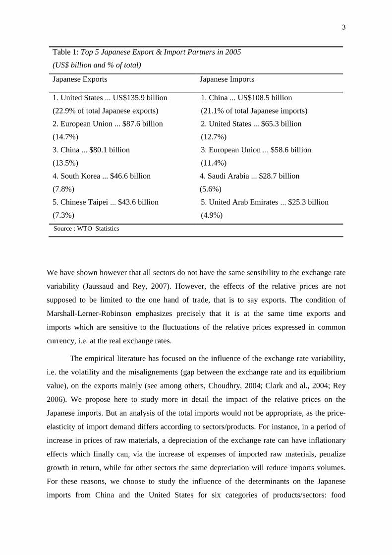
China, the European Unions and the United States are nowadays the main trading

partners of Japan, as table 1 shows. On the import size, China ranks first, and the USA

second, which leads us to choose these two countries as trading partners of Japan in order to

investigate the long-run determinants of Japanese import flows. Which are the determinants of

Japanese imports? Generally speaking, the domestic demand constitutes an important

determinant. But, on the other hand, changes in relative prices and consequences in

international trade are still a matter of concern and polemic. Debates on the under-evaluation

of the yuan or on the overvaluation of the euro facing the American dollar are particularly

brisk. Most often the academic literature deals with this subject by analysing the impact of the

exchange rate on the exports of a country. Indeed, exports often constitute a powerful motor

of economic growth. Following the example of Germany, Japan is a textbook case of this type

of strategy.

3

Table 1: Top 5 Japanese Export & Import Partners in 2005

(US$ billion and % of total)

Japanese Exports Japanese Imports

1. United States ... US$135.9 billion

(22.9% of total Japanese exports)

1. China ... US$108.5 billion

(21.1% of total Japanese imports)

2. European Union ... $87.6 billion

(14.7%)

2. United States ... $65.3 billion

(12.7%)

3. China ... $80.1 billion

(13.5%)

3. European Union ... $58.6 billion

(11.4%)

4. South Korea ... $46.6 billion

(7.8%)

4. Saudi Arabia ... $28.7 billion

(5.6%)

5. Chinese Taipei ... $43.6 billion

(7.3%)

5. United Arab Emirates ... $25.3 billion

(4.9%)

Source : WTO Statistics

We have shown however that all sectors do not have the same sensibility to the exchange rate

variability (Jaussaud and Rey, 2007). However, the effects of the relative prices are not

supposed to be limited to the one hand of trade, that is to say exports. The condition of

Marshall-Lerner-Robinson emphasizes precisely that it is at the same time exports and

imports which are sensitive to the fluctuations of the relative prices expressed in common

currency, i.e. at the real exchange rates.

The empirical literature has focused on the influence of the exchange rate variability,

i.e. the volatility and the misalignements (gap between the exchange rate and its equilibrium

value), on the exports mainly (see among others, Choudhry, 2004; Clark and al., 2004; Rey

2006). We propose here to study more in detail the impact of the relative prices on the

Japanese imports. But an analysis of the total imports would not be appropriate, as the price-

elasticity of import demand differs according to sectors/products. For instance, in a period of

increase in prices of raw materials, a depreciation of the exchange rate can have inflationary

effects which finally can, via the increase of expenses of imported raw materials, penalize

growth in return, while for other sectors the same depreciation will reduce imports volumes.

For these reasons, we choose to study the influence of the determinants on the Japanese

imports from China and the United States for six categories of products/sectors: food

4

products, raw material, mineral fuel, textile, chemicals and machinery and equipment. On the

basis of a precise analysis of Japanese imports by sectors, we will undertake an econometric

analysis on determinants of imports.

For that,

1- We estimate functions of Japanese imports from China and the United States

for each of six sectors.

2- The econometric estimate of imports functions will rest on standard

approaches in terms of cointegration (long run relationships) and Vector Error

Correction Model (VECM, short run relationships). The covered period will go

from 1971 to 2007.

To analyze the long run determinants of Japanese imports by sectors, we proceed as

follows. Section 2 presents a brief overview of the evolution of sectoral imports from China

and the United States. In section 3, the import model is exposed. Section 4 presents

preliminary data analysis, i.e. units root and cointegration tests. Specifically, we employ the

Saikkonen-Lütkepohl method, which takes into account the presence of breaks in the

variables. Section 5 reports and analyses the empirical results from the Vector Error

Correction Model (hereafter VECM) estimation. Section 6 concludes this contribution.

2. Background

In order to be able to better interpret some of the results that we may find, it may be

useful to remind the context: Japan’s foreign trade and foreign trade policy (2.1). Then we

shall consider more precisely trends in Japanese imports, on a sectoral basis (2.2).

2.1. Japan’s foreign trade, a long term perspective

Through the period under investigation (1971-2007), Japan’s foreign trade has

experienced various situations, or sub-periods, that may be summarized as follows:

- during the 70s, Japan’s has still a rather fragile equilibrium in foreign trade towards

the rest of the world. Exports are growing quickly on the period, but imports are

dramatically affected by the two oil shocks (1973 et 1979);

- during the first half of the 80s, Japan enjoys increasing trade surpluses, as Japanese

firms emerge as major exporters and majors competitors to the West in an increasing

5

number of industries. Trade frictions intensify, the yen is regarded by most observers

as significantly undervalued, and the US dollar as too strong. This leads to the Plaza

Agreement in September 1985, and subsequent currencies realignment (almost 40%

appreciation within one year for the yen against the US dollar);

- from 1986 to 2007, trade surpluses of Japan have been rather stabilized, at very high

levels indeed, from 80 to 100 billion dollars a year, and her foreign exchange policy is

devoted to avoidance of strong fluctuations of the yen towards the US dollar;

- from 2008, a sharp decline in surpluses of Japan occurs, in relation with the current

economic crisis, but this is out of the period under investigation in this paper.

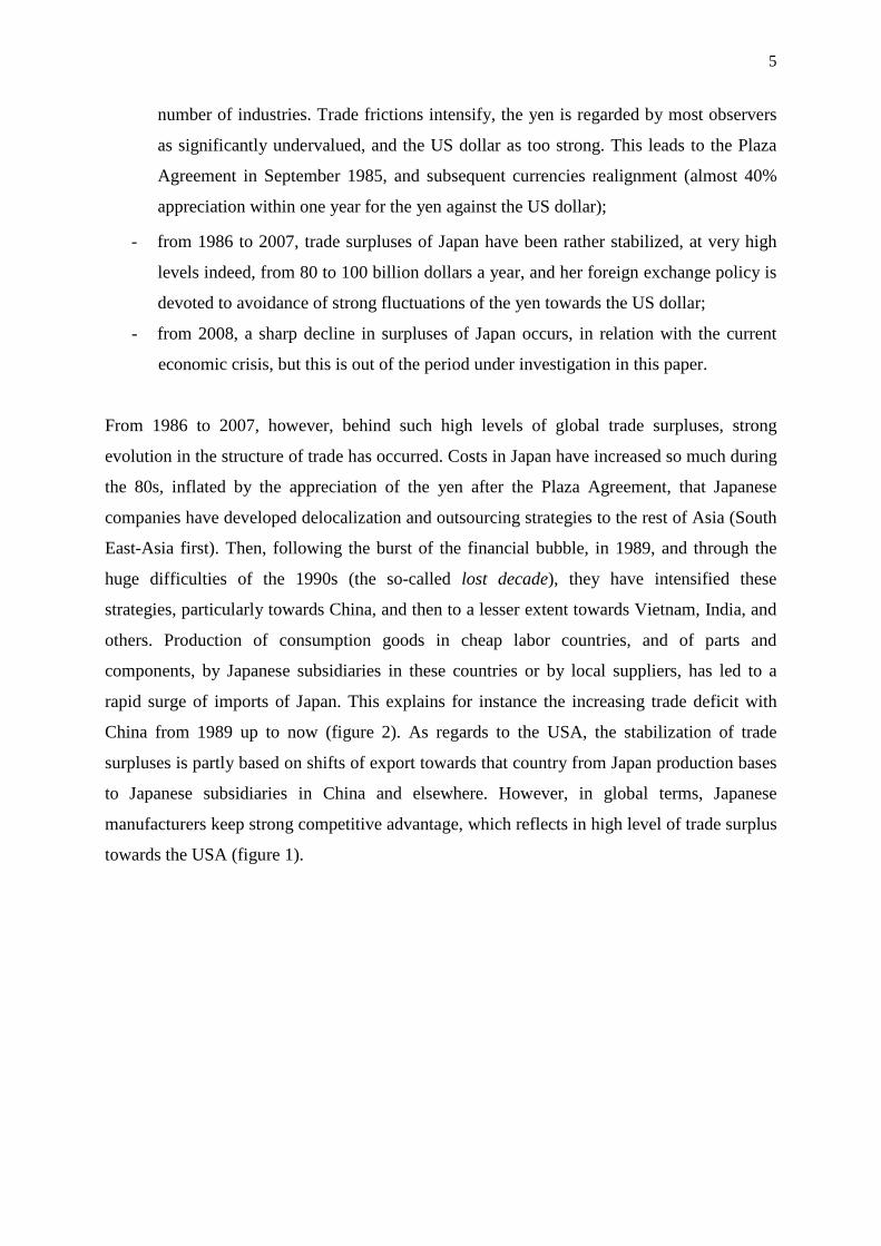
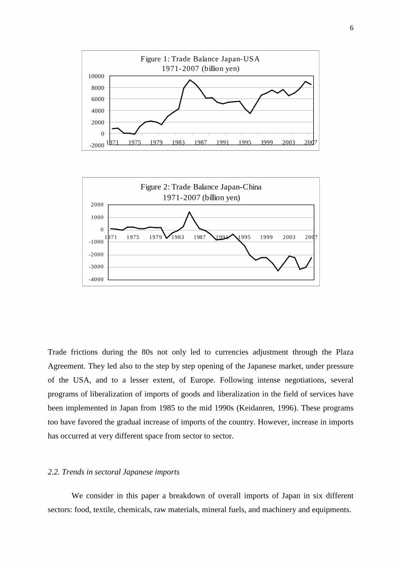
From 1986 to 2007, however, behind such high levels of global trade surpluses, strong

evolution in the structure of trade has occurred. Costs in Japan have increased so much during

the 80s, inflated by the appreciation of the yen after the Plaza Agreement, that Japanese

companies have developed delocalization and outsourcing strategies to the rest of Asia (South

East-Asia first). Then, following the burst of the financial bubble, in 1989, and through the

huge difficulties of the 1990s (the so-called lost decade), they have intensified these

strategies, particularly towards China, and then to a lesser extent towards Vietnam, India, and

others. Production of consumption goods in cheap labor countries, and of parts and

components, by Japanese subsidiaries in these countries or by local suppliers, has led to a

rapid surge of imports of Japan. This explains for instance the increasing trade deficit with

China from 1989 up to now (figure 2). As regards to the USA, the stabilization of trade

surpluses is partly based on shifts of export towards that country from Japan production bases

to Japanese subsidiaries in China and elsewhere. However, in global terms, Japanese

manufacturers keep strong competitive advantage, which reflects in high level of trade surplus

towards the USA (figure 1).

6

Figure 1: Trade Balance Japan-USA1971-2007 (billion yen)

-2000

0

2000

4000

6000

8000

10000

1971 1975 1979 1983 1987 1991 1995 1999 2003 2007

Figure 2: Trade Balance Japan-China1971-2007 (billion yen)

-4000

-3000

-2000

-1000

0

1000

2000

1971 1975 1979 1983 1987 1991 1995 1999 2003 2007

Trade frictions during the 80s not only led to currencies adjustment through the Plaza

Agreement. They led also to the step by step opening of the Japanese market, under pressure

of the USA, and to a lesser extent, of Europe. Following intense negotiations, several

programs of liberalization of imports of goods and liberalization in the field of services have

been implemented in Japan from 1985 to the mid 1990s (Keidanren, 1996). These programs

too have favored the gradual increase of imports of the country. However, increase in imports

has occurred at very different space from sector to sector.

2.2. Trends in sectoral Japanese imports

We consider in this paper a breakdown of overall imports of Japan in six different

sectors: food, textile, chemicals, raw materials, mineral fuels, and machinery and equipments.

7

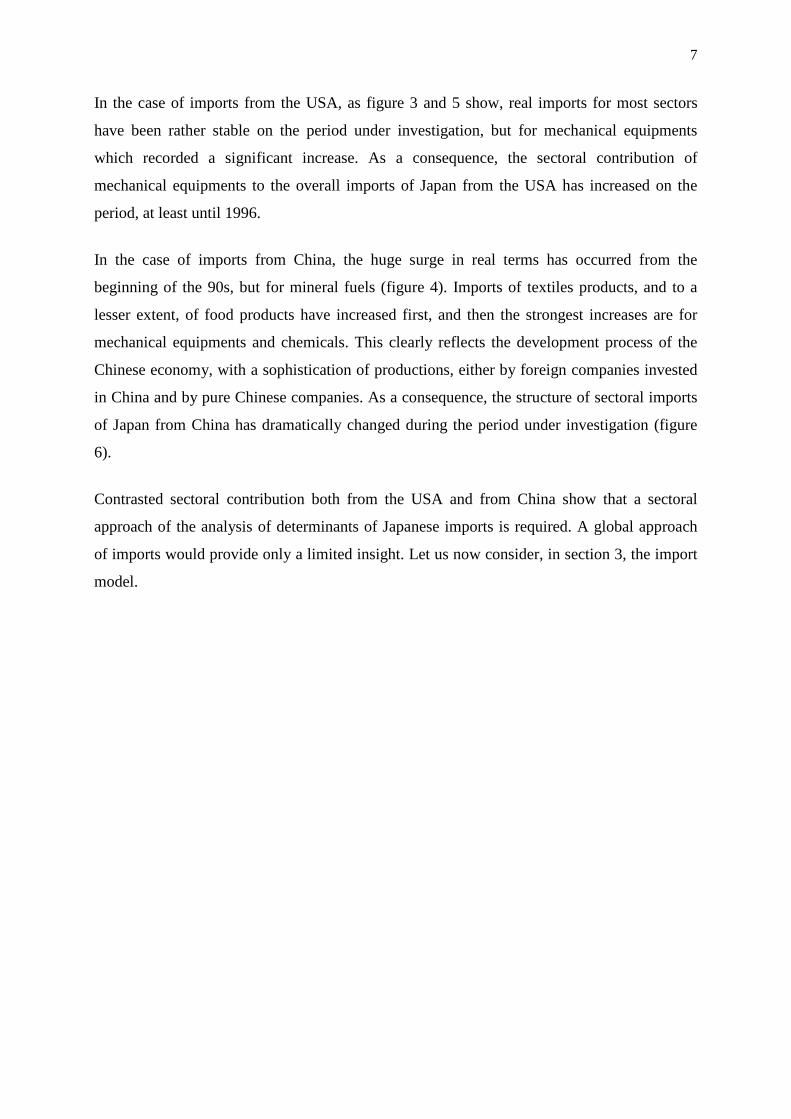
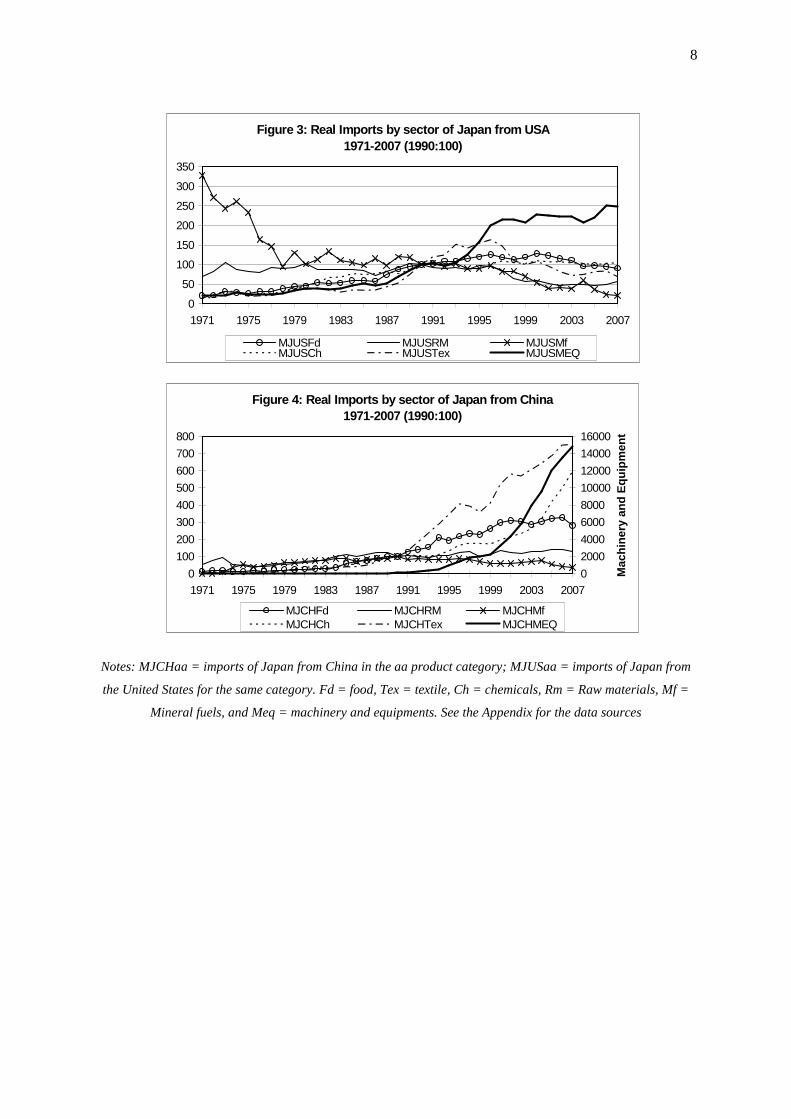
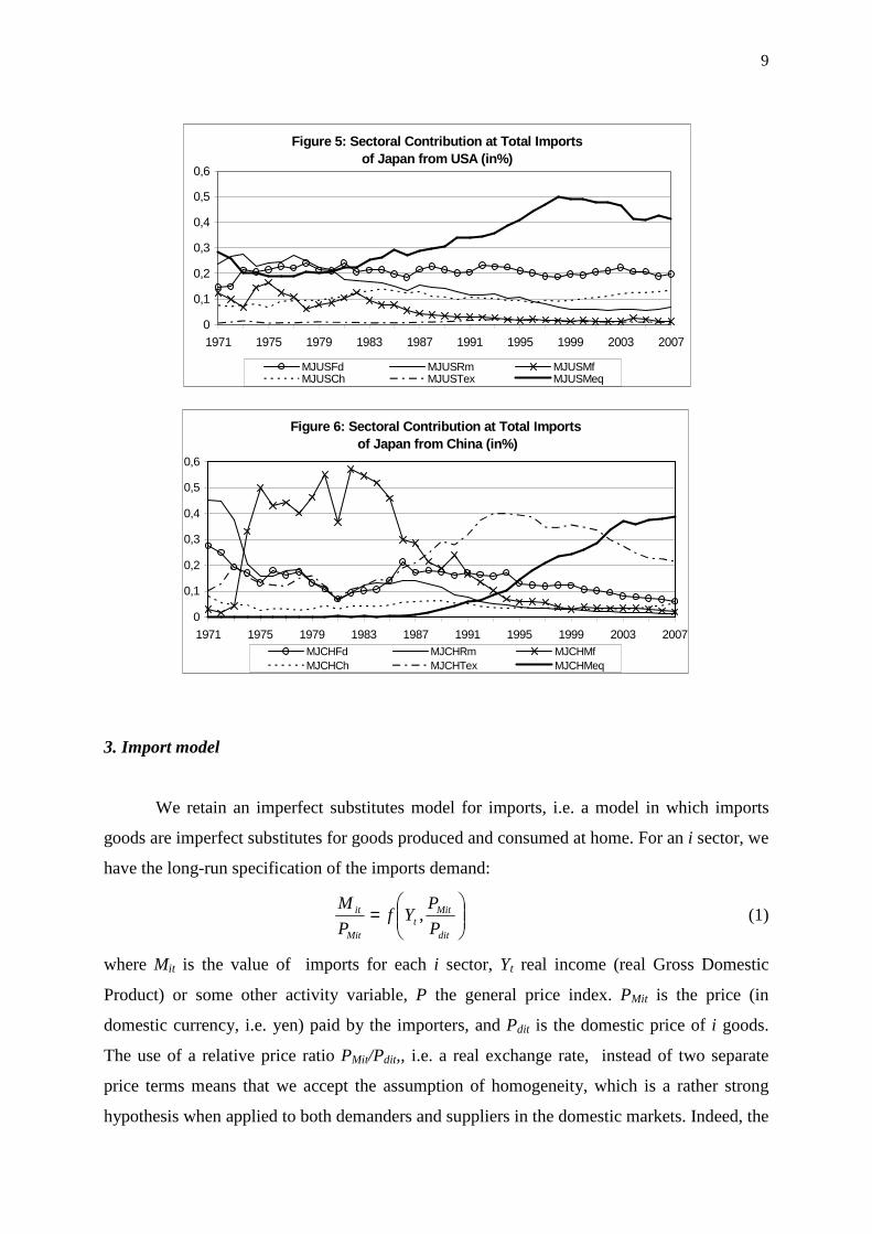
In the case of imports from the USA, as figure 3 and 5 show, real imports for most sectors

have been rather stable on the period under investigation, but for mechanical equipments

which recorded a significant increase. As a consequence, the sectoral contribution of

mechanical equipments to the overall imports of Japan from the USA has increased on the

period, at least until 1996.

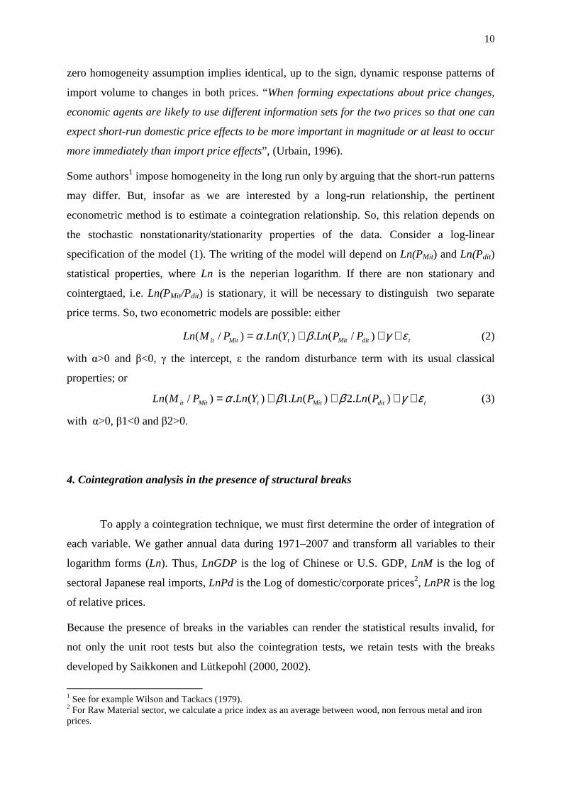
In the case of imports from China, the huge surge in real terms has occurred from the

beginning of the 90s, but for mineral fuels (figure 4). Imports of textiles products, and to a

lesser extent, of food products have increased first, and then the strongest increases are for

mechanical equipments and chemicals. This clearly reflects the development process of the

Chinese economy, with a sophistication of productions, either by foreign companies invested

in China and by pure Chinese companies. As a consequence, the structure of sectoral imports

of Japan from China has dramatically changed during the period under investigation (figure

6).

Contrasted sectoral contribution both from the USA and from China show that a sectoral

approach of the analysis of determinants of Japanese imports is required. A global approach

of imports would provide only a limited insight. Let us now consider, in section 3, the import

model.

8

Figure 3: Real Imports by sector of Japan from USA1971-2007 (1990:100)

0

50

100

150

200

250

300

350

1971 1975 1979 1983 1987 1991 1995 1999 2003 2007

MJUSFd MJUSRM MJUSMfMJUSCh MJUSTex MJUSMEQ

Figure 4: Real Imports by sector of Japan from China1971-2007 (1990:100)

0

100

200

300

400

500

600

700

800

1971 1975 1979 1983 1987 1991 1995 1999 2003 20070

2000

4000

6000

8000

10000

12000

14000

16000

Mac

hin

ery

and

Eq

uip

men

tMJCHFd MJCHRM MJCHMfMJCHCh MJCHTex MJCHMEQ

Notes: MJCHaa = imports of Japan from China in the aa product category; MJUSaa = imports of Japan from

the United States for the same category. Fd = food, Tex = textile, Ch = chemicals, Rm = Raw materials, Mf =

Mineral fuels, and Meq = machinery and equipments. See the Appendix for the data sources

9

Figure 5: Sectoral Contribution at Total Imports of Japan from USA (in%)

0

0,1

0,2

0,3

0,4

0,5

0,6

1971 1975 1979 1983 1987 1991 1995 1999 2003 2007

MJUSFd MJUSRm MJUSMfMJUSCh MJUSTex MJUSMeq

Figure 6: Sectoral Contribution at Total Imports of Japan from China (in%)

0

0,1

0,2

0,3

0,4

0,5

0,6

1971 1975 1979 1983 1987 1991 1995 1999 2003 2007MJCHFd MJCHRm MJCHMfMJCHCh MJCHTex MJCHMeq

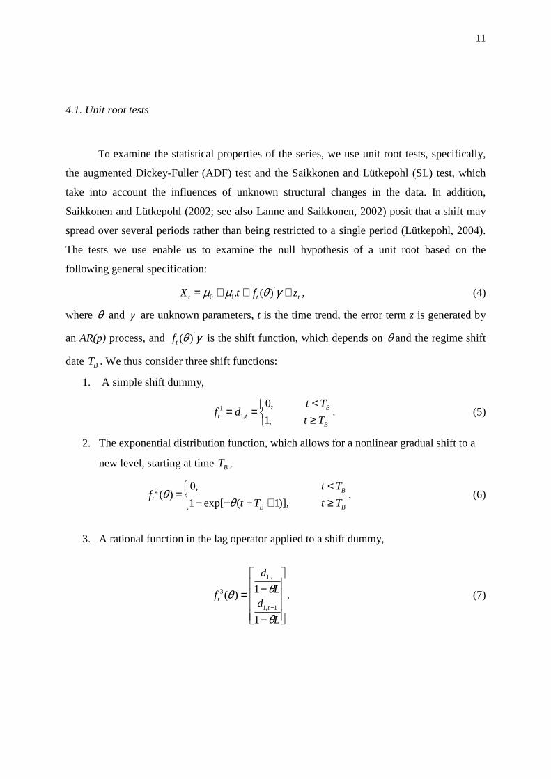
3. Import model

We retain an imperfect substitutes model for imports, i.e. a model in which imports

goods are imperfect substitutes for goods produced and consumed at home. For an i sector, we

have the long-run specification of the imports demand:

=

dit

Mitt

Mit

it

P

PYf

P

M, (1)

where Mit is the value of imports for each i sector, Yt real income (real Gross Domestic

Product) or some other activity variable, P the general price index. PMit is the price (in

domestic currency, i.e. yen) paid by the importers, and Pdit is the domestic price of i goods.

The use of a relative price ratio PMit/Pdit,, i.e. a real exchange rate, instead of two separate

price terms means that we accept the assumption of homogeneity, which is a rather strong

hypothesis when applied to both demanders and suppliers in the domestic markets. Indeed, the

10

zero homogeneity assumption implies identical, up to the sign, dynamic response patterns of

import volume to changes in both prices. “When forming expectations about price changes,

economic agents are likely to use different information sets for the two prices so that one can

expect short-run domestic price effects to be more important in magnitude or at least to occur

more immediately than import price effects”, (Urbain, 1996).

Some authors1 impose homogeneity in the long run only by arguing that the short-run patterns

may differ. But, insofar as we are interested by a long-run relationship, the pertinent

econometric method is to estimate a cointegration relationship. So, this relation depends on

the stochastic nonstationarity/stationarity properties of the data. Consider a log-linear

specification of the model (1). The writing of the model will depend on Ln(PMit) and Ln(Pdit)

statistical properties, where Ln is the neperian logarithm. If there are non stationary and

cointergtaed, i.e. Ln(PMit/Pdit) is stationary, it will be necessary to distinguish two separate

price terms. So, two econometric models are possible: either

tditMittMitit PPnLYLnPMLn εγβα +++= )/(.)(.)/( (2)

with α>0 and β<0, γ the intercept, ε the random disturbance term with its usual classical

properties; or

tditMittMitit PLnPnLYLnPMLn εγββα ++++= )(.2)(.1)(.)/( (3)

with α>0, β1<0 and β2>0.

4. Cointegration analysis in the presence of structural breaks

To apply a cointegration technique, we must first determine the order of integration of

each variable. We gather annual data during 1971–2007 and transform all variables to their

logarithm forms (Ln). Thus, LnGDP is the log of Chinese or U.S. GDP, LnM is the log of

sectoral Japanese real imports, LnPd is the Log of domestic/corporate prices2, LnPR is the log

of relative prices.

Because the presence of breaks in the variables can render the statistical results invalid, for

not only the unit root tests but also the cointegration tests, we retain tests with the breaks

developed by Saikkonen and Lütkepohl (2000, 2002).

1 See for example Wilson and Tackacs (1979). 2 For Raw Material sector, we calculate a price index as an average between wood, non ferrous metal and iron prices.

11

4.1. Unit root tests

To examine the statistical properties of the series, we use unit root tests, specifically,

the augmented Dickey-Fuller (ADF) test and the Saikkonen and Lütkepohl (SL) test, which

take into account the influences of unknown structural changes in the data. In addition,

Saikkonen and Lütkepohl (2002; see also Lanne and Saikkonen, 2002) posit that a shift may

spread over several periods rather than being restricted to a single period (Lütkepohl, 2004).

The tests we use enable us to examine the null hypothesis of a unit root based on the

following general specification:

ttt zftX +++= γθµµ '10 )(. , (4)

where θ and γ are unknown parameters, t is the time trend, the error term z is generated by

an AR(p) process, and γθ ')(tf is the shift function, which depends on θ and the regime shift

date BT . We thus consider three shift functions:

1. A simple shift dummy,

≥<

==B

Btt Tt

Ttdf

,1

,0,1

1 . (5)

2. The exponential distribution function, which allows for a nonlinear gradual shift to a

new level, starting at time BT ,

≥+−−−<

=BB

Bt TtTt

Ttf

)],1(exp[1

,0)(2

θθ . (6)

3. A rational function in the lag operator applied to a shift dummy,

−

−=−

L

dL

d

ft

t

t

θ

θθ

1

1)(1,1

,1

3 . (7)

12

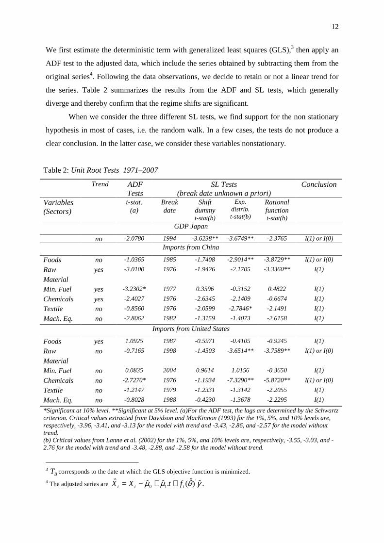
We first estimate the deterministic term with generalized least squares (GLS),3 then apply an

ADF test to the adjusted data, which include the series obtained by subtracting them from the

original series4. Following the data observations, we decide to retain or not a linear trend for

the series. Table 2 summarizes the results from the ADF and SL tests, which generally

diverge and thereby confirm that the regime shifts are significant.

When we consider the three different SL tests, we find support for the non stationary

hypothesis in most of cases, i.e. the random walk. In a few cases, the tests do not produce a

clear conclusion. In the latter case, we consider these variables nonstationary.

Table 2: Unit Root Tests 1971–2007

Trend ADF Tests

SL Tests (break date unknown a priori)

Conclusion

Variables (Sectors)

t-stat. (a)

Break date

Shift dummy t-stat(b)

Exp. distrib. t-stat(b)

Rational function t-stat(b)

GDP Japan

no -2.0780 1994 -3.6238** -3.6749** -2.3765 I(1) or I(0)

Imports from China

Foods no -1.0365 1985 -1.7408 -2.9014** -3.8729** I(1) or I(0)

Raw

Material

yes -3.0100 1976 -1.9426 -2.1705 -3.3360** I(1)

Min. Fuel yes -3.2302* 1977 0.3596 -0.3152 0.4822 I(1)

Chemicals yes -2.4027 1976 -2.6345 -2.1409 -0.6674 I(1)

Textile no -0.8560 1976 -2.0599 -2.7846* -2.1491 I(1)

Mach. Eq. no -2.8062 1982 -1.3159 -1.4073 -2.6158 I(1)

Imports from United States

Foods yes 1.0925 1987 -0.5971 -0.4105 -0.9245 I(1)

Raw

Material

no -0.7165 1998 -1.4503 -3.6514** -3.7589** I(1) or I(0)

Min. Fuel no 0.0835 2004 0.9614 1.0156 -0.3650 I(1)

Chemicals no -2.7270* 1976 -1.1934 -7.3290** -5.8720** I(1) or I(0)

Textile no -1.2147 1979 -1.2331 -1.3142 -2.2055 I(1)

Mach. Eq. no -0.8028 1988 -0.4230 -1.3678 -2.2295 I(1)

*Significant at 10% level. **Significant at 5% level. (a)For the ADF test, the lags are determined by the Schwartz criterion. Critical values extracted from Davidson and MacKinnon (1993) for the 1%, 5%, and 10% levels are, respectively, -3.96, -3.41, and -3.13 for the model with trend and -3.43, -2.86, and -2.57 for the model without trend. (b) Critical values from Lanne et al. (2002) for the 1%, 5%, and 10% levels are, respectively, -3.55, -3.03, and -2.76 for the model with trend and -3.48, -2.88, and -2.58 for the model without trend.

3 BT corresponds to the date at which the GLS objective function is minimized.

4 The adjusted series are γθµµ ˆ)ˆ(.ˆˆˆ '10 ttt ftXX ++−= .

13

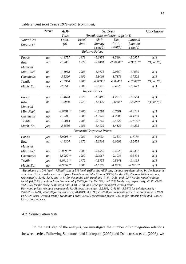
Table 2: Unit Root Testss 1971–2007 (continued)

Trend ADF Tests

SL Tests (break date unknown a priori)

Conclusion

Variables (Sectors)

t-stat. (a)

Break date

Shift dummy t-stat(b)

Exp. distrib. t-stat(b)

Rational function t-stat(b)

Relative Prices

Foods no -1.8757 1978 -1.6451 -1.5894 -2.0957 I(1)

Raw

Material

no -1.2081 1979 -2.2461 -2.9680** -2.9823** I(1) or I(0)

Min. Fuel no -1.1952 1986 -1.9778 -2.0357 -1.7039 I(1)

Chemicals no -2.5260 1986 -1.9003 -1.7179 -1.7202 I(1)

Textile no -1.5960 1986 -2.6593* -2.8445* -4.7387** I(1) or I(0)

Mach. Eq. yes -2.5511 1986 -2.5312 -2.4329 -2.0611 I(1)

Import Prices

Foods no -1.4674 1978 -1.3406 -1.2716 -1.8564 I(1)

Raw Material

no -1.5959 1979 -1.6429 -2.6895* -2.6998* I(1) or I(0)

Min. Fuel no -3.0591** 1986 -0.8191 -0.7581 -0.3749 I(1)

Chemicals no -1.2411 1986 -1.3942 -1.2805 -0.1793 I(1)

Textile no -1.2013 1986 -2.3745 -2.5622 -2.9739* I(1)

Mach. Eq. yes -2.8536 1986 -1.4122 -1.4126 -1.4252 I(1)

Domestic/Corporate Prices

Foods yes -8.9205** 1980 0.3422 -0.2330 1.4779 I(1)

Raw Material

no -1.9304 1976 -1.6901 -2.0698 -2.2458 I(1)

Min. Fuel no -3.0395** 1980 -0.4555 -0.4926 -0.2452 I(1)

Chemicals no -5.5989** 1980 -2.0967 -2.1036 -0.5494 I(1)

Textile yes -3.0912** 1976 -0.8955 -0.8341 -1.4133 I(1)

Mach. Eq. no -7.9652** 1980 -1.5722 -1.0534 -2.6918* I(1)

*Significant at 10% level. **Significant at 5% level. (a)For the ADF test, the lags are determined by the Schwartz criterion. Critical values extracted from Davidson and MacKinnon (1993) for the 1%, 5%, and 10% levels are, respectively, -3.96, -3.41, and -3.13 for the model with trend and -3.43, -2.86, and -2.57 for the model without trend. (b) Critical values from Lanne et al. (2002) for the 1%, 5%, and 10% levels are, respectively, -3.55, -3.03, and -2.76 for the model with trend and -3.48, -2.88, and -2.58 for the model without trend. For wood prices, we have respectively for SL tests the t-stat: -2.3366; -2.4146; -3.5471 for relative price; -2.0702; -2.1894; -2.6998 for import price; -0.4619; -1.1098; -1.0998 for corporate price. The break date is 1979. For ADF tests (without trend), we obtain t-stat; -2.4629 for relative price; -2.6948 for imports price and -2.8573 for corporate price.

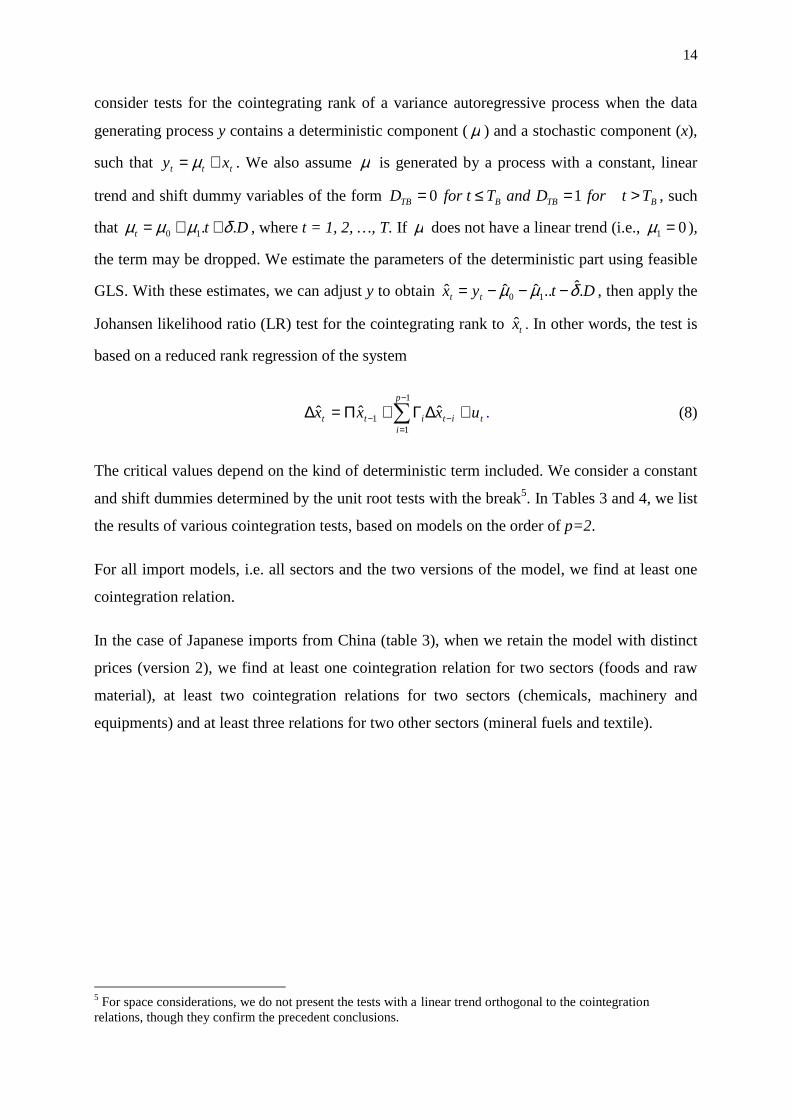
4.2. Cointegration tests

In the next step of the analysis, we investigate the number of cointegration relations

between series. Following Saikkonen and Lütkepohl (2000) and Demetrescu et al. (2008), we

14

consider tests for the cointegrating rank of a variance autoregressive process when the data

generating process y contains a deterministic component (µ ) and a stochastic component (x),

such that ttt xy += µ . We also assume µ is generated by a process with a constant, linear

trend and shift dummy variables of the form BTBBTB TtforDandTtforD >=≤= 10 , such

that Dtt ..10 δµµµ ++= , where t = 1, 2, …, T. If µ does not have a linear trend (i.e., 01 =µ ),

the term may be dropped. We estimate the parameters of the deterministic part using feasible

GLS. With these estimates, we can adjust y to obtain Dtyx tt .ˆ..ˆˆˆ 10 δµµ −−−= , then apply the

Johansen likelihood ratio (LR) test for the cointegrating rank to tx̂ . In other words, the test is

based on a reduced rank regression of the system

tit

p

iitt uxxx +∆Γ+Π=∆ −

−

=− ∑ ˆˆˆ

1

11 . (8)

The critical values depend on the kind of deterministic term included. We consider a constant

and shift dummies determined by the unit root tests with the break5. In Tables 3 and 4, we list

the results of various cointegration tests, based on models on the order of p=2.

For all import models, i.e. all sectors and the two versions of the model, we find at least one

cointegration relation.

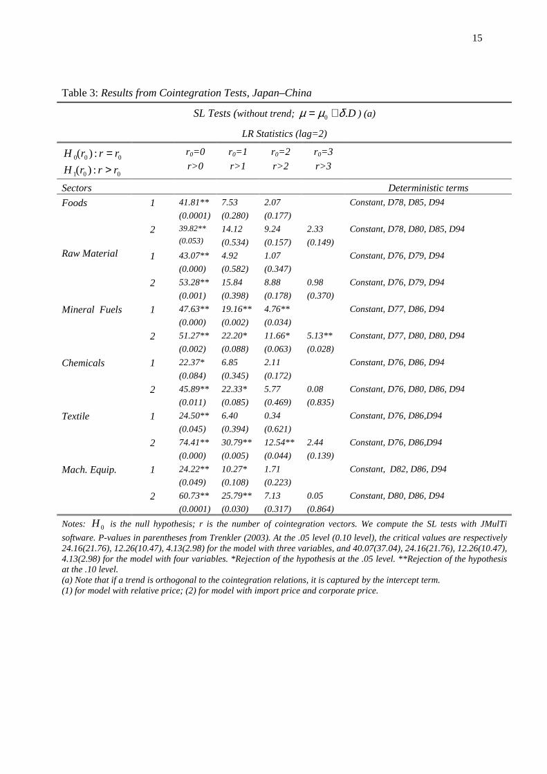
In the case of Japanese imports from China (table 3), when we retain the model with distinct

prices (version 2), we find at least one cointegration relation for two sectors (foods and raw

material), at least two cointegration relations for two sectors (chemicals, machinery and

equipments) and at least three relations for two other sectors (mineral fuels and textile).

5 For space considerations, we do not present the tests with a linear trend orthogonal to the cointegration relations, though they confirm the precedent conclusions.

15

Table 3: Results from Cointegration Tests, Japan–China

SL Tests (without trend; D.0 δµµ += ) (a)

LR Statistics (lag=2)

000 :)( rrrH =

001 :)( rrrH >

r0=0

r>0

r0=1

r>1

r0=2

r>2

r0=3

r>3

Sectors Deterministic terms

Foods 1 41.81**

(0.0001)

7.53

(0.280)

2.07

(0.177)

Constant, D78, D85, D94

2 39.82**

(0.053)

14.12

(0.534)

9.24

(0.157)

2.33

(0.149)

Constant, D78, D80, D85, D94

Raw Material 1 43.07**

(0.000)

4.92

(0.582)

1.07

(0.347)


2 53.28**

(0.001)

15.84

(0.398)

8.88

(0.178)

0.98

(0.370)


Mineral Fuels 1 47.63**

(0.000)

19.16**

(0.002)

4.76**

(0.034)


2 51.27**

(0.002)

22.20*

(0.088)

11.66*

(0.063)

5.13**

(0.028)


Chemicals 1 22.37*

(0.084)

6.85

(0.345)

2.11

(0.172)


2 45.89**

(0.011)

22.33*

(0.085)

5.77

(0.469)

0.08

(0.835)


Textile 1 24.50**

(0.045)

6.40

(0.394)

0.34

(0.621)

Constant, D76, D86,D94

2 74.41**

(0.000)

30.79**

(0.005)

12.54**

(0.044)

2.44

(0.139)


Mach. Equip. 1 24.22**

(0.049)

10.27*

(0.108)

1.71

(0.223)


2 60.73**

(0.0001)

25.79**

(0.030)

7.13

(0.317)

0.05

(0.864)


Notes: 0H is the null hypothesis; r is the number of cointegration vectors. We compute the SL tests with JMulTi

software. P-values in parentheses from Trenkler (2003). At the .05 level (0.10 level), the critical values are respectively 24.16(21.76), 12.26(10.47), 4.13(2.98) for the model with three variables, and 40.07(37.04), 24.16(21.76), 12.26(10.47), 4.13(2.98) for the model with four variables. *Rejection of the hypothesis at the .05 level. **Rejection of the hypothesis at the .10 level. (a) Note that if a trend is orthogonal to the cointegration relations, it is captured by the intercept term. (1) for model with relative price; (2) for model with import price and corporate price.

16

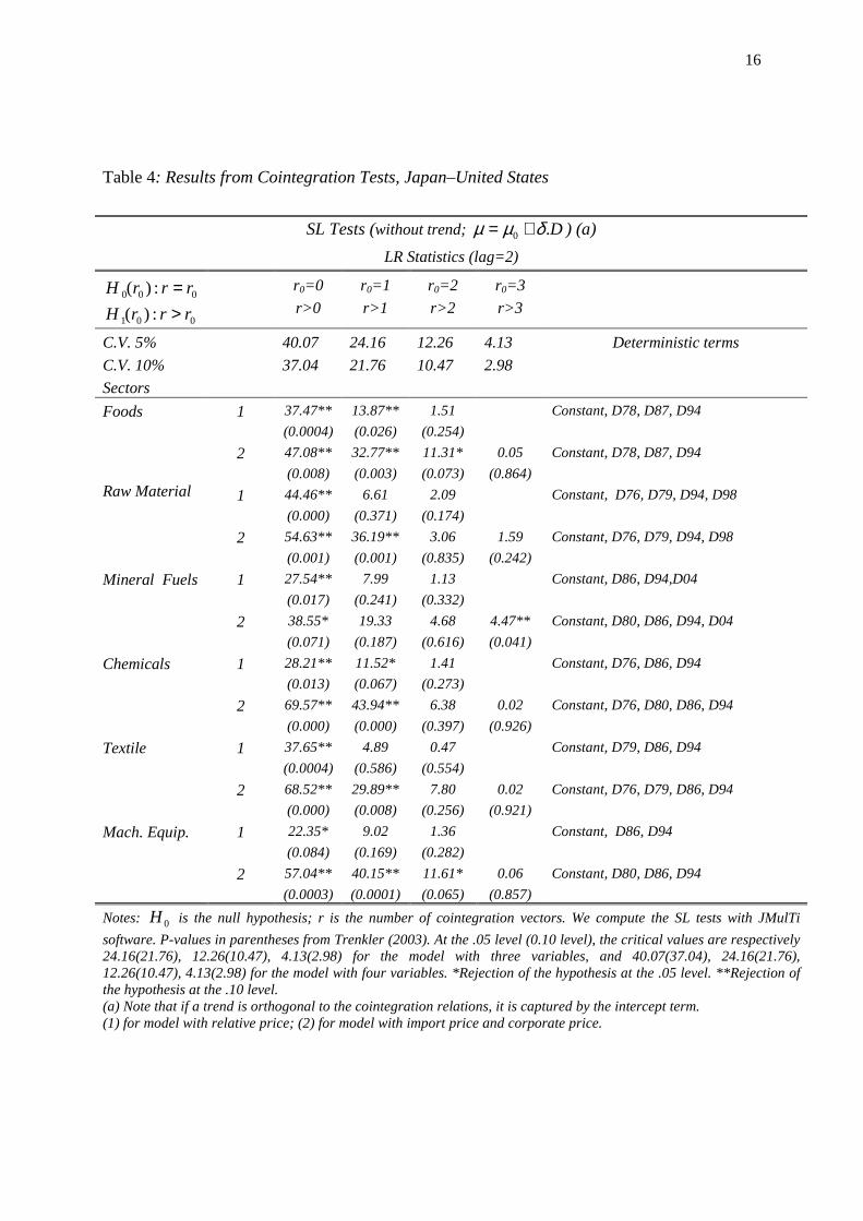
Table 4: Results from Cointegration Tests, Japan–United States

SL Tests (without trend; D.0 δµµ += ) (a)

LR Statistics (lag=2)

000 :)( rrrH =

001 :)( rrrH >

r0=0

r>0

r0=1

r>1

r0=2

r>2

r0=3

r>3

C.V. 5%

C.V. 10%

Sectors

40.07

37.04

24.16

21.76

12.26

10.47

4.13

2.98

Deterministic terms

Foods 1 37.47**

(0.0004)

13.87**

(0.026)

1.51

(0.254)


2 47.08**

(0.008)

32.77**

(0.003)

11.31*

(0.073)

0.05

(0.864)


Raw Material 1 44.46**

(0.000)

6.61

(0.371)

2.09

(0.174)


2 54.63**

(0.001)

36.19**

(0.001)

3.06

(0.835)

1.59

(0.242)


Mineral Fuels 1 27.54**

(0.017)

7.99

(0.241)

1.13

(0.332)


2 38.55*

(0.071)

19.33

(0.187)

4.68

(0.616)

4.47**

(0.041)


Chemicals 1 28.21**

(0.013)

11.52*

(0.067)

1.41

(0.273)


2 69.57**

(0.000)

43.94**

(0.000)

6.38

(0.397)

0.02

(0.926)


Textile 1 37.65**

(0.0004)

4.89

(0.586)

0.47

(0.554)


2 68.52**

(0.000)

29.89**

(0.008)

7.80

(0.256)

0.02

(0.921)


Mach. Equip. 1 22.35*

(0.084)

9.02

(0.169)

1.36

(0.282)

Constant, D86, D94

2 57.04**

(0.0003)

40.15**

(0.0001)

11.61*

(0.065)

0.06

(0.857)


Notes: 0H is the null hypothesis; r is the number of cointegration vectors. We compute the SL tests with JMulTi

software. P-values in parentheses from Trenkler (2003). At the .05 level (0.10 level), the critical values are respectively 24.16(21.76), 12.26(10.47), 4.13(2.98) for the model with three variables, and 40.07(37.04), 24.16(21.76), 12.26(10.47), 4.13(2.98) for the model with four variables. *Rejection of the hypothesis at the .05 level. **Rejection of the hypothesis at the .10 level. (a) Note that if a trend is orthogonal to the cointegration relations, it is captured by the intercept term. (1) for model with relative price; (2) for model with import price and corporate price.

17

For the Japanese imports from USA and the second model with distinct prices (table 4), we

find at least one cointegration relation for two sectors (mineral fuels and chemicals), at least

two cointegration relations for two sectors (raw materials and textile) and at least three

relations for two other sectors (foods, machinery and equipments).

5. Import equations

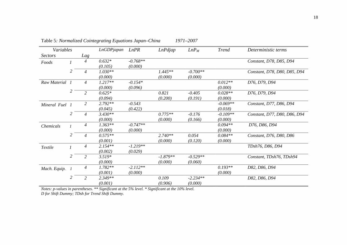
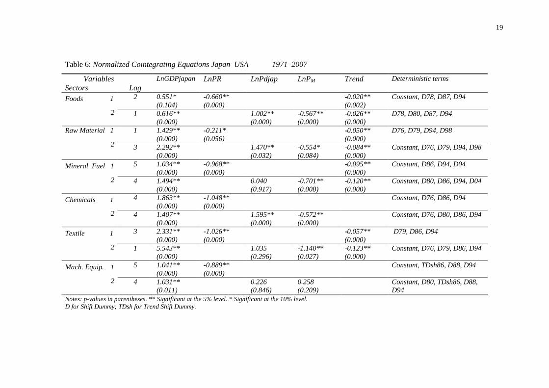
Tables 5 and 6 present results for the estimations of cointegration relationships, for

two partners and two versions of the model. A synthesis of results is exposed in Tables 7 and

8. For the version 1 of the model, the coefficients of domestic demand (GDP) and relative

prices are significant in all cases and with expected signs. One should note that for four

sectors of imports from China (table 5) and for three sectors of imports from USA (table 6),

the demand elasticity is higher than the price elasticity. In other cases, the values of

elasticities are close in absolute value. For the version 2 of the model, we distinguish domestic

and import prices. We verify that the homogeneity hypothesis can be rejected. Indeed, in most

of the cases, i.e. four cases on six for imports from China, and three cases on six for Imports

from USA, the elasticities with respect to domestic prices are nearly double (in absolute

value) than the ones with respect to imports prices. These results lead to reject the assumption

of price homogeneity. The differences of volatilities of the prices can be at the origin of these

differences in the price elasticities. Indeed, the volatility of the prices may indicate different

degrees of uncertainty associated with change in the two prices. So, “the information set that

consumers and producers use to forecast the price of goods abroad will usually be more

limited than the information set used for the prices of domestic goods” (Petousssis, 1985,

p.92).

18

Table 5: Normalized Cointegrating Equations Japan–China 1971–2007

Variables Sectors

Lag

LnGDPjapan LnPR LnPdjap LnPM Trend Deterministic terms

4 0.632* (0.105)

-0.768** (0.000)

Constant, D78, D85, D94 Foods 1

2 4 1.030** (0.000)

1.445** (0.000)

-0.700** (0.000)


4 1.217** (0.000)

-0.154* (0.096)

0.012** (0.000)

D76, D79, D94 Raw Material 1

2 2 0.625* (0.094)

0.821 (0.200)

-0.405 (0.191)

0.028** (0.000)

D76, D79, D94

2 2.792** (0.045)

-0.543 (0.422)

-0.069** (0.018)

Constant, D77, D86, D94 Mineral Fuel 1

2 4 3.430** (0.000)

0.775** (0.000)

-0.176 (0.166)

-0.109** (0.000)


4 1.363** (0.000)

-0.747** (0.000)

0.094** (0.000)

D76, D86, D94 Chemicals 1

2 4 0.575** (0.001)

2.740** (0.000)

0.054 (0.120)

0.084** (0.000)


4 2.154** (0.002)

-1.219** (0.029)

TDsh76, D86, D94 Textile 1

2 2 3.519* (0.000)

-1.879** (0.000)

-0.529** (0.060)

Constant, TDsh76, TDsh94

4 1.782** (0.001)

-2.112** (0.000)

0.193** (0.000)

D82, D86, D94 Mach. Equip. 1

2 2 2.349** (0.001)

0.109 (0.906)

-2.234** (0.000)

D82, D86, D94

Notes: p-values in parentheses. ** Significant at the 5% level. * Significant at the 10% level. D for Shift Dummy; TDsh for Trend Shift Dummy.

19

Table 6: Normalized Cointegrating Equations Japan–USA 1971–2007

Variables Sectors

Lag

LnGDPjapan LnPR LnPdjap LnPM Trend Deterministic terms

2 0.551* (0.104)

-0.660** (0.000)

-0.020** (0.002)

Constant, D78, D87, D94 Foods 1

2 1 0.616** (0.000)

1.002** (0.000)

-0.567** (0.000)

-0.026** (0.000)

D78, D80, D87, D94

1 1.429** (0.000)

-0.211* (0.056)

-0.050** (0.000)

D76, D79, D94, D98 Raw Material 1

2 3 2.292** (0.000)

1.470** (0.032)

-0.554* (0.084)

-0.084** (0.000)


5 1.034** (0.000)

-0.968** (0.000)

-0.095** (0.000)

Constant, D86, D94, D04 Mineral Fuel 1

2 4 1.494** (0.000)

0.040 (0.917)

-0.701** (0.008)

-0.120** (0.000)


4 1.863** (0.000)

-1.048** (0.000)

Constant, D76, D86, D94 Chemicals 1

2 4 1.407** (0.000)

1.595** (0.000)

-0.572** (0.000)


3 2.331** (0.000)

-1.026** (0.000)

-0.057** (0.000)

D79, D86, D94 Textile 1

2 1 5.543** (0.000)

1.035 (0.296)

-1.140** (0.027)

-0.123** (0.000)


5 1.041** (0.000)

-0.889** (0.000)

Constant, TDsh86, D88, D94 Mach. Equip. 1

2 4 1.031** (0.011)

0.226 (0.846)

0.258 (0.209)

Constant, D80, TDsh86, D88, D94

Notes: p-values in parentheses. ** Significant at the 5% level. * Significant at the 10% level. D for Shift Dummy; TDsh for Trend Shift Dummy.

20

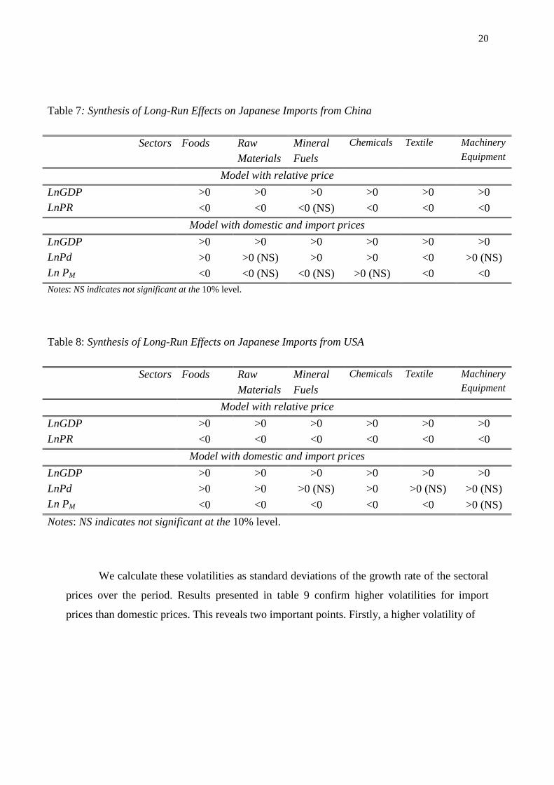
Table 7: Synthesis of Long-Run Effects on Japanese Imports from China

Sectors

Foods

Raw

Materials

Mineral

Fuels

Chemicals

Textile Machinery

Equipment

Model with relative price

>0 >0 >0 >0 >0 >0 LnGDP LnPR <0 <0 <0 (NS) <0 <0 <0

Model with domestic and import prices

>0 >0 >0 >0 >0 >0

>0 >0 (NS) >0 >0 <0 >0 (NS)

LnGDP

LnPd

Ln PM <0 <0 (NS) <0 (NS) >0 (NS) <0 <0 Notes: NS indicates not significant at the 10% level.

Table 8: Synthesis of Long-Run Effects on Japanese Imports from USA

Sectors

Foods

Raw

Materials

Mineral

Fuels

Chemicals

Textile Machinery

Equipment

Model with relative price

>0 >0 >0 >0 >0 >0 LnGDP LnPR <0 <0 <0 <0 <0 <0

Model with domestic and import prices

>0 >0 >0 >0 >0 >0

>0 >0 >0 (NS) >0 >0 (NS) >0 (NS)

LnGDP

LnPd

Ln PM <0 <0 <0 <0 <0 >0 (NS)

Notes: NS indicates not significant at the 10% level.

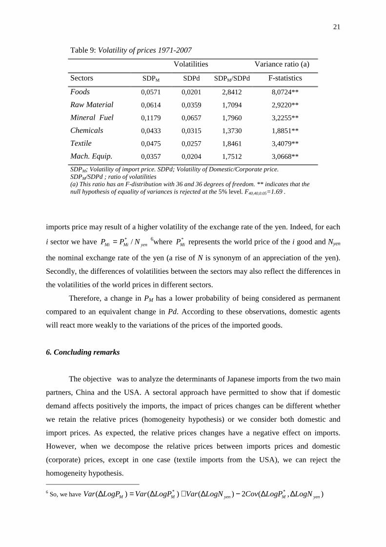
We calculate these volatilities as standard deviations of the growth rate of the sectoral

prices over the period. Results presented in table 9 confirm higher volatilities for import

prices than domestic prices. This reveals two important points. Firstly, a higher volatility of

21

Table 9: Volatility of prices 1971-2007

Volatilities Variance ratio (a)

Sectors SDPM SDPd SDPM/SDPd F-statistics

Foods 0,0571 0,0201 2,8412 8,0724**

Raw Material 0,0614 0,0359 1,7094 2,9220**

Mineral Fuel 0,1179 0,0657 1,7960 3,2255**

Chemicals 0,0433 0,0315 1,3730 1,8851**

Textile 0,0475 0,0257 1,8461 3,4079**

Mach. Equip. 0,0357 0,0204 1,7512 3,0668**

SDPM; Volatility of import price. SDPd; Volatility of Domestic/Corporate price. SDPM/SDPd ; ratio of volatilities (a) This ratio has an F-distribution with 36 and 36 degrees of freedom. ** indicates that the null hypothesis of equality of variances is rejected at the 5% level. F40,40,0.05=1.69 .

imports price may result of a higher volatility of the exchange rate of the yen. Indeed, for each

i sector we have yenMiMi NPP /*= 6where *MiP represents the world price of the i good and Nyen

the nominal exchange rate of the yen (a rise of N is synonym of an appreciation of the yen).

Secondly, the differences of volatilities between the sectors may also reflect the differences in

the volatilities of the world prices in different sectors.

Therefore, a change in PM has a lower probability of being considered as permanent

compared to an equivalent change in Pd. According to these observations, domestic agents

will react more weakly to the variations of the prices of the imported goods.

6. Concluding remarks

The objective was to analyze the determinants of Japanese imports from the two main

partners, China and the USA. A sectoral approach have permitted to show that if domestic

demand affects positively the imports, the impact of prices changes can be different whether

we retain the relative prices (homogeneity hypothesis) or we consider both domestic and

import prices. As expected, the relative prices changes have a negative effect on imports.

However, when we decompose the relative prices between imports prices and domestic

(corporate) prices, except in one case (textile imports from the USA), we can reject the

homogeneity hypothesis. 6 So, we have ),(2)()()( **

yenMyenMM LogNLogPCovLogNVarLogPVarLogPVar ∆∆−∆+∆=∆

22

In most of cases, the coefficients of domestic prices are double than the ones with respect of

import prices. A possible explanation is the greater volatility of import prices than domestic

prices which leads importers to wait when import prices change, insofar as they don’t know if

these changes are temporary or permanent. We show that this hypothesis is verified for three

sectors, at the same time for imports from China and imports from USA. It remains one case,

textile imports from China, for which we obtain a negative sign of domestic price coefficient

contrary to expectations.

A possible extension of this work would be to introduce a FDI (Foreign Direct Investment)

variable in the model and to estimate the import equations on subperiods after a stability

analysis.

References

Arize, A.C. and S.S. Shwiff (1998) “Does Exchange-Rate Volatility Affect Import Flows”,

Applied Economics 30, 1269-1276(8)

Clark, P., N. Tamirisa, S.-J. Wei, A. Sadikov and L. Zeng (2004), “Exchange Rate Volatility

and Trade Flows - Some New Evidence”, IMF working paper, May.

Davidson, R., Mac Kinnon, J., (1993), Estimation and Inference in Econometrics, Oxford

University Press, London.

Demetrescu, M., Lütkepohl, H., Saikkonen, P. (2008), “Testing for the cointegrating Rank of

a Vector Autoregressive Process with Uncertain Deterministic Trend Term”, European

University Institute, working paper 2008/24.

Jaussaud, J. and S. Rey (2008) “Real Exchange Rate and Sectoral Japanese Exports to China

and USA”, in Evolving Corporate Structures and Cultures, Dzever, S., Jaussaud, J.

Andreosso-O'Callaghan (Eds.), Hermes Sciences, London.

Keller, W. (2004): ‘‘International Technology Diffusion,’’ Journal of Economic Literature,

42(3), 752–782.

Lanne, M., Lütkepohl, H., Saikkonen, P. (2002), “Comparison of Unit Root Tests for Time

Series with Level Shifts”, Journal of Time Series Analysis 23 (November), 667-685.

Lawrence, R. Z. and D. E. Weinstein (1999), “Trade and Growth: Import-Led or Export-Led?

Evidence from Japan and Korea”, NBER working paper, July.

Lütkepohl, H., (2004), “Recent Advances in Cointegration Analysis”, Economics Working

Papers ECO2004/12, European University Institute.

23

Lütkepohl, H., Kratzig, M., Boreiko D., (2006), “VAR Analysis in JMulTi”, mimeo, January,

http://www.jmulti.com/download/help/var.pdf.

Petoussis, E. (1985), “The Aggregate Import Equation: Price Homogeneity and Monetary

Effects”, Empirical Economics, 10, 91-101.

Rey, S. (2006), “Effective Exchange Rate Volatility and MENA Countries' Exports to EU",

Journal of Economic Development 31, Issue 2.

Saikkonen, P., Lütkepohl, H. (2000), “ Testing for the Cointegrating Rank of a VAR Process

with an Intercept”, Econometric Theory 16, 373-406.

Saikkonen, P., Lütkepohl, H. (2002), “Testing for a Unit Root in a Time Series with a Level

Shift at Unknown Time”, Econometric Theory 18, 313-348.

Urbain, J.-P. (1996), “Japanese Import Behavior and Cointegration: A Comment”, Journal of

Policy Modeling, 18(6), 583-601»,

Wilson, J., and Tackacs, W. (1979), “Differential Responses to Prices and Exchange Rates

Influence in the Foreign Trade of Selected Industrial Countries”, Review of Economics

and Statistics, 51, 96-104.

Appendix

Data Sources

Information about imports of Japan from China and the United States come from

several editions of the Japan Statistical Yearbook. To obtain the volume of sectoral Japanese

imports (real imports), we divide the value series by the import price indexes of each sector.

Data on domestic and import prices are extracted from Bank of Japan;

http://www.boj.or.jp/en/theme/stat/index.htm. Japanese GDP data are extracted from IFS CD-

Rom.

Documents

Working Pa - CORE · Working Pa pers Series CATT WP No. 8. ... importers to wait when import prices change, ... and then to a lesser extent towards Vietnam, India, and