Embed Size (px)
Citation preview

ZENTRUM FÜR ENTWICKLUNGSFORSCHUNG
Groundwater potential to supply population demand within the Kompienga dam
basin in Burkina Faso
Inaugural-Dissertation
zur
Erlangung des Grades
Doktor der Agrarwissenschaften
(Dr. Agr.)
der
Hohen Landwirtschaftlichen Fakultät
der
Rheinischen Friedrich-Wilhelms-Universität
zu Bonn
vorgelegt am
8. Oktober 2007
von
Wennegouda Jean Pierre Sandwidi
aus
Koupéla (Burkina Faso)

1. Referent: Prof. Dr. Paul L. G. Vlek, ZEF
2. Referent: Prof. Dr.-Ing. Dr. h.c. Janos J. Bogardi
3. Referent: Prof. Dr. Ir. Nick van de Giesen
Tag der Promotion: 8. Oktober 2007
Erscheinungsjahr: 2007
Diese Dissertation ist auf dem Hochschulschriftenserver der ULB Bonn
http://hss.ulb.uni-bonn.de/diss_online elektronisch publiziert

To my parents Simon-Pierre and Pauline, my wife Thérèse Noélie and our twins, Elvis and Edwige
“C’est au plus profond de la nuit, qu’apparaît l’aube”
“We must treat each and every swamp, river basin, river and tributary, forest and field with the greatest care, for all these things are the elements of a very complex system that serves to preserve water reservoirs – and that represents the river of life.” Mikhail Gorbatchev
“Water is the earth’s eye, looking into which the beholder measures the depth of his own nature.” Henry David Thoreau
“If the misery of our poor be caused not by the laws of nature, but by our institutions, great is our sin.” Charles Darwin
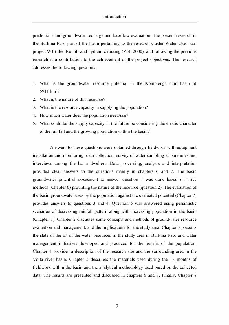
ABSTRACT Groundwater recharge is constrained by various factors with rainfall playing a key role. The Kompienga dam basin located in southeastern Burkina Faso displays semi-arid climatic conditions with rainfall occurring five months per year. The average long-term (1959-2005) mean annual rainfall amounted to 830.2 mm with high temporal and spatial variability. During the year, evaporation always exceeds rainfall, except for a few months in the rainy season when recharge can take place in the basin. In addition, the crystalline rocks of granites and amphibolites mainly underlying the basin have a poor water storage capacity. Therefore, groundwater recharge in the basin is estimated to be as low as 43.9 mm, which represents 5.3% of the rainfall in 2005 for a potential groundwater volume of 259.5 million m³. The estimation based on the water balance method, the chloride mass balance method and the water table fluctuation method shows that the basin recharge is mostly through matrix flow with considerable spatial variability based on soil textures, crystalline rock fracturing, land-use/land-cover and topography. Thus, preferential flow processes are dominant in the basin recharge in the southwestern part around Tanyélé, where the chloride concentration in the groundwater is about that in rainwater.
Annual recharge in the basin is determined by an annual rainfall threshold ranging between 314.3 mm and 336.6 mm reached during the first two to three months of the rains. This relationship provided the equation for deriving annual groundwater recharge in the basin. According to Eddy correlation measurements, actual evaporation in the basin depletes the aquifers at an average rate of 0.6 mm per day during the dry season. This situation contributes to the reduction of the groundwater resources and limits the possibilities of developing these resources to improve the population’s livelihoods.
The basin population in 2005 was 270 000 inhabitants living in 15 departments in 5 provinces, and water withdrawal was estimated at an average rate of 76 l/c/d (including livestock watering) in the dry season period. This represents 5 million m³ of water, making up 2 % of the annual recharge to the aquifers. In anticipation of decreasing rainfall and increasing population in the Kompienga dam basin, scenarios of recharges against withdrawals show that the annual recharge will support the demand for water till 2030 at a supply rate of 25 l/c/d from 1260 functional boreholes operating 12 hours per day at an average unit yield of 1 m³ per hour. The nationally formulated norm for rural water provision of 20 l/c/d was found to respond to basic needs only, and 35 l/c/d is considered the required supply rate especially from March to May when the water demand is highest. Therefore, the revision of the national norm and policy target for rural water supply is recommended.

Grundwasserpotential zur Versorgung der Bevölkerung im Kompienga Staudammbecken in Burkina Faso KURZFASSUNG Grundwasseranreicherung wird durch verschiedene Faktoren bestimmt, wobei dem Niederschlag eine Schlüsselrolle zukommt. Das Kompienga Staudammbecken im süd-östlichen Teil Burkina Fasos weist mit seinen durchschnittlich fünf Regenmonaten pro Jahr und einem mittleren Jahresniederschlag (1959-2005) von 830,2 mm bei hoher zeitlicher und räumlicher Varianz. Im Laufe des Jahres übersteigt dort die Evaporation die Niederschlagsmengen, mit Ausnahme von wenigen Monaten während der Regenzeit, in denen die Grundwasseranreicherung im Becken stattfinden kann. Zudem haben die kristallinischen Granite und Amphibolite, die sich unter dem Becken befinden, nur eine geringe Speicherfähigkeit. Die Schätzung der Grundwasseranreicherung für das Becken ergibt darum einen niedrigen Wert von 5,3 % der jährlichen Niederschlagsmenge im Jahr 2005 für ein potenzielles Grundwasservolumen von 259,5 Mio. m³. Die auf der Wasserbilanz-Methode, der Chlorid-Mengenbilanz-Methode und der Grundwasserspiegel-Fluktuationsmethode basierende Schätzung zeigt, dass die Anreicherung hauptsächlich über matrix flow gespeist wird, mit einer hohen räumlichen Varianz je nach Bodenbeschaffenheit, Vorkommen von Frakturen im kristallinischen Gestein, Landnutzung und -bedeckung sowie Topografie. Dementsprechend dominieren preferential flow Prozesse im süd-westlichen Teil nahe Tanyélé, wo die Chloridkonzentration des Grundwassers ungefähr der des Niederschlagswassers entspricht.
Die jährliche Anreicherung im Becken wird durch den jährlichen Niederschlag (314,3 mm bis 336,6 mm), der während der ersten zwei bis drei Regenmonate erreicht wird, bestimmt. Den Eddy correlation Messungen zufolge führt die aktuelle Evaporation während der Trockenzeit zu einer Abnahme des in den Aquiferen gespeicherten Grundwassers um einem durchschnittlichen Wert von 0,6 mm pro Tag und damit zur Reduzierung der Grundwasserressourcen. Hierdurch sind die Möglichkeiten, diese Ressourcen zu entwickeln und so zu einer Verbesserung der Lebensgrundlage der Bevölkerung beizutragen, begrenzt.
Im Jahr 2005 lebten die 270 000 Bewohner des Beckens in fünfzehn Distrikten bzw. fünf Provinzen, und ihre Wasserentnahme in der Trockenzeit entsprach ca. 76 l/c/d (einschließlich Wasser für das Vieh). Das entspricht 5 Mio. m³ Wasser und 2 % der jährlichen Grundwasseranreicherungsmenge. Vergleichende Szenarien auf der Grundlage der zu erwartenden geringeren Niederschläge und steigendenden Bevölkerungszahlen im Kompienga Staudammbecken zeigen, dass die jährliche Grundwasseranreicherung ausreichen wird, um den Wasserbedarf bis 2030 bei einer Versorgung mit Wasser von 25 l/c/d durch 1260 funktionale Bohrlöcher im 12-stündigen Betrieb bei einer Pumprate von 1 m³ pro Stunde zu decken. Die auf nationaler Ebene formulierte Norm von 20 l/c/d für ländliche Gebiete kann lediglich die Grundversorgung sicherstellen, da tatsächlich 35 l/c/d benötigt werden, insbesondere in der Zeit von März bis Mai, wenn der Wasserbedarf am höchsten ist. Daraus ergibt sich die Empfehlung, die nationale Norm und politische Zielvorgabe für die ländliche Versorgung zu überprüfen und gegebenenfalls zu korrigieren.

Potentialités en eaux souterraines pour la satisfaction des besoins des populations du bassin versant du barrage de la Kompienga au Burkina Faso
RESUME Les recharges des nappes d’eau souterraines sont conditionnées par divers facteurs dont les pluies jouent un rôle principal. Sur le basin versant du barrage de la Kompienga au Sud-est du Burkina Faso en conditions climatiques semi-aride, les pluies se caractérisent par une forte variabilité spatio-temporelle de 5 mois par an avec une hauteur pluviométrique moyenne interannuelle (1959-2005) de 830.2 mm. Tout au long de l’année, l’évaporation mensuelle sur le site dépasse généralement les pluies sauf durant quelques mois au cours de la saison des pluies où ont lieu les recharges des nappes. En plus de ces conditions défavorables, le site de Kompienga se trouve sur un socle cristallin de granites et d’amphibolites peu propice à la constitution d’aquifères importants. Une estimation de la recharge des nappes du bassin a conséquemment révélé un faible niveau de recharge de 43.9 mm représentant 5.3% de la pluie annuelle en 2005 et correspondant à un potentiel en eau de 259.5 millions de m³. Cette estimation faite à partir de la méthode des chlorures, la méthode du bilan hydrologique et celle de variations des niveaux statiques des nappes a montré que les recharges au niveau du bassin se faisaient principalement suivant des écoulements en nappe spatialement variables selon les textures des sols, le degré de fracturation des roches du socle, la végétation et l’utilisation des terres ainsi que la topographie. Relativement à cette variabilité spatiale des processus de recharge des nappes du bassin, les processus d’écoulements préférentiels se sont révélés dominants dans la partie sud-ouest du bassin autour de la zone de Tanyélé où les eaux souterraines présentent des teneurs en chlorures voisines de celles des eaux de pluies.
Un seuil de hauteur de pluie annuelle conditionne les recharges des nappes du bassin versant. Ce seuil varie entre 314.3 mm et 336.6 mm et n’est atteint qu’au bout des 2 ou 3 premiers mois de la saison des pluies. Cette relation a permis de formuler une équation pour l’estimation des recharges annuelles du bassin suivant les hauteurs pluviométriques moyennes annuelles. Les données climatiques de saison sèche de la station Eddy correlation ont montré que l’évaporation actuelle réduisait en moyenne les aquifères du bassin de 0.6 mm d’eau par jour. Ce qui réduit considérablement les possibilités de développement des ressources en eau souterraine du bassin pour l’amélioration des conditions de vie des populations. En 2005, l’approvisionnement en eau des 270 000 habitants environ vivant dans les 15 départements des 5 provinces couvrant le bassin versant a été estimé à une moyenne de 76 litres d’eau par jour par personne (76 l/j/pers y compris l’abreuvement des animaux) durant la période sèche. Ce qui correspond à un volume de 5 millions de m³ d’eau prélevés des aquifères ; soit 2% de la recharge totale de l’année. En prévision de l’accroissement de la population du bassin et de scénarios de baisses de la pluviométrie, les recharges résultantes ont montré la capacité des nappes du bassin à supporter les besoins en eau des populations jusqu’en 2030 avec 25 l/j/pers à partir de 1260 forages d’eau fonctionnant continuellement chaque jour pendant 12 heures à un débit unitaire moyen de 1 m³/h par forage. La norme nationale de 20 l/j/pers en zone rurale s’est révélée juste pour la satisfaction des besoins de base et mérite donc d’être revue pour tenir compte du taux d’approvisionnement moyen utile de 35 l/j/pers observée au niveau du site pendant la période de fortes demandes en eau des mois de Mars à Mai.

TABLE OF CONTENTS
1 INTRODUCTION................................................................................................... 1
2 BACKGROUND AND LITERATURE REVIEW ................................................. 5 2.1 Definition of basic terms ................................................................................... 5 2.2 Review of groundwater resources evaluation and management: concepts,
methods and implications .................................................................................. 7
3 OVERVIEW OF WATER RESOURCES IN BURKINA FASO......................... 15 3.1 Introduction ..................................................................................................... 15 3.2 Surface water resources ................................................................................... 17 3.3 Groundwater resources.................................................................................... 18 3.4 Water resources management.......................................................................... 19 3.5 Conclusion....................................................................................................... 21
4 STUDY AREA...................................................................................................... 23 4.1 Introduction ..................................................................................................... 23 4.2 Volta river basin .............................................................................................. 23 4.3 Kompienga dam basin ..................................................................................... 27 4.3.1 Geology and geomorphology ....................................................................... 31 4.3.2 Hydrogeology ............................................................................................... 33 4.3.3 Temperatures ................................................................................................ 33 4.3.4 Soils .............................................................................................................. 33 4.3.5 Vegetation and land use................................................................................ 34 4.3.6 Population..................................................................................................... 34
4.4 Conclusion....................................................................................................... 35
5 MATERIALS AND METHODS .......................................................................... 36 5.1 Introduction ..................................................................................................... 36 5.2 Materials and methods..................................................................................... 36 5.2.1 Chloride mass balance method..................................................................... 40 5.2.2 Water balance method .................................................................................. 43 5.2.3 Water table fluctuation method .................................................................... 51 5.2.4 Groundwater use quantities and water supply rate estimation ..................... 53
5.3 Conclusion....................................................................................................... 56
6 GROUNDWATER POTENTIAL EVALUATION.............................................. 57 6.1 Introduction ..................................................................................................... 57 6.2 Groundwater potential evaluation using chloride mass balance method ........ 58 6.2.1 Background................................................................................................... 58 6.2.2 Results and discussion.................................................................................. 60
6.3 Groundwater potential evaluation using water balance method...................... 71 6.3.1 Background................................................................................................... 71 6.3.2 Results and discussion.................................................................................. 72

6.4 Groundwater potential evaluation using water table fluctuation method........ 83 6.4.1 Background................................................................................................... 83 6.4.2 Results and discussion.................................................................................. 84
6.5 Conclusion....................................................................................................... 89
7 GROUNDWATER USE AND WATER SUPPLY RATE ................................... 93 7.1 Introduction ..................................................................................................... 93 7.2 Results and discussion on the basin groundwater use ..................................... 93 7.3 Water demand and supply within the basin................................................... 101 7.3.1 Actual water supply.................................................................................... 102 7.3.2 Future water supply .................................................................................... 106
7.4 Conclusions ................................................................................................... 113
8 GENERAL CONCLUSIONS AND RECOMMENDATIONS .......................... 116 8.1 General conclusions....................................................................................... 116 8.2 Recommendations ......................................................................................... 119
9 REFERENCES .................................................................................................... 121
10 APPENDICES..................................................................................................... 132
ACKNOWLEDGEMENTS

ACRONYMS AND ABBREVIATIONS ARFA
BMBF
BUMIGEB
CD/MAHRH
CIRD-Ouagadougou
CNRST
DEP
DGAEP
DGIRH
DGRE
EU
FAO
GDP
GIRE
HDI
HPIC
IMF
INERA
INSD
IWACO BV
MAHRH/DRAHRH-Est
Association de Recherche et de Formation Agro-écologique
Bundesministerium für Bildung und Forschung (Germany)
BUreau des MInes et de la GEologie du Burkina
Centre de Documentation du Ministère de l’Agriculture, de
l’Hydraulique et des Ressources Halieutiques
Centre d’Information sur la Recherche et le Développement
Centre National de la Recherche Scientifique et
Technologique
Direction des Etudes et de la Planification (Ministère de
l’Environnement et de l’Eau)
Direction Générale de l’Approvisionnement en Eau Potable
Direction Générale de l’Inventaire des Ressources
Hydrauliques
Direction Générale des Ressources en Eau (Ministère de
l’Agriculture, de l’Hydraulique et des Ressources
Halieutiques)
European Union
Food and Agriculture Organization
Gross Domestic Product (in purchasing power parity)
Projet Gestion Intégrée des Ressources en Eau
Human Development Index
Heavily Poor Indebted Countries
International Monetary Fund
Institut de l’Environnement et de Recherches Agricoles
Institut National de la Statistique et de la Démographie
Dutch consulting group of research/development on water
resources
Ministère de l’Agriculture, de l’Hydraulique et des
Ressources Halieutiques/Direction Régionale de
l’Agriculture, de l’Hydraulique et des Ressources
Halieutiques de l’Est

MEF/DPD-Est
ONEA/Kpg
OSS
PPB/Est
PPIV
SONABEL
TUDelft
UNDP
UNU-EHS
US$
VINVAL
WCED
WHO
WMO
ZEF
Ministère de l’Economie et des Finances - Direction
Provinciale pour le Développement de l’Est
Office National de l’Eau et de l’Assainissement-Kompienga
Observatory of the Sahara and the Sahel. An organization
composed of Arabic Maghreb Union (AMU) countries
(Algeria, Egypt, Lybia, Mauritania, Morocco and Tunisia),
Permanent Interstate Committee for Drought Control in the
Sahel (CILSS) countries (Burkina Faso, Cape Verde, Chad,
Gambia, Guinea-Bissau, Mali, Mauritania, Niger and
Senegal) and countries of the Intergovernmental Authority
on Development (IGAD) with Djibouti, Eritrea, Ethiopia,
Kenya, Somalia, Sudan and Uganda.
Projet Petits Barrages de la région de l’Est
Projet Promotion de la Petite Irrigation Villageoise
SOciété NAtionale Burkinabé d’ELectricité
Technische Universiteit Delft (The Netherlands)
United Nations Development Program
United Nations University - Institute for Environment and
Human Security
Dollar of United States of America
Project on the Impact of changing land cover on the
production and ecological functions of vegetation in inland
valleys in West Africa
World Commission on Environment and Development
World Health Organization
World Meteorological Organization
Zentrum für Entwicklungsforschung (Germany)

Introduction
1
1 INTRODUCTION
The planet earth is the only planet of the solar system to support living creatures mainly
due to the presence of water in gaseous, liquid and solid form. “L’eau, c’est la vie”
(water is life) is a common French saying to show how important water is for life.
Pielou (1998, prologue) added that “living things depend on water but water does not
depend on living things” as “it has a life of its own”. Hillel (1994) in the same reflexion,
described the essence of water in human life, with our body composed of 90% of water
at birth and “drying up” to 65% in old age.
Water’s importance on earth is therefore undeniable for human beings and is
increasingly so, as water is becoming more and more scarce in major parts of the world.
At the same time, in fewer areas, water availability is considered excessive (Hillel 1994)
in addition to frequent floods occurrence. This dual characteristic of excess and scarcity
of water on our planet seems unrealistic, since the global earth water budget has
remained almost unchanged with only negligible inter-annual variation since the 1980’s
(Pielou 1998). Global climate change has induced and even worsened the unequal
spatial distribution of rains around the world with a drastic decrease in rainfall in
African countries (Dale 1997, Arnell and Liu 2001, Agyare 2004 and
www.news.bbc.co.uk). In these parts of the world and especially in West African
countries, temporal and spatial rainfall variability has increased together with a decrease
in amounts during the last decades (Somé 2002 and Paturel et al. 2002). Meanwhile, as
lack of consensus among scientists on climate change impacts, Nicholson (2005) and
Jung (2006) among others predicted a spatially complex pattern of increase in the
annual rainfall in West Africa and especially in the Volta basin. Nevertheless, from the
observations on this zone since the 1960’s and 1970’s, an overall decrease tendency in
rainfall was agreed on (Lebarbé and Lebel 1997, Servant et al.1998, Hulme et al. 2001
and Amani 2001). Therefore, water availability within West African countries will
mostly decrease (UNESCO 2004), and the growing population is going to face more
frequent and severe shortages. Water supply to the populations in these countries using
surface waters has shown to be limited due to high evaporative effects on such open-air
water resources (Pouyaud 1985, 1986 & 1994, Milville 1991 and MEE 2001) and
sedimentation (Lulseged 2005) due to considerable soil erosion in tropical zones (Vlek

Introduction
2
1993, Vlek et al. 1997, Katyal and Vlek 2000). Shallow hand-dug wells also show
limited efficiency due to low annual water recharge combined with high evaporation
from such shallow aquifers close to soil surface. In addition, these aquifers are mainly
laid in the regolith of the weathered crystalline basement rocks often of lesser thickness
and unable of substantial water storage.
A relevant resource for sufficient water supplies in West Africa is considered
to be deep groundwater. Deep aquifers of crystalline rocks sufficiently provided with
fractures, fissures and joints storing substantial recharges are effectively providing
water supply to the population through boreholes equipped with hand pumps and
modern wells in addition to the existing traditional hand-dug wells. However, any or
only little information related to these aquifers is available for planning their sustainable
exploitation.
In Burkina Faso, groundwater studies by Savadogo (1984) and Geirnaert et al.
(1984) proved the presence of tritium in the water samples, giving evidence of
permanent seasonal recharge of the groundwater aquifers and therefore their annual
renewability. However, the recharge level remains insufficiently investigated. As a main
water source, groundwater needs to be durably managed based on information on
aquifer quantities, seasonal and annual variability, characteristics, and response to
intensive exploitation, etc.
The Glowa Volta project funded by the German Ministry of Education,
Sciences and Technology (BMBF) is set to develop a scientifically sound decision-
support system for the assessment, development and sustainable use of water resources
in the Volta basin by means of an integrated model of the basin (Andreini et al.2000,
p.2). In this project, groundwater and water resources management is one of the main
objectives for supporting the people’s fight against water shortages. Land resources
management under changing land use, rainfall reliability and water demands in the
Volta basin is also part of the project objectives (ZEF 2000). Previous research within
the framework of this project in Ghana and Burkina Faso has addressed various issues
related to integrated water resources management in the Volta river basin. Among these
can be mentioned Ajayi (2004), Martin (2005) and Amisigo (2005), whose studies
focused on hydrological and hydrogeological aspects of the Volta Basin. Mainly based
on modeling, this research addresses the basin rainfall-runoff relationship, riverflow
Introduction
3
predictions and groundwater recharge and baseflow evaluation. The present research in
the Burkina Faso part of the basin pertaining to the research cluster Water Use, sub-
project W1 titled Runoff and hydraulic routing (ZEF 2000), and following the previous
research is a contribution to the achievement of the project objectives. The research
addresses the following questions:
1. What is the groundwater resource potential in the Kompienga dam basin of
5911 km²?
2. What is the nature of this resource?
3. What is the resource capacity in supplying the population?
4. How much water does the population need/use?
5. What could be the supply capacity in the future be considering the erratic character
of the rainfall and the growing population within the basin?
Answers to these questions were obtained through fieldwork with equipment
installation and monitoring, data collection, survey of water sampling at boreholes and
interviews among the basin dwellers. Data processing, analysis and interpretation
provided clear answers to the questions mainly in chapters 6 and 7. The basin
groundwater potential assessment to answer question 1 was done based on three
methods (Chapter 6) providing the nature of the resource (question 2). The evaluation of
the basin groundwater uses by the population against the evaluated potential (Chapter 7)
provides answers to questions 3 and 4. Question 5 was answered using pessimistic
scenarios of decreasing rainfall pattern along with increasing population in the basin
(Chapter 7). Chapter 2 discusses some concepts and methods of groundwater resource
evaluation and management, and the implications for the study area. Chapter 3 presents
the state-of-the-art of the water resources in the study area in Burkina Faso and water
management initiatives developed and practiced for the benefit of the population.
Chapter 4 provides a description of the research site and the surrounding area in the
Volta river basin. Chapter 5 describes the materials used during the 18 months of
fieldwork within the basin and the analytical methodology used based on the collected
data. The results are presented and discussed in chapters 6 and 7. Finally, Chapter 8

Introduction
4
gives the conclusions on the research results and findings along with some
recommendations for further research.
Research is never ended, never finished; as findings always raise questions to
solve. There are only stops and pauses in research to evaluate what has been achieved
and prepare for the following steps. The actual research therefore stops here to continue
further on the induced recommendations presented at the “end” of this thesis.
May these results contribute to build sustainable management schemes for the
basin groundwater resources and improve thereby the livelihood of the population living
in the basin.
Background and literature review
5
2 BACKGROUND AND LITERATURE REVIEW
2.1 Definition of basic terms
Before presenting the basin groundwater potential evaluation, basic terms used in the
text are defined to provide an understanding of the theories and ideas developed in this
thesis. An example is the evapotranspiration term, which is replaced by either
evaporation or transpiration according to the situation in reference to Savenije (2004),
except for expressions derived from references and theories explicitly cited.
River basin
A river basin at a given point represents the whole surface pertaining to this river on
which any rainfall flows into the river and arrives at the given point. According to Pierre
(1970), a basin is a geographical space providing water to a river and drained by it.
Recharge
Recharge is broadly defined by Lerner (1997) in Scanlon et al. (2002) as water that
reaches an aquifer from any direction (down, up or laterally) while Freeze and Cherry
(1979) in Gee and Hillel (1988, p.256) see it as “the surplus of infiltration over
evapotranspiration drains from the root zone and continues to flow downward through
the vadose zone (or unsaturated zone) toward the water table where it augments or
replenishes the groundwater reservoir (aquifer)”. In this study, the term recharge will be
considered as defined by Freeze and Cherry (1979) as being all the water that moves
downward to replenish the basin aquifers.
Aquifer
Pielou (1998, p.14) defines aquifer as “a body of rock or sediment that holds water in
‘useful’ amounts; that is, the water is abundant enough, and can flow through the
ground fast enough for the aquifer to serve as a natural underground reservoir”.

Background and literature review
6
Saturated zone
The saturated zone of aquifers represents the portion of these aquifers saturated with
water. For Fetter (1994), it is the zone in which, the voids in the rock or soil are filled
with water at a pressure greater than the atmospheric pressure.
Unsaturated zone
The unsaturated zone above the saturated zone consists of water and air trapped in the
voids of the soil materials. Also called vadose zone for its shallow position in the soil
profile, the unsaturated zone is the zone closest to the ground surface. It encompasses
the root zone, the intermediate zone and the capillary fringe (Fetter 1994).
Water table
The water table represents the level or the upper limit of the water, which permanently
fills the aquifers in the saturated zone. Lerner et al. (1990) also define it as the position
where the porewater pressure is equal to the atmospheric pressure.
Unconfined aquifer
An unconfined aquifer or water table aquifer is an aquifer saturated with water up to the
water table (Pielou 1998) and free of a confining bed between the saturation zone and
the surface (Fetter 1994).
Confined aquifer
A confined aquifer is an aquifer confined between two impermeable soil layers forming
an aquifer under pressure, where any perforation of the top impermeable layer, called
aquitard, (Rodhe and Killingtveit 1997) induces a rise of the water over the top of the
aquifer consequently to the pressure release.
Regolith
The regolith is a common term for geologists characterizing the decomposed and
weathered zone of crystalline basement aquifers (Nyagwambo 2006), including both
soil and weathered bedrock (Fetter 1994).

Background and literature review
7
Preferential flow process
Preferential flow is a flow process in groundwater recharge where water infiltration
passes, by channels of deep roots, fissures, cracks or any pathway in the soil material to
by-pass the bulk of the soil matrix and reach the water table in the saturated zone. It is
also known as by-pass flow (Hoogmoed et al. 1991) inducing instant, rapid and
localized recharge (de Vries and Simmers 2002, Gee and Hillel 1988).
Diffuse flow process
Diffuse flow process in groundwater recharge is mainly based on a progressive wetting
of the soil layers. Here, the wetting front has an approximately uniform flow
progressing downward, filling the soil pores and voids with water to their field capacity
and then percolating to the water table. This flow process is also called matrix flow.
Indirect recharge
Also called focused or localized recharge, indirect recharge is a diffuse flow from lakes,
streams and all the depressions collecting surface waters (Scanlon et al. 2002). It results
from percolation to the water table following runoff and localization in joints as
ponding in low-lying areas and lakes, or through the beds of surface-water courses
(Lerner et al.1990).
Direct recharge
Direct recharge is a recharge from diffuse flow processes (Scanlon et al.2002). Lerner et
al. (1990, p.6) also define it as “water added to the groundwater reservoir in excess of
soil moisture deficits and evapotranspiration, by direct vertical percolation of
precipitation through the unsaturated zone”.
2.2 Review of groundwater resources evaluation and management: concepts,
methods and implications
Groundwater is in the junction of various sciences mainly geology, hydrology, soils
sciences and hydrodynamics. Also called hidden treasure or blue gold, groundwater is
the biggest water resource volume estimated to range from 7 million km³ (Nace 1971)
to 23.4 million km³ (Korzun 1978), not including polar glaciers and permanent snow
Background and literature review
8
(UNESCO-WWAP 2003). Foster et al. (1997) and Burke and Moench (2000) estimated
that more than 1.2 billion urban dwellers worldwide rely on groundwater with “70% of
the European Union piped water supply, rural livelihood in sub-saharan Africa and the
green agriculture revolution success in Asia” (UNESCO-WWAP 2003, p.78) also based
on it. Groundwater science; hydrogeology, is considered young as stated by Aureli in
the preface of Foster and Loucks (2006) and like all sciences, is still evolving with rapid
progress due to the frequent occurrence of major droughts in the past decades and the
increasing population, which has considerably increased water demands in the world.
Quantifying groundwater resources is worldwide a prerequisite to sustainable
development (Lal 1991) and methods to satisfy this indispensable need have been
developed by scientists. Applicable to the different parts of the soil profile from the soil
surface to the unsaturated zone and the saturated zone, methods in estimating
groundwater resources vary from physical and chemical methods to isotopic methods
and mathematical models (Allison 1988). Physical methods range from direct
measurements with seepage meters, lysimeters and baseflow discharge to water balance,
zero-flux plane, thermal profile and water table fluctuation methods as well as empirical
methods using physical measurement data for recharge estimation (Sammis et al. 1982,
Allison 1988, Gee and Hillel 1988, Kumar 1996, Scanlon et al. 2002). Chemical
methods encompass natural tracers and artificial tracers used in isotope methods of
recharge estimation and mostly based on 2H, 18O, 3H, 36Cl, 3He, 4He, 60Co, Cl and Br as
showed in Chandrasekharan et al. (1988), Lerner et al. (1990) and Selaolo et al. (2000)
among others. Mathematical models consist of all the numerical methods for recharge
estimation simulating natural processes that lead to recharge and based on the various
hydraulic and hydrodynamic laws governing water movements on the soil surface and
in the unsaturated and saturated zones according to physical characteristics and climatic
conditions. Examples are quoted in Scanlon et al. (2002) with the mathematical models
of WaSiM-ETH, HYDRUS, MODFLOW, SWAT, etc based on Richards’s equations.
Mathematical models always need field data from direct measurements for calibration
refinement and results validation. An example is given in Puri et al. (2006) on the
numerical model of the Western Jamahiriya Aquifer in Libya refined twice (1980 and
1990 from the original model built in 1970) using new hydrogeological data from
Background and literature review
9
additional exploration/observation wells, which served as a pillar of the Great Man-
Made River Project - Phase II.
Particular techniques among the physical methods in groundwater recharge
estimation are the recently developed techniques of remote sensing and its twin
technique geographical information systems (GIS). More and more used worldwide
alone or in combination with other techniques or methods, remote sensing techniques
are described by Brunner et al. (2004), Van de Griend and Gurney (1988) in studies in
Botswana and Klock and Udluft (2002) based on their research in Namibia as
successfully deriving more accurate recharge estimates than conventional methods. Puri
et al. (2006) describing aquifer characterization techniques also quoted the successful
use by El Baz (1999) of digital satellite images including multi-spectral data from
Landsat Thematic Mapper and radar images from the Spaceborne Imaging Radar to map
the eastern Sahara groundwater basins.
According to Lerner et al. (1990), the choice of methods to investigate
groundwater recharge is dependent on the objectives and the study area characteristics
(including the flow mechanisms within the study area leading to the recharge), which
determine the adequacy of the methods and the investigation time step. Scanlon et al.
(2002) and Lerner et al. (1990) outlined furthermore the importance of the spatial and
temporal scales of the recharge estimation in guiding the choice of the methods and
techniques of groundwater recharge. In addition, subsidiary factors like the methods
costs of remote sensing techniques and the required duration for deriving the parameters
in the recharge estimation are also restrictive when selecting a method.
Besides the variety of methods aforementioned in the recharge estimation,
none alone has enough accuracy to provide reliable recharge estimates. This is partly
due to the hidden nature of groundwater resources, which implies that calculations be at
best approximative, based on consistent assumptions on the components governing the
resource occurrence as aquifer and known to be temporally and spatially variable and
therefore likely to induce inaccuracies in the evaluation (Foster et al. 2000). Secondly,
recharge estimation methods have their own limitations in terms of applicability and
estimate reliability (Beekman and Xu 2003) and more than one should be used for
recharge estimation as suggested by Lerner et al. (1990), Beekman et al. (1996),
Scanlon et al. (2002), de Vries and Simmers (2002) and Risser et al. (2005). Van

Background and literature review
10
Tonder and Bean (2003, p.19) quoting Simmers’ preface of the proceedings of a
conference on recharge estimation (1987 in Turkey), reported that “no single
comprehensive estimation technique can yet be identified from the spectrum of methods
available; all are reported to give suspect results”. Based upon that consideration,
combinations of different methods termed “hybrid methods” have been developed in
order to improve recharge estimation accuracy as done by Sophocleous (1991) by
combining the unsaturated zone water balance with the water table fluctuation method.
Sophocleous and Perkins (2000) have also integrated SWAT and MODFLOW for a
unique and optimized model that better constrains the parameters for recharge
estimation (Scanlon et al. 2002).
Meanwhile, according to the location (climatic conditions) of the concerned
aquifer, some methods are considered more relevant than others. Allison et al. (1994,
p.12) demonstrated based on studies in Australia that “the greater the aridity of the
climate, the smaller and potentially more variable the recharge flux” and better adapted
to the estimate the chloride mass balance method (Allison 1988, p.66) which
“concentration is inversely proportional to recharge rate and the estimation precision
increasing with decrease in the recharge rate”. Nevertheless, the suggested method
cannot be considered as an all-purpose method or a panacea for recharge estimation, as
limitations in a single method also apply to this method of chloride mass balance.
Guidelines in choosing methods for recharge estimate exist, but no user-friendly
framework or user manual of recharge estimation methods is available to date
(Beekman and Xu 2003).
Despite the recommendation on using multiple methods to improve the
recharge estimation reliability, the difference in recharge values derived from different
methods applied to the same aquifer can remain high leaving no clue as to the precise
recharge figure. Examples are given by Martin (2005) in estimating recharge to a
northern Ghana site with 3 different methods from which, results were in the range of
20 to 147 mm/yr. 90 to 400 mm/yr deep percolation flow rates were estimated in
Arizona (USA) using three different methods (Sammis et al. 1982) and a range of 45.4
to 81.3 mm/yr of recharge was also derived from three methods for a Tanzanian
catchment in 1997 by Mkwizu (2002). The current arithmetic mean or average of the
derived results is not always representative or significant nor does it reflect the realities

Background and literature review
11
that research attempts to figure out in groundwater recharge assessment. Therefore, it
implies that the representative recharge value to consider among a range of recharge
estimates to a given aquifer system does not depend only on the estimation methods but
also on the objectives attached to the estimation with consideration of the various
characteristics of the aquifer system. For example, if the objective in estimating the
recharge is to know the extent of contaminant or pollutant effects on an aquifer system
according to the recharge rate, the focus will be on the pollutant effects on the
groundwater resource or the recharge flow process leading to the contaminant
propagation in the aquifer. Therefore, an average of the estimates can be considered. In
the contrast, when the recharge estimate leads to a water supply management according
to the withdrawals, then the recharge accuracy is of crucial importance and additional
considerations (like the geological and the unsaturated zone characteristics of the
aquifer and the climatic conditions) are indispensable in the recharge estimate when the
results of the different methods are too different. In such case, the principle of
precaution recommends that the lower range of recharge be considered in order to avoid
any water shortages likely to happen with the upper bounds recharge estimates.
Additional solutions to reduce uncertainties in estimation methods are
suggested by Lerner et al. (1990) for permanent annual recharge estimations and
comparison of estimates for aquifers with similar physical and climatic conditions.
Indeed, groundwater recharge estimation according to the temporal variability of the
components should neveur be done only once but in a continuing iterative process in
order to update estimations and adjust management schemes (Lerner et al. 1990 and
Puri et al. 2006).
Besides inaccuracy in groundwater recharge estimation, another considerable
factor in groundwater management is the aquifer capacity to accept recharge. As stated
previously, many factors contribute substantially to groundwater recharge, and rainfall
is considered to play the predominant role. In effect, rainfall is an essential source
inducing recharge and has considerable spatial and temporal variability in arid and
semi-arid zones. Nevertheless, when rainfall becomes less constraining in groundwater
recharge, the next limiting factor in recharge is considered to be the geological
structures forming the aquifer. Indeed, when geological formation characteristics are
less suitable for storing water, whatever the rainfall amount, the storage capacity will

Background and literature review
12
limit the recharge to such aquifers. Such situation is encountered in hard rock
environments of crystalline basement aquifers where the unique secondary porosity
acquired from fracturing, are generally of lesser storage capacity consecutively to the
lack of primary porosity. In contrast, porous geological structures like unconsolidated
sedimentary formations have considerable storage possibilities for satisfactory recharge
acceptance. Rushton (1988) in Lerner et al. (1990, p.8) pointed out among others the
“ability of aquifers to accept water” as important to consider.
Recharge estimation has rarely been, if not to say never, a final objective of
research studies on an aquifer system but always an intermediary stage to a final step
that is often the groundwater resource management. Lerner (2003, p.105) for this
purpose stated that “recharge estimation is only part of the story of resource
management. Not all recharge is available for abstraction by wells, for both technical
and environmental reasons”. Recharge is rarely estimated in isolation, but is usually just
one aspect of a wider study such as on groundwater resources, pollution transport,
subsidence or wellfield design (Lerner et al. 1990). Beyond groundwater recharge
estimations, are the general objectives of resource sustainable management representing
all the activities and initiatives toward a sustainable use of the available resources to
supply actual population without compromising the possibility to correctly supply
future generations (WCED 1987). This definition, applicable to all kind of resources, is
restricted to water resources by Beek et al. (2003, p.31) as “the regulation, control,
allocation, distribution and efficient use of existing supplies of water to offstream uses
such as irrigation, power cooling, municipalities and industries as well as to the
development of new supplies, control of floods and provision of water for instream uses
such as navigation, hydro-electric power, recreation and environmental flow”. Bogardi
(1994) in introducing the system analysis approach has defined water resource
management as the interface between and integration of different disciplines including
technical, natural and social sciences. From these concepts, one can note that
groundwater management mainly implies permanent use efficiency in all natural, social
and technical aspects. As such, the implications for the Kompienga groundwater
resources are their efficient use by the current population and future generations to
satisfy their basic needs and generate as much income as possible for their well-being.
In the Kompienga dam basin, water resource availability and population demands

Background and literature review
13
quantities are parameters varying along the year due to climatic conditions associated to
spatial variations in the geophysical parameters. The monomodal rainfall regime
governing the basin recharge is in contrast with the withdrawals. While during the
recharge periods of the rainy season withdrawals by the population are low, the dry
season without recharge is the period of high withdrawals and water demands. In
addition, the geological structures of crystalline rocks with storage capacity and
transmissivity are spatially variable and are coupled with uneven population density in
the basin. For these reasons, successful management of the basin water resources
requires that all the involved variables be well defined and evaluated.
Meanwhile very little has been done in this sense for evaluation and
management of the basin water resources. Only the hydrological studies by Haskoning
BV (Dipama 1997) for the dam construction and the “Bilan d’Eau” project activities of
the Water Ministry for the whole country executed by IWACO BV under the financial
assistance of the Dutch government in 1990 can be mentioned. These studies for
establishing a national master plan for fresh water supply have provided regional results
on groundwater potential, in which the Kompienga basin was included in Fada
N’gourma region for a total renewable groundwater potential of 2.2 billion m³ of water
(MEE 1998). The study evaluated the potential of siting productive boreholes in the
country and the Kompienga region was considered as having a good water potential
(DEP/IWACO 1990). Martin (2005) drew the same conclusion in her studies at the
whole Volta basin scale considering the Kompienga dam basin to be in the class with
good to moderate groundwater potential (Figure 2.1). A groundwater potential in these
studies was considered to be a function of accessibility (based on the success rate of
drilling boreholes), exploitability in terms of yield and extraction depth and a function
of supply reliability from the amount of the stored water in the aquifer, its mobility to
wells and the amount of recharge in non-drought years (Martin 2005).

Background and literature review
14
Figure 2.1: Geology and groundwater potential in the Volta river basin. Modified
from Martin (2005)
In all these studies, the basin was considered to be provided with a good
groundwater potential. However, no precise figure of this potential was given to allow
sustainable management planning of these resources. Therefore, a need for
complementary studies such as the present research on the basin was expressed.
Kompienga
Overview of water resources in Burkina Faso
15
3 OVERVIEW OF WATER RESOURCES IN BURKINA FASO
3.1 Introduction
Burkina Faso is a landlocked country in the center of West Africa surrounded by Mali
in the north to west, Niger in the east and the coastal countries Côte d’Ivoire, Ghana,
Togo and Benin south-west to southeast. Covering 274 000 km², the country is located
between the north latitude of 9°30’ and 15°00’ and the longitudes 2°30’ East and 5°30’
West (Paturel et al. 2002, MEE 1998). With a total number of 10 313 511 inhabitants
according to the 1996 census (INSD 2000), the population was estimated in 2004 at
13.5 million (13 393 000 inhabitants) according to FAO (2005) while the preliminary
results of the 2006 census recently published by newspapers revealed a total population
of 13 730 258 inhabitants (www.lefaso.net).
Burkina Faso is a flat country with altitudes mainly in the range of 250 to 300
m asl (above sea level) except for the Tenakourou peak in the west at 749 m asl. The
80% of the country is underlain by geological formations composed of Paleoproterozoic
granitoids of the baoulé-mossi domain (Castaing et al. 2003) covered by Neoproterozoic
sedimentary rocks in the west, north and southeast and Cenozoic Continental Terminal
rocks in the northwest and extreme east.
The climatic conditions prevailing in the country are essentially the tropical
climate with a monomodal rainfall pattern of variable duration and increasing from
north to south from 3 to 7 months (MEE 2001). Eight 100-mm isohyets (period 1951-
1980) with a maximum of 500 mm in the extreme north to 1200 mm in the southwest
have been determined (Somé 2002) to cover the country. According to these isohyets,
there are three climatic zones. The south Sudanean zone covering the southern part of
the latitude 11°30’N from the isohyets 900 mm to 1200 mm, the north Sudanean zone
occupying the central part of the country between the latitudes 11°30’N and 14°N
including the isohyets 900 mm to 600 mm. The third climatic zone is the Sahelian zone
including the region above the latitude 14°N with isohyets of 600 mm maximum (MEE
1998). Due to its geographical position, Burkina Faso shares three international river
basins with the neighboring countries, namely the Comoé river basin, the Niger river
basin and the Volta river basin, which is the object of this groundwater research under
the framework of the GLOWA Volta project. At the national level, these basins are

Overview of water resources in Burkina Faso
16
divided into four national basins, i.e., the Niger river basin, the Comoé river basin, the
Mouhoun river basin and the Nakanbé river; the latter are subdivisions of the
international Volta river basin. The national basins are subdivided into 17 sub-basins
(MEE 2001) draining mainly surface waters during the rainy seasons and drying up in
the remaining period of the year except for the Mouhoun and the Comoé (Comoé and
Léraba rivers) basins with permanent runoff as baseflow from the sedimentary aquifers
in the western part of the country. To these basins can be added the Nakanbé basin for
the rivers downstream of the two hydropower dams of Bagré and Kompienga, which
have almost perennial flows due to the electricity production from the reservoirs.
Figure 3.1: Main rivers in Burkina Faso and their drainage basins (MEE 1998)
M A L
I N I G E R
B E
N I N
TOG
O
GHANA
COTE D'IVOIRE
Com
oé
Lér aba
Mouhoun
Mouh
oun
Sou ro u
Sissili
Nazinon
Nakanbé
Nakanbé
Mass ili
No u
hao
Oua lé
Béli
Sirba
Faga
Faga
Bonso
aga
Diamon
gou
Tapoa
Babongou
Gorouol
Feildgassé
Singou
DoudodoGrand-Balé
Vranso
Poni
Bougou
r iba
Pendjari
Gouaya
Ko u
Vou
n -h o
u
Siou
Banifing
N
BURKINA FASOBassins versants nationaux et cours d'eau principaux
Bassin versant de la Comoé
Bassin versant du M ouhoun
Bassin versant du Nakanbé
Bassin versant du Niger
Cours d'eau princ ipaux
Cellu le Informatique de la D GH - Ju illet 1998

Overview of water resources in Burkina Faso
17
3.2 Surface water resources
Water resources, whether surface or beneath the ground, are rainfed. Rainfall in Burkina
Faso is characterized by the monomodal regime of the prevailing tropical climate. Two
seasons, induced by the ITCZ (Inter Tropical Convergence Zone) front with its
northward and southward oscillations, govern the water availability in the country: the
rainy season of short duration with abundant rainfall during storm events inducing more
runoff than infiltration, and the long dry season where no rainfall occurs but
temperatures and evaporation are high. Faced with this situation, the governmental
authorities decided to build reservoirs for accumulation of the runoff during the short
rainy season for use in the dry season. In Burkina Faso, a number of 2000 reservoirs
(MEE 2001) regulate water availability for population and livestock. The total volume
of these reservoirs was estimated in 2001 by the GIRE project to be 2.66 billion m³ of
water at their maximum capacity for an approximate total area of 100 000 ha. The
average annual runoff volume (period 1961-1999) of the national river basins is
estimated at 7.5 billion m³ and the average annual potential of surface water is 8.6
billion m³.
Table 3.1: Surface water resources in Burkina Faso (modified from MEE 2001) National basin
Basin area (% of the country)
Flow volume downstream the basin
(billion m³)
Volume in the reservoirs
(billion m³)
Potential of surface water (billion m³)
Potential from modeling
(billion m³)
Comoé Mouhoun Nakanbé Niger
7 30 36 27
1.55 2.64 2.44 0.86
0.8 0.29 2.20 0.1
1.63 2.75 3.32 0.9
1.41 2.94 3.08 1.36
Total 100 7.5 2.66 8.6 8.79

Overview of water resources in Burkina Faso
18
3.3 Groundwater resources
Groundwater resources in Burkina Faso are closely linked to the geological structures
and rainfall occurrence. The geological core formation is the Man-Leo shield of the
West African craton from the Precambrian age (Ouédraogo et al. 2003). Mainly
composed of crystalline rocks of low porosity in 82 % of the territory (MEE 1998) and
based on fracturing and weathered regolith, they are overlain by Cambrian sedimentary
rocks consisting of sandstones, schists or limestones with clay layers in the western
parts of the country around the southeast of the Taoudeni basin. Recent Tertiary
sedimentary rocks forming the so-called Continental Terminal are found in the north
and the extreme southeastern parts. Based on these geological structures, the
groundwater resources vary accordingly. Rainfall amounts and frequencies together
with the land-cover and land-use changes are further factors. While in the sedimentary
rocks, drilled boreholes can easily yield 10 m³/h and more, in the crystalline basement
rocks the average yield is around 2 m³/h (MEE 2001). In these geological formations,
the probability of siting positive boreholes depends on the thickness of the weathered
zone; i.e., the regolith. The evaluation of the country’s potential groundwater resources
is based on careful assumptions on the specific yield of the geological structures known
to be spatially highly variable (Table 3.2).
Table 3.2: Groundwater resources of Burkina Faso (MEE 2001)
National river basin Estimated storage potential (Mm³) Annual renewal potential (Mm³) a
Comoé Mouhoun Nakanbé Niger
88080 175000
80000 59000
2530 12400 8400 9100
Total 402080 32430 a This potential represents the infiltrated part of the rainfall in these river basins.
Overview of water resources in Burkina Faso
19
3.4 Water resources management
Opoku-Ankomah et al. (2006) demonstrated that water resources management has been
the population’s concern since pre-colonial times. From traditional management under
the responsibility of chiefs and priests to actual codifications with laws and rules, water
resources have been permanently under careful management as they are considered as a
common resource like land, which need to be shared equitably and in a sustainable way
for long-term use. In Burkina Faso, since the independence, this need for water
resources management by political authorities arose only after the droughts of 1973-
1974 (MEE 1998). In the will to tackle the water problems that arose from this drought
and its negative impacts, the first political decisions on water resources were elaborated
in 1975. Since then, many other decisions and organizational structures have dealt with
water resources management and development for equitable supply and livelihood
improvement of the population. Among these decisions are the following (MEE 2001):
• Reconsideration of the first political decisions on water resources in 1982 in
connection with the international decade of clean drinking water and sanitation
(DIEPA 1981-1990);
• Creation in 1984 of a Ministry entirely and solely devoted to water resources, which
later was restructured into the Water and Environment Ministry in 1995 integrating
water as part of the environment to be consequently managed and now known as the
Ministry of Agriculture, Hydraulic and Fisheries.
• Adoption in 1998 of the document on the national policies and strategies of water
resources (Politique et stratégies en matière d’eau) considered as the final stage of
the reconsiderations on the first political decisions. Together with this, the GIRE
project was established in 1999 for the integrated aspects of water resources
management as recommended in the Dublin and Rio international conferences on
water and environment.
These developments depict the changes in the national concepts of water
resources management with the adaptations in the organizational structures of public
and private administrations in addition to laws and legal legislations codifying water
resources management, usage and development. Among these laws are the national
Overview of water resources in Burkina Faso
20
water code adopted in 1983 (MEE 1998), the land reform law (RAF) in 1996, the
environmental code in 1997 and the water management law in 2001 (Youkhana et al.
2006). Governmental initiatives on national water resources management often attached
to international decisions are locally supported by external partnerships and active
national/international NGOs/institutions in the water sector. Youkhana et al. (2006) in
their inventory of actors and institutions in the water sector of Burkina Faso listed 110
different actors including donor institutions (bilateral and multilateral, NGOs and
international research projects), national corporate bodies, private companies, research
and scientific institutions.
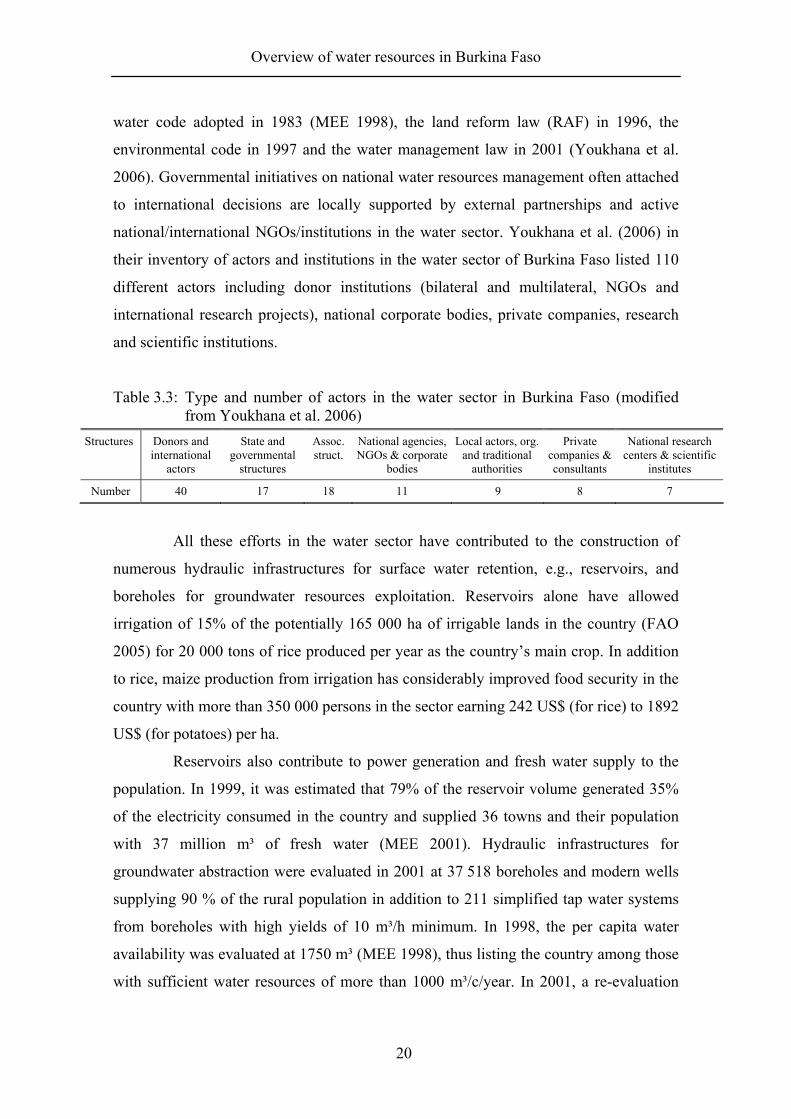
Table 3.3: Type and number of actors in the water sector in Burkina Faso (modified from Youkhana et al. 2006)
Structures Donors and international
actors
State and governmental
structures
Assoc. struct.
National agencies, NGOs & corporate
bodies
Local actors, org. and traditional
authorities
Private companies & consultants
National research centers & scientific
institutes
Number 40 17 18 11 9 8 7
All these efforts in the water sector have contributed to the construction of
numerous hydraulic infrastructures for surface water retention, e.g., reservoirs, and
boreholes for groundwater resources exploitation. Reservoirs alone have allowed
irrigation of 15% of the potentially 165 000 ha of irrigable lands in the country (FAO
2005) for 20 000 tons of rice produced per year as the country’s main crop. In addition
to rice, maize production from irrigation has considerably improved food security in the
country with more than 350 000 persons in the sector earning 242 US$ (for rice) to 1892
US$ (for potatoes) per ha.
Reservoirs also contribute to power generation and fresh water supply to the
population. In 1999, it was estimated that 79% of the reservoir volume generated 35%
of the electricity consumed in the country and supplied 36 towns and their population
with 37 million m³ of fresh water (MEE 2001). Hydraulic infrastructures for
groundwater abstraction were evaluated in 2001 at 37 518 boreholes and modern wells
supplying 90 % of the rural population in addition to 211 simplified tap water systems
from boreholes with high yields of 10 m³/h minimum. In 1998, the per capita water
availability was evaluated at 1750 m³ (MEE 1998), thus listing the country among those
with sufficient water resources of more than 1000 m³/c/year. In 2001, a re-evaluation
Overview of water resources in Burkina Faso
21
gave a value of 852 m³ as the annual per capita available water resources, predisposing
the country to water shortages. UNESCO (2004) in its report foresaw the country to be
part of the ten OSS (Observatory of the Sahara and the Sahel) countries with water
shortages by 2025. Seckler et al. (1998) evaluated the available per capita world water
resources and confirmed UNESCO predictions given 808 m³ per capita for Burkina
Faso by 2025.
In 1996, water use by agriculture was 55 % of the total water consumption in
the country (UNESCO 2004). In 2000, of the total water demand of 2.5 billion m³
(MEE 2001), 80% represent electricity generation and 20% for other activities. Of
these, water demand for irrigation was 64%, for domestic needs 21% and for livestock
14%. The remaining 1% covered industrial demand, mines, environment, fishing and
recreation.
3.5 Conclusion
Water resources in Burkina Faso are limited. Located in the heart of West Africa
without access to sea, Burkina Faso water resources are constrained by the monomodal
rainfall regime of the prevailing tropical climatic conditions. Underlain mostly by
crystalline rocks, and thus poor aquifer conditions (unless they are enough provided
with fractures and fissures), water resources are also limited by the fact that the country
is the drainage zone and source of three transboundary river basins.
The severe droughts in the 1970’s just after independence revealed the
country’s vulnerability to natural disasters due to insufficient preparedness. They led to
plans and programs for water resources mobilization, conservation, protection and
development in order to avoid future water shortages. Political and institutional reforms
through laws and legislation have been developed and supported by international
partners and local active organizations for numerous hydraulic infrastructures, water
resources personnel training, water resources development programs, etc. Water supply
to the rural population passed from 10 l/c/d to 20 l/c/d in 1990, and irrigation provided
jobs for more than 350 000 people in addition to jobs for thousands of people involved
in the transformation and commercialization of irrigation products. Irrigation
development for vegetable and rainfed cotton production have substantially improved
rural population income, with some people earning more than middle class public
administration employees (MEE 2001).
Overview of water resources in Burkina Faso
22
Meanwhile, much remains to be done to secure water supplies in anticipation
of negative impacts of the predicted climate change in the coming years. The weak
economic situation1 of the country is much constraining this possibility since it has
limited investments in the water sector to a mere annual 16% of the required funds.
Moreover, the lack of competent personnel in the water sector, equipment for data
collection and reliable databases, office facilities and insufficient coordination between
water actors (MEE 2001) remain also negative factors, which need to be eliminated in
order to achieve water security for the population.
1 Burkina Faso had a GDP of 314 US$/c in 2003 (FAO 2005) and ranked 162nd in the world in 2005 (IMF 2005) for
its GDP at purchasing power parity of 1285 US$/c and 174th based on its HDI of 0.342 (UNDP 2006).

Study area
23
4 STUDY AREA
4.1 Introduction
In Burkina Faso, the name Kompienga refers at the same time to one of the 45
provinces, a department in this province and the biggest national hydropower dam built
in 1988. The word derives from “Koul-péolgo” or “Kompiana”, which in the language
of the Yana and Gulmatché communities living in the basin means “white river”, the
color of the main river waters draining the basin (Dipama 1997, Koalaga/Onadja and
Kano 2000). The Kompienga dam basin, in which the present research activities on
groundwater potential for supplying the population’s water demand took place, is
located in the Oti river basin.
4.2 Volta river basin
The Volta river basin is known as the 9th largest river basin in sub-saharan Africa (GEF-
UNEP 2002) from the 63 transboundary river basins quoted by Opoku-Ankomah et al.
(2006). It has an approximate watershed of 400 000 km² and covers six riparian
countries in West Africa2. Almost 85 % of this area spans Burkina Faso (66.8% of the
territory) and Ghana (63.7 %) and the remaining 15% stretch across Mali (0.8 %), Togo
(47%), Benin (14.2%) and Cote d’Ivoire (2.2%). Located between the north latitudes of
5° 30’ and 14°30’ and the longitudes 5°30’W to 2°00’E (Amisigo 2005), the Volta river
basin is drained by the lower Volta sub-basin in the south and the three main sub-basins
in the north pertaining to the tributaries of Nakanbé (formerly White Volta), Mouhoun
(formerly Black Volta) and Oti rivers (Andreini et al. 2000). The three tributaries flow
southward to join each other at a confluence in the north central region of Ghana and
flow downstream through a narrow gorge at Akosombo where a dam built in 1964 for
hydropower generation has created the largest man-made lake in the world, Lake Volta
(van de Giesen et al. 2001). All the rivers draining the basin are ephemeral and therefore
dry up during the dry season except the Mouhoun river in Burkina Faso with baseflow
mainly from the western sedimentary zone of the sandstone aquifers.
2 This watershed area varies greatly from one author to another. Niasse (2004) quoted 412 800 km² as the area of the
basin, while van de Giesen et al. (2001) mentioned 398 000 km², Amisigo (2005) 394 196 km² referring to FAO (1997) and GEF-UNEP (2002) quoted 417 382 km² citing national reports from the basin countries. 400 000 km² is the average Volta basin area commonly used in literature.

Study area
24
Figure 4.1: Volta river basin and its four sub-basins (Andreini et al. 2000)
The long-term average annual rainfall (1936-1963) of the basin (van de Giesen
et al. 2001) varies between 1025 mm in the south and 600 mm in the north in the Sahel
zone of northern Burkina Faso. The coefficient of variation of 7% from the mean
rainfall for the whole basin in this period and 16% for Ouagadougou station (during the
same period) depicts the temporal and spatial variability of the rainfall in the basin with
a bimodal pattern in the south and a monomodal pattern in the north. Between the two
zones exists a transition zone of 2 rainy seasons almost mingled. The major part of the
basin going from the extreme northern Burkina Faso to the northern Ghana is under the
monomodal rainfall regime of only 3 to 5 months duration. This situation consequently
affects the Akosombo dam filling and energy production in Ghana as this upstream part
of the basin is subject to recurrent droughts (Ofori-Sarpong 1985).
The climate in the basin as for all the West African countries is governed by
the annual ITCZ oscillations from south to north and vice versa bringing rainfall to the
southern parts between March and October and leaving the northern parts dry and hot
with harmattan winds (GEF-UNEP 2002). The potential evaporation in the basin varies
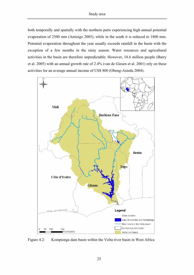
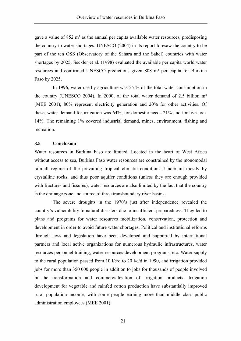
Study area
25
both temporally and spatially with the northern parts experiencing high annual potential
evaporation of 2500 mm (Amisigo 2005), while in the south it is reduced to 1800 mm.
Potential evaporation throughout the year usually exceeds rainfall in the basin with the
exception of a few months in the rainy season. Water resources and agricultural
activities in the basin are therefore unpredictable. However, 18.6 million people (Barry
et al. 2005) with an annual growth rate of 2.4% (van de Giesen et al. 2001) rely on these
activities for an average annual income of US$ 800 (Obeng-Asiedu 2004).
Figure 4.2: Kompienga dam basin within the Volta river basin in West Africa

Study area
26
Temperatures in the basin vary, from 27°C to 30°C with mean daily
temperatures between 32°C to 44°C for daytime and 15°C for nighttime. Like
temperatures, relative humidity in the basin varies according to locations and periods
between 6% in the north during the dry season and 95% during the rainy season in the
south of the basin (Oguntunde 2004).
The basin has a low relief with altitudes up to 972 m asl. Mountain chains are
in the southern sub-basin, e.g., the Atakora ranges in the Oti sub-basin (GEF-UNEP
2002). The geological formations of the basin are dominated by the Voltaian system
consisted of Precambrian to Paleozoic sandstones, shales and conglomerates. In
addition, the basin comprises Buem formations, Togo series of sedimentary formations,
Dahomeyan systems of metamorphic rocks and tertiary formations of the so-called
Continental Terminal. The rock basement consists mainly of granites with Birrimian
metamorphosed lavas and pyroclastic rocks, Tarkwaian quartzites, phyllites and schists.
The Volta basin formations are mostly characterized by fractured porosity, thus a
storage capacity and aquifer yield strongly depend on the density of fractures and
fissures and the relative importance of the weathered zone induced by the water
circulation and interactions with the rock materials.
Table 4.1: Hydrogeological characteristics of the Volta basin (GEF-UNEP 2002) Sub-basin Runoff
coeff. (%)
Boreholes yield
(m³/h)
Mean yield boreholes
(m³/h)
Specific capacity (m³/h/m)
Depth to aquifers
(m)
Mean depth to aquifers
(m)
Depth of boreholes
(m)
Mean depth of borehole
(m) Nakanbé Mouhoun Oti Lower Volta
10.8 8.3
14.8 17.0
0.03-24.0 0.1-36.0 0.6-36.0
0.02-36.0
2.1 2.2 5.2 5.7
0.01-21.1 0.02-5.28
0.06-10.45 0.05-2.99
3.7-51.5 4.3-82.5 6.0-39.0 3.0-55.0
18.4 20.6 20.6 22.7
7.4-123.4 -
25.0-82.0 21-129.0
24.7 -
32.9 44.5
Specific capacity is equivalent to transmissivity
Based on the four climatic zones (Figure 4.3) of Equatorial rain forest and
Guinean savannah in the south of the basin, Sudanean savannah and Sahelian savannah
in the north (Martin 2005), the basin vegetation and land-uses vary strongly. Amisigo
(2005) referring to World Resource Institute (2003) report established the percentage of
the land-cover/land-use of the basin depicting the high loss of the original forest zones
which have been reduced to a very small area of 0.7% of the basin and therefore
followed by the importance of the dry land areas as the consequence of the first
observation.

Study area
27
Figure 4.3: Climatic zones over the Volta river basin in West Africa (Martin 2005)
4.3 Kompienga dam basin
The study site is located in the eastern part of the country about 400 km southeast of
Ouagadougou, the capital city of Burkina Faso. Kompienga hosts a hydropower dam
built in 1988 on the Ouale (Kompiana) river and in 1995, provided 20% of the country’s
energy consumption (Dipama 1997). The dam’s lake has an estimated area of 210 km²
and a maximum capacity of 2 050 million m³ of water (SONABEL 2003) coming from
the drainage of a watershed approximately covering 5911 km² over the provinces
Kourittenga (northwest), Gourma (northeast and northwest), Boulgou (west),
Koulpeologo (west and south), Kompienga (east and south) with Togo bordering the
south (Figure 5.2). The basin is about 142 km long and 41 km wide.

Study area
28
Figure 4.4: Kompienga dam basin and the four research stations
The tropical climate in the study area is characterized by two main seasons: a
long dry season of 7 to 8 months (October/November to April) and a short rainy season
of 5 months. The rainy season is characterized by heavy rainstorm events highly
variable within time and space (Figure 4.7). The long-term mean annual precipitation
(Thiessen polygon method) from 1959 to 2005 is 830.2 mm with a standard deviation of
126 mm, which illustrates the inter-annual variability of the rains. Within this period, a
wet year with 1197 mm was observed in 1994 as well as a dry year with only 573 mm
in 1984 (Figure 4.6). The area is therefore, considered as a semi-arid region with
ephemeral rivers only flowing during the rainy season. In the dry season, they all dry up
without any baseflow from aquifers. The Kompienga basin has a dendritic drainage
system with an average drainage density of 0.6 km/km² around the main river Oualé (or
Kompiana) and its two tributaries of Koul-peologo and Otabango (Dipama 1997).

Study area
29
0
50
100
150
200
250
Jan Feb Mar Apr May Jun July Aug Sept Oct Nov DecMonth
Mon
thly
rain
fall
and
Ep (m
m)
Monthly rainfallMonthly Ep
Downstream of the dam, the Kompiana river discharges its waters into the Pendjari,
which flows into Togo and becomes the Oti river flowing down to the Akosombo dam
in Ghana. Since the Kompienga dam construction, a national water company station
producing drinking water has been established. The station supplies treated water of
negligible volumes from the dam’s lake to the local population.
According to the rainfall pattern in the basin, it can be observed that the only
favorable period of groundwater recharge is the rainy season, where rainfall can exceed
potential evaporation for a few months (Figure 4.5) and induce runoff to fill the dam for
energy production. Potential evaporation on the basin varies annually with an average of
2094.4 mm from the two years measurements (2004 and 2005) of the meteorological
station at Tanyélé. Agricultural activities are mainly intensive during the rainy season
period and no significant irrigation scheme exists in the basin.
Figure 4.5: Monthly rainfall and evaporation ( Ep ) in the Kompienga dam basin in 2005

Study area
30
400
500
600
700
800
900
1000
1100
1200
1300
1400
1959 1963 1967 1971 1975 1979 1983 1987 1991 1995 1999 2003
Year
Prec
ipita
tion
(mm
)
Average mean annual rainfall in the basin (830.2 mm)
0
50
100
150
200
250
300
350
April May June July August Sept. October
Month
Mon
thly
rain
fall
(mm
)
Kouaré
Natiabouani
Pama
Tanyélé
Figure 4.6: Inter-annual rainfall variability from long-term (1959-2005) weighted mean annual rainfall variability in the Kompienga dam basin from measurements at Koupéla, Fada, Pama and Ouargaye stations
Figure 4.7: Temporal and spatial rainfall variability in the Kompienga dam basin in 2005

Study area
31
4.3.1 Geology and geomorphology
The revised geological map of Pama at scale 1:200 000 in digital and paper format
combined with review of literature provided the geological and geomorphologic data of
the Kompienga dam basin. The morphology is defined as a plateau with a flat
topography on which a few hills exist mainly in the downstream area, where the dam is
located. The highest elevation in the basin is about 328 m asl south of the Kouaré
station and the lowest point is 140 m asl in a river bed downstream of the dam’s
spillway (Dipama 1997). The geological formations are paleoproterozoic or
Precambrian (more than 2000 billion years old). The rocks mainly form the West
African craton (Ouédraogo et al. 2003), which covers major parts of Burkina Faso and
Côte d’Ivoire as the Man or Leo shield. This shield is made of volcanic sedimentary
rocks and granitoids known as Birrimian rocks. Granitoids are the main (80%)
components of the basement rocks forming around 60% of the Volta river basin (Martin
2005). They comprise migmatites, granodiorites and migmatic granites in combination
with volcanic sedimentary rocks, mainly amphibolites. The other rocks are schists and
quartzites in the center of the basin, partially covered by the dam’s lake, orthogneiss in
the northwestern part, green rocks (gabbro and diorite) in the south, and basalts and
andesites in the southeast corner of the basin. Most of the structural faults in the basin
are oriented NE-SW, sometimes with quartz veins as observed in the center of the basin
from east to west. The basement rocks are often covered by lateritic soils resulting from
weathering, which provide the sediments in the riverbeds and on the river banks as
sands (Ouédraogo et al. 2003). The Tanyélé station is underlain by granite and
leucogranite with biotite, the Pama station by granodiorite, tonalite and diorite with
striped and folded quartzite dated from 2170 ± 6 million years. The Natiabouani station
is underlain by granite with biotite and amphibole dated from 2143 ± 4 million years,
and Kouaré is located on granite, granodiorite and quartziferous diorite with amphibole
and biotite (2128 ± 4 million years).
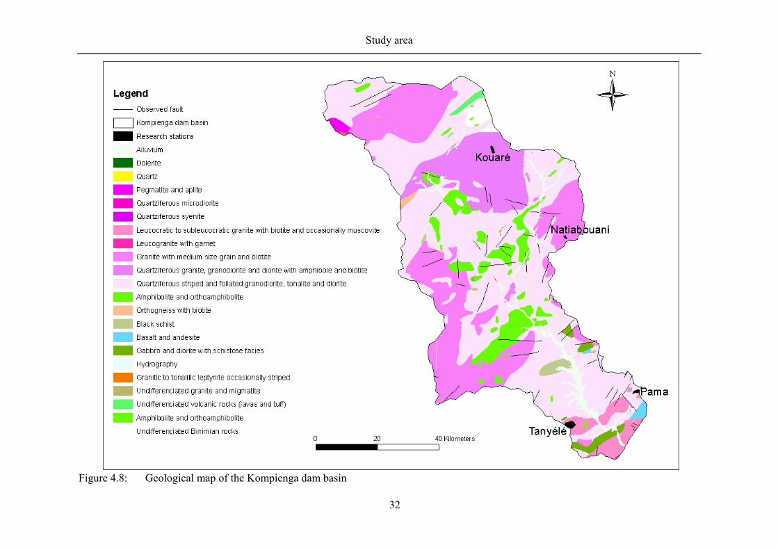
Study area
32
Figure 4.8: Geological map of the Kompienga dam basin
Study area
33
4.3.2 Hydrogeology
The basement rocks of the basin are known to be with fractured porosity, and they thus
form poor aquifers for groundwater storage. Two hydrogeological domains are
described by Ouédraogo et al. (2003) to be attached to the two main basement rocks of
the basin, namely the granitoid aquifers and the volcanic sedimentary rocks aquifers.
The former aquifers are called “early granitoids” aquifers often consisting of thin
regolith with many fractures associated with successful boreholes siting. They are the
only aquifers with exceptional yields of 10 m³ of water per hour when the regolith is
thick. The other granitoid aquifers are named “belated granitoids” aquifers with very
thin regolith, less fractured and thus less productive boreholes siting. Meanwhile, the
volcanic sedimentary basement aquifers with thick regolith have successful boreholes
siting; however, the yield of these boreholes is often low.
4.3.3 Temperatures
The monthly average temperatures in the basin fluctuate between 25°C in January and
32°C in April. The daily mean maximum temperature is around 36°C in April with the
highest maximum temperature observed in 1937 (44°C) and the daily mean minimum
temperature is 20°C with 12°C in January 1936 (Dipama 1997). Recent observations on
the temperatures indicate a rise in the daily mean minimum temperature of 1°C between
1960 and 1990 (Paturel et al. 2002) with 1.2°C for the Kompienga zone (from 20.9°C to
22.1°C between 1950 and 1999).
4.3.4 Soils
The crystalline basement rocks of the basin are generally covered by mineral soils
mainly composed of leached ferruginous tropical soils found on most of the uplands of
the basin (Dipama 1997). On the glacis, eutrophic brown soils associated to lithosols
and hydromorphic soils exist while the lowlands are composed of alluvial plains of
sandy and clayey soils under cultivation. The wetlands in the lowest topographical areas
of the basin are composed of vertisols, hydromorphic soils and brown soils.
Boulet (1969) described the basin to be mainly composed of 6 soil textures:
gravel in 46.57% of the basin area followed by clayey soil (26.67%), loamy sand
(12.14%), sandy clay (6.62%), gravelly loamy sand (5.51%), alluvium (1.93%) and
Study area
34
gravelly clay (0.57%). However, soil textures are subject to temporal and spatial
(horizontally and vertically) variability, and peculiarities are likely to occur within the
same environment, as was observed for the four research stations. In these stations, soil
textures were described as being sandy loam at Tanyélé (Bagayoko 2006), gravelly clay
at Pama, gravelly silt at Natiabouani and sandy clay at Kouaré.
4.3.5 Vegetation and land use
The climatic conditions in Kompienga have resulted in savannah vegetation of the
Sudanian phytogeographic zone of the Guinko (1984) classification. This savannah
vegetation is mainly composed of woody savannah made of large tree species of
Vitellaria paradoxum sp., Parkia biglobosa, Lannea microcarpa, Adansonia digitata,
Tamarindus indica,Sclerocarya birrea, Bombax costatum, Borassus aethiopium. In the
shrubby savannah, Combretum glutinosum, Combretum nigricans, Ximenia Americana,
Entada Africana, Anogeisus leiocarpus, Acacia gourmaensis, Strychnos spinosa occur.
The herbaceous savannah is made up of Andropogon gayanus, Andropogon tectorium,
Hyparrhenia rufa, Hyperthelia dissoluta, Hyparrhenia glabriuscula. The Kompienga
dam basin is one of the relatively well-vegetated parts of Burkina Faso due to restricted
and protected zones developed by the authorities for wild animal protection and tourism
purposes. However, since the dam construction, where part of the basin vegetation was
destroyed, permanent threats to the remaining vegetation exist through new settlers
needing lands for housing, agriculture, domestic and commercial purposes. In 1978,
rainfed agriculture, mainly cereal crops, was estimated to be occupying 6% of the basin
area (334.28 km²) and practiced by 97% of the inhabitants (Dipama 1997), while the
remaining area was covered by natural vegetation. In 1988, cropping areas were seen to
be occupying 961.81 km² (17% of the basin area), i.e., an increase of 183 % to the
detriment of the natural vegetation.
4.3.6 Population
The population in the Kompienga basin was estimated in 1985 to be 104 000 inhabitants
living in 134 villages (Dipama 1997) with a density of 18 inhabitants/km², which is
lower than the national density of 29 inhabitants/km² but more than the Gourma
province population density (11 inhabitants/km²). In 1975, the census revealed a total

Study area
35
population of 63 000 inhabitants in the basin, while the census in 2005 (MAHRH 2006)
depicted approximately 270 000 inhabitants living in about 215 villages in 15
departments in 5 provinces. Referring to Balk et al. (2005) formula, the population
growth rate can be estimated at 4.8 %. This growth rate is higher than the rate of 3.2 %
stated by Dipama (1997), which is certainly due to the difference in the considered
boundaries of the basin in the two estimates. The latter estimate refers to the whole
population in the basin and its vicinity, which is likely different from the first estimate
in 1975, where the basin boundaries were different, as the dam in the south had not yet
been built. Moreover, after the dam construction in 1988, the population of the basin
significantly increased with the creation of new villages like those for settling fishermen
and their families, who came sometimes from far away (Mali or Niger; Dipama 1997),
mainly for fishing and sometimes agricultural purposes.
4.4 Conclusion
The Kompienga dam basin within the Volta river basin in the southeastern part of
Burkina Faso is a hydropower dam basin in a watershed of about 6 000 km² where
approximately 270 000 people live. Practicing mainly subsistence agriculture
comprising rainfed cereal crops, they cultivate poor lands with gravelly and clayey
textures in addition to fishing in the dam’s lake. The originally dense vegetation in the
basin was cleared for dam construction, and this has remained so due to an increasing
population wishing to benefit from the dam. The monomodal rainfall pattern with a 5-
month rainy season in addition to the geological formations of crystalline basement
rocks consisting of granites and amphibolites, very much limit groundwater recharge to
the basin aquifers. These aquifers, on which the population mainly rely for their supply
through wells and hand pump boreholes are currently found in fractures and similar
features of the basement rocks.

Materials and methods
36
5 MATERIALS AND METHODS
5.1 Introduction
The research site Kompienga dam basin is located between the northern latitudes 11°00’
and 12°10’ and longitudes 00°50’ east and 00°20’ west. In this basin of 5911 km², four
representative stations of 1 to 6 km² of mainly first order watersheds were selected.
They are: the Pama station circa 5 km east of the dam’s lake with a watershed of 2.19
km², the Tanyélé 5 km to the west with a second order watershed of 6.04 km², the
Natiabouani station about 60 km north of Pama with a watershed of 0.86 km², and
Kouaré located at the extreme upstream part of the dam basin in a 2.09 km² watershed
(Figure 4.4). The stations were selected based on criteria of accessibility, areal
importance of their geological formations in the basin, geographical position to the
dam’s lake, and the resources availability for the research activities.
5.2 Materials and methods
Three methods for estimating the groundwater potential were foreseen to be used, and
accordingly on each of the four stations, the following instruments were installed:
• Rain gauges for measuring rainfall and collecting rainwater samples;
• Divers; Eijkelkamp Co. devices placed downstream of the station watershed for
automatically recording rainfall runoff at fixed 3-minute intervals. The total runoff
discharge of the basin was calculated using the data from the dam office
administration; SONABEL (Société Nationale Burkinabé d’électricité);
• Piezometers set up with augers at a maximum depth of 5.5 m to monitor shallow
groundwater level fluctuations during the seasons.
To evaluate the groundwater potential using the chloride mass balance
approach, water samples were taken from boreholes, piezometers and rain gauges on a
monthly basis. Water samples from rain gauges for each month were the mixed total of
rainfall taken to the laboratory for chloride analysis. From piezometers, water was
sampled upstream and downstream of the watersheds. All samples were separately
collected in 100-cm³ plastic containers and transported to the laboratory for analysis of
chloride concentration.

Materials and methods
37
The 10-m flexible mast on top of which are placed the Krypton hygrometer and the ultrasonic anemometer
The solar panel and the battery for energy supply to the EC system
The cabinet containing the Palmtop computer recording the raw data on PCMCIA cards
The Tanyélé station had a complete weather station and an Eddy Correlation
(EC; Figure 5.1) station installed in November 2002 in the framework of a project
funded by the European Union (VINVAL). This station consisted of two main devices:
a Gill Windmaster Pro (3-dimensional) ultrasonic anemometer, and a Campbell Krypton
KH2O hygrometer, which recorded in 10 Hz frequency, air temperature and humidity as
well as wind velocity from 3 directions (Elbers 2002). Fluxes were averaged over
hourly intervals to obtain moisture and heat fluxes. Recorded raw data were stored on a
PCMCIA card via Palmtop computer using the Basic software Eddylogp. The data were
processed using FORTRAN program named ALTEDDY to derive latent and sensible
heat flux, friction velocity, Monin-Obukhov length, flux footprint and necessary error
corrections (Bagayoko 2006).
Figure 5.1: Eddy Correlation station at Boudtenga near Ouagadougou
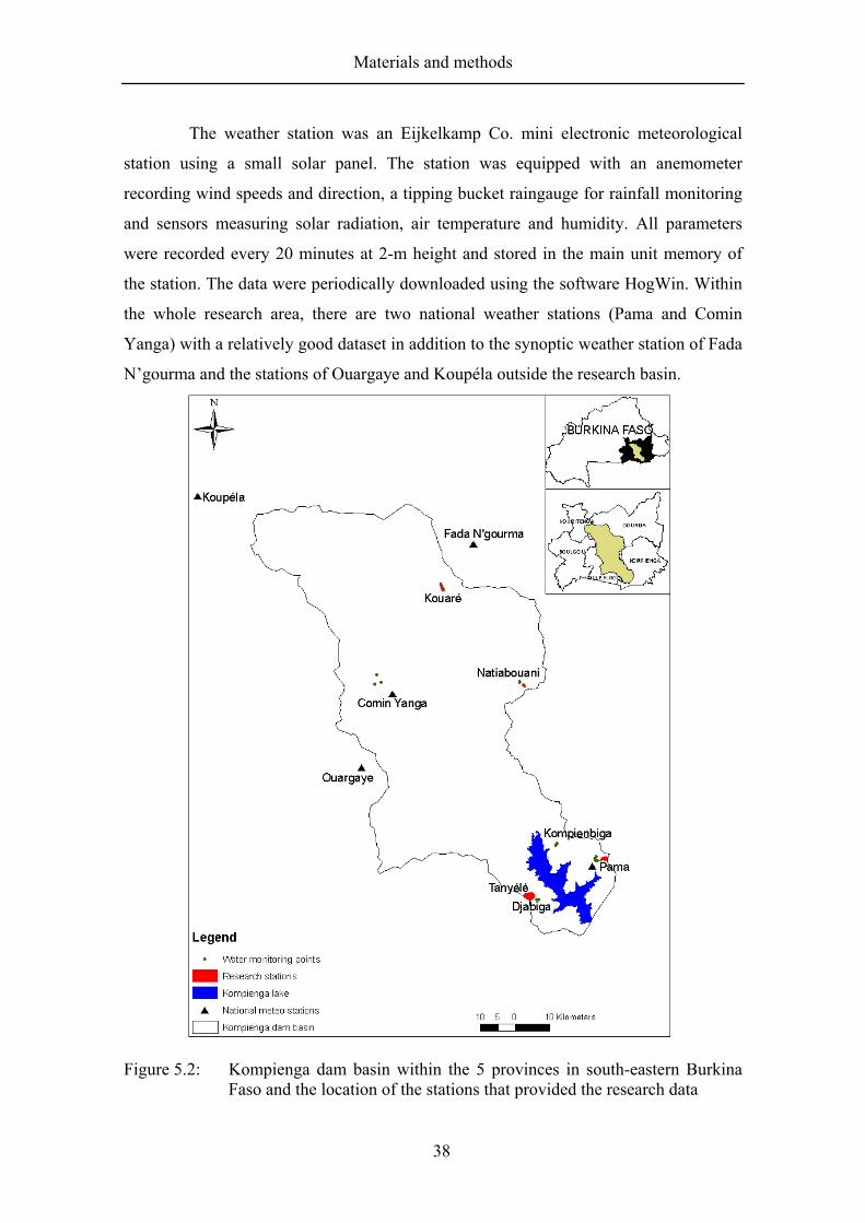
Materials and methods
38
The weather station was an Eijkelkamp Co. mini electronic meteorological
station using a small solar panel. The station was equipped with an anemometer
recording wind speeds and direction, a tipping bucket raingauge for rainfall monitoring
and sensors measuring solar radiation, air temperature and humidity. All parameters
were recorded every 20 minutes at 2-m height and stored in the main unit memory of
the station. The data were periodically downloaded using the software HogWin. Within
the whole research area, there are two national weather stations (Pama and Comin
Yanga) with a relatively good dataset in addition to the synoptic weather station of Fada
N’gourma and the stations of Ouargaye and Koupéla outside the research basin.
Figure 5.2: Kompienga dam basin within the 5 provinces in south-eastern Burkina Faso and the location of the stations that provided the research data

Materials and methods
39
Additionally, river parameters (slope and transversal section dimensions) were
measured to complement the runoff recorded by the divers and derive watershed
discharge. Meanwhile, the whole basin runoff into the dam and the discharge from the
dam for energy production as well as lake evaporation data were collected from
SONABEL. Long-term rainfall data series and meteorological parameters (wind speed,
relative humidity, air temperature and solar radiation) from weather stations near or
within the study basin were also collected from the local administration of the
Agriculture, Hydraulics and Fisheries Ministry (DRAHRH) and the national
meteorology office in Ouagadougou.
Table 5.1: Instruments installed on the research stations
Instruments Tanyélé Pama Natiabouani Kouaré
Rain gauges Piezometers Divers Weather station
1 5 2 1
1 4 1 1
1 2 1 0
1 6 1 0
Rainfall was measured daily with rain gauges during the same period at all the
stations. Surveyors recruited from population were trained for recording rainfall in
notebooks and collecting monthly water samples from rain gauges into 10-liter plastic
containers for chloride analysis in the laboratory. For piezometers, recruited local
surveyors monitored the daily water level fluctuations in the pipes at the same period of
the day with bell-tape measurers (Figure 5.8) until water disappeared below the pipes.
At the Natiabouani station, as it was not possible to find a suitable person, the author
did the monitoring by collecting the water level data in the fieldwork period during the
trips to the research stations.
To evaluate the groundwater potential with the water balance method, runoff,
evaporation and rainfall recorded from the four stations were brought to the whole
basin, and the infiltrated part of the rainfall recharging the research area was then
deduced.
For the chloride mass balance approach, the station data were areally weighted
using the Thiessen polygon method with ArcView software. Some well known
prerequisites in the use of this approach and quoted in Bazuhair and Wood (1996),

Materials and methods
40
Bromley et al. (1997), Martin (2005) and McNamara (2005) were verified and found
valid for using the method in evaluating the basin groundwater potential.
5.2.1 Chloride mass balance method
One of the methods used in this study on estimating the Kompienga dam basin
groundwater potential is the Chloride Mass Balance method (CMB). As quoted by
Gieske (1992), this method for groundwater recharge determination is based on the ratio
of chloride concentration in rainwater to that in groundwater of a given water system.
The equation for groundwater recharge estimation is derived from the application of the
principle of mass conservation of chlorides in the water system. Prerequisites in the use
of the method consist of the conservative state of chloride ions, rainfall considered as
the sole source of chlorides in the water system, chlorides not taken up significantly by
plants, no significant runoff out of the system or inflow from other water systems into
the considered water system (Bromley et al. 1997). Considering these prerequisites
fulfilled, the groundwater recharge of a water system is given by the equation:
gw
P
ClCl
PR .= (5.1)
where R is the groundwater recharge flux [ ]1−LT , P the average annual precipitation
[ ]1−LT , and pCl , the average rainfall-weighted chloride concentration [ ]3−ML and gwCl ,
the average groundwater-weighted chloride concentration. M represents mass, T is
time and L is length, all in consistent units.
From this equation, the basin rainwater chloride concentration; pCl , was
determined from weighting the unit rainwater chloride concentration of each station,
psCl derived from equation 5.2.
∑∑=
i
iips
P
ClPCl (5.2)

Materials and methods
41
with [ ]LPi , the ith precipitation in each research station having a chloride concentration
iCl [ ]3−ML in its sample.
To obtain the groundwater chloride concentration of the whole basin, gwCl , the
unit groundwater chloride concentration of the four stations, gwsCl was first calculated
using the harmonic mean of all monthly values of each station with equation 5.3 in
order to reduce the differences between the unit values:
1
1
1.−
⎟⎟⎠
⎞⎜⎜⎝
⎛= ∑
N
gwigws Cl
NCl (5.3)
with N the dimensionless total number of monthly values for each station, and gwiCl
represents groundwater chloride concentration for the station in month i with consistent
units of [ ]3−ML .
The unit chloride concentrations in the groundwater of the stations, gwsCl ,
were then spatially averaged to derive the chloride concentration in the groundwater of
the whole study area termed gwCl . The areal weights of the stations (Table 6.5) were
determined using the geographical coordinates of the stations with the Thiessen polygon
method.
The data on the rainwater chloride concentrations in 2005 were thought to
have major errors making them not valid for estimation of the annual basin recharge.
For this reason, a second data collection during a short period of 3 weeks was realized
in September 2006 (details in Section 6.2.2). This provided explanations for the
shortcomings in the 2005 data, as well as additional data and ways to better re-evaluate
the basin recharge. Given this opportunity, the basin long-term annual recharge was re-
evaluated for 2005 and 2006 using the following procedures.
Basin recharge in 2005
According to the correlation observed between the chloride concentration in the
groundwater data series in 2005 and 2006 (Figure 6.4), the first data were updated
according to the correlation equation. The chloride concentrations in the groundwater

Materials and methods
42
for each station, gwsCl , were calculated using equation 5.3 and the whole basin
groundwater chloride concentration, gwCl , was the average of the areal weighted unit
gwsCl . Rainwater chloride data for 2005 were discarded for lack of correlation with the
2006 data series (correlation coefficient of -0.0048) and the basin rainwater chloride
concentration, pCl , was determined by averaging the unit chloride concentration of the
four stations in 2006 obtained from equation 5.2. The basin recharge in 2005 was then
re-evaluated from equation 5.1 with pCl and gwCl as determined above and P was the
annual precipitation in the basin in 2005.
Basin recharge in 2006
The parameter gwCl of the whole basin recharge estimation in 2006 was determined
from averaging the of the unit areal weight of the groundwater chloride concentration
measured at the stations in 2006, which was the average of the two values from the
groundwater sample of the stations. pCl , the chloride concentration in rainwater of the
whole basin in 2006, was the chloride concentration in the rainwater of the 3-week
period of survey brought to the whole rainy season rainwater volume using equation
5.2. Finally, with the two parameters and the annual precipitation in the basin in 2006,
the recharge was calculated.
Basin recharge using data from nearby sites
After discarding the rainwater chloride concentration of 2005, using the groundwater
chloride concentration, a rough estimate of the basin recharge was made based on the
rainwater chloride concentration of nearby sites (northern Ghana, southwest Niger and
central Burkina Faso). The basin rainwater chloride concentration was the average of
the rainwater chloride concentration of these sites and the groundwater chloride
concentration for the basin was the same as determined previously from the average of
the weighted harmonic mean value of the groundwater chloride concentration of the
stations. The formula of equation 5.1 was used to derive the basin recharge for 2005
according to the precipitation.

Materials and methods
43
5.2.2 Water balance method
This method is based on the knowledge of the hydrological balance parameters of the
water system from which the recharge is calculated. Despite the uncertainties in the
recharge estimate by this method for arid and semi-arid zones due to difficulties in
obtaining reliable values of the balance components, the method remains valid in
recharge estimation if time steps and spatial boundaries of the water systems are well
defined (Sokolov and Chapman 1974, Gee and Hillel 1988 and Lerner et al. 1990). The
method is based on the principle of mass conservation applied in hydrology (equation
5.4):
dtdSOI =− (5.4)
where I [ ]1−LT represents the input flows, O [ ]1−LT the output flows, [ ]LdS the
change in storage, and [ ]Tdt the time increment.
Considering the Kompienga dam basin, the equation can be stated as:
η+∆±+=+ SQEQP offon (5.5)
where P is precipitation, onQ the flow in the basin, offQ the flow from the basin, E the
evaporation in the basin, and S∆ the change in the stock including recharge. All the
parameters are in consistent units of [ ]1−LT . η is an error term accounting for
discrepancies due to errors in component measurement or estimation and is used in
order to obtain a water balance that is as accurate as possible.
Applying the water balance method to the Kompienga dam basin recharge
estimates requires definition of spatial and temporal boundaries. The spatial boundaries
are the limits of the Kompienga dam basin, and temporal boundaries are the time scale
(year) of the recharge assessment so that the estimate can be compared with other
methods. To assess the annual recharge of the basin with the known parameters of the
water balance, the spatial boundaries will be divided into two parts with the dam as one
unit and the other parts of the basin considered as a second unit. It is assumed that no

Materials and methods
44
external surface water or groundwater is flowing into the basin. Using equation 5.4 for
each part yields:
• For the dam part, parameters involved in the balance are :
dP = precipitation to the reservoir (lake) surface;
0E = lake evaporation;
L = water withdrawn from the lake for drinking water and energy production;
1R = recharge from the lake;
1S∆ = stock variations in the lake reservoir;
1r = basin runoff into the lake;
All the parameters are in consistent units of [ ]13 −TL . The equation of the mass
conservation principle in hydrology implies that:
1011 SLERrPd ∆±++=+ (5.6)
From equation 5.6, 1r can be inferred as:
dPSLERr −∆±++= 1011 (5.7)
• For the basin part, the balance parameters are:
bP = precipitation in the basin;
Ea = actual evaporation over the basin;
2r = runoff in the basin;
2R = recharge in the basin;
2S∆ = stock changes in the basin
The parameters are in consistent units of [ ]13 −TL .
The application of equation 5.4 to the basin part yields:
222 SEaRrPb ∆±++= (5.8)
From equation 5.8, 2r can also be inferred as:

Materials and methods
45
222 SEaRPr b ∆±−−= (5.9)
As can be seen, 1r and 2r are the same parameters of the balance and express the runoff
from the basin into the lake. Therefore, equalizing equations 5.7 and 5.9 yields equation
5.10 for annual groundwater recharge in the whole basin:
210 SSLEEaPR ∆±∆±−−−= (5.10)
with R = annual recharge under the whole Kompienga basin comprising 1R and 2R ;
P = annual precipitation in the basin;
Ea = annual (actual) evaporation on the basin;
0E = annual evaporation of the lake;
1S∆ = annual change in storage within the lake according to input (rainfall and run-
on) and output (energy and drinking water production);
L = annual water withdrawn from the dam for drinking water and energy
production;
2S∆ = annual stock flux in the basin (the unsaturated zone soil moisture). This flux at
an annual time scale is considered zero. This implies that equation 5.10 becomes 5.11
for the annual time scale recharge estimation:
10 SLEEaPR ∆±−−−= (5.11)
At shorter time steps, in addition to the lake fluxes, one should also consider the stock
variations according to soil moisture storage and retention capacity in the unsaturated
zone, 2S∆ .
All parameters involved in the recharge estimate with the water balance
method are measured at the basin scale with the exception of rainfall measurements
done from the four stations and brought to the basin level using areal weights of the
Thiessen polygons. In addition, complementary data were collected from local
institutions of the Agriculture, Hydraulics and Fisheries Ministry (DRAHRH),
SONABEL, ONEA/Kpg and the national meteorology office for precipitation, runoff in

Materials and methods
46
the basin, lake evaporation, lake level fluctuations and water quantities withdrawn from
the lake for energy and drinking water production.
Actual evaporation ( Ea ) data were inferred from the EC station in correlation
with rainfall amounts and Ep (potential evaporation) derived from the 2-m high
meteorological station. The Ea derivation procedures are described below. For runoff
in the basin, the correctness of the SONABEL data was verified by means of the daily
records of the lake level fluctuations, the withdrawals from the lake and the tare curves
of the lake volume and surface against water heights (Figure 5.3). In the same way, the
estimated lake evaporation data by SONABEL were corrected when necessary,
according to interpolated values from Pouyaud’s (1985) studies on evaporation of Lake
Bam (Burkina Faso) and Lake Tchad (Chad).
Figure 5.3: Fitted regression curves for Kompienga dam water levels versus volumes
(A) and levels versus lake area (B) Actual evaporation derivation procedures
The EC station located near the dam’s lake at the Tanyélé station measured latent and
sensible heat fluxes. The raw data retrieved from the EC station were in ASCII format
and were processed with Alteddy software producing three different files. One file from
the three (Appendix 1, Elbers 2002) was made of latent heat flux and daily mean
temperature parameters used to derive hourly actual evaporation in combination with
the latent heat of vaporization ( λ ) as in the equations below (Monteith and Unsworth
1990):
Volume (x10^6 m³)
500 1000 1500 2000 2500 3000 3500
Wat
er le
vels
(m)
160
165
170
175
180
185
Heights vs water volumes curve of Kompienga damRegression curve of heights vs water volumes
Lake surface (km²)
50100150200250300
Wat
er le
vels
(m)
160
165
170
175
180
185
Heights vs lake area curve of Kompienga damRegression curve of heights vs lake area
f=a*x/(b+x)+c*x/(d+x)+e*x
a=161.4b=0.8c=16.8d=722.6e=0.003
f=y0+a*x^b
y0=152.6a=1.5b=0.5
Rsqr = 0.99
Rsqr = 0.99
A B
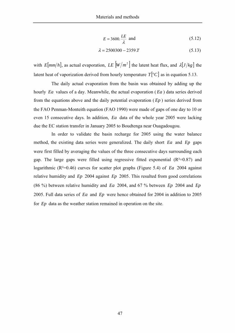
Materials and methods
47
λ
LEE .3600= and (5.12)
T.23592500300 −=λ (5.13)
with [ ]hmmE , as actual evaporation, LE [ ]2mW the latent heat flux, and [ ]kgJλ the
latent heat of vaporization derived from hourly temperature [ ]CT ° as in equation 5.13.
The daily actual evaporation from the basin was obtained by adding up the
hourly Ea values of a day. Meanwhile, the actual evaporation ( Ea ) data series derived
from the equations above and the daily potential evaporation ( Ep ) series derived from
the FAO Penman-Monteith equation (FAO 1990) were made of gaps of one day to 10 or
even 15 consecutive days. In addition, Ea data of the whole year 2005 were lacking
due the EC station transfer in January 2005 to Boudtenga near Ouagadougou.
In order to validate the basin recharge for 2005 using the water balance
method, the existing data series were generalized. The daily short Ea and Ep gaps
were first filled by averaging the values of the three consecutive days surrounding each
gap. The large gaps were filled using regressive fitted exponential (R²=0.87) and
logarithmic (R²=0.46) curves for scatter plot graphs (Figure 5.4) of Ea 2004 against
relative humidity and Ep 2004 against Ep 2005. This resulted from good correlations
(86 %) between relative humidity and Ea 2004, and 67 % between Ep 2004 and Ep
2005. Full data series of Ea and Ep were hence obtained for 2004 in addition to 2005
for Ep data as the weather station remained in operation on the site.
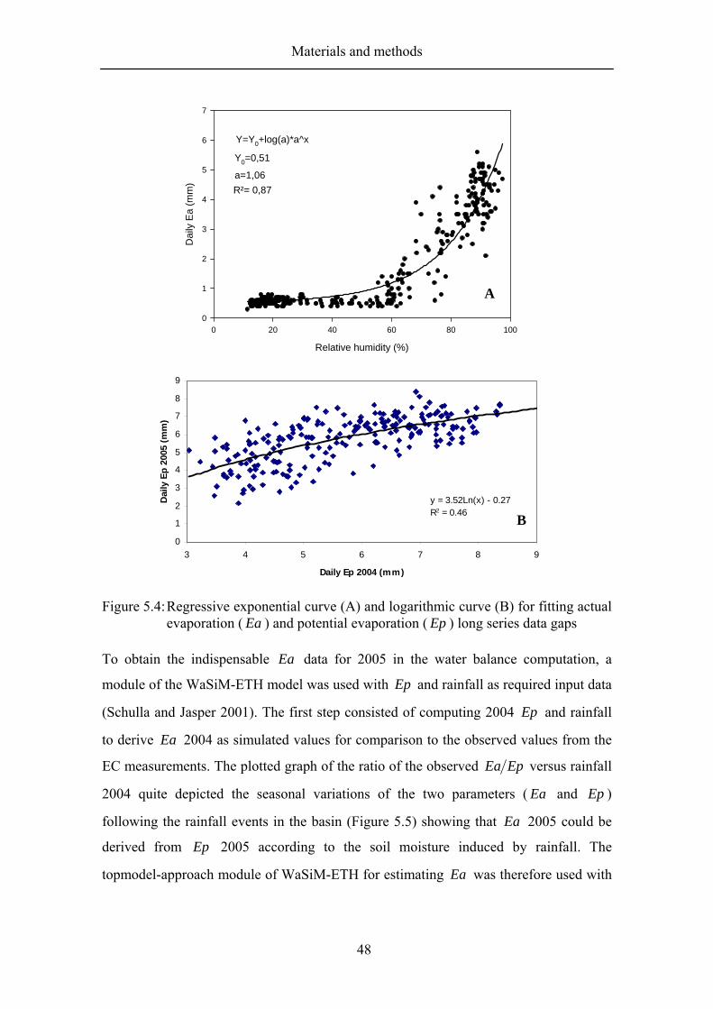
Materials and methods
48
Figure 5.4: Regressive exponential curve (A) and logarithmic curve (B) for fitting actual evaporation ( Ea ) and potential evaporation ( Ep ) long series data gaps
To obtain the indispensable Ea data for 2005 in the water balance computation, a
module of the WaSiM-ETH model was used with Ep and rainfall as required input data
(Schulla and Jasper 2001). The first step consisted of computing 2004 Ep and rainfall
to derive Ea 2004 as simulated values for comparison to the observed values from the
EC measurements. The plotted graph of the ratio of the observed EpEa versus rainfall
2004 quite depicted the seasonal variations of the two parameters ( Ea and Ep )
following the rainfall events in the basin (Figure 5.5) showing that Ea 2005 could be
derived from Ep 2005 according to the soil moisture induced by rainfall. The
topmodel-approach module of WaSiM-ETH for estimating Ea was therefore used with
y = 3.52Ln(x) - 0.27R2 = 0.46
0
1
2
3
4
5
6
7
8
9
3 4 5 6 7 8 9
Daily Ep 2004 (mm)
Dai
ly E
p 20
05 (m
m)
Relative humidity (%)
0 20 40 60 80 100
Dai
ly E
a (m
m)
0
1
2
3
4
5
6
7
Y=Y0+log(a)*a^x
R²= 0,87
Y0=0,51
a=1,06
B
A
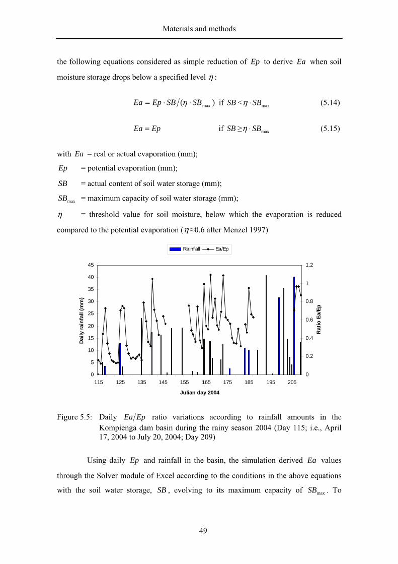
Materials and methods
49
0
5
10
15
20
25
30
35
40
45
115 125 135 145 155 165 175 185 195 205
Julian day 2004
Dai
ly ra
infa
ll (m
m)
0
0.2
0.4
0.6
0.8
1
1.2
Rat
io E
a/Ep
Rainfall Ea/Ep
the following equations considered as simple reduction of Ep to derive Ea when soil
moisture storage drops below a specified level η :
)( maxSBSBEpEa ⋅⋅= η if SB < maxSB⋅η (5.14)
EpEa = if SB ≥ maxSB⋅η (5.15)
with Ea = real or actual evaporation (mm);
Ep = potential evaporation (mm);
SB = actual content of soil water storage (mm);
maxSB = maximum capacity of soil water storage (mm);
η = threshold value for soil moisture, below which the evaporation is reduced
compared to the potential evaporation (η ≈0.6 after Menzel 1997)
Figure 5.5: Daily EpEa ratio variations according to rainfall amounts in the Kompienga dam basin during the rainy season 2004 (Day 115; i.e., April 17, 2004 to July 20, 2004; Day 209)
Using daily Ep and rainfall in the basin, the simulation derived Ea values
through the Solver module of Excel according to the conditions in the above equations
with the soil water storage, SB , evolving to its maximum capacity of maxSB . To

Materials and methods
50
0
1
2
3
4
5
6
92 107 122 137 152 167 182 197 212 227 242 257 272 287 302 317 332 347 362
Julian day 2004
Dai
ly E
a (m
m)
0
10
20
30
40
50
60
70
80
Dai
ly ra
infa
ll (m
m)
Rainfall Predicted Ea Observed Ea
Rainy season period
Dry season period
evaluate the simulation quality, a Nash-Sutcliffe Efficiency coefficient NSE (Nash and
Sutcliffe 1970) was calculated using equation 5.16:
⎟⎟⎠
⎞⎜⎜⎝
⎛−⋅=
o
rNSEσσ1100 (5.16)
with rσ the variance of the residuals (difference of observed and predicted Ea values)
and oσ the variance of the observed values.
A NSE close to 1 or 100% obtained after a trial with different values of
maximum soil water storage using the unit residuals square sum and the initial soil
water storage as target values gives the simulation efficiency. The lower the sum of the
unit residuals square, the higher the NSE and better the simulation with the derived
target values conserved as the basin characteristics to infer the 2005 Ea values. The
simulation derived good results with a NSE of 97% showing a perfect fit of the
predicted values to the observed ones for the rainy season 2004 (Figure 5.6).
Nevertheless, the NSE for the dry season period appears low (64%) as an indication of
the simulation weakness for periods without soil moisture and substantiated by the
occurrence of the two exceptional rains (light showers) in November 2004 (the 5th and
13th) bringing the two parameters to close values.
Figure 5.6: Predicted and observed actual evaporation ( Ea ) values in 2004 using WaSiM-ETH Topmodel-approach module

Materials and methods
51
Considering the basin initial soil moisture SB to be 0.4 mm (equivalent to the first Ea
value of the simulation), the simulation gave at NSE = 97%, maxSB of 139.5 mm.
Keeping these parameters constant, the Ea 2005 values were derived by replacing Ep
and rainfall of 2004 by those of 2005. The derived Ea were compared to values of
previous years in order to find possible correlation and use the regressive equation to fill
the dry season period Ea . Finally, a full data series of 2005 daily Ea values were
obtained by completing with the observed January data from the EC before its removal.
Estimating the basin recharge for 2005 with the water balance method implies disposal
of the balance parameters for the period of the corresponding hydrological year of April
2005 to March 2006. The daily Ea values in 2006 for the 3-month period in the dry
season to complete the available Ea 2005 data were obtained by averaging the daily
first quarter Ea values of the three previous years.
5.2.3 Water table fluctuation method
The water table fluctuation method used the daily data of water levels inside the
piezometers installed at the four stations in the Kompienga dam basin. Piezometers are
plastic pipes with strainers/liners for water to flow in from the aquifer. Closed at their
bottom, piezometers were installed in augered holes on the banks of the rivers according
to Philippe and Nicolas (1998). They were longer than the depth of the hole inside
which they were placed in order to prevent surface water inflow and the part above
ground is used as reference to the water level measurements (Figure 5.7).
Figure 5.7: Piezometer with the pipe
above the ground surface Figure 5.8: Bell tape measurer for
monitoring the water levels inside the piezometer

Materials and methods
52
The piezometers were monitored daily with a bell-tape measurer (Figure 5.8) to record
the water level fluctuations till water disappeared below the piezometer’s bottom. Based
on the recorded water levels and the respective soil texture, the water recharging the
basin was evaluated according to the formula developed in Healy and Cook (2002):
t
hSdtdhSR yy ∆∆⋅=⋅= (5.17)
where R is the recharge, yS the specific yield of the aquifer, h∆ the water table rise,
and t∆ the time period within which the rise occurred. yS is a dimensionless parameter,
while R and t∆ are consistent units of [ ]1−LT and [ ]T , respectively. [ ]Lh∆ is
expressed as the difference between the peak of the water level rise and the extrapolated
antecedent recession curve at the time of the peak (Figure 5.9). The specific yield yS is
defined as the “volume of water released from a unit volume of saturated aquifer
material drained by a falling water table” (Sophocleous 1991, p.236).
Figure 5.9: Graphic representation of h∆ as used to compute groundwater recharge
by the water table fluctuation method
It has to be noted that the piezometers installed in the mid rainy season 2004
were mostly damaged during the dry season period without monitoring, and from the
total of 18 piezometers, 11 were re-installed in the early rainy season of 2005 for the
continuity of the water level monitoring.
∆t
∆hWater level
Time
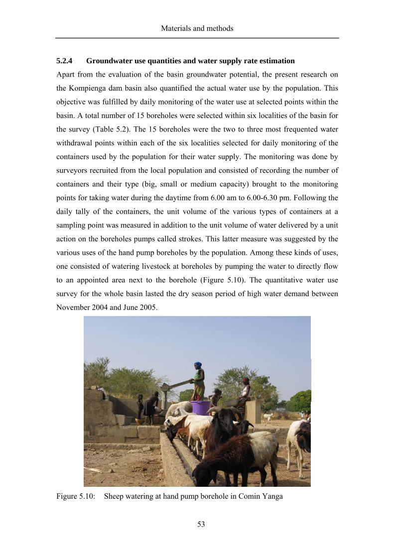
Materials and methods
53
5.2.4 Groundwater use quantities and water supply rate estimation
Apart from the evaluation of the basin groundwater potential, the present research on
the Kompienga dam basin also quantified the actual water use by the population. This
objective was fulfilled by daily monitoring of the water use at selected points within the
basin. A total number of 15 boreholes were selected within six localities of the basin for
the survey (Table 5.2). The 15 boreholes were the two to three most frequented water
withdrawal points within each of the six localities selected for daily monitoring of the
containers used by the population for their water supply. The monitoring was done by
surveyors recruited from the local population and consisted of recording the number of
containers and their type (big, small or medium capacity) brought to the monitoring
points for taking water during the daytime from 6.00 am to 6.00-6.30 pm. Following the
daily tally of the containers, the unit volume of the various types of containers at a
sampling point was measured in addition to the unit volume of water delivered by a unit
action on the boreholes pumps called strokes. This latter measure was suggested by the
various uses of the hand pump boreholes by the population. Among these kinds of uses,
one consisted of watering livestock at boreholes by pumping the water to directly flow
to an appointed area next to the borehole (Figure 5.10). The quantitative water use
survey for the whole basin lasted the dry season period of high water demand between
November 2004 and June 2005.
Figure 5.10: Sheep watering at hand pump borehole in Comin Yanga

Materials and methods
54
Table 5.2: Location of 15 water monitoring points in the Kompienga dam basin Site Nature of the water
monitoring point UTM coordinates
X Y Altitude (m asl)
Djabiga Borehole 1 Borehole 2
0233642 0233113
1231984 1232024
215 219
Pama
Modern well Borehole 1 Borehole 2 Borehole 3
0250228 0250651 0249913 0250050
1244500 1243334 1243857 1243286
211 199 200 193
Kompienbiga Borehole 1 Borehole 2
0238839 0238576
1248178 1247781
208 201
Natiabouani Borehole 1 Borehole 2
0228079 0228186
1294782 1295084
258 258
Kouaré Borehole 1 Borehole 2
0206059 0205861
1321983 1321866
347 349
Comin Yanga
Modern well Borehole 1 Borehole 2
0188111 0186826 0186194
1294806 1297130 1294214
267 270 283
For various reasons (pump breakdown, wells drying up, etc.), temporary
interruptions were observed at some monitoring points. For these points, the preceding
water volume was considered as the actual month volume to fill the gap. The reason is
that the population who collected water at these points moved due to the breakdown to
other nearby points in order to satisfy their water demand, which led to a temporary
increase in the withdrawal quantities at these points. At Pama, in addition to the
monitoring points, tap water from a local piped distribution system using a power-
driven pump taking water from a borehole to a reservoir also supplied fresh water to the
population. The supply was estimated at an approximate rate of 6200 m³ per year
according to fuel availability for the motor pump. Taking into account all these
parameters, the monthly water volumes from the 15 monitoring points were determined.

Materials and methods
55
Supply rate estimation
In order to evaluate the future water supply quality to the population, scenarios were
built based on available information for forecasting rainfall, population increase and
recharge to the basin aquifers. The daily water volume ( 1V ) to supply the basin
population was determined according to the population of a given year of projection and
a fixed supply rate. This volume is compared to the real water volume ( 2V ) that can be
delivered by the functional boreholes in the basin according to their unit yields, their
number and the daily withdrawal. For a given year and a fixed supply rate, 1V and 2V
are calculated as follows:
Let P [ ]c be the total number of inhabitants in the basin in that year,
s be the fixed supply rate in units of [ ]113 −− dcm (cubic meter per capita per day), then :
PsV ⋅=1 (5.18)
with 1V in units of [ ]13 −dm (cubic meter per day) and P in [ ]c units (capita).
2V is obtained from the following equation:
tqnV ⋅⋅=2 (5.19)
with 2V in consistent units of [ ]13 −dm ; n the total number of functional boreholes in
the basin [ ]b (borehole), q the unit borehole yield [ ]113 −− bhm (cubic meter per hour per
borehole), and t the daily withdrawal duration [ ]1−hd (hour per day).
For a satisfactory supply, 2V is supposed equal to 1V . If this is not the case, the
number of boreholes to satisfy this condition is calculated according to the fixed supply
rate, the borehole yield and the daily duration of withdrawals using an equation from
equalizing equations 5.19 and 5.18 as follows:
tqPsn⋅⋅= (5.20)
According to equation 5.20, the higher the population within the basin, the
higher the number of functional boreholes for a satisfactory supply. In contrast, an
Materials and methods
56
increase in the borehole yields and the daily duration of withdrawal contributes to
reduce the number of functional boreholes necessary to supply the population.
5.3 Conclusion
The groundwater potential for the Kompienga dam basin was evaluated based on three
methods: the water balance method, the chloride mass balance method and the water
table fluctuation method. To assess the basin groundwater potential with these methods,
various qualitative and quantitative data from hydrologic to climatic data were collected
from equipment installed in the basin or from public administration offices. The
hydrological data were composed of piezometric measurements, lake level fluctuations,
runoff heights in rivers, and water volumes for electricity and fresh water production.
Climatic data were from the Eddy Correlation station and the weather station in addition
to rain gauge measurements in the basin and precipitation data from the national
meteorology office.
The collected data varied with respect to measurement time scale and spatial
representation. Therefore, they were consequently brought to the whole basin level for
the recharge estimation. Indispensable but unavailable data of a given period were
generalized from known data using adequate and proven tools. An example is the
geological map resulting from four different maps composed of 3 recent numerical
formats (Ouédraogo et al. 2003) of the maps of Tenkodogo, Boulsa and Pama (thanks to
BUMIGEB) combined with a paper map of Fada N’gourma (Bos 1967) scanned,
digitalized and updated according to the numerical maps.
To evaluate the groundwater use quantities and estimate the population water
demands and the supply quality according to pessimistic scenarios, daily monitoring of
the water withdrawal at boreholes was carried out. The measurements supported sound
processing procedures to derive results for analysis and suggestions for sustainable
schemes of the basin groundwater resources management.

Groundwater potential evaluation
57
6 GROUNDWATER POTENTIAL EVALUATION
6.1 Introduction
Providing enough water to meet demands is a major concern of decision makers
worldwide. In Africa, and especially in Burkina Faso, the situation is worsening due to
prevailing climatic conditions. The tropical climate in Burkina Faso with 3 to 5 months
of rainfall per year and a long dry season highly limits water supplies for the population.
This supply limitation is aggravated by the high spatial and temporal variability in
rainfall in addition to the observed annual downward trend in its quantities since last
decade (Somé 2002 and Paturel et al. 2002). The geological formations in the country,
mainly granitic rocks basement do not form good aquifers and the high potential
evaporation in this semi-arid zone representing 2 to 10 times the annual rainfall
(Pouyaud 1994), are additional unfavorable factors with respect to local water
resources. Although in the same time, evaporation is also considered useful (Savenije
1997) as it has preserved West African sahelian zones from not yet being totally
covered by desert. Quantifying water resources and especially groundwater resources is
a prerequisite for sustainable water management (Foster 1988). Hence, this study
evaluates the groundwater potential in the Kompienga dam basin in the southeastern
part of Burkina Faso.
The evaluation is based on the methods chloride mass balance, basin water
balance and water table fluctuation. Difficulties in obtaining accurate data for
groundwater recharge assessment, and uncertainties and limitations in the methods
(Martin 2005), have led to the recommendation that these assessments be based on
multiple methods (Risser et al. 2005) for cross-checking the results to improve their
reliability, as no single method can provide enough reliable results (Scanlon et al. 2002).

Groundwater potential evaluation
58
6.2 Groundwater potential evaluation using chloride mass balance method
6.2.1 Background
Simmers (1988), Lerner et al. (1990), Sophocleous (1991), Bromley et al. (1997),
Scanlon et al. (2002), de Silva (2004), Martin (2005), McNamara (2005) and other
authors described techniques for groundwater recharge assessment that vary in their
complexity and cost (Risser et al. 2005). In the wide range of these methods, the
chloride mass balance method used in this study has been recognized as simple (Ayers
1985, Bazuhair and Wood 1996, Martin 2005), of low cost, and straightforward for use
in semi-arid and arid zones. This tracer method based on chloride ion conservation
appears relevant for these zones due to its insensitivity to evapotranspiration, a
parameter generally difficult to quantify accurately. Evapotranspiration does not
transport chloride but increases its concentration in the soils (Bromley et al. 1997).
Wood (1999) and Scanlon et al. (2002) state that the increasing effect of
evapotranspiration on chloride concentration in the soils is directly proportional to the
depth within the root zone, below which it remains relatively constant. This limits the
suitability of the chloride method to deep groundwater as done in this study with the
groundwater samples taken from boreholes drilled in the fractured crystalline rocks at
an average depth of 20 to 40 m (Ouédraogo et al. 2003).
The chloride mass balance method relies on the assumption that the chloride
ion is stable and conservative (non-reactive and the downward concentration not
decreased by interactions with the solid phase; Phillips 1994) and not taken up
significantly by plants (Allison 1988, Edmunds et al. 1988, Gieske 1992 and Bromley et
al. 1997). Rainfall from the atmosphere is also considered as the sole source of chloride
in the water flow system, and no net change in chloride storage is observable below the
unsaturated zone due to plants, soil fauna or water-rock interaction (Bromley et al.
1997). The implication of these assumptions is that for any existing chloride sources
apart from rain like mineralogical weathering, industrial pollution or fertilizers, the
basic formula for the recharge evaluation has to be readapted (Nyagwambo 2006). For
the study area Kompienga, these assumptions are considered valid, as these other
sources of chloride are rare or even non-existent. However, some commencing but as
yet negligible fertilizing practices within the basin for cash crop production, especially
cotton, under government incentives can be mentioned. Another possible source of
Groundwater potential evaluation
59
chloride is weathering due to water or external groundwater source enriched with
chloride and flowing into the basin. The latter is unlikely as in granitic rock like in the
Kompienga dam basin; the hydrological boundaries are almost equivalent to the
hydrogeological ones, implying that no external groundwater is likely to flow into the
basin. For the first assumption, without any chemical investigations on the geological
formations, it can be assumed that the granitic rocks, which are free of halide minerals,
are unlikely to provide chloride to the aquifers.
Another assumption from Bromley et al. (1997) on the use of the chloride
method stated that no significant net surface run-on or run-off should occur on the site.
The watershed has a relatively flat geomorphology (mean slope of 0.12 %) and
relatively important vegetation (Mihin 1984) during the rainy seasons, which slow down
the surface run-on in the basin creating ponds and marshes. Moreover, with the dam’s
spillway downstream, the entire surface runoff is collected to infiltrate in the basin as
focused, localized or indirect groundwater recharge (Scanlon et al. 2002). The run-off
from the basin is thus under control, with only periodical and negligible releases (8.4%
of the annual rainfall on average of 18-year period, Table 6.1) for national energy
production by the company in charge of the dam and for drinking water.
McNamara (2005) referring to Allison and Hughes (1978) stated that the
chloride mass balance was first developed as a one-dimensional estimation of point
recharge in desert soils and called chloride profiling method. Due to regional
specificities (mountainous and semi-arid regions), this method was later modified by
Detinger (McNamara 2005) to be applied to watersheds in Nevada, hence the watershed
chloride mass balance approach integrating the spatial variability of soil parameters of
the chloride profiling method. This method was also preferred to chloride profiling in
this study due to previous studies in the research zones showing the spatial recharge
character of the groundwater resources preferably to point-based recharge through
individual soil profiles (Martin 2005).
Considering all the assumptions valid for the Kompienga dam basin, the
groundwater potential is estimated using equation 5.1.

Groundwater potential evaluation
60
Table 6.1: Percentage of annual rainfall in the Kompienga dam basin as run-off used for energy and drinking water production
Year Average annual rainfall (mm)
Volume for electricity (hm³)
Volume for drinking water (x10-6hm³)
Total volume out of the dam (hm³)
% of annual rainfall flowing out of the dam
1989 1990 1991 1992 1993 1994 1995 1996 1997 1998 1999 2000 2001 2002 2003 2004 2005 2006
921 633 962 795 807 1197 850.4 768.5 613.4 991.4 862.7 746.3 765.8 671.1 976.3 823.7 829.6 804.0
36.84 140.86 177.75 289.45 306.39 361.11 561.55 586.55 387.5
541.68 729.58 694.97 477.32 297.47 332.92 528.98 573.8
285.47
40000 40000 56000 56000 56000 56000 56000 56000 56000 56000 56000 56000 56000 56000 56000 61572 65277 68933
36.88 140.90 177.81 289.51 306.45 361.17 561.61 586.61 387.56 541.74 729.64 695.03 477.38 297.53 332.98 529.04 573.87 285.54
0.68 3.77 3.13 6.16 6.42 5.10
11.17 12.91 10.69 9.24
14.31 15.75 10.55 7.50 5.77
10.87 11.70 6.01
Total (834.3) 7310.19 1003782 7311.19 (8.43) Numbers between brackets are average of the columns. Source: SONABEL (water quantities for electricity) and ONEA/Kpg (water quantities for drinking water production).
6.2.2 Results and discussion
Chloride in rainwater
The chloride concentration in water samples from rainfall and groundwater collected
during the rainy season 2005 from the research stations in the Kompienga dam basin
were analyzed (Table 6.2).

Groundwater potential evaluation
61
Table 6.2: Chloride concentration in rainwater and groundwater samples along with monthly weighted precipitation in the Kompienga dam basin in 2005
Chloride concentration (mg/l) Month Kouaré Natiabouani Pama Tanyélé
Average basin precipitation (mm)
April 05 Rain - 27 10 20 11.7 Rain 7.5 8.5 10 8.5 May Groundwater 27.5 24.3 27.0 13.0 86.1
Rain 10 6 9 7 June Groundwater 28.8 24.3 27.5 11.3 195.7
Rain 2.6 5 2 4.2 July Groundwater 27 20.2 23.2 9 224.4
Rain 4.6 5.8 4.8 5.8 August Groundwater 28 19.4 - 1.8 153.1
Rain 5 5 27.5 7.5 September Groundwater 30 22 - 10 126.3
Rain 7.5 10 7.5 20 October Groundwater 32.5 18 27.5 12.5 32.1
November Groundwater 30 - 30 15 - January 06 Groundwater 32.5 27.5 32.5 15 - March 06 Groundwater 30 25 27.2 12.5 -
A comparison of these data with those of previous studies on nearby sites
(Table 6.3) in central Burkina Faso, Ghana and Niger, shows that the chloride
concentrations in rainwater are remarkably high. They ranged from 2 mg/l to 27.5 mg/l
compared to 0.1 mg/l to 3.7 mg/l observed in northern Ghana in 2004 close to the study
site (Martin 2005). The average rainwater chloride concentration was 6.37 mg/l, and
22.63 mg/l for the basin average groundwater chloride concentration.
Table 6.3: Chloride concentration in rainwater and groundwater in previous study sites
Average concentration Authors Site location Cl-1 Cl-2 Cl-1 Cl-2
Roose (1981) Turner et al. (1996) Bromley et al. (1997) Martin (2005)
Central Burkina Faso Central Ghana (Kumasi) Southwest Niger Northern Ghana
1 1.9 0.12-10.2 0.1-3.71
0.5-7.8 - 5-150 0.8-39
1 1.9
0.62 (0.42) 0.20
2.3 -
36.4 (27) 6.2 (3)
Cl-1 (mg/l) represents chloride concentration in rain, Cl-2 (mg/l) represents chloride concentration in groundwater and numbers between brackets are average chloride concentration without high values of the range.
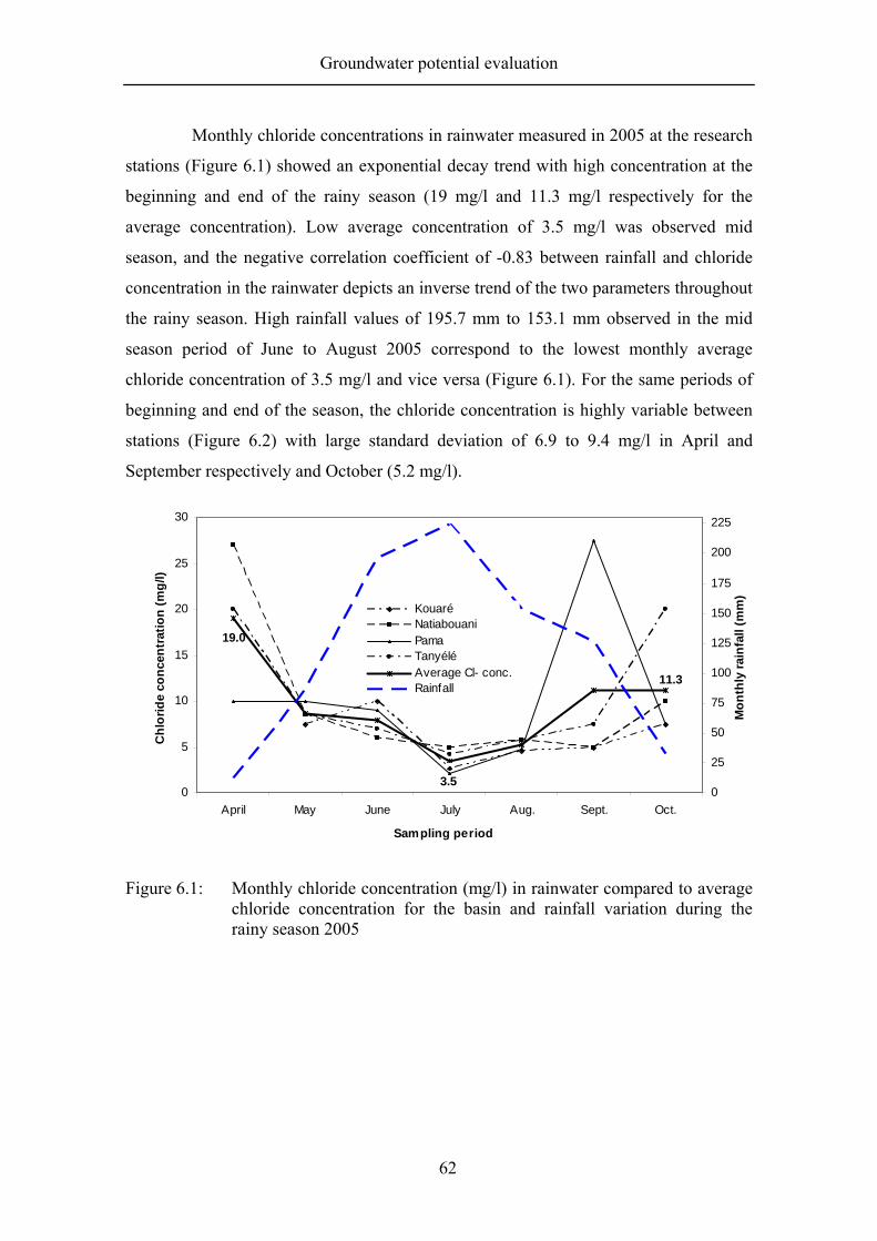
Groundwater potential evaluation
62
11.3
19.0
3.50
5
10
15
20
25
30
April May June July Aug. Sept. Oct.
Sampling period
Chl
orid
e co
ncen
trat
ion
(mg/
l)
0
25
50
75
100
125
150
175
200
225
Mon
thly
rain
fall
(mm
)
KouaréNatiabouaniPamaTanyéléAverage Cl- conc.Rainfall
Monthly chloride concentrations in rainwater measured in 2005 at the research
stations (Figure 6.1) showed an exponential decay trend with high concentration at the
beginning and end of the rainy season (19 mg/l and 11.3 mg/l respectively for the
average concentration). Low average concentration of 3.5 mg/l was observed mid
season, and the negative correlation coefficient of -0.83 between rainfall and chloride
concentration in the rainwater depicts an inverse trend of the two parameters throughout
the rainy season. High rainfall values of 195.7 mm to 153.1 mm observed in the mid
season period of June to August 2005 correspond to the lowest monthly average
chloride concentration of 3.5 mg/l and vice versa (Figure 6.1). For the same periods of
beginning and end of the season, the chloride concentration is highly variable between
stations (Figure 6.2) with large standard deviation of 6.9 to 9.4 mg/l in April and
September respectively and October (5.2 mg/l).
Figure 6.1: Monthly chloride concentration (mg/l) in rainwater compared to average
chloride concentration for the basin and rainfall variation during the rainy season 2005
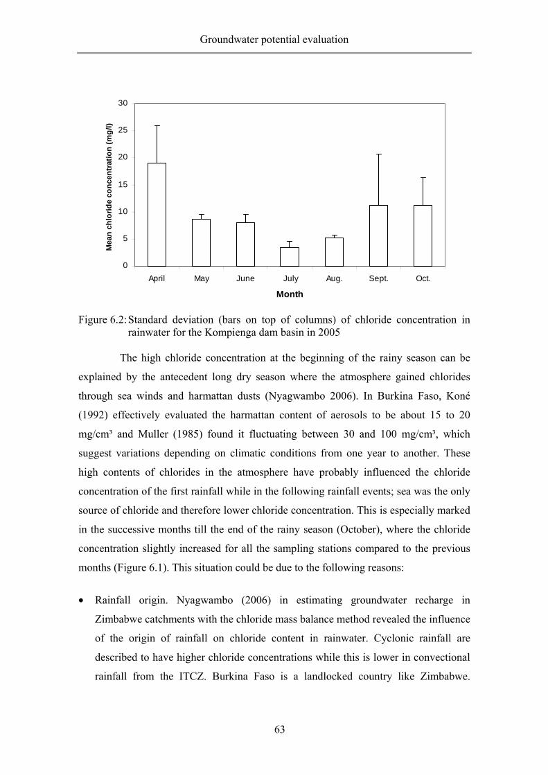
Groundwater potential evaluation
63
0
5
10
15
20
25
30
April May June July Aug. Sept. Oct.
Month
Mea
n ch
lorid
e co
ncen
trat
ion
(mg/
l)
Figure 6.2: Standard deviation (bars on top of columns) of chloride concentration in rainwater for the Kompienga dam basin in 2005
The high chloride concentration at the beginning of the rainy season can be
explained by the antecedent long dry season where the atmosphere gained chlorides
through sea winds and harmattan dusts (Nyagwambo 2006). In Burkina Faso, Koné
(1992) effectively evaluated the harmattan content of aerosols to be about 15 to 20
mg/cm³ and Muller (1985) found it fluctuating between 30 and 100 mg/cm³, which
suggest variations depending on climatic conditions from one year to another. These
high contents of chlorides in the atmosphere have probably influenced the chloride
concentration of the first rainfall while in the following rainfall events; sea was the only
source of chloride and therefore lower chloride concentration. This is especially marked
in the successive months till the end of the rainy season (October), where the chloride
concentration slightly increased for all the sampling stations compared to the previous
months (Figure 6.1). This situation could be due to the following reasons:
• Rainfall origin. Nyagwambo (2006) in estimating groundwater recharge in
Zimbabwe catchments with the chloride mass balance method revealed the influence
of the origin of rainfall on chloride content in rainwater. Cyclonic rainfall are
described to have higher chloride concentrations while this is lower in convectional
rainfall from the ITCZ. Burkina Faso is a landlocked country like Zimbabwe.
Groundwater potential evaluation
64
Cyclonic rainfalls from the south at the end of the 2005 rainy season, could have
affected Kompienga site at the borders of the coastal countries of Togo and Benin. It
could be supposed that all the rains of the season were of cyclonic origin, hence the
high chloride concentration measured in the rainwater. It is known that the seasons
and thus the climatic conditions in Burkina Faso, as in the whole of western Africa,
are governed by the oscillations of the inter-tropical front (ITCZ) which moves from
5° latitude north in January to 20° in August and back (Dipama 1997, Leroux 2001),
describing thus the season’s succession. The inter-tropical front formed by the
convergence of two marine air masses of the northern anti-cyclonic dry air of the
Azores and the humid southern anti-cyclonic air of St Helene is a zone where the
surrounding southern parts are rainy and humid while the northern parts are dry and
hazy. The surrounding zones are associated with heavy rainfall storms and thunder,
while the southern parts of the front have light rain and mainly continuous showers.
• Shortcomings in sampling the rainwater. The rainwater samples were taken by field
surveyors taught and committed to manually record the daily rainfall amounts from
the rain gauges and collect the rainwater in plastic containers. Some errors in sample
collection and neglected precautions during the sample storage could have possibly
led to such high chloride concentrations, thus explaining the generally high chloride
content observed in season rainwater. Furthermore, independent from surveyors,
other possible errors occurring during rainwater sampling at the rain gauges or at the
laboratory level when analyzing the samples could also explain the high chloride
content.
Chloride in groundwater
The chloride concentration in the groundwater samples was more or less homogenous
all along the rainy season 2005 for all the four sampling stations. Exceptions were
observed with some extremely low concentrations likely to be outliers like the 1.8 mg/l
recorded in August at Tanyélé. Meanwhile, slightly increasing trends were also
observed (Figure 6.3) throughout the season for all the stations (monthly average of
20.16 mg/l in May 2005 to 24.31 mg/l in January 2006) with a decreasing trend at the
beginning of the dry season (March 2006).

Groundwater potential evaluation
65
The Tanyélé station had the lowest groundwater chloride concentration, which
indicates higher recharge at this site compared to the others (Figure 6.3). This can be
explained by the location of the sampling borehole close to a riverbed highly
contributing to groundwater recharge. Bagayoko (2006) described the soil texture of
Tanyélé to be sandy loam, an additional factor favoring local water infiltration at the
site in comparison to the other sites, which are composed of gravelly clay (Pama),
gravelly silty (Natiabouani) and sandy clay soils (Kouaré). In addition, Tanyélé located
near the dam’s lake at about 5 km distance like the Pama station had received more
precipitation in the preceding month of July (Figure 4.7) and could have benefited from
the lake due to favorable hydraulic gradient.
Besides the noticeably low chloride concentration in the Tanyélé groundwater
samples along the season suggesting higher recharge at this station than at the others, a
general decreasing trend of all the curves is also remarkable in the July-August period
(Figure 6.3). This situation indicates that the basin aquifers seemed to be responding
relatively well to rainfall events and suggests the occurrence of preferential flow
processes at that period within the basin. These flows prevailing in the basin recharge
processes confirm the conclusions from previous studies quoted in Martin (2005) on
similar granitic basement aquifers within the West African region. For this reason, the
Tanyélé station, which showed higher recharge, could have more preferential pathways
than the other stations. However, it cannot be excluded that the flow process be also
diffuse, as the first noticeable recharge effect was only observed in July-August after 3
rainy months. During these months, rain is supposed to have sufficiently wetted the
topsoil to meet the soil moisture deficit as well as evaporation and transpiration
demands and percolate through the wet unsaturated zone to reach the water table and
dilute the groundwater. Meanwhile, for a diffuse flow process, once the recharge takes
place it is reasonable to expect a continuous process when rains are still falling in the
basin (Figure 4.7). After the supposed recharge of the aquifers in July-August (Figure
6.3), the chloride concentration increased again in the groundwater. This suggests that
the observed recharge in July-August resulted from preferential flow through the soil
cracks and fissures. Later, these preferential paths, due to swelling of clay soil particles
as suggested by Lloyd (1986) and Nyagwambo (2006) are blocked and the subsequent
rainwater therefore percolate through diffuse flow processes to recharge the basin

Groundwater potential evaluation
66
0
5
10
15
20
25
30
35
May05 June July Aug. Sept. Oct. Nov. Jan06 Mar06
Month
Chl
orid
e in
gro
undw
ater
(mg/
l)
KouaréNatiabouaniPamaTanyélé
groundwater after the rainy period depending on the depth to the water table. This
conception is substantiated by the decrease in the curves observed between January and
March (Figure 6.3). The remarkable increase in the groundwater chloride concentration
of all the stations after the preferential flow recharge process is likely to be the result of
transpiration of trees, which extracted the recharged water and left the aquifer with more
chloride resulting from the preferential flow recharge. This is confirmed by the actual
evaporation values observed from the EC measurements in the basin, which never
tended to zero during the dry season (Figure 5.6). Authors like Adar and Leibundgut
(1995), Haase et al. (1996) and de Vries et al. (2000) also mentioned upward fluxes of
groundwater by deep-rooted vegetation from 15 m to 50 m in semi-arid and arid zones
amounting to 1 mm/a (Nyagwambo, 2006).
Figure 6.3: Monthly chloride concentration in groundwater from boreholes of the study stations from May 2005 to March 2006
Comparing the groundwater monthly chloride concentration values of the
stations to those of nearer sites (Table 6.3), the data appear to be in the range of those
from Niger (5-150 mg/l) and Ghana (0.8-39) with the same geological formations of
West African crystalline basement. The groundwater chloride values in the study are
therefore acceptable for the basin recharge estimation. The difference between these
data and the rainwater data can be mainly attributed to shortcomings in the rainwater

Groundwater potential evaluation
67
sampling method by the local surveyor as the author sampled the groundwater every
month from the boreholes.
Basin recharge estimation
In the light of the shortcomings that led to the high chloride content in the rainwater, a
second rainwater sampling was realized in September 2006. This time, trained staff did
the rainwater sampling for three of the stations while the author collected the samples at
the fourth station. During three weeks, rainwater was recorded and sampled in
individual plastic bottles for each rainfall event. In addition, two samples were taken
from boreholes at each site at the beginning and end of the 3-week period. Finally, the
samples were divided into two parts when it was possible, and taken to laboratories in
Burkina Faso (the same laboratory that in 2005 analyzed the rainwater and groundwater
samples) and Germany (Bonn) for chloride analysis. The same analysis method (ion
chromatography) was applied by the two laboratories. It can be seen from the results
that the laboratory analysis in Burkina Faso was the reason for the high chloride content
in the rainwater in 2005. Apparently, unsuitable equipment was used to analyze the
rainwater samples likely to have low chloride contents. Weaver and Talma (2005) and
Beekman and Sunguro (2002) in their studies on analysis of chloride concentration in
water samples underlined that not all laboratories are equipped for measuring low
chloride content of water samples (chloride concentration below 5 mg/l with a precision
of less than 0.5 mg/l). They therefore, suggested that samples be duplicated and sent to
at least two reputable laboratories. The unsuitability of the laboratory equipment in
Burkina Faso for measuring the rainwater chloride concentration as stated above is
substantiated by the weak correlation coefficient of -0.0048 between the analysis results
of this laboratory and those of the Bonn laboratory. In contrast, the chloride
concentration in the groundwater samples from the two laboratories correlates with a
coefficient of 0.99, when excluding the second value of groundwater chloride
concentration of Pama, considered an outlier in comparison to the data series from the
Burkina Faso laboratory. The strong correlation between the two data series of
groundwater chloride concentration gave a linear regressive equation with R²=0.98
(Figure 6.4). The suppression of the outlier value of 10 mg/l at the Pama station is based
on the values from all four stations, where Tanyélé received more recharge than the

Groundwater potential evaluation
68
three other showed. Comparing the data of all stations during the 3-week sampling, the
Pama station showed the lowest precipitation of 69.9 mm while Tanyélé, Natiabouani
and Kouaré received 74.4 mm, 78.5 mm and 136.5 mm, respectively. At the same time,
the two groundwater samples of each station analyzed by the laboratory in Burkina Faso
always showed to have the same chloride concentration despite the 3-week time lag
separating the two sampling dates, except for Pama where a significant difference can
be observed (Table 6.4). If a recharge occurred at the Pama station as indicated by the
decrease in the chloride concentration of the groundwater samples, the favorable
difference in the precipitation in addition to the sandy loam texture should have also led
to a recharge at Tanyélé. As that was not the case, the second groundwater chloride
value at Pama is therefore likely to be erroneous.

Groundwater potential evaluation
69
Table 6.4: Chloride concentration in rainwater and groundwater from the four research stations in the Kompienga dam basin in 2006 analyzed in Burkina Faso and German (Bonn) laboratories
Sample nature Rainwater
Station Kouaré Pama Natiabouani
Sampling date in Sept. 2006 07 08 09 12 15 18 21 22 09 12 15 16 19 20 23 24 09 10 13 16 17 19
Sample code K1 K2 K3 K4 K5 K6 K7 K8 P1 P2 P3 P4 P5 P6 P7 P8 N1 N2 N3 N4 N5 N6
Bonn laboratory (mg/l) 9.49* 1.41 2.69 0.76 1.64 1.77 0.93 0.51 2.31 0.89 0.69 0.59 288.44* 2.28 0.57 0.73 0.45 0.38 0.74 0.56 0.55 0.41
Burkina Faso laboratory (mg/l) 5.0 10.0 10.0 5.0 10.0 5.0 5.0 5.0 28.0 - 10.0 - - 10.0 10.0 10.0 8.0 8.0 8.0 8.0 8.0 8.0
Table 6.4 continued Sample nature Rainwater Groundwater
Station Tanyélé Kouaré Pama Tanyélé Natiabouani
Sampling date in Sept. 2006 9 11 12 15 16 19 21 22 24 24 07 25 11 25 08 25 07 25
Sample code T1 T2 T3 T4 T5 T6 T7 T8 T9 T9’ K1F K2F P1F P2F T1F T2F N1F N2F
Bonn laboratory (mg/l) 0.96 0.74 1.55 0.50 1.15 0.67 579.17* 6.67* 1.29 0.47 22.87 22.92 20.80 20.50 3.90 3.38 15.49 15.99
Burkina Faso laboratory (mg/l) 8.0 8.0 - 8.0 - - - - 8.0 - 30.0 30.0 28.0 10.0 10.0 10.0 25.0 24.0 * High chloride content samples discarded from the analysis

Groundwater potential evaluation
70
y = 0.94x - 6.09R2 = 0.98
0
5
10
15
20
25
30
35
0 5 10 15 20 25 30 35
Cl- BF lab (mg/l)
Cl-
Bon
n la
b (m
g/l)
Considering the above analysis, it appears that laboratory equipment in
Burkina Faso was suitable for analyzing the high chloride contents in the groundwater
samples but not the low ones, as it was the case for the rainwater samples. Therefore,
using the regressive equation of the correlation between the groundwater chloride
concentration analyzed in the two laboratories (Figure 6.4), the groundwater chloride
concentration data from the Burkina Faso laboratory in 2005 were corrected and used in
combination with the rainwater chloride concentration analyzed in 2006 to re-evaluate
the Kompienga dam basin annual groundwater recharge with the methodology
described in section 5.2.1.
Figure 6.4: Relationship between chloride concentration in rainwater analyzed in Burkina Faso and German laboratories
The average chloride concentration in rainwater pCl was estimated equal to
0.87 mg/l and gwCl was 15.91 mg/l for the groundwater chloride concentration in 2005.
For 2006, pCl was equal to 0.88 mg/l and gwCl , 16.52 mg/l. The average chloride
concentration in rainwater from nearby sites was estimated to be 0.61 mg/l. The results
therefore show the annual recharge of the basin in 2005 to be 45.4 mm representing
5.5% of the annual rainfall and in 2006, 42.9 mm equivalent to 5.3% of the annual
precipitation of 804 mm. With the nearby sites rainwater average chloride
concentration, the recharge in 2005 is shown to be approximately 31.6 mm, i.e., 3.8% of
the annual rainfall. Initially, with the average groundwater chloride concentration
1:1 line

Groundwater potential evaluation
71
without regression, this estimate was 22.2 mm, representing 2.7 % of the annual
precipitation in 2005.
Table 6.5: Areal weights and groundwater chloride concentration for estimating recharge in the Kompienga dam basin
Stations Kouaré Natiabouani Pama Tanyélé
Areal weights [ ]1−mglClgws
0.44 21.6
0.28 15.0
0.06 19.8
0.22 4.7
It can be observed that these estimations fall within the range of previous estimates of 2
to 16% of the total annual precipitation quoted in van der Sommen and Geirnaert (1988)
for natural groundwater recharge in Burkina Faso using water balance method, water
table fluctuation and isotope analysis. The main observation deriving from the different
estimations, except for the evaluation using rainwater chloride concentrations of the
nearby sites, shows that the annual recharge roughly represents 5% of the annual
precipitation, although the observations in 2006 were too short to be representative. The
recharge estimated from the average rainwater chloride concentration of the nearby sites
can be considered as a rough estimate for preliminary results of the basin recharge in the
absence of valid observed data.
6.3 Groundwater potential evaluation using water balance method
6.3.1 Background
Among the variety of methods existing for groundwater recharge estimation, the water
balance method is a method applicable to any water system. Sokolov and Chapman
(1974) described the method as providing an indirect evaluation of an unknown water
balance component from the residual unexplained by the known components. For this
reason, the method was defined as the application in hydrology of the principle of
conservation of mass with the implication that:
• for any arbitrary control volume and during any period of time, the difference
between total input and output has to be balanced by the change of water storage
within the volume;
• time and spatial boundaries of the water system must be well-defined;

Groundwater potential evaluation
72
• measurements of storage and fluxes of water at appropriate time scales must exist or
be expected.
The application of this method provides a groundwater recharge estimation as
a residual of all the other fluxes (Lerner et al. 1990). Therefore, the method is
considered flexible with a wide range of space and time applicability without any
presuppositions except the availability of the balance terms (Scanlon et al. 2002) and the
advantage of using readily available data. Meanwhile, a disadvantage of the method,
which reduces its usefulness, is that recharge being residual, errors and uncertainties in
measuring other water balance components affect its estimation. Gee and Hillel (1988)
noted that calculating small figures such as recharge in semi-arid and arid regions from
large figures like precipitation and potential evaporation in these regions is likely to
induce a high level of uncertainty in the evaluation. Recharge estimation with the water
balance method is therefore considered inappropriate for semi-arid and arid regions
where potential evaporation, a key component of the method, amounts to 60% or 80%
of the annual water budget (Martin 2005), and 60% of the global annual precipitation
(Seckler et al. 1998 and Compaoré 2006). This shortfall prompted Gee and Hillel
(1988), Lerner et al. (1990), and Hendrickx and Walker (1997) to question its usefulness
in such parts of the world where runoff is often low. Indeed, the water balance method
was developed for temperate climates where, in general, annual rainfall exceeds
potential evaporation (Lerner et al. 1990, Martin 2005). In arid and semi-arid zones,
rainfall occurs during storm events within short periods of time, and recharge
mechanisms are rather through ponding and preferential flow than through the matrix
flow process as in the temperate zones. Nevertheless, the method remains useful in
providing preliminary insight for any groundwater system recharge when estimation
time steps are adapted.
6.3.2 Results and discussion
Annual time step water balance recharge estimation
The application of the water balance method to the Kompienga dam basin was based on
available data for the components of equation 5.11 collected from different field
measurements and from SONABEL and ONEA/Kpg in volume units, which were
converted into millimeters according to the basin watershed area. An exception is made
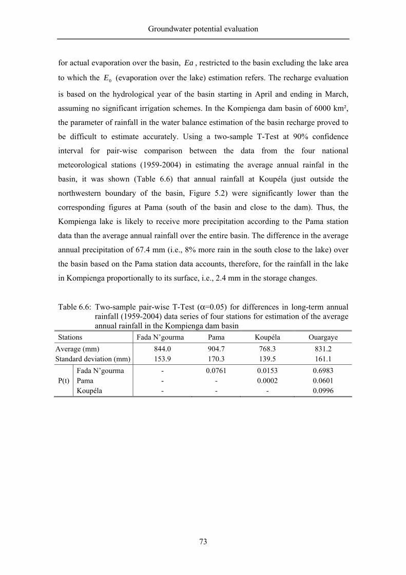
Groundwater potential evaluation
73
for actual evaporation over the basin, Ea , restricted to the basin excluding the lake area
to which the 0E (evaporation over the lake) estimation refers. The recharge evaluation
is based on the hydrological year of the basin starting in April and ending in March,
assuming no significant irrigation schemes. In the Kompienga dam basin of 6000 km²,
the parameter of rainfall in the water balance estimation of the basin recharge proved to
be difficult to estimate accurately. Using a two-sample T-Test at 90% confidence
interval for pair-wise comparison between the data from the four national
meteorological stations (1959-2004) in estimating the average annual rainfal in the
basin, it was shown (Table 6.6) that annual rainfall at Koupéla (just outside the
northwestern boundary of the basin, Figure 5.2) were significantly lower than the
corresponding figures at Pama (south of the basin and close to the dam). Thus, the
Kompienga lake is likely to receive more precipitation according to the Pama station
data than the average annual rainfall over the entire basin. The difference in the average
annual precipitation of 67.4 mm (i.e., 8% more rain in the south close to the lake) over
the basin based on the Pama station data accounts, therefore, for the rainfall in the lake
in Kompienga proportionally to its surface, i.e., 2.4 mm in the storage changes.
Table 6.6: Two-sample pair-wise T-Test (α=0.05) for differences in long-term annual rainfall (1959-2004) data series of four stations for estimation of the average annual rainfall in the Kompienga dam basin
Stations Fada N’gourma Pama Koupéla Ouargaye Average (mm) Standard deviation (mm)
844.0 153.9
904.7 170.3
768.3 139.5
831.2 161.1
P(t) Fada N’gourma Pama Koupéla
- - -
0.0761 - -
0.0153 0.0002
-
0.6983 0.0601 0.0996

Groundwater potential evaluation
74
Table 6.7: Annual recharge of the Kompienga dam basin in 2005 estimated with the water balance method
Parameters (hm³) (mm) % of P
P
1S∆
Ea
0E
L
4903.7 85.8
4286.9 254.4 438.3
829.6 14.5 725.2 43.0 7.1
100 1.8 87.4 5.2 0.9
R 9.9 1.7 0.2 with R = annual groundwater recharge in the whole Kompienga dam basin; P = annual precipitation in the basin; 1S∆ = annual change in storage within the lake; Ea = annual (actual) evaporation over the basin; 0E
= annual evaporation of the lake water; L = annual water withdrawn from the dam for drinking water and energy production.
The groundwater recharge in the Kompienga dam basin in 2005 with the water
balance method is therefore equal to 1.7 mm (Table 6.7), which represents almost 0.2%
of the annual rainfall of the basin in that year. Taking into account the favorable
difference of rainfall over the lake as suggested by the T-Test between the
meteorological stations, the annual recharge can then be estimated to be 4.1 mm,
representing 0.5% of the annual rainfall in the basin. This recharge, nevertheless,
remains lower than the recharge estimated using the chloride mass balance method. The
difference in the estimate between the two methods can be attributed to the main
problem of the water balance method of recharge estimation in arid and semi-arid
environments quoted by many authors (Sokolov and Chapman 1974, Gee and Hillel
1988, Lerner et al. 1990). Indeed, parameters like evaporation ( Ea and 0E ) and rainfall
(derived from spatially variable sample measurements) used in this water balance were
an additional source of inaccuracy in the final estimation as demonstrated in the
following section.
Error estimation on the annual time step water balance recharge in the basin
In order to quantify the likely uncertainty associated with the annual time step water
balance estimate of the basin recharge, a basic error propagation exercise was
conducted. The annual time step estimation of the basin recharge is based on equation
5.11 with all the parameters in units of [ ]13 −TL :
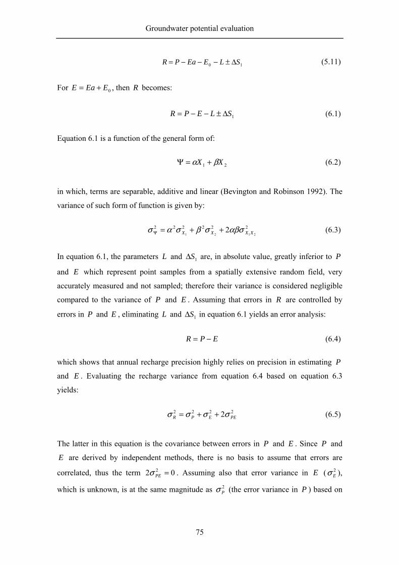
Groundwater potential evaluation
75
10 SLEEaPR ∆±−−−= (5.11)
For 0EEaE += , then R becomes:
1SLEPR ∆±−−= (6.1)
Equation 6.1 is a function of the general form of:
21 XX βα +=Ψ (6.2)
in which, terms are separable, additive and linear (Bevington and Robinson 1992). The
variance of such form of function is given by:
222222
21212 XXXX αβσσβσασ ++=Ψ (6.3)
In equation 6.1, the parameters L and 1S∆ are, in absolute value, greatly inferior to P
and E which represent point samples from a spatially extensive random field, very
accurately measured and not sampled; therefore their variance is considered negligible
compared to the variance of P and E . Assuming that errors in R are controlled by
errors in P and E , eliminating L and 1S∆ in equation 6.1 yields an error analysis:
EPR −= (6.4)
which shows that annual recharge precision highly relies on precision in estimating P
and E . Evaluating the recharge variance from equation 6.4 based on equation 6.3
yields:
2222 2 PEEPR σσσσ ++= (6.5)
The latter in this equation is the covariance between errors in P and E . Since P and
E are derived by independent methods, there is no basis to assume that errors are
correlated, thus the term 02 2 =PEσ . Assuming also that error variance in E ( 2Eσ ),
which is unknown, is at the same magnitude as 2Pσ (the error variance in P ) based on
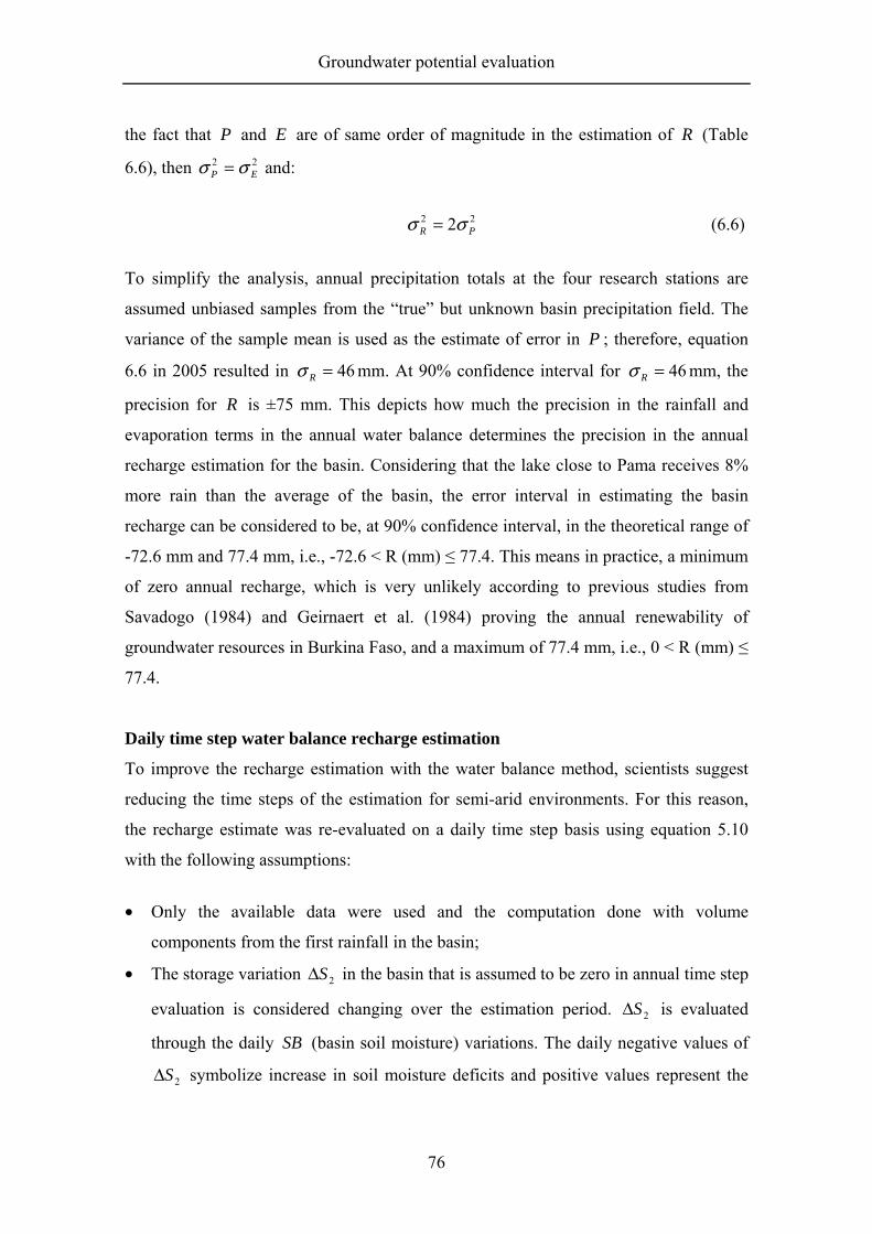
Groundwater potential evaluation
76
the fact that P and E are of same order of magnitude in the estimation of R (Table
6.6), then 22EP σσ = and:
22 2 PR σσ = (6.6)
To simplify the analysis, annual precipitation totals at the four research stations are
assumed unbiased samples from the “true” but unknown basin precipitation field. The
variance of the sample mean is used as the estimate of error in P ; therefore, equation
6.6 in 2005 resulted in 46=Rσ mm. At 90% confidence interval for 46=Rσ mm, the
precision for R is ±75 mm. This depicts how much the precision in the rainfall and
evaporation terms in the annual water balance determines the precision in the annual
recharge estimation for the basin. Considering that the lake close to Pama receives 8%
more rain than the average of the basin, the error interval in estimating the basin
recharge can be considered to be, at 90% confidence interval, in the theoretical range of
-72.6 mm and 77.4 mm, i.e., -72.6 < R (mm) ≤ 77.4. This means in practice, a minimum
of zero annual recharge, which is very unlikely according to previous studies from
Savadogo (1984) and Geirnaert et al. (1984) proving the annual renewability of
groundwater resources in Burkina Faso, and a maximum of 77.4 mm, i.e., 0 < R (mm) ≤
77.4.
Daily time step water balance recharge estimation
To improve the recharge estimation with the water balance method, scientists suggest
reducing the time steps of the estimation for semi-arid environments. For this reason,
the recharge estimate was re-evaluated on a daily time step basis using equation 5.10
with the following assumptions:
• Only the available data were used and the computation done with volume
components from the first rainfall in the basin;
• The storage variation 2S∆ in the basin that is assumed to be zero in annual time step
evaluation is considered changing over the estimation period. 2S∆ is evaluated
through the daily SB (basin soil moisture) variations. The daily negative values of
2S∆ symbolize increase in soil moisture deficits and positive values represent the

Groundwater potential evaluation
77
groundwater recharge when SB is above field capacity of maxSB as in Rushton and
Ward (1979);
• The daily changes in the lake storage, 1S∆ , are derived from the lake level
fluctuations and the tare curve of water levels versus lake volume using the attached
regressive equation;
• A maximum soil water storage capacity of the unsaturated zone is considered equal
to maxSB determined in the Ea 2005 derivation with WaSiM-ETH topmodel
module;
• At the end of the rainy season, where no input water was available and after maxSB
was exhausted, groundwater depletion by upward circulation was considered and
limited to extraction alone by deep-rooted vegetation depicted by the daily Ea
measurements from the EC station (Figure 5.6);
• The daily lake evaporation values 0E used in the simulation were interpolated daily
values from Pouyaud (1985) studies on Lake Bam and Lake Tchad;
• The withdrawals of groundwater by the population of the basin are considered
negligible in the water balance as observed by Martin and van de Giesen (2005)
from their estimation of groundwater potential of the whole Volta river basin.
The main principle of the annual recharge estimate through daily time step
evaluation is based on the consideration that the unsaturated zone of the basin is a
reservoir with a maximum storage capacity of maxSB representing the soil moisture SB
at field capacity over the depth of the unsaturated zone profile. The estimates consider
that according to its intensity, the first rainfall contributes to the generation of runoff in
the basin, satisfies plants transpiration demands and evaporation as well as infiltration
for recharge. When the sum of the infiltrated part of the daily rainfall reaches the
threshold value of the unsaturated zone storage capacity of maxSB , then all additional
infiltrated rainfall is considered to percolate to the water table as recharge. Once the
unsaturated zone reaches the maximum storage capacity, the following dry days with a
negative balance are considered to deplete this unsaturated zone storage, and the
subsequent rainfall refills this storage to maxSB for new recharge occurrence.
Groundwater potential evaluation
78
From the above assumptions, and using equation 5.10 as daily recharge
estimation, the total basin recharge in 2005 from 15 rains amounted to 59.8 mm with a
maximum recharge of 33 mm on July 10, 2005, and a lowest recharge of 0.5 mm on
September 3, 2005. It can be observed that this recharge, like those derived from the
chloride mass balance method, fall within the interval of the predicted annual recharge
quantity in the basin with the error estimation. The estimated recharge period appears to
have lasted the 2 months between July 10 and September 8, 2005. The estimate, which
represents 7.2% of the annual basin rainfall in 2005, is considerably higher than the
annual time step estimation at 0.5% of the annual rainfall with the same method. The
difference in recharge between the two methods lies solely in the water storage change
2S∆ within the basin with the sum of all the other components over the year equal to
the corresponding cumulative water balance components. Assumed to be zero over the
whole year in the annual time step recharge estimation, the water storage change is
considered to be changing along the year in the daily time step recharge estimate. This
result of the daily time step water balance recharge estimate substantiates somewhat the
results of Rushton and Ward (1979) in Northern Lincolnshire Chalk aquifer (United
Kingdom) that show 10% underestimates of recharge from weekly input data and 25%
from monthly data. This thus shows the appropriateness of adapting the recharge
evaluation time steps to natural processes occurrence (Howard and Lloyd 1979) in semi-
arid zones like the Kompienga region in Burkina Faso, where potential evaporation
often exceeds rainfall for most of the year (Figure 4.5) leaving in general hardly any
little possibility for recharge. Nevertheless, this does not mean that the method is more
reliable than any other method, but only expresses the adequacy of the recharge
evaluation with time steps close to real and natural occurrence of events. The recharge
occurrence details provided by the estimation process (Figure 6.5) provide better
possibilities for groundwater resource management in the basin.

Groundwater potential evaluation
79
0
10
20
30
40
50
60
70
80
14-A
pr-0
5
24-A
pr-0
5
4-M
ay-0
5
14-M
ay-0
5
24-M
ay-0
5
3-Ju
n-05
13-J
un-0
5
23-J
un-0
5
3-Ju
l-05
13-J
ul-0
5
23-J
ul-0
5
2-Au
g-05
12-A
ug-0
5
22-A
ug-0
5
1-Se
p-05
11-S
ep-0
5
21-S
ep-0
5
1-O
ct-0
5
11-O
ct-0
5
21-O
ct-0
5
31-O
ct-0
5
Date
Rec
harg
e (m
m)
0
20
40
60
80
100
120
Rainfall (m
m)
Figure 6.5: Daily recharge (upward bars) in Kompienga dam basin compared to daily
rainfall depths (downward bars)
From the daily simulated groundwater recharge graph (Figure 6.5), the following can be
observed:
• There is a time lag between begin of rainfall and begin of recharge. The first rainfall
was observed on April 14, while the first recharge was 3 months later on July 10
after the highest rainfall of the season. This delay in recharge is due to many factors.
One factor is the recharge process assumed in the water balance method with the
daily processing time steps to be the matrix or diffuse flow. In this flow process,
rain first has to wet the unsaturated zone to its field capacity before deep percolation
starts. Therefore, depending on the unsaturated zone field capacity and its thickness,
i.e., the depth to the water table, the delay between rainfall occurrence and recharge
can be short or long. Other factors are soil characteristics (partially involved in the
previous factor) and rainfall characteristics combined with the basin land cover and
topographical aspects. Indeed, as explained by Ajayi (2004), water infiltration to
induce recharge is a complex process involving rainfall, soil matrix, terrain
topography and morphology as well as land covers. In the Kompienga dam basin
with its flat terrain without significant slopes (van de Giesen et al. 2001), the
topography and morphology have less influence on the infiltration processes than

Groundwater potential evaluation
80
the rainfall-soil matrix interrelations. Indeed, rainfall intensities in addition to
heterogeneity according to structure and texture and land use in relation to hydraulic
properties as quoted in Spaan and Stroosnijder (1997), van de Giesen et al. (2000),
Stomph et al. (2002) and Ajayi (2004) are the main influences of surface runoff and
infiltration processes. Nyagwambo (2006) studies on a small catchment in
Zimbabwe with similar geological characteristics and climatic conditions like those
in Kompienga confirm this fact, pointing out that a threshold rainfall depth exists for
the commencement of any detectable recharge to aquifer independent of the
recharge flow process. The level of the threshold, meanwhile, depends intrinsically
on the flow process. For the Kompienga dam basin in 2005, this threshold rainfall
according to the results from the water balance is estimated at 336.6 mm,
representing 41% of the annual rainfall, which is used during the time lead to satisfy
evaporative demands and soil moisture deficits in the basin.
• After the first recharge takes place in the basin, the following rains easily produce
recharge proportional to their amount (Figure 6.5). The highest daily recharge (33
mm) in the basin was observed to correspond to the highest precipitation (61.2 mm)
in the year. It appears that after the threshold rainfall for the recharge is reached, the
subsequent rainfall recharges the basin according to the wetness of the soil and the
rainfall amount. According to this observation, the daily recharge rates following the
first recharge of the season vary from 13% to 87% of the daily rainfall. The lowest
recharge rate (13%) is derived from 10.4 mm rainfall on July 14, 2005 and the
highest recharge rate (87%) from 22.5 mm rainfall on July 15, the day following the
highest rainfall in the basin. While almost the same precipitation of 26.8 mm on
September 8 following 4 dry days only produced a recharge rate of 44% (half of that
derived from the rainfall on July 15), a precipitation of 9.1 mm in a wet spell of 7
rainy days contributed to 71% as recharge. Despite the strong correlation
(correlation coefficient of 89%) between daily rainfall and daily recharge in the
basin once the unsaturated zone is above field capacity, it remains difficult to
generalize in predicting from the derived results, the exact pattern of the daily
recharge according to daily rainfall. This is partly due to the high erratic behaviour
in the daily rainfall, which supposes that dry spells appearing within the rainy
season compromise all possibility of recharge as the unsaturated zone wetness has to

Groundwater potential evaluation
81
y = 149.05Ln(x) - 857.1R2 = 0.94
0
20
40
60
80
100
120
140
160
200 300 400 500 600 700 800 900
Cumulative rainfall (mm)
Cum
ulat
ive
rech
arge
(mm
)
be refilled before new recharge occurrence; depending on the rainfall depth and the
level of lowering of the unsaturated zone wetness. Nevertheless, it can be stated that
during the recharge period and without dry spell, the daily rainfall threshold for
recharge is approximately equal to the daily actual evaporation in the basin.
• From cumulative rainfall and cumulative recharge within the basin, a strong
relationship was observed and made it possible to derive the rainfall-recharge
relation for the annual recharge estimation based on the annual rainfall amount. This
relationship, similar to the daily rainfall-recharge relation depicts a threshold of
rainfall for commencement of recharge to the basin. From the linear relationship of
R²=0.94 (Figure 6.6), this rainfall threshold is equal to 314.3 mm, and the equation
for the annual recharge estimation using the precipitation is:
EaPLnR −−⋅= )75.5)((05.149 (6.7)
with [ ]LR as the annual water recharge in the basin, [ ]LP the annual precipitation,
and [ ]LEa the total actual evaporation calculated for the period between the end of
the rainy season and the end of the hydrological year of the recharge estimation. As
depicted by the Eddy correlation measurements (Figure 5.6 and Appendix 3), Ea in
the basin is never zero during the dry season period, most likely due to transpiration
of deep-rooted trees.
Figure 6.6: Relationship between cumulative rainfall amount and recharge in the
Kompienga dam basin in 2005
Groundwater potential evaluation
82
• The last recharge occurred in the basin on September 8, while rains continued
falling until October 14 (Figure 6.5), more than a month later. The cumulative
rainfall of this period amounts to 97.6 mm (12% of annual rainfall) with two
consecutive days receiving the highest precipitation of 16 mm without any recharge
occurrence. This situation substantiates the previous conclusions indicating that
recharge is strongly dependent on soil wetness memory. Indeed, temperature and
consequently evaporation in the research area of Kompienga are described
(Bagayoko 2006) to be increasing at the end of the rainy season. This situation
observed in the comparative trend of rainfall and pE (Figure 4.5) in 2005 depicted
in October where pE was considerably higher, being 5 times the precipitation.
Therefore, little possibility is given to the decreasing rainfalls to induce recharge. In
addition, spatial variability in rainfall and soil characteristics may influence recharge
evaluation at the whole basin scale and be a source of bias in the interpretation of
the results. For example, rainfall amount recorded by only one of the four stations in
a given period will be considered through the Thiesen polygon to have occurred
over the whole basin at a lower rate of 50% to 30% or only 25% of that at the given
station. Therefore, while insufficient for recharge at the whole basin scale, it could
have been sufficient at the local station. It seems thus advisable to consider carefully
the recharge results derived at the whole basin scale, which tend to mask local
specificities of rainfall as revealed by the T-Test results, soils, land cover and
topography that are likely to exist for a basin covering 5911 km². An example is the
basin recharge derived from the two methods of water table fluctuation and water
balance. While the last recharge is estimated by the water balance to have occurred
at the whole basin scale on September 8, the water levels fluctuations in a
piezometer at Pama for example (Figure 6.8), show that it was on October 8, 2005,
i.e., one month later.

Groundwater potential evaluation
83
6.4 Groundwater potential evaluation using water table fluctuation method
6.4.1 Background
The variations of the water table within the saturated zone express the groundwater
level fluctuations under recharge and discharge processes. The water table fluctuation
(WTF) method for groundwater recharge evaluation is one of the most widely used
methods due to current availability of groundwater level data, the method’s simplicity
and insensitivity to mechanisms of water movements through the unsaturated zone
(Healy and Cook, 2002). From the water table definition, it is obvious that the WTF
method is solely applicable to unconfined aquifers and best fits to shallow groundwater
where sharp water level rises and declines can be observed. The main assumption in the
WTF method is that rise in the water table is an indication of recharge of water arriving
in the groundwater (equation 5.17). From the assumption and the derived equation,
some remarks need to be made regarding the limitations of the method:
• Not all water table rises can be solely attributed to recharge. Groundwater recovery
from pumping or extraction, evapotranspiration, barometric pressure effects and
many other causes (entrapped air in the unsaturated zone, changes in groundwater
flow processes from adjacent aquifers, temperature variation, etc.) independent of
input of water to the water table can lead to rises in groundwater levels
(Sophocleous 1991, Healy and Cook 2002). Therefore, a clear distinction should be
made between the effects of water input and other possible factors on water table
rise for a better groundwater recharge evaluation with the WTF method. These
effects are assumed to be minimal.
• For shallow groundwater, a time scale evaluation longer than a rain event period in
semi-arid and arid zones is likely to underestimate the recharge (Healy and Cook
2002). Indeed, the evaporation effects on shallow groundwater and discharges to
streams are considerable in long time lag and tend to reduce the effects of individual
rain events on the water table, and thus lead to underestimation of the recharge.
• The specific yield in equation 5.17 for the recharge estimation is a parameter known
to be difficult to estimate accurately. Some authors (Lerner et al. 1990) even suggest
considering standard soil texture values from literature rather than field test
measurements when values from laboratories are unavailable. The recharge
accuracy of the WTF method critically relies on the specific yield defined by

Groundwater potential evaluation
84
Sophocleous (1991, p.236) as the “volume of water released from a unit volume of
saturated aquifer material drained by a falling water table”. It reflects the difference
between the porosity and the specific retention of the soil materials as quoted in
Healy and Cook (2002).
6.4.2 Results and discussion
Groundwater levels in the Kompienga dam basin were measured daily in 2005 from
piezometers installed at the four main research stations. These measurements provided
evidence of groundwater recharge within the basin during 2005 rainy season by means
of the water table fluctuation method (Figure 6.7).

Groundwater potential evaluation
85
0
100
200
300
400
500
600
1 41 81 121 161 201 241 281 321 361 401 441Days from August 14, 2004
Wat
er le
vel (
cm)
020406080100120140160180200
Dai
ly ra
infa
ll (m
m)
Daily rainfall
Water level in piezometer:Natiabouani
0
50
100
150
200
250
300
350
400
450
500
1 41 81 121 161 201 241 281 321 361 401 441
Days from August 14, 2004
Wat
er le
vel (
cm)
0
20
40
60
80
100
120
Dai
ly ra
infa
ll (m
m)
Daily rainfall
Water level inpiezometer: Pama
0
100
200
300
400
500
600
700
800
900
1 41 81 121 161 201 241 281 321 361 401 441
Days from August 14, 2004W
ater
leve
l (cm
)
0
50
100
150
200
250
300350
400450
500
Dai
ly ra
infa
ll (m
m)
Daily rainfall
Water level in piezometer:Tanyélé
0
50
100
150
200
250
300
350
400
1 41 81 121 161 201 241 281 321 361 401 441
Days from August 14, 2004
Wat
er le
vel (
cm)
0
50
100
150
200
250
Dai
ly ra
infa
ll (m
m)
Daily rainfall
Water level in piezometer:Kouaré
Figure 6.7: Water levels in piezometers and daily rainfall (vertical bars) at four stations in the Kompienga dam basin from August 14, 2004
to November 21, 2005

Groundwater potential evaluation
86
The water levels fluctuations showed that the water levels rose and fell
according to rainfall events till the end of the rainy season where, in the absence of
input of water, they continuously fell. This pattern is only observed after a certain
period in the rainy season. It is remarkable that all the curves, despite the gaps between
the two rainy seasons, show that all rainfall events of the first 2 to 3 months of the
season failed to induce recharge, while the water balance in the same period showed the
occurrence of the highest recharge of the season (Figure 6.5). This situation describes
the delay in groundwater recharge as similarly observed with the water balance method
at daily processing time steps and suggests complex relations between the rainfall, soil
matrix, terrain topography and morphology as well as land cover to be the main causes.
It should be stressed that the piezometers do not represent the deeper aquifers.
Comparing the water level fluctuation curves to those of the chloride
concentration in the groundwater along the rainy season 2005 (Figure 6.8), a shift in the
trends can be observed. While the water levels in the piezometers of the research
stations started to decline mostly after the last recharge on September 18, 2005 (day 401
from August 14, 2004) following the end of the rainy season, the CMB method only
showed the same recharge in January-February 2006 (Figure 6.8). At the same time, the
preferential flow recharge in the basin observed with the CMB method in July-August is
only visible on the WTF curves for the Tanyélé station. Sudden and exceptional peaks
of the water table normally depict the preferential flow considered as localized, instant
and fast recharge flow process (Gee and Hillel 1988, de Vries and Simmers 2002). For
these reasons, the two methods seem to have monitored two different aquifers in the
basin. Considering the shallow depths (5.5 m maximum) of the piezometers compared
to the drilled hand pump boreholes of 40-70 m depth in the granite bedrock (Ouédraogo
et al. 2003) where the groundwater samples were taken for the chloride analysis, the two
methods are likely to have evaluated two different aquifers. In this case, the WTF
method estimates recharge to perched aquifers whilst the CMB method estimates
recharge to deep aquifers. Therefore, it took four months (from September to January)
for the perched aquifer recharge to pass through the unsaturated zone by percolation and
reach the water table of the deep basin aquifer depending on the hydraulic conductivity
of the confining bed. Meanwhile, two exceptional peaks can be observed at the Tanyélé
station on 15 and 25 July 2005 with the WTF method (Figure 6.7) as observed with the

Groundwater potential evaluation
87
0
50
100
150
200
250
300
350
400
450
500
1 41 81 121 161 201 241 281 321 361 401 441
Days from August 14, 2004
Wat
er le
vel (
cm)
0
20
40
60
80
100
120
Dai
ly ra
infa
ll (m
m)
Daily rainfall
Water level inpiezometer: Pama
Last recharge observed on October 8, 2005
A
0
5
10
15
20
25
30
May05 June July August Sept Oct Nov Jan06 Mar
Sampling period
Cl-
in g
w (m
g/l)
Kouaré Natiabouani Pama Tanyélé
Beginning of recharge:January-February 2006
B
CMB method (Figure 6.3). It can also be seen that the preferential flow at Tanyélé was
more important than at the three other stations. Consequently, and considering the gaps
in the monitoring water levels due to the piezometers shallowness, the suggested
difference in the basin aquifers monitored by the two methods has to be reconsidered.
As the CMB method shows that the preferential flow recharge was relatively low for the
three stations, due to the shallowness of the piezometers such low peaks are likely to
have occurred below the piezometers and therefore remained undetected. Hence, the
impression that the recharge at these stations was to perched aquifers different from the
deep water table aquifers exploited by the hand pump boreholes. At the actual stage of
the study, no conclusion can be drawn on the exact figure of the aquifer structure in the
basin and the importance of the suggested perched aquifers.
Figure 6.8: Water levels fluctuation at Pama station (A) and variation of chloride concentration in groundwater (B; regression data) along the rainy season 2005 showing the shift in the recharge occurrence

Groundwater potential evaluation
88
From the water level fluctuation figures, the water recharge depths were
determined. Considering the soil textures at the four research stations and standard
values of soil specific yields from Johnson (1967), Prickett (1965), Castany (1982),
Todd (1980), and Sinha and Sharma (1988), annual groundwater recharge at the stations
was derived (Table 6.8). The specific yields in the recharge estimation were the average
values of the specific yields of the soil texture at each station considering the vertical
variability of the soil layer textures and the corresponding specific yields from the
surface to the granite bedrock.
Table 6.8: Specific yield ( yS ) according to soil texture and the recharge in 2005 using the WTF method
Station Soil class yS
Min Max
∆h (mm)
Recharge (mm) Min Max Average Stdev CV(%)
Tanyélé Pama Natiabouani Kouaré
Sandy loam Gravelly clay Gravelly silt Sandy clay
0.005 0.01 0.02 0.03
0.10 0.12 0.13 0.06
3950 2800 2410 1850
19.8 28.0 48.2 55.5
395.0 336.0 313.3 111.0
207.4 182.0 180.8 83.3
187.6 154.0 132.6 27.8
90 85 73 33
CV = Coefficient of Variation; Stdev = Standard deviation
The overall basin recharge in 2005 varied between 43.9 mm and 243.6 mm
using the weights determined with the Thiessen polygon method (Table 6.5). Compared
to the annual rainfall of 829.6 mm, the recharge fluctuated between 5.3% and 29.4%
with an average of 17% representing 143.8 mm. The reason to this wide range of
recharge is most certainly the soil specific yield. Indeed, the reference values in the
literature are given in wide ranges of specific yields according to the soil textures in the
basin. The lack of laboratory data on the soils of the stations and the prohibitive cost of
long-duration pumping tests to derive adapted in situ data meant that standard values
from literature had to be used. However, although the aforementioned field
measurements were done, nothing predicts that they would have been better than the
standard values quoted in Healy and Cook (2002) due to intrinsic shortcomings attached
to such field measurements. Likewise, the graphical determination of h∆ (station
recharge heights) suggested by the method, is an additional source of uncertainty in
recharge estimation.
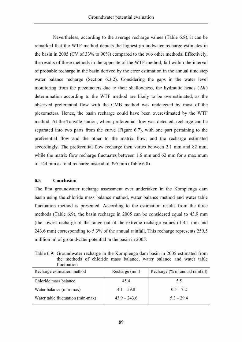
Groundwater potential evaluation
89
Nevertheless, according to the average recharge values (Table 6.8), it can be
remarked that the WTF method depicts the highest groundwater recharge estimates in
the basin in 2005 (CV of 33% to 90%) compared to the two other methods. Effectively,
the results of these methods in the opposite of the WTF method, fall within the interval
of probable recharge in the basin derived by the error estimation in the annual time step
water balance recharge (Section 6.3.2). Considering the gaps in the water level
monitoring from the piezometers due to their shallowness, the hydraulic heads ( h∆ )
determination according to the WTF method are likely to be overestimated, as the
observed preferential flow with the CMB method was undetected by most of the
piezometers. Hence, the basin recharge could have been overestimated by the WTF
method. At the Tanyélé station, where preferential flow was detected, recharge can be
separated into two parts from the curve (Figure 6.7), with one part pertaining to the
preferential flow and the other to the matrix flow, and the recharge estimated
accordingly. The preferential flow recharge then varies between 2.1 mm and 82 mm,
while the matrix flow recharge fluctuates between 1.6 mm and 62 mm for a maximum
of 144 mm as total recharge instead of 395 mm (Table 6.8).
6.5 Conclusion
The first groundwater recharge assessment ever undertaken in the Kompienga dam
basin using the chloride mass balance method, water balance method and water table
fluctuation method is presented. According to the estimation results from the three
methods (Table 6.9), the basin recharge in 2005 can be considered equal to 43.9 mm
(the lowest recharge of the range out of the extreme recharge values of 4.1 mm and
243.6 mm) corresponding to 5.3% of the annual rainfall. This recharge represents 259.5
milllion m³ of groundwater potential in the basin in 2005.
Table 6.9: Groundwater recharge in the Kompienga dam basin in 2005 estimated from
the methods of chloride mass balance, water balance and water table fluctuation
Recharge estimation method Recharge (mm) Recharge (% of annual rainfall)
Chloride mass balance
Water balance (min-max)
Water table fluctuation (min-max)
45.4
4.1 – 59.8
43.9 – 243.6
5.5
0.5 – 7.2
5.3 – 29.4

Groundwater potential evaluation
90
The estimation is in line with previous evaluations within the research area of
West African crystalline basement aquifers quoted in van der Sommen and Geirnaert
(1988), Bromley et al. (1997) and Martin (2005) and varying between 2% and 16% of
the annual rainfall.
Table 6.10: Recharge rates from previous studies within West African crystalline basement aquifers
Site Pann. (mm)
Recharge(mm)
Recharge (% of Pann)
Method Source
Southwest Niger Central Burkina Faso Northern Ghana Central north Burkina Faso West African region
564 690
910-1138 517
515-1000 850
10-19 23-45
59 10-37
10-250 17-136
1.8-3.4 3.3-6.5
6 1.9-7.2
- 2.0-16.0
Chloride profiling Modeling Chloride mass balance Soil moisture profiling Modeling WB, WTF & isotope analysis
Bromley et al. (1997) Thiery (1988) Martin (2005) Milville (1991) Milville (1991) van der Sommen and Geirnaert (1988)
WB = Water Balance method; WTF = Water Table Fluctuation method; Pann. = annual precipitation
Meanwhile, the recharge estimates from the three methods depicted
differences for reasons additional to the fact that they were evaluated using different
methods and are expected, a priori, to be different. Uncertainties in the determination of
the parameters are one of the main reasons for these differences as showed with the
water balance annual time step recharge estimation. For example, in the process of
estimating the water balance components (Chapter 5) for the basin recharge evaluation,
errors are likely to arise and reduce the reliability of the estimate (Lerner et al. 1990 and
Gee and Hillel 1988) by as much as 100%. Howard and Lloyd (1979) at this purpose,
observed from studies on Northern Lincolnshire Chalk aquifers (United Kingdom) that
an overestimation of the potential evaporation by 10% in the water balance method can
result in underestimating the recharge by 5%. Another important reason is the intrinsic
nature of the methods. The recharge estimations with the CMB and the WTF methods
integrate large areas 200 m to several kilometers from the measurement points (Wood
and Sanford 1995). Using this property, the results from the four stations were brought
to the whole basin level, while the water balance method derived the recharge of the
whole basin in one step and directly from the parameters observed at the outlet of the
dam without considering spatial specificities likely to influence the whole basin
recharge. According to the precedents, precision in groundwater recharge estimation

Groundwater potential evaluation
91
whatever the method, remains limited by the accuracy level of the estimation
components.
The CMB method proved the existence of fractures and similar features all
over the whole Kompienga dam basin inducing preferential flow recharge prior to the
diffuse flow processes. In line with the WTF method, the CMB method showed that the
Tanyélé station received more recharge than the three other stations, mostly due to the
existence of preferred flow pathways, favorable soil texture and the proximity to the
dam’s lake. The Kouaré station at the upstream part of the basin with low recharge
suggests unfavorable soil textures as well as probable discharge of the aquifer
downstream to the dam’s lake and surrounding aquifers. The latter assumption is
substantiated by the station’s groundwater recharge levels (Table 6.8), where an
increase following the watershed slope is observed. The suggested preferential flow
impact in the whole basin recharge processes seems to be of little importance as
groundwater samples depicted a relatively high chloride content in comparison to that in
rainwater. Effectively, for a dominant preferential flow process of recharge in the basin,
the groundwater chloride content would have been closer to that of rainwater as
observed for the Tanyélé station, where this flow process of recharge appeared
predominant due to the low groundwater chloride content of less than 10 mg/l (Figure
6.8).
The daily time step evaluation of the basin recharge with the water balance
method shows strong relationship between rainfall and recharge through the soil
moisture. The equation derived from this relationship shows that annual recharge in the
basin can only start after a threshold of cumulative rainfall of approximately 314.3 mm.
The annual recharge directly proportional to the annual rainfall is derived from this
relation with reduction of the total Ea measured at the end of the rainy season till the
end of the annual period due to transpiration of the deep-rooted trees in the basin.
With the WTF and the water balance methods, a time lag of approximately 2
to 3 months was observed between the rainfall events and the commencement of the
recharge to the basin aquifers. This time lag depends on various factors (Spaan and
Stroosnijder 1997, van de Giesen et al. 2000, Ajayi 2004 and Nyagwambo 2006) and is
a key factor in any sustainable planning scheme for groundwater resource management
in the basin. The results of the study on the basin recharge suggest the existence of

Groundwater potential evaluation
92
perched aquifers at three of the four research stations, probably induced by the
weathering of the basin crystalline rocks, which are known to lead to formation of clay
in the soil profile and therefore reduce hydraulic conductivity (Dubois 2002 and
Nyagwambo 2006).
Although the results of this study can be considered substantial for preliminary
steps in the basin water resources management, additional studies need to be carried out
for their validation and for planning of sustainable water management. The
recommended studies are mainly:
• Analysis of satellite images of the basin area to detect the preferred flow pathways
and similar features suggested by the CMB method;
• One or two years more of rain and groundwater sampling for chloride analysis as
suggested by Bromley et al. (1997) for validating the basin groundwater recharge
estimate using the CMB method.

Groundwater use and water supply rate
93
7 GROUNDWATER USE AND WATER SUPPLY RATE
7.1 Introduction
Water resource management and especially groundwater management requires
knowledge on the aquifer characteristics in terms of quantity, quality, renewability,
withdrawal and temporal and spatial variability. Following the basin groundwater
potential evaluation, the withdrawal quantities were evaluated as a complementary
parameter in setting up the groundwater management plans for the Kompienga dam
basin. Based on the annual renewability of the basin resources according to climatic
conditions and the geophysical characteristics of the basin, management planning will
basically aim at ensuring a reliable water supply for the population and improving their
livelihood by adding economic value to the basin water productivity whenever possible.
7.2 Results and discussion on the basin groundwater use
From the survey of the 15 water monitoring sites in the basin and in accordance with the
considerations to fill the gaps in the non-survey periods, the monthly withdrawal
volumes from the monitoring sites were determined (Table 7.1). For extrapolation of
these monthly volumes to the whole Kompienga dam basin, additional calculations were
done to determine the total number of boreholes within the basin and the average
monthly withdrawal volumes for each borehole.

Groundwater use and water supply rate
94
0200400600800
1000
12001400160018002000
Nov 04 Dec Jan 05 Feb Mar Apr May Jun
Month
Mon
thly
with
draw
al (m
³)
0
1000
2000
3000
4000
5000
6000
Mon
thly
with
draw
al (m
³)
D1 D2 P1 P2 P3 Kp1
Kp2 N1 N2 K1 K2 C-MW
C1 C2 P-MW
Table 7.1: Groundwater withdrawal volumes (m³) in the dry season 2005 derived from 15 monitoring points within six localities in the Kompienga dam basin
Locality Comin Yanga Kouaré Natiabouani Kompienbiga Pama Djabiga Total
No. of survey pts Population Nov 04 December January 05 February March April May June
3 5373
1022.04 1159.40 1353.35 1547.29 1589.39 1655.34 1840.41 1486.70
2 5990
184.17 221.46 698.87 1176.27 1334.23 2624.32 2023.49 1748.06
2 11565 825.52 823.31 891.94 960.57 1045.71 930.14 884.81 614.95
2 4745
591.32 440.62 611.68 782.74 916.95 1083.92 1353.63 1262.75
4 6204
2853.39 6185.27 5845.96 5506.65 5538.13 3972.97 3972.97 3972.97
2 1878
1401.55 2006.59 1621.74 1236.90 1246.92 2554.72 1899.56 1700.93
15 35755
6877.99 10836.65 11023.54 11210.42 11671.33 12821.41 11974.87 10786.36
Total vol. until April 2005 8326.81 6239.32 5477.19 4427.23 29902.37 10068.42
the total volume is calculated till April 2005 to evaluate the relationship between the survey parameters. After April, the monthly volumes at Pama were mostly estimated and less representative of the real situation at this site. According to the data, the localities seemed to cluster except for Pama and Djabiga (Figure 7.1).
Figure 7.1: Monthly groundwater withdrawal quantities during the dry season 2005 from 15 water monitoring points in the Kompienga dam basin. D1 and D2 represent hand pump boreholes in Djabiga; P1, P2 and P3, hand pump boreholes in Pama; Kp1 and Kp2, hand pump boreholes in Kompienbiga; N1 and N2, hand pump boreholes in Natiabouani; K1 and K2, hand pump boreholes in Kouaré; C1 and C2, hand pump boreholes in Comin Yanga; and P-MW and C-MW, modern wells in Pama and Comin Yanga respectively. The curve P-MW refers to the secondary axe of monthly withdrawal (0-6000 m³).

Groundwater use and water supply rate
95
It can be seen that the monitoring points are mostly separated into two groups.
One group has a minimum withdrawal rate of 3000 m³/month, while the second group,
where most of the sites are found, has a maximum withdrawal rate of 2000 m³ per
month. Most of the monitoring points depicted an expected pattern of increasing
withdrawal quantities with increasing heat till the heat peak period of April, typical of
the climatic conditions in the country. Meanwhile, at Pama and Djabiga (curves P-MW,
D1 and D2), an almost reverse trend is observable with a decrease in the withdrawal
volumes between December and April. One reason is that the main water monitoring
point at Pama that is a modern concrete well was drying up, as it gets far deep in the dry
season with heat increasing. Another reason was the breakdown of the two monitoring
boreholes pumps, which led to an extrapolation of the previous withdrawal quantities in
March for the periods of April till June; these values are therefore underestimated. In
Djabiga, the trend is due to temporary malfunction in the borehole pump leading to a
lower yield of withdrawal.
When comparing the survey parameters of the localities, it appears that Pama
had the highest withdrawal quantities due probably to more survey points at this site (4
points including the volumes of the local pipe distribution system; Figure 7.2). It can be
seen that the withdrawal quantities are well correlated to the number of monitoring
points (graph A with R²=0.79) than the number of inhabitants around the survey site
(graph B with R²=0.007). The withdrawals should be correlated to the population size of
the localities, but because the survey did not include all the water monitoring points in
the localities, there is no correlation.
Figure 7.2: Correlation of withdrawal volumes versus number of survey points (graph
A) and withdrawal versus population per locality (graph B) during the dry season 2005 in the Kompienga dam basin
y = 10260x - 14910R2 = 0.80
0
5000
10000
15000
20000
25000
30000
35000
1 2 3 4 5
Number of monitoring points
With
draw
al v
olum
e (m
³)
R2 = 0.0075
0
5000
10000
15000
20000
25000
30000
35000
0 2000 4000 6000 8000 10000 12000 14000
Population
With
draw
al v
olum
e (m
³)
Graph A
Graph B

Groundwater use and water supply rate
96
From this analysis and the considerations above, the monthly withdrawal
volumes per monitoring point to be considered for evaluating the whole basin
withdrawal volume in 2005 was taken to be the mean monthly withdrawal volume of
the 15 monitoring points (Table 7.2).
Table 7.2: Mean monthly withdrawal volumes per water monitoring point in the Kompienga dam basin
Period Nov 04 Dec Jan 05 Feb Mar April May June Unit water monitoring point volume (m³) 458 723 736 749 779 856 799 720
To determine the total number of water withdrawal points within the whole
Kompienga dam basin, the BNDT-BF database (Topographic database of Burkina Faso)
with all the villages in the country was used in ArcView to locate the position of the
water withdrawal points in the Kompienga dam basin. This database was combined with
the data of the recent national inventory of the hydraulic infrastructures (MAHRH 2006)
to determine the number of water withdrawal points inside the basin and the population
within the basin and in the villages surrounding the basin limits. The populations in the
surrounding areas of the basin were taken into account based on the assumption that
they are likely to use the basin water withdrawal points according to their accessibility
(distance and easiness of fetching water, water demand intensity, pump breakdown or
even preferences in terms of quality and taste). The same behavior applies to the
population inside the basin toward the water withdrawal points surrounding the basin.
When counting the water withdrawal points, those outside the basin limits were not
considered, as they do not tap the basin aquifer. This consideration supports the
assumptions for the basin recharge estimation with the water balance method stating
that the basin aquifers are limited inside the boundaries only and no inflow from
adjacent aquifers exist. All water withdrawal points in the MAHRH’s inventory period
were considered whatever their nature, whether modern wells, traditional hand-dug
wells or permanent hand-pump boreholes or those drying up temporarily. Meanwhile,
new boreholes without equipment for water abstraction and abandoned wells and
boreholes were not included as they were unable to allow water withdrawal from the
basin aquifers. The number of water withdrawal points and the population number were

Groundwater use and water supply rate
97
determined with updated data of the national census of the population in 1996 (INSD
2000) according to the local growth rate.
The estimation of the hydraulic infrastructures inside the basin area based on
the MAHRH’s inventory revealed a total number of 1223 water withdrawal points
including all the intermittent traditional hand-dug wells as stated above. The total
monthly withdrawal volumes of these points were determined (Table 7.3).

Groundwater use and water supply rate
98
0200400600800
100012001400160018002000
Nov 04 Dec Jan 05 Feb Mar Apr May Jun
Month
Mon
thly
ave
rage
with
draw
al (m
³)
Table 7.3: Monthly water volume (m³) withdrawn from the Kompienga dam basin aquifers in 2005
Figure 7.3: Standard deviation (top bars) from monthly withdrawals per water monitoring point in the Kompienga dam basin in 2004-2005
Period Nov 04 Dec Jan 05 Feb Mar April May June Total
Mean vol. of water withdrawal points 458 723 736 749 779 856 799 720 -
Monthly withdrawal 560786 884751 900131 915511 953091 1046860 977840 880937 7119907
Standard deviation 365.5 1161.7 1052.1 954.2 956 679.1 620.7 626 -
Coefficient of Variation-CV (%) 79.7 160.6 142.9 127.5 122.7 79.3 77.6 86.9 -

Groundwater use and water supply rate
99
According to the monthly withdrawals, the volume in November was
relatively low compared to that of December. The difference in volume between these
two months (323 966 m³) is higher than that between the other months (Figure 7.3).
Variability in the monthly withdrawals from one monitoring point to another was high
(CV>100%) due to factors like the yield of the water monitoring points, the nature of
these water points (well or borehole) and their density in the localities in relation to the
density of the population. Another factor explaining the high level of the coefficient of
variation in the monthly withdrawals is the quality of the monitoring by the surveyors
likely to be different and thus influencing the recorded withdrawal quantities. The low
withdrawal volume in November is probably because the rainy season had just ended
and many ponds and marshes in the basin were still holding surface water for livestock
watering, laundry and even for bathing. People, therefore, only use boreholes and wells
for part of their supplies (drinking and cooking). Moreover, two exceptional rains were
recorded in the basin at Tanyélé on 5 November (36 mm) and on 13 November at Pama
(5.3 mm), which significantly reduced the need for water from boreholes.
The average monthly withdrawal volumes per borehole seem inconsistent with
the hand pump yields reported by UNDP/World bank (1986) which varied between 5
and 36 l per minute, i.e., 0.3 m³/h and 2.16 m³/h with 0.7 m³/h as a currently observed
yield for most of boreholes. Indeed, with a maximum daily pumping duration of 18
hours, which implies uninterrupted pumping from 4.00 am till 10.00 pm, a borehole
could yield only 391 m³ of water in a month. But in this study, the survey involved
modern wells that were sometimes the main source of water, e.g., in the urban zone of
Pama where most of the hand pump boreholes had broken down during the dry season
of the survey in 2005. The very modern well in Pama (Figure 7.5) was rectangular (6 m
x 4 m and 17 m deep) with more or less permanent water throughout the year. The
volumes of such wells increased the overall basin volume. Moreover, the hand pump
boreholes could have been yielding more than the suggested 0.7 m³/h in the
UNDP/World bank report (1986). Nevertheless, excluding the withdrawal volumes of
these two wells in the survey (Table 7.1) gives an average monthly volume per water
monitoring point of 321 m³ in November and 628 m³ in April (Figure 7.4). This
corresponds to a maximum withdrawal volume for the whole basin of 770 000 m³ of
water in April for a monthly unit borehole yield fluctuating between 0.7 m³/h in

Groundwater use and water supply rate
100
0
100
200
300
400
500
600
700
800
900
Nov 04 Dec Jan 05 Feb Mar Apr May Jun
Month
Mon
thly
vol
ume
(m³)
Volume w ithout Pama & Comin Yanga MW
Volume including Pama & Comin Yanga MW
November and 1.5 m³/h in April; this is the range of yields reported by UNDP/World
bank (1986).
Figure 7.4: Variation of monthly withdrawal volumes per water monitoring point in the
Kompienga dam basin based on the volumes of modern wells
Figure 7.5: Monitoring modern wells in Pama (A) and Comin Yanga (B)
Based on this evaluation, the total water volume withdrawn from the basin
during the dry season 2005 represents approximately 7 million m³ (Table 7.3)
equivalent to 1.2 mm of water according to the basin area. It corresponds to 3 % of the
annual recharge evaluated at 43.9 mm. A similarly low groundwater withdrawal of 0.7
% of the annual recharge was reported by Martin and van de Giesen (2005), who
evaluated the groundwater potential in the Volta basin parts of Burkina Faso and Ghana.
Martin (2005) also reported an abstraction rate of 4 mm/a in the Atankwidi catchment in
A B

Groundwater use and water supply rate
101
northern Ghana for a recharge of 60 mm/a. Therefore, the actual evaluation is
considered acceptable and consistent with the assumption made for the daily time step
recharge estimation of the basin using the water balance method (Section 6.3.2).
From this evaluation, it can be concluded that the water withdrawals within the
basin are very unlikely to deplete the groundwater aquifers in the Kompienga dam
basin. Considerable opportunities, therefore, exist for improving the population’s
livelihood through development of the basin’s water resources if the estimations
elsewhere are considered reliable. Meanwhile, if for any reason (e.g., underestimation of
the monthly withdrawal volumes or existing withdrawal points in the basin or not
considered nighttime withdrawals reported by the surveyors, or even inconsistent
assumptions in the withdrawal estimation), an estimation error of 100% of the
withdrawal volume is considered, a correction will merely bring it to 2.4 mm, which is
still remarkably low compared to the 43.9 mm of recharge.
7.3 Water demand and supply within the basin
The previous results show the low importance of the withdrawals compared to the
recharge. Now the supply level should be examined in order to ensure that the
withdrawals satisfy the population demands as suggested by the positive difference
between recharge and withdrawals. Groundwater resource management assumes that the
population demands are satisfied at all times and for all people everywhere in the basin.
Before evaluating the supply quality, the question arises what happened to the large
remaining part of the annual recharge to the basin in 2005? Was there no carry-over of
the aquifer’s water from one year to another if it is considered that withdrawals are
nearly negligible compared to recharge? Answers to these questions can be found in the
study of van der Sommen and Geirnaert (1988) on the continuity of the aquifer systems
in the crystalline basement in Burkina Faso. The study proved that within such aquifers,
lateral discharge flow is of the same magnitude as recharge and the authors concluded
the existence of continuity in the regional lateral flow of the basin recharge within the
crystalline basement aquifers. Thus, the observed extensive recharge to the Kompienga
dam basin aquifer is mainly for discharge to adjacent aquifers due to the favorable
hydraulic gradients, toward the downstream parts. Therefore, there is no carry-over of
water from one year to another. This conclusion provides opportunities for substantial
Groundwater use and water supply rate
102
planning schemes in groundwater resource management to satisfy water demands in the
basin. For this reason, the water supply has to be evaluated, as the recharge appears
enough to support more than the population demands.
7.3.1 Actual water supply
To evaluate the supply rate, monthly withdrawal volumes are compared to the volume
of recharge to the basin. It can be seen that the recharge within the basin corresponds
with the rainy season, while the withdrawals are mainly in the dry season period where
no recharge takes place; the withdrawals are from the last rainy season recharge. The
daily basin recharge estimation with the water balance method shows that from
November 29 (Appendix 2), the basin soil moisture started to deplete and the recharged
water then started to contribute to the daily water balance at the rate of the transpiration
of deep-rooted trees and the withdrawals. From this period, the total withdrawals of
about 560 000 m³ of water (Table 7.3) in addition to actual evaporation and the
following dry season withdrawals of 6.5 million m³ are considered normally satisfied by
the recharged water volume of 259.5 million m³. Before this period, losses through
withdrawals and tree transpiration are supposed to be compensated by inputs through
rainfall. However, in reality the supply satisfaction from the basin recharge is not as
simple as presented. Indeed, the suggested regional lateral flow is occurring
simultaneously with evaporation, transpiration and withdrawals to deplete the recharged
water resources. With such considerations and depending on aquifer transmissivity
spatially variable, the water levels of the aquifers can drop too fast or too slowly,
resulting in rapid or slow drying up of some wells and boreholes. Hence, subsequent
low withdrawal volumes and low supply to the population. The storage capacity of the
crystalline basement aquifers, spatially variable, is therefore an important parameter to
take into consideration for the supply estimation. According to the degree of fracturing
of the rock materials, the storage capacity will be more or less considerable, as the
induced secondary porosity will vary accordingly (Kellgren and Sander 2000). This
parameter highly influences success of borehole siting in hard rocks terrain, boreholes
yields and the abstraction rate. For the Kompienga dam basin, studies in the area
revealed the success of borehole siting to be related to the thickness of the weathered
layer of the geological formations (Ministère de l’Eau 1990). The thicker the weathered

Groundwater use and water supply rate
103
layer, the more successful are the boreholes sitings. This spatial variability of the basin
aquifer storage will thus play a major role in the water supply quality, which is likely to
differ, as the geological formations in the basin are mainly crystalline. Related to the
spatial variability of the supply quality is the distribution of the hydraulic infrastructures
all over the basin according to the population density. For a good water supply, every
inhabitant in rural areas should receive a minimum of 20 l of water per day (MEE 2001
and WHO 2003). This standard rate of supply is the basis for evaluating the supply
quality within the Kompienga dam basin. Using inventory data (MAHRH 2006) with
the above assumptions on the local population and the number of hydraulic
infrastructures, the estimate shows (Table 7.4) that the water supply quality is
satisfactory when compared to standard norms of supply mentioned by Gleick (1996) as
ranging between 27 and 200 liters per capita per day (l/c/d).
Table 7.4: Water supply rate for the administrative departments in the Kompienga dam basin based on population and estimated withdrawal quantities in 2005
Department Inhabitants Hydraulic infrastructures
Annual withdrawal volume (m³)
Water supply rate (l/c/d)
Diabo Diapangou Comin Yanga Yondé Gounghinb Bissiga Dourtenga Ouargaye Sangha Soudougui Kompienga Pama Tibga Fada
48947 21960 34401 24931 19859 213 2692 7954 9821 18737 8324 13802 2280 56435
305 124 168 102 158 1 31 13 25 29 36 89 17 125
1 773 119 720 875 976 669 592 977 918 534 5 814
180 219 75 576 145 338 168 592 209 286 517 402 98 830 726 688
149.7 135.6 117.3 98.3 191.1 112.8 276.6 39.3 61.2 37.2 103.9 154.9 179.1 53.2
Total 270 356 1 223 7 109 916 (122.2) b Total population of this department includes that of the 15th department (Yorgo) Number between brackets is the average of the column

Groundwater use and water supply rate
104
Meanwhile, the derived results should be read with caution as:
• The supply rate refers to the whole water volume taken from all withdrawal points
and for all purposes including livestock watering. The supply rates reflect thus
household uses and livestock watering, while the WHO standard refers to household
uses only, comprising consumption and hygiene, i.e., drinking, cooking and
personal hygiene; laundering is not included.
• The supply volumes were estimated considering that all the water withdrawal points
are permanently bearing water and have functioned so, during the whole dry season
in 2005. For the estimation of the basin water abstraction, such assumption was
tolerable but for the effective water supply rate to the population it has to be
reconsidered as some of these water-bearing points dry up before the next rainy
season starts. For this reason, the water supply to the basin population was re-
estimated based only on the number of effectively permanent water-bearing points
within the basin listed in the official inventory report (MAHRH 2006).
Table 7.5: Water supply rate per administrative department in the Kompienga dam
basin according to the number of functional hand pump boreholes and the population in 2005
Department Hydraulic infrastructures
Annual withdrawal volumes (m³)
Water supply rate (l/c/d)
Diabo Diapangou Comin Yanga Yondé Gounghin Bissiga Dourtenga Ouargaye Sangha Soudougui Kompienga Pama Tibga Fada
220 90 73 71 142 1 11 11 19 17 19 46 14 94
1 278 971 523 215 424 389 412 759 825 518 5 814 63 949 63 949 110 457 98 830 110 457 267 421 81 389 546 469
108.0 94.9 51.0 68.4 171.8 112.8 98.2 33.2 46.5 21.8 54.8 80.1 147.5 40.0
Total 828 4 813 582 (80.6) Number between brackets is the average of the column
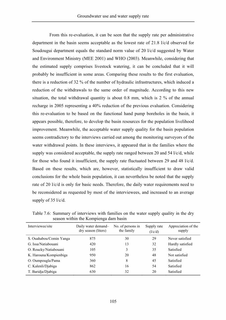
Groundwater use and water supply rate
105
From this re-evaluation, it can be seen that the supply rate per administrative
department in the basin seems acceptable as the lowest rate of 21.8 l/c/d observed for
Soudougui department equals the standard norm value of 20 l/c/d suggested by Water
and Environment Ministry (MEE 2001) and WHO (2003). Meanwhile, considering that
the estimated supply comprises livestock watering, it can be concluded that it will
probably be insufficient in some areas. Comparing these results to the first evaluation,
there is a reduction of 32 % of the number of hydraulic infrastructures, which induced a
reduction of the withdrawals to the same order of magnitude. According to this new
situation, the total withdrawal quantity is about 0.8 mm, which is 2 % of the annual
recharge in 2005 representing a 40% reduction of the previous evaluation. Considering
this re-evaluation to be based on the functional hand pump boreholes in the basin, it
appears possible, therefore, to develop the basin resources for the population livelihood
improvement. Meanwhile, the acceptable water supply quality for the basin population
seems contradictory to the interviews carried out among the monitoring surveyors of the
water withdrawal points. In these interviews, it appeared that in the families where the
supply was considered acceptable, the supply rate ranged between 20 and 54 l/c/d, while
for those who found it insufficient, the supply rate fluctuated between 29 and 48 l/c/d.
Based on these results, which are, however, statistically insufficient to draw valid
conclusions for the whole basin population, it can nevertheless be noted that the supply
rate of 20 l/c/d is only for basic needs. Therefore, the daily water requirements need to
be reconsidered as requested by most of the interviewees, and increased to an average
supply of 35 l/c/d.
Table 7.6: Summary of interviews with families on the water supply quality in the dry
season within the Kompienga dam basin Interviewee/site Daily water demand–
dry season (liters) No. of persons in
the family Supply rate
(l/c/d) Appreciation of the
supply
S. Ouahabou/Comin Yanga G. Issa/Natiabouani O. Roucky/Natiabouani K. Harouna/Kompienbiga O. Oumpougla/Pama C. Kalenli/Djabiga T. Baridja/Djabiga
875 420 105 950 360 862 630
30 13 3
20 8
16 32
29 32 35 48 45 54 20
Never satisfied Hardly satisfied Satisfied Not satisfied Satisfied Satisfied Satisfied

Groundwater use and water supply rate
106
7.3.2 Future water supply
According to the previous scenarios, it appears that the actual water supply was
satisfactory. Thus, considerable possibilities are open for resources development.
However, will this situation last in the basin considering the erratic rainfall conditions in
this semi-arid zone of Kompienga in addition to the so-called climatic change and its
forecasted side effects, as well as the growing population in the basin? What should
sustainable water resources development in the basin look like?
Such questions are vital for decision makers, who need to know how to
proceed without delay in order to secure the population welfare for years ahead. Martin
(2005) evaluating the recharge to the Atankwidi catchment in northern Ghana with a
monomodal rainfall pattern, realized that a 20 % reduction in the annual rainfall reduces
the annual groundwater recharge by 30 to 60 %. Nyagwambo (2006) made the same
observation in his research on the small Nyundo catchment in Zimbabwe under tropical
climate conditions, where he noted that a reduction of 40 % in the annual rainfall has
induced a 30 to 60 % reduction in the catchment annual recharge of the aquifers. Based
on these results where the characteristics of the aquifers are similar to those in the
Kompienga dam basin, similar conclusions can be made with regard to the rainfall and
groundwater recharge relationship. Moreover, the analysis of the long-term rainfall data
series (1959-2005) in the basin showed that 24 years over 46 recorded on average 11.8
% reduction of the average mean annual rainfall of 830.2 mm. From these years, only 4
years (1983, 1984, 1990 and 1997; Table 7.7); i.e. 17 %, recorded rainfall lower than 20
% reduction (664.2 mm) of the average long term mean annual rainfall; which is nearly
the basin average rainfall depth in 2005 (829.6 mm). Therefore, considering 20%
reduction in the basin average precipitation in 2005 as basis for the simulation scenarios
appears reasonable and consistent.

Groundwater use and water supply rate
107
Table 7.7: Reduction rate of average annual rainfall in the Kompienga dam basin according to the average mean annual rainfall (830.2) of the long term rainfall data series (1959-2005)
Year Average annual rainfall (mm)
Reduction rate (%) according to average mean annual rainfall
1970 1971 1972 1973 1976 1977 1978 1980 1981 1982 1983 1984
748.1 785
756.6 783.3 808.3 754.5 771.8 715.5 789.2 729.7 657.6 561.8
9.9 5.4 8.9 5.7 2.6 9.1 7.0
13.8 4.9
12.1 20.8 32.3
Year Average annual rainfall (mm)
Reduction rate (%) according to average mean annual rainfall
1985 1986 1987 1988 1990 1993 1996 1997 2000 2001 2002 2004
673.9 716.2 692.6 789.2 632.2 806.2 768.5 620.3 746.3 765.8 671.1 823.7
18.8 13.7 16.6 4.9
23.8 2.9 7.4
25.3 10.1 7.8
19.2 0.8
Somé (2002) and Paturel et al. (2002) reported an almost cyclic 20-year
dynamism pattern of the rainfall in Burkina Faso with consequent impacts on the
groundwater recharge as observed by Thiery (1988) with piezometric measurements
from a site in Ouagadougou. It was observed for example, that low precipitations
occurred in the periods 1972-1973 and 1983-1984 with consequent droughts, while the
1950’s, 1960’s and 1990-1999 were reported to have higher precipitation (Somé 2002,
Paturel et al. 2002). In reference to such results and according to the results of this
study, realistic scenarios of rainfall variations can be simulated to derive the basin
recharges and determine adequate water supply rates in relation to projected withdrawal
volumes from standards of water supply rates and the population size.
According to the long-term annual rainfall pattern in the basin region (Figure
4.6), the 2005 precipitation of 829.6 mm ranged within the average precipitations.
Within this long-term annual rainfall, the years 1983-1987, 1990, 1997 and 2002 which
fall almost within the low rainfall periods reported in Somé (2002), showed amounts
fluctuating between 500 and 750 mm, which represents a 19% to 32% reduction of the
2005 rainfall. Considering the observed rainfalls patterns, the decades 2010 to 2020 are
likely to be dry or at best with annual average rainfall, as the decades since 1990’s can
be considered rainy or with average rainfall. In the simulation scenario for assessing the
water supply to the population, five important parameters are considered:
Groundwater use and water supply rate
108
1. Annual rainfall depth influencing the recharge;
2. Population size;
3. Number of water withdrawal points (wells and boreholes);
4. Average daily withdrawal duration at each water point
5. Average unit yield of the water withdrawal points.
From these parameters, the scenarios will be built around the two first parameters and
the derived supply rates will be improved if necessary by refining the other parameters.
Subsequent assumptions for the basis of the simulation are therefore:
• The annual population growth rate considered equal to 3.2% (Dipama 1997);
• The total number of 828 boreholes in the basin considered unchanged despite the
population increase for the reason that, maybe new boreholes have replaced some
broken down ones or no new borehole has been added to the existing functioning
boreholes;
• The water demand by population will be determined based on the national standard
of water supply in rural areas (20 l/c/d) and on Gleick’s (1996) estimations reported
in Seckler et al. (1998) and consistent with the survey results (Table 7.3) for 20
m³/c/year which corresponds to 55 l/c/d;
• The average unit borehole yield will be taken equal to 0.7 m³/h; the minimum
drilling yield that a borehole in Burkina Faso should have to be equipped with pump
for water abstraction;
• The dry season period of November to June (242 days) will be the period of the
simulations as in the estimation of the actual supply rate to the population.
First scenario: 20 % reduction in the actual annual rainfall amount with
population size unchanged or negligibly changed. A possible
scenario in 2007.
In this case, and considering the proximity of the study area to the Atankwidi catchment
in northern Ghana with similar geological formation, the recharge reduction will be
considered proportional to that at this site (Martin 2005). The unchanged population
size or negligible change implies that the withdrawals also remain more or less the same

Groundwater use and water supply rate
109
as the actual withdrawal quantities with slight increase during the rainy period due to
the rainfall reduction, which will be compensated by subsequent rainfalls. Moreover,
this period is not included in the withdrawals evaluation.
Second scenario: 20 % reduction in the actual annual rainfall amount and increase
in the population
This is a scenario likely to happen in the coming decades according to Somé (2002) and
Paturel et al. (2002). The population increase will induce an increase in the water
demand that will be estimated based on the assumptions above.
Third scenario: No reduction in the annual rainfall but increase in the population
This scenario is likely to occur anytime from 2005 onward. The recharge is here
considered equal to the actual recharge of 259.5 million m³ of water for supplying more
people than the actual population.
Considering these scenarios, the simulations will first evaluate the capacity of
the recharge to support the corresponding water demands. Second, the feasibility of the
demand satisfaction will be examined according to the existing number of boreholes and
their unit yield associated with the possible daily duration of abstraction (Section 5.2.4).
Finally, suggestions will be made on how to satisfy the water demand by increasing the
number of boreholes (equation 5.20), the daily withdrawal duration, or even limiting the
supply rate.

Groundwater use and water supply rate
110
Table 7.8: Water demand satisfaction in the Kompienga dam basin according to projected scenarios Annual recharge (mm) Water demandc (mm) Scenario Year Population Annual
rainfall 2005 (mm)
Annual recharge
2005 (mm)
20% reduction
rainfall (mm) 30% reduction 60% reduction 20 l/c/d 55 l/c/d
Demand satisfaction
rate (%)
Scenario 1 2007 288224 0.2 0.6
Scenario 2
2015 2025 2030
372315 512725 601688
663.7 30.7 17.6 0.3 0.4 0.5
0.8 1.2 1.4
Scenario 3
2007 2015 2025 2030
288224 372315 512725 601688
829.6
43.9
-
43.9
0.2 0.3 0.4 0.5
0.6 0.8 1.2 1.4
>100
c The water demand refers to the population needs only using equation 5.18 brought to the basin area. The projections didn’t take into account livestock’s needs and it was therefore remarkable that the actual withdrawal in 2005 estimated from the 15 boreholes survey was higher than the projected demands till 2025 with the supply rate of 55 l/c/d. Meanwhile, livestock demands volume can be projected equal to that of the population as unit supply rate is reported equivalent to 35 l/UBT/d (MEE, 2001). These demands are considered satisfied with modern and traditional wells in addition to natural lakes and the Kompienga dam Lake discarded from the water demands scenarios. UBT= unité de bétail tropical; approximately unit tropical livestock. Table 7.9: Water demand satisfaction based on possible withdrawal quantities in the Kompienga dam basin
Water demand (mm) Possible withdrawal quantitiesd (mm) Satisfaction rate (%)
20 l/c/d 55 l/c/d
Scenarios Year Population
20 l/c/d 55 l/c/d 12 h/d
06:00-18:00 14 h/d
05:00-19:00 18 h/d
04:00-22:00 12h 14h 18h 12h 14h 18h
Scenario 1 2007 288224 0.2 0.6 140 165 215 47 55 72
Scenario 2
2015 2025 2030
372315 512725 601688
0.3 0.4 0.5
0.8 1.2 1.4
0.28
0.33
0.43 93 70 56
110 83 66
143 108 86
35 23 20
41 28 24
54 36 31
d These quantities refer to the limitations of the hand pump yield of the boreholes and the daily duration of abstraction during the whole dry season period of 242 days. Their calculation refers to equation 5.19 brought to the dry season period duration and the basin area. h/d = hours per day.
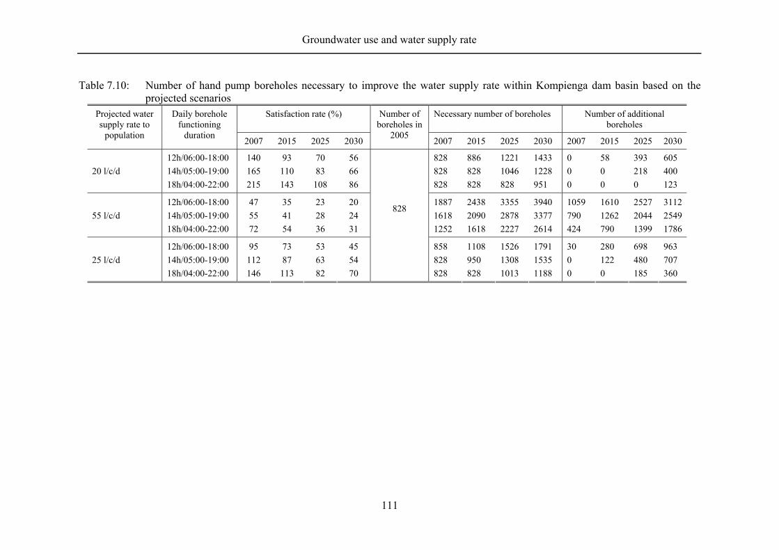
Groundwater use and water supply rate
111
Table 7.10: Number of hand pump boreholes necessary to improve the water supply rate within Kompienga dam basin based on the projected scenarios
Satisfaction rate (%) Necessary number of boreholes Number of additional boreholes
Projected water supply rate to
population
Daily borehole functioning
duration 2007 2015 2025 2030
Number of boreholes in
2005 2007 2015 2025 2030 2007 2015 2025 2030
20 l/c/d
12h/06:00-18:00 14h/05:00-19:00 18h/04:00-22:00
140 165 215
93 110 143
70 83
108
56 66 86
828 828 828
886 828 828
1221 1046 828
1433 1228 951
0 0 0
58 0 0
393 218 0
605 400 123
55 l/c/d
12h/06:00-18:00 14h/05:00-19:00 18h/04:00-22:00
47 55 72
35 41 54
23 28 36
20 24 31
1887 1618 1252
2438 2090 1618
3355 2878 2227
3940 3377 2614
1059 790 424
1610 1262 790
2527 2044 1399
3112 2549 1786
25 l/c/d
12h/06:00-18:00 14h/05:00-19:00 18h/04:00-22:00
95 112 146
73 87
113
53 63 82
45 54 70
828
858 828 828
1108 950 828
1526 1308 1013
1791 1535 1188
30 0 0
280 122 0
698 480 185
963 707 360

Groundwater use and water supply rate
112
The main results of the simulations (Table 7.10) can be summarized as followed:
• The option of 55 l/c/d as a water supply rate to be achieved for the population can
only be considered as an ideal target as the necessary installation of the large
number of new boreholes is hardly feasible;
• The 18 hours as a daily pumping duration for water abstraction at the basin
boreholes appears to be extremely high and not to be recommended due to the
predictable frequent breakdown of the borehole pumps that are supposed to be
repaired by the population as reported by the interviewees (Appendix 6);
• Two options are relevant and feasible for achieving an acceptable water supply rate
to the basin population within the next years whatever the scenario: the 12-hour and
at most the 14-hour options of daily borehole pumping duration at 0.7 m³/h;
• The supply rate of 20 l/c/d as used by decision makers in Burkina Faso (MEE 2001)
for water supply in rural areas is hereby seen to be acceptable for supplying basic
needs as described by WHO (2003). Otherwise, there would be a need for
improvement according to the interview results (Table 7.6) and in reference to the
water use quantities in 2005 (Table 7.4).
The non-relevance of the 55 l/c/d option is due to the induced high number of
boreholes required and can be considered economically and technically unrealistic and
hence less feasible. One consequence of this option would be the addition by 2030 of at
least 3100 boreholes to the current functional boreholes in the basin. Considering one
borehole installation costs around US$11 000 (MEE 2001) and the number of years it
took to install the existing 1000 boreholes in the basin, installing 3100 boreholes in 20
years is practically impossible, as this will be unaffordable for the basin community.
Moreover, adding 3100 boreholes to the existing ones will imply at least 4000 boreholes
within the basin area of 6000 km², i.e., almost 1 borehole per km² considering the
existing wells. The consequence would be that such density of boreholes would likely
reduce the productivity of each borehole by lowering the yield due to interferences in
the recharge and abstraction sources even the withdrawals revealed low. Thus, a rapid
depletion of the aquifers would occur and hence the boreholes would dry up. Moreover,
not all the basin areas are suitable for siting boreholes due to the crystalline nature of the

Groundwater use and water supply rate
113
basement rocks, where aquifers are mainly found in the fractured zones. However, as
the number of necessary boreholes is inversely proportional to borehole yield and the
daily abstraction duration (equation 5.20), if good sites for installing boreholes were to
be found providing excellent yields for withdrawals, the supply rate of 55 l/c/d could be
satisfied with less boreholes. In addition, the supply rates described by the interviewees
and close to 55 l/c/d are considered as an indispensable supply rate for the 3-month
period of March to May. While during the other months, less water is needed and the
daily borehole functioning duration is far less than 12 hours (Appendix 6).
The simulation results of the scenarios to determine the basin capacity in
supporting the population water demands show that a 20 % reduction in the rainfall
amounts cannot considerably affect the supply quality as the water demands remain
lower than the subsequent recharge rates, and when an adequate number of functional
boreholes is available for withdrawal. Meanwhile, the general situation depicting a high
capacity of the recharge to support the population demands needs to be verified with
substantial monitoring of the deep groundwater level fluctuations throughout the whole
basin.
The simulations also reveal the need of additional boreholes according to the
increasing population along the years and the subsequent water demand increase. These
new boreholes should be installed according to the supply rate of the different localities
in the basin if the hydrogeological context is favorable. Therefore, localities with a low
supply rate like the Soudougui, Sangha and Ouargaye departments as observed in the
2005 estimations (Table 7.5) should be first provided.
7.4 Conclusions
The actual water withdrawals from the Kompienga dam basin aquifers in 2005 were
relatively low compared to the annual recharge. Estimated at 2% of the annual recharge
to the basin, these low withdrawals mean much possibility for water resources
development. The withdrawal estimations based on assumptions and data for 2005 may,
however, not remain valid, as the situation is always changing with probably new
boreholes thanks to projects or previously broken down boreholes now functioning.
Scenarios for decreasing rainfall in the basin and increasing population with
subsequent increasing water demands reveal that it will be possible to supply the

Groundwater use and water supply rate
114
population with sufficient water if the required number of functional boreholes is
available. Meanwhile, the recharge sufficient to supply the population demands needs to
be substantiated by long-term deep groundwater level monitoring due to the nature of
the basin crystalline basement rocks characterized by spatial variability in the
hydrogeological parameters in addition to the concave morphology of the basin favoring
unequal distribution of the recharge. It is also likely that in the long term, rainfall
decrease will induce a higher reduction in the aquifer recharge than expected due to a
probable reduction in the basin vegetation, which will result in higher runoff in the
basin than infiltration for recharge as observed by Kincaid and Williams (1966),
Albergel (1988), Lane et al. (1997) and Bagayoko (2006). In such case, the derived
acceptable supply rates could be compromised and the population suffers from water
shortages. Meanwhile, results from Gee et al. (1994) show that recharge is higher in
non-vegetated than in vegetated areas (Scalon et al. 2002), higher in grasslands and
under annual crops than in areas with trees and shrubs (Prych 1998) as observed by
Allison et al. (1990) in Australia. They effectively noted a significant increase in
recharge of two orders of magnitude after replacement of deep-rooted native eucalyptus
trees by shallow-rooted crops. Nevertheless, and whatever the situation in the
Kompienga dam basin, the existence of the dam is likely to contribute to accumulation
of the whole basin runoff for indirect recharge to the aquifers. Therefore, only
negligible changes in the supposed recharge rate might be observed and maybe even an
increase in the recharge.
The supply rate of 20 l/c/d for 12 to 14 hours per day of withdrawal is
considered as a reasonable option to satisfy the population’s water demands.
Nevertheless, there is a real need for improvement at least temporarily during the high
demand in the heat period (March till May). This improvement, of course, should not
target the rate of 55 l/c/d shown to be unfeasible (Table 7.10), but 25-30 l/c/d in order to
fulfill the demand expressed through the interviews. Considering the unequal
distribution of the boreholes in the basin due to the spatial variability in the aquifers
suitability for siting boreholes, low supply rates may exist in some localities while in
some others, they may be high as suggests GEF-UNEP’s (2002) report (Table 4.1)
indicating average boreholes yield of 5.2 m³/h in the Oti sub-basin where the
Kompienga dam basin is located.
Groundwater use and water supply rate
115
Recharge within the basin mainly occurs during the rainy season period of low
water demand while in the dry season of high water demand no recharge exists. The
estimated general satisfaction of the supply according to the annual recharge can
therefore be hindered, as in the natural context sub-lateral flow processes and
transpiration from deep-rooted trees take place simultaneously with the withdrawals.
The simulations for the quality of the water supply to the population assumed
that all recharge water to the basin is of good quality. Any poor quality of these waters
would reduce the predicted possibilities and therefore induce water shortages. This
situation cannot be completely discarded, as intensive cotton production has developed
on the basin under the government incentives that in the long term, will lead to
groundwater pollution due to pesticides as well as fertilizers (Morris et al. 2003).
The projected scenarios revealed considerable possibilities for developing the
basin water resources. Within such possibilities, small-scales irrigation schemes from
boreholes are considered suitable for cropping vegetables during the dry season if local
markets and neighboring countries can absorb the production. This will provide
additional income to the population for livelihood improvement and therefore reinforce
the government’s initiatives. Indeed, in January 2007 through a financial agreement
with the Islamic Development Bank (IDB) for a project on development of agricultural
activities downstream of small dams in the eastern part of Burkina Faso, a dam is
planned by the government at Kouaré in the upstream part of the Kompienga dam basin
(www.lefaso.net).

General conclusions and recommendations
116
8 GENERAL CONCLUSIONS AND RECOMMENDATIONS
8.1 General conclusions
In this study, the first groundwater potential evaluation was made for the Kompienga
dam basin in Burkina Faso. The basin hosts a national hydropower dam of 2.05 billion
m³ of water at its maximum capacity mainly used for generating electricity and
marginally for fresh water production to supply the Kompienga population.
The geographical position of the basin in the southeastern part of the country
between the isohyets 900 and 1000 mm (Somé 2002) provided a relatively favorable
annual rainfall to the site estimated at 830.2 mm in the period 1959-2005. However, as
is the case for the whole country with its tropical climate, rainfall is characterized by
seasonal and inter-annual variability with a standard deviation of 126 mm in the inter-
annual rainfall amount. During the year, potential evaporation exceeds rainfall for most
of the periods except for a few months in the rainy season. Therefore, only a daily or
weekly water balance can be applied to estimate satisfactorily the basin groundwater
recharge, as these time steps are closer to the natural occurrence of rainfall and recharge
events. The basin groundwater recharge was estimated using three methods: the water
balance, the chloride mass balance (CMB) and the water table fluctuation (WTF)
methods. They provided different values for the basin recharge due to their intrinsic
limitations and uncertainties in the measurements. However, the overall basin annual
recharge was evaluated at 43.9 mm; i.e., 5.3% of the annual rainfall in 2005. This
estimate appears to be in line with the results of previous studies within the West
African region of crystalline basement rocks as underlying the Kompienga dam basin
depicting the general low level of aquifer recharge in these semi-arid zones.
With the water balance method at daily time step estimation, it was shown
that:
• in accordance with the WTF method, an approximate 2- to 3-month period exists as
a time lag between the commencement of rainfall relative to the recharge. This
period therefore represents the required duration for the basin soil moisture to be
restored after the long dry season period before deep percolation starts;
• during the aforementioned time lag, the corresponding annual threshold rainfall was
evaluated ranging between 314.3 mm and 336.6 mm.

General conclusions and recommendations
117
Appropriate for estimating temporal variability of the basin recharge, the water balance
method, however, is less adapted for estimating spatial variability of recharge.
The CMB method of recharge estimation provided the basin long-term annual
recharge estimate and moreover, depicted in accordance with the WTF method, the flow
processes governing the recharge. The preferential flow was shown to have occurred
earlier and during a short period in the rainy season within the basin with variable
importance according to the location, i.e., the geological characteristics. Meanwhile, the
CMB method’s high reliance on the chloride analysis of the samples as a prerequisite to
its successful use has to be noticed. The CMB and WTF methods are appropriate to
depict both spatial and temporal variability of recharge to aquifers. They revealed that
three of the four research stations likely had perched aquifers due to the weathering of
the crystalline rocks into clay layers of low permeability and hence leading to a low
recharge to the deep basin aquifers of these stations compared to the fourth station,
which had a high preferential flow recharge. In addition, the results from the WTF
method suggest some sublateral flows following the topographical gradient of the basin
for discharge of the upstream parts to the downstream parts.
The evaluation of the basin annual recharge potential provides a basis for
planning the water resources according to the population demands and the annual and
spatial variability in the aquifer characteristics. A further step is to determine the water
demands within the basin, which have to be satisfied with the evaluated water potential.
These demands were projected based on the actual water uses quantities
determined from daily water sampling campaigns at selected boreholes in the basin. The
water use quantity by the population in 2005 was estimated at about 5 million m³ of
water for the dry season period of high water use of November 2004 to June 2005. This
represents an average monthly volume of 725 m³ of water per functional hand pump
borehole in the basin for 18 m³ per inhabitant and livestock during the whole dry season
period as the survey took into account all the water use types in the basin (from
domestic use to livestock watering and brick making).
Simulations were also used to determine the future basin population supply
quality based on pessimistic scenarios of reduction in the annual rainfall amount by
20% with a concurrent increase in the population size. They showed that the resulting
70% to 40% of the long-term average annual recharge is still sufficient to adequately

General conclusions and recommendations
118
supply the population demands at 20 l/c/d. Considering that this supply rate is to be
achieved by hand pump boreholes with an average yield of 0.7 m³/h during 12 to 14
hours maximum per day of withdrawal, it can be seen that by 2030, 1200 to 1450
functional boreholes are necessary in the basin (Appendix 5.1). According to the
unequal distribution of the actual number of boreholes in the basin, the new boreholes
should be installed in the areas with the lowest density of boreholes like the Soudougui,
Ouargaye and Sangha departments if favorable hydrogeological conditions exist there.
Interviews of the monitors of the water withdrawal points revealed that the
supply rate of 20 l/c/d as assumed satisfactory for basic needs has to be slightly
improved to ensure easy supply during the very high water demand period of March to
May. This increase in the supply rate is seen to be possible through the increase in the
daily withdrawal duration already practiced by the population and good organization of
the water withdrawal in addition to good internal organization in the families regarding
enough containers for water provision during the day. However, as the supply is directly
proportional to the pumps yield, considering an average hand pump yield of 1 m³/h as
quoted in Ouédraogo and Ilboudo (1996) for Burkina Faso, there is no need for
additional boreholes to adequately supply the basin population till 2015 at 25 l/c/d if the
existing boreholes remain functional. To maintain the supply rate at 25 l/c/d with 12-
hour daily withdrawal duration, by 2025 only 240 additional boreholes from the actual
number will be needed and by 2030, 425 boreholes are necessary. Increasing the pumps
average yield; which is reasonable as 0.7 m³/h is the lowest possible yield for hand
pump boreholes, was revealed therefore, to be highly beneficial as the 43% increase
from 0.7 m³/h to 1 m³/h made it possible to improve the supply rate by 25% with a 40%
reduction in the number of new boreholes.
Numerous scenarios remain to test the basin groundwater capacity for
supplying the population demands. For example:
• What can be the supply rate to the population if the annual rainfall depth drops
below the 20% reduction in the long-term average annual rainfall in the basin?
• What can the supply be when two consecutive years record rainfall less than or
equivalent to the 20% reduction in the long-term average annual rainfall?

General conclusions and recommendations
119
These worst-case scenarios cannot be discarded in reference to periods 1972-
1973 and 1982-1984 (Table 7.7). However, consistent answers are not possible to draw,
as reliable databases do not exist. Therefore, the endless character of the research
sciences once again demonstrated.
8.2 Recommendations
In order to draw consistent and sustainable water resources management and
development schemes it is essential to develop and maintain a reliable database of the
basin groundwater potential through continual evaluations with improved methods such
as modeling.
Additional to these activities is the necessity to evaluate the importance of the
preferential flow pathways and similar features in the basin for early recharge
occurrences that are substantial in the basin resources renewal and facilitate
management.
Monitoring deep groundwater level fluctuations and the existing boreholes
drillers logs are essential to evaluate the basin aquifer’s capacity to support all the
abstractions during the long dry season period without recharge and to obtain the exact
pattern of the aquifer structuring.
Further research studies need to be carried out for estimation of the spatial
variability of the recharge according to the geophysical (geology, land cover and land
use, topography) and hydrogeological (hydraulic conductivity, transmissivity and
storativity) characteristics of the basin in order to guide through a clear pattern,
boreholes siting for the groundwater resources development for the benefit of the
population.
Studies on the future groundwater quality are necessary to prevent pollution of
the basin resources as foreseeable from the existing cotton production intensification.
The newly installed factory for shelling the cotton shows the central role that the basin
zone will play in the future for cotton production in the country. An intensification of
pesticides and fertilizers (generally chemical fertilizers) use and negative side effects for
groundwater resources are to be expected (Morris et al. 2003).
Installation of adequate pumps in term of production yield can contribute to
better supply the population and be beneficial for the investors.

General conclusions and recommendations
120
According to the possibilities depicted by the high recharge potential to supply
the population demand, the basin water resources development should be carried out.
These resources development should be done with small-scale irrigation schemes, as
successfully developed since 2001 by the PPIV project (small irrigation scheme
promotion at the community level) of the Water and Environment Ministry under HPIC
(Heavily Poor Indebted Countries) financial assistance (Youkhana et al. 2006) to
procure income for the population. Such developments are more feasible at the
administrative entities level such as departments, provinces and regions than at the
uncommon basin level. Therefore, decision makers at those levels are invited to
undertake such initiatives and improve the livelihood of the population.

References
121
9 REFERENCES
Adar EM and Leibundgut C (eds) (1995) Application of tracers in arid zone hydrology. IAHS Publication no. 232, 452p
Agyare WA (2004) Soil characterization and modeling of spatial distribution of saturated hydraulic conductivity at two sites in the Volta basin of Ghana. PhD thesis, University of Bonn, Bonn
Ajayi AE (2004) Surface runoff and infiltration processes in the Volta Basin, West Africa: observation and modeling. PhD thesis, University of Bonn, Bonn
Albergel J (1988) Genèses et prédétermination des crues au Burkina Faso. Etudes et Thèses, ORSTOM, Paris
Allison GB (1988) A review of some of the physical, chemical and isotopic techniques available for estimating groundwater recharge. In: Simmers I (ed) Estimation of natural groundwater recharge. Reidel publishing company, Dordrecht, The Netherlands, pp49-72
Allison GB and Hughes MW (1978) The use of environmental chloride and tritium to estimate total recharge to an unconfined aquifer. Aust. J. Soil Res. 16:181-195
Allison GB, Cook PG, Barnett SR, Walker GR, Jolly ID and Hughes MW (1990) Land clearance and river salinisation in the Western Murray basin. Australia. J Hydrol 119:1-26.
Allison GB, Gee GW and Tyler SW (1994) Vadose-Zone Techniques for Estimating Groundwater Recharge in Arid and Semi-Arid Regions. Soil Sci Soc Am J 58:6-14
Amani A (2001) Assessment of precipitation and resources variability across the Sahelian region. In: Gash JHC, Odada EO, Oyebande L and Schulz RE (eds) Report of the International Workshop on Africa’s Water Resources. Nairobi, 26-30 October 1999 (BAHC)
Andreini M, van de Giesen NC, van Edig A, Fosu M and Andah W (2000) Volta basin water balance. ZEF discussion papers on development policy. No. 21. Zentrum für Entwicklungsforschung, Bonn, Germany
Arnell NW and Liu C (2001) Hydrology and Water Resources. In: MCarthy JJ, Osvaldo FC, Neil AL, David JD and Kasey SW (eds) Climate Change 2001: Impacts, Adaptation and Vulnerability. Cambridge, Royaume-Uni: Cambridge University Press for the Intergovernmental Panel on Climate Change, Cambridge
Ayers JF (1985) Estimate of groundwater recharge: The chloride balance approach. http://www.siwin.org/textbase/swtb0011.pdf. Cited 25 Sep 2004
Bagayoko F (2006) Impact of land use intensity on evaporation and surface runoff: processes and parameters for eastern Burkina Faso, West Africa. PhD thesis, University of Bonn, Bonn
Balk D, Brickman M, Anderson B, Pozzi F and Yetman G (2005) Estimates of future global population distribution to 2015. Annex. In: Salvatore M, Pozzi F, Ataman E, Huddleston B and Bloise M Mapping global urban and rural population distributions. FAO 24. Environment and natural resources working paper. http://www.fao.org/docrep/009/a0310e/A0310E10.htm. Cited 25 Mar 2007

References
122
Barry B, Obuobie E, Andreini M, Andah W and Pluquet M (2005) The Volta river basin. Comprehensive assessment of water management in agriculture. Comparative study of river basin development and management. Draft. http://www.iwmi.cgiar.org/Assessment/Research_Projects/River_Basin_Development_and_Management/Projects_Locations/volta_river_burkina_faso_ghana.htm. Cited 15 Jun 2007
Bazuhair AS and Wood WW (1996) Chloride mass-balance method for estimating ground water recharge in arid areas: examples from western Saudi Arabia. J Hydrol 186:153-159
BBCnews (2006) Climate change 'hitting Africa'. http://news.bbc.co.uk/go/pr/fr/-/2/hi/africa/6092564.stm. Cited 29 Oct 2006
Beek E van, Helmut ME, Schulze RE and Stakhiv E (2003) Coping with climate variability and climate change in water resources. In: Kabat P, Schulze RE, Hellmuth ME, Veraat JA (eds) Coping with impacts of climate variability and climate change in water management: a scoping paper. DWC-report paper no. DWCSSO-01 International secretariat of the dialogue on water and climate, Wageningen, the Netherlands, pp30-47
Beekman HE and Sunguro S (2002) Groundwater recharge estimation. Suitability and reliability of three types of rain gauges for monitoring chloride deposition. In: Tales of a hidden treasure. Proceedings of conference of the geological society of South Africa. Western Cape Branch, Groundwater Division, Geological Society of South Africa. 16 September 2002
Beekman HE and Xu Y (2003) Review of Groundwater Recharge Estimation in Arid and Semi-Arid Southern Africa. In: Xu Y and Beekman HE (eds) Groundwater recharge estimation in Southern Africa. UNESCO IHP Series No. 64, UNESCO Paris, pp3-18
Beekman HE, Gieske A and Selaolo ET (1996) GRES: Groundwater Recharge Studies in Botswana 1987-1996. Botswana J of Earth Sci III:1-17
Bevington PR and Robinson DK (1992) Data reduction and error analysis for the physical sciences. Second edition. WCB/McGraw-Hill
Bogardi JJ (1994) Introduction of Systems Analysis: Terminology, Concepts, Objective Function and Constrains. In: Bogardi JJ and Nachtnebel HP (eds) Multicriteria Decision Analysis in Water Resources Management, Report WS14. 23–32. Paris, France, UNESCO. International Hydrological Programme. http://unesdoc.unesco.org/images/0009/000974/097402eo.pdf. Cited 05 Apr 2007
Bos P (1967) Carte géologique de Fada N’gourma. Echelle 1/200 000. République de Haute Volta. Ministère du plan et des travaux publics. Direction de la géologie et des mines. Bureau des recherches géologiques et minières. Fonds d’aide et de coopération de la république Française
Bromley J, Edmunds WM, Fellman E, Brouwer J, Gaze SR, Sudlow J and Taupin JD (1997) Estimation of rainfall inputs and direct recharge to the deep unsaturated zone of southern Niger using the chloride profile method. J Hydrol 188-189:139-154
Brunner P, Bauer P, Eugster M and Kinzelbach W (2004) Using remote sensing to regionalize local precipitation recharge rates obtained from the chloride method. J Hydrol 294:241-250

References
123
Burke JJ and Moench MH (2000) Groundwater and society: resources, tensions and opportunities. United Nations Publication ST/ESA/205
Castaing C, Billa M, Milesi JP, Thieblemont D, Le Metour J, Egal E, Donzeau M (BRGM) (Coordonnateurs) et Guerrot C, Cochere A, Chevremont P, Egal E (BRGM), Zida B, Ouédraogo I, Koté S, Kaboré BE, Ouédraogo C (BUMIGEB), Ki JC, Zunino C (ANTEA) (2003) Notice explicative de la carte géologique et minière du Burkina Faso à 1/1000 000
Castany G (1982) Principes et méthodes de l’hydrogéologie. Dunod Université. Bordas, Paris
Chandrasekharan H, Navada SV, Jain SK, Rao SM and Singh YP (1988) Studies on natural recharge to the groundwater by isotope techniques in arid western Rajasthan, India. In: Simmers I (ed) Estimation of natural groundwater recharge. Reidel publishing company, Dordrecht, The Netherlands, pp205-220
Compaoré H (2006) The impact of savannah vegetation on the spatial and temporal variation of the actual evaporation in the Volta Basin, Navrongo, Upper East Ghana. PhD thesis, University of Bonn, Bonn
Dale HV (1997) The relationship between land-use change and climate change. Ecol Appl 7 (3):753-769
de Silva RP (2004) Spatial variability of groundwater recharge-I. Is it really variable? Journal of Spatial Hydrology 4:(1), 11p.
de Vries JJ and Simmers I (2002) Groundwater recharge: an overview of processes and challenges. Hydrogeol J 10 (1):5-17
de Vries JJ, Selaolo ET and Beekman HE (2000) Groundwater recharge in the Kalahari, with reference to paleo-hydrologic conditions. J Hydrol 238:110-123
DEP/IWACO (1990) Stratégies d’implantation des points d’eau au Burkina Faso. Rapport Bilan d’Eau n°60-235/41
Dipama JM (1997) Les impacts du barrage hydroélectrique sur le basin versant de la Kompienga (Burkina Faso). Thèse de doctorat de l’Université de Bordeaux III. Option géographie tropicale
Dubois M (2002) Processus géochimiques de surface. Lecture notes on soil weathering processes. UFR des sciences de la terre de l’Université de Lille. http://www.univ-lille1.fr/geosciences/cours/mbg_web/processus_2.html. Cited 12 Feb 2006
Edmunds WM, Darling WG and Kinniburgh DG (1988) Solute profile technique for recharge estimation in semi-arid and arid terrain. In: Simmers I (ed) Estimation of natural groundwater recharge. Reidel publishing company, Dordrecht, The Netherlands, pp139-157.
El Baz F (1999) Remote Sensing of Groundwater Basins in the Eastern Sahara. Proc. Int. Conf. ‘Regional Aquifer Systems – Managing Non-Renewable Resources’ (Tripoli, Nov. 1999). UNESCO/IHP-V Technical Documents in Hydrology 42, UNESCO
Elbers JA (2002) Eddy Correlation system Alterra. User manuel. Version 4.0, Wageningen, the Netherlands
FAO (1990) Expert consultation on revision of FAO methodologies for crop water requirements. Annex V. FAO Penman-Monteith Formula, FAO; Rome
FAO (1997) Irrigation potential in Africa: A basin approach. FAO Land and Water Bulletin 4, FAO, Rome

References
124
FAO (2005) L’irrigation en Afrique en chiffres. Burkina Faso. Enquête AQUASTAT 2005. FAO rapports sur l’eau. 29. http://www.fao.org/ag/agl /aglw/aquastat/countries /burkina_faso/indexfra.stm. Cited 19 Mar 2007
Foster S and Loucks DP (2006) Non-renewable groundwater resources: a guide book on socially-sustainable management for water-policy makers. UNESCO/IAH/GW-MATE, World Bank. IHP-VI, series on groundwater No 10
Foster SDD, Chilton PJ, Moench M, Cardy WF and Schiffler M (2000) Groundwater in Rural Development: Facing the Challenges of Supply and Resource Sustainability. Technical Paper 463, New York, World Bank
Foster SDD, Lawrence AR, Morris BL (1997) Groundwater in Urban Development: Assessing Management Needs and Formulating Policy Strategies. World Bank Technical Paper 390, New York
Foster SSD (1988) Quantification of groundwater recharge in arid regions: a practical view for resource development and management. In: Simmers I (ed) Estimation of natural groundwater recharge. Reidel publishing company, Dordrecht, The Netherlands, pp323-338
Freeze RA and Cherry JA (1979) Groundwater. Prentice Hall, Englewood, New Jersey. Gee GW and Hillel D (1988) Groundwater recharge in arid regions : review and critique
of estimation methods. Hydrol Process 2:255-266 Gee GW, Wierenga PJ, Andraski BJ, Young MH, Fayer MJ, Rockhold ML (1994)
Variations in water balance and recharge potential at three western desert sites. Soil Sc Soc Am J 58:63-71
GEF-UNEP (2002) Volta river basin. Preliminary strategic program. Final report. www.gefweb.org/Documents/Council_Documents/GEF_C21/IW_-_Regional_-_Volta_River_Basin_-_Annexes.pdf. Cited 10 Jan 2007
Geirnaert W, Groen M, van der Sommen JJ (1984) Isotopes studies as a final stage in groundwater investigations on African shield. Challenges in African hydrology and water resources. IAH publication. 144
Gieske ASM (1992) Dynamics of groundwater recharge: a case study in semi-arid eastern Botswana. PhD thesis, Vrije Universiteit, Amsterdam, The Netherlands
Gleick P (1996) Basic water requirements for human activities: Meeting basic needs. Water Int 21(2):83-92
Guinko S (1984) Végétation de la Haute Volta. Thèse de Doct. Es Sc. Nat., Bordeaux III
Haase P, Pugnaire FI, Fernandez EM, Puigdefabregas J, Clark SC and Incoll LD (1996) An investigation of rooting depth of the semi-arid shrub Retama sphaerocarpa (L.) Boiss. by labelling of groundwater with a chemical tracer. J Hydrol 177:23-31
Healy RW and Cook PG (2002) Using groundwater levels to estimate recharge. Hydrogeol J 10:91-109
Hendrickx JMH and Walker GR (1997) Recharge from precipitation. In: Simmers I (ed) Recharge of phreatic aquifers in (semi-) arid areas. International Association of Hydrogeologists (IAH) 19, AA Balkema, Rotterdam
Hillel D (1994) Rivers of Eden: The Struggle for Water and the Quest for Peace in the Middle East. Oxford University Press, New York

References
125
Hoogmoed WB, Klaij MC & Brouwer J (1991) Infiltration, runoff and drainage in the Sudano-Sahelian zone. In: Sivakumar MVK, Wallace JS, Renard C & Giroux C (eds) Soil water balance in the Sudano-Sahelian zone. Proc. Int. Workshop, Nyamey, Niger, February 1991. IAHS Publ. no. 199. IAHS Press, Institute of Hydrology, Wallington, UK
Howard KWF & Lloyd JW (1979) The sensitivity of parameters in the Penman evaporation equations and direct recharge balance. J Hydrol 41:329-344.
Hulme M, Doherty R, Ngara T, New M & Lister D (2001) African climate change: 1900-2100. Climate Res 17:145–168
IMF (2005) World economic outlook. Globalization and external imbalances. World economic and financial surveys. https://www.internationalmonetaryfund.org /external/pubs/ft/weo/2005/01/pdf/frontm.pdf. Cited 12 Apr 2007
INSD (2000) Recensement général de la population et de l’habitation. Fichier des villages du Burkina Faso
Johnson AI (1967) Specific yield – compilation of specific yields for various materials. US Geological survey. Water-Supply Paper 1662-D, 74p
Jung G (2006) Regional Climate Change and the Impact on Hydrology in the Volta Basin of West Africa. Doctoral thesis. IMK-IFU. Garmisch-Partenkirchen
Katyal JC and Vlek PLG (2000) Desertification – concepts, causes and amelioration. ZEF-Discussion Papers on Development Policy, No. 33, Center for Development Research, Bonn
Kellgren N and Sander P (2000) Benefits of incorporating remote sensing techniques as a methodological approach for improved borehole siting in fractured rock aquifers. In: Sililo et al (eds) Groundwater: past achievements and future challenges. Balkema, Rotterdam, pp175-180
Kincaid DR and Williams G (1966) Rainfall effect on soil surface characteristics following range improvement treatments. J Range Manag 19:346-351.
Klock H and Udluft P (2002) Mapping groundwater recharge and discharge zones in the Kalahari: A remote sensing approach. Arid lands newsletter 51. Using geospatial technologies to understand dryland dynamics. http://ag.arizona. edu/OALS/ALN/aln51/klock.html. Cited 20 Dec 2005
Koalaga/Onadja E and Kano H (2000) Monographie de la commune de Pama. Rapport final. SAGEDECOM. Version électronique par DPICOL, 2003. www.inforoute-communale.gov.bf/monographie_nouveau/Monographie_ pama.htm. Cited 15 Jun 2006
Koné N (1992) Contribution à l´étude du fonctionnement des écosystèmes naturels en zone soudano sahélienne (Cas du Burkina Faso). Approche de la dynamique de la sécheresse par télédétection. Thèse Doct., Univ. Toulouse, ICIV, 207p
Korzun VI (1978) World Water Balance and Water Resources of the Earth. Vol. 25 of Studies and Reports in Hydrology. Paris, United Nations Educational, Scientific and Cultural Organization
Kumar CP (1996) Assessment of ground water potential. Seminar on small watershed development. http://www.angelfire.com/nh/cpkumar/publication/gwpot.pdf. Cited 14 Jan 2006

References
126
Lal R (1991) Current research on crop water balance and implication for the future. In: Sivakumar MVK, Wallace JS, Renard C & Giroux C (eds) Soil water balance in the Sudano-Sahelian zone. Proc. Int. Workshop, Nyamey, Niger, February 1991. IAHS Publ. no. 199. IAHS Press, Institute of Hydrology, Wallington, UK. pp31-44
Lane L, Hernandez M and Nichols M (1997) Processes controlling sediment yield from watersheds as functions of spatial scale. Environ Model Softw 12:355-369
Lavigne DP et Camphuis N (1998) Aménager les bas-fonds dans les pays du Sahel. Guide d’appui à la maîtrise locale, Paris, Gret, coll. Le Point sur
Le Barbé L & Lebel T (1997) Rainfall climatology of the HAPEX-Sahel region during the years 1950-1990. J Hydrol 188-189:43–73
Lefaso.net (2007) Recensement général de la population: 14 millions, les étrangers compris. http://www.lefaso.net/article.php3?id_article=20377. Cited 25 Apr 2007
Lefaso.net (2007) Routes de Pissy et de Bendogo : les dinars islamiques sont là. http://www.lefaso.net/article.php3?id_article=18792. Cited 24 Jan 2007
Lerner DN (1997) Groundwater recharge. In: Saether OM & de Caritat P (eds) Geochemical processes, weathering and groundwater recharge in catchments. AA Balkema, Rotterdam, pp109-150
Lerner DN (2003) Surface Water–Groundwater Interactions in the Context of Groundwater Resources. In: Xu Y and Beekman HE (eds) Groundwater recharge estimation in Southern Africa. UNESCO IHP Series No. 64, UNESCO Paris, 207p
Lerner DN, Issar AS and Simmers I (1990) Groundwater recharge. A guide to understanding and estimating natural recharge. International contributions to hydrogeology. Heise, Hannover
Leroux M (2001) The meteorology and climate of tropical Africa. London, New York, Springer, Chichester, UK. Praxis Publication
Lloyd JW (1986) A review of aridity and groundwater. Hydrol Process 1:63-78 Lulseged TD (2005) Reservoir siltation in Ethiopia: Causes, source areas, and
management options. PhD thesis, University of Bonn, Bonn MAHRH 2006. Inventaire National des Ouvrages Hydrauliques et d’Assainissement Au
Burkina Faso. Rapport général d’exécution. (Version Finale). DGIRH – DGAEP – DRAHRHs
Martin N (2005). Development of a water balance for the Atankwidi catchment, West Africa - A case study of groundwater recharge in a semi-arid climate. Doctoral thesis. University of Göttingen
Martin N and van de Giesen N (2005) Spatial distribution of groundwater use and groundwater potential in the Volta River basin of Ghana and Burkina Faso. Water Int 30 (2):239-249
McNamara JP (2005) An assessment of the potential for using water and chloride budgets to estimate groundwater recharge in granitic, mountain environments. Final report. http://deq.idaho.gov/water/data_reports/ground_water/bsu_report _for_deq_gw_recharge_granitic_mountain.pdf. Cited 12 Nov 2006
MEE (1998) Politique et stratégies en matière d’eau. Ouagadougou, 126p MEE (2001) Etat des lieux des ressources en eau du Burkina Faso et de leur cadre de
gestion. Version finale. Royaume de Danemark. Ministère des Affaires Etrangères. DANIDA
References
127
Menzel L (1997) Modelling canopy resistances and transpiration of grassland. Physics and Chemistry of the Earth, special issue: Atmospheric and Hydrological Processes and Models at the Soil Vegetation Atmosphere Interface
Mihin J-P (1987) Contribution à l’étude hydrologique de la Kompienga en vue de son aménagement : essai d’application d’un modèle simplifié de transfert pluies-débits. Mémoire de fin d’études d’ingénieur des travaux en hydrologie. Centre de formation et d’application en agrométéorologie et hydrologie opérationnelle. CILSS/PNUD/OMM. Programme AGRHYMET
Milville F (1991) Etude Hydrodynamique et Quantification de la Recharge des Aquifères en Climat Soudano-Sahélien: Application à un Bassin Expérimental au Burkina Faso. In: Sivakumar MVK, Wallace JS, Renard C & Giroux C (eds) Soil water balance in the Sudano-Sahelian zone. Proc. Int. Workshop, Nyamey, Niger, February 1991. IAHS Publ. no. 199. IAHS Press, Institute of Hydrology, Wallington, UK
Ministère de l’eau (1990) Carte hydrogéologique du Burkina Faso. Echelle 1/500 000. Feuille de Fada N’gourma. Projet Bilan d’eau. DIRH. IWACO BV
Mkwizu YB (2002) Balancing abstraction and natural groundwater recharge as a mechanism of sustainable water use: a case study of the Kizinga catchment in Dar es Salaam region, Tanzania. 3rd WaterNet/Warfsa symposium on Water demand management for sustainable development. http://www.waternetonline. ihe.nl/aboutWN/pdf/Mkwizu.pdf. Cited 20 Feb 2006
Monteith JL and Unsworth MH (1990) Principles of Environmental Physics, 2nd edn, Edward Arnold, London
Morris BL, Lawrence ARL, Chilton PJC, Adams B, Calow RC and Klinck BA (2003) Groundwater and its Susceptibility to Degradation: A Global Assessment of the Problem and Options for Management. Early Warning and Assessment Report Series, RS. 03-3. United Nations Environment Programme, Nairobi, Kenya
Muller E (1985) Etude de la végétation de la région de Kongoussi (Burkina Faso) à partir de données MSS-Landsat du 12 Nov. 1972 et du 6 Nov. 1975. Rapport DESS, CETEL-GDTA, 86p
Nace RL (1971) Scientific Framework of the World Water Balance. Paris, United Nations Educational, Scientific and Cultural Organization, Technical Papers in Hydrology, No. 7
Nash JE and Sutcliffe JV (1970) River Flow forecasting through conceptual models. Part I – A discussion of principles. J Hydrol 10:282-290
Niasse M (2004) Prévenir les conflits et promouvoir la coopération dans la gestion des fleuves transfrontaliers en Afrique de l’Ouest. VertigO 5:1
Nicholson SE (2005) On the question of the ‘‘recovery’’ of the rains in the West African Sahel. J Arid Environ 63:615–641
Nyagwambo NL (2006) Groundwater recharge estimation and water resources assessment in a tropical crystalline basement aquifer. PhD thesis. UNESCO-IHE, TUDelft. AA Balkema Publishers
Obeng-Asiedu P (2004) Allocating Water Resources for Agricultural and Economic Development in the Volta River Basin. Doctoral thesis. European University Studies. Series V. Economies and management. Vol/Bd 3096. Peter Lang, Frankfurt

References
128
Ofori-Sarpong E (1983) The drought of 1970-1977 in Upper Volta. In : Singapore J Trop Geo 4:53-61
Oguntunde PG (2004) Evapotranspiration and complementarity relations in the water balance of the Volta Basin: field measurements and GIS-based regional estimates. PhD thesis, University of Bonn, Bonn
Opoku-Ankomah Y, Dembélé Y, Ampomah, BY, Somé L (2006) Hydro-political assessment of water governance from the top-down and review of literature on local level institutions and practices in the Volta Basin. Colombo, Sri Lanka. International Water Management Institute. 36p. (IWMI Working Paper 111). www.iwmi.cgiar.org/pubs/working/WOR111.pdf. Cited 08 Feb 2007
Ouédraogo K et Ilboudo P (1996) Etude sur les possibilités d’irrigation à partir des ressources en eau souterraine (forages à grands débits). Rapport intermédiaire provisoire. Etude de connaissance des ressources en eau souterraine. Ministère de l’environnement et de l’eau. IIMI
Ouédraogo OF et Equipe projet SYSMIN (Coordination C. Castaing, BRGM) (2003) Carte géologique du Burkina Faso à 1/200 000. Feuille de Pama
Ouédraogo OF et Equipe projet SYSMIN (Coordination C. Castaing, BRGM) (2003) Notice explicative de la carte géologique du Burkina Faso au 1/200 000. Feuille de Pama
Paturel JE, Koukponou P, Ouattara F, L’aour A, Mahe G, Cres FN (2002) Variabilité du climat du Burkina Faso au cours de la seconde moitié du XXeme siècle. Sud sciences & technologies n°8. www.eieretsher.org/IMG/pdf/SST08_4.pdf. Cited 11 Oct 2006
Phillips FM (1994) Environmental tracers for water movement in desert soils of the American southwest. Soil Sci Soc Am J 58:15-24
Pierre G (1970) Dictionnaire de la géographie. P.U.F. Paris. 448 p Pouyaud B (1985) Contribution à l'évaluation de l'évaporation de nappes d'eau libre en
climat tropical sec: exemple du lac de Bam et de la mare d'Oursi (Burkina Faso), du lac Tchad et d'açudes du Nordeste brésilien. Paris (FRA). ORSTOM. 255p. Theses Sciences. Naturelles, Université de Paris Sud, Orsay. http://horizon.documentation.ird.fr/exl-doc/pleins_textes/pleins_textes_2/etudes_theses/25392.pdf. Cited 24 Feb 2007
Pouyaud B (1986) L'évaporation, composante majeure du cycle hydrologique. http://horizon.documentation.ird.fr/exl-doc/pleins_textes/pleins_textes_4/colloques/23597.pdf. Cited 19 Feb 2007
Pouyaud B (1994) Evaporation from free water surfaces in the sudano-sahelian climate. ORSTOM fonds documentaire. B 169
Prickett TA (1965) Type-curve solution to aquifer tests under water-table conditions. Ground Water 3:5-14
Prych EA (1998) Using chloride and chlorine-36 as soil-water tracers to estimate deep percolation at selected locations on the US Department of Energy Hanford Site, Washington. US Geol Surv Water-Supply Pap 2481:67
Puri S, Margat J, Yurtsever Y and Wallin B (2006) Aquifer characterisation techniques. In: Foster S and Loucks DP (eds) Non-renewable groundwater resources: a guide book on socially-sustainable management for water-policy makers. UNESCO/IAH/GW-MATE, World Bank. IHP-VI, series on groundwater No 10:35-47
References
129
Risser DW, Gburek WJ and Folmar GJ (2005) Comparison of methods for estimating ground-water recharge and base flow at a small watershed underlain by fractured bedrock in the eastern United States. Scientific investigations report 2005-5038. ground-water resources program. http://pubs.usgs.gov/ sir/2005/5038/pdf/sir2005-5038.pdf. Cited 12 Jan 2006
Rodhe A and Killingtveit A (1997) Catchment hydrology. In: Saether O.M. & de Caritat P. (eds) Geochemical processes, weathering and groundwater recharge in catchments. AA Balkema publishers. Rotterdam, the Netherlands
Roose E (1981) Dynamique actuelle de sols ferrallithiques et ferrugineux tropicaux d’Afrique occidentale. Etude expérimentale des transferts hydrologiques et biologiques de matières sous végétations naturelles ou cultivées. Travaux et documents de l’ORSTOM n°130. ORSTOM Paris
Rushton KR (1988) Numerical and conceptual models for recharge estimation in arid and semi-arid zones. In: Simmers I (ed) Estimation of natural groundwater recharge. Reidel publishing company, Dordrecht, The Netherlands, pp223-238
Rushton KR and Ward C (1979) The estimation of groundwater recharge. J Hydrol 41:345-361
Sammis TW, Evans DD and Warrick AW (1982) Comparison of methods to estimate deep percolation rates. Water Resour Bull 18(3):465-470
Savadogo AN (1984) Géologie et hydrogéologie du socle cristallin de Haute Volta. Etude régionale du bassin versant de la Sissili. Thèse doctorat es Sciences, Université scientifique et médicale de Grenoble, 351p
Savenije HHG (1997) Determination of evaporation from a catchment water balance at a monthly time scale. Hydrol Earth Syst Sc 1:93-100
Savenije HHG (2004) The importance of interception and why we should delete the term evapotranspiration from our vocabulary. Hydrol Process 18:1507-1511.
Scanlon BR, Healy RW and Cook PG (2002) Choosing appropriate techniques for quantifying groundwater recharge. Hydrogeol J 10:18-39
Schulla J and Jasper K (2001) Model Description WaSiM-ETH (Runoff and Water balance Simulation Model ETH). http://homepage.hispeed.ch/wasim/ download/doku/wasim_2006_en.pdf. Cited 14 Mar 2007
Seckler D, Upali A, Molden D, Radhika de S and Randolph B (1998) World water demand and supply, 1990 to 2025: Scenarios and issues. Research Report 19. Colombo, Sri Lanka: International Water Management Institute
Selaolo ET, Hilton DR and Beekman HE (2000) Groundwater recharge deduced from He isotopes in the Botswana Kalahari. In: Sililo et al (eds) groundwater: past achievements and future challenges. Balkema, Rotterdam, pp313-318
Servant E, Patureel I, Kouamé B, Ouédraogo T, Boyer J-F, Lubés-Neil H, Fritsch J-M, Masson J-M. & Marieu B (1998) Identification, characterization and consequences of a hydrological variability in West and Central Africa. In: Proc. Int. Conf. at Abidjan on the variability of water resources in Africa in the 20th century. IAHS Publication No. 252:307-314
Simmers I (ed) (1988) Estimation of natural groundwater recharge. NATO ASI series. Series C: mathematical and physical sciences. D. Reidel publishing company, Dordrecht, The Netherlands, 510p
Sinha BPC and Sharma SK (1988) Natural groundwater recharge estimation methodologies in India. In: Simmers I (ed) Estimation of natural groundwater recharge. Reidel publishing company, pp301-311
References
130
Sokolov AA and Chapman TG (1974) Methods for water balance computations. An international guide for research and practice. UNESCO Press, Paris
Somé L (2002) Analysis of climate variability in Burkina Faso. www.csae.ox.ac.uk/conferences/2002-UPaGiSSA/papers/Some-csae2002.pdf. Cited 17 Aug 2006
SONABEL (2003) Barrage de la Kompienga. Informations hydrologiques et énergétiques de 1988 à 2002. Division hydraulique Kompienga
Sophocleous MA (1991) Combining the soilwater balance and water-level fluctuation methods to estimate natural groundwater recharge: practical aspects. J Hydrol, 124:229-241
Sophocleous MA and Perkins SP (2000) Methodology and application of combined watershed and ground-water models in Kansas. J Hydrol 236:185-201
Spaan W and Stroosnijder L (1997) Effect of scale and vegetation on runoff prediction in Burkina Faso, West Africa. In: proceedings 8th international conference on rainwater catchment systems, April 21-25, Teheran
Stomph TJ, de Ridder N, Steenhuis TS and van de Giesen NC (2002) Scale effects of Hortonian overland flow and rainfall-runoff dynamics: laboratory validation of a process-based model. Earth Surf Processes 27:847–855
Thiery D (1988) Analysis of long-duration piezometric records from Burkina Faso used to determine aquifer recharge. In: Simmers I (ed) Estimation of natural groundwater recharge. Reidel publishing company, Dordrecht, The Netherlands, pp477-489
Todd D.K. 1980. Groundwater hydrology 2nd edn, Wiley, New York Turner BF, Gardner LR, Sharp WE and Blood ER (1996) The geochemistry of Lake
Bosumtwi, a hydrologically closed basin in the humid zone of tropical Ghana. Limnol Oceanogr 41(7):1415-1424
UNDP/World Bank (1986) Community Water Supply: The handpump Option. Rural Water Supply Project
UNESCO (2004) Water resources in the OSS (Observatory of the Sahara and the Sahel) countries: evaluation, use and management. UNESCO, Paris
UNESCO-WWAP (2003) Water for people, water for life. The United Nations world water development report. World water assessment programme. UNESCO Publishing/BERGHAHN books
van de Giesen NC, Andreini M, Van Edig A & Vlek P (2001) Competition for water resources of the Volta basin. Regional Management of Water Resources. Proceedings of a symposium held during the Sixth IAHS. Scientific Assembly at Maastricht, The Netherlands, July 2001. IAHS Publ no. 268. 2001
van de Giesen NC, Stomph TJ and de Rider N (2000) Scale effects of Hortonian overland flow and rainfall-runoff dynamics in a West African catena landscape. Hydrol Process 14(1):165-175
van de Griend AA and Gurney RJ (1988) Satellite remote sensing and energy balance modeling for water balance assessment in (semi-) arid regions. In: Simmers I (ed). Estimation of natural groundwater recharge. Reidel publishing company, Dordrecht, The Netherlands, pp89-116
van der Sommen JJ and Geirnaert W (1988) On the continuity of aquifer systems on the crystalline basement of Burkina Faso. In: Simmers I (ed) Estimation of natural groundwater recharge. Reidel publishing company, Dordrecht, The Netherlands, pp29-45

References
131
van Tonder GJ and Bean J (2003) Challenges in Estimating Groundwater Recharge. In: Xu Y and Beekman HE (eds) Groundwater recharge estimation in Southern Africa. UNESCO-IHP Series No. 64, UNESCO Paris
Vlek PLG (1993) Strategies for Sustaining Agriculture in sub-Saharan Africa: The Fertilizer Technology Issue. In: Ragland J and Lal R (eds) Technologies for Sustainable Agriculture in the Tropics. ASA Special Publication No 56:265-278
Vlek PLG, Kühne RF and Denich M (1997) Nutrient resources for crop production in the tropics. Phil Trans R Soc Lond B 352:975-985
WCED (1987) Our common future. Oxford University Press, New York. NY Weaver JMC and Talma AS (2005) Cumulative rainfall collector – a tool for assessing
groundwater recharge. Water SA. 31(3):283-290. http://www.wrc.org.za/downloads/watersa/2005/Jul-05/1800.pdf. Cited 28 Jan 2006
WHO (2003) Domestic water quantity, service level and health. Executive summary. http://www.who.int/water_sanitation_health/diseases/WSH0302exsum.pdf. Cited 02 Apr 2007
Wood WW (1999) Use and misuse of the chloride-mass balance method in estimating ground water recharge. Ground Water 37 (1):2-3
Wood WW and Sanford WE (1995) Chemical and isotopic methods for quantifying ground-water recharge in a regional, semi-arid environment. Ground Water 33:458-468
WRI (2003) Watersheds of Africa: Water Resources eAtlas Land Cover and Use Variables: A19 Volta. World Resources Institute
Youkhana E, Korth O, Lamizana B, Sebaly C and van der Schaaf C (2006) The water sector in Burkina Faso: Actors and institutions. ZEF, GLOWA Volta Project
ZEF (2000) Sustainable water use under changing land use, rainfall reliability and water demands in the Volta basin-GLOWA project. University of Bonn, Germany

Appendices
132
10 APPENDICES
Appendix 1: Example of .fmv file datasheet processed by the Alteddy software from Eddy correlation raw data file
Yr Doy DecTim Flx_Tsonic Flx_Krypto Mea_WINDSP Mea_Tsonic Mea_Krypto U-star Z-over-L Wind-Dir 80PercFlux Var_U-Wind Var_V-Wind Var_W-Wind Var_Tsonic Var_Krypto
4 333 10 1.15E+02 3.81E+01 3.98E+00 2.64E+01 9.04E+00 4.07E-01 -2.05E-01 1.08E+02 4.40E+01 1.08E+00 1.05E+00 2.75E-01 5.84E+01 6.53E-02 4 333 11 1.84E+02 6.18E+01 4.45E+00 2.88E+01 8.29E+00 4.98E-01 -1.81E-01 8.84E+01 4.20E+01 1.38E+00 1.31E+00 3.34E-01 1.21E+02 1.88E-02 4 333 12 2.03E+02 5.08E+01 4.53E+00 2.97E+01 8.17E+00 5.29E-01 -1.66E-01 9.29E+01 4.00E+01 1.52E+00 1.33E+00 3.20E-01 1.08E+02 1.19E-02 4 333 13 2.30E+02 5.37E+01 3.73E+00 3.08E+01 8.40E+00 4.61E-01 -2.79E-01 9.50E+01 3.80E+01 1.48E+00 1.26E+00 3.29E-01 1.16E+02 1.03E-02 4 333 14 1.79E+02 4.96E+01 3.27E+00 3.19E+01 8.37E+00 3.90E-01 -3.59E-01 9.72E+01 3.60E+01 9.50E-01 1.28E+00 2.84E-01 1.03E+02 1.18E-02 4 333 15 9.15E+01 4.15E+01 3.08E+00 3.23E+01 8.63E+00 3.95E-01 -1.80E-01 1.17E+02 3.80E+01 7.09E-01 1.01E+00 2.14E-01 6.96E+01 1.95E-02 4 333 16 2.61E+01 4.21E+01 3.17E+00 3.22E+01 8.82E+00 3.49E-01 -8.18E-02 1.15E+02 4.60E+01 6.49E-01 3.88E-01 1.58E-01 3.02E+01 3.20E-02 4 333 17 -5.96E+00 2.60E+01 2.60E+00 3.16E+01 9.68E+00 2.73E-01 2.18E-02 1.05E+02 5.80E+01 4.21E-01 1.88E-01 1.00E-01 3.20E+01 5.16E-02 4 333 18 -1.15E+01 1.00E+01 2.29E+00 3.02E+01 9.93E+00 1.51E-01 3.60E-01 9.99E+01 1.52E+02 1.13E-01 5.93E-02 3.15E-02 -2.75E+01 1.05E-02 4 333 19 -1.81E+01 5.46E+00 2.45E+00 2.85E+01 1.06E+01 1.55E-01 5.47E-01 1.07E+02 1.86E+02 1.65E-01 1.09E-01 3.95E-02 -2.75E+01 3.00E-02 4 333 20 -2.29E+01 1.81E+01 2.34E+00 2.70E+01 1.21E+01 1.54E-01 6.86E-01 1.23E+02 2.00E+02 2.34E-01 3.84E-01 4.25E-02 -2.66E+02 1.19E-01 4 333 21 -1.61E+01 9.65E+00 2.38E+00 2.62E+01 1.18E+01 1.43E-01 6.15E-01 1.18E+02 2.06E+02 1.14E-01 6.04E-02 3.34E-02 -3.75E+01 4.52E-02 4 333 22 -2.18E+01 1.42E+01 2.63E+00 2.56E+01 1.17E+01 1.88E-01 3.60E-01 1.05E+02 1.42E+02 2.83E-01 1.32E-01 5.74E-02 -5.33E+01 4.19E-02 4 333 23 -2.45E+01 7.99E+00 2.36E+00 2.48E+01 1.14E+01 1.88E-01 4.12E-01 9.06E+01 1.40E+02 2.06E-01 1.28E-01 5.63E-02 -4.05E+01 1.46E-02 4 333 24 -2.49E+01 9.84E+00 2.02E+00 2.43E+01 1.13E+01 1.81E-01 4.70E-01 1.18E+02 1.34E+02 2.03E-01 1.68E-01 5.70E-02 -8.11E+01 3.73E-02 4 334 1 -1.90E+01 4.52E+00 1.61E+00 2.34E+01 1.15E+01 1.31E-01 9.61E-01 1.20E+02 1.96E+02 1.61E-01 1.24E-01 4.28E-02 -5.24E+01 1.00E-02 4 334 2 -1.70E+01 7.11E+00 1.55E+00 2.28E+01 1.17E+01 1.34E-01 7.92E-01 1.19E+02 1.72E+02 1.25E-01 7.82E-02 3.28E-02 -3.75E+01 2.36E-02 4 334 3 -2.56E+01 1.02E+01 1.76E+00 2.20E+01 1.12E+01 1.77E-01 5.20E-01 1.27E+02 1.28E+02 2.33E-01 1.21E-01 5.82E-02 -6.10E+01 1.57E-02 4 334 4 -2.52E+01 7.39E+00 1.87E+00 2.18E+01 1.08E+01 2.01E-01 3.50E-01 1.34E+02 1.04E+02 2.95E-01 2.03E-01 6.72E-02 -9.71E+01 3.11E-02 4 334 5 -3.06E+01 1.43E+01 1.58E+00 2.13E+01 1.08E+01 2.18E-01 3.29E-01 1.16E+02 8.40E+01 4.64E-01 2.71E-01 7.75E-02 -8.42E+01 1.79E-02 4 334 6 -6.65E+00 6.36E-01 1.26E+00 2.12E+01 1.08E+01 9.20E-02 9.74E-01 1.15E+02 2.14E+02 1.67E-01 7.90E-02 2.56E-02 -5.81E+00 1.27E-02 4 334 7 -1.31E+01 8.29E+00 1.61E+00 2.06E+01 1.11E+01 1.29E-01 6.76E-01 1.38E+02 1.72E+02 1.17E-01 1.35E-01 2.96E-02 -6.14E+01 1.72E-02 4 334 8 4.96E+00 1.71E+01 1.82E+00 2.07E+01 1.09E+01 1.65E-01 -1.52E-01 1.36E+02 4.80E+01 2.50E-01 1.46E-01 6.21E-02 -1.42E+02 8.52E-02 4 334 9 6.44E+01 4.46E+01 2.92E+00 2.25E+01 9.79E+00 3.43E-01 -1.96E-01 1.17E+02 4.00E+01 5.65E-01 4.67E-01 1.69E-01 4.14E+01 2.15E-02 4 334 10 1.33E+02 5.26E+01 4.08E+00 2.49E+01 9.01E+00 4.91E-01 -1.37E-01 9.78E+01 4.00E+01 1.20E+00 9.13E-01 2.84E-01 6.99E+01 4.49E-02 4 334 11 1.44E+02 3.59E+01 5.93E+00 2.69E+01 8.26E+00 5.48E-01 -1.09E-01 9.13E+01 5.00E+01 1.76E+00 1.46E+00 4.20E-01 6.09E+01 1.15E-02 4 334 12 2.03E+02 2.88E+01 4.74E+00 2.80E+01 8.48E+00 5.38E-01 -1.57E-01 8.51E+01 4.20E+01 1.42E+00 1.72E+00 3.73E-01 5.58E+01 1.13E-02

Appendices
133
Appendix 1 (continued): Meaning of the columns headings in the datasheet table
Column’s heading Indication Units
Yr Doy DecTim Flx_Tsonic Flx_Krypto Mea_WINDSP Mea_Tsonic Mea_Krypto U-star Z-over-L Wind-Dir 80PercFlux Var_U-Wind Var_V-Wind Var_W-Wind Var_Tsonic Var_Krypto
Year day of year (Julian day) time sensible heat flux from Sonic temperature H2O flux from Krypton hygrometer mean wind speed U mean temperature from Sonic H2O mean from Krypton hygrometer u* z/L wind direction distance of 80% integration of flux variance wind speed U variance wind speed V variance wind speed W variance temperature from Sonic H2O variance from Krypton hygrometer
- - hour W m-2
W m-2
m s-1
°c g m-3 m2 s-2 degrees m m2 s-2 m2 s-2 m2 s-2 °c2 g m-3

Appendices
134
Appendix 2: Daily time step recharge resulting from the water balance method
Day
Daily electri. volume-hm³
Daily vol. ONEA-10-6hm³
Daily lake evap-hm³
Daily lake flux-hm³
Daily rain hm³
Daily Ea hm³
SB (∆S2) mm
∆S2/SBmax mm
Rech. mm
1-Apr-05 2.36 238 0.71 -2.72 0.00 3.30 -1.54 0.00 0.0 2-Apr-05 1.08 259 0.71 -2.71 0.00 3.16 -1.30 0.00 0.0 3-Apr-05 1.28 228 0.70 -0.90 0.00 4.15 -1.19 0.00 0.0 4-Apr-05 2.83 207 0.70 -2.70 0.00 4.16 -1.76 0.00 0.0 5-Apr-05 2.66 257 0.70 -2.69 0.00 4.21 -1.74 0.00 0.0 6-Apr-05 2.39 254 0.70 -2.68 0.00 4.22 -1.69 0.00 0.0 7-Apr-05 2.35 221 0.70 -5.33 0.00 2.65 -1.86 0.00 0.0 8-Apr-05 2.89 224 0.69 -5.29 0.00 3.31 -2.06 0.00 0.0 9-Apr-05 3.21 240 0.69 -2.63 0.00 3.63 -1.72 0.00 0.0 10-Apr-05 1.03 241 0.69 -4.37 0.00 2.75 -1.49 0.00 0.0 11-Apr-05 2.25 240 0.68 -1.74 0.00 2.69 -1.25 0.00 0.0 12-Apr-05 3.05 248 0.68 -5.20 0.00 4.24 -2.23 0.00 0.0 13-Apr-05 2.74 261 0.68 -2.59 0.00 2.64 -1.46 0.00 0.0 14-Apr-05 2.60 253 0.67 -6.00 2.98 2.97 -1.57 0.00 0.0 15-Apr-05 2.86 194 0.67 -2.56 11.59 2.75 0.46 0.46 0.0 16-Apr-05 1.88 250 0.67 -2.55 0.00 3.60 -1.47 -1.01 0.0 17-Apr-05 1.21 236 0.66 -3.38 0.28 3.13 -1.37 -2.38 0.0 18-Apr-05 2.40 233 0.66 -3.37 0.00 3.11 -1.62 -3.99 0.0 19-Apr-05 1.65 249 0.66 -2.52 0.00 3.91 -1.48 -5.47 0.0 20-Apr-05 2.71 236 0.66 -3.34 0.00 2.50 -1.56 -7.03 0.0 21-Apr-05 1.41 288 0.65 -2.50 0.00 4.29 -1.50 -8.53 0.0 22-Apr-05 3.04 300 0.65 -4.14 0.00 4.45 -2.08 -10.61 0.0 23-Apr-05 1.58 264 0.65 -3.30 0.00 2.90 -1.43 -12.03 0.0 24-Apr-05 0.72 186 0.65 0.00 7.85 3.42 0.52 -11.51 0.0 25-Apr-05 2.84 275 0.64 -4.10 0.57 3.00 -1.70 -13.21 0.0 26-Apr-05 2.63 263 0.64 -3.26 3.97 2.23 -0.81 -14.02 0.0 27-Apr-05 2.76 198 0.64 -3.25 0.00 2.13 -1.48 -15.51 0.0 28-Apr-05 2.56 235 0.64 -4.04 0.00 1.89 -1.54 -17.05 0.0 29-Apr-05 2.74 200 0.63 -3.21 42.11 1.63 5.73 -11.32 0.0 30-Apr-05 2.02 246 0.63 -3.20 0.00 1.69 -1.27 -12.59 0.0 1-May-05 0.35 206 0.62 -0.80 0.00 1.59 -0.57 -13.16 0.0 2-May-05 1.16 187 0.62 -2.39 21.85 1.43 2.75 -10.41 0.0 3-May-05 2.29 223 0.62 -2.38 12.48 0.87 1.07 -9.34 0.0 4-May-05 2.59 199 0.62 -3.94 0.00 1.07 -1.39 -10.73 0.0 5-May-05 0.65 118 0.61 -1.57 0.00 1.02 -0.65 -11.38 0.0 6-May-05 1.83 280 0.61 -2.35 0.00 0.90 -0.96 -12.35 0.0 7-May-05 1.37 193 0.61 -2.34 0.00 1.03 -0.90 -13.25 0.0 8-May-05 0.31 149 0.61 0.00 2.20 0.89 0.07 -13.18 0.0 9-May-05 1.38 189 0.61 0.00 3.33 0.78 0.10 -13.09 0.0
10-May-05 0.75 165 0.61 0.00 82.14 3.32 13.10 0.02 0.0 11-May-05 1.49 157 0.61 -0.78 6.24 3.40 0.00 0.01 0.0 12-May-05 1.22 222 0.61 -3.11 0.00 3.45 -1.42 -1.41 0.0 13-May-05 1.40 215 0.60 0.00 0.00 3.41 -0.92 -2.32 0.0 14-May-05 0.24 214 0.60 -0.77 0.00 3.18 -0.81 -3.13 0.0 15-May-05 0.00 144 0.60 -0.77 0.28 2.81 -0.66 -3.79 0.0 16-May-05 2.23 214 0.60 -2.31 16.65 5.64 0.99 -2.80 0.0

Appendices
135
Appendix 2 (continued) Day
Daily electri. volume-hm³
Daily vol. ONEA-10-6hm³
Daily lake evap-hm³
Daily lake flux-hm³
Daily rain hm³
Daily Ea hm³
SB (∆S2) mm
∆S2/SBmax mm
Rech. mm
17-May-05 1.91 197 0.60 -3.07 0.00 5.31 -1.84 -4.65 0.0 18-May-05 1.21 179 0.60 -1.53 0.00 4.99 -1.41 -6.06 0.0 19-May-05 1.38 212 0.60 -2.29 0.00 4.74 -1.52 -7.58 0.0 20-May-05 2.47 208 0.59 -3.04 0.00 3.78 -1.67 -9.25 0.0 21-May-05 0.57 211 0.59 -1.51 22.18 3.90 2.64 -6.61 0.0 22-May-05 0.06 185 0.59 -0.76 0.00 4.01 -0.92 -7.53 0.0 23-May-05 1.60 210 0.59 -2.26 0.00 3.60 -1.36 -8.89 0.0 24-May-05 1.73 273 0.59 -3.75 0.00 3.31 -1.59 -10.48 0.0 25-May-05 1.62 214 0.58 -3.73 0.00 2.87 -1.49 -11.97 0.0 26-May-05 2.40 199 0.58 -2.23 0.00 2.10 -1.24 -13.20 0.0 27-May-05 2.63 206 0.58 -3.69 0.07 2.53 -1.58 -14.79 0.0 28-May-05 1.49 198 0.58 -2.20 65.02 2.37 9.88 -4.91 0.0 29-May-05 0.11 182 0.57 -0.73 0.00 2.04 -0.59 -5.50 0.0 30-May-05 1.37 188 0.57 2.94 138.43 1.43 23.35 17.85 0.0 31-May-05 0.83 149 0.57 2.21 138.24 17.25 20.61 38.46 0.0 1-Jun-05 1.35 152 0.54 3.71 39.22 23.77 2.92 41.38 0.0 2-Jun-05 1.48 181 0.54 0.74 32.04 22.61 1.38 42.76 0.0 3-Jun-05 1.71 192 0.54 1.49 41.59 18.65 3.75 46.51 0.0 4-Jun-05 0.25 139 0.54 0.00 48.00 22.74 4.14 50.65 0.0 5-Jun-05 0.02 152 0.54 0.75 0.00 21.39 -3.59 47.06 0.0 6-Jun-05 1.81 162 0.54 -2.24 0.00 21.85 -4.47 42.59 0.0 7-Jun-05 1.71 167 0.54 12.03 74.76 20.02 10.91 53.50 0.0 8-Jun-05 1.07 160 0.55 2.28 151.04 30.82 20.45 73.95 0.0 9-Jun-05 1.57 147 0.55 1.53 0.00 27.16 -4.70 69.26 0.0 10-Jun-05 1.60 182 0.55 0.00 1.06 25.60 -4.52 64.74 0.0 11-Jun-05 0.30 164 0.56 -2.29 1.30 27.10 -4.90 59.85 0.0 12-Jun-05 0.03 127 0.55 0.00 0.00 26.68 -4.61 55.23 0.0 13-Jun-05 1.51 136 0.55 -1.52 0.00 26.04 -5.01 50.22 0.0 14-Jun-05 2.06 169 0.55 -1.52 10.40 25.54 -3.26 46.96 0.0 15-Jun-05 0.73 155 0.55 0.00 15.60 25.75 -1.93 45.03 0.0 16-Jun-05 1.33 128 0.55 3.04 72.25 28.45 7.61 52.63 0.0 17-Jun-05 2.11 145 0.55 6.12 154.75 28.65 21.92 74.55 0.0 18-Jun-05 0.22 148 0.56 2.31 150.21 31.27 20.38 94.93 0.0 19-Jun-05 0.00 147 0.56 34.81 0.00 30.81 0.58 95.52 0.0 20-Jun-05 1.29 150 0.57 0.00 32.77 29.92 0.17 95.68 0.0 21-Jun-05 0.75 170 0.59 4.07 18.87 29.03 -1.26 94.43 0.0 22-Jun-05 0.86 163 0.59 0.00 0.00 27.65 -4.92 89.50 0.0 23-Jun-05 2.07 130 0.59 4.92 41.05 27.37 2.69 92.20 0.0 24-Jun-05 1.67 128 0.59 0.82 0.00 27.26 -4.86 87.34 0.0 25-Jun-05 0.39 123 0.60 3.30 54.12 28.92 4.66 92.00 0.0 26-Jun-05 0.44 170 0.60 1.66 133.00 26.42 18.13 110.13 0.0 27-Jun-05 1.30 120 0.60 5.83 21.14 27.81 -0.46 109.67 0.0 28-Jun-05 0.65 153 0.60 0.00 0.00 26.29 -4.66 105.01 0.0 29-Jun-05 0.51 119 0.61 -3.33 55.28 27.20 4.00 109.00 0.0 30-Jun-05 0.38 131 0.60 -1.66 8.61 25.61 -3.33 105.68 0.0
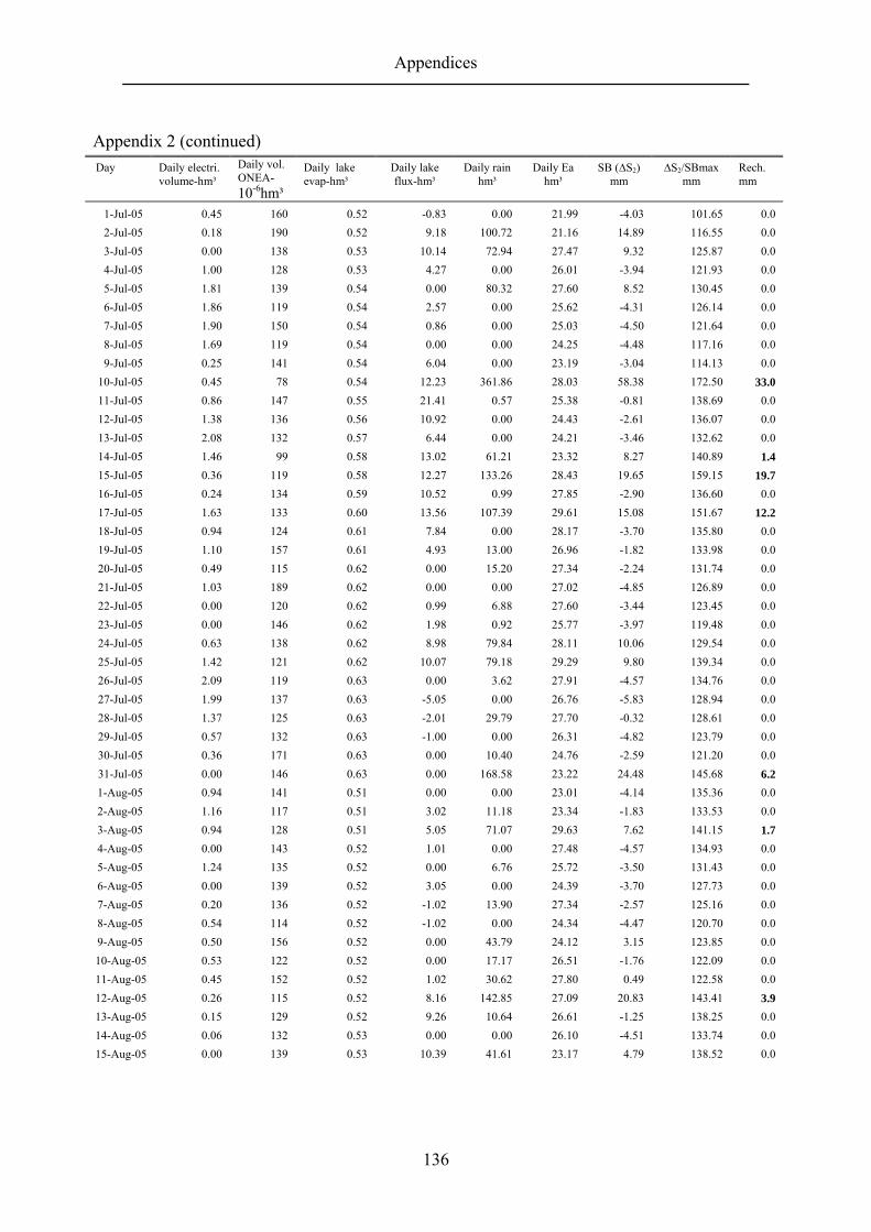
Appendices
136
Appendix 2 (continued) Day
Daily electri. volume-hm³
Daily vol. ONEA-10-6hm³
Daily lake evap-hm³
Daily lake flux-hm³
Daily rain hm³
Daily Ea hm³
SB (∆S2) mm
∆S2/SBmax mm
Rech. mm
1-Jul-05 0.45 160 0.52 -0.83 0.00 21.99 -4.03 101.65 0.0 2-Jul-05 0.18 190 0.52 9.18 100.72 21.16 14.89 116.55 0.0 3-Jul-05 0.00 138 0.53 10.14 72.94 27.47 9.32 125.87 0.0 4-Jul-05 1.00 128 0.53 4.27 0.00 26.01 -3.94 121.93 0.0 5-Jul-05 1.81 139 0.54 0.00 80.32 27.60 8.52 130.45 0.0 6-Jul-05 1.86 119 0.54 2.57 0.00 25.62 -4.31 126.14 0.0 7-Jul-05 1.90 150 0.54 0.86 0.00 25.03 -4.50 121.64 0.0 8-Jul-05 1.69 119 0.54 0.00 0.00 24.25 -4.48 117.16 0.0 9-Jul-05 0.25 141 0.54 6.04 0.00 23.19 -3.04 114.13 0.0
10-Jul-05 0.45 78 0.54 12.23 361.86 28.03 58.38 172.50 33.0 11-Jul-05 0.86 147 0.55 21.41 0.57 25.38 -0.81 138.69 0.0 12-Jul-05 1.38 136 0.56 10.92 0.00 24.43 -2.61 136.07 0.0 13-Jul-05 2.08 132 0.57 6.44 0.00 24.21 -3.46 132.62 0.0 14-Jul-05 1.46 99 0.58 13.02 61.21 23.32 8.27 140.89 1.4 15-Jul-05 0.36 119 0.58 12.27 133.26 28.43 19.65 159.15 19.7 16-Jul-05 0.24 134 0.59 10.52 0.99 27.85 -2.90 136.60 0.0 17-Jul-05 1.63 133 0.60 13.56 107.39 29.61 15.08 151.67 12.2 18-Jul-05 0.94 124 0.61 7.84 0.00 28.17 -3.70 135.80 0.0 19-Jul-05 1.10 157 0.61 4.93 13.00 26.96 -1.82 133.98 0.0 20-Jul-05 0.49 115 0.62 0.00 15.20 27.34 -2.24 131.74 0.0 21-Jul-05 1.03 189 0.62 0.00 0.00 27.02 -4.85 126.89 0.0 22-Jul-05 0.00 120 0.62 0.99 6.88 27.60 -3.44 123.45 0.0 23-Jul-05 0.00 146 0.62 1.98 0.92 25.77 -3.97 119.48 0.0 24-Jul-05 0.63 138 0.62 8.98 79.84 28.11 10.06 129.54 0.0 25-Jul-05 1.42 121 0.62 10.07 79.18 29.29 9.80 139.34 0.0 26-Jul-05 2.09 119 0.63 0.00 3.62 27.91 -4.57 134.76 0.0 27-Jul-05 1.99 137 0.63 -5.05 0.00 26.76 -5.83 128.94 0.0 28-Jul-05 1.37 125 0.63 -2.01 29.79 27.70 -0.32 128.61 0.0 29-Jul-05 0.57 132 0.63 -1.00 0.00 26.31 -4.82 123.79 0.0 30-Jul-05 0.36 171 0.63 0.00 10.40 24.76 -2.59 121.20 0.0 31-Jul-05 0.00 146 0.63 0.00 168.58 23.22 24.48 145.68 6.2 1-Aug-05 0.94 141 0.51 0.00 0.00 23.01 -4.14 135.36 0.0 2-Aug-05 1.16 117 0.51 3.02 11.18 23.34 -1.83 133.53 0.0 3-Aug-05 0.94 128 0.51 5.05 71.07 29.63 7.62 141.15 1.7 4-Aug-05 0.00 143 0.52 1.01 0.00 27.48 -4.57 134.93 0.0 5-Aug-05 1.24 135 0.52 0.00 6.76 25.72 -3.50 131.43 0.0 6-Aug-05 0.00 139 0.52 3.05 0.00 24.39 -3.70 127.73 0.0 7-Aug-05 0.20 136 0.52 -1.02 13.90 27.34 -2.57 125.16 0.0 8-Aug-05 0.54 114 0.52 -1.02 0.00 24.34 -4.47 120.70 0.0 9-Aug-05 0.50 156 0.52 0.00 43.79 24.12 3.15 123.85 0.0 10-Aug-05 0.53 122 0.52 0.00 17.17 26.51 -1.76 122.09 0.0 11-Aug-05 0.45 152 0.52 1.02 30.62 27.80 0.49 122.58 0.0 12-Aug-05 0.26 115 0.52 8.16 142.85 27.09 20.83 143.41 3.9 13-Aug-05 0.15 129 0.52 9.26 10.64 26.61 -1.25 138.25 0.0 14-Aug-05 0.06 132 0.53 0.00 0.00 26.10 -4.51 133.74 0.0 15-Aug-05 0.00 139 0.53 10.39 41.61 23.17 4.79 138.52 0.0

Appendices
137
Appendix 2 (continued) Day
Daily electri. volume-hm³
Daily vol. ONEA-10-6hm³
Daily lake evap-hm³
Daily lake flux-hm³
Daily rain hm³
Daily Ea hm³
SB (∆S2) mm
∆S2/SBmax mm
Rech. mm
16-Aug-05 0.16 109 0.53 15.79 31.54 24.76 3.70 142.22 2.7 17-Aug-05 0.04 135 0.54 10.66 54.00 26.00 6.44 145.94 6.4 18-Aug-05 0.14 119 0.54 4.29 45.02 27.93 3.50 143.00 3.5 19-Aug-05 0.77 150 0.55 2.15 2.06 27.35 -4.14 135.36 0.0 20-Aug-05 0.23 149 0.55 0.00 0.00 25.60 -4.46 130.90 0.0 21-Aug-05 0.18 124 0.55 2.16 0.00 25.29 -4.04 126.86 0.0 22-Aug-05 0.95 142 0.55 -2.16 0.00 22.84 -4.48 122.38 0.0 23-Aug-05 0.60 123 0.55 1.08 73.08 23.69 8.34 130.72 0.0 24-Aug-05 0.67 155 0.55 0.00 5.53 22.92 -3.15 127.58 0.0 25-Aug-05 0.73 159 0.55 1.08 40.05 21.41 3.12 130.70 0.0 26-Aug-05 0.16 161 0.55 1.08 22.11 25.49 -0.51 130.19 0.0 27-Aug-05 0.00 133 0.55 0.00 20.55 24.36 -0.74 129.45 0.0 28-Aug-05 0.15 160 0.55 5.42 0.00 23.19 -3.12 126.32 0.0 29-Aug-05 0.03 122 0.55 4.36 207.83 26.13 31.38 157.70 18.2 30-Aug-05 0.23 148 0.56 3.28 13.38 26.07 -1.72 137.78 0.0 31-Aug-05 0.56 138 0.56 1.09 0.14 25.78 -4.34 133.43 0.0 1-Sep-05 0.55 122 0.58 3.29 102.99 27.70 13.10 146.54 7.0 2-Sep-05 0.00 154 0.59 11.04 76.16 28.10 9.90 149.40 9.9 3-Sep-05 0.16 131 0.59 10.03 20.29 26.79 0.47 139.97 0.5 4-Sep-05 0.12 143 0.59 12.38 0.00 25.70 -2.37 137.13 0.0 5-Sep-05 1.04 120 0.60 7.95 0.00 24.44 -3.07 134.06 0.0 6-Sep-05 0.38 171 0.60 8.01 2.27 23.80 -2.45 131.60 0.0 7-Sep-05 0.92 139 0.61 5.75 0.00 23.36 -3.24 128.37 0.0 8-Sep-05 0.19 126 0.61 5.78 158.25 28.43 22.80 151.17 11.7 9-Sep-05 0.48 144 0.61 2.32 0.00 27.08 -4.37 135.13 0.0
10-Sep-05 0.63 158 0.62 2.32 0.00 26.38 -4.28 130.85 0.0 11-Sep-05 0.58 145 0.62 0.00 0.00 25.50 -4.52 126.33 0.0 12-Sep-05 1.04 140 0.62 0.00 0.00 24.98 -4.51 121.82 0.0 13-Sep-05 1.46 159 0.62 -2.32 2.13 24.39 -4.51 117.31 0.0 14-Sep-05 1.36 201 0.62 -1.16 0.00 24.59 -4.69 112.62 0.0 15-Sep-05 1.78 145 0.62 -2.32 7.28 25.72 -3.92 108.71 0.0 16-Sep-05 1.19 173 0.62 -1.16 0.00 24.54 -4.65 104.05 0.0 17-Sep-05 0.26 169 0.62 -1.16 0.00 23.40 -4.30 99.75 0.0 18-Sep-05 0.11 158 0.61 1.16 0.00 22.96 -3.81 95.94 0.0 19-Sep-05 1.51 177 0.61 -2.31 0.00 21.91 -4.46 91.48 0.0 20-Sep-05 0.63 123 0.61 0.00 82.68 27.12 9.19 100.67 0.0 21-Sep-05 1.14 160 0.61 -1.15 8.65 26.76 -3.56 97.12 0.0 22-Sep-05 1.70 151 0.61 -1.15 0.00 26.07 -5.00 92.12 0.0 23-Sep-05 1.61 130 0.61 -2.30 46.29 24.79 2.87 94.99 0.0 24-Sep-05 0.31 144 0.61 -1.15 0.00 23.13 -4.26 90.73 0.0 25-Sep-05 0.07 143 0.61 0.00 0.92 21.48 -3.59 87.13 0.0 26-Sep-05 1.41 122 0.61 -1.15 0.00 18.99 -3.75 83.39 0.0 27-Sep-05 0.17 96 0.61 0.00 96.92 21.58 12.61 96.00 0.0 28-Sep-05 0.93 111 0.61 4.60 94.53 20.84 12.98 108.98 0.0 29-Sep-05 1.45 118 0.61 2.31 0.00 20.42 -3.41 105.57 0.0 30-Sep-05 1.97 133 0.61 -2.31 47.33 19.71 3.85 109.41 0.0
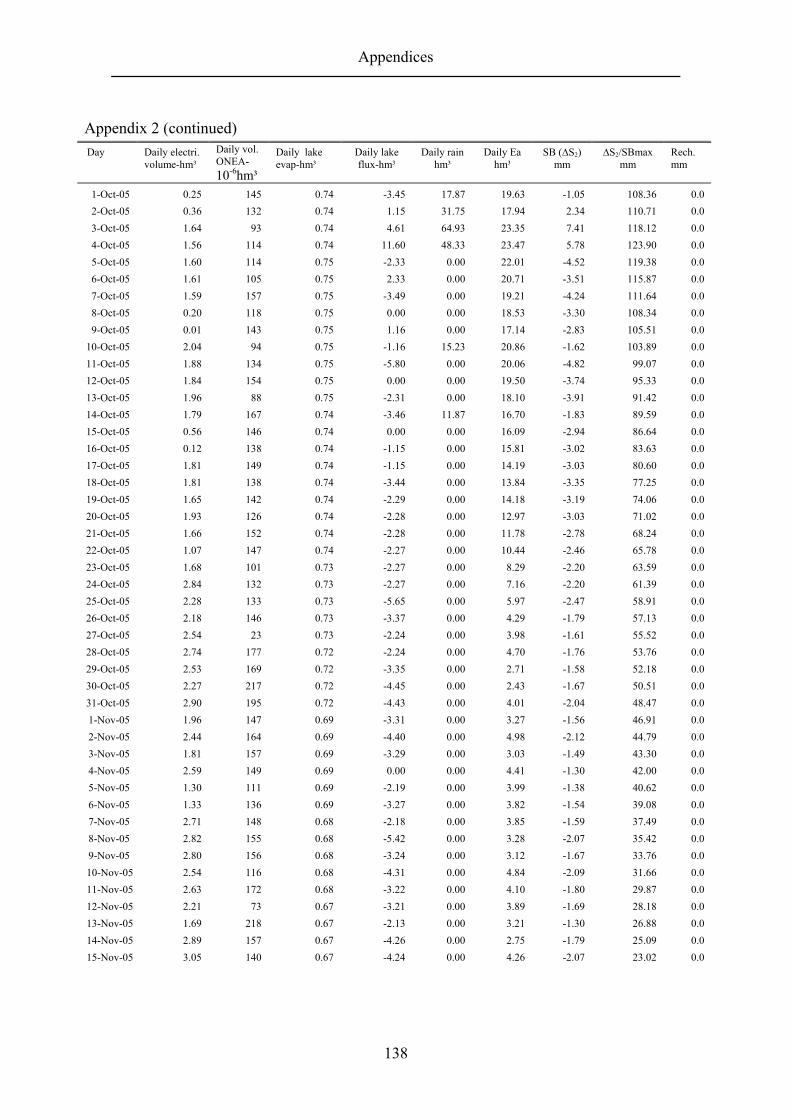
Appendices
138
Appendix 2 (continued) Day
Daily electri. volume-hm³
Daily vol. ONEA-10-6hm³
Daily lake evap-hm³
Daily lake flux-hm³
Daily rain hm³
Daily Ea hm³
SB (∆S2) mm
∆S2/SBmax mm
Rech. mm
1-Oct-05 0.25 145 0.74 -3.45 17.87 19.63 -1.05 108.36 0.0 2-Oct-05 0.36 132 0.74 1.15 31.75 17.94 2.34 110.71 0.0 3-Oct-05 1.64 93 0.74 4.61 64.93 23.35 7.41 118.12 0.0 4-Oct-05 1.56 114 0.74 11.60 48.33 23.47 5.78 123.90 0.0 5-Oct-05 1.60 114 0.75 -2.33 0.00 22.01 -4.52 119.38 0.0 6-Oct-05 1.61 105 0.75 2.33 0.00 20.71 -3.51 115.87 0.0 7-Oct-05 1.59 157 0.75 -3.49 0.00 19.21 -4.24 111.64 0.0 8-Oct-05 0.20 118 0.75 0.00 0.00 18.53 -3.30 108.34 0.0 9-Oct-05 0.01 143 0.75 1.16 0.00 17.14 -2.83 105.51 0.0
10-Oct-05 2.04 94 0.75 -1.16 15.23 20.86 -1.62 103.89 0.0 11-Oct-05 1.88 134 0.75 -5.80 0.00 20.06 -4.82 99.07 0.0 12-Oct-05 1.84 154 0.75 0.00 0.00 19.50 -3.74 95.33 0.0 13-Oct-05 1.96 88 0.75 -2.31 0.00 18.10 -3.91 91.42 0.0 14-Oct-05 1.79 167 0.74 -3.46 11.87 16.70 -1.83 89.59 0.0 15-Oct-05 0.56 146 0.74 0.00 0.00 16.09 -2.94 86.64 0.0 16-Oct-05 0.12 138 0.74 -1.15 0.00 15.81 -3.02 83.63 0.0 17-Oct-05 1.81 149 0.74 -1.15 0.00 14.19 -3.03 80.60 0.0 18-Oct-05 1.81 138 0.74 -3.44 0.00 13.84 -3.35 77.25 0.0 19-Oct-05 1.65 142 0.74 -2.29 0.00 14.18 -3.19 74.06 0.0 20-Oct-05 1.93 126 0.74 -2.28 0.00 12.97 -3.03 71.02 0.0 21-Oct-05 1.66 152 0.74 -2.28 0.00 11.78 -2.78 68.24 0.0 22-Oct-05 1.07 147 0.74 -2.27 0.00 10.44 -2.46 65.78 0.0 23-Oct-05 1.68 101 0.73 -2.27 0.00 8.29 -2.20 63.59 0.0 24-Oct-05 2.84 132 0.73 -2.27 0.00 7.16 -2.20 61.39 0.0 25-Oct-05 2.28 133 0.73 -5.65 0.00 5.97 -2.47 58.91 0.0 26-Oct-05 2.18 146 0.73 -3.37 0.00 4.29 -1.79 57.13 0.0 27-Oct-05 2.54 23 0.73 -2.24 0.00 3.98 -1.61 55.52 0.0 28-Oct-05 2.74 177 0.72 -2.24 0.00 4.70 -1.76 53.76 0.0 29-Oct-05 2.53 169 0.72 -3.35 0.00 2.71 -1.58 52.18 0.0 30-Oct-05 2.27 217 0.72 -4.45 0.00 2.43 -1.67 50.51 0.0 31-Oct-05 2.90 195 0.72 -4.43 0.00 4.01 -2.04 48.47 0.0 1-Nov-05 1.96 147 0.69 -3.31 0.00 3.27 -1.56 46.91 0.0 2-Nov-05 2.44 164 0.69 -4.40 0.00 4.98 -2.12 44.79 0.0 3-Nov-05 1.81 157 0.69 -3.29 0.00 3.03 -1.49 43.30 0.0 4-Nov-05 2.59 149 0.69 0.00 0.00 4.41 -1.30 42.00 0.0 5-Nov-05 1.30 111 0.69 -2.19 0.00 3.99 -1.38 40.62 0.0 6-Nov-05 1.33 136 0.69 -3.27 0.00 3.82 -1.54 39.08 0.0 7-Nov-05 2.71 148 0.68 -2.18 0.00 3.85 -1.59 37.49 0.0 8-Nov-05 2.82 155 0.68 -5.42 0.00 3.28 -2.07 35.42 0.0 9-Nov-05 2.80 156 0.68 -3.24 0.00 3.12 -1.67 33.76 0.0 10-Nov-05 2.54 116 0.68 -4.31 0.00 4.84 -2.09 31.66 0.0 11-Nov-05 2.63 172 0.68 -3.22 0.00 4.10 -1.80 29.87 0.0 12-Nov-05 2.21 73 0.67 -3.21 0.00 3.89 -1.69 28.18 0.0 13-Nov-05 1.69 218 0.67 -2.13 0.00 3.21 -1.30 26.88 0.0 14-Nov-05 2.89 157 0.67 -4.26 0.00 2.75 -1.79 25.09 0.0 15-Nov-05 3.05 140 0.67 -4.24 0.00 4.26 -2.07 23.02 0.0
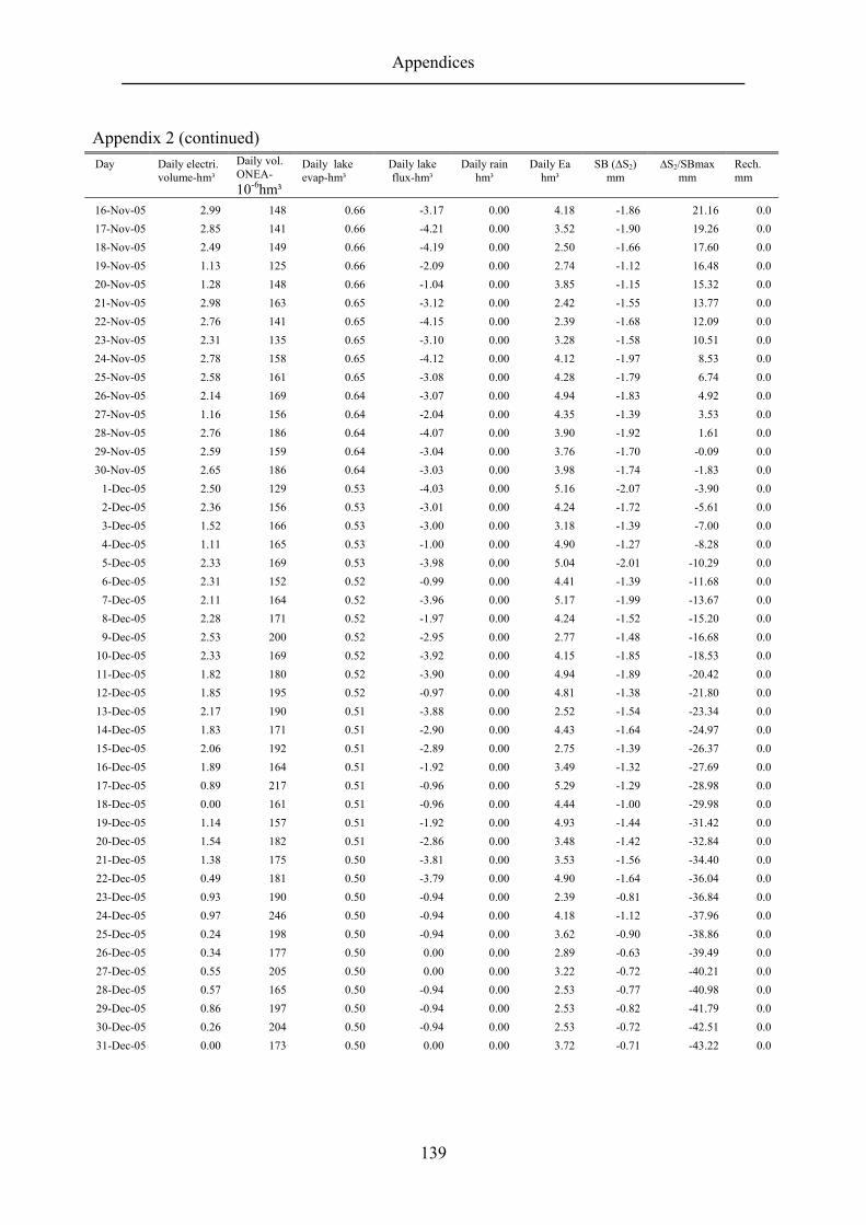
Appendices
139
Appendix 2 (continued) Day
Daily electri. volume-hm³
Daily vol. ONEA-10-6hm³
Daily lake evap-hm³
Daily lake flux-hm³
Daily rain hm³
Daily Ea hm³
SB (∆S2) mm
∆S2/SBmax mm
Rech. mm
16-Nov-05 2.99 148 0.66 -3.17 0.00 4.18 -1.86 21.16 0.0 17-Nov-05 2.85 141 0.66 -4.21 0.00 3.52 -1.90 19.26 0.0 18-Nov-05 2.49 149 0.66 -4.19 0.00 2.50 -1.66 17.60 0.0 19-Nov-05 1.13 125 0.66 -2.09 0.00 2.74 -1.12 16.48 0.0 20-Nov-05 1.28 148 0.66 -1.04 0.00 3.85 -1.15 15.32 0.0 21-Nov-05 2.98 163 0.65 -3.12 0.00 2.42 -1.55 13.77 0.0 22-Nov-05 2.76 141 0.65 -4.15 0.00 2.39 -1.68 12.09 0.0 23-Nov-05 2.31 135 0.65 -3.10 0.00 3.28 -1.58 10.51 0.0 24-Nov-05 2.78 158 0.65 -4.12 0.00 4.12 -1.97 8.53 0.0 25-Nov-05 2.58 161 0.65 -3.08 0.00 4.28 -1.79 6.74 0.0 26-Nov-05 2.14 169 0.64 -3.07 0.00 4.94 -1.83 4.92 0.0 27-Nov-05 1.16 156 0.64 -2.04 0.00 4.35 -1.39 3.53 0.0 28-Nov-05 2.76 186 0.64 -4.07 0.00 3.90 -1.92 1.61 0.0 29-Nov-05 2.59 159 0.64 -3.04 0.00 3.76 -1.70 -0.09 0.0 30-Nov-05 2.65 186 0.64 -3.03 0.00 3.98 -1.74 -1.83 0.0
1-Dec-05 2.50 129 0.53 -4.03 0.00 5.16 -2.07 -3.90 0.0 2-Dec-05 2.36 156 0.53 -3.01 0.00 4.24 -1.72 -5.61 0.0 3-Dec-05 1.52 166 0.53 -3.00 0.00 3.18 -1.39 -7.00 0.0 4-Dec-05 1.11 165 0.53 -1.00 0.00 4.90 -1.27 -8.28 0.0 5-Dec-05 2.33 169 0.53 -3.98 0.00 5.04 -2.01 -10.29 0.0 6-Dec-05 2.31 152 0.52 -0.99 0.00 4.41 -1.39 -11.68 0.0 7-Dec-05 2.11 164 0.52 -3.96 0.00 5.17 -1.99 -13.67 0.0 8-Dec-05 2.28 171 0.52 -1.97 0.00 4.24 -1.52 -15.20 0.0 9-Dec-05 2.53 200 0.52 -2.95 0.00 2.77 -1.48 -16.68 0.0
10-Dec-05 2.33 169 0.52 -3.92 0.00 4.15 -1.85 -18.53 0.0 11-Dec-05 1.82 180 0.52 -3.90 0.00 4.94 -1.89 -20.42 0.0 12-Dec-05 1.85 195 0.52 -0.97 0.00 4.81 -1.38 -21.80 0.0 13-Dec-05 2.17 190 0.51 -3.88 0.00 2.52 -1.54 -23.34 0.0 14-Dec-05 1.83 171 0.51 -2.90 0.00 4.43 -1.64 -24.97 0.0 15-Dec-05 2.06 192 0.51 -2.89 0.00 2.75 -1.39 -26.37 0.0 16-Dec-05 1.89 164 0.51 -1.92 0.00 3.49 -1.32 -27.69 0.0 17-Dec-05 0.89 217 0.51 -0.96 0.00 5.29 -1.29 -28.98 0.0 18-Dec-05 0.00 161 0.51 -0.96 0.00 4.44 -1.00 -29.98 0.0 19-Dec-05 1.14 157 0.51 -1.92 0.00 4.93 -1.44 -31.42 0.0 20-Dec-05 1.54 182 0.51 -2.86 0.00 3.48 -1.42 -32.84 0.0 21-Dec-05 1.38 175 0.50 -3.81 0.00 3.53 -1.56 -34.40 0.0 22-Dec-05 0.49 181 0.50 -3.79 0.00 4.90 -1.64 -36.04 0.0 23-Dec-05 0.93 190 0.50 -0.94 0.00 2.39 -0.81 -36.84 0.0 24-Dec-05 0.97 246 0.50 -0.94 0.00 4.18 -1.12 -37.96 0.0 25-Dec-05 0.24 198 0.50 -0.94 0.00 3.62 -0.90 -38.86 0.0 26-Dec-05 0.34 177 0.50 0.00 0.00 2.89 -0.63 -39.49 0.0 27-Dec-05 0.55 205 0.50 0.00 0.00 3.22 -0.72 -40.21 0.0 28-Dec-05 0.57 165 0.50 -0.94 0.00 2.53 -0.77 -40.98 0.0 29-Dec-05 0.86 197 0.50 -0.94 0.00 2.53 -0.82 -41.79 0.0 30-Dec-05 0.26 204 0.50 -0.94 0.00 2.53 -0.72 -42.51 0.0 31-Dec-05 0.00 173 0.50 0.00 0.00 3.72 -0.71 -43.22 0.0

Appendices
140
Appendix 2 (continued) Day
Daily electri. volume-hm³
Daily vol. ONEA-10-6hm³
Daily lake evap-hm³
Daily lake flux-hm³
Daily rain hm³
Daily Ea hm³
SB (∆S2) mm
∆S2/SBmax mm
Rech. mm
1-Jan-06 0.00 196 0.48 -0.94 0.00 2.78 -0.71 -43.93 0.0 2-Jan-06 0.00 207 0.48 0.00 0.00 2.67 -0.53 -44.47 0.0 3-Jan-06 0.16 196 0.48 0.00 0.00 2.81 -0.58 -45.05 0.0 4-Jan-06 0.35 182 0.48 -0.94 0.00 2.83 -0.78 -45.83 0.0 5-Jan-06 0.38 189 0.48 -0.94 0.00 3.11 -0.83 -46.66 0.0 6-Jan-06 1.39 181 0.48 -1.87 0.00 3.38 -1.20 -47.87 0.0 7-Jan-06 0.00 191 0.48 -0.93 0.00 3.69 -0.86 -48.73 0.0 8-Jan-06 0.00 216 0.48 0.00 0.00 4.05 -0.77 -49.50 0.0 9-Jan-06 0.88 193 0.48 -0.93 0.00 4.06 -1.08 -50.57 0.0 10-Jan-06 0.08 237 0.48 -0.93 0.00 3.80 -0.90 -51.47 0.0 11-Jan-06 1.58 202 0.48 -1.86 0.00 3.22 -1.21 -52.68 0.0 12-Jan-06 1.11 179 0.48 -1.86 0.00 4.05 -1.27 -53.95 0.0 13-Jan-06 1.17 225 0.48 -2.78 0.00 3.47 -1.34 -55.28 0.0 14-Jan-06 0.91 157 0.48 -1.85 0.00 3.51 -1.14 -56.42 0.0 15-Jan-06 0.27 221 0.48 -0.92 0.00 3.57 -0.89 -57.31 0.0 16-Jan-06 1.72 203 0.48 -1.84 0.00 2.96 -1.18 -58.49 0.0 17-Jan-06 1.51 209 0.48 -2.75 0.00 3.66 -1.42 -59.91 0.0 18-Jan-06 1.06 217 0.47 -0.92 0.00 3.74 -1.05 -60.96 0.0 19-Jan-06 1.06 185 0.47 -1.83 0.00 3.26 -1.12 -62.08 0.0 20-Jan-06 2.14 266 0.47 -1.82 0.00 2.76 -1.22 -63.30 0.0 21-Jan-06 0.75 234 0.47 -2.73 0.00 3.65 -1.29 -64.59 0.0 22-Jan-06 0.51 198 0.47 -0.91 0.00 3.11 -0.85 -65.43 0.0 23-Jan-06 1.81 248 0.47 -2.72 0.00 4.47 -1.60 -67.03 0.0 24-Jan-06 1.55 155 0.47 -1.81 0.00 3.46 -1.23 -68.26 0.0 25-Jan-06 1.75 249 0.47 -2.70 0.00 3.77 -1.47 -69.73 0.0 26-Jan-06 2.20 204 0.47 -2.69 0.00 3.77 -1.54 -71.28 0.0 27-Jan-06 1.90 252 0.46 -2.68 0.00 3.71 -1.48 -72.76 0.0 28-Jan-06 1.03 217 0.46 -1.78 0.00 3.95 -1.22 -73.98 0.0 29-Jan-06 0.51 199 0.46 0.00 0.00 3.38 -0.74 -74.72 0.0 30-Jan-06 2.07 215 0.46 -2.67 0.00 3.19 -1.42 -76.14 0.0 31-Jan-06 1.19 223 0.46 -2.66 0.00 3.06 -1.25 -77.39 0.0 1-Feb-06 0.73 178 0.54 -0.88 0.00 3.84 -1.01 -78.40 0.0 2-Feb-06 1.65 224 0.54 -1.77 0.00 3.67 -1.29 -79.69 0.0 3-Feb-06 0.91 225 0.54 -1.76 0.00 4.36 -1.28 -80.97 0.0 4-Feb-06 0.39 187 0.54 0.00 0.00 4.42 -0.90 -81.87 0.0 5-Feb-06 0.00 229 0.53 -1.76 0.00 3.86 -1.04 -82.91 0.0 6-Feb-06 1.21 211 0.53 -0.88 0.00 3.72 -1.07 -83.99 0.0 7-Feb-06 1.45 201 0.53 -2.63 0.00 4.29 -1.51 -85.49 0.0 8-Feb-06 1.64 271 0.53 -1.75 0.00 3.86 -1.31 -86.81 0.0 9-Feb-06 1.05 197 0.53 -2.61 0.00 3.84 -1.36 -88.17 0.0 10-Feb-06 0.22 224 0.53 -0.87 0.00 3.25 -0.82 -88.99 0.0 11-Feb-06 0.04 220 0.53 0.00 0.00 3.26 -0.65 -89.64 0.0 12-Feb-06 0.00 242 0.53 -0.87 0.00 3.49 -0.83 -90.46 0.0 13-Feb-06 1.04 220 0.53 -1.73 0.00 3.81 -1.20 -91.67 0.0 14-Feb-06 1.03 263 0.53 0.00 0.00 3.45 -0.85 -92.51 0.0 15-Feb-06 2.26 214 0.53 -1.73 0.00 3.46 -1.35 -93.86 0.0

Appendices
141
Appendix 2 (concluded) Day
Daily electri. volume-hm³
Daily vol. ONEA-10-6hm³
Daily lake evap-hm³
Daily lake flux-hm³
Daily rain hm³
Daily Ea hm³
SB (∆S2) mm
∆S2/SBmax mm
Rech. mm
16-Feb-06 2.06 166 0.53 -1.73 0.00 3.57 -1.33 -95.20 0.0 17-Feb-06 0.45 228 0.52 -0.86 0.00 3.84 -0.96 -96.16 0.0 18-Feb-06 0.00 211 0.52 -1.72 0.00 3.63 -0.99 -97.15 0.0 19-Feb-06 0.00 228 0.52 -0.86 0.00 3.56 -0.84 -97.99 0.0 20-Feb-06 0.22 189 0.52 -0.86 0.00 3.39 -0.85 -98.83 0.0 21-Feb-06 0.22 227 0.52 -0.86 0.00 3.14 -0.80 -99.63 0.0 22-Feb-06 0.32 249 0.52 0.00 0.00 3.14 -0.67 -100.31 0.0 23-Feb-06 0.30 231 0.52 -0.86 0.00 3.66 -0.90 -101.21 0.0 24-Feb-06 0.02 182 0.52 -0.85 0.00 2.98 -0.74 -101.95 0.0 25-Feb-06 0.00 270 0.52 0.00 0.00 3.06 -0.61 -102.56 0.0 26-Feb-06 0.00 231 0.52 -0.85 0.00 3.46 -0.82 -103.37 0.0 27-Feb-06 0.66 200 0.52 -0.85 0.00 3.50 -0.94 -104.31 0.0 28-Feb-06 0.72 249 0.52 -1.70 0.00 3.18 -1.04 -105.35 0.0 1-Mar-06 2.06 220 0.61 -2.55 0.00 3.46 -1.47 -106.81 0.0 2-Mar-06 2.03 237 0.60 -3.38 0.00 3.83 -1.67 -108.48 0.0 3-Mar-06 1.69 263 0.60 -0.84 0.00 4.02 -1.21 -109.69 0.0 4-Mar-06 0.06 248 0.60 0.00 0.00 3.84 -0.76 -110.45 0.0 5-Mar-06 0.00 224 0.60 -0.84 0.00 3.74 -0.88 -111.33 0.0 6-Mar-06 0.70 253 0.60 -1.68 0.00 4.01 -1.18 -112.51 0.0 7-Mar-06 0.37 234 0.60 -1.68 0.00 3.94 -1.11 -113.62 0.0 8-Mar-06 0.23 264 0.60 -0.84 0.00 3.91 -0.94 -114.56 0.0 9-Mar-06 0.00 200 0.60 0.00 0.00 3.63 -0.71 -115.28 0.0 10-Mar-06 0.00 202 0.60 -0.84 0.00 3.45 -0.83 -116.11 0.0 11-Mar-06 0.00 308 0.59 -0.84 0.00 3.33 -0.81 -116.91 0.0 12-Mar-06 0.00 236 0.59 -0.83 0.00 3.62 -0.85 -117.77 0.0 13-Mar-06 0.24 217 0.59 -0.83 0.00 3.52 -0.88 -118.64 0.0 14-Mar-06 0.55 259 0.59 -0.83 0.00 3.37 -0.90 -119.55 0.0 15-Mar-06 0.18 231 0.59 0.00 0.00 3.32 -0.69 -120.24 0.0 16-Mar-06 1.24 229 0.59 -0.83 0.00 2.84 -0.93 -121.17 0.0 17-Mar-06 0.35 304 0.59 -3.32 0.00 2.65 -1.17 -122.34 0.0 18-Mar-06 0.00 244 0.59 0.00 0.00 3.15 -0.63 -122.97 0.0 19-Mar-06 0.00 303 0.59 0.00 0.00 3.36 -0.67 -123.64 0.0 20-Mar-06 0.78 241 0.59 -1.65 0.00 3.26 -1.06 -124.70 0.0 21-Mar-06 0.75 226 0.59 -0.82 0.00 2.90 -0.86 -125.56 0.0 22-Mar-06 0.50 249 0.59 -0.82 0.00 3.94 -0.99 -126.55 0.0 23-Mar-06 0.77 332 0.59 -1.64 0.00 2.85 -0.99 -127.54 0.0 24-Mar-06 1.21 246 0.59 -1.64 0.00 3.61 -1.19 -128.73 0.0 25-Mar-06 0.47 258 0.58 -1.64 0.00 3.40 -1.03 -129.76 0.0 26-Mar-06 0.00 253 0.58 0.00 0.00 3.84 -0.75 -130.51 0.0 27-Mar-06 1.63 252 0.58 -2.45 0.00 3.49 -1.38 -131.89 0.0 28-Mar-06 1.00 263 0.58 -1.63 0.00 4.35 -1.28 -133.17 0.0 29-Mar-06 0.62 242 0.58 -1.62 0.00 3.57 -1.08 -134.25 0.0 30-Mar-06 0.00 230 0.58 -0.81 0.00 3.51 -0.83 -135.08 0.0 31-Mar-06 0.00 224 0.58 -0.81 0.00 3.46 -0.82 -135.90 0.0

Appendices
142
0
20
40
60
80
100
120
140
160
180
200
22/1
1/20
02
31/0
1/20
03
11/0
4/20
03
20/0
6/20
03
29/0
8/20
03
07/1
1/20
03
16/0
1/20
04
26/0
3/20
04
04/0
6/20
04
13/0
8/20
04
22/1
0/20
04
31/1
2/20
04
11/0
3/20
05
20/0
5/20
05
29/0
7/20
05
07/1
0/20
05
16/1
2/20
05
Date
Dai
ly ra
infa
ll (m
m)
0
1
2
3
4
5
6
7
8
9
10
Dai
ly E
a &
Ep
(mm
)
Daily rainfall Daily Ea Daily Ep
Appendix 3: Daily Ea and Ep fluctuations along with the daily rainfall in the Kompienga dam basin from 2002 to 2005

Appendices
143
Appendix 4: Results of the daily water sampling survey in the basin
Appendix 4.1: Monthly number of containers at each water monitoring point and number of strokes or buckets (others) according to their
size of big (B), small (S) or medium (M)
Buckets Pans Cans Barils Canaris Others Month
Survey site B S M B S M B S M B S M B S M B S M
Comin Yanga 3186 1797 1012 4108 2060 1659 3656 2001 1191 194 25 8 479 180 209 6385
Kouaré 683 245 408 479 175 303 803 369 568 41 0 4 87 31 36 1019
Natiabouani 2181 201 451 4845 479 597 2300 1908 202 389 0 13 2 0 0 1752
Kompienbiga 364 113 51 1524 333 182 701 114 110 0 0 0 18 0 0 4719
Pama 2954 2048 1971 7202 3578 4337 3764 1847 3271 1854 10 153 0 0 0 6178 531 178
Nov 15-30
Djabiga 2401 1545 1607 9346 3362 3959 2884 1750 1580 0 0 0 0 0 0 8512
Comin Yanga 3681 2389 1264 4143 2765 1810 3886 2542 1436 210 13 11 593 259 279 8209
Kouaré 716 474 477 712 355 420 1000 445 605 17 2 0 76 20 48 1269
Natiabouani 2036 244 522 4441 564 720 2444 2166 209 402 0 6 2 0 0 2763
Kompienbiga 603 307 287 2981 808 854 1146 246 177 2 0 1 13 0 0 6794
Pama 8374 3775 3616 11524 8217 6581 8197 5550 4624 6412 0 19 0 0 0 3405 543 201
Dec 01-14
Djabiga 3119 2175 2546 11376 5582 6991 5380 3658 2134 0 0 0 0 0 0 7611
Comin Yanga 4027 2848 2667 5090 3915 3547 4855 3494 2979 323 22 5 568 185 277 17225
Kouaré 3656 1720 1118 5967 2558 1130 5779 2119 886 19 0 0 64 17 5 34095
Natiabouani 2031 369 390 6112 556 657 1715 3411 335 394 0 0 0 0 0 4049
Kompienbiga 611 320 227 5657 1310 1188 2718 232 138 12 0 0 17 0 0 7878
Pama 3835 2512 1871 7263 4611 4915 5197 4684 4207 6223 0 0 0 0 0 2083 1098 563
Feb 14-28
Djabiga 1350 727 865 7799 3151 5469 2590 1293 1343 0 0 0 0 0 0 8721
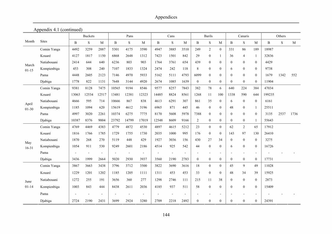
Appendices
144
Appendix 4.1 (continued) Buckets Pans Cans Barils Canaris Others
Month Sites B S M B S M B S M B S M B S M B S M
Comin Yanga 4492 3259 2887 5301 4175 3590 4947 3885 3510 249 2 0 331 86 189 18987
Kouaré 4127 1817 1150 6868 2648 1312 7423 1501 842 29 0 1 36 4 1 32836
Natiabouani 2414 644 640 6236 803 903 1764 3761 654 439 0 0 0 0 0 4429
Kompienbiga 453 308 240 7107 1833 1324 2474 242 118 8 0 0 6 0 0 9738
Pama 4448 2605 2123 7146 4970 5933 5162 5111 4793 6099 0 0 0 0 0 1679 1342 552
March 01-15
Djabiga 1778 822 1131 7648 3144 4920 2674 1085 1639 0 0 0 0 0 0 11904
Comin Yanga 9381 8128 7475 10565 9194 8546 9577 8257 7843 382 78 6 640 224 384 47034
Kouaré 13063 12534 12517 13481 12381 12323 14485 8824 8561 1268 11 100 1338 590 644 199235
Natiabouani 4666 595 714 10666 867 838 4613 6291 307 861 35 0 6 0 0 6161
Kompienbiga 1185 1094 620 15619 4612 3196 6965 871 445 46 0 0 48 0 1 25511
Pama 4997 3020 2261 10374 6275 7775 8170 5608 5978 7388 0 0 0 0 0 3135 2537 1736
April 01-30
Djabiga 10387 8376 9004 23792 14799 17019 12548 8609 9166 2 0 0 0 0 1 55643
Comin Yanga 4769 4469 4383 4779 4872 4530 4897 4615 5212 23 0 0 62 2 65 17912
Kouaré 1816 1766 1785 1729 1755 1730 2035 1000 995 176 0 0 143 97 130 26410
Natiabouani 1870 268 270 5119 448 429 1927 3036 156 430 27 34 0 0 0 3275
Kompienbiga 1054 911 530 9249 2601 2186 4514 925 542 44 0 0 6 0 0 16726
Pama - - - - - - - - - - - - - - - - - -
May 16-31
Djabiga 3436 1999 2664 5020 2930 3937 3560 2190 2783 0 0 0 0 0 0 17731
Comin Yanga 3867 3663 3438 3796 3712 3500 3822 3690 3616 18 0 0 45 9 49 11028
Kouaré 1229 1201 1202 1185 1205 1111 1311 453 453 33 0 0 48 34 39 15925
Natiabouani 1272 255 191 3656 360 277 1298 2746 111 215 11 38 0 0 0 2873
Kompienbiga 1003 843 444 8438 2611 2036 4185 937 511 58 0 0 0 0 0 15409
Pama - - - - - - - - - - - - - - - - - -
June 01-14
Djabiga 2724 2190 2431 3699 2924 3280 2709 2218 2492 0 0 0 0 0 0 24391
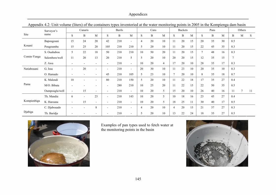
Appendices
145
Appendix 4.2: Unit volume (liters) of the containers types inventoried at the water monitoring points in 2005 in the Kompienga dam basin Canaris Barils Cans Buckets Pans Others
Site Surveyor’s name S B M S B M S B M S B M S B M B M S
Bapougouni 15 24 20 42 210 - 4 20 10 11 20 15 20 35 30 0.5 Kouaré Pougoumba 15 25 20 105 210 210 5 20 10 11 20 15 22 45 35 0.3
S. Ouahabou 5 22 18 50 210 210 10 50 20 11 20 15 7 48 16 0.3
Salembere/well 11 20 13 20 210 5 5 20 10 20 20 15 12 35 15 7
Comin-Yanga
Z. Awa - - - - 210 - 10 20 4 17 20 10 28 35 17 0.3
G. Issa - 20 - - 210 - 20 30 10 11 23 10 20 35 10 0.3 Natiabouani
O. Hamado - - - 45 210 105 5 23 10 7 20 10 8 35 18 0.7
K. Malendi 10 - - 80 210 150 5 20 10 11 22 18 17 35 27 0.4
M/O. Bibata - - - - 280 210 10 25 20 11 22 15 22 50 35 0.5
Pama
Oumpougla/well - 15 - - 210 - 10 20 5 15 20 10 26 40 16 11 7 11
Th. Mandia 6 - 23 - 210 143 10 20 5 10 18 16 23 45 27 0.4 Kompienbiga K. Harouna - 15 - - 210 - 10 20 5 18 25 11 30 40 17 0.5
C. Djabouado - - 8 - 210 - 4 20 10 4 20 15 21 37 27 0.3 Djabiga Th. Baridja - - - - 210 - 5 20 10 13 22 24 18 35 27 0.5
Examples of pan types used to fetch water at the monitoring points in the basin

Appendices
146
Appendix 4.3: Monthly withdrawal volumes at the 15 water monitoring points in the Kompienga dam basin from 2004 to 2005
MW = modern well, B = borehole and B3 (Pama) represents the borehole of the tap water system.
Site Djabiga Pama Kompienbiga Natiabouani Kouaré Comin Yanga Survey point B1 B2 MW B1 B2 B3 B1 B2 B1 B2 B1 B2 MW B1 B2
Average mthly withdrawal volume (m³)
November 2004 566.2 835.3 1626.2 383.2 325.9 518.1 208.2 383.2 584.6 240.9 67.3 116.9 411.9 371.7 238.4 458.5 December 872.8 1133.8 4954.6 383.2 344.1 518.1 171.5 269.1 548.3 275.0 125.3 96.2 371.1 478.0 310.2 723.4 January 2005 633.4 988.3 4617.0 383.2 344.1 518.1 244.3 367.4 528.0 364.0 397.1 301.8 389.4 603.3 360.7 736.0 February 394.1 842.8 4279.4 383.2 344.1 518.1 317.0 465.7 507.6 453.0 668.9 507.4 407.6 728.5 411.2 748.6 March 487.1 759.9 4310.9 383.2 344.1 518.1 381.8 535.2 575.0 470.7 819.8 514.5 371.0 814.4 404.0 779.3 April 661.4 1893.4 2745.8 383.2 344.1 518.1 408.9 675.0 550.6 379.5 1338.8 1285.5 243.2 1054.3 357.9 856.0 May 661.4 1238.2 2745.8 383.2 344.1 518.1 574.7 779.0 462.3 422.6 738.0 1285.5 243.2 1280.0 317.3 799.5 June 661.4 1039.6 2745.8 383.2 344.1 518.1 541.4 721.3 272.9 342.1 462.6 1285.5 243.2 1049.9 193.6 720.3
Mean monthly volume (m³) per survey point 617.2 1091.4 3503.2 383.2 341.8 518.1 356.0 524.5 503.7 368.5 577.2 674.1 335.1 797.5 324.2
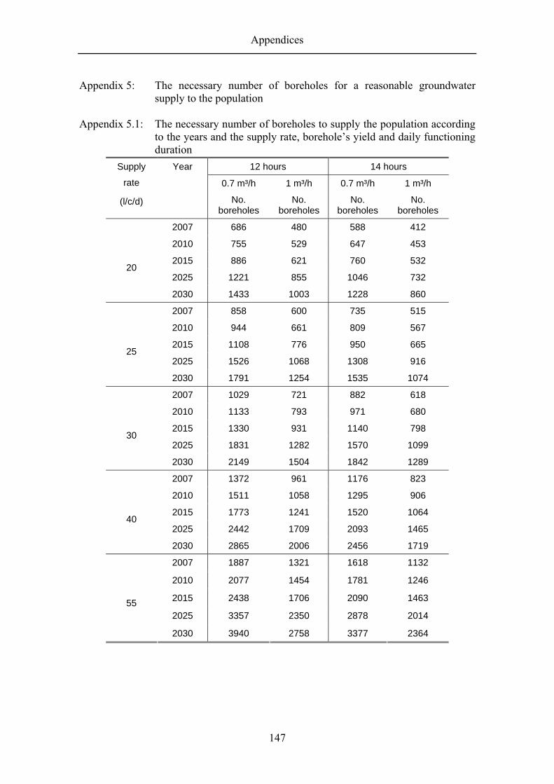
Appendices
147
Appendix 5: The necessary number of boreholes for a reasonable groundwater supply to the population
Appendix 5.1: The necessary number of boreholes to supply the population according
to the years and the supply rate, borehole’s yield and daily functioning duration
12 hours 14 hours
0.7 m³/h 1 m³/h 0.7 m³/h 1 m³/h
Supply
rate
(l/c/d)
Year
No. boreholes
No. boreholes
No. boreholes
No. boreholes
2007 686 480 588 412
2010 755 529 647 453
2015 886 621 760 532
2025 1221 855 1046 732
20
2030 1433 1003 1228 860
2007 858 600 735 515
2010 944 661 809 567
2015 1108 776 950 665
2025 1526 1068 1308 916
25
2030 1791 1254 1535 1074
2007 1029 721 882 618
2010 1133 793 971 680
2015 1330 931 1140 798
2025 1831 1282 1570 1099
30
2030 2149 1504 1842 1289
2007 1372 961 1176 823
2010 1511 1058 1295 906
2015 1773 1241 1520 1064
2025 2442 1709 2093 1465
40
2030 2865 2006 2456 1719
2007 1887 1321 1618 1132
2010 2077 1454 1781 1246
2015 2438 1706 2090 1463
2025 3357 2350 2878 2014
55
2030 3940 2758 3377 2364

Appendices
148
Appendix 5.2: The number of boreholes for water supply to the population of the Kompienga dam basin according to the pump’s yield and the daily withdrawal duration
200
400
600
800
1000
1200
1400
1600
2007 2010 2015 2025 2030
Year
Num
ber o
f bor
ehol
es
12 h/d at 0.7 m³/h 12 h/d at 1 m³/h 14 h/d at 0.7 m³/h 14 h/d at 1 m³/h
Figure 5.2a: Number of boreholes for a supply rate of 20 l/c/d
400
600
800
1000
1200
1400
1600
1800
2000
2007 2010 2015 2025 2030
Year
Num
ber o
f bor
ehol
es
12 h/d at 0.7 m³/h 12 h/d at 1 m³/h 14 h/d at 0.7 m³/h 14 h/d at 1 m³/h
Figure 5.2b: Number of boreholes for a supply rate of 25 l/c/d

Appendices
149
500700900
1100130015001700190021002300
2007 2010 2015 2025 2030
Year
Num
ber o
f bor
ehol
es12 h/d at 0.7 m³/h 12 h/d at 1 m³/h
14 h/d at 0.7 m³/h 14 h/d at 1 m³/h
Figure 5.2c: Number of boreholes for a supply rate of 30 l/c/d
500
1000
1500
2000
2500
3000
2007 2010 2015 2025 2030
Year
Num
ber o
f bor
ehol
es
12 h/d at 0.7 m³/h 12 h/d at 1 m³/h
14 h/d at 0.7 m³/h 14 h/d at 1 m³/h
Figure 5.2d: Number of boreholes for a supply rate of 40 l/c/d

Appendices
150
1000
1500
2000
2500
3000
3500
4000
4500
2007 2010 2015 2025 2030
Year
Num
ber o
f bor
ehol
es12 h/d at 0.7 m³/h 12 h/d at 1 m³/h
14 h/d at 0.7 m³/h 14 h/d at 1 m³/h
Figure 5.2e: Number of boreholes for a supply rate of 55 l/c/d

Appendices
151
Appendix 6: Interviews on the water supply quality in the Kompienga dam basin among the surveyors of the water monitoring points
1. La période la plus exigeante des 4 en suivi des prélèvements d’eau Thiombiano Bapougouni (Kouaré) Période Mai Juin car début des travaux champêtres et dilemme avec le suivi des prélèvements d’eau. Zoumboudre Awa (Comin Yanga) Même réponse que le précédent. Sana Ouahabou (Comin Yanga) Période d’Avril en raison de la très forte chaleur ayant induit une forte affluence des populations aux points d’eau ; ce qui signifie plus de prélèvements et donc de sollicitations en terme de suivi ; spécialement les prélèvements « autres ». Guiguemkoudre Issa (Natiabouani) Aucune des périodes de suivi n’a été plus exigeante que l’autre. Kiemkodogo Harouna (Kompienbiga) Période Nov/Dec due à la non maîtrise et non discernement du travail demandé. Thiombiano Mandia (Kompienbiga) Période de Mars car forte affluence des femmes aux forages et difficultés à bien suivre les prélèvements. Onadja Oumpougla (Pama) Période Fev/Mars avec les fortes affluences des populations aux points d’eau. Combary Kalenli (Djabiga) Période d’Avril Sanfo Pougoumba (Kouaré) Période d’Avril car beaucoup de prélèvements et donc plus de suivi. Thiombiano Baridja (Djabiga) Période Mai/Juin en raison de forte affluence des populations. 2. Les prélèvements nocturnes d’eau et leur ampleur par rapport aux
prélèvements diurnes T. Bapougouni Ils sont apparus seulement durant la période Mai/Juin en raison du démarrage des travaux champêtres sinon inexistants durant les autres périodes en raison de la fermeture de la pompe chaque jour à partir de 19h. Z. Awa Pas de prélèvements nocturnes excepté les enfants qui s’y amusent la nuit à se laver. S. Ouahabou Prélèvements nocturnes existent mais moindres par rapport aux prélèvements journaliers. Les prélèvements nocturnes vont de 18h à 22h et reprennent à partir de 4h du matin le jour suivant. G. Issa Les prélèvements nocturnes existent fortement et sont surtout l’œuvre des hommes. Ils sont estimés à 1,5 fois les prélèvements journaliers en terme de quantité. K. Harouna Les prélèvements existent mais inférieurs à ceux diurnes. T. Mandia Les prélèvements nocturnes sont permanents au niveau de ce forage.

Appendices
152
O. Oumpougla Ils existent et ont été très élevés (>à ceux de jour) en Avril lorsque bon nombre de forages de la ville étaient en panne pendant que les besoins en eau étaient très élevés. C. Kalenli Prélèvements nocturnes inexistants en général. C’est lorsque certains forages tombent en panne qu’apparaissent les prélèvements nocturnes. Le village est suffisamment doté de points d’eau. S. Pougoumba Les prélèvements nocturnes existent surtout en Mars/Avril (période de fortes sollicitations en eau) mais de moindre quantité par rapport aux prélèvements de jour. T. Baridja Ils existent et sont même permanents mais restent de moindre quantité par rapport aux prélèvements journaliers. 3. Coût de l’eau puisée (FCFA) T. Bapougouni Couple du village : 750 F/an dont 250 F/femme et 500 F/homme. Avant 2003 : paiement en argent ou en nature (céréales) suivant les possibilités. En 2003 : 500 F/femme/an, 1500 F/homme/an et 500 F/tête de bœuf/an (petits ruminants exemptés) 2004 : année sabbatique 2005 : 250 F/bœuf/an, 500 F/homme/an et 250 F/femme/an Z. Awa 100 F/femme/mois G. Issa 1800 F/femme/an S. Ouahabou 600 F/femme/homme/an 1000 F/an/propriétaire d’animaux domestiques K. Harouna 300 F/mois/personne prélevant l’eau au forage, 1000 F/personne confectionnant des briques. T. Mandia 200 F/femme/mois O. Oumpougla Point d’eau à grand diamètre ; eau gratuite. C. Kalenli 150 F/femme/mois puis 100 F/femme/mois depuis 2004. S. Pougoumba 1500 F/femme/an et 1000 F/homme/an T. Baridja 100 F/femme/mois 4. Durée journalière moyenne de suivi des prélèvements d’eau T. Bapougouni 6h-18h sans discontinuité dès l’ouverture de la pompe dont je suis le détenteur de la clé. Z. Awa 6h-18h

Appendices
153
S. Ouahabou 6h-18h, chaque jour. G. Issa 6h ou 7h à 18h ou 19h. K. Harouna 6h-19h et rupture de 10h à 11h pour déjeuner pendant 15-20 mn. S. Pougoumba 6h-18h/19h T. Baridja Du lever au coucher du jour. 5. Périodes journalières de prélèvements d’eau T. Baridja A tout moment sans discontinuité durant les périodes chaudes de l’année. Alors que pendant le froid et les pluies les fortes fréquentations vont de 11h à 13h ; le reste de la journée est à faible fréquentation. S. Pougoumba Pendant la période de chaleur : 6h-10h puis 14h-17h. Pendant la période du froid : matin et midi. C. Kalenli Grande affluence : 6h-11h et 15h-17h/18h Faible affluence : 12h-14h O. Oumpougla Pendant la période de chaleur (Février-Mars) : affluence sans discontinuité. Autres périodes de l’année : du matin jusqu'à 11h puis 14h-18h/19h. T. Mandia Période de chaleur : du matin jusqu'à la nuit sans discontinuer Autres périodes : du matin à 10h puis de 15h à la nuit. K. Harouna Pompage permanent sans discontinuer quelque soit le jour. G. Issa A toutes les périodes de l’année, affluence des femmes au forage sans discontinuité du matin au soir mais périodes de chaleur encore très affluente. S. Ouahabou 5h-11h et 14h-18h : très forte affluence journalière. 11h-14h : légère affluence. Z. Awa 8h-12h puis 14h-18h. T. Bapougouni 6h-11h et 15h-18h/19h, forte affluence ; 11h-15h, faible affluence mais considérable en période de chaleur. 6. Quantité d’eau prélevée suivant le nombre d’éléments dans la famille et les
périodes de l’année S. Ouahabou L’eau du forage est insuffisante. En saison sèche, notre famille de 30 personnes environ n’est jamais complètement satisfaite à hauteur de ses besoins journaliers de 20 à 25 grands plats.
Appendices
154
G. Issa Pour une famille de 13 personnes utilisant 2 grandes barriques d’eau par jour, il est difficile d’obtenir ces quantités durant les périodes chaudes de l’année (Février à Avril). Roucky (Natiabouani) Notre famille de 3 personnes est largement satisfaite tous les jours avec 3 grands plats d’eau. K. Harouna Pour notre famille de 20 personnes, 20 grands plats et 5 petits plats environ sont nécessaires pour nos besoins journaliers. Il est difficile de pouvoir satisfaire ces besoins dans les mois de Novembre à Mars : baisse alors des quantités à 15-18 grands plats par jour. O. Oumpougla Famille de 8 personnes avec des besoins quotidiens en eau de 7 grands plats environ satisfaits à chaque moment de l’année avec quelque fois une augmentation des quantités journalières passant à 9 grands plats. C. Kalenli Les besoins journaliers peuvent être estimés à environ 16 grands plats + 6 plats moyens et 6 grands bidons pour notre famille de 16 personnes. Ces volumes sont facilement acquis chaque jour sans difficulté. S. Pougoumba Notre famille de 25 personnes arrivent difficilement a satisfaire ses besoins en Avril (période de grande chaleur) et se contente des quantités disponibles. T. Baridja Famille de 32 personnes environ, nos besoins journaliers en eau de 3 grandes barriques sont toujours satisfaits tout au long de l’année sans problème. 7. Les pannes des pompes et les réparations T. Baridja Forage de 3 ans d’age, n’est pas encore tombé en panne. S. Pougoumba Forage de 15 ans d’age environ et 1 panne par mais 3 pannes certaines années. Les réparations sont payées à hauteur de 20 000 à 25 000 FCFA parfois 50 000 FCFA à partir des ressources des cotisations collectées par 3 personnes différentes. C. Kalenli Forage en panne pour la première fois depuis 2003, année de son implantation. O. Oumpougla Puits à débits faibles à partir de Mars jusqu’en Mai. Il n’y a donc pas de panne ni de réparations quelconques. T. Mandia Forage implanté en 2001, il n’y a encore pas de panne. K. Harouna Les redevances mensuelles collectées et gérées par un vieux à sa guise (sans contrôle) sont sensées servir aux réparations des pompes du village. Mais un forage en panne depuis un mois demeure ainsi sans réparation jusqu'à nos jours. G. Issa Le forage du village a été réalisé en 2002 et est tombé en panne pour la première fois en Juin 2005 et réparé à 99000 FCFA sur les cotisations annuelles collectées. S. Ouahabou

Appendices
155
Forage réalisé en 1992 avec 3 pannes enregistrées et réparées sur les cotisations collectées annuellement. Z. Awa Forage de 2001, pas de panne jusqu'à ce jour.
ACKNOWLEDGEMENTS
I thank God, the Almighty, for all the circumstances that made possible for me to
achieve successfully this study. Meanwhile I want to, first of all, thank GLOWA Volta
project that has involved my belonging research institute; INERA. Through GLOWA
Volta project, my thanks and gratitude go to German people and their government with
BMBF Ministry for granting me funds for the research undertaken within the
framework of the project.
Special thanks are due to Prof. Dr P. L. G. Vlek, Director of ZEF and hereby
supervisor of my research for all the supports he provided me for the best completion of
my research. To Prof. Dr Ir N. C. van de Giesen, my sincere and profound gratitude is
addressed to you for everything I did within this study since my application until the
thesis completion through field and office works, daily advices and sound guidance
during my writing. Prof. Nick, I am infinitely grateful to you. To Prof. Dr - Ing. Dr h. c.
J. J. Bogardi, Director of UNU-EHS (Bonn, Germany), I cannot express enough my
gratitude to you for supervising my research. I am deeply grateful to you for your huge
contribution to this research achievement. I owe my gratitude to Dr C. Rodgers,
GLOWA Volta project Coordinator and tutor of my research, for his sound and
immense contributions with comments and close assistance in finalizing this
dissertation.
Dr V. Konrad, GLOWA Volta project Coordinator in Burkina Faso, I
gratefully acknowledge your kind assistance during my fieldwork. Dr B. Amisigo and
Dr B. Tischbein, senior researchers in ZEFc are highly acknowledged. I am grateful to
D. Rupprecht and K. Kremer in University of Bonn for their assistance in analyzing the
chloride concentration of the water samples brought from Burkina Faso. I deeply
acknowledge Dr M. Günther and the assistants of BIGS-DR, ZEFc secretariat staff, M.
Volker and L. Hammer for administrative and academic assistances. I am grateful to M.
Jend for taking time to meticulously read and substantially improve my thesis.
I wouldn’t be able to undertake this research without the consent of the
research structures of my country. I present my regards to Pr G. Konaté (Director of
INERA), Pr H. Boly, Pr B. L. Guissou (Director of CNRST), Dr V. Hien and Mr T.
Traoré. My special thanks go to Dr L. Thiombiano who was the first suggesting my
application to ZEF doctoral program under GLOWA Volta project framework. I am

deeply indebted to you for this success topping your efforts to provide me with
sufficient in-depth research skill. I owe my regards to University of Ouagadougou and
specially Pr N. A. Savadogo and Dr Y. Koussoubé of the hydrogeology laboratory for
their kind assistance with advices and sound recommendations during my field works.
My thanks go to VINVAL project, ARFA and governmental structures in
Burkina Faso (SONABEL, BUMIGEB, MAHRH/DRAHRH-Est, PPB/Est, ONEA/Kpg,
GIRE, MEF/DPD-Est, CD/MAHRH, CIRD, DGRE, Direction nationale de la
météorologie …) which easily provided me with data requested, documents and field
equipments.
My gratitude to colleagues in ZEF with especial thanks to L. Tia for his
invaluable contribution to this research, F. Bagayoko, B. K. Nyarko, D. S. Kpongor, H.
Compaoré, A. Sessouma, R. T. Capote-Fuentes for helps, encouragements and well-
living supports they provided me all along the study duration in Germany. Colleagues in
INERA, mainly Dr N. Koné, Dr J. M. Dipama, O. Kaboré,… who did their best in
assisting me during my field works, you deserve my gratitude. Population and field
assistants in the study area, please find through this thesis, the results of your kind
contributions and efforts to assist me, and above all, my acknowledgements and
profound gratitude.
To my parents Simon-Pierre and P. Zougmoré, I specially owe this success to
you and gratefully thank you for your cares, encouragements and moral endurance to
see me leaving for this study abroad. All my brothers, sisters, parents and friends are
also acknowledged for their various contributions to this success.
Finally but not least, I address my profound and sincere gratitude to my nuclear
family, my wife Thérèse Noélie and our twins Elvis and Edwige, for their patience and
moral endurance during these months of absence, and their prayers to support me
completing successfully this study. I dedicate this thesis to you.


![[Adresse 1] - Stahlbau Zentrum Schweiz · 5.2 Situation initiale 5.3 Termes et définition ... Les revêtements se mettent à gonfler sous l’effet de la chaleur (dès 120–200](https://img.pdfslide.fr/doc/110x75/5b9c83b309d3f29b498ccd99/adresse-1-stahlbau-zentrum-52-situation-initiale-53-termes-et-definition.jpg)