Appendix
A1. Laws of probability
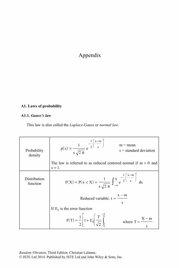
A1.1. Gauss’s law
This law is also called the Laplace-Gauss or normal law.
Probabilitydensity
( )p xs
e
x m
s=−
−
1
2
1
2
2
π
m = means = standard deviation
The law is referred to as reduced centered normal if m = 0 ands = 1.
Distributionfunction ( ) ( )F X P x X
se dx
x m
sX= < =
−−
−∞1
2
1
2
2
π
Reduced variable: tx m
s=
−
If E1 is the error function
( )F T ET
= +
1
21
21 where T
X m
s=
−
Random Vibration, Third Edition. Christian Lalanne.© ISTE Ltd 2014. Published by ISTE Ltd and John Wiley & Sons, Inc.
512 Random Vibration
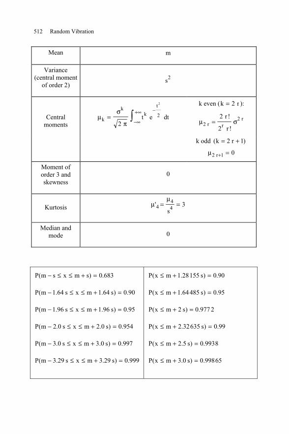
Mean m
Variance(central moment
of order 2)s2
Centralmoments
μσ
πk
kk
t
t e dt=−
−∞
+∞2
2
2
k even (k r= 2 ):
μ σ222
2r r
rr
r=
!
!
k odd )1r2k( +=
μ2 1 0r+ =
Moment oforder 3 andskewness
0
Kurtosis μμ
'444 3= =s
Median andmode 0
P(m s x m s) 0.683− ≤ ≤ + =
P(m 1.64 s x m 1.64 s) 0.90− ≤ ≤ + =
P(m 1.96 s x m 1.96 s) 0.95− ≤ ≤ + =
P(m 2.0 s x m 2.0 s) 0.954− ≤ ≤ + =
P(m 3.0 s x m 3.0 s) 0.997− ≤ ≤ + =
P(m 3.29 s x m 3.29 s) 0.999− ≤ ≤ + =
P(x m 1.28155 s) 0.90≤ + =
P(x m 1.64485 s) 0.95≤ + =
P(x m 2 s) 0.9772≤ + =
P(x m 2.32635 s) 0.99≤ + =
P(x m 2.5 s) 0.9938≤ + =
P(x m 3.0 s) 0.99865≤ + =
Appendix 513
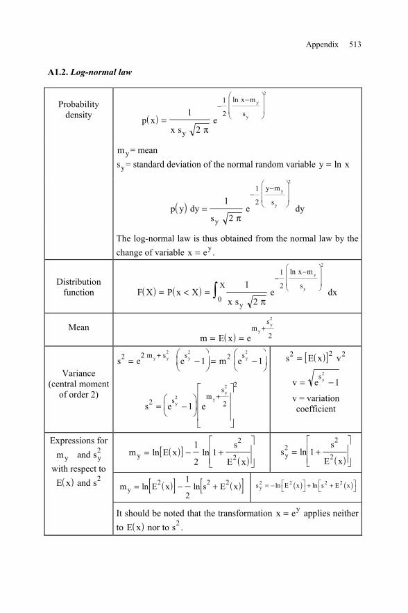
A1.2. Log-normal law
Probabilitydensity ( )p x
x se
y
x m
sy
y=−
−
1
2
1
2
2
π
ln
my= meansy= standard deviation of the normal random variable y x= ln
( )p y dys
e dyy
y m
sy
y=−
−
1
2
1
2
2
π
The log-normal law is thus obtained from the normal law by thechange of variable x ey= .
Distributionfunction ( ) ( )F X P x X
x se dx
y
x m
sXy
y= < =−
−
1
2
1
2
0
2
π
ln
Mean( )m E x e
ms
yy
= =+
2
2
Variance(central moment
of order 2)
s e e m em s s sy y y y2 2 2
2 2 2
1 1= −
= −
+
s e es m
s
yy
y
2 2
22
2
1= −
+
( )[ ]s E x v2 2 2=
v esy= −2
1
v = variationcoefficient
Expressions formy and sy
2
with respect to( )E x and s2
( )[ ]( )
m E xs
E xy = − +
ln ln1
21
2
2 ( )s
s
E xy2
2
21= +
ln
( )[ ] ( )[ ]m E x s E xy = − +ln ln2 2 21
2( ) ( )2 2 2 2
ys ln E x ln s E x = − + +
It should be noted that the transformation x ey= applies neitherto ( )E x nor to s2 .
514 Random Vibration
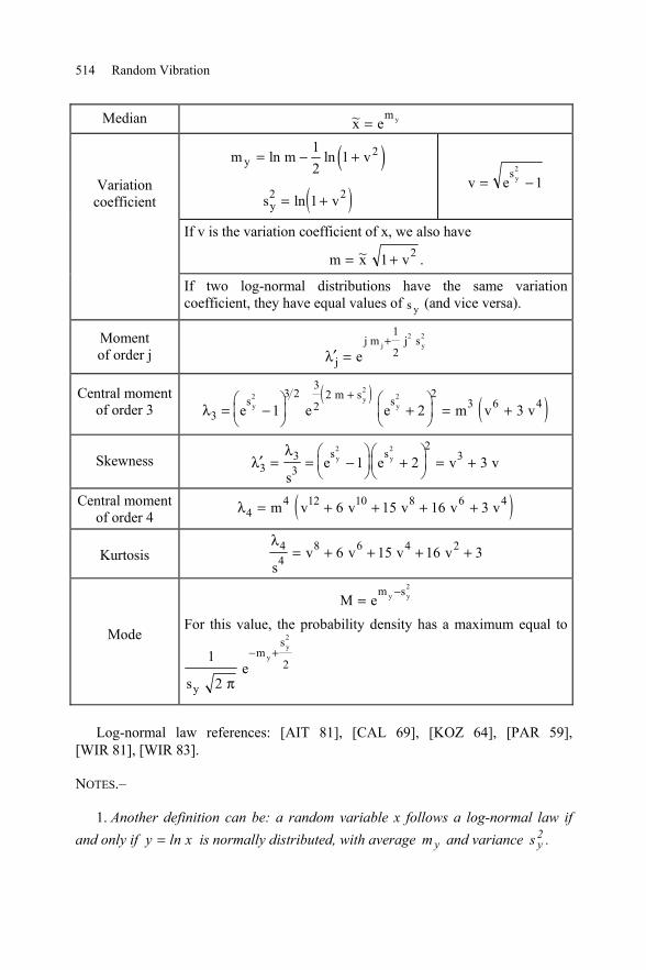
Median ~x em y=
Variationcoefficient
( )2y1
m ln m ln 1 v2
= − +
( )s vy2 21= +ln
v esy= −2
1
If v is the variation coefficient of x, we also have
m x v= +~ 1 2 .
If two log-normal distributions have the same variationcoefficient, they have equal values of s y (and vice versa).
Momentof order j ′ =
+λ j
j m j se
j y
1
22 2
Central momentof order 3
( ) ( )λ33 2
3
22 2
3 6 42
22
1 2 3= −
+
= +
+e e e m v vs m s sy
yy
Skewness ′ = = −
+
= +λ
λ3
33
23
2 2
1 2 3s
e e v vs sy y
Central momentof order 4 ( )λ4
4 12 10 8 6 46 15 16 3= + + + +m v v v v v
Kurtosisλ44
8 6 4 26 15 16 3s
v v v v= + + + +
Mode
M em sy y=
− 2
For this value, the probability density has a maximum equal to
1
2
2
2
se
y
ms
yy
π
− +
Log-normal law references: [AIT 81], [CAL 69], [KOZ 64], [PAR 59],[WIR 81], [WIR 83].
NOTES.–
1. Another definition can be: a random variable x follows a log-normal law ifand only if y ln x= is normally distributed, with average ym and variance 2
ys .
Appendix 515
2. This law has several names: the Galton, Mc Alister, Kapteyn, Gibrat law orthe logarithmic-normal or logarithmo-normal law.
3. The definition of the log-normal law can be given starting from base 10logarithms 10( y log x )= :
( )
210 y
y
log x m12 s
y
1p x e
x s 2 ln 10π
−−
= [A1.1]
With this definition for base 10 logarithms, we have:
y 10m log x= [A1.2]
( )2y 10 y1
m log s 0.4342m 10
+ = [A1.3]
2ys 0.434v 10 1= − [A1.4]
( )2y 10 101
m log x log 1 v2
= − + [A1.5]
( )2 2y 10s 0.434 log 1 v= + [A1.6]
Hereafter, we will consider only the definition based on Napierian logarithms.
4. Some authors make the variable change defined by y 20 log x= , y beingexpressed in decibels. We then have:
2ys 75.44v e 1= − [A1.7]
since220
75.44ln 10
≈
.
5. Depending on the values of the parameters ym and ys , it can sometimes be
difficult to imagine a priori which law is best adjusted to a range of experimental
516 Random Vibration
values. A method making it possible to choose between the normal law and thelognormal law consists of calculating:
– the variation coefficients
vm
= ;
– the skewness 33s
λ;
– the kurtosis 44s
λ;
knowing that
( )i
ix
E x mn
= =
[A1.8]
( )2i2 i
x m
sn
−
=
[A1.9]
( )3ii
3
x m
nλ
−
=
[A1.10]
and
( )4ii
4
x m
nλ
−
=
[A1.11]
If the skewness is close to zero and the kurtosis is close to 3, the normal law is
that which is best adjusted. If v 0.2< and 3 3v
λ ′≈ , the log-normal law is
preferable.
A1.3. Exponential law
This law is often used with reliability where it expresses the time expired up tofailure (or the time interval between two consecutive failures).
Appendix 517
Probability density ( )p x e x= −λ λ
Distribution function ( ) ( )F X P x X e X= < = − −1 λ
Mean ( )m E x11
= =λ
Moments mn n
mn n n= = −!
λ λ1
Variance (central momentof order 2) s2 2
1=
λ
Central moments μλ
μn nn
= + −1 1
Variation coefficient v = 1
Moment of order 3(skewness) ′ = = +μ
μλ3
33
3 3s
Kurtosis ′ = + +μ λ λ44 34 12
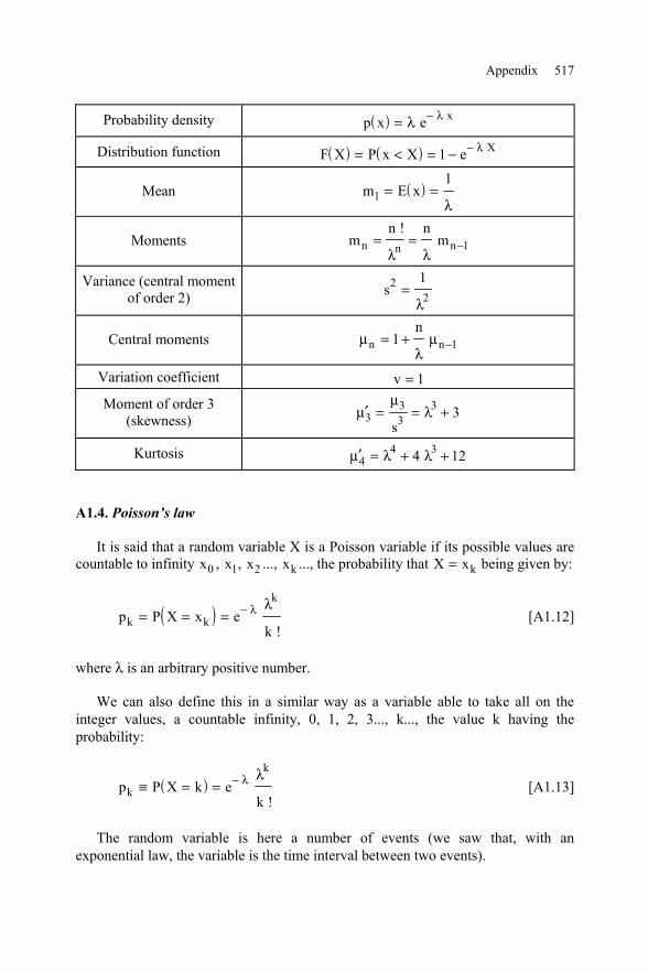
A1.4. Poisson’s law
It is said that a random variable X is a Poisson variable if its possible values arecountable to infinity x0 , x1, x2 ..., xk ..., the probability that X xk= being given by:
( )p P X x ek
k k
k
= = = − λ λ
![A1.12]
where λ is an arbitrary positive number.
We can also define this in a similar way as a variable able to take all on theinteger values, a countable infinity, 0, 1, 2, 3..., k..., the value k having theprobability:
( )p P X k ek
k
k
≡ = = − λ λ
![A1.13]
The random variable is here a number of events (we saw that, with anexponential law, the variable is the time interval between two events).
518 Random Vibration
Distribution function ( ) ( )F X P x X ek
k
k
n= ≤ < = −
=0
0
λ λ
!(n X n< ≤ + 1)
Mean ( )m E x k ek
k
k1
0
= = =−
=
∞
λ λλ
!
Moment of order 2 ( )m2 1= +λ λ
Variance (centralmoment of order 2)
s2 = λ
Central momentsμ λ3 =
μ λ λ423= +
Variation coefficient v =1
λ
Skewness ′ =μλ
31
Kurtosis ′ =+
μλ
λ4
1 3
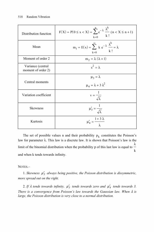
The set of possible values n and their probability pk constitutes the Poisson’slaw for parameter λ. This law is a discrete law. It is shown that Poisson’s law is the
limit of the binomial distribution when the probability p of this last law is equal toλ
kand when k tends towards infinity.
NOTES.–
1. Skewness 3μ ′ always being positive, the Poisson distribution is dissymmetric,more spread out on the right.
2. If λ tends towards infinity, 3μ ′ tends towards zero and 4μ ′ tends towards 3.There is a convergence from Poisson’s law towards the Gaussian law. When λ islarge, the Poisson distribution is very close to a normal distribution.
Appendix 519
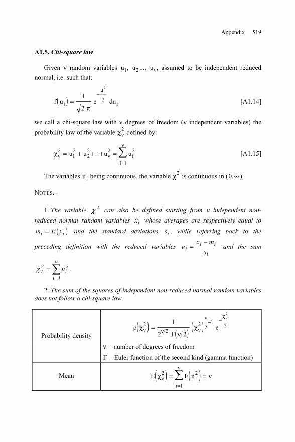
A1.5. Chi-square law
Given ν random variables u1, u2 ..., uν, assumed to be independent reducednormal, i.e. such that:
( )f u e dui
u
i
i
=−1
2
2
2
π[A1.14]
we call a chi-square law with ν degrees of freedom (ν independent variables) theprobability law of the variable χν
2 defined by:
χν ν
ν2
12
22 2 2
1
= + + + ==u u u u ii
[A1.15]
The variables u i being continuous, the variable χ2 is continuous in (0,∞ ).
NOTES.–
1. The variable 2χ can also be defined starting from ν independent non-reduced normal random variables ix whose averages are respectively equal to
( )i im E x= and the standard deviations is , while referring back to the
preceding definition with the reduced variables i ii
i
x mu
s−
= and the sum
2 2i
i 1u
ν
νχ=
= .
2. The sum of the squares of independent non-reduced normal random variablesdoes not follow a chi-square law.
Probability density( ) ( ) ( )p eχ
νχν ν ν
ν χν
22
2 21
21
2 2
2
=− −
Γ
ν = number of degrees of freedomΓ = Euler function of the second kind (gamma function)
Mean ( ) ( )E E u ii
χ νν
ν2 2
1
= ==
520 Random Vibration
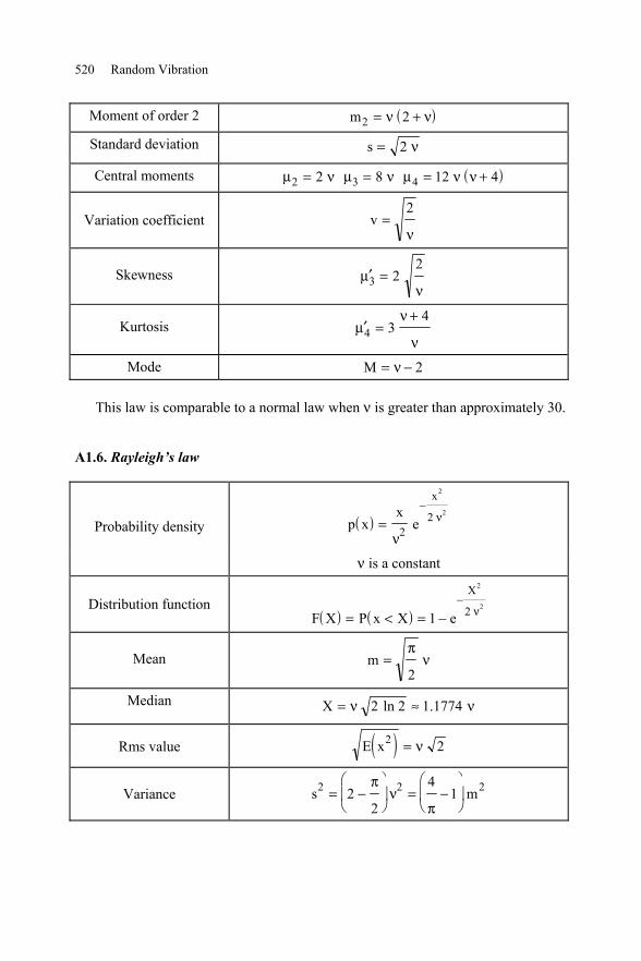
Moment of order 2 ( )m2 2= +ν ν
Standard deviation s = 2 ν
Central moments μ ν2 2= μ ν3 8= ( )μ ν ν4 12 4= +
Variation coefficient v =2
ν
Skewness ′ =μν
3 22
Kurtosis ′ =+
μν
ν4 3
4
Mode M = −ν 2
This law is comparable to a normal law when ν is greater than approximately 30.
A1.6. Rayleigh’s law
Probability density ( )p xx
e
x
=−
νν
22
2
2
ν is a constant
Distribution function( ) ( )F X P x X e
X
= < = −−
1
2
22 ν
Mean m =π
ν2
Median ν≈ν= 1774.12ln2X
Rms value ( )E x2 2= ν
Variance s m2 2 222
41= −
= −
πν
π
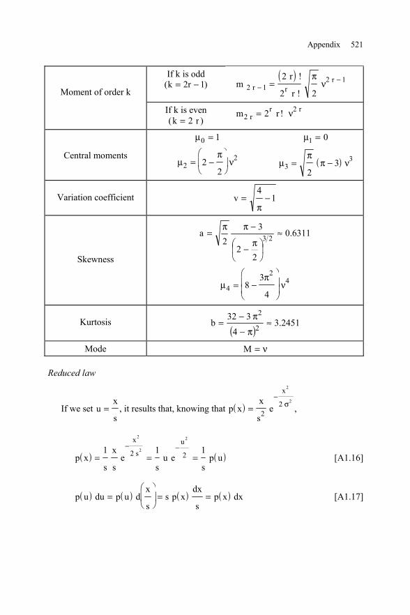
Appendix 521
Moment of order k
If k is odd)1r2k( −=
( )m
r
rr r
r2 1
2 12
2 2−
−=!
!
πν
If k is even(k r= 2 )
m rrr r
222= ! ν
Central moments
μ0 1=
μπ
ν222
2= −
μ1 0=
( )μπ
π ν33
23= −
Variation coefficient v = −4
1π
Skewness
6311.0
22
32
a 23 ≈
π−
−ππ=
μπ
ν4
248
3
4= −
Kurtosis( )
2451.34
332b 2
2≈
π−
π−=
Mode M = ν
Reduced law
If we set ux
s= , it results that, knowing that ( )p x
x
se
x
=−
22
2
2σ ,
( ) ( )p xs
x
se
su e
sp u
x
su
= = =− −1 1 1
2
2
2
2 2 [A1.16]
( ) ( ) ( ) ( )p u du p u dx
ss p x
dx
sp x dx=
= = [A1.17]
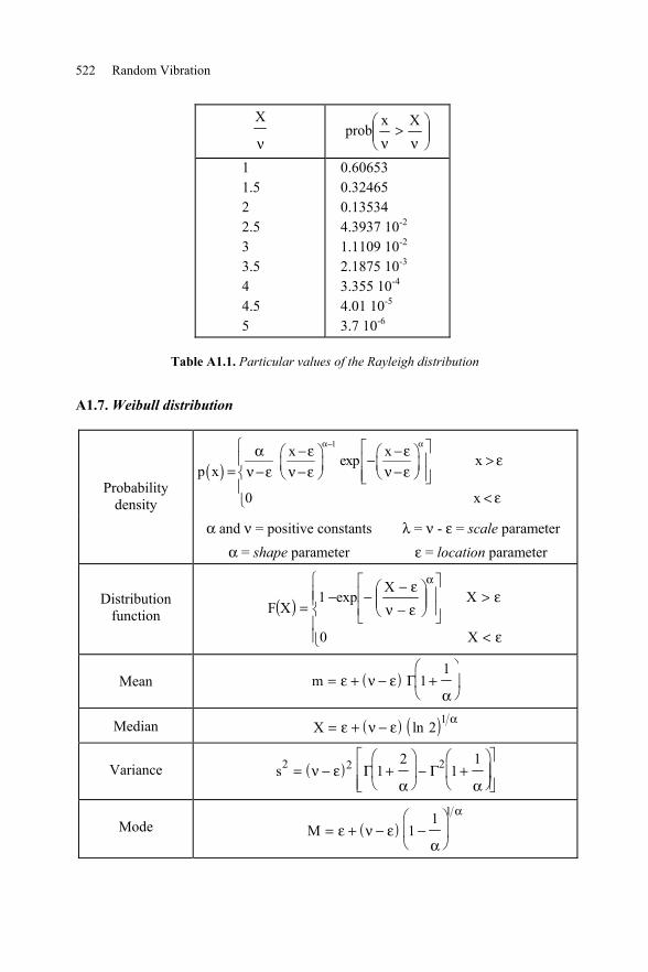
522 Random Vibration
X
ν
ν>
νXx
prob
11.522.533.544.55
0.606530.324650.135344.3937 10-2
1.1109 10-2
2.1875 10-3
3.355 10-4
4.01 10-5
3.7 10-6
Table A1.1. Particular values of the Rayleigh distribution
A1.7.Weibull distribution
Probabilitydensity
( )1x xexp x
p x
0 x
α− α α −ε −ε − > ε = ν −ε ν −ε ν −ε
< ε
α and ν = positive constantsα = shape parameter
λ = ν - ε = scale parameterε = location parameter
Distributionfunction ( )
ε<
ε>
ε−νε−
−−=
α
X0
XX
exp1XF
Mean ( )m = + − +
ε ν ε
αΓ 1
1
Median ( ) ( )X = + −ε ν ε αln 2 1
Variance ( )s2 2 212
11
= − +
− +
ν εα α
Γ Γ
Mode ( )M = + − −
ε ν ε
α
α
11 1
Appendix 523
Weilbull distribution references: [KOZ 64], [PAR 59].
NOTE.–
We sometimes use the constant η ν ε= − in the above expressions.
A1.8. Normal Laplace-Gauss law with n variables
Let us set x1, x2 ..., xn n random variables with zero average. The normal lawwith n variable xi is defined by its probability density:
( ) ( )p x x x MM
M x xnn
iji j
n
i j1 22 1 22
1
2, , , exp
,
= −
− − π [A1.18]
where M is the determinant of the square matrix:
M
n
n
n n nn
=
μ μ μ
μ μ μ
μ μ μ
11 12 1
21 22 2
1 2
[A1.19]
( )μij i jE x x= =, moments of order 2 of the random variables
M ij = cofactor of μij in M .
Examples
1. n = 1
( ) ( )p x MM
Mx1
1 2 1 2 11122
1
2= −
− −π exp
with
M = μ11
M = μ11
524 Random Vibration
M11 1=
( )μ11 12 2= =E x s
yielding
( )p xs
e
x
s1
21
2
12
2
=−
π[A1.20]
which is the probability density of a one-dimensional normal law as definedpreviously.
2. n = 2
( ) ( ) (p x x MM
M x1 21 1 2
11 122
1
2, exp= −
− −π
)+ + + M x x M x x M x12 1 2 21 2 1 22 2
2 [A1.21]
with
M =μ μ
μ μ11 12
21 22M = −μ μ μ μ11 22 12 21
( )μ11 12
12= =E x s M11 22= μ
( ) ( )μ μ ρ12 1 2 2 1 21 1 2= = = =E x x E x x s s M M12 21 12 21= − = − =μ μ
( )μ22 22
22= =E x s M22 11= μ
ρ is the coefficient of linear correlation between the variables x1 and x2 ,defined by:
( )( ) ( )
ρ =cov ,x x
s x s x1 2
1 2
[A1.22]
where ( )2x,1xcov is the covariance between the two variables x1 and x2 :
Appendix 525
( ) ( )[ ] ( )[ ] ( ) 2121221121 dxdxx,xpXExXExX,Xcov −−= +∞
∞−[A1.23]
The covariance can be negative, zero or positive. It is zero when x1 and x2 arecompletely independent variables. Conversely, a zero covariance is not a sufficientcondition for x1 and x2 to be independent.
It is shown that ρ is included in the interval [ ]1,1− . ρ = 1 is a necessary andsufficient condition of linear dependence between x1 and x2 .
This yields
( ) ( )p x xs s
x
s
x x
s s
x
s1 2
1 22 2
1
1
21 2
1 2
2
2
21
2 1
1
2 12, exp=
−−
−
− +
π ρ ρ
ρ
[A1.24]
NOTE.–
If the averages were not zero, we would have
( ) ( )( ) 2
1 11 2 22 11 2
x E x1 1p x , x exp
s2 12 s s 1 ρπ ρ
− = − − −
( ) ( ) ( ) 21 1 2 2 2 2
1 2 2
x E x x E x x E x2
s s sρ
− − − − +
[A1.25]
If ρ = 0 , we can write ( ) ( ) ( )p x , x p x p x1 2 1 2= where
( )p xs
e
x
s1
1
21
2
12
12
=−
πand ( )p x
se
x
s2
2
21
2
22
22
=−
π. x1 and x2 are independent
random variables.
526 Random Vibration
It is easily shown that, by using the reduced centered variables( )
tx E x
s1
1 1
1
=−
and( )
tx E x
s2
2 2
2
=−
,
( )p x x dx dx1 2 1 2 1=−∞
+∞
−∞
+∞ [A1.26]
Indeed, with these variables,
( ) ( ) ( )p t ts s
t t t t1 21 2
2 2 12
1 2 221
2 1
1
2 12, exp=
−−
−− +
π ρ ρρ
[A1.27]
and
( ) ( )t t t t t t t12
1 2 22
1 22 2
222 1− + = − + −ρ ρ ρ [A1.28]
Let us set ut t
=−
−
1 221
ρ
ρand calculate
1
2
2222 2
2π
e e dt duu t− −−∞
+∞
−∞
+∞ [A1.29]
i.e.
1
2
1
2
2222 2
2π π
e du e dtu t−−∞
+∞ −−∞
+∞ . [A1.30]
We thus have
( ) ( )p u du p t dt2 2 1−∞
+∞
−∞
+∞ = [A1.31]
NOTE.–
It is shown that, if the terms ijμ are zero when i j≠ , i.e. if all the correlationcoefficients of the variables xi and x j are zero (i j≠ ), we have:
Appendix 527
11
nn
0 00 0
M0 00 0 0
μ
μ
=
[A1.32]
n
iii 1
M μ=
= ∏
ijM 0= if i j≠
ijii
MM
μ= if i j=
and
( ) ( )n 2
1 2n 2 i1 2 n
iii 1
1 xp x , x , , x 2 M exp
2π
μ−−
=
= −
[A1.33]
( ) ( )n
1 2 n ii 1
p x , x , x p x=
= ∏ [A1.34]
For normally distributed random variables, it is sufficient that the cross-correlation functions are zero for these variables to be independent.
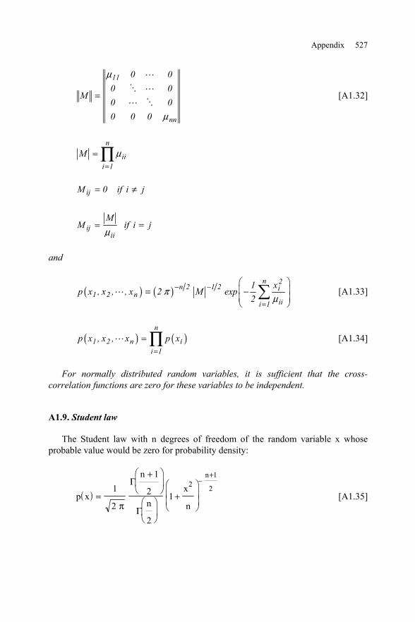
A1.9. Student law
The Student law with n degrees of freedom of the random variable x whoseprobable value would be zero for probability density:
( )p x
n
nx
n
n
=
+
+
−+
1
2
1
2
2
12
1
2
π
Γ
Γ[A1.35]
528 Random Vibration
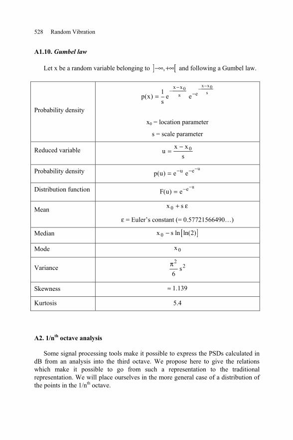
A1.10. Gumbel law
Let x be a random variable belonging to ] [,−∞ +∞ and following a Gumbel law.
Probability density
x x00s
x xes1
p(x) e es
−−−
− −=
x0 = location parameter
s = scale parameter
Reduced variable 0x xu
s−
=
Probability density uu ep(u) e e−− −=
Distribution function ueF(u) e−−=
Mean 0x s+ ε
ε = Euler’s constant (= 0.57721566490…)
Median [ ]0x s ln ln(2)−
Mode 0x
Variance2
2s6
π
Skewness 1.139≈
Kurtosis 5.4
A2. 1/nth octave analysis
Some signal processing tools make it possible to express the PSDs calculated indB from an analysis into the third octave. We propose here to give the relationswhich make it possible to go from such a representation to the traditionalrepresentation. We will place ourselves in the more general case of a distribution ofthe points in the 1/nth octave.
Appendix 529
A2.1. Center frequencies
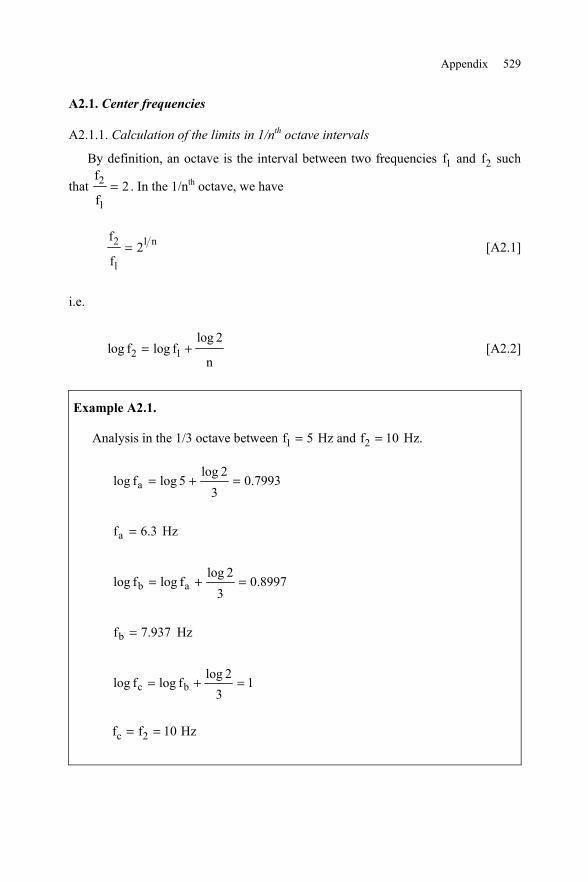
A2.1.1. Calculation of the limits in 1/nth octave intervals
By definition, an octave is the interval between two frequencies f1 and f2 such
thatf
f2
1
2= . In the 1/nth octave, we have
f
fn2
1
12= [A2.1]
i.e.
log loglog
f fn
2 12
= + [A2.2]
Example A2.1.
Analysis in the 1/3 octave between f1 5= Hz and f2 10= Hz.
7993.032log
5logflog a =+=
3.6fa = Hz
8997.032log
flogflog ab =+=
937.7fb = Hz
132log
flogflog bc =+=
f fc = =2 10 Hz

530 Random Vibration
A2.1.2. Width of the interval fΔ centered around f
The width of this interval is equal to
limitlowerlimitupperf −=Δ
Figure A2.1. Frequency interval
Let α be a constant characteristic of width Δf (Figure A2.1) such that:
( ) ( )log log log loglog
f fn
+ − − =α α2
[A2.3]
yielding
α = 21 2n [A2.4]
We deduce
Δf ff
= −αα
[A2.5]
Δf f= −
α
α
1[A2.6]
This value of Δf is particularly useful for the calculation of the rms value of avibration defined by a PSD expressed in dB.
Example A2.2.
For 3n = , it results that 122462.1≈α and f231563.0f ≈Δ . At 5 Hz, wehave 15.1f =Δ Hz.
Appendix 531
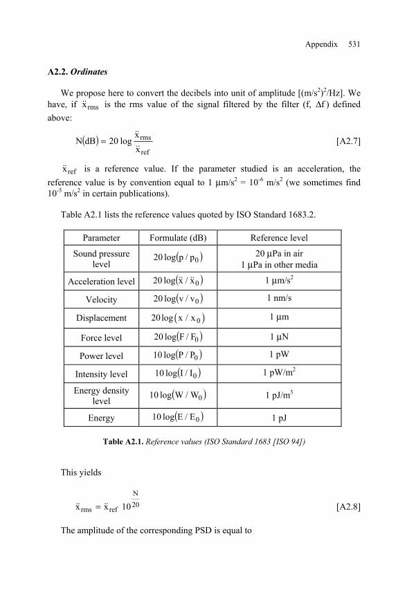
A2.2. Ordinates
We propose here to convert the decibels into unit of amplitude [(m/s2)2/Hz]. Wehave, if rmsx is the rms value of the signal filtered by the filter (f, Δf ) definedabove:
( )ref
rms
xx
log20dBN
= [A2.7]
refx is a reference value. If the parameter studied is an acceleration, thereference value is by convention equal to 1 μm/s2 = 10-6 m/s2 (we sometimes find10-5 m/s2 in certain publications).
Table A2.1 lists the reference values quoted by ISO Standard 1683.2.
Parameter Formulate (dB) Reference level
Sound pressurelevel
( )0p/plog20 20 μPa in air1 μPa in other media
Acceleration level ( )0x/xlog20 1 μm/s2
Velocity ( )0v/vlog20 1 nm/s
Displacement ( )020log x / x 1 μm
Force level ( )0F/Flog20 1 μN
Power level ( )0P/Plog10 1 pW
Intensity level ( )0I/Ilog10 1 pW/m2
Energy densitylevel
( )0W/Wlog10 1 pJ/m3
Energy ( )0E/Elog10 1 pJ
Table A2.1. Reference values (ISO Standard 1683 [ISO 94])
This yields
20N
refrms 10xx = [A2.8]
The amplitude of the corresponding PSD is equal to
532 Random Vibration
f10x
fx
G10N
2ref
2rms
Δ=
Δ=
[A2.9]
f10x
12
2G
10N
2ref
n1
n21
−= [A2.10]
or
−=
refn21
n1
xGf
2
12log10N
[A2.11]
Example A2.3.
If 5ref 10x −= m/s2
Gf
N
=
−1010
10
Δ
and if n = 3
Gf
N
=−
−2
2 1
101 6
1 3
1010
Gf
N
≈
−10
0 23
1010
.
If, at 5 Hz, the spectrum gives N = 50 dB,
G =−
−2
2 1
10
5
1 6
1 3
50
1010
6106369.8G −≈ (m/s2)2/Hz.
Appendix 533
A3. Conversion of an acoustic spectrum into a PSD
A3.1. Need
When the real environment is an acoustic noise, it is possible to evaluate thevibratory levels induced by this noise in a structure and the stresses which resultfrom it using finite element calculation software.
At the stage of the writing of specifications, we do not normally have such amodel of the structure. It is nevertheless very important to obtain an evaluation ofthe vibratory levels for the dimensioning of the material.
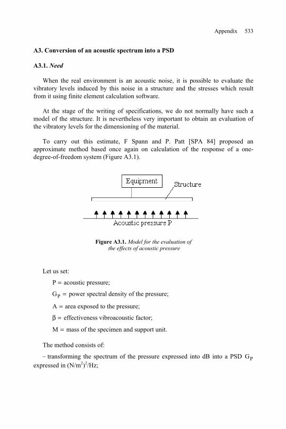
To carry out this estimate, F Spann and P. Patt [SPA 84] proposed anapproximate method based once again on calculation of the response of a one-degree-of-freedom system (Figure A3.1).
Figure A3.1.Model for the evaluation ofthe effects of acoustic pressure
Let us set:
P = acoustic pressure;
GP = power spectral density of the pressure;
A = area exposed to the pressure;
β = effectiveness vibroacoustic factor;
M = mass of the specimen and support unit.
The method consists of:
– transforming the spectrum of the pressure expressed into dB into a PSD GPexpressed in (N/m2)2/Hz;
534 Random Vibration
– calculating, in each frequency interval (in general in the third octave), theresponse of an equivalent one-degree-of-freedom system from the value of the PSDpressure, the area A exposed to the pressure P and the effective mass M;
– smoothing the spectrum obtained.
A3.2. Calculation of the pressure spectral density
By definition, the number N of dB is given by
NP
P= 20 10
0
log [A3.1]
where P0 = reference pressure = 2 10-5 N/m2 and P = rms pressure = G fP Δ .
For a 1/nth octave filter centered on the frequency fc , we have
Δf fnn c= −
2
1
21 2
1 2 [A3.2]
yielding
( )G
P
fP
N
=0
20 210
Δ[A3.3]
In the particular case of an analysis in the third octave, we would have
32.4f
f23.0f2
12f c
cc6161 ≈≈
−=Δ [A3.4]
and
( )G
P
fP
N
c
=−
020 2
1 61 6
10
21
2
[A3.5]
Appendix 535
A3.3. Response of an equivalent one-degree-of-freedom system
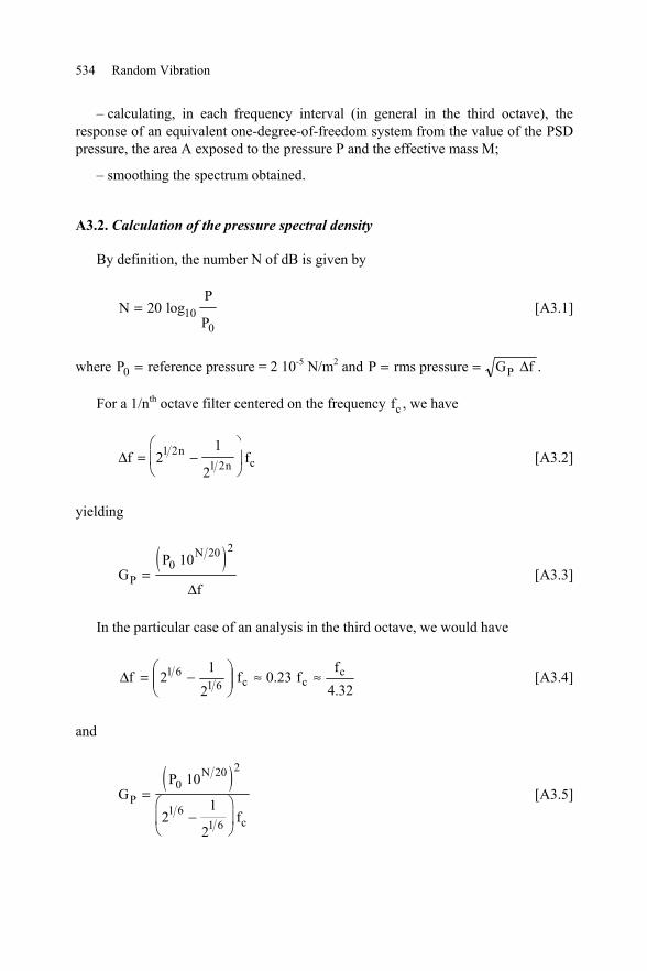
Figure A3.2. One-degree-of-freedom system subjected to a force
Let us consider the one-degree-of-freedom linear system in Figure A3.2, excitedby a force F applied to mass m. The transfer function of this system is equal to:
( )( )
H fz
F
y
F
h
m h h Q= = =
− +
2
2 2 2 21 2
1[A3.6]
y and z being respectively the absolute response and the relative response of themass m, and
hf
f=
0
At resonance, h = 1 and
HQ
m= [A3.7]
The PSD GF of the transmitted force is given by:
( )G A GF P= β 2 [A3.8]
(F A P= β ) and the PSD of the response y to the force F applied to the one-degree-of-freedom system is equal, at resonance, to:
536 Random Vibration
G H Gy F = 2 [A3.9]
( )GQ
mA Gy P =
2
22β [A3.10]
( )G
A
mQ
P
fy
N
nn c
=
−
β22
2 020 2
1 21 2
10
21
2
[A3.11]
In the case of the third octave analysis,
( )G
A
mQ
P
fy
N
c
=
−
β22
2 020 2
1 61 6
10
21
2
[A3.12]
F. Spann and P. Patt set 5.4Q = and 5.2=β , yielding
P
2
y GmA
6.126G
= [A3.13]
A4. Mathematical functions
The object of this appendix is to provide tools facilitating the evaluation of somemathematical expressions, primarily integrals, intervening very frequently incalculations related to the analysis of random vibrations and their effect on a one-degree-of-system mechanical system.
A4.1. Error function
This function, also called the probability integral, is the subject of twodefinitions.
A4.1.1. First definition
The error function is expressed:
Appendix 537
2X t1 0
2E (x) e dt−=
π [A4.1]
If x → ∞ , ( )E x1 tends towards E1∞ which is equal to
E1 0
21
2
∞∞ −= =
πe dtt [A4.2]
and if x = 0 , ( )E1 0 0= . If we set tu
=2, it becomes
E1x
edux
u
2
2
202
2
=
−
π
E1x
e dux
u
2
20
2
2
=
−
π[A4.3]
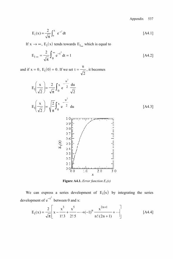
Figure A4.1. Error function E1(x)
We can express a series development of ( )xE1 by integrating the series
development of e t− 2
between 0 and x:
E1
3 5 2 12
1 3 2 51
2 1( )
! !( )
! ( )x x
x x x
n nn
n
= − + − + −+
+
+
π [A4.4]
538 Random Vibration
This series converges for any x. For large x, we can obtain the asymptoticdevelopment according to [ANG 61], [CRA 63]:
E1( ). . .
( ). . ( )
xe
x x x x
n
x
xn
n n≈ − − + − + + −−
+
−−
− −1 11
2
13
2
135
21
135 2 3
2
2
2 2 4 3 61
1 2 2π
[A4.5]
For sufficiently large x, we have
E1( )xe
x
x
≈ −−
1
2
π[A4.6]
If x 1.6,= ( )1E x 0.976,= whilst the value approximated by the expressionabove is
( ) 973.0xE1 ≈ .
For x 1.8,= ( )1E x 0.9891≈ instead of 0.890.
The ratio of two successive terms, equal to2 1
2
n
x
−, is close to 1 when n is close
to x2 . This remark makes it possible to limit the calculation by minimizing the erroron ( )E x1 .
NOTE.–
( )E x is the error function and ( )1 E x − , noted ( )erfc x , is the
“complementary error function”.
2tx
2erfc(x )= e dt
π
∞ − [A4.7]
Function2x t
1 0
2E ( x ) e dt
π−=
Approximate calculation of 1E
The error function can be estimated using the following approximaterelationships [ABR 70], [HAS 55]:
22 3 4 5 x1 1 2 3 4 5E (x) 1 (a t a t a t a t a t ) e (x)−= − + + + + + ε [A4.8]
where
Appendix 539
tpx
x=+
≤ < ∞1
10( )
( ) 7105.1x −≤ε
x ( )E x1 ΔE1 x ( )E x1 ΔE1 x ( )E x1 ΔE1
0.0250.0500.0750.1000.1250.1500.1750.2000.2250.2500.2750.3000.3250.3500.3750.4000.4250.4500.4750.5000.5250.5500.5750.6000.6250.6500.6750.7000.7250.7500.7750.8000.825
0.028200.056370.084470.112460.140320.168000.195470.222700.249670.276330.302660.328630.354210.379380.404120.428390.452190.475480.498260.5205000.542190.563320.583880.603860.623240.642030.660220.677800.694780.7111560.726930.742100.75668
0.028200.028170.028100.027990.027860.027680.027470.027230.026970.026660.026330.025970.025580.025170.024740.024270.23800.023290.022780.022240.021690.021130.020560.019980.019380.018790.018190.017580.016980.016380.015770.015170.01458
0.8500.8750.9000.9250.9500.9751.0001.0251.0501.0751.1001.1251.1501.1751.2001.2251.2501.2751.3001.3251.3501.3751.4001.4251.4501.4751.5001.5251.5501.5751.6001.6251.650
0.770670.784080.796910.809180.820890.832060.842700.852820.862440.871560.880210.888390.896120.903430.910310.916800.922900.9298630.934010.939050.0943760.948170.952290.956120.959700.963020.966110.968970.971620.974080.976350.978440.98038
0.013990.013410.012830.012270.011710.011170.010640.010120.009620.009120.008650.008180.007730.007310.006880.006490.006100.005730.005380.005040.004720.004410.004120.003830.003560.003320.003090.002860.002650.002460.002270.002090.00194
1.6751.7001.7251.7501.7751.8001.8251.8501.8751.9001.9251.9501.9752.0002.0252.0502.0752.1002.1252.1502.1752.2002.2252.2502.2752.3002.3252.3502.3752.4002.4252.4502.4752.500
0.982150.983790.985290.986670.987930.9890900.990150.991110.991990.992790.993520.994180.994780.995320.997810.996260.996660.997020.997350.997640.997900.998140.998350.998540.998710.998860.998990.999110.999220.999310.999400.999470.999540.99959
0.001770.001640.001500.001380.001260.001160.001060.000960.000880.000800.000730.000660.000600.000540.000490.000450.000400.000360.000330.000290.000260.000240.000210.000190.000170.000150.000130.000120.000110.000090.000090.000070.000070.00005
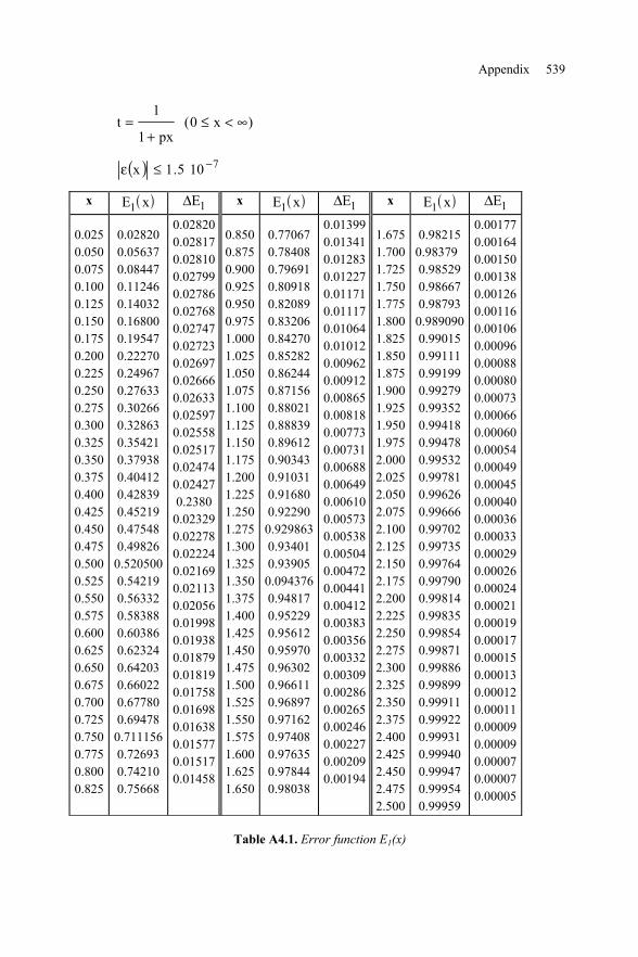
Table A4.1. Error function E1(x)
540 Random Vibration
p = 0.3275911 a3 = 1.421413741a1 = 0.254829592 a4 = -1.453152027a2 = -0.284496736 a5 = 1.061495429
22 3 x1 1 2 3E (x) 1 (a t a t a t ) e (x)−= − + + + ε [A4.9]
( ) 5105.2xxp1
1t −≤ε
+=
p = 0.47047 a2 = -0.095879a1 = 0.3480242 a3 = 0.7478556
Other approximate relationships of this type have been proposed [HAS 55][SPA 87], with developments of the 3rd, 4th and 5th order. C. Hastings also suggeststhe expression
E11 2
23
34
45
56
6 1611
1( )
( )x
a x a x a x a x a x a x= −
+ + + + + +[A4.10]
a1 = 0.0705230784 a4 = 0.0001520143a2 = 0.0422820123 a5 = 0.0002765672a3 = 0.0092705272 a6 = 0.0000430638
(0 ≤ ≤ ∞x )
Derivatives
d E x
dxe x1 2 2( )
= −
π[A4.11]
d E x
dxx e x
212
4 2( )= − −
π[A4.12]
Appendix 541
Approximate formula
The approximate relationship [DEV 62]
E xx
1
2
14
( ) exp= − −
π
[A4.13]
gives results of a sufficient precision for many applications (error lower than somethousandths, regardless of the value of x).
NOTE.–
The probability−
−∞=
2tx 21
P e dt2π
(normal distribution) can be calculated
numerically using the approximate relations of this error function from
= +
11 x
P 1 E2 2
[A4.14]
A4.1.2. Second definition
The error function is often defined by [PAP 65], [PIE 70]:
E x e dt
tx
22
0
1
2
2
( ) =−
π
[A4.15]
With this definition
E x
Ex
2
12
2( ) =
[A4.16]
yielding
E E1 2( ) ( )x x= 2 2 [A4.17]
542 Random Vibration
Applications
1
2
2
2
1
2 22
22
1
α π
β
α
β
α
β
αe dx Ex
Ex
x
x
x−
−
=−
−
−
( )
[A4.18]
where α and β are two arbitrary constants [PIE 70] and
e dt
t−
−∞
∞ =
2
2 2π [A4.19]
Properties of ( )2E x
( )E x2 tends towards 0.5 when x → ∞ :
5.0dte21
E0
2t
2
2
=π
= ∞ −
[A4.20]
( )E2 0 0=
( ) ( )E x E x2 2− = −
Function
2tx
22 0
1E ( x ) e dt
2π
−=
Approximate calculation of 2E ( x )
The function ( )E x2 can be approximated, for x > 0, by the expression definedas follows [LAM 76], [PAP 65]:
++++−≈
−2x
54322
2
e)tetdtctbta(121
)x(E [A4.21]
where
Appendix 543
11 0.2316418
tx
=+
a = 0.254829592 b = -0.284496736
c = 1.421413741 d = -1.453152027 e = 1.061405429
The approximation is very good (at least 5 decimal points).
NOTE.–
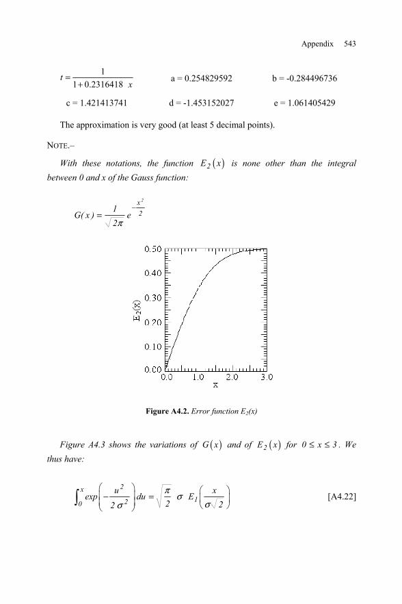
With these notations, the function ( )2E x is none other than the integralbetween 0 and x of the Gauss function:
2x21
G( x ) e2π
−=
Figure A4.2. Error function E2(x)
Figure A4.3 shows the variations of ( )G x and of ( )2E x for 0 x 3≤ ≤ . Wethus have:
2x120
u xexp du E
2 22π σ
σσ
− =
[A4.22]
544 Random Vibration
x 2E (x) 2EΔΔ x 2E (x) 2EΔΔ x 2E (x) 2EΔΔ
0.05
0.10
0.15
0.20
0.25
0.30
0.35
0.40
0.45
0.50
0.55
0.60
0.65
0.70
0.75
0.80
0.85
0.90
0.95
1.00
1.05
1.10
1.15
1.201.25
1.30
1.35
0.01994
0.03983
0.05962
0.07926
0.09871
0.11791
0.13683
0.15542
0.17364
0.19146
0.20884
0.22575
0.24215
0.25804
0.27337
0.28814
0.30234
0.31594
0.32894
0.34134
0.35314
0.36433
0.37493
0.38493
0.39435
0.40320
0.41149
0.01994
0.01989
0.01979
0.01964
0.01945
0.01920
0.01892
0.01859
0.01822
0.01782
0.01738
0.01691
0.01640
0.01589
0.01533
0.01477
0.01420
0.01360
0.01300
0.01240
0.01180
0.01119
0.01060
0.01000
0.00942
0.00885
0.00829
1.40
1.45
1.50
1.55
1.60
1.65
1.70
1.75
1.80
1.85
1.90
1.95
2.00
2.05
2.10
2.15
2.20
2.25
2.30
2.35
2.40
2.45
2.50
2.55
2.60
2.65
2.70
0.41924
0.42647
0.43319
0.43943
0.44520
0.45053
0.45543
0.45994
0.46407
0.46784
0.47128
0.47441
0.47725
0.47982
0.48214
0.48422
0.48610
0.48778
0.48928
0.49061
0.49180
0.49286
0.49379
0.49461
0.49534
0.49598
0.49653
0.00775
0.00723
0.00672
0.00624
0.00577
0.00533
0.00490
0.00451
0.00413
0.00377
0.00344
0.00313
0.00284
0.00257
0.00232
0.00208
0.00188
0.00168
0.00150
0.00133
0.00119
0.00106
0.00093
0.00082
0.00072
0.00064
0.00055
2.75
2.80
2.85
2.90
2.95
3.00
3.05
3.10
3.15
3.20
3.25
3.30
3.35
3.40
3.45
3.50
3.55
3.60
3.65
3.70
3.75
3.80
3.85
3.90
3.95
4.00
0.49702
0.49744
0.49781
0.49813
0.49981
0.49865
0.49886
0.49903
0.49918
0.49931
0.49942
0.49952
0.49960
0.49966
0.49972
0.49977
0.49841
0.49984
0.49987
0.49989
0.49991
0.49993
0.49994
0.49995
0.049996
0.49997
0.00049
0.00042
0.00037
0.00032
0.00028
0.00024
0.00021
0.00017
0.00015
0.00013
0.00011
0.00010
0.00008
0.00006
0.00006
0.00005
0.00004
0.00003
0.00003
0.00002
0.00002
0.00002
0.00001
0.00001
0.00001
0.00001
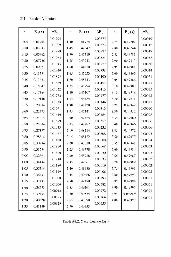
Table A4.2. Error function E2(x)
Appendix 545
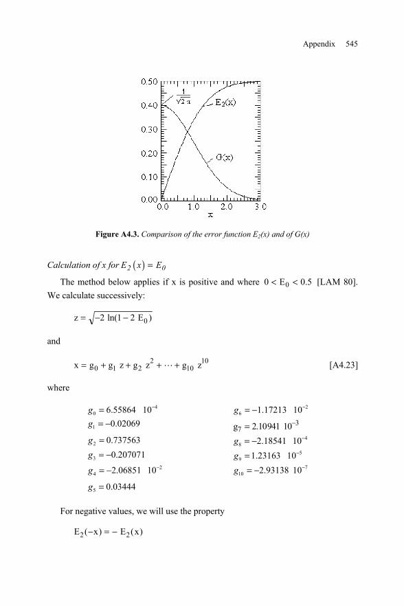
Figure A4.3. Comparison of the error function E2(x) and of G(x)
Calculation of x for ( )2 0E x E=
The method below applies if x is positive and where 5.0E0 0 << [LAM 80].We calculate successively:
z E= − −2 1 2 0ln( )
and
x g g z g z g z= + + + +0 1 22
1010 [A4.23]
where
40 6.55864 10g −= 2
6 1.17213 10g −= −
1 0.02069g = − 37g 2.10941 10−=
2 0.737563g = 48 2.18541 10g −= −
3 0.207071g = − 59 1.23163 10g −=
24 2.06851 10g −= − 7
10 2.93138 10g −= −
5 0.03444g =
For negative values, we will use the property
E x E x2 2( ) ( )− = −
546 Random Vibration
NOTE.–
To calculate x from the given 1E set 12
EE
2= , calculate x, and then
x2.
A4.2. Calculation of the integral a x ne x dxWe have [DWI 66]:
e
xdx x
a x a x a x a
n
x
n
a x n n
= + + + + + + ln! ! ! !1 2 2 3 3
2 2 3 3
[A4.24]
yielding, since
( )e
xdx
e
n x
a
n
e
xdx
a x
n
a x
n
a x
n = −−
+−− −1 11 1 [A4.25]
( ) ( ) ( ) ( ) ( )e
xdx
e
n x
a e
n n x
a e
n x
a
n
e
xdx
ax
n
ax
n
ax
n
n ax n ax
= −−
−− −
− −−
+−− −
− −
1 1 2 1 11 2
2 1
! !
[A4.26]
A4.3. Euler’s constant
Definition
ε = + + + −
→∞lim lnn n
n11
2
1 [A4.27]
0.57721566490 ...ε ≈
An approximate value is given by [ANG 61]:
( )ε ≈ −1
210 13
i.e.
0.5772173 ...ε ≈
Appendix 547
Applications
It is shown that [DAV 64]:
ln λ λ ελe d−∞ = −0
[A4.28]
and that
(ln )λ λπ
ελ20
2
6e d−∞ = + [A4.29]
A5. Complements to the transfer functions
A5.1. Error related to digitization of transfer function
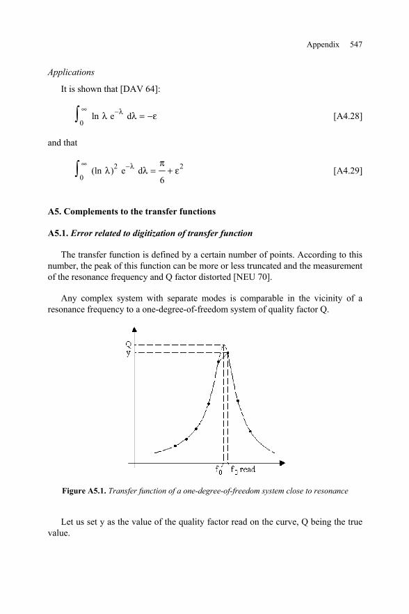
The transfer function is defined by a certain number of points. According to thisnumber, the peak of this function can be more or less truncated and the measurementof the resonance frequency and Q factor distorted [NEU 70].
Any complex system with separate modes is comparable in the vicinity of aresonance frequency to a one-degree-of-freedom system of quality factor Q.
Figure A5.1. Transfer function of a one-degree-of-freedom system close to resonance
Let us set y as the value of the quality factor read on the curve, Q being the truevalue.
548 Random Vibration
Let us set β =y
Qand
frequencyresonancetruefrequencyresonanceread
ff
0==α . When α is different
from 1, we can set α δ= −1 , if δ is the relative deviation on the value of theresonance frequency. For δ = 0, we have α = 1 and β = 1. For δ ≠ 0, β is less than1. The resolution error is equal to ε βR = −1 . The amplitude of the transfer functionaway from resonance is given by y such that:
( ) ( )y Q
Q
Q
Q
2
2
2
2 2 2
2
2 2
2 2 2 2
1
1 1=
+
− +
=+
− +
α
αα
α
α α[A5.1]
( )
( )
( )β
α
α α
α
δ δ2
2
2
2
2
2 2 2 2
2
2
2 2 2
1
1
11
1= =
+
− +=
+−
+ −
y
Q
Q
Q
Q
Q[A5.2]
For large Q, we have
( )β
α α
22 2 2 2
1
1≈
− +Q[A5.3]
i.e., replacing α with 1 - δ and assuming Q2 to be large compared to 1,
βδ δ
22 2
1
1 2 4≈
− + Q[A5.4]
and
ε βδ δ
RQ
= − ≈ −− +
1 11
1 2 4 2 2[A5.5]
Appendix 549
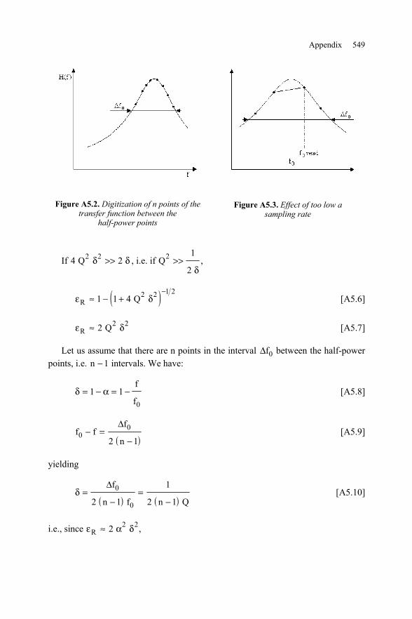
Figure A5.2. Digitization of n points of thetransfer function between the
half-power points
Figure A5.3. Effect of too low asampling rate
If 4 22 2Q δ δ>> , i.e. if Q2 1
2>>
δ,
( )ε δR Q≈ − +−
1 1 4 2 2 1 2[A5.6]
ε δR Q≈ 2 2 2 [A5.7]
Let us assume that there are n points in the interval Δf0 between the half-powerpoints, i.e. n −1 intervals. We have:
δ α= − = −1 10
f
f[A5.8]
( )f f
f
n0
0
2 1− =
−
Δ[A5.9]
yielding
( ) ( )δ =
−=
−
Δf
n f n Q0
02 1
1
2 1[A5.10]
i.e., since ε α δR ≈ 2 2 2,
550 Random Vibration
( )εR
n≈
−
1
2 1 2[A5.11]
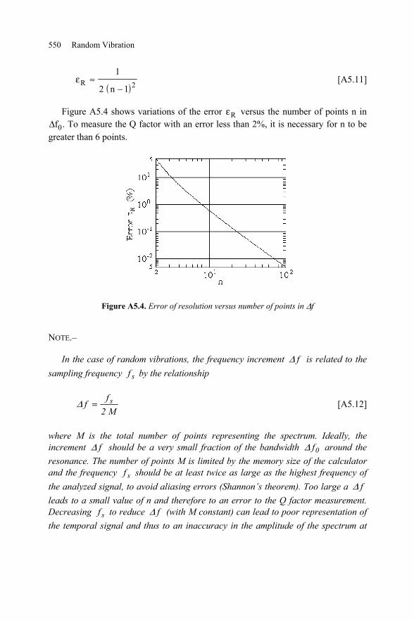
Figure A5.4 shows variations of the error εR versus the number of points n inΔf0. To measure the Q factor with an error less than 2%, it is necessary for n to begreater than 6 points.
Figure A5.4. Error of resolution versus number of points in Δf
NOTE.–
In the case of random vibrations, the frequency increment fΔ is related to thesampling frequency sf by the relationship
sff2 M
Δ = [A5.12]
where M is the total number of points representing the spectrum. Ideally, theincrement fΔ should be a very small fraction of the bandwidth 0fΔ around theresonance. The number of points M is limited by the memory size of the calculatorand the frequency sf should be at least twice as large as the highest frequency ofthe analyzed signal, to avoid aliasing errors (Shannon’s theorem). Too large a fΔleads to a small value of n and therefore to an error to the Q factor measurement.Decreasing sf to reduce fΔ (with M constant) can lead to poor representation ofthe temporal signal and thus to an inaccuracy in the amplitude of the spectrum at
Appendix 551
high frequencies. It is recommended to choose a sampling frequency greater than 6times the largest frequency to be analyzed [TAY 75].
A5.2. Use of a fast swept sine for the measurement of transfer functions
The measurement of a transfer function starting from a traditional swept sine testleads to a test of relatively long duration and, in addition, requires material with agreat measurement dynamics.
Transfer functions can also be measured from random vibration tests or by usingshocks, the test duration obviously being in this latter case very short. On thisassumption, the choice of the form of shock to use is important because, the transferfunction being calculated from the ratio of the Fourier transforms of the response (ina point of the structure) and excitation, it is necessary that this latter transform doesnot present a zero or too small an amplitude in a certain range of frequency. In thepresence of noise, the low levels in the denominator lead to uncertainties in thetransfer function [WHI 69].
The interest of the fast linear swept sine lies in two points:
– the Fourier transform of a linear swept sine has a roughly constant amplitude inthe swept frequency range. W.H. Reed, A.W. Hall, L.E. Barker [REE 60], thenR.G. White [WHI 72] and R.J. White and R.J. Pinnington [WHI 82] showed that theaverage module of the Fourier transform of a linear swept sine is equal to:
( ) X
x
bmω =
2[A5.13]
where mx = amplitude of acceleration defining the swept sine
bf f
tb=
−=2 1 sweep rate
and that, more generally,
Xx
fm=
2[A5.14]
where f is the sweep rate for an arbitrary law,
552 Random Vibration
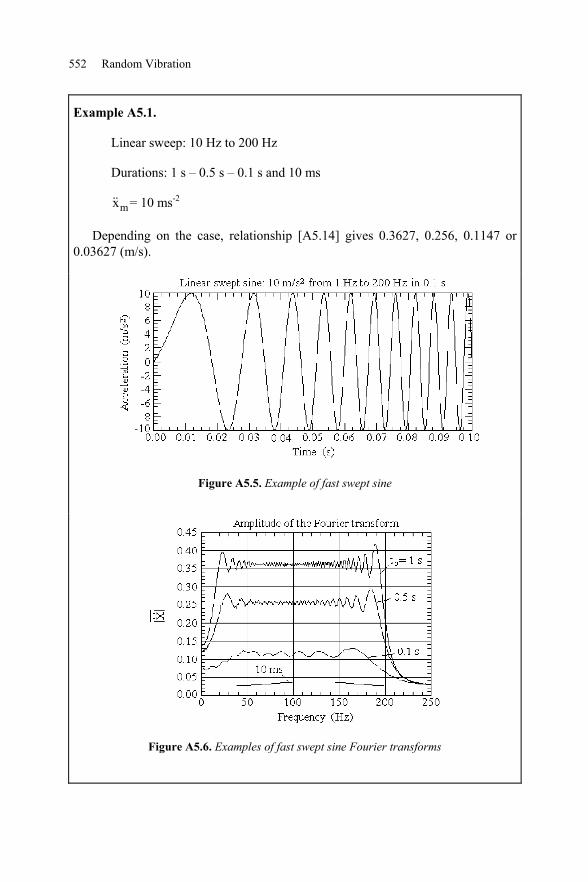
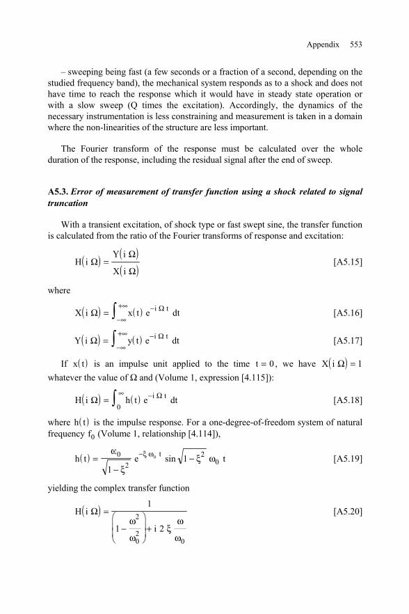
Example A5.1.
Linear sweep: 10 Hz to 200 Hz
Durations: 1 s – 0.5 s – 0.1 s and 10 ms
xm= 10 ms-2
Depending on the case, relationship [A5.14] gives 0.3627, 0.256, 0.1147 or0.03627 (m/s).
Figure A5.5. Example of fast swept sine
Figure A5.6. Examples of fast swept sine Fourier transforms
Appendix 553
– sweeping being fast (a few seconds or a fraction of a second, depending on thestudied frequency band), the mechanical system responds as to a shock and does nothave time to reach the response which it would have in steady state operation orwith a slow sweep (Q times the excitation). Accordingly, the dynamics of thenecessary instrumentation is less constraining and measurement is taken in a domainwhere the non-linearities of the structure are less important.
The Fourier transform of the response must be calculated over the wholeduration of the response, including the residual signal after the end of sweep.
A5.3. Error of measurement of transfer function using a shock related to signaltruncation
With a transient excitation, of shock type or fast swept sine, the transfer functionis calculated from the ratio of the Fourier transforms of response and excitation:
( ) ( )( )
H iY i
X iΩ
Ω
Ω= [A5.15]
where
( ) ( )X i x t e dti tΩ Ω= −−∞
+∞ [A5.16]
( ) ( )Y i y t e dti tΩ Ω= −−∞
+∞ [A5.17]
If ( )x t is an impulse unit applied to the time t = 0 , we have ( )X i Ω = 1whatever the value of Ω and (Volume 1, expression [4.115]):
( ) ( )H i h t e dti tΩ Ω= −∞0 [A5.18]
where ( )h t is the impulse response. For a one-degree-of-freedom system of naturalfrequency f0 (Volume 1, relationship [4.114]),
( )h t e tt=−
−−ω
ξξ ωξ ω0
22
01
10 sin [A5.19]
yielding the complex transfer function
( )H i
i
Ω =
−
+
1
1 22
02
0
ω
ωξ
ω
ω
[A5.20]
554 Random Vibration
Relationship [A5.18] could be used in theory to determine ( )H i Ω from theresponse to an impulse, but, in practice, a truncation of the response is difficult toavoid, either because the decreasing signal becomes non-measurable or because thetime of analysis is limited to a value τm [WHI 69]. The effects of truncation havebeen analyzed by B.L. Clarkson and A.C. Mercer [CLA 65], who showed:
– that the resonance frequency can still be identified from the diagram vector as
the frequency to which the rate of variation in the length of arc with frequency,ds
df,
is maximum;
– that the damping measured from such a diagram (established with a truncatedsignal) is larger than the true value.
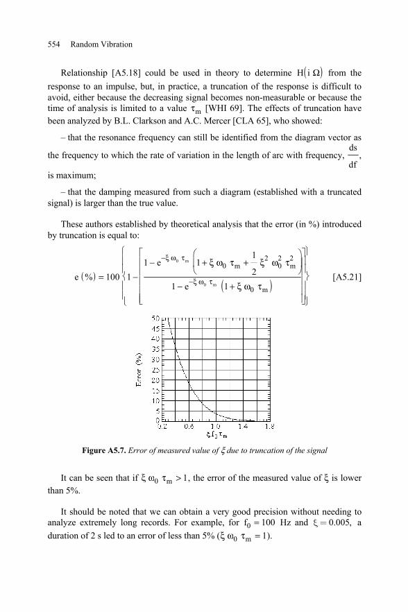
These authors established by theoretical analysis that the error (in %) introducedby truncation is equal to:
( )( )
ee
e
m
m
m m
m
% = −− + +
− +
−
−100 11 1
1
21 1
0
0
02
02 2
0
ξ ω τ
ξ ω τ
ξ ω τ ξ ω τ
ξ ω τ[A5.21]
Figure A5.7. Error of measured value of ξ due to truncation of the signal
It can be seen that if ξ ω τ0 1m > , the error of the measured value of ξ is lowerthan 5%.
It should be noted that we can obtain a very good precision without needing toanalyze extremely long records. For example, for f0 100= Hz and 0.005,x = aduration of 2 s led to an error of less than 5% (ξ ω τ0 1m = ).
Appendix 555
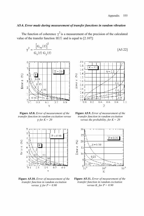
A5.4. Error made during measurement of transfer functions in random vibration
The function of coherence γ 2 is a measurement of the precision of the calculatedvalue of the transfer function ( )H f and is equal to [2.107]:
( )[ ]( ) ( )
γ 22
=G f
G f G f
xy
x y
[A5.22]
Figure A5.8. Error of measurement of thetransfer function in random excitation versus
γ, for K = 20
Figure A5.9. Error of measurement of thetransfer function in random excitationversus the probability, for K = 20
Figure A5.10. Error of measurement of thetransfer function in random excitation
versus γ, for P = 0.90
Figure A5.11. Error of measurement of thetransfer function in random excitation
versus K, for P = 0.90
556 Random Vibration
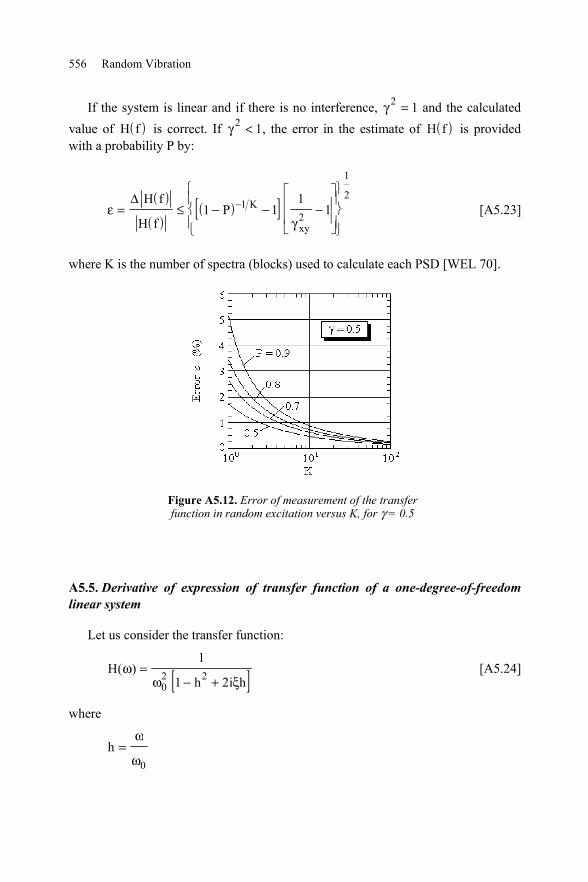
If the system is linear and if there is no interference, γ 2 1= and the calculatedvalue of ( )H f is correct. If γ 2 1< , the error in the estimate of ( )H f is providedwith a probability P by:
( )( )
( )[ ]εγ
= ≤ − − −
−Δ H f
H fP K
xy
1 11
112
1
2[A5.23]
where K is the number of spectra (blocks) used to calculate each PSD [WEL 70].
Figure A5.12. Error of measurement of the transferfunction in random excitation versus K, for γ = 0.5
A5.5. Derivative of expression of transfer function of a one-degree-of-freedomlinear system
Let us consider the transfer function:
[ ]Hh i h
( )ωω ξ
=− +
1
1 202 2 [A5.24]
where
h =ω
ω0
Appendix 557
using multiplication of the denominator’s conjugate quantity, we obtain
( )H h A i h A( )ω ξ= − −1 22
if we set
( ) ( )A
h h=
− +
1
1 202 2 2 2ω ξ
yielding
( )dH
dhh A i A h
dA
dhh i
dA
dh= − − + − −2 2 1 22ξ ξ [A5.25]
with
( )( ) ( )
dA
dh
h h
h h=
− −
− +
4 1 2
1 2
2 2
02 2 2 2
2
ξ
ω ξ[A5.26]
[ ]dH
dhh i A h h i
dA
dh= − + + − −2 1 22( )ξ ξ [A5.27]
A6. Calculation of integrals
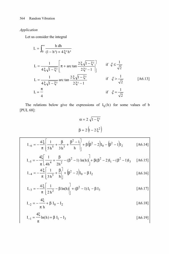
A6.1. Integral ( ) =− +
bhI h dhb ( h ) h2 2 2
41 4
ξξππ ξξ
b 32
b 2 b 44 h
I (h) 2 (1 2 ) I I if b 3b b 3
−
− −ξ
= + − ξ − ≠π −
23 1 1
4I (h) ln h + 2 (1 2 ) I I if b= 3−ξ= − ξ −
π[A6.1]
558 Random Vibration
A6.1.1. Demonstration
From [PUL 68]:
( )1 4 12 2 2 2 4 2− + = − +h h h hξ β
if we set ( )2212 ξ−=β . By division, we obtain
b b 2 b 4b 4
4 2 4 2h h h
h if b 3h h 1 h h 1
− −− β −
= + ≠− β + − β +
yielding recurrence relation [A6.1]. The use of these expressions requires knowledgeof ( )I hb for some values from b, for example, b = 0 , 1 and 2.
A6.1.2. Calculation of ( )I h0 and ( )I h2
The calculation of ( )I h0 and ( )I h2 can be carried out easily by writing thefunctions to be integrated respectively in the forms
( )1
1 4
1
4 1
2 1
2 1 1
2 1
2 1 12 2 2 2 2
2
2 2
2
2 2− +=
−
+ −
+ − +−
− −
− − +
h h
h
h h
h
h hξ ξ
ξ
ξ
ξ
ξ
[A6.2]
and
( )h
h h
h
h h
h
h h
2
2 2 2 2 2 2 2 2 21 4
1
4 1 2 1 1 2 1 1− +=
−
−
+ − ++
− − +
ξ ξ ξ ξ
[A6.3]
Let us set
Ih
h hdh=
+ −
+ − + 2 1
2 1 1
2
2 2
ξ
ξ
Ih
h hdh
h hdh=
+ −
+ − ++
−
+ − + 1
2
2 2 1
2 1 1
1
2 1 1
2
2 2
2
2 2
ξ
ξ
ξ
ξ
Appendix 559
Knowing what +ξ−+=δ 22 1h2h 1 can be put in the form
δ ξξ
= +
22
2 1X
with X h= + −1 2ξ
it results that
ξξ−+
ξξ−
+
+ξ−+=
2222 1h
tanarc1
11h2hln21
I
In the same way,
Jh
h hdh=
− −
− − + 2 1
2 1 1
2
2 2
ξ
ξ
Jh
h hdh
h hdh=
− −
− − +−
−
− − + 1
2
2 2 1
2 1 1
1
2 1 1
2
2 2
2
2 2
ξ
ξ
ξ
ξ
With a change of variable such that:
X h= − −1 2ξ
h hX2 2 22
22 1 1 1− − + = +
ξ ξ
ξ
we obtain
ξξ−−
ξξ−
−
+ξ−−=
2222 1h
tanarc1
11h2hln21
J
yielding
11h2h
11h2hln
12)h(I
22
22
20+ξ−−
+ξ−+
ξ−π
ξ=
2 2h 1 h 11arc tan arc tan + − ξ − − ξ + + π ξ ξ
[A6.4]
560 Random Vibration
NOTES.–
1. Knowing that
x yarc tan x arc tan y arc tan
1 x y+
+ =−
[A6.5]
0I ( h ) can be also written
2 2
0 22 2 2
h 2h 1 1 1 2hI ( h ) ln arc tan
1 h2 1 h 2h 1 1
ξξ ξππ ξ ξ
+ − += +
−− − − +[A6.6]
However, expression [A6.6] must be used with caution, [A6.5] being correctonly under precise conditions.
Relation [A6.5], established from
( ) tan a tan btan a b
1 tan a tan b+
+ =−
is exact only if
a k2π π≠ +
b k2π π≠ +
a b k2π π+ ≠ +
From these first two conditions, if tan a x= and tan b y= , it is necessary that
a2 2π π
− < < and that b2 2π π
− < < .
Appendix 561
Taking into account these inequalities, a b+ can thus vary between π− and π(limits not included). The second member in addition lays down that
a b2 2π π
− < + < . Let us set a bΘ = + . If
arc tan x arc tan y2π
+ > [A6.7]
we must thus take as the valuex y
arc tan1 x y
+−
of the angle Θ π− .
If
arc tan x arc tan y2π
+ < − [A6.8]
we consider Θ π+ .
2. It is easy to show that we are in the situation of an inequality [A6.7] as soonas we have x y 2+ > . Indeed, let us search for the minimal value of the sum
z tan x tan x2π = + −
i.e. of
2X 1z
X
+ =
While setting X tan x= , we find that the derivativedzdx
is cancelled when
2X 1= , yielding z 2= (condition [A6.7]) or z 2= − (condition [A6.8]).
562 Random Vibration
Following what precedes,
dh11h2h
12h221
dh11h2h
h22
2
22 +ξ−+
ξ−+=
+ξ−+
dh11h2h
11
222
+ξ−+ξ−−
ξξ−+
ξξ−
−
+ξ−+=
+ξ−+
2222
22
1htanarc
111h2hln
21
dh11h2h
h
and
ξξ−−
ξξ−
−
+ξ−−=
+ξ−−
2222
22
1htanarc
111h2hln
21
dh11h2h
h
yielding
11h2h
11h2hln
12)h(I
22
22
22+ξ−+
+ξ−−
ξ−π
ξ=
ξξ−−
+ξ
ξ−+π
+22 1h
tanarc1h
tanarc1
which can be written, with the same reservations as above,
222
22
22h1
h2tanarc
1
11h2h
11h2hln
12)h(I
−
ξπ
++ξ−+
+ξ−−
ξ−π
ξ= [A6.9]
NOTE.–
When h → ∞ , 0I ( h ) → 1 and 2I ( h ) 1→ .
If h 0→ , 0I ( h ) 0→ yielding, while setting
( )20 222
GK dh
h1 h
Q
∞=
− +
Appendix 563
(0
fh
f= )
( )0 20 22
2
dhK G f
h1 h
Q
∞=
− +
0G f QK
2π
= [A6.10]
A6.1.3. Calculation of 1I ( h )
I hh dh
h h1 2 2 2 2
4
1 4( )
( )=
− +ξ
π ξ
h
h h h h h h( )1 4
1
4 1
1
2 1 1
1
2 1 12 2 2 2 2 2 2 2 2 2− +
=− − − +
−+ − +
ξ ξ ξ ξ
yielding
ξξ−+
−ξ
ξ−−
ξ−π=
22
211h
tanarc1h
tanarc1
1)h(I [A6.11]
Knowing that
yx1yx
tanarcytanarcxtanarc+
−=−
I h1( ) can be also written (always with the same reservations):
22
2
21h21
12tanarc
1
1)h(I
−ξ−
ξ−ξ
ξ−π= [A6.12]
564 Random Vibration
Application
Let us consider the integral
∞
ξ+−=
0 ²h²4²)h1(dhh
L
−ξξ−ξ
+πξ−ξ
=1²2²12
tanarc²14
1L
1if2
ξ ≤
1²2²12
tanarc²14
1L
−ξξ−ξ
ξ−ξ=
1if2
ξ > [A6.13]
L =π
4
1if2
ξ =
The relations below give the expressions of I hb ( ) for some values of b[PUL 68]:
α ξ= −2 1 ²
( )2212 ξ−=β
( ) ( ) 22
02
2
356 I1I2h1
h3h5
14I −β−−ββ+
−β+
β+
πξ
−=− [A6.14]
Ih h
h I I− = − + − −
+ − − −5 4 2
2 21
23
4 1
4 21 2 1
ξ
π
ββ β β β( ) ln( ) ( ) ( ) [A6.15]
( ) 202
34 II2hh3
14I β−−β+
β+
πξ
−=− [A6.16]
312
23 II)1()hln(h2
14I β−−β+
β−
πξ
−=− [A6.17]
Ih
I I− = − + −2 0 24ξ
πβ [A6.18]
I h I I− = + −1 1 34ξ
πβln( ) [A6.19]
Appendix 565
ξα−
+ξ
α+π
++α−
+α+απ
ξ= )
2h2
tan(arc)2h2
tan(arc1
)1hh
1hhln(I 2
2
0 [A6.20]
ξα+
−ξ
α−απ
= )2h2
tan(arc)2h2
tan(arc2
I1 [A6.21]
ξα−
+ξ
α+π
++α++α−
απξ
= )2h2
tan(arc)2h2
tan(arc1
)1hh1hh
ln(I 2
2
2 [A6.22]
[ ]
ξα+
−ξ
α−απ
β+ξ+−
πξ
= )2h2
tan(arc)2h2
tan(arch4)h1(lnI 22223
[A6.23]
024 IIh4
I −β+πξ
= [A6.24]
Ih
I I5
2
3 14
2= + −
ξ
πβ [A6.25]
022
3
6 II)1(h3h4
I β−−β+
β+
πξ
= [A6.26]
132
24
7 II)1(2h
4h4
I β−−β+
β+
πξ
= [A6.27]
02
222
35
8 I)1(I)2(h)1(3h
5h4
I −β−−ββ+
−β+
β+
πξ
= [A6.28]
12
32
22
46
9 I)1(I)2(2h
)1(4h
6h4
I −β−−ββ+
−β+
β+
πξ
= [A6.29]
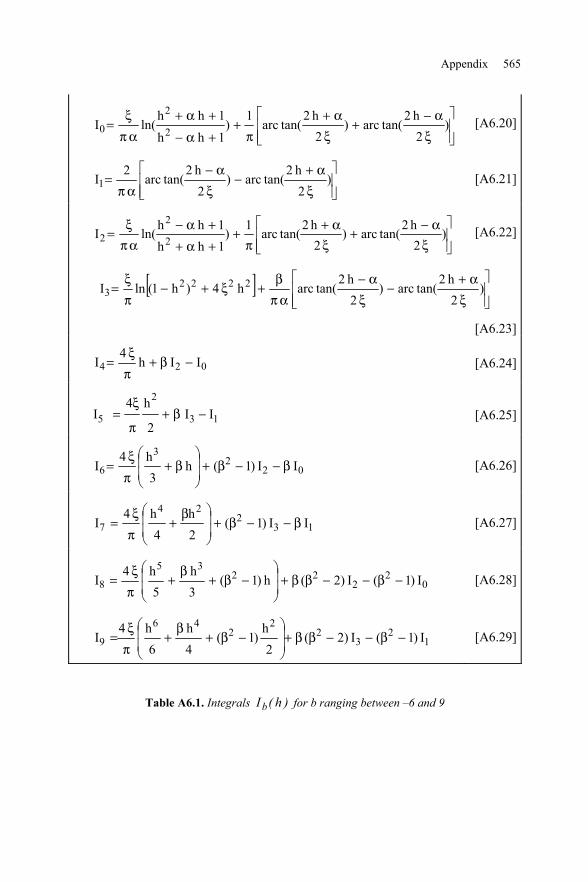
Table A6.1. Integrals bI ( h ) for b ranging between –6 and 9
566 Random Vibration
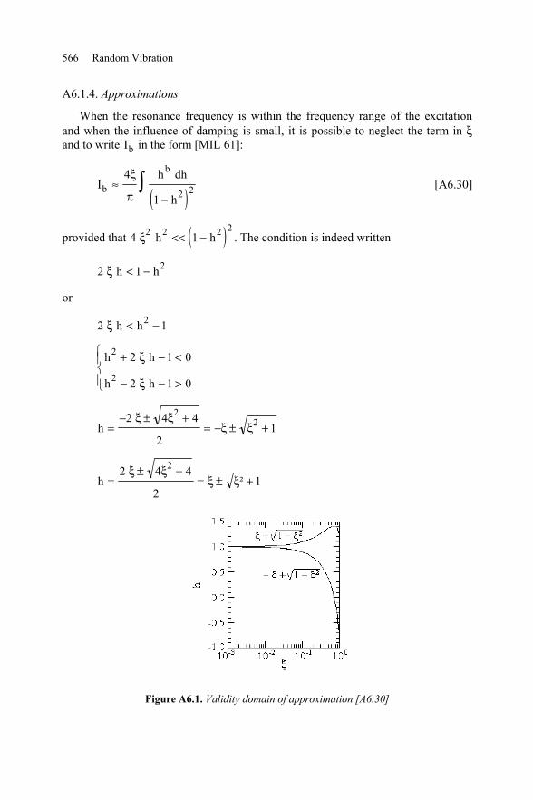
A6.1.4. Approximations
When the resonance frequency is within the frequency range of the excitationand when the influence of damping is small, it is possible to neglect the term in ξand to write Ib in the form [MIL 61]:
( )I
h dh
hb
b
≈−
4
1 2 2ξ
π[A6.30]
provided that ( )4 12 2 2 2ξ h h<< − . The condition is indeed written
2 1 2ξ h h< −
or
2 12ξ h h< −
h h
h h
2
2
2 1 0
2 1 0
+ − <
− − >
ξ
ξ
h =− ± +
= − ± +2 4 4
21
22ξ ξ
ξ ξ
h =± +
= ± +2 4 4
21
2ξ ξξ ξ²
Figure A6.1. Validity domain of approximation [A6.30]
Appendix 567
yielding
− − + ≤ ≤ − + +
+ + ≤ ≤ − +
ξ ξ ξ ξ
ξ ξ ξ ξ
1 1
1 1
2 2
2 2
h
h
Knowing that h is always positive or zero and that ξ varies between 0 and 1,these conditions become
h
h
≤ − + +
≥ + +
ξ ξ
ξ ξ
1
1
2
2
For 0.05,x = these conditions lead for example to:
><
0512.1h9512.0h
The smaller the damping, the larger the useful range.
If 2.0=ξ
><
22.1h82.0h
We increase, for safety, these values by approximately 40%:
ξ++ξ≥
ξ++ξ−≤
2
2
14.1h
14.1h
For h small and less than 1:
( ) ( )++++≈−
642b22
bh4h3h21h
h1
h[A6.31]
568 Random Vibration
For h large and higher than 1:
( )h
h
h
h h h h
b b
11
2 3 42 2 4 2 4 6
−≈ − + − +
[A6.32]
While replacing( )
h
h
b
1 2 2−
with its expression in Ib and while integrating, it
results that
Ih
b
h
b
h
bb
b b b
≈+
++
++
+
+ + +4
1
2
3
3
5
1 3 5ξ
π 1hfor ≤
[A6.33]
Ih
b
h
b
h
bb
b b b
≈−
−−
+−
−
− − −4
3
2
5
3
7
3 5 7ξ
π 1hfor ≥
as long as no denominator is zero. If one of them is zero, the corresponding term isto be replaced by a logarithm. Thus, if b m± = 0, the term
mh
b m
b m+
±
±1
2
must be written
mh
+ 1
2ln
A6.1.5. Particular cases
2 200
H h d Q2
∞ πΩ = ω [A6.34]
200
H d Q2
∞ πΩ = ω [A6.35]
Appendix 569
where h =Ω
ω0
and
( )H
hh
Q
2
22
2
1
1
=
− +
.
These results can be deduced directly from [A6.22] and [A6.20] [WAT 62].
NOTE.–
More generally, if b 0= [DWI 66]:
4 20
dx2 c ka x 2 b x c
π∞=
+ + [A6.36]
where k = 2 (b+ a c ) and a, c and k 0> .
A6.2. Integral( )ò
b
b 22
hJ (h) = dh1-h
[A6.37]
From the above relations, we deduce
( )0 2
1 h 1 hJ (h) ln4 h 1 2 1 h
−= − ++ −
if h > 1 [A6.38]
( )0 2
1 1 h hJ (h) ln4 1 h 2 1 h
+= +− −
if h < 1 [A6.39]
( )2 2
1 h 1 hJ (h) ln4 h 1 2 1 h
−= ++ −
if h > 1 [A6.40]
( )2 2
1 1 h hJ (h) ln4 1 h 2 1 h
+= − +− −
if h < 1 [A6.41]
The expressions of J hb ( ) for the other values of b can be calculated startingfrom these relations using the recurrence formula:
( )J hh
bJ J b
J h h J J b
b
b
b b=−
+ − ≠
= + − =
−
− −
−
3
2 4
3 1 1
32 3
2 3( ) ln
[A6.42]
Recommended