1 Lois discrètes - maths.cnam.frmaths.cnam.fr/Membres/ghorbanzadeh/lois.pdf · 10/25 Simulation des lois usuelles avec Matlab Propriété Si X etY sontdeuxvariablesaléatoires indépendantessuivantlamême

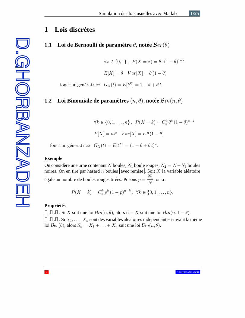
Simulation des lois usuelles avec Matlab 1/25

1 Lois discrètes

1.1 Loi de Bernoulli de paramètreθ, notéeBer(θ)

∀x ∈ {0, 1} , P (X = x) = θx (1 − θ)1−x

E[X] = θ V ar[X] = θ (1 − θ)

fonction generatrice GX(t) = E[tX ] = 1 − θ + θ t.

1.2 Loi Binomiale de paramètres(n, θ), notéeBin(n, θ)

∀k ∈ {0, 1, . . . , n} , P (X = k) = Ckn θk (1 − θ)n−k

E[X] = n θ V ar[X] = n θ (1 − θ)

fonction generatrice GX(t) = E[tX ] = (1 − θ + θ t)n.

Exemple

On considère une urne contenantN boules,N1 boule rouges,N2 = N−N1 boulesnoires. On en tire par hasardn boules avec remise. SoitX la variable aléatoire

égale au nombre de boules rouges tirées. Posonsp =N1

N, on a :

P (X = k) = Ckn pk (1 − p)n−k , ∀k ∈ {0, 1, . . . , n}.

Propriétés

➊.➋.➊. Si X suit une loiBin(n, θ), alorsn − X suit une loiBin(n, 1 − θ).

➊.➋.➋. SiX1, . . . , Xn sont des variables aléatoires indépendantes suivant la mêmeloi Ber(θ), alorsSn = X1 + . . . + Xn suit une loiBin(n, θ).

K D.GHORBANZADEH

2/25 Simulation des lois usuelles avec Matlab

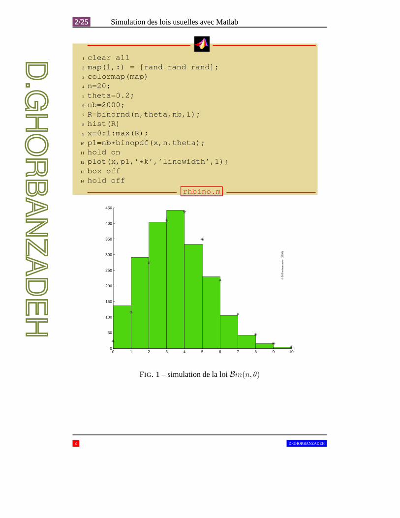
1 clear all2 map(1,:) = [rand rand rand];3 colormap(map)4 n=20;5 theta=0.2;6 nb=2000;7 R=binornd(n,theta,nb,1);8 hist(R)9 x=0:1:max(R);

10 p1=nb*binopdf(x,n,theta);11 hold on12 plot(x,p1,’*k’,’linewidth’,1);13 box off14 hold off

rhbino.m

0 1 2 3 4 5 6 7 8 9 100

50

100

150

200

250

300

350

400

450

© D

.Gho

rban

zade

h (1

997)

FIG. 1 – simulation de la loiBin(n, θ)

K D.GHORBANZADEH


1.3 Loi géométrique de paramètreθ, notéeGeo(θ)

∀k ∈ N⋆ , P (X = x) = θ (1 − θ)k−1

E[X] =1

θV ar[X] =

1 − θ

θ2

fonction generatrice GX(t) = E[tX ] =θ t

1 − (1 − θ)t.

◮ Remarque

Dans certains ouvrages la loiGeo(θ) est présentée sous la forme :

∀k ∈ N , P (X = x) = θ (1 − θ)k.

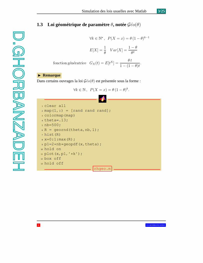
1 clear all2 map(1,:) = [rand rand rand];3 colormap(map)4 theta=.13;5 nb=500;6 R = geornd(theta,nb,1);7 hist(R)8 x=0:1:max(R);9 p1=2*nb*geopdf(x,theta);

10 hold on11 plot(x,p1,’*k’);12 box off13 hold off

rhgeo.m

K D.GHORBANZADEH


0 5 10 15 20 25 30 35 40 450

50

100

150

200

250

© D

.Gho

rban

zade

h (1

997)

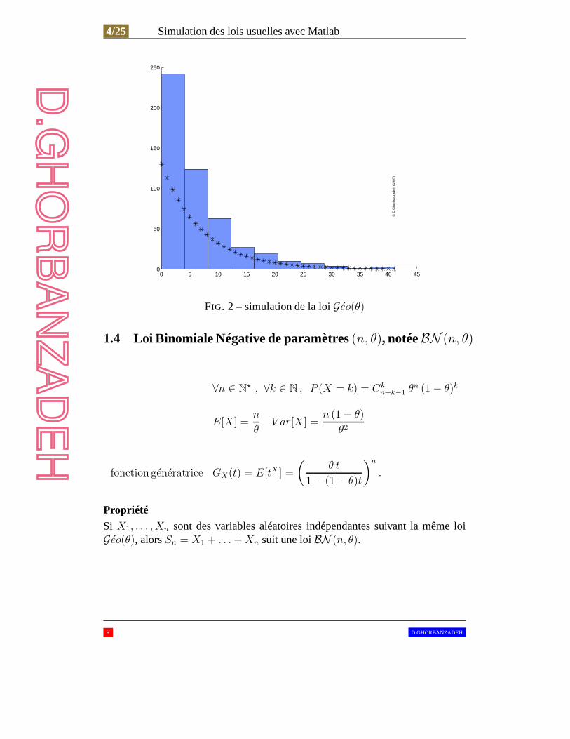
FIG. 2 – simulation de la loiGeo(θ)

1.4 Loi Binomiale Négative de paramètres(n, θ), notéeBN (n, θ)

∀n ∈ N⋆ , ∀k ∈ N , P (X = k) = Ck

n+k−1 θn (1 − θ)k

E[X] =n

θV ar[X] =

n (1 − θ)

θ2

fonction generatrice GX(t) = E[tX ] =

(

θ t

1 − (1 − θ)t

)n

.

Propriété

Si X1, . . . , Xn sont des variables aléatoires indépendantes suivant la même loiGeo(θ), alorsSn = X1 + . . . + Xn suit une loiBN (n, θ).

K D.GHORBANZADEH


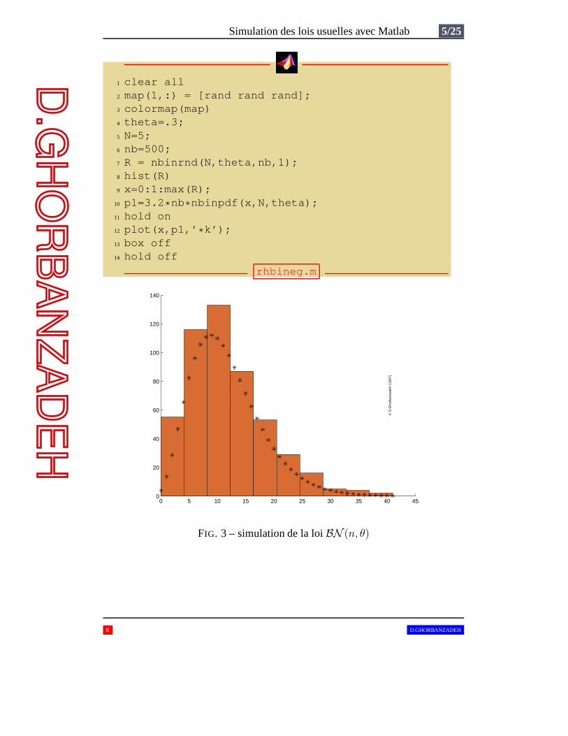
1 clear all2 map(1,:) = [rand rand rand];3 colormap(map)4 theta=.3;5 N=5;6 nb=500;7 R = nbinrnd(N,theta,nb,1);8 hist(R)9 x=0:1:max(R);

10 p1=3.2*nb*nbinpdf(x,N,theta);11 hold on12 plot(x,p1,’*k’);13 box off14 hold off

rhbineg.m

0 5 10 15 20 25 30 35 40 450

20

40

60

80

100

120

140

© D

.Gho

rban

zade

h (1

997)

FIG. 3 – simulation de la loiBN (n, θ)

K D.GHORBANZADEH


1.5 Loi de Poisson de paramètreλ, notéeP(λ)

∀k ∈ N , P (X = k) = e−λ λk

k!

E[X] = λ V ar[X] = λ

fonction generatrice GX(t) = E[tX ] = eλ (1−t).

Propriété

Si X1, . . . , Xn sont des variables aléatoires indépendantes de lois respectives :

P(λ1), . . . ,P(λn), alorsSn = X1 + . . . + Xn suit une loiP(

n∑

k=1

λk).

1 clear all2 map(1,:) = [rand rand rand];3 colormap(map)4 lambda=7;5 nb=1000;6 R = poissrnd(lambda,nb,1);7 hist(R)8 x=0:1:max(R)+1;9 p1=1.7*nb*poisspdf(x,lambda);

10 hold on11 plot(x,p1,’*k’,’linewidth’,1);12 box off13 hold off

rhpois.m

K D.GHORBANZADEH


0 2 4 6 8 10 12 14 16 180

50

100

150

200

250

300

350

© D

.Gho

rban

zade

h (1

997)

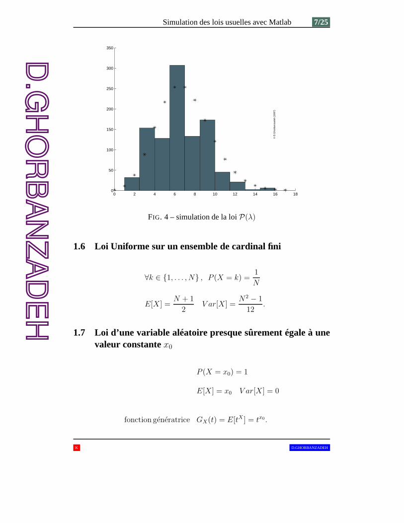
FIG. 4 – simulation de la loiP(λ)

1.6 Loi Uniforme sur un ensemble de cardinal fini

∀k ∈ {1, . . . , N} , P (X = k) =1

N

E[X] =N + 1

2V ar[X] =

N2 − 1

12.

1.7 Loi d’une variable aléatoire presque sûrement égale à unevaleur constantex0

P (X = x0) = 1

E[X] = x0 V ar[X] = 0

fonction generatrice GX(t) = E[tX ] = tx0.

K D.GHORBANZADEH


2 Lois continues

2.1 Loi Uniforme sur l’intervalle [a, b], notéeU([a, b])

densite fX(x) =1

b − al1[a,b](x)

fonction de repartition FX(x) =

0 si x ≤ 0

x − a

b − asi a < x < b

1 si x ≥ b

E[X] =a + b

2V ar[X] =

(b − a)2

12

fonction caracteristique ϕX(t) = E[ei tX ] =ei bt − ei at

i t(b − a).

1 clear all2 map(1,:) = [rand rand rand];3 colormap(map)4 a=2;5 b=7;6 nb=1000;7 R = unifrnd(a,b,nb,1);8 hist(R)9 x = a:0.1:b;

10 p1=.55*nb*unifpdf(x,a,b);11 hold on12 plot(x,p1,’k’,’linewidth’,2);13 box off14 hold off

rhunif.m

K D.GHORBANZADEH


2 2.5 3 3.5 4 4.5 5 5.5 6 6.5 70

20

40

60

80

100

120

© D

.Gho

rban

zade

h (1

997)

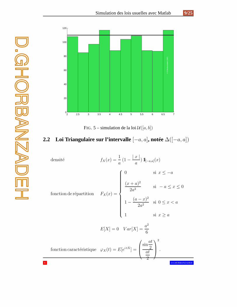
FIG. 5 – simulation de la loiU([a, b])

2.2 Loi Triangulaire sur l’intervalle [−a, a], notée∆([−a, a])

densite fX(x) =1

a(1 − | x |

a) l1[−a,a](x)


0 si x ≤ −a

(x + a)2

2a2si − a ≤ x ≤ 0

1 − (a − x)2

2a2si 0 ≤ x < a

1 si x ≥ a

E[X] = 0 V ar[X] =a2

6

fonction caracteristique ϕX(t) = E[ei tX ] =

sinat

2at

2

2

.

K D.GHORBANZADEH


Propriété

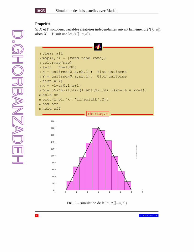
SiX etY sont deux variables aléatoires indépendantes suivant la même loiU([0, a]),alorsX − Y suit une loi∆([−a, a]).

1 clear all2 map(1,:) = [rand rand rand];3 colormap(map)4 a=3; nb=1000;5 X = unifrnd(0,a,nb,1); %loi uniforme6 Y = unifrnd(0,a,nb,1); %loi uniforme7 hist(X-Y)8 x = -1-a:0.1:a+1;9 p1=.55*nb*(1/a)*(1-abs(x)./a).*(x>=-a & x<=a);

10 hold on11 plot(x,p1,’k’,’linewidth’,2);12 box off13 hold off

rhtriag.m

−4 −3 −2 −1 0 1 2 3 40

20

40

60

80

100

120

140

160

180

200

© D

.Gho

rban

zade

h (1

997)

FIG. 6 – simulation de la loi∆([−a, a])

K D.GHORBANZADEH


2.3 Loi Normale de paramètres(m, σ2), notéeN (m, σ2)

densite fX(x) =1

σ√

2 πe−

(x − m)2

2σ2

E[X] = m V ar[X] = σ2

fonction caracteristique ϕX(t) = E[ei tX ] = exp(i mt − 1

2σ2t2)

transformee de Laplace ϕX(t) = E[etX ] = exp(mt +1

2σ2t2).

Propriétés

➋.➌.➊. La densité et la fonction de répartition de la loiN (0, 1) sont notées par :

ϕ(x) =1√2 π

e−x2

2 Φ(x) =

∫ x

−∞

ϕ(t) dt.

➋.➌.➋. Pourx ∈ R on a : Φ(x) + Φ(−x) = 1.

➋.➌.➌. Pourα ∈]0, 1[ on a : Φ−1(α) + Φ−1(1 − α) = 0 , où Φ−1 désigne lafonction réciproque deΦ.

➋.➌.➍. Si X suit une loiN (m, σ2), alors pourα 6= 0 et pour toutβ, α X ± βsuit une loiN (αm ± β, α2 σ2).

➋.➌.➎. Si X suit une loiN (m, σ2), alorsX − m

σsuit une loiN (0, 1).

➋.➌.➏. Si X1, . . . , Xn sont des variables aléatoires indépandantes suivant des

lois :N (m1, σ21), . . . ,N (mn, σ

2n), alors

n∑

k=1

αk Xk suit une loiN (n∑

k=1

αk mk,n∑

k=1

α2k σ2

k).

➋.➌.➐. SiX1, . . . , Xn sont des variables aléatoires indépandantes suivant la même

loi N (m, σ2). Alors Xn =1

n

n∑

i=1

Xi et S2n =

1

n − 1

n∑

i=1

(

Xi − Xn

)2sont indé-

pendants.

K D.GHORBANZADEH


1 clear all2 map(1,:) = [rand rand rand];3 colormap(map)4 m=7;5 sigma2=13;6 nb=2000;7 R= normrnd(m,sqrt(sigma2),nb,1);8 hist(R)9 x=m-4*sqrt(sigma2):0.01:m+4*sqrt(sigma2);

10 p1=2*nb*normpdf(x,m,sqrt(sigma2));11 hold on12 plot(x,p1,’k’,’linewidth’,2);13 box off14 hold off

rhnormal.m

−10 −5 0 5 10 15 20 250

50

100

150

200

250

300

350

400

450

500

© D

.Gho

rban

zade

h (1

997)

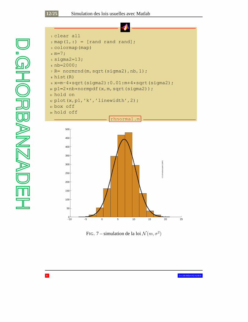
FIG. 7 – simulation de la loiN (m, σ2)

K D.GHORBANZADEH


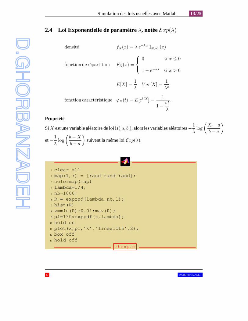
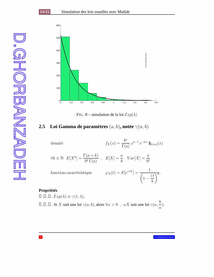
2.4 Loi Exponentielle de paramètreλ, notéeExp(λ)

densite fX(x) = λ e−λ x l1]0,∞[(x)


0 si x ≤ 0

1 − e−λ x si x > 0

E[X] =1

λV ar[X] =

1

λ2

fonction caracteristique ϕX(t) = E[ei tX ] =1

1 − i t

λ

.

Propriété

SiX est une variable aléatoire de loiU(]a, b[), alors les variables aléatoires−1

λlog

(

X − a

b − a

)

et−1

λlog

(

b − X

b − a

)

suivent la même loiExp(λ).

1 clear all2 map(1,:) = [rand rand rand];3 colormap(map)4 lambda=1/4;5 nb=1000;6 R = exprnd(lambda,nb,1);7 hist(R)8 x=min(R):0.01:max(R);9 p1=130*exppdf(x,lambda);


rhexp.m

K D.GHORBANZADEH


0 0.2 0.4 0.6 0.8 1 1.2 1.4 1.6 1.80

100

200

300

400

500

600

© D

.Gho

rban

zade

h (1

997)

FIG. 8 – simulation de la loiExp(λ)

2.5 Loi Gamma de paramètres(a, b), notéeγ(a, b)

densite fX(x) =ba

Γ(a)xa−1 e−b x l1]0,∞[(x)

∀k ∈ N E[Xk] =Γ(a + k)

bk Γ(a), E[X] =

a

bV ar[X] =

a

b2

fonction caracteristique ϕX(t) = E[ei tX ] =1

(

1 − i t

b

)a .

Propriétés

➋.➎.➊. Exp(λ) ≡ γ(1, λ).

➋.➎.➋. Si X suit une loiγ(a, b), alors∀α > 0 , αX suit une loiγ(a,b

α).

K D.GHORBANZADEH


➋.➎.➌. Si X suit une loiγ(a, b), alors la densité de la loi de1

Xest définie par :

f 1

X

(x) =ba

Γ(a)

e−

b

x

xa+1l1]0,∞[(x).

➋.➎.➍. Si X suit une loiγ(a, b), alors poura > 2 on a :

E[1

X] =

b

a − 1V ar[

1

X] =

b2

(a − 1)2 (a − 2).

➋.➎.➎. Si X suit une loiγ(a, b), alors pourα > 0, la densité de la loi deX1

α estdéfinie par :

fX

1α(x) =

α ba

Γ(a)xα a−1 e−b xα

l1]0,∞[(x).

➋.➎.➏. SiX1, . . . , Xn sont des variables aléatoires indépendantes de lois respec-

tives :γ(a1, b), . . . , γ(an, b), alorsSn = X1 + . . . + Xn suit une loiγ(

n∑

k=1

ak, b).

➋.➎.➐. SiX1, . . . , Xn sont des variables aléatoires indépendantes suivant la même

loi Exp(λ), alors1

n

n∑

k=1

Xk suit une loiγ(n, n λ).

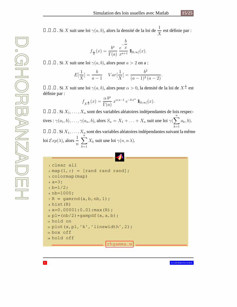
1 clear all2 map(1,:) = [rand rand rand];3 colormap(map)4 a=3;5 b=1/2;6 nb=1000;7 R = gamrnd(a,b,nb,1);8 hist(R)9 x=0.00001:0.01:max(R);

10 p1=(nb/2)*gampdf(x,a,b);11 hold on12 plot(x,p1,’k’,’linewidth’,2);13 box off14 hold off

rhgamma.m

K D.GHORBANZADEH


0 1 2 3 4 5 6 70

50

100

150

200

250

300

350

© D

.Gho

rban

zade

h (1

997)

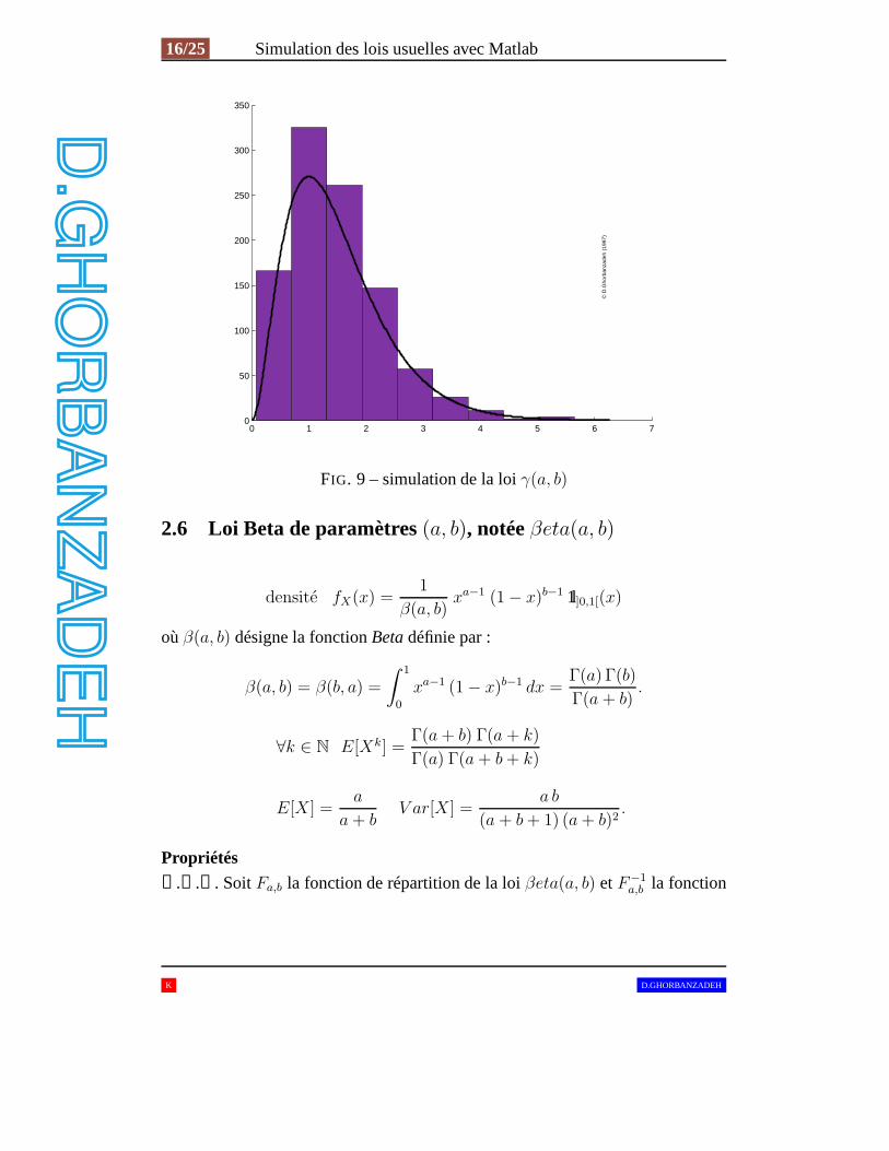
FIG. 9 – simulation de la loiγ(a, b)

2.6 Loi Beta de paramètres(a, b), notéeβeta(a, b)

densite fX(x) =1

β(a, b)xa−1 (1 − x)b−1 l1]0,1[(x)

oùβ(a, b) désigne la fonctionBeta définie par :

β(a, b) = β(b, a) =

∫ 1

0

xa−1 (1 − x)b−1 dx =Γ(a) Γ(b)

Γ(a + b).

∀k ∈ N E[Xk] =Γ(a + b) Γ(a + k)

Γ(a) Γ(a + b + k)

E[X] =a

a + bV ar[X] =

a b

(a + b + 1) (a + b)2.

Propriétés

➋.➏.➊. SoitFa,b la fonction de répartition de la loiβeta(a, b) etF−1a,b la fonction

K D.GHORBANZADEH


réciproque deFa,b. Alors, elles vérifient les relations suivantes :

∀x ∈]0, 1[ , Fa,b(x) = 1 − Fb,a(1 − x)

∀α ∈]0, 1[ , F−1a,b (α) + F−1

b,a (1 − α) = 1.

➋.➏.➋. SiX etY sont deux variables alátoires indépendantes de lois respectives :

γ(a1, b) etγ(a2, b), alorsX

X + Ysuit une loiβeta(a1, a2).

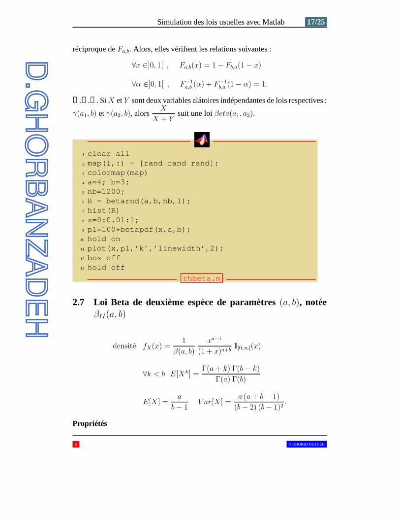
1 clear all2 map(1,:) = [rand rand rand];3 colormap(map)4 a=4; b=3;5 nb=1200;6 R = betarnd(a,b,nb,1);7 hist(R)8 x=0:0.01:1;9 p1=100*betapdf(x,a,b);


rhbeta.m

2.7 Loi Beta de deuxième espèce de paramètres(a, b), notéeβII(a, b)

densite fX(x) =1

β(a, b)

xa−1

(1 + x)a+bl1]0,∞[(x)

∀k < b E[Xk] =Γ(a + k) Γ(b − k)

Γ(a) Γ(b)

E[X] =a

b − 1V ar[X] =

a (a + b − 1)

(b − 2) (b − 1)2.

Propriétés

K D.GHORBANZADEH


0 0.1 0.2 0.3 0.4 0.5 0.6 0.7 0.8 0.9 10

50

100

150

200

250

© D

.Gho

rban

zade

h (1

997)

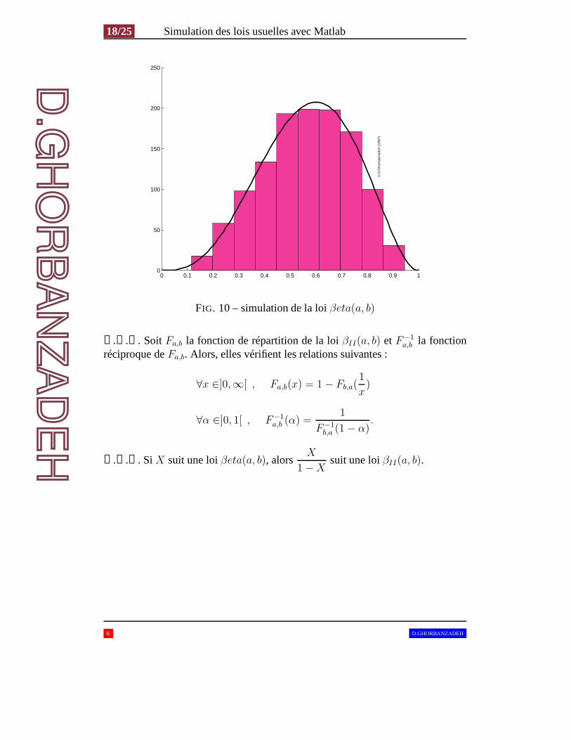
FIG. 10 – simulation de la loiβeta(a, b)

➋.➐.➊. Soit Fa,b la fonction de répartition de la loiβII(a, b) et F−1a,b la fonction

réciproque deFa,b. Alors, elles vérifient les relations suivantes :

∀x ∈]0,∞[ , Fa,b(x) = 1 − Fb,a(1

x)

∀α ∈]0, 1[ , F−1a,b (α) =

1

F−1b,a (1 − α)

.

➋.➐.➋. Si X suit une loiβeta(a, b), alorsX

1 − Xsuit une loiβII(a, b).

K D.GHORBANZADEH


2.8 Loi Chi-deux àm degrés de liberté notéeχ2m

densite fX(x) =1

2m/2 Γ(m2)

xm/2−1 e−x

2 l1]0,∞[(x)

∀k ∈ N E[Xk] = 2kΓ(m

2+ k)

Γ(m2)

E[X] = m V ar[X] = 2 m.

K D.GHORBANZADEH


Propriétés

➋.➑.➊. SiX1, . . . , Xn sont des variables aléatoires indépendantes de lois respec-

tives :χ2m1

, . . . , χ2mn

, alorsSn = X1+ . . .+Xn suit une loiχ2m avecm =

n∑

k=1

mk.

➋.➑.➋. SiX1, . . . , Xn sont des variables aléatoires indépendantes de lois respec-

tives :N (µ1, σ21), . . . ,N (µn, σ

2n), alors

n∑

k=1

(

Xk − µk

σk

)2

suit une loiχ2n.

➋.➑.➌. SiX1, . . . , Xn sont des variables aléatoires indépendantes suivant la même

loi N (µ, σ2), alorsn∑

k=1

(

Xk − Xn

σ

)2

suit une loiχ2n−1 oùXn =

1

n

n∑

k=1

Xk.

1 clear all2 map(1,:) = [rand rand rand];3 colormap(map)4 m=6;5 nb=1000;6 R = chi2rnd(m,nb,1);7 hist(R)8 x=0.0001:0.01:max(R);9 p1=2*nb*chi2pdf(x,m);


rhchi2.m

K D.GHORBANZADEH


0 5 10 15 20 25 300

50

100

150

200

250

300

350

© D

.Gho

rban

zade

h (1

997)

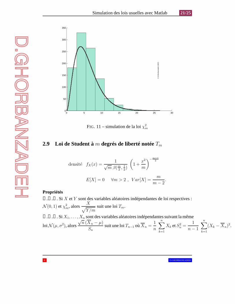
FIG. 11 – simulation de la loiχ2m

2.9 Loi de Student àm degrés de liberté notéeTm

densite fX(x) =1√

m β(m2, 1

2)

(

1 +x2

m

)−m+1

2

E[X] = 0 ∀m > 2 , V ar[X] =m

m − 2.

Propriétés

➋.➒.➊. Si X etY sont des variables aléatoires indépendantes de loi respectives :

N (0, 1) etχ2m, alors

X√

Y/msuit une loiTm.

➋.➒.➋. SiX1, . . . , Xn sont des variables aléatoires indépendantes suivant la même

loi N (µ, σ2), alors

√n (Xn − µ)

Snsuit une loiTn−1 oùXn =

1

n

n∑

k=1

Xk etS2n =

1

n − 1

n∑

k=1

(Xk − Xn)2.

K D.GHORBANZADEH


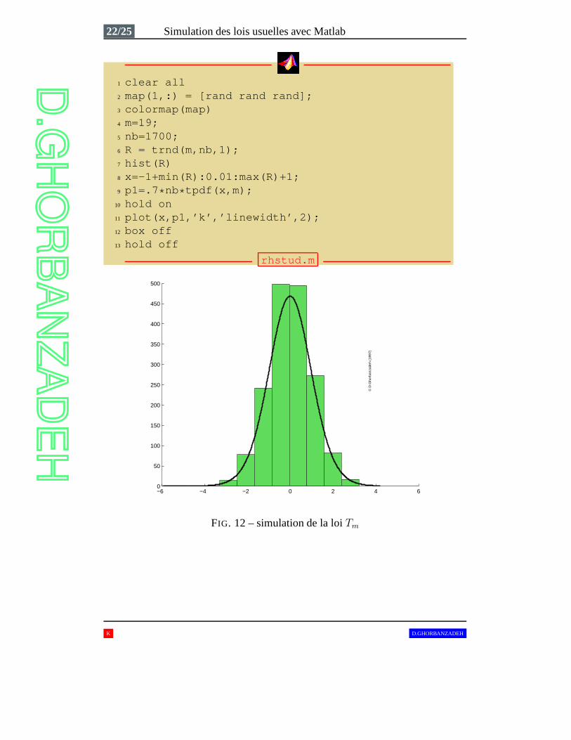
1 clear all2 map(1,:) = [rand rand rand];3 colormap(map)4 m=19;5 nb=1700;6 R = trnd(m,nb,1);7 hist(R)8 x=-1+min(R):0.01:max(R)+1;9 p1=.7*nb*tpdf(x,m);


rhstud.m

−6 −4 −2 0 2 4 60

50

100

150

200

250

300

350

400

450

500

© D

.Gho

rban

zade

h (1

997)

FIG. 12 – simulation de la loiTm

K D.GHORBANZADEH


2.10 Loi de Fisher à(m, n) degrés de liberté, notéeFm,n

densite fX(x) =

(m

n

)m

2

β(m2, n

2)

(

1 +m

nx)−

m+n

2

xm

2−1 l1]0,∞(x)

si n > 2 : E[X] =n

n − 2

si n > 4 : V ar[X] =2n2(m + n − 2)

m(n − 4)(n − 2)2.

Propriétés

➋.➓.➊. Soit Fm,n la fonction de répartition de la loiFm,n et F−1m,n la fonction

réciproque deFm,n. Alors, elles vérifient les relations suivantes :

∀x ∈]0,∞[ , Fm,n(x) = 1 −Fn,m(1

x)

∀α ∈]0, 1[ , F−1m,n(α) =

1

F−1n,m(1 − α)

.

➋.➓.➋. Si X suit une loiFm,n, alors1

Xsuit uneFn,m.

➋.➓.➌. Si X suit une loiTm, alorsX2 suit uneF1,m.

➋.➓.➍. SiX etY sont des variables aléatoires indépendantes de lois respectives :

χ2m etχ2

n, alorsX/m

Y/nsuit une loiFm,n.

➋.➓.➎. Si X suit une loiβII(a, b), alorsb

aX suit uneF2a,2b.

K D.GHORBANZADEH


3 Quelques relations entre les lois usuelles

3.1 Binomiale et Poisson

La loi Binomiale de paramètres(n, p) est approximée par la loi dePoisson deparamètreλ, pourn → ∞, p → 0 avecnp → λ.

En pratique, cette approximation est faite sip < 0, 5 etn > 20.

3.2 Binomiale et Normale

La loi Binomiale de paramètres(n, p) est approximée par la loinormale de moyennenp et varaincenp(1 − p), pourn → ∞ avec0 < p < 1.

En pratique, cette approximation est faite sinp(1 − p) > 9.

• Si X est une varaible aléatoire de loiBinomiale de paramètres(n, p), avecnp(1 − p) > 9 ; alors, on a l’approximation suivante :

P (a ≤ X ≤ b) ≈n>36

Φ

(

b − np√

np(1 − p)

)

− Φ

(

a − np√

np(1 − p)

)

oùΦ désigne la fonction de répartition de la loinormale de moyenne0 et variance1.

3.3 Poisson et Normale

La loi dePoisson de paramètreλ est approximée par la loinormale de moyenneλ et varainceλ, pourλ → ∞.

En pratique, cette approximation est faite siλ ≥ 20.

• Si X est une varaible aléatoire de loiPoisson de paramètreλ, avecλ ≥ 20 ;alors, on a l’approximation suivante :

P (a ≤ X ≤ b) ≈λ≥20

Φ

(

b − λ√λ

)

− Φ

(

a − λ√λ

)

3.4 Khi-deux et Normale

La loi de Khi-deux à m degrés de libeté est approximée par la loinormale demoyennem et varaince2m, pourm > 30.

K D.GHORBANZADEH


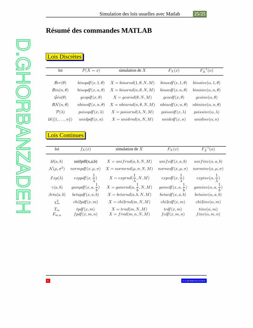
Résumé des commandes MATLAB

Lois Discrètes

loi P (X = x) simulation deX FX(x) F−1

X (α)

Ber(θ) binopdf(x, 1, θ) X = binornd(1, θ, N, M) binocdf(x, 1, θ) binoinv(α, 1, θ)

Bin(n, θ) binopdf(x, n, θ) X = binornd(n, θ, N, M) binocdf(x, n, θ) binoinv(α, n, θ)

Geo(θ) geopdf(x, θ) X = geornd(θ, N, M) geocdf(x, θ) geoinv(α, θ)

BN (n, θ) nbincdf(x, n, θ) X = nbinrnd(n, θ, N, M) nbincdf(x, n, θ) nbininv(α, n, θ)

P(λ) poisspdf(x, λ) X = poissrnd(λ, N, M) poisscdf(x, λ) poissinv(α, λ)

U({1, . . . , n}) unidpdf(x, n) X = unidrnd(n, N, M) unidcdf(x, n) unidinv(α, n)

Lois Continues

loi fX(x) simulation deX FX(x) F−1

X (α)

U(a, b) unifpdf(x,a,b) X = unifrnd(a, b, N, M) unifcdf(x, a, b) unifinv(α, a, b)

N (µ, σ2) normpdf(x, µ, σ) X = normrnd(µ, σ, N, M) normcdf(x, µ, σ) norminv(α, µ, σ)

Exp(λ) exppdf(x,1

λ) X = exprnd(

1

λ, N, M) expcdf(x,

1

λ) expinv(α,

1

λ)

γ(a, b) gampdf(x, a,1

b) X = gamrnd(a,

1

b, N, M) gamcdf(x, a,

1

b) gaminv(α, a,

1

b)

βeta(a, b) betapdf(x, a, b) X = betarnd(a, b, N, M) betacdf(x, a, b) betainv(α, a, b)

χ2

m chi2pdf(x, m) X = chi2rnd(m, N, M) chi2cdf(x, m) chi2inv(α, m)

Tm tpdf(x, m) X = trnd(m, N, M) tcdf(x, m) tinv(α, m)Fm,n fpdf(x, m, n) X = frnd(m, n, N, M) fcdf(x, m, n) finv(α, m, n)

K D.GHORBANZADEH

Documents

1 Lois discrètes - maths.cnam.frmaths.cnam.fr/Membres/ghorbanzadeh/lois.pdf · 10/25 Simulation des lois usuelles avec Matlab Propriété Si X etY sontdeuxvariablesaléatoires indépendantessuivantlamême