Embed Size (px)
Citation preview
tkz-
fct1
.13
c AlterMundusAlterMundus
Alain Matthes
http://altermundus.fr http://altermundus.com
20 janvier 2011
tkz-fct
Alt
erM
un
du
s
Alain Matthestkz-fct.sty est un package pour créer à l’aide de TikZ, des représentations graphiques de fonctionsen 2D le plus simplement possible. Il est dépendant de TikZ et fera partie d’une série de modulesayant comme point commun, la création de dessins utiles dans l’enseignement des mathématiques.Ce package existait déjà, et était disponible sur mon site internet. La version « officielle » a pourpremier numéro de version 1.13 c (c pour CTAN) ; de plus, la syntaxe a évolué et certaines macros ontcommencé une mutation qui permettra de rendre l’ensemble de mes packages plus homogène. Cepackage nécessite la version 2.1 de TikZ.
t Je souhaite remercier Till Tantau pour avoir créé le merveilleux outil TikZ, ainsi que Michel Bovani pourfourier, dont l’association avec utopia est excellente.
t Je souhaite remercier aussi David Arnold qui a corrigé un grand nombre d’erreurs et qui a testé de nombreuxexemples, Wolfgang Büchel qui a corrigé également des erreurs et a construit de superbes scripts pour obtenirles fichiers d’exemples, John Kitzmiller et ses exemples, et enfin Gaétan Marris pour ses remarques.
t Vous trouverez de nombreux exemples sur mes sites : altermundus.com ou altermundus.fr
Vous pouvez envoyer vos remarques, et les rapports sur des erreurs que vous aurez constatées à l’adressesuivante : Alain Matthes.
This file can be redistributed and/or modified under the terms of the LATEX Project Public License Distributedfrom CTAN archives.
Table des matières 3
Table des matières
1 Fonctionnement 6
2 Installation de tkz-fct 72.1 Avec TeXLive sous OS X, Linux et Windows . . . . . . . . . . . . . . . . . . . . . . . . . . . . . . . . 72.2 Avec MikTeX sous Windows XP . . . . . . . . . . . . . . . . . . . . . . . . . . . . . . . . . . . . . . . 82.3 Résumé de l’installation . . . . . . . . . . . . . . . . . . . . . . . . . . . . . . . . . . . . . . . . . . . 8
3 Utilisation de Gnuplot 103.1 Mécanisme d’interaction entre TikZ et Gnuplot . . . . . . . . . . . . . . . . . . . . . . . . . . . . . 103.2 Installation de Gnuplot . . . . . . . . . . . . . . . . . . . . . . . . . . . . . . . . . . . . . . . . . . . 123.3 Test de l’installation de tkz-base . . . . . . . . . . . . . . . . . . . . . . . . . . . . . . . . . . . . . . 133.4 Test de l’installation de tkz-fct . . . . . . . . . . . . . . . . . . . . . . . . . . . . . . . . . . . . . . . 13
4 Les différentes macros 154.1 Tracé d’une fonction avec gnuplot \tkzFct . . . . . . . . . . . . . . . . . . . . . . . . . . . . . . . 154.2 option : samples . . . . . . . . . . . . . . . . . . . . . . . . . . . . . . . . . . . . . . . . . . . . . . . 154.3 options : xstep, ystep . . . . . . . . . . . . . . . . . . . . . . . . . . . . . . . . . . . . . . . . . . . 164.4 Modification de xstep et ystep . . . . . . . . . . . . . . . . . . . . . . . . . . . . . . . . . . . . . . 164.5 ystep et les fonctions constantes . . . . . . . . . . . . . . . . . . . . . . . . . . . . . . . . . . . . . . 174.6 Les fonctions affines ou linéaires . . . . . . . . . . . . . . . . . . . . . . . . . . . . . . . . . . . . . . 184.7 Sous-grille . . . . . . . . . . . . . . . . . . . . . . . . . . . . . . . . . . . . . . . . . . . . . . . . . . . 184.8 Utilisation des macros de tkz-base . . . . . . . . . . . . . . . . . . . . . . . . . . . . . . . . . . . . 19
5 Placer un point sur une courbe 205.1 Exemple avec \tkzGetPoint . . . . . . . . . . . . . . . . . . . . . . . . . . . . . . . . . . . . . . . . 205.2 Exemple avec \tkzGetPoint et tkzPointResult . . . . . . . . . . . . . . . . . . . . . . . . . . . . 215.3 Options draw et ref . . . . . . . . . . . . . . . . . . . . . . . . . . . . . . . . . . . . . . . . . . . . . 215.4 Placer des points sans courbe . . . . . . . . . . . . . . . . . . . . . . . . . . . . . . . . . . . . . . . . 225.5 Placer des points sans se soucier des coordonnées . . . . . . . . . . . . . . . . . . . . . . . . . . . 235.6 Placer des points avec deux fonctions . . . . . . . . . . . . . . . . . . . . . . . . . . . . . . . . . . . 24
6 Labels 256.1 Ajouter un label . . . . . . . . . . . . . . . . . . . . . . . . . . . . . . . . . . . . . . . . . . . . . . . . 25
7 Macros pour tracer des tangentes 277.1 Représentation d’une tangente \tkzDrawTangentLine . . . . . . . . . . . . . . . . . . . . . . . . 277.2 Tangente avec xstep et ystep différents de 1 . . . . . . . . . . . . . . . . . . . . . . . . . . . . . . 277.3 Les options kl, kr et l’option draw . . . . . . . . . . . . . . . . . . . . . . . . . . . . . . . . . . . . . 287.4 Tangente et l’option with . . . . . . . . . . . . . . . . . . . . . . . . . . . . . . . . . . . . . . . . . . 297.5 Quelques tangentes . . . . . . . . . . . . . . . . . . . . . . . . . . . . . . . . . . . . . . . . . . . . . 307.6 Demi-tangentes . . . . . . . . . . . . . . . . . . . . . . . . . . . . . . . . . . . . . . . . . . . . . . . 317.7 Demi-tangentes Courbe de Lorentz . . . . . . . . . . . . . . . . . . . . . . . . . . . . . . . . . . . . 327.8 Série de tangentes . . . . . . . . . . . . . . . . . . . . . . . . . . . . . . . . . . . . . . . . . . . . . . . 337.9 Série de tangentes sans courbe . . . . . . . . . . . . . . . . . . . . . . . . . . . . . . . . . . . . . . . 34
7.9.1 Utilisation de \tkzFctLast . . . . . . . . . . . . . . . . . . . . . . . . . . . . . . . . . . . . 347.10 Calcul de l’antécédent . . . . . . . . . . . . . . . . . . . . . . . . . . . . . . . . . . . . . . . . . . . . 35
7.10.1 Valeur numérique de l’antécédent . . . . . . . . . . . . . . . . . . . . . . . . . . . . . . . . 357.10.2 utilisation de la valeur numérique . . . . . . . . . . . . . . . . . . . . . . . . . . . . . . . . 35
tkz-fct AlterMundus
Table des matières 4
8 Macros pour définir des surfaces 368.1 Représentation d’une surface \tkzDrawArea ou \tkzArea . . . . . . . . . . . . . . . . . . . . . . 368.2 Naissance de la fonction logarithme népérien . . . . . . . . . . . . . . . . . . . . . . . . . . . . . . 368.3 Surface simple . . . . . . . . . . . . . . . . . . . . . . . . . . . . . . . . . . . . . . . . . . . . . . . . . 378.4 Surface et hachures . . . . . . . . . . . . . . . . . . . . . . . . . . . . . . . . . . . . . . . . . . . . . . 388.5 Surface comprise entre deux courbes \tkzDrawAreafg . . . . . . . . . . . . . . . . . . . . . . . . 398.6 Surface comprise entre deux courbes en couleur . . . . . . . . . . . . . . . . . . . . . . . . . . . . 398.7 Surface comprise entre deux courbes avec des hachures . . . . . . . . . . . . . . . . . . . . . . . . 408.8 Surface comprise entre deux courbes avec l’option between . . . . . . . . . . . . . . . . . . . . . 408.9 Surface comprise entre deux courbes : courbes de Lorentz . . . . . . . . . . . . . . . . . . . . . . . 418.10 Mélange de style . . . . . . . . . . . . . . . . . . . . . . . . . . . . . . . . . . . . . . . . . . . . . . . 428.11 Courbes de niveaux . . . . . . . . . . . . . . . . . . . . . . . . . . . . . . . . . . . . . . . . . . . . . . 43
9 Sommes de Riemann 449.1 Somme de Riemann . . . . . . . . . . . . . . . . . . . . . . . . . . . . . . . . . . . . . . . . . . . . . 449.2 Somme de Riemann Inf . . . . . . . . . . . . . . . . . . . . . . . . . . . . . . . . . . . . . . . . . . . 459.3 Somme de Riemann Inf et Sup . . . . . . . . . . . . . . . . . . . . . . . . . . . . . . . . . . . . . . . 469.4 Somme de Riemann Mid . . . . . . . . . . . . . . . . . . . . . . . . . . . . . . . . . . . . . . . . . . . 47
10Droites particulières 4810.1 Tracer une ligne verticale . . . . . . . . . . . . . . . . . . . . . . . . . . . . . . . . . . . . . . . . . . 4810.2 Ligne verticale . . . . . . . . . . . . . . . . . . . . . . . . . . . . . . . . . . . . . . . . . . . . . . . . 4810.3 Lignes verticales . . . . . . . . . . . . . . . . . . . . . . . . . . . . . . . . . . . . . . . . . . . . . . . . 4910.4 Ligne verticale et valeur calculée par fp . . . . . . . . . . . . . . . . . . . . . . . . . . . . . . . . . 4910.5 Une ligne horizontale . . . . . . . . . . . . . . . . . . . . . . . . . . . . . . . . . . . . . . . . . . . . 5010.6 Asymptote horizontale . . . . . . . . . . . . . . . . . . . . . . . . . . . . . . . . . . . . . . . . . . . . 5010.7 Lignes horizontales . . . . . . . . . . . . . . . . . . . . . . . . . . . . . . . . . . . . . . . . . . . . . . 5110.8 Asymptote horizontale et verticale . . . . . . . . . . . . . . . . . . . . . . . . . . . . . . . . . . . . . 52
11Courbes avec équations paramétrées 5311.1 Courbe paramétrée exemple 1 . . . . . . . . . . . . . . . . . . . . . . . . . . . . . . . . . . . . . . . 5311.2 Courbe paramétrée exemple 2 . . . . . . . . . . . . . . . . . . . . . . . . . . . . . . . . . . . . . . . 5411.3 Courbe paramétrée exemple 3 . . . . . . . . . . . . . . . . . . . . . . . . . . . . . . . . . . . . . . . 5511.4 Courbe paramétrée exemple 4 . . . . . . . . . . . . . . . . . . . . . . . . . . . . . . . . . . . . . . . 5611.5 Courbe paramétrée exemple 5 . . . . . . . . . . . . . . . . . . . . . . . . . . . . . . . . . . . . . . . 5711.6 Courbe paramétrée exemple 6 . . . . . . . . . . . . . . . . . . . . . . . . . . . . . . . . . . . . . . . 5811.7 Courbe paramétrée exemple 7 . . . . . . . . . . . . . . . . . . . . . . . . . . . . . . . . . . . . . . . 59
12Courbes en coordonnées polaires 6012.1 Équation polaire exemple 1 . . . . . . . . . . . . . . . . . . . . . . . . . . . . . . . . . . . . . . . . . 6012.2 Équation polaire exemple 2 . . . . . . . . . . . . . . . . . . . . . . . . . . . . . . . . . . . . . . . . . 6112.3 Équation polaire Heart . . . . . . . . . . . . . . . . . . . . . . . . . . . . . . . . . . . . . . . . . . . . 6212.4 Équation polaire exemple 4 . . . . . . . . . . . . . . . . . . . . . . . . . . . . . . . . . . . . . . . . . 6312.5 Équation polaire Cannabis ou Marijuana Curve . . . . . . . . . . . . . . . . . . . . . . . . . . . . . 6412.6 Scarabaeus Curve . . . . . . . . . . . . . . . . . . . . . . . . . . . . . . . . . . . . . . . . . . . . . . . 65
13Symboles 66
14Quelques exemples 6714.1 Variante intermédiaire : TikZ + tkz-fct . . . . . . . . . . . . . . . . . . . . . . . . . . . . . . . . . 6714.2 Courbes de Lorentz . . . . . . . . . . . . . . . . . . . . . . . . . . . . . . . . . . . . . . . . . . . . . 6814.3 Courbe exponentielle . . . . . . . . . . . . . . . . . . . . . . . . . . . . . . . . . . . . . . . . . . . . . 6914.4 Axe logarithmique . . . . . . . . . . . . . . . . . . . . . . . . . . . . . . . . . . . . . . . . . . . . . . 7014.5 Un peu de tout . . . . . . . . . . . . . . . . . . . . . . . . . . . . . . . . . . . . . . . . . . . . . . . . . 71
tkz-fct AlterMundus
Table des matières 5
14.6 Interpolation . . . . . . . . . . . . . . . . . . . . . . . . . . . . . . . . . . . . . . . . . . . . . . . . . . 7214.6.1 Le code . . . . . . . . . . . . . . . . . . . . . . . . . . . . . . . . . . . . . . . . . . . . . . . . 7214.6.2 la figure . . . . . . . . . . . . . . . . . . . . . . . . . . . . . . . . . . . . . . . . . . . . . . . . 73
14.7 Courbes de Van der Waals . . . . . . . . . . . . . . . . . . . . . . . . . . . . . . . . . . . . . . . . . 7514.7.1 Tableau de variations . . . . . . . . . . . . . . . . . . . . . . . . . . . . . . . . . . . . . . . . 7514.7.2 Première courbe avec b=1 . . . . . . . . . . . . . . . . . . . . . . . . . . . . . . . . . . . . . 7614.7.3 Deuxième courbe b=1/3 . . . . . . . . . . . . . . . . . . . . . . . . . . . . . . . . . . . . . 7714.7.4 Troisième courbe b=32/27 . . . . . . . . . . . . . . . . . . . . . . . . . . . . . . . . . . . . 78
14.8 Valeurs critiques . . . . . . . . . . . . . . . . . . . . . . . . . . . . . . . . . . . . . . . . . . . . . . . . 7914.8.1 Courbes de Van der Walls . . . . . . . . . . . . . . . . . . . . . . . . . . . . . . . . . . . 7914.8.2 Courbes de Van der Walls (suite) . . . . . . . . . . . . . . . . . . . . . . . . . . . . . . . 80
15Exemples avec les packages alterqcm et tkz-tab 8115.0.3 Première représentation . . . . . . . . . . . . . . . . . . . . . . . . . . . . . . . . . . . . . . 8315.0.4 Seconde représentation . . . . . . . . . . . . . . . . . . . . . . . . . . . . . . . . . . . . . . 83
16Utilisation pgfmath et de fp.sty 8416.1 pgfmath . . . . . . . . . . . . . . . . . . . . . . . . . . . . . . . . . . . . . . . . . . . . . . . . . . . . 8416.2 fp.sty . . . . . . . . . . . . . . . . . . . . . . . . . . . . . . . . . . . . . . . . . . . . . . . . . . . . . 84
17Quelques remarques 8617.1 Fonctions de gnuplot . . . . . . . . . . . . . . . . . . . . . . . . . . . . . . . . . . . . . . . . . . . . 87
18Liste de toutes les macros 8818.1 Liste de toutes les macros fournies par ce package . . . . . . . . . . . . . . . . . . . . . . . . . . . 8818.2 Liste de toutes des macros essentielles de \tkz-base . . . . . . . . . . . . . . . . . . . . . . . . . . 88
Index 89
tkz-fct AlterMundus
1 Fonctionnement 6
SECTION 1
Fonctionnement
TikZ apporte différentes possibilités pour obtenir les représentations graphiques des fonctions. J’ai privilégiél’utilisation de gnuplot, car je trouve pgfmath trop lent et les résultats trop imprécis.
Avec TikZ et gnuplot, on obtient la représentation d’une fonction à l’aide de
\draw[options] plot function {gnuplot expression};
Dans cette nouvelle version de tkz-fct, la macro \tkzFct reprend le code précédent avec les mêmes optionsque celles de TikZ. Parmi les options, les plus importantes sont domain et samples.
La macro \tkzFct remplace \draw plot function mais exécute deux tâches supplémentaires, en plus dutracé. Tout d’abord, l’expression de la fonction est sauvegardée avec la syntaxe de gnuplot et également sauve-gardée avec la syntaxe de fp pour une utilisation ultérieure. Cela permet, sans avoir à redonner l’expression,de placer par exemple, des points sur la courbe (les images sont calculées à l’aide de fp), ou bien encore, detracer des tangentes.
Ensuite, et c’est le plus important, \tkzFct tient compte des unités utilisées pour l’axe des abscisses et celuides ordonnées. Ces unités sont définies en utilisant la macro \tkzInit du package tkz-base avec les optionsxstep et ystep.
La macro \tkzFct intercepte les valeurs données à l’option domain et évidemment l’expression mathématiquede la fonction ; si xstep et ystep diffèrent de 1 alors il est tenu compte de ces valeurs pour le domaine, ainsique pour les calculs d’images. Lorsque xstep diffère de 1 alors l’expression donnée, doit utiliser uniquement\x comme variable, c’est ainsi qu’il est possible d’ajuster les valeurs. Cela permet d’éviter des débordementsdans les calculs.
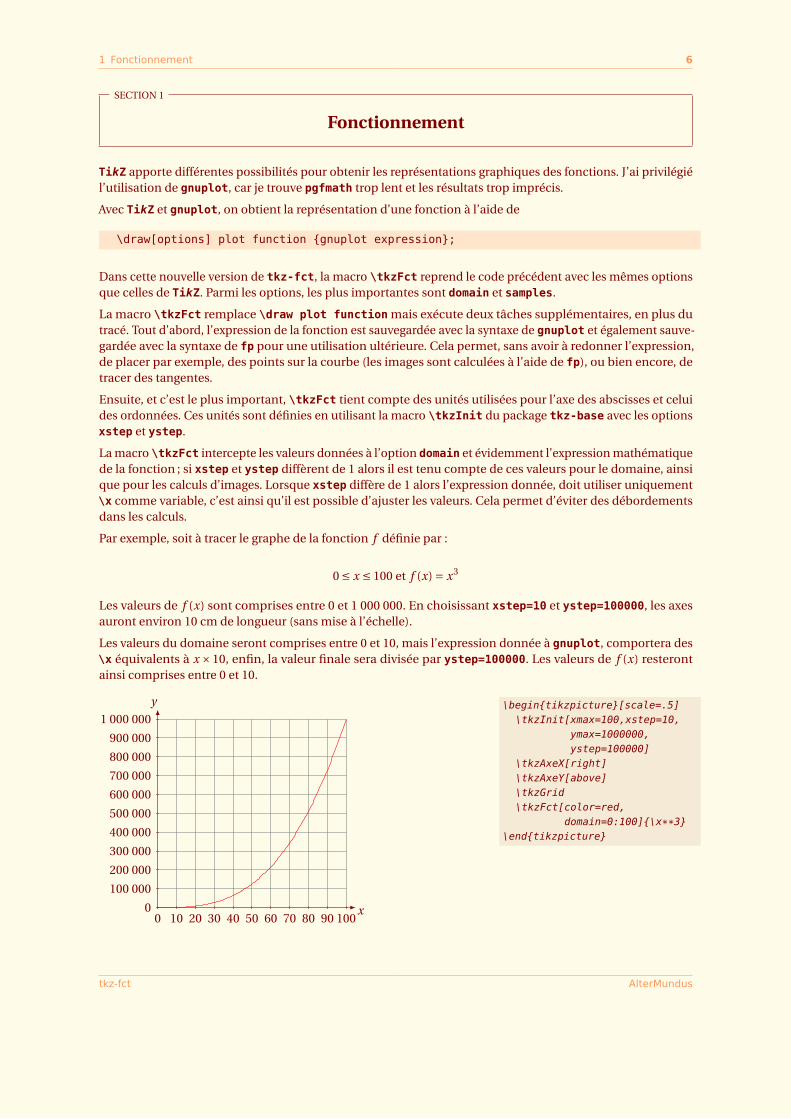
Par exemple, soit à tracer le graphe de la fonction f définie par :
0 ≤ x ≤ 100 et f (x) = x3
Les valeurs de f (x) sont comprises entre 0 et 1 000 000. En choisissant xstep=10 et ystep=100000, les axesauront environ 10 cm de longueur (sans mise à l’échelle).
Les valeurs du domaine seront comprises entre 0 et 10, mais l’expression donnée à gnuplot, comportera des\x équivalents à x ×10, enfin, la valeur finale sera divisée par ystep=100000. Les valeurs de f (x) resterontainsi comprises entre 0 et 10.
0 10 20 30 40 50 60 70 80 90 100x
y
0
100 000
200 000
300 000
400 000
500 000
600 000
700 000
800 000
900 000
1 000 000\begin{tikzpicture}[scale=.5]
\tkzInit[xmax=100,xstep=10,ymax=1000000,ystep=100000]
\tkzAxeX[right]\tkzAxeY[above]\tkzGrid\tkzFct[color=red,
domain=0:100]{\x**3}\end{tikzpicture}
tkz-fct AlterMundus
2 Installation de tkz-fct 7
SECTION 2
Installation de tkz-fct
Il est possible que lorsque vous lirez ce document, tkz-fct soit présent sur le serveur du CTAN 1. Si tkz-fctne fait pas encore partie de votre distribution, cette section vous montre comment l’installer, elle est aussinécessaire, si vous avez envie d’installer une version plus récente ou personnalisée de tkz-fct. Attention, laprésence dans mon dossier texmf, des fichiers de PGF, s’explique par l’utilisation occasionnelle de la version CVSde PGF.
2.1 Avec TeXLive sous OS X, Linux et Windows
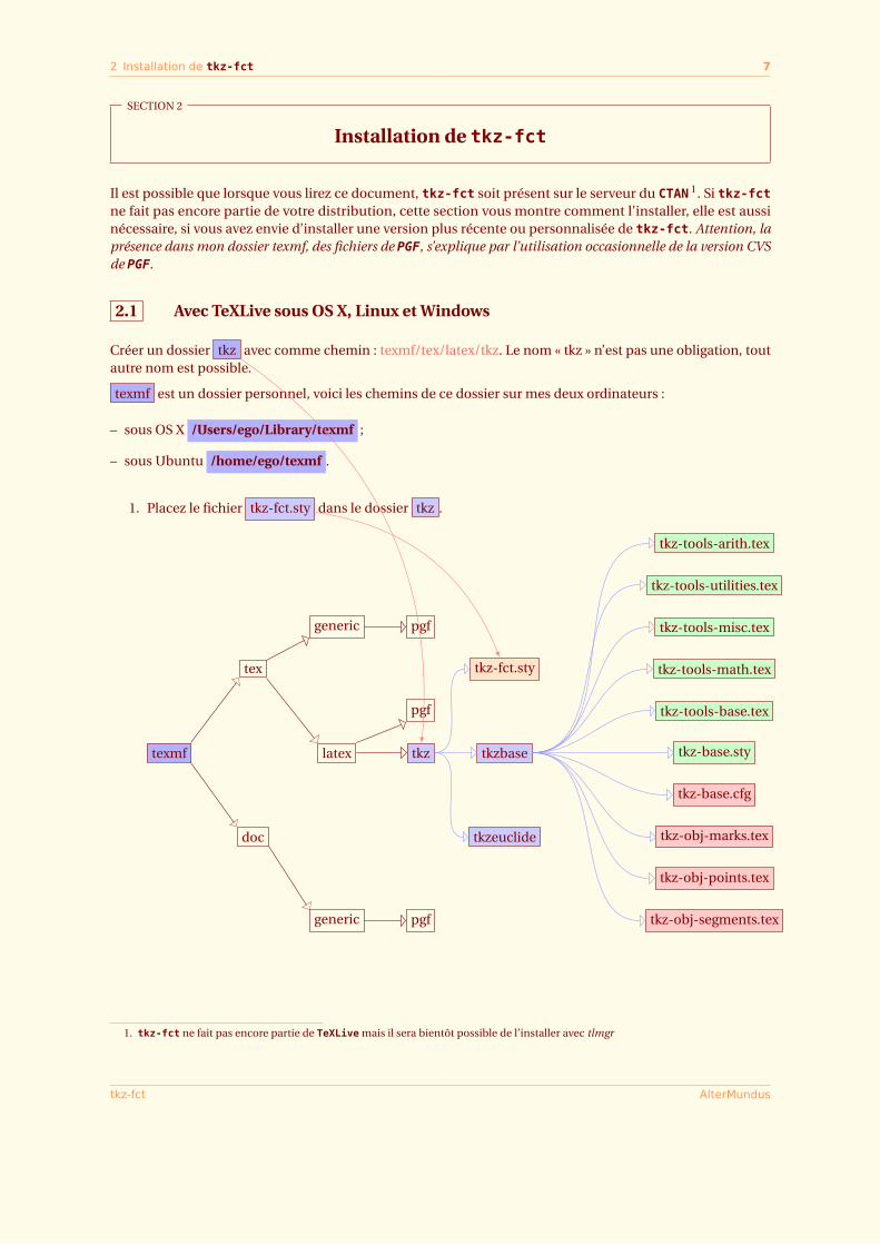
Créer un dossier tkz avec comme chemin : texmf/tex/latex/tkz. Le nom « tkz » n’est pas une obligation, toutautre nom est possible.
texmf est un dossier personnel, voici les chemins de ce dossier sur mes deux ordinateurs :
– sous OS X /Users/ego/Library/texmf ;
– sous Ubuntu /home/ego/texmf .
1. Placez le fichier tkz-fct.sty dans le dossier tkz .
texmf
tex
doc
generic
generic
latex
pgf
pgf
tkz
pgf
tkz-fct.sty
tkzbase
tkzeuclide
tkz-tools-arith.tex
tkz-tools-utilities.tex
tkz-tools-misc.tex
tkz-tools-math.tex
tkz-tools-base.tex
tkz-base.sty
tkz-base.cfg
tkz-obj-marks.tex
tkz-obj-points.tex
tkz-obj-segments.tex
1. tkz-fct ne fait pas encore partie de TeXLive mais il sera bientôt possible de l’installer avec tlmgr
tkz-fct AlterMundus
2.2 Avec MikTeX sous Windows XP 8
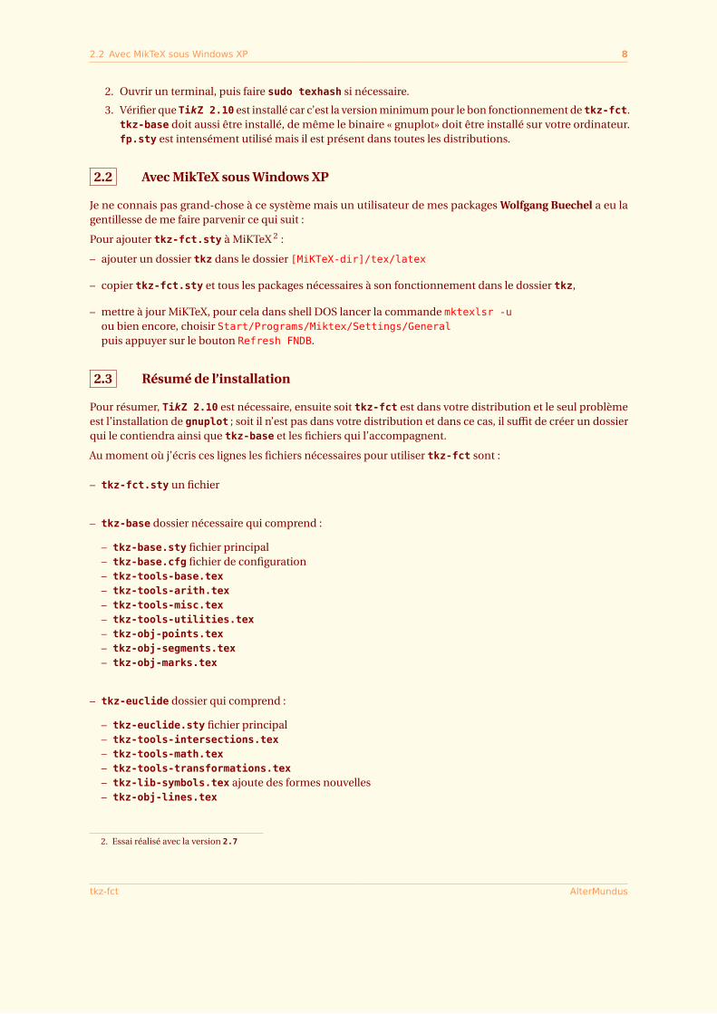
2. Ouvrir un terminal, puis faire sudo texhash si nécessaire.
3. Vérifier que TikZ 2.10 est installé car c’est la version minimum pour le bon fonctionnement de tkz-fct.tkz-base doit aussi être installé, de même le binaire « gnuplot» doit être installé sur votre ordinateur.fp.sty est intensément utilisé mais il est présent dans toutes les distributions.
2.2 Avec MikTeX sous Windows XP
Je ne connais pas grand-chose à ce système mais un utilisateur de mes packages Wolfgang Buechel a eu lagentillesse de me faire parvenir ce qui suit :
Pour ajouter tkz-fct.sty à MiKTeX 2 :
– ajouter un dossier tkz dans le dossier [MiKTeX-dir]/tex/latex
– copier tkz-fct.sty et tous les packages nécessaires à son fonctionnement dans le dossier tkz,
– mettre à jour MiKTeX, pour cela dans shell DOS lancer la commande mktexlsr -uou bien encore, choisir Start/Programs/Miktex/Settings/Generalpuis appuyer sur le bouton Refresh FNDB.
2.3 Résumé de l’installation
Pour résumer, TikZ 2.10 est nécessaire, ensuite soit tkz-fct est dans votre distribution et le seul problèmeest l’installation de gnuplot ; soit il n’est pas dans votre distribution et dans ce cas, il suffit de créer un dossierqui le contiendra ainsi que tkz-base et les fichiers qui l’accompagnent.
Au moment où j’écris ces lignes les fichiers nécessaires pour utiliser tkz-fct sont :
– tkz-fct.sty un fichier
– tkz-base dossier nécessaire qui comprend :
– tkz-base.sty fichier principal– tkz-base.cfg fichier de configuration– tkz-tools-base.tex– tkz-tools-arith.tex– tkz-tools-misc.tex– tkz-tools-utilities.tex– tkz-obj-points.tex– tkz-obj-segments.tex– tkz-obj-marks.tex
– tkz-euclide dossier qui comprend :
– tkz-euclide.sty fichier principal– tkz-tools-intersections.tex– tkz-tools-math.tex– tkz-tools-transformations.tex– tkz-lib-symbols.tex ajoute des formes nouvelles– tkz-obj-lines.tex
2. Essai réalisé avec la version 2.7
tkz-fct AlterMundus
2.3 Résumé de l’installation 9
– tkz-obj-addpoints.tex compléments sur les points– tkz-obj-circles.tex– tkz-obj-arcs.tex– tkz-obj-angles.tex– tkz-obj-polygons.tex– tkz-obj-sectors.tex– tkz-obj-protractor.tex
tkz-fct AlterMundus
3 Utilisation de Gnuplot 10
SECTION 3
Utilisation de Gnuplot
3.1 Mécanisme d’interaction entre TikZ et Gnuplot
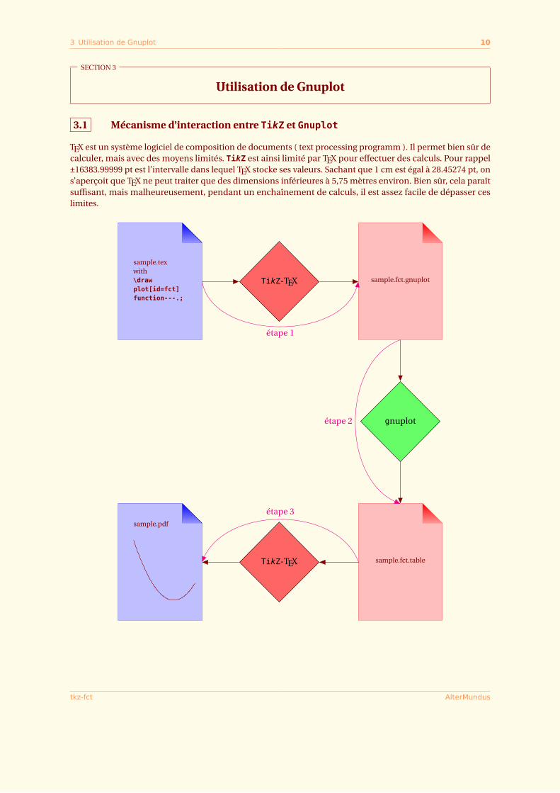
TEX est un système logiciel de composition de documents ( text processing programm ). Il permet bien sûr decalculer, mais avec des moyens limités. TikZ est ainsi limité par TEX pour effectuer des calculs. Pour rappel±16383.99999 pt est l’intervalle dans lequel TEX stocke ses valeurs. Sachant que 1 cm est égal à 28.45274 pt, ons’aperçoit que TEX ne peut traiter que des dimensions inférieures à 5,75 mètres environ. Bien sûr, cela paraîtsuffisant, mais malheureusement, pendant un enchaînement de calculs, il est assez facile de dépasser ceslimites.
sample.texwith\drawplot[id=fct]function---.;
sample.fct.gnuplot
sample.fct.table
sample.pdf
TikZ-TEX
gnuplot
TikZ-TEX
étape 1
étape 2
étape 3
tkz-fct AlterMundus
3.1 Mécanisme d’interaction entre TikZ et Gnuplot 11
Pour tracer des courbes en 2D en contournant ces problèmes, un moyen simple offert par TikZ, est d’utilisergnuplot.
tkz-fct.sty s’appuie sur le programme gnuplot et le package fp.sty. Le premier est utilisé pour obtenirune liste de points, et le second pour évaluer ponctuellement des valeurs.
Vous devez donc installer Gnuplot, son installation dépend de votre système, puis il faudra que votre distribu-tion trouve Gnuplot, et que TEX autorise Gnuplot à écrire un fichier.
– Étape 1On part du fichier sample.tex suivant :
\documentclass{article}\usepackage{tikz}\begin{document}\begin{tikzpicture}\draw plot[id=f1,samples=200,domain=-2:2] function{x*x};\end{tikzpicture}\end{document}
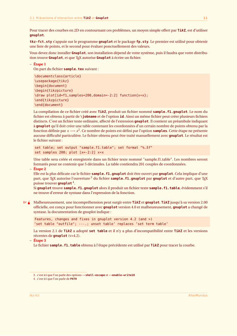
La compilation de ce fichier créé avec TikZ, produit un fichier nommé sample.f1.gnuplot. Le nom dufichier est obtenu à partir de \jobname et de l’option id. Ainsi un même fichier peut créer plusieurs fichiersdistincts. C’est un fichier texte ordinaire, affecté de l’extension gnuplot. Il contient un préambule indiquantà gnuplot qu’il doit créer une table contenant les coordonnées d’un certain nombre de points obtenu par lafonction définie par x −→ x2. Ce nombre de points est défini par l’option samples. Cette étape ne présenteaucune difficulté particulière. Le fichier obtenu peut être traité manuellement avec gnuplot. Le résultat estle fichier suivant :
set table; set output "sample.f1.table"; set format "%.5f"set samples 200; plot [x=-2:2] x*x
Une table sera créée et enregistrée dans un fichier texte nommé "sample.f1.table". Les nombres serontformatés pour ne contenir que 5 décimales. La table contiendra 201 couples de coordonnées.
– Étape 2Elle est la plus délicate car le fichier sample.f1.gnuplot doit être ouvert par gnuplot. Cela implique d’unepart, que TEX autorise l’ouverture 3 du fichier sample.f1.gnuplot par gnuplot et d’autre part, que TEXpuisse trouver gnuplot 4.Si gnuplot trouve sample.f1.gnuplot alors il produit un fichier texte sample.f1.table, évidemment s’ilne trouve d’erreur de syntaxe dans l’expression de la fonction.
tL Malheureusement, une incompréhension peut surgir entre TikZ et gnuplot. TikZ jusqu’à sa version 2.00officielle, est conçu pour fonctionner avec gnuplot version 4.0 et malheureusement, gnuplot a changé desyntaxe. la documentation de gnuplot indique :
Features, changes and fixes in gnuplot version 4.2 (and >)’set table "outfile"; ---.; unset table’ replaces ’set term table’
La version 2.1 de TikZ a adopté set table et il n’y a plus d’incompatibilité entre TikZ et les versionsrécentes de gnuplot (v>4.2).
– Étape 3Le fichier sample.f1.table obtenu à l’étape précédente est utilisé par TikZ pour tracer la courbe.
3. c’est ici que l’on parle des options --shell-escape et --enable-write184. c’est ici que l’on parle de PATH
tkz-fct AlterMundus
3.2 Installation de Gnuplot 12
# Curve 0 of 1, 201 points# Curve title: "x*x"# x y type-2.00000 4.00000 i-1.98000 3.92040 i-1.96000 3.84160 i---.1.98000 3.92040 i2.00000 4.00000 i
1. Il faut remarquer qu’au cours d’une seconde compilation, si le fichier sample.f1.gnuplot ne changepas, alors gnuplot n’est pas lancé et le fichier présent sample.f1.table est utilisé.
2. On peut aussi remarquer que si vous êtes paranoïaque et que vous n’autorisez pas le lancement degnuplot, alors un première compilation permettra de créer le fichier sample.f1.table, ensuite manuel-lement, vous pourrez lancer gnuplot et obtenir le fichier sample.f1.table.
3. Il est aussi possible de créer manuellement ou encore avec un quelconque programme, un fichierdata.table que TikZ pourra lire avec
\draw plot[smooth] file {data.table};
3.2 Installation de Gnuplot
Gnuplot est proposé avec la plupart des distributions Linux, et existe pour OS X ainsi que pour Windows.
1. Ubuntu ou un autre système Linux: on l’installe en suivant la procédure classique d’installation d’unnouveau paquetage.
2. Windows Les utilisateurs de Windows doivent se méfier, après avoir téléchargé la bonne version et installégnuplot alors il faudra renommé wgnuplot en gnuplot. Ensuite il faudra modifier le path. Si le chemindu programme est C:\gnuplot alors il faudra ajouter C:\gnuplot\bin\ aux variables environnement(Aller à "Poste de Travail" puis faire "propriétés", dans l’onglet "Avancé", cliquer sur "Variables d’en-vironnement". ). Ensuite pour compiler sous latex, il faudra ajouter au script de compilation l’option--enable-write18 .
3. OS X C’est le système en version Snow Leopard qui pose le plus de problème, car il faut compiler lessources. Si vous n’utilisez gnuplot qu’en collaboration avec TikZ alors il vous suffit de compiler lessources ainsi :
a) Télécharger les sources de gnuplot, déposer les sources sur le bureau.
b) Ouvrir un terminal puis taper cd et glisser le dossier des sources après cd (en laissant un espace)Cela doit donner
$ cd /Users/ego/Desktop/gnuplot-4.4.2
c) ensuite taper la ligne suivante et valider
$ ./configure --with-readline=builtin
d) puis
$ make
e) et enfin
$ sudo make install
tkz-fct AlterMundus
3.3 Test de l’installation de tkz-base 13
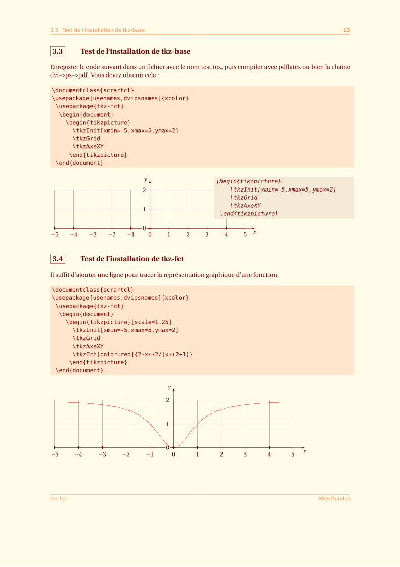
3.3 Test de l’installation de tkz-base
Enregister le code suivant dans un fichier avec le nom test.tex, puis compiler avec pdflatex ou bien la chaînedvi–>ps–>pdf. Vous devez obtenir cela :
\documentclass{scrartcl}\usepackage[usenames,dvipsnames]{xcolor}\usepackage{tkz-fct}\begin{document}\begin{tikzpicture}\tkzInit[xmin=-5,xmax=5,ymax=2]\tkzGrid\tkzAxeXY
\end{tikzpicture}\end{document}
x
y
−5 −4 −3 −2 −1 0 1 2 3 4 50
1
2\begin{tikzpicture}
\tkzInit[xmin=-5,xmax=5,ymax=2]\tkzGrid\tkzAxeXY
\end{tikzpicture}
3.4 Test de l’installation de tkz-fct
Il suffit d’ajouter une ligne pour tracer la représentation graphique d’une fonction.
\documentclass{scrartcl}\usepackage[usenames,dvipsnames]{xcolor}\usepackage{tkz-fct}\begin{document}\begin{tikzpicture}[scale=1.25]\tkzInit[xmin=-5,xmax=5,ymax=2]\tkzGrid\tkzAxeXY\tkzFct[color=red]{2*x**2/(x**2+1)}
\end{tikzpicture}\end{document}
x
y
−5 −4 −3 −2 −1 0 1 2 3 4 50
1
2
tkz-fct AlterMundus
3.4 Test de l’installation de tkz-fct 14
\begin{tikzpicture}[scale=1.25]\tkzInit[xmin=-5,xmax=5,ymax=2]\tkzGrid\tkzAxeXY\tkzFct[color=red]{2*x**2/(x**2+1)}
\end{tikzpicture}
tkz-fct AlterMundus
4 Les différentes macros 15
SECTION 4
Les différentes macros
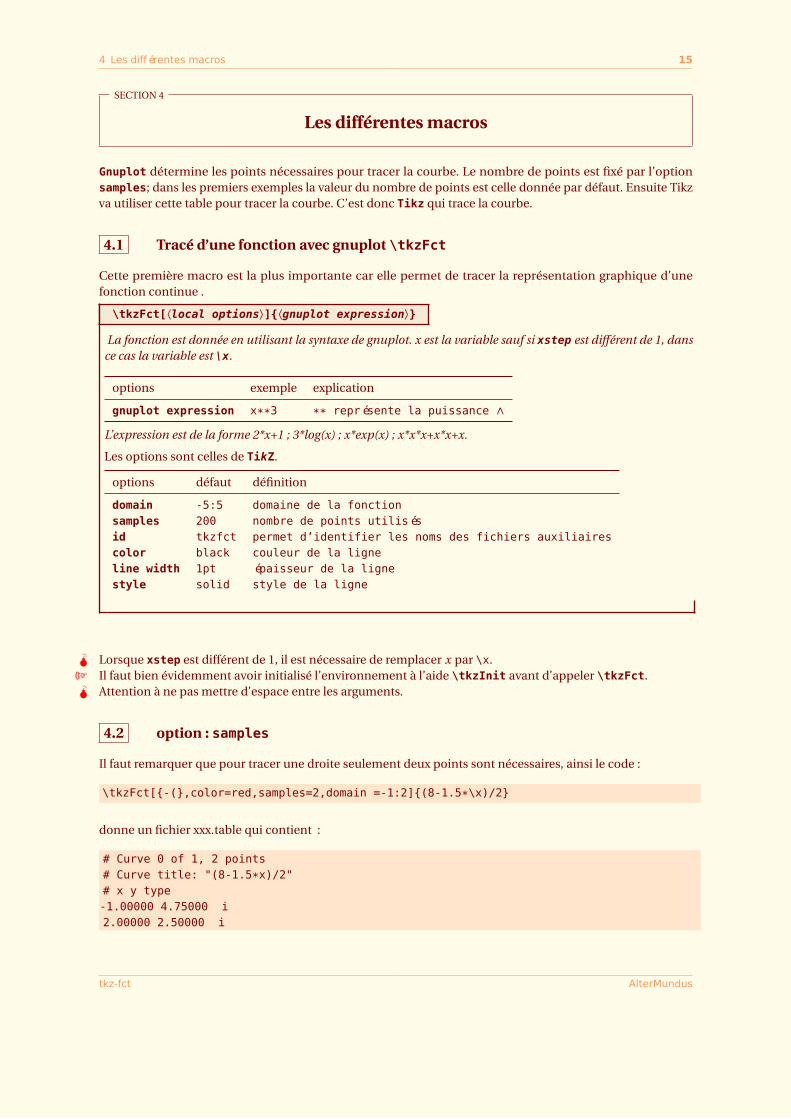
Gnuplot détermine les points nécessaires pour tracer la courbe. Le nombre de points est fixé par l’optionsamples; dans les premiers exemples la valeur du nombre de points est celle donnée par défaut. Ensuite Tikzva utiliser cette table pour tracer la courbe. C’est donc Tikz qui trace la courbe.
4.1 Tracé d’une fonction avec gnuplot \tkzFct
Cette première macro est la plus importante car elle permet de tracer la représentation graphique d’unefonction continue .
\tkzFct[⟨local options⟩]{⟨gnuplot expression⟩}La fonction est donnée en utilisant la syntaxe de gnuplot. x est la variable sauf si xstep est différent de 1, dans
ce cas la variable est \x.
options exemple explication
gnuplot expression x**3 ** représente la puissance ∧L’expression est de la forme 2*x+1 ; 3*log(x) ; x*exp(x) ; x*x*x+x*x+x.
Les options sont celles de TikZ.
options défaut définition
domain -5:5 domaine de la fonctionsamples 200 nombre de points utilisésid tkzfct permet d’identifier les noms des fichiers auxiliairescolor black couleur de la ligneline width 1pt épaisseur de la lignestyle solid style de la ligne
L Lorsque xstep est différent de 1, il est nécessaire de remplacer x par \x.t Il faut bien évidemment avoir initialisé l’environnement à l’aide \tkzInit avant d’appeler \tkzFct.L Attention à ne pas mettre d’espace entre les arguments.
4.2 option : samples
Il faut remarquer que pour tracer une droite seulement deux points sont nécessaires, ainsi le code :
\tkzFct[{-(},color=red,samples=2,domain =-1:2]{(8-1.5*\x)/2}
donne un fichier xxx.table qui contient :
# Curve 0 of 1, 2 points# Curve title: "(8-1.5*x)/2"# x y type-1.00000 4.75000 i2.00000 2.50000 i
tkz-fct AlterMundus
4.3 options : xstep, ystep 16
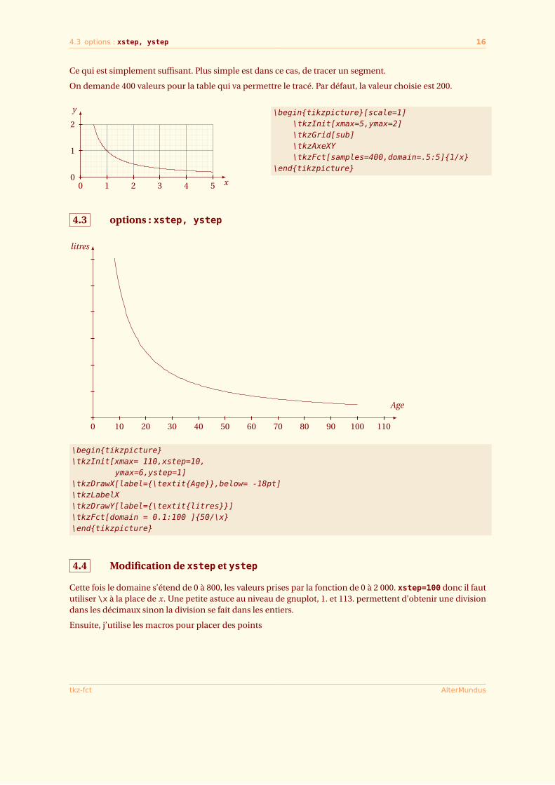
Ce qui est simplement suffisant. Plus simple est dans ce cas, de tracer un segment.
On demande 400 valeurs pour la table qui va permettre le tracé. Par défaut, la valeur choisie est 200.
x
y
0 1 2 3 4 50
1
2\begin{tikzpicture}[scale=1]
\tkzInit[xmax=5,ymax=2]\tkzGrid[sub]\tkzAxeXY\tkzFct[samples=400,domain=.5:5]{1/x}
\end{tikzpicture}
4.3 options : xstep, ystep
Age
0 10 20 30 40 50 60 70 80 90 100 110
litres
\begin{tikzpicture}\tkzInit[xmax= 110,xstep=10,
ymax=6,ystep=1]\tkzDrawX[label={\textit{Age}},below= -18pt]\tkzLabelX\tkzDrawY[label={\textit{litres}}]\tkzFct[domain = 0.1:100 ]{50/\x}\end{tikzpicture}
4.4 Modification de xstep et ystep
Cette fois le domaine s’étend de 0 à 800, les valeurs prises par la fonction de 0 à 2 000. xstep=100 donc il faututiliser \x à la place de x. Une petite astuce au niveau de gnuplot, 1. et 113. permettent d’obtenir une divisiondans les décimaux sinon la division se fait dans les entiers.
Ensuite, j’utilise les macros pour placer des points
tkz-fct AlterMundus
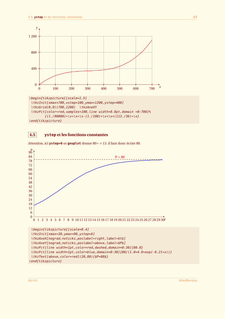
4.5 ystep et les fonctions constantes 17
x
y
0 100 200 300 400 500 600 7000
400
800
1 200
\begin{tikzpicture}[scale=1.5]\tkzInit[xmax=700,xstep=100,ymax=1200,ystep=400]\tkzGrid(0,0)(700,1200) \tkzAxeXY\tkzFct[color=red,samples=100,line width=0.8pt,domain =0:700]%
{(1./90000)*\x*\x*\x-(1./100)*\x*\x+(113./36)*\x}\end{tikzpicture}
4.5 ystep et les fonctions constantes
Attention, ici ystep=6 or gnuplot donne 80÷= 13. il faut donc écrire 80.
0 1 2 3 4 5 6 7 8 9 10 11 12 13 14 15 16 17 18 19 20 21 22 23 24 25 26 27 28 29 30t
P
06
1218243036424854606672788490
P = 80
\begin{tikzpicture}[scale=0.4]\tkzInit[xmax=30,ymax=90,ystep=6]\tkzAxeX[nograd,noticks,poslabel=right,label=$t$]\tkzAxeY[nograd,noticks,poslabel=above,label=$P$]\tkzFct[line width=1pt,color=red,dashed,domain=0:30]{80.0}\tkzFct[line width=1pt,color=blue,domain=0:30]{80/(1.0+4.0*exp(-0.21*x))}\tkzText[above,color=red](20,80){$P=80$}
\end{tikzpicture}
tkz-fct AlterMundus
4.6 Les fonctions affines ou linéaires 18
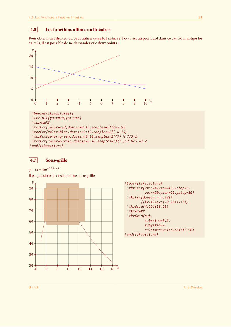
4.6 Les fonctions affines ou linéaires
Pour obtenir des droites, on peut utiliser gnuplot même si l’outil est un peu lourd dans ce cas. Pour alléger lescalculs, il est possible de ne demander que deux points !
x
y
0 1 2 3 4 5 6 7 8 9 100
5
10
15
20
\begin{tikzpicture}[]\tkzInit[ymax=20,ystep=5]\tkzAxeXY\tkzFct[color=red,domain=0:10,samples=2]{2*x+5}\tkzFct[color=blue,domain=0:10,samples=2]{-x+15}\tkzFct[color=green,domain=0:10,samples=2]{7} % 7/5=1\tkzFct[color=purple,domain=0:10,samples=2]{7.}%7.0/5 =1.2
\end{tikzpicture}
4.7 Sous-grille
y = (x −4)e−0.25x+5
Il est possible de dessiner une autre grille.
x
y
4 6 8 10 12 14 16 1820
30
40
50
60
70
80
90\begin{tikzpicture}\tkzInit[xmin=4,xmax=18,xstep=2,
ymin=20,ymax=90,ystep=10]\tkzFct[domain = 5:18]%
{(\x-4)*exp(-0.25*\x+5)}\tkzGrid(4,20)(18,90)\tkzAxeXY\tkzGrid[sub,
subxstep=0.5,subystep=2,color=brown](6,60)(12,90)
\end{tikzpicture}
tkz-fct AlterMundus
4.8 Utilisation des macros de tkz-base 19
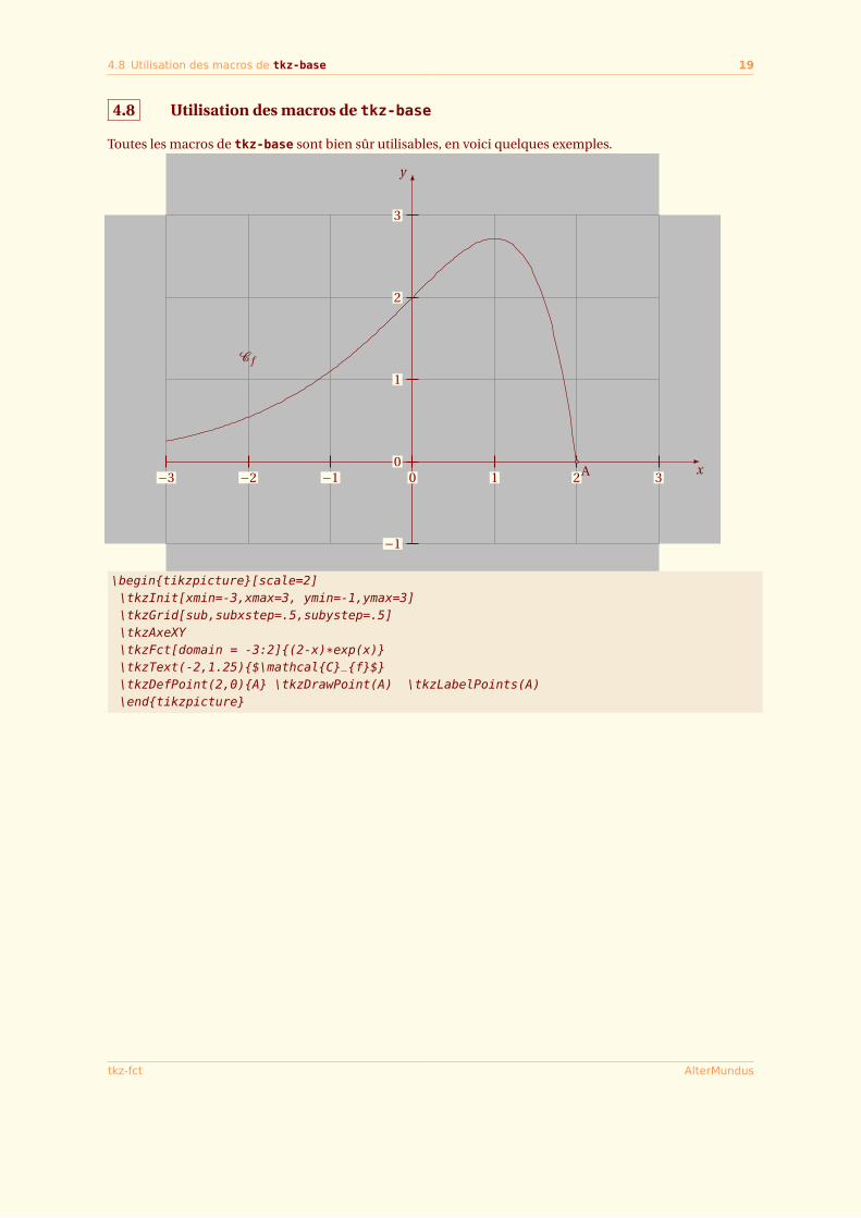
4.8 Utilisation des macros de tkz-base
Toutes les macros de tkz-base sont bien sûr utilisables, en voici quelques exemples.
x
y
−3 −2 −1 0 1 2 3
−1
0
1
2
3
C f
A
\begin{tikzpicture}[scale=2]\tkzInit[xmin=-3,xmax=3, ymin=-1,ymax=3]\tkzGrid[sub,subxstep=.5,subystep=.5]\tkzAxeXY\tkzFct[domain = -3:2]{(2-x)*exp(x)}\tkzText(-2,1.25){$\mathcal{C}_{f}$}\tkzDefPoint(2,0){A} \tkzDrawPoint(A) \tkzLabelPoints(A)\end{tikzpicture}
tkz-fct AlterMundus
5 Placer un point sur une courbe 20
SECTION 5
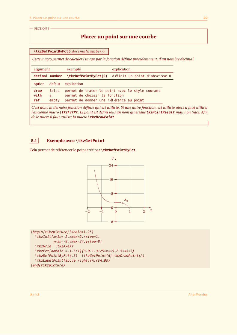
Placer un point sur une courbe
\tkzDefPointByFct(⟨deci mal number ⟩)Cette macro permet de calculer l’image par la fonction définie précédemment, d’un nombre décimal.
argument exemple explication
decimal number \tkzDefPointByFct(0) définit un point d’abscisse 0
option defaut explication
draw false permet de tracer le point avec le style courantwith a permet de choisir la fonctionref empty permet de donner une référence au point
C’est donc la dernière fonction définie qui est utilisée. Si une autre fonction, est utilisée alors il faut utiliserl’ancienne macro \tkzFctPt. Le point est défini sous un nom générique tkzPointResult mais non tracé. Afinde le tracer il faut utiliser la macro \tkzDrawPoint.
5.1 Exemple avec \tkzGetPoint
Cela permet de référencer le point créé par \tkzDefPointByFct.
x
y
−2 −1 0 1 2
−8
0
8
16
24
A0
\begin{tikzpicture}[scale=1.25]\tkzInit[xmin=-2,xmax=2,xstep=1,
ymin=-8,ymax=24,ystep=8]\tkzGrid \tkzAxeXY\tkzFct[domain =-1.5:1]{3.0-1.3125*x**5-2.5*x**3}\tkzDefPointByFct(.5) \tkzGetPoint{A}\tkzDrawPoint(A)\tkzLabelPoint[above right](A){$A_0$}
\end{tikzpicture}
tkz-fct AlterMundus
5.2 Exemple avec \tkzGetPoint et tkzPointResult 21
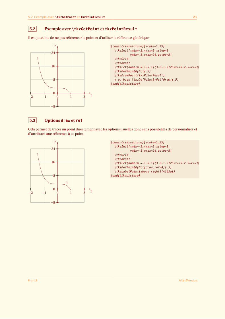
5.2 Exemple avec \tkzGetPoint et tkzPointResult
Il est possible de ne pas référencer le point et d’utiliser la référence générique.
x
y
−2 −1 0 1 2
−8
0
8
16
24
\begin{tikzpicture}[scale=1.25]\tkzInit[xmin=-2,xmax=2,xstep=1,
ymin=-8,ymax=24,ystep=8]\tkzGrid\tkzAxeXY\tkzFct[domain =-1.5:1]{3.0-1.3125*x**5-2.5*x**3}\tkzDefPointByFct(.5)\tkzDrawPoint(tkzPointResult)% ou bien \tkzDefPointByFct[draw](.5)
\end{tikzpicture}
5.3 Options draw et ref
Cela permet de tracer un point directement avec les options usuelles donc sans possibilités de personnaliser etd’attribuer une référence à ce point.
x
y
−2 −1 0 1 2
−8
0
8
16
24
a
\begin{tikzpicture}[scale=1.25]\tkzInit[xmin=-2,xmax=2,xstep=1,
ymin=-8,ymax=24,ystep=8]\tkzGrid\tkzAxeXY\tkzFct[domain =-1.5:1]{3.0-1.3125*x**5-2.5*x**3}\tkzDefPointByFct[draw,ref=A](.5)\tkzLabelPoint[above right](A){$a$}
\end{tikzpicture}
tkz-fct AlterMundus
5.4 Placer des points sans courbe 22
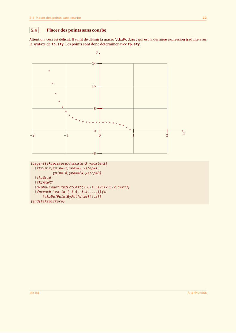
5.4 Placer des points sans courbe
Attention, ceci est délicat. Il suffit de définir la macro \tkzFctLast qui est la dernière expression traduite avecla syntaxe de fp.sty. Les points sont donc déterminer avec fp.sty.
x
y
−2 −1 0 1 2
−8
0
8
16
24
\begin{tikzpicture}[xscale=3,yscale=2]\tkzInit[xmin=-2,xmax=2,xstep=1,
ymin=-8,ymax=24,ystep=8]\tkzGrid\tkzAxeXY\global\edef\tkzFctLast{3.0-1.3125*x^5-2.5*x^3}\foreach \va in {-1.5,-1.4,...,1}{%
\tkzDefPointByFct[draw](\va)}\end{tikzpicture}
tkz-fct AlterMundus
5.5 Placer des points sans se soucier des coordonnées 23
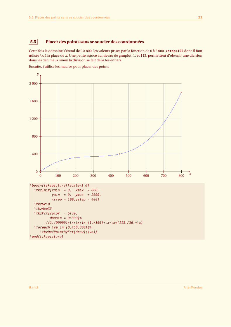
5.5 Placer des points sans se soucier des coordonnées
Cette fois le domaine s’étend de 0 à 800, les valeurs prises par la fonction de 0 à 2 000. xstep=100 donc il faututliser \x à la place de x. Une petite astuce au niveau de gnuplot, 1. et 113. permettent d’obtenir une divisiondans les décimaux sinon la division se fait dans les entiers.
Ensuite, j’utilise les macros pour placer des points
x
y
0 100 200 300 400 500 600 700 8000
400
800
1 200
1 600
2 000
\begin{tikzpicture}[scale=1.6]\tkzInit[xmin = 0, xmax = 800,
ymin = 0, ymax = 2000,xstep = 100,ystep = 400]
\tkzGrid\tkzAxeXY\tkzFct[color = blue,
domain = 0:800]%{(1./90000)*\x*\x*\x-(1./100)*\x*\x+(113./36)*\x}
\foreach \va in {0,450,800}{%\tkzDefPointByFct[draw](\va)}
\end{tikzpicture}
tkz-fct AlterMundus
5.6 Placer des points avec deux fonctions 24
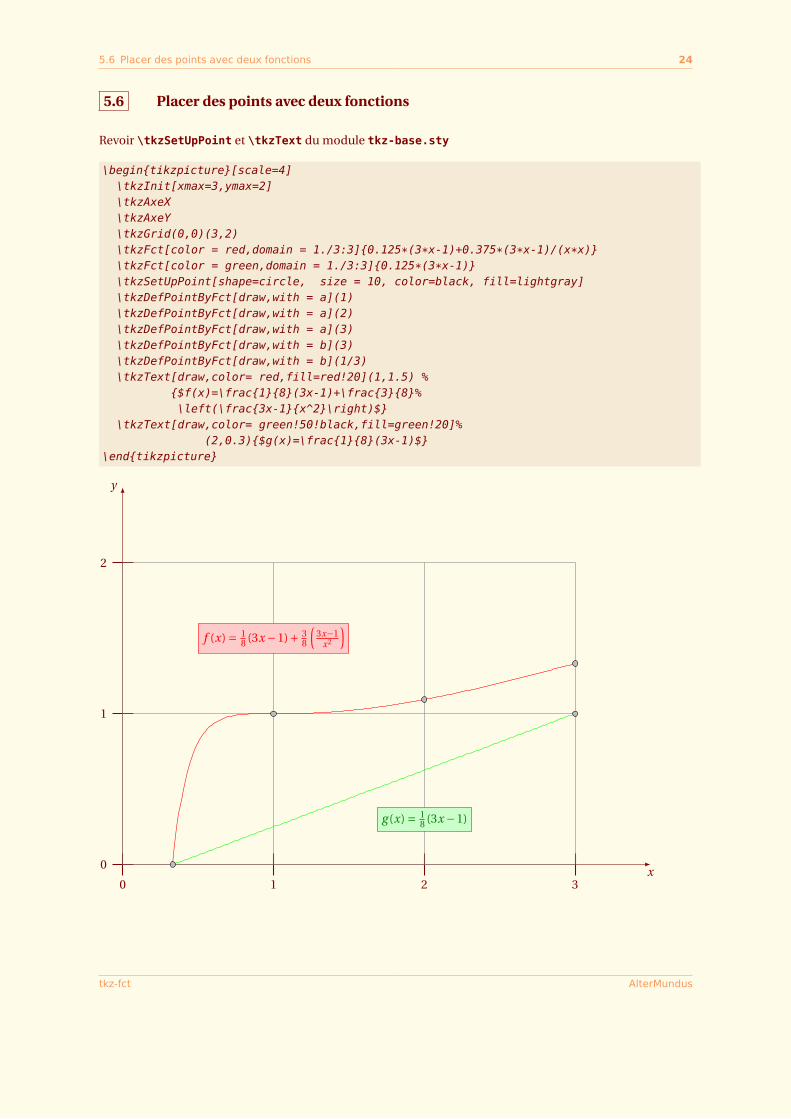
5.6 Placer des points avec deux fonctions
Revoir \tkzSetUpPoint et \tkzText du module tkz-base.sty
\begin{tikzpicture}[scale=4]\tkzInit[xmax=3,ymax=2]\tkzAxeX\tkzAxeY\tkzGrid(0,0)(3,2)\tkzFct[color = red,domain = 1./3:3]{0.125*(3*x-1)+0.375*(3*x-1)/(x*x)}\tkzFct[color = green,domain = 1./3:3]{0.125*(3*x-1)}\tkzSetUpPoint[shape=circle, size = 10, color=black, fill=lightgray]\tkzDefPointByFct[draw,with = a](1)\tkzDefPointByFct[draw,with = a](2)\tkzDefPointByFct[draw,with = a](3)\tkzDefPointByFct[draw,with = b](3)\tkzDefPointByFct[draw,with = b](1/3)\tkzText[draw,color= red,fill=red!20](1,1.5) %
{$f(x)=\frac{1}{8}(3x-1)+\frac{3}{8}%\left(\frac{3x-1}{x^2}\right)$}
\tkzText[draw,color= green!50!black,fill=green!20]%(2,0.3){$g(x)=\frac{1}{8}(3x-1)$}
\end{tikzpicture}
0 1 2 3x
y
0
1
2
f (x) = 18 (3x −1)+ 3
8
(3x−1
x2
)
g (x) = 18 (3x −1)
tkz-fct AlterMundus
6 Labels 25
SECTION 6
Labels
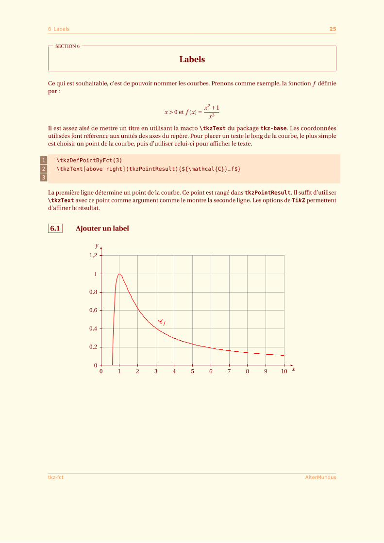
Ce qui est souhaitable, c’est de pouvoir nommer les courbes. Prenons comme exemple, la fonction f définiepar :
x > 0 et f (x) = x2 +1
x3
Il est assez aisé de mettre un titre en utilisant la macro \tkzText du package tkz-base. Les coordonnéesutilisées font référence aux unités des axes du repère. Pour placer un texte le long de la courbe, le plus simpleest choisir un point de la courbe, puis d’utiliser celui-ci pour afficher le texte.
1 \tkzDefPointByFct(3)
2 \tkzText[above right](tkzPointResult){${\mathcal{C}}_f$}
3
La première ligne détermine un point de la courbe. Ce point est rangé dans tkzPointResult. Il suffit d’utiliser\tkzText avec ce point comme argument comme le montre la seconde ligne. Les options de TikZ permettentd’affiner le résultat.
6.1 Ajouter un label
x
y
0 1 2 3 4 5 6 7 8 9 100
0,2
0,4
0,6
0,8
1
1,2
Courbe de f
C f
tkz-fct AlterMundus
6.1 Ajouter un label 26
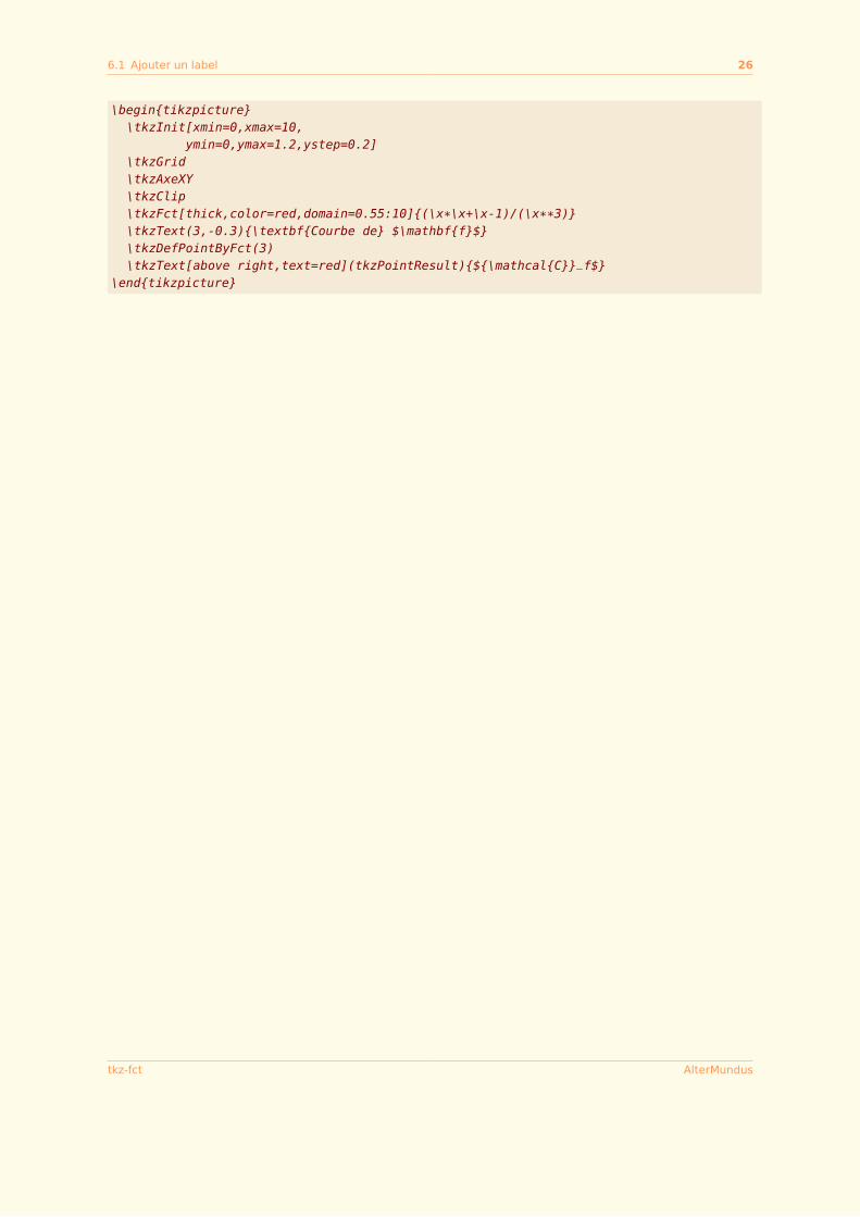
\begin{tikzpicture}\tkzInit[xmin=0,xmax=10,
ymin=0,ymax=1.2,ystep=0.2]\tkzGrid\tkzAxeXY\tkzClip\tkzFct[thick,color=red,domain=0.55:10]{(\x*\x+\x-1)/(\x**3)}\tkzText(3,-0.3){\textbf{Courbe de} $\mathbf{f}$}\tkzDefPointByFct(3)\tkzText[above right,text=red](tkzPointResult){${\mathcal{C}}_f$}
\end{tikzpicture}
tkz-fct AlterMundus
7 Macros pour tracer des tangentes 27
SECTION 7
Macros pour tracer des tangentes
Si une seule fonction est utilisée, elle est stockée avec comme nom \tkzFcta, si une deuxième fonction estutilisée, elle sera stockée avec comme nom \tkzFctb, et ainsi de suite. . . Si plusieurs fonctions sont présententdans un même environnement alors l’option with permet de choisir celle qui sera mise à contribution.
tL Il faut bien évidemment, avoir initialisé l’environnement à l’aide \tkzInit, avant d’appeler \tkzFct et\tkzDrawTangentLine. Pour la longueur des vecteurs représentants les demi-tangentes, il faut attribuer unevaleur aux coefficients kl et kr. kl = 0 ou kr = 0 annule le dessin de la demi-tangente correspondante (l=left)et (r=right). Si xstep=1 et ystep=1 alors si la pente est égale à 1, la demi-tangente a pour mesure
p2. Dans
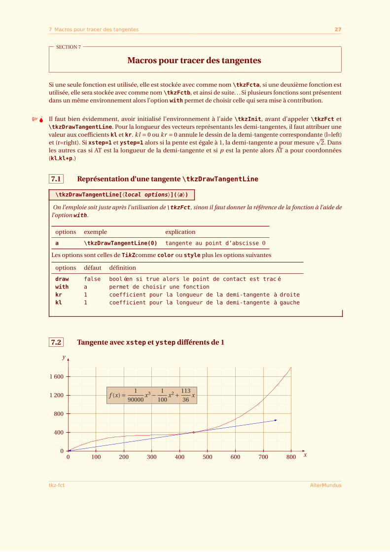
les autres cas si AT est la longueur de la demi-tangente et si p est la pente alors ~AT a pour coordonnées(kl,kl*p.)
7.1 Représentation d’une tangente \tkzDrawTangentLine
\tkzDrawTangentLine[⟨local options⟩](⟨a⟩)On l’emploie soit juste après l’utilisation de \tkzFct, sinon il faut donner la référence de la fonction à l’aide del’option with.
options exemple explication
a \tkzDrawTangentLine(0) tangente au point d’abscisse 0
Les options sont celles de TikZcomme color ou style plus les options suivantes
options défaut définition
draw false booléen si true alors le point de contact est tracéwith a permet de choisir une fonctionkr 1 coefficient pour la longueur de la demi-tangente à droitekl 1 coefficient pour la longueur de la demi-tangente à gauche
7.2 Tangente avec xstep et ystep différents de 1
x
y
0 100 200 300 400 500 600 700 8000
400
800
1 200
1 600
f (x) = 1
90000x3 − 1
100x2 + 113
36x
tkz-fct AlterMundus
7.3 Les options kl, kr et l’option draw 28
Il faut remarquer qu’il n’est point nécessaire de faire des calculs. Il suffit d’utiliser les valeurs qui correspondentaux graduations.
On peut changer le style des tangentes avec, par exemple,
\tikzset{tan style/.style={-}} par défaut on a :
\tikzset{tan style/.style={->,>=latex}}
\begin{tikzpicture}[xscale=1.5]\tikzset{tan style/.style={-}}\tkzInit[xmin=0,xmax=800,xstep=100,
ymin=0,ymax=1800,ystep=400]\tkzGrid[color=brown,sub,subxstep=50,subystep=200](0,0)(800,1800)\tkzAxeXY\tkzFct[color=red,samples=100,domain = 0:800]%
{(1./90000)*\x*\x*\x-(1./100)*\x*\x+(113./36)*\x}\tkzDrawTangentLine[color=blue,kr=300,kl=450,coord](450)\tkzText[draw, color = black,%
fill = brown!50, opacity = 0.8](300,1200)%{$f(x)=\dfrac{1}{90000}x^3 -\dfrac{1}{{100}}x^2 +\dfrac{113}{36}x$}\end{tikzpicture}
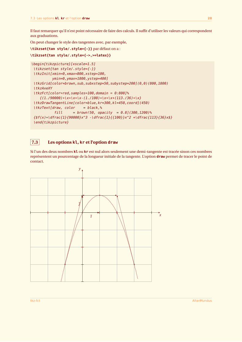
7.3 Les options kl, kr et l’option draw
Si l’un des deux nombres kl ou kr est nul alors seulement une demi-tangente est tracée sinon ces nombresreprésentent un pourcentage de la longueur initiale de la tangente. L’option draw permet de tracer le point decontact.
x
y
~
~ı
tkz-fct AlterMundus
7.4 Tangente et l’option with 29
\begin{tikzpicture}[scale=1.5]\tkzInit[xmin=-3,xmax=4,ymin=-4,ymax=2]\tkzGrid \tkzDrawXY \tkzClip\tkzFct[domain = -2.15:3.2]{(-x*x)+2*x}\tkzDefPointByFct[draw](2)\tkzDrawTangentLine[kl=0,draw](-1)\tkzDrawTangentLine[draw](1)\tkzDrawTangentLine[kr=0,draw](3)\tkzRep
\end{tikzpicture}
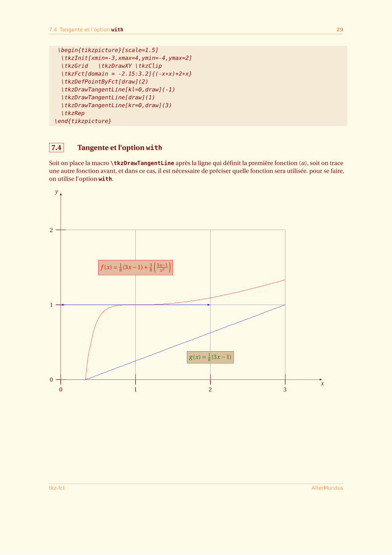
7.4 Tangente et l’option with
Soit on place la macro \tkzDrawTangentLine après la ligne qui définit la première fonction (a), soit on traceune autre fonction avant, et dans ce cas, il est nécessaire de préciser quelle fonction sera utilisée. pour se faire,on utilise l’option with.
x
y
0 1 2 3
0
1
2
f (x) = 18 (3x −1)+ 3
8
(3x−1
x2
)
g (x) = 18 (3x −1)
tkz-fct AlterMundus
7.5 Quelques tangentes 30
\begin{tikzpicture}[scale=4]\tkzInit[xmax=3,ymax=2]\tkzAxeXY\tkzGrid(0,0)(3,2)\tkzFct[color = red, domain = 1/3:3]{0.125*(3*x-1)+0.375*(3*x-1)/(x*x)}\tkzFct[color = blue, domain = 1/3:3]{0.125*(3*x-1)}\tkzDrawTangentLine[with=a,
color=blue](1)\tkzText[draw,
color= red,fill=brown!50](1,1.5)%{$f(x)=\frac{1}{8}(3x-1)+\frac{3}{8}\left(\frac{3x-1}{x^2}\right)$}
\tkzText[draw,color= green!50!black,fill=brown!50](2,0.3)%{$g(x)=\frac{1}{8}(3x-1)$}
\end{tikzpicture}
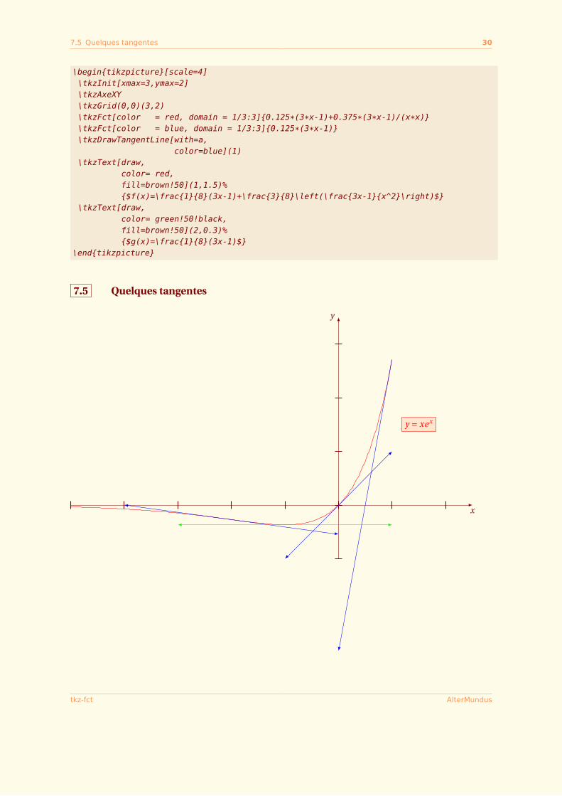
7.5 Quelques tangentes
x
y
y = xex
tkz-fct AlterMundus
7.6 Demi-tangentes 31
\begin{tikzpicture}[scale=2]\tkzInit[xmin=-5,xmax=2,ymin=-1, ymax=3]\tkzDrawX\tkzDrawY\tkzText[draw,color = red,fill = orange!20]( 1.5,1.5){$y = xe^x$}\tkzFct[color = red, domain = -5:1]{x*exp(x)}%\tkzDrawTangentLine[color=blue,kr=2,kl=2](-2)\tkzDrawTangentLine[color=green,kr=2,kl=2](-1)\tkzDrawTangentLine[color=blue](0)\tkzDrawTangentLine[color=blue,kr=0](1)
\end{tikzpicture}
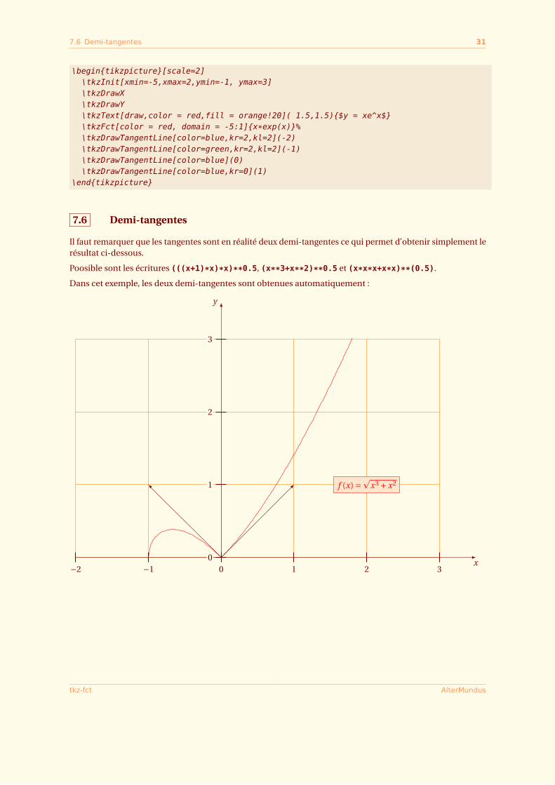
7.6 Demi-tangentes
Il faut remarquer que les tangentes sont en réalité deux demi-tangentes ce qui permet d’obtenir simplement lerésultat ci-dessous.
Poosible sont les écritures (((x+1)*x)*x)**0.5, (x**3+x**2)**0.5 et (x*x*x+x*x)**(0.5).
Dans cet exemple, les deux demi-tangentes sont obtenues automatiquement :
−2 −1 0 1 2 3x
y
0
1
2
3
f (x) =p
x3 +x2
tkz-fct AlterMundus
7.7 Demi-tangentes Courbe de Lorentz 32
\begin{tikzpicture}[scale=2.75]\tkzInit[xmin=-2,xmax=3,ymax=3]\tkzGrid[color=orange](-2,0)(3,3)\tkzAxeX\tkzAxeY\tkzFct[color = red ,domain = -1:2]{(((x+1)*x)*x)**0.5}\tkzDrawTangentLine(0)\tkzText[draw,color = red,fill = orange!20](2,1){$f(x)=\sqrt{x^3+x^2}$}
\end{tikzpicture}
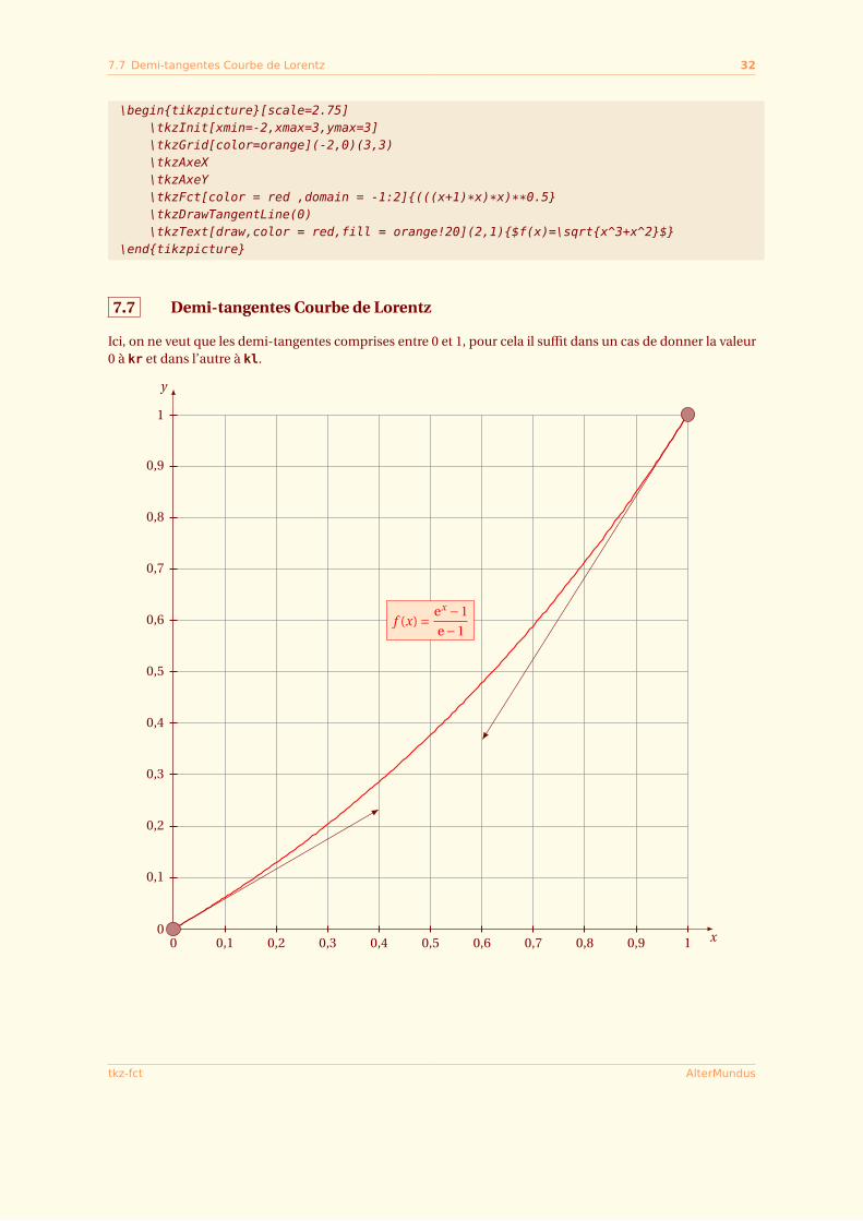
7.7 Demi-tangentes Courbe de Lorentz
Ici, on ne veut que les demi-tangentes comprises entre 0 et 1, pour cela il suffit dans un cas de donner la valeur0 à kr et dans l’autre à kl.
x
y
0 0,1 0,2 0,3 0,4 0,5 0,6 0,7 0,8 0,9 10
0,1
0,2
0,3
0,4
0,5
0,6
0,7
0,8
0,9
1
f (x) = ex −1
e−1
tkz-fct AlterMundus
7.8 Série de tangentes 33
\begin{tikzpicture}[scale=1.25]\tkzInit[xmax=1,ymax=1,xstep=0.1,ystep=0.1]\tkzGrid(0,0)(1,1)\tkzAxeXY\tkzFct[color = red,thick, domain =0:1]{(exp(\x)-1)/(exp(1)-1)}\tkzSetUpPoint[size=12]\tkzDrawTangentLine[draw, kl = 0, kr = 0.4](0)\tkzDrawTangentLine[draw, kl = 0.4,kr = 0 ](1)\tkzText[draw,color = red,fill = orange!20](0.5,0.6)%
{$f(x)=\dfrac{\text{e}^x-1}{\text{e}-1}$}\end{tikzpicture}
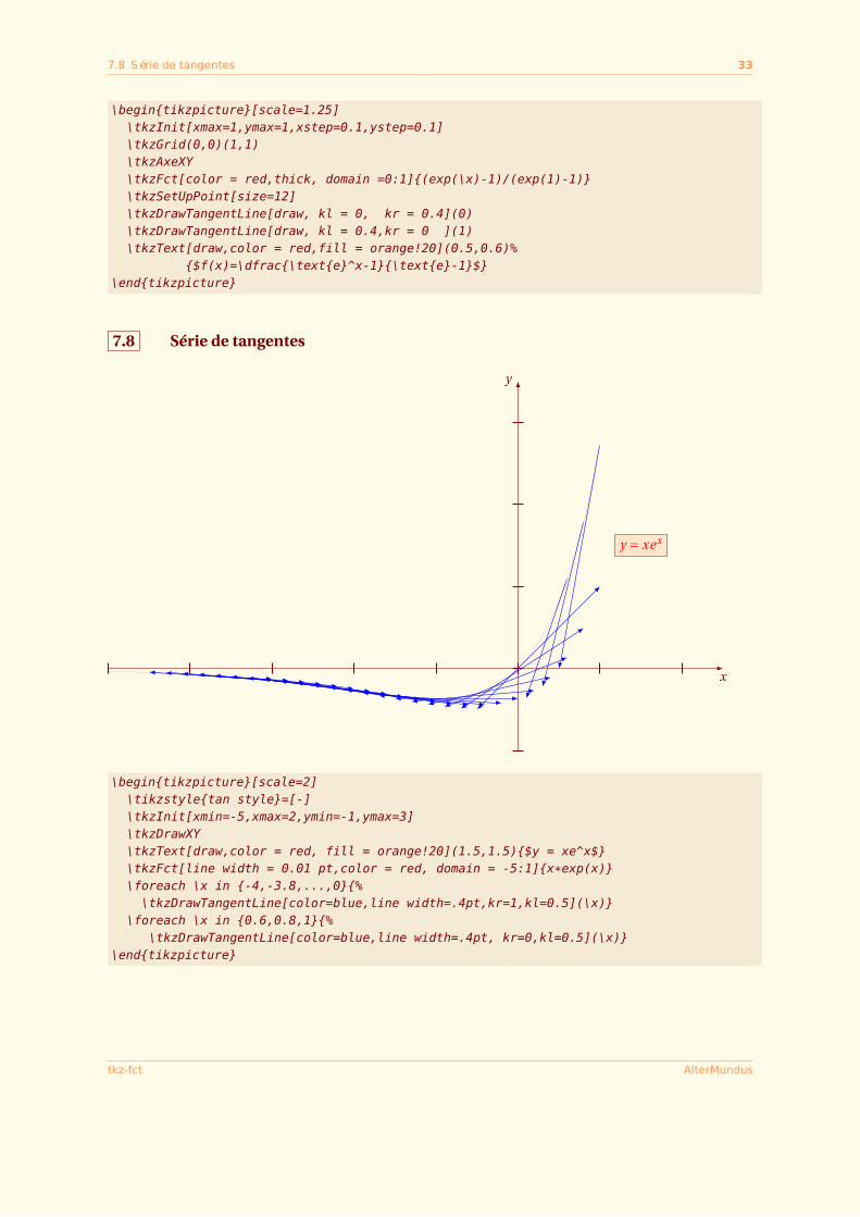
7.8 Série de tangentes
x
y
y = xex
\begin{tikzpicture}[scale=2]\tikzstyle{tan style}=[-]\tkzInit[xmin=-5,xmax=2,ymin=-1,ymax=3]\tkzDrawXY\tkzText[draw,color = red, fill = orange!20](1.5,1.5){$y = xe^x$}\tkzFct[line width = 0.01 pt,color = red, domain = -5:1]{x*exp(x)}\foreach \x in {-4,-3.8,...,0}{%\tkzDrawTangentLine[color=blue,line width=.4pt,kr=1,kl=0.5](\x)}
\foreach \x in {0.6,0.8,1}{%\tkzDrawTangentLine[color=blue,line width=.4pt, kr=0,kl=0.5](\x)}
\end{tikzpicture}
tkz-fct AlterMundus
7.9 Série de tangentes sans courbe 34
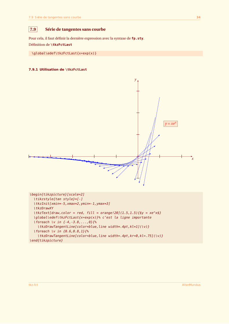
7.9 Série de tangentes sans courbe
Pour cela, il faut définir la dernière expression avec la syntaxe de fp.sty.
Définition de \tkzFctLast
\global\edef\tkzFctLast{x*exp(x)}
7.9.1 Utilisation de \tkzFctLast
x
y
y = xex
\begin{tikzpicture}[scale=2]\tikzstyle{tan style}=[-]\tkzInit[xmin=-5,xmax=2,ymin=-1,ymax=3]\tkzDrawXY\tkzText[draw,color = red, fill = orange!20](1.5,1.5){$y = xe^x$}\global\edef\tkzFctLast{x*exp(x)}% c’est la ligne importante\foreach \v in {-4,-3.8,...,0}{%\tkzDrawTangentLine[color=blue,line width=.4pt,kl=1](\v)}
\foreach \v in {0.6,0.8,1}{%\tkzDrawTangentLine[color=blue,line width=.4pt,kr=0,kl=.75](\v)}
\end{tikzpicture}
tkz-fct AlterMundus
7.10 Calcul de l’antécédent 35
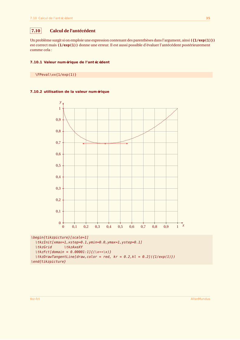
7.10 Calcul de l’antécédent
Un problème surgit si on emploie une expression contenant des parenthèses dans l’argument, ainsi ({1/exp(1)})est correct mais (1/exp(1)) donne une erreur. Il est aussi possible d’évaluer l’antécédent postérieurementcomme cela :
7.10.1 Valeur numérique de l’antécédent
\FPeval\vx{1/exp(1)}
7.10.2 utilisation de la valeur numérique
x
y
0 0,1 0,2 0,3 0,4 0,5 0,6 0,7 0,8 0,9 10
0,1
0,2
0,3
0,4
0,5
0,6
0,7
0,8
0,9
1
\begin{tikzpicture}[scale=1]\tkzInit[xmax=1,xstep=0.1,ymin=0.0,ymax=1,ystep=0.1]\tkzGrid \tkzAxeXY\tkzFct[domain = 0.00001:1]{(\x**\x)}\tkzDrawTangentLine[draw,color = red, kr = 0.2,kl = 0.2]({1/exp(1)})
\end{tikzpicture}
tkz-fct AlterMundus
8 Macros pour définir des surfaces 36
SECTION 8
Macros pour définir des surfaces
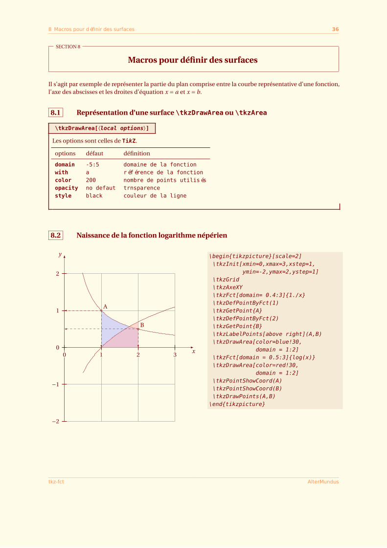
Il s’agit par exemple de représenter la partie du plan comprise entre la courbe représentative d’une fonction,l’axe des abscisses et les droites d’équation x = a et x = b.
8.1 Représentation d’une surface \tkzDrawArea ou \tkzArea
\tkzDrawArea[⟨local options⟩]Les options sont celles de TikZ.
options défaut définition
domain -5:5 domaine de la fonctionwith a référence de la fonctioncolor 200 nombre de points utilisésopacity no defaut trnsparencestyle black couleur de la ligne
8.2 Naissance de la fonction logarithme népérien
x
y
0 1 2 3
−2
−1
0
1
2
A
B
\begin{tikzpicture}[scale=2]\tkzInit[xmin=0,xmax=3,xstep=1,
ymin=-2,ymax=2,ystep=1]\tkzGrid\tkzAxeXY\tkzFct[domain= 0.4:3]{1./x}\tkzDefPointByFct(1)\tkzGetPoint{A}\tkzDefPointByFct(2)\tkzGetPoint{B}\tkzLabelPoints[above right](A,B)\tkzDrawArea[color=blue!30,
domain = 1:2]\tkzFct[domain = 0.5:3]{log(x)}\tkzDrawArea[color=red!30,
domain = 1:2]\tkzPointShowCoord(A)\tkzPointShowCoord(B)\tkzDrawPoints(A,B)
\end{tikzpicture}
tkz-fct AlterMundus
8.3 Surface simple 37
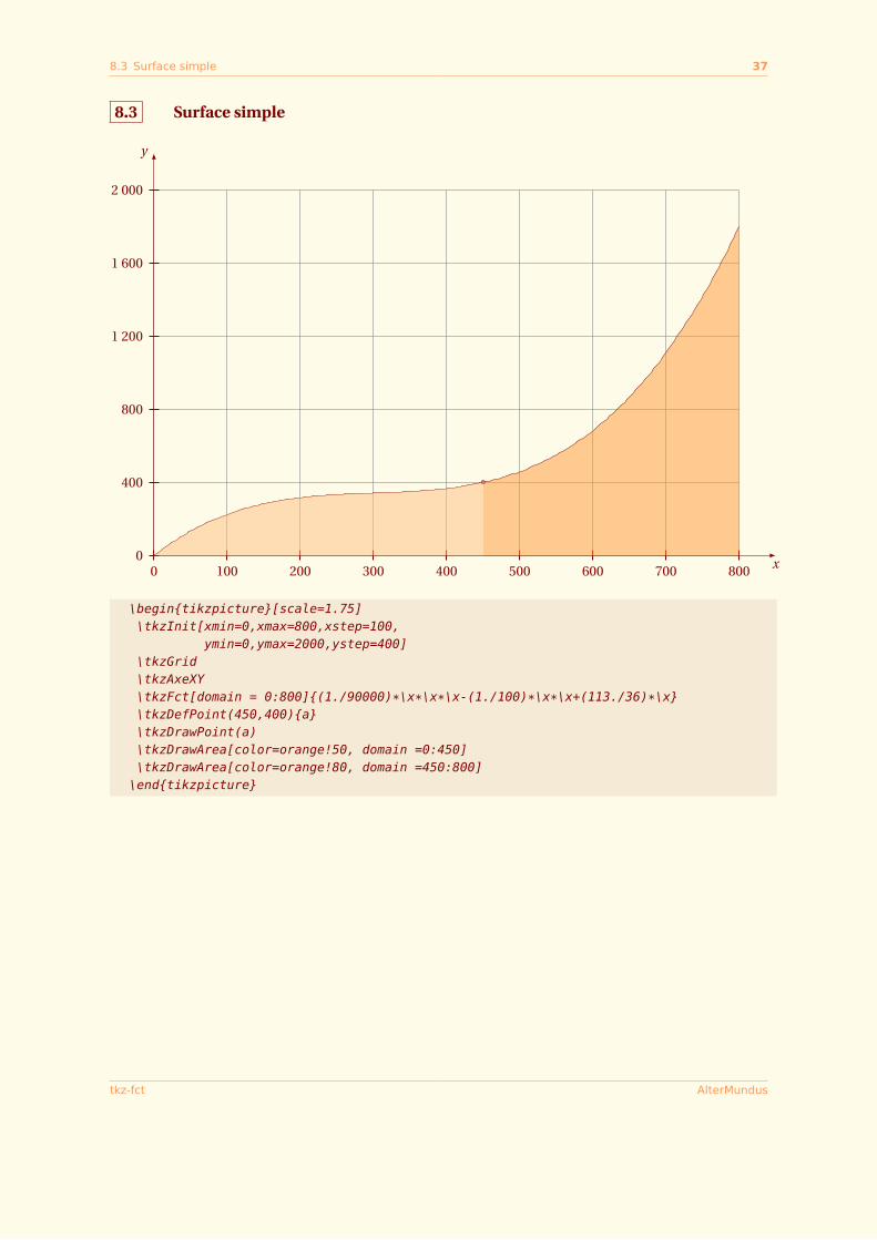
8.3 Surface simple
x
y
0 100 200 300 400 500 600 700 8000
400
800
1 200
1 600
2 000
\begin{tikzpicture}[scale=1.75]\tkzInit[xmin=0,xmax=800,xstep=100,
ymin=0,ymax=2000,ystep=400]\tkzGrid\tkzAxeXY\tkzFct[domain = 0:800]{(1./90000)*\x*\x*\x-(1./100)*\x*\x+(113./36)*\x}\tkzDefPoint(450,400){a}\tkzDrawPoint(a)\tkzDrawArea[color=orange!50, domain =0:450]\tkzDrawArea[color=orange!80, domain =450:800]
\end{tikzpicture}
tkz-fct AlterMundus
8.4 Surface et hachures 38
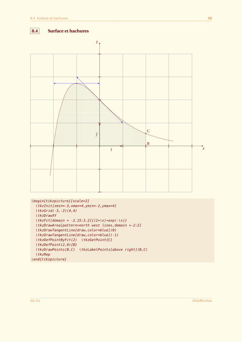
8.4 Surface et hachures
x
y
B
C~
~ı
\begin{tikzpicture}[scale=2]\tkzInit[xmin=-3,xmax=4,ymin=-2,ymax=4]\tkzGrid(-3,-2)(4,4)\tkzDrawXY\tkzFct[domain = -2.15:3.2]{(2+\x)*exp(-\x)}\tkzDrawArea[pattern=north west lines,domain =-2:2]\tkzDrawTangentLine[draw,color=blue](0)\tkzDrawTangentLine[draw,color=blue](-1)\tkzDefPointByFct(2) \tkzGetPoint{C}\tkzDefPoint(2,0){B}\tkzDrawPoints(B,C) \tkzLabelPoints[above right](B,C)\tkzRep
\end{tikzpicture}
tkz-fct AlterMundus
8.5 Surface comprise entre deux courbes \tkzDrawAreafg 39
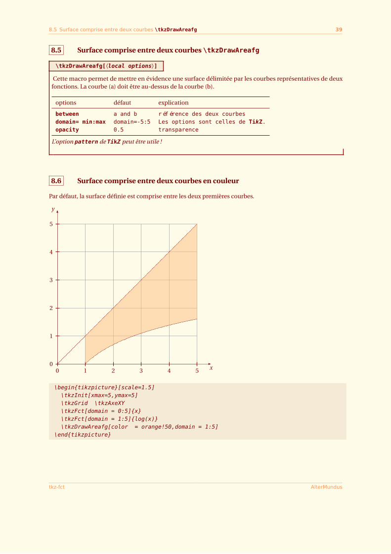
8.5 Surface comprise entre deux courbes \tkzDrawAreafg
\tkzDrawAreafg[⟨local options⟩]Cette macro permet de mettre en évidence une surface délimitée par les courbes représentatives de deux
fonctions. La courbe (a) doit être au-dessus de la courbe (b).
options défaut explication
between a and b référence des deux courbesdomain= min:max domain=-5:5 Les options sont celles de TikZ.opacity 0.5 transparence
L’option pattern de TikZ peut être utile !
8.6 Surface comprise entre deux courbes en couleur
Par défaut, la surface définie est comprise entre les deux premières courbes.
x
y
0 1 2 3 4 50
1
2
3
4
5
\begin{tikzpicture}[scale=1.5]\tkzInit[xmax=5,ymax=5]\tkzGrid \tkzAxeXY\tkzFct[domain = 0:5]{x}\tkzFct[domain = 1:5]{log(x)}\tkzDrawAreafg[color = orange!50,domain = 1:5]
\end{tikzpicture}
tkz-fct AlterMundus
8.7 Surface comprise entre deux courbes avec des hachures 40
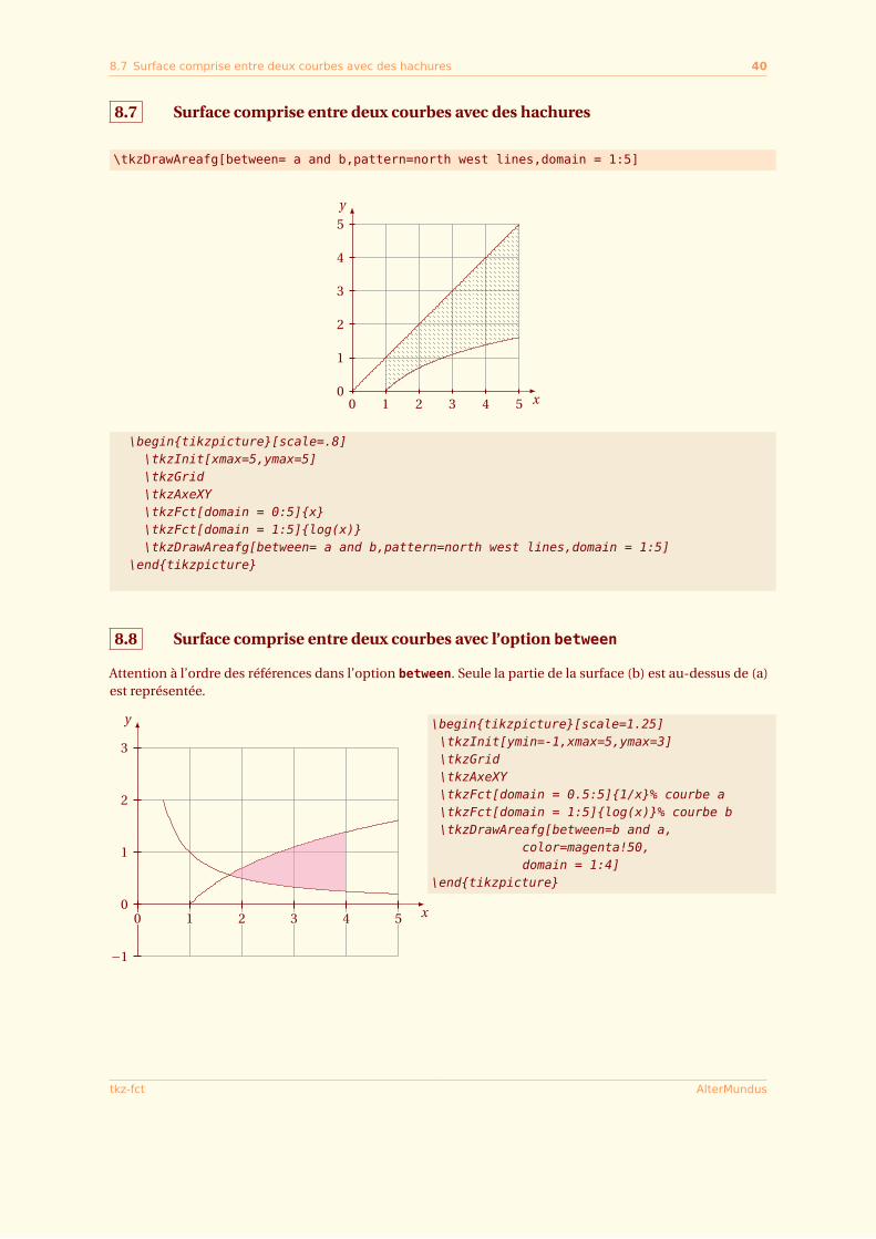
8.7 Surface comprise entre deux courbes avec des hachures
\tkzDrawAreafg[between= a and b,pattern=north west lines,domain = 1:5]
x
y
0 1 2 3 4 50
1
2
3
4
5
\begin{tikzpicture}[scale=.8]\tkzInit[xmax=5,ymax=5]\tkzGrid\tkzAxeXY\tkzFct[domain = 0:5]{x}\tkzFct[domain = 1:5]{log(x)}\tkzDrawAreafg[between= a and b,pattern=north west lines,domain = 1:5]
\end{tikzpicture}
8.8 Surface comprise entre deux courbes avec l’option between
Attention à l’ordre des références dans l’option between. Seule la partie de la surface (b) est au-dessus de (a)est représentée.
x
y
0 1 2 3 4 5
−1
0
1
2
3
\begin{tikzpicture}[scale=1.25]\tkzInit[ymin=-1,xmax=5,ymax=3]\tkzGrid\tkzAxeXY\tkzFct[domain = 0.5:5]{1/x}% courbe a\tkzFct[domain = 1:5]{log(x)}% courbe b\tkzDrawAreafg[between=b and a,
color=magenta!50,domain = 1:4]
\end{tikzpicture}
tkz-fct AlterMundus
8.9 Surface comprise entre deux courbes : courbes de Lorentz 41
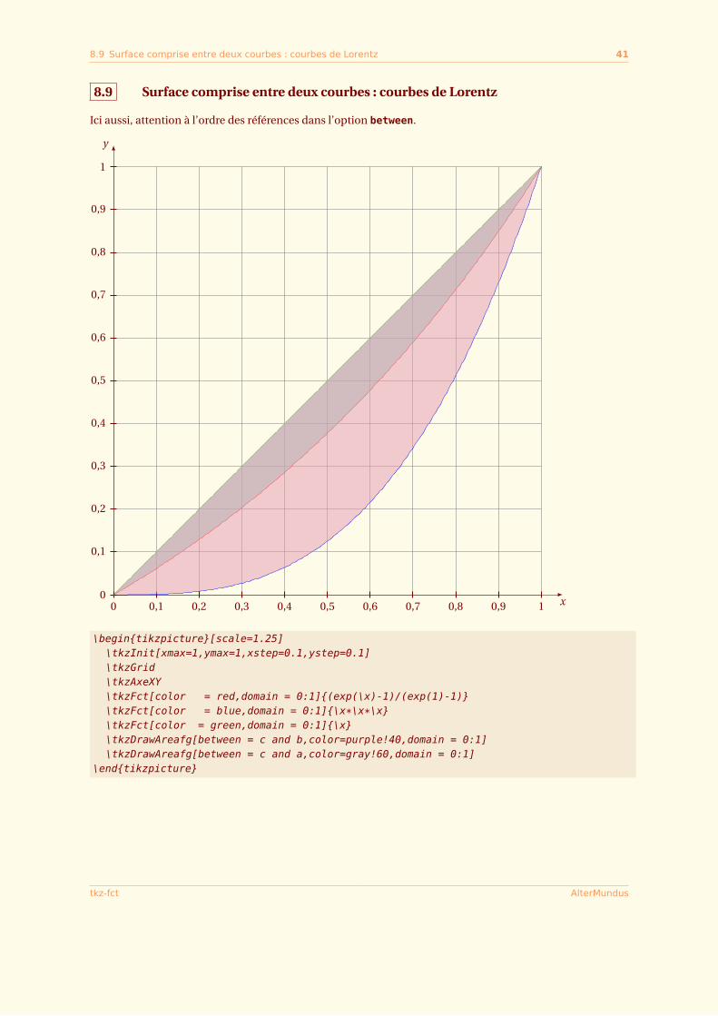
8.9 Surface comprise entre deux courbes : courbes de Lorentz
Ici aussi, attention à l’ordre des références dans l’option between.
x
y
0 0,1 0,2 0,3 0,4 0,5 0,6 0,7 0,8 0,9 10
0,1
0,2
0,3
0,4
0,5
0,6
0,7
0,8
0,9
1
\begin{tikzpicture}[scale=1.25]\tkzInit[xmax=1,ymax=1,xstep=0.1,ystep=0.1]\tkzGrid\tkzAxeXY\tkzFct[color = red,domain = 0:1]{(exp(\x)-1)/(exp(1)-1)}\tkzFct[color = blue,domain = 0:1]{\x*\x*\x}\tkzFct[color = green,domain = 0:1]{\x}\tkzDrawAreafg[between = c and b,color=purple!40,domain = 0:1]\tkzDrawAreafg[between = c and a,color=gray!60,domain = 0:1]
\end{tikzpicture}
tkz-fct AlterMundus
8.10 Mélange de style 42
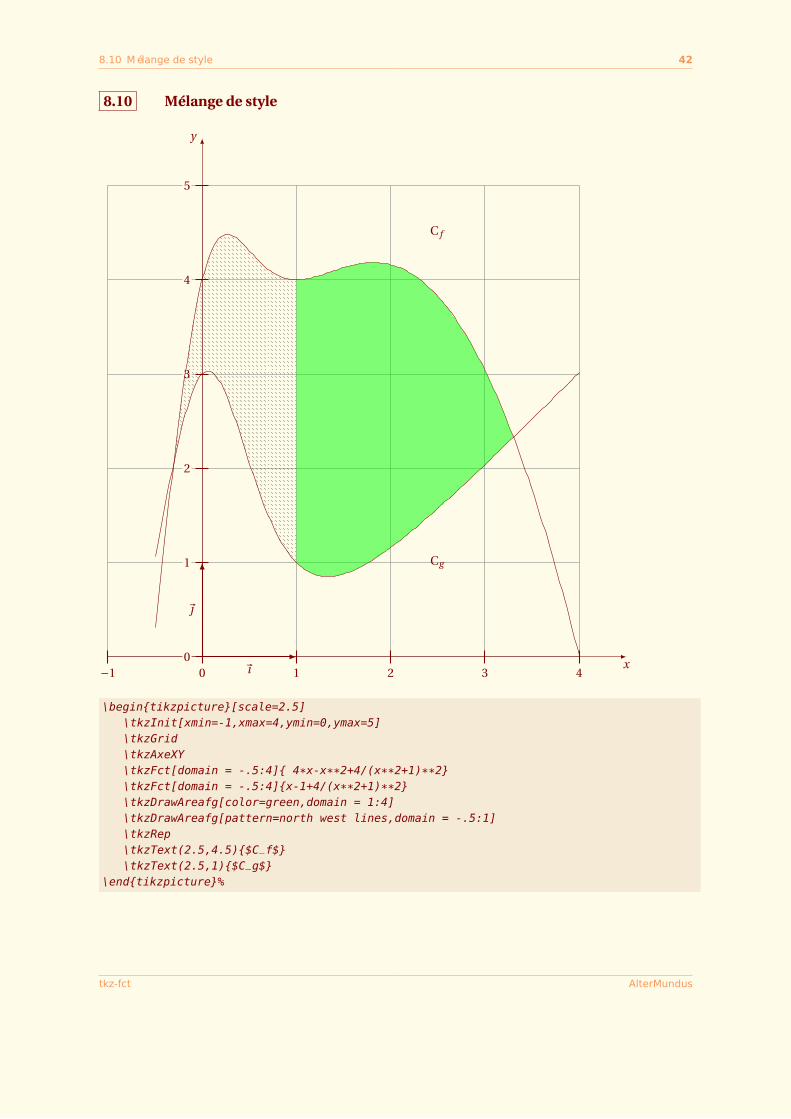
8.10 Mélange de style
x
y
−1 0 1 2 3 40
1
2
3
4
5
~
~ı
C f
Cg
\begin{tikzpicture}[scale=2.5]\tkzInit[xmin=-1,xmax=4,ymin=0,ymax=5]\tkzGrid\tkzAxeXY\tkzFct[domain = -.5:4]{ 4*x-x**2+4/(x**2+1)**2}\tkzFct[domain = -.5:4]{x-1+4/(x**2+1)**2}\tkzDrawAreafg[color=green,domain = 1:4]\tkzDrawAreafg[pattern=north west lines,domain = -.5:1]\tkzRep\tkzText(2.5,4.5){$C_f$}\tkzText(2.5,1){$C_g$}
\end{tikzpicture}%
tkz-fct AlterMundus
8.11 Courbes de niveaux 43
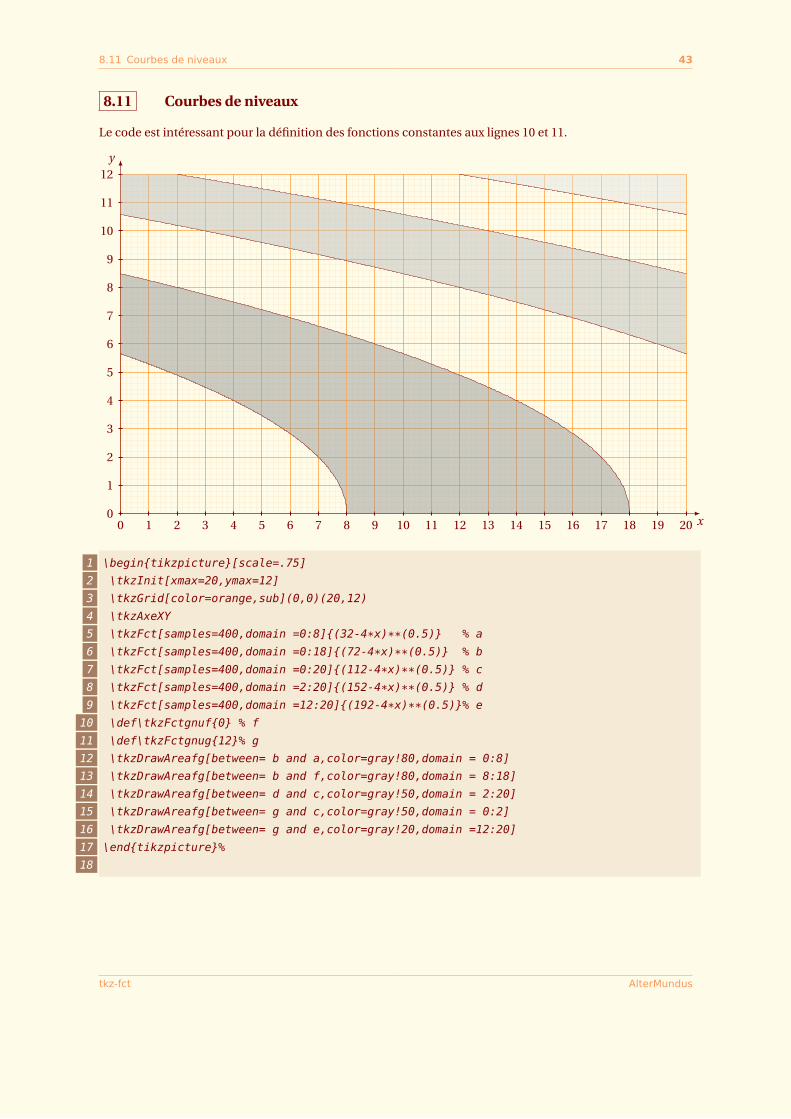
8.11 Courbes de niveaux
Le code est intéressant pour la définition des fonctions constantes aux lignes 10 et 11.
x
y
0 1 2 3 4 5 6 7 8 9 10 11 12 13 14 15 16 17 18 19 200
1
2
3
4
5
6
7
8
9
10
11
12
1 \begin{tikzpicture}[scale=.75]
2 \tkzInit[xmax=20,ymax=12]
3 \tkzGrid[color=orange,sub](0,0)(20,12)
4 \tkzAxeXY
5 \tkzFct[samples=400,domain =0:8]{(32-4*x)**(0.5)} % a
6 \tkzFct[samples=400,domain =0:18]{(72-4*x)**(0.5)} % b
7 \tkzFct[samples=400,domain =0:20]{(112-4*x)**(0.5)} % c
8 \tkzFct[samples=400,domain =2:20]{(152-4*x)**(0.5)} % d
9 \tkzFct[samples=400,domain =12:20]{(192-4*x)**(0.5)}% e
10 \def\tkzFctgnuf{0} % f
11 \def\tkzFctgnug{12}% g
12 \tkzDrawAreafg[between= b and a,color=gray!80,domain = 0:8]
13 \tkzDrawAreafg[between= b and f,color=gray!80,domain = 8:18]
14 \tkzDrawAreafg[between= d and c,color=gray!50,domain = 2:20]
15 \tkzDrawAreafg[between= g and c,color=gray!50,domain = 0:2]
16 \tkzDrawAreafg[between= g and e,color=gray!20,domain =12:20]
17 \end{tikzpicture}%
18
tkz-fct AlterMundus
9 Sommes de Riemann 44
SECTION 9
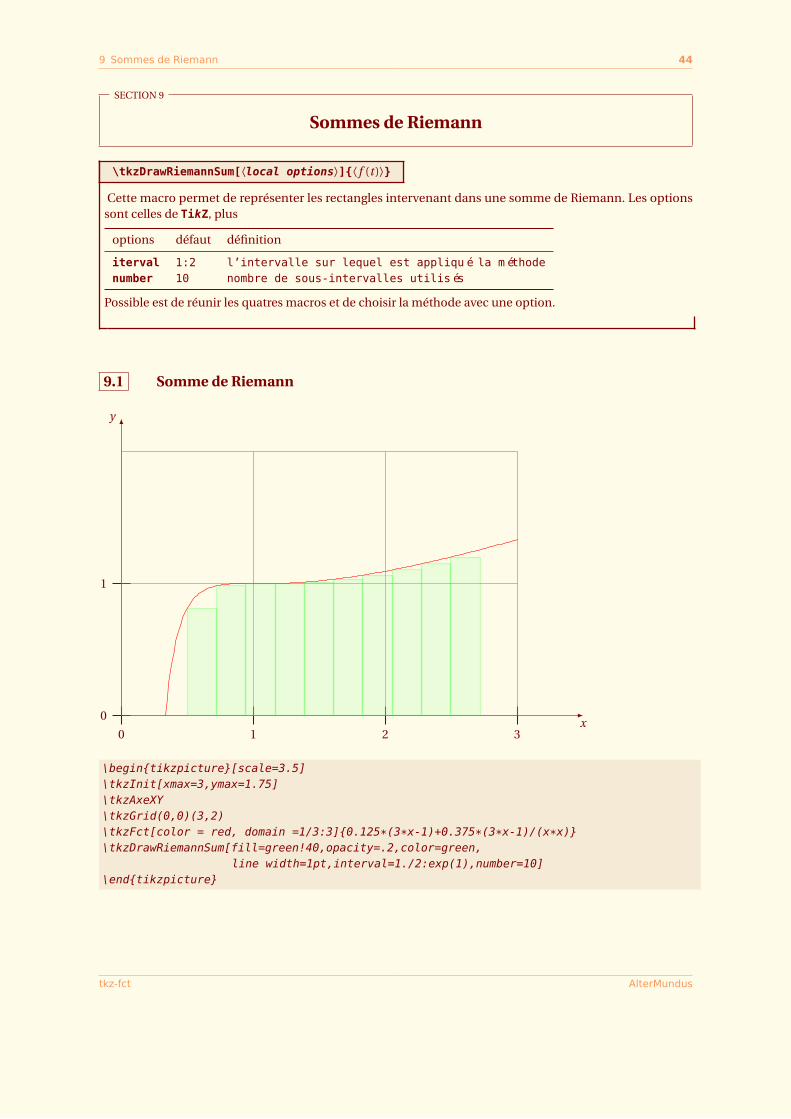
Sommes de Riemann
\tkzDrawRiemannSum[⟨local options⟩]{⟨ f (t )⟩}Cette macro permet de représenter les rectangles intervenant dans une somme de Riemann. Les options
sont celles de TikZ, plus
options défaut définition
iterval 1:2 l’intervalle sur lequel est appliqué la méthodenumber 10 nombre de sous-intervalles utilisés
Possible est de réunir les quatres macros et de choisir la méthode avec une option.
9.1 Somme de Riemann
x
y
0 1 2 3
0
1
\begin{tikzpicture}[scale=3.5]\tkzInit[xmax=3,ymax=1.75]\tkzAxeXY\tkzGrid(0,0)(3,2)\tkzFct[color = red, domain =1/3:3]{0.125*(3*x-1)+0.375*(3*x-1)/(x*x)}\tkzDrawRiemannSum[fill=green!40,opacity=.2,color=green,
line width=1pt,interval=1./2:exp(1),number=10]\end{tikzpicture}
tkz-fct AlterMundus
9.2 Somme de Riemann Inf 45
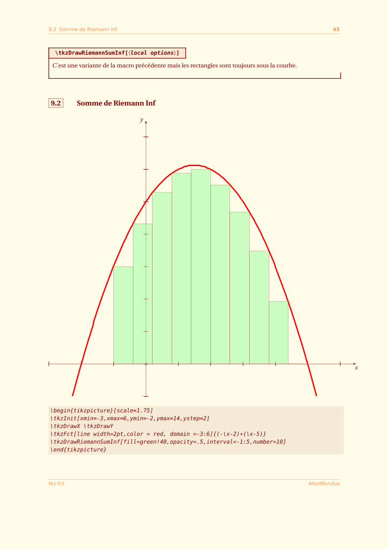
\tkzDrawRiemannSumInf[⟨local options⟩]C’est une variante de la macro précédente mais les rectangles sont toujours sous la courbe.
9.2 Somme de Riemann Inf
x
y
\begin{tikzpicture}[scale=1.75]\tkzInit[xmin=-3,xmax=6,ymin=-2,ymax=14,ystep=2]\tkzDrawX \tkzDrawY\tkzFct[line width=2pt,color = red, domain =-3:6]{(-\x-2)*(\x-5)}\tkzDrawRiemannSumInf[fill=green!40,opacity=.5,interval=-1:5,number=10]\end{tikzpicture}
tkz-fct AlterMundus
9.3 Somme de Riemann Inf et Sup 46
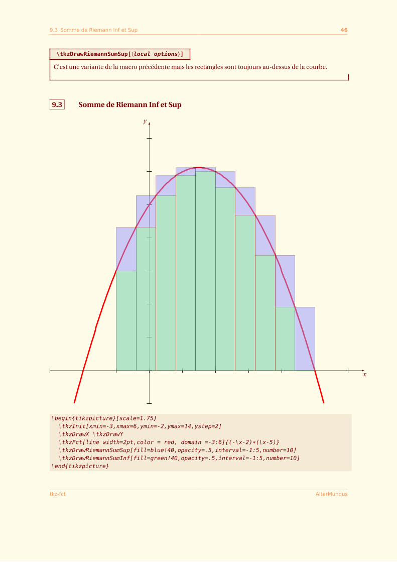
\tkzDrawRiemannSumSup[⟨local options⟩]C’est une variante de la macro précédente mais les rectangles sont toujours au-dessus de la courbe.
9.3 Somme de Riemann Inf et Sup
x
y
\begin{tikzpicture}[scale=1.75]\tkzInit[xmin=-3,xmax=6,ymin=-2,ymax=14,ystep=2]\tkzDrawX \tkzDrawY\tkzFct[line width=2pt,color = red, domain =-3:6]{(-\x-2)*(\x-5)}\tkzDrawRiemannSumSup[fill=blue!40,opacity=.5,interval=-1:5,number=10]\tkzDrawRiemannSumInf[fill=green!40,opacity=.5,interval=-1:5,number=10]
\end{tikzpicture}
tkz-fct AlterMundus
9.4 Somme de Riemann Mid 47
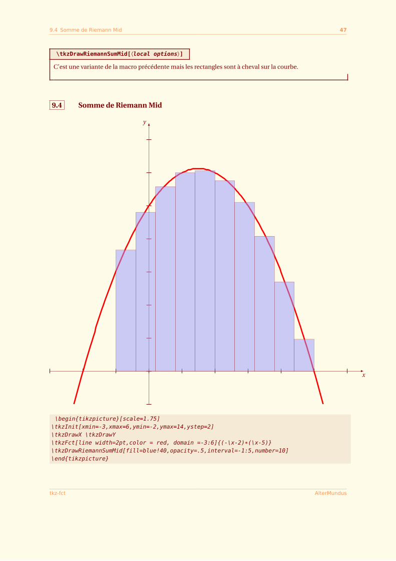
\tkzDrawRiemannSumMid[⟨local options⟩]C’est une variante de la macro précédente mais les rectangles sont à cheval sur la courbe.
9.4 Somme de Riemann Mid
x
y
\begin{tikzpicture}[scale=1.75]\tkzInit[xmin=-3,xmax=6,ymin=-2,ymax=14,ystep=2]\tkzDrawX \tkzDrawY\tkzFct[line width=2pt,color = red, domain =-3:6]{(-\x-2)*(\x-5)}\tkzDrawRiemannSumMid[fill=blue!40,opacity=.5,interval=-1:5,number=10]\end{tikzpicture}
tkz-fct AlterMundus
10 Droites particulières 48
SECTION 10
Droites particulières
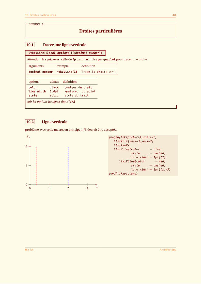
10.1 Tracer une ligne verticale
\tkzVLine[⟨local options⟩]{⟨decimal number⟩}Attention, la syntaxe est celle de fp car on n’utilise pas gnuplot pour tracer une droite.
arguments exemple définition
decimal number \tkzVLine{1} Trace la droite x = 1
options défaut définition
color black couleur du traitline width 0.6pt épaisseur du pointstyle solid style du trait
voir les options les lignes dans TikZ
10.2 Ligne verticale
problème avec cette macro, en principe 1./3 devrait être acceptée.
x
y
0 1 2 30
1
2
\begin{tikzpicture}[scale=2]\tkzInit[xmax=3,ymax=2]\tkzAxeXY\tkzVLine[color = blue,
style = dashed,line width = 1pt]{2}
\tkzVLine[color = red,style = dashed,line width = 1pt]{1./3}
\end{tikzpicture}
tkz-fct AlterMundus
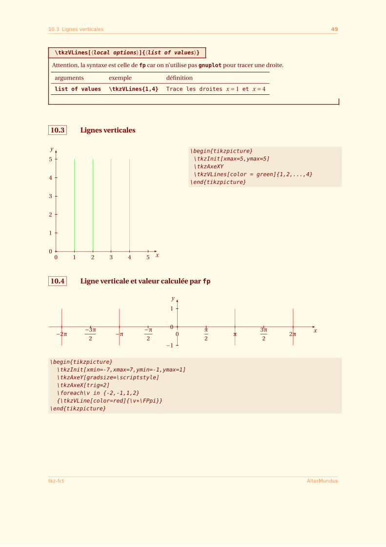
10.3 Lignes verticales 49
\tkzVLines[⟨local options⟩]{⟨list of values⟩}Attention, la syntaxe est celle de fp car on n’utilise pas gnuplot pour tracer une droite.
arguments exemple définition
list of values \tkzVLines{1,4} Trace les droites x = 1 et x = 4
10.3 Lignes verticales
x
y
0 1 2 3 4 50
1
2
3
4
5\begin{tikzpicture}\tkzInit[xmax=5,ymax=5]\tkzAxeXY\tkzVLines[color = green]{1,2,...,4}
\end{tikzpicture}
10.4 Ligne verticale et valeur calculée par fp
y
−1
0
1
−2π−3π
2−π −π
20
π
2π
3π
22π
x
\begin{tikzpicture}\tkzInit[xmin=-7,xmax=7,ymin=-1,ymax=1]\tkzAxeY[gradsize=\scriptstyle]\tkzAxeX[trig=2]\foreach\v in {-2,-1,1,2}{\tkzVLine[color=red]{\v*\FPpi}}
\end{tikzpicture}
tkz-fct AlterMundus
10.5 Une ligne horizontale 50
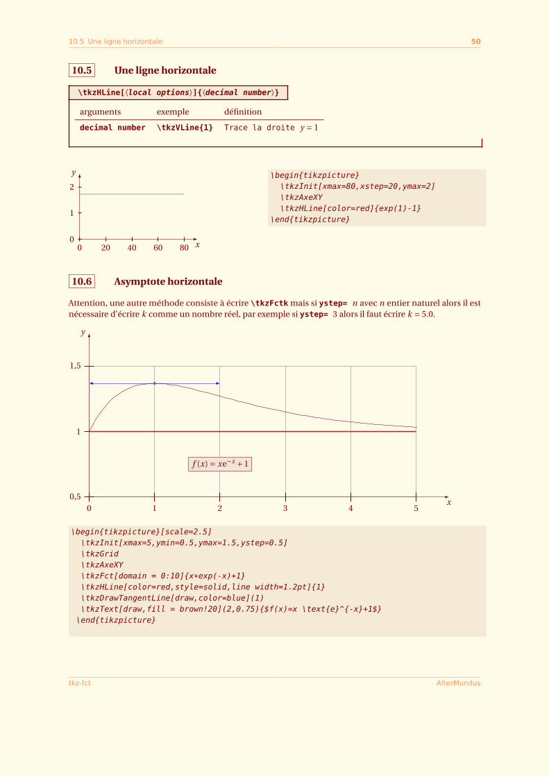
10.5 Une ligne horizontale
\tkzHLine[⟨local options⟩]{⟨decimal number⟩}
arguments exemple définition
decimal number \tkzVLine{1} Trace la droite y = 1
x
y
0 20 40 60 800
1
2\begin{tikzpicture}
\tkzInit[xmax=80,xstep=20,ymax=2]\tkzAxeXY\tkzHLine[color=red]{exp(1)-1}
\end{tikzpicture}
10.6 Asymptote horizontale
Attention, une autre méthode consiste à écrire \tkzFctk mais si ystep= n avec n entier naturel alors il estnécessaire d’écrire k comme un nombre réel, par exemple si ystep= 3 alors il faut écrire k = 5.0.
x
y
0 1 2 3 4 50,5
1
1,5
f (x) = xe−x +1
\begin{tikzpicture}[scale=2.5]\tkzInit[xmax=5,ymin=0.5,ymax=1.5,ystep=0.5]\tkzGrid\tkzAxeXY\tkzFct[domain = 0:10]{x*exp(-x)+1}\tkzHLine[color=red,style=solid,line width=1.2pt]{1}\tkzDrawTangentLine[draw,color=blue](1)\tkzText[draw,fill = brown!20](2,0.75){$f(x)=x \text{e}^{-x}+1$}
\end{tikzpicture}
tkz-fct AlterMundus
10.7 Lignes horizontales 51
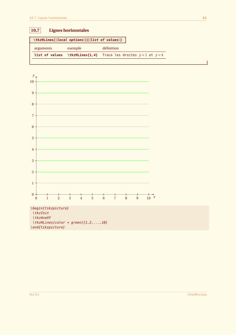
10.7 Lignes horizontales
\tkzHLines[⟨local options⟩]{⟨list of values⟩}
arguments exemple définition
list of values \tkzHLines{1,4} Trace les droites y = 1 et y = 4
x
y
0 1 2 3 4 5 6 7 8 9 100
1
2
3
4
5
6
7
8
9
10
\begin{tikzpicture}\tkzInit\tkzAxeXY\tkzHLines[color = green]{1,2,...,10}
\end{tikzpicture}
tkz-fct AlterMundus
10.8 Asymptote horizontale et verticale 52
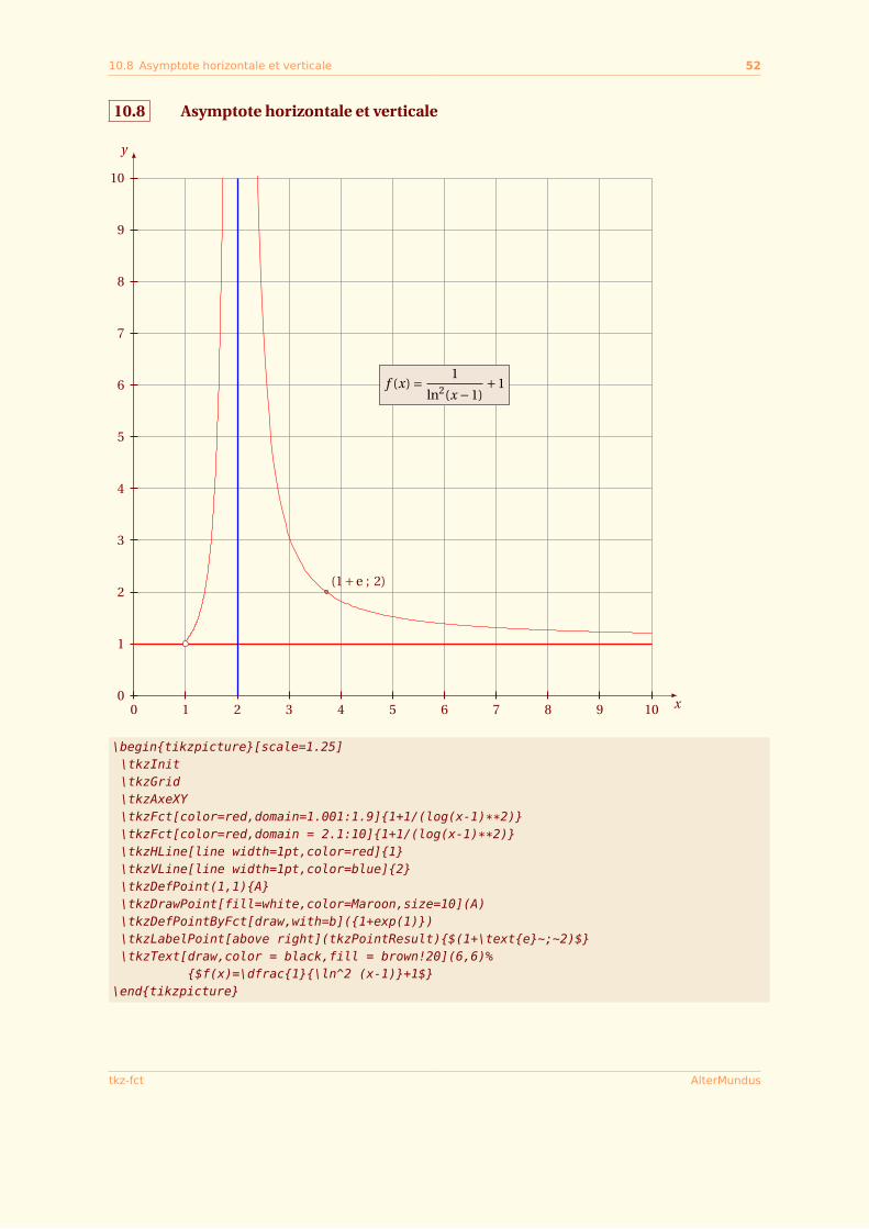
10.8 Asymptote horizontale et verticale
x
y
0 1 2 3 4 5 6 7 8 9 100
1
2
3
4
5
6
7
8
9
10
(1+e ; 2)
f (x) = 1
ln2(x −1)+1
\begin{tikzpicture}[scale=1.25]\tkzInit\tkzGrid\tkzAxeXY\tkzFct[color=red,domain=1.001:1.9]{1+1/(log(x-1)**2)}\tkzFct[color=red,domain = 2.1:10]{1+1/(log(x-1)**2)}\tkzHLine[line width=1pt,color=red]{1}\tkzVLine[line width=1pt,color=blue]{2}\tkzDefPoint(1,1){A}\tkzDrawPoint[fill=white,color=Maroon,size=10](A)\tkzDefPointByFct[draw,with=b]({1+exp(1)})\tkzLabelPoint[above right](tkzPointResult){$(1+\text{e}~;~2)$}\tkzText[draw,color = black,fill = brown!20](6,6)%
{$f(x)=\dfrac{1}{\ln^2 (x-1)}+1$}\end{tikzpicture}
tkz-fct AlterMundus
11 Courbes avec équations paramétrées 53
SECTION 11
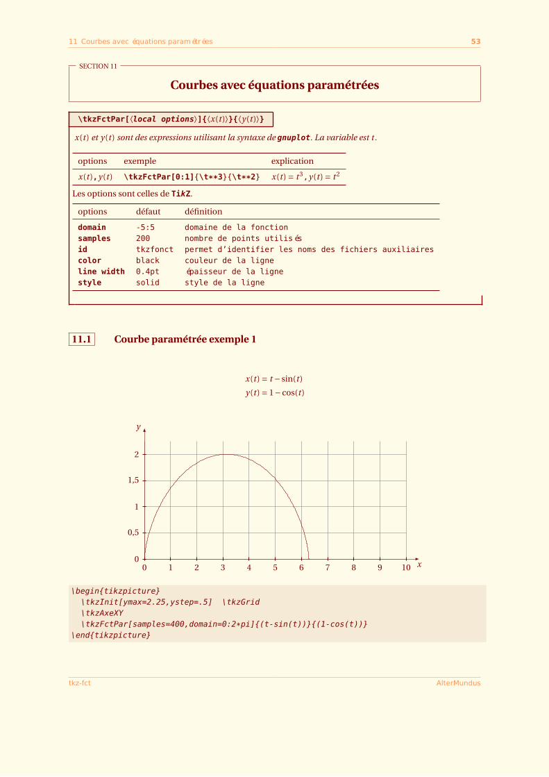
Courbes avec équations paramétrées
\tkzFctPar[⟨local options⟩]{⟨x(t )⟩}{⟨y(t )⟩}x(t ) et y(t ) sont des expressions utilisant la syntaxe de gnuplot. La variable est t .
options exemple explication
x(t ),y(t ) \tkzFctPar[0:1]{\t**3}{\t**2} x(t ) = t 3,y(t ) = t 2
Les options sont celles de TikZ.
options défaut définition
domain -5:5 domaine de la fonctionsamples 200 nombre de points utilisésid tkzfonct permet d’identifier les noms des fichiers auxiliairescolor black couleur de la ligneline width 0.4pt épaisseur de la lignestyle solid style de la ligne
11.1 Courbe paramétrée exemple 1
x(t ) = t − sin(t )
y(t ) = 1−cos(t )
x
y
0 1 2 3 4 5 6 7 8 9 100
0,5
1
1,5
2
\begin{tikzpicture}\tkzInit[ymax=2.25,ystep=.5] \tkzGrid\tkzAxeXY\tkzFctPar[samples=400,domain=0:2*pi]{(t-sin(t))}{(1-cos(t))}
\end{tikzpicture}
tkz-fct AlterMundus
11.2 Courbe paramétrée exemple 2 54
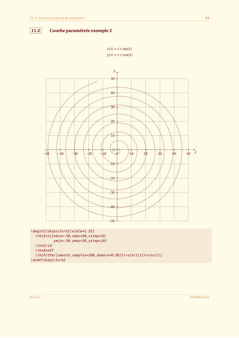
11.2 Courbe paramétrée exemple 2
x(t ) = t × sin(t )
y(t ) = t ×cos(t )
x
y
−50 −40 −30 −20 −10 0 10 20 30 40 50
−50
−40
−30
−20
−10
0
10
20
30
40
50
\begin{tikzpicture}[scale=1.25]\tkzInit[xmin=-50,xmax=50,xstep=10,
ymin=-50,ymax=50,ystep=10]\tkzGrid\tkzAxeXY\tkzFctPar[smooth,samples=200,domain=0:50]{t*sin(t)}{t*cos(t)}
\end{tikzpicture}
tkz-fct AlterMundus
11.3 Courbe paramétrée exemple 3 55
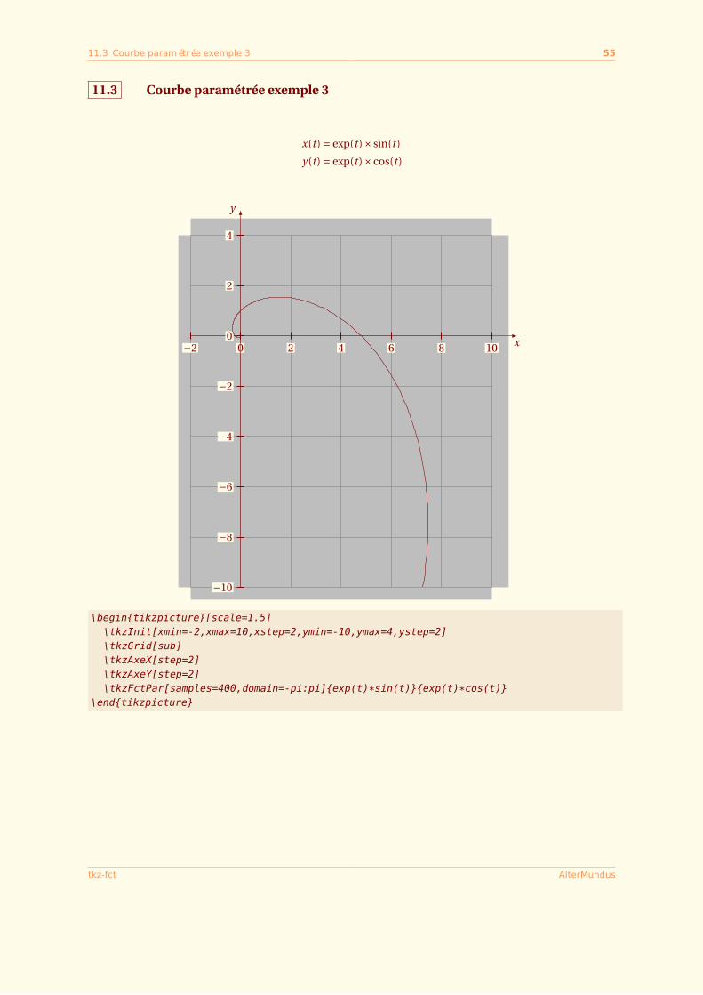
11.3 Courbe paramétrée exemple 3
x(t ) = exp(t )× sin(t )
y(t ) = exp(t )×cos(t )
−2 0 2 4 6 8 10 x
y
−10
−8
−6
−4
−2
0
2
4
\begin{tikzpicture}[scale=1.5]\tkzInit[xmin=-2,xmax=10,xstep=2,ymin=-10,ymax=4,ystep=2]\tkzGrid[sub]\tkzAxeX[step=2]\tkzAxeY[step=2]\tkzFctPar[samples=400,domain=-pi:pi]{exp(t)*sin(t)}{exp(t)*cos(t)}
\end{tikzpicture}
tkz-fct AlterMundus
11.4 Courbe paramétrée exemple 4 56
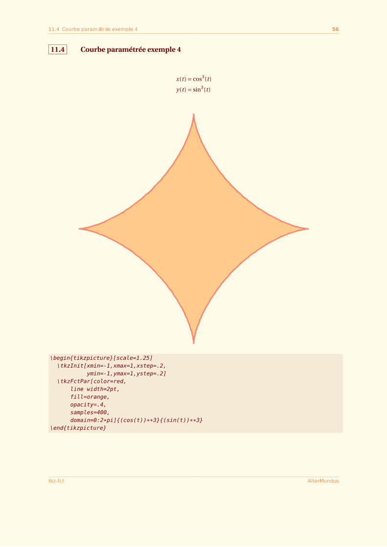
11.4 Courbe paramétrée exemple 4
x(t ) = cos3(t )
y(t ) = sin3(t )
\begin{tikzpicture}[scale=1.25]\tkzInit[xmin=-1,xmax=1,xstep=.2,
ymin=-1,ymax=1,ystep=.2]\tkzFctPar[color=red,
line width=2pt,fill=orange,opacity=.4,samples=400,domain=0:2*pi]{(cos(t))**3}{(sin(t))**3}
\end{tikzpicture}
tkz-fct AlterMundus
11.5 Courbe paramétrée exemple 5 57
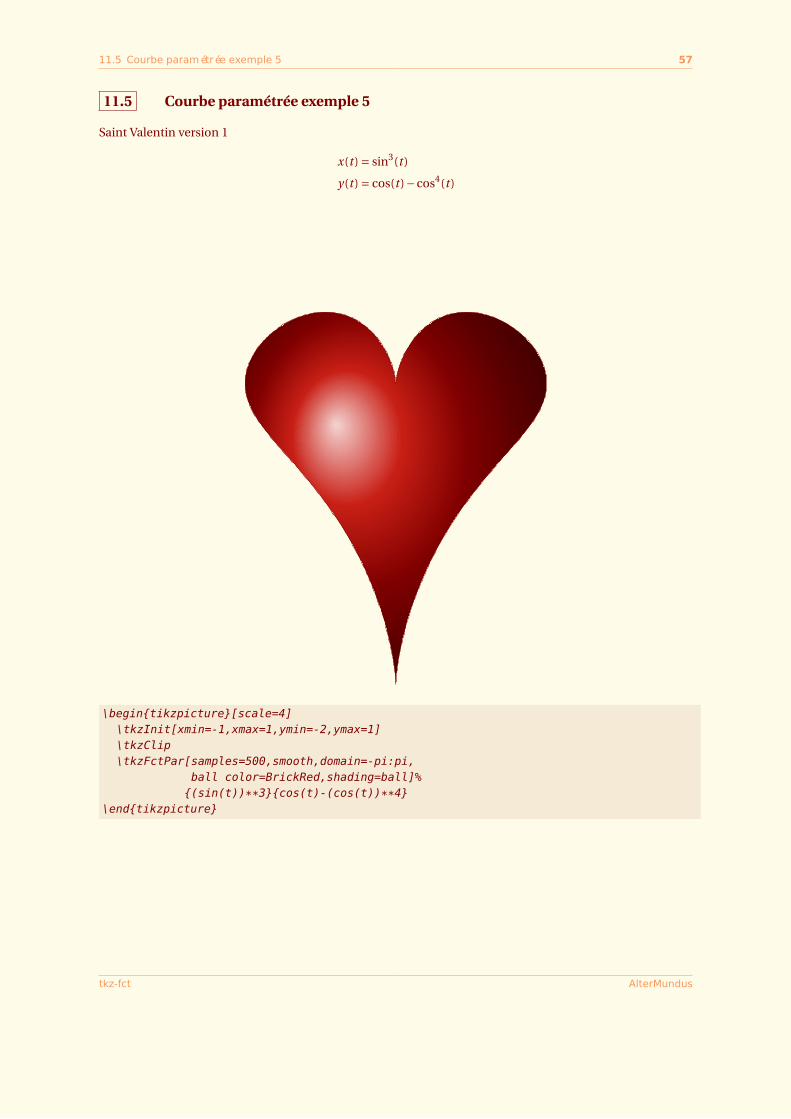
11.5 Courbe paramétrée exemple 5
Saint Valentin version 1
x(t ) = sin3(t )
y(t ) = cos(t )−cos4(t )
\begin{tikzpicture}[scale=4]\tkzInit[xmin=-1,xmax=1,ymin=-2,ymax=1]\tkzClip\tkzFctPar[samples=500,smooth,domain=-pi:pi,
ball color=BrickRed,shading=ball]%{(sin(t))**3}{cos(t)-(cos(t))**4}
\end{tikzpicture}
tkz-fct AlterMundus
11.6 Courbe paramétrée exemple 6 58
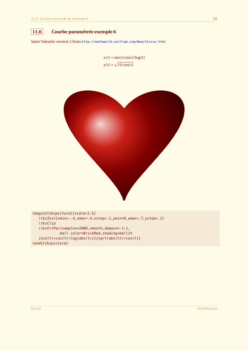
11.6 Courbe paramétrée exemple 6
Saint Valentin version 2 from http://mathworld.wolfram.com/HeartCurve.html
x(t ) = sin(t )cos(t ) log(t)
y(t ) =√
(t)cos(t )
\begin{tikzpicture}[scale=1.5]\tkzInit[xmin=-.4,xmax=.4,xstep=.1,ymin=0,ymax=.7,ystep=.1]\tkzClip\tkzFctPar[samples=2000,smooth,domain=-1:1,
ball color=BrickRed,shading=ball]%{sin(t)*cos(t)*log(abs(t))}{sqrt(abs(t))*cos(t)}
\end{tikzpicture}
tkz-fct AlterMundus
11.7 Courbe paramétrée exemple 7 59
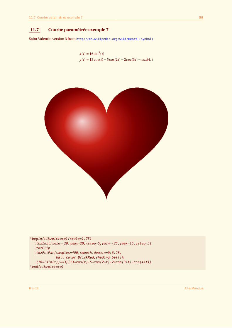
11.7 Courbe paramétrée exemple 7
Saint Valentin version 3 from http://en.wikipedia.org/wiki/Heart_(symbol)
x(t ) = 16sin3(t )
y(t ) = 13cos(t )−5cos(2t )−2cos(3t )− cos(4t )
\begin{tikzpicture}[scale=1.75]\tkzInit[xmin=-20,xmax=20,xstep=5,ymin=-25,ymax=15,ystep=5]\tkzClip\tkzFctPar[samples=400,smooth,domain=0:6.28,
ball color=BrickRed,shading=ball]%{16*(sin(t))**3}{13*cos(t)-5*cos(2*t)-2*cos(3*t)-cos(4*t)}
\end{tikzpicture}
tkz-fct AlterMundus
12 Courbes en coordonnées polaires 60
SECTION 12
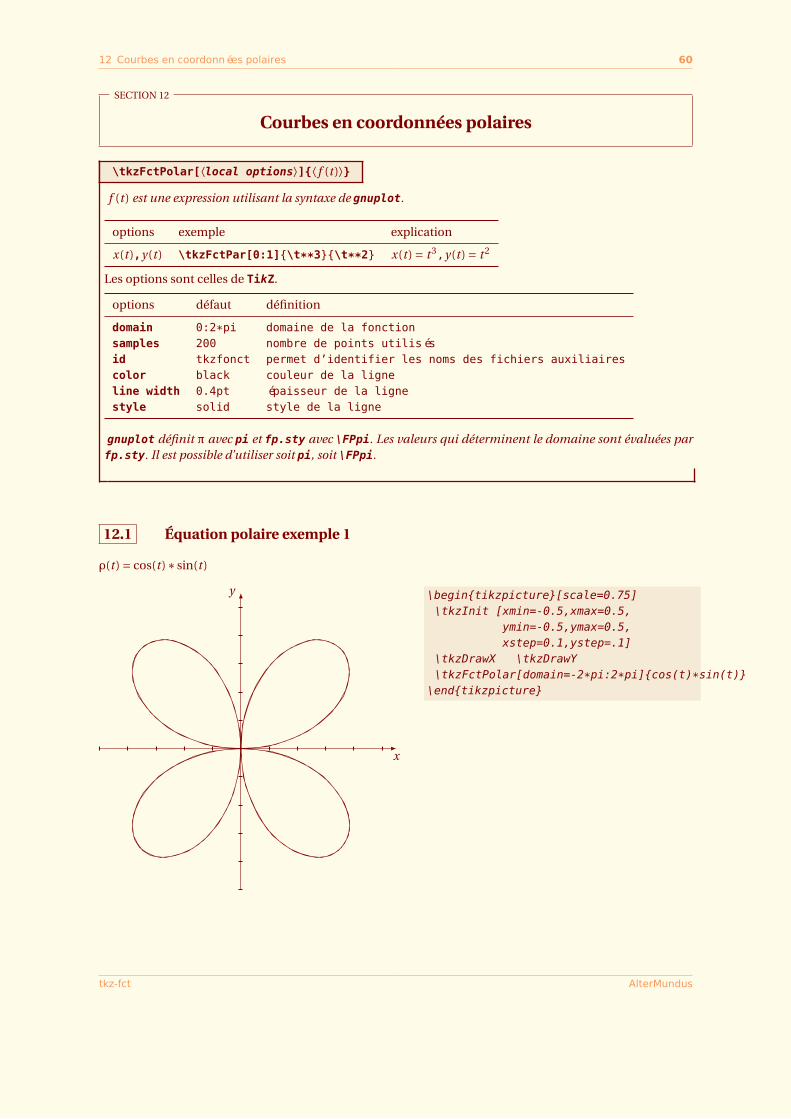
Courbes en coordonnées polaires
\tkzFctPolar[⟨local options⟩]{⟨ f (t )⟩}f (t ) est une expression utilisant la syntaxe de gnuplot.
options exemple explication
x(t ),y(t ) \tkzFctPar[0:1]{\t**3}{\t**2} x(t ) = t 3,y(t ) = t 2
Les options sont celles de TikZ.
options défaut définition
domain 0:2*pi domaine de la fonctionsamples 200 nombre de points utilisésid tkzfonct permet d’identifier les noms des fichiers auxiliairescolor black couleur de la ligneline width 0.4pt épaisseur de la lignestyle solid style de la ligne
gnuplot définit π avec pi et fp.sty avec \FPpi. Les valeurs qui déterminent le domaine sont évaluées parfp.sty. Il est possible d’utiliser soit pi, soit \FPpi.
12.1 Équation polaire exemple 1
ρ(t ) = cos(t )∗ sin(t )
x
y \begin{tikzpicture}[scale=0.75]\tkzInit [xmin=-0.5,xmax=0.5,
ymin=-0.5,ymax=0.5,xstep=0.1,ystep=.1]
\tkzDrawX \tkzDrawY\tkzFctPolar[domain=-2*pi:2*pi]{cos(t)*sin(t)}
\end{tikzpicture}
tkz-fct AlterMundus
12.2 Équation polaire exemple 2 61
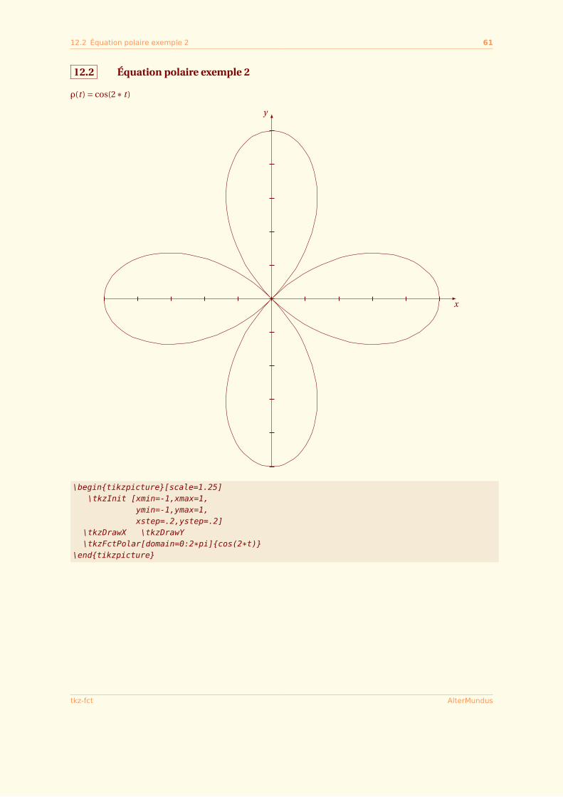
12.2 Équation polaire exemple 2
ρ(t ) = cos(2∗ t )
x
y
\begin{tikzpicture}[scale=1.25]\tkzInit [xmin=-1,xmax=1,
ymin=-1,ymax=1,xstep=.2,ystep=.2]
\tkzDrawX \tkzDrawY\tkzFctPolar[domain=0:2*pi]{cos(2*t)}
\end{tikzpicture}
tkz-fct AlterMundus
12.3 Équation polaire Heart 62
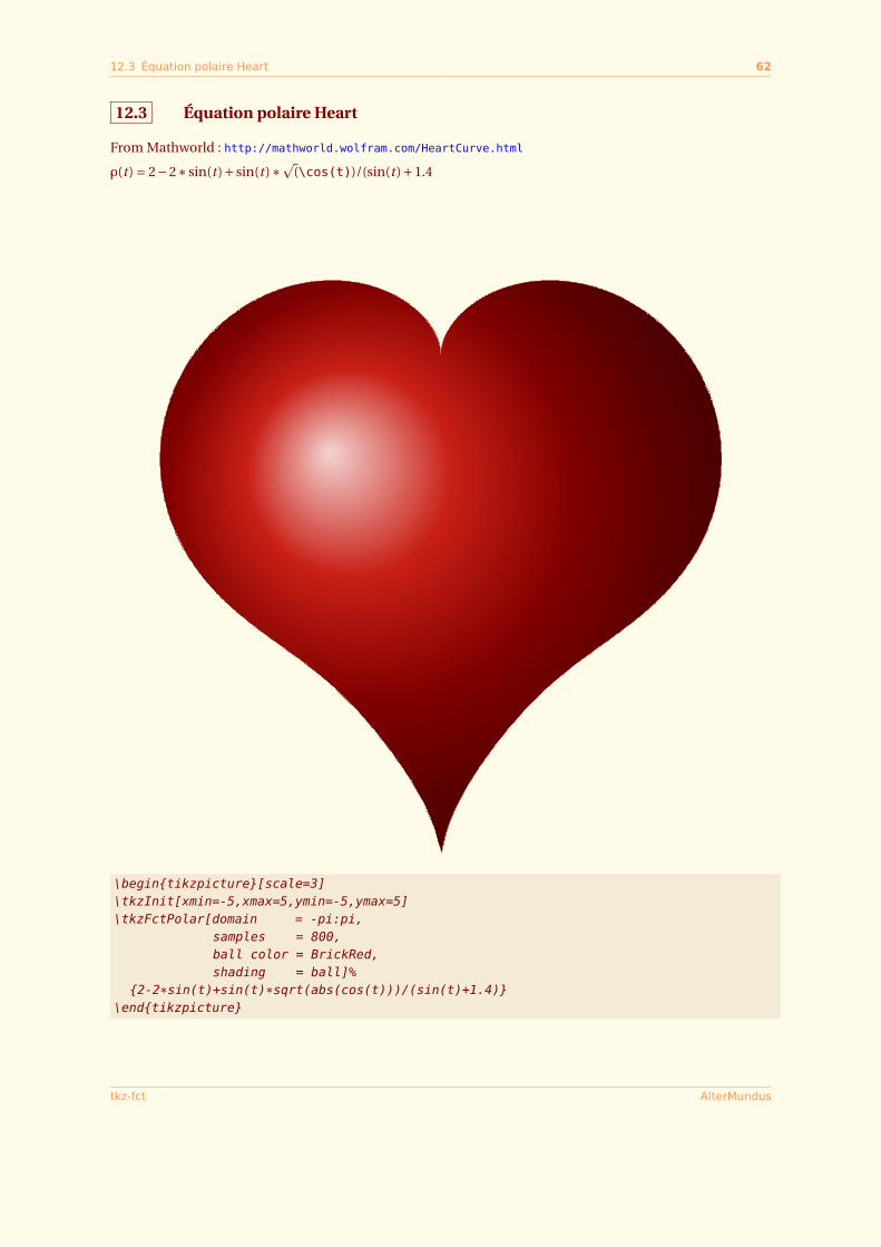
12.3 Équation polaire Heart
From Mathworld : http://mathworld.wolfram.com/HeartCurve.html
ρ(t ) = 2−2∗ sin(t )+ sin(t )∗p(\cos(t))/(sin(t )+1.4
\begin{tikzpicture}[scale=3]\tkzInit[xmin=-5,xmax=5,ymin=-5,ymax=5]\tkzFctPolar[domain = -pi:pi,
samples = 800,ball color = BrickRed,shading = ball]%
{2-2*sin(t)+sin(t)*sqrt(abs(cos(t)))/(sin(t)+1.4)}\end{tikzpicture}
tkz-fct AlterMundus
12.4 Équation polaire exemple 4 63
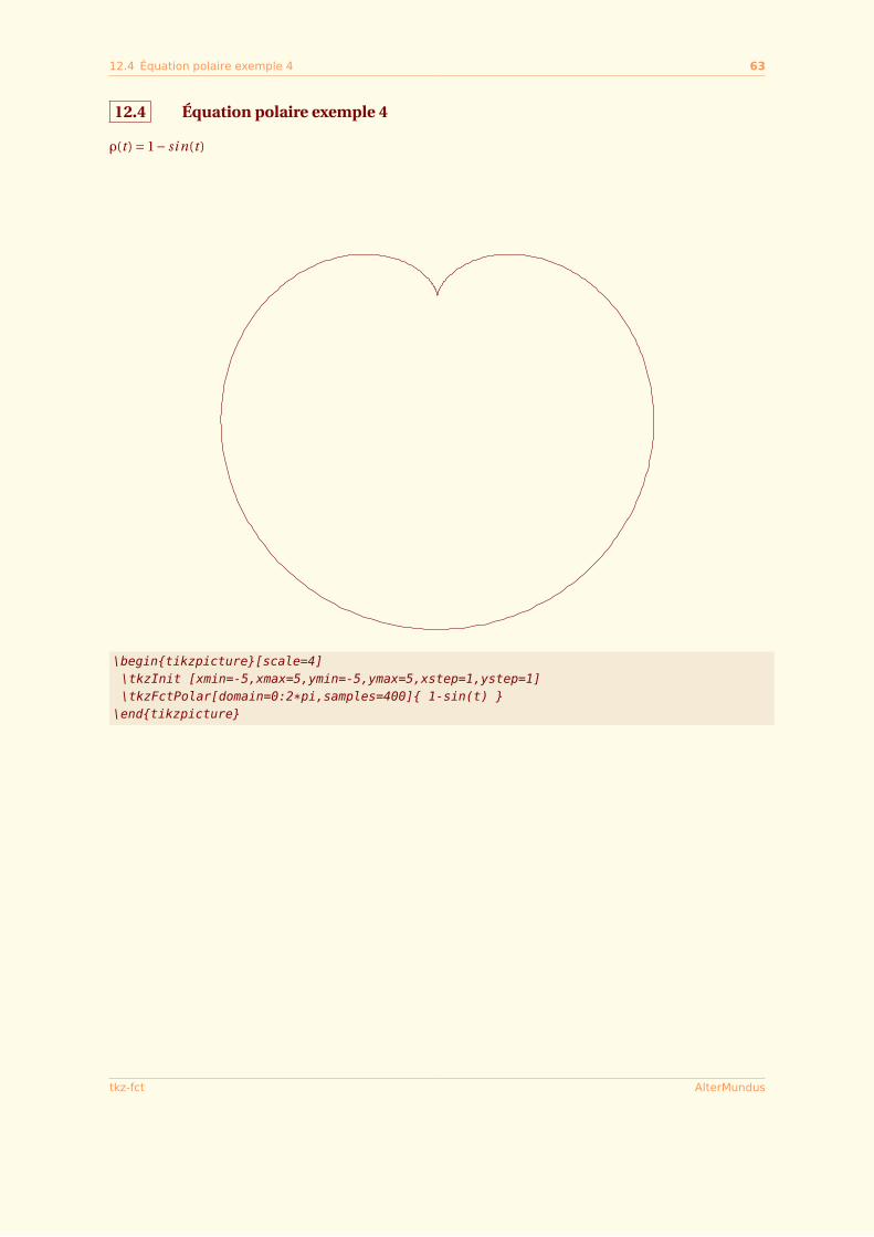
12.4 Équation polaire exemple 4
ρ(t ) = 1− si n(t )
\begin{tikzpicture}[scale=4]\tkzInit [xmin=-5,xmax=5,ymin=-5,ymax=5,xstep=1,ystep=1]\tkzFctPolar[domain=0:2*pi,samples=400]{ 1-sin(t) }
\end{tikzpicture}
tkz-fct AlterMundus
12.5 Équation polaire Cannabis ou Marijuana Curve 64
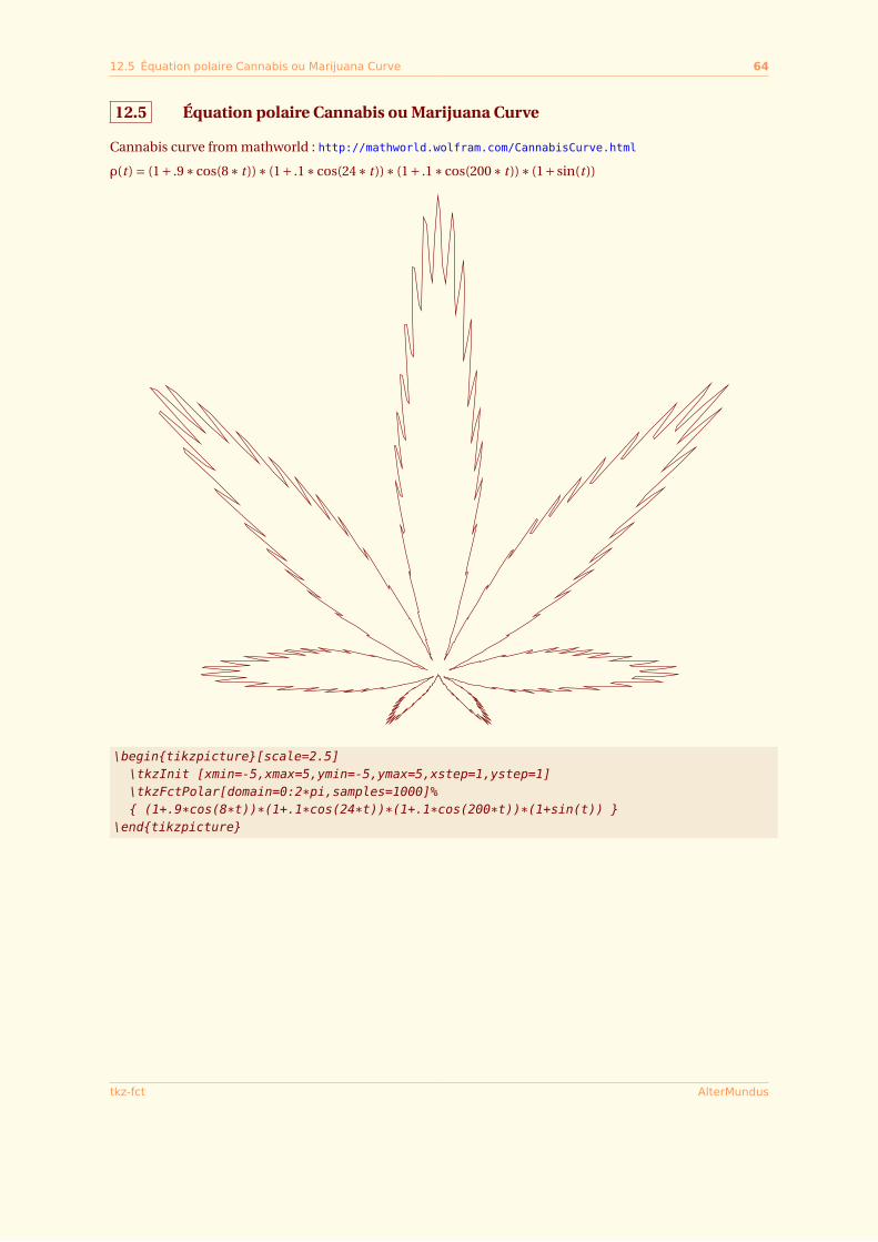
12.5 Équation polaire Cannabis ou Marijuana Curve
Cannabis curve from mathworld : http://mathworld.wolfram.com/CannabisCurve.html
ρ(t ) = (1+ .9∗cos(8∗ t ))∗ (1+ .1∗cos(24∗ t ))∗ (1+ .1∗cos(200∗ t ))∗ (1+ sin(t ))
\begin{tikzpicture}[scale=2.5]\tkzInit [xmin=-5,xmax=5,ymin=-5,ymax=5,xstep=1,ystep=1]\tkzFctPolar[domain=0:2*pi,samples=1000]%{ (1+.9*cos(8*t))*(1+.1*cos(24*t))*(1+.1*cos(200*t))*(1+sin(t)) }
\end{tikzpicture}
tkz-fct AlterMundus
12.6 Scarabaeus Curve 65
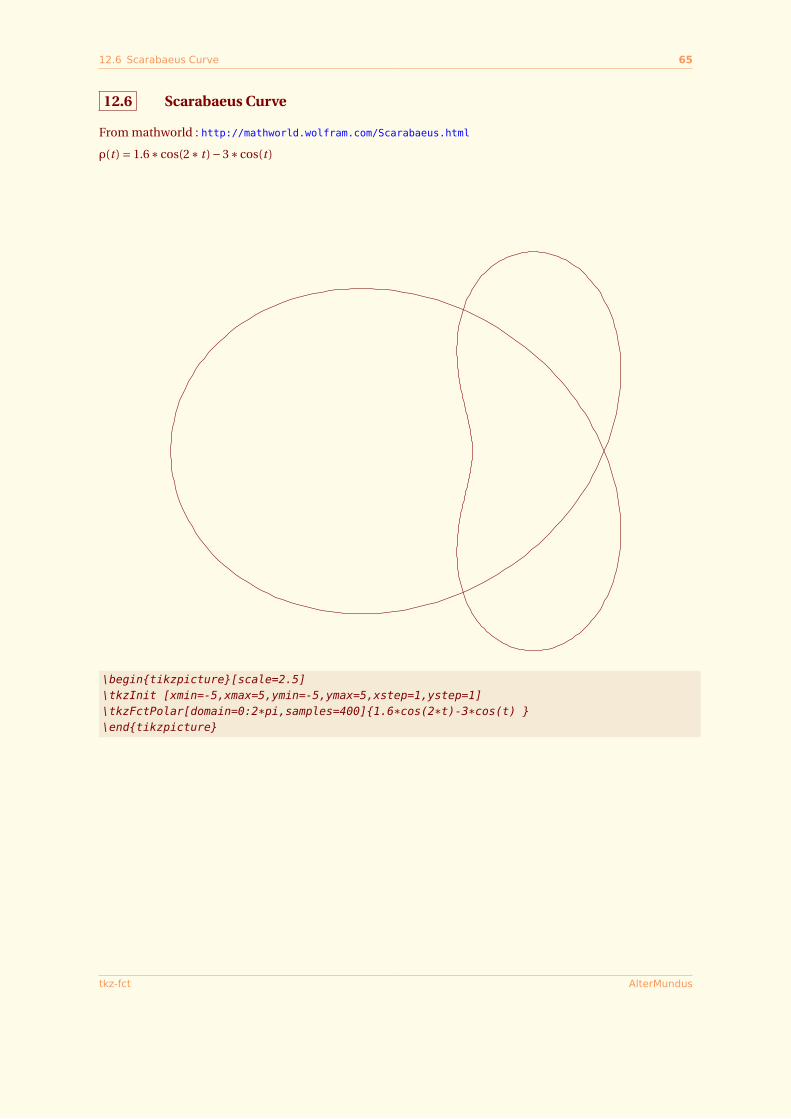
12.6 Scarabaeus Curve
From mathworld : http://mathworld.wolfram.com/Scarabaeus.html
ρ(t ) = 1.6∗cos(2∗ t )−3∗cos(t )
\begin{tikzpicture}[scale=2.5]\tkzInit [xmin=-5,xmax=5,ymin=-5,ymax=5,xstep=1,ystep=1]\tkzFctPolar[domain=0:2*pi,samples=400]{1.6*cos(2*t)-3*cos(t) }\end{tikzpicture}
tkz-fct AlterMundus
13 Symboles 66
SECTION 13
Symboles
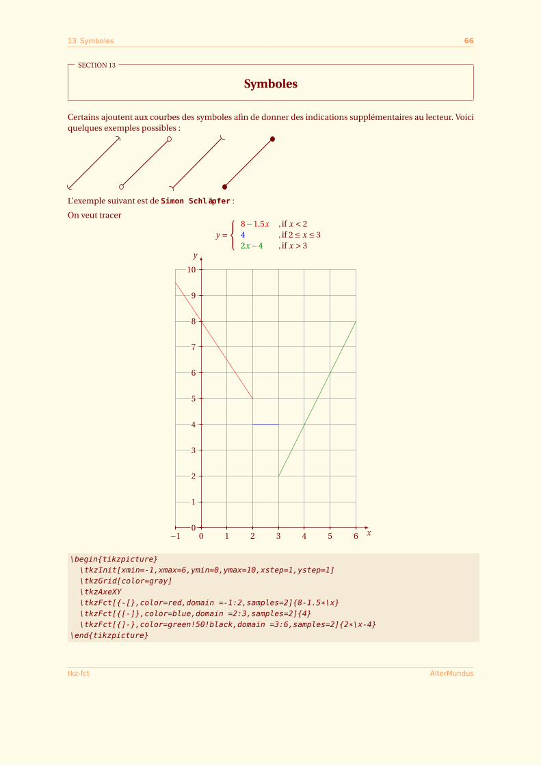
Certains ajoutent aux courbes des symboles afin de donner des indications supplémentaires au lecteur. Voiciquelques exemples possibles :
L’exemple suivant est de Simon Schläpfer :
On veut tracer
y =
8−1.5x , if x < 24 , if 2 ≤ x ≤ 32x −4 , if x > 3
x
y
−1 0 1 2 3 4 5 60
1
2
3
4
5
6
7
8
9
10
\begin{tikzpicture}\tkzInit[xmin=-1,xmax=6,ymin=0,ymax=10,xstep=1,ystep=1]\tkzGrid[color=gray]\tkzAxeXY\tkzFct[{-[},color=red,domain =-1:2,samples=2]{8-1.5*\x}\tkzFct[{[-]},color=blue,domain =2:3,samples=2]{4}\tkzFct[{]-},color=green!50!black,domain =3:6,samples=2]{2*\x-4}
\end{tikzpicture}
tkz-fct AlterMundus
14 Quelques exemples 67
SECTION 14
Quelques exemples
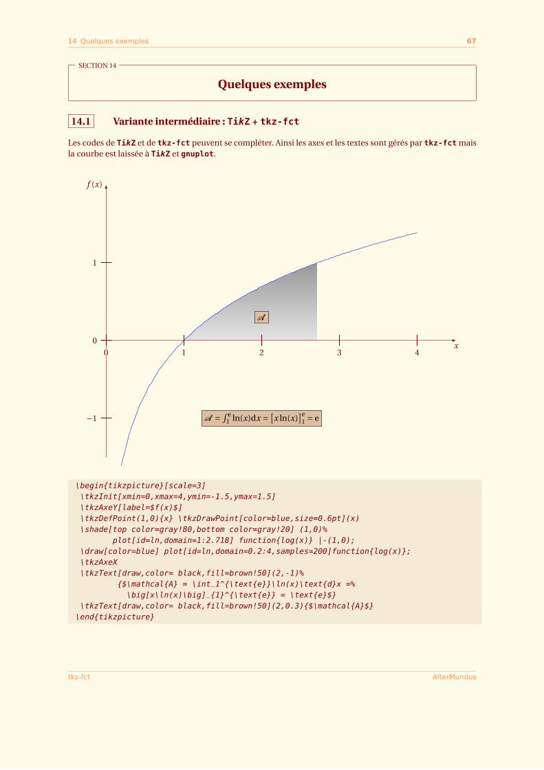
14.1 Variante intermédiaire : TikZ + tkz-fct
Les codes de TikZ et de tkz-fct peuvent se compléter. Ainsi les axes et les textes sont gérés par tkz-fct maisla courbe est laissée à TikZ et gnuplot.
f (x)
−1
0
1
0 1 2 3 4x
A = ∫ e1 ln(x)dx = [
x ln(x)]e
1 = e
A
\begin{tikzpicture}[scale=3]\tkzInit[xmin=0,xmax=4,ymin=-1.5,ymax=1.5]\tkzAxeY[label=$f(x)$]\tkzDefPoint(1,0){x} \tkzDrawPoint[color=blue,size=0.6pt](x)\shade[top color=gray!80,bottom color=gray!20] (1,0)%
plot[id=ln,domain=1:2.718] function{log(x)} |-(1,0);\draw[color=blue] plot[id=ln,domain=0.2:4,samples=200]function{log(x)};\tkzAxeX\tkzText[draw,color= black,fill=brown!50](2,-1)%
{$\mathcal{A} = \int_1^{\text{e}}\ln(x)\text{d}x =%\big[x\ln(x)\big]_{1}^{\text{e}} = \text{e}$}
\tkzText[draw,color= black,fill=brown!50](2,0.3){$\mathcal{A}$}\end{tikzpicture}
tkz-fct AlterMundus
14.2 Courbes de Lorentz 68
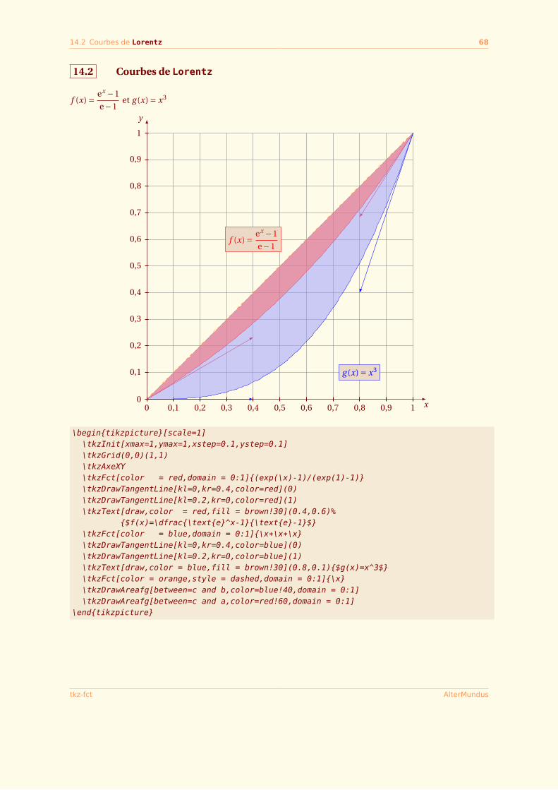
14.2 Courbes de Lorentz
f (x) = ex −1
e−1et g (x) = x3
x
y
0 0,1 0,2 0,3 0,4 0,5 0,6 0,7 0,8 0,9 10
0,1
0,2
0,3
0,4
0,5
0,6
0,7
0,8
0,9
1
f (x) = ex −1
e−1
g (x) = x3
\begin{tikzpicture}[scale=1]\tkzInit[xmax=1,ymax=1,xstep=0.1,ystep=0.1]\tkzGrid(0,0)(1,1)\tkzAxeXY\tkzFct[color = red,domain = 0:1]{(exp(\x)-1)/(exp(1)-1)}\tkzDrawTangentLine[kl=0,kr=0.4,color=red](0)\tkzDrawTangentLine[kl=0.2,kr=0,color=red](1)\tkzText[draw,color = red,fill = brown!30](0.4,0.6)%
{$f(x)=\dfrac{\text{e}^x-1}{\text{e}-1}$}\tkzFct[color = blue,domain = 0:1]{\x*\x*\x}\tkzDrawTangentLine[kl=0,kr=0.4,color=blue](0)\tkzDrawTangentLine[kl=0.2,kr=0,color=blue](1)\tkzText[draw,color = blue,fill = brown!30](0.8,0.1){$g(x)=x^3$}\tkzFct[color = orange,style = dashed,domain = 0:1]{\x}\tkzDrawAreafg[between=c and b,color=blue!40,domain = 0:1]\tkzDrawAreafg[between=c and a,color=red!60,domain = 0:1]
\end{tikzpicture}
tkz-fct AlterMundus
14.3 Courbe exponentielle 69
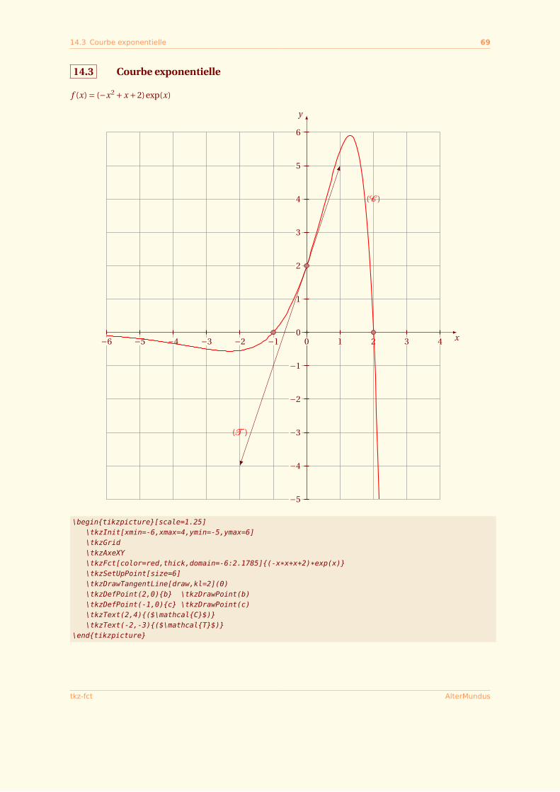
14.3 Courbe exponentielle
f (x) = (−x2 +x +2)exp(x)
x
y
−6 −5 −4 −3 −2 −1 0 1 2 3 4
−5
−4
−3
−2
−1
0
1
2
3
4
5
6
(C )
(T )
\begin{tikzpicture}[scale=1.25]\tkzInit[xmin=-6,xmax=4,ymin=-5,ymax=6]\tkzGrid\tkzAxeXY\tkzFct[color=red,thick,domain=-6:2.1785]{(-x*x+x+2)*exp(x)}\tkzSetUpPoint[size=6]\tkzDrawTangentLine[draw,kl=2](0)\tkzDefPoint(2,0){b} \tkzDrawPoint(b)\tkzDefPoint(-1,0){c} \tkzDrawPoint(c)\tkzText(2,4){($\mathcal{C}$)}\tkzText(-2,-3){($\mathcal{T}$)}
\end{tikzpicture}
tkz-fct AlterMundus
14.4 Axe logarithmique 70
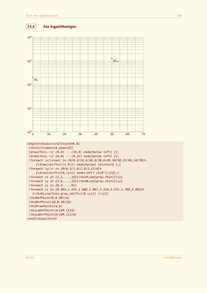
14.4 Axe logarithmique
0 10 20 30 40 50 60 70100
101
102
103
104
M1
M11
\begin{tikzpicture}[scale=0.8]\tkzInit[xmax=14,ymax=12]\draw[thin,->] (0,0) -- (14,0) node[below left] {};\draw[thin,->] (0,0) -- (0,12) node[below left] {};\foreach \x/\xtext in {0/0,2/10,4/20,6/30,8/40,10/50,12/60,14/70}%
{\draw[shift={(\x,0)}] node[below] {$\xtext$ };}\foreach \y/\z in {0/0,3/1,6/2,9/3,12/4}%
{\draw[shift={(0,\y)}] node[left] {$10^{\z}$};}\foreach \x in {1,2,...,14}{\tkzVLine[gray,thin]{\x}}\foreach \y in {3,6,...,12}{\tkzHLine[gray,thin]{\y}}\foreach \y in {0,3,...,9}{\foreach \z in {0.903,1.431,1.806,2.097,2.334,2.535,2.709,2.863}%{\tkzHLine[thin,gray,shift={(0,\y)}] {\z}}}
\tkzDefPoint(0,6.90){a}\tkzDefPoint(10,9.30){b}\tkzDrawPoints(a,b)\tkzLabelPoint(a){$M_{1}$}\tkzLabelPoint(b){$M_{11}$}
\end{tikzpicture}
tkz-fct AlterMundus
14.5 Un peu de tout 71
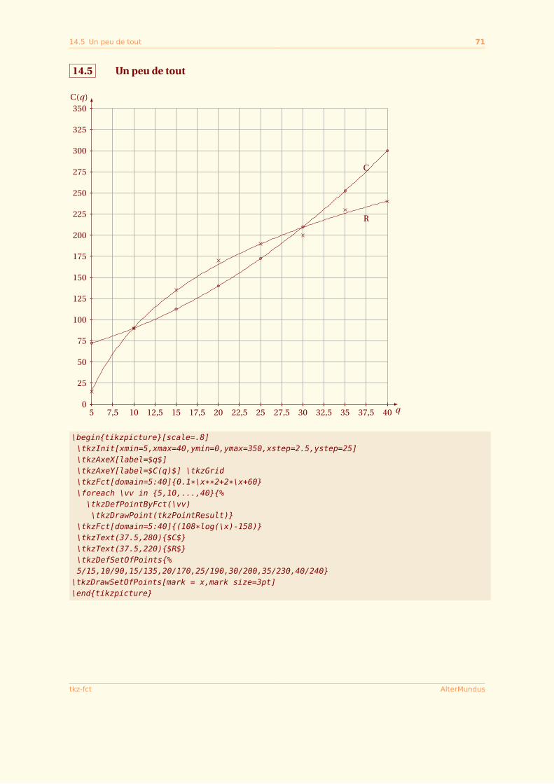
14.5 Un peu de tout
5 7,5 10 12,5 15 17,5 20 22,5 25 27,5 30 32,5 35 37,5 40 q
C(q)
0
25
50
75
100
125
150
175
200
225
250
275
300
325
350
C
R
\begin{tikzpicture}[scale=.8]\tkzInit[xmin=5,xmax=40,ymin=0,ymax=350,xstep=2.5,ystep=25]\tkzAxeX[label=$q$]\tkzAxeY[label=$C(q)$] \tkzGrid\tkzFct[domain=5:40]{0.1*\x**2+2*\x+60}\foreach \vv in {5,10,...,40}{%\tkzDefPointByFct(\vv)\tkzDrawPoint(tkzPointResult)}
\tkzFct[domain=5:40]{(108*log(\x)-158)}\tkzText(37.5,280){$C$}\tkzText(37.5,220){$R$}\tkzDefSetOfPoints{%5/15,10/90,15/135,20/170,25/190,30/200,35/230,40/240}
\tkzDrawSetOfPoints[mark = x,mark size=3pt]\end{tikzpicture}
tkz-fct AlterMundus
14.6 Interpolation 72
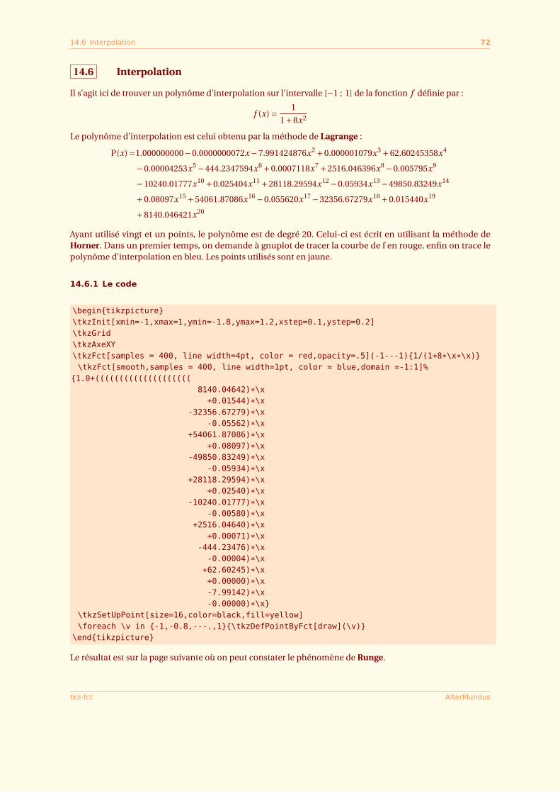
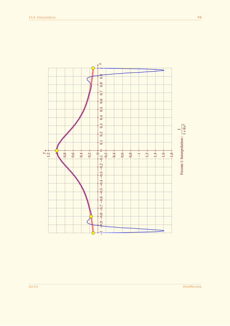
14.6 Interpolation
Il s’agit ici de trouver un polynôme d’interpolation sur l’intervalle [−1 ; 1] de la fonction f définie par :
f (x) = 1
1+8x2
Le polynôme d’interpolation est celui obtenu par la méthode de Lagrange :
P(x) =1.000000000−0.0000000072x −7.991424876x2 +0.000001079x3 +62.60245358x4
−0.00004253x5 −444.2347594x6 +0.0007118x7 +2516.046396x8 −0.005795x9
−10240.01777x10 +0.025404x11 +28118.29594x12 −0.05934x13 −49850.83249x14
+0.08097x15 +54061.87086x16 −0.055620x17 −32356.67279x18 +0.015440x19
+8140.046421x20
Ayant utilisé vingt et un points, le polynôme est de degré 20. Celui-ci est écrit en utilisant la méthode deHorner. Dans un premier temps, on demande à gnuplot de tracer la courbe de f en rouge, enfin on trace lepolynôme d’interpolation en bleu. Les points utilisés sont en jaune.
14.6.1 Le code
\begin{tikzpicture}\tkzInit[xmin=-1,xmax=1,ymin=-1.8,ymax=1.2,xstep=0.1,ystep=0.2]\tkzGrid\tkzAxeXY\tkzFct[samples = 400, line width=4pt, color = red,opacity=.5](-1---1){1/(1+8*\x*\x)}\tkzFct[smooth,samples = 400, line width=1pt, color = blue,domain =-1:1]%
{1.0+((((((((((((((((((((8140.04642)*\x+0.01544)*\x
-32356.67279)*\x-0.05562)*\x
+54061.87086)*\x+0.08097)*\x
-49850.83249)*\x-0.05934)*\x
+28118.29594)*\x+0.02540)*\x
-10240.01777)*\x-0.00580)*\x
+2516.04640)*\x+0.00071)*\x
-444.23476)*\x-0.00004)*\x
+62.60245)*\x+0.00000)*\x-7.99142)*\x-0.00000)*\x}
\tkzSetUpPoint[size=16,color=black,fill=yellow]\foreach \v in {-1,-0.8,---.,1}{\tkzDefPointByFct[draw](\v)}
\end{tikzpicture}
Le résultat est sur la page suivante où on peut constater le phénomène de Runge.
tkz-fct AlterMundus
14.6 Interpolation 73
14.6.2 la figure
tkz-fct AlterMundus
14.6 Interpolation 74
x
y
−1−0
,9−0
,8−0
,7−0
,6−0
,5−0
,4−0
,3−0
,2−0
,10
0,1
0,2
0,3
0,4
0,5
0,6
0,7
0,8
0,9
1
−1,8
−1,6
−1,4
−1,2−1−0,8
−0,6
−0,4
−0,20
0,2
0,4
0,6
0,81
1,2
Fig
ure
1:In
terp
ola
tio
n:
1
1+8
x2
tkz-fct AlterMundus
14.7 Courbes de Van der Waals 75
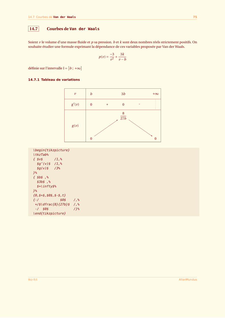
14.7 Courbes de Van der Waals
Soient v le volume d’une masse fluide et p sa pression. b et k sont deux nombres réels strictement positifs. Onsouhaite étudier une formule exprimant la dépendance de ces variables proposée par Van der Waals.
p(v) = −3
v2 + 3k
v −b
définie sur l’intervalle I = ]b ; +∞]
14.7.1 Tableau de variations
v
g ′(v)
g (v)
b 3b +∞
0 + 0 -
00
8
27b
8
27b
00
\begin{tikzpicture}\tkzTab%{ $v$ /1,%$g’(v)$ /1,%$g(v)$ /3%
}%{ $b$ ,%$3b$ ,%$+\infty$%
}%{0,$+$,$0$,$-$,t}{-/ $0$ /,%+/$\dfrac{8}{27b}$ /,%-/ $0$ /}%
\end{tikzpicture}
tkz-fct AlterMundus
14.7 Courbes de Van der Waals 76
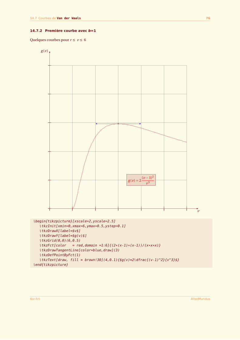
14.7.2 Première courbe avec b=1
Quelques courbes pour r ≤ v ≤ 6
v
g (v)
g (v) = 2(v −1)2
v3
\begin{tikzpicture}[xscale=2,yscale=2.5]\tkzInit[xmin=0,xmax=6,ymax=0.5,ystep=0.1]\tkzDrawX[label=$v$]\tkzDrawY[label=$g(v)$]\tkzGrid(0,0)(6,0.5)\tkzFct[color = red,domain =1:6]{(2*(x-1)*(x-1))/(x*x*x)}\tkzDrawTangentLine[color=blue,draw](3)\tkzDefPointByFct(1)\tkzText[draw, fill = brown!30](4,0.1){$g(v)=2\dfrac{(v-1)^2}{v^3}$}
\end{tikzpicture}
tkz-fct AlterMundus
14.7 Courbes de Van der Waals 77
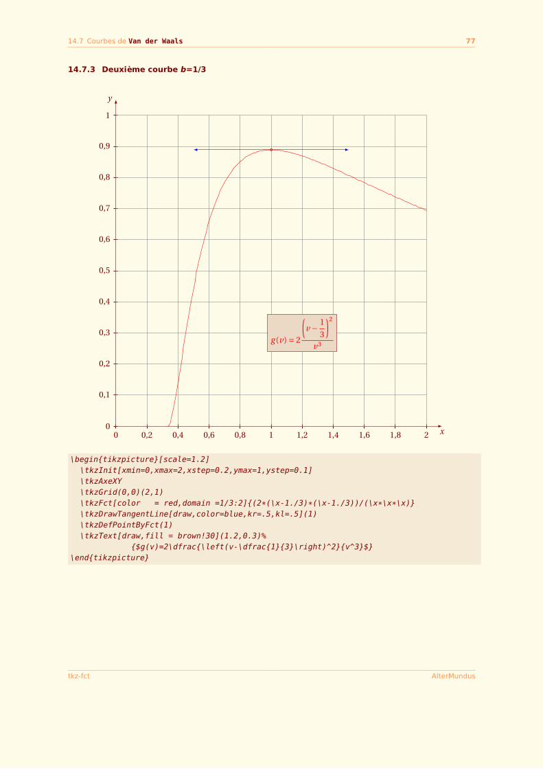
14.7.3 Deuxième courbe b=1/3
x
y
0 0,2 0,4 0,6 0,8 1 1,2 1,4 1,6 1,8 20
0,1
0,2
0,3
0,4
0,5
0,6
0,7
0,8
0,9
1
g (v) = 2
(v − 1
3
)2
v3
\begin{tikzpicture}[scale=1.2]\tkzInit[xmin=0,xmax=2,xstep=0.2,ymax=1,ystep=0.1]\tkzAxeXY\tkzGrid(0,0)(2,1)\tkzFct[color = red,domain =1/3:2]{(2*(\x-1./3)*(\x-1./3))/(\x*\x*\x)}\tkzDrawTangentLine[draw,color=blue,kr=.5,kl=.5](1)\tkzDefPointByFct(1)\tkzText[draw,fill = brown!30](1.2,0.3)%
{$g(v)=2\dfrac{\left(v-\dfrac{1}{3}\right)^2}{v^3}$}\end{tikzpicture}
tkz-fct AlterMundus
14.7 Courbes de Van der Waals 78
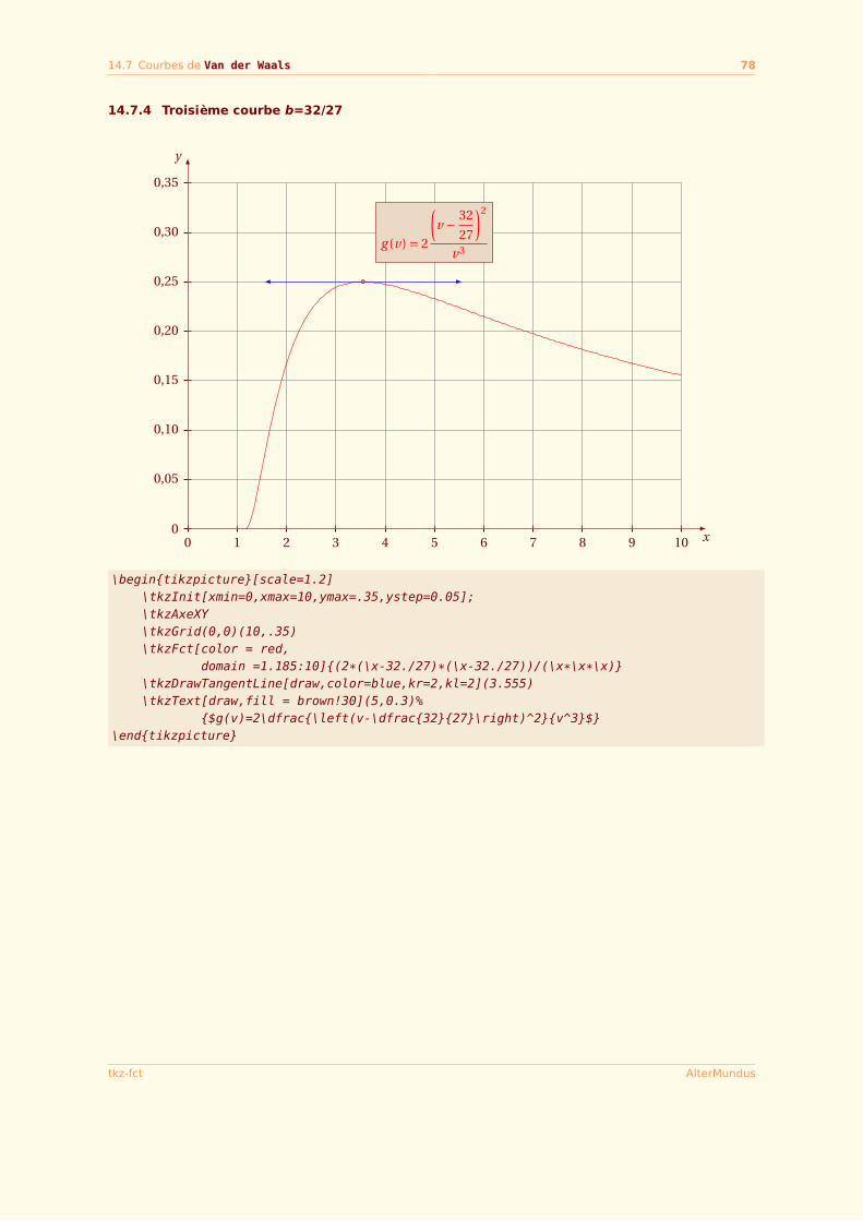
14.7.4 Troisième courbe b=32/27
x
y
0 1 2 3 4 5 6 7 8 9 100
0,05
0,10
0,15
0,20
0,25
0,30
0,35
g (v) = 2
(v − 32
27
)2
v3
\begin{tikzpicture}[scale=1.2]\tkzInit[xmin=0,xmax=10,ymax=.35,ystep=0.05];\tkzAxeXY\tkzGrid(0,0)(10,.35)\tkzFct[color = red,
domain =1.185:10]{(2*(\x-32./27)*(\x-32./27))/(\x*\x*\x)}\tkzDrawTangentLine[draw,color=blue,kr=2,kl=2](3.555)\tkzText[draw,fill = brown!30](5,0.3)%
{$g(v)=2\dfrac{\left(v-\dfrac{32}{27}\right)^2}{v^3}$}\end{tikzpicture}
tkz-fct AlterMundus
14.8 Valeurs critiques 79
14.8 Valeurs critiques
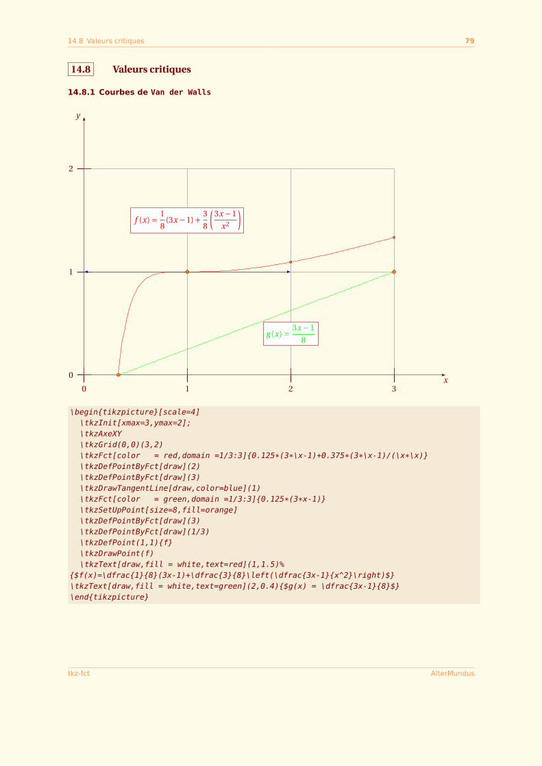
14.8.1 Courbes de Van der Walls
x
y
0 1 2 3
0
1
2
f (x) = 1
8(3x −1)+ 3
8
(3x −1
x2
)
g (x) = 3x −1
8
\begin{tikzpicture}[scale=4]\tkzInit[xmax=3,ymax=2];\tkzAxeXY\tkzGrid(0,0)(3,2)\tkzFct[color = red,domain =1/3:3]{0.125*(3*\x-1)+0.375*(3*\x-1)/(\x*\x)}\tkzDefPointByFct[draw](2)\tkzDefPointByFct[draw](3)\tkzDrawTangentLine[draw,color=blue](1)\tkzFct[color = green,domain =1/3:3]{0.125*(3*x-1)}\tkzSetUpPoint[size=8,fill=orange]\tkzDefPointByFct[draw](3)\tkzDefPointByFct[draw](1/3)\tkzDefPoint(1,1){f}\tkzDrawPoint(f)\tkzText[draw,fill = white,text=red](1,1.5)%
{$f(x)=\dfrac{1}{8}(3x-1)+\dfrac{3}{8}\left(\dfrac{3x-1}{x^2}\right)$}\tkzText[draw,fill = white,text=green](2,0.4){$g(x) = \dfrac{3x-1}{8}$}\end{tikzpicture}
tkz-fct AlterMundus
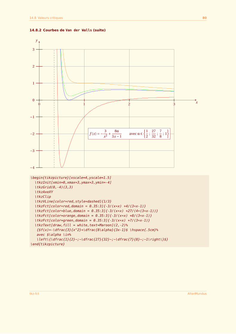
14.8 Valeurs critiques 80
14.8.2 Courbes de Van der Walls (suite)
x
y
0 1 2 3
−4
−3
−2
−1
0
1
2
3
f (x) =− 3
x2 + 8α
3x −1avec α ∈
{1
2;
27
32;
7
8; 1
}
\begin{tikzpicture}[xscale=4,yscale=1.5]\tkzInit[xmin=0,xmax=3,ymax=3,ymin=-4]\tkzGrid(0,-4)(3,3)\tkzAxeXY\tkzClip\tkzVLine[color=red,style=dashed]{1/3}\tkzFct[color=red,domain = 0.35:3]{-3/(x*x) +4/(3*x-1)}\tkzFct[color=blue,domain = 0.35:3]{-3/(x*x) +27/(4*(3*x-1))}\tkzFct[color=orange,domain = 0.35:3]{-3/(x*x) +8/(3*x-1)}\tkzFct[color=green,domain = 0.35:3]{-3/(x*x) +7/(3*x-1)}\tkzText[draw,fill = white,text=Maroon](2,-2)%{$f(x)=-\dfrac{3}{x^2}+\dfrac{8\alpha}{3x-1}$ \hspace{.5cm}%avec $\alpha \in%\left\{\dfrac{1}{2}~;~\dfrac{27}{32}~;~\dfrac{7}{8}~;~1\right\}$}
\end{tikzpicture}
tkz-fct AlterMundus
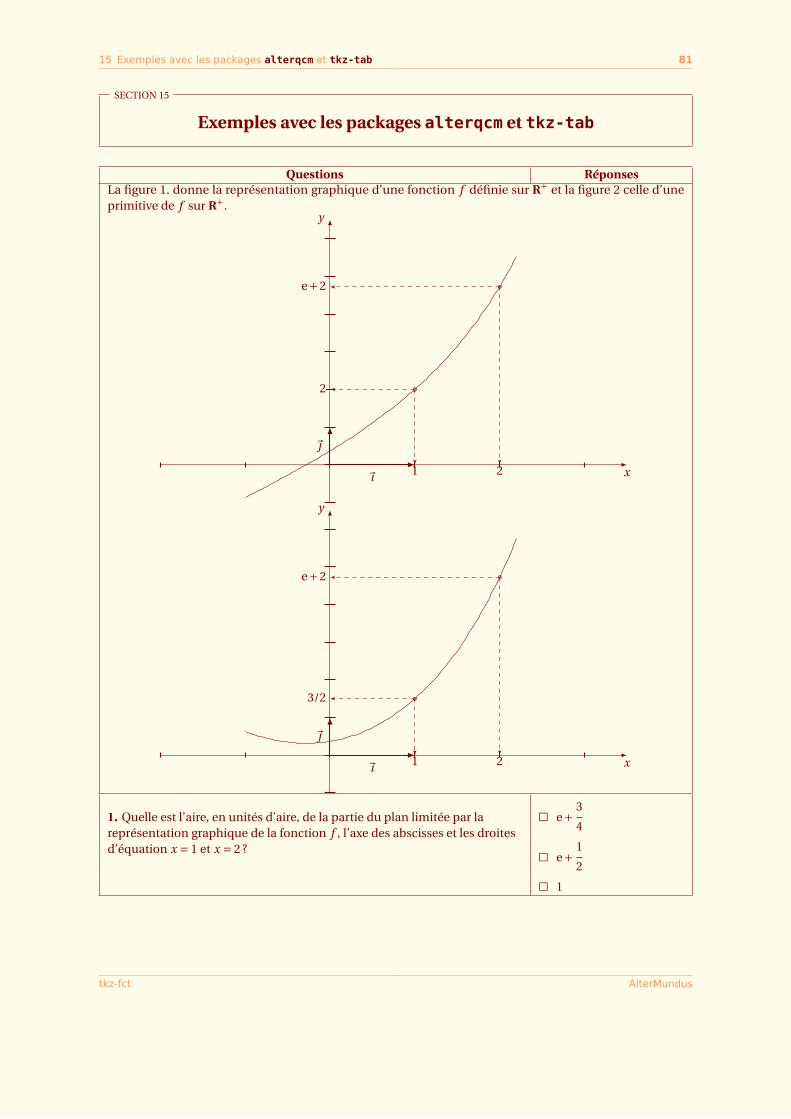
15 Exemples avec les packages alterqcm et tkz-tab 81
SECTION 15
Exemples avec les packages alterqcm et tkz-tab
Questions RéponsesLa figure 1. donne la représentation graphique d’une fonction f définie sur R+ et la figure 2 celle d’uneprimitive de f sur R+.
x
y
1
2
2
e+2
~
~ı
x
y
1
3/2
2
e+2
~
~ı
1. Quelle est l’aire, en unités d’aire, de la partie du plan limitée par lareprésentation graphique de la fonction f , l’axe des abscisses et les droitesd’équation x = 1 et x = 2 ?
ä e+ 3
4
ä e+ 1
2
ä 1
tkz-fct AlterMundus
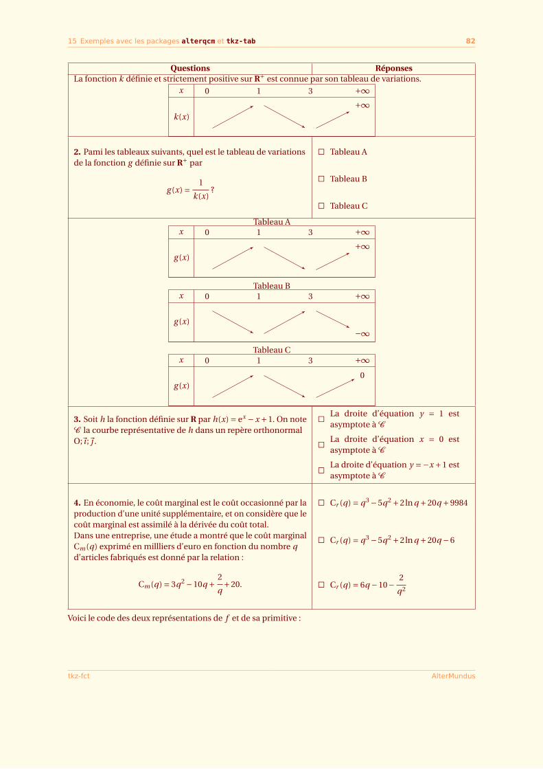
15 Exemples avec les packages alterqcm et tkz-tab 82
Questions RéponsesLa fonction k définie et strictement positive sur R+ est connue par son tableau de variations.
x
k(x)
0 1 3 +∞+∞+∞
2. Pami les tableaux suivants, quel est le tableau de variationsde la fonction g définie sur R+ par
g (x) = 1
k(x)?
ä Tableau A
ä Tableau B
ä Tableau C
Tableau Ax
g (x)
0 1 3 +∞+∞+∞
Tableau Bx
g (x)
0 1 3 +∞
−∞−∞Tableau C
x
g (x)
0 1 3 +∞00
3. Soit h la fonction définie sur R par h(x) = ex −x +1. On noteC la courbe représentative de h dans un repère orthonormalO;~ı ;~ .
ä La droite d’équation y = 1 estasymptote à C
ä La droite d’équation x = 0 estasymptote à C
ä La droite d’équation y =−x +1 estasymptote à C
4. En économie, le coût marginal est le coût occasionné par laproduction d’une unité supplémentaire, et on considère que lecoût marginal est assimilé à la dérivée du coût total.Dans une entreprise, une étude a montré que le coût marginalCm(q) exprimé en millliers d’euro en fonction du nombre qd’articles fabriqués est donné par la relation :
Cm(q) = 3q2 −10q + 2
q+20.
ä Cr (q) = q3 −5q2 +2ln q +20q +9984
ä Cr (q) = q3 −5q2 +2ln q +20q −6
ä Cr (q) = 6q −10− 2
q2
Voici le code des deux représentations de f et de sa primitive :
tkz-fct AlterMundus
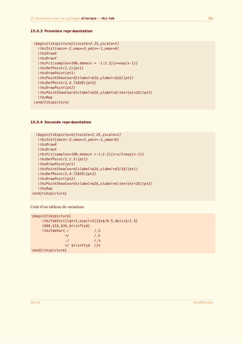
15 Exemples avec les packages alterqcm et tkz-tab 83
15.0.3 Première représentation
\begin{tikzpicture}[xscale=2.25,yscale=1]\tkzInit[xmin=-2,xmax=3,ymin=-1,ymax=6]\tkzDrawX\tkzDrawY\tkzFct[samples=100,domain = -1:2.2]{x+exp(x-1)}\tkzDefPoint(1,2){pt1}\tkzDrawPoint(pt1)\tkzPointShowCoord[xlabel=$1$,ylabel=$2$](pt1)\tkzDefPoint(2,4.71828){pt2}\tkzDrawPoint(pt2)\tkzPointShowCoord[xlabel=$2$,ylabel=$\text{e}+2$](pt2)\tkzRep
\end{tikzpicture}
15.0.4 Seconde représentation
\begin{tikzpicture}[xscale=2.25,yscale=1]\tkzInit[xmin=-2,xmax=3,ymin=-1,ymax=6]\tkzDrawX\tkzDrawY\tkzFct[samples=100,domain =-1:2.2]{x*x/2+exp(x-1)}\tkzDefPoint(1,1.5){pt1}\tkzDrawPoint(pt1)\tkzPointShowCoord[xlabel=$1$,ylabel=$3/2$](pt1)\tkzDefPoint(2,4.71828){pt2}\tkzDrawPoint(pt2)\tkzPointShowCoord[xlabel=$2$,ylabel=$\text{e}+2$](pt2)\tkzRep
\end{tikzpicture}
Code d’un tableau de variations
\begin{tikzpicture}\tkzTabInit[lgt=1,espcl=2]{$x$/0.5,$k(x)$/1.5}{$0$,$1$,$3$,$+\infty$}\tkzTabVar{-/ /,%
+/ /,%-/ /,%+/ $+\infty$ /}%
\end{tikzpicture}
tkz-fct AlterMundus
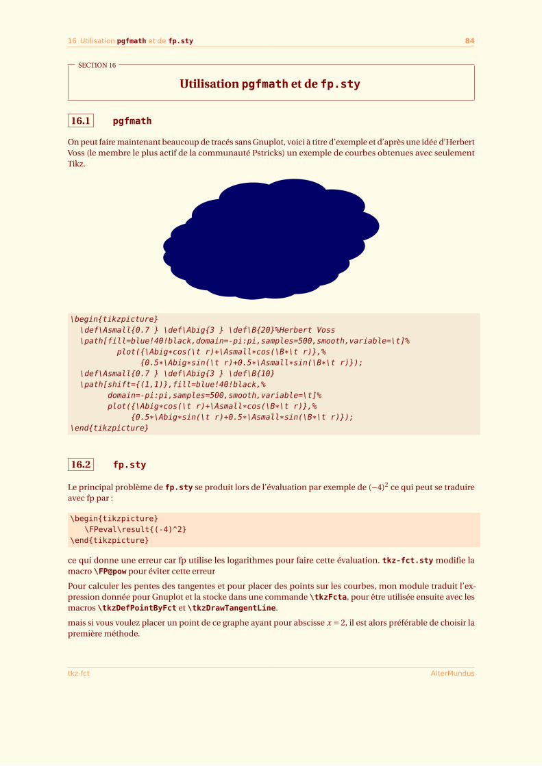
16 Utilisation pgfmath et de fp.sty 84
SECTION 16
Utilisation pgfmath et de fp.sty
16.1 pgfmath
On peut faire maintenant beaucoup de tracés sans Gnuplot, voici à titre d’exemple et d’après une idée d’HerbertVoss (le membre le plus actif de la communauté Pstricks) un exemple de courbes obtenues avec seulementTikz.
\begin{tikzpicture}\def\Asmall{0.7 } \def\Abig{3 } \def\B{20}%Herbert Voss\path[fill=blue!40!black,domain=-pi:pi,samples=500,smooth,variable=\t]%
plot({\Abig*cos(\t r)+\Asmall*cos(\B*\t r)},%{0.5*\Abig*sin(\t r)+0.5*\Asmall*sin(\B*\t r)});
\def\Asmall{0.7 } \def\Abig{3 } \def\B{10}\path[shift={(1,1)},fill=blue!40!black,%
domain=-pi:pi,samples=500,smooth,variable=\t]%plot({\Abig*cos(\t r)+\Asmall*cos(\B*\t r)},%
{0.5*\Abig*sin(\t r)+0.5*\Asmall*sin(\B*\t r)});\end{tikzpicture}
16.2 fp.sty
Le principal problème de fp.sty se produit lors de l’évaluation par exemple de (−4)2 ce qui peut se traduireavec fp par :
\begin{tikzpicture}\FPeval\result{(-4)^2}
\end{tikzpicture}
ce qui donne une erreur car fp utilise les logarithmes pour faire cette évaluation. tkz-fct.sty modifie lamacro \FP@pow pour éviter cette erreur
Pour calculer les pentes des tangentes et pour placer des points sur les courbes, mon module traduit l’ex-pression donnée pour Gnuplot et la stocke dans une commande \tkzFcta, pour être utilisée ensuite avec lesmacros \tkzDefPointByFct et \tkzDrawTangentLine.
mais si vous voulez placer un point de ce graphe ayant pour abscisse x = 2, il est alors préférable de choisir lapremière méthode.
tkz-fct AlterMundus
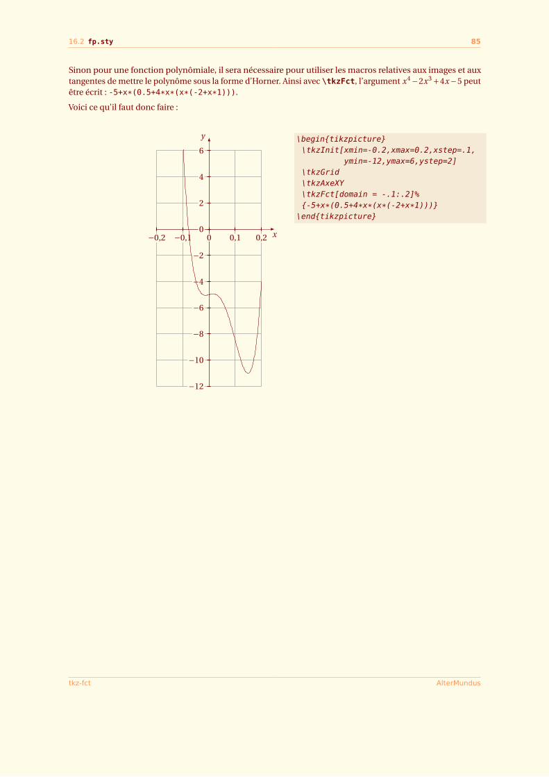
16.2 fp.sty 85
Sinon pour une fonction polynômiale, il sera nécessaire pour utiliser les macros relatives aux images et auxtangentes de mettre le polynôme sous la forme d’Horner. Ainsi avec \tkzFct, l’argument x4−2x3+4x−5 peutêtre écrit : -5+x*(0.5+4*x*(x*(-2+x*1))).
Voici ce qu’il faut donc faire :
x
y
−0,2 −0,1 0 0,1 0,2
−12
−10
−8
−6
−4
−2
0
2
4
6\begin{tikzpicture}\tkzInit[xmin=-0.2,xmax=0.2,xstep=.1,
ymin=-12,ymax=6,ystep=2]\tkzGrid\tkzAxeXY\tkzFct[domain = -.1:.2]%{-5+x*(0.5+4*x*(x*(-2+x*1)))}
\end{tikzpicture}
tkz-fct AlterMundus
17 Quelques remarques 86
SECTION 17
Quelques remarques
1. Modification avec les anciennes versions :– \tkzTan est devenu \tkzDrawTangentLine– Désormais le domaine est donné comme avec TikZ et ce n’est plus (⟨xa ..xb⟩)– \tkzFctPt est devenu \tkzDefPointByFct
2. Quand xstep est différent de 1, la variable doit être \x.
3. Quand une fonction est passée en argument à la macro \tkzFct, elle est stockée avec la syntaxe degnuplot dans la macro \tkzFctgnua. tkzFctgnu est un préfixe, « a » est la référence associée à lafonction, la fonction suivante dans le même environnement tikzpicture sera référencée « b » et ainside suite...
Elle est aussi stockée avec la syntaxe de fp.sty dans la macro \tkzFcta avec le préfixe tkzFcta.
La dernière macro utilisée est également sauvegardée sous les deux syntaxes avec \tkzFctgnuLast et\tkzFctLast.
4. Attention dans gnuplot un quotient doit être entré sous la forme 1./3, car 1/3 donne le quotient d’unedivision euclidienne (ici 0).
5. Problème avec gnuplot :– Si le fichier xxx.table n’est pas créé, la cause probable est :
– soit que TEX ne trouve pas gnuplot, c’est en général un problème de « PATH »,– soit TEX n’autorise pas le lancement de gnuplot alors c’est que l’option shell-escape n’est pas
autorisé.Une autre possibilité est que le fichier xxx.gnuplot soit incorrect. Il suffit de l’ouvrir avec un éditeurpour lire les commandes passées à gnuplot. Il est à remarquer un changement de syntaxe de gnuplotautour de la version 4.2. La syntaxe pour créer une table avec des versions ultérieures (4.4 et bientôt4.5), est désormais set table.
– π est, avec gnuplot, défini par pi– π est, avec fp.sty défini par \FPpi.– (set) samples =2 est suffisant pour tracer une droite.
6. La puissance ab est notée a ∧b avec fp et pgfmath mais a ∗∗b avec gnuplot.
7. tkz-fct modife FP@pow (code modifié de Christian Tellechea 2009) afin d’autoriser les puissancesentières de nombres négatifs.
8. (1/exp(1)) est correct mais (1/exp(1)) donne une erreur
tkz-fct AlterMundus
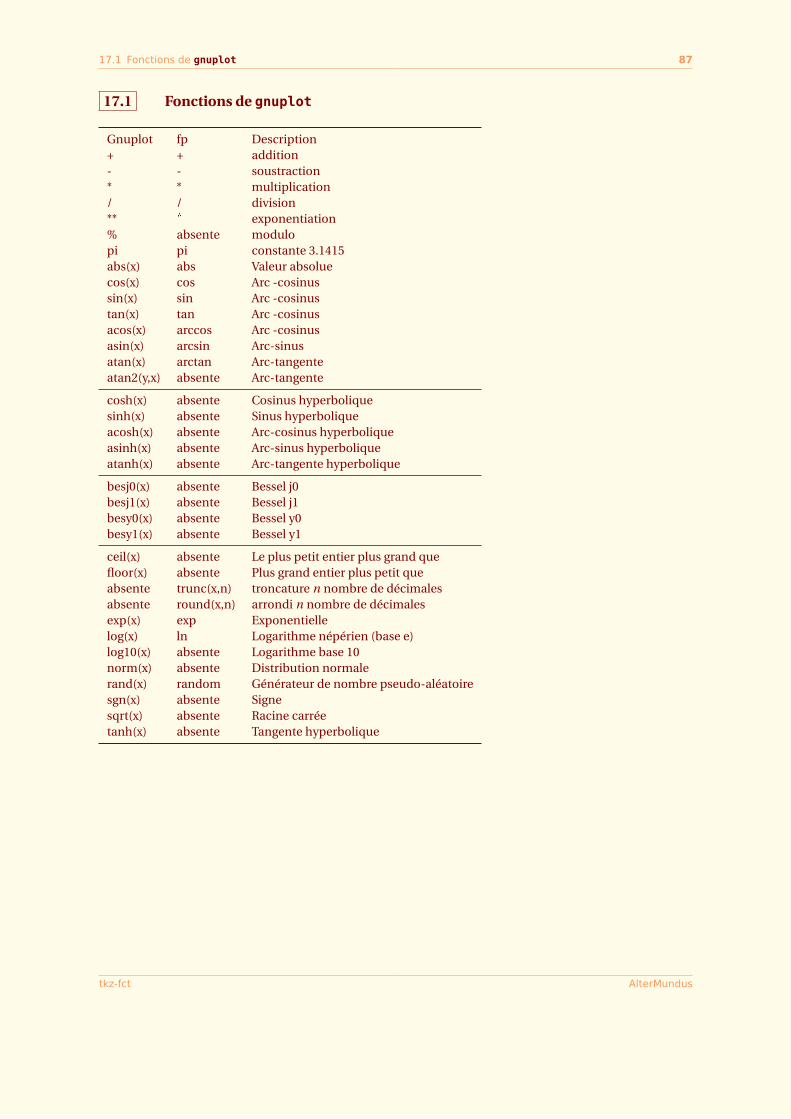
17.1 Fonctions de gnuplot 87
17.1 Fonctions de gnuplot
Gnuplot fp Description+ + addition- - soustraction* * multiplication/ / division** t exponentiation% absente modulopi pi constante 3.1415abs(x) abs Valeur absoluecos(x) cos Arc -cosinussin(x) sin Arc -cosinustan(x) tan Arc -cosinusacos(x) arccos Arc -cosinusasin(x) arcsin Arc-sinusatan(x) arctan Arc-tangenteatan2(y,x) absente Arc-tangente
cosh(x) absente Cosinus hyperboliquesinh(x) absente Sinus hyperboliqueacosh(x) absente Arc-cosinus hyperboliqueasinh(x) absente Arc-sinus hyperboliqueatanh(x) absente Arc-tangente hyperbolique
besj0(x) absente Bessel j0besj1(x) absente Bessel j1besy0(x) absente Bessel y0besy1(x) absente Bessel y1
ceil(x) absente Le plus petit entier plus grand quefloor(x) absente Plus grand entier plus petit queabsente trunc(x,n) troncature n nombre de décimalesabsente round(x,n) arrondi n nombre de décimalesexp(x) exp Exponentiellelog(x) ln Logarithme népérien (base e)log10(x) absente Logarithme base 10norm(x) absente Distribution normalerand(x) random Générateur de nombre pseudo-aléatoiresgn(x) absente Signesqrt(x) absente Racine carréetanh(x) absente Tangente hyperbolique
tkz-fct AlterMundus
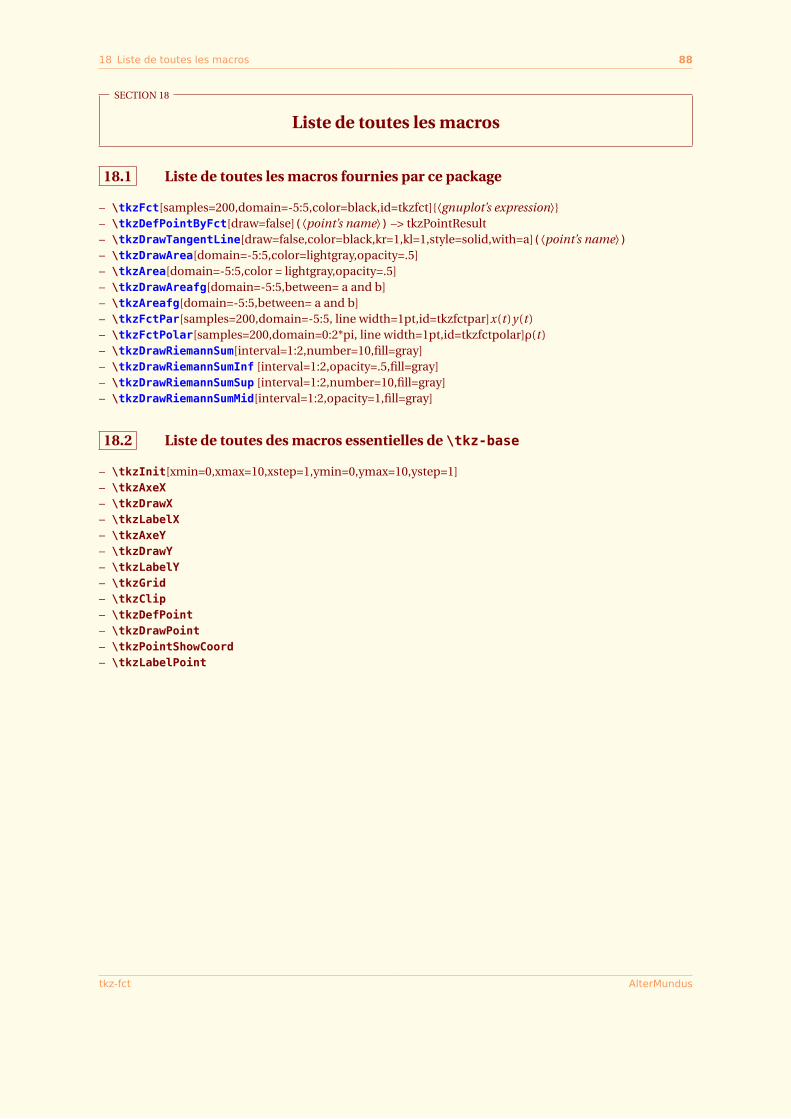
18 Liste de toutes les macros 88
SECTION 18
Liste de toutes les macros
18.1 Liste de toutes les macros fournies par ce package
– \tkzFct[samples=200,domain=-5:5,color=black,id=tkzfct]{⟨gnuplot’s expression⟩}– \tkzDefPointByFct[draw=false](⟨point’s name⟩) –> tkzPointResult– \tkzDrawTangentLine[draw=false,color=black,kr=1,kl=1,style=solid,with=a](⟨point’s name⟩)– \tkzDrawArea[domain=-5:5,color=lightgray,opacity=.5]– \tkzArea[domain=-5:5,color = lightgray,opacity=.5]– \tkzDrawAreafg[domain=-5:5,between= a and b]– \tkzAreafg[domain=-5:5,between= a and b]– \tkzFctPar[samples=200,domain=-5:5, line width=1pt,id=tkzfctpar]x(t )y(t )– \tkzFctPolar[samples=200,domain=0:2*pi, line width=1pt,id=tkzfctpolar]ρ(t )– \tkzDrawRiemannSum[interval=1:2,number=10,fill=gray]– \tkzDrawRiemannSumInf [interval=1:2,opacity=.5,fill=gray]– \tkzDrawRiemannSumSup [interval=1:2,number=10,fill=gray]– \tkzDrawRiemannSumMid[interval=1:2,opacity=1,fill=gray]
18.2 Liste de toutes des macros essentielles de \tkz-base
– \tkzInit[xmin=0,xmax=10,xstep=1,ymin=0,ymax=10,ystep=1]– \tkzAxeX– \tkzDrawX– \tkzLabelX– \tkzAxeY– \tkzDrawY– \tkzLabelY– \tkzGrid– \tkzClip– \tkzDefPoint– \tkzDrawPoint– \tkzPointShowCoord– \tkzLabelPoint
tkz-fct AlterMundus
Index
D\draw plot function . . . . . . . . . . . . . . . . . . . . . . . . . . . . . . . . . . . . . . . . . . . . . . . . . . . . . . . . . . . . . . . . . . . . . . . . . . . . . . . . . . . . . . . . . 6\draw plot[id=fct] function---.; . . . . . . . . . . . . . . . . . . . . . . . . . . . . . . . . . . . . . . . . . . . . . . . . . . . . . . . . . . . . . . . . . . . . . . .10
F\FPpi . . . . . . . . . . . . . . . . . . . . . . . . . . . . . . . . . . . . . . . . . . . . . . . . . . . . . . . . . . . . . . . . . . . . . . . . . . . . . . . . . . . . . . . . . . . . . . . . . . . . . . .60, 86
J\jobname . . . . . . . . . . . . . . . . . . . . . . . . . . . . . . . . . . . . . . . . . . . . . . . . . . . . . . . . . . . . . . . . . . . . . . . . . . . . . . . . . . . . . . . . . . . . . . . . . . . . . . 11
OOperating System
Linux Ubuntu . . . . . . . . . . . . . . . . . . . . . . . . . . . . . . . . . . . . . . . . . . . . . . . . . . . . . . . . . . . . . . . . . . . . . . . . . . . . . . . . . . . . . . . . . . . . 12OS X . . . . . . . . . . . . . . . . . . . . . . . . . . . . . . . . . . . . . . . . . . . . . . . . . . . . . . . . . . . . . . . . . . . . . . . . . . . . . . . . . . . . . . . . . . . . . . . . . . . . . . 12Windows XP . . . . . . . . . . . . . . . . . . . . . . . . . . . . . . . . . . . . . . . . . . . . . . . . . . . . . . . . . . . . . . . . . . . . . . . . . . . . . . . . . . . . . . . . . . . . 8, 12
T\t**2 . . . . . . . . . . . . . . . . . . . . . . . . . . . . . . . . . . . . . . . . . . . . . . . . . . . . . . . . . . . . . . . . . . . . . . . . . . . . . . . . . . . . . . . . . . . . . . . . . . . . . . .53, 60\t**3 . . . . . . . . . . . . . . . . . . . . . . . . . . . . . . . . . . . . . . . . . . . . . . . . . . . . . . . . . . . . . . . . . . . . . . . . . . . . . . . . . . . . . . . . . . . . . . . . . . . . . . .53, 60TeX Distributions
MikTeX . . . . . . . . . . . . . . . . . . . . . . . . . . . . . . . . . . . . . . . . . . . . . . . . . . . . . . . . . . . . . . . . . . . . . . . . . . . . . . . . . . . . . . . . . . . . . . . . . . . . . 8TeXLive . . . . . . . . . . . . . . . . . . . . . . . . . . . . . . . . . . . . . . . . . . . . . . . . . . . . . . . . . . . . . . . . . . . . . . . . . . . . . . . . . . . . . . . . . . . . . . . . . . . .7
TikZ . . . . . . . . . . . . . . . . . . . . . . . . . . . . . . . . . . . . . . . . . . . . . . . . . . . . . . . . . . . . . . . . . . . . . . . . . . . . . . . . . . . . . . . . . . . . . . . . . . . . . . . . . . . . . 8\tikzset{tan style/.style={->,>=latex}} . . . . . . . . . . . . . . . . . . . . . . . . . . . . . . . . . . . . . . . . . . . . . . . . . . . . . . . . . . . . . 28\tikzset{tan style/.style={-}} . . . . . . . . . . . . . . . . . . . . . . . . . . . . . . . . . . . . . . . . . . . . . . . . . . . . . . . . . . . . . . . . . . . . . . . . . 28\tkz-base . . . . . . . . . . . . . . . . . . . . . . . . . . . . . . . . . . . . . . . . . . . . . . . . . . . . . . . . . . . . . . . . . . . . . . . . . . . . . . . . . . . . . . . . . . . . . . . . . . . . . 88\tkzArea . . . . . . . . . . . . . . . . . . . . . . . . . . . . . . . . . . . . . . . . . . . . . . . . . . . . . . . . . . . . . . . . . . . . . . . . . . . . . . . . . . . . . . . . . . . . . . . . . . . . . . 36\tkzAxeX . . . . . . . . . . . . . . . . . . . . . . . . . . . . . . . . . . . . . . . . . . . . . . . . . . . . . . . . . . . . . . . . . . . . . . . . . . . . . . . . . . . . . . . . . . . . . . . . . . . . . . 88\tkzAxeY . . . . . . . . . . . . . . . . . . . . . . . . . . . . . . . . . . . . . . . . . . . . . . . . . . . . . . . . . . . . . . . . . . . . . . . . . . . . . . . . . . . . . . . . . . . . . . . . . . . . . . 88\tkzClip . . . . . . . . . . . . . . . . . . . . . . . . . . . . . . . . . . . . . . . . . . . . . . . . . . . . . . . . . . . . . . . . . . . . . . . . . . . . . . . . . . . . . . . . . . . . . . . . . . . . . . 88\tkzDefPoint . . . . . . . . . . . . . . . . . . . . . . . . . . . . . . . . . . . . . . . . . . . . . . . . . . . . . . . . . . . . . . . . . . . . . . . . . . . . . . . . . . . . . . . . . . . . . . . . . 88\tkzDefPointByFct(0) . . . . . . . . . . . . . . . . . . . . . . . . . . . . . . . . . . . . . . . . . . . . . . . . . . . . . . . . . . . . . . . . . . . . . . . . . . . . . . . . . . . . . . 20\tkzDefPointByFct . . . . . . . . . . . . . . . . . . . . . . . . . . . . . . . . . . . . . . . . . . . . . . . . . . . . . . . . . . . . . . . . . . . . . . . . . . . . . . . . . . . 20, 84, 86\tkzDefPointByFct: arguments
decimal number . . . . . . . . . . . . . . . . . . . . . . . . . . . . . . . . . . . . . . . . . . . . . . . . . . . . . . . . . . . . . . . . . . . . . . . . . . . . . . . . . . . . . . . . . 20\tkzDefPointByFct: options
draw . . . . . . . . . . . . . . . . . . . . . . . . . . . . . . . . . . . . . . . . . . . . . . . . . . . . . . . . . . . . . . . . . . . . . . . . . . . . . . . . . . . . . . . . . . . . . . . . . . . . . . 20ref . . . . . . . . . . . . . . . . . . . . . . . . . . . . . . . . . . . . . . . . . . . . . . . . . . . . . . . . . . . . . . . . . . . . . . . . . . . . . . . . . . . . . . . . . . . . . . . . . . . . . . . .20with . . . . . . . . . . . . . . . . . . . . . . . . . . . . . . . . . . . . . . . . . . . . . . . . . . . . . . . . . . . . . . . . . . . . . . . . . . . . . . . . . . . . . . . . . . . . . . . . . . . . . . 20
\tkzDefPointByFct(⟨deci mal number ⟩) . . . . . . . . . . . . . . . . . . . . . . . . . . . . . . . . . . . . . . . . . . . . . . . . . . . . . . . . . . . . . . . . . . 20\tkzDrawArea . . . . . . . . . . . . . . . . . . . . . . . . . . . . . . . . . . . . . . . . . . . . . . . . . . . . . . . . . . . . . . . . . . . . . . . . . . . . . . . . . . . . . . . . . . . . . . . . . 36\tkzDrawArea: options
color . . . . . . . . . . . . . . . . . . . . . . . . . . . . . . . . . . . . . . . . . . . . . . . . . . . . . . . . . . . . . . . . . . . . . . . . . . . . . . . . . . . . . . . . . . . . . . . . . . . . . 36domain . . . . . . . . . . . . . . . . . . . . . . . . . . . . . . . . . . . . . . . . . . . . . . . . . . . . . . . . . . . . . . . . . . . . . . . . . . . . . . . . . . . . . . . . . . . . . . . . . . . .36opacity . . . . . . . . . . . . . . . . . . . . . . . . . . . . . . . . . . . . . . . . . . . . . . . . . . . . . . . . . . . . . . . . . . . . . . . . . . . . . . . . . . . . . . . . . . . . . . . . . . 36style . . . . . . . . . . . . . . . . . . . . . . . . . . . . . . . . . . . . . . . . . . . . . . . . . . . . . . . . . . . . . . . . . . . . . . . . . . . . . . . . . . . . . . . . . . . . . . . . . . . . . 36with . . . . . . . . . . . . . . . . . . . . . . . . . . . . . . . . . . . . . . . . . . . . . . . . . . . . . . . . . . . . . . . . . . . . . . . . . . . . . . . . . . . . . . . . . . . . . . . . . . . . . . 36
\tkzDrawAreafg . . . . . . . . . . . . . . . . . . . . . . . . . . . . . . . . . . . . . . . . . . . . . . . . . . . . . . . . . . . . . . . . . . . . . . . . . . . . . . . . . . . . . . . . . . . . . . 39\tkzDrawAreafg: options
between . . . . . . . . . . . . . . . . . . . . . . . . . . . . . . . . . . . . . . . . . . . . . . . . . . . . . . . . . . . . . . . . . . . . . . . . . . . . . . . . . . . . . . . . . . . . . . . . . . 39
Index 90
domain= min:max . . . . . . . . . . . . . . . . . . . . . . . . . . . . . . . . . . . . . . . . . . . . . . . . . . . . . . . . . . . . . . . . . . . . . . . . . . . . . . . . . . . . . . . . 39opacity . . . . . . . . . . . . . . . . . . . . . . . . . . . . . . . . . . . . . . . . . . . . . . . . . . . . . . . . . . . . . . . . . . . . . . . . . . . . . . . . . . . . . . . . . . . . . . . . . . 39
\tkzDrawAreafg[⟨local options⟩] . . . . . . . . . . . . . . . . . . . . . . . . . . . . . . . . . . . . . . . . . . . . . . . . . . . . . . . . . . . . . . . . . . . . . . . . . 39\tkzDrawArea[⟨local options⟩] . . . . . . . . . . . . . . . . . . . . . . . . . . . . . . . . . . . . . . . . . . . . . . . . . . . . . . . . . . . . . . . . . . . . . . . . . . . 36\tkzDrawPoint . . . . . . . . . . . . . . . . . . . . . . . . . . . . . . . . . . . . . . . . . . . . . . . . . . . . . . . . . . . . . . . . . . . . . . . . . . . . . . . . . . . . . . . . . . . . 20, 88\tkzDrawRiemannSum . . . . . . . . . . . . . . . . . . . . . . . . . . . . . . . . . . . . . . . . . . . . . . . . . . . . . . . . . . . . . . . . . . . . . . . . . . . . . . . . . . . . . . . . . 44\tkzDrawRiemannSum: options
iterval . . . . . . . . . . . . . . . . . . . . . . . . . . . . . . . . . . . . . . . . . . . . . . . . . . . . . . . . . . . . . . . . . . . . . . . . . . . . . . . . . . . . . . . . . . . . . . . . . . 44number . . . . . . . . . . . . . . . . . . . . . . . . . . . . . . . . . . . . . . . . . . . . . . . . . . . . . . . . . . . . . . . . . . . . . . . . . . . . . . . . . . . . . . . . . . . . . . . . . . . . 44
\tkzDrawRiemannSumInf . . . . . . . . . . . . . . . . . . . . . . . . . . . . . . . . . . . . . . . . . . . . . . . . . . . . . . . . . . . . . . . . . . . . . . . . . . . . . . . . . . . . . 45\tkzDrawRiemannSumInf[⟨local options⟩] . . . . . . . . . . . . . . . . . . . . . . . . . . . . . . . . . . . . . . . . . . . . . . . . . . . . . . . . . . . . . . . 45\tkzDrawRiemannSumMid . . . . . . . . . . . . . . . . . . . . . . . . . . . . . . . . . . . . . . . . . . . . . . . . . . . . . . . . . . . . . . . . . . . . . . . . . . . . . . . . . . . . . 47\tkzDrawRiemannSumMid[⟨local options⟩] . . . . . . . . . . . . . . . . . . . . . . . . . . . . . . . . . . . . . . . . . . . . . . . . . . . . . . . . . . . . . . . 47\tkzDrawRiemannSumSup . . . . . . . . . . . . . . . . . . . . . . . . . . . . . . . . . . . . . . . . . . . . . . . . . . . . . . . . . . . . . . . . . . . . . . . . . . . . . . . . . . . . . 46\tkzDrawRiemannSumSup[⟨local options⟩] . . . . . . . . . . . . . . . . . . . . . . . . . . . . . . . . . . . . . . . . . . . . . . . . . . . . . . . . . . . . . . . 46\tkzDrawRiemannSum[⟨local options⟩]{⟨ f (t )⟩} . . . . . . . . . . . . . . . . . . . . . . . . . . . . . . . . . . . . . . . . . . . . . . . . . . . . . . . . . . .44\tkzDrawTangentLine(0) . . . . . . . . . . . . . . . . . . . . . . . . . . . . . . . . . . . . . . . . . . . . . . . . . . . . . . . . . . . . . . . . . . . . . . . . . . . . . . . . . . . . 27\tkzDrawTangentLine . . . . . . . . . . . . . . . . . . . . . . . . . . . . . . . . . . . . . . . . . . . . . . . . . . . . . . . . . . . . . . . . . . . . . . . . . . . . . 27, 29, 84, 86\tkzDrawTangentLine: arguments
a . . . . . . . . . . . . . . . . . . . . . . . . . . . . . . . . . . . . . . . . . . . . . . . . . . . . . . . . . . . . . . . . . . . . . . . . . . . . . . . . . . . . . . . . . . . . . . . . . . . . . . . . . . 27\tkzDrawTangentLine: options
draw . . . . . . . . . . . . . . . . . . . . . . . . . . . . . . . . . . . . . . . . . . . . . . . . . . . . . . . . . . . . . . . . . . . . . . . . . . . . . . . . . . . . . . . . . . . . . . . . . . . . . . 27kl . . . . . . . . . . . . . . . . . . . . . . . . . . . . . . . . . . . . . . . . . . . . . . . . . . . . . . . . . . . . . . . . . . . . . . . . . . . . . . . . . . . . . . . . . . . . . . . . . . . . . . . . . 27kr . . . . . . . . . . . . . . . . . . . . . . . . . . . . . . . . . . . . . . . . . . . . . . . . . . . . . . . . . . . . . . . . . . . . . . . . . . . . . . . . . . . . . . . . . . . . . . . . . . . . . . . . . 27with . . . . . . . . . . . . . . . . . . . . . . . . . . . . . . . . . . . . . . . . . . . . . . . . . . . . . . . . . . . . . . . . . . . . . . . . . . . . . . . . . . . . . . . . . . . . . . . . . . . . . . 27
\tkzDrawTangentLine[⟨local options⟩](⟨a⟩) . . . . . . . . . . . . . . . . . . . . . . . . . . . . . . . . . . . . . . . . . . . . . . . . . . . . . . . . . . . . 27\tkzDrawX . . . . . . . . . . . . . . . . . . . . . . . . . . . . . . . . . . . . . . . . . . . . . . . . . . . . . . . . . . . . . . . . . . . . . . . . . . . . . . . . . . . . . . . . . . . . . . . . . . . . . 88\tkzDrawY . . . . . . . . . . . . . . . . . . . . . . . . . . . . . . . . . . . . . . . . . . . . . . . . . . . . . . . . . . . . . . . . . . . . . . . . . . . . . . . . . . . . . . . . . . . . . . . . . . . . . 88\tkzFct . . . . . . . . . . . . . . . . . . . . . . . . . . . . . . . . . . . . . . . . . . . . . . . . . . . . . . . . . . . . . . . . . . . . . . . . . . . . . . . . . . . . . . . . . . 6, 15, 27, 85, 86\tkzFct: arguments
gnuplot expression . . . . . . . . . . . . . . . . . . . . . . . . . . . . . . . . . . . . . . . . . . . . . . . . . . . . . . . . . . . . . . . . . . . . . . . . . . . . . . . . . . . . 15\tkzFct: options
color . . . . . . . . . . . . . . . . . . . . . . . . . . . . . . . . . . . . . . . . . . . . . . . . . . . . . . . . . . . . . . . . . . . . . . . . . . . . . . . . . . . . . . . . . . . . . . . . . . . . . 15domain . . . . . . . . . . . . . . . . . . . . . . . . . . . . . . . . . . . . . . . . . . . . . . . . . . . . . . . . . . . . . . . . . . . . . . . . . . . . . . . . . . . . . . . . . . . . . . . . . . . .15id . . . . . . . . . . . . . . . . . . . . . . . . . . . . . . . . . . . . . . . . . . . . . . . . . . . . . . . . . . . . . . . . . . . . . . . . . . . . . . . . . . . . . . . . . . . . . . . . . . . . . . . . . 15line width . . . . . . . . . . . . . . . . . . . . . . . . . . . . . . . . . . . . . . . . . . . . . . . . . . . . . . . . . . . . . . . . . . . . . . . . . . . . . . . . . . . . . . . . . . . . . . 15samples . . . . . . . . . . . . . . . . . . . . . . . . . . . . . . . . . . . . . . . . . . . . . . . . . . . . . . . . . . . . . . . . . . . . . . . . . . . . . . . . . . . . . . . . . . . . . . . . . . 15style . . . . . . . . . . . . . . . . . . . . . . . . . . . . . . . . . . . . . . . . . . . . . . . . . . . . . . . . . . . . . . . . . . . . . . . . . . . . . . . . . . . . . . . . . . . . . . . . . . . . . 15
\tkzFcta . . . . . . . . . . . . . . . . . . . . . . . . . . . . . . . . . . . . . . . . . . . . . . . . . . . . . . . . . . . . . . . . . . . . . . . . . . . . . . . . . . . . . . . . . . . . . . . 27, 84, 86\tkzFctb . . . . . . . . . . . . . . . . . . . . . . . . . . . . . . . . . . . . . . . . . . . . . . . . . . . . . . . . . . . . . . . . . . . . . . . . . . . . . . . . . . . . . . . . . . . . . . . . . . . . . . 27\tkzFctgnua . . . . . . . . . . . . . . . . . . . . . . . . . . . . . . . . . . . . . . . . . . . . . . . . . . . . . . . . . . . . . . . . . . . . . . . . . . . . . . . . . . . . . . . . . . . . . . . . . . 86\tkzFctgnuLast . . . . . . . . . . . . . . . . . . . . . . . . . . . . . . . . . . . . . . . . . . . . . . . . . . . . . . . . . . . . . . . . . . . . . . . . . . . . . . . . . . . . . . . . . . . . . . 86\tkzFctLast . . . . . . . . . . . . . . . . . . . . . . . . . . . . . . . . . . . . . . . . . . . . . . . . . . . . . . . . . . . . . . . . . . . . . . . . . . . . . . . . . . . . . . . . . . . 22, 34, 86\tkzFctPar[0:1] . . . . . . . . . . . . . . . . . . . . . . . . . . . . . . . . . . . . . . . . . . . . . . . . . . . . . . . . . . . . . . . . . . . . . . . . . . . . . . . . . . . . . . . . . 53, 60\tkzFctPar . . . . . . . . . . . . . . . . . . . . . . . . . . . . . . . . . . . . . . . . . . . . . . . . . . . . . . . . . . . . . . . . . . . . . . . . . . . . . . . . . . . . . . . . . . . . . . . . . . . .53\tkzFctPar: arguments
x(t ),y(t ) . . . . . . . . . . . . . . . . . . . . . . . . . . . . . . . . . . . . . . . . . . . . . . . . . . . . . . . . . . . . . . . . . . . . . . . . . . . . . . . . . . . . . . . . . . . . . . . . . . 53\tkzFctPar: options
color . . . . . . . . . . . . . . . . . . . . . . . . . . . . . . . . . . . . . . . . . . . . . . . . . . . . . . . . . . . . . . . . . . . . . . . . . . . . . . . . . . . . . . . . . . . . . . . . . . . . . 53domain . . . . . . . . . . . . . . . . . . . . . . . . . . . . . . . . . . . . . . . . . . . . . . . . . . . . . . . . . . . . . . . . . . . . . . . . . . . . . . . . . . . . . . . . . . . . . . . . . . . .53id . . . . . . . . . . . . . . . . . . . . . . . . . . . . . . . . . . . . . . . . . . . . . . . . . . . . . . . . . . . . . . . . . . . . . . . . . . . . . . . . . . . . . . . . . . . . . . . . . . . . . . . . . 53line width . . . . . . . . . . . . . . . . . . . . . . . . . . . . . . . . . . . . . . . . . . . . . . . . . . . . . . . . . . . . . . . . . . . . . . . . . . . . . . . . . . . . . . . . . . . . . . 53samples . . . . . . . . . . . . . . . . . . . . . . . . . . . . . . . . . . . . . . . . . . . . . . . . . . . . . . . . . . . . . . . . . . . . . . . . . . . . . . . . . . . . . . . . . . . . . . . . . . 53
tkz-fct AlterMundus
Index 91
style . . . . . . . . . . . . . . . . . . . . . . . . . . . . . . . . . . . . . . . . . . . . . . . . . . . . . . . . . . . . . . . . . . . . . . . . . . . . . . . . . . . . . . . . . . . . . . . . . . . . . 53\tkzFctPar[⟨local options⟩]{⟨x(t )⟩}{⟨y(t )⟩} . . . . . . . . . . . . . . . . . . . . . . . . . . . . . . . . . . . . . . . . . . . . . . . . . . . . . . . . . . . . .53\tkzFctPolar . . . . . . . . . . . . . . . . . . . . . . . . . . . . . . . . . . . . . . . . . . . . . . . . . . . . . . . . . . . . . . . . . . . . . . . . . . . . . . . . . . . . . . . . . . . . . . . . . 60\tkzFctPolar: arguments
x(t ),y(t ) . . . . . . . . . . . . . . . . . . . . . . . . . . . . . . . . . . . . . . . . . . . . . . . . . . . . . . . . . . . . . . . . . . . . . . . . . . . . . . . . . . . . . . . . . . . . . . . . . . 60\tkzFctPolar: options
color . . . . . . . . . . . . . . . . . . . . . . . . . . . . . . . . . . . . . . . . . . . . . . . . . . . . . . . . . . . . . . . . . . . . . . . . . . . . . . . . . . . . . . . . . . . . . . . . . . . . . 60domain . . . . . . . . . . . . . . . . . . . . . . . . . . . . . . . . . . . . . . . . . . . . . . . . . . . . . . . . . . . . . . . . . . . . . . . . . . . . . . . . . . . . . . . . . . . . . . . . . . . .60id . . . . . . . . . . . . . . . . . . . . . . . . . . . . . . . . . . . . . . . . . . . . . . . . . . . . . . . . . . . . . . . . . . . . . . . . . . . . . . . . . . . . . . . . . . . . . . . . . . . . . . . . . 60line width . . . . . . . . . . . . . . . . . . . . . . . . . . . . . . . . . . . . . . . . . . . . . . . . . . . . . . . . . . . . . . . . . . . . . . . . . . . . . . . . . . . . . . . . . . . . . . 60samples . . . . . . . . . . . . . . . . . . . . . . . . . . . . . . . . . . . . . . . . . . . . . . . . . . . . . . . . . . . . . . . . . . . . . . . . . . . . . . . . . . . . . . . . . . . . . . . . . . 60style . . . . . . . . . . . . . . . . . . . . . . . . . . . . . . . . . . . . . . . . . . . . . . . . . . . . . . . . . . . . . . . . . . . . . . . . . . . . . . . . . . . . . . . . . . . . . . . . . . . . . 60
\tkzFctPolar[⟨local options⟩]{⟨ f (t )⟩} . . . . . . . . . . . . . . . . . . . . . . . . . . . . . . . . . . . . . . . . . . . . . . . . . . . . . . . . . . . . . . . . . . 60\tkzFctPt . . . . . . . . . . . . . . . . . . . . . . . . . . . . . . . . . . . . . . . . . . . . . . . . . . . . . . . . . . . . . . . . . . . . . . . . . . . . . . . . . . . . . . . . . . . . . . . . . 20, 86\tkzFctk . . . . . . . . . . . . . . . . . . . . . . . . . . . . . . . . . . . . . . . . . . . . . . . . . . . . . . . . . . . . . . . . . . . . . . . . . . . . . . . . . . . . . . . . . . . . . . . . . . . . . . 50\tkzFct[⟨local options⟩]{⟨gnuplot expression⟩} . . . . . . . . . . . . . . . . . . . . . . . . . . . . . . . . . . . . . . . . . . . . . . . . . . . . . .15\tkzGetPoint . . . . . . . . . . . . . . . . . . . . . . . . . . . . . . . . . . . . . . . . . . . . . . . . . . . . . . . . . . . . . . . . . . . . . . . . . . . . . . . . . . . . . . . . . . . . . 20, 21\tkzGrid . . . . . . . . . . . . . . . . . . . . . . . . . . . . . . . . . . . . . . . . . . . . . . . . . . . . . . . . . . . . . . . . . . . . . . . . . . . . . . . . . . . . . . . . . . . . . . . . . . . . . . 88\tkzHLine . . . . . . . . . . . . . . . . . . . . . . . . . . . . . . . . . . . . . . . . . . . . . . . . . . . . . . . . . . . . . . . . . . . . . . . . . . . . . . . . . . . . . . . . . . . . . . . . . . . . . 50\tkzHLine: arguments
decimal number . . . . . . . . . . . . . . . . . . . . . . . . . . . . . . . . . . . . . . . . . . . . . . . . . . . . . . . . . . . . . . . . . . . . . . . . . . . . . . . . . . . . . . . . . 50\tkzHLines{1,4} . . . . . . . . . . . . . . . . . . . . . . . . . . . . . . . . . . . . . . . . . . . . . . . . . . . . . . . . . . . . . . . . . . . . . . . . . . . . . . . . . . . . . . . . . . . . . 51\tkzHLines . . . . . . . . . . . . . . . . . . . . . . . . . . . . . . . . . . . . . . . . . . . . . . . . . . . . . . . . . . . . . . . . . . . . . . . . . . . . . . . . . . . . . . . . . . . . . . . . . . . . 51\tkzHLines: arguments
list of values . . . . . . . . . . . . . . . . . . . . . . . . . . . . . . . . . . . . . . . . . . . . . . . . . . . . . . . . . . . . . . . . . . . . . . . . . . . . . . . . . . . . . . . . . 51\tkzHLines[⟨local options⟩]{⟨list of values⟩} . . . . . . . . . . . . . . . . . . . . . . . . . . . . . . . . . . . . . . . . . . . . . . . . . . . . . . . 51\tkzHLine[⟨local options⟩]{⟨decimal number⟩} . . . . . . . . . . . . . . . . . . . . . . . . . . . . . . . . . . . . . . . . . . . . . . . . . . . . . . . . 50\tkzInit . . . . . . . . . . . . . . . . . . . . . . . . . . . . . . . . . . . . . . . . . . . . . . . . . . . . . . . . . . . . . . . . . . . . . . . . . . . . . . . . . . . . . . . . . . . . 6, 15, 27, 88\tkzLabelPoint . . . . . . . . . . . . . . . . . . . . . . . . . . . . . . . . . . . . . . . . . . . . . . . . . . . . . . . . . . . . . . . . . . . . . . . . . . . . . . . . . . . . . . . . . . . . . . 88\tkzLabelX . . . . . . . . . . . . . . . . . . . . . . . . . . . . . . . . . . . . . . . . . . . . . . . . . . . . . . . . . . . . . . . . . . . . . . . . . . . . . . . . . . . . . . . . . . . . . . . . . . . .88\tkzLabelY . . . . . . . . . . . . . . . . . . . . . . . . . . . . . . . . . . . . . . . . . . . . . . . . . . . . . . . . . . . . . . . . . . . . . . . . . . . . . . . . . . . . . . . . . . . . . . . . . . . .88\tkzPointShowCoord . . . . . . . . . . . . . . . . . . . . . . . . . . . . . . . . . . . . . . . . . . . . . . . . . . . . . . . . . . . . . . . . . . . . . . . . . . . . . . . . . . . . . . . . . 88\tkzSetUpPoint . . . . . . . . . . . . . . . . . . . . . . . . . . . . . . . . . . . . . . . . . . . . . . . . . . . . . . . . . . . . . . . . . . . . . . . . . . . . . . . . . . . . . . . . . . . . . . 24\tkzTan . . . . . . . . . . . . . . . . . . . . . . . . . . . . . . . . . . . . . . . . . . . . . . . . . . . . . . . . . . . . . . . . . . . . . . . . . . . . . . . . . . . . . . . . . . . . . . . . . . . . . . . .86\tkzText . . . . . . . . . . . . . . . . . . . . . . . . . . . . . . . . . . . . . . . . . . . . . . . . . . . . . . . . . . . . . . . . . . . . . . . . . . . . . . . . . . . . . . . . . . . . . . . . . . .24, 25\tkzVLine{1} . . . . . . . . . . . . . . . . . . . . . . . . . . . . . . . . . . . . . . . . . . . . . . . . . . . . . . . . . . . . . . . . . . . . . . . . . . . . . . . . . . . . . . . . . . . . . 48, 50\tkzVLine . . . . . . . . . . . . . . . . . . . . . . . . . . . . . . . . . . . . . . . . . . . . . . . . . . . . . . . . . . . . . . . . . . . . . . . . . . . . . . . . . . . . . . . . . . . . . . . . . . . . . 48\tkzVLine: arguments
decimal number . . . . . . . . . . . . . . . . . . . . . . . . . . . . . . . . . . . . . . . . . . . . . . . . . . . . . . . . . . . . . . . . . . . . . . . . . . . . . . . . . . . . . . . . . 48\tkzVLine: options
color . . . . . . . . . . . . . . . . . . . . . . . . . . . . . . . . . . . . . . . . . . . . . . . . . . . . . . . . . . . . . . . . . . . . . . . . . . . . . . . . . . . . . . . . . . . . . . . . . . . .48line width . . . . . . . . . . . . . . . . . . . . . . . . . . . . . . . . . . . . . . . . . . . . . . . . . . . . . . . . . . . . . . . . . . . . . . . . . . . . . . . . . . . . . . . . . . . . . . 48style . . . . . . . . . . . . . . . . . . . . . . . . . . . . . . . . . . . . . . . . . . . . . . . . . . . . . . . . . . . . . . . . . . . . . . . . . . . . . . . . . . . . . . . . . . . . . . . . . . . .48
\tkzVLines{1,4} . . . . . . . . . . . . . . . . . . . . . . . . . . . . . . . . . . . . . . . . . . . . . . . . . . . . . . . . . . . . . . . . . . . . . . . . . . . . . . . . . . . . . . . . . . . . . 49\tkzVLines . . . . . . . . . . . . . . . . . . . . . . . . . . . . . . . . . . . . . . . . . . . . . . . . . . . . . . . . . . . . . . . . . . . . . . . . . . . . . . . . . . . . . . . . . . . . . . . . . . . .49\tkzVLines: arguments
list of values . . . . . . . . . . . . . . . . . . . . . . . . . . . . . . . . . . . . . . . . . . . . . . . . . . . . . . . . . . . . . . . . . . . . . . . . . . . . . . . . . . . . . . . . . 49\tkzVLines[⟨local options⟩]{⟨list of values⟩} . . . . . . . . . . . . . . . . . . . . . . . . . . . . . . . . . . . . . . . . . . . . . . . . . . . . . . . 49\tkzVLine[⟨local options⟩]{⟨decimal number⟩} . . . . . . . . . . . . . . . . . . . . . . . . . . . . . . . . . . . . . . . . . . . . . . . . . . . . . . . . 48
X\x . . . . . . . . . . . . . . . . . . . . . . . . . . . . . . . . . . . . . . . . . . . . . . . . . . . . . . . . . . . . . . . . . . . . . . . . . . . . . . . . . . . . . . . . . . . . . . . . . . . . . . . . 6, 15, 86
tkz-fct AlterMundus


![20150306 - PRES 4-3 - A IMPRIMER - VF [Lecture seule]...Entrées en contentieux (hors fct) Dont coût du risque* Coût du risque / Encours** Compte de résultat 39 Bpifrance consolidé](https://img.pdfslide.fr/doc/110x75/6021a7f5d4a6c01b8909d79e/20150306-pres-4-3-a-imprimer-vf-lecture-seule-entres-en-contentieux.jpg)