AqbA - univ-lille.fr · 2017-09-25 · V - RESUME ET CONCLUSIONS CHAPITRE III - LES LARGEURÇ EQUIVALEN'JXS DE RAIES EN SPECTROPOLARIMETRE. lfSpecmopoZarimetry of Venus and Jupiter

S C I E N C E S

NO d'ordre 507

50 376 AqbA

T E C H N I Q U E S

L'UNIVERSITE DES SCIENCES

ET TECHNIQUES DE LILLE

pour obtenir le grade de

DOCTEUR ES SCIENCES PHYSIQUES

J.C. B U R I E Z

C O N T R I B U T I O N A L'ETUDE DES ATMOSPHERES NUAGEUSES

PAR I N T E R P R E T A T I O N DE SPECTRES A HAUTE RESOLUTION

A P P L I C A T I O N A V E N U S ET A U X P L A N E TES J O V I E N N E S

Soutenue le 2 8 - 0 1 - 19 8 1 devant Io Commission d'examen

Membres du Jury H.C. Van de BULST President J. LENOBLE M. HEFU.1A.N Examinateurs P. GLORIEUX Y. FOUQUART C. de BERGH Rapporteurs A.L. FYYAT

U . E . R . D E . P H Y S I Q U E F O N D A M E N T A L E

Monsieur Van de HULST, professeur à l'université de Leiden, a bien

voulu me faire l'honneur de présider mon jury. Je lui en suis proCondément

reconnaissant.

Je tiens à remercier Madane LENOBLE, professeur à l'université de

Lille 1, qui dirige le laboratoire d'Optique Atmosphérique dans lequel

ce travail a été effectué. J'adresse également mes remerciements à

Messieurs HE- et GLORIEUX, professeurs à l'université de Lille 1, qui

ont accepté de juger ce travail.

Les articles inclus dans cette thèse témoignent de l'étroite colla-

boration que j'ai eue avec Y. FOUQUART, maitre-assistant à l'université de

Lille 1 qui a dirigé ce travail, C. de BERGH, chargée de recherches à

l'Observatoire de Meudon et A.L. FYblAT, du Jet Propulsion Laboratory. Ils

savent que je leur suis reconnaissant bien sûr d'avoir accepté de juger

mon travail, mais surtout d'en avoir permis la réalisation.

Sans cette collaboration, ce travail n'aurait pu aboutir. Mais il

n'aurait pu être réalisé non plus sans la collaboration des membres du

laboratoire d'optique Atmosphérique. Je ne voudrais pas dresser ici la

liste (trop longue) de ceux qui, à des titres très divers, m'ont aidé dans

mon travail. Qu'ils sachent que tous, chercheurs, ingénieurs, techniciens,

secrétaires, je les remercie vivement.

S O M M A I R E

INTRODUCTION

CHAPITRE I - GENERALISATION DE L'APPROXIMATION DE CURTIS-GODSON AUX ATMOSPHERES DIFFUSANTES INHOMOGENES.

"GénéraZisation of the CURTIS-WDSON approximation

t u inhomogeneous scattering atmospheref'

(J.C. BURIEZ and Y . FOUQUART, J. Quant. Spectros.

Radiat. Transfer 24, 407 (1 980) ) . - - INTRf3DUCTION 1 - DISTRIBUTION DES ABONDANCES PONDEREES D'ABSOR-

BANT DANS UNE ATMOSPHERE NUAGEUSE

II - GENERALISATION DE L'APPROXIMATION DE CURTIS-GODSON III - PRECISION DE L'APPROXIMATION GENERALISEE IV - RESUME ET CONCLUSIONS

CHAPITRE II - INFORNATIONS CONTENUES DANS LES LARGEURS EQUIVALENTES DE RAIES.

- INTRODUCTION 1 - RAIES FORMEES DANS UNE ATNOPHERE CLAIRE HOMOGENE II - RAIES FORMEES DANS UNE ATMOSPHERE NON-HOMOGENE

MAIS IS0THEXM.E

III - RAIES FORMEES DANS UNE ATMOSPHERE QUELCONQUE a) Cas des raies faibles

b) Cas des raies fortes

C ) Illustration

IV - MESURE DES LARGEURS EQUIVALENTES V - RESUME ET CONCLUSIONS

CHAPITRE III - LES LARGEURÇ EQUIVALEN'JXS DE RAIES EN SPECTROPOLARIMETRE.

lfSpecmopoZarimetry of Venus and Jupiter mouds :

Information Content of EquivaZent Widths"

( J . C . BURIEZ, Y . FOUQUART and A. L . FYPAT,

Astron. Astrophys. - 79 , 287 (1979)).

1 - INTRODUCTION

II - LARGEURS EQUIVALENTES EN ATMOSPHERE DIFFUSANTE A - Intensité B - Généralisation à la polarisation

C - Comparaison entre intensité et polarisation III - INFORMATION ATMOSPHERIQUE A PARTIR DES LARGEURS

EQUIVALENTES EN POLARISATIOIJ

A - Altitude du sommet du nuage B - Rapport des échelles de hauteur C - Profil vertical des paramètres du nuage

IV - RESUME ET CONCLUSIONS

CHAPITRE IV - LES PROFILS DE RAIES - INTRODUCTION 1 - POSSIBILITES ET LIMITES

a) Raies isolées

b) Raies non isolées

II - METHODE DE CALCUL a) Toute l'absorption a lieu en atmosphère claire

b) Toute l'absorption a lieu en atmosphère nuageuse

C) L'absorption a lieu en atmosphere claire et en

atmosphère nuageuse

III - APPLICATION AUX SPECTRES DE JUPITER ET SATURNE "Méthane Zine prof i les n e m 1.1 p as a probe of the

Jupiter cZoud structure and C/H ratio"

(J.C. BURIEZ and C . DE BERGH, Astron. Astrophys.

83, 149 (1980)). - "A study of the amosphere of Saturne based on

methane Zine prof i les n e m 2 .2 p"

( J . C. BURIEZ and C . DE BERGH, Astron. Astrophys.,

i n press ( 2 981 1 ) .

CONCLUS ION

% - ANNEXE A : Schéma de calcul de la distribution p(u) et de la %

pression P (introduite au chap. 1).

- ANNEXE B : Schéma de la méthode décrite au chapitre IV 2b 2

(détermination de Pv) .

I N T R O D U C T I O N

A l'époque des sondes spatiales, on peut se demander si l'obser-

vation des planètes à partir du sol terrestre présente encore un intérêt.

En fait, les sondes ne permettent pas de tout mesurer, et encore moins - de tout mesurer directement. Les méthodes d'analyse des données transmises

sont souvent très proches des méthodes d'interprétation des observations au

sol. L'accumulation des informations acquises grâce aux observatoires ter-

restres permet de définir les mesures à effectuer lors des missions spa-

tiales. Réciproquement, les nouveaux résultats ainsi obtenus précisent

les mesures à effectuer depuis la terre. Missions spatiales et observations

au sol sont complémentaires pour l'étude des planètes.

L'état actuel des connaissances implique toutefois une meilleure

précision de la mesure comme de l'analyse. Dans le proche infra-rouge, la

méthode la plus utilisée pour l'interprétation quantitative des spectres

planétaires a été -et reste encore -elle de la courbe de croissance

des largeurs équivalentes de raies. Elle a été développée initialement pour

le modèle de la cou:che réfléchissante (RLM) . L'atmosphère est considérée comme une couche gazeuse purement absorbante au-dessus d'une surface ré-

fléchissante. Cette couche inhomogène en température et en pression peut

être assimilée à une couche isotherme à une pression moitié de celle de

la surface réfléchissante (approximation dite "de CURTIS-GODSON") . L'at- mosphère est alors caractérisée par trois paramètres (température, pression,

abondance de gaz absorbant) que la mesure des largeurs équivalentes de raies

permet de déterminer.

Cette méthode est bien adaptée à l'étude de l'atmosphère de Mars,

elle convient beaucoup moins à l'étude des atmosphères diffusantes de Vénus

ou Jupiter. Un modèle aussi simple que celui de la couche réfléchissante ne

peut plus être retenu pour l'étude d'une atmosphère nuageuse. En 1965, 1

CHAMBERLAIN développe la théorie de la formation des raies dans une atmos-

phère diffusante. La méthode de la courbe de croissance est ainsi étendue

au cas des atmosphères diffusantes homogènes (HSM) ; les largeurs équiva-

lentes de raies sont calculées analytiquement pour la diffusion isotrope 2 3

(BELTON , 1968) puis anisotrope: FOUQUART et LENOBLE (1973) développent leurs calculs à l'aide de la fonction de distribution du chemin optique, définie

5 par VAN DE HULST et IR VINE^ (1962) . FOUQUART (1975) élargit ce concept

pour l'étude des atmosphères diffusantes inhomogènes, en introduisant la

notion de profondeur de pénétration des photons. Cette méthode est cepen-

dant peu précise, et la complexité des modèles inhomogènes conduit à re-

courir à des méthodes d'intégration numérique en fréquence pour le calcul

des largeurs équivalentes de raies (par exemple SATO et al6 (1977)).

Dans ce travail nous développons une méthode d'analyse des spectres

formés dans un milieu diffusant réaliste où pression, température, etc...

varient. Nous appliquons ensuite cette méthode aux spectres de Jupiter et

Saturne aux environs de l , l LI. Dans un premier temps, nous généralisons au

cas des atmosphères nuageuses l'approximation de CURTIS-GODSON. Pour cela,

nous introduisons la distribution de l'abondance de gaz absorbant pondérée

par la pression et la température (chapitre 1). Nous pouvons alors dévelop-

per une expression analytique de la largeur équivalente d'une raie élargie

essentiellement par effet de pression, et étendre la technique de la courbe

de croissance à n'importe quelle atmosphère non-conservative (chapitre II).

Cette généralisation n'est d'ailleurs pas limitée à l'intensité totale

réfléchie par l'atmosphère planétaire mais peut s'appliquer aussi à l'in-

tensité polarisée (chapitre III).

En fait, le principal obstacle à l'étude des largeurs équivalentes

des raies formées en atmosphère nuageuse ne se situe pas tellement au ni-

veau de l'interprétation à l'aide de modèles d'atmosphère plus ou moins

complexes, mais plus directement au niveau de la mesure elle-même. La lar-

geur équivalente d'une raie est d'autant plus difficile à mesurer que l'at-

mosphère est diffusante (chapitre II). Dès 1968, BELTON, HUNTEN et GOODY 7

considèrent la mesure des largeurs équivalentes du gaz carbonique sur

Vénus trop imprécise ("où finit la raie et où est le continuum ?") . Ils abandonnent la méthode usuelle d'interprétation des raies d'absorption et

développent une méthode dans laquelle les raies sont analysées en faisant

coïncider un spectre synthétique avec les observations. Le profil d'une

raie suffisamment résolue est évidemment plus riche en informations que sa

seule largeur équivalente ; par contre, l'analyse d'un spectre est beau-

coup plus rapide au moyen des largeurs équivalentes. C'est pourquoi la

technique du spectre synthétique est peu utilisée. Citons toutefois pour

Vénus les raies de la bande du CO à 1,05 et à 0,78 LI étudiées par 2

8- 9 REGAS et al en tenant compte de l'inhomogénéité verticale de l'atmos-

phère, et pour les planètes joviennes les spectres de la bande 3 v du 3

CH4 étudiés- avant ce travail- à l'aide de modèles où toute l'atmos- 10-16

phère ou du moins toute la couche nuageuse est supposée homogène

Nous nous sommes intéressés plus particulièrement aux spectres

à haute résolution enregistrés à l'aide d'un spectromètre à transformée

de FOUFUER, par CONNES et MICHEL17 en 1973 (résolution instrumentale : -

0,016 cm-' pour le spectre de Vénus) et par CONNES et MAILLARD 15-16

en - 1 - 1

1974 (résolution instrumentale : 0,05 cm pour Jupiter et 0,l cm pour

Saturne). La bande du CO sur Vénus aux environs de 1,22 v a été étudiée 2 en collaboration avec DURTESTE'* ; nous ne reviendrons pas ici sur l'ana-

lyse de ce spectre de Vénus qui reste malheureusement incertaine du fait

d'une très grande incertitude expérimentale sur le niveau zéro. Par

contre, une étude plus approfondie a porté sur les spectres de Jupiter

et de Saturne dans la région de la bande 3 v du méthane. Bien que les 3

méthodes de résolution de l'équation de transfert en milieu inhomogène

aient beaucoup gagné en rapidité, il est hors de question de résoudre

l'équation de transfert pour chaque fréquence (pour la région de la 3 v 3 ' l'intervalle de 90 cm-' a été étudié avec un pas de 0.012 cm-') . Nous avons ainsi été amené à développer une méthode rapide de calcul approché

du profil d'une raie, non isolée, formée dans une atmosphère nuageuse

quelconque (chapitre IV). Cette méthode, basée sur le concept de distri-

bution de "l'abondance pondérée" introduite pour la généralisation de

l'approximation de CURTIS-GODSON, a été appliquée aux principaux modèles

d'atmosphères inhomogènes utilisés pour l'étude des planètes.

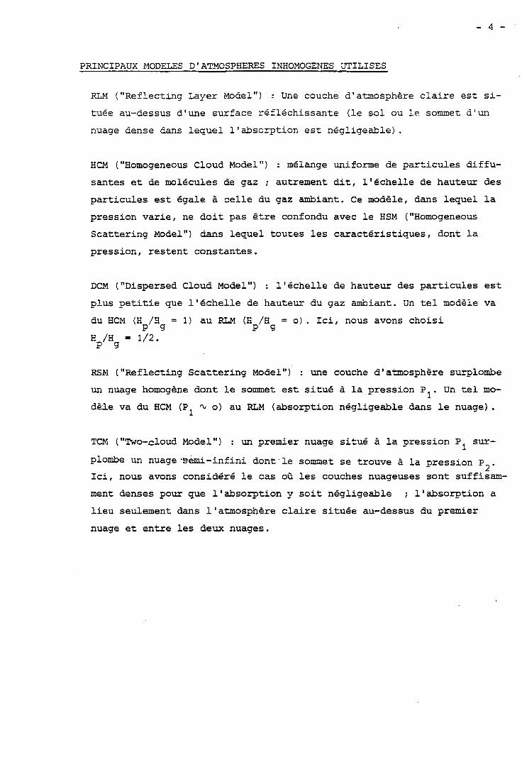
PRINCIPAUX MODELES D'ATMOSPHERES INHOMOGENES UTILISES

RLM ("Reflecting Layer Model") : Une couche d'atmosphère claire est si-

tuée au-dessus d'une surface réfléchissante (le sol ou le sommet d'un

nuage dense dans lequel l'absorption est négligeable).

HCM ("Homogeneous Cloud Model") : mélange uniforme de particules diffu-

santes et de molécules de gaz ; autrement dit, l'échelle de hauteur des

particules est égale à celle du gaz ambiant. Ce modèle, dans lequel la

pression varie, ne doit pas être confondu avec le HSM ("Homogeneous

Scattering Model") dans lequel toutes les caractéristiques, dont la

pression, restent constantes.

DCM ("Dispersed Cloud Model") : l'échelle de hauteur des particules est

plus petitie que l'érhelle de hauteur du gaz ambiant. Un tel modèle va

du HCM ( H ~ / H ~ = 1) au RLM (H /H = O). Ici, nous avons choisi P g

P/H~ = 1/2.

RSM ("Reflecting Scattering Model") : une couche d'atmosphère surplombe

un nuage homogène dont le sommet est situé à la pression P Un tel mo- 1 '

dèle va du HCM (Pl % O) au RLM (absorption négligeable dans le nuage).

TCM ("Two-cloud Model") : un premier nuage situé à la pression P, sur- .. plombe un nuage 'sd-infini dont le sommet se trouve à la pression P

2 Ici, nous avons considéré le cas où les couches nuageuses sont suffisam-

ment denses pour que l'absorption y soit négligeable ; l'absorption a

lieu seulement dans l'atmosphère claire située au-dessus du premier

nuage et entre les deux nuages.

R E F E R E N C E S

1 - CHAMBERLAIN, J . W . , Ast rophys. J . - 141, 1184 (1965) .

2 - BELTON, M.J.S., J. Atm. S c i . - 25, 596 (1968) .

3 - FOUQUART Y . , LENOBLE, J. , J.Q.S.R.T. - 13 , 447 (1973) .

4 - VAN DE HULST H.C., IRVINE W.M., La Physique d e s P l anè t e s ,Cong rè s e t

c o l l o q u e s d e l ' u n i v e r s i t é de L i ège , - 24, 78 (1962) .

5 - FOUQUART Y . , Thèse , Université d e s S c i e n c e s e t Techniques d e L i l l e

( 1975 ) .

6 - SATO M . , KAWABATA K. , HANSEN J.E., Astrophys. J. - 216, 947 (1977) .

7 - BELTON M.J.S., HUNTEN D.M., GOODY R.M., The a tmospheres o f Venus

and Mars, J.C. B rand t and M.B. McElroy Ed., Gordon & Breach, 69 (1969 ) .

8 - REGAS J .L . , GIVER L.P., BOESE R.W., MILLER J . H . , As t rophys . J.

173, 711 (1972 ) . - 9 - REGAS J .L . , GIVER L.P., BOESE R.W., MILLER J . H . , I c a r u s - 24, 1 1

(1975) . 10 - TRAFTON L., As t rophys . J. 182, 615 (1973) . 11 - TRAFTON L., MACY W . , As t rophys . J. - 196, 867 (1975 ) .

12 - MACY W . , I c a r u s 29, 49 (1976 ) . - 13 - MAILLARD J.P., COMBES M . , ENCRENAZ T., LECACHEUX J., As t ron . AS-

t r o p h y s . 25, 219 (1973) . - 14 - DE BERGH C., VION M . , COMBES M . , LECACHEUX J., MAILLARD J .P . , As t ron .

Astrophys . - 28 , 457, (1973) . 15 - DE BERGH C., MAILLARD J .P. , LECACHEUX J., COMBES M. , Icarus 29, 307 -

(1976) . 16 - LECACHEUX S . , DE BERGH C., COMBES M. , MAILLARD J .P . , As t ron . A s t r o -

phys . 53, 29 (1976) . 17 - CONNES P . , MICHEL G., Astrophys. J. L e t t e r s , 190, L29 (1974 ) . - 18 - DURTESTE Y . , D i p l G m e d ' é t u d e s app ro fond i e s , U n i v e r s i t é d e L i l l e

(1978) .

C H A P I T R E 1

GENERALISATION DE L'APPROXIMATION DE CURTIS-GODSON AUX ATMOSPHERES

DIFFUSANTES INHOMOGENES

1. @,OU. Sprcrmrc. Rdolioi. Troc<(r. Vni. ?J. pp 8 7 4 1 9 @ Pcrgmon I'rcss Lld.. IW. PnnicJ In Cirr~i Rriiain

GENERALIZATION O F THE C'JRTIS-GODSON APPROXIMATION TO INHOMOGENEOUS SCATTERING

ATMOSPHERES

J. C. BURIEZ and Y. FOUQUART Laboratoire d'optique Atmosphérique lERA 466). Université des Sciences et Techniques de Lille. 5%55

Villeneuve D'ascq-Cedex. France

Abstrad-The CurtiLrGodson approximation. which was initialiy derived to compute the transmission through clear inhoaogencous ntrnospheres. has bcen gencralized to any c!oud) atrnosphere by means of the scciled amount distribution. For mosr of the realistic atrnospheres. ihe accuncy of this generalized approximation is comparable io or even better than for the clear case.

Radiative transfer cornputations in realistic atrnospheres deal with absorption along non- homogeneous paths. For the case of clear atmospheres. approximations with one paranieter ("scaling approximatibn") or two parameters ("Curtisl-Godson' approximation") are extensively used. These approximate solutions reduce the non-homogeneous path to a hornogeneous path with equivalent amount of absorber fi. pressure P and temperature 8.

In the scaling approximation (see Goody,' Chap. 6) . i t is assumed that 4 and é can be assigned lo fixed standard values and only ii is determined. In the Curtis-Godson approximation (CGA), a ternperature-scaled amount of absorber and a mean pressure are calculated. Physically, in the scaling approximation only the Iine intensity of the gas absorbing along the equivalent homogencous path is adjusted, while in the CGA both width and intensity are adjusted so as to give the correct absorption in the strong and weak line regions. The CG.4 is obviously much more poweriul and accurate. but fails when nost of the absorbing gas is located at the lower pressures: this is the reason whv the CGA cannot be used to compute ndiative hratinç rates in the stratosphere where ozone absorption occurs in the upper i e ~ e l s . ~

In the case of cloudy atrnospncres. the exact prith ioliowed by the photon, cannot be determined: thus. the gaseous absorption cannot be directly calculated. Even for the ideal côse of a homogeneous scattering atmosphere, the calculation of an absorption profile is a complicated process which requires the solving of the Radiative Transfer Equation (RTE) many times. The transmission functions averaged over a broad spectral interval can be approximated by a sum of exponentials5 and the corresponding calculations are largely reduced. This method has been extensively used to compute the radiative heating and cooling rates in the atrn~sphere.~,' An alternative procedure makes use of the distribution of photon optical path? which enables us Io separate scattering and absorption processes. This latter method also applies to compute synthetic profiles and has been used to analyze the spectra refiected by planetary atrnosphere~.~. 'O

In this paper, we generalize the GG.4 to the case of inhornogeneous scattering atmospheres. The use of the scaled amount for the inhornogeneous clear atmospheres and the effectiveness of the distribution of photon optical paths in the case of hornogeneous scattcring atmospheres led us to introduce the distribution of scaled amount. This distribution function, devefoped in the first part of this paper, is then used to derive the generalized approximation. The results of some test of accuracy are presented and discussed in the third part.

1 . DISTRIBUTION OF SCALED AMOUNTS OF ABSORBER IN A CI.OUDY ATMOSPHERE

Clearly, since the photon path is undefinable in scattering atmospheres. the classical CGA does not apply. On the other hand, the distribution of photon optical paths enables us to generalize most of tiie clcar case nethods to homoçeneous scatteriri.; atinosplieres. These considerations suggest that we make use of some distribution function in the more general case

408 1. C. BURIEZ and Y. FOUQUART

of inhomogeneous scattering atmospheres. The problem is that the amounts of absorber, pressure and temperature Vary along the path, so that there is no direct relationship between the total path length followed by the photon and the corrcsponding absorption. We arc thus led to make use of a distribution of total amounts of absorber instead of a total photon path length distribution.

Consider A' photons which are reflected (transmitted) by a cloudy atmosphere. The ratio of the radiances in the line and the conlinuum can be written as

where k, is the absorption coefficient at the frequency v, which varies with pressure and temperature, and du, is the amount of absorbing gas encountered by the ith photon between altitudes 2 and r +dz (du, = P, n(2)d.z where n(z) is the nurnber density of absorbing gas molecules and p, is an amplification factor which depends on the scattering process and the boundary conditions but is independent of the absorption process).

'

For clear. non-homogeneous atrnospheres, the scaling approximation applies when the absorption coefficient can be factored as

With the same condition, the scaling approximation can be generalized to scattering atmospheres and we may define a s ca l~d amount ü such that

where and 6 are fixed standards of pressure and temperature. In this definition, the ratio dl?/dic depends only upon the altitude but does not depend on the

particular photon considered. Thus. with Eq. (3). Eq. I l ) becornes

I l x 2 = - 2 exp 1-k,(p, @ f i i ) , I, X i = ,

where û, is the total scaicd amount of absorbing gas encountered by the ith photon. In general, we will introduce the probability distribution p(N) of a photon contributing to the

continuum radiance after encountering the scaled amount ü, so that, instead of Eq. (4). we Iiave

with the normalization condition i0 = 1, where the fi, are the generalized moments

& = /'p(ü)iii O di . (6)

This distribution function p ( u ) can be directly calculated by means of the Monte-Carlo method, as has been done for the path length distribution."-l3 lt is also possible to invert the Laplace transform, Eq. ( 5). This latter method requires the separate task of calculating the reflected (transrnitted) radiances for different values of the absorption coefficient k, (P , I?') and that of inverting the Laplace tranqform. Several exact methods are available to solve the RTE in vertically inhomogeneous atmospheres (see, for cxample, Lenoble'*). Equation ( 5) is quite general and also applies to horizontally inhornogeneous atmospheres: nevertheless, the prohlem of computing I J I , is much more complex. and Monte Carlo or Markov Chain techniques" are the only exact methods available.

To invert the Laplace transforrn, we make use of a fast method developed by Fouquart'' to cornpute the photon path length distribiition. The ratios I , l I , can be approximnted by means of

Generalization of the Curtis-Godson approximation to inhomogeneous scattering atmospheres 409

Padé approxirnants," viz.

where Io is the lirnit of I , l I , for k,,(P, 6)-+=; PA,-,(k,.) and QN(k, , ) are polynornials of degree N - 1 and N, respectively. A typical value is N = 5, which requires us to solve the RTE for 2N = 10 values of the absorption coefficient using any rnethod.

Invertirig analyticaliy tlir Laplace transform, Eq. (5), we get the distribution function

P ( Ü ) -loS(O) + x A, exp (y,#), n=l

(8)

where 6 is the Dirac function, y, is the tith root of QN(k,,). and A, is the corresponding residue. Bec;iuse of the propertics of the function in Eq. (7), the roots are known to be real negative or cornpiex conjugale. The generalized moments, Eq.(6), can be written

where T(x + 1) = xT(x) is the gamma function. The accuracy of the approximation in Eq. (7) is generally excellent but it is well known that

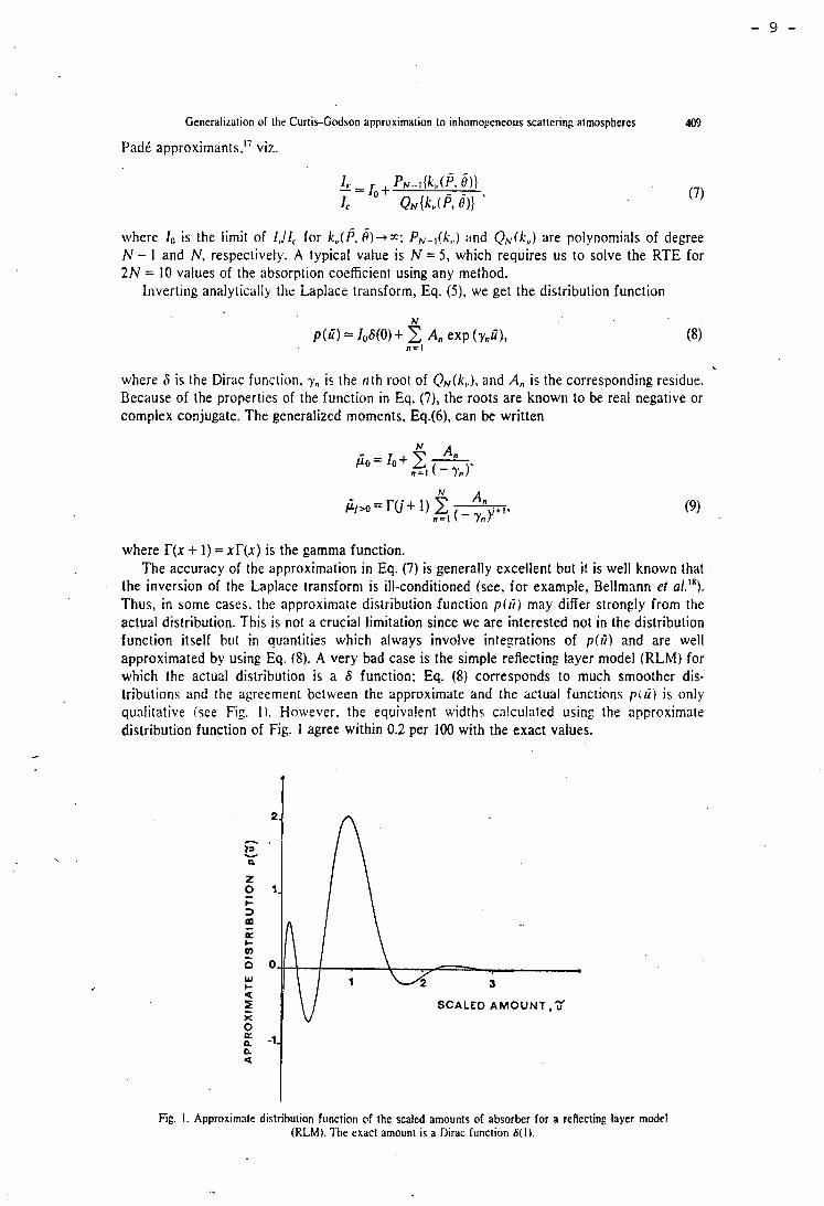
the inversion of the Laplace transforrn is ill-conditioned (see, for example, Bellmann et al."). Thus, in some cases, the approximate distribution function p ( l i ) may differ strongly from the actual distribution. This is not a crucial limitation since wc are interested not in the distribution function itself but in quantities which alwavs involve interrations of p ( i ) and are well approxirnated by using Eq. (8). A very bad case is the simple refiecting layer model (RLM) for which the actual distribution is a S function: Eq. (8) corresponds to much srnoother distributions and the agreement between the approximate and the actual functions p t ü ) is only qualitative (see Fig. 1). However. the equivalent widths calculated using the approximate distribution function of Fig. 1 agree within 0.2 per 100 with the exact values.

Fig. 1. Approximate distribution function of the scaled amounts of absorber for a refiecting layer model (RLM). The exact amount is a Dirac lunction Hl) .

410 J. C. DURIEZ and Y. FOUQUART

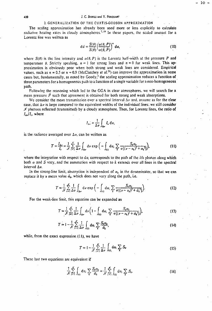
2. G E N E R A L J Z A T I O N O F T H E C U R T J S G O D S O N A P P R O X I M A T I O N . . The scaling approximation has already bccn uscd more or less explicitly to calculatc

radiative heatirig rates in cloudy atniosph~rcs.'.'~ In these papers, thc scalcd anioiitit for a Lorentz line was written as

where $ 0 ) is the line intcnsity and d B , P) is thc L-orentz half-width at the pressure P and temperature 8. Strictly speaking, n = l for strong lincs and n = O for weak lincs. This approximation is obviously poor when both strong and weak lines are considered. Empirical values, such as n = 0.5 or n = 0.9 (McClatchey et al.") can improve the approximation in some cases but, iundamentally, as noted by Goody: the scaiing approximation reduces a function of three parameters for a homogeneous path to a function of a single variable for a non-homogeneous path.

Following the reasoning which led to the GGA in clear atmospheres. we will search for a mean pressure F) such that agreement is obtaincd for both strong and weak absorptions.

We consider the mean transmission over a spectral interval Ai! and. assume as for the clear case. that AV is large compared to the equivalent widths of the individual lines: we still consider X photons reflected (transmitted) by a cloudy atmosphere. Then, for Lorentz lines, the ratio of l ,JIc, where -

is the radiance averaged over hv, can bc written as

where the integration with respect to du, corresponds to the path of the ith photon dong which both a and S Vary, and the sumrnation with respect to k extends over al1 lincs in the spectral interval Av.

I n the strong-line limit, absorption is independent of ak in the dcnominator, so that we can replace i t by a mean value Qik, which does not Vary along the path, i.e.

For the weak-iine limit, this equrition can be expanded as

whiie, froin the exact expression ( 1 1), we have

Thesc !as( two equations are equivaleiit if

Generaliation of tlic Curiis-Godson approximation îo inliomogeneous scattcriiig ntniosplieres 41 1

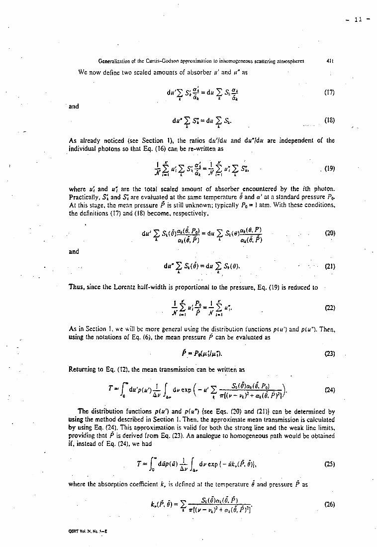
We now definc two scaled amounts of absorber I I ' and rr" as

and

As already noticed (see Section 1). tlie ratios du'ldrr and duNldri are independent of the individual photons so that Eq. (16) cari be re-written as

where u; and u: zre the total scaled amount of absorber encountered by the ith photon. Practically, Si and Si are evaluated at the same temperature 6 and a' at n standard pressure Po. A l this stage, the menn pressure P is still unknown; typically Po = 1 atm. With these conditions, the dcfinitions (17) and (18) become, respectively,

- a,(û P) du' 2 ~,(~)al(s . = du Si($)- , .

L @k(e, P) L P)

and

. . . .

Thus, sincc the Lorentz hall-width is proportional to the pressure, Eq. (19) is rediiced 10

As in Section 1. we uill bc more general using rhe distribuiion functions p(uf) and p(uW). Then, using the notations of Eq. (6). the mean pressure P can be evaluated as

Retuming to Eq. (12). the mean transmission can be written as

The distribution functions p(ul) and p(u")see Eqs. (20) and (2l)} can be deiermined by using the method describcd iii Section 1. Then, the approximate mean transmission is calculated by using Eq. (24). This approximation is valid for both the strong iine and the weak iine limits, providing that is derived from Eq. (23). An analogue to homogeneous path would bc obtained if, instead of Eq. (24), we had

where the absorption coefficient k, is clefincd at the temperature ë and pressure as

QSRT Vd. 24. No. . L E

412 J . C. BURIEZ and Y. FOUQUART

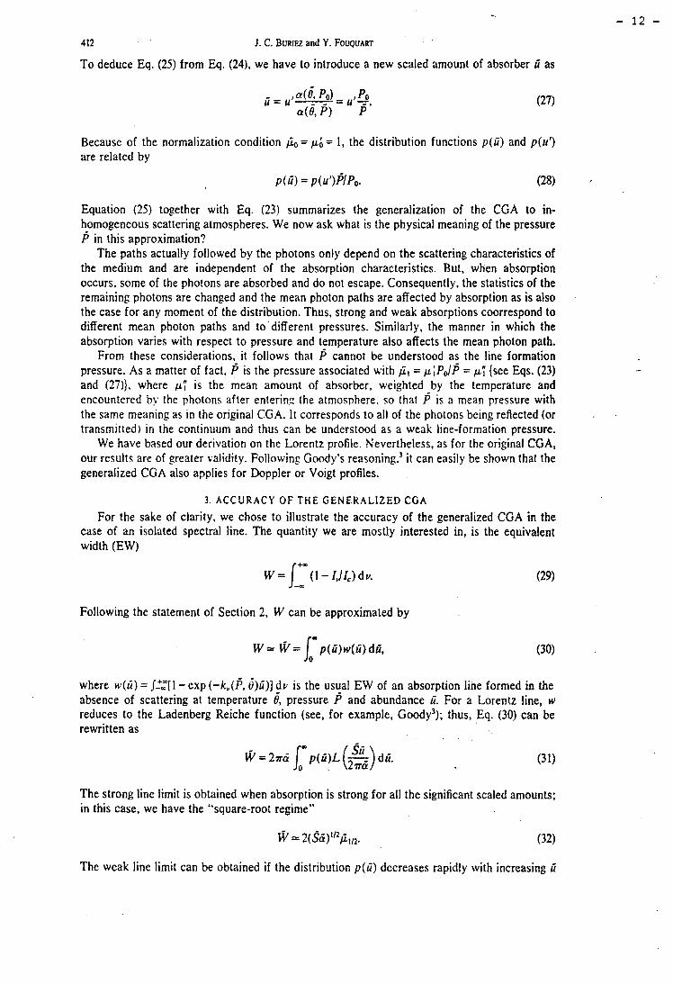
To deduce Eq. (25) from Eq. (24) , we have to introduce a new scaled amount of absorber ü as

Because of the normalization condition fio = pi = 1, the distribution functions p ( ü ) and p(ul ) are related by

Equation (25) together with Eq. (23) summarizes the generalization of the CGA to inhomogeneous scattering atmospheres. We now ask what is the physical meaning of the pressure P in this approximation?

The paths actually followed by the photons only depend on the scattering characteristics of the medium and are independent of the absorption characteristics. But. when absorption occurs, some of the photons are absorbed and do not escape. Consequently, the statistics of the remaining photons are changed and the mean photon paths are affected by absorption as is also the case for any moment of the distribution. Thus, strong and weak absorptions coorrespond to different mean photon paths and to different pressures. Similarly, the manner in which the absorption varies with respect to pressure and temperature also affects the mean photon path.

From these considerations, it follows that P cannot be understood as the line formation pressure. As a matter of fact. P is the pressure associated with f i , = p;~ , , lP = pI; {see Eqs. (23) and (27)) . where p; is the mean amount of absorber, weighted by the temperature and encountered by the photons after enterin? the atmoîphere. so that ? is a mean pressure with the same meaning as in the original CGA. lt corresponds to al1 of the photons being reflected (or transmirted) in the continuum and thus can be understood as a weak line-formation pressure.

We have based our derivation on the Lorentz profile. Nevertheless, as for the original CGA, Our results are of greater vôliditv. Following Goody's reasoning.' it can easily be shown that the generalized CGA also applies for Doppler or Voigt profiles.

3. A C C U R A C Y OF THE G E N E R A L I Z E D CGA

For the sake of clarity, we chose to illustrate the accuracy of the generalized CGA in the case of an isolated spectral line. The quantity we are mostly interested in, is the equivalent width (EW)

Following the statement of Section 2 , W can be approximated by

W = w = 1 p(ü)w(ü) dü, (30)

where w ( ü ) = J;,"[l- exp ( -k , (P , 6 ) 6 ) ] dv is the usual EW of an absorption line formed in the absence of scattering at temperature 8, pressure P and abundance 6. For a Lorentz line, w reduces to the Ladenberg Reiche function (see, for example, Goody3); thus, Eq. (30) can be rewritten as

The strong line limit is obtained when absorption is strong for al1 the significant scaled amounts; in this case, we have the "square-root regime"

The weak line limit can be obtained if the distribstion p ( 6 ) dccreases rapidly with increasing ü

Cieneraliziition of the Curtis-Godson iipproxirnalion 10 inhornogeneous scatlering atmosphcres 413

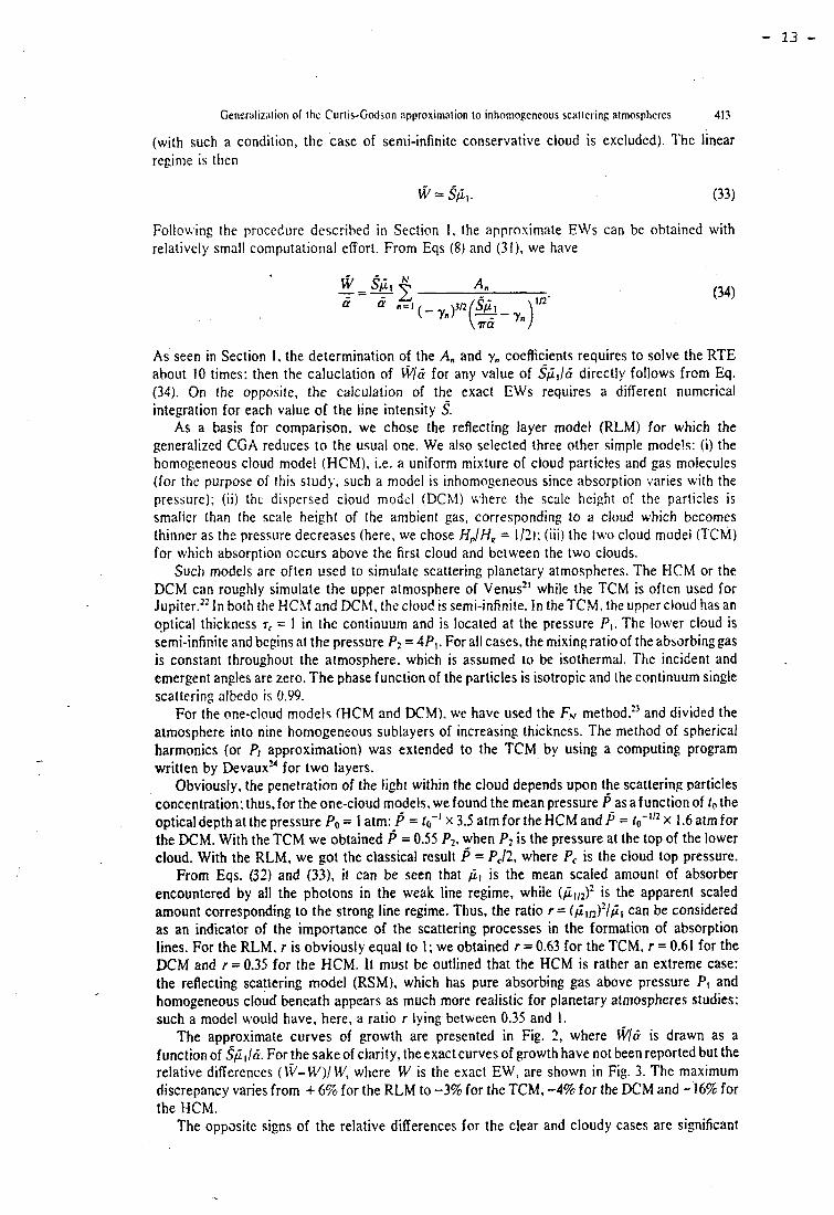
(with such a condition, tlie case of semi-infinite conservativc cloud is excluded). l'he linear regime is then

Follo\~:ing the procediirc described in Section 1, the approsimate EWs can be obtained with relatively small computatiorlal effort. From Eqs (8) and (31), we have

As seen in Section 1 , the determination of the A, and y, coefficients requires to solve the RTE abolit 10 times: then the caluclation of w/& for any value of ~ f i ~ l c i directly follows from Eq. (34). On the opposite, the calculation of the exact EWs requires a different numerical integration for each value of the line intensity 3.

As a basis for comparison, we chose the reflecting layer modei (RLM) for which the generalized CGA reduces to the usual one. We also selected three other simple mode!s: (i) the homogeneous cloud rnodel (HCM), i.e. a uniform mixture of cloud particles and gas molecules (for the purpose of this study, such a model is inhomogeneous since absorption varies with the pressure); ( i i ) thc dispersed cloud modcl (DCA!) uhere the serile height of the particles is smalier than the scale height of the ambient gas, corresponding to a cloud which becomes thinner as the pressure decreases (here, we chose H,,IH, = 112); (ii i) the t ~ ~ o cloud model (TCM) for which absorption occurs above the first cloud and bctween the two clouds.

Such models are often used to simulate scattering planetary atmospheres. The HCM or the DCM can roughly simulate the upper atmosphere of Venus" while the TCM is often used for Jupiter." In both the HC31 and DCht, the cloud is semi-infinite. In the TCM, the upper cloud has an optical thickness T, = 1 in ihe continuum and is located at the pressure PI. The lower cloud is semi-infinite and begins at the pressure Pl = 4Pl. For al1 cases, the mixing ratioof the absorbinggas is constant throughout the atmosphere, which is assumed to be isothermal. The incident and emergent angles are zero. The phase function of the particles is isotropie and the continuum single scattering albedo is 0.99.

For the one-clnud mode15 (HCM and DCML we have used the & meth~d. '~ and divided the atmosphere into nine hornogeneous sublayers of increasing thickness. The method of spherical harmonics (or P, approximation) was extended to the TCM by using a computing program written by D e ~ a u x ' ~ for two layers.

Obviously, the penetration of the light within the cloud depends upon the scattering particles concentration: thus,for the one-cloud models, we found the mean pressure P as afunction of f , the optical depth at the pressure Po = 1 atm: P = fo-' x 3.5 atm for the HCM and P = to-'12 X 1.6 atm for the DCM. With the TCM we obtained = 0.55 Pl, when P2 is the pressure at the top of the lower cloud. With the RLM, we got the classical result P = Pc/2, where Pc is the cloud top pressure.

From Eqs. (32) and (33), it can be seen that 6, is the mean scaled amount of absorber encountered by al1 the photons in the weak fine regime, while (fi112)2 is the apparent scaled amount corresponding to the strong line regime. Thus, the ratio r = (@llz)21fiI can be considered as an indicator of the importance of the scattering processes in the formation of absorption lines. For the RLM, r is obviously equal to 1; we obtained r = 0.63 for the TCM. r = 0.61 for the DCM and r = 0.35 for the HCM. It must be outlined that the HCM is rather an extreme case: the reflecting scattering model (RSM), which has pure absorbing gas above pressure PI and homogeneous clouci beneath appears as much more reaiistic for planetary atmospheres studies: such a model would have, here, a ratio r lying between 0.35 and 1.

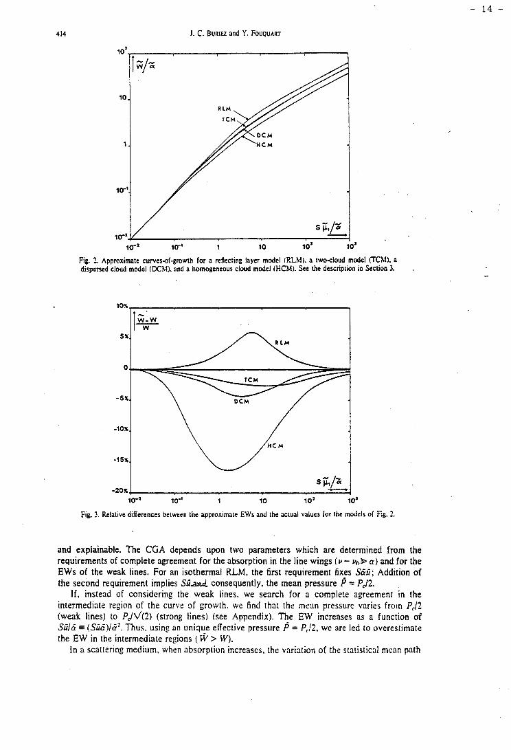
The approximate curves of growth are presented in Fig. 2, where is drawn as a function of $,L,l&. For the sake of clarity, theexact curves of growth have not been reported but the relative differences (I"j-w)/ W, where W is the exact EW, are shown in Fig. 3. The maximum discrepancy varies from + 6% for the R L M to -3% for the TCM, -4% for the DCM and - 16% for the HCM.

The oppssitc signs of the relative differences for the clear and cloudy cases arc significant

J . C. BURIEZ and Y. FOUQUART

Fig. 2. Approximate curves-of-growth for a reflecting layer mode1 (RLM). a two-cloud mode1 (TM). a dispersed cloud mode1 (DCM), and a homogeneous cloud modcl (HCM). See the description in Section 3.

Fig. 3. Relative differences between the approxirnate EWs and the actual values for the models of Fig. 2.

and explainable. The CGA depends upon two parameters which are deterrnined frorn the requirements of cornplete agreement for the absorption in the line wings ( v - vo S a) and for the EWs of the weak Iines. For an isothermal RLM, the first requirement fixes SC%; Addition of the second requirement irnpiies S ü d consequently, the mean pressure = Pc/2.

If, instead of considering the weak lines, we search for a cornplete agreement in the interrnediate region of the curve of growth, we find that the metin pressurc varies froin Pc/2 iweak iines) to ~ J v ( 2 ) (strong lines) (see Appendix). The EW increases as a function of SüIa = (Sü&)lG2. Thus, using an unique effective pressure P = PJ2, we are led to overestimate the EW in the intermediate regions ( W > W).

In a scattering medium, when absorption increases, the variation of the statistical mcan path

Genernl~zation of the Curtk-Godsnn approximation to inhomogeneouî scatlering atmospheres 415

length produces a reduction of the line formation pressure. We thus have Iwo compensating effects which recult in an absolilte decrease of (fi'- W ) . For the present cases, the overall eflect is to undcrcstimate the EW so that the relative diffeience is negative.

As already mcntioned. the ratio r = ( ,~ I , ,~) ' / f i , can be coiisidered as a measure of the importance of the scattering processes in the line formation. Qualitatively, the smaller r, the larger is the reduction of the formation pressure with increasing absorption: thus the larger is the compensating effect compaied to the clear case (KLM). This is the reason for tlie increasing error when poing from the DCM (r = 0.61) to the HCM ( r =0.35). For the same reason, in scattering medium;the generalized CGA can be more accurate than the original CGA; this is particularly the case for the present DChl and TCM for which the maximum discrepancy is lower than for the RLM.

Small value of r are associated with large 6,. In this case, the line wings are strongly deepened and the continuum level is hardly measurable. For the R(0) line of the 0.783 p m CO2 band, Sato et al." report discrepancies as large as a factor of two for the HCM depending on the use of a continuum I c ~ e l which is 0.99 or 0.999 of the real value. Compnred to the usual experimental uncerlainties, the accuracy of the generalized CGA appears quite tolerable.

It is worth to note that, for the extreme case r+O ( p , - 7 ~ ) , the linear regime no longer exists: this is the case of a semi-infinite conservative cloud for which al1 lines belong to the square-root regime. In this case, P is undefined, but a one-parameter approximation is quite sufficient.

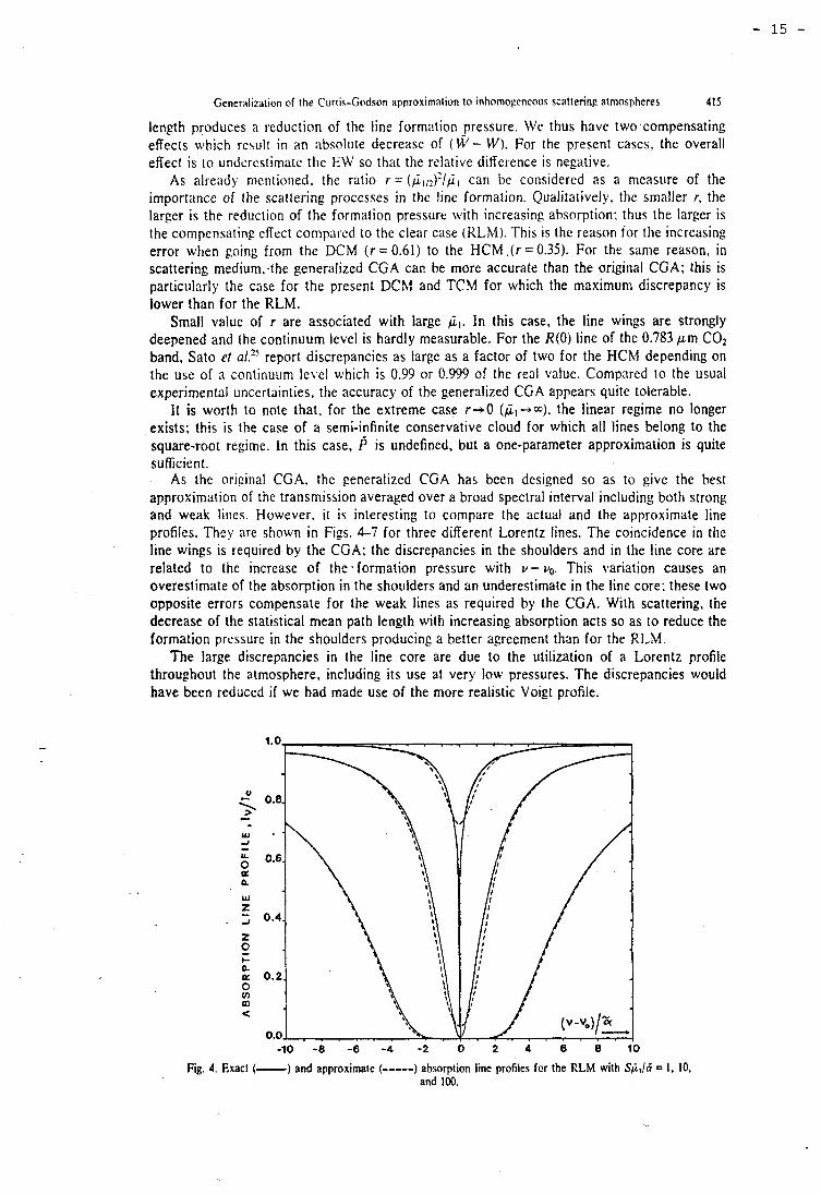
As the oricinal CGA. the generalized CGA has been designed so as to give the best approximation of the transmission averaged over a broad spectral interval including both strong and weak liiics. Huwever. it iq interesting to compare the actual and the approximate line profiles. They are shown in Figs. 4-7 for three different Lorentz lines. The coincidence in ttie line wings is required by the CGA; the discrepancies in the shoulders and in the line core are related to the increase of thesformation pressure with v - v,. This variation causes an overestimate of the absorption in the shoulders and an underestimate in the line core; these two opposite errors compensaie for the weak lines as required by the CGA. With scattering, the decrease of the statistical mean path length with increasing absorption acts so as to reduce the formation pressure in the shoulders producing a better agreement than for the R1,M.

The large discrepancies in the line core are due to the utilization of a 1,orentz profile throuphout the atmosphere. including its use at very low pressures. The discrepancies would have been redüced i f we had made use of the more realistic Voigt profile.

Fig. 4. Exact (-) and approximate (-----) absorption line profiles for the RLM with S@lla' = 1 , 10, and 100.

J. C. BURIEZ and Y. FOUQUART

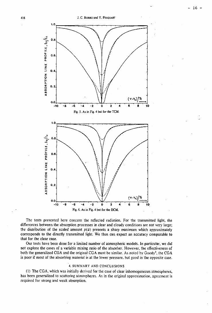
Fig. 5. As in Fig. 4 but for the TCM.

Fig. 6. As in Fig. 4 but for the DCM.

The tests presented here concern the reflected radiation. For the transmitted light, the differences between the absorption processes in clear and cloudy conditions are not very large: the distribution of the scaled amount p ( Q ) presents a sharp maximum which approximately corresponds to the directly transmitted light. We thus can expect an accuracy comparable to that for the clear case.

Our tests have been done for a limited number of aimospheric models. In particular, we did not explore the cases of a variable rnixing ratio of the absorber. However, the effectiveness of both the generalized CGA and the original CGA must be similar. As noted by Goody3, the CGA is poor if most of the absorbing material is at the lower pressure. but good in the opposite case.

4. SUMM.4RY A N D C O N C L U S I O N S

(1) The CGA, which was initially derived for the case of clear inhomogeneous atmospheres, has been generalized to scattering atmospheres. As in the original approximation. agreement is required for strong and weak absorption.

Ceneralizntion of the Curtis-Godson approximation to inhomogeneous scattering atmospheres 417

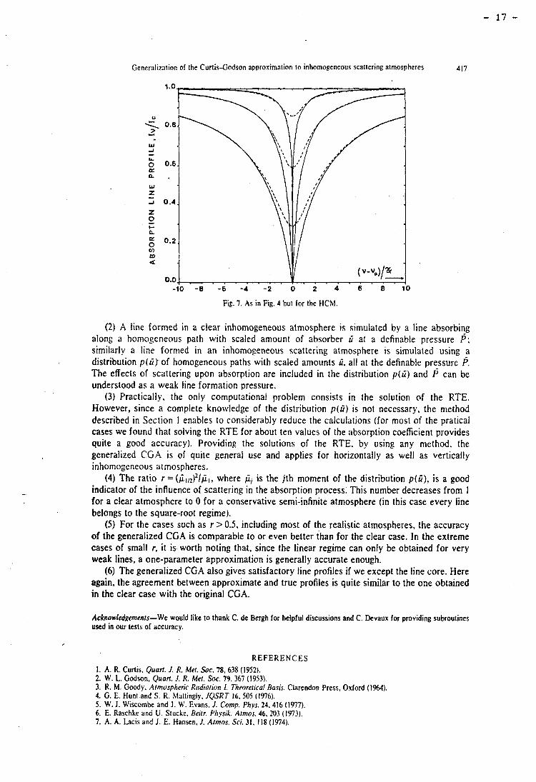
Fig. 7 . As in Fig. 4 but for the HCM.

(2) A line formed in a clear inhomogeneous atmosphere is simulated by a line absorbing along a homogeneous path with scaled arnount of absorber N at a definable pressure P ; sirnilarly a line fornied in an inhomogeneous scattering atmosphere is simulated using a distribution p ( ü r of hornogeneous paths with scaled arnounts ü. al1 at the definabie pressure p. The effects of scattering upon absorption are included in the distribution p(ü) and P can be understood as a weak line formation pressure.

(3) Practically, the only computational problern consists in the solution of the RTE. Howevcr, since a complete knowledge of the distribution p ( ü ) is no1 necessary, the method described in Section 1 enables to considerably reduce the calculations (for rnost of the pratical cases WC found that solving the RTE for about ten values of the absorption coefficient provides quite a good accuracy). Providing the solutions of the RTE. by using any method, the generalized CGA is of quite general use and applies for horizontally as well as vertically inhomogeneous atmospheres.

(4) The ratio r =(jï,,2)2/$,, where fi, is the jth moment of the distribution p ( ü ) , is a good indicator of the influence of scattering in the absorption process. This nurnber decreases from I for a clear atmosphere to O for a conservative semi-infinite atmosphere (in this case every iine belongs to the square-root regirne).

(5) For the cases such as r > 0.5, including most of the realistic atmospheres, the accuracy of the generalized CGA is comparable to or even better than for the clear case. In the extreme cases of small r. it is worth noting that, since the linear regime can only be obtained for very weak lines, a one-parameter approximation is generally accurate enough.

(6) The generalized CGA also gives satisfactory line profiles if we except the line core. Here again, the agreement between approximate and true profiles is quite similar to the one obtained in the clear case with the original CGA.

Acknowledgements-We would like to thank C. de Bergh for helpful discussions and C. Devaux for providing subroutines used in our tests of accuracy.

REFERENCES 1. A. R. Curtis, Quarf. J. R. Met. Soc. 78, 638 (1952). 2. W. L. Godson, Quart. !. R. Met. SOC. 79,367 (1953). 3. R. M. Goody, Atmospheric R<rdiotion I. Theore~ical Bosis. Clarendon Press. Oxford (1%4). 4. G. E. Huni and S. R. Mattingly, JQSRT 16, 505 (1976). S. W. J . Wiscombe and 1. W. Evans. J. Comp. Phvs. 24.416 (1977). 6. E. Raschke and Li. Stucke. Beiir. Ph'hysik. Aimos. 46, 203 (1973). 7. A. A. Lacis and J . E. Hansen, J. Atmos. Sci. 31. 118 (1974).

418 J . C. BURIEZ and Y. FOUQUART - ..

8. H. C. Van de Hulst and W. M. Irvine, in L a Physique des Planètes, Congrès d Colloques de I'llnivcrsité de Liège. Vol. 24. 78 (1962).

9. Y. Fouquart, Thesis, Université des Sciences et Techniques de Lille, France (1975). 10. J. C. Duriez. Y. Fouquart. and A. 1,. Fymiit. A s t r ~ . Astrophys. 79, 287 (1979). II. B. A. Kargin. L. D. Kritsokutskaya. and Y. E. Feygelson. Bull. (1:c.) Acad. Sci USSR. Atm. Oc. Phys. 8,287 (1972). 12. V . 1. Dianov-Klokov, N. A. Yevstratov. 1. P. Malkov, and 0. P. Ozerenski, Bull. (Izv.) Acud. Sci USSR, Atm. Oc.

Phvs. 10,452 (1974). 13. J . F. Appleby and W. M. Irvine. Astrophys. J. 183, 337 (1973). 14. J . Lenoble 1Ed.j. Stondnrd Procedurez io Compute Atmosphenc Radiative Transfer in a Scattering Atmosphere.

IAMAP. Boulder. Colorado (1977). 15. L. W. Esposiio and L. L. House. Astrophys. J. 219, 1058 (1978). 16. Y. Fouquart, JQSRT 14,497 (1974). 17. G. Baker, The Pade Approximanr in Theoretical Phpsics. Chap. 1. Academic Press, New York (1970). 18. R. Bellrnann. R. E. Kalaba. and J. A. Lockett. Numencal Inversions of the Laplace Transjon. Elsevier. New York

(1966). 19. Y. Fouquart and B. Bonnel. Beitr. Phvsilr. Atmos 53. 35 (1980). 20. R. A. Mc Clatchey. R. W. Fenn. J . E. A. Selby. F. E. Volz. and J . S. Garing, Optical Properties of the Atmosphen.

AFCRL 714279, Envir. Res. Papers No. 354.91 pp. 21. A. A. Lacis. J. Aimas. Sci. 32. 1107 (1975). 22. J. C. Buriez and C. de Bergh, Asiron. Astrophys. 83. 149 (1980). 23. C. Devaux, P. Grandjean. Y. Ishiguro. and C. E. Siewert, Astrophys. Space Sci. 62, 225 (1979). 24. C. Devaux, Thesis. Université des Sciences et Techniques de Lille, France (1977). 25. M. Salo. K. Kawabata. and J. E. Hansen, Astrophys. 3. 216,947 (1977).

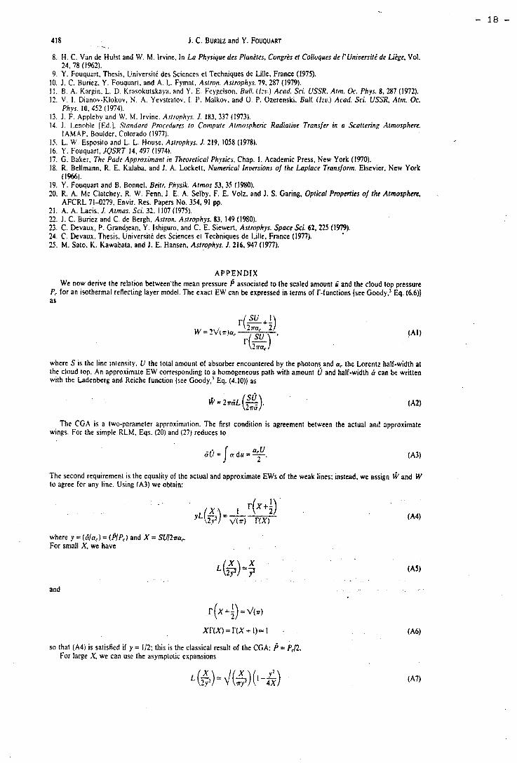
A P P E N D I X We now derive the relation between'the mean pressure P associated to the scaled amount ü and the cloud top pressure

P, for an isothermal reflecting layer model. The exact EW can be expressed in ierms of r-functions {see Goody,) Eq. (6.6)) as

where S 1s the line intensity. U the total arnoiint of absorber encountered by the photons-and a, the Lorentz half-width al the cloud top. An approximate EW conesponding to a homogeneous path with amount U and half-width a can be written with the Ladenberg and Keiche function (see Goody,' Eq. (4.10)) as

The CGA is a Iwo-parameter approximation. The first condition is agreement between the actual and approximate wings. For the simple RLhZ, Eqs. (20) and (27) reduces to

The second requirernent is the equaliiy of the actual and approximate EWs of the weak lines: instead, we assign w and W Io agree fcr any line. Using (A3) we obtain:

where y =(&/a,) = (PIF',) and X = SUltna, For small X, we have

and

so that (A4) is satisfied if y = Il?: this is the classical result of the CGA: P = PJ2. For large X, we can use the asymptotic expansions

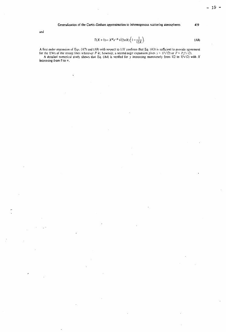
Generalizaiion of the Curtis-Godson approximation to inhomogenous scattering atmospheres 419

and

A first order expansion of Eqç. (Al) and (-8) with respect io 1/X confirnis that Eq. (A3) is suficien1 to providc ngreement for ihe EWs of the strong lines u,hatevcr P is; however, a secondor&r expansion gives y = II\'(?) or P = 1' , / \ , (7) .

A deiailed numerical study shows iliat Eq. (A4) is verified for y increasing monotoncly froni Il? to I/v(Z) with X increasing from O Io r.

C H A P I T R E II

INFORMATIONS CONTENUES DANS LES LARGEURS EQUIVALENTES DE RAIES

INTRODUCTION

Si l'on considère un modèle d'atmosphère claire homogène, on peut

déterminer, à partir des largeurs équivalentes de raies, l'abondance de gaz

absorbant rencontrée par les photons le long de leur trajet, la pression

de formation des raies et leur température de rotation.

Si maintenant . on considère une atmosphère quelconque, qui peut être inhomogène verticalement et horizontalement, quelles informations peut

on déduire des largeurs équivalentes mesurées à partir d'un spectre expéri-

mental ? A quoi correspond l'abondance, la pression et la température que

l'on déduit des mesures en appliquant les relations établies pour le simple

modèle de la "couche réfléchissante" ?

Nous supposerons dans un premier temps que La mesure des largeurs

équivalentes de raies à partir d'un spectre expérimental ne pose pas de

problème. On considèrera notamment que le niveau continu (en absence d'ab-

sorption) du spectre est très bien défini et que les raies sont suffisamment

isolées les unes des autres... On verra quelles informations peuvent être

déduites de telles largeurs équivalentes sans faire d'hypothèse sur le type

d ' atmosphère.

En pratique, la mesure de la largeur équivalente d'une raie, qui,

par définition, correspond à un intervalle spectral infini, n'est pas pos-

sible directement. On est amené à extrapoler sa valeur à partir d'une mesure

correspondant à un intervalle spectral fini. A partir d'une même mesure, on

montrera que l'on peut obtenir des valeurs de largeurs équivalentes diffé-

rentes pour des modèles d'atmosphères différents, ce qui rend alors impos-

sible l'obtention d'informations sans faire d'hypothèse sur le type d'at-

mosphère .

Nous nous limiterons au cas où toutes les raies appartiennent à

un même spectre ; nous n'envisagerons pas l'étude des variations des largeurs

équivalentes en fonction des angles d'incidence et d'émergence. Une telle

étude peut apporter des informations complémentaires mais essentiellement

d'ordre qualitatif. Par exemple, la variation de l'absorption due au CO sur 2

Vénus en fonction de l'angle de phase- observée pour la première fois par

KUIPER' en 1952- a permis d'exclure le modèle de la "couche réfléchissante".

Pour que ces informations soient quantitatives, il faudrait que les mesures

à différents angles de phase ou à différents endroits d'une planète corres-

pondent à la même réalité physique. Ceci suppose, en pratique, que les va-

riations temporelles et spatiales soient négligeables.

1 - RAIES FORMEES DANS UNE ATMOSPHERE CLAIRE: HOMOGENE

La largeur équivalente d'une raie de LORENTZ formée dans une atmos-

phère claire homogène s'exprime à l'aide de la fonction de LADENBERG ET REICHE 2

(voir, par exemple, GOODY )

a étant la demi-largeur de LORENTZ - qui dépend de la température O et est proportionnelle à la pression P -, S l'intensité de la raie et U l'abondance totale de gaz absorbant rencontrée par les photons . En utilisant le déve- loppement limité de la fonction de LADENBERG et REICHE pour les petits argu-

ments ( S U / ~ T ~ <<1), on obtient le "régime linéaire" pour les raies faibles

et en utilisant le régime asymptotique (SU/2Ta > 3 ) , on obtient le "régime

en racine carrée" pour les raies fortes

Les deux dernières équations peuvent être résumées sous la forme

avec b = 1 pour le régime linéaire et b = 1/2 pour le régime en racine

carrée.

La largeur équivalente d'une raie varie avec le nombre quantique

m, par l'intermédiaire de l'intensité de la raie

où S est l'iatensité de la bande, Q la fonction de partition de rotation, b r

Bm(m-1) l'énergie de rotation dans l'état le plus bas, h la constante de

PLANCK, c la vitesse de la lumière et k la constante de BOLTZMANN. Nous négli-

gerons ici la variation de la demi-largeur de LORENTZ avec le nombre quantique

pour simplifier mais ceci n'affecte en rien les raisonnements qui suivent.

Les équations (11-4) et (11-5) permettent alors d'écrire

où W correspond à la largeur équivalente de la raie R(0). 1

Ainsi, la mesure des largeurs équivalentes de plusieurs r~aies d'une

même bande, appartenant au même régime de la courbe de croissance, permet de b

déterminer la "température de ratation" O à partir de la pente de Rn (W,/lml )

en fonction de m(m-1). A partir de l'origine de cette courbe, on peut déter-

miner l'abondance U si b = 1, ou le produit de U par la pression P si

b = 1 j 2 (voir Equ. (11-7) ) .

Rigoureusement, l'équation (11-6) n'est valable que si toutes les

raies appartiennent soit au régime linéaire soit au régime en racine carrée. 3

Son utilisation développée par GRAY YOUNG pour des raies du régime inter-

médiaire est approximative. La détermination de la température à partir de

raies appartenant à des régimes différents n'est possible que si l'on fait

une hypothèse sur la valeur de la pression P, à priori inconnue (MARGOLIS 4

et FOX ) . Nous priviligierons, dans ce qui suit, l'étude du régime linéaire

et celle du régime en racine carrée.

II - RAIES FORMEES DANS UNE ATMOSPWRE NON-HOMOGENE MAIS ISOTHERME

Considérons une atmosphère dont la structure verticale et horizon-

tale est quelconque mais isotherme dans la région de formation des raies.

Nous utiliserons la fonction de distribution p (g) de l'abondance de gaz absorbant pondérée simplement par la pression et définie à partir de

% Pour une atmosphère claire, p(u) est une simple fonction de Dirac. Pour le

cas général, le schéma de calcul a été donné dans le premier chapitre. La 'L

pression P est la pression de formation des raies faibles ; elle est telle

que l'"abondance pondérée" moyenne est égale à l'abondance vraie de gaz

absorbant rencontrée en moyenne par les photons,

Les largeurs équivalentes des raies fortes peuvent s'exprimer à l'aide du %

moment d'ordre 1/2 de la fonction p(u) (cf.Equ. 1-32)

et celles des raies très faibles à l'aide du moment d'ordre 1 (cf. Equ. 1-33)

En utilisant l'"indicateur de diffusion" dejà rencontré au chapitre 1

les équations (11-10) et (11-11) peuvent être mises sous la forme

avec b = 1 pour le régime linéaire (ou régime de très faible absorption)

et b = 1/2 pour le régime en racine carrée (ou régime de forte absorption).

Les régimes obtenus pour une atmosphère claire homogène (Equ. 11-4)

et pour une atmosphère isotherme (Equ. 11-13) sont identiques à condition que

ce qui définit l'atmosphère claire homogène équivalente (ou "apparente") par %

l'abondance "apparente" ri et la pression "apparente" rP. 1

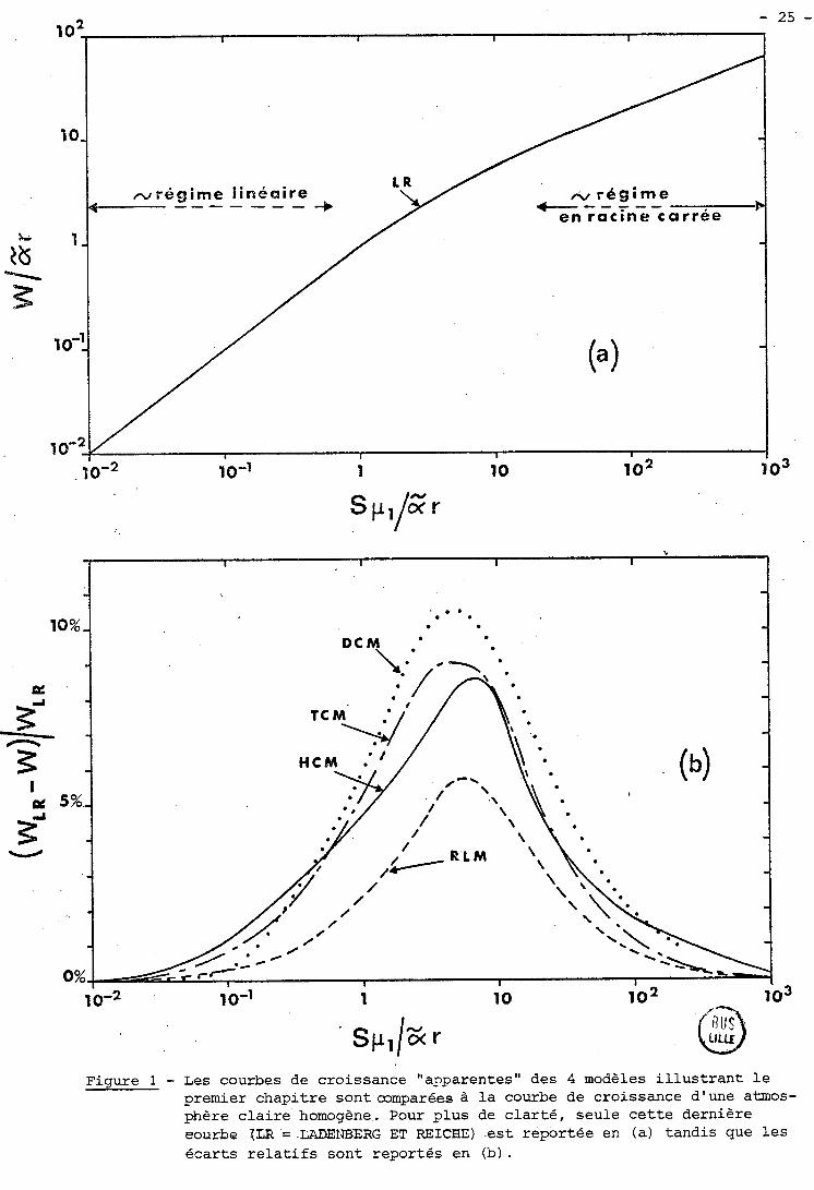
Figure 1 - Les courbes de croissance "apparentes" des 4 modèles i l l u s t r a n t l e premier chapitre sontoûmparées à l a courbe de croissance d'une atmos- - - -

phère c l a i r e homogène. Pour plus de c l a r t é , seule c e t t e dernière eourbe 7LR = ZADEl3BERG ET REICHE) e s t reportée en (a ) tandis que l e s écar t s r e l a t i f s sont reportés en (b).

Ainsi, la température de rotation O peut être déterminée en sui-

vant la même démarche que dans le cas d'une atmosphère claire homogène

(cf. Equ. 11-6 et 7 ) . On peut déterminer ensuite l'abondance moyenne p, si A

% les raies appartiennent au régime linéaire, ou le produit v rP si les raies

1 appartiennent au régime en racine carrée. Si le domaine d'intensité des raies

étudiées s'étend du régime linéaire au régime en racine carrée, on détermine

ainsi une abondance p et une pression r3. 1

A ce stade, on peut s'interroger si une information supplémentaire

ne peut pas être déduite des raies appartenant au régime intermédiaire. En % 'Il

fait, les courbes W/ar = f(Spl/ar), qui sont équivalentes à des courbes de

croissance, différent relativement peu selon le type d'atmosphère. Sur la

figure 1, les courbes correspondant aux quatre modèles inhomogènes qui ont

illustré le premier chapitre sont comparées à la courbe de croissance de

raies formées en atmosphère claire homogène (Equ. 11-1). Les écarts relatifs

restent inférieurs ou de l'ordre de 10 %, ce qui n'est pas excessif compte-

tenu des incertitudes expérimentales. De plus, ces écarts sont dus pour une

grande part à la variation de la pression dans l'atmosphère, indépendamment

de l'influence de la diffusion, puisque l'on observe déjà des écarts de

l'ordre de 6 % entre les largeurs équivalentes formées en atmosphère claire

inhomogène (P varie de O à P ) et celles formées en atmosphère claire homo- C.

gène (P = pc/2). Il ne faut donc pas s'attendre à obtenir une information

spécifique à partir du régime intermédiaire. Cependant, plus l'indicateur de

diffusion r est petit, plus le régime linéaire correspond à des largeurs équi-

valentes de raies petites et donc difficilement mesurables. Dans ce cas, les

raies appartenant au régime intermédiaire peuvent servir à extrapoler de

façon plus ou moins précise le régime linéaire. Nous excluons bien sar de

cette étude le cas irréaliste d'une atmosphère diffusante semi-infinie sans

absorption conthue pour laquelle r -t o.

Une détermination de l'abondance "apparente" pl et de la pression 'Il

"apparente" rP peut permettre d'éliminer un certain nombre de modèles atmos-

phériques. La pression apparentEdes raies formées en atmosphère claire est

égale à la moitié de la pression au sommet de la couche réfléchissante P cf et l'abondance apparente est égale à

c étant la concentration de gaz absorbant supposée constante dans l'atmos- Y

phère, H' l'échelle de hauteur de pression ramenée à la température de 273' K, - 1

et n le facteur de masse d'air égal à cos + cos-'@, et O étant les

angles d'incidence et d'émergence. Définissons le facteur de masse d'air

"apparent"

Pour les exemples qui illustrent le premier chapitre, ce facteur est égal à

2.0 pour l'atmosphère claire ( R L M ) , à 4.6 pour le modèle à deux nuages (TCM),

à 4.0 pour le nuage dispersé (DCM) et à 6.5 pour le nuage homogène (HCM). Si

la concentration c est connue avec une bonne precision - telle celle du gaz carbonique sur Vénus - il est alors possible à partir de la connaissance du

rapport pl/ (2c dl r8) d'éliminer un certain nombre de modèles d'atmosphère. Si, au contraire, la concentration en gaz absorbant est une inconnue à déter-

miner, la seule connaissance des largeurs équivalentes de raies de ce gaz

absorbant ne permet pas de déterminer cette concentration. Il est cependant

possible de la déterminer en comparant les largeurs équivalentes de raies du

gaz absorbant de concentration inconnue et celles d'un autre gaz de concentra-

tion connue (par exemple, les raies de HCR et celle de CO2 sur Vénus). Mais

il est alors nécessaire (i) qu'il s'agisse d'un même spectre expérimental

pour éviter .l'influence des variations temporelles et spatiales, (ii) qu'il

s'agisse du même domaine spectral à cause de la variation des propriétés

des particules diffusantes avec la longueur d'onde, (iii) et surtout qu'il

s'agisse du même régime de la courbe de croissance. Cette dernière condition

est souvent difficile à réaliser car le régime en racine carrée n'est pas

toujours atteint par les raies d'un gaz mineur, et le régime linéaire ne peut

être atteint que par des raies extrêment faibles et donc difficiles à mesurer.

III - RAIES FORMEES DANS UNE ATMOSPHERE QUELCONQUE

Nous n'avons considéré jusqu'à présent que des atmosphères isothermes

de sorte qu'il n'y avait aucune ambiguïté sur la signification de la tapé-

rabure de rotation. Dans une- atmosphère réaliste, la température varie avec 5

la pression;SAGAN et REGAS ont souligné l'importance de ce problème que

nous reprenons ici de façon plus quantitative à l'aide des abondances "pon-

dérées" de gaz absorbant.

a) - Cas des raies faibles (régime linéaire)

'-b Dans le premier chapitre, la pression P associée à la fonction de

% distribution p(u) a été introduite parce que l'on s'intéressait à la fois

aux raies fortes et aux raies faibles. Ici, nous ne nous intéresserons d'a-

bord qu'aux raies faibles dont la largeur équivalente est indépendante de la

pression. Il suffit donc de pondérer l'abondance de gaz absorbant

par l'intensité de la raie (cf Equ. 1-18)

pour exprimer la largeur équivalente d'une raie faible à l'aide du moment

d'ordre 1 de la fonction de distribution p(u9'(m))

Wm = Sm (O") p" (m) . (II- 17)

la tempéra.ture O" est.arbitraire. Nous choisirons ici pour 6" la température de rotation des raies faibles définie à partir de l'équation (11-6)

(avec b = 1) . Plus précisément, la courbe Rn (W/ lm 1 ) en fonction de m(m - 1) n'est plus rigoureusement une droite puisque le terme

qui représente l'ordonnée à l'origine dépend du nombre quantique de chaque

raie. La température de rotation O" - et de même.l'abondance "apparente" Un - est donc définie par le critère des moindres carrés qui minimise l'écart qua-

dratique

En tenant compte des équations (11-17) et (11-51, on peut aussi écrire

= 1 raies

ce qui équivaut à minimiser la variation de p" avec m, 1

Cette relation ne peut pas être explicitée aisément dans le cas

général, mais peut l'être davantage dans le cas du modèle de la "couche ré-

fléchissante" (RLM) pour lequel l'intégration de l'équation (11-16) donne

Développons le calcul de façon approchée en considérant, d'une part, que

l'atm sphère est adiabatique de sorte que la température O est proportionnelle Y-? -

à P Y et, d'autre part, que l'intensité S (8) est proportionnelle à [Op m

(avec x > 01.-Ceci est pratiquement exact pour m = 1 mais très approximatif m c pour les autres valeurs de m.- Supposons de plus que la concentration en gaz

absorbant reste constante dans l'atmosphère de sorte que l'abondance soit

proportionnelle à la pression. Les relations (11-21) et (11-22) donnent alors V

O étant la température au niveau de la surface réfléchissante. En dérivant C l'équation (11-23) par rapport à xm, on obtient

soit pour y - 1 < < 1

Ainsi, ce calcul trés approché montre que dans le cas d'une atmosphère

claire, la température de rotation O" obtenue à partir des largeurs équiva-

lentes des raies faibles est peu différente de la température moyenne de

1 ' atmosphère, définie par ,f O du /! du. bien qu' elle ne lui soit pas rigou-

reusement égale. Dans le cas d'une atmosphère nuageuse, on peut s'attendre

à ce que la température de rotation des raies faibles soit peu différente

de la température moyenne des couches traversées par les photons en l'absence

d'absorption.

D'après le critère des moindres carrés (cf Equ. 11-21) , l'abondance "apparente" U" diffère peu des abondances pondérées correspondant à chaque

* C raie individuellement p" (m) . En particulier U" 'L p" (m ) , où m est un

1 'L 1

nombre quantique tel que l'intensité S , soit sensiblement indépendante de * m

la température. Dans ce cas ~ " ~ ( m )=pl, l'abondance vraie de gaz absorbant

rencontrée en moyenne par les photons. L'abondance "apparente" U" est donc

sensiblement égale à l'abondance moyenne 1 -

b) - Cas des raies fortes (réuime en racine carrée)

Reprenons la même démarche pour les raies fortes en pondérant l'a-

bondance de gaz absorbant à la fois par l'intensité de la raie et par la

demi- largeur de LORENTZ, soit (cf Equ. 1-19)

du' (m) Sm(O1) a(@' ,Pt) = du Sm(@) a(O,P) . (11-26)

La largeur équivalente d'une raie forte s'exprime à l'aide du moment d'ordre

1/2 de la fonction de distribution p (u' (m) )

La pression P' est arbitraire. Comme précédemment, on choisit pour O' la

température de rotation des raies fortes obtenue à partir de l'équation

(11-6) (avec b = 1/2), c'est à dire par minimilisation.de l'écart quadra-

tique

E' = 1 hc B m(m-1) raies 1 2

(11-28)

- au'- étant le produit de la demi-largeur de LORENTZ par l'abondance "appa-

rente". En tenant compte des équations (11-27) et (II-5), cet écart quadra-

tique devient

1 Ln2 ( ai^' , P ' ) c~',,2(m)) 1 E' = - 1.

raies - au '

Autrement dit, la température de rotation O' des raies fortes est telle

que les moments y' (m) définis pour cette température de référence et pour 1/2

une pression arbitraire Pt, soient sensiblement indépendants du nombre quan-

tique,

Dans le cas particulier du modèle de la'bouche réfléchissante"

(RLM) , 1 ' intégration de 1 'équation (11-26) donne

En posant les mêmes hypothèses simplificatric s que celles définies P 50 1/2

pour 1 'étude des raies faibles, avec a (O. P) = a (p) (e) les rela- 0 -

tions (11-30) et III-31) donnent u

(y!k3) (3y+l) X +-

X +. - m 2(y-1)

m 2(y-1)

dO = Oc

Cte W m , x % (11-32) O' 3y + 1) O'

m ' m + 2<y-1)

soit, après dérivation par rapport à x m

O' % O exp ( - (y-1) % C 1

1 . 2y + (x - 2) (y-1) m

Pour y - 1 << 1, on obtient

Ainsi, pour une atmosphère claire, la température de rotation O'

des raies fortes ne peut plus être assimilée à la température moyenne de

l'atmosphère. Si la température croft avec la pression, la température de

rotation O' des raies fortes est supérieure à la température de rotation O"

des raies faibles, à cause de la pondération de l'abondance par la pression

(cf Equ. 11-31, ou de façon plus explicite, Equ. 11-34).

Dans le cas d'une atmosphère nuageuse, les pressions élevées jouent

encore un rôle important à cause de cette pondération de l'abondance par la

pression ; mais, d'un autre côté, les raies fortes sont formées moins pro-

fondément que les raies faibles. La température O' peut donc être supérieure

ou inférieure à O" selon l'importance de la diffusion.

Hormis le cas irréaliste d'une atmosphère isotherme, les tempéra-

tures de rotation des raies fortes et des raies faibles ne peuvent être

égales que si la diffusion joue un rôle important dans le processus de for-

mation des raies.

- Le produit "apparent" au' est peu différent de chacun des produits

a 0 1 ' h"1/2 2

(ml) (Equ. 11-30). En particulier, considérons une raie

telle que le produit a(0 ,P) S *(O) soit sensiblement indépendant de la tempé- * m

rature ; l'abondance u"(m ) est alors pondérée uniquement par la pression.

Pour cette raie, l'équation (11-26) se ramène à l'équation (11-8) si l'on

choisit comme pression de référence non plus une pression P' arbitraire, mais 'L

la pression moyenne P (définie implicitement par l'équation 11-9). Ainsi le 'L % 2

produit z' sera peu différent de a (O' ,Pl (",2) soit, en tenant compte de 'L 'L

(11-9) et (II-12)a(d1 ,PI rul ou a(O' ,rP) pl.

En conclusion, si les températures de rotation sont déterminées

par la méthode habituellement utilisée pour des atmosphères claires homogènes,

on déduit comme pour un modèle isotherme, l'abondance moyenne p à partir 1 des largeurs iquivalentes appartenant au régime linéaire et le produit de

'L cette abondance p par la pression rP à partir des largeurs équivalentes

1 appartenant au régime en racine carrée.

c) - Illustration

Les températures de rotation déterminées à partir des largeurs équi-

valentes de raies du CO mesurées suc les spectres de Vénus sont de l'ordre 2

de 240-250' K (voir la revue par YOUNG~ en 1972, ou plus récemment les mesures 12

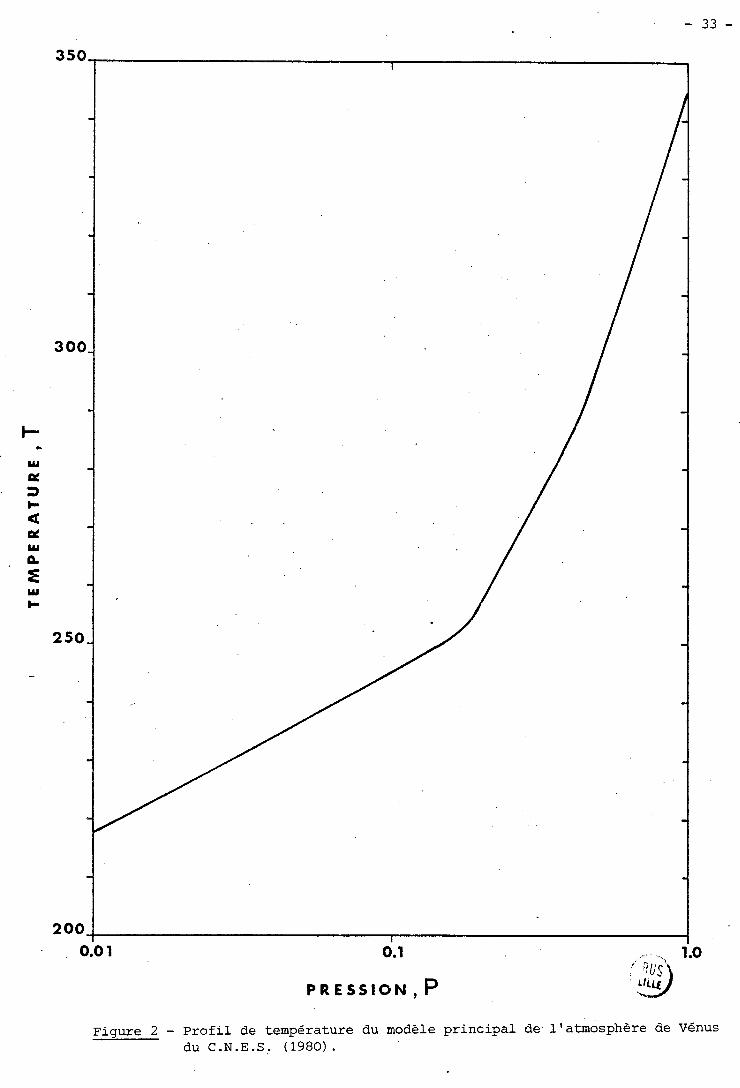
de YOUNG et al '-l1 ou celles de DIERENFELDT et al En utilisant le profil - - de température (Fig. 2) du modèle principal de l'atmosphère de Vénus du

C.N.E.S. l3 - tenant compte des résultats des Venera 11 et 12 et de Pioneer- Venus - une température de 24S0 K correspond à une pression de l'ordre de

0,10 atm.

Nous avons simulé numériquement les processus d'absorption dans deux

types d'atmosphères - une atmosphère claire et une atmosphère nuageuse - qui, pour les mêmes conditions d'observations (les angles d'incidence et d'émer-

'L gence étant O = = 45'), correspond.ent à une pression moyenne P égale à

0,10 atm. Nous avons alors calculé les largeurs équivalentes de raies en

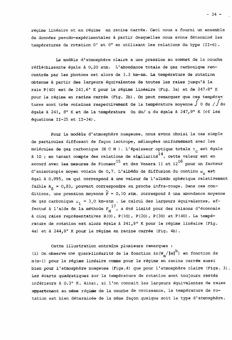
régime linéaire et en régime en racine carrée. Ceci nous a fourni un ensemble

de données pseudo-expérimentales à partir desquelles nous avons déterminé les

températures de rotation O' et O" en utilisant les relations du type (11-6).

Le modèle d'atmosphère claire a une pression au sommet de la couche

réfléchissante égale à 0,20 atm. L'abondance totale de gaz carbonique ren-

contrée par les photons est alors de 3.3 km-am. La température de rotation

obtenue à partir des largeurs équivalentes de toutes les raies jusqu'à la

raie P(40) est de 241,6O K pour le régime linéaire (Fig. 3a) et de 24718~ K

pour le régime en racine carrée (Fig. 3b). On peut remarquer que ces tempéraz

tues sont très voisines respectivement de la température moyenne l' O du / 1 au égale à 241, 8O K et de la température Oa du/ a du égale à 247,g0 K (cf les

équations 11-25 et 11-34).

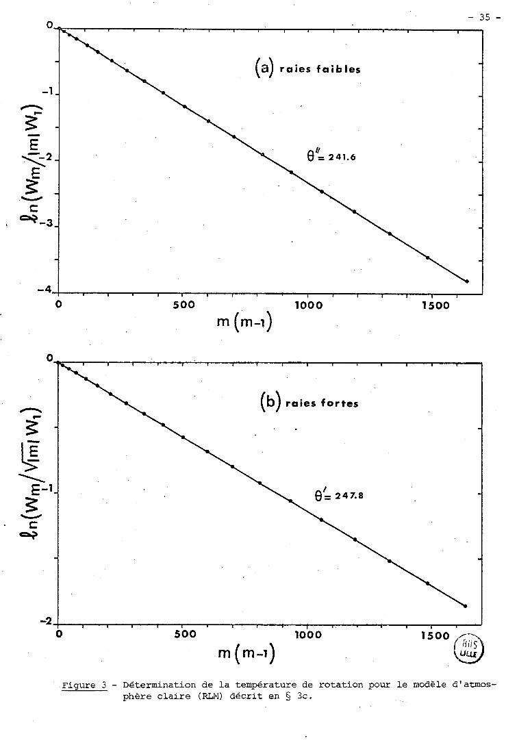
Pour le modèle d'atmosphère nuageuse, nous avons choisi le cas simple

de particules diffusant de façon isotrope, mélangées uniformément avec les

molécules de gaz carbonique (H C M ) . L'épaisseur optique totale rc est égale

à 10 ; en tenant compte des relations de similarité14, cette valeur est en

accord avec les mesures de Pioneer15 et des Venera 11 et 1216 pour un facteur

d'anisotropie moyen voisin de 0,7. L'albédo de diffusion du continu wc est

égal à 0,995, ce qui correspond à une valeur de l'albédo sphérique relativement

faible A = 0,83, pouvant correspondre au proche infra-rouge. Dans ces con- s <L

ditions, une pression moyenne P = 0,lO atm. correspond à une abondance moyenne

de gaz carbonique p = 3,O km-atm . Le calcul des largeurs équivalentes, ef- 1

fectué à l'aide de la méthode F~~~ , a été limité pour des raisons d'économie à cinq raies représentatives R(0) , P ( 10) , P (20) , P (30) et P (40) . La tempé- rature de rotation est alors égale à 241,g0 K pour le régime linéaire (Fig.

4a) et à 244,8O K pour le régime en racine carrée (Fig. 4b).

Cette illustration entralne plusieurs remarques : b

(i) On observe une quasklinéarité de la fonction Rn(W /lm1 ) en fonction de m

m(m-1) pour le régime linéaire comme pour le régime en racine carrée aussi

bien pour l'atmosphère nuageuse (Figs.4) que pour l'atmosphère claire (Figs. 3).

Les écarts quadratiques sur la température de rotation sont toujours restés

inférieurs à 0,3O K. Ainsi, si l'on connait les largeurs équivalentes de raies

appartenant au même régi* de la courbe de croissance, la température de ro-

tation est bien déterminée de la même façon quelque soit le type d'atmosphère.

.Figure 3 - Détermination de l a température de ro ta t ion pour l e modèle d'atmos- phère c l a i r e (FUN) déc r i t en § 3c.

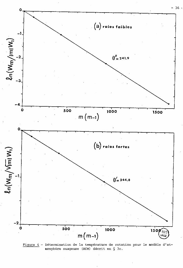
Figure 4 - Détermination de la température de rotation pour le modèle d'at- mosphère nuageuse (HCM) décrit en § 3 c .

(ii) Alors que les deux types d'atmosphères donnent une température de rota-

tion des raies faibles 0" % 242' KI on observe bien pour les raies fortes

une température de rotation correspondant à une pénétration moins profonde

en atmosphère nuageuse (O' f l ~ 245' K) qu'en atmosphère claire ( 0 ' 2, 248' KI . *pendant, même pour le modèle d'atmosphère nuageuse - pour lequel l'indicateur de diffusion a une valeur relativement petite : r = 0.36 - la température de rotation 0' des raies fortes reste plus élevée que la température de ro-

tation 0" des raies faibles. D'autre part, dans le cas limite OU r + O, toutes

les raies appartiennent au régime en racine carrée et correspondent donc à

la mgme température. Il est donc plus aisé de définir une température pour

toute la courbe de croissance en atmosphère nuageuse qu'en atmosphère claire 12

(contrairement aux idées communément admises ; voir DIERENFELDT et al par - exemple) . (iii) Les écarts observés entre l'abondance apparente U" calculée à partir

de 1 'origine de la courbe in (W / m ) en fonction de m(m-1) à l'aide de rela- m tions du type (11-6) et (11-7) (avec b=l) et l'abondance réelle p rencontrée 1 en moyenne par les photons en absence d'absorption sont inférieurs au mil-

lième en valeur relative aussi bien pour l'atmosphère claire (Fig. 3a) que

pour l'atmosphère nuageuse (Fig. 4a). Une telle précision a été obtenue éga- - lement en ce qui concerne les raies fortes en comparant la quantité au' cal-

culée à partir des courbes 3b et 4b et le produit de l'abondance réelle

moyenne p par la demi-largeur de LORENTZ associée à la température de rota- 1 tion 0' et à la pression r8.

(iiii) Incidemment, on peut essayer de vérifier la compatibilité entre la dé-

termination des températures de rotation ( % 240 ou 250' K) issues des mesures

expérimentales de largeurs équivalentes et la connaissance actuelle de l'at-

mosphère de Vénus. Nous avons comparé notre modèle d'atmosphère nuageuse avec

le modèle préliminaire de la structure de Vénus déduit des mesures de distri-

bution des particules lors de la descente de la sonde pioneer15. La figure 5

représente l'épaisseur optique isotrope equivalente obtenue à l'aide des re-

lations de similarité14 d'une part en utilisant un facteur d'anisotropie

g n, 0.7 pour toutes les particules (modèle A de la figure 5), d'autre part en

utilisant un facteur d'anisotropie g % 0.2 pour les plus petites particules

(celles du "mode 1" dans le modèle de TOMASKO et a115) et g % 0.7 pour les

autres particules (modèle B de la figure 5). Ce dernier modèle, plus réaliste,

est beaucoup plus proche du modèle qui a servi pour notre illustration. On

peut observer sur la figure 5 que même avec ce modèle B on sonde des niveaux

de pressions plus élevées qu'avec notre modèle de nuage homogène puisque r C

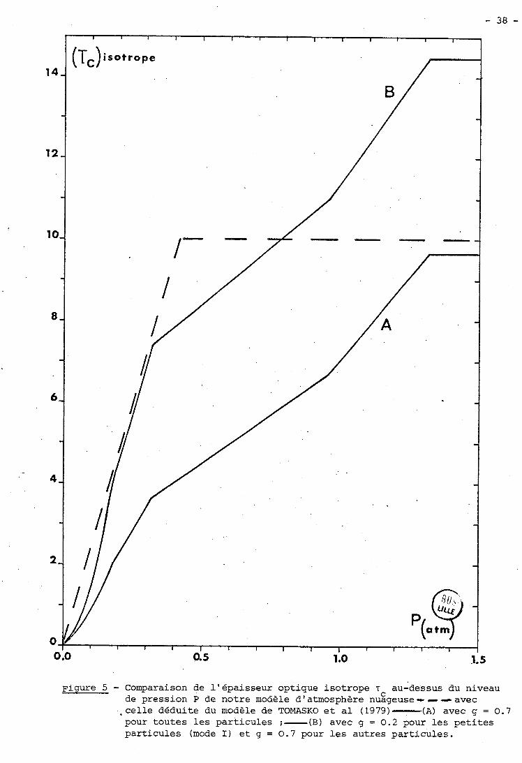
~ i g u r e 5 - Comparaison de l ' épa i s seu r optique isotrope T au-dessus du niveau C

de pression P de notre modèle d'atmosphère nuageuse---avec . ce l l e dédui te du modèle de TOMASKO e t a l ( 1979) - (A) avec g = 0.7 pour t ou t e s l e s par t i cu les ;- (B) avec g = 0 . 2 pour l e s p e t i t e s par t i cu les (mode 1) e t g = 0.7 pour l e s autres par t i cu les .

y augmente moins rapidement avec la pression, ce qui correspondrait à des

températures de rotation supérieures à 245' K. Cet effet serait amplifié si

l'albédo de diffusion du continu w était très proche de 1 comme ce doit C

être le cas aux environs de 0,6 um. Cependant, étant donnée l'incertitude

liée au profil de température (% 10' K), il apparait que le modèle prélimi-

naire de la structure nuageuse de Vénus reste compatible avec des températures

de rotation de l'ordre de 240 - 250' K. Il ne semble pas toutefois que la dé-

termination de la température de rotation puisse être un argument décisif pour

éliminer tel ou tel modèle atmosphérique à cause des incertitudes très grandes

liées à la mesure des largeurs équivalentes de raies.

IV - MESURE DES LARGEURS EQUIVALENTES

Dans ce qui précède, on a vu que l'on pouvait conserver la même tech-

nique que celle établie pour le simple modèle de la "couche réfléchissante"

pour déduire à partir des largeurs équivalentes de raies une température de

rotation (ou des températures de rotation assez voisines pour les régimes

extrêmes), l'abondance de gaz absorbant rencontrée en moyenne par les photons % %

en absence d'absorption, et la pression rP produit de la pression moyenne P

par l'indicateur de diffusion r. Ceci revient à dire que si l'on connait les

largeurs équivalentes de raies d'absorption, on peut en déduire ces quantités

(température, abondance, pression) sans faire d'hypothèse préalable sur la

structure de l'atmosphère étudiée.

En pratique, cependant, on ne peut pas mesurer directement une lar-

geur équivalente W définie pour un intervalle de fréquence infini. On doit

se contenter de la mesure correspondant à un intervalle de fréquence fini, qui

peut être relativement faible à cause du recouvrement des raies. Nous allons

voir que l'extrapolation de la valeur de W à partir de cette mesure peut dé-

pendre fortement du modèle d'atmosphère envisagé.

Les raies d'absorption ne peuvent être mesurées que sur un intervalle

de fréquence 2 Av fini. De plus, la connaissance du niveau continu 1 est C

d souvent incertaine. On mesure donc une quantité W limitée par un niveau 1

O

et un intervalle de fréquence 2Av,

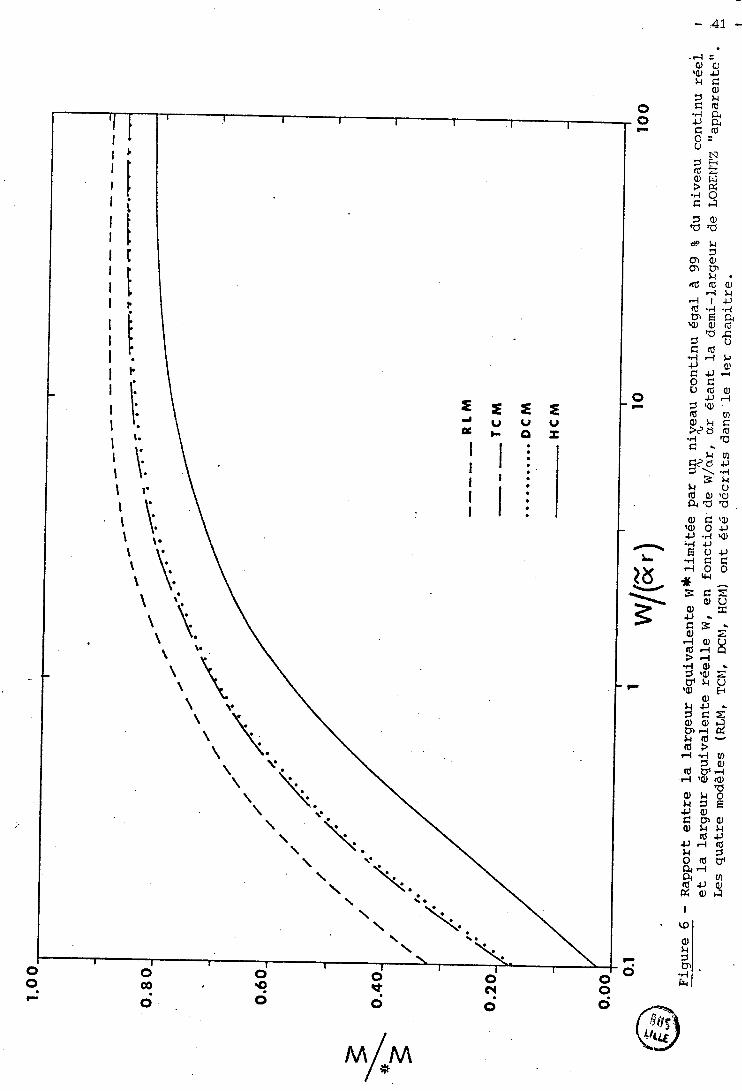
Pour chacun des modèles d'atmosphères décrit dans le premier chapitre,

les quantités W* ont été calculées, à l'aide de l'approximation de .

CURTIS-GODSON généralisée, pour un niveau 1 égal à 99 % du niveau continu O

réel 1 sur un intervalle de fréquence 2av défini par I(aV)_ Io. Les rapports * c

W /W sont reportés sur la figure 6, en fonction de W/(ar), W étant la largeur %

équivalente réelle et ar la demi-largeur de LORENTZ "apparente". Ces rapports * W /W diminuent évidemment avec W mais aussi avec r. Ceci apparait clairement

sur la figure 6 où r varie de 1 (RLM) à 0,35 (HCM) . On peut le mettre en évi- dence de façon analytique en réécrivant l'équation (11-32) sous la forme

L'intégrale peut être calculée en supposant Av >>a(O,P) de sorte que le coef-

ficient d'absorption devienne

ou encore que l'intensité puisse être mise sous la forme (cf Equ. 1-5)

(V - V >/ Av) O

En limitant le développement en série de l'exponentielle au ler ordre, l'é-

quation (11-33) devient alors

Dans le cas où 1 (Av) 5 1-, on obtient

soit, pour les régimes extrêmes, en tenant compte d'une relation du type

-d rl 7 tn

'al k

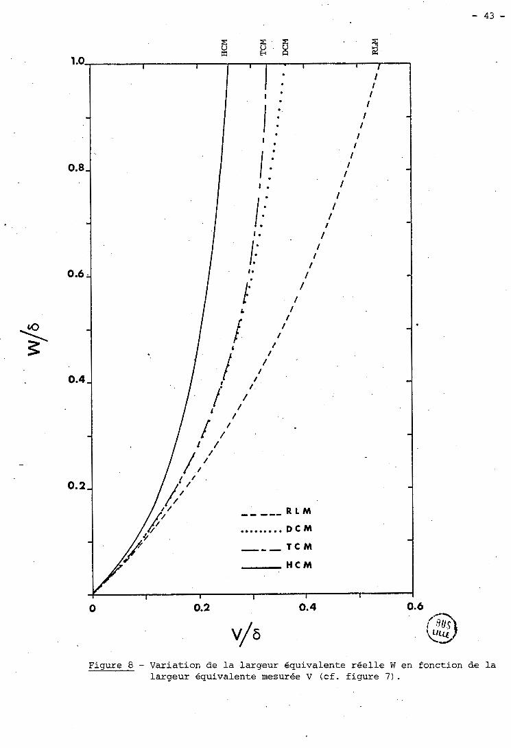
Figure 8 - Variation de l a largeur équivalente r é e l l e W en fonction de l a largeur équivalente mesurée V (.cf. figure 7 ) .

Pour une largeur équivalente W correspondant à une pression apparente r3, l'é- *

cart entre W et W varie en 1 / Jr. L'extrapolation de la largeur équivalente

w à partir d'une mesure de W* dépend donc du modèle d' atmosphère envisagé. Pou, * W-W

les raies faibles (b = 1) , 1 'écart relatif -- W

varie comme 1 / JW alors que

pour les raies fortes (b = 1/2), cet écart est indépendant de la largeur équi-

valente elle-même.

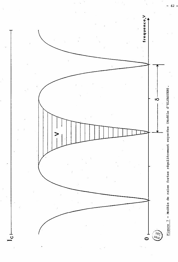
En fait, en ce qui concerne les raies fortes, l'incertitude est beau-

coup plus importante à cause du recouvrement des raies. Pour illustrer ce pro-

blème, nous avons considéré un modèle régulier du type ELSASSER. Les raies

fortes de même intensité sont régulièrement espacées d'un intervalle . Nous avons calculé, pour les différents modèles d'atmosphères illustrant le premier

chapitre, la largeur équivalente "apparente" VI hachurée sur la figure 7, et

la largeur équivalente W qui serait obtenue pour une raie isolée. La figure 8

montre clairement que la relation entre W et V dépend du modèle d'atmosphère - 1

envisagé. Par exemple, une largeur équivalente mesurée V 2, 0,4 cm pour un - 1 - 1

intervalle 6 2, 2 cm correspond à une largeur équivalente W égale à 0,47 cm - 1

pour 1 'atmosphère claire (FUN) , à 0,57 cm pour le nuage dispersé (DCM) ou - 1

pour le modèle à 2 nuages (TCM) et à 0,94 cm pour le nuage homogène (HCM) ;

autrement dit, à une mesure de V correspond dans ce cas une valeur de W

double avec le HCM que celle obtenue avec le FUN. -

Ainsi, l'extrapolation des valeurs de W à partir des mesures dépend de

l'hypothèse faite sur le type d'atmosphère, et donc la température de rotation

et l'abondance "apparentes" qui sont déduites des mesures, peuvent être très

différentes de la température et de l'abondance qui auraient été déduites à

partir des valeurs exactes des largeurs équivalentes.

V - FG3SUME ET CONCLUSIONS

1 - Les largeurs équivalentes de raies formées en atmosphère diffusante inhomogène suivent pratiquement la même courbe de croissance que si elles

étaient formées dans une atmosphère claire dans laquelle l'abondance totale de

gaz absorbant serait égale à l'abondance p de gaz absorbant rencontrée en 1

moyenne par les photons en absence d'absorption, et pour laquelle la pression 2,

de formation des raies serait égale au produit de la pression moyenne P par

l'indicateur de diffusion r.

2 - Les températures de rotation peuvent être déterminées de la même façon quelque soit le type d'atmosphère. En toute rigueur, la température

de rotation des raies fortes est différente de celle de raies faibles. Cepen-

dant l'écart entre ces températures de rotation est encore plus faible en

atmosphère diffusante qu'en atmosphère claire.

3 - En pratique, la mesure de la largeur équivalente d'une raie isolée et définie sur un intervalle de fréquence infini n'est pas possible. Sa valeur est

extrapolée à partir d'une mesure correspondant à un intervalle de fréquence

limité. Cette extrapolation dépend du modèle d'atmosphère envisagé. S'il s'a-

git d'une atmosphère nuageuse et que l'on effectue cette extrapolation en

faisant l'hypothèse d'une atmosphère claire, alors on sous-estime les valeurs

des largeurs équivalentes ; ceci peut entraîner une erreur sur la température

de rotation et une sous-estimation de l'abondance moyenne de gaz absorbant.

R E F E R E N C E S

1 - KUIPER G.P. , The Atmospheres of the Earth and Planets, Univ. of Chicago Press (1952) .

2 - GOODY R.M., Atmospheric Radiation 1. Theoretical basis, Clarendon Press (1964) .

3 - GRAY YOUNG L. , Icarus 11, 66 ( 1969) . - 4 - MARGOLIS J.S. and FOX K., Astrophys. J. 157, 935 (1969). - 5 - SAGAN C. and REGAS J., Comm. Astroph. Space Phys. 2, 161 (1970). - 6 - YOUNG L.D.G., Icarus 17, 632 (1972). - 7 - SCHORN R.A.J., WOSZCZYK A. and YOUNG L.D.G., Icarus 25, 64 (1974). - 8 - YOUNG L.D.G., YOUNG A.T. and WOSZCZYK A., Icarus 25, 239 (1975). - 9 - YOUNG L.D.G., SCHORN R.A.J. and YOUNG A.T., Icarus 30, 559 (1977). - 10 - YOUNG A.T., YOUNG L.D.G. and SCHORN R.A.J., Icarus 34, 46 (1978). - 11 - SCHORN R.A.J., YOUNG A.T. and YOUNG L.D.G., Icarus 38, 420 (1979). - 12 - DIERENFELDT K.E., FINK U. and LARSON H.P., Icarus 14, 11 (1977). - 13 - Modèle d'atmosphère de Vénus - Actualisation janvier 80, Projet Vénus,

Centre National dlEtudes Spatiales, France (1980).

14 - VAN DE HULST H.C. and GROSSMAN K., in The Atmospheres of Venus and Mars, BRANDT J.C. and McELROY M.B. Ed.,Gordon & Breach, 35 (1968).

15 - TOMASKO M.G., DOOSE L.R. and SMITH P.H., Science 205, 80 (1979). - 16 - MOROZ V.I., GOLOVIN Yu.M., EKONOMOV A.P., MOSHKIN B.E., PARFENT'EV N.A.,

SAN'KO N.F., Nature 284, 243 (1980). - 17 - DEVAUX C., GRANDJEAN P., ISHIGURO Y. and SIEWERT C.E., Astrophys. Space

Sci., 2, 225 (1979) .

C H A P I T R E III

LES LARGEURS EQUIVALENTES DE RAIES EN SPECTROPOLARIMETRIE

Les spectres à haute résolution enregistrés entre 1,2 et 2,5 m par CONNES et & en 1966 ont permis un important approfondissement de la connaissance de l'atmosphère de Vénus. Avant p&ne les premières mesures" in

situ" effectuées lors de la descente de Venera IV en octobre 1967, on con-

sidérait que "CO est probablement le constituant majeur dans l'atmosphère 2 de Vénus", on savait que les raies d'absorption étaient formées dans une

couche nuageuse située aux environs de 0, l atm à une température Q 240" KI

et on connaissait les rapports de mélange des gaz mineurs tels que HCR ou

HF avec une bonne précision. De même, l'analyse de la raie de la vapeur O

d'eau à 8189 A montra que "les nuages sont composés d'une autre substance

que la glace"2.

3 D'un autre côté, HANSEN et ARKING interprétèrent les mesures de

polarisation sur Vénus et déterminèrent l'indice de réfraction et le rayon

moyen des particules situées aux environs de 0,05 atm . C'est essentiellement la prise en compte des résultats de la spectroscopie quantitative et de la

polarimétrie qui mit en évidence que les nuages visibles de Vénus sont for- 4

més d'une solution aqueuse d'acide sulfurique .

Puisque les phénomènes d'absorption affectent chacun des paramètres

de STOKES (I,Q,U,V) , il est séduisant .d'associer la spectroscopie et la po- larimétrie. Le but de l'article qui suit est de voir quelles informations

peuvent être fournies par la spectropolarimétrie en plus des informations

données par la spectroscopie et par la polarimétrie.

On a défini par l'équation (1-5) la fonction de distribution "d'a- %

bondance pondérée" u de gaz absorbant. De façon similaire, on p u t définir

pour chacun des paramètres X = 1, QI U, VI une fonction de distribution %

p (X,u) définie par

(III- 1)

Pour une première approche de la spectropolarimétrie, nous avons utilisé

le simple modèle diffusant homogène (HSM), dans lequel toutes les caracté-

ristiques de l'atmosphère, y compris la pression, restent constantes. Ce

modèle simple avait permis de mettre en évidence le rôle joué par les par-

ticules diffusantes dans l'atmosphère de Vénus par l'interprétation des

2 largeurs équivalentes5 et des profils de raies correspondant à l'intensité

totale 1. Dans une couche diffusante homogène, l'abondance de gaz rencontrée

le long d'un trajet de longueur L est

2 M étant "l'abondance spécifique" , u! l'albédo de diffusion continu et A

C 6

le chemin optique introduit par VAN DE HULST et IRVINE A = (a+ kc) LI a et

k étant les coefficients de diffusion et d'absorption des particules. Pour C

le modèle diffusant homogène (HSM) il est alors plus simple d'utiliser les

fonctions de distributions p(X,A) qui ne dépendent que des caractéristiques %

des particules diffusantes. Les fonctions de distributions p(X,u) leur sont

reliées par la relation

Dans l'article concernant les largeurs équivalentes de raies en

spectropolarimétrie, nous utilisons donc des distributions de chemin op-

tique, mais la généralisation à n'importe quel type d'atmosphère inhomogène

peut être faite à l'aide des distributions "d'abondance pondérée" qui peuvent

être calculées d'une façon similaire à celle décrite dans le premier cha-

pitre .

R E F E R E N C E S

1 - CONNES P . , CONNES J . , BENEDICT W.S. a , d KAPLAN L.D. , A s t r o p h y s . J. 147, - 1 2 3 0 ( 1 9 6 7 ) .

2 - BELTON M.J .S . , HUNTEN D.M. and GOODY R.M. i n the A t m o s p h e r e s of V e n u s

and M a r s , BRANDT J - C . and McELROY M.B. Ed . , GORDON & BREACH, 69 ( 1 9 6 9 ) .

3 - HANSEN J . E . and ARKING A. , Science 171, 669 ( 1 9 7 1 ) . - 4 - YOUNG A . T . , Icarus 18, 546 ( 1 9 7 3 ) . - 5 - BELTON M.J .S . , J. Atm. Sci. 25, 596 ( 1 9 6 9 ) . - 6 - VAN DE HULST H.C. and IRVINE W.M., i n L a P h y s i q u e des P l a n è t e s , C o n g r è s

e t C o l l o q u e s de l ' un ive r s i t é de L i è g e 24 , 78 ( 1 9 6 2 ) .

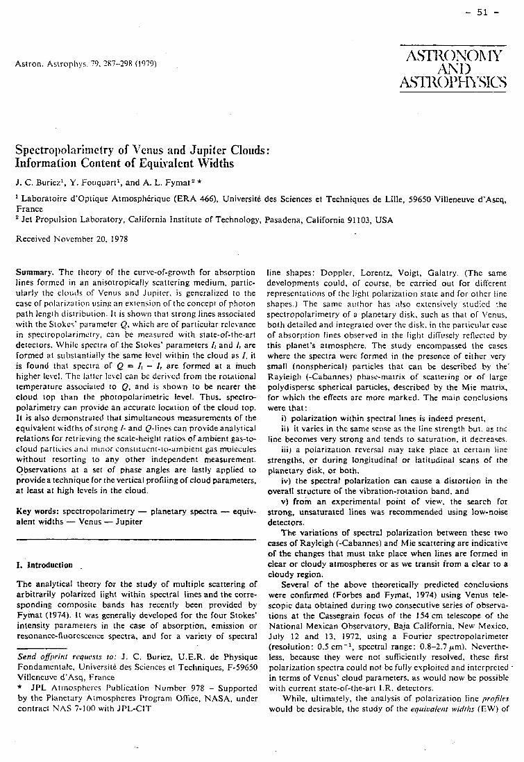
Astron. Astropliys. 79. 287-298 (1979)

Spectropolarimetry of Venus arid Jupiter Clouds: Information Content of Equivalent Widths

J. C. Buriczl, Y. Fouquart', and A. L. Fymat2 * ' Laboratoire d'optique Atniosphérique (ERA 466), Université des Sciences et Techniques de Lille, 59650 Villeneuve d'Ascq, France

Jet Prop~ilsion Laboratory, California Institute of Technology, Pasadena, California 91 103, USA

Received Novembcr 20, 1978

Summary. The theory of the curve-of-growth for absorption lines formcd in an anisotropically scattering medium, particularly tlic cloutis of Venus and Jupiter, is generalized to the case of polarization using an extension of the concept of photon path length distribution. I t is showii thrit stronp lines associated with the Stokes' paranleter &, whicti arc of particular relevance in spectropolarimctry, can be mcasured with state-of-the-art detectors. Whilc spectra of the Stokes' parameters Il and 1, are forrned at sübstantially the same level within the cloud as 1, it is found that spectra of Q = Il - 1, are formed at a much tiigher Ievel. Thc luttcr Icvcl can bc derivcd from the rotational temperature associalcd to Q, and is shown to be nearer the cloud top than the photopolarimetric level. Thus, spectropolarirnetry can provide an accurate location of the cloud top. l t is also demonstrated that sirnultaneous measurernents of the eqiiivalent uidths of strong 1- and Q-lincs can provide analytical relations fcr retrieving the scalc-heigtit ratios of arnbient gas-to- cloud particles anli rninor ions~itur.nt-to-amoient gas mlocules without resorting to any other independent measurernent. Observations at a set of phase angles are lastly applied to providea technique for the vertical profiling of cloud pararneters, a t least at high levels in the cloud.

Key words: spectropolarirnetry - planetary spectra - equivalent widths - Venus - Jupiter

1. Introduction .

The analytical theory for the study of multiple scattering of arbitrarily polarized light within spectral lines and the corresponding composite bands has recently been provided by Fymat (1974). It was generally developed for the four Stokes' intensity parameters in the case of absorption, ernission or resonance-fluorescence spectra, and for a variety of spectral

Send ofll)ririt rcqupsts IO: J. C. Buriez, U.E.R. de Physique Fondamentale, Université des Sciences et Techniques, F-59650 Villeneuve d'Asq, France * JPL Atinospheres Publication Nuniber 978 - Supported by thc Planctary Atmospheres Program Office, NASA, under contraci N A S 7-100 with JPL-CIT

line shapes: Doppler, Lorentz, Voigt, Galatry. (The same developments could, of course, be carried out for diffèrent represcntations of thc liglit polarizatiori state and for othcr line shapes.) The same author has ;ils0 cxtcnsivcly stiidicd the spectropolarimetry of a planetary disk, such as that of Venus, both detailcd and integrated over thc disk, in the particular case of absorption lines observed in the liglit difusely ref1rc:ed by this planet's atmosphere. The study encompassed the cases where the spectra were formed in the presence of either very srnall (nonspherical) particles that can be described by the' Rayleigh (-Cabannes) phase-matrix of scatteiing or of large polydispersc spherical particles, described by the Mie matrix, for which the eKects are more marked. The main conclusions were that :

i) polarization within spectral lines is indeed present, ii) it varies in the same sense as the line strençth but. as thc

line becomes very strong and tends to saturation. it decreases. iiil a polarization reversai may raite place ar certain iine

strengths, or during longitudinal or iatitudinal scans of the planetary disk, or both,

iv) the spectral polarization can cause a distortion in the overall structure of the vibration-rotation band, and

V) frorn an experirnental point of view, the search for strong, unsaturated lines was recornmendrd using low-noise detectors.

The variations of spectrrl polarization between these two cases of Rayleigh (-Cabannes) and Mie scattering are indicative of the. changes that rnust take place when lines are formed in clear or cloudy atrnospheres or as we transit from a clear to a cloudy region.

Several of the above theoretically predicted conclusions were confirrned (Forbes and Fymat, 1974) using Venus tele- scopic data obtained during two consecutive series of observations at the Cassegrain focus of the 154 cm telescope of the National Mexican Observatory, Baja California, New Mexico. July 12 and 13, 1972, using a Fourier spectropolarimeter (resolution: 0.5 cm-', spectral range: 0.8-2.7 p m ) Neverthe- less, because they were not suficicntly resolved, these first polarization spectra could not be fully exploitcd and interpreted . in terms of Venus' cloud parameters, as would now be possible with current state-of-the-art 1.R. detectors.

While, ultimately, the analysis of polarization line profiles would be desirable, the study of tlic equiualetrt wiclrlls (EW) of

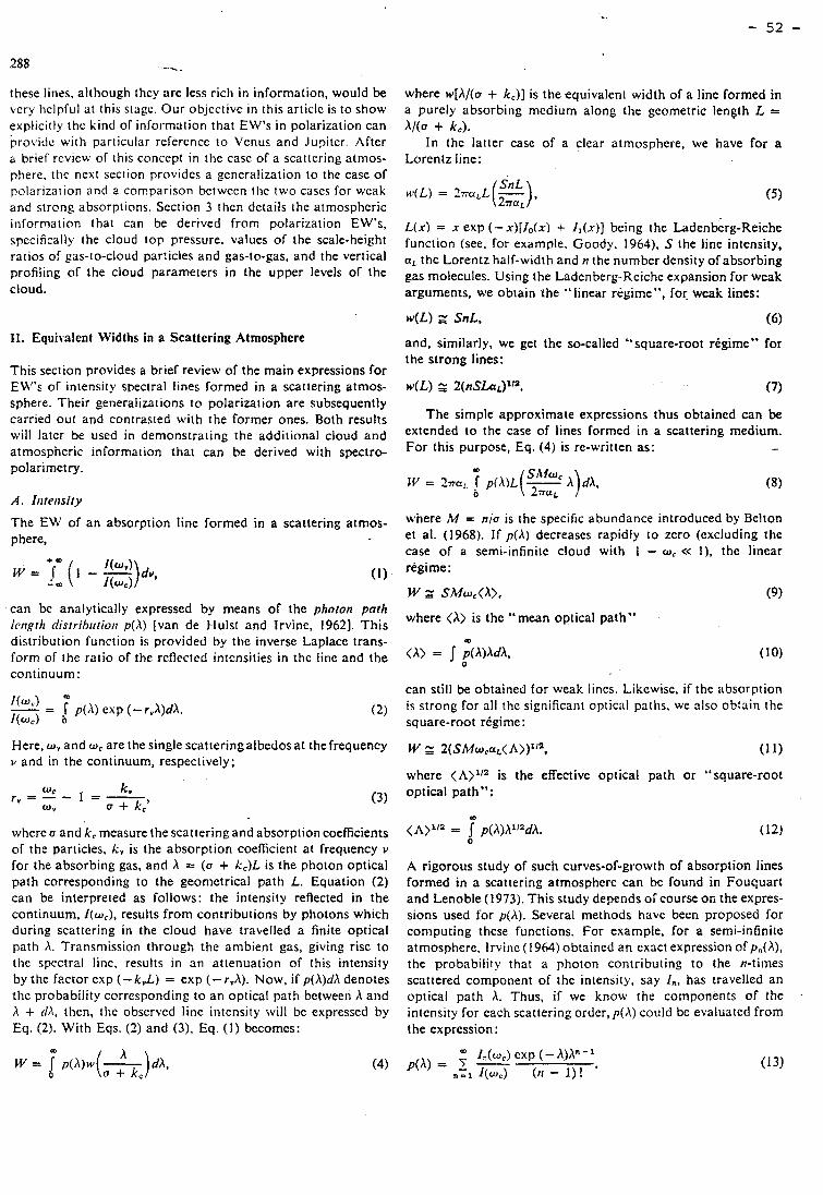
these linrs, although they are less rich in information, would be vcry hclpful rit this strige. Our objective in this articlc is to show explicitly the kind of information that EW's in polarization can provide with particular refercnce to Venus and Jupiter. After a brief review of this concept in the case of a scattering atmosphere. tlie next section provides a generalization to the case of polarizaiion and a cornparison between the two cases for weak and strong absorptions. Section 3 thcn details the atmosphcric information that can be derived from polarization EW's, specificalty the cloud top pressure. values of the scale-height ratios of gas-to-cloud particles and gas-to-gas, and the vertical profiling of the cloud parameters in the upper levels of the cloud.

I l . Equivalent Widths in a Scattering Atmosphere

This section provides a brief review of the main expressions for EW's of intensity spectral lines formed in a scattering atmos- sphere. Their generalizations to polarization are subsequently carried out and contrasted with the former ones. Both results will later be used in demonstraiing the additional cloud and atmospheric information that can be derived with spectropolarimetry.

The EW of an absorption linc formed in a scattering atmosphere,

can be analytically expressed by means of the photon parh lcrrgth distribrrtion p(h) [van de k-lulst and Irvine, 19621. This distribution function is provided by the inverse Laplace transform of the ratio of the reflectcd intcnsities in the line and the continuum:

m

- - '(Wb' - 1 p(h) exp (-r.A)dh. I(wc) 0

(2)

Here, w, and w, are the single scatteringalbedosat the frequency v and in the continuum, respectively;

where O and k , measure the scattering and absorption coefficients of thc particles, k , is the absorption coefficient at frequency v for the absorbing gas, and h = (o + k,)L is the photon optical path corresponding to the geometrical path L. Equation (2) car) be interpreted as follows: the intensity reflected in the continuum. I(w,), results from contributions by photons which during scattering in the cloud have travelled a finite optical path A. Transmission through the ambient gas, giving rise to the spectral linc, results in an attenuation of this intensity by the f ~ c t o r exp (- k,L) = exp (- r,h). Now, if p(h)dh denotes the probability corresponding to an optical paf h between h and h + rlh, tlien, the observed liiie intensity will be expressed by Eq. (2). With Eqs. (2) and (3). Eq. (1) bccomes:

where w[X/(u + kc)] is tlie equivalent width of a line formed in a purely absorbing mcdium along the gcometric iength L = A/(. + kc).

In the latter case of a clear atmosphere, we have for a Lorentz line:

L(x) = x exp (-x)[l,,(x) + I,(x)] being the ~ a d e n b i r g - ~ e i c h e function (see, for example, Goody, 1964). S the line intensity, a, the Lorentz half-width and n the number density of absorbing gas molecules. Using the Ladenberg-Reiche expansion for weak arguments, we obtain the "linear régime", for weak lines:

and, similarly, we get the so-called "square-root régime" for the strong lines:

The simple approximate expressions thus obtained can be extended to the case of lines formed in a scattering medium. For this purpose, Eq. (4) is re-written as: -

where M = n/o is the specific abundance introduced by Belton et al. (1968). If p(A) decreases rapidly to zero (excluding the case of a semi-infinite cloud with 1 - w, << l ) , the linear régime:

where (A) is the "mean optical path"

can still be obtained for weak lines. Likewise, if the absorption is strong for al1 the significant optical paths, we ulso obtain the square-root régime:

where (A)112 is the effective optical path or "square-root optical path":

A rigorous study of such curves-of-growth of absorption Iines formed in a scattering atmosphere can be found in Fouquart and Lenoble (1973). This study depends or course on the expressions used for p(A). Several methods have been proposed for computing these functions. For example, for a semi-infinite atmosptiere, lrvine (1964) obtained an exact expression of p,(h), the probability that a photon contributing to the n-limes scattered cornpolient of the intensity, say ln, has travelled an optical path h. Thus, if we know the components of the intensity for each scattering ordcr,p(h) could be evaluated from the expression :

" I,(w,) exp (- A)Xn-l P ( ~ ) = , , Z ~ = ( n - I ) ! .

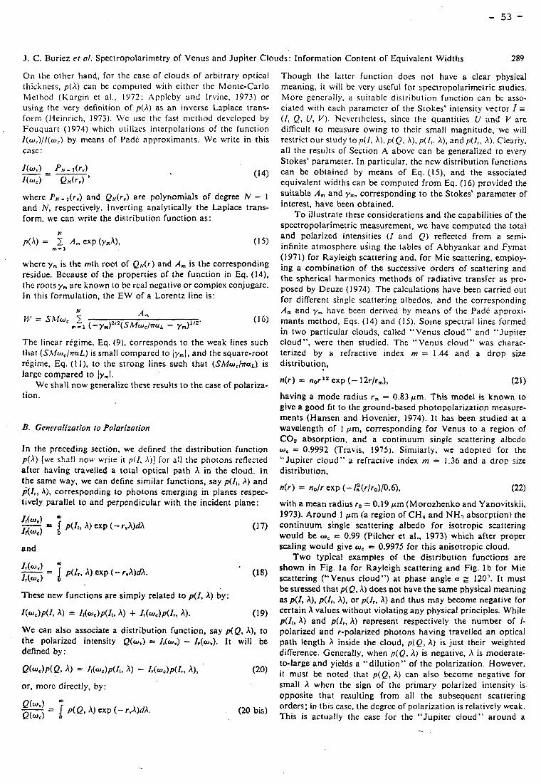
J. C. Buriez et 01. Spectropolarirnetry of Venus and Jupiter Clc ~uds : Information Content of Equivalent Widths 289

On the oiher hana, for the case of clouds of arbitrary optical tiiickncss, p(X) can be conipiiied with either the Monte-Carlo Mcthod (Kargin et al.. 1972; Applcby and Irviiic. 1973) or using the very definition of p(X) as an inverse Laplace transform (Heinrich. 1973). M'c lise tlie fast rncthod cievclopcd by Fouquart (1974) which utilizes interpolations of the function I(w,)/l(w,) by means of Padé approxirnants. We urrite in this case :

where P N - l(rV) and QN(rv) are polynornials of degree N - 1 and N, respectively. lnverting analytically the Laplace transform, we can write the distribution function as:

where y, is the mth root of QN(r) and A, is the corresponding residue. Bccause of the properties of the function in Eq. (14), thc roots y, are known to bc real negative or cornplex conjugale. In tliis formulation, the EW of a Lorentz line is:

The linear régime. Eq. (9) , corresponds to the weak lines such tliat (SiZIw,/naL) is srnall cornpared to ly,l, and the square-root régime, Eq. ( 1 l), to the strong lines such that (Sh.lwc/7raL) is large compared to [y,l.

WC sliall now generalize these results to the case of polariza- lion.

In the preceding section, we defined the distribution function p(A) [we shnll nou write i t p ( l , A) ] for a11 the photons refiected after having travelled a total optical path A in the cloud. In the sarne way, we can define sirnilar functions, say p(Il, A) and p ( I , , A), corresponding to photons ernerging in planes respectively parallel to and perpendicular with the incident plane:

and

These new functions are simply related to p(I, A) by:

I(UJ~)P(~, A) = It(wc)p(I~> A) + Ir(~~c)p(Ir, A). (19)

WC can also associate a distribution function, Say p(Q, A), to the polarized intensity Q(w,) = Il(wv) - Ir(wv). It will be defined by :

or, more diiectly, by:

<D

- - '(wu' - l p(Q, A) exp (- r.A)dX. Q(w3 o

(20 bis)

Though tlie latter function docs not have a clear physical meaning, i t will be very useful for spectropolarimetric studies. h4orc generally, a suitable distribution function can be associated with eacti parameter of the Stokes' intensity vector 1 r (I. Q, U , V ) . Neverihcless, since the quantities U and V are dificult to mcasure owing to their small magnitude, we will restrict our study top(1, A), p(Q, A), p(I,, A), and p(l,, A). Clcnrly. al1 the results of Section A abovc can be generalized to ewry Stokes' parameter. In particular, the new distribution functions can be obtained by rneans of Eq. (15), and the associated equivalent widths can be computed from Eq. (16) provided the suitable A, and y,, corresponding to the Stokes' parameter of interest, have been obtained.

T o illustrate these considerations and the capabilities of the spectropolarimetric measurement, we have computed the total and polarized intensities ( I and Q) reflected frorn a semi- infinite atrnosphere using the tables of Abhyankar and Fymat (1971) for Rayleigh scattering and, for Mie scattering, ernploy- ing a cornbination of the successive orders of scattering and the spherical harmonies methods of radiative transfer as proposed by Deuze (1974). The calculations have been carried out for diflèrent single scattering albedos, and the corresponding A, and y, have been derived by rneans of the 13adC approximants rnethod, Eqs. (14) and (15). Soine spectral lines formed in two particular clouds, called "Venüs cloud" and "Jupiter cloud", were then studied. The "Venus cloud" was charac- terized by a refractive index nr = 1.44 and a drop size distribution,

n(r) = nor12 exp (- 12r/r,), (21)

having a mode radius r:, = 0.83 Fm. This mode1 is known to givc a good fit to the ground-based photopolarization rneasure- ments (Hansen and Hovenier, 1974). It has been studied at a wavelength of 1 Pm, corresponding for Venus to a region of COz absorption, and a continuum single scattering albcdo UJC = 0.9992 (Tra\is. 1975). Simiiarly, we adopteci for the "Jupiter cloud" a refracrive index m = 1.36 and a drop size distribution,

n(r) = no/r exp (- 1,2(r]r0)/0.6), (22)

with a mean radius ro = 0.19 prn (Morozhenko and Yanovitskii, 1973). Around 1 prn (a region of CH, and NH, absorption) the continuum single scattering albedo for isotropic scattering would be w, = 0.99 (Pilcher et al., 1973) which after proper scaling would give wc = 0.9975 for this anisotropic cloud.

TWO typical exarnples of the distribution functions are shown in Fig. l a for Rayleigh scattering and Fig. Ib for Mie scattering ("Venus cloud") at phase angle a z 120'. It rnust be stressed that p(Q, A) does not have the same physical rneaning as p(I, A), p(Ir. A), or p(Ir, A) and thus may becorne negative for certain values without violating any physical principles. While ~ ( I I , A) and p(l,, A) represent respectiveiy the number of I- polarized and r-polarized photons having travelled an optical path iength A inside the cloud, p(Q, A) is just their weighted difierence. Generally, when p(Q, A) is negative. X is rnoderate- to-large and yields a "dilution" of the polarization. However, it must be noted that p ( Q , A) can also becorne negative for srnall when the sign of the prirnary polarized intensity is. opposite that resulting frorn al1 the subsequent scattering orders; in this case, the degrce of polarization is relatively weak. This is actually the case for the "Jupiter cloud" aiound a

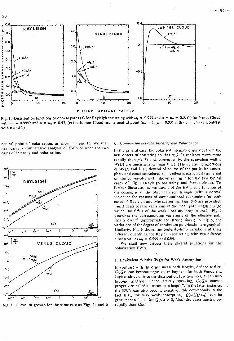
. . . . . . . . . . . . . . . . . . RAYLEIGH

2 0 - ; 0.5. -

VENUS CLOUD

O 10 20

Fig. 1. Distribution functions of optical paths (a) for Rayleigh scattering with w, = 0.999 and p = po = 0.5, (b) for Venus Cloud with w , = 0.9992 and p = po = 0.47, (c) for Jupiter Cloud near a neutral point = 1; p = 0.93) with w , = 0.9975 (contrast with a and b) -

neutral point of polarization, as shown in Fig. Ic. We shall C. Cornparison brtn~eoi Iriloisir~~ aridPolurizariori next carry a comparative analysis of EW's between the two cases of intensity and polarization.

Fig. 2. Curves of growth for the same case as Figs. l a and b

In the general case, the poiarizcd intensity originatcs frorn the first orders of scattcring so that p ( Q . A ) vanishcs much more rapidly than p(I, A) and. consequently, the equivalent widths W ( Q ) are much smaller than lV(1). (The relative proportions of MT(Q) and 1ff(1) depend of course of the particular atmospherc and cloud considered.) This cffcct is particiilnrly apparent on thc curves-of-growth shown in Fig. 2 for the two typical cases of Fig. 1 (Rayleigh scattering and Venus cloud). T o further illustrate, the variations of the EW's as a function of the cosine, p, of the obscrver's zcnith angle (with a normal incidence for reasons of coiiiputitional econornies) for both cases of Rayleigh and Mie scaitcring, Figs. 3-6 are provided: Fig. 3 describes the variations of the mean paih Iength < h i (to which the EW's of thc weak lines arc proportional); Fig. 4 describes the corresponding variations of the effective path lcnpth (appropriate for strong lincs); in Fig. 5, the variations of the degree of continuum polarization are graphed. Sirnilarly, Fig. 6 shows the center-to-lirnb variations of thcse different quantities, for Rayleigli scattering, with two different albedo values w, = 0.999 and 0.99.

We shall now discuss these several situations for the polarization EW's.

1. Equivalent Widths W(Q) for Weak Absorption

In contrast with the other mean path lengths, defined earlier, <X(Q)) can becorne negative, as happens for both Venus and Jupiter clouds, sincc the distribution function p(Q, A ) can also become negative. Hence, strictly speakirig, <X(Q)) cannot properly bc called a "rnean path iength". In the latter instance, the EW's can also beconie negative; this corresponds to the fact that, for very weak absorption, jQ(w,)/Q(w,)l can br: greatcr than 1, Le., for Q(w,) > O, I,(w,) decreases much more rapidly than I,(w,).

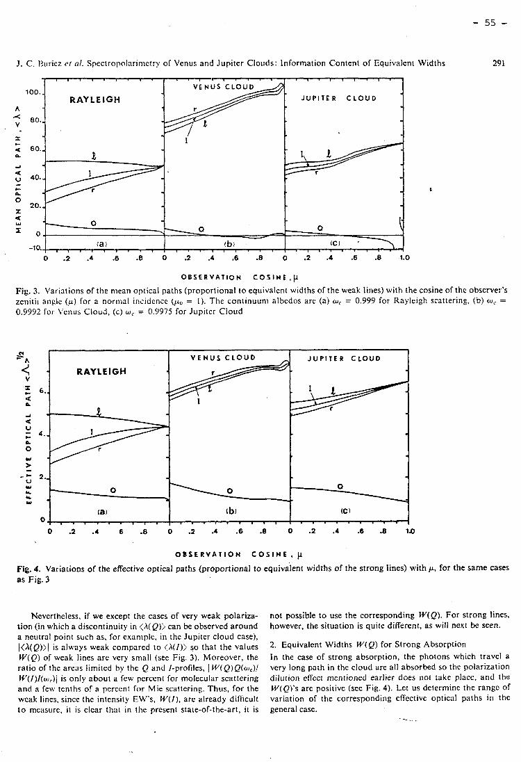
J. C. I3uriez et nl. Spectropolnriinetry of Venus and Jupiter Clouds: Information Content of Equivalent Widths

i i , , , , , , , . 1 1 1 , 1 1 1 .

VENUS CLOUD 100..

RAYLEIGH JUPITER C L O U D

80.-

60.-

- -

O o.

-10. , , , , , , , , , (a 1

O .2 .4 .6 .8 O .2 .4 .6 .8 O .2 .4 .6 .8 1.0

OBSERVATION C O S I N E , p Fig. 3. Variations of the mean optical paths (proportional to equivalcnt widths of the weak liries) with the cosine of the observer's zeiiitli angle ( p ) for a normal incidence (yo = 1 ) . Tlie continuun1 albedos are (a) w, = 0.999 for Kayleigh scattering, (b) OJ, = 0.9992 for Vcnus Cloud, (c) w , = 0.9975 for Jupiter Cloud

V E N U S C L O U D JUPITER C L O U D

RAYLEIGH v x c 6.. u A

- - c - U

2 .. W Y O

O Y b u -

5

ra) cb) (c) O,

V I . . . . . . . . . '

O .2 .4 6 .8 O -2 .4 .6 .8 O .2 .4 .6 .8 1.û

O B S E R V A T I O N C O S I N E ,

Fig. 4. Variations of the effective optical paths (proporticnal to equivalent widths of the strong lines) with p, for the same cases a s Fig. 3

Ncverthcless. if we except the cases of very weak polarization (in which a discontinuity in <h(Q)) can be observed around a ncutral point such as, for exampie, in the Jupitcr cloud case), l<h(Q)>) is always weak compared to (NI)) so that the values W(Q) of weak lines are vcry small (see Fig. 3). Moreover, the ratio of the areas limited by the Q and 1-profiles, 1 W(Q)Q(w,)/ IY(/)I(w,)i is only about a few pcrccnt for molecular scattering and a few tenths of a percent for Mie scattering. Thus, for the wcak lines, since the intensity EW's, W(I), are already difficult t o mcasure, i t is clear that in tlie present state-of-the-art, it is

not possible to use the corresponding W(Q). For strong lines, however, the situation is quite different, as will next be seen.

2. Equivalcnt Widths W(Q) for Strong Absorption

In the case of strong absorption, the photons which travcl a very long path in the cloud arc al1 absorbed so the polarization dilution effect mentioncd earljer does not takc place, aiid tho W(Q)'s arc positive (see Fig. 4). Lct us determine the range of variation of the corresponding effective optical paths in the gencral casc. .- .

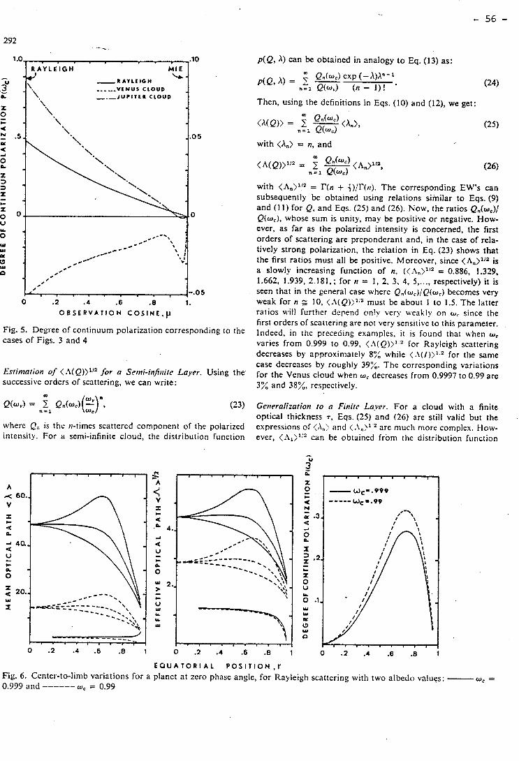
R A Y L E I G H -.-..-VENUS CLOUD ,.-JUPITER CLOUD

O .2 .4 .6 -8 1.

OBSERVATION COSINE, p

Fig. 5. Degree of continuum polarization corresponding to the cases of Figs. 3 and 4

Estintarion of < -l( Q)>li2 for a S~tni-infirite Layer. Using the successive orders of scattering, we can write:

p(Q, A) can be obtained in analogy to Eq. (13) as:

" Qn(wc) exp (- A)An-1 P'Q. A) = ( n - l ) ! '

Then, using the definitions in Eqs. (10) and (12), we get:

with <An) = n, and

with <An>lf2 = r ( n + +)Ir(,). The corresponding EW's can subsequently be obtained using relations similar to Eqs. (9) and (1 1 ) for Q. and Eqs. (25) and (26). Now, the ratios Q,(w,)] Q(wc), whose sum is unity, may be positive or negative. How- ever, as far as the polarized intensity is concerned, the first orders of scattering are preponderant and, in the case of relatively strong polarization, the relation in Eq. (23) shows that the first ratios must al1 be positive. Moreover, since <An>1;2 is a slowly increasing function of n, ((.2,>li2 = 0.886, 1.329, 1.662, 1.939, 2.181,; for 11 = 1, 2, 3, 4. 5 ,..., respectively) it is seen that in the general case where Q,(w,)/Q(wc) becomcs very weak for n 2 10, <.l(Q):1.2 must be about 1 to 1.5. The latter ratios will further depend on!v very ~ e a k i y on w, since the first orders of scattering are not very sensitive to this parameter. Indeed, in the preceding examples. it is found that when w,

varies from 0.999 to 0.99, <"i(Q)>l for Rayleigh scattering decreases by approxiniately 87; while <.l(/)>1.2 for the sanle case decreascs by rouglily 39%. The corresponding variations for the Venus cloud when wc decrcases from 0.9997 10 0.99 are 3% and 38//,, respectively.

m

~ ( w . 1 = n i 1 I: ~ . ( w , > ( % ) ~ , WC

(23) Generalization to a Finite Laver. For a cloud with a finite optical thickness 7, Eqs. (25) and (26) are still valid but the

where Q, is the fi-times scattercd componctit of the polarized expressions of <A,: and are much more complcx. 1-low- intensity. For a semi-infinite cloud, the distribution funciion ever, can be obtained from the distribution function

E O U A T O R I A L P O S I T I O N , r

Fig. 6. Center-to-limb variations for a planet at zero phase angle, for Rayleigh scattering with two albedo values: - w, = 0.999 ;ilid ------ w, = 0.99

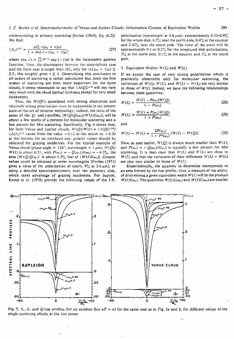
J. C. Buriez rr al. Spectropolarinietry of Venus and Jupiter Clouds: Information Content of Equivalent Widths 293

c&responding to prirnary scattering [Irvine (1964), Eq. (6 .2) ] . We find:

where y(a, x) = 1: t a+ ' exp (- t )d! is the incomplete gamma function. I'hiis, the discrepancy betuceii the semi-infinitc case aiid the finite case is larger than 10% only for 7(1/p0 + 1/p) 5 2.5; this roughly gives 7 5 1. Generalizing this conclusion to al1 orders of scattering is rather speculative but, since the first orders of scattering are even more important for the finite clouds, it seerns reasonable to say that (A(Q)>li2 will not Vary very much with the cloud optical thickncss except for very small thicknesses.

Thus, thc W(Q)'s associated with strong absorption and relatively strong polarization inust be n~easurable in tlie present state-of-the-art of detector technology; indeed, the ratio of the areas of the Q- and 1-profiles, 1 W(Q)Q(w,)/ W(I)l(w,)l, will be about a few tenths of a percent for molccular scattering and a few percent for Mie scattering. Specifically, Fig. 4 shows that, for both Vcnus and Jupiter clouds, 11,'((Z)IW(l) = (A(Q)>lI2/ <h(f ) )1*2 varies from the value -0.13 at the zenith to -0.30 ai the horizon for an overhead Sun; greater values should be obtained for grazing incidences. For the typical example of Venus cloiid (phase angle = ,124"; wavelength = 1 pm), I.V(Q)/ W(I) is about 0.3 1 ; with P(w,) = - &(w,)/l(w,) = -4.37:, the area 1 W(Q)Q(w,)I is about 1.3% that of 1 W(I)l(w,)l. Greater values could be obrained ai other wavelengths [Forbes (1971) gives a value of the polarization of nearly 9% at 3.6pm], or using a detailcd spectropolarimetry over the planetary disk, which takes advantage of grazing incidences. For Jupiter, Kemp et al. (1978) providc the following values of the I.R.

polarization (wavelength = 1.6 pm): approxirnatcly 0.32-0.9% for the whole disk. 6.7% near the north pole, 0.4% at the equator and 2.42% near the soutli pole. The ratio of the arens \vil1 be approximately 0.1 or 0.3y4 for the intcgrated disk polarization, 3% at the north pole, 0.10,; at the equator aiid 1% at thc south pole.

3. Equivalent Widths W(Il) and W(Ir)

If we except the case of very strong polarization which is practically observable only for molecular scattering, the variations of Mf(Il), W(I,), and W(Il) - IY(f,) are very similar to thosc of W(I). Indeed, we have the following relationships between these quantities:

W(Ir) = I+'(I) + P(wc) rY(Q)

1 + P(w,) '

and

Now, as seen earlier, IV(Q) is always müch smailer than U'(I), and P(wC) = - Q(wC)/I(wc) is typically a few percent for Mie scattering. It is then clear that W/(li) and M,'(I,) are close to IY(I), and that the variations of their difference IY(Il) - W(I,) are also very similar to those of CY(I).

Experimentally, the quantity to determine corresponds to an area lirnited by the line profile; thus, a measure of the ability of dctermining a given equivalent width IY(I) will be the product W(I)l(w,). The quantities U'(Il)Il(w,) and W(I)I,(w,) are smaller

a RAYLEIGH VENUS CLOUD

0 0 , . , , -50 O =+50 -50 O & +50

=L - L

Fig. 7. Il-, I,- and Q-line profiles (for an incident flux nF = a) for the sarne case as in Fig. l a and b, for different single scatlering albedo at tlie line center

-.

values of the

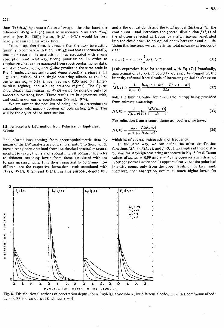
than LV(l)l(w,) by about a factor of two; on the olher hand, the diffcrcnce 11/(11) - IV(/,) must bc associated to an area P(w,) sn~aller [see Eq. (30)]; hence, W(Il) - W(1,) would be very hardly mcasurablc for wcak lines.

To sum up, thercfore, it appcars that the most interesting quantity to compare with M/( / ) is W(Q) and that experimentally, one must rcstrict the analysis to lines associated with strong absorption and relatively. strong polarization. In order to emphasize what can be expccted from spectropolarimetric data, we have drawn II-, 1,-, and Q-line profiles in the sarne scale in Fig. 7 (molecular scattering and Venus cloud) at a phase angle u = 120'. Values of the single scattering albedo at the line center are w,, = 0.99 (linear régime), 0.95 and 0.7 (intermediate régime), and 0.2 (square-root régime). The figures show clearly that measuring W(Q) would be possible only for

and 7 the optical depth and the total optical thickness "in the continuum", and introducc the gcncral distribution f,(l, t ) of the photons refiected at frequency v after having penetrated into the cloud down to an optical dcpth bctwecn rand t t dt. Using this function, we can write the total intensity at Frequcncy v as:

[This expression is to be compared with Eq. (2).] Practically, approximations to f,(I, r ) could be obtained by computing the iniensity reflected frorn clouds of increasing optical thicknesses:

1 I ( W ~ , t + Ar) - I(w,, r - Af) f"(I, r) = - 2At I (wc, 7 )

9 (32)

moderate-to-strong lines. These results are in agreement with. with the limiting value for r 3 0 (cloud top) being provided

and confirrn Our earlier conclusions (Fymat, 1974). from prirnary scattering:

We are now in the position of being able to determine the - atrnospherjc information content of polarization EW's. This will be the object of the next section. j(** O) =

For reflection from a semi-infinite atrnosphere, we have:

III. Atmospheric Information from Polarization Equivalent ppo I,(wc, Widths f ( r , o ) = -

p + po 4% ml '

The informations coming from spectropolarirnetric data by means of the EW analysis are of a similar nature to those which havc already been obtained from the classical spectral measurements. However, thcy are of spccial interest because they refer to different souriding levels from thosc associated with the former measurements. It is thcn important to determine how difiercnt are the respective fornialion levels associated with IV(/), W ( Q ) , W(ll). and W(1,). For this purpose, denote by f

which is, of course, independent of frequency. ln the same way, we can define the other distribution

functions /,(Il, t),/,(I,, t ) , and f,( Q , 1). Examples of thcse distributions for Rayleigh scattering are shown in Fig. 8 for different values of CU,, W, = 0.99 and r = 4 ; the observer's zenitli angle is 60' for normal incidence. lt appears clcarly that the polarited intensity comcs only from the upper le\,els of the layer and, therefore, that absorption occurs at much higher levels for

P E N E T R A T I O N D E P T H I N T H E C L O U D , t

Fig. S. Distribution functions of pcnetration dcptli r for a Rayleigh atmosphere, for different aibcdos w,,, with a continuum albedo w, = 0.99 and an optical thickiiess 7 = 4

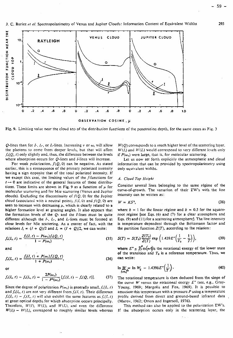
J. C. Birricz r t 01. Spectropolarimetry of Venus and Jupiter Clouds: Information Content of Equivalent Widtlis

O B S E R V A T I O N C O S I N E ,

Fig. 9. Limiting value near the cloud top of the distribution functions of the penetration depth, for the same cases as Fig. 3

Q-lines than for I-, Il-, or I,-lines. Increasing T or W= \vil1 allow the photons to comc from deeper le\cls, but that will affcct f,(Q, t ) only slightly and, thus, the difierence between the levels where absorption occurs for Q-lines and I-lines will increase.

For weak polarization, f(Q, 0) can be negative. As stated eariier, tliis is a corisequence of the primary polarized intensity h a ~ i n g a sign opposite that of the total polarized intensity. If we except this cas;, the limiting values of the fifunctions for t -+ O are indicative of the general features of these distributions. These limits are shown in Fig. 9 as a function of p for molecular scattering and for Mie scattering (Venus and Jupiter clouds). Excluding the discontinuity of f(Q, 0) for the Jupiter cloud (associrited with a ncutral point), J'(I, 0 ) and f ( Q , 0) are seen to increase with decreasing p, which is clearly related to a higher formation level at grazing angles. It also appears that the formation levels of the Q- and the I-lines must be quite different although the 1-, 1,-, and 1,-lines must be formed at close levels for Mie scattering. As a matter of fact, with the relations Il = (1 + Q)/2 and 1, = ( I + Q)/2, we can write:

and

Since the degree of poiarization P(wC) is generally small, f,(I,, r) and f,(I,, t ) are not very difierent from fJ1, t ) . Their difference f,(Il, t ) - f,(I,, t ) will also exhibit the same features as f , ( I , t ) at great optical depths for which absorption occurs principally. Therefore, W 7 ( J ) , lY(Il), and Pt'(/,), and even the difïerence W(I,) - W(I,), correspond to roughly similar levels whereas

W(Q) corresponds to a much higher level of the scattering layer. W(Il) and IY(I,) would correspond to very direrent levels only if P(w,) were large, that is, for molecular scattering.

Let us now set forth expiicitly the atmospheric and cloud information that can be provided by spectropolarimetry using only equi\,alent widths.

A. CIolrd Top Hcight

Consider several lines belonging to the same régime of the curve-of-growth. The variation of their EW's with the line intensity can be written as:

where b = 1 for the linear régime and b = 0.5 for the square- root régime [see Eqs. (6) and (7) for a clear atmosphere and Eqs. (9) and (1 1) for a scattering atrnosphere]. The line intensily is temperature dependent through the Boltzmann factor and the partition function Z(T), according to the relation:

1 = s(T,,) '5) Z(T) exp ( 1 . 4 3 9 ~ " ( ~ - $) ),

where Ba= ~'m(nri)is the rotational energy of the lower state of the transition and To is a reference temperature. Thus, we can write:

The rotational temperature is then deduced from the siope of the curve W versus the rotational energy E" (see, e.g., Gray- Young, 1969; Margolis and Fox, 1969). It is possible to associate this temperature with a pressure P usirig a temperature profile derived from direct and ground-based infrared data (Marov, 1962; Orton and Ingersoll, 1976).

This method cari also be applied to the polarization EW's. If the absorption occurs only in the scattering layer, the

rotational tenipcrature T( Q) derived from M'(Q) will correspond to a higher level than that derived froni cither the intensity or the photopolarization, and this level will also be closer to the cloud top ( P > P,,,,). On the contrary, i f the absorption occurs only in the clear atmosphere (with no scattering) above the cloud. the rotational tenipcraturcs dcrived from both the total aiid the polarized intensitics will bc similar and will correspond to a pressure P - P,,,/2. In a realistic case, the rotational teinperature T ( Q) can be associated with a level relatively close to the cloud top; while the precise location of this level depends on the relative importance of the absorption in the clear and the cloudy atmosphere. it will always be higher and nearer the cloud top than that derived from either intensity or photopolarization data. Such measurements could equally be helpful for.the study of the Jovian atmosphere for which, unlike the Venus atmosphcre, neither the pressure at the top of the first cloud layer nor the relative importance of the clear and cloudy atmospheres are well known. Concerning the Venus atmosphere, the rotational temperature derived from the polarized intensity could be used to locate more precisely the cloud top and confirm that the clear atmosphere above the cloud has only a small influence. This problem. however, becomes more complex when absorption occurs simul~aneously in both the clear and the cloudy atmosphere because the expression of the EW's becomes much more complicared ana inkoibes more parameiers (Fouquari, 1975).

B. Sralc-height Ratios

Let us recall briefly what can be deduced from the total intensity line measurements. The relations in Eqs. (9) and ( 1 I ) , or the more general relations in Eqs. (8) or (16), have been derived for homogcneous scattering atmospheres in which the parameters M, S, and a, remain constant within the cioud. If further, w , does not Vary with optical ciepth, the path lengths (A) and < h > l t 2 , and more generally the distribution functions, will remain unchanged for the realistic atmosphcric mode1 in which the presîurc varies with thc optical depth. (They can bc computed for a given w , and a drop size distribution which can themselves bc derived froni photometric and photopolarimetric data.) In this case, the average quantities M, 3 and EL will be generally different for different régimes of the curve-of-growth. With the kiiowledge of the rotational temperature and the line intensity, and for given scattering properties of the cloud layer, one can derivc the specific abtrndance hl, froni the weak lines [see Eq. (9)] and, from the strong lines [see Eq. ( 1 l)], tlie product M,P,, where P, is the pressure of the formation level of the strong lines. Now, if the scale heights of the scattering particles and the absorbing gas were equal, MW = hls, and one could obtain P, from simultaneous nieasurements of strong and weak lines belonging to the same narrow spectral interval. (This is a restrictive condition due to the wavelength variations of the particles' properties.) On the other hand, if the scale-height ratio is unknowri, one must use some independent data such as occultation or polarization measurements in order to determine it (Lacis, 1975). Spectropolarimctry could be very hclpful in this regarcl sincc the above ratio could be deduccd dircctly from simultaneous nieasiirenients of 1- and Q-lines without resorting to iiideperidenr experiments. We shall detail the procediire iri the case of cloird particles or a gnseous minor consiitucnt imbcddcd in thc ambient air.

1. Gas-to-cloud Particles

Let m = H,/Hp denote the scale-height ratio of the ambicnt gas IO the scattering particlcs, and assume that the mixing ratio of the absorbing gas to the anibient gas is roughly constant within the cloud (this is, for example, the case of CO2 on Venus). Tnen. the quantities Ad,(I)P,(I) and M,( Q)P,(Q) can be derived from the equivalent widths of the strong 1- and Q-lines; here, PJI) and Pb( (2) are the pressure at the I- and Q-line formation levels. Thus, if the difierence in altitude between these two levels is z(z > O), we have:

f"(I) = Pd Q) exp (zlH,), (41)

and thus,

Without any assumption on z, one can readily derive some information about the value of rn since:

With somc idea about the value of 2. m can be determined more precisely. As an example, for the Venus clouds, the photo- polarimtion level was found to be close to 50 mb (Kawabata and Hansen, 1975) (Note that this levcl could be determined, as discussed in Sect. Il1.A above, from the rotational tempcra- turc of the Q-iincs); the formation levcl of the CO, lines is around 120 inb (Diercnfeldt et al., 1977). Tliese prcssures correspond approximately to 68 km and 64 km heights (hlarov, 1972); with If, = 5.3 km, WC have from Eq. (43):

or, assuming cc, = u ~ ( P ~ P ~ ) ( T ~ / T ) ~ ' ~ in Eq. (1 l),

where TI and T4 are the I and Q rotational temperatures. This relation could be used to derive nr and to vcrify the value m = 1.5 proposed by Lacis (1975).

2. Gas-to-gas

When m = H9/Hp is known, it is possible to derive the scale- height Hm of some minor constituent such as CO on Venus. indeed, instead of Eq. (48) we Iiave in this case:

where M;(Q)P:(Q) and M,'(Z)P:!I) are obviously deduced from the EW's of the strong lines of the minor constituent, and z' would correspond to the difference in the levcls of formation of the I- and Q-lines of this same constituent. In this mariner, it should be possible for exaniplc to determirie the scale-hcight of C O on Venus and, thus, to have soinc inforr~rition about the dependence on altitude of the rnisirig ratio of CO to COI. AS

J. C. Buriez et ul. Spectropolarimetry of Venus and Jupiter CIO tuds: Information Content of Equivalent Widths 297

in the pre\rioiis situation, cveii witlio~it thc knowlcdgc of z', we can readily state the rcsult

< ff, H m '

If, however, z' is known, Eq. (47) could be used for deriving Hm more accurately.

C. Vertical Pt.ofîlir~g of Clortd Parat?lrfers

More generally, a better knowledgc of the vertical profile of sonie cloud paramcters could be retrieved from spectropolarimetric measurements. Oiie way of obtaining information about the vertical structure of a planetary atmosphere using spectroscopic data is to study the reflected radiation for different zenith anglcs (phase-angle variations or center-to-limb variations for thc outer plancts). I-icrc, u e rccall that IV((-) is essentially sensitive to the first orders of scattering and that it corresponds to levels of formation in the cloud that Vary according to the zenithal angles of incidence (Bo = cos-'po) and observatiori (O = cos-' p). This will be much more pronounced than for )+'(!) since the latter quantity corresponds to the deeper lcvels \vticre the higher scattering ordcrs play an important role. T h ~ i , for I l f ( ! ) , the depth rcached by a givcn photon optical path h 1975) while in single depth is:

Hence, the formation lcvels associated with IY(Q) must have a strong variation with (p, po) as confirmed by Fig. 9. Conse- quently, dilïcrcnt cloud levels will be sounded with different (p, po) values, i.e. with different phase angles. The deepest Q formation levels should approach the higliest I formation levels (corresponding to great zenith angles). Spectropolarimetry is thus a very useful tool for vertical investigation of cloud characteristics.

Moreover, if molecular scattering is important (which may be- the case for UV spectra), it could be possible to sound simultaneously four different formation levels associated to W(I ) , W(Q), W(I,), and WU,) (see Figs. 8 or 9).

IV. Summary and Conclusions

1. The theory for the curve-of-growth of absorption lines formed in Venus's and Jupiter's clouds has been generalized to the case of polarization, particularly for the Stokes's parameters II , I , , and Q. Linear and square-root régimes, with the corre- sporiding mean and effective optical paths, have been obtained in each case. When the photon path-length distributions associated with each Stokes's parameter are evaluated using Padé's approximants, analytical expressions can be derived for the corresponding equivalent widths. in both Venus and Jupiter, the equivalent width for Q is always smaller than those for I, I,, and I, and must therefore correspond to a higher level in the cloud. For the disk-integrated polarization, i t is approximately 1-5% that of I in the case of Venus, and approximately 0.5% for Jupitcr. Hcnce, it is concludeci tliat equivaicnt widths

in polarization are measiirablc for botli planets with good I.R. detectors. Polarization detaiied over the planetary disk would be diflèrcnt according to the rerion observed on the disk and to phase angle, but it uill yield in most cases a larger ratio of the equivalent widtlis which would lcad to an cven siinplcr measurement.

2. Spectral line polarization (particularly that for QI, if forined in thc cloud, will correspond to levels somewliere between the cloud top (P,,,) and the photopolarization level bclow. The component intensities, 1, and I,, are formed fiirther below but at substantially the same level as 1. An approxirnate location of the cloud top that is more accurate than that derived from photopolarization can be obtained from the rotational temperature of the Q-lines. On the other hand, if the spectral polarization is formed in the ciear atmosphere above the cloud, the associated rotational temperature and that dcrived froin the intensit) spectrun~ wou!d correspond scnsibly to the same level, P,,,/2. This argument can in turn bc used for determining whether the clear atmosphere above the cloud plays any significant role in the line absorption and polarization processes.

3. Since spectropolarinietry sounds simultaneously two different cloud levels (one corresponding to the unpolarized, and the othcr to the polarized, iniensity) the ratio of the COa scale-height to that of the cloud particles can be determined from the combined interprctation of intensity and polarization equivalent widths. This determination does not resort to any other independent measurement. For Venus. if the altitude difierence between the levels of forrnation of Q- and 1-lines is known, an analytical expression, Eq. (43), has been provided for this ratio.

4. With the knowledge of the CO2-to-cloud particles scale- height ratio, the similar ratio bet~reen CO (or any other appropriate minor constituent) and CO2 can likewise be deterniined, Eq. (47).

5. Another interest of W(Q) over M'(I), !+'(Il), and W ( I , ) is the fact that. beinç essentially sensitive to the first orders of scattering, it will correspond to levels of formation in the cloud that are different according to the angles of incidence. po, and observation, p. This will be much more pronounced than for W(I) since WII) is formed at deeper levels where the higher scattering orders enter into play. In this latter case, the depth in the cloud reached by a given photon optical path h will depend little on the geometry (Fouquart, 1975) while, in single scattering, this depth is ( l / p + l/po)-lh. Thus, different cloud levels will be sounded with aifferent (p, pO) values, Le. with different phase angles.

Acknowledgement. W e gratefully acknowledge helpful discussions with Dr. J. Lenoble.

References

Abhyankar, K.D., Fymat. A. L.: 1971, Asrrophys. J. 165, 673 Abhyankar, K.D., Fymat,A.L.: 1971, Asrrophys. J. Suppl. 195,

35 Appleby,J. F., Irvine, W. M.: 1974, Astrophys. J. 183, 337 Belton, M., Hunten,D. M., Goody,R. M.: 1968, in Tlie Afmos-

pheres of Vet~us and Mars, J. C. Brandt and M. B. McElroy Ed., Gordon and Breach, 69

Dierenfcit, K. E., Fink, U., Larson,H. P.: 1977, Icarus, 31, 1 1

.Deuzc,J. L.: 1974. Thèse de 3ème Cycle, Université de Lille Forbes, F. F. : 1971. A~trophj~s . J. 165, L21 Forbes, F. F., Fyma:, A. L. : 1974, in Planets, Stars and Nebulae

stlcJicd with pliotopolari~~ie~r)~, T . Gehrels, Ed., The Univcr- sity of Arizona Press, 639

Fouquart,Y.: 1974, J. Quant. Spectrosc. Radiat. Trartsfer 14, 497

Fouquart, Y. : 1975, Thèse, Université de Lille Fouquart, Y., Lenoble, J.: 1973, J. Quant. Spectrosc. Radiat.

Transfer 13, 447 Fymat, A. L. : 1974, in Platiets, Stars and Nebulae studied with

Photopolarimetry, T. Gehrels, Ed., The University of Arizona Press, 61 7

Gray-Y0ung.L.D.: 1969, Icarus, 11, 66 Goody, R. M.: 1964, Atmospheric Radiation 1. Theoretical

basis, Clarendon Press Hansen, J. E., Hovenier, J. W. : 1974, J. Atmospheric Sci. 31,

1137

Heinrich, M.: 1973, Proceedings of the International Radiation Symposium, Sendaï, Japan, 287

Irvine, W. M.: 1964, Bull. Astron. Irrst. Neth. 17, 266 Kargin, B. A., Krasnokutskaya, L. D., Feyfel'son, Yc. M.: 1972,

Bull. (Izc.) Acad. Sci. U.S.S.R. 8 , 287 Kawabata, K., Hanscn, J . E. : 1975, J. Atmospheric Sri. 32, II 33 Kemp, J. C., Rudy,R. J., Lebofsky, M. J., Ricke,G.H.: 1978,

lcarus 35, 263 Lacis, A. A. : 1975, J. Atrnospheric Sci. 32, 1 107 Margolis,J.S., Fox, K.: 1969, Astrophys. J. 157, 935 Marov, M. Ya. : 1972, lcarus 16, 415 Morozhenko,A. V., Yanovitskii,E. G . : 1973, lcarits 18, 583 Orton,G. S., Ingersoll, A. P. : 1976, in Jupiter, .T. Gehrels, Ed.,

The University of Arizona Press, 206 Pilcher, C. B., Prinn, R. G., McCord.7. B. : 1973, J. Atmospheric

Sci. 30, 302 Travis, L. D. : 1975, J. Atmosplieric Sri. 32, 1 190 van de Hulst,H.C., Irvine, W. M.: 1962, in La Physique des

Planètes, Congrès et Colloques de l'université de Liège 24, 78

C H A P I T R E I V

LES PROFILS DE RAIES

1 NTRODUCTION

Nous avons d s j à souligné l a d i f f i c u l t é de dé f in i r l a largeur équi-

valente d'une r a i e du f a i t que l ' i n t e r v a l l e spec t r a l e s t toujours l im i t é e t

l e niveau continu souvent incer ta in ( c f . chapi t re II-§ 4 ) . Cet inconvénient

e s t part iculièrement renforcé pour l a bande 3v du méthane dans l e s spectres 3

joviens, d'une p a r t à cause de l a présence de mul t ip le t s parmi l e s r a i e s du

méthane, e t d ' au t r e p a r t à cause de l a présence d'une absorption continue

due à l'hydrogène.

Dans l a bande 3v3 du méthane, les r a i e s correspondant à un nombre

quantique J 5 2 - son t en f a i t des mul t ip le t s de r a i e s t r è s rapprochées.

L'absorption t o t a l e n ' e s t pas suffisamment f a i b l e pour que l 'approximation

l i n é a i r e s o i t applicable e t l e s r a i e s dans un mul t ip le t ne sont pas suf-

fisamment séparées pour que l ' absorp t ion puisse ê t r e négligée dans l a ré-

gion de recouvrement ; il n ' e s t donc pas possible de considérer l a largeur

équivalente d'un mul t ip le t comme l a somme des largeurs équivalentes indivi-

duel les des r a i e s du mul t ip le t . De ce f a i t , même pour l e modèle de l a couche

ré f léch issan te (FGM), il n ' e x i s t e plus d 'expression analytique de l a l a r -

geur équivalente. La technique de l a courbe de croissance peut encore ê t r e

appliquée1 mais e l l e nécess i te de ca lcu le r l e s largeurs équivalentes par

in tégra t ion numérique avec un pas en fréquence suffisamment f i n . Le ca lcu l

de l a largeur équivalente nécess i te donc, en prat ique l e ca lcu l du p r o f i l

de l a r a i e .

La présence d'une absorption continue due à l a bande d ipo la i re de

l'hydrogène2 l imi t e encore l e s p o s s i b i l i t é s de l a technique des largeurs

équivalentes. En e f f e t (i) l e niveau du pseudo-continuum e s t mal dé f in i

car l 'a f fa issement du continuum e s t dû à l ' a i l e de l a bande d ipo la i re mais

auss i aux a i l e s de r a i e s f o r t e s du méthane ; c e t t e dernière cause a d'au-

t a n t p lus d'importance que l'atmosphère e s t d i f fusante ; a i n s i , l a mesure

de l a largeur équivalente d'une r a i e d o i t ê t r e évaluée t r é s différemment

selon que l ' o n considère une atmosphère c l a i r e (RLM) ou un nuage homogène

(HCM) ; (ii) l ' absorp t ion due à l'hydrogène n ' e s t pas constante sur t o u t

l ' i n t e r v a l l e spec t r a l considéré ; c e t t e var ia t ion a f fec te l e s paramètres

t e l s que l'abondance "apparente" : l'abondance de méthane rencontrée

par l e s photons en absence d 'absorption par l e méthane n ' e s t pas l a même

suivant l ' importance de l ' absorp t ion par l'hydrogène, dans une atmosphère

d i f fusan te .

Ainsi , l ' é t u d e des p r o f i l s de r a i e s s ' avère ê t r e pratiquement l a

seule méthode d 'analyse de l a région de l a bande 3v du méthane dans l e s 3

spectres joviens. Nous présenterons d 'abord, de manière non exhaustive,

l e s p o s s i b i l i t é s e t l e s l imi tes de l a technique du spectre synthétique. NOUS

développerons ensu i te une méthode de ca lcu l adaptée à c e t t e technique. S i

l e calcul e s t a i s é lorsque l ' absorp t ion dans l e s nuages e s t négligeable par

rapport à l ' absorp t ion en atmosphère c l a i r e , il n'en e s t pas de même lorsque

tou te l ' absorp t ion a l i e u dans l e nuage. L'approximation de CURTIS-GODSON

généralisée n ' e s t pas s a t i s f a i s a n t e au voisinage du centre d'une r a i e mais

donne un exce l l en t accord dans l e s a i l e s ( c f . chap. 1) . E l l e appara i t donc

comme une bonne base de départ pour rechercher une approximation valable

pour t o u t l e p r o f i l . Nous présenterons Pa méthode de ca l cu l dans un cadre

t o u t à f a i t général ; nous conserverons, pour l e s i l l u s t r a t i o n s , les modèles

d'atmosphères d é c r i t s dans l e chapi t re 1. Nous verrons ensu i te son applica-

t i o n aux spec t res de Jupi ter e t de Saturne.

1 - POSSIBILITES ET LIMITES

Nous ne nous sommes pas souciés jusqu'à présent de l a convolution du

p r o f i l d'une r a i e d 'absorption par un p r o f i l instrumental . En e f f e t , c e t t e

convolution ne modifie pas l a mesure de l a largeur équivalente d'une r a i e s i

l a l im i t e de réso lu t ion r e s t e t r è s p e t i t e devant l ' i n t e r v a l l e spec t r a l con-

s idéré . Par contre , l e p r o f i l instrumental a une t r è s grande importance

lorsque l ' o n compare des p r o f i l s synthétiques à des p r o f i l s expérimentaux.

Il importe donc de d é f i n i r au départ quelques ordres de grandeurs concernant

l a résolut ion des spec t res é tudiés . Ceux-ci son t présentés dans l e tableau

page suivante.

La l im i t e de réso lu t ion expérimentale AU e s t comparée à l a demi-largeur de

LOwNTZ "apparente" a (8,r?P) , c ' e s t à d i r e c e l l e qui s e r a i t déduite de 1 ' étude 'Il 'b de largeurs équivalente de r a i e s i so l ée s . Le rapport Av / a(O,rP) e s t très

grossièrement éga l à 2 pour l e s modèles moyens obtenus pour vénus3 e t Jup i t e r 4 5 e t % 10 pour l e modèle moyen obtenu pour Saturne .

De même, on peut s ' i nqu ié t e r de savoir s i l e p r o f i l d 'absorption e s t

suffisamment bien représenté par un p r o f i l de LORENTZ e t s ' i l n ' y a pas l i e u

d ' u t i l i s e r un p r o f i l de VOIGT tenant compte à l a f o i s de l 'é largissement

de l a r a i e par co l l i s i ons e t par e f f e t DOPPLER. Les dif férences en t r e l e s

largeurs équivalentes de r a i e s de VOIGT e t de LORENTZ ne sont notables que

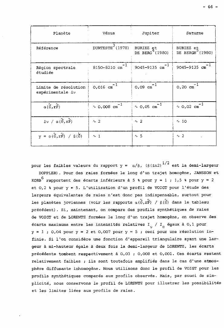
Planète Vénus Jup i t e r I I Saturne 1 i 1

' Référence DURTESTE' ( 1978) BURIEZ z t ; BURIEZ eg DE BERG ( 1980) ! DE BERGH (1980)

I 1

Région spec t ra le 8150-8210 cm-' 9045-9135 cm-' 1 9045-9135 cm-' étudiée l l

L

1

- 1 - 1 Limite de résolut ion ' 0,016 cm 0,09 cm expérimentale Av 1

pour l e s f a i b l e s valeurs du rapport y = a / @ , (fi(kn2) e s t l a demi-largeur

0,20 cm-'

, s s

a(O,rP) 1 s 0,008 cm-' s 0,05 cm-' I

DOPPLER). Pour des r a i e s formées l e long d'un t r a j e t homogène, JANSSON e t 6

KORB rapportent des é c a r t s i n f é r i eu r s à 5 % pour y = 1 ; 1,5 % pour y = 2

e t 0,2 % pour y = 5. L ' u t i l i s a t i o n d'un p r o f i l de VOIGT pour l ' é t u d e des

largeurs équivalentes de r a i e s n ' e s t donc pas indispensable, sur tou t pour s s %

l e s planètes joviennes (voir l e s rapports a ( O , rP) / fi ( O ) dans l e tableau

précédent) . S i , maintenant, on compare des p r o f i l s synthétiques de r a i e s

de VOIGT e t de LORENTZ formées l e long d'un t r a j e t homogène, on observe des

éca r t s maximums en t re l e s i n t e n s i t é s r e l a t i v e s 1 / Ic égaux à 0 , l pour v

y = 1 ; 0,04 pour y = 2 e t 0,007 pour y = 5 ; cec i pour une résolut ion in-

f i n i e . S i l ' o n considère une fonction d ' appare i l t r i angu la i r e ayant une la r -

geur à mi-hauteur égale à deux f o i s l a demi-largeur de LORENTZ, l e s é c a r t s

précédents tombent respectivement à 0,03 ; 0,008 e t 0,001. Ces éca r t s r e s t e n t

relativement f a ib l e s ; i l s sont tou te fo i s amplifiés dans l e cas d'une atmos-

phère d i f fusan te inhomogène. Nous u t i l i s o n s donc l e p r o f i l de VOIGT pour l e s

p r o f i l s synthétiques comparés aux p r o f i l s observés. Mais, par souci de s i m -

p l i c i t é , nous conservons l e p r o f i l de LORENTZ pour i l l u s t r e r l e s p o s s i b i l i t é s

e t l e s l imi tes l i é e s aux p r o f i l s de r a i e s .

z 0,02 cm-'

Comme pour l ' é t u d e des largeurs équivalentes de r a i e s (chap- II)

nous nous l imiterons d 'abord au cas i d é a l de r a i e s i so lées (déf in ies su r un

i n t e rva l l e s p e c t r a l théoriquement i n f i n i ) . Nous nous placerons ensui te dans

l e cas plus r é a l i s t e de r a i e s non i s o l é e s .

a ) - Raies i s o l é e s

Nous avons vu, dans l e chapi t re II, que l ' é t ude des la rgeurs équiva-

l en t e s de r a i e s permet-dans l e cas i d é a l de r a i e s suffisamment i so l ée s

- de déterminer l'abondance de gaz absorbant "apparente" (ou abondance 'L

"moyenne") u e t l a demi-largeur de LORENTZ "apparente" a ((3, r3) . Mais e l l e 1

ne permet pas de déterminer séparèment l ' i n d i c a t e u r de d i f fus ion r e t l a 'L

demi-largeur "moyenne" cc (0 , 3) . Sur l a f igure 1 , l e s prof i l s de r a i e s i so l ée s %

correspondent à une même abondance p e t une même demi-largeur a ( (3 , r i ) pour 1

l e s d i f f é r en t s modèles d'atmosphères (RLM, TCM, HCM, DCM) dé j à u t i l i s é s

dans l e s chapi t res 1 e t II. A une i n t e n s i t é de r a i e S ( O ) donnée, correspondent

des largeurs équivalentes sensiblement égales pour l e s quatre modèles ( l e s

é c a r t s r e s t e n t i n f é r i eu r s à 5 % ) . Trois valeurs représentat ives du rapport

s ( 0 ) p l / a ( @ , & ont é t é sélectionnées : 0,3 ( r a i e f a ib l e ) ; 3 ( r a i e i n t e r -

médiaire) ; 30 ( r a i e f o r t e ) . Les p r o f i l s sont convolués par une fonction

t r i angu la i r e de largeur à mi-hauteur égale à deux f o i s l a demi-largeur '-b "apparente" de LORENTZ (Av/a(O,rP) = 2 ) .

Cette f igure 1 i l l u s t r e de façon part iculièrement frappante l e

t i t r e de c e t t e sect ion : schématiquement, à d r o i t e de l a f i gu re , l e s "pos-

s i b i l i t é s " e t à gauche, l e s "l imites". D'un cb té , l e s p r o f i l s correspondant

à l a couche r é f l éch i s san t e (RLM) e t au nuage homogène (HCM) son t très diffé-

r e n t s bien q u ' i l s correspondent auX mêmes valeurs de l'abondance p e t de l a 1

pression "apparente" r3. De 1 'au t re cô t é , les p r o f i l s correspondant au mo-

dè l e à deux nuages (TCM) e t au nuage dispersé (DCM) sont très vois ins bien

q u ' i l s correspondent à une r é a l i t é t r è s d i f f é r en t e .

Les deux premiers modèles (RLM e t HCM) correspondent à des valeurs

de l ' i n d i c a t e u r de d i f fus ion t r è s d i f f é r en t e s : respectivement r = 1 e t

0,35. Au con t r a i r e , les deux autres modèles (TCM e t DCM) correspondent res-

pectivement à 0,63 e t 0,61. D'une façon générale, l ' ana lyse des p r o f i l s de

r a i e s permet de déterminer l ' i n d i c a t e u r de d i f fus ion r : dès que l a dis tance

au centre de l a r a i e (v-v ) e s t grande devant l a demi-largeur de LORENTZ, l e O

rapport des i n t e n s i t é s à l a fréquence v e t dans l e continu peut s ' é c r i r e de

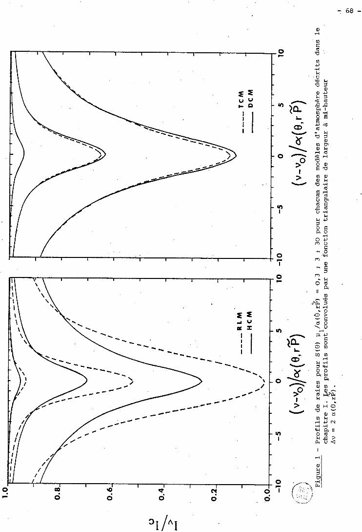
-4 k U 'al k a 7

al al ci Q 7 /al rd s s $i E ci #id lu - k a 7

al ffl tn al k rl rd )al ri a O al E a 10 al al LI a -4

(d C F I 7 3 U 0 rd C

5 4

- k O id

. II a 10 - 'al

za 7 k rl

.G $ C

a O \ U 4

façon quasi-exacte

(IV- 1)

% où p ( u ) est la aistribution de l'abondance de gaz absorbant pondérée par la

pression et la température (cf. chap. 1) . En particulier, très loin dans les ailes, lorsque l'absorption devient

faible, on obtient

'L L'analyse des ailes de raies permet de déterminer le produit ~~(8.8) vl. Les

profils de raies permettent évidemment d'obtenir l'information contenue dans 'L

les largeurs équivalentes, c'est à dire les quantités p 1 2 vl

et % %

a (8, r8) = r a (O ,Pl . Il est ainsi possible de déterminer 1' abondance "moyenne" %

pl, la demi-largeur de LORENTZ "moyenne" a(@,$) et l'indicateur de diffu-

sion r.

L'inversion de l'équation (IV-1) permet, en théorie, de déterminer 'L

non seulement le rapport r = ) / mais aussi toute la fonction de 2i

1 distribution p(u). En pratique, l'inversion de la transformée de LAPLACE est

mal conditionnée. Nous avons déjà souligné ce problème dans le chapitre 1.

Des calculs d'intensités ont été effectués pour un trajet homogène à l'aide

de la fonction de DIRAC et à l'aide de la fonction de distribution approchée

représentée sur la figure 1 du chapitre 1. Bien que les deux distributions

soient bien différentes, les écarts AI / Ic restent inférieurs à v

5 x 10' (pour Iv/Ic > 0,005) . La distinction entre les deux distributions nécessiterait donc un rapport signal / bruit à peu près 1000 fois supérieur

à celui obtenu pour les spectres joviens étudiés. Il est donc, en pratique,

impossible d'obtenir par inversion de l'équation (IV-1) la distribution 2,

p(u) exacte. Par contre, la détermination de quantités intégrées telles que 'L 'L

les moments pl et est possible.

Nous n'avons fait appel, pour la détermination de l'indicateur

de diffusion r, qu'à la forme des ailes des raies. Une information supplé-

mentaire peut être obtenue à partir de la région centrale des raies : com-

parons les raies correspondant au modèle à deux nuages (TCM) et au modèle

du nuage dispersé (DCM) de l a f igure 1. Au cen t re des r a i e s , l e s éca r t s ne

sont pas dû au f a i t que les indicateurs de dif fusion r so i en t légèrement

d i f f é r en t s . D'une façon qu i peut p a r a î t r e paradoxale, lorsque l ' o n a jus te

l e rapport p1/p2 (pression du l e r nuage / pression au sommet de 2e nuage)

pour ob ten i r r = 0,61 comme pour l e nuage dispersé , l e s éca r t s maximals

aux cen t re des r a i e s sont doublés : A I ~ / I ~ = 0,050 pour P /P = 0.20 1 2

(au l i e u de A I / I = 0,025 pour p1/p2 = 0,25) . Ceci e s t l i é au f a i t que l a v%

d i s t r i bu t ion p ( u ) n ' e s t appropriée que pour l e s a i l e s , l à où l e coef f ic ien t

d 'absorption e s t proportionnel à l a demi-largeur de LOFtENTZ a. El l e n ' e s t

pas appropriée pour l e centre e t l e s épaules de r a i e s puisque l e coeff i -

c i en t d 'absorption diminue avec a pour v - vo < a puis augmente pour

v - v > ci. Au cent re d'une r a i e "convoluée", il n ' e s t pas possible de dé- O

f i n i r "un"coefficient d 'absorption. L'information supplémentaire obtenue

par l ' ana lyse de l a région cen t ra le des r a i e s ne peut donc pas s 'exprimer

d'une façon aussi simple que pour l e s a i l e s de r a i e s . Cependant, à cause

de l a l o i de var ia t ion du coe f f i c i en t d 'absorption en fonction de l a pres-

sion, il e s t c l a i r que c e t t e information concerne l e s hautes couches de 'L

1 ' atmosphère a l o r s que l e s a i l e s de r a i e s sensibles au fac teur p a (O ,& 1 sondent des couches plus profondes.

Il e s t hors de question d 'espérer déterminer l a s t ruc ture r é e l l e ,

extrêmement complexe, de l'atmosphère à p a r t i r des seu ls p r o f i l s de ra ies .

Imaginons que l a s t ruc tu re de l'atmosphère étudiée s o i t c e l l e d'un nuage

dispersé (DCM) e t que l e s t r o i s r a i e s r e p o r t é e s su r l a f igure 1 so i en t des

r a i e s expérimentales. Essayons de f a i r e coïncider l e s p r o f i l s d'un modèle

à deux nuages (TCM) avec ces p r o f i l s "expérimentaux". La mesure des largeurs %

équivalentes f i x e l e s paramètres e t r P . On peut encore a ju s t e r l e rap- 1 por t des pressions p1/P2 e t l ' épa i s seu r optique r du premier nuage. Pour

1 l e cas de l a f i gu re 1 (P1/P2 = 0,25 e t r1 = l ) , les éca r t s en t re les p r o f i l s

synthétiques e t "expérimentaux" ne son t s i g n i f i c a t i f s (supérieurs au b r u i t

expérimental) que s i l e rapport s i gna l / b r u i t e s t supérieur à 40. Pour .r l

f ixé , l e meil leur accord e s t obtenu pour P /P = 0,30, cas où l e s éca r t s ne 1 2

sont s i g n i f i c a t i f s que pour s/n > 100. On pour r a i t encore améliorer c e t accord

en f a i s a n t va r i e r T Il n ' e s t donc pas possible d 'él iminer l 'hypothèse de 1

deux couches nuageuses denses d i s t i n c t e s . Du po in t de vue optique, ce modèle

à deux nuages e s t une schématisation- gross ière - du nuage dispersé. La

f igure 2 représente l a r e l a t i o n en t r e l a profondeur optique t (déf in ie C

dans l e continu) e t l a pression P pour l e s deux modèles (DCM e t TCM) : nous

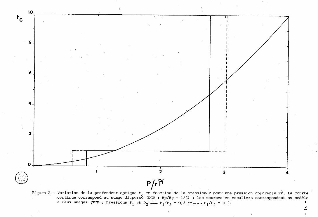
avons reporté le cas où P /P = 0,20 (cf. 5 précédent : même indicateur r 1 2

que pour le nuage dispersé, et donc meilleur accord dans les ailes de

raies) et le cas où P /P = 0,30 (meilleur accord pour tout le profil) ; la 1 2

courbe continue du nuage dispersé est approximée par les courbes en escalier

des modèles à deux nuages ; la relation t (P) est mieux approximée par le cas C

P1/P2 = 0,30 dans les hautes couches de l'atmosphère ; c'est pourquoi il

donne un meilleur accord aux centres de raies.

En pratique, la technique du spectre synthétique permet d'éliminer

un certain nombre de modèles d'atmosphère mais elle ne permet pas de déter-

miner "le" modèle d'atmosphère. Les différents modèles qui permettent l'ac-

cord entre spectre synthétique et spectre observé correspondent, du point

de vue optique, à une schématisation-plus ou moins grossière suivant la

qualité du spectre expérimental- de la structure réelle de l'atmosphère.

b) - Raies non isolées

Nous avons vu dans le chapitre II, que la largeur équivalente d'une

raie est difficile à mesurer à cause d'un intervalle spectral toujours li-

mité et d'un niveau continu souvent incertain. Ces inconvénients conservent-

ils autant d'importance pour les profils de raies ?

Considérons d'abord le recouvrement des raies dans le cas d'un ni-

veau continu connu. Si l'on utilise la technique de la courbe de croissance,

il faut extrapoler dans les ailes la forme qu'aurait une raie si elle était

iuolie. Lorsqu'on calcule un profil synthétique, on prend en compte les raies

voisines et il n'y a donc pas lieu de faire une telle extrapolation ; on

analyse tout le profil expérimental ; en particulier la région de recouvre- w

ment des raies est favorable à la détermination du produit Pu puisque, 1 '

comme pour l'équation ( I V - 2 ) , on peut écrire

avec

la sommation sur j concerne toutes les raies du spectre ; P est une pres- O

sion de référence (P = 1 atm). Le recouvrement des raies n'entraîne pas O

de limitation dans la détermination des différents paramètres, sauf si l'on

analyse un domaine spectral où l'absorption est si forte que l'on observe

en tout point un affaissement notable du continuum. Dans ce cas, le passage

à la limite de l'équation (IV-3) est imprécis.

Un affaissement du continuum rend en général difficile la localisa-

tion de celui-ci sur le tracé du spectre. Il en résulte une incertitude sur

l',intensité dans les ailes de raies et donc sur les principaux paramètres

physiques. La valeur de l'intensité aux centres des raies reste cependant

peu modifiée et donc l'information concernant les très hautes couches de

l'atmosphère est peu perturbée.

En conclusion, l'analyse des profils des raies est beaucoup plus

riche en informations que la seule étude de leurs largeurs équivalentes.

Le recouvrement des raies n'est pas "en soi" un handicap pour l'interpré-

tation des profils alors qu'il en est un pour celle des largeurs équiva-

lentes. Une analyse fine du spectre expérimental requiert toutefois une

bonne détermination du .niveau continu,

La technique du spectre synthétique ne permet pas de déterminer la

structure réelle de l'atmosphère mais simplement une schématisation de

celle-ci. L'utilisation de modèles très complexes ne peut être justifiée

que si (1) de nombreux paramètres peuvent être fixés grâce à des mesures in-

dépendantes de l'étude des profils de raies, (2) les spectres sont de qualité

exceptionnelle à la fois en résolution et en rapport signal / bruit.

Si l'atmosphère étudiée est encore mal connue, il faut donc se con-

tenter d'utiliser des modèles d'atmosphère très simples et rechercher des

informations essentielles telles que : (i) quelle région de l'atmosphère

sonde-t-on avec les spectres observés ? (la détermination de la pression 2i fb

"apparente" rP ou la pression moyenne P fournit une information intéressante) ;

(ii) cette région de l'atmosphère est-elle très diffusante ? (r est un excel-

lent indicateur) ; (iii) en particulier, la diffusion joue-t-elle un rôle

important dans les très hautes couches de l'atmosphère ? (les centres de

raies y sont essentiellement formés) ; (iv) éventuellement, quelle est la

concentration du gaz absorbant ? (pl est l'abondance "moyenne" de gaz absor-

bant) .

II - METHODE DE CALCUL

La technique du profil synthétique nécessite de calculer le rapport

des intensités 1 /I en tout point du spectre étudié. Malgré le développement v c

de méthodes de résolution de l'équation de transfert, celles-ci ne sont pas

actuellement adaptées à cette technique. En effet, prenons l'exemple précis

des spectres joviens que nous avons étudiés ; l'intervalle spectral de - 1 - 1

90 cm est décrit avec un pas de 0,012 cm (pas nécessaire pour prendre

en compte la convolution par la fonction d'appareil) ; il est hors de ques-

tion de résoudre l'équation de transfert 90 / 0,012 = 7500 fois pour chaque

modèle envisagé !

Ce nombre peut être restreint : si le calcul exact de l'intensité

réfléchie est effectué pour quelques fréquences judicieusement choisies,

on peut interpoler les valeurs de l'intensité aux autres fréquences. Le

profil d'une raie individuelle peut être assez bien décrit à partir d'une

dizaine de points (% 5 points, si elle est symétrique). Plus de 40 raies

du méthane ont été étudiées ; ainsi, cette méthode nécessiterait encore de

résoudre l'équation de transfert de 200 à 400 fois pour chaque modèle

(c'est à dire à chaque fois que l'on change une caractéristique de l'at-

mosphère, ne serait-ce que la concentration en gaz absorbant) .

Il a donc été nécessaire de développer une méthode de calcul appro-

ché, très rapide, adaptée à la technique du spectre synthétique. La néces-

sité de résoudre de nombreuses fois l'équation de transfert tient au fait

que les processus d'absorption et de diffusion sont intimement liés dans

les atmosphères diffusantes inhomogènes. Nous envisagerons donc d'abord

deux cas extrèmes : (a) toute l'absorption a lieu en atmosphère claire (la

séparation entre les phénomènes de diffusion et d'absorption est relati-

vement simple), (b), toute l'absorption a lieu en atmosphère nuageuse. Nous

verrons ensuite le cas du modèle "diffusant et réfléchissant" (RSM) qui est

le modèle d'atmosphère inhomogène le plus couramment utilisé pour l'étude 7-8

des planètes (voir, par exemple, pour Vénus, REGAS et al ; pour Jupiter, 12 13

cLEMENTs~, ~ALUCE et SMITH~~, COCHRAN~ l, WEST ; pour Saturne, MACY 1 .

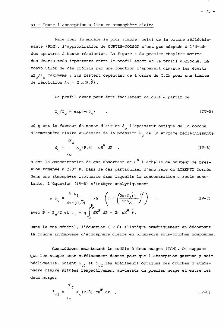
a) - Toute l'absorption a lieu en atmosphère claire

Même pour le modèle le plus simple, celui de la couche réfléchis-

sante (RLM) , l'approximation de CURTIS-GODSON n'est pas adaptée à l'étude

des spectres à haute résolution. La figure 4 du premier chapitre montre

des écarts très importants entre le profil exact et le profil approché. La

convolution de ces profils par une fonction d'appareil diminue les écarts

AI /I maximums ; ils restent cependant de l'ordre de 0,05 pour une limite v c

% de résolution Av = 2 a (@,Pl .

Le profil exact peut être facilement calculé à partir de

où n est le facteur de masse d'air et 6 l'épaisseur optique de la couche v

d'atmosphère claire au-dessus de la pression P de la surface réfléchissante C

Y c est la concentration de gaz absorbant et H l'échelle de hauteur de pres-

sion ramenée à 273' K. Dans le cas particulier d'une raie de LORENTZ formée

dans une atmosphère isotherme dans laquelle la concentration c reste cons-

tante, l'équation (IV-6) s'intègre analytiquement

- n 6 v - % (l + (2:i:is) 7 ) , 4~ra ( O , P)

% avec P = pC/2 et u l = dP = 211 cd* $.

Dans le cas général, l'équation (IV-6) s'intègre numériquement en découpant

la couche inhomogène d'atmosphère claire en plusieurs sous-couches homogènes.

Considérons maintenant le modèle à deux nuages (TCM). On suppose

que les nuages sont suffisamment denses pour que l'absorption gazeuse y soit

négligeable. Soient 6 et 6 les épaisseurs optiques des couches d'atmos- v 1 v2

phère claire situées respectivement au-dessus du premier nuage et entre les

deux nuages

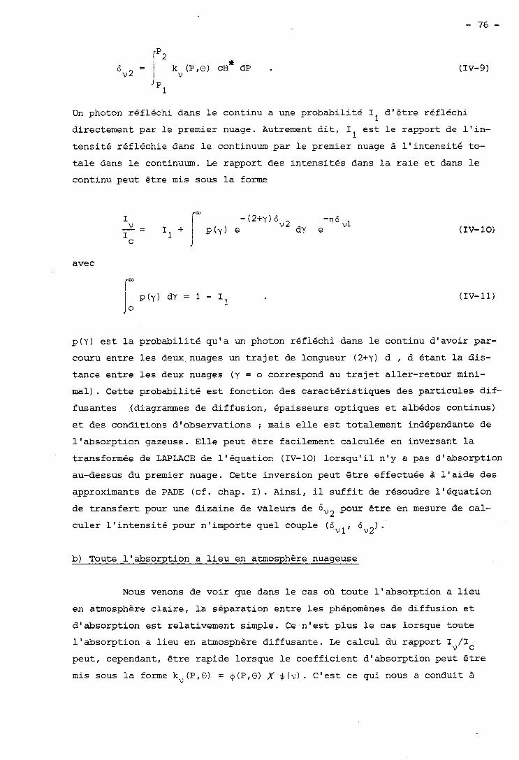
Un photon réfléchi dans le continu a une probabilité 1 d'être réfléchi 1

directement par le premier nuage. Autrement dit, 1 est le rapport de l'in- 1

tensité réfléchie dans le continuum par le premier nuage à l'intensité to-

tale dans le continuum. Le rapport des intensités dans la raie et dans le

continu peut être mis sous la forme

avec

rw

p(y) est la probabilité qu'a un photon réfléchi dans le continu d'avoir par-

couru entre les deux~nuages un trajet de longueur (2+y) d , d étant la dis- tance entre les deux nuages (y = O correspond au trajet aller-retour mini-

mal). Cette probabilité est fonction des caractéristiques des particules dif-

fusantes (diagrammes de diffusion, épaisseurs optiques et albédos continus)

et des conditions d'observations ; mais elle est totalement indépendante de

l'absorption gazeuse. Elle peut être facilement calculée en inversant la

transformée de LAPLACE de l'équation (IV-10) lorsqu'il n'y a pas d'absorption

au-dessus du premier nuage. Cette inversion peut être effectuée à l'aide des

approximants de PADE (cf. chap. 1). Ainsi, il suffit de résoudre l'équation

de transfert pour une dizaine de valeurs de 6 Our être en mesure de cal- v2

culer l'intensité pour n'importe quel couple (6v1, 6v2).

b) Toute l'absorption a lieu en atmosphère nuageuse

Nous venons de voir que dans le cas où toute l'absorption a lieu

en atmosphère claire, la séparation entre les phénomènes de diffusion et

d'absorption est relativement simple. Ce n'est plus le cas lorsque toute

l'absorption a lieu en atmosphère diffusante. Le calcul du rapport 1 /I v C

peut, cependant, être rapide lorsque le coefficient d'absorption peut être

mis sous la forme kv(P,O) = $(Pl@) ,Y $ ( v ) . C'est ce qui nous a conduit à

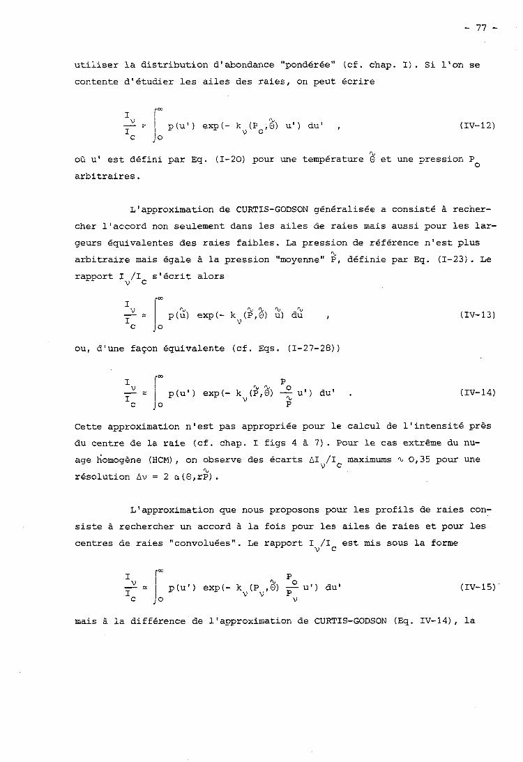
u t i l i s e r l a dis t r ibut ion d'abondance "pondérée" (c f . chap. 1) . Si l 'on se

contente d 'é tudier l e s a i l e s des raies , on peut écr i re

% où u' e s t défini par Eq. (1-20) pour une température O e t une pression P

O

a rb i t ra i res .

L'approximation de CURTIS-GODSON généralisée a consisté à recher-

cher l 'accord non seulement dans les a i l e s de raies mais aussi pour l e s lar-

geurs équivalentes des raies faibles . La pression de référence n ' e s t plus CL

a rb i t r a i r e mais égale à l a pression "moyenne" P l définie par Eq. (1-23). Le

rapport 1 /Ic s ' é c r i t alors v

( I V - 13)

ou, d ' une façon équivalente ( c f . Eqs . (1-27-28) )

( I V - 14)

Cette approximation n ' e s t pas appropriée pour l e calcul de l ' i n t e n s i t é près

du centre de l a r a i e ( c f . chap. 1 f igs 4 à 7 ) . Pour l e cas extrême du nu-

age 6omogène ( H C M ) , on observe des écar ts A I /I maximums % 0,35 pour une %

V C

résolution Av = 2 a (O, rP) .

L'approximation que nous proposons pour l e s prof i l s de ra ies con-

s i s t e à rechercher un accord à l a fo is pour l e s a i l e s de raies e t pour l e s

centres de raies "convoluées". Le rapport 1 /Ic e s t m i s sous l a forme V

mais à l a différence de l'approximation de CURTIS-GODSON (Eq. IV-14), l a

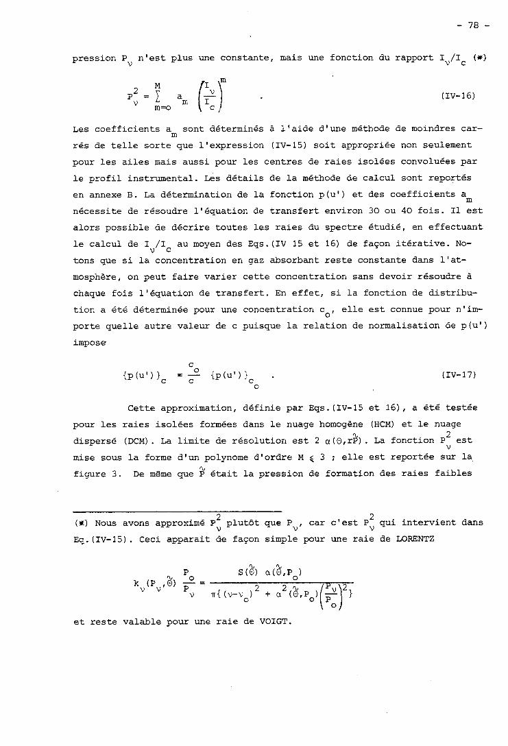
pression P n'est plus une constante, mais une fonction du rapport 1 /I (w) v v C

(IV- 16)

Les coefficients a sont déterminés à l'aide d'une méthode de moindres car- m

rés de telle sorte que l'expression (IV-15) soit appropriée non seulement

pour les ailes mais aussi pour les centres de raies isolées convoluées par

le profil instrumental. Les détails de la méthode de calcul sont reportés

en annexe B. La détermination de la fonction p(ul) et des coefficients a m nécessite de résoudre l'équation de transfert environ 30 ou 40 fois. Il est

alors possible de décrire toutes les raies du spectre étudié, en effectuant

le calcul de 1 /I au moyen des Eqs.(IV 15 et 16) de façon itérative. No- v c

tons que si la concentration en gaz absorbant reste constante dans l'at-

mosphère, on peut faire varier cette concentration sans devoir résoudre à

chaque fois l'équation de transfert. En effet, si la fonction de distribu-

tion a été déterminée pour une concentration cor elle est connue pour n'im-

porte quelle autre valeur de c puisque la relation de normalisation de p(u')

impose

Cette approximation, définie par Eqs.(IV-15 et 16), a été testée

pour les raies isolées formées dans le nuage homogène (HCM) et le nuage 'b

dispersé (DCM) . La limite de résolution est 2 a r P . La fonction p2 est V

mise sous la forme d'un polynome d'ordre M 6 3 ; elle est reportée sur la 'b

figure 3. De même que P était la pression de formation des raies faibles

2 ( x ) NOUS avons approximé P plutdt que P car c'est P2 qui intervient dans

v v v Eq.(IV-15). Ceci apparait de façon simple pour une raie de LORGlNTZ

et reste valable pour une raie de VOIGT.

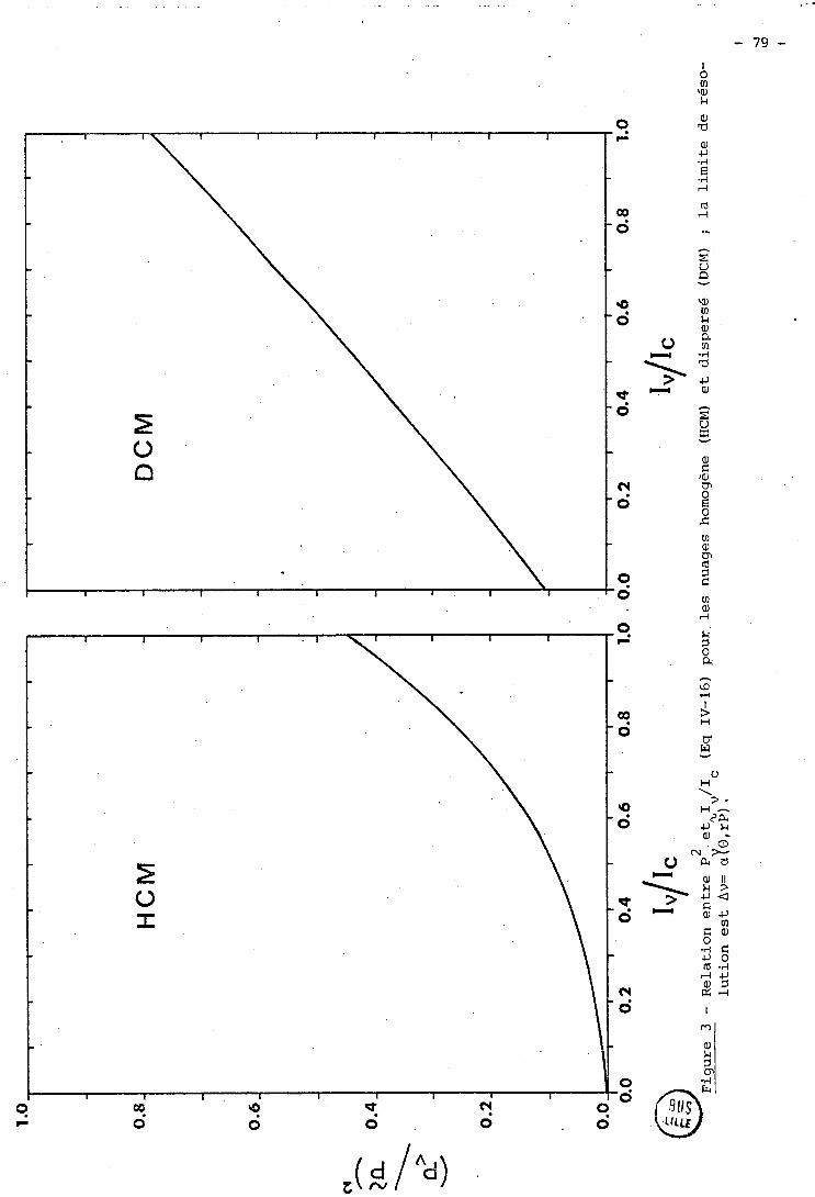
'a, U) l4 ai

O "

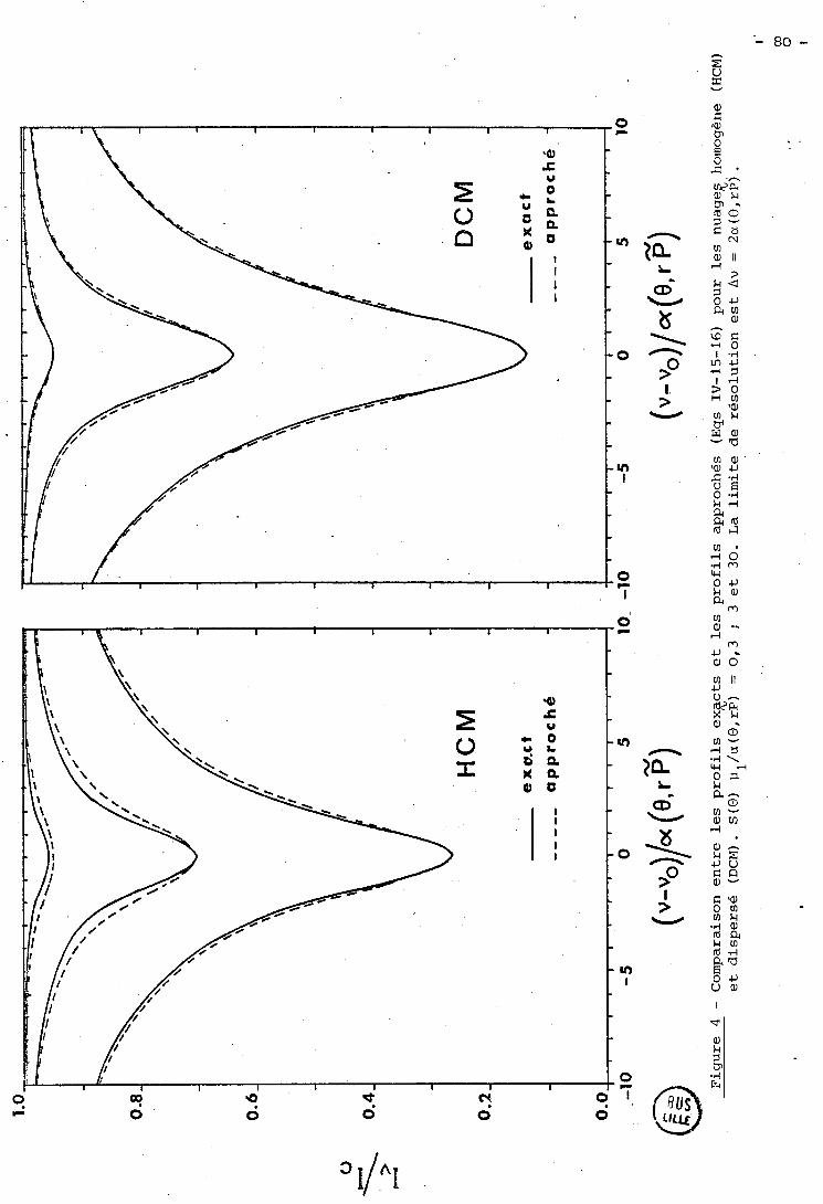
(chap. 1) , P peut être considéré comme la pression de formation des 9

centres de raies convoluées ("pression de formation" s'entend ici au sens

large du terme) ; P correspond ainsi à des pressions inférieures à 8 (voir V

fig. 3).

Les profils approchés sont comparés aux profils exacts sur la fi-

gure 4. Les écarts AI /Ic sont toujours très faibles aux centres des raies v 2

(à cause de la définition de P et dans les ailes (1 /I y est pratiquement CI v V c

indépendant de pL) . Dans les épaules de raies, les écarts restent respecti- v

vement inférieurs à 0,035 et 0,025 pour n'importe quelle raie formée dans

les nuages homogènes (HCM) et dispersé (DCM). De telles incertitudes sont ..

comparables au bruit expérimental des spectres joviens étudiés (s/n = 30

pour Jupiter et '25 pour Saturne) .

La précision de l'approximation dépend évidemment de la résolution

spectrale. Par exemple, dans le cas du nuage homogène, l'incertitude AI /Ic v

maximale est trois fois plus grande si la résolution est dix fois meilleure.

Une meilleure précision peut être obtenue si le domaine des intensités de

raies étudiées est limité : l'étude de la bande du gaz carbonique à 1

8192 cm-' sur Vénus ne concerne que des raies fortes ; l'étude de la région 3

de la bande 3 vg du méthane sur ~ u ~ i t e r ~ et Saturne porte sur des raies

fortes et des raies intermédiaires. La précision de la méthode est liée

principalement à la prise en compte de l'absorption aux très faibles pres-

sions (jusqu'à P % O). Les modèles envisagés ici sont en fait des cas ex-

trêmes.

Il est important de souligner que les écarts AI /I observés dans v c

les épafiles de raies ne sont pas aléatoires, mais toujours de même signe

(car P2 est trop faible). Lors de la comparaison entre spectre synthétique v

et spectre expérimental, il est intéressant de savoir que l'intensité appro-

chée n'est en aucun cas supérieure à l'intensité exacte.

En toute rigueur, tout le spectre ne peut être décrit à l'aide

de (Eq. IV-15) que si la distribution p (u' ) est la même pour toutes les raies

du spectre étudié. Elle dépend de la façon dont l'absorption varie en fonc-

tion de la température. Rappelons la définition de l'abondance "pondérée"

U' (Eq. 1-20)

% cck(@,Po) ak (8'

du' SI<(@) = du Sk(0) L, ak t 6 , ~ 7 ak (C:g)

k

En génGral, l'abondance "pondérée" u' n'est pas définie pour tout le spectre.

Une seule distribution p(u') est rigoureusement valable pour toutes les

raies (i) soit si l'on se contente d'étudier des raies correspondant au 3r 3%

même nombre quantique (par exemple les multiplets R(5) , R(5) et R(5)

dans les spectres joviens ; (ii) soit si l'atmosphère peut être considérée

isotherme ; dans ce dernier cas, l'équation (IV-18) se réduit à

Nous avons vu, dans le 5 1 de ce chapitre, qu'il n'était pas possible de connaitre la structure réelle de l'atmosphère à partir des seuls profils

de raies. En particulier, le profil de température O(P) peut difficilement

être obtenu à partir des profils de raies (dans le proche infra-rouge).

Dans ces conditions, (i) ou bien on se contente de la détermination d'"unen

température voisine de la température de rotation définie à partir des

largeurs équivalentes de raies isolées (cf. chap II), (ii) ou bien on uti-

lise un profil thermique obtenu à partir d'observations indépendantes (me-

sures dans l'infra-rouge lointain ou éventuellement mesures "in situ"). Dans

l'hypothèse d'un modèle d'atmosphère non isotherme, il est encore concevable

d'utiliser une seule distribution p(u')-définie pour un nombre quantique 1 ( % 'boyen - à condition que la température de référence 0 , qui intervient dans

les équations (IV-18 et 151, ne soit plus arbitraire. Prenons comme exemple

le modèle d'atmosphère nuageuse de Vénus qui a servi d'illustration dans le

chapitre 11 ; nous avons utilisé la mëme distribution p(u')-définie pour

la raie P (20) -pour les raies R(0) , P(l0) , P(30) et P (40) ; les écarts AI 1 entre les intensités calculées à l'aide de cette distribution et v C

'L à l'aide des distributions exactes restent 4 0,03 si l'on choisit pour O

% la température de rotation (O = 245' K) ; ils deviennent$ 0,01 si l'on

'L ajuste cette température de référence (O =230° K). Cette dernière température

est inférieure à la température de rotation parce que l'intensité aux centres

des raies (formés très haut dans l'atmosphère) joue un rôle plus important

pour l'analyse des profils de raies que pour celle des largeurs équivalentes.

De même que P 8 pourrait être exprimé en fonction de 1 /I - ceci n'est v , v C t

pas indispensable car l'approximation O = constante est moins grossière que

l'approximation P = constante.

C) L'absorption a lieu en atmosphère claire et en atmosphère nuageuse

Le modèle gravitationnel le plus fréquemment utilisé pour l'étude

des atmosphère planétaires consiste en une couche d'atmosphère nuageuse re-

couverte d'une couche d'atmosphère claire. Pour un tel modèle "diffusant et

réfléchissant'' (RSM), le rapport des intensités dans la raie et dans le

continu peut être mis sous la forme

I \

P représente la pression au sommet de la couche nuageuse. L'épaisseur optique 1

6 , définie par une équation du type (IV-8) est facilement calculée de façon v exacte. La contribution des couches situées à des pressions supérieures à P

1 est prise en compte à l'aide de l'approximation développée précédemment (Sb$,.

Rappelons que d'une part, la distribution p(ul) est définie pour les

ailes et non pour le coeur de la raie, d'autre part, le centre de la raie

est formée essentiellement aux faibles pressions. Le calcul exact de l'ab-

sorption dans les couches supérieures de l'atmosphère améliore ainsi fortement

la précision du rapport 1 /I . Ceci est à rapprocher du fait que l'approxi- v c

mation de CURTIS-GODSON est mal adaptée au calcul de l'absorption aux faibles

pressions ; nous avons déjà rapporté une incertitude A I /I maximale de v c

l'ordre de 0,05 pour le simple modèle de la "couche réfléchissante" (RLM) %

pour des profils convolués (limite de résolution Av = 2a (O,rP),) ; cette

incertitude est diminuée pax un facteur 3 si seulement le 1/3 supérieur de

l'atmosphère est pris en compte de façon exacte.

Ainsi pour l'étude des spectres joviens, nous avons pu obtenir dans la plu-

part des cas une précision AI /I % 0,Ol. Dans le cas du spectre moins ré- V c

solu de Saturne, on a même souvent pu choisir la pression P , définie pour V

la couche nuageuse, constante pour toutes les valeurs de 1 /ICI en conser- v

vant cette précision.

III - APPLICATION AUX SPECTRES DE JUPITER ET SATURNE

L'étude des profils des raies du méthane au voisinage de 1,l

est compliquée par la présence d'une absorption continue due à la bande di-

polaire de l'hydrogène. L'épaisseur optique due à l'absorption moléculaire

est pour une couche d' épaisseur Az

F~ est la densité en unités d'hagat du gaz G ; s est le coefficient d'ab-

v sorption de la bande de l'hydrogène (voir DE BERGH et al2 et les références

correspondantes) ; kvi est le coefficient d'absorption de la ième raie du

méthane. La distribution d'abondance "pondérée" est définie dans les ailes

de raie, 12 où le coefficient d'absorption se ramène à

avec a = 0,078 cm-'/atm à = 273' K. O

Si l'on suppose vérifiés l'équilibre hydrostatique et la loi des gaz par-

faits, l'abondance du gaz G peut s'écrire

?r C étant la concentration du gaz et H l'échelle de hauteur de pression G

Y ramenée à 273O K ; H AP est l'abondance totale de gaz (absorbant ou non)

comprise dans la couche d'épaisseur Az.

Les concentrations du méthane et de l'hydrogène peuvent être considérées

constantes dans l'atmosphère. En tenant compte des Eqs (IV-22 et 231, l'é-

quation (IV-21) peut être réécrite

d = f (O) P H AP

avec

Ainsi, puisque l'on est en présence de deux gaz absorbants, il est plus com-

mode d'utiliser la distribution de l'abondance de gaz total pondérée par la

pression P et la fonction f(O) . Notons cette abondance "pondérée" v'. On a la relation simple

Pour l e s d i f fé ren ts modèles dans lesquels l 'absorpt ion a l i e u en atmosphère

nuageuse, c e t t e fonction a pu ê t r e calculée par l a méthode décr i te dans l e

chapitre 1. Les calculs ont é t é effectués pour des r a i e s de nombre quantique %

J = 5. Pourvu que l a température O de référence s o i t bien représentative de

l a couche nuageuse (cf § 2b) , c e t t e fonction p ( v l ) e s t bien adaptée au cal-

cul de l 'absorpt ion par n'importe quel le r a i e du méthane (O -5 J 6 7 ) e t par

l a bande dipolai re de l'hydrogène, quelque s o i t l e rapport CH /H 4 2 '

Malgré son e f f i cac i t é , l a méthode générale décr i te en § 2b-c est

moins précise e t moins rapide que c e l l e qui a é t é développée pour l e s mo-

dèles dans lesquels l 'absorpt ion a l i e u uniquement en atmosphère c l a i r e

(§ 2-a). Aussi un t r a v a i l préliminaire à l a comparaison en t re spectres

synthétiques e t spectre expérimental a é t é nécessaire. I l a consisté à étu-

dier l a déformation des p r o f i l s de quelques r a i e s représentatives du spectre

en fonction des principaux paramètres d'un modèle d'atmosphère. Cette ana-

lyse préliminaire e t l e s r é su l t a t s obtenus à l ' a i d e des spectres synthé-

t iques sont présentés dans l e s deux a r t i c l e s inclus à l a s u i t e de ce cha-

p i t r e .

R E F E R E N C E S

1 - MARGOLIS J . S . , FOX K . , A s t r o p h y s . J . - 1 5 7 , 9 3 5 ( 1 9 6 9 ) .

2 - DE BERGH C . , LECACHEUX J . , COMBES M., MAILLARD J .P . , A s t r o n . A s t r o -

phys.35, - 333 ( 1 9 7 4 ) .

3 - DURTESTE Y . , D i p l ô m e d 'é tudes approfondies, U n i v e r s i t é de L i l l e ( 1 9 7 8 ) .

4 - BURIEZ J. C. , DE BERCH C. , A s t r o n . A s t r o p h y s . 83, 1 4 9 ( 1 9 8 0 ) . ( i n c l u s - dans ce t r a v a i l ) .

5 - BURIEZ J . C . , DE BERGH C . , A s t r o n . A s t r o p h y s . (1981), i n press

( inc lus dans ce t r a v a i l ) .

6 - JANSSON P.A. , KORB C.L. , J .Q.S .R.T . - 8, 1 3 9 9 ( 1 9 6 8 ) .

7 - REGAS J . L . , GIVER L . P . , BOESE, R.W., MILLER J . H . , A s t r o p h y s . J. - 173,

7 1 1 ( 1 9 7 2 ) .

8 - REGAS J . L . , GIVER L . P . , BOESE, R.W., MILLER J . H . , Icarus 2 4 , 11 ( 1 9 7 5 ) . - 9 - CLEMENTS A . E . , Ph. D. t he s i s , U n i v . of A r i z o n a , T u c s o n ( 1 9 7 4 ) .

10 - WALLACE L . , SMITH G.R., A s t r o p h y s . J . 2 1 2 , 2 5 2 ( 1 9 7 7 ) . - 11 - COCHRAN W.D., Icarus 31, 3 2 5 ( 1 9 7 7 ) . - 1 2 - WEST R.A. , Icarus 38, 3 4 ( 1 9 7 9 ) . - 1 3 - MACY W . , Icarus 3 2 , 3 2 8 ( 1 9 7 7 ) . -

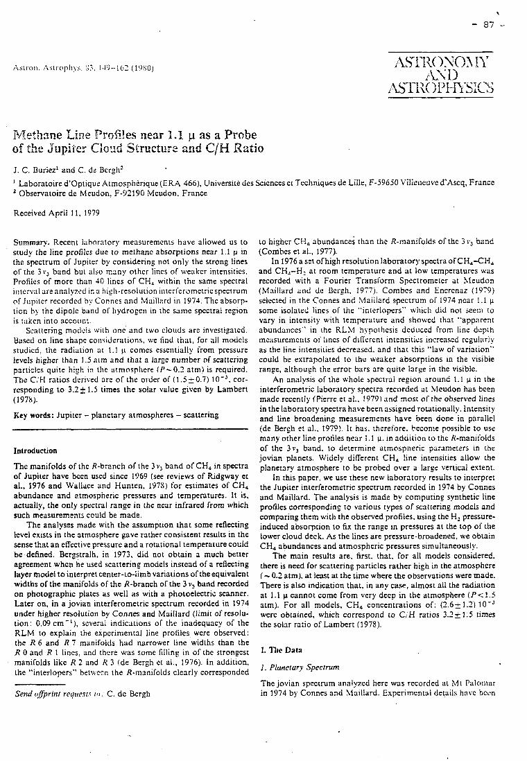
PAeihme Line Prr~6tes near 1.1 p as a Probe of th2 Jupiter CIor~d Structura and C/H Ratio

J. C. Duriez1 and C. de Ber;h2

' Laboratoire d'optique Atmospliérique (EKA 466), Université des Sciences et Tccliniques de Lille, F-59650 Villei~cuved'Ascq, France Observatoire de h,leudon, F-92190 Meudon, France

Received April 1 1, 1979

Summary. Recent Iahorritory measurements have rillowed us to srudy the line profiles due to methanc absorptions near 1.1 p in the spectrum of Jupiter by considering not only the strong lines of the 3 r, band but also many other lincs o r weakcr intensitics. Proiiles of more than 40 lincs of CH, within the samr: spectral iiiicr\r;il areanaly7ccl in higli-resolution iii~crfcrornetric spectrum of Jiipitcr recordcd by Connes and k1aill;ird in 1973. Tlie absorption b) the dipolc band of liydrogen in the same spectral region is tiikcn in10 accoiint.

Sc:iitering mocicls with one and two cloiids are investigated. Based on line shnpe coiisiderations, we find that, for ail models studicd, thc radiation at 1.1 p comcs csscntially from pressure levels tiigher than 1.5 atm and that a largc nurnber of scattcring particlcs quite high in tlic ntmosphcre (P-0.3 atm) is required. Thc CiFI ratios dcrived are of the oidcr of (1.5 20.7) l O V 3 . corrcsponding t o 3 .22 1.5 times the solar value given by Lambert (1978).

Key words: Jupiter - planctary atmosphercs - scattering

Introduction

The manifolds of thc R-branch of the 3 v , band of CH, in spectra of Jupiter have bccn used since 1969 (see reviews of Ridgway et al., 1976 and Wallace and Huntcn, 1978) for estimates of CH, abundance and atmospheric pressures and temperatures. It is, actually, the only spectral range in the near infrared from which such measurements could be made.

The analyses made with the assumption that some reflecting lcvel exists in the atmosphere gave rather consistent results in the sense that a n effective pressure and a rotaiional temperaturecould be defined. Bergstralh, in 1973, did not obtain a much better agreement whcn he used scattering models instead of a reîlecting Payer mode1 t o interpret center-to-limb variations of the equivalent widths of the manifolds of the R-branch of the 3 v, band recorded on photographic plates as well as with a photoelectric scanner. Later on, in a jovian interferometric spectrum recorded in 1974 under higher resolution by Connes and Maillard (lirnit of resolution: 0.09 cm- ' ) , several indications of the inadequricy of the R L M to explain the expcrimental line profiles wcre observed: the R 6 and R 7 manifolds had narrower line widths than the R O and R 1 lincs, and thcre was sorne filling in of the strongcst manifolds like R 2 and R 3 (de Bergh et al., 1976). In addition, the "interiopers" betwccn the R-ii~rinifolds clearly correspondcd

Send offpririt reqitesr.c 1 0 : C. de Bergh

to highcr CH, abundances than the R-manifolds of the 3 r, bünd (Combes et al., 1977).

In 1976 a set of high resolution laboratory spectra oïCH,-CH, and CH,-H2 at room temperature and a t low temperatures was recorded with a Fourier Transform Spectrometcr a t Aleudon (Maillard and de Bergh. 1977). Combes and Encrenüz (1979) selected in the Connes and hlaillard 9pectrum of 1974 ncar 1.1 p some isolatrd lines of the "inrerlopers" whicli did not seeni ta Vary in intcnsity with temperature arid showed that "apparent abundarices" i r i the RLM hypothcsis deduccd from line d c p ~ h mc;isiircincrits oî' lincs of dilTerent intensitics iiicreased rcguliirly as the line iiitensities decreased. and tliat this "law of variation" could be extrapoiated to thc weaker absorptions in the visible range, although the error bars are quite large in the visible.

An an;ilysis of the whole s p c c t r ~ l region around 1.1 p in the interferometric laboratory spectra recorded nt bleudon has bccn made rccentiy (fierre et al., 1979) and most of the observed lines in the laboratory spectra have been assigncd rotationally. Intensity and line broadening measurements have been done in pnrallel (de Bergh et al., 1979). It has. theret'ore. becon~e possible to use many other line protiles near 1.1 p. in addition to the K-manifolds of the 3v3 band. to determine atmospheric paramerers in r n r jovian planets. Widely different CH, line intensities allow the planetriry atmosphere to be probed over a large vertical extent.

in this paper. we use these new Iaboratory results to interpret the Jupiter interferometric spectrum recorded in 1974 by Connes and Maillard. The analysis is made by computing synthetic line profiles corresponding to various types of scattering rnodelï and comparing them witli the observed profiles. using the Hz pressure- induced absorption to fix the range in pressures ai the top of the lower cloud deck. As the lines are pressure-broadened. we obtain CH, abundances and atmospheric pressures srmultaneously.

The main results are, first, that. for al1 models considered. there is need for scattering particles rather high in the atmosphcre ( - 0.2 atm), a t least a t the time where the observations were made. There is also indication that, in any case, almost al1 the radiation at 1.1 p cannot come from very deep in the atmosphere (P< 1.5 atm). For al1 models, CH, concentrations of: (2.6k1.2) werc obtained, which correspond to C / H ratios 3.2& 1.5 times the solar ratio of Lambert (1975).

1. T11e Data

'1 OIililr The jovian spectrum analyzed here was recorded at h4t P. 1 in 1974 by Connes and Xlaillard. Expcrirncntal details hnvc bccn

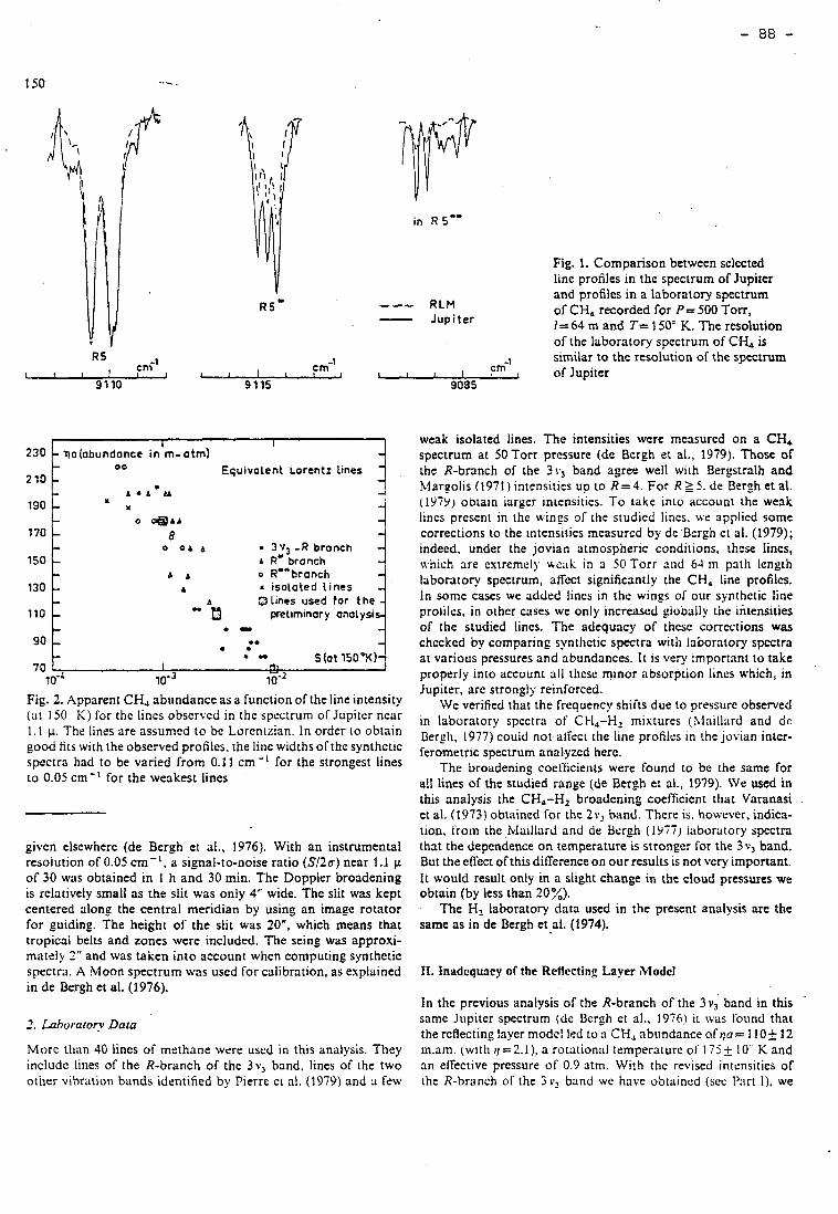
--- R L M - Jupiter

Fig. 2. Apparent CH, abundance as a function of the line intensity

230

210

190

170

150

130

110

90

70

(at 150 K ) for the lines observcd iri the spcctrum of Jupiter ncar 1.1 p. The lines are assumed to be Lorentzian. In order to obtnin

- ?o(obundonce inlm- atm) I -

- 00 Equivolent Lorentz Lines - - - - a - a M 4 - x

x - - O ~ A A - - 8 - - O O A A 3v3 - R bronch - - A R* bronch - - A A o RW*bronch - - A a isolated lines - - A EJ Lines used for the - - .. t2 pretiminory onotys~s- - 9 - - -0 - . . - . "

m S lot 150°K)- . 1

good fits with the observed profiles. the liiie widths of the synthetic spectra had to be varied from 0.11 cm-' for the strongest lines to 0.05 cm-' for the weakest lines

IO-' 1 0 - ~ IO-^

givcn elscwhere (de Bergh et al., 1976). With an instrumental resolution of 0.05 cm-', a signal-to-noise ratio (S/2o) near 1.1 p of 30 was obtained in 1 h and 30 min. The Doppler broadening is rclatively small as the slit was only 4" wide. The slit was kept centered along the central rneridian by using an image rotator for guiding. The height of the slit was 20", which means that tropical belts and zones were included. The seing was approximately 2" and was taken into account wlien con~puting synthetic spectrn. A Moon spectrum was used for cÿlibration, as expliiined in de Bergh et al. (1976).

2. labo rat or.^ Data

Morc than 40 lines of mcthnne wrrr used in this analysis. Tliey includc lines of the R-branch of the 3v, band, lines of the two ottler vibration bands idrntificd by Pierre et al. (1979) and a few

Fig. 1. Comparison between selected line profiles in the spectrum of Jupiter and profiles in a laboratory spectrum of CH, recorded for P= 500 Torr, 1% 64 m and T= 1 50" K. The resolution of the laboratory spectrum of CH, is similar to the resolution of the spectrum of Jupiter

weak isolated lines. The intensities were measured on a CH, spectrum at 50 Torr pressure (de Bcrgh et al., 1979). Those of the R-branch of the 3i., band agree well with Bergstralh and hlarpolis (1971) intensities up to R=4. For R>= 5. de Bergh et al. (1979) obra~n iarger intensities. To Lake into account the weak lincs present in the wings of the studied lines. wr applied some corrections to the tntensities measurtd by de Brrgh et al. (1979); indeed, under the jovian atmospheric conditions, thcse lines, ahich are cxtremcly wc;iii in ri 50 Torr and 61 m path iength laboratory spectrum, aHcct significrintly the CH, line profiles. In sonie cases we added lines in the wings of otir synrhctic line pro1ilt.s. in othcr cases we only increascd globslly the intensities of the studied lincs. Thc adequacy of thcsc corrections was chccked by comparing synthctic spectra willi laboratory spcctra at various pressures and abundances. I t is very important to take properly into account al1 thcse minor absorption lines which, in Jupiter, arc strongly reinforced.

We verified that the frequency shiits due to pressure observed in laboratory spectra of Cl-1,-H, mixtures (>laillard and de Berpli, 1977) could not alfect tiie line profiles in the jovian inter- feromettic spectrum analyzcd here.

The broadening coeffïcieiits were found to bc the same for a!l lines of the studied range (de Bergh et al., 1979). \Ve used in this analysis the CH,-H, broadening coefficient tliat Varanasi et al. (1977) obtliined for thc 2r, band. Thcre is. however, indication, flo~ii the Mailinrd and de Bergh (1977) iiiboratory spectra that the dependence on temperature is strongcr for the 3 v , band. But the cffect of this difierence on our results is not vcry important. It would result only in a slight change in the cioud pressures we obtain (by less than 20%).

The H2 l a b o r a t o ~ data used in :he present analysis are the same as in de Bergh et al. (1974).

II. Inadequacy of the Reflccting Layer Mode1

In the previous analysis of the R-branch of the 3 v, band in this same Jupiter spectrum (de Bergh et al.. 1976) it was found that the reflecting lnyer modc! led to a CH, abundance of vc7= 1105 12 In.am. (with t l = 2.1), a rotation;il temperature of 175 I 1 O' K and an effcctive pressure of 0.9 atm. With thc reviscd intensities of the R-branch of the 3 v, band we have obtaincd (see i';irt 1), we

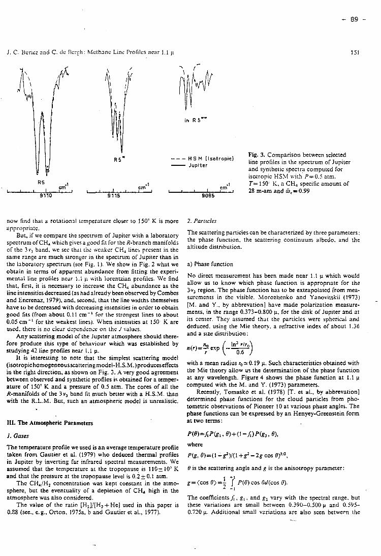
J. C. 13uritz and C. dc Ilcigh: klçthanc Line I'rofilcs ncsr 1.1 i i

RS*

-1 I I I

cm I '

9 115

--- H S M ( lsotropic) - Jupiter

now find that a rotational tcmperature closer IO 150' K is more appropriatc.

But, if we compare the spcctrum of Jupiter with a laboratory spcctrum of CH, whiih givcs a good fit for the R-branch manifolds of thc 3 I!, band. we sec thiit tiie wcnkcr CH, lincs prcscnt in the same range are much strongcr in the spectrum of Jupiter than in the laboratory spectrum (sce Fig. 1). We show in Fig. 2 what we obtain in terms of apprirent abundance from fittiny the experi- inciital line profiles ncar 1.1 p with lorcntzian profiles. WC find that, first, it is neccssary to increase the CH, abundiince as the linc intcnsitiesdecreased (as had already been obscrved by Combes and Encrenaz, 1979), and. second. chat the line widths themselves have 10 be dccreased wiih decreasing intcnsities in order to obtain good fits (frorn about 0.1 1 cm-i for the strongest lines to about 0.05 cm-' for the weakcst lines). When intensities at 150- K are used, there is no clcar dcpcndesce on the J values.

Any scattering model of the Jupiter atmosphere should therefore produce this type of behaviour wnich was established by studying 42 line profiles near 1.1 p.

It is interesting to note that the simplest scattering model (isotropic homogeneousscattering model-H.S. M.)produces effects in the right direction, as shown on Fig. 3. .A very good agreement bctween observed and synthetic profiles is obtained for a temperature of 150' K and a pressure of 0.5 atm. The cores of al1 the R-manifolds of the 3 v, band fit much better with a H.S.M. than with the R.L.M. But, such an atmospheric model is unrealistic.

III. The Atmwpheric Parameters

I . Gares

The temperature profile we used is an average teniperature profile taken from Gautier et al. (1979) who deduced thermal profiles in Jupiter by invertinç far infrared spectral mcasurements. We assumed that the temperature at the tropopause is 110k 10' K and that the pressure at the tropopause level is 0.2 51 0.1 atm.

The CH,/H, concentration was kept constant in the atmosphere, but the eventuality of a depletion of CH, high in the atmosphere was also considered.

The value of the ratio [H,]/[H,+He] used in this paper is 0.3 (see., e.g., Orton, 1375a, b and Gauiier et al., 1977).

Fig. 3. Comparison between selected line profiles in the spectrum of Jupiter and synthetic spectra computed for iscrtropic HS\I wirh P = 0.5 atm. T= 150 K, a CH, specific amount of 28 m-am and W, = 0.99

2. Particles

The scatteriiiç partides can be characttrized by tliree parameters : the phase function, the scattering continuum albedo, and the altitude distribution.

a) Phase function

No direct mcasurcment has been made near 1.1 p which would allow us to kriow which phase function is appropriate for the 3 v, region. The phase function has to be extrapolated from mea- surcments in thc visible. hlorozhcnko and Yanovitskii (1973) [M. and Y.. by abbrevation] have made polartzation measurements. in the range 0.373-0.800 p. for the disk of Jupiter and nt its ccntcr. They assumed that the particles were sphericül and deduced. usine the Mie theory, a refractive index of about 1.36 and a size distribution:

with a mean radius r , z 0.19 p. Such characteristics obtained with the Mie theory allow us the determination of the phase function at any wavelenyth. Figure 4 shows the phase function at 1.1 p computed with the IV. and Y. (1973) parameters.

Recently, Tomasko et al. (1978) [T. et al., by abbrevation] detcrmined phase functions for the cloud particles from photometric observations of Pioneer 10 at vanous phase angles. The phase functions can be expressed by an Henyey-Greenstein form at two terms:

where

P(g, 0)=(1 -gl)/(l +g2 -2g cos

6' is the scattering angle and g is the anisotropy parameter:

1 +' COS O ) = - P(0) cos Od(cos O). 2 - 1

The coefficients A , g, , and g2 Vary with the spectral range, but thesc variations are small bctwcen 0.390-0.500 p and 0.595- 0.730 p. Additional small variations are also seen betwern tlie

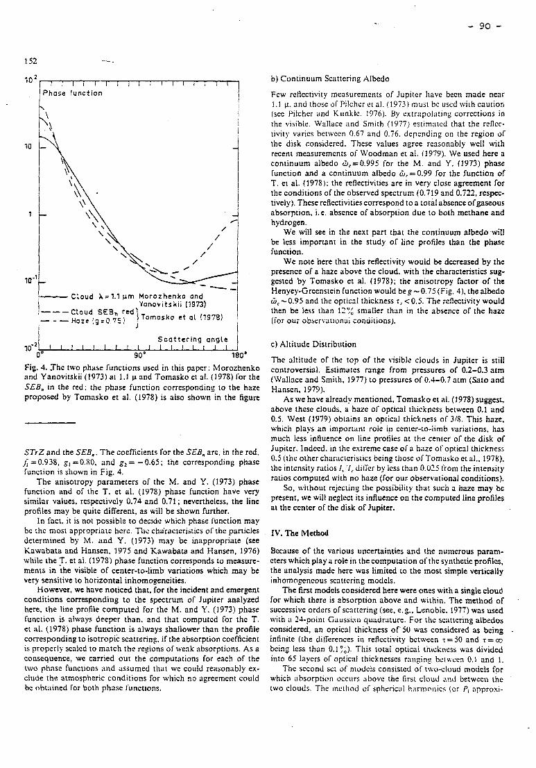
1 0 2 . 1 1 1 1 i l l I I I I I I [ I [ I

Phose function

\

\ 1 1

\b 1 i 1 1

I

i i -

/

/ /

/ /

/

\- CLoud X = 1.1 rrrn Morozhenko and 1 ! Yonovitskii (1973) ,---

- - - ioomsko et aL !1978)

l J

! 1

Scat ier ing ongle

90' 180'

Fie. 3. .The two phase functions used in this paper: Morozhenko and Yanovitskii (1973) at 1.1 p and Tornasko et 31. (1978) [or the SEB, in the red; the phase function corresponding to the haze proposed by Tomasko et al. (1978) is abo shown in the figure

STrZ and the SEB,. The coefficients for the SEB, arc. in the red, j; = 0.938, g, = 0.80, and g, = - 0.65; the corresponding phasc function is sliown in Fig. 4.

The anisotropy parameters of the M. and Y. (1973) phase function and of the T. et al. (1978) phasc function have very similar values, respectively 0.74 and 0.71 ; nevertheless, the line profiles rnay be quitc different, as will be shown further.

In fact, it is not possible to decide which phase function rnay be the most appropriate here. Tlic ciiiracteristics of the particles determined by M. and Y. (1973) may be inappropriate (see Kawabata and Hansen, 1975 and Kawabata and Hansen, 1976) wliile the ?. et al. (1975) phase function corresponds to measurements in the visible of center-to-lirnb variations which rnay be very sensitive to horizontal inhomopneities.

However, we have noticed that, for the incident and crnergent conditions corresponding to the spectrurn of Jupiter analyzed here. the line profile computed for the M. and Y. (1973) phase function is always deeper than, and that cornputcd for the T. et al. (1978) phase function is always shallower than the profile corresponding to isotropic scattering, if the absorption coefficient is properly scalcd to match the regions of wenk absorptions. As a consequence, we carried out the computations for each of the two ptinse functions and assumed tliat we could reasonnbly excludc the atmospheric conditions for which no agreement could bc ohtained for both phase functions.

b) Continuum Scattering Albedo

Few reilectivity ineasurements of Jupiter have becn made near 1.1 p. and thosc or Pilchcr et al. (1973) must bc used w i ~ h caution (see Pilchcr and Kiinklc. 1976). By extr;lpolatiny corrections in the visible. Wallace and Smith (1977) estirnatcd that the rcflcc- tivity varies betwecn 0.67 and 0.76. depcnding on the rcgion of the disk considercd. These values agree rcasonably well with recent me3suremcnts of Woodman et al. (1979). We used here a continuum albedo G,=0.995 for the M. and Y. (1973) phase function and a continuum albedo G,=0.99 for the function of T. et al. (1978): the reflectivities are in very close agreement for the conditions of the observed spectrum (0.719 and 0.722, respectively). These reflectivities correspond to a total absence ofgaseous absorption, i. e. absence of absorption due to both rnethane and hydrogen.

We will see in the next part that the continuum albedo will be lcss important in the study of line profiles than the phase function.

We note here that this reflectivity would be decreased by the presence of a haze above the cloud. with the characteristics sug- gestcd by Tornasko et al. (1978); the anisotropy factor of the Henyey-Grcenstein function would be g - 0.75 (Fig. 4). the albedo WC -0.95 and the optical thickness r, c 0.5. The reflectivity would then be less than 13:; smaller than in the absence of the haze (for our observational conditions).

c) Altitude Distribution

The altitude of the top of the visible clouds in Jupitcr is still controversial. Estimates range from pressures of 0.2-0.3 atm (Wallace and Smith. 1977) to pressures of 0.4-0.7 atm (Sato and Hansen, 1979).

As we have already mentioned, Tomasko et al. (1978) suggest, above thesc clouds. a haze of' optical tiiickncss between 0.1 and 0.5. West (1979) obtnins an optical thickness of 31'5. This haze. which plriys an importarit iolc in center-to-limh variations. has much less influence on line proiilrs at tlir centcr of thc disk of Jupiter. Indced. in thc extrcme case o f a haze of optical thickness 0.5 (the other chiiriictcristics being thosc of Tomasko et al., 1978). the intensity ratios I , , ~ I , difrcr by lcss than 0 .03 Sroni the intensity ratios computed with no haze (for Our observational conditions).

So, without rejecting the possibility that such a h u e may bc present, we will neglect its influence on the cornputed line profiles at the center of the disk of Jupiter.

IV. The Method

Because of the various uncertainties and the numerous parameters which play a role in the computation of the synthetic profiles, the analysis made here was Iirnited to the rnost simple vcrticaliy inhorno~encous scrittcring modcls.

The first modcls considered here were ones with a single cloud for which therc is absorption above and within. The metliod of successive orders of scnttering (see, e.g., Lenoble. 1977) was used with a 24-point Gaussi~iri quadrature. For thc scattering aibedos considered, an optical thickness of 50 was considered as being infiiiite (the ditïerences in reflectivity bctween r = 50 and T = m bcing lcss than 0.1 i,). Tliis total opticai thickness was divided into 65 layers of optical thicknesscs rnriging hct\qcen 0.1 and 1.

Thc sccond set of rnodcls consisted of rwo-cloud niodels for which absorption occiirs abovc the first cloud ii i i~l betweeri the two clouds. Tlic inctliod of sphrricctl hariiic~ciics (or P, approxi-

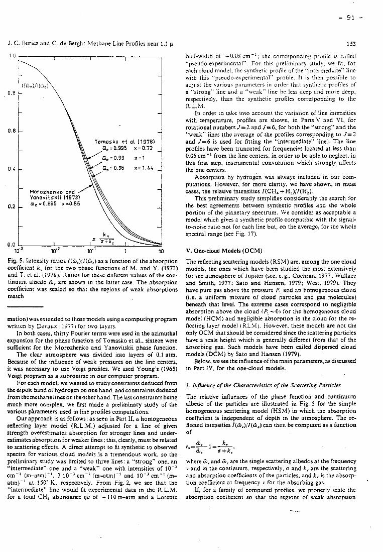
J. C. Riirirz and C. de Bergh: hletliane Line Profiles near 1.1 p

-

0.6 - Tomosko e t 01 (1978)

WC = 0.995 x = 0.72 - -

0.4 - -

Morozhenko and -

0.2 - W C =0.995 x ~ 0 . 5 5

-

0.0 b

103 IO-' IO- l 7 10

Fig. S. lntensity ratios I(W,),'I(O,) as a function of the absorption cocfficicnt k , for the two phase functions of M. and Y. (1973) and T. et al. (1978). Ratios for thesc diircrent values of the continuum albcdo W, are shown in the latter case. The absorption coeficient was scaled so that the rcgions of wcak absorptions match

mation) was extended to thosc models using a computing program writiçn by Dcvriux .r 1977) for two laycrs.

In both cases, thirty Fourier terms were used in the azimuthal expansion for the phase function of Tomasko et al.. sixteen were sufficient for the blorozhenko and Yanovitskii phase function.

The clear atmosphere was divided into layers of 0.1 atm. Because of the influence of weak pressures on the line centers, it was necessary to use Voigt profiles. We used Young's (1965) Voigt program as a subroutine in Our computer program.

For each model, we wanted to study constraints deduced from the dipole band of hydrogen on one hand. and constraints dcduced from the methane lines on the other hand. The last constraints being much more complex, we fint made a preliminary study of the various p'arameters used in !ine profiles computations.

Our approach is as follows: as seen in Part II. a homogeneous reflecting layer model (R.L.iM.) adjusted for a line of given strength overestimates absorption for stronger lines and under- estimates absorption for weaker lines; this, clearly, must be related to scattering effects. A direct attempt to fit synthetic to observed spectra for various cloud models is a tremendous work, so the preliminary study was limited to three lines: a "strong" one, an "intermediate" one and a "weak" one with intensitics of IO-' cm-' (m-atm)-', 3 IO- ' cm-' (m-atm)-' and cm-' (m- atm)-' at 150' K, respectlvely. From Fig. 2, we see that the "interinediate" line would fit experimental data in the R.L.M. for a total CH, abundance ila of - 1 I O m-atm and a Lorentz

haIf-width of -O.OS cm-' ; thc corrcsponding proiile is c;illcd "pscudo-experiiiie~ital". For tliis preiiniinary study, we fi:, for each cloud niodsl. thc syntlietic profile of the "ii~tcrincdiate" liiic with tliis "pseudo-~xperiiiieiit:~1~~ pi'otile. It is thcn possible to adjiist the various pwraiiietcrs iii order ihat syntlieiic profiirs of a "strong" line aiid a "weiik" line bc lcss dcep aiid inoie deep, respectively, than the synthetic profiles corresponding to the R.L.M.

In order to take into account thc variation of line intensities with temperature, profiles are sliowii, in Parts V and VI, for rotational numbers J = 2 and J=6 , for both the "strotig" and the "weak" lines (the average or the profiles corresponding to J = 2 and J = 6 is used for fitting the "intermediate" linej. The line profiles have been truncated for frequencies located at less than 0.05 cm-' from the line centers, in order to be able to neglect. in this first step, instrumental convolution which stronglg affects the line centers.

Absorption by hydrogén was always included in our computations. However, for more clarity, we have shown, in most cases, the relative intensities I(CH, -t HI):I(H,).

This preliminary study simplifies considcrably the search for the best agreements between synthetic profiles and the whole portion of the planetary spectrum. We considei as acceptable a model which gives a syntheric profile compatible with the signal- 10-noise ratio no1 for cach line but, on the average. for the whole spectral range (sec Fig. 17).

V. Onccloud Models (OChI)

The reflecting scattering models (RSM) are, among the one cloud models, the ones which have been studied the most extcnsiveiy for the atmosphere of Jupiter (see, cg., Cochran, 1977: Wallace and Smith, 1977: Sato and Hansen, 1979; West. 1979). They have pure gas above the pressure Pi and an homogeneous cloud (Le. a uniform mixture of cloud particies and gas molecules) beneath that level. The extreme cases correspond to negligible absorption above the cloud IP! -0) for the homogeneous cloud model (HCM) and negiigible absorption in the cloud for the reflecting layer model t RLM). tiowever. these models are not the only OCM that should be considered since the scattering particies have a scale height which is generally different from that of the absorbing gas. Such models have been called dispersed cloud models (DCM) by Sato and Hansen (1979).

Below. we see the influence of the main parameters, as discussed in Part IV, for the onecloud models.

1. Inpuence of the Characreristics of the Scattering Particles

The relative influences of the phase function and continuum albedo of the particles are illustrated in Fig. 5 for the simpie homogeneous scattering mode! (HSM) in which the absorption coefficient is independent of depth in the atmosphere. The refiected intensities I(W,)/I(&,) can then be computed as a function of

where 6, and 8, are the single scattering albedos at the frequency v and in the continuum, respectiveiy, u and k, are the scattcnng and absorption coefficients of the particles, and k , is the übsorp- tion coefficient at frequency v for the absorbing gas.

If, for a family of computed profiles, wc properly scale the absorption coefficient so that the regions of weak absorption

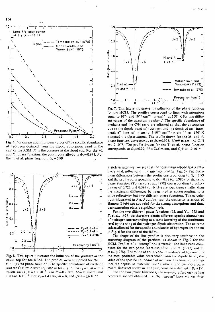
Speci f i c abundonce of H t ( km-a tm) k - - - Tornasko e t a l (1978)

b'\ Morozhenko and Yanovitskii (1973)

t \ \ \

6 \

I M. ond Y.-U 1

- 'Morozhenko ond

Frequency (~6') 0.0 - 1 O O +1

Fig. 7. This figure illustrates the influence of the phase frinction for the HCM. The profiles correspond to lines with intensitirs cqual to IO-' and IO- ' cm-' (m-am)-' at 1 SOC K for two diffcrent values of the quantum numbcr J. The specific abundance of methane and the C/H ratio are adjusted so that the absorption duc to thc d i p ~ l e band of hydrogcn 2nd thc dcpth of iin '-intermediate" 'line of intcnsity 3 IO- ' cm-' (m-am)-' at 1 ZG" K maiched thc observations. Thc profilc drnwn for the M. and Y .

Fig. 6. Maximum and minimum values of the specific abundance phase function corresponds to W,=0.995. .M=9 m-am iind C/K

of tibdrogen dcduced from the dipolc absorption band in the = 1.2 IO-'. Thc profile drawn for thc T. ct a!. ptiasc fiinction

case of the RSM. Pl is the pressure a t the cloud top. For the M. corresponds to Wc=0.99, iU =23.5 m-am, and CjH = 1.9 IO-^ and Y. phase function, the continuum albedo is Wc=0.995. For ilic T. et al. phase function, WC = 0.99

match in intcnsity, we see that thc continuum albedo has a relatively weak influence on the intensity profi!es (Fie. Sj. Tlie maximum difiercnces bctween the profile corrcspoiiding to W,=0.99 and the profile corrcsponding to &, = 0.98 (or 0.995j for ille saine - piiasc functioii (Tomasko et 81.. 1978) correspondiny ro rcflec- tivitics of 0.722 and 0.594 (or 0.531) nie four times smaller than the maximum difircnces bctwcen prolilcs correspoiiding to a

- same refiectivity but two differcnt phase functions. Tlie calculations illustrated in Fig. 5 contirm that thc siinilarity relations of

0.2- !! - Hansen (1969) are not valid for the strong absorptions and that, 0.0- la backscattering plays a significant role. - For tlic two diffcrcnt phase functions (M. and Y.. 1973 and

T. et al.. 1978) we thcrefore obtain difycrent specific abundances - of hydrogen corresponding to a same lowering of tlic continuum level by the wing of the hydrogen dipole absorption. The extreme

-- - pl= 0. O atm - values allowed for the specific abundanccs of hydrogen are shown - - - - - - - Pl= O .2 atm - in Fig. 6 for the crise of the RSM. - Pl= 1.4 otm The shapc of the line profiles is nlso vcry se~sitive to the - scattering diagram of. the particles, as shown in Fig. 7 for the

Frequency lcm-l) HCM. Profiles of a "strong" and a "weak" line have been com- I I I puted for the tu.0 phiisc functions of > I . and Y. (1973) and T.

-1 O + l " -1 O +' et al. (11)7Y). Tiic viiluc of tlic spccifri: abiindiince of hpdro-cn is Fig. 8. This figure illustrates the influence of the pressure at the the most probable value determincd iroin the dipole band; the .

cloud top for thc RSM. The profiles were computed for the T. value of the spccific abundarice of methane has been adjustcd so et al. (1978) pii:isc function. The spccific abundcince of metliane that the dcpths of "intermediate" s~~ntlictic and pseudo-expcri- and the C/H ratio were adjusted as for Fie. 7. For Pl =O, h.l=23.5 ment:il lines(not shown in thefiçurc)coincitlensdcfincd in Pnrt IV. m-sin. and C/H= 1.9 IO-'. For Pl =0.2 atm, hl= 11 m-am, and For thc Iwo pliase Sunctions, tlic rcquired eliect oii the line C/H=0.6 IO-'. For P, = 1.4 atm, ,t/=0, and C/M-0.6 IO-' centers is indecd obtaincd; i.e. tlic "strong" lines Lirc less deep

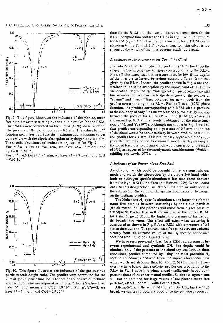
J. C. Buriez and C. dc Bergh: Metliaiic Linc Profiles ncar 1.1 1

Fig. 9. Tliis figurc illustrates the influence of the photon mean free path between scattering by the cloud particles for the RSM. The profilcs wcrc computed for the T. et al. (1978) phasc function. Tlic pressure nt thc cloud top is P, = 0.5 atm. Thc v;ilucs for a- ' (photon mean frce patli) are the maximum and minimum values compatiblc wiih ihc dipole absorptiori of hydrogen at P= 1 atm. Tlie spccific abundancc of nicthanc is iidjustcd as for Fig. 7. For O - ' = 1.4 km at P = l atm, WC have 6 1 1 3 . 5 m-am, and CIH = 0.96 1 O". For a-l=4.6 km at P = l atm, we have M=7.7 m-am and C/H = 0.66 IO-'

Fig. 10. This figure illustrates the influence of thc gas-tocloud paniclcs scaie-height ratio. The profiles were computcd for the T. et al. (1978) phasc function. The specific abundance of methane and thc Cil-1 ratio are adjusted as for Fig. 7 . For Hg/I ip= 1 , we have M=23.5 m-am and C/I-I= 1.9 IO-'. For Hg/I lp=2 , we have M = 7 m-am, and C/H = 0.9 1 O-'

tIiat1 l'ür thc RLM anci the "\veakV liiics arc dccper tlirin for the RLbI [compare linc profiles for H C M in Fig. 7 with line p~ofilcs for KLSf (P, = 1.3 atm) in Fis. SI . klowever. for a I-ICLI ccorrc- spo~iuing to ille T. et al. (197s) pliasc Sunçtion, tiiis e f ic t is too strong as tlic wings of the lincs become much too broad.

2. bfli~ence of rite Pres.~ure at the Top of rhc Clotid

1t is obvious that, the higlier the pressure at the cloud top the closes the line profiles arc to those corrcsponding to the RLiCI. Figure 8 illustrates that this pressure must be low if the depths of tlie lines are to have a. behaviour notably different from that given by the RLM. Indeed, the profiles shown in Fig. 8 are con- strained to the same absorption by the dipole band of H, and to an identical depth for the "intermediate" pseudo-experimental line in order that we can study the departures of the profiles of "strong" and "weak" lines obtained for ncw mociels [rom the profilcs corresponding ;O tne RLM. For the T. et al. (1978) pliase function, the profiles corresponding to a RSM with a pressure at the cloud top of only 0.2 atm are located approximateiy midway between the profiles for HCM (P, = O ) and RLM (P, = 1.4 atm) shown on Fig. 8. A similar result is obtained for the phasc îunc- tion of hl. and Y. (1973). Altiiough not shown in Fig. S WC find that profilcs corrcsponding to a pressure of 0.5 atm at the top of the cloud would be about midway bctwcen profiles for 0.2 atm and profiles for 1.4 atm. This preliminary zpproach already sug- gests that WC may be led to eliminate modeis with pressures at the cloud top close to 0.5 atm which would correspond to a c!oud of NII, as suggested by tliermodynamic considerations (Weiden- schilling and Lewis, 1973). ~

3. Influence o j the PItoton Afcon Free Patlr

An objection which could be brought is that we constrain our models to match the absorption by the dipole 2-0 band which leads to hydrogen specific sbundances less than those deduced from the Hz 4-0 S ( 1 ) line fSato and Hansen. 1979). We will come back to this disagrcement tn Pan VI. but here we only look at the tnduence of the value of the specific abundance of hydrogen on the methane profiles.

The higher the H, spccific abundance. the larger the photon mean free path is between scatterings by the cloud particies (which means that the photons will come from higher pressure atmospheric Icvels). It is well known that, in the simple RL,M. for a Iine of given depth, the higher the pressure of formation, the broader the wings. This effect still exists when scattering 1s considered as shown ln Fig. 9 for a RSM with a pressure of 0.5 atm at the cloud top. The photon mean free paths used are deduced directly from the extreme values of the H, specific abundancc obtained from the dipole band (Fig. 6).

We have seen previously that, for a RSM. an agreement between experimental and synthetic CH, line depths could be obtaincd only if the pressure at the clorid top was low. In these conditions, profiles computed by using the most probable H, specific abundances deduced from the dipole absorption have wings which are stronger than for the RLM (see Fig. 8). How- ever, we have found that synthetic profiles corresponding to the RLM in Fig. 8 have line wings already sufficiently broad compared to those of the experimental profiles. So, the bes~ agreements will not be obtained for large values of the photon mean free path but, rather, for small values of this path.

Alternatively, if the wing of the synthetic CH, lines arc too broad, we can try to obtain a good fit to the planetary spectrum

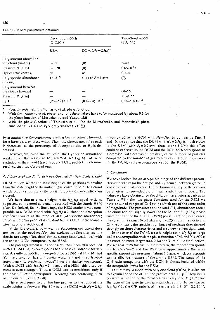
156 . Table 1. Model parameters obtained

One-cloud models (O.C.M.)

Two-cloud model (T.C.M.)

RSM D C M (Hg=21ip)'

CH, amouiit above the top cloud (m-am) 0-25 (0) Pressure P, (atm) 0-0.20 (0) 0.05-0.35 Optical thickness z, CO w 0.5-4 CH, specific abundance 12-21 6-13 a t P=l atm (0) (m-am) CH, amount between the clouds (m-am) - - 60-1 50 Pressure P, (atm) - - 1.1-1.5'

a Possible only with the Tomasko et al. phase function With the Tomasko et al. phase function: tliese values have to be multiplied by about 0.6 for the phase function of Morozhcnko and Yanovitskii Miith the phase function of Tomasko et al.; for the Morozhenko and Yanovitskii phase - function: 7, - 1-6 and P, slightly weaker (-10%)

hy assuming that the continuuin level has been effectively lowered. is compnred to the HCM with I Ig= f ip By comparing Figs. 8 for a large part. by thcse wings. Then. the photon mean free path and 10. we can see thar the DCA1 uith Hp = 7 I j p 15 niuch clober 1s decreased, as the percentape of absorption due t o H2 is de- to the RSM (with P, =0.2 atm) than to the H C h l ; this effect creased could be expected as the DCM and the RSM both correspond t o

However, we round that values of the H, spccific abundance a decrease, with decreasing pressure, of the number of pariiclcs weaker than tlie values we had selccied (see Fig. 6 ) had to bc compared to the number o l -as niolecules (in a continuous way excluded as they would have prodiiced CH, protiles much more for the DCM, and discontinuous way for the RSM). resolved than the observed ones.

4. I~fit<crice of tlir Ratio Beiiveen Gus and Particle Scale Heiglti WC have lookzd for an acceptable r;inge of the dif i rent param-

DCM models wliere the scalc heignt of the particles is smaller eters rather tlinn for the best possihlr: +rccn;ent bctwccn syrithctic than the scale height of the ambient gas, corresponding to a cloud which beconies tliinncr as tlie pressure decreases, were also considered.

We have chosen a scale height ratio I ig l l lp equal to 2, as .suggested by the good agreement obtained wiih the simple HSM (Part II). Indeed, for the iine wings, the HSM model is very comparable to a D C M model with I Ig/Hp=2, since the absorption coefficient varies as the product :MP (M: specific abundance; P: pressure); this product is constant for this DCM if the temperature profile is isothermal.

At the line centers, however, the absorption coefficient does not Vary as the product M P ; this explains the fact that the Iine depths are deeper (less deep) for the strong lines (weak lines) with the chosen DCM, compared to the HSM.

Tlie sood agreement witli the observational spectruni obtained with a HSM (Fig. 3) corresponds t o the case of isotropie scatter- in&. A synthetic spectrum coniputed for a HSM with the M. and Y. phase function has line depths which are not in such good ripseenlenL (the synthetic "stroiiç" lincs are sliplitly too strong). With a DCM with l ig/Hp=2, instead of a HSh.1, this disagrce- nicrit is cven strongcr. Tiius. a DCM cari be considercd only if the phase fuiiction corresponds to strong back scattering, such as thc one of T. et al. (1978).

The strong sensitivity of the linc profiles to the ratio of the scale heights is sliown in Fig. 10 whcre the DCh4 with l!g=3 I ip

and obscrvational spectra. The prclin~iiiary study or thc varivus paranretcrs has provided uscfril insights iiito thcir i:ifluencc. The values we have obtained for ihc di!icrcnt parameters arc givcn in Table 1. With the two phase functions used for the I i S X l we have obtnined ranges of C!H ratios which are of the same order of magnitude. The pressures and the total CH, abundances above the cloud top are slightly lower for the M. and Y. (1973) pliase function than for the T. et al. (1978) phase function; in al1 cases, the? are in tlie nirire: 0-0.3 atni and 0-0.35 m.atm., respectivcly. On the contrary, the specific abundance of methane docs dcpend strongly on those characteristics and is somewhat less significant.

In the case of the DCM, a scale hciglit ratio HgiHp as largc as 2 is not compatible with the phase function of M. and Y. (1 973); it cannot be much larger than 2 for the 7. et al. phase function. We sce tliat. n,ith this last phase function, thc modcl carrcspond- ing to HgiHp=2 and .the RSM give approximately the saine specific amount at a pressure of about 0.5 atni, which corrcspcnds to the erîective pressure of the siinplc HSXI. The range of the Cil-i ratio conipatiiiic sit th tlic DCM is alrnost includcd \ritlii:i the acceptablc limits for the RSM.

In summary, a mode1 ni th only one cloud (OCM) is sufficicnt to explain tlie shapc of the linc proiilcs near 1 . l p. It requises 11

pressure at tlic top of ilic cloud which is very low: P, 5 0.2 atni; the ratio of the scale heiglits &as-p;:rticlcs cannot bc \,ery large: I l g / l l ~ l < 2 ; the C/H ratio is of the order of: 0.8 1 @ - ~ - 2 . 2 IO-',

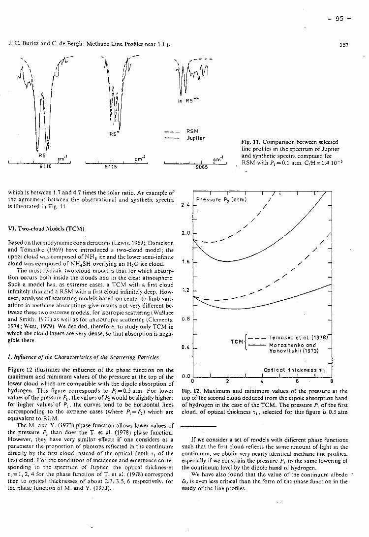
J. C. Buricz and C. de Bergh: Methane Line Profiles ne,ar 1.1 p

--- RSM - Jupiter

which is bttwccn 1.7 and 4.7 times the solar ratio. An example of the aprecniçn! bct\vceri the observational and synthetic spectra is illustrated in Fig. 1 1 .

VI. T W O - C ~ O U ~ hludcls (TCM)

Based on tlierrnoc1yn:iinic considerations (LcLvis, 1969), Dsriielson and Tomasko (1969) have introdticed a two-cloud model; the upper cloud was composcd of NH, ice and tlic lower scnli-infinite cloud was composed of NH,SH overlying an H,O ice cloud.

The mus( rciilistic twocloud model is that for which absorption occurs both iiiside the clouds and in the clcar atmosphere. Such a model has. as estremc cases. a TCM with a first cloud infinitely thiii aiid a K S h I with a first cloud infinitely deep. How- ever, analyses of scattering models based 011 centcr-to-limb variations in n1cth;ine absorptions rive results not vcry diffcrent betwccn thesc two extreme modcls, for isotropie scattering (Wallace and sr nit!^, 1977 J 2 5 \\cl1 2 s for anisotropic bcattering (Clcments. 1974; West, 1979). We decided. therefore, t o study only TCM in which the cloud lnyers are very dense, so that absorption 1s negligible there.

I . Influence of the Characteristics of the Scattering Particles

Figure 12 illustrates the influence of the phase function on the maximum and minimum values of the pressure at the top of the lower cloud which are compatible with the dipole absorption of hydrogen. This figure corresponds to Pl = 0.5 atm. For lower values of the pressure Pl . the values of P, would be slightly higher; for higher values'of P,, :he curves tend to be horizontal lines corresponding to the extreme cases (where P, =Pz) which are equivalent t o RLM.

The M. and Y. (1973) phase function allows lower values of the pressure P, than does the T. et al. (1978) phase function. However, they have vcry similar efïects if one considers as a paranleter the proportion of photons rcflected in the continuum directly by the first cloud instead of the optical depth 7, of the first cloud. For the conditions of incidciice and emergence corresponding 'to the spectrum of Jupiter, the optical thicknesses .ri = 1 , 2, 4 for the phase function of T. et al. (1978) correspond then to optical thicknesses of abolit 2.3, 3.5, 6 respcctively. for the phase ruiiction of M. aiid Y. (1973).

Fig. 11. Coinparison between selectcd line profiles in the spectrum of Jupiter and synthetic spectra computed for RSM with Pl = 0.1 atm, C/H= 1.4

- - - Tomasko e t 01 (1978) M o r o t h e n k o and Yonovi ts kii (1973)

Fig. 12. Maximum and minimum values of the pressure at the top of the second cloud deduced from the dipole absorption band of hydrogen in the case of the TCM. The pressure Pi of the first cloud, of optical thickness 71, selected for this figure is 0.5 atm

0.0

If we consider a set of models with different phase functions such that the first cloud rcRects the same amount of light in the continuum, we obtain vcry nearly idcntical methane linc profiles. especially if we constrain thc pressure P, to the same lowering of the continuum lcvcl by the dipole band of hydrogen.

We have also found that the valrie of the continuum albedo '

W C is evcn less critical than the form of thc phase function in the study of the line profiles.

O p t i c o l t h i c k n e s s I l I I 1 I i

O 2 L 6 8

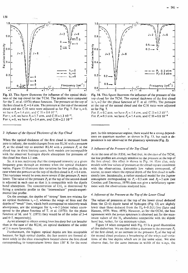
Fig. 13. This figure illustrates the influence of the optical thick- riess of the top cioud for tne T C M . The profiles were computed for the T. et al. (1978) phase function. The pressure at the top of the first cloud is P, = 0.4 atm. The pressure at the t o p of the second cloud and the CIH ratio u3ere adjusted as for Fig. 7. For 7, = O . we ha1.e & = 1.4 alm. and C 'II = 0.6 IO-'. For 7: =4. we ha\'e P,=1 .7 atm. and C:H=1.3 IO-'. For T, =8, we have P2 =3.4 atm, and CIH =2.1 IO-'

Fig. 14. This figure illustrates the influence of the pressure of the iop cloud for the TCM. The opiical thickness of the first cloud is 7 , =:! for the phase function of T. et al. (1978). The pressure at the top of the second cloud and the C,'H ratio were adjusted as for Fig. 7. For Pl = 0.2 atm. \ve have Pz = 1.3 a:m, and C 'H = 1.3 1 O-3. For P, =O..'> atm. we have P2 = 1.4 atm. and C:H=0.8 IO-'

2. InJuence ofthe Oprical Thickile.ss of rhc Top Clnird

Whcn the optical thickness of the first cloud is increased from zero to infinity, the model changes froni one RLhl witli a pressure P: at the cloud top to another RLM with a pressure Pl at the cloud top; in therc liniitiiig cases. both models are incompatible viith the observed hydrogcn dipolc absorption for pressures of the cloud less than 1.1 atm.

So, it is noi surprising thzt the computed inteiisity at a givcn frcquency goes through an extrerne wlien the optical thickness varies. Figure 13 illustrates this variation for line profiles, in the case where the pressure at the top of the first cloud is Pl = 0.4 atm. This variation would be even more scvere if the pressure Pl were lower. The value of the pressurc P, a t the top of the second cloud is adjusted in each case so that it is compatible witli the dipole band absorption. The concentration of CH, is detcrinincd by fitting a synthetic profile to the "interniediate" pseudo-experimental line profile.

On the average, the depths of "strong" lines are minima for a n optical thickness .r, -2, whereas the wings o f liiies and the deptlis of "weak" lines, which both correspond t o relatively weük absorptioiis, a re the stroiigest for T, -4-5 [ ~ h c s e valucs correspond to the phase function of T. et al. (1978); for the phase function of M. and Y. (1973) they would be of the order of 3-4 and 6-7, respectively].

As we attenipt to obtain strong lines less decp but not broader than in the case of the RLM, a n optical thickness of the order of 2 is niore favorable.

Fiirthcrmore, the !iighest optical depths are lcss acceptable bccause, for higli oiltical depths. thc liiie centçrs arc Sormcd al- inost solely in the clear atmosphere locatcd above the first cloud corrcspondiiig to tcrilpcratures lowcr thaii 150' K for tlic niost

part. In this iernperaturc regime. there would be a strong dependence on quantum number. az shoun in Fif 13. but such a de- pcndence is not observed in the planetary spectrum (Fig. 2).

3. It$uet~ce o j ~ h e Pressure o j ~ l i e Top Cloird

As in the case of the RSM, ive find tha!, in the cace of the TCiM, the line profiles are strongly sensitive io the pressurc at the top or the first cloud: this etTcct is sh0u.n in Fig. 14. kI-rc a!so, only mo<lels with los, valiies of pressure nt the cloud top are coiisisterit with the observations. Extremely low valiies corresporid, of course. to cases whcrc the optical dcpth of the f i~s t cloud is siiffi- ciently low. Incidentally, a rather standard model for the Jupiter atmosphere corresponding t o Pl -0.5 a tm and Pz-2 atm (sce Coinbes and Encrenaz, 1979) does not &ive a satisfactory agree- iiicnt witli the observ:itions analyzed Iiere.

4. InPirence oJ the Pressure ut ihe Top of the Lobucr Cloird

The values of pressures a t the top of the lower cloud deduced from the (2-0) dipole band of hydrogen (Fig. 12) are slightly lowcr tlian thoac dcduccd froril tiic: II, 4-0 S(1) line (Sata and Hansen, 1979; West, 1979). However, a s for the OCiM, the best agreement with the jovian spectrum is obtained not foi. the maximum valiies of the tl, abundancc coinpatible with the dipole baiid but, rathcr, for tiic niiiiinium v;ilucs.

Figure 14 wlien compared with Fig. 15 is a good illustration of ttiis deduction. Wc sec that either a dccrcase in the pressure Pl of the first cloud, or an increase in tlic pressure P, nt [lie top of the second cloud produces n broadeiiing of tlic \i.iiigs iiiid vnria- tions of tlic line dcpths which arc in the same scnsc. We also observe that, Sor the samc incrcasc in width of the ~ i n g s , tlic

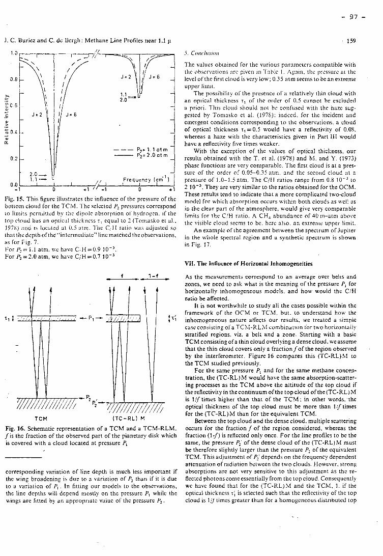
J. C. Buriez and C. dc Ucrgli: Methane Line I'rofiles riear 1.1 p

Fig. 15. This figure illustrates the influence of the pressure of the butiorii cloud for the 7'CM. 'fhe selected P, pressures correspond to limits pcrniittcd by tlie dipole nbsorprion of h!.drogen. if the top clniid has an optic;il thickncss r , equal to 2 (Toinasko et al., 19:a) nild is locuted at 0.5 alin. l'iic Cil I ratio was adjusted so that the dcpih ofthe "intermediate" linc inatched theobservations. as for Fig. 7. t'or 1% = 1.1 atm, ive have C:.li=0.9 IO- ' . For 1; =2.0 atm, we have C/H = 0.7 1

T CM (TC-RL) M

Fig. 16. Schematic representation of a T C M and a TCM-RLM. f i s the fraction of the obsewed part of the planetary disk which is covered with a cloud located at pressure Pl

corresponding variation of line depth is much less important if the wing broadening is due to a variation of Pz than if it is due to a variation of P l . In fitting our riiodels to the observations, the line depths will depend mostly on the pressure Pl while the wings are fitted by an appropriütc value 01' the pressure Pz.

The values obtaincd for the various pnr:iineters conipatibie with the observatiniis arc giveii in Tciblc 1. hg:iin, tlic pscss~iri: ni the level of the first cloud is very low; 0.35 a tm seenls to be an extreme upper liinil.

The possibility of the presence of a relatively tliin cloud with aii oprical thickncss T , of the order of 0.5 cnnnot be excluded a priori. 7-Iiis cloud should iiot be confused witli the haze sug- gcsted by Toniasko et al. (1978); iiidred, for tlie incident and elilesgent conditions corresponding t o the observalions, a cloud of optical thickncss r , =0.5 would have a reflectivity of 0.08, whereas a haze with the characteristics given in Part III would havc a reflectivity five times weaker.

With the exception of the values of optical tliickness, our resulls obtained with the T. et al. (1978) and hl. and Y. (1973) phase functions are very comparable. The first cloud is a t a pressure of thc ordcr of 0.05-0.75 atm. and the sccond cloud ;it a. pressure of 1.0-1.5 atm. The CIE1 ratios range from 0.8 IO-^ to 2 They are very similar t o the ratios obtained for the OCM. These results tend to indicate that a more complicated two-cloud modcl for whicli absorption occurs within both clouds as tvell as in the clear part of the atmosphere, would give very coniparable Iimits for the C!H ratio. A CH, abundancc of 40 rn-ritrn above the visible cloiid seems to be. herc also. a n extrenie upper limit.

An example of the agreement betueen the spectrum of Jupiter in the whole spectral rcgion and a synthetic spectrum is siiowil in Fig. 17.

VII. Ttie Influence of Horizontal Inhomogeneities

As the measurements correspond t o a n average over belis and zones, we nced to ask what is the meaning of the pressure Pl for horizontally inhomogeneous models. and hoar would the C / H ratio be aKected.

It is not worthwhile to study al1 the cases possible within the frarnework of the OCV or TCXI. but. to understand hou. the inhomogeneous nature atfects our rcsults. -.ve trsatcd a sizipie case consisring o ï a TChl-RLhl combinaiion i'or two horizon~aiiy stratified regions. viz. a belt and a zone. Starting with a basic TCM consisting of a thin cloud overlying a dense cloud. we assume that the thin cloud covers only a fraction f of the region observed by the interferometer. Figure 16 compares this (TC-RL) SI to the TCM studied previously.

For the same pressure Pl and for the same methane concentration, the (TC-RL)M would have the same absorption-scattcring processes as the TCM above the altitude of the top cloud if the reflectivity in the continuum of the top cloud of the (TC-RL) M is llf times higher than that of the T C M : in other words. the optical thickness of the top cloud must be more than liftimes for the (TC-RL) M than for the equivalent TCM.

Between the top cloud and the dense cloud. multiple scattering occurs for the fraction f of the region considered. whereas the fraction (1 y) is reflected only once. For the iine profiles to be the same, the pressure Pi of the dense cloud of the (TC-KL) M must be therefore slightly larger than the pressure Pz of the equivalent TCM. This adjustment of Pi depends on the frequency dependent attenuation of rüdiation between the two clouds. klowever. strong absorptions are not very sensitive to this adjustment as the reflected photonscome essentially from the top cloud. Consequently we have found that for the (TC-RL),M and the TCM, 1 . if the optical thickncss 1; is selected such that the reflectivity of the top cloud is 1U'tiines greater than for a hornogcneous distributed top

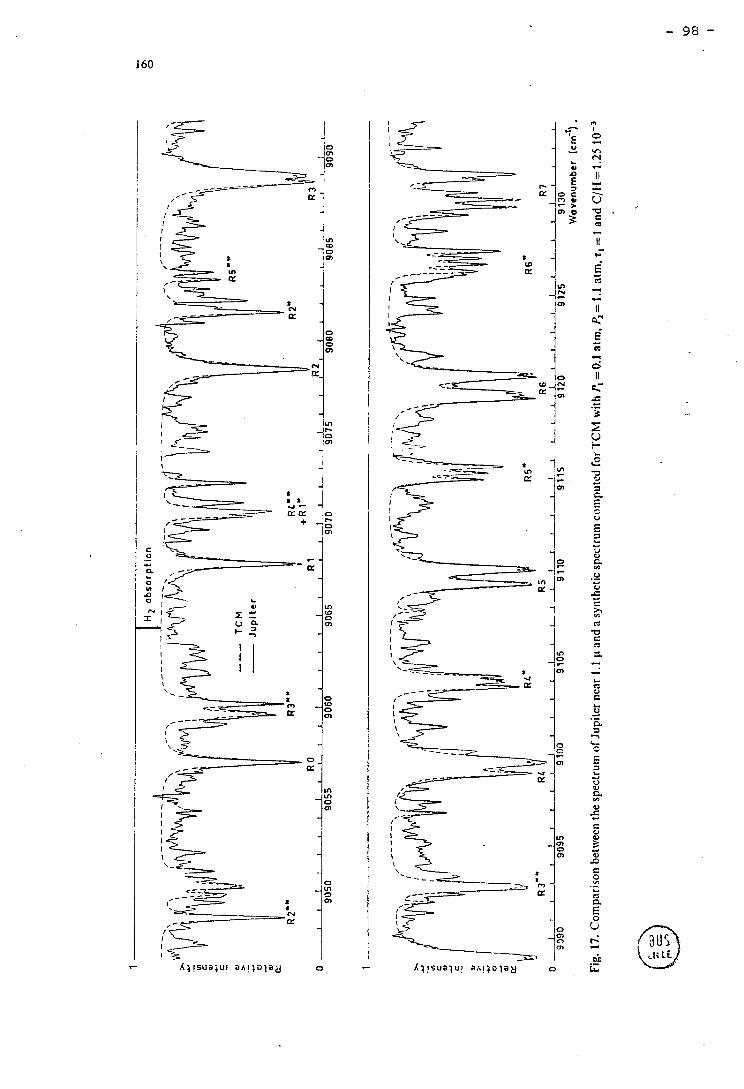
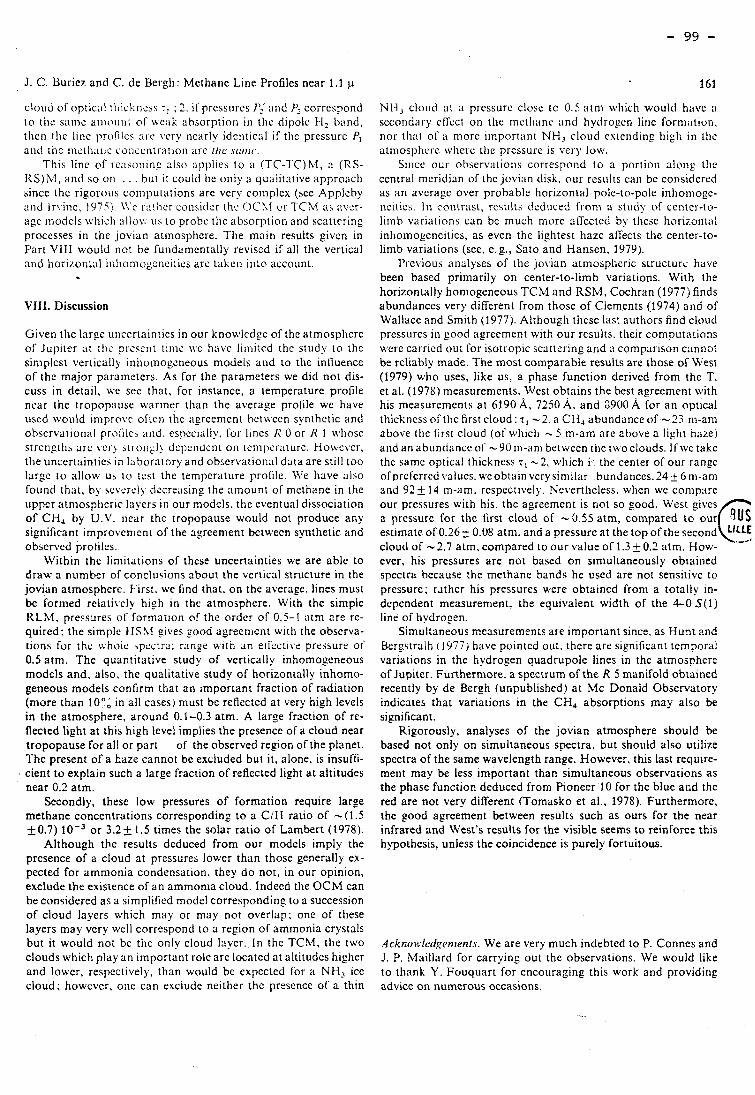
J. C. Buriez and C. de Bergli: Methaiie Liiie Profiles near 1.1 p

cloud ofopticiil i l i~~ki iess Y , ; 2. i f ~ ~ C S S L I ~ C S 1': :ind fi correspond to tiic saine ariiniirit of nc;il; absorption in the dipolc 1-1, band, thcn !lie linc ~irofiles :ii.e vrry ncarly idciitic31 if thc pressure P, and thc riictliaiic ~.oiicciitr;iiioii are rile scitlic,.

This linc of rcnsoiiin: also ripplies to 21 (TC-?'C)M, a (RS- I iS)M, and so oii . . . but it could be oiily a qulilitative appro;ich since thc rigoroiis coniputations are very coriiplex (see Applcby and lr\.iiic, 1975) 1's'~ ratlier consider th- ur TCM as ;ivcr- age modeis \vtiicli ;illi>\v lis to probe tlic absorption and scattering processes in the jovian atii1ospliere. The main results givcn in Part VI11 would iiot be fuiidamcntally reviscd if al1 the vertical and liorizoilial itihomogrnciiics arc takeii iiito account.

VITI. Discussion

Given ihe large uiiccrtainties in our knowledge of the atmosphcre of Jupiter a t tlle prescnt tirne \vc have liinited the study io the siniplcst vertically inliomogcneous models aiid to the inlluence of the major parameters. As for the parameters we did not discuss in detail. WC sec that, for instance: a temperature profile near the tropopnusc \varin? tlian the average profile we have used woiild iniprove oficri the iigrcemcnt hctwcen synthctic and observaiional profilcs aiid. espccirilly. for lincs R 0 or R 1 whose srrcnsthb arc ver) sti-oiigl! dcpcndcnt oii tcnipcriiture. tlou.cvcr, the uncertaintics in Iiiboratory and observational data are still too large to allow u, to icst the temperature profile. \Ve have also foiirid that, by sc\crcl>. dscreasiiig the arnount of nicthane in the iippcr atmosplicric layers in our models. thc cventual dissociation of Cl-i, by U.V. iiear thc tropopause would not produce any significant improvcment of the agreement betwecn synthetic and obscrved proliles.

Within the liniitatioris of thcse uncertainties we are able to draw a number of conclii~ions about the vertical structure in the jovian atmosphcrc. First. we find that. on the average. lines must be forined relativcly high in the atmosphere. With the simple KLM. pressures of formation of the order of 0.5-1 atm are required; the simple FIS51 ?ives zood a-reemcnt with the observations for thc choie zpcc:ral range witn an eiïcc:ivr: pressure or' 0.5 atm. The quantitative study of vertically inhomogcneous models and, also, the qualitative study of horizontally inhomogeneous models confirm that an imporrant fraction of radiation (more than 10:; in al1 cases) must be reilccted at very high levels in the atmosphere, around 0.1-0.3 atm. A large fraction of reflected light a t this high level implies the presence of a cloud near tropopause for al1 or part of the observed region of the planet. The present of a t a z e cannot be excluded but it, alone, is insuffi- cient t o explain such a large fraction of reflected light a t altitudes near 0.2 atm.

Secondly, these low pressures of formation require large methane concentrations corresponding to a CiH ratio of -(1.5 -10.7) o r 3 .2k 1.5 times the solar ratio of Lambert (1978).

Although the results deduced from our models imply the prcsence of a cloud at pressures lower than those generally expected for ammonia condensation, they d o not, in our opinion, exclude the existence of a n ammonia cloud. Indeed the OCM can be considered as a simplificd model corresponding to a succession of cloud layers which may or niay not overlap; one of these layers may very wcll correspond to a region of ammonia crystals but it would not bc the only cloud layer. ln thc TCM. the two clouds wliich play a n important role are iocated at altitudes higher and lower, respcctively. than would bc expccted for a NII, ice cloud; however, oiie can excludc neither thc presence of a thin

N11, cloiici :it :i prcssurc close io 0.5 atm u.liicli would have ;I

sccoiidary cfrcct on tlie nictli~inc and hydiogcri liiic foriii:iiion, nor th:it of a more important NH, cloucj esteiiding higli in tlic atmosl,herc \vlierc tlie prcssure is vers low.

Siiice our observ;itioiis correspoiid to a portion aloiig the central nicridran of thc jovian disk. oiir rcsults caii be considcrcd as ;in avcragc over probable horizontal pole-to-pole inlioinogc- iicitics. In coiitrast, results dcdiicrd from a stiidy of centcr-to- lirnb variations can be niuch more aKected by tliese horizontal in~~ornogcneities, as even the lightest liaze affects the center-to- limb variations (see, e.g., Sato and Hansen, 1979).

Pi-evious analyses of the jo\.ian atn~osphcric structure have been based primarily on center-to-limb variations. With the horizontally honiogeneous TCM and RSM, Cochran (1977) finds abundances very different from those of Clements (1974) and of Wallace and Smith (1977). Although these las! authors find cloud pressures in good agreement with our results. their compiitrttions wcre carricd out for isotropie scattering and a comparison cnnnot be reliably made. The most comparable resul~s arc those of West (1979) who uses, like us, a phase function derived from the T. et al. (1978) measurements. West obtains the best agreement with his measurements at 6190 A, 7250A. and ô900 A for an optical thickncssof the first cloud: 7, -2. a CI{, abundance of -33 rn-am above the first cloud (of which - 5 m-am are above a Iipht h u e ) and an abundance of -901i-1-ani betwcen tlie t \~oclouds. Ifwc takc the same opticsl thickness 7, -2, which ic the center of our range ofprcfcrrcd valucs. weobtain very similar bundances.24 + 6 m-an1 and 97 & 14 in-am. respectively. Ncvertheless. wlien we conip:ire our pressures with his, the agreement is not so good. West gives a pressure for the first cloud of -0.55 atm, compared t o our estimate of 0 .261 0.08 atm. and a pressure nt the top of the second cloud of -2.7 atm, compared to our value of 1.3 kO.2 aim. How- ever, his pressures are not based on siniultaneously obrained spectra because the methane bands he uscd are not sensitive to pressure; rather his pressures were obtaincd from a totally in- dcpcndent measurement. the equivalent width of the 4-0 S(1) line of hydrogen.

Simultaneous mcasurements are important sincc. as Hunt and Bergstraih 11977) have pointcd our. there are significant temporai variations in the hydrogen quadrupole lines in the atmosrhere of Jupiter. Furthermore. a spectrum of the R 5 manifold obtained recently by de Bergh (unpublished) at Mc Donald Observatory indicates that variations in the CH, absorptions may also be significant.

Rigorously, analyses of the jovian atmosphere should be based not only on simultaneous spectra, but should also utilize spectra of the same wavelength range. However, this last requirement may be less important than simultaneous observations as the phase function deduced from Pioneer 10 for the blue ai;d the red are not very different (Tomasko et al., 1978). Furthermore, the good agreement between results such as ours for the near infrared and West's results for the visible seems to reinforce this hypothesis, unless the coincidence is purely fortuitous.

Acknorrle&enients. We are very much indebted to P. Connes and J. P. Maillard for carrying out the observations. We would like to thank Y. Fouquart for encouraging this work and providirig advice on numerous occasions.

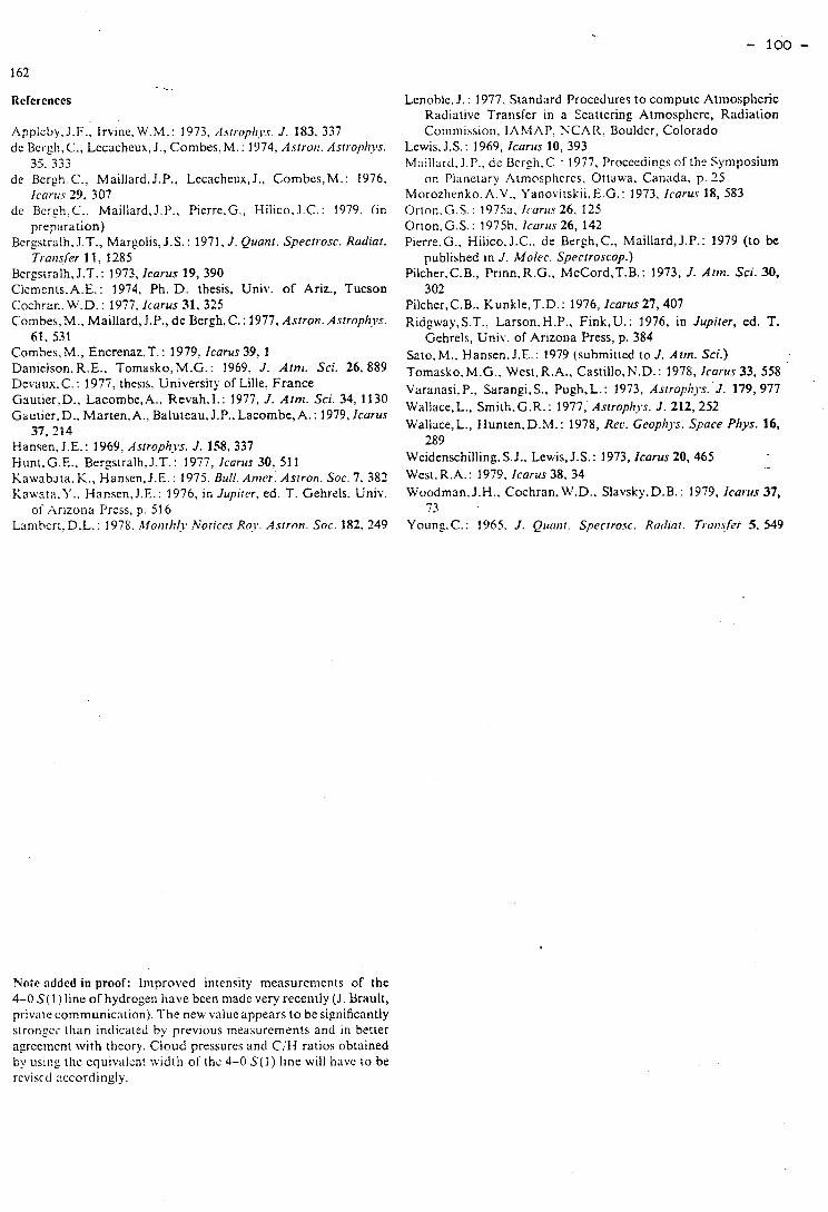
Applcby,J.F.. Irvinc. W.M.: 1973, /Is~roplr.vs. J. 183, 337 de Bci-gh, C., Lccachcux, J., Combes, M. : 1974. Asfrorl. Asrrol>hys.

35. 333 de Bergh,C., Maillard, J.P., Lecacheux, J.. Combes, M. : 1976.

Icnrüs 29, 307 dc Bcrgh,C.. Maillard. J.P.. Pierre.G.: Hilico. J.C.: 1979. (in

prep:iration) Bergstralh. J.T.. Margolis, J.S. : 1971, J. Quant. Spectiosc. Radia?.

Trarlsfer 11, 1285 Bergstralh, J.T. : 1973, Icarus 19, 390 Clements,A.E.: 1974, Ph. D. thesis, Univ. of Ariz., Tucson C0chran.W.D. : 1977, Icarus 31. 325 Combes, M., Maillard, J.P., d e Bergh, C. : 1977. Astron. Astrophys.

61. 531 Combes, M., Encrenaz, T. : 1979, Icarus 39, 1 Danielson.R.E., Tomasko,M.G.: 1969, J . Afnt. Sci. 26, 889 Devaux.C.: 1977, thesis, University of Lille, France Gautier, D., Lacombe, A., Revah. 1. : 1977. J . Atnt. Sci. 34, 11 30 Gauticr.D.. Marten,A., Baiuteau, J.P., Lacombe,A. : 1979, Icarus

37, 214 Hansen, J.E. : 1969, Astrophys. J. 1.58, 337 Hunt.G.E., Bergstralh, J.T. : 1977, Icarus 30, 51 1 Kawabata. K.. Hansen.J.E. : 1975, Bull. ~ r l i e r ; Astron. Soc. 7. 387 Kau-3ta.Y.. 1-lansen,J.E.: 1976. in Jupiter. ed. T. Gehrels. Univ.

ol' Arizona Press, p. 51 6 Lambert. D.L. : 1978. .hfonrlr/j~ Notices Rej,. Asrrnn. Soc. 182. 249

Lenoblc, J. : 1977. Stand;ird Proccdures t o computc Ainiosplicric Radiativc Transfer in a Scattering Atmosphere, Radiation Coiiimissiori, IAhtAP, NCAR, Boulder, Colorado

Lewis. J.S. : 1969, Icarirs 10, 393 M;iillard.J.P.. di: i3crgh.C. : 1977. Proccedings of the Syniposium

on Plailetary Atmosphercs, Ottawa. Canada, p. 35 Morozhenko.A.\'.. Yanovitskii.E.G.: 1973, Icarus 18, 583 0rton.Ci.S. : 1975a. lcarirs 26, 125 0rton.G.S.: 1975b. Icarirs 26, 142 Pierre.G., Hilico. J.C.. de Bergh, C., Maillard, J.P.: 1979 (10 be

published in J. Molec. Specrroscop.) Pilcher, C.B., Prinn, R.G., McCord,T.B. : 1973, J. Atin. Sci. 30,

3 02 Pilcher, C.B.. Kunkle, T.D. : 1976, Icarus 27, 407 Ridgway, S.T., Larson, H.P., Fink, U. : 1976, in Jupiter, ed. T.

Gehrels. Univ. of Arizona Press, p. 384 Saro, hl. , Hansen. J.E.: 1979 (submitted to J. Atm. Sci.) T0masko.M.G.. West, R.A., Casti1l0,N.D.: 1978, Icarus 33, 558 Varanasi, P., Sarangi, S., Pugh,L.: 1973, Asrropllys. J. 179, 977 Wallacc,L., Smith.G.R.: 1977, Asiroplzys. J . 212, 252 Wallrice,L., Hunten,D.M.: 1978, Rer. Geop1~j.s. Space Phys. 16,

289 Weidenschilling. S.J.. Lewis, J.S.: 1973, lcarur 20, 465 West. R.A.: 1979, Icarus 38, 34 Woodman. J.H.. Cochran, N1.D., Slavsky. D.B. : 1979. icartts 37,

73 Y0ung.C.: 1965. J . Quuilr. Spectrosc. Rodint. Trori.$ei 5 . 549

Notc ndded in proof: Iniproved intensity mensurcments of the 4-0 S(1) line of hydrogen liave bcen made very recently (J. Braiilt, private coinmunication). The new valiic appears to bc significniitly siroiigcr than indiratcd by prcvious ineasuremerits and in better agreement with theory. Cloud pressures and C/H ratios obtained by usiilg the equivnlcnt widtli of thc 4-0 S(1) liiie will have to be rcvisc(l accor(ling1y.

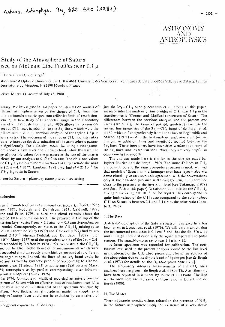
ibor;!tnirc d'Optiqiic ;itii~orplii.riqiic (IiliA 466). Uiiivcrsitit dcs Sciciiccs ci l'cchniqucs de Lilic. F-59655 Villciicuvc d'Ascq. Fr;incc bscrvaioirc dc hlcudoti. 1:-92190 hlcudon. France

, . :civcd hlarcli 1 1 . acccprcd July 15, 19SO , .

iiriiary. \\'c irivcstig;itc in this papcr consiraiiits or1 modcls of Saaurn ;itiiiosphcrc givcn by thc sliapes of Cl+, lincs ncar

p in ail intcrfcronictric spcctruni (cITcctive liinit o r rcsolution: cni '). A nc\v study of tliis spcctr;il r;ingc in thc Iaboratory *rrc el ;il.. 19SO; de I3cr~li et al.. 19PO) allo\vs us t o considcr I C F O U ~ C'Il4 lines in additiori to ilic 3 i,, lirics. \rliich \vcrc ille !. liiics iricludcJ i i i ;il1 prcvious ;inii!!\ci of tlic rcgiori 1 . 1 11 in iirri spcctra. Tlic \r,idcriirip of tlic r;ingc of CII, linc intciisiiics c;irs IO iiiiprove the dctcrri~inatiori uf tlic ;itniosplicric param- s sipnificaritly. For a cI:is~;i~;iI niodcl incl~idinp a clcar ;itnio- crc abovc a hazc In'er aiid ii dciibc cloud bclow the h;izc. tlie CC of possible valiics Cor the prcssurc ;II thc top of the hazc is rictcd by our analysis to 0.1720.06 atiii. The obiaincd valucs lic C l 1,. I I , riiiio ;ire riiorc unccri;iiii bui ihcy cnclu~ic thc soiiir ic (C/ t I=4 .7 IO-"; 1-arnhcrt, 1978); wc find ( 4 5 2 ) I O - ' for ClI,/l I l ratio in Saturii.

; words: S:iturn - planctiirj atmosphercs - scattering

roduction

current rnodcls of Saiurn's atmosphere (scc. e.g.. Teifcl. 1976; icy. 1977: Podolak and Daniclson. 1377; Caldwell. 1977: Inz and Price. 1979). a hazc or a cloud extcnds above the jcctcd Nti, sublimation le\el. The pressure at the top of the tterinç layer varies from -0.1 atni to -0.5 atm Jcpcndinç on model. Consequcritly. csiinilites oi' the Cll, I I , mixing ratio qiiite unccrtain: Macy (1977) and Crildwe11 (19771 find values

,und 2 10-' whereas Podolak and Daniclson (1977) prclcr IO-'. Macy (1977) used the equivalcnt widths o r t h c 3i., -CH,

:s rccorded by Trafton in 1970-1971 to constrain the CH,8F12 io, but he also nccdcd to use othcr rncasuremcnts which were : rccordcd siniultaneously and which correspondcd IO difkrenr vclcngth rJngcs. lndecd. the lincs of the 3i., band couid be cd jus1 as wcll by synthetic profiles corresponding to a homo- icous clcar (Trafton. 1973) or scattering (Traiton and Macy. IS) atrnospherc as by profiles corrcsponding IO a n inhorno- icous atniospherc (Macy. 1976). In 1974. C'onncs anci M;iill:ird rccordcd an inïcrfcronictric

!ctrurn of S:iturn wifh an cfictivc l i i i i i t «i'rcsolutron n c x 1.1 p tcr by ;i factor of - 2 tliaii that 01 ' tlic spcctruni rccordcd by î i o n . Ncvcrthclcss. an atriiosphcric riiodcl :is siniplc as a rcly rcflcciing Iayer could not bc cxcliidcd by an ;inalysis of

jiist the 3i.,-Cll, b:ind (Lccaclicus ci al.. 1976). In this p:ipcr. \ve rccoiisider the arialysis of linc profiles oi' Cf I, nc;ir 1.1 11 iri thc iiitcrfcronictric (Coiincs and 3laill;ird) spictruni of Siiturn. The difiercnces bct~vccii the prcvioirs anril!sis and th? prcscnt onc arc: ( i ) UT ciilargc the r;liigc of possib1c rnodcls: (ii) WC usc the reviscd linc intcnsitics of' tlic 3 i., -Cil, b;ind of dc 13crgIi ci ; i l .

i 19SO) \r liicli din'cr si~riific;intly frorii ilic \;ililc3 oi'I3eg~ir;iliIIi and hlargolis (1971) uscd i i i tlie lirst ;iii;ilysi\. i:nd. aoo\c ail. ( i i i ) \ \c ;inalysc. in additiori. lincs and 1:-innifolils locatcd bctv;ccn tlic 3 Y, lincs. I'licsc intcrlopcrs have intcnsitics \\.cakcr tiian nioct of tlic 3 i., lincs. and. as sve \vil1 sec furthcr. thcy arc ver;. hclpful iri coiistrainiiig the rnodcls.

Tlie analysis rniidc hcrc is sirnilar to iIic one we made for Jupiter (Iiuricz and de Rcrgh. 1980). Tlic s:inic 42 liilrs ni' CII, arc considcrcd aiid thc sanie cornputcr prograin is i ixd. \i'c find that modclJ of Saturn \vith a honiogencous îiaze layer - abovc a dcrise cloud - givr an acceptable agrecrncnt ui th i h ~ oh~erviiiions only if thc hazc-top prcssurc is 0.17 = O.C5 atm. and thcrci'orc close to th t pressure ar the inversion levcl [sec Tokunaga i 197s) and Scct. IV-b i r i tliis paper]. \ i 'c al50 obraiii I i i i i i t ~ ori ihe Ci i, 11 , mixing riitio: ( 1 . 0 ~ 5.0) I O - ' . .A> for J ~ i > i t ~ i . tl1cy iorrc\p:~iid Io quite high valucs of thc C i l ratio corriparcd IO the soiar \aluc: C'Fi on Saturii is b e t ~ e e n 2.1 and 6.4 tintcs the soiar ratio (Lani- bcrt. 1978).

1. Tlie Data

.A detailed description of the 'iturn spectium analyzed hcrc has been givcn in Lecachcun ct ai. (1976). \Vc uill only rncntiori thsi the instrumental resolutron is 0.1 cm - ' and that the slit, 5"6 v:idc and 13" high, includcd cssentiaily the squth tcmpcrate and polar regions. The signal-to-noise ratio ncar 1.1 p is - 25.

X lunar spcctrurn was rccordcd for calibration. The continuuni lcvcl uscd in the prcsenr analysis uould bc the flux 1cvi.i in the abscnce of the Ctl, absorptions and also in the abscnce of the absorption duc to the dipolc band oi'1i)-drogcn [sec de Hcrgh et al. (1974) for details on the II2 ahborption ncar 1.i 111.

The laborritory intensity rncasurenicnis of the CII, lincs anaiyzcd hcri.:ire givcn in de Rcrgh ct al. (1980). Thc J-utrributions have been reportcd in a p;ipcr by I'icrre ci al. (1980). Thc liiic widths used lierc are thc sarnc as thosc uscd in Buricz and J e Bcrgh (l9SO).

Tlicrriiodyn;iniic considcr;itioiis rclatcd I O [tic prcscncc of NI-1; iri tlic S;iitirn aiinosphcrc iiiiply tlic existcric~c of ;i vcry tlcnw

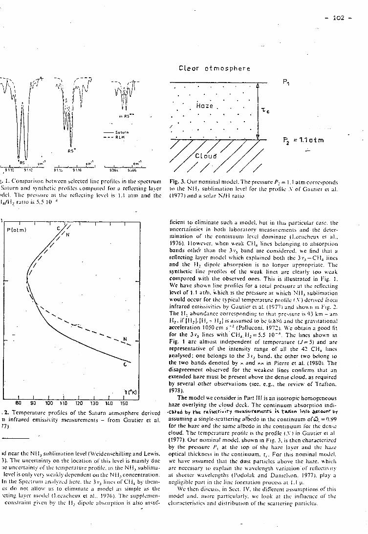
CLeor a t r n o s p h e r e

- Soturn - - - R L H

;. 1. Coriipiirison bct\vec~i bclccted linc prolilcs in ttic spcctruiil S;iii~rn zind s y i i ~ l i c t i ~ profiles c o m ~ ~ ~ ~ t e i i for ;I rcflcctiiig la!cr iiicl. 1-tic prc5hirrc ;II ilic rcflcciing Iç\.cl is 1 . 1 atm and thc I J I : r;iiio is 5.5 10

- 2 . Tcrnpcraturc profiles of thc Saturn atrnosphere derived n infrared en~ibbivity me;isureniciits - [rom Gautier et al. 77)

id ncar the NI-1, siiblini;ition lcvcl (\\'cidcii.;chilling and Lewis. 3). Thc uncertainiy on the location of t l i i h level is mainly duc IC unccrt;iinty ofttic tcii~pcr:itur-c prolile. ;i\ ttic N11, sublinia- lcvel is oiily ver) \sc;iLIy Jcpcndcnt ori the NI 1, conccntration.

In t11c Spcci~uiii ;in;ily/cJ Iicrc. the 3 Y, iilics of Cli, by tliciii- cs d o not ;illo\v iis to cliniiii;itc :i niodcl ;is siiiiplc ;is the :cling Iaycr iiiotlcl (I.cc;iclicux ci ;il.. 1976). l 'hc supplcriicn- constr:iiiii givcii by tlic I l 2 ilipolc absoi-piioii is also iiisuf-

P2 = 1.1 a t m .-.-

Fig. 3. O u r noiiiiii;il niodcl. l'lic prcssurc P2 = 1 . 1 atm C O ~ I . C S ~ ) O ~ I ~ S

to ilic N11, subIiiii;itic)ri Ic\.cl fur ilic profilc .Y of G:itiiicr ci ;il. i 1977) aiid a solnr S f l i ratio

ficien1 to cliniinate sucli a modcl. but i i i this pr i ic i i lar casc. itie iinccrt;ii'ntics in both laboratory iiie;isiii.cniciiis iind . the dctcr- niination of ihc continuuni Ievc.1 doriiinaic (Lcciichcu.r et al.. 1976). Ilowcvcr. Ivhcn wcak Cil, lincs bc!onging IO absorption bands otiic'r tti;in thc 3 ~ , band arc considcrcd. 1t.e iind ihar a rcfiecting Iaycr niodcl which expliiincd bot11 the 3 i., -Cl] , Iincs and ihc I I 2 dipolc absorption is no longer ;rppropriritc. Ttie syntlictic linc prolilcs of thc wcak lincs arc clc;irly ioo \r.cak coinparcd witti the obscrved oncs. This is il1ustr;ticd in Fig. 1 . \ire have shotrn !inc profilcs for a rotdl prrsburc ai thc rcflcciing lcvcl of 1 . 1 athi, i-hich is thc prcssurc zii \\hich Ni l3 subliniaiion would occur for thc typica! tcrnpcrriturc. profilc ( . \ ' ) Jcrivcd froni infrared cniissivitiej by Gautier ci 21. (1977) and shouri in Fig. 7 . The i l , abund:incc correcponding ri: thiir prcisure is 93 km - an1 11,. if [tl2];[I1,.- tI2] is assumed 10 oc.O.bi(6 and ttic gravitation;iI acceleration IO50 cm s ' l (Palluconi. 1972). \i'e obtain a good fit for the 3 % lines uVith'Ct-1,. I l2=5.5 IO-'. The lines shoxn in Fig. 1 a re alniost independent of temperature i J = 5 ) and are representative of the intrnsity range of ail the 41 CH, lincs analyscd; one bclongs to the 3i., band. the other two bclong :O

the two bands drnoted by t and 2% in Picrrc et al. (1980,. The disagreemtiit observed for thc weakcst lincs confirms that an cxtended hazc must bc present übove the dense cloud. as requirrd by several othcr observation^ (sec. cg. , the revicw of Trat'ton. 1978).

The rnodel u e consider in Part 111 is an isotropie homogcncous haze overlying the cloud dcçk. The continuum abborpiion indi- .catod bl bhe ret \echvtty me%S..;urenwts is taKun lnrt apcwnr bl assuming a single-scaitcring ;ilbcdo in thc continuum ofW, =0.99 far the hazc and the same iilbcdo in the continuuiii foi the d c n c cloud. The tcriipcrature protilc is the profile ( .Y in Gautier et al (1977). Our noniinal rnodcl. shown in Fig. 3. is thcn ch3ractcrixd by the prcssurc f', at tlic top of the hazc laycr ariJ thc haze optical thiçkncss iii the continuum. r, . For this noiiiinal niodcl. \vc havc iissunicd tfiat the dust particles abovc the h u e . uhic.11 arc ncccssziry IO explain the \vnvclcngth variation (if rcllcciivi!~ ;ii shortcr w;ivelcrigths (I'odolak and Daniclhon. 1977). play a ricgiiyiblc p;irt i i i iIie liiic I'oriiiiiiion proce*s a i 1 .I 11.

\ire tlicri discuss. in Scct. IV. tlic difkrcn! :issuniptions of this niodel aiid. iiiorc particiil;irly. h c look ;II ttic iiifliiciicc of itic c1i~ir;icirristics ;inti ili~trit>iirion of ttic scaticriiig p;irticlc~.

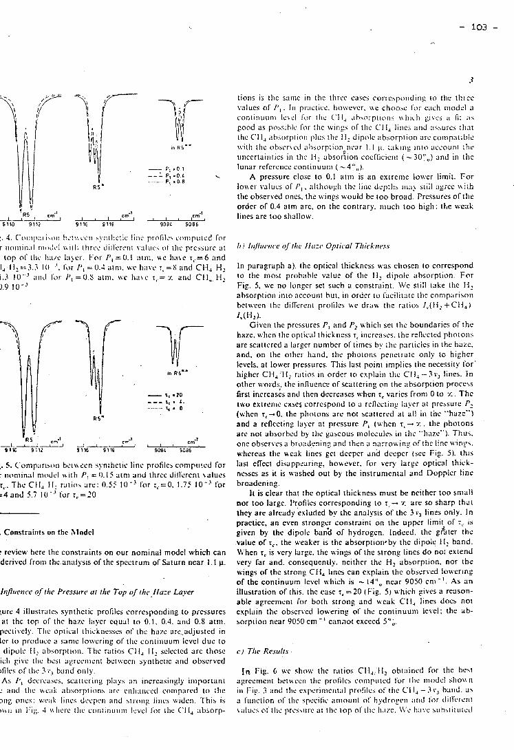
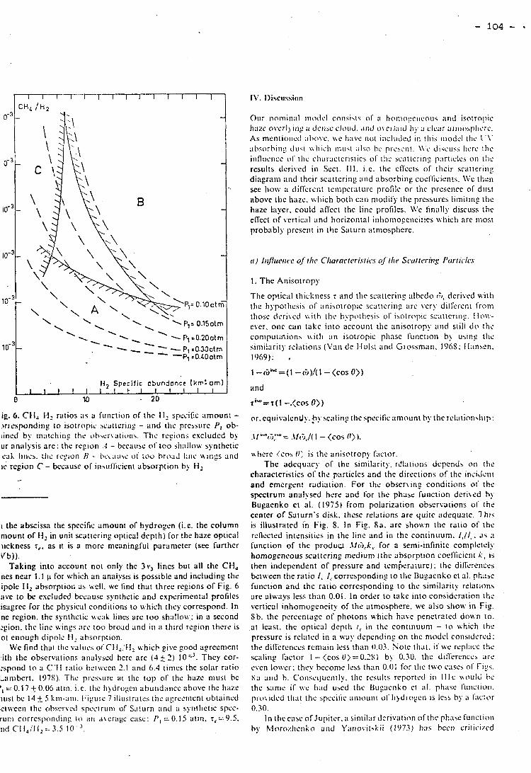
03/cbiL / ~ 2

Y:, Oiir iioiiiiri;il iiiodcl corisi\t% ol' n hniiioliciicniis iiiid isotrol>ic hnzc otrcrlj iiig ;I J c i i x cloud. ;ii,il o\~crl;iid !,y a c1c;ir aiii)o.\phcrc. As mentioiicd :iho\.c. \vc ti;ivc iiot incliitlcd i i i tliis iiiodcl ilic \.\. ;ihsor!iiiig c l u \ i \\liicIi i i i ~ i \ t ;il\o hi. pi-c>ciit. \ \ 'CS dihciis\ 11crc ihc iiifliiciicc ol' [lie cli;ir;ictcristics of ilic sc;ittcrin? prirticlch oii 111c rcsulis dcrivcd ii i Seci. 111. i.c. the cll'ccts of tlicii- sc;itteriii_r diagrani aiid thcir scattcring niid absorbiiig cocflicicilts. \Vc rlieii sce Iiow :i <iin'crciit tcriipcr;ituie profile o r thc prcscncc of diist above ilic liazc, tvliich botli cati niodiiy the pressures liiniting tlic hazc laycr. could a k c t the liiic profiles. We linally discuss the elTect of vcrtic;il and horizontal inlioniogciicitics \\hich are inost probribly prcsciit in t)ie Saturn iitmosphcrc.

ig. 6. CII, 1 l 2 ratios 11s a fuiictioii of thc f i 2 spccific rimoun! - >rrcsponding to isotrcipi' bciiiicrir~g - and the prcssiirc P, ob- iincd by rnriichiri~ the oh\cr\atiuns. Ttic region.; excluded b j ur anrilysis arc: the rcgion .-I - bccauhc of ioo sli;illo~v synthctic cal, Iiricb. tlic region H - bc~;iii\e ~i too broad litle \rings and ie rcgion C - bccause o l iiibiiilicicnt absorption by HL

i the abscissa the spccific amount of hydrogcn (Le. the column mount of H2 in unit scattcring optical dcpth) for the haze optical iickness r,. as it is a more meiiningful parametcr (sec furthcr V5) ) .

Taking into account not only the 3r, lincs but al1 the CH, ncs near 1.1 p for which an analysis is possible and including the ipolc 1i2 absorptioii as ;vcll. WC lind that threc rcgions of Fig. 6 ;ive Io be cxcludcd bccause synthetic and experimcntal profiles isagrcc for thc physical conditions io tvhich they correspond. in ne rcgion. the synthctic ue;ik liiics arc too shiillo\v: in a sccond :pion. thc linc wings arc too broad and iri n third rcgion thcrc is ot cnough dipolc 1-1: iibsorrption.

WC find thai tlic valiicb 0l'Ct4,'I4~ whict! givc good agrecnicni i th tlic observiiiions analyscd hcrc arc ( 4 5 2 ) IO"'. Thcy cor- tspond Io 3 C '1 I r;itio bci\vccn 2.1 and 6.4 tinics thc soliir ratio Lariibcrt. 197s). Tlic prcssurc at tlic iop o f tlic hazc niiist bc I , - - 0.17 k0 .06 i i t r i i . i.c. tlic Iiytlrogcii abund;incc abovc rhc fiazc

iiist bc 14 1 5 kni-iirii. 1;igurc 7 illiistiatcs the ogrccincnt obtaincd ci\vecii the ot>scl.vcd spcciruiii of Sa!urn aritl ii syiiihctic spcc- ru171 corrcsjioritliii~: io ;in ;i\,cr;igc crise: P i =0.15 ntrn, 7,-9.5. iid CII,/lI, =- 3.5 10- '.

1. Thc Anisotropy

The optic;il thickiiess 7 and the sc;ittcring albcdo G), derivcd u.it1i tiic hypotlicsis of iiriisotropic scattcriiig ;ire \,Cr\, dilkrcn! from tliosc dcri\.cd ni th the hypotlicsis of i\otropic sc;irrcriii_r. 1 loi\.- cvcr. oric can take into account the anisotropy aiid stili d o the coiiiput;i~ionh \\itli on isotropie phnsc fiinction by usin? tlic simil;irit) rcl;iiioiis (Vari dc I+ulst aiid Grossm;in. 196s: 1l;insen. 1969): . 1 -<Gia =(1 -<0)/(1 - (cos O) )

and

r b = r ( l -.(cos O ) )

or. cqiitv;ilcnJ! .$y sc;ilirig the spccific anlorlint by the rclritinn~liip:

.\l'*o,Gt'u' = .\fc;),/( 1 - (cos 0 ) 1.

u hcrc (cos 0: is the anisctropy fiictor. The adequacy of the similarity. rtlatioiis dcpcnds on rlic

ch;iracteristics ol'thr: particles and the directions of the inci~icrit and emcrgcnt radiation. For the o b s c r ~ i n g conditions oi' thc spcctruni analysed hcre and Tor the phase funciion dcri\cd h! Rugaenko et 31. (1975) from polarization observations o i the center of Saturn's disk. these relations are quitc :idequate. 7 h i i is illustrated in Fig. S. In Fig. Sa. arc shoun the ratio of the rcflccied intcnsiiics in thc linc and iri the continiium. /,Il,. a fùnction of the p roduu .Zl(!i,k, for a semi-infini:c con:pletrly homogencous scattering medium (the absorption cocfficicnt k , is

c.LI1CcS then indepcndent of pressure and tcmi>eraturc): the ditl'... bctween the ratio 1, li corrcspondins to tlie Bugaenko et al. phi:>c. funciion and the ratio corrcspondinp to the similarity rrlaricins are a1u;ivs ICSS than 0.01. In ordcr IO take into co~siderat ion rhc vcrtical inhoniugcncity of the atmospherc. we alho >hou. in Fi-. Sb. the pcrccntagc of photons uhich h a ~ c penetratcd do\ \n 10.

al Icast. thc optical dcpth r , in the contiiiuuni - to uhich thc pressure is rcl:itcd in a way dcpcnding on the niodcl coiisidcred; the dilTcrcnccs rcmain lcss than 0.03. S o i e tiiat. i fwc repl~icc the sciilirig factor I - (cos U ) =O.?Sl by 0.30. the difl'crenccs air: cvcn lower: thcy beconic Icss thiin 0.01 for [lie IWO casos of Fis-;. Xa aiid b. Corisct~ucntly. ilic rcsiilis reportcd in I l l e \voiilti hc the sanie if \vc Iirid uscd tlic ~ ~ L I ~ ~ C I I ~ O ct ; I I . ph;isc Iiiiicti~~ii. pi-ti\idcd t1i;ii thc spccitiç ; i i i ic i i i i i i o i li)diogcri ib Iehs by ;i liiciar 0.30.

In tlic c a ~ of Jupiter. a siniil;ir tlcriv;ition of tlic ph;isc fiinctioii hy MorozJicriko arid Y;irio\.it>kii (1973) h:is hccn critici7cd

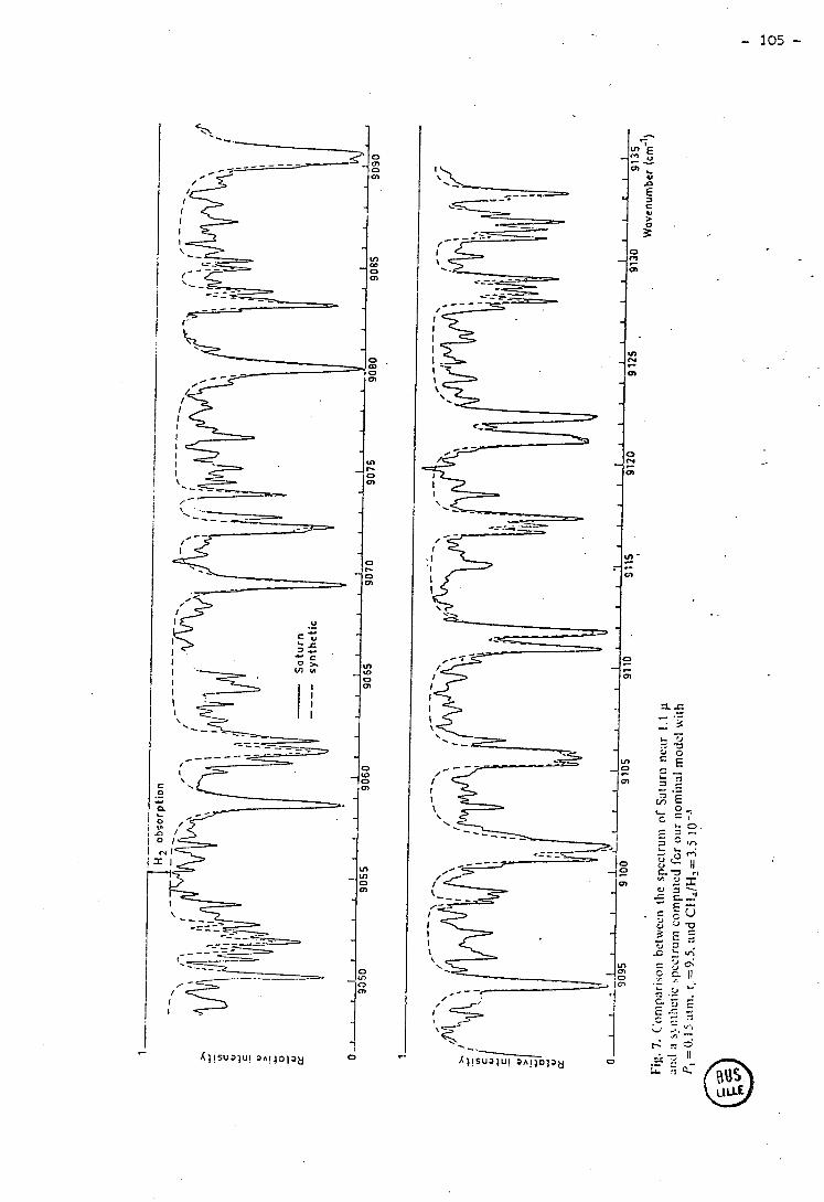
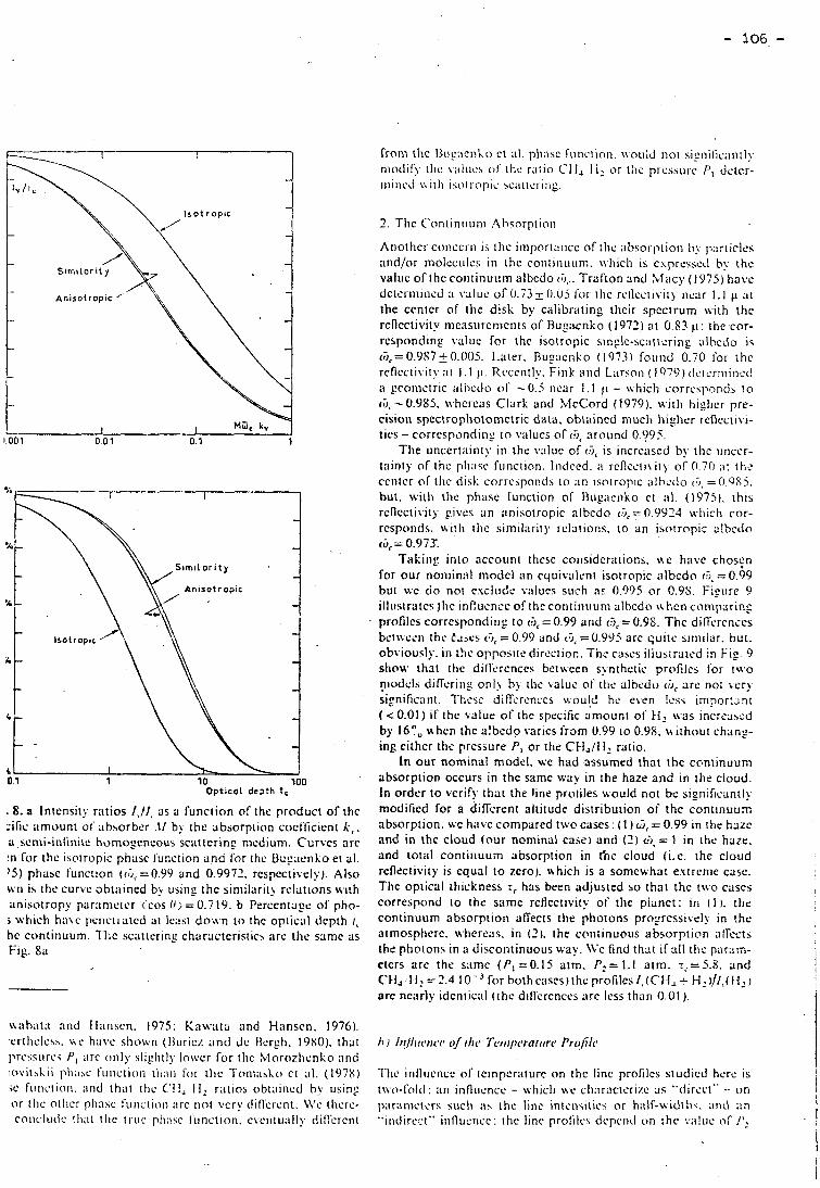
-8. a Inicnsity ratios 1,/1, as a funciion of the product of the :ific aniount o i iibsorbcr .il by the absorption cocl'ficicnt k , . a,scnii-in!iriiic hi>mogcncous sciiticring niediuni. Curves are :n for the isotropic phase iunction a n a for the Bugiicnko et al. 15) phase function ( ( 5 , =0.99 and 0.9972. respcctively). Also \vil is the curvc ûhtiiined by usitig the siniilarity relations trith iinisotropy pariimeter (cos 0; = 0.7 19. D Percentagr. of pho-

5 wfiich have periciiritcd ai Icast doivn to the opticiil dcpth 1,

he continuum. l ' l ie sciitteririp char;icteristics are the samc as Fig. Sa

tv;ih;ii;i and lliiiiscn. 1975: Knwntri and Hansen. 1976). .crtliclcsh. u e have shown (Iiiiricz and dc IIcrgh. 1980). thar Ivcssiirch P l Lire only sliglitly lo\ïcr for tlic Morozlienko ;iiid ~ o v i i ~ L i i p11;ihc f~i i ic t io~i ~ \ I ; I I ~ l'or the Toiii;idic) C I :il. (197s) <c fiiiiciioii. ;ilid thiii tlic C'Il, I l2 ratios obt:iiiicd hy using or tlic otlicr pliase furictioii ;ire iiot vcry (lill'creiir. M'c tlicrc- coiicliidc t l i ; i l tlic iriic pli;i\c 1'~inction. evciiiii:illy ciiflCrcnt

rroni iIic I<ii~:icnko ci al. pliiisc riinciion. noiild iiot sigiiiiic;iriily rnotliry tlic 1.aliic.5 o r the ratio CI 1, I I 2 or tlic prcs>i~rc PI dctcr- iiliric~i i \ i t l i i>oii.i>pic iciirteriiig.

Ariothcr conccrri is thc iiiiporiaiicc of tlie ;ibsoiptioii b!. particles ;ind/or molcciilcs in thc coriiiiiuiim. \I hich is csprcsse~l by ilic valiic of the coritinuiiin albcdo Trafton and hlacy (1975) havc dcici-iiiiiicd a \~aiuc o r 0.73 - U.U5 toi. ilic rcilcctivit\ iic;ir 1 . 1 p a i the ccntcr of iliz disk by caliùr;iting their spcctrum \\.;th ttic rcncctivity nieasiirciiicnts of B u g x n k o (1977) at 0.83 11: the corrcsponding value for thc isoiropic single-scaticriiig alhcdo is tG,= 0.9S7 2 0.005. Laier. Bugaciiko ( 1973) fotiiid 0.70 for ihc rcflccti\.ity nt 1 . l 11. Rcccnily. Fink aiid Liirsoii ( 1979) dCtc.riiii~icd a pcoiiictric ;~llxxio c)I' -0.5 iicar 1.1 11 - \vhich corri.>pond> I O

15, -0.985. \vhcrc;is Clark and McCord (1979). u i th Iiighcr pre- cisioii spcctropliotonictric data. obtaincd niucli higlicr rcficciivi- tics - correspondiii_r to v:ilucs of (5, riroiind 0.995.

The iincertainty in the \.:iluc of tu, is iiicrcased b!~ thc iiiicer- tainty of thc p1i;isc fiiriction. 1rider.d. :i rcflecii\i!) of 0.70 ;il th*: cciilcr of tlic dis); corrcspoiid~ I O :in isotropie iilhi.do (3 , =O.QSj . but, witli tlic phase function of Hug;iciiko et :il. 0975) . this rcncctivity givrs a n anisotropic albcdo (CJ, =0.9924 \vliicli cor- rcsporids. with thc simil;irity relations. to an isotropic alhcdo <O, = 0.973.

Takiiig irito accouiit tlicse considcrntior,~. \\-c t i ; i \ ~ choscn for our iioiiiiniil nlodcl an equivalcnt isotropic nlbcdo G'=0.99 but tvc d o not excliidc values such nc. 0.995 or 0.98. J-igiire 9 il1iistraics)lic influence of thc contiiiiiiim albcdo \\ heii conipriring prafilcs corrcspondiiig to c?i, = 0.99 arid (5, = 0.98. Thc dif i rcnccs bci\+ccii ihc Ca3cs CG,= 0.99 and 13, = 0.995 arc quite siriiilar. but. obviously. in the opposire direction. The c;i>cs i l l~>iï : i t td in Fi:. Y show that the dilTcrcnccs bctween synthctic prcifilcj for tu.0 ?iodcls difkriiig onl) b j the \aluc of tlte albcdo (5; arc rio1 \ t r > siynific;int. Thesc diffcrcnccs \vou!d bc even lcss inipor:rinr ( ~ 0 . 0 1 ) if the value of the specific arnount of 11, \vas incrcascd by 16°, when the a!bcdo varies from 0.99 to 0.98. \+ithoui chang- ing eithcr the pressure P, or the CF1,/f I 2 ratio.

In our nominal model. we had assumed that the continuum absorption occurs in the same u a y in the haze and in the cloud. In ordcr to verify that the line proiiles would no1 bc significanri' modified for a d i f i ren t altitude distribution o i the continuum absorption. WC havc compared two cascs : (1 ) W, = 0.99 in rhc hazc and in the cloud (our nominal case) and (2) 6% = 1 in ihc haze. and total contiriuum absorption in tkc cloud (Le. the cloud reflrctivity is equal IO zcro). uhich is a somcwhat extrcriic casc. The optical thickness 7, has been adjusted so that thc t\vo cascs correspond to the sarne reflectivity of the pianet: in ( 1 1. the continuum absorption aîTects the photons progrcssivcly in ?hc atmosphcre. uhcreiis. in ( 2 ) . the coiitinuoiis absorption rilTcc!s the photoris in a discontinuous uay. \Vr find that if 311 the piir;in- eters are the samc ( P i =O.15 atm. P I = 1.1 atm. r ,=S.S. and Ctj;f i z =?.4 IO-' for both cascs)thc profilcs I , ( C ~ + , - L t12 )/1,(J1,1 are ncarly identical ( the diflèrcnces are less than 0.01 ).

7.11~ iiilli~cricc of tcinpcr;iturc on thc linc profilcs studicd hcrc is t~vo-Li>lcl: an infliicncc - \vliich \vc cli;ir;icieri;lc a s "(iircct" - on p;iraiiic~ers siicli iis the liiie intcn\itics or h;ilf-\vidit~i. :ind ;in "iridircct" irilliicr~cc: the linc pro:ilc.s drpcnil oii thc v;i!~ic of /':

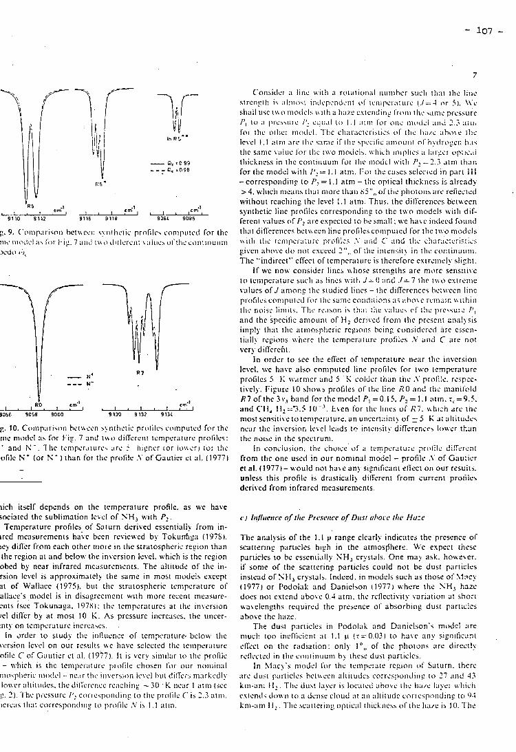
g. 9, C'oriip;irisoii bct\vccii zyiitliciic profile\ conipiitcd Tor thc iii<* iiio~lcl 1.01. 1-ig. 7 i i11~1 tu O ~ I t i ~ c r c i i ~ \ iiliic~ ol'tlic ct~nt~iiuiiiii ~ c d t )

g. 10. Coinp;irison hei\\c.cn ~ ~ r i t l i c t i c proiilc\ ci3mputcd for the iiic niode1 :is for kif . 7 ;ind t \ \o diRerciii icrripcr;iturc profiles:

and ii - . I lie tciiipcr.iiurc\ arc 5 tiigikcr ior io\ \cr j t'or tlic ofilc N+ (or N - ) than for the profile .\' of Gauticr et al. i 1977)

iich itsclf dcpends on the tcmpcraturc profile. as WC have socintcd the sublimation Icvcl of NH, \r.ith P z .

Teni-pcrature profilcs of Saturn d e r i ~ e d esscntiiilly from in- ircd nicasurcmcnts ha;,c bccn review-ed by Tokunhga (1978). icy difli.r from each orher more in the straiospheric region than tlie rcgion at and belo\v the invcrsion Icvel. which is thc region obcd by ncar infrared nieiisurcmcnis. Thc altitiide of the in- rsion lcvel is approximatcly the sanie in most niodcls txccpt ;it of Wallace (1975). but tlic stratosphcric tcnipcraturc of al1:rce's niodcl is in disagrccincnt with more reccnt mcasure- ~'ii ts ~ S C C Tokunaga. 1978): the temperiturcs ar tlie in\.crsion !cl dinFr by at most 10 K . As prcssurc iiicreascs. thc iinccr- inty on tcmpcraturc incrca\es.

In d e r i o study tlic influence of tcmperaturr. belou ttic icrsioii Icvcl on Our rcsulis \ve hnvc sclcctcd tlie icmpcriiture olilc C of Ciii~iticr et al. (1977 1. 1i is vcry siiiiil;ir to the profile - \\.hich is the tciiipcriiturc profilc choseri for oiir noriiirial

niosplicric iiioclcl - - nc,ir tlrc iri\.crrion Icvcl l > i i t <lillCi:; niiirkcdly lo\vcr :iltiiiitlcs. the dilfcrericc rc;icliing - 30 K riciir I ;ilni (sec 1:. 3). The p~.cssiirc 1'' cosrcspoi-idiiii IO tlic profile (' is 2.3 i i t i i i .

icrciis ih;it corrcsl>oiidiiig to ~>rc>lilc ;2' is 1.1 iitin.

Co~is ic l~r ii liric \vit11 8 rot~tioii;il ~iiiiiibcr siicti tli:it 11ic l i~ ic strcnptli 15 :i111io>1 iii~1cpcndt:iit O S t c i i ~ p e i ~ ; ~ t ~ ~ r c ( J = 4 o r 5). \\'c sliiill lise t\\,o ~iio(icl> \\.II ti ii h : i ~ cx~ciicliiig Sroiii tlic ~;iiiic prcs5urc /'1 1 0 i l ]~l.c>~lll.c 1, c~1i1.11 Io 1 .1 i1t111 [o r oiic iiioti<i ;iiid 2.3 . i i i i i

for tIic oilicr iiindcl. Tlic c1i;tcicicristics of tlic l i i i~c :ibo\r rhc Icvcl 1 . 1 i i t r i ~ ;ire tlic .;:inle if itic 4p:cilis ;iiiiouiii nl 'h~tliogcrt 1i:i.

tlic sitiiie v;iliic l'os tlic I \ V O niotic'l\. \vhicli i i i i />lic~ ii liiigcr ~l>ii<.il tliickiicss in the coritiiiuum for III' modcl \r,iili 1";. 3.3 airn 11i.iii

for tlic iiiodcl \ \ i i l i = 1 .1 atrii. I'oi the cases sclccrcd in piiri I I I - corrcspoiidiii~ t o PI = 1.1 atm - tlic optical tliickiicss is already > 4, wliich ii-icaiis tliai niore tliaii d j " , , c~filic plic~ioris arc relicsicd without rcacliirig thc lcvcl 1.1 aini. Thus. thc dill'creiiccs ber\vecn syiitlictic linc profiles correspondii i to thc t\i.o inodels \vitIl dif- Ccrcnt \talues of 1'? nrc expcctcd 10 hcsm:ill: \vc h a w iiidccd ftsiind tl i i i t difièrciiccs bct\\ccn line profilcs coiiipuicd for tlic ttvo i~icsclcls

. . \ \ i i l i tlic icnipci-iiiiirc prfifilcs .Y iiiid C' iirid tlic chi;r:ic:cr!si:cs giveii ;ihovc d o not cxcced 7 " , , of ilic ii i trn~it). in flic C O I ~ ~ ~ I I L I L I I ~ ~ .

Tlie "iiidircct" elTcci of tcmper;iiiirc is ihercfore cxirc.:iirl>. slight. If \vc no\v consider lines \iliosc strcrigths arc more sensiit\c

io iciiipcriiturc siicli ;is lincs \vith J = O ;ifid .1=7 thc t \ \o cxtrciiic viiliics of J amon: thc studicd liiics -{!le diffcrcnccs 1ictu.cen linc profilcs conil>iiicd for ilic saine coiiciitions i i i iit>o\e rïrii:iin \\ . i i l i i i i

ilic noise liiiiiis. 7.11~ rc.isoii is t1i;i: riic \iiliic\ of ilic prc55u:-s P , iiiid thc spccific amouni of H2 d e r i d frorii tIie presciit a:ial) ris iinply th;it tlic ;itiiiosplicric rcgioiiq bcing considci-cti ;ire csscn- tiitlly rcginiis ivhcrc the tcmpcriiiiirc profiics .\; aiid C are not vcry d ikrc i i i .

in ordcr to sec the c f i c t of tcmpcraturc ritiar thc invcrsioti Ic\,el. \ve Ii:ivc also cnmpiited linc profiles for iwo tcrnperaiure profilcs 5 t: \v;irriicr ;ind 5 K coldcr ihan tlic .Y profl:e. rcspcc- tivcly. I'igutc 10 sho\vs profiles of the linc RO and tlic nianii'eld R I o f t h c 3 ~ , b:irid for ihe modcl P, =0.15. Pz= 1 . 1 nim. r,=9.5. aiid CH, !1,=*3.5 I O - ' . t v e n for the iiiics of 1i7. \\hicn are inc niost scnsiti\c to tcnipcraturc. a n unccrt:tirit! of 5 K a; altitudes nciir the inversion Icvcl 1e;ids t c intciisit!. cjilTcrense> Iowcr than the noibc in the spccrrum.

I r i conciiision. the ciioice of ii icnpcraturs profile d i f i ren t froni the one uscd in Our nominal modcl - profilr .Y o r Gautier et al. (1977)- would no1 have any significant etTeci on Our resui~s. unlcss this profilc ii; drastically difi'crent from current profiles dcrived from infrared measurements.

c / It!/lrcc~trre oftlie Pri.seirre of Birsr ahorcp tlic Hure

The analysis of the 1.1 p range clearly indicates the prcsence of sc;itieririg piiriiclcs high in the atmosfihere. LVe expect tncsc particles to bc esscnti;illy NH, crystals. One miiy ask. how-evcr. if somc of the scrirtcring particles could not bc dust piirticles instead of NtI, crystals. Indced. in niodcls such a s those oi'\l:ccy (1977) o r Podolak and Daniclson (1977) n-hcre the SH, hazc doçs not extend above 0.4 atni. the rcflectivity variation at shorr \\avclcngths rcquircd the prcscnce of absorbing dust piirric!cs abovc the haze.

The dust particlcs in Podolak and Daniclson's modcl :trc niuct: too incfficicnt at 1.1 11 (7=0.03) to have :in. sigriificiini clkct on the radiation: only 1 O, of the pliotoiis arc directly rcilccted in tlie cciiiiiriiiurii b j thcsc dus1 particlcs.

In X4;tc)'s iiiodcl for the tcmpcraic rcgion of Saturn. ilierc ;ire dirsi piirticlcs bctuccn ;iliiiu~lcs corrcspoiitliii~ I O 27 iiiici 43 kiii-iini 11:. .Tlic diist Iiiycr is lociiicd vbovc tlic Ii:i/c Iii!cr tvhicii csicn(1.i Jo\r.ii to :i dcnsc cloud ;it ;i i i ;iliitiiclc coric\poii;iing to 0-1 km-;iiii II.. 7.11~ scattcririç optic;~l rtiicknc5s of ilic Iiii/c is 10. l'lie

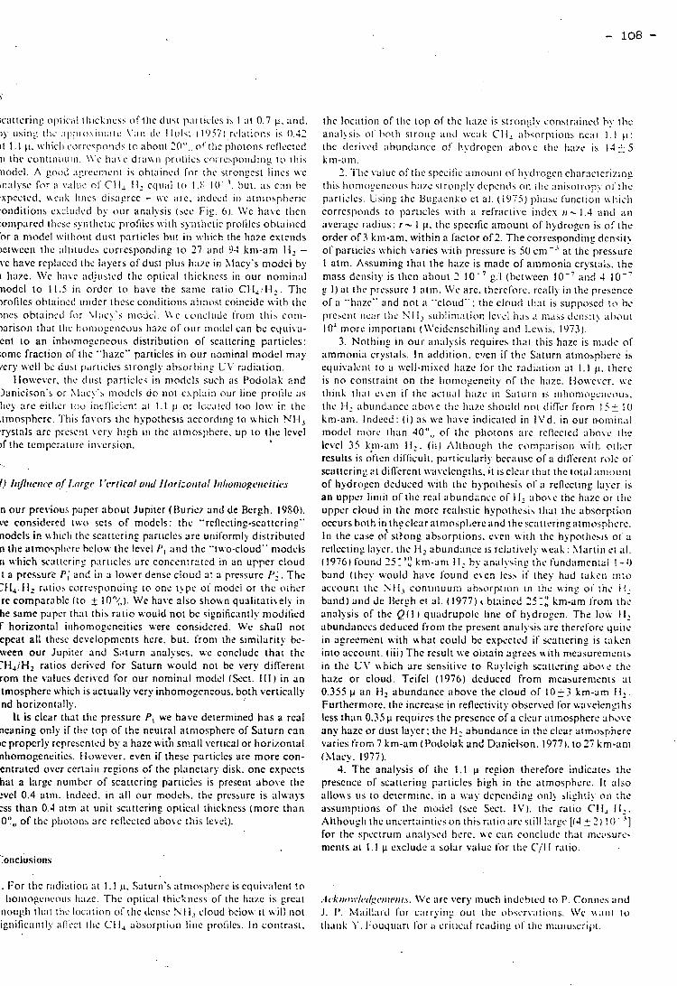
fcrcnccs

I1cr~l1.C.. l . ~ ~ c ~ ~ ~ l ~ ~ ~ i \ . S . . Coilihc\. A l . : 1074. .4\1rori, .-I.\~J~I~/~/I!~.S. 35. 333 13ci~Ii.C.. l-cciicl~c~~\..l . . ~1;iill ;1rtl .~.l ' . : 1977. ~1,strorr. ,.I.\II.o- /)Ii!,.\. 56. 227 Ucrgh. C . . hl;iill:ird.J.P.. 1'icrrc.G.. F1ilico.S.C.: 1980 (in prcp- ~i iot ion)

i.p,str~illi. J.T., hl;ii.golis. J.S. : 197 1 . J. Qitrrrir. Sj><,crrosc.op. Rnrliut. Trf~~i.\;/<~r 1 1. 12s 5

picnko. L.A. : 1972, A.rtr.ori. k",.srrt. 6. 19 giiciiko, L.A. : 1973. Ciindidate's Disscriiitioii. Kiev g:icnko,O.l.. DIii_r;ich.ZIi.M.. Moroz l ic i iko .~ .V: .~ano\~ i t sk i i . E.G.: 1975. Sol ir .Yj..srcwi Re.seurc/i 13. 9

riez. J.C., tic Ijcrgh. C. : 19SO. Asfroii. :lsiropli~.s. 83. 149 1du.cll. J. : 1977. Il.(rrri.v 30. 493 ~rl, .R.ii . . hlc(.i)id.~l..I3.: 1079. I(.iirit.\ 40. ISU ik. U.. L:irson. 11.1'. : 1979. A.s~ro/>/rj..c. .1. 233. 1021 iiiz.O.G., 1'1-icc. h4.J. : 1979, Icariis 37. 272 u1ier.D.. L;icoriibc.A., Rcvah,I.: 1977, ~lsrron. Asfrophj,s. 61. 1-19 iiiicr. D.. Coiirtiii. Ii.: 1979. 1rrrrir.s 39. 28 iiscn. S.E. : 1'909, ..l.rri.opli!~.\. J. 158. 337 n tic t l i i ls i . l~.C' . : 1'957. Ligtit k:iitcriri; hy Stiiall Pariiclcs. \ililey. Kcu-York I (le l{iilsi. 1 I.C.. Crossman. K.: 196s. in Ti!(, .-ltrtiosltli;~rc.v (?f i..'i,rrit.\ rrirrl ,\lrrr..c. S . C. 13r;indi and M. V. hlcfilroy cd.. Gnrdoii and Drcach. Net( -)'ork. 35

Kii\viilxit;i. K .. 1 ~ ; I I I \ C I I . .l. 1;. : 1975. Bit//. .~!rir~~ï. ..l.vtrt~~~. Sol.. 7. 3x2 Kn\vnta.Y.. Il;iriscii. J . i : . : 1070. in Ji/pit<,r. T. Gclircls cd.. l . ' r i i \ .

ol' : ' i i - i ~ ~ ~ i l ; l l)lK.>\. 5 1 O L;it~ibcrt. 11.L. : 197s. . \~oIII / / /J . .\'oIi(x*.\ RI)!,. :l.\!ro~i. Soc. 182. 249

Lc~.~iclicii\.S.. de Ilcig1i.C.. Cuiiibc\.F\,l.. X~l;iill;irtl..l.: 1c):fi.

rf.str/~:r. ,I .sri~~pl!i..\. 53. 29 Mac)'. \\'. : 1076. I(.arii.\ 29. 49 Miicy. \\'. : 1977. 1~~nrir.s 32. 378 Marti1i.T.Z.. Criiikshiink. D.I'., Pilc1icr.C.B.. Sintnii.\V.I\l.:

1976. Iccrrir.r 27. 391 MorozhciiLo.A.V.. Yanoviizkii. E.G.: 1973. Ic<rrirs 18. 583 Palliiconi. F.D. : 1972. Tllc Piiinct Satiirn ( 1970). NASA Sp;icc

Vcliicli. 1)csigii Criicri;~ (I.ii\.iroiinioiii. \.AS;\ SP-8091 Picrrc.G.. 14 ilico. S.C.. de 13cr~li. C . b1;iiIlrirt~. S.1'. : 19SO..i. .\1<,/,.,..

Sp(.c.fr. l iii prcw i

Pod~li ik . X I . . I);inicl\<iri. II. : 1977. I(.trr.~i.c 30. 470

Teilcl. V. : 1976. Soi.i~,r A.\rroii. 19. 5UO Toniiisko. h.1.G.. IL'esi. R . A . . Casiillo. S.D.: 1973. I(xrrri\ 33. 55s Tokuiiiiy;i.A.T.: 1978. 1-hc S;itui.n Systciii. I'iocccding~ ot' ri

NASA \vorkshop. Reston. Virginiri. 13 Trafioii. L. : 1973. A.r~ro/)li~..c. ../. 182. 6 15 Trafion.l..: 1978. Tlic Snturn Syhicin. Procccdings of a NrZS.4

worksliop. Rcstoti. Virsiiiia. 31 Trnfion. Id.. J1acy.W.: 1975. .-lstroph!..c. J. !O(>. 867 \\'iillacc. L.': 1'975. /c.rrrir.r 25. 535 Weideiisciii1iing.S.J.. Lc\vis. S.S.: 1973. I<,rrrit.s 20. 465

C O N C L U S I O N

Notre but était d'interpréter des spectres planétaires dans le

proche infra-rouge en utilisant dans la mesure du possible une méthode de

calcul simple. L'une des raisons était, disons, "financière" : étant

donnés les temps de calculs numériques nécessaires à la résolution del'é-

quation de transfert en milieu inhomogène, il est nécessaire de limiter

l'utilisation de tels programmes de calcul. L'autre raison est plus "phy-

sique" : on ne peut cerner ce qui est essentiel dans le transfert du

rayonnement que si l'on utilise des modèles physiques assez simples.

Le modèle d'atmosphère le plus simple est celui de la "couche

réfléchissante" (RLM) . Même pour ce modèle dans lequel seules pression, température et éventuellement concentration de gaz absorbant varient, il

a fallu introduire l'approximation de CURTIS-GODSON. L'atmosphère est %

alors assimilée à une couche homogène définie par une pression P l une %

température O et une abondance de gaz absorbant u. Un tel modèle, s'il

est réaliste, est idéal pour l'analyse des spectres planétaires puisque,

en laboratoire, une cellule d'absorption permet une simulation directe de

la couche d'atmosphère.

Les photons réfléchis par une atmosphère claire ont tous ren-

contré la même abondance de gaz. Il n'en est pas de même dans le cas

d'une atmosphère nuageuse. Les modèles diffusants ne peuvent plus être

simulBs à l'aide d'une seule cellule d'absorption. Si l'atmosphère est

homogène, une cellule contenant une abondance de gaz u simule le modèle

pour les photons réfléchis par l'atmosphère après avoir rencontré cette

même abondance u. Une simulation est donc encore possible si l'on dis-

pose d'un grand nombre de cellules différentes. Si l'atmosphère n'est

pas homogène, les photons qui ont rencontré une abondance de gaz u ne sont

pas absorbés de la même manière s'ils ont pénétré profondément dans l'at-

mosphère ou non. Selon les conditions de température et de pression ré-

gnant dans l'atmosphère le long du trajet des photons, la cellule d'ab-

sorption doit donc contenir une abondance de gaz plus ou moins importante.

Le problème est compliqué par le fait que la loi de variation de

l'absorption avec l'altitude n'est pas la même suivant la fréquence ob-

servée. On fait alors l'approximation suivante : le gaz est soumis aux

mêmes conditions de température et de pression dans toutes les cellules

d'absorption ; les abondances de gaz dans ces cellules sont choisies

pour permettre une simulation de l'effet de l'atmosphère sur l'absorp-

tion dans les ailes des raies. Si l'on s'intéresse aux largeurs équiva-

lentes de raies, la simulation permet de déterminer les largeurs équi-

valentes de raies fortes (pour lesquelles l'influence des ailes est pré-

pondérante) ; la pression à priori arbitraire est alors choisie de façon

à pouvoir déterminer aussi les largeurs équivalentes des raies faibles.

Si au contraire on s'intéresse aux profils des raies, la pression est

choisie de sorte que la simulation soit valable non seulement dans les

ailes mais aussi aux centres des raies.

Cette idée simple de reconstituer un spectre planétaire à l'aide

d'un grand nombre de cellules d'absorption nous a conduit à introduire la

fonction de distribution de l'abondance de gaz absorbant pondérée par la

température et la pression. Pour le calcul des largeurs équivalentes de

raies, nous avons ainsi pu généraliser au cas de n'importe quel type

d'atmosphère l'approximation de CURTIS-GODSON initialement développée

pour les atmosphères claires. Une approximation du même type a été dé-

veloppée pour les profils de raies synthétiques ; elle nous a permis de

réduire de façon notable les temps de calculs numériques.

Il nous semble plus important encore de souligner que la no-

tion de "distribution d'abondance pondérée" nous a permis de voir sous

un angle nouveau quels types d'informations peuvent être obtenus à par-

tir d'un spectre planétaire :

Les largeurs équivalentes de raies idéalement isolées et for-

mées dans une atmosphère nuageuse (non conservative) différent très peu

de celles qui seraient formées dans une atmosphère claire définie par % %

une température 0 , une pression rP et une abondance de gaz absorbant %

: 0 est la température de rotation déterminée à partir des équations

classiques établies pour le modèle de la couche réfléchissante ; u1 est l'abondance de gaz absorbant rencontrée en moyenne par les photons en

% absence d'absorption et P est la pression de formation corresponaante ;

r est le rapport des abondances "pondérées" en régime d'absorption forte

et faible ; il varie de i (pas de diffusion) i O (nuage conservatif semi-

infini) ; c'est donc un excellent "indicateur de diffusion".

A partir de la mesure de largeurs équivalentes de raies, il

n'est possible d'éliminer des modèles d'atmosphères que si l'on connait 'L

une relation liant p et rP, ce qui nécessite de connaître la concentra- 1

tion en gaz absorbant. L'interprétation des profils de raies est plus

riche en informations : l'analyse des ailes de raies permet de déterminer

l'indicateur de diffusion r et donc d'éliminer un certain nombre de

modëles sans faire d'hypothèse sur la concentration en gaz absorbant ;

l'analyse de la région centrale des raies impose des conditions supplé-

mentaires sur la structure des hautes couches de l'atmosphère.

La possibilité d'une détermination précise des paramètres tels 'L 'L

que O, P, pl et r doit être envisagée avec précaution: les raies ne sont

jamais parfaitement isolées. Pour la mesure d'une largeur équivalente, la

forme des ailes de la raie doit être extrapolée dizféremment suivant le t ype de 'b '-b

modèle envisagé. Les quantités 0, pl et rP peuvent être déterminées à

partir des valeurs des largeurs équivalentes de la même façon quelque

soit le modèle d'atmosphère, mais, en pratique, les largeurs équivalentes

des raies observées doivent être mesurées différemment suivant le type

d' atmosphère (pour tenir compte de la forme des ailes de raies) . Pour l'a- nalyse des profils de raies, le problème est différent puisque l'on étudie

le spectre en tenant compte du recouvrement des raies. Une grande incer-

titude peut toutefois subsister si le niveau continu n'est pas connu avec

précision.

Dans tous les cas,llanalyse d'un spectre planétaire ne permet pas

de déterminer la structure réelle de l'atmosphère, mais simplement une

schématisation de celle-ci. Pour des atmosphères extrêmement complexes

telles que celles de Jupiter et Saturne, nous avons défini les informations

essentielles que l'on peut obtenir à partir d'un spectre observé : (i) la

région sondée par l'atmosphère, (ii) l'importance de la diffusion dans cette

région, (iii) plus particulièrement le rôle joué par la diffusion dans les

très hautes couches de l'atmosphère ; (iv) la concentration du gaz absorbant.

Nous avons analysé la région de la bande 3v du méthane dans les 3

spectres de Jupiter et de Saturne enregistrés par CONNES et 1.lAILLARD en

1974. Nous pouvons résumer les résultats obtenus sous fo-?ne de réponses

aux questions précédentes :

(i) l'atmosphère sondée correspond pour les différents modèles sélectionnés

à des pressions "apparentes" relativement faibles

r$ = 0,s I 0,2 atm pour Jupiter

r$ = 0,2 2 0,l atm pour Saturne.

(ii) C'indicateur de diffusion obtenu est

r = 0,7 + 0,2 pour Jupiter r = 0,6 2 0,2 pour Saturne

ce qui exclut l'hypothèse d'une atmosphère claire, sans que l'on puisse

faire la distinction entre un modèle à un seul nuage étendu et un modèle

à plusieurs nuages denses.

(iii) cependant, dans tous les cas, la prosence de particules diffusantes

haut dans l'atmosphère est nécessaire. Plus de 10 % des photons réfléchis

par Jupiter pénètrent tout au plus jusqu'au niveau correspondant à 0,3 atm.

Cette proportion passe à 30 % pour le même niveau dans le cas de Saturne.

(iv) Les concentrations obtenues correspondent à un enrichissement du rap-

port C/H comparé à la valeur solaire

cH4 - c

- 3 (2,8 + 1,3) 10 pour Jupiter ( j i r )

H2

Cfi4 - = - 3 (4 ?: 2) 10 pour Saturne

(*) Valeurs révisées à l'aide des mesures d'intensités S, les plus récentes J

(C. DE BERGH, communication privée) .

L'imprécision du résultat est liée aux limites expérimentales à la

fois au niveau du spectre observé (résolution instrumentale et rapport s/n)

et au niveau des mesures en laboratoire (incertituàes sur les intensités

des raies, les deni-largeurs de LORENTZ,...). Mais cette imprécision est

aussi lige h la technique du spectre synthétique elle-même (indépendamment

des difficultés pour utiliser cette technique). Pour repousser plus loin

les limites de la connaissance des planètes à partir d'un spectre observé,

on peut joindre à la spectroscopie l'apport de la polarimétrie. Nous avons

montré que l'on pouvait généraliser à n'importe quel paramètre de STOKES

la notion de distribution d'abondance "pondérée". Tandis que les spectres

des paramètres de STOKES 1 et 1 sont formés à l'intérieur d'un nuage R r

pratiquement au mëme niveau que 1, le spectre de Q = IR - 1 est formé r beaucoup plus haut dans l'atmosphère. L'obtention du spectre de Q pemet-

trait ainsi une meilleure localisation du sommet des nuages. De plus, la

comparaison entre les largeurs équivalentes des raies fortes formées dans

un nuage et associées respectivement à 1 et Q permettrait une détermination

du rapport des échelles de hauteur gaz ambiant- particules ou gaz mineur-

gaz ambiant. S'il est possible d'obtenir un rapport signal/bruit suffisam-

ment élevé pour permettre une comparaison entre les profils des raies fortes,

l'information sera encore plus riche : de la mëme façon que pour 1, on

obtient pour Q un indicateur de diffusion correspondant à &es niveaux plus

élevés dans l'atmosphère. La spectropolarimétrie apparalt donc comme un

puissant moyen d'investigation des planètes qui devrait être développé

dans les années à venir.

A N N E X E A

% % Scnéma de calcul de la distribution p ( u ) et de la pression P (introduites

au cnapitre 1) .

1 - Découpage de l'atmosphère en un nombre fini de couches homogènes. La i-ème couche est caractérisée par :

- le diagramme de diffusion - l'épaisseur optique mise sous la forme

A T ci) représente l'épaisseur optique de la couche dans le continu ; K est C

homogène à un coefficient d'absorption massique ; f(i) sera la fonction de

pondération ; Aa(i) est l'abondance réelle de gaz absorbant contenue dans

la couche.

- l'albédo de simple diffusion

wc ( i l étant 1 ' albédo continu.

2 - Calcul préliminaire de l'intensité continue 1 : résolution de l'équa- C

tion de transfert pour K = O dans Eq. (BI).

3 - Calcul de la fonction p (u' ) :

- calcul de la fonction de pondération intervenant dans Eq. (BI) :

f (il = du / du' ; ce rapport est défini par Eq. (1-20)

- résolution de l'équation de transfert pour (2N-1) valeurs de K bien

réparties sur 1 ' intervalle j O, [ et éventuellement pour K -t si une par-

tie du rayonnement est réfléchie sans rencontrer de gaz absorbant. Typi-

quement, N = 5 .

- Approximation des rapports des intensités I(K) / 1 au moyen de C

Eq. (1-7).

- Calcul de la fonction p(ur) par Eq. (1-8) et des moments p', et 1 fb 2 %

1/2 par Eq. 1 - . A ce stade, "l'indicateur de diffusion" r = (+1/2) /pl

2 peur être calculé puisqu'il est identique à /$II.

4 - Calcul du moment p" . 1 '

- Calcul d'une nouvelle fonction de pondération intervenant dans Eq. (BI) : f (il = du / du" ; ce rapport est défini par Eq. (1-21).

- Calcul de p(u") puis de un1 comme précédemment (§ 3) ou plus direc-

tement calcul de "" à partir de la résolution de l'équation de transfert 1

pour K très petit

soit

1 pl'l = K - 0 , pour K très petit.

% % 5 - Détermination de P et p(u) par Eqs. (1-23 et 28) .

A N N E X E B

Schéma de la méthode décrite au chapitre IV 2b (détermination de pL) v

1 - Le rapport des intensités 1 /I défini par Eq (IV-15) est approximé à v c

l'aide d'un approximant de PADE (cf. chap. 1 ou Annexe 1 : calcul de la

fonction p (u' ) )

avec

(1 f O seulement si une partie du rayonnement est réfléchie sans rencontrer O

. de gaz absorbant).

2 - Résolution de l'équation de transfert à J fréquencsv pour L intensi- j

tés S de raies isolées, réparties sur l'intervalle [S R min1 'max

] des inten-

sités des raies observées. Les fréquences v sont choisies de manière à j

permettre l'interpolation du profil de la raie R à partir des J intensités

1 (SR,vj). Typiquement L = J = 5 .

3 - Si Av est la limite de résolution expérimentale, on choisit une fré- quence v sur 1 ' intervalle ] vol vo + Av r . Pour cette fréquence, les L

j valeurs de 1 2

(Sa,vj) permettent de déterminer L valeurs de P (IV ) à v

partir de Eq (BI). Par moindres carrés, on obtient une première détermina-

tion des coefficients a de Eq (IV-16) m

4 - Calcul de l'intensité 1 convoluée au centre de la raie (R = 1, L). OR

exact (a) à partir des intensités 1 (S ,v ) calculées au § 2 : v R j I ~ R

(b) à partir des Eqs . (BI) et (B2) de façon itérative : I ~ ~ ~ ~ . OR

5 - Les p a r a r ~ ~ è t r e s a son t co r r igés de proche en proche jusqu'à ce que l 'é- m

c a r t quadratique moyen

s o i t minimal. Pour accé lé re r ce c a l c u l , on u t i l i s e une méthode de g rad ien t

minimal. En général 3 ou 4 i t é r a t i o n s s u f f i s e n t .

L

E = C R = l

6 - On peut a l o r s ca lcu le r 1 pour n ' importe que l l e r a i e ( i s o l é e ou non) v

à n' importe que l l e fréquence à p a r t i r des Eqs. (BI) e t (B2). La préc is ion

de l a méthode dans l a zone c r i t i q u e des épaules de r a i e s peut ê t r e estimée

en comparant l e s p r o f i l s convoluées approchés aux p r o f i l s convolués

"exacts" (à p a r t i r de § 2 ) .

.-

exact - =OR - -

Documents

AqbA - univ-lille.fr · 2017-09-25 · V - RESUME ET CONCLUSIONS CHAPITRE III - LES LARGEURÇ EQUIVALEN'JXS DE RAIES EN SPECTROPOLARIMETRE. lfSpecmopoZarimetry of Venus and Jupiter