Embed Size (px)
Citation preview
This article was downloaded by: [American Public University System]On: 24 February 2014, At: 12:22Publisher: Taylor & FrancisInforma Ltd Registered in England and Wales Registered Number: 1072954 Registered office: MortimerHouse, 37-41 Mortimer Street, London W1T 3JH, UK
Hydrological Sciences JournalPublication details, including instructions for authors and subscription information:http://www.tandfonline.com/loi/thsj20
Assessing uncertainties in a conceptual waterbalance model using Bayesian methodology /Estimation bayésienne des incertitudes au sein d’unemodélisation conceptuelle de bilan hydrologiqueKolbjørn Engeland , Chong-Yu Xu & Lars Gottschalka Cemagref, 3bis quai Chauveau, CP220, F-69336 Lyon Cedex 09, Franceb Department of Earth Sciences–Hydrology, Uppsala University, Villavagen 16, S-75236Uppsala, Swedenc Department of Geophysics, University of Oslo, PO Box 1022 Blindern, N-0315 Oslo,NorwayPublished online: 15 Dec 2009.
To cite this article: Kolbjørn Engeland , Chong-Yu Xu & Lars Gottschalk (2005) Assessing uncertainties in a conceptualwater balance model using Bayesian methodology / Estimation bayésienne des incertitudes au sein d’une modélisationconceptuelle de bilan hydrologique, Hydrological Sciences Journal, 50:1, -63, DOI: 10.1623/hysj.50.1.45.56334
To link to this article: http://dx.doi.org/10.1623/hysj.50.1.45.56334
PLEASE SCROLL DOWN FOR ARTICLE
Taylor & Francis makes every effort to ensure the accuracy of all the information (the “Content”) containedin the publications on our platform. However, Taylor & Francis, our agents, and our licensors make norepresentations or warranties whatsoever as to the accuracy, completeness, or suitability for any purpose ofthe Content. Any opinions and views expressed in this publication are the opinions and views of the authors,and are not the views of or endorsed by Taylor & Francis. The accuracy of the Content should not be reliedupon and should be independently verified with primary sources of information. Taylor and Francis shallnot be liable for any losses, actions, claims, proceedings, demands, costs, expenses, damages, and otherliabilities whatsoever or howsoever caused arising directly or indirectly in connection with, in relation to orarising out of the use of the Content.
This article may be used for research, teaching, and private study purposes. Any substantial or systematicreproduction, redistribution, reselling, loan, sub-licensing, systematic supply, or distribution in anyform to anyone is expressly forbidden. Terms & Conditions of access and use can be found at http://www.tandfonline.com/page/terms-and-conditions
Hydrological Sciences–Journal–des Sciences Hydrologiques, 50(1) February 2005
Open for discussion until 1 August 2005 Copyright 2005 IAHS Press
45
Assessing uncertainties in a conceptual water balance model using Bayesian methodology KOLBJØRN ENGELAND1, CHONG-YU XU2 & LARS GOTTSCHALK3
1 Cemagref, 3bis quai Chauveau, CP220, F-69336 Lyon Cedex 09, France [email protected]
2 Department of Earth Sciences—Hydrology, Uppsala University, Villavagen 16, S-75236 Uppsala, Sweden
3 Department of Geophysics, University of Oslo, PO Box 1022 Blindern, N-0315 Oslo, Norway
Abstract The aim of this study was to estimate the uncertainties in the streamflow simulated by a rainfall–runoff model. Two sources of uncertainties in hydrological modelling were considered: the uncertainties in model parameters and those in model structure. The uncertainties were calculated by Bayesian statistics, and the Metropolis-Hastings algorithm was used to simulate the posterior parameter distribution. The parameter uncertainty calculated by the Metropolis-Hastings algorithm was compared to maximum likelihood estimates which assume that both the parameters and model residuals are normally distributed. The study was performed using the model WASMOD on 25 basins in central Sweden. Confidence intervals in the simulated discharge due to the parameter uncertainty and the total uncertainty were calculated. The results indicate that (a) the Metropolis-Hastings algorithm and the maximum likelihood method give almost identical estimates concerning the parameter uncertainty, and (b) the uncertainties in the simulated streamflow due to the parameter uncertainty are less important than uncertainties originating from other sources for this simple model with fewer parameters. Key words Bayesian analysis; Markov Chain Monte Carlo analysis; maximum likelihood estimation; model uncertainty; water balance models
Estimation bayésienne des incertitudes au sein d’une modélisation conceptuelle de bilan hydrologique Résumé L’étude est consacrée à l’évaluation des incertitudes entachant les débits simulés par un modèle pluie–débit conceptuel. Deux sources d’incertitudes dans la modélisation hydrologique ont été prises en compte: les incertitudes dues aux paramètres du modèle et celles dues à sa structure. Ces incertitudes ont été évaluées par une approche bayésienne, et l’algorithme de Metropolis-Hastings a été utilisé pour simuler la distribution a posteriori des paramètres. L’incertitude sur les paramètres évalués par l’algorithme de Metropolis-Hastings a été comparée à celle que fournit la méthode du maximum de vraisemblance sous hypothèse de normalité de la distribution de ces paramètres et des résidus du modèle. L’étude a été menée en appliquant le modèle WASMOD à 25 bassins versants du centre de la Suède. Les intervalles de confiance relatifs aux débits simulés dus à la seule incertitude sur les paramètres d’une part, et dus à l’incertitude totale d’autre part, ont été calculés. Les résultats indiquent que (a) l’algorithme de Metropolis-Hastings et la méthode du maximum de vraisemblance donnent des résultats quasiment identiques pour l’incertitude sur les paramètres, et que (b) pour les débits simulés, les incertitudes liées aux paramètres sont plus petites que celles qui sont dues à d’autres causes, pour ce modèle simple à peu de paramètres. Mots clefs analyse bayésienne; analyse Markov-Chaîne de Monte Carlo; maximum de vraisemblance; incertitude de modèle; modèles de bilan hydrologique
INTRODUCTION Conceptual catchment models are common tools in calculating the runoff dynamics and the water balance at various scales and regions. The model parameters are usually
Dow
nloa
ded
by [
Am
eric
an P
ublic
Uni
vers
ity S
yste
m]
at 1
2:22
24
Febr
uary
201
4
Kolbjørn Engeland et al.
Copyright 2005 IAHS Press
46
calibrated in order to obtain a good fit between observed and simulated outputs. Since computer models are not a perfect representation of reality, the results are uncertain. In many cases, assessment of the uncertainties is important, e.g. in water recourses management, where decisions have to be taken based on several uncertain factors; climate change impact studies; and water balance calculations in ungauged basins. The uncertainties in hydrological modelling have four important sources (e.g. Refsgaard & Storm, 1996): (a) uncertainties in input data (e.g. precipitation and temperature); (b) uncertainties in data used for calibration (e.g. streamflow); (c) uncertainties in model parameters; and (d) imperfect model structure. The error sources (a) and (b) depend on the quality of data, whereas (c) and (d) are more model specific. The uncertainties in the input data (a) originate from the observations (e.g. Førland et al., 1996) and the interpolation in space (e.g. Lebel et al., 1987). The uncertainties in the streamflow observations (b) depend on the quality of the rating curve. Some examples are given in Kuczera (1996), Clarke et al. (2000), Clarke (1999) and Jónsson et al. (2002). In this study the uncertainties (c) and (d) were investigated. Perhaps no studies include a full investigation of how the four error sources contribute and interact in the total modelling uncertainty. However, there are several papers where two or three of the error sources are evaluated simultaneously. Andréassian et al. (2001) demonstrate that the quality of the rainfall data influences both the simulation errors and the calibrated model parameters. Several studies indicate that the precipitation is the most important uncertainty factor compared to the model parameters (e.g. Thorsen et al., 2001; Refsgaard et al., 1983; Storm et al., 1988) or the model structure (e.g. Krzysztofowicz, 1999). The papers cited above indicate that results presented here should be interpreted carefully since the study does not account explicitly for the error sources (a) and (b). What appears to be a parameter or model uncertainty might partially be caused by uncertainties in the observations. Several methods are available for evaluating the parameter sensitivity and assessing the modelling uncertainties. Many studies focus on the formulation of the objective function that describes the fit between observed and simulated values. In a statistical framework, the objective function is called the likelihood function and is a stochastic model for the simulation errors. To account for auto-correlations, stochastic error model of AR(1) and ARMA types are used (e.g. Sorooshian & Dracup, 1980; Alley, 1984; Xu, 2001). To account for non-constant variance, heteroscedastic error models are used (e.g. Sorooshian & Dracup, 1980) or the data are transformed (e.g. Kuzczera, 1983; Xu, 2001). A transformation might also account for the non-normality of the simulation errors (e.g. Krzysztofowicz, 1999). Some papers focus on the parameter sensitivity without aiming to estimate a probability distribution (e.g. Mein & Brown, 1978; Spear et al., 1994; Wagener et al., 2003). The multi-objective method (Yapo et al., 1998) is used to quantify parameter uncertainty and analyse model structural uncertainty by generating a Pareto optimal set of parameters with respect to different output fluxes (e.g. Beldring, 2002) or different objective functions (e.g. Madsen, 2000). Examples of statistical approaches for quantification of parameter uncertainty include maximum likelihood methods (e.g. Xu, 2001) and Bayesian methods (e.g. Kuczera, 1983; Engeland & Gottschalk, 2002). A variant of the Bayesian method was introduced under the name generalized likelihood uncertainty estimation (GLUE) by Beven & Binley (1992). In the GLUE concept, it is recognized that a number of the requirements in the Bayesian method cannot be fulfilled in many cases.
Dow
nloa
ded
by [
Am
eric
an P
ublic
Uni
vers
ity S
yste
m]
at 1
2:22
24
Febr
uary
201
4
Assessing uncertainties in a conceptual water balance model using Bayesian methodology
Copyright 2005 IAHS Press
47
It might be difficult to define a likelihood function, and the response surfaces in the parameter space can be very complex due to the interacting modelling errors. A “subjective” likelihood is therefore used in the GLUE approach instead of a more strictly defined statistical one. The aim is to discover the whole response surface in order to find a set of many different models that can be acceptable. The GLUE concept is now becoming a popular method in studying the parameter uncertainty and interval prediction in both hydrological and hydraulic models (e.g. Beven et al., 2000; Hankin et al., 2001; Aronica et al., 2002), and a dynamic version of GLUE is developed in Wagener et al. (2003). In developing and implementing the Bayesian method, the Metropolis-Hastings (MH) algorithm (Hastings, 1970), a Markov Chain Monte Carlo (MCMC) method, has been used. The MCMC method has been especially popular in Bayesian statistics (e.g. Geyer, 1992), and more recently the MH algorithm has been applied to hydrological models (e.g. Kuczera & Parent, 1998; Engeland & Gottschalk, 2002; Vrugt et al., 2003). In this study, the Bayesian method was applied as presented in Engeland & Gottschalk (2002). They used the physically-based Ecomag model operating on a daily time resolution, but two properties prohibited application of the Bayesian method in a consistent way: a complex behaviour of the simulation errors, and a complex shape of the parameter distribution. In order to overcome these difficulties and evaluate the Bayesian method in a consistent framework, a more simplistic model was applied in this study. A monthly water balance model called WASMOD was chosen because it has been carefully constructed to have well-defined, independent parameters and simulation errors that are normally distributed (Xu et al., 1996; Xu 2001, 2002). The aim of this study was to estimate the model parameters and to quantify the uncertainties of the simulated streamflows that resulted from both parameter uncertainty (c) and model structure uncertainty (d). To start with, only two of the four error sources were chosen, to keep the calculations simple, but it is intended to include additional error sources at a later stage. This aim was achieved by estimating the probability density of the model parameters and the statistical parameter of the simulation errors simultaneously. Both the maximum likelihood (ML) method and the Bayesian method were used to calculate the parameter uncertainty, and the results were compared. For the Bayesian method, the calculations were performed by the MH algorithm. The Bayesian method was used to calculate confidence intervals for simulated streamflows. To account for heteroscedastic residuals, i.e. dependence of error variance on computed runoff, a square-root transformation on both computed and observed runoff data was used. The resulting model error was assumed to be a white noise process with Gaussian distribution. The later hypothesis was then tested with a cross-basin validation approach. The robustness of the model performance and the confidence intervals were also tested by cross-validation. The study was performed using the WASMOD model (Xu, 2002) on 25 basins in central Sweden. The paper is organized as follows: after this brief introduction, the study area, data and the WASMOD model are described. The subsequent section outlines the Bayesian method and the specific consideration in using the method in this study, which includes the choice of likelihood function, the prior and proposal densities, the MH simulation procedure, etc. Next, the application results including parameter estimates and resulted streamflow simulation uncertainties are presented, then the results are
Dow
nloa
ded
by [
Am
eric
an P
ublic
Uni
vers
ity S
yste
m]
at 1
2:22
24
Febr
uary
201
4
Kolbjørn Engeland et al.
Copyright 2005 IAHS Press
48
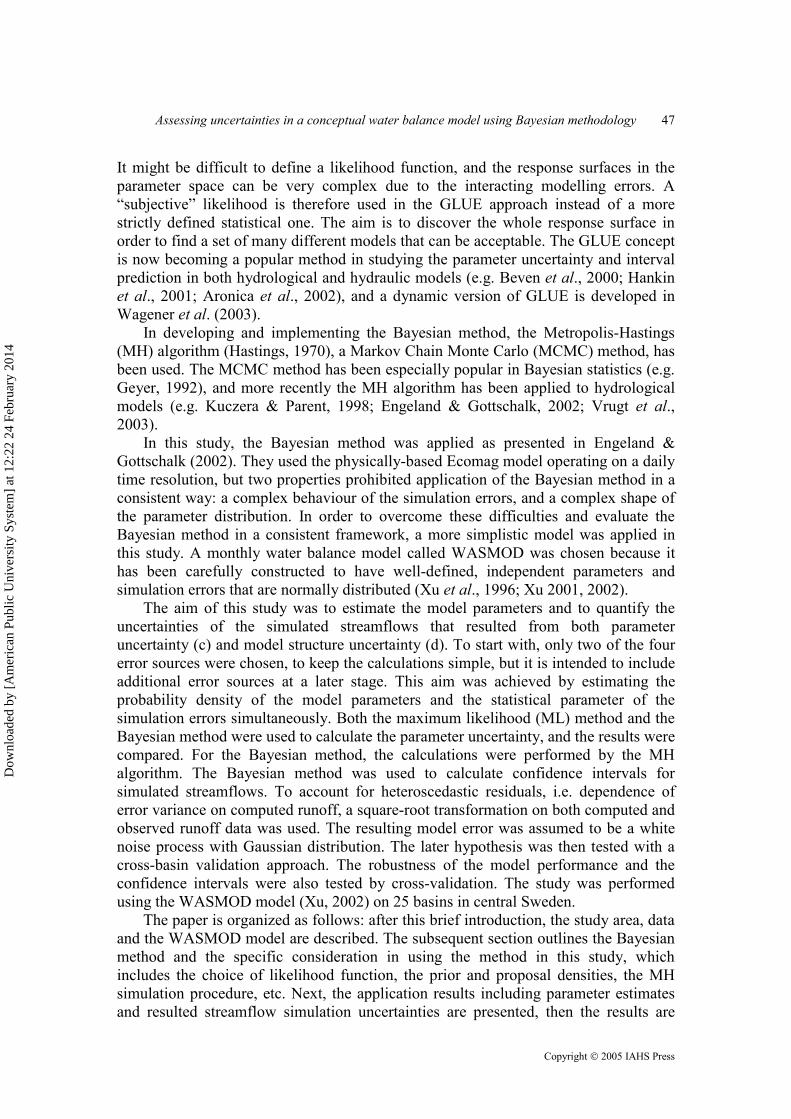
discussed and, finally, the conclusions and proposal for further investigations are presented. THE STUDY AREA AND THE HYDROLOGICAL MODEL The study area The study area is located in central Sweden (Fig. 1). The area has 30 sub-catchments ranging in size from 6 to 4000 km2. Available meteorological data consist of daily precipitation from 41 stations, daily temperature data from 12 stations and all with an observation period of at least 10 years. Twenty-five of the 30 sub-catchments were used in this study, since earlier investigations (e.g. Xu, 2003) showed that some sub-catchments might have errors in the determination of water divides. The mean annual precipitation and discharge are 800 and 310 mm, respectively. The land use of the area includes 5.7% lake (not including Lake Mälaren itself), 69.3% forest and 25% agricultural land. The hydrological and land-use data of the study region are shown in Table 1.
1.NOPEX region2. Study region 1.NOPEX region2. Study region
SOSO
Fig. 1 The study area and basins (see Table 1 for abbreviations of basins).
The WASMOD model The monthly water balance model WASMOD was developed for water balance computation for the NOPEX region (Xu et al., 1996; Xu, 2002). The model parameters are related to the physical characteristics of the basins (Xu 1999; Müller-Wohlfeil et al., 2003). The input data for using the model on gauged basins are monthly areal precipitation, potential evapotranspiration and/or air temperature. To use the model on ungauged basins, the land-use and/or soil distribution data are needed. The model outputs are monthly river flow and other water balance components, such as actual
Dow
nloa
ded
by [
Am
eric
an P
ublic
Uni
vers
ity S
yste
m]
at 1
2:22
24
Febr
uary
201
4
Assessing uncertainties in a conceptual water balance model using Bayesian methodology
Copyright 2005 IAHS Press
49
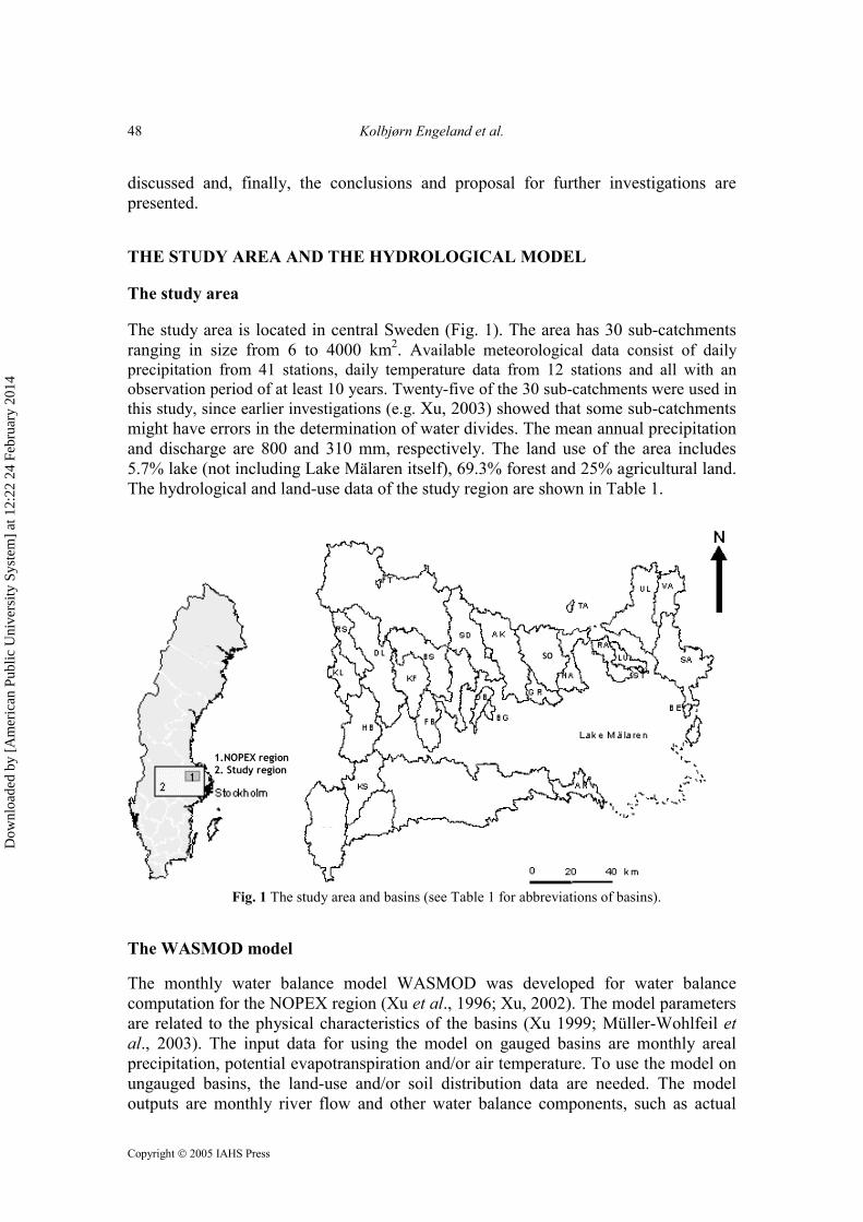
Table 1 General information of the 25 study basins in central Sweden.
Station Abbr. Code Area Mean precip.
Mean*
evap. Mean runoff
Lake Forest Open Basin slope
(km2) (cm) (cm) (cm) (%) (%) (%) Åkesta Kv. AK 2216 727 60.1 39.6 21.6 4.0 69.0 27.0 3.3 Åkers Krut. AR 2249 214 60.3 43.3 17.6 5.2 66.3 28.5 Bergsh. BE 2300 21.6 55.6 40.2 16.3 0.2 69.5 30.3 Berg BG 2218 36.5 63.9 43.0 22.2 0.0 71.4 28.6 Bernsh. BS 1573 595 78.0 43.4 34.9 8.6 77.3 14.1 Dalkarlsh. DL 2206 1182 76.4 42.4 35.2 7.5 74.6 17.9 Fellingsbr. FB 2205 298 62.6 39.9 24.6 6.0 63.8 30.2 Finntorp. FT 2242 6.96 65.9 43.9 22.1 4.7 95.3 0.0 Gränvad GR 2217 167 59.4 40.9 19.8 0.0 41.1 58.9 2.7 Härnevi HA 2248 312 60.2 38.1 23.3 1.0 55.0 44.0 3.4 Hammarby HB 2153 891 73.3 43.1 30.9 9.5 80.9 9.7 Kåfalla KF 1532 413 81.0 44.3 36.9 6.2 80.8 13.0 Kringlan KL 2229 294 78.3 44.3 34.2 7.6 87.2 5.2 Karlslund KS 2139 1293 69.7 43.4 27.0 6.6 62.7 30.7 Lurbob LU 2245 122 60.8 36.3 25.2 0.3 68.2 31.5 4.0 Odensvibr. OB 2221 110 63.6 41.7 23.3 6.3 71.0 22.7 Ransta RA 2247 197 59.8 38.2 22.3 0.9 66.1 33.0 3.5 Rällsälv RS 2207 298 79.3 43.1 38.4 7.4 78.8 13.8 Sävja SA 2243 722 59.7 40.4 19.5 2.0 64.0 34.0 1.5 Skräddart. SD 2222 17.7 66.7 41.6 25.3 2.5 96.1 1.4 Sörsätra SO 2220 612 60.8 33.5 27.3 1.1 61.0 37.9 Stabbyb ST 1742 6.18 56.4 36.2 18.7 0.0 95.6 4.4 10.3 Tärnsjöb TA 2299 13.7 59.7 39.5 21.8 1.5 84.5 14.0 7.1 Ulva Kv. UL 2246 976 61.2 43.9 17.1 3.0 61.0 36.0 1.6 Vattholma VA 2244 293 60.6 40.8 21.0 4.8 71.0 24.2 1.8 * Actual evapotranspiration calculated by the model. Table 2 Principal equations for the six-parameter WASMOD model.
Snowfall st = pt{1 – exp[–(ct – a)/(a1 – a2)]2}+ a1 ≥ a2 Rainfall rt = pt – st Snow storage spt = spt-1 + st – mt Snowmelt mt = spt{1 – exp[–(ct – a2)/(a1 – a2)]2}+ Potential evapotranspiration ept = [1 + a3(ct – cm)]epm Actual evapotranspiration et = min{wt[1 – exp(–a4ept)], ept} 0 ≤ a4 ≤ 1 Slow flow bt = a5(sm+
t-1)2 a5 ≥ 0 Fast flow ft = a6(sm+
t-1)2(mt + nt) a6 ≥ 0 Water balance smt = smt-1 + rt + mt – et – bt – ft wt = rt + sm+
t-1 is the available water; sm+t-1 is the available storage; nt = rt – ept(1 – exp(rt/ept)) is the
active rainfall; pt and ct are monthly precipitation and air temperature respectively; and epm and cm are long-term monthly averages. ai (i = 1, …, 6) are the model parameters. The superscript plus means x+ = max(x,0). evapotranspiration, slow and fast components of river flow, soil-moisture storage and accumulation of snowpack, etc. The primary equations of the model are presented in Table 2, and a schematic computational flow chart is shown in Fig. 2. The parameters a1 and a2 determine the phase of precipitation and the rate of snowmelt. Parameter a3
Dow
nloa
ded
by [
Am
eric
an P
ublic
Uni
vers
ity S
yste
m]
at 1
2:22
24
Febr
uary
201
4
Kolbjørn Engeland et al.
Copyright 2005 IAHS Press
50
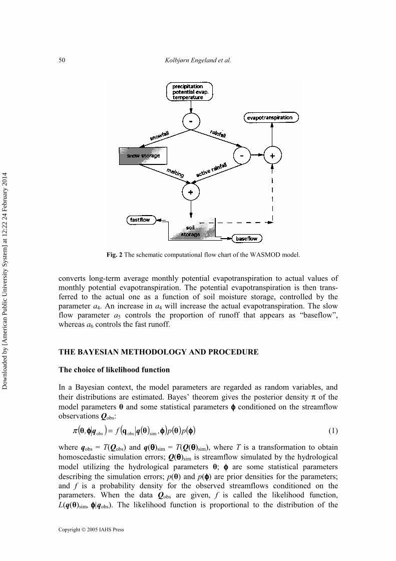
Fig. 2 The schematic computational flow chart of the WASMOD model.
converts long-term average monthly potential evapotranspiration to actual values of monthly potential evapotranspiration. The potential evapotranspiration is then trans-ferred to the actual one as a function of soil moisture storage, controlled by the parameter a4. An increase in a4 will increase the actual evapotranspiration. The slow flow parameter a5 controls the proportion of runoff that appears as “baseflow”, whereas a6 controls the fast runoff. THE BAYESIAN METHODOLOGY AND PROCEDURE The choice of likelihood function In a Bayesian context, the model parameters are regarded as random variables, and their distributions are estimated. Bayes’ theorem gives the posterior density π of the model parameters θ and some statistical parameters φφφφ conditioned on the streamflow observations Qobs:
( ) ( )( ) ( ) ( )φφφφφφφφφφφφ pp,f, θθqθ simobsobs qq =π (1)
where qobs = T(Qobs) and q(θθθθ)sim = T(Q(θθθθ)sim), where T is a transformation to obtain homoscedastic simulation errors; Q(θθθθ)sim is streamflow simulated by the hydrological model utilizing the hydrological parameters θ; φφφφ are some statistical parameters describing the simulation errors; p(θ) and p(φφφφ) are prior densities for the parameters; and f is a probability density for the observed streamflows conditioned on the parameters. When the data Qobs are given, f is called the likelihood function, L(q(θ)sim, φφφφ|qobs). The likelihood function is proportional to the distribution of the
Dow
nloa
ded
by [
Am
eric
an P
ublic
Uni
vers
ity S
yste
m]
at 1
2:22
24
Febr
uary
201
4
Assessing uncertainties in a conceptual water balance model using Bayesian methodology
Copyright 2005 IAHS Press
51
-6
-4
-2
0
2
4
6
0 2 4 6 8 10 12 14Simulated streamflow (mm1/2)
Resid
ual (
mm
1/2 )
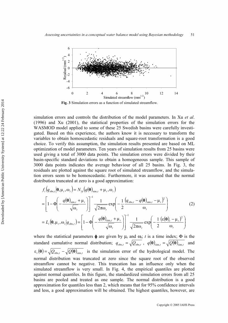
Fig. 3 Simulation errors as a function of simulated streamflow.
simulation errors and controls the distribution of the model parameters. In Xu et al. (1996) and Xu (2001), the statistical properties of the simulation errors for the WASMOD model applied to some of these 25 Swedish basins were carefully investi-gated. Based on this experience, the authors know it is necessary to transform the variables to obtain homoscedastic residuals and square-root transformation is a good choice. To verify this assumption, the simulation results presented are based on ML optimization of model parameters. Ten years of simulation results from 25 basins were used giving a total of 3000 data points. The simulation errors were divided by their basin-specific standard deviations to obtain a homogeneous sample. This sample of 3000 data points indicates the average behaviour of all 25 basins. In Fig. 3, the residuals are plotted against the square root of simulated streamflow, and the simula-tion errors seem to be homoscedastic. Furthermore, it was assumed that the normal distribution truncated at zero is a good approximation:
( ) ( )( )( ) ( )( )
( ) ( ) ( )( )��
�
�
��
�
� −−
��
�
�
�
��
�
�
��
�
� +−−==
��
�
�
��
�
� −−−
��
�
�
�
��
�
�
��
�
� +−−=
+=
−
−
t
tt
tt
tttttt
t
ttt
tt
tt
ttttttt
qqL
qqq
qNqf
ωµε
21exp
πω21
ωµ
Φ1ω,µ,
ωµ
21exp
πω21
ωµ
Φ1
ω,µω,µ,
21
,sim,obs
2,sim,obs
1
,sim
,sim0,obs
θθθ
θθ
θθ
(2)
where the statistical parameters φφφφ are given by µt and ωt; t is a time index; Φ is the standard cumulative normal distribution; tt Qq ,obs,obs = , ( ) ( ) tt Qq ,sim,sim θθ = and
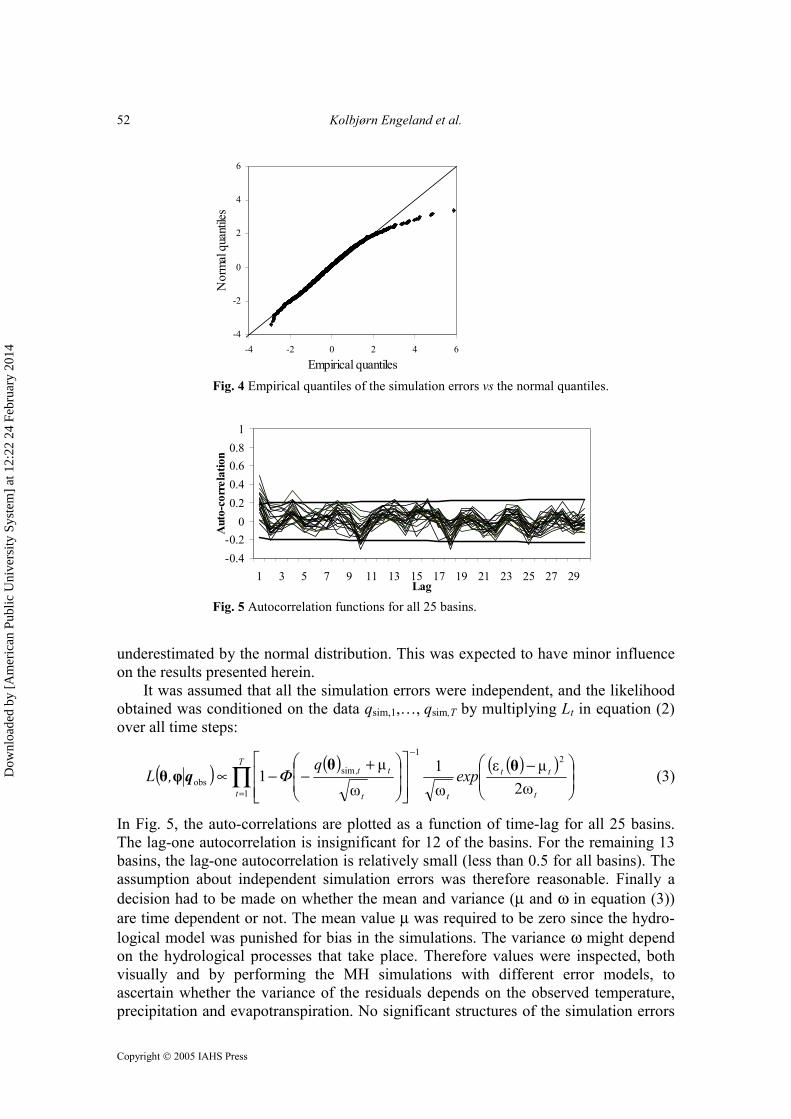
( ) ( ) ttt QQ ,sim,obsε θθ −= is the simulation error of the hydrological model. The normal distribution was truncated at zero since the square root of the observed streamflow cannot be negative. This truncation has an influence only when the simulated streamflow is very small. In Fig. 4, the empirical quantiles are plotted against normal quantiles. In this figure, the standardized simulation errors from all 25 basins are pooled and treated as one sample. The normal distribution is a good approximation for quantiles less than 2, which means that for 95% confidence intervals and less, a good approximation will be obtained. The highest quantiles, however, are
Dow
nloa
ded
by [
Am
eric
an P
ublic
Uni
vers
ity S
yste
m]
at 1
2:22
24
Febr
uary
201
4
Kolbjørn Engeland et al.
Copyright 2005 IAHS Press
52
-4
-2
0
2
4
6
-4 -2 0 2 4 6
Empirical quantiles
Nor
mal
quan
tiles
Fig. 4 Empirical quantiles of the simulation errors vs the normal quantiles.
-0.4-0.2
00.20.40.60.8
1
1 3 5 7 9 11 13 15 17 19 21 23 25 27 29Lag
Aut
o-co
rrel
atio
n
Fig. 5 Autocorrelation functions for all 25 basins.
underestimated by the normal distribution. This was expected to have minor influence on the results presented herein. It was assumed that all the simulation errors were independent, and the likelihood obtained was conditioned on the data qsim,1,…, qsim,T by multiplying Lt in equation (2) over all time steps:
( ) ( ) ( )( )��
�
�
��
�
� −��
�
�
�
��
�
�
��
�
� +−−∝ ∏
=
−
t
ttT
t tt
tt, expq
,Lω2
µεω1
ωµ
12
1
1
simobs
θθφθ Φq (3)
In Fig. 5, the auto-correlations are plotted as a function of time-lag for all 25 basins. The lag-one autocorrelation is insignificant for 12 of the basins. For the remaining 13 basins, the lag-one autocorrelation is relatively small (less than 0.5 for all basins). The assumption about independent simulation errors was therefore reasonable. Finally a decision had to be made on whether the mean and variance (µ and ω in equation (3)) are time dependent or not. The mean value µ was required to be zero since the hydro-logical model was punished for bias in the simulations. The variance ω might depend on the hydrological processes that take place. Therefore values were inspected, both visually and by performing the MH simulations with different error models, to ascertain whether the variance of the residuals depends on the observed temperature, precipitation and evapotranspiration. No significant structures of the simulation errors
Dow
nloa
ded
by [
Am
eric
an P
ublic
Uni
vers
ity S
yste
m]
at 1
2:22
24
Febr
uary
201
4
Assessing uncertainties in a conceptual water balance model using Bayesian methodology
Copyright 2005 IAHS Press
53
were found. This is in accordance with previous studies (e.g. Xu, 2001). Therefore a constant variance was chosen for the residuals. All the parameters including ω, were estimated independently for each catchment. The prior densities Since the variance has to be positive, flat priors above 0 were used for ω ( ( ) ( )∞,0Uniform~ωp ). For the WASMOD model parameters, uniform priors between the limits listed in Table 3 were applied. The parameter ranges shown in the table are consistent with the constraints given in Table 2, but in a practical situation the ranges are much smaller. Table 3 The prior intervals for the WASMOD parameters.
Parameter Uniform prior interval a1 a2 ∞ a2 –∞ a1 a3 –∞ ∞ a4 0.00 0.02 a5 0.00 ∞ a6 0.00 ∞ The MCMC simulations The Metropolis Hastings (MH) algorithm (Hastings, 1970), a Markov Chain Monte Carlo (MCMC) methodology, was used to estimate the parameters. The MH algorithm generates a Markov chain that converges to the distribution of interest. After removing the initial “burn-in”, this chain might be used as a dependent sample from the distribution. In this implementation of the MH algorithm, the parameters were updated for each iteration in a random order. The vector of all parameters (here a1–a6 and ω), is denoted by x, their posterior densities by π, their proposal densities by d, the number of iterations by m, and the number of parameters by n (here n = 7). The algorithm involves the following steps: – For L = 1, 2, ..., m, let x(L) be the current state of the chain. – Draw I randomly from 1, 2, ..., n (only once for each iteration; this is actually a
random permutation). – Draw a new value for xI from a specified irreducible proposal distribution d:
( )( )** ,~ xx LI dx where ( ) Ijxx L
jj ≠∀=* (4)
– Compute the acceptance probability:
( ) ( ) ( )[ ]( ) ( )[ ]��
�
���
= *)(
***)(
,π,π,1min,
xxxxxxxx LL
LL
dda (5)
let ( )( )( )
( ) ( )( )���
−=+
*
**1
,1yprobabilitwith,yprobabilitwith
xxxxLL
I
LIL
I axax
x (6)
Dow
nloa
ded
by [
Am
eric
an P
ublic
Uni
vers
ity S
yste
m]
at 1
2:22
24
Febr
uary
201
4
Kolbjørn Engeland et al.
Copyright 2005 IAHS Press
54
As the ratio of two posteriors densities is calculated in equation (5), this algorithm does not require the normalization constant of the posterior probability density. The proposal densities A random walk proposal density (equation (4)) was used, i.e. the proposal distribution was dependent on the current state of the chain. For the ω parameter, uniform proposal centred at the current parameter value was used. However, no negative values were proposed because the acceptance probability then will always be zero.
( )( ) ( )( )[ ]ωωωω +− sssd LL 2,ωmax,ω,0maxUniform~ (7)
For the WASMOD parameters, uniform proposals with the limitations specified in Table 3 were used. The acceptance probabilities For all parameters, the uniform proposal densities were constructed to have a constant variance. As a result, ( )( ) ( )( )LL dd xxxx ,, ** = , and the acceptance probability (equation (5)) could be simplified to calculate only the ratio of the new and old posteriors:
( ) ( )( )��
�
���
ππ= )(
**)( ,1min, t
Laxxxx (8)
Tuning the MH algorithm In order to obtain a chain that converged fast, the amplitude of the uniform proposal densities was tuned. If the variances of the proposals are too large, only a few of the new parameters will be accepted, thus the chain will easily get stuck in one point. If the variance is too small, the chain will need many iterations to explore the entire parameter space. According to Chib & Greenberg (1995), the acceptance rate for a new point in the chain should be about 45%. The amplitudes were tuned to have an acceptance rate between 40 and 50% for each parameter. Convergence of the chain The convergence of the chain was studied by looking into the lagged auto-covariances for each parameter. For a chain that has converged, the auto-correlations decrease rapidly towards zero. The convergence was also visually inspected by plotting the chains as functions of iteration. Confidence intervals for streamflow To calculate confidence intervals for streamflow, 100 000 streamflow values for each month were obtained by running the model with all the 100 000 parameter sets from
Dow
nloa
ded
by [
Am
eric
an P
ublic
Uni
vers
ity S
yste
m]
at 1
2:22
24
Febr
uary
201
4
Assessing uncertainties in a conceptual water balance model using Bayesian methodology
Copyright 2005 IAHS Press
55
the MH sample. The 95% confidence intervals due to parameter uncertainty were estimated from these streamflow samples. The 95% confidence intervals for both the parameter uncertainty and the model structure uncertainty were calculated by adding the model residuals in the form of a random uncertainty with zero mean and sample dependent standard deviation ωi to each of the 100 000 streamflow values that were available for each time step:
( ) ( ) ( )
2
simsampsim
0θ ����
�� +=
− ii,i,tQii,i,t,i,t ,rnormQQ ωωθ
(9)
where t is a time index, i is a sample index, samp is an index for streamflow sample with the random term added, sim is an index for streamflow calculated from the WASMOD model, and rnorm is a random number from a truncated normal distribution with the specified parameters. The truncation assured that no negative values were simulated. MAXIMUM LIKELIHOOD ESTIMATION To provide a comparative result with the MH algorithm, ML estimation method was also performed in the study. Maximum likelihood estimation was carried out by maximizing equation (3) without the truncation term, zero mean and constant variance. The optimization was performed with the help of the VA05A computer package (Hopper, 1978; Vandewiele et al., 1992) and the program EOX4F (NAG Fortran Subroutine Library, 1981). In the ML method, it is assumed that the parameters are normally distributed. Based on this assumption the covariance matrix is estimated. Derivation of covariance matrix for the model parameters is shown in Vandewiele et al. (1992). CROSS-VALIDATION Three cross-validation tests were carried out to test the quality of at-site simulations. In all tests, blocks of data from two years were successively left out in the parameter estimation. Then the streamflow and the confidence intervals were calculated for the independent data. The cross-validated Nash-Sutcliffe coefficient Reff and the cross-validated bias were calculated using all the independent simulations. To test the quality of the estimated confidence intervals, the number of observed streamflow values that fall outside the confidence intervals for the independent simulations were counted. RESULTS Convergence of the MCMC routine The parameters were estimated independently for each basin, thus a total of 25 chains with 110 000 iterations were calculated by the MH algorithm. The first 10 000 iterations in each chain, the “burn-in”, were discarded and the remaining 100 000 iterations were used as samples from the distributions. Visual inspection of the trajectories of the chains indicated that the MH algorithm had converged. They seemed
Dow
nloa
ded
by [
Am
eric
an P
ublic
Uni
vers
ity S
yste
m]
at 1
2:22
24
Febr
uary
201
4
Kolbjørn Engeland et al.
Copyright 2005 IAHS Press
56
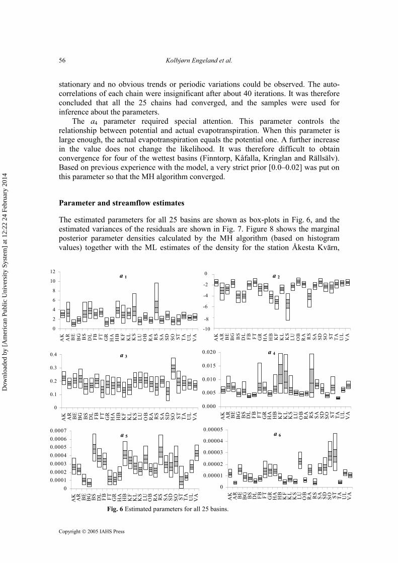
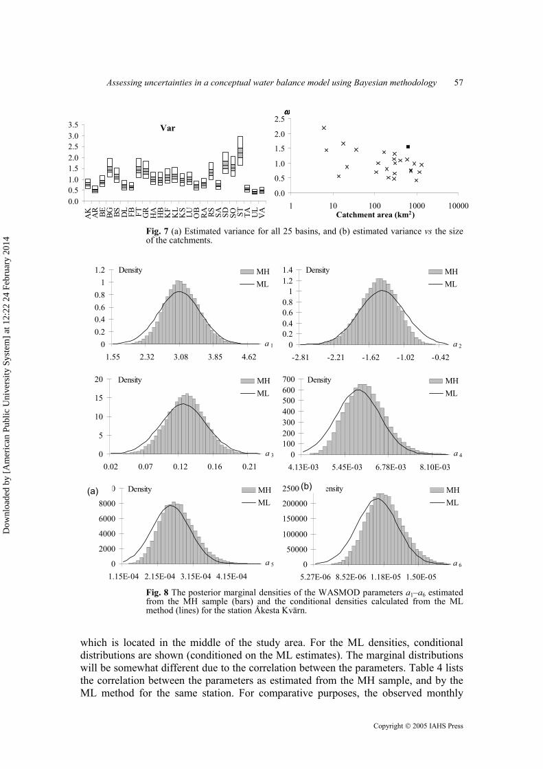
stationary and no obvious trends or periodic variations could be observed. The auto-correlations of each chain were insignificant after about 40 iterations. It was therefore concluded that all the 25 chains had converged, and the samples were used for inference about the parameters. The a4 parameter required special attention. This parameter controls the relationship between potential and actual evapotranspiration. When this parameter is large enough, the actual evapotranspiration equals the potential one. A further increase in the value does not change the likelihood. It was therefore difficult to obtain convergence for four of the wettest basins (Finntorp, Kåfalla, Kringlan and Rällsälv). Based on previous experience with the model, a very strict prior [0.0–0.02] was put on this parameter so that the MH algorithm converged. Parameter and streamflow estimates The estimated parameters for all 25 basins are shown as box-plots in Fig. 6, and the estimated variances of the residuals are shown in Fig. 7. Figure 8 shows the marginal posterior parameter densities calculated by the MH algorithm (based on histogram values) together with the ML estimates of the density for the station Åkesta Kvärn,
a 1
0
2
4
6
8
10
12
AK
AR
BE
BG BS
DL
FB FT GR
HA
HB
KF
KL
KS
LU OB
RA RS
SA SD SO ST TA UL
VA
a 2
0
2
4
6
8
10
AK
AR
BE
BG BS
DL
FB FT GR
HA
HB
KF
KL
KS
LU
OB
RA RS
SA SD SO ST TA
UL
VA
-10
-8
-6
-4
-2
0
a 4
0.000
0.005
0.010
0.015
0.020
AK AR BE
BG BS
DL
FB FT GR
HA
HB
KF
KL
KS
LU OB
RA RS
SA SD SO ST TA UL
VA
a 5
00.00010.00020.00030.00040.00050.00060.0007
AK AR BE
BG BS
DL
FB FT GR
HA
HB
KF
KL
KS
LU OB
RA RS
SA SD SO ST TA UL
VA
a 6
0
0.00001
0.00002
0.00003
0.00004
0.00005
AK AR BE
BG BS
DL
FB FT GR
HA
HB
KF
KL
KS
LU OB
RA RS
SA SD SO ST TA UL
VA
a 3
0
0.1
0.2
0.3
0.4
AK AR BE
BG BS
DL
FB FT GR
HA
HB
KF
KL
KS
LU OB
RA RS
SA SD SO ST TA UL
VA
Fig. 6 Estimated parameters for all 25 basins.
Dow
nloa
ded
by [
Am
eric
an P
ublic
Uni
vers
ity S
yste
m]
at 1
2:22
24
Febr
uary
201
4
Assessing uncertainties in a conceptual water balance model using Bayesian methodology
Copyright 2005 IAHS Press
57
Var
0.00.51.01.52.02.53.03.5
AK AR BE BG BS DL FB FT GR
HA HB
KF
KL
KS
LU OB
RA RS SA SD SO ST TA UL
VA
0.0
0.5
1.0
1.5
2.0
2.5
1 10 100 1000 10000Catchment area (km2)
ωωωω
0.0
0.5
1.0
1.5
2.0
2.5
1 10 100 1000 10000Catchment area (km2)
ωωωω
Fig. 7 (a) Estimated variance for all 25 basins, and (b) estimated variance vs the size of the catchments.
00.20.40.60.8
11.2
1.55 2.32 3.08 3.85 4.62a 1
Density MHML
00.20.40.60.8
11.21.4
-2.81 -2.21 -1.62 -1.02 -0.42a 2
Density MHML
0
5
10
15
20
0.02 0.07 0.12 0.16 0.21a 3
Density MHML
0
2000
4000
6000
8000
10000
1.15E-04 2.15E-04 3.15E-04 4.15E-04
a 5
Density MHML
0100200300400500600700
4.13E-03 5.45E-03 6.78E-03 8.10E-03
a 4
Density MHML
0
50000
100000
150000
200000
250000
5.27E-06 8.52E-06 1.18E-05 1.50E-05
a 6
Density MHML
Fig. 8 The posterior marginal densities of the WASMOD parameters a1–a6 estimated from the MH sample (bars) and the conditional densities calculated from the ML method (lines) for the station Åkesta Kvärn.
which is located in the middle of the study area. For the ML densities, conditional distributions are shown (conditioned on the ML estimates). The marginal distributions will be somewhat different due to the correlation between the parameters. Table 4 lists the correlation between the parameters as estimated from the MH sample, and by the ML method for the same station. For comparative purposes, the observed monthly
(b) (a)
Dow
nloa
ded
by [
Am
eric
an P
ublic
Uni
vers
ity S
yste
m]
at 1
2:22
24
Febr
uary
201
4
Kolbjørn Engeland et al.
Copyright 2005 IAHS Press
58
Table 4 Correlation between the parameters estimated by the Metropolis Hastings (MH) and maximum likelihood (ML) methods.
a1 a2 a3 a4 a5 a6 MH ML MH ML MH ML MH ML MH ML MH ML a1 1.00 1.00 –0.49 –0.62 –0.04 –0.02 –0.05 –0.04 –0.36 –0.43 0.10 0.16 a2 –0.49 –0.62 1.00 1.00 0.02 –0.00 0.05 0.04 0.35 0.46 0.03 0.00 a3 –0.04 –0.02 0.02 –0.00 1.00 1.00 –0.06 –0.11 0.01 –0.02 –0.08 –0.11 a4 –0.05 –0.04 0.05 0.04 –0.06 –0.11 1.00 1.00 0.36 0.37 0.43 0.49 a5 –0.36 –0.43 0.35 0.46 0.01 –0.02 0.36 0.37 1.00 1.00 0.42 0.46 a6 0.10 0.16 0.03 0.00 –0.08 –0.11 0.43 0.49 0.42 0.46 1.00 1.00
0
40
80
120
160
1 13 25 37 49 61 73 85 97 109Month
Q(mm)
0
40
80
120
160
1 13 25 37 49 61 73 85 97 109Month
Q(mm)
0
40
80
120
160
1 13 25 37 49 61 73 85 97 109Month
Q(mm)
0
40
80
120
160
1 13 25 37 49 61 73 85 97 109Month
Q(mm)
a)
b)
a)
b) Qobs QsimQobsQobs QsimQsim
Qobs QsimQobsQobs QsimQsim
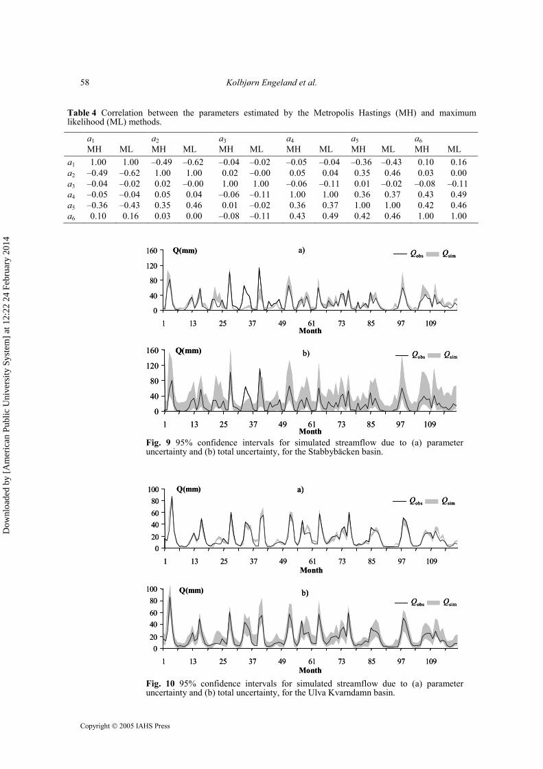
Fig. 9 95% confidence intervals for simulated streamflow due to (a) parameter uncertainty and (b) total uncertainty, for the Stabbybäcken basin.
020406080
100
1 13 25 37 49 61 73 85 97 109Month
Q(mm)
020406080
100
1 13 25 37 49 61 73 85 97 109Month
Q(mm)
a)
b)
020406080
100
1 13 25 37 49 61 73 85 97 109Month
Q(mm)
020406080
100
1 13 25 37 49 61 73 85 97 109Month
Q(mm)
a)
b)
a)
b)
Qobs QsimQobsQobs QsimQsim
Qobs QsimQobsQobs QsimQsim
Fig. 10 95% confidence intervals for simulated streamflow due to (a) parameter uncertainty and (b) total uncertainty, for the Ulva Kvarndamn basin.
Dow
nloa
ded
by [
Am
eric
an P
ublic
Uni
vers
ity S
yste
m]
at 1
2:22
24
Febr
uary
201
4
Assessing uncertainties in a conceptual water balance model using Bayesian methodology
Copyright 2005 IAHS Press
59
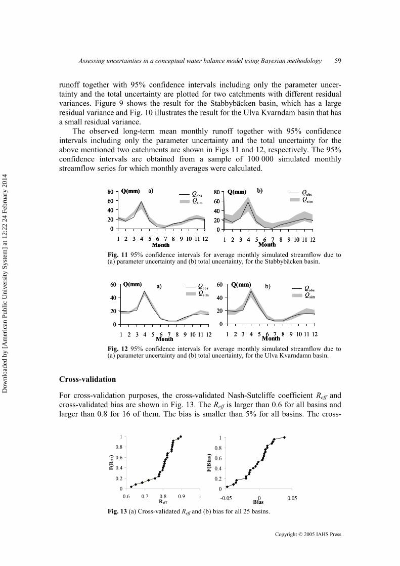
runoff together with 95% confidence intervals including only the parameter uncer-tainty and the total uncertainty are plotted for two catchments with different residual variances. Figure 9 shows the result for the Stabbybäcken basin, which has a large residual variance and Fig. 10 illustrates the result for the Ulva Kvarndam basin that has a small residual variance. The observed long-term mean monthly runoff together with 95% confidence intervals including only the parameter uncertainty and the total uncertainty for the above mentioned two catchments are shown in Figs 11 and 12, respectively. The 95% confidence intervals are obtained from a sample of 100 000 simulated monthly streamflow series for which monthly averages were calculated.
020406080
1 2 3 4 5 6 7 8 9 10 11 12Month
Q(mm)
020406080
1 2 3 4 5 6 7 8 9 10 11 12Month
Q(mm)a) b)
020406080
1 2 3 4 5 6 7 8 9 10 11 12Month
Q(mm)
020406080
1 2 3 4 5 6 7 8 9 10 11 12Month
Q(mm)
020406080
1 2 3 4 5 6 7 8 9 10 11 12Month
Q(mm)
020406080
1 2 3 4 5 6 7 8 9 10 11 12Month
Q(mm)a) b)a) b)QobsQsim
QobsQsim
QobsQsim
QobsQsim
Fig. 11 95% confidence intervals for average monthly simulated streamflow due to (a) parameter uncertainty and (b) total uncertainty, for the Stabbybäcken basin.
0
20
40
60
1 2 3 4 5 6 7 8 9 10 11 12Month
Q(mm)
0
20
40
60
1 2 3 4 5 6 7 8 9 10 11 12Month
Q(mm)
0
20
40
60
1 2 3 4 5 6 7 8 9 10 11 12Month
Q(mm)
0
20
40
60
1 2 3 4 5 6 7 8 9 10 11 12Month
Q(mm)a) b)a) b) QobsQsim
QobsQsim
QobsQsim
QobsQsim
Fig. 12 95% confidence intervals for average monthly simulated streamflow due to (a) parameter uncertainty and (b) total uncertainty, for the Ulva Kvarndamn basin.
Cross-validation For cross-validation purposes, the cross-validated Nash-Sutcliffe coefficient Reff and cross-validated bias are shown in Fig. 13. The Reff is larger than 0.6 for all basins and larger than 0.8 for 16 of them. The bias is smaller than 5% for all basins. The cross-
0
0.2
0.4
0.6
0.8
1
0.6 0.7 0.8 0.9 1Reff
F(R
eff)
0
0.2
0.4
0.6
0.8
1
-0.05 0 0.05Bias
F(B
ias)
Fig. 13 (a) Cross-validated Reff and (b) bias for all 25 basins.
Dow
nloa
ded
by [
Am
eric
an P
ublic
Uni
vers
ity S
yste
m]
at 1
2:22
24
Febr
uary
201
4
Kolbjørn Engeland et al.
Copyright 2005 IAHS Press
60
validated confidence intervals show that 42% of the observed streamflow values falls inside the 95% confidence intervals when only the parameter uncertainty is taken into account. When the simulation residuals are added, however, 95% of the observed values were inside the confidence intervals. These cross-validation tests indicate that in at-site applications WASMOD gives robust estimates of monthly water balance, long-term average water balance and confidence intervals. DISCUSSION Comparison of MH and ML estimates The estimates from the MH routine indicate that the parameter densities are only slightly skewed (Fig. 6). The standard deviations estimated by the MH and ML methods are almost identical (Fig. 8). This shows that the shape of the likelihood function at the optimum value and the normal assumption in the ML method are reasonable approximations. The estimated densities are only slightly different. The two methods indicate similar patterns for the correlations, but the MH-estimated correlations are somewhat lower than those obtained from the ML method (Table 4). Similar results are also found for the other 24 stations. All these results indicate that the ML estimates give a good approximation to the parameter density for the monthly WASMOD model applied in Sweden. For models operating on daily time steps, more complex parameter distributions are reported (e.g. Duan et al., 1992; Kuczera & Parent, 1998; Engeland & Gottschalk, 2002; Vrugt et al., 2003), and the normal distribution will not necessarily be a good approximation. Parameter estimates Both the median values and the variance of the WASMOD parameters depend on the basins (Fig. 6). The sign of the skewness is identical for all basins. The a1 and a2 parameters that control the snow cover formation and snowmelt processes are basin-dependent. The a3 and a4 parameters that control the evapotranspiration have the smallest variation between basins. The Sörsätra basin has an exceptionally high a3 parameter. This basin has a high mean runoff compared to its neighbours (Åkesta Kvärn, Gränvad and Härnevi, see Table 1), and should be treated carefully in a regionalization context. The parameters that control the runoff, a5 and a6, show the largest variation between basins. In particular, the a5 parameter is significantly different between several basins. Xu (1999) estimated relationships between the model parameters and basin characteristics for this dataset using multiple linear regression analysis. He found that a1 is positively correlated to the lake and the forest percentages whereas the a2 is negatively related to the lake and open field percentages. No correlations were found between the basin characteristics and the parameters a3 and a4. The slow flow parameter a5 was positively related to the lake and forest percentages, whereas the fast flow parameter a6 was negatively related to lake percentage and positively related to forest percentage. The study not only verified the physical interpretations about the model parameters, but also established quantitative parameter estimation equations in the study area. Similar regression equations between the
Dow
nloa
ded
by [
Am
eric
an P
ublic
Uni
vers
ity S
yste
m]
at 1
2:22
24
Febr
uary
201
4
Assessing uncertainties in a conceptual water balance model using Bayesian methodology
Copyright 2005 IAHS Press
61
WASMOD model parameters and catchment physical characteristics were established for a Danish catchment by Müller-Wohlfeil et al. (2003). The success of such a regionalization procedure depends also on the quality of the input data and the observed streamflow data used for calibration as biased data might introduce biased parameters (Andréassian et al., 2001). Uncertainties in streamflow simulations The uncertainties in the model parameters cannot account for all the uncertainties in the simulations. About 45% of the observations were inside these confidence intervals (Figs 9(a) and 10(a)). When the total uncertainty was included, the confidence intervals got much wider (Figs 9(b) and 10(b)). This indicates that the parameter uncertainty is less important than the uncertainties caused by the model structure. The WASMOD model simulated the average intra-annual variations well (Figs 11 and 12). The parameter uncertainty is getting more important compared to the results in Figs 9 and 10. This is due to the way these two error sources were represented. The parameters were assumed to be constant in time and they were therefore selected randomly from their distribution for the whole simulation period. However, the simulation error part was assumed to be independent between the months, and it was therefore selected randomly for each month in the simulation period. This part of the uncertainty will therefore decrease by a factor of n 1 , where n is the number of years used for averaging. There are several indications that the variance of the simulation errors was caused not only by an imperfect model structure, but also by uncertainties in the observed data. Based on the results presented in this study it is not possible to tell to what extent errors in the observations contributed to the total simulation errors. Lebel et al. (1987) showed that the estimation variance of interpolated area rainfall decreases with increasing basin size. A similar pattern is seen in Fig. 7(b): the residual variance decreases with increasing basin size (streamflow values in mm were used here for all calculations, so the direct effect of basin size on variance of the residuals should have been removed). It may also be seen that the high residual variance for the Stabbybäcken basin was caused by one flood-event that is not captured by the model (Fig. 9(a)). This is the smallest basin with an area of 6.18 km2 and there are no meteorological observations within the basin borders. The quality of the interpolated precipitation in this basin was therefore very sensitive to local rainfall events. The quality of the observed streamflow data might also have influenced the simulation errors. The variance marked as a filled square in Fig. 7(b) represents the Sörsätra basin, which has the highest variance for basins with an area larger than 100 km2. The observed streamflow from this basin might be doubtful (see subsection “Parameter estimates”). CONCLUSIONS The WASMOD model was applied to 25 basins in central Sweden. A Bayesian methodology combined with the MH algorithm was used to estimate the model
Dow
nloa
ded
by [
Am
eric
an P
ublic
Uni
vers
ity S
yste
m]
at 1
2:22
24
Febr
uary
201
4
Kolbjørn Engeland et al.
Copyright 2005 IAHS Press
62
parameters and their uncertainty. The Bayesian estimates were compared to the ML estimates. This study allows one to draw some conclusions that will be important for further investigations, i.e. in estimating regional parameters. All the assumptions in the application of the Bayesian method have been tested. The investigation of the simulation residuals showed that the square-root transforma-tion is sufficient to obtain homoscedastic residuals. The residuals are approximately normally distributed, the variance of the residuals is as good as independent of the climatic conditions and the residuals are nearly independent. These results are only valid for the 25 basins that were used in this study and they have to be checked for each new application. The authors were able to identify parameter densities for all 25 basins and the ML estimation was shown to give a reasonable approximation to the distribution of the model parameters as the MH algorithm and ML method gave almost identical estimates of the parameter uncertainty. Ninety-five percent confidence intervals were calculated around the simulated streamflows. The confidence intervals around the simulated streamflows indicate that parameter uncertainty is less important than the other uncertainty sources in the streamflow estimations. It is anticipated that this conclusion is valid for simple con-ceptual models with few well-defined parameters. The cross-validation tests showed that water balance calculations and the confidence intervals are reliable. Most of the model parameters depended on the basin. Further work will be to carry out a full regionalization of the model parameters by relating them to basin charac-teristics. Bayesian hierarchical modelling (Gelman et al., 1995) then offers suitable tools for such estimation. Another topic for further investigation is to include the uncertainties in meteoro-logical data and in streamflow observations in the uncertainty assessment. This would help one to understand how all the four error sources contribute in the total modelling uncertainty. REFERENCES Alley, W. M. (1984) On the treatment of evapotranspiration, soil moisture accounting and aquifer recharge in monthly
water balance models. Water Resour. Res. 20(8), 1137–1149. Andréassian, V., Perrin, C., Michel, C., Usart-Sanchez, I. & Lavabre, J. (2001) Impact of imperfect rainfall knowledge on
the efficiency and the parameters of watershed models. J. Hydrol. 250, 206–223. Aronica, G., Bates, P. D. & Horritt, M. S. (2002) Assessing the uncertainty in distributed model predictions using observed
binary pattern information within GLUE. Hydrol. Processes 16(10), 2001–2016. Beldring, S. (2002) Multi-criteria validation of a precipitation–runoff model. J. Hydrol. 257, 189–211. Beven, K. J. & Binley, A. M. (1992) The future of distributed models—model calibration and uncertainty prediction.
Hydrol. Processes 15, 509–711. Beven, K. J., Freer, J., Hankin, B. & Schulz, K. (2000) The use of generalised likelihood measures for uncertainty
estimation in high order models of environmental systems. In: Nonlinear and Nonstationary Signal Processing (ed. by W. J. Fitzgerald, R. L. Smith, A. T. Walden & P. C. Young), 115–151. Cambridge Univ. Press, Cambridge, UK.
Chib, S. & Greenberg, E. (1995) Understanding the Metropolis-Hasting Algorithm. The American Statistician 49(4), 327–335.
Clarke, R. T. (1999) Uncertainty in the estimation of mean annual flood due to rating-curve indefinition. J. Hydrol. 222, 185–190.
Clarke, R. T., Mendiondo, E. M. & Brusa, L. C. (2000). Uncertainties in mean discharges from two large South American rivers due to rating curve variability. Hydrol. Sci. J. 45(2), 221–236.
Duan, Q., Sorooshian, S. & Gupta, V. (1992). Effective and efficient global optimisation for conceptual rainfall–runoff models. Water Resour. Res. 28(4), 1015–1031.
Engeland, K. & Gottschalk, L. (2002) Bayesian estimation of parameters in a regional hydrological model. Hydrol. Earth System Sci. 6(5), 883–898.
Dow
nloa
ded
by [
Am
eric
an P
ublic
Uni
vers
ity S
yste
m]
at 1
2:22
24
Febr
uary
201
4
Assessing uncertainties in a conceptual water balance model using Bayesian methodology
Copyright 2005 IAHS Press
63
Førland, E. J., Allerup, P., Dahlström, B., Elomaa, E., Jonsson, T., Madsen, H., Perälä, J., Rissanen, P., Vedin, H., Vedin, H. & Vejen, F. (1996) Manual for Operational Correction of Nordic Precipitation Data. DNMI Klima Report no. 24/96, Norwegian Meteorological Institute, Oslo, Norway.
Gelman, A., Carlin, J. B., Stern, H. S. & Rubin, D. B. (1995) Bayesian Data Analysis. Chapman & Hall, London, UK. Geyer, C. J. (1992) Practical Markov Chain Monte Carlo. Statist. Sci. 7(4), 473–483. Gottschalk, L., Jensen, J. L., Lundquist, D., Solantie, R. & Tollan, A. (1979) Hydrologic regions in the Nordic countries.
Nordic Hydrol. 10, 273–286. Hankin, B. G., Hardy R., Kettle, H. & Beven, K. J. (2001) Using CFD in a GLUE framework to model the flow and
dispersion characteristics of a natural fluvial dead zone. Earth Surf. Processes Landf. 26(6), 667–687. Hastings, W. K. (1970) Monte Carlo sampling methods using Markov chains and their applications. Biometrica 57, 97–109. Hopper, M. J. (1978) A Catalogue of Subroutines. Harwell Subroutines Library, HMSO, London, UK. Jónsson, P., Petersen-Øverleir, A., Nilsson, E., Edström, M., Iversen, H. L. & Sirvio, H. (2002). Methodological and
personal uncertainties in the establishment of rating curves. In: XXII Nordic Hydrological Conference (ed. by Ǻ. Killingtveit) (Nordic Association for Hydrology, Røros, Norway, 4–7 August 2002). NHP Report no. 47, vol. 1, 35–44.
Krzysztofowicz, R. (1999) Bayesian theory of probabilistic forecasting via deterministic hydrologic model. Water Resour. Res. 35(9), 2739–2750.
Kuczera, G. (1983) Improved parameter inference in catchment models 1. Evaluating parameter uncertainty. Water Resour. Res. 19(5), 1151–1162.
Kuczera, G. (1996) Correlated rating curve in flood frequency inference. Water Resour. Res. 32(7), 2119–2127. Kuczera, G. & Parent, E. (1998) Monte Carlo assessment of parameter uncertainty in conceptual catchment models: the
Metropolis algorithm. J. Hydrol. 211, 69–85. Lebel, T. Bastin, G., Obled, C. & Creutin, D. (1987) On the accuracy of areal rainfall estimation: a case study. Water
Resour. Res. 23(11), 2123–2134. Madsen, H. (2000) Automatic calibration of a conceptual rainfall–runoff model using multiple objectives. J. Hydrol. 235,
276–288. Mein, R. G. & Brown, B. M. (1978) Sensitivity of optimized parameters in watershed models. Water Resour. Res. 14,
299–303. Müller-Wohlfeil, D. I., Xu, C.-Y. & Iversen, H. L. (2003). Estimation of monthly river discharge from Danish catchments.
Nordic Hydrol. 34(4), 295–320. NAG Fortran Subroutine Library (1981) E04XAF NAG Fortran Library Routine Document, NP1490/13. Refsgaard, J. C. & Storm, B. (1996) Construction, calibration and validation of hydrological models. In: Distributed
Hydrological Modelling (ed. by M. B. Abbott & J. C. Refsgaard), 41–54. Water Science and Technology Library, vol. 22, Kluwer Academic Publishers, Dordrecht, The Netherlands.
Refsgaard, J. C., Rosbjerg, D. & Markussen, L. M. (1983), Application of Kalman filter to real-time operation and to uncertainty analyses in hydrological modelling. In: Scientific Procedures Applied to the Planning, Design and Management of Water Resource Systems (ed. by E. Plate & N. Buras), 273–282. IAHS Publ. 147. IAHS Press, Wallingford, UK.
Sorooshian, S. & Dracup, J. A. (1980) Stochastic parameter estimation procedures for hydrologic rainfall–runoff models: correlated and heteroscedastic error cases. Water Resour. Res. 16(2), 430–442.
Spear, R. C., Grieb , T. M. & Shang, N. (1994) Parameter uncertainty interaction in complex environmental models. Water Resour. Res. 30(11), 3159–3169.
Storm, B., Jensen, K. H. & Refsgaard, J. C. (1988) Estimation of catchment rainfall uncertainty and its influence on runoff predictions. Nordic Hydrol. 19, 77–88.
Thorsen, M., Refsgaard, J. C., Hansen, S., Pebesma, E., Jensen, J. B. & Kleeschulte, S. (2001) Assessment of uncertainty in simulation of nitrate leaching to aquifers at catchment scale. J. Hydrol. 242, 210–227.
Vandewiele, G. L., Xu, C.-Y. & Ni-Lar-Win (1992) Methodology and comparative study on monthly water balance models in Belgium, China and Burma. J. Hydrol. 134, 315–347.
Vrugt, J. A., Gupta, H. V., Bastidas, L. A., Bouten, W. & Sorooshian, S. (2003) A shuffled complex evolution Metropolis algorithm for optimization and uncertainty assessment of hydrologic model parameters. Water Resour. Res. 39(8), 39, doi:10.1029/2002WR001642.
Wagener, T., McIntyre, N., Lees, M. J., Wheater, H. S. & Gupta, H. V. (2003) Towards reduced uncertainty in conceptual rainfall–runoff modelling: dynamic identifiability analysis. Hydrol. Processes 17, 455–476.
Xu, C.-Y. (1999) Estimation of parameters of a conceptual water balance model for ungauged catchments. Water Resour. Manage. 13(5), 353–368.
Xu, C.-Y. (2001) Statistical analysis of parameters and residuals of a conceptual water balance model—methodology and case study. Water Resour. Manage. 15, 75–92.
Xu, C.-Y. (2002) WASMOD—The Water And Snow balance MODelling system. In: Mathematical Models of Small Watershed Hydrology and Applications (ed. by V. P. Singh & D. K. Frevert), Ch. 17. Water Resources Publications, LLC, Chelsea, Michigan, USA.
Xu, C.-Y., Seibert, J. & Halldin, S. (1996) Regional water balance modelling in the NOPEX area: development and application of monthly water balance models. J. Hydrol. 180, 211–236.
Yapo, P. O., Gupta, H. V. & Sorooshian, S. (1998) Multi-objective global optimisation for hydrologic models. J. Hydrol. 204, 83–97.
Received 21 August 2003; accepted 5 November 2004
Dow
nloa
ded
by [
Am
eric
an P
ublic
Uni
vers
ity S
yste
m]
at 1
2:22
24
Febr
uary
201
4

Dow
nloa
ded
by [
Am
eric
an P
ublic
Uni
vers
ity S
yste
m]
at 1
2:22
24
Febr
uary
201
4