WINNER D2.6 v 1.0

Page 1 (264)

IST-2003-507581 WINNER D2.6 version 1.0

Assessment of Multiple Access Technologies

Contractual Date of Delivery to the CEC: 30/10/2004.

Actual Date of Delivery to the CEC: 30/10/2004

Editor: Krzysztof Wesolowski

Author(s): Pirjo Pasanen, Mikael Sternad, Per Skillermark, Sorour Falahati, Elena Costa, Karsten Brüninghaus, Krzysztof Wesolowski, Simon Plass, Cornelis Hoek, Thorsten Wild, Xinqun Liu, Yong Teng, Hao Guan, Stephan Pfletschinger, Diego Bartolomé, Monica Navarro, Christian Ibars, Tommy Svensson, Armin Dammann, Marie-Hélène Hamon, Zexian Li, Pedro Coronel, Wolfgang Schott, Antti Sorri, Samuli Visuri, Kimmo Kansanen, David Astély

Participant(s): NOK, CTTC, PUT, NOKCH, CTH, CTH/UU, DLR, ACL, EAB, IBM, SM, SM(RMR), FT, UOULU

Workpackage: WP2 – Radio Interface

Estimated person months: 88

Security: RE

Nature: R

Version: 1.0

Total number of pages: 264

Abstract: The objective of this deliverable is to perform a first assessment of wireless access/multiple access technologies for the WINNER system concept. The study of multiple access schemes is the responsibility of Task 4 within the WINNER workpackage 2. The work requires the collection and assessment of the numerous ideas and proposals available. The technologies and combinations of technologies are also assessed and compared, to identify the most promising strategies and combinations. The latter work is primarily performed by multi-link simulation and system-level simulation

Keyword list: Multiple Access, radio interfaces, TDMA, FDMA, CDMA, OFDMA, MC-CDMA, SDMA

Disclaimer:

WINNER D2.6 v 1.0

Page 2 (264)

Executive Summary

The objective of this deliverable is to perform a first assessment of wireless access/multiple access technologies for the WINNER system concept. The study of multiple access schemes is the responsibility of Task 4 within the WINNER work package 2. The work requires the collection and assessment of the numerous ideas and proposals available. The most promising ones are then developed, refined and combined, and research is performed, to meet the WINNER system requirements. The technologies and combinations of technologies are also assessed and compared, to identify the most promising strategies and combinations. The latter work is primarily performed by multi-link simulation and system-level simulation. The simulation is performed using simulation tools provided, modified and developed by the involved partners. Classical strategies for multiple access include FDMA, TDMA and CDMA. These, in themselves, are probably not sufficient to meet the WINNER technical requirements. Therefore, two additional concepts are studied in detail. One is the use of Orthogonal Frequency Division Multiplexing as a means for multiple access, providing different users with different parts of the total resource by techniques called OFDMA and multi-carrier CDMA. Compared to classical FDMA, these methods have the potential to provide a significant increase in flexibility and spectral efficiency. The other main novel concept is SDMA, or Spatial Division Multiple Access. While far from new in itself, the development of suitable combinations of SDMA and the other access techniques is an unsolved problem, and the potential for significant synergies and performance increases is high. The feasibility of adaptive transmission is furthermore of central importance for the choice of a multiple access scheme, and for the efficiency and flexibility of the resulting scheme. This question is regarded as central in all the considered schemes, whether they are based on multi-carrier or single carrier transmission, or on TDMA, OFDMA, multi-carrier CDMA or SDMA.

The choice of a single-carrier or multi-carrier-based scheme is one important design consideration. Single-carrier schemes have the advantage of a low signal peak-to-average power ratio (PAPR), which leads to higher power efficiency at transmission, while multi-carrier schemes offer the potential of adaptation of transmission parameters in the frequency domain, which leads to improved resource utilization. Regarding the possible impact on the multiple access and the medium access schemes, no fundamental difference is identified. In the downlink, the low PAPR of single-carrier signals is not considered as a major advantage and accordingly, no significant argument advocating single-carrier based access in the downlink are identified. Hence, in downlinks, the focus of the work and the evaluations in this report is on multiple access methods based on multi-carrier transmission schemes. In the uplink, however, a transmitted signal with low PAPR may be favorable, especially for wide-area coverage. On the other hand, for short-range communications the PAPR is less important and it seems attractive to employ multi-carrier transmission also in the uplink. Both single and multi-carrier based access schemes are hence seen as viable uplink alternatives, and further studies are needed within this area. Accordingly, uplink access methods based on both single and multi-carrier transmissions schemes are studied throughout this report. Among schemes that are based on multi-carrier transmission, and provide orthogonal resource bins to different users, TDMA/OFMDA is the most flexible. It distributes localized time-frequency bins among users. Since it has significant potential for high performance via adaptive transmission that utilizes some channel state information at the transmission, special studies are performed on the feasibility of adaptive transmission in this setting. Adaptive transmission is also studied for OFDMA schemes aimed at stationary users. The preliminary conclusions from these studies are the following: First, adaptive TDMA/OFDMA resource allocation that adjusts to the frequency selective fading by link adaptation, and attains multi-user scheduling gains, is feasible at 5 GHz for users with velocities of 50-70 km/h, at reasonable SINR values. It is infeasible for higher velocities, why it has to be complemented by a non-adaptive fallback mode, that is based on coding or spreading combined with interleaving. Second, this principle is feasible in uplinks, under the crucial assumption that adequate frequency synchronization can be attained and maintained for all involved terminals. Thus, adaptive multi-carrier uplink transmission remains a feasible alternative to be further evaluated also for the case of large cell sizes and mobile users. Third, adaptive TDMA/OFDMA is feasible in both TDD (Time-division duplexing) and FDD (Frequency-division duplexing) systems. This is a significant conclusion for the WINNER system design since it implies that the feasibility of adaptive multiple access using SISO links does not place strong

WINNER D2.6 v 1.0

Page 3 (264)

constraints on the choice of duplex scheme. The crucial aspect of either a FDD or a TDD scheme is that the time-durations of the transmission frames must be kept short.

Several conclusion are drawn regarding design proposals for multi-carrier multiple access schemes that use spreading:

• Pre-equalization techniques for Spread-spectrum multi-carrier multiple access (SS-MC-MA) result in no significant performance improvements as they do for Multi-carrier CDMA in the uplink;

• A spreading component gains in combination with link adaptation compared to non-spread schemes and spreading should be done in the time direction;

• Design in a multi-cell environment has to be coordinated to the major inter-cell interference resulting from the two closest interfering cells.

Multiple access schemes that have an additional SDMA component, in addition either to TDMA, FDMA and/or CDMA, have also been investigated. The coordinated use of multiple antennas in some configuration is crucial in attaining some of the most challenging WINNER performance requirements, like that of 100 Mbit/s throughput per access point in the presence of interference. Three types of SDMA schemes are investigated: Fixed beamforming, adaptive beamforming and pseudo-random beamforming that is combined with scheduling. Fixed beamforming is a simple, robust and straightforward technique that allows Spatial Multiplexing in wide area environments with low angular spread. In these environments traditional beamforming techniques can be used and a minimum of channel state information (CSI) is needed (e.g. only DOA Direction of Arrival). The number of users that can be spatially multiplexed with the fixed beam approach is approximately equal to the number of transmit antennas divided by 2. Adaptive beams can be used for two purposes. First in a classical fixed beam environment the maximum number of users that can be handled simultaneously is increased by a factor of up to 2. On the other hand in environments with higher angular spread separation it can use the full CSI information and provide adaptive beams that allow sufficient separation of the individual users were the fixed beam approach fails. SDMA with both fixed beams and adaptive beams can be used in combination with OFDM, FDMA, TDMA and CDMA. Considering implementation and performance aspects the most promising combinations are OFDM-SDMA-TDMA and OFDM-SDMA-TDMA-CDMA.

It is hard to simultaneously obtain both large cell sizes and high data rates over 100 MHz bandwidths, when the transmit energy is severely limited. This is illustrated e.g. in the performance assessment of an OFDM/TDMA TDD system, presented in the deliverable. This problem poses an important challenge for the future research. An important aspect in this regard is the possibility to define a dual bandwidth system with the narrower band utilized for wide area coverage. For scenarios in which wide area coverage is required, the combined use of a lower radio bandwidth than 100 MHz, the use of multiple antennas/sectoring at access points, adaptive transmission, and the possible use of relays in outer parts of sectors can be envisioned. A crucial restriction on the data rates at long transmission ranges in the uplink are restrictions on the transmit power due to EMC requirements. Terminal designs, antenna concepts and deployment concepts that mitigate or remove this restriction would be highly valuable.

WINNER D2.6 v 1.0

Page 4 (264)

Authors Partner Name Phone / Fax / e-mail DLR Simon Plass Phone: +49 8153 282874 Fax: +49 8153 281871 e-mail: simon.plass@dlr.de SM Elena Costa Phone: +49 89 63644812 Fax: +49 89 63645591 e-mail: elena.costa@siemens.com SM Karsten Brüninghaus Phone: +49 2871 91 1742 Fax: +49 2871 91 3387 e-mail: karsten.brueninghaus@siemens.com SM(RMR) Bill ‘Xinqun’ Liu Phone: +44 1794 833547 Fax: +44 1794 833586 e-mail: Xinqun.liu@roke.co.uk ACL Cornelis Hoek Phone: +49 711 821 32117 Fax: +49 711 821 32185 e-mail: Cornelis.Hoek@alcatel.de ACL Thorsten Wild Phone: +49 711 821 35762 Fax: +49 711 821 32185 e-mail: thorsten.wild@alcatel.de CTTC Diego Bartolomé Phone: +34 93 205 84 21 Fax: +34 93 205 83 99 e-mail: diego.bartolome@cttc.es CTTC Christian Ibars Phone: +34 93 205 85 61 Fax: +34 93 205 83 99 e-mail: christian.ibars@cttc.es CTTC Monica Navarro Phone: +34 93 205 84 25 Fax: +34 93 205 83 99 e-mail: monica.navarro@cttc.es CTTC Stephan Pfletschinger Phone: +34 93 205 85 61 Fax: +34 93 205 83 99 e-mail: stephan.pfletschinger@cttc.es CTH Tommy Svensson Phone: 46 31 772 1823 Fax: +46 31 772 1782 e-mail: tommy.svensson@s2.chalmers.se

WINNER D2.6 v 1.0

Page 5 (264)

CTH/UU Mikael Sternad Phone +46 18 471 3078 Fax: +46 18 555096 e-mail mikael.sternad@signal.uu.se CTH/UU Sorour Falahati Phone +46 18 471 3071 Fax: +46 18 555096 e-mail sorour.falahati@signal.uu.se EAB David Astély Phone: +46 8 58530149 Fax: +46 8 58531480 e-mail: david.astely@ericsson.com EAB Per Skillermark Phone +46 8 58531922 Fax: +46 8 7575720 e-mail per.skillermark@ericsson.com DLR Armin Dammann Phone: +49 8153 282871 Fax: +49 8153 281871 e-mail: armin.dammann@dlr.de FT Marie-Hélène Hamon Phone: +33 29 9124873 Fax: +33 29 9124098 e-mail: mhelene.hamon@francetelecom.com FT Rodolphe Legouable Phone: +33 29 9124701 Fax: +33 29 9124098 e-mail: rodolphe.legouable@francetelecom.com NOKCH Yong Teng Phone: +86 10 65392828 2753 Fax: +86 10 84210576 e-mail: yong.teng@nokia.com NOKCH Hao Guan Phone: +86 10 65392828 2761 Fax: +86 10 84210576 e-mail: hao.guan@nokia.com UOULU Zexian Li Phone: +358 8 5532877 Fax: +358 8 5532845 e-mail: zexian.li@ee.oulu.fi UOULU Kimmo Kansanen Phone +358 8 5532833 Fax: +358 8 5532845 email: kimmo.kansanen@ee.oulu.fi IBM Pedro Coronel Phone: +41-1-724 8532 Fax: +41-1-724 8955 e-mail: pco@zurich.ibm.com

WINNER D2.6 v 1.0

Page 6 (264)

IBM Wolfgang Schott Phone: +41-1-724 8476 Fax: +41-1-724 8955 e-mail: sct@zurich.ibm.com PUT Krzysztof Wesolowski Phone: +48 61 665 2741 Fax: +48 61 665 2572 e-mail: wesolows@et.put.poznan.pl NOK Pirjo Pasanen Phone: + 358 7180 36250 Fax: +358 7180 36857 e-mail: pirjo.pasanen@nokia.com NOK Antti Sorri Phone: +358 7180 21294 Fax: +358 7180 36857 e-mail: antti.sorri@nokia.com NOK Samuli Visuri Phone: + 358 7180 20921 Fax: + 358 7180 36857 e-mail: samuli.visuri@nokia.com

WINNER D2.6 v 1.0

Page 7 (264)

Table of Contents

1. Introduction ................................................................................................. 16 1.1 The considered multiple access technologies ..............................................................................16 1.2 Strategy for evaluating and comparing multiple access technologies.........................................18

2. Multiple Access Technologies .................................................................. 19 2.1 Introduction...................................................................................................................................19 2.2 FDMA...........................................................................................................................................19 2.3 TDMA...........................................................................................................................................20 2.4 CDMA ..........................................................................................................................................21

2.4.1 Single-carrier CDMA ..........................................................................................................21 2.4.2 Multi-carrier CDMA............................................................................................................23 2.4.3 Downlink multi-carrier schemes .........................................................................................23

2.4.3.1 VSF-OFCDM ...........................................................................................................25 2.4.4 Uplink multi-carrier schemes ..............................................................................................26

2.4.4.1 IFDMA / FDOSS......................................................................................................26 2.4.4.2 VSCRF-CDMA ........................................................................................................28 2.4.4.3 SS-MC-MA ..............................................................................................................28 2.4.4.4 M&Q-Modification in MC-CDMA .........................................................................29

2.5 OFDMA........................................................................................................................................30 2.5.1 Basic overview.....................................................................................................................30 2.5.2 Bit loading algorithms for single-user OFDM ....................................................................31 2.5.3 Bit loading and subcarrier allocation for multi-user OFDM ..............................................33 2.5.4 Adaptive multi-user TDMA/OFDMA for mobile terminals ..............................................34

2.6 SDMA...........................................................................................................................................36 2.6.1 SDMA based on beamforming ............................................................................................36 2.6.2 Multi-user scheduling/SDMA .............................................................................................37

2.7 Quantitative comparisons of multiple access schemes: Information theoretic aspects ..............37

3. Methodology................................................................................................ 41 3.1 Introduction...................................................................................................................................41 3.2 Evaluation methodology...............................................................................................................41

3.2.1 Link simulations...................................................................................................................41 3.2.2 Multi-link simulation ...........................................................................................................42 3.2.3 System simulations ..............................................................................................................42 3.2.4 Reliability and comparability ..............................................................................................42

3.3 Link simulator calibration ............................................................................................................44 3.3.1 Transmission ........................................................................................................................44 3.3.2 Reception..............................................................................................................................45

Decoding ..................................................................................................................................47 Error detection..........................................................................................................................47

3.3.3 Channel models....................................................................................................................47 Vehicular A ..............................................................................................................................48

3.4 Calibration metric .........................................................................................................................48 3.4.1 Parameters and transmission schemes.................................................................................48

3.5 Comparison case...........................................................................................................................52 3.5.1 Common parameters ............................................................................................................52

WINNER D2.6 v 1.0

Page 8 (264)

3.5.2 Propagation scenario and cell size.......................................................................................52 3.5.3 Distribution and behaviour of terminals..............................................................................54 3.5.4 Assumed data streams and scheduling algorithms..............................................................55 3.5.5 Antennas, in SISO and SDMA cases ..................................................................................55 3.5.6 Output and test metrics ........................................................................................................56

4. Single-Carrier and Multi-Carrier Based Access Schemes...................... 57 4.1 Introduction...................................................................................................................................57 4.2 Link characteristics.......................................................................................................................57

4.2.1 Power efficiency ..................................................................................................................57 4.2.2 Variable transmission bandwidth ........................................................................................58 4.2.3 Robustness to time dispersion and fading ...........................................................................58 4.2.4 Link adaptation ....................................................................................................................58 4.2.5 Diversity...............................................................................................................................59 4.2.6 Robustness to impairments ..................................................................................................59

4.3 System characteristics ..................................................................................................................59 4.3.1 Multiple access.....................................................................................................................59 4.3.2 Medium access.....................................................................................................................59

4.4 Summary and conclusions............................................................................................................60

5. Single-Carrier Uplink Multiple Access...................................................... 61 5.1 Introduction...................................................................................................................................61 5.2 Single-carrier CDMA ...................................................................................................................61

5.2.1 Single-carrier (SC), direct sequence (DS) CDMA system model ......................................61 5.2.2 Time and frequency domain strategies for the reception of synchronous DS-CDMA ......62

5.2.2.1 TD-RAKE receiver...................................................................................................62 5.2.2.2 FD-RAKE receiver...................................................................................................64

5.2.3 Reduced complexity solutions.............................................................................................65 5.2.4 Asynchronous DS-CDMA...................................................................................................65 5.2.5 Dual high rate/low rate system ............................................................................................66 5.2.6 Link-level performance evaluation......................................................................................66

5.3 Single-carrier TDMA ...................................................................................................................70 5.3.1 Description of scheme .........................................................................................................70 5.3.2 Channel characteristics ........................................................................................................71 5.3.3 Receiver strategies ...............................................................................................................71 5.3.4 Adaptive transmission..........................................................................................................71 5.3.5 Multiple access.....................................................................................................................71 5.3.6 Link-level performance evaluation......................................................................................72

5.4 Conclusions...................................................................................................................................75

6. Multi-Carrier Access Technologies – FDMA/TDMA ................................ 76 6.1 TDMA/OFDMA...........................................................................................................................77

6.1.1 Key system design aspects...................................................................................................78 6.1.2 TDD versus FDD considerations.........................................................................................81 6.1.3 Feasibility of fast link adaptation ........................................................................................83

6.1.3.1 Review of issues related to link adaptation .............................................................83 6.1.3.2 Fast link adaptation in FDD and TDD Systems ......................................................84 6.1.3.3 Summary and topics for further studies...................................................................88

6.1.4 An adaptive TDMA/OFDMA TDD scheme based on channel prediction ........................89

WINNER D2.6 v 1.0

Page 9 (264)

6.1.4.1 Design features .........................................................................................................89 6.1.4.2 Basic TDD link level parameters .............................................................................89 6.1.4.3 TDD frame structure ................................................................................................90 6.1.4.4 Interference avoidance .............................................................................................91 6.1.4.5 Channel prediction and feedback loops ...................................................................92

6.1.5 An adaptive TDMA/OFDMA FDD scheme based on channel prediction.........................93 6.1.5.1 Design features .........................................................................................................93 6.1.5.2 Basic FDD link level parameters .............................................................................93 6.1.5.3 FDD frame structure.................................................................................................94 6.1.5.4 Channel prediction and feedback loops ...................................................................96 6.1.5.5 Crucial open issues regarding the FDD uplink design ............................................97

6.1.6 Performance modelling and evaluation...............................................................................98 6.1.6.1 Prediction error model..............................................................................................98 6.1.6.2 Prediction performance in TDD and FDD downlinks and uplinks.........................99 6.1.6.3 Multiuser diversity .................................................................................................103

6.2 OFDMA......................................................................................................................................105 6.2.1 OFDMA with fast link adaptation.....................................................................................105

6.2.1.1 Link adaptation in worst case channels .................................................................106 6.2.1.2 Link adaptation with fixed resource allocation in FDD ........................................106 6.2.1.3 Link adaptation with fixed resource allocation in TDD........................................107

6.2.2 Adaptive OFDMA uplink ..................................................................................................107 6.2.2.1 Adaptive single-user OFDM..................................................................................107 6.2.2.2 Single-user bitloading ............................................................................................109 6.2.2.3 Subcarrier allocation and bitloading for OFDMA.................................................109 6.2.2.4 Simulation results for a simple showcase ..............................................................115 6.2.2.5 Simulation results for WINNER parameters .........................................................117

6.2.3 Multi-cell environment ......................................................................................................121 6.2.3.1 Distance dependent propagation model.................................................................122 6.2.3.2 Cellular interference modelling .............................................................................123 6.2.3.3 Simulation results ...................................................................................................123

6.3 TDMA.........................................................................................................................................126 6.3.1 Power consumption............................................................................................................126 6.3.2 Transceiver complexity and signalling..............................................................................126 6.3.3 Resource allocation............................................................................................................126 6.3.4 Inter-cell interference.........................................................................................................126 6.3.5 Performance assessment of an OFDM/TDMA TDD system ...........................................127

6.3.5.1 Models and assumptions ........................................................................................127 6.3.5.2 OFDM link quality model......................................................................................129 6.3.5.3 Performance measures............................................................................................132 6.3.5.4 Performance of a single-cell deployment ..............................................................132 6.3.5.5 Performance of a multi-cell deployment ...............................................................134 6.3.5.6 Discussion of the results.........................................................................................136

6.4 Dual bandwidth system ..............................................................................................................137 6.4.1 Motivation for a dual bandwidth system...........................................................................137 6.4.2 TDMA dual bandwidth system..........................................................................................137

6.5 Multi-user time synchronisation in TDMA/OFDMA systems..................................................140 6.5.1 TDMA/OFDMA TDD frame structure with CP extension method .................................141 6.5.2 TDMA/OFDMA TDD frame structure with timing advance method..............................142

6.6 Conclusions on multi-carrier access technologies – FDMA/TDMA........................................144

WINNER D2.6 v 1.0

Page 10 (264)

7. Multi-Carrier Technologies with Spreading ........................................... 146 7.1 Introduction.................................................................................................................................146 7.2 Spreading concepts.....................................................................................................................147

7.2.1 Spreading codes .................................................................................................................147 7.2.1.1 Orthogonal codes....................................................................................................148 7.2.1.2 Non-orthogonal codes ............................................................................................148 7.2.1.3 Peak-to-Average Power Ratio (PAPR)..................................................................149

7.2.2 One-dimensional spreading and two-dimensional spreading ...........................................149 7.3 MIMO schemes ..........................................................................................................................150

7.3.1 Layered space-frequency coded MIMO MC-CDMA systems .........................................151 7.4 Data pre- and post-processing techniques..................................................................................155

7.4.1 Transmitter .........................................................................................................................155 7.4.1.1 System overview ....................................................................................................155 7.4.1.2 Pre-equalization......................................................................................................156

7.4.2 Receiver..............................................................................................................................157 7.4.2.1 Single-user detection receiver ................................................................................157 7.4.2.2 Soft parallel interference cancellation ...................................................................159

7.4.3 Simulations.........................................................................................................................161 7.4.3.1 System parameters..................................................................................................161 7.4.3.2 Results ....................................................................................................................161

7.5 Implementation issues ................................................................................................................163 7.6 Flexible and adaptive resource allocation..................................................................................165

7.6.1 System model and used notation .......................................................................................165 7.6.1.1 Orthogonal frequency division multiple access.....................................................165 7.6.1.2 Multi-carrier spread-spectrum multiple access......................................................165 7.6.1.3 Spreading in frequency domain or MC-CDMA ....................................................166 7.6.1.4 Spreading in time domain or MC-DS-CDMA.......................................................166 7.6.1.5 Spreading in time and frequency or MC-TF-CDMA............................................166

7.6.2 An overview of some multi-user adaptation techniques...................................................167 7.6.2.1 Adaptive subcarrier allocation, bit and power loading in OFDMA System.........167 7.6.2.2 Adaptive subcarrier allocation for forward links in MC-DS-CDMA ...................168 7.6.2.3 Adaptive subband allocation in MC-CDMA/FDMA ............................................168

7.6.3 Optimisation of multi-carrier spread spectrum systems ...................................................169 7.6.3.1 Bit and power loading for a fixed user allocation in MC-CDMA/FDMA............169 7.6.3.2 Adaptive user allocation, bit and power loading in MC-SS..................................169

7.6.4 Simulation results...............................................................................................................171 7.7 Cellular structure ........................................................................................................................175 7.8 Conclusion on multi-carrier spread spectrum............................................................................177

8. Combinations of Access Technologies ................................................. 179 8.1 Introduction.................................................................................................................................179 8.2 OFDM-SDMA based downlink .................................................................................................179

8.2.1 Fixed beamforming............................................................................................................179 8.2.1.1 OFDM-SDMA+TDMA+FDMA ...........................................................................181 8.2.1.2 OFDM-SDMA+TDMA+FDMA+CDMA.............................................................183 8.2.1.3 Simulation results ...................................................................................................184

8.2.2 Adaptive beamforming ......................................................................................................185 8.2.2.1 OFDM-SDMA+TDMA+FDMA ...........................................................................186 8.2.2.2 OFDM-SDMA+TDMA+FDMA+CDMA.............................................................186

WINNER D2.6 v 1.0

Page 11 (264)

8.2.3 Pseudo-random beamforming and opportunistic scheduling............................................187 8.2.3.1 Overview ................................................................................................................187 8.2.3.2 Evaluation...............................................................................................................188

8.2.4 Joint beamforming and scheduling....................................................................................191 8.2.4.1 Introduction ............................................................................................................191 8.2.4.2 Problem statement ..................................................................................................192 8.2.4.3 Spatial bit allocation strategies ..............................................................................193 8.2.4.4 Space-frequency multi-user scheduling.................................................................196 8.2.4.5 Simulations .............................................................................................................198

8.3 Conclusions.................................................................................................................................200

9. Initial Comparisons of Access Technologies ........................................ 201 9.1 Introduction.................................................................................................................................201 9.2 General comparison criteria .......................................................................................................201

9.2.1 Link level performance......................................................................................................201 9.2.2 System level performance..................................................................................................202

9.2.2.1 Handover issues......................................................................................................202 9.2.3 Bandwidth requirements....................................................................................................203

9.2.3.1 Spectral efficiency..................................................................................................203 9.2.3.2 Frequency reuse......................................................................................................203 9.2.3.3 Coverage.................................................................................................................203

9.2.4 Robustness .........................................................................................................................203 9.2.4.1 Sensitivity to synchronization and power ranging ................................................203 9.2.4.2 Sensitivity to interference ......................................................................................204

9.2.5 Complexity and cost ..........................................................................................................204 9.2.5.1 Hardware implementation......................................................................................204 9.2.5.2 Power consumption ................................................................................................204

9.2.6 Network and service flexibility .........................................................................................204 9.2.7 Other criteria ......................................................................................................................205

9.3 Possible comparison scenarios ...................................................................................................205 9.3.1 Constraints on the simulation systems ..............................................................................205

9.3.1.1 General constraints .................................................................................................205 9.3.1.2 Technology dependent constraints.........................................................................206

9.3.2 Basic (single-cell) comparison scenario............................................................................206 9.3.3 Multi-cellular comparison scenario...................................................................................206 9.3.4 Link adaptation comparison scenario................................................................................206 9.3.5 Advanced techniques comparison scenario.......................................................................206 9.3.6 Robustness comparison scenario .......................................................................................206

9.4 Initial link level comparison of OFDMA schemes and multi-carrier MA schemes with spreading.....................................................................................................................................206

9.4.1 Comparison scenario and parameters................................................................................207 9.4.1.1 OFDMA schemes ...................................................................................................207 9.4.1.2 MC-CDMA.............................................................................................................209

9.4.2 Comparison results ............................................................................................................210 9.4.2.1 Downlink results.....................................................................................................210 9.4.2.2 Uplink results..........................................................................................................216

9.4.3 Multi-cellular comparison .................................................................................................223 9.5 Conclusion ..................................................................................................................................225

WINNER D2.6 v 1.0

Page 12 (264)

10. Multiple Access and System Design ...................................................... 226 10.1 Duplexing ...................................................................................................................................226

10.1.1 Reciprocity .........................................................................................................................226 10.1.2 Interference ........................................................................................................................226 10.1.3 Dual bandwidth systems ....................................................................................................227

10.2 System deployment ....................................................................................................................227 10.2.1 Introduction........................................................................................................................227 10.2.2 Throughput and robustness gains ......................................................................................228 10.2.3 Cell coverage extension.....................................................................................................229

10.2.3.1 Amplify-and-forward relaying...............................................................................229 10.2.3.2 Decode-and-forward relaying ................................................................................231 10.2.3.3 Application .............................................................................................................233

10.3 Protocol issues ............................................................................................................................233 10.4 Applications................................................................................................................................234

10.4.1 Peer-to-peer and ad-hoc networking .................................................................................234 10.4.1.1 Centralized versus decentralized ad-hoc networks................................................235 10.4.1.2 Multiple-access schemes ........................................................................................235

10.4.2 Broadcast and multicast transmission ...............................................................................237

11. Summary and Conclusions ..................................................................... 238 11.1 Further studies ............................................................................................................................240

12. References................................................................................................. 242

13. Appendix.................................................................................................... 258 13.1 AWGN, Case 1 ...........................................................................................................................259 13.2 AWGN, Case 2 ...........................................................................................................................260 13.3 VehA, Case 1, 35km/h and 70km/h ...........................................................................................261 13.4 VehA, Case 2, 35km/h and 70km/h ...........................................................................................262 13.5 Case 3, VehA, 35km/h and 70km/h ...........................................................................................263 13.6 Case 4, VehA, 35km/h and 70km/h ...........................................................................................264

WINNER D2.6 v 1.0

Page 13 (264)

List of Acronyms and Abbreviations AD Analog to Digital ADC Analog to Digital Converter AF Amplify and Forward AMPS Advanced Mobile Phone System AP Access Point ARQ Automatic Repeat Request ASBA Adaptive SubBand Allocation AWGN Additive White Gaussian Noise BER Bit Error Rate BICM Bit Interleaved Coded Modulation BOFDMA Block Orthogonal Frequency Division Multiple Access BS Base Station CA Collision Avoidance CAI Co-Antenna Interference CBR Constant Bit Rate CC Convolutional Code CDMA Code Division Multiple Access CF Crest Factor CI Carrier Interferometry CIR Channel Impulse Response CNR Channel gain to Noise Ratio CP Cyclic Prefix CQI Channel Quality Indicators CSI Channel State Information CSMA Carrier Sense Multiple Access CTA Channel Time Allocation CTS Clear To Send CT-2 Cordless Telephony 2 DA Digital to Analog DCH Dedicated CHannel DF Decode-and-Forward DL DownLink DOA Direction Of Arrival DS-CDMA Direct Sequence CDMA EGC Equal Gain Combining FACH Forward Access CHannel FDD Frequency Division Duplex FDMA Frequency Division Multiple Access FD-MC-CDMA Frequency Division Multi-Carrier Code Division Multiple Access FDOSS Frequency Division Orthogonal Spread Spectrum FH-SS Frequency Hopping Spread Spectrum FSK Frequency Shift Keying GCG General Constant Gain GPS Global Positioning System GPRS General Packet Radio Service IBO Input Back-Off

WINNER D2.6 v 1.0

Page 14 (264)

IC Interference Cancellation ICI Inter-Carrier Interference IDD Iterative Detection and Decoding IFDMA Interleaved Frequency Division Multiple Access IOFDMA Interleaved Orthogonal Frequency Division Multiple Access IP Internet Protocol ISI Inter-Symbol Interference LA Link Adaptation LLR Log-Likelihood Ratio LP-OFDM Linear Precoded-OFDM MAC Medium Access Control MAI Multiple Access Interference MAP Maximum A Posteriori MC-CDMA Multi-Carrier CDMA MC-DS-CDMA Multi-Carrier DS-CDMA MC-SS Multi-Carrier Spread Spectrum MIMO Multiple Input Multiple Output MLSE Maximum Likelihood Sequence Estimator MMSE Minimum Mean Square Error MRC Maximum Ratio Combing MS Mobile Station MCS Modulation and Coding System MSE Mean Squared Error MT Mobile Terminal MT-CDMA Multi-Tone Code Division Multiple Access MUD Multi-User Detection NMT Nordic Mobile Telephony NB Narrow Band OFDM Orthogonal Frequency Division Multiplexing OFDMA Orthogonal Frequency Division Multiple Access OVSF Orthogonal Variable Spreading Factor PAPR Peak-To-Average Power Ratio PCS Personal Communication System PER Packet Error Rate PIC Parallel Interference Cancellation PN Pseudo Noise PSD Power Spectral Density PSK Phase Shift Keying QAM Quadrature Amplitude Modulation QoS Quality of Service QPSK Quadrature Phase Shift Keying RACH Random Access CHannel RF Radio Frequency RL Resource Load RRM Radio Resource Management RTS Request To Send Rx Receiver SDMA Space Division Multiple Access SF Space-Frequency

WINNER D2.6 v 1.0

Page 15 (264)

SINR Signal to Interference and Noise Ratio SIR Signal-to-Interference Ratio SISO Single Input Single Output SNR Signal-to-Noise Ratio SS-MC-MA Spread Spectrum Multi-Carrier Multiple Access STC Space Time Code SUD Single User Detection TCM Trellis Coded Modulation TDD Time Divison Duplex TDMA Time Division Multiple Access TF Time-Frequency TFL CDMA Time-Frequency Localized Code Division Multiple Access TTI Transmission Time Interval TS Training Sequence Tx Transmitter UL UpLink UMTS Universial Mobile Telecommunications System VSCRF CDMA Variable Spreading Chip Repetition Factor Code Division Multiple Access VSF-OFCDM Variable Spreading Factor Orthogonal Frequency Code Division Multiplexing WB Wide Band WCDMA Wideband Code division Multiple Access WH Walsh-Hadamard WHT Walsh-Hadamard Transform WLAN Wireless Local Area Network WSSUS Wide-Sense Stationary Uncorrelated Scattering ZF Zero Forcing

WINNER D2.6 v 1.0

Page 16 (264)

1. Introduction A multiple access scheme for a radio interface specifies how to allocate a shared radio resource to multiple clients, or users. The objective of this deliverable is to perform a first assessment of wireless access/multiple access technologies for the WINNER system concept. The study of multiple access schemes is the responsibility of Task 4 within WINNER work package 2, here denoted T2.4. The work requires the collection and assessment of the numerous ideas and proposals available. The most promising ones are then developed, refined and combined, and novel research is being performed, to meet the WINNER system requirements. The technologies and combinations of technologies are also assessed and compared, to identify the most promising strategies and combinations. The latter work is primarily performed by multi-link simulation and system-level simulation. The work within T2.4 is ongoing. This deliverable describes the results obtained at a point where

• the initial theoretical assessment of multiple access schemes is complete; • link- and multiple-link simulation tools are developed and calibrated, and system level

simulation tools have been modified for simulating some of the proposed access schemes; • the assessment of different schemes by simulation is ongoing, and the first results on comparing

schemes are available. While the detailed assessment of the technologies is a delicate and complicated task that will require the whole time span of WINNER phase I, the present deliverable outlines a set of powerful technologies and many quantitative and qualitative results on their performance. It also presents the initial steps in a strategy for systematic evaluation and comparison of the performance of different schemes. These aspects are described in more detail below, together with an overview of the structure of the deliverable.

1.1 The considered multiple access technologies Research on the WINNER radio interface aims towards performance targets as specified in the WINNER System Requirements D7.1 [WIN_D71] and Assessment Criteria Specification D7.2 [WIN_D72]. These documents specify the high level requirements that the system should satisfy, and identify the methods how the performance of the system should be assessed, in a way that ensures reliability and comparability of the results. Key criteria for the evaluation of access methods are

1. High performance. 2. Adaptability and flexibility: The system should ideally reach the performance targets in all

specified scenarios and environments. This means high degree of adaptation to varying channel, interference and traffic conditions. Also the suitability of the access methods for different network deployment concepts, supported services and resource allocation types needs to be taken into account.

3. Efficiency of used resources: To avoid problems with spectrum allocation, the total bandwidth required for the WINNER concept should be minimized. This will lead into requirements for high spectral efficiency, for all types of services and data rates. Efficient adaptation methods and advanced radio resource management will be needed.

4. Complexity and cost: The complexity of the whole system, ease of implementation and cost need to be kept in mind. A sensible balance between complexity and adaptability has to be maintained in order to make the whole concept feasible.

Classical strategies for multiple access include FDMA, TDMA and CDMA. These, in themselves, are probably not sufficient to meet the WINNER technical requirements. Therefore, two additional concepts are studied in detail. One is the use of Orthogonal Frequency Division Multiplexing as a means for multiple access, providing different users with different parts of the total resource by techniques called OFDMA and multi-carrier CDMA. Compared to classical FDMA, these methods have the potential to provide a significant increase in flexibility and spectral efficiency. The other main novel concept is SDMA, or Spatial Division Multiple Access. While far from new in itself, the development of suitable combinations of SDMA and the other access techniques is an unsolved problem, and the potential for significant synergies and performance increases is high.

WINNER D2.6 v 1.0

Page 17 (264)

The problem of multiple access is basically a problem of resource allocation under uncertainty, and under economic constraints. One can here distinguish two fundamentally different ways of handling the problem of uncertainty, in particular uncertain channels states and interference environments.

1. Averaging. In the case of time-varying channels, averaging of time-varying propagation properties to combat fading is accomplished by coding and interleaving. Multiple antennas may also be utilized to reduce the channel variations, by means of different techniques of space-time coding at transmitters and diversity combining at receivers. Spreading and frequency hopping are classical techniques for making the interference properties more predictable by averaging their properties over a large bandwidth.

2. Adaptation. If the channel/interference states are at least partly known at the transmitter, link

adaptation can be used to adjust the data rate to/from each terminal to the instantaneous quality of the link. Adaptive beamforming may also be used. Since channels and interference levels for different users in general vary independently, the resources can furthermore be allocated to users who at the moment can utilize them best. Thus, the variations are utilized, rather than averaged away, which potentially provides a large increase in the throughput and in the spectral efficiency. Furthermore, if transmission can be coordinated over a wider area, then the most significant interferers can be avoided by advanced radio resource management. Interference avoidance by coordinated transmission has the potential of significantly increasing the spectral efficiency of the system.

Averaging provides robustness, while adaptive transmission and reception provides a potentially large increase of performance. The feasibility of adaptive transmission is of central importance for the choice of a multiple access scheme, and for the efficiency and flexibility of the resulting scheme. It will be evident in the coming chapters that this question is regarded as central in all the considered schemes, whether they are based on multi-carrier or single carrier transmission, or on TDMA, OFDMA, multi-carrier CDMA or SDMA.

Another general aspect that recurs in several of the chapters is the question of orthogonality versus contention. Multiple access schemes may be based on orthogonal (non-overlapping) resource allocation, such as TDMA, FDMA or OFDMA, together with inter-cell frequency resource partitioning or perhaps coordinated scheduling to avoid inter-cell interference. Orthogonal schemes offer the potential to obtain a high spectral efficiency within each link. Methods that are not designed based on orthogonality, and that allow for high levels of interference or packet collisions, lead to a lower spectral efficiency but allow a more flexible deployment. The trade-off between these aspects has so far not been fully studied and will be important in the continued work of T2.4 and WINNER in general.

The presentation and assessment of techniques for multiple access has been organized as follows.

Chapter 2 provides a tutorial introduction and an extensive literature survey for all the considered schemes, while Chapter 3 outlines the simulation methodology used.

Chapter 4 discusses the relative advantages of single-carrier and multi-carrier transmission. It concludes that while multi-carrier transmission has many advantages in the downlink (access point to terminal), the pros and cons are more evenly balanced in uplinks (terminals to access points). The subsequent chapter 5 presents some single-carrier based schemes for multiple access in the uplink, and discusses their feasibility for transmission over wide bandwidths.

Chapter 6 outlines multiple access technologies that utilize OFDMA, OFDMA combined with TDMA and TDMA over OFDM –based radio interfaces. This is an extensive chapter that contains also results on several aspects of wider interest than only multiple access:

• Sections 6.1.4 and 6.1.5 discuss the feasibility of adaptive transmission also for vehicular mobile users, that require a fast adaptation loop and channel prediction due to the delay of this loop. This is discussed partly by theoretical considerations and partly by a detailed feasibility study of a system concept based on adaptive OFDMA/TDMA transmission, both for TDD systems and half-duplex FDD systems. The basic adaptive scheme is proposed to be combined with a non-adaptive fallback mode for cases where adaptation is infeasible.

• Section 6.2.3 outlines and tests a method for inter-cell interference avoidance.

WINNER D2.6 v 1.0

Page 18 (264)

• Section 6.4 introduces a dual-bandwidth system that utilizes a narrow band of e.g. 10.4 MHz signal bandwidth and a wider band of e.g. 83.2 MHz. The use of such an approach has the potential to significantly improve the economy of the infrastructure used for wide-area deployment of the WINNER radio interface.

Chapter 7 presents several alternatives within the class of multi-carrier technologies that use spreading. It presents schemes that utilize spreading in the time domain, in the frequency domain, and combinations thereof. Combinations with MIMO schemes and beamforming are discussed, as well as multi-user adaptation techniques, based on bit loading, power loading, sub-band allocation and subcarrier allocation. The chapter contains several feasibility studies based on simulation.

Chapter 8 focuses on combinations of access technologies that have an additional SDMA component. Here, the antenna at the access point is assumed to have multiple elements, while the terminal has a single antenna. The three considered SDMA schemes are based on fixed beamforming, adaptive beamforming and pseudo-random beamforming with opportunistic scheduling.

Chapter 9 discusses assessment criteria and contains an initial assessment of two schemes based on the averaging paradigm, one based on multi-carrier CDMA and another based on OFDMA.

Chapter 10 finally considers some consequences of the multiple access scheme on the system design, such as duplex schemes, system deployment, in particular the user of relaying, and on protocols.

1.2 Strategy for evaluating and comparing multiple access technologies Comparing multiple access schemes within WINNER is a task of considerable complexity discussed in Chapter 3 and Chapter 9. Many conceivable schemes and variants are to be evaluated and compared, in several propagation and usage scenarios. This has to be performed in a coordinated way by multiple partners, who utilize different simulation tools. It was furthermore decided to initially focus on one of the most challenging scenarios: transmission at 5 GHz, the highest frequency considered within WINNER, with a total bandwidth of 100 MHz, the highest bandwidth considered. To solve this task, the simulation tools are calibrated, and cases are defined which allow for a direct comparison between schemes. This work is performed by a multi-step procedure:

1. To minimize delays within the compressed timeframe of the Phase I of WINNER, a set of basic link-level parameters to be used within T2.4 were specified early in the project [WINBASIC]. These parameter choices make no claim to being optimal, but they are believed to be reasonable for a 100 MHz radio interface. They assume transmission over a utilized bandwidth of 83.2 MHz, using OFDM with 2048 sub-carriers, 50 kHz subcarrier spacing, and 2.5 µs guard space between OFDM symbols. An initial limited comparison of non-adaptive OFDMA and multi-carrier CDMA schemes was performed based on this parameter set. The results of this comparison can be found in Section 9.4.

2. The link-level simulators used by the partners have been evaluated and compared on a

calibration case that utilizes the basic link-level parameters. This test case is specified in Section 3.3. A summary of the calibration results is presented in the Appendix (Section 13). The results are in general in very good agreement.

3. Initial comparisons between the different considered multiple access schemes are then performed

on a first comparison case, specified in Section 3.4. This scenario describes an isolated single cell with multiple users, all moving with the same velocity, in an urban environment.

4. Continued development and comparison of schemes is then planned to be performed. This

requires a sequence of successively more advanced and realistic comparison cases. Combinations of schemes, intended to meet the WINNER System Requirements outlined in D7.1, will be designed and investigated. An initial discussion about relevant performance metrics and criteria for this continued work is found in Section 9.2 and Section 9.3.

WINNER D2.6 v 1.0

Page 19 (264)

2. Multiple Access Technologies

2.1 Introduction The choice of the multiple access scheme is one of the crucial decisions made in the design of a communication system and is particularly important in case of mobile radio systems. The aim of a multiple access scheme is to enable sharing common resources available to the system (such as spectrum and time) among many users. Thanks to the access scheme the signals generated by users can be effectively separated at the receivers. In a mobile communication system the radio interface determines only a small part of the overall system cost. However, its design largely influences the total system design including the fixed part of the network and determines the cost and quality of the system operation to a large extent [BJK96]. There are three basic multiple access schemes: FDMA – Frequency Division Multiple Access, TDMA – Time Division Multiple Access and CDMA – Code Division Multiple Access. They often occur in a hybrid form as a combination of at least two of them. They can be additionally supported by application of antenna arrays allowing for SDMA – Space Division Multiple Access. Recently, OFDMA – Orthogonal Frequency Division Multiple Access, which can be considered as a special type of FDMA, has become a serious candidate for a multiple access scheme in certain applications. Basic multiple access schemes have been described in many books on digital or wireless communications (see [Rap96], [Pro95], [Skl88], [LM88], [Wes02], [PL95] as examples).

With respect to sharing common spectral resources among many users, some authors distinguish between the concepts of multiplexing and multiple access [SVM00]. The first term refers to the function performed at the base station in the downlink in which the signals available locally are distributed to the mobile terminals. The second term refers to the function performed by mobile terminals communicating with the base station in the uplink. In this case the signals originate from different geographical locations. As a result, their timing and power have to be adjusted in order to arrive to the common base station within the time frame and approximately at the same received power.

The performance and quality achieved due to the multiple access scheme applied in a mobile or wireless system has to be considered in a particular environment. The results of comparison of several multiple access schemes can be different if we consider them in a single or multiple cell environment. Propagation conditions also play an important role in such comparison. It is well known that in a single cell environment with AWGN channels, all, appropriately designed multiple access schemes are equivalent with respect to capacity and possibility of separation of user signals at the receivers [Bai94]. The differences among multiple access schemes become visible when transmission channels feature frequency selectivity and time variability. The multiple access schemes are sometimes grouped into narrowband and wideband systems, depending on the bandwidth allocated to a single user with respect to the coherence bandwidth of the channel. This is one of the reasons why multiple access schemes need to be carefully studied.

Multiple access schemes are mostly accompanied by duplexing techniques [WIN_D25] which allow the users to send and receive signals simultaneously, or quasi-simultaneously. They are categorized into two basic techniques: FDD – Frequency Division Duplex and TDD – Time Division Duplex. In the first method, transmission directions are separated on the frequency axis by assigning different bands to them, whereas in TDD, the direction of transmission is periodically reverted using the same frequency band.

Multiple access schemes can be applied jointly with several types of modulation. Both single- and multi-carrier transmission techniques are applied in various systems.

Below we provide an overview of basic multiple access schemes. The overview serves both as a literature survey and as a tutorial introduction to the various schemes that are studied in detail in later parts of the report.

2.2 FDMA FDMA is historically the first applied multiple access scheme. Initially it was applied in analogue telephony transmission [Skl88]. For a long time, due to the level of communication technology, it was the only method possible to use. Digitalization of transmission enabled the use of other methods, in particular TDMA and CDMA.

WINNER D2.6 v 1.0

Page 20 (264)

Although FDMA is widely known, there are not so many references in which FDMA is treated in detail, as compared to other multiple access schemes. In FDMA, individual frequency bands which define transmission channels are assigned to individual users. Except in unidirectional systems, such as TV or radio broadcasting, each user is assigned a pair of channels characterized by two different carrier frequencies, so FDD is almost exclusively associated with FDMA. The only exception known to the authors is the cordless telephony standard CT-2 [ETS94], in which FDMA is supported by TDD.

In [Rap96] one can find basic features of the FDMA multiple access scheme. The most important of them are:

• Each FDMA channel carries only one connection at a time.

• FDMA requires tight RF filtering to separate the user signals and minimize adjacent channel interference. Adjacent channels are separated on the frequency axis by guard bands, which are necessary due to the finite slope between pass-band and stop-band of the channel filter characteristics. This in turn decreases the FDMA spectral efficiency.

• Due to simultaneous operation of transmitters and receivers when using FDMA in combination with FDD, duplex filters are necessary in terminals and base stations, which increases their cost.

• After channel assignment, the base and terminals transmit simultaneously and continuously.

• The bandwidths of FDMA channels are relatively narrow because each channel is used by only one connection at a time. In this sense, FDMA can be analyzed as a narrowband approach, although the total utilized bandwidth may be much larger than the coherence bandwidth.

• In narrowband traditional FDMA systems in which channel is almost flat fading the data symbol period is large as compared to the average delay spread. Therefore, the inter-symbol interference is small or moderate and in such cases no or only simple channel equalization is needed.

• FDMA, as a continuous transmission scheme, requires a small number of bits for synchronization and framing.

• A base station power amplifier amplifies the signal, which is the sum of many individual channel signals; thus, it has to be highly linear due to a high PAPR value of the aggregated signal.

In mobile communications FDMA has been applied in many older systems such as the first generation cellular systems AMPS [BSTJ79], NMT [West93] and others. Frequency division multiplexing is further widely applied in analogue TV and radio broadcasting.

It is important to stress that if we have in mind not only mobile terminals but also mobile stations, FDMA is present as a natural component of virtually all practical schemes using TDMA or CDMA [BJK96]. The reason for that is that the total bandwidth of a typical mobile communication system can be difficult to manage, if TDMA or CDMA schemes are applied exclusively. This would require broadband high-cost system components and, in case of TDMA, result in very short burst lengths in order to support an adequate number of simultaneous users. Application of FDMA as a multiple access component relaxes these requirements and allows for higher flexibility of resource management in multiservice and multi-operator environments [BJK96].

In a multi-cell environment typical in mobile systems, the choice of FDMA solely as a multiple access scheme results in the necessity of frequency reuse (frequency reuse factor smaller than one) and hard handover. It also requires careful radio network design taking frequency planning into account. All these factors are considered as drawbacks of this multiple access scheme.

2.3 TDMA TDMA is a well-understood access technology, which has been successfully applied in many wired and wireless digital transmission systems. In TDMA, the time axis is typically divided into a sequence of periodically repeating time slots. In each slot, only one user is allowed to transmit or receive. Typically, a user has periodical access to the time slot assigned to him. The time slots are organized in frames. Very often higher hierarchy time structures are defined, which allow for efficient resource management, signaling and network and frame synchronization. TDMA is accompanied by either TDD or FDD duplex schemes. The hybrid TDMA/FDMA/FDD version is used in GSM [Meh97] and IS-136 systems [HSJ98].

A basic description of TDMA can be found in [Rap96]. Its properties from the perspective of its application in PCS systems were also considered in [FAG95]. TDMA applied in mobile communications is characterized by the following main properties:

WINNER D2.6 v 1.0

Page 21 (264)

• A single-carrier frequency is shared by a number of users. Each of them transmits or receives a signal in non-overlapping time slots.

• Data transmission has a bursty nature, so transmission has exclusively a digital form. For a certain fraction of time the mobile station can be in an idle state, thus the battery can be saved. Outside of slots in which the mobile station transmits or receives, it can monitor surrounding base stations. This enables and simplifies a mobile-assisted handover procedure.

• Duplexing filters are not needed in terminals, due to the fact that transmission and reception are organized to take place in different time slots, regardless the duplexing method used. However, TDMA in conjunction with FDD could require duplexing filters. Fortunately, this can be avoided by using (T+F)DD method [WIN_D25].

• Due to the shorter fraction of time assigned to a single user, a higher bandwidth is needed to transmit the same amount of data as compared with FDMA. Practically, this results in the necessity of (adaptive) equalization of the transmission channel and sending a training sequence within the data burst.

• Data bursts in the uplink have to be separated by guard periods to account for time misalignments as a consequence of synchronization imperfections in the terminals. In case of TDD, a guard period is also required to account for the time interval needed to switch from receive to transmit mode and vice versa.

• A relatively large overhead is required for frame and slot synchronization.

Application of TDMA allows for flexible time slot assignment, so that the number of time slots can be adjusted to the needs of particular users (see, for example, the GPRS operation rules [SSP03]). This has facilitated the introduction of packet switching. When TDMA is combined with FDMA, as is common, careful frequency planning has to be applied in a multicell environment. Hard handover is the only practical possibility for TDMA/FDMA systems, although mobile assisted handover can be utilized.

2.4 CDMA

2.4.1 Single-carrier CDMA CDMA is a multiple access scheme [Pra96] that originates from direct sequence spread-spectrum systems (DS-SS) [Dix84] originally invented for military applications. The crucial feature of the DS-SS systems used in CDMA scheme is the robustness of the transmitted signal to jamming. All users transmit and receive their signals in the same band, applying unique code sequences assigned to them [Vit95]. The code sequence chip rate is N times higher than the data rate. All applied user code sequences are mutually fully orthogonal or quasi-orthogonal. In the first case an orthogonal set of code sequences is used. A good example of such sequences are the Walsh-Hadamard sequences applied as channelization codes in IS-95 [LM98] and the OVSF (Orthogonal Variable Spreading Factor) codes applied in UMTS [HT00], [SW02]. In the second quasi-orthogonal case, pseudonoise (PN) m-sequences or Gold sequences derived from maximum length linear feedback shift registers (LFSR) are used. Particular cells of a cellular CDMA system are typically distinguished by application of appropriate scrambling codes based on PN or Gold sequences as well, in addition to the channelization codes

Selection of either a fully orthogonal or a quasi-orthogonal set of spreading sequences is an important factor of CDMA system design. In the first case, if the sequence period is equal to N, at most N users can transmit simultaneously over flat (non-dispersive) and time-invariant channels without mutual interference. In the second case, due to residual cross-correlation between spreading sequences, the number of active users is limited by the tolerated noise level at the receivers and the system performance gradually decreases with the increasing number of simultaneous users. The performance is furthermore affected significantly by the presence of multipath propagation. Reception of delayed copies of the codewords will then reduce the performance of, in particular, single-user receivers.

In [Rap96], the basic features of a classical CDMA scheme have been summarized. The most important among them are:

• CDMA users share the same frequency band. Both FDD or TDD duplexing methods are applicable (see WCDMA and TDMA/CDMA applied in UMTS radio interface as the examples [HT00]).

• As described above, CDMA using pseudo-noise sequences has a soft capacity limit.

WINNER D2.6 v 1.0

Page 22 (264)

• Influence of multipath fading is potentially substantially reduced due to signal spreading over a large spectrum. This results in frequency diversity.

• Due to a very high chip rate applied in spreading codes, extraction of separate path signals arriving through the multipath channel is possible at the receiver to combine them efficiently (by a RAKE receiver [Pro95], by MMSE linear combining or Maximum Likelihood detection).

• Knowledge of all spreading (channelization) codes of the users in a cell allows for joint (multiuser) detection [Ver98] of user signals taking into account residual cross-correlation between the spreading codes and loss of orthogonality due to multipath propagation.

• The frequency reuse factor is normally selected to be equal to one. Thus, all surrounding cells use the same frequency band. As a result, soft handover is possible, in which the mobile terminal temporarily receives signals from more than one base station or the signal from the mobile terminal is received by more than one base station (macrodiversity). In the latter case, the signals are properly combined at a location in contact with all the involved base stations

• Of special concern in CDMA single-user receivers is the near-far problem. The performance of such receivers is very sensitive to the quality of power control. Due to residual cross-correlation of the spreading sequences, or destroyed mutual orthogonality caused by a multipath channel, it is desirable that the signals sent by different users arrive with the same mean power. Otherwise residual cross-correlation of the stronger signal constitutes a substantial noise level for reception of a weaker signal. The near-far effect is also a problem in multi-user receivers albeit to a smaller extent.

A very extensive literature exists on many efforts to investigate CDMA schemes and improve their properties. Some basic features of CDMA in the period when this technology was introduced, and its advantages were extensively advocated, were presented in classical papers [Lee91], [PMS91]. In [Vit92] Viterbi showed perspectives for application of CDMA in satellite communications, that, as we know, became reality. In [KMM95], characteristics of spread spectrum access methods in the form of DS-SS and frequency hopping (FH) SS for wireless communications were considered. These aspects include frequency reuse, power control, soft handover and space diversity, coding, cellular user capacity . In [SVM00] Sari et al. considered extension of capacity of multiple access channels. They have observed (what has already been mentioned above) that application of the orthogonal set of spreading sequences creates a hard limit on the number of users in a cell, whereas for PN sequences, this limit is soft. Based on this observation, they proposed to extend the cell capacity beyond the spreading factor N while maintaining interference-free transmission when the number of users K is less or equal to N by application of CDMA with orthogonal spreading sequences and augmenting it with pseudonoise CDMA when K exceeds N [SVM99]. It is proposed that signal detection is carried out iteratively for which each iteration consists of two stages, one for the users applying orthogonal sequences and the other for the users applying PN sequences. Another idea considered in [SVM00], [SVM99a] and [SVM00a] is the application of two sets of orthogonal signals. In such an arrangement, the users applying sequences from the same set of orthogonal sequences do not interfere with each other. However, interference occurs between users applying the spreading sequences from two different sets. An iterative multistage detection technique is again used to cancel interference between the two sets of users. This new concept is described using orthogonal CDMA and TDMA as the sets of signal waveforms, but it can be generalized to other orthogonal sets.

Recently some new ideas for improving spectral efficiency and CDMA system capacity have been proposed. Some introductory motivation for these improvements has been presented by Lee in [Lee02], whereas the main idea has been introduced in [Li03]. Lee stressed the well known fact that increasing spectral efficiency requires elimination of interference. Instead of regular CDMA spreading sequences, some smart sequences can be applied. Their features allow to apply Code Division Duplex (CDD) approach instead of traditional FDD or TDD schemes. The applied sequences feature not only zero autocorrelation for their shifted versions, but they are characterized by a very limited cross-correlation between any pair of selected sequences within a certain range of time shifts. Two different smart codes can isolate interference at the same frequency and in the same time frame. Thus, applied in a TDD mode they convert the duplex scheme into CDD mode. In [Li03], the author calls the system using the above described smart codes a Large Area Synchronous CDMA (LAS-CDMA) system and claims that such a system has much higher capacity as well as higher spectral efficiency than traditional CDMA. These properties are attained thanks to much smaller interference level as compared with CDMA in which traditional channelization codes are used. Such an approach is seriously considered in China as a candidate for the multiple access scheme in 4G systems [ChFL02].

CDMA is not only applied to cellular systems. In [Hou01], in view of CATV network applications, a CDMA scheme with orthogonal Walsh Hadamard spreading was considered together with M-QAM or

WINNER D2.6 v 1.0

Page 23 (264)

M-PSK modulation. Performance of both types of multilevel modulations was compared with respect to BER and sensitivity to synchronization errors smaller than the chip period was investigated.

So far we have considered CDMA based on direct sequence spreading. However, other spreading methods are well known too. The most important among them is frequency hopping (FH), which is the other basic type of spread spectrum transmission. In FH systems, the available spectrum is divided into contiguous set of frequency slots [Pro95]. During transmission of a data symbol, one or more frequency slots are selected in a pseudo-random manner. Typically the used carrier is FSK modulated. An example of a FH system is included in the 802.11 standard. 2- or 4-level Gaussian FSK is applied resulting in transmission rates of 1 or 2 Mbit/s. In the U.S.A., a minimum hop rate of 2.5 hop/s is required. Terminals select different hopping patterns resulting in multiple access. Generally, application of FH methods allow for asynchronous reception and result in less expensive implementation of the mobile transceivers. Another example of a FH-SS system is Bluetooth [Haa00], [Wes02]. In this system frequency hopping with time division duplex (FH/TDD) is applied. Time is divided into 625-µs slots. The system band is divided into 79 one-MHz frequency channels. During each time slot the signal occupies one of these channels according to the selected hopping pattern. In consequence, there are 1600 hops per second. The direction of transmission alternates from slot to slot. In the Bluetooth system, mobile terminals are organized in piconets, that may consist of up to 8 terminals. Different piconets use different hop sequences. The sequences have been carefully selected to ensure their statistical properties and immunity to mutual interference. At the same time their number should be large enough so they are not fully orthogonal. The lack of orthogonality is compensated by coding and ARQ techniques.

Frequency hopping systems are typically applied in a difficult environment in which asynchronous reception is preferable and in small range wireless systems such as Bluetooth, in which system capacity is not a critical parameter. In cellular systems, direct sequence spreading is preferable technique used to implement CDMA. However, there exist solutions in which synchronous FH is applied, e.g. Flarion uses synchronous FH as part of its Flash-OFDM technology (see [FLA]).

Recently, ultra-wideband (UWB) communication has become a subject of intensive research and implementation [SMK04]. In some proposals for UWB transmission, multiple access can be achieved by application of different patterns of time division spreading sequences (TD-SS). In this arrangement, time is divided into frames, which in turn are divided into narrow slots. The slot in which a signal from the given transmitter will be emitted in the current frame is selected in a pseudorandom fashion. Within the slot a very narrow properly modulated pulse is transmitted. Due to a large number of slots and short duration of applied pulses the system can feature extremely wide bandwidth. Multiple access can be achieved by selection of mutually orthogonal sequences of time slots. As FH-SS, the UWB system is a potentially good solution for short-range communications.

2.4.2 Multi-carrier CDMA Multi-carrier CDMA [FK03], [HP97] is a multiple access technique strictly related to CDMA using direct sequence spreading (DS-SS). This multiple access scheme applies a multi-carrier modulation, mostly OFDM (Orthogonal Frequency Division Multiplexing) [HWK00], [NP00], [Bin90] as a tool for efficient use of the available spectrum.

2.4.3 Downlink multi-carrier schemes Combination of OFDM and CDMA were proposed in 1993 in a series of papers [ChBJ93], [DSS93], [Faz93], [FP93], [KM93], [Van93], [YLF93] showing different possible approaches to use OFDM and CDMA jointly as a multiple access scheme. In [HP97] three types of multiple access schemes are distinguished. These are: “multi-carrier (MC-) CDMA”, “multi-carrier DS-CDMA,” and “multitone (MT-) CDMA”.

However, typically multi-carrier CDMA schemes are categorized into two types. In the first type the original data stream is spread using a given spreading code and then a different subcarrier is modulated with each chip (the spreading operation is performed in the frequency domain) [ChBJ93], [FP93], [YLF93]. As a result, the MC-CDMA (known also as OFDM-CDMA or MC-SSMA) can be meant as a serial concatenation of DS spreading and multi-carrier modulation.

The transmitter structure of MC-CDMA scheme is similar to that of a regular OFDM scheme. The main difference is how the subcarriers are actually used to transmit data. A MC-CDMA scheme transmits the same symbol in parallel through many subcarriers. Obviously MC-CDMA with spreading factor of 1 reduces to OFDM.

WINNER D2.6 v 1.0

Page 24 (264)

The MC-CDMA receiver requires coherent detection for successful despreading operation. MC-CDMA data detection techniques can be classified as single-user detection (SUD) and multi-user detection (MUD).

The advantages of MC-CDMA are:

• frequency diversity: effective combining of the energy of the received signal scattered in the frequency domain,

• lower symbol rate on each subcarrier, • one cell frequency reuse, • simple one-tap equalizer.

In turn, the disadvantages of it are:

• Inter-code interference, • High Peak-to-Average Power Ratio (PAPR).

In the second type of multi-carrier CDMA schemes the data stream is initially serial-to-parallel converted into low-rate substreams, the resulting substreams are spread using a given spreading code and then each substream modulates its own subcarrier (the spreading operation is performed in the time domain) [DSS93], [Van93], [DSS94], [ChSP95], [SN96], [Van95].

The second type of multiple access applying multi-carrier modulation and CDMA has two already mentioned variants: MC-DS-CDMA and MT-CDMA [Kai98]. In MC-DS-CDMA, the data substreams after S/P conversion modulate subcarriers with a spacing equal to the reciprocal of the chip duration in order to ensure orthogonality between the signals of the substreams after DS spreading [DSS94], [ChSP95], [SN96]. In consequence a single data symbol is spread in time. Since each OFDM subchannel is frequency non-selective, appropriate interleaving or subcarrier hopping [ChSP95] has to be applied. Otherwise only time diversity is exploited.

In MT-CDMA the same data mapping and spreading as in MC-DS-CDMA are applied, however, the subcarrier spacing is N times smaller than the reciprocal of the chip duration [Van93], [Van95] (N is the number of subcarriers). Due to the relation between the chip rate on a subcarrier and the subcarrier frequency separation, inter-carrier interference (ICI) is introduced [HP96]. Due to the tight subcarrier spacing the MT-CDMA system may supply more users, however, at the expense of much more complicated receivers applying multi-user detectors [Van93], [Van95], [Van97].

MC-DS-CDMA is a combination of time domain spreading and multi-carrier modulation. When setting the number of subcarriers to be one, it becomes equivalent to a normal DS-CDMA scheme. Summarizing, there are three types of MC-DS-CDMA with different frequency spacing ∆ between adjacent subcarriers (Tc is the chip period): • Orthogonal MC-DS-CDMA, for which ∆ =1/Tc , • MT-CDMA, for which ∆ =1/Ts , • MC-DS-CDMA with no subcarrier overlapping, for which ∆ >1/Tc . It can be regarded that MC-DS-CDMA constitutes a trade-off between SC DS-CDMA and MC-CDMA in the context of the system’s architecture and performance [YH03]. The advantages of MC-DS-CDMA are: • lower chip rate spreading codes (lower rate signal processing) than in case of SC DS-CDMA • lower number of subcarriers (lower PAPR) than MC-CDMA which makes it a good candidate for the

uplink, • high time diversity gain due to spreading in time direction, • capability of supporting ubiquitous communication • the highest degree of freedom in the family of CDMA schemes that can be beneficially exploited

during the system design and reconfiguration. whereas the disadvantages of MC-DS-CDMA are [FK03]: • ICI and/or ISI can occur, resulting in more complex receivers, • less spectral efficient if other multi-carrier modulation schemes than OFDM are used. In addition, orthogonal MC-DS-CDMA using time and frequency domain spreading has also been proposed and will be treated in the next section. Frequency domain spreading across several subcarriers is additionally employed to further increase the total attainable processing gain.

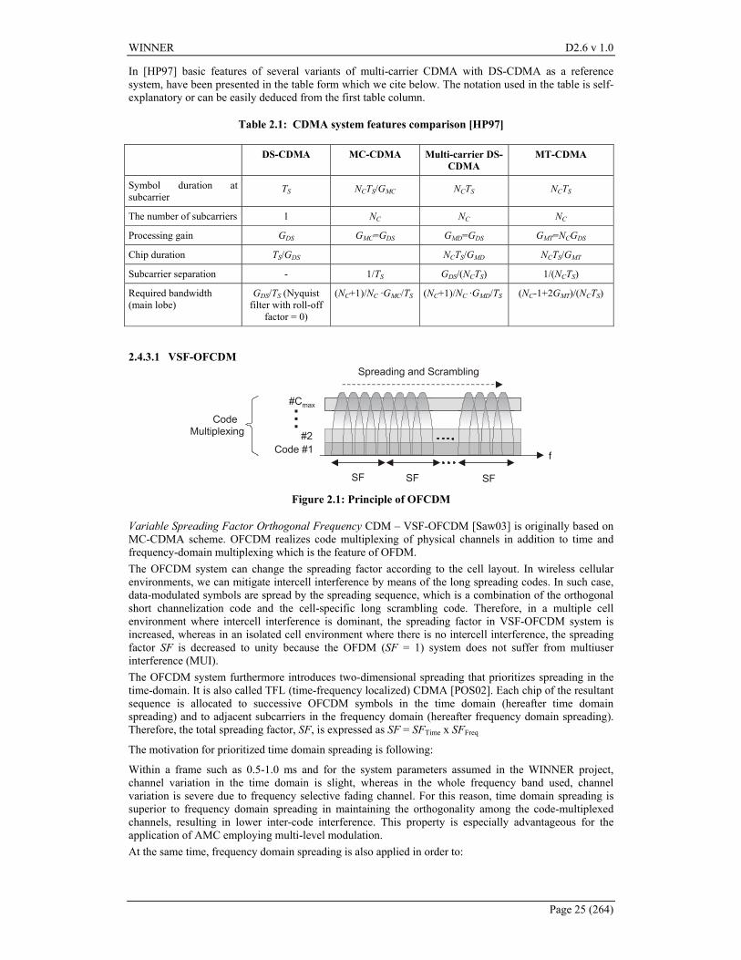
WINNER D2.6 v 1.0

Page 25 (264)

In [HP97] basic features of several variants of multi-carrier CDMA with DS-CDMA as a reference system, have been presented in the table form which we cite below. The notation used in the table is self-explanatory or can be easily deduced from the first table column.

Table 2.1: CDMA system features comparison [HP97]

DS-CDMA MC-CDMA Multi-carrier DS-CDMA

MT-CDMA

Symbol duration at subcarrier

TS NCTS/GMC NCTS NCTS

The number of subcarriers 1 NC NC NC

Processing gain GDS GMC=GDS GMD=GDS GMT=NCGDS

Chip duration TS/GDS NCTS/GMD NCTS/GMT

Subcarrier separation - 1/TS GDS/(NCTS) 1/(NCTS)

Required bandwidth (main lobe)

GDS/TS (Nyquist filter with roll-off

factor = 0)

(NC+1)/NC ·GMC/TS (NC+1)/NC ·GMD/TS (NC-1+2GMT)/(NCTS)

2.4.3.1 VSF-OFCDM

Figure 2.1: Principle of OFCDM

Variable Spreading Factor Orthogonal Frequency CDM – VSF-OFCDM [Saw03] is originally based on MC-CDMA scheme. OFCDM realizes code multiplexing of physical channels in addition to time and frequency-domain multiplexing which is the feature of OFDM. The OFCDM system can change the spreading factor according to the cell layout. In wireless cellular environments, we can mitigate intercell interference by means of the long spreading codes. In such case, data-modulated symbols are spread by the spreading sequence, which is a combination of the orthogonal short channelization code and the cell-specific long scrambling code. Therefore, in a multiple cell environment where intercell interference is dominant, the spreading factor in VSF-OFCDM system is increased, whereas in an isolated cell environment where there is no intercell interference, the spreading factor SF is decreased to unity because the OFDM (SF = 1) system does not suffer from multiuser interference (MUI). The OFCDM system furthermore introduces two-dimensional spreading that prioritizes spreading in the time-domain. It is also called TFL (time-frequency localized) CDMA [POS02]. Each chip of the resultant sequence is allocated to successive OFCDM symbols in the time domain (hereafter time domain spreading) and to adjacent subcarriers in the frequency domain (hereafter frequency domain spreading). Therefore, the total spreading factor, SF, is expressed as SF = SFTime x SFFreq

The motivation for prioritized time domain spreading is following:

Within a frame such as 0.5-1.0 ms and for the system parameters assumed in the WINNER project, channel variation in the time domain is slight, whereas in the whole frequency band used, channel variation is severe due to frequency selective fading channel. For this reason, time domain spreading is superior to frequency domain spreading in maintaining the orthogonality among the code-multiplexed channels, resulting in lower inter-code interference. This property is especially advantageous for the application of AMC employing multi-level modulation. At the same time, frequency domain spreading is also applied in order to:

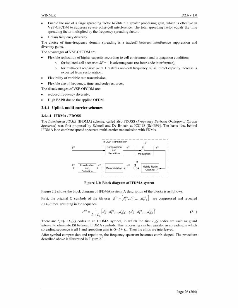
WINNER D2.6 v 1.0

Page 26 (264)

• Enable the use of a large spreading factor to obtain a greater processing gain, which is effective in VSF-OFCDM to suppress severe other-cell interference. The total spreading factor equals the time spreading factor multiplied by the frequency spreading factor,

• Obtain frequency diversity. The choice of time-frequency domain spreading is a tradeoff between interference suppression and diversity gains. The advantages of VSF-OFCDM are: • Flexible realization of higher capacity according to cell environment and propagation conditions

o for isolated-cell scenario: SF = 1 is advantageous (no inter-code interference), o for multi-cell scenario: SF > 1 realizes one-cell frequency reuse; direct capacity increase is

expected from sectorisation, • Flexibility of variable rate transmission, • Flexible use of frequency, time, and code resources, The disadvantages of VSF-OFCDM are: • reduced frequency diversity, • High PAPR due to the applied OFDM.

2.4.4 Uplink multi-carrier schemes

2.4.4.1 IFDMA / FDOSS The Interleaved FDMA (IFDMA) scheme, called also FDOSS (Frequency Division Orthogonal Spread Spectrum) was first proposed by Schnell and De Broeck at ICC’98 [SchB99]. The basic idea behind IFDMA is to combine spread spectrum multi-carrier transmission with FDMA.

Compressionand

Repetition

Demodulation Mobile RadioChannel

Equalizationand

Detection

Modulation

IFDMA Transmission ( )is( )id ( )ic ( )ix

( )ih

( )iy( )ir( )id̂n

Figure 2.2: Block diagram of IFDMA system

Figure 2.2 shows the block diagram of IFDMA system. A description of the blocks is as follows.

First, the original Q symbols of the ith user [ ]TiQ

iii ddd )(1

)(1

)(0

)( ,,, −= Kd are compressed and repeated L+L∆-times, resulting in the sequence:

[ ]TiQ

iiiQ

iii ddddddLL

c )(1

)(1

)(0

)(1

)(1

)(0

)( ,...,,;...;,...,,1−−

∆+= (2.1)

There are Lc=(L+L∆)Q codes in an IFDMA symbol, in which the first L∆Q codes are used as guard interval to eliminate ISI between IFDMA symbols. This processing can be regarded as spreading in which spreading sequence is all 1 and spreading gain is G=L+ L∆. Then the chips are interleaved. After symbol compression and repetition, the frequency spectrum becomes comb-shaped. The procedure described above is illustrated in Figure 2.3.

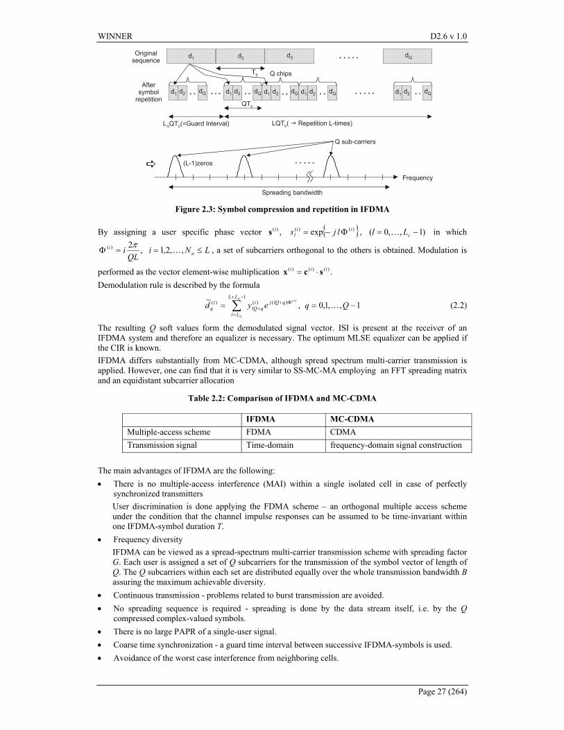
WINNER D2.6 v 1.0

Page 27 (264)

Figure 2.3: Symbol compression and repetition in IFDMA

By assigning a user specific phase vector ,)(is { })()( exp iil ljs Φ−= , )1,,0( −= cLl K in which

,2)(

QLii π

=Φ LNi u ≤= ,,2,1 K , a set of subcarriers orthogonal to the others is obtained. Modulation is

performed as the vector element-wise multiplication .)()()( iii scx ⋅= Demodulation rule is described by the formula

1,,1,0,~ 1

)()()( )(

−== ∑−+

=

Φ++

∆

∆

QqeydLL

Ll

qlQjiqlQ

iq

i

K (2.2)

The resulting Q soft values form the demodulated signal vector. ISI is present at the receiver of an IFDMA system and therefore an equalizer is necessary. The optimum MLSE equalizer can be applied if the CIR is known. IFDMA differs substantially from MC-CDMA, although spread spectrum multi-carrier transmission is applied. However, one can find that it is very similar to SS-MC-MA employing an FFT spreading matrix and an equidistant subcarrier allocation

Table 2.2: Comparison of IFDMA and MC-CDMA

IFDMA MC-CDMA Multiple-access scheme FDMA CDMA Transmission signal Time-domain frequency-domain signal construction

The main advantages of IFDMA are the following: • There is no multiple-access interference (MAI) within a single isolated cell in case of perfectly

synchronized transmitters User discrimination is done applying the FDMA scheme – an orthogonal multiple access scheme under the condition that the channel impulse responses can be assumed to be time-invariant within one IFDMA-symbol duration T.

• Frequency diversity IFDMA can be viewed as a spread-spectrum multi-carrier transmission scheme with spreading factor G. Each user is assigned a set of Q subcarriers for the transmission of the symbol vector of length of Q. The Q subcarriers within each set are distributed equally over the whole transmission bandwidth B assuring the maximum achievable diversity.

• Continuous transmission - problems related to burst transmission are avoided. • No spreading sequence is required - spreading is done by the data stream itself, i.e. by the Q

compressed complex-valued symbols. • There is no large PAPR of a single-user signal. • Coarse time synchronization - a guard time interval between successive IFDMA-symbols is used. • Avoidance of the worst case interference from neighboring cells.

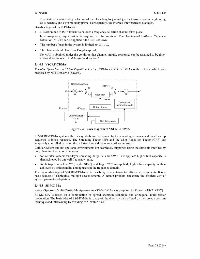
WINNER D2.6 v 1.0

Page 28 (264)

This feature is achieved by selection of the block lengths Qu and Qv for transmission in neighboring cells, where u and v are mutually prime. Consequently, the intercell interference is averaged.

Disadvantages of the IFDMA are: • Distortion due to ISI if transmission over a frequency-selective channel takes place.

In consequence, equalization is required at the receiver. The Maximum-Likelihood Sequence Estimator (MLSE) can be applied if the CIR is known.

• The number of user in the system is limited to ,LN u ≤

• The channel should have low Doppler spread, No MAI is obtained under the condition that channel impulse responses can be assumed to be time-invariant within one IFDMA-symbol duration T.

2.4.4.2 VSCRF-CDMA Variable Spreading and Chip Repetition Factors CDMA (VSCRF CDMA) is the scheme which was proposed by NTT DoCoMo [Saw03].

Figure 2.4: Block diagram of VSCRF-CDMA

In VSCRF-CDMA systems, the data symbols are first spread by the spreading sequence and then the chip sequence is block repeated. The Spreading Factor (SF) and the Chip Repetition Factor (CRF) are adaptively controlled based on the cell structure and the number of access users. Cellular system and hot-spot area environments are seamlessly supported using the same air interface by only changing the radio parameters: • for cellular systems two-layer spreading, large SF and CRF=1 are applied; higher link capacity is

then achieved by one-cell frequency reuse, • for hot-spot area low SF (maybe SF=1) and large CRF are applied; higher link capacity is then

achieved by orthogonality among users in the frequency domain. The main advantage of VSCRF-CDMA is its flexibility in adaptation to different environments. It is a basic feature of a ubiquitus multiple access scheme. A certain problem can create the efficient way of system parameter adaptation.

2.4.4.3 SS-MC-MA Spread-Spectrum Multi-Carrier Multiple-Access (SS-MC-MA) was proposed by Kaiser in 1997 [KF97]. SS-MC-MA is based on a combination of spread spectrum technique and orthogonal multi-carrier modulation. The basic idea of SS-MC-MA is to exploit the diversity gain offered by the spread spectrum technique and interleaving by avoiding MAI within a cell.

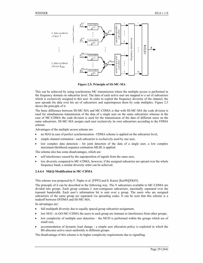
WINNER D2.6 v 1.0

Page 29 (264)

Figure 2.5: Principle of SS-MC-MA

This can be achieved by using synchronous MC transmission where the multiple access is performed in the frequency domain on subcarrier level. The data of each active user are mapped to a set of subcarriers which is exclusively assigned to this user. In order to exploit the frequency diversity of the channel, the user spreads his data over his set of subcarriers and superimposes them by code multiplex. Figure 2.5 shows the principle of it. The basic difference between SS-MC-MA and MC-CDMA is that with SS-MC-MA the code division is used for simultaneous transmission of the data of a single user on the same subcarriers whereas in the case of MC-CDMA the code division is used for the transmission of the data of different users on the same subcarriers. SS-MC-MA assigns each user exclusively its own subcarriers according to the FDMA scheme. Advantages of the multiple access scheme are: • no MAI in case of perfect synchronization - FDMA scheme is applied on the subcarrier level, • simple channel estimation - each subcarrier is exclusively used by one user, • low complex data detection - for joint detection of the data of a single user, a low complex

maximum-likelihood sequence estimation MLSE is applied. The scheme also has some disadvantages, which are: • self interference caused by the superposition of signals from the same user, • low diversity compared to MC-CDMA, however, if the assigned subcarries are spread over the whole

frequency band, a similar diversity order can be achieved.

2.4.4.4 M&Q-Modification in MC-CDMA

This scheme was proposed by F. Papke et al. [FP93] and S. Kaiser [Kai98][FK03]. The principle of it can be described in the following way. The N subcarriers available to MC-CDMA are divided into groups. Each group contains L non-contiguous subcarriers, maximally separated over the transmit bandwidth. Each user’s information bit is sent over a group. The users who are assigned subcarriers of the same group are separated via spreading codes. It can be seen that this scheme is a tradeoff between OFDMA and SS-MC-MA. Its advantages are: • full multipath diversity due to equally spaced group subcarrier assignment, • low MAI - in GO-MC-CDMA the users in each group are immune to interference from other groups, • low complexity of multiple user detection – the MUD is performed within the groups which are of

small size, • accommodation of dynamic load change - a simple user allocation policy is exploited in which the

BS allocates active users uniformly to different groups. The disadvantage of this scheme is its higher complexity requirements due to signalling.

WINNER D2.6 v 1.0

Page 30 (264)

2.5 OFDMA

2.5.1 Basic overview OFDMA (Orthogonal Frequency Division Multiple Access) is, similarly to MC-CDMA, also derived from OFDM. The idea of OFDMA was probably first shown in [SLK96] and [SLK97]. The authors of those papers reported application of OFDMA as the multiple access method in the return CATV channel. Each individual user of the CATV network is assigned a single subcarrier, which is orthogonal to the other subcarrriers assigned to other users. The necessary carrier and timing synchronization is attainable thanks to a PLL, transmission of pilot symbols towards the users and application of a cyclic prefix.

In OFDMA, an individual subcarrier or groups of subcarriers is assigned to different users. There are several methods for allocating subcarriers to users. The most widely used two are: grouped subcarriers and interleaved spread subcarriers. The method of using grouped subcarriers is the simplest, in which each user is assigned a group of contiguous subcarriers. In the comb spread subcarriers method, subcarriers are allocated in a fixed comb pattern, which causes spreading them over the entire system bandwidth. Obviously, grouped subcarriers method minimizes inter-user interference, but is susceptible to fading, as some user’s whole group of subcarriers may suffer from a null in the spectrum. The use of comb spread subcarriers can partly overcome fading by frequency diversity, but is more susceptible to inter-user interference in case of imperfectly synchronized users. In addition to OFDMA, hybrid TDMA/OFDMA can also be used to allocate time-frequency resources to users in the system. The advantages of OFDMA or hybrid TDMA/ OFDMA are: • robustness to frequency selective fading, • no inter-code interference (as compared to CDMA-based schemes), • easy data rate adjustment (as compared to TDMA), • possibility of adaptive scheduling, • increased spectral efficiency (no guard band needed as compared to FDMA) In turn, the disadvantages are: • Severe OFDMA performance degradation when the underlying channel undergoes deep fading; FEC

(possibly in conjunction with frequency hopping) is imperative for OFDMA, • difficulty in subcarrier synchronization, • need for coordinated subcarrier assignments, • performance degradation in multi-cell environment due to co-channel interference from other cells, • all disadvantages typical for OFDM such as sensitivity to frequency offset, high PAPR, etc. Since the first publications OFDMA has become the area of intensive research. In [NBDZ98] the authors considered the uplink performance of an OFDMA system for mobile communications. They described the random OFDMA system based on multi-carrier FDMA, in which each user has a set of randomly selected subchannels. The subchannels assigned to the individual user are the analogy to the user individual number. The subchannels are utilized by the user in any cell in which he may be located. The disadvantage of the proposed system is the problem of corrupted subchannels due to collisions with subchannels used by other users, which results in the loss of capacity, however, this loss is at least partially compensated by the fact that no signaling protocols for the assignment of subchannels to the users are needed. The handover is also simplified. The effect of Doppler spread in OFDM and OFDMA mobile radio systems was in turn analyzed in [RK99]. The simulation results presented in this paper showed the validity of Doppler frequency correction in the detection process.

Strictly connected with OFDMA scheme is the problem of optimization of the OFDM system for many users. Because of diverse channel patterns between the base station and user terminals, power allocation and bit loading become an important factor. In addition, different users may have different QoS requirements, which further complicates the problem of resource allocation. It has been shown that an OFDMA system with multiuser subcarrier, power and bit allocation can offer a substantially larger capacity over OFDM/TDMA [WChLM99]. Following this conclusion Yin and Liu presented in [YL00] the efficient multiuser loading algorithm for OFDM based wireless systems which maximizes the overall transmit data rate subject to the total power constraint and each user’s rate constraint. The key idea of their algorithm was first to estimate the resource required to satisfy the rate requirement of each user according to their average channel gain and then pick the good subcarriers so that the total rate is maximized. The authors claimed that their algorithm has significantly higher capacity and lower outage probability than the TDMA-OFDM scheme.

WINNER D2.6 v 1.0

Page 31 (264)

The paper [KLL03] is devoted to a similar topic, i.e. the problem of finding an optimal subcarrier and power allocation strategy for downlink communication to multiple users in OFDMA system. The criterion of the system optimization is minimization of total power consumption with constraints on the bit-error rate and transmission rate for users requiring different classes of service. The problem of joint subcarrier and power allocation is divided into two steps. In the first step, the number of subcarriers assigned to each user is determined based on the users’ average signal-to-noise ratio. In the second stage, the algorithm finds the best assignment of subcarriers to users. Similar subject related to subcarrier allocation is tackled in [PJ01]. The authors compared collision-based and orthogonal subcarrier allocation for congestion resolving in an uplink OFDMA system. They define a congestion as a situation when all the radio resources (OFDM subcarriers) are already distributed but still there are traffic demands to be satisfied. In [PJ01] the OFDMA system allows for assignment of the subcarriers already occupied temporarily to the new user. Thus, a congestion occurs. The other possibility is to increase the modulation order on specific subcarriers, thus freeing some system resources and allowing addition of more users at the expense of moderate QoS degradation. The authors show that orthogonal allocation gives slightly lower QoS penalty.

The resource allocation in OFDMA is also considered in the report [KJ04]. The authors show via a counter example that water-filling based subcarrier allocation policies, contrary to conventional knowledge, fail to provide rate-stability for an otherwise stabilizable OFDMA system. They focus on a long-term average performance rather than instantaneous optimization performed by water-filling principle. They propose a long-run objective to minimize the average holding cost of the system.

OFDMA has recently become one of the modes in IEEE 802.16 wireless access. In [KR02] the general idea of OFDMA application is shown. It has been proposed that 2048 or 4096 subcarriers are divided into subchannels. They are used in downstream for separating the data into logical streams. These streams employ different modulation, coding and amplitude to address the subscribers with different channel characteristics. In the uplink, the subchannels are used for multiple access. The subscribers are assigned on subchannels through Media Access Protocol (MAP) messages sent in the downlink. The subcarriers constituting a subchannel are spread along frequency axis to mitigate the frequency selective fading.

As already mentioned, OFDMA, similarly to OFDM modulation, is sensitive to phase jitter and suffers from high PAPR. Both problems are considered respectively in [SMS98] and [ZYCh00]. In [ZYCh00] the optimized pilot symbol technique is proposed to reduce PAPR in OFDMA systems. The proposed PAPR reduction scheme has been designed for OFDMA systems where the subcarriers assigned to each user are selected in clusters of consecutive subcarriers.

Finally, Persson et al. investigated in [POS04] the downlink performance of multiple access schemes based on OFDM such as MC-CDMA, MC-DS-CDMA and Time-Frequency-Localized CDMA operating in a system with frequency reuse equal to one. They showed that for high system loads, OFDMA, due to its lower complexity and ability to maintain orthogonality on frequency-selective fading channels, outperforms the other multiple access schemes.

Let us focus our attention on the problem of OFDMA optimization. Before we consider it let us overview the optimization problem of OFDM transmission, which can be treated as an introduction to OFDMA optimization.

2.5.2 Bit loading algorithms for single-user OFDM Under the condition that the cyclic prefix is longer than the channel impulse response, OFDM decomposes a broadband frequency-selective channel into parallel, independent, flat-fading narrowband channels. The channel model as depicted in Figure 2.6 is given as

Nnknkxhky nnnn ,,1],[][][ K=+⋅= (2.3)

The channel transfer coefficients hn are usually different and are often modeled by an i.i.d. Rayleigh distribution. The channel inputs symbols xn[k] are QAM symbols, with bn bits per symbol and power

].|][[| 2kxEp nn = The number of bits per OFDM symbol is thus

∑=

=N

nnbb

1 (2.4)

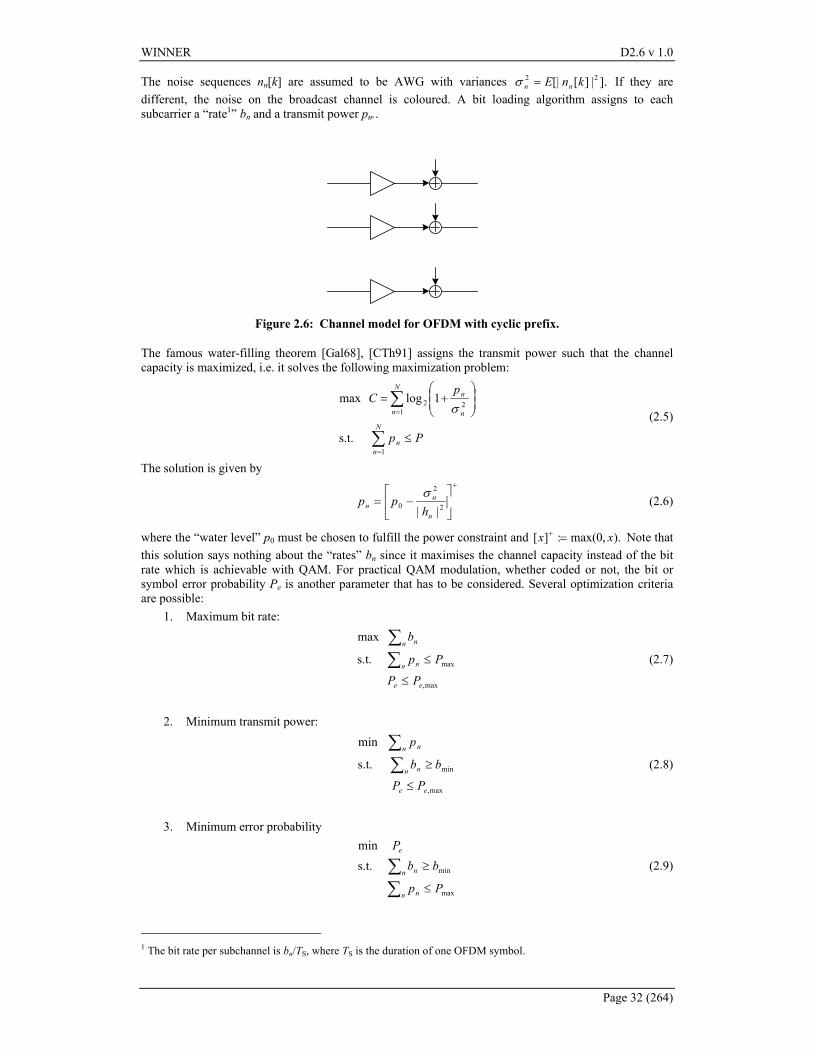
WINNER D2.6 v 1.0

Page 32 (264)

The noise sequences nn[k] are assumed to be AWG with variances ].|][[| 22 knE nn =σ If they are different, the noise on the broadcast channel is coloured. A bit loading algorithm assigns to each subcarrier a “rate1” bn and a transmit power pn..

Figure 2.6: Channel model for OFDM with cyclic prefix.

The famous water-filling theorem [Gal68], [CTh91] assigns the transmit power such that the channel capacity is maximized, i.e. it solves the following maximization problem:

∑

∑

=

=

≤

+=

N

nn

N

n n

n

Pp

pC

1

122

s.t.

1logmaxσ (2.5)

The solution is given by

+

−= 2

2

0 || n

nn h

ppσ

(2.6)

where the “water level” p0 must be chosen to fulfill the power constraint and ).,0max(:][ xx =+ Note that this solution says nothing about the “rates” bn since it maximises the channel capacity instead of the bit rate which is achievable with QAM. For practical QAM modulation, whether coded or not, the bit or symbol error probability Pe is another parameter that has to be considered. Several optimization criteria are possible:

1. Maximum bit rate:

max,

maxs.t.

max

ee

n n

n n

PP

Pp

b

≤

≤∑∑

(2.7)

2. Minimum transmit power:

max,

mins.t.

min

ee

n n

n n

PP

bb

p

≤

≥∑∑

(2.8)

3. Minimum error probability

∑∑

≤

≥

n n

n n

e

Pp

bbP

max

mins.t.min

(2.9)

1 The bit rate per subchannel is bn/TS, where TS is the duration of one OFDM symbol.

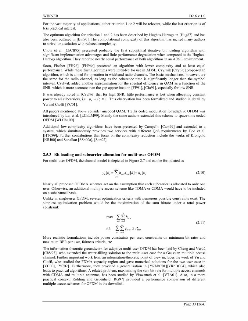
WINNER D2.6 v 1.0

Page 33 (264)

For the vast majority of applications, either criterion 1 or 2 will be relevant, while the last criterion is of less practical interest.

The optimum algorithm for criterion 1 and 2 has been described by Hughes-Hartogs in [Hug87] and has also been outlined in [Bin90]. The computational complexity of this algorithm has incited many authors to strive for a solution with reduced complexity.

Chow et al. [ChCB95] presented probably the first suboptimal iterative bit loading algorithm with significant implementation advantages and little performance degradation when compared to the Hughes-Hartogs algorithm. They reported nearly equal performance of both algorithms in an ADSL environment.

Soon, Fischer [FH96], [FH96a] presented an algorithm with lower complexity and at least equal performance. While these first algorithms were intended for use in ADSL, Czylwik [Czyl96] proposed an algorithm, which is aimed for operation in wideband radio channels. The basic mechanisms, however, are the same for the radio channel, as long as the coherence time is significantly longer than the symbol interval. Czylwik added another approximation for the spectral efficiency in QAM as a function of the SNR, which is more accurate than the gap approximation [FE91], [Cio91], especially for low SNR.

It was already noted in [Czyl96] that for high SNR, little performance is lost when allocating constant power to all subcarriers, i.e. .0 nPpn ∀= This observation has been formalized and studied in detail by Yu and Cioffi [YC01].

All papers mentioned above consider uncoded QAM. Trellis coded modulation for adaptive OFDM was introduced by Lai et al. [LChLM99]. Mainly the same authors extended this scheme to space-time coded OFDM [WLCh+00].

Additional low-complexity algorithms have been presented by Campello [Cam99] and extended to a system, which simultaneously provides two services with different QoS requirements by Hoo et al. [HTC99]. Further contributions that focus on the complexity reduction include the works of Krongold [KRJ00] and Sonalkar [SSh00a], [Son02].

2.5.3 Bit loading and subcarrier allocation for multi-user OFDM For multi-user OFDM, the channel model is depicted in Figure 2.7 and can be formulated as

∑=

+=U

unnunun knkxhky

1,, ][][][ (2.10)

Nearly all proposed OFDMA schemes act on the assumption that each subcarrier is allocated to only one user. Otherwise, an additional multiple access scheme like TDMA or CDMA would have to be included on a subchannel basis. Unlike in single-user OFDM, several optimization criteria with numerous possible constraints exist. The simplest optimization problem would be the maximization of the sum bitrate under a total power constraint:

∑∑

∑∑

= =

= =

≤U

u

N

nnu

U

u

N

nnu

Pp

b

1 1max,

1 1,

s.t.

max (2.11)

More realistic formulations include power constraints per user, constraints on minimum bit rates and maximum BER per user, fairness criteria, etc.

The information-theoretic groundwork for adaptive multi-user OFDM has been laid by Cheng and Verdú [ChV93], who extended the water-filling solution to the multi-user case for a Gaussian multiple access channel. Further important work from an information-theoretic point of view includes the work of Yu and Cioffi, who studied the FDMA capacity region and gave numerical solutions for the two-user case in [YC00], [YC02]. Furthermore, they provided a generalization in [YRhBC01][YRhBC04], which also leads to practical algorithms. A related problem, maximizing the sum bit rate for multiple access channels with CDMA and multiple antennas, has been studied by Viswanath et al. [VTA01]. Also, in a more practical context, Rohling and Gruenheid [RG97] provided a performance comparison of different multiple access schemes for OFDM in the downlink.

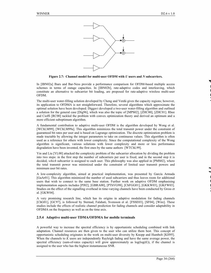
WINNER D2.6 v 1.0

Page 34 (264)

Figure 2.7: Channel model for multi-user OFDM with U users and N subcarriers.

In [IBN02a] Ibars and Bar-Ness provide a performance comparison for OFDM-based multiple access schemes in terms of outage capacities. In [IBN02b], rate-adaptive codes and interleaving, which constitute an alternative to subcarrier bit loading, are proposed for rate-adaptive wireless multi-user OFDM.

The multi-user water-filling solution developed by Cheng and Verdú gives the capacity regions; however, its application to OFDMA is not straightforward. Therefore, several algorithms which approximate the optimal solution have been developed. Diggavi developed a two-user water-filling algorithm and outlined a solution for the general case [Dig96], which was also the topic of [MPS02], [ZHC00], [ZHC01]. Rhee and Cioffi [RC00] tackled the problem with convex optimization theory and derived an optimum and a more efficient suboptimum algorithm.

A fundamental contribution to adaptive multi-user OFDM is the algorithm developed by Wong et al. [WChLM99], [WChLM99a]. This algorithm minimizes the total transmit power under the constraint of guaranteed bit rates per user and is based on Lagrange optimization. The discrete optimization problem is made tractable by allowing the integer parameters to take on continuous values. This algorithm is often used as a reference for others with lower complexity. Since the computational complexity of the Wong algorithm is significant, various solutions with lower complexity and more or less performance degradation have been invented, the first ones by the same authors [WTChL99].

Yin and Liu [YL00] attacked the complexity problem of the subcarrier allocation by dividing the problem into two steps: in the first step the number of subcarriers per user is fixed, and in the second step it is decided, which subcarrier is assigned to each user. This philosophy was also applied in [PMS02], where the total transmit power was minimized under the constraint of limited user transmit powers and minimum user bit rates.

A low-complexity algorithm, aimed at practical implementation, was presented by García Armada [GaAr01]. This algorithm minimized the number of used subcarriers and thus leaves room for additional users that wish to connect to the same base station. Further work on adaptive OFDM emphasising implementation aspects includes [PJ02], [GBRA00], [PThVG98], [ChFGG01], [GKKW03], [GKFW03]. Studies on the effect of the signalling overhead in time-varying channels have been conducted by Gross et al. [GKW04].

A very promising research line, which has its origins in adaptive modulation for fading channels [ChG01], [GC97], is followed by Sternad, Falahati, Svensson et al. [FSSE03], [SF04], [Wire]. These studies include the effects of realistic channel prediction for fading channels and consider adaptability in OFDMA on the frequency as well as on the time axis.

2.5.4 Adaptive multi-user TDMA/OFDMA for mobile terminals A powerful way to increase the spectral efficiency is by opportunistic scheduling combined with link adaptation. Channel resources are then given to the user who can utilize them best. This concept of opportunistic scheduling originates in the work on multi-user diversity by Knopp and Humbelt [KH95]. When the channels to K users are independently Rayleigh fading and have the same average power, the spectral efficiency (sum-of-rates capacity) will grow approximately as log(log(K)), if the channel is assigned to the user who has the highest instantaneous SNR.

WINNER D2.6 v 1.0

Page 35 (264)

Efficient use of opportunistic scheduling requires a new approach to radio system design, since channel variability is utilized, rather than counteracted by e.g. interleaving. Traditional approaches for improving radio links by reducing their variability by diversity combining would in fact decrease the possibility to improve spectral efficiency by opportunistic scheduling.

There are mainly two potential practical difficulties that may reduce the gains promised by opportunistic scheduling combined with link adaptation:

• Some channel state information is required at the transmitter. Due to time delays in the transmission feedback control loop, this information could be outdated and unreliable. Since the link adaptation will be based on outdated channel state information, the performance of channel predictors is an important determining factor of these adaptation schemes.

• The feedback overhead grows with the number of active users and with the speed of the time-variability that is to be utilized. A too high feedback data rate could negate the potential gains attained by the adaptive scheme.

Opportunistic scheduling can be applied to timeslots in TDMA systems. However, when the transmission bandwidth is increased above the coherence bandwidth, the channel variability between timeslots will be reduced, due to independent fading within different parts of the total bandwidth. The opportunity for scheduling gains is then reduced. In wideband fading channels, it is attractive to allocate time-frequency resources (here denoted bins), each of which has an approximately flat channel. Adaptation over frequency as well as time may furthermore potentially reduce the time delays encountered by the data streams to slow-moving users.

For example, in an adaptive multi-user OFDM/TDMA downlink, predictions of the channel quality in each time-frequency bin would be generated for the time instance when these slots can be utilized for transmission. Based on these predictions and the requirements of different data streams, a scheduling algorithm would allocate the time-frequency bins to the different users. Adaptive modulation and possibly also power control by multiuser water-filling is used to adapt the transmission to the link quality within each bin.

The most challenging environment in which to evaluate such schemes would be one with

• wide-area coverage, giving rise to large delay spreads and small correlation bandwidth. This would limit the useful frequency extent of time-frequency resources allocated to different users. The number of bins utilized within a given bandwidth thus becomes large, which increases the required feedback data rate.

• high speed user mobility, which increases the difficulty of predicting the channel sufficiently far ahead, and increases the required feedback data rate.

• large bandwidth; if the whole bandwidth is to be potentially allocated to all users, the required feedback data rate would increase in proportion to the total bandwidth.

Adaptive systems that are shown to work acceptably under the above conditions would work better in less challenging conditions of shorter-range communication, lower expected terminal velocities and smaller bandwidths.

In [WOS+03] and [SOAS03], the downlink of an adaptive OFDM FDD system is adjusted for use in present 3G bands of 5 MHz at 2 GHz. With 512 subcarriers, a subcarrier spacing of 10 kHz and a guard time/cyclic prefix of 11 microseconds, it is designed for macrocellular environments. The design vehicle speed is 100 km/h, and the assumed total feedback delay requires channel prediction of 2 ms ahead in time. At 2 GHz and 100 km/h, this corresponds to a required prediction range of 0.3 wavelengths. In [ESA02], [Ekm02], [SA03], it is shown that prediction of the short-term fading of the power is feasible over the required horizon and in [FSES04], [GKFW03] it is shown that the corresponding prediction errors will result in only a minor reduction of the throughput when using uncoded adaptive M-QAM. The performance of Trellis-Coded Modulation (TCM) is reduced by these levels of prediction inaccuracy, but TCM will still outperform uncoded M-QAM by 1-2 dB, according to [FSSM03]. The effect of prediction inaccuracy on other coded adaptive modulation schemes has not yet been investigated.

Due to the time-frequency selectivity, the channel will vary within the allocated time-frequency bins. In [WOS+03], it is shown that for a bin size of 20 subcarriers times 6 symbols (200 kHz by 0.666 milliseconds) this results in a minor performance degradation in suburban environments with vehicle speeds of 70-120 km/h at 2 GHz. Adaptive uncoded M-QAM modulation, with 1-8 bits per symbol, is used in the described case study [WOS+03], [SOAS03]. Each user predicts the channel and reports the suggested modulation format for each bin, using 3 bits to indicate on of the 8 modulation rates. In

WINNER D2.6 v 1.0

Page 36 (264)

[WOS+03], the resulting feedback data rate is shown to be acceptable, and a large potential exists for reducing it further by e.g. utilizing the fact that most users will move slowly. Recent results by Johansson [Joh04] show that a one- or two-bit feedback per bin seems adequate; The terminals do not have to report back all the results, only the most competitive ones.

The resulting spectral efficiency will depend crucially on the choice of scheduling strategy, on the deployment scenario and on the possibility of reducing inter-cell interference. In [SOAS03], best effort traffic to K active users within a cellular sector is investigated. The time-frequency resources are allocated to the user who has the best channel, relative to its own average. This scheduling strategy is related to the proportionally fair scheduler proposed by Tse et. al. in [VTL02]. Effects of differences in QoS requirements and required data rates are not investigated. A simple frequency reuse strategy is used in [SOAS03], in which reuse 1 is used in inner parts of sectors and reuse 3 is used in the outer parts. With a fully loaded system with 60-degre sectors in hexagonal pattern, an average reuse factor of ca. 1.7 provides optimal performance. With lower loads, a reuse factor closer to 1 can be used. The spectral efficiency, including overhead, varies between 1.2 bit/s/Hz/sector for one active user per sector to 2 bits/s/Hz/sector for 30 active users per sector in fully loaded systems, if each terminal has a single antenna. Rayleigh fading and path loss were taken into account in these simulations, while the effect of shadow fading was not investigated.

2.6 SDMA Space Division Multiple Access (SDMA) is a powerful multiple access scheme which can support any of the previously described multiple access schemes. It adds an additional dimension to a multiple access scheme in form of the terminal angular separation. It is achieved by directing the beam towards the selected terminal. Depending on the advancement of the applied technique, beamforming can be applied in the uplink and in both uplink and downlink. The efficiency of SDMA strongly depends on the angular distribution of terminals located in the cell or the range of an access point.

2.6.1 SDMA based on beamforming

The key bottleneck for the application of SDMA is spatial separability.

Spatial separability means that for successful transmission of two users sharing the same resource certain beamforming vectors exist for which a certain SIR threshold will not be underrun. For a given channel, spatial separability depends on the number of users and on their spatial channel properties. In addition, beamforming vectors and transmission powers affect interference levels and SIRs at all receivers and thus affect spatial separability. This brings up the need for interference balancing. A joint optimization of antenna weights and decision on spatial separability is a complex nonlinear problem. In [FN98] the second order statistics of the channel are used to minimize transmit power with the proposed "Power Minimizer" algorithm or its linearized or simplified versions.

In a downlink multi-user environment, the achievable signal-to-interference-ratios (SIR) of all users are limited by the amount of mutual cross-talk. In [BSch03] the beamforming weights also are to be determined in a joint optimization under the given channel condition to aim at balancing the relative SIR levels.

A joint treatment of MAC and physical layer for SDMA promises to optimize throughput with the help of adaptive modulation and resource allocation. In [KRT03] a combination of SDMA together with three different multiple access schemes (TDMA, CDMA and OFDMA) is investigated. The proposed heuristic algorithms are based on greedy assignment strategies.

In [SM03] a combination of SDMA and MC-CDMA is studied. Single-user criteria based on maximum ratio transmission are compared to a multiuser-criterion based on maximization of SIR. Even with the loss of orthogonality caused by beamforming, the system load can be considerably increased by the combination of SDMA and CDMA.

All the above mentioned algorithms have a non-negligible computational cost. A cheap and simple alternative, which is suitable for macro-cellular environments with small angular spreads, is the usage of a grid of fixed beams with reuse of resources of non-neighbored beams. In UMTS-WCDMA, the performance of fixed beams [BNB02] is even superior to the performance of dedicated beams due to better channel estimation, which is caused by using so-called secondary common pilot channels. Thus, fixed beams are a simple option for SDMA.

WINNER D2.6 v 1.0

Page 37 (264)

2.6.2 Multi-user scheduling/SDMA

The work on SDMA techniques typically contemplates the use of multiple antennas at the transmitter side, typically the Base Station (BS) or Access Point (AP), since the current status of technology suggests single-antenna terminals. Whereas in TDMA or FDMA the frame duration is limited in length or by the number of frequencies, in SDMA the low number of antennas limits severely the performance of the system [BPN04]. There, the authors select Zero Forcing (ZF) as the beamforming criterion [HAP01], which yields a closed-form solution with low complexity. Moreover, it is equivalent to the Minimum Mean Square Error (MMSE) solution at high Signal to Noise Ratio (SNR). Furthermore, it provides a valid framework to study cross-layer issues such as the scheduling or fairness [BPN04a], which are clearly of practical relevance. Optimal transmit beamforming is studied in e.g. [RFLT98] or [BO01], where the users require some Quality of Service (QoS) for their communications. However, their methods involve more computational load.

One should also take opportunistic communications into account, mentioned in Section 2.5.4. SDMA methods that use time-varying randomly generated beam patterns have even been suggested as means to amplify the naturally occurring variations of the transmission properties [VTL02]. In systems that utilize opportunistic scheduling, the trade-off between performance and complexity plays a crucial role, since the design of a scheduler combining information from both the physical layer and the DLC is not a straightforward task, e.g. we could prefer to use a simple power allocation for the sake of a more complicated space-time scheduler which yields additional improvement [BPN04]. Other alternatives are considered e.g. in [KT02] or [BW01], where SDMA techniques are applied and the fairness of the schedulers is evaluated. It is well known that techniques maximizing the total througput for an access point tend to generate an uneven distribution of the resources, whereas strategies that maximize the minimum offered capacity for each user tend to waste some limited resource with the poorer users, at the expense of the collective revenue [BPN03]. Therefore, the choices at the AP are not straightforward and shall be carefully considered, especially when fairness issues are to be taken into account.

Furthermore, the assumption that the number of users is not higher than the number of antennas is unrealistic. In this sense, if there are many users in the cell, some kind of user grouping shall be performed in the system, e.g. [BPN03] or [BPPN03]. Several alternatives are possible, where usually more complexity yields a better performance. In that case, quasi optimum techniques based on Simulated Annealing are possible when also the terminals have multiple antennas [PIPN03], but they might not be of practical relevance in the realistic implementation of future multiuser systems. Practical algorithms are generally suboptimum, see also [ShTKL01], [KTShK01] and [YL02].

Extensions to the case where both transmitter and receiver have multiple antennas have been proposed in [SSH04]. The authors present two constrained solutions, namely a block diagonalization and successive optimization, which yield closed-form expressions to maximize the sum capacity and provide a reasonable trade-off between performance and complexity [SSH04]. Besides, they provide extensions if these two methods cannot be supported. In [ChM04], the multiuser Multiple Input Multiple Output (MIMO) channel is decomposed into several parallel independent conventional single-user MIMO channels, in which if a transmit antenna is added, the number of spatial channels for each user is increased also by one. Finally, iterative algorithms are considered for uplink MIMO systems in [SY04] to find the optimum transmit and receive linear filters according to the mean squared error criterion, assuming an error-free low-delay feedback channel.

2.7 Quantitative comparisons of multiple access schemes: Information theoretic aspects Before we start comparing different multiple access schemes, we have to clarify the meaning of the term capacity. Generally, this term has different meanings depending on the point of view of our comparisons. At least two meanings of the term capacity occur with respect to multiple access schemes. The first one arises from the information-theoretic approach and allows for evaluation of performance limits rather than estimation of a real performance. However, it is an important tool for multiple access schemes’ comparisons and allows for drawing valuable conclusions on multiple access strategies. The capacity is measured in bit/s/Hz and shows the maximum amount of information per spectrum unit, which can be sent by all active users. In cellular network design capacity is meant as a maximum number of users simultaneously served by the system located on the unit area, or alternatively the maximum value of traffic served by the system per unit area. One can also find the definition of multiple access capacity as the number of users that can be supported at a given error performance [Med00]. All these approaches to capacity evaluation are used in the literature and mobile communication practice.

WINNER D2.6 v 1.0

Page 38 (264)

Let us in this section concentrate on the information-theoretic approach. The basic considerations on capacity of multiple access schemes can be found in [Pro95]. In this academic handbook, the FDMA, TDMA and CDMA schemes are compared in terms of the information rate that each multiple access method achieves in an ideal AWGN channel of bandwidth W. It is shown that on the AWGN channel FDMA and TDMA schemes offer basically the same capacity, whereas for CDMA, the capacity depends on how much the system is cooperative i.e. if the user can apply knowledge about other users’ signatures to detect his own signal or if this is not possible (the problem of usability of joint detection).

The situation becomes more complicated when transmission takes place over a fading channel. Many papers have been devoted to capacity calculations for SISO and MIMO transmission. The capacity depends on if channel state information is available to the receiver and transmitter and if it is perfect or not. The papers [Med00], [TT00], [Tel99] show such capacity calculations for single-user transmission.

Several aspects of digital transmission over fading channels for single user and multiple users have been widely considered in the large tutorial and state-of-the art paper [BPSh98]. Among others, the sense and importance of ergodic capacity and outage capacity is explained. Assuming the long-term ergodic properties of the fading process h(t,τ), describing the time varying channel impulse response, the capacity is meant ergodic if the total transmission time T is much longer than the channel coherence time Tcoh. The ergodic capacity with the channel state known to the receiver is then given by the following formula

+= ∫

∞+

∞−

dfN

ftHPEC

0

2av

erg

);(1log (2.12)

where E[.] denotes expectation taken with respect to the statistics of the random process H(t;f) described by the formula

( )∫∞

∞−

−= ττπττ dfjthtH 2exp);();( (2.13)

Under the ergodic assumptions these statistics are independent of either t or f, and the capacity is described by the formula (ν is the instantaneous signal-to-noise-ratio)

∫∞

+=

+=0

2av

2av

erg 1log)(1log νσ

νν

σν

ν dP

pP

EC (2.14)

However, ergodic assumption is not necessarily satisfied in practical communication systems operating on fading channels. For example if stringent delay constraints are set, the ergodicity requirement that T>>Tcoh is not fulfilled. In this case, where channel variability during the whole transmission does not reflect statistical properties of the channel, the channel capacity has to be viewed as a random entity which depends on the instantaneous random channel parameters. The capacity-versus-outage performance is then determined by the probability that the channel cannot support a given rate [BPSh98]. In consequence, we define the outage capacity as the rate Cout for which the probability that the instantaneous capacity C(Pav,H) is smaller than Cout is equal to the outage probability p0. Thus Cout can be calculated frm the following equation

{ }outCHPCp <= ),(Pr av0 (2.15)

The terms of outage and instantaneous capacities can easily be extended on multiple access channels. The detailed study on fading channel capacities for multiple users with FDMA, TDMA and CDMA schemes can be found in [BPSh98]. Considerations on discrete time flat fading channel transmission show that it can occur that for the TDMA multiple access, the channel capacity can be higher than for CDMA multiple access scheme, if channel state information (CSI) is available to receivers only. If CSI is also available to the transmitters, the power control can be taken into account. As written in [BPSh98], contrary to the single-user case, in the multiple-users scenario the optimal power control results in a substantial growth in capacity for TDMA increasing with the number of users as compared with the fixed transmitted-power case with the optimal CDMA strategy. The same situation occurs for frequency selective channels for which a similar power control strategy can be applied to the channel subbands.

The information-theoretic considerations on multiple-access channel for a single-cell transmission in which the signals from transmitters located in other cells are treated as noise can be found in [ShW97], whereas in [ShW97a] the considerations are extended on the case in which receivers process the signals

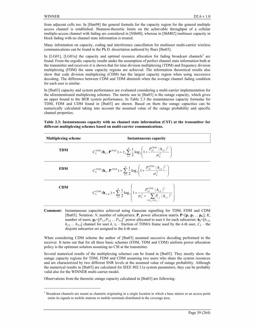
WINNER D2.6 v 1.0

Page 39 (264)

from adjacent cells too. In [Han98] the general formula for the capacity region for the general multiple access channel is established. Shannon-theoretic limits on the achievable throughput of a cellular multiple-access channel with fading are considered in [SSh00], whereas in [ShM02] multiuser capacity in block fading with no channel state information is treated.

Many information on capacity, coding and interference cancellation for multiuser multi-carrier wireless communications can be found in the Ph.D. dissertation authored by Ibars [Iba03].

In [LG01], [LG01a] the capacity and optimal resource allocation for fading broadcast channels2 are found. From the ergodic capacity results under the assumption of perfect channel state information both at the transmitter and receivers it is shown that for time division multiplexing (TDM) and frequency division multiplexing (FDM) the same capacity regions are achieved. The information theoretical results also show that code division multiplexing (CDM) has the largest capacity region when using successive decoding. The difference between CDM and TDM diminish when the average channel fading condition for each user is similar.

In [Iba03] capacity and system performance are evaluated considering a multi-carrier implementation for the aforementioned multiplexing schemes. The metric use in [Iba03] is the outage capacity, which gives an upper bound to the BER system performance. In Table 2.3 the instantaneous capacity formulae for TDM, FDM and CDM found in [Iba03] are shown. Based on them the outage capacities can be numerically calculated taking into account the assumed value of the outage probability and specific channel properties.

Table 2.3: Instantaneous capacity with no channel state information (CST) at the transmitter for different multiplexing schemes based on multi-carrier communications.

Multiplexing scheme Instantaneous capacity

TDM ∑=

+=

N

i k

kiTDMki

kTDM

kTDMk

hPC

12

2,,

2

||1log

21),(

στPh

FDM ∑=

+=

N

i k

kiFDMkiFDM

kFDMk

hPC

12

2,,

2

||1log

21),(

σPh

CDM ∑ ∑=

<

−

++=

N

ihhi

jijik

kiCDMki

KCDMk

jiki

hPhP

C1

||||:

2,,

2

2,,

21

,,

||||

1log21)(

σh

Comment: Instantaneous capacities achieved using Gaussian signalling for TDM, FDM and CDM [Iba03]. Notation: N, number of subcarriers; P, power allocation matrix P=[p1 p2 ... pK]; K, number of users; pk=[P1,k P2,k ... PN,k]T power allocated to user k for each subcarrier; hk=[h1,k, h2,k ... hN,k] channel for user k, τk – fraction of TDMA frame used by the k-th user, Ck – the disjoint subcarrier set assigned to the k-th user .

When considering CDM scheme the author of [Iba03] assumed succesive decoding performed in the receiver. It turns out that for all three basic schemes (FDM, TDM and CDM) uniform power allocation policy is the optimum solution assuming no CSI at the transmitter.

Several numerical results of the multiplexing schemes can be found in [Iba03]. They mostly show the outage capacity regions for TDM, FDM and CDM assuming two users who share the system resources and are characterized by two different SNR levels at the assumed value of outage probability. Although the numerical results in [Iba03] are calculated for IEEE 802.11a system parameters, they can be probably valid also for the WINNER multi-carrier model.

Observations from the theoretic outage capacity calculated in [Iba03] are following:

2 Broadcast channels are meant as channels originating in a single location in which a base station or an access point

emits its signals to mobile stations or mobile terminals distributed in the coverage area.

WINNER D2.6 v 1.0

Page 40 (264)

• From the theoretic outage capacity point of view CDM outperforms TDM and FDM. However when CDM is implemented with MC-CDMA and low complexity linear receiver, its capacity decreases bellow that of FDM and TDM. Real performance very much depends on the practical system implementation. Capacity of CDM is receiver dependent.

• When users experience a similar level of SNR the gain of CDM with respect to TDM and FDM diminishes.

These initial theoretical comparisions provide some interesting guidelines for what results to expect in simple evaluation cases, under the exact conditions and assumptions involved. Unfortunately, the WINNER scenarios involve numerous assumptions and constraints that are hard to formulate in an information-theoretic framework. It then becomes more appropriate to consider the multiple access design problem as a problem of resource allocation under various types of constraints. To obtain realistic estimates of their performance, one has to turn to simulation studies. The next chapter outlines the sets of assumptions that have been evolved for these studies.

WINNER D2.6 v 1.0

Page 41 (264)

3. Methodology

3.1 Introduction The study of multiple access technologies is, essentially, to characterize and assess different methods of sharing a common resource - the channel. Such sharing of resources among users within a system should preferably be both efficient and fair. In radio communication systems, which is the focus here, the channel is a broadcast channel meaning that a message transmitted from one node to another can typically be noticed by at least a few other nodes in the system. That is, transmission between a pair of nodes can potentially interfere with a simultaneously ongoing transmission between another pair of nodes and vice versa. In some cases, the receivers may handle such interference while it in other cases may cause one or both of the transmissions to fail. In other words, one important objective of the multiple access scheme in a radio communication system is to provide means to control the interference. The basic multiple access schemes- TDMA, FDMA, and CDMA (reviewed in Chapter 2) – are well-known ways to separate transmission and hence to control the interference. Moreover, since a radio channel may be frequency selective and also undergoes temporal variations, there are ways of increasing the efficiency in a radio communication system by assigning resources to users in a way that the transmission takes place when the conditions are favorable. To facilitate such channel dependent allocation of resources (channel dependent scheduling) may also be an important objective of the multiple access scheme. The study of multiple access technologies in radio communication systems can typically not be performed without considerations of the radio link. The multiple access scheme and the radio link are indeed tightly interconnected and should, if possible, be jointly considered. For example, different types of links may be able to handle different amounts of time dispersion and interference. Likewise, the capability of adapting the transmission according to the current channel and interference conditions may vary in between links of different type. Hence, when analyzing different multiple access techniques it is essential to consider the capabilities of the radio link. Moreover, in the assessment of multiple access schemes it is also important to take the environment and user behavior into account, since eventually, the objective in the design of a communication system is to serve users according to their respective demands. The environment describes e.g. the physical environment in which users are located and influences, directly or indirectly, the radio conditions. In the user behavior we include measures like the user location, mobility, use of service and user satisfaction criteria. There are several ways to analyze and assess the performance of multiple access schemes. One possibility is to make use of statistical models that, in this case, characterize e.g. the user behavior and the performance of the radio link, given the environment in which the user is located. Based on these statistical models, one may then analyze different multiple access schemes by applying e.g. queuing theory. Another option is to assess the performance of different multiple access schemes by computer simulations. The latter alternative is what has been used for the performance assessment in this study, mainly since it was otherwise seen as infeasible to include the level of detail required. In the following, we describe how these simulations have been structured and performed. Moreover, the means used to assure reliability and comparability of results (from different partners) is explained.

3.2 Evaluation methodology Throughout the work with the assessment of multiple access technologies, three different kinds of evaluations have been performed, namely (single) link evaluations, multi-link evaluations and system evaluations – all in the form of computer simulations. Each simulation type is defined in the sub-chapters below. One may say that (single) link simulations are used to characterize the performance of the radio link while multi-link and system simulation are used when assessing and evaluating the multiple access scheme.

3.2.1 Link simulations Link simulations are used to evaluate the physical layer performance of a single radio link. Such simulations are typically quite detailed and many of the procedures performed at the transmitter and receiver side are implemented like (de)coding, (de)modulation, channel equalization and (de)spreading. Typically, time dispersion and fading is considered in the channel model while pathloss and shadow fading is not modeled. Since only a single link is considered, there is no interference so the channel and the noise largely determine the performance.

WINNER D2.6 v 1.0

Page 42 (264)

Single link simulations are useful to characterize and assess the performance of a radio link, like the robustness to time dispersion and the link adaptation possibilities, but in themselves they are not sufficient when multiple access schemes are to be studied. However, link simulations do indeed provide useful input to the study of multiple access techniques in radio communication systems.

3.2.2 Multi-link simulation A multi-link simulation operates at the same level of detail as the single link simulation described above. However, as the name implies, more than one link is considered. If a cellular radio system is analyzed, the multiple links may be within a single cell or several cells may be studied. That is, in multi-link simulations the multiple access interference, both within a cell and/or in between neighboring cells, can be captured. Typically, both baseband channel models that include time dispersion and fading are implemented as well as models for pathloss and shadow fading. Evaluations by means of multi-link simulations capture both the important characteristics of the radio link as well as the interaction in between links (users) within the system, and are hence well suited for performance assessments of multiple access schemes.

3.2.3 System simulations A system simulation is here defined as a simulation in which the performance of a radio communication system serving multiple users is assessed. In a cellular radio context, it typically means that multiple cells are considered but also a single cell scenario can be studied. Compared to a multi-link simulation (described above), physical layer procedures such as (de)modulation and (de)coding are not implemented in the system simulator. Instead, link quality models are used to capture the performance of the radio link (physical layer). Typically, (single) link simulations are needed in order to derive and train such link quality models. This connection between the link and the system simulators are often referred to as a link to system interface. System level simulations are well suited for evaluations of different multiple access schemes. It is, however, required to have input from link simulations in order to train the employed link quality models. Compared to multi-link simulations, system simulations are typically less complex (since many physical layer procedures are not implemented but modeled by the link quality models) and it may hence be possible to include additional functionality, higher layer procedures/protocols or perhaps evaluate a larger system during longer time, compared to what is possible when using multi-link simulations.

3.2.4 Reliability and comparability There are many partners contributing to the work presented in this report. Since most partners already before joining the WINNER project performed studies of similar kind, basically all partners also have access to in-house developed, proprietary simulation tools. Even though not originally developed with the WINNER project in mind, these simulation tools were seen as feasible for performance evaluations within the WINNER project with just limited adjustments. Considering this, together with the time constraints of the work and the possible legal problems of sharing simulation tools between partners, it was agreed among the partners that everyone would use its own simulation tool for evaluation. A drawback with this solution is that one must spend resource to assure that results from different partners (and thus produced by different simulations tools) are reliable and comparable. Advantages with this approach are that the start-up time is short (no common simulator must be created) and that everyone can work with tools with which they are accustomed. Two measures have been employed throughout this work to assure that produced results are reliable and comparable. First, a link simulator calibration case is defined to assure that the different link simulators are calibrated, i.e. that different tools produce same, or at least similar, results for a well-defined case. The link simulator calibration case is presented in Section 3.3 and comprises a limited set of link simulations that should be performed by all partners working with link (or multi-link) simulations. The results are compared in Appendix (Chapter 13). The second measure is the definition of a comparison case, which in essence is a set of assumptions and parameters that, for all studied multiple access schemes, should be used as a basic reference case and for benchmarking. The comparison case is presented in Section 3.5. The different multiple access schemes under consideration are studied according to the assumptions of the comparison case and the performance under these specific assumptions can then be compared. With this as a base, it is then possible to add more advanced functionality and features, typically specific to the different multiple access schemes, in order to exploit the potential of the different schemes and also study the performance enhancement achieved by these improvements.

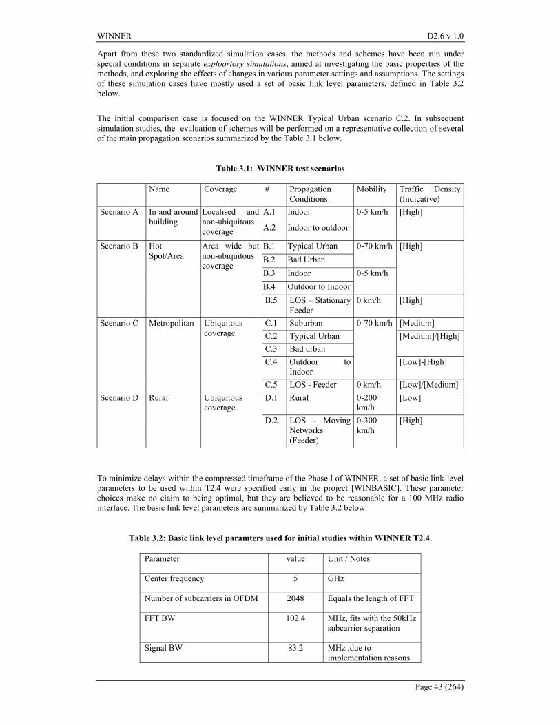
WINNER D2.6 v 1.0

Page 43 (264)

Apart from these two standardized simulation cases, the methods and schemes have been run under special conditions in separate exploartory simulations, aimed at investigating the basic properties of the methods, and exploring the effects of changes in various parameter settings and assumptions. The settings of these simulation cases have mostly used a set of basic link level parameters, defined in Table 3.2 below. The initial comparison case is focused on the WINNER Typical Urban scenario C.2. In subsequent simulation studies, the evaluation of schemes will be performed on a representative collection of several of the main propagation scenarios summarized by the Table 3.1 below.

Table 3.1: WINNER test scenarios

Name Coverage # Propagation Conditions

Mobility Traffic Density (Indicative)

A.1 Indoor Scenario A In and around building

Localised and non-ubiquitous coverage A.2 Indoor to outdoor

0-5 km/h [High]

B.1 Typical Urban B.2 Bad Urban

0-70 km/h

B.3 Indoor B.4 Outdoor to Indoor

0-5 km/h

[High] Scenario B Hot Spot/Area

Area wide but non-ubiquitous coverage

B.5 LOS – Stationary Feeder

0 km/h [High]

C.1 Suburban [Medium] C.2 Typical Urban C.3 Bad urban

[Medium]/[High]

C.4 Outdoor to Indoor

0-70 km/h

[Low]-[High]

Scenario C Metropolitan Ubiquitous coverage

C.5 LOS - Feeder 0 km/h [Low]/[Medium] D.1 Rural 0-200

km/h [Low] Scenario D Rural Ubiquitous

coverage D.2 LOS - Moving

Networks (Feeder)

0-300 km/h

[High]

To minimize delays within the compressed timeframe of the Phase I of WINNER, a set of basic link-level parameters to be used within T2.4 were specified early in the project [WINBASIC]. These parameter choices make no claim to being optimal, but they are believed to be reasonable for a 100 MHz radio interface. The basic link level parameters are summarized by Table 3.2 below.

Table 3.2: Basic link level paramters used for initial studies within WINNER T2.4.

Parameter value Unit / Notes

Center frequency 5 GHz

Number of subcarriers in OFDM 2048 Equals the length of FFT

FFT BW 102.4 MHz, fits with the 50kHz subcarrier separation

Signal BW 83.2 MHz ,due to implementation reasons

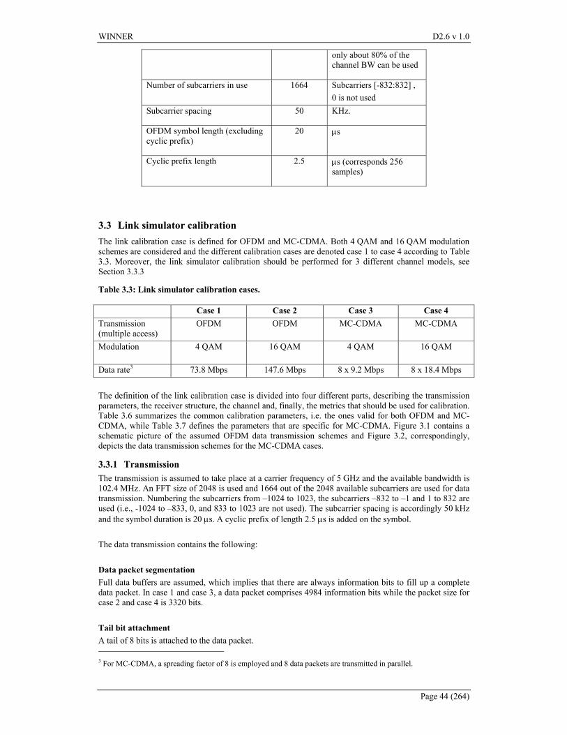
WINNER D2.6 v 1.0

Page 44 (264)

only about 80% of the channel BW can be used

Number of subcarriers in use 1664 Subcarriers [-832:832] , 0 is not used

Subcarrier spacing 50 KHz.

OFDM symbol length (excluding cyclic prefix)

20 µs

Cyclic prefix length 2.5 µs (corresponds 256 samples)

3.3 Link simulator calibration The link calibration case is defined for OFDM and MC-CDMA. Both 4 QAM and 16 QAM modulation schemes are considered and the different calibration cases are denoted case 1 to case 4 according to Table 3.3. Moreover, the link simulator calibration should be performed for 3 different channel models, see Section 3.3.3

Table 3.3: Link simulator calibration cases.

Case 1 Case 2 Case 3 Case 4 Transmission (multiple access)

OFDM OFDM MC-CDMA MC-CDMA

Modulation

4 QAM 16 QAM 4 QAM 16 QAM

Data rate3 73.8 Mbps 147.6 Mbps 8 x 9.2 Mbps 8 x 18.4 Mbps The definition of the link calibration case is divided into four different parts, describing the transmission parameters, the receiver structure, the channel and, finally, the metrics that should be used for calibration. Table 3.6 summarizes the common calibration parameters, i.e. the ones valid for both OFDM and MC-CDMA, while Table 3.7 defines the parameters that are specific for MC-CDMA. Figure 3.1 contains a schematic picture of the assumed OFDM data transmission schemes and Figure 3.2, correspondingly, depicts the data transmission schemes for the MC-CDMA cases.

3.3.1 Transmission The transmission is assumed to take place at a carrier frequency of 5 GHz and the available bandwidth is 102.4 MHz. An FFT size of 2048 is used and 1664 out of the 2048 available subcarriers are used for data transmission. Numbering the subcarriers from –1024 to 1023, the subcarriers –832 to –1 and 1 to 832 are used (i.e., -1024 to –833, 0, and 833 to 1023 are not used). The subcarrier spacing is accordingly 50 kHz and the symbol duration is 20 µs. A cyclic prefix of length 2.5 µs is added on the symbol. The data transmission contains the following: Data packet segmentation Full data buffers are assumed, which implies that there are always information bits to fill up a complete data packet. In case 1 and case 3, a data packet comprises 4984 information bits while the packet size for case 2 and case 4 is 3320 bits. Tail bit attachment A tail of 8 bits is attached to the data packet. 3 For MC-CDMA, a spreading factor of 8 is employed and 8 data packets are transmitted in parallel.

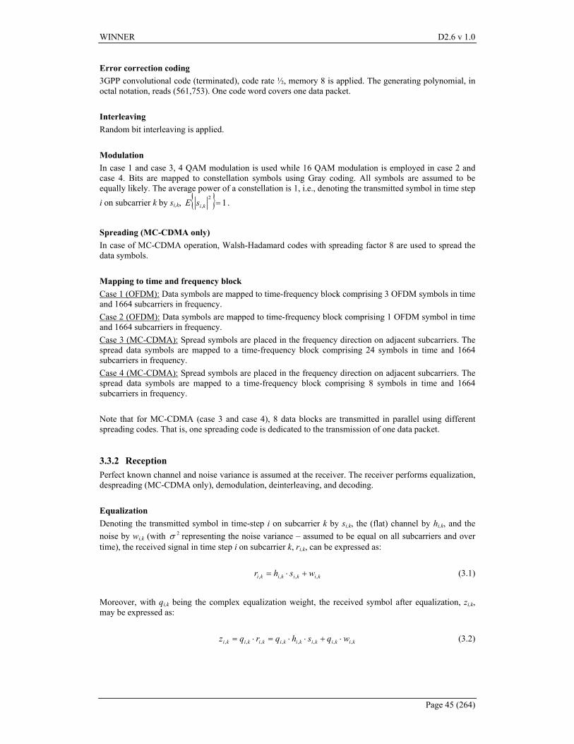
WINNER D2.6 v 1.0

Page 45 (264)

Error correction coding 3GPP convolutional code (terminated), code rate ½, memory 8 is applied. The generating polynomial, in octal notation, reads (561,753). One code word covers one data packet. Interleaving Random bit interleaving is applied. Modulation In case 1 and case 3, 4 QAM modulation is used while 16 QAM modulation is employed in case 2 and case 4. Bits are mapped to constellation symbols using Gray coding. All symbols are assumed to be equally likely. The average power of a constellation is 1, i.e., denoting the transmitted symbol in time step i on subcarrier k by si,k, { } 1

2, =kisE .

Spreading (MC-CDMA only) In case of MC-CDMA operation, Walsh-Hadamard codes with spreading factor 8 are used to spread the data symbols. Mapping to time and frequency block Case 1 (OFDM): Data symbols are mapped to time-frequency block comprising 3 OFDM symbols in time and 1664 subcarriers in frequency. Case 2 (OFDM): Data symbols are mapped to time-frequency block comprising 1 OFDM symbol in time and 1664 subcarriers in frequency. Case 3 (MC-CDMA): Spread symbols are placed in the frequency direction on adjacent subcarriers. The spread data symbols are mapped to a time-frequency block comprising 24 symbols in time and 1664 subcarriers in frequency. Case 4 (MC-CDMA): Spread symbols are placed in the frequency direction on adjacent subcarriers. The spread data symbols are mapped to a time-frequency block comprising 8 symbols in time and 1664 subcarriers in frequency. Note that for MC-CDMA (case 3 and case 4), 8 data blocks are transmitted in parallel using different spreading codes. That is, one spreading code is dedicated to the transmission of one data packet.

3.3.2 Reception Perfect known channel and noise variance is assumed at the receiver. The receiver performs equalization, despreading (MC-CDMA only), demodulation, deinterleaving, and decoding. Equalization Denoting the transmitted symbol in time-step i on subcarrier k by si,k, the (flat) channel by hi,k, and the noise by wi,k (with 2σ representing the noise variance – assumed to be equal on all subcarriers and over time), the received signal in time step i on subcarrier k, ri,k, can be expressed as: kikikiki wshr ,,,, +⋅= (3.1)

Moreover, with qi,k being the complex equalization weight, the received symbol after equalization, zi,k, may be expressed as: kikikikikikikiki wqshqrqz ,,,,,,,, ⋅+⋅⋅=⋅= (3.2)

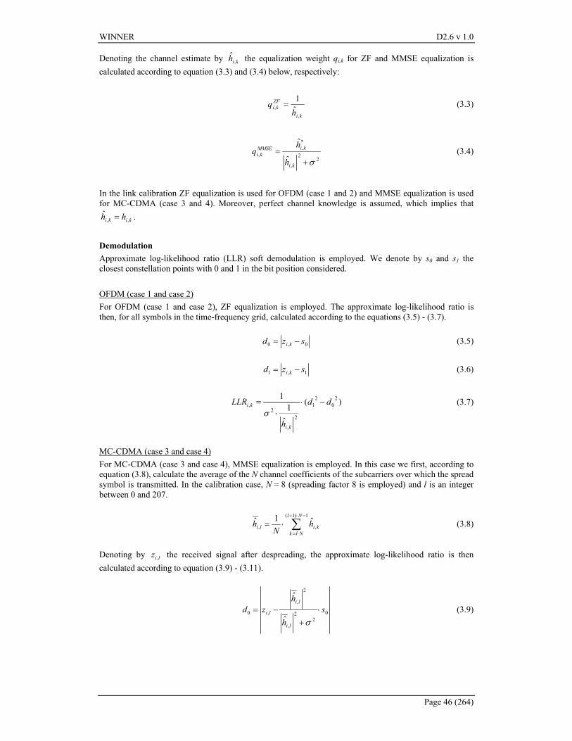
WINNER D2.6 v 1.0

Page 46 (264)

Denoting the channel estimate by kih ,ˆ the equalization weight qi,k for ZF and MMSE equalization is

calculated according to equation (3.3) and (3.4) below, respectively:

ki

ZFki

hq

,, ˆ

1= (3.3)

2

2

,

*,

,ˆ

ˆ

σ+=

ki

kiMMSEki

h

hq (3.4)

In the link calibration ZF equalization is used for OFDM (case 1 and 2) and MMSE equalization is used for MC-CDMA (case 3 and 4). Moreover, perfect channel knowledge is assumed, which implies that

kiki hh ,,ˆ = .

Demodulation Approximate log-likelihood ratio (LLR) soft demodulation is employed. We denote by s0 and s1 the closest constellation points with 0 and 1 in the bit position considered. OFDM (case 1 and case 2) For OFDM (case 1 and case 2), ZF equalization is employed. The approximate log-likelihood ratio is then, for all symbols in the time-frequency grid, calculated according to the equations (3.5) - (3.7).

0,0 szd ki −= (3.5)

1,1 szd ki −= (3.6)

)(

ˆ1

1 20

21

2

,

2, dd

h

LLR

ki

ki −⋅⋅

=σ

(3.7)

MC-CDMA (case 3 and case 4) For MC-CDMA (case 3 and case 4), MMSE equalization is employed. In this case we first, according to equation (3.8), calculate the average of the N channel coefficients of the subcarriers over which the spread symbol is transmitted. In the calibration case, N = 8 (spreading factor 8 is employed) and l is an integer between 0 and 207.

∑−⋅+

⋅=

⋅=1)1(

,,ˆ1ˆ

Nl

Nlkkili h

Nh (3.8)

Denoting by liz , the received signal after despreading, the approximate log-likelihood ratio is then calculated according to equation (3.9) - (3.11).

02

2

,

2

,

,0ˆ

ˆs

h

hzd

li

li

li ⋅+

−=σ

(3.9)

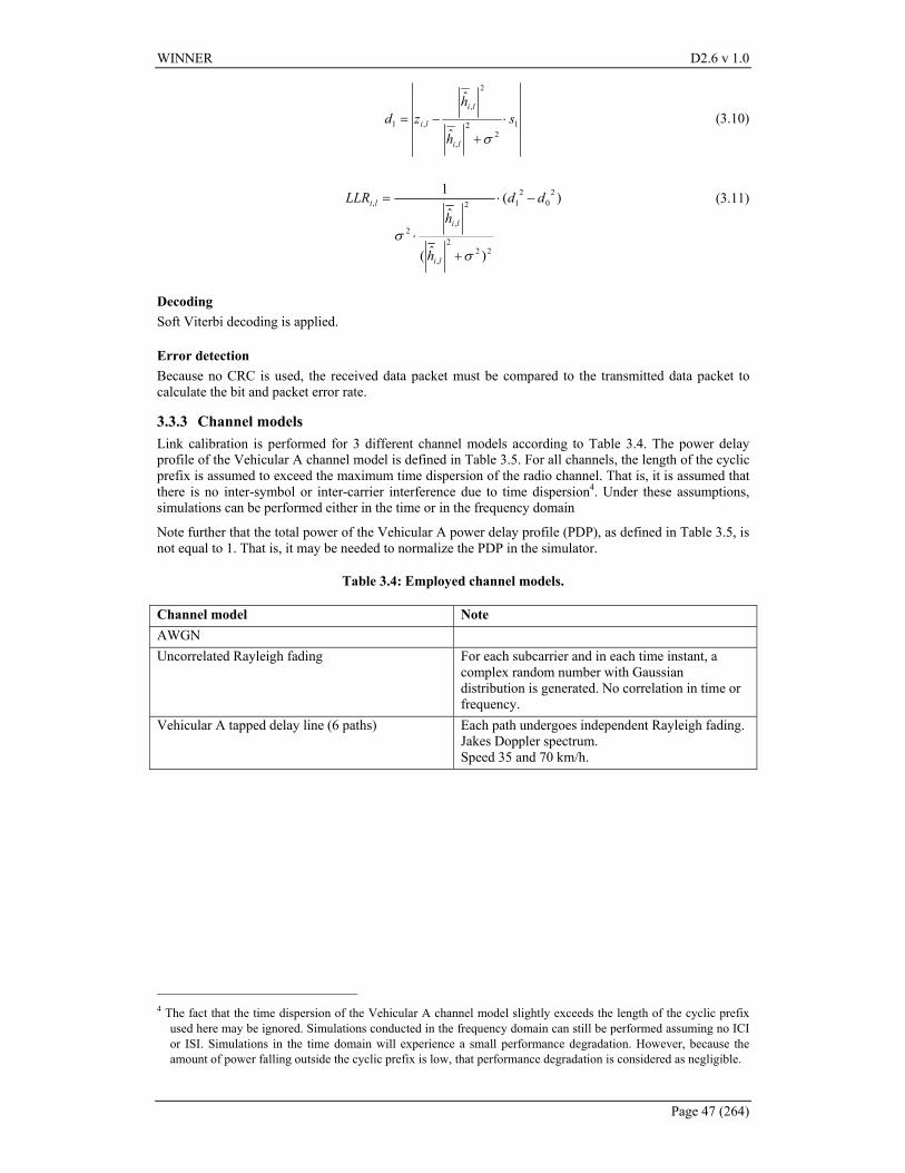
WINNER D2.6 v 1.0

Page 47 (264)

12

2

,

2

,

,1ˆ

ˆs

h

hzd

li

li

li ⋅+

−=σ

(3.10)

)(

)ˆ(

ˆ

1 20

21

222

,

2

,2

, dd

h

hLLR

li

li

li −⋅

+⋅

=

σσ

(3.11)

Decoding Soft Viterbi decoding is applied.

Error detection Because no CRC is used, the received data packet must be compared to the transmitted data packet to calculate the bit and packet error rate.

3.3.3 Channel models Link calibration is performed for 3 different channel models according to Table 3.4. The power delay profile of the Vehicular A channel model is defined in Table 3.5. For all channels, the length of the cyclic prefix is assumed to exceed the maximum time dispersion of the radio channel. That is, it is assumed that there is no inter-symbol or inter-carrier interference due to time dispersion4. Under these assumptions, simulations can be performed either in the time or in the frequency domain

Note further that the total power of the Vehicular A power delay profile (PDP), as defined in Table 3.5, is not equal to 1. That is, it may be needed to normalize the PDP in the simulator.

Table 3.4: Employed channel models.

Channel model Note AWGN Uncorrelated Rayleigh fading For each subcarrier and in each time instant, a

complex random number with Gaussian distribution is generated. No correlation in time or frequency.

Vehicular A tapped delay line (6 paths) Each path undergoes independent Rayleigh fading. Jakes Doppler spectrum. Speed 35 and 70 km/h.

4 The fact that the time dispersion of the Vehicular A channel model slightly exceeds the length of the cyclic prefix

used here may be ignored. Simulations conducted in the frequency domain can still be performed assuming no ICI or ISI. Simulations in the time domain will experience a small performance degradation. However, because the amount of power falling outside the cyclic prefix is low, that performance degradation is considered as negligible.

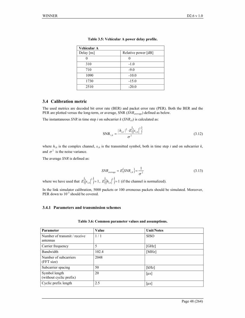
WINNER D2.6 v 1.0

Page 48 (264)

Table 3.5: Vehicular A power delay profile.

Vehicular A Delay [ns] Relative power [dB]

0 0 310 -1.0 710 -9.0 1090 -10.0 1730 -15.0 2510 -20.0

3.4 Calibration metric The used metrics are decoded bit error rate (BER) and packet error rate (PER). Both the BER and the PER are plotted versus the long-term, or average, SNR (SNRaverage) defined as below.

The instantaneous SNR in time step i on subcarrier k (SNRi,k) is calculated as:

{ }

2

2,

2,

,

||SNR

σkiki

ki

sEh ⋅= (3.12)

where hi,k is the complex channel, si,k is the transmitted symbol, both in time step i and on subcarrier k, and 2σ is the noise variance.

The average SNR is defined as:

{ } 2,1

σ== kiaverage SNRESNR (3.13)

where we have used that { } 12

, =kisE , { } 12

, =kihE (if the channel is normalized).

In the link simulator calibration, 5000 packets or 100 erroneous packets should be simulated. Moreover, PER down to 10-3 should be covered.

3.4.1 Parameters and transmission schemes

Table 3.6: Common parameter values and assumptions.

Parameter Value Unit/Notes Number of transmit / receive antennas

1 / 1 SISO

Carrier frequency 5 [GHz] Bandwidth 102.4 [MHz] Number of subcarriers (FFT size)

2048

Subcarrier spacing 50 [kHz] Symbol length (without cyclic prefix)

20 [µs]

Cyclic prefix length 2.5 [µs]

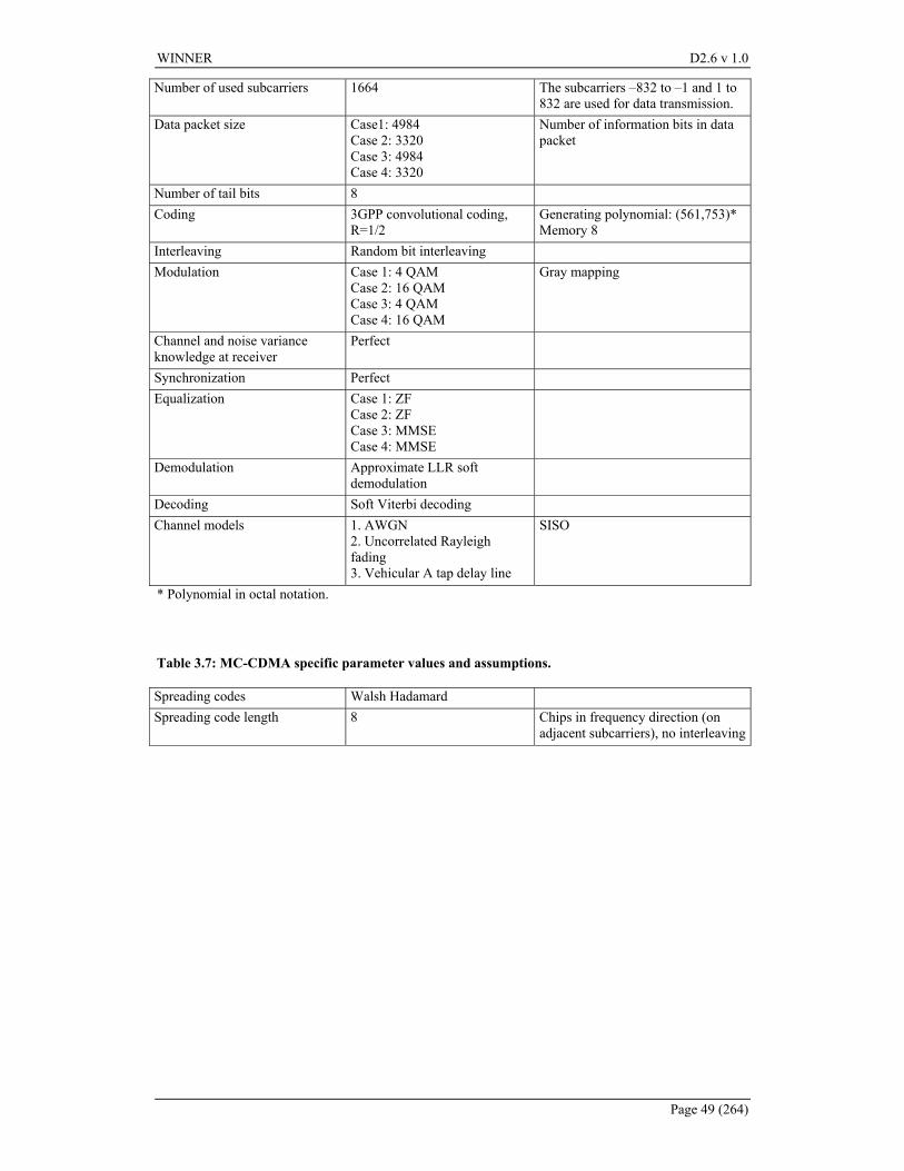
WINNER D2.6 v 1.0

Page 49 (264)

Number of used subcarriers 1664 The subcarriers –832 to –1 and 1 to 832 are used for data transmission.

Data packet size Case1: 4984 Case 2: 3320 Case 3: 4984 Case 4: 3320

Number of information bits in data packet

Number of tail bits 8 Coding 3GPP convolutional coding,

R=1/2 Generating polynomial: (561,753)* Memory 8

Interleaving Random bit interleaving Modulation Case 1: 4 QAM

Case 2: 16 QAM Case 3: 4 QAM Case 4: 16 QAM

Gray mapping

Channel and noise variance knowledge at receiver

Perfect

Synchronization Perfect Equalization Case 1: ZF

Case 2: ZF Case 3: MMSE Case 4: MMSE

Demodulation Approximate LLR soft demodulation

Decoding Soft Viterbi decoding Channel models 1. AWGN

2. Uncorrelated Rayleigh fading 3. Vehicular A tap delay line

SISO

* Polynomial in octal notation.

Table 3.7: MC-CDMA specific parameter values and assumptions.

Spreading codes Walsh Hadamard Spreading code length 8 Chips in frequency direction (on

adjacent subcarriers), no interleaving

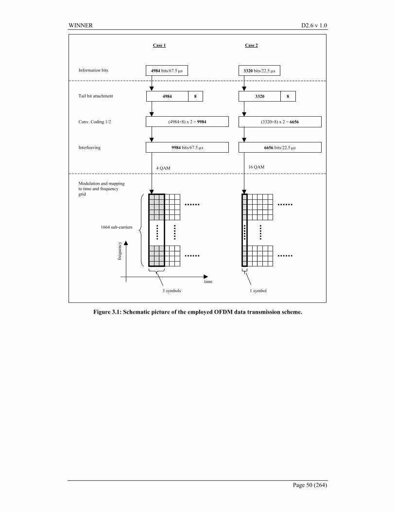
WINNER D2.6 v 1.0

Page 50 (264)

4984 bits/67.5 µs

8

(4984+8) x 2 = 9984

9984 bits/67.5 µs

time

freq

uenc

y

Information bits

Tail bit attachment

Conv. Coding 1/2

Interleaving

Modulation and mapping to time and frequency grid

4984

3320 bits/22.5 µs

8

(3320+8) x 2 = 6656

6656 bits/22.5 µs

3320

4 QAM 16 QAM

1664 sub-carriers

3 symbols 1 symbol

Case 1 Case 2

Figure 3.1: Schematic picture of the employed OFDM data transmission scheme.

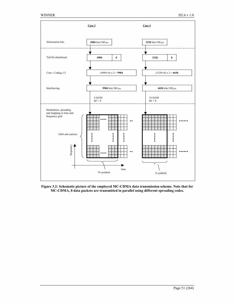
WINNER D2.6 v 1.0

Page 51 (264)

4984 bits/540 µs

8

(4984+8) x 2 = 9984

time

freq

uenc

y

Information bits

Tail bit attachment

Conv. Coding 1/2

Interleaving

Modulation, spreading and mapping to time and frequency grid

4984

3320 bits/180 µs

8

(3320+8) x 2 = 6656

3320

1664 sub-carriers

24 symbols 8 symbols

9984 bits/540 µs 6656 bits/180 µs

Case 3 Case 4

4 QAM SF = 8

16 QAMSF = 8

Figure 3.2: Schematic picture of the employed MC-CDMA data transmission scheme. Note that for MC-CDMA, 8 data packets are transmitted in parallel using different spreading codes.

WINNER D2.6 v 1.0

Page 52 (264)

3.5 Comparison case The comparison case is the initial test case for comparing the behaviour and performance of different multiple access schemes. This case focuses on a single isolated cell working at 5 GHz, using a 100 MHz total bandwidth, in an urban/suburban environment. The basic assumptions and considerations behind this case are as follows.

• It is based on the link level simulation parameters that were also used for the Calibration case. • It is based on scenario C.2 (urban, non-line of sight), see the WINNER System Assessment

Criteria Specifications D7.2. • It is a tool for initial comparisons, and is designed for ease of use, rather than realism in detail. • These simulation specifications are intended to set the scene, and paint the background, rather

than to script the play. Specifications and constraints on the utilized algorithms and MA methods have been minimized, to allow flexibility for algorithm optimization.

• The parameters are intended to be such that all schemes that are described within D2.6 can be evaluated in this context, in a reasonably fair way. Parameters are set so that the task of attaining access to/from multiple users is not made impossible for any of the considered methods, although the attained performance of the methods will of course differ considerably.

3.5.1 Common parameters All multiple access schemes based on OFDM and MC-CDMA utilize basic link level parameters for 5 GHz summarized by Table 3.2, that were also used in the link level calibration case. One OFDM symbol is the whole FFT, which includes 1664 data bearing subcarriers. Single-carrier schemes do not use these settings, but they also utilize a signal bandwidth of up to 83.2 MHz at 5 GHz.

Duplex: TDD, with asymmetry factor 1. No guardspace is assumed between uplink and downlink slots, since a small isolated cell is assumed. The TDD frame length is left unspecified.

Coding, spreading and interleaving: These properties are left unspecified, and free to be optimized within each particular multiple access method. The exact choices made should be described in such detail that the experiments could be repeated by other partners.

Power control: Left unspecified, and free to be optimized, under the constraint that the maximal average power levels specified below are respected. Thus, multi-user water-filling may be used in the downlink, and power control may be used in uplinks, e.g. to equalize the received power levels, if desired. The instantaneous peak transmit power is not restricted, as long as the average constraint is fulfilled. Note, however, that there in practice exist restrictions on analog-to-digital conversion resolution, that are relevant when considering such schemes. Such restrictions should be taken into account in the later, more advanced, comparison scenarios.

Channel estimation: Perfect channel estimation at the receiver is assumed.

Synchronization: Perfect synchronization at the receiver is assumed.

Data block length: 1656 bits.

The data blocks are assumed to be filled exclusively with payload bits. Thus, link-level overhead is not considered in this first comparison case.

3.5.2 Propagation scenario and cell size Propagation parameters are selected for the WINNER Scenario C.2, as suggested in the Determination of WINNER Propagation Scenarios D5.2. The path loss model was obtained by Nokia. It was fitted to non-line of sight measurements in urban macrocells performed at 5.25 GHz. This model was fitted to data at ranges 100 m – 2000 m. It will here be used for distances of 20-200 m. (Its validity is questionable at the shortest ranges, where line-of-sight components will in practice often occur.)

Path loss model:

[ ] [ ] BmdAdBdPL +⋅= )(log)( 10 (3.14)

where A = 28.3, and B = 61.5.

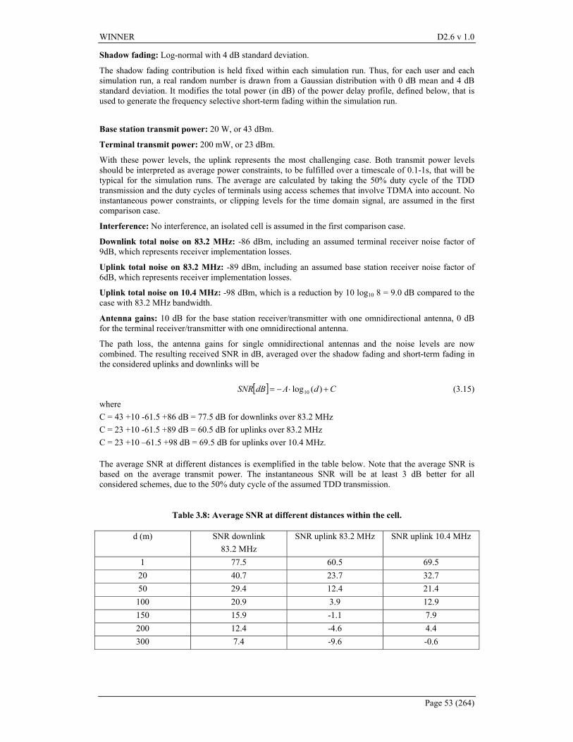
WINNER D2.6 v 1.0

Page 53 (264)

Shadow fading: Log-normal with 4 dB standard deviation.

The shadow fading contribution is held fixed within each simulation run. Thus, for each user and each simulation run, a real random number is drawn from a Gaussian distribution with 0 dB mean and 4 dB standard deviation. It modifies the total power (in dB) of the power delay profile, defined below, that is used to generate the frequency selective short-term fading within the simulation run.

Base station transmit power: 20 W, or 43 dBm.

Terminal transmit power: 200 mW, or 23 dBm.

With these power levels, the uplink represents the most challenging case. Both transmit power levels should be interpreted as average power constraints, to be fulfilled over a timescale of 0.1-1s, that will be typical for the simulation runs. The average are calculated by taking the 50% duty cycle of the TDD transmission and the duty cycles of terminals using access schemes that involve TDMA into account. No instantaneous power constraints, or clipping levels for the time domain signal, are assumed in the first comparison case.

Interference: No interference, an isolated cell is assumed in the first comparison case.

Downlink total noise on 83.2 MHz: -86 dBm, including an assumed terminal receiver noise factor of 9dB, which represents receiver implementation losses.

Uplink total noise on 83.2 MHz: -89 dBm, including an assumed base station receiver noise factor of 6dB, which represents receiver implementation losses.

Uplink total noise on 10.4 MHz: -98 dBm, which is a reduction by 10 log10 8 = 9.0 dB compared to the case with 83.2 MHz bandwidth.

Antenna gains: 10 dB for the base station receiver/transmitter with one omnidirectional antenna, 0 dB for the terminal receiver/transmitter with one omnidirectional antenna.

The path loss, the antenna gains for single omnidirectional antennas and the noise levels are now combined. The resulting received SNR in dB, averaged over the shadow fading and short-term fading in the considered uplinks and downlinks will be

[ ] CdAdBSNR +⋅−= )(log10 (3.15)

where C = 43 +10 -61.5 +86 dB = 77.5 dB for downlinks over 83.2 MHz C = 23 +10 -61.5 +89 dB = 60.5 dB for uplinks over 83.2 MHz C = 23 +10 –61.5 +98 dB = 69.5 dB for uplinks over 10.4 MHz.

The average SNR at different distances is exemplified in the table below. Note that the average SNR is based on the average transmit power. The instantaneous SNR will be at least 3 dB better for all considered schemes, due to the 50% duty cycle of the assumed TDD transmission.

Table 3.8: Average SNR at different distances within the cell.

d (m) SNR downlink 83.2 MHz

SNR uplink 83.2 MHz SNR uplink 10.4 MHz

1 77.5 60.5 69.5 20 40.7 23.7 32.7 50 29.4 12.4 21.4 100 20.9 3.9 12.9 150 15.9 -1.1 7.9 200 12.4 -4.6 4.4 300 7.4 -9.6 -0.6

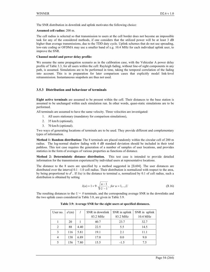
WINNER D2.6 v 1.0

Page 54 (264)

The SNR distribution in downlink and uplink motivates the following choice:

Assumed cell radius: 200 m.

The cell radius is selected so that transmission to users at the cell border does not become an impossible task for any of the considered methods, if one considers that the utilized power will be at least 3 dB higher than average transmissions, due to the TDD duty cycle. Uplink schemes that do not use spreading, low-rate coding or OFDMA may use a smaller band of e.g. 10.4 MHz for each individual uplink user, to improve the SNR.

Channel model and power delay profile:

We assume the same propagation scenario as in the calibration case, with the Vehicular A power delay profile of Table 3.3, for all users within the cell: Rayleigh fading, without line-of sight components in any path, is assumed. Simulations are to be performed in time, taking the temporal correlation of the fading into account. This is in preparation for later comparison cases that explicitly model link-level retransmission. Instantaneous snapshots are thus not used.

3.5.3 Distribution and behaviour of terminals Eight active terminals are assumed to be present within the cell. Their distances to the base station is assumed to be unchanged within each simulation run. In other words, quasi-static simulations are to be performed. All terminals are assumed to have the same velocity. Three velocities are investigated:

1. All users stationary (mandatory for comparison simulations), 2. 35 km/h (optional), 3. 70 km/h (optional).

Two ways of generating locations of terminals are to be used. They provide different and complementary types of information.

Method 1: Random distribution: The 8 terminals are placed randomly within the circular cell of 200 m radius. The log-normal shadow fading with 4 dB standard deviation should be included in their total pathloss. This test case requires the generation of a number of samples of user locations, and provides statistics in the form of averages of various properties as functions of distance.

Method 2: Deterministic distance distribution. This test case is intended to provide detailed information for the transmission experienced by individual users at representative locations.

The distance to the 8 users are specified by a method suggested in [Eri04]. The user distances are distributed over the interval 0.1 –1.0 cell radius. Their distribution is normalized with respect to the area, by being proportional to d2.. If l(u) is the distance to terminal u, normalized by 0.1 of cell radius, such a distribution is obtained by setting

UuforUuul ,...,1,

1191)( =

−−

⋅+= (3.16)

The resulting distances to the U = 8 terminals, and the corresponding average SNR in the downlinks and the two uplink cases considered in Table 3.8, are given in Table 3.9.

Table 3.9: Average SNR for the eight users at specified distances.

User no. d (m) l SNR in downlink 83.2 MHz

SNR in uplink 83.2 MHz

SNR in uplink 10.4 MHz

1 20 1 40.7 23.7 32.7 2 88 4.40 22.5 5.5 14.5 3 116 5.81 19.1 2.1 11.1 4 138 6.89 17.0 0.0 9.0 5 156 7.80 15.5 -1.5 7.5

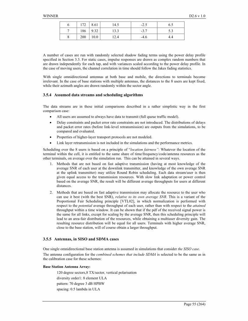
WINNER D2.6 v 1.0

Page 55 (264)

6 172 8.61 14.5 -2.5 6.5 7 186 9.32 13.3 -3.7 5.3 8 200 10.0 12.4 -4.6 4.4

A number of cases are run with randomly selected shadow fading terms using the power delay profile specified in Section 3.3. For static cases, impulse responses are drawn as complex random numbers that are drawn independently for each tap, and with variances scaled according to the power delay profile. In the case of moving users, the channel correlation in time should follow the Jakes fading statistics.

With single omnidirectional antennas at both base and mobile, the directions to terminals become irrelevant. In the case of base stations with multiple antennas, the distances to the 8 users are kept fixed, while their azimuth angles are drawn randomly within the sector angle.

3.5.4 Assumed data streams and scheduling algorithms The data streams are in these initial comparisons described in a rather simplistic way in the first comparison case:

• All users are assumed to always have data to transmit (full queue traffic model). • Delay constraints and packet error rate constraints are not introduced. The distributions of delays

and packet error rates (before link-level retransmission) are outputs from the simulations, to be compared and evaluated.

• Properties of higher-layer transport protocols are not modeled. • Link layer retransmission is not included in the simulations and the performance metrics.

Scheduling over the 8 users is based on a principle of “location fairness”: Whatever the location of the terminal within the cell, it is entitled to the same share of time/frequency/code/antenna resources as the other terminals, on average over the simulation run. This can be attained in several ways.

1. Methods that are not based on fast adaptive transmission (having at most knowledge of the average SNR of each user at the downlink transmitter, and knowledge of the own average SNR at the uplink transmitter) may utilize Round Robin scheduling. Each data stream/user is then given equal access to the transmission resources. With slow link adaptation or power control based on the average SNR, the result will be different average throughputs for users at different distances.

2. Methods that are based on fast adaptive transmission may allocate the resource to the user who can use it best (with the best SNR), relative to its own average SNR. This is a variant of the Proportional Fair Scheduling principle [VTL02], in which normalization is performed with respect to the potential average throughput of each user, rather than with respect to the attained throughput within a time window. It can be shown that if the pdf of the received signal power is the same for all links, except for scaling by the average SNR, then this scheduling principle will lead to an area-fair distribution of the resources, while obtaining a multiuser diversity gain. The resulting resource distribution will be equal for all users. Terminals with higher average SNR, close to the base station, will of course obtain a larger throughput.

3.5.5 Antennas, in SISO and SDMA cases

One single omnidirectional base station antenna is assumed in simulations that consider the SISO case. The antenna configuration for the combined schemes that include SDMA is selected to be the same as in the calibration case for these schemes:

Base Station Antenna Array: 120 degree sectors,8 TX/sector, vertical polarisation diversity order1: 8 element ULA pattern: 70 degree 3 dB HPBW spacing: 0.5 lambda in ULA

WINNER D2.6 v 1.0

Page 56 (264)

Mobile Station: diversity order1: 1 RX, vertical polarisation pattern: omni.

The total average SNR per link will for the SDMA test case be different from the SISO estimates of Sections 3.5.2 and 3.5.3.

3.5.6 Output and test metrics • Goodput (i.e. bits contained in correctly received frames), per second, for individual terminals. • Packet or Frame error rate (FER). • Total access point DL/UL goodput.

When generating user locations by Method 1, these quantities are collected from R simulation runs, for each of the 8 simulated terminals, together with the corresponding distances. Statistics is collected for R>20 runs. Average values can then be calculated for terminals that fell within a range of distances and the results can be presented as plots, or histograms, of these averages as a function of the distance in meters.

When generating user locations by Method 2, the results are obtained for eight specific distances. Distribution of the three properties above is measured, to study their variability due to the short-term fading and the shadow fading. Distributions of FER and goodput are then displayed for each of the eight users.

The presented results should also, if possible, estimate representative fractions of overhead and efficiency loss generated by different mechanisms within each scheme. These effects include

• Guardtimes /cyclic prefixes • Fraction of pilots • Fraction of total resources used for control signaling (in-band or out-of band) • Fractions of resources (TDMA slots, time-frequency bins) unfilled with payload, due to the use

of a link-level frame with fixed prespecified size. Delay statistics for the link-level frames should be added to the test metrics in future evolved comparison cases that include link-level retransmission mechanisms.

WINNER D2.6 v 1.0

Page 57 (264)

4. Single-Carrier and Multi-Carrier Based Access Schemes

4.1 Introduction This chapter compares access methods that employ single and multi-carrier transmission techniques. The comparison is based on results available in the literature and on qualitative arguments. Some specific multiple access schemes, based on single-carrier and multi-carrier transmission techniques, relevant in the WINNER project, are later on described and analyzed in Chapter 5, 6 and 7, respectively. The transmission scheme determines how a link utilizes the bandwidth that it has been assigned to. If constellation symbols are transmitted one by one, i.e. serially, the transmission is characterized as a single-carrier scheme. Likewise, if symbols are modulated and transmitted in parallel on different sub channels (subcarriers) the scheme is categorized as a multi-carrier transmission scheme. In the literature, single-carrier and multi-carrier transmission schemes are sometimes also referred to as serial and parallel modulation techniques, respectively. The multiple access method defines how several users share and access a common communication resource and can typically not be selected independent of the transmission scheme. Instead, the characteristics of the transmission scheme put requirements on the multiple access method and vice versa. This relationship between the transmission scheme and the multiple access method is the focus of the discussion in this chapter. In particular, the chapter discusses how the transmission technique impacts the choice of multiple access method. Section 4.2 briefly introduces and compares the link characteristics of single-carrier and multi-carrier transmission schemes with their respective pros and cons. With this as a base, the characteristics of radio communication systems that employ single-carrier and multi-carrier transmission are elaborated on in Section 4.3. Section 4.4, finally, summarizes the discussion and draws a few conclusions for further work.

4.2 Link characteristics Favorable characteristics of a transmission scheme include high power amplifier efficiency, a variable transmission bandwidth and a capability to operate efficiently in environments in which the channel is time dispersive and fading. Moreover, the link should facilitate flexible and efficient adaptation and, at least in some situations, offer diversity. The link, finally, should preferably be robust towards different kinds of impairments, like frequency offsets and phase noise. Below, we briefly address each of these items and compare the properties of single-carrier and multi-carrier transmission schemes. A similar comparison is also available in [Kla04], see Section 4.13-4.17.

4.2.1 Power efficiency A high efficiency of the power amplifier, which is largely determined by the transmitted signal’s peak-to-average power ratio (PAPR), is, especially in the uplink, an important property of a radio communication system. A signal with high PAPR implies that the power amplifier must operate at a level that, on average, is significantly (several dB) below the maximum output power. Accordingly, an access scheme in which the signal’s PAPR is high obtains lower coverage than an access scheme in which the signal’s PAPR is low - given that the same power amplifier is used. Or, similarly, for a required coverage, a signal with high PAPR requires a power amplifier with higher maximum output power and larger linear region. The PAPR also influences the required resolution of the AD and DA converters. In this context, single-carrier transmission schemes that provide a low PAPR are preferred to multi-carrier schemes for which the PAPR is relatively high already for a few carriers. In particular, the PAPR issue is important in the uplink since the power amplifier in user terminals typically have relatively tough constraints in terms of cost, size and power consumption. Such considerations are less important in the design of an access point. However, there exist techniques that reduce the PAPR problem experienced by multi-carrier transmission schemes. In [NP00], these techniques are grouped into 3 different categories. In the first category, the signal is distorted in order to limit the PAPR. This includes (non-linear) techniques such as clipping and windowing, which limits the PAPR but results in increased out of band emissions and in-band distortion [NL95], [LC98]. The second class of techniques makes use of special coding techniques that excludes combinations with high PAPR [Nee96], [Pop91], [WJ95]. Within the third category, finally, one finds probabilistic methods. Constellation symbols are scrambled by a set of scrambling sequences and the sequence with the lowest PAPR is selected, see e.g. [MH97]. Hence, this type of PAPR reduction technique reduces the risk that a high PAPR occurs. Any form of PAPR reduction technique, however, do imply a somewhat increased complexity, e.g. in the form of additional signal processing and signaling overhead, and even though

WINNER D2.6 v 1.0

Page 58 (264)

some techniques significantly reduce the PAPR of the multi-carrier signal, the problem is only partly solved.

4.2.2 Variable transmission bandwidth One important requirement on a new radio interface is to support operation in spectrum allocations of different sizes. Such spectrum flexibility would make it possible to deploy the system in different frequency bands under various constraints. In this context, a signal with an variable transmission bandwidth is attractive. A variable transmission bandwidth, furthermore, also brings additional multiple access flexibility for systems using FDMA. Multi-carrier schemes inherently support a variable transmission bandwidth with a granularity that, in principle, equals the width of a single subcarrier. The bandwidth adjustment of single-carrier signals is performed by adjusting the transmitted symbol rate and typically does not exhibit the same flexibility as multi-carrier schemes. However, because the use of front-end filters to limit out-of-band emissions is present for both single and multi-carrier signals, the bandwidth adjustment capabilities of the access scheme is not restricted to the baseband signal generation but is to a large extent also an RF issue. Note that there is work ongoing in WINNER within the area of variable and multi-bandwidth transmissions, see [Mun04]. This work provides further guidance in this area.

4.2.3 Robustness to time dispersion and fading A transmission scheme should deliver high data rates also in ‘difficult’ time dispersiveand fading radio channels. Multi-carrier transmission schemes, like OFDM, are robust to time dispersion thanks to the use of the cyclic prefix. As long as the length of the cyclic prefix exceeds the maximum dispersion of the radio channel, time dispersion causes neither inter-carrier nor inter-symbol interference. In single-carrier transmission schemes, (adaptive) time domain equalizers have typically been employed at the receiver side to restore the channel and suppress inter-symbol interference. The complexity of such time domain equalizers, however, grows rapidly with the bandwidth. The solution seems hence not very attractive in case of high rate transmissions over highly dispersive radio channels. An alternative approach is to use single-carrier transmission and a frequency domain equalizer (FDE) at the receiver side. Such a solution is considered in e.g. [FAB+02], [Czyl97], [SKJ94] and [SKJ95]. As for multi-carrier modulation, data is typically transmitted in blocks and a cyclic prefix is added to the signal. The use of a cyclic prefix makes the signal look periodic at the receiver side and prevents contamination of ISI from previous block. The overall complexity of the single-carrier solution with FDE is similar to that of a multi-carrier scheme [FAB+02]. For single-carrier transmission schemes, the complexity is concentrated to the receiver side while the complexity in multi-carrier schemes is more evenly distributed between the transmitter and the receiver side. The structure and the basic building blocks in the transmitter and receiver chain are similar (both rely on FFT and IFFT operations). Several studies indicate that single-carrier schemes using FDE can handle time dispersion equally well as multi-carrier (OFDM) schemes. The results in [Czyl97], [SKJ94] and [SKJ95] show that without channel coding, a single-carrier transmission scheme with a FDE outperforms a comparable OFDM solution (provided that a fixed modulation scheme is employed in the OFDM system). Including the effects of channel coding, the results indicate that single-carrier transmission schemes using FDE achieves comparable performance as OFDM based transmission schemes [FAB+02], [SKJ94], [SKJ95]. Somewhat simplified, it seems like a single-carrier scheme is to prefer when the code rate is high but a multi-carrier scheme performs better when the code rate is low [WMG04]. Quickly fading channels will affect the performance of both single and multi-carrier transmission schemes. Typically, both type of schemes rely on that accurate channel estimates are available in the receiver and that the channel remains virtually constant over the transmitted block.

4.2.4 Link adaptation Link adaptation is to adapt the transmission parameters, like modulation order, channel coding scheme, spreading factor and output power, such that the transmission fits the current channel conditions. In single-carrier transmission schemes, the link adaptation can only be performed in the time domain, i.e., the transmission can only be adapted to temporal variations. In a multi-carrier transmission scheme, on the other hand, also the frequency domain can be adaptively utilized by adjusting the transmission parameters on different sub channels according to the frequency selectivity. This possibility of adapting the transmission according to the frequency response of the channel may, in some situations, be a considerable advantage. On the other hand, it also requires more signaling and that the transmitter has access to detailed channel state information. In a case when the channel state information is received via a feedback link from the receiver, the amount of measurement data reported back to the transmitter increases.

WINNER D2.6 v 1.0

Page 59 (264)

4.2.5 Diversity In frequency selective fading channels, multi-carrier transmission schemes obtain diversity by coding over the subcarriers. In single-carrier transmission schemes, in which every constellation symbol is transmitted over the whole bandwidth, the equalizer acts as a diversity combiner.

4.2.6 Robustness to impairments Frequency offsets, phase noise and timing errors may cause problems for both single and multi-carrier transmission schemes. Single-carrier transmission schemes are often considered as more robust than multi-carrier schemes to impairments like frequency offsets and phase noise. The performance degradation in both type of schemes, however, seems to be limited as long as the offsets are relatively small. The results in [SKJ95] show that OFDM is more sensitive to carrier frequency errors than a single-carrier scheme. The conclusions in both [NP00] and [WMG04] are similar, but also concludes that the effect is small as long as the carrier-frequency offset is limited. Moreover, [NP00] shows that thanks to the cyclic prefix, multi-carrier schemes (OFDM) are relatively insensitive to timing errors. Such timing errors do however reduce the robustness to time dispersion. In a similar way, timing errors in single-carrier schemes (using block-wise transmission and a cyclic prefix) can be absorbed by the cyclic prefix at the cost of decreased robustness to time dispersion.

4.3 System characteristics In multi-user communication systems, several users share a common resource. The multiple access method defines how users share such resources and the medium access principle dictates the rules according to which users may access the medium. Section 4.3.1 and Section 4.3.2 briefly discusses how single-carrier and multi-carrier transmission schemes can be utilized in multi-user (multi cellular) networks and if the different transmission schemes implies any fundamental difference in a system perspective. Section 4.3.1 focuses on the multiple access and Section 4.3.2 on the medium access (transmission scheduling) – two tightly interconnected areas.

4.3.1 Multiple access In essence, the multiple access method defines how a common resource is divided into different portions that can be assigned to and used by different users. The division may be performed in time, frequency, by codes or spatially. The properties of these multiple access schemes are reviewed in Chapter 2. Some desirable characteristics of the multiple access method are that the mutual interference in between multiple transmissions can be controlled. Furthermore, the multiple access method should facilitate a flexible and efficient resource sharing. We distinguish here between orthogonal and non-orthogonal multiple access methods. Orthogonal multiple access methods rely on orthogonal waveforms that occupy non-overlapping parts of the resource, in order to avoid multiple access interference. Examples of such multiple access methods are TDMA and FDMA. A non-orthogonal multiple access method, on the other hand, relies on processing gain in order to suppress the multiple access interference, like (non-synchronous) uplink CDMA. Moreover, in cellular systems, it may be useful to separate the intra-cell and the inter-cell multiple access method. The former separates transmissions within the same cell while the latter separates transmissions of different cells.

Both orthogonal multiple access schemes, like TDMA and FDMA, and non-orthogonal multiple access schemes like (non-synchronous) CDMA, can be realized both if a single-carrier or a multi-carrier transmission scheme is used on the physical layer. However, the multiple access method should naturally not be chosen independent of the transmission scheme (and vice versa). In TDMA systems, a common time reference among the nodes is required to avoid that the transmission of different nodes overlap in time. In FDMA systems, in which the available frequency band is typically divided in disjoint parts that are used for transmission by different nodes, nodes must share a common frequency reference. In (non-synchronous) CDMA systems, which rely on suppression of the multiple-access interference, there is basically no need of coordination among nodes. It seems hard to state any general guidance regarding the suitability of using any of the mentioned multiple access schemes in combination with single or multi-carrier transmission techniques. Instead, one must assess and compare specific solutions in which the transmission scheme and the multiple access method are jointly considered.

4.3.2 Medium access The medium access (transmission scheduling) principle defines the rules according to which users may access the medium (the channel) and use it for data transmission. The transmission scheduling resides in the medium access control (MAC) protocol and one may distinguish between two fundamentally different principles: conflict-free and contention-based medium access. This classification is used in [RS90].

WINNER D2.6 v 1.0

Page 60 (264)

Conflict-free medium access assures that, at any time, there is never more than one user accessing a certain channel resource. In a contention based medium access scheme, on the other hand, transmissions are not coordinated and conflicts may occur. That is, it may happen that there are two (or more) users that simultaneously try to access the same channel resource. Even if caption mechanisms may be used when packets collide, a collision typically implies that at least one of the transmissions fails and the packet must be retransmitted. In a cellular system, true conflict free transmission may be achieved within a cell but normally not within a system (comprising multiple cells) due to the requirement that resources must be reused throughout the network. Contention based transmission can be applied both within and in between cells. Moreover, within a cell, it is reasonable that a conflict-free scheduling scheme is applied in the downlink since it is straightforward to coordinate downlink transmissions from the same node (access point). In uplink, however, conflict free transmissions, coordinated by the access point (network), comes with a cost in the form of an increased medium access delay. Therefore, both contention-based and conflict free medium access schemes may be seen as viable solutions in the uplink. Moreover, scheduling may be used as a mean to control the fairness among users within a communication system. If the scheduling is quality based, considering some form of channel state information, it may further increase the efficiency of the network by capturing a multi-user diversity gain. Such channel dependent scheduling can be employed in systems based on both single-carrier and multi-carrier transmission, both in the time and in the frequency domain. It seems like, however, that a multi-carrier scheme to some extent exhibits a higher flexibility when considering channel dependent scheduling in the frequency domain. For further guidance within the area of medium access control principles and transmission scheduling we refer to WINNER task 2.6, see e.g. [SK04]. The transmission scheduling principle is, however, essentially independent of the transmission scheme. It does not depend on whether a single-carrier or a multi-carrier scheme is used on the physical layer. In both cases, channel dependent scheduling can be applied, in time and in frequency. That is, considering medium access and transmission scheduling principles, neither single-carrier nor multi-carrier schemes seems to offer any distinctive advantage.

4.4 Summary and conclusions In this chapter, access schemes based on single-carrier and multi-carrier transmission techniques have been briefly described and compared with their respective pros and cons. Similar comparisons are available in the literature and also within the WINNER project, see e.g. [Kla04]. Regarding the link characteristics the PAPR of the generated signal and the link adaptation possibilities were identified as the major differences. Single-carrier schemes have the advantage of a low signal PAPR while multi-carrier schemes offers a potential of adaptation of transmission parameters in the frequency domain. Concerning the possible impact on the multiple access and the medium access schemes, no fundamental difference was identified. In the downlink, the low PAPR of single-carrier signals is not considered as a major advantage and accordingly, no significant argument advocating single-carrier based access in the downlink were identified. Hence, in downlink, the focus of the work and the evaluations in this report is on multiple access methods based on multi-carrier transmission schemes. In the uplink, however, a transmitted signal with low PAPR may be favorable, especially for wide-area coverage. On the other hand, for short-range communications the PAPR is less important and it seems attractive to employ multi-carrier transmission also in the uplink. Both single and multi-carrier based access schemes are hence seen as viable uplink alternatives and further studies are needed within this area. Accordingly, uplink access methods based on both single and multi-carrier transmissions schemes are studied throughout this report.

WINNER D2.6 v 1.0

Page 61 (264)

5. Single-Carrier Uplink Multiple Access

5.1 Introduction This chapter considers uplink access schemes based on single-carrier transmission techniques. Both spread and non-spread solutions, namely DS-CDMA and single-carrier TDMA, are considered. We highlight that the main challenge for single-carrier systems is how to deal with a channel response spanning many symbols, resulting from the combination of wide transmission bandwidths and channel time dispersion. In Section 5.2, an uplink DS-CDMA system is studied and it is shown that Rake receiver implementations in time and frequency domain provide similar robustness to time dispersion. The frequency domain implementation is less complex but typically also results in a reduced spectral efficiency because of the additional overhead (in the form of a cyclic prefix). The results in Section 5.2 further indicate that a MMSE multi-user detector may offer a substantial performance improvement compared to the matched filter. Such a solution does however come with a cost of a significant complexity increase. Section 5.3 addresses non-spread single-carrier systems using TDMA. A linear MMSE frequency domain equalizer and an iterative frequency domain MMSE turbo equalizer are employed to combat time dispersion and suppress inter-symbol interference. The results indicate that while the performance of the two receivers are similar for QPSK modulation, the turbo equalizer exhibit a performance advantage in case of higher order modulation like 16QAM. In Section 5.4, finally, we summaries the obtained results and we outline a few possible further studies.

5.2 Single-carrier CDMA This section is devoted to propose and evaluate single-carrier CDMA, usually known as direct sequence (DS) CDMA [Ver98], [Vit95], for the uplink in the WINNER project. CDMA has been shown to have the potential to achieve the capacity of multiple access channels [CTh91], albeit at the cost of higher complexity than TDMA and FDMA. A single-carrier system is being proposed for the uplink as an alternative to a multi-carrier setup for its more natural handling of asynchronous multiple access, and with the aim of reducing the transmitter complexity. On the other hand, the high bandwidth and corresponding high resolution of the receiver envisioned for the WINNER project raise questions about the feasibility of the traditional approach to the DS-CDMA receiver, namely the Rake receiver, since with 100 MHz the signal energy is likely to be dispersed among many resolvable paths, and many Rake fingers may be needed. An alternative solution being proposed for this problem is a frequency domain (FD) Rake [AI03]which performs maximal ratio combining (MRC) in the frequency domain, although due to its block processing nature it may be more difficult to apply in asynchronous systems.

The outline of this section is as follows: first, we consider a synchronous uplink system and propose continuous and block transmission schemes, suitable for time domain (TD) and FD implementations of the Rake receiver, respectively. The receiver in either domain is described next, and a preliminary complexity evaluation is shown. Next, reduced complexity methods are proposed. Asynchronous and dual-rate systems are also addressed. Finally, link-level simulation results are shown.

5.2.1 Single-carrier (SC), direct sequence (DS) CDMA system model Two transmission schemes are considered: block transmission (BT) and continuous transmission (CT). These two schemes are introduced in order to consider processing in FD and TD, respectively. In the former symbols are arranged in blocks separated by a guard band or cyclic prefix, with the same parameters as the multi-carrier counterpart in terms of block size and prefix length. In the latter symbols are transmitted continuously. The transmitted DS-CDMA signal for BT is defined as

( ) ( ) ( ) ( )( )∑ ∑ ∑∞

−∞=

−

−=

−

=

−+−−−=i

M

Gj

N

nckkkk TGMijTnTtpncjibAtx

1 1

01, (5.1)

where:

M is the block size, N is the processing gain, G is the prefix/guard interval length, Ak is the signal amplitude,

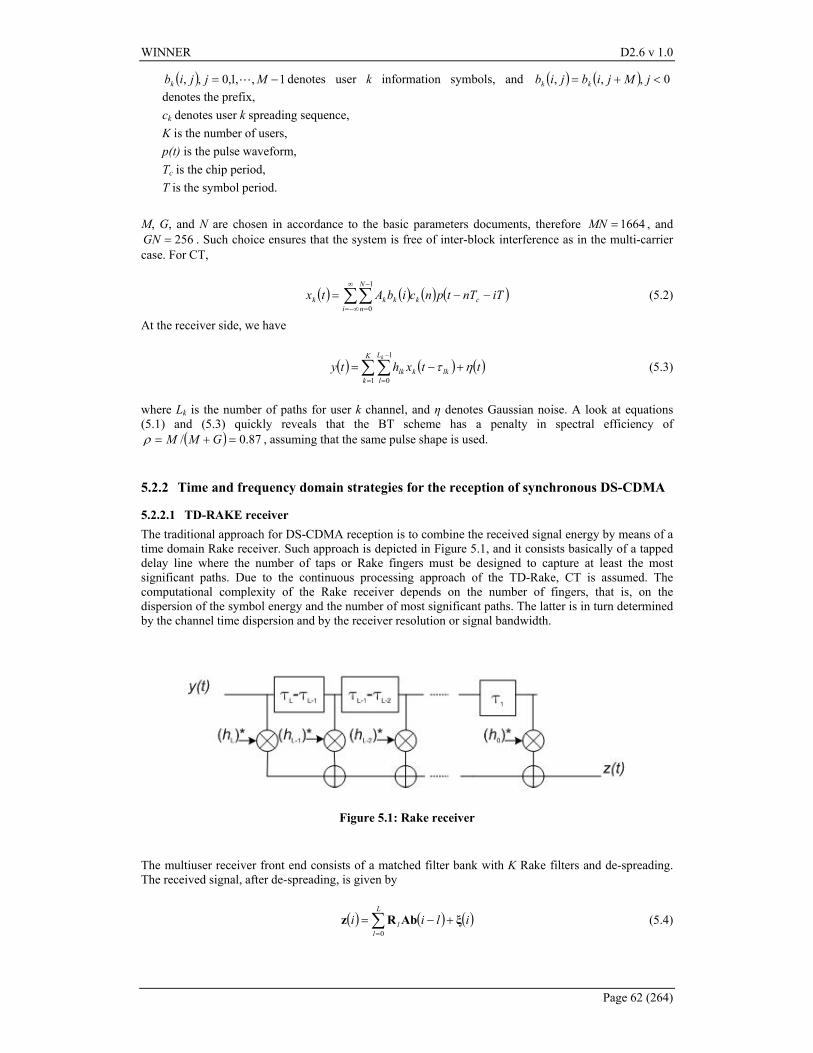
WINNER D2.6 v 1.0

Page 62 (264)

( ) 1,,1,0,, −= Mjjibk L denotes user k information symbols, and ( ) ( ) 0,,, <+= jMjibjib kk denotes the prefix, ck denotes user k spreading sequence, K is the number of users, p(t) is the pulse waveform, Tc is the chip period, T is the symbol period.

M, G, and N are chosen in accordance to the basic parameters documents, therefore 1664=MN , and

256=GN . Such choice ensures that the system is free of inter-block interference as in the multi-carrier case. For CT,

( ) ( ) ( ) ( )∑∑∞

−∞=

−

=

−−=i

N

nckkkk iTnTtpncibAtx

1

0 (5.2)

At the receiver side, we have

( ) ( ) ( )∑ ∑=

−

=

+−=K

k

L

llkklk ttxhty

k

1

1

0ητ (5.3)

where Lk is the number of paths for user k channel, and η denotes Gaussian noise. A look at equations (5.1) and (5.3) quickly reveals that the BT scheme has a penalty in spectral efficiency of

( ) 87.0/ =+= GMMρ , assuming that the same pulse shape is used.

5.2.2 Time and frequency domain strategies for the reception of synchronous DS-CDMA

5.2.2.1 TD-RAKE receiver The traditional approach for DS-CDMA reception is to combine the received signal energy by means of a time domain Rake receiver. Such approach is depicted in Figure 5.1, and it consists basically of a tapped delay line where the number of taps or Rake fingers must be designed to capture at least the most significant paths. Due to the continuous processing approach of the TD-Rake, CT is assumed. The computational complexity of the Rake receiver depends on the number of fingers, that is, on the dispersion of the symbol energy and the number of most significant paths. The latter is in turn determined by the channel time dispersion and by the receiver resolution or signal bandwidth.

Figure 5.1: Rake receiver

The multiuser receiver front end consists of a matched filter bank with K Rake filters and de-spreading. The received signal, after de-spreading, is given by

( ) ( ) ( )∑=

+−=L

ll ilii

0ξAbRz (5.4)

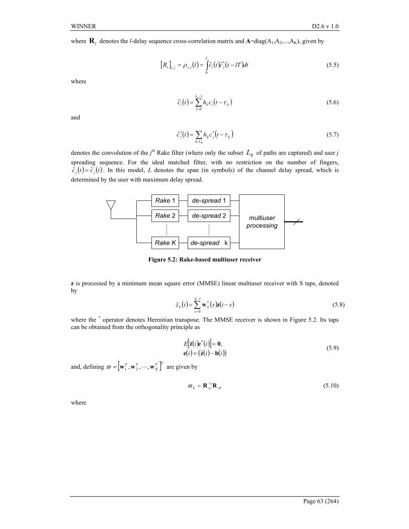
WINNER D2.6 v 1.0

Page 63 (264)

where lR denotes the l-delay sequence cross-correlation matrix and A=diag(A1,A2,...,AK), given by

[ ] ( ) ( ) ( )∫ −==T

jijijil dtlTtctclR0

*,, ˆ~ρ (5.5)

where

( ) ( )∑−

=

−=1

0

~ iL

lliilii tchtc τ (5.6)

and

( ) ( )∑∈

−=RLl

ljjljj tchtc τ**ˆ (5.7)

denotes the convolution of the jth Rake filter (where only the subset RL of paths are captured) and user j spreading sequence. For the ideal matched filter, with no restriction on the number of fingers,

( ) ( )tctc jj~ˆ = . In this model, L denotes the span (in symbols) of the channel delay spread, which is

determined by the user with maximum delay spread.

Rake 1

Rake 2

Rake K

de-spread 1

de-spread 2

de-spread k

multiuserprocessing

Figure 5.2: Rake-based multiuser receiver

z is processed by a minimum mean square error (MMSE) linear multiuser receiver with S taps, denoted by

( ) ( ) ( )∑−

=

−=1

0

*S

skk sisiz zw (5.8)

where the * operator denotes Hermitian transpose. The MMSE receiver is shown in Figure 5.2. Its taps can be obtained from the orthogonality principle as

( ) ( )[ ]( ) ( ) ( )( )iii

iiEbze0ez

−== ,*

(5.9)

and, defining [ ]TTK

TT www ,,, 21 L=ϖ are given by

zbzzk RR 1−=ϖ (5.10)

where

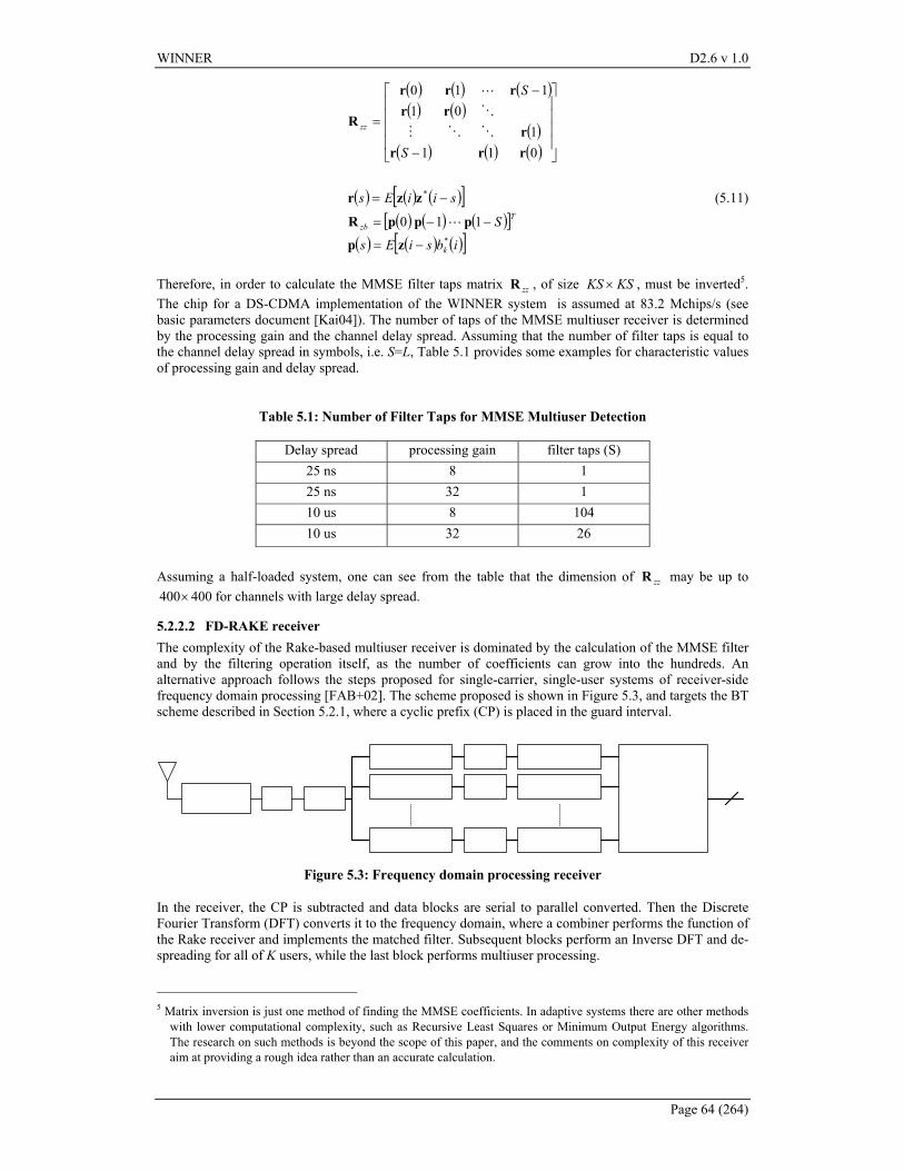
WINNER D2.6 v 1.0

Page 64 (264)

( ) ( ) ( )( ) ( )

( )( ) ( ) ( )

( ) ( ) ( )[ ]( ) ( ) ( )[ ]

( ) ( ) ( )[ ]ibsiEs

S

siiEs

S

S

k

Tzb

zz

*

*

110

0111

01110

−=

−−=

−=

−

−

=

zp

pppR

zzr

rrrr

rrrrr

R

L

OOM

O

L

(5.11)

Therefore, in order to calculate the MMSE filter taps matrix zzR , of size KSKS × , must be inverted5. The chip for a DS-CDMA implementation of the WINNER system is assumed at 83.2 Mchips/s (see basic parameters document [Kai04]). The number of taps of the MMSE multiuser receiver is determined by the processing gain and the channel delay spread. Assuming that the number of filter taps is equal to the channel delay spread in symbols, i.e. S=L, Table 5.1 provides some examples for characteristic values of processing gain and delay spread.

Table 5.1: Number of Filter Taps for MMSE Multiuser Detection

Delay spread processing gain filter taps (S) 25 ns 8 1 25 ns 32 1 10 us 8 104 10 us 32 26

Assuming a half-loaded system, one can see from the table that the dimension of zzR may be up to

400400× for channels with large delay spread.

5.2.2.2 FD-RAKE receiver The complexity of the Rake-based multiuser receiver is dominated by the calculation of the MMSE filter and by the filtering operation itself, as the number of coefficients can grow into the hundreds. An alternative approach follows the steps proposed for single-carrier, single-user systems of receiver-side frequency domain processing [FAB+02]. The scheme proposed is shown in Figure 5.3, and targets the BT scheme described in Section 5.2.1, where a cyclic prefix (CP) is placed in the guard interval.

Figure 5.3: Frequency domain processing receiver

In the receiver, the CP is subtracted and data blocks are serial to parallel converted. Then the Discrete Fourier Transform (DFT) converts it to the frequency domain, where a combiner performs the function of the Rake receiver and implements the matched filter. Subsequent blocks perform an Inverse DFT and de-spreading for all of K users, while the last block performs multiuser processing.

5 Matrix inversion is just one method of finding the MMSE coefficients. In adaptive systems there are other methods

with lower computational complexity, such as Recursive Least Squares or Minimum Output Energy algorithms. The research on such methods is beyond the scope of this paper, and the comments on complexity of this receiver aim at providing a rough idea rather than an accurate calculation.

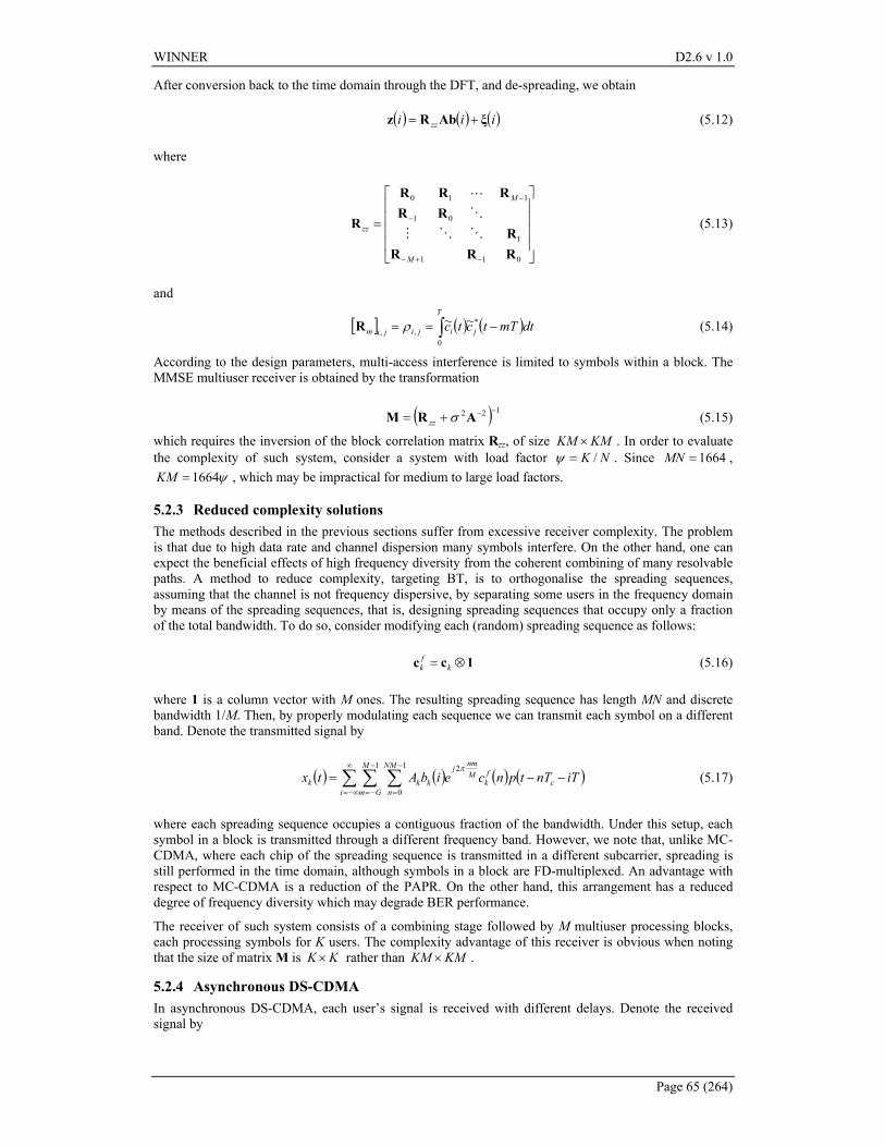
WINNER D2.6 v 1.0

Page 65 (264)

After conversion back to the time domain through the DFT, and de-spreading, we obtain

( ) ( ) ( )iii zz ξAbRz += (5.12)

where

=

−+−

−

−

011

1

01

110

RRRR

RRRRR

R

M

M

zz OOM

O

L

(5.13)

and

[ ] ( ) ( )∫ −==T

jijijim dtmTtctc0

*,,

~~ρR (5.14)

According to the design parameters, multi-access interference is limited to symbols within a block. The MMSE multiuser receiver is obtained by the transformation

( ) 122 −−+= ARM σzz (5.15)

which requires the inversion of the block correlation matrix Rzz, of size KMKM × . In order to evaluate the complexity of such system, consider a system with load factor NK /=ψ . Since 1664=MN ,

ψ1664=KM , which may be impractical for medium to large load factors.

5.2.3 Reduced complexity solutions The methods described in the previous sections suffer from excessive receiver complexity. The problem is that due to high data rate and channel dispersion many symbols interfere. On the other hand, one can expect the beneficial effects of high frequency diversity from the coherent combining of many resolvable paths. A method to reduce complexity, targeting BT, is to orthogonalise the spreading sequences, assuming that the channel is not frequency dispersive, by separating some users in the frequency domain by means of the spreading sequences, that is, designing spreading sequences that occupy only a fraction of the total bandwidth. To do so, consider modifying each (random) spreading sequence as follows:

1cc ⊗= kfk (5.16)

where 1 is a column vector with M ones. The resulting spreading sequence has length MN and discrete bandwidth 1/M. Then, by properly modulating each sequence we can transmit each symbol on a different band. Denote the transmitted signal by

( ) ( ) ( ) ( )∑ ∑ ∑∞

−∞=

−

−=

−

=

−−=i

M

Gm

NM

nc

fk

Mnmj

kkk iTnTtpnceibAtx1 1

0

2π (5.17)

where each spreading sequence occupies a contiguous fraction of the bandwidth. Under this setup, each symbol in a block is transmitted through a different frequency band. However, we note that, unlike MC-CDMA, where each chip of the spreading sequence is transmitted in a different subcarrier, spreading is still performed in the time domain, although symbols in a block are FD-multiplexed. An advantage with respect to MC-CDMA is a reduction of the PAPR. On the other hand, this arrangement has a reduced degree of frequency diversity which may degrade BER performance.

The receiver of such system consists of a combining stage followed by M multiuser processing blocks, each processing symbols for K users. The complexity advantage of this receiver is obvious when noting that the size of matrix M is KK × rather than KMKM × .

5.2.4 Asynchronous DS-CDMA In asynchronous DS-CDMA, each user’s signal is received with different delays. Denote the received signal by

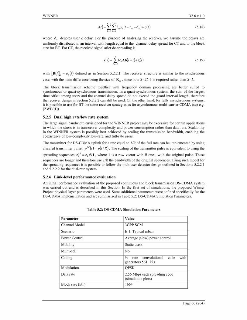
WINNER D2.6 v 1.0

Page 66 (264)

( ) ( ) ( )∑ ∑−

=

−

=

+−−=1

0

1

0

K

k

L

lklkklk

k

ttxhty ηδτ (5.18)

where kδ denotes user k delay. For the purpose of analysing the receiver, we assume the delays are uniformly distributed in an interval with length equal to the channel delay spread for CT and to the block size for BT. For CT, the received signal after de-spreading is

( ) ( ) ( )∑−=

+−=L

Lll ilii ξAbRz (5.19)

with ( )[ ] ( )ll ijij ρ=R defined as in Section 5.2.2.1. The receiver structure is similar to the synchronous case, with the main difference being the size of zzR , since now S=2L-1 is required rather than S=L.

The block transmission scheme together with frequency domain processing are better suited to synchronous or quasi-synchronous transmission. In a quasi-synchronous system, the sum of the largest time offset among users and the channel delay spread do not exceed the guard interval length, therefore the receiver design in Section 5.2.2.2 can still be used. On the other hand, for fully asynchronous systems, it is possible to use for BT the same receiver strategies as for asynchronous multi-carrier CDMA (see e.g. [ZWB01]).

5.2.5 Dual high rate/low rate system The large signal bandwidth envisioned for the WINNER project may be excessive for certain applications in which the stress is in transceiver complexity and power consumption rather than data rate. Scalability in the WINNER system is possibly best achieved by scaling the transmission bandwidth, enabling the coexistence of low-complexity low-rate, and full-rate users.

The transmitter for DS-CDMA uplink for a rate equal to 1/R of the full rate can be implemented by using a scaled transmitter pulse, ( ) ( )RtptpLR /= . The scaling of the transmitter pulse is equivalent to using the

spreading sequences 1cc ⊗= kLRk , where 1 is a row vector with R ones, with the original pulse. These

sequences are longer and therefore use 1/R the bandwidth of the original sequences. Using such model for the spreading sequences it is possible to follow the multiuser detector design outlined in Sections 5.2.2.1 and 5.2.2.2 for the dual-rate system.

5.2.6 Link-level performance evaluation An initial performance evaluation of the proposed continuous and block transmission DS-CDMA system was carried out and is described in this Section. In the first set of simulations, the proposed Winner Project physical layer parameters were used. Some additional parameters were defined specifically for the DS-CDMA implementation and are summarized in Table 5.2: DS-CDMA Simulation Parameters.

Table 5.2: DS-CDMA Simulation Parameters

Parameter Value Channel Model 3GPP SCM

Scenario B.1, Typical urban

Power Control Average (slow) power control

Mobility Static users

Multi-cell No

Coding ½ rate convolutional code with generators 561, 753

Modulation QPSK

Data rate 2.56 Mbps each spreading code (simulation plots)

Block size (BT) 1664

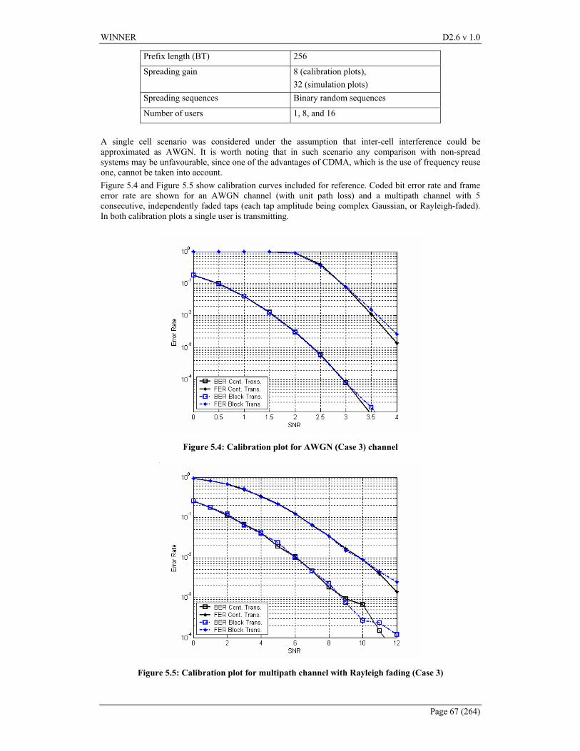
WINNER D2.6 v 1.0

Page 67 (264)

Prefix length (BT) 256

Spreading gain 8 (calibration plots), 32 (simulation plots)

Spreading sequences Binary random sequences

Number of users 1, 8, and 16

A single cell scenario was considered under the assumption that inter-cell interference could be approximated as AWGN. It is worth noting that in such scenario any comparison with non-spread systems may be unfavourable, since one of the advantages of CDMA, which is the use of frequency reuse one, cannot be taken into account. Figure 5.4 and Figure 5.5 show calibration curves included for reference. Coded bit error rate and frame error rate are shown for an AWGN channel (with unit path loss) and a multipath channel with 5 consecutive, independently faded taps (each tap amplitude being complex Gaussian, or Rayleigh-faded). In both calibration plots a single user is transmitting.

Figure 5.4: Calibration plot for AWGN (Case 3) channel

Figure 5.5: Calibration plot for multipath channel with Rayleigh fading (Case 3)

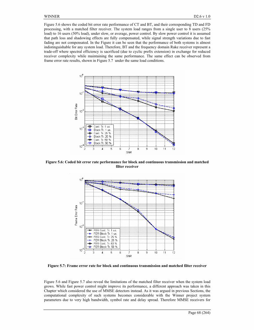
WINNER D2.6 v 1.0

Page 68 (264)

Figure 5.6 shows the coded bit error rate performance of CT and BT, and their corresponding TD and FD processing, with a matched filter receiver. The system load ranges from a single user to 8 users (25% load) to 16 users (50% load), under slow, or average, power control. By slow power control it is assumed that path loss and shadowing effects are fully compensated, while signal strength variations due to fast fading are not compensated. In the Figure it can be seen that the performance of both systems is almost indistinguishable for any system load. Therefore, BT and the frequency domain Rake receiver represent a trade-off where spectral efficiency is sacrificed (due to cyclic prefix extension) in exchange for reduced receiver complexity while maintaining the same performance. The same effect can be observed from frame error rate results, shown in Figure 5.7 under the same load conditions.

Figure 5.6: Coded bit error rate performance for block and continuous transmission and matched filter receiver

Figure 5.7: Frame error rate for block and continuous transmission and matched filter receiver

Figure 5.6 and Figure 5.7 also reveal the limitations of the matched filter receiver when the system load grows. While fast power control might improve its performance, a different approach was taken in this Chapter which considered the use of MMSE detectors instead. As it was argued in previous Sections, the computational complexity of such systems becomes considerable with the Winner project system parameters due to very high bandwidth, symbol rate and delay spread. Therefore MMSE receivers for

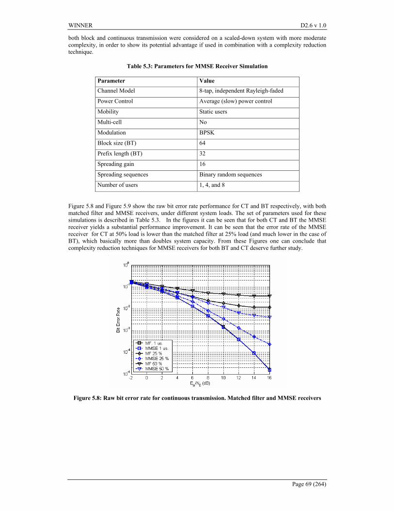
WINNER D2.6 v 1.0

Page 69 (264)

both block and continuous transmission were considered on a scaled-down system with more moderate complexity, in order to show its potential advantage if used in combination with a complexity reduction technique.

Table 5.3: Parameters for MMSE Receiver Simulation

Parameter Value Channel Model 8-tap, independent Rayleigh-faded

Power Control Average (slow) power control

Mobility Static users

Multi-cell No

Modulation BPSK

Block size (BT) 64

Prefix length (BT) 32

Spreading gain 16

Spreading sequences Binary random sequences

Number of users 1, 4, and 8

Figure 5.8 and Figure 5.9 show the raw bit error rate performance for CT and BT respectively, with both matched filter and MMSE receivers, under different system loads. The set of parameters used for these simulations is described in Table 5.3. In the figures it can be seen that for both CT and BT the MMSE receiver yields a substantial performance improvement. It can be seen that the error rate of the MMSE receiver for CT at 50% load is lower than the matched filter at 25% load (and much lower in the case of BT), which basically more than doubles system capacity. From these Figures one can conclude that complexity reduction techniques for MMSE receivers for both BT and CT deserve further study.

Figure 5.8: Raw bit error rate for continuous transmission. Matched filter and MMSE receivers

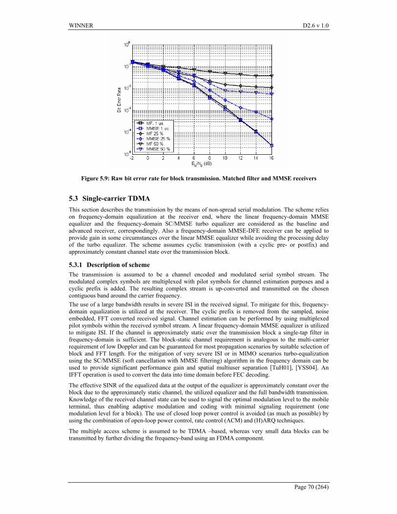
WINNER D2.6 v 1.0

Page 70 (264)

Figure 5.9: Raw bit error rate for block transmission. Matched filter and MMSE receivers

5.3 Single-carrier TDMA This section describes the transmission by the means of non-spread serial modulation. The scheme relies on frequency-domain equalization at the receiver end, where the linear frequency-domain MMSE equalizer and the frequency-domain SC/MMSE turbo equalizer are considered as the baseline and advanced receiver, correspondingly. Also a frequency-domain MMSE-DFE receiver can be applied to provide gain in some circumstances over the linear MMSE equalizer while avoiding the processing delay of the turbo equalizer. The scheme assumes cyclic transmission (with a cyclic pre- or postfix) and approximately constant channel state over the transmission block.

5.3.1 Description of scheme The transmission is assumed to be a channel encoded and modulated serial symbol stream. The modulated complex symbols are multiplexed with pilot symbols for channel estimation purposes and a cyclic prefix is added. The resulting complex stream is up-converted and transmitted on the chosen contiguous band around the carrier frequency. The use of a large bandwidth results in severe ISI in the received signal. To mitigate for this, frequency-domain equalization is utilized at the receiver. The cyclic prefix is removed from the sampled, noise embedded, FFT converted received signal. Channel estimation can be performed by using multiplexed pilot symbols within the received symbol stream. A linear frequency-domain MMSE equalizer is utilized to mitigate ISI. If the channel is approximately static over the transmission block a single-tap filter in frequency-domain is sufficient. The block-static channel requirement is analogous to the multi-carrier requirement of low Doppler and can be guaranteed for most propagation scenarios by suitable selection of block and FFT length. For the mitigation of very severe ISI or in MIMO scenarios turbo-equalization using the SC/MMSE (soft cancellation with MMSE filtering) algorithm in the frequency domain can be used to provide significant performance gain and spatial multiuser separation [TuH01], [YSS04]. An IFFT operation is used to convert the data into time domain before FEC decoding.

The effective SINR of the equalized data at the output of the equalizer is approximately constant over the block due to the approximately static channel, the utilized equalizer and the full bandwidth transmission. Knowledge of the received channel state can be used to signal the optimal modulation level to the mobile terminal, thus enabling adaptive modulation and coding with minimal signaling requirement (one modulation level for a block). The use of closed loop power control is avoided (as much as possible) by using the combination of open-loop power control, rate control (ACM) and (H)ARQ techniques.

The multiple access scheme is assumed to be TDMA –based, whereas very small data blocks can be transmitted by further dividing the frequency-band using an FDMA component.

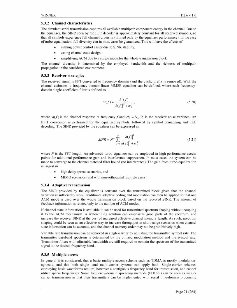
WINNER D2.6 v 1.0

Page 71 (264)

5.3.2 Channel characteristics The circulant serial transmission captures all available multipath component energy in the channel. Due to the equalizer, the SINR seen by the FEC decoder is approximately constant for all received symbols, so that all symbols experience full channel diversity (limited only by the equalizer performance). In the case of turbo equalization, full diversity can in most cases be guaranteed. This will have the effects of

• making power control easier due to SINR stability, • easing channel code design, • simplifying ACM due to a single mode for the whole transmission block.

The channel diversity is determined by the employed bandwidth and the richness of multipath propagation in the considered environment.

5.3.3 Receiver strategies The received signal is FFT-converted to frequency domain (and the cyclic prefix is removed). With the channel estimates, a frequency-domain linear MMSE equalizer can be defined, where each frequency-domain single-coefficient filter is defined as

20

2

*

)(

)()(

σ+=

fh

fhfw , (5.20)

where )( fh is the channel response at frequency f and 2/020 N=σ is the receiver noise variance. An

IFFT conversion is performed for the equalized symbols, followed by symbol demapping and FEC decoding. The SINR provided by the equalizer can be expressed as

∑=

−

+=

N

f fh

fhNSINR

120

2

21

)(

)(

σ (5.21)

where N is the FFT length. An advanced turbo equalizer can be employed in high performance access points for additional performance gain and interference suppression. In most cases the system can be made to converge to the channel matched filter bound (no interference). The gain from turbo-equalization is largest in

• high delay spread scenarios, and • MIMO scenarios (and with non-orthogonal multiple users).

5.3.4 Adaptive transmission The SINR provided by the equalizer is constant over the transmitted block given that the channel variation is sufficiently slow. Traditional adaptive coding and modulation can then be applied so that one ACM mode is used over the whole transmission block based on the received SINR. The amount of feedback information is related only to the number of ACM modes.

If channel state information is available it can be used for transmitted spectrum shaping without coupling it to the ACM mechanism. A water-filling solution can emphasize good parts of the spectrum, and increase the receiver SINR at the cost of increased effective channel memory length. As such, spectrum shaping could be seen as an effective way to increase throughput in short-range scenarios when channel state information can be accurate, and the channel memory order may not be prohibitively high.

Variable rate transmission can be achieved in single-carrier by adjusting the transmitted symbol rate. The transmitter baseband spectrum is determined by the utilized modulation method and the symbol rate. Transmitter filters with adjustable bandwidth are still required to contain the spectrum of the transmitted signal to the desired frequency band.

5.3.5 Multiple access In general it is considered, that a basic multiple-access scheme such as TDMA is mostly modulation-agnostic, and that both single- and multi-carrier systems can apply both. Single-carrier schemes employing basic waveforms require, however a contiguous frequency band for transmission, and cannot utilize sparse frequencies. Some frequency-domain spreading methods (FDOSS) can be seen as single-carrier transmission in that their transmitters can be implemented with serial time-domain processing

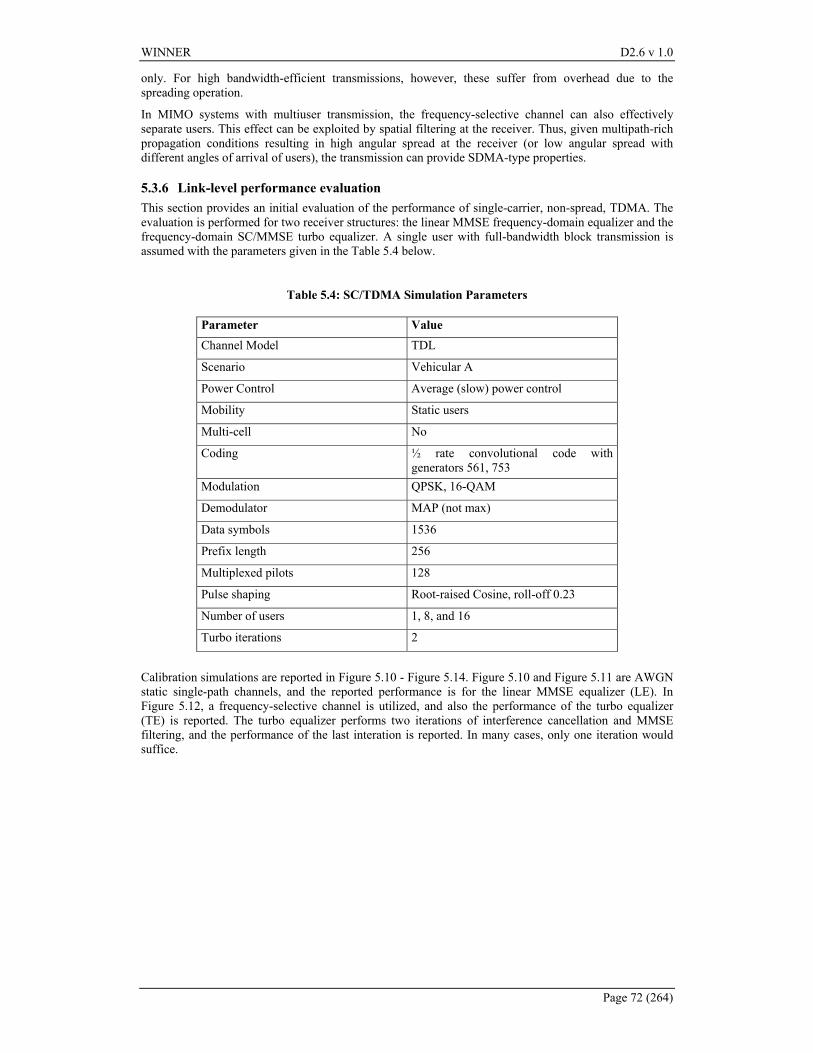
WINNER D2.6 v 1.0

Page 72 (264)

only. For high bandwidth-efficient transmissions, however, these suffer from overhead due to the spreading operation.

In MIMO systems with multiuser transmission, the frequency-selective channel can also effectively separate users. This effect can be exploited by spatial filtering at the receiver. Thus, given multipath-rich propagation conditions resulting in high angular spread at the receiver (or low angular spread with different angles of arrival of users), the transmission can provide SDMA-type properties.

5.3.6 Link-level performance evaluation This section provides an initial evaluation of the performance of single-carrier, non-spread, TDMA. The evaluation is performed for two receiver structures: the linear MMSE frequency-domain equalizer and the frequency-domain SC/MMSE turbo equalizer. A single user with full-bandwidth block transmission is assumed with the parameters given in the Table 5.4 below.

Table 5.4: SC/TDMA Simulation Parameters

Parameter Value Channel Model TDL

Scenario Vehicular A

Power Control Average (slow) power control

Mobility Static users

Multi-cell No

Coding ½ rate convolutional code with generators 561, 753

Modulation QPSK, 16-QAM

Demodulator MAP (not max)

Data symbols 1536

Prefix length 256

Multiplexed pilots 128

Pulse shaping Root-raised Cosine, roll-off 0.23

Number of users 1, 8, and 16

Turbo iterations 2

Calibration simulations are reported in Figure 5.10 - Figure 5.14. Figure 5.10 and Figure 5.11 are AWGN static single-path channels, and the reported performance is for the linear MMSE equalizer (LE). In Figure 5.12, a frequency-selective channel is utilized, and also the performance of the turbo equalizer (TE) is reported. The turbo equalizer performs two iterations of interference cancellation and MMSE filtering, and the performance of the last interation is reported. In many cases, only one iteration would suffice.

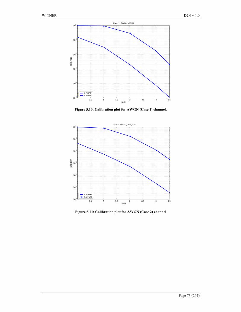
WINNER D2.6 v 1.0

Page 73 (264)

0.5 1 1.5 2 2.5 3 3.510

−5

10−4

10−3

10−2

10−1

100

SNR

BE

R,F

ER

Case 1: AWGN, QPSK

LE BERLE FER

Figure 5.10: Calibration plot for AWGN (Case 1) channel.

6.5 7 7.5 8 8.5 9 9.510

−6

10−5

10−4

10−3

10−2

10−1

100

SNR

BE

R,F

ER

Case 2: AWGN, 16−QAM

LE BERLE FER

Figure 5.11: Calibration plot for AWGN (Case 2) channel

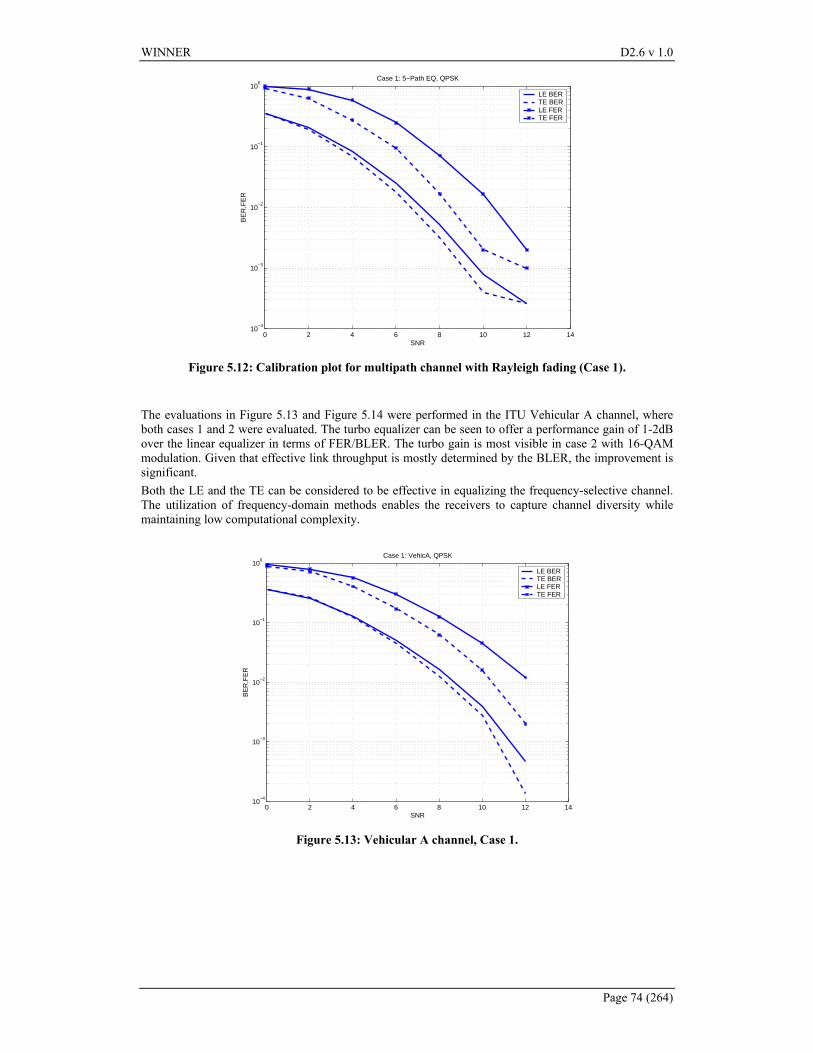
WINNER D2.6 v 1.0

Page 74 (264)

0 2 4 6 8 10 12 1410

−4

10−3

10−2

10−1

100

SNR

BE

R,F

ER

Case 1: 5−Path EQ, QPSK

LE BERTE BERLE FERTE FER

Figure 5.12: Calibration plot for multipath channel with Rayleigh fading (Case 1).

The evaluations in Figure 5.13 and Figure 5.14 were performed in the ITU Vehicular A channel, where both cases 1 and 2 were evaluated. The turbo equalizer can be seen to offer a performance gain of 1-2dB over the linear equalizer in terms of FER/BLER. The turbo gain is most visible in case 2 with 16-QAM modulation. Given that effective link throughput is mostly determined by the BLER, the improvement is significant. Both the LE and the TE can be considered to be effective in equalizing the frequency-selective channel. The utilization of frequency-domain methods enables the receivers to capture channel diversity while maintaining low computational complexity.

0 2 4 6 8 10 12 1410

−4

10−3

10−2

10−1

100

SNR

BE

R,F

ER

Case 1: VehicA, QPSK

LE BERTE BERLE FERTE FER

Figure 5.13: Vehicular A channel, Case 1.

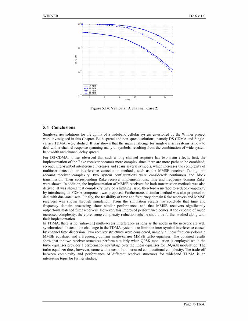
WINNER D2.6 v 1.0

Page 75 (264)

4 6 8 10 12 1410

−3

10−2

10−1

100

SNR

BE

R,F

ER

LE BERTE BERLE FERTE FER

Figure 5.14: Vehicular A channel, Case 2.

5.4 Conclusions Single-carrier solutions for the uplink of a wideband cellular system envisioned by the Winner project were investigated in this Chapter. Both spread and non-spread solutions, namely DS-CDMA and Single-carrier TDMA, were studied. It was shown that the main challenge for single-carrier systems is how to deal with a channel response spanning many of symbols, resulting from the combination of wide system bandwidth and channel delay spread. For DS-CDMA, it was observed that such a long channel response has two main effects: first, the implementation of the Rake receiver becomes more complex since there are more paths to be combined; second, inter-symbol interference increases and spans several symbols, which increases the complexity of multiuser detection or interference cancellation methods, such as the MMSE receiver. Taking into account receiver complexity, two system configurations were considered: continuous and block transmission. Their corresponding Rake receiver implementations, time and frequency domain Rake, were shown. In addition, the implementation of MMSE receivers for both transmission methods was also derived. It was shown that complexity may be a limiting issue, therefore a method to reduce complexity by introducing an FDMA component was proposed. Furthermore, a similar method was also proposed to deal with dual-rate users. Finally, the feasibility of time and frequency domain Rake receivers and MMSE receivers was shown through simulation. From the simulation results we conclude that time and frequency domain processing show similar performance, and that MMSE receivers significantly outperform matched filter receivers. However, this improved performance comes at the expense of much increased complexity, therefore, some complexity reduction scheme should be further studied along with their implementation. In TDMA, there is no (intra-cell) multi-access interference as long as the nodes in the network are well synchronized. Instead, the challenge in the TDMA system is to limit the inter-symbol interference caused by channel time dispersion. Two receiver structures were considered, namely a linear frequency-domain MMSE equalizer and a frequency-domain single-carrier MMSE turbo equalizer. The obtained results show that the two receiver structures perform similarly when QPSK modulation is employed while the turbo equalizer provides a performance advantage over the linear equalizer for 16QAM modulation. The turbo equalizer does, however, come with a cost of an increased computational complexity. The trade-off between complexity and performance of different receiver structures for wideband TDMA is an interesting topic for further studies.

WINNER D2.6 v 1.0

Page 76 (264)

6. Multi-Carrier Access Technologies – FDMA/TDMA Higher spectral efficiency is a key issue to meet the requirements on the WINNER air interface. A promising approach, in particular for the downlink, is to minimize interference between users within a sector/cell by orthogonal signalling in the form of Orthogonal Frequency Division Multiplexing (OFDM). Multiple users may then in a flexible manner share the total bandwidth by orthogonally multiplexing their data in time, frequency or jointly in time and frequency. In an OFDM system that adapts to the channel selectivity in time and/or frequency, spectral efficiency can be improved by allocating time, frequency or joint time-frequency resources based on throughput requirements, quality of service constraints and the channel quality of each user. A scheduler, which optimizes the resource allocation for multiple active users, becomes a key element in such a solution. By using link adaptation in the time-frequency resources, i.e. adaptively allocating power and/or adapting the modulation and coding scheme (MCS) to the channel conditions, spectral efficiency of the system can be further improved. In an adaptive OFDM system, where orthogonal time-frequency resources are given to the user who can utilize them best, the spectral efficiency will increase with the number of active users. This effect is referred to as ‘multi-user diversity’. In general, a minimum service requirement to the individual users (fairness criterion) is a constraint to the achievable gain in spectral efficiency with respect to multi-user diversity. In the uplink we are faced with less coordinated individual user signals. Designing a multiple access scheme based on Orthogonal Frequency Division Multiple Access (OFDMA) requires advanced frequency synchronization algorithms to avoid subcarrier interference due to less synchronized transmitter frequency (phase noise), Doppler shifts, and non-linear amplifiers, since they are sensitive to the large envelope variations in an OFDM signal (peak-to-average power ratio, PAPR). The large PAPR of OFDM is a problem also for the downlink, but more linear and thus more costly amplifiers are normally possible to use in the base stations. The channel adaptation can be based on channel estimation, where the scheduler typically performs resource allocation based on the slow (large-scale) fading characteristics of the individual user’s channels. If accurate enough channel state information is available at the scheduler, it can perform fast resource allocation based on the individual user’s instantaneous channel characteristics. The channel state information (CSI) can be found by channel prediction. In TDD, the channel predictors could potentially be located in either the base station or the mobile station (under the assumption of channel reciprocity), whereas in FDD the channel predictors for the downlink have to be located in the mobile stations and the prediction result feed back to the base station. In the downlink the base station performs a multiplexing operation of the user’s data streams onto the downlink channel, and in the uplink the channel access rules form a multiple-access scheme. For simplicity, we denote frequency adaptive multiple-access/multiplexing with OFDM modulation as OFDMA, time adaptive multiple-access/multiplexing with OFDM modulation as TDMA and time-frequency adaptive multiple-access/multiplexing with OFDM modulation as TDMA/OFDMA, see Figure 6.1 for an example. In this figure, we assume that the minimum transmission unit is a channel element (bin) comprising N subcarriers in frequency and extending K symbols in time (so in total, there are N*K symbols within a channel element). In all cases, provided that N > 1, we have multi-carrier transmission.

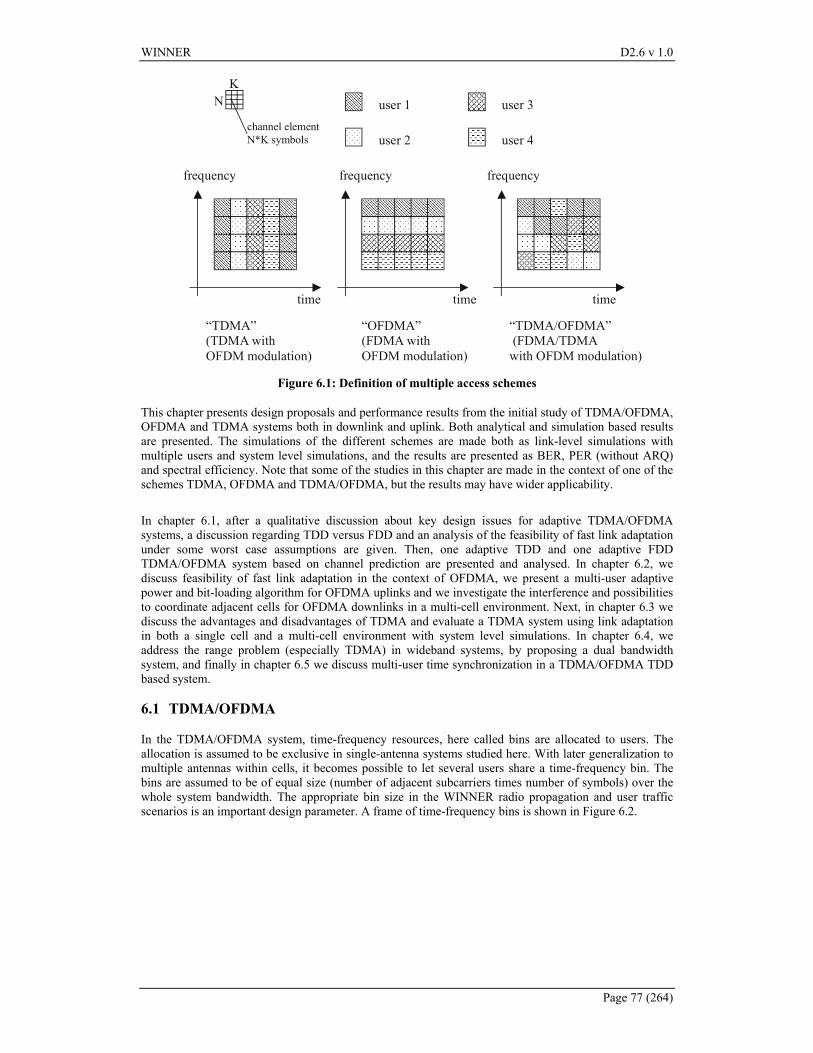
WINNER D2.6 v 1.0

Page 77 (264)

user 1

user 2

user 3

user 4

time

frequency

“TDMA” (TDMA with OFDM modulation)

frequency

time

“OFDMA” (FDMA with OFDM modulation)

frequency

time

“TDMA/OFDMA”(FDMA/TDMA

with OFDM modulation)

N K

channel element N*K symbols

Figure 6.1: Definition of multiple access schemes

This chapter presents design proposals and performance results from the initial study of TDMA/OFDMA, OFDMA and TDMA systems both in downlink and uplink. Both analytical and simulation based results are presented. The simulations of the different schemes are made both as link-level simulations with multiple users and system level simulations, and the results are presented as BER, PER (without ARQ) and spectral efficiency. Note that some of the studies in this chapter are made in the context of one of the schemes TDMA, OFDMA and TDMA/OFDMA, but the results may have wider applicability. In chapter 6.1, after a qualitative discussion about key design issues for adaptive TDMA/OFDMA systems, a discussion regarding TDD versus FDD and an analysis of the feasibility of fast link adaptation under some worst case assumptions are given. Then, one adaptive TDD and one adaptive FDD TDMA/OFDMA system based on channel prediction are presented and analysed. In chapter 6.2, we discuss feasibility of fast link adaptation in the context of OFDMA, we present a multi-user adaptive power and bit-loading algorithm for OFDMA uplinks and we investigate the interference and possibilities to coordinate adjacent cells for OFDMA downlinks in a multi-cell environment. Next, in chapter 6.3 we discuss the advantages and disadvantages of TDMA and evaluate a TDMA system using link adaptation in both a single cell and a multi-cell environment with system level simulations. In chapter 6.4, we address the range problem (especially TDMA) in wideband systems, by proposing a dual bandwidth system, and finally in chapter 6.5 we discuss multi-user time synchronization in a TDMA/OFDMA TDD based system.

6.1 TDMA/OFDMA

In the TDMA/OFDMA system, time-frequency resources, here called bins are allocated to users. The allocation is assumed to be exclusive in single-antenna systems studied here. With later generalization to multiple antennas within cells, it becomes possible to let several users share a time-frequency bin. The bins are assumed to be of equal size (number of adjacent subcarriers times number of symbols) over the whole system bandwidth. The appropriate bin size in the WINNER radio propagation and user traffic scenarios is an important design parameter. A frame of time-frequency bins is shown in Figure 6.2.

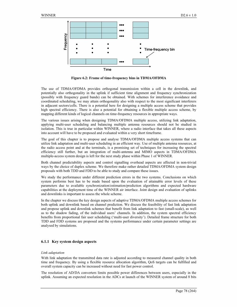
WINNER D2.6 v 1.0

Page 78 (264)

•••

•••

•••

•••

•••

•••

•••

TimeFr

eque

ncy

•••

Time-frequency bin

•••

•••

•••

•••

•••

•••

•••

TimeFr

eque

ncy

•••

Time-frequency bin

Figure 6.2: Frame of time-frequency bins in TDMA/OFDMA

The use of TDMA/OFDMA provides orthogonal transmission within a cell in the downlink, and potentially also orthogonality in the uplink if sufficient time alignment and frequency synchronization (possibly with frequency guard bands) can be obtained. With schemes for interference avoidance and coordinated scheduling, we may attain orthogonality also with respect to the most significant interferers in adjacent sectors/cells. There is a potential here for designing a multiple access scheme that provides high spectral efficiency. There is also a potential for obtaining a flexible multiple access scheme, by mapping different kinds of logical channels on time-frequency resources in appropriate ways.

The various issues arising when designing TDMA/OFDMA multiple access, utilizing link adaptation, applying multi-user scheduling and balancing multiple antenna resources should not be studied in isolation. This is true in particular within WINNER, where a radio interface that takes all these aspects into account will have to be proposed and evaluated within a very short timeframe.

The goal of this chapter is to propose and analyse TDMA/OFDMA multiple access systems that can utilize link adaptation and multi-user scheduling in an efficient way. Use of multiple antenna resources, at the radio access point and at the terminals, is a promising set of techniques for increasing the spectral efficiency still further, but an integration of multi-antenna and MIMO aspects in TDMA/OFDMA multiple-access system design is left for the next study phase within Phase 1 of WINNER.

Both channel predictability aspects and control signalling overhead aspects are affected in non-trivial ways by the choice of duplex scheme. We therefore make rather detailed TDMA/OFDMA system design proposals with both TDD and FDD to be able to study and compare these issues.

We study the performance under different prediction errors in the two systems. Conclusions on which system performs best has to be made based upon the evaluation of attainable error levels of these parameters due to available synchronization/estimation/prediction algorithms and expected hardware capabilities at the deployment time of the WINNER air interface. Joint design and evaluation of uplinks and downlinks is important to assess the whole scheme.

In the chapter we discuss the key design aspects of adaptive TDMA/OFDMA multiple access schemes for both uplink and downlink based on channel prediction. We discuss the feasibility of fast link adaptation and propose uplink and downlink schemes that benefit from link adaptation to fast (small-scale), as well as to the shadow fading, of the individual users’ channels. In addition, the system spectral efficiency benefits from proportional fair user scheduling (‘multi-user diversity’). Detailed frame structure for both TDD and FDD systems are proposed and the systems performance under certain parameter settings are analysed by simulations.

6.1.1 Key system design aspects Link adaptation With link adaptation the transmitted data rate is adjusted according to measured channel quality in both time and frequency. By using a flexible resource allocation algorithm, QoS targets can be fulfilled and overall system capacity can be increased without need for fast power control.

The resolution of AD/DA converters limits possible power differences between users, especially in the uplink. Assuming an expected resolution in the ADCs at launch of the WINNER system of around 8 bits

WINNER D2.6 v 1.0

Page 79 (264)

at 200 MHz sampling frequency in the MSs and around 14 bits at 200 MHz in the BSs, our system proposals focus on adaptive bit-loading using adaptive coding and modulation, but without adaptive power allocation per subcarrier.

Scheduling

Multi-user scheduling provides an additional scheduling gain, called ‘multi-user diversity’. The reason for this is that the variations of channels to/from different terminals will be uncorrelated. We may then increase the spectral efficiency of the system by allocating resources to users with the instantaneously best channels, under the QoS constraints of the active users’ calls/sessions. The total throughput then increases with the number of active users in a cell, in contrast with present CDMA systems, where it decreases with the number of users due to system self-interference.

The choice of user scheduling algorithm is central in a spectrally efficient adaptive TDMA/OFDMA system. The algorithm should balance the goal to maximize system throughput, but at the same time provide a certain degree of fairness between the users and their user data flows. In general, the fairness criteria between users and the system capacity with respect to different QoS classes should be tuneable in order to satisfy operators having different business models regarding offered services and user subscription models.

Inter-cell interference mitigation under small frequency reuse factor

Inter-cell interference avoidance is another important application for scheduling to reduce the frequency reuse factor in cellular systems, by coordinating users at the cell-borders of adjacent cells. This is especially important in TDD systems as discussed later. We have to balance the SINR within cells with the resource reuse between cells. Scheduling can easily be coordinated between sectors/beams of a radio access point, to reduce interference. To reduce interference between opposing sectors, a very simple semi-static solution is to use a separate time-frequency allocation in high-interference areas, which is reused with reuse factor 3 [SOAS03]. This results in a system with good SIR in most parts of sectors within a regular hexagonal pattern. The total reuse factor is between 1 and 2. A more flexible approach, with potentially better performance in less than fully loaded systems, is to coordinate the use of time-frequency bins also with respect to the opposing sector, in the high-interference outer parts of the sectors (see chapter 6.2.3 in the context of OFDMA). Another tool is to use relays in outer parts of sectors. However, both these methods imply increased control signalling between base stations/relays and additional signalling delays. Channel prediction

An adaptive scheme requires prediction of the channel state, over a time horizon D that covers the total feedback delay. Different designs of TDMA/OFDMA systems along with different duplex schemes will result in different feedback delays. The feedback delay limits the largest terminal velocity v for which fast link adaptation can be used. The key property is the required normalized prediction horizon in space, expressed as a fraction of the carrier wavelength λ and prediction horizon in time D,

λ/vD (6.1)

Prediction over significantly more than 1/3 carrier wavelength will be infeasible in most propagation environments, under realistic assumptions on the SNR and the utilized prediction algorithm [ESA02]. In equation (6.1) we also see the dependence of the carrier frequency. The lower the carrier frequency, the larger maximal user speed can be supported, given a predictor with a certain prediction horizon. The predictability as a function of the SNR and the required prediction horizon will be characterized in more detail in Section 6.1.6.2.

Impact of channel state prediction errors

The performance of link adaptation degrades with increasing prediction uncertainty. This problem can be handled by first using robust adjustments of rate limits in the coding-modulation schemes, so that the design goals are fulfilled and constraints are met also in the presence of SINR prediction errors. If spectral efficiency is to be maximized under BER constraints, with various power constraints, the methods presented in [FSES04] can be applied. If the aim is to maximize the number of bits in error-free bins, the solution is presented in [SF04].

Moreover, the impact of prediction errors can be mitigated by some form of (more or less) opportunistic multi-user scheduling. An opportunistic scheduler will tend to give the bins to the user who has the best channel in these bins, while fulfilling various QoS constraints. Opportunistic scheduling makes the system more robust with respect to prediction errors [SF04], [Ekm02]: the prediction error for a locally

WINNER D2.6 v 1.0

Page 80 (264)

good channel is lower than for a channel experiencing a fading dip. As the number of active users is increased, fewer bins in the system are allocated to users with relatively bad channels. The effect of prediction errors will therefore decrease with the number of active users.

Fallback mode

Adaptive transmission is feasible only up to a certain velocity limit. The achievable velocity limit depends on the SINR in the channel predictor. In order to support high speed users, the proposed systems perform adaptive transmission to/from those terminals that are below the velocity limit. For the remaining users, a non-adaptive fallback mode is used that utilizes a subset of the time-frequency resources. The fallback mode could be based on coding, possibly spreading, interleaving and a safe choice of modulation format for a given average SINR. The details of the fallback mode and coexistence aspects of the adaptive and the fallback mode are subjects for further study.

Bin size

The allocation of and link adaptation within time-frequency resources are based on the assumption of an approximately flat channel within the allocated time-frequency bin. Therefore, the maximum bin size is determined by the minimum coherence bandwidth and by the minimum coherence time of the channel for users served by adaptive transmission. The minimum coherence bandwidth depends on the multi-path properties of the deployment scenario. The minimum coherence time depends on the maximal user velocity limit for which adaptive transmission is supported. Thus, supporting users with very different speeds and multi-path environments will cause the bin size to be unnecessarily small for certain users.

As a consequence, the definition of logical channels (link-level frames) and the size of the time-frequency bins should be decoupled. In this way, both small network layer packets can be efficiently supported and large channel coding blocks can be defined over several bins (with independent adaptive modulation levels) for logical channels targeted to slow or stationary users.

Control signalling The system overhead due to link adaptation signalling must be kept small, otherwise the overall spectral efficiency of the system will be deteriorated. The link adaptation overhead consists of pilots for channel estimation/prediction, control information for organizing the uplink and downlink user access and feedback information.

Feedback information

The feedback information can consist of:

• Reports of suggested modulation/coding schemes from terminals. This overhead appears in adaptive schemes based on FDD. Feedback reports are also needed in TDD systems when reciprocity with respect to SINR is not valid.

• Uplink pilots. Each uplink channel is assumed to be estimated for channel equalization purposes and predicted for input to the scheduler using unique known pilot symbols from each active user.

Maintaining orthogonality

The overhead due to maintaining orthogonality includes guard time/cyclic prefix between OFDM symbols, the Tx/Rx guard time in TDD schemes and the guard bands required to maintain orthogonality in the frequency domain of uplink transmissions. When different terminals transmit on adjacent subcarriers, inter-carrier interference will be generated due to differing velocities and non-synchronized local oscillators. Unused guard subcarriers eliminate the problem. However, their fraction of the total number of subcarriers should be low. This can be accomplished if each timeslot is shared by only a few users, or is allocated exclusively (TDMA). However, the resulting link-level frames would then be large, which would be inefficient for transmission of small packets.

Pilot schemes

Good channel prediction requires robust pilot symbols and a not too sparse, preferably regular, sampling of the channel in time. A rule of thumb is that the channel sampling rate should be at least 10 samples per wavelength. We need pilot patterns that attain this, without requiring too much pilot overhead. On the other hand, the frame time has to be small enough to provide a low required prediction horizon. A short frame time furthermore enables small delays at the physical layer, so link-layer ARQ may be used also for delay sensitive user data flows.

Control/allocation symbols can be used as additional pilot information in a decision-directed channel estimation/prediction scheme. The control symbols and the user allocation table have to use a fixed ”safe”

WINNER D2.6 v 1.0

Page 81 (264)

modulation-coding scheme that is detectable by all active users in the downlink and from all active users that are detectable by the base station in the uplink. This also requires the control/allocation symbols to be located at time instances within the frame were it is convenient for the channel estimation scheme.

In the system proposals below, we suggest specific pilot schemes, but finding an optimal pilot scheme taking full system requirements for different deployment and user scenarios into account is a complex task, and there are room for further studies within this subject. For example, enhancing the channel estimation by algorithms that utilize the cyclic prefixes or other signals within the guard time is an interesting possibility for improving the estimation and prediction, see e.g. WINNER deliverable D2.1 [Kla04].

Decision-directed estimation that uses payload data can unfortunately not be used for improving the prediction over the whole band. The reason is that payload data that is not destined to a particular user might very well use a coding-modulation rate that is undetectable by that user. Completely blind channel estimation methods are problematic, since they either require heavy computations or require large data sets/long acquisition times.

Uplink pilot scheme in FDD

The number of received FDD uplink pilot symbols will increase with the number of active users. In order not to reduce the number of symbols usable for payload data, the uplink pilot symbols must be simultaneously transmitted in certain time-frequency bins, so-called overlapping pilots. One suggested approach is to use multi-carrier CDMA, where the terminals simultaneously transmit their individual pilot pattern using a spreading sequence, as was outlined in [OAB+02]. Multi-user channel estimation is thereafter performed by the base station. Due to frequency selectivity, perfect orthogonality between pilot symbols will be destroyed at reception, but this could perhaps be acceptable when using a rather large spreading factor provided power control is used to avoid near-far effects.

In our FDD uplink design outlined below, we instead use overlapping pilots and let a Kalman predictor utilize the time-frequency correlation in the individual users’ channels to perform a joint multi-channel prediction. The channel prediction accuracy is somewhat lower than for the FDD downlink, but the MSE increases rather slowly with the number of active users [SA04]. Results for the prediction accuracy will be presented in Section 6.1.6.2 below. Thus, it seems possible to use pilot-assisted adaptive transmission in a TDMA/OFDMA FDD uplink, but this is still a topic for further refinement, especially with regard to the prediction complexity, although the predictor resides in the base station.

Flexible system bandwidth

Another aspect is the assumed total system bandwidth. Use of the maximal bandwidth of 100 MHz, as defined in Table 3.6, enables maximal peak data rates. Use of lower bandwidths increases the transmission range (and therefore the system economy) for a given transmit power. We assume a flexible design that can be used for 100 MHz as well as lower system bandwidth.

Flexible terminal bandwidth

If we let all active users contend for all uplink resources by adaptive allocation of users in a system with 100 MHz bandwidth (initial assumption is 2048 50 kHz wide subcarriers) we would potentially require much feedback bandwidth in an FDD downlink with closed feedback loop. A solution is to let all except the users with the very highest required peak data rates be in competition for only parts of the total system bandwidth, like 4-20 MHz, or 80-400 subcarriers each of 50 kHz. This reduces the required feedback data rate for FDD downlinks, but still allows the scheduler to obtain multi-user diversity. In FDD as well as TDD systems, it also reduces the computational demand and terminal power demand. It furthermore enables use of the system by cheap or power-constrained terminals that may not be able to transmit on the full bandwidth. To avoid situations where a terminal has been permanently allocated to a part of the total spectrum that experiences a low channel gain, a mechanism for slow re-allocation of users to other spectral regions could be used.

6.1.2 TDD versus FDD considerations The choice of duplex mode affects the TDMA/OFDMA design and we propose both a TDD and an FDD mode. Conclusions on performance of (T+F)DD (half duplex FDD in mobile terminals) and hybrid TDD/FDD modes should be possible to derive based on the performance of pure TDD and FDD systems. Duplex schemes have been studied within WINNER deliverable D2.5 [WIN_D25], and in chapter 10.1 some general remarks are given on the impact that the choice of multiple access scheme has on the choice of duplex scheme. Below we summarize some pros and cons for TDD and FDD with focus of an adaptive TDMA/OFDMA system.

WINNER D2.6 v 1.0

Page 82 (264)

Flexible UL/DL assignment of system level capacity asymmetry ratio

This is an inherent flexibility in TDD. However, for full coverage cellular systems, switch of TDD asymmetry factor has to be coordinated between all interfering base stations (BSs) and mobile stations (MSs) in order to avoid BS-BS and MS-MS interference. This requires a fully synchronous system. This also implies that the asymmetry ratio has to be the same in all adjacent cells, which for a full coverage system means the whole cellular system. Hence, an asymmetry ratio change can be difficult to achieve also in a wide-area TDD system, especially if different operators are involved. In hot spot scenarios the synchronization problem is smaller and the TDD flexibility compared to FDD is advantageous.

With FDD, the system level capacity asymmetry ratio is fixed when the UL/DL bandwidth is assigned. On the other hand, future dynamic frequency assignment methods can let a system expand its bandwidth adaptively. With OFDM based UL/DL it is possible to utilize a dynamically broadened UL/DL channel bandwidth to increase UL/DL capacity.

Bandwidth consumption

There is no fundamental difference in the bandwidth usage for FDD and TDD. FDD needs two paired frequency bands with a certain duplex distance (typically 15*BW) in order to avoid cross-talk between Tx and Rx chains in the transceivers. For the same capacity, TDD needs a frequency band with double bandwidth.

Channel estimation/prediction

TDD implies physical channel reciprocity with respect to the propagation conditions, but the different RF front-ends in UL/DL have to be (dynamically) compensated for in MS and BS, especially for multiple-antenna systems. However, in terms of channel gain and perhaps also channel SNR, channel reciprocity should hold for TDD. In terms of channel SINR, this is not true in general. The reason is that the interference experienced by the terminal may not be the same as that experienced by the base station due to e.g. the inter-cell interference. In this case, the interference level at the receiving station has to be continuously feed back to the transmitter in an adaptive system. Due to channel reciprocity in TDD, channel prediction can be made either in the mobile stations or the base station for the UL and DL channels. Locating the channel predictor in the base station means that each mobile contending for a certain time-frequency bin has to send pilot signals within that frequency range and the base station has to either separate the different pilot signals or make a joint prediction of the channels to the contending mobile stations. In addition, each mobile has to feed back the current interference level to the scheduler in the base station. Locating the channel predictor in the mobile stations would eliminate pilots for channel prediction for the individual users in the uplink channel. However, the scheduler still has to be located in the base station and locating the channel predictors in the mobile stations will introduce extra delay, since the mobile stations have to report the prediction results to the scheduler in the base station. The additional delay implies a longer required prediction horizon, which will introduce a larger channel prediction error, and that will deteriorate the scheduler.

In FDD channels reciprocity cannot be used, and the mobile stations have to provide pilot signals in the UL to the channel predictor located in the base station. Similarly, the base station has to provide pilot signals in the DL to assist the DL channel predictors located in each mobile station. The mobile stations can either feed back values of the full channel model parameters plus interference level or, presumably causing less overhead, decisions on appropriate modulation and coding scheme to be used by the scheduler located in the base station.

Hardware implications

The transceiver for FDD is more complex, since it requires a duplex branching filter to isolate the UL and DL signals and two carrier frequencies have to be handled. In TDD a UL/DL switch and the TDD time synchronization algorithm has to be implemented. In TDD, the amplifier peak power output level is 3 dB larger than in FDD with the same cell size and the bandwidth is twice (i.e. FDD and TDD have the same transmit power spectral density). The linearity requirements are almost the same for the FDD and TDD systems, since there is no big difference in peak to average power ratio (PAPR) in a system using more than some tens of OFDM subcarriers. In TDD, the sampling rate has to be twice as fast compared to FDD, but FDD have to run the Tx and Rx chains in parallel.

Synchronization

There is no fundamental difference between TDD and FDD regarding physical layer and link layer synchronization. In general, UL and DL in an FDD system do not have to be time synchronous as for

WINNER D2.6 v 1.0

Page 83 (264)

TDD. However, in an adaptive system based on channel prediction the closed loop scheduling requires the UL and DL to be time synchronous on the frame level.

Synchronization of sampling frequency and timing (sampling time, OFDM symbol timing and frame start) should be equally difficult in TDD and in FDD. In TDD, the carrier frequency offset for UL is corrected based on frequency offset estimation from the DL carrier. In FDD the UL and DL carriers are different, but it should be possible to synchronize the UL carrier from the DL carrier frequency estimation also in FDD. Thus, the mobile station should be able to synchronize itself based on the DL signal equally well in a TDD and in an FDD system.

Channel estimation is needed in both MS and BS regardless of duplex scheme in order to equalize the OFDM subcarriers prior to data detection.

Cellular interference

The interference in FDD consists of MS-BS and BS-MS interference from neighbouring cells. In TDD also MS-MS and BS-BS interference has to be considered. The MS-MS interference is the most severe interference, since two mobile stations belonging to two different base stations can be very close at the cell border.

Peer-to-peer support

It should be easier to implement peer-to-peer support in TDD than in FDD, since in FDD one MS has to switch the uplink and downlink channels. Interference issues on the other hand should be easier to handle in FDD.

Handover

Measurements of received signal levels from different base stations in cell search and to assist handover between cells is easier to support in TDD due to the idle periods. On the other hand, the scheduler can allocate these idle periods also in a wide-band FDD system, since the frame time is designed to be short, i.e. a wide-band FDD system is not necessarily a continuous transmission system from the perspective of an individual mobile station.

Cell size

In FDD the cell size is mainly restricted by the path loss and maximum output power at MS and BS. In TDD, the acceptable guard time overhead for the TDD UL/DL switch also limits the cell size or the minimum frame size (which is bad for channel prediction), unless an advanced time-advance algorithm is implemented in all mobile stations. For this reason, FDD is more suitable than TDD for wide-area coverage.

Power control

Under the channel reciprocity assumption, TDD makes open loop power control possible. In FDD, closed loop power control is needed due to the independence of the UL and DL.

6.1.3 Feasibility of fast link adaptation We investigate the feasibility of fast link adaptation in a downlink by considering the typical channel propagation conditions, the transmission technology and transmission parameters defined in the context of WINNER [WINIR21], [WINBASIC]. The section aims at deriving conservative bounds on the maximum vehicle speed for adaptive transmission based on channel prediction, and takes as input some basic assumptions in the literature on loop delay and needed feedback information. In the system proposals outlined in Section 6.1.4 and 6.1.5, we show that tighter feed loops are possible and there we also discuss the possibilities to reduce the amount of feedback information. The main requirement for a beneficial link adaptation is an accurate knowledge of the channel state information (CSI) at the transmitter. In fast fading case, the CSI in the future transmission period will be different from the current period. Therefore channel estimation and/or prediction must be performed and the CSI must be available at the transmitter as soon as possible in order to avoid mismatch between the CSI used in the link adaptation and the actual channel state.

6.1.3.1 Review of issues related to link adaptation Link adaptation has been receiving much attention for wireless communications for quite a while [GC98], which includes adaptive modulation, adaptive coding, adaptive power control/loading, adaptive resource allocation etc. All these adaptive schemes require the channel state information (CSI) being known by the transmitter for the future transmission period. This can be realised in the following two ways:

WINNER D2.6 v 1.0

Page 84 (264)

• For slow fading channels, once the channel estimate has provided the CSI, it is sufficient to keep the adaptation update period much shorter than the channel coherence time, e.g., max/1.0 Df≤ ( maxDf is the maximum Doppler spread of the channel) , so that the channel can be regarded as constant during the period. In this case, a new channel estimation/prediction is not necessary. For fast fading channels, however, this restriction on the update period will become unrealistic.

• For fast fading channels (i.e., large Doppler spread or short coherence time), the channel can no longer be treated as time invariant. In this case, channel estimation/prediction must be performed for the future transmission period.

The accuracy of channel prediction is the main factor that determines the feasibility of fast link adaptation. In order to avoid mismatch between the CSI used in the link adaptation and the actual channel state, the CSI available at the transmitter has to be as recent as possible. In a TDD system, channel reciprocity could be exploited to make a prompt use of the uplink channel estimate at the base station for the adaptation of downlink transmission. However, in a multi-cell environment, the interference experienced by the transmitter may be different from that experienced by the receiver due to the inter-cell interference. Hence even in TDD, channel reciprocity for SINR estimation can not always be guaranteed. Therefore, ideally, for fast fading channels, channel prediction by the receiver is still expected and the predicted CSI has to be feed back to the transmitter as in the case of FDD. Since there will be a reaction delay (update period) for link adaptation because of the signal processing time for channel estimation/prediction and information feedback delay etc., the channel predictor must be able to predict the CSI one step ahead equal or longer than this reaction delay. In addition, the channel is also desired to remain relatively constant for the transmission period (e.g., a timeslot, or a transmission time interval (TTI)).

The link adaptation procedure is:

• In timeslot j , all active terminals predict the CSI (i.e., SINR) at timeslot delaynj + for all or part of the time-frequency bins, where delayn is the reaction delay in terms of number of timeslots.

• The terminals send back to the base station their predicted CSI. We assume 3 bits are enough to indicate 8 levels of channel state.

• Scheduling is then performed by the base station, allocation (including resource allocation, modulation and coding) decisions for timeslot delaynj + are broadcast.

There are many publications on the topic of channel estimation/prediction which can be found in [HMCK03], [Sch04], [Ekm02], [ESA02], [OAB+02], [SA03], [FSES04], [SOAS03], [WOS+03], [Ste04], [Bee98]. In summary, no matter what channel prediction/estimation methods (MMSE, LS, etc.) are employed, the following conclusion holds [ESA02], [OAB+02], [SA03], [FSES04]: to obtain a usable (i.e., accurate enough) channel prediction, the prediction step should be shorter than

max3

1

Df (6.2)

(i.e., λ31 of terminal moving range), where maxDf is the maximum Doppler spread, λ is the carrier

wavelength. Note: In some circumstances, the prediction step can be up to max2

1

Df (i.e., λ

21 of terminal

moving range) and the predicted CSI is still usable [OAB+02].

6.1.3.2 Fast link adaptation in FDD and TDD Systems

Considered system model In this section the application of fast link adaptation in an OFDM system is considered. In the context of WINNER there is a general agreement on the deployment of OFDM transmission technique for the downlink air interface [WINIR21]. The focus here is on the derivation of uplink control bandwidth demand and mobile speed constraints for fast link adaptation in flat fading as well as frequency selective fading channels. The analysis is carried out for both FDD and TDD duplex schemes. Some case studies are carried out for a system design with link adaptation. The parameters in [WINBASIC] for the 5GHz carrier frequency case listed in Table 3.6 are considered.

WINNER D2.6 v 1.0

Page 85 (264)

In the considered OFDM system, the resource is divided into units of time-frequency bins as shown in Figure 6.2. Each time-frequency bin can be treated as a timeslot in the time direction, and consists of one or several contiguous subcarriers in frequency direction. The bandwidth of the bin should be such that the channel remains relatively constant in the frequency direction. Each time-frequency bin is allocated exclusively to one user [SOAS03].

General system design for link adaptation For effective implementation of link adaptation, the system design should meet the following three requirements:

D

slot fT 1.0

≤ (6.3)

D

delay fT

31

≤ (6.4)

τ51

≤∆ bf (6.5)

where Df and τ are channel Doppler spread and channel delay spread, respectively, of a particular user,

slotT is the timeslot duration and delayT is the reaction delay. Equation (6.3) ensures that the channel remains relatively constant during a timeslot [Note: This requirement could be loosen to some extent, say,

Dslot fT /15.0≤ ]. Equation (6.4) ensures that the channel prediction is accurate enough. Equation (6.5) ensures that the channel is relatively constant within a time-frequency bin in the frequency direction.

In summary, the design should be such that the channel remains relatively constant within a time-frequency bin, and the channel can be predicted a step ahead equal to the reaction delay time. The timeslot duration slotT should be rounded to integer multiples of the OFDM symbol length sT . The bandwidth of the time-frequency bin bf∆ should be rounded to integer multiples of subcarrier spacing

f∆ .

In a system with link adaptation in operation, all the uK active terminals feed back their predicted CSI ( 8=CSIN levels) for all or part of the time-frequency bins bK in a slot of duration slotT . A simple implementation requires an uplink control bandwidth of ucB to be used for the CSI feedback, which is given by [WOS+03].

slot

CSIbuuc TNKKB 1)(log2= (6.6)

In equation (6.6), if bK is the number of all the time-frequency bins in a timeslot, the link adaptation is for the whole bandwidth, which can be referred to as full bandwidth LA. If bK is the number of part of the bins in a timeslot, the link adaptation is for part of the bandwidth, which can be referred to as partial bandwidth LA. Before analysing issues related to the application of fast link adaptation in conjunction in particular with FDD or with TDD, we derive a general conclusion regarding link adaptation in extreme channel propagation conditions, referred to as worst case channels.

Link adaptation in worst case channels The conditions of a wireless communication channel depend on the product of its delay spread and Doppler spread τDf . The larger the τDf is, the larger variability of the channel in time and frequency. From [WINBASIC], the worst case channel will be for the high-speed terminals in the wide-area rural and suburban scenarios. Hence for the worst case terminals, we have a Doppler spread of 926=Df Hz (for an equivalent terminal speed of 200km/h) and delay spread of 1=τ µs (Note: we can also use suburban parameters: 463=Df Hz and 2=τ µs).

Assumer here a prediction feedback delay of 4 timeslots. According to equation (6.3) and (6.4), the maximum timeslot duration should then be selected as sTT sslot µ904 == .

WINNER D2.6 v 1.0

Page 86 (264)

According to equation (6.5), the maximum bandwidth of a time-frequency bin can be selected as

20051

==∆τbf kHz, which is equivalent to 4 subcarriers.

Hence the total number of time-frequency bins per timeslot within a signal bandwidth of 83.2 MHz is

416_ =∆⋅∆

=b

SDTotalb f

NfK . The uplink control bandwidth demand for the full bandwidth LA would be

slotCSIbuuc T

NKKB 1)(log2= = uK9.13 [Mbits/s] if no scheme for e.g. source coding of the feedback data

is applied. This data rate is too large to suit any realistic application. Therefore, in practice, full bandwidth fast link adaptation will not be feasible for this kind of worst case channels. However, for partial bandwidth LA, e.g., for a 12.5% partial bandwidth LA (i.e., 52125.0 _ ≈= Totalbb KK ), the uplink control bandwidth becomes uK74.1 [Mbits/s]. Hence in the case of few high speed terminals within a cell/sector, the partial bandwidth LA may still be applicable.

Link adaptation in FDD

Reaction delay in FDD An extensive analysis of link adaptation in FDD OFDM systems in which the resources are assigned as described above can be found in [SOAS03], [WOS+03], [Ste04], where it is demonstrated that the link adaptation reaction delay of this FDD system is slotdelay TT 3= . Depending on the feedback information allocation within a timeslot, this reaction delay could normally be up to slotdelay TT 4= . In the 1st slot, the terminal performs channel prediction; in the 2nd slot, the terminal feeds back CSI information; in the 3rd slot, the BS makes decision and scheduling; in the 4th slot, the control information is broadcast together with data information.

Frequency selective fading Fortunately, in real applications, there are usually very few fast moving terminals within a cell/sector. So it will be a good practice in the system design to meet the requirements of most of the terminals, i.e., low speed terminals, in a frequency selective fading environment. As a design rule, the delay spread τ (this parameter is not related directly to the terminals) should be determined and fixed first. Here in the following example, we set 1=τ µs. According to equation (6.5), the bandwidth of a time-frequency bin can be selected as

20051

==∆τbf kHz which is equivalent to 4 subcarriers, and the total number of time-frequency bins in

a timeslot is 416_ =∆⋅∆

=b

SDTotalb f

NfK .

We assume there are very few fast moving terminals within a cell/sector, thus a 1.0 Mbits/s per user uplink control bandwidth overhead is considered acceptable (you may think this is still too high) for the fast moving users. Hence, to keep the uplink control bandwidth relatively small, the following requirement should be satisfied:

uSlot

CSIbuuc KT

NKKB 0.11)(log2 <= [Mbits/s] (6.7)

That is: )(log2 CSIbslot NKT > [µs] (6.8)

The following design results can be deduced for full bandwidth link adaptation and partial bandwidth link adaptation.

a) For full bandwidth LA (i.e., 416_ == Totalbb KK ), from (6.8), we have 1248>slotT µs. Therefore we can select 135060 == sslot TT µs for convenience. By reverse calculation from equation (6.3) and (6.4) with slotdelay TT 3= , we know that this timeslot duration design can cope with terminals with a Doppler spread up to 74Hz, i.e., terminals with an equivalent speed of up to 16km/h. If the link adaptation reaction delay is slotdelay TT 4= , from (6.3) and (6.4) it can be

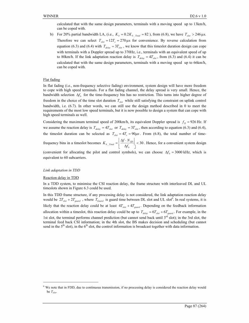
WINNER D2.6 v 1.0

Page 87 (264)

calculated that with the same design parameters, terminals with a moving speed up to 13km/h, can be coped with.

b) For 20% partial bandwidth LA, (i.e., 822.0 _ == Totalbb KK ), from (6.8), we have 246>slotT µs. Therefore we can select 27012 == sslot TT µs for convenience. By reverse calculation from equation (6.3) and (6.4) with slotdelay TT 3= , we know that this timeslot duration design can cope with terminals with a Doppler spread up to 370Hz, i.e., terminals with an equivalent speed of up to 80km/h. If the link adaptation reaction delay is slotdelay TT 4= , from (6.3) and (6.4) it can be calculated that with the same design parameters, terminals with a moving speed up to 66km/h, can be coped with.

Flat fading In flat fading (i.e., non-frequency selective fading) environment, system design will have more freedom to cope with high speed terminals. For a flat fading channel, the delay spread is very small. Hence, the bandwidth selection bf∆ for the time-frequency bin has no restriction. This turns into higher degree of freedom in the choice of the time slot duration slotT while still satisfying the constraint on uplink control bandwidth, i.e. (6.7). In other words, we can still use the design method described in 0 to meet the requirements of the most low speed terminals, but it is now possible to design a system that can cope with high speed terminals as well.

Considering the maximum terminal speed of 200km/h, its equivalent Doppler spread is 926=Df Hz. If we assume the reaction delay is slotdelay TT 4= or slotdelay TT 3= , then according to equation (6.3) and (6.4), the timeslot duration can be selected as sTT sslot µ904 == . From (6.8), the total number of time-

frequency bins in a timeslot becomes 30_ <

∆⋅∆

=b

SDTotalb f

NfK . Hence, for a convenient system design

(convenient for allocating the pilot and control symbols), we can choose 3000=∆ bf kHz, which is equivalent to 60 subcarriers.

Link adaptation in TDD

Reaction delay in TDD In a TDD system, to minimise the CSI reaction delay, the frame structure with interleaved DL and UL timeslots shown in Figure 6.3 could be used.

In this TDD frame structure, if any processing delay is not considered, the link adaptation reaction delay would be guardslot TT 22 + , where GuardT is guard time between DL slot and UL slot6. In real systems, it is likely that the reaction delay could be at least guardslot TT 44 + . Depending on the feedback information allocation within a timeslot, this reaction delay could be up to guardslotdelay TTT 66 += . For example, in the 1st slot, the terminal performs channel prediction (but cannot send back until 3rd slot); in the 3rd slot, the terminal feed back CSI information; in the 4th slot, the BS makes decision and scheduling (but cannot send in the 5th slot), in the 6th slot, the control information is broadcast together with data information.

6 We note that in FDD, due to continuous transmission, if no processing delay is considered the reaction delay would

be Tslot.

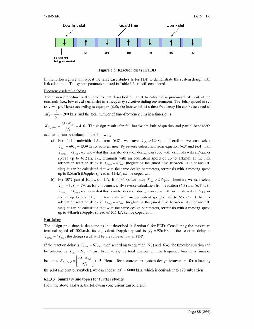
WINNER D2.6 v 1.0

Page 88 (264)

Downlink slot Uplink slotGuard time

Current slot being transmitted

1st 2nd 3rd 4th 5rd 6th

Downlink slot Uplink slotGuard time

Current slot being transmitted

1st 2nd 3rd 4th 5rd 6th

Figure 6.3: Reaction delay in TDD

In the following, we will repeat the same case studies as for FDD to demonstrate the system design with link adaptation. The system parameters listed in Table 3.6 are still considered.

Frequency selective fading The design procedure is the same as that described for FDD to cater the requirements of most of the terminals (i.e., low speed terminals) in a frequency selective fading environment. The delay spread is set to 1=τ µs. Hence according to equation (6.5), the bandwidth of a time-frequency bin can be selected as

20051

==∆τbf kHz, and the total number of time-frequency bins in a timeslot is

416_ =∆⋅∆

=b

SDTotalb f

NfK . The design results for full bandwidth link adaptation and partial bandwidth

adaptation can be deduced in the following. a) For full bandwidth LA, from (6.8), we have 1248>slotT µs. Therefore we can select

135060 == sslot TT µs for convenience. By reverse calculation from equation (6.3) and (6.4) with

slotdelay TT 4= , we know that this timeslot duration design can cope with terminals with a Doppler spread up to 61.5Hz, i.e., terminals with an equivalent speed of up to 13km/h. If the link adaptation reaction delay is slotdelay TT 6= (neglecting the guard time between DL slot and UL slot), it can be calculated that with the same design parameters, terminals with a moving speed up to 8.5km/h (Doppler spread of 41Hz), can be coped with.

b) For 20% partial bandwidth LA, from (6.8), we have 246>slotT µs. Therefore we can select 27012 == sslot TT µs for convenience. By reverse calculation from equation (6.3) and (6.4) with

slotdelay TT 4= , we know that this timeslot duration design can cope with terminals with a Doppler spread up to 307.5Hz, i.e., terminals with an equivalent speed of up to 65km/h. If the link adaptation reaction delay is slotdelay TT 6= (neglecting the guard time between DL slot and UL slot), it can be calculated that with the same design parameters, terminals with a moving speed up to 44km/h (Doppler spread of 205Hz), can be coped with.

Flat fading The design procedure is the same as that described in Section 0 for FDD. Considering the maximum terminal speed of 200km/h, its equivalent Doppler spread is 926=Df Hz. If the reaction delay is

slotdelay TT 4= , the design result will be the same as that of FDD.

If the reaction delay is slotdelay TT 6= , then according to equation (6.3) and (6.4), the timeslot duration can be selected as sTT sslot µ452 == . From (6.8), the total number of time-frequency bins in a timeslot

becomes 15_ <

∆⋅∆

=b

SDTotalb f

NfK . Hence, for a convenient system design (convenient for allocating

the pilot and control symbols), we can choose 6000=∆ bf kHz, which is equivalent to 120 subcarriers.

6.1.3.3 Summary and topics for further studies From the above analysis, the following conclusions can be drawn:

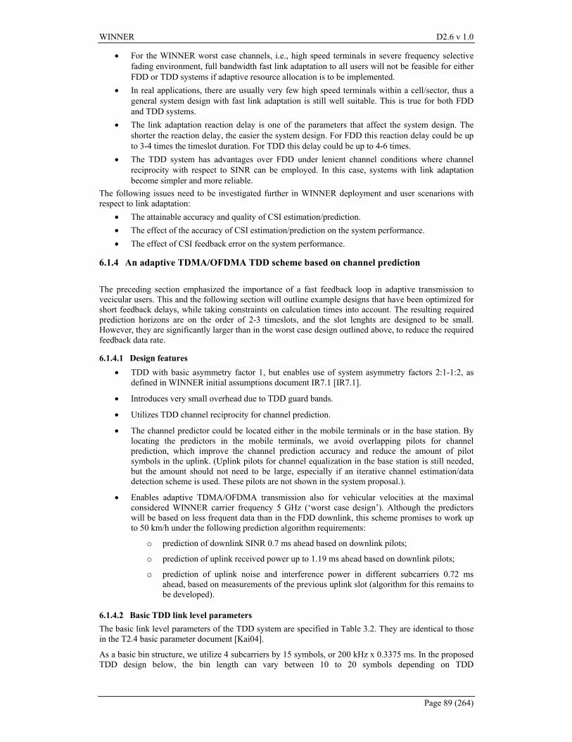
WINNER D2.6 v 1.0

Page 89 (264)

• For the WINNER worst case channels, i.e., high speed terminals in severe frequency selective fading environment, full bandwidth fast link adaptation to all users will not be feasible for either FDD or TDD systems if adaptive resource allocation is to be implemented.

• In real applications, there are usually very few high speed terminals within a cell/sector, thus a general system design with fast link adaptation is still well suitable. This is true for both FDD and TDD systems.

• The link adaptation reaction delay is one of the parameters that affect the system design. The shorter the reaction delay, the easier the system design. For FDD this reaction delay could be up to 3-4 times the timeslot duration. For TDD this delay could be up to 4-6 times.

• The TDD system has advantages over FDD under lenient channel conditions where channel reciprocity with respect to SINR can be employed. In this case, systems with link adaptation become simpler and more reliable.

The following issues need to be investigated further in WINNER deployment and user scenarions with respect to link adaptation:

• The attainable accuracy and quality of CSI estimation/prediction. • The effect of the accuracy of CSI estimation/prediction on the system performance. • The effect of CSI feedback error on the system performance.

6.1.4 An adaptive TDMA/OFDMA TDD scheme based on channel prediction The preceding section emphasized the importance of a fast feedback loop in adaptive transmission to vecicular users. This and the following section will outline example designs that have been optimized for short feedback delays, while taking constraints on calculation times into account. The resulting required prediction horizons are on the order of 2-3 timeslots, and the slot lenghts are designed to be small. However, they are significantly larger than in the worst case design outlined above, to reduce the required feedback data rate.

6.1.4.1 Design features • TDD with basic asymmetry factor 1, but enables use of system asymmetry factors 2:1-1:2, as

defined in WINNER initial assumptions document IR7.1 [IR7.1].

• Introduces very small overhead due to TDD guard bands.

• Utilizes TDD channel reciprocity for channel prediction.

• The channel predictor could be located either in the mobile terminals or in the base station. By locating the predictors in the mobile terminals, we avoid overlapping pilots for channel prediction, which improve the channel prediction accuracy and reduce the amount of pilot symbols in the uplink. (Uplink pilots for channel equalization in the base station is still needed, but the amount should not need to be large, especially if an iterative channel estimation/data detection scheme is used. These pilots are not shown in the system proposal.).

• Enables adaptive TDMA/OFDMA transmission also for vehicular velocities at the maximal considered WINNER carrier frequency 5 GHz (‘worst case design’). Although the predictors will be based on less frequent data than in the FDD downlink, this scheme promises to work up to 50 km/h under the following prediction algorithm requirements:

o prediction of downlink SINR 0.7 ms ahead based on downlink pilots;

o prediction of uplink received power up to 1.19 ms ahead based on downlink pilots;

o prediction of uplink noise and interference power in different subcarriers 0.72 ms ahead, based on measurements of the previous uplink slot (algorithm for this remains to be developed).

6.1.4.2 Basic TDD link level parameters The basic link level parameters of the TDD system are specified in Table 3.2. They are identical to those in the T2.4 basic parameter document [Kai04].

As a basic bin structure, we utilize 4 subcarriers by 15 symbols, or 200 kHz x 0.3375 ms. In the proposed TDD design below, the bin length can vary between 10 to 20 symbols depending on TDD

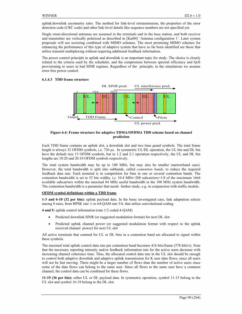
WINNER D2.6 v 1.0

Page 90 (264)

uplink/downlink asymmetry ratio. The method for link-level retransmission, the properties of the error detection code (CRC code) and other link-level details like sequence numbers are not specified yet.

Single omni-directional antennas are assumed in the terminals and in the base station, and both receiver and transmitter are vertically polarized as described in [Kai04] ‘Antenna configuration 1’. Later system proposals will use sectoring combined with MIMO schemes. The most promising MIMO schemes for enhancing the performance of this type of adaptive system that have so far been identified are those that utilize transmit multiplexing without requiring additional feedback information.

The power control principle in uplink and downlink is an important topic for study. The choice is closely related to the criteria used by the scheduler, and the compromise between spectral efficiency and QoS provisioning to users in bad SINR regimes. Regardless of the principle, in the simulations we assume error-free power control.

6.1.4.3 TDD frame structure

TDD Frame Guard Control Pilots

DL UL DL UL UL 1 15 16 3032

UL interference pred. DL SINR pred.

UL power pred.

Figure 6.4: Frame structure for adaptive TDMA/OFDMA TDD scheme based on channel prediction

Each TDD frame contains an uplink slot, a downlink slot and two time guard symbols. The total frame length is always 32 OFDM symbols, i.e. 720 µs. In symmetric UL/DL operation, the UL bin and DL bin have the default size 15 OFDM symbols, but in 1:2 and 2:1 operation respectively, the UL and DL bin lengths are 10:20 and 20:10 OFDM symbols respectively.

The total system bandwidth may be up to 100 MHz, but may also be smaller (narrowband case). However, the total bandwidth is split into subbands, called contention bands, to reduce the required feedback data rate. Each terminal is in competition for bins in one or several contention bands. The contention bandwidth is set to 52 bin widths, i.e. 10.4 MHz=208 subcarriers=1/8 of the maximum 1664 available subcarriers within the maximal 84 MHz useful bandwidth in the 100 MHz system bandwidth. The contention bandwidth is a parameter that needs further study, e.g. in conjunction with traffic models.

OFDM symbol definitions within a TDD frame

1-3 and 6-10 (32 per bin): uplink payload data. In the basic investigated case, link adaptation selects among 8 rates, from BPSK rate ½ to 64-QAM rate 5/6, that utilize convolutional coding.

4 and 5: uplink control information (rate 1/2 coded 4-QAM)

• Predicted downlink SINR (or suggested modulation format) for next DL slot

• Predicted uplink channel power (or suggested modulation format with respect to the uplink received channel power) for next UL slot

All active terminals that contend for UL or DL bins in a contention band are allocated to signal within these symbols.

The maximal total uplink control data rate per contention band becomes 416 bits/frame (578 kbit/s). Note that the necessary reporting intensity and/or feedback information rate for the active users decrease with increasing channel coherence time. Thus, the allocated control data rate in the UL slot should be enough to control both adaptive downlink and adaptive uplink transmission for K user data flows, since all users will not be fast moving. There might be a larger number of flows than the number of active users since some of the data flows can belong to the same user. Since all flows to the same user have a common channel, the control data can be combined for these flows.

11-19 (36 per bin): either UL or DL payload data. In symmetric operation, symbol 11-15 belong to the UL slot and symbol 16-19 belong to the DL slot.

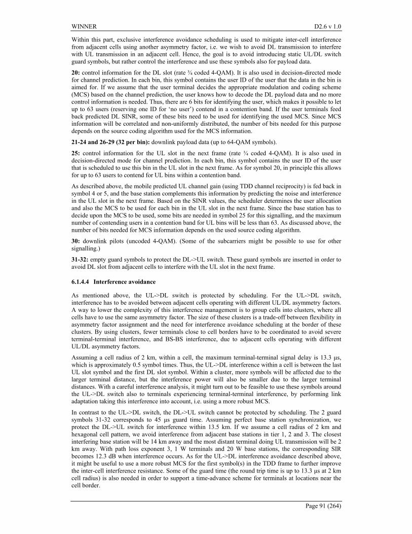
WINNER D2.6 v 1.0

Page 91 (264)

Within this part, exclusive interference avoidance scheduling is used to mitigate inter-cell interference from adjacent cells using another asymmetry factor, i.e. we wish to avoid DL transmission to interfere with UL transmission in an adjacent cell. Hence, the goal is to avoid introducing static UL/DL switch guard symbols, but rather control the interference and use these symbols also for payload data.

20: control information for the DL slot (rate ¾ coded 4-QAM). It is also used in decision-directed mode for channel prediction. In each bin, this symbol contains the user ID of the user that the data in the bin is aimed for. If we assume that the user terminal decides the appropriate modulation and coding scheme (MCS) based on the channel prediction, the user knows how to decode the DL payload data and no more control information is needed. Thus, there are 6 bits for identifying the user, which makes it possible to let up to 63 users (reserving one ID for ‘no user’) contend in a contention band. If the user terminals feed back predicted DL SINR, some of these bits need to be used for identifying the used MCS. Since MCS information will be correlated and non-uniformly distributed, the number of bits needed for this purpose depends on the source coding algorithm used for the MCS information.

21-24 and 26-29 (32 per bin): downlink payload data (up to 64-QAM symbols).

25: control information for the UL slot in the next frame (rate ¾ coded 4-QAM). It is also used in decision-directed mode for channel prediction. In each bin, this symbol contains the user ID of the user that is scheduled to use this bin in the UL slot in the next frame. As for symbol 20, in principle this allows for up to 63 users to contend for UL bins within a contention band.

As described above, the mobile predicted UL channel gain (using TDD channel reciprocity) is fed back in symbol 4 or 5, and the base station complements this information by predicting the noise and interference in the UL slot in the next frame. Based on the SINR values, the scheduler determines the user allocation and also the MCS to be used for each bin in the UL slot in the next frame. Since the base station has to decide upon the MCS to be used, some bits are needed in symbol 25 for this signalling, and the maximum number of contending users in a contention band for UL bins will be less than 63. As discussed above, the number of bits needed for MCS information depends on the used source coding algorithm.

30: downlink pilots (uncoded 4-QAM). (Some of the subcarriers might be possible to use for other signalling.)

31-32: empty guard symbols to protect the DL->UL switch. These guard symbols are inserted in order to avoid DL slot from adjacent cells to interfere with the UL slot in the next frame.

6.1.4.4 Interference avoidance

As mentioned above, the UL->DL switch is protected by scheduling. For the UL->DL switch, interference has to be avoided between adjacent cells operating with different UL/DL asymmetry factors. A way to lower the complexity of this interference management is to group cells into clusters, where all cells have to use the same asymmetry factor. The size of these clusters is a trade-off between flexibility in asymmetry factor assignment and the need for interference avoidance scheduling at the border of these clusters. By using clusters, fewer terminals close to cell borders have to be coordinated to avoid severe terminal-terminal interference, and BS-BS interference, due to adjacent cells operating with different UL/DL asymmetry factors.

Assuming a cell radius of 2 km, within a cell, the maximum terminal-terminal signal delay is 13.3 µs, which is approximately 0.5 symbol times. Thus, the UL->DL interference within a cell is between the last UL slot symbol and the first DL slot symbol. Within a cluster, more symbols will be affected due to the larger terminal distance, but the interference power will also be smaller due to the larger terminal distances. With a careful interference analysis, it might turn out to be feasible to use these symbols around the UL->DL switch also to terminals experiencing terminal-terminal interference, by performing link adaptation taking this interference into account, i.e. using a more robust MCS.

In contrast to the UL->DL switch, the DL->UL switch cannot be protected by scheduling. The 2 guard symbols 31-32 corresponds to 45 µs guard time. Assuming perfect base station synchronization, we protect the DL->UL switch for interference within 13.5 km. If we assume a cell radius of 2 km and hexagonal cell pattern, we avoid interference from adjacent base stations in tier 1, 2 and 3. The closest interfering base station will be 14 km away and the most distant terminal doing UL transmission will be 2 km away. With path loss exponent 3, 1 W terminals and 20 W base stations, the corresponding SIR becomes 12.3 dB when interference occurs. As for the UL->DL interference avoidance described above, it might be useful to use a more robust MCS for the first symbol(s) in the TDD frame to further improve the inter-cell interference resistance. Some of the guard time (the round trip time is up to 13.3 µs at 2 km cell radius) is also needed in order to support a time-advance scheme for terminals at locations near the cell border.

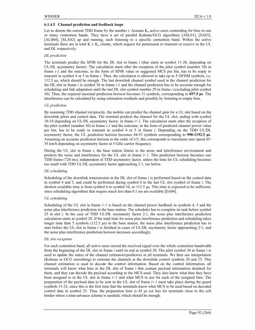
WINNER D2.6 v 1.0

Page 92 (264)

6.1.4.5 Channel prediction and feedback loops Let us denote the current TDD frame by the number i. Assume Ku active users contending for bins in one or many contention bands. They have a set of parallel Kalman/GCG algorithms [ASL01], [SA03], [ALS04], [SLA02] up and running, each listening to a specific contention band. Within the active terminals there are in total K ≥ Ku clients, which request for permission to transmit or receive in the UL and DL respectively.

DL prediction

The terminals predict the SINR for the DL slot in frame i (that starts at symbol 11-20, depending on UL/DL asymmetry factor). The calculation starts after the reception of the pilot symbol (number 30) in frame i-1 and the outcome, in the form of SINR value or suggested MCS per bin, has to be ready to transmit in symbol 4 or 5 in frame i. Thus, the calculation is allowed to take up to 5 OFDM symbols, i.e. 112.5 µs, which should be enough. The last downlink channel symbol used in the channel prediction for the DL slot in frame i is symbol 30 in frame i-1 and the channel prediction has to be accurate enough for scheduling and link adaptation until the last DL slot symbol number 29 in frame i (excluding pilot symbol 30). Thus, the required maximal prediction horizon becomes 31 symbols, corresponding to 697.5 µs. The interference can be calculated by using estimation residuals and possibly by listening to empty bins.

UL prediction

By assuming TDD channel reciprocity, the mobile can predict the channel gain for a UL slot based on the downlink pilots and control data. The terminal predicts the channel for the UL slot, ending with symbol 10-19 depending on UL/DL asymmetry factor, in frame i+1. The calculation starts after the reception of the pilot symbol (number 30) in frame i-1 and the outcome, in the form of predicted channel power value per bin, has to be ready to transmit in symbol 4 or 5 in frame i. Depending on the TDD UL/DL asymmetry factor, the UL prediction horizon becomes 44-53 symbols corresponding to 990-1192.5 µs. Assuming an accurate prediction horizon in the order of λ/5, this corresponds to maximum user speed 45-55 km/h depending on asymmetry factor at 5 GHz carrier frequency.

During the UL slot in frame i, the base station listens to the noise and interference environment and predicts the noise and interference for the UL slot in frame i+1. This prediction horizon becomes one TDD frame (720 ms), independent of TDD asymmetry factor, unless the time for UL scheduling becomes too small with TDD UL/DL asymmetry factor approaching 2:1, see below.

DL scheduling

Scheduling of the downlink transmission in the DL slot of frame i is performed based on the control data in symbol 4 and 5, and could be performed during symbol 6 to the last UL slot symbol of frame i. The shortest available time is from symbol 6 to symbol 10, or 112.5 µs. This time is expected to be sufficient, since scheduling algorithms that require much less than 0.1 ms are available [Eri04].

UL scheduling

Scheduling of the UL slot in frame i+1 is based on the channel power feedback in symbols 4, 5 and the noise plus interference prediction in the base station. The scheduler has to complete its task before symbol 25 in slot i. In the case of TDD UL/DL asymmetry factor 2:1, the noise plus interference prediction calculation starts at symbol 20. If the total time for noise plus interference prediction and scheduling takes longer time than 5 symbols (112.5 µs) in the base station, the noise plus interference prediction has to start before the UL slot in frame i is finished in cases of UL/DL asymmetry factor approaching 2:1, and the noise plus interference prediction horizon increases accordingly.

DL slot reception

For each contention band, all active users record the received signal over the whole contention bandwidth from the beginning of the DL slot in frame i until its end at symbol 30. The pilot symbol 30 in frame i is used to update the states of the channel estimators/predictors in all terminals. We then use interpolation (Kalman or GCG smoothing) to estimate the channels at the downlink control symbols 20 and 25. This channel estimation is used to decode the control information. Based on the control information, all terminals will know what bins in the DL slot of frame i that contain payload information destined for them, and they can decode the payload according to the MCS used. They also know what bins they have been assigned to in the UL slot in frame i+1 and what MCS to use for each of the assigned bins. The preparation of the payload data to be sent in the UL slot of frame i+1 must take place during the guard symbols 31-32, since this is the first time that the terminals know what MCS to be used based on decoded control data in symbol 25. Thus, the preparation time is 45 µs (or less for terminals close to the cell border where a time-advance scheme is needed), which should be enough.

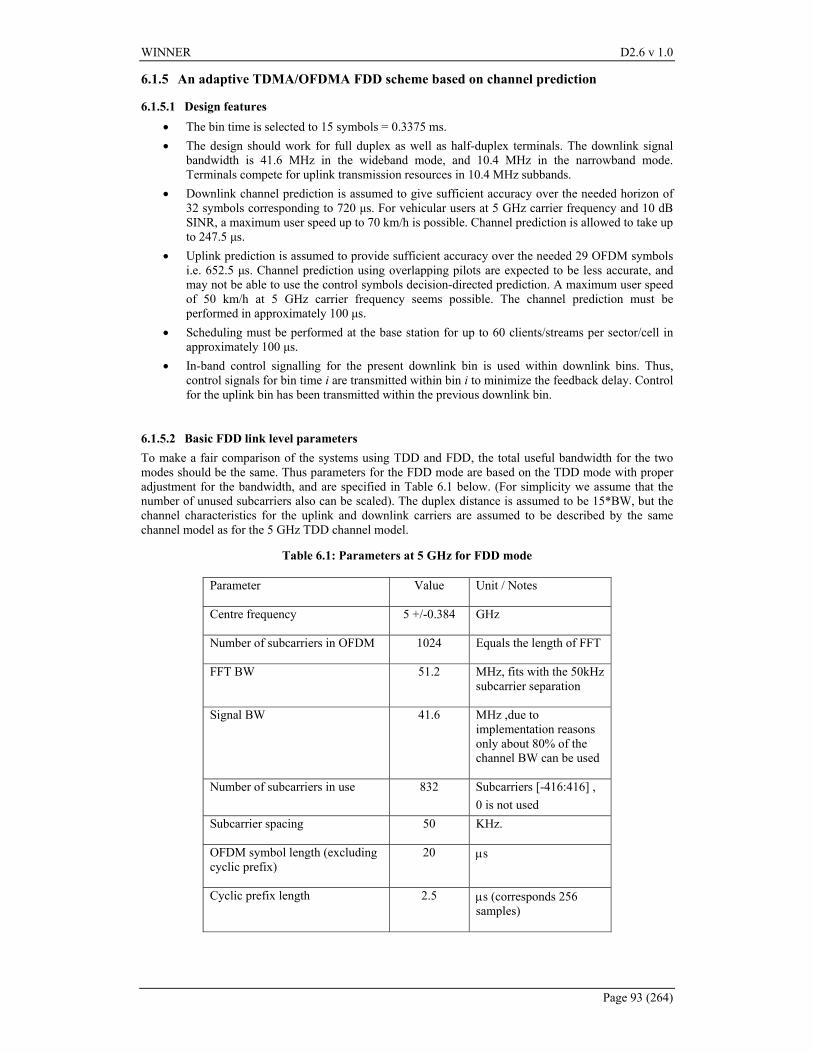
WINNER D2.6 v 1.0

Page 93 (264)

6.1.5 An adaptive TDMA/OFDMA FDD scheme based on channel prediction

6.1.5.1 Design features • The bin time is selected to 15 symbols = 0.3375 ms. • The design should work for full duplex as well as half-duplex terminals. The downlink signal

bandwidth is 41.6 MHz in the wideband mode, and 10.4 MHz in the narrowband mode. Terminals compete for uplink transmission resources in 10.4 MHz subbands.

• Downlink channel prediction is assumed to give sufficient accuracy over the needed horizon of 32 symbols corresponding to 720 µs. For vehicular users at 5 GHz carrier frequency and 10 dB SINR, a maximum user speed up to 70 km/h is possible. Channel prediction is allowed to take up to 247.5 µs.

• Uplink prediction is assumed to provide sufficient accuracy over the needed 29 OFDM symbols i.e. 652.5 µs. Channel prediction using overlapping pilots are expected to be less accurate, and may not be able to use the control symbols decision-directed prediction. A maximum user speed of 50 km/h at 5 GHz carrier frequency seems possible. The channel prediction must be performed in approximately 100 µs.

• Scheduling must be performed at the base station for up to 60 clients/streams per sector/cell in approximately 100 µs.

• In-band control signalling for the present downlink bin is used within downlink bins. Thus, control signals for bin time i are transmitted within bin i to minimize the feedback delay. Control for the uplink bin has been transmitted within the previous downlink bin.

6.1.5.2 Basic FDD link level parameters To make a fair comparison of the systems using TDD and FDD, the total useful bandwidth for the two modes should be the same. Thus parameters for the FDD mode are based on the TDD mode with proper adjustment for the bandwidth, and are specified in Table 6.1 below. (For simplicity we assume that the number of unused subcarriers also can be scaled). The duplex distance is assumed to be 15*BW, but the channel characteristics for the uplink and downlink carriers are assumed to be described by the same channel model as for the 5 GHz TDD channel model.

Table 6.1: Parameters at 5 GHz for FDD mode

Parameter Value Unit / Notes

Centre frequency 5 +/-0.384 GHz

Number of subcarriers in OFDM 1024 Equals the length of FFT

FFT BW 51.2 MHz, fits with the 50kHz subcarrier separation

Signal BW 41.6 MHz ,due to implementation reasons only about 80% of the channel BW can be used

Number of subcarriers in use 832 Subcarriers [-416:416] , 0 is not used

Subcarrier spacing 50 KHz.

OFDM symbol length (excluding cyclic prefix)

20 µs

Cyclic prefix length 2.5 µs (corresponds 256 samples)

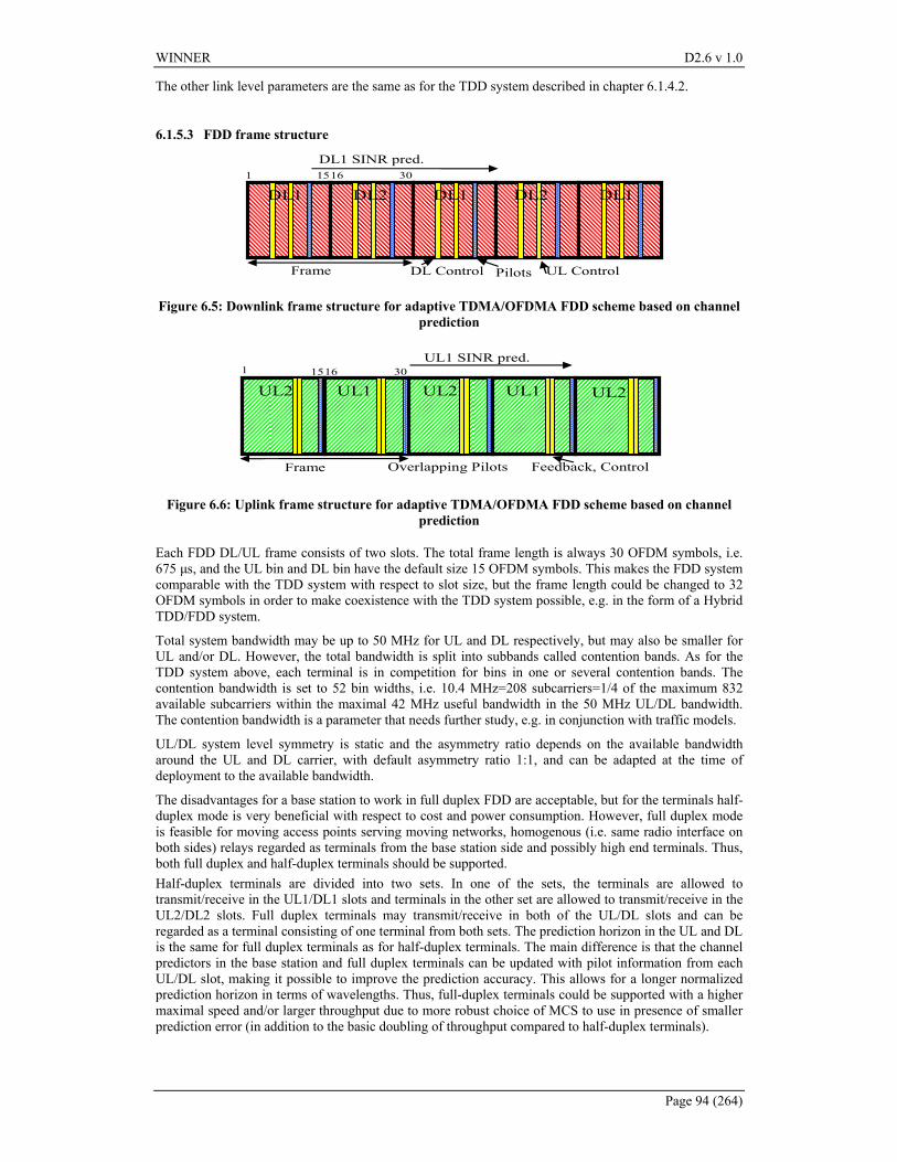
WINNER D2.6 v 1.0

Page 94 (264)

The other link level parameters are the same as for the TDD system described in chapter 6.1.4.2.

6.1.5.3 FDD frame structure

Frame DL Control UL Control

DL1

Pilots

DL2 DL1 DL2 DL1 1 16 30 15

DL1 SINR pred.

Figure 6.5: Downlink frame structure for adaptive TDMA/OFDMA FDD scheme based on channel prediction

Frame Feedback, Control

UL2

Overlapping Pilots

UL1 UL2 UL1 UL2

1 15 16 30UL1 SINR pred.

Figure 6.6: Uplink frame structure for adaptive TDMA/OFDMA FDD scheme based on channel prediction

Each FDD DL/UL frame consists of two slots. The total frame length is always 30 OFDM symbols, i.e. 675 µs, and the UL bin and DL bin have the default size 15 OFDM symbols. This makes the FDD system comparable with the TDD system with respect to slot size, but the frame length could be changed to 32 OFDM symbols in order to make coexistence with the TDD system possible, e.g. in the form of a Hybrid TDD/FDD system.

Total system bandwidth may be up to 50 MHz for UL and DL respectively, but may also be smaller for UL and/or DL. However, the total bandwidth is split into subbands called contention bands. As for the TDD system above, each terminal is in competition for bins in one or several contention bands. The contention bandwidth is set to 52 bin widths, i.e. 10.4 MHz=208 subcarriers=1/4 of the maximum 832 available subcarriers within the maximal 42 MHz useful bandwidth in the 50 MHz UL/DL bandwidth. The contention bandwidth is a parameter that needs further study, e.g. in conjunction with traffic models.

UL/DL system level symmetry is static and the asymmetry ratio depends on the available bandwidth around the UL and DL carrier, with default asymmetry ratio 1:1, and can be adapted at the time of deployment to the available bandwidth.

The disadvantages for a base station to work in full duplex FDD are acceptable, but for the terminals half-duplex mode is very beneficial with respect to cost and power consumption. However, full duplex mode is feasible for moving access points serving moving networks, homogenous (i.e. same radio interface on both sides) relays regarded as terminals from the base station side and possibly high end terminals. Thus, both full duplex and half-duplex terminals should be supported. Half-duplex terminals are divided into two sets. In one of the sets, the terminals are allowed to transmit/receive in the UL1/DL1 slots and terminals in the other set are allowed to transmit/receive in the UL2/DL2 slots. Full duplex terminals may transmit/receive in both of the UL/DL slots and can be regarded as a terminal consisting of one terminal from both sets. The prediction horizon in the UL and DL is the same for full duplex terminals as for half-duplex terminals. The main difference is that the channel predictors in the base station and full duplex terminals can be updated with pilot information from each UL/DL slot, making it possible to improve the prediction accuracy. This allows for a longer normalized prediction horizon in terms of wavelengths. Thus, full-duplex terminals could be supported with a higher maximal speed and/or larger throughput due to more robust choice of MCS to use in presence of smaller prediction error (in addition to the basic doubling of throughput compared to half-duplex terminals).

WINNER D2.6 v 1.0

Page 95 (264)

OFDM symbol definitions within FDD DL frames:

A DL frame consists of two DL slots, one for each set of half-duplex terminals, starting with DL1. The DL1 and DL2 slots have the same symbol definitions within the slot, but the symbol numbers for slot DL2 are delayed by 15 symbols, and the control information is related to the DL2 and UL2 slots. For this reason, only symbol 1-15 for DL1 are defined below.

1-5, 7-10, 12 and 14-15 (48 per bin): downlink payload data (up to 64-QAM symbols)

As for the TDD system, the link adaptation selects an appropriate modulation-coding rate, based on the predicted SINR. In the basic investigated design, 8 rates from BPSK rate ½ to 64-QAM rate 5/6, that utilize convolutional coding, are used.

6: control information for the DL slot (rate ¾ coded 4-QAM). It is also used in decision-directed mode for channel prediction. In each bin, this symbol contains the user ID of the user that the data in the bin is aimed for. If we assume that the user terminal decides the appropriate modulation and coding scheme (MCS) based on the channel prediction, the user knows how to decode the DL payload data and no more control information is needed. Thus, there are 6 bits for identifying the user, which makes it possible to let up to 63 users (reserving one ID for ‘no user’) contend in a contention band. If the user terminals feed back predicted DL SINR, some of these bits need to be used for identifying the used MCS. Since MCS information will be correlated and non-uniformly distributed, the number of bits needed for this purpose depends on the source coding algorithm used for the MCS information.

11: control information for the next UL1 slot (rate ¾ coded 4-QAM). It is also used in decision-directed mode for channel prediction. In each bin, this symbol contains the user ID of the user that is scheduled to use this bin in the UL1 slot in next frame. As for symbol 6, in principle this allows for up to 63 users to contend for UL bins within a contention band.

Since the base station performs the link adaptation based on UL channel prediction, also information about which MCS to be used for each bin in the UL slot in next frame has to be provided in this symbol. Thus, some bits are needed in symbol 11 for this signalling, and the maximum number of contending users in a contention band for UL1 bins will be less than 63. As discussed above, the number of bits needed for MCS information depends on the used source coding algorithm.

13: downlink pilots (uncoded 4-QAM). (Some of the subcarriers might be possible to use for other signalling.)

OFDM symbol definitions within FDD UL frames:

As for the DL frame, an UL frame consists of two UL slots, one for each set of half-duplex terminals, starting with UL2. The UL1 and UL2 slots have the same symbol definitions within the slot, but the symbol numbers for the slot UL2 are 15 symbols earlier, and the control information is related to the DL2 and UL2 slots. For this reason, only symbol 16-30 for UL1 are defined below.

16-24 and 27-29 (48 per bin): uplink payload data (up to 64-QAM symbols).

25 and 26: uplink control information (rate 1/2 coded 4-QAM).

These symbols contains predicted downlink SINR (or suggested modulation format) for the next DL1 slot. All active terminals that contend for DL bins in a contention band are allocated to signal within these symbols.

The total maximal uplink control data rate per contention band becomes 416 bits/frame (578 kbit/s). This is the same data rate as for the TDD system described above, even though no DL channel power value has to be transmitted. The reason for this is that the necessary reporting intensity and/or feedback information rate for the active users increase with decreasing channel coherence time. An FDD system should be easier to deploy in a wide area scenario (see arguments in chapter 6.1.2 above) with more users at vehicular speeds. If not all control data symbols are needed, some could be used to insert more (overlapping) uplink pilots possibly improving UL channel prediction.

The allocated control data rate in the UL slot should be enough to control an adaptive downlink transmission for K user data flows. (There might be a larger number of flows than the number of active users since some of the data flows can belong to the same user.)

30: uplink (overlapping) pilots (uncoded 4-QAM).

WINNER D2.6 v 1.0

Page 96 (264)

6.1.5.4 Channel prediction and feedback loops Let us denote the current FDD UL/DL frame with number i. A full-duplex terminal can be mainly regarded as consisting of one half-duplex terminal from each of the two sets. Without loss of generality, we therefore focus on half duplex terminals using the UL1/DL1 slots. (As discussed above, the full-duplex terminals will have a better prediction accuracy, since they can listen to more DL pilots.) Assume Ku active users contending for bins in one or many contention bands. They have a set of parallel Kalman/GCG algorithms [ASL01], [SA03] up and running, each listening to a specific contention band in the DL. Within the active terminals there are in total K ≥ Ku clients, which request for permission to transmit or receive in the UL and DL respectively.

DL prediction

The terminals predict the SINR for the DL1 slot in frame i+1. The calculation starts after the reception of the pilot symbol (number 13) of slot DL1 in frame i and the outcome, in the form of SINR value or suggested MCS per bin, has to be ready to transmit in symbol 25 and 26 of slot UL1 in frame i. Thus, the calculation is allowed to take up to 11 OFDM symbols, i.e. 247.5 µs, which should be enough. The last downlink channel symbol used in the channel prediction for the DL1 slot in frame i+1 is symbol 13 in frame i. The channel prediction has to be accurate enough for scheduling and link adaptation until the last DL1 slot symbol number 15 in frame i+1. Thus, the prediction horizon becomes 32 symbols corresponding to 720 µs. The channel prediction uses the control symbols number 6 and 11 in slot DL1 in frame i as aid in decision-directed prediction. Assuming an accurate prediction horizon in the order of λ/3, this corresponds to maximum user speed of up to 100 km/h at 5 GHz carrier frequency. The interference can be calculated by using estimation residuals and possibly by listening to empty bins.

UL prediction

The base station predicts the SINR for the UL1 slot in frame i+1 based on overlapping pilots in symbol 30 of the UL1 slot in frame i. The calculation starts after the reception of the pilot symbol (number 30) in frame i and the outcome, in the form of predicted SINR per bin, is forwarded to the scheduler. The prediction based UL scheduling result has to be ready to feed back in DL1 symbol 11 of frame i+1, which gives 10 OFDM symbols or 225 µs for UL channel prediction and UL scheduling of all active users. The UL prediction horizon becomes 29 OFDM symbols i.e. 652.5 µs. Channel prediction using overlapping pilots are expected to be less accurate, and may not be able to use the control symbols in UL1 for decision-directed prediction. Assuming an accurate prediction horizon in the order of λ/5 [SA04], this corresponds to maximum user speed 70 km/h at 5 GHz carrier frequency. The prediction accuracy with overlapping pilots is discussed in Section 6.1.6.2.

During all UL slots in frame i, the base station listens to the noise and interference environment and predicts the noise and interference for the UL1 slot in frame i+1. This prediction horizon becomes as long as the channel prediction above, i.e. one FDD frame minus the overlapping pilot symbol, i.e. 29 OFDM symbols or 652.5 µs.

DL scheduling

Scheduling of the downlink transmission in the DL1 slot of frame i+1 is performed based on the UL control data in symbol 25 and 26, and is performed during symbol 27 to the last UL slot symbol, which corresponds to 90 µs. This time is expected to be sufficient, since scheduling algorithms needing much less than 0.1 ms are available [Eri04].

UL scheduling

Scheduling of the UL slot in frame i+1 is based on the SNIR prediction made in the base station based on the overlapping pilots in the UL1 of frame i. As stated above 10 OFDM symbols or 225 µs are available for UL channel prediction and UL scheduling of all active users, which might be sufficient. The UL1 slot allocation for frame i+1 is then feed back in the DL1 slot symbol 11 of frame i+1.

DL slot reception

For each contention band, all active users record the received signal over the whole contention bandwidth from the beginning of the DL1 slot in frame i. The pilot symbol 13 in frame i is used to update the states of the channel estimators/predictors in all terminals. We then use interpolation (Kalman or GCG smoothing) to estimate the channels at the downlink control symbols 6 and 11. This channel estimation is used to decode the control information. Based on the control information, all terminals will know what bins in the DL1 slot of frame i that contain payload information destined for them, and they can decode the payload according to the MCS used. They also know what bins they have been assigned to in the next UL1 slot and what MCS to use for each of the assigned bins.

WINNER D2.6 v 1.0

Page 97 (264)

The preparation of the payload data to be sent in the UL slot of frame i+1 have to be prepared during symbols 12-15 in slot DL1, since this is the first time that the terminals know what MCS to be used, based on decoded control data in symbol 11. Thus, the preparation time is 90 µs (minus the time for channel estimation and decoding of symbol 11) , which should be enough.

6.1.5.5 Crucial open issues regarding the FDD uplink design 1. Is it possible to predict uplink channels for all users based on overlapping pilots in only approximately 100 µs? (Recall from above, that the prediction based UL scheduling result has to be ready to feed back in DL1 symbol 11 of frame i+1, which gives 10 OFDM symbols or 225 µs for the UL channel prediction and the UL scheduling of all active users.) The answer to this question is yes, but there remain unresolved issues regarding the computational complexity of the considered predictor based on overlapping pilot. It is at present unclear if it is possible to update the predictor states in the remaining available time. This is no problem with the GCG algorithm, but it may require too many operations with a Kalman algorithm [AM79] that requires a Kalman Riccati difference equation update. Unfortunately, there are at present numerical problems with the GCG algorithm when used with overlapping pilots, due to the large size of the involved state vector. Downlink estimation requires a smaller state vector dimension, which avoids these numerical problems. Research on these and other alternative channel prediction methods based on overlapping pilots is therefor important. The required computational complexity of the channel prediction step has been estimated under the following conditions:

• The assumed base station computational power 10 years from now is 20·109 32-bit operations or 2·106 operations/0.1ms. (For a terminal a factor of 40 less computational power could be assumed.)

• Prediction operation: ttL

tLt xCFh |

^

|

^=+ , where the real-valued matrix FL is diagonal and the

matrix C is sparse. The number of operations in calculating tLth |

^

+ is approximated by the state vector dimension nx = KTpnD, where KT is the number of active terminals in the contention band (number of overlapping pilots), p is the number of adjacent pilot-containing subcarriers used in each predictor and nD is the order of AR-process used to describe the fading dynamics.

For example, assuming KT = 8, p = 8 and nD = 4 gives nx = 256 states in predictor. We perform three predictions (to the early, middle and late part of bin i+1). Each predictor covers 8·50 kHz = 400 kHz. Over the full FDD system bandwidth we thus need 104 such predictors working in parallel. All prediction operations therefore require approximately 256 operations/prediction · 3 predictions · 104 predictors ≈ 80·103 operations. This is a factor of 20 less than the available budget of 1.8·106 operations/0.09 ms. However, the complexity of the Riccati difference equation update, with block-diagonal covariance matrix, using the structure of C and F has to be analysed further. 2. Is it reasonable to assume that only 8 coded 4-QAM symbols per uplink bin can carry the required feedback information? The answer to this question is likely to be yes, but requires further study. Outline of an estimation of the feedback bitrate: Assume 8 4-QAM control symbols with rate ½ coding. In each uplink bin, we would have 8 feedback bits per bin. With 8 MCS levels requiring 3 bits, less than three competing users seem to be able to report their results over these 8 bits. However, by

• reporting only “good” results, and • source coding by taking the correlation of the MCS choice over time and frequency into account,

it is possible to reduce the feedback information. It can also be utilized that all MCSs are not equally likely to be used.

These methods are expected to reduce the required feedback rate by a factor 4-20, which would imply that the available feedback rate is adequate for 10-50 active terminals per contention band. The factor depends on the user scenario mix of stationary, slow and fast moving users. Better estimates of the required feedback rate in different scenarios is an important topic for further study. An alternative could be to use separate subcarriers only for control, but this would increase the uplink control transmission delay. In addition, in rare cases when there are too many fast moving users for the feedback bandwidth in the system, it is possible to move more users to the non-adaptive fallback mode.

WINNER D2.6 v 1.0

Page 98 (264)

3. Can uplink prediction be performed with sufficient accuracy using overlapping pilots? This has been investigated, and first obtained results, discussed in Section 6.1.6.2, are encouraging. Continued investigations are planned.

4. Is it reasonable to assume that scheduling can be performed within 100 µs? The answer to this question is yes. Recall the assumed budget of 2·106 operations/0.1 ms in future base station processors. There are scheduling algorithms that require much less than 2·106 operations. An example is the ITER algorithm developed in [Eri04]. It can balance requirements of data streams with different delay constraints, priorities and throughput requirements, while still attaining scheduling gains due to the independent fading of the channels for the different users.

6.1.6 Performance modelling and evaluation In this section, we describe some aspects of the simulation of the two schemes described in Section 6.1.4 and Section 6.1.5. First, Section 6.1.6.1 describes the model with which the predictor performance is described in multilink simulations and system-level simulations. Section 6.1.6.2 then describes the predictor performance that was obtained by applying Kalman predictors, using 8 parallel subcarriers, on the Vehicular A-channel that is being used for first evaluations. The last subsection shows results that indicate the multiuser diversity gain that may be obtained by using the proposed adaptive transmission.

6.1.6.1 Prediction error model The scheduler needs to know the predicted channel power. In the simulations aimed at investigating the adaptive TDMA/OFDMA approach, we do not perform channel prediction. Instead we add a prediction error, generated by a prediction error model, to the actual simulated channel. Assume that the complex scalar channel h(t) is predicted by a linear MMSE estimator, e.g. a Kalman predictor in the frequency domain, designed to minimize

2^

2 |)|()(| LtththEh

−−=εσ (6.9)

The received power is assumed to be predicted by an unbiased quadratic power predictor [ESA02], [Ekm02]. For a given prediction of the complex channel, this operation can be expressed by

22^^

|)|(|)|(h

LtthLttp εσ+−=− (6.10)

In multilink- and system level simulators, a model is needed for generating predicted channels in a simple way, without having to run numerous prediction algorithms for each active terminal. Such a prediction error model, using a complex Gaussian prediction error with appropriate variance, can then be defined as:

)()()|(^

thtchLtth ∆+=− , (6.11)

where

)/(1 22hh

c σσ ε−= (6.12)

and

))1(,0()( 2hccNth σ−∈∆ , (6.13)

with 2hσ being the channel power. The complex-valued error ∆h(t) is selected as constant within a bin.

This model will reproduce not only the correct variance, but also the correct pdf, of the prediction error. For a given vehicle velocity, SNIR and predictor implementation, the complex prediction error variance (6.9) is assumed to be known. Predicted channel samples, with appropriate statistical properties of the prediction error, can then be reproduced within a multi-link simulator by drawing one complex-valued Gaussian random number per bin. Link adaptation and scheduling routines in a multilink simulator utilize these predicted channel values.

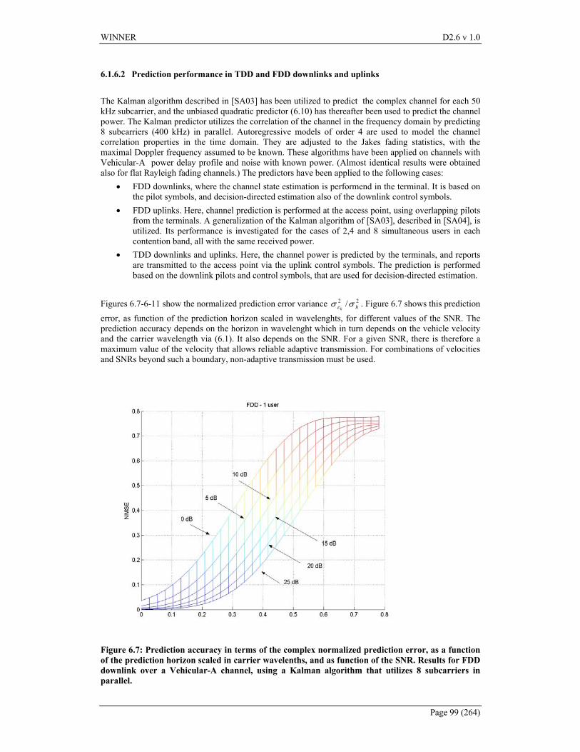
WINNER D2.6 v 1.0

Page 99 (264)

6.1.6.2 Prediction performance in TDD and FDD downlinks and uplinks The Kalman algorithm described in [SA03] has been utilized to predict the complex channel for each 50 kHz subcarrier, and the unbiased quadratic predictor (6.10) has thereafter been used to predict the channel power. The Kalman predictor utilizes the correlation of the channel in the frequency domain by predicting 8 subcarriers (400 kHz) in parallel. Autoregressive models of order 4 are used to model the channel correlation properties in the time domain. They are adjusted to the Jakes fading statistics, with the maximal Doppler frequency assumed to be known. These algorithms have been applied on channels with Vehicular-A power delay profile and noise with known power. (Almost identical results were obtained also for flat Rayleigh fading channels.) The predictors have been applied to the following cases:

• FDD downlinks, where the channel state estimation is performend in the terminal. It is based on the pilot symbols, and decision-directed estimation also of the downlink control symbols.

• FDD uplinks. Here, channel prediction is performed at the access point, using overlapping pilots from the terminals. A generalization of the Kalman algorithm of [SA03], described in [SA04], is utilized. Its performance is investigated for the cases of 2,4 and 8 simultaneous users in each contention band, all with the same received power.

• TDD downlinks and uplinks. Here, the channel power is predicted by the terminals, and reports are transmitted to the access point via the uplink control symbols. The prediction is performed based on the downlink pilots and control symbols, that are used for decision-directed estimation.

Figures 6.7-6-11 show the normalized prediction error variance 22 / hhσσ ε . Figure 6.7 shows this prediction

error, as function of the prediction horizon scaled in wavelenghts, for different values of the SNR. The prediction accuracy depends on the horizon in wavelenght which in turn depends on the vehicle velocity and the carrier wavelength via (6.1). It also depends on the SNR. For a given SNR, there is therefore a maximum value of the velocity that allows reliable adaptive transmission. For combinations of velocities and SNRs beyond such a boundary, non-adaptive transmission must be used.

Figure 6.7: Prediction accuracy in terms of the complex normalized prediction error, as a function of the prediction horizon scaled in carrier wavelenths, and as function of the SNR. Results for FDD downlink over a Vehicular-A channel, using a Kalman algorithm that utilizes 8 subcarriers in parallel.

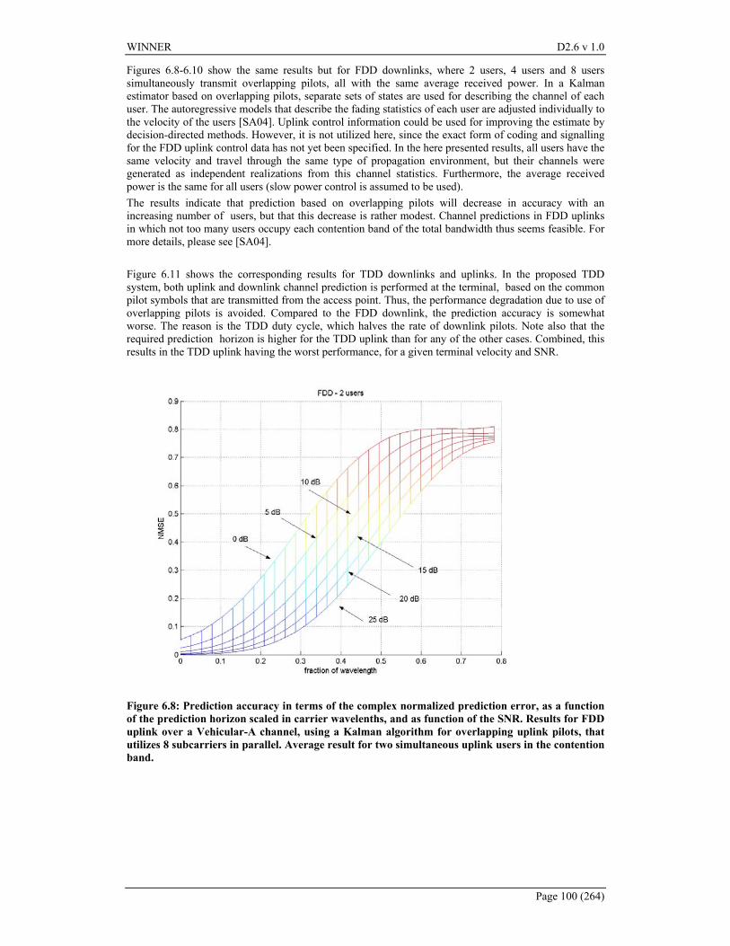
WINNER D2.6 v 1.0

Page 100 (264)

Figures 6.8-6.10 show the same results but for FDD downlinks, where 2 users, 4 users and 8 users simultaneously transmit overlapping pilots, all with the same average received power. In a Kalman estimator based on overlapping pilots, separate sets of states are used for describing the channel of each user. The autoregressive models that describe the fading statistics of each user are adjusted individually to the velocity of the users [SA04]. Uplink control information could be used for improving the estimate by decision-directed methods. However, it is not utilized here, since the exact form of coding and signalling for the FDD uplink control data has not yet been specified. In the here presented results, all users have the same velocity and travel through the same type of propagation environment, but their channels were generated as independent realizations from this channel statistics. Furthermore, the average received power is the same for all users (slow power control is assumed to be used). The results indicate that prediction based on overlapping pilots will decrease in accuracy with an increasing number of users, but that this decrease is rather modest. Channel predictions in FDD uplinks in which not too many users occupy each contention band of the total bandwidth thus seems feasible. For more details, please see [SA04]. Figure 6.11 shows the corresponding results for TDD downlinks and uplinks. In the proposed TDD system, both uplink and downlink channel prediction is performed at the terminal, based on the common pilot symbols that are transmitted from the access point. Thus, the performance degradation due to use of overlapping pilots is avoided. Compared to the FDD downlink, the prediction accuracy is somewhat worse. The reason is the TDD duty cycle, which halves the rate of downlink pilots. Note also that the required prediction horizon is higher for the TDD uplink than for any of the other cases. Combined, this results in the TDD uplink having the worst performance, for a given terminal velocity and SNR.

Figure 6.8: Prediction accuracy in terms of the complex normalized prediction error, as a function of the prediction horizon scaled in carrier wavelenths, and as function of the SNR. Results for FDD uplink over a Vehicular-A channel, using a Kalman algorithm for overlapping uplink pilots, that utilizes 8 subcarriers in parallel. Average result for two simultaneous uplink users in the contention band.

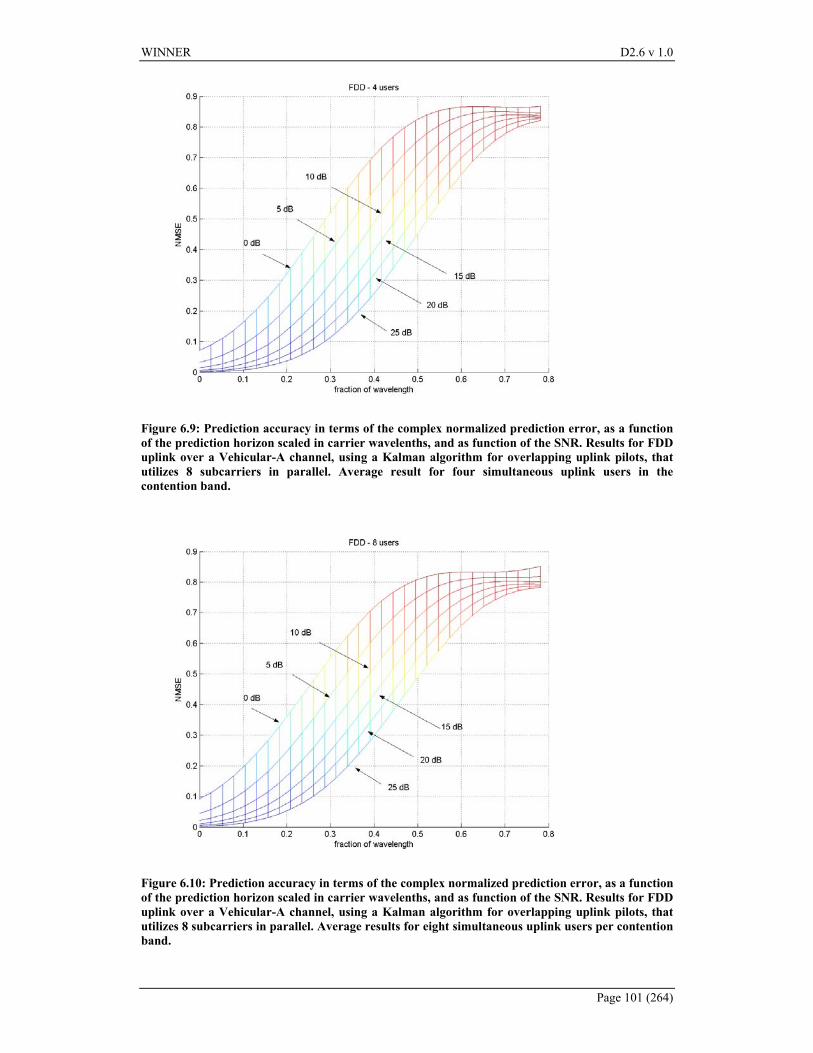
WINNER D2.6 v 1.0

Page 101 (264)

Figure 6.9: Prediction accuracy in terms of the complex normalized prediction error, as a function of the prediction horizon scaled in carrier wavelenths, and as function of the SNR. Results for FDD uplink over a Vehicular-A channel, using a Kalman algorithm for overlapping uplink pilots, that utilizes 8 subcarriers in parallel. Average result for four simultaneous uplink users in the contention band.

Figure 6.10: Prediction accuracy in terms of the complex normalized prediction error, as a function of the prediction horizon scaled in carrier wavelenths, and as function of the SNR. Results for FDD uplink over a Vehicular-A channel, using a Kalman algorithm for overlapping uplink pilots, that utilizes 8 subcarriers in parallel. Average results for eight simultaneous uplink users per contention band.

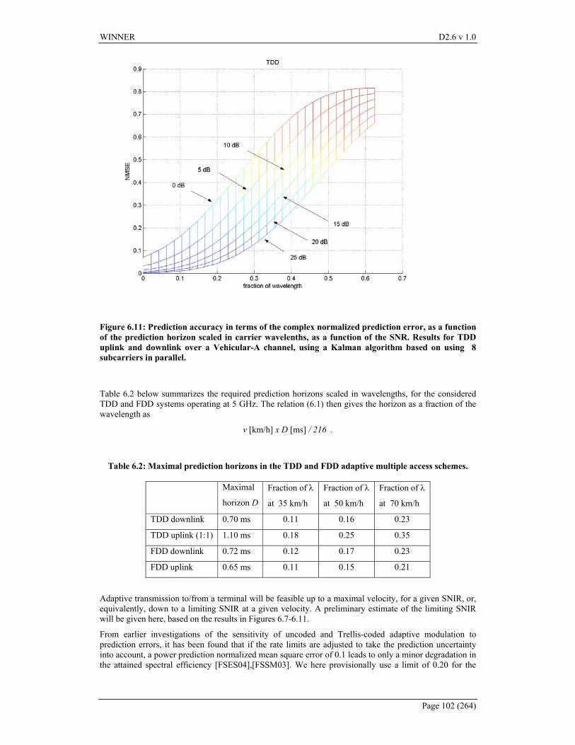
WINNER D2.6 v 1.0

Page 102 (264)

Figure 6.11: Prediction accuracy in terms of the complex normalized prediction error, as a function of the prediction horizon scaled in carrier wavelenths, as a function of the SNR. Results for TDD uplink and downlink over a Vehicular-A channel, using a Kalman algorithm based on using 8 subcarriers in parallel.

Table 6.2 below summarizes the required prediction horizons scaled in wavelengths, for the considered TDD and FDD systems operating at 5 GHz. The relation (6.1) then gives the horizon as a fraction of the wavelength as

v [km/h] x D [ms] / 216 .

Table 6.2: Maximal prediction horizons in the TDD and FDD adaptive multiple access schemes.

Maximal

horizon D

Fraction of λ

at 35 km/h

Fraction of λ

at 50 km/h

Fraction of λ

at 70 km/h

TDD downlink 0.70 ms 0.11 0.16 0.23

TDD uplink (1:1) 1.10 ms 0.18 0.25 0.35

FDD downlink 0.72 ms 0.12 0.17 0.23

FDD uplink 0.65 ms 0.11 0.15 0.21

Adaptive transmission to/from a terminal will be feasible up to a maximal velocity, for a given SNIR, or, equivalently, down to a limiting SNIR at a given velocity. A preliminary estimate of the limiting SNIR will be given here, based on the results in Figures 6.7-6.11.

From earlier investigations of the sensitivity of uncoded and Trellis-coded adaptive modulation to prediction errors, it has been found that if the rate limits are adjusted to take the prediction uncertainty into account, a power prediction normalized mean square error of 0.1 leads to only a minor degradation in the attained spectral efficiency [FSES04],[FSSM03]. We here provisionally use a limit of 0.20 for the

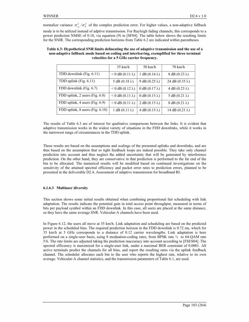
WINNER D2.6 v 1.0

Page 103 (264)

normalize variance 22 / hhσσ ε of the complex prediction error. For higher values, a non-adaptive fallback

mode is to be utilized instead of adptive transmission. For Rayleigh fading channels, this corresponds to a power prediction NMSE of 0.18, via equation (9) in [SF04]. The table below shows the resulting limits for the SNIR. The corresponding prediction horizons from Table 6.2 are indicated within parentheses.

Table 6.3: Hypothetical SNR limits delineating the use of adaptive transmission and the use of a non-adaptive fallback mode based on coding and interleaving, exemplified for three terminal

velocities for a 5 GHz carrier frequency.

35 km/h 50 km/h 70 km/h

TDD downlink (Fig. 6.11) < 0 dB (0.11 λ) 1 dB (0.16 λ) 8 dB (0.23 λ)

TDD uplink (Fig. 6.11) 5 dB (0.18 λ) 9 dB (0.25 λ) 24 dB (0.35 λ)

FDD downlink (Fig. 6.7) < 0 dB (0.12 λ) 0 dB (0.17 λ) 4 dB (0.23 λ)

FDD uplink, 2 users (Fig. 6.8) < 0 dB (0.11 λ) 0 dB (0.15 λ) 5 dB (0.21 λ)

FDD uplink, 4 users (Fig. 6.9) < 0 dB (0.11 λ) 2 dB (0.15 λ) 8 dB (0.21 λ)

FDD uplink, 8 users (Fig. 6.10) 1 dB (0.11 λ) 4 dB (0.15 λ) 14 dB (0.21 λ)

The results of Table 6.3 are of interest for qualitative comparisons between the links. It is evident that adaptive transmission works in the widest variety of situations in the FDD downlinks, while it works in the narrowest range of circumstances in the TDD uplink.

These results are based on the assumptions and scalings of the presented uplinks and downlinks, and are thus based on the assumption that so tight feedback loops are indeed possible. They take only channel prediction into account and thus neglect the added uncertainty that will be generated by interference prediction. On the other hand, they are conservative in that prediction is performed to the far end of the bin to be allocated. The numerical results will be modified based on continued investigations on the sensitivity of the attained spectral efficiency and packet error rates to prediction errors, planned to be presented in the deliverable D2.4, Assessment of adaptive transmission for broadband RI.

6.1.6.3 Multiuser diversity This section shows some initial results obtained when combining proportional fair scheduling with link adaptation. The results indicate the potential gain in total access point throughput, measured in terms of bits per payload symbol within an FDD downlink. In this case, all users are placed at the same distance, so they have the same average SNR. Vehicular-A channels have been used. In Figure 6.12, the users all move at 35 km/h. Link adaptation and scheduling are based on the predicted power in the scheduled bins. The required prediction horizon in the FDD downlink is 0.72 ms, which for 35 km/h at 5 GHz corresponds to a distance of 0.12 carrier wavelengths. Link adaptation is here performed on a single-user basis, using 8 moduation-coding rates, from BPSK rate ½ to 64-QAM rate 5/6. The rate limits are adjusted taking the prediction inaccuracy into account according to [FSES04]. The spectral efficiency is maximized for a single-user link, under a maximal BER constraint of 0.0001. All active terminals predict the channels for all bins, and report the resulting rates via the uplink feedback channel. The scheduler allocates each bin to the user who reports the highest rate, relative to its own average. Vehicular-A channel statistics, and the transmission parameters of Table 6.1, are used.

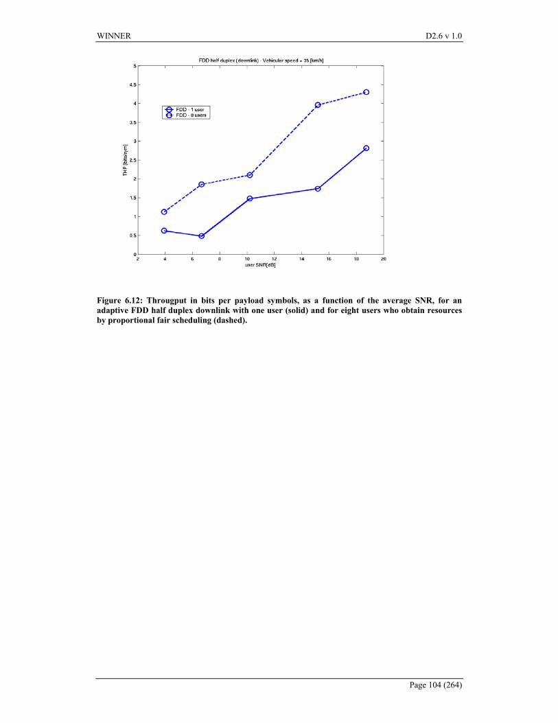
WINNER D2.6 v 1.0

Page 104 (264)

Figure 6.12: Througput in bits per payload symbols, as a function of the average SNR, for an adaptive FDD half duplex downlink with one user (solid) and for eight users who obtain resources by proportional fair scheduling (dashed).

WINNER D2.6 v 1.0

Page 105 (264)

6.2 OFDMA Recall the description of a TDMA/OFDMA scheme in chapter 6.1, where the physical channel resource can be partitioned into units of time-frequency bins as shown in Figure 6.2. Each time-frequency bin can be treated as a timeslot in time direction, and consists of one or several subcarriers in frequency direction. In OFDMA systems, typically bins at a certain frequency are allocated statically or semi-statically to the individual users. The subcarriers in a frequency bin can be either contiguous or picked up from interleaved positions over the entire available subcarriers. The former can be referred to as block OFDMA (BOFDMA), and the latter can be referred to as interleaved OFDMA (IOFDMA). That is, the BOFDMA is OFDMA without subcarrier interleaving and IOFDMA is OFDMA with subcarrier interleaving. As discussed in the context of TDMA/OFDMA systems above, fast link adaptation in an OFDMA system is also attractive, in order to increase the spectral efficiency of an OFDMA system. The difference to TDMA/OFDMA is then that fast user scheduling between bins at different frequencies is not performed. If link adaptation with adaptive frequency resource allocation is going to be used with an OFDMA scheme, BOFDMA is apparently the right choice. This is because in IOFDMA the subcarrier interleaving provides an averaging effect, thus the property of each time-frequency bin will tend to be similar. If link adaptation with fixed frequency resource allocation is used, either BOFDMA or IOFDMA can be adopted, but the performance depends on the channel conditions.

6.2.1 OFDMA with fast link adaptation Different from frequency hopping and interleaving which belong to channel and interference averaging technology, adaptive resource allocation is a channel and interference avoidance technology. However, from the analysis in section 6.1.3.2 it can be seen that adaptive resource allocation of the fast link adaptation makes the system complicated and not easy to implement. This is because:

• each terminal has to predict the CSI for all or part of the time-frequency resources, which greatly increases the computational complexity in the terminal and the feedback bandwidth requirement,

• it also increases the computation load of the base station and the control and signalling overhead.

It has been discussed in chapter 6.1.3.2 that under bad channel conditions (e.g., fast time-varying), the system design with adaptive resource allocation becomes difficult. Therefore, to compromise the advantage and disadvantage, we can employ a fast link adaptation scheme without adaptive resource allocation. That is, the other adaptation techniques such as adaptive modulation, adaptive coding, adaptive power control/loading etc., can still be used [GC98], [WChLM99], [PMS02]. In this scheme, to diversify the channel conditions and interferences, interleaved OFDMA (IOFDMA), can also be employed.

The frame structure of Figure 6.2 can still be used. The difference is that in the case of IOFDMA, the subcarriers within a time-frequency bin are not contiguous, and the bin size in the frequency direction is also not limited by the channel coherence bandwidth anymore.

The equations (6.3) ~(6.5) for a system design are still valid here. The link adaptation procedure becomes:

• In timeslot j , each active terminal predicts the CSI at timeslot delaynj + for the time-frequency bins being allocated to it, where delayn is the reaction delay in terms of number of timeslot.

• Each active terminal sends back to the base station their predicted CSI. We assume 3 bits are enough to indicate 8=CSIN levels of channel state.

• Adaptation (except resource allocation) is then performed by the base station and decisions (modulation, coding, etc.) for timeslot delaynj + are broadcast.

The uplink control bandwidth demand now becomes much smaller. In the worst scenario where all the terminals are fast moving and all the time-frequency bins in a timeslot are being used, the uplink control bandwidth ucB becomes:

slot

CSITotalbuc TNKB 1)(log 2_= (6.14)

From the case analyses in the following subsections, it can be seen that the system design becomes easier to cope with fast fading.

WINNER D2.6 v 1.0

Page 106 (264)

6.2.1.1 Link adaptation in worst case channels These are the channel conditions depicted in section 6.1.3.2. For the worst case channels, we have a Doppler spread of 926=Df Hz (for an equivalent terminal speed of 200km/h) and delay spread of

1=τ µs (Note: we can also use suburban parameters: 463=Df Hz and 2=τ µs).

According to equation (6.3) and (6.4), the maximum timeslot duration can be selected as sTT sslot µ904 == .

According to equation (6.5), the maximum bandwidth of a time-frequency bin can be selected as

20051

==∆τbf kHz, which is equivalent to 4 subcarriers.

Hence the total number of time-frequency bins in a timeslot is 416_ =∆⋅∆

=b

SDTotalb f

NfK . And the worst

scenario uplink control bandwidth demand becomes slot

CSITotalbuc TNKB 1)(log 2_= = 9.13 [Mbits/s],

which may still be feasible for a real application.

6.2.1.2 Link adaptation with fixed resource allocation in FDD

Frequency selective fading The design rule and process are the same as that described in section 6.1.3.2. Hence the bandwidth of a

time-frequency bin can be selected as 20051

==∆τbf kHz (equivalent to 4 subcarriers), and the total

number of time-frequency bins in a timeslot is 416_ =∆⋅∆

=b

SDTotalb f

NfK .

If we assume a total uplink control bandwidth of 5.0 Mbits/s is acceptable, the following requirement should be satisfied for a worst scenario system design:

0.51)(log 2_ <=Slot

CSITotalbuc TNKB [Mbits/s] (6.15)

That is:

)(log2.0 2_ CSITotalbslot NKT > [µs] (6.16)

From (6.16), we have 6.249>slotT µs. Therefore we can select 27012 == sslot TT µs for convenience. By reverse calculation from equation (6.3) and (6.4) with slotdelay TT 3= , we know that this timeslot duration design can cope with terminals with a Doppler spread up to 370 Hz , i.e., terminals with an equivalent speed of up to 80km/h. If the link adaptation reaction delay is slotdelay TT 4= , from (6.3) and (6.4) it can be calculated that with the same design parameters, terminals with a moving speed up to 66km/h (Doppler spread of 308Hz), can be coped with.

It should be noted that if not all the terminals within a cell/sector are fast moving, longer timeslot can be used for the slow moving terminals, and accordingly the total uplink control bandwidth will be smaller.

Flat fading The design principle is the same as that described in section 6.1.3.2. Considering the maximum terminal speed of 200km/h, its equivalent Doppler spread is 926=Df Hz. According to equation (6.3) and (6.4), the timeslot duration can be selected as sTT sslot µ904 == .

To keep the uplink control bandwidth relatively small, we still use (6.16) to decide the total number of

time-frequency bins in a timeslot, which results in 150_ <

∆⋅∆

=b

SDTotalb f

NfK . Hence, for a convenient

WINNER D2.6 v 1.0

Page 107 (264)

system design (convenient for allocating the pilot and control symbols), we can choose 600=∆ bf kHz, which is equivalent to 12 subcarriers.

6.2.1.3 Link adaptation with fixed resource allocation in TDD If we still assume that channel reciprocity doesn’t hold for TDD in terms of SINR, the system design procedure will be the same as that depicted in Section 6.2.1.2 for FDD. Some similar case analyses are given in the following subsections.

Frequency selective fading The design procedure is the same as that described in Section 6.1.3.2. From (6.16), we have

6.249>slotT µs. Therefore we select 27012 == sslot TT µs for convenience. By reverse calculation from equation (6.3) and (6.4) with slotdelay TT 4= , we know that this timeslot duration design can cope with terminals with a speed of up to 66km/h. If the link adaptation reaction delay is slotdelay TT 6= (neglecting the guard time between DL slot and UL slot), it can be calculated that with the same design parameters, terminals with a moving speed up to 44km/h (Doppler spread of 205Hz), can be coped with.

Flat fading The design principle is the same as that described in Section 6.1.3.2 for FDD. Considering the maximum terminal speed of 200km/h, its equivalent Doppler spread is 926=Df Hz. If the reaction delay is

slotdelay TT 4= , the design result is the same as that of FDD in Section 6.1.3.2.

If the reaction delay is slotdelay TT 6= , then according to equation (6.3) and (6.4), the timeslot duration can be selected as sTT sslot µ452 == . Then from (6.16), the total number of time-frequency bins in a timeslot

becomes 75_ <

∆⋅∆

=b

SDTotalb f

NfK . Hence, for a convenient system design (convenient for allocating

the pilot and control symbols), we can choose 1200=∆ bf kHz, which is equivalent to 24 subcarriers.

6.2.2 Adaptive OFDMA uplink In OFDMA uplink transmission, several parameters can be adapted as a function of the channel conditions and the traffic type. In order to tackle this highly complex optimization problem, we separate it in two main steps:

1. Subcarrier allocation: This step determines which subcarrier is allocated to which user. 2. Bit and power loading: After the subcarriers have been assigned to the users, the problem of

adaptively assigning the appropriate QAM constellation and power for each subcarrier can be solved for each user individually.

The second step is basically a single-user problem, which allows to make use of existing bit-loading algorithms, see e.g. [Bin90], [Cam99], [ChCB95], [Czyl96], [FH96], [FH96a], [Hug87], [KRJ00], [LChLM99], [Son02], [SSh00a], [YC01]. In the following, we first briefly review the single-user problem before describing adaptive algorithms for OFDMA in some detail.

6.2.2.1 Adaptive single-user OFDM In order to approximate the channel capacity in a frequency-selective channel with Gaussian noise, the transmitter PSD has to be shaped according to the water-filling theorem [Gal68], [CTh91], as depicted in Figure 6.13: The inverse channel gain to noise ratio (CNR) forms the bottom of a bowl, which is filled with an amount of water corresponding to the available power ptot. The resulting optimum PSD corresponds to the water depth.

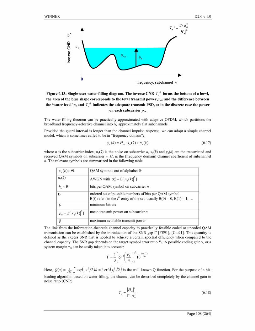
WINNER D2.6 v 1.0

Page 108 (264)

c 0

0

pn

frequency, subchannel n

ptot

2

21

n

nn

HT σ⋅Γ

=−

inve

rse

CN

R 1

/Tn

c 0

0

pnpn

frequency, subchannel n

ptot

2

21

n

nn

HT σ⋅Γ

=−

inve

rse

CN

R 1

/Tn

Figure 6.13: Single-user water-filling diagram. The inverse CNR 1−nT forms the bottom of a bowl,

the area of the blue shape corresponds to the total transmit power ptot, and the difference between the ‘water level’ c0 and 1−

nT indicates the adequate transmit PSD, or in the discrete case the power on each subcarrier pn.

The water-filling theorem can be practically approximated with adaptive OFDM, which partitions the broadband frequency-selective channel into Nc approximately flat subchannels.

Provided the guard interval is longer than the channel impulse response, we can adopt a simple channel model, which is sometimes called to be in “frequency domain”:

)()()( knkxHky nnnn +⋅= (6.17)

where n is the subcarrier index, nn(k) is the noise on subcarrier n, xn(k) and yn(k) are the transmitted and received QAM symbols on subcarrier n. Hn is the (frequency domain) channel coefficient of subchannel n. The relevant symbols are summarized in the following table.

∈)(kxn Θ QAM symbols out of alphabet Θ

nn(k) AWGN with ])(E[ 22 knnn =σ

∈nb Β bits per QAM symbol on subcarrier n

Β ordered set of possible numbers of bits per QAM symbol Β(i) refers to the ith entry of the set, usually Β(0) = 0, Β(1) = 1, …

b)

minimum bitrate

])([ 2kxEp nn = mean transmit power on subcarrier n

p( maximum available transmit power

The link from the information-theoretic channel capacity to practically feasible coded or uncoded QAM transmission can be established by the introduction of the SNR gap Γ [FE91], [Cio91]. This quantity is defined as the excess SNR that is needed to achieve a certain spectral efficiency when compared to the channel capacity. The SNR gap depends on the target symbol error ratio PS. A possible coding gain γc or a system margin γm can be easily taken into account:

10

21 10

431 cm

SPQ

γ−γ−

=Γ

Here, ( ) ( )2erfc2exp)( 212

21 xdttxQ

x=−= ∫

∞

π is the well-known Q-function. For the purpose of a bit-

loading algorithm based on water-filling, the channel can be described completely by the channel gain to noise ratio (CNR)

2

2

n

nn

HT

σ⋅Γ= (6.18)

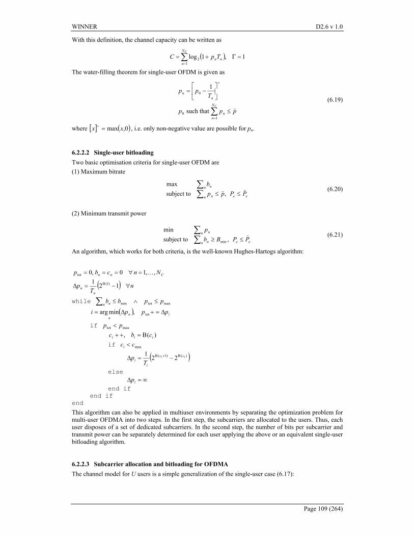
WINNER D2.6 v 1.0

Page 109 (264)

With this definition, the channel capacity can be written as

( ) 1,1log1

2 =Γ+= ∑=

CN

nnnTpC

The water-filling theorem for single-user OFDM is given as

ppp

Tpp

CN

nn

nn

(≤

−=

∑=

+

10

0

such that

1

(6.19)

where [ ] ( )0,max xx =+ , i.e. only non-negative value are possible for pn.

6.2.2.2 Single-user bitloading Two basic optimisation criteria for single-user OFDM are (1) Maximum bitrate

een n

n n

PPppb

(( ≤≤∑∑

,subject tomax

(6.20)

(2) Minimum transmit power

een n

n n

PPBbp

(≤≥∑

∑,subject to

min

min (6.21)

An algorithm, which works for both criteria, is the well-known Hughes-Hartogs algorithm:

Cnn Nncbp ,,10,0tot K=∀=== ( ) n

Tp

nn ∀−=∆ 121 )1(Β

while maxtotmin ppbbn n ≤∧≤∑

( ) inn

pppi ∆=+∆= tot,minarg if maxtot pp < )(, iii cbc Β=++ if maxcci < ( ))()1( 221 ii cc

ii T

p ΒΒ −=∆ +

else ∞=∆ ip end if end if end This algorithm can also be applied in multiuser environments by separating the optimization problem for multi-user OFDMA into two steps. In the first step, the subcarriers are allocated to the users. Thus, each user disposes of a set of dedicated subcarriers. In the second step, the number of bits per subcarrier and transmit power can be separately determined for each user applying the above or an equivalent single-user bitloading algorithm.

6.2.2.3 Subcarrier allocation and bitloading for OFDMA The channel model for U users is a simple generalization of the single-user case (6.17):

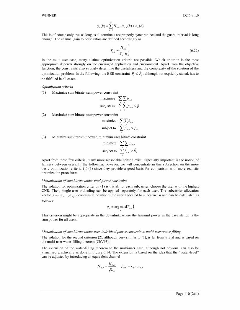
WINNER D2.6 v 1.0

Page 110 (264)

)()()(1

,, knkxHky n

U

uununn +⋅= ∑

=

This is of course only true as long as all terminals are properly synchronized and the guard interval is long enough. The channel gain to noise ratios are defined accordingly as

2

2,

,nu

unun

HT

σ⋅Γ= (6.22)

In the multi-user case, many distinct optimization criteria are possible. Which criterion is the most appropriate depends strongly on the envisaged application and environment. Apart from the objective function, the constraints also strongly determine the usefulness and the complexity of the solution of the optimization problem. In the following, the BER constraint ee PP

(≤ , although not explicitly stated, has to

be fulfilled in all cases.

Optimization criteria (1) Maximize sum bitrate, sum power constraint

pp

b

u nnu

u nnu

(≤∑∑∑∑

,

,

subject to

maximize

(2) Maximize sum bitrate, user power constraint

u

nnu

u nnu

pp

b(≤∑

∑∑,

,

subject to

maximize

(3) Minimize sum transmit power, minimum user bitrate constraint

u

nnu

u nnu

bb

p)

≥∑∑∑

,

,

subject to

minimize

Apart from these few criteria, many more reasonable criteria exist. Especially important is the notion of fairness between users. In the following, however, we will concentrate in this subsection on the more basic optimization criteria (1)-(3) since they provide a good basis for comparison with more realistic optimization procedures.

Maximization of sum bitrate under total power constraint The solution for optimization criterion (1) is trivial: for each subcarrier, choose the user with the highest CNR. Then, single-user bitloading can be applied separately for each user. The subcarrier allocation vector ),,( 1 CNaa K=a contains at position n the user allocated to subcarrier n and can be calculated as follows: ( )un

un Ta ,maxarg=

This criterion might be appropriate in the downlink, where the transmit power in the base station is the sum power for all users.

Maximization of sum bitrate under user-individual power constraints: multi-user water-filling The solution for the second criterion (2), although very similar to (1), is far from trivial and is based on the multi-user water-filling theorem [ChV93].

The extension of the water-filling theorem to the multi-user case, although not obvious, can also be visualised graphically as done in Figure 6.14. The extension is based on the idea that the “water-level” can be adjusted by introducing an equivalent channel

unuunu

unun pp

HH ,,

,, ˆ,ˆ ⋅λ=

λ=

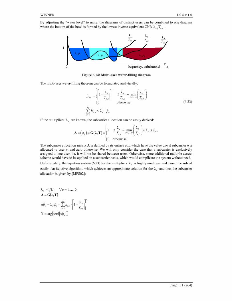
WINNER D2.6 v 1.0

Page 111 (264)

By adjusting the “water level” to unity, the diagrams of distinct users can be combined to one diagram where the bottom of the bowl is formed by the lowest inverse equivalent CNR ,u n uTλ .

1

0 nfrequency, subchannel

2

,2nTλ1

,1nTλ

3

,3nTλ

1 1pλ (

2 2pλ (3 3pλ (

1

0 nfrequency, subchannel

2

,2nTλ1

,1nTλ

3

,3nTλ

1 1pλ (

2 2pλ (3 3pλ (

Figure 6.14: Multi-user water-filling diagram

The multi-user water-filling theorem can be formulated analytically:

uu

N

nun

ln

l

Ulun

u

un

u

un

pp

TTTp

C (

K

⋅λ≤

λ=

λ

λ−=

∑=

=

+

1,

,,,1

,,,

ˆ

otherwise0

min if1ˆ (6.23)

If the multipliers uλ are known, the subcarrier allocation can be easily derived:

( ) ( ) ,1, ,, ,

1 if min,

0 otherwise

u lu n ul U

ij n u n l

Ta T T=

λ λ= ∧ λ ≤ = = =

A G λ T K

The subcarrier allocation matrix A is defined by its entries an,u, which have the value one if subcarrier n is allocated to user u, and zero otherwise. We will only consider the case that a subcarrier is exclusively assigned to one user, i.e. it will not be shared between users. Otherwise, some additional multiple access scheme would have to be applied on a subcarrier basis, which would complicate the system without need. Unfortunately, the equation system (6.23) for the multipliers uλ is highly nonlinear and cannot be solved easily. An iterative algorithm, which achieves an approximate solution for the uλ and thus the subcarrier allocation is given by [MPS02]:

Uu 1=λ Uu ,,1K=∀ ( )Tλ,GA =

∑=

+

λ−⋅−λ=∆

CN

n un

uunuuu T

app1 ,

, 1ˆ (

( )( )up̂sortarg ∆=Υ

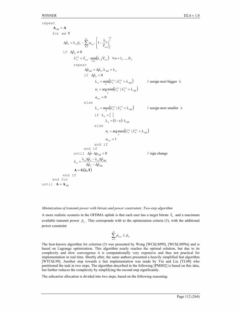
WINNER D2.6 v 1.0

Page 112 (264)

repeat AA =old for Υ∈u

∑=

+

λ−⋅−λ=∆

CN

n un

uunuuu T

app1 ,

, 1ˆ (

if 0ˆ ≠∆ up ( ) Clnlulun

sn NnTT ,,1min ,,

)( K=∀λ⋅=λ≠

repeat uupp λ=λ∆=∆ oldold ,ˆˆ if 0ˆ <∆ up ( )old

)()( |min λ>λλ=λ sn

snnu // assign next bigger λ

( )old)()(

1 |minarg λ>λλ= sn

sn

nn

0, =una else ( )old

)()( |max λ<λλ=λ sn

snnu // assign next smaller λ

if { }=λu ( ) old1 λ⋅ε−=λu else ( )old

)()(1 |maxarg λ<λλ= s

nsn

nn

1, =una end if end if until 0ˆ old <∆⋅∆ pp // sign change

old

old

ˆˆˆˆ

pppp

u

uuuu ∆−∆

∆λ−∆λ=λ

( )Tλ,GA = end if end for until oldAA =

Minimization of transmit power with bitrate and power constraints: Two-step algorithm

A more realistic scenario in the OFDMA uplink is that each user has a target bitrate ub)

and a maximum available transmit power up( . This corresponds with to the optimization criteria (3), with the additional power constraint

u

N

nun pp (≤∑

=1,

The best-known algorithm for criterion (3) was presented by Wong [WChLM99], [WChLM99a] and is based on Lagrange optimization. This algorithm nearly reaches the optimal solution, but due to its complexity and slow convergence it is computationally very expensive and thus not practical for implementation in real time. Shortly after, the same authors presented a heavily simplified fast algorithm [WTChL99]. Another step towards a fast implementation was made by Yin and Liu [YL00] who partitioned the task in two steps. The algorithm described in the following [PMS02] is based on this idea, but further reduces the complexity by simplifying the second step significantly.

The subcarrier allocation is divided into two steps, based on the following reasoning:

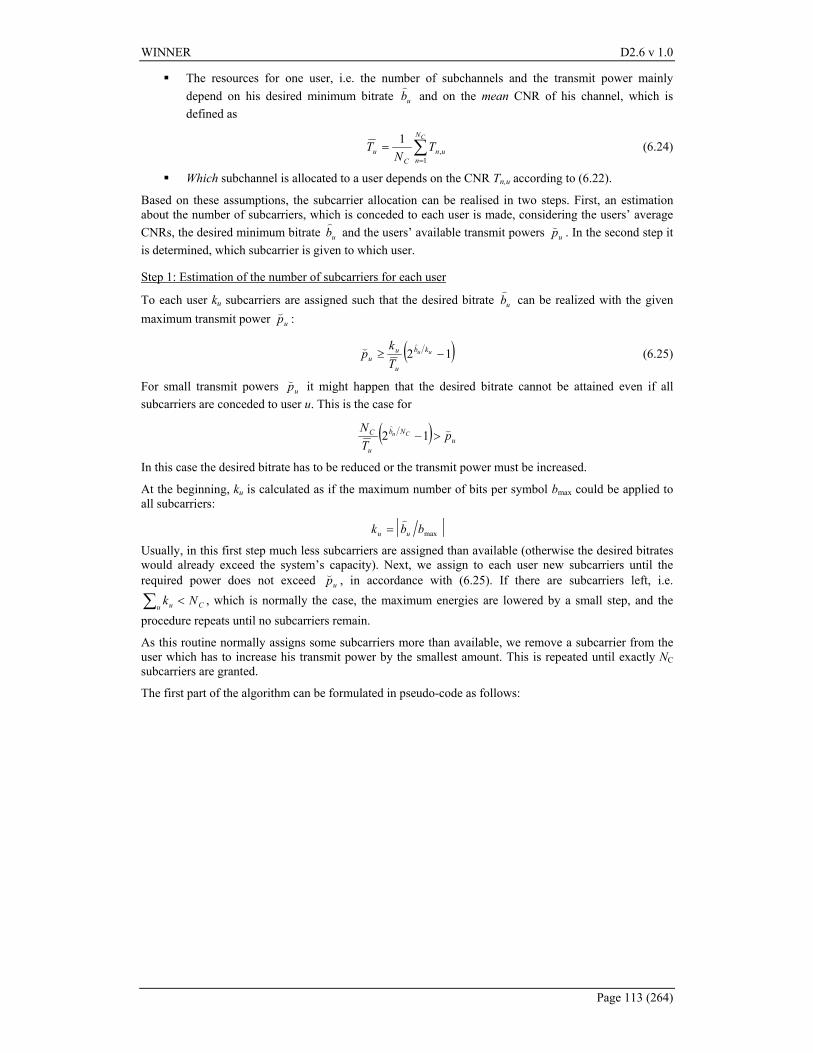
WINNER D2.6 v 1.0

Page 113 (264)

The resources for one user, i.e. the number of subchannels and the transmit power mainly depend on his desired minimum bitrate ub

) and on the mean CNR of his channel, which is

defined as

∑=

=CN

nun

Cu T

NT

1,

1 (6.24)

Which subchannel is allocated to a user depends on the CNR Tn,u according to (6.22).

Based on these assumptions, the subcarrier allocation can be realised in two steps. First, an estimation about the number of subcarriers, which is conceded to each user is made, considering the users’ average CNRs, the desired minimum bitrate ub

) and the users’ available transmit powers up( . In the second step it

is determined, which subcarrier is given to which user.

Step 1: Estimation of the number of subcarriers for each user

To each user ku subcarriers are assigned such that the desired bitrate ub)

can be realized with the given maximum transmit power up( :

( )12 −≥ uu kb

u

uu T

kp

)( (6.25)

For small transmit powers up( it might happen that the desired bitrate cannot be attained even if all subcarriers are conceded to user u. This is the case for

( ) uNb

u

C pTN

Cu ()

>−12

In this case the desired bitrate has to be reduced or the transmit power must be increased.

At the beginning, ku is calculated as if the maximum number of bits per symbol bmax could be applied to all subcarriers:

maxbbk uu

)=

Usually, in this first step much less subcarriers are assigned than available (otherwise the desired bitrates would already exceed the system’s capacity). Next, we assign to each user new subcarriers until the required power does not exceed up( , in accordance with (6.25). If there are subcarriers left, i.e.

Cu u Nk <∑ , which is normally the case, the maximum energies are lowered by a small step, and the procedure repeats until no subcarriers remain.

As this routine normally assigns some subcarriers more than available, we remove a subcarrier from the user which has to increase his transmit power by the smallest amount. This is repeated until exactly NC subcarriers are granted.

The first part of the algorithm can be formulated in pseudo-code as follows:

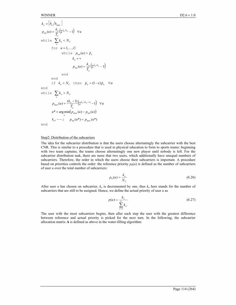
WINNER D2.6 v 1.0

Page 114 (264)

maxbbk uu

)=

( ) uTk

up uu kb

u

u ∀−= 12)(tot

)

while Cu

u Nk <∑ for Uu ,,1K= while upup (>)(tot ++uk

( )12)(tot −= uu kb

u

u

Tk

up)

end end if Cu Nk < then upp uu ∀ε−= (( )1( end while C

uu Nk >∑

( ) uT

kup uu kb

u

u ∀−−

= − 12)1(

)( )1(new

)

( ))()(minarg* totnew upupuu

−= −−*uk ; *)(*)( newtot upup = end

Step2: Distribution of the subcarriers The idea for the subcarrier distribution is that the users choose alternatingly the subcarrier with the best CNR. This is similar to a procedure that is used in physical education to form to sports teams: beginning with two team captains, the teams choose alternatingly one new player until nobody is left. For the subcarrier distribution task, there are more that two users, which additionally have unequal numbers of subcarriers. Therefore, the order in which the users choose their subcarriers is important. A procedure based on priorities controls the order: the reference priority p0(u) is defined as the number of subcarriers of user u over the total number of subcarriers:

C

u

Nk

up =)(0 (6.26)

After user u has chosen on subcarrier, ku is decremented by one, thus ku here stands for the number of subcarriers that are still to be assigned. Hence, we define the actual priority of user u as

∑

=

= U

uu

u

k

kup

1''

)( (6.27)

The user with the most subcarriers begins, then after each step the user with the greatest difference between reference and actual priority is picked for the next turn. In the following, the subcarrier allocation matrix A is defined as above in the water-filling algorithm:

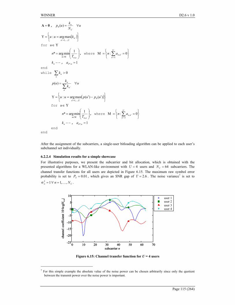
WINNER D2.6 v 1.0

Page 115 (264)

0A = , uNk

upC

u ∀=)(0

( )

== ′

=′u

Uukuu

,,1maxarg:K

Υ

for Υ∈u

=

∈ unn Tn

,

1minarg*Μ

, where

== ∑=′

′ 0:1

,

U

uunanΜ

−−uk , 1*, =una end while 0>∑

uuk

uk

kup

uu

u ∀=∑

′′

)(

( )

′−′==

=′)()(maxarg: 0

,,1upupuu

Uu K

Υ

for Υ∈u

=

∈ unn Tn

,

1minarg*Μ

, where

== ∑=′

′ 0:1

,

U

uunanΜ

−−uk , 1*, =una end end

After the assignment of the subcarriers, a single-user bitloading algorithm can be applied to each user’s subchannel set individually.

6.2.2.4 Simulation results for a simple showcase For illustrative purposes, we present the subcarrier and bit allocation, which is obtained with the presented algorithms for a WLAN-like environment with 4=U users and 64=CN subcarriers. The channel transfer functions for all users are depicted in Figure 6.15. The maximum raw symbol error probability is set to 01.0=SP , which gives an SNR gap of 6.2=Γ . The noise variance7 is set to

Cn Nn ,,112 K=∀=σ .

0 10 20 30 40 50 60 70-25

-20

-15

-10

-5

0

5

10

subcarrier n

chan

nel c

oeff

icie

nt 1

0·lo

g|Hn,

u| user 1user 2user 3user 4

0 10 20 30 40 50 60 70-25

-20

-15

-10

-5

0

5

10

subcarrier n

chan

nel c

oeff

icie

nt 1

0·lo

g|Hn,

u| user 1user 2user 3user 4

Figure 6.15: Channel transfer function for U = 4 users

7 For this simple example the absolute value of the noise power can be chosen arbitrarily since only the quotient

between the transmit power over the noise power is important.

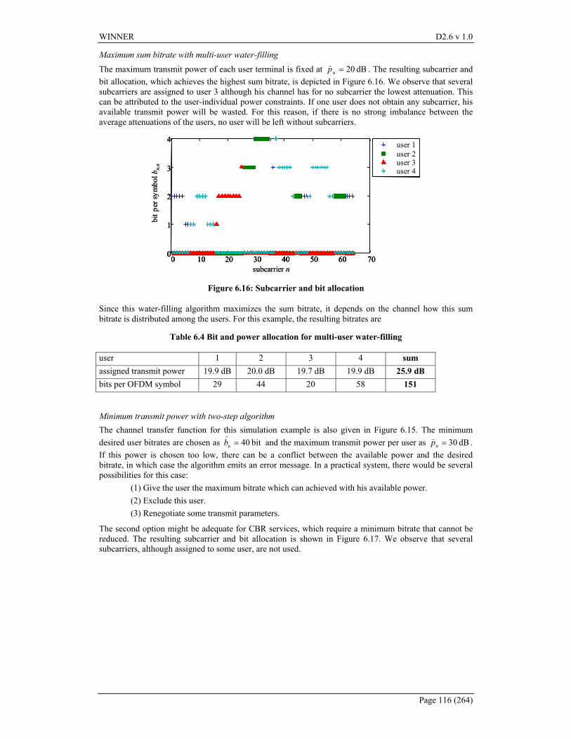
WINNER D2.6 v 1.0

Page 116 (264)

Maximum sum bitrate with multi-user water-filling The maximum transmit power of each user terminal is fixed at dB 20=up( . The resulting subcarrier and bit allocation, which achieves the highest sum bitrate, is depicted in Figure 6.16. We observe that several subcarriers are assigned to user 3 although his channel has for no subcarrier the lowest attenuation. This can be attributed to the user-individual power constraints. If one user does not obtain any subcarrier, his available transmit power will be wasted. For this reason, if there is no strong imbalance between the average attenuations of the users, no user will be left without subcarriers.

0 10 20 30 40 50 60 700

1

2

3

4

subcarrier n

bit p

er sy

mbo

l bn,

u

user 1user 2user 3user 4

0 10 20 30 40 50 60 700

1

2

3

4

0 10 20 30 40 50 60 700

1

2

3

4

subcarrier n

bit p

er sy

mbo

l bn,

u

user 1user 2user 3user 4

Figure 6.16: Subcarrier and bit allocation

Since this water-filling algorithm maximizes the sum bitrate, it depends on the channel how this sum bitrate is distributed among the users. For this example, the resulting bitrates are

Table 6.4 Bit and power allocation for multi-user water-filling

user 1 2 3 4 sum assigned transmit power 19.9 dB 20.0 dB 19.7 dB 19.9 dB 25.9 dB bits per OFDM symbol 29 44 20 58 151

Minimum transmit power with two-step algorithm The channel transfer function for this simulation example is also given in Figure 6.15. The minimum desired user bitrates are chosen as bit 40=ub

) and the maximum transmit power per user as dB 30=up( .

If this power is chosen too low, there can be a conflict between the available power and the desired bitrate, in which case the algorithm emits an error message. In a practical system, there would be several possibilities for this case:

(1) Give the user the maximum bitrate which can achieved with his available power. (2) Exclude this user. (3) Renegotiate some transmit parameters.

The second option might be adequate for CBR services, which require a minimum bitrate that cannot be reduced. The resulting subcarrier and bit allocation is shown in Figure 6.17. We observe that several subcarriers, although assigned to some user, are not used.

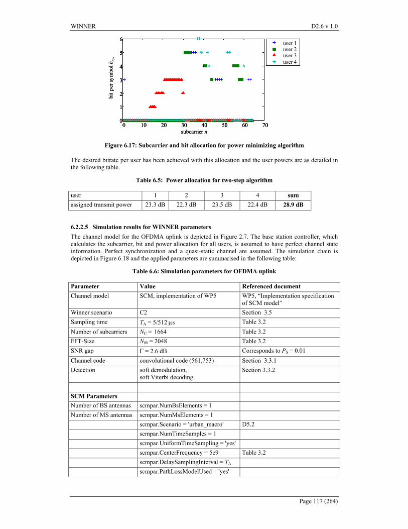
WINNER D2.6 v 1.0

Page 117 (264)

0 10 20 30 40 50 60 700

1

2

3

4

5

6

subcarrier n

bit p

er sy

mbo

l bn,

u

user 1user 2user 3user 4

0 10 20 30 40 50 60 700

1

2

3

4

5

6

0 10 20 30 40 50 60 700

1

2

3

4

5

6

subcarrier n

bit p

er sy

mbo

l bn,

u

user 1user 2user 3user 4

Figure 6.17: Subcarrier and bit allocation for power minimizing algorithm

The desired bitrate per user has been achieved with this allocation and the user powers are as detailed in the following table.

Table 6.5: Power allocation for two-step algorithm

user 1 2 3 4 sum assigned transmit power 23.3 dB 22.3 dB 23.5 dB 22.4 dB 28.9 dB

6.2.2.5 Simulation results for WINNER parameters The channel model for the OFDMA uplink is depicted in Figure 2.7. The base station controller, which calculates the subcarrier, bit and power allocation for all users, is assumed to have perfect channel state information. Perfect synchronization and a quasi-static channel are assumed. The simulation chain is depicted in Figure 6.18 and the applied parameters are summarised in the following table:

Table 6.6: Simulation parameters for OFDMA uplink

Parameter Value Referenced document Channel model SCM, implementation of WP5 WP5, “Implementation specification

of SCM model” Winner scenario C2 Section 3.5 Sampling time TA = 5/512 µs Table 3.2 Number of subcarriers NC = 1664 Table 3.2 FFT-Size Nfft = 2048 Table 3.2 SNR gap Γ = 2.6 dB Corresponds to PS = 0.01 Channel code convolutional code (561,753) Section 3.3.1 Detection soft demodulation,

soft Viterbi decoding Section 3.3.2

SCM Parameters Number of BS antennas scmpar.NumBsElements = 1 Number of MS antennas scmpar.NumMsElements = 1 scmpar.Scenario = 'urban_macro' D5.2 scmpar.NumTimeSamples = 1 scmpar.UniformTimeSampling = 'yes' scmpar.CenterFrequency = 5e9 Table 3.2 scmpar.DelaySamplingInterval = TA scmpar.PathLossModelUsed = 'yes'

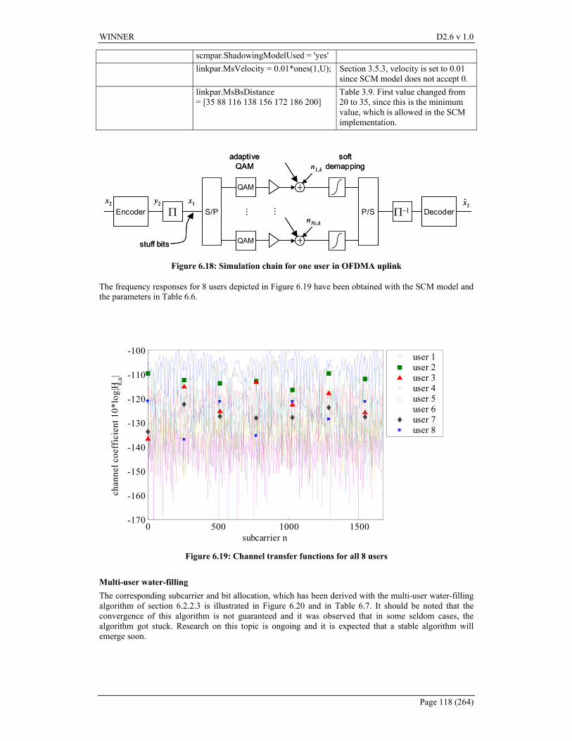
WINNER D2.6 v 1.0

Page 118 (264)

scmpar.ShadowingModelUsed = 'yes' linkpar.MsVelocity = 0.01*ones(1,U); Section 3.5.3, velocity is set to 0.01

since SCM model does not accept 0. linkpar.MsBsDistance

= [35 88 116 138 156 172 186 200] Table 3.9. First value changed from 20 to 35, since this is the minimum value, which is allowed in the SCM implementation.

Encoder Π S/P P/Sx2 y2 x1

nNc,k

… DecoderΠ−1

n1,k

2x̂

QAM

QAM…

adaptiveQAM

softdemapping

stuff bits

Encoder Π S/P P/Sx2 y2 x1

nNc,k

… DecoderΠ−1

n1,k

2x̂

QAM

QAM…

adaptiveQAM

softdemapping

stuff bits

Figure 6.18: Simulation chain for one user in OFDMA uplink

The frequency responses for 8 users depicted in Figure 6.19 have been obtained with the SCM model and the parameters in Table 6.6.

0 500 1000 1500-170

-160

-150

-140

-130

-120

-110

-100

subcarrier n

chan

nel c

oeff

icie

nt 1

0*lo

g|H n,

u|

user 1user 2user 3user 4user 5user 6user 7user 8

Figure 6.19: Channel transfer functions for all 8 users

Multi-user water-filling The corresponding subcarrier and bit allocation, which has been derived with the multi-user water-filling algorithm of section 6.2.2.3 is illustrated in Figure 6.20 and in Table 6.7. It should be noted that the convergence of this algorithm is not guaranteed and it was observed that in some seldom cases, the algorithm got stuck. Research on this topic is ongoing and it is expected that a stable algorithm will emerge soon.

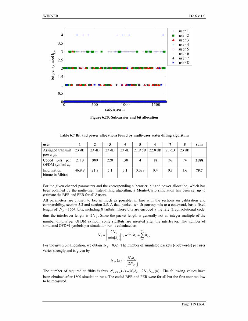
WINNER D2.6 v 1.0

Page 119 (264)

0 500 1000 15000

0.5

1

1.5

2

2.5

3

3.5

4

subcarrier n

bit p

er sy

mbo

l bn,

u

user 1user 2user 3user 4user 5user 6user 7user 8

Figure 6.20: Subcarrier and bit allocation

Table 6.7 Bit and power allocations found by multi-user water-filling algorithm

user 1 2 3 4 5 6 7 8 sum Assigned transmit power pu

23 dB 23 dB 23 dB 23 dB 21.9 dB 22.8 dB 23 dB 23 dB

Coded bits per OFDM symbol bu

2110 980 228 138 4 18 36 74 3588

Information bitrate in Mbit/s

46.9.8 21.8 5.1 3.1 0.088 0.4 0.8 1.6 79.7

For the given channel parameters and the corresponding subcarrier, bit and power allocation, which has been obtained by the multi-user water-filling algorithm, a Monte-Carlo simulation has been set up to estimate the BER and PER for all 8 users. All parameters are chosen to be, as much as possible, in line with the sections on calibration and comparability, section 3.3 and section 3.5. A data packet, which corresponds to a codeword, has a fixed length of 1664=pN bits, including 8 tailbits. These bits are encoded a the rate ½ convolutional code, thus the interleaver length is pN2 . Since the packet length is generally not an integer multiple of the number of bits per OFDM symbol, some stuffbits are inserted after the interleaver. The number of simulated OFDM symbols per simulation run is calculated as

( )

=

u

p

bN

Nmin

22 , with ∑

=

=CN

nunu bb

1,

For the given bit allocation, we obtain 8322 =N . The number of simulated packets (codewords) per user varies strongly and is given by

=

p

u

NbN

uN2

)( 2cw

The number of required stuffbits is thus )(2)( cw2stuffbits uNNbNuN pu −= . The following values have been obtained after 1800 simulation runs. The coded BER and PER were for all but the first user too low to be measured.

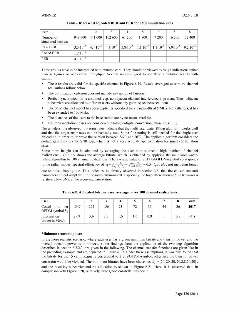
WINNER D2.6 v 1.0

Page 120 (264)

Table 6.8: Raw BER, coded BER and PER for 1800 simulation runs

user 1 2 3 4 5 6 7 8 Number of simulated packets

948 600 441 000 102 600 61 200 1 800 7 200 16 200 32 400

Raw BER 3.3·10−2 4.4·10−3 4.3·10−3 5.8·10−3 1.1·10−2 1.1·10−2 8.9·10−3 9.2·10−3 Coded BER 1.2·10−5 PER 4.1·10−3 These results have to be interpreted with extreme care. They should be viewed as rough indications rather than as figures on achievable throughput. Several issues suggest to use these simulation results with caution: These results are valid for the specific channel in Figure 6.19. Results averaged over more channel

realizations follow below. The optimization criterion does not include any notion of fairness. Perfect synchronization is assumed, esp. no adjacent channel interference is present. Thus, adjacent

subcarriers are allocated to different users without any guard space between them. The SCM channel model has been explicitly specified for a bandwidth of 5 MHz. Nevertheless, it has

been extended to 100 MHz. The distances of the users to the base station are by no means realistic. No implementation losses are considered (analogue-digital conversion, phase noise, …)

Nevertheless, the observed low error rates indicate that the multi-user water-filling algorithm works well and that the target error rates can be basically met. Some fine-tuning is still needed for the single-user bitloading in order to improve the relation between SNR and BER. The applied algorithm considers the coding gain only via the SNR gap, which is not a very accurate approximation for small constellation sizes. Some more insight can be obtained by averaging the user bitrates over a high number of channel realizations. Table 6.9 shows the average bitrate, which is obtained by applying the multi-user water-filling algorithm to 100 channel realizations. The average value of 2017 bit/OFDM-symbol corresponds to the rather modest spectral efficiency of Hzbpss

sTT

TN gu

u

p/54.05.22

2016642

201722017 ===η µ

µ⋅+ , not including losses

due to pulse shaping, etc. This indicates, as already observed in section 3.5, that the chosen transmit parameters do not adapt well to the radio environment. Especially the high attenuation at 5 GHz causes a relatively low SNR at the receiving base station.

Table 6.9: Allocated bits per user, averaged over 100 channel realizations

user 1 2 3 4 5 6 7 8 sum Coded bits per OFDM symbol bu

1347 252 156 73 72 37 44 36 2017

Information bitrate in Mbit/s

29.9 5.6 3.5 1.6 1.6 0.8 1 0.8 44.8

Minimum transmit power In the more realistic scenario, where each user has a given minimum bitrate and transmit power and the overall transmit power is minimized, some findings from the application of the two-step algorithm described in section 6.2.2.3, are given in the following. The channel transfer functions are given like in the preceding example and are depicted in Figure 6.19. Under these assumptions, it was first found that the bitrate for user 5 can maximally correspond to 2 bits/OFDM-symbol, otherwise the transmit power constraint would be violated. The minimum bitrates have been chosen as 20]20,2,8,20, 20, 20, [20,=ub

),

and the resulting subcarrier and bit allocation is shown in Figure 6.21. Here, it is observed that, in comparison with Figure 6.20, relatively large QAM constellations occur.

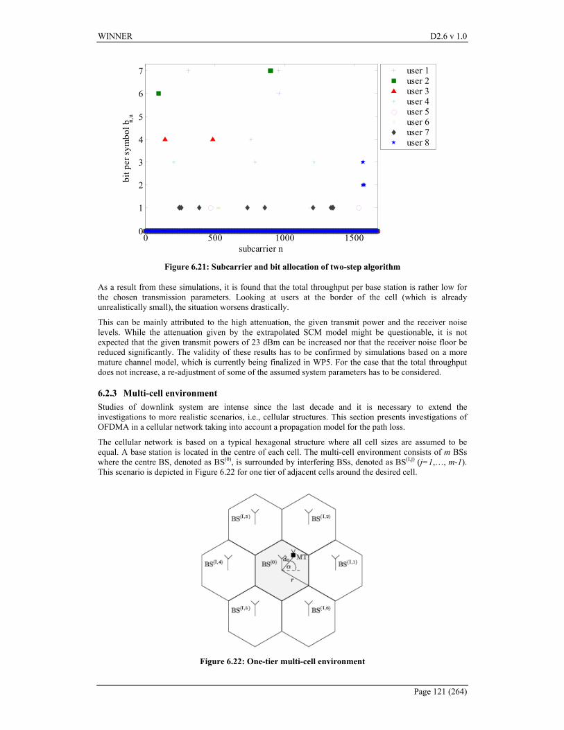
WINNER D2.6 v 1.0

Page 121 (264)

0 500 1000 15000

1

2

3

4

5

6

7

subcarrier n

bit p

er sy

mbo

l bn,

u

user 1user 2user 3user 4user 5user 6user 7user 8

Figure 6.21: Subcarrier and bit allocation of two-step algorithm

As a result from these simulations, it is found that the total throughput per base station is rather low for the chosen transmission parameters. Looking at users at the border of the cell (which is already unrealistically small), the situation worsens drastically.

This can be mainly attributed to the high attenuation, the given transmit power and the receiver noise levels. While the attenuation given by the extrapolated SCM model might be questionable, it is not expected that the given transmit powers of 23 dBm can be increased nor that the receiver noise floor be reduced significantly. The validity of these results has to be confirmed by simulations based on a more mature channel model, which is currently being finalized in WP5. For the case that the total throughput does not increase, a re-adjustment of some of the assumed system parameters has to be considered.

6.2.3 Multi-cell environment Studies of downlink system are intense since the last decade and it is necessary to extend the investigations to more realistic scenarios, i.e., cellular structures. This section presents investigations of OFDMA in a cellular network taking into account a propagation model for the path loss.

The cellular network is based on a typical hexagonal structure where all cell sizes are assumed to be equal. A base station is located in the centre of each cell. The multi-cell environment consists of m BSs where the centre BS, denoted as BS(0), is surrounded by interfering BSs, denoted as BS(I,j) (j=1,…, m-1). This scenario is depicted in Figure 6.22 for one tier of adjacent cells around the desired cell.

Figure 6.22: One-tier multi-cell environment

WINNER D2.6 v 1.0

Page 122 (264)

The mobile terminal moves along a straight line from BS(0) towards the border to an arbitrary point of the current cell. This line forms an angle α with the line connecting BS(0) and BS(I,1). rdd /0=∆ represents the ratio of the cell radius r of BS(0) and the distance d0 between MT and BS(0). We assume a normalized cell radius of 1. Through the definitions of d∆ and α along the direction of motion, an appropriate geometric reference system is introduced.

6.2.3.1 Distance dependent propagation model A propagation loss model is assumed to calculate the received signal energy Einterfere from the interfering BSs. The slowly varying signal energy attenuation due to path loss is generally modelled as the product of the ρ th power of distance and a log-normal component representing shadowing losses. Shadow variations are caused by large terrain features between the BS and MT such as buildings and hills. Since fast multipath fading is modelled by the channel transfer function and detection mitigates the more rapidly varying Rayleigh fading loss and other channel distortions, such as multiple access interference, the fast multipath fading process is not included in the propagation model [TC03]. Hence, the jth BS causes the MT to receive the interfering signal energy

10/,t 10 j

jjj dEE ηρ ⋅⋅= − , (6.28)

where Et,j is the transmitted signal energy from the jth BS, ρ is the distance decay factor and dj is the distance between the MT and the jth BS. Furthermore, the shadowing factor jη is a normally distributed random variable with zero mean and standard deviation pσ and is given in dB. In [VVZ94], the standard deviation pσ and the distance decay factor ρ are set to 8 dB and 4, respectively, as suggested by experimental data. These values are used throughout this section.

In a multi-cell environment, comparison of path losses among two or more BSs is necessary. Since the path loss from one BS to the MT correlates with the path loss from another BS to the MT, this interaction of the path losses is included in the model [VVZ94]. The shadowing factor can be split up into two components: first, a near-field component ζ which is common to all BSs; second, a component iζ with regard to the received signal at the MT which is independent from one BS to another. Since the single path losses in dB are Gaussian, we assume a joint Gaussian probability density for the path losses when receiving from two or more BSs.

Now, the random component of the dB loss for the jth BS can be expressed as

ii ba ζζη += , (6.29)

where 122 =+ ba , 0}{}{}{ === jj EEE ζζη , }{Var}{Var}{Var2p jj ζζησ === for all j, 0}{ =jE ζζ

for all j and 0}{ =jiE ζζ for all j and i with ji ≠ . The correlation coefficient is defined as the normalized covariance and set to 0.5 [VVZ94]:

5.01/}{ 222p =−== abE ji σηη . (6.30)

For notational convenience, the interfering energy is scaled by 1/E0, the reciprocal of the received desired signal energy, and therefore the overall received signal energy from all interfering BSs is

10/

10/

0

1

1 0,t

,t1

1 0interfere 010

10η

ηρj

dd

EE

EE

E jm

j

jm

j

j ⋅

⋅==

−−

=

−

=∑∑ . (6.31)

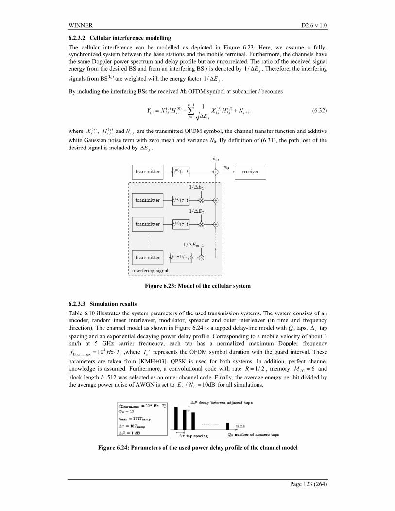
WINNER D2.6 v 1.0

Page 123 (264)

6.2.3.2 Cellular interference modelling The cellular interference can be modelled as depicted in Figure 6.23. Here, we assume a fully-synchronized system between the base stations and the mobile terminal. Furthermore, the channels have the same Doppler power spectrum and delay profile but are uncorrelated. The ratio of the received signal energy from the desired BS and from an interfering BS j is denoted by jE∆/1 . Therefore, the interfering signals from BS(I,j) are weighted with the energy factor jE∆/1 .

By including the interfering BSs the received lth OFDM symbol at subcarrier i becomes

iljil

jil

m

j jililil NHX

EHXY ,

)(.

)(.

1

1

)0(.

)0(.,

1+

∆+= ∑

−

=

, (6.32)

where )(,jilX , )(

,jilH and ilN , are the transmitted OFDM symbol, the channel transfer function and additive

white Gaussian noise term with zero mean and variance N0. By definition of (6.31), the path loss of the desired signal is included by jE∆ .

Figure 6.23: Model of the cellular system

6.2.3.3 Simulation results Table 6.10 illustrates the system parameters of the used transmission systems. The system consists of an encoder, random inner interleaver, modulator, spreader and outer interleaver (in time and frequency direction). The channel model as shown in Figure 6.24 is a tapped delay-line model with Q0 taps, τ∆ tap spacing and an exponential decaying power delay profile. Corresponding to a mobile velocity of about 3 km/h at 5 GHz carrier frequency, each tap has a normalized maximum Doppler frequency

'10 s4

maxDnorm, THzf ⋅= ,where 'sT represents the OFDM symbol duration with the guard interval. These parameters are taken from [KMH+03]. QPSK is used for both systems. In addition, perfect channel knowledge is assumed. Furthermore, a convolutional code with rate 2/1=R , memory 6CC =M and block length b=512 was selected as an outer channel code. Finally, the average energy per bit divided by the average power noise of AWGN is set to dB10/ 0b =NE for all simulations.

Figure 6.24: Parameters of the used power delay profile of the channel model

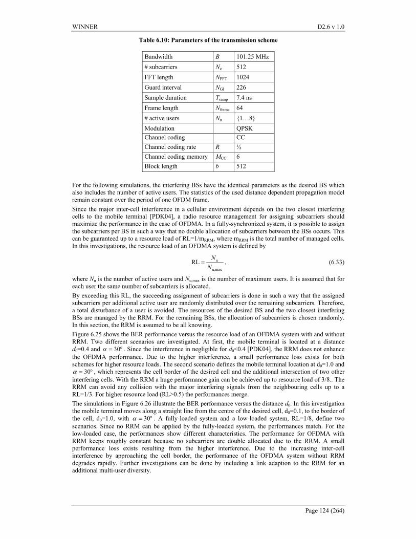
WINNER D2.6 v 1.0

Page 124 (264)

Table 6.10: Parameters of the transmission scheme

Bandwidth B 101.25 MHz # subcarriers Nc 512 FFT length NFFT 1024 Guard interval NGI 226 Sample duration Tsamp 7.4 ns Frame length Nframe 64 # active users Nu {1…8} Modulation QPSK Channel coding CC Channel coding rate R ½ Channel coding memory MCC 6 Block length b 512

For the following simulations, the interfering BSs have the identical parameters as the desired BS which also includes the number of active users. The statistics of the used distance dependent propagation model remain constant over the period of one OFDM frame. Since the major inter-cell interference in a cellular environment depends on the two closest interfering cells to the mobile terminal [PDK04], a radio resource management for assigning subcarriers should maximize the performance in the case of OFDMA. In a fully-synchronized system, it is possible to assign the subcarriers per BS in such a way that no double allocation of subcarriers between the BSs occurs. This can be guaranteed up to a resource load of RL=1/mRRM, where mRRM is the total number of managed cells. In this investigations, the resource load of an OFDMA system is defined by

maxu,

uRLN

N= , (6.33)

where Nu is the number of active users and Nu,max is the number of maximum users. It is assumed that for each user the same number of subcarriers is allocated. By exceeding this RL, the succeeding assignment of subcarriers is done in such a way that the assigned subcarriers per additional active user are randomly distributed over the remaining subcarriers. Therefore, a total disturbance of a user is avoided. The resources of the desired BS and the two closest interfering BSs are managed by the RRM. For the remaining BSs, the allocation of subcarriers is chosen randomly. In this section, the RRM is assumed to be all knowing. Figure 6.25 shows the BER performance versus the resource load of an OFDMA system with and without RRM. Two different scenarios are investigated. At first, the mobile terminal is located at a distance d0=0.4 and °= 30α . Since the interference in negligible for d0<0.4 [PDK04], the RRM does not enhance the OFDMA performance. Due to the higher interference, a small performance loss exists for both schemes for higher resource loads. The second scenario defines the mobile terminal location at d0=1.0 and

°= 30α , which represents the cell border of the desired cell and the additional intersection of two other interfering cells. With the RRM a huge performance gain can be achieved up to resource load of 3/8.. The RRM can avoid any collision with the major interfering signals from the neighbouring cells up to a RL=1/3. For higher resource load (RL>0.5) the performances merge. The simulations in Figure 6.26 illustrate the BER performance versus the distance d0. In this investigation the mobile terminal moves along a straight line from the centre of the desired cell, d0=0.1, to the border of the cell, d0=1.0, with °= 30α . A fully-loaded system and a low-loaded system, RL=1/8, define two scenarios. Since no RRM can be applied by the fully-loaded system, the performances match. For the low-loaded case, the performances show different characteristics. The performance for OFDMA with RRM keeps roughly constant because no subcarriers are double allocated due to the RRM. A small performance loss exists resulting from the higher interference. Due to the increasing inter-cell interference by approaching the cell border, the performance of the OFDMA system without RRM degrades rapidly. Further investigations can be done by including a link adaption to the RRM for an additional multi-user diversity.

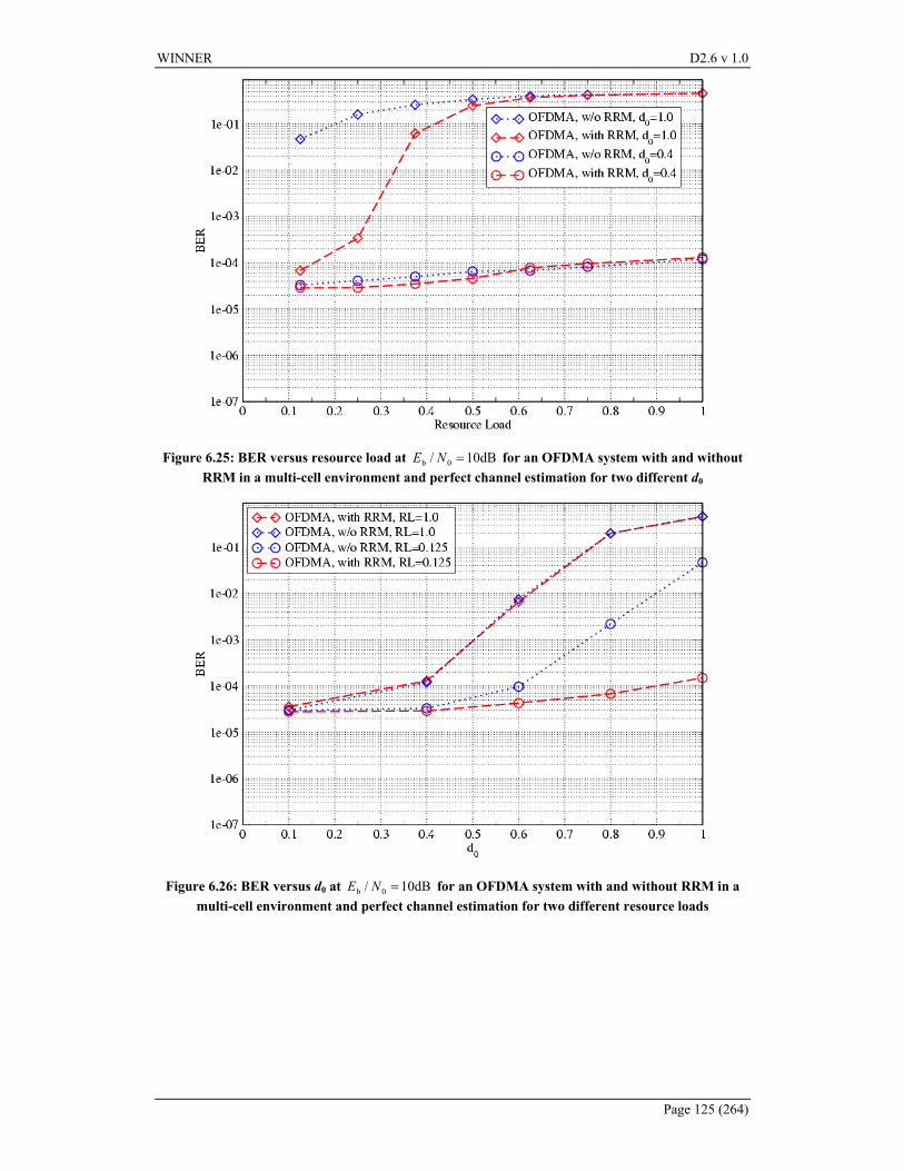
WINNER D2.6 v 1.0

Page 125 (264)

Figure 6.25: BER versus resource load at dB10/ 0b =NE for an OFDMA system with and without RRM in a multi-cell environment and perfect channel estimation for two different d0

Figure 6.26: BER versus d0 at dB10/ 0b =NE for an OFDMA system with and without RRM in a multi-cell environment and perfect channel estimation for two different resource loads

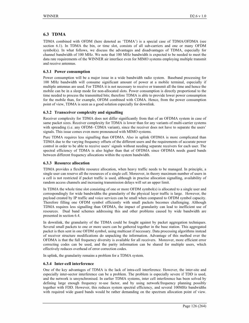
WINNER D2.6 v 1.0

Page 126 (264)

6.3 TDMA TDMA combined with OFDM (here denoted as ‘TDMA’) is a special case of TDMA/OFDMA (see section 6.1). In TDMA the bin, or time slot, consists of all sub-carriers and one or many OFDM symbol(s). In what follows, we discuss the advantages and disadvantages of TDMA, especially for channel bandwidth of 100 MHz. We note that 100 MHz bandwidth is expected to be needed to meet the data rate requirements of the WINNER air interface even for MIMO systems employing multiple transmit and receive antennas.

6.3.1 Power consumption Power consumption will be a major issue in a wide bandwidth radio system. Baseband processing for 100 MHz bandwidth will consume significant amount of power at a mobile terminal, especially if multiple antennas are used. For TDMA it is not necessary to receive or transmit all the time and hence the mobile can be in a sleep mode for non-allocated slots. Power consumption is directly proportional to the time needed to process the transmitted bits; therefore TDMA is able to provide lower power consumption for the mobile than, for example, OFDM combined with CDMA. Hence, from the power consumption point of view, TDMA is seen as a good solution especially for downlink.

6.3.2 Transceiver complexity and signalling Receiver complexity for TDMA does not differ significantly from that of an OFDMA system in case of same packet sizes. Receiver complexity for TDMA is lower than for any variants of multi-carrier systems with spreading (i.e. any OFDM- CDMA variant), since the receiver does not have to separate the users’ signals. This issue comes even more pronounced with MIMO systems. Pure TDMA requires less signalling than OFDMA. Also in uplink OFDMA is more complicated than TDMA due to the varying frequency offsets of the different users and the requirements of accurate power control in order to be able to receive users’ signals without needing separate receivers for each user. The spectral efficiency of TDMA is also higher than that of OFDMA since OFDMA needs guard bands between different frequency allocations within the system bandwidth.

6.3.3 Resource allocation TDMA provides a flexible resource allocation, when heavy traffic needs to be managed. In principle, a single user can reserve all the resources of a single cell. Moreover, in theory maximum number of users in a cell is not restricted if packet traffic is used, although in practise allocation signalling, availability of random access channels and increasing transmission delays will set an upper limit.

In TDMA the whole time slot consisting of one or more OFDM symbol(s) is allocated to a single user and correspondingly for wide bandwidths the granularity of the physical layer traffic is large. However, the payload created by IP traffic and voice services can be small when compared to OFDM symbol capacity. Therefore filling one OFDM symbol efficiently with small packets becomes challenging. Although TDMA requires less signalling than OFDMA, the impact of granularity can lead to inefficient use of resources. Dual band schemes addressing this and other problems caused by wide bandwidth are presented in section 6.4.

In downlink, the granularity of the TDMA could be fought against by packet aggregation techniques. Several small packets to one or more users can be gathered together in the base station. This aggregated packet is then sent in one OFDM symbol, using multicast if necessary. Data processing algorithms instead of receiver structure modifications do unpacking the information. Advantage of this method over the OFDMA is that the full frequency diversity is available for all receivers. Moreover, more efficient error correcting codes can be used, and the parity information can be shared for multiple users, which effectively reduces overhead of error correction codes.

In uplink, the granularity remains a problem for a TDMA system.

6.3.4 Inter-cell interference One of the key advantages of TDMA is the lack of intra-cell interference. However, the inter-site and especially inter-sector interference can be a problem. The problem is especially severe if TDD is used, and the network is unsynchronised. In earlier TDMA systems, inter cell interference has been solved by defining large enough frequency re-use factor, and by using network/frequency planning possibly together with FDD. However, this reduces system spectral efficiency, and several 100MHz bandwidths with required wide guard bands would be rather demanding on the spectrum allocation point of view.

WINNER D2.6 v 1.0

Page 127 (264)

Thus, in 4G networks a low frequency re-use factor is mandatory. The inter-cell interference can be reduced by separating the interfering transmissions in time, frequency or space. In particular, a very promising and potentially effective technique for solving the inter-cell interference issue of TDMA is SDMA. The combination SDMA and TDMA is studied in chapter 8.

The traditional way to separate the signals in time would be the static time reuse, i.e. to schedule traffic so that neighbouring cell or sector do not transmit at the same time. This would however reduce the spectral efficiency equivalently to FDMA system without alleviating the noise performance. One could consider using static time reuse for critical portions, like training sequences and allocation tables.

More efficient way of mitigating the effects of inter-cell interference is advanced packet scheduling between the users requiring high transmitting power. The idea is to reduce interference by allocating these users to designated time intervals that do not overlap between neighbouring sites. This could be realized as synchronized cell breathing. However, synchronized cell breathing cannot cope with interference on the sector borders of a sectorised cell. Providing some additional information, such as channel quality measurements for the algorithms, can be useful for handling interference on the sector borders. This would however mean that additional measurements on neighbouring cells and some signalling between the base stations are required. Dynamic frequency allocation is also an interesting possibility, which would increase the degrees of freedom for the advanced packet scheduling principles.

When developing this kind of algorithms, one should find ways to make sure that unnecessary handovers are avoided, and seamless coverage is achieved. Also signalling load should be considered, if some channel state information is used. On the receiver side, advanced interference cancellation algorithms could improve the system level performance significantly. Further study with system level simulations is needed to find out how effective this kind of algorithms can be.

For TDD-TDMA, inter-site synchronization is required in order to avoid downlink to uplink interference. If narrow guard bands are used for spectral efficiency, the synchronization should be achieved also between operators. One possible way to achieve the inter-site / inter-network synchronization is utilizing GPS, which is already used in mobile location services, such as uplink-TDOA, to measure the timing differences of the base stations. GPS receiver attached to a base station can provide a global reference time to the network, provided that the receiver can find required satellites. The availability of GPS is restricted in indoor and urban areas, thus this method is not sufficient by itself. The transmissions of other cells can be used to synchronize a cell, if frequency allocation or a time separation scheme gives possibilities to receive the transmissions of neighbouring cells. For such methods a way of compensating the propagation delay should be developed. Although the networks can be synchronized using these method, the downlink-uplink sharing has to be done in the same proportions in all cells and by all operators, which reduces the flexibility of TDD system.

6.3.5 Performance assessment of an OFDM/TDMA TDD system In the following, the performance of an OFDM/TDMA TDD network is assessed by means of system simulations. Both a single-cell and a multi-cell deployment have been considered.

6.3.5.1 Models and assumptions The assumptions and models used throughout this evaluation have, with one exception (the length of the data block), been aligned to the comparison case defined in Section 3.5. The general assumptions of the comparison case are not repeated here so we refer to Section 3.5 for an overview. Access points are equipped with omni-directional antennas and if multiple cells are deployed, access points (sites) are located in a regular, hexagonal pattern. A single antenna is used for transmission and reception in both the access points and the user terminals. Moreover, the network is assumed to be perfectly synchronized, i.e., we assume that all nodes in the system, both access points and user terminals, share a common time and frequency reference. The multi-cell network is deployed with a frequency reuse of 1. Users are static and located at random positions within the coverage area of the network. In the single-cell deployment 8 users are located in the cell while the load in the multi-cell deployment is, on average, 8 users/cell. A user terminal connects to the access point in the network to which it measures the lowest (long-term) pathloss. OFDM transmission is employed in both uplink and downlink. Moreover, in both links scheduling of users is performed periodically in a round-robin fashion. That is, within a cell pure time-sharing of the channel is employed (TDMA) and the transmission scheduling is not channel dependent. When scheduled for transmission, a user gets access to the whole bandwidth. Uplink and downlink transmissions are separated by the time division duplex scheme.

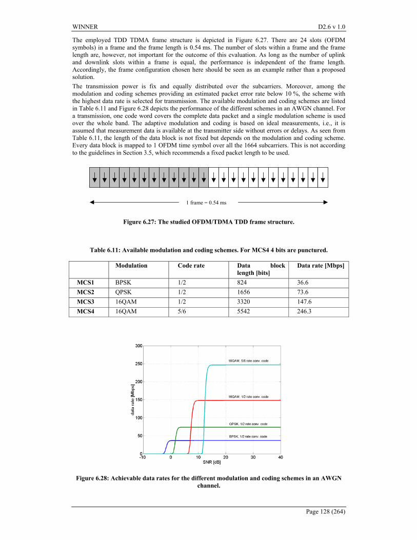
WINNER D2.6 v 1.0

Page 128 (264)

The employed TDD TDMA frame structure is depicted in Figure 6.27. There are 24 slots (OFDM symbols) in a frame and the frame length is 0.54 ms. The number of slots within a frame and the frame length are, however, not important for the outcome of this evaluation. As long as the number of uplink and downlink slots within a frame is equal, the performance is independent of the frame length. Accordingly, the frame configuration chosen here should be seen as an example rather than a proposed solution. The transmission power is fix and equally distributed over the subcarriers. Moreover, among the modulation and coding schemes providing an estimated packet error rate below 10 %, the scheme with the highest data rate is selected for transmission. The available modulation and coding schemes are listed in Table 6.11 and Figure 6.28 depicts the performance of the different schemes in an AWGN channel. For a transmission, one code word covers the complete data packet and a single modulation scheme is used over the whole band. The adaptive modulation and coding is based on ideal measurements, i.e., it is assumed that measurement data is available at the transmitter side without errors or delays. As seen from Table 6.11, the length of the data block is not fixed but depends on the modulation and coding scheme. Every data block is mapped to 1 OFDM time symbol over all the 1664 subcarriers. This is not according to the guidelines in Section 3.5, which recommends a fixed packet length to be used.

1 frame = 0.54 ms

Figure 6.27: The studied OFDM/TDMA TDD frame structure.

Table 6.11: Available modulation and coding schemes. For MCS4 4 bits are punctured.

Modulation Code rate Data block length [bits]

Data rate [Mbps]

MCS1 BPSK 1/2 824 36.6 MCS2 QPSK 1/2 1656 73.6 MCS3 16QAM 1/2 3320 147.6 MCS4 16QAM 5/6 5542 246.3

Figure 6.28: Achievable data rates for the different modulation and coding schemes in an AWGN channel.

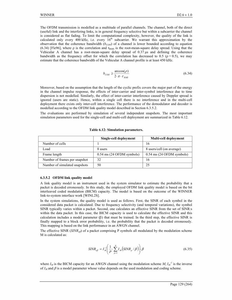
WINNER D2.6 v 1.0

Page 129 (264)

The OFDM transmission is modelled as a multitude of parallel channels. The channel, both of the direct (useful) link and the interfering links, is in general frequency selective but within a subcarrier the channel is considered as flat fading. To limit the computational complexity, however, the quality of the link is calculated only every 400 kHz, i.e. every 16th subcarrier. We warrant this approximation by the observation that the coherence bandwidth (bCOH) of a channel is lower bounded according to equation (6.34) [Fle96], where ρ is the correlation and τRMS is the root-mean-square delay spread. Using that the Vehicular A channel has a root-mean-square delay spread of 0.37 µs and defining the coherence bandwidth as the frequency offset for which the correlation has decreased to 0.5 (ρ = 0.5), we may estimate that the coherence bandwidth of the Vehicular A channel profile is at least 450 kHz.

RMS

COHbτπ

ρ⋅⋅

≥2

)arccos( (6.34)

Moreover, based on the assumption that the length of the cyclic prefix covers the major part of the energy in the channel impulse response, the effects of inter-carrier and inter-symbol interference due to time dispersion is not modelled. Similarly, the effect of inter-carrier interference caused by Doppler spread is ignored (users are static). Hence, within a single cell there is no interference and in the multi-cell deployment there exists only inter-cell interference. The performance of the demodulator and decoder is modelled according to the OFDM link quality model described in Section 6.3.5.2. The evaluations are performed by simulation of several independent snapshots. The most important simulation parameters used for the single-cell and multi-cell deployment are summarized in Table 6.12.

Table 6.12: Simulation parameters.

Single-cell deployment Multi-cell deployment Number of cells 1 16 Load 8 users 8 users/cell (on average) Frame length 0.54 ms (24 OFDM symbols) 0.54 ms (24 OFDM symbols) Number of frames per snapshot 32 16 Number of simulated snapshots 50 25

6.3.5.2 OFDM link quality model A link quality model is an instrument used in the system simulator to estimate the probability that a packet is decoded erroneously. In this study, the employed OFDM link quality model is based on the bit interleaved coded modulation (BICM) capacity. The model is based on the outcome of the WINNER link-to-system interface work [WINL2S]. In the system simulations, the quality model is used as follows. First, the SINR of each symbol in the considered data packet is calculated. Due to frequency selectivity (and temporal variations), the symbol SINR typically varies within a packet. Second, one calculates an effective SINR from the set of SINR:s within the data packet. In this case, the BICM capacity is used to calculate the effective SINR and this calculation includes a model parameter (β) that must be trained. In the third step, the effective SINR is finally mapped to a block error probability, i.e. the probability that the packet is decoded erroneously. This mapping is based on the link performance in an AWGN channel. The effective SINR (SINReff) of a packet comprising P symbols all modulated by the modulation scheme M is calculated as:

( ) ββ ⋅

⋅= ∑

=

−P

ppMMeff SINRI

PISINR

1

1 /1 (6.35)

where IM is the BICM capacity for an AWGN channel using the modulation scheme M, IM

-1 is the inverse of IM and β is a model parameter whose value depends on the used modulation and coding scheme.

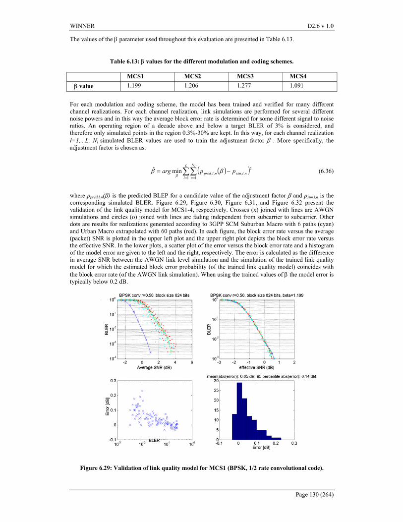
WINNER D2.6 v 1.0

Page 130 (264)

The values of the β parameter used throughout this evaluation are presented in Table 6.13.

Table 6.13: β values for the different modulation and coding schemes.

MCS1 MCS2 MCS3 MCS4 β value 1.199 1.206 1.277 1.091

For each modulation and coding scheme, the model has been trained and verified for many different channel realizations. For each channel realization, link simulations are performed for several different noise powers and in this way the average block error rate is determined for some different signal to noise ratios. An operating region of a decade above and below a target BLER of 3% is considered, and therefore only simulated points in the region 0.3%-30% are kept. In this way, for each channel realization l=1,..,L, Nl simulated BLER values are used to train the adjustment factor β . More specifically, the adjustment factor is chosen as:

( )( )∑∑= =

−=L

l

N

nnlsimnlpred

l

pparg1 1

2,,,,minˆ ββ

β (6.36)

where ppred,l,n(β) is the predicted BLEP for a candidate value of the adjustment factor β and psim,l,n is the corresponding simulated BLER. Figure 6.29, Figure 6.30, Figure 6.31, and Figure 6.32 present the validation of the link quality model for MCS1-4, respectively. Crosses (x) joined with lines are AWGN simulations and circles (o) joined with lines are fading independent from subcarrier to subcarrier. Other dots are results for realizations generated according to 3GPP SCM Suburban Macro with 6 paths (cyan) and Urban Macro extrapolated with 60 paths (red). In each figure, the block error rate versus the average (packet) SNR is plotted in the upper left plot and the upper right plot depicts the block error rate versus the effective SNR. In the lower plots, a scatter plot of the error versus the block error rate and a histogram of the model error are given to the left and the right, respectively. The error is calculated as the difference in average SNR between the AWGN link level simulation and the simulation of the trained link quality model for which the estimated block error probability (of the trained link quality model) coincides with the block error rate (of the AWGN link simulation). When using the trained values of β the model error is typically below 0.2 dB.

Figure 6.29: Validation of link quality model for MCS1 (BPSK, 1/2 rate convolutional code).

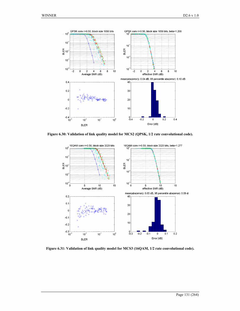
WINNER D2.6 v 1.0

Page 131 (264)

Figure 6.30: Validation of link quality model for MCS2 (QPSK, 1/2 rate convolutional code).

Figure 6.31: Validation of link quality model for MCS3 (16QAM, 1/2 rate convolutional code).

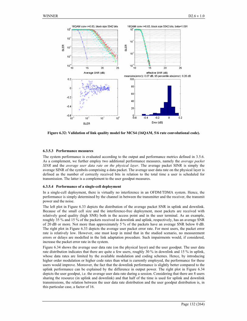
WINNER D2.6 v 1.0

Page 132 (264)

Figure 6.32: Validation of link quality model for MCS4 (16QAM, 5/6 rate convolutional code).

6.3.5.3 Performance measures The system performance is evaluated according to the output and performance metrics defined in 3.5.6. As a complement, we further employ two additional performance measures, namely the average packet SINR and the average user data rate on the physical layer. The average packet SINR is simply the average SINR of the symbols comprising a data packet. The average user data rate on the physical layer is defined as the number of correctly received bits in relation to the total time a user is scheduled for transmission. The latter is a complement to the user goodput measures.

6.3.5.4 Performance of a single-cell deployment In a single-cell deployment, there is virtually no interference in an OFDM/TDMA system. Hence, the performance is simply determined by the channel in between the transmitter and the receiver, the transmit power and the noise. The left plot in Figure 6.33 depicts the distribution of the average packet SNR in uplink and downlink. Because of the small cell size and the interference-free deployment, most packets are received with relatively good quality (high SNR) both in the access point and in the user terminal. As an example, roughly 35 % and 15 % of the packets received in downlink and uplink, respectively, has an average SNR of 20 dB or more. Not more than approximately 5 % of the packets have an average SNR below 0 dB. The right plot in Figure 6.33 depicts the average user packet error rate. For most users, the packet error rate is relatively low. However, one must keep in mind that in the studied scenario, no measurement errors or delays are modelled in the link adaptation procedure. Such impairments would, if considered, increase the packet error rate in the system. Figure 6.34 shows the average user data rate (on the physical layer) and the user goodput. The user data rate distribution indicates that there are quite a few users, roughly 30 % in downlink and 15 % in uplink, whose data rates are limited by the available modulation and coding schemes. Hence, by introducing higher order modulation or higher code rates than what is currently employed, the performance for these users would improve. Moreover, the fact that the downlink performance is slightly better compared to the uplink performance can be explained by the difference in output power. The right plot in Figure 6.34 depicts the user goodput, i.e. the average user data rate during a session. Considering that there are 8 users sharing the resource (in uplink and downlink) and that half of the time is used for uplink and downlink transmissions, the relation between the user data rate distribution and the user goodput distribution is, in this particular case, a factor of 16.

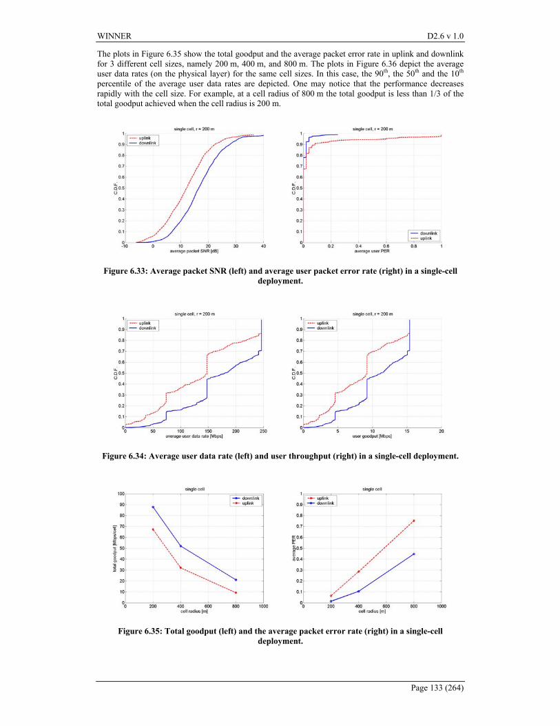
WINNER D2.6 v 1.0

Page 133 (264)

The plots in Figure 6.35 show the total goodput and the average packet error rate in uplink and downlink for 3 different cell sizes, namely 200 m, 400 m, and 800 m. The plots in Figure 6.36 depict the average user data rates (on the physical layer) for the same cell sizes. In this case, the 90th, the 50th and the 10th percentile of the average user data rates are depicted. One may notice that the performance decreases rapidly with the cell size. For example, at a cell radius of 800 m the total goodput is less than 1/3 of the total goodput achieved when the cell radius is 200 m.

Figure 6.33: Average packet SNR (left) and average user packet error rate (right) in a single-cell deployment.

Figure 6.34: Average user data rate (left) and user throughput (right) in a single-cell deployment.

Figure 6.35: Total goodput (left) and the average packet error rate (right) in a single-cell deployment.

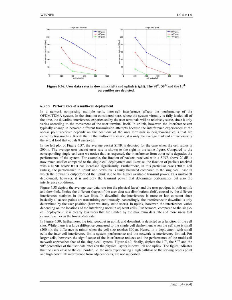
WINNER D2.6 v 1.0

Page 134 (264)

Figure 6.36: User data rates in downlink (left) and uplink (right). The 90th, 50th and the 10th percentiles are depicted.

6.3.5.5 Performance of a multi-cell deployment In a network comprising multiple cells, inter-cell interference affects the performance of the OFDM/TDMA system. In the situation considered here, where the system virtually is fully loaded all of the time, the downlink interference experienced by the user terminals will be relatively static, since it only varies according to the movement of the user terminal itself. In uplink, however, the interference can typically change in between different transmission attempts because the interference experienced at the access point receiver depends on the positions of the user terminals in neighbouring cells that are currently transmitting. Recall that in the multi-cell scenario, it is only the average load and not necessarily the actual load that equals 8 users/cell. In the left plot of Figure 6.37, the average packet SINR is depicted for the case when the cell radius is 200 m. The average user packet error rate is shown to the right in the same figure. Compared to the corresponding single-cell case we notice that, as expected, the interference from other cells degrades the performance of the system. For example, the fraction of packets received with a SINR above 20 dB is now much smaller compared to the single-cell deployment and likewise, the fraction of packets received with a SINR below 0 dB has increased significantly. Furthermore, in this particular case (200 m cell radius), the performance in uplink and downlink is fairly balanced compared to the single-cell case in which the downlink outperformed the uplink due to the higher available transmit power. In a multi-cell deployment, however, it is not only the transmit power that determines performance but also the interference conditions. Figure 6.38 depicts the average user data rate (on the physical layer) and the user goodput in both uplink and downlink. Notice the different shapes of the user data rate distributions (left), caused by the different interference statistics in the two links. In downlink, the interference is more or less constant since basically all access points are transmitting continuously. Accordingly, the interference in downlink is only determined by the user position (here we study static users). In uplink, however, the interference varies depending on the locations of the interfering users in adjacent cells. Furthermore, compared to the single-cell deployment, it is clearly less users that are limited by the maximum data rate and more users that cannot reach even the lowest data rate. In Figure 6.39, furthermore, the total goodput in uplink and downlink is depicted as a function of the cell size. While there is a large difference compared to the single-cell deployment when the cell size is small (200 m), the difference is minor when the cell size reaches 800 m. Hence, in a deployment with small cells the inter-cell interference limits system performance and the network is interference limited. For larger cells, however, the significance of the interference reduces and the performance of the multi-cell network approaches that of the single-cell system. Figure 6.40, finally, depicts the 10th, the 50th and the 90th percentiles of the user data rates (on the physical layer) in downlink and uplink. The figure indicates that the users close to the cell border, i.e. the ones experiencing a high pathloss to the serving access point and high downlink interference from adjacent cells, are not supported.

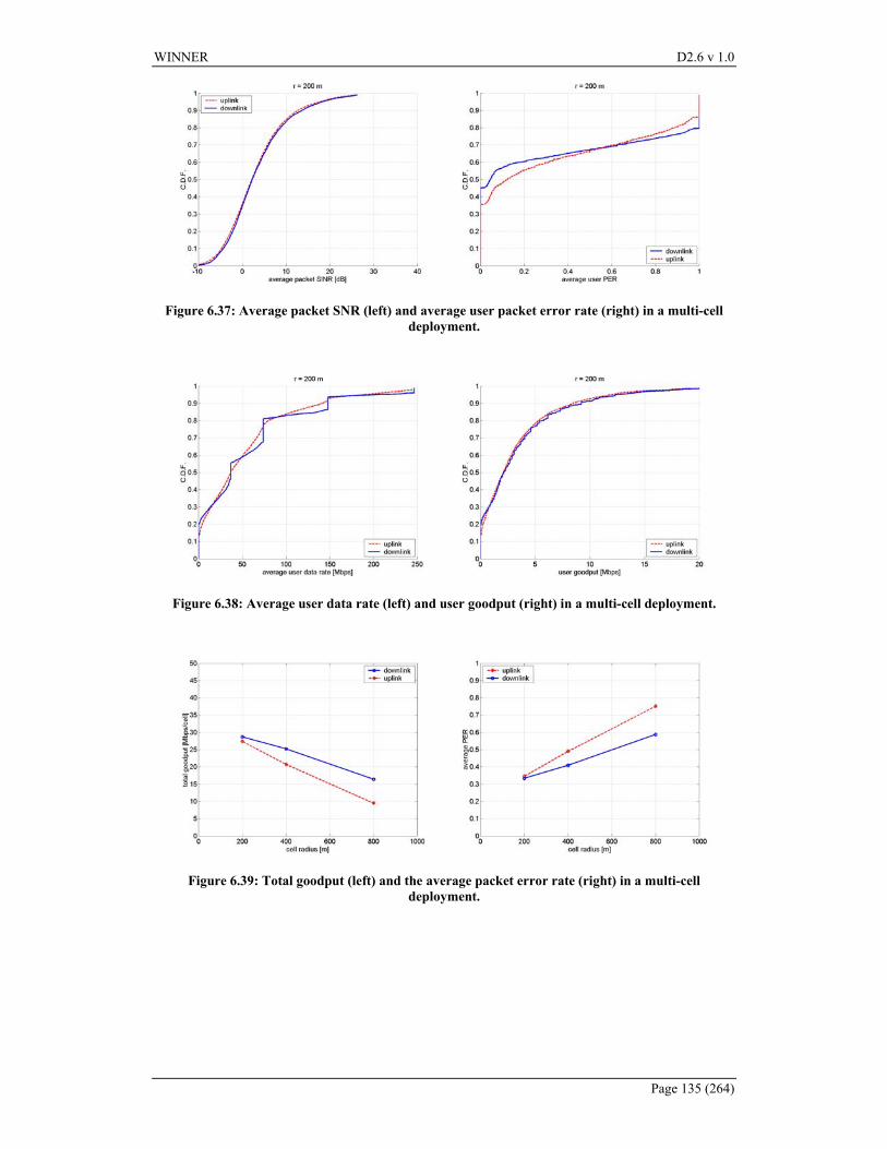
WINNER D2.6 v 1.0

Page 135 (264)

Figure 6.37: Average packet SNR (left) and average user packet error rate (right) in a multi-cell deployment.

Figure 6.38: Average user data rate (left) and user goodput (right) in a multi-cell deployment.

Figure 6.39: Total goodput (left) and the average packet error rate (right) in a multi-cell deployment.

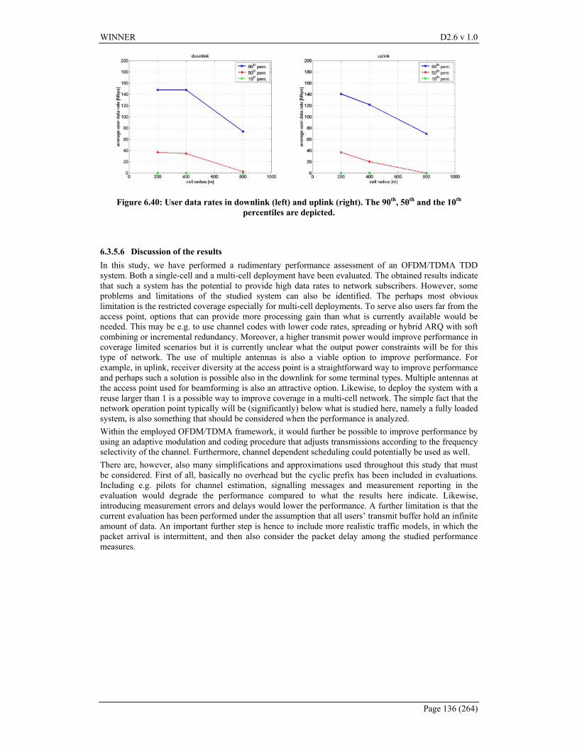
WINNER D2.6 v 1.0

Page 136 (264)

Figure 6.40: User data rates in downlink (left) and uplink (right). The 90th, 50th and the 10th percentiles are depicted.

6.3.5.6 Discussion of the results In this study, we have performed a rudimentary performance assessment of an OFDM/TDMA TDD system. Both a single-cell and a multi-cell deployment have been evaluated. The obtained results indicate that such a system has the potential to provide high data rates to network subscribers. However, some problems and limitations of the studied system can also be identified. The perhaps most obvious limitation is the restricted coverage especially for multi-cell deployments. To serve also users far from the access point, options that can provide more processing gain than what is currently available would be needed. This may be e.g. to use channel codes with lower code rates, spreading or hybrid ARQ with soft combining or incremental redundancy. Moreover, a higher transmit power would improve performance in coverage limited scenarios but it is currently unclear what the output power constraints will be for this type of network. The use of multiple antennas is also a viable option to improve performance. For example, in uplink, receiver diversity at the access point is a straightforward way to improve performance and perhaps such a solution is possible also in the downlink for some terminal types. Multiple antennas at the access point used for beamforming is also an attractive option. Likewise, to deploy the system with a reuse larger than 1 is a possible way to improve coverage in a multi-cell network. The simple fact that the network operation point typically will be (significantly) below what is studied here, namely a fully loaded system, is also something that should be considered when the performance is analyzed. Within the employed OFDM/TDMA framework, it would further be possible to improve performance by using an adaptive modulation and coding procedure that adjusts transmissions according to the frequency selectivity of the channel. Furthermore, channel dependent scheduling could potentially be used as well. There are, however, also many simplifications and approximations used throughout this study that must be considered. First of all, basically no overhead but the cyclic prefix has been included in evaluations. Including e.g. pilots for channel estimation, signalling messages and measurement reporting in the evaluation would degrade the performance compared to what the results here indicate. Likewise, introducing measurement errors and delays would lower the performance. A further limitation is that the current evaluation has been performed under the assumption that all users’ transmit buffer hold an infinite amount of data. An important further step is hence to include more realistic traffic models, in which the packet arrival is intermittent, and then also consider the packet delay among the studied performance measures.

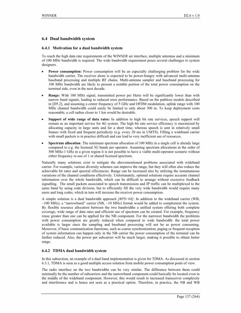
WINNER D2.6 v 1.0

Page 137 (264)

6.4 Dual bandwidth system

6.4.1 Motivation for a dual bandwidth system

To reach the high data rate requirements of the WINNER air interface, multiple antennas and a minimum of 100 MHz bandwidth is required. The wide bandwidth requirement poses several challenges to system designers.

• Power consumption: Power consumption will be an especially challenging problem for the wide bandwidth carrier. The receiver alone is expected to be power-hungry with advanced multi-antenna baseband processing and multiple RF chains. Multi-antenna sampler and baseband processing for 100 MHz bandwidth are likely to present a notable portion of the total power consumption on the terminal side, even in the next decade.

• Range: With 100 MHz signal, transmitted power per Hertz will be significantly lower than with narrow band signals, leading to reduced error performance. Based on the pathloss models described in [D5.2], and assuming a center frequency of 5 GHz and OFDM modulation, uplink range with 100 MHz channel bandwidth could easily be limited to only about 300 m. To keep deployment costs reasonable, a cell radius closer to 1 km would be desirable.

• Support of wide range of data rates: In addition to high bit rate services, speech support will remain as an important service for 4G system. The high bit rate service efficiency is maximized by allocating capacity in large units and for a short time, whereas speech is sent in relatively small frames with fixed and frequent periodicity (e.g. every 20 ms in UMTS). Filling a wideband carrier with small packets is in practice difficult and can lead to very inefficient use of resources.

• Spectrum allocation: The minimum spectrum allocation of 100 MHz in a single cell is already large compared to e.g. the licensed 3G bands per operator. Assuming spectrum allocations in the order of 500 MHz-1 GHz in a given region it is not possible to have a viable multi-operator scenario without either frequency re-use of 1 or shared licensed spectrum.

Naturally many solutions exist to mitigate the abovementioned problems associated with wideband carrier. For example, various diversity schemes can improve the range, but they will often also reduce the achievable bit rates and spectral efficiencies. Range can be increased also by utilizing the instantaneous variations of the channel conditions effectively. Unfortunately, optimal solutions require accurate channel information over the whole bandwidth, which can be difficult to arrange without excessive feedback signalling. The small packets associated to speech transmission and IP traffic can be multiplexed to the same band by using code division, but to efficiently fill the very wide bandwidth would require many users and long codes, which in turn will increase the receiver power consumption.

A simple solution is a dual bandwidth approach [RPS+04]: In addition to the wideband carrier (WB, ~100 MHz), a “narrowband” carrier (NB, ~10 MHz) format would be added to complement the system. By flexible resource allocation between the two bandwidths a unified system offering both complete coverage, wide range of data rates and efficient use of spectrum can be created. For example, frequency reuse greater than one can be applied for the NB component. For the narrower bandwidth the problems with power consumption are greatly reduced when compared to wide bandwidth: the total power available is larger since the sampling and baseband processing will not be as power consuming. Moreover, if basic communication functions, such as coarse synchronization, paging or frequent reception of system information can happen only in the NB carrier the power consumption of the terminal can be further reduced. Also, the power per subcarrier will be much larger, making it possible to obtain better range.

6.4.2 TDMA dual bandwidth system

In this subsection, an example of a dual band implementation is given for TDMA. As discussed in section 6.3.1, TDMA is seen as a good multiple access solution from mobile power consumption point of view.

The radio interface on the two bandwidths can be very similar. The difference between them could minimally be the number of subcarriers and the narrowband component could basically be located even in the middle of the wideband component. However, this would result to increased transceiver complexity and interference and is hence not seen as a practical option. Therefore, in practice, the NB and WB

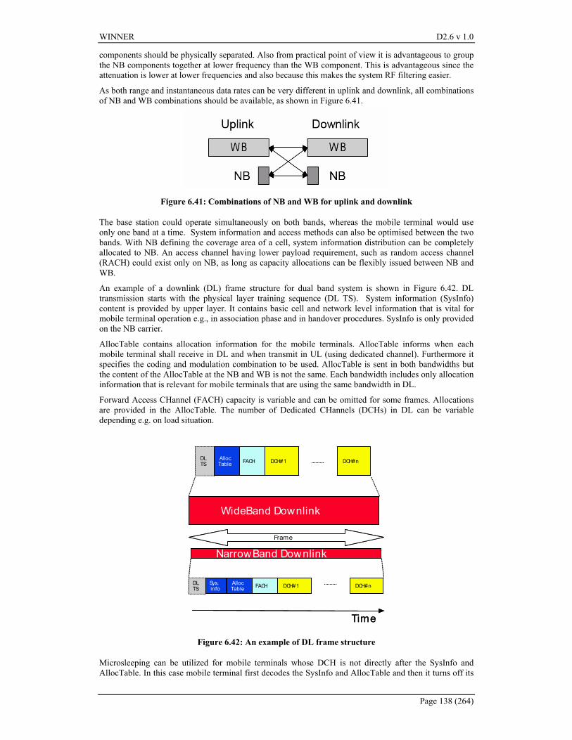
WINNER D2.6 v 1.0

Page 138 (264)

components should be physically separated. Also from practical point of view it is advantageous to group the NB components together at lower frequency than the WB component. This is advantageous since the attenuation is lower at lower frequencies and also because this makes the system RF filtering easier.

As both range and instantaneous data rates can be very different in uplink and downlink, all combinations of NB and WB combinations should be available, as shown in Figure 6.41.

Figure 6.41: Combinations of NB and WB for uplink and downlink

The base station could operate simultaneously on both bands, whereas the mobile terminal would use only one band at a time. System information and access methods can also be optimised between the two bands. With NB defining the coverage area of a cell, system information distribution can be completely allocated to NB. An access channel having lower payload requirement, such as random access channel (RACH) could exist only on NB, as long as capacity allocations can be flexibly issued between NB and WB.

An example of a downlink (DL) frame structure for dual band system is shown in Figure 6.42. DL transmission starts with the physical layer training sequence (DL TS). System information (SysInfo) content is provided by upper layer. It contains basic cell and network level information that is vital for mobile terminal operation e.g., in association phase and in handover procedures. SysInfo is only provided on the NB carrier.

AllocTable contains allocation information for the mobile terminals. AllocTable informs when each mobile terminal shall receive in DL and when transmit in UL (using dedicated channel). Furthermore it specifies the coding and modulation combination to be used. AllocTable is sent in both bandwidths but the content of the AllocTable at the NB and WB is not the same. Each bandwidth includes only allocation information that is relevant for mobile terminals that are using the same bandwidth in DL.

Forward Access CHannel (FACH) capacity is variable and can be omitted for some frames. Allocations are provided in the AllocTable. The number of Dedicated CHannels (DCHs) in DL can be variable depending e.g. on load situation.

NarrowBand Downlink

DLTS

Sys.info

AllocTable DCH#1FACH DCH#n

Time

WideBand Downlink

DLTS

AllocTable DCH#1FACH DCH#n

Frame

NarrowBand Downlink

DLTS

Sys.info

AllocTable DCH#1FACH DCH#n

Time

WideBand Downlink

DLTS

AllocTable DCH#1FACH DCH#n

Frame

Figure 6.42: An example of DL frame structure

Microsleeping can be utilized for mobile terminals whose DCH is not directly after the SysInfo and AllocTable. In this case mobile terminal first decodes the SysInfo and AllocTable and then it turns off its

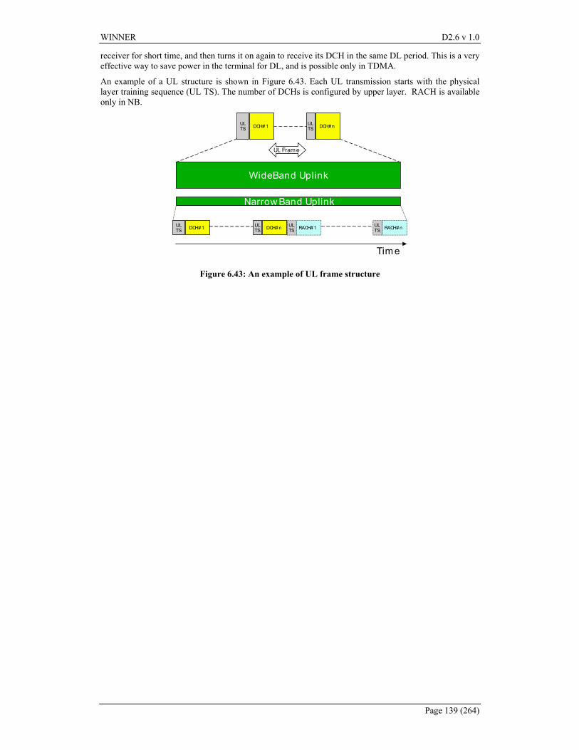
WINNER D2.6 v 1.0

Page 139 (264)

receiver for short time, and then turns it on again to receive its DCH in the same DL period. This is a very effective way to save power in the terminal for DL, and is possible only in TDMA.

An example of a UL structure is shown in Figure 6.43. Each UL transmission starts with the physical layer training sequence (UL TS). The number of DCHs is configured by upper layer. RACH is available only in NB.

Tim e

Narrow Band Uplink

ULTS DCH#1 UL

TS DCH# n ULTS RACH# 1 UL

TS RACH# n

WideBand Uplink

ULTS DCH# 1 UL

TS DCH#n

UL Fram e

Figure 6.43: An example of UL frame structure

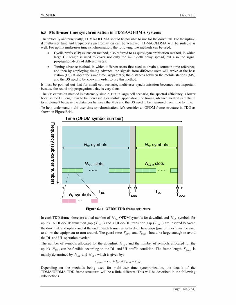
WINNER D2.6 v 1.0

Page 140 (264)

6.5 Multi-user time synchronisation in TDMA/OFDMA systems Theoretically and practically, TDMA/OFDMA should be possible to use for the downlink. For the uplink, if multi-user time and frequency synchronisation can be achieved, TDMA/OFDMA will be suitable as well. For uplink multi-user time synchronisation, the following two methods can be used:

• Cyclic prefix (CP) extension method, also referred to as quasi-synchronisation method, in which large CP length is used to cover not only the multi-path delay spread, but also the signal propagation delay of different users.

• Timing advance method, in which different users first need to obtain a common time reference, and then by employing timing advance, the signals from different users will arrive at the base station (BS) at about the same time. Apparently, the distances between the mobile stations (MS) and the BS need to be known in order to use this method.

It must be pointed out that for small cell scenario, multi-user synchronisation becomes less important because the round-trip propagation delay is very short. The CP extension method is extremely simple. But in large cell scenario, the spectral efficiency is lower because the CP length has to be increased. For mobile application, the timing advance method is difficult to implement because the distances between the MSs and the BS need to be measured from time to time. To help understand multi-user time synchronization, let's consider an OFDM frame structure in TDD as shown in Figure 6.44.

TDL TULTDUG TUDG

Time (OFDM symbol number)Frequency (sub-carrier number)

NDL symbols NUL symbols

NDLst slots NULst slots…… ……

…NL symbols

TDL TULTDUG TUDG

Time (OFDM symbol number)Frequency (sub-carrier number)

NDL symbols NUL symbols

NDLst slots NULst slots…… ……

…NL symbols

Figure 6.44: OFDM TDD frame structure

In each TDD frame, there are a total number of DLN OFDM symbols for downlink and ULN symbols for uplink. A DL-to-UP transition gap ( DUGT ) and a UL-to-DL transition gap ( UDGT ) are inserted between the downlink and uplink and at the end of each frame respectively. These gaps (guard times) must be used to allow the equipment to turn around. The guard time DUGT and UDGT should be large enough to avoid the DL and UL operation overlap. The number of symbols allocated for the downlink DLN , and the number of symbols allocated for the uplink ULN , can be flexible according to the DL and UL traffic condition. The frame length frameT is mainly determined by DLN and ULN , which is given by:

UDGDUGULDLframe TTTTT +++=

Depending on the methods being used for multi-user time synchronization, the details of the TDMA/OFDMA TDD frame structures will be a little different. This will be described in the following sub-sections.

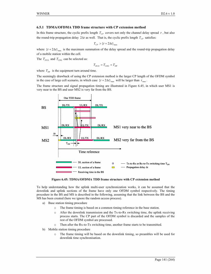
WINNER D2.6 v 1.0

Page 141 (264)

6.5.1 TDMA/OFDMA TDD frame structure with CP extension method In this frame structure, the cyclic prefix length CPT covers not only the channel delay spread τ , but also the round-trip propagation delay t∆2 as well. That is, the cyclic prefix length CPT satisfies:

max}2{ tTCP ∆+> τ

where max}2{ t∆+τ is the maximum summation of the delay spread and the round-trip propagation delay of a mobile station within the cell. The DUGT and UDGT can be selected as:

SWUDGDUG TTT ==

where SWT is the equipment turn around time.

The seemingly drawback of using the CP extension method is the larger CP length of the OFDM symbol in the case of large cell scenario, in which case max}2{ t∆+τ will be larger than maxτ .

The frame structure and signal propagation timing are illustrated in Figure 6.45, in which user MS1 is very near to the BS and user MS2 is very far from the BS.

BS

MS1

MS2

DL/TX UL/RX

DL/RX

DL/RX UL/TX

UL/TX

∆t

Tx-to-Rx or Rx-to-Tx switching time TSWDL section of a frame

UL section of a frame

TSW

Propagation delay ∆t

DL/TX

DL/RX

DL/RX

Receiving time in the BS

MS1 very near to the BS

MS2 very far from the BS

One TDD frame

Time reference

BS

MS1

MS2

DL/TX UL/RX

DL/RX

DL/RX UL/TX

UL/TX

∆t

Tx-to-Rx or Rx-to-Tx switching time TSWDL section of a frame

UL section of a frame

TSW

Propagation delay ∆t

DL/TX

DL/RX

DL/RX

Receiving time in the BS

MS1 very near to the BS

MS2 very far from the BS

One TDD frame

Time reference

Figure 6.45: TDMA/OFDMA TDD frame structure with CP extension method

To help understanding how the uplink multi-user synchronization works, it can be assumed that the downlink and uplink sections of the frame have only one OFDM symbol respectively. The timing procedure in the BS and MS is described in the following, assuming that the link between the BS and the MS has been created (here we ignore the random access process).

a) Base station timing procedure o The frame timing is based on a common timing reference in the base station. o After the downlink transmission and the Tx-to-Rx switching time, the uplink receiving

process starts. The CP part of the OFDM symbol is discarded and the samples of the rest of the OFDM symbol are processed.

o Then after the Rx-to-Tx switching time, another frame starts to be transmitted. b) Mobile station timing procedure

o The frame timing will be based on the downlink timing, so preambles will be used for downlink time synchronisation.

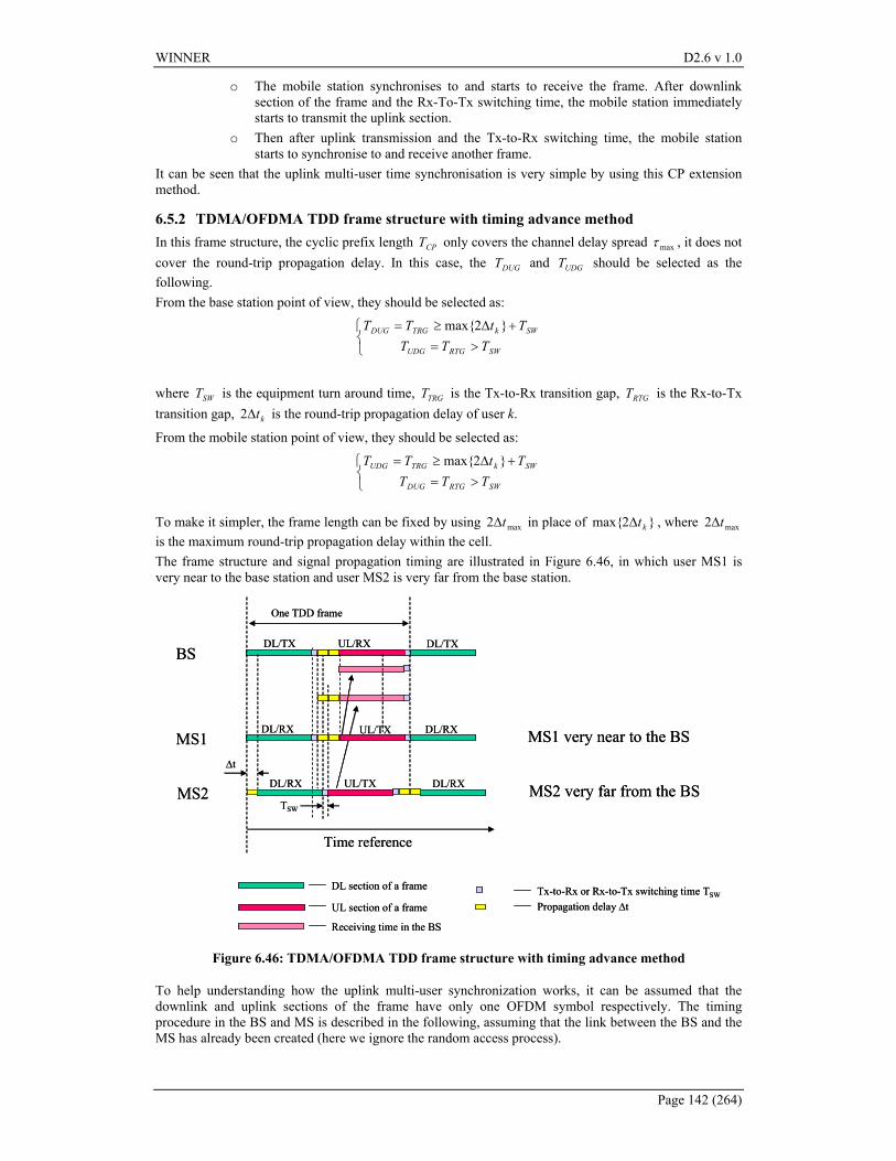
WINNER D2.6 v 1.0

Page 142 (264)

o The mobile station synchronises to and starts to receive the frame. After downlink section of the frame and the Rx-To-Tx switching time, the mobile station immediately starts to transmit the uplink section.

o Then after uplink transmission and the Tx-to-Rx switching time, the mobile station starts to synchronise to and receive another frame.

It can be seen that the uplink multi-user time synchronisation is very simple by using this CP extension method.

6.5.2 TDMA/OFDMA TDD frame structure with timing advance method In this frame structure, the cyclic prefix length CPT only covers the channel delay spread maxτ , it does not cover the round-trip propagation delay. In this case, the DUGT and UDGT should be selected as the following. From the base station point of view, they should be selected as:

>=+∆≥=

SWRTGUDG

SWkTRGDUG

TTTTtTT }2max{

where SWT is the equipment turn around time, TRGT is the Tx-to-Rx transition gap, RTGT is the Rx-to-Tx transition gap, kt∆2 is the round-trip propagation delay of user k.

From the mobile station point of view, they should be selected as:

>=+∆≥=

SWRTGDUG

SWkTRGUDG

TTTTtTT }2max{

To make it simpler, the frame length can be fixed by using max2 t∆ in place of }2max{ kt∆ , where max2 t∆ is the maximum round-trip propagation delay within the cell. The frame structure and signal propagation timing are illustrated in Figure 6.46, in which user MS1 is very near to the base station and user MS2 is very far from the base station.

BS

MS1

MS2

DL/TX UL/RX

DL/RX

DL/RX UL/TX

UL/TX

∆t

Tx-to-Rx or Rx-to-Tx switching time TSWDL section of a frame

UL section of a frame

TSW

Propagation delay ∆t

DL/TX

DL/RX

DL/RX

Receiving time in the BS

MS1 very near to the BS

MS2 very far from the BS

One TDD frame

Time reference

BS

MS1

MS2

DL/TX UL/RX

DL/RX

DL/RX UL/TX

UL/TX

∆t

Tx-to-Rx or Rx-to-Tx switching time TSWDL section of a frame

UL section of a frame

TSW

Propagation delay ∆t

DL/TX

DL/RX

DL/RX

Receiving time in the BS

MS1 very near to the BS

MS2 very far from the BS

One TDD frame

Time reference

Figure 6.46: TDMA/OFDMA TDD frame structure with timing advance method

To help understanding how the uplink multi-user synchronization works, it can be assumed that the downlink and uplink sections of the frame have only one OFDM symbol respectively. The timing procedure in the BS and MS is described in the following, assuming that the link between the BS and the MS has already been created (here we ignore the random access process).

WINNER D2.6 v 1.0

Page 143 (264)

c) Base station timing procedure o The frame timing is based on a common timing reference in the base station. o After the downlink transmission, and the Tx-to-Rx transition gap TRGT which can be

selected as the maximum round-trip propagation delay plus the Tx-to-Rx switching time, the uplink receiving process starts. The CP part of the OFDM symbol is discarded and the samples of the rest of the OFDM symbol are processed.

o Then after the Rx-to-Tx switching time, another frame starts to be transmitted. d) Mobile station timing procedure

o First of all, the distance between the MS and the BS needs to be known (Note the procedure of this can be complicated, especially for fast moving users).

o The frame timing will be based on the downlink timing, so preambles will be used for downlink time synchronisation.

o The mobile station synchronises to and starts to receive the frame. After downlink section of the frame and the Rx-To-Tx switching time, the mobile station will wait for a little while before starts to transmit the uplink section. This waiting time depends on the distance between the MS and BS. In the two extreme cases, the waiting time of the MS very near to the cell border will be zero; and the waiting time of the MS very near to the BS will be maximum round-trip propagation delay.

o Then after uplink transmission and the Tx-to-Rx switching time, the mobile station starts to synchronise to and receive another frame.

It can be seen the timing advance method will be complicated for mobile applications.

WINNER D2.6 v 1.0

Page 144 (264)

6.6 Conclusions on multi-carrier access technologies – FDMA/TDMA In this chapter we discussed pros and cons of TDMA/OFDMA, OFDMA and TDMA systems, presented design proposals and performance results from the initial study of TDMA/OFDMA, OFDMA and TDMA systems both in downlink and uplink. In contrast to spreading based systems, these systems are based on the paradigm of orthogonality. The goal is to keep the resources as orthogonal as possible, thus avoiding interference to as large extent as possible. Efficient synchronization algorithms in time and frequency are then crucial enabling technologies, and they are important topics for futher studies within the context of the WINNER deployment and user scenarios. For TDMA/OFDMA and OFDMA, power control in the multi-user uplink is another important tool for maintaining sufficient degree of orthogonality between users in a real system with imperfect synchronization. Adaptive TDMA/OFDMA schemes are the most advanced schemes, which rely on accurate synchronization of both time and frequency in addition to accurate channel state information for link adaptation and user scheduling. Availability to accurate channel state information depends on efficient prediction algorithms and fast feedback to the scheduler. Also an efficient scheduling algorithm is crucial in order to take full advantage of multi-user diversity, as discussed in chapter 6.1. In adaptive OFDMA systems, we reduce the complexity by avoiding fast user scheduling, and in adaptive TDMA systems we do not need to schedule users in the frequency domain. In chapter 6.2, we presented algorithms and results for multi-user adaptive power and bit-loading in OFDMA uplinks, and in chapter 6.5 we discussed multi-user time synchronization. Another important aspect of adaptive TDMA/OFDMA system design is the choice of duplex scheme, since it affects the design of the closed feedback loops in these systems. The initial studies indicate that FDD (or half-duplex FDD) is the most suitable duplex scheme in wide-area coverage scenarios and that the more flexible TDD system is the best candidate for small-range scenarios. Independently of adaptive user scheduling, link adaptation in OFDM based systems is a promising technique to improve the system spectral efficieny. Adapting to the small-scale channel fading is depending on accurate channel state information. Link adaptation is possible up to a certain maximum user speed, and a fallback mode for users moving with speeds above this limit is needed. The value of the maximum speed limit depends crucially on the users’ channels and on the required SINR prediction horizon, which is connected to the overall frame structure in the system. Supporting vehicular users in a wide-area coverage scenario is possible, as we discussed in chapter 6.1 for TDMA/OFDMA systems and in chapter 6.2 for OFDMA systems. For the fallback mode, the design of TDMA/OFDMA, OFDMA and TDMA systems based on less required transmitter CSI can be made by using larger bins in the time and/or frequency domain, and by adapting to these resources with more traditional diversity based interleaved coding and modulation techniques. For TDMA/OFDMA, OFDMA and TDMA systems to be spectrally efficient in a multi-cell environment, the frequency reuse factor has to be close to 1. We analyzed the impact of multi-cell interference in chapter 6.2 for an OFDMA system and in chapter 6.3 for a TDMA system. A conclusion is that an important tool to achive a low reuse factor is to coordinate the resources, at least between adjacent cells. TDMA/OFDMA is the most flexible system, but as mentioned above, requires good quality CSI and fast scheduling. In the uplink, also power control is needed. In OFDMA, less complicated user scheduling is required, but power control is still needed in the uplink. In TDMA systems, the power control is much simpler and the terminals can be power efficient due to a small duty-cycle. A problem with TDMA is the coverage range for wide-band systems, unless the allowed peak transmit power level can fully compensate for the low duty-cycle. Also, efficient support of small packets is a problem as discussed in chapter 6.3. A wide system bandwidth is also problematic in adaptive systems, since pilot overhead and feedback information tends to be too demanding. A solution to the above problems is to define subbands. In the context of adaptive TDMA/OFDMA in chapter 6.1, we defined so-called contention bands for the users, which are a fraction of the total system bandwidth. In chapter 6.4, we proposed a dual bandwidth system using a wideband carrier and a narrowband carrier. Such a solution makes it possible to define a TDMA system with larger cell size. There are many important issues for further studies within WINNER in order to fully understand the potential of the above mentioned schemes within the WINNER deployment and user scenarios.

• Synchronization (large cells, TDD interference environment, phase noise, local oscillator instabilities, Doppler spread)

• Co-design with MIMO systems

WINNER D2.6 v 1.0

Page 145 (264)

• Suitability to foreseen WINNER user behaviour and traffic scenarions (velocity distributions, distribution of QoS services, number of active users, realistic traffic models, system load)

• Detailed analysis of the performance on accurate channel models for the WINNER deployment scenarios

• Multi-cell interference modelling and management with minimized frequency reuse factor • Transceiver limitations (PAPR, ADC, processing power)

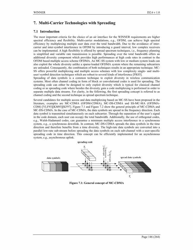
WINNER D2.6 v 1.0

Page 146 (264)

7. Multi-Carrier Technologies with Spreading

7.1 Introduction The most important criteria for the choice of an air interface for the WINNER requirements are higher spectral efficiency and flexibility. Multi-carrier modulations, e.g., OFDM, can achieve high spectral efficiency by multiplexing multiple user data over the total bandwidth. Due to the avoidance of inter-carrier and inter-symbol interference in OFDM by introducing a guard interval, low complex receivers can be implemented. A high flexibility is offered by spread spectrum techniques, i.e., frequency planning is simplified and variable rate transmission is possible. Spreading over the total bandwidth offers an additional diversity component which provides high performances at high code rates in contrast to the OFDM based multiple access scheme OFDMA. An MC-SS system with low or medium system loads can also exploit the whole diversity unlike a sparse-loaded OFDMA system where the remaining subcarriers are unloaded. Consequently, the combination of both techniques results in an appropriate technique. MC-SS offers powerful multiplexing and multiple access schemes with low complexity single- and multi-user/-symbol detection techniques which are robust to several kinds of interference [FK03]. Spreading of data symbols is a common technique to exploit diversity in wireless communication systems. Most often channel coding in form of block or convolutional codes is used for spreading. The spreading code can either be designed to only exploit diversity which is typical for classical channel coding or as spreading code where besides the diversity gain a code multiplexing is performed in order to separate multiple data streams. For clarity, in the following, the first spreading concept is referred to as channel coding and the second technique as spread spectrum technique.

Several candidates for multiple access and data multiplexing based on MC-SS have been proposed in the literature, examples are MC-CDMA (OFDM-CDMA), MC-DS-CDMA and SS-MC-MA (OFDMA-CDM) [YLF93][KM93][KF97]. Figure 7.1 and Figure 7.2 show the general principle of MC-CDMA and MC-DS-CDMA. In the case of MC-CDMA, the data symbols are spread in the frequency direction. Each data symbol is transmitted simultaneously on each subcarrier. Through the separation of the user’s signal in the code domain, each user can occupy the total bandwidth. Additionally, the use of orthogonal codes, e.g., Walsh-Hadamard codes, can guarantee a minimum multiple access interference in a synchronous system, e.g., a synchronous downlink. In contrast, MC-DS-CDMA spreads the data symbols in the time direction and therefore benefits from a time diversity. The high-rate data symbols are converted into a parallel low-rate sub-stream before spreading the data symbols on each sub-channel with a user-specific spreading code in time direction. This concept can be efficiently implemented for an asynchronous system, e.g., asynchronous uplink.

Figure 7.1: General concept of MC-CDMA

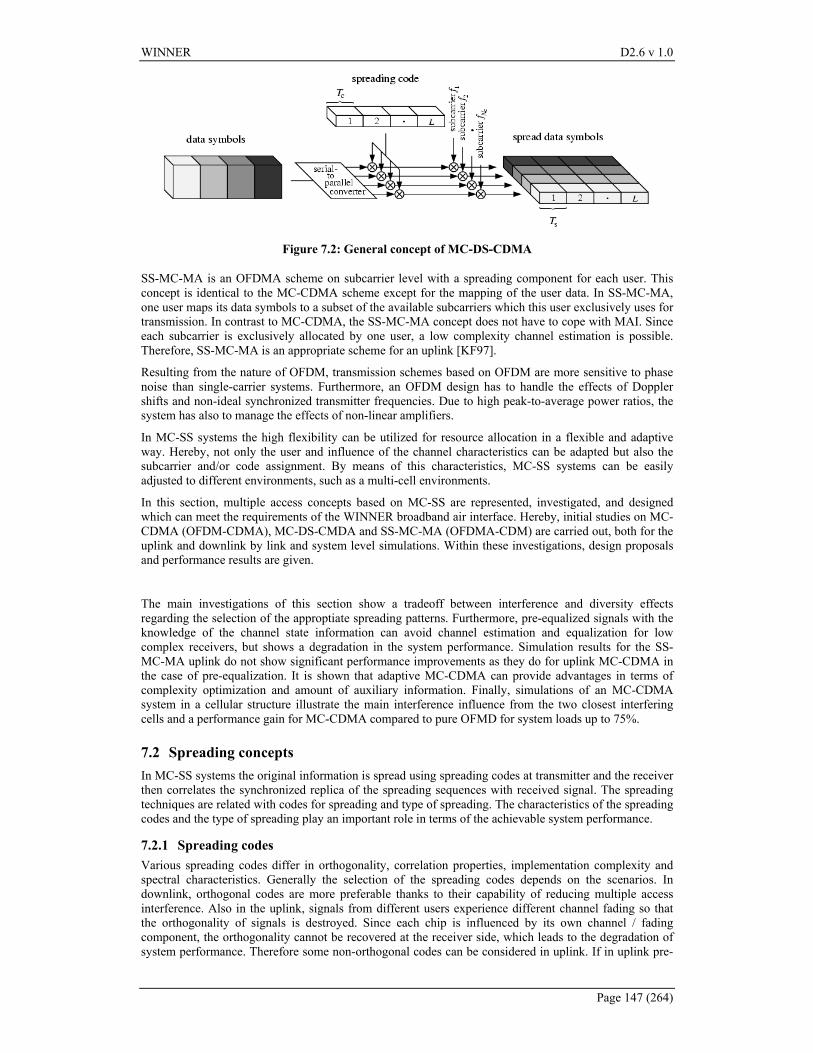
WINNER D2.6 v 1.0

Page 147 (264)

Figure 7.2: General concept of MC-DS-CDMA

SS-MC-MA is an OFDMA scheme on subcarrier level with a spreading component for each user. This concept is identical to the MC-CDMA scheme except for the mapping of the user data. In SS-MC-MA, one user maps its data symbols to a subset of the available subcarriers which this user exclusively uses for transmission. In contrast to MC-CDMA, the SS-MC-MA concept does not have to cope with MAI. Since each subcarrier is exclusively allocated by one user, a low complexity channel estimation is possible. Therefore, SS-MC-MA is an appropriate scheme for an uplink [KF97].

Resulting from the nature of OFDM, transmission schemes based on OFDM are more sensitive to phase noise than single-carrier systems. Furthermore, an OFDM design has to handle the effects of Doppler shifts and non-ideal synchronized transmitter frequencies. Due to high peak-to-average power ratios, the system has also to manage the effects of non-linear amplifiers.

In MC-SS systems the high flexibility can be utilized for resource allocation in a flexible and adaptive way. Hereby, not only the user and influence of the channel characteristics can be adapted but also the subcarrier and/or code assignment. By means of this characteristics, MC-SS systems can be easily adjusted to different environments, such as a multi-cell environments.

In this section, multiple access concepts based on MC-SS are represented, investigated, and designed which can meet the requirements of the WINNER broadband air interface. Hereby, initial studies on MC-CDMA (OFDM-CDMA), MC-DS-CMDA and SS-MC-MA (OFDMA-CDM) are carried out, both for the uplink and downlink by link and system level simulations. Within these investigations, design proposals and performance results are given.

The main investigations of this section show a tradeoff between interference and diversity effects regarding the selection of the approptiate spreading patterns. Furthermore, pre-equalized signals with the knowledge of the channel state information can avoid channel estimation and equalization for low complex receivers, but shows a degradation in the system performance. Simulation results for the SS-MC-MA uplink do not show significant performance improvements as they do for uplink MC-CDMA in the case of pre-equalization. It is shown that adaptive MC-CDMA can provide advantages in terms of complexity optimization and amount of auxiliary information. Finally, simulations of an MC-CDMA system in a cellular structure illustrate the main interference influence from the two closest interfering cells and a performance gain for MC-CDMA compared to pure OFMD for system loads up to 75%.

7.2 Spreading concepts In MC-SS systems the original information is spread using spreading codes at transmitter and the receiver then correlates the synchronized replica of the spreading sequences with received signal. The spreading techniques are related with codes for spreading and type of spreading. The characteristics of the spreading codes and the type of spreading play an important role in terms of the achievable system performance.

7.2.1 Spreading codes Various spreading codes differ in orthogonality, correlation properties, implementation complexity and spectral characteristics. Generally the selection of the spreading codes depends on the scenarios. In downlink, orthogonal codes are more preferable thanks to their capability of reducing multiple access interference. Also in the uplink, signals from different users experience different channel fading so that the orthogonality of signals is destroyed. Since each chip is influenced by its own channel / fading component, the orthogonality cannot be recovered at the receiver side, which leads to the degradation of system performance. Therefore some non-orthogonal codes can be considered in uplink. If in uplink pre-

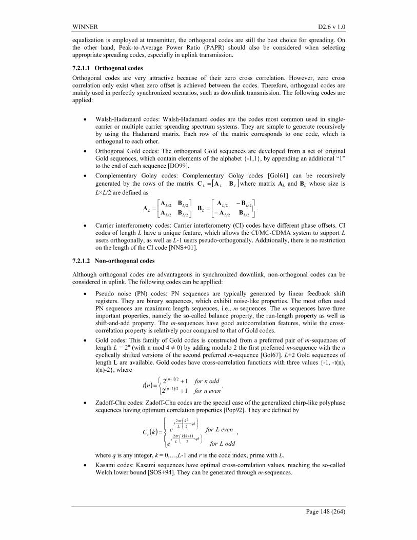
WINNER D2.6 v 1.0

Page 148 (264)

equalization is employed at transmitter, the orthogonal codes are still the best choice for spreading. On the other hand, Peak-to-Average Power Ratio (PAPR) should also be considered when selecting appropriate spreading codes, especially in uplink transmission.

7.2.1.1 Orthogonal codes Orthogonal codes are very attractive because of their zero cross correlation. However, zero cross correlation only exist when zero offset is achieved between the codes. Therefore, orthogonal codes are mainly used in perfectly synchronized scenarios, such as downlink transmission. The following codes are applied:

• Walsh-Hadamard codes: Walsh-Hadamard codes are the codes most common used in single-carrier or multiple carrier spreading spectrum systems. They are simple to generate recursively by using the Hadamard matrix. Each row of the matrix corresponds to one code, which is orthogonal to each other.

• Orthogonal Gold codes: The orthogonal Gold sequences are developed from a set of original Gold sequences, which contain elements of the alphabet {-1,1}, by appending an additional “1” to the end of each sequence [DO99].

• Complementary Golay codes: Complementary Golay codes [Gol61] can be recursively generated by the rows of the matrix [ ]LLL BAC = where matrix AL and BL whose size is L×L/2 are defined as

−

−=

=

22

22

22

22

LL

LLL

LL

LLL BA

BAB

BABA

A .

• Carrier interferometry codes: Carrier interferometry (CI) codes have different phase offsets. CI codes of length L have a unique feature, which allows the CI/MC-CDMA system to support L users orthogonally, as well as L-1 users pseudo-orthogonally. Additionally, there is no restriction on the length of the CI code [NNS+01].

7.2.1.2 Non-orthogonal codes

Although orthogonal codes are advantageous in synchronized downlink, non-orthogonal codes can be considered in uplink. The following codes can be appllied:

• Pseudo noise (PN) codes: PN sequences are typically generated by linear feedback shift registers. They are binary sequences, which exhibit noise-like properties. The most often used PN sequences are maximum-length sequences, i.e., m-sequences. The m-sequences have three important properties, namely the so-called balance property, the run-length property as well as shift-and-add property. The m-sequences have good autocorrelation features, while the cross-correlation property is relatively poor compared to that of Gold codes.

• Gold codes: This family of Gold codes is constructed from a preferred pair of m-sequences of length L = 2n (with n mod 4 ≠ 0) by adding modulo 2 the first preferred m-sequence with the n cyclically shifted versions of the second preferred m-sequence [Gol67]. L+2 Gold sequences of length L are available. Gold codes have cross-correlation functions with three values {-1, -t(n), t(n)-2}, where

( )( )

( )

++

=+

+

evennforoddnfor

nt n

n

1212

22

21

.

• Zadoff-Chu codes: Zadoff-Chu codes are the special case of the generalized chirp-like polyphase sequences having optimum correlation properties [Pop92]. They are defined by

( )( )

=

+

+

+

oddLfore

evenLforekCqkkk

Lrj

qkkL

rj

r

212

22 2

π

π

,

where q is any integer, k = 0,…,L-1 and r is the code index, prime with L. • Kasami codes: Kasami sequences have optimal cross-correlation values, reaching the so-called

Welch lower bound [SOS+94]. They can be generated through m-sequences.

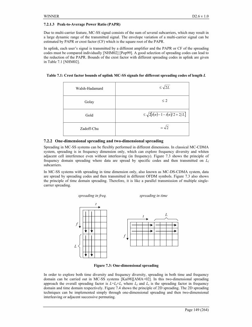
WINNER D2.6 v 1.0

Page 149 (264)

7.2.1.3 Peak-to-Average Power Ratio (PAPR)

Due to multi-carrier feature, MC-SS signal consists of the sum of several subcarriers, which may result in a large dynamic range of the transmitted signal. The envelope variation of a multi-carrier signal can be estimated by PAPR or crest factor (CF) which is the square root of the PAPR.

In uplink, each user’s signal is transmitted by a different amplifier and the PAPR or CF of the spreading codes must be compared individually [NHM02] [Pop99]. A good selection of spreading codes can lead to the reduction of the PAPR. Bounds of the crest factor with different spreading codes in uplink are given in Table 7.1 [NHM02].

Table 7.1: Crest factor bounds of uplink MC-SS signals for different spreading codes of length L

Walsh-Hadamard L2≤

Golay 2≤

Gold ( ) ( )[ ]Lntnt 2212 +−−≤

Zadoff-Chu 2=

7.2.2 One-dimensional spreading and two-dimensional spreading Spreading in MC-SS systems can be flexibly performed in different dimensions. In classical MC-CDMA system, spreading is in frequency dimension only, which can explore frequency diversity and whiten adjacent cell interference even without interleaving (in frequency). Figure 7.3 shows the principle of frequency domain spreading where data are spread by specific codes and then transmitted on Lf subcarriers.

In MC-SS systems with spreading in time dimension only, also known as MC-DS-CDMA system, data are spread by spreading codes and then transmitted in different OFDM symbols. Figure 7.3 also shows the principle of time domain spreading. Therefore, it is like a parallel transmission of multiple single-carrier spreading.

f

t

L

L

f

t

spreading in freq. spreading in time

Figure 7.3: One-dimensional spreading

In order to explore both time diversity and frequency diversity, spreading in both time and frequency domain can be carried out in MC-SS systems [Kai98][AMA+02]. In this two-dimensional spreading approach the overall spreading factor is L=Lf×Lt where Lf and Lt is the spreading factor in frequency domain and time domain respectively. Figure 7.4 shows the principle of 2D spreading. The 2D spreading techniques can be implemented simply through one-dimensional spreading and then two-dimensional interleaving or adjacent successive permuting.

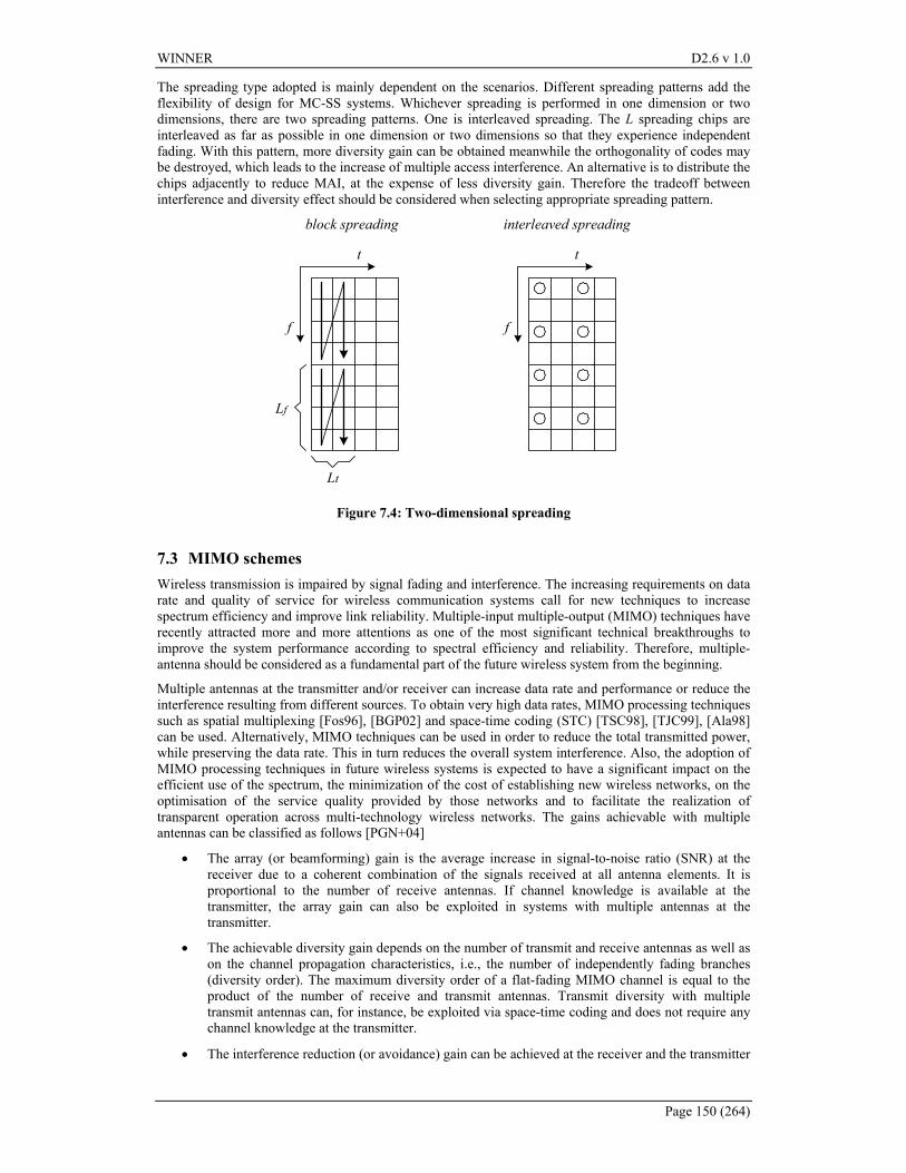
WINNER D2.6 v 1.0

Page 150 (264)

The spreading type adopted is mainly dependent on the scenarios. Different spreading patterns add the flexibility of design for MC-SS systems. Whichever spreading is performed in one dimension or two dimensions, there are two spreading patterns. One is interleaved spreading. The L spreading chips are interleaved as far as possible in one dimension or two dimensions so that they experience independent fading. With this pattern, more diversity gain can be obtained meanwhile the orthogonality of codes may be destroyed, which leads to the increase of multiple access interference. An alternative is to distribute the chips adjacently to reduce MAI, at the expense of less diversity gain. Therefore the tradeoff between interference and diversity effect should be considered when selecting appropriate spreading pattern.

f

t

interleaved spreadingblock spreading

f

t

Lf

Lt

Figure 7.4: Two-dimensional spreading

7.3 MIMO schemes Wireless transmission is impaired by signal fading and interference. The increasing requirements on data rate and quality of service for wireless communication systems call for new techniques to increase spectrum efficiency and improve link reliability. Multiple-input multiple-output (MIMO) techniques have recently attracted more and more attentions as one of the most significant technical breakthroughs to improve the system performance according to spectral efficiency and reliability. Therefore, multiple-antenna should be considered as a fundamental part of the future wireless system from the beginning.

Multiple antennas at the transmitter and/or receiver can increase data rate and performance or reduce the interference resulting from different sources. To obtain very high data rates, MIMO processing techniques such as spatial multiplexing [Fos96], [BGP02] and space-time coding (STC) [TSC98], [TJC99], [Ala98] can be used. Alternatively, MIMO techniques can be used in order to reduce the total transmitted power, while preserving the data rate. This in turn reduces the overall system interference. Also, the adoption of MIMO processing techniques in future wireless systems is expected to have a significant impact on the efficient use of the spectrum, the minimization of the cost of establishing new wireless networks, on the optimisation of the service quality provided by those networks and to facilitate the realization of transparent operation across multi-technology wireless networks. The gains achievable with multiple antennas can be classified as follows [PGN+04]

• The array (or beamforming) gain is the average increase in signal-to-noise ratio (SNR) at the receiver due to a coherent combination of the signals received at all antenna elements. It is proportional to the number of receive antennas. If channel knowledge is available at the transmitter, the array gain can also be exploited in systems with multiple antennas at the transmitter.

• The achievable diversity gain depends on the number of transmit and receive antennas as well as on the channel propagation characteristics, i.e., the number of independently fading branches (diversity order). The maximum diversity order of a flat-fading MIMO channel is equal to the product of the number of receive and transmit antennas. Transmit diversity with multiple transmit antennas can, for instance, be exploited via space-time coding and does not require any channel knowledge at the transmitter.

• The interference reduction (or avoidance) gain can be achieved at the receiver and the transmitter

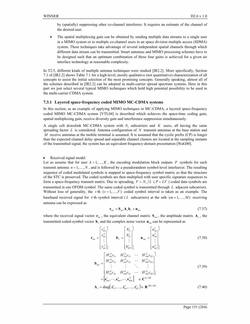
WINNER D2.6 v 1.0

Page 151 (264)

by (spatially) suppressing other co-channel interferers. It requires an estimate of the channel of the desired user.

• The spatial multiplexing gain can be obtained by sending multiple data streams to a single user in a MIMO system or to multiple co-channel users in an space division multiple access (SDMA) system. These techniques take advantage of several independent spatial channels through which different data stream can be transmitted. Smart antennas and MIMO processing schemes have to be designed such that an optimum combination of these four gains is achieved for a given air interface technology at reasonable complexity.

In T2.5, different kinds of multiple antenna techniques were studied [IR2.2]. More specifically, Section 7.1 of [IR2.2] shows Table 7.1 for a high-level, mostly qualitative (not quantitative) characterization of all concepts to assist the initial selection of the most promising concepts. Generally speaking, almost all of the schemes described in [IR2.2] can be adopted in multi-carrier spread spectrum systems. Here in this part we just select several typical MIMO techniques which hold high potential possibility to be used in the multi-carrier CDMA system.

7.3.1 Layered space-frequency coded MIMO MC-CDMA systems In this section, as an example of applying MIMO techniques in MC-CDMA, a layered space-frequency coded MIMO MC-CDMA system [VTL04] is described which achieves the space-time coding gain, spatial multiplexing gain, receive diversity gain and interference suppression simultaneously.

A single cell downlink MC-CDMA system with Nc subcarriers and K users, all having the same spreading factor L is considered. Antenna configuration of N transmit antennas at the base station and M receive antennas at the mobile terminal is assumed. It is assumed that the cyclic prefix (CP) is longer than the expected channel delay spread and separable channel clusters are located at the sampling instants of the transmitted signal, the system has an equivalent frequency-domain presentation [WaG00].

• Received signal model Let us assume that for user Kk ,,1 K= , the encoding modulation block outputs P symbols for each transmit antenna Nn ,,1 K= , and is followed by a pseudorandom symbol-level interleaver. The resulting sequence of coded modulated symbols is mapped to space-frequency symbol matrix so that the structure of the STC is preserved. The coded symbols are then multiplied with user specific signature sequences to form a space-frequency transmit matrix. Due to spreading, LNV c= ( LVP = ) coded data symbols are transmitted in one OFDM symbol. The same coded symbol is transmitted through L adjacent subcarriers. Without loss of generality, the v th ),,1( Vv K= coded symbol interval is taken as an example. The baseband received signal for v th symbol interval ( L subcarriers) at the mth ),,1( Mm K= receiving antenna can be expressed as mvvvmvmv nbASr += (7.37)

where the received signal vector mvr , the equivalent channel matrix mvS , the amplitude matrix vA , the transmitted coded-symbol vector vb and the complex noise vector mvn can be represented as

=

Lmv

mv

mv

mv

r

rr

M

2

1

r

=

vKN

v

v

v

b

bb

M12

11

b

=

Lmv

mv

mv

mv

n

nn

M

2

1

n (7.38)

[ ] NKLNKm

nkmm

KLvLNmL

vLmL

vLm

KvNm

vm

vm

KvNm

vm

vm

mv

cHcHcH

cHcHcHcHcHcH

×∈=

=

Csss

S

,,,,11

1211

22

122

2122

1

11

111

2111

1

LL

L

MOMM

L

L

(7.39)

( ) NKNKvkN

vkn

vv AAA ×∈= RA ,,,,diag 11 KK (7.40)

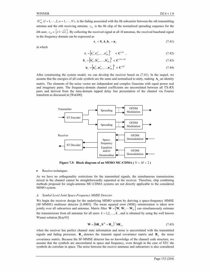
WINNER D2.6 v 1.0

Page 152 (264)

vlnmH ),,1;,,1( NnLl LL == , is the fading associated with the lth subcarrier between the nth transmitting

antenna and the mth receiving antenna. klc is the lth chip of the normalized spreading sequence for the

kth user, { }Lckl /1±∈ . By collecting the received signal at all M antennas, the received baseband signal in the frequency domain can be expressed as vvvvv nbASr += (7.41)

in which

[ ] ,,, TTT2

T1

LMMvvvv Crrrr ∈= K , (7.42)

[ ] ,,, TTT2

T1

NKLMMvvvv

×∈= CSSSS K (7.43)

[ ] LMMvvvv Cnnnn ∈= ,,, TTT

2T1 K (7.44)

After constructing the system model, we can develop the receiver based on (7.41). In the sequel, we assume that the energies of all code symbols are the same and normalised to unity, making pA an identity matrix. The elements of the noise vector are independent and complex Gaussian with equal power real and imaginary parts. The frequency-domain channel coefficients are uncorrelated between all TX-RX pairs and derived from the time-domain tapped delay line presentation of the channel via Fourier transform as discussed in [WaG00].

Figure 7.5: Block diagram of an MIMO MC-CDMA ( 2== MN )

• Receive techniques

As we have no orthogonality restrictions for the transmitted signals, the simultaneous transmissions mixed in the channel cannot be straightforwardly separated at the receiver. Therefore, chip combining methods proposed for single-antenna MC-CDMA systems are not directly applicable to the considered MIMO system.

A. Symbol Level Joint Space-Frequency MMSE Detector

We begin the receiver design for the underlying MIMO system by deriving a space-frequency MMSE (SF-MMSE) multiuser detector [LiM03]. The mean squared error (MSE) minimization is taken now jointly over all subcarriers and antennas. Matrix filter [ ]KWWWW L21 = can simultaneously estimate the transmissions from all antennas for all users Kk ,,2,1 K= , and is obtained by using the well known Wiener solution [Kay93]

( ) xxH

xx SRRSSRW1−

+= η (7.45)

when the receiver has perfect channel state information and noise is uncorrelated with the transmitted signals and fading processes. xxR denotes the transmit signal covariance matrix and ηR the noise covariance matrix. Because the SF-MMSE detector has no knowledge of the channel code structure, we assume that the symbols are uncorrelated in space and frequency, even though in the case of STC the symbols do correlate in space. The noise between the receive antennas and subcarriers is also considered

ST Encoder

Spreading OFDM

Modulation

OFDM Modulation Spreading

Transmitter

Receiver

ST Decoder

Space-

frequency Equalizer

and/or Despreading

OFDM Demodulation

OFDM Demodulation

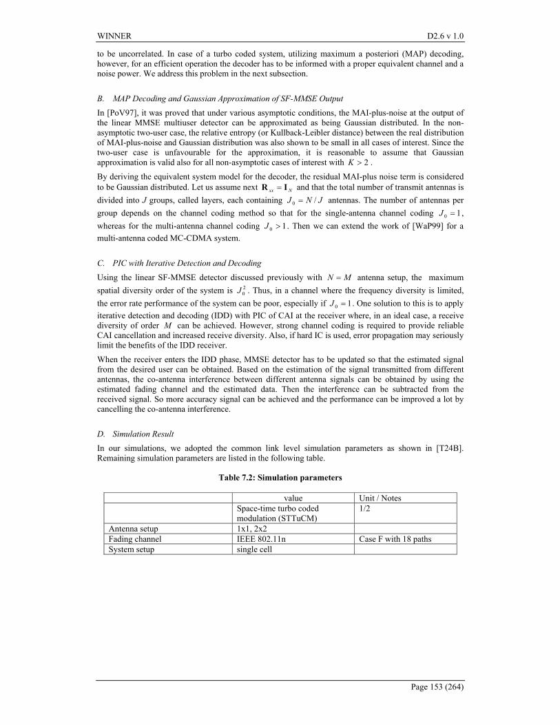
WINNER D2.6 v 1.0

Page 153 (264)

to be uncorrelated. In case of a turbo coded system, utilizing maximum a posteriori (MAP) decoding, however, for an efficient operation the decoder has to be informed with a proper equivalent channel and a noise power. We address this problem in the next subsection. B. MAP Decoding and Gaussian Approximation of SF-MMSE Output

In [PoV97], it was proved that under various asymptotic conditions, the MAI-plus-noise at the output of the linear MMSE multiuser detector can be approximated as being Gaussian distributed. In the non-asymptotic two-user case, the relative entropy (or Kullback-Leibler distance) between the real distribution of MAI-plus-noise and Gaussian distribution was also shown to be small in all cases of interest. Since the two-user case is unfavourable for the approximation, it is reasonable to assume that Gaussian approximation is valid also for all non-asymptotic cases of interest with 2>K .

By deriving the equivalent system model for the decoder, the residual MAI-plus noise term is considered to be Gaussian distributed. Let us assume next Nxx IR = and that the total number of transmit antennas is divided into J groups, called layers, each containing JNJ /0 = antennas. The number of antennas per group depends on the channel coding method so that for the single-antenna channel coding 10 =J , whereas for the multi-antenna channel coding 10 >J . Then we can extend the work of [WaP99] for a multi-antenna coded MC-CDMA system. C. PIC with Iterative Detection and Decoding

Using the linear SF-MMSE detector discussed previously with MN = antenna setup, the maximum spatial diversity order of the system is 2

0J . Thus, in a channel where the frequency diversity is limited, the error rate performance of the system can be poor, especially if 10 =J . One solution to this is to apply iterative detection and decoding (IDD) with PIC of CAI at the receiver where, in an ideal case, a receive diversity of order M can be achieved. However, strong channel coding is required to provide reliable CAI cancellation and increased receive diversity. Also, if hard IC is used, error propagation may seriously limit the benefits of the IDD receiver.

When the receiver enters the IDD phase, MMSE detector has to be updated so that the estimated signal from the desired user can be obtained. Based on the estimation of the signal transmitted from different antennas, the co-antenna interference between different antenna signals can be obtained by using the estimated fading channel and the estimated data. Then the interference can be subtracted from the received signal. So more accuracy signal can be achieved and the performance can be improved a lot by cancelling the co-antenna interference. D. Simulation Result

In our simulations, we adopted the common link level simulation parameters as shown in [T24B]. Remaining simulation parameters are listed in the following table.

Table 7.2: Simulation parameters

value Unit / Notes Space-time turbo coded

modulation (STTuCM) 1/2

Antenna setup 1x1, 2x2 Fading channel IEEE 802.11n Case F with 18 paths System setup single cell

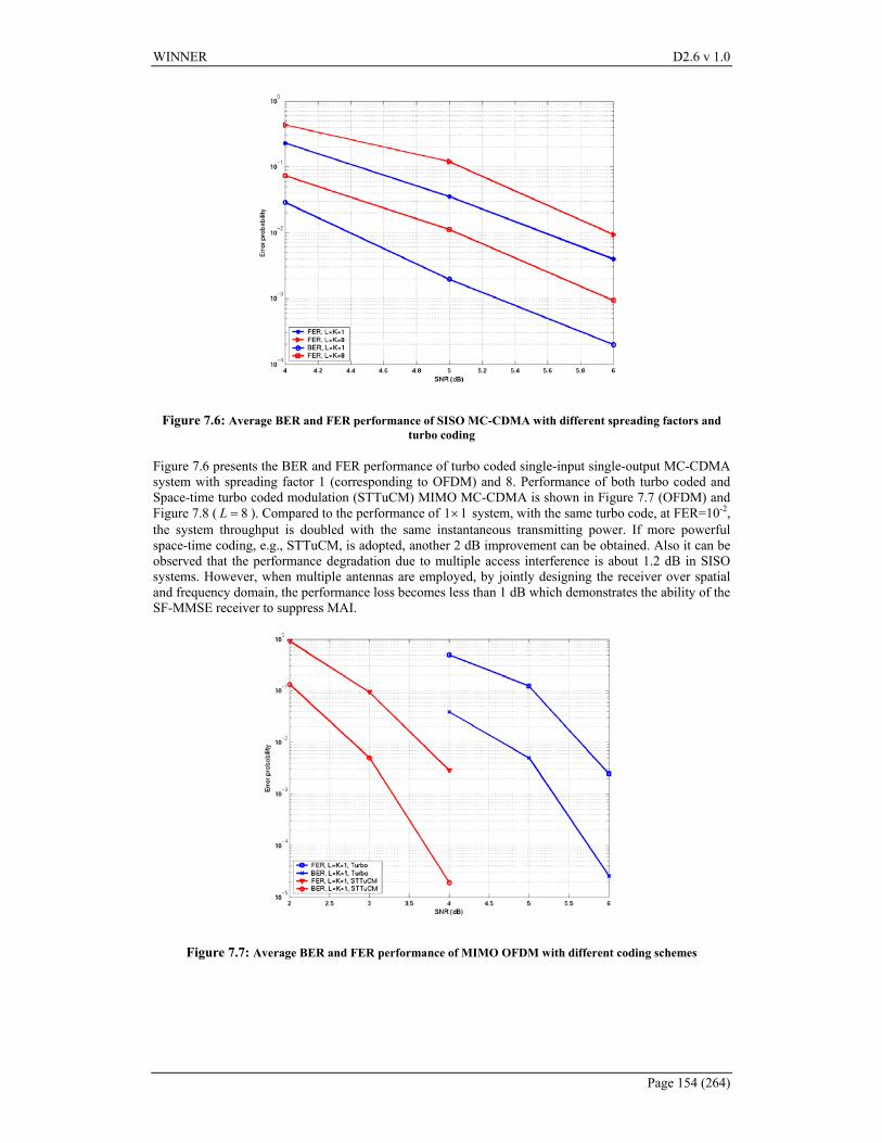
WINNER D2.6 v 1.0

Page 154 (264)

Figure 7.6: Average BER and FER performance of SISO MC-CDMA with different spreading factors and turbo coding

Figure 7.6 presents the BER and FER performance of turbo coded single-input single-output MC-CDMA system with spreading factor 1 (corresponding to OFDM) and 8. Performance of both turbo coded and Space-time turbo coded modulation (STTuCM) MIMO MC-CDMA is shown in Figure 7.7 (OFDM) and Figure 7.8 ( 8=L ). Compared to the performance of 11× system, with the same turbo code, at FER=10-2, the system throughput is doubled with the same instantaneous transmitting power. If more powerful space-time coding, e.g., STTuCM, is adopted, another 2 dB improvement can be obtained. Also it can be observed that the performance degradation due to multiple access interference is about 1.2 dB in SISO systems. However, when multiple antennas are employed, by jointly designing the receiver over spatial and frequency domain, the performance loss becomes less than 1 dB which demonstrates the ability of the SF-MMSE receiver to suppress MAI.

Figure 7.7: Average BER and FER performance of MIMO OFDM with different coding schemes

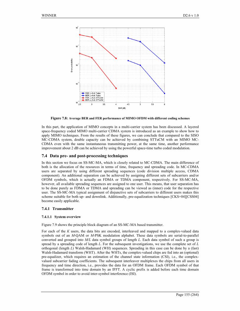
WINNER D2.6 v 1.0

Page 155 (264)

Figure 7.8: Average BER and FER performance of MIMO OFDM with different coding schemes

In this part, the application of MIMO concepts in a multi-carrier system has been discussed. A layered space-frequency coded MIMO multi-carrier CDMA system is introduced as an example to show how to apply MIMO techniques. From the results of these figures, we can conclude that compared to the SISO MC-CDMA system, double capacity can be achieved by combining STTuCM with an MIMO MC-CDMA even with the same instantaneous transmitting power, at the same time, another performance improvement about 2 dB can be achieved by using the powerful space-time turbo coded modulation.

7.4 Data pre- and post-processing techniques In this section we focus on SS-MC-MA, which is closely related to MC-CDMA. The main difference of both is the allocation of the resources in terms of time, frequency and spreading code. In MC-CDMA users are separated by using different spreading sequences (code division multiple access, CDMA component). An additional separation can be achieved by assigning different sets of subcarriers and/or OFDM symbols, which is actually an FDMA or TDMA component, respectively. For SS-MC-MA, however, all available spreading sequences are assigned to one user. This means, that user separation has to be done purely as FDMA or TDMA and spreading can be viewed as (inner) code for the respective user. The SS-MC-MA typical assignment of disjunctive sets of subcarriers to different users makes this scheme suitable for both up- and downlink. Additionally, pre-equalization techniques [CKS+04][CSS04] become easily applicable.

7.4.1 Transmitter

7.4.1.1 System overview

Figure 7.9 shows the principle block diagram of an SS-MC-MA based transmitter.

For each of the K users, the data bits are encoded, interleaved and mapped to a complex-valued data symbols out of an M-QAM or M-PSK modulation alphabet. These data symbols are serial-to-parallel converted and grouped into M/L data symbol groups of length L. Each data symbol of such a group is spread by a spreading code of length L. For the subsequent investigations, we use the complete set of L orthogonal (length L) Walsh-Hadamard (WH) sequences. Spreading in this case can be done by a (fast) Walsh-Hadamard transform (WHT). After the WHTs, the complex-valued chips are fed into an (optional) pre-equalizer, which requires an estimation of the channel state information (CSI), i.e., the complex-valued subcarrier fading coefficients. The subsequent interleaver multiplexes the chips from all users in frequency and time direction, i.e., provides the data for an OFDM frame. Each OFDM symbol of that frame is transformed into time domain by an IFFT. A cyclic prefix is added before each time domain OFDM symbol in order to avoid inter-symbol interference (ISI).

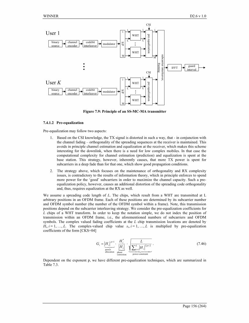
WINNER D2.6 v 1.0

Page 156 (264)

binarysource

channelencoder

codebitinterleaver modulator

S/P

WHT

preequalizationWHT subcarrierinterleaver,

framing

IFFT guardinterval

CSI

1

L

1

L

1

M

1

M

binarysource

channelencoder

codebitinterleaver modulator

S/P

WHT

preequalizationWHT

1

L

1

L

1

M

......

...

User 1

User K

CSI

Figure 7.9: Principle of an SS-MC-MA transmitter

7.4.1.2 Pre-equalization

Pre-equalization may follow two aspects:

1. Based on the CSI knowledge, the TX signal is distorted in such a way, that - in conjunction with the channel fading – orthogonality of the spreading sequences at the receiver is maintained. This avoids in principle channel estimation and equalization at the receiver, which makes this scheme interesting for the downlink, when there is a need for low complex mobiles. In that case the computational complexity for channel estimation (prediction) and equalization is spent at the base station. This strategy, however, inherently causes, that more TX power is spent for subcarriers in a deep fade than for that one, which show good propagation conditions.

2. The strategy above, which focuses on the maintenance of orthogonality and RX complexity issues, is contradictory to the results of information theory, which in principle enforces to spend more power for the ‘good’ subcarriers in order to maximize the channel capacity. Such a pre-equalization policy, however, causes an additional distortion of the spreading code orthogonality and, thus, requires equalization at the RX as well.

We assume a spreading code length of L. The chips, which result from a WHT are transmitted at L arbitrary positions in an OFDM frame. Each of these positions are determined by its subcarrier number and OFDM symbol number (the number of the OFDM symbol within a frame). Note, this transmission positions depend on the subcarrier interleaving strategy. We consider the pre-equalization coefficients for L chips of a WHT transform. In order to keep the notation simple, we do not index the position of transmission within an OFDM frame, i.e., the aforementioned numbers of subcarriers and OFDM symbols. The complex valued fading coefficients at the L chip transmission locations are denoted by Hi, i = 1, …, L. The complex-valued chip value si, i = 1, …, L is multiplied by pre-equalization coefficients of the form [CKS+04]

{ 44 344 21

321

constraintpower

1

22

correctionphase

*

allocationpower

1

∑ =

+

+⋅⋅= L

i

pii

ipii

HL

HH

HG . (7.46)

Dependent on the exponent p, we have different pre-equalization techniques, which are summarized in Table 7.3.

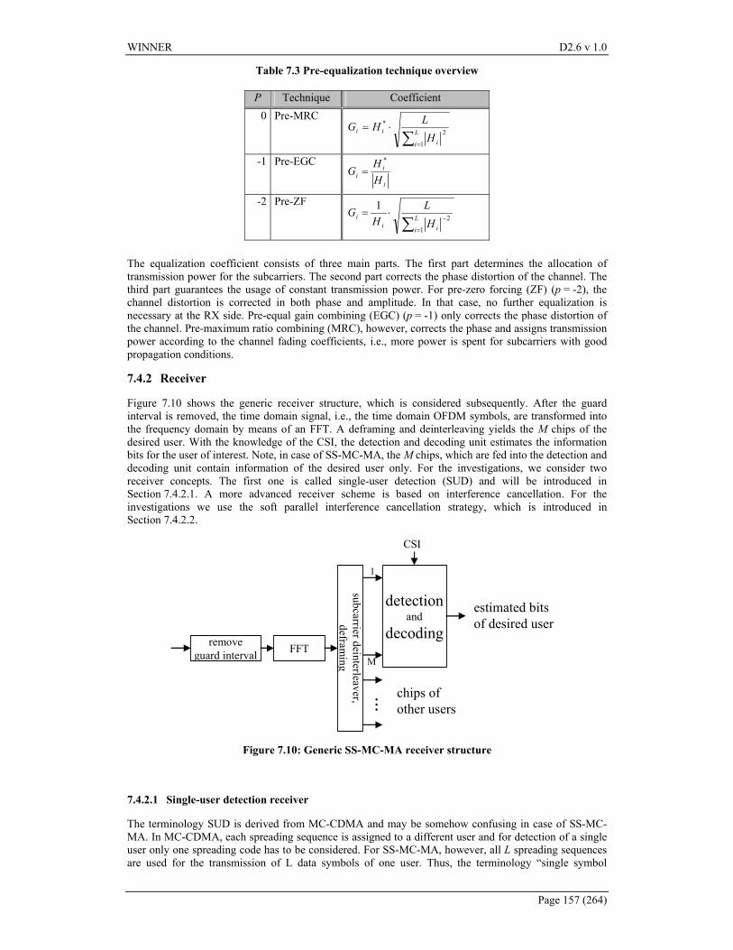
WINNER D2.6 v 1.0

Page 157 (264)

Table 7.3 Pre-equalization technique overview

P Technique Coefficient 0 Pre-MRC

∑ =

⋅= L

i i

iiH

LHG1

2*

-1 Pre-EGC

i

ii H

HG

*

=

-2 Pre-ZF

∑ =

−⋅= L

i iii

HL

HG

1

2

1

The equalization coefficient consists of three main parts. The first part determines the allocation of transmission power for the subcarriers. The second part corrects the phase distortion of the channel. The third part guarantees the usage of constant transmission power. For pre-zero forcing (ZF) (p = -2), the channel distortion is corrected in both phase and amplitude. In that case, no further equalization is necessary at the RX side. Pre-equal gain combining (EGC) (p = -1) only corrects the phase distortion of the channel. Pre-maximum ratio combining (MRC), however, corrects the phase and assigns transmission power according to the channel fading coefficients, i.e., more power is spent for subcarriers with good propagation conditions.

7.4.2 Receiver

Figure 7.10 shows the generic receiver structure, which is considered subsequently. After the guard interval is removed, the time domain signal, i.e., the time domain OFDM symbols, are transformed into the frequency domain by means of an FFT. A deframing and deinterleaving yields the M chips of the desired user. With the knowledge of the CSI, the detection and decoding unit estimates the information bits for the user of interest. Note, in case of SS-MC-MA, the M chips, which are fed into the detection and decoding unit contain information of the desired user only. For the investigations, we consider two receiver concepts. The first one is called single-user detection (SUD) and will be introduced in Section 7.4.2.1. A more advanced receiver scheme is based on interference cancellation. For the investigations we use the soft parallel interference cancellation strategy, which is introduced in Section 7.4.2.2.

detectionand

decoding

subcarrierdeinterleaver,defram

ing

removeguard interval FFT

CSI

1

M

chips ofother users

...

estimated bitsof desired user

Figure 7.10: Generic SS-MC-MA receiver structure

7.4.2.1 Single-user detection receiver

The terminology SUD is derived from MC-CDMA and may be somehow confusing in case of SS-MC-MA. In MC-CDMA, each spreading sequence is assigned to a different user and for detection of a single user only one spreading code has to be considered. For SS-MC-MA, however, all L spreading sequences are used for the transmission of L data symbols of one user. Thus, the terminology “single symbol

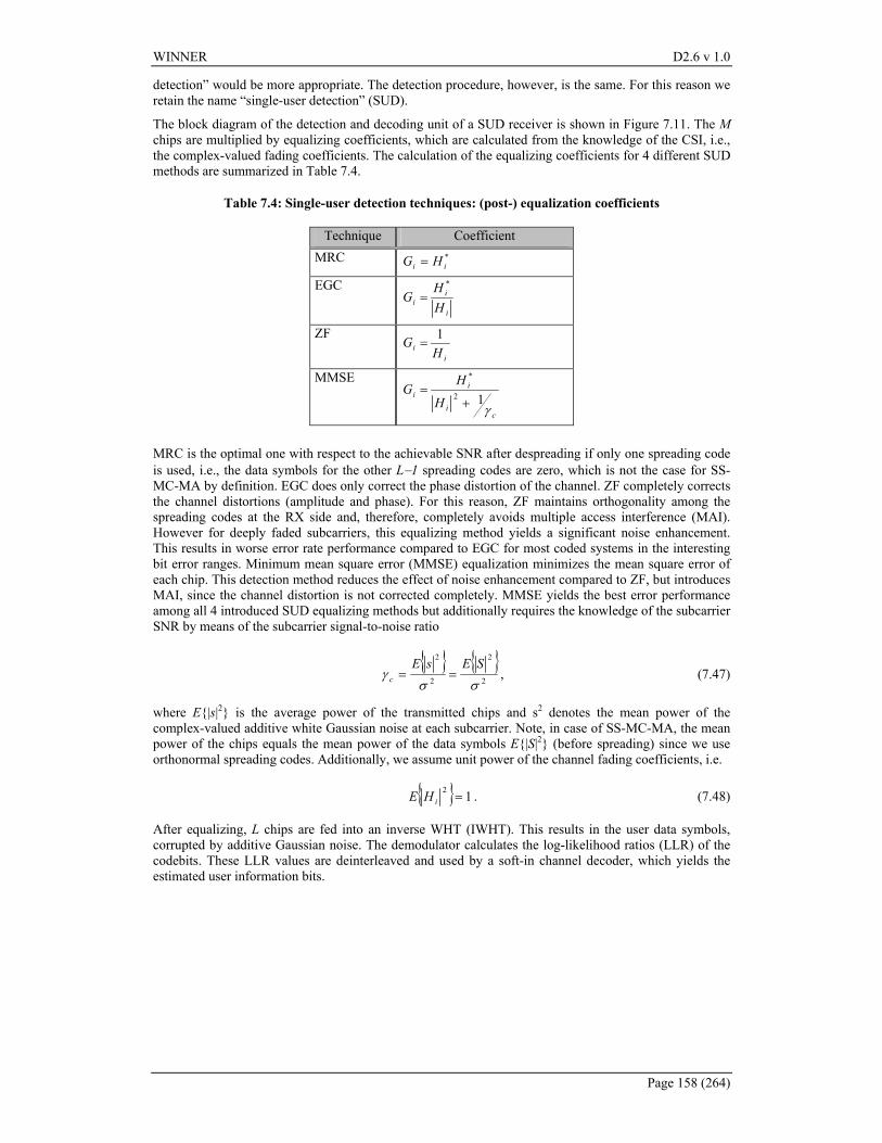
WINNER D2.6 v 1.0

Page 158 (264)

detection” would be more appropriate. The detection procedure, however, is the same. For this reason we retain the name “single-user detection” (SUD).

The block diagram of the detection and decoding unit of a SUD receiver is shown in Figure 7.11. The M chips are multiplied by equalizing coefficients, which are calculated from the knowledge of the CSI, i.e., the complex-valued fading coefficients. The calculation of the equalizing coefficients for 4 different SUD methods are summarized in Table 7.4.

Table 7.4: Single-user detection techniques: (post-) equalization coefficients

Technique Coefficient MRC *

ii HG =

EGC

i

ii H

HG

*

=

ZF

ii H

G 1=

MMSE

ci

ii

H

HG

γ12

*

+=

MRC is the optimal one with respect to the achievable SNR after despreading if only one spreading code is used, i.e., the data symbols for the other L−1 spreading codes are zero, which is not the case for SS-MC-MA by definition. EGC does only correct the phase distortion of the channel. ZF completely corrects the channel distortions (amplitude and phase). For this reason, ZF maintains orthogonality among the spreading codes at the RX side and, therefore, completely avoids multiple access interference (MAI). However for deeply faded subcarriers, this equalizing method yields a significant noise enhancement. This results in worse error rate performance compared to EGC for most coded systems in the interesting bit error ranges. Minimum mean square error (MMSE) equalization minimizes the mean square error of each chip. This detection method reduces the effect of noise enhancement compared to ZF, but introduces MAI, since the channel distortion is not corrected completely. MMSE yields the best error performance among all 4 introduced SUD equalizing methods but additionally requires the knowledge of the subcarrier SNR by means of the subcarrier signal-to-noise ratio

{ } { }

2

2

2

2

σσγ

SEsEc == , (7.47)

where E{|s|2} is the average power of the transmitted chips and s2 denotes the mean power of the complex-valued additive white Gaussian noise at each subcarrier. Note, in case of SS-MC-MA, the mean power of the chips equals the mean power of the data symbols E{|S|2} (before spreading) since we use orthonormal spreading codes. Additionally, we assume unit power of the channel fading coefficients, i.e.

{ } 12=iHE . (7.48)

After equalizing, L chips are fed into an inverse WHT (IWHT). This results in the user data symbols, corrupted by additive Gaussian noise. The demodulator calculates the log-likelihood ratios (LLR) of the codebits. These LLR values are deinterleaved and used by a soft-in channel decoder, which yields the estimated user information bits.

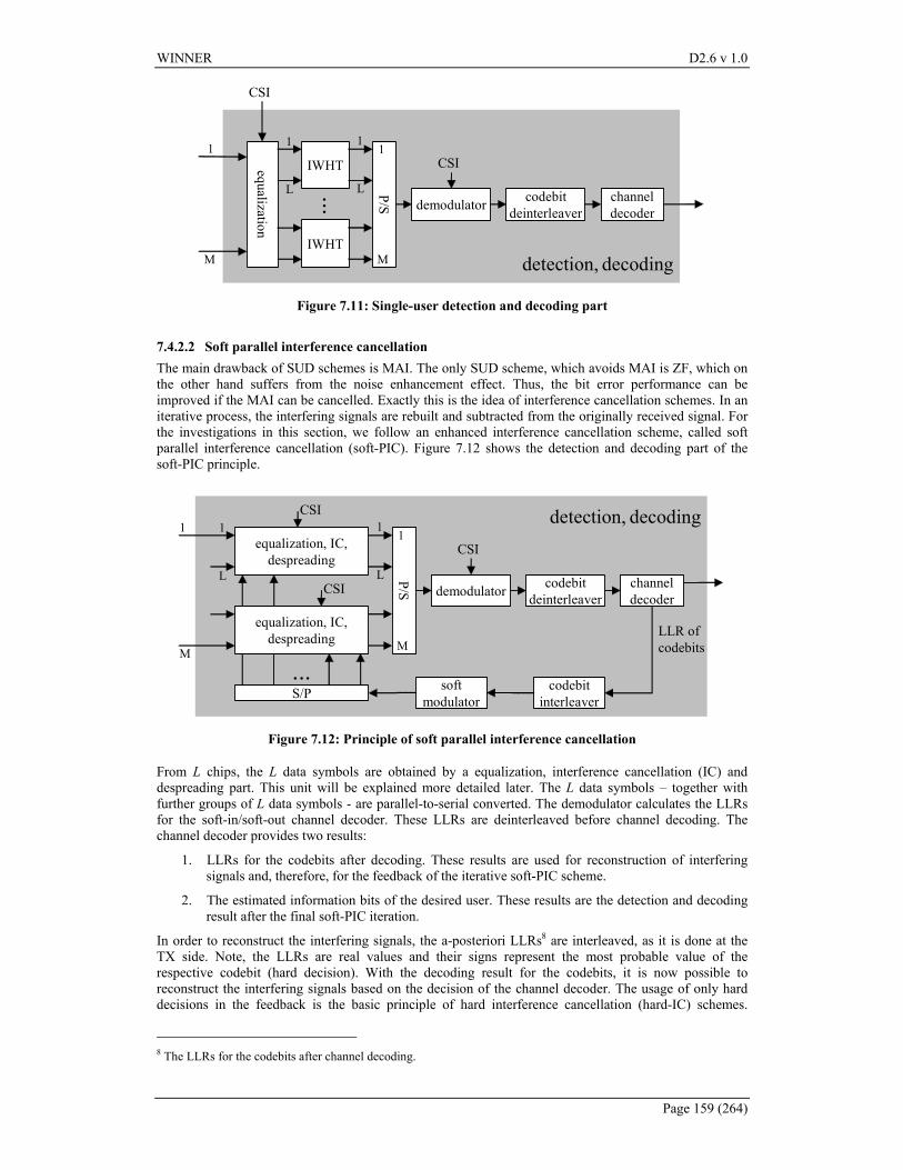
WINNER D2.6 v 1.0

Page 159 (264)

channeldecoder

codebitdeinterleaverdemodulator

P/S

1

M

IWHTequalization

IWHT

1

L

1

L...

CSI

1

M

CSI

detection, decoding

Figure 7.11: Single-user detection and decoding part

7.4.2.2 Soft parallel interference cancellation The main drawback of SUD schemes is MAI. The only SUD scheme, which avoids MAI is ZF, which on the other hand suffers from the noise enhancement effect. Thus, the bit error performance can be improved if the MAI can be cancelled. Exactly this is the idea of interference cancellation schemes. In an iterative process, the interfering signals are rebuilt and subtracted from the originally received signal. For the investigations in this section, we follow an enhanced interference cancellation scheme, called soft parallel interference cancellation (soft-PIC). Figure 7.12 shows the detection and decoding part of the soft-PIC principle.

channeldecoder

codebitdeinterleaverdemodulator

P/S

1

M

equalization, IC,despreading

1

L

1

L

1

M

CSI

detection, decoding

codebitinterleaver

softmodulatorS/P

...

equalization, IC,despreading LLR of

codebits

CSI

CSI

Figure 7.12: Principle of soft parallel interference cancellation

From L chips, the L data symbols are obtained by a equalization, interference cancellation (IC) and despreading part. This unit will be explained more detailed later. The L data symbols – together with further groups of L data symbols - are parallel-to-serial converted. The demodulator calculates the LLRs for the soft-in/soft-out channel decoder. These LLRs are deinterleaved before channel decoding. The channel decoder provides two results:

1. LLRs for the codebits after decoding. These results are used for reconstruction of interfering signals and, therefore, for the feedback of the iterative soft-PIC scheme.

2. The estimated information bits of the desired user. These results are the detection and decoding result after the final soft-PIC iteration.

In order to reconstruct the interfering signals, the a-posteriori LLRs8 are interleaved, as it is done at the TX side. Note, the LLRs are real values and their signs represent the most probable value of the respective codebit (hard decision). With the decoding result for the codebits, it is now possible to reconstruct the interfering signals based on the decision of the channel decoder. The usage of only hard decisions in the feedback is the basic principle of hard interference cancellation (hard-IC) schemes.

8 The LLRs for the codebits after channel decoding.

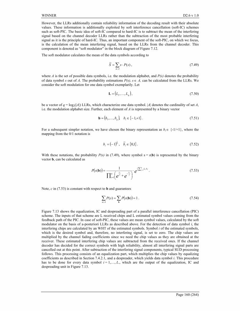
WINNER D2.6 v 1.0

Page 160 (264)

However, the LLRs additionally contain reliability information of the decoding result with their absolute values. These information is additionally exploited by soft interference cancellation (soft-IC) schemes such as soft-PIC. The basic idea of soft-IC compared to hard-IC is to subtract the mean of the interfering signal based on the channel decoder LLRs rather than the subtraction of the most probable interfering signal as it is the principle of hard-IC. Thus, an important component of the soft-PIC, on which we focus, is the calculation of the mean interfering signal, based on the LLRs from the channel decoder. This component is denoted as “soft modulator” in the block diagram of Figure 7.12.

The soft modulator calculates the mean of the data symbols according to

∑∈

⋅=As

sPsS )(~ , (7.49)

where A is the set of possible data symbols, i.e. the modulation alphabet, and P(s) denotes the probability of data symbol s out of A. The probability estimations P(s), s ∈ A, can be calculated from the LLRs. We consider the soft modulation for one data symbol exemplarily. Let

( )qLL ,,1 K=L , (7.50)

be a vector of q = log2(|A|) LLRs, which characterize one data symbol. |A| denotes the cardinality of set A, i.e. the modulation alphabet size. Further, each element of A is represented by a binary vector

( ) { }1,1,,,1 +−∈= iq bbb Kb . (7.51)

For a subsequent simpler notation, we have chosen the binary representation as bi ∈ {-1/+1}, where the mapping from the 0/1 notation is

( ) { }1,0~

,1~

∈−= ib

i bb i . (7.52)

With these notations, the probability P(s) in (7.49), where symbol s = s(b) is represented by the binary vector b, can be calculated as

( ) eee

qi ii

iLiL

bL

q

i

sP ∑⋅

+

= =⋅

=

−∏12

1

221

1)(b . (7.53)

Note, c in (7.53) is constant with respect to b and guarantees

( ) 1)()( == ∑∑∈ b

bsPsPAs

. (7.54)

Figure 7.13 shows the equalization, IC and despreading part of a parallel interference cancellation (PIC) scheme. The inputs of that scheme are L received chips and L estimated symbol values coming from the feedback path of the PIC. In case of soft-PIC, these values are mean symbol values, calculated by the soft modulator on the basis of a-posteriori LLRs as described above. For the detection of data symbol i, the interfering chips are calculated by an WHT of the estimated symbols. Symbol i of the estimated symbols, which is the desired symbol and, therefore, no interfering signal, is set to zero. The chip values are multiplied by the channel fading coefficients since we need the chip values as they are obtained at the receiver. These estimated interfering chip values are subtracted from the received ones. If the channel decoder has decided for the correct symbols with high reliability, almost all interfering signal parts are cancelled out at this point. After subtraction of the interfering signal components, typical SUD processing follows. This processing consists of an equalization part, which multiplies the chip values by equalizing coefficients as described in Section 7.4.2.1, and a despreader, which yields data symbol i. This procedure has to be done for every data symbol i = 1,…, L., which are the output of the equalization, IC and despreading unit in Figure 7.13.

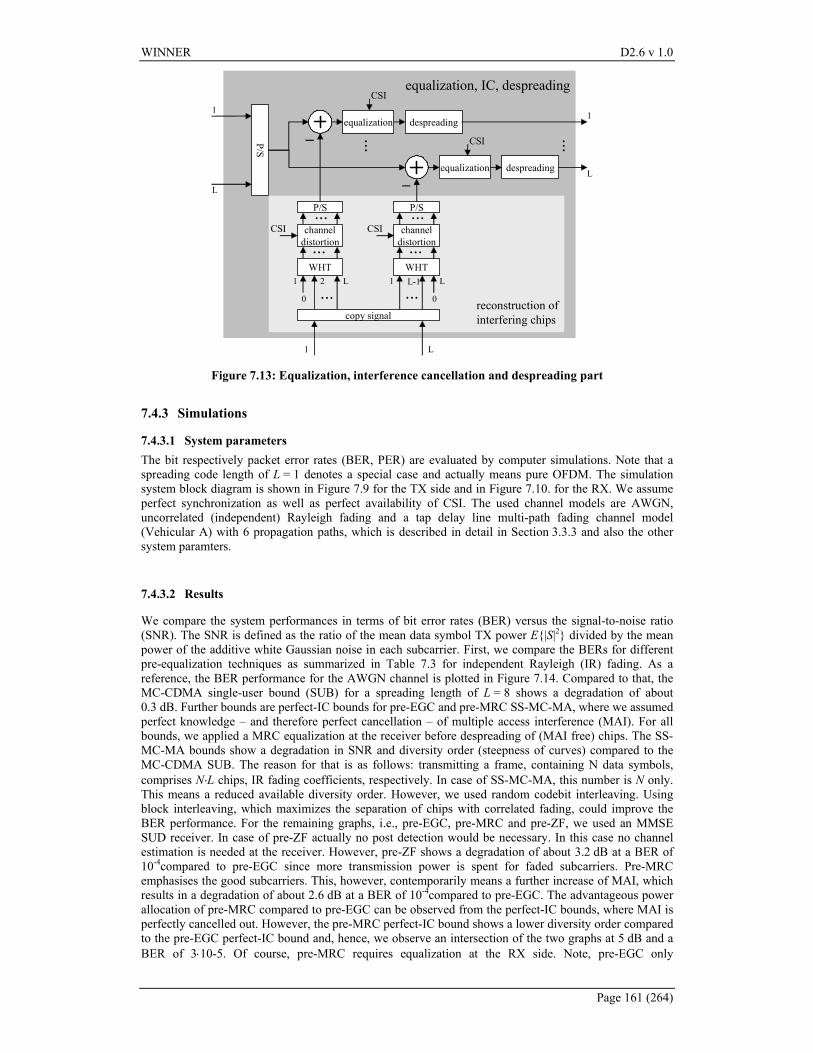
WINNER D2.6 v 1.0

Page 161 (264)

_

_P/S

1

L

despreadingequalization

WHT

channeldistortion

P/S

1 2 L

0

CSI

1 L-1 L

0

copy signal

1 L

... ...

...

...

WHT

channeldistortion

P/S

CSI

...

...

despreadingequalization

......

reconstruction ofinterfering chips

CSI

CSI

1

L

equalization, IC, despreading

Figure 7.13: Equalization, interference cancellation and despreading part

7.4.3 Simulations

7.4.3.1 System parameters The bit respectively packet error rates (BER, PER) are evaluated by computer simulations. Note that a spreading code length of L = 1 denotes a special case and actually means pure OFDM. The simulation system block diagram is shown in Figure 7.9 for the TX side and in Figure 7.10. for the RX. We assume perfect synchronization as well as perfect availability of CSI. The used channel models are AWGN, uncorrelated (independent) Rayleigh fading and a tap delay line multi-path fading channel model (Vehicular A) with 6 propagation paths, which is described in detail in Section 3.3.3 and also the other system paramters.

7.4.3.2 Results

We compare the system performances in terms of bit error rates (BER) versus the signal-to-noise ratio (SNR). The SNR is defined as the ratio of the mean data symbol TX power E{|S|2} divided by the mean power of the additive white Gaussian noise in each subcarrier. First, we compare the BERs for different pre-equalization techniques as summarized in Table 7.3 for independent Rayleigh (IR) fading. As a reference, the BER performance for the AWGN channel is plotted in Figure 7.14. Compared to that, the MC-CDMA single-user bound (SUB) for a spreading length of L = 8 shows a degradation of about 0.3 dB. Further bounds are perfect-IC bounds for pre-EGC and pre-MRC SS-MC-MA, where we assumed perfect knowledge – and therefore perfect cancellation – of multiple access interference (MAI). For all bounds, we applied a MRC equalization at the receiver before despreading of (MAI free) chips. The SS-MC-MA bounds show a degradation in SNR and diversity order (steepness of curves) compared to the MC-CDMA SUB. The reason for that is as follows: transmitting a frame, containing N data symbols, comprises N⋅L chips, IR fading coefficients, respectively. In case of SS-MC-MA, this number is N only. This means a reduced available diversity order. However, we used random codebit interleaving. Using block interleaving, which maximizes the separation of chips with correlated fading, could improve the BER performance. For the remaining graphs, i.e., pre-EGC, pre-MRC and pre-ZF, we used an MMSE SUD receiver. In case of pre-ZF actually no post detection would be necessary. In this case no channel estimation is needed at the receiver. However, pre-ZF shows a degradation of about 3.2 dB at a BER of 10-4compared to pre-EGC since more transmission power is spent for faded subcarriers. Pre-MRC emphasises the good subcarriers. This, however, contemporarily means a further increase of MAI, which results in a degradation of about 2.6 dB at a BER of 10-4compared to pre-EGC. The advantageous power allocation of pre-MRC compared to pre-EGC can be observed from the perfect-IC bounds, where MAI is perfectly cancelled out. However, the pre-MRC perfect-IC bound shows a lower diversity order compared to the pre-EGC perfect-IC bound and, hence, we observe an intersection of the two graphs at 5 dB and a BER of 3⋅10-5. Of course, pre-MRC requires equalization at the RX side. Note, pre-EGC only

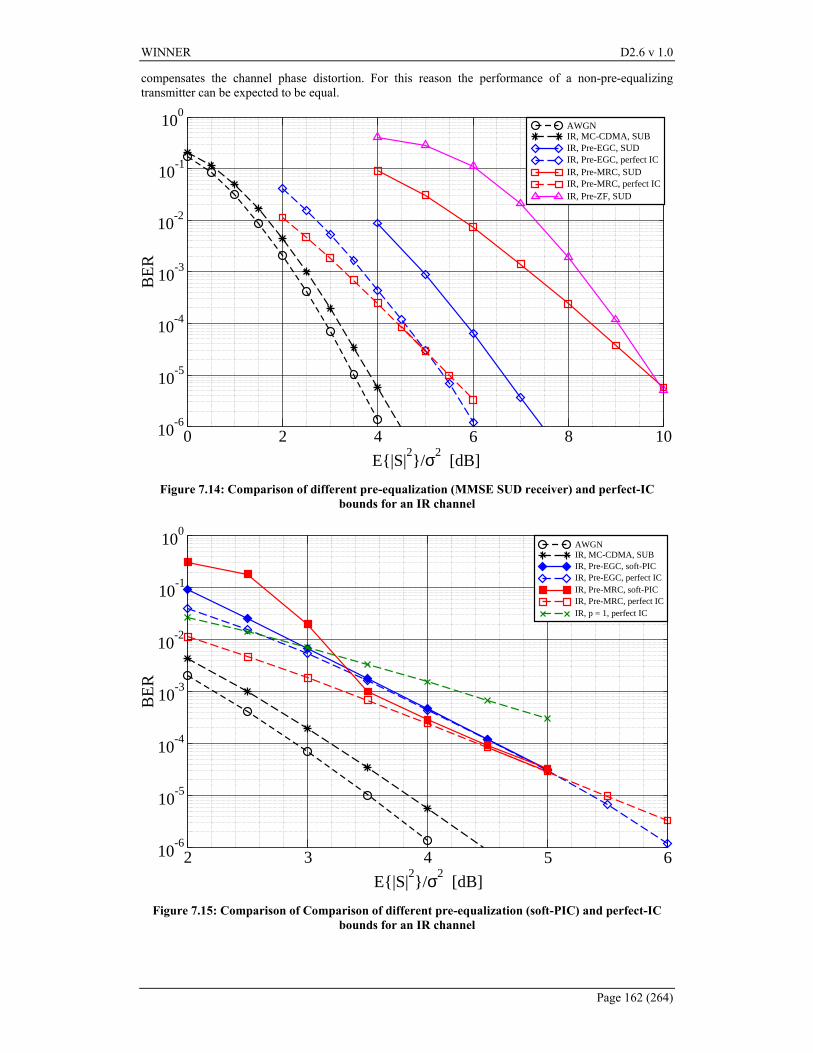
WINNER D2.6 v 1.0

Page 162 (264)

compensates the channel phase distortion. For this reason the performance of a non-pre-equalizing transmitter can be expected to be equal.

0 2 4 6 8 10

E{|S|2}/σ2

[dB]

10-6

10-5

10-4

10-3

10-2

10-1

100

BE

R

AWGNIR, MC-CDMA, SUBIR, Pre-EGC, SUDIR, Pre-EGC, perfect ICIR, Pre-MRC, SUDIR, Pre-MRC, perfect ICIR, Pre-ZF, SUD

Figure 7.14: Comparison of different pre-equalization (MMSE SUD receiver) and perfect-IC bounds for an IR channel

2 3 4 5 6

E{|S|2}/σ2

[dB]

10-6

10-5

10-4

10-3

10-2

10-1

100

BE

R

AWGNIR, MC-CDMA, SUBIR, Pre-EGC, soft-PICIR, Pre-EGC, perfect ICIR, Pre-MRC, soft-PICIR, Pre-MRC, perfect ICIR, p = 1, perfect IC

Figure 7.15: Comparison of Comparison of different pre-equalization (soft-PIC) and perfect-IC bounds for an IR channel

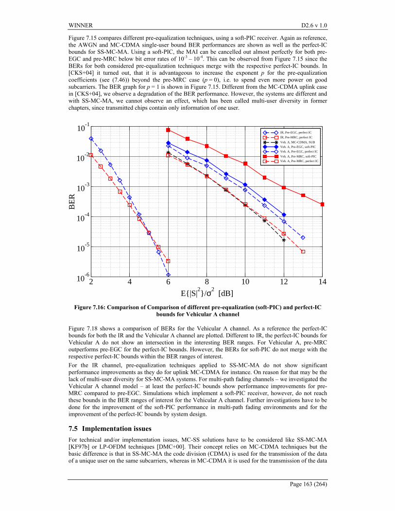
WINNER D2.6 v 1.0

Page 163 (264)

Figure 7.15 compares different pre-equalization techniques, using a soft-PIC receiver. Again as reference, the AWGN and MC-CDMA single-user bound BER performances are shown as well as the perfect-IC bounds for SS-MC-MA. Using a soft-PIC, the MAI can be cancelled out almost perfectly for both pre-EGC and pre-MRC below bit error rates of 10-3 – 10-4. This can be observed from Figure 7.15 since the BERs for both considered pre-equalization techniques merge with the respective perfect-IC bounds. In [CKS+04] it turned out, that it is advantageous to increase the exponent p for the pre-equalization coefficients (see (7.46)) beyond the pre-MRC case (p = 0), i.e. to spend even more power on good subcarriers. The BER graph for p = 1 is shown in Figure 7.15. Different from the MC-CDMA uplink case in [CKS+04], we observe a degradation of the BER performance. However, the systems are different and with SS-MC-MA, we cannot observe an effect, which has been called multi-user diversity in former chapters, since transmitted chips contain only information of one user.

2 4 6 8 10 12 14

E{|S|2}/σ2

[dB]

10-6

10-5

10-4

10-3

10-2

10-1

BE

R

IR, Pre-EGC, perfect IC

IR, Pre-MRC, perfect IC

Veh. A, MC-CDMA, SUB

Veh. A, Pre-EGC, soft-PIC

Veh. A, Pre-EGC, perfect IC

Veh. A, Pre-MRC, soft-PIC

Veh. A, Pre-MRC, perfect IC

Figure 7.16: Comparison of Comparison of different pre-equalization (soft-PIC) and perfect-IC bounds for Vehicular A channel

Figure 7.18 shows a comparison of BERs for the Vehicular A channel. As a reference the perfect-IC bounds for both the IR and the Vehicular A channel are plotted. Different to IR, the perfect-IC bounds for Vehicular A do not show an intersection in the interesting BER ranges. For Vehicular A, pre-MRC outperforms pre-EGC for the perfect-IC bounds. However, the BERs for soft-PIC do not merge with the respective perfect-IC bounds within the BER ranges of interest. For the IR channel, pre-equalization techniques applied to SS-MC-MA do not show significant performance improvements as they do for uplink MC-CDMA for instance. On reason for that may be the lack of multi-user diversity for SS-MC-MA systems. For multi-path fading channels – we investigated the Vehicular A channel model – at least the perfect-IC bounds show performance improvements for pre-MRC compared to pre-EGC. Simulations which implement a soft-PIC receiver, however, do not reach these bounds in the BER ranges of interest for the Vehicular A channel. Further investigations have to be done for the improvement of the soft-PIC performance in multi-path fading environments and for the improvement of the perfect-IC bounds by system design.

7.5 Implementation issues For technical and/or implementation issues, MC-SS solutions have to be considered like SS-MC-MA [KF97b] or LP-OFDM techniques [DMC+00]. Their concept relies on MC-CDMA techniques but the basic difference is that in SS-MC-MA the code division (CDMA) is used for the transmission of the data of a unique user on the same subcarriers, whereas in MC-CDMA it is used for the transmission of the data

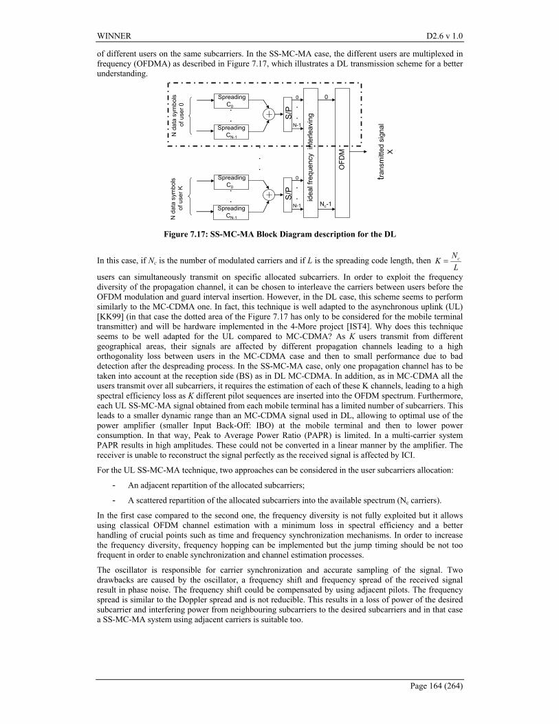
WINNER D2.6 v 1.0

Page 164 (264)

of different users on the same subcarriers. In the SS-MC-MA case, the different users are multiplexed in frequency (OFDMA) as described in Figure 7.17, which illustrates a DL transmission scheme for a better understanding.

N d

ata

sym

bols

of

use

r 0

SpreadingC0

SpreadingCN-1

S/P

0

N-1

.

...

SpreadingC0

SpreadingCN-1

S/P

0

N-1

.

...

N d

ata

sym

bols

of

use

r K

.

.

.

0

Nc-1

idea

l fre

quen

cy i

nter

leav

ing

OFD

M

trans

mitt

ed s

igna

lX

Figure 7.17: SS-MC-MA Block Diagram description for the DL

In this case, if Nc is the number of modulated carriers and if L is the spreading code length, then LNK c=

users can simultaneously transmit on specific allocated subcarriers. In order to exploit the frequency diversity of the propagation channel, it can be chosen to interleave the carriers between users before the OFDM modulation and guard interval insertion. However, in the DL case, this scheme seems to perform similarly to the MC-CDMA one. In fact, this technique is well adapted to the asynchronous uplink (UL) [KK99] (in that case the dotted area of the Figure 7.17 has only to be considered for the mobile terminal transmitter) and will be hardware implemented in the 4-More project [IST4]. Why does this technique seems to be well adapted for the UL compared to MC-CDMA? As K users transmit from different geographical areas, their signals are affected by different propagation channels leading to a high orthogonality loss between users in the MC-CDMA case and then to small performance due to bad detection after the despreading process. In the SS-MC-MA case, only one propagation channel has to be taken into account at the reception side (BS) as in DL MC-CDMA. In addition, as in MC-CDMA all the users transmit over all subcarriers, it requires the estimation of each of these K channels, leading to a high spectral efficiency loss as K different pilot sequences are inserted into the OFDM spectrum. Furthermore, each UL SS-MC-MA signal obtained from each mobile terminal has a limited number of subcarriers. This leads to a smaller dynamic range than an MC-CDMA signal used in DL, allowing to optimal use of the power amplifier (smaller Input Back-Off: IBO) at the mobile terminal and then to lower power consumption. In that way, Peak to Average Power Ratio (PAPR) is limited. In a multi-carrier system PAPR results in high amplitudes. These could not be converted in a linear manner by the amplifier. The receiver is unable to reconstruct the signal perfectly as the received signal is affected by ICI.

For the UL SS-MC-MA technique, two approaches can be considered in the user subcarriers allocation:

- An adjacent repartition of the allocated subcarriers;

- A scattered repartition of the allocated subcarriers into the available spectrum (Nc carriers).

In the first case compared to the second one, the frequency diversity is not fully exploited but it allows using classical OFDM channel estimation with a minimum loss in spectral efficiency and a better handling of crucial points such as time and frequency synchronization mechanisms. In order to increase the frequency diversity, frequency hopping can be implemented but the jump timing should be not too frequent in order to enable synchronization and channel estimation processes.

The oscillator is responsible for carrier synchronization and accurate sampling of the signal. Two drawbacks are caused by the oscillator, a frequency shift and frequency spread of the received signal result in phase noise. The frequency shift could be compensated by using adjacent pilots. The frequency spread is similar to the Doppler spread and is not reducible. This results in a loss of power of the desired subcarrier and interfering power from neighbouring subcarriers to the desired subcarriers and in that case a SS-MC-MA system using adjacent carriers is suitable too.

WINNER D2.6 v 1.0

Page 165 (264)

7.6 Flexible and adaptive resource allocation According to Shannon’s waterfilling theorem, the capacity of a frequency-selective channel is maximized if most of the power is spent over the good part of the channel [Pro95]. A great number of practical single-user bit and power loading algorithms based on Shannon’s approach has been designed in the last 15 years [BFB02], [ChCB95], [FH96a], [KRJ00]. Typically these algorithms adjust modulation format and transmitter gain in order to achieve some target quality measure at the receiver.

The main difference in a multi-user scenarios with respect to the single-user case is the need to control not only modulation formats and transmitter gains, but also the channel sharing among users. Depending on the adopted multiple access method, e.g., FDMA, CDMA, TDMA, in order to optimise the channel sharing cases it may be necessary to optimise the assignment of the users to subcarriers, spreading sequences, time slots, etc.

Section 7.6.1 presents the system model, introduces the notation used and provides a brief overview of the multi-carrier spread-spectrum multiple-access schemes considered in this section. Section 7.6.2 gives an overview of some adaptive techniques for multi-user systems. In Section 7.6.3 some novel methods for optimisation of subcarrier allocation, bit and power loading in multi-carrier spread-spectrum systems are proposed. Finally, simulation results are discussed in Section 7.6.4.

7.6.1 System model and used notation

Let us model the OFDM multi-carrier downlink transmission in frequency domain. The signal received by user k over subcarrier i for the jth OFDM symbol can be expressed as

,..1,..1,)()()( NiKksr jki

jiki

jki ==+= ηµ (7.55)

where K is the number of active users and N is the total number of subcarriers, si is the signal transmitted by the base station over the ith subcarrier in the jth OFDM symbol period, kiµ is the subcarrier channel

transfer factor and )( jkiη represents additive white Gaussian noise (AWGN) with variance 2σ . It is also

helpful to introduce the subcarrier channel-to-noise ratio defined as

,||

2

2

σµ

ξ kiki = (7.56)

7.6.1.1 Orthogonal frequency division multiple access

In an OFDMA system each subcarrier is exclusively assigned to one user. Hence the signal transmitted by the base station over subcarrier i is given by

,)()( jii

ji yVs = (7.57)

where )( jiy indicates the modulated symbol produced by the user k(i) assigned to the ith subcarrier and Vi

denotes the transmitter gain for ith subcarrier. yi is assumed to be selected from a ic2 -QAM constellation. By letting ci=0 for some i data transmission over subcarrier i is disabled. Hence the total data rate of the kth user is given by

∑=

=kiki

ik cR)(:

(7.58)

7.6.1.2 Multi-carrier spread-spectrum multiple access

As illustrated in the introduction of Section 7.1, there are different ways of combining spread-spectrum and multi-carrier technologies. Here we consider MC-CDMA and MC-DS-CDMA. Traditionally, the transmitter gain is assumed to be the same for all users [YH03]. However, since link adaptation may require adjusting it, here we extend standard definitions of MC-CDMA and MC-DS-CDMA to take into account adjustable gains for different users.

WINNER D2.6 v 1.0

Page 166 (264)

7.6.1.3 Spreading in frequency domain or MC-CDMA

Consider an OFDM system with N subcarriers9. Let us assume that each user transmits P=N/Lf symbols per OFDM symbol, where Lf is the spreading factor in frequency direction. The set of N subcarriers is partitioned into P disjoint sub-sets, ,1, PpWp K= of size Lf and each sub-set is used for transmission of a CDMA signal given by

PpLsayVs f

K

kks

jkpkp

jwps

KK 1,10,1

)()( =−== ∑=

(7.59)

where wps is the sth subcarrier in the pth sub-set Wp, aks is the sth chip of the spreading sequence ),...,( 1,0 −=

fLkkk aaa utilized by the kth user, )( jkpy is the pth symbol transmitted by user k in the OFDM

symbol period j, and Vkp is the corresponding gain factor. Assuming that the spreading sequences are perfectly orthogonal, the maximal number of users supported by such a system is equal to K=Lf. Since it may be impracticable to utilize long spreading sequences, given the large transmission bandwidths envisaged for the WINNER air interface, a number Q of MC-CDMA systems may be accommodated within the set of available subcarriers. This approach is denoted in the sequel by MC-CDMA/FDMA. In this case the total number of subcarrier must satisfy N=PQLf.

7.6.1.4 Spreading in time domain or MC-DS-CDMA

Consider a multi-carrier system with N subcarriers. Let us assume that each user transmits modulated symbols over all subcarriers within one OFDM symbol period, and CDMA is used for user separation. Then the signal transmitted over each subcarrier is given by

,0,1

1)()( ∑

=−

+ ==K

ktks

jkiki

sjLi LsayVs t K (7.60)

where ),...,( 1,0 −=tLkkk aaa is the spreading sequence used by user k and Lt is the spreading factor in time

direction. If each user uses exactly one spreading sequence, the total number of users is limited by the number of orthogonal spreading sequences Lt, and each user can simultaneously transmit N symbols. However, if each subcarrier is associated with a pool of Lt orthogonal spreading sequences, then it can be considered as a set of Lt sub-channels. These sub-channels can be arbitrarily distributed among at most LtN users.

7.6.1.5 Spreading in time and frequency or MC-TF-CDMA

The approaches described above can be combined10, i.e., spreading can be performed both in time and frequency, yielding the transmitted signal

,1,10,10,1

,)()( PpLiLsayVs ft

K

ksiLk

jkpkp

sjLw t

tpi

KKK =−=−== ∑=

++ (7.61)

where ),...,( 1,0 −=tf LLkkk aaa is the spreading sequence used by user k and wpi is the ith subcarrier in the

pth sub-set Wp. In this case the total number of users is limited by LtLf under the assumption of orthogonal spreading sequences. Notice that each sub-set Wp associated with LtLf orthogonal spreading sequences can be again considered as a set of LtLf sub-channels. Hence this system appears to be a generalized version of the one obtained by introducing an FDMA component (MC-CDMA/FDMA) as explained above. This system will be denoted by multi-carrier time-frequency CDMA (MC-TF-CDMA) in the following.

9Note that here N does not need to correspond to the total number of subcarriers. The construction described here may be applied to any sub-set of the whole set of subcarriers. 10In [YH03] this is also called MC-DS-CDMA, but this name seems to be misleading.

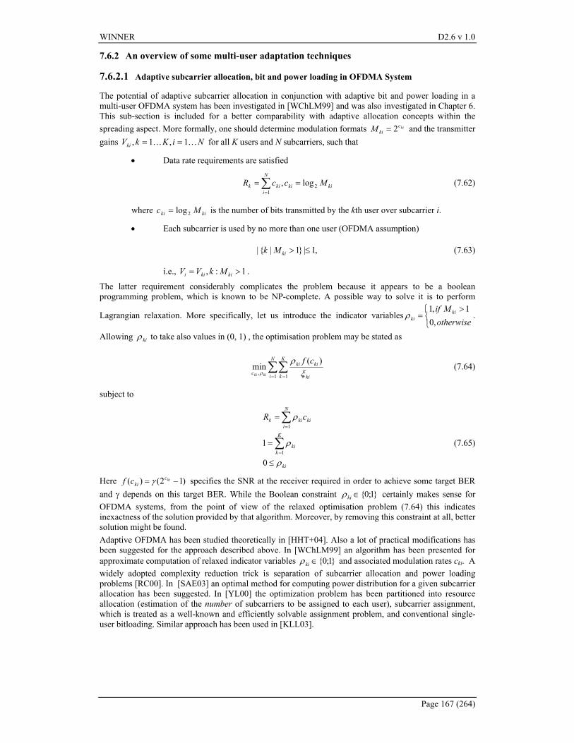
WINNER D2.6 v 1.0

Page 167 (264)

7.6.2 An overview of some multi-user adaptation techniques

7.6.2.1 Adaptive subcarrier allocation, bit and power loading in OFDMA System

The potential of adaptive subcarrier allocation in conjunction with adaptive bit and power loading in a multi-user OFDMA system has been investigated in [WChLM99] and was also investigated in Chapter 6. This sub-section is included for a better comparability with adaptive allocation concepts within the spreading aspect. More formally, one should determine modulation formats kic

kiM 2= and the transmitter gains NiKkVki KK 1,1, == for all K users and N subcarriers, such that

• Data rate requirements are satisfied

kiki

N

ikik MccR 2

1log, == ∑

=

(7.62)

where kiki Mc 2log= is the number of bits transmitted by the kth user over subcarrier i.

• Each subcarrier is used by no more than one user (OFDMA assumption)

,1|}1|{| ≤>kiMk (7.63)

i.e., 1:, >= kikii MkVV .

The latter requirement considerably complicates the problem because it appears to be a boolean programming problem, which is known to be NP-complete. A possible way to solve it is to perform

Lagrangian relaxation. More specifically, let us introduce the indicator variables >

=otherwise

Mif kiki ,0

1,1ρ .

Allowing kiρ to take also values in (0, 1) , the optimisation problem may be stated as

∑∑= =

N

i

K

k ki

kiki

c

cfkiki 1 1,

)(min

ξρ

ρ (7.64)

subject to

ki

K

kki

N

ikikik cR

ρ

ρ

ρ

≤

=

=

∑

∑

=

=

0

11

1

(7.65)

Here )12()( −= kickicf γ specifies the SNR at the receiver required in order to achieve some target BER

and γ depends on this target BER. While the Boolean constraint }1;0{∈kiρ certainly makes sense for OFDMA systems, from the point of view of the relaxed optimisation problem (7.64) this indicates inexactness of the solution provided by that algorithm. Moreover, by removing this constraint at all, better solution might be found. Adaptive OFDMA has been studied theoretically in [HHT+04]. Also a lot of practical modifications has been suggested for the approach described above. In [WChLM99] an algorithm has been presented for approximate computation of relaxed indicator variables }1;0{∈kiρ and associated modulation rates cki. A widely adopted complexity reduction trick is separation of subcarrier allocation and power loading problems [RC00]. In [SAE03] an optimal method for computing power distribution for a given subcarrier allocation has been suggested. In [YL00] the optimization problem has been partitioned into resource allocation (estimation of the number of subcarriers to be assigned to each user), subcarrier assignment, which is treated as a well-known and efficiently solvable assignment problem, and conventional single-user bitloading. Similar approach has been used in [KLL03].

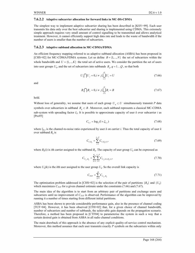
WINNER D2.6 v 1.0

Page 168 (264)

7.6.2.2 Adaptive subcarrier allocation for forward links in MC-DS-CDMA

The simplest way to implement adaptive subcarrier sharing has been described in [KSY+99]. Each user transmits his data only over the best subcarrier and sharing is implemented using CDMA. This extremely simple approach requires very small amount of control signalling to be transmitted and allows analytical treatment. However, it cannot efficiently support high data rate and leads to the waste of bandwidth if the number of users is smaller than the number of subcarriers.

7.6.2.3 Adaptive subband allocation in MC-CDMA/FDMA

An efficient frequency mapping referred to as adaptive subband allocation (ASBA) has been proposed in [CHS+02] for MC-CDMA/FDMA systems. Let us define },...,1{ NB = the set of subcarriers within the whole bandwidth and },...,1{ KU = the total set of active users. We consider the partition the set of users into user groups Uq, and the set of subcarriers into subbands QqBq K1, = , so that both

UIQ

iiji UUjiUU

1

;,0=

=≠= (7.66)

and

UIQ

iiji BBjiBB

1

;,0=

=≠= (7.67)

hold.

Without loss of generality, we assume that users of each group UU q ⊂ simultaneously transmit P data symbols over subcarriers in subband BBq ⊂ . Moreover, each subband represents a classical MC-CDMA sub-system with spreading factor Lf. It is possible to approximate capacity of user k over subcarrier i as [Pro95]

)1(log ,2, ikikC ξ+= (7.68)

where ξk,i is the channel-to-noise ratio experienced by user k on carrier i. Thus the total capacity of user k over subband Bq is

,1

)(,, ∑=

=PL

iiBkBk

f

qqCC (7.69)

where Bq(i) is ith carrier assigned to the subband Bq. The capacity of user group Uq can be expressed as

∑∑= =

=q f

qqqq

K

k

PL

iiBkUBU CC

1 1)(),(, , (7.70)

where Uq(k) is the kth user assigned to the user group Uq. So the overall link capacity is

∑=

=Q

qBUTOT qq

CC1

, (7.71)

The optimisation problem addressed in [CHS+02] is the selection of the pair of partitions {Bq} and {Uq} which maximizes CTOT for a given channel estimate under the constraints (7.66) and (7.67).

The main idea of the algorithm is to start from an arbitrary pair of partitions and exchange users and subcarriers until no improvement of CTOT is observed. Performance of the algorithm can be improved by running it a number of times starting from different initial partitions.

ASBA has been shown to provide considerable performance gain, also in the presence of channel coding [TCF+04]. However, it has been observed [CFH+02] that, for a given choice of channel bandwidth, number of subcarriers and number of subbands, the achievable gain depends on the propagation scenario. Therefore, a method has been proposed in [CTF04] to parameterise the system in such a way that a certain desired gain is obtained from ASBA in all radio channel conditions.

The main drawback of this approach is the absence of any explicit quality-of-service control mechanism. Moreover, this method assumes that each user transmits exactly P symbols on the subcarriers within only

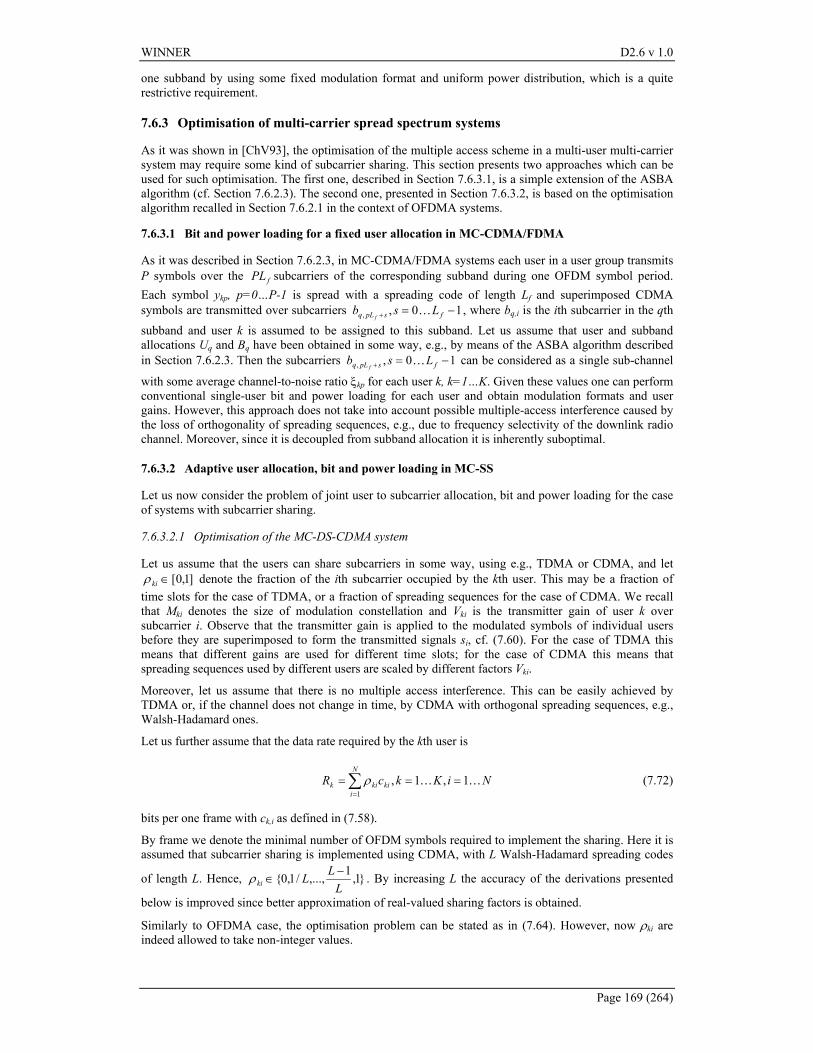
WINNER D2.6 v 1.0

Page 169 (264)

one subband by using some fixed modulation format and uniform power distribution, which is a quite restrictive requirement.

7.6.3 Optimisation of multi-carrier spread spectrum systems

As it was shown in [ChV93], the optimisation of the multiple access scheme in a multi-user multi-carrier system may require some kind of subcarrier sharing. This section presents two approaches which can be used for such optimisation. The first one, described in Section 7.6.3.1, is a simple extension of the ASBA algorithm (cf. Section 7.6.2.3). The second one, presented in Section 7.6.3.2, is based on the optimisation algorithm recalled in Section 7.6.2.1 in the context of OFDMA systems.

7.6.3.1 Bit and power loading for a fixed user allocation in MC-CDMA/FDMA

As it was described in Section 7.6.2.3, in MC-CDMA/FDMA systems each user in a user group transmits P symbols over the fPL subcarriers of the corresponding subband during one OFDM symbol period. Each symbol ykp, p=0…P-1 is spread with a spreading code of length Lf and superimposed CDMA symbols are transmitted over subcarriers 10,, −=+ fspLq Lsb

fK , where bq,i is the ith subcarrier in the qth

subband and user k is assumed to be assigned to this subband. Let us assume that user and subband allocations Uq and Bq have been obtained in some way, e.g., by means of the ASBA algorithm described in Section 7.6.2.3. Then the subcarriers 10,, −=+ fspLq Lsb

fK can be considered as a single sub-channel

with some average channel-to-noise ratio ξkp for each user k, k=1…K. Given these values one can perform conventional single-user bit and power loading for each user and obtain modulation formats and user gains. However, this approach does not take into account possible multiple-access interference caused by the loss of orthogonality of spreading sequences, e.g., due to frequency selectivity of the downlink radio channel. Moreover, since it is decoupled from subband allocation it is inherently suboptimal.

7.6.3.2 Adaptive user allocation, bit and power loading in MC-SS

Let us now consider the problem of joint user to subcarrier allocation, bit and power loading for the case of systems with subcarrier sharing.

7.6.3.2.1 Optimisation of the MC-DS-CDMA system

Let us assume that the users can share subcarriers in some way, using e.g., TDMA or CDMA, and let ]1,0[∈kiρ denote the fraction of the ith subcarrier occupied by the kth user. This may be a fraction of

time slots for the case of TDMA, or a fraction of spreading sequences for the case of CDMA. We recall that Mki denotes the size of modulation constellation and Vki is the transmitter gain of user k over subcarrier i. Observe that the transmitter gain is applied to the modulated symbols of individual users before they are superimposed to form the transmitted signals si, cf. (7.60). For the case of TDMA this means that different gains are used for different time slots; for the case of CDMA this means that spreading sequences used by different users are scaled by different factors Vki.

Moreover, let us assume that there is no multiple access interference. This can be easily achieved by TDMA or, if the channel does not change in time, by CDMA with orthogonal spreading sequences, e.g., Walsh-Hadamard ones.

Let us further assume that the data rate required by the kth user is

NiKkcRN

ikikik KK 1,1,

1=== ∑

=

ρ (7.72)

bits per one frame with ck,i as defined in (7.58).

By frame we denote the minimal number of OFDM symbols required to implement the sharing. Here it is assumed that subcarrier sharing is implemented using CDMA, with L Walsh-Hadamard spreading codes

of length L. Hence, }1,1,...,/1,0{L

LLki−

∈ρ . By increasing L the accuracy of the derivations presented

below is improved since better approximation of real-valued sharing factors is obtained.

Similarly to OFDMA case, the optimisation problem can be stated as in (7.64). However, now ρki are indeed allowed to take non-integer values.

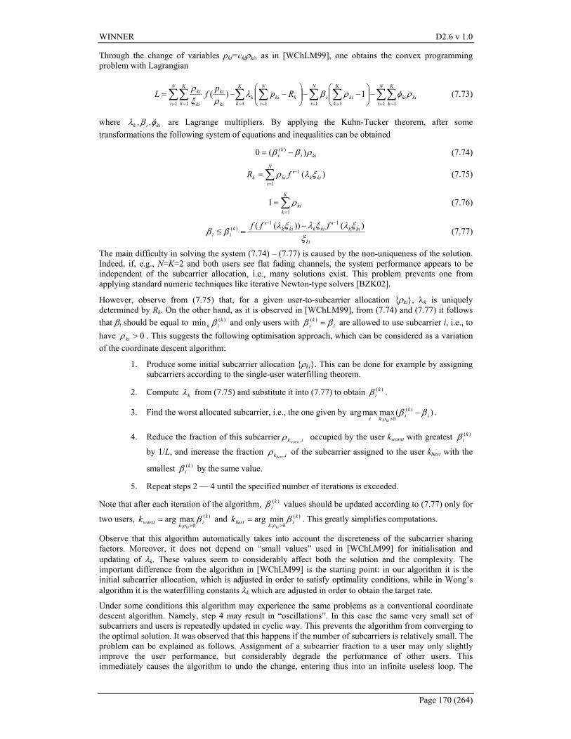
WINNER D2.6 v 1.0

Page 170 (264)

Through the change of variables pki=ckiρki, as in [WChLM99], one obtains the convex programming problem with Lagrangian

∑ ∑∑∑∑ ∑∑∑= = === == =

−

−−

−−=

N

i

N

i

K

kkiki

K

kkii

K

kk

N

ikik

N

i

K

k ki

ki

ki

ki Rpp

fL1 1 111 11 1

1)( ρφρβλρξ

ρ (7.73)

where kiik φβλ ,, are Lagrange multipliers. By applying the Kuhn-Tucker theorem, after some transformations the following system of equations and inequalities can be obtained

kiik

i ρββ )(0 )( −= (7.74)

∑=

−=N

ikikkik fR

1

1 )(' ξλρ (7.75)

∑=

=K

kki

11 ρ (7.76)

ki

kikkikkikkii

fffξ

ξλξλξλββ

)('))('( 11)(

−− −=≤ (7.77)

The main difficulty in solving the system (7.74) – (7.77) is caused by the non-uniqueness of the solution. Indeed, if, e.g., N=K=2 and both users see flat fading channels, the system performance appears to be independent of the subcarrier allocation, i.e., many solutions exist. This problem prevents one from applying standard numeric techniques like iterative Newton-type solvers [BZK02].

However, observe from (7.75) that, for a given user-to-subcarrier allocation {ρki}, λk is uniquely determined by Rk. On the other hand, as it is observed in [WChLM99], from (7.74) and (7.77) it follows that βi should be equal to )(min k

ik β and only users with ik

i ββ =)( are allowed to use subcarrier i, i.e., to have 0>kiρ . This suggests the following optimisation approach, which can be considered as a variation of the coordinate descent algorithm:

1. Produce some initial subcarrier allocation {ρki}. This can be done for example by assigning subcarriers according to the single-user waterfilling theorem.

2. Compute kλ from (7.75) and substitute it into (7.77) to obtain )(kiβ .

3. Find the worst allocated subcarrier, i.e., the one given by )(maxmaxarg )(

0: ik

iki ki

ββρ

−>

.

4. Reduce the fraction of this subcarrier ikworst ,ρ occupied by the user kworst with greatest )(kiβ

by 1/L, and increase the fraction ikbest ,ρ of the subcarrier assigned to the user kbest with the

smallest )(kiβ by the same value.

5. Repeat steps 2 — 4 until the specified number of iterations is exceeded.

Note that after each iteration of the algorithm, )(kiβ values should be updated according to (7.77) only for

two users, )(

0:maxarg k

ikworstki

k βρ >

= and )(

0:minarg k

ikbestki

k βρ >

= . This greatly simplifies computations.

Observe that this algorithm automatically takes into account the discreteness of the subcarrier sharing factors. Moreover, it does not depend on “small values” used in [WChLM99] for initialisation and updating of λk. These values seem to considerably affect both the solution and the complexity. The important difference from the algorithm in [WChLM99] is the starting point: in our algorithm it is the initial subcarrier allocation, which is adjusted in order to satisfy optimality conditions, while in Wong’s algorithm it is the waterfilling constants λk which are adjusted in order to obtain the target rate.

Under some conditions this algorithm may experience the same problems as a conventional coordinate descent algorithm. Namely, step 4 may result in “oscillations”. In this case the same very small set of subcarriers and users is repeatedly updated in cyclic way. This prevents the algorithm from converging to the optimal solution. It was observed that this happens if the number of subcarriers is relatively small. The problem can be explained as follows. Assignment of a subcarrier fraction to a user may only slightly improve the user performance, but considerably degrade the performance of other users. This immediately causes the algorithm to undo the change, entering thus into an infinite useless loop. The

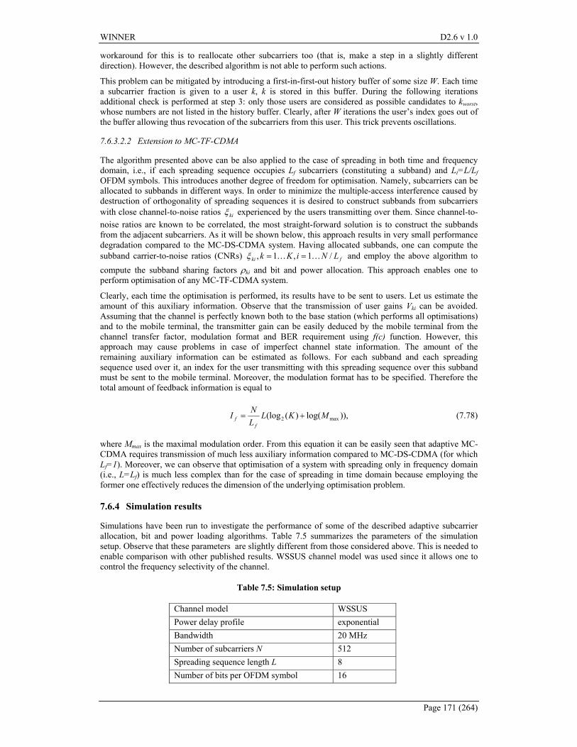
WINNER D2.6 v 1.0

Page 171 (264)

workaround for this is to reallocate other subcarriers too (that is, make a step in a slightly different direction). However, the described algorithm is not able to perform such actions.

This problem can be mitigated by introducing a first-in-first-out history buffer of some size W. Each time a subcarrier fraction is given to a user k, k is stored in this buffer. During the following iterations additional check is performed at step 3: only those users are considered as possible candidates to kworst, whose numbers are not listed in the history buffer. Clearly, after W iterations the user’s index goes out of the buffer allowing thus revocation of the subcarriers from this user. This trick prevents oscillations.

7.6.3.2.2 Extension to MC-TF-CDMA

The algorithm presented above can be also applied to the case of spreading in both time and frequency domain, i.e., if each spreading sequence occupies Lf subcarriers (constituting a subband) and Lt=L/Lf OFDM symbols. This introduces another degree of freedom for optimisation. Namely, subcarriers can be allocated to subbands in different ways. In order to minimize the multiple-access interference caused by destruction of orthogonality of spreading sequences it is desired to construct subbands from subcarriers with close channel-to-noise ratios kiξ experienced by the users transmitting over them. Since channel-to-noise ratios are known to be correlated, the most straight-forward solution is to construct the subbands from the adjacent subcarriers. As it will be shown below, this approach results in very small performance degradation compared to the MC-DS-CDMA system. Having allocated subbands, one can compute the subband carrier-to-noise ratios (CNRs) fki LNiKk /1,1, KK ==ξ and employ the above algorithm to compute the subband sharing factors ρki and bit and power allocation. This approach enables one to perform optimisation of any MC-TF-CDMA system.

Clearly, each time the optimisation is performed, its results have to be sent to users. Let us estimate the amount of this auxiliary information. Observe that the transmission of user gains Vki can be avoided. Assuming that the channel is perfectly known both to the base station (which performs all optimisations) and to the mobile terminal, the transmitter gain can be easily deduced by the mobile terminal from the channel transfer factor, modulation format and BER requirement using f(c) function. However, this approach may cause problems in case of imperfect channel state information. The amount of the remaining auxiliary information can be estimated as follows. For each subband and each spreading sequence used over it, an index for the user transmitting with this spreading sequence over this subband must be sent to the mobile terminal. Moreover, the modulation format has to be specified. Therefore the total amount of feedback information is equal to

)),log()((log max2 MKLLNI

ff += (7.78)

where Mmax is the maximal modulation order. From this equation it can be easily seen that adaptive MC-CDMA requires transmission of much less auxiliary information compared to MC-DS-CDMA (for which Lf=1). Moreover, we can observe that optimisation of a system with spreading only in frequency domain (i.e., L=Lf) is much less complex than for the case of spreading in time domain because employing the former one effectively reduces the dimension of the underlying optimisation problem.

7.6.4 Simulation results

Simulations have been run to investigate the performance of some of the described adaptive subcarrier allocation, bit and power loading algorithms. Table 7.5 summarizes the parameters of the simulation setup. Observe that these parameters are slightly different from those considered above. This is needed to enable comparison with other published results. WSSUS channel model was used since it allows one to control the frequency selectivity of the channel.

Table 7.5: Simulation setup

Channel model WSSUS Power delay profile exponential Bandwidth 20 MHz Number of subcarriers N 512 Spreading sequence length L 8 Number of bits per OFDM symbol 16

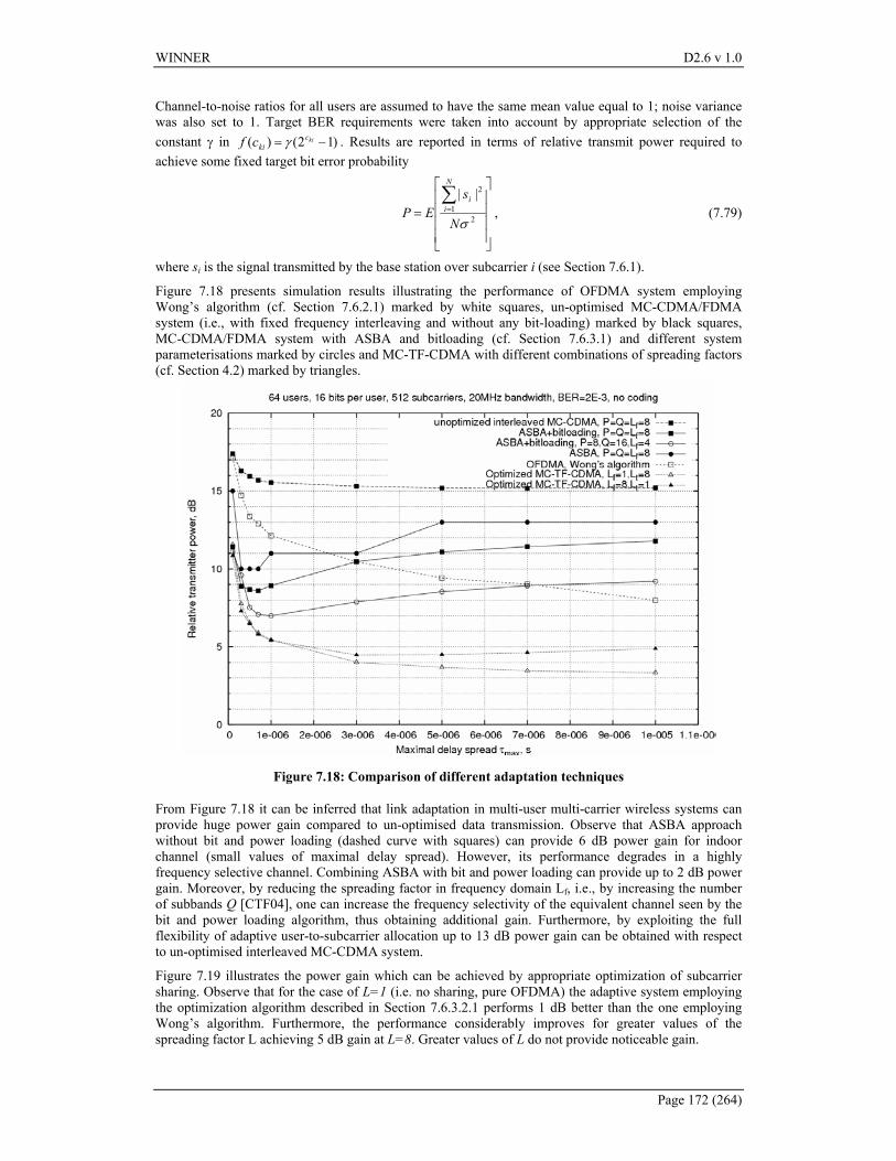
WINNER D2.6 v 1.0

Page 172 (264)

Channel-to-noise ratios for all users are assumed to have the same mean value equal to 1; noise variance was also set to 1. Target BER requirements were taken into account by appropriate selection of the constant γ in )12()( −= kic

kicf γ . Results are reported in terms of relative transmit power required to achieve some fixed target bit error probability

=∑

=

2

21

||

σN

sEP

N

ii

, (7.79)

where si is the signal transmitted by the base station over subcarrier i (see Section 7.6.1).

Figure 7.18 presents simulation results illustrating the performance of OFDMA system employing Wong’s algorithm (cf. Section 7.6.2.1) marked by white squares, un-optimised MC-CDMA/FDMA system (i.e., with fixed frequency interleaving and without any bit-loading) marked by black squares, MC-CDMA/FDMA system with ASBA and bitloading (cf. Section 7.6.3.1) and different system parameterisations marked by circles and MC-TF-CDMA with different combinations of spreading factors (cf. Section 4.2) marked by triangles.

Figure 7.18: Comparison of different adaptation techniques

From Figure 7.18 it can be inferred that link adaptation in multi-user multi-carrier wireless systems can provide huge power gain compared to un-optimised data transmission. Observe that ASBA approach without bit and power loading (dashed curve with squares) can provide 6 dB power gain for indoor channel (small values of maximal delay spread). However, its performance degrades in a highly frequency selective channel. Combining ASBA with bit and power loading can provide up to 2 dB power gain. Moreover, by reducing the spreading factor in frequency domain Lf, i.e., by increasing the number of subbands Q [CTF04], one can increase the frequency selectivity of the equivalent channel seen by the bit and power loading algorithm, thus obtaining additional gain. Furthermore, by exploiting the full flexibility of adaptive user-to-subcarrier allocation up to 13 dB power gain can be obtained with respect to un-optimised interleaved MC-CDMA system.

Figure 7.19 illustrates the power gain which can be achieved by appropriate optimization of subcarrier sharing. Observe that for the case of L=1 (i.e. no sharing, pure OFDMA) the adaptive system employing the optimization algorithm described in Section 7.6.3.2.1 performs 1 dB better than the one employing Wong’s algorithm. Furthermore, the performance considerably improves for greater values of the spreading factor L achieving 5 dB gain at L=8. Greater values of L do not provide noticeable gain.

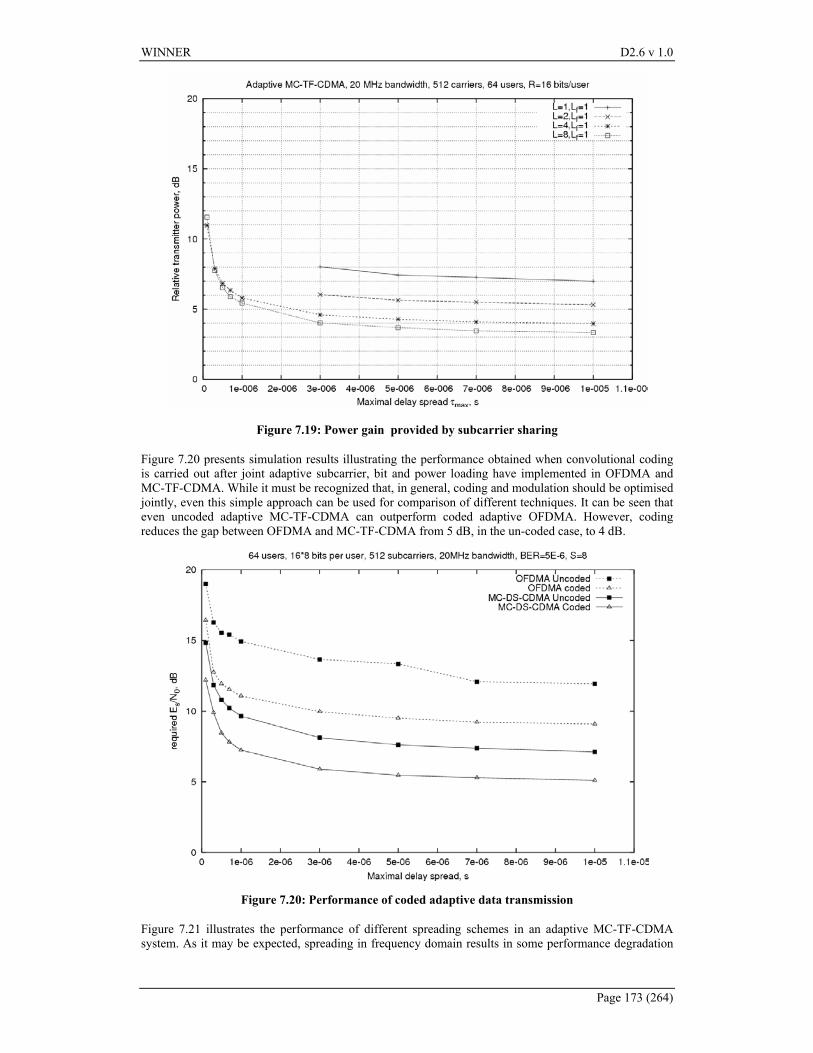
WINNER D2.6 v 1.0

Page 173 (264)

Figure 7.19: Power gain provided by subcarrier sharing

Figure 7.20 presents simulation results illustrating the performance obtained when convolutional coding is carried out after joint adaptive subcarrier, bit and power loading have implemented in OFDMA and MC-TF-CDMA. While it must be recognized that, in general, coding and modulation should be optimised jointly, even this simple approach can be used for comparison of different techniques. It can be seen that even uncoded adaptive MC-TF-CDMA can outperform coded adaptive OFDMA. However, coding reduces the gap between OFDMA and MC-TF-CDMA from 5 dB, in the un-coded case, to 4 dB.

Figure 7.20: Performance of coded adaptive data transmission

Figure 7.21 illustrates the performance of different spreading schemes in an adaptive MC-TF-CDMA system. As it may be expected, spreading in frequency domain results in some performance degradation

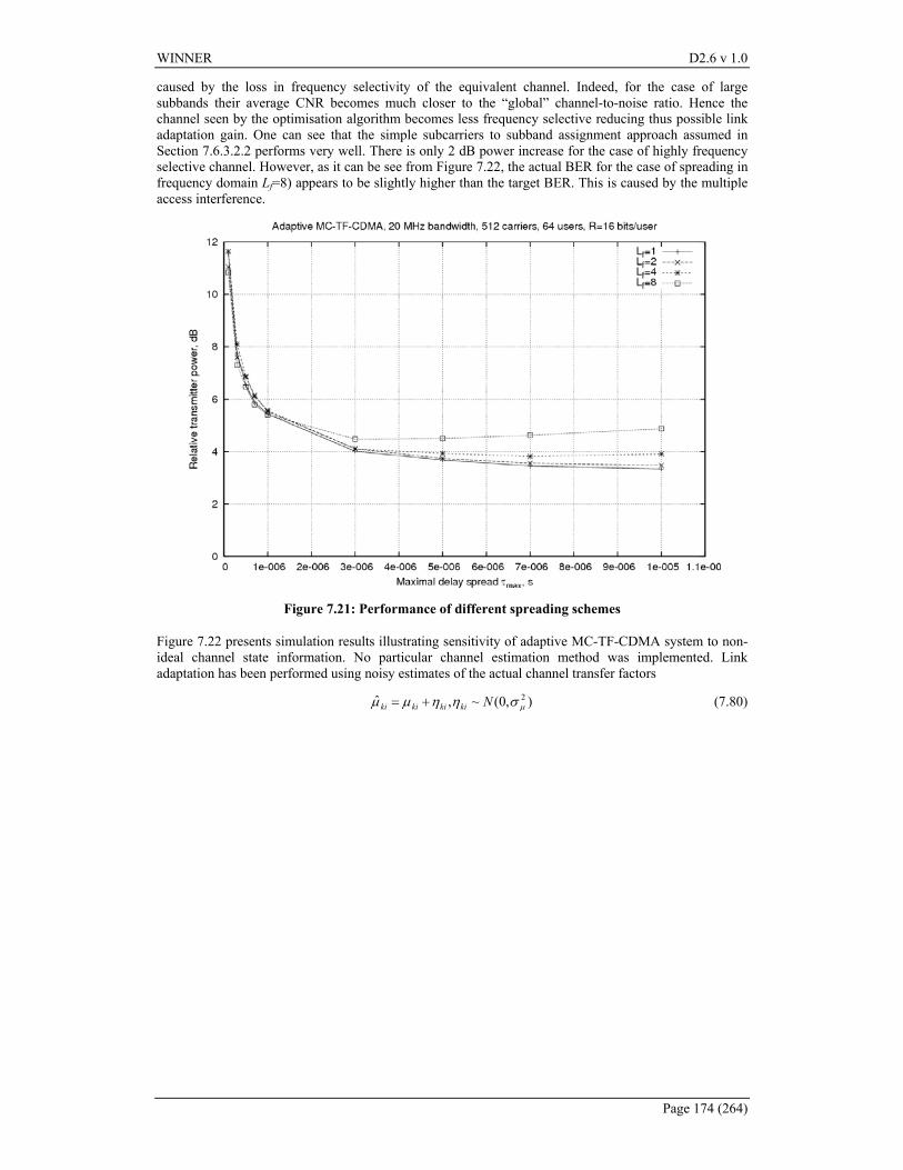
WINNER D2.6 v 1.0

Page 174 (264)

caused by the loss in frequency selectivity of the equivalent channel. Indeed, for the case of large subbands their average CNR becomes much closer to the “global” channel-to-noise ratio. Hence the channel seen by the optimisation algorithm becomes less frequency selective reducing thus possible link adaptation gain. One can see that the simple subcarriers to subband assignment approach assumed in Section 7.6.3.2.2 performs very well. There is only 2 dB power increase for the case of highly frequency selective channel. However, as it can be see from Figure 7.22, the actual BER for the case of spreading in frequency domain Lf=8) appears to be slightly higher than the target BER. This is caused by the multiple access interference.

Figure 7.21: Performance of different spreading schemes

Figure 7.22 presents simulation results illustrating sensitivity of adaptive MC-TF-CDMA system to non-ideal channel state information. No particular channel estimation method was implemented. Link adaptation has been performed using noisy estimates of the actual channel transfer factors

),0(~,ˆ 2µσηηµµ Nkikikiki += (7.80)

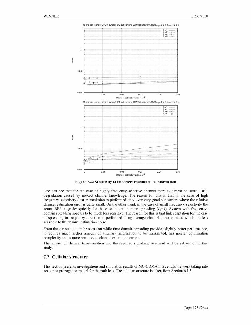
WINNER D2.6 v 1.0

Page 175 (264)

Figure 7.22 Sensitivity to imperfect channel state information

One can see that for the case of highly frequency selective channel there is almost no actual BER degradation caused by inexact channel knowledge. The reason for this is that in the case of high frequency selectivity data transmission is performed only over very good subcarriers where the relative channel estimation error is quite small. On the other hand, in the case of small frequency selectivity the actual BER degrades quickly for the case of time-domain spreading (Lf=1). System with frequency-domain spreading appears to be much less sensitive. The reason for this is that link adaptation for the case of spreading in frequency direction is performed using average channel-to-noise ratios which are less sensitive to the channel estimation noise.

From these results it can be seen that while time-domain spreading provides slightly better performance, it requires much higher amount of auxiliary information to be transmitted, has greater optimisation complexity and is more sensitive to channel estimation errors. The impact of channel time-variation and the required signalling overhead will be subject of further study.

7.7 Cellular structure

This section presents investigations and simulation results of MC-CDMA in a cellular network taking into account a propagation model for the path loss. The cellular structure is taken from Section 6.1.3.

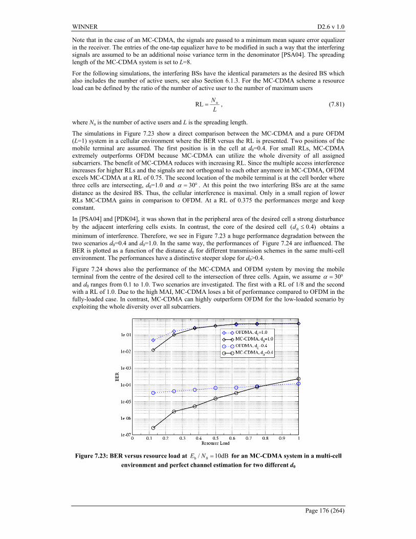
WINNER D2.6 v 1.0

Page 176 (264)

Note that in the case of an MC-CDMA, the signals are passed to a minimum mean square error equalizer in the receiver. The entries of the one-tap equalizer have to be modified in such a way that the interfering signals are assumed to be an additional noise variance term in the denominator [PSA04]. The spreading length of the MC-CDMA system is set to L=8.

For the following simulations, the interfering BSs have the identical parameters as the desired BS which also includes the number of active users, see also Section 6.1.3. For the MC-CDMA scheme a resource load can be defined by the ratio of the number of active user to the number of maximum users

L

NuRL = , (7.81)

where Nu is the number of active users and L is the spreading length.

The simulations in Figure 7.23 show a direct comparison between the MC-CDMA and a pure OFDM (L=1) system in a cellular environment where the BER versus the RL is presented. Two positions of the mobile terminal are assumed. The first position is in the cell at d0=0.4. For small RLs, MC-CDMA extremely outperforms OFDM because MC-CDMA can utilize the whole diversity of all assigned subcarriers. The benefit of MC-CDMA reduces with increasing RL. Since the multiple access interference increases for higher RLs and the signals are not orthogonal to each other anymore in MC-CDMA, OFDM excels MC-CDMA at a RL of 0.75. The second location of the mobile terminal is at the cell border where three cells are intersecting, d0=1.0 and °= 30α . At this point the two interfering BSs are at the same distance as the desired BS. Thus, the cellular interference is maximal. Only in a small region of lower RLs MC-CDMA gains in comparison to OFDM. At a RL of 0.375 the performances merge and keep constant.

In [PSA04] and [PDK04], it was shown that in the peripheral area of the desired cell a strong disturbance by the adjacent interfering cells exists. In contrast, the core of the desired cell )4.0( 0 ≤d obtains a minimum of interference. Therefore, we see in Figure 7.23 a huge performance degradation between the two scenarios d0=0.4 and d0=1.0. In the same way, the performances of Figure 7.24 are influenced. The BER is plotted as a function of the distance d0 for different transmission schemes in the same multi-cell environment. The performances have a distinctive steeper slope for d0>0.4.

Figure 7.24 shows also the performance of the MC-CDMA and OFDM system by moving the mobile terminal from the centre of the desired cell to the intersection of three cells. Again, we assume °= 30α and d0 ranges from 0.1 to 1.0. Two scenarios are investigated. The first with a RL of 1/8 and the second with a RL of 1.0. Due to the high MAI, MC-CDMA loses a bit of performance compared to OFDM in the fully-loaded case. In contrast, MC-CDMA can highly outperform OFDM for the low-loaded scenario by exploiting the whole diversity over all subcarriers.

Figure 7.23: BER versus resource load at dB10/ 0b =NE for an MC-CDMA system in a multi-cell environment and perfect channel estimation for two different d0

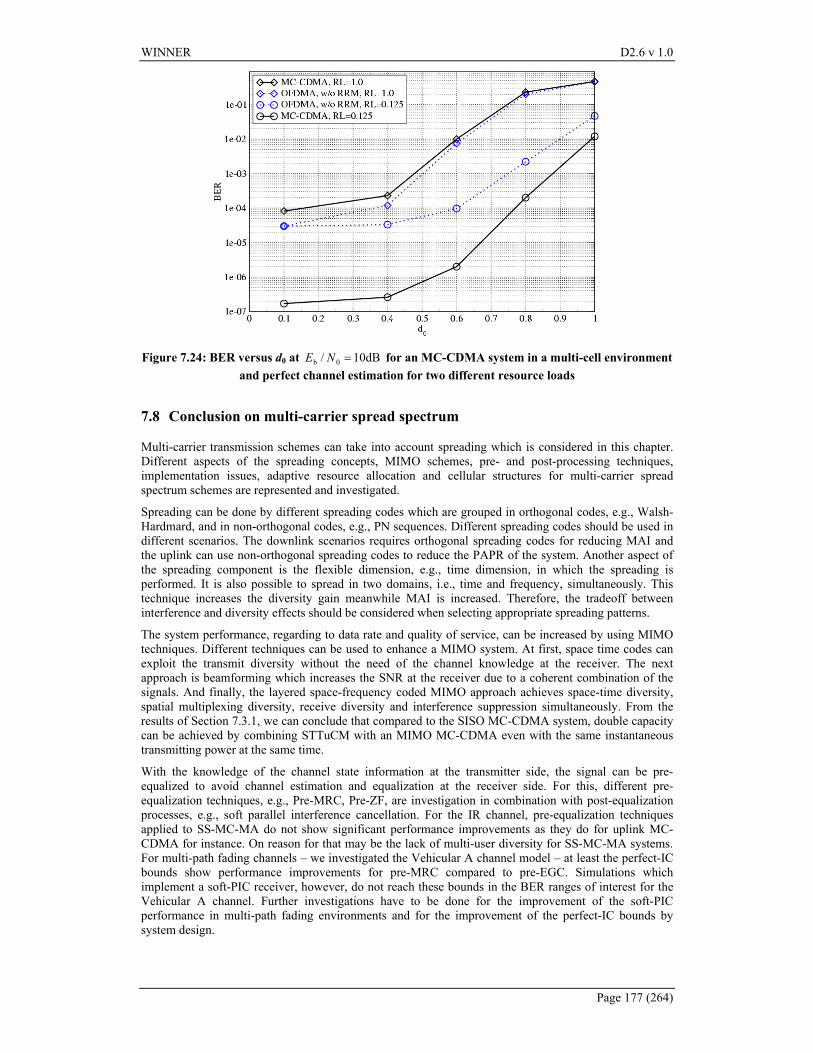
WINNER D2.6 v 1.0

Page 177 (264)

Figure 7.24: BER versus d0 at dB10/ 0b =NE for an MC-CDMA system in a multi-cell environment and perfect channel estimation for two different resource loads

7.8 Conclusion on multi-carrier spread spectrum

Multi-carrier transmission schemes can take into account spreading which is considered in this chapter. Different aspects of the spreading concepts, MIMO schemes, pre- and post-processing techniques, implementation issues, adaptive resource allocation and cellular structures for multi-carrier spread spectrum schemes are represented and investigated.

Spreading can be done by different spreading codes which are grouped in orthogonal codes, e.g., Walsh-Hardmard, and in non-orthogonal codes, e.g., PN sequences. Different spreading codes should be used in different scenarios. The downlink scenarios requires orthogonal spreading codes for reducing MAI and the uplink can use non-orthogonal spreading codes to reduce the PAPR of the system. Another aspect of the spreading component is the flexible dimension, e.g., time dimension, in which the spreading is performed. It is also possible to spread in two domains, i.e., time and frequency, simultaneously. This technique increases the diversity gain meanwhile MAI is increased. Therefore, the tradeoff between interference and diversity effects should be considered when selecting appropriate spreading patterns.

The system performance, regarding to data rate and quality of service, can be increased by using MIMO techniques. Different techniques can be used to enhance a MIMO system. At first, space time codes can exploit the transmit diversity without the need of the channel knowledge at the receiver. The next approach is beamforming which increases the SNR at the receiver due to a coherent combination of the signals. And finally, the layered space-frequency coded MIMO approach achieves space-time diversity, spatial multiplexing diversity, receive diversity and interference suppression simultaneously. From the results of Section 7.3.1, we can conclude that compared to the SISO MC-CDMA system, double capacity can be achieved by combining STTuCM with an MIMO MC-CDMA even with the same instantaneous transmitting power at the same time.

With the knowledge of the channel state information at the transmitter side, the signal can be pre-equalized to avoid channel estimation and equalization at the receiver side. For this, different pre-equalization techniques, e.g., Pre-MRC, Pre-ZF, are investigation in combination with post-equalization processes, e.g., soft parallel interference cancellation. For the IR channel, pre-equalization techniques applied to SS-MC-MA do not show significant performance improvements as they do for uplink MC-CDMA for instance. On reason for that may be the lack of multi-user diversity for SS-MC-MA systems. For multi-path fading channels – we investigated the Vehicular A channel model – at least the perfect-IC bounds show performance improvements for pre-MRC compared to pre-EGC. Simulations which implement a soft-PIC receiver, however, do not reach these bounds in the BER ranges of interest for the Vehicular A channel. Further investigations have to be done for the improvement of the soft-PIC performance in multi-path fading environments and for the improvement of the perfect-IC bounds by system design.

WINNER D2.6 v 1.0

Page 178 (264)

Link adaptation is essential in order to exploit OFDM flexibility and granularity. In multi-user OFDM systems, not only bit and power loading should be performed, but also sharing of the subcarriers among users should to be optimized. An optimisation approach has been proposed, based on which adaptive multi-carrier DS-CDMA provides the best performance among other adaptive multi-carrier multiple access approaches. However, adaptive MC-CDMA provides some advantages in terms of optimization complexity and amount of auxiliary information at the expense of quite small performance degradation.

In a cellular structure the spread multi-carrier transmission scheme, MC-CDMA, is mainly influenced by the two closest interfering base stations. The spreading component can exploit more diversity and therefore MC-CDMA can gain compared to non-spread systems, pure OFDM, up to a system load of 75%. For higher system loads, the MAI degrades the performance of MC-CDMA and the non-spread system outperforms the spread system. A conclusion can be drawn regarding design proposals:

• Pre-equalization techniques for SS-MC-MA result in no significant performance improvements as they do for MC-CDMA in the uplink;

• A spreading component gains in combination with link adaption compared to non-spread schemes and spreading should be done in time direction;

• Design in a multi-cell environment has to be coordinated to the major inter-cell interference resulting from the two closest interfering cells.

The presented results are a first step for investigations towards comparative guidlines for the design of multi-carrier spread spectrum schemes. Further investigations are necessary for finding an appropriate system design in terms of multiple access.

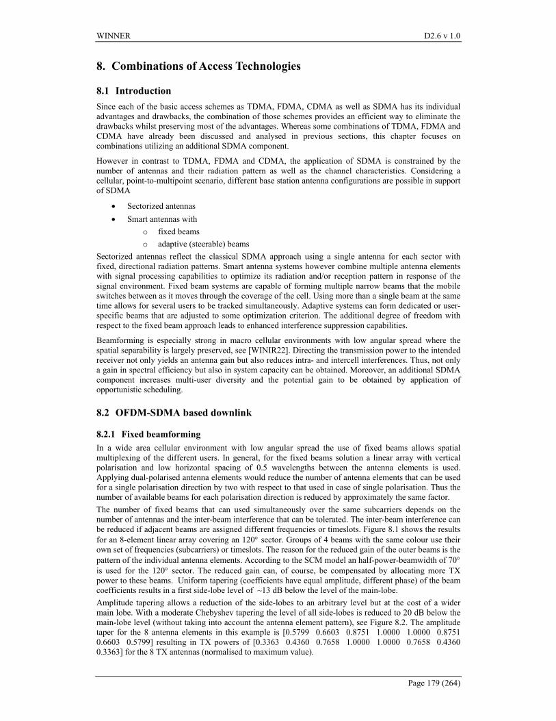
WINNER D2.6 v 1.0

Page 179 (264)

8. Combinations of Access Technologies

8.1 Introduction Since each of the basic access schemes as TDMA, FDMA, CDMA as well as SDMA has its individual advantages and drawbacks, the combination of those schemes provides an efficient way to eliminate the drawbacks whilst preserving most of the advantages. Whereas some combinations of TDMA, FDMA and CDMA have already been discussed and analysed in previous sections, this chapter focuses on combinations utilizing an additional SDMA component.

However in contrast to TDMA, FDMA and CDMA, the application of SDMA is constrained by the number of antennas and their radiation pattern as well as the channel characteristics. Considering a cellular, point-to-multipoint scenario, different base station antenna configurations are possible in support of SDMA

• Sectorized antennas • Smart antennas with

o fixed beams o adaptive (steerable) beams

Sectorized antennas reflect the classical SDMA approach using a single antenna for each sector with fixed, directional radiation patterns. Smart antenna systems however combine multiple antenna elements with signal processing capabilities to optimize its radiation and/or reception pattern in response of the signal environment. Fixed beam systems are capable of forming multiple narrow beams that the mobile switches between as it moves through the coverage of the cell. Using more than a single beam at the same time allows for several users to be tracked simultaneously. Adaptive systems can form dedicated or user-specific beams that are adjusted to some optimization criterion. The additional degree of freedom with respect to the fixed beam approach leads to enhanced interference suppression capabilities.

Beamforming is especially strong in macro cellular environments with low angular spread where the spatial separability is largely preserved, see [WINIR22]. Directing the transmission power to the intended receiver not only yields an antenna gain but also reduces intra- and intercell interferences. Thus, not only a gain in spectral efficiency but also in system capacity can be obtained. Moreover, an additional SDMA component increases multi-user diversity and the potential gain to be obtained by application of opportunistic scheduling.

8.2 OFDM-SDMA based downlink

8.2.1 Fixed beamforming In a wide area cellular environment with low angular spread the use of fixed beams allows spatial multiplexing of the different users. In general, for the fixed beams solution a linear array with vertical polarisation and low horizontal spacing of 0.5 wavelengths between the antenna elements is used. Applying dual-polarised antenna elements would reduce the number of antenna elements that can be used for a single polarisation direction by two with respect to that used in case of single polarisation. Thus the number of available beams for each polarisation direction is reduced by approximately the same factor. The number of fixed beams that can used simultaneously over the same subcarriers depends on the number of antennas and the inter-beam interference that can be tolerated. The inter-beam interference can be reduced if adjacent beams are assigned different frequencies or timeslots. Figure 8.1 shows the results for an 8-element linear array covering an 120° sector. Groups of 4 beams with the same colour use their own set of frequencies (subcarriers) or timeslots. The reason for the reduced gain of the outer beams is the pattern of the individual antenna elements. According to the SCM model an half-power-beamwidth of 70° is used for the 120° sector. The reduced gain can, of course, be compensated by allocating more TX power to these beams. Uniform tapering (coefficients have equal amplitude, different phase) of the beam coefficients results in a first side-lobe level of ~13 dB below the level of the main-lobe. Amplitude tapering allows a reduction of the side-lobes to an arbitrary level but at the cost of a wider main lobe. With a moderate Chebyshev tapering the level of all side-lobes is reduced to 20 dB below the main-lobe level (without taking into account the antenna element pattern), see Figure 8.2. The amplitude taper for the 8 antenna elements in this example is [0.5799 0.6603 0.8751 1.0000 1.0000 0.8751 0.6603 0.5799] resulting in TX powers of [0.3363 0.4360 0.7658 1.0000 1.0000 0.7658 0.4360 0.3363] for the 8 TX antennas (normalised to maximum value).

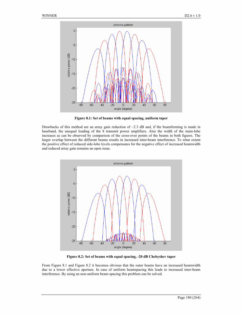
WINNER D2.6 v 1.0

Page 180 (264)

Figure 8.1: Set of beams with equal spacing, uniform taper

Drawbacks of this method are an array gain reduction of ~2.3 dB and, if the beamforming is made in baseband, the unequal loading of the 8 transmit power amplifiers. Also the width of the main-lobe increases as can be observed by comparison of the cross-over points of the beams in both figures. The larger overlap between the different beams results in increased inter-beam interference. To what extent the positive effect of reduced side-lobe levels compensates for the negative effect of increased beamwidth and reduced array gain remains an open issue.

Figure 8.2: Set of beams with equal spacing, -20 dB Chebyshev taper

From Figure 8.1 and Figure 8.2 it becomes obvious that the outer beams have an increased beamwidth due to a lower effective aperture. In case of uniform beamspacing this leads to increased inter-beam interference. By using an non-uniform beam-spacing this problem can be solved.

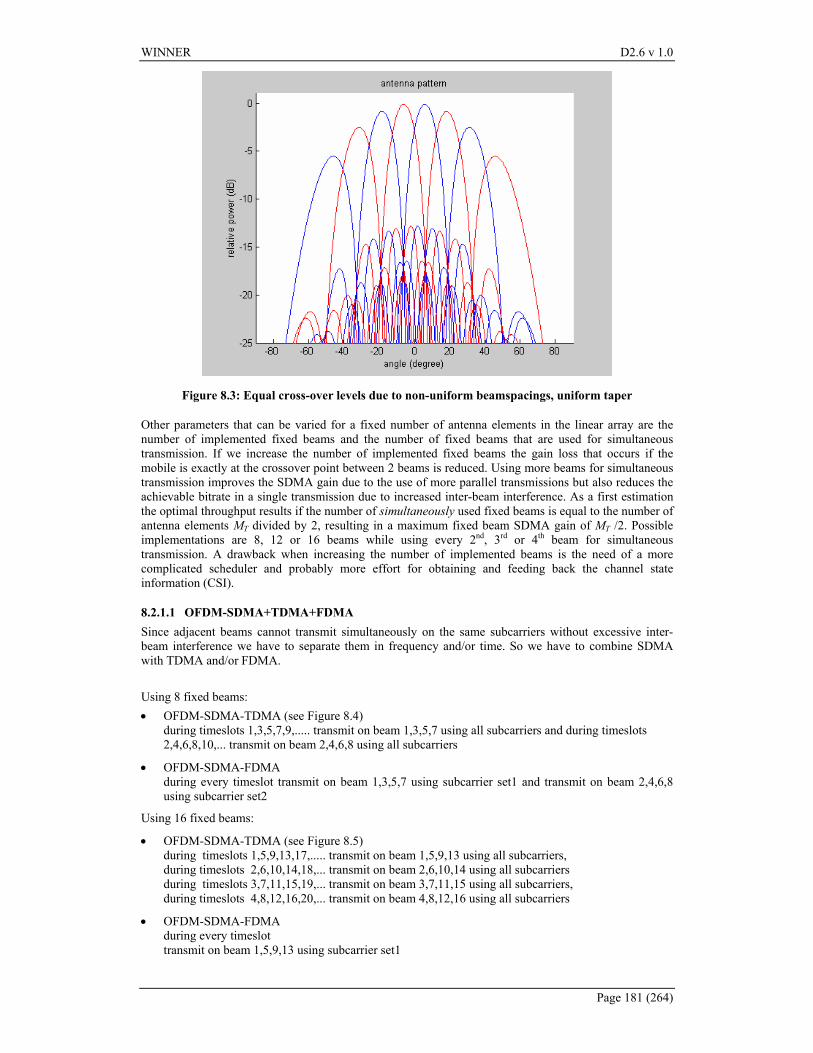
WINNER D2.6 v 1.0

Page 181 (264)

Figure 8.3: Equal cross-over levels due to non-uniform beamspacings, uniform taper

Other parameters that can be varied for a fixed number of antenna elements in the linear array are the number of implemented fixed beams and the number of fixed beams that are used for simultaneous transmission. If we increase the number of implemented fixed beams the gain loss that occurs if the mobile is exactly at the crossover point between 2 beams is reduced. Using more beams for simultaneous transmission improves the SDMA gain due to the use of more parallel transmissions but also reduces the achievable bitrate in a single transmission due to increased inter-beam interference. As a first estimation the optimal throughput results if the number of simultaneously used fixed beams is equal to the number of antenna elements MT divided by 2, resulting in a maximum fixed beam SDMA gain of MT /2. Possible implementations are 8, 12 or 16 beams while using every 2nd, 3rd or 4th beam for simultaneous transmission. A drawback when increasing the number of implemented beams is the need of a more complicated scheduler and probably more effort for obtaining and feeding back the channel state information (CSI).

8.2.1.1 OFDM-SDMA+TDMA+FDMA Since adjacent beams cannot transmit simultaneously on the same subcarriers without excessive inter-beam interference we have to separate them in frequency and/or time. So we have to combine SDMA with TDMA and/or FDMA. Using 8 fixed beams: • OFDM-SDMA-TDMA (see Figure 8.4)

during timeslots 1,3,5,7,9,..... transmit on beam 1,3,5,7 using all subcarriers and during timeslots 2,4,6,8,10,... transmit on beam 2,4,6,8 using all subcarriers

• OFDM-SDMA-FDMA during every timeslot transmit on beam 1,3,5,7 using subcarrier set1 and transmit on beam 2,4,6,8 using subcarrier set2

Using 16 fixed beams:

• OFDM-SDMA-TDMA (see Figure 8.5) during timeslots 1,5,9,13,17,..... transmit on beam 1,5,9,13 using all subcarriers, during timeslots 2,6,10,14,18,... transmit on beam 2,6,10,14 using all subcarriers during timeslots 3,7,11,15,19,... transmit on beam 3,7,11,15 using all subcarriers, during timeslots 4,8,12,16,20,... transmit on beam 4,8,12,16 using all subcarriers

• OFDM-SDMA-FDMA during every timeslot transmit on beam 1,5,9,13 using subcarrier set1

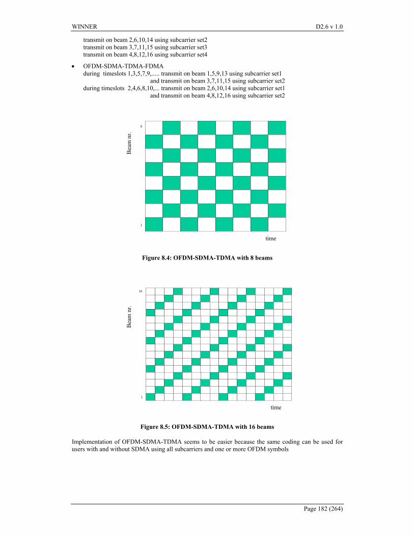
WINNER D2.6 v 1.0

Page 182 (264)

transmit on beam 2,6,10,14 using subcarrier set2 transmit on beam 3,7,11,15 using subcarrier set3 transmit on beam 4,8,12,16 using subcarrier set4

• OFDM-SDMA-TDMA-FDMA during timeslots 1,3,5,7,9,..... transmit on beam 1,5,9,13 using subcarrier set1 and transmit on beam 3,7,11,15 using subcarrier set2 during timeslots 2,4,6,8,10,... transmit on beam 2,6,10,14 using subcarrier set1 and transmit on beam 4,8,12,16 using subcarrier set2

time

Bea

m n

r.

1

8

Figure 8.4: OFDM-SDMA-TDMA with 8 beams

time

Bea

m n

r.

1

16

Figure 8.5: OFDM-SDMA-TDMA with 16 beams

Implementation of OFDM-SDMA-TDMA seems to be easier because the same coding can be used for users with and without SDMA using all subcarriers and one or more OFDM symbols

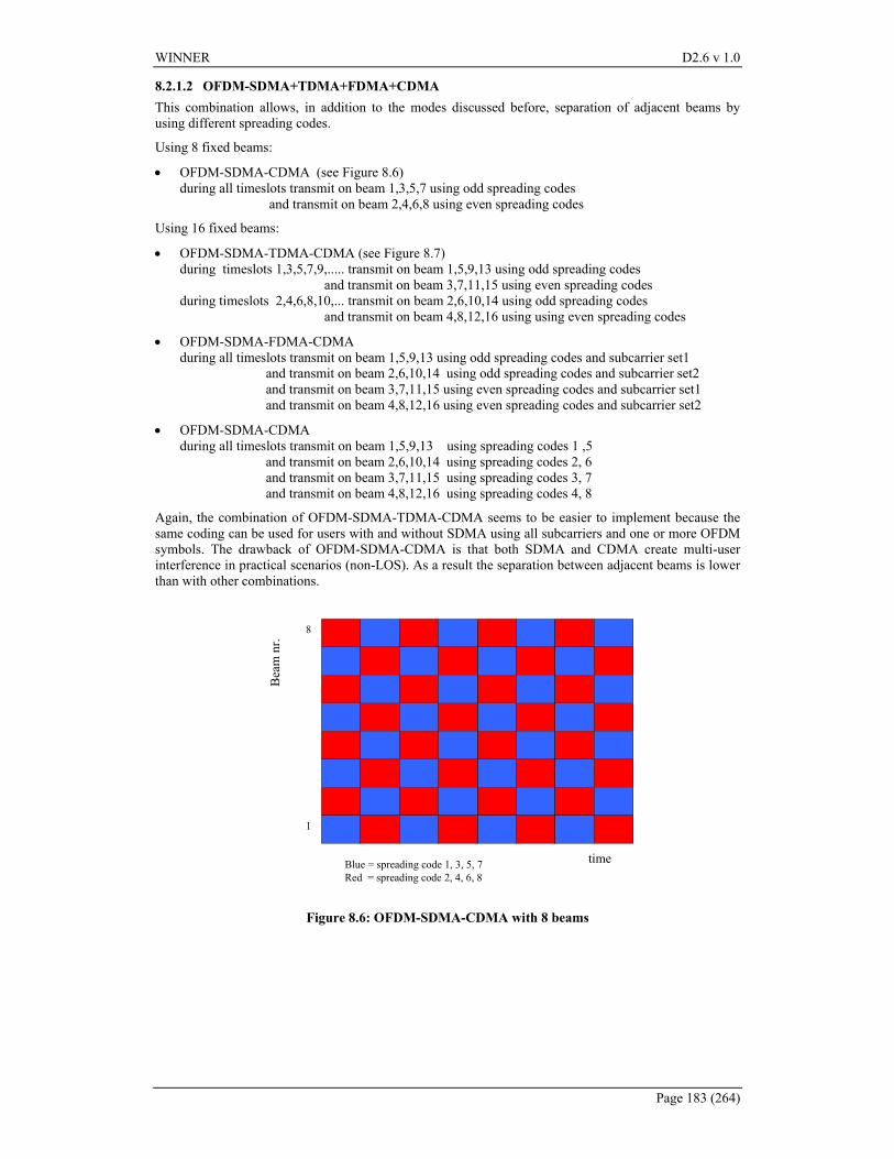
WINNER D2.6 v 1.0

Page 183 (264)

8.2.1.2 OFDM-SDMA+TDMA+FDMA+CDMA This combination allows, in addition to the modes discussed before, separation of adjacent beams by using different spreading codes.

Using 8 fixed beams:

• OFDM-SDMA-CDMA (see Figure 8.6) during all timeslots transmit on beam 1,3,5,7 using odd spreading codes and transmit on beam 2,4,6,8 using even spreading codes

Using 16 fixed beams:

• OFDM-SDMA-TDMA-CDMA (see Figure 8.7) during timeslots 1,3,5,7,9,..... transmit on beam 1,5,9,13 using odd spreading codes and transmit on beam 3,7,11,15 using even spreading codes during timeslots 2,4,6,8,10,... transmit on beam 2,6,10,14 using odd spreading codes and transmit on beam 4,8,12,16 using using even spreading codes

• OFDM-SDMA-FDMA-CDMA during all timeslots transmit on beam 1,5,9,13 using odd spreading codes and subcarrier set1 and transmit on beam 2,6,10,14 using odd spreading codes and subcarrier set2 and transmit on beam 3,7,11,15 using even spreading codes and subcarrier set1 and transmit on beam 4,8,12,16 using even spreading codes and subcarrier set2

• OFDM-SDMA-CDMA during all timeslots transmit on beam 1,5,9,13 using spreading codes 1 ,5 and transmit on beam 2,6,10,14 using spreading codes 2, 6 and transmit on beam 3,7,11,15 using spreading codes 3, 7 and transmit on beam 4,8,12,16 using spreading codes 4, 8

Again, the combination of OFDM-SDMA-TDMA-CDMA seems to be easier to implement because the same coding can be used for users with and without SDMA using all subcarriers and one or more OFDM symbols. The drawback of OFDM-SDMA-CDMA is that both SDMA and CDMA create multi-user interference in practical scenarios (non-LOS). As a result the separation between adjacent beams is lower than with other combinations.

time

Bea

m n

r.

1

8

Blue = spreading code 1, 3, 5, 7 Red = spreading code 2, 4, 6, 8

Figure 8.6: OFDM-SDMA-CDMA with 8 beams

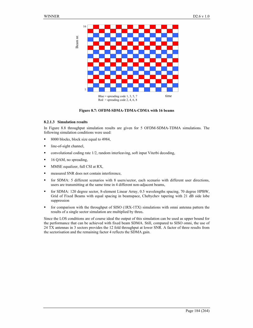
WINNER D2.6 v 1.0

Page 184 (264)

Bea

m n

r.

time

1

16

Blue = spreading code 1, 3, 5, 7 Red = spreading code 2, 4, 6, 8

Figure 8.7: OFDM-SDMA-TDMA-CDMA with 16 beams

8.2.1.3 Simulation results In Figure 8.8 throughput simulation results are given for 5 OFDM-SDMA-TDMA simulations. The following simulation conditions were used:

8000 blocks, block size equal to 4984,

line-of-sight channel,

convolutional coding rate 1/2, random interleaving, soft input Viterbi decoding,

16 QAM, no spreading,

MMSE equalizer, full CSI at RX,

measured SNR does not contain interference,

for SDMA: 5 different scenarios with 8 users/sector, each scenario with different user directions, users are transmitting at the same time in 4 different non-adjacent beams,

for SDMA: 120 degree sector, 8-element Linear Array, 0.5 wavelengths spacing, 70 degree HPBW, Grid of Fixed Beams with equal spacing in beamspace, Chebychev tapering with 21 dB side lobe suppression

for comparison with the throughput of SISO (1RX-1TX) simulations with omni antenna pattern the results of a single sector simulation are multiplied by three.

Since the LOS conditions are of course ideal the output of this simulation can be used as upper bound for the performance that can be achieved with fixed beam SDMA. Still, compared to SISO omni, the use of 24 TX antennas in 3 sectors provides the 12 fold throughput at lower SNR. A factor of three results from the sectorisation and the remaining factor 4 reflects the SDMA gain.

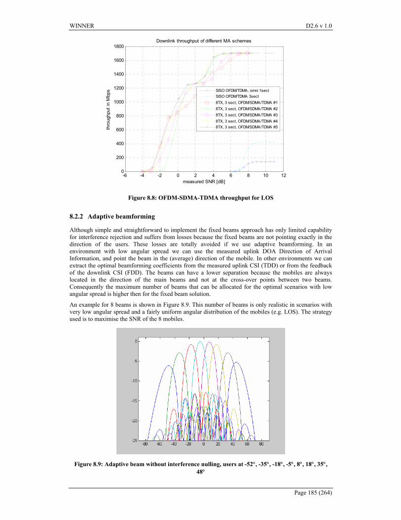
WINNER D2.6 v 1.0

Page 185 (264)

-6 -4 -2 0 2 4 6 8 10 120

200

400

600

800

1000

1200

1400

1600

1800Downlink throughput of different MA schemes

measured SNR [dB]

thro

ughp

ut in

Mbp

s SISO OFDM/TDMA, omni 1sectSISO OFDM/TDMA 3sect8TX, 3 sect, OFDM/SDMA/TDMA #18TX, 3 sect, OFDM/SDMA/TDMA #28TX, 3 sect, OFDM/SDMA/TDMA #38TX, 3 sect, OFDM/SDMA/TDMA #48TX, 3 sect, OFDM/SDMA/TDMA #5

Figure 8.8: OFDM-SDMA-TDMA throughput for LOS

8.2.2 Adaptive beamforming

Although simple and straightforward to implement the fixed beams approach has only limited capability for interference rejection and suffers from losses because the fixed beams are not pointing exactly in the direction of the users. These losses are totally avoided if we use adaptive beamforming. In an environment with low angular spread we can use the measured uplink DOA Direction of Arrival Information, and point the beam in the (average) direction of the mobile. In other environments we can extract the optimal beamforming coefficients from the measured uplink CSI (TDD) or from the feedback of the downlink CSI (FDD). The beams can have a lower separation because the mobiles are always located in the direction of the main beams and not at the cross-over points between two beams. Consequently the maximum number of beams that can be allocated for the optimal scenarios with low angular spread is higher then for the fixed beam solution.

An example for 8 beams is shown in Figure 8.9. This number of beams is only realistic in scenarios with very low angular spread and a fairly uniform angular distribution of the mobiles (e.g. LOS). The strategy used is to maximise the SNR of the 8 mobiles.

Figure 8.9: Adaptive beam without interference nulling, users at -52°, -35°, -18°, -5°, 8°, 18°, 35°, 48°

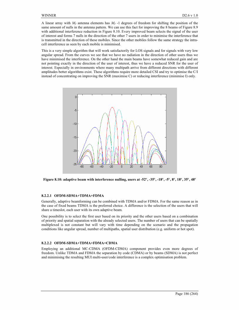
WINNER D2.6 v 1.0

Page 186 (264)

A linear array with MT antenna elements has MT -1 degrees of freedom for shifting the position of the same amount of nulls in the antenna pattern. We can use this fact for improving the 8 beams of Figure 8.9 with additional interference reduction in Figure 8.10. Every improved beam selects the signal of the user of interest and forms 7 nulls in the direction of the other 7 users in order to minimise the interference that is transmitted in the direction of these mobiles. Since the other mobiles follow the same strategy the intra-cell interference as seen by each mobile is minimised.

This is a very simple algorithm that will work satisfactorily for LOS signals and for signals with very low angular spread. From the curves we see that we have no radiation in the direction of other users thus we have minimised the interference. On the other hand the main beams have somewhat reduced gain and are not pointing exactly in the direction of the user of interest, thus we have a reduced SNR for the user of interest. Especially in environments where many multipath arrive from different directions with different amplitudes better algorithms exist. These algorithms require more detailed CSI and try to optimise the C/I instead of concentrating on improving the SNR (maximise C) or reducing interference (minimise I) only.

Figure 8.10: adaptive beam with interference nulling, users at -52°, -35°, -18°, -5°, 8°, 18°, 35°, 48°

8.2.2.1 OFDM-SDMA+TDMA+FDMA Generally, adaptive beamforming can be combined with TDMA and/or FDMA. For the same reason as in the case of fixed beams TDMA is the preferred choice. A difference is the selection of the users that will share a timeslot, each user with its own adaptive beam.

One possibility is to select the first user based on its priority and the other users based on a combination of priority and spatial separation with the already selected users. The number of users that can be spatially multiplexed is not constant but will vary with time depending on the scenario and the propagation conditions like angular spread, number of multipaths, spatial user distribution (e.g. uniform or hot spot).

8.2.2.2 OFDM-SDMA+TDMA+FDMA+CDMA Employing an additional MC-CDMA (OFDM-CDMA) component provides even more degrees of freedom. Unlike TDMA and FDMA the separation by code (CDMA) or by beams (SDMA) is not perfect and minimising the resulting MUI multi-user/code interference is a complex optimisation problem.

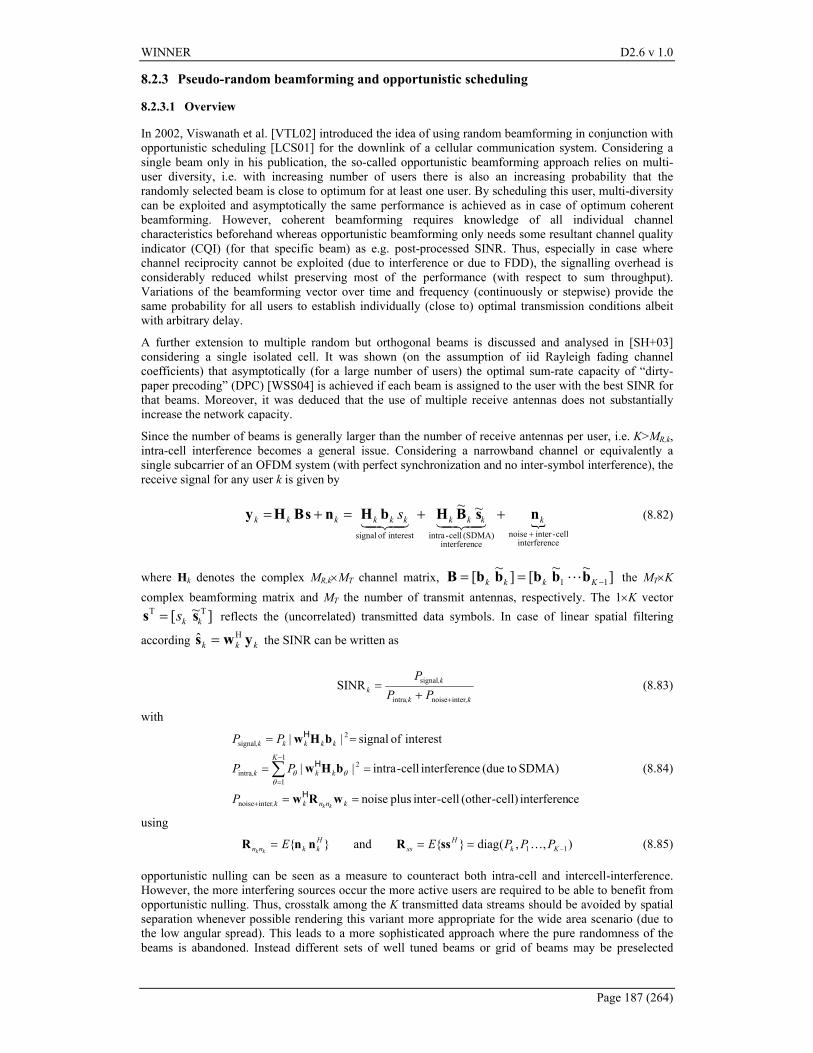
WINNER D2.6 v 1.0

Page 187 (264)

8.2.3 Pseudo-random beamforming and opportunistic scheduling

8.2.3.1 Overview

In 2002, Viswanath et al. [VTL02] introduced the idea of using random beamforming in conjunction with opportunistic scheduling [LCS01] for the downlink of a cellular communication system. Considering a single beam only in his publication, the so-called opportunistic beamforming approach relies on multi-user diversity, i.e. with increasing number of users there is also an increasing probability that the randomly selected beam is close to optimum for at least one user. By scheduling this user, multi-diversity can be exploited and asymptotically the same performance is achieved as in case of optimum coherent beamforming. However, coherent beamforming requires knowledge of all individual channel characteristics beforehand whereas opportunistic beamforming only needs some resultant channel quality indicator (CQI) (for that specific beam) as e.g. post-processed SINR. Thus, especially in case where channel reciprocity cannot be exploited (due to interference or due to FDD), the signalling overhead is considerably reduced whilst preserving most of the performance (with respect to sum throughput). Variations of the beamforming vector over time and frequency (continuously or stepwise) provide the same probability for all users to establish individually (close to) optimal transmission conditions albeit with arbitrary delay.

A further extension to multiple random but orthogonal beams is discussed and analysed in [SH+03] considering a single isolated cell. It was shown (on the assumption of iid Rayleigh fading channel coefficients) that asymptotically (for a large number of users) the optimal sum-rate capacity of “dirty-paper precoding” (DPC) [WSS04] is achieved if each beam is assigned to the user with the best SINR for that beams. Moreover, it was deduced that the use of multiple receive antennas does not substantially increase the network capacity.

Since the number of beams is generally larger than the number of receive antennas per user, i.e. K>MR,k, intra-cell interference becomes a general issue. Considering a narrowband channel or equivalently a single subcarrier of an OFDM system (with perfect synchronization and no inter-symbol interference), the receive signal for any user k is given by

{

ceinterferencell-inter noise

ceinterferen(SDMA) cell-intrainterest of signal

~~

+

++=+= kkkkkkkkkk s nsBHbHnsBHy4342143421

(8.82)

where Hk denotes the complex MR,k×MT channel matrix, ]~~[]~[ 11 −== Kkkk bbbbbB L the MT×K complex beamforming matrix and MT the number of transmit antennas, respectively. The 1×K vector

]~[ TTkks ss = reflects the (uncorrelated) transmitted data symbols. In case of linear spatial filtering

according kkk yws Hˆ = the SINR can be written as

,k,k

,kk PP

P

internoiseintra

signalSINR++

= (8.83)

with

ceinterferen cell)-(other cell-inter plus noise

SDMA) to(due ceinterferen cell-intra ||

interest of signal ||

internoise

1

1

2intra

2signal

==

==

==

+

−

=∑

knnk,k

K

kk,k

kkkk,k

kkP

PP

PP

wRw

bHw

bHw

H

H

H

θθθ (8.84)

using

),,(diag}{and}{ 11 −=== KkH

ssHkknn PPPEE

kkKssRnnR (8.85)

opportunistic nulling can be seen as a measure to counteract both intra-cell and intercell-interference. However, the more interfering sources occur the more active users are required to be able to benefit from opportunistic nulling. Thus, crosstalk among the K transmitted data streams should be avoided by spatial separation whenever possible rendering this variant more appropriate for the wide area scenario (due to the low angular spread). This leads to a more sophisticated approach where the pure randomness of the beams is abandoned. Instead different sets of well tuned beams or grid of beams may be preselected

WINNER D2.6 v 1.0

Page 188 (264)

according to some criterion. Switching between those sets in a random or successive manner induces the variations required for exploitation of multi-user diversity. This type of approach, which is denoted here as pseudo-random beamforming, will be considered in this subsection.

Whereas the combination of random or pseudo-random beamforming with opportunistic scheduling has certain benefits as

• asymptotically optimum performance in terms of sum capacity (at least analytically)

• support of low complex single antenna mobile terminals

• inherent intra-cell and intercell-interference suppression (just by not serving terminals suffering from a high interference level)

• flexible operation either in TDD or FDD mode (or any combination thereof)

certain constraints apply as well:

• the channel and interference situation must not vary significantly during beam probing, feedback and payload phase (denoted as beam pattern switching period, BPSP, in the sequel) otherwise the (multiuser) resource and PHY mode assignment is no longer „optimum“. This implies that

1. the BPSP should be smaller than the coherence time of the channel

2. the BPSP should be synchronized among adjacent base stations both in length and in phase.

• The basic opportunistic scheduling approach does neither account for any QoS requirements nor for fairness and thus may induce arbitrary delays for certain users to be served. This implies that

1. some coupling between scheduling and beamforming should be applied (either for all or a subset of beams) to enhance the probability of users running delay sensitive applications to see “good” channels (e.g. steering the beam in the direction of the users or using the same beam more often which has been proven to be a good one for that user in the past).

2. the scheduling criterion should take at least the relative SINR values for each user into account (referred to his average) and not the absolute values alone to avoid unfairness. Proportional fair scheduling [VTL02] is an example for such a class of schedulers.

• The signalling overhead may become significant for a large number of users. Considering K beams and a single antenna receiver, K SINR values must be determined to be able to identify the “best” data stream. Overhead reduction may be achieved by

1. reducing the amount of feedback information to K’< K SINR values (the best ones) but in this case an additional indexing is required to identify the corresponding beams.

2. omitting the feedback entirely if all measured SINR values lie below a certain threshold and the currently running application has no stringent delay requirements.

3. grouping resource element into blocks, see [Sve04]. Especially in case of OFDM, frequency blocks may be defined in the order of the coherence bandwidth. Due to the high correlation of the corresponding channel matrices the SINR computation needs to be done only once for each block provided that the same beampattern is applied across these subcarriers. Alternating the beampattern between subcarrier blocks (instead of leaving them constant) enhances the variability of the channel and thus enhances the diversity order for each user.

8.2.3.2 Evaluation

8.2.3.2.1 System and simulation assumptions An assessment of the performance of pseudo-random beamforming in conjunction with opportunistic scheduling can only be achieved via system simulations (i.e. layer 1 and 2). A possible TDD frame structure which was taken as a baseline for the evaluation is depicted in Figure 8.11. No intercell-interference was taken into account at this stage.

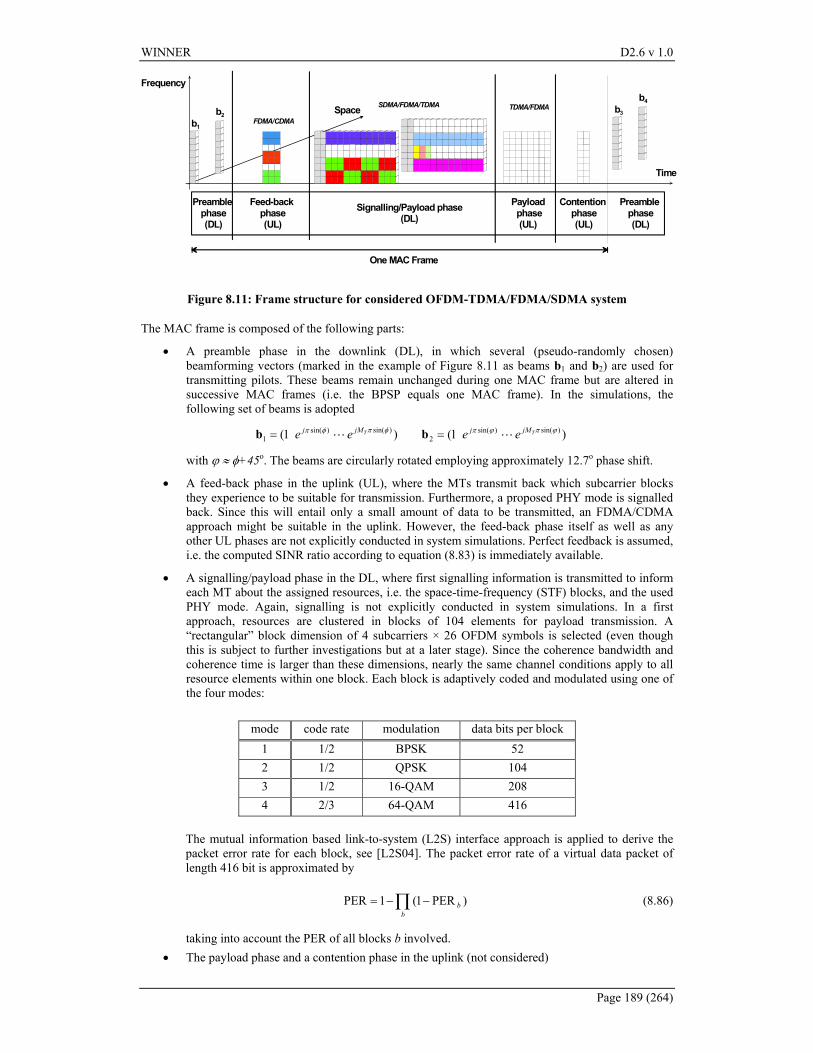
WINNER D2.6 v 1.0

Page 189 (264)

FDMA/CDMAb1

b2

Frequency

Space

Time

Preamble phase (DL)

Feed-back phase (UL)

Signalling/Payload phase(DL)

Payload phase(UL)

SDMA/FDMA/TDMA

Contention phase (UL)

TDMA/FDMA b3

b4

Preamble phase (DL)

One MAC Frame

Figure 8.11: Frame structure for considered OFDM-TDMA/FDMA/SDMA system

The MAC frame is composed of the following parts:

• A preamble phase in the downlink (DL), in which several (pseudo-randomly chosen) beamforming vectors (marked in the example of Figure 8.11 as beams b1 and b2) are used for transmitting pilots. These beams remain unchanged during one MAC frame but are altered in successive MAC frames (i.e. the BPSP equals one MAC frame). In the simulations, the following set of beams is adopted

)1()1( )sin()sin(2

)sin()sin(1

ϕπϕπφπφπ TT jMjjMj eeee LL == bb

with ϕ ≈ φ+45o. The beams are circularly rotated employing approximately 12.7o phase shift.

• A feed-back phase in the uplink (UL), where the MTs transmit back which subcarrier blocks they experience to be suitable for transmission. Furthermore, a proposed PHY mode is signalled back. Since this will entail only a small amount of data to be transmitted, an FDMA/CDMA approach might be suitable in the uplink. However, the feed-back phase itself as well as any other UL phases are not explicitly conducted in system simulations. Perfect feedback is assumed, i.e. the computed SINR ratio according to equation (8.83) is immediately available.

• A signalling/payload phase in the DL, where first signalling information is transmitted to inform each MT about the assigned resources, i.e. the space-time-frequency (STF) blocks, and the used PHY mode. Again, signalling is not explicitly conducted in system simulations. In a first approach, resources are clustered in blocks of 104 elements for payload transmission. A “rectangular” block dimension of 4 subcarriers × 26 OFDM symbols is selected (even though this is subject to further investigations but at a later stage). Since the coherence bandwidth and coherence time is larger than these dimensions, nearly the same channel conditions apply to all resource elements within one block. Each block is adaptively coded and modulated using one of the four modes:

mode code rate modulation data bits per block 1 1/2 BPSK 52 2 1/2 QPSK 104 3 1/2 16-QAM 208 4 2/3 64-QAM 416

The mutual information based link-to-system (L2S) interface approach is applied to derive the packet error rate for each block, see [L2S04]. The packet error rate of a virtual data packet of length 416 bit is approximated by

)PER1(1PER ∏ −−=b

b (8.86)

taking into account the PER of all blocks b involved. • The payload phase and a contention phase in the uplink (not considered)

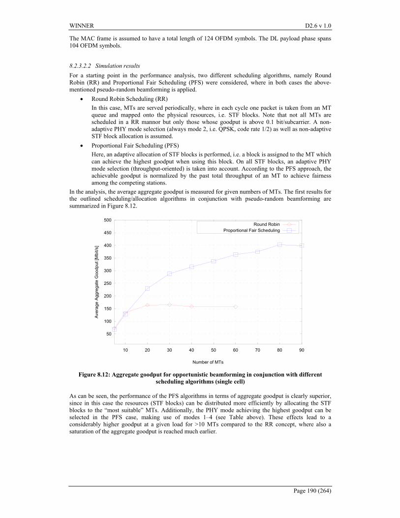
WINNER D2.6 v 1.0

Page 190 (264)

The MAC frame is assumed to have a total length of 124 OFDM symbols. The DL payload phase spans 104 OFDM symbols.

8.2.3.2.2 Simulation results For a starting point in the performance analysis, two different scheduling algorithms, namely Round Robin (RR) and Proportional Fair Scheduling (PFS) were considered, where in both cases the above-mentioned pseudo-random beamforming is applied.

• Round Robin Scheduling (RR) In this case, MTs are served periodically, where in each cycle one packet is taken from an MT queue and mapped onto the physical resources, i.e. STF blocks. Note that not all MTs are scheduled in a RR mannor but only those whose goodput is above 0.1 bit/subcarrier. A non-adaptive PHY mode selection (always mode 2, i.e. QPSK, code rate 1/2) as well as non-adaptive STF block allocation is assumed.

• Proportional Fair Scheduling (PFS) Here, an adaptive allocation of STF blocks is performed, i.e. a block is assigned to the MT which can achieve the highest goodput when using this block. On all STF blocks, an adaptive PHY mode selection (throughput-oriented) is taken into account. According to the PFS approach, the achievable goodput is normalized by the past total throughput of an MT to achieve fairness among the competing stations.

In the analysis, the average aggregate goodput is measured for given numbers of MTs. The first results for the outlined scheduling/allocation algorithms in conjunction with pseudo-random beamforming are summarized in Figure 8.12.

50

100

150

200

250

300

350

400

450

500

10 20 30 40 50 60 70 80 90

Aver

age

Aggr

egat

e G

oodp

ut [M

bit/s

]

Number of MTs

Round RobinProportional Fair Scheduling

Figure 8.12: Aggregate goodput for opportunistic beamforming in conjunction with different scheduling algorithms (single cell)

As can be seen, the performance of the PFS algorithms in terms of aggregate goodput is clearly superior, since in this case the resources (STF blocks) can be distributed more efficiently by allocating the STF blocks to the “most suitable” MTs. Additionally, the PHY mode achieving the highest goodput can be selected in the PFS case, making use of modes 1–4 (see Table above). These effects lead to a considerably higher goodput at a given load for >10 MTs compared to the RR concept, where also a saturation of the aggregate goodput is reached much earlier.

WINNER D2.6 v 1.0

Page 191 (264)

8.2.4 Joint beamforming and scheduling

Optimizing a communication of a MT-antenna Access Point (AP) with Nu single antenna terminals is not straightforward. Since a global optimization might not be solvable in real time, the AP has several alternatives involving both the physical layer, e.g. beamforming and power/bit allocation, and the Data Link Control (DLC) layer, such as scheduling. The purpose of this section is twofold. First, for Nu <= MT we compare traditional bit allocation strategies with a novel modified approach, especially in terms of fairness. Second, we focus on the combinatorial problem that arises when Nu > MT, and propose several alternatives for the scheduling of the users into groups, which is done together with the bit allocation. Simulations show that better performance is obtained at the expense of complexity. The presented techniques are based on [BPN04a].

8.2.4.1 Introduction

We study the downlink of a wireless system, where a MT-antenna Base Station (BS) or Access Point (AP) communicates simultaneously with Nu single antenna terminals. The spatial diversity can be deployed to enhance the performance of the scheduling task. For this purpose, we distinguish among the cases Nu≤MT and Nu > MT.

The case Nu not higher than MT is treated first. In such a scenario, the scheduling at the PHYsical layer (PHY) reduces to the allocation of the scarce instantaneous power. Besides, with multiple signal mappings and multiple antennas, the rate optimization under Bit Error Rate (BER) constraints leads to a spatial bit allocation problem [Hug87]. Moreover, the AP has to choose an adequate beamforming criterion. The optimum strategy implies the computation of the transmit covariance matrices [Pal03], which might be difficult to implement in practice. Then, the solution to the scheduling is conceptually divided into the transmit beamforming and the power (and bit) allocation, mainly because of two reasons. First, the capacity region of this multi-antenna broadcast channel has been very recently characterized [WSS04]; second and more importantly, this separation allows to search for simple procedures that enable a fast and realizable joint PHY and Data Link Control (DLC) cross-layer design [BPPN03].

As in [VTL02], we assume that terminals are dumb, whereas all the intelligence is located at the AP. Differently to e.g. [SSH04], the AP performs a Zero Forcing (ZF) transmit beamforming, so that the symbols received by the terminals are only corrupted by noise and not by the signals transmitted for the other users [HAP01]. Compared to optimum downlink beamforming, see e.g. [BO01] or [RFLT98] and references therein, the main powerful characteristics of ZF are the low complexity and the closed-form solution. Although there is a certain degradation with respect to other schemes such as precoding with Dirty Paper, which attains the maximum sum capacity [CS03], or a regularized channel inversion with additional encoding that yields quasi-optimum performance [PHS03], ZF provides a valid framework for analyzing fairness issues and scheduling aspects.

In order to maximize the rate, the power allocation under BER requirements leads naturally to a spatial bit allocation. In the literature, the bit allocation/loading problem has been extensively studied since [Hug87], where an optimal algorithm for single-user discrete bit loading in multi-carrier systems is proposed, see also e.g. [Cam99], [SSh03], [KRJ00] and references therein. Essentially, two strategies can be found, namely bit filling and bit removal. The former adds a bit to the user/subcarrier providing the lowest increase in total power, and bit removal schemes remove the most penalizing bit until the power constraint is fulfilled. On the other hand, the authors in [LSC03] (see also references therein) have extensively studied multi-user multi-carrier integer bit loading. Particularly in [LSC03], the authors extend the Levin-Campello algorithm in order to minimize the total transmitted power with a target sum rate for all the users and a total power budget. There exists a clear trade-off between performance and complexity in bit loading algorithms.

With ZF, the spatial channel gains gather the influence of the simultaneously-served users, differently to e.g. [GC97] and other references. Since the system performance varies dramatically depending on the subset of the users that are served, the algorithms cited previously shall be modified. Moreover, the fairness implications are rarely evaluated, see e.g. [HL03] and [KH95]. We focus primarily on the implications in the short-term, and provided an integer number of bits per symbol (rate), we analyze two perspectives, namely the Maximization of the Sum Rate (MSR) and the Maximization of the Minimum Rate (MMR). Additionally, we modify the MMR so as to improve its behaviour, and we show that the throughput can be improved without decreasing the number of bits assigned by the MMR to any user. This means that a Pareto improvement [FT91] is obtained over the traditional MMR.

When Nu > MT, the AP has to distribute the users into groups, and then perform the power and bit allocation, which is a combinatorial problem. We extend [BAIPN03] to deal with the bit allocation.

WINNER D2.6 v 1.0

Page 192 (264)

Similarly in [ShTKL01], the authors propose a dynamic slot allocation for the uplink of a SDMA/TDMA system. Their NP-complete objective (and also ours) is to minimize the length of the frame, while ensuring a minimum Signal to Interference to Noise Ratio (SINR). In [YL02] the authors take the best fit strategy proposed in [ShTKL01] and extend the algorithm to take into account several QoS parameters. Results of these issues are given afterwards.

8.2.4.2 Problem statement

In the following, boldface capital (lowercase) letters refer to matrices (vectors). The conjugate transpose of a is aH and the element at row i th and column j th of A is denoted by [ ] ji,A . The square matrix with the diagonal given by a1,a2,…,an is denoted by diag(a1,a2,…,an). The elements nk within the set K={n1,n2,…,nK} are denoted by Kknkk ≤≤= 1,ω , and the cardinality of the set K is expressed by K . The vector 1k has zeros at all positions but the kth. In the downlink, where a MT-antenna AP communicates simultaneously with Nu single-antenna terminals (gathered in K={1,2,…,K}) and we assume that Nu not higher than MT for the moment. At any time instant, the received signal vector is at the uth subcarrier (we omit the subcarrier index for the moment)

nHBsy += (8.87)

where at the uth subcarrier, the kth position of vector y(s) is the received (transmitted) signal for user k. H is the Nu×MT complex flat-fading channel matrix, the ith row of which contains the 1×MT vector of the channel gains for the ith user, i.e. T

ui,h . We assume that the components of the channel matrix are independent and identically distributed complex Gaussian random variables with zero mean and unit variance. If terminals send/receive a periodic training sequence to/from the AP, but not to/from other terminals, it might not be far from reality the assumption that the channel matrix is known at the AP, whereas the receivers are only aware of their own channel response. The noise vector is complex Gaussian with variance 2

oσ , and the transmit beamvectors for the Nu users are gathered in the matrix

[ ]KbbbB K21= .

Since it is meaningful to separate the effect of the channel and the power allocation, we normalize the ZF beamvector, so an equivalent spatial channel is obtained, together with the power allocation. After the convenient computations, de previous signal model can be reduced to a very simple expression:

kkkkk wsy +=⇒+= βαβα wsDDy (8.88)

in which the equivalent channels αk are affected by the channels of the other users. With this model, the Signal to Noise Ratio (SNR) for the kth user is given by 2/ okkk σβαγ = , where we have assumed that the symbols have unitary mean energy, particularly, normalized Quadrature Amplitude Modulation (QAM) symbols are considered. Since simplicity is an important feature for schedulers, we use the easy-differentiable approximate BER expression given in [ChG01]

−

−≈12

exp)( 21 m

ccBER

γγ

(8.89)

where m is the number of bits in the constellation, c1=0.2, and c2=1.6. This expression is valid within 1.5dB of error for a BER lower than 0.001. If several signal mappings are available, the throughput (rate) depends on the number of bits of the symbols and on the BER. At the PHY, rate is the maximum number of bits per symbol m that can be transmitted while fulfilling a target BER, and it can be obtained using the

previous BER approximation as

Γ

+=γ1logm , where the constant Γ is given by

( ) 21 //log cBERc t=Γ . In fact, 1=Γ can be interpreted as the classical Shannon’s limit to error-free bit rate (capacity). Typically, m is a real number, and a spatial waterfilling can be performed in order to achieve the maximum sum rate of the SDMA channel [CTh91]. However, practical systems have only a finite set of possible mappings, thus m is an integer.

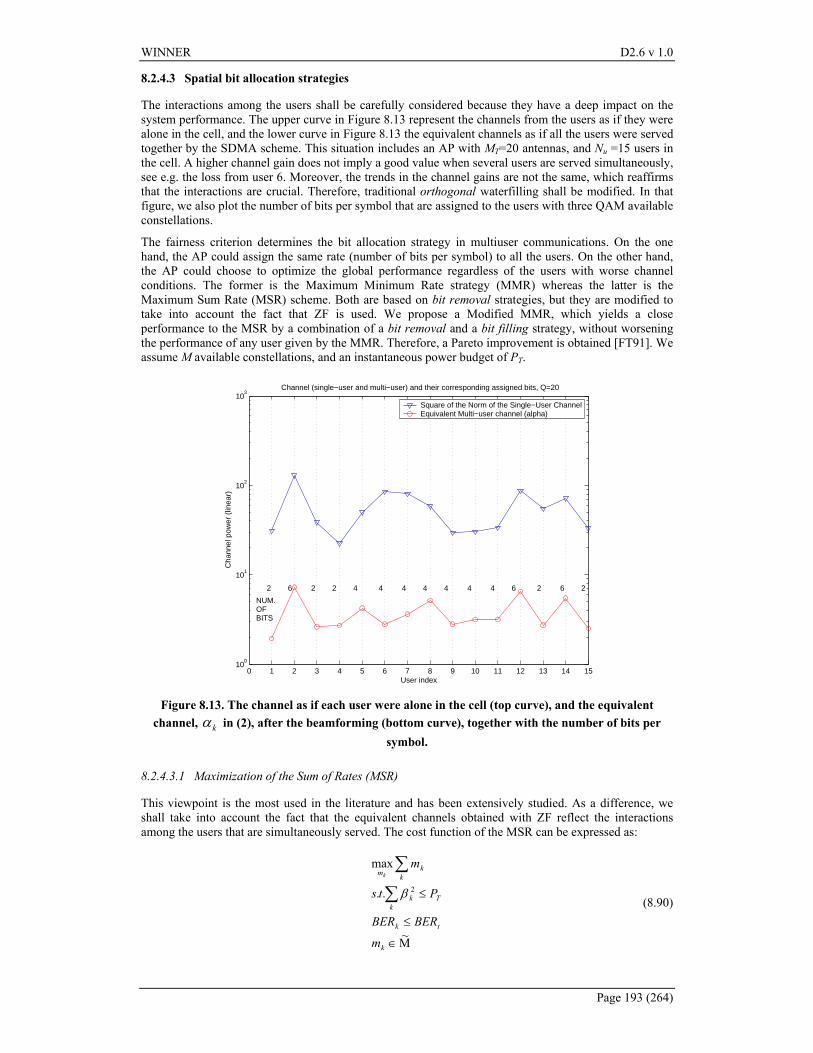
WINNER D2.6 v 1.0

Page 193 (264)

8.2.4.3 Spatial bit allocation strategies

The interactions among the users shall be carefully considered because they have a deep impact on the system performance. The upper curve in Figure 8.13 represent the channels from the users as if they were alone in the cell, and the lower curve in Figure 8.13 the equivalent channels as if all the users were served together by the SDMA scheme. This situation includes an AP with MT=20 antennas, and Nu =15 users in the cell. A higher channel gain does not imply a good value when several users are served simultaneously, see e.g. the loss from user 6. Moreover, the trends in the channel gains are not the same, which reaffirms that the interactions are crucial. Therefore, traditional orthogonal waterfilling shall be modified. In that figure, we also plot the number of bits per symbol that are assigned to the users with three QAM available constellations.

The fairness criterion determines the bit allocation strategy in multiuser communications. On the one hand, the AP could assign the same rate (number of bits per symbol) to all the users. On the other hand, the AP could choose to optimize the global performance regardless of the users with worse channel conditions. The former is the Maximum Minimum Rate strategy (MMR) whereas the latter is the Maximum Sum Rate (MSR) scheme. Both are based on bit removal strategies, but they are modified to take into account the fact that ZF is used. We propose a Modified MMR, which yields a close performance to the MSR by a combination of a bit removal and a bit filling strategy, without worsening the performance of any user given by the MMR. Therefore, a Pareto improvement is obtained [FT91]. We assume M available constellations, and an instantaneous power budget of PT.

0 1 2 3 4 5 6 7 8 9 10 11 12 13 14 15

100

101

102

103

User index

Cha

nnel

pow

er (

linea

r)

Channel (single−user and multi−user) and their corresponding assigned bits, Q=20

Square of the Norm of the Single−User ChannelEquivalent Multi−user channel (alpha)

2 6 2 2 4 4 4 4 4 4 4 6 2 6 2

NUM.OFBITS

Figure 8.13. The channel as if each user were alone in the cell (top curve), and the equivalent channel, kα in (2), after the beamforming (bottom curve), together with the number of bits per

symbol.

8.2.4.3.1 Maximization of the Sum of Rates (MSR)

This viewpoint is the most used in the literature and has been extensively studied. As a difference, we shall take into account the fact that the equivalent channels obtained with ZF reflect the interactions among the users that are simultaneously served. The cost function of the MSR can be expressed as:

Μ∈

≤

≤∑

∑

~

..

max

2

k

tk

kTk

kkm

m

BERBER

Pts

mk

β (8.90)

WINNER D2.6 v 1.0

Page 194 (264)

where, due to algorithmic issues the set Μ~ is defined as the union of the possible constellations together

with 0 (no transmission), that is, Μ∪=Μ }0{~ . The optimum solution is very complex since it requires an exhaustive search among all possible combinations of users and number of bits. The exhaustive search could be feasible for moderate number of users and antennas, but the complexity is relatively high with MT= Nu =6. Besides, in case the problem is not feasible, the AP has to perform the admission control, i.e. choose the users that will be served. In any case, the ultimate goal is to optimize the cell performance regardless of the poorer users, thus the distribution of the resources is uneven (unfair). The spatial bit allocation algorithm proposed next yields a close-to-optimum solution that could be implemented in real time. First, note that the BER constraint fixes the power allocation according to

( )

−=

tk

m

k BERc

c

k1

22

22 log12

ασβ (8.91)

which helps in the definition of a function that reflects the power decrease of using a lower constellation size. We assume that the constellation size for each user i is expressed as iω , except for the kth user, which changes the number of bits to k

jω instead of kiω , where k

iω is higher than kjω . Then, the power

reduction can be obtained as (this is the power variation function)

( )( )

Μ∉−

Μ∈−

=

∑ ∑Κ∈ Κ∈i ~i

22

2

if ~22

if 221

,kj

ii

kj

kkj

kik ii

ki

ki

pω

αα

ωα

ωω ωω

ωω

(8.92)

where the set Κ~ gathers all the users but the kth and the equivalent channels with the tilde are computed

for the users in Κ~ . In fact, this is not the exact power saving that is obtained because if a user is removed,

the rest of the users have the chance to increase their modulation index. However, the reduction in complexity of this approximation justifies the use of the previous cost function.

The MSR algorithm in the following table is essentially a bit removal technique, but since the spatial channel gains change whenever the set of active users varies, it is combined with a bit filling scheme. Briefly, the MSR works as follows. First, it tries to serve all the users with the highest modulation at steps 1-4. If the power constraint is not fulfilled (step 4), the scheduler decides which user should reduce the constellation size or which user should not be served. Since the number of bits shall be reduced, the scheduler selects the user having a maximum incremental cost of using a lower modulation, i.e. the user that saves more power if the bit rate is reduced, see steps 6 and 7. The AP reduces the number of bits of the selected user, and if it belongs to a possible constellation the algorithm goes again to step 1. Otherwise, it drops that user out from the set of active users (step 8), and the constellation size of all the remaining users is set again to the maximum (step 2), so that the power and bit allocation need to be done again. The algorithm finishes when the power constraint is fulfilled or if only one user forms the set of active users (step 5). In that case, that user is allocated all the power with the highest constellation satisfying the BER constraint.

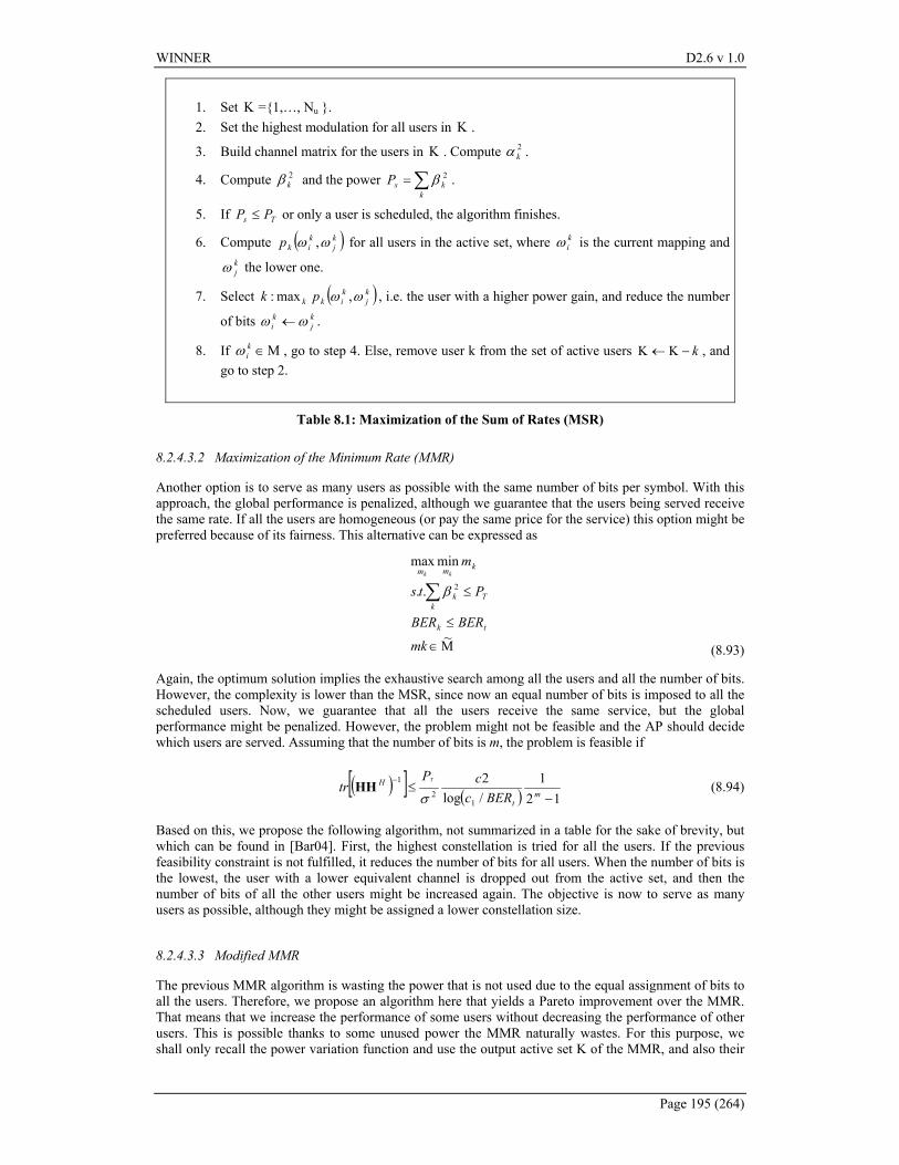
WINNER D2.6 v 1.0

Page 195 (264)

1. Set Κ ={1,…, Nu }. 2. Set the highest modulation for all users in Κ .

3. Build channel matrix for the users in Κ . Compute 2kα .

4. Compute 2kβ and the power ∑=

kksP 2β .

5. If Ts PP ≤ or only a user is scheduled, the algorithm finishes.

6. Compute ( )kj

kikp ωω , for all users in the active set, where k

iω is the current mapping and kjω the lower one.

7. Select ( )kj

kikk pk ωω ,max: , i.e. the user with a higher power gain, and reduce the number

of bits kj

ki ωω ← .

8. If Μ∈kiω , go to step 4. Else, remove user k from the set of active users k−Κ←Κ , and

go to step 2.

Table 8.1: Maximization of the Sum of Rates (MSR)

8.2.4.3.2 Maximization of the Minimum Rate (MMR)

Another option is to serve as many users as possible with the same number of bits per symbol. With this approach, the global performance is penalized, although we guarantee that the users being served receive the same rate. If all the users are homogeneous (or pay the same price for the service) this option might be preferred because of its fairness. This alternative can be expressed as

Μ∈

≤

≤∑

~

..

minmax

2

mk

BERBER

Pts

m

tk

kTk

kmm kk

β

(8.93)

Again, the optimum solution implies the exhaustive search among all the users and all the number of bits. However, the complexity is lower than the MSR, since now an equal number of bits is imposed to all the scheduled users. Now, we guarantee that all the users receive the same service, but the global performance might be penalized. However, the problem might not be feasible and the AP should decide which users are served. Assuming that the number of bits is m, the problem is feasible if

( )[ ] ( ) 121

/log2

12

1

−≤

−

mt

H

BERccP

trT

σHH (8.94)

Based on this, we propose the following algorithm, not summarized in a table for the sake of brevity, but which can be found in [Bar04]. First, the highest constellation is tried for all the users. If the previous feasibility constraint is not fulfilled, it reduces the number of bits for all users. When the number of bits is the lowest, the user with a lower equivalent channel is dropped out from the active set, and then the number of bits of all the other users might be increased again. The objective is now to serve as many users as possible, although they might be assigned a lower constellation size.

8.2.4.3.3 Modified MMR

The previous MMR algorithm is wasting the power that is not used due to the equal assignment of bits to all the users. Therefore, we propose an algorithm here that yields a Pareto improvement over the MMR. That means that we increase the performance of some users without decreasing the performance of other users. This is possible thanks to some unused power the MMR naturally wastes. For this purpose, we shall only recall the power variation function and use the output active set K of the MMR, and also their

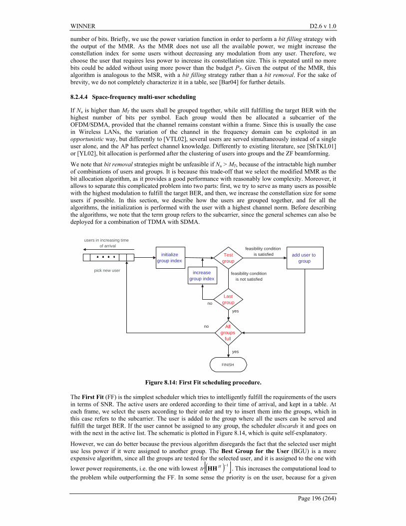
WINNER D2.6 v 1.0

Page 196 (264)

number of bits. Briefly, we use the power variation function in order to perform a bit filling strategy with the output of the MMR. As the MMR does not use all the available power, we might increase the constellation index for some users without decreasing any modulation from any user. Therefore, we choose the user that requires less power to increase its constellation size. This is repeated until no more bits could be added without using more power than the budget PT. Given the output of the MMR, this algorithm is analogous to the MSR, with a bit filling strategy rather than a bit removal. For the sake of brevity, we do not completely characterize it in a table, see [Bar04] for further details.

8.2.4.4 Space-frequency multi-user scheduling

If Nu is higher than MT the users shall be grouped together, while still fulfilling the target BER with the highest number of bits per symbol. Each group would then be allocated a subcarrier of the OFDM/SDMA, provided that the channel remains constant within a frame. Since this is usually the case in Wireless LANs, the variation of the channel in the frequency domain can be exploited in an opportunistic way, but differently to [VTL02], several users are served simultaneously instead of a single user alone, and the AP has perfect channel knowledge. Differently to existing literature, see [ShTKL01] or [YL02], bit allocation is performed after the clustering of users into groups and the ZF beamforming.

We note that bit removal strategies might be unfeasible if Nu > MT, because of the intractable high number of combinations of users and groups. It is because this trade-off that we select the modified MMR as the bit allocation algorithm, as it provides a good performance with reasonably low complexity. Moreover, it allows to separate this complicated problem into two parts: first, we try to serve as many users as possible with the highest modulation to fulfill the target BER, and then, we increase the constellation size for some users if possible. In this section, we describe how the users are grouped together, and for all the algorithms, the initialization is performed with the user with a highest channel norm. Before describing the algorithms, we note that the term group refers to the subcarrier, since the general schemes can also be deployed for a combination of TDMA with SDMA.

users in increasing timeof arrival

initializegroup index

Testgroup

feasibility conditionis satisfied add user to

group

feasibility conditionis not satisfied

Lastgroup

yes

pick new user

no

increasegroup index

Allgroups

full

no

FINISH

yes

Figure 8.14: First Fit scheduling procedure.

The First Fit (FF) is the simplest scheduler which tries to intelligently fulfill the requirements of the users in terms of SNR. The active users are ordered according to their time of arrival, and kept in a table. At each frame, we select the users according to their order and try to insert them into the groups, which in this case refers to the subcarrier. The user is added to the group where all the users can be served and fulfill the target BER. If the user cannot be assigned to any group, the scheduler discards it and goes on with the next in the active list. The schematic is plotted in Figure 8.14, which is quite self-explanatory.

However, we can do better because the previous algorithm disregards the fact that the selected user might use less power if it were assigned to another group. The Best Group for the User (BGU) is a more expensive algorithm, since all the groups are tested for the selected user, and it is assigned to the one with lower power requirements, i.e. the one with lowest ( )[ ]1−Htr HH . This increases the computational load to the problem while outperforming the FF. In some sense the priority is on the user, because for a given

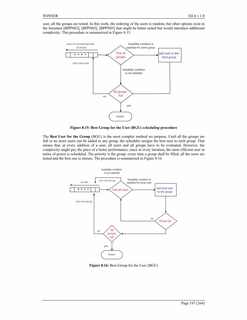
WINNER D2.6 v 1.0

Page 197 (264)

user, all the groups are tested. In this work, the ordering of the users is random, but other options exist in the literature [BPPN03], [BPPN03], [BPPN03] that might be better suited but would introduce additional complexity. This procedure is summarized in Figure 8.15.

users in increasing timeof arrival

Test allgroups

feasibility condition issatisfied for some group

feasibility conditionis not satisfied

pick new user

add user to thebest group

All groupsfullno

yes

FINISH

Figure 8.15: Best Group for the User (BGU) scheduling procedure

The Best User for the Group (BGU) is the most complex method we propose. Until all the groups are full or no more users can be added to any group, the scheduler assigns the best user to each group. That means that, at every addition of a user, all users and all groups have to be evaluated. However, the complexity might pay the price of a better performance, since at every iteration, the most efficient user in terms of power is scheduled. The priority is the group: every time a group shall be filled, all the users are tested and the best one is chosen. The procedure is summarized in Figure 8.16.

groups

Test all users

feasibility condition issatisfied for some user

feasibility conditionis not satisfied

pick new group

add best userto the group

Group full

yes

no

FINISH

Allgroups

full

no

pick new group

Figure 8.16: Best Group for the User (BGU)

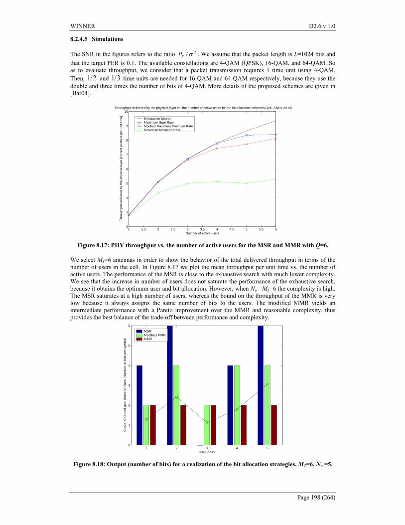
WINNER D2.6 v 1.0

Page 198 (264)

8.2.4.5 Simulations

The SNR in the figures refers to the ratio 2/ σTP . We assume that the packet length is L=1024 bits and that the target PER is 0.1. The available constellations are 4-QAM (QPSK), 16-QAM, and 64-QAM. So as to evaluate throughput, we consider that a packet transmission requires 1 time unit using 4-QAM. Then, 1 2/ and 1 3/ time units are needed for 16-QAM and 64-QAM respectively, because they use the double and three times the number of bits of 4-QAM. More details of the proposed schemes are given in [Bar04].

1 1.5 2 2.5 3 3.5 4 4.5 5 5.5 62

3

4

5

6

7

8

9

10

Number of active users

Thr

ough

put d

eliv

ered

by

the

phys

ical

laye

r [c

orre

ct p

acke

ts p

er u

nit t

ime]

Throughput delivered by the physical layer vs. the number of active users for the bit allocation schemes,Q=6, SNR= 20 dB

Exhaustive SearchMaximum Sum RateModfied Maximum Minimum RateMaximum Minimum Rate

Figure 8.17: PHY throughput vs. the number of active users for the MSR and MMR with Q=6.

We select MT=6 antennas in order to show the behavior of the total delivered throughput in terms of the number of users in the cell. In Figure 8.17 we plot the mean throughput per unit time vs. the number of active users. The performance of the MSR is close to the exhaustive search with much lower complexity. We see that the increase in number of users does not saturate the performance of the exhaustive search, because it obtains the optimum user and bit allocation. However, when Nu =MT=6 the complexity is high. The MSR saturates at a high number of users, whereas the bound on the throughput of the MMR is very low because it always assigns the same number of bits to the users. The modified MMR yields an intermediate performance with a Pareto improvement over the MMR and reasonable complexity, thus provides the best balance of the trade-off between performance and complexity.

1 2 3 4 50

1

2

3

4

5

6

User index

Cur

ve: C

hann

el g

ain

(line

ar)

/ Bar

s: N

umbe

r of

bits

per

sym

bol

MSRModified MMRMMR

Figure 8.18: Output (number of bits) for a realization of the bit allocation strategies, MT=6, Nu =5.

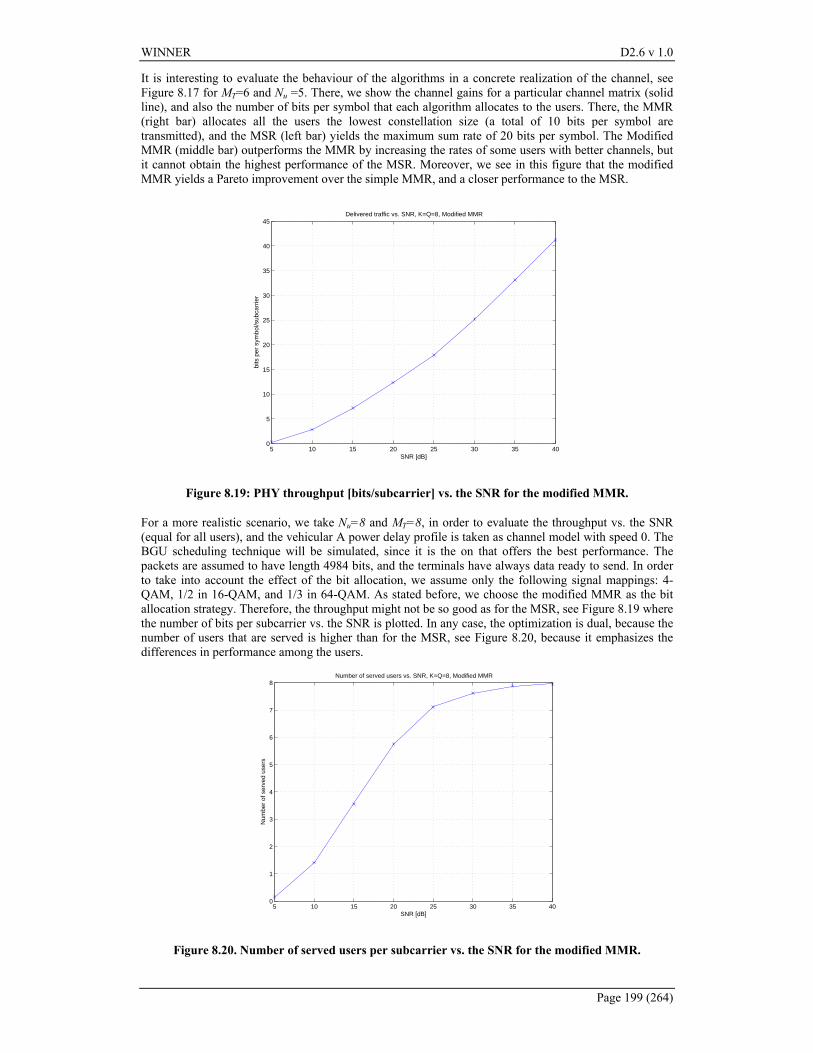
WINNER D2.6 v 1.0

Page 199 (264)

It is interesting to evaluate the behaviour of the algorithms in a concrete realization of the channel, see Figure 8.17 for MT=6 and Nu =5. There, we show the channel gains for a particular channel matrix (solid line), and also the number of bits per symbol that each algorithm allocates to the users. There, the MMR (right bar) allocates all the users the lowest constellation size (a total of 10 bits per symbol are transmitted), and the MSR (left bar) yields the maximum sum rate of 20 bits per symbol. The Modified MMR (middle bar) outperforms the MMR by increasing the rates of some users with better channels, but it cannot obtain the highest performance of the MSR. Moreover, we see in this figure that the modified MMR yields a Pareto improvement over the simple MMR, and a closer performance to the MSR.

5 10 15 20 25 30 35 400

5

10

15

20

25

30

35

40

45

SNR [dB]

bits

per

sym

bol/s

ubca

rrie

r

Delivered traffic vs. SNR, K=Q=8, Modified MMR

Figure 8.19: PHY throughput [bits/subcarrier] vs. the SNR for the modified MMR.

For a more realistic scenario, we take Nu=8 and MT=8, in order to evaluate the throughput vs. the SNR (equal for all users), and the vehicular A power delay profile is taken as channel model with speed 0. The BGU scheduling technique will be simulated, since it is the on that offers the best performance. The packets are assumed to have length 4984 bits, and the terminals have always data ready to send. In order to take into account the effect of the bit allocation, we assume only the following signal mappings: 4-QAM, 1/2 in 16-QAM, and 1/3 in 64-QAM. As stated before, we choose the modified MMR as the bit allocation strategy. Therefore, the throughput might not be so good as for the MSR, see Figure 8.19 where the number of bits per subcarrier vs. the SNR is plotted. In any case, the optimization is dual, because the number of users that are served is higher than for the MSR, see Figure 8.20, because it emphasizes the differences in performance among the users.

5 10 15 20 25 30 35 400

1

2

3

4

5

6

7

8

SNR [dB]

Num

ber

of s

erve

d us

ers

Number of served users vs. SNR, K=Q=8, Modified MMR

Figure 8.20. Number of served users per subcarrier vs. the SNR for the modified MMR.

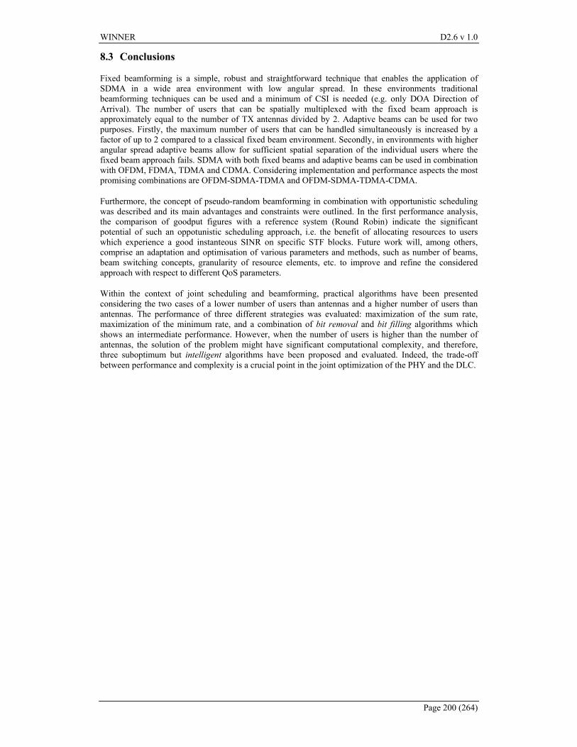
WINNER D2.6 v 1.0

Page 200 (264)

8.3 Conclusions

Fixed beamforming is a simple, robust and straightforward technique that enables the application of SDMA in a wide area environment with low angular spread. In these environments traditional beamforming techniques can be used and a minimum of CSI is needed (e.g. only DOA Direction of Arrival). The number of users that can be spatially multiplexed with the fixed beam approach is approximately equal to the number of TX antennas divided by 2. Adaptive beams can be used for two purposes. Firstly, the maximum number of users that can be handled simultaneously is increased by a factor of up to 2 compared to a classical fixed beam environment. Secondly, in environments with higher angular spread adaptive beams allow for sufficient spatial separation of the individual users where the fixed beam approach fails. SDMA with both fixed beams and adaptive beams can be used in combination with OFDM, FDMA, TDMA and CDMA. Considering implementation and performance aspects the most promising combinations are OFDM-SDMA-TDMA and OFDM-SDMA-TDMA-CDMA.

Furthermore, the concept of pseudo-random beamforming in combination with opportunistic scheduling was described and its main advantages and constraints were outlined. In the first performance analysis, the comparison of goodput figures with a reference system (Round Robin) indicate the significant potential of such an oppotunistic scheduling approach, i.e. the benefit of allocating resources to users which experience a good instanteous SINR on specific STF blocks. Future work will, among others, comprise an adaptation and optimisation of various parameters and methods, such as number of beams, beam switching concepts, granularity of resource elements, etc. to improve and refine the considered approach with respect to different QoS parameters.

Within the context of joint scheduling and beamforming, practical algorithms have been presented considering the two cases of a lower number of users than antennas and a higher number of users than antennas. The performance of three different strategies was evaluated: maximization of the sum rate, maximization of the minimum rate, and a combination of bit removal and bit filling algorithms which shows an intermediate performance. However, when the number of users is higher than the number of antennas, the solution of the problem might have significant computational complexity, and therefore, three suboptimum but intelligent algorithms have been proposed and evaluated. Indeed, the trade-off between performance and complexity is a crucial point in the joint optimization of the PHY and the DLC.

WINNER D2.6 v 1.0

Page 201 (264)

9. Initial Comparisons of Access Technologies

9.1 Introduction All current known multiple access techniques, as well as combinations thereof, are studied in above chapters. The choice of air interface for WINNER will closely depend on the evaluations and comparisons of these multiple access schemes. As the WINNER air interface should work in different deployment scenarios, it is possible that the best multiple access scheme differs according to the scenario. The range of considered techniques will narrow down later to a few techniques, or even maybe a single one, which will be the best choice for the scenarios and will be used by certain WINNER mode(s). The final multiple access schemes must have high performance and spectrum efficiency, keep good flexibility with resource allocation, while having reasonable complexity. These requirements should be considered and reflected in the comparison of different multiple access schemes. This chapter is aimed at providing a fair ground of comparison between the different multiple-access techniques which will be considered within this chapter. Another document from Workpackage 7 [WIN_D72] defines comparability and assessment criteria from a general viewpoint. This chapter focuses on the more specific and technical aspects inherent to multiple-access schemes. Some general thoughts on possible criteria for future comparisons are therefore provided, from the viewpoint of multiple-access techniques. Further work beyond this deliverable will consist in determining the most relevant criteria for the comparison of the multiple-access techniques described in the previous chapters, and unifying them with the assessment criteria contained in [WIN_D72]. Practical constraints set on the simulation systems or environments to guarantee fairness are described next. Some comparison scenarios are defined in order to cover a wide range of situations and transmission conditions.

9.2 General comparison criteria This section is a survey of possible criteria for the future comparisons of the multiple access techniques described in this deliverable. A first step in these future comparisons will be a selection of the most appropriate ones and an alignment with the assessment criteria from [WIN_D72].

9.2.1 Link level performance Assessment and comparison of multiple-access techniques through link level performance should qualify the robustness of each technique against transmission impairments such as channel fading, noise and multi-user interference. The Bit Error Rate (BER) and Block Error Rate (BLER) are commonly employed in link layer studies. The BER represents the probability of having a bit wrong after reception, and qualifies the average transmission error statistics of the physical layer. The BLER corresponds to the probability of having a transmission block in error (i.e. with at least one bit in error) and gives some information about the distribution of the errors in the transmitted stream. The BLER criterion depends strongly on the considered block size. For a fair comparison, the number of information bits in the block should be similar to all the techniques. If the definition of a common block size is too problematic, a set of different block sizes could be used, to show the performance of the different systems with different block sizes. In the end, the user traffic scenarios should define the most appropriate block size(s). These quantities should be evaluated versus Eb/N0, the ratio of the useful average energy per bit (average energy per information bit) over the energy of the noise. The energy per information bit is usually the received energy. Moreover, the SNR should also be characterized, as performances can be measured versus the instantaneous SNR or the average SNR (i.e. short-term/long-term SNR). In a multi-user context, the BER and BLER can be evaluated over all the active transmissions within a cell, to determine the average performance of the cell. They can also be computed for each user individually, if transmission conditions vary among the users. In multi-user situation the interference from other users can also be taken into account by generating interfering signals in the link simulation. Link layer results shall be given together with the spectral efficiency (i.e. transmitted bits/s/Hz). To ease comparison, link layers shall be defined with same, or close, spectral efficiencies. Also the link throughput needs to be analysed, particularly when adaptive transmission schemes are used. The measure for throughput is correctly received information bits per second. Even for link level spectral efficiency and throughput also the required channel bandwidth needs to be taken into account (see section 9.2.3).

WINNER D2.6 v 1.0

Page 202 (264)

9.2.2 System level performance From a qualitative viewpoint, the system level performance of a radio network is evaluated by its ability to satisfy the following requirements: providing connections to the maximum number of users and for each user, providing the radio connection with the expected Quality of Service (QoS). From a quantitative viewpoint, the system performance is measured with different metrics according to the type of applications which are transported by the radio interface. Two basic categories of services can be distinguished: the real time services (i.e. packet transmission with stringent delay constraints) and the non real time or packet services. Real time services such as video-telephony only bear very low end-to-end delay of data transmission, while non real time services such as www browsing and file downloading have no strong delay constraints. For the performance of a pure real time services radio network, a relevant performance metric is the system capacity. Indeed, because of its low-delay constraint, a real time service connection requires constant level of QoS (i.e. their expected bit rate, BER and delay constraint) during the entire connection. In order to guarantee the QoS level to most connections, the network allows Radio Resource Management (RRM) mechanisms to drop or to block a call that undergoes too bad propagation and interference conditions or when overload occurs (lack of resources). Thus, the goal of the radio network is to achieve an optimal trade-off between maximising the number of active users per cell and minimizing the dropping and blocking probabilities. Consequently, the system capacity is naturally measured by the maximum average number of users of a given real-time service that can be supported by one cell, for a given maximum blocking probability, and a given maximum dropping probability. Other equivalent metrics are used: the maximum data bit rate per cell under the real-time service constraint, the spectrum efficiency that measures the capacity over the system bandwidth. Regarding the performance of a pure packet services radio network, a relevant performance metric is the average throughput per sector. More precisely, the average throughput per sector is the total number of bits that are correctly transmitted over a network during a large period T, divided by T, and divided by the number of sectors. There is no strong delay constraint for packet services, thus queuing, ARQ and packet scheduling can be used to maximise this metric. However, RRM algorithms maximizing this metric usually tend to serve only users in very good propagation and interference conditions or low interfered at the expense of the others. Moreover, streaming services such as streaming video can only tolerate bounded end-to-end delay although they are not real time services. Hence, other metrics such as the statistics of packet delays (including ARQ), the average throughput per user will be used to introduce some fairness. For the performance of a mixed real time and packet services radio network, performance evaluation is naturally derived from the two previous ones. The real time service target capacity values (i.e. the average number of voice connections per cell for instance, the target maximum dropping probability and the target maximum blocking probability) are first fixed. The maximum sector throughput for packet services that can be achieved is then measured, under the condition that the real time services capacity is achieved.

9.2.2.1 Handover issues Handover is a Radio Resource Management mechanism that allows a user to change of cell when needed while keeping its connection to the network. Handovers impact strongly the system capacity and throughput. First of all, handovers imply overhead that can be considered as a loss of capacity and throughput: radio resources must be used for signalling between the base stations and the users to report and control radio link quality measurements, to prepare, to perform and to acknowledge handovers. If sectors are considered as a way of defining a cell, the cases involving one or two base distinctions should be distinguished (the cells that can be coordinated from one site could be referred to as 'cell group'). The second case implies additional signalling and delay overhead, as it requires coordination between the two base stations. Therefore, handover should be performed with as low frequency as possible. However, reducing the rate of handovers excessively, by enabling handover procedure to start lately, can lead to a lot of dropping, and therefore to a loss of capacity. Another issue is the handover delay that must be significantly reduced, especially for real time services. To summarize, the aim of the handover is an optimal trade-off between ensuring seamless service handover to each user in the radio network and maximising the system capacity and throughput.

WINNER D2.6 v 1.0

Page 203 (264)

The performance of the handover mechanism is naturally measured with the handover delay statistics, the handover failure statistics and the impact (quantitative difference) of various handover mechanisms on capacity and throughput (handover overhead can be estimated for systems with advanced specifications).

9.2.3 Bandwidth requirements The required spectrum for one complete system needs to be minimized. This in turn translates to a requirement of high spectral efficiency. This requirement can be related to the system bandwidth, as a larger bandwidth offers more possibilities to utilize frequency selectivity for diversity and/or multi-user scheduling (multiplexing-) gain. In addition to high spectral efficiency of the radio link also the overall spectrum need has to be considered: guard bands needed around the frequency band, frequency reuse patterns etc.

9.2.3.1 Spectral efficiency Multi-carrier systems are known to offer good spectral occupancy properties, especially when the number of carriers is large: Power Spectrum Density (PSD) is very steep. Those systems easily fit transmit spectral masks. To do so band guards are set up: some carriers, on the edges of the spectrum, are not used. The required size of band guards to fit a particular spectrum mask is a point of comparison. Also, the Peak To Average Power Ratio (PAPR) problem impacts directly the spectrum occupancy.

9.2.3.2 Frequency reuse In any cellular system, frequency reuse is an important issue for radio network planning. In some multiple access schemes, frequency reuse factor larger than 1 is used to mitigate the co-channel interference and adjacent interference and then capacity is increased. However, large frequency reuse factor leads to the decline of spectrum efficiency. In multi-carrier systems, frequency reuse pattern is an interesting topic since one advantage of multi-carrier systems is high spectrum efficiency. Therefore the frequency reuse should be an optimal tradeoff.

9.2.3.3 Coverage Coverage refers to the number of base stations or cell sites that are required to “cover” or provide service to a given area with an acceptable grade of service. This is an important consideration when a cellular system is first deployed. From the cost point of view, the cellular system that requires the fewest number of base stations to cover a given geographic area is more advantageous. Coverage of a cellular system is mainly determined by the maximum allowable path loss and the path loss characteristic, but also by the system bandwidth. With a fixed transmit power at BS and MT, the coverage is decreased when a larger bandwidth is used, since the power spectral density of the signals goes down. A possible solution could be the use of a subset of the time-frequency dimensions through e.g. spreading, frequency hopping between subbands and/or time division.

9.2.4 Robustness

9.2.4.1 Sensitivity to synchronization and power ranging In the uplink, the system performances of a multiple access scheme are very depending on the sensitivities to time and frequency synchronisation, to power ranging and of course to the precision that can be achieved on those parameters. The comparison study should put forward the level of performance degradation induced by those three parameters, independently and in a combined manner. Frequency, time and power misalignment could be characterized for different levels of degradation expressed in terms of END (Equivalent Noise Degradation, in dB, which reflects the level of C/N extra margin necessary to reach the targeted BER under the real environment of misalignment compared to a perfect case). The comparison could encompass both the self-degradation induced by a terminal synchronisation and power misalignment on its transmission, as well as the degradation it induces on the [-N,.., +N] closer sub-channels used by different terminals for simultaneous or consecutive transmissions. On this latter case, an aggregated degradation, corresponding to a sum of the degradation induced by the misaligned simultaneous or consecutive transmissions from different terminals onto a terminal perfectly aligned, should also be evaluated.

WINNER D2.6 v 1.0

Page 204 (264)

The frequency error is related to the carrier inter-spacing. The timing error can be expressed as a fraction of an OFDM symbol duration. The power misalignment depends on the variation to the reception typical value.

9.2.4.2 Sensitivity to interference The sensitivity to multi-users interference is addressed by providing results of BER or BLER versus C/I. The interference represented in the C/I term is of 2 types: either intra-cell interference or inter-cell channel interference. Interference will be modeled through multi-link-level simulations, but also system-level simulations. Sensitivity to interference is a crucial aspect of multiple-access schemes candidates for cellular systems such as OFDMA and MC-CDMA. Indeed, MC-CDMA is by definition a spread-spectrum technique, and spread spectrum enables deployment with a frequency reuse equal to one, which increases the overall system spectral efficiency. In this case, a high level of interference is foreseen, and sensitivity to this interference is a key point. This conclusion holds also for OFDMA combined with frequency hopping.

9.2.5 Complexity and cost

9.2.5.1 Hardware implementation This kind of comparison requires an identification of the key blocks for the different multiple-access techniques considered, for both the base station and the user's modems. The complexity of the associated algorithms (in terms of MOPS) is derived from this input, as well as the quantification and memory requirements.

9.2.5.2 Power consumption Power consumption will be an especially challenging problem for the wide bandwidth carrier. The receiver alone is expected to be quite power-hungry with advanced multi-antenna baseband processing and multiple RF chains. Also at the terminal transmitter side, the power efficiency can be low if waveforms with high peak-to-average-power ratio are used. Thermal issues can be a severely limiting factor in future mobile terminals due to power consumption. Because of these reasons activity times of the mobile transceivers should be kept as low as possible. When comparing different multiple access technologies the DC power consumption of the terminal should be assumed to be the same. In the deliverable on assessment criteria [WIN_D72], test scenarios with different terminal types are defined. There the maximum DC power consumption for normal handheld device was assumed to be 2W. However, the output Tx power can vary between different multiple access schemes. Multi-carrier signal show a high dynamic, and the power amplifier non-linear zone can be often used, leading to signal distortions with very high frequencies. Thus a back-off is needed to fit the transmit spectral masks. Multiple-access techniques might have different signal dynamic characteristics, and thus need different back-offs, especially on the uplink. In addition to the peak and average power consumption also the duty cycles need to be considered. Low duty cycle and microsleep help to keep the temperature of the terminal within specified limits.

9.2.6 Network and service flexibility There are various criteria enabling the evaluation of the multiple access scheme flexibility. The most important ones are:

- resource allocation types (the data rate granularity, the maximum data rates for a given maximum power, the possible access modes)

- network deployment features ( the suitabilityto the different deployment and user traffic scenarios, the frequency reuse factor, the flexibility on cell coverage versus the transmitted data rate)

- type of supported services (real-time or not, peer-to-peer, broadcast, multicast, mixed).

WINNER D2.6 v 1.0

Page 205 (264)

9.2.7 Other criteria - Compatibility with existing systems or systems in the process of deployment: several wireless

technologies are foreseen to cohabit in a complement-type scenario, and therefore compatibility of multiple-access schemes considered in WINNER project with other systems should be investigated. Items such as the interferences induced on other systems could be characterized for example.

9.3 Possible comparison scenarios When comparing different multiple access technologies there are two basic possibilities:

1. Comparison without any additional constraints on the used technologies. This type of comparison has been the goal of [WIN_D72]. There a fixed set of Figures of Merit (FoM) and particular test scenarios were defined in such way that they would not have any pre-set assumptions on the technologies.

2. Comparisons based on some assumptions on the used technologies. This approach tries to separate the comparison of multiple access technologies from the other building blocks of the system.

The first option, while being more generic is problematic because it would in principle require a whole system concept. The second can lead to comparisons that are not totally fair: for example if certain reception technique is assumed for different multiple access technologies the results may be favorable to one technology, whereas if reception suited better to each MA technology would be used the results could be different. This then implies the need for trading the FoM against each other. The trade-offs can of course not be totally avoided, but to simplify the analysis the need for those should be minimized. Therefore we will try to compromise between these two approaches: simplifying assumptions on other system building blocks are made when it is seen that their impact on the results would be minimal, in particular on those cases where the MA technologies compared are similar enough their common parameters should be fixed. In addition we will need more general FoM’s that allow the comparisons of very different technologies – for example comparison of single-carrier and multi-carrier systems.

9.3.1 Constraints on the simulation systems In order to provide fair comparison of the different multiple-access schemes considered in Task 2.4, several criteria from the list above should be respected. They can be transformed into practical constraints on the simulation systems and environments:

9.3.1.1 General constraints In addition to the parameters fixed in the test scenarios defined in [WIN_D72] these constraints should be respected even for very different types of systems. They are:

- same channel bandwidth, - same system bandwidth, - same carrier frequency, - same type of system deployment, - same DC power consumption in terminals and base stations, - similar complexity: if the complexities are different the tradeoffs between FoMs need to be

addressed, - same amount of Channel State Information (CSI) enabled at the transmitter. Or if the amount of

the CSI is not the same it should be taken into account in the calulations of spectral efficiency and throughput.

- duplexing method: either TDD or F+TDD hybrid, or if pure FDD is used also in the terminal side, its effect on the transmit power, SNR requirements, system bandwidth and terminal complexity needs to be addressed.

WINNER D2.6 v 1.0

Page 206 (264)

9.3.1.2 Technology dependent constraints The following technology dependent constraints have to be taken into account:

- similar coding schemes implemented and similar coding rates, - similar signal constellations, - similar frame structures, if feasible, - interleaving should be performed equivalently in the simulation systems: same kind of

interleaving, same number of dimensions (frequency only, both time and frequency…), - same number of users. With MC-CDMA, this constraint impacts the number of spreading codes

employed. The case of partially loaded systems should be considered cautiously, as the results make sense in a multi-cellular context,

- same detection schemes. Single-User Detection (MMSE, ZF,…) or Multi-User Detection (Parallel/Serial Interference Cancellation,…) algorithms can be employed.

- if link adaptation is performed, same kind of parameters should be adapted: coding, constellation size, subcarrier allocation….

These constraints lead to the definition of different comparison scenarios, to compare the performance of multiple-access techniques from different points of view, as the multiple-access schemes may possibly behave differently according to the simulation system/environment considered. Some scenarios are proposed in the following paragraphs, with a simple scenario for first comparison, which can then be upgraded differently according to the conditions/environment considered.

9.3.2 Basic (single-cell) comparison scenario

The simulation conditions for this scenario has been described in the first comparison case of Section 3.4.

9.3.3 Multi-cellular comparison scenario This is a natural generalization of the first comparison scenario.

9.3.4 Link adaptation comparison scenario Full or partial channel state information is provided in this case to the transmitter, to enable adaptation techniques and evaluate their impact on the MA techniques. Several types of adaptation could be tested such as those using power, coding, or other resources.

9.3.5 Advanced techniques comparison scenario In this scenario, multiple-access schemes are compared in enhanced simulation systems. The influence of advanced coding schemes on performance of the MA techniques considered can be evaluated through the introduction of coding schemes such as turbo codes (the 3GPP turbo code for example). The comparison can also be extended to MIMO techniques, such as Alamouti space-time block coding. It should be noted that different MA technologies will work differently when combined with advanced antenna techniques – this requires thorough investigation in order not to compromise the performance of the final system concept by poorly matched set of technologies.

9.3.6 Robustness comparison scenario Ideal hypothesis should be avoided here and impacts of different impairments on the performance of multiple-access techniques could be assessed: realistic channel estimation, frequency offset and others.

9.4 Initial link level comparison of OFDMA schemes and multi-carrier MA schemes with spreading

This section provides first comparison results of a subset of the multiple-access techniques considered within WINNER. These schemes are OFDM/TDMA, OFDMA (with and without frequency-hopping), and multiple-access schemes involving spreading: MC-CDMA and SS-MC-MA (for the uplink). These schemes rely on diversity-based systems with no CSI at the transmitter. All the candidate multiple-access

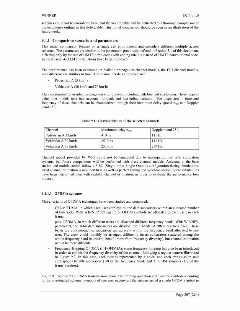
WINNER D2.6 v 1.0

Page 207 (264)

schemes could not be considered here, and the next months will be dedicated to a thorough comparison of the techniques outlind in this deliverable. This initial comparison should be seen as an illustration of the future work.

9.4.1 Comparison scenario and parameters This initial comparison focuses on a single cell environment and considers different multiple access schemes. The parameters are similar to the parameters previously defined in Section 3.1 of this document, differing only by the use of UMTS turbo code (with coding rate ½) instead of UMTS convolutional code. In most cases, 4-QAM constellations have been employed. The performance has been evaluated on realistic propagation channel models, the ITU channel models, with different variabilities in time. The channel models employed are:

- Pedestrian A (3 km/h)

- Vehicular A (30 km/h and 70 km/h)

They correspond to an urban propagation environment, including path loss and shadowing. These tapped-delay line models take into account multipath and fast-fading variation. The dispersion in time and frequency of these channels can be characterized through their maximum delay spread τmax and Doppler band 2*fD:

Table 9.1: Characteristics of the selected channels

Channel Maximum delay τmax Doppler band 2*fD Pedestrian A 3 km/h 410 ns 11 Hz Vehicular A 30 km/h 2510 ns 111 Hz Vehicular A 70 km/h 2510 ns 259 Hz

Channel model provided by WP5 could not be employed due to incompatibilities with simulation systems, but future comparisons will be performed with these channel models. Antennas at the base station and mobile station follow a SISO (Single-Input Single-Output) configuration during simulations. Ideal channel estimation is assumed first, as well as perfect timing and synchronisation. Some simulations have been performed then with realistic channel estimation, in order to evaluate the performance loss induced.

9.4.1.1 OFDMA schemes

Three variants of OFDMA techniques have been studied and compared:

- OFDM/TDMA, in which each user employs all the data subcarriers within an allocated number of time slots. With WINNER settings, three OFDM symbols are allocated to each user, in each frame.

- pure OFDMA, in which different users are allocated different frequency bands. With WINNER parameters, the 1664 data subcarriers are divided into 8 bands of 208 subcarriers each. These bands are continuous, i.e. subcarriers are adjacent within the frequency band allocated to one user. The users could possibly be arranged differently (users subcarriers scattered among the whole frequency band in order to benefit more from frequency diversity), but channel estimation would be more difficult.

- Frequency-Hopping OFDMA (FH-OFDMA): some frequency hopping has also been introduced in order to exploit the frequency diversity of the channel, following a regular pattern illustrated in Figure 9.2. In this case, each user is represented by a color, and each transmission unit corresponds to 208 subcarriers (1/8 of the frequency band) and 3 OFDM symbols (1/8 of the frame duration).

Figure 9.1 represents OFDMA transmission chain. The framing operation arranges the symbols according to the investigated scheme: symbols of one user occupy all the subcarriers of a single OFDM symbol in

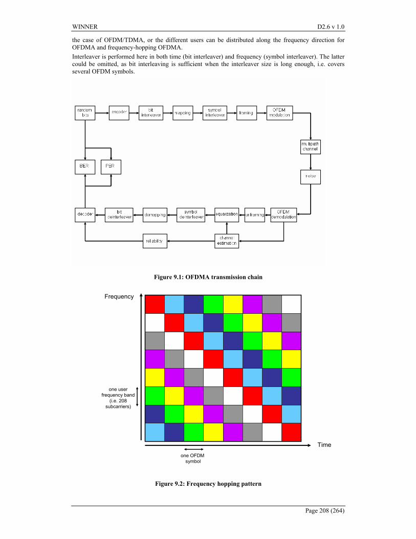
WINNER D2.6 v 1.0

Page 208 (264)

the case of OFDM/TDMA, or the different users can be distributed along the frequency direction for OFDMA and frequency-hopping OFDMA. Interleaver is performed here in both time (bit interleaver) and frequency (symbol interleaver). The latter could be omitted, as bit interleaving is sufficient when the interleaver size is long enough, i.e. covers several OFDM symbols.

Figure 9.1: OFDMA transmission chain

Time

Frequency

one OFDM symbol

one user frequency band

(i.e. 208 subcarriers)

Figure 9.2: Frequency hopping pattern

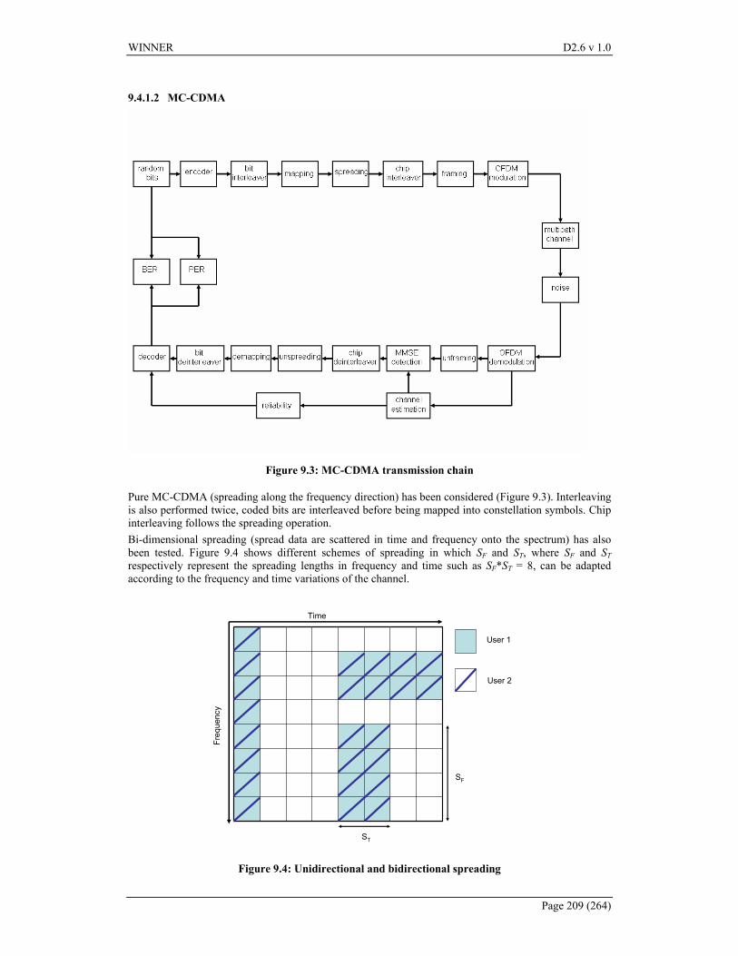
WINNER D2.6 v 1.0

Page 209 (264)

9.4.1.2 MC-CDMA

Figure 9.3: MC-CDMA transmission chain

Pure MC-CDMA (spreading along the frequency direction) has been considered (Figure 9.3). Interleaving is also performed twice, coded bits are interleaved before being mapped into constellation symbols. Chip interleaving follows the spreading operation. Bi-dimensional spreading (spread data are scattered in time and frequency onto the spectrum) has also been tested. Figure 9.4 shows different schemes of spreading in which SF and ST, where SF and ST respectively represent the spreading lengths in frequency and time such as SF*ST = 8, can be adapted according to the frequency and time variations of the channel.

Time

User 1

User 2

ST

SF

Freq

uenc

y

Figure 9.4: Unidirectional and bidirectional spreading

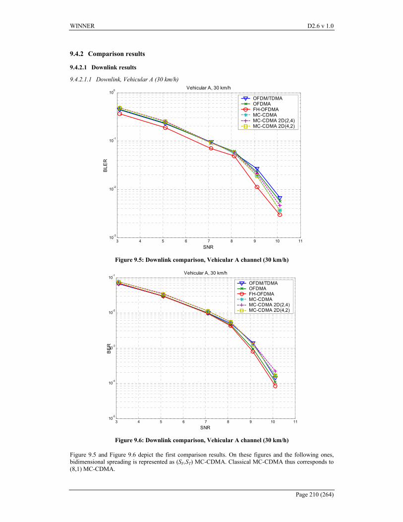
WINNER D2.6 v 1.0

Page 210 (264)

9.4.2 Comparison results

9.4.2.1 Downlink results

9.4.2.1.1 Downlink, Vehicular A (30 km/h)

3 4 5 6 7 8 9 10 1110-3

10-2

10-1

100

SNR

BLE

R

Vehicular A, 30 km/h

OFDM/TDMAOFDMAFH-OFDMAMC-CDMAMC-CDMA 2D(2,4)MC-CDMA 2D(4,2)

Figure 9.5: Downlink comparison, Vehicular A channel (30 km/h)

3 4 5 6 7 8 9 10 1110

-5

10-4

10-3

10-2

10-1

SNR

BE

R

Vehicular A, 30 km/h

OFDM/TDMAOFDMAFH-OFDMAMC-CDMAMC-CDMA 2D(2,4)MC-CDMA 2D(4,2)

Figure 9.6: Downlink comparison, Vehicular A channel (30 km/h)

Figure 9.5 and Figure 9.6 depict the first comparison results. On these figures and the following ones, bidimensional spreading is represented as (SF,ST) MC-CDMA. Classical MC-CDMA thus corresponds to (8,1) MC-CDMA.

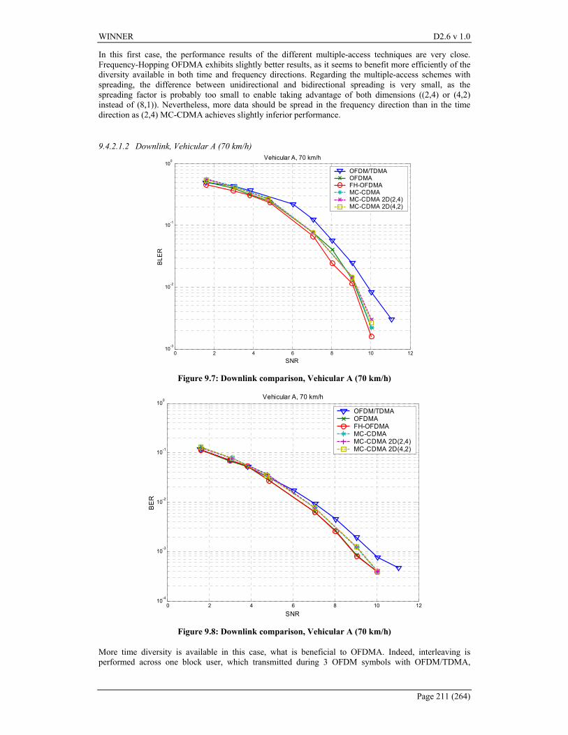
WINNER D2.6 v 1.0

Page 211 (264)

In this first case, the performance results of the different multiple-access techniques are very close. Frequency-Hopping OFDMA exhibits slightly better results, as it seems to benefit more efficiently of the diversity available in both time and frequency directions. Regarding the multiple-access schemes with spreading, the difference between unidirectional and bidirectional spreading is very small, as the spreading factor is probably too small to enable taking advantage of both dimensions ((2,4) or (4,2) instead of (8,1)). Nevertheless, more data should be spread in the frequency direction than in the time direction as (2,4) MC-CDMA achieves slightly inferior performance.

9.4.2.1.2 Downlink, Vehicular A (70 km/h)

0 2 4 6 8 10 1210-3

10-2

10-1

100

SNR

BLE

RVehicular A, 70 km/h

OFDM/TDMAOFDMAFH-OFDMAMC-CDMAMC-CDMA 2D(2,4)MC-CDMA 2D(4,2)

Figure 9.7: Downlink comparison, Vehicular A (70 km/h)

0 2 4 6 8 10 1210-4

10-3

10-2

10-1

100

SNR

BE

R

Vehicular A, 70 km/h

OFDM/TDMAOFDMAFH-OFDMAMC-CDMAMC-CDMA 2D(2,4)MC-CDMA 2D(4,2)

Figure 9.8: Downlink comparison, Vehicular A (70 km/h)

More time diversity is available in this case, what is beneficial to OFDMA. Indeed, interleaving is performed across one block user, which transmitted during 3 OFDM symbols with OFDM/TDMA,

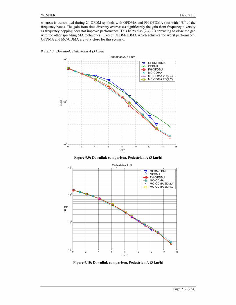
WINNER D2.6 v 1.0

Page 212 (264)

whereas is transmitted during 24 OFDM symbols with OFDMA and FH-OFDMA (but with 1/8th of the frequency band). The gain from time diversity overpasses significantly the gain from frequency diversity as frequency hopping does not improve performance. This helps also (2,4) 2D spreading to close the gap with the other spreading MA techniques . Except OFDM/TDMA which achieves the worst performance, OFDMA and MC-CDMA are very close for this scenario.

9.4.2.1.3 Downlink, Pedestrian A (3 km/h)

0 2 4 6 8 10 12 14 1610

-2

10-1

100

SNR

BLE

RPedestrian A, 3 km/h

OFDM/TDMAOFDMAFH-OFDMAMC-CDMAMC-CDMA 2D(2,4)MC-CDMA 2D(4,2)

Figure 9.9: Downlink comparison, Pedestrian A (3 km/h)

0 2 4 6 8 10 12 14 16 10-3

10-2

10-1

100

SNR

BER

Pedestrian A, 3 km/h

OFDM/TDMAOFDMAFH-OFDMAMC-CDMAMC-CDMA 2D(2,4) MC-CDMA 2D(4,2)

Figure 9.10: Downlink comparison, Pedestrian A (3 km/h)

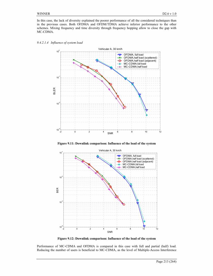
WINNER D2.6 v 1.0

Page 213 (264)

In this case, the lack of diversity explained the poorer performance of all the considered techniques than in the previous cases. Both OFDMA and OFDM/TDMA achieve inferior performance to the other schemes. Mixing frequency and time diversity through frequency hopping allow to close the gap with MC-CDMA.

9.4.2.1.4 Influence of system load

-2 0 2 4 6 8 10 1210-3

10-2

10-1

100

SNR

BLE

R

Vehicular A, 30 km/h

OFDMA, full loadOFDMA,half load (scattered)OFDMA,half load (adjacent)MC-CDMA,full loadMC-CDMA,half load

Figure 9.11: Downlink comparison: Influence of the load of the system

-2 0 2 4 6 8 10 1210-4

10-3

10-2

10-1

SNR

BE

R

Vehicular A, 30 km/h

OFDMA, full loadOFDMA,half load (scattered)OFDMA,half load (adjacent)MC-CDMA,full loadMC-CDMA,half load

Figure 9.12: Downlink comparison: Influence of the load of the system

Performance of MC-CDMA and OFDMA is compared in this case with full and partial (half) load. Reducing the number of users is beneficial to MC-CDMA, as the level of Multiple-Access Interference

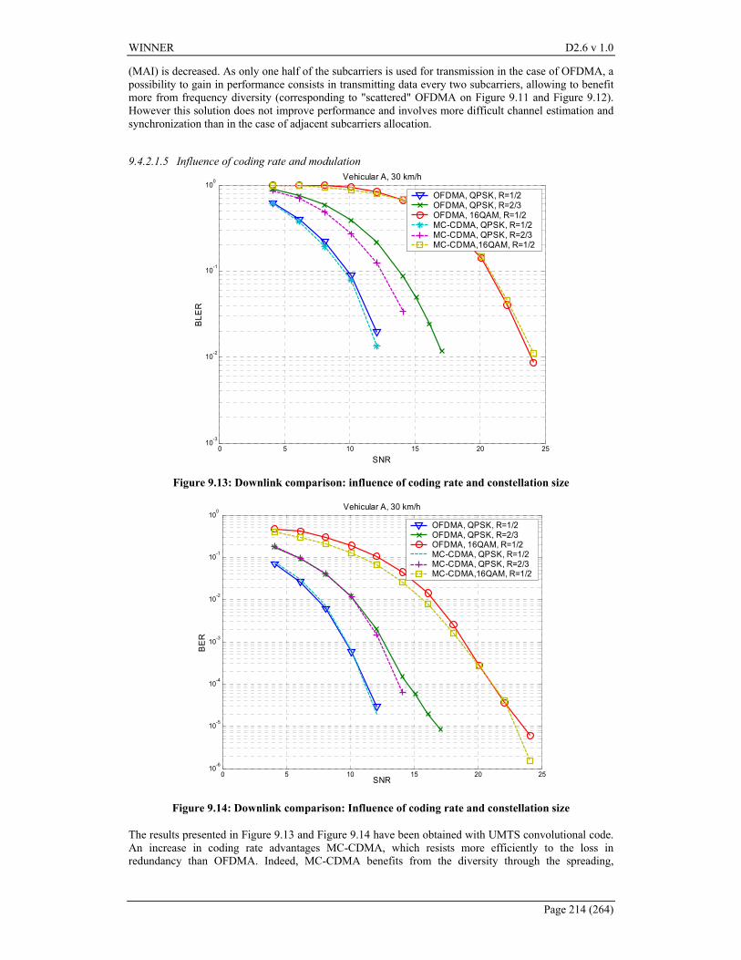
WINNER D2.6 v 1.0

Page 214 (264)

(MAI) is decreased. As only one half of the subcarriers is used for transmission in the case of OFDMA, a possibility to gain in performance consists in transmitting data every two subcarriers, allowing to benefit more from frequency diversity (corresponding to "scattered" OFDMA on Figure 9.11 and Figure 9.12). However this solution does not improve performance and involves more difficult channel estimation and synchronization than in the case of adjacent subcarriers allocation.

9.4.2.1.5 Influence of coding rate and modulation

0 5 10 15 20 2510-3

10-2

10-1

100

SNR

BLE

R

Vehicular A, 30 km/h

OFDMA, QPSK, R=1/2OFDMA, QPSK, R=2/3OFDMA, 16QAM, R=1/2MC-CDMA, QPSK, R=1/2MC-CDMA, QPSK, R=2/3MC-CDMA,16QAM, R=1/2

Figure 9.13: Downlink comparison: influence of coding rate and constellation size

0 5 10 15 20 2510-6

10-5

10-4

10-3

10-2

10-1

100

SNR

BE

R

Vehicular A, 30 km/h

OFDMA, QPSK, R=1/2OFDMA, QPSK, R=2/3OFDMA, 16QAM, R=1/2MC-CDMA, QPSK, R=1/2MC-CDMA, QPSK, R=2/3MC-CDMA,16QAM, R=1/2

Figure 9.14: Downlink comparison: Influence of coding rate and constellation size

The results presented in Figure 9.13 and Figure 9.14 have been obtained with UMTS convolutional code. An increase in coding rate advantages MC-CDMA, which resists more efficiently to the loss in redundancy than OFDMA. Indeed, MC-CDMA benefits from the diversity through the spreading,

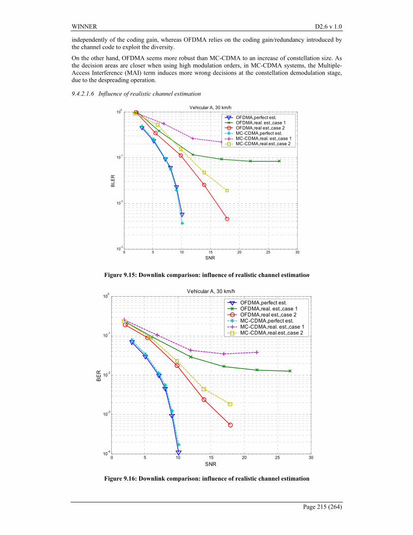
WINNER D2.6 v 1.0

Page 215 (264)

independently of the coding gain, whereas OFDMA relies on the coding gain/redundancy introduced by the channel code to exploit the diversity.

On the other hand, OFDMA seems more robust than MC-CDMA to an increase of constellation size. As the decision areas are closer when using high modulation orders, in MC-CDMA systems, the Multiple-Access Interference (MAI) term induces more wrong decisions at the constellation demodulation stage, due to the despreading operation.

9.4.2.1.6 Influence of realistic channel estimation

0 5 10 15 20 25 3010-3

10-2

10-1

100

SNR

BLE

RVehicular A, 30 km/h

OFDMA,perfect est.OFDMA,real. est.,case 1OFDMA,real est.,case 2MC-CDMA,perfect est.MC-CDMA,real. est.,case 1MC-CDMA,real.est.,case 2

Figure 9.15: Downlink comparison: influence of realistic channel estimation

0 5 10 15 20 25 3010-4

10-3

10-2

10-1

100

SNR

BE

R

Vehicular A, 30 km/h

OFDMA,perfect est.OFDMA,real. est.,case 1OFDMA,real est.,case 2MC-CDMA,perfect est.MC-CDMA,real. est.,case 1MC-CDMA,real.est.,case 2

Figure 9.16: Downlink comparison: influence of realistic channel estimation

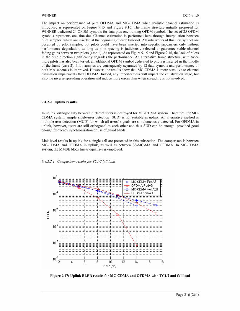
WINNER D2.6 v 1.0

Page 216 (264)

The impact on performance of pure OFDMA and MC-CDMA when realistic channel estimation is introduced is represented on Figure 9.15 and Figure 9.16. The frame structure initially proposed for WINNER dedicated 24 OFDM symbols for data plus one training OFDM symbol. The set of 25 OFDM symbols represents one timeslot. Channel estimation is performed here through interpolation between pilot samples, which are inserted at the beginning of each timeslot. All subcarriers of this first symbol are occupied by pilot samples, but pilots could have been inserted into specific subcarriers only without performance degradation, as long as pilot spacing is judiciously selected to guarantee stable channel fading gains between two pilots (case 1). As represented on Figure 9.15 and Figure 9.16, the lack of pilots in the time direction significantly degrades the performance. An alternative frame structure, with twice more pilots has also been tested: an additional OFDM symbol dedicated to pilots is inserted in the middle of the frame (case 2). Pilot samples are consequently separated by 12 data symbols and performance of both MA schemes is improved. However, the results show that MC-CDMA is more sensitive to channel estimation impairments than OFDMA. Indeed, any imperfectness will impact the equalization stage, but also the inverse spreading operation and induce more errors than when spreading is not involved.

9.4.2.2 Uplink results In uplink, orthogonality between different users is destroyed for MC-CDMA system. Therefore, for MC-CDMA system, simple single-user detection (SUD) is not suitable in uplink. An alternative method is multiple user detection (MUD) for which all users’ signals are simultaneously detected. For OFDMA in uplink, however, users are still orthogonal to each other and thus SUD can be enough, provided good enough frequency synchronization or use of guard bands. Link level results in uplink for a single cell are presented in this subsection. The comparison is between MC-CDMA and OFDMA in uplink, as well as between SS-MC-MA and OFDMA. In MC-CDMA system, the MMSE block linear equalizer is employed.

9.4.2.2.1 Comparison results for TC1/2 full load

Figure 9.17: Uplink BLER results for MC-CDMA and OFDMA with TC1/2 and full load

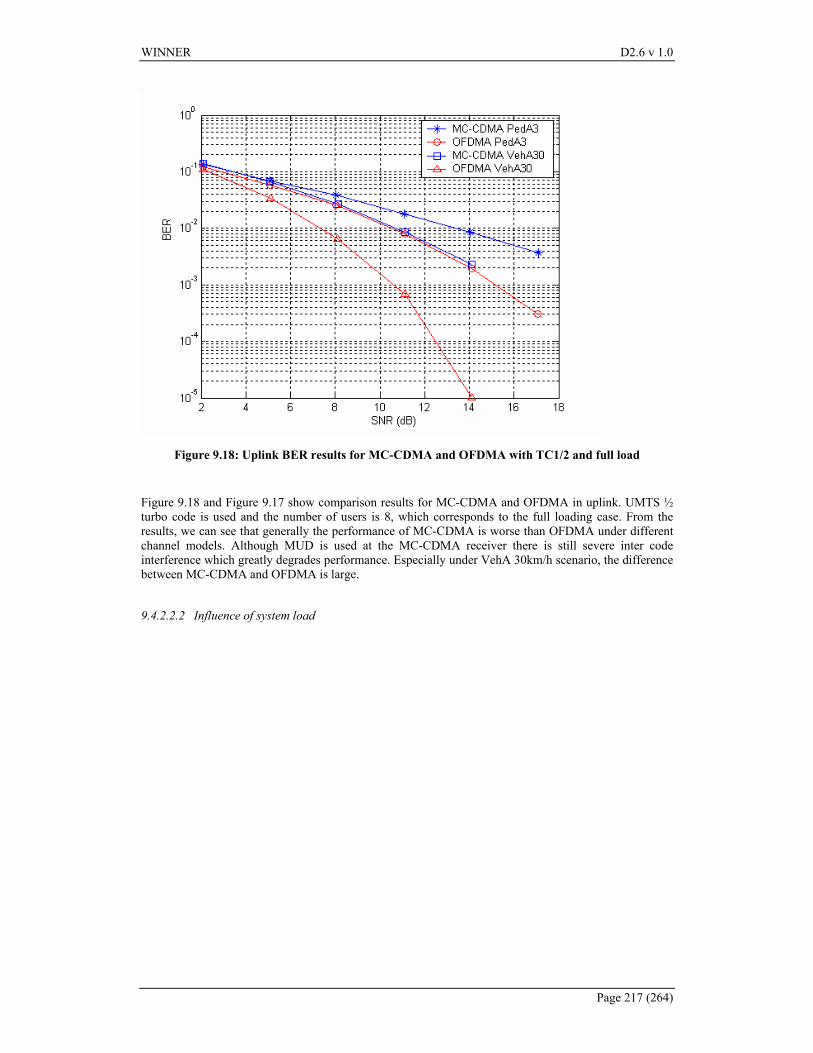
WINNER D2.6 v 1.0

Page 217 (264)

Figure 9.18: Uplink BER results for MC-CDMA and OFDMA with TC1/2 and full load

Figure 9.18 and Figure 9.17 show comparison results for MC-CDMA and OFDMA in uplink. UMTS ½ turbo code is used and the number of users is 8, which corresponds to the full loading case. From the results, we can see that generally the performance of MC-CDMA is worse than OFDMA under different channel models. Although MUD is used at the MC-CDMA receiver there is still severe inter code interference which greatly degrades performance. Especially under VehA 30km/h scenario, the difference between MC-CDMA and OFDMA is large.

9.4.2.2.2 Influence of system load

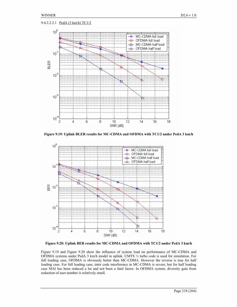
WINNER D2.6 v 1.0

Page 218 (264)

9.4.2.2.2.1 PedA (3 km/h) TC1/2

Figure 9.19: Uplink BLER results for MC-CDMA and OFDMA with TC1/2 under PedA 3 km/h

Figure 9.20: Uplink BER results for MC-CDMA and OFDMA with TC1/2 under PedA 3 km/h

Figure 9.19 and Figure 9.20 show the influence of system load on performance of MC-CDMA and OFDMA systems under PedA 3 km/h model in uplink. UMTS ½ turbo code is used for simulation. For full loading case, OFDMA is obviously better than MC-CDMA. However the reverse is true for half loading case. For full loading case, inter code interference in MC-CDMA is severe, but for half loading case MAI has been reduced a lot and not been a fatal factor. In OFDMA system, diversity gain from reduction of user number is relatively small.

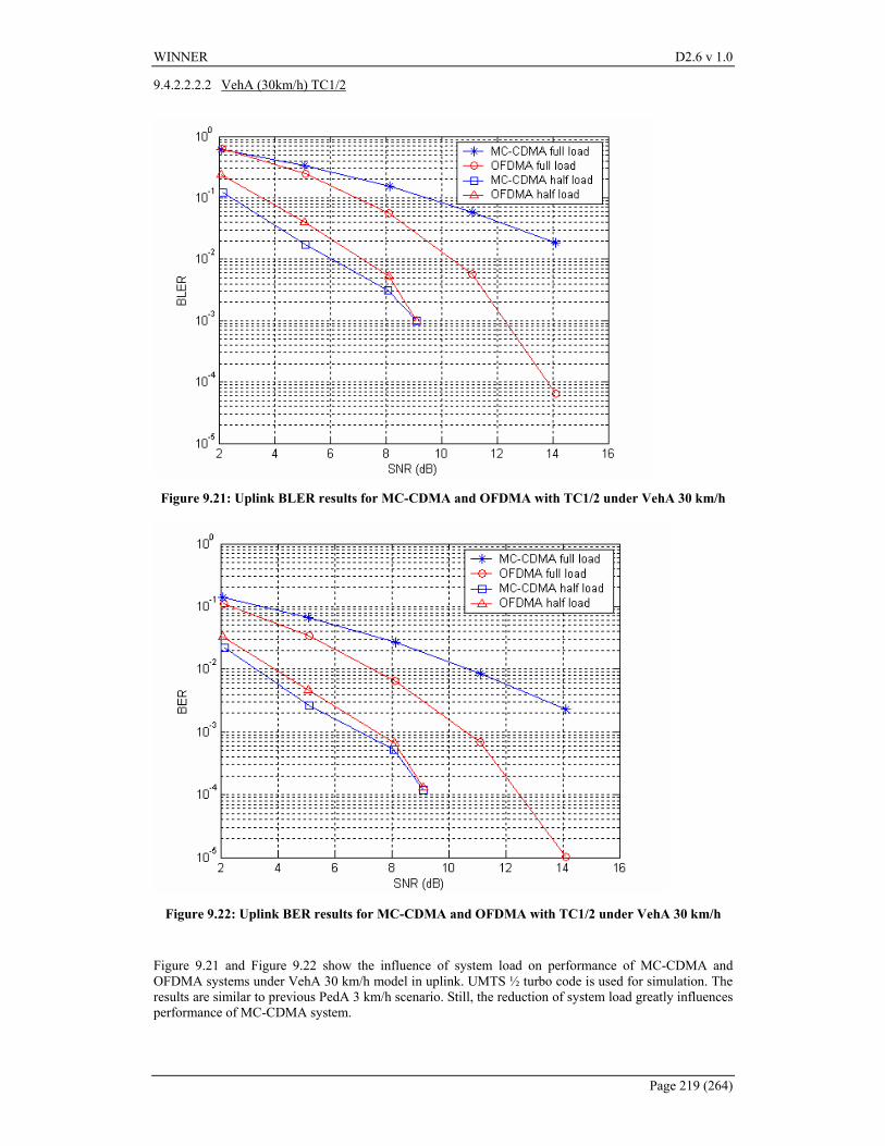
WINNER D2.6 v 1.0

Page 219 (264)

9.4.2.2.2.2 VehA (30km/h) TC1/2

Figure 9.21: Uplink BLER results for MC-CDMA and OFDMA with TC1/2 under VehA 30 km/h

Figure 9.22: Uplink BER results for MC-CDMA and OFDMA with TC1/2 under VehA 30 km/h

Figure 9.21 and Figure 9.22 show the influence of system load on performance of MC-CDMA and OFDMA systems under VehA 30 km/h model in uplink. UMTS ½ turbo code is used for simulation. The results are similar to previous PedA 3 km/h scenario. Still, the reduction of system load greatly influences performance of MC-CDMA system.

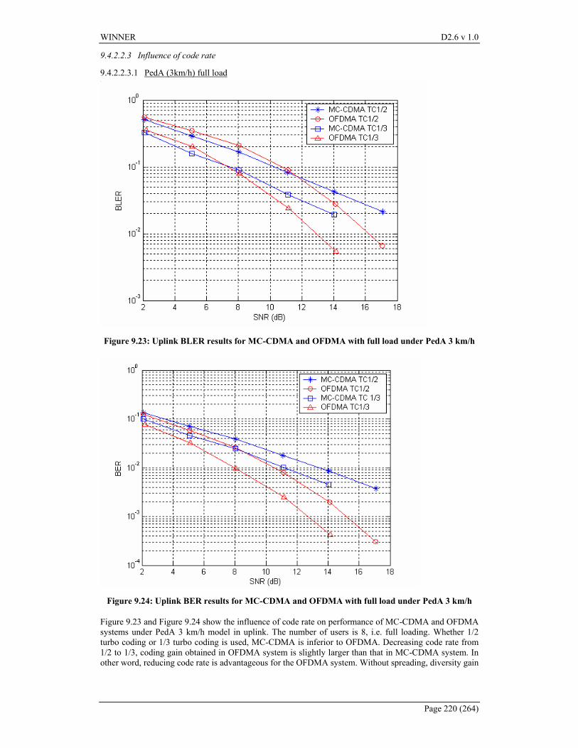
WINNER D2.6 v 1.0

Page 220 (264)

9.4.2.2.3 Influence of code rate

9.4.2.2.3.1 PedA (3km/h) full load

Figure 9.23: Uplink BLER results for MC-CDMA and OFDMA with full load under PedA 3 km/h

Figure 9.24: Uplink BER results for MC-CDMA and OFDMA with full load under PedA 3 km/h

Figure 9.23 and Figure 9.24 show the influence of code rate on performance of MC-CDMA and OFDMA systems under PedA 3 km/h model in uplink. The number of users is 8, i.e. full loading. Whether 1/2 turbo coding or 1/3 turbo coding is used, MC-CDMA is inferior to OFDMA. Decreasing code rate from 1/2 to 1/3, coding gain obtained in OFDMA system is slightly larger than that in MC-CDMA system. In other word, reducing code rate is advantageous for the OFDMA system. Without spreading, diversity gain

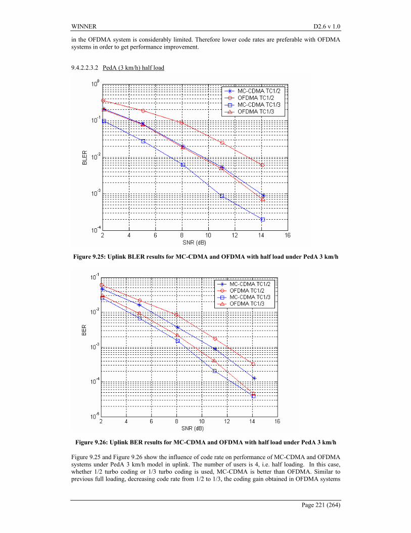
WINNER D2.6 v 1.0

Page 221 (264)

in the OFDMA system is considerably limited. Therefore lower code rates are preferable with OFDMA systems in order to get performance improvement.

9.4.2.2.3.2 PedA (3 km/h) half load

Figure 9.25: Uplink BLER results for MC-CDMA and OFDMA with half load under PedA 3 km/h

Figure 9.26: Uplink BER results for MC-CDMA and OFDMA with half load under PedA 3 km/h

Figure 9.25 and Figure 9.26 show the influence of code rate on performance of MC-CDMA and OFDMA systems under PedA 3 km/h model in uplink. The number of users is 4, i.e. half loading. In this case, whether 1/2 turbo coding or 1/3 turbo coding is used, MC-CDMA is better than OFDMA. Similar to previous full loading, decreasing code rate from 1/2 to 1/3, the coding gain obtained in OFDMA systems

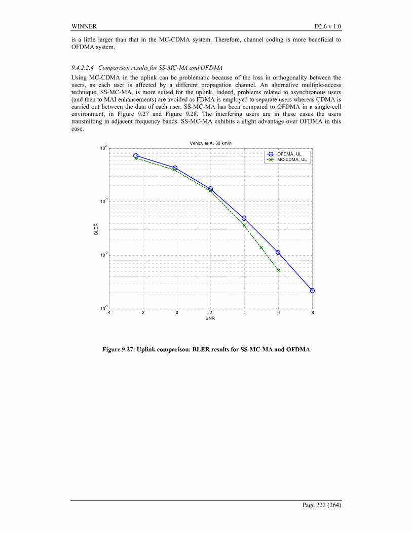
WINNER D2.6 v 1.0

Page 222 (264)

is a little larger than that in the MC-CDMA system. Therefore, channel coding is more beneficial to OFDMA system.

9.4.2.2.4 Comparison results for SS-MC-MA and OFDMA Using MC-CDMA in the uplink can be problematic because of the loss in orthogonality between the users, as each user is affected by a different propagation channel. An alternative multiple-access technique, SS-MC-MA, is more suited for the uplink. Indeed, problems related to asynchronous users (and then to MAI enhancements) are avoided as FDMA is employed to separate users whereas CDMA is carried out between the data of each user. SS-MC-MA has been compared to OFDMA in a single-cell environment, in Figure 9.27 and Figure 9.28. The interfering users are in these cases the users transmitting in adjacent frequency bands. SS-MC-MA exhibits a slight advantage over OFDMA in this case.

-4 -2 0 2 4 6 810

-3

10-2

10-1

100

SNR

BLE

R

Vehicular A, 30 km/h

OFDMA, ULMC-CDMA, UL

Figure 9.27: Uplink comparison: BLER results for SS-MC-MA and OFDMA

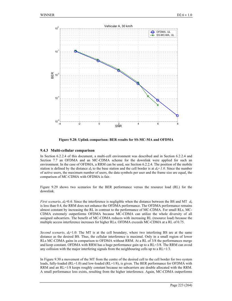
WINNER D2.6 v 1.0

Page 223 (264)

-4 -2 0 2 4 6 810-4

10-3

10-2

10-1

100

SNR

BE

R

Vehicular A, 30 km/h

OFDMA, ULSS-MC-MA, UL

Figure 9.28: Uplink comparison: BER results for SS-MC-MA and OFDMA

9.4.3 Multi-cellular comparison In Section 6.2.2.4 of this document, a multi-cell environment was described and in Section 6.2.2.4 and Section 7.7 an OFDMA and an MC-CDMA scheme for the downlink were applied for such an environment. In the case of OFDMA, a RRM can be used, see Section 6.2.2.4. The position of the mobile station is defined by the distance d0 to the base station and the cell border is at d0=1.0. Since the number of active users, the maximum number of users, the data symbols per user and the frame size are equal, the comparison of MC-CDMA with OFDMA is fair. Figure 9.29 shows two scenarios for the BER performance versus the resource load (RL) for the downlink. First scenario, d0=0.4: Since the interference is negligible when the distance between the BS and MT d0 is less than 0.4, the RRM does not enhance the OFDMA performance. The OFDMA performance remains almost constant by increasing the RL in contrast to the performance of MC-CDMA. For small RLs, MC-CDMA extremely outperforms OFDMA because MC-CDMA can utilize the whole diversity of all assigned subcarriers. The benefit of MC-CDMA reduces with increasing RL (resource load) because the multiple access interference increases for higher RLs. OFDMA exceeds MC-CDMA at a RL of 0.75. Second scenario, d0=1.0: The MT is at the cell boundary, where two interfering BS are at the same distance as the desired BS. Thus, the cellular interference is maximal. Only in a small region of lower RLs MC-CDMA gains in comparison to OFDMA without RRM. At a RL of 3/8 the performances merge and keep constant. OFDMA with RRM has a huge performance gain up to a RL=3/8. The RRM can avoid any collision with the major interfering signals from the neighbouring cells up to a RL=1/3. In Figure 9.30 a movement of the MT from the centre of the desired cell to the cell border for two system loads, fully-loaded (RL=1.0) and low-loaded (RL=1/8), is given. The BER performance for OFDMA with RRM and an RL=1/8 keeps roughly constant because no subcarriers are double allocated with the RRM. A small performance loss exists, resulting from the higher interference. Again, MC-CDMA outperforms

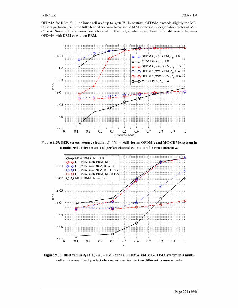
WINNER D2.6 v 1.0

Page 224 (264)

OFDMA for RL=1/8 in the inner cell area up to d0=0.75. In contrast, OFDMA exceeds slightly the MC-CDMA performance in the fully-loaded scenario because the MAI is the major degradation factor of MC-CDMA. Since all subcarriers are allocated in the fully-loaded case, there is no difference between OFDMA with RRM or without RRM.

Figure 9.29: BER versus resource load at dB10/ 0b =NE for an OFDMA and MC-CDMA system in a multi-cell environment and perfect channel estimation for two different d0

Figure 9.30: BER versus d0 at dB10/ 0b =NE for an OFDMA and MC-CDMA system in a multi-cell environment and perfect channel estimation for two different resource loads

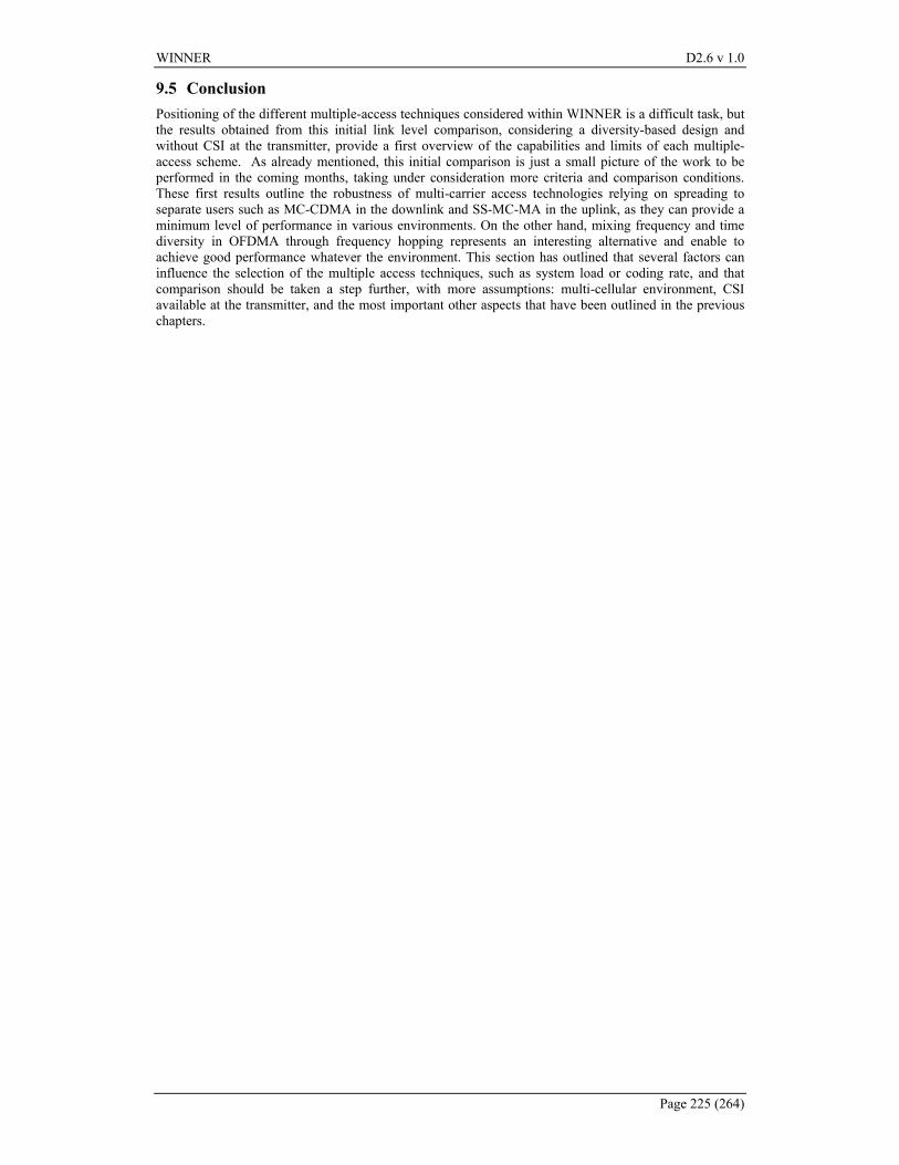
WINNER D2.6 v 1.0

Page 225 (264)

9.5 Conclusion Positioning of the different multiple-access techniques considered within WINNER is a difficult task, but the results obtained from this initial link level comparison, considering a diversity-based design and without CSI at the transmitter, provide a first overview of the capabilities and limits of each multiple-access scheme. As already mentioned, this initial comparison is just a small picture of the work to be performed in the coming months, taking under consideration more criteria and comparison conditions. These first results outline the robustness of multi-carrier access technologies relying on spreading to separate users such as MC-CDMA in the downlink and SS-MC-MA in the uplink, as they can provide a minimum level of performance in various environments. On the other hand, mixing frequency and time diversity in OFDMA through frequency hopping represents an interesting alternative and enable to achieve good performance whatever the environment. This section has outlined that several factors can influence the selection of the multiple access techniques, such as system load or coding rate, and that comparison should be taken a step further, with more assumptions: multi-cellular environment, CSI available at the transmitter, and the most important other aspects that have been outlined in the previous chapters.

WINNER D2.6 v 1.0

Page 226 (264)

10. Multiple Access and System Design System design issues have been discussed in relation to some specific types of multiple access schemes, see for example Sections 6.1.1 and 6.1.2. This chapter discusses preliminary studies on some aspects of general relevance, aimed at identifying crucial points for further studies. First, the choice of duplex scheme affects the design and performance of multiple access methods. Section 10.1 provides a short review on the duplex method considered in the report [WIN_D25], and on their interaction with the choice of multiple access scheme. A discussion on the effect of the choice of TDD or FDD in the particular case of OFDMA/TDMA can furthermore be found in Section 6.1.2. The type of system deployment implicitly assumed in previous chapters has been that of a cellular infrastructure-based system. Section 10.2 introduces extensions of that concept in the form of cooperative diversity and relaying, issues to be studied in collaboration with WP3 of WINNER, by studying the ideas introduced in Section 10.2. The diversity effect is here mainly discussed within the averaging-based paradigm mentioned in Section 1. Section 10.3 discusses some issues related to MAC protocols, scheduling and link-level retransmission. Section 10.4 finally provides an initial discussion of problems related to peer-to-peer transmissions, ad-hoc networking, broadcasting and multicasting.

10.1 Duplexing The choice of duplexing scheme has been studied in depth in the WINNER project and the results can be found in [WIN_D25]. This section describes the impact that the choice of the multiple access scheme has on the choice of duplex scheme.

A number of different duplexing options were considered. The most promising candidates being:

• Pure TDD,

• Dual Band TDD,

• Half Duplex FDD.

These options were chosen for the strengths that they possess in different scenarios.

10.1.1 Reciprocity

One of the advantages stated for TDD based duplexes is that the channel can be considered reciprocal. It is unclear at the present time how this reciprocity can be used in a WINNER system. One aspect that is clear, however, is that in the short term interference levels are not reciprocal and so TDD does not give an advantage for link adaptation techniques requiring knowledge of interference conditions.

Section 6.1.4.2 of this document analyses the effect that the choice of duplex scheme has on reaction delay and thus the maximum mobile speed at which a link adaptation scheme can cope with frequency selective fading. The analysis shows that FDD has a faster reaction delay than TDD and can therefore support faster moving users if the same amount of information is feed back in each scheme. The time slot structures of the half duplex FDD scheme give the same reaction delay as FDD because the access point is capable of simultaneous transmission and reception. Thus half duplex FDD has an advantage over the TDD based options in this regard.

The reciprocity of the TDD duplex may give advantages when using SDMA although the use of SDMA does not preclude a half duplex FDD scheme. There may also be gains when using some of the more ground-breaking MIMO pre-equalisation techniques. These aspects are for further study.

10.1.2 Interference

Another advantage stated for TDD systems is that different uplink / downlink asymmetries can be supported by changing the switching point. This can be easily managed in isolated cells, however, when incorporated into a cellular network UL DL and DL UL interference become a serious problem. The elimination of the problem requires synchronising the cells in the network and setting all switching points equally (co-ordinating). This removes some of the flexibility of the asymmetry. Interference avoidance methods could be employed to cope with such a problem as shown in [WIN_D25].

WINNER D2.6 v 1.0

Page 227 (264)

However, the interference issue becomes more severe when two operators co-exist within the same area, especially in case of co-location of access points. However, in this case, it is likely that the operators will have similar requirements in terms of traffic asymmetry, so that co-ordination of switching points might not prevent service flexibility.

Half Duplex FDD can manage the interference between UL and DL by having a suitable duplex distance at the expense of asymmetry.

10.1.3 Dual bandwidth systems

Dual bandwidth systems are being investigated as discussed in Section 6.4 to reduce power consumption when using long range, low data rate services. For this reason, the dual band TDD scheme is being considered. However, such a system would need to operate in a synchronised and co-ordinated network due to the interference problems associated with TDD based systems.

10.2 System deployment

10.2.1 Introduction

Future communications systems are expected to fulfill stringent requirements in terms of data rates, coverage and efficiency. Relaying techniques will contribute to the achievement of these goals. Relaying is beneficial in several respects, both in ad-hoc networks, for which it represents the basic building block, and in cellular networks. In general, relays are used to extend the network connectivity, to use more efficiently the resources and obtain cost-efficient network architectures. Although twice the network resources of a single-hop are required, the power requirements for reliable communication over a link are lowered due to shorter-distance transmissions. Thus, from an efficiency point of view, multihop transmissions relayed by intermediary nodes might be preferable to a single-hop between two distant nodes. In fact, relaying increases throughput by reducing transmission range and, as an important consequence, it also mitigates co-channel interference.

Recently, a particular type of relaying has been pointed out in literature, namely “cooperative diversity” or “user cooperation diversity”. It is particularly beneficial for wireless channels, where the random fluctuations that the received signal level experiences, termed as fading, cause very poor error performance. Diversity techniques are used to combat this impairment and improve the link reliability. Over the years, several forms of diversity have been considered, either in time, frequency or space. Cooperative diversity aims at achieving the same objective but in a distributed fashion.

As illustrated in Figure 10.1, there are various types of relaying, each of those resulting in different degrees of complexity and performance. The scheme with lowest complexity is the repeater, which either relays the signal after amplification or that decodes it before forwarding it. Additionally, several techniques achieving transmit diversity can be envisioned when multiple relays take part to the forwarding process. For instance, the same packet can be transmitted from several relays using different processing (e.g. delay diversity) and the destination can receive it more reliably by combining the replicas appropriately. Another method, also used in co-located antennas systems, is selection diversity, where the transmission only happens over the link of best quality. When multiple relays are involved in the transmission, MIMO-like gains can be obtained.

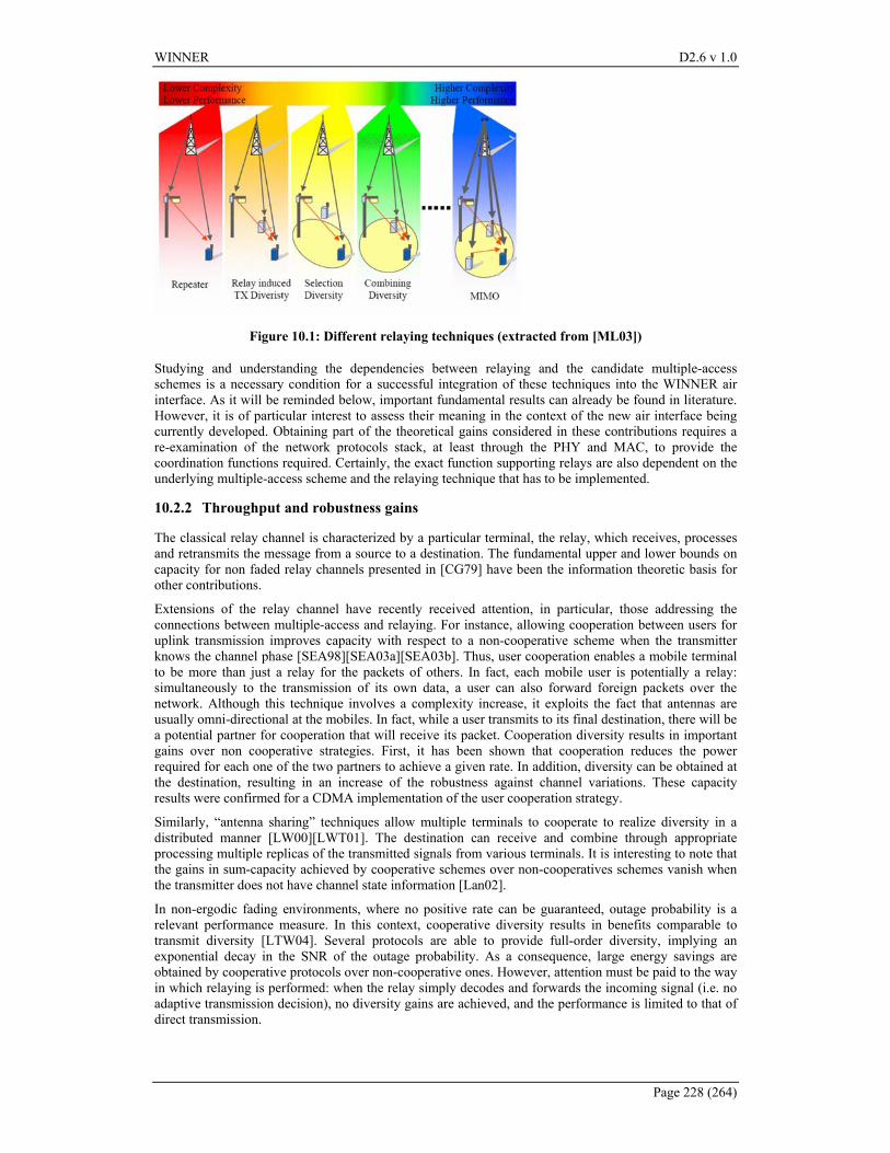
WINNER D2.6 v 1.0

Page 228 (264)

Figure 10.1: Different relaying techniques (extracted from [ML03])

Studying and understanding the dependencies between relaying and the candidate multiple-access schemes is a necessary condition for a successful integration of these techniques into the WINNER air interface. As it will be reminded below, important fundamental results can already be found in literature. However, it is of particular interest to assess their meaning in the context of the new air interface being currently developed. Obtaining part of the theoretical gains considered in these contributions requires a re-examination of the network protocols stack, at least through the PHY and MAC, to provide the coordination functions required. Certainly, the exact function supporting relays are also dependent on the underlying multiple-access scheme and the relaying technique that has to be implemented.

10.2.2 Throughput and robustness gains

The classical relay channel is characterized by a particular terminal, the relay, which receives, processes and retransmits the message from a source to a destination. The fundamental upper and lower bounds on capacity for non faded relay channels presented in [CG79] have been the information theoretic basis for other contributions.

Extensions of the relay channel have recently received attention, in particular, those addressing the connections between multiple-access and relaying. For instance, allowing cooperation between users for uplink transmission improves capacity with respect to a non-cooperative scheme when the transmitter knows the channel phase [SEA98][SEA03a][SEA03b]. Thus, user cooperation enables a mobile terminal to be more than just a relay for the packets of others. In fact, each mobile user is potentially a relay: simultaneously to the transmission of its own data, a user can also forward foreign packets over the network. Although this technique involves a complexity increase, it exploits the fact that antennas are usually omni-directional at the mobiles. In fact, while a user transmits to its final destination, there will be a potential partner for cooperation that will receive its packet. Cooperation diversity results in important gains over non cooperative strategies. First, it has been shown that cooperation reduces the power required for each one of the two partners to achieve a given rate. In addition, diversity can be obtained at the destination, resulting in an increase of the robustness against channel variations. These capacity results were confirmed for a CDMA implementation of the user cooperation strategy.

Similarly, “antenna sharing” techniques allow multiple terminals to cooperate to realize diversity in a distributed manner [LW00][LWT01]. The destination can receive and combine through appropriate processing multiple replicas of the transmitted signals from various terminals. It is interesting to note that the gains in sum-capacity achieved by cooperative schemes over non-cooperatives schemes vanish when the transmitter does not have channel state information [Lan02].

In non-ergodic fading environments, where no positive rate can be guaranteed, outage probability is a relevant performance measure. In this context, cooperative diversity results in benefits comparable to transmit diversity [LTW04]. Several protocols are able to provide full-order diversity, implying an exponential decay in the SNR of the outage probability. As a consequence, large energy savings are obtained by cooperative protocols over non-cooperative ones. However, attention must be paid to the way in which relaying is performed: when the relay simply decodes and forwards the incoming signal (i.e. no adaptive transmission decision), no diversity gains are achieved, and the performance is limited to that of direct transmission.

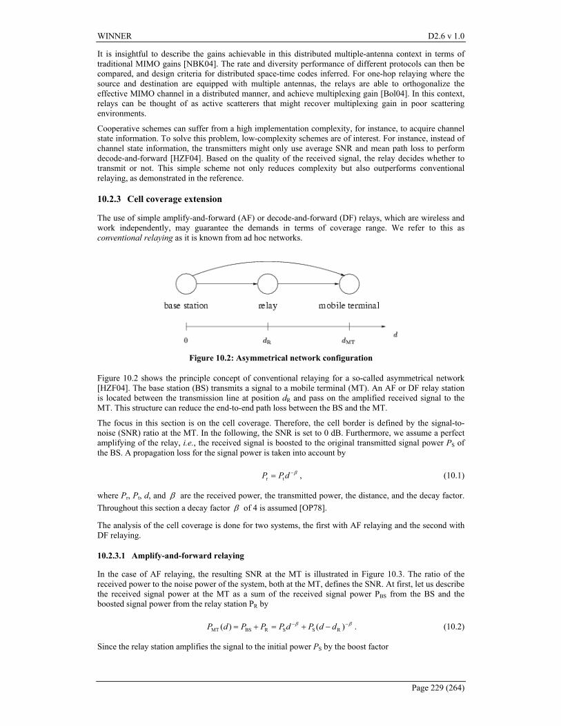
WINNER D2.6 v 1.0

Page 229 (264)

It is insightful to describe the gains achievable in this distributed multiple-antenna context in terms of traditional MIMO gains [NBK04]. The rate and diversity performance of different protocols can then be compared, and design criteria for distributed space-time codes inferred. For one-hop relaying where the source and destination are equipped with multiple antennas, the relays are able to orthogonalize the effective MIMO channel in a distributed manner, and achieve multiplexing gain [Bol04]. In this context, relays can be thought of as active scatterers that might recover multiplexing gain in poor scattering environments.

Cooperative schemes can suffer from a high implementation complexity, for instance, to acquire channel state information. To solve this problem, low-complexity schemes are of interest. For instance, instead of channel state information, the transmitters might only use average SNR and mean path loss to perform decode-and-forward [HZF04]. Based on the quality of the received signal, the relay decides whether to transmit or not. This simple scheme not only reduces complexity but also outperforms conventional relaying, as demonstrated in the reference.

10.2.3 Cell coverage extension

The use of simple amplify-and-forward (AF) or decode-and-forward (DF) relays, which are wireless and work independently, may guarantee the demands in terms of coverage range. We refer to this as conventional relaying as it is known from ad hoc networks.

Figure 10.2: Asymmetrical network configuration

Figure 10.2 shows the principle concept of conventional relaying for a so-called asymmetrical network [HZF04]. The base station (BS) transmits a signal to a mobile terminal (MT). An AF or DF relay station is located between the transmission line at position dR and pass on the amplified received signal to the MT. This structure can reduce the end-to-end path loss between the BS and the MT.

The focus in this section is on the cell coverage. Therefore, the cell border is defined by the signal-to-noise (SNR) ratio at the MT. In the following, the SNR is set to 0 dB. Furthermore, we assume a perfect amplifying of the relay, i.e., the received signal is boosted to the original transmitted signal power PS of the BS. A propagation loss for the signal power is taken into account by

β−= dPP tr , (10.1)

where Pr, Pt, d, and β are the received power, the transmitted power, the distance, and the decay factor. Throughout this section a decay factor β of 4 is assumed [OP78].

The analysis of the cell coverage is done for two systems, the first with AF relaying and the second with DF relaying.

10.2.3.1 Amplify-and-forward relaying

In the case of AF relaying, the resulting SNR at the MT is illustrated in Figure 10.3. The ratio of the received power to the noise power of the system, both at the MT, defines the SNR. At first, let us describe the received signal power at the MT as a sum of the received signal power PBS from the BS and the boosted signal power from the relay station PR by

ββ −− −+=+= )()( RSSRBSMT ddPdPPPdP . (10.2)

Since the relay station amplifies the signal to the initial power PS by the boost factor

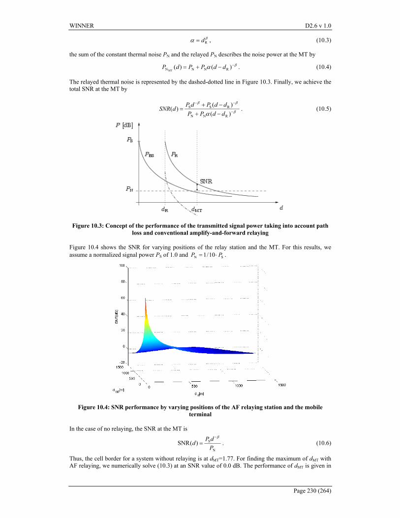
WINNER D2.6 v 1.0

Page 230 (264)

βα Rd= , (10.3)

the sum of the constant thermal noise PN and the relayed PN describes the noise power at the MT by

βα −−+= )()( RNNNMTddPPdP . (10.4)

The relayed thermal noise is represented by the dashed-dotted line in Figure 10.3. Finally, we achieve the total SNR at the MT by

β

ββ

α −

−−

−+−+

=)()(

)(RNN

RSS

ddPPddPdP

dSNR . (10.5)

Figure 10.3: Concept of the performance of the transmitted signal power taking into account path loss and conventional amplify-and-forward relaying

Figure 10.4 shows the SNR for varying positions of the relay station and the MT. For this results, we assume a normalized signal power PS of 1.0 and SN 10/1 PP ⋅= .

Figure 10.4: SNR performance by varying positions of the AF relaying station and the mobile terminal

In the case of no relaying, the SNR at the MT is

N

S)(SNRPdP

dβ−

= . (10.6)

Thus, the cell border for a system without relaying is at dMT=1.77. For finding the maximum of dMT with AF relaying, we numerically solve (10.3) at an SNR value of 0.0 dB. The performance of dMT is given in

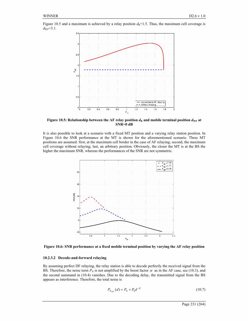
WINNER D2.6 v 1.0

Page 231 (264)

Figure 10.5 and a maximum is achieved by a relay position dR=1.5. Thus, the maximum cell coverage is dMT=3.1.

Figure 10.5: Relationship between the AF relay position dR and mobile terminal position dMT at SNR=0 dB

It is also possible to look at a scenario with a fixed MT position and a varying relay station position. In Figure 10.6 the SNR performance at the MT is shown for the aforementioned scenario. Three MT positions are assumed: first, at the maximum cell border in the case of AF relaying; second, the maximum cell coverage without relaying; last, an arbitrary position. Obviously, the closer the MT is at the BS the higher the maximum SNR, whereas the performances of the SNR are not symmetric.

Figure 10.6: SNR performance at a fixed mobile terminal position by varying the AF relay position

10.2.3.2 Decode-and-forward relaying

By assuming perfect DF relaying, the relay station is able to decode perfectly the received signal from the BS. Therefore, the noise term PN is not amplified by the boost factor α as in the AF case, see (10.3), and the second summand in (10.4) vanishes. Due to the decoding delay, the transmitted signal from the BS appears as interference. Therefore, the total noise is

β−+= dPPdP SNN )(MT

(10.7)

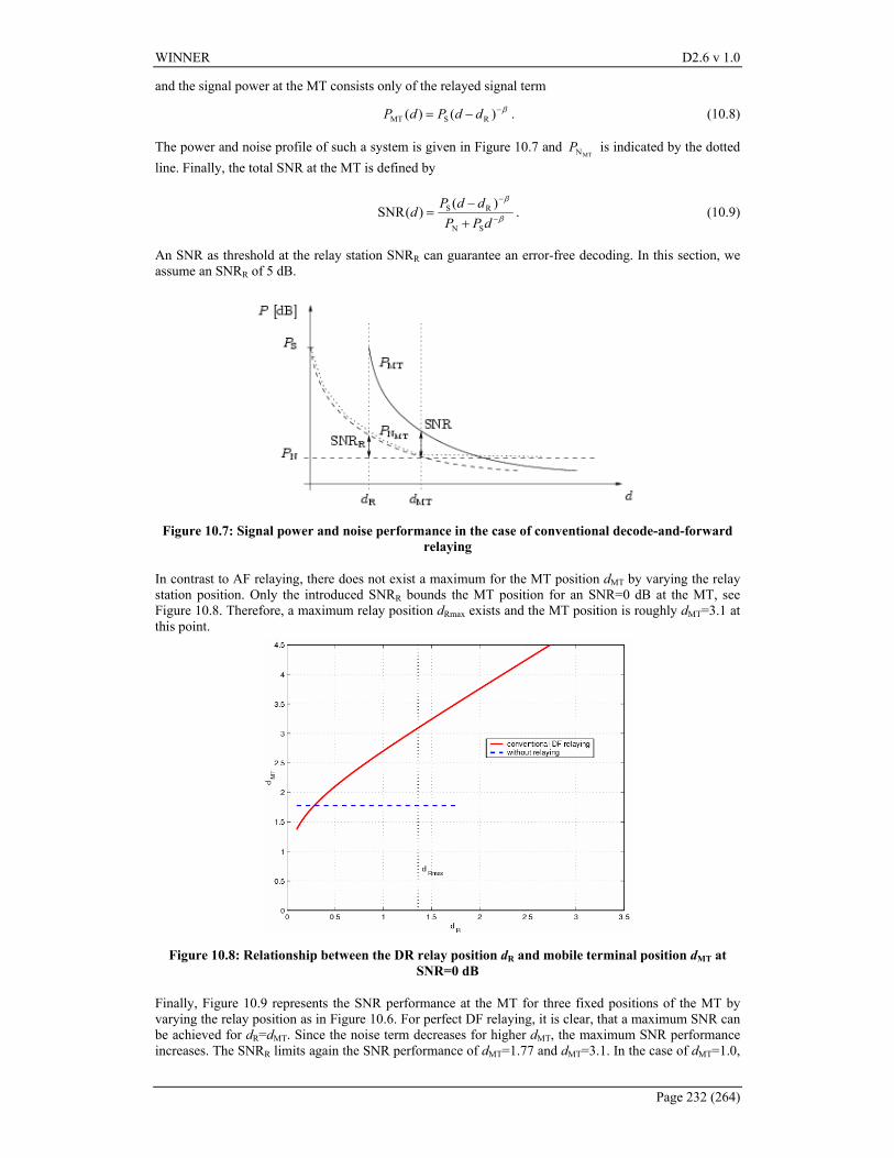
WINNER D2.6 v 1.0

Page 232 (264)

and the signal power at the MT consists only of the relayed signal term

β−−= )()( RSMT ddPdP . (10.8)

The power and noise profile of such a system is given in Figure 10.7 and MTNP is indicated by the dotted

line. Finally, the total SNR at the MT is defined by

β

β

−

−

+−

=dPP

ddPd

SN

RS )()(SNR . (10.9)

An SNR as threshold at the relay station SNRR can guarantee an error-free decoding. In this section, we assume an SNRR of 5 dB.

Figure 10.7: Signal power and noise performance in the case of conventional decode-and-forward relaying

In contrast to AF relaying, there does not exist a maximum for the MT position dMT by varying the relay station position. Only the introduced SNRR bounds the MT position for an SNR=0 dB at the MT, see Figure 10.8. Therefore, a maximum relay position dRmax exists and the MT position is roughly dMT=3.1 at this point.

Figure 10.8: Relationship between the DR relay position dR and mobile terminal position dMT at SNR=0 dB

Finally, Figure 10.9 represents the SNR performance at the MT for three fixed positions of the MT by varying the relay position as in Figure 10.6. For perfect DF relaying, it is clear, that a maximum SNR can be achieved for dR=dMT. Since the noise term decreases for higher dMT, the maximum SNR performance increases. The SNRR limits again the SNR performance of dMT=1.77 and dMT=3.1. In the case of dMT=1.0,

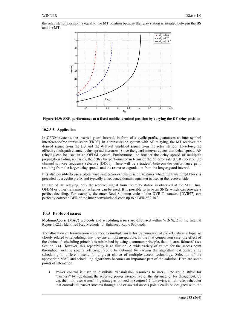
WINNER D2.6 v 1.0

Page 233 (264)

the relay station position is equal to the MT position because the relay station is situated between the BS and the MT.

Figure 10.9: SNR performance at a fixed mobile terminal position by varying the DF relay position

10.2.3.3 Application

In OFDM systems, the inserted guard interval, in form of a cyclic prefix, guarantees an inter-symbol interference-free transmission [FK03]. In a transmission system with AF relaying, the MT receives the desired signal from the BS and the delayed amplified signal from the relay station. Therefore, the effective multipath channel delay spread increases. Since the guard interval covers that delay spread, AF relaying can be used in an OFDM system. Furthermore, the broader the delay spread of multipath propagation fading scenarios, the better the performance in terms of the bit error rate (BER) because the channel is more frequency selective [DK01]. There will be a tradeoff between the performance gain, resulting from the larger delay spread, and the resource degradation from the longer guard interval.

It is also possible to use a block wise single-carrier transmission schemes where the transmitted block is preceded by a cyclic prefix and typically a frequency domain equalizer is used at the receiver side.

In case of DF relaying, only the received signal from the relay station is observed at the MT. Thus, OFDM or other transmission schemes can be used. It is possible to have an SNRR which can provide a perfect decoding. For example, the outer Reed-Solomon code of the DVB-T standard [DVB97] can perfectly correct a BER of the inner convolutional code up to a BER of 2 10-4.

10.3 Protocol issues Medium-Access (MAC) protocols and scheduling issues are discussed within WINNER in the Internal Report IR2.3: Identified Key Methods for Enhanced Radio Protocols. The allocation of transmission resources to multiple users for transmission of packet data is a topic so closely related to scheduling, that they are almost inseparable. In the first comparison case, the effect of the choice of scheduling principle is minimized by using a common principle, that of “area-fairness” (see Section 3.4). However, this separability is an illusion. A wide variety of values for the access point throughput and the spectral efficiency could be obtained by varying the algorithm that controls the scheduling to different users, for a given choice of multiple access technology. Selection of the appropriate MAC and scheduling algorithms becomes an important part of the solution. Here are some points of interaction:

• Power control is used to distribute transmission resources to users. One could strive for “fairness” by equalizing the received power irrespective of the distance, or for throughput, by e.g. the multi-user waterfilling strategies utilized in Section 6.2. Likewise, a multi-user scheduler that controls all packet streams through one or several access points could be designed with the

WINNER D2.6 v 1.0

Page 234 (264)

aim of maximizing fairness, maximizing throughput, or combinations thereof. It should be clear that these two entities should be considered and designed jointly.

• Scheduling, and the related handling of data packets, contributes to the total delay of the feedback loop used in adaptive systems that require channel state information at the transmitter. These issues were seen to be of crucial importance in Section 6.1. There do exist powerful scheduling algorithms of very low computational complexity that can handle mixes of data streams with different delay requirements and throughput requirements, and that can also utilize the independent channel variations of different clients to attain a multi-user scheduling gain in the total throughput. See e.g. [Eri04].

• The introduction of SDMA changes and enriches the types of resources potentially available to a scheduler. A discussion of these issues can be found in Chapter 8.

Another important issue is the size of link level frames, the units used for link-level retransmission. The size of the link-level frame is an important design parameter. A too small size will result in large link-level overhead. A too large size would result in inefficiencies when transporting small packets, e.g. ACK packets. It could also result in a larger delay in the link-level retransmission. In the multiple access schemes, there is in general a basic resource (a set of subcarriers, timeslots, time/frequency/spatial resources) that is to be distributed among users, in a way that cannot be subdivided with arbitrary resolution. How should the size of the link-level frame relate to that of the basic resource unit of a multiple access scheme? The most straightforward choice would be to set the size of the retransmission frame equal to the basic MA resource. However, with the use of either slow or fast link adaptation, the MA resources will bear unequal amounts of payload data for different users. Furthermore, these resources are in general scaled with regard to physical constraints, such as channel coherence times and coherence bandwidths. The resulting size would in general represent a suboptimal choice as seen from higher layers. We have in this report in Chapter 3.4 assumed the use of a link-level frame of fixed size.

10.4 Applications

10.4.1 Peer-to-peer and ad-hoc networking

Wireless networks can be divided into infrastructure-based and ad-hoc networks. Traditionally, radio networks are often infrastructure-based, as in cellular environments. There, a base-station organizes and controls the communications taking place within the cell. Additional management operations are also performed over multiple neighboring cells. The allocation of common resources – in particular, access to the channel - is done in a simple way since there is a single responsible entity at the cell-level.

In spite of that, the interest in self-organizing networks has recently grown owing to its multiple benefits. Their deployment is spontaneous, without a need for assistance from an existing infrastructure. This property makes ad-hoc networks very amenable to scenarios where the network topology is changing rapidly. The fact that they do not depend on specific network components increases their robustness to infrastructure failures.

However, a station is demanded to implement more networking functions, since those have now to be distributed across the network. A fundamental issue arising from the absence of infrastructure is the need for every node to run routing algorithms. In addition to its own packets, a node has also to collaborate with others to route their packets through the network. Thus, the multihop character of the communications converts every node in a relay. In this context, the problem of allocating network resources to the nodes is now much more complex, since it does not depend anymore from a single entity. In particular, the optimal allocation strategy for channel access should coordinate the transmission from all nodes, an extremely difficult task in a distributed environment.

Although many open issues remain in this space, several solutions addressing particular scenarios already exist. These are specific to two distinguishable classes of ad-hoc networks: centralized (also called clustered) and decentralized ad-hoc networks, where only peer-to-peer communication takes place. In the following, we briefly describe each of these classes and, on that basis, we discuss in more detail the dependencies between the ad-hoc character of a network and the underlying multiple-access scheme.

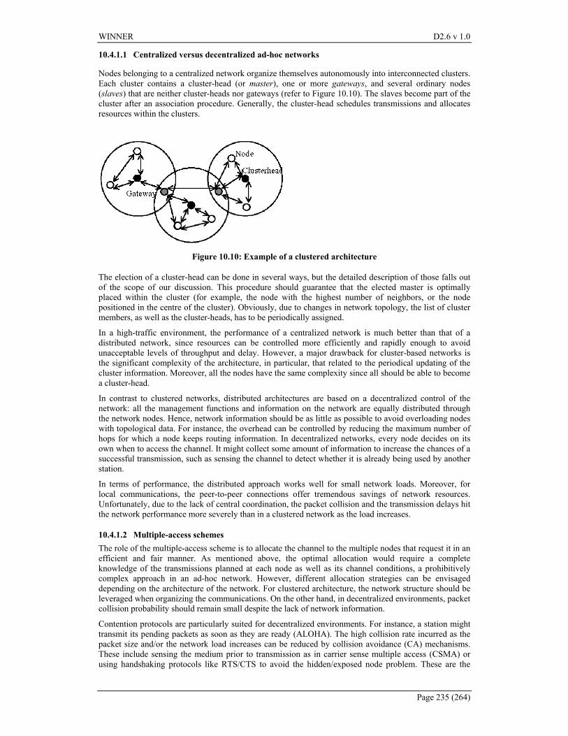
WINNER D2.6 v 1.0

Page 235 (264)

10.4.1.1 Centralized versus decentralized ad-hoc networks

Nodes belonging to a centralized network organize themselves autonomously into interconnected clusters. Each cluster contains a cluster-head (or master), one or more gateways, and several ordinary nodes (slaves) that are neither cluster-heads nor gateways (refer to Figure 10.10). The slaves become part of the cluster after an association procedure. Generally, the cluster-head schedules transmissions and allocates resources within the clusters.

Figure 10.10: Example of a clustered architecture

The election of a cluster-head can be done in several ways, but the detailed description of those falls out of the scope of our discussion. This procedure should guarantee that the elected master is optimally placed within the cluster (for example, the node with the highest number of neighbors, or the node positioned in the centre of the cluster). Obviously, due to changes in network topology, the list of cluster members, as well as the cluster-heads, has to be periodically assigned.

In a high-traffic environment, the performance of a centralized network is much better than that of a distributed network, since resources can be controlled more efficiently and rapidly enough to avoid unacceptable levels of throughput and delay. However, a major drawback for cluster-based networks is the significant complexity of the architecture, in particular, that related to the periodical updating of the cluster information. Moreover, all the nodes have the same complexity since all should be able to become a cluster-head.

In contrast to clustered networks, distributed architectures are based on a decentralized control of the network: all the management functions and information on the network are equally distributed through the network nodes. Hence, network information should be as little as possible to avoid overloading nodes with topological data. For instance, the overhead can be controlled by reducing the maximum number of hops for which a node keeps routing information. In decentralized networks, every node decides on its own when to access the channel. It might collect some amount of information to increase the chances of a successful transmission, such as sensing the channel to detect whether it is already being used by another station.

In terms of performance, the distributed approach works well for small network loads. Moreover, for local communications, the peer-to-peer connections offer tremendous savings of network resources. Unfortunately, due to the lack of central coordination, the packet collision and the transmission delays hit the network performance more severely than in a clustered network as the load increases.

10.4.1.2 Multiple-access schemes The role of the multiple-access scheme is to allocate the channel to the multiple nodes that request it in an efficient and fair manner. As mentioned above, the optimal allocation would require a complete knowledge of the transmissions planned at each node as well as its channel conditions, a prohibitively complex approach in an ad-hoc network. However, different allocation strategies can be envisaged depending on the architecture of the network. For clustered architecture, the network structure should be leveraged when organizing the communications. On the other hand, in decentralized environments, packet collision probability should remain small despite the lack of network information.

Contention protocols are particularly suited for decentralized environments. For instance, a station might transmit its pending packets as soon as they are ready (ALOHA). The high collision rate incurred as the packet size and/or the network load increases can be reduced by collision avoidance (CA) mechanisms. These include sensing the medium prior to transmission as in carrier sense multiple access (CSMA) or using handshaking protocols like RTS/CTS to avoid the hidden/exposed node problem. These are the

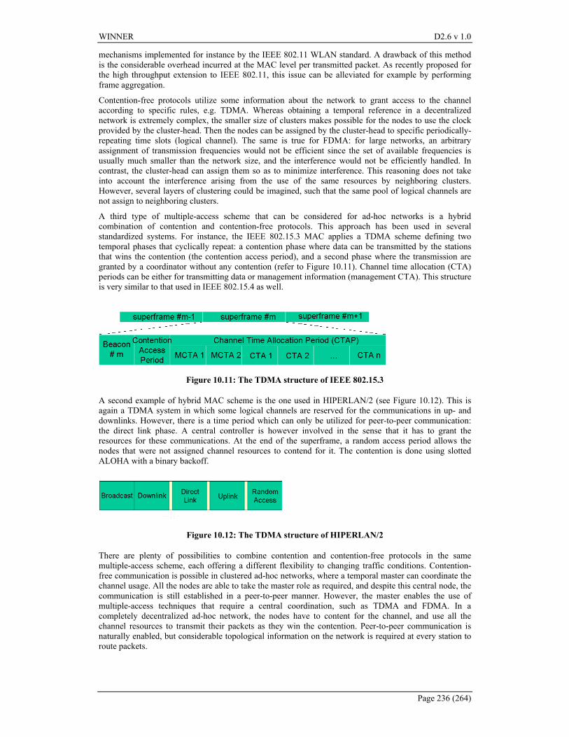
WINNER D2.6 v 1.0

Page 236 (264)

mechanisms implemented for instance by the IEEE 802.11 WLAN standard. A drawback of this method is the considerable overhead incurred at the MAC level per transmitted packet. As recently proposed for the high throughput extension to IEEE 802.11, this issue can be alleviated for example by performing frame aggregation.

Contention-free protocols utilize some information about the network to grant access to the channel according to specific rules, e.g. TDMA. Whereas obtaining a temporal reference in a decentralized network is extremely complex, the smaller size of clusters makes possible for the nodes to use the clock provided by the cluster-head. Then the nodes can be assigned by the cluster-head to specific periodically-repeating time slots (logical channel). The same is true for FDMA: for large networks, an arbitrary assignment of transmission frequencies would not be efficient since the set of available frequencies is usually much smaller than the network size, and the interference would not be efficiently handled. In contrast, the cluster-head can assign them so as to minimize interference. This reasoning does not take into account the interference arising from the use of the same resources by neighboring clusters. However, several layers of clustering could be imagined, such that the same pool of logical channels are not assign to neighboring clusters.

A third type of multiple-access scheme that can be considered for ad-hoc networks is a hybrid combination of contention and contention-free protocols. This approach has been used in several standardized systems. For instance, the IEEE 802.15.3 MAC applies a TDMA scheme defining two temporal phases that cyclically repeat: a contention phase where data can be transmitted by the stations that wins the contention (the contention access period), and a second phase where the transmission are granted by a coordinator without any contention (refer to Figure 10.11). Channel time allocation (CTA) periods can be either for transmitting data or management information (management CTA). This structure is very similar to that used in IEEE 802.15.4 as well.

Figure 10.11: The TDMA structure of IEEE 802.15.3

A second example of hybrid MAC scheme is the one used in HIPERLAN/2 (see Figure 10.12). This is again a TDMA system in which some logical channels are reserved for the communications in up- and downlinks. However, there is a time period which can only be utilized for peer-to-peer communication: the direct link phase. A central controller is however involved in the sense that it has to grant the resources for these communications. At the end of the superframe, a random access period allows the nodes that were not assigned channel resources to contend for it. The contention is done using slotted ALOHA with a binary backoff.

Figure 10.12: The TDMA structure of HIPERLAN/2

There are plenty of possibilities to combine contention and contention-free protocols in the same multiple-access scheme, each offering a different flexibility to changing traffic conditions. Contention-free communication is possible in clustered ad-hoc networks, where a temporal master can coordinate the channel usage. All the nodes are able to take the master role as required, and despite this central node, the communication is still established in a peer-to-peer manner. However, the master enables the use of multiple-access techniques that require a central coordination, such as TDMA and FDMA. In a completely decentralized ad-hoc network, the nodes have to content for the channel, and use all the channel resources to transmit their packets as they win the contention. Peer-to-peer communication is naturally enabled, but considerable topological information on the network is required at every station to route packets.

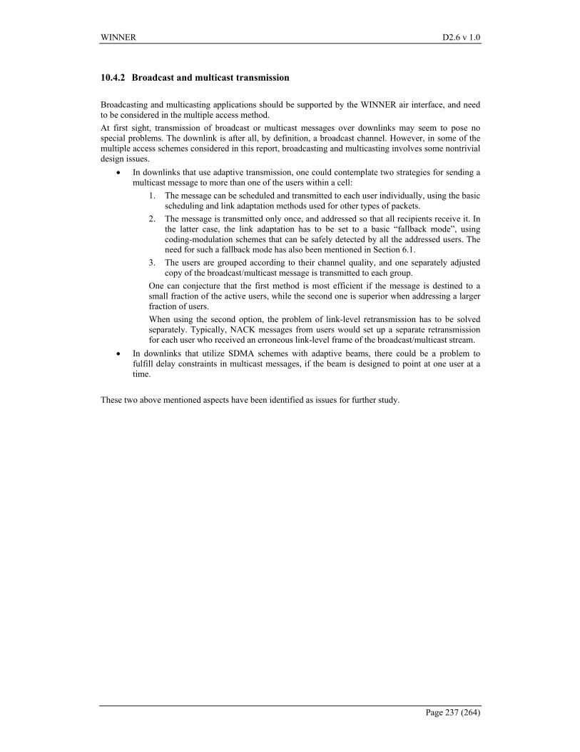
WINNER D2.6 v 1.0

Page 237 (264)

10.4.2 Broadcast and multicast transmission Broadcasting and multicasting applications should be supported by the WINNER air interface, and need to be considered in the multiple access method. At first sight, transmission of broadcast or multicast messages over downlinks may seem to pose no special problems. The downlink is after all, by definition, a broadcast channel. However, in some of the multiple access schemes considered in this report, broadcasting and multicasting involves some nontrivial design issues.

• In downlinks that use adaptive transmission, one could contemplate two strategies for sending a multicast message to more than one of the users within a cell:

1. The message can be scheduled and transmitted to each user individually, using the basic scheduling and link adaptation methods used for other types of packets.

2. The message is transmitted only once, and addressed so that all recipients receive it. In the latter case, the link adaptation has to be set to a basic “fallback mode”, using coding-modulation schemes that can be safely detected by all the addressed users. The need for such a fallback mode has also been mentioned in Section 6.1.

3. The users are grouped according to their channel quality, and one separately adjusted copy of the broadcast/multicast message is transmitted to each group.

One can conjecture that the first method is most efficient if the message is destined to a small fraction of the active users, while the second one is superior when addressing a larger fraction of users. When using the second option, the problem of link-level retransmission has to be solved separately. Typically, NACK messages from users would set up a separate retransmission for each user who received an erroneous link-level frame of the broadcast/multicast stream.

• In downlinks that utilize SDMA schemes with adaptive beams, there could be a problem to fulfill delay constraints in multicast messages, if the beam is designed to point at one user at a time.

These two above mentioned aspects have been identified as issues for further study.

WINNER D2.6 v 1.0

Page 238 (264)

11. Summary and Conclusions The preceding chapters have given an overview and first assessment of a large number of methods for multiple access. The main contributions and conclusions are reviewed here, and important open issues are indicated. Single-carrier solutions for the uplink are investigated in Chapter 5. Compared to multi-carrier based schemes, single carrier uplinks potentially provide a simpler method for attaining asynchronous multiple access. Furthermore, they are of interest since their transmitted signal may have lower peak-to-average power ratio than for multi-carrier based solutions, and thus attain higher power efficiency. In Chapter 5, both spread and non-spread solutions, namely DS-CDMA and Single-carrier TDMA, are studied. It is shown that the main challenge for single-carrier systems is how to deal with a channel response spanning many symbols, resulting from the combination of wide system bandwidth and channel delay spread. For DS-CDMA, MMSE receivers significantly outperform matched filter receivers. However, this improved performance comes at the expense of much increased complexity. Therefore, some complexity reduction scheme should be further studied along with their implementation and consequences for the performance. For single-carrier TDMA without spreading, there are also challenging issues in balancing receiver complexity against performance. Thus, the question of receiver complexity versus performance is of primary importance in the continued study of single-carrier link-level algorithms, and single-carrier uplink MA schemes. The main theme of Chapter 6 is on obtaining, preserving, and utilizing orthogonality in the resource allocation to users. To obtain high performance, methods based on adaptation, rather than methods based on averaging, are emphasized. Efficient synchronization algorithms in time and frequency are then crucial enabling technologies, and are important topics for further studies within the context of WINNER deployment and user scenarios. Based on OFDM transmission, there are three different methods for orthogonal time-frequency resource allocation:

• TDMA/OFDMA, or FDMA combined with TDMA using OFDM modulation. Here, time-frequency bins of predetermined size are allocated to users. In chapter 6, exclusive allocation of these resources to users is assumed, mainly to simplify the schemes. The time-frequency bins are scaled to the correlation time and correlation bandwidth of the channel, so that the channel is almost flat within each bin. This simplifies the design of transmission and reception.

• OFDMA. Here, fixed or slowly time-varying partitions of the subcarriers are allocated to different users. This method is a special case of TDMA/OFDMA mainly for use for stationary users, with time-invariant channels.

• TDMA, where one or several OFDM symbols are allocated exclusively to users. This is a special case of TDMA/OFDMA of use for mobile users, with a simpler but less flexible resource allocation scheme.

Of the above variants, TDMA/OFDMA is the most flexible, and potentially the most powerful in combination with adaptive resource allocation, based on feedback of channel state information to the transmitters. Availability to accurate channel state information depends on efficient prediction algorithms and fast feedback to the scheduler. As outlined in Section 2.5.4, high carrier frequencies, high terminal speeds and high frequency selectivity place bounds on the feasibility of adaptive transmission, by limiting the attainable prediction of the channel and interference and by their effect on the required feedback information rates. It has therefore been of interest to explore the limits and the feasibility of adaptive transmission in the context of the WINNER air interface, and how this affects the design of a multiple access scheme. Section 6.1 represents the first half of such a feasibility study, which will be expanded within deliverable D2.4, Assessment of adaptive transmission for broadband RI. The feasibility is assessed by theoretical considerations and by the detailed design of resource units in both TDD and FDD systems that take the known constraints into account. The preliminary conclusions from this study are:

1. Adaptive TDMA/OFDMA resource allocation that adjusts to the frequency selective fading by link adaptation and attains multi-user scheduling gains is feasible for users at vehicular velocities of 50-70 km/h, at 5 GHz and at reasonable SINR values. It is

WINNER D2.6 v 1.0

Page 239 (264)

infeasible for higher velocities, why it has to be complemented by a non-adaptive fallback mode, that is based on coding or spreading combined with interleaving.

2. This principle is feasible in uplinks, under the crucial assumption that adequate

frequency synchronization can be attained and maintained for all involved terminals. Thus, adaptive multi-carrier uplink transmission remains a feasible alternative to be further evaluated also for the case of large cell sizes and mobile users.

3. Adaptive TDMA/OFDMA is feasible in both TDD and FDD systems. In the example

implementation, the worst performance is obtained in TDD uplinks, due to the required long prediction horizons for that case. This is a significant conclusion for the WINNER system design since it implies that the feasibility of adaptive multiple access using SISO links does not place strong constraints on the choice of duplex scheme. The crucial aspect of either a FDD or a TDD schemes is that the time-durations of the transmission frames must be kept short. Short frames will also be required by the basic WINNER requirement of a short RI delay.

The use of OFDMA is discussed in Section 6.2. A general point here is that the possibility to adapt the resource use to the channel properties at different frequencies adds an important degree of freedom to the MA resource allocation scheme. It increases the possibility to attain scheduling gains due to the different channels to different terminals. Without using the frequency dimension, one would be restricted to using the variability of channels in time. This variability decreases with the utilized bandwidth. The use of interference-avoidance resource allocation with respect to the strongest interferers is discussed in a simulation study in Section 6.2. This aspect is important for attaining high spectral efficiency.

Chapter 7 focuses on multi-carrier transmission schemes that utilize spreading. Different aspects of the spreading concepts, MIMO schemes, pre- and post-processing techniques, implementation issues, adaptive resource allocation and cellular structures for multi-carrier spread spectrum schemes are represented and investigated. In a cellular structure the spread multi-carrier transmission scheme, MC-CDMA, is mainly influenced by the two closest interfering base stations. The spreading component can exploit more diversity and therefore MC-CDMA can gain compared to non-spread systems, pure OFDM, up to a system load of 75%. For higher system loads, the MAI degrades the performance of MC-CDMA and the non-spread system outperforms the spread system. Several conclusion are drawn regarding design proposals for multi-carrier MA schemes that use spreading:

• Pre-equalization techniques for SS-MC-MA result in no significant performance improvements as they do for MC-CDMA in the uplink;

• A spreading component gains in combination with link adaptation compared to non-spread schemes and spreading should be done in the time direction;

• Design in a multi-cell environment has to be coordinated to the major inter-cell interference resulting from the two closest interfering cells.

The results presented in Chapter 7 are a first step for investigations towards comparative guidelines for the design of multi-carrier spread spectrum schemes. Further investigations are necessary for finding an appropriate system design in terms of multiple access.

Chapter 8 outlines MA schemes that have an additional SDMA component, in addition to either TDMA, FDMA and /or CDMA. The coordinated use of multiple antennas in some configuration is crucial in attaining some of the most challenging WINNER performance requirements, like that of 100 Mbit/s throughput per access point in the presence of interference. Three types of SDMA schemes are investigated: Fixed beamforming, adaptive beamforming and pseudo-random beamforming that is combined with scheduling. Fixed beamforming is a simple, robust and straightforward technique that allows Spatial Multiplexing in wide area environments with low angular spread. In these environments traditional beamforming techniques can be used and a minimum of CSI is needed (e.g. only DOA Direction of Arrival). The number of users that can be spatial multiplexed with the fixed beam approach is approximately equal to the number of TX antennas divided by 2. Adaptive beams can be used for two purposes. First in a classical fixed beam environment the maximum number of users that can be handled simultaneously is increased by a factor of up to 2. On the other hand in environments with higher angular spread separation it can use the full CSI information and provide adaptive beams that allow sufficient

WINNER D2.6 v 1.0

Page 240 (264)

separation of the individual users were the fixed beam approach fails. SDMA with both fixed beams and adaptive beams can be used in combination with OFDM, FDMA, TDMA and CDMA. Considering implementation and performance aspects the most promising combinations are OFDM-SDMA-TDMA and OFDM-SDMA-TDMA-CDMA.

General conclusions for the relative merits of the different multiple access schemes must be left to the near future, since comparison simulations on the harmonized first comparison case have just begun. Also, more thorough evaluation on more advanced comparison cases will have to be performed before reliable conclusions can be drawn. Some general observations can be made on the inter-relatedness of different aspects that have so far been studied within separate tasks and work packages within WINNER. For example, the allocation of transmission resources to multiple users for transmission of packet data is a topic so closely related to scheduling, that they are almost inseparable. In the first comparison case, the effect of the choice of scheduling principle is minimized by using a common principle, that of “area-fairness” (see Section 3.4). However, this separability is an illusion. A wide variety of values for the access point throughput and the spectral efficiency could be obtained by varying the algorithm that controls the scheduling to different users, for a given choice of multiple access technology. It is far from clear that the problem of investigating multiple access can, or should, be studied separately from the problem of selecting appropriate scheduling and MAC algorithms. Furthermore, it is hard to separate a multiple access scheme from the numerous choices that must be made in the design of the underlying link: synchronization, channel estimation, coding, and receiver algorithms. What is really compared when comparing schemes are not the different multiple access schemes per se, but rather very specific combinations of multiple access schemes and physical layer implementations. There is one major aspect of the challenge posed by the WINNER system requirements that is rather obvious, and can in fact be seen in the basic construction of the first comparison case in Section 3.4: It is hard to simultaneously obtain both large cell sizes and high data rates, when the transmit energy is severely limited. This has been illustrated e.g. in the performance assessment of an OFDM/TDMA TDD system, that was presented in Section 6.3.5. Obtaining reasonably large coverage areas for each site is likely to be important for any WINNER radio interface that one can hope would complement and perhaps eventually replace 3G systems in future suburban and rural environments. An important aspect in this regard is the possibility to define a dual bandwidth system, as outlined in Section 6.4.2, with the narrower band utilized for wide area coverage. For scenarios in which wide area coverage is required, the combined use of a lower radio bandwidth than 100 MHz, the use of multiple antennas/sectoring at access points, adaptive transmission, and the possible use of relays in outer parts of sectors can be envisioned. This is a topic that lies in-between the research focus of T2.4 and WP3. A crucial restriction on the data rates at long transmission ranges in the uplink are restrictions on the transmit power due to EMC requirements. Terminal designs, antenna concepts and deployment concepts that mitigate or remove this restriction would be highly valuable. Another important study topic placed in-between WP2 and WP3 is that of advanced radio resource management, to obtain interference avoidance.

11.1 Further studies Here is a summary of important aspects that are not touched by most basic simulation studies in this deliverable and are not included in the present first comparison case, but that are important from different perspectives. It should be noted that it is doubtful if all aspects can be taken into account fully within WINNER phase I. A selection and prioritization of near term aims and results is a key topic for decision in the near future.

• Modified physical layer parameters and algorithms obtained through the work within WP2. • Performance in an extended set of different scenarios: A1, B1, B5, C2, D1.

WINNER D2.6 v 1.0

Page 241 (264)

• Integration of MIMO transmission methods. • System simulations in a multi-cell environment, possibly using a harmonized link-to system

interface. Estimation of capacity, spectral efficiency, coverage, user data rates, and the QoS distribution in this setting.

• Levels of inter-cell interference. Methods for dealing with the inter-cell interference in order to

minimize the frequency reuse factor. Use of interference control and coordinated scheduling, in cooperation with WP3.

• Introduction of modified link-level parameters (frame size, use of link-level retransmission).

• More realistic models of data streams and the user behaviour. Also, realistic distributions of

mobilities and velocities of terminals in different scenarios would be required to go further in the assessment of different designs of multiple access schemes based on adaptive transmission, that work up to a limiting user velocity.

• More realistic channel models, provided by WP5.

• Impact of RF issues (phase noise, frequency synchronization, Doppler spread).

• Better modeling of implementation constraints (peak-to-average ratio, adjacent channel power

ratio, power consumption (per bit) at UE, etc.) In particular, introduction of simultaneous average power constraints and instantaneous power constraints (or peak value constraints).

• Suitability for peer-to-peer operation.

• Suitability for multi-cast/broadcast operation, in particular when using multibeam antennas.

• Flexibility of resource management for all scenarios, channel and traffic conditions, adaptation

methods and criteria.

WINNER D2.6 v 1.0

Page 242 (264)

12. References

[AGR98] P. Alexander, A. Grant and M. Reed, “Iterative Multiuser Detection in Code-Division Multiple-Access with Error Control Coding”, European Trans. Telecommun., vol. 9, pp. 419-425, Sep.-Oct. 1998.

[AI03] F. Adachi, T. Itagaki, “Frequency-Domain Rake Combining Antenna Diversity Reception of DS-CDMA Signals,” IEICE Trans. on Commun., Vol. E86-B, N. 9, pp. 2781-2784, Sept. 2003.

[Ala98] S. M. Alamouti, "A Simple Transmitter Diversity Scheme for Wireless Communications", IEEE Selected Areas of Comm., V. 16, No. 8, pp. 1451-1458, Oct. 1998.

[ALS04] A. Ahlén, L. Lindbom and M. Sternad, "Analysis of stability and performance of adaptation algorithms with time-invariant gains," IEEE Transactions on Signal Processing, vol. 52, pp. 103-116. January 2004.

[AM79] B.D.O. Anderson and J.B. Moore, Optimal Filtering. Prentice Hall, 1979.

[AMA+02] H. Atarashi, N. Maeda, S. Abeta, and M. Sawahashi, ”Broadband packet wireless access based on VSF-OFCDM and MC/DS-CDMA”, in proc. of PIMRC’2002, Lisbon, pp. 992-997, 2002.

[ASL01] A. Ahlén, M. Sternad and L. Lindbom , “Iterative Wiener Design of Adaptation Laws with Constant Gains”, IEEE International Conference on Acoustics, Speech and Signal Processing, Salt Lake City, May 7-11 2001, pp. 3861-3864.

[Bai94] P. W. Baier, “CDMA or TDMA? CDMA for GSM?”, Proc. of IEEE PIMRC 1994, The Haque, pp. 1280-1284

[BAIPN03] D. Bartolome, A. Pascual Iserte, A. I. Perez-Neira, “Spatial Scheduling Algorithms for Wireless Systems,” in Proc. Int. Conf. Acoustics, Speech, Sign. Proc. (ICASSP), Apr. 2003.

[Bar04] D. Bartolome, “A Unified Framework for Fairness in Multi-antenna Multi-user Channels,” Ph.D. Dissertation, in preparation.

[Bee98] J. Van de Beek , Synchronization and Channel Estimation in OFDM Systems, PhD thesis, Lulea University of Technology, 1998.

[BFB02] E. Baccarelli, A. Fasano, and M. Biagi. Novel efficient bit-loading algorithms for peak-energy-limited ADSL-type multi-carrier systems. IEEE Transactions on Signal Processing, 50(5), May 2002.

[BGP02] H. Bölcskei, D. Gesbert, and A. J. Paulraj, “On the capacity of OFDM-based spatial multiplexing systems,” IEEE Trans. Commun., vol. 50, pp. 225–234, Feb. 2002.

[Bin90] J. A.C. Bingham,“Mulitcarrier modulation for data transmission: an idea whose time has come”, IEEE Communications Magazine, Vol. 28, No. 5, May 1990, pp. 5-14

[Bing00] B. Bing, “High-Speed Wireless ATM and LANs”, Artech House, Boston, 2000

[BJK96] P. W. Baier, P. Jung, A. Klein, “Taking Challenge of Multiple Access for Third-Generation Cellular Mobile Radio Systems – A European View”, IEEE Communications Magazine, February 1996, pp. 82-89

[BNB02] T. Baumgartner, T. Neubauer E. Bonek, "Performance of a Downlink Beam Switching for UMTS FDD in the Presence of Angular Spread", IEEE ICC 2002, New York

[BNG99] R.M. Buehrer, S.P. Nicoloso and S. Gollamudi, “Linear versus Nonlinear Interference Cancellation”, Journal Commun. Networks, vol. 1, pp. 118-133, Jun. 1999.

[BO01] M. Bengtsson and B. Ottersten, “Optimal and suboptimal transmit beamforming,” in Handbook of Antennas in Wireless Communications, L. C. Godara, Ed. CRC Press, 2001.

[Bol04] H. Boelsckei et al., “Capacity Scaling Laws in MIMO Relay Networks,” Trans. On Wireless Communications, April 2004, submitted.

WINNER D2.6 v 1.0

Page 243 (264)

[BPG01] S. Barbarossa, M. Pompili, G. B. Giannakis, “Time and Frequency Synchronisation of Orthogonal Frequency Division Multiple Access Systems”, Proc. of ICC 2001, pp. 1674-1678

[BPN03] D. Bartolomé, A. I. Pérez-Neira, “Spatial Scheduling in Multiuser Wireless Systems: from Power Allocation to Admission Control”, submitted to IEEE Trans. On Wireless Communications, October 2003.

[BPN04] D. Bartolomé, A. I. Pérez-Neira, “Performance Analysis of Scheduling and Admission Control for Multiuser Downlink SDMA”, IEEE International Conference on Acoustics, Speech, and Signal Processing (ICASSP 2004). Montreal (Canada), May 17-21 2004.

[BPN04a] D. Bartolomé, A. I. Pérez-Neira, “Multiuser Spatial Scheduling in the Downlink of Wireless Systems”, in Proceedings of the 3rd IEEE Sensor Array and Multichannel Signal Processing Workshop (SAM), Sitges, Spain, July 2004.

[BPPN03] D. Bartolomé, D.P. Palomar, A.I. Pérez-Neira, “Real-Time Scheduling for Wireless Multiuser MISO Systems under Different Fairness Criteria,” in Proceedings of the International Symposium on Signal Processing and Applications (ISSPA 2003), Paris (France), July 1-4 2003.

[BPSh98] E. Biglieri, J. Proakis, Sh. Shamai, “Fading Channels: Information-Theoretic and Communication Aspects”, IEEE Transactions on Information Theory, Vol. 44, No. 6, October 1998, pp. 2619-1292

[BSch03] H. Boche and M. Schubert, “Optimal Multi-User Interference Balancing Using Transmit Beamforming“, Wireless Personal Communications (WPC), Vol 26, no 4, pages 305-324, Sept.2003

[BSTJ79] Bell System Technical Journal, special issue on AMPS, Vol. 58, No.1, January 1979

[BW01] S. Borst and P. Whiting, “The Use of Diversity Antennas in High-Speed Wireless Systems: Capacity Gains, Fairness Issues, Multi-User Scheduling,” Bell Labs Technical Memorandum, 2001.

[BW97] R. M. Buehrer and B.D. Woerner, “The Asymptotic Multiuser Efficiency of m-stage Interference Cancellation Receivers”, in 8th IEEE PIMRC’97, Helsinki, Finland, Sep. 1997, pp. 570-574.

[BZK02] N. Bahvalov, N. Zhidkov, and G. Kobelkov. Numerical methods. Fizmatlit, 2002. In Russian

[Cam99] J. Campello, “Practical bit loading for DMT,” in Proc. of the IEEE International Conf. on Commun. (ICC), June 1999.

[CFH+02] E. Costa, A. Filippi, H. Haas, S. Ometto, E. Schulz, "Adaptive subband allocation in MC-CDMA/FDM systems," Proc. 7th International OFDM Workshop 2002, Hamburg, Germany, September 2002.

[CG79] T. M. Cover and E. E. Gamal, “Capacity Theorems for the Relay Channel,” IEEE Trans. Inf. Theory, vol. 25, no. 5, pp. 572-584, Sept. 1979.

[ChBJ93] A. Chouly, A. Brajal, S. Jourdan, “Orthogonal multi-carrier techniques applied to direct sequence spread spectrum CDMA systems”, Proc. of IEEE GLOBECOM’93, Houston, Nov./Dec. 1993, pp. 1723-1728

[ChCB95] P. S. Chow, J. M. Cioffi, John A. C. Bingham,“A practical discrete multitone transceiver loading algorithm for data transmission over spectrally shaped channels”, IEEE Trans. Communications, vol. 43, no. 2/3/4, pp. 773-775, Feb./Mar./Apr. 1995.

[ChFGG01] B. Chen, F. Fitzek, J. Gross, R. Grünheid, “Framework for combined optimization of DLC and physical layer in mobile OFDM systems,” International OFDM Workshop, Hamburg, Sept. 2001.

[ChFL02] H.-H. Chen, CH.-X. Fan, W. W. Lu, “China’s Perspectives on 3G Mobile Communications and Beyond: TD-SCDMA Technology”, IEEE Wireless Communications, April 2002, pp. 48 - 59

[ChG01] S. T. Chung, A. J. Goldsmith, “Degrees of freedom in adaptive modulation: A unified view,” IEEE Trans. Comm., vol. 49, no. 9, Sept. 2001.

WINNER D2.6 v 1.0

Page 244 (264)

[ChM04] L.U. Choi and R.D. Murch, “A Transmit Preprocessing Technique for Multiuser MIMO Systems Using a Decomposition Approach,” IEEE Trans. Wireless Commun., vol. 3, no. 1, pp. 20 – 24, Jan. 2004.

[CHS+02] E. Costa, H. Haas, E. Schulz, and A. Filippi. “Capacity optimisation in MC-CDMA systems”, European Transactions on Telecommunications, October 2002.

[ChSP95] Q. Chen, E. S. Sousa, S. Pasupathy, “Performance of a Coded Multi-Carrier DS-CDMA System in Multipath Fading Channels”, Wireless Personal Communications, Vol. 2, 1995, pp. 167-183

[ChSP95a] Q. Chen, E. S. Sousa, S. Pasupathy, “Multi-Carrier DS-CDMA with Adaptive Subcarrier Hopping for Fading Channels”, Proc. of IEEE PIMRC’95, Toronto, September 1995, pp. 76-80

[ChV93] R. Cheng and S. Verdu, “Gaussian multiaccess channels with ISI: capacity region and multiuser water-filling”, IEEE Trans. on Information Theory , vol. 39 , no. 3 , pp. 773 – 785, May 1993.

[Cio91] J. M. Cioffi: A Multi-carrier Primer. ANSI T1E1.4 Committee Contribution, Nov. 1991.

[CKS+04] I. Cosovic, S. Kaiser, M. Schnell, and A. Springer, “Performance of coded uplink MC-CDMA with combined-equalization in fading channels,” Proceedings IST Mobile & Wireless Communications Summit (IST 04), June 2004, accepted for publication.

[CS03] G. Caire and S. Shamai, “On the achievable Throughput of a Multiantenna Gaussian Broadcast Channel,” IEEE Trans. Inform. Theory, vol. 49, no. 7, pp. 1691 – 1706, July 2003.

[CSS04] I. Cosovic, M. Schnell, and A. Springer, “Pre-, post-, and combined-equalization single-user bounds for MC-CDMA,” Proceedings European Conference on Wireless Technology (ECWT 04), Oct. 2004, submitted.

[CTF04] E. Costa, P. Trifonov and A. Filippi, "Location Based Adaptive Subband Allocation for Multi-carrier Multiple Access Systems", Proceedings of the 15th IEEE International Symposium on Personal, Indoor and Mobile Radio Communications, PIMRC 2004

[CTh91] Th. M. Cover, J. A. Thomas: Elements of Information Theory. John Wiley & Sons, 1991.

[CZhG] X. Cai, S. Zhou, G. B. Giannakis, “Group-Orthogonal Multi-carrier CDMA”, IEEE Trans. on Commun. to appear.

[Czyl96] A. Czylwik: “Adaptive OFDM for wideband radio channels”, Globecom’96, London, pp. 713-718, Nov. 1996.

[Czyl97] A. Czylwik, “Comparison between Adaptive OFDM and Single-carrier Modulation with Frequency Domain Equalization”, Proceedings of IEEE Vehicular Technology Conference (VTC’97), pp. 865 – 869, Vol. 2, May 1997

[D5.2] WINNER D5.2, “Determination of propagation scenarios”, 2004.

[Dig96] S. N. Diggavi,“Multiuser DMT: a multiple access modulation scheme”, Globecom 96, London, pp. 1566-1570, November 1996.

[Dix84] R. C. Dixon, Spread Spectrum Systems, 2nd Edition, John Wiley & Sons, New York 1984

[DK01] A. Dammann and S. Kaiser, “Transmit/Receive Antenna Diversity Techniques for OFDM Systems,” European Transactions on Telecommunications, vol. 13, no. 5, pp. 531-538, September/October 2001.

[DMC+00] M. Debbah, B. Muquet, M. de Courville, M. Muck, S. Simoens, and P. Loubaton, "A New MMSE Successive Interference Cancellation Scheme for Spread OFDM Systems", in Proceedings of the IEEE Vehicular Technology Conference, volume 2, pages 745-749, Tokyo, Japan, May 2000.

[DO99] H. Donelan and T. O’Farrell, “Method for generating sets of orthogonal sequences”, Electronics letters, vol. 35, no. 18, pp. 1537-1538, Sep. 1999.

[DS95] D. Divsalar and M.K. Simon, “Improved Parallel Interference Cancellation for CDMA”, JPL publication, Oct. 1995.

WINNER D2.6 v 1.0

Page 245 (264)

[DSR98] D. Divsalar, M.K. Simon, and D. Raphaeli, “Improved Parallel Interference Cancellation for CDMA”, IEEE Trans. Commun., vol.446, no.2, pp. 258-268, Feb. 1998.

[DSS93] V. DaSilva, E. S. Sousa, “Performance of Orthogonal CDMA Codes for Quasi-Synchronous Communication Systems”, Proc. of ICUPC’93, Ottawa, October 1993, pp. 995-999

[DSS94] V. DaSilva, E. S. Sousa, “Multi-carrier Orthogonal CDMA Signals for Quasi-Synchronous Communication Systems”, IEEE Journal on Selected Areas in Communications, Vol. 12, June 1994, pp. 842-852

[Due93] A. Duell-Hallen, “Decorrelating Decision-Feedback Multiuser Detector for Synchronous CDMA”, IEEE Trans. Commun., vol.41, pp. 285-290, Feb. 1993.

[Due95] A. Duell-Hallen, “A Family of Multiuser Decision-Feedback Detectors for Asynchronous Code-Division Multiple Access Schemes”, IEEE Trans. Commun., vol.43, no. 2/3/4, pp. 421-434, Feb./Mar./Apr. 1995.

[DVB97] Digital Video Broadcasting (DVB); Framing Structure, channel coding and modulation for digital terrestrial television, European Telecommunications Standard Institute ETSI, 1997, EN 300 744 V1.1.2.

[EBSch97] H. Elders-Boll, A. Busboom and H-D. Schotten, “Implementation of Linear Detectors for Asynchronous CDMA Systems by Linear Interference Cancellation Algorithms”, in IEEE Vehicular Technology Conference, Phoenix, Arizona, May 1997, pp.2163-2167.

[EBSch97a] H. Elders-Boll, A. Busboom and H-D. Schotten, “Spreading Sequences for Zero-Forcing DS-CDMA Multiuser Detectors”, in IEEE PIMRC’97, Helsinki, Finland, Sep. 1997, pp. 53-57.

[Ekm02] T. Ekman, Prediction of Mobile Radio Channels. Modelling and Design. PhD Thesis, Signals and Systems, Uppsala University, Sweden, 2002. http://www.signal.uu.se/Publications/abstracts/a023.html

[Eri04] N. C. Ericsson. Revenue Maximization in Resource Allocation. Applications in Wireless Communication Networks. Ph.D. Thesis, Uppsala University, Sweden, October 2004. Online: http://www.signal.uu.se/Publications/abstracts/a043.html

[ESA02] T. Ekman, M. Sternad and A. Ahlen, "Unbiased power prediction on broadband channels" IEEE VTC 2002-Fall, Vancouver, Canada, Sept. 2002.

[ESchB98] H. Elders-Boll, H-D. Schotten and A. Busboom, “Efficient Implementation of Linear Multiuser Detectors for Asynchronous CDMA Systems by Linear Interference Cancellation”, European Trans. Telecommun., vol. 9, pp. 427-438, Sep.-Oct. 1998.

[ETS94] I-ETS 300 131, “Radio Equipment and Systems (RES); Common air interface specification to be used for interworking between cordless telephone apparatus in the frequency band 864.1 MHz to 868.1 MHz including public access services”, November 1994, Second Edition

[FAB+02] D. Falconer, S. L. Ariyavisitakul, A. Benymin-Seeyar, B. Eidson, “Frequency Domain Equalization for Single-Carrier Broadband Wireless Systems”, IEEE Communications Magazine, April 2002

[FAG95] D. D. Falconer, F. Adachi, B. Gudmundson, “Time Division Multiple Access Methods for Wireless Personal Communications”, IEEE Communications Magazine, January 1995, pp. 50-57

[Faz93] K. Fazel, “Performance of CDMA/OFDM for Mobile Communication System”, Proc. of ICUPC’93, Ottawa, October 1993, pp. 975-979

[FE91] G.D. Forney Jr., M. V. Eyuboglu: “Combined equalization and coding using precoding”. IEEE Communications Magazine, Dec. 1991.

[FH96] R. Fischer, J. Huber: Neues Verfahren zur Raten- und Leistungsverteilung bei Mehrträgersystemen. OFDM-Fachgespräch, Braunschweig, Sep. 1996.

[FH96a] R. Fischer, J. Huber,“A new loading algorithm for discrete multitone transmission”. Globecom ’96, London, pp. 724-728, Nov. 1996.

WINNER D2.6 v 1.0

Page 246 (264)

[FK03] K. Fazel, S. Kaiser, “Multi-Carrier and Spread Spectrum Systems”, John Wiley & Sons, Chichester, 2003

[FLA] www.flarion.com

[Fle96] B. H. Fleury “An Uncertainty Relation for WSS Processes and Its Applications to WSSUS Systems” in IEEE Transactions on Communications, Vol. 44, No. 12, December 1996

[FN98] C. Farsakh and J. A. Nossek, "Spatial covariance based downlink beamforming in an SDMA mobile radio system", IEEE Trans. Commun., vol. 46, pp. 1497-1506, Nov. 1998

[Fos96] G. J. Foschini, “Layered space-time architecture for wireless communication in a fading environment when using multi-element antennas,” Bell Labs Tech. J., vol.1, no.2, pp. 41-59, 1996.

[FP93] K. Fazel, L. Papke, “On the Performance of Convolutionally-Coded CDMA/OFDM for Mobile Communication System”, Proc. of IEEE PIMRC’93, Yokohama, September 1993, pp. 468-472

[FSES04] S. Falahati, A. Svensson, T. Ekman and M. Sternad, "Adaptive modulation systems for predicted wireless channels," IEEE Trans. on Communications, vol. 52, Feb. 2004, pp. 307-316.

[FSSE03] S. Falahati, A. Svensson, M. Sternad, T. Ekaman, “Adaptive modulation systems for predicted wireless channels,” Globecom ’03, Dec. 2003.

[FSSM03] S. Falahati, A. Svensson, M. Sternad and H. Mei, "Adaptive Trellis-coded modulation over predicted flat fading channels," IEEE VTC 2003-Fall, Orlando, Fla, Oct. 2003.

[FT91] D. Fudenberg and J. Tirole, Game Theory.MIT Press, 1991.

[GaAr01] A. García-Armada: “A simple multiuser bit loading algorithm for multi-carrier WLAN”. ICC ’01, Helsinki, Finland, June 2001.

[Gal68] R. G. Gallager: Information Theory and Reliable Communication. John Wiley & Sons, 1968.

[GBRA00] R. Grünheid, E. Bolinth, H. Rohling, K. Aretz, “Adaptive modulation for the HIPERLAN/2 air interface,” 5th International OFDM Workshop, Hamburg, Sept. 2000.

[GC97] A. J. Goldsmith, S.-G. Chua, “Variable-rate variable-power MQAM for fading channels,” IEEE Trans. Comm., vol. 45, no. 10, Oct. 1997.

[GC98] A. Goldsmith. S. Chua., “Adaptive Coded Modulation for Fading Channels,” IEEE Trans. On Commun., vol.46, no.5, pp.595-602, May 1998.

[GKFW03] J. Gross, H. Karl, F. Fitzek, A. Wolisz, “Comparison of heuristic and optimal subcarrier assignment algorithms,” ICWN ’03, June 2003.

[GKKW03] J. Gross, J. Klaue, H. Karl, A. Wolisz, “Subcarrier allocation for variable bit rate video streams in wireless OFDM systems,” VTC Fall ’03, Florida, Oct. 2003.

[GKW04] J. Gross, H. Karl, A. Wolisz, “On the effect of inband signaling and realistic channel knowledge on dynamic OFDM-FDMA systems,” 5 th European Wireless Conference, Barcelona, Feb. 2004.

[Gol61] M. J. E. Golay, “Complementary series”, IRE Transactions on Communications, vol. IT-7, pp. 82-87, Apr. 1961.

[Gol67] R. Gold, “Optimal binary sequences for spread spectrum multiplexing”, IEEE Transactions on Information Theory, pp. 619-621, Oct. 1967.

[GRSL00] D. Guo, L. Rasmussen, S. Sun and T.J. Lim, ”A Matrix-Algebraic Approach to Linear Parallel Interference Cancellation in CDMA”, IEEE Trans. Commun., vol. 48, pp. 152-161, Jan. 2000.

[GSch01] A. Grant and C. Schlegel, “Iterative Implementations for Linear Multiuser Detectors”, IEEE Trans. Commun., vol. 49, pp. 1824-1834, Oct. 2001.

[Haa00] J. C. Haartsen, “The Bluetooth Radio System”, IEEE Personal Communications, February 2000, pp. 28-36

WINNER D2.6 v 1.0

Page 247 (264)

[Han98] T. S. Han, “An Information-Spectrum Approach to Capacity Theorems for the General Multiple-Access Channel”, IEEE Transactions on Information Theory, Vol. 44, No. 7, November 1998, pp. 2773-2795

[HAP01] R.W. Heath, M. Airy, and A.J. Paulraj, “Multiuser Diversity for MIMO Wireless Systems with Linear Receivers”, in Proc. of the Thirty-Fifth Asilomar Conference on Signals, Systems and Computers, Nov. 2001.

[HHT+04] L. M. C. Hoo, B. Halder, J. Tellado and J. M. Cioffi, “Multiuser Transmit Optimization for Multi-carrier Broadcast Channels: Asymptotic FDMA Capacity Region and Algorithms”, IEEE Transactions On Communications, 52(6), June 2004

[HL03] Z. Han and K.J.R. Liu, “Throughput Maximization Using Adaptive Modulation in Wireless Networks with Fairness Constraint,” in Wireless Commun. and Networking Conf. (WCNC), Mar. 2003.

[HMCK03] L. Hanzo, M. Munster, B. Choi, and T. Keller, OFDM and MC-CDMA for Broadband Multi-user Communications, WLANs and Broadcasting, John Wiley & Sons, Ltd., 2003.

[HoM00] B. M. Hochwald and T. L. Marzetta, “Unitary space-time modulation for multiple-antenna communications in Rayleigh flat fading,” IEEE. Trans. on Inf. Theory, pp. 543-564, March 2000.

[Hou01] W. J. van Houtum, “Quasi-Synchronous Code-Division Multiple Access with High-Order Modulation”, IEEE Transactions on Commun., Vol. COM-49, July 2001, pp. 1240-1249

[HP96] S. Hara, R. Prasad, “DS-CDMA, MC-CDMA and MT-CDMA for Mobile Multimedia Communications”, Proc. of IEEE VTC’96, Atlanta, April/May 1996, pp. 1106-1110

[HP97] S. Hara, R. Prasad, “Overview of Multi-carrier CDMA”, IEEE Communications Magazine, December 1997, pp. 126-133

[HSJ98] L. J. Harte, A. D. Smith, Ch. A. Jacobs, “IS-136 TDMA Technology, Economics and Services”, Artech House, Boston 1998

[HT00] H. Holma, A. Toskala (Eds.), “WCDMA for UMTS”, John Wiley & Sons, Chichester 2000

[HTC99] L. M. C. Hoo, J. Tellado, J. M. Cioffi: “Discrete dual QoS loading algorithms for multi-carrier systems”. ICC ’99, Vancouver, Canada, pp. 796-800, June 1999.

[Hug87] D. Hughes-Hartogs: Ensemble modem structure for imperfect transmission media. US patent 4 679 227, filed May 20, 1985, issued July 7, 1987.

[HWK00] L. Hanzo, W. Webb, T. Keller, “Single- and Multi-Carrier Quadrature Amplitude Modulation”, John Wiley & Sons, Chichester 2000

[HZF04] P. Herhold, E. Zimmermann and G. Fettweis, “A Simple Cooperative Extension to Wireless Relaying,” in Proc. IEEE IZS, Feb. 2004, p. 36.

[Iba03] C. Ibars, “Capacity, Coding, and Interference Cancellation in Multiuser Multi-carrier Wireless Communications Systems”, PhD. Thesis, New Jersey Institute of Technology, Aug. 2003.

[IBN02] C. Ibars and Y. Bar-Ness, “The principle of time-frequency duality of DS and MC CDMA”, Proc. 36th. Annual Conference on Information Sciences and Systems (CISS), Princeton, New Jersey, Mar. 2002.

[IBN02a] C. Ibars and Y. Bar-Ness, “Outage Capacities of a Multi-Carrier WLAN Downlink under Different Resource Sharing Techniques”, Proc. IEEE International Symposium on Spread Spectrum Techniques and Applications (ISSSTA), pp. 144-149, Prague, Czech Republic, Sep. 2002.

[IBN02b] C. Ibars, Y. Bar-Ness, Rate-adaptive coded multiuser OFDM for downlink wireless systems. Multi-Carrier Spread-Spectrum & Related Topics, pp. 199-207, K. Fazel and S. Kaiser Eds., Kluwer, 2002.

[IR2.2] WINNER T2.5 IR2.2, “Identification of advanced beamforming and MIMO technologies”, 2004.

[IR7.1] WINNER IR7.1, “A compilation of all assumtions related to the WINNER research”,

WINNER D2.6 v 1.0

Page 248 (264)

2004.

[IST4] IST 4MORE project, web site http://www.ist-4more.org.

[JD96] K. Jamal and E. Dahlman, “Multi-stage Interference Cancellation for DS-CDMA”, in IEEE Vehicular Technology Conference, Atlanta, Georgia, pp. 671-675, Apr. 1996.

[JG03] N. Jindal and A. Goldsmith, “Capacity and Optimal Power Allocation for Fading Broadcast Channels with Minimum Rates”, IEEE Trans. on Information Theory, vol.49, no.11, Nov. 2003.

[Joh04] M. Johansson, "Diversity-enhanced equal access- Considerable throughput gains with 1-bit feedback," IEEE SPAWC, Workshop on Signal Processing in Wireless Communications, Lisbon, Portugal, July 11-14, 2004.

[Joh98] A.-L. Johansson, “ Successive Interference Cancellation in DS-CDMA Systems”, PhD. Thesis, Chalmers University of Technology, Department of Signals and Systems, Göteborg, Sweden, Oct. 1998.

[Jok04] J. Jokela, “Test Scenarios”, WINNER Internal Document, 19.04.04

[Kai04] S. Kaiser (ed.), “T2.4 Basic link level simulation parameters”, WINNER Internal Document, 16.04.04

[Kai98] S. Kaiser, “Multi-Carrier CDMA Mobile Radio Systems – Analysis and Optimization of Detection, Decoding, and Channel Estimation”, Ph.D. Thesis, Munich 1998, VDI-Verlag, Duesseldorf 1998

[Kato02] O. Kato, A Study on Radio Access Method for the 4th Generation Mobile Communication System and its Issues, International Forum on 4G Mobile Communications, May 2002

[Kay93] S. M. Kay, Fundamentals of Statistical Signal Processing, Volume I:Estimation Theory. New Jersey: Prentice Hall PTR, 1993.

[KF97] S. Kaiser and K. Fazel, “A flexible spread-spectrum multi-carrier multiple-access system for multi-media applications”, Proc. of PIMRC'97, Sept. 1997, pp. 100-104

[KF97b] S. Kaiser and K. Fazel, "A Spread-Spectrum Multi-Carrier Multiple Access System for mobile Communications", First International Workshop on Multi-carrier Spread Spectrum, Oberpfaffenhofen, Sept. 1997.

[KH95] R. Knopp and P.A. Humbelt, "Multiple-accessing over frequency-selective channels", IEEE PIMRC, Toronto, Canada, Sept. 27-29 1995.

[KH97] S. Kaiser, J. Hagenauer, “Multi-Carrier CDMA with Iterative Decoding and Soft-Interference Cancellation”, in IEEE GLOBECOM’97, Phoenix, USA, pp. 6-10, Nov. 1997.

[KIHP90] R. Kohno, N. Ishii, M. Hatori, and S. Pasupathy, “Combination of an Adaptive Array Antenna and a Canceller Interference for Direct-Sequence Spread Spectrum Multiple-Access System”, IEEE J. Selected Areas Commun., vol. 8, no. 4, pp. 675-682, May 1990.

[KJ04] S. Kittipiyakul, T. Javidi, “Resource Allocation in OFDMA: How Load-Balancing Maximizes Throughput when Water-Filling Fails”, Dept. of Electrical Engineering, University of Washington, Seattle, UWEE Technical Report Nr UWEETR-2004-0007

[KK99] S. Kaiser, W.A. Krzymien, "Performance effects of the uplink asynchronism in a spread spectrum multi-carrier multiple access system", European Transactions on Telecommunications, Special Issue on Multi-Carrier Spread-Spectrum, 10, N°4, July/August 1999.

[Kla04] G. Klang et al., “Identification of Radio Link Technologies” WINNER deliverable D2.1, August 19, 2004

[KLL03] D. Kivanc, G. Li, H. Liu, “Computationally Efficient Bandwidth Allocation and Power Control for OFDMA”, IEEE Transactions on Communications, Vol. 2, No. 6, November 2003, pp. 1150-1158

[KM93] S. Kondo, L. B. Milstein, “On the Use of Multi-carrier Direct Sequence Spread Spectrum Systems”, Proc. of IEEE MILCOM’93, Boston, October 1993, pp. 52-56

WINNER D2.6 v 1.0

Page 249 (264)

[KMH+03] Y. Kishiyama, N. Maeda, K. Higuchi, H. Atarashi, and M. Sawahashi, “Experiments on throughput performance above 100-Mbps in forward link for VSF-OFCDM broadband packet wireless access,” in Proc. IEEE Vehiv. Technol. Conf. 2003-Fall (VTC’F 03), Orlando, USA, October 2003.

[KMM95] R. Kohno, R. Meidan, L. B. Milstein, “Spread Spectrum Access Methods for Wireless Communications”, IEEE Communications Magazine, January 1995, pp. 58-67

[KR02] I. Koffman, V. Roman, “Broadband Wireless Access Solutions Based on OFDM Access in IEEE 802.16”, IEEE Communications Magazine, April 2002, pp. 96-103

[KRJ00] B. S. Krongold, K. Ramchandran, D. L. Jones: “Computationally efficient optimal power allocation algorithms for multi-carrier communication systems”. IEEE Trans. Communications, vol. 48, no. 1, pp. 23-27, Jan. 2000.

[KRT03] I. Koutsopoulos, T. Ren, L. Tassiulas: "The Impact of Space Division Multiplexing on Resource Allocation: A Unified Approach", IEEE INFOCOM 2003, , New York

[KSY+99] Y.H. Kim, I. Song, S. Yoon, and S.R. Park. A multi-carrier CDMA system with adaptive subchannel allocation for forward links. IEEE Transactions On Vehicular Technology, 48(5), September 1999.

[KT02] I. Koutsopoulos and L. Tassiulas, “Adaptive Resource Allocation in SDMA-based Wireless Broadband NEtworks with OFDM Signaling,” in Proc. of IEEE INFOCOM, June 2002.

[KTShK01] R. Kuehner, T.D. Todd, F. Shad, and V. Kezys, “Forward-Link Capacity in Smart Antenna Base Stations with Dynamic Slot Allocation,” IEEE Trans. Veh. Technol., vol. 50, no. 4, July 2001.

[L2S04] “Link to System Interface Methodology”, WINNER Internal Document, Version 2.0, 30.09.04

[Lan02] J. N. Laneman, “Cooperative Diversity in Wireless Networks: Algorithms and Architectures,” Ph.D. Thesis, MIT, Cambridge, MA, September 2002.

[LC98] X. Li, L. J. Cimini “Effects of Clipping and Filtering on the Performance of OFDM”, IEEE Communications Letters, Vol. 2, No. 5, May 1998

[LChLM99] S. K. Lai, R. S. Cheng, K. B. Letaief, R. D. Murch: “Adaptive trellis coded MQAM and power optimization for OFDM transmission”. VTC Spring ’99, Houston, USA, May 1999.

[LCS01] X. Liu, E. K. P Chong and N. B. Shroff, “Opportunistic scheduling for efficient wireless network utilization with QoS constraints,” Technical Report, http://shay.ecn.purdue.edu/~xinliu/papers.html, 2001.

[Lee02] W. C. Y. Lee, “The Most Spectrum-Efficient Duplexing Scheme: CDD”, IEEE Communications Magazine, March 2002, pp. 163-166

[Lee91] W. C. Y. Lee, “Overview of CDMA”, IEEE Trans. Vehicular Technology, Vol. 40 No. 2, May 1991, pp. 291-302

[LG01] L. Li and A. Goldsmith, “Capacity and optimal resource allocation for fading broadcast channels .I. Ergodic capacity”, IEEE Trans. on Information Theory, vol.47, no..3, pp. 1083-1102, Mar 2001.

[LG01a] L. Li and A. Goldsmith, “Capacity and optimal resource allocation for fading broadcast channels .II. Outage capacity”, IEEE Trans. on Information Theory, vol.47, no.3, pp. 1103-1127, Mar 2001.

[Li03] D. Li, “The Perspective of Large Area Synchronous CDMA Technology for the Fourth-Generation Mobile Radio”, IEEE Communications Magazine, March 2003, pp. 114-118

[LiH02] T. Liew, L. Hanzo, “Space-Time Codes and Concatenated Channel Codes for Wireless Communications”, Proceedings of the IEEE, V. 90, No. 2, February 2002, pp. 187-219.

[LiM03] Z. Li and M. Latva-aho, “MMSE based receiver design for MC-CDMA systems”, Prof. of IEEE PIMRC. pp:2640 – 2644, Sept. 2003.

WINNER D2.6 v 1.0

Page 250 (264)

[LM88] E. A. Lee, D. G. Messerschmitt, “Digital Communication”, Kluwer Academic Publishers, Boston, 1988

[LM98] J. S. Lee, L. E. Miller, “CDMA Systems Engineering Handbook”, Artech House, Boston 1998

[LSC03] J. Lee, R. V. Sonalkar, and J. M. Cioffi, “Multi-user bit-loading for multi-carrier systems,” submitted to IEEE Trans. Commun., 2003.

[LTW04] J. N. Laneman, D. N. C. Tse and G. W. Wornell, “Cooperative Diversity in Wireless Networks: Efficient Protocols and Outage Behavior,” IEEE Trans. Inf. Theory, to appear.

[LW00] J. N. Laneman and G. W. Wornell, “Energy-Efficient Antenna Sharing and Relaying for Wireless Networks,” in Proc. IEEE WCNC, vol. 1, Chicago, IL, Sept. 2000, pp. 7-12.

[LWT01] J. N. Laneman, G. W. Wornell and D. N. C. Tse, “An Efficient Protocol for Realizing Cooperative Diversity in Wireless Networks,” in Proc. IEEE ISIT, Washington, DC, June 2001, p. 294.

[Med00] M. Medard, “The Effect upon Channel Capacity in Wireless Communications of Perfect and Imperfect Knowledge of the Channel”, IEEE Transactions on Information Theory, Vol. 46, Nr 3, May 2000, pp. 933-946

[Meh97] A. Mehrotra, “GSM System Engineering”, Artech House, Boston 1997

[MH97] S. H. Müller, J. B. Huber, “OFDM with reduced peak-to-average power ratio by optimum combination of partial transmit sequences”, Electronics Letters, 27th February, 1997, Vol. 33, No. 5

[ML03] G. Malmgren and P. Larsson, “Cooperative Relaying in Cellular Network”, Wireless World Research Forum (WWRF), 2003.

[Mosh96] S. Moshavi, “Multi-user Detection for DS-CDMA”, IEEE Commun. Magazine, pp 124-136, Oct. 1996.

[MPS02] G. Münz, S. Pfletschinger, J. Speidel: “An efficient waterfilling algorithm for multiple access OFDM”. Globecom ’02, Taipei, Taiwan, Nov. 2002.

[Mun04] M. Muck et al “Feasaibility of multi-bandiwdth transmissions”, WINNER deliverable D2.2, 05.10.04

[MVE01] S. Marinkovic, B.S. Vucetic, and J. Evans, “Improved Iterative Parallel Interference Cancellation for Coded CDMA Systems”, in proceedings of IEEE ISIT, pp. 34, Jul. 2001.

[NBDZ98] R. Nogueroles, M. Bossert, A. Donder, V. Zyablov, “Performance of a Random OFDMA System for Mobile Communications”, Proc. of 1998 Int. Zurich Seminar on Broadband Communications, February 1998, pp. 37-43

[NBK04] R. U. Nabar, H. Boelcskei and F. W. Kneubuehler, “Fading Relay Channels: Performance Limits and Space-Time Signal Design”, IEEE Journal on Selected Areas in Communications, June 2004, to appear.

[Nee96] R. D. J. van Nee “OFDM Codes for Peak-to-Average Power Reduction and Error Correction” Global Communications Conference 1996 (Globecom’96), pp. 740-744, Vol. 1, November 1996

[NHM02] S. Nobilet, J. –F. Helard, and D. Mottier, “Spreading sequences for uplink and downlink MC-CDMA systems: PAPAR and MAI minimization”, European Transactions on Telecommunications (ETT), vol. 13, pp. 465-474, Sep./Oct. 2002.

[NL95] R. O’Neill, L. B. Lopes “Envelope Variations and Spectral Splitter in Clipped Multi-carrier Signals”, Proceedings of IEEE Symposium in Personal, Indoor and Mobile Radio Communications, 1995 (PIMRC’95), pp 71-75, Vol. 1, September 1995

[NNS+01] B. Natarajan, C.R. Nassar, S. Shattil, et.al, “High-performance MC-CDMA via carrier interferometry codes”, IEEE Transactions on Vehicular Technology, vol. 50, pp. 1344 –1353, Nov. 2001.

[Non01] D. L. Noneaker, “On the Spectral Efficiency of Wideband CDMA Systems”, IEEE Journal on Selected Areas in Commun., Vol. 19, January 2001, pp. 33-47

WINNER D2.6 v 1.0

Page 251 (264)

[NP00] R. van Nee, R. Prasad, “OFDM for Wireless Multimedia Communications”, Artech House, Boston 2000

[OAB+02] T. Ottosson, A. Ahlén, A. Brunström, M. Sternad and A. Svensson, ”Towards 4G IP-based wireless systems: A proposal for the uplink”, 5th and 6th Wireless World Research Forum Meetings, Temple AR, March 2002 and London, June 2002.

[OP78] G. D. Ott and A. Plitkins, “Urban Path-Loss Characteristics at 820 MHz,” IEEE Trans. Veh. Technol., vol. VT-27, pp. 189-197, November 1978.

[Pal03] D.P. Palomar, “A Unified Framework for Communications through MIMO Channels,” Ph.D. Thesis, May 2003.

[PDK04] S. Plass, A. Dammann, and S. Kaiser, “Analysis of coded OFDMA in a downlink multi-cell scenario,” in Proc. 9th Int. OFDM Workshop (InOWo 04), Dresden, Germany, Sept. 2004.

[PGN+04] A. J. Paulraj, D. A. Gore, R. U. Nabar and H. Bölcskei, “An oview of MIMO communications - A key to gigabit wireless,” Proc. of the IEEE, vol. 92, no.2, pp.198-218, Feb. 2004.

[PH93] P. Patel and J. Holtzman, “Analysis of a Simple Successive Interference Cancellation Scheme in DS/CDMA System”, in Proc. 1993 IEEE Global Telecomm. Conf., pp. 76-80, Nov. 1993.

[PHS03] C. Peel, B. Hochwald, and L. Swindlehurst, “A Vector-Perturbation Technique for Near-Capacity Multi-Antenna Multi-User Communication,” submitted to IEEE Trans. Wireless Commun., June 2003.

[PIPN03] A. Pascual-Iserte, A. I. Perez-Neira, M.A. Lagunas-Hernandez, “An Approach to Optimum Joint Beamforming Design in a MIMO-OFDM Multiuser System,” submitted to EURASIP Journal on Wireless Commun., Nov. 2003.

[PJ01] S. Pietrzyk, G. J. M. Janssen, “Comparison of Collision-Based and Orthogonal Subcarrier Allocation for Congestion Control in the Uplink OFDMA System”, Proc. of 6th Int. OFDM-Workshop (InWo) 2001, Hamburg, pp. 33-1-33-4

[PJ02] S. Pietrzyk, G. J. M. Janssen, “Multiuser subcarrier allocation for QoS provision in the OFDMA systems,” VTC Fall ’02, Sept. 2002.

[PL95] K. Pahlavan, A. H. Levesque, “Wireless Information Networks”, John Wiley & Sons, New York 1995

[PMS02] S. Pfletschinger, G. Münz, Joachim Speidel: “Efficient subcarrier allocation for multiple access in OFDM systems”. 7th International OFDM Workshop, Hamburg, Sept. 2002.

[PMS91] R. L. Pickholtz, L. B. Milstein, D. L. Schilling, “Spread Spectrum for Mobile Communications”, IEEE Trans. Vehicular Technology, Vol. 40 No. 2, May 1991, pp. 313-322

[Pop91] B. M. Popovic “Synthesis of Power Efficient Multitone Signals with Flat Amplitude Spectrum”, IEEE Transactions on Communications, Vol. 39, No. 7, July 1991

[Pop92] B. M. Popovic, “Generalized chirp-like polyphase sequences with optimum correlation properties”, IEEE Transactions on Information Theory, vol. 38, pp. 1406-1409, July 1992.

[Pop99] B. M. Popovic, “Spreading sequences for multi-carrier CDMA systems”, IEEE Transactions on Communications, vol. 47, pp. 918-926, June 1999.

[POS02] A. Persson, T. Ottosson, E. Ström, “Time-frequency localized CDMA for downlink multi-carrier systems”, Proc. of IEEE 7th International Symp. on Spread Spectrum Tech. & Applications (ISSSTA), Sept. 2002, pp. 118 –122

[POS04] A. Persson, T. Ottosson, E. Ström, “Comparison of Coded OFDMA and OFDM-CDMA in a Frequency Reuse One System”, Draft of paper, January 2004

[PoV97] V. Poor and S. Verdú, “Probability of error in MMSE multiuser detection,” IEEE Trans. Inform. Theory, vol. 43, no. 3, pp. 858–871, 1997.

[PPR02] D.C. Popescu, O. Popescu, C. Rose: “Interference avoidance for multiaccess vector channels”. ISIT 2002.

WINNER D2.6 v 1.0

Page 252 (264)

[PR03] D.C. Popescu, C. Rose: Interference avoidance for wireless systems. In Wiley Encyclopedia of Telecommunications, J.G. Proakis (Ed.), Wiley 2003.

[PR03a] D.C. Popescu, C. Rose: “Multiuser MIMO systems and interference avoidance”. ICASSP 2003.

[PR03b] D.C. Popescu, C. Rose: “Interference avoidance and power control for uplink CDMA systems”. VTC Oct. 2003

[PR03c] O. Popescu, C. Rose: “Water filling may not good neighbors make”. Globecom 2003.

[PR99] D.C. Popescu, C. Rose: “Interference avoidance and dispersive channels: a new look at multi-carrier modulation”. 37th Allerton Conf. on Communication, Control and Computing, Sep. 1999.

[Pra96] R. Prasad, “CDMA for Wireless Personal Communications”, Artech House, Boston, 1996

[Pro95] J. G. Proakis, “Digital Communications”, McGraw-Hill, New York, 1995

[PSA04] S. Plass, S. Sand, and G. Auer, “Modeling and Analysis of a cellular MC-CDMA downlink system,” in Proc. IEEE Int. Symposium on Personal, Indoor and Mobile Radio Communications (PIMRC’04), Barcelona, Spain, Sept. 2004.

[PThVG98] L. Van der Perre, S. Thoen, P. Vandenameele, B. Gyselinckx, “Adaptive loading strategy for a high speed OFDM-based WLAN,” Globecom ’98, Nov. 1998.

[Rap96] Th. S. Rappaport, “Wireless Communications. Principles and Practice”, Prentice Hall PTR, Upper Saddle River, N.J. 1996

[RBC04] W. Yu, W. Rhee, S. Boyd, J. M. Cioffi, “Iterative water-filling for Gaussian vector multiple access channels”. IEEE Trans. Information Theory, Jan. 2004.

[RC00] W. Rhee, J. M. Cioffi, “Increase in capacity of multiuser OFDM system using dynamic subchannel allocation”. VTC Spring ’00, Tokyo, Japan, pp. 1085-1089, May 2000.

[RFLT98] F. Rashid-Farrokhi, K.J. Ray Liu, and L. Tassiulas, “Transmit Beamforming and Power Control for Cellular Wireless Systems,” IEEE J. Select. Areas Commun., vol. 16, no. 8, pp. 1437–1449, October 1998.

[RG97] H. Rohling, R. Grünheid: Performance comparison of different multiple access schemes for the downlink of an OFDM communication system. VTC Spring ’97, Phoenix, USA, May 1997.

[RK99] P. Robertson, S. Kaiser, “The Effects of Doppler Spreads in OFDM(A) Mobile Radio Systems”, Proc. of IEEE VTC’99, pp. 329-333

[RM94] M. Rupf, J.L. Massey, “Optimum sequence multisets for synchronous CDMA channels”. IEEE Trans. Info. Theory, vol. 40, no. 4, July 1994.

[Ros01] C. Rose, “CDMA codeword optimization: Interference avoidance and convergence via class warfare”. IEEE Trans. Inf. Theory, vol. 47, no. 6, Sep. 2001.

[RPS+04] M. Rinne, P. Pasanen, P. Seppinen, K. Leppänen: “Dual bandwidth approach to new air interface”. WWRF#11 WG4, 10-11.6. 2004, Oslo.

[RS90] R. Rom, M. Sidi, ”Multiple Access Protocols”, Springer, 1990

[RUY02] C.Rose, S. Ulukus, R. Yates, “Wireless systems and interference avoidance”. IEEE Trans. Wireless Communciations, vol. 1, no. 3, July 2002.

[SA03] M. Sternad and D. Aronsson, “Channel estimation and prediction for adaptive OFDM downlinks," IEEE VTC 2003-Fall, Orlando, Fla, Oct. 2003.

[SA04] M. Sternad and D. Aronsson, ”Channel estimation and prediction for adaptive OFDMA/TDMA uplinks, based on overlapping pilots”, submitted to International Conference on Acoustics, Speech and Signal Processing (ICASSP 2005). Philadelphia, PA, USA, March 19-23 2005.

[SAE03] Z. Shen, J. Andrews, and Brian L. Evans, “Optimal Power Allocation in Multiuser OFDM Systems”, in Proceendings of IEEE Global Communications Conference, December 2003, vol.1, pp. 337-341

WINNER D2.6 v 1.0

Page 253 (264)

[Sar01] H. Sari, “A Multimode CDMA with Reduced Intercell Interference for Broadband Wireless Networks”, IEEE Journal on Selected Areas in Commun., Vol. 19, July 2001, pp. 1316-1323

[Saw03] M. Sawahashi, “Broadband Packet Wireless Access Supporting Cellular System and Hot-spot Environments and Its Experiments”, the 5th Smart Antenna Workshop with Emphasis on SDR Applications, April 2003

[Sch04] D. Schafhuber, Wireless OFDM Systems: Channel Prediction and System Capacity, PhD thesis, Vienna University of Technology, 2004.

[SchB99] M. Schnell and I. De Broeck, “Interleaved FDMA: equalization and coded performance in mobile radio applications”, Proc. of ICC '99, June 1999, pp.1939 –1944

[SEA03a] A. Sendonaris, E. Erkip and B. Aazhang, “User Cooperation Diversity – Part I: System Description,” IEEE Trans. Comm., vol. 51, no. 11, pp. 1927-1938, November 2003.

[SEA03b] A. Sendonaris, E. Erkip and B. Aazhang, “User Cooperation Diversity – Part II: Implementation Aspects and Performance Analysis,” IEEE Trans. Comm., vol. 51, no. 11, Nov. 2003, pp. 1939-1948.

[SEA98] A. Sendonaris, E. Erkip and B. Aazhang, “Increasing Uplink Capacity Via User Cooperation Diversity,” in Proc. IEEE ISIT, Cambridge, MA, Aug. 1998, p.156.

[SF04] M. Sternad, S. Falahati, “Maximizing throughput with adaptive M-QAM based on imperfect channel predictions,” PIMRC 2004, Barcelona, Sept. 2004.

[SH+03] M. Sharif, B. Hassibi, “On the capacity of MIMO broadcast channel with partial side information,” Proc. Asilomar Conf. Signals, Systems and Computers, vol. 1, Nov. 2003, pp. 958-962, online via http://www.its.caltech.edu/~masoud/mimobc.pdf

[ShM02] Sh. Shamai, Th. Marzetta, “Multiuser Capacity in Block Fading with No Channel State Information”, IEEE Transactions on Information Theory, Vol. 48, No. 4, April 2002, pp. 938-942

[ShTKL01] F. Shad, T.D. Todd, V. Kezys, and J. Litva, “Dynamic Slot Allocation (DSA) in Indoor SDMA/TDMA Using a Smart Antenna Basestation,” IEEE/ACM Trans. Networking, vol. 9, no. 1, Feb. 2001.

[ShW97] Sh. Shamai, A. D. Wyner, “Information-Theoretic Considerations for Symmetric, Cellular, Multiple-Access Fading Channels – Part I”, IEEE Transactions on Information Theory, Vol. 43, No. 6, November 1997, pp. 1877-1894

[ShW97a] Sh. Shamai, A. D. Wyner, “Information-Theoretic Considerations for Symmetric, Cellular, Multiple-Access Fading Channels – Part II”, IEEE Transactions on Information Theory, Vol. 43, No. 6, November 1997, pp. 1895-1911

[SK04] K-E. Sunell, O. Klein et al “Identified Key Methods for Enhanced Radio Protocols” WINNER internal report IR2.3, 27.09.04

[SKJ94] H. Sari, G. Karam, I. Jeanclaude, ”Frequency-Domain Equalization of Mobile Radio and Terrestrial Broadcast Channels” Proceeding of Global Communications Conference 1994 (Globecom’94), pp. 1-5, Vol. 1, November/December 1994

[SKJ95] H. Sari, G. Karam, I. Jeanclaude, “Transmission Techniques for Digital Terrestrial TV Broadcasting”, IEEE Communications Magazine, February 1995

[Skl88] B. Sklar, “Digital Communications. Fundamentals and Applications”, Prentice Hall PTR, Englewood Cliffs, N.J. 1988

[SLA02] M. Sternad, L. Lindbom and A. Ahlén, "Wiener design of adaptation algorithms with time-invariant gains," IEEE Transactions on Signal Processing, vol. 50, pp. 1895-1907, August 2002.

[SLK96] H. Sari, Y. Levy, G. Karam, “Orthogonal Frequency-Division Multiple Access for the Return Channel on CATV Networks”, Proc. of Int. Conference on Telecommunications (ICT’96), Istanbul, April 1996, pp. 602-607

[SLK97] H. Sari, Y. Levy, G. Karam, “An Analysis of Orthogonal Frequency-Division Multiple Access”, Proc. of IEEE GLOBECOM’97, pp 1635-1639

WINNER D2.6 v 1.0

Page 254 (264)

[SM03] T. Sälzer, and D. Mottier, "Transmit Beamforming for SDMA in Multi-carrier CDMA Downlink on a per subcarrier basis, " in Proc. Int. Conference on Telecommunications, Papeete, Vol. 1, pp. 793-798, Feb. 2003

[SMG02] C.U. Saraydar, N.B. Mandayam, D.J. Goodman: “Efficient power control via pricing in wireless data networks”. IEEE Trans. Communications, vol. 50, no. 2, Feb. 2002.

[SMK04] K. Siwiak, D. McKeown, “Ultra-Wideband Radio Technology”, John Wiley & Sons, New York, 2004

[SMS98] H. Steendam, M. Moeneclaey, H. Sari, “The Effect of Carrier Phase Jitter on the Performance of Orthogonal Frequency-Division Multiple Access Systems”, IEEE Transactions on Communications, Vol. 46, No.4, April 1998, pp. 456-459

[SN96] E. A. Sourour, M. Nakagawa, “Performance of Orthogonal Multi-Carrier CDMA in a Multipath Fading Channel”, IEEE Transactions on Communications, Vol. 44, March 1996, pp. 356-367

[SOAS03] M. Sternad, T. Ottosson, A. Ahlen and A. Svensson, "Attaining both coverage and high spectral efficiency with adaptive OFDM downlinks". IEEE VTC 2003-Fall, Orlando, Fla, Oct. 2003.

[Son02] R. V. Sonalkar, “Bit- and power-allocation algorithm for symmetric operation of DMT-based DSL modems”. IEEE Trans. Communications, vol. 50, no. 6, pp. 902-906, June 2002.

[SOS+94] M. Simon, J. Omura, R. Scholtz, and B. Levitt, Spread Spetrum Communications Handbook, McGraw-Hill, 1994.

[SSh00] O. Somekh, Sh. Shamai, “Shannon-Theoretic Approach to a Gaussian Cellular Multiple-Access Channel with Fading”, IEEE Transactions on Information Theory, Vol. 46, No. 4, July 2000, pp. 1401-1425

[SSh00a] R. V. Sonalkar, R. R. Shively, “An efficient bit-loading algorithm for DMT applications”. IEEE Communcations Letters, vol. 4, no. 3, pp. 80-82, Mar. 2000.

[SSh03] R. V. Sonalkar and R.R. Shively, “An efficient bit-loading algorithm for DMT Applications,” IEEE Commun. Lett., Mar. 2003.

[SSH04] Q.H. Spencer, A.L. Swindlehurst, and M. Haardt, “Zero-Forcing Methods for Downlink Spatial Multiplexing in Multiuser MIMO Channels,” IEEE Trans. Signal Processing, vol. 52, no. 2, pp. 461 – 471, Feb. 2004.

[SSP03] E. Seurre, P. Savelli, P.-J. Pietri, “GPRS for Mobile Internet”, Artech House, Boston 2003

[Ste04] M. Sternad, “Overview of the Wireless IP Project and Progress Report on Adaptive OFDM,” WIP Project Presentation, Uppsala University, Feb. 2004.

[Sve04] P. Svedman et al, “A simplified opportunistic feedback and scheduling scheme for OFDM,” Proceedings IEEE Vehicular Technology Conference, May 2004

[SVM00] H. Sari, F. Vanhaverbeke, M. Moeneclaey, “Extending Capacity of Multiple Access Channels”, IEEE Communications Magazine, January 2000, pp. 74-82

[SVM00a] H. Sari, F. Vanhaverbeke, M. Moeneclaey, “Multiple Access Using Two Sets of Orthogonal Signal Waveforms”, IEEE Communications Letters, Vol. 4, pp. 4-6, January 2000

[SVM99] H. Sari, F. Vanhaverbeke, M. Moeneclaey, “Increasing the Capacity of CDMA Using Hybrid Spreading Sequences and Iterative Multistage Detection”, Proc. of IEEE VTC’99-Fall, September 1999, pp. 1160-1164

[SVM99a] H. Sari, F. Vanhaverbeke, M. Moeneclaey, “Some Novel Concepts in Multiplexing and Multiple Access”, Proc. of 2nd International Workshop on Multi-Carrier Spread-Spectrum and Related Topics, Oberpfaffenhofen, Germany, Spetember 1999

[SW02] A. Springer, R. Weigel, “UMTS. The Physical Layer of Universal Mobile Telecommunications System”, Springer Verlag, Berlin 2002

[SY04] S. Serbetli and A. Yener, “Transceiver Optimization for Multiuser MIMO Systems,” IEEE Trans. Signal Processing, vol. 52, no. 1, pp. 214 – 226, Jan. 2004.

WINNER D2.6 v 1.0

Page 255 (264)

[T24B] Task 2.4, “Basic Link Level Simulation Parameters”, 12.07.04.

[TC03] F. Z. Tian and K. Chang, “Multistation Data Fusion for CDMA Wireless Communications,” Journal on Optical Engineering, vol. 42, pp. 1572-1582, June 2003.

[TCF+04] P. Trifonov, E. Costa, A. Filippi and E. Schulz, Adaptive coding in MC-CDMA/FDMA systems with adaptive subband allocation, European Transactions on Telecommunications, 15(3), May/June, 2004

[Tel99] E. Telatar, “Capacity of Multi-Antenna Gaussian Channels”, European Transactions on Telecommunications, Vol. 10, No. 6, November-December 1999, pp. 585-595

[TJC99] V. Tarokh, H. Jafarkhani, A. R. Calderbank. “Space-Time Block Codes from Orthogonal Designs”. IEEE Trans. Information Theory, V. 45, No. 5, July 1999, 1456-1467.

[TSC98] V. Tarokh, N. Seshadri, A. R. Calderbank. “Space-Time Codes for High Data Rate Wireless Communications: Performance criterion and code construction”. IEEE Trans. Information Theory, V. 44, No. 2, March 1998, pp. 744-765.

[TT00] I. E. Telatar, D. N. C. Tse, “Capacity and Mutual Information of Wideband Multipath Fading Channels”, IEEE Transactions on Information Theory, Vol. 46, Nr 4, July 2000, pp. 1384-1400

[TuH01] M. Tüchler and J. Hagenauer, “Linear time and frequency domain turbo equalisation,” Proc. IEEE Veh. Technol. Conf., October 7-11 2001, vol. 4, pp. 2773–2777.

[UY98] S. Ulukus, R.D. Yates, “Iterative signature adaption for capacity maximization of CDMA systems”. 36th Allerton Conf. on Communications, Control and Computing, Sep. 1998.

[VA90] M. K. Varanasi and B. Aazhang, “Multistage Detection in Asynchronous Code-Division Multiple-Access Communications”, IEEE Trans. Commun., vol. 38, pp. 509-519, Apr. 1990.

[VA91] M. Varanasi and B. Aazhang, “Near Optimum Detection in Synchronous Code-Division Multiple-Access Scheme”, IEEE Trans. Commun. , vol. 39, pp. 725-736, May 1991.

[Van93] L. Vanderdorpe, “Multitone Direct Sequence CDMA System in an Indoor Wireless Environment”, Proc. of IEEE First Symposium of Communications and Vehicular Technology in the Benelux”, Delft, October 1993, pp. 4.1.1-4.1.8

[Van95] L. Vanderdorpe, “Multitone Spread Spectrum Multiple Access Communications Systems in a Multipath Rician Fading Channel”, IEEE Transactions on Vehicular Technology, Vol. 44, May 1995, pp. 327-337

[Van97] L. Vanderdorpe, “Overview of the Results about Multitone CDMA Detection”, Proc. of the First International Workshop on Multi-Carrier Spread Spectrum, Oberpfaffenhofen, April 1997, pp. 13-21

[VAT99] P. Viswanath, V. Anatharam, D. Tse: Optimal sequences, power control, and user capacity of synchronous CDMA systems with linear MMSE multiuser receivers. IEEE Trans. Inf. Theory, vol. 45, no. 6, Sep. 1999.

[Ver86] S. Verdú, “Capacity region of Gaussian CDMA channels: the symbol-synchronous case”. Allerton Conf. on Communications, Control and Computing, pp. 1025-1034, Oct. 1986.

[Ver98] S. Verdú, “Multiuser Detection”, Cambridge University Press, 1998.

[Vit92] A. J. Viterbi, “A Perspective on the Evolution of Multiple Access Satellite Communications”, IEEE Journal on Selected Areas in Communications, Vol. 10, August 1992, pp. 980-984

[Vit95] A. J. Viterbi, “CDMA: Principles of Spread Spectrum Communications”, Addison-Wesley, Reading, MA 1995

[VTA01] P. Viswanath, D. N. C. Tse, V. Anantharam, “Asymptotically optimal water-filling in vector multiple-access channels”, IEEE Trans. Information Theory, vol. 47, no. 1, pp. 241-267, Jan. 2001.

[VTL02] P. Viswanath, D.N.C. Tse, and R. Laroia, “Opportunistic beamforming using dumb antennas,” IEEE Trans. Inform. Theory, vol. 48, pp. 1277–1294, June 2002.

[VTL04] M. Vehkapera, D. Tujkovic,Z. Li and M. Juntti, “Layered space-frequency coding and

WINNER D2.6 v 1.0

Page 256 (264)

receiver design for MIMO MC-CDMA”, Proc. of IEEE ICC, pp:3005 – 3009, June 2004.

[VVZ94] A. J. Viterbi, A. M. Viterbi, and E. Zehavi, “Other-cell Interference in Cellular Power-Controlled CDMA,” IEEE Transactions on Communications, vol. 42, no. 2/3/4, pp. 1501-1504, February/March/April 1994.

[WaG00] Z. Wang and G. B. Giannakis, “Wireless multi-carrier communications: Where Fourier meets Shannon,” IEEE Signal Processing Magazine., vol. 17, no. 3, pp. 29–48, May 2000.

[WaP99] X. Wang and H. V. Poor, “Iterative (turbo) soft interference cancellation and decoding for coded CDMA,” IEEE Trans. Commun., vol. 47, no. 7, pp. 1046–1061, July 1999.

[WChLM99] Ch. Y. Wong, R. S. Cheng, K. B. Letaief, R. D. Murch, “Multiuser OFDM with adaptive subcarrier, bit, and power allocation”. IEEE JSAC, vol. 17, no. 10, pp. 1747-1757, Oct. 1999.

[WChLM99a] Ch. Y. Wong, R. S. Cheng, K. B. Letaief, R. D. Murch, “Multiuser subcarrier allocation for OFDM transmission using adaptive modulation”. VTC Spring ’99, Houston, USA, May 1999.

[Wes02] K. Wesolowski, “Mobile Communication Systems”, John Wiley & Sons, Chichester 2002

[West93] D. Westin, “NMT: The Nordic Solution”, [in:] D. M. Balston, R. C. V. Macario: “Cellular Radio Systems”, Artech House, Boston 1993, pp. 73-111

[win] http://www.winlab.rutgers.edu/~crose/#IA

[WIN_D25] E Costa, K Hooli, J Nystrom, S Obermanns, P Seppinen, D Thomas, “Duplex Arrangements for Future Broadband Radio Interfaces”, IST-2003-507581 WINNER D2.5, Oct. 2004.

[WIN_D71] System requirements, IST-2003-507 581 WINNER

[WIN_D72] System Assessment Criteria Specification, IST-2003-507581 WINNER

[WINBASIC] “Task 2.4 Basic Link Level Simulation Parameters,” Draft (12-07-04), WINNER internal document.

[WINIR21] Winner IR 2. 1, https://bscw.eurescom.de/bscw/bscw.cgi/0/64801

[WINIR22] Winner IR 2.2, „Identification of Advanced Beamforming and MIMO Technologies”, June 2004, https://bscw.eurescom.de/bscw/bscw.cgi/0/67451

[WINL2S] WINNER Link to System Interface Methodology. Internal report, version Aug. 23, 2004

[Wire] Wireless IP Project, http://www.signal.uu.se/Research/PCCwirelessIP.html

[WJ95] T. A. Wilkinson, A. E. Jones “Minimisation of the Peak to Mean Envelope Power Ratio of Multi-carrier Transmission Schemes by Block Coding” Proceedings of IEEE Vehicular Technology Conference (VTC’95), pp. 825-829, Vol. 2, July 1995

[WLCh+00] K.-K. Wong, S.-K. Lai, R. S-K Cheng, K.B. Letaief, R.D. Murch, “Adaptive spatial-subcarrier trellis coded MQAM and power optimization for OFDM transmission”. VTC Spring ’00, Tokyo, May 2000.

[WMG04] Z. Wang, X. Ma, G. B. Giannakis, “OFDM or Single-Carrier Block Transmission”, IEEE Transactions on Communications, Vol. 52, No. 3, March 2004

[WNN01] Z. Wu, C.R. Nassar, B. Natarajan, “FD-MC-CDMA: a frequency-based multiple access architecture for high performance wireless communication”, Proc. of IEEE RAWCON 2001, Aug. 2001, pp. 169 –172

[WOS+03] W. Wang, T. Ottosson, M. Sternad, A. Ahlen and A. Svensson, "Impact of multiuser diversity and channel variability on adaptive OFDM," IEEE VTC 2003-Fall, Orlando, Fla, Oct. 2003.

[WSch94] L. Wei and C. Schlegel, “Synchronous DS-SSMA System Improved Decorrelating Decision Feedback Multiuser Detection”, in IEEE Trans. Veh. Technol., vol. 43, pp. 767-772, Aug. 1994.

[WSS04] H. Weingarten, Y. Steinberg, and S. Shamai, “The Capacity Region of the Gaussian MIMO Broadcast Channel},” in Proc. of the Conf. on Information Sciences and Systems (CISS), Mar. 2004.

WINNER D2.6 v 1.0

Page 257 (264)

[WTChL99] Ch. Y. Wong, C. Y. Tsui, R. S. Cheng, K. B. Letaief, “A real-time subcarrier allocation scheme for multiple access downlink OFDM transmission”. VTC Fall ’99, Amsterdam, The Netherlands, pp. 1124-1128, Sept. 1999.

[YC00] W. Yu, J. M. Cioffi, “FDMA capacity of the Gaussian multiple access channel with ISI”. ICC ’00, New Orleans, USA, pp. 1365-1369, June 2000.

[YC01] W. Yu, J. M. Cioffi, “On constant power water-filling”. ICC ’01, Helsinki, Finland, June 2001.

[YC02] W. Yu, J. M. Cioffi, “FDMA capacity of Gaussian multiple-access channels with ISI”. IEEE Trans. Communications, vol. 50, no. 1, pp. 102-111, Jan. 2002.

[YH03] L. Yang, L. Hanzo, “Multi-carrier DS-CDMA: a multiple access scheme for ubiquitous broadband wireless communications”, IEEE Commun. Magazine, Vol. 41 No. 10, Oct. 2003, pp.116 –124

[YL00] H. Yin, H. Liu: “An efficient multiuser loading algorithm for OFDM-based broadband wireless systems”. Globecom ’00, San Francisco, USA, pp. 103-107, Nov. 2000.

[YL02] H. Yin and H. Liu, “Performance of Space-Division Multiple-Access (SDMA) with Scheduling,” IEEE Trans. Wireless Commun., vol. 1, no. 4, pp. 611 – 618, Oct. 2002.

[YLF93] N. Yee, J. P. Linartz, G. Fettweis, “Multi-Carrier CDMA in Indoor Wireless Radio Networks”, Proc. of IEEE PIMRC’93, Yokohama, September 1993, pp. 109-113

[YRhBC01] W. Yu, W. Rhee, S. Boyd, J. M. Cioffi, “Iterative water-filling for Gaussian vector multiple access channels”. IEEE International Symposium on Information Theory (ISIT), Washington, USA, June 2001.

[YRhBC04] W. Yu, W. Rhee, S. Boyd, J. M. Cioffi, “Iterative water-filling for Gaussian vector multiple access channels”. IEEE Trans. Information Theory, Jan. 2004.

[YSS04] M.S.Yee, M.Sandell, and Y.Sun, “Comparison study of single-carrier and multi-carrier modulation using iterative based receiver for MIMO system,” Proc. IEEE Veh. Technol. Conf., Milan, Italy, May 17–19 2004.

[Yu02] W. Yu: Competition and Cooperation in Multi-User Communication Environments. Ph.D. Thesis, Stanford University 2002.

[YZNW00] K.-W. Yip, X. Zhang, T.-S. Ng, J. Wang, “On the Multiple-Access Capacity of Multitone-CDMA Communications”, IEEE Communications Letters, Vol. 4, Nr 2, February 2000, pp. 40-42

[ZHC00] Ch. Zeng, L. M. C. Hoo, J. M. Cioffi- “Efficient water-filling algorithms for a Gaussian multiaccess channel with ISI”. VTC Fall ’00, Boston, USA, pp. 1072-1077, Sept. 2000.

[ZHC01] Ch. Zeng, L. M. C. Hoo, J. M. Cioffi, “Optimal water-filling algorithms for a Gaussian multiaccess channel with inter-symbol interference”. ICC ’01, Helsinki, Finland, June 2001.

[ZWB01] P. Zong, K. Wang and Y. Bar-Ness, “Partial sampling MMSE interference suppression in asynchronous multi-carrier CDMA system,” IEEE Journal on Selected Areas in Commun., Vol. 19, N. 8, pp. 1605-1613, Aug. 2001.

[ZYCh00] Y. Zhang, A. Yongacoglu, J.-Y. Chouinard, “Orthogonal Frequency Division Multiple Access Peak-to-Average Power Ratio Reduction Using Optimized Pilot Symbols”, Proc. of Int. Conference on Communication Technology, ICCT 2000, pp. 574-577

WINNER D2.6 v 1.0

Page 258 (264)

13. Appendix The appendix contains a series of plots which serve as a calibration for simulation performed independently by different partners. They have been obtained for the link-level calibration case, defined in Section 3.3. Results are shown for the AWGN case and for the Vehicular A channel. In most of tests, the link-level simulators of the different partners differ by 2 dB or less in performance.

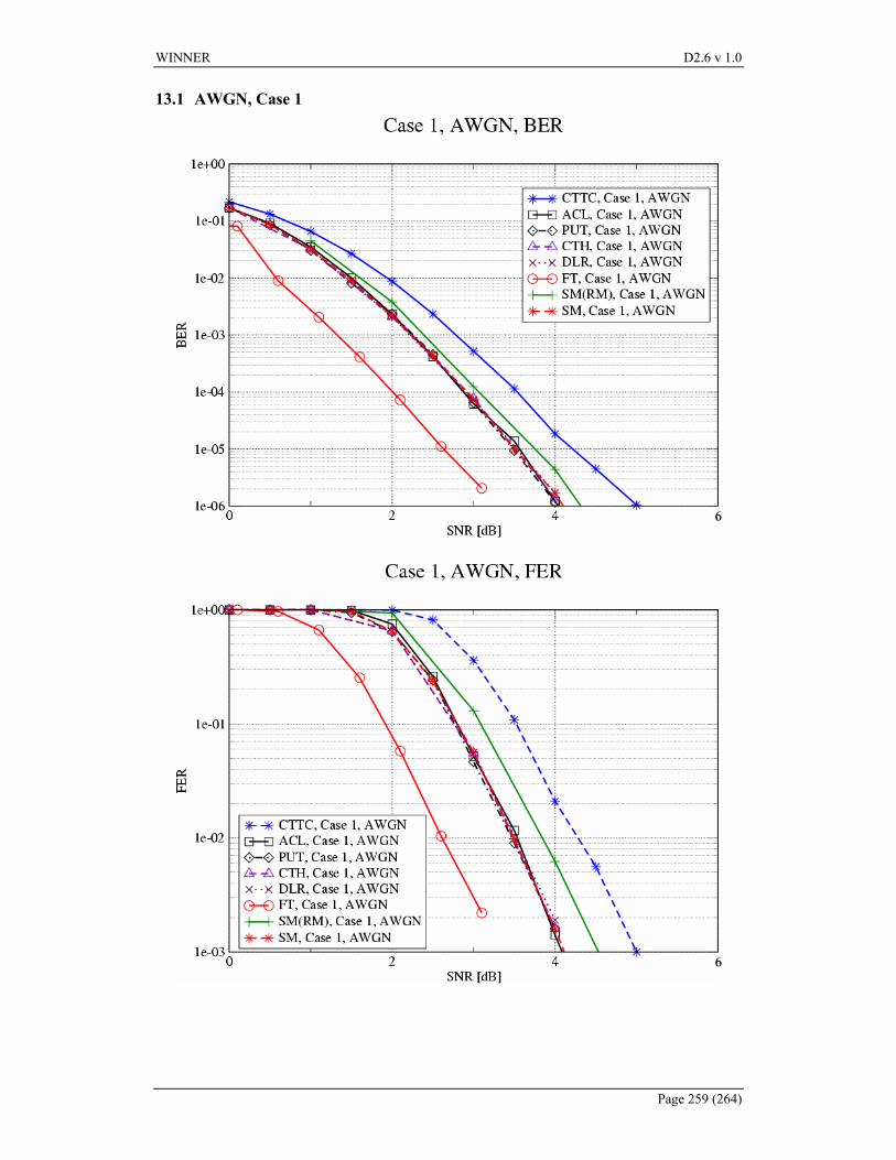
WINNER D2.6 v 1.0

Page 259 (264)

13.1 AWGN, Case 1

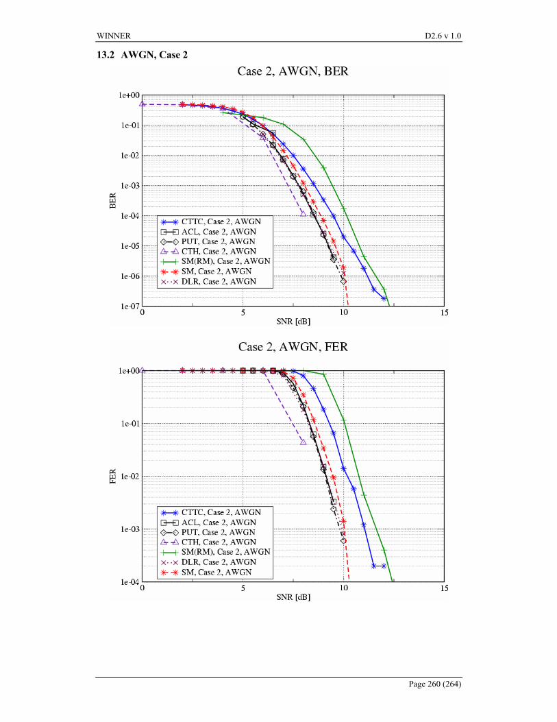
WINNER D2.6 v 1.0

Page 260 (264)

13.2 AWGN, Case 2

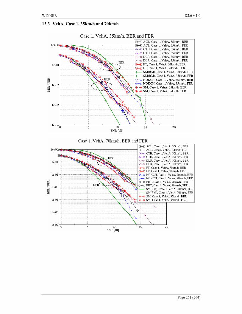
WINNER D2.6 v 1.0

Page 261 (264)

13.3 VehA, Case 1, 35km/h and 70km/h

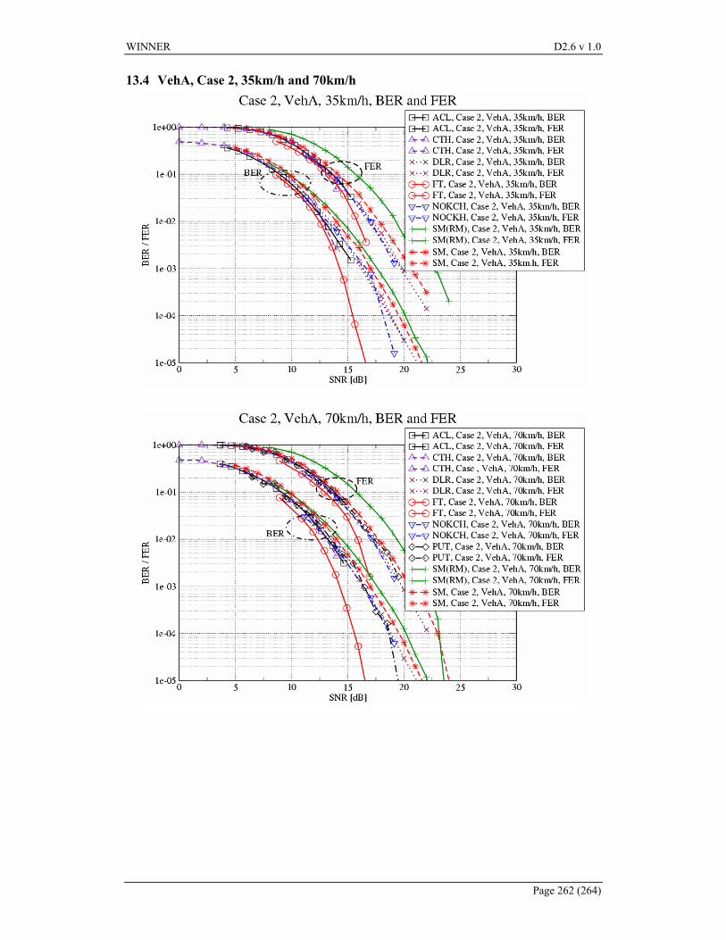
WINNER D2.6 v 1.0

Page 262 (264)

13.4 VehA, Case 2, 35km/h and 70km/h

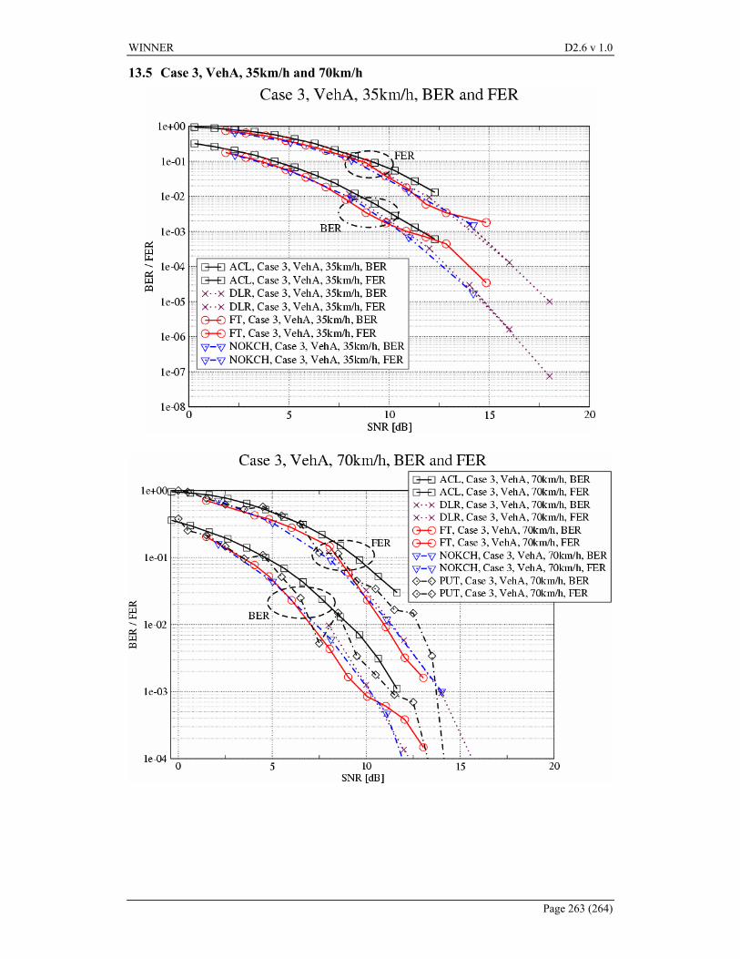
WINNER D2.6 v 1.0

Page 263 (264)

13.5 Case 3, VehA, 35km/h and 70km/h

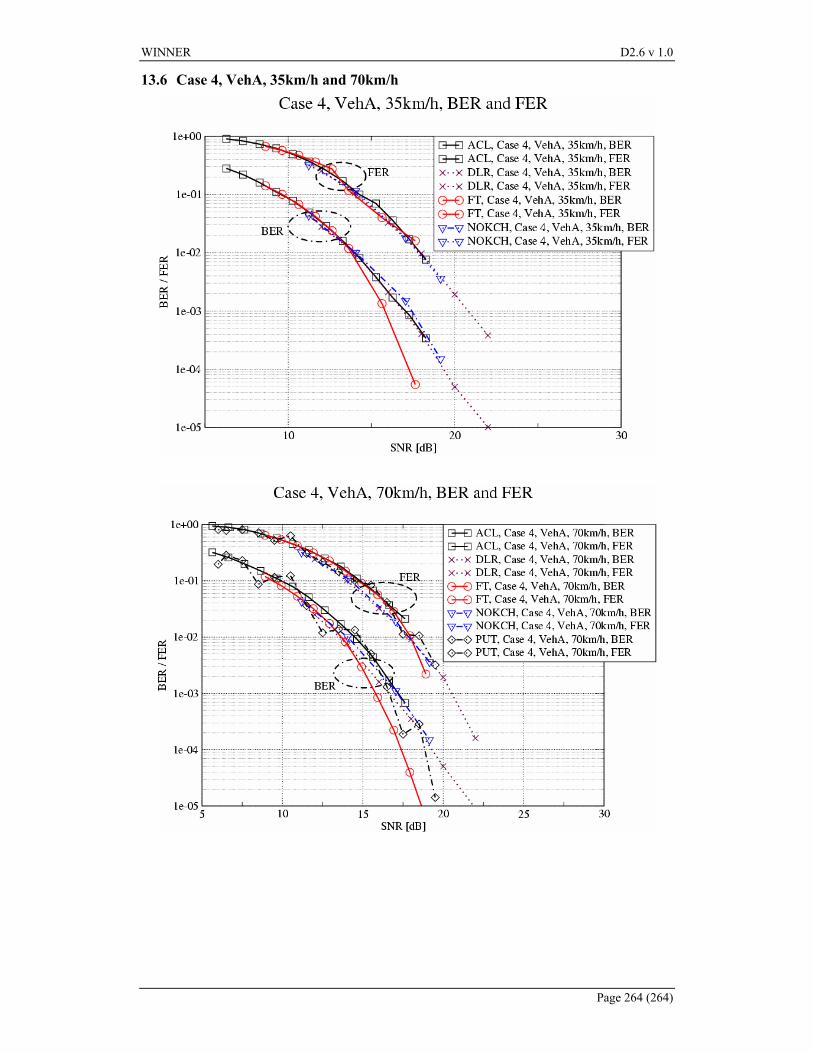
WINNER D2.6 v 1.0

Page 264 (264)

13.6 Case 4, VehA, 35km/h and 70km/h