Embed Size (px)
Citation preview

Complex Qualitative Models in Biology: A New Approach P. Veber
a M. Le Borgne
a A. Siegel
a S. Lagarrigue
b O. Radulescu
c
a Projet Symbiose, Institut de Recherche en Informatique et Systèmes Aléatoires,
IRISA-CNRS 6074, Université de Rennes 1, b UMR Génétique animale,
Agrocampus Rennes-INRA et c Institut de Recherche Mathématique de Rennes,
UMR-CNRS 6625, Université de Rennes 1, Rennes , France
Dr. Philippe Veber, Projet Symbiose, Institut de Recherche en
Informatique et Systèmes Aléatoires
IRISA-CNRS 6074, Université de Rennes 1, Campus de Beaulieu
FR–35042 Rennes Cedex (France)
Tel. +33 299 847 100, Fax +33 299 847 171,
E-Mail [email protected]
© 2005 S. Karger AG, Basel
1424–8492/05/0024–0140
$22.00/0
Complexus 2004–05;2:140– 151
B I O L O G I C A L M O D E L L I N G
Key Words Equilibrum shift � Qualitative algebra � Decision diagrams � Experiment design
Abstract We advocate the use of qualitative models in the analysis of large biological systems. We show how qualitative models are linked to theoretical differential models and practical graphical models of biological networks. A new technique for analyzing qualitative models is introduced, which is based on an effi cient representation of qualitative systems. As shown through several applications, this representation is a relevant tool for the understanding and testing of large and complex biological networks.
Copyright © 2005 S. Karger AG, Basel
Published online: August 22, 2006
DOI: 10.1159/000093686
Fax +41 61 306 12 34
E-Mail [email protected]
www.karger.com
Accessible online at:
www.karger.com/cpu
Simplexus Biological Extrapolation In the past, biologists characterized
whole organisms, identifying them, de-scribing them, and classifying them. The discovery of DNA changed all that, and bi-ology gained a prefi x – molecular. While there are still countless biologists studying whole organisms, today a biologist is just as likely to investigate the interactions of molecules as members of a species.
In the present paper, Veber and col-leagues propose a method for studying and computing steady-state shifts of differen-tial systems describing biological net-works. Critically, the researchers suggest that qualitative models can be linked to theoretical models of biological networks and might ultimately lead to new insights into understanding large biological sys-tems, by which we mean many interacting molecular species.
Given recent major developments in molecular biology such as microarrays, mass spectrometry, and protein chips, the development of a quantitatively robust method for coping with putatively thou-sands of variables in any given biological system simultaneously would be rather timely. Network-based representations have been used widely to describe gene regulation or metabolic pathways at the cellular level. Network reconstruction re-lies on gathering vast amounts of quantita-tive data from microarrays. However, these analytical techniques are still imperfect and sensitive to interference and noise, therefore not always quantitatively reliable. Available experimental data can only be in-terpreted on qualitative grounds. Microar-rays, for instance, which are used to com-pare gene activity, only tell us that gene G is more active in situation A than in situa-tion B.
Veber and his colleagues wanted to cope with this situation. Previously, they de-vised a novel framework for comparing two sets of experimental conditions – situ-ation A and situation B, for example. With
141 Complexus 2004–05;2:140–151 Veber /Le Borgne /Siegel /Lagarrigue /Radulescu
1 Introduction Understanding the behaviour of a bio-
logical system from the interplay of its mo-lecular components is a particularly diffi -cult task. A model-based approach propos-es a framework to express some hypotheses about a system and make some predictions out of it, in order to compare with experi-mental observations. Traditional ap-proaches [see 1 for an interesting review] include ordinary differential equations or stochastic processes. While they are pow-erful tools to acquire a fi ne grained knowl-edge of the system at hand, these frame-works need accurate experimental data on chemical reaction kinetics, which are scarcely available. Furthermore, they also are computationally demanding and their practical use is restricted to a limited num-ber of variables.
As an answer to these issues, many ap-proaches were proposed that abstract from quantitative details of the system. Among others, let us stress the work done on gene regulation dynamics [2] , hybrid systems [3] or discrete event systems [4, 5] . The goal of such qualitative frameworks is to enable system level analysis of a biological phenomenon. This appears as a relevant answer to a recent technical breakthrough in experimental biology: • microarrays, mass spectrometry, pro-tein chips currently allow to measure thou-sands of variables simultaneously • obtained measurements are rather noisy, and may not be quantitatively reli-able
Microarrays, for instance, are used for comparing the activity of genes between two experimental settings. A microarray experiment gives a differential measure between two experimental settings. It de-livers information on the relative activity of each gene represented on the array. De-spite many attempts made to quantify the output of microarrays, the essential output of the technique says, for example, that a gene G is more active in situation A than in situation B.
this approach they side-step the data and gene perturbation information from mi-croarrays and their ilk and build a network not from scratch, but by gathering infor-mation from the literature. This allowed them to analyze even incomplete models and to compare models and data. As such, the emergent mathematical results con-nect network topology and information from steady-state shift experiments, which are used by chemists to reveal reaction mechanisms.
Gene networks are essentially graphical models of molecular interactions involved in the expression machinery of genes. The particular genes being used by a cell under specifi c conditions depend on these inter-actions and the set of active genes reveal a cell’s specialization. Liver cells, for instance, express different genes to neurons or mus-cle cells. In order to understand cell func-tion a good model is essential as too is knowledge of the topology of the networks that allow the cell to function. Each one of these problems is diffi cult and there are no well-established methods to solve them, as there are no machines that photograph or read gene networks. Gene network recon-struction is a painful process of knowledge accumulation and consists in interpreting the response of genes to perturbations such as deleting or silencing some genes, overexpressing other genes or changing the external conditions. In this process er-rors are inevitable.
Qualitative methods, however, have been used for error detection and correc-tion since the 1980s in various applications such as electronic circuit design and diag-nosis. In the current paper, Veber and his colleagues have built on this approach and developed a method for applying qualita-tive constraints to possible deviations in a gene network model. They have created an effi cient way of representing the set of solu-tions of a qualitative system, which they explain, allows one to solve systems with hundreds of variables.
In this paper, we use a framework devel-oped by Siegel et al. [6] for the comparison of two experimental conditions, in order to derive qualitative constraints on the pos-sible variations of the variables. Our main contribution is the use of an effi cient rep-resentation for the set of solutions of a qualitative system. This representation al-lows to solve systems with hundreds of variables. Moreover, this representation opens the way to a fi ner analysis of qualita-tive systems. This new approach is illus-trated by solving three important prob-lems: • checking the accordance of a qualitative system with qualitative experimental data • minimally correcting corrupted data in discordance with a model • helping in the design of experiments
Our main focus here is to show how to use large qualitative models and qualita-tive interpretations of experimental data. In this respect our work could be used as an extension to what was proposed by Gutierrez-Rios et al. [7] , where basically the authors propose to analyze pangenom-ic gene expression arrays in Escherichia coli , using simple qualitative rules.
In the fi rst section we establish links be-tween differential, graphical and qualita-tive models.
2 Mathematical Modelling In this section we show how qualitative
models can be linked to more traditional differential models. Differential models are central to the theory of metabolic con-trol [8, 9] . They also have been applied to various aspects of gene network dynamics. The purpose of this section is to lay down a set of qualitative equations describing steady-state shifts of differential models. For the sake of completeness, we rederive in a simpler case results that have been es-tablished in greater generality [6, 10] .
2.1 Modelling Assumptions Let us consider a network of interacting
cellular constituents, numbered from 1 to n .
142 Complexus 2004–05;2:140–151 Complex Qualitative Models in Biology: A New Approach
As proof of principle, the researchers have used an example derived from the physiology of higher organisms – the ge-netic regulation of fatty acid synthesis in liver. The liver has two ways of making fat-ty acids: saturated and monounsaturated fatty acids are produced from citrates via a four enzyme route, while polyunsaturated fatty acids (PUFA) are produced from es-sential fatty acids from the diet using just two enzymes. PUFAs play a key role in sev-eral biological functions, such as regula-tion of gene expression that in turn im-pacts on lipid, carbohydrate, and protein metabolism, various receptors mediate their actions.
The receptors involved in PUFA media-tion are the variables in the model and are abbreviated as PPAR, LXR, and SREBP. The receptors are synthesized from the corre-sponding genes and are then modifi ed to make the active forms. Another protein SCAP cleaves SREBP and interacts with yet another protein family denoted INSIG, which hints at just how complicated the molecular mechanism is. Also included in the model are the fi nal products ACL, ACC, FAS, SCD1, D5D, D6D, and PUFAs them-selves. All these variables then have differ-ent interactions: SREBP activates tran-scription of ACL, ACC, FAS, SCD1, D5D and D6D. LXR activates transcription of SREBP and FAS, and indirectly activates ACL, ACC and SCD1, and so on, all aimed at regulat-ing the production of PUFA in the liver.
An experiment to investigate just how these systems work would involve re-feed-ing fasting laboratory animals and quanti-fying the various liver products using mi-croarray analysis. Currently, there are no methods available that would allow re-searchers to feed the vast amounts of data retrieved from a study into an analytical model. Furthermore, quantitative data is incomplete and highly inaccurate. Qualita-tive modelling is a solution that might cope with incomplete and inaccurate data, ex-plains Veber. Indeed, the present research-ers are not the only ones to recognize this
These constituents may be proteins, RNA transcripts or metabolites for instance. The state vector X denotes the concentra-tion of each constituent.
Differential Dynamics X is assumed to evolve according to the
following differential equation:
dXdt
= F(X)
where F is an (unknown) non-linear, dif-ferentiable function. A steady-state X eq of the system is a solution of the algebraic equation:
F ( X eq ) = 0.
Steady states are asymptotically stable if they attract all nearby trajectories. A steady state is non-degenerated if the Jaco-bian calculated in that steady state is non-vanishing. According to the Grobman-Hartman theorem, a suffi cient condition to have non-degenerated asymptotically sta-ble steady states is Re ( � i ) ! – C , C 1 0, i = 1, ..., n , where � i are the eigenvalues of the Jacobian matrix calculated at the steady state.
Experiment Modelling Typical two-state experiments such as
differential microarrays are modelled as steady-state shifts. We suppose that under a change of the control parameters in the experiment, the system goes from one non-degenerated stable steady state to an-other one. The output of the two-state ex-periment can be expressed in terms of con-centration variations for a subset of prod-ucts, between the two states. We suppose that the signs of these variations were proven to be statistically signifi cant.
Interaction Graph The only knowledge we require about
the function F concerns the signs of the de-rivatives
∂Fi∂X j
.
These are interpreted as the action of the product j on the product i . It is an activa-tion if the sign is +, an inhibition if the sign is –. A null value means no action.
An interaction graph G ( V , E ) is derived from the Jacobian matrix of F : (1) with nodes V = {1, ..., n } corresponding to products and (2) (oriented) edges
E = {( j, i)| ∂Fi∂X j
�= 0}.
Edges are labelled by
s( j, i) = sgn( ∂Fi∂X j
).
The set of predecessors of a node i in G is denoted pred( i ). The interaction graph is actually built from information gathered in the literature. In consequence in some places it may be incomplete (some interac-tions may be missing), in others it may be redundant (some interactions may appear several times as direct and indirect inter-actions). It is an important issue that nei-ther incompleteness nor redundancy do not introduce inconsistencies and this will be addressed in section 5.
Negative Diagonal in the Jacobian Matrix For any product i , we exclude the pos-
sibility of vanishing diagonal elements of the Jacobian
∂Fi∂Xi
.
This can be justifi ed by taking into account degradation and dilution (cell growth) processes that can be represented as nega-tive self-loops in the interaction graph, that is for all i , ( i , i ) D E and s ( i , i ) = –.
Discussion In our mathematical modelling we sup-
pose that the system starts and ends in non-degenerated stable steady states. Of course this is not always the case for sev-eral reasons: there is too much waiting time to reach steady state; one can end up in a limit cycle and oscillate instead of reaching a steady state. All these possibili-
143 Complexus 2004–05;2:140–151 Veber /Le Borgne /Siegel /Lagarrigue /Radulescu
ties should be considered with caution. Ac-tually this hypothesis might be diffi cult to check from the two states only. Comple-mentary strategies such as time series analysis could be employed in order to as-sess the possibility of limit cycle oscilla-tions.
Positive self-regulation is also possible but introduces a supplementary complica-tion. In this case for certain values of the concentrations degradation exactly com-pensates the positive self-regulation and the diagonal elements of the Jacobian van-ish (this is a consequence of the intermedi-ate value theorem). We can avoid dealing with this situation by considering that the positive self-regulation does not act direct-ly and that it involves intermediate species. This is a realistic assumption because a molecule never really acts directly on itself (transcripts can be autoregulated but only via protein products). Thus, all nodes can keep their negative self-loops and all diag-onal elements of the Jacobian can be con-sidered to be non-vanishing. Although the positive regulation may imply vanishing higher order minors of the Jacobian, this will not affect our local qualitative equa-tions.
2.2 Quantitative Variation of One Variable We focus here on the variation of the
concentration of a single chemical species represented by a component X i of the vec-tor X . Since we have adopted a static point of view, we are only interested in the varia-tion of X i between two non-degenerated stable steady states X1
eq and X2eq indepen-
dently of the trajectory of the dynamical system between the two states.
Let us denote by X^
i the vector of dimen-
sion n i obtained by keeping from X all co-ordinates j that are predecessors of i in the interaction graph. Then, under some ad-ditional assumptions described and dis-cussed by Radulescu et al. [10] , we have the following result:
problem. Boolean or multivalue logical models, for instance, also provide qualita-tive descriptions. Compared to these mod-els Veber and his colleagues use an alterna-tive algebra, better adapted to the problem of equilibrium shifts, and, fi nally, provide reasonable algorithms to code and solve qualitative equations.
In order to compare model and data, one needs a mathematical description of the relation between the two, a comparison calculus, in other words. This can be done by predicting how the equilibrium of the genetic regulation system changes under different conditions, for instance, how lipid metabolism changes during fasting and normal feeding. A gene network behaves similarly to an elastic medium, according to Veber and colleagues’ fi ndings. Pertur-bations somewhere in the network are transported along the graph in the direc-tion of the regulation arrows and obey an analogue of quantitative elastic moduli. Nonetheless, under certain mild condi-tions, the signs of variations of gene ex-pression is the qualitative sum of the signs of infl uences coming from its neighbours in the network. For instance, gene A is pos-itively regulated by B and also by C. The qualitative equation is dA = dB + dC.
This is purely dependent on topology and does not imply the need for a choice of Boolean function of B and C (AND, OR, etc.) to give A as is required in a Boolean gene network (a parallel fi eld of qualitative gene modelling). In three valued sign alge-bra (+,-,?) a + variation of A (dA = +) and a + variation of B (dB = +) is compatible either with dC = + or with dC = –. Further-more, the situation dA = –, dB = + is only compatible with dC = –. The latter example is illustrative of the predictive power of qualitative equations: if one knows that A decreases and B increases, and one knows that the only infl uence on A comes from B and C, then there is no need to measure C, as it should decrease.
Veber and colleagues explain that the qualitative equations can be reduced to a
Theorem 2. 1 The variation of the concentration of spe-
cies i between two non-degenerated steady states X1
eq and X2eq is given by
X1eqi
−X2eqi
=
∫S−
(∂Fi
∂Xi
)−1
∑k∈pred(i)
∂Fi
∂XkdXk
(1)
where S is the segment linking
X1eqi
to X2eqi
.
Full proof is given by Radulescu et al. [10] . The above formula is a quantitative relation between the variation of concen-trations and the derivatives
∂Fi∂X j
.
Now our next move will be to introduce a qualitative abstraction of this relation.
2.3 Qualitative Equations We propose here to study equation 1 in
sign algebra. By sign algebra, we mean the set { + , – , ? }, where ? represents an undeter-mined sign. This set is provided with the natural commutative operations:
+ + – = ? + + + = + – + – = – + ! – = – + ! + = + – ! – = + ? + – = ? ? + + = ? ? + ? = ? ? ! – = ? ? ! + = ? ? ! ? = ?
Equality in sign algebra � is defi ned as follows:
≈ + − ?+ T F T− F T T? T T T
Importantly, qualitative equality is not an equivalence relation, since it is not tran-sitive. This implies that computations in qualitative algebra must be carried out with care. At least two major properties should be emphasized: • If a term of a sum is indeterminate (?) then the whole sum is indeterminate.
144 Complexus 2004–05;2:140–151 Complex Qualitative Models in Biology: A New Approach
fi nite set of clauses in polynomial time, so resolution of this qualitative system is an NP-complete problem. However by encod-ing the qualitative equations associated with the problem as algebraic equations, they offer a solution that can be computed with greatly reduced time and complexity and so without the need for vast computer power.
One additional benefi t of the technique developed by Veber and colleagues is in ex-periment design. Models are built on ac-cumulated knowledge. However, one would like to optimize the process by choosing the most economic way to gain the neces-sary knowledge. For instance, one might decide which genes to observe or perturb in an experiment. The choice is based on an estimate of the amount of information that such an experiment would bring. In the approach of Veber and colleagues, this choice is connected to the number of solu-tions of the qualitative equations con-strained by a certain result of the experi-ment. The higher this number, the less in-formative will be the experiment and so an alternative route could be taken.
The researchers now plan to validate their approach further on metabolic path-ways in yeast and Escherichia coli . These organisms have large pathways represent-ed by vast quantities of microarray data that are publicly available. Despite the scale of such databases, Veber and colleagues have found that 200 variable sets can be handled within minutes.
David Bradley of Sciencebase.com
• If one hand of a qualitative equality is indeterminate, then the equality is satis-fi ed whatever the value of the other hand is.
A qualitative system is a set of algebraic equations with variables in { + , – , ? }. A solu-tion of this system is a valuation of the un-known which satisfi es each equation, and in such a way that no variable is instanti-ated to ? . This last requirement is impor-tant since otherwise any system would have trivial solutions (like all variables to ? ).
Theorem 2.2 Under the assumptions and notations of
theorem 2.1, if the sign of
∂Fi∂X j
i s constant, then the following relation holds in sign algebra:
s(∆Xi) ≈ ∑k∈pred(i)
s(k, i)s(∆Xk) (2)
where s( � X k ) denotes the sign of
X 1eqk
−X2eqk
.
By writing equation 2 for all nodes in the graph, we obtain a system of equations on signs of variations, later referred to as qualitative system associated with the in-teraction graph G . This will be used exten-sively in the next sections.
2.4 Link between Qualitative and Quantitative The qualitative system obtained from
equation 2 is a consequence of the quanti-tative relations that result from Theorem 2.1. So the sign function maps a quantita-tive variation between two equilibrium points onto a qualitative solution of equa-tion 2. The converse is not true in general. For a given solution S of the qualitative sys-tem, there might be no equilibrium change � X in the differential quantitative model, such that each real-valued component of � X has the sign given by S .
However, some components of the solu-tion vectors are uniquely determined by the qualitative system. They take the same sign value in every solution vector. For such so-called hard components, the sign of any quantitative solution (if it exists) is completely determined by the qualitative system.
We will use the previous properties to check the coherence between models and experimental data. By experimental data we mean the sign of the observed variation in concentration for some nodes. In par-ticular, if the qualitative system associated with an interaction graph G has no solu-tion given some experimental observa-tions, then no function F satisfying the sign conditions on the derivatives can de-scribe the observed equilibrium shift, meaning that either the model is wrong or some data are corrupted. In the next sec-tion, we introduce a simplifi ed model re-lated to lipid metabolism, and illustrate the above-described formalism.
3 Toy Example: Regulation of the Synthesis of Fatty Acids In order to illustrate our approach, we
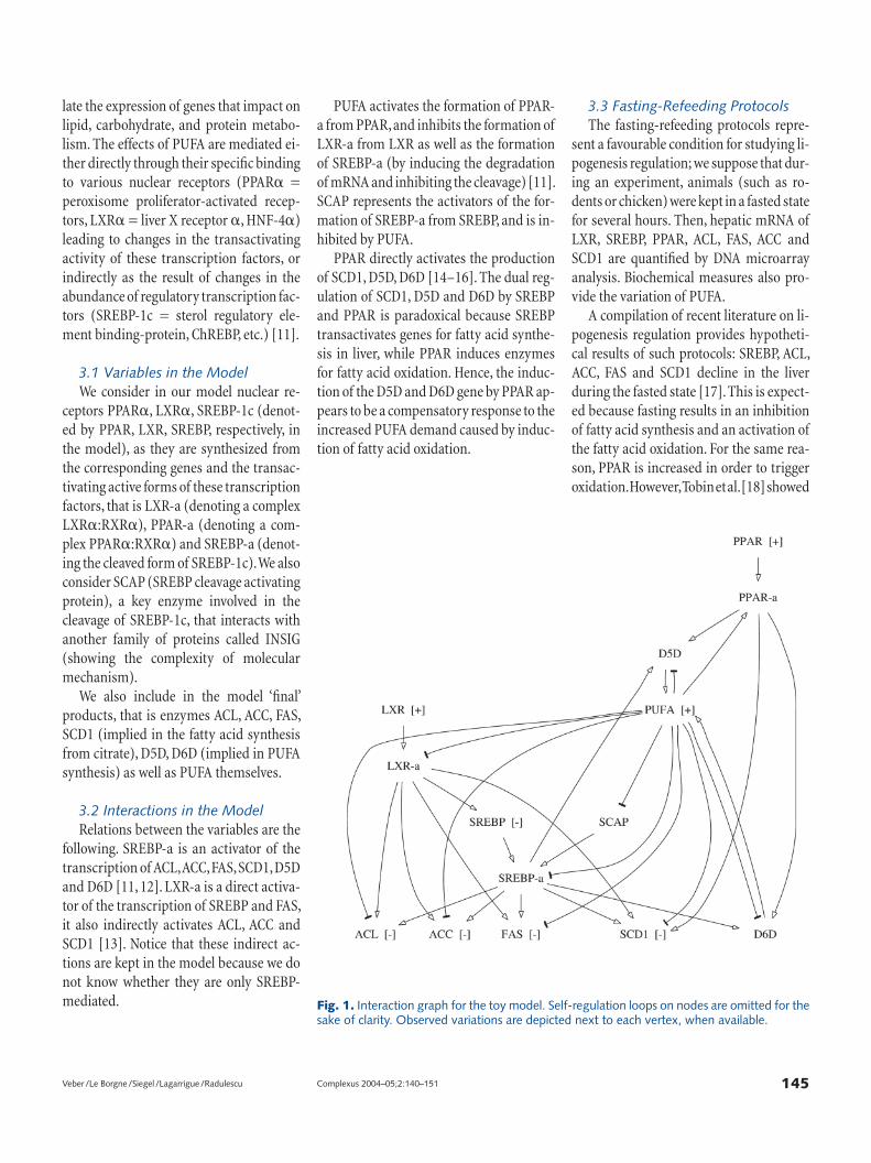
use a toy example describing a simplifi ed model of genetic regulation of fatty acid synthesis in liver. The corresponding inter-action graph is shown in fi gure 1 .
Two ways of production of fatty acids coexist in the liver. Saturated and monoun-saturated fatty acids are produced from ci-trates thanks to a metabolic pathway com-posed of four enzymes, namely ACL (ATP citrate lyase), ACC (acetyl-coenzyme A carboxylase), FAS (fatty acid synthase) and SCD1 (stearoyl-CoA desaturase 1). Polyunsaturated fatty acids (PUFA) such as arachidonic acid and docosahexaenoic acid are synthesized from essential fatty acids provided by nutrition; D5D (delta-5 desaturase) and D6D (delta-6 desaturase) catalyze the key steps of the synthesis of PUFA.
PUFA plays pivotal roles in many bio-logical functions; among them, they regu-
145 Complexus 2004–05;2:140–151 Veber /Le Borgne /Siegel /Lagarrigue /Radulescu
late the expression of genes that impact on lipid, carbohydrate, and protein metabo-lism. The effects of PUFA are mediated ei-ther directly through their specifi c binding to various nuclear receptors (PPAR � = peroxisome proliferator-activated recep-tors, LXR � = liver X receptor � , HNF-4 � ) leading to changes in the transactivating activity of these transcription factors, or indirectly as the result of changes in the abundance of regulatory transcription fac-tors (SREBP-1c = sterol regulatory ele-ment binding-protein, ChREBP, etc.) [11] .
3.1 Variables in the Model We consider in our model nuclear re-
ceptors PPAR � , LXR � , SREBP-1c (denot-ed by PPAR, LXR, SREBP, respectively, in the model), as they are synthesized from the corresponding genes and the transac-tivating active forms of these transcription factors, that is LXR-a (denoting a complex LXR � :RXR � ), PPAR-a (denoting a com-plex PPAR � :RXR � ) and SREBP-a (denot-ing the cleaved form of SREBP-1c). We also consider SCAP (SREBP cleavage activating protein), a key enzyme involved in the cleavage of SREBP-1c, that interacts with another family of proteins called INSIG (showing the complexity of molecular mechanism).
We also include in the model ‘fi nal’ products, that is enzymes ACL, ACC, FAS, SCD1 (implied in the fatty acid synthesis from citrate), D5D, D6D (implied in PUFA synthesis) as well as PUFA themselves.
3.2 Interactions in the Model Relations between the variables are the
following. SREBP-a is an activator of the transcription of ACL, ACC, FAS, SCD1, D5D and D6D [11, 12] . LXR-a is a direct activa-tor of the transcription of SREBP and FAS, it also indirectly activates ACL, ACC and SCD1 [13] . Notice that these indirect ac-tions are kept in the model because we do not know whether they are only SREBP-mediated.
PUFA activates the formation of PPAR-a from PPAR, and inhibits the formation of LXR-a from LXR as well as the formation of SREBP-a (by inducing the degradation of mRNA and inhibiting the cleavage) [11] . SCAP represents the activators of the for-mation of SREBP-a from SREBP, and is in-hibited by PUFA.
PPAR directly activates the production of SCD1, D5D, D6D [14–16] . The dual reg-ulation of SCD1, D5D and D6D by SREBP and PPAR is paradoxical because SREBP transactivates genes for fatty acid synthe-sis in liver, while PPAR induces enzymes for fatty acid oxidation. Hence, the induc-tion of the D5D and D6D gene by PPAR ap-pears to be a compensatory response to the increased PUFA demand caused by induc-tion of fatty acid oxidation.
3.3 Fasting-Refeeding Protocols The fasting-refeeding protocols repre-
sent a favourable condition for studying li-pogenesis regulation; we suppose that dur-ing an experiment, animals (such as ro-dents or chicken) were kept in a fasted state for several hours. Then, hepatic mRNA of LXR, SREBP, PPAR, ACL, FAS, ACC and SCD1 are quantifi ed by DNA microarray analysis. Biochemical measures also pro-vide the variation of PUFA.
A compilation of recent literature on li-pogenesis regulation provides hypotheti-cal results of such protocols: SREBP, ACL, ACC, FAS and SCD1 decline in the liver during the fasted state [17] . This is expect-ed because fasting results in an inhibition of fatty acid synthesis and an activation of the fatty acid oxidation. For the same rea-son, PPAR is increased in order to trigger oxidation. However, Tobin et al. [18] showed
Fig. 1. Interaction graph for the toy model. Self-regulation loops on nodes are omitted for the sake of clarity. Observed variations are depicted next to each vertex, when available.
146 Complexus 2004–05;2:140–151 Complex Qualitative Models in Biology: A New Approach
that rats fasting for 24 h increased the he-patic LXR mRNA, although LXR positively regulates fatty acid synthesis in its activat-ed form. Finally, PUFA levels can be consid-ered to be increased in liver following star-vation because of the important lipolysis from adipose tissue as shown by Lee et al. [19] in mice after 72 h fasting.
3.4 Qualitative System Derived from the Graph As explained in the previous section, we
derive a qualitative system from the inter-action graph shown in fi gure 1 . For ease of presentation, we denote by A the sign of variation for species A. (See table below).
In the next section, we propose an effi -cient representation for such qualitative systems.
4 Analysis of Qualitative Equations: a New Approach 4.1 Resolution of Qualitative Systems The resolution of (even linear) qualita-
tive systems is an NP-complete problem [see for instance 20, 21] . One can show this by reducing the satisfi ability problem for a fi nite set of clauses to the resolution of a qualitative system in polynomial time.
Let us consider a collection C = { c 1 , ..., c n } of clauses on a fi nite set V of variables. Let { + , – , ? } a sign qualitative al-gebra. In order to reduce the satisfi ability problem to the resolution of a qualitative
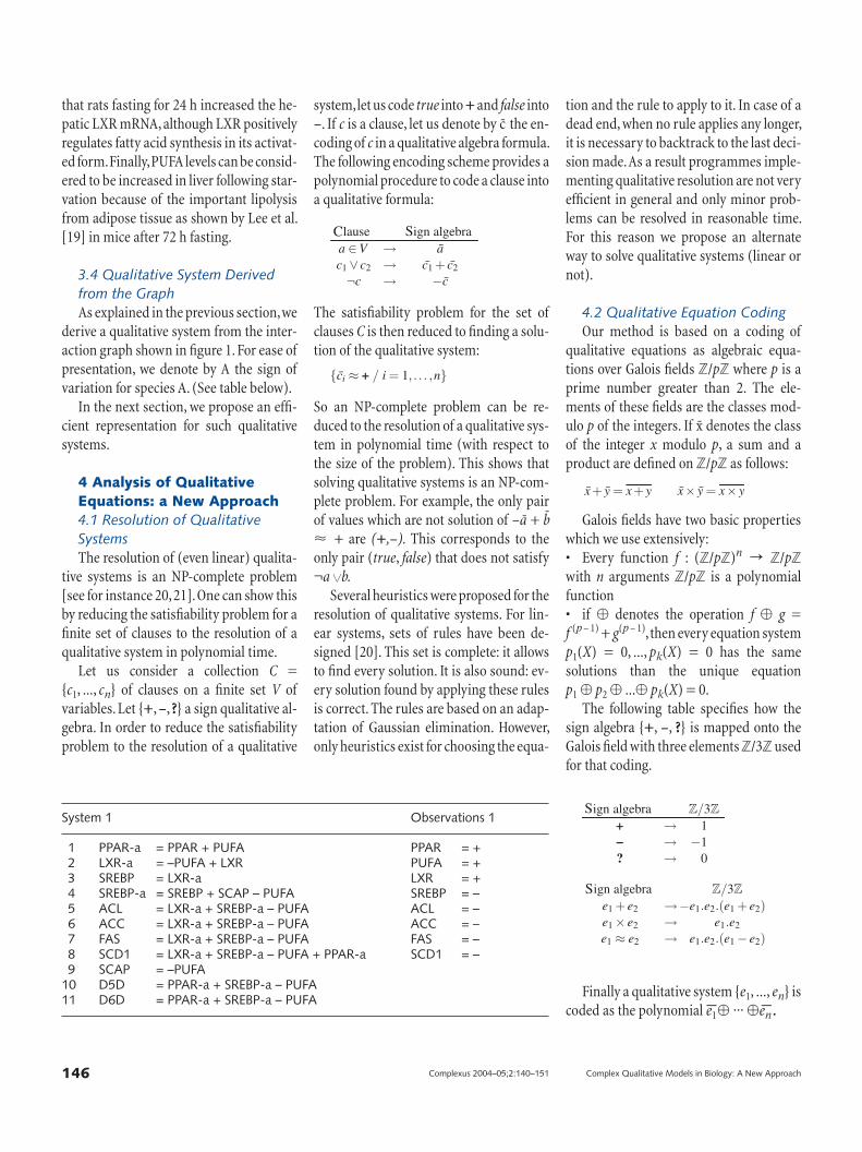
system, let us code true into + and false into –. If c is a clause, let us denote by c the en-coding of c in a qualitative algebra formula. The following encoding scheme provides a polynomial procedure to code a clause into a qualitative formula:
laus ign algebraa ∈V → ac1 ∨ c2 → c1 + c2¬c → −c
C Se
The satisfi ability problem for the set of clauses C is then reduced to fi nding a solu-tion of the qualitative system:
{ci ≈ + / i = 1, . . . ,n}
So an NP-complete problem can be re-duced to the resolution of a qualitative sys-tem in polynomial time (with respect to the size of the problem). This shows that solving qualitative systems is an NP-com-plete problem. For example, the only pair of values which are not solution of –a + b � + are (+,–). This corresponds to the only pair ( true , false ) that does not satisfy ¬a �b.
Several heuristics were proposed for the resolution of qualitative systems. For lin-ear systems, sets of rules have been de-signed [20] . This set is complete: it allows to fi nd every solution. It is also sound: ev-ery solution found by applying these rules is correct. The rules are based on an adap-tation of Gaussian elimination. However, only heuristics exist for choosing the equa-
tion and the rule to apply to it. In case of a dead end, when no rule applies any longer, it is necessary to backtrack to the last deci-sion made. As a result programmes imple-menting qualitative resolution are not very effi cient in general and only minor prob-lems can be resolved in reasonable time. For this reason we propose an alternate way to solve qualitative systems (linear or not).
4.2 Qualitative Equation Coding Our method is based on a coding of
qualitative equations as algebraic equa-tions over Galois fi elds �/ p � where p is a prime number greater than 2. The ele-ments of these fi elds are the classes mod-ulo p of the integers. If x denotes the class of the integer x modulo p , a sum and a product are defi ned on �/ p � as follows:
x+ y = x+ y x× y = x× y
Galois fi elds have two basic properties which we use extensively: • Every function f : (�/ p �) n ] �/ p � with n arguments �/ p � is a polynomial function • if � denotes the operation f � g = f ( p – 1) + g ( p – 1) , then every equation system p 1 ( X ) = 0, ..., p k ( X ) = 0 has the same solutions than the unique equation p 1 � p 2 � ...� p k ( X ) = 0.
The following table specifi es how the sign algebra { + , – , ? } is mapped onto the Galois fi eld with three elements �/ 3 � used for that coding.
ign algebra Z/3Z
+ → 1− → −1? → 0
S
ign algebra Z/3Z
e1 + e2 → 1 2 1 + e2)e1 × e2 → e1.e2e1 ≈ e2 → e1.e2.(e1 − e2)
Se .e .(e−
Finally a qualitative system { e 1 , ..., e n } is coded as the polynomial e1
−� ... �en−.
System 1 Observations 1
1 PPAR-a = PPAR + PUFA PPAR = +2 LXR-a = –PUFA + LXR PUFA = +3 SREBP = LXR-a LXR = + 4 SREBP-a = SREBP + SCAP – PUFA SREBP = –5 ACL = LXR-a + SREBP-a – PUFA ACL = –6 ACC = LXR-a + SREBP-a – PUFA ACC = –7 FAS = LXR-a + SREBP-a – PUFA FAS = –8 SCD1 = LXR-a + SREBP-a – PUFA + PPAR-a SCD1 = –9 SCAP = –PUFA
10 D5D = PPAR-a + SREBP-a – PUFA11 D6D = PPAR-a + SREBP-a – PUFA
147 Complexus 2004–05;2:140–151 Veber /Le Borgne /Siegel /Lagarrigue /Radulescu
A similar coding for the qualitative algebra { + , – , 0 , ? } uses the Galois fi eld �/ 5 � and will not be presented here.
With this coding, every qualitative sys-tem has a solution if and only if the corre-sponding polynomial has a solution with-out null component. Null solutions are ex-cluded since ? solutions are excluded for qualitative systems. In general we will have to add polynomial equations X 2 = 1 to in-sure this.
4.3 An Effi cient Representation of Polynomial Functions Recall that our purpose is to effi ciently
solve an NP-complete problem. There is no hope to fi nd a representation of polynomi-al functions allowing to solve polynomial systems of equations in polynomial time. The coding of a qualitative system as a polynomial equation is obviously polyno-mial in the size of the system (number of variables plus number of equations). So fi nding the solution of a polynomial sys-tem of equations is itself an NP-complete problem. It is more or less the satisfi ability problem.
Nevertheless, there exists a representa-tion of polynomial functions on Galois fi elds which gives, in practice, good perfor-mances for polynomials with hundreds of variables. This kind of representation was fi rst used for logical functions which may be considered as polynomial functions over the fi eld �/ 2 �. This representation is known as BDD (binary decision diagrams) and is widely used in checking logical cir-cuits [22] and in model checkers as nu-SMV [23] .
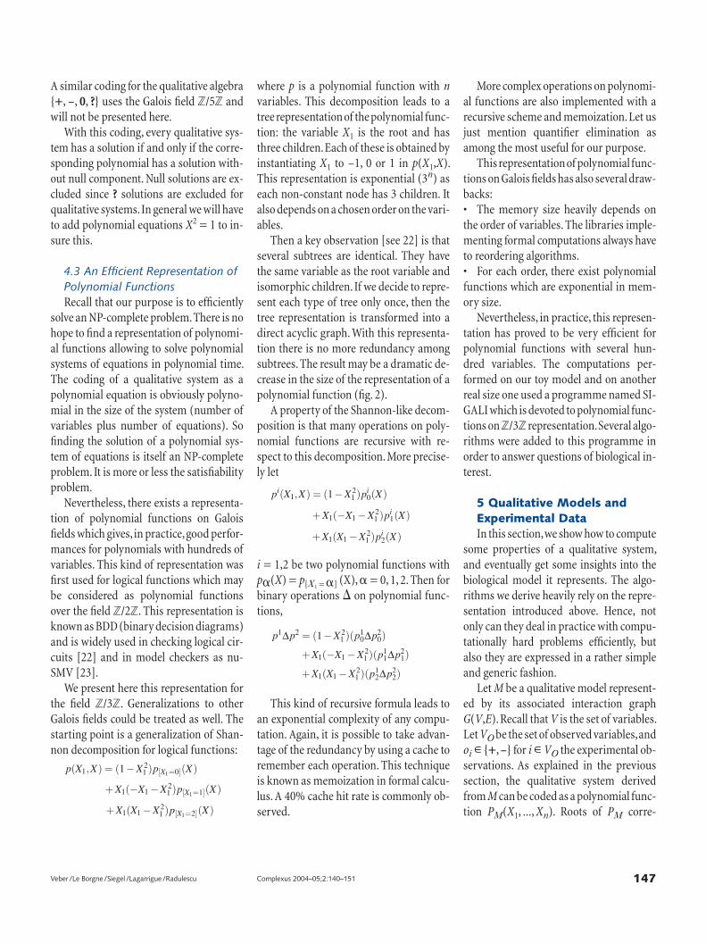
We present here this representation for the fi eld �/ 3 �. Generalizations to other Galois fi elds could be treated as well. The starting point is a generalization of Shan-non decomposition for logical functions:
p(X1,X) = (1−X 21 )p[X1=0](X)
+X1(−X1 −X21 )p[X1=1](X)
+X1(X1 −X21 )p[X1=2](X)
where p is a polynomial function with n variables. This decomposition leads to a tree representation of the polynomial func-tion: the variable X 1 is the root and has three children. Each of these is obtained by instantiating X 1 to –1, 0 or 1 in p ( X 1 , X ). This representation is exponential (3 n ) as each non-constant node has 3 children. It also depends on a chosen order on the vari-ables.
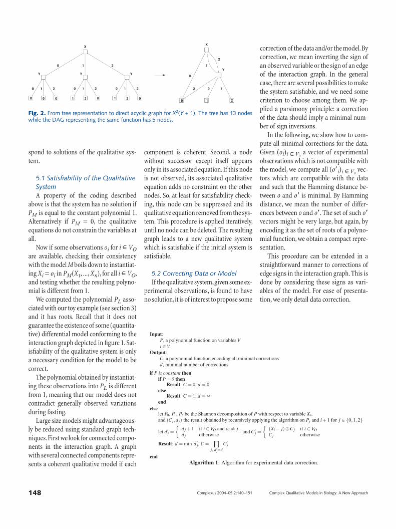
Then a key observation [see 22] is that several subtrees are identical. They have the same variable as the root variable and isomorphic children. If we decide to repre-sent each type of tree only once, then the tree representation is transformed into a direct acyclic graph. With this representa-tion there is no more redundancy among subtrees. The result may be a dramatic de-crease in the size of the representation of a polynomial function ( fi g. 2 ).
A property of the Shannon-like decom-position is that many operations on poly-nomial functions are recursive with re-spect to this decomposition. More precise-ly let
pi(X1,X) = (1−X 21 )pi
0(X)
+X1(−X1 −X21 )pi
1(X)
+X1(X1 −X21 )pi
2(X)
i = 1,2 be two polynomial functions with p � ( X ) = p [ X 1 = � ] (X), � = 0, 1, 2. Then for binary operations � on polynomial func-tions,
p1∆p2 = (1−X21 )(p1
0∆p20)
+X1(−X1 −X21 )(p1
1∆p21)
+X1(X1 −X21 )(p1
2∆p22)
This kind of recursive formula leads to an exponential complexity of any compu-tation. Again, it is possible to take advan-tage of the redundancy by using a cache to remember each operation. This technique is known as memoization in formal calcu-lus. A 40% cache hit rate is commonly ob-served.
More complex operations on polynomi-al functions are also implemented with a recursive scheme and memoization. Let us just mention quantifi er elimination as among the most useful for our purpose.
This representation of polynomial func-tions on Galois fi elds has also several draw-backs: • The memory size heavily depends on the order of variables. The libraries imple-menting formal computations always have to reordering algorithms. • For each order, there exist polynomial functions which are exponential in mem-ory size.
Nevertheless, in practice, this represen-tation has proved to be very effi cient for polynomial functions with several hun-dred variables. The computations per-formed on our toy model and on another real size one used a programme named SI-GALI which is devoted to polynomial func-tions on �/ 3 � representation. Several algo-rithms were added to this programme in order to answer questions of biological in-terest.
5 Qualitative Models and Experimental Data In this section, we show how to compute
some properties of a qualitative system, and eventually get some insights into the biological model it represents. The algo-rithms we derive heavily rely on the repre-sentation introduced above. Hence, not only can they deal in practice with compu-tationally hard problems effi ciently, but also they are expressed in a rather simple and generic fashion.
Let M be a qualitative model represent-ed by its associated interaction graph G ( V , E ). Recall that V is the set of variables. Let V O be the set of observed variables, and o i D { + , – } for i D V O the experimental ob-servations. As explained in the previous section, the qualitative system derived from M can be coded as a polynomial func-tion P M ( X 1 , ..., X n ). Roots of P M corre-
148 Complexus 2004–05;2:140–151 Complex Qualitative Models in Biology: A New Approach
spond to solutions of the qualitative sys-tem.
5.1 Satisfi ability of the Qualitative System A property of the coding described
above is that the system has no solution if P M is equal to the constant polynomial 1. Alternatively if P M = 0, the qualitative equations do not constrain the variables at all.
Now if some observations o i for i D V O are available, checking their consistency with the model M boils down to instantiat-ing X i = o i in P M ( X 1 , ..., X n ), for all i D V O , and testing whether the resulting polyno-mial is different from 1.
We computed the polynomial P L asso-ciated with our toy example (see section 3) and it has roots. Recall that it does not guarantee the existence of some (quantita-tive) differential model conforming to the interaction graph depicted in fi gure 1 . Sat-isfi ability of the qualitative system is only a necessary condition for the model to be correct.
The polynomial obtained by instantiat-ing these observations into P L is different from 1, meaning that our model does not contradict generally observed variations during fasting.
Large size models might advantageous-ly be reduced using standard graph tech-niques. First we look for connected compo-nents in the interaction graph. A graph with several connected components repre-sents a coherent qualitative model if each
component is coherent. Second, a node without successor except itself appears only in its associated equation. If this node is not observed, its associated qualitative equation adds no constraint on the other nodes. So, at least for satisfi ability check-ing, this node can be suppressed and its qualitative equation removed from the sys-tem. This procedure is applied iteratively, until no node can be deleted. The resulting graph leads to a new qualitative system which is satisfi able if the initial system is satisfi able.
5.2 Correcting Data or Model If the qualitative system, given some ex-
perimental observations, is found to have no solution, it is of interest to propose some
correction of the data and/or the model. By correction, we mean inverting the sign of an observed variable or the sign of an edge of the interaction graph. In the general case, there are several possibilities to make the system satisfi able, and we need some criterion to choose among them. We ap-plied a parsimony principle: a correction of the data should imply a minimal num-ber of sign inversions.
In the following, we show how to com-pute all minimal corrections for the data. Given ( o i ) i D V O
a vector of experimental observations which is not compatible with the model, we compute all ( o � i ) i D V O
vec-tors which are compatible with the data and such that the Hamming distance be-tween o and o � is minimal. By Hamming distance, we mean the number of differ-ences between o and o � . The set of such o � vectors might be very large, but again, by encoding it as the set of roots of a polyno-mial function, we obtain a compact repre-sentation.
This procedure can be extended in a straightforward manner to corrections of edge signs in the interaction graph. This is done by considering these signs as vari-ables of the model. For ease of presenta-tion, we only detail data correction.
Fig. 2. From tree representation to direct acyclic graph for X 2 ( Y + 1). The tree has 13 nodes while the DAG representing the same function has 5 nodes.
Input:P, a polynomial function on variables Vi ∈V
Output:C, a polynomial function encoding all minimal correctionsd, minimal number of corrections
if P is constant thenif P = 0 then
Result: C = 0, d = 0else
Result: C = 1, d = ∞end
elselet P0, P1, P2 be the Shannon decomposition of P with respect to variable Xi,and (C j,d j) the result obtained by recursively applying the algorithm on Pj and i+ 1 for j ∈ {0,1,2}
let d′j =
{d j + 1 if i ∈VO and oi �= jd j otherwise and C′
j =
{(Xi − j)⊕C j if i ∈VOC j otherwise
Result: d = min d′j, C = ∏
j, d′j=d
C′j
endAlgorithm 1: Algorithm for experimental data correction.
149 Complexus 2004–05;2:140–151 Veber /Le Borgne /Siegel /Lagarrigue /Radulescu
Let us illustrate this algorithm on our toy example: during fasting experiments, synthesis of fatty acids tends to be inhib-ited, while oxidation, which produces ATP, is activated. In particular ACC, ACL, FAS and SCD1 are implied in the same pathway to produce saturated and monounsaturat-ed fatty acids. Expectedly, they are known to decline together at fasting. Suppose we introduce some wrong observation, say for instance an increase of ACL, while keeping all other observations given above. The polynomial obtained from P L including these new observations is equal to 1, and hence has no solution. Applying algorithm 1, we recover this error. Now if we wrongly change two values, say ACL and ACC to 1, the algorithm proposes a different correc-tion, namely to change the observed value of SREBP to 1, which is more parsimoni-ous.
5.3 Experiment Design It is often the case that not all variables
in the system under study can be observed. Biochemical measurements of metabolites can be costly and/or time consuming. By experiment design, we mean here the choice of the variables to observe so that an experiment might be informative.
Let P M ( X O , X U ) be the polynomial function coding for the qualitative system M . X O (or X U ) denotes the state vector of observed (or unobserved) variables. The polynomial function representing the ad-missible values of the observed variables is obtained by elimination of the quantifi er in � X U P M ( X O , X U ). Let PM
O( X O ) denote the resulting polynomial function.
For some choice of observed variables, it might well be that PM
O is null, which basi-cally means that the experiment is totally useless. Remark that no improvement can be found by taking a subset of X O . The so-lution is either to add new observed vari-ables or to choose a completely different set of observed variables.
In order to assess the relevance of a giv-en experiment (namely of a given observed
subset), we suggest to compute the follow-ing ratio: number of consistent valuations for observed variables versus the total number of valuations of observed vari-ables. A very stringent experiment has a low ratio. An experiment having a ratio val-ue of one is useless.
Again this computation is carried out in a recursive fashion. Let P be a polynomial function representing the set of admissible observed values. Let Rat ( p ) the percentage of solutions of P ( X ) = 0 in the space (�/ p �) n , where n is the number of vari-ables X . If P is constant then Rat ( P ) = 1 (or Rat ( P ) = 0) if P = 0 (or P 0 0). Else, let P 1 , P 2 , P 3 be a Shannon-like decomposition of P ( X ) with respect to some variable of P . Then it is easy to prove:
Rat ( P ) = ( Rat ( P 0 ) + Rat ( P 1 ) + Rat ( P 2 ))/3
The relevance of this approach was as-sessed on our toy example: for each subset O of variables in the model, containing at most four variables, we computed Rat (PL
O). Expectedly, the lowest ratios (i.e. the most stringent experiments) were achieved ob-serving four variables: either {SCAP, PUFA, PPAR-a, PPAR}, or {SREBP, SCAP, PUFA, LXR-a}, or {SREBP, PPAR-a, PPAR, LXR-a}.
Interestingly, the procedure captures what might be thought of as control vari-ables, like PUFA/SCAP, SREBP/LXR-a and PPAR/PPAR-a. The fi rst two pairs control the activation of fatty acid synthesis; the third one controls fatty acid oxidation.
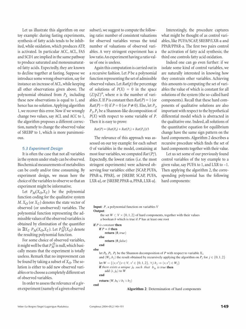
Indeed one can go even further: if we isolate some kind of control variables, we are naturally interested in knowing how they constrain other variables. Achieving this amounts to computing the set of vari-ables the value of which is constant for all solutions of the system (the so-called hard components). Recall that these hard com-ponents of qualitative solutions are also important with respect to the hypothetical differential model which is abstracted in the qualitative one. Indeed, all solutions of the quantitative equation for equilibrium change have the same sign pattern on the hard components. Algorithm 2 describes a recursive procedure which fi nds the set of hard components together with their value.
Let us set some of our previously found control variables of the toy example to a given value, say PUFA to 1, and LXR to –1. Then applying the algorithm 2, the corre-sponding polynomial has the following hard components:
Input: P, a polynomial function on variables VOutput:
the set W ⊂V ×{0,1,2} of hard components, together with their valuesa boolean b which is true if P has at least one root
if P is constant thenif P = 0 then
return ( /0, true)else
return ( /0, false)end
elselet P0, P1, P2 be the Shannon decomposition of P with respect to variable Xi,and (Wj,b j) the result obtained by recursively applying the algorithm on Pj for j ∈ {0,1,2}
let W = {(v,v′)|v ∈V, v′ ∈ {0,1,2}, ∀ j b j ⇒ (v,v′) ∈Wj}if there exists a unique j0 b j0 is true then
add (i, j0) to Wend
return (W,b0 ∨b1 ∨b2)end
Algorithm 2: Determination of hard components
such that
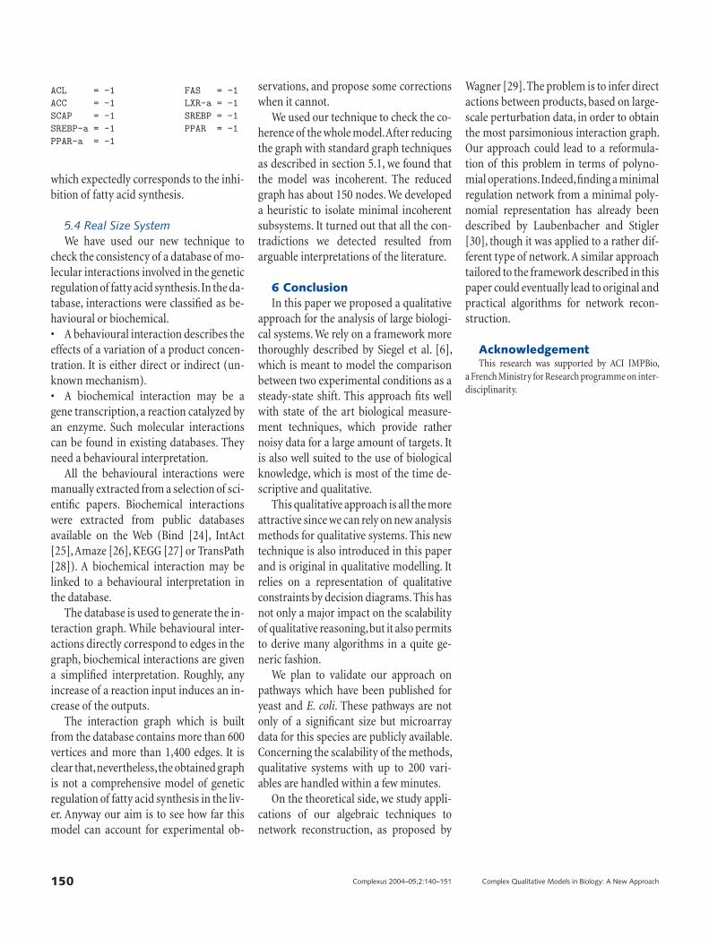
150 Complexus 2004–05;2:140–151 Complex Qualitative Models in Biology: A New Approach
ACL = -1 FAS = -1
ACC = -1 LXR-a = -1
SCAP = -1 SREBP = -1
SREBP-a = -1 PPAR = -1
PPAR-a = -1
which expectedly corresponds to the inhi-bition of fatty acid synthesis.
5.4 Real Size System We have used our new technique to
check the consistency of a database of mo-lecular interactions involved in the genetic regulation of fatty acid synthesis. In the da-tabase, interactions were classifi ed as be-havioural or biochemical. • A behavioural interaction describes the effects of a variation of a product concen-tration. It is either direct or indirect (un-known mechanism). • A biochemical interaction may be a gene transcription, a reaction catalyzed by an enzyme. Such molecular interactions can be found in existing databases. They need a behavioural interpretation.
All the behavioural interactions were manually extracted from a selection of sci-entifi c papers. Biochemical interactions were extracted from public databases available on the Web (Bind [24] , IntAct [25] , Amaze [26] , KEGG [27] or TransPath [28] ). A biochemical interaction may be linked to a behavioural interpretation in the database.
The database is used to generate the in-teraction graph. While behavioural inter-actions directly correspond to edges in the graph, biochemical interactions are given a simplifi ed interpretation. Roughly, any increase of a reaction input induces an in-crease of the outputs.
The interaction graph which is built from the database contains more than 600 vertices and more than 1,400 edges. It is clear that, nevertheless, the obtained graph is not a comprehensive model of genetic regulation of fatty acid synthesis in the liv-er. Anyway our aim is to see how far this model can account for experimental ob-
servations, and propose some corrections when it cannot.
We used our technique to check the co-herence of the whole model. After reducing the graph with standard graph techniques as described in section 5.1, we found that the model was incoherent. The reduced graph has about 150 nodes. We developed a heuristic to isolate minimal incoherent subsystems. It turned out that all the con-tradictions we detected resulted from arguable interpretations of the literature.
6 Conclusion In this paper we proposed a qualitative
approach for the analysis of large biologi-cal systems. We rely on a framework more thoroughly described by Siegel et al. [6] , which is meant to model the comparison between two experimental conditions as a steady-state shift. This approach fi ts well with state of the art biological measure-ment techniques, which provide rather noisy data for a large amount of targets. It is also well suited to the use of biological knowledge, which is most of the time de-scriptive and qualitative.
This qualitative approach is all the more attractive since we can rely on new analysis methods for qualitative systems. This new technique is also introduced in this paper and is original in qualitative modelling. It relies on a representation of qualitative constraints by decision diagrams. This has not only a major impact on the scalability of qualitative reasoning, but it also permits to derive many algorithms in a quite ge-neric fashion.
We plan to validate our approach on pathways which have been published for yeast and E. coli . These pathways are not only of a signifi cant size but microarray data for this species are publicly available. Concerning the scalability of the methods, qualitative systems with up to 200 vari-ables are handled within a few minutes.
On the theoretical side, we study appli-cations of our algebraic techniques to network reconstruction, as proposed by
Wagner [29] . The problem is to infer direct actions between products, based on large-scale perturbation data, in order to obtain the most parsimonious interaction graph. Our approach could lead to a reformula-tion of this problem in terms of polyno-mial operations. Indeed, fi nding a minimal regulation network from a minimal poly-nomial representation has already been described by Laubenbacher and Stigler [30] , though it was applied to a rather dif-ferent type of network. A similar approach tailored to the framework described in this paper could eventually lead to original and practical algorithms for network recon-struction.
Acknowledgement This research was supported by ACI IMPBio,
a French Ministry for Research programme on inter-disciplinarity.
151 Complexus 2004–05;2:140–151 Veber /Le Borgne /Siegel /Lagarrigue /Radulescu
References 1 de Jong H: Modeling and simulation of genetic regula-
tory systems: a literature review. J Comput Biol 2002; 9: 69–105.
2 de Jong H, Gouzé J-L, Hernandez C, Page M, Sari T, Geiselmann J: Qualitative simulation of genetic regu-latory networks using piecewise-linear models. Bull Math Biol 2004; 66: 301–340.
3 Ghosh R, Tomlin C: Symbolic reachable set computa-tion of piecewise affi ne hybrid automata and its ap-plication to biological modelling: delta-notch protein signalling. Syst Biol 2004; 1: 170–183.
4 Chaouiya C, Remy E, Ruet P, Thieffry D: Qualitative modelling of genetic networks: from logical regula-tory graphs to standard petri nets. Lecture Notes in Computer Science. Berlin , Springer-Verlag , 2004, vol 3099, pp 137–156.
5 Chabrier-Rivier N, Chiaverini M, Danos V, Fages F, Schächter V: Modeling and querying biomolecular interaction networks. Theor Comput Sci 2004; 325: 25–44.
6 Siegel A, Radulescu O, Le Borgne M, Veber P, Ouy J, Lagarrigue S: Qualitative analysis of the relation be-tween DNA microarray data and behavioral models of regulation networks. Biosystems, submitted.
7 Gutierrez-Rios RM, Rosenblueth DA, Loza JA, Huerta AM, Glasner JD, Blattner FR, Collado-Vides J: Regulatory network of Escherichia coli : consistency between literature knowledge and microarray profi les. Genome Res 2003; 13: 2435–2443.
8 Fell D: Understanding the Control of Metabolism. London, Portland Press, 1997.
9 Heinrich R, Schuster S: The Regulation of Cellular Systems. New York, Chapman & Hall, 1996.
10 Radulescu O, Lagarrigue S, Siegel A, Le Borgne M, Veber P: Topology and linear response of interaction networks in molecular biology. R Soc Interface, sub-mitted.
11 Jump DB: Fatty acid regulation of gene transcription. Crit Rev Clin Lab Sci 2004; 41: 41–78.
12 Nara TY, He WS, Tang C, Clarke SD, Nakamura MT: The e-box like sterol regulatory element mediates the suppression of human delta-6 desaturase gene by highly unsaturated fatty acids. Biochem Biophys Res Commun 2002; 296: 111–117.
13 Steffensen KR, Gustafsson JA: Putative metabolic effects of the liver x receptor (lxr). Diabetes 2004; 53(supp 1):36–52.
14 Matsuzaka T, Shimano H, Yahagi N, et al: Dual regula-tion of mouse delta(5)- and delta(6)-desaturase gene expression by SREBP-1 and PPARalpha. J Lipid Res 2002; 43: 107–114.
15 Miller CW, Ntambi JM: Peroxisome proliferators in-duce mouse liver stearoyl-CoA desaturase 1 gene ex-pression. Proc Natl Acad Sci USA 1996; 93: 9443–9448.
16 Tang C, Cho HP, Nakamura MT, Clarke SD: Regulation of human delta-6 desaturase gene transcription: iden-tifi cation of a functional direct repeat-1 element. J Lipid Res 2003; 44: 686–695.
17 Liang G, Yang J, Horton JD, Hammer RE, et al: Dimin-ished hepatic response to fasting/refeeding and liver x receptor agonists in mice with selective defi ciency of sterol regulatory element-binding protein-1c. J Biol Chem 2002; 277: 9520–9528.
18 Tobin KA, Steineger HH, Alberti S, Spydevold O, et al: Cross-talk between fatty acid and cholesterol metabo-lism mediated by liver x receptor-alpha. Mol Endocri-nol 2000; 14: 741–752.
19 Lee SS, Chan WY, Lo CK, et al: Requirement of PPA-Ralpha in maintaining phospholipid and triacylglyc-erol homeostasis during energy deprivation. J Lipid Res 2004; 45: 2025–2037.
20 Dormoy JL: Controlling qualitative resolution. Pro-ceedings of the 7th National Conference on Artifi cial Intelligence, AAAI88, Saint Paul, 1988.
21 Travé-Massuyès L, Dague P: Modèles et raisonne-ments qualitatifs. Paris, Hermès Sciences, 2003.
22 Bryan RE: Graph-based algorithm for boolean func-tion manipulation. IEEE Trans Comput 1986; 8: 677–691.
23 Clarke E, Grumberg O, Long D: Verifi cation tools for fi nite-state concurrent systems; in A Decade of Con-currency – Refl ections and Perspectives. Lecture Notes in Computer Science. Berlin , Springer-Verlag , 1994, vol 803, pp 124–128.
24 Bader GD, Betel D, Hogue CW: Bind: the biomolecular interaction network database. Nucleic Acids Res 2003; 31: 248–250.
25 Hermjakob H, Montecchi-Palazzi L, Lewington C, Mudali S, et al: IntAct – an open source molecular interaction database. Nucleic Acids Res 2004; 32:D452–D455.
26 Lemer C, Antezana E, Couche F, et al: The aMAZE LightBench: a web interface to a relational database of cellular processes. Nucleic Acids Res 2004; 32:D443–D448.
27 Ogata H, Goto S, Sato K, Fujibuchi W, et al: Kegg: Kyoto encyclopedia of genes and genomes. Nucleic Acids Res 1999; 27: 29–34.
28 Schacherer F, Choi C, Gotze U, Krull M, Pistor S, Wing-ender E: The TRANSPATH signal transduction data-base: a knowledge base on signal transduction net-works. Bioinformatics 2001; 17: 1053–1057.
29 Wagner A: Reconstructing pathways in large genetic networks from genetic perturbations. J Comput Biol 2004; 11: 53–60.
30 Laubenbacher R, Stigler B: A computational algebra approach to the reverse engineering of gene regula-tory networks. J Theor Biol 2004; 229: 523–537.