Conformal field theory of the Flory model of polymer melting

Conformal field theory of the Flory model of polymer melting

Jesper Lykke Jacobsen*Laboratoire de Physique Théorique et Modèles Statistiques, Université Paris–Sud, Bâtiment 100, F-91405 Orsay, France

Jané Kondev†

Physics Department, MS057, Brandeis University, Waltham, Massachusetts 02454, USA(Received 26 January 2004; published 4 June 2004)

We study the scaling limit of a fully packed loop model in two dimensions, where the loops are endowedwith a bending rigidity. The scaling limit is described by athree-parameterfamily of conformal field theories,which we characterize via its Coulomb-gas representation. One choice for two of the three parameters repro-duces the critical line of the exactly solvable six-vertex model, while another corresponds to the Flory modelof polymer melting. Exact central charge and critical exponents are calculated for polymer melting in twodimensions. Contrary to predictions from mean-field theory we show that polymer melting, as described by theFlory model, iscontinuous. We test our field theoretical results against numerical transfer matrix calculations.

DOI: 10.1103/PhysRevE.69.066108 PACS number(s): 05.50.1q, 05.20.2y

I. INTRODUCTION

Over the years, polymers physics has greatly benefitedfrom studies of lattice models. One persistent theme has beenthe use of lattice models to uncover universal properties ofchain molecules. An example is provided by the scaling ex-ponents which characterize the statistical properties of poly-mer conformations, in the limit of very long chains[1]. Forpolymer chains confined to live in two dimensions, exactvalues of exponents were calculated by Nienhuis[2] usingthe self-avoiding walk on the honeycomb lattice. The pre-dicted value of the swelling exponent, which relates the lin-ear size of the polymer to the number of monomers, wasdirectly measured in recent fluorescence microscopy studiesof DNA absorbed on a lipid bilayer[3].

Here we turn to the problem of polymer melting, whichdeals with a possible phase transition induced by the compe-tition between chain entropy and bending rigidity. Bendingrigidity determines the persistence length of the polymer.This is the distance over which the relative orientations oftwo chain segments are decorrelated due to thermal fluctua-tions. The long chain limit mentioned in the previous para-graph is obtained when the polymer length is much greaterthan its persistence length.

It is important to point out that the effect of finite bendingrigidity depends crucially on the steric constraints imposedon the polymer by its interactions with the solvent. For ex-ample, in the presence of a good solvent the polymer is in a“dilute” phase. Typical chain conformations are swollen withempty space between the monomers filled by solvent mol-ecules. On the lattice, the dilute phase is characterized by avanishing fraction of sites occupied by monomers. In thisphase, the bending rigidity simply increases the persistencelength of the polymer, and it does not lead to a phase transi-tion. This can be verified analytically in two dimensions,

within the framework of Nienhuis’ self-avoiding walk model[4,5].

The picture changes considerably when the polymer is ina “compact” phase, with the monomers occupying all theavailable space. Such a situation is relevant, for instance,when modeling the conformations of globular proteins[6].Compactness in this case follows from the interaction be-tween hydrophobic amino acids and the solvent(water),which leads to the expulsion of the solvent from the bulk ofthe protein. The simplest way to model this effect is to en-force compactness as a global, steric constraint on the poly-mer configurations[6]. Within this compact phase, one ex-pects a phase transition from a disordered melt to an orderedcrystal as the stiffness of the polymer is increased.

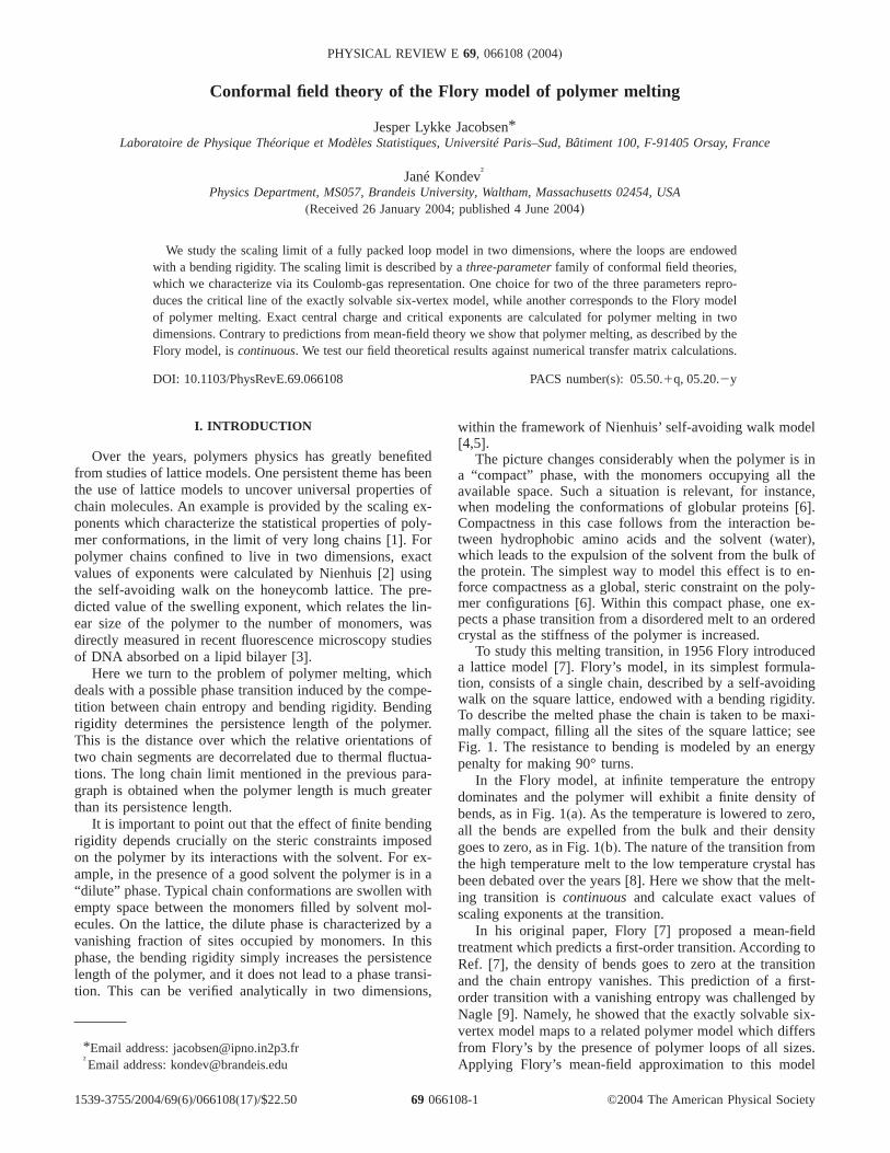
To study this melting transition, in 1956 Flory introduceda lattice model[7]. Flory’s model, in its simplest formula-tion, consists of a single chain, described by a self-avoidingwalk on the square lattice, endowed with a bending rigidity.To describe the melted phase the chain is taken to be maxi-mally compact, filling all the sites of the square lattice; seeFig. 1. The resistance to bending is modeled by an energypenalty for making 90° turns.

In the Flory model, at infinite temperature the entropydominates and the polymer will exhibit a finite density ofbends, as in Fig. 1(a). As the temperature is lowered to zero,all the bends are expelled from the bulk and their densitygoes to zero, as in Fig. 1(b). The nature of the transition fromthe high temperature melt to the low temperature crystal hasbeen debated over the years[8]. Here we show that the melt-ing transition iscontinuousand calculate exact values ofscaling exponents at the transition.

In his original paper, Flory[7] proposed a mean-fieldtreatment which predicts a first-order transition. According toRef. [7], the density of bends goes to zero at the transitionand the chain entropy vanishes. This prediction of a first-order transition with a vanishing entropy was challenged byNagle [9]. Namely, he showed that the exactly solvable six-vertex model maps to a related polymer model which differsfrom Flory’s by the presence of polymer loops of all sizes.Applying Flory’s mean-field approximation to this model

*Email address: [email protected]†Email address: [email protected]

PHYSICAL REVIEW E 69, 066108(2004)

1539-3755/2004/69(6)/066108(17)/$22.50 ©2004 The American Physical Society69 066108-1

leads once again to the prediction of a first-order meltingtransition. However, as Nagle pointed out, this is at oddswith the exact solution of the six-vertex model[10] whichpredicts a continuous, infinite order transition. This observa-tion makes it questionable that the Flory approach is valid inthe original model as well. In fact, a few years later Gujratiand Goldstein[11] proved that the polymer entropy in Flo-ry’s model stays finite all the way down to zero temperaturewhen it finally vanishes. However, the order of the transitionstill remained an unresolved question.

Monte Carlo simulations of Baumgartner and Yoon[12],where they allowed for many chains and a finite density ofempty sites, showed a first-order melting transition. Soonthereafter Saleur[13], using a transfer matrix approach, pre-sented numerical evidence of a continuous transition, similarto the one found in the six-vertex model. The analogy withthe six-vertex model points at the possibility of having ahigh-temperature phase with continuously varying expo-nents. A few years later, Bascle, Garel, and Orland[14] pro-posed an improved mean-field treatment of the Flory model,which does not suffer from the problem of a vanishing en-tropy at the transition. It also predicts a first-order transition.This is however at odds with more recent Monte Carlo workby Mansfield[15] which, although strictly speaking dealingwith a system of many chains, is again in favor of a continu-ous transition.

Here we show that polymer melting is continuous, asoriginally argued by Saleur[13], by making use of a particu-lar model, thesemiflexible loop(SFL) model, and its heightrepresentation. Furthermore, we calculate the central chargeand exact scaling exponents at the transition. These resultsare checked against detailed numerical transfer matrix com-putations.

The SFL loop model can be thought of as a “loop gener-alization” of the so-called F model[9], in which suitablydefined loops carry additional Boltzmann weights. The Fmodel is a special case of the six-vertex model[10], in whichall vertices carry equal weights. This connection will serve asthe motivation for introducing a more general model, thegeneralized six-vertex model, in which the general(zero-field) six-vertex model is endowed with extra loop weights.We shall finally introduce a similarly generalized version ofthe eight-vertex model[10]. Its interest from a polymer pointof view is that it allows for a unified description of semiflex-ible lattice polymers in a variety of phases: compact, dense,and dilute. Furthermore, it allows us to discuss the effect ofvacancies on the polymer melting transition.

The paper is organized as follows. In the following sec-tion we introduce the SFL model, which, in the limit of zeroloop weight, gives the Flory model of polymer melting, andwe discuss its phase diagram. In Sec. III we discuss theheight representation of the loop model and how it leads to aconformal field theory in the scaling limit. We make use ofthe field theory in Sec. IV to calculate the central charge andscaling exponents, which we check against numerical trans-fer matrix computations in Sec. V. In Sec. VI we propose aphase diagram for the generalized six-vertex and eight-vertexmodels. We end with a discussion of the scaling of semiflex-ible compact polymers, and we argue that the generalizedeight-vertex model furnishes a rather complete description ofnoncompact semiflexible polymers. An appendix is reservedfor a detailed discussion of the construction of the transfermatrices.

II. SEMIFLEXIBLE LOOP MODEL

Here we define the SFL model, and give a rough sketch ofits phase diagram based on the limits of weak and strongbending rigidity. The fact that the SFL model reduces to theF model in the limit of unit loop fugacity[9] plays an im-portant role in guiding our intuition about the loop model. Italso provides an exactly solvable line in the phase diagram,against which the field theoretical and numerical results canbe checked.

A. Definition of the model

The semiflexible fully packed loop model on the squarelattice (the SFL model) is defined by filling the square latticewith loops drawn along the lattice edges. Allowed loop con-figurations satisfy two constraints:(a) self avoidance—loopsare not allowed to cross, and(b) full packing—every site isvisited by exactly one loop.

On the square lattice with periodic boundary conditions,edges that are not covered by loops also form loops, as thereare two unoccupied edges associated with every site of thelattice. We refer these to as “ghost loops.”

Given the configurations of the semiflexible loop model,the Boltzmann weights are defined in the following way.Every real loop is given a weightnb, and every ghost loophas weightng. (In all the figures the real and ghost loops areshown as black and gray, respectively, whence the subscriptsb and g.) The parametersnb and ng act as fugacities of thetwo-loop flavors, and as such they control the average num-

FIG. 1. Compact polymer con-figurations on an 11315 squarelattice: (a) Typical configurationin the melt phase, and(b) zero-temperature crystalline state, inwhich the number of bends isminimum.

J. L. JACOBSEN AND J. KONDEV PHYSICAL REVIEW E69, 066108(2004)

066108-2

ber of loops of each flavor[16]. They can be varied indepen-dently as the number of ghost loops is not fixed by the num-ber of real loops[17]. Furthermore, a weightwX is assignedto each vertex of the lattice at which the real and ghost loopscross. ForwX .1 this has the effect of disfavoring vertices atwhich the loop makes a 90° bend, or, in other words, theloops are semiflexible. The partition function of the semi-flexible loop model is

Z = oG

nbNbng

NgwXV , s1d

where the sum runs over all allowed loop configurationsG.Nb and Ng are the number of real and ghost loops, respec-tively, while V is the number of crossing vertices; these arethe two rightmost vertices in Fig. 3. In the limitnb→0, withng=1, we recover the Flory model:Z/nb counts compactpolymer loops each weighed bywX

V.The semiflexible loop model can be thought of as the

generalization of the fully packed loop model on the squarelattice sFPL2d model introduced in Ref.[17]. The FPL2

model is given by the partition function, Eq.(1), with wX=1. It has a critical phase forunbu , unguø2, characterized by apower-law distribution of loop sizes. For other values of theloop weights the model is noncritical with a distribution ofloop sizes cut off at a finite value(fixed by the correlationlength). Below we will show that the vertex weightwX, foreach point in the critical phase of the FPL2 model, producesa line of fixed points which terminates in a Kosterlitz-Thouless transition.

B. Qualitative phase diagram

Rough, qualitative features of the phase diagram of thesemiflexible loop model can be deduced from the limits ofzero and infinite bending rigidity. The motivation for devel-oping a precise theory of the phase diagram, as mentioned inthe Introduction, stems from the interest in thenb→0, ng=1 case, which is the Flory model of polymer melting. Weare also motivated by the relation of the SFL model to theintegrable six-vertex model, and its generalizations.

1. Flory model

In the Flory limit of the SFL model, thewX =1 point is thecompact polymer problem, which we have studied previ-ously [17]. Here one is concerned with enumerating all self-avoiding walks that visit every site of the lattice. We haveshown that compact polymers on the square lattice are acritical geometry characterized by non-mean-field scaling ex-ponents which can be calculated exactly from a field theory.

As wX is increased away from one, we are dealing with acompact polymer with a bending rigidity. In the limitwX→` we arrive at a frozen phase in which the density ofvertices at which the polymer bends goes to zero. This is thepolymer crystal. At an intermediate weightwX=wX

c s1,wXc ,`d there will be a melting transition. One of

the important unresolved problems is the nature of this tran-sition. Here we construct an effective field theory of theFlory model and show that the melting transition iscontinu-ous.

Another interesting issue is the region of 0øwX ,1. AswX →0, straight-going vertices are completely suppressed,

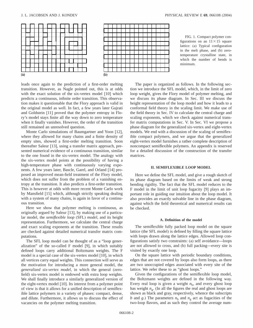
FIG. 2. Typical configurations in the SFL model withnb=ng=2 and bending rigidity parameterwX =1/4 (a), wX =1 (b), andwX =4 (c).We shall show that the left and middle panels correspond to critical melt states, while the right panel is a noncritical crystalline state. In thelatter, domains of nonzero staggered polarization(see Sec. II B 2) are clearly visible.

CONFORMAL FIELD THEORY OF THE FLORY MODEL… PHYSICAL REVIEW E 69, 066108(2004)

066108-3

and with appropriate boundary conditions the only allowedconfigurations are those of a checkerboard pattern of smallloops, each loop having its minimal length of 4. If the Florylimit snb→0d is taken before thewX →0 limit, there has tobe a number of straight-going vertices at the boundary, thedominant configurations being those of a single wiggly line.In any case, thewX →0 limit is again a crystalline phase ofzero entropy. We shall however argue below that the corre-sponding crystallization transition is located atwX =0 and isthus rather uninteresting.

A qualitative idea of the physics underlying the phasediagram of the SFL model can be obtained by looking atsome typical configurations for various values ofwX; seeFig. 2. The images were obtained by performing MonteCarlo simulations on a square lattice of size 1003100 withtoroidal boundary conditions. For technical reasons[18] wetakenb=ng=2 and no loops of noncontractible topology areallowed. (Further details on the algorithm used for thesesimulations can be found in Ref.[18].)

2. Six-vertex model

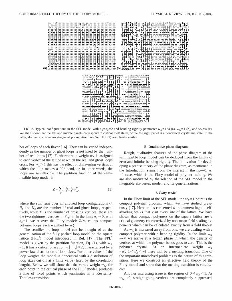
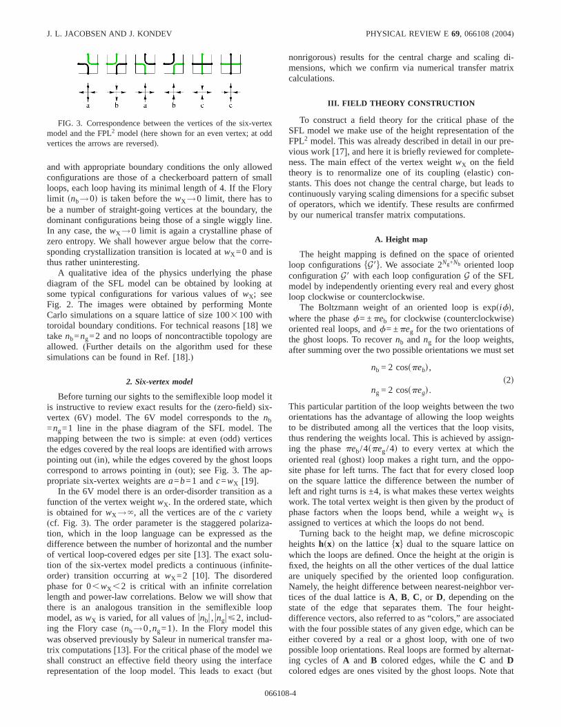
Before turning our sights to the semiflexible loop model itis instructive to review exact results for the(zero-field) six-vertex (6V) model. The 6V model corresponds to thenb=ng=1 line in the phase diagram of the SFL model. Themapping between the two is simple: at even(odd) verticesthe edges covered by the real loops are identified with arrowspointing out(in), while the edges covered by the ghost loopscorrespond to arrows pointing in(out); see Fig. 3. The ap-propriate six-vertex weights area=b=1 andc=wX [19].

In the 6V model there is an order-disorder transition as afunction of the vertex weightwX. In the ordered state, whichis obtained forwX →`, all the vertices are of thec variety(cf. Fig. 3). The order parameter is the staggered polariza-tion, which in the loop language can be expressed as thedifference between the number of horizontal and the numberof vertical loop-covered edges per site[13]. The exact solu-tion of the six-vertex model predicts a continuous(infinite-order) transition occurring atwX =2 [10]. The disorderedphase for 0,wX ,2 is critical with an infinite correlationlength and power-law correlations. Below we will show thatthere is an analogous transition in the semiflexible loopmodel, aswX is varied, for all values ofunbu , unguø2, includ-ing the Flory casesnb→0,ng=1d. In the Flory model thiswas observed previously by Saleur in numerical transfer ma-trix computations[13]. For the critical phase of the model weshall construct an effective field theory using the interfacerepresentation of the loop model. This leads to exact(but

nonrigorous) results for the central charge and scaling di-mensions, which we confirm via numerical transfer matrixcalculations.

III. FIELD THEORY CONSTRUCTION

To construct a field theory for the critical phase of theSFL model we make use of the height representation of theFPL2 model. This was already described in detail in our pre-vious work[17], and here it is briefly reviewed for complete-ness. The main effect of the vertex weightwX on the fieldtheory is to renormalize one of its coupling(elastic) con-stants. This does not change the central charge, but leads tocontinuously varying scaling dimensions for a specific subsetof operators, which we identify. These results are confirmedby our numerical transfer matrix computations.

A. Height map

The height mapping is defined on the space of orientedloop configurationshG8j. We associate 2Ng+Nb oriented loopconfigurationG8 with each loop configurationG of the SFLmodel by independently orienting every real and every ghostloop clockwise or counterclockwise.

The Boltzmann weight of an oriented loop is expsifd,where the phasef= ±peb for clockwise(counterclockwise)oriented real loops, andf= ±peg for the two orientations ofthe ghost loops. To recovernb and ng for the loop weights,after summing over the two possible orientations we must set

nb = 2 cosspebd,s2d

ng = 2 cosspegd.

This particular partition of the loop weights between the twoorientations has the advantage of allowing the loop weightsto be distributed among all the vertices that the loop visits,thus rendering the weights local. This is achieved by assign-ing the phasepeb/4speg/4d to every vertex at which theoriented real(ghost) loop makes a right turn, and the oppo-site phase for left turns. The fact that for every closed loopon the square lattice the difference between the number ofleft and right turns is ±4, is what makes these vertex weightswork. The total vertex weight is then given by the product ofphase factors when the loops bend, while a weightwX isassigned to vertices at which the loops do not bend.

Turning back to the height map, we define microscopicheightshsxd on the latticehxj dual to the square lattice onwhich the loops are defined. Once the height at the origin isfixed, the heights on all the other vertices of the dual latticeare uniquely specified by the oriented loop configuration.Namely, the height difference between nearest-neighbor ver-tices of the dual lattice isA, B, C, or D, depending on thestate of the edge that separates them. The four height-difference vectors, also referred to as “colors,” are associatedwith the four possible states of any given edge, which can beeither covered by a real or a ghost loop, with one of twopossible loop orientations. Real loops are formed by alternat-ing cycles ofA and B colored edges, while theC and Dcolored edges are ones visited by the ghost loops. Note that

FIG. 3. Correspondence between the vertices of the six-vertexmodel and the FPL2 model (here shown for an even vertex; at oddvertices the arrows are reversed).


066108-4

the difference between anABAB¯ and aBABA¯ cycleencodes the orientation of the corresponding(real) loop.

The fully packing constraint and the requirement that theheight be unique(i.e., the sum of height differences alongany closed lattice path must be zero) imposes a single alge-braic constraint on the four colors:A +B+C+D=0. It fol-lows that only three of the four vectors are linearly indepen-dent. A convenient choice that respects the symmetriesbetween the four colors is to let the corresponding vectorspoint from the center to the vertices of a regular tetrahedron:

A = s− 1, + 1, + 1d, B = s+ 1, + 1,− 1d,s3d

C = s− 1,− 1,− 1d, D = s+ 1,− 1, + 1d.

The effective field theory for the SFL model describes thefluctuations of the coarse-grained heights which retains onlythe long-wavelength(much larger than the lattice spacing)Fourier modes of the microscopic heights.

B. Effective field theory: wX =1

For wX =1 we have the familiar case of the fully packedloop model on the square lattice. Its effective field theorywas discusses in a previous publication[17] and here it isreviewed for completeness.

The partition function of the loop model in the heightrepresentation can be written as a path integral over thecoarse grained heights with the(dimensionless) action:

S= SE + SB + SL . s4d

This action only takes into account the long-wavelength fluc-tuations of the microscopic height. The three terms in theaction are of different origin.

The elastic term

SE =1

2E d2xhK11fs h1d2 + s h3d2g + 2K13s h1 · h3d

+ K22s h2d2j s5d

accounts for the height fluctuations due to the entropy offully packing the square lattice with oriented loops. Equiva-lently, this is the entropy of edge coloring the square latticewith four different colors. The elastic term favors orientedloop configurations that minimize the variance of the micro-scopic height; these are the macroscopically flat states. Interms of the color degrees of freedom the flat states have theproperty that the four edges of each elementary plaquette arecolored by two colors only.

The particular form of the matrix of elastic constantsK isfixed by the lattice symmetries and symmetries associatedwith permuting the colorsA, B, C, andD. The elastic con-stantsKij are functions of the loop fugacity. For thewX =1case they were calculated in Ref.[17] using the loop ansatz[22], which allows one to identify the marginal screeningcharges[23]. For the FPL2 model there are four screeningcharges:

es1d = s− p,0, +pd,

es2d = s− p,0,−pd,s6d

es3d = s− p, + p,0d,

es4d = s− p,− p,0d.

These electric charges are associated with the most relevantvertex operators appearing in the Fourier expansion of theoperator conjugate to the loop weight[see Eq.(12) below].

Demanding that all four charges have scaling dimensionequal to 2 gives[using Eq.(16)]

K11 =p

8s2 − eg − ebd,

s7d

K13 =p

8seb − egd,

K22 =p

2

s1 − ebds1 − egd2 − eb − eg

for the elastic constants of the FPL2 model;eb andeg satisfyEq. (2) and take their values on the intervalf0,1/2g. Belowwe will argue that the effect ofwX Þ1 is to change the valueof the elastic constantK22 while leaving the other two un-changed.

The boundary term in the action,

SB =i

4pE d2xfe0 ·hsxdgrsxd, s8d

enforces the correct weight of topologically nontrivial loops.If the oriented loop model is defined with periodic boundaryconditions along one direction(i.e., on a cylinder) thesewould be the loops that completely wind around the cylinder[24]. On a cylinder the scalar curvaturer is nonzero only atthe two boundaries at infinity.SB has the effect of placingbackground electric charges ±e0 at the two boundaries,where the identification

e0 = −p

2seg + eb,0,eg − ebd s9d

comes about by demanding that the oriented winding loopsbe assigned correct phase factors, exps±ipebd or exps±ipegd[17].

The third term, called the Liouville term,

SL =E d2xwfhsxdg, s10d

owes its existence to the complex weights associated withoriented loops in the bulk. The local redistribution of theloop weights made in Sec. III A leads to complex vertexweights, which in turn depend only on the colors of the fouredges around the vertex. If we write the vertex weight asexps−wd, then


066108-5

wsB,C,A,Dd = 0,

wsB,D,A,Cd = 0,

wsA,B,C,Dd = 7 ip

4seg + ebd,

wsB,A,C,Dd = 7 ip

4seg − ebd, s11d

wsA,B,D,Cd = 7 ip

4seb − egd,

wsB,A,D,Cd = 7 ip

4s− eb − egd;

the top(bottom) sign is for even(odd) vertices, and the col-ors are listed in order, starting from the leftmost edge andproceeding clockwise around the vertex. The weight operatorw is invariant under cyclic permutations of the colors and itis a periodic function of the heights around a vertex. In thescaling limit the vertex weights give rise to the operatorwfhsxdg in Eq. (10) which can be written as a Fourier series

wfhsxdg = oePRw

*

we exp fie ·hsxdg. s12d

The electric chargese appearing in the Fourier expansion aredictated by the lattice of periodicitiesRw of the operatorwfhg; Rw

* is the reciprocal lattice.Rw is determined by in-spection of the values the loop weight operator takes on theflat states: vectors inRw connect flat states on which the loopweight operator takes identical values. The most relevantcharges inRw

* are the four given in Eq.(6). We identify themwith the screening charges[23] of the Coulomb gas. This isthe content of the loop ansatz introduced in Ref.[22].

C. Effective field theory: wXÅ1

For the SFL model, whenwX Þ1, the Liouville term inEq. (4) is modified, while the elastic and the boundary termsare unchanged. The number of marginal screening chargesappearing in Eq.(12) is reduced from four to two, and theloop ansatz fixes the values ofK11 andK13 only. They do notdepend on the value ofwX and are given by thewX =1 for-mulas, Eq.(7). K22, on the other hand, is a nonuniversalfunction of wX. Below we present arguments for this sce-nario, which is supported by exact results available in the 6Vcase(i.e., for nb=ng=1), and by our numerical transfer ma-trix calculations described in Sec. V below.

The new vertex weightwX changes the value ofw in Eq.(11) from 0 to −lnwX for the vertex statessB ,C ,A ,Dd,sB ,D ,A ,Cd, and six other related to these two by cyclicpermutations of the colors. The weights of the other 16 ver-tex states are unchanged. We consider the consequences ofthis change on the effective field theory.

In the height representation of the SFL model, the changein vertex weight corresponds to adding

SX =E d2x Xfhsxdg s13d

to the action. TheX operator takes the value lnwX on the flatstates made up ofsB ,C ,A ,Dd or sB ,D ,A ,Cd type vertices,and vanishes on all the others. By inspection of the graph offlat states we find that the lattice of periodicities for the op-eratorX, RX, is the span ofs1,0,−1d, s1,0,1d, ands0,1,0d;these are the height difference vectors between the flat statesin the support ofX. This observation implies thatXfhg can beexpanded in a Fourier series over electric charges that live inthe dual latticeRx

* which is the span ofsp ,0 ,pd, sp ,0 ,−pd, ands0,2p ,0d.

If we consider the effect ofSX as a perturbation on theaction of the FPL2 model, the electric chargess0, ±2p ,0dplay a special role. Namely, the operator product expansionof exp fis0,2p ,0d ·hg and expf−is0,2p ,0d ·hg contains thesh2d2 operator, and therefore leads to the renormalization ofK22 [25]. This follows from the fact that the backgroundcharge, Eq.(9), has a vanishing second component. On theother hand, for chargese with nonzero first or third compo-nent, the effect of the background charge is that the operatorproduct expansion of expsie·hd and exps−ie·hd does notcontainhi ·hj operators and therefore does not lead to therenormalization of the elastic constantsKij .

The Coulomb gas representation of the height model pro-vides a clear physical picture of the effect ofSX on the criti-cal action of the FPL2 model. ForwX =1 the dimension of thes0, ±2p ,0d charges follows from Eq.(16),

xX =s2pd2

4pK22= 2S 1

1 − eb+

1

1 − egD . s14d

It is greater than 2 in the whole critical region of the FPL2

model. These charges are therefore irrelevant in the renor-malization group sense. In the Coulomb gas picture thes0, ±2p ,0d charges appear as bound pairs of neutral dipoles.IncreasingwX will have the effect of increasing the barefugacity of these dipoles, which will in turn increase thevalue of the couplingK22 appearing in the effective fieldtheory. Formally, this can be seen in perturbation theorymaking use of the operator product expansion[25]. Physi-cally, the renormalization ofK22 can be understood as thescreening effect of dipoles. The dipoles lower the Coulombenergy between two electric test charges having a nonzerosecond component, corresponding to an increase in the valueof K22 which plays the role of a dielectric constant.

At a critical valuewXc there will be a Kosterlitz-Thouless-

type transition of the SFL model into a flat state with a van-ishing density of vertices at which the polymer bends. At thetransition thes0, ±2p ,0d charges are marginal, i.e., theirscaling dimension is equal to 2. Using Eq.(14) this observa-tion gives rise to the prediction for the critical value ofK22:

K22swXc d =

p

2. s15d

For values ofwX smaller thanwXc , K22 will be a nonuniversal

function of wX. In the nb=ng=1 case, the formulaK22


066108-6

=arcsinswX /2d follows from the exact solution of the 6Vmodel [10]. The critical value of the vertex weight iswX

c s6Vd=2 andK22s2d=p /2 is in agreement with Eq.(15).For other values ofnb andng our numerical transfer matrixcalculations are in good agreement with Eq.(15).

The introduction of the vertex weightwX also has an ef-fect on the screening charges, Eq.(6), which appear in theLiouville part of the action. First consider thenb=ng case ofthe SFL model. Due to the presence of thewX term cyclicpermutations of the four colors around a vertex are no longera symmetry of the vertex weight. Therefore, unlike thewX=1 case[17], there are now two independent elastic con-stantsK22 andK11 appearing inSE. K13=0 follows from theremainingZ2 symmetry of the vertex weights which are in-variant undertwo cyclic permutations, such assA ,B ,C ,Dd→ sC ,D ,A ,Bd. The deduced structure of the elasticity ma-trix implies that the four electric charges in Eq.(6) are nolonger degenerate in dimension for arbitrarywX. Since thedimensions ofes1d andes2d are independent ofK22, they areidentified as the two screening charges tied to the nonrenor-malizability of the loop weights[17]. As in the FPL2 modelwe then assume that these two charges remain marginalwhen nbÞng. Using the dimension formula, Eq.(16), thisthen fixes the values of the two elastic constants,K11 andK13, to the values quoted in Eq.(7).

Finally, it is interesting to look at some extreme limits ofK22 in view of the effective field theory. Consider first thelimit K22→` in which height fluctuations in the secondheight component are completely suppressed.(As we areoutside the critical phase, we are here referring to the barevalue of the coupling.) Clearly, height fluctuations must al-ways be present in the microscopic four-coloring model, butit is nevertheless instructive to look for the states that mini-mize the fluctuations ofh2. From the choice of the colorvectors, Eq.(3), it is not difficult to see that on the four sitesof hxj surrounding a given vertex,h2 fluctuates by two unitsfor the first four vertices of Fig. 3 and by one unit for the lasttwo vertices. All vertices must therefore be of thec type,corresponding to the limitwX →`. Thus, K22→` aswX →`.

Conversely, asK22→0, the fluctuations inh2 become un-bounded and the effective field theory loses its consistency(since it was based on the assumption that the interfacialentropy is due to bounded fluctuations around the macro-scopically flat states). However, the argument given aboveindicates that a small value ofK22 should correspond to asmall number of straight-going vertices in the loop model.Thus, we would conjecture thatK22→0 aswX →0. This ex-pectation is confirmed by the exact result for the 6V case[10] and also by extrapolation of our numerical results forK22swXd in the Flory case.

Apart from these limiting values, we would of course ex-pect K22 to be a monotonically increasing function ofwXthroughout the critical phase.

In the following section we compute the central chargeand the scaling dimensions of various operators in the semi-flexible loop model from its effective field theory. We iden-tify quantities that depend on the nonuniversal elastic con-stantK22; these are then predicted to vary continuously withwX.

IV. OPERATORS AND SCALING DIMENSIONS

The effective field theory of the semiflexible loop modeldescribes a Coulomb gas of electric and magnetic charges inthe presence of background and screening charges. The mag-netic chargesm are vectors inR which is the lattice ofperiodicities of the graph of flat states, while the electricchargese take their values in the reciprocal latticeR* [17].With the normalization adopted for the vectorsA throughD,Eq. (3), R is a face-centered cubic lattice whose conven-tional cubic cell has sides of length 4, whileR* is a body-centered cubic lattice whose conventional cubic cell hassides of lengthp.

The scaling dimension of an operator which has totalelectromagnetic chargese,md is the sum of its electric andmagnetic dimensions, and it is a function of the elastic con-stants and the background charge[23]:

xse,md =1

4pfseK−1d · se− 2e0d + smK d ·mg. s16d

K is the 333 matrix of elastic constants andK −1 is its in-verse.

From Eq.(16) and the form ofK [Eq. (5)] and e0 [Eq.(9)], it immediately follows that operators whose electric andmagnetic charges both have a vanishing second componentwill have aK22-independent scaling dimension. The scalingdimension in this case is independent ofwX and equal to itsknown value atwX =1 [17]. Operators withe andm chargeswhose second components are not both zero will, on theother hand, have a scaling dimension that varies continu-ously with wX. These predictions are confirmed by our nu-merical results.

A. Central charge

The central charge of the SFL model follows from itscritical action. The three height components(bosonic freefields) each contribute one unit to the central charge whilethe contribution from the background charge is 12xse0,0d.Using Eq.(16) for xse0,0d, Eq.(9) for the background chargee0, and the calculated values of the elastic constantsK11 andK13, Eq. (7), we find

c = 3 − 6S eb2

1 − eb+

eg2

1 − egD , s17d

independentof the unknown value ofK22.For the 6V model, which corresponds to theeb=eg=1/3

line in the SFL model, the above formula givesc=1 for thecentral charge along the critical line. This result also followsdirectly from the exact solution of the 6V model.

For the Flory model of polymer melting, which is theeb=1/2, eg=1/3 case, the predicted central charge isc=−1.This value is confirmed by our numerical transfer matrixcalculations(see Sec. V).

B. Thermal operator

The SFL model can be thought of as the zero-temperaturelimit of a more general model where we allow for thermal


066108-7

excitations that violate the fully packing constraint. Viola-tions of the constraint lead to vertices with the four adjacentedges coloredsC ,D ,C ,Dd. In the height representation sucha vertex is identified with a topological defect(screw dislo-cation) whose charge, i.e., the sum of height differencesaround the vertex, is

mT = 2sC + Dd = s0,− 4,0d. s18d

Other vertices which have noA or B colored edges are pos-sible, but they have a larger magnetic charge and are henceless relevant.

In the Coulomb gas picture a topological defect corre-sponds to a magnetic charge. Therefore, the thermal dimen-sion can be calculated using Eq.(16), and we find

xT = xs0,mTd =4

pK22. s19d

We make use of this equation below as it allows us to deter-mine the unknown elastic constantK22 from a measurementof the thermal scaling dimension. Once this elastic constantis known, scaling dimensions of all electromagnetic opera-tors can be calculated from Eq.(16).

C. String operators

A particularly important set of operators in any loopmodel are the string operators. Their two-point function isdefined as the probability of having the small neighborhoodsaround two fixed points on the lattice, which are separated bya large distance, connected bysb real loop segments andsgghost loop segments. For simplicity, we shall requiresb andsg to be either both even or both odd;sb+sg odd requiresL tobe odd which produces a twist in the height, as discussed inRef. [17]. In the height representation these string configu-rations are mapped to two topological defects, one serving asthe source and the other as the sink of oriented loop seg-ments. When the oriented loop segments wind around thedefect points they are assigned spurious phase factors by thevertex weights; these phase factors can however be compen-sated by introducing appropriate electric charges at the posi-tions of the defects[26].

In the casesb=2kb andsg=2kg, i.e., when the number ofreal and ghost strings are both even, the electric and mag-netic charge of the corresponding string operator are[17]

e2kb,2kg= −

p

2seb,0,−ebds1 − dkb,0d −

p

2seg,0,egds1 − dkg,0d,

s20dm2kb,2kg

= − 2skb + kg,0,kg − kbd.

Since the charges have vanishing second component theirdimension is independent ofK22 and constant along thewhole critical linewX øwX

c . The value of the string dimen-sion follows from Eq.(16),

x2kb,2kg=

1

2Fs1 − ebdkb

2 + s1 − egdkg2 −

eb2

1 − ebs1 − dkb,0d

−eg

2

1 − egs1 − dkg,0dG , s21d

and is identical to that of the FPL2 model[17]. Our numeri-cal simulations confirm that even string dimensions are con-stant along the critical line.

In the odd string case, whensb=2kb−1 andsg=2kg−1,the electric and magnetic charge are[17]

e2kb−1,2kg−1 = −p

2seg + eb,0,eg − ebd,

s22dm2kb−1,2kg−1 = − 2skb + kg − 1,1,kg − kbd.

Notably, the magnetic charge has a nonvanishing secondcomponent. Using Eq.(16) we calculate

x2kb−1,2kg−1 =K22

p+

1

8fs1 − ebds2kb − 1d2 + s1 − egds2kg − 1d2g

−1

2F eb

2

1 − eb+

eg2

1 − egG s23d

for the odd string dimension. It depends on the value ofK22and will therefore vary continuously withwX. At the meltingtransition the exponents are exactly known from Eq.(15).This is confirmed by our numerical transfer matrix results,which we describe next.

V. TRANSFER MATRIX RESULTS

To check the correctness of our field theoretical predic-tions, we have numerically diagonalized the transfer matrixof the semiflexible loop model(and of its various generali-zations, to be discussed below) defined on semi-infinite cyl-inders of even widthsL ranging from 4 to 14.

The existence of a transfer matrix may not bea prioriobvious, since the Boltzmann weights depend on the numberof loops, which is a nonlocal quantity. We have howeveralready shown in an earlier publication[17] how this is re-solved by working in a basis of states that contains nonlocalinformation about how loop segments are interconnected at agiven stage of the computations. In that paper, it was alsoshown that the full transfer matrix contains various sectors,the leading eigenvalues of which provide finite-size estima-tions of the free energy and of the various critical exponents,using the standard conformal field theory(CFT) relations[27,28]

f0sLd = f0s`d −pc

6L2 + ¯ , s24d

fksLd − f0sLd =2pxk

L2 + ¯ . s25d

Here, the labelk refers either to a higher eigenvalue in thesector to whichf0 belongs, or to the leading eigenvalue in


066108-8

another sector characterized by some topological defect ofchargek.

To access critical exponents, we shall mainly be con-cerned with topological defects that consist in enforcing thata certain number of strings of either flavor propagate alongthe length direction of the cylinder. These give rise to a two-parameter family of critical exponentsxsb,sg

corresponding tosb real strings andsg ghost strings. The corresponding topo-logical charges, Eqs.(20) and (22), take the form of three-dimensional electromagnetic vector charges. In the transfermatrix calculations, each of these topological sectors is asso-ciated with a different state space. The difficulty of preciselycharacterizing these spaces limited our previous approach[17] to at most two strings. In the Appendix we present analgorithm that explicitly constructs the required state spacesfor any ssb,sgd, based on an iterative procedure and hashingtechniques.

By inspection of the eigenstates produced by our previousalgorithm[17], it turns out that many of the basis states carryzero weight. One would then expect that identical results canbe obtained more efficiently by working in a basis in whichsuch states have been eliminated from the outset. We deferthe technical details of how this can be done to the Appen-dix. It is also shown how the block-diagonalization schemecan be carried even further, by exploiting various conserva-tion laws that are most easily understood from the analogybetween the SFL model and the six-vertex model. One im-portant consequence is that the constrained free energyfTsLdthat is linked to the thermal scaling dimension can now beobtained as a leading eigenvalue, rather than as the secondeigenvalue in the stringless sector. This considerably im-proves the efficiency of the computations.

Finally, the matrix elements need some modification inorder to take into account the bending rigidity parameterwX.This is readily done, without any modification of the basisstates, sincewX is a purely local quantity.

Before turning to our numerical results, we should men-tion that we have submitted our transfer matrices to severaltests, in order to verify their correctness:

(1) For wX =1, all numerically determined string dimen-sionsxsb,sg

with sb+sg=2 or 4 agree to at least three signifi-cant digits with their exact values in the casessnb,ngd=s1,1d [10] and snb,ngd=s0,1d [17].

(2) All eigenvalues found for the FPL2 model agree withthose obtained from our previous algorithm[17].

(3) For the six-vertex model[10], we have compared theextrapolated bulk free energy with Baxter’s exact expression.

(4) Again for the six-vertex model, we find excellentagreement with the exact formulasx1,1=K22/p and xT=4K22/p, whereK22=arcsinswX /2d is the elastic constant.

(5) We have also found agreement with the first fewterms in diagrammatic expansions around various limits ofinfinite fugacities.

A. Central charge

A crucial prediction of our field theory is that, for givenvalues of the loop fugacitiessnb,ngd, the central charge of theSFL model should be independent ofwX, as long as the latter

is constrained to the critical regime, 0,wX øwXc .

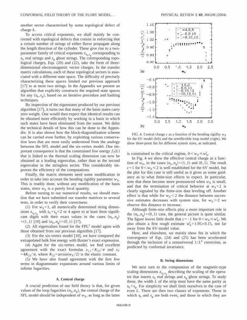
In Fig. 4 we show the effective central charge as a func-tion of wX, in the casessnb,ngd=s1,1d ands0,1d. The resultc=1 for 0,wX ø2 is well established for the 6V model, butthe plot for this case is still useful as it gives us some guid-ance as to what finite-size effects to expect. In particular,note that these become more pronounced whenwX is small,and that the termination of critical behavior atwX =2 isclearly signaled by the finite-size data leveling off. Anothereffect is that while forwX ,2 the distance between succes-sive estimates decreases with system size, forwX .2 weobserve this distance to increase.

Although finite-size effects play a more important role inthe snb,ngd=s0,1d case, the general picture is quite similar.The figure leaves little doubt thatc=−1 for 0,wX øwX

c . Wealso obtain a first rough estimatewX

c =1.95±0.15, not faraway from the 6V-model value.

Here, and elsewhere, we mainly show fits in which theconvergence of Eqs.(24) and (25) has been acceleratedthrough the inclusion of a nonuniversal 1/L4 correction, aspredicted by conformal invariance.

B. String dimensions

We next turn to the computation of the magnetic-typescaling dimensionsxsb,sg

describing the scaling of the opera-tor that insertssb real strings andsg ghost strings. To studythese, the widthL of the strip must have the same parity assb+sg. For simplicity we shall limit ourselves to the case ofevenL. There are then two classes of exponents: Those inwhich sb andsg are both even, and those in which they are

FIG. 4. Central chargec as a function of the bending rigiditywX

for the 6V model(left) and the semiflexible loop model(right). Weshow three-point fits for different system sizes, as indicated.


066108-9

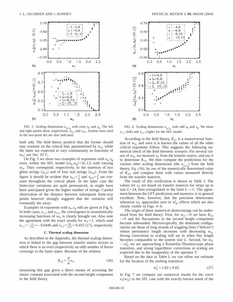
both odd. The field theory predicts that the former shouldstay constant on the critical line, parametrized bywX, whilethe latter are expected to vary continuously as functions ofwX; see Sec. IV C.

On Fig. 5 we show two examples of exponents withsb,sgeven, within the SFL model[snb,ngd=s0,1d] with varyingwX. They correspond, respectively, to the insertion of twoghost stringssx0,2d and of four real stringssx4,0d. From thefigure it should be evident thatx0,2=

14 and x4,0=

34 are con-

stant throughout the critical phase. In the latter case thefinite-size variations are quite pronounced, as might havebeen anticipated given the higher number of strings. Carefulobservation of the distance between subsequent finite-sizepoints however strongly suggests that the variation willeventually die away.

Examples of exponents withsb,sg odd are given in Fig. 6.In both cases,x1,1 andx3,1, the convergence to monotonicallyincreasing functions ofwX is clearly brought out. Also notethe agreement with the exact results forwX =1, which readx1,1=− 5

112.−0.0446 andx3,1=51112.0.455[17], respectively.

C. Thermal scaling dimension

As described in the Appendix, the thermal scaling dimen-sion is linked to the gap between transfer matrix sectors inwhich there is an even(respectively an odd) number of flavorcrossings in the basis states. Because of the relation

K22 =p

4xT, s26d

measuring this gap gives a direct means of accessing theelastic constant associated with the second height componentin the field theory.

According to the field theory,K22 is a nonuniversal func-tion of wX, and once it is known the values of all the othercritical exponents follow. This suggests the following nu-merical check of the field theoretic scenario. For several val-ues ofwX, we measurexT from the transfer matrix, and use itto determineK22. We then compute the predictions for thevarious other scaling dimensions(the xsb,sg

) from the fieldtheory, Eq.(16), by use of the numerically determined valueof K22, and compare them with values measured directlyfrom the transfer matrices.

The result of this verification is shown in Table I. Thevalues forxT are based on transfer matrices for strips up tosizeL=14, here extrapolated to the limitL→`. The agree-ment between the CFT predictions and numerics is in generalexcellent. Note, however, that the precision deteriorateswheneverwX approaches zero orwX

c , effects which are alsoclearly visible in Figs. 4–6.

The origin of these numerical shortcomings can be under-stood from the field theory. First, forwX →0 we haveK22→0 and the fluctuations in the second height componentbecome unbounded. Microscopically, the dominant configu-rations are those of long strands of wiggling lines(“helices”)whose persistence length increases with decreasingwX.Strong corrections to scaling will set in when this lengthbecomes comparable to the system sizeL. Second, forwX→wX

c we are approaching a Kosterlitz-Thouless-type phasetransition, and strong logarithmic corrections to scaling areexpected due to the marginality of the operatorT.

Based on the data in Table I, we can refine our estimatefor the location of the melting transition:

wXc = 1.92 ± 0.02. s27d

In Fig. 7 we compare our numerical results for the curvexTswXd in the SFL case with the exactly known result of the

FIG. 5. Scaling dimensionsxsb,sgwith evensb and sg. The left

and right panels show, respectively,x0,2 andx4,0. System sizes usedin the two-point fits are also indicated.

FIG. 6. Scaling dimensionsxsb,sgwith odd sb andsg. We show

x1,1 (left) andx3,1 (right) for the SFL model.


066108-10

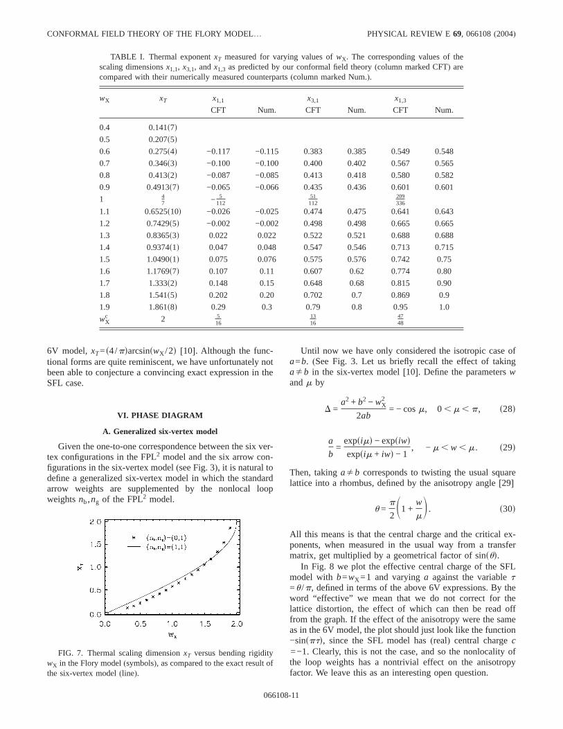
6V model,xT=s4/pdarcsinswX /2d [10]. Although the func-tional forms are quite reminiscent, we have unfortunately notbeen able to conjecture a convincing exact expression in theSFL case.

VI. PHASE DIAGRAM

A. Generalized six-vertex model

Given the one-to-one correspondence between the six ver-tex configurations in the FPL2 model and the six arrow con-figurations in the six-vertex model(see Fig. 3), it is natural todefine a generalized six-vertex model in which the standardarrow weights are supplemented by the nonlocal loopweightsnb,ng of the FPL2 model.

Until now we have only considered the isotropic case ofa=b. (See Fig. 3. Let us briefly recall the effect of takingaÞb in the six-vertex model[10]. Define the parameterswandm by

D =a2 + b2 − wX

2

2ab= − cosm, 0 , m , p, s28d

a

b=

expsimd − expsiwdexpsim + iwd − 1

, − m , w , m. s29d

Then, takingaÞb corresponds to twisting the usual squarelattice into a rhombus, defined by the anisotropy angle[29]

u =p

2S1 +

w

mD . s30d

All this means is that the central charge and the critical ex-ponents, when measured in the usual way from a transfermatrix, get multiplied by a geometrical factor of sinsud.

In Fig. 8 we plot the effective central charge of the SFLmodel with b=wX =1 and varyinga against the variablet=u /p, defined in terms of the above 6V expressions. By theword “effective” we mean that we do not correct for thelattice distortion, the effect of which can then be read offfrom the graph. If the effect of the anisotropy were the sameas in the 6V model, the plot should just look like the function−sinsptd, since the SFL model has(real) central chargec=−1. Clearly, this is not the case, and so the nonlocality ofthe loop weights has a nontrivial effect on the anisotropyfactor. We leave this as an interesting open question.

TABLE I. Thermal exponentxT measured for varying values ofwX. The corresponding values of thescaling dimensionsx1,1, x3,1, andx1,3 as predicted by our conformal field theory(column marked CFT) arecompared with their numerically measured counterparts(column marked Num.).

wX xT x1,1 x3,1 x1,3

CFT Num. CFT Num. CFT Num.

0.4 0.141s7d0.5 0.207s5d0.6 0.275s4d −0.117 −0.115 0.383 0.385 0.549 0.548

0.7 0.346s3d −0.100 −0.100 0.400 0.402 0.567 0.565

0.8 0.413s2d −0.087 −0.085 0.413 0.418 0.580 0.582

0.9 0.4913s7d −0.065 −0.066 0.435 0.436 0.601 0.601

1 47 − 5

11251

112209336

1.1 0.6525s10d −0.026 −0.025 0.474 0.475 0.641 0.643

1.2 0.7429s5d −0.002 −0.002 0.498 0.498 0.665 0.665

1.3 0.8365s3d 0.022 0.022 0.522 0.521 0.688 0.688

1.4 0.9374s1d 0.047 0.048 0.547 0.546 0.713 0.715

1.5 1.0490s1d 0.075 0.076 0.575 0.576 0.742 0.75

1.6 1.1769s7d 0.107 0.11 0.607 0.62 0.774 0.80

1.7 1.333s2d 0.148 0.15 0.648 0.68 0.815 0.90

1.8 1.541s5d 0.202 0.20 0.702 0.7 0.869 0.9

1.9 1.861s8d 0.29 0.3 0.79 0.8 0.95 1.0

wXc 2 5

161316

4748

FIG. 7. Thermal scaling dimensionxT versus bending rigiditywX in the Flory model(symbols), as compared to the exact result ofthe six-vertex model(line).


066108-11

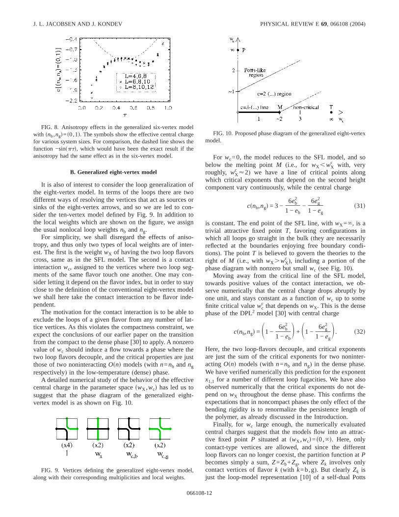
B. Generalized eight-vertex model

It is also of interest to consider the loop generalization ofthe eight-vertex model. In terms of the loops there are twodifferent ways of resolving the vertices that act as sources orsinks of the eight-vertex arrows, and so we are led to con-sider the ten-vertex model defined by Fig. 9. In addition tothe local weights which are shown on the figure, we assignthe usual nonlocal loop weightsnb andng.

For simplicity, we shall disregard the effects of aniso-tropy, and thus only two types of local weights are of inter-est. The first is the weightwX of having the two loop flavorscross, same as in the SFL model. The second is a contactinteractionwc, assigned to the vertices where two loop seg-ments of the same flavor touch one another. One may con-sider letting it depend on the flavor index, but in order to stayclose to the definition of the conventional eight-vertex modelwe shall here take the contact interaction to be flavor inde-pendent.

The motivation for the contact interaction is to be able toexclude the loops of a given flavor from any number of lat-tice vertices. As this violates the compactness constraint, weexpect the conclusions of our earlier paper on the transitionfrom the compact to the dense phase[30] to apply. A nonzerovalue ofwc should induce a flow towards a phase where thetwo loop flavors decouple, and the critical properties are justthose of two noninteractingOsnd models(with n=nb andng

respectively) in the low-temperature(dense) phase.A detailed numerical study of the behavior of the effective

central charge in the parameter spaceswX ,wcd has led us tosuggest that the phase diagram of the generalized eight-vertex model is as shown on Fig. 10.

For wc=0, the model reduces to the SFL model, and sobelow the melting pointM (i.e., for wX ,wX

c with, veryroughly, wX

c <2) we have a line of critical points alongwhich critical exponents that depend on the second heightcomponent vary continuously, while the central charge

csnb,ngd = 3 −6eb

2

1 − eb−

6eg2

1 − egs31d

is constant. The end point of the SFL line, withwX =`, is atrivial attractive fixed pointT, favoring configurations inwhich all loops go straight in the bulk(they are necessarilyreflected at the boundaries enjoying free boundary condi-tions). The pointT is believed to govern the theories to theright of M (i.e., with wX .wX

c ), including a portion of thephase diagram with nonzero but smallwc (see Fig. 10).

Moving away from the critical line of the SFL model,towards positive values of the contact interaction, we ob-serve numerically that the central charge drops abruptly byone unit, and stays constant as a function ofwc up to somefinite critical valuewc

c that depends onwX. This is the densephase of the DPL2 model [30] with central charge

csnb,ngd = S1 −6eb

2

1 − ebD + S1 −

6eg2

1 − egD . s32d

Here, the two loop-flavors decouple, and critical exponentsare just the sum of the critical exponents for two noninter-actingOsnd models(with n=nb andng) in the dense phase.We have verified numerically this prediction for the exponentx1,1 for a number of different loop fugacities. We have alsoobserved numerically that the critical exponents do not de-pend onwX throughout the dense phase. This confirms theexpectations that in noncompact phases the only effect of thebending rigidity is to renormalize the persistence length ofthe polymer, as already discussed in the Introduction.

Finally, for wc large enough, the numerically evaluatedcentral charges suggest that the models flow into an attrac-tive fixed point P situated atswX ,wcd=s0,`d. Here, onlycontact-type vertices are allowed, and since the differentloop flavors can no longer coexist, the partition function atPbecomes simply a sum,Z=Zb+Zg, whereZk involves onlycontact vertices of flavork (with k=b,g). But clearlyZk isjust the loop-model representation[10] of a self-dual Potts

FIG. 8. Anisotropy effects in the generalized six-vertex modelwith snb,ngd=s0,1d. The symbols show the effective central chargefor various system sizes. For comparison, the dashed line shows thefunction −sinsptd, which would have been the exact result if theanisotropy had the same effect as in the six-vertex model.

FIG. 9. Vertices defining the generalized eight-vertex model,along with their corresponding multiplicities and local weights.

FIG. 10. Proposed phase diagram of the generalized eight-vertexmodel.


066108-12

model withqk=snkd2 states. It is intuitively clear(and explic-itly brought out by the exact solution[10]) that the free en-ergy of theq-state Potts model is an increasing function ofq.Therefore, the sumZ=Zb+Zg will be dominated by the termwith the largest value ofq. Thus, the pointP has centralcharge

csnb,ngd = maxS1 −6eb

2

1 − eb,1 −

6eg2

1 − egD , s33d

and, by the usual identification of the critical Potts modelwith the dense phase of theOsn=Îqd model, the criticalexponents are simply those of a singleOfmax snb,ngdgmodel in the dense phase.

We would expect that only this large-wc portion of thephase diagram gets modified by letting the contact interac-tion be flavor dependent. Let us recall that in the conven-tional Osnd model[2] with a finitepositivevacancy fugacitywc the critical behavior of the loops is described by either oftwo critical branches. The first branch, known as thedensebranch [2,31], is attractive inwc and as such controls theentire domain of lowwc. Its central charge is the one referredto above:

c = 1 − 6e2/s1 − ed s34d

in the usual parametrizationn=2 cossped. The secondbranch, known as thedilute branch[2,32], is repulsive inwcand as such requireswc to be tuned to a particularn-dependent critical value. In other words, the fugacity of avacancy can tune theOsnd model to its critical point. Thecentral charge of the dilute phase is

c = 1 − 6e2/s1 + ed, s35d

using the same parametrization as above.In particular, in the DPL2 model[30] the two loop-flavors

act as decoupledOsnd models, and depending on the fugaci-ties of the two flavors of vacancies each of the models canreside in either the dense or the dilute phase, giving a total offour different phases. We expect this conclusion to hold truein the generalized eight-vertex model(i.e., with an addedbending rigidity wX). Note that only whennb=ng can wesimultaneously take the twoOsnd models to their criticalpoint by tuning a vacancy fugacitywc which is common forthe two loop-flavors. In the general case, whennbÞng wewould need two distinct parameters,wc,b and wc,g, as indi-cated on Fig. 9. Presumably, this would lead to a richer phasediagram, with critical lines corresponding to dense-dilute,dilute-dense, and dilute-dilute behavior of the twoOsnd mod-els.

Let us return to the phase diagram shown in Fig. 10. Inthe special case of the eight-vertex model, the two obliquetransition lines shown on Fig. 10 are known to be of slope1/2 [10]. Actually, they are just images of the line OM undercertain exact symmetries of the eight-vertex model[10].Thus, they have againc=1, whereas the “bulk” of the phasediagram is noncritical.

These two features can be accounted for within the frame-work of the generalized eight-vertex model withsnb,ngd=s1,1d. First, note that our field theory predicts that the re-gion on Fig. 10 which is limited by the two oblique lines andthe coordinate axes is actuallycritical with central chargec=0 (dense phase); this is obtained by settingeb=eg=1/3 inEq. (32). This is not in contradiction with the exact result[10] that this same region is noncritical within the eight-vertex model. Namely, the generalized eight-vertex model isembedded in a much larger Hilbert space. More precisely,our statement is that the first and third height componentspossess critical fluctuations and constitute ac=0 theory, eventhough the second height component is massive. This sce-nario is brought out very clearly by the numerics, as weobserve the leading transfer matrix eigenvalues in the sectorsdetermining the free energy andxT to coincide within theconcerned region. Thus,xT andK22 vanish identically, cf. Eq.(26).

Second, the field theory also accounts for the fact that,within the 8V model, the two oblique lines are critical withc=1. Namely, we claim that they simply correspond todilute-phase behavior within the generalized 8V model.More precisely, sincenb=ng, the two decoupledOsnd modelsmust be driven to their critical points simultaneously by tun-ing the common parameterwc,b=wc,g;wc. Settinge=1/3 inEq. (35) gives a contribution ofc=1/2 for each of the mod-els, whencectotal=1/2+1/2=1 asexpected.

Finally, in the 8V model, the part of thewc axis with0,wc,1 constitutes a further image of the line OM underan exact symmetry. We believe this to be “accidental” in thesense that we have seen no sign of a finite interval of thewcbeing critical within the generalized 8V model with othervalues of the fugacities.

Taking a common contact parameterwc,b=wc,g for thegeneralized 8V model withnbÞng destroys the criticality ofthe two oblique lines of Fig. 10. They still act as transitionlines in the sense that they separate the basins of attraction ofthe dense phase and the pointsP andT, respectively. How-ever, the transition is now expected to be a first-order one.This is confirmed by our numerical results for thesnb,ngd=s0,1d case which show that the effective central chargedevelops violent finite-size effects upon approach of the tran-sition lines. Further support for this scenario is furnished byMonte Carlo simulations[12] where a finite concentration ofempty sites was shown to lead to a first-order transition.

The oblique lines in Fig. 10 are expected to move awayfrom their exactly known 8V positions when we vary theloop fugacities away from the trivial valuessnb=ng=1d.Some evidence for this is already available from our deter-mination of the melting pointM in the Flory case; see Eq.(27). In general, we have been able to numerically determinethe position of the uppermost line from the transfer matrixspectra. Recall from the discussion near Eq.(26) that thecoupling K22 can be linked to the gap between the leadingeigenvalues in two topologically characterized transfer ma-trix sectors. By scanning throughwc at fixed wX we haveobserved(at least in the Flory case) that these two eigenval-ues become degenerate as soon aswc moves away from zero(even at a value as small aswc.10−6). This degeneracy


066108-13

eventually disappears when there is a level crossing in theground-state sector of the transfer matrix, at some finitewc.

We have measured the position of this level crossing as afunction of system size and extrapolated it to the thermody-namic limit. To test the reliability of the method, we havefirst applied it to thesnb,ngd=s1,1d case. Our final estimatewc=1.52±0.02 at fixedwX =1 is in good agreement with theexact resultwc=3/2 [10]. The same method applied to theFlory case, snb,ngd=s0,1d, yields wc=1.4294±0.0005 atwX =1 and wc=1.958±0.005 atwX =2. These values areclearly different from those predicted by the 8V model.

In conclusion, we believe that it would be most interestingto study the generalized eight-vertex model in more detail,using the exact techniques of integrable systems. In particu-lar, it is conceivable that the present treatment misses somesubtle exceptional points in the phase diagram.

VII. DISCUSSION

The semiflexible loop model was defined as a generaliza-tion of the two-flavor fully packed loop model on the squarelattice, by introducing a vertex weight associated with verti-ces at which the loop does not undergo a 90° turn. We haveproposed an effective field theory of the semiflexible loopmodel based on its height representation. This leads to exactresults for the Flory model of polymer melting in two dimen-sions. Furthermore, we have shown that the loop model pro-vides a generalization of the eight-vertex model with an in-teresting phase diagram. Here we comment further on thesetwo main results.

A. Scaling of semiflexible compact polymers

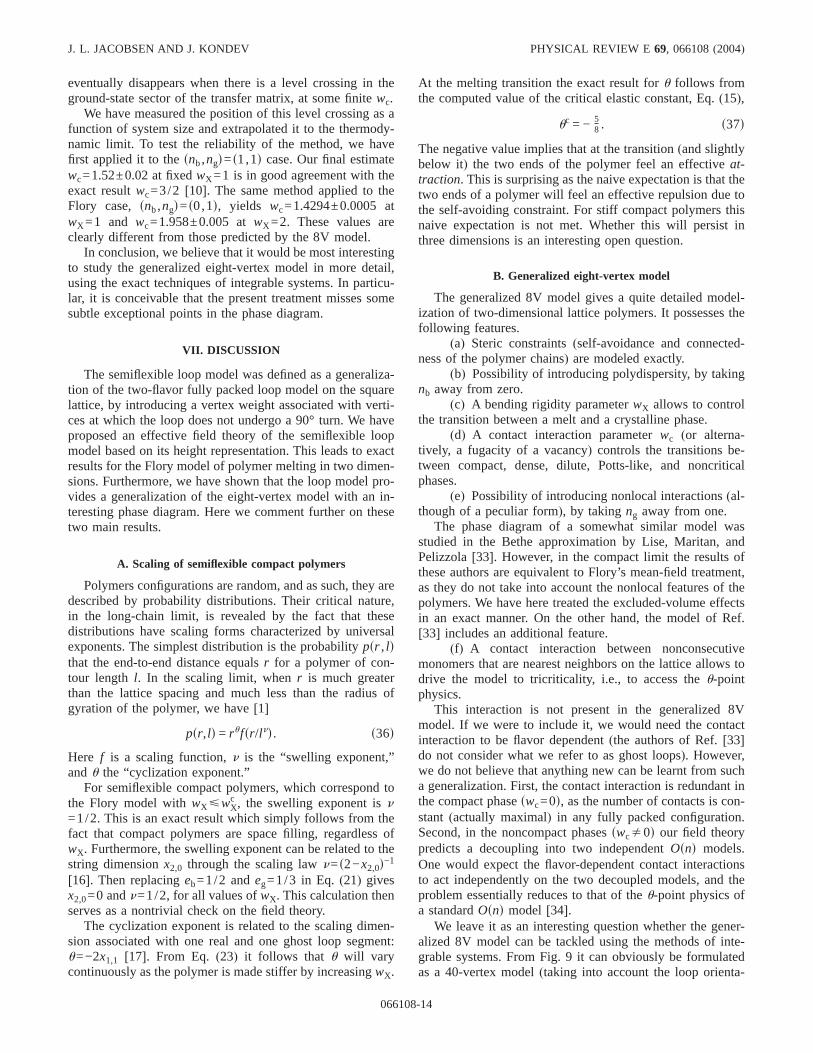
Polymers configurations are random, and as such, they aredescribed by probability distributions. Their critical nature,in the long-chain limit, is revealed by the fact that thesedistributions have scaling forms characterized by universalexponents. The simplest distribution is the probabilitypsr , ldthat the end-to-end distance equalsr for a polymer of con-tour length l. In the scaling limit, whenr is much greaterthan the lattice spacing and much less than the radius ofgyration of the polymer, we have[1]

psr,ld = rufsr/lnd. s36d

Here f is a scaling function,n is the “swelling exponent,”andu the “cyclization exponent.”

For semiflexible compact polymers, which correspond tothe Flory model withwX øwX

c , the swelling exponent isn=1/2.This is an exact result which simply follows from thefact that compact polymers are space filling, regardless ofwX. Furthermore, the swelling exponent can be related to thestring dimensionx2,0 through the scaling lawn=s2−x2,0d−1

[16]. Then replacingeb=1/2 andeg=1/3 in Eq.(21) givesx2,0=0 andn=1/2, for allvalues ofwX. This calculation thenserves as a nontrivial check on the field theory.

The cyclization exponent is related to the scaling dimen-sion associated with one real and one ghost loop segment:u=−2x1,1 [17]. From Eq. (23) it follows that u will varycontinuously as the polymer is made stiffer by increasingwX.

At the melting transition the exact result foru follows fromthe computed value of the critical elastic constant, Eq.(15),

uc = − 58 . s37d

The negative value implies that at the transition(and slightlybelow it) the two ends of the polymer feel an effectiveat-traction. This is surprising as the naive expectation is that thetwo ends of a polymer will feel an effective repulsion due tothe self-avoiding constraint. For stiff compact polymers thisnaive expectation is not met. Whether this will persist inthree dimensions is an interesting open question.

B. Generalized eight-vertex model

The generalized 8V model gives a quite detailed model-ization of two-dimensional lattice polymers. It possesses thefollowing features.

(a) Steric constraints(self-avoidance and connected-ness of the polymer chains) are modeled exactly.

(b) Possibility of introducing polydispersity, by takingnb away from zero.

(c) A bending rigidity parameterwX allows to controlthe transition between a melt and a crystalline phase.

(d) A contact interaction parameterwc (or alterna-tively, a fugacity of a vacancy) controls the transitions be-tween compact, dense, dilute, Potts-like, and noncriticalphases.

(e) Possibility of introducing nonlocal interactions(al-though of a peculiar form), by takingng away from one.

The phase diagram of a somewhat similar model wasstudied in the Bethe approximation by Lise, Maritan, andPelizzola[33]. However, in the compact limit the results ofthese authors are equivalent to Flory’s mean-field treatment,as they do not take into account the nonlocal features of thepolymers. We have here treated the excluded-volume effectsin an exact manner. On the other hand, the model of Ref.[33] includes an additional feature.

(f) A contact interaction between nonconsecutivemonomers that are nearest neighbors on the lattice allows todrive the model to tricriticality, i.e., to access theu-pointphysics.

This interaction is not present in the generalized 8Vmodel. If we were to include it, we would need the contactinteraction to be flavor dependent(the authors of Ref.[33]do not consider what we refer to as ghost loops). However,we do not believe that anything new can be learnt from sucha generalization. First, the contact interaction is redundant inthe compact phaseswc=0d, as the number of contacts is con-stant (actually maximal) in any fully packed configuration.Second, in the noncompact phasesswcÞ0d our field theorypredicts a decoupling into two independentOsnd models.One would expect the flavor-dependent contact interactionsto act independently on the two decoupled models, and theproblem essentially reduces to that of theu-point physics ofa standardOsnd model [34].

We leave it as an interesting question whether the gener-alized 8V model can be tackled using the methods of inte-grable systems. From Fig. 9 it can obviously be formulatedas a 40-vertex model(taking into account the loop orienta-


066108-14

tions) with complex vertex weights. To our knowledge, sucha model has not been studied previously. If one could solveit, it would be particularly interesting to work out the exactexpression of the coupling constantK22swXd as a function ofthe loop fugacitiesnb andng. Also, it is conceivable that ourfield theoretical approach has missed some exceptional criti-cal points in the phase diagram.

C. Order of the melting transition

In this paper we have established that the order of themelting transition within the Flory model is second order, asfirst suggested by Saleur[13]. We have also explained howthe introduction of a finite density of vacancies may lead to afirst-order transition, as observed in Monte Carlo simulations[12]. This combined scenario settles a long controversy inthe literature[8].

ACKNOWLEDGMENTS

We are grateful to Ken Dill for introducing us to the Florymodel of polymer melting. J.K. would further like to thankthe KITP in Santa Barbara for hospitality, where this workwas initiated. The research of J.K. was supported by the NSFunder Grant No. DMR-9984471 and by the Cottrell Founda-tion.

APPENDIX: CONSTRUCTION OF THETRANSFER MATRICES

The transfer matrix construction of Ref.[17] relied on anexplicit bijection between the set of allowed connectivitystatesC and the set of integersZuCu=h1,2,3, . . . ,uCuj. How-ever, in many cases it is difficult to furnish ana priori char-acterization of the set of allowed basis states and its cardi-nality. Moreover, some of the states utilized in Ref.[17] werefound to carry zero weight in the leading eigenvectors of thecorresponding sectors of the transfer matrix, and so oneshould think that it would be possible to eliminate them fromthe outset.

To remedy this situation it is preferable to use anotherapproach. Without prior knowledge of the state space, thelatter is explicitly generated by acting with the transfer ma-trix T on a reference stateuv0l which is known to belong tothe image ofT in the concerned sector. In this way, a certainnumber of image states is generated, which can be inserted inan appropriate data structure using hashing techniques[35].One then acts withT on these states, generating a new list ofstates, and continues in this way until no new states are gen-erated. The resulting list is the complete state space ofT inthe concerned sector.

It remains to find an appropriate reference stateuv0l foreach physically interesting sector ofT. For the sectorssb,sgdin which sk flavor-k strings sk=b,gd span the length of thecylinder generated upon action ofT, the reference state canbe chosen as shown in Fig. 11. This state simply consists ofsL−sb−sgd /2 real arches followed bysb real strings andsg

ghost strings.L must of course have the same parity assb+sg.

Choosing the sector corresponding to the thermal scalingdimension is a little less obvious. A useful observation ismade by exploiting the correspondence with states of thesix-vertex model, as depicted in Fig. 3. In a given row, letNk

even and Nkodd be the number of flavor-k loop segments re-

siding on even and odd vertical edges, respectively. Thendefine

Q = sNbeven− Nb

oddd − sNgeven− Ng

oddd. sA1d

By inspection of Fig. 3 it is seen thatQ is nothing but thevertical flux of arrows within a given row. By the ice rule,Qis a conserved quantity and can thus be used to label a sectorof T.

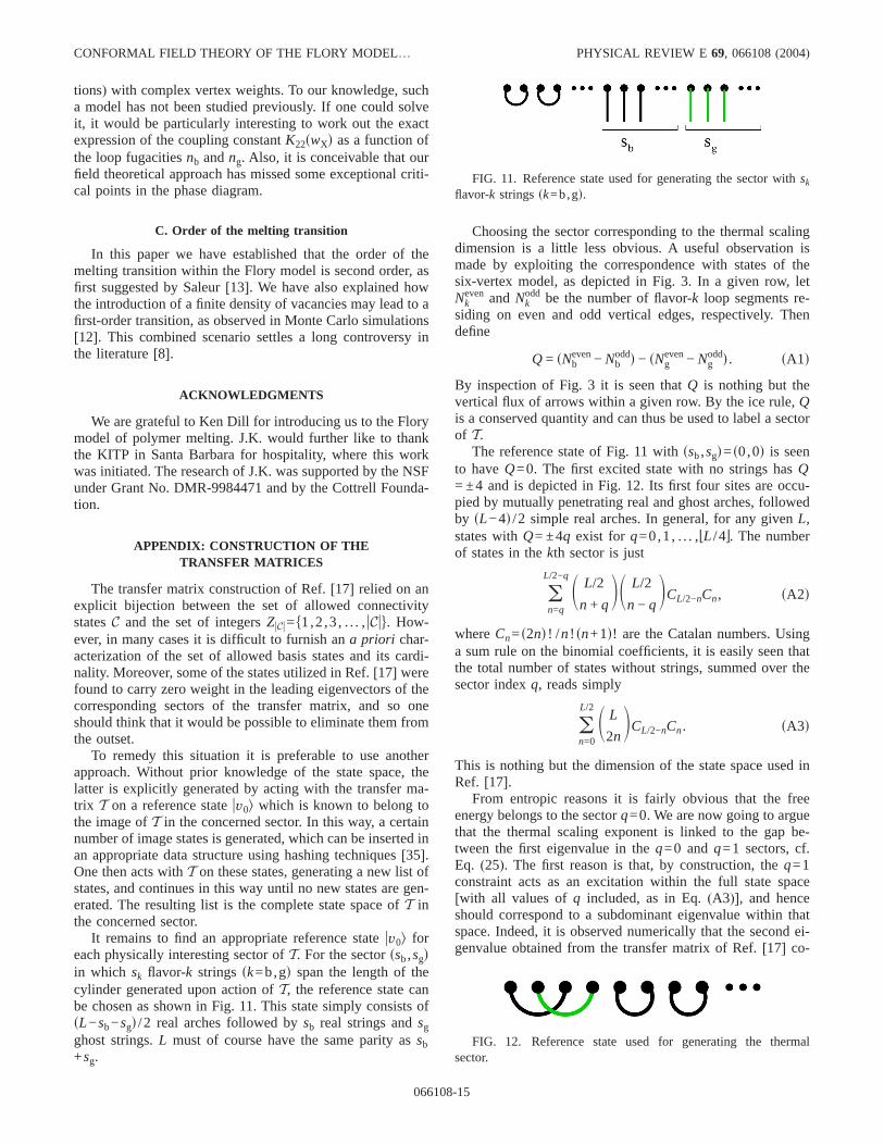
The reference state of Fig. 11 withssb,sgd=s0,0d is seento haveQ=0. The first excited state with no strings hasQ= ±4 and is depicted in Fig. 12. Its first four sites are occu-pied by mutually penetrating real and ghost arches, followedby sL−4d /2 simple real arches. In general, for any givenL,states withQ= ±4q exist for q=0,1, . . . ,bL /4c. The numberof states in thekth sector is just

on=q

L/2−q S L/2

n + qDS L/2

n − qDCL/2−nCn, sA2d

whereCn=s2nd ! / n! sn+1d! are the Catalan numbers. Usinga sum rule on the binomial coefficients, it is easily seen thatthe total number of states without strings, summed over thesector indexq, reads simply

on=0

L/2 S L

2nDCL/2−nCn. sA3d

This is nothing but the dimension of the state space used inRef. [17].

From entropic reasons it is fairly obvious that the freeenergy belongs to the sectorq=0. We are now going to arguethat the thermal scaling exponent is linked to the gap be-tween the first eigenvalue in theq=0 andq=1 sectors, cf.Eq. (25). The first reason is that, by construction, theq=1constraint acts as an excitation within the full state space[with all values ofq included, as in Eq.(A3)], and henceshould correspond to a subdominant eigenvalue within thatspace. Indeed, it is observed numerically that the second ei-genvalue obtained from the transfer matrix of Ref.[17] co-

FIG. 11. Reference state used for generating the sector withsk

flavor-k stringssk=b,gd.

FIG. 12. Reference state used for generating the thermalsector.


066108-15

incides with the leading eigenvalue of theq=1 sector, ob-tained by using the techniques outlined above.

As a second argument, note that in the language of theSFL model height mapping, encircling the first four sites ofFig. 12 yields a height dislocation ofA −C+B−D. By thefour-coloring rule,A +B+C+D=0, this is the same as

mT = 2sA + Bd = − 2sC + Dd. sA4d

But the latter isalso the height defect associated with a de-fect vertex sC ,D ,C ,Dd that corresponds to excluding thereal loops from that vertex, which is exactly a thermal-typeexcitation(and to wit the one that is used for computing thecritical exponentxT within the field theory).

In the field theory, one might compute the exponent cor-responding to the insertion of magnetic defects ±q8mT ateither end of the cylinder. In the transfer matrix, these shouldsimply be linked to the gap between the sectorsq=0 andq=q8.

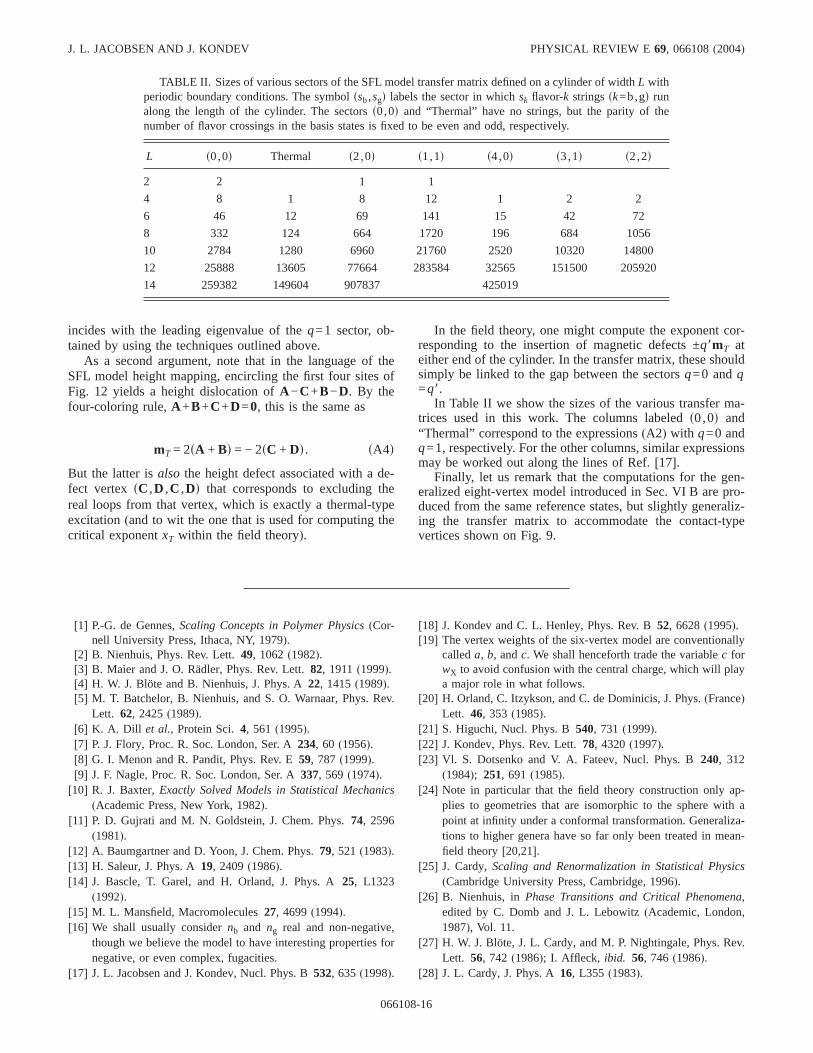
In Table II we show the sizes of the various transfer ma-trices used in this work. The columns labeleds0,0d and“Thermal” correspond to the expressions(A2) with q=0 andq=1, respectively. For the other columns, similar expressionsmay be worked out along the lines of Ref.[17].

Finally, let us remark that the computations for the gen-eralized eight-vertex model introduced in Sec. VI B are pro-duced from the same reference states, but slightly generaliz-ing the transfer matrix to accommodate the contact-typevertices shown on Fig. 9.

[1] P.-G. de Gennes,Scaling Concepts in Polymer Physics(Cor-nell University Press, Ithaca, NY, 1979).

[2] B. Nienhuis, Phys. Rev. Lett.49, 1062(1982).[3] B. Maier and J. O. Rädler, Phys. Rev. Lett.82, 1911(1999).[4] H. W. J. Blöte and B. Nienhuis, J. Phys. A22, 1415(1989).[5] M. T. Batchelor, B. Nienhuis, and S. O. Warnaar, Phys. Rev.

Lett. 62, 2425(1989).[6] K. A. Dill et al., Protein Sci.4, 561 (1995).[7] P. J. Flory, Proc. R. Soc. London, Ser. A234, 60 (1956).[8] G. I. Menon and R. Pandit, Phys. Rev. E59, 787 (1999).[9] J. F. Nagle, Proc. R. Soc. London, Ser. A337, 569 (1974).

[10] R. J. Baxter,Exactly Solved Models in Statistical Mechanics(Academic Press, New York, 1982).

[11] P. D. Gujrati and M. N. Goldstein, J. Chem. Phys.74, 2596(1981).

[12] A. Baumgartner and D. Yoon, J. Chem. Phys.79, 521 (1983).[13] H. Saleur, J. Phys. A19, 2409(1986).[14] J. Bascle, T. Garel, and H. Orland, J. Phys. A25, L1323

(1992).[15] M. L. Mansfield, Macromolecules27, 4699(1994).[16] We shall usually considernb and ng real and non-negative,

though we believe the model to have interesting properties fornegative, or even complex, fugacities.

[17] J. L. Jacobsen and J. Kondev, Nucl. Phys. B532, 635 (1998).

[18] J. Kondev and C. L. Henley, Phys. Rev. B52, 6628(1995).[19] The vertex weights of the six-vertex model are conventionally

calleda, b, andc. We shall henceforth trade the variablec forwX to avoid confusion with the central charge, which will playa major role in what follows.

[20] H. Orland, C. Itzykson, and C. de Dominicis, J. Phys.(France)Lett. 46, 353 (1985).

[21] S. Higuchi, Nucl. Phys. B540, 731 (1999).[22] J. Kondev, Phys. Rev. Lett.78, 4320(1997).[23] Vl. S. Dotsenko and V. A. Fateev, Nucl. Phys. B240, 312

(1984); 251, 691 (1985).[24] Note in particular that the field theory construction only ap-

plies to geometries that are isomorphic to the sphere with apoint at infinity under a conformal transformation. Generaliza-tions to higher genera have so far only been treated in mean-field theory[20,21].

[25] J. Cardy,Scaling and Renormalization in Statistical Physics(Cambridge University Press, Cambridge, 1996).

[26] B. Nienhuis, inPhase Transitions and Critical Phenomena,edited by C. Domb and J. L. Lebowitz(Academic, London,1987), Vol. 11.

[27] H. W. J. Blöte, J. L. Cardy, and M. P. Nightingale, Phys. Rev.Lett. 56, 742 (1986); I. Affleck, ibid. 56, 746 (1986).

[28] J. L. Cardy, J. Phys. A16, L355 (1983).

TABLE II. Sizes of various sectors of the SFL model transfer matrix defined on a cylinder of widthL withperiodic boundary conditions. The symbolssb,sgd labels the sector in whichsk flavor-k stringssk=b,gd runalong the length of the cylinder. The sectorss0,0d and “Thermal” have no strings, but the parity of thenumber of flavor crossings in the basis states is fixed to be even and odd, respectively.

L s0,0d Thermal s2,0d s1,1d s4,0d s3,1d s2,2d

2 2 1 1

4 8 1 8 12 1 2 2

6 46 12 69 141 15 42 72

8 332 124 664 1720 196 684 1056

10 2784 1280 6960 21760 2520 10320 14800

12 25888 13605 77664 283584 32565 151500 205920

14 259382 149604 907837 425019


066108-16

[29] D. Kim and P. A. Pearce, J. Phys. A20, L451 (1987).[30] J. L. Jacobsen and J. Kondev, J. Stat. Phys.96, 21 (1999).[31] B. Duplantier and H. Saleur, Nucl. Phys. B290, 291 (1987).[32] H. Saleur, J. Phys. A19, L807 (1986).[33] S. Lise, A. Maritan, and A. Pelizzola, e-print cond-mat/

9809210.[34] B. Duplantier and H. Saleur, Phys. Rev. Lett.59, 539 (1987).[35] R. Sedgewick,Algorithms in C (Addison-Wesley, Reading,

MA, 1990).


066108-17

Documents

Conformal field theory of the Flory model of polymer melting