Direction des Études et Synthèses Économiques

G 2013 / 15

Which size and evolution of the government expenditure multiplier in France (1980-2010)?

Guillaume CLÉAUD*, Matthieu LEMOINE#

et Pierre-Alain PIONNIER*

Document de travail

Institut National de la Statistique et des Études Économiques

INSTITUT NATIONAL DE LA STATISTIQUE ET DES ÉTUDES ÉCONOMIQUES

Série des documents de travail de la Direction des Études et Synthèses Économiques

DÉCEMBRE 2013

Nous remercions pour leurs commentaires Frédérique BEC, Éric DUBOIS, Luca GAMBETTI, Emmanuel JESSUA, Julien MATHERON, Michel NORMANDIN, Vladimir PASSERON, Corinne PROST, les participants aux séminaires du département des études économiques de l’INSEE, du CREST-LMA et de la Banque de France, ainsi que les participants aux conférences T2M 2013 et ISF 2013. Nous remercions également Sophie GAIGNON d’avoir constitué la base de données des prévisions d’investissement public.

_____________________________________________ * Au moment de la rédaction de l’étude : Département des Études Économiques - Division « Études Macroéconomiques » Timbre G220 -

15, bd Gabriel Péri - BP 100 - 92244 MALAKOFF CEDEX et CREST-LMA -15, bd Gabriel Péri - 92245 MALAKOFF CEDEX # Banque de France - Direction générale des Études et des Relations Internationales - 31, rue Croix des Petits Champs - 75049

Paris CEDEX 01. The views expressed in this paper do not necessarily reflect those of Banque de France.

Département des Études Économiques - Timbre G201 - 15, bd Gabriel Péri - BP 100 - 92244 MALAKOFF CEDEX - France - Tél. : 33 (1) 41 17 60 68 - Fax : 33 (1) 41 17 60 45 - CEDEX - E-mail : d3e-dg@insee.fr - Site Web Insee : http://www.insee.fr

Ces documents de travail ne reflètent pas la position de l’Insee et n'engagent que leurs auteurs.

Working papers do not reflect the position of INSEE but only their author's views.

G 2013 / 15

Which size and evolution of the government expenditure multiplier in France (1980-2010)?

Guillaume CLÉAUD*, Matthieu LEMOINE#

et Pierre-Alain PIONNIER*

Which size and evolution of the government expenditure multiplier in France (1980-2010)?

Abstract The importance of the stimulus packages that were injected in most advanced economies from the start of the financial crisis and the speed at which budgets are now being consolidated in Europe has revived the long-lasting debate on the size of fiscal multipliers. In this study, we focus on government expenditures on goods and services. Our conclusion following Blanchard and Perotti (2002) for the identification of government spending shocks is that the multiplier is significant and not far from 1 on impact and becomes statistically insignificant after about 3 years in France. We provide numerous robustness checks concerning the definition of expenditures, assumptions about data stationarity, the role of expectations and the choice of the sample. Moreover, using a time-varying SVAR model, our main findings are (1) that the multiplier did not evolve significantly at any horizon since the beginning of the 1980s and (2) that the variance of shocks hitting the economy evolves a lot more than the model autoregressive parameters. Even in alternative specifications where the Bayesian priors are pushed towards time-variation, the main evolution that we uncover is a (non-significant) decrease of the medium term expenditure multiplier, partly linked to a more aggressive monetary policy since the 1990s. We do not find evidence of an increase of the multiplier during every recession in France, contrary to the finding of Auerbach and Gorodnichenko (2012) for the United States. At least, business cycle conditions do not seem to be the main driver of the evolution of the expenditure multiplier in the last 30 years in France. JEL-codes: E62, C54 Keywords: Government expenditure multiplier, Evolution, TV-SVAR

Quelle amplitude et quelle évolution du multiplicateur de dépenses publiques en France (1980-2010) ?

Résumé L'importance des plans de relance budgétaire mis en œuvre dans la plupart des économies avancées depuis le déclenchement de la crise financière et la vitesse à laquelle les budgets des États sont maintenant consolidés en Europe a donné une nouvelle actualité au débat sur le multiplicateur de dépenses publiques. Cette étude est centrée sur l'effet des dépenses publiques en biens et services. En utilisant la procédure d'identification des chocs de dépenses publiques proposée par Blanchard et Perotti (2002), nous parvenons à la conclusion que le multiplicateur est statistiquement significatif et peu éloigné de 1 à l'impact et qu'il devient non significatif après environ 3 ans en France. Nous effectuons de nombreux tests de robustesse liés à la définition des dépenses publiques, aux hypothèses de stationnarité des variables considérées, à l'effet des anticipations et au choix de l'échantillon de données. Par ailleurs, en estimant un modèle VAR structurel à coefficients variables dans le temps, nous trouvons (1) que le multiplicateur n'a pas significativement évolué, quel que soit l'horizon temporel considéré, depuis le début des années 1980 et (2) que la variance des chocs affectant l'économie évolue bien davantage que les coefficients autorégressifs du modèle. Même avec des spécifications alternatives où les a priori bayésiens favorisent l'évolution des coefficients dans le temps, l'évolution principale est une réduction (non significative) du multiplicateur de moyen terme, en lien avec une politique monétaire plus réactive depuis les années 1990. Nous ne trouvons pas d'indice d'une augmentation systématique du multiplicateur de dépenses publiques lors de chaque récession en France, contrairement à la conclusion d'Auerbach et Gorodnichenko (2012) pour les États-Unis. En tout cas, la position dans le cycle économique ne semble pas être le facteur principal ayant influencé le multiplicateur de dépenses publiques en France au cours des 30 dernières années. Codes JEL : E62, C54 Mots clés : Multiplicateur de dépenses publiques, Évolution, TV-SVAR

1 Introduction

The importance of the stimulus packages that were injected in most advanced economiesfrom the start of the financial crisis and the speed at which budgets are now beingconsolidated in Europe has revived the long-lasting debate on the size of fiscal multipliers.There is no clear theoretical answer to this question. These multipliers may depend,among other factors, on the expenditures, transfers and taxes that are being considered,on the degree of openness of the economy, and on the reaction of monetary policy. Forthese reasons, these multipliers may not be unique and may change over time.

This paper focuses on the evolution of the expenditure multiplier in France during thelast 30 years. Our definition of expenditures is more restrictive than the sum of govern-ment consumption and investment computed in national accounts. It only correspondsto the purchase of goods and services by the government and does not include the com-pensation of civil servants (see Appendix B). Although the statistical model developedin this paper entails a measure of government net receipts, the focus on expenditures ismotivated by two reasons. First, government net receipts include very different kinds oftaxes and their evolution may be explained by modifications of marginal tax rates or oftax bases, whose effect on economic activity could be very different. Second, a shockon government expenditures is easier to identify than a shock on government receipts,especially in a time-varying context (see infra).

Very few papers try to assess if the size of fiscal multipliers has evolved over time.Our work is closely related to Kirchner et al. (2010) and to Auerbach and Gorodnichenko(2012) which are the two main contributions in this field. Kirchner et al. (2010) estimate atime-varying structural VAR (TV-SVAR) on Euro-Area data starting in 1980Q1 whereasAuerbach and Gorodnichenko (2012) estimate a regime-switching VAR model on U.S.post-WWII quarterly data1. Both of these studies also focus on the evolution of theexpenditure multiplier.

Kirchner et al. (2010) conclude that the short run effectiveness of government spend-ing in stimulating GDP in the Euro-Area (as a whole) increased until the end-1980s andcontinuously decreased afterwards. Their impact spending multiplier has a value of 0.7in 1980 and 0.5 in 2008, with an intermediary value slightly above 1 at the end of the1980s. Their long run spending multiplier continuously decreases from -0.7 to -1.7: thiscontinuous evolution in the long run is the main evolution that they uncover. At thisstage, we can already notice that the multipliers computed by Kirchner et al. (2010)reach their lowest value at the beginning of the Great Recession. However, they do not

1Auerbach and Gorodnichenko (2012) impose that the regimes are linked to the state of the businesscycle (expansion or recession)

3

report the shape of the probability distribution around their median estimates.Auerbach and Gorodnichenko (2012) report that the spending multiplier in the United

States is significantly higher during recessions (2.2 after 5 years) than it is during expan-sions (-0.3 after 5 years). However, this result is driven by defense expenditures onlywhose share in total government expenditures is much higher in the United Stated thanin France2. The non-defense spending multipliers estimated by Auerbach et al. (2012) arenot significantly different during recessions and expansions3 4. Moreover, using a longersample (1890q1-2010q4) and relying on a different econometric methodology (local pro-jections rather than VARs), Owyang et al. (2013) do not observe higher multipliers duringtimes of slack in the United States. Given that VARs cannot be considered as alwayssuperior to local projections from a theoretical point of view (Jorda (2005)), there seemsto be room for further econometric studies on the evolution of governement spendingmultipliers.

There are arguments in favor of a continuous evolution of the size of the multiplier,independently of business cycle conditions. For instance, the French economy has becomemore open since the beginning of the 1980s and this could have led to a growing leakageeffect, an argument often heard in the French public debate on the effectiveness of a fiscalstimulus. Moreover, the monetary policy reaction to a fiscal stimulus might have changed.Disinflation became a priority of the French central bank at the beginning of the 1990s,in order for France to qualify for the euro; the French central bank became independentin 1993 and its prerogatives were partly transferred to the European Central Bank (ECB)in 1999. Finally, opposite effects may have influenced the size of the multiplier during theGreat Recession: on the one hand, the zero lower bound may have muted the responseof monetary policy and pushed multipliers above one (Christiano et al. 2011, Woodford2011) but on the other hand, the rapid increase of French public debt may have ledconsumers to behave in a more Ricardian way (Sutherland 1997). Hence, we do not

2In the United States, defense expenditures represent 25% of government consumption and investmentfrom 1995 to 2010 and 35% from 1960 to 1994 (NIPA, Table 3.15.5). The breakdown of governmentexpenditures by function is only available since 1995 in France. From 1995 to 2010, defense expendituresrepresent only 6% of all government expenditures in France. This share is roughly the same for thecompensation of civil servants (D1) and for the expenditures on goods and services (P2+P51+D631A).

3When they focus on non-defense spending, Auerbach et al. (2012) compute a multiplier after 5 yearsequal to 1.0 during expansions and to 1.1 during recessions.

4For France, Bouthevillain and Dufrénot (2011) adopt a similar approach and find that the shortrun elasticity of output growth to government spending is 13 percentage points higher during recessionsthan they are during expansions, but this difference is not significant. Using a Neo-Keynesian macro-econometric model with time-varying hysteresis effects, Creel et al. (2011) find for France that theshort run expenditure multiplier is slightly above one whatever the cycle position, whereas the long runmultiplier would stay above one for a shock impulsed at a trough and would fall close to zero for a shockimpulsed at a peak.

4

impose a priori, like Auerbach and Gorodnichenko (2012), that the value of multipliersshould only depend on whether the economy is in a recessionary or in an expansionarystate.

Since time-variation could come from multiple sources, a flexible non-linear modelis the appropriate tool to use. Here, we rely on a time-varying structural VAR (TV-SVAR) model (see Appendix D). The same kind of model has been used by Cogley andSargent (2001), Cogley and Sargent (2005) and Primiceri (2005) to assess the evolutionof monetary policy in the United States and its impact on the economy. All coefficientsof the model, including those of the variance-covariance matrix, are left free to vary overtime. This means that the size of the policy shocks identified by the model, as well astheir contemporaneous and lagged impacts on the economy, are time-dependent. Sincethis model contains a lot of parameters, it is estimated using Bayesian techniques. Indeed,the likelihood function in highly-parameterized models tends to be very complicated. Ittypically contains many narrow peaks, possibly in regions where parameter values areincredible, so that it is difficult for a maximization algorithm to discriminate betweenthem. The use of Bayesian priors allows focusing particularly on certain regions of thelikelihood function.

We rely on a quarterly VAR with five variables (real government expenditures, realgovernment net receipts5, real GDP, GDP deflator and nominal 3-month interest rate).The first three variables are those proposed by Blanchard and Perotti (2002). Like(Perotti 2002), we add the other two variables (GDP deflator and short term interestrate), in order to take into account the feedback of prices and monetary policy. For theidentification of the structural shocks, we assume that government spending does notreact to activity nor to net receipts or interest rates within a quarter. This assumption ismotivated by the fact that there is no evidence of an automatic response of governmentspending to business cycle conditions and that any discretionary response is necessarilydelayed due to the existence of decision and implementation lags6. Finally, we assumethat government spending is fixed in nominal terms, so that the volume of expendituresreacts negatively, with a unitary elasticity, to unexpected inflation within a quarter. Thisis the only difference with Blanchard and Perotti (2002), motivated by the fact that weinclude prices and interest rates in our model7.

5Government net receipts are defined as the sum of government financing capacity and governmentexpenditures (see Appendix B). Hence, for instance, unemployment benefits are treated as a negativereceipt.

6Net receipts can react contemporaneously to business cycle conditions due to the existence of au-tomatic stabilizers but the same lags explain why they cannot react to business cycle conditions in adiscretionary manner within a quarter. However, these considerations would only be important if wetried to identify structural shocks on government net receipts (see Appendix C).

7This identification scheme has already been implemented on French data using a fixed coefficients

5

Two main objections have been raised in the literature against the use of aggregatedata and SVAR models in order to assess the effectiveness of fiscal policy.

First of all, the effect of government spending may vary from one kind of expendituresto another. For instance, government consumption as measured by national accounts iscomposed of both direct purchases of goods and services and compensation of civil ser-vants, two expenditures that do not affect the rest of the economy in the same way. Somegoods and services, if they generate externalities (e.g.: education or research expendi-tures) may also have an indirect impact on the utility of consumers or on the productionfunction of firms. This is why some authors favor the use of defense expenditures only(Barro and Redlick 2009). Another advantage generally put forth to support the use ofdefense expenditures is the fact that they depend on geostrategic considerations ratherthan on business cycle conditions. Thus, they are more easily considered as exogenous.

However, this particular choice of data has two drawbacks. First, it is not sure thatresults obtained with defense expenditures can be extended to non-defense spending.Second, these results, on U.S. data, are mainly driven by what happened during WWIIor the Korean war (Hall 2009) and are not necessarily relevant in the present context(e.g.: goods rationing and capacity constraints during wars, cf. Perotti (2011)). More-over, a multivariate model can effectively address the issue of endogeneity, contrary tothe univariate regressions used by Barro and Redlick (2009). The only identifying as-sumption we need is to suppose that the value of government spending cannot adjustto business conditions within a quarter, which seems reasonable. Finally, we distinguishdirect purchases of goods and services from compensation of civil servants, hence limitingthe heterogeneity issue.

The second objection raised against the use of SVAR models in the context of fis-cal policy concerns the identification scheme and the treatment of expectations. Ramey(2011b) shows that government spending shocks identified following a Blanchard andPerotti procedure on U.S. data are Granger-caused by forecasts based on exogenous in-formation. She relies on the median forecast from the Survey of Professional Forecasters(SPF) available since 1969 or on a military spending news variable constructed from pressreleases and available since 19398. In other words, innovations computed by an econome-

SVAR model in a study by Biau and Girard (2005). Their results are compatible with ours althoughthey define government spending as the sum of public consumption and public investment and theirestimation sample ends up in 2003. They compute that a government spending shock has a positiveshort term effect on GDP, with an impact multiplier of 1.4, and a statistically non significant effect inthe medium term.

8The defense news variable is based on episodes where Business Week began to forecast large rises indefense spending: the Ramey-Shapiro variable identifies three major episodes (the Korean war, the Viet-nam war and the Carter-Reagan buildup); another richer variable contains, for 31 dates, the magnitudeof increase in spending for the next years.

6

trician who estimates a SVAR model à la Blanchard and Perotti are not innovations foreconomic agents because their information set is larger than the set of past and presentvalues of the variables included in the model. In this case, estimated parameters andimpulse-response functions (IRF) computed using them are inconsistent.

In order to address this issue, Ramey (2011b) embeds one of her news variable into astandard SVAR used for the analysis of fiscal policy. This news variable is ordered firstin the model, just before government spending, and a Cholesky identification scheme isused. In practice, this identification scheme amounts to regress reduced-form residualsfrom the government spending equation on residuals from the news equation in order toidentify unanticipated government spending shocks. When she compares responses to ausual government spending shock (Blanchard and Perotti 2002, Perotti 2007) and to anunanticipated government spending shock, Ramey (2011b) identifies two main differences.Private consumption increases and private investment decreases on impact in the firstcase but the opposite result holds in the second case. A recent controversy (Ramey 2011a,Perotti 2011) highlighted that these results were sensitive to the inclusion of particularobservations9 and that IRFs for private consumption and GDP in the two cases wereprobably not significantly different from each other (see Figure 1 in Ramey (2011a)).Using European data and relying on forecasts from the European Commission, Beetsmaand Giuliodori (2011) do not find significant evidence of an anticipation effect either.

Although the empirical relevance of anticipation effects remains controversial, con-trolling for these effects provides a good robustness check. A first way to deal withanticipation effects, advocated by Sims (2009) and by Forni and Gambetti (2010), isto include forward-looking variables, like short term interest rates, consumer prices andstock prices, in the model. In our paper, short term interest rates and prices (GDPdeflator) are actually included in the model. Following Ramey’s methodology, we havealso assembled a database of government investment forecasts made by the forecastingdepartment of the French statistical institute (INSEE)10. We use it in order to controlfor expectations not already absorbed by the VAR model. However, its impact on theestimation of the government investment multiplier is only marginal.

Our conclusion using a TV-SVAR model and following Blanchard and Perotti (2002)for the identification of government expenditure shocks is that the size of the expendituremultiplier in France did not evolve statistically significantly at any horizon since thebeginning of the 1980s. The impact multiplier is significant and not far from 1 whereasthe medium term multiplier is not significantly different from 0. The variance of shocks

9For example, Perotti (2011) shows that the results of Ramey (2011b) are reversed by dummyingout two quarters (1950Q4 and 1951Q1) following a wave of panic buying and corresponding to theintroduction of specific regulations by the Federal Reserve.

10The same could not be done for governement consumption of goods and services.

7

hitting the economy evolves a lot more than the model autoregressive parameters. Thesame kind of conclusion has also been reached by Primiceri (2005) with a TV-SVARfocusing on monetary policy in the United States11.

Even in alternative specifications where the Bayesian priors are pushed towards time-variation, the main evolution that we uncover is a (non significant) decrease of the mediumterm expenditure multiplier, partly linked to a more aggressive monetary policy since the1990s. We do not find evidence of an increase of the multiplier during every recessionin France, contrary to the finding of Auerbach and Gorodnichenko (2012) for the UnitedStates. At least, business cycle conditions do not seem to be the main driver of theevolution of the expenditure multiplier in the last 30 years in France. One possibleexplanation could be that the unemployment rate, generally considered as an indicatorof slack, remained high in France since the middle of the 1980s12. But if one thinks thatthe last 30 years of data only enable measuring the government spending multiplier in badtimes for France, the practical relevance of conclusions reached on U.S. data regardingthe evolution of the expenditure multiplier seems to be limited for the French economy.

11His main findings are the following: 1. Time-variation is mostly located in the variance of shockshitting the economy: shocks to inflation and unemployment but also discretionary monetary policyshocks; 2. Impulse response functions of inflation and unemployment to a monetary policy shock arehardly modified since the beginning of the 1970s; 3. Even if the systematic part of monetary policy (i.e.:the parameters of the Taylor rule) displays some time-variation, this evolution does not explain at allwhy inflation rose and fell in the United States in the 1970s and 1980s.

12France is not an isolated case: Owyang et al. (2013) who estimate expenditure multipliers in goodand bad times on U.S. and Canadian data consider that Canada was characterized by a very long periodof slack from 1975 to 2005. This is due to the steadily high Canadian unemployment rate - over 7% - onthis period.

8

2 Constant parameter OLS estimates

2.1 Benchmark specification

The model that we consider is a quarterly VAR with 5 variables and l lags13. This modelcan be written as:

yt =(I5 I5 ⊗ y′t−1 ... I5 ⊗ y′t−l

)· β + A−1idtfA

−1Σ · εt= Zt · β + A−1idtfA

−1Σ · εt

where εt ∼ NID(0, 1) are structural innovations and the (25l + 5)× 1 vector β containscoefficients of constants and lags.

The five variables of the VAR are government expenditures, government net receipts,GDP, GDP deflator and the 3-month interest rate, ordered in this way. The first 3variables are expressed in real terms, deflated by the GDP deflator14. Depending onthe case, the first 4 variables may be considered in log-levels or in log-differences. The3-month interest rate is always expressed in percentage points.

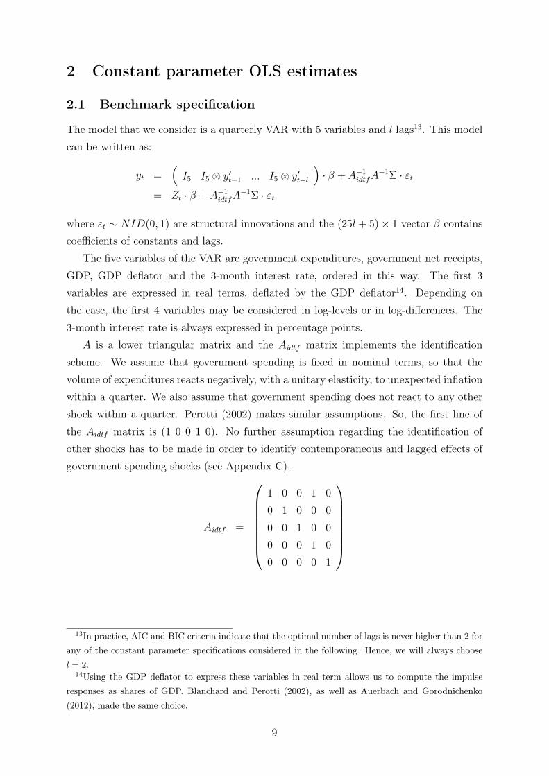
A is a lower triangular matrix and the Aidtf matrix implements the identificationscheme. We assume that government spending is fixed in nominal terms, so that thevolume of expenditures reacts negatively, with a unitary elasticity, to unexpected inflationwithin a quarter. We also assume that government spending does not react to any othershock within a quarter. Perotti (2002) makes similar assumptions. So, the first line ofthe Aidtf matrix is (1 0 0 1 0). No further assumption regarding the identification ofother shocks has to be made in order to identify contemporaneous and lagged effects ofgovernment spending shocks (see Appendix C).

Aidtf =

1 0 0 1 0

0 1 0 0 0

0 0 1 0 0

0 0 0 1 0

0 0 0 0 1

13In practice, AIC and BIC criteria indicate that the optimal number of lags is never higher than 2 forany of the constant parameter specifications considered in the following. Hence, we will always choosel = 2.

14Using the GDP deflator to express these variables in real term allows us to compute the impulseresponses as shares of GDP. Blanchard and Perotti (2002), as well as Auerbach and Gorodnichenko(2012), made the same choice.

9

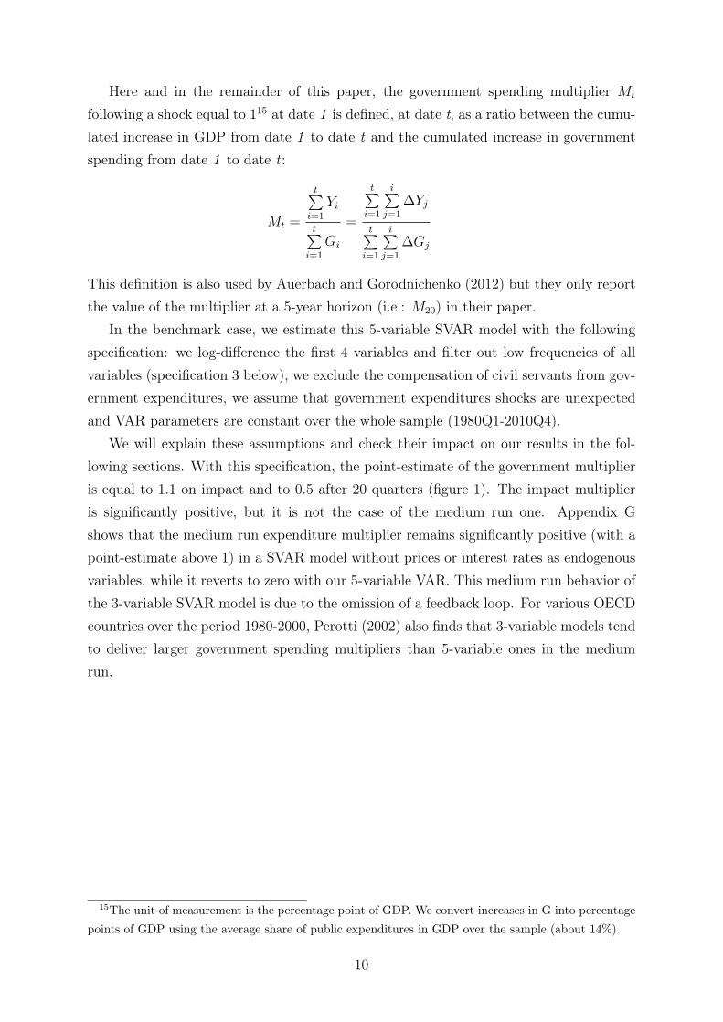
Here and in the remainder of this paper, the government spending multiplier Mt

following a shock equal to 115 at date 1 is defined, at date t, as a ratio between the cumu-lated increase in GDP from date 1 to date t and the cumulated increase in governmentspending from date 1 to date t :

Mt =

t∑i=1

Yi

t∑i=1

Gi

=

t∑i=1

i∑j=1

∆Yj

t∑i=1

i∑j=1

∆Gj

This definition is also used by Auerbach and Gorodnichenko (2012) but they only reportthe value of the multiplier at a 5-year horizon (i.e.: M20) in their paper.

In the benchmark case, we estimate this 5-variable SVAR model with the followingspecification: we log-difference the first 4 variables and filter out low frequencies of allvariables (specification 3 below), we exclude the compensation of civil servants from gov-ernment expenditures, we assume that government expenditures shocks are unexpectedand VAR parameters are constant over the whole sample (1980Q1-2010Q4).

We will explain these assumptions and check their impact on our results in the fol-lowing sections. With this specification, the point-estimate of the government multiplieris equal to 1.1 on impact and to 0.5 after 20 quarters (figure 1). The impact multiplieris significantly positive, but it is not the case of the medium run one. Appendix Gshows that the medium run expenditure multiplier remains significantly positive (with apoint-estimate above 1) in a SVAR model without prices or interest rates as endogenousvariables, while it reverts to zero with our 5-variable VAR. This medium run behavior ofthe 3-variable SVAR model is due to the omission of a feedback loop. For various OECDcountries over the period 1980-2000, Perotti (2002) also finds that 3-variable models tendto deliver larger government spending multipliers than 5-variable ones in the mediumrun.

15The unit of measurement is the percentage point of GDP. We convert increases in G into percentagepoints of GDP using the average share of public expenditures in GDP over the sample (about 14%).

10

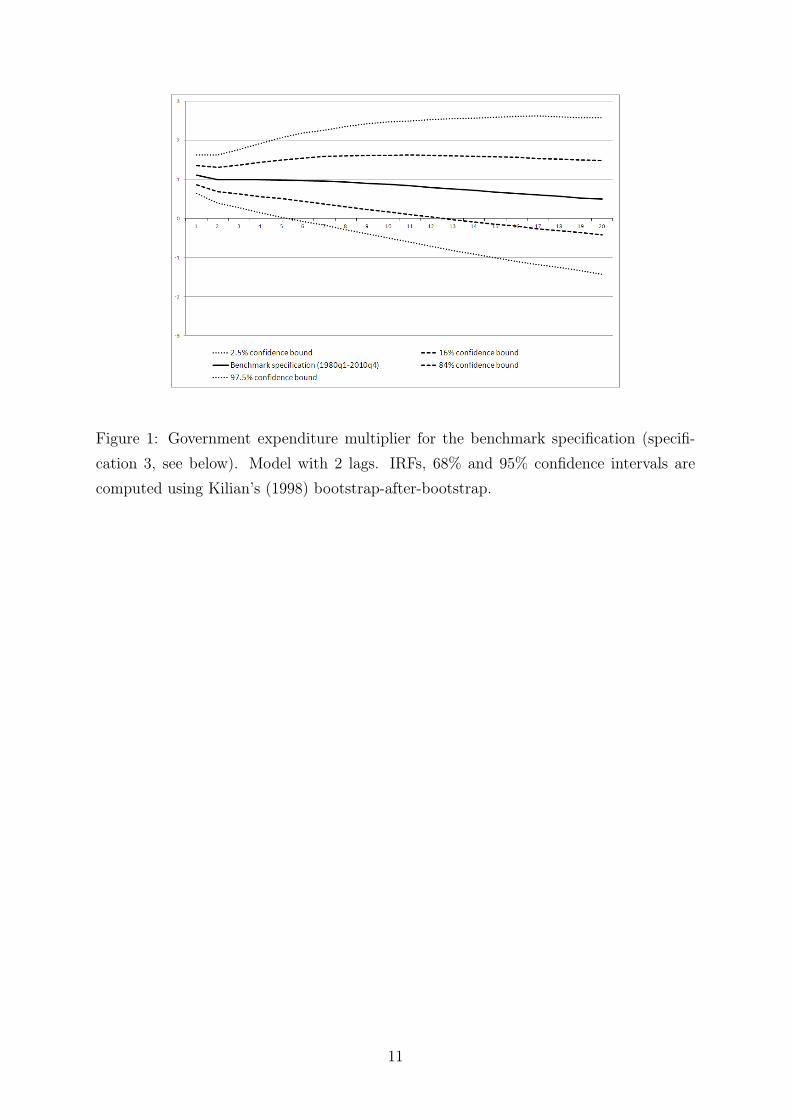
Figure 1: Government expenditure multiplier for the benchmark specification (specifi-cation 3, see below). Model with 2 lags. IRFs, 68% and 95% confidence intervals arecomputed using Kilian’s (1998) bootstrap-after-bootstrap.

11

2.2 Data handling: to difference or not, to detrend or not

2.2.1 Data persistence

Auerbach and Gorodnichenko (2012) estimate the equations of their model with (U.S.)data in log-levels, without differencing or filtering them although they are nonstationaryor, at least, very persistent16. They consider it as a simple way to preserve possiblecointegrating relationships among the variables. They acknowledge that an alternative,but more difficult, way of handling data would have been to estimate the equations inlog differences and to include error correction terms. In fact, there is a long tradition ofestimating SVAR models, especially those measuring the effects of monetary policy, withall data in log-levels17.

Another reason could justify the practice of estimating VAR models in log-levels. Eventhough there is a spurious regression problem when one regresses a nonstationary variableon another independent nonstationary variable, leading to a regression coefficient thatconverges to a stochastic variable rather than to 0, the same problem does not necessarilyoccur in VAR models. Sims et al. (1990) show that some linear combinations of the VARcoefficients have the usual asymptotic distribution: standard theory applies if coefficientsof interest can be rewritten as coefficients on stationary, mean zero, variables. A practicalconsequence of this result, when the vector of autoregressive coefficients in equation i atlag l is noted φil, is that

√T(

Φ̂il − Φil

)is asymptotically Gaussian for each p as long as

the number of lags in the model is sufficient. The asymptotic distribution of the VARcoefficients does not have any bias in this case.

However, small sample results, with sample sizes usually available in macroeconomics,may be noticeably different from what these asymptotic results suggest. For instance, theestimation of autoregressive coefficients in (V)AR models when data are very persistentis affected by finite sample bias. Kilian (1998) proposes a way to deal with this issuefor the computation of IRFs. In the following, whenever we do not rely on Bayesian

16The variables considered by Auerbach and Gorodnichenko (2012) are real government purchases(consumption + investment), real government net receipts and real GDP.

17Here we name just a few prominent examples in this field. Sims (1992) estimates a 6-variable VARmodel for different countries including a short term interest rate, a monetary aggregate, a consumer priceindex, an industrial production index, an index of the foreign exchange value of domestic currency and acommodity price index. All variables but the interest rate enter the model as log-levels while this variableis entered as a percent. Bernanke and Gertler (1995) estimate a 4-variable VAR model including the logof real GDP, the log of the GDP deflator, the log of an index of commodity prices and the federal fundsrate in percentage points. Finally, Eichenbaum and Evans (1995) estimate a 5-variable VAR model thatincludes the U.S. industrial production index, the U.S. consumer price index, the ratio of non-borrowedto total reserves, a measure of the difference between U.S. and foreign short term interest rates and thereal exchange rate. All variables are in log-levels except the interest rates.

12

estimation techniques, we always adopt his bootstrap-after-bootstrap method to computeIRFs and the corresponding confidence intervals. Concerning IRFs, Kilian and Chang(2000) show that confidence bands may have poor coverage properties in small samplesin the presence of very persistent variables, even if standard methods of inference arejustified asymptotically. In the following, we follow their recommendation to discountinterval estimates for higher horizons and report IRFs at a horizon of only 20 quarters (theminimum required to compare our results with those of Auerbach and Gorodnichenko2012).

2.2.2 Low-frequency evolutions: the case of the 1980s in France

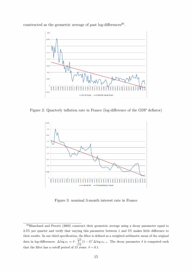
French data on the last 30 years are characterized by low-frequency evolutions that aredifficult to explain using only the 5 endogenous variables of the model. For instance,the inflation rate (log-difference of the GDP deflator) continuously decreased during the1980s (see figure 2). The second oil shock in 1979 and the counter-oil shock in 1985,but also decisions taken by the French government to achieve disinflation are exogenousevents, beyond the short term interest rate movements that we have in the model, thatmay explain why the inflation rate rose and fell in the 1980s.

Ignoring these exogenous events would most certainly bias the coefficients of our 5-variable model. Hence, three different data specifications will be considered in order todeal with these low-frequency evolutions:

• Specification 1: Our first data set consists in real government expenditures, realgovernment net receipts, real GDP, prices (GDP deflator) and the 3-month interestrate. All series are specified in log-level, except the 3-month interest rate whichis specified in level (% points). In order to take into account that prices (GDPdeflator) have an important low-frequency component (the inflation rate is steadilydecreasing, see figure 2 and appendix A), we allow for linear and quadratic trendsin each of the equations of the VAR. This specification is intended to be closestto the specifications in Auerbach and Gorodnichenko (2012) and Kirchner et al.(2010) and to the specification of usual monetary policy VARs.

• Specification 2: In order to apply a standard multivariate cointegration analysis onI(1) variables, we consider the previous data set with a single modification: pricesare replaced by price inflation. Hence, the cointegration analysis is done with thefirst three series (real government expenditures, real government net receipts andreal GDP) remaining specified in log-level, price inflation being defined as the log-difference of the GDP deflator and the 3-month interest rate remaining specifiedin level. In this way, all variables may be considered as I(1), even around a linear

13

deterministic trend (ADF or ERS tests).

In order to be consistent with our first specification, we allow for a linear determinis-tic trend in the cointegration space18. Both the trace and the maximum-eigenvaluecointegration test conclude to the existence of a single cointegration relation in thiscase19. Moreover, an LR test with a 5% level does not reject the joint hypothe-sis that real government expenditures, real government net receipts and real GDPmay be excluded from the cointegration relation and that this cointegration relationmay, itself, be excluded from the inflation equation. Hence, only price inflation, the3-month interest rate and the linear trend are linked together in the long run.

This multivariate cointegration analysis justifies a second data set with real gov-ernment expenditures, real government net receipts, real GDP and prices (GDPdeflator) specified in log-difference and the 3-month interest rate remaining in level.In this case, we allow for a linear trend in each of the equations of the VAR. Thisspecification allows taking into account the long run relation between inflation andthe 3-month interest rate. The fact that we are taking the log-difference of thefirst three variables (real government expenditures, real government net receiptsand real GDP) does not imply any loss of information since these variables may beexcluded from the cointegration relation.

• Specification 3: The third data set is identical to the second, but instead of allowingfor a linear trend in each of the equations of the VAR (which is equivalent topreviously regressing them on a linear trend), we pre-filter all data in subtractingto them a changing mean, constructed as the geometric average of their past.

Data specifications 1 and 3 are very close to those chosen by Blanchard and Per-otti (2002) who are also confronted to low-frequency movements on U.S. data (see pp.1339-1340 of their article). It leads them to present their results with two differentspecifications. In their first specification, all data (real government expenditures, realgovernment net receipts and real GDP) are specified in log-levels and they allow forlinear and quadratic trends in each of the equations of the VAR. In their second specifi-cation, all data are specified in log-differences from which they subtract a changing mean,

18This is case 4 decribed by Juselius (2006), p.100 of her book.19We rely on cointegration tests at a 10% level. This is consistent with Juselius (2006), p.145 of her

book: "[...] In small samples we often lack information to make a sharp distinction between unit roots,near unit roots and very stationary roots. In such cases, choosing the rank based on a small p-valuelike 0.05 is likely to exclusively pick up cointegration relations with relatively fast adjustment back toequilibrium. Unfortunately, the probability of excluding stationary relations characterized by slow, butnevertheless significant adjustments, is likely to be high, i.e. the probability of type 2 errors is generallyhigh for such relations. [...]"

14

constructed as the geometric average of past log-differences20.

Figure 2: Quarterly inflation rate in France (log-difference of the GDP deflator)

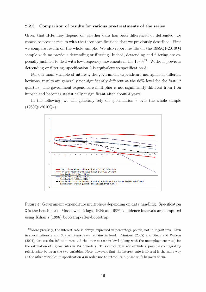
Figure 3: nominal 3-month interest rate in France

20Blanchard and Perotti (2002) construct their geometric average using a decay parameter equal to2.5% per quarter and verify that varying this parameter between 1 and 5% makes little difference totheir results. In our third specification, the filter is defined as a weighted arithmetic mean of the original

data in log-differences: ˜∆ log xt = δ ·+∞∑i=0

(1− δ)i ∆ log xt−i. The decay parameter δ is computed such

that the filter has a cutoff period of 15 years: δ ∼ 0.1.

15

2.2.3 Comparison of results for various pre-treatments of the series

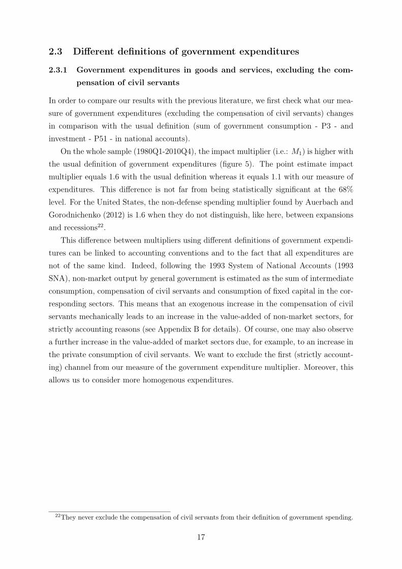
Given that IRFs may depend on whether data has been differenced or detrended, wechoose to present results with the three specifications that we previously described. Firstwe compare results on the whole sample. We also report results on the 1989Q1-2010Q4sample with no previous detrending or filtering. Indeed, detrending and filtering are es-pecially justified to deal with low-frequency movements in the 1980s21. Without previousdetrending or filtering, specification 2 is equivalent to specification 3.

For our main variable of interest, the government expenditure multiplier at differenthorizons, results are generally not significantly different at the 68% level for the first 12quarters. The government expenditure multiplier is not significantly different from 1 onimpact and becomes statistically insignificant after about 3 years.

In the following, we will generally rely on specification 3 over the whole sample(1980Q1-2010Q4).

Figure 4: Government expenditure multipliers depending on data handling. Specification3 is the benchmark. Model with 2 lags. IRFs and 68% confidence intervals are computedusing Kilian’s (1998) bootstrap-after-bootstrap.

21More precisely, the interest rate is always expressed in percentage points, not in logarithms. Evenin specifications 2 and 3, the interest rate remains in level. Primiceri (2005) and Stock and Watson(2001) also use the inflation rate and the interest rate in level (along with the unemployment rate) forthe estimation of Taylor rules in VAR models. This choice does not exclude a possible cointegratingrelationship between the two variables. Note, however, that the interest rate is filtered is the same wayas the other variables in specification 3 in order not to introduce a phase shift between them.

16

2.3 Different definitions of government expenditures

2.3.1 Government expenditures in goods and services, excluding the com-

pensation of civil servants

In order to compare our results with the previous literature, we first check what our mea-sure of government expenditures (excluding the compensation of civil servants) changesin comparison with the usual definition (sum of government consumption - P3 - andinvestment - P51 - in national accounts).

On the whole sample (1980Q1-2010Q4), the impact multiplier (i.e.: M1) is higher withthe usual definition of government expenditures (figure 5). The point estimate impactmultiplier equals 1.6 with the usual definition whereas it equals 1.1 with our measure ofexpenditures. This difference is not far from being statistically significant at the 68%level. For the United States, the non-defense spending multiplier found by Auerbach andGorodnichenko (2012) is 1.6 when they do not distinguish, like here, between expansionsand recessions22.

This difference between multipliers using different definitions of government expendi-tures can be linked to accounting conventions and to the fact that all expenditures arenot of the same kind. Indeed, following the 1993 System of National Accounts (1993SNA), non-market output by general government is estimated as the sum of intermediateconsumption, compensation of civil servants and consumption of fixed capital in the cor-responding sectors. This means that an exogenous increase in the compensation of civilservants mechanically leads to an increase in the value-added of non-market sectors, forstrictly accounting reasons (see Appendix B for details). Of course, one may also observea further increase in the value-added of market sectors due, for example, to an increase inthe private consumption of civil servants. We want to exclude the first (strictly account-ing) channel from our measure of the government expenditure multiplier. Moreover, thisallows us to consider more homogenous expenditures.

22They never exclude the compensation of civil servants from their definition of government spending.

17

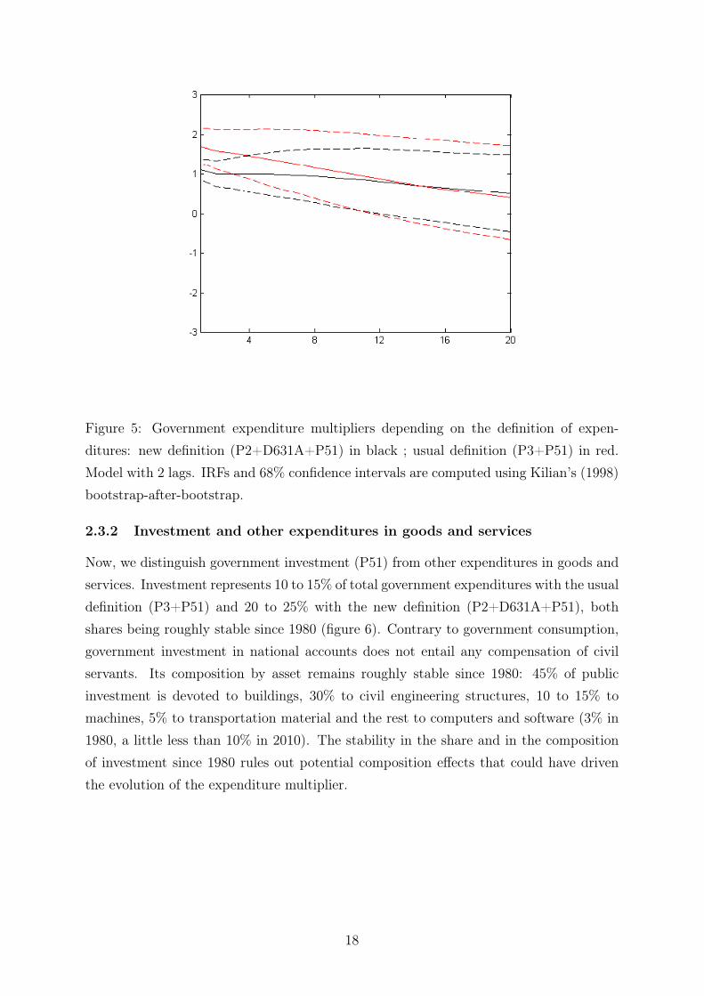
Figure 5: Government expenditure multipliers depending on the definition of expen-ditures: new definition (P2+D631A+P51) in black ; usual definition (P3+P51) in red.Model with 2 lags. IRFs and 68% confidence intervals are computed using Kilian’s (1998)bootstrap-after-bootstrap.

2.3.2 Investment and other expenditures in goods and services

Now, we distinguish government investment (P51) from other expenditures in goods andservices. Investment represents 10 to 15% of total government expenditures with the usualdefinition (P3+P51) and 20 to 25% with the new definition (P2+D631A+P51), bothshares being roughly stable since 1980 (figure 6). Contrary to government consumption,government investment in national accounts does not entail any compensation of civilservants. Its composition by asset remains roughly stable since 1980: 45% of publicinvestment is devoted to buildings, 30% to civil engineering structures, 10 to 15% tomachines, 5% to transportation material and the rest to computers and software (3% in1980, a little less than 10% in 2010). The stability in the share and in the compositionof investment since 1980 rules out potential composition effects that could have driventhe evolution of the expenditure multiplier.

18

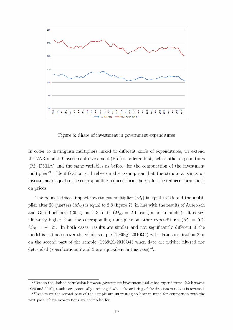
Figure 6: Share of investment in government expenditures

In order to distinguish multipliers linked to different kinds of expenditures, we extendthe VAR model. Government investment (P51) is ordered first, before other expenditures(P2+D631A) and the same variables as before, for the computation of the investmentmultiplier23. Identification still relies on the assumption that the structural shock oninvestment is equal to the corresponding reduced-form shock plus the reduced-form shockon prices.

The point-estimate impact investment multiplier (M1) is equal to 2.5 and the multi-plier after 20 quarters (M20) is equal to 2.8 (figure 7), in line with the results of Auerbachand Gorodnichenko (2012) on U.S. data (M20 = 2.4 using a linear model). It is sig-nificantly higher than the corresponding multiplier on other expenditures (M1 = 0.2,M20 = −1.2). In both cases, results are similar and not significantly different if themodel is estimated over the whole sample (1980Q1-2010Q4) with data specification 3 oron the second part of the sample (1989Q1-2010Q4) when data are neither filtered nordetrended (specifications 2 and 3 are equivalent in this case)24.

23Due to the limited correlation between government investment and other expenditures (0.2 between1980 and 2010), results are practically unchanged when the ordering of the first two variables is reversed.

24Results on the second part of the sample are interesting to bear in mind for comparison with thenext part, where expectations are controlled for.

19

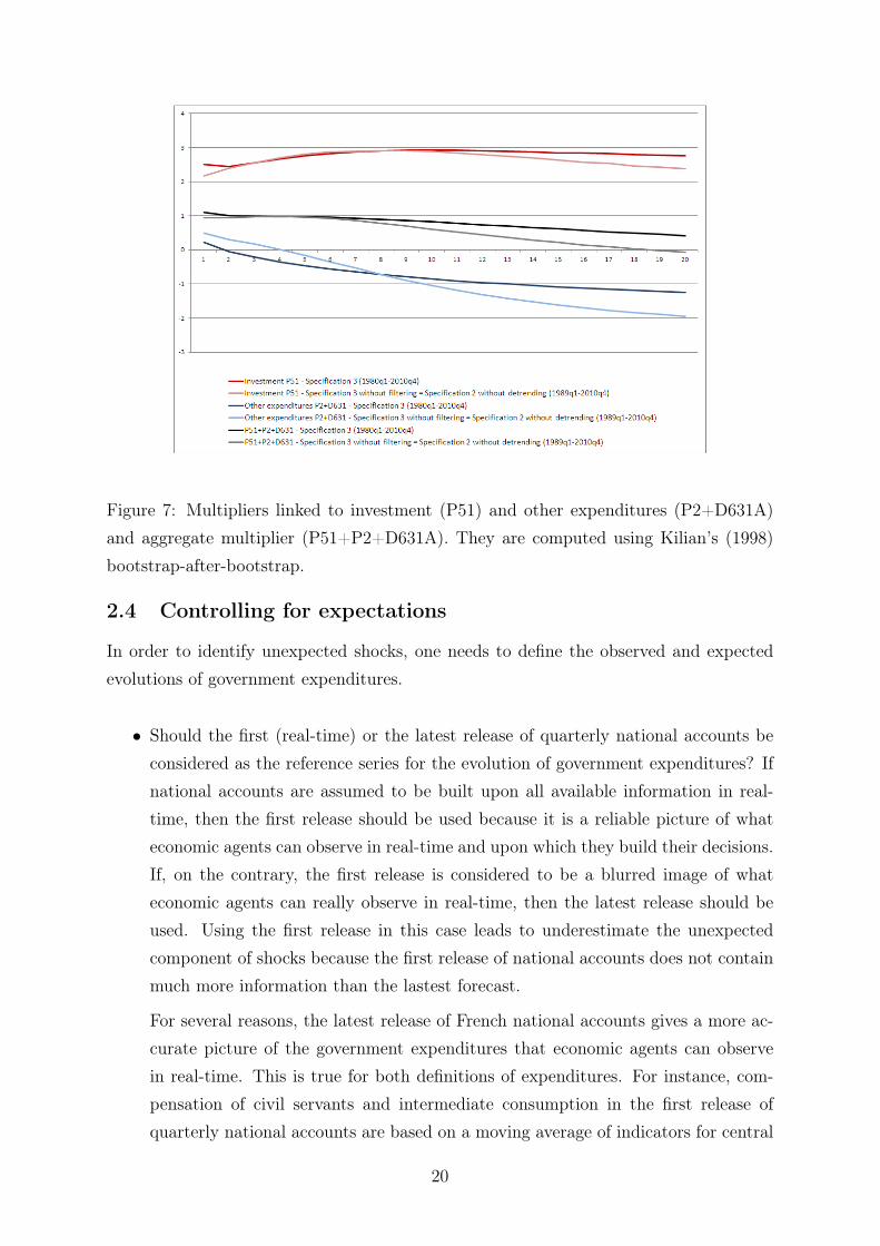
Figure 7: Multipliers linked to investment (P51) and other expenditures (P2+D631A)and aggregate multiplier (P51+P2+D631A). They are computed using Kilian’s (1998)bootstrap-after-bootstrap.

2.4 Controlling for expectations

In order to identify unexpected shocks, one needs to define the observed and expectedevolutions of government expenditures.

• Should the first (real-time) or the latest release of quarterly national accounts beconsidered as the reference series for the evolution of government expenditures? Ifnational accounts are assumed to be built upon all available information in real-time, then the first release should be used because it is a reliable picture of whateconomic agents can observe in real-time and upon which they build their decisions.If, on the contrary, the first release is considered to be a blurred image of whateconomic agents can really observe in real-time, then the latest release should beused. Using the first release in this case leads to underestimate the unexpectedcomponent of shocks because the first release of national accounts does not containmuch more information than the lastest forecast.

For several reasons, the latest release of French national accounts gives a more ac-curate picture of the government expenditures that economic agents can observein real-time. This is true for both definitions of expenditures. For instance, com-pensation of civil servants and intermediate consumption in the first release ofquarterly national accounts are based on a moving average of indicators for central

20

government only because there is no reliable information for local administrationsavailable to national accountants at the time of the first release. Moreover, the de-composition of investment between firms and general government is conventional inthis first release. This is why we define unexpected shocks as the difference betweenthe latest release of quarterly national accounts and real-time forecasts made bythe forecasting department of the statistical institute.

• Another difficulty in the identification of unexpected shocks arises when accountingconcepts have changed between the release of the forecast and the release of nationalaccounts. In this case, using the latest release would lead to overestimate theunexpected component. The definition of government investment has remainedpractically unchanged since the 1980s25 but this is not the case for governmentconsumption26. Moreover, we do not have forecasts of government intermediateconsumption (P2) or social benefits in kind (D631A). Therefore, we only try tocontrol for expected government investment (P51) shocks.

• The latest forecast made by the forecasting department of the French statisticalinstitute (INSEE) before the first release of national accounts is used as an approx-imation of the expected evolution of government investment in France. The firstavailable forecast in our database is the forecast for 1989Q1.

• The correlation between forecasted investment growth and investment growth inthe latest release of national accounts lies between 0.2 and 0.3 and remains roughlystable on the available sample.

Following Ramey (2011a) and Auerbach and Gorodnichenko (2012), we expand theVAR model in order to control for expectations. The first three variables are nowgovernment investment forecasts, government investment itself and other expenditures(P2+D631A). The following four variables remain unchanged. The structural shock oninvestment is now a shock to the second variable. By construction, it is orthogonal togovernment investment forecasts27. Using this methodology, there is no evidence of an

25The only notable exception is the decision to treat software as an investment, rather than an in-termediate consumption, at the end of the 1990s. But at that time, this asset represented only 6% ofgovernment investment.

26Before the introduction of the 1993 SNA at the end of the 1990s, the definition of governmentconsumption was narrower. For instance, all the expenditures incurred on the market by the governmenton behalf of households were recorded as households’ consumption.

27We consider this methodology to be definitely superior to the one consisting in the inclusion govern-ment investment forecast errors as a first variable in the VAR instead of government investment forecasts.

21

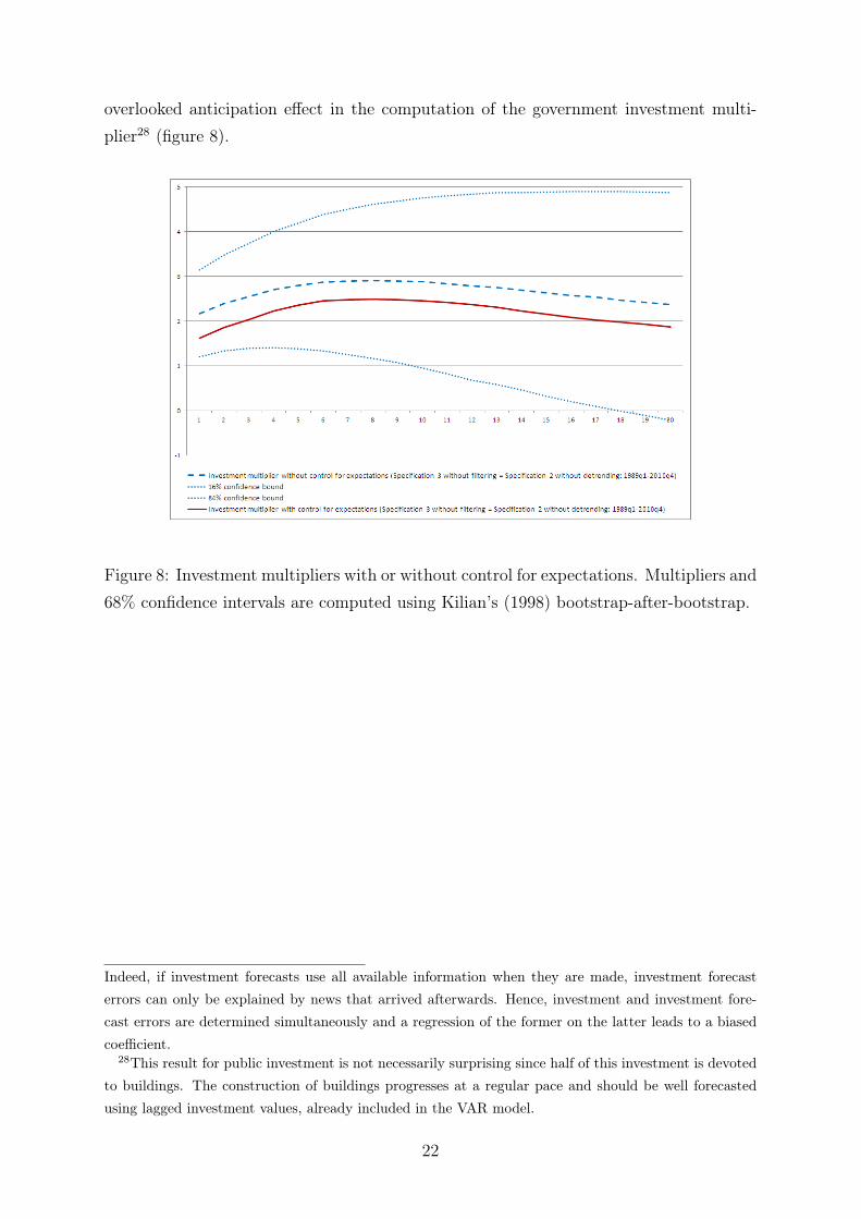
overlooked anticipation effect in the computation of the government investment multi-plier28 (figure 8).

Figure 8: Investment multipliers with or without control for expectations. Multipliers and68% confidence intervals are computed using Kilian’s (1998) bootstrap-after-bootstrap.

Indeed, if investment forecasts use all available information when they are made, investment forecasterrors can only be explained by news that arrived afterwards. Hence, investment and investment fore-cast errors are determined simultaneously and a regression of the former on the latter leads to a biasedcoefficient.

28This result for public investment is not necessarily surprising since half of this investment is devotedto buildings. The construction of buildings progresses at a regular pace and should be well forecastedusing lagged investment values, already included in the VAR model.

22

2.5 Different estimation samples

We now focus on results obtained with our measure of government expenditures on dif-ferent samples. Here are the main conclusions:

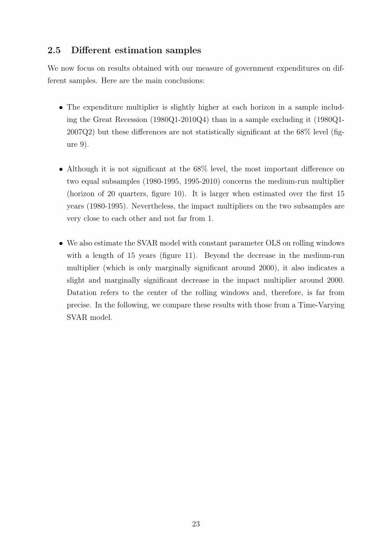
• The expenditure multiplier is slightly higher at each horizon in a sample includ-ing the Great Recession (1980Q1-2010Q4) than in a sample excluding it (1980Q1-2007Q2) but these differences are not statistically significant at the 68% level (fig-ure 9).

• Although it is not significant at the 68% level, the most important difference ontwo equal subsamples (1980-1995, 1995-2010) concerns the medium-run multiplier(horizon of 20 quarters, figure 10). It is larger when estimated over the first 15years (1980-1995). Nevertheless, the impact multipliers on the two subsamples arevery close to each other and not far from 1.

• We also estimate the SVAR model with constant parameter OLS on rolling windowswith a length of 15 years (figure 11). Beyond the decrease in the medium-runmultiplier (which is only marginally significant around 2000), it also indicates aslight and marginally significant decrease in the impact multiplier around 2000.Datation refers to the center of the rolling windows and, therefore, is far fromprecise. In the following, we compare these results with those from a Time-VaryingSVAR model.

23

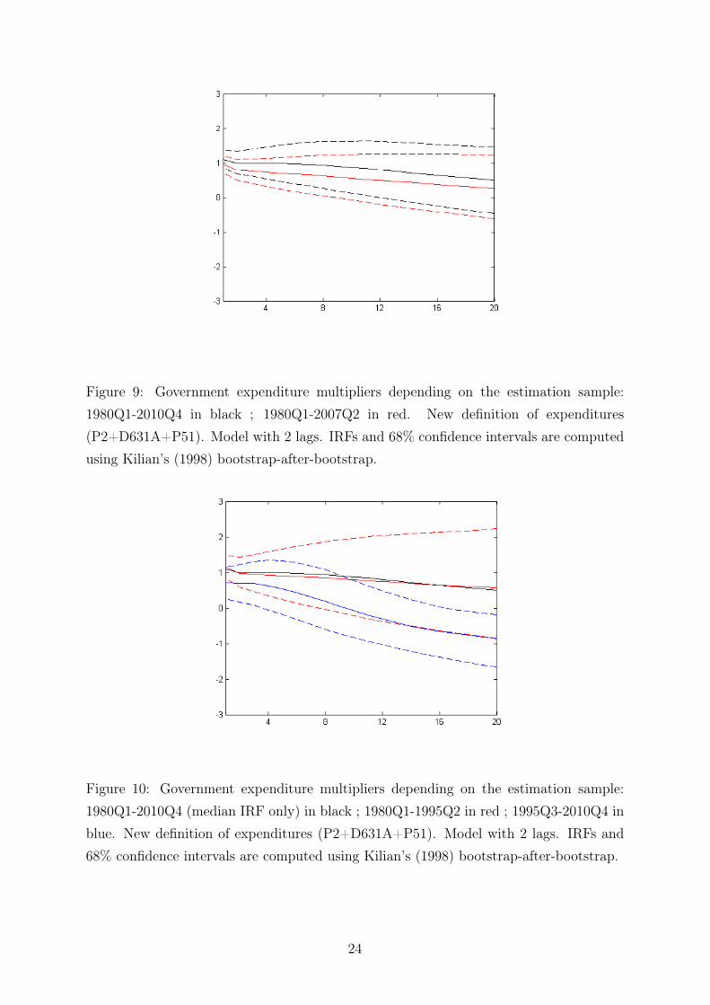
Figure 9: Government expenditure multipliers depending on the estimation sample:1980Q1-2010Q4 in black ; 1980Q1-2007Q2 in red. New definition of expenditures(P2+D631A+P51). Model with 2 lags. IRFs and 68% confidence intervals are computedusing Kilian’s (1998) bootstrap-after-bootstrap.

Figure 10: Government expenditure multipliers depending on the estimation sample:1980Q1-2010Q4 (median IRF only) in black ; 1980Q1-1995Q2 in red ; 1995Q3-2010Q4 inblue. New definition of expenditures (P2+D631A+P51). Model with 2 lags. IRFs and68% confidence intervals are computed using Kilian’s (1998) bootstrap-after-bootstrap.

24

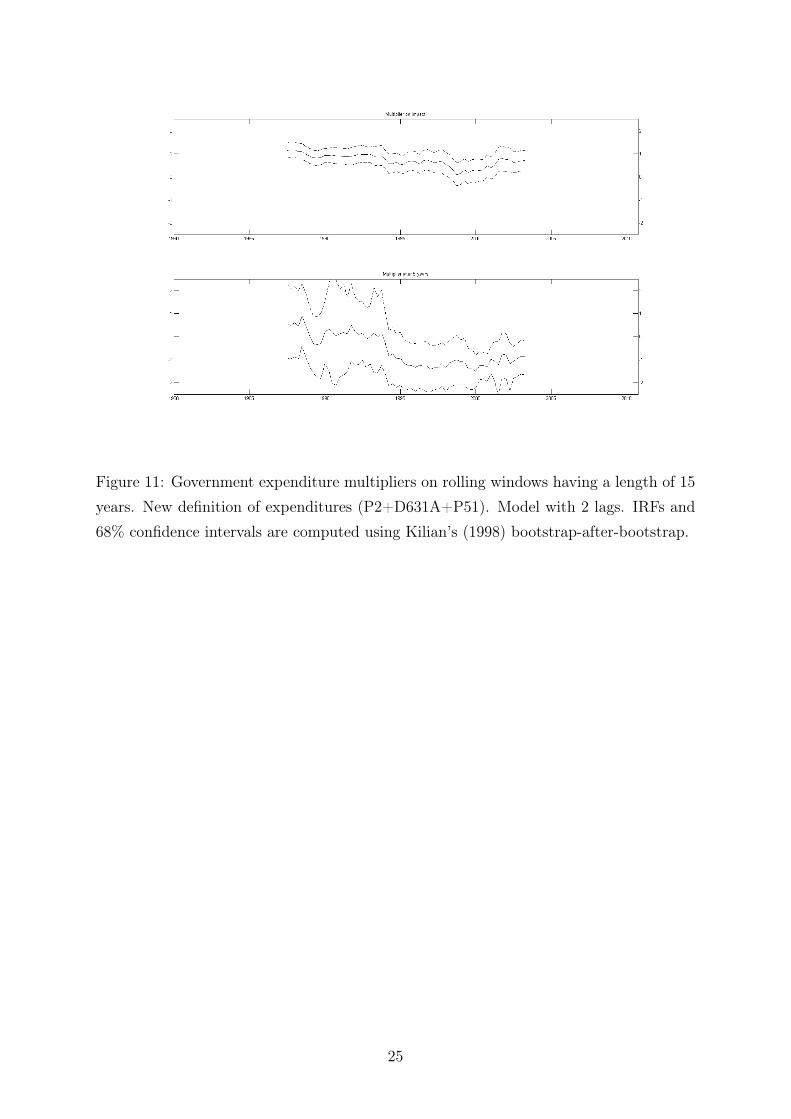
Figure 11: Government expenditure multipliers on rolling windows having a length of 15years. New definition of expenditures (P2+D631A+P51). Model with 2 lags. IRFs and68% confidence intervals are computed using Kilian’s (1998) bootstrap-after-bootstrap.

25

3 Assessing the evolution of the expenditure multiplier

3.1 Econometric methodology

3.1.1 Description of the TV-SVAR model

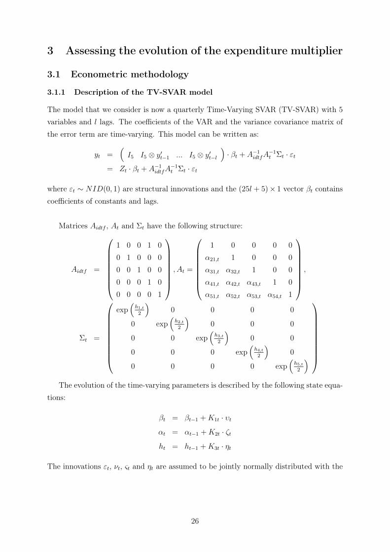
The model that we consider is now a quarterly Time-Varying SVAR (TV-SVAR) with 5variables and l lags. The coefficients of the VAR and the variance covariance matrix ofthe error term are time-varying. This model can be written as:

yt =(I5 I5 ⊗ y′t−1 ... I5 ⊗ y′t−l

)· βt + A−1idtfA

−1t Σt · εt

= Zt · βt + A−1idtfA−1t Σt · εt

where εt ∼ NID(0, 1) are structural innovations and the (25l + 5)× 1 vector βt containscoefficients of constants and lags.

Matrices Aidtf , At and Σt have the following structure:

Aidtf =

1 0 0 1 0

0 1 0 0 0

0 0 1 0 0

0 0 0 1 0

0 0 0 0 1

, At =

1 0 0 0 0

α21,t 1 0 0 0

α31,t α32,t 1 0 0

α41,t α42,t α43,t 1 0

α51,t α52,t α53,t α54,t 1

,

Σt =

exp(h1,t2

)0 0 0 0

0 exp(h2,t2

)0 0 0

0 0 exp(h3,t2

)0 0

0 0 0 exp(h4,t2

)0

0 0 0 0 exp(h5,t2

)

The evolution of the time-varying parameters is described by the following state equa-

tions:

βt = βt−1 +K1t · υtαt = αt−1 +K2t · ζtht = ht−1 +K3t · ηt

The innovations εt, νt, ςt and ηt are assumed to be jointly normally distributed with the

26

following variance covariance matrix:

V = V ar

εt

υt

ζt

ηt

=

I5 0 . . . 0

0 Q. . . ...

... . . . S 0

0 · · · 0 W

These state equations are augmented with parameters Kit (i = 1, 2, 3) which can be

equal to 0 or 1. Depending on the value of Kit, state variables βt, αt and ht evolvebetween date t − 1 and date t or remain constant. When, for instance, K1t = 0, all thecomponents of the state vector βt remain unchanged between date t−1 and date t. Koopet al. (2009) introduced this specification into the TV-SVAR framework developed byPrimiceri (2005) in order to assess whether the monetary transmission mechanism in theUnited States changed and whether changes were gradual or abrupt.

3.1.2 Bayesian estimation strategy

Following Canova and Ciccarelli (2009), priors on α0, β0, h0, Q, S and W are specifiedusing OLS estimates on the 1980Q1-2007Q2 sample (i.e.: on a sample excluding theGreat Recession).

β0 ∼ N

(ˆ

βOLS, 4 ·ˆ

V

(ˆ

βOLS

))α0 ∼ N

(ˆαOLS, 4 ·

ˆ

V(

ˆαOLS

))h0 ∼ N

(2 · log

ˆσOLS, 4 ·

ˆ

V(

ˆσOLS

))

Q, S and W are diagonal matrices with diagonal elements qi, si and wi

qi ∼ IG

(k2q · νq ·

ˆ

Vi,i

(ˆ

βOLS

), νq

)si ∼ IG

(k2s · νs ·

ˆ

Vi,i

(ˆαOLS

), νs

)wi ∼ IG

(k2w · νw ·

ˆ

Vi,i

(ˆσOLS

), νw

)

ˆ

Vi,i

(ˆ

βOLS

),

ˆ

Vi,i

(ˆαOLS

)and

ˆ

Vi,i

(ˆσOLS

)correspond, respectively, to the diagonal

elements of matricesˆ

V

(ˆ

βOLS

),

ˆ

V(

ˆαOLS

)and

ˆ

V(

ˆσOLS

). The meaning of hyperpa-

rameters kq, ks, kw, νq, νs and νw will be clarified in the next section.

27

Finally, the Gibbs sampling algorithm is used to simulate the joint posterior distri-bution

p(β1..T , Q, α1..T , S, h1..T ,W,K1..T

1 , K1..T2 , K1..T

3 , s1..T |y1..T)

where x1..T corresponds to (x1, ..., xT ). The implementation of this algorithm is describedin Appendix D.

3.2 Results with the TV-SVAR model

3.2.1 Benchmark specification

We now estimate the TV-SVAR model presented above. In the definition of the Bayesianpriors, we have to set important hyperparameters governing time variation of the modelparameters.

• First, we have to set the hyperparameter p scaling the probability to observe ajump in the parameter values between date t − 1 and date t. In the benchmarkspecification, this hyperparameter is defined so that the mean probability to observea jump is 0.5 for the three classes of model parameters (autoregressive parameters,parameters of the impact matrix At and variances of the orthogonalized shocks).

• Second, we have to set the hyperparameters kq, ks and kw governing the variance ofparameter innovations. The econometric literature gives some guidance when thelaw of motion of parameters is a random walk with Gaussian innovations (i.e. whenthe probability of jump between two successive dates is equal to 1). Following Stockand Watson (1996), the choice of kq = 0.01 has become standard in the literature ontime-varying parameter regressions (Cogley and Sargent 2001, Cogley and Sargent2005, Primiceri 2005). It corresponds to a standard error of the innovations in therandom walk processes describing parameter evolutions equal to 1% of the standarderror of the OLS estimates. Here, taking into account that the probability p of jumpis not equal to 1 in our prior specification, we follow Koop et al. (2009) and we setthe benchmark values for kq, ks and kw at 0.01√

pwith p = 0.5.

• Third, hyperparameters νq, νs and νw corresponding to the tightness of the priorsscaling time variation are chosen so that these priors are proper and to avoid im-plausible behavior of the parameters. In practice, we set νs = νw = 1

2and νq = 5

2

in the benchmark specification29.29Remind that νq, νs and νw are homogenous to a number of points, to be compared with half the

size of the sample used for the estimation of the model, 1222 = 61 points here.

28

Recall that these choices direct but do not fully constrain time-variation a posteriori.Indeed, the weight given to priors in final (a posteriori) estimates declines with the sizeof the sample and asymptotically converges to 0.

With this benchmark specification, we find that posterior means for the transitionprobabilities are comprised between 0.35 and 0.75 (E(p1|y1...T ) = 0.5, E(p2|y1...T ) = 0.35

and E(p3|y1...T ) = 0.75). Thus, although our benchmark specification does not excluderare abrupt changes, our results are close to those of a TV-SVAR model à la Primiceri.Results indicate that time variation is mostly located in the variance of (reduced-form)shocks (figure 12) 30.

Two features are worth noticing:

• a gradual decrease of the variance of residuals in the price inflation equation sincethe beginning of the 1980s;

• a peak of volatility in 1992-1993 in the interest rate equation, corresponding to thecrisis of the European Monetary System (EMS)31. This means that the restrictivemonetary policy at that time is partly interpreted as an interest rate shock, withmore variance than usual, rather than only as a strengthening of the systematicmonetary response to business cycle conditions. It seems particularly useful in suchcases to estimate a model which is able to discriminate between heteroscedasticityand time-varying parameters.

However, there is only very limited variation over time of the impulse response func-tions (IRFs) to a government spending shock (see figure 13 showing government expen-diture multipliers on 20 quarters and at 4 different dates: 1980, 1990, 2000 and 2010).

30Notice that the algorithm advocated by DelNegro and Primiceri (2013) leads to smoother variancesthan the algorithm originally advocated by Primiceri (2005), see Appendix D.

31Since the beginning of the 1990s, France and the other members of the EMS had chosen to an-chor their currency to the Deutsche Mark. In practice, this meant that the French central bank wasconstrained to follow the German short term interest rate policy. Difficulties arose after the Germanreunification when the Bundesbank began to counteract the inflationary pressures following the choice ofa rate of exchange of 1:1 for conversion of East German money to Deutschmarks and the fiscal expansiondecided by the German government. Following the same monetary policy outside Germany with worsemacroeconomic conditions meant positive interest rate shocks. The size of these shocks rapidly increasedbecause other countries had to offer a growing spread relative to the German interest rate in order tomaintain a fixed parity with the Deutsche Mark. Some countries (UK, Italy, Spain) chose to leave theEMS at the end of 1992. France paid an interest rate spread of 200bp until the summer 1993 whenfluctuation bands inside the EMS were enlarged. The interest rate spread relative to Germany thendisappeared rapidly. For more details on the EMS crisis, see Muet (1994).

29

Figure 12: Posterior median of the standard deviation of shocks ; 16% and 84% confidencebounds. Benchmark specification.

Figure 13: Government spending multiplier for a shock initiated at different dates (1980,1990, 2000 and 2010). Benchmark specification.

3.2.2 Two alternative specifications where time variation is more favored by

the Bayesian priors

The hyperparameters governing time variation of the model parameters are now set toalternative values. We consider two alternative specifications:

30

• In the first specification, the probability p of observing a jump in parameter valuesbetween two successive dates is set at a prior mean value of 0.01 instead of 0.5.Consequently, the hyperparameters kQ, kS and kW are revised upwards (kQ = kS =

kW = 0.01√p). In this case, we set νs = νw = 1

2(unchanged) and νq = 20

2. This

specification is intended to be closer to the regime-switching VAR specificationadopted by Auerbach and Gorodnichenko (2012) but, contrary to them, we do notconstrain the regime switch to be influenced by business cycle conditions only. Welet the data decide for the timing and size of the jumps, only indicating that jumpsshould be rare and rather important a priori.

• In the second specification, the probability of observing a jump has a prior meanvalue of 0.5, as in the benchmark, but the hyperparameters kQ, kS and kW are setat a value of 0.1√

0.5instead of 0.01√

0.5in the benchmark specification. Consequently,

evolutions are assumed to be gradual but with a much higher amplitude than inthe benchmark. In this case, we set νs = νw = 1

2(unchanged) and νq = 50

2. This

prior specification is intended to really push the model towards time-variation butit can be considered as extreme given what is usually considered reasonable in theliterature (cf. Stock and Watson (1996)).

Examining the results of the first alternative specification shows that even when theBayesian priors are more in line with the Auerbach and Gorodnichenko (2012) specifica-tion, data information is strong enough to pull posterior transition probabilities upwardsfor the log-variances ht (E(p3|y1...T ) = 0.25, compared to a prior transition probabilityequal to 0.01). However, posterior transition probabilities for coefficients αt and βt re-main very close to the prior probabilities (E(p1|y1...T ) = 0.02, E(p2|y1...T ) = 0.01), whichmay indicate that data is less informative for these coefficients. All in all, IRFs, multi-pliers and evolutions of shock variances remain practically unchanged compared to thebenchmark specification (not shown).

It is only with the second alternative specification that one may see an evolution inthe IRFs and in the expenditure multiplier. The most notable evolution is a decreasein the medium term multiplier between the beginning and the end of the sample. Thisis consistent with what we previously obtained relying on simple rolling windows OLSestimates. Another visible evolution in the IRFs concerns the systematic response ofmonetary policy: the upward adjustment of the short term interest rate following agovernment spending shock becomes more aggressive in the 1990s (figure 14). Thisevolution can probably be linked to the disinflation and exchange rate policy followed bythe French Central Bank at that time.

This visual inspection is confirmed if one compares the observed evolution of thegovernment expenditure multiplier with its counterfactual evolution if the systematic

31

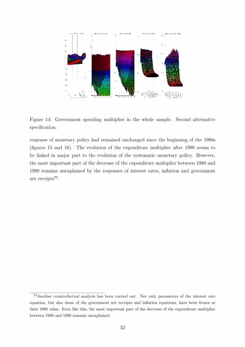
Figure 14: Government spending multiplier in the whole sample. Second alternativespecification.

response of monetary policy had remained unchanged since the beginning of the 1980s(figures 15 and 16). The evolution of the expenditure multiplier after 1990 seems tobe linked in major part to the evolution of the systematic monetary policy. However,the most important part of the decrease of the expenditure multiplier between 1980 and1990 remains unexplained by the responses of interest rates, inflation and governmentnet receipts32.

32Another counterfactual analysis has been carried out. Not only parameters of the interest rateequation, but also those of the government net receipts and inflation equations, have been frozen attheir 1980 value. Even like this, the most important part of the decrease of the expenditure multiplierbetween 1980 and 1990 remains unexplained.

32

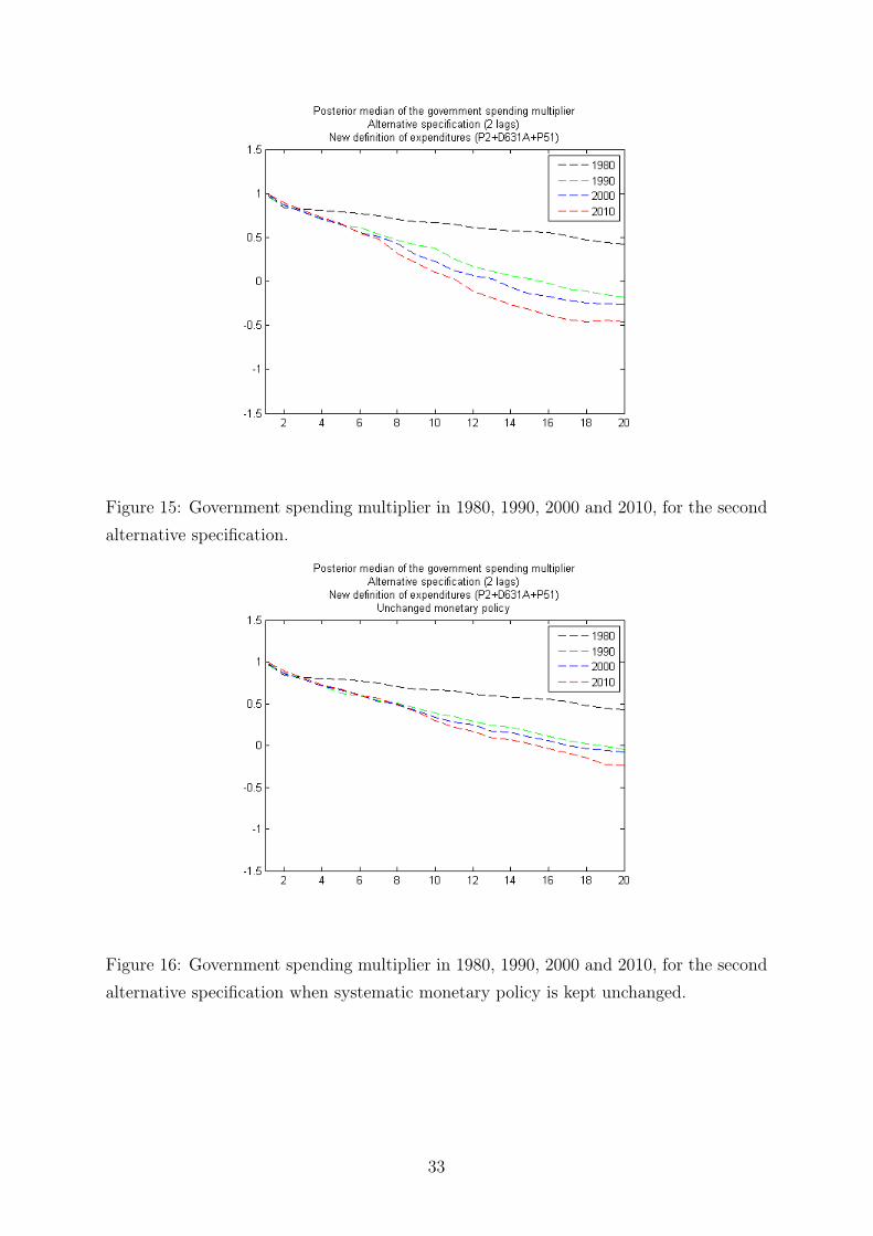
Figure 15: Government spending multiplier in 1980, 1990, 2000 and 2010, for the secondalternative specification.

Figure 16: Government spending multiplier in 1980, 1990, 2000 and 2010, for the secondalternative specification when systematic monetary policy is kept unchanged.

33

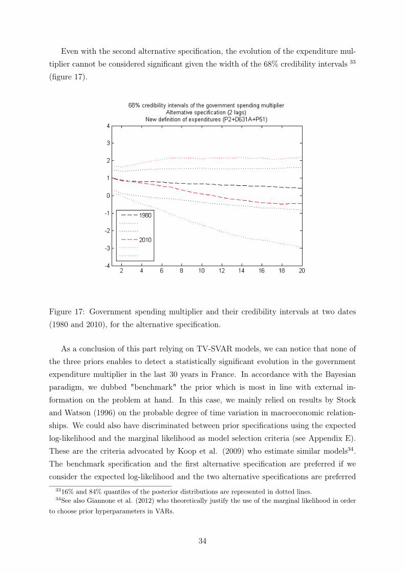
Even with the second alternative specification, the evolution of the expenditure mul-tiplier cannot be considered significant given the width of the 68% credibility intervals 33

(figure 17).

Figure 17: Government spending multiplier and their credibility intervals at two dates(1980 and 2010), for the alternative specification.

As a conclusion of this part relying on TV-SVAR models, we can notice that none ofthe three priors enables to detect a statistically significant evolution in the governmentexpenditure multiplier in the last 30 years in France. In accordance with the Bayesianparadigm, we dubbed "benchmark" the prior which is most in line with external in-formation on the problem at hand. In this case, we mainly relied on results by Stockand Watson (1996) on the probable degree of time variation in macroeconomic relation-ships. We could also have discriminated between prior specifications using the expectedlog-likelihood and the marginal likelihood as model selection criteria (see Appendix E).These are the criteria advocated by Koop et al. (2009) who estimate similar models34.The benchmark specification and the first alternative specification are preferred if weconsider the expected log-likelihood and the two alternative specifications are preferred

3316% and 84% quantiles of the posterior distributions are represented in dotted lines.34See also Giannone et al. (2012) who theoretically justify the use of the marginal likelihood in order

to choose prior hyperparameters in VARs.

34

if we consider the marginal likelihood. Nevertheless, this slight ambiguity resulting fromthe choice of model selection criteria does not affect the overall conclusion of the article.

4 Conclusion

Relying on OLS estimation of a SVAR model over the period 1980-2010, we find thatthe government expenditure multiplier is significant and not far from 1 on impact andbecomes statistically insignificant after about 3 years in France. This result is based ona careful exploitation of national accounts in order to use the most relevant definition ofgovernment expenditures (excluding the compensation of civil servants). We also carryout numerous robustness checks concerning assumptions about data stationarity, the roleof expectations and the choice of the sample.

We only rely on the Blanchard-Perotti identification scheme in order to identify struc-tural shocks on government expenditures on goods and services. Hence, we do not needto know the correct value of the elasticity of government net receipts relative to businesscycle conditions. We justify this partial identification scheme in appendix C.

Our second conclusion using a Time Varying-SVAR model is that the expendituremultiplier in France did not evolve significantly at any horizon since the beginning ofthe 1980s. The variance of shocks hitting the economy evolves a lot more than theautoregressive parameters of the model. Even in alternative specifications where theBayesian priors are pushed towards time-variation, the main evolution that we uncover isa (non significant) decrease of the medium term expenditure multiplier, partly linked to amore aggressive monetary policy since the 1990s. We do not find evidence of an increaseof the multiplier during every recession in France, contrary to the finding of Auerbachand Gorodnichenko (2012) for the United States. At least, business cycle conditions donot seem to be the main driver of the evolution of the expenditure multiplier in thelast 30 years in France. One possible explanation could be that the unemployment rate,generally considered as an indicator of slack, remained high in France since the middleof the 1980s. But if one thinks that the last 30 years of data only enable measuringthe government spending multiplier in bad times for France, the practical relevance ofconclusions reached on U.S. data regarding the evolution of the expenditure multiplierseems to be limited for the French economy.

35

References

Andrews, D. W. (1991). Heteroskedastic and Autocorrelation Consistent CovarianceMatrix Estimation. Econometrica 59, 817–858.

Auerbach, A. and Y. Gorodnichenko (2012). Measuring the Output Responses to FiscalPolicy. American Economic Journal: Economic Policy 4 (2), 1–27.

Barro, R. J. and C. J. Redlick (2009). Macroeconomic Effects from Government Pur-chases and Taxes. NBER Working Paper 15369.

Beetsma, R. and M. Giuliodori (2011). The Effects of Government Purchases Shocks:Review and Estimates for the EU. The Economic Journal 121, 4–32.

Bernanke, B. S. and M. Gertler (1995). Inside the Black Box: the Credit Channel ofMonetary Policy Transmission. Journal of Economic Perspectives 9 (4), 27–48.

Biau, O. and E. Girard (2005). Politique budgétaire et dynamique économique enFrance : l’approche VAR structurel. Economie et Prévision 169-171.

Blanchard, O. and R. Perotti (2002). An Empirical Characterization of the DynamicEffects of Changes in Government Spending and Taxes on Output. The QuarterlyJournal of Economics 117 (4), 1329–1368.

Bouthevillain, C. and G. Dufrénot (2011). Are the Effects of Fiscal Changes Different inTimes of Crisis and Non Crisis? The French Case. Revue d’économie politique 121,371–407.

Canova, F. and M. Ciccarelli (2009). Estimating Multicountry VAR Models. Interna-tional Economic Review 50 (3), 929–959.

Carlin, B. P. and T. A. Louis (2000). Bayes and Empirical Bayes Methods for DataAnalysis. Chapman and Hall .

Carter, C. K. and R. Kohn (1994). On Gibbs Sampling for State Space Models.Biometrika 81 (3), 541–553.

Christiano, L. J., M. Eichenbaum, and S. Rebelo (2011). When is the GovernmentSpending Multiplier Large? Journal of Political Economy 119 (1), 78–121.

Cogley, T. and T. J. Sargent (2001). Evolving Post-World War II U.S. Inflation Dy-namics. NBER Macroeconomics Annual 16, 331–373.

Cogley, T. and T. J. Sargent (2005). Drifts and Volatilities: Monetary Policies andOutcomes in the Post WWII U.S. Review of Economic Dynamics 8, 262–302.

Creel, J., E. Heyer, and M. Plane (2011). Petit précis de politique budgétaire par tousles temps. Les multiplicateurs budgétaires au cours du cycle. Revue de l’OFCE 116,

36

61–88.

DelNegro, M. and G. Primiceri (2013). Time-Varying Structural Vector Autoregres-sions and Monetary Policy: A Corrigendum. Federal Reserve Bank of New YorkStaff Reports No 619 .

Eichenbaum, M. and C. L. Evans (1995). Some Empirical Evidence on the Effectsof Shocks to Monetary Policy on Exchange Rates. Quarterly Journal of Eco-nomics 110 (4), 975–1009.

Forni, M. and L. Gambetti (2010). Fiscal Foresight and the Effects of GovernmentSpending. Mimeo.

Gelfand, A. E. and D. K. Dey (1994). Bayesian Model Choice: Asymptotics and ExactCalculations. Journal of the Royal Statistical Society - Series B 56 (3), 501–514.

Gerlach, R., C. Carter, and R. Kohn (2000). Efficient Bayesian Inference for DynamicMixture Models. Journal of the American Statistical Association 95 (451), 819–828.

Geweke, J. (1992). Evaluating the Accuracy of Sampling-Based Approaches to theCalculation of Posterior Moments. Bayesian Statistics - J.M. Bernardo, J. Berger,A.P. David, A.F.M. Smith eds., Oxford University Press , 169–193.

Geweke, J. (1998). Using Simulation Methods for Bayesian Econometric Models: In-ference, Development and Communication. Federal Reserve Bank of Minneapolis,Research Department Staff Report 249.

Giannone, D., M. Lenza, and G. E. Primiceri (2012). Prior Selection for Vector Au-toregressions. Working Paper .

Hall, R. E. (2009). By How Much Does GDP Rise If the Government Buys MoreOutput? Brookings Papers on Economic Activity Fall, 183–231.

Jorda, O. (2005). Estimation and Inference of Impulse Responses by Local Projections.American Economic Review 95 (1), 161–182.

Juselius, K. (2006). The Cointegrated VAR Model. Oxford University Press .

Justiniano, A. and G. E. Primiceri (2008). The Time-Varying Volatility of Macroeco-nomic Fluctuations. American Economic Review 98 (3), 604–641.

Kilian, L. (1998). Small Sample Confidence Intervals for Impulse Response Functions.The Review of Economics and Statistics 80 (2), 218–230.

Kilian, L. and P.-L. Chang (2000). How Accurate are Confidence Intervals for ImpulseResponses in Large VAR Models? Economics Letters 69, 299–307.

37

Kim, S., N. Shephard, and S. Chib (1998). Stochastic Volatility: Likelihood Inferencein Comparison with ARCH Models. The Review of Economic Studies 65 (3), 361–393.

Kirchner, M., J. Cimadomo, and S. Hauptmeier (2010). Transmission of GovernmentSpending Shocks in the Euro Area - Time Variation and Driving Forces. ECBWorking Paper 1219.

Koop, G., R. Leon-Gonzalez, and R. W. Strachan (2009). On the Evolution of MonetaryPolicy. Journal of Economic Dynamics and Control 33, 997–1017.

Muet, P.-A. (1994). La récession de 1993 réexaminée. Revue de l’OFCE 49, 103–123.

Owyang, M. T., V. A. Ramey, and S. Zubairy (2013). Are Government SpendingMultipliers Greater during Periods of Slack? Evidence from Twentieth-CenturyHistorical Data. American Economic Review 103 (3), 129–134.

Perotti, R. (2002). Estimating the Effects of Fiscal Policy in OECD Countries. ECBWorking Paper No 168 .

Perotti, R. (2007). In Search of the Transmission Mechanism of Fiscal Policy. NBERMacroeconomics Annual 22, 169–226.

Perotti, R. (2011). Expectations and Fiscal Policy: An Empirical Investigation.Mimeo.

Primiceri, G. (2005). Time Varying Structural Vector Autoregressions and MonetaryPolicy. The Review of Economic Studies 72 (3), 821–852.

Ramey, V. A. (2011a). A Reply to Roberto Perotti’s "Expectations and Fiscal Policy:An Empirical Investigation". Mimeo.

Ramey, V. A. (2011b). Identifying Government Spending Shocks: It’s All in the Tim-ing. The Quarterly Journal of Economics 126 (1), 1–50.

Sims, C. A. (1992). Interpreting the Macroeconomic Time Series Facts - The Effectsof Monetary Policy. European Economic Review 36, 975–1011.

Sims, C. A., J. H. Stock, and M. W. Watson (1990). Inference in Linear Time SeriesModels with Some Unit Roots. Econometrica 58 (1), 113–144.

Sims, E. R. (2009). Non-Invertibilities and Structural VARs. Mimeo.

Stock, J. H. and M. W. Watson (1996). Evidence on Structural Instability in Macroe-conomic Time Series Relations. Journal of Business and Economic Statistics 14 (1),11–30.

Stock, J. H. and M. W. Watson (2001). Vector Autoregressions. Journal of EconomicPerspectives 15 (4), 101–115.

38

Sutherland, A. (1997). Fiscal Crises and Aggregate Demand: Can High Public DebtReverse the Effects of Fiscal Policy. Journal of Public Economics 65, 147–162.

Woodford, M. (2011). Simple analytics of the government expenditure multiplier.American Economic Journal Macroeconomics 3 (1), 1–35.

39

A Data handling

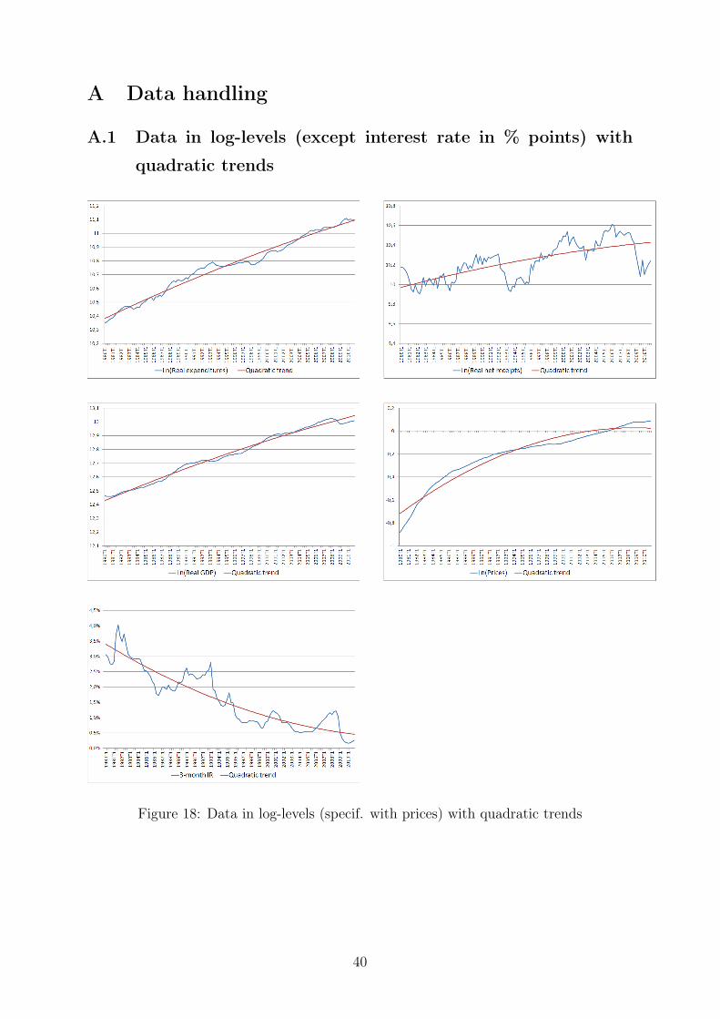
A.1 Data in log-levels (except interest rate in % points) with

quadratic trends

Figure 18: Data in log-levels (specif. with prices) with quadratic trends

40

A.2 Data in log-differences (except interest rate in % points)

with linear trends

Figure 19: Data in log-levels (specif. with inflation) with linear trends

41

B Defining government expenditures using the SNA

The 1993 System of National Accounts (1993 SNA) is an international reference manualon national accounts35. It has been produced jointly by the OECD, the United NationsStatistical Division, the International Monetary Fund, the World Bank and the Com-mission of the European Communities. The 1995 European Accounting System (1995ESA) directly derives from the 1993 SNA: it is the reference manual for the elaborationof national accounts all over the European Union.

The sum of general government (S13)36 consumption (P3) and investment (i.e.: grossfixed capital formation, P51) is the most obvious definition of "government expenditures".In this case, net receipts are defined as the difference between the government financingcapacity (B9A) and these expenditures. Net receipts mainly include taxes, net of subsidiesand transfers.

However, this definition of government expenditures corresponds both to purchasesof goods and services and to the compensation of civil servants (D1). One can criti-cize this definition for two reasons. First, increasing purchases of goods and servicesand increasing the compensation of civil servants are two different ways to stimulate theeconomy that should have different effects. Second, Figure 20 shows that the value ofnon-market production (P1) by general government is defined in national accounts as thesum of the compensation of civil servants (D1), its intermediate consumption (P2) and itsconsumption of fixed capital (K1). On the demand side, the main part of this non-marketproduction is consumed by the general government itself. As a consequence, when thecompensation of civil servants increases, non-market production and general governmentconsumption simultaneously increase, as well as GDP, but for strictly accounting rea-sons. Of course, civil servants may spend part of their wage increase in order to buymarket products: this is the economic channel that economists generally have in mindwhen they try to estimate the government expenditure multiplier. But when governmentexpenditures are defined as the sum of general government consumption and investment,the economic and accounting channels are mixed up.

A simple way to measure government purchases of goods and services is to sum upintermediate consumption (P2), social benefits in kind corresponding to market products(D631A)37 and gross fixed capital formation (P51) in the general government account38

35It is available at: http://www.oecd.org/std/nationalaccounts/systemofnationalaccounts1993.htm36Codes in brackets correspond to the international classification of national accounts. They are used

in 1993 SNA and 1995 ESA.37We only consider reimbursements of market products. By definition, using the 1993 SNA classifica-

tion, D631A ≡ D6311 +D6312A+D6313A.38Theoretically, one should only consider intermediate consumption of market products (P a2 ) but this

disaggregate series is not easily available in national accounts. Moreover, intermediate consumption of

42

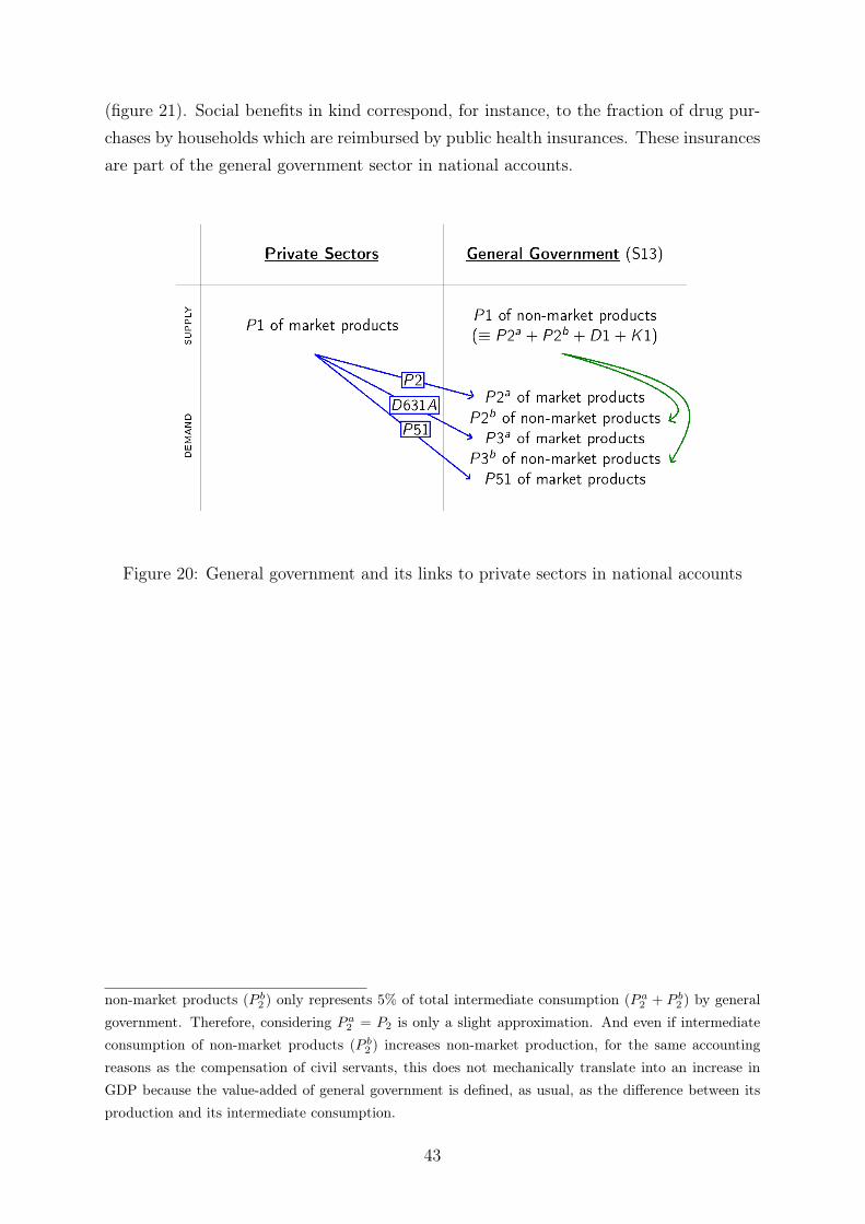
(figure 21). Social benefits in kind correspond, for instance, to the fraction of drug pur-chases by households which are reimbursed by public health insurances. These insurancesare part of the general government sector in national accounts.

Figure 20: General government and its links to private sectors in national accounts

non-market products (P b2 ) only represents 5% of total intermediate consumption (P a2 + P b2 ) by generalgovernment. Therefore, considering P a2 = P2 is only a slight approximation. And even if intermediateconsumption of non-market products (P b2 ) increases non-market production, for the same accountingreasons as the compensation of civil servants, this does not mechanically translate into an increase inGDP because the value-added of general government is defined, as usual, as the difference between itsproduction and its intermediate consumption.

43

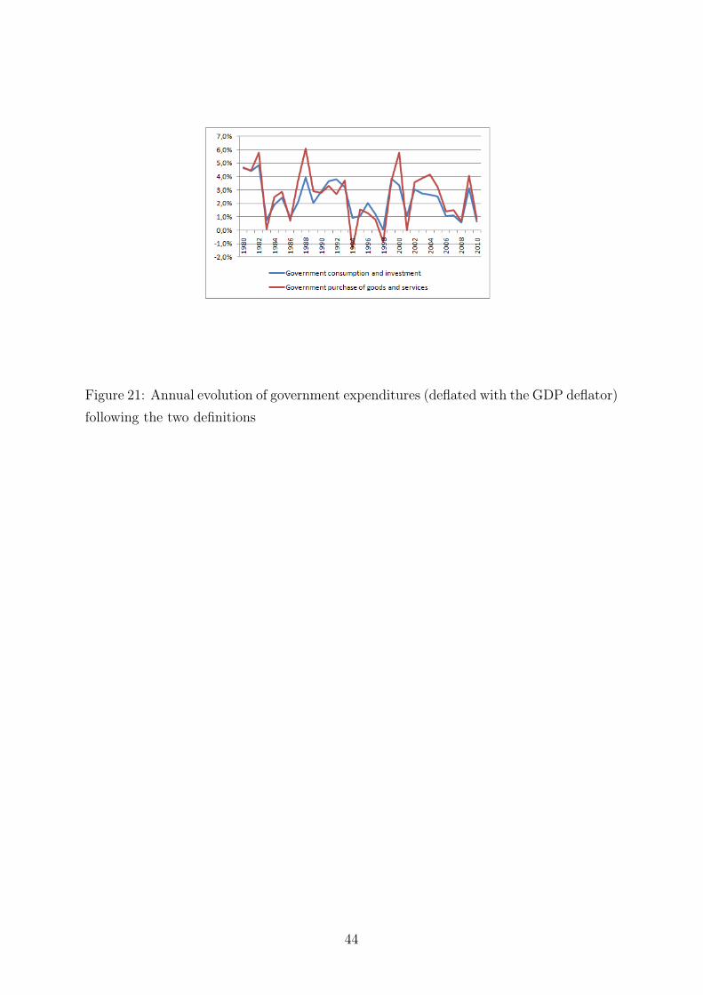
Figure 21: Annual evolution of government expenditures (deflated with the GDP deflator)following the two definitions

44

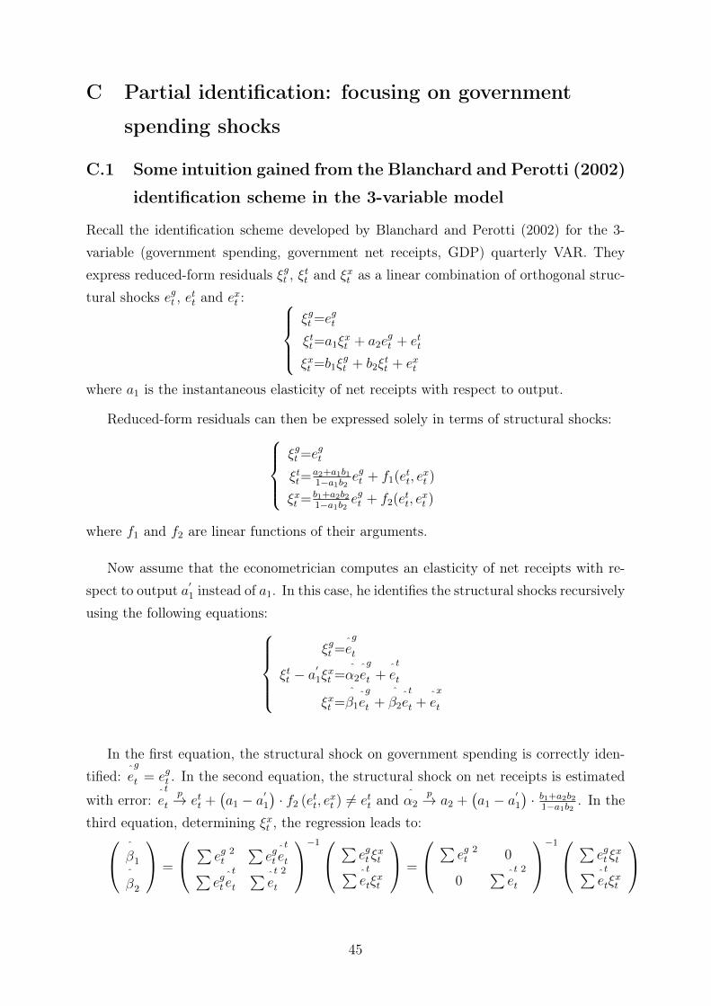
C Partial identification: focusing on government

spending shocks

C.1 Some intuition gained from the Blanchard and Perotti (2002)

identification scheme in the 3-variable model

Recall the identification scheme developed by Blanchard and Perotti (2002) for the 3-variable (government spending, government net receipts, GDP) quarterly VAR. Theyexpress reduced-form residuals ξgt , ξtt and ξxt as a linear combination of orthogonal struc-tural shocks egt , ett and ext :

ξgt =egt

ξtt=a1ξxt + a2e

gt + ett

ξxt =b1ξgt + b2ξ

tt + ext

where a1 is the instantaneous elasticity of net receipts with respect to output.

Reduced-form residuals can then be expressed solely in terms of structural shocks:ξgt =e

gt

ξtt=a2+a1b11−a1b2 e

gt + f1(e

tt, e

xt )

ξxt = b1+a2b21−a1b2 e

gt + f2(e

tt, e

xt )

where f1 and f2 are linear functions of their arguments.

Now assume that the econometrician computes an elasticity of net receipts with re-spect to output a′

1 instead of a1. In this case, he identifies the structural shocks recursivelyusing the following equations:

ξgt =ˆeg

t

ξtt − a′1ξxt =

ˆα2

ˆeg

t +ˆet

t

ξxt =ˆ

β1ˆeg

t +ˆ

β2ˆet

t +ˆex

t

In the first equation, the structural shock on government spending is correctly iden-tified: ˆ

eg

t = egt . In the second equation, the structural shock on net receipts is estimated

with error: ˆet

t

p→ ett +(a1 − a

′1

)· f2 (ett, e

xt ) 6= ett and

ˆα2

p→ a2 +(a1 − a

′1

)· b1+a2b2

1−a1b2 . In thethird equation, determining ξxt , the regression leads to: ˆ

β1ˆ

β2

=

∑eg 2t

∑egt

ˆet

t∑egt

ˆet

t

∑ ˆet 2

t

−1 ∑egt ξ

xt∑ ˆ

et

tξxt

=

∑eg 2t 0

0∑ ˆet 2

t

−1 ∑egt ξ

xt∑ ˆ

et

tξxt

45

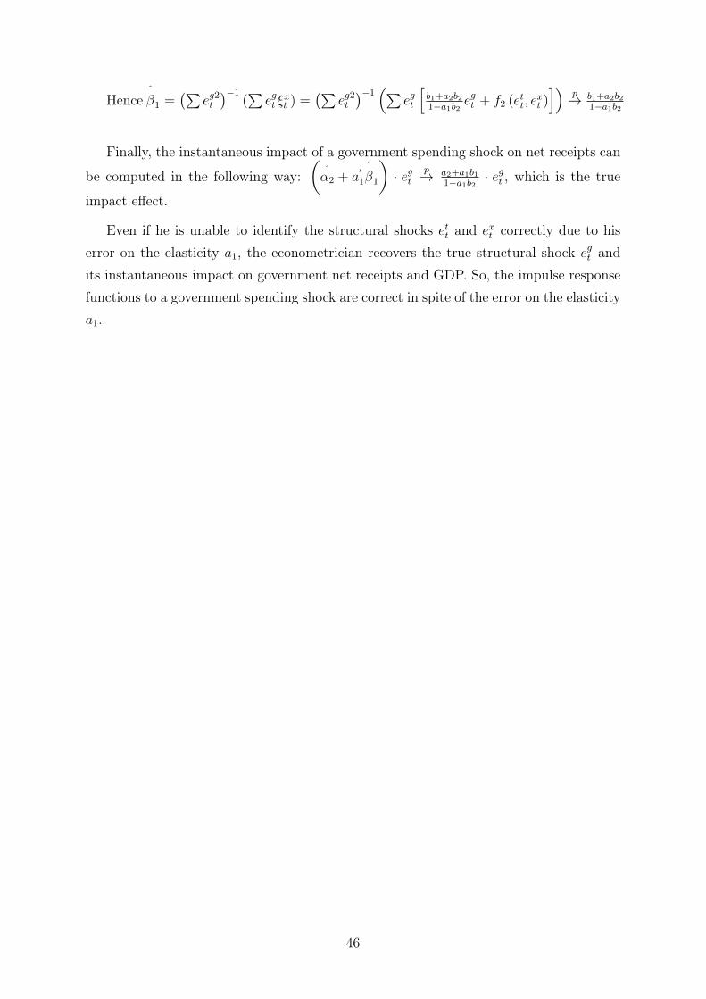
Henceˆ

β1 =(∑

eg2t)−1

(∑egt ξ

xt ) =

(∑eg2t)−1 (∑

egt

[b1+a2b21−a1b2 e

gt + f2 (ett, e

xt )])

p→ b1+a2b21−a1b2 .

Finally, the instantaneous impact of a government spending shock on net receipts can

be computed in the following way:(

ˆα2 + a

′1

ˆ

β1

)· egt

p→ a2+a1b11−a1b2 · e

gt , which is the true

impact effect.

Even if he is unable to identify the structural shocks ett and ext correctly due to hiserror on the elasticity a1, the econometrician recovers the true structural shock egt andits instantaneous impact on government net receipts and GDP. So, the impulse responsefunctions to a government spending shock are correct in spite of the error on the elasticitya1.

46

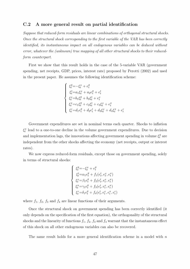
C.2 A more general result on partial identification

Suppose that reduced-form residuals are linear combinations of orthogonal structural shocks.Once the structural shock corresponding to the first variable of the VAR has been correctlyidentified, its instantaneous impact on all endogenous variables can be deduced withouterror, whatever the (unknown) true mapping of all other structural shocks to their reduced-form counterpart.

First we show that this result holds in the case of the 5-variable VAR (governmentspending, net receipts, GDP, prices, interest rate) proposed by Perotti (2002) and usedin the present paper. He assumes the following identification scheme:

ξgt =−ξπt + egt

ξtt=a1ξxt + a2e

gt + ett

ξxt =b1ξgt + b2ξ

tt + ext

ξπt =c1ξgt + c2ξ

tt + c3ξ

xt + eπt

ξrt=d1egt + d2e

tt + d3ξ

xt + d4ξ

πt + ert

Government expenditures are set in nominal terms each quarter. Shocks to inflationξπt lead to a one-to-one decline in the volume government expenditures. Due to decisionand implementation lags, the innovations affecting government spending in volume ξgt areindependent from the other shocks affecting the economy (net receipts, output or interestrates).

We now express reduced-form residuals, except those on government spending, solelyin terms of structural shocks:

ξgt =−ξπt + egt

ξtt=α1egt + f1(e

tt, e

xt , e

πt )

ξxt =β1egt + f2(e

tt, e

xt , e

πt )

ξπt =γ1egt + f3(e

tt, e

xt , e

πt )

ξrt=δ1egt + f4(e

tt, e

xt , e

πt , e

rt )

where f1, f2, f3 and f4 are linear functions of their arguments.

Once the structural shock on government spending has been correctly identified (itonly depends on the specification of the first equation), the orthogonality of the structuralshocks and the linearity of functions f1, f2, f3 and f4 warrant that the instantaneous effectof this shock on all other endogenous variables can also be recovered.

The same result holds for a more general identification scheme in a model with n

47

endogenous variables and n structural shocks:

1 b2 b3 b4 ... bn

a2

a3

a4

...

an

B

ξ1t

ξ2t

ξ3t

ξ4t

...

ξnt

=

1 0 0 0 ... 0

c2

c3

c4

...

cn

U

e1t

e2t

e3t

e4t

...

ent

Using partitioned inverse formulas and defining submatrix W as

W =

B −

a2

a3

...

an

(b2 b3 ... bn

)−1

, this system can be rewritten in the fol-

lowing form:

1 b2 b3 b4 ... bn

0 1 0 0 ... 0

0 0 1 0 ... 0

0 0 0 1 ... 0

... ... ... ... ...

0 0 0 0 ... 1

ξ1t

ξ2t

ξ3t

ξ4t

...

ξnt

=

1 0 0 0 ... 0

-W

a2

a3

a4

...

an

W

e1t

e2t

e3t

e4t

...

ent

The orthogonality conditions warrant that the (n-1) elements of the column vector

W

a2

a3

a4

...

an

can be identified without error.

48

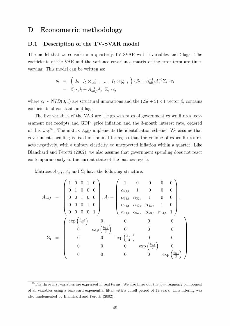
D Econometric methodology

D.1 Description of the TV-SVAR model

The model that we consider is a quarterly TV-SVAR with 5 variables and l lags. Thecoefficients of the VAR and the variance covariance matrix of the error term are time-varying. This model can be written as:

yt =(I5 I5 ⊗ y′t−1 ... I5 ⊗ y′t−l

)· βt + A−1idtfA

−1t Σt · εt

= Zt · βt + A−1idtfA−1t Σt · εt

where εt ∼ NID(0, 1) are structural innovations and the (25l + 5)× 1 vector βt containscoefficients of constants and lags.

The five variables of the VAR are the growth rates of government expenditures, gov-ernment net receipts and GDP, price inflation and the 3-month interest rate, orderedin this way39. The matrix Aidtf implements the identification scheme. We assume thatgovernment spending is fixed in nominal terms, so that the volume of expenditures re-acts negatively, with a unitary elasticity, to unexpected inflation within a quarter. LikeBlanchard and Perotti (2002), we also assume that government spending does not reactcontemporaneously to the current state of the business cycle.

Matrices Aidtf , At and Σt have the following structure:

Aidtf =

1 0 0 1 0

0 1 0 0 0

0 0 1 0 0

0 0 0 1 0

0 0 0 0 1

, At =

1 0 0 0 0

α21,t 1 0 0 0

α31,t α32,t 1 0 0

α41,t α42,t α43,t 1 0

α51,t α52,t α53,t α54,t 1

,

Σt =

exp(h1,t2

)0 0 0 0

0 exp(h2,t2

)0 0 0

0 0 exp(h3,t2

)0 0

0 0 0 exp(h4,t2

)0

0 0 0 0 exp(h5,t2

)

39The three first variables are expressed in real terms. We also filter out the low-frequency componentof all variables using a backward exponential filter with a cutoff period of 15 years. This filtering wasalso implemented by Blanchard and Perotti (2002).

49

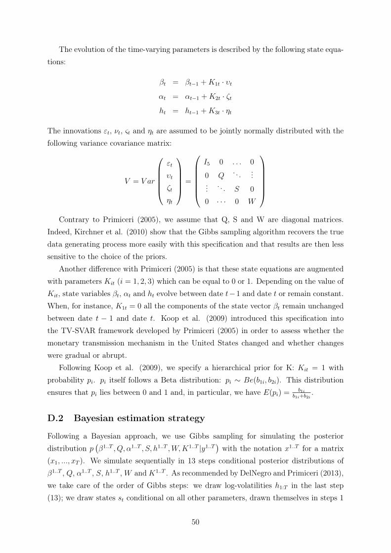
The evolution of the time-varying parameters is described by the following state equa-tions:

βt = βt−1 +K1t · υtαt = αt−1 +K2t · ζtht = ht−1 +K3t · ηt

The innovations εt, νt, ςt and ηt are assumed to be jointly normally distributed with thefollowing variance covariance matrix:

V = V ar

εt

υt

ζt

ηt

=

I5 0 . . . 0

0 Q. . . ...

... . . . S 0

0 · · · 0 W

Contrary to Primiceri (2005), we assume that Q, S and W are diagonal matrices.

Indeed, Kirchner et al. (2010) show that the Gibbs sampling algorithm recovers the truedata generating process more easily with this specification and that results are then lesssensitive to the choice of the priors.

Another difference with Primiceri (2005) is that these state equations are augmentedwith parameters Kit (i = 1, 2, 3) which can be equal to 0 or 1. Depending on the value ofKit, state variables βt, αt and ht evolve between date t−1 and date t or remain constant.When, for instance, K1t = 0 all the components of the state vector βt remain unchangedbetween date t − 1 and date t. Koop et al. (2009) introduced this specification intothe TV-SVAR framework developed by Primiceri (2005) in order to assess whether themonetary transmission mechanism in the United States changed and whether changeswere gradual or abrupt.

Following Koop et al. (2009), we specify a hierarchical prior for K: Kit = 1 withprobability pi. pi itself follows a Beta distribution: pi ∼ Be(b1i, b2i). This distributionensures that pi lies between 0 and 1 and, in particular, we have E(pi) = b1i

b1i+b2i.

D.2 Bayesian estimation strategy

Following a Bayesian approach, we use Gibbs sampling for simulating the posteriordistribution p

(β1..T , Q, α1..T , S, h1..T ,W,K1..T |y1..T

)with the notation x1..T for a matrix

(x1, ..., xT ). We simulate sequentially in 13 steps conditional posterior distributions ofβ1..T , Q, α1..T , S, h1..T ,W andK1..T . As recommended by DelNegro and Primiceri (2013),we take care of the order of Gibbs steps: we draw log-volatilities h1:T in the last step(13); we draw states st conditional on all other parameters, drawn themselves in steps 1

50

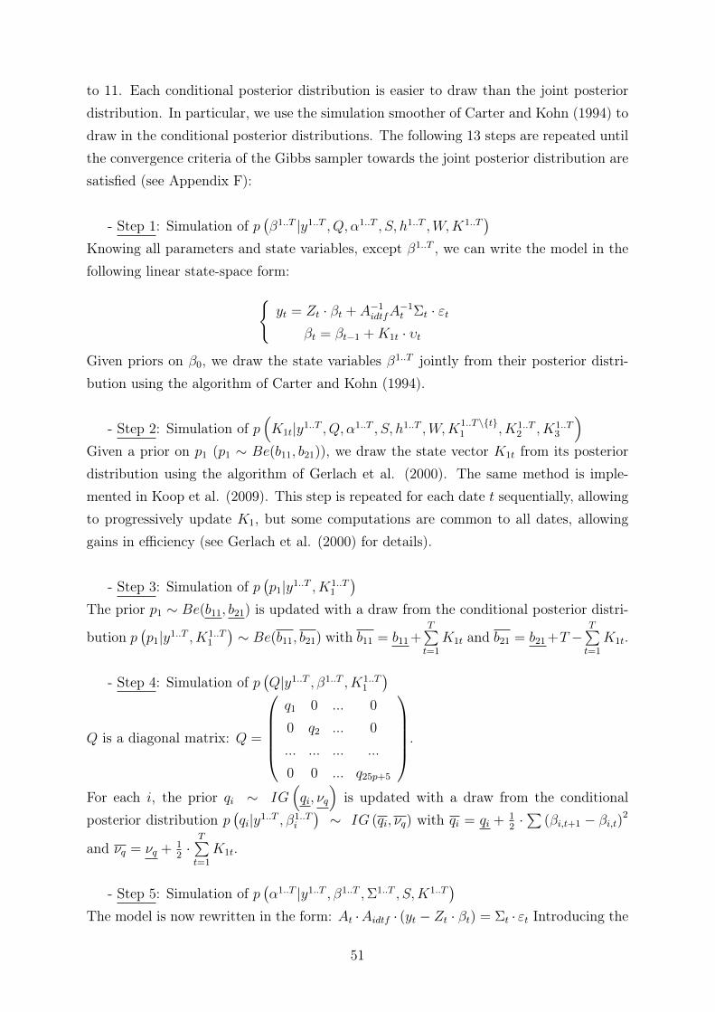
to 11. Each conditional posterior distribution is easier to draw than the joint posteriordistribution. In particular, we use the simulation smoother of Carter and Kohn (1994) todraw in the conditional posterior distributions. The following 13 steps are repeated untilthe convergence criteria of the Gibbs sampler towards the joint posterior distribution aresatisfied (see Appendix F):

- Step 1: Simulation of p(β1..T |y1..T , Q, α1..T , S, h1..T ,W,K1..T

)Knowing all parameters and state variables, except β1..T , we can write the model in thefollowing linear state-space form:{

yt = Zt · βt + A−1idtfA−1t Σt · εt

βt = βt−1 +K1t · υt

Given priors on β0, we draw the state variables β1..T jointly from their posterior distri-bution using the algorithm of Carter and Kohn (1994).

- Step 2: Simulation of p(K1t|y1..T , Q, α1..T , S, h1..T ,W,K

1..T\{t}1 , K1..T

2 , K1..T3

)Given a prior on p1 (p1 ∼ Be(b11, b21)), we draw the state vector K1t from its posteriordistribution using the algorithm of Gerlach et al. (2000). The same method is imple-mented in Koop et al. (2009). This step is repeated for each date t sequentially, allowingto progressively update K1, but some computations are common to all dates, allowinggains in efficiency (see Gerlach et al. (2000) for details).

- Step 3: Simulation of p(p1|y1..T , K1..T

1

)The prior p1 ∼ Be(b11, b21) is updated with a draw from the conditional posterior distri-

bution p(p1|y1..T , K1..T

1

)∼ Be(b11, b21) with b11 = b11+

T∑t=1

K1t and b21 = b21+T −T∑t=1

K1t.

- Step 4: Simulation of p(Q|y1..T , β1..T , K1..T

1

)

Q is a diagonal matrix: Q =

q1 0 ... 0

0 q2 ... 0

... ... ... ...

0 0 ... q25p+5

.

For each i, the prior qi ∼ IG(qi, νq

)is updated with a draw from the conditional

posterior distribution p(qi|y1..T , β1..T

i

)∼ IG (qi, νq) with qi = qi + 1

2·∑

(βi,t+1 − βi,t)2

and νq = νq + 12·T∑t=1

K1t.

- Step 5: Simulation of p(α1..T |y1..T , β1..T ,Σ1..T , S,K1..T

)The model is now rewritten in the form: At ·Aidtf · (yt − Zt · βt) = Σt · εt Introducing the

51

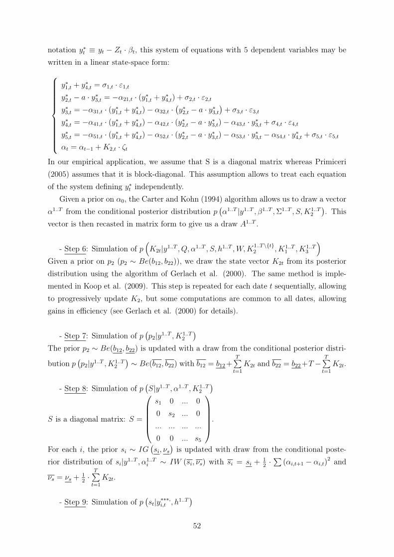
notation y∗t ≡ yt − Zt · βt, this system of equations with 5 dependent variables may bewritten in a linear state-space form:

y∗1,t + y∗4,t = σ1,t · ε1,ty∗2,t − a · y∗3,t = −α21,t · (y∗1,t + y∗4,t) + σ2,t · ε2,ty∗3,t = −α31,t · (y∗1,t + y∗4,t)− α32,t ·

(y∗2,t − a · y∗3,t

)+ σ3,t · ε3,t

y∗4,t = −α41,t · (y∗1,t + y∗4,t)− α42,t · (y∗2,t − a · y∗3,t)− α43,t · y∗3,t + σ4,t · ε4,ty∗5,t = −α51,t · (y∗1,t + y∗4,t)− α52,t · (y∗2,t − a · y∗3,t)− α53,t · y∗3,t − α54,t · y∗4,t + σ5,t · ε5,tαt = αt−1 +K2,t · ζt

In our empirical application, we assume that S is a diagonal matrix whereas Primiceri(2005) assumes that it is block-diagonal. This assumption allows to treat each equationof the system defining y∗t independently.

Given a prior on α0, the Carter and Kohn (1994) algorithm allows us to draw a vectorα1..T from the conditional posterior distribution p

(α1..T |y1..T , β1..T ,Σ1..T , S,K1..T

2

). This

vector is then recasted in matrix form to give us a draw A1..T .

- Step 6: Simulation of p(K2t|y1..T , Q, α1..T , S, h1..T ,W,K

1..T\{t}2 , K1..T

1 , K1..T3

)Given a prior on p2 (p2 ∼ Be(b12, b22)), we draw the state vector K2t from its posteriordistribution using the algorithm of Gerlach et al. (2000). The same method is imple-mented in Koop et al. (2009). This step is repeated for each date t sequentially, allowingto progressively update K2, but some computations are common to all dates, allowinggains in efficiency (see Gerlach et al. (2000) for details).

- Step 7: Simulation of p(p2|y1..T , K1..T

2

)The prior p2 ∼ Be(b12, b22) is updated with a draw from the conditional posterior distri-

bution p(p2|y1..T , K1..T

2

)∼ Be(b12, b22) with b12 = b12+

T∑t=1

K2t and b22 = b22+T −T∑t=1

K2t.

- Step 8: Simulation of p(S|y1..T , α1..T , K1..T

2

)

S is a diagonal matrix: S =

s1 0 ... 0

0 s2 ... 0

... ... ... ...

0 0 ... s5

.

For each i, the prior si ∼ IG(si, νs

)is updated with draw from the conditional poste-

rior distribution of si|y1..T , α1..Ti ∼ IW (si, νs) with si = si + 1

2·∑

(αi,t+1 − αi,t)2 and

νs = νs + 12·T∑t=1

K2t.

- Step 9: Simulation of p(st|y∗∗∗,i,t , h

1..T)52

A new state si,t is drawn for each i ∈ {1, .., 3} and each t ∈ {1, .., T} using the probability:Pr(si,t = j|y∗∗∗i,t

)∝ qj · fN

(y∗∗∗i,t |hi,t +mj − 1.2704, v2j

).

- Step 10: Simulation of p(h1..T |y1..T , A1..T , β1..T , s1..T ,W,K1..T

)Introducing the notation y∗∗t ≡ At · Aidtf · (yt − Zt · βt), y∗∗∗t ≡ log

(y∗∗t

2)and ε∗∗∗t =

log (εt2), the model may be rewritten in the state-space form:{

y∗∗∗t = ht + ε∗∗∗t

ht = ht−1 +K3t · ηtFollowing Kim et al. (1998), the distribution of ε∗∗∗i,t for i ∈ {1, .., 3} is approximated by

a mixture of 7 normals: p(ε∗∗∗i,t)≈∑qj · fN

(ε∗∗∗i,t |mj − 1.2704, v2j

)where the parameters

qj, mj and vj are given by Kim, Shephard and Chib (1998). Concretely, we introduce 7states for each component of the vector y∗∗∗t : si,t ∈ {1, .., 7}. Conditional on being in oneof these states, ε∗∗∗i,t follows a normal law: ε∗∗∗i,t | si,t = j ∼ N

(mj − 1.2704, v2j

).

Given priors on h0, the Carter and Kohn (1994) algorithm allows us to draw vectorsh1..T from the conditional posterior distribution p

(h1..T |y1..T , A1..T , β1..T , s1..T ,W,K1..T

).

Eventually, the draw on h1..T is transformed into a draw on σ1..T using the formulaσi,t ≡ exp

(hi,t2

).

- Step 11: Simulation of p(K3t|y1..T , Q, α1..T , S, h1..T ,W,K

1..T\{t}3 , K1..T

1 , K1..T2

)Given a prior on p3 (p3 ∼ Be(b13, b23)), we draw the state variables K3t from their pos-terior distribution using the algorithm of Gerlach et al. (2000). The same method isimplemented in Koop et al. (2009). This step is repeated for each date t sequentially,allowing to progressively update K3, but some computations are common to all dates,allowing gains in efficiency (see Gerlach et al. (2000) for details).

- Step 12: Simulation of p(p3|y1..T , K1..T

3

)The prior p3 ∼ Be(b13, b23) is updated with a draw from the conditional posterior distri-

bution p(p3|y1..T , K1..T

3

)∼ Be(b13, b23) with b13 = b13+

T∑t=1

K3t and b23 = b23+T −T∑t=1

K3t.

- Step 13: Simulation of p(W |y1..T , h1..T , K1..T

3

)

W is a diagonal matrix: W =

w1 0 ... 0

0 w2 ... 0

... ... ... ...

0 0 ... w5

.

For each i, the prior wi ∼ IG(wi, νw

)is updated with draw from the conditional poste-

rior distribution of wi|y1..T , h1..Ti ∼ IW (wi, νw) with wi = wi + 12·∑

(hi,t+1 − hi,t)2 and

53

νw = νw + 12·T∑t=1

K3t.

D.3 Specification of the priors

Following Canova and Ciccarelli (2009), priors on α0, β0, h0, Q, S and W are specifiedusing OLS estimates on the sample where the TV-SVAR model is also estimated40.

β0 ∼ N

(ˆ

βOLS, 4 ·ˆ

V

(ˆ

βOLS

))α0 ∼ N

(ˆαOLS, 4 ·

ˆ

V(

ˆαOLS

))h0 ∼ N

(2 · log

ˆσOLS, 4 ·

ˆ

V(

ˆσOLS

))

Q, S and W are diagonal matrices with diagonal elements qi, si and wi

qi ∼ IG

(k2q · νq ·

ˆ

Vi,i

(ˆ

βOLS

), νq

)si ∼ IG

(k2s · νs ·

ˆ

Vi,i

(ˆαOLS

), νs

)wi ∼ IG

(k2w · νw ·

ˆ

Vi,i

(ˆσOLS

), νw

)

ˆ

Vi,i

(ˆ

βOLS

)and

ˆ

Vi,i

(ˆαOLS

)correspond, respectively, to the diagonal elements of

matricesˆ

V

(ˆ

βOLS

)and

ˆ

V(

ˆαOLS

).

40More precisely, we use OLS estimates on the 1980Q1-2007Q2 sample, ending just before the GreatRecession.

54

E Bayesian model selection criteria

Following Koop et al. (2009) who estimate similar models, we compute two model se-lection criteria: the marginal likelihood and the expected log-likelihood. In fact, themarginal likelihood of a model is often difficult to compute and may be more sensitiveto prior information than to posterior information, especially in highly parameterizedmodels such as TV-VARs. The computation of the expected log-likelihood is advocatedby Carlin and Louis (2000) and can be considered as a robustness check.

E.1 Marginal likelihood

In order to compute the marginal likelihood, we use the modified harmonic mean esti-mator of Gelfand and Dey (1994). This estimator derives from the equality:

m (y) =

[∫1

L (y|θ)f (θ)

π (θ)p (θ|y) dθ

]−1where m (y) is the marginal likelihood, L (y|θ) the (conditional) data likelihood, π (θ) theprior density, p (θ|y) the posterior density and f any function such that

∫f(θ)dθ = 1. It

takes the following form:

ˆm (y) ≡

[1

N

N∑i=1

1

p (y|θ(i))f(θ(i))

π (θ(i))

]−1where θ(i) is a draw from the posterior distribution p (θ|y) simulated by the Gibbs sampler.

The weighting factor f(θ)π(θ)

must be chosen so that the random variable 1L(y|θ)

f(θ)π(θ)

has

a finite variance, ensuring that the estimator ˆm (y) is stable and follows a central limit

theorem41. In practice, following Geweke (1998), f is chosen to be a truncated normalvariable with mean and variance equal to the mean and variance of the posterior drawsθ(i).

θ is the vector of model parameters that have to be integrated out. As a first way toreduce the dimension of θ, we use an output of the Gibbs sampling algorithm (step 2,see Appendix D above) where all autoregressive parameters β1..T have been analyticallyintegrated out. More precisely, we rely on a by-product of the algorithm of Gerlach et al.(2000): L

(y1..T |Q,α1..T , S, h1..T ,W,K1..T

1 , K1..T2 , K1..T

3

).

41A non-modified harmonic mean estimator could be defined following the equality:

m (y) =

[∫1

L (y|θ)p (θ|y) dθ

]−1However, the (conditional) data likelihood may take very low values on some regions of the posteriordensity. Hence, the assumption of a finite variance for the random variable 1

L(y|θ) may be violated.

55

Following Justiniano and Primiceri (2008), (1) we choose

f(Q,α1..T , S, h1..T ,W,K1..T1 , K1..T

2 , K1..T3 ) = f(Q)f(S)f(W )f(α1..T , h1..T )f(K1..T

1 , K1..T2 , K1..T

3 )

and (2), for computational convenience, we set

f(α1..T , h1..T ) = π(α1..T , h1..T )

This choice is only motivated by the fact that the dimension of matrices α1..T andh1..T is large.

Moreover, K1..T1 , K1..T

2 and K1..T3 are discrete variables, with values 0 or 1. Hence it

seems unlikely that a severe instability in the computation of the marginal likelihood canoriginate from these K parameters. That is why we set

f(K1..T1 , K1..T

2 , K1..T3 ) = π(K1..T

1 , K1..T2 , K1..T

3 )

E.2 Expected log-likelihood

Carlin and Louis (2000) (p.220) recommend to use the expected log-likelihood as anoverall measure of model fit to be compared across models. In practice, this function ofinterest is computed using posterior samples:

ˆ

l (y) ≡ 1

N

N∑i=1

logL(y|θ(i)

)We do not consider penalizing the expected log-likelihood for the number of parametersbecause all the models that we consider are of the same size. They only differ in thespecification of the prior distributions.

56

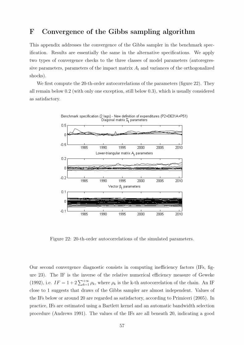
F Convergence of the Gibbs sampling algorithm

This appendix addresses the convergence of the Gibbs sampler in the benchmark spec-ification. Results are essentially the same in the alternative specifications. We applytwo types of convergence checks to the three classes of model parameters (autoregres-sive parameters, parameters of the impact matrix At and variances of the orthogonalizedshocks).

We first compute the 20-th-order autocorrelations of the parameters (figure 22). Theyall remain below 0.2 (with only one exception, still below 0.3), which is usually consideredas satisfactory.

Figure 22: 20-th-order autocorrelations of the simulated parameters.

Our second convergence diagnostic consists in computing inefficiency factors (IFs, fig-ure 23). The IF is the inverse of the relative numerical efficiency measure of Geweke(1992), i.e. IF = 1 + 2

∑+∞k=1 ρk, where ρk is the k-th autocorrelation of the chain. An IF

close to 1 suggests that draws of the Gibbs sampler are almost independent. Values ofthe IFs below or around 20 are regarded as satisfactory, according to Primiceri (2005). Inpractice, IFs are estimated using a Bartlett kernel and an automatic bandwidth selectionprocedure (Andrews 1991). The values of the IFs are all beneath 20, indicating a good

57

convergence of the Gibbs sampler.

Figure 23: Inefficiency factors of the simulated parameters.

58

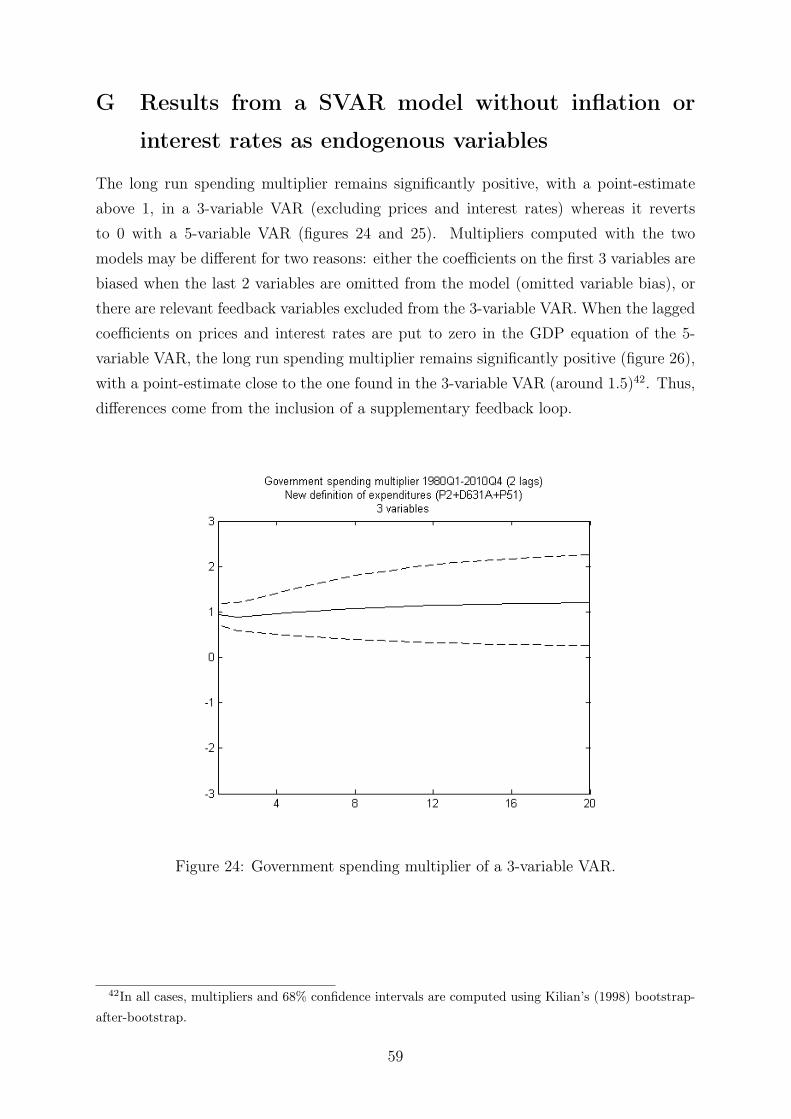
G Results from a SVAR model without inflation or

interest rates as endogenous variables

The long run spending multiplier remains significantly positive, with a point-estimateabove 1, in a 3-variable VAR (excluding prices and interest rates) whereas it revertsto 0 with a 5-variable VAR (figures 24 and 25). Multipliers computed with the twomodels may be different for two reasons: either the coefficients on the first 3 variables arebiased when the last 2 variables are omitted from the model (omitted variable bias), orthere are relevant feedback variables excluded from the 3-variable VAR. When the laggedcoefficients on prices and interest rates are put to zero in the GDP equation of the 5-variable VAR, the long run spending multiplier remains significantly positive (figure 26),with a point-estimate close to the one found in the 3-variable VAR (around 1.5)42. Thus,differences come from the inclusion of a supplementary feedback loop.

Figure 24: Government spending multiplier of a 3-variable VAR.

42In all cases, multipliers and 68% confidence intervals are computed using Kilian’s (1998) bootstrap-after-bootstrap.

59

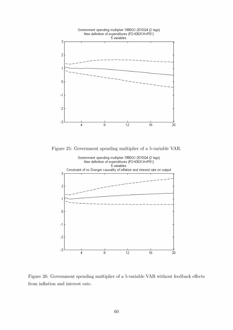
Figure 25: Government spending multiplier of a 5-variable VAR.

Figure 26: Government spending multiplier of a 5-variable VAR without feedback effectsfrom inflation and interest rate.

60

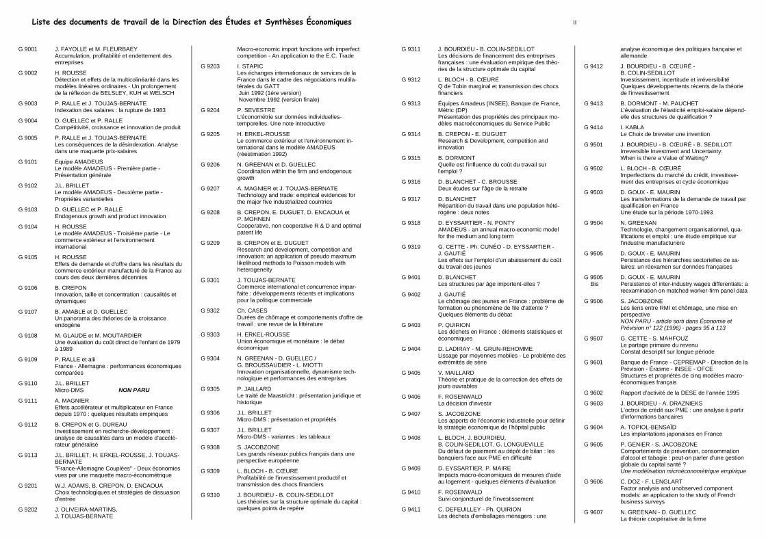
G 9001 J. FAYOLLE et M. FLEURBAEY Accumulation, profitabilité et endettement des entreprises

G 9002 H. ROUSSE Détection et effets de la multicolinéarité dans les modèles linéaires ordinaires - Un prolongement de la réflexion de BELSLEY, KUH et WELSCH

G 9003 P. RALLE et J. TOUJAS-BERNATE Indexation des salaires : la rupture de 1983

G 9004 D. GUELLEC et P. RALLE Compétitivité, croissance et innovation de produit

G 9005 P. RALLE et J. TOUJAS-BERNATE Les conséquences de la désindexation. Analyse dans une maquette prix-salaires

G 9101 Équipe AMADEUS Le modèle AMADEUS - Première partie -Présentation générale

G 9102 J.L. BRILLET Le modèle AMADEUS - Deuxième partie -Propriétés variantielles

G 9103 D. GUELLEC et P. RALLE Endogenous growth and product innovation

G 9104 H. ROUSSE Le modèle AMADEUS - Troisième partie - Le commerce extérieur et l'environnement international

G 9105 H. ROUSSE Effets de demande et d'offre dans les résultats du commerce extérieur manufacturé de la France au cours des deux dernières décennies

G 9106 B. CREPON Innovation, taille et concentration : causalités et dynamiques

G 9107 B. AMABLE et D. GUELLEC Un panorama des théories de la croissance endogène

G 9108 M. GLAUDE et M. MOUTARDIER Une évaluation du coût direct de l'enfant de 1979 à 1989

G 9109 P. RALLE et alii France - Allemagne : performances économiques comparées

G 9110 J.L. BRILLET Micro-DMS NON PARU

G 9111 A. MAGNIER Effets accélérateur et multiplicateur en France depuis 1970 : quelques résultats empiriques

G 9112 B. CREPON et G. DUREAU Investissement en recherche-développement : analyse de causalités dans un modèle d'accélé-rateur généralisé

G 9113 J.L. BRILLET, H. ERKEL-ROUSSE, J. TOUJAS-BERNATE "France-Allemagne Couplées" - Deux économies vues par une maquette macro-économétrique

G 9201 W.J. ADAMS, B. CREPON, D. ENCAOUA Choix technologiques et stratégies de dissuasion d'entrée

G 9202 J. OLIVEIRA-MARTINS, J. TOUJAS-BERNATE

Macro-economic import functions with imperfect competition - An application to the E.C. Trade

G 9203 I. STAPIC Les échanges internationaux de services de la France dans le cadre des négociations multila-térales du GATT Juin 1992 (1ère version) Novembre 1992 (version finale)

G 9204 P. SEVESTRE L'économétrie sur données individuelles-temporelles. Une note introductive

G 9205 H. ERKEL-ROUSSE Le commerce extérieur et l'environnement in-ternational dans le modèle AMADEUS (réestimation 1992)

G 9206 N. GREENAN et D. GUELLEC Coordination within the firm and endogenous growth

G 9207 A. MAGNIER et J. TOUJAS-BERNATE Technology and trade: empirical evidences for the major five industrialized countries

G 9208 B. CREPON, E. DUGUET, D. ENCAOUA et P. MOHNEN Cooperative, non cooperative R & D and optimal patent life

G 9209 B. CREPON et E. DUGUET Research and development, competition and innovation: an application of pseudo maximum likelihood methods to Poisson models with heterogeneity

G 9301 J. TOUJAS-BERNATE Commerce international et concurrence impar-faite : développements récents et implications pour la politique commerciale

G 9302 Ch. CASES Durées de chômage et comportements d'offre de travail : une revue de la littérature

G 9303 H. ERKEL-ROUSSE Union économique et monétaire : le débat économique

G 9304 N. GREENAN - D. GUELLEC / G. BROUSSAUDIER - L. MIOTTI Innovation organisationnelle, dynamisme tech-nologique et performances des entreprises

G 9305 P. JAILLARD Le traité de Maastricht : présentation juridique et historique

G 9306 J.L. BRILLET Micro-DMS : présentation et propriétés

G 9307 J.L. BRILLET Micro-DMS - variantes : les tableaux

G 9308 S. JACOBZONE Les grands réseaux publics français dans une perspective européenne

G 9309 L. BLOCH - B. CŒURE Profitabilité de l'investissement productif et transmission des chocs financiers

G 9310 J. BOURDIEU - B. COLIN-SEDILLOT Les théories sur la structure optimale du capital : quelques points de repère

Liste des documents de travail de la Direction des Études et Synthèses Économiques ii

G 9311 J. BOURDIEU - B. COLIN-SEDILLOT Les décisions de financement des entreprises françaises : une évaluation empirique des théo-ries de la structure optimale du capital

G 9312 L. BLOCH - B. CŒURÉ Q de Tobin marginal et transmission des chocs financiers

G 9313 Équipes Amadeus (INSEE), Banque de France, Métric (DP) Présentation des propriétés des principaux mo-dèles macroéconomiques du Service Public

G 9314 B. CREPON - E. DUGUET Research & Development, competition and innovation

G 9315 B. DORMONT Quelle est l'influence du coût du travail sur l'emploi ?

G 9316 D. BLANCHET - C. BROUSSE Deux études sur l'âge de la retraite

G 9317 D. BLANCHET Répartition du travail dans une population hété-rogène : deux notes

G 9318 D. EYSSARTIER - N. PONTY AMADEUS - an annual macro-economic model for the medium and long term

G 9319 G. CETTE - Ph. CUNÉO - D. EYSSARTIER -J. GAUTIÉ Les effets sur l'emploi d'un abaissement du coût du travail des jeunes

G 9401 D. BLANCHET Les structures par âge importent-elles ?

G 9402 J. GAUTIÉ Le chômage des jeunes en France : problème de formation ou phénomène de file d'attente ? Quelques éléments du débat

G 9403 P. QUIRION Les déchets en France : éléments statistiques et économiques

G 9404 D. LADIRAY - M. GRUN-REHOMME Lissage par moyennes mobiles - Le problème des extrémités de série

G 9405 V. MAILLARD Théorie et pratique de la correction des effets de jours ouvrables

G 9406 F. ROSENWALD La décision d'investir

G 9407 S. JACOBZONE Les apports de l'économie industrielle pour définir la stratégie économique de l'hôpital public

G 9408 L. BLOCH, J. BOURDIEU, B. COLIN-SEDILLOT, G. LONGUEVILLE Du défaut de paiement au dépôt de bilan : les banquiers face aux PME en difficulté

G 9409 D. EYSSARTIER, P. MAIRE Impacts macro-économiques de mesures d'aide au logement - quelques éléments d'évaluation

G 9410 F. ROSENWALD Suivi conjoncturel de l'investissement

G 9411 C. DEFEUILLEY - Ph. QUIRION Les déchets d'emballages ménagers : une

analyse économique des politiques française et allemande

G 9412 J. BOURDIEU - B. CŒURÉ - B. COLIN-SEDILLOT Investissement, incertitude et irréversibilité Quelques développements récents de la théorie de l'investissement

G 9413 B. DORMONT - M. PAUCHET L'évaluation de l'élasticité emploi-salaire dépend-elle des structures de qualification ?

G 9414 I. KABLA Le Choix de breveter une invention

G 9501 J. BOURDIEU - B. CŒURÉ - B. SEDILLOT Irreversible Investment and Uncertainty: When is there a Value of Waiting?

G 9502 L. BLOCH - B. CŒURÉ Imperfections du marché du crédit, investisse-ment des entreprises et cycle économique

G 9503 D. GOUX - E. MAURIN Les transformations de la demande de travail par qualification en France Une étude sur la période 1970-1993

G 9504 N. GREENAN Technologie, changement organisationnel, qua-lifications et emploi : une étude empirique sur l'industrie manufacturière

G 9505 D. GOUX - E. MAURIN Persistance des hiérarchies sectorielles de sa-laires: un réexamen sur données françaises

G 9505 D. GOUX - E. MAURIN Bis Persistence of inter-industry wages differentials: a

reexamination on matched worker-firm panel data

G 9506 S. JACOBZONE Les liens entre RMI et chômage, une mise en perspective NON PARU - article sorti dans Économie et Prévision n° 122 (1996) - pages 95 à 113

G 9507 G. CETTE - S. MAHFOUZ Le partage primaire du revenu Constat descriptif sur longue période

G 9601 Banque de France - CEPREMAP - Direction de la Prévision - Érasme - INSEE - OFCE Structures et propriétés de cinq modèles macro-économiques français

G 9602 Rapport d’activité de la DESE de l’année 1995

G 9603 J. BOURDIEU - A. DRAZNIEKS L’octroi de crédit aux PME : une analyse à partir d’informations bancaires

G 9604 A. TOPIOL-BENSAÏD Les implantations japonaises en France

G 9605 P. GENIER - S. JACOBZONE Comportements de prévention, consommation d’alcool et tabagie : peut-on parler d’une gestion globale du capital santé ? Une modélisation microéconométrique empirique

G 9606 C. DOZ - F. LENGLART Factor analysis and unobserved component models: an application to the study of French business surveys

G 9607 N. GREENAN - D. GUELLEC La théorie coopérative de la firme

iii

G 9608 N. GREENAN - D. GUELLEC Technological innovation and employment reallocation

G 9609 Ph. COUR - F. RUPPRECHT L’intégration asymétrique au sein du continent américain : un essai de modélisation

G 9610 S. DUCHENE - G. FORGEOT - A. JACQUOT Analyse des évolutions récentes de la producti-vité apparente du travail

G 9611 X. BONNET - S. MAHFOUZ The influence of different specifications of wages-prices spirals on the measure of the NAIRU: the case of France

G 9612 PH. COUR - E. DUBOIS, S. MAHFOUZ, J. PISANI-FERRY The cost of fiscal retrenchment revisited: how strong is the evidence?

G 9613 A. JACQUOT Les flexions des taux d’activité sont-elles seule-ment conjoncturelles ?

G 9614 ZHANG Yingxiang - SONG Xueqing Lexique macroéconomique Français-Chinois

G 9701 J.L. SCHNEIDER La taxe professionnelle : éléments de cadrage économique

G 9702 J.L. SCHNEIDER Transition et stabilité politique d’un système redistributif

G 9703 D. GOUX - E. MAURIN Train or Pay: Does it Reduce Inequalities to En-courage Firms to Train their Workers?

G 9704 P. GENIER Deux contributions sur dépendance et équité

G 9705 E. DUGUET - N. IUNG R & D Investment, Patent Life and Patent Value An Econometric Analysis at the Firm Level

G 9706 M. HOUDEBINE - A. TOPIOL-BENSAÏD Les entreprises internationales en France : une analyse à partir de données individuelles

G 9707 M. HOUDEBINE Polarisation des activités et spécialisation des départements en France

G 9708 E. DUGUET - N. GREENAN Le biais technologique : une analyse sur données individuelles

G 9709 J.L. BRILLET Analyzing a small French ECM Model

G 9710 J.L. BRILLET Formalizing the transition process: scenarios for capital accumulation

G 9711 G. FORGEOT - J. GAUTIÉ Insertion professionnelle des jeunes et processus de déclassement

G 9712 E. DUBOIS High Real Interest Rates: the Consequence of a Saving Investment Disequilibrium or of an in-sufficient Credibility of Monetary Authorities?

G 9713 Bilan des activités de la Direction des Études et Synthèses Économiques - 1996

G 9714 F. LEQUILLER Does the French Consumer Price Index Over-state Inflation?

G 9715 X. BONNET Peut-on mettre en évidence les rigidités à la baisse des salaires nominaux ? Une étude sur quelques grands pays de l’OCDE

G 9716 N. IUNG - F. RUPPRECHT Productivité de la recherche et rendements d’échelle dans le secteur pharmaceutique français

G 9717 E. DUGUET - I. KABLA Appropriation strategy and the motivations to use the patent system in France - An econometric analysis at the firm level

G 9718 L.P. PELÉ - P. RALLE Âge de la retraite : les aspects incitatifs du régime général

G 9719 ZHANG Yingxiang - SONG Xueqing Lexique macroéconomique français-chinois, chinois-français

G 9720 M. HOUDEBINE - J.L. SCHNEIDER Mesurer l’influence de la fiscalité sur la locali-sation des entreprises

G 9721 A. MOUROUGANE Crédibilité, indépendance et politique monétaire Une revue de la littérature

G 9722 P. AUGERAUD - L. BRIOT Les données comptables d’entreprises Le système intermédiaire d’entreprises Passage des données individuelles aux données sectorielles

G 9723 P. AUGERAUD - J.E. CHAPRON Using Business Accounts for Compiling National Accounts: the French Experience

G 9724 P. AUGERAUD Les comptes d’entreprise par activités - Le pas-sage aux comptes - De la comptabilité d’entreprise à la comptabilité nationale - A paraître

G 9801 H. MICHAUDON - C. PRIGENT Présentation du modèle AMADEUS

G 9802 J. ACCARDO Une étude de comptabilité générationnelle pour la France en 1996

G 9803 X. BONNET - S. DUCHÊNE Apports et limites de la modélisation « Real Business Cycles »

G 9804 C. BARLET - C. DUGUET - D. ENCAOUA - J. PRADEL The Commercial Success of Innovations An econometric analysis at the firm level in French manufacturing

G 9805 P. CAHUC - Ch. GIANELLA - D. GOUX - A. ZILBERBERG Equalizing Wage Differences and Bargaining Power - Evidence form a Panel of French Firms

G 9806 J. ACCARDO - M. JLASSI La productivité globale des facteurs entre 1975 et 1996

iv

G 9807 Bilan des activités de la Direction des Études et Synthèses Économiques - 1997

G 9808 A. MOUROUGANE Can a Conservative Governor Conduct an Ac-comodative Monetary Policy?

G 9809 X. BONNET - E. DUBOIS - L. FAUVET Asymétrie des inflations relatives et menus costs : tests sur l’inflation française

G 9810 E. DUGUET - N. IUNG Sales and Advertising with Spillovers at the firm level: Estimation of a Dynamic Structural Model on Panel Data

G 9811 J.P. BERTHIER Congestion urbaine : un modèle de trafic de pointe à courbe débit-vitesse et demande élastique

G 9812 C. PRIGENT La part des salaires dans la valeur ajoutée : une approche macroéconomique

G 9813 A.Th. AERTS L’évolution de la part des salaires dans la valeur ajoutée en France reflète-t-elle les évolutions individuelles sur la période 1979-1994 ?

G 9814 B. SALANIÉ Guide pratique des séries non-stationnaires

G 9901 S. DUCHÊNE - A. JACQUOT Une croissance plus riche en emplois depuis le début de la décennie ? Une analyse en compa-raison internationale

G 9902 Ch. COLIN Modélisation des carrières dans Destinie

G 9903 Ch. COLIN Évolution de la dispersion des salaires : un essai de prospective par microsimulation

G 9904 B. CREPON - N. IUNG Innovation, emploi et performances

G 9905 B. CREPON - Ch. GIANELLA Wages inequalities in France 1969-1992 An application of quantile regression techniques

G 9906 C. BONNET - R. MAHIEU Microsimulation techniques applied to inter-generational transfers - Pensions in a dynamic framework: the case of France

G 9907 F. ROSENWALD L’impact des contraintes financières dans la dé-cision d’investissement

G 9908 Bilan des activités de la DESE - 1998

G 9909 J.P. ZOYEM Contrat d’insertion et sortie du RMI Évaluation des effets d’une politique sociale

G 9910 Ch. COLIN - Fl. LEGROS - R. MAHIEU Bilans contributifs comparés des régimes de retraite du secteur privé et de la fonction publique

G 9911 G. LAROQUE - B. SALANIÉ Une décomposition du non-emploi en France

G 9912 B. SALANIÉ Une maquette analytique de long terme du marché du travail

G 9912 Ch. GIANELLA

Bis Une estimation de l’élasticité de l’emploi peu qualifié à son coût

G 9913 Division « Redistribution et Politiques Sociales » Le modèle de microsimulation dynamique DESTINIE

G 9914 E. DUGUET Macro-commandes SAS pour l’économétrie des panels et des variables qualitatives

G 9915 R. DUHAUTOIS Évolution des flux d’emplois en France entre 1990 et 1996 : une étude empirique à partir du fichier des bénéfices réels normaux (BRN)

G 9916 J.Y. FOURNIER Extraction du cycle des affaires : la méthode de Baxter et King

G 9917 B. CRÉPON - R. DESPLATZ - J. MAIRESSE Estimating price cost margins, scale economies and workers’ bargaining power at the firm level

G 9918 Ch. GIANELLA - Ph. LAGARDE Productivity of hours in the aggregate production function: an evaluation on a panel of French firms from the manufacturing sector

G 9919 S. AUDRIC - P. GIVORD - C. PROST Évolution de l’emploi et des coûts par quali-fication entre 1982 et 1996

G 2000/01 R. MAHIEU Les déterminants des dépenses de santé : une approche macroéconomique

G 2000/02 C. ALLARD-PRIGENT - H. GUILMEAU - A. QUINET The real exchange rate as the relative price of nontrables in terms of tradables: theoretical investigation and empirical study on French data

G 2000/03 J.-Y. FOURNIER L’approximation du filtre passe-bande proposée par Christiano et Fitzgerald

G 2000/04 Bilan des activités de la DESE - 1999

G 2000/05 B. CREPON - F. ROSENWALD Investissement et contraintes de financement : le poids du cycle Une estimation sur données françaises

G 2000/06 A. FLIPO Les comportements matrimoniaux de fait

G 2000/07 R. MAHIEU - B. SÉDILLOT Microsimulations of the retirement decision: a supply side approach

G 2000/08 C. AUDENIS - C. PROST Déficit conjoncturel : une prise en compte des conjonctures passées

G 2000/09 R. MAHIEU - B. SÉDILLOT Équivalent patrimonial de la rente et souscription de retraite complémentaire

G 2000/10 R. DUHAUTOIS Ralentissement de l’investissement : petites ou grandes entreprises ? industrie ou tertiaire ?

G 2000/11 G. LAROQUE - B. SALANIÉ Temps partiel féminin et incitations financières à l’emploi

G2000/12 Ch. GIANELLA Local unemployment and wages

v

G2000/13 B. CREPON - Th. HECKEL - Informatisation en France : une évaluation à partir de données individuelles - Computerization in France: an evaluation based on individual company data

G2001/01 F. LEQUILLER - La nouvelle économie et la mesure de la croissance du PIB - The new economy and the measure ment of GDP growth

G2001/02 S. AUDRIC La reprise de la croissance de l’emploi profite-t-elle aussi aux non-diplômés ?

G2001/03 I. BRAUN-LEMAIRE Évolution et répartition du surplus de productivité

G2001/04 A. BEAUDU - Th. HECKEL Le canal du crédit fonctionne-t-il en Europe ? Une étude de l’hétérogénéité des comportements d’investissement à partir de données de bilan agrégées

G2001/05 C. AUDENIS - P. BISCOURP - N. FOURCADE - O. LOISEL Testing the augmented Solow growth model: An empirical reassessment using panel data

G2001/06 R. MAHIEU - B. SÉDILLOT Départ à la retraite, irréversibilité et incertitude

G2001/07 Bilan des activités de la DESE - 2000

G2001/08 J. Ph. GAUDEMET Les dispositifs d’acquisition à titre facultatif d’annuités viagères de retraite

G2001/09 B. CRÉPON - Ch. GIANELLA Fiscalité, coût d’usage du capital et demande de facteurs : une analyse sur données individuelles

G2001/10 B. CRÉPON - R. DESPLATZ Évaluation des effets des dispositifs d’allégements de charges sociales sur les bas salaires

G2001/11 J.-Y. FOURNIER Comparaison des salaires des secteurs public et privé

G2001/12 J.-P. BERTHIER - C. JAULENT R. CONVENEVOLE - S. PISANI Une méthodologie de comparaison entre consommations intermédiaires de source fiscale et de comptabilité nationale

G2001/13 P. BISCOURP - Ch. GIANELLA Substitution and complementarity between capital, skilled and less skilled workers: an analysis at the firm level in the French manufacturing industry

G2001/14 I. ROBERT-BOBEE Modelling demographic behaviours in the French microsimulation model Destinie: An analysis of future change in completed fertility

G2001/15 J.-P. ZOYEM Diagnostic sur la pauvreté et calendrier de revenus : le cas du “Panel européen des ménages »

G2001/16 J.-Y. FOURNIER - P. GIVORD La réduction des taux d’activité aux âges extrêmes, une spécificité française ?

G2001/17 C. AUDENIS - P. BISCOURP - N. RIEDINGER Existe-t-il une asymétrie dans la transmission du prix du brut aux prix des carburants ?

G2002/01 F. MAGNIEN - J.-L. TAVERNIER - D. THESMAR Les statistiques internationales de PIB par habitant en standard de pouvoir d’achat : une analyse des résultats

G2002/02 Bilan des activités de la DESE - 2001

G2002/03 B. SÉDILLOT - E. WALRAET La cessation d’activité au sein des couples : y a-t-il interdépendance des choix ?

G2002/04 G. BRILHAULT - Rétropolation des séries de FBCF et calcul du

capital fixe en SEC-95 dans les comptes nationaux français

- Retropolation of the investment series (GFCF) and estimation of fixed capital stocks on the ESA-95 basis for the French balance sheets

G2002/05 P. BISCOURP - B. CRÉPON - T. HECKEL - N. RIEDINGER How do firms respond to cheaper computers? Microeconometric evidence for France based on a production function approach

G2002/06 C. AUDENIS - J. DEROYON - N. FOURCADE L’impact des nouvelles technologies de l’information et de la communication sur l’économie française - un bouclage macro-économique

G2002/07 J. BARDAJI - B. SÉDILLOT - E. WALRAET Évaluation de trois réformes du Régime Général d’assurance vieillesse à l’aide du modèle de microsimulation DESTINIE

G2002/08 J.-P. BERTHIER Réflexions sur les différentes notions de volume dans les comptes nationaux : comptes aux prix d’une année fixe ou aux prix de l’année précédente, séries chaînées

G2002/09 F. HILD Les soldes d’opinion résument-ils au mieux les réponses des entreprises aux enquêtes de conjoncture ?

G2002/10 I. ROBERT-BOBÉE Les comportements démographiques dans le modèle de microsimulation Destinie - Une comparaison des estimations issues des enquêtes Jeunes et Carrières 1997 et Histoire Familiale 1999

G2002/11 J.-P. ZOYEM La dynamique des bas revenus : une analyse des entrées-sorties de pauvreté

G2002/12 F. HILD Prévisions d’inflation pour la France

G2002/13 M. LECLAIR Réduction du temps de travail et tensions sur les facteurs de production

G2002/14 E. WALRAET - A. VINCENT - Analyse de la redistribution intragénérationnelle dans le système de retraite des salariés du privé - Une approche par microsimulation - Intragenerational distributional analysis in the french private sector pension scheme - A microsimulation approach

vi

G2002/15 P. CHONE - D. LE BLANC - I. ROBERT-BOBEE Offre de travail féminine et garde des jeunes enfants

G2002/16 F. MAUREL - S. GREGOIR Les indices de compétitivité des pays : inter-prétation et limites

G2003/01 N. RIEDINGER - E.HAUVY Le coût de dépollution atmosphérique pour les entreprises françaises : Une estimation à partir de données individuelles

G2003/02 P. BISCOURP et F. KRAMARZ Création d’emplois, destruction d’emplois et internationalisation des entreprises industrielles françaises : une analyse sur la période 1986-1992

G2003/03 Bilan des activités de la DESE - 2002

G2003/04 P.-O. BEFFY - J. DEROYON - N. FOURCADE - S. GREGOIR - N. LAÏB - B. MONFORT Évolutions démographiques et croissance : une projection macro-économique à l’horizon 2020

G2003/05 P. AUBERT La situation des salariés de plus de cinquante ans dans le secteur privé

G2003/06 P. AUBERT - B. CRÉPON Age, salaire et productivité La productivité des salariés décline-t-elle en fin de carrière ?

G2003/07 H. BARON - P.O. BEFFY - N. FOURCADE - R. MAHIEU Le ralentissement de la productivité du travail au cours des années 1990

G2003/08 P.-O. BEFFY - B. MONFORT Patrimoine des ménages, dynamique d’allocation et comportement de consommation

G2003/09 P. BISCOURP - N. FOURCADE Peut-on mettre en évidence l’existence de rigidités à la baisse des salaires à partir de données individuelles ? Le cas de la France à la fin des années 90

G2003/10 M. LECLAIR - P. PETIT Présence syndicale dans les firmes : quel impact sur les inégalités salariales entre les hommes et les femmes ?

G2003/11 P.-O. BEFFY - X. BONNET - M. DARRACQ-PARIES - B. MONFORT MZE: a small macro-model for the euro area

G2004/01 P. AUBERT - M. LECLAIR La compétitivité exprimée dans les enquêtes trimestrielles sur la situation et les perspectives dans l’industrie

G2004/02 M. DUÉE - C. REBILLARD La dépendance des personnes âgées : une projection à long terme

G2004/03 S. RASPILLER - N. RIEDINGER Régulation environnementale et choix de localisation des groupes français

G2004/04 A. NABOULET - S. RASPILLER Les déterminants de la décision d’investir : une approche par les perceptions subjectives des firmes

G2004/05 N. RAGACHE La déclaration des enfants par les couples non mariés est-elle fiscalement optimale ?

G2004/06 M. DUÉE L’impact du chômage des parents sur le devenir scolaire des enfants

G2004/07 P. AUBERT - E. CAROLI - M. ROGER New Technologies, Workplace Organisation and the Age Structure of the Workforce: Firm-Level Evidence

G2004/08 E. DUGUET - C. LELARGE Les brevets accroissent-ils les incitations privées à innover ? Un examen microéconométrique

G2004/09 S. RASPILLER - P. SILLARD Affiliating versus Subcontracting: the Case of Multinationals

G2004/10 J. BOISSINOT - C. L’ANGEVIN - B. MONFORT Public Debt Sustainability: Some Results on the French Case

G2004/11 S. ANANIAN - P. AUBERT Travailleurs âgés, nouvelles technologies et changements organisationnels : un réexamen à partir de l’enquête « REPONSE »

G2004/12 X. BONNET - H. PONCET Structures de revenus et propensions différentes à consommer - Vers une équation de consommation des ménages plus robuste en prévision pour la France

G2004/13 C. PICART Évaluer la rentabilité des sociétés non financières

G2004/14 J. BARDAJI - B. SÉDILLOT - E. WALRAET Les retraites du secteur public : projections à l’horizon 2040 à l’aide du modèle de microsimulation DESTINIE

G2005/01 S. BUFFETEAU - P. GODEFROY Conditions de départ en retraite selon l’âge de fin d’études : analyse prospective pour les générations 1945 à1974

G2005/02 C. AFSA - S. BUFFETEAU L’évolution de l’activité féminine en France : une approche par pseudo-panel

G2005/03 P. AUBERT - P. SILLARD Délocalisations et réductions d’effectifs dans l’industrie française

G2005/04 M. LECLAIR - S. ROUX Mesure et utilisation des emplois instables dans les entreprises

G2005/05 C. L’ANGEVIN - S. SERRAVALLE Performances à l’exportation de la France et de l’Allemagne - Une analyse par secteur et destination géographique

G2005/06 Bilan des activités de la Direction des Études et Synthèses Économiques - 2004

G2005/07 S. RASPILLER La concurrence fiscale : principaux enseigne-ments de l’analyse économique

G2005/08 C. L’ANGEVIN - N. LAÏB Éducation et croissance en France et dans un panel de 21 pays de l’OCDE

G2005/09 N. FERRARI Prévoir l’investissement des entreprises

vii

Un indicateur des révisions dans l’enquête de conjoncture sur les investissements dans l’industrie.

G2005/10 P.-O. BEFFY - C. L’ANGEVIN Chômage et boucle prix-salaires : apport d’un modèle « qualifiés/peu qualifiés »

G2005/11 B. HEITZ A two-states Markov-switching model of inflation in France and the USA: credible target VS inflation spiral

G2005/12 O. BIAU - H. ERKEL-ROUSSE - N. FERRARI Réponses individuelles aux enquêtes de conjoncture et prévision macroéconomiques : Exemple de la prévision de la production manufacturière

G2005/13 P. AUBERT - D. BLANCHET - D. BLAU The labour market after age 50: some elements of a Franco-American comparison

G2005/14 D. BLANCHET - T. DEBRAND - P. DOURGNON - P. POLLET L’enquête SHARE : présentation et premiers résultats de l’édition française

G2005/15 M. DUÉE La modélisation des comportements démogra-phiques dans le modèle de microsimulation DESTINIE

G2005/16 H. RAOUI - S. ROUX Étude de simulation sur la participation versée aux salariés par les entreprises

G2006/01 C. BONNET - S. BUFFETEAU - P. GODEFROY Disparités de retraite de droit direct entre hommes et femmes : quelles évolutions ?

G2006/02 C. PICART Les gazelles en France

G2006/03 P. AUBERT - B. CRÉPON -P. ZAMORA Le rendement apparent de la formation continue dans les entreprises : effets sur la productivité et les salaires

G2006/04 J.-F. OUVRARD - R. RATHELOT Demographic change and unemployment: what do macroeconometric models predict?

G2006/05 D. BLANCHET - J.-F. OUVRARD Indicateurs d’engagements implicites des systèmes de retraite : chiffrages, propriétés analytiques et réactions à des chocs démographiques types

G2006/06 G. BIAU - O. BIAU - L. ROUVIERE Nonparametric Forecasting of the Manufacturing Output Growth with Firm-level Survey Data

G2006/07 C. AFSA - P. GIVORD Le rôle des conditions de travail dans les absences pour maladie

G2006/08 P. SILLARD - C. L’ANGEVIN - S. SERRAVALLE Performances comparées à l’exportation de la France et de ses principaux partenaires Une analyse structurelle sur 12 ans

G2006/09 X. BOUTIN - S. QUANTIN Une méthodologie d’évaluation comptable du coût du capital des entreprises françaises : 1984-2002

G2006/10 C. AFSA L’estimation d’un coût implicite de la pénibilité du travail chez les travailleurs âgés

G2006/11 C. LELARGE Les entreprises (industrielles) françaises sont-elles à la frontière technologique ?

G2006/12 O. BIAU - N. FERRARI Théorie de l’opinion Faut-il pondérer les réponses individuelles ?

G2006/13 A. KOUBI - S. ROUX Une réinterprétation de la relation entre productivité et inégalités salariales dans les entreprises

G2006/14 R. RATHELOT - P. SILLARD The impact of local taxes on plants location decision

G2006/15 L. GONZALEZ - C. PICART Diversification, recentrage et poids des activités de support dans les groupes (1993-2000)

G2007/01 D. SRAER Allègements de cotisations patronales et dynamique salariale

G2007/02 V. ALBOUY - L. LEQUIEN Les rendements non monétaires de l’éducation : le cas de la santé

G2007/03 D. BLANCHET - T. DEBRAND Aspiration à la retraite, santé et satisfaction au travail : une comparaison européenne

G2007/04 M. BARLET - L. CRUSSON Quel impact des variations du prix du pétrole sur la croissance française ?

G2007/05 C. PICART Flux d’emploi et de main-d’œuvre en France : un réexamen

G2007/06 V. ALBOUY - C. TAVAN Massification et démocratisation de l’enseignement supérieur en France

G2007/07 T. LE BARBANCHON The Changing response to oil price shocks in France: a DSGE type approach

G2007/08 T. CHANEY - D. SRAER - D. THESMAR Collateral Value and Corporate Investment Evidence from the French Real Estate Market

G2007/09 J. BOISSINOT Consumption over the Life Cycle: Facts for France

G2007/10 C. AFSA Interpréter les variables de satisfaction : l’exemple de la durée du travail

G2007/11 R. RATHELOT - P. SILLARD Zones Franches Urbaines : quels effets sur l’emploi salarié et les créations d’établissements ?

G2007/12 V. ALBOUY - B. CRÉPON Aléa moral en santé : une évaluation dans le cadre du modèle causal de Rubin

G2008/01 C. PICART Les PME françaises : rentables mais peu dynamiques

viii

G2008/02 P. BISCOURP - X. BOUTIN - T. VERGÉ The Effects of Retail Regulations on Prices Evidence form the Loi Galland

G2008/03 Y. BARBESOL - A. BRIANT Économies d’agglomération et productivité des entreprises : estimation sur données individuelles françaises

G2008/04 D. BLANCHET - F. LE GALLO Les projections démographiques : principaux mécanismes et retour sur l’expérience française

G2008/05 D. BLANCHET - F. TOUTLEMONDE Évolutions démographiques et déformation du cycle de vie active : quelles relations ?

G2008/06 M. BARLET - D. BLANCHET - L. CRUSSON Internationalisation et flux d’emplois : que dit une approche comptable ?

G2008/07 C. LELARGE - D. SRAER - D. THESMAR Entrepreneurship and Credit Constraints - Evidence from a French Loan Guarantee Program

G2008/08 X. BOUTIN - L. JANIN Are Prices Really Affected by Mergers?

G2008/09 M. BARLET - A. BRIANT - L. CRUSSON Concentration géographique dans l’industrie manufacturière et dans les services en France : une approche par un indicateur en continu

G2008/10 M. BEFFY - É. COUDIN - R. RATHELOT Who is confronted to insecure labor market histories? Some evidence based on the French labor market transition

G2008/11 M. ROGER - E. WALRAET Social Security and Well-Being of the Elderly: the Case of France

G2008/12 C. AFSA Analyser les composantes du bien-être et de son évolution Une approche empirique sur données individuelles

G2008/13 M. BARLET - D. BLANCHET - T. LE BARBANCHON Microsimuler le marché du travail : un prototype

G2009/01 P.-A. PIONNIER Le partage de la valeur ajoutée en France, 1949-2007

G2009/02 Laurent CLAVEL - Christelle MINODIER A Monthly Indicator of the French Business Climate

G2009/03 H. ERKEL-ROUSSE - C. MINODIER Do Business Tendency Surveys in Industry and Services Help in Forecasting GDP Growth? A Real-Time Analysis on French Data

G2009/04 P. GIVORD - L. WILNER Les contrats temporaires : trappe ou marchepied vers l’emploi stable ?

G2009/05 G. LALANNE - P.-A. PIONNIER - O. SIMON Le partage des fruits de la croissance de 1950 à 2008 : une approche par les comptes de surplus

G2009/06 L. DAVEZIES - X. D’HAULTFOEUILLE Faut-il pondérer ?… Ou l’éternelle question de l’économètre confronté à des données d’enquête

G2009/07 S. QUANTIN - S. RASPILLER - S. SERRAVALLE Commerce intragroupe, fiscalité et prix de transferts : une analyse sur données françaises

G2009/08 M. CLERC - V. MARCUS Élasticités-prix des consommations énergétiques des ménages

G2009/09 G. LALANNE - E. POULIQUEN - O. SIMON Prix du pétrole et croissance potentielle à long terme

G2009/10 D. BLANCHET - J. LE CACHEUX - V. MARCUS Adjusted net savings and other approaches to sustainability: some theoretical background

G2009/11 V. BELLAMY - G. CONSALES - M. FESSEAU - S. LE LAIDIER - É. RAYNAUD Une décomposition du compte des ménages de la comptabilité nationale par catégorie de ménage en 2003

G2009/12 J. BARDAJI - F. TALLET Detecting Economic Regimes in France: a Qualitative Markov-Switching Indicator Using Mixed Frequency Data

G2009/13 R. AEBERHARDT - D. FOUGÈRE - R. RATHELOT Discrimination à l’embauche : comment exploiter les procédures de testing ?

G2009/14 Y. BARBESOL - P. GIVORD - S. QUANTIN Partage de la valeur ajoutée, approche par données microéconomiques

G2009/15 I. BUONO - G. LALANNE The Effect of the Uruguay round on the Intensive and Extensive Margins of Trade

G2010/01 C. MINODIER Avantages comparés des séries des premières valeurs publiées et des séries des valeurs révisées - Un exercice de prévision en temps réel de la croissance trimestrielle du PIB en France

G2010/02 V. ALBOUY - L. DAVEZIES - T. DEBRAND Health Expenditure Models: a Comparison of Five Specifications using Panel Data

G2010/03 C. KLEIN - O. SIMON Le modèle MÉSANGE réestimé en base 2000 Tome 1 – Version avec volumes à prix constants

G2010/04 M.-É. CLERC - É. COUDIN L’IPC, miroir de l’évolution du coût de la vie en France ? Ce qu’apporte l’analyse des courbes d’Engel

G2010/05 N. CECI-RENAUD - P.-A. CHEVALIER Les seuils de 10, 20 et 50 salariés : impact sur la taille des entreprises françaises

G2010/06 R. AEBERHARDT - J. POUGET National Origin Differences in Wages and Hierarchical Positions - Evidence on French Full-Time Male Workers from a matched Employer-Employee Dataset

G2010/07 S. BLASCO - P. GIVORD Les trajectoires professionnelles en début de vie active : quel impact des contrats temporaires ?

G2010/08 P. GIVORD Méthodes économétriques pour l’évaluation de politiques publiques

ix

G2010/09 P.-Y. CABANNES - V. LAPÈGUE - E. POULIQUEN - M. BEFFY - M. GAINI Quelle croissance de moyen terme après la crise ?

G2010/10 I. BUONO - G. LALANNE La réaction des entreprises françaises à la baisse des tarifs douaniers étrangers

G2010/11 R. RATHELOT - P. SILLARD L’apport des méthodes à noyaux pour mesurer la concentration géographique - Application à la concentration des immigrés en France de 1968 à 1999

G2010/12 M. BARATON - M. BEFFY - D. FOUGÈRE Une évaluation de l’effet de la réforme de 2003 sur les départs en retraite - Le cas des enseignants du second degré public

G2010/13 D. BLANCHET - S. BUFFETEAU - E. CRENNER S. LE MINEZ Le modèle de microsimulation Destinie 2 : principales caractéristiques et premiers résultats

G2010/14 D. BLANCHET - E. CRENNER Le bloc retraites du modèle Destinie 2 : guide de l’utilisateur

G2010/15 M. BARLET - L. CRUSSON - S. DUPUCH - F. PUECH Des services échangés aux services échan-geables : une application sur données françaises

G2010/16 M. BEFFY - T. KAMIONKA Public-private wage gaps: is civil-servant human capital sector-specific?

G2010/17 P.-Y. CABANNES - H. ERKEL-ROUSSE - G. LALANNE - O. MONSO - E. POULIQUEN Le modèle Mésange réestimé en base 2000 Tome 2 - Version avec volumes à prix chaînés

G2010/18 R. AEBERHARDT - L. DAVEZIES Conditional Logit with one Binary Covariate: Link between the Static and Dynamic Cases

G2011/01 T. LE BARBANCHON - B. OURLIAC - O. SIMON Les marchés du travail français et américain face aux chocs conjoncturels des années 1986 à 2007 : une modélisation DSGE

G2011/02 C. MARBOT Une évaluation de la réduction d’impôt pour l’emploi de salariés à domicile

G2011/03 L. DAVEZIES Modèles à effets fixes, à effets aléatoires, modèles mixtes ou multi-niveaux : propriétés et mises en œuvre des modélisations de l’hétérogénéité dans le cas de données groupées

G2011/04 M. ROGER - M. WASMER Heterogeneity matters: labour productivity differentiated by age and skills

G2011/05 J.-C. BRICONGNE - J.-M. FOURNIER V. LAPÈGUE - O. MONSO De la crise financière à la crise économique L’impact des perturbations financières de 2007 et 2008 sur la croissance de sept pays industrialisés

G2011/06 P. CHARNOZ - É. COUDIN - M. GAINI Wage inequalities in France 1976-2004: a quantile regression analysis

G2011/07 M. CLERC - M. GAINI - D. BLANCHET Recommendations of the Stiglitz-Sen-Fitoussi Report: A few illustrations

G2011/08 M. BACHELET - M. BEFFY - D. BLANCHET Projeter l’impact des réformes des retraites sur l’activité des 55 ans et plus : une comparaison de trois modèles

G2011/09 C. LOUVOT-RUNAVOT L’évaluation de l’activité dissimulée des entre-prises sur la base des contrôles fiscaux et son insertion dans les comptes nationaux

G2011/10 A. SCHREIBER - A. VICARD La tertiarisation de l’économie française et le ralentissement de la productivité entre 1978 et 2008

G2011/11 M.-É. CLERC - O. MONSO - E. POULIQUEN Les inégalités entre générations depuis le baby-boom

G2011/12 C. MARBOT et D. ROY Évaluation de la transformation de la réduction d'impôt en crédit d'impôt pour l'emploi de salariés à domicile en 2007

G2011/13 P. GIVORD - R. RATHELOT - P. SILLARD Place-based tax exemptions and displacement effects: An evaluation of the Zones Franches Urbaines program

G2011/14 X. D’HAULTFOEUILLE - P. GIVORD - X. BOUTIN The Environmental Effect of Green Taxation: the Case of the French “Bonus/Malus”

G2011/15 M. BARLET - M. CLERC - M. GARNEO - V. LAPÈGUE - V. MARCUS La nouvelle version du modèle MZE, modèle macroéconométrique pour la zone euro

G2011/16 R. AEBERHARDT - I. BUONO - H. FADINGER Learning, Incomplete Contracts and Export Dynamics: theory and Evidence form French Firms

G2011/17 C. KERDRAIN - V. LAPÈGUE Restrictive Fiscal Policies in Europe: What are the Likely Effects?

G2012/01 P. GIVORD - S. QUANTIN - C. TREVIEN A Long-Term Evaluation of the First Generation of the French Urban Enterprise Zones

G2012/02 N. CECI-RENAUD - V. COTTET Politique salariale et performance des entreprises

G2012/03 P. FÉVRIER - L. WILNER Do Consumers Correctly Expect Price Reductions? Testing Dynamic Behavior

G2012/04 M. GAINI - A. LEDUC - A. VICARD School as a shelter? School leaving-age and the business cycle in France

G2012/05 M. GAINI - A. LEDUC - A. VICARD A scarred generation? French evidence on young people entering into a tough labour market

G2012/06 P. AUBERT - M. BACHELET Disparités de montant de pension et redistribution dans le système de retraite français

G2012/07 R. AEBERHARDT - P GIVORD - C. MARBOT Spillover Effect of the Minimum Wage in France: An Unconditional Quantile Regression Approach

x

G2012/08 A. EIDELMAN - F. LANGUMIER - A. VICARD Prélèvements obligatoires reposant sur les ménages : des canaux redistributifs différents en 1990 et 2010

G2012/09 O. BARGAIN - A. VICARD Le RMI et son successeur le RSA découragent-ils certains jeunes de travailler ? Une analyse sur les jeunes autour de 25 ans

G2012/10 C. MARBOT - D. ROY Projections du coût de l’APA et des caractéristiques de ses bénéficiaires à l’horizon 2040 à l’aide du modèle Destinie

G2012/11 A. MAUROUX Le crédit d’impôt dédié au développement durable : une évaluation économétrique

G2012/12 V. COTTET - S. QUANTIN - V. RÉGNIER Coût du travail et allègements de charges : une estimation au niveau établissement de 1996 à 2008

G2012/13 X. D’HAULTFOEUILLE, P. FEVRIER et L. WILNER Demand Estimation in the Presence of Revenue Management

G2012/14 D. BLANCHET et S. LE MINEZ Joint macro/micro evaluations of accrued-to-date pension liabilities: an application to French reforms

G2013/01- T. DEROYON - A. MONTAUT et P-A PIONNIER F1301 Utilisation rétrospective de l’enquête Emploi à

une fréquence mensuelle : apport d’une modélisation espace-état

G2013/02- C. TRÉVIEN F1302 Habiter en HLM : quel avantage monétaire et

quel impact sur les conditions de logement ?

G2013/03 A. POISSONNIER Temporal disaggregation of stock variables - The

Chow-Lin method extended to dynamic models

G2013/04 P. GIVORD - C. MARBOT Does the cost of child care affect female labor

market participation? An evaluation of a French reform of childcare subsidies

G2013/05 G. LAME - M. LEQUIEN - P.-A. PIONNIER Interpretation and limits of sustainability tests in

public finance

G2013/06 C. BELLEGO - V. DORTET-BERNADET La participation aux pôles de compétitivité : quelle

incidence sur les dépenses de R&D et l’activité des PME et ETI ?

G2013/07 P-Y. CABANNES - A.MONTAUT - P-A. PIONNIER Évaluer la productivité globale des facteurs en

France : l’apport d’une mesure de la qualité du capital et du travail

G2013/08 R. AEBERHARDT - C. MARBOT Evolution of Instability on the French Labour

Market During the Last Thirty Years

G2013/09 J-B. BERNARD - G. CLÉAUD Oil price: the nature of the shocks and the impact

on the French economy

G2013/10 G. LAME Was there a « Greenspan Conundrum » in the

Euro area?

G2013/11 P. CHONÉ - F. EVAIN - L. WILNER - E. YILMAZ Introducing activity-based payment in the hospital

industry : Evidence from French data

G2013/12 C. GRISLAIN-LETRÉMY Natural Disasters: Exposure and Underinsurance

G2013/13 P.-Y. CABANNES - V. COTTET - Y. DUBOIS - C. LELARGE - M. SICSIC French Firms in the Face of the 2008/2009 Crisis

G2013/14 A. POISSONNIER - D. ROY Households Satellite Account for France in 2010.

Methodological issues on the assessment of domestic production

G2013/15 G. CLÉAUD - M. LEMOINE - P.-A. PIONNIER Which size and evolution of the government

expenditure multiplier in France (1980-2010)?