DOCUMENT

DE TRAVAIL

N° 496

FINANCIAL SHOCKS AND THE CYCLICAL BEHAVIOR OF SKILLED

AND UNSKILLED UNEMPLOYMENT

Jose Ignacio Lopez and Virginia Olivella Moppett

July 2014

DIRECTION GÉNÉRALE DES ÉTUDES ET DES RELATIONS INTERNATIONALES

DIRECTION GÉNÉRALE DES ÉTUDES ET DES RELATIONS INTERNATIONALES

FINANCIAL SHOCKS AND THE CYCLICAL BEHAVIOR OF SKILLED

AND UNSKILLED UNEMPLOYMENT

Jose Ignacio Lopez and Virginia Olivella Moppett

July 2014

Les Documents de travail reflètent les idées personnelles de leurs auteurs et n'expriment pas nécessairement la position de la Banque de France. Ce document est disponible sur le site internet de la Banque de France « www.banque-france.fr ». Working Papers reflect the opinions of the authors and do not necessarily express the views of the Banque de France. This document is available on the Banque de France Website “www.banque-france.fr”.

Financial Shocks and the Cyclical Behavior

of Skilled and Unskilled Unemployment∗

Jose Ignacio LopezHEC Paris

Virginia OlivellaBanque de France

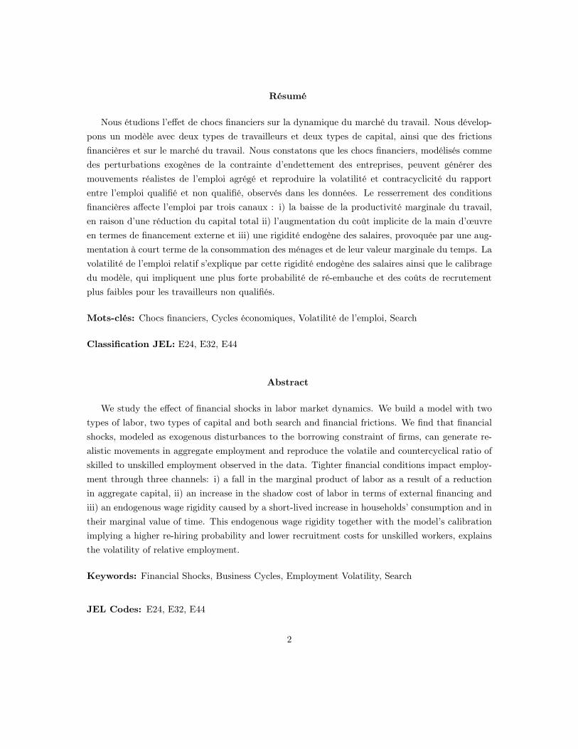
∗We are grateful for comments from Lee Ohanian, Vincenzo Quadrini, Marcus Hagedorn, Christian Hellwig, JuliaThomas, Patrick Pintus, Nicolas Coeurdacier, Pierre-Olivier Weil and participants at the Latin American Econo-metric Society Conference (2012), Macroeconomics Workshop on Financial Frictions and Labor Markets HEC Paris(2012), the Brown Bag Seminar at Banque de France (2012), European Central Bank Network (2012), Paris School ofEconomics Seminar (2013), Macroeconomics Midwest Economic Conference (2013), North-American Summer Meet-ings (2013), Annual Meetings French Economic Association (2013) and the European Econometric Society Meetings(2013). The views expressed in this paper are those of the authors alone and do not reflect those of the Banque deFrance. First Version April 30th, 2012

1

Résumé

Nous étudions l’effet de chocs financiers sur la dynamique du marché du travail. Nous dévelop-pons un modèle avec deux types de travailleurs et deux types de capital, ainsi que des frictionsfinancières et sur le marché du travail. Nous constatons que les chocs financiers, modélisés commedes perturbations exogènes de la contrainte d’endettement des entreprises, peuvent générer desmouvements réalistes de l’emploi agrégé et reproduire la volatilité et contracyclicité du rapportentre l’emploi qualifié et non qualifié, observés dans les données. Le resserrement des conditionsfinancières affecte l’emploi par trois canaux : i) la baisse de la productivité marginale du travail,en raison d’une réduction du capital total ii) l’augmentation du coût implicite de la main d’œuvreen termes de financement externe et iii) une rigidité endogène des salaires, provoquée par une aug-mentation à court terme de la consommation des ménages et de leur valeur marginale du temps. Lavolatilité de l’emploi relatif s’explique par cette rigidité endogène des salaires ainsi que le calibragedu modèle, qui impliquent une plus forte probabilité de ré-embauche et des coûts de recrutementplus faibles pour les travailleurs non qualifiés.

Mots-clés: Chocs financiers, Cycles économiques, Volatilité de l’emploi, Search

Classification JEL: E24, E32, E44

Abstract

We study the effect of financial shocks in labor market dynamics. We build a model with twotypes of labor, two types of capital and both search and financial frictions. We find that financialshocks, modeled as exogenous disturbances to the borrowing constraint of firms, can generate re-alistic movements in aggregate employment and reproduce the volatile and countercyclical ratio ofskilled to unskilled employment observed in the data. Tighter financial conditions impact employ-ment through three channels: i) a fall in the marginal product of labor as a result of a reductionin aggregate capital, ii) an increase in the shadow cost of labor in terms of external financing andiii) an endogenous wage rigidity caused by a short-lived increase in households’ consumption and intheir marginal value of time. This endogenous wage rigidity together with the model’s calibrationimplying a higher re-hiring probability and lower recruitment costs for unskilled workers, explainsthe volatility of relative employment.

Keywords: Financial Shocks, Business Cycles, Employment Volatility, Search

JEL Codes: E24, E32, E44

2

Non-technical summary

The last financial and economic crisis in the US has brought renewed interest in models offinancial frictions and their impact on economic fluctuations. Whereas most of the literature priorto the great recession had focused on the role of the financial sector in propagating real shocks,new research has began to explore the importance of financial shocks, that is, shocks originatingdirectly in the financial sector. In this paper we try to shed light on this issue by studying the roleof financial shocks in the business cycle dynamics of labor markets. In particular, we ask whetherfinancial shocks can help to improve the performance of the standard search model in terms ofaggregate and skill-specific employment volatilities relative to the case in which the only source ofuncertainty comes from productivity shocks.

To address this question, we build a model with two types of labor, two types of capital andboth search and financial frictions. We begin by analyzing the behavior of our benchmark modelwhen hit by a negative shock to aggregate productivity and find that the results in Shimer (2005,2010) carry over to our model with financial frictions. TFP shocks cannot on their own produceenough volatility of employment because wage dynamics offset any changes in labor productivity.The same can be said about relative employment.

Financial shocks have a very different impact. Modeled as a tightening of the borrowing con-straint, a financial shock generates a big drop in employment in this economy as well as a fairlyvolatile and countercyclical ratio of skilled to unskilled employment. The high volatility of employ-ment in the model generated by financial shocks can be explained as follows. On the productionside, a tighter borrowing constraint forces entrepreneurs to reduce their debt and scale down theiroperation. It also gives them incentives to reallocate resources towards the pledgable asset at theexpense of investment in the non-collateralized one, so as to offset the tighter borrowing constraint.The overall effect is a decline in aggregate capital that reduces the marginal product of labor andthus the incentives to hire workers. On the cost side, the financial shock introduces an endogenouswage rigidity in the model, as a result of a short-lived increase in households’ consumption and inthe marginal rate of substitution between consumption and leisure of workers that occurs at thetime of the shock, which prevents wages from falling as otherwise. Additionally, as a result of theneed for working capital, the tightening of the borrowing constraint generates an increase in theshadow cost of financing labor, providing further incentives for firms to cut back employment.

We also find that financial shocks trigger a larger drop in unskilled employment relative to theskilled. The reason for this is twofold. First, entrepreneurs internalize that future re-hiring is easierin the unskilled market given the larger pool of unemployed and the lower cost of recruitment. Thisasymmetry results from our calibration, which is consistent with higher steady state unemploymentof unskilled workers, but does not rely on a larger replacement ratio for this type. Moreover, theendogenous wage rigidity generated by the financial shock reinforces this effect. This follows fromthe full risk sharing assumption, which implies that the outside option of both types of workers

3

exhibit the same dynamics. Thus, wages of the unskilled do not fall as much, giving additionalincentives for firms to cut hiring in the unskilled labor market.

Finally, we feed into the model times series for productivity and financial shocks estimated fromUS data, and find that financial shocks are capable of replicating the behavior of employment duringthe whole sample period (1976.II-2012.II.), including the sharp drops during all four recessions:1980s, 1990-1991, 2001 and 2008-2009. In particular, for the last recession the financial shockgenerates a drop in employment almost of the same magnitude as observed in the data. The modelwith financial shocks is also able to capture the dynamics of relative employment between skilledand unskilled workers, and can account for all of its increase during the last crisis. When feedingthe model with the time series of productivity shocks, we find that it fails to produce enoughmovements in either aggregate or skill-specific employment, consistent with the literature and ourprevious results.

4

1 Introduction

The last financial and economic crisis in the US has brought renewed interest in models of financialfrictions and their impact on economic fluctuations1. Whereas most of the literature prior to thegreat recession had focused on the role of the financial sector in propagating real shocks, new researchhas began to explore the importance of financial shocks, that is, shocks originating directly in thefinancial sector2. In this paper we try to shed light on this issue by studying the role of financialshocks in the business cycle dynamics of labor markets. In particular, we ask whether financialshocks can help to improve the performance of the standard search model in terms of aggregateand skill-specific employment volatilities relative to the case in which the only source of uncertaintycomes from productivity shocks3.

We construct a model with labor search frictions and financial frictions, in the form of a collat-eral constraint. Our economy is populated by relative impatient entrepreneurs and a representativehousehold with two types of workers: skilled and unskilled, calibrated to capture differences in la-bor shares, wages, job exit rates and costs of recruitment. Households supply labor in exchange forlabor income and provide funds to finance the entrepreneurs’ productive activity. Entrepreneursuse the skilled and unskilled labor input to run a constant returns to scale production functionwith two types of capital: structures and equipment. Because of limited enforceability of contracts,entrepreneurs can only borrow up to a fraction of the value of their stock of capital structures4. En-trepreneurs cannot use capital equipment as collateral and need working capital , which introducesa labor wedge in our economy.

We find that a financial shock, modeled as a tightening of the borrowing constraint, generatesa big drop in employment in this economy as well as a fairly volatile and countercyclical ratio ofskilled to unskilled employment. When feeding into the model productivity and financial shocksestimated from the data, we find that financial shocks are capable of replicating the behavior ofemployment during the whole sample period, including the sharp drops during all four recessions:1980s, 1990-1991, 2001 and 2008-2009. For the last recession the financial shock generates a dropin employment almost of the same magnitude as observed in the data. The model with financialshocks is also able to capture the dynamics of relative employment between skilled and unskilledworkers, and can account for all of its increase during the last crisis. At the same time, we findthat productivity shocks fail to produce enough movements in either aggregate or skill-specific

1Quadrini (2011) has a recent survey on the literature.2See, for example, Christiano, Motto and Rostagno (2010), Jermann and Quadrini (2012), Kiyotaki and Moore

(2012), Gilchrist and Zakrajsek (2012) and Khan and Thomas (2013), for models with financial shocks.3Since the seminal work of Merz (1995), Andolfato (1996) and the influential paper by Shimer (2005), there

has been a lot of work devoted to study the quantitative performance of the search and matching Mortensen andPissarides (1994) model with productivity shocks and flexible wages. Hornstein, Krusell and Violante (2005) andShimer (2010) present a summary of this literature.

4The introduction of collateralized debt as a way of modeling procyclical credit supply follows Kiyotaki and Moore(1997).

5

employment, consistent with the literature.The high volatility of employment in the model generated by financial shocks can be explained as

follows. On the production side, a tighter borrowing constraint forces entrepreneurs to reduce theirdebt and scale down their operation. It also gives them incentives to reallocate resources towardsthe pledgable asset at the expense of investment in the non-collateralized one, so as to offset thetighter borrowing constraint. The overall effect is a decline in aggregate capital that reduces themarginal product of labor and thus the incentives to hire workers. On the cost side, the financialshock introduces an endogeneous wage rigidity in the model, as a result of a short-lived increase inhouseholds’ consumption and in the marginal rate of substitution between consumption and leisureof workers that occurs at the time of the shock, which prevents wages from falling as otherwise.Additionally, as a result of the need for working capital, the tightening of the borrowing constraintgenerates an increase in the shadow cost of financing labor, providing further incentives for firmsto cut back employment. Overall, the dynamics of labor costs cannot offset the fall in marginalproduct, causing a significant decrease in employment.

We also find that financial shocks trigger a larger drop in unskilled employment relative to theskilled. The reason for this is twofold. First, entrepreneurs internalize that future re-hiring is easierin the unskilled market given the larger pool of unemployed and the lower cost of recruitment. Thisasymmetry results from our calibration, which is consistent with higher steady state unemploymentof unskilled workers, but does not rely on a larger replacement ratio for this type5. Moreover, theendogenous wage rigidity generated by the financial shock reinforces this effect. This follows fromthe full risk sharing assumption, which implies that the outside option of both types of workersexhibit the same dynamics. Thus, wages of the unskilled do not fall as much, giving additionalincentives for firms to cut hiring in the unskilled labor market.

With respect to TFP shocks, the results in Shimer (2005, 2010) carry over to our model withfinancial frictions. TFP shocks cannot on their own produce enough volatility of employmentbecause wage dynamics offset any changes in labor productivity. The same can be said about relativeemployment. Even when we introduce capital-skill complementarity in the model, movements inrelative employment resulting from a TFP shock are of several orders of magnitude smaller than inthe data and than in the specification with financial shocks.

We perform sensitivity analysis to assess how much of the model’s employment volatility dependson our specific modeling assumptions and find thathaving only one pledgeable asset and assumingthat entrepreneurs need working capital are quantitatively important for our results. In a modelin which both types of capitals can be used as collateral, or equivalently there is only one type ofcapital, a tightening of the borrowing constraint leads to a higher stock of capital in the economy,and with it an increase in the marginal product of labor. In this setup a financial shock cannot

5Hagedorn and Manovskii (2008) show that a calibration that implies a high replacement ratio, defined as theflow of utility of being unemployed relative to the worker’s productivity, translates into high employment volatility.

6

explain a large decline in employment, and for some parameterizations can result in an expansionof output rather than in a contraction, depending on the strength of the accumulation motive ofthe collateral asset.

We also find the calibration of the inter-temporal elasticity of substitution (risk aversion) ofconsumers and the difference in discount rates between households and entrepreneurs, which deter-mines the amount of borrowing in steady state, to be quantitatively important for the endogenouswage rigidity caused by financial shocks. If households are risk linear, the marginal rate of substi-tution between consumption and leisure is constant. Thus, changes in consumption have no effecton wages, which will only respond to variations in the marginal product of labor. Alternatively, ifhouseholds’ utility exhibits more curvature, changes in consumption have a stronger effect on wages,bringing higher employment volatility. The same is true if the model is calibrated to sustain higherborrowing and lending in steady-state. If a large fraction of the household’s income is derived fromlending, consumption falls less during unemployment spells. This raises the reservation wage ofworkers and increases the volatility of employment implied by the model.

Our model is in line with recent work by Wasmer and Weil (2004), Caggese and Perez (2013)and Petrosky-Nadeau and Wasmer (2013), that incorporates both search and financial frictions. Itdiffers however in that we consider shocks directly affecting the financing conditions in the economy.These shocks resemble the financial shocks studied in Jermann and Quadrini (2012), in which thefinancial sector acts too as a source of business cycles. Moreover, we follow their procedure regardingthe construction of financial shocks based on the model’s enforcement constraint. Different to theirwork, we focus on the interaction between financial and labor market frictions rather than on theinteraction between financial frictions and the firm’s equity and debt flows. Monacelli, Quadrini andTrigaru (2011) also study how labor markets respond to shocks on financing conditions. Our paperdiffers from theirs in that in our model the financial shock is transmitted through the standardcredit channel (higher cost of financing employment), while in theirs financing costs are constantover time. In addition, in their environment a reduction in borrowing put firms in a less favorablebargaining position with workers, which explains why after a contraction in credit their modelpredicts high wages and depresses job creation. Other papers that study financial shocks but inthe context of models with heterogenous agents include Lorenzoni and Guerrieri (2012), Khan andThomas (2013), Buera and Moll (2012) and Gilchrist, Sim and Zakrajsek (2013).

Finally, our paper is related to the literature that studies skill-specific labor market dynamics.A recent paper by Cajner and Cairo (2013) analyzes the importance of on-the-job training inexplaining the level and dynamics of skilled and unskilled employment, but does so in a standardsearch model, abstracting from financial frictions. Regarding the skill wage premium, we findseveral papers that study the effects of skill-biased technological change on its dynamics, such asGreenwood et al. (1997), Krusell et al (2000), Lindquist (2004) and Baller and Van Rens (2013).However, none of these consider models with labor market frictions or financial frictions.

7

The rest of the paper is organized as follows. In the next section we present the model andequilibrium conditions. Section 3 discusses the effect of leverage on steady state employment whilethe main quantitative results are presented in section 4, where we analyze the dynamics of themodel induced by shocks estimated from the data, and compute the impulse response functionsof the model as well as the standard business cycle statistics. In section 5 we perform sensitivityanalyses to assess the impact that changes in key elements of the model have on our results. Finally,we conclude.

2 Model Description

2.1 Households

There is a representative household composed by a unit measure of infinitely lived individuals withthe same preferences over consumption and disutility of working. There are two types of familymembers, skilled and unskilled, with measure s and u respectively, where u = 1−s. In every period,each member of the household can be either employed or unemployed. The disutility of working ofthe two types is represented by γS and γU for skilled and unskilled members, respectively. Eachtype searches for employment in a separate labor market, but there is only one level of consumptionwithin the household, as if markets were complete. Wages of the two types of workers are determinedin separate markets and in equilibrium there is a fraction ns and nu of family members of the skilledand unskilled type, respectively, that are employed.

The representative household supplies funds to entrepreneurs in the form of non-contingent one-period bonds, Dt. There is a household-level budget constraint, which states that the consumptionof all family members, ct, and the amount of funds supplied to the firm should be equal to the totallabor income of the household plus the return on the previous period bond holdings.

The optimization problem of the representative household can be written as:

maxct,Dt+1E0

∑∞t=0 β

t [log (ct)− γSnS,t − γUnU,t]

subject to the budget constraint

ct +Dt+1 = ns,tWS,t + nu,tWU,t + (1 + rt)Dt

and laws of motion of the fraction of skilled and unskilled employed workers given by:

nS,t+1 = (1− xS)nS,t + fS,t (θS,t) (s− nS,t)

nU,t+1 = (1− xU )nU,t + fU,t (θU,t) (u− nU,t)

8

where WS,t and WU,t are wages of skilled and unskilled workers respectively, rt is the interestrate on loans determined in the bond market, fS,t and fU,t are the job finding rates of skilledand unskilled, respectively, which depend on the market tightness of each labor market, θS,t andθU,t. Finally, xS and xU are exogenous death shocks, specific to each match type6. The laws ofmotion indicate that skilled and unskilled employment in the next period will be determined by thisperiod’s surviving matches plus the new matches formed in each market. The first-order optimalconditions for the household problem are summarized in the following Euler equation:

1ct

= βEt

[1

ct+1(1 + rt+1)

]2.2 Entrepreneurs

Entrepreneurs own capital and produce final goods using capital structures KS,t, capital equipmentKE,t, skilled labor LS,t and unskilled labor LU,t. The production technology exhibits constantreturns to scale and is given by:

F (KS,t,KE,t, LS,t, LU,t) = Yt = ZtKαKSS,t K

αKEE,t L

αLSS,t L

1−αKS−αKE−αLSU,t

where αKS , αKE , αLS are the income shares of structures, equipment and skilled labor and Ztis an aggregate productivity shock.

Firms use some of their labor input to recruit new workers7. For this purpose the firm dividesworkers of each type between two tasks: production (LS,t, LU,t) and recruiting (V S,t, V U,t)8. Totallabor demand for each type can be written as:

nS,t = LS,t + V S,t

nU,t = LU,t + V U,t

and their laws of motion given by:

nS,t+1 = (1− xS)nS,t + ω (θS,t)V S,t

nU,t+1 = (1− xU )nU,t + ω (θU,t)V U,t

6In the next section we discuss the calibration of the parameters governing the dynamics of each labor market.Given that in the data most of the employment fluctuations for both skilled and unskilled workers are driven bychanges in the job finding rate, we don’t find the assumption of an exogenous separation rate restrictive.

7This specification follows Shimer (2010) and is consistent with the view that recruiting is a time-intensive activity.Our results are robust to the alternative specification in which recruiting costs are denominated in units of the finalgood (as in Mortensen and Pissarides)

8In the sensitivity analysis section we modify this assumption and make recruiting an activity exclusive of theskilled type

9

where ω (θS,t) and ω (θU,t), are functions of the market tightness of each labor market andrepresent the number of workers that a skilled and an unskilled recruiter can hire, respectively.From the entrepreneurs’s point of view, next-period employment will be a function of the survivingmatches this period and the amount of new workers that current recruiters are able to hire

Entrepreneurs maximize their expected discounted flow of consumption CEt , by choosing howmuch to invest in physical capital, structures and equipment, how two divide workers of each typebetween production and recruiting activities and how much to borrow from households Bt+1. Theoptimization problem of the entrepreneur is thus summarized by:

maxCEt ,KS,t+1,KE,t+1,VS,t,VU,t,Bt+1E0

∑∞t=0 γ

t (CEt )1−σE

1−σE

subject to the following budget constraint:

CEt + (1 + rt)Bt + (KS,t+1 − (1− δS)KS,t) + (KE,t+1 − (1− δE)KE,t) +WU,tnU,t +WS,tnS,t =

F (Kt, LS,t, LU,t) +Bt+1

where δS and δE are depreciation rates of capital structures and equipment respectively. Theentrepreneurs are assumed to be less patient and less risk adverse than households, thus, theirdiscount factor satisfies γ < β and their coefficient of risk aversion σE < 1. In fact, in order toinsure that entrepreneurs are financially constrained, we set their risk aversion coefficient such thatthey are very close to being risk neutral9. Finally, entrepreneurs cannot commit to repaying theirloans, and thus face the following borrowing constraint:

Bt+1(1 + rt+1) ≤ χtKS,t+1 − (WU,tnU,t +WS,tnS,t)

This constraint implies that entrepreneurs are able to borrow up to the point where the repay-ment equals a fraction χt of the total value of their capital structures minus the wage bill. Thismeans that even in the event of default in which the entrepreneur appropriates 1 − χt of the col-lateral and liquidates the firm, there is enough pledgable asset to pay the workers. The fractionof collateralized capital χt, sometimes referred to as the “hair-cut”, evolves stochastically in thiseconomy and reflects shocks to the terms of loans or current financial conditions. For example, anegative shock to χt implies that creditors are willing to lend less to the entrepreneur, relative tothe same level of collateral. The timing of the constraint implies the following sequence of events:At the beginning of every period entrepreneurs repay their debt, Bt (1 + rt), and ask for a newloan, Bt+1 to finance production. Then they produce, invest in physical capital, pay workers, andconsume. In equilibrium there is no default and entrepreneurs maximize their external financing,so the borrowing constraint always holds with equality.

Let µt(cEt )−σ be the multiplier associated to the borrowing constraint. The Euler equation forcapital structures is described by:

9The risk aversion coefficient is set to be very small, but not zero, to insure that the consumption of the en-trepreneurs does not become negative in any of the simulations

10

1− µtχt = γ(cEt+1

cEt

)−σEt [rS,t+1 + (1− δS)]

where rS,t+1 is the return on physical capital in terms of the final good defined by the standardcapital-output ratio: rS,t+1 = αKS

Yt+1

KS,t+1. The multiplier associated to the borrowing constraint

µt affects the optimal decisions regarding capital structures directly. In particular, whenever theborrowing constraint binds, it provides incentives for entrepreneurs to increase investment in capitalstructures, so as to relax their financial constraint. The Euler equation of capital equipment iscompletely standard:

1 = γ(cEt+1

cEt

)−σEt [rE,t+1 + (1− δE)]

where rE,t+1 is the return of equipment, defined as: rE,t+1 = αKEYt+1

KE,t+1. The Euler equation

for debt can be expressed as:

µt = 1(1+rt+1) − γEt

(cEt+1

cEt

)−σGiven the differences in discount factors between the representative household and the en-

trepreneur, the multiplier µt is positive in steady-state, which implies that in steady-state theborrowing constraint is satisfied with equality. In addition, a low value of the risk-aversion coeffi-cient for the entrepreneur ensures that the borrowing constraint remains binding in the stochasticapproximation around the steady-state.

Regarding the decision of assigning workers between productive labor and recruiting, the fol-lowing Euler equations describe the trade-off faced by the entrepreneur in each market:

MPLS,tω(θS,t)

= γ(cEt+1

cEt

)−σEt

[MPLS,t+1

(1 + 1−xS

ω(θS,t+1)

)−WS,t+1 (1 + µt+1)

]MPLU,tω(θU,t)

= γ(cEt+1

cEt

)−σEt

[MPLU,t+1

(1 + 1−xU

ω(θU,t+1)

)−WU,t+1 (1 + µt+1)

]In each of these two equations the left-hand side indicates the opportunity cost of hiring one

extra worker, which implies increasing the number of recruiters today, at the expense of productivelabor. As we indicated before, the functions ω (θS,t) and ω (θU,t) indicate the number of workersthat a skilled and unskilled recruiter can hire respectively, so their inverses,1/ω (θS,t) and 1/ω (θU,t)

represent the number of recruiters needed to hire one worker. Thus, the left-hand side of eacheuler equation is equal to the value of foregone production associated with increasing the numberof recruiters, so as to increase the number of productive workers by one. The right-hand side ofboth equations is the expected discounted value of increasing the size of the firm by one worker.The first term is given by the benefit in terms of marginal product of hiring a new worker plus thesaving (also in terms of marginal product) associated to the need of less recruiters in t+1 to keepthe number of workers constant. The second term is the cost of increasing the firm’s payroll which

11

includes the wage of the newly hired worker plus the shadow cost in terms of external funds. Inall these expressions MPLS,t and MPLU,t stands for the marginal product of skilled and unskilledlabor in terms of the final good: MPLS,t = αLS

YtLS,t

and MPLU,t = αLUYtLS,t

.

2.3 Wage Determination

Following most of the literature, we assume Nash Bargaining in the wage determination for boththe skilled and unskilled markets10. Each type of worker bargains with the entrepreneur, separately,over the surplus created in the match. The wage conditions for skilled and unskilled workers aregiven by the following two equations (see the Appendix for the full derivation).

WS = βφφβ+(1−φ)γ

MPLS(1+µ)

(1 + θS + γ−β

γβ1

ω(θS)

)+ γ(1−φ)

φβ+(1−φ)γ γS · c

WU = βφφβ+(1−φ)γ

MPLU(1+µ)

(1 + θU + γ−β

γβ1

ω(θU )

)+ γ(1−φ)

φβ+(1−φ)γ γU · c

As in the standard search model, equilibrium wages in each market are determined as a weigthedaverage of two terms, the marginal product of labor and the marginal rate of substitution betweenleisure and consumption. In our setup however, the wedge between the discount factors of householdand firms and the shadow cost of financing labor that results from the working capital assumptiongive rise to some differences relative to the standard specification. In particular, in our equilibriumwages the marginal product of labor is adjusted by the financing cost of labor, and the weights usedare a function not only of the bargaining power of workers (φ), but of β and γ as well. Note that ifthese two parameters were equal, then the weights would only be function of the bargaining powerof workers, as in the standard model. In addition, the difference in impatience between householdsand entrepreneurs introduces a new term, multiplying the marginal product of labor, which modifiesthe value of the surplus of a match relative to the standard model. Increasing the size of the firm byone worker, frees up resources by an amount equivalent to the cost of recruiting in terms of units ofthe final good: MPLS

(1+µ)1

ω(θS) . The present value associated to these savings is valued differently byhouseholds and entrepreneurs, as the two agents discount the future at different rates. If there wasno wedge between β and γ, then this additional term would disappear, as happens in the standardmodel.

10As in Shimer (2010), we assume that firms don’t internalize that investment and hiring decisions affect wagesthrough changes in the marginal product of labor. We study the quantitative implications of departing from thisassumption in an online appendix. In order to solve for the equilibrium wages assuming intra-firm bargaining, wefollow Cahuec and Wasmer (2007). We find that after re-calibrating the steady-state of the model, this specificationdelivers business cycle statistics for aggregate variables almost identical to our benchmark. This result is in line withthe findings by Krause and Lubik (2007).

12

2.4 Equilibrium

An equilibrium in this economy consists of sequences of prices {rt,WS,t,WU,t}∞t=0 and allocations forthe households and entrepreneurs such that, given prices, initial conditions, the borrowing constraintof the entrepreneur and the stochastic processes, these allocations are optimal, as defined by thefirst-order conditions mentioned before, and labor and debt markets clear:

fS,t (θS,t) (s− nS,t) = ω (θS,t)V S,t

fU,t (θU,t) (u− nU,t) = ω (θU,t)V U,t

Dt+1 = Bt+1

Finally, we assume a constant returns to scale matching function in which the elasticity withrespect to the market tightness is the same as the bargaining power of workers, meeting the Hosios(1990) condition:

mi,t = ωiuφi,tV

1−φi,t

where mi is the number of matches and ui is the number of unemployed workers in each labormarket for i = S,U . Under this assumption the recruiting cost function can be expressed as:

ω (θi) = ωiθ−φi

and the market-tightness for unskilled and skilled labor market is defined by:

θU = VU1−s−nU and θS = VS

s−nS

3 Leverage, Financial Shocks and Elasticity of Employment

Before solving the model numerically we explore the response of employment to financial shocksaround the steady state. We find that as a result of the assumptions that guarantee a balanced-growth, aggregate productivity plays no role in steady state. On the contrary, the fraction χ has afirst-order effect on market tightness and all other endogenous variables.

To simplify the analysis, we focus on a parameterization of the model in which there are nodifferences between skilled and unskilled workers. We begin by solving for the wage from the steadystate Euler equation for employment as a function of the marginal product of labor:

W = MPL(1+µ)

(1 + [1−x−1/γ]

ω(θ)

)Also, from the Nash Bargaining equation:

W = λMPL(1+µ)

(1 + θ + γ−β

γβ1

ω(θ)

)+ (1− λ) γ · c

13

where λ = βφφβ+(1−φ)γ . In the steady state allocation, in which bond asset holdings are constant,

the budget constraint of the household, combined with the borrowing constraint of entrepreneurs,allows us to express consumption as follows:

c = βWn+ (1− β)χKs

Combining the steady state Euler equation with the Nash-Bargaining equation and substitutingfor consumption we get the following labor market clearing expression:

MPL(1+µ)

(1 + [1−x−1/γ]

ω(Θ)

)= λMPL

(1+µ)

(1 + θ + γ−β

γβ1

ω(θ)

)+ (1− λ) γ (βWn+ (1− β)χKs)

From the Euler-equation we get the capital structures-output ratio:

KsY =

γαKS1−µχ−γ(1−δS)

Finally, using the fact that MPL = αLYL , L = n− V = f−θx

f+x and ω (θ) = f(θ)θ , we can rewrite

the labor market clearing expression (after diving both sides by Y and simplyfing) as:(f(θ)+xf(θ)−θx

) [1 + θ

f(θ) (1− x− 1/γ)− λ(

1 + θ + γ−βγβ

θf(θ)

)]=

(1− λ) γβ(

f(θ)f(θ)−θx

) [1 + θ

f(θ) (1− x− 1/γ)]

+ (1− λ) γ(1− β)(1+µ)γ(αKS /αL)

1−µχ−γ(1−δS) χ

Solving for the labor market equilibrium implies solving for the market tightness θ. The lastequation defines market tightness as a function only of parameters and χ. Productivity shocks do notappear in this equation, which means that in the steady state the ratio of recruiters to unemployedworkers is independent of productivity11. The high non-linearity of this equation prevents us fromgetting a closed form solution for θ as a function of χ, but using total derivatives we can show thatthere is a negative relationship between the two. The numerical simulation allows us to verify thisrelationship, by changing the steady state level of χ and comparing the results.

The intuition behind this is the following. A higher χ implies that higher debt can be sustainedin equilibrium. This in turn implies that a higher fraction of household income is unrelated to theemployment status of its members. Hence, as more borrowing and lending can be sustained, themarginal rate of substitution between leisure and consumption increases as consumption falls lessduring unemployment spells. In addition, as entrepreneurs become less constrained they can borrowmore, they produce more, thus using more labor which reduces its marginal product. Overall, theoutside option of workers and wages increase and the marginal product of labor falls, reducing thetotal surplus of a match in the steady state. In the sensitivity analysis section we quantitativelyassess the effect of changes in the steady state value of χ on the volatilty of aggregate variables.

11Shimer (2010) shows that this neutrality result for the steady state also carries through to the stochastic simu-lation of a model with no capital, one type of labor and no financial frictions

14

Regarding its effect on employment volatility, a calibration with high steady state leverage canbe compared to that in Hagedorn and Manovskii (2008) with high unemployment benefits (a highreplacement ratio)12.

4 Quantitative Analysis

4.1 Calibration

Following most of the literature on search models, we calibrate the model on a monthly basis.Table 1 presents the complete list of parameter values used in our numerical simulation. UsingBLS data for civilian labor force and employment by educational attainment we calculate theaverage labor force participation rate and the unemployment rate for skilled and unskilled workers13.Based on these numbers we set the fraction of skilled workers in the labor force to 0.31. We usethe disutility parameters γs and γu to match the long-run average unemployment rate for skilledand unskilled workers of 2.8% and 5.2%, respectively. The discount factor of the representativehousehold, β, is set to 0.996, implying a real annual interest rate of 5%. The income share ofcapital structures and equipment, αKS and αKE are set equal to 0.13 and 0.17, following estimatesby Greenwood, Hercowitz, and Krusell, (1997), used also in Krusell et al (2000) and Lindquist(2004). The depreciation rates of capital structures and of capital equipment, δS and δE , are setequal to 0.01 and 0.05 respectively, to match the ratio of investment in capital structures and capitalequipment to output, as observed in the National Income and Product Accounts data. The incomeshare of skilled workers is consistent with a wage premium of 60%, as suggested by the estimationsof Acemoglu (1998) and Krusell et al (2000).

The entrepreneur’s discount factor, γ, is set equal to 0.85, so as to match, together with themean value of the share of collateralized capital, χ, a steady state ratio of debt to quarterly GDPof 0.63 (1.89 in our monthly calibration). This is the average ratio over the period 1976.II-2012.IIIfor the nonfinancial business sector based on data from the Flow of Funds (for debt) and NationalIncome and Product Accounts (for GDP). The mean value of the share of collateralized capital iscomputed by assuming that the borrowing constraint is always binding. We first compute χt asa residual using empirical series for end of period debt (Flow of Funds), capital structures (NIPAand own calculations) and wage bill (also from NIPA), all relative to GDP and transformed intomonthly frequency. Then, χ is determined as the average of this residual over the sample period.

12An alternative way to see this effect is by looking at the steady-state replacement ratio of workers defined asγC(1+µ)MPL

. The higher the value of the multiplier µ, which is given in steady-state by the difference between β and γ,the higher the replacement ratio in the model.

13Series: LNS11027659, LNS12027659, LNS11027660 for less than High School Diploma, LNS11027660,LNS12027660 for High School Graduates, LNS11027689, LNS12027689 For less than Bachelor’s Degree andLNS11027662, LNS12027662 for College Graduates. Monthly data from January 1992 to July 2012. We also completethis data we time series for job finding and destruction rates from Elsby et al (2010).

15

The intertemporal elasticity of substitution of the entrepreneur, σE , which is also the risk aver-sion parameter, is set to 0.08, so that the entrepreneur is close to being a risk neutral agent butalways exhibits non-negative consumption. Regarding the workers’ bargaining power we follow theliterature, in particular the paramaterization of Shimer (2010), and set φ equal to 0.5. The separa-tion rates for both skilled and unskilled are set to 0.0113 and 0.0268, respectively, to match theirempirical counterpart as reported by Elsby et al (2010). The parameters governing the matchingefficiency for both skilled and unskilled are chosen to match the recruitment costs in hours of eachtype as reported by the Employment Opportunity Pilot Project (EOPP) 1982 survey and reportedby Cajner and Cairo (2012). In our robustness section we change the configuration of the recruitingtechnology so that only skilled workers can be used to recruit new workers.

Table 1. Parameter ValuesParameter Source / Target Symbol Value

Skilled Labor Force Fraction BLS Data s 0.31

Household’s discount factor 5% Annual Interest Rate β 0.996

Skilled workers’ disutility of work Unempl. Rate 2.8%, Replacement Ratio 0.71, γS 1.328

Unskilled workers’ disutility of work Unempl. Rate 5.2%, Replacement Ratio 0.71, γU 0.842

Entrepreneur’s discount factor Quarterly Debt-to-GDP of 0.63 γ 0.85

Entrepreneur’s risk aversion Risk Neutral Entrepreneur σE 0.08

Unconditional mean of financial shock Quarterly Debt-to-GDP of 0.63 χ 0.85

Depreciation of capital structures Investment-to-GDP of 4.1% NIPA δS 0.01

Depreciation of capital equipment Investment-to-GDP of 7.3%NIPA δE 0.05

Income share of capital structures Greenwood, Hercowitz, and Krusell (1997) αKS 0.13

Income share of capital equipment Greenwood, Hercowitz, and Krusell (1997) αKE 0.17

Income share of the skilled Skill Premium of 60% αLS 0.3

Workers’ bargaining power and Elasticity Shimer (2005) φ 0.5

Exogenous separation rate for skilled Elsby et al (2010) xs 0.0113

Exogenous separation rate for unskilled Elsby et al (2010) xu 0.0268

Matching function efficiency for skilled Recruitment costs in hours (EOPP) ωs 1.91

Matching function efficiency for unskilled Recruitment costs in hours (EOPP) ωu 2.75

4.2 Stochastic Processes

The economy is subject to both aggregate productivity shocks zt and financial shocks, that is,shocks to the share of collateralized capital χt . To recover zt from the data, we use the standardsolow residual approach. From the production function we get:

zt = yt − αKS kS,t − αKE kE,t − αLS lS,t − (1− αKS − αKE − αLS )lU,t

16

where hat variables are percentage deviations from trend. Given the values for the parametersαKS , αKE and αLSand empirical series for yt, kS,t, kE,t, lS,t and lU,t we can construct the zt series.

To construct the series for the financial shock, we assume that the borrowing constraint holdsand write all the variables relative to output:

Bt+1(1+rt+1)Yt

+WU,tnU,t+WS,tnS,t

Yt= χt

KS,t+1

Yt

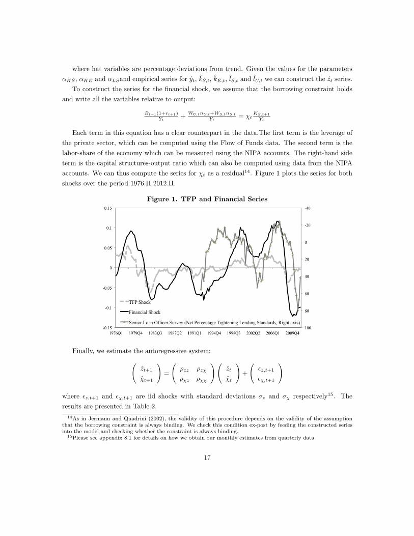
Each term in this equation has a clear counterpart in the data.The first term is the leverage ofthe private sector, which can be computed using the Flow of Funds data. The second term is thelabor-share of the economy which can be measured using the NIPA accounts. The right-hand sideterm is the capital structures-output ratio which can also be computed using data from the NIPAaccounts. We can thus compute the series for χt as a residual14. Figure 1 plots the series for bothshocks over the period 1976.II-2012.II.

Figure 1. TFP and Financial Series

Finally, we estimate the autoregressive system:(zt+1

χt+1

)=

(ρzz ρzχ

ρχz ρχχ

)(zt

χt

)+

(εz,t+1

εχ,t+1

)

where εz,t+1 and εχ,t+1 are iid shocks with standard deviations σz and σχ respectively15. Theresults are presented in Table 2.

14As in Jermann and Quadrini (2002), the validity of this procedure depends on the validity of the assumptionthat the borrowing constraint is always binding. We check this condition ex-post by feeding the constructed seriesinto the model and checking whether the constraint is always binding.

15Please see appendix 8.1 for details on how we obtain our monthly estimates from quarterly data

17

Table 2. Stochastic Properties of ShocksStandard deviation productivity shock σz 0.0044Standard deviation financial shock σχ 0.0057Covariance parameter innovations σzχ 0.0008

σχz 0.0008Autoregressive parameter for productivity shock ρzz 0.9824Autoregressive parameter for financial shock ρχχ 0.9738Spill-over from financial shock to productivity ρzχ -0.0032Spill-over from productivity to financial shocks ρχz 0.1072

4.3 Impulse-Responses

We begin by analyzing the behavior of our benchmark model when hit by a one standard de-viation negative shock to aggregate productivity and to the parameter governing the fraction ofcollateralized asset. Figures 2 shows the impulse response functions.

We first look at the effects of a TFP shock. This shock impacts output directly, and is capableof generating a larger fall in output and consumption relative to a financial shock. However, theresponse of labor market variables and the aggregate capital stock over a long horizon to a TFPshock is relatively weak. The small decline in employment and other labor market variables is notsurprising in light of two results. First, Shimer’s (2005, 2010) neutrality result, that predicts, asdiscussed earlier, low volatility of employment when changes in productivity affect in a similar wayboth consumption and the marginal product of labor, leaving the surplus of a match unchanged.As seen from the impulse response functions, TFP shocks produce a fall in wages of a similarmagnitude as the drop in the marginal product of labor. Second, as shown in Olivella and Roldan(2012), in models with reproducible capital general equilibrium effects dampen the response of realvariables to productivity shocks, even in the presence of financial frictions.

Regarding relative variables, a TFP shock has little effect on relative employment of skilled tounskilled workers and also a negligible effect on the composition of capital. Changes in TFP affectall production inputs uniformly and have little reallocation effects between the two types of workersand the two types of capital.

18

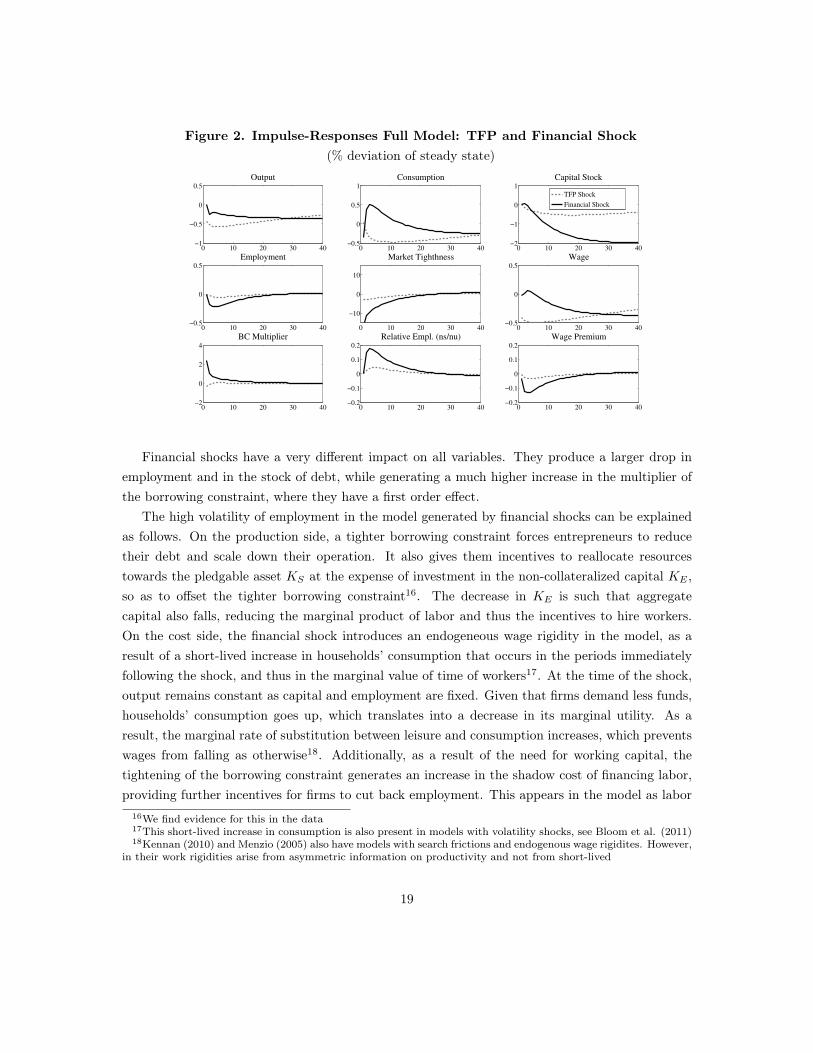
Figure 2. Impulse-Responses Full Model: TFP and Financial Shock(% deviation of steady state)

0 10 20 30 40−1

−0.5

0

0.5

Output

0 10 20 30 40−0.5

0

0.5

1

Consumption

0 10 20 30 40−2

−1

0

1

Capital Stock

TFP Shock

Financial Shock

0 10 20 30 40−0.5

0

0.5

Employment

0 10 20 30 40

−10

0

10

Market Tighthness

0 10 20 30 40−0.5

0

0.5

Wage

0 10 20 30 40−2

0

2

4

BC Multiplier

0 10 20 30 40−0.2

−0.1

0

0.1

0.2

Relative Empl. (ns/nu)

0 10 20 30 40−0.2

−0.1

0

0.1

0.2

Wage Premium

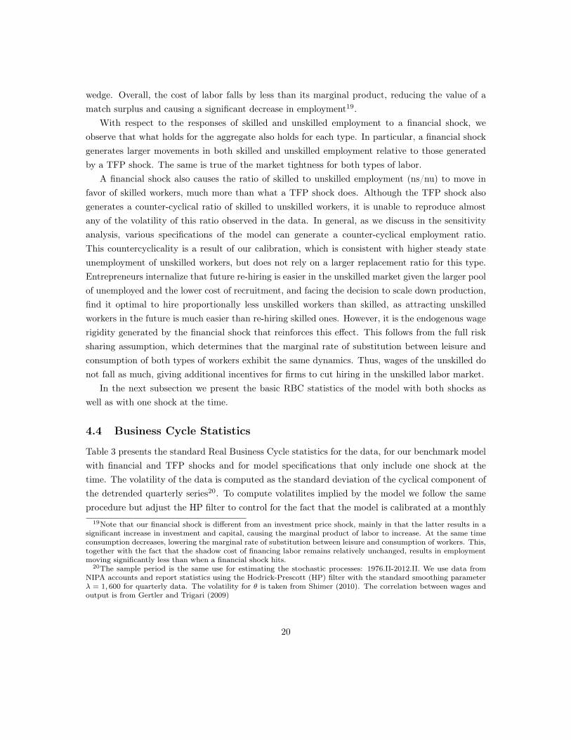
Financial shocks have a very different impact on all variables. They produce a larger drop inemployment and in the stock of debt, while generating a much higher increase in the multiplier ofthe borrowing constraint, where they have a first order effect.

The high volatility of employment in the model generated by financial shocks can be explainedas follows. On the production side, a tighter borrowing constraint forces entrepreneurs to reducetheir debt and scale down their operation. It also gives them incentives to reallocate resourcestowards the pledgable asset KS at the expense of investment in the non-collateralized capital KE ,so as to offset the tighter borrowing constraint16. The decrease in KE is such that aggregatecapital also falls, reducing the marginal product of labor and thus the incentives to hire workers.On the cost side, the financial shock introduces an endogeneous wage rigidity in the model, as aresult of a short-lived increase in households’ consumption that occurs in the periods immediatelyfollowing the shock, and thus in the marginal value of time of workers17. At the time of the shock,output remains constant as capital and employment are fixed. Given that firms demand less funds,households’ consumption goes up, which translates into a decrease in its marginal utility. As aresult, the marginal rate of substitution between leisure and consumption increases, which preventswages from falling as otherwise18. Additionally, as a result of the need for working capital, thetightening of the borrowing constraint generates an increase in the shadow cost of financing labor,providing further incentives for firms to cut back employment. This appears in the model as labor

16We find evidence for this in the data17This short-lived increase in consumption is also present in models with volatility shocks, see Bloom et al. (2011)18Kennan (2010) and Menzio (2005) also have models with search frictions and endogenous wage rigidites. However,

in their work rigidities arise from asymmetric information on productivity and not from short-lived

19

wedge. Overall, the cost of labor falls by less than its marginal product, reducing the value of amatch surplus and causing a significant decrease in employment19.

With respect to the responses of skilled and unskilled employment to a financial shock, weobserve that what holds for the aggregate also holds for each type. In particular, a financial shockgenerates larger movements in both skilled and unskilled employment relative to those generatedby a TFP shock. The same is true of the market tightness for both types of labor.

A financial shock also causes the ratio of skilled to unskilled employment (ns/nu) to move infavor of skilled workers, much more than what a TFP shock does. Although the TFP shock alsogenerates a counter-cyclical ratio of skilled to unskilled workers, it is unable to reproduce almostany of the volatility of this ratio observed in the data. In general, as we discuss in the sensitivityanalysis, various specifications of the model can generate a counter-cyclical employment ratio.This countercyclicality is a result of our calibration, which is consistent with higher steady stateunemployment of unskilled workers, but does not rely on a larger replacement ratio for this type.Entrepreneurs internalize that future re-hiring is easier in the unskilled market given the larger poolof unemployed and the lower cost of recruitment, and facing the decision to scale down production,find it optimal to hire proportionally less unskilled workers than skilled, as attracting unskilledworkers in the future is much easier than re-hiring skilled ones. However, it is the endogenous wagerigidity generated by the financial shock that reinforces this effect. This follows from the full risksharing assumption, which determines that the marginal rate of substitution between leisure andconsumption of both types of workers exhibit the same dynamics. Thus, wages of the unskilled donot fall as much, giving additional incentives for firms to cut hiring in the unskilled labor market.

In the next subsection we present the basic RBC statistics of the model with both shocks aswell as with one shock at the time.

4.4 Business Cycle Statistics

Table 3 presents the standard Real Business Cycle statistics for the data, for our benchmark modelwith financial and TFP shocks and for model specifications that only include one shock at thetime. The volatility of the data is computed as the standard deviation of the cyclical component ofthe detrended quarterly series20. To compute volatilites implied by the model we follow the sameprocedure but adjust the HP filter to control for the fact that the model is calibrated at a monthly

19Note that our financial shock is different from an investment price shock, mainly in that the latter results in asignificant increase in investment and capital, causing the marginal product of labor to increase. At the same timeconsumption decreases, lowering the marginal rate of substitution between leisure and consumption of workers. This,together with the fact that the shadow cost of financing labor remains relatively unchanged, results in employmentmoving significantly less than when a financial shock hits.

20The sample period is the same use for estimating the stochastic processes: 1976.II-2012.II. We use data fromNIPA accounts and report statistics using the Hodrick-Prescott (HP) filter with the standard smoothing parameterλ = 1, 600 for quarterly data. The volatility for θ is taken from Shimer (2010). The correlation between wages andoutput is from Gertler and Trigari (2009)

20

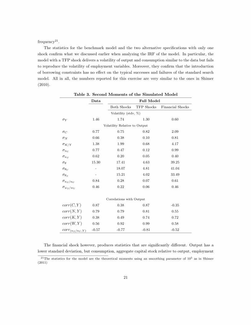
frequency21.The statistics for the benchmark model and the two alternative specifications with only one

shock confirm what we discussed earlier when analyzing the IRF of the model. In particular, themodel with a TFP shock delivers a volatility of output and consumption similar to the data but failsto reproduce the volatility of employment variables. Moreover, they confirm that the introductionof borrowing constraints has no effect on the typical successes and failures of the standard searchmodel. All in all, the numbers reported for this exercise are very similar to the ones in Shimer(2010).

Table 3. Second Moments of the Simulated ModelData Full Model

Both Shocks TFP Shocks Financial Shocks

Volatility (stdv, %)

σY 1.46 1.74 1.30 0.60

Volatility Relative to Output

σC 0.77 0.75 0.82 2.09

σN 0.66 0.38 0.10 0.81

σK/Y 1.38 1.99 0.68 4.17

σnU 0.77 0.47 0.12 0.99

σnS 0.62 0.20 0.05 0.40

σθ 15.30 17.41 4.63 39.25

σθU - 18.07 4.81 41.04

σθS - 15.21 4.02 33.49

σnS/nU 0.84 0.28 0.07 0.61

σwS/wU 0.46 0.22 0.06 0.46

Correlations with Output

corr(C, Y ) 0.87 0.38 0.87 -0.35

corr(N,Y ) 0.79 0.79 0.81 0.55

corr(K,Y ) 0.38 0.49 0.74 0.72

corr(W,Y ) 0.56 0.92 0.99 0.58

corr(nS/nU ,Y ) -0.57 -0.77 -0.81 -0.52

The financial shock however, produces statistics that are significantly different. Output has alower standard deviation, but consumption, aggregate capital stock relative to output, employment

21The statistics for the model are the theoretical moments using an smoothing parameter of 105 as in Shimer(2011)

21

(of both skilled and unskilled workers) and the market tightness for both labor markets are morevolatile than their counterpart with TFP shocks. The volatilities of most labor market variablesin this specification are higher than what is observed in the data. For example, the volatility ofemployment relative to output is 0.81, higher than the 0.66 reported in the data. The same is truefor the volatility of unskilled employment (0.99 in the model vs 0.77 in the data) and the aggregatemarket tightness (39 in the model vs 15 in the data). As we discussed earlier, the financial shock hasa first order effect on employment as it affects the shadow cost of hiring as well as the reservationwages through the movement in consumption. In fact, the financial shock predicts a counterfactualnegative correlation between consumption and output, given that, as shown before, during the firstfew months after the shock, consumption is above steady-state levels while output is falling. Thisexplains the lower correlation of aggregate wages to output in the presence of financial shocks (0.58),relative to case with TFP shocks (0.99), in which wages follow very closely output dynamics.

The model that includes both shocks (with properties as estimated in section 4.2) is able todeliver statistics closer to the data. The model explains almost 58% of the volatility in employmentrelative to output (0.38 in the model vs 0.66 in the data), and 69% of the absolute volatility ofemployment (0.66 in the model and 0.96 in the data). The volatility of theta relative to output is17.41 in the model with both shocks, close to the 15.3 of the data and almost 4 times bigger thanthe volatility delivered by the standard search model with TFP shocks. The benchmark model alsodelivers the correct correlation among aggregate variables, although the correlation of consumptionand output is lower than in the data and than in the standard search model with TFP shocks.

Finally, in the three specifications the ratio of employment of skilled to unskilled is countercycli-cal. However, for the TFP shock this ratio has a very low volatility, in line with our findings fromthe IRF analysis.

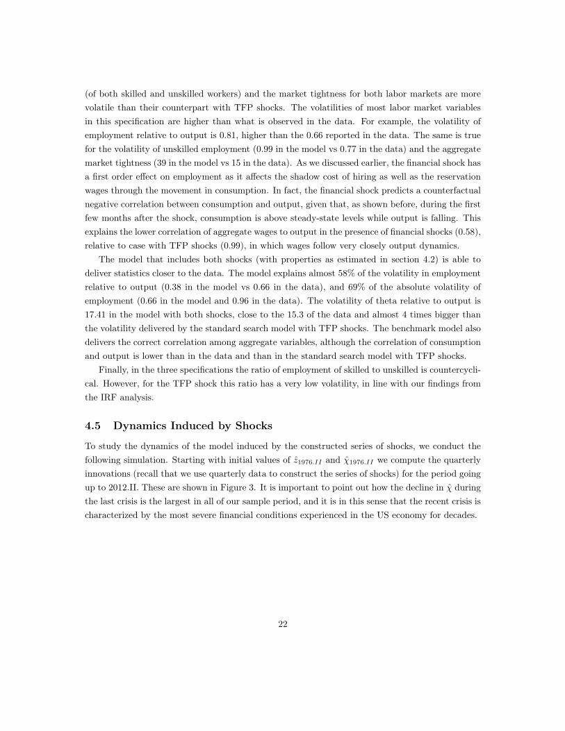
4.5 Dynamics Induced by Shocks

To study the dynamics of the model induced by the constructed series of shocks, we conduct thefollowing simulation. Starting with initial values of z1976.II and χ1976.II we compute the quarterlyinnovations (recall that we use quarterly data to construct the series of shocks) for the period goingup to 2012.II. These are shown in Figure 3. It is important to point out how the decline in χ duringthe last crisis is the largest in all of our sample period, and it is in this sense that the recent crisis ischaracterized by the most severe financial conditions experienced in the US economy for decades.

22

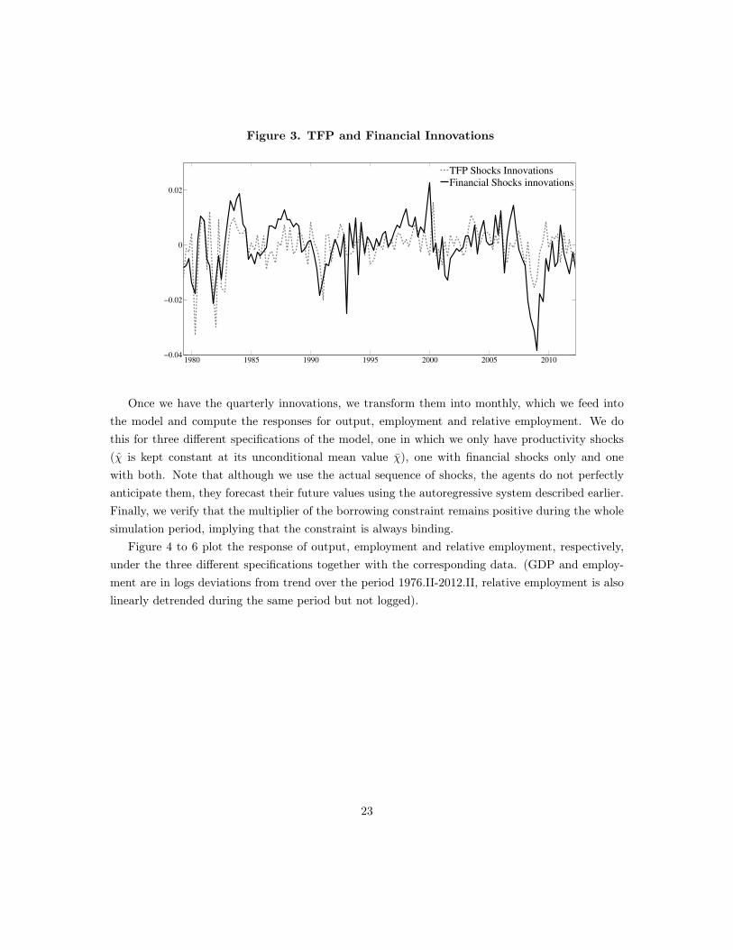
Figure 3. TFP and Financial Innovations

1980 1985 1990 1995 2000 2005 2010−0.04

−0.02

0

0.02

TFP Shocks Innovations

Financial Shocks innovations

Once we have the quarterly innovations, we transform them into monthly, which we feed intothe model and compute the responses for output, employment and relative employment. We dothis for three different specifications of the model, one in which we only have productivity shocks(χ is kept constant at its unconditional mean value χ), one with financial shocks only and onewith both. Note that although we use the actual sequence of shocks, the agents do not perfectlyanticipate them, they forecast their future values using the autoregressive system described earlier.Finally, we verify that the multiplier of the borrowing constraint remains positive during the wholesimulation period, implying that the constraint is always binding.

Figure 4 to 6 plot the response of output, employment and relative employment, respectively,under the three different specifications together with the corresponding data. (GDP and employ-ment are in logs deviations from trend over the period 1976.II-2012.II, relative employment is alsolinearly detrended during the same period but not logged).

23

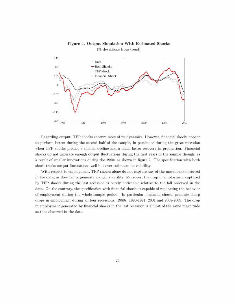
Figure 4. Output Simulation With Estimated Shocks(% deviations from trend)

1980 1985 1990 1995 2000 2005 2010−0.2

−0.15

−0.1

−0.05

0

0.05

0.1

0.15

Data

Both Shocks

TFP Shock

Financial Shock

Regarding output, TFP shocks capture most of its dynamics. However, financial shocks appearto perform better during the second half of the sample, in particular during the great recessionwhen TFP shocks predict a smaller decline and a much faster recovery in production. Financialshocks do not generate enough output fluctuations during the first years of the sample though, asa result of smaller innovations during the 1980s as shown in figure 2. The specification with bothshock tracks output fluctuations well but over estimates its volatility.

With respect to employment, TFP shocks alone do not capture any of the movements observedin the data, as they fail to generate enough volatility. Moreover, the drop in employment capturedby TFP shocks during the last recession is barely noticeable relative to the fall observed in thedata. On the contrary, the specification with financial shocks is capable of replicating the behaviorof employment during the whole sample period. In particular, financial shocks generate sharpdrops in employment during all four recessions: 1980s, 1990-1991, 2001 and 2008-2009. The dropin employment generated by financial shocks in the last recession is almost of the same magnitudeas that observed in the data.

24

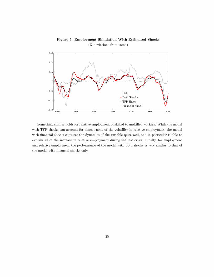
Figure 5. Employment Simulation With Estimated Shocks(% deviations from trend)

1980 1985 1990 1995 2000 2005 2010−0.06

−0.04

−0.02

0

0.02

0.04

0.06

Data

Both Shocks

TFP Shock

Financial Shock

Something similar holds for relative employment of skilled to unskilled workers. While the modelwith TFP shocks can account for almost none of the volatility in relative employment, the modelwith financial shocks captures the dynamics of the variable quite well, and in particular is able toexplain all of the increase in relative employment during the last crisis. Finally, for employmentand relative employment the performance of the model with both shocks is very similar to that ofthe model with financial shocks only.

25

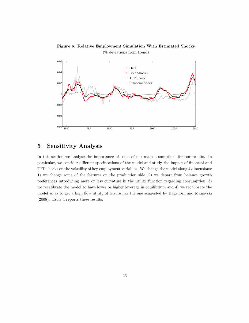
Figure 6. Relative Employment Simulation With Estimated Shocks(% deviations from trend)

1980 1985 1990 1995 2000 2005 2010−0.06

−0.04

−0.02

0

0.02

0.04

0.06

Data

Both Shocks

TFP Shock

Financial Shock

5 Sensitivity Analysis

In this section we analyse the importance of some of our main assumptions for our results. Inparticular, we consider different specifications of the model and study the impact of financial andTFP shocks on the volatility of key employment variables. We change the model along 4 dimensions:1) we change some of the features on the production side, 2) we depart from balance growthpreferences introducing more or less curvature in the utility function regarding consumption, 3)we recalibrate the model to have lower or higher leverage in equilibrium and 4) we recalibrate themodel so as to get a high flow utility of leisure like the one suggested by Hagedorn and Manovski(2008). Table 4 reports these results.

26

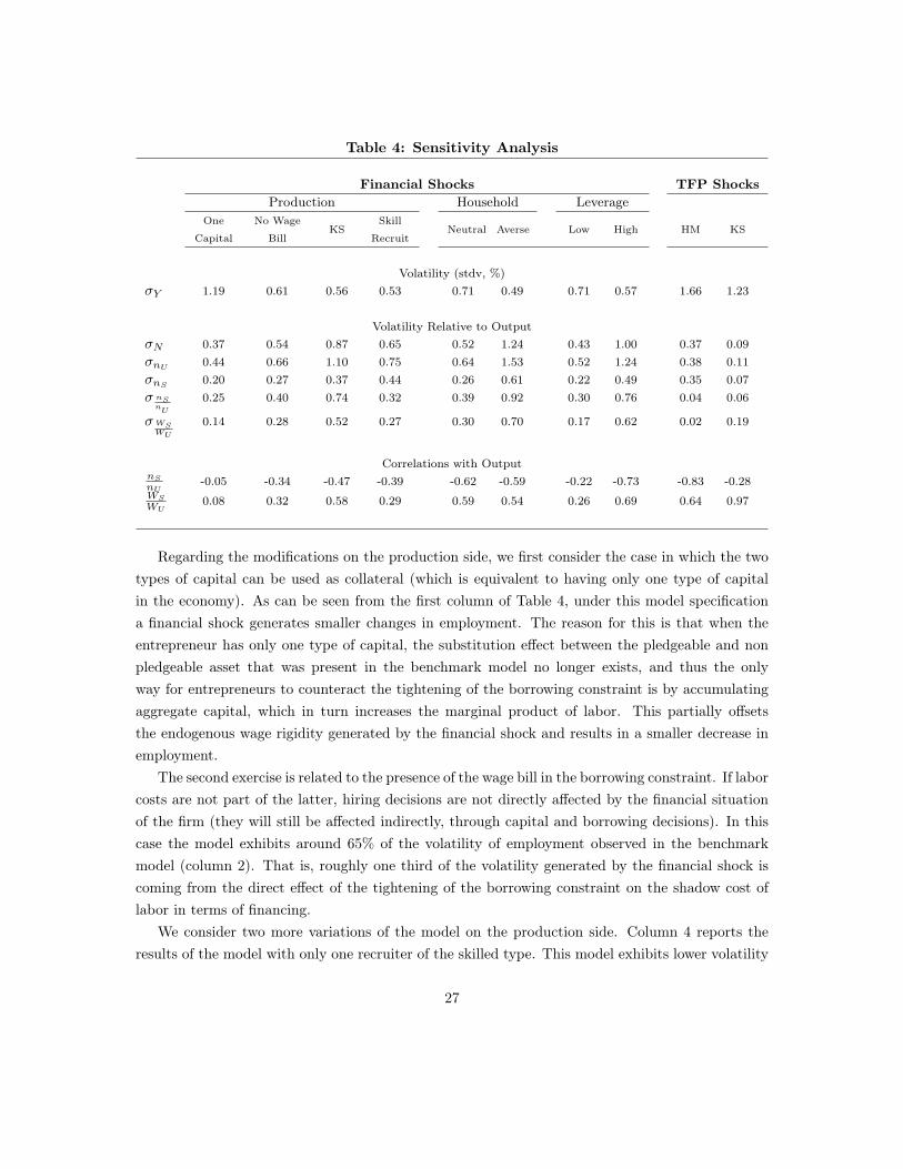
Table 4: Sensitivity Analysis

Financial Shocks TFP ShocksProduction Household Leverage

One

Capital

No Wage

BillKS

Skill

RecruitNeutral Averse Low High HM KS

Volatility (stdv, %)σY 1.19 0.61 0.56 0.53 0.71 0.49 0.71 0.57 1.66 1.23

Volatility Relative to OutputσN 0.37 0.54 0.87 0.65 0.52 1.24 0.43 1.00 0.37 0.09σnU 0.44 0.66 1.10 0.75 0.64 1.53 0.52 1.24 0.38 0.11σnS 0.20 0.27 0.37 0.44 0.26 0.61 0.22 0.49 0.35 0.07σ nSnU

0.25 0.40 0.74 0.32 0.39 0.92 0.30 0.76 0.04 0.06

σWSWU

0.14 0.28 0.52 0.27 0.30 0.70 0.17 0.62 0.02 0.19

Correlations with OutputnSnU

-0.05 -0.34 -0.47 -0.39 -0.62 -0.59 -0.22 -0.73 -0.83 -0.28WS

WU0.08 0.32 0.58 0.29 0.59 0.54 0.26 0.69 0.64 0.97

Regarding the modifications on the production side, we first consider the case in which the twotypes of capital can be used as collateral (which is equivalent to having only one type of capitalin the economy). As can be seen from the first column of Table 4, under this model specificationa financial shock generates smaller changes in employment. The reason for this is that when theentrepreneur has only one type of capital, the substitution effect between the pledgeable and nonpledgeable asset that was present in the benchmark model no longer exists, and thus the onlyway for entrepreneurs to counteract the tightening of the borrowing constraint is by accumulatingaggregate capital, which in turn increases the marginal product of labor. This partially offsetsthe endogenous wage rigidity generated by the financial shock and results in a smaller decrease inemployment.

The second exercise is related to the presence of the wage bill in the borrowing constraint. If laborcosts are not part of the latter, hiring decisions are not directly affected by the financial situationof the firm (they will still be affected indirectly, through capital and borrowing decisions). In thiscase the model exhibits around 65% of the volatility of employment observed in the benchmarkmodel (column 2). That is, roughly one third of the volatility generated by the financial shock iscoming from the direct effect of the tightening of the borrowing constraint on the shadow cost oflabor in terms of financing.

We consider two more variations of the model on the production side. Column 4 reports theresults of the model with only one recruiter of the skilled type. This model exhibits lower volatility

27

but sufficiently high to show that this particular feature is not key for the results of the bench-mark model. One important difference between this specification and the benchmark model is thevolatility of unskilled workers, which falls to 0.75 from 0.99. When only skilled workers can recruit,the opportunity cost of hiring unskilled is determined by skilled wages, and hence the differencesbetween the two types of labor narrow. Finally, column 3 presents the results of our capital-skillcomplementarity specification, which we discuss in more detail later in this section.

A second dimension we explore is that of household’s preferences. Column 5 and 6 present theresults of a model recalibrated to have the same steady state as the benchmark but in which therisk aversion coefficient (the intertemporal substitution parameter), is different from one. In thefirst of these two columns we report the results for the case in which households are very close tohaving linear utility in consumption and in the second we present the case in which the risk aversioncoefficient is 2. Given that the two specifications have the same steady state as in the benchmarkmodel, this allows us to isolate the effect of a financial shock on wages, and hence on the overallelasticity of employment, that comes solely from consumption dynamics. When agents are risk-neutral, the relative volatility of employment to output is 64% of the one observed in the benchmark,falling to 0.52 from 0.81. This drop in volatility occurs for both skilled and unskilled employment,as well as for the relative employment ratio. This result suggests that in the benchmark model,about one-third of the volatility of employment generated by financial shocks is explained by thegeneral equilibrium effect of consumption on wages and employment. Alternatively, if households’utility exhibits more curvature, changes in consumption have a stronger effect on wages, bringinghigher employment volatility, as shown in column 6.

We then consider a model that is calibrated to have lower or higher leverage in equilibrium, andshow that the elasticity of employment resulting from financial shocks is directly related to the levelof leverage in the economy. For the benchmark calibration we chose parameter values of χ and γconsistent with a debt-to-gdp ratio of 0.63 at quarterly basis. In the last two columns we presenta calibration of the model that favors lower and higher leverage respectively. For the first casewe re-calibrate γ to be consistent with a steady state debt-to-gdp ratio of 0.2 at quarterly basis.For the high leverage case we target a ratio of 1. The economy with higher leverage shows highervolatilities across all labor market variables, as suggested in our earlier discussion on leverage andemployment.

Regarding the ability of the model to generate movements in labor variables with productivityshocks, we conduct two robustness exercises. First, we follow a calibration in which we maximize theflow utility derived from unemployment in line with the work by Hagedorn and Manovksi (2008).For this case we set the bargaining power parameter (φ) close to zero and choose the leisure utilityparameters, γs and γu, so as to match the unemployment level of skilled and unskilled workers.Table 4 shows that, when hit by a TFP shock, this specification (under the label HM) exhibitsa larger volatility of employment relative to output than in the basic model, just as in the setup

28

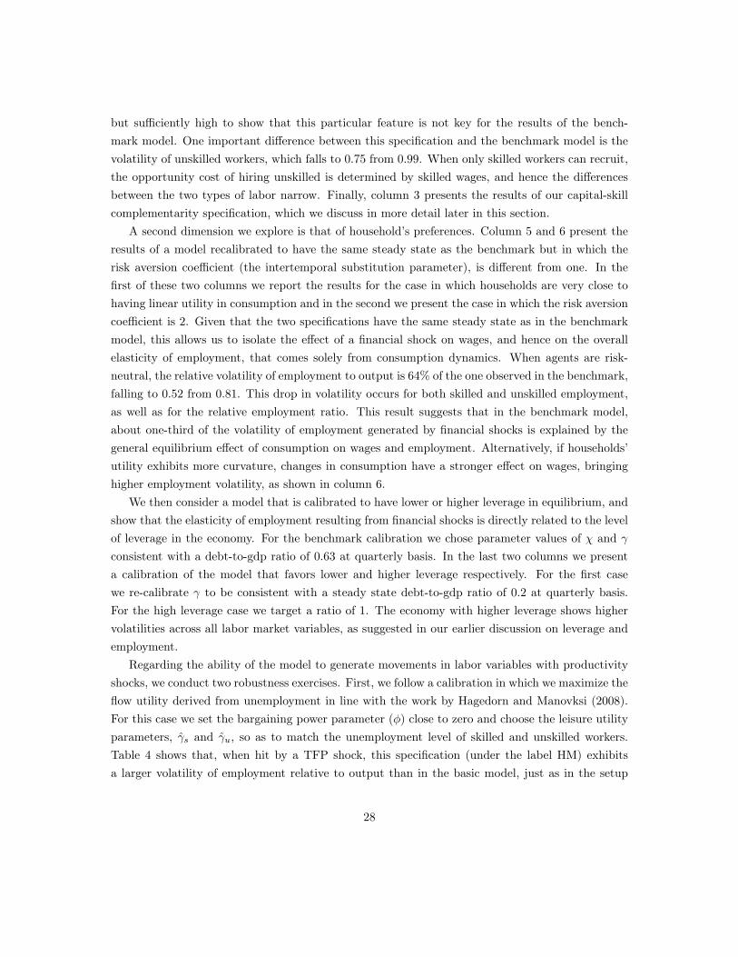
of Hagedorn and Manovksi (2008). However, the overall employment volatility is lower than inour benchmark model with both TFP and financial shocks and also lower than in the model withfinancial shocks only. Moreover, Figure 7 shows that this model specification, calibrated to havehigher leisure utility, does a poor job in replicating the observed pattern of employment fluctuationswhen fed with the actual realizations of the aggregate productivity series.

Figure 7. Employment Simulation HM Calibration(% deviations from trend)

1980 1985 1990 1995 2000 2005 2010−0.06

−0.04

−0.02

0

0.02

0.04

0.06

Data

Both Shocks

TFP Shock (Baseline)

Financial Shock

TFP Shock (Hagedorn−Manovskii Calibration)

In terms of relative employment, the HM specification delivers a low volatility of the nSnU

ratio.That is, while TFP shocks create incentives for firms to re-scale their production, they don’t generateany strong reallocation incentives among production inputs. Moreover, if we were to change thecalibration to generate higher movements in the relative ratio of employment, we would have to seta higher bargaining power for unskilled workers. This, however, would in turn reduce the volatilityof aggregate employment, because of the lower γu needed to keep the steady-state unemploymentlevel of unskilled workers unchanged. Additionally, it would be at odds with the conjecture thatskill workers should have, if any different, a higher bargaining power than the unskilled.

In our second exercise we test whether departing from a Cobb-Douglas production functioncould help to generate realistic employment fluctuations under TFP shocks. In order assess this weconsider a production function and parameter values such that there is capital-skill complementarityas in the work by Greenwood et al. (1997) and Krusell et al (2000).

Under this specification the production technology is given by:

F (KS,t,KE,t, LS,t, LU,t) = ZtKθS,t

[αLνU,t + (1− α)

[λKϕ

E,t + (1− λ)LϕS,t

] νϕ

] 1−θν

29

where θ, α, λ ∈ (0, 1); ν, ϕ ∈ (−∞, 1) and ν, ϕ 6= 0 . This production function has been appliedboth to study long-term dynamics of the wage skill premium (such as Krusell et al, 2000), as wellas business cycle dynamics under TFP shocks as well as shocks to the relative price of investmenton equipment (Lindquist, 2004). More recently, Baller and Van Rens (2013) have challenged theview that there is any evidence of capital-skill complementarity at the business cycle frequency andsuggest an alternative parameterization in which capital and skill are mildly substitutable .

Parameters ν and ϕ are the two key substitution parameters. 1/(1 − ϕ) defines the elasticityof substitution between capital equipment and skilled labor, while the elasticity of substitutionbetween capital equipment and unskilled labor and between skilled and unskilled labor are bothgiven by 1/(1−ν). If ν > ϕ, the production function is said to exhibit capital-skill complementarity.

Income share of capital structures is given by θ,while α and λ determine the income shares ofskilled and unskilled labor and of capital equipment. We set the substitution parameters, ν = 0.401

and ϕ = −0.495, as in Krusell et al. (2000), and choose the other parameters in order to match thesame moments as in our benchmark model.

We report the main statistics of employment-related variables for this exercise in Table 4 underthe label “KS”. Both aggregate and relative employment fluctuations are similar for the specificationwith capital-skill complementarity and the benchmark Cobb-Douglas calibration for both TFPand financial shocks respectively. That is, the capital-skill complementarity specification does notappear to contribute much regarding employment volatilities, and the same results that hold in ourbenchmark scenario carry over.

6 Conclusions

In this paper we study the effect of exogenous shocks to financing conditions on labor market out-comes. We find that financial shocks, unlike aggregate productivity shocks, can replicate the largefluctuations in aggregate and skill-specific employment as observed in the data. This suggests thatunderstanding cyclical changes in credit is important to help us understand economic fluctuationsand labor market dynamics. Given that we assume here a representative entrepreneur, understand-ing how financial shocks reallocate resources from different labor markets between heterogeneousproducers or sectors is beyond the scope of this paper but is a promising area for research. Re-cent papers by Khan and Thomas (2013) and Buera, Fattal-Jaef and Shin (2013) discuss financialshocks in the context of heterogeneous firms but with homogenous labor markets. Allowing forheterogeneity in labor markets could be important for understanding the differences in employmentlevels as well as the persistence of unemployment across skill types observed during and after thecrisis.

30

7 References

Acemoglu, D. 1998. “Why do new technologies complement skills? Directed technical change andwage inequality.” The Quarterly Journal of Economics 113 (4): 1055–1089.

Andolfatto, David. 1996. “Business cycles and labor-market search.” The American EconomicReview, pp. 112–132.

Balleer, A., and T. Van Rens. 2013. “Skill-biased technological change and the business cycle.”Review of Economics and Statistics 95:1222–1237.

Bloom, Nicholas, Max Floetotto, Nir Jaimovich, Itay Saporta-Eksten, and Stephen J Terry. 2012.“Really Uncertain Business Cycles.” NBER Working Paper.

Buera, Francisco, Roberto Fattal-Jaef, and Yongseok Shin. 2013. “Anatomy of a Credit Crunch:from Capital to Labor Markets.” Working Paper.

Buera, Francisco J, and Benjamin Moll. 2012. “Aggregate implications of a credit crunch.” NBERWorking Paper.

Caggese, Andrea, and Ander Perez. 2013. “Aggregate Implications of Financial and Labor MarketFrictions.” Working Paper.

Cahuc, Pierre, and Etienne Wasmer. 2001. “Does intrafirm bargaining matter in the large firm’smatching model?” Macroeconomic Dynamics 5 (05): 742–747.

Cajner, T., and I. Cairo. 2011. “Human Capital and Unemployment Dynamics: Why MoreEducated Workers Enjoy Greater Employment Stability.” Working Paper, no. 1145.

Christiano, Lawrence J, Roberto Motto, and Massimo Rostagno. 2010. “Financial Factors inEconomic Fluctuations.” ECB Working Paper.

Elsby, M, Michael WL, and B. Hobijn. 2010. “The Labor Market in the Great Recession.” BrookingsPapers on Economic Activity.

Gertler, Mark, and Antonella Trigari. 2009. “Unemployment Fluctuations with Staggered NashWage Bargaining.” Journal of Political Economy 117 (1): 38–86.

Gilchrist, Simon, Jae Sim, and Egon Zakrajśek. 2012. “Uncertainty, Financial Frictions, andInvestment Dynamics.” Working Paper.

Gilchrist, Simon, and Egon Zakrajsek. 2012. “Credit Spreads and Business Cycle Fluctuations.”The American Economic Review 102 (4): 1692–1720.

Greenwood, J., Z. Hercowitz, and P. Krusell. 1997. “Long-run implications of investment-specifictechnological change.” The American Economic Review, pp. 342–362.

Guerrieri, Veronica, and Guido Lorenzoni. 2011. “Credit crises, precautionary savings, and theliquidity trap.” NBER Working Paper.

31

Hagedorn, M., and I. Manovskii. 2008. “The Cyclical Behavior of Equilibrium Unemployment andVacancies Revisited.” American Economic Review 98 (4): 1692–1706.

Hornstein, Andreas, Per Krusell, and Giovanni Violante. 2005. “Unemployment and vacancyfluctuations in the matching model: Inspecting the mechanism.” FRB Richmond EconomicQuarterly 91 (3): 19–51.

Hosios, A.J. 1990. “On the efficiency of matching and related models of search and unemployment.”The Review of Economic Studies 57 (2): 279–298.

Jermann, U., and V. Quadrini. 2012. “Macroeconomic effects of financial shocks.” The AmericanEconomic Review 102 (1): 238–271.

Kennan, John. 2010. “Private information, wage bargaining and employment fluctuations.” TheReview of Economic Studies 77 (2): 633–664.

Khan, A., and J.K. Thomas. 2013. “Credit Shocks and Aggregate Fluctuations in an Economywith Production Heterogeneity.” The Journal of Political Economy.

Kiyotaki, N., and J. Moore. 1997. “Credit Cycles.” The Journal of Political Economy 105 (2):211–248.

Kiyotaki, Nobuhiro, and John Moore. 2012. “Liquidity, business cycles, and monetary policy.”Working Paper.

Krause, Michael, and Thomas A Lubik. 2007. “Does intra-firm bargaining matter for businesscycle dynamics?” Working Paper Deutschen Bundesbank.

Krusell, P., L.E. Ohanian, J.V. Ríos-Rull, and G.L. Violante. 2000. “Capital-skill complementarityand inequality: A macroeconomic analysis.” Econometrica 68 (5): 1029–1053.

Lindquist, M.J. 2004. “Capital–skill complementarity and inequality over the business cycle.”Review of Economic Dynamics 7 (3): 519–540.

Marcellino, Massimiliano. 1999. “Some consequences of temporal aggregation in empirical analy-sis.” Journal of Business & Economic Statistics 17 (1): 129–136.

Menzio, Guido. 2005. “High frequency wage rigidity.” Manuscript. Univ. Pennsylvania.

Merz, Monika. 1995. “Search in the labor market and the real business cycle.” Journal of MonetaryEconomics 36 (2): 269–300.

Monacelli, T., V. Quadrini, and A. Trigari. 2011. “Financial markets and unemployment.” NBERWorking Paper.

Mortensen, Dale T, and Christopher A Pissarides. 1994. “Job creation and job destruction in thetheory of unemployment.” The Review of Economic Studies 61 (3): 397–415.

Olivella, V., and J. Roldan. 2011. “Re-Examining the Role of Financial Constraints: is SomethingWrong with the Credit Multiplier?” Working Paper.

32

Petrosky-Nadeau, Nicolas, and Etienne Wasmer. 2013. “The Cyclical Volatility of Labor Marketsunder Frictional Financial Markets.” American Economic Journal: Macroeconomics 5 (1):193–221.

Quadrini, Vincenzo. 2011. “Financial frictions in macroeconomic fluctuations.” FRB RichmondEconomic Quarterly 97 (3): 209–254.

Shimer, Robert. 2005. “The cyclical behavior of equilibrium unemployment and vacancies.” Amer-ican economic review, pp. 25–49.

. 2010. Labor Markets and Business Cycles. Princeton University Press.

Wasmer, Etienne, and Philippe Weil. 2004. “The Macroeconomics of Labor and Credit MarketImperfections.” American Economic Review, pp. 944–963.

33

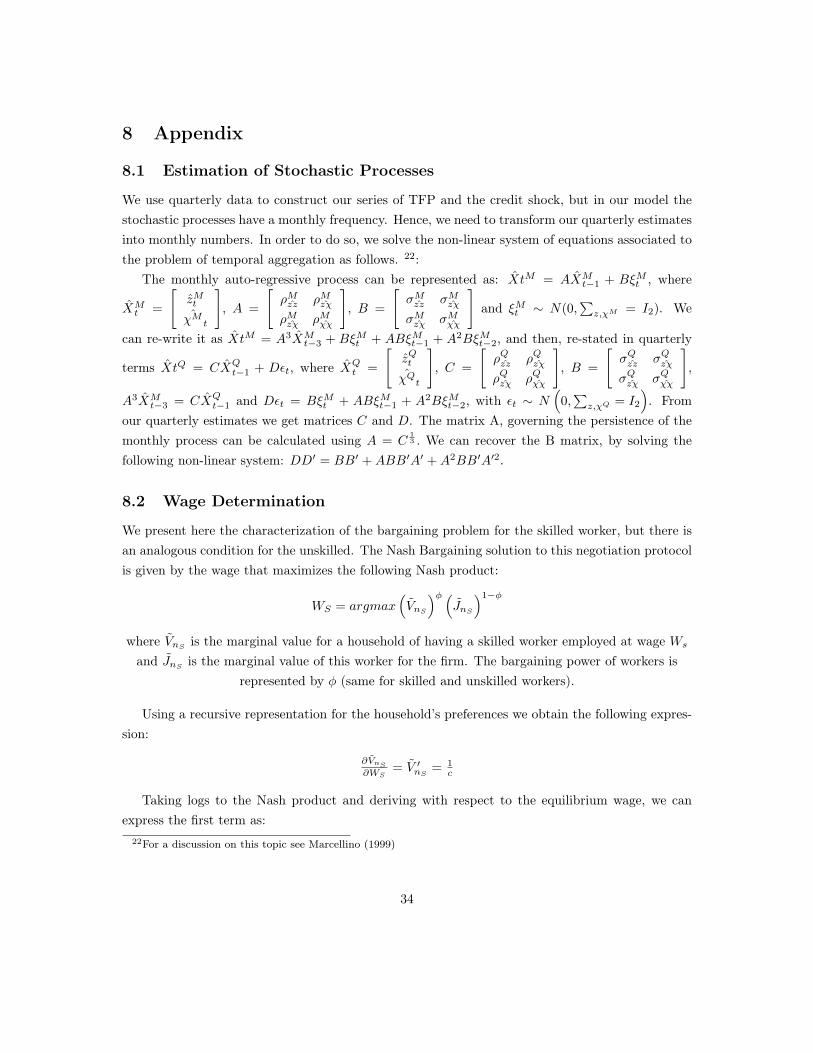
8 Appendix

8.1 Estimation of Stochastic Processes

We use quarterly data to construct our series of TFP and the credit shock, but in our model thestochastic processes have a monthly frequency. Hence, we need to transform our quarterly estimatesinto monthly numbers. In order to do so, we solve the non-linear system of equations associated tothe problem of temporal aggregation as follows. 22:

The monthly auto-regressive process can be represented as: XtM = AXMt−1 + BξMt , where

XMt =

[zMt

χMt

], A =

[ρMzz ρMzχρMzχ ρMχχ

], B =

[σMzz σMzχσMzχ σMχχ

]and ξMt ∼ N(0,

∑z,χM = I2). We

can re-write it as XtM = A3XMt−3 + BξMt + ABξMt−1 + A2BξMt−2, and then, re-stated in quarterly

terms XtQ = CXQt−1 + Dεt, where XQ

t =

[zQt

χQt

], C =

[ρQzz ρQzχρQzχ ρQχχ

], B =

[σQzz σQzχσQzχ σQχχ

],

A3XMt−3 = CXQ

t−1 and Dεt = BξMt + ABξMt−1 + A2BξMt−2, with εt ∼ N(

0,∑z,χQ = I2

). From

our quarterly estimates we get matrices C and D. The matrix A, governing the persistence of themonthly process can be calculated using A = C

13 . We can recover the B matrix, by solving the

following non-linear system: DD′ = BB′ +ABB′A′ +A2BB′A′2.

8.2 Wage Determination

We present here the characterization of the bargaining problem for the skilled worker, but there isan analogous condition for the unskilled. The Nash Bargaining solution to this negotiation protocolis given by the wage that maximizes the following Nash product:

WS = argmax(VnS

)φ (JnS

)1−φ

where VnS is the marginal value for a household of having a skilled worker employed at wage Ws

and JnS is the marginal value of this worker for the firm. The bargaining power of workers isrepresented by φ (same for skilled and unskilled workers).

Using a recursive representation for the household’s preferences we obtain the following expres-sion:

∂VnS∂WS

= V ′nS = 1c

Taking logs to the Nash product and deriving with respect to the equilibrium wage, we canexpress the first term as:

22For a discussion on this topic see Marcellino (1999)

34

φV ′nS (WS)V nS (WS)

= φ (1/c)VnS

= φ [1−β(1−xS−f(θS))]Ws−c·γS

For the firm side, we can compute the marginal value of a worker employed at a wage WS forone period, instead of the equilibrium wage WS :

JnS (KE ,KS , B, nS , nU ,WS) =(WS − WS

)(1 + µ) + JnS

Taking logs and the derivative with respect to the wage, we have:

(1− φ)J′nSJnS

= −(1−φ)(1+µ)JnS

= (1+µ)(1−φ)γω(θS)MPLS

Putting together the expressions from the household and firm side:

φV ′nS (WS)V nS (WS)

+ (1− φ)J′nSJnS

= φ (1−β(1−xS−f(θS)))Ws−c·γS = (1−φ)γω(θS)(1+µ)

MPLS

and simplifying and solving for the equilibrium wage, we get:

WS = βφφβ+(1−φ)γ

MPLS(1+µ)

(1 + θS + γ−β

γβ1

ω(θS)

)+ γ(1−φ)

φβ+(1−φ)γ γS · c

35

Documents de Travail

480. E. Mengus, “Honoring Sovereign Debt or Bailing Out Domestic Residents: A Theory of Internal Costs of Default,” March 2014

481. C. Labonne and G. Lamé, “Credit Growth and Bank Capital Requirements: Binding or Not?,” March 2014

482. S. Gilchrist and B. Mojon, “Credit Risk in the Euro area,” April 2014

483. G. Vuillemey and R. Breton, “Endogenous Derivative Networks,” April 2014

484. G. Cette, R. Lecat and A-O-A. Jiddou, “How do firms adjust production factors to the cycle?,” April 2014

485. M. Bussière, B. Camara, F.-D. Castellani, V. Potier and J. Schmidt, “ Shock Transmission Through International

Banks - Evidence From France,” May 2014

486. A. Monfort, J-P. Renne and G. Roussellet, “A Quadratic Kalman Filter,” May 2014

487. P. Benczúr, G. Kátay, Á. Kiss and O. M. Rácz, “Income Taxation, Transfers and Labour Supply at the Extensive

Margin,” June 2014

488. R. Jimborean and A. Kelber, “Foreign direct investment drivers and growth in Central and Eastern Europe in the aftermath of the 2007 global financial crisis,” June 2014

489. F. Pegoraro, A. F. Siegel and L. Tiozzo ‘Pezzoli, “International Yield Curves and Principal Components Selection

Techniques: An Empirical Assessment,” June 2014

490. F. Pegoraro, A. F. Siegel and L. Tiozzo ‘Pezzoli, “Specification Analysis of International Treasury Yield Curve Factors,” June 2014

491. J-S. Mésonnier and A. Monks, “Did the EBA Capital Exercise Cause a Credit Crunch in the Euro Area?,”

June 2014

492. F. Alvarez , H. Le Bihan and F. Lippi, “Small and large price changes and the propagation of monetary shocks,” June 2014

493. A. Devulder, “Heterogeneity, Unemployment Benefits and Voluntary Labor Force Participation,” June 2014 494. C. Bortoli, L. Harreau, C. Pouvelle, “Determinants of OECD countries’ sovereign yields: safe havens, purgatory,

and the damned,” June 2014

495. A. Bernales and M Guidolin, “The Effects of Information Asymmetries on the Ex-Post Success of Stock Option Listings,” June 2014

496. J. I. Lopez and V. Olivella Moppett, “Financial Shocks and the Cyclical Behavior of Skilled and Unskilled

Unemployment,” July 2014

Pour accéder à la liste complète des Documents de Travail publiés par la Banque de France veuillez consulter le site : www.banque-france.fr For a complete list of Working Papers published by the Banque de France, please visit the website: www.banque-france.fr Pour tous commentaires ou demandes sur les Documents de Travail, contacter la bibliothèque de la Direction Générale des Études et des Relations Internationales à l'adresse suivante : For any comment or enquiries on the Working Papers, contact the library of the Directorate General Economics and International Relations at the following address : BANQUE DE FRANCE 49- 1404 Labolog 75049 Paris Cedex 01 tél : 0033 (0)1 42 97 77 24 ou 01 42 92 63 40 ou 48 90 ou 69 81 email : 1404-ut@banque-france.fr