Embed Size (px)
Citation preview
sustainability
Article
Coffee Output Reaction to Climate Change andCommodity Price Volatility: The Nigeria Experience
Anthony Oko-Isu 1,*, Agnes Ugboego Chukwu 2, Grace Nyereugwu Ofoegbu 3,Christiana Ogonna Igberi 1, Kennedy Okechukwu Ololo 4, Tobechi Faith Agbanike 4 ,Lasbrey Anochiwa 4, Nkechinyere Uwajumogu 4, Michael Oguwuike Enyoghasim 4 ,Uzoma Nnaji Okoro 5 and Adeolu Adewale Iyaniwura 1
1 Department of Agriculture, Faculty of Agriculture, Alex Ekwueme Federal University Ndufu-Alike, Ikwo,Ebonyi State 482131, Nigeria; [email protected] (C.O.I.); [email protected] (A.A.I.)
2 College of Management Sciences, Michael Okpara University of Agriculture, Umudike 440109, Nigeria;[email protected]
3 Department of Accountancy, Faculty of Business Administration, University of Nigeria Enugu Campus,Enugu State 400241, Nigeria; [email protected]
4 Faculty of Management and Social Sciences, Alex Ekwueme Federal University Ndufu-Alike, Ikwo,Ebonyi State 482131, Nigeria; [email protected] (K.O.O.); [email protected] (T.F.A.);[email protected] (L.A.); [email protected] (N.U.);[email protected] (M.O.E.)
5 Heritage Bank Nigeria PLC, Umuahia Branch 440221, Nigeria; [email protected]* Correspondence: [email protected]
Received: 22 April 2019; Accepted: 12 June 2019; Published: 26 June 2019�����������������
Abstract: Empirical evidence is lacking on the nexus between coffee commodity output, climatechange, and commodity price volatility of Africa’s most populous country, Nigeria, and otherdeveloping countries. To fill this gap, this study analyzed the reaction of coffee output to climatechange and commodity price volatility. We used secondary data from 1961 to 2015 from reliablesources for Nigeria. The study adopted generalized autoregressive conditional heteroscedasticity(GARCH), autoregressive conditional heteroscedasticity (ARCH), and fully modified ordinary leastsquare (FMOLS) in analysis of coffee output reaction to climate change and commodity price volatility.The findings show that coffee output in Nigeria is influenced by climate change and the internationalcommodity price of coffee. The study demonstrates the potential benefits of improving coffee outputand export through climate mitigation and adaptation measures and revival of agricultural commoditymarketing in Nigeria and other developing countries.
Keywords: coffee output; climate change; commodity price volatility; GARCH; ARCH; FMOLS
1. Introduction
The World Bank Group (WBG) 2018 reports that Africa’s food market, which, in 2013, was valuedat about US$ 313 billion a year, could triple by 2030 [1]. According to the report, this could only beachieved when African governments invest in infrastructure, smart business, and improved tradepolicies, linking her dynamic agribusiness sector with consumers in her growing urban areas. Thisaligns with the African development bank (AfDB) report of 2015 that Africa’s development fortune ison its high points and in recent times, enjoying its strongest growth at an average of 5%–6% in thelast 40 years, with significant progress, also achieving some of the millennium development goals(MDGs) [2]. Notwithstanding, this growth has not positively impacted the food and nutrition securitystatus and wellbeing for all Africans. Therefore, agribusiness small and medium enterprises (SMEs) areimportant for economic development with high potentials for employment generation, food security,
Sustainability 2019, 11, 3503; doi:10.3390/su11133503 www.mdpi.com/journal/sustainability
Sustainability 2019, 11, 3503 2 of 19
foreign exchange earnings, and poverty reduction. It is also critical in linking smallholder producersto national markets, meeting food demand, and creating tomorrow’s jobs [3]. These potentials ofagribusiness have remained largely untapped. This has, over time, led to the dwindling performanceof the agricultural sector both domestically and in international trade. Nigeria is reported to be thepoverty capital of the world, faced with an increasing population and heavy dependence on import,and reliance on crude oil earnings needs to find a solution on how to tap the potentials and solveher problems.
More so, coffee, like other tree crops, represents one group of agribusiness that merit specialattention for climate change adaptation planning as they have a series of traits that make themparticularly susceptible to climate change [4]. Coffee is an important tree crop capable of beingharnessed by Nigeria as an important green investment option since Nigeria is the most populousblack nation in the world with a massive landmass and very young population, but not mentioned inthe major exporters of coffee [5].
However, the so-called ‘coffee crisis’, provoked by the breakdown of the International coffeeagreement in 1989, triggered a dramatic drop in international prices in the late 1990s [6]. With Guatemalahit the worst, coffee prices, which continued to fall in the first years of this century and although werereversed from 2005 reached a maximum in 2011 (above US$ 300 per pound), had again. by November2013, fallen to the level of US$ 123 per pound [7]. Price volatility has wreaked drastic negative impactson small producers in many developing countries [8,9]. Ironically, the disproportionate effects of theprice volatility are mainly on the marginalized populations who make up a large population of coffeefarmers, especially women and youths. According to reports [10], the roles of these marginalizedgroups differ within and between countries and have become more dynamic in different parts of theworld. AfDB [11] noted that 70% of Africa’s smallholder farmers are women and are responsible formore than 90% of Africa’s agricultural production [12].
The macroeconomic impacts of commodity prices are important because of its effect on the levelof per capita income, which is the ultimate key in determining living standards for families as wellas individuals. Generally speaking, high international prices for food commodities benefit countriesthat export those products, while low prices benefit importing countries. In the longer term, however,higher prices could cause some importing countries to invest in their agriculture and reduce imports,or even become exporters [10].
To the best of our knowledge, no information exists on the reaction of coffee output in Africa toclimate change and commodity price volatility. This study, therefore, was conceived in order to fillthe gap and to showcase the past, present, and predict the future of coffee as an agribusiness optionworthy of investment in Africa’s most populous nation.
2. Methodology
2.1. Study Area
The study area is Nigeria. The Federal Republic of Nigeria is in West Africa between latitudes40 and 140 north and between longitudes 2021 and 140301 east. To the north, the country is boundedby Niger Republic (1497 km) and Chad (853 km), to the west by Benin Republic (773 km). to the eastby Cameroon Republic (1690 km), and to the south by the Atlantic Ocean. Nigeria has a land area ofabout 923,769 km2 [13], a north–south length of about 1450 km, and west-east breadth of about 800 kmwith only 50% of the land proportion presently cultivated. Its total land boundary is 4047 km while thecoastline is 853 km. Potential estimates for irrigation in Nigeria vary from 1.5 to 3.2 million ha. Thecurrent estimate is about 2.3 million ha, with over 1 million ha located in northern Nigeria [14,15].
Nigeria is made up of 36 states and the Federal Capital Territory located in Abuja and enjoysthe humid tropical climate with two clear identifiable seasons, the wet and dry seasons. The climatecondition varies among regions: Equatorial in the south, tropical in the center, and arid in the north.Annual rainfall is between 2000–3000 mm in a year characterized by high temperatures and relative
Sustainability 2019, 11, 3503 3 of 19
humidity. Nigeria has four agro-ecological zones with rainfall along the south–north gradient. Thecountry has marked ecological diversity and climatic contrast with the lowest point in the AtlanticOcean at sea level of 0 m, and the highest point on the Chappalwaddi at 2419 m [15].
Nigeria’s population is estimated to be over 173.6 million [16], with diverse biophysicalcharacteristics, ethnic nationalities (more than 250), agro-ecological zones, and socio-economicconditions [15,17]. Popular indigenous languages are Igbo, Hausa, and Yoruba while the Englishlanguage is the official language. Farming is the predominant occupation of the people; about halfof the working population is engaged in agriculture, the majority of whom are smallholder farmers.Cocoa, coffee, oil palm, and rubber are among the major tree crops grown in Nigeria.
The country is faced with an economy characterized by an unstable exchange rate and ecosystemsseverely affected by global warming, and for the past decade has hurt farming in coastal communitiesand desertification is ravaging the Sahel. Other environmental issues affecting the country include soildegradation, rapid deforestation, water pollution, desertification, oil spill affecting water, air and soil,loss of arable land, and rapid urbanization.
2.2. Sources of Data
This study was based on data obtained from various sources spanning from 1961 to 2015. Nationalaggregated level data were used for the study. The data include monthly data on climatic variables(temperature and rainfall), the output of coffee (yield and production), as well as internationalcommodity prices of the coffee tree crop. Other macro-economic variables such as real exchangerate, inflation, and trade openness index were also used. The sources of the data collected includevarious published editions of the National Bureau of Statistics (NBS) and Central Bank of Nigeria(CBN) statistical bulletins for data on the real exchange rate, inflation, and data used in calculatingtrade openness index. Climate data came from Nigerian meteorological agency (NIMET), whiledata on the output of coffee were sourced from Food, Agriculture Organization (FAO) database.The coffee commodity price for the period studied (1961–2015) was sourced from the InternationalCoffee Organization (ICO) and the World Bank database (the time series data are included inSupplementary Data).
General-purpose model for making predictions or inferences from incomplete information [18],to estimate the spatial distribution of climatic conditions that are suitable for growing coffee throughoutNigeria was used. A similar approach has previously been used for modeling the impacts of climatechange on coffee in Mexico [19], Central America [20], and East Africa [21]. With some modifications,it has also been used for predicting the impacts of climate change on other tree crops [22].
The climate data were obtained from the Nigerian Meteorological Agency (NIMET) and the coffeeoutput data from the Central Bank of Nigeria (CBN) Statistical Bulletins and Food and AgriculturalOrganization (FAO) database. The national aggregated level of data usage was because coffee can begrown in all the zones in Nigeria. As obtained from the current report, [23], the locations of majorcurrent coffee production states in Nigeria cuts across the six geopolitical zones (Taraba, Plateau,Adamawa, Oyo, Osun, Ondo, Ogun, Lagos, Edo, Kwara, Kogi, Niger, Kaduna, Benue, Abia, CrossRiver, and Akwa Ibom).
To capture the heterogeneity of climate and coffee production data, the altitudinal belt, assumed torepresent the typical climates for coffee production, was identified for each of the six geo-political zonesbased on observations made by one of the contributing authors over 10 years of field research in Nigeria.This pattern was used by [24] for national data from stations for which there were long-standingrecords, calculating means of the 1960–1990 period and including only weather stations with morethan 10 years of data. The maximum altitude for all climate variables is 3023 m.
For calibrating the climate model, 5600 points were generated systematically covering the sixcoffee production polygons with a 0.5 arcmin grid. In addition, a random background sample at a5:1 ratio of background to calibration points was drawn from outside the coffee production zones to
Sustainability 2019, 11, 3503 4 of 19
characterize the general environment. Background sampling at this ratio is within the range supportedby the literature [25,26] and resulted in the most accurate predicted distributions.
Our model used the bioclimatic variables provided by NIMET that are derived from the monthlytemperature and rainfall values. These variables are often used in ecological niche modeling [27].They represent annual trends (such as mean annual temperature and annual precipitation), seasonality(such as annual range in temperature and precipitation), and extreme or limiting environmental factors(such as the temperature of the coldest and warmest months, and precipitation of the wettest anddriest quarters). An area was considered suitable for growing coffee if the suitability calculated byMaxent was >35% and unsuitable if it was less. This threshold was determined by the maximum sumof sensitivity and specificity criterion as suggested by [28].
2.3. Method of Data Analysis
Data for the study were analyzed using both descriptive and inferential statistical tools.To achieve objectives, graph form of descriptive statistics, the generalized sutoregressive conditionalheteroscedasticity (GARCH), and autoregressive conditional heteroscedasticity (ARCH) models withthe fully modified ordinary least square (FM-OLS) approach were employed. The hypothesis, however,was tested with the use of pairwise Granger causality approach.
2.4. Volatility Test
In literature, various measures of commodity price volatility have been used in examining thevariability of pair-wise cross-country commodity prices based on the observation that commodity pricetime series data are typically heteroscedastic, leptokurtic, and exhibit volatility clustering—that is,having variance figure varying over a specified period of time [29–33]. On the basis of this and in linewith the research objectives, this study examined the extent of coffee commodity price volatility between1961 and 2015. Similar to other empirical studies, the autoregressive conditional heteroscedasticity(ARCH) model by [34] and the generalized ARCH (GARCH) model by [35] were employed to analyzethe extent of coffee tree crop commodity prices volatility in Nigeria during the period of study.
The choice of these models was based on their previous use in various areas of econometricmodeling, such as financial time series analysis [36–38] and their acceptance of the approaches infinancial time series modeling with an autoregressive structure in that heteroscedasticity observedover different periods may be autocorrelated.
In the development of an ARCH model, two distinct specifications are considered—the conditionalmean and the conditional variance. In general, the standard GARCH (p,q) specification is expressed inimplicit form as:
yt = α+k∑
i=1
nixt−1εt (1)
where;
yt = measure of commodity price volatility at time t,α = mean,xt−1 = exogenous variables,εt = error term.
δ =
√√√1N
k∑i=1
(xi −X)2
(2)
where;
δ = variance,xi = mean,
Sustainability 2019, 11, 3503 5 of 19
X = standard deviation.
δt2 = ω+∑p
i=1αiε
2t−i +
∑q
i=1βiδ
2t−i (3)
where;
δt2 = conditional variance,P = order of the GARCH,δ2
t−i.= the GARCH term.
The mean in Equation (1) is expressed as a constant function α- (taken as mean if other exogenousvariables were assumed to be zero), exogenous variable(s) xt−1- (majorly in autoregressive (AR)structure of order k), and with an error term εt.
Note that yt was considered a measure of commodity price volatility at time t.From Equation (3), the conditional variance equation specified in (3) represents a function of three
components: The mean ω; the volatility information from the previous period. This is measured asthe lag of the squared residual from the mean equation: ε2
t−i (which is ARCH term); and the forecastvariance of last periods: δ2
t−i (which is the GARCH term).From Equation (1), k represents the order of the autoregressive term, while for Equation (3),
p represents the ARCH term as ordered and q represents the GARCH term as ordered. In Gujarati(2004), a GARCH (p, q) model is equivalent to an ARCH (p + q), that is, the presence of a first-orderARCH term (the first term n parentheses-p, lagged term of the conditional variance).
For this study, volatility clustering presence was determined by the lagged volatility seriesparameters-yt significance. The degree of extent of volatility on the other hand in the commodity pricewas ascertained by use of the autoregressive root, and this was the sum of α + β and the indication ofthe degree of volatility was as follows:
If α + β is between 0.51–1 or =1 (i.e., greater than 0.51 to 1 or equal to 1), it indicates that volatilityis present and persistent;
If α + β > 1 (i.e., greater than 1) it indicates that there is overshooting of volatility.If α + β < 0.5 (i.e., less than 0.5) it indicates no volatility.
2.5. Baseline Model Specification
The baseline analytical model for the study is specified as follows:
Yt = α + β1CMt + β2CPt + β3(CM × CP)t + Ut (4)
where;
Yt = Tree crop yield at time t;CM = Climate change at time t;CP = Commodity price change at time t;(CM × CP)t = interaction between CM and CP at time t; andµt = other unobserved variables.
2.6. The FM-OLS Regression Approach
The FM-OLS regression approach used following [39] is specified below;
Yit = f (CPit, Tt, P, IR, TO, ER, CM × CP, Σt) (5)
where
Yit = yield for crop i at time t (tons/hectare),
Sustainability 2019, 11, 3503 6 of 19
CPit = Coffee commodity price at time t (U.S. $),T = mean annual temperature (◦C),P = total annual rainfall (mm),IR = total annual Inflation rate (%),TO = Trade openness (%),ER = Exchange Rate (Naira),CM × CP = climate variables × coffee commodity price at time t (U.S. $),Σt = error term
andPit = f (CPit, Tt, P, IR, TO, ER, CM × CP, Σt) (6)
where;
Pit = yield for the coffee crop at time t (tons/hectare),CPit = Coffee commodity price at time t (U.S. $),T = mean annual temperature (◦C),P = total annual rainfall (mm),IR = total annual Inflation rate (%),TO = Trade openness (%),ER = Exchange Rate (Naira),CM × CP = climate variables × commodity price of the crop I at time t (U.S. $),Σt = error term.
2.7. The Granger Causality Test Model
The Granger causality test, according to [40], is specified as;
Wt = εny−1 α1 Zy−1 + ε
n−ij βwy−1 + uit (7)
Zt = εnp−1α1Zt−1 + ε
nj−1d1wt−1 + u2t (8)
where
Wt = yield for each of coffee tree crop (tons/hectare),Zt = commodity price for coffee tree crop (U.S. $),
t−1 = lag variables,α1 and β1 = parameters to be estimated,U1t and U2t = error terms.
2.8. Estimating Trade Openness
The trade openness data were taken from the trade openness index, which is an economic metriccalculated as the ratio of country’s total trade, the sum of exports plus imports, to the country’s grossdomestic product.
Trade Openness =Exports + Imports
GDP(9)
The interpretation of the openness index is that the higher the index, the larger the influence oftrade on domestic activities and the stronger the country’s economy.
2.9. Pre-Data Processing Flow Chart
The secondary data used for the study was pre-processed before the analysis. The pre-Dataprocessing flow chart is shown in Chart 1 below. This gives a very clear picture of the entire
Sustainability 2019, 11, 3503 7 of 19
pre-data processing starting from the data extraction sources and variables sourced to Unit root andco-integration tests.Sustainability 2019, 11, x FOR PEER REVIEW 7 of 20
Chart 1. A flow chart of data pre-process by authors.
2.10. Similar Studies with Their Adopted Analytical Models
The adopted research analytical method by this study was compared with similar studies in the world. The summary of the adopted analytical methods with similar studies is shown in Table 1. The Table 1 below displays the authors, the region studied, the period covered by the study and the methods adopted by the various studies.
Table 1. Summary of siamilar studies with their adopted analytical models.
Authors Region Period Methods [41] Asian Countries 1980-2014 FMOLS [42] Pakistan 1988–2011 VAR, ARDL, and VECM [43] Pakistan 1980–2013 ARDL and VECM [44] 14 MENA countries 1996–2012 FMOLS [45] Nigeria 1980–2008 ARDL and VECM [46] USA 1960–2010 VAR and ARDL [47] China 1975–2000 STIRPAT model [48] Tunisia 1971–2012 ARDL and ECM [49] Malaysia VECM Model [50] China 1953–2006 ARDL
[51] South Asia 1975–2011 Co-integration test and Granger causality test
[52] Malaysia 1970–2008 Bounds test and Granger
causality
Chart 1. A flow chart of data pre-process by authors.
2.10. Similar Studies with Their Adopted Analytical Models
The adopted research analytical method by this study was compared with similar studies in theworld. The summary of the adopted analytical methods with similar studies is shown in Table 1.The Table 1 below displays the authors, the region studied, the period covered by the study and themethods adopted by the various studies.
Table 1. Summary of siamilar studies with their adopted analytical models.
Authors Region Period Methods
[41] Asian Countries 1980-2014 FMOLS[42] Pakistan 1988–2011 VAR, ARDL, and VECM[43] Pakistan 1980–2013 ARDL and VECM[44] 14 MENA countries 1996–2012 FMOLS[45] Nigeria 1980–2008 ARDL and VECM[46] USA 1960–2010 VAR and ARDL[47] China 1975–2000 STIRPAT model[48] Tunisia 1971–2012 ARDL and ECM[49] Malaysia VECM Model[50] China 1953–2006 ARDL[51] South Asia 1975–2011 Co-integration test and Granger causality test[52] Malaysia 1970–2008 Bounds test and Granger causality
Sustainability 2019, 11, 3503 8 of 19
Table 1. Cont.
Authors Region Period Methods
[53] China 1978–2006 STIRPAT model +[54] Turkey 1960–2007 F test[55] Turkey 1968–2005 VAR[56] Iran 1971–2007 ARDL[57] 22 emerging countries 1990–2006 GMM
[58,59] South Africa 1965–2008 ARDL
[60] Indonesia 1975Q1–2011Q4ARDLVECM
IAA
[61] 13 European and 12 EastAsia and Oceania countries 1989–2011 PVAR
STIRPAT, stochastic impacts by regression on population, affluence, and technology; GMM, generalized methodof moments; URB, urbanization; EC, energy consumption; ARDL, autoregressive distributed lag model; VECM,vector error correction model; FD, financial development; SR, stock return; DCPS, domestic credit to private sector;EC, energy consumption; EG economic growth; POP population; CO2, Carbon dioxide emission. Source: Adaptedfrom [41] and improved.
3. Results and Discussions
3.1. The Trend of Coffee Tree Crop Commodity Price, Production, and Yield 1961–2015
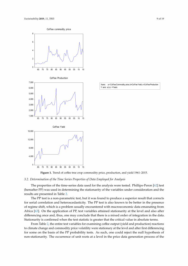
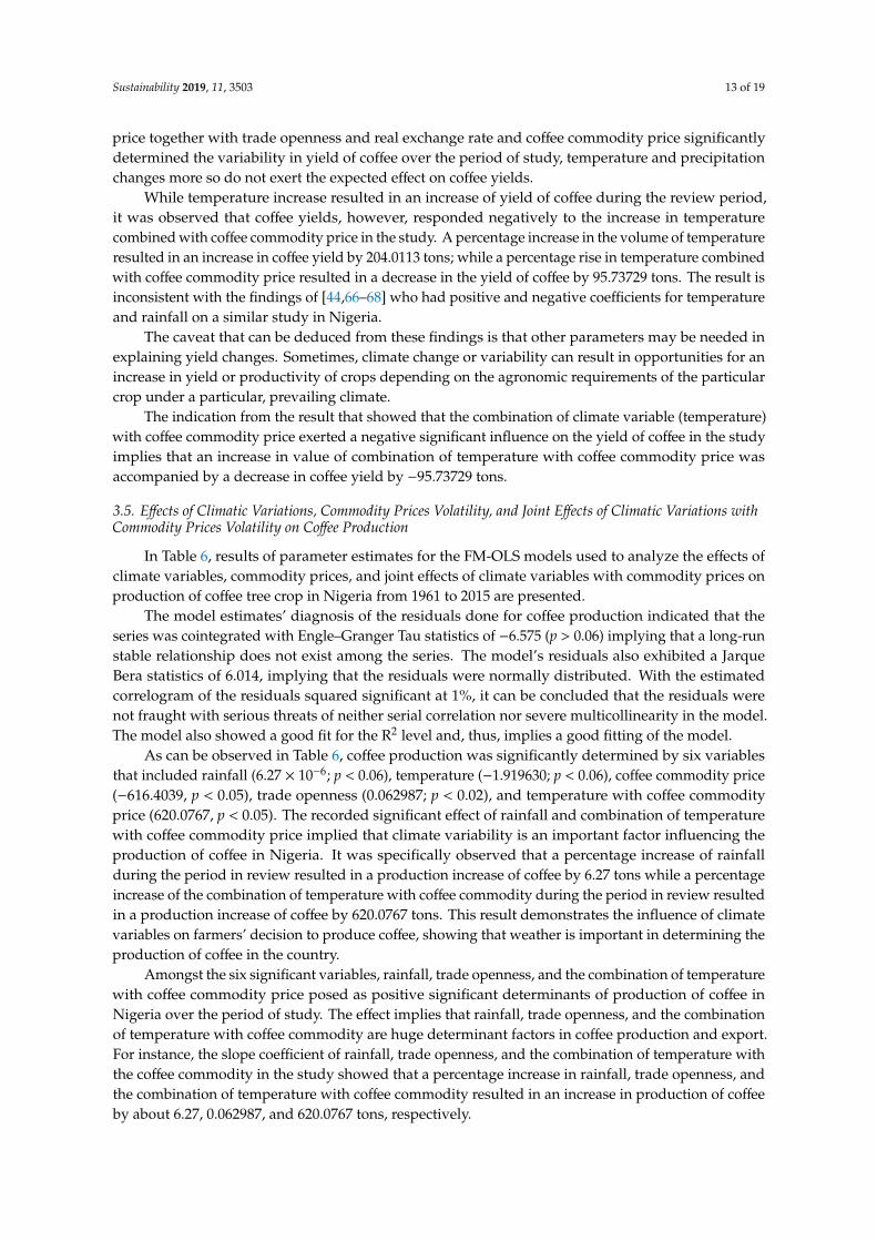
Considering the international monthly commodity prices of coffee tree crop for the 648 months(1961–2015), there has been considerable variability and instability of the prices of the commodity.As shown in Figure 1, the general trend pattern is characterized by sharp growth and also a sharpdecline for the time period under study. Between 1961 and 1972, coffee recorded a somewhat similarpattern in its commodity price, which was accompanied immediately by a rapid growth from 1975 to1978 followed by a sharp fall thereafter. It was also observed from Figure 1 that the upward trend didnot characterize the whole period but rather a zigzag trend. In fact, there were steady fluctuations incommodity prices of the selected export tree crops from 1961 to 2015 as shown in Figure 1. Between1975 and 1978 there was a sharp increase in coffee commodity price from below $2/kg to over $5/kgfollowed by a decline from 1978 and another sharp increase to its peak price of $5.98/kg recordedin 2011.
The graph of the trend of coffee tree crop yield (Tons/Ha) as also shown in Figure 1 reveals gradualfluctuations in coffee yield. Coffee yield trend was observed to show fluctuating trend but a steadyyield value of 5000 Tons/ha was noticed from 1973 to 1983, and a gradual increase to 5233 Tons/ha from1984 to 14,394 Tons/ha in 2006. The figure shows that the production of coffee showed a somewhatinsignificant unstable trend of 4000 tons in 1966 to 6000 tons in 1985 and down to 3604 tons in 2015.
Sustainability 2019, 11, 3503 9 of 19Sustainability 2019, 11, x FOR PEER REVIEW 9 of 20
0
2
4
6
8
65 70 75 80 85 90 95 00 05 10 15
Cof fee commodity price
1,000
2,000
3,000
4,000
5,000
6,000
7,000
65 70 75 80 85 90 95 00 05 10 15
Cof fee Production
0
4,000
8,000
12,000
16,000
65 70 75 80 85 90 95 00 05 10 15
Cof fee Yield
X axis: a = Cof fee Commodity price; b=Cof f ee Yield; c=Cof fee ProductionY axis: a,b,c =Years
Figure 1. Trend of coffee tree crop commodity price, production, and yield 1961–2015.
3.2. Determination of the Time Series Properties of Data Employed for Analysis
The properties of the time-series data used for the analysis were tested. Phillips-Peron [62] test (hereafter PP) was used in determining the stationarity of the variables under consideration and the results are presented in Table 2.
The PP test is a non-parametric test, but it was found to produce a superior result that corrects for serial correlation and heteroscedasticity. The PP test is also known to be better in the presence of regime shift, which is a problem usually encountered with macroeconomic data emanating from Africa [63]. On the application of PP, test variables attained stationarity at the level and also after differencing once and, thus, one may conclude that there is a mixed order of integration in the data. Stationarity is confirmed when the test statistic is greater that the critical value in absolute terms.
From Table 2, the entire test variables for examining coffee output (yield and production) reactions to climate change and commodity price volatility were stationary at the level and after first differencing for some on the basis of the PP probability tests. As such, one could reject the null hypothesis of non-stationarity. The occurrence of unit roots at a level in the price data generation process of the commodity gives a preliminary indication of shocks having a permanent or long-
Figure 1. Trend of coffee tree crop commodity price, production, and yield 1961–2015.
3.2. Determination of the Time Series Properties of Data Employed for Analysis
The properties of the time-series data used for the analysis were tested. Phillips-Peron [62] test(hereafter PP) was used in determining the stationarity of the variables under consideration and theresults are presented in Table 2.
The PP test is a non-parametric test, but it was found to produce a superior result that correctsfor serial correlation and heteroscedasticity. The PP test is also known to be better in the presenceof regime shift, which is a problem usually encountered with macroeconomic data emanating fromAfrica [63]. On the application of PP, test variables attained stationarity at the level and also afterdifferencing once and, thus, one may conclude that there is a mixed order of integration in the data.Stationarity is confirmed when the test statistic is greater that the critical value in absolute terms.
From Table 2, the entire test variables for examining coffee output (yield and production) reactionsto climate change and commodity price volatility were stationary at the level and after first differencingfor some on the basis of the PP probability tests. As such, one could reject the null hypothesis ofnon-stationarity. The occurrence of unit roots at a level in the price data generation process of the
Sustainability 2019, 11, 3503 10 of 19
commodity gives a preliminary indication of shocks having a permanent or long-lasting effect, thus, notmaking it easy for traditional price stabilization policies common in African countries to survive [64].
Table 2. Unit root test result.
Phillips-Perron Test
Variable Level 1st Difference Order of Integration
Climate change
Rainfall −5.045133(0.0001) I(0)
Temperature −4.260020(0.0013) I(0)
Commodity prices
Coffee −2.565541(0.1064)
−8.338275(0.0000) I(1)
Output (production)
Coffee −5.406997(0.0000) I(0)
Output (Yield)
Coffee −2.724048(0.0766) I(0)
Others
Real Exchange rate 1.310611(0.9984)
−6.287971(0.0000) I(1)
Trade openness −3.007864(0.1396)
−9.084742(0.0000) I(1)
Inflation rate −3.243140(0.0228) I(0)
Source: E-views 9 Researchers’ calculations output result from FAO, WBG, NBS, CBN, ICO, NIMET data. Note:Values in parentheses are probability values.
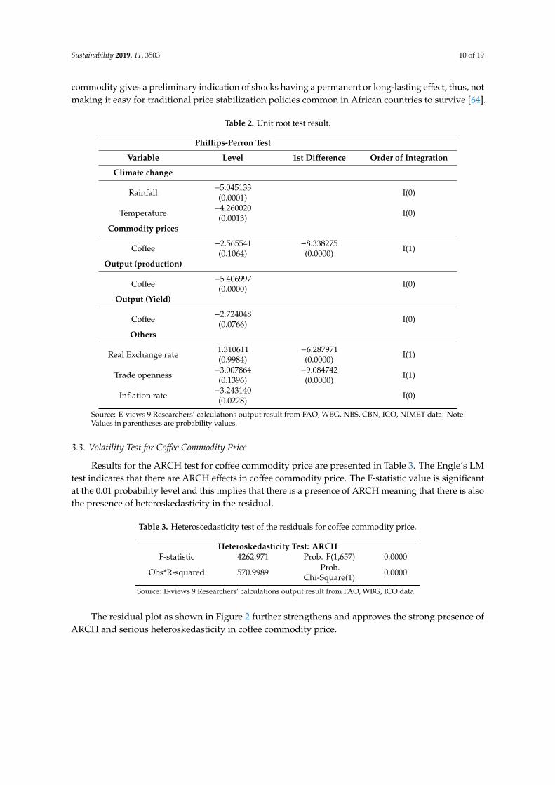
3.3. Volatility Test for Coffee Commodity Price
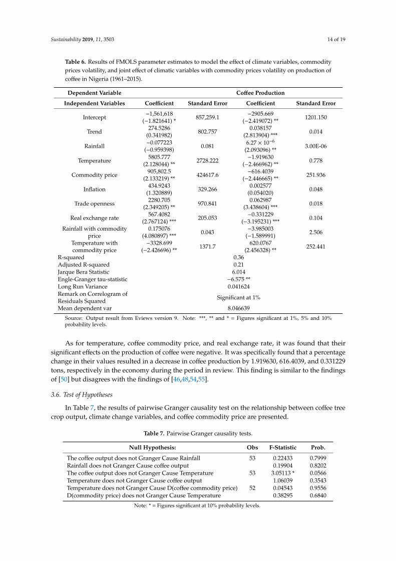
Results for the ARCH test for coffee commodity price are presented in Table 3. The Engle’s LMtest indicates that there are ARCH effects in coffee commodity price. The F-statistic value is significantat the 0.01 probability level and this implies that there is a presence of ARCH meaning that there is alsothe presence of heteroskedasticity in the residual.
Table 3. Heteroscedasticity test of the residuals for coffee commodity price.
Heteroskedasticity Test: ARCHF-statistic 4262.971 Prob. F(1,657) 0.0000
Obs*R-squared 570.9989 Prob.Chi-Square(1) 0.0000
Source: E-views 9 Researchers’ calculations output result from FAO, WBG, ICO data.
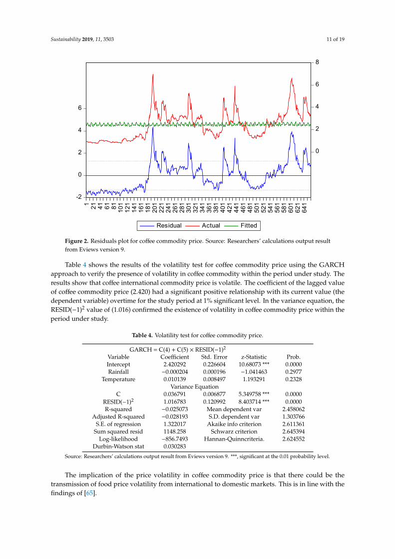
The residual plot as shown in Figure 2 further strengthens and approves the strong presence ofARCH and serious heteroskedasticity in coffee commodity price.
Sustainability 2019, 11, 3503 11 of 19Sustainability 2019, 11, x FOR PEER REVIEW 11 of 20
-2
0
2
4
6
0
2
4
6
8
1 21 41 61 81 101
121
141
161
181
201
221
241
261
281
301
321
341
361
381
401
421
441
461
481
501
521
541
561
581
601
621
641
Residual Actual Fitted Figure 2. Residuals plot for coffee commodity price. Source: Researchers’ calculations output result from Eviews version 9.
Table 4 shows the results of the volatility test for coffee commodity price using the GARCH approach to verify the presence of volatility in coffee commodity within the period under study. The results show that coffee international commodity price is volatile. The coefficient of the lagged value of coffee commodity price (2.420) had a significant positive relationship with its current value (the dependent variable) overtime for the study period at 1% significant level. In the variance equation, the RESID(−1)2 value of (1.016) confirmed the existence of volatility in coffee commodity price within the period under study.
The implication of the price volatility in coffee commodity price is that there could be the transmission of food price volatility from international to domestic markets. This is in line with the findings of [65].
Table 4. Volatility test for coffee commodity price.
GARCH = C(4) + C(5) × RESID(−1)2 Variable Coefficient Std. Error z-Statistic Prob. Intercept 2.420292 0.226604 10.68073 *** 0.0000 Rainfall −0.000204 0.000196 −1.041463 0.2977
Temperature 0.010139 0.008497 1.193291 0.2328 Variance Equation
C 0.036791 0.006877 5.349758 *** 0.0000 RESID(−1)2 1.016783 0.120992 8.403714 *** 0.0000 R-squared −0.025073 Mean dependent var 2.458062
Adjusted R-squared −0.028193 S.D. dependent var 1.303766 S.E. of regression 1.322017 Akaike info criterion 2.611361
Sum squared resid 1148.258 Schwarz criterion 2.645394 Log-likelihood −856.7493 Hannan-Quinncriteria. 2.624552
Durbin-Watson stat 0.030283 Source: Researchers’ calculations output result from Eviews version 9. ***, significant at the 0.01 probability level.
Figure 2. Residuals plot for coffee commodity price. Source: Researchers’ calculations output resultfrom Eviews version 9.
Table 4 shows the results of the volatility test for coffee commodity price using the GARCHapproach to verify the presence of volatility in coffee commodity within the period under study. Theresults show that coffee international commodity price is volatile. The coefficient of the lagged valueof coffee commodity price (2.420) had a significant positive relationship with its current value (thedependent variable) overtime for the study period at 1% significant level. In the variance equation, theRESID(−1)2 value of (1.016) confirmed the existence of volatility in coffee commodity price within theperiod under study.
Table 4. Volatility test for coffee commodity price.
GARCH = C(4) + C(5) × RESID(−1)2
Variable Coefficient Std. Error z-Statistic Prob.Intercept 2.420292 0.226604 10.68073 *** 0.0000Rainfall −0.000204 0.000196 −1.041463 0.2977
Temperature 0.010139 0.008497 1.193291 0.2328Variance Equation
C 0.036791 0.006877 5.349758 *** 0.0000RESID(−1)2 1.016783 0.120992 8.403714 *** 0.0000R-squared −0.025073 Mean dependent var 2.458062
Adjusted R-squared −0.028193 S.D. dependent var 1.303766S.E. of regression 1.322017 Akaike info criterion 2.611361
Sum squared resid 1148.258 Schwarz criterion 2.645394Log-likelihood −856.7493 Hannan-Quinncriteria. 2.624552
Durbin-Watson stat 0.030283
Source: Researchers’ calculations output result from Eviews version 9. ***, significant at the 0.01 probability level.
The implication of the price volatility in coffee commodity price is that there could be thetransmission of food price volatility from international to domestic markets. This is in line with thefindings of [65].
Sustainability 2019, 11, 3503 12 of 19
3.4. Effects of Climatic Variations and Commodity Price Volatility on the Yield and Output of the Coffee Output
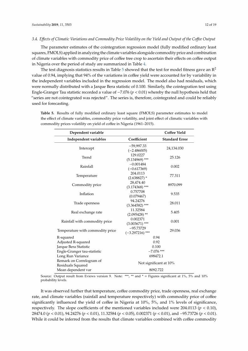
The parameter estimates of the cointegration regression model (fully modified ordinary leastsquares, FMOLS) applied in analyzing the climate variables alongside commodity price and combinationof climate variables with commodity price of coffee tree crop to ascertain their effects on coffee outputin Nigeria over the period of study are summarized in Table 4.
The test diagnosis statistics results in Table 5 showed that the test for model fitness gave an R2
value of 0.94, implying that 94% of the variations in coffee yield were accounted for by variability inthe independent variables included in the regression model. The model also had residuals, whichwere normally distributed with a Jarque Bera statistic of 0.100. Similarly, the cointegration test usingEngle-Granger Tau statistic recorded a value of −7.076 (p < 0.01) whereby the null hypothesis held that“series are not cointegrated was rejected”. The series is, therefore, cointegrated and could be reliablyused for forecasting.
Table 5. Results of fully modified ordinary least square (FMOLS) parameter estimates to modelthe effect of climate variables, commodity price volatility, and joint effect of climatic variables withcommodity prices volatility on yield of coffee in Nigeria (1961–2015).
Dependent variable Coffee Yield
Independent variables Coefficient Standard Error
Intercept −59,997.33(−2.486005) 24,134.030
Trend 129.0227(5.134969) *** 25.126
Rainfall −0.001484(−0.617369) 0.002
Temperature 204.0113(2.638827) * 77.311
Commodity price 28,474.40(3.174368) *** 8970.099
Inflation 0.757708(0.079467) 9.535
Trade openness 94.24276(3.364582) *** 28.011
Real exchange rate 11.32584(2.095428) ** 5.405
Rainfall with commodity price 0.002371(3.003671) *** 0.001
Temperature with commodity price −95.73729(−3.297216) *** 29.036
R-squared 0.94Adjusted R-squared 0.92Jarque Bera Statistic 0.100Engle-Granger tau-statistic −7.076 ***Long Run Variance 698472.1Remark on Correlogram ofResiduals Squared Not significant at 10%
Mean dependent var 8092.722
Source: Output result from Eviews version 9. Note: ***, ** and * = Figures significant at 1%, 5% and 10%probability levels.
It was observed further that temperature, coffee commodity price, trade openness, real exchangerate, and climate variables (rainfall and temperature respectively) with commodity price of coffeesignificantly influenced the yield of coffee in Nigeria at 10%, 5%, and 1% levels of significance,respectively. The slope coefficients of the mentioned variables included were 204.0113 (p < 0.10),28474.0 (p < 0.01), 94.24276 (p < 0.01), 11.32584 (p < 0.05), 0.002371 (p < 0.01), and −95.73726 (p < 0.01).While it could be inferred from the results that climate variables combined with coffee commodity
Sustainability 2019, 11, 3503 13 of 19
price together with trade openness and real exchange rate and coffee commodity price significantlydetermined the variability in yield of coffee over the period of study, temperature and precipitationchanges more so do not exert the expected effect on coffee yields.
While temperature increase resulted in an increase of yield of coffee during the review period,it was observed that coffee yields, however, responded negatively to the increase in temperaturecombined with coffee commodity price in the study. A percentage increase in the volume of temperatureresulted in an increase in coffee yield by 204.0113 tons; while a percentage rise in temperature combinedwith coffee commodity price resulted in a decrease in the yield of coffee by 95.73729 tons. The result isinconsistent with the findings of [44,66–68] who had positive and negative coefficients for temperatureand rainfall on a similar study in Nigeria.
The caveat that can be deduced from these findings is that other parameters may be needed inexplaining yield changes. Sometimes, climate change or variability can result in opportunities for anincrease in yield or productivity of crops depending on the agronomic requirements of the particularcrop under a particular, prevailing climate.
The indication from the result that showed that the combination of climate variable (temperature)with coffee commodity price exerted a negative significant influence on the yield of coffee in the studyimplies that an increase in value of combination of temperature with coffee commodity price wasaccompanied by a decrease in coffee yield by −95.73729 tons.
3.5. Effects of Climatic Variations, Commodity Prices Volatility, and Joint Effects of Climatic Variations withCommodity Prices Volatility on Coffee Production
In Table 6, results of parameter estimates for the FM-OLS models used to analyze the effects ofclimate variables, commodity prices, and joint effects of climate variables with commodity prices onproduction of coffee tree crop in Nigeria from 1961 to 2015 are presented.
The model estimates’ diagnosis of the residuals done for coffee production indicated that theseries was cointegrated with Engle–Granger Tau statistics of −6.575 (p > 0.06) implying that a long-runstable relationship does not exist among the series. The model’s residuals also exhibited a JarqueBera statistics of 6.014, implying that the residuals were normally distributed. With the estimatedcorrelogram of the residuals squared significant at 1%, it can be concluded that the residuals werenot fraught with serious threats of neither serial correlation nor severe multicollinearity in the model.The model also showed a good fit for the R2 level and, thus, implies a good fitting of the model.
As can be observed in Table 6, coffee production was significantly determined by six variablesthat included rainfall (6.27 × 10⁻⁶; p < 0.06), temperature (−1.919630; p < 0.06), coffee commodity price(−616.4039, p < 0.05), trade openness (0.062987; p < 0.02), and temperature with coffee commodityprice (620.0767, p < 0.05). The recorded significant effect of rainfall and combination of temperaturewith coffee commodity price implied that climate variability is an important factor influencing theproduction of coffee in Nigeria. It was specifically observed that a percentage increase of rainfallduring the period in review resulted in a production increase of coffee by 6.27 tons while a percentageincrease of the combination of temperature with coffee commodity during the period in review resultedin a production increase of coffee by 620.0767 tons. This result demonstrates the influence of climatevariables on farmers’ decision to produce coffee, showing that weather is important in determining theproduction of coffee in the country.
Amongst the six significant variables, rainfall, trade openness, and the combination of temperaturewith coffee commodity price posed as positive significant determinants of production of coffee inNigeria over the period of study. The effect implies that rainfall, trade openness, and the combinationof temperature with coffee commodity are huge determinant factors in coffee production and export.For instance, the slope coefficient of rainfall, trade openness, and the combination of temperature withthe coffee commodity in the study showed that a percentage increase in rainfall, trade openness, andthe combination of temperature with coffee commodity resulted in an increase in production of coffeeby about 6.27, 0.062987, and 620.0767 tons, respectively.
Sustainability 2019, 11, 3503 14 of 19
Table 6. Results of FMOLS parameter estimates to model the effect of climate variables, commodityprices volatility, and joint effect of climatic variables with commodity prices volatility on production ofcoffee in Nigeria (1961–2015).
Dependent Variable Coffee Production
Independent Variables Coefficient Standard Error Coefficient Standard Error
Intercept −1,561,618(−1.821641) * 857,259.1 −2905.669
(−2.419072) ** 1201.150
Trend 274.5286(0.341982) 802.757 0.038157
(2.813904) *** 0.014
Rainfall −0.077223(−0.959398) 0.081 6.27 × 10⁻⁶
(2.093096) **3.00E-06
Temperature 5805.777(2.128044) ** 2728.222 −1.919630
(−2.466962) ** 0.778
Commodity price 905,802.5(2.133219) ** 424617.6 −616.4039
(−2.446665) ** 251.936
Inflation 434.9243(1.320889) 329.266 0.002577
(0.054020) 0.048
Trade openness 2280.705(2.349205) ** 970.841 0.062987
(3.438604) *** 0.018
Real exchange rate 567.4082(2.767124) *** 205.053 −0.331229
(−3.195231) *** 0.104
Rainfall with commodityprice
0.175076(4.080897) *** 0.043 −3.985003
(−1.589991) 2.506
Temperature withcommodity price
−3328.699(−2.426696) ** 1371.7 620.0767
(2.456328) ** 252.441
R-squared 0.36Adjusted R-squared 0.21Jarque Bera Statistic 6.014Engle-Granger tau-statistic −6.575 **Long Run Variance 0.041624Remark on Correlogram ofResiduals Squared Significant at 1%
Mean dependent var 8.046639
Source: Output result from Eviews version 9. Note: ***, ** and * = Figures significant at 1%, 5% and 10%probability levels.
As for temperature, coffee commodity price, and real exchange rate, it was found that theirsignificant effects on the production of coffee were negative. It was specifically found that a percentagechange in their values resulted in a decrease in coffee production by 1.919630, 616.4039, and 0.331229tons, respectively in the economy during the period in review. This finding is similar to the findingsof [50] but disagrees with the findings of [46,48,54,55].
3.6. Test of Hypotheses
In Table 7, the results of pairwise Granger causality test on the relationship between coffee treecrop output, climate change variables, and coffee commodity price are presented.
Table 7. Pairwise Granger causality tests.
Null Hypothesis: Obs F-Statistic Prob.
The coffee output does not Granger Cause Rainfall 53 0.22433 0.7999Rainfall does not Granger Cause coffee output 0.19904 0.8202The coffee output does not Granger Cause Temperature 53 3.05113 * 0.0566Temperature does not Granger Cause coffee output 1.06039 0.3543Temperature does not Granger Cause D(coffee commodity price) 52 0.04543 0.9556D(commodity price) does not Granger Cause Temperature 0.38295 0.6840
Note: * = Figures significant at 10% probability levels.
Sustainability 2019, 11, 3503 15 of 19
Hypothesis 1. There is no significant relationship between the output of selected coffee tree crop and thevariation of rainfall in Nigeria.
The null hypothesis that held that rainfall did not Granger cause coffee output and vice versa wereaccepted as their F-Statistic were not significant at any probability level. This enabled us to concludethat rainfall has no significant relationship with the output of coffee and vice versa.
Hypothesis 2. Variation in temperature has no significant effect on coffee tree crop output in Nigeria.
In testing hypothesis two, the null hypothesis that coffee output did not Granger cause temperaturegave an F-Statistic of 3.05113 (p > 0.05) indicating that we have to reject the hypothesis at a significantvalue of 10%. This enabled us to conclude that coffee output influenced the variation of temperature.
It would, thus, be interpreted that the outputs of coffee in the previous year will transmitinformation to its producers, marketers, or exporters that there would be either glut or scarcity of theproduct in the present year as its output is associated with variation of temperature degrees. This will,in turn, influence the present international commodity prices of these tree crops.
Hypothesis 3. Commodity price volatility has no significant effect on coffee tree crop output in Nigeria.
The null hypotheses that held that the international commodity prices of coffee did not Grangercause coffee output and vice versa were accepted as their F-Statistic were not significant at anyprobability level. This enabled us to conclude that the commodity price of coffee tree crop has nosignificant effects on the outputs of coffee and vice versa.
3.7. Summary of Findings
The study examined the response of climate variability, commodity prices volatility, and otherselect macro-economic indicators on the output of coffee tree crop in Nigeria 1961–2015. Descriptivestatistics, GARCH, and ARCH models and the F-MOLS were analytical tools employed to realize thespecific objectives.
The descriptive analysis of the trend in commodity prices, yield, and production of coffee exporttree crop showed there are fluctuations (upward and downward trend) in price, yield, and productionof the coffee tree crop.
In determining the time series properties of data employed, the results of the unit root test byPhilip-Perron showed a mixed order of integration among the variables employed. That is to say that,some of the variables were nonstationary in their level form but became stationary when subjected tothe first difference.
The result from the volatility test shows that there is volatility in the international commodityprice of coffee. The coefficient of the lagged value of their commodity price had a significant positiverelationship with its current value over time for the study period. The variance equation value ofcoffee tree crops still confirmed the existence of volatility in their commodity prices within the periodunder study.
The analysis on the effects of climate variables, commodity price, and combination of climatevariables with commodity price to ascertain their effects on coffee tree crops yield using FM-OLSshowed that the model used had a good fit with their observed R2 levels and other diagnosis statistics.
Specifically, the yield of coffee showed that it was negatively affected by a combination of climatevariable (temperature) with coffee commodity price at 1% level of significance and positively affectedby temperature, coffee commodity price, trade openness, real exchange rate, and combination ofrainfall with coffee commodity at 10%, 1%, and 5% levels of significance, respectively.
Furthermore, coffee production result from the FM-OLS showed that it was positively influencedby rainfall, trade openness, and combination of temperature with coffee commodity price at different
Sustainability 2019, 11, 3503 16 of 19
levels of significance, respectively, and negatively by temperature, coffee commodity price, and realexchange rate, also at various levels of significance.
More so, the null hypothesis that held that rainfall did not Granger cause coffee output and viceversa were accepted while, the null hypothesis that coffee output did not Granger cause temperaturewas rejected. Also, the null hypotheses that held that the international commodity prices of coffee didnot Granger cause coffee output and vice versa and the null hypothesis that held that coffee output didnot Granger cause coffee commodity price were accepted. However, the null hypothesis that held thatcoffee output did not Granger cause temperature was rejected.
4. Conclusions
Based on the findings of this study, the conclusion, therefore, is that there is a need for tradefacilitation to reduce inherent risks in agribusiness marketing by re-introducing and re-invigorating theCentre for Agricultural Commodity Marketing (CACMART) by the Government of Nigeria throughits institutions.
Supplementary Materials: Supplementary materials are available online at http://www.mdpi.com/2071-1050/11/13/3503/s1.
Author Contributions: Conceptualization, A.O.I.; A.U.C.; U.N.O.; and G.N.O.; methodology, A.O.I., K.O.O;software, T.F.A.; L.A.; N.U.; and M.O.E.; validation, A.O.I.; A.A.I.; C.O.I.; and A.U.C.; formal analysis, A.O.I.;T.F.A; and L.A.; investigation, A.O.I; M.O.E and K.O.O; resources, A.O.I; C.O.I; and U.N.O.; data curation, A.O.I;A.A.I; and N.U.; writing—original draft preparation, A.O.I; G.N.O; T.F.A; C.O.I.; and K.O.O; writing—review andediting, A.O.I; visualization, A.O.I, G.N.O.; and A.U.C.; supervision, C.O.I and G.N.O.; project administration,A.O.I.; funding acquisition, A.O.I; U.N.O; and K.O.O.
Funding: This research received no external funding.
Acknowledgments: The authors acknowledge the contributions of Robert Onyeneke of AE-FUNAI and the twoanonymous peer reviewers of this manuscript for their constructive criticisms.
Conflicts of Interest: The authors declare no conflict of interest.
References
1. World Bank Group. Agribusiness and Value Chains. Understanding Poverty Report Updated. Availableonline: https://www.worldbank.org/en/topic/agribusiness (accessed on 24 September 2018).
2. African Development Bank (AfDB). Level 1 Development in Africa. In Annual Development EffectivenessReview; AfDB: Abidjan, Côte d’Ivoire, 2015.
3. World Bank Group. World Bank Report on the Potential of Agribusiness in Africa 2018. Available online:http://www.worldbank.org/en/news/feature/2013/03/04/africa-agribusiness-report (accessed on 15 March2019).
4. Akinbobola, T.O.; Adedokun, S.A.; Nwosa, P.I. The Impact of Climate Change on Composition of AgriculturalOutput in Nigeria. Am. J. Environ. Prot. 2015, 3, 44–47. Available online: http://pubs.sciepub.com/env/3/2/1/
env-3-2-1.pdf (accessed on 7 September 2016). [CrossRef]5. International Coffee Organization (ICO). World Coffee Production Report. 2019. Available online: http:
//www.ico.org/prices/po-production.pdf (accessed on 15 March 2019).6. Petchers, S.; Harris, S. The roots of the coffee crisis. In Confronting the Coffee Crisis: Fair Trade Sustainable
Livelihoods and Ecosystems in Mexico and Central America; Bacon, C.M., Méndez, V.E., Gliessman, S.R.,Goodman, D., Fox, J.A., Eds.; MIT Press: Cambridge, MA, USA, 2008; pp. 43–66.
7. International Coffee Organization (ICO). Volatility of Prices Paid to Coffee Growers in Selected Exporting Countries;ICO Document; ICC: London, UK, 2011; pp. 107–110.
8. International Coffee Council (ICC). Impact of the Coffee Crisis on Poverty in Producing Countries; 89th Session;ICC: Cartagena, Colombia, 2003; pp. 89–95, Rev. 1.
9. Ortiz-Miranda Dionisio, A.; Moragues-Faus, M. Governing Fair Trade Coffee Supply: Dynamics andChallenges in Small Farmers’ Organizations. Sustain. Dev. 2015, 23, 41–54. [CrossRef]
Sustainability 2019, 11, 3503 17 of 19
10. Food and Agriculture Organization (FAO). The State of Food Insecurity in the World 2011, Policy Options toAddress Price Volatility and High Prices. Available online: http://www.fao.org/docrep/014/i2330e/i2330e05.pdf (accessed on 7 September 2016).
11. African Development Bank (AfDB). AfDB Gender Strategy (2014–2018); AfDB: Tunis, Tunisia, 2014.12. Ayodeji, A.; Ajibola, C.; Oladipo Akogun, E.; Owoniyi Adebayo, C.; Shaba, M.; Mercy, N.; Halimat, S.;
Hamdalat Opeyemi, J. Gender Differentials among Subsistence Rice Farmers and Willingness to undertakeAgribusiness in Africa: Evidence and Issues from Nigeria. Afr. Dev. Rev. 2017, 29, 198–212, No. S2.
13. Federal Office of Statistics (FOS). Geography of Federal Republic of Nigeria; FOS: Malaysia, Vietnam, 1989.14. World Bank. Project Appraisal Document on a Proposed Credit for Transforming Irrigation Management in Nigeria
Project; World Bank: Washington, DC, USA, 2014.15. Food and Agriculture Organization (FAO). How to Feed the World in 2050, High Level Expert Forum-Office of
the Director, Agricultural Development Economics Division Economic and Social Development DepartmentViale delle Terme di Caracalla, 00153 Rome, Italy. 2009. Available online: http://www.fao.org/fileadmin/
templates/wsfs/docs/Issues_papers/HLEF2050_Investment.pdf (accessed on 7 September 2016).16. National Bureau of Statistics (NBS). National Bureau of Statistics Report on Nigerian Population Estimate as
at 2013. Available online: http://www.nigerianstat.gov.ng/pdfuploads/2014%20Statistical%20Report%20on%20Women%20and%20Men%20in%20Nigeria_.pdf (accessed on September 2016).
17. Nigerian Meteorological Agency (NIMET). Nigerian Meteorol Agency Report; NIMET: Kaduna, Nigeria, 2008.18. Phillips, S.J.; Anderson, R.P.; Schapire, R.E. Maximum entropy modeling of species geographic distributions.
Ecol. Model. 2006, 190, 231–259. [CrossRef]19. Schroth, G.; Laderach, P.; Dempewolf, J.; Philpott, S.M.; Haggar, J.P.; Eakin, H.; Castillejos, T.; Garcia-Moreno, J.;
Soto-Pinto, L.; Hernandez, R.; et al. Towards a climate change adaptation strategy for coffee communitiesand ecosystems in the Sierra Madre de Chiapas, Mexico. Mitig. Adapt. Strateg. Glob. Chang. 2009, 14, 605–625.[CrossRef]
20. Rahn, E.; Laderach, P.; Baca, M.; Cressy, C.; Schroth, G.; Malin, D.; van Rikxoort, H.; Shriver, J. Climatechange adaptation and mitigation in coffee production: Where are the synergies? Mitig. Adapt. StrategGlob. Chang. 2014. [CrossRef]
21. Laderach, P.; van Asten, P. Coffee and climate change. Coffee suitability in East Africa. In Proceedings of the9th African Fine Coffee Conference and Exhibition, Addis Ababa, Ethiopia, 16–18 February 2012.
22. Laderach, P.; Martinez, A.; Schroth, G.; Castro, N. Predicting the future climatic suitability for cocoa farmingof the world’s leading producer countries, Ghana and Côte d’Ivoire. Clim. Chang. 2013, 119, 841–854.[CrossRef]
23. Guardian. Much ado about Nigeria’s Dwindling Coffee Cultivation Level. Guardian Newspapers. 2019.Features Report By Gbenga Akinfenwa on 06 January 2019. Available online: https://guardian.ng/features/agro-care/much-ado-about-nigerias-dwindling-coffee-cultivation-level/ (accessed on 15 March 2019).
24. Hijmans, R.J.; Cameron, S.E.; Parra, J.L.; Jones, P.G.; Jarvis, A. Very high resolution interpolated climatesurfaces for global land areas. Int. J. Climatol. 2005, 25, 1965–1978. [CrossRef]
25. Lobo, J.M.; Tognelli, M.F. Exploring the effects of quantity and location of pseudo-absences and samplingbiases on the performance of distribution models with limited point occurrence data. J. Nat. Conserv. 2011,19, 1–7. [CrossRef]
26. Barbet-Massin, M.; Jiguet, F.; Albert, C.H.; Thuiller, W. Selecting pseudo-absences for species distributionmodels: How, where and how many? Methods Ecol. Evol. 2012, 3, 327–338. [CrossRef]
27. Schroth, G.; Läderach, P.; Blackburn, D.S.B.; Neilson, J.; Bunn, C. Winner or loser of climate change?A modeling study of current and future climatic suitability of Arabica coffee in Indonesia. Reg. Environ.Chang. 2015, 15, 1473–1482. [CrossRef]
28. Liu, C.; White, M.; Newell, G. Selecting thresholds for the prediction of species occurrence with presence-onlydata. J. Biogeogr. 2013, 40, 778–789. [CrossRef]
29. Kenen, P.B.; Rodrik, D. Measuring and Analysing the Effects of Short-term Volatility in Real Exchange Rate.Rev. Econ. Stat. 1986, 68, 311–315. [CrossRef]
30. Bailey, M.; George, T.; Micheal, U. Exchange Rate Variability and Trade Performance: Evidence for the BigSeven Industrial Countries. Weltwirlschaftliches Archiv. 1986, 1, 467–477. [CrossRef]
31. Peree, E.; Steineir, A. Exchange Rate Uncertainty and Foreign Trade. Eur. Econ. Rev. 1989, 33, 1241–1264.[CrossRef]
Sustainability 2019, 11, 3503 18 of 19
32. Côté, A. Exchange Rate Volatility and Trade: A Survey. In Bank of Canada. Working Paper; Bank of Canada:Ottawa, ON, Canada, 1994; pp. 94–95. Available online: https://www.bankofcanada.ca/wp-content/uploads/2010/04/wp94-5.pdf (accessed on 15 March 2019).
33. McKenzie, M.; Brooks, R.D. The impact of ERV on German-U.S Trade Flows. J. Int. Financ. Mark. Inst. Money1997, 7, 73–87. [CrossRef]
34. Engle, R.F. Autoregressive Conditional Heteroscedasticity with Estimates of the Variance of UK Inflation.Econometrica 1982, 50, 987–1008. [CrossRef]
35. Bollerslev, T. Generalized Autoregressive Conditional Heteroscedasticity. J. Econom. 1986, 6, 307–327.[CrossRef]
36. Yinusa, D.O. Between dollarization and Exchange Rate Volatility: Nigeria’s Portfolio Diversification Option.J. Policy Model. 2008, 30, 811–826. [CrossRef]
37. Akpokodje, G. Exchange rate volatility and External Trade: The Experience of Selected African Countries.In Applied Econometrics and Macroeconomic Modelling in Nigeria; Adeola, A., Dipo, B., Olofin, S., Eds.; IbadanUniversity Press: Ibadan, Nigerija, 2009; pp. 79–87.
38. Olowe, R.A. Modelling Naira/Dollar Exchange Rate Volatility: Application of GARCH and AssymetricModels. Int. Rev. Bus. Res. Pap. 2009, 5, 377–398.
39. Phillips, P.C.B.; Hansen, B.E. Statistical inference in instrumental variables regression with I (1) processes.Rev. Econ. Stud. 1990, 57, 99–125. [CrossRef]
40. Granger, C.W.J. Investigating Causal Relations by Econometric Models and Cross-Spectral Methods.Econometrica 1969, 37, 424–438. [CrossRef]
41. Philips, P.C.B.; Perron, P. Testing for a unit root in time series regression. Biometrika 1988, 73, 335–346.[CrossRef]
42. Abdul, Q.K.; Naima, S.; Syeda, T.F. Financial development, income inequality, and CO2 emissions in Asiancountries using STIRPAT model. Environ. Sci. Pollut. Res. 2018, 25, 6308–6319. [CrossRef]
43. Abbasi, F.; Riaz, K. CO2 emissions and financial development in an emerging economy: An augmented VARapproach. Energy Policy 2016, 90, 102–114. [CrossRef]
44. Ahmed, K.; Shahbaz, M.; Qasim, A.; Long, W. The linkages between deforestation, energy and growth forenvironmental degradation in Pakistan. Ecol. Indic. 2015, 49, 95–103. [CrossRef]
45. Al-Mulali, U.; Ozturk, I. The effect of energy consumption, urbanization, trade openness, industrial output,and the political stability on the environmental degradation in the MENA (Middle East and North African)region. Energy 2015, 84, 382–389. [CrossRef]
46. Bello, A.K.; Abimbola, O.M. Does the level of economic growth influence environmentalquality in Nigeria:A test of environmental Kuznets curve (EKC) hypothesis. Pak. J. Soc. Sci. 2010, 7, 325–329.
47. Dogan, E.; Turkekul, B. CO2 emissions, real output, energy consumption, trade, urbanization and financialdevelopment: Testing the EKC hypothesis for the USA. Environ. Sci. Pollut. Res. 2016, 23, 1203–1213.[CrossRef]
48. Fan, Y.; Liu, L.C.; Wu, G.; Wei, Y.M. Analyzing impact factors of CO2 emissions using STIRPAT model.Environ. Impact Assess. Rev. 2006, 26, 377–395. [CrossRef]
49. Farhani, S.; Ozturk, I. Causal relationship between CO2 emissions, real GDP, energy consumption, financialdevelopment, trade openness, and urbanization in Tunisia. Environ. Sci. Pollut. Res. 2015, 22, 15663–15676.[CrossRef] [PubMed]
50. Islam, F.; Shahbaz, M.; Alam, M. Financial development and energy consumption nexus in Malaysia:A multivariate time series analysis. In MPRA Paper 28403; University Library of Munich: Munch, Germany,2011.
51. Jalil, A.; Feridun, M. The impact of growth, energy and financial development on the environment in China:A cointegration analysis. Energy Econ. 2011, 33, 284–291. [CrossRef]
52. Azam, M.; Khan, A.Q.; Bakhtyar, B.; Emirullah, C. The causal relationship between energy consumption andeconomic growth in the ASEAN-5 countries. Renew. Sustain. Energy Rev. 2015, 47, 732–745. [CrossRef]
53. Lau, L.S.; Choong, C.; Eng, Y.K. Investigation of the environmental Kuznets curve for carbon emissions inMalaysia: Do foreign direct investment and trade matter? Energy Policy 2014, 68, 490–497. [CrossRef]
Sustainability 2019, 11, 3503 19 of 19
54. Lin, S.; Zhao, D.; Marinova, D. Environmental impact of China: Analysis based on the STIRPAT model.In Proceedings of the Second International Association for Energy Economics (IAEE) Asian Conference,Perth, Australia, 5–7 November 2008; Cabalu, H., Marinova, D., Eds.; Curtin University of Technology: Perth,Australia, 2008; pp. 164–192.
55. Ozturk, I.; Acaravci, A. The long-run and causal analysis of energy, growth, openness and financialdevelopment on carbon emissions in Turkey. Energy Econ. 2013, 36, 262–267. [CrossRef]
56. Acaravci, A.; Ozturk, I. On the relationship between energy consumption, CO2 emissions and economicgrowth in Europe. Energy 2010, 35, 5412–5420. [CrossRef]
57. Saboori, B.; Soleymani, A. CO2 emissions, economic growth and energy consumption in Iran: A cointegrationapproach. Int. J. Environ. Sci. 2011, 2, 44–53.
58. Sadorsky, P. The impact of financial development on energy consumption in emerging economies.Energy Policy 2010, 38, 2528–2535. [CrossRef]
59. Shahbaz, M.; Mutascu, M.; Azim, P. Environmental Kuznets curve in Romania and the role of energyconsumption. Renew. Sustain. Energy Rev. 2013, 18, 165–173. [CrossRef]
60. Hahbazm, O.I.; Afza, T.; Ali, A. Revisiting the environmental Kuznets curve in a global economy.Renew. Sustain. Energy Rev. 2013, 25, 494–502.
61. Shahbaz, M.; Hye, Q.; Tiwari, A.K.; Leitão, N.C. Economic growth, energy consumption, financialdevelopment, international trade and CO2 emissions in Indonesia. Renew. Sustain. Energy Rev. 2013,25, 109–121. [CrossRef]
62. Ziaei, S.M. Effects of financial development indicators on energy consumption and CO2 emission of European,East Asian and Oceania countries. Renew. Sustain. Energy Rev. 2015, 42, 752–759. [CrossRef]
63. Yusuf, S.A.; Yusuf, W.A. Determinants of selected agricultural export crops in Nigeria: An ECM approach.In Proceedings of the African Association of Agricultural Economists, Abuja Nigeria, 23–26 September 2007;pp. 469–472.
64. Cashin, P.; Céspedes, L.; Sahay, R. Commodity Currencies and the Real Exchange Rate. J. Dev. Econ. 2004, 75,239–268. [CrossRef]
65. Musunuru, N. Testing the presence of calendar anomalies in agricultural commodity markets. Reg. Bus. Rev.2013, 32, 32–47.
66. Kalu, C. Impact of Climate Variability and Change on Supply of Grain in Nigeria from 1961–2012. UnpublishedPh.D. Dissertation, Department of Agribusiness and Management, Michael Okpara University of Agriculture,Umudike, Abia State, Nigeria, 2015; pp. 28–45.
67. Lloyd, T.A.; McCorriston, S.; Morgan, C.W.; Zgovu, E. The Experience of Food Price Inflation across the EU.In TRANSFOP; Working Paper No.5, TRANSFOP Project, EU 7th Framework Programme, Grant AgreementNo. KBBE-265601-4-TRANSFOP; 2014; Available online: http://www.transfop.eu/ (accessed on 7 September2016).
68. Ayinde, O.E.; Ojehomon, V.E.T.; Daramola, F.S.; Falaki, A.A. Evaluation of the effects of climate change onrice production in Niger State, Nigeria. Ethiop. J. Environ. Stud. Manag. 2013, 6, 763–773. [CrossRef]
© 2019 by the authors. Licensee MDPI, Basel, Switzerland. This article is an open accessarticle distributed under the terms and conditions of the Creative Commons Attribution(CC BY) license (http://creativecommons.org/licenses/by/4.0/).