Gance et al

8/7/2019 Gance et al

http://slidepdf.com/reader/full/gance-et-al 1/6



Each material is attributed to a group by the samealgorithm so that the materials belonging to a grouphave some mechanical properties in common (Figure

1). The number of group is also arbitrary fixed.

2.2 Determination of the hydro-mechanicalparameters

After the mesh has been created, the program at-tributes to each material the values of 9 hydro-mechanical parameters necessary to define theDrucker-Prager constitutive law in GEFDYN.

Figure 1. Creation of a mesh from the Vp data grid.

Four of these parameters are identical to all mate-

rials composing a group. These properties are the

solid density, the cohesion, the friction angle and thePoisson ratio. If the model is constituted of 3 groups,three different sets of parameters need to be speci-fied.

The other parameters are supposed to vary spa-tially within a specific material; they are calculatedfor each of them from the Vp values and the constantparameters of the group. Although the petrophysicalrelationships used for this estimation are rather validfor rocks, they have been selected because of theirsimplicity and their coherent results in most of geo-logical materials. By this mean, continuous varia-tions of realistic parameters can be modelled, even if the reality is anyway more complex to describe. Theparameters derived from Vp are the following: - The porosity n: it is calculated with the relationproposed by Castagna (1985):

clp V nV 221094205810

(1)

where n refers to the porosity in percent, V cl, the clayvolume in percent. V cl is taken equal to zero to keep

a good range of porosity in the model. - The Young modulus E : it is calculated with a rela-tion restricted to isotropic homogeneous medium:

1

2112

pvE (2)

- The permeability k is calculated with the relationproposed by Berg (1970):

)385.1exp(101,5 21.56d k (3)

Where k is the permeability in darcy; is porosity in

percent, d is median diameter of grains in mm, φ isthe standard deviation and equals to P90 – P10.

We choose, after calibration, φ = 0 and d = 0.12mm. The coefficient of earth pressure at rest is cal-culated from the friction angle:

sin10K (4)

The friction angle will be taken under 35.3° for thegood accuracy of the results (Desrues 2002).

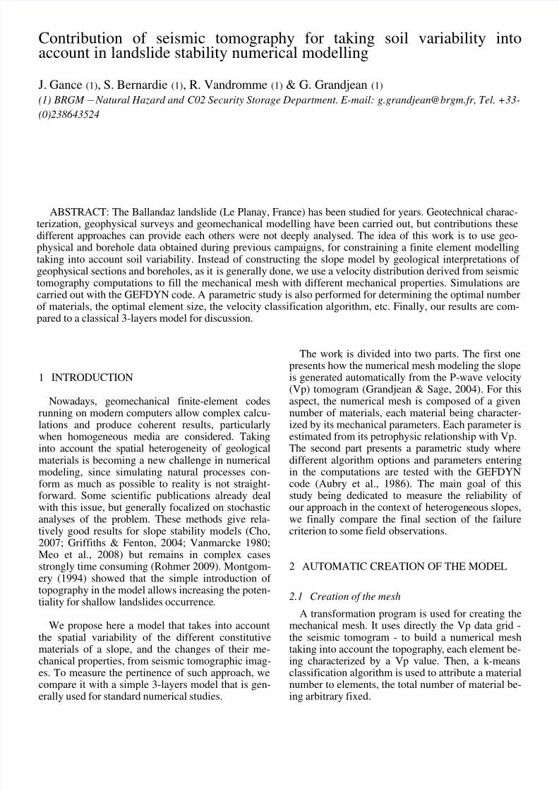
Figure 2 (top) shows the mesh constituted by thethree different groups, each group containing a cer-tain number of materials (non-visible here), and eachmaterial being defined by 9 hydro-mechanical prop-erties. Figure 2 (bottom) shows the classical 3-layersmodel to compare.

Figure 2. Model created automatically from the Vp data

grid (top). 3-layers model used for the comparison.

2.3 Boundary conditions

The calculations were carried out with the Druck-er-Prager constitutive law defined in the GEFDYNfinite-elements code, using the plane strain approxi-

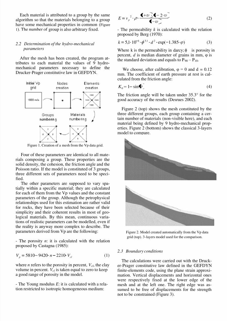
mation. Vertical displacements and horizontal oneswere respectively fixed at the lower edge of themesh and at the left one. The right edge was as-sumed to be free of displacements for the strengthnot to be constrained (Figure 3).



In the case of hydro-mechanical calculation, the

pore pressure is imposed at each node. We model thepresence of water using a linear water table. All thepressures imposed are hydrostatic ones (Figure 4).The simulation then refers to a non-coupled hydro-mechanical calculation.

Figure 3. Conditions on displacements.

Figure 4. Imposed pore pressure.

3 RESULTS OF CALCULATIONS

3.1 Preliminary tests on the size of the elements and the number of materials

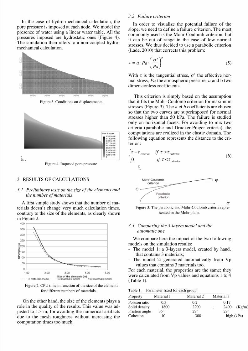
A first simple study shows that the number of ma-terials doesn’t change very much calculation times,contrary to the size of the elements, as clearly shownin Figure 2.

Figure 2. CPU time in function of the size of the elements

for different numbers of materials.

On the other hand, the size of the elements plays arole in the quality of the results. This value was ad-justed to 1.3 m, for avoiding the numerical artifactsdue to the mesh roughness without increasing thecomputation times too much.

3.2 Failure criterion

In order to visualize the potential failure of theslope, we need to define a failure criterion. The mostcommonly used is the Mohr-Coulomb criterion, butit can be out of range in the case of low normalstresses. We thus decided to use a parabolic criterion(Lade, 2010) that corrects this problem:

b

PaPaa ' (5)

With τ is the tangential stress, σ’ the effective nor-mal stress, Pa the atmospheric pressure, a and b twodimensionless coefficients.

This criterion is simply based on the assumption

that it fits the Mohr-Coulomb criterion for maximumstresses (Figure 3). The a et b coefficients are chosenso that the two curves are superimposed for normalstresses higher than 50 kPa. The failure is studiedonly on horizontal facets. For avoiding to mix twocriteria (parabolic and Drucker-Prager criteria), thecomputations are realized in the elastic domain. Thefollowing equation represents the distance to the cri-terion:

criterion

criterioncriterion

if

if

0(6)

Figure 3. The parabolic and Mohr-Coulomb criteria repre-

sented in the Mohr plane.

3.3 Comparing the 3-layers model and theautomatic one.

We compare here the impact of the two followingmodels on the simulation results:- The model 1: a 3-layers model, created by hand,

that contains 3 materials;- The model 2: generated automatically from Vp

values that contains 3 materials too.For each material, the properties are the same; theywere calculated from Vp values and equations 1 to 4(Table 1). Table 1. Parameter fixed for each group.______________________________________________Property Material 1 Material 2 Material 3______________________________________________Poisson ratio 0.3 0.2 0.17Solid density 1800 2200 , 2400 (Kg/mFriction angle 35° 29° 29°Cohesion 10 300 high (kPa)



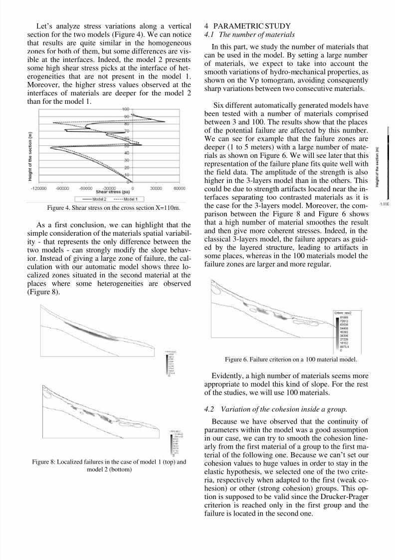
Let’s analyze stress variations along a verticalsection for the two models (Figure 4). We can noticethat results are quite similar in the homogeneouszones for both of them, but some differences are vis-ible at the interfaces. Indeed, the model 2 presentssome high shear stress picks at the interface of het-erogeneities that are not present in the model 1.Moreover, the higher stress values observed at the

interfaces of materials are deeper for the model 2than for the model 1.

Figure 4. Shear stress on the cross section X=110m.

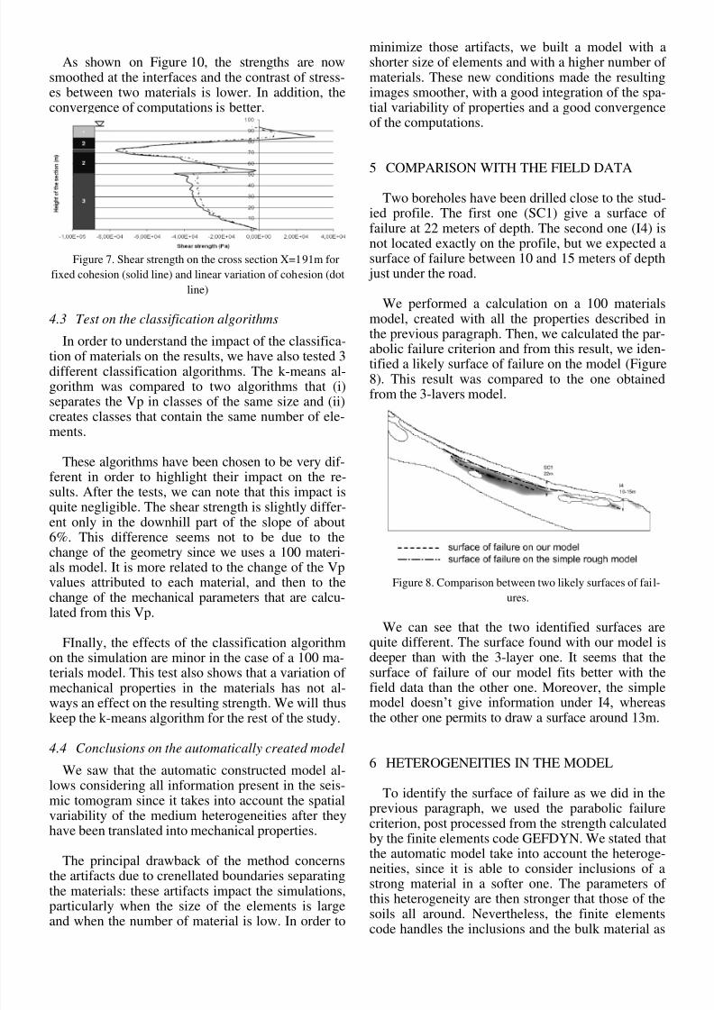
As a first conclusion, we can highlight that the

simple consideration of the materials spatial variabil-ity - that represents the only difference between thetwo models - can strongly modify the slope behav-ior. Instead of giving a large zone of failure, the cal-culation with our automatic model shows three lo-calized zones situated in the second material at the

places where some heterogeneities are observed(Figure 8).

Figure 8: Localized failures in the case of model 1 (top) and

model 2 (bottom)

4 PARAMETRIC STUDY4.1 The number of materials

In this part, we study the number of materials thatcan be used in the model. By setting a large numberof materials, we expect to take into account thesmooth variations of hydro-mechanical properties, asshown on the Vp tomogram, avoiding consequentlysharp variations between two consecutive materials.

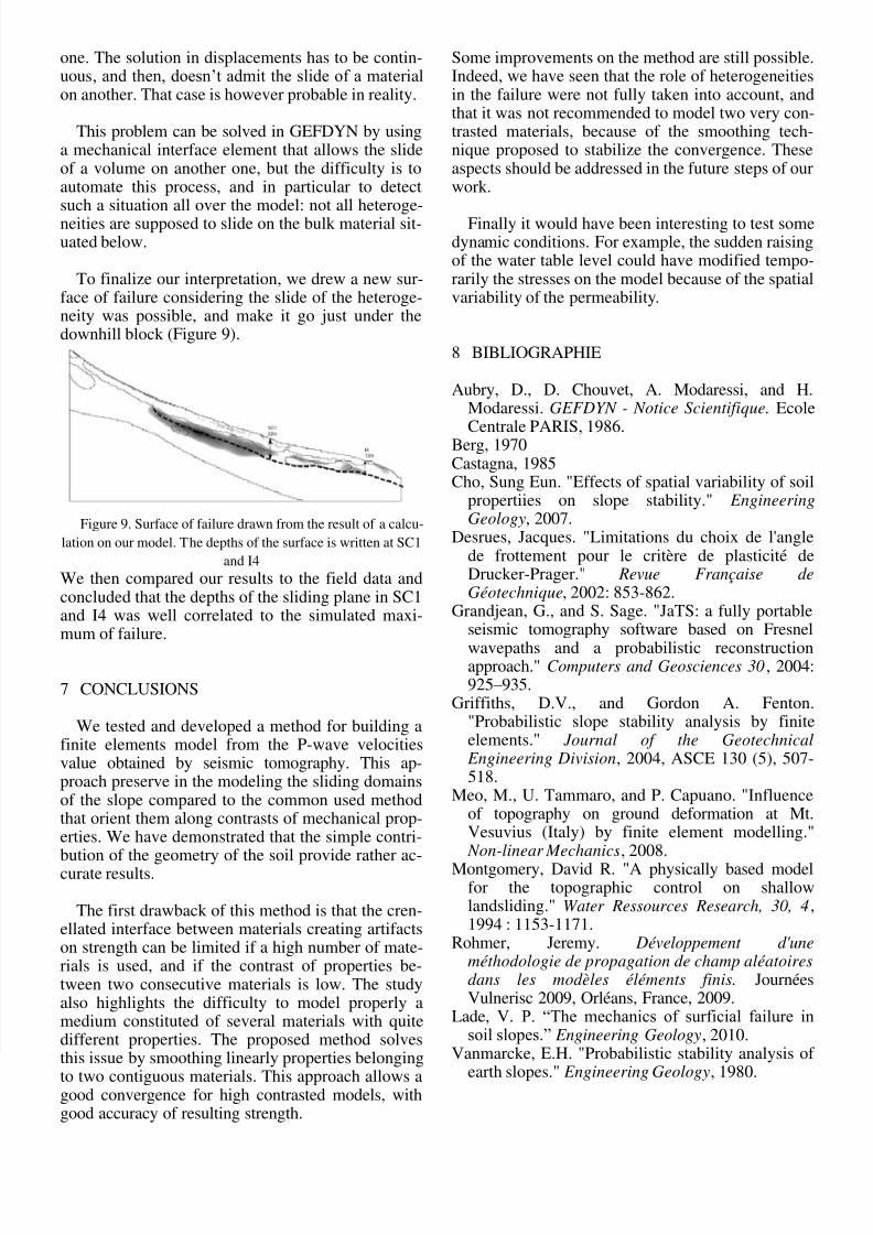
Six different automatically generated models have

been tested with a number of materials comprisedbetween 3 and 100. The results show that the placesof the potential failure are affected by this number.We can see for example that the failure zones aredeeper (1 to 5 meters) with a large number of mate-rials as shown on Figure 6. We will see later that thisrepresentation of the failure plane fits quite well withthe field data. The amplitude of the strength is alsohigher in the 3-layers model than in the others. This

could be due to strength artifacts located near the in-terfaces separating too contrasted materials as it isthe case for the 3-layers model. Moreover, the com-parison between the Figure 8 and Figure 6 showsthat a high number of material smoothes the resultand then give more coherent stresses. Indeed, in theclassical 3-layers model, the failure appears as guid-ed by the layered structure, leading to artifacts insome places, whereas in the 100 materials model thefailure zones are larger and more regular.

Figure 6. Failure criterion on a 100 material model.

Evidently, a high number of materials seems more

appropriate to model this kind of slope. For the restof the studies, we will use 100 materials. 4.2 Variation of the cohesion inside a group.

Because we have observed that the continuity of parameters within the model was a good assumptionin our case, we can try to smooth the cohesion line-arly from the first material of a group to the first ma-terial of the following one. Because we can’t set our cohesion values to huge values in order to stay in theelastic hypothesis, we selected one of the two crite-

ria, respectively when adapted to the first (weak co-hesion) or other (strong cohesion) groups. This op-tion is supposed to be valid since the Drucker-Pragercriterion is reached only in the first group and thefailure is located in the second one.



As shown on Figure 10, the strengths are now

smoothed at the interfaces and the contrast of stress-es between two materials is lower. In addition, theconvergence of computations is better.

Figure 7. Shear strength on the cross section X=191m for

fixed cohesion (solid line) and linear variation of cohesion (dot

line) 4.3 Test on the classification algorithms

In order to understand the impact of the classifica-tion of materials on the results, we have also tested 3different classification algorithms. The k-means al-gorithm was compared to two algorithms that (i)separates the Vp in classes of the same size and (ii)creates classes that contain the same number of ele-ments.

These algorithms have been chosen to be very dif-ferent in order to highlight their impact on the re-sults. After the tests, we can note that this impact isquite negligible. The shear strength is slightly differ-

ent only in the downhill part of the slope of about6%. This difference seems not to be due to thechange of the geometry since we uses a 100 materi-als model. It is more related to the change of the Vpvalues attributed to each material, and then to thechange of the mechanical parameters that are calcu-lated from this Vp.

FInally, the effects of the classification algorithmon the simulation are minor in the case of a 100 ma-terials model. This test also shows that a variation of

mechanical properties in the materials has not al-ways an effect on the resulting strength. We will thuskeep the k-means algorithm for the rest of the study. 4.4 Conclusions on the automatically created model

We saw that the automatic constructed model al-lows considering all information present in the seis-mic tomogram since it takes into account the spatialvariability of the medium heterogeneities after theyhave been translated into mechanical properties.

The principal drawback of the method concernsthe artifacts due to crenellated boundaries separatingthe materials: these artifacts impact the simulations,particularly when the size of the elements is largeand when the number of material is low. In order to

minimize those artifacts, we built a model with ashorter size of elements and with a higher number of materials. These new conditions made the resultingimages smoother, with a good integration of the spa-tial variability of properties and a good convergenceof the computations.

5 COMPARISON WITH THE FIELD DATA Two boreholes have been drilled close to the stud-

ied profile. The first one (SC1) give a surface of failure at 22 meters of depth. The second one (I4) isnot located exactly on the profile, but we expected asurface of failure between 10 and 15 meters of depthjust under the road.

We performed a calculation on a 100 materials

model, created with all the properties described inthe previous paragraph. Then, we calculated the par-

abolic failure criterion and from this result, we iden-tified a likely surface of failure on the model (Figure8). This result was compared to the one obtainedfrom the 3-layers model.

Figure 8. Comparison between two likely surfaces of fail-

ures.

We can see that the two identified surfaces arequite different. The surface found with our model isdeeper than with the 3-layer one. It seems that thesurface of failure of our model fits better with the

field data than the other one. Moreover, the simplemodel doesn’t give information under I4, whereasthe other one permits to draw a surface around 13m.

6 HETEROGENEITIES IN THE MODEL

To identify the surface of failure as we did in theprevious paragraph, we used the parabolic failurecriterion, post processed from the strength calculatedby the finite elements code GEFDYN. We stated thatthe automatic model take into account the heteroge-

neities, since it is able to consider inclusions of astrong material in a softer one. The parameters of this heterogeneity are then stronger that those of thesoils all around. Nevertheless, the finite elementscode handles the inclusions and the bulk material as



one. The solution in displacements has to be contin-uous, and then, doesn’t admit the slide of a materialon another. That case is however probable in reality.

This problem can be solved in GEFDYN by usinga mechanical interface element that allows the slideof a volume on another one, but the difficulty is toautomate this process, and in particular to detect

such a situation all over the model: not all heteroge-neities are supposed to slide on the bulk material sit-uated below.

To finalize our interpretation, we drew a new sur-

face of failure considering the slide of the heteroge-neity was possible, and make it go just under thedownhill block (Figure 9).

Figure 9. Surface of failure drawn from the result of a calcu-

lation on our model. The depths of the surface is written at SC1

and I4 We then compared our results to the field data andconcluded that the depths of the sliding plane in SC1and I4 was well correlated to the simulated maxi-

mum of failure.

7 CONCLUSIONS

We tested and developed a method for building afinite elements model from the P-wave velocitiesvalue obtained by seismic tomography. This ap-proach preserve in the modeling the sliding domainsof the slope compared to the common used methodthat orient them along contrasts of mechanical prop-

erties. We have demonstrated that the simple contri-bution of the geometry of the soil provide rather ac-curate results.

The first drawback of this method is that the cren-

ellated interface between materials creating artifactson strength can be limited if a high number of mate-rials is used, and if the contrast of properties be-tween two consecutive materials is low. The studyalso highlights the difficulty to model properly amedium constituted of several materials with quitedifferent properties. The proposed method solves

this issue by smoothing linearly properties belongingto two contiguous materials. This approach allows agood convergence for high contrasted models, withgood accuracy of resulting strength.

Some improvements on the method are still possible.Indeed, we have seen that the role of heterogeneitiesin the failure were not fully taken into account, andthat it was not recommended to model two very con-trasted materials, because of the smoothing tech-nique proposed to stabilize the convergence. Theseaspects should be addressed in the future steps of ourwork.

Finally it would have been interesting to test somedynamic conditions. For example, the sudden raisingof the water table level could have modified tempo-rarily the stresses on the model because of the spatialvariability of the permeability.

8 BIBLIOGRAPHIE

Aubry, D., D. Chouvet, A. Modaressi, and H.Modaressi. GEFDYN - Notice Scientifique. Ecole

Centrale PARIS, 1986.Berg, 1970Castagna, 1985Cho, Sung Eun. "Effects of spatial variability of soil

propertiies on slope stability." EngineeringGeology, 2007.

Desrues, Jacques. "Limitations du choix de l'anglede frottement pour le critère de plasticité deDrucker-Prager." Revue Française deGéotechnique, 2002: 853-862.

Grandjean, G., and S. Sage. "JaTS: a fully portable

seismic tomography software based on Fresnelwavepaths and a probabilistic reconstructionapproach." Computers and Geosciences 30, 2004:925– 935.

Griffiths, D.V., and Gordon A. Fenton."Probabilistic slope stability analysis by finiteelements." Journal of the GeotechnicalEngineering Division, 2004, ASCE 130 (5), 507-518.

Meo, M., U. Tammaro, and P. Capuano. "Influenceof topography on ground deformation at Mt.Vesuvius (Italy) by finite element modelling."

Non-linear Mechanics, 2008.Montgomery, David R. "A physically based model

for the topographic control on shallowlandsliding." Water Ressources Research, 30, 4,1994 : 1153-1171.

Rohmer, Jeremy. Développement d'uneméthodologie de propagation de champ aléatoiresdans les modèles éléments finis. JournéesVulnerisc 2009, Orléans, France, 2009.

Lade, V. P. “The mechanics of surficial failure insoil slopes.” Engineering Geology, 2010.

Vanmarcke, E.H. "Probabilistic stability analysis of earth slopes." Engineering Geology, 1980.

Documents

Gance et al