Embed Size (px)
Citation preview

Discussion Paper No. 308
The Minimum Approval Mechanism Implements the Efficient
Public Good Allocation Theoretically and Experimentally
Takehito Masuda, Yoshitaka Okano, and Tatsuyoshi Saijo
May 2013; revised September 2013
GCOE Secretariat Graduate School of Economics
OSAKA UNIVERSITY 1-7 Machikaneyama, Toyonaka, Osaka, 560-0043, Japan
GCOE Discussion Paper Series
Global COE Program Human Behavior and Socioeconomic Dynamics

The Minimum Approval Mechanism Implements the Efficient Public Good Allocation
Theoretically and Experimentally
September 2013
Takehito Masuda a,b,*, Yoshitaka Okano c, and Tatsuyoshi Saijo c, d
a Graduate School of Economics, Osaka University 1-7, Machikaneyama, Toyonaka, Osaka 560-0043, Japan
b Research Fellow of the Japan Society for the Promotion of Science, Kojimachi Business Center Building,
5-3-1 Kojimachi, Chiyoda, Tokyo 102-0083, Japan
c Research Center for Social Design Engineering, Kochi University of Technology, Tosayamada, Kami, Kochi
782-8502, Japan
d Center for Environmental Innovation Design for Sustainability, Osaka University, 2-1 Yamada-oka, Suita, Osaka
565-0871, Japan
Abstract
We propose the minimum approval mechanism (MAM) for a standard linear public good
environment with two players. Players simultaneously and privately choose their
contributions to the public good in the first stage. In the second stage, they simultaneously
decide whether to approve the other’s choice. Both contribute what they choose in the first
stage if both players approve; otherwise, both contribute the minimum of the two choices
in the first stage. The MAM multiply implements the Pareto-efficient allocation in
backward elimination of weakly dominated strategies (BEWDS), limit logit agent quantal
response equilibrium, subgame perfect minimax regret equilibrium, level-k thinking, and
diagonalization heuristics. Moreover, the MAM is unique under plausible conditions.
Overall, contributions in the MAM experiment averaged 94.9%. Quantifying subjects’
responses to the questionnaire revealed the heterogeneity of reasoning processes to be
consistent with the model.
JEL Classification: C72; C92; D74; H41; P43
Keywords: Public good experiment; Approval mechanism; Multiple implementation
* Corresponding author. Postal address: Research Center for Social Design Engineering, Kochi University of Technology, Tosayamada, Kami, Kochi 782-8502, Japan. Tel.: +81-887-57-2795; Fax: +81-887-57-2366. E-mail addresses: [email protected] (T. Masuda), [email protected] (Y. Okano), and [email protected] (T. Saijo). Abbreviations: MAM = minimum approval mechanism, BEWDS = backward elimination of weakly dominated strategies, MCM = mate choice mechanism.
1
1. Introduction
The free-rider problem lies at the heart of public good provision. To solve this problem,
theorists have traditionally concentrated on designing mechanisms yielding efficient
outcomes, given that players are self-interested. In this mechanism design or
implementation approach, individual theorists have discretion over which equilibrium
concept or behavioral rule to use, such as dominant strategy equilibrium, Nash equilibrium,
or subgame perfect Nash equilibrium (SPNE). However, recent experimental results have
raised questions concerning this fundamental assumption.1 It is also widely observed that
experimental subjects are heterogeneous in their motive to choose their contributions to the
public good.
We offer an alternative approach, multiple implementations, in order to bridge
gaps between the theory and experiments. That is, public good mechanisms should be
robust to as many as possible equilibrium concepts or behavioral rules. More precisely, we
design the minimum approval mechanism (MAM) that multiply implements the
symmetric Pareto-efficient allocation for linear public good environments with two players.
The MAM consists of two stages. Each player chooses his/her contribution in the
first stage, following which each player observes the other’s choice and approves or
disapproves the same. If both players approve, their final contributions are what they chose
in the first stage. If either disapproves, both finally contribute the minimum of their
first-stage choices.
Under the MAM, both players fully contribute in all five equilibrium concepts or
heuristics: (i) backward elimination of weakly dominated strategies (BEWDS; Saijo et al.,
2013)2, (ii) limit logit agent quantal response equilibrium (limit LAQRE; Mckelvey and
Palfrey, 1995; 1998), (iii) subgame perfect minimax regret equilibrium (SPMRE; Renou and
Schlag, 2011), (iv) level-k thinking (Costa-Gomes and Crawford, 2006), and (v)
diagonalization heuristics.
Moreover, we show that the MAM is a unique BEWDS-implementing approval
mechanism, satisfying the following natural properties. Forthrightness requires that the
outcome must be what players choose whenever both approve the other's first-stage
choices. Voluntariness mandates that no player is forced to finally contribute more than
what he/she chooses in the first stage.3 Monotonicity states that final contributions increase
as their first-stage choices increase.
In experiments under the perfect stranger matching protocol, we observe, as
predicted, a rapid convergence to efficient allocation in the MAM. Subjects successfully
1 See Chen (2008) for an excellent survey. 2 As Saijo et al. (2013) noted, Kalai (1981) used BEWDS. 3 In other words, we only provide refunds to players, rather than using coercive power.
2

sustained high average contribution rates, beginning with 76.9% in the first period and
ending with 89.7% in the final period. The overall average contribution rate is 94.9%.4 Our
experimental results of the MAM are in sharp contrast with those of existing mechanisms
that need dozens of iterations to converge to the efficient Nash equilibrium in experiments.
We also conduct experiments for the mate choice mechanism (MCM) of Saijo et al. (2013),
which theoretically does not work in our public good environment and observe that the
average contribution fluctuates within a middle range.
In order to capture subjects’ reasoning processes, we apply a coding scheme
similar to the one of Cooper and Kagel (2005). Two coders independently quantified
subjects’ responses to open questions during and after the session. The coding confirms
that subjects are heterogeneous in their motive. In particular, 20.0% of subjects in the MAM
are deemed to have used diagonalization heuristics. Moreover, 16.7% and 11.7% of subjects
in the MAM and MCM, respectively are deemed to minimize regret. Finally, 21.7% and
45.0% of subjects in the MCM are deemed to have followed level-1 and level-2 thinking,
respectively.
Our approach differs from much of the experimental research on the public good
mechanism, which thus far has mainly focused on evaluating mechanism designs based on
dominant strategy equilibrium, Nash equilibrium, or SPNE. For dominant strategy
mechanisms, Attiyeh et al. (2000) found that subjects in the pivotal mechanism frequently
misrepresent their private information and become stuck at a weakly dominated Nash
equilibrium. To solve this problem, Saijo et al. (2007) introduced secure implementation (or
double implementation in dominant strategy equilibrium and Nash equilibrium). Further,
Cason et al. (2006) experimentally showed that the frequency of dominant strategy play
was significantly increased in a secure Groves–Clarke mechanism relative to a nonsecure
pivotal mechanism, although the former’s frequency was only slightly over 80%.
The Groves–Ledyard (Groves and Ledyard, 1977) and Walker (1981) mechanisms
have difficulty in attaining efficient Nash equilibria in one-shot play, because of subjects’
bounded rationalities.5 Andreoni and Varian (1999) reported similar results for Varian’s
(1994) extensive form mechanism with the unique SPNE. Chen and Plott (1996), Chen and
Tang (1998), Chen and Gazzale (2004), Healy (2006), and Healy and Mathevet (2012)
characterized the stable mechanisms to achieve efficient Nash equilibria as rest points of
various learning dynamics. Nonetheless, these studies still required dozens of repetitions,
which may not be feasible in practical situations. A notable exception is Falkinger et al.
(2000), who observed that under Falkinger’s (1996) mechanism, contributions approached
4 We obtained a similar result in the simplified MAM (SMAM) treatment, in which the player with the higher first-stage choice alone can proceed to the second stage. 5 See Chen and Plott (1996) and Chen and Tang (1998).
3
the efficient Nash equilibrium in only a few periods.6
The remainder of this paper is organized as follows. Section 2 overviews the
MCM proposed by Saijo et al. (2013), introduces the MAM with examples, and presents the
implementation results. Section 3 describes the proof of the uniqueness of the MAM.
Section 4 argues in favor of the MAM’s robustness. Section 5 describes the experimental
design. Section 6 discusses the experimental results. Section 7 provides an analysis of
subjects’ responses to the open-ended questionnaire. Section 8 discusses further
implications and concludes.
2. The model and the MAM
Consider a voluntary contribution mechanism (VCM) in the provision of a public good
with two players. Each player i has an initial endowment w > 0, and he/she must decide
the contribution [0, ]is S w∈ = . The sum of the contribution is multiplied by (0.5, 1)α∈ ,
and the benefit passes to every player, which expresses the non-rivalness of the public
good. That is, player i’s payoff is ( , ) ( ) ( ),i i j i i ju s s w s s s j i= − +α + ≠ . Then, 1 2 0s s= = is the
dominant strategy equilibrium, and hence, no public good is provided. When there are only two levels of the contribution (i.e., 0 or w) when players face
the prisoner’s dilemma, Saijo et al. (2013) introduced the notion of the MCM following the
dilemma decision. By knowing the other player’s choice between cooperation (contributing
w and abbreviated by C) and defection (contributing 0 and abbreviated by D) in the
dilemma or the first stage, each player must approve (y) or disapprove (n) it. If both players
approve the choices of their counterparts in the first stage, the outcome or payoff vector is
what they choose. If either player disapproves, however, the outcome is that when both
choose D.
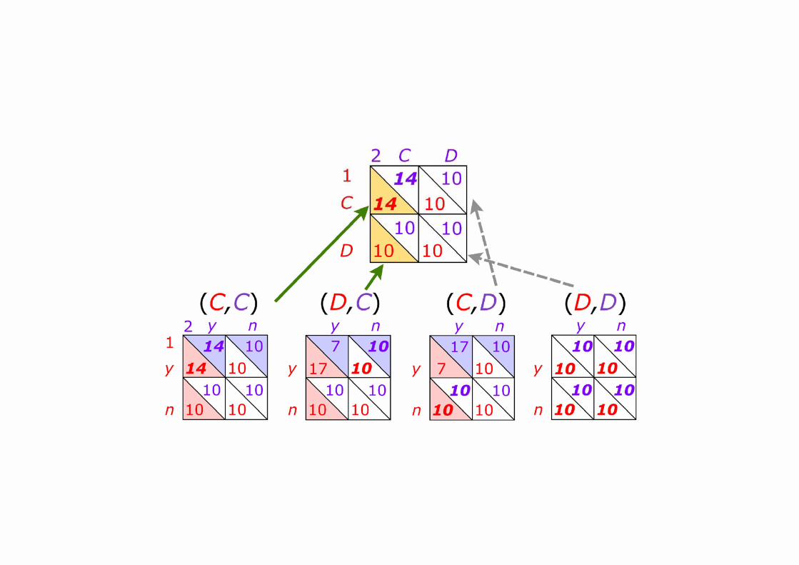
<Figure 1 about here.>
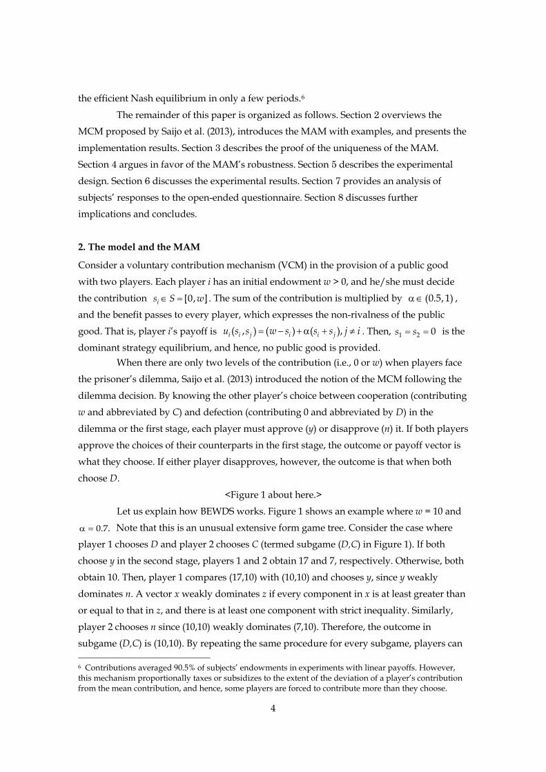
Let us explain how BEWDS works. Figure 1 shows an example where w = 10 and
0.7.α = Note that this is an unusual extensive form game tree. Consider the case where
player 1 chooses D and player 2 chooses C (termed subgame (D,C) in Figure 1). If both
choose y in the second stage, players 1 and 2 obtain 17 and 7, respectively. Otherwise, both
obtain 10. Then, player 1 compares (17,10) with (10,10) and chooses y, since y weakly
dominates n. A vector x weakly dominates z if every component in x is at least greater than
or equal to that in z, and there is at least one component with strict inequality. Similarly,
player 2 chooses n since (10,10) weakly dominates (7,10). Therefore, the outcome in
subgame (D,C) is (10,10). By repeating the same procedure for every subgame, players can
6 Contributions averaged 90.5% of subjects’ endowments in experiments with linear payoffs. However, this mechanism proportionally taxes or subsidizes to the extent of the deviation of a player’s contribution from the mean contribution, and hence, some players are forced to contribute more than they choose.
4

construct the normal form game. Then, by comparing (14,10) with (10,10), the player
chooses C since the former weakly dominates the latter. Thus, BEWDS achieves (C,C) in the
prisoner’s dilemma game with the MCM.
Saijo et al. (2013) showed that subjects achieve nearly full cooperation in the MCM
experiment, where each subject was randomly paired with another, and the same two
subjects were not paired more than once. With the help of a related experiment, the authors
also showed that BEWDS is most consistent with the data among the behavioral principles
based upon Nash equilibrium, SPNE, neutrally stable strategies, and BEWDS.7 Following
Saijo et al. (2013), we use BEWDS as a basic behavioral principle and restrict ourselves to the class of mechanisms where each player chooses is S∈ in the first stage and y or n in the
second stage. We call this mechanism an approval mechanism. In other words, the MCM is
an approval mechanism.
However, the simple extension of the MCM with two strategies 0 and w to a case
with many strategies cannot implement the symmetric Pareto-efficient outcome. For
simplicity, hereafter, we call the extended MCM with many strategies as the MCM. In the
MCM, if both players approve the other player’s choice in the first stage, then both
contribute what they choose, whereas if either one disapproves, then both contribute 0. To
see why the MCM breaks down, consider the case with w = 10 and 0.7α = once more. For
simplicity, each player can choose a contribution from {0,2,4,6,8,10}. Table 1 shows player
1’s (the row player) payoff table. The symmetric Pareto-efficient outcome is (14,14) when
both players contribute 10. Consider subgame (10,8). Then, both choose y, since for player 1
(12.6,10) weakly dominates (10,10), and for player 2 (14.6,10) weakly dominates (10,10).
Thinking in reverse, player 2 will find choosing 8 a profitable deviation, which shows that
the MCM cannot achieve efficiency.
<Table 1 about here.>
In order to implement the symmetric Pareto-efficient outcome, we introduce the
MAM. In this mechanism, if both players approve the contribution of the other in the first
stage, then both contribute what they choose, whereas if either one disapproves, then both
contribute the minimum of the two contributions in the first stage.
Using Table 1, let us consider two examples of subgames under the MAM. In
subgame (6,2) on the left-hand side of Table 2, if either disapproves the other’s choice, the
mechanism returns 4 (= 6 − 2) to player 1, and both players contribute 2 and obtain 10.8.
Therefore, player 1 chooses n since (10.8,10.8) weakly dominates (9.6,10.8), and player 2
chooses y since (13.6,10.8) weakly dominates (10.8,10.8). Therefore, both obtain 10.8.
7 Neutrally stable strategies also attain (C,C), though the outcomes of the Nash equilibrium and the SPNE show every possibility, namely (C,C), (C,D), (D,C), and (D,D). As shown in Saijo et al. (2013), the strategies of BEWDS are a subset of neutrally stable strategies even though both achieve (C,C).
5
<Table 2 about here.>
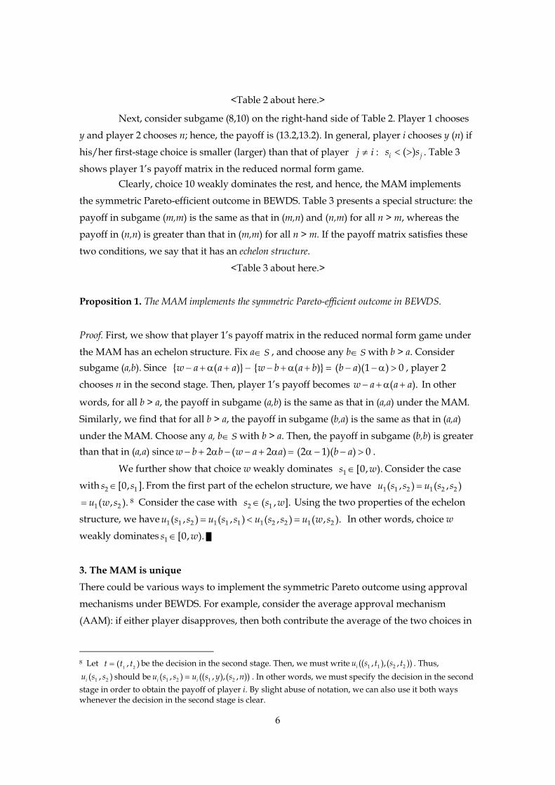
Next, consider subgame (8,10) on the right-hand side of Table 2. Player 1 chooses
y and player 2 chooses n; hence, the payoff is (13.2,13.2). In general, player i chooses y (n) if
his/her first-stage choice is smaller (larger) than that of player ≠j i : < >( )i js s . Table 3
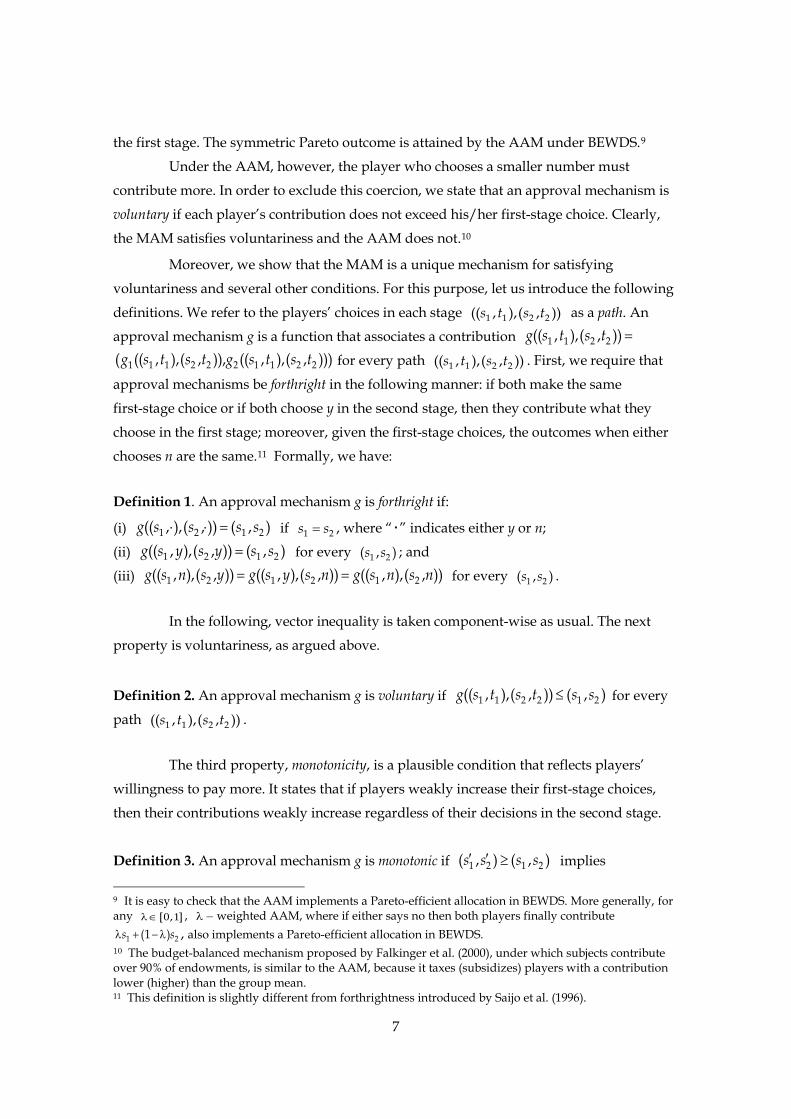
shows player 1’s payoff matrix in the reduced normal form game. Clearly, choice 10 weakly dominates the rest, and hence, the MAM implements
the symmetric Pareto-efficient outcome in BEWDS. Table 3 presents a special structure: the
payoff in subgame (m,m) is the same as that in (m,n) and (n,m) for all n > m, whereas the
payoff in (n,n) is greater than that in (m,m) for all n > m. If the payoff matrix satisfies these
two conditions, we say that it has an echelon structure.
<Table 3 about here.>
Proposition 1. The MAM implements the symmetric Pareto-efficient outcome in BEWDS.
Proof. First, we show that player 1’s payoff matrix in the reduced normal form game under
the MAM has an echelon structure. Fix a∈S , and choose any b∈S with b > a. Consider subgame (a,b). Since { ( )}w a a a− + α + − { ( )}w b a b− + α + = ( )(1 ) 0b a− − α > , player 2
chooses n in the second stage. Then, player 1’s payoff becomes ( ).w a a a− + α + In other
words, for all b > a, the payoff in subgame (a,b) is the same as that in (a,a) under the MAM.
Similarly, we find that for all b > a, the payoff in subgame (b,a) is the same as that in (a,a)
under the MAM. Choose any a, b∈S with b > a. Then, the payoff in subgame (b,b) is greater than that in (a,a) since 2 ( 2 )w b b w a a− + α − − + α = (2 1)( ) 0b aα − − > .
We further show that choice w weakly dominates 1 [0, ).s w∈ Consider the case
with 2 1[0, ].s s∈ From the first part of the echelon structure, we have 1 1 2 1 2 2( , ) ( , )u s s u s s=
1 2( , ).u w s= 8 Consider the case with 2 1( , ].s s w∈ Using the two properties of the echelon
structure, we have 1 1 2 1 1 1 1 2 2 1 2( , ) ( , ) ( , ) ( , ).u s s u s s u s s u w s= < = In other words, choice w
weakly dominates 1 [0, ).s w∈ █
3. The MAM is unique
There could be various ways to implement the symmetric Pareto outcome using approval
mechanisms under BEWDS. For example, consider the average approval mechanism
(AAM): if either player disapproves, then both contribute the average of the two choices in
8 Let 1 2( , )t t t= be the decision in the second stage. Then, we must write 1 1 2 2(( , ),( , ))iu s t s t . Thus,
1 2( , )iu s s should be 1 2 1 2( , ) (( , ),( , ))i iu s s u s y s n= . In other words, we must specify the decision in the second stage in order to obtain the payoff of player i. By slight abuse of notation, we can also use it both ways whenever the decision in the second stage is clear.
6
the first stage. The symmetric Pareto outcome is attained by the AAM under BEWDS.9
Under the AAM, however, the player who chooses a smaller number must
contribute more. In order to exclude this coercion, we state that an approval mechanism is
voluntary if each player’s contribution does not exceed his/her first-stage choice. Clearly,
the MAM satisfies voluntariness and the AAM does not.10
Moreover, we show that the MAM is a unique mechanism for satisfying
voluntariness and several other conditions. For this purpose, let us introduce the following
definitions. We refer to the players’ choices in each stage 1 1 2 2(( , ),( , ))s t s t as a path. An
approval mechanism g is a function that associates a contribution 1 1 2 2(( , ),( , ))g s t s t =
1 1 1 2 2 2 1 1 2 2( (( , ),( , )), (( , ),( , )))g s t s t g s t s t for every path 1 1 2 2(( , ),( , ))s t s t . First, we require that
approval mechanisms be forthright in the following manner: if both make the same
first-stage choice or if both choose y in the second stage, then they contribute what they
choose in the first stage; moreover, given the first-stage choices, the outcomes when either
chooses n are the same.11 Formally, we have:
Definition 1. An approval mechanism g is forthright if:
(i) 1 2 1 2(( , ),( , )) ( , )g s s s s⋅ ⋅ = if 1 2s s= , where “・” indicates either y or n;
(ii) 1 2 1 2(( , ),( , )) ( , )g s y s y s s= for every 1 2( , )s s ; and
(iii) 1 2 1 2 1 2(( , ),( , )) (( , ),( , )) (( , ),( , ))g s n s y g s y s n g s n s n= = for every 1 2( , )s s .
In the following, vector inequality is taken component-wise as usual. The next
property is voluntariness, as argued above.
Definition 2. An approval mechanism g is voluntary if 1 1 2 2 1 2(( , ),( , )) ( , )g s t s t s s≤ for every
path 1 1 2 2(( , ),( , ))s t s t .
The third property, monotonicity, is a plausible condition that reflects players’
willingness to pay more. It states that if players weakly increase their first-stage choices,
then their contributions weakly increase regardless of their decisions in the second stage.
Definition 3. An approval mechanism g is monotonic if 1 2 1 2( , ) ( , )s s s s′ ′ ≥ implies
9 It is easy to check that the AAM implements a Pareto-efficient allocation in BEWDS. More generally, for any 0 1[ , ]λ∈ , λ − weighted AAM, where if either says no then both players finally contribute
1 2(1 )s sλ + −λ , also implements a Pareto-efficient allocation in BEWDS. 10 The budget-balanced mechanism proposed by Falkinger et al. (2000), under which subjects contribute over 90% of endowments, is similar to the AAM, because it taxes (subsidizes) players with a contribution lower (higher) than the group mean. 11 This definition is slightly different from forthrightness introduced by Saijo et al. (1996).
7

1 1 2 2 1 1 2 2(( , ),( , )) (( , ),( , ))g s t s t g s t s t′ ′ ≥ for every 1 2( , )t t .
The above properties are sufficient to prove the uniqueness of the MAM.12
Proposition 2. Suppose that a forthright approval mechanism implements the Pareto-efficient
allocation in BEWDS. If it is voluntary and monotonic, then it must be the MAM.
Proof. See Appendix. █
4. Multiple implementations of the MAM
In this section, we explore other equilibrium properties and the outcome of heuristics
under the MAM. First, we present the main result of implementation in several equilibrium
concepts and heuristics.13 Then we derive the result step by step.
Proposition 3. The MAM multiply implements the symmetric Pareto-efficient outcome in limit
LAQRE, SPMRE, level-k thinking, and diagonalization heuristics.
Proof. It immediately follows from Lemmata 2-5. █
The concept of SPNE is often used to analyze multistage games. We denote player
i’s strategy by = ⋅( ( ))i i ip s ,t , where ∈is S , and ⋅( )it is a function that associates y or n to
each first-stage choice 1 2( )s ,s . Let = =1 2P P P be the pure strategy set. With a slight abuse
of notation, we write i’s payoff function induced by the MAM as iu . A strategy profile
= 1 2( )p p , p is a Nash equilibrium if for each i, j with ≠j i , ( ) ( )i i i ju p u p ,p′≥ for all ′ ∈ip P .
A Nash equilibrium p is subgame perfect if it constitutes a Nash equilibrium in every
subgame.
Lemma 1. In the MAM, the set of SPNE contributions is the set of symmetric contributions.
Proof. See Appendix. █
12 Although it is artificial, the following forthright mechanism is voluntary, but not monotonic. Consider a forthright rule in which a player who announces a bigger contribution than the other in the first stage must contribute 0, and the other player must contribute what he/she chooses in the first stage if either one chooses n in the second stage. Apparently, this mechanism is voluntary. However, it is not monotonic, since = < =1 1((6, ), (2, )) 0 ((2, ), (2, )) 2.g n y g n y It is easy to check that the mechanism implements a Pareto-efficient allocation in BEWDS. 13 We thank an anonymous referee for pointing out this possibility.
8

Mckelvey and Palfrey (1995, 1998) introduced logit quantal response equilibrium
(QRE) concept for the normal and extensive form games. They modeled the players who
make noisy best response to other players. The probability of choosing an action is
proportional to the exponential function of the observed payoff of the action, divided by a
parameter 0µ > . Even in such a case, the MAM can implement the efficient outcome in
limiting equilibrium, which survives as players become fully sensitive to their payoffs:
0µ→ . Assume µ is common to both players and all their information sets. To ensure the
existence of the limiting equilibrium by Theorem 1 of Mckelvey and Palfrey (1998), we
focus on the case where players contribute in integer.
Let 1 2( )i i i,σ = σ σ be player i’s behavioral strategy with the superscript denoting
stage, and let σ = σ σ1 2( , ) be a strategy profile. Let ( )i isπ be i’s expected payoff from
when he/she chooses {1,2, , }i ds S w∈ = 2 , while all the other actions of the players are
prescribed by σ . Similarly, let π = π( ) ( | )i i i i i jt t s ,s , =it y ,n be i’s expected payoff when
he/she chooses it at subgame ( i js ,s ), while ≠j i is following σ in the subgame, where
the vertical “|” indicates “conditional on.” A strategy profile σ is an LAQRE if it solves
the following equations: for each i = 1,2, ≠j i ,
for each i ds S∈ , and
for each i j ds ,s S∈ . A strategy profile σ is a limit LAQRE, if it is an LAQRE as 0µ→ .
In the limit, since the player with a higher first-stage choice surely chooses n, the
other player randomizes y and n by indifference. Still, the reduced normal form game
approaches the echelon form.14 Then, analogous to Proposition 5 of Anderson et al. (2001)
for minimum effort games, the full contribution is the unique equilibrium. Therefore, we
have Lemma 2.
Lemma 2. The MAM implements the symmetric Pareto-efficient outcome in limit LAQRE.
Proof. See Appendix. █
The third alternative equilibrium concept is SPMRE. Some subjects imagine
foregone payoffs from unchosen strategies. This is close to the simplest version of -ε
minimax regret equilibrium introduced by Renou and Schlag (2011), who incorporated into
game-theoretic models experimental evidence that people avoid ambiguity and the
decision-theoretic formulation of such behavior. The basic idea is that a player imagines
14 For a more general discussion of the QRE, see Mckelvey and Palfrey (1995, 1998).
1 exp( ( )/ )( )exp( ( )/ )
d
i ii i
ix S
ssx
∈
π µσ =
π µ∑2
1 2exp( ( )/ )( , )
exp( ( )/ )+exp( ( )/ )i
ii i
yy|s sy n
π µσ =
π µ π µ
9

foregone payoffs from unchosen strategies. For every pure strategy profile = 1 2( , )p p p ,
player i’s regret at p is defined by ( ) max ( , ) ( , )ii p i i j i i jR p u p p u p p′ ′= − , j i≠ . This is the
difference between his/her maximal payoff when player i best responds to j’s strategy jp
and his/her payoff when he/she plays ip . A strategy profile p is a minimax regret
equilibrium if for each i, j with j i≠ and for all ′ip , ′ ′′ ′ ′≤max ( , ) max ( , )j jp i i j p i i jR p p R p p . In
other words, each player chooses the strategy that minimizes the largest possible regret in
the equilibrium.15 We say that a minimax regret equilibrium p is subgame perfect if the
action profile induced by p constitutes a minimax regret equilibrium in every subgame.
Lemma 3. The MAM implements the symmetric Pareto-efficient outcome in SPMRE.
Proof. See Appendix. █
We now propose two alternative heuristics that predict that players make the full
contribution. The first one is level-k thinking. We apply such heuristics to the reduced
normal form game induced by elimination of weakly dominated strategies. Consider Table
3 as an illustration. Assume that player 1 expects player 2 to choose each number with
equal probability (level-0) and to eliminate weakly dominated strategies in the second
stage. In the case of the MAM, player 1’s best response to level-0 is to choose 10. Thus,
efficiency can be achieved by any pair of players of level-1 or above.16
Lemma 4. The MAM implements the symmetric Pareto-efficient outcome in level-1 or above.
Proof. Straightforward. █
The fifth possibility is a heuristic called diagonalization, of which we find notable
descriptions given by the subjects in the questionnaires during and after the experiment.
Some subjects wrote that the player who chooses the higher first-stage choice will
disapprove the other’s choice, and both would obtain the payoffs on the diagonal line in
the payoff table. Then, subjects can easily find that full contributions attain the maximum
payoff among the payoffs on the diagonal line. Thus, we have the following simple
proposition.
15 Here, we assume that each player believes that his/her opponent may choose any strategy. 16 Lemma 4 also holds if we consider the level-0 player who chooses w.
10
Lemma 5. If both players follow diagonalization in the MAM, then the outcome is symmetric
Pareto-efficient.
Proof. Straightforward. █
Now, Proposition 3 is verified for the MAM. Proposition 4 for the MCM provides
the counterparts to Propositions 1 and 3 for the MAM. Moreover, the results are quite
contrasting. Consider Table 1 again. Let us begin with BEWDS. Since both obtain 10 if either chooses n, player 1 will know that player 2 disapproves if and only if 1 2( )s ,s = (0,x)
with ≥ 2x , (2,x) with ≥ 6x , or (4,10). Then, the choices of 0, 8, and 10 are eliminated, but
any choice of 2, 4, and 6 survives under BEWDS. Every pair of contributions such that both
players get at least 10 can be supported as an SPNE.17 Consider level-k thinking. Given that
player 2 randomly chooses any number, player 1 can see that the best response is to choose
6. This also minimizes regret. Another step of iterated reasoning leads player 1 to
contribute 4, which is the best response to player 2’s 6. The third iteration result uniquely selects the choice of 2.18 (2,2) is also a limit LAQRE contributions. Let β = − α α(1 ) / .
Proposition 4. Under the MCM, the following holds.
i) A player following BEWDS chooses any contribution in β(0, ]w .
ii) There exists an SPNE where players contribute 1 2( , )g g if and only if −β ≤ ≤ β 1
2 1 2g g g .
iii) A limit LAQRE supports contributions (1,1) if players choose their contributions in integers.
iv) The unique SPMRE contribution is βw . v) Level-k player’s contribution is βk w , which decreases as k increases.
Proof. See Appendix. █
5. Experimental design
We conducted four treatments in order to test the performances of the approval
mechanisms. The VCM was the control treatment, while the other three treatments were
the MCM, MAM, and simplified MAM (SMAM). Under the SMAM, if both players make
the same first-stage choice, the game ends. Otherwise, only the player with the higher
first-stage choice proceeds to the second stage. If he/she approves, they contribute what
they choose in the first stage. If he/she disapproves, both players contribute the minimum
of their choices in the first stage. The SMAM also implements the efficient allocation in
17 That is, (x,x) with {0, 2, 4, 6, 8, 10}x∈ , (4,2), (6,4), (8,4), (8,6), (10,6), (10,8), and their permutations. 18 Proposition 4-iv) also holds if we consider the level-0 player who chooses w.
11
BEWDS.19 Each of the above-mentioned four treatments had three experimental sessions.
These 12 sessions were conducted at Osaka University in March, April, September, and
November 2011. Subjects were recruited from Osaka University through campus-wide
advertisements and were inexperienced in this particular type of experiment. No
individual participated in more than one session. The experiment was computerized using
the experimental software z-Tree (Fischbacher, 2007). Twenty subjects participated in each
session. Each was seated at a computer terminal assigned by lottery. All terminals were
separated by partitions. No communication was allowed between subjects.
Each subject had a set of printed instructions, a record sheet, and a payoff table
(called the points table).20 In the distributed payoff table, each subject was considered to be player 1. Player i’s payoff is given by = − + +1 2300{(24 ) 0.7( )}i iu g g g for each pair of
contribution 1 2( , )g g . Since we consider two players with identical utility functions and
endowments, the payoff table is identical for all subjects. Subjects were informed that they
had identical payoff tables.
Instructions were read aloud by an experimenter for approximately 10 minutes.
After that, subjects were given another 10 minutes to ask questions. Then, subjects
proceeded to the payment periods. There was no practice period. Each session consisted of
19 periods under the perfect stranger matching protocol. Subjects were informed that each
of them would meet any other subject just once.
The approval mechanism treatments continued as follows. At the beginning of
each period, all subjects endowed with 24 tokens were anonymously paired. In the first
stage, subjects were asked to enter their contributions as nonnegative integers into a box in
the display and to write down their choices along with their reasoning in the
corresponding row in the record sheet. Once all subjects had finished their tasks, they
clicked the OK button. In the second stage, the first-stage choices of both players and the
payoff matrix in the second stage were displayed. After all players wrote down the
first-stage choices of their counterparts, they chose to approve or disapprove by clicking
the relevant radio button and recording the decision along with the reason. If a subject in
the SMAM did not proceed to the second stage, he/she simply wrote down the first-stage
choice of his/her counterpart before the other subjects finished the second stage and circled
“none” while facing the waiting screen. Once all the subjects in the second stage had
finished the above tasks and clicked the OK button, they proceeded to the results screen.
The results screen included the first-stage choices of both players, their “approve” or
19 Recall that under the MAM, the decision by the player with the higher first-stage choice alone determines the outcome in every second stage. The SPNE, SPMRE, limit LAQRE, and level-k thinking outcomes of the SMAM are the same as those of the MAM. 20 See Online Appendix.
12

“disapprove” decisions, and their payoffs (points earned) in the period. No information on
the choices of the other nine groups was provided to the subjects. Finally, the subjects
wrote down the decisions of their counterparts and the points they had earned and clicked
the Next button to begin the next period. The treatment without the second stage became
the VCM treatment.
After playing for 19 periods, the subjects completed a questionnaire and were
immediately paid privately in cash. Each subject was paid an amount proportional to the
sum of the points that he/she had earned for the 19 periods. Individual payments ranged
from $49.91 to $87.97.
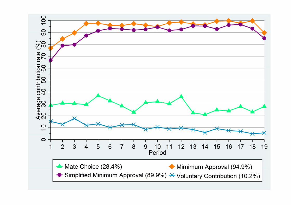
6. Experimental results
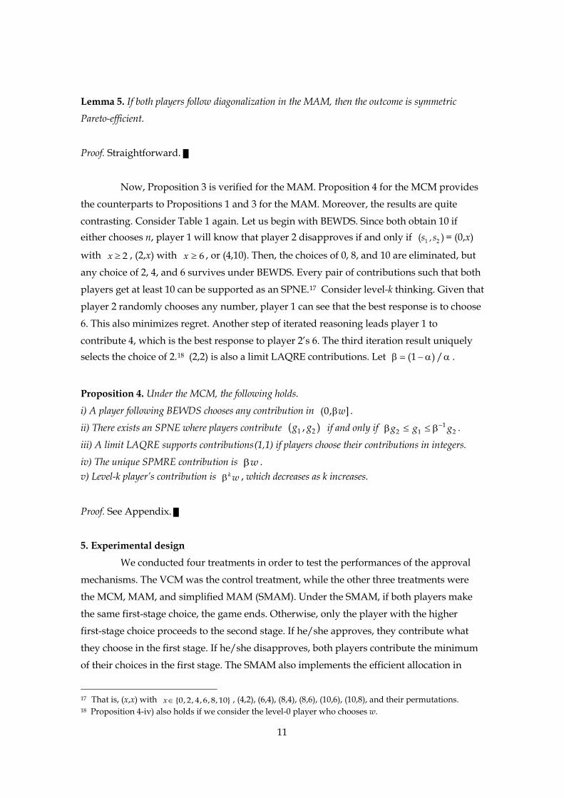
Figure 2 shows the time path of average contributions over the 19 periods arranged by
mechanism. Individual contributions were evaluated after the second stage in the MAM,
MCM, and SMAM.
<Figure 2 about here.>
We first assess the results of the VCM. The time path of average contribution in
the VCM shows a similar pattern to that of previous VCM experiments (e.g., Ledyard,
1995). In the first period, subjects contributed 15.3% of endowments (3.68 tokens), with
contribution rates gradually decreasing to 5.7% (1.37 tokens) in the last period. The
hypothesis test based on Spearman’s rank correlation coefficient shows that the downward trend in average contributions was statistically significant ( -0.916, 0.001)pρ = < . Data
pooled across all 19 periods and 3 sessions show that the subjects contributed 10.2% of
endowments (2.44 tokens). Out of 570 outcomes (10 pairs × 19 periods × 3 sessions), there is
no case where both players contributed all endowments.
Introducing the MAM facilitates almost full contributions among subjects, even in
the earlier period. Contributions in the first period average 76.9% of endowments (18.45
tokens). They then rise repeatedly for the first five periods, achieving 97.8% (23.47 tokens)
in period 5. Then, cooperation is sustained with an average contribution rate of over 95% in
every period except the final one. Moreover, the convergence to the efficient allocation
under the MAM is statistically supported by Spearman’s rank correlation test, which helps examine the upward trend in average contributions ( 0.557, 0.009)pρ = = . When the data
are pooled across all 19 periods and 3 sessions, subjects in the MAM contribute on average
94.9% of endowments (22.78 tokens). Out of 570 outcomes, there are 475 outcomes where
both players contributed all endowments. Table 4 compares the contributions for the four
treatments using a two-tailed Mann–Whitney test. This test shows that subjects in the
MAM contributed significantly more than those in the VCM, with the test statistic z = 9.445
13

(p < 0.001).21
<Table 4 about here.>
The contributions in the SMAM show similar patterns to those in the MAM. It
took five periods to achieve a contribution rate of over 90%, and almost all subjects
maintained full contributions until the end of the session. Spearman’s rank correlation test
shows that the upward trend in average contributions is statistically significant( 0.625, 0.004)pρ = = . Overall, the average contribution rate of the SMAM is 89.9%. Of the
570 outcomes, there were 424 outcomes where both players contributed all endowments.
The contribution rate of the SMAM was significantly lower than that of the MAM (z = 3.799,
p < 0.001).22 There is no significant difference, however, in the first-stage choices between
the SMAM and MAM (z = 0.456, p = 0.649). The contribution rate of the SMAM is
significantly higher than that of the VCM (z = 9.275, p < 0.001).
In contrast to the MAM and the SMAM, only 7 of the 540 pairs of the MCM
achieved full contributions and the approval of both players. The average contribution
under the MCM fluctuated within a relatively narrow range, but decreased repeatedly, and
it remained higher than that of the VCM in every period. Spearman’s rank correlation test
shows that the downward trend in average contributions is statistically significant ( -0.525, 0.001)pρ = < . The overall average contribution rate of the MCM is 28.4% (6.83
tokens), which is significantly higher than that of the VCM (z = 7.284, p < 0.001). However,
the contribution rate was significantly lower than that of the MAM and the SMAM (z =
9.450 and p < 0.001 for the MCM vs. the MAM and z = 9.133 and p < 0.001 for the MCM vs.
the SMAM).
In reality, the average contributions by subjects in one session are mutually
dependent, although in a two-tailed Mann–Whitney test we assume that they are
independent. In order to account for this dependence, we also run a regression to predict
contribution after the approval stage, using three approval mechanism dummies and
clustering standard errors by session. The estimation results are similar to those of a
two-tailed Mann–Whitney test, indicating that all three approval mechanisms significantly
increase contribution relative to the VCM. In particular, the MAM increases contribution by
20.34 tokens with a standard error of 0.633, followed by the SMAM which increases
21 The null hypothesis is that the contribution rates are the same between the MAM and the VCM. We use the method presented by Andreoni and Miller (1993). We first calculate the average contribution rate of each subject across periods and then calculate the test statistic using these averages, in order to eliminate cross-period correlation. 22 The statistical difference exists mainly because the lower choices of two of the subjects in the SMAM were disapproved. One of them mistakenly thought that she had to allocate 24 tokens across 19 periods. The other subject intentionally chose low contributions, expecting that his/her matched subjects might approve by giving up a small number of their points.
14

contribution by 19.1 tokens and a standard error of 0.886, and the MCM which increases
contribution by 4.38 tokens and a standard error of 0.659.
7. Heterogeneous reasoning processes coexist
We report a third-party assessment and classification of descriptions in the questionnaire
during and after the experiment, called coding, in order to investigate which type of
reasoning process (including diagonalization, regret minimization, and level-k thinking)
was used by the subjects.23 The coding proceeded as follows. First, we read the responses
in the MAM and the MCM separately. Then, we created 30 sentence-based categories from
typical responses (see Online Appendix). Two research assistants (hereafter coders) were
independently instructed, and each coder created the coding for all 120 subjects in the
MAM and the MCM. For each subject, the coders were required to read subjects’
descriptions and determine the categories to which his/her descriptions belong and to
check all relevant categories (0 = description does not fall into the category, 1 = description
falls into the category). We refer to a coder’s binary decision as the rating. Coders never met
face-to-face, and no efforts were made to reconcile the differences in individual coding.
For each category of our interest, we regard a subject rated positively by at least
one coder as a follower of the equilibrium strategy or heuristics in the category. In
particular, Category 10 is designed to capture subjects in the MAM who directly mentioned
the diagonal line of the payoff table. Such subjects are deemed to follow diagonalization
heuristics. Category 12 is designed to capture regret minimization in the first stage in the
MAM and MCM. Categories 16 and 17 are set to capture level-1 and level-2 in the MCM,
respectively.24,25
Let us summarize the coding result. In the MAM, 20.0% (= 12/60) of the subjects
are deemed to follow diagonalization heuristics, and 16.7% (= 10/60) subjects fall in the
regret minimization category. In the MCM, on the other hand, 21.7% (= 13/60) and 45.0%
(= 27/60) of the subjects are deemed to follow level-1 and level-2 thinking, respectively. In
addition, 11.7% (= 7/60) of the subjects are deemed to follow regret minimization, which
appears commonly in both treatments. Although no category of our interest records an
absolute majority, these results suggest that subjects are heterogeneous in reasoning
23 This method is similar to that presented by Cooper and Kagel (2005). Note that our experiments did not allow communication among subjects, while Cooper and Kagel (2005) investigated specific words and attitudes in informal communication that facilitated cooperation among group members. 24 We did not make level-k categories for the MAM because we could not find such responses in the questionnaires. The same applies to regret minimization in the second stage for both the MAM and the MCM. 25 At the start of the coding process, Category 12 and 13 were classified as regret minimization. However, we found that the sentence of Category 13 was too imprecise to capture regret minimization. Therefore, we do not consider Category 13 to describe regret minimization in the analysis.
15

processes, and the appearance frequency of each reasoning process may depend on the
mechanisms.26
8. Discussion and conclusion
Prior theoretical work on public good mechanisms has given theorists broad latitude the
choice of equilibrium concept or behavioral rule, such as dominant strategy equilibrium,
Nash equilibrium, or SPNE. However, recent experimental studies reveal that there is a
wide gap between the theory and subjects’ behavior.
This paper, in contrast, theoretically showed that the MAM multiply implements
the Pareto-efficient provision of the public good in five equilibrium concepts and heuristics,
namely BEWDS, limit LAQRE, SPMRE, level-k thinking, and diagonalization heuristics.
Consistent with our predictions, we observed rapid convergence towards efficient
allocation in the MAM sessions. Further, our inclusive coding of subjects’ responses helped
pinpoint their reasoning processes. The coding results suggest that the subjects are
heterogeneous in reasoning processes. Although our public good environment is simple,
our result is in stark contrast to those of recent experimental studies, which have often
needed dozens of repetitions to attain efficiency in the laboratory.
To our knowledge, this is the first theoretical and experimental study to
successfully design a public good mechanism robust to several behavioral rules. This paper
should at least stimulate constructive discussion on mechanism design, to emphasize the
alignment of players with various behavioral rules towards a social optimum.
One direction for further research is to evaluate experimental approval
mechanisms in more general public good environments. First, if we consider asymmetric
cases, Proposition 1 still holds if two players have moderately different preferences
towards the public good.27 Further, if the endowment is heterogeneous, the problem
reduces to a symmetric case, through the definition of a new strategy space, where each
player/subject chooses a contribution rate relative to his/her endowment in the first stage.
If the public good is harmful for some player, the MAM with transfer implements the
symmetric Pareto-efficient allocation in BEWDS (see Masuda, 2013). The second extension
is toward the n-person case. In public good environments with binary choices, Huang et al.
26 We did not obtain sufficiently high agreement in ratings between any two coders for the following two reasons. First, even though our coders had excellent and comparable game theoretic skills, the sensitivity of coders to track subjects’ reasoning processes, or to pick up any subtle nuance in Japanese, is heterogeneous. Second, we made coders work independently throughout the coding process to prevent coordination among them, though experiments in psychology permit communication between two coders before rating each subject. 27 If we write player i’s benefit per public good as iα , the conditions are 1 2α ≠ α , 1 2, (0, 1)α α ∈ , and
1 2 1α + α > .
16

(2013) succeeded in constructing a variant of an n-person approval mechanism. Masuda
(2013) also generalized the mechanism of Huang et al. (2013) to homogeneous n-person
public good environments with continuous contributions and linear payoffs in the spirit of
the SMAM, where players other than those with the minimum choice can proceed to the
second stage. Third, in a more realistic setting, we may consider the ratification process for
international agreements involving countries; nature determines the order of the player
who may decide to approve or otherwise. Our results hold in such cases also.
Appendix This appendix gives the proofs for Propositions 2 and 3.
Proof of Proposition 2. Let g be a forthright approval mechanism that implements the
Pareto-efficient allocation in BEWDS and that satisfies voluntariness and monotonicity. Let
1 2( , )s s be any first-stage choice. If 1 2 ,s s= 1 2 1 2(( , ),( , )) ( , )g s s s s⋅ ⋅ = according to condition
(i) of forthrightness, which shows the outcome of the MAM. Consider the case where
1 2 .s s≠ Without loss of generality, assume that 1 2s s> , and consider two cases:
1 1 and .s w s w= < First, consider subgame 2( , )w s with 2 .w s> In order to implement
the efficient allocation in BEWDS, w must weakly dominate 2s for player 2 in the reduced
normal form game. In other words,
(A.1) 2 2 1 2 2(( , ),( , )) (( , ),( , ))g gu w w u w t s t⋅ ⋅ ≥
where giu is i’s payoff function induced by g, and it is player i’s decision under BEWDS.
Suppose that 1 2t t y= = . Then, by conditions (i) and (ii) of forthrightness, we have
(A.2) 2 2 2 2 2(( , ),( , )) ( ) ( ) ( ) ( ) (( , ),( , ))g gu w y s y w s w s w w w w u w w= − + α + > − + α + = ⋅ ⋅ ,
which contradicts to (A.1). Thus, 1 2 or .t n t n= = Together, condition (iii) of forthrightness
and (A.2) show that 2 2 2 2(( , ),( , )) (( , ),( , ))g gu w y s y u w y s n> 2 2(( , ),( , ))gu w n s y= = 2 2(( , ),( , ))gu w n s n . Hence, y weakly dominates n for player 2 in the second stage, namely
2t y= , which implies 1t n= .
Consider now the reduced normal form game under g, and compare the outcomes
in subgames 2 2( , )s s and (w, 2s ). Since player 1 chooses w by assumption, we have
1 2 1 2 2(( , ),( , )) (( , ),( , ))g gu w n s y u s s≥ ⋅ ⋅ . Let 2 1 2(( , ),( , )) ( , ).g w n s y g g= Then,
1 2 1 1 2(( , ),( , )) ( )gu w n s y w g g g= − + α + ≥ 2 2 2( )w s s s− + α + = 1 2 2(( , ),( , ))gu s s⋅ ⋅ . Since g is
voluntary, 1 2 2( , ) ( , ).g g w s≤ Because of the monotonicity of g, 1 2 2 2( , ) ( , )g g s s≥ . The
intersection of these three inequalities shows 1 2 2 2( , ) ( , ).g g s s= Thus, according to
17
condition (iii) of forthrightness, we have
(A.3) 2 2 2 2 2(( , ),( , )) (( , ),( , )) (( , ),( , )) ( , ).g w n s y g w y s n g w n s n s s= = =
In other words, both players contribute 2s , which is the minimum of 2( , )w s ,
when at least one player chooses n.
Now take any 1 2( , )s s w∈ . Together with 2 1 2 2 2( , ) ( , ) ( , )w s s s s s≥ ≥ and (A.3), since
g is monotonic, we have 2 2 2 1 2 2 2 2 2( , ) (( , ),( , )) (( , ),( , )) (( , ),( , )) ( , ).s s g w n s y g s n s y g s n s y s s= ≥ ≥ =
Hence, we have 1 2 2 2(( , ),( , )) ( , ).g s n s y s s= In other words, g is the MAM. █
Proof of Lemma 1. Suppose, on the contrary, that for some SPNE = ⋅ ⋅1 1 2 2(( , ( )),( , ( )))p s t s t ,
players contribute differently, i.e., ≠1 2g g . Then, by construction of the MAM, ≠1 2s s
and =1 2( , )it s s y for i = 1,2. Define ),( 21 ppp ′=′ with ))(,( ⋅′=′ 111 tsp as the strategy profile
where player 1 deviates from p only in the first stage. Without loss of generality, assume >1 2s s . Assume ′ =1 2s s , then 1 2 2 2 1 1 2 1( ) ( ) ( ) ( )u p w s s s w s s s u p′ = − + α + > − + α + = by >1 2s s , which is a contradiction. Thus, =1 2g g . Next, we show that any symmetric pair of
contributions can be supported as an SPNE. Let ∈s S . Consider the strategy profile = ⋅ ⋅(( , ( )),( , ( )))q s t s t , where ⋅( )t is a function such that =1 2( , )t s s n for all ∈1 2,s s S .
Clearly, p constitutes a Nash equilibrium (n,n) for every second-stage subgame. Now,
consider the reduced normal form game. Suppose that player 1 unilaterally deviates to ′ >1s s in the first stage. Let ))(,( ⋅′=′ tsq 11 and let ),( 21 qqq ′=′ . Since both players choose n
at ′1( , )s s and by ′ >1s s , we have 1( )u q′ = 1( ) ( )w s s s u q− +α + = . Suppose ′ <1s s . Then,
we have 1( )u q′ = 1 1 1( )w s s s′ ′ ′− + α + 1( ) ( )w s s s u q< − +α + = . The above argument also
applies to player 2. Hence, q is an SPNE. █
Proof of Lemma 2. First, consider the second stage. Take any 1 2( , )s s . Note thatσ σ2 2( )=1- ( )j jn y ,
− α +(( , ),( , ))=( )+ ( )i i j i i ju s y s y w s s s and if ( , ) ( , )i jt t y y≠ , (( , ),( , ))=( )+ ( )i i i j ju s t s t w s s s− α +
= ( )i nπ where = min{ , }i js s s . Then,
(A.4) 2 2 2
{ , }( )= ( ) (( , ),( , )) ( ){( )+ ( )} {1- ( )} ( ).
j
i j j i i j j j i i j j it y n
y t u s y s t y w s s s y n∈
π σ = σ − α + + σ π∑
By substituting (A.4) into the second equation satisfied by the LAQRE, we have
(A.5) [ ]
12
121 2
12
1+exp{ ( - ) ( )/ } <
( ) 1+exp{( ( )- ( ))/ } 0 5 =
1+exp{(1- )( - ) ( )/ } >
i j j i j
i i i
i j j i j
s s y if s s ,
y n y . if s s ,
s s y if s s .
−
−
−
α σ µ σ = π π µ = α σ µ
18

For each i ds S∈ , 1( )= ( ) ( , ),d
i i j i is S
s x s x∈
π σ π∑ where 2 2( , ) ( ) ( ) (( , ),( , ))i i i j i is x y y u s y x yπ = σ σ +
2 2(1 ( ) ( )) (( , ),( , ))i j i iy y u s n x n− σ σ . Since
2 2 2 2
2 2
1
2 2
( , ) ( ) ( ){( )+ ( )} (1 ( ) ( )){( )+ ( )}
( ) ( )( ) (2 1) < ,(2 1) = ,
(1 ) ( ) ( )( ) (2 1) > ,
i i j i j i i j i j
i j j i i j
j
i j j i i j
s s y y w s s s y y w s s s
y y s s s w if s ss w if s s
y y s s s w if s s
π = σ σ − α + + − σ σ − α +
ασ σ − + α − += α − +
− α σ σ − + α − +
we have
(A.6)
1 1 1
1 1 2 2
1 2 2
( )= ( ) ( , ) ( ) ( , ) ( ) ( , )
( ){(2 1)min{ , } } (1 ) ( ) ( ) ( )( )
( ) ( ) ( )( ).
d i i
d i
i
i i j i i j i i j i ix S x s x s
j i j i j ix S x s
j i j ix s
s x s x x s x x s x
x s x w x y y x s
x y y x s
∈ ≤ >
∈ ≤
>
π σ π = σ π + σ π
= σ α − + + − α σ σ σ −
+ α σ σ σ −
∑ ∑ ∑
∑ ∑
∑
Now, let us consider limiting equilibrium. If 1 2=s s , by (A.5), 2 21 2( ( ) ( ))y , yσ σ
=(0.5,0.5) for any µ . Consider next that 1 2<s s . Consider player 2’s equilibrium strategy.
Note by 1 2<s s , and 21 2 2( - ) ( )/ 0s s yα σ µ < , we have 2
10.5 ( ) 1y< σ < for any µ . Define a
function of x , [ ] 11 2 2 1( ; )= 1+exp{(1- )( - ) }f x s ,s s s x −α . Then, by (A.5), 2
10.5 ( ) 1y< σ < for any
µ , and since f is decreasing, 2 21 2 2 1 1 2(0.5/ ; ) ( ) ( ( )/ ; ) 0f s ,s y f y s ,sµ > σ = σ µ > for any µ .
Moreover, 1 20lim (0.5/ ; )=0f s ,sµ→
µ . Then, 220
lim ( )=0y .µ→
σ Consider player 1’s equilibrium
strategy. Note 2 21 2 2 1 1 2(0.5/ ; )/ ( )/ ( ( )/ ; )/ 0f s ,s y f y s ,sµ µ > σ µ = σ µ µ > . By letting =0.5/y µ ,
1 2 2 1 2 10lim (0.5/ ; , )/ lim 2 {1+exp((1- )( - ) )}=lim 2 {1/ +exp((1- )( - ) )/ }=0
y yf s s y / s s y / y s s y y
µ→ →∞ →∞µ µ = α α .
Then, 220
lim ( )/ 0y .µ→
σ µ = By substituting this into (A.5), we have
[ ]1
12 21 1 2 20 0
lim ( ) 1+exp{ ( - )lim( ( )/ )} 1+exp(0) 0 5y s s y . .−
−
µ→ µ→
σ = α σ µ = = Therefore, 2 2
1 2( ( ), ( ))y yσ σ
=(0.5 0), in limiting equilibrium. Similarly, if 1 2>s s , 2 21 2( ( ), ( ))y yσ σ (0 0 5), .= in limiting
equilibrium.
Next, we will show that for each i, 1( ) 1i wσ → as µ→ 0 . For each i, define a
function of x , 1 2 2( ; , ) ( ) ( ) ( )( )i i j i j ih x s x y y x sµ = σ σ σ − . By the above argument, for any
,i ds x S∈ with ix s≠ , we have
where ( , ) ( , )m k i j= if ix s> and ( , ) ( , )m k j i= otherwise. Finally, ( ; , ) 0.i i ih s s µ = Hence,
( ; , )i ih x s µ converges to the constant function 0 on S as µ→ 0 . Then, the second and third
terms in (A.6) also converge to 0. Then, for each i and any i ds S∈ , we have
1( ) ( ){(2 1)min{ , } }as 0.d
i i j ix S
s x s x w∈
π → σ α − + µ→∑
1 2 2 1
0 0 0 0 0 0 0lim ( ; , ) lim ( ) lim ( ) lim ( ) lim( )=lim ( ) 0.5 0 lim( )=0i i j m k i j ih x s x y y x s x x sµ→ µ→ µ→ µ→ µ→ µ→ µ→
µ = σ ⋅ σ ⋅ σ ⋅ − σ ⋅ ⋅ ⋅ −
19

Now we assume on the contrary that there exists i and s w< with 1=min{ ( )>0}d is x S | x∈ σ in the limiting equilibrium. Let { 1 }s s ,...,w′∈ + . Then , we have
(A.6)
1
1 1
1
( ) ( ) ( )(2 1)(min{ , } min{ , })
( )(2 1)( ) ( )(2 1)( )as 0.d
i i jx S
j js x s s x w
s s x s x s x
x x s x s s∈
′ ′≤ ≤ − ≤ ≤
′ ′π − π → σ α − −
′= σ α − − + σ α − − µ→
∑
∑ ∑
Together with (0 5 1). ,α∈ , s s′< , and 1( ) 0i xσ ≥ for each i and any dx S∈ , (A.6) is nonnegative. By the definition of limit LAQRE and the assumption of 1( )>0i sσ ,
(A.6) is nonpositive. Then, (A.7) must be 0. Then, 1 1( ) ( )>0i is s′σ = σ in the limiting
equilibrium. Together with 1=min{ ( )>0}d is x S | x∈ σ and the definition of limit LAQRE, it
implies that 1iσ is the uniform distribution over { }s,...,w , that is, 1( )=1/( - +1)i x w sσ if
{ }x s,...,w∈ and 1( )=0i xσ otherwise. By substituting 1( )=1/( - +1)j x w sσ into (A.6),
( ) ( )i is s′π − π converges to some strictly positive value, a contradiction to 1 1( ) ( )>0i is s′σ = σ .
Hence, for each i, 1( ) 1i wσ → as µ→ 0 . Therefore, the unique limit LAQRE outcome is
efficient. █
Proof of Lemma 3. Let 1 2(( , ( )),( , ( )))p w t w t= ⋅ ⋅ with for each i, 1 2( , ) if ,i i jt s s y s s= <
1 2( , ) orit s s y n= 1 2if , ( , ) otherwise.i j is s t s s n= = If 1 2 ,s s= 1 2 1 2(( , ),( , )) ( , )g s s s s⋅ ⋅ = , and
hence both players are indifferent between y and n. Next, consider the case 1 2 .s s≠ Since ti
prescribes weakly dominant choice in every second stage, for each i, j i≠ and each
{ , }jt y n′ ∈ , 1 2 1 2 1 2( ( , ), | , ) max ( , | , )ii i j t i i ju t s s t s s u t t s s′′ ′ ′= . Then, for each i, i it t′′ ≠ implies
1 2 1 2 1 2( ( , ), | , ) 0 ( , | , )i i i iR t s s s s R t y s s′′⋅ = < . Hence, p prescribes the SPMRE choice in every
second stage. Then, the reduced normal form game has an echelon structure. Since
1 2( , | , )iu w w t t = 2 wα > 1 2(2 1) ( , | , )i i iw s u s w t t+ α − = for each i, j i≠ and any ≠is w , we
have 1 2 1 2 1 2max ( , | , ) 0 (2 1)( ) ( , | , ) max ( , | , )j j
i j i i i i i js S s SR w s t t w s R s w t t R s s t t
∈ ∈= < α − − = = . █
Proof of Proposition 4. Let g be the mate choice mechanism (MCM).
(i) BEWDS. Consider the second stage. Take any ,a b S∈ . Note that ( ) ( )w a a b w− + α + ≥
if and only if 1a b−≤ β . Then, 1( , )t a b y= if 1a b−≤ β and 1( , )t a b n= otherwise.28 Then,
in the reduced normal form game, 1( , ) ( ) ( )u a b w a a b= − + α + and
2 ( , ) ( ) ( )u a b w b a b= − + α + if 1b a b−β ≤ ≤ β and 1 2( , ) ( , )u a b u a b w= = otherwise. A similar
argument holds for player 2.
28 We assume that a player chooses y if y and n are indifferent.
20

First, we show that for each i, choice wβ weakly dominates any choice
{0} ( , ]is w w∈ ∪ β . Take any i and ( , ]is w w∈ β . If [ , ]j is s w∈ β , then 1j i js s s−β < ≤ β .
Together with 1j js w s−β ≤ β ≤ β , it implies that ( , ) ( ) ( )i j ju w s w w w sβ = −β + α β +
( )iw s> − + ( )= ( , )i j i i js s u s sα + . If 2( , )j is w s∈ β β , then we have 1j js w s−β < β < β and
1i js s−> β . Then, ( , ) ( ) ( )i j ju w s w w w s wβ = −β + α β + > = ( , )i i ju s s . If 2[0, ]js w∈ β , then we
have 1jw s−β ≥ β and 1
i js s−> β . Then, ( , )i ju w s wβ = = ( , )i i ju s s . Next, assume 0is = .
Then, j is sβ > , for any 0js > . Then, we have ( , ) (0, )i j i ju w s w u sβ ≥ = for any 0js ≥ ,
with strict inequality for 2js w> β . Second, for any (0, ]is w∈ β , is is the unique best
response to 1is−β in the reduced normal form game and hence is survives under
BEWDS. Therefore, we get the desired result.
(ii) SPNE. Consider the second stage. Take any SPNE 1 1 2 2(( , ( )),( , ( )))p s t s t= ⋅ ⋅ . If 1
1 2s s−> β or 12 1s s−> β , some player chooses n in subgame 1 2( , )s s , otherwise the player
does not provide the best response. Hence, the players finally contribute nothing in p. Next,
take any 1 2( , )s s such that 12 1 2s s s−β ≤ ≤ β . We show that there exists an SPNE where both
players approve and hence contribute 1 2( , )s s . Consider the strategy profile
1 2(( , ( )),( , ( )))q s t s t= ⋅ ⋅ with 1 2( , )t s s y= and n otherwise. Clearly, q constitutes a Nash
equilibrium for every second-stage subgame. Now, consider the reduced normal form
game. Assume player 1 deviates to 1 1s s′ ≠ . By construction of q, such a deviation results in
(n,n). Together with 11 2s s−≤ β , this implies that 1( )u q 1 1 2( ) ( )w s s s= − + α + w≥ 1 1( , )u s q′= .
Hence, choosing 1s is the best response to 2s . This is also true for player 2. Hence, q is an
SPNE with contributions 1 2( , )s s .
(iii) LAQRE. Let {0,1, , }dS w= 2 . Take any 1 2, ds s S∈ . If ( , ) ( , )i jt t y y≠ ,
(( , ),( , ))= = ( )i i i j j iu s t s t w nπ . Then, 2( ) ( )( ) ( )i j j i iy y s s nπ = ασ −β + π . Together, this and the
definition of LAQRE imply that
(A.8) 2 1 2 1( ) {1+exp(( ( )- ( ))/ )} {1+exp(- ( )( )/ )}i i i j j iy n y y s s− −σ = π π µ = ασ −β µ .
On the other hand, by the first equation satisfied by LAQRE, for each is S∈ ,
we have 1( )= ( ) ( , ),d
i i j i ix S
s x s x∈
π σ π∑ where 2 2( , ) ( ) ( ) (( , ),( , ))i i i j i is x y y u s y x yπ = σ σ +
2 2(1 ( ) ( )) (( , ),( , ))i j i iy y u s n x n− σ σ . Since ( , )i is xπ = 2 2( ) ( ){( )+ ( )}i j i i jy y w s s sσ σ − α + +
2 2 2 2(1 ( ) ( )) ( ) ( )( ) ,i j i j j iy y w y y s s w− σ σ = ασ σ −β + we have
(A.9)
Now let us consider limiting equilibrium. Consider first 1 2( , ) (0,0)s s = . Then,
1 1 2 2 1( )= ( ) ( , ) ( ) ( ) ( )( ) ( ) d d d
i i j i i j i j i jx S x S x S
s x s x x y y x s w x∈ ∈ ∈
π σ π = α σ σ σ −β + σ∑ ∑ ∑
21

2 21 2( ( ), ( ))=(0,0)y yσ σ constitutes the unique limiting equilibrium in the second stage.
Consider next 1 2( , ) (0,0)s s ≠ . If 1( , )i j js s s−∈ β β for each i = 1,2, j i≠ , 2 21 2( ( ), ( ))=(1,1)y yσ σ
constitutes the unique limiting equilibrium. Similarly, if 1is w−β < and 1( , ]j is s w−∈ β , then
2 2( ( ), ( ))=(0.5,0)i jy yσ σ constitutes the limiting equilibrium. If 1i js s−= β , then
2 2( ( ), ( ))=(0.5,1)i jy yσ σ constitutes the limiting equilibrium.
In order to get the first-stage behavioral strategy in limiting equilibrium, for each i,
let us see 2 2( ) ( )( )i j iy y x sσ σ −β as a function of dx S∈ . Then, by the limiting equilibrium
choices in the second stage, we have 2 2( ) ( )( )i j i iy y x s x sσ σ −β → −β as 0µ→ if 1[ , )i ix s s−∈ β β , 2 2 1( ) ( )( ) 0.5( )i j i iy y x s s−σ σ −β → β −β as 0µ→ if 1
ix s−= β , and 2 2( ) ( )( ) 0i j iy y x sσ σ −β → as 0µ→ otherwise. By substituting these results into (A.9), if 1
is−β is an integer,
and otherwise Next, we show that there
exists a limiting equilibrium where both players choose 1 with probability 1. Suppose that
for each i, 1(1) 1iσ → as 0µ→ . By 1β < , we have for each i,
Let 1is > . We have for each i,
where the equality holds if 1isβ ≤ . Therefore, we get the desired result. █
(iv) SPMRE. Let 1 2( , ( )),( , ( )))p w t w t= β ⋅ β ⋅ be a strategy profile with for each i,
j i≠ , 11 2( , ) ifi i jt s s y s s−= ≤ β and 1 2( , )it s s n= otherwise. If 1 ,i js s−= β player i is
indifferent between y and n. Next, consider the case 1 .i js s−≠ β Since ti prescribes weakly
dominant choice in every second stage, for each i, j i≠ and each { , }jt y n′ ∈ , 1 2( , )i it t s s′ ≠
implies 1 2 1 2( ( , ), | , )i i ju t s s t s s′ = 1 2 1 2max ( , | , ) ( , | , )it i i j i iu t t s s u t y s s′′ ′′ ′ ′> . Hence, p prescribes the
unique SPMRE choice in every second stage.
Consider the reduced normal form game, which is identical to the one induced by
BEWDS. Take any 1 2,s s S∈ . As shown in part (i), player i best responds to player j if
i js s= β . Then, for each i, 1 2max ( , | , ) ( ) (1 )is i i j j j j ju s s t t w s s s w s= −β + α β + = + −β .
Consider player 1’s regret. If 11 2s s−> β or 1
2 1s s−> β , either player chooses n and hence
1 1 2( , )u s s w= . Then, 1 1 2 2 2( , ) ( (1 ) ) (1 )R s s w s w s= + −β − = −β . If 12 1 2s s s−β ≤ ≤ β , both
players choose y in the second stage. Then, we have 1 1 2 1 1 2( , ) ( )u s s w s s s= − + α + and 2
1 1 2 2 1 1 2 1 2( , ) ( (1 ) ) { ( )} ( ) /(1 )R s s w s w s s s s s= + −β − − + α + = β −β +β , which is maximized at
1
1
[ , )( ) ( ) ) as 0. (
d i i
i i j ix S s s
s x x s w−∈ ∩ β β
π →α σ −β + µ→∑
1 1
1 1
[ , ) [ , )(1) ( ) ( )( ) ( )( )
1 (1 ) 1 (1 )( 1) 0
d d i i
i i i j j ix S x S s s
i
i
s x x w x x s w
ss
− −∈ ∩ β β ∈ ∩ β β
π − π →α σ −β + − α σ −β −
≥ α ⋅ ⋅ −β − α ⋅ ⋅ −β= αβ − >
∑ ∑
1
1 1 1 1
[ , )( ) ( )( ) 0.5 ( )( ) as 0
d i i
i i j i j i ix S s s
s x x s s s w−
− −
∈ ∩ β β
π →α σ −β + ασ β β −β + µ→∑
1
1
[ , )(1) (0) ( )( ) (1 ) 0.
d
i i jx S
x x w w−∈ ∩ β β
π − π →α σ −β + − = α −β >∑
22
2 1s s= β . Hence, player 1’s maximum regret at 1s is given by
By (0.5,1)α∈ , we have 1β < . Together with 1s w≤ , it implies that 1s w= β minimizes
the maximum regret and gives the solution. .The same argument holds for player 2.
Therefore, ( , )w wβ β constitutes the unique minimax regret equilibrium of the reduced
normal form game.
(v) Level-k. First, we show that wβ is the best response to level-0 player. Given
that the other player uniformly randomizes in the reduced normal form game, by a similar
argument in (iii), the expected payoff ( )i is′π when player i chooses is is
.
Then, =is wβ maximizes ( )i is′π . Let B(k) be a sequence of the level-k player’s contribution
where 1k ≥ . Then, B(1) = wβ and B(k) = BR(B(k − 1)) until B(k) = B(k - 1), where BR(.) is the
best response to B(k − 1) in the reduced normal form game induced by elimination of
weakly dominated strategies. Since ( )BR s s= β for any s S∈ , we get the desired result. █
Acknowledgements
We would like to thank two anonymous referees for their suggestions. We also thank
Kanemi Ban, Vincent Crawford, Yukihiko Funaki, Keigo Inukai, Michihiro Kandori,
Tetsuya Kawamura, Shuhei Morimoto, Yuko Morimoto, Masahiro Okuno, Kazuki Onji,
Ariel Rubinstein, Tatsuhiro Shichijo, Masanori Takaoka, Masanori Takezawa, Wataru
Tamura, Toshio Yamagishi, and Takafumi Yamakawa. Keiko Takaoka provided
outstanding research assistance. We are also grateful to the participants at the 11th SAET
Conference; the 2011 Japanese Economic Association Autumn Meeting; the 2011, 2012, and
2013 Asia-Pacific Economic Science Association Meeting; and the seminar at Osaka
Prefecture University for their helpful comments. This research was supported by the Joint
Usage/Research Center at ISER, Osaka University and “Experimental Social Sciences:
Toward Experimentally-based New Social Sciences for the 21st Century,” the latter being a
project under the aegis of the Grant-in-Aid for Scientific Research on Priority Areas of the
Ministry of Education, Science, and Culture of Japan.
References
Anderson, S., Goeree, J.K., Holt, C.A., 2001. Minimum-effort coordination games: stochastic
potential and logit equilibrium. Games Econ. Behav. 34 (2), 177-199.
Andreoni, J., Miller, J.H., 1993. Rational cooperation in the finitely repeated prisoner’s
dilemma: experimental evidence. Econ. J. 103 (418), 570-585.
2
1 1 11 1 2
1 1 1 1
( , ) (1 ) if ,max ( , )
( , ) (1 ) otherwise.sR s w w s w
R s sR s s s
= −β < β= β = β −β
1min{ , } 1 2( )= ( ) / 1 (min{ , } ) / 2 1.i
i
w si i i i is
s x s wdx w s s w−β −
β′π −β + = β −β +∫
23
Andreoni, J., Varian, H., 1999. Preplay contracting in the prisoners’ dilemma. Proc. Natl.
Acad. Sci. 96 (19), 10933-10938.
Attiyeh, G., Robert, F., Isaac, R.M., 2000. Experiments with the pivot process for providing
public goods. Public Choice. 102 (1), 93-112.
Cason, T.N., Saijo, T., Sjöstrom, T., Yamato, T., 2006. Secure implementation experiments:
do strategy-proof mechanisms really work? Games Econ. Behav. 57 (2), 206-235.
Chen, Y., 2008. Incentive-Compatible Mechanisms for Pure Public Goods: A Survey of
Experimental Literature. Plott, C.R. and Smith, V.L. (Eds.), The Handbook of
Experimental Economics Results, Elsevier, 625-643.
Chen, Y., Gazzale, R., 2004. When does learning in games generate convergence to Nash
equilibrium? The role of supermodularity in an experimental setting. Amer. Econ. Rev.
94 (5), 1505-1535.
Chen, Y., Plott, C.R., 1996. The Groves–Ledyard mechanism: an experimental study of
institutional design. J. Public Econ. 59 (3), 335-364.
Chen, Y., Tang, F., 1998. Learning and incentive compatible mechanisms for public goods
provision: an experimental study. J. Polit. Economy. 106 (3), 633-662.
Cooper, D.J., Kagel, J.H., 2005. Are two heads better than one? Team versus individual play
in signaling games. Amer. Econ. Rev. 95 (3), 477-509.
Costa-Gomes, M.A., Crawford, V.P., 2006. Cognition and behavior in two-person guessing
games: an experimental study. Amer. Econ. Rev. 96 (5), 1737-1768.
Falkinger, J., 1996. Efficient private provision of public goods by rewarding deviations
from average. J. Public Econ. 62 (3), 413-422.
Falkinger, J., Fehr, E., Gachter, S., Winter-Ebmer, R., 2000. A simple mechanism for the
efficient provision of public goods: experimental evidence. Amer. Econ. Rev. 90 (1),
247-264.
Fischbacher, U., 2007. z-Tree: Zurich toolbox for ready-made economic experiments. Exper.
Econ. 10 (2), 171-178.
Groves, T., Ledyard, J., 1977. Optimal allocation of public goods: a solution to the “free
rider” problem. Econometrica. 45 (4), 783-809.Healy, P.J., Mathevet, L., 2012. Designing
stable mechanisms for economic environments. Theoretical Econ. 7, 609-661.
Healy, P.J., 2006. Learning dynamics for mechanism design: an experimental comparison of
public goods mechanisms. J. Econ. Theory. 129 (1), 114-149.
Huang, X., Masuda, T., Okano, Y., Saijo, T., 2013. Toward solving social dilemma: theory
and experiment. Unpublished manuscript.
Kalai, E., 1981. Preplay negotiations and the prisoner’s dilemma. Math. Soc. Sci. 1 (4),
375-379.
24
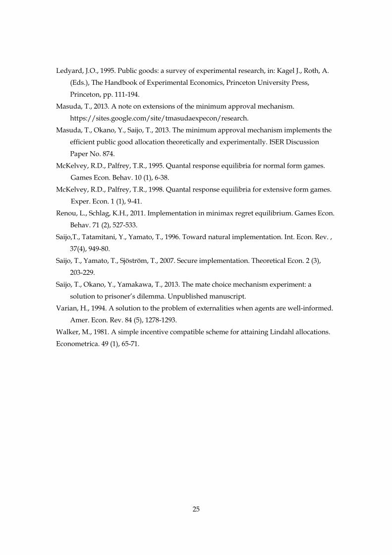
Ledyard, J.O., 1995. Public goods: a survey of experimental research, in: Kagel J., Roth, A.
(Eds.), The Handbook of Experimental Economics, Princeton University Press,
Princeton, pp. 111-194.
Masuda, T., 2013. A note on extensions of the minimum approval mechanism.
https://sites.google.com/site/tmasudaexpecon/research.
Masuda, T., Okano, Y., Saijo, T., 2013. The minimum approval mechanism implements the
efficient public good allocation theoretically and experimentally. ISER Discussion
Paper No. 874.
McKelvey, R.D., Palfrey, T.R., 1995. Quantal response equilibria for normal form games.
Games Econ. Behav. 10 (1), 6-38.
McKelvey, R.D., Palfrey, T.R., 1998. Quantal response equilibria for extensive form games.
Exper. Econ. 1 (1), 9-41.
Renou, L., Schlag, K.H., 2011. Implementation in minimax regret equilibrium. Games Econ.
Behav. 71 (2), 527-533.
Saijo,T., Tatamitani, Y., Yamato, T., 1996. Toward natural implementation. Int. Econ. Rev. ,
37(4), 949-80.
Saijo, T., Yamato, T., Sjöström, T., 2007. Secure implementation. Theoretical Econ. 2 (3),
203-229.
Saijo, T., Okano, Y., Yamakawa, T., 2013. The mate choice mechanism experiment: a
solution to prisoner’s dilemma. Unpublished manuscript.
Varian, H., 1994. A solution to the problem of externalities when agents are well-informed.
Amer. Econ. Rev. 84 (5), 1278-1293.
Walker, M., 1981. A simple incentive compatible scheme for attaining Lindahl allocations.
Econometrica. 49 (1), 65-71.
25

Figure 1. Prisoner’s dilemma game with the MCM in Saijo et al. (2013).
Figure 2. Average contributions by period, sorted by mechanism.

0 2 4 6 8 10
0 10 11.4 12.8 14.2 15.6 17
2 9.4 10.8 12.2 13.6 15 16.4
4 8.8 10.2 11.6 13 14.4 15.8
6 8.2 9.6 11 12.4 13.8 15.2
8 7.6 9 10.4 11.8 13.2 14.6
10 7 8.4 9.8 11.2 12.6 14
Table 1. Player 1’s payoff table when w = 10 and 0.7.α =
1

Table 2. Payoff tables in subgames (6,2) and (8,10).
y n y n
y (9.6,13.6) (10.8,10.8) y (14.6,12.6) (13.2,13.2)
n (10.8,10.8) (10.8,10.8) n (13.2,13.2) (13.2,13.2)
Subgame (6,2) Subgame (8,10)
2

0 2 4 6 8 10
0 10 10 10 10 10 10
2 10 10.8 10.8 10.8 10.8 10.8
4 10 10.8 11.6 11.6 11.6 11.6
6 10 10.8 11.6 12.4 12.4 12.4
8 10 10.8 11.6 12.4 13.2 13.2
10 10 10.8 11.6 12.4 13.2 14
Table 3. Player 1’s payoff table in the reduced normal form game under the MAM.
3

Notes: ** p < 0.01.
Table 4. Two-tailed Mann–Whitney test statistics for the equality of average contributions,
grouped by treatment.
Treatment SMAM MCM VCMMAM 3.799** 9.450** 9.445**SMAM 9.133** 9.275**MCM 7.284**
4